GRAVITATION
Charles W. MISN£R Kip S. THORNE John Archibald WHEELER
UNIVERSITY OF MARYLAND CALIFORNIA INSTITUTE OF TECHNOLOGY PRINCETON UNIVERSITY
W. H. FREEMAN AND COMPANY San Francisco

Library of Congress Cataloging in Publication Data
Misner, Charles W, 1932-
Gravitation.
Bibliography; p.
1. Gravitation. 2. Astrophysics. 3. General
relativity (Physics) I. Thome, Kip S,, 1940- joint author.
II. Wheeler, John Archibald, 1911- joint author.
III. Title.
QC178.M57 53Г.14 78-156043
ISBN 0-7167-0334-3
ISBN 0-7167-0344-0 (pbk)
Copyright © 1970 and 1971 by Charles W. Misner,
Kip S. Thorne, and John Archibald Wheeler.
Copyright © 1973 by W. H, Freeman and Company.
No part of this book may be reproduced
by any mechanical, photographic, or electronic process,
or in the form of a phonographic recording,
nor may it be stored in a retrieval system, transmitted,
or otherwise copied for public or private use
without the written permission of the publisher.
Printed in the United States of America
10 11 12 13 14 15 16 17 18 19 20 KP 8 9 8 7 6 5 4 3 2 1

SIGN CONVENTIONS
This book follows the "Landau-Lifshitz Spacelike Convention" (LLSC). Arrows
below mark signs that are "+" in it. The facing table shows signs that other authors
use.
+g = -(a/0J + (ш1J + (a/2J + (ш3J
g sign
(col. 2)
/, v) = ▼„▼„- ▼„ ▼„
Riemann sign
(col. 3)
R = Ra
quotient of Einstein
and Riemann signs
Einstein
Einstein sign
(col. 4)
all authors agree
on this "positive
energy density" sign
The above sign choice for Riemann is convenient for coordinate-free methods, as
in the curvature operator ftf(i/, v) above, in the curvature 2-forms (equation 14.19),
and for matrix computations (exercise 14.9), The definitions of Ricci and Einstein
with the signs adopted above are those that make their eigenvalues (and R = R^M)
positive for standard spheres with positive definite metrics.

TABLE OF SIGN CONVENTIONS
^ дф Space time
Reference \Cp <^ ,£>" four-dimensional
ф Ф V indices
Landau, Lifshitz A962) "spacelike convention" + + + latin
Landau, Lifshitz A971) "timelike convention" — + + latin
Misner, Thorne, Wheeler A973; this text) + + + greek
Adler, Bazin, Schifl'er A965) -
Anderson A967) - - -b
Bergmann A942) - -a -
Cartan A946) - -
Davis A970) - + -
Eddington A922) - + -
Ehlers A971) + + +
Einstein A950) + -
Eisenhart A926) + -
FockA959)
FokkerA965) - +
Hawking and Ellis A973) + + +
Hicks A965) + +
lnfeld, Plebanski A960) +
Lichnerowicz A955) — + +
McVittie A956) - + -
Misner A969a) + + +
M0llerA952) +
Pauli A958) + - -
Penrose A968) - - -
Pirani A965) - - -
Robertson, Noonan A968) + + —
Sachs A964) ± + +
Schild A967) +
Schouten A954) - +
Schroedinger A950) - + -
Synge A960b) + +
Thorne A967) + +
Tolman A934a) - + -
Trautman A965) - - -
Weber A961) + + +
Weinberg A972) +
WeylA922) + +
Wheeler A964a) + + +
greek
greek
greek
greek
greek
greek
greek
greek
greek
greek
greek
greek
greek
greek
greek
latin
latin
latin
latin
latin
latin
latin
latin
latin
latin
latin
latin
latin
latin
latin
"Unusual index positioning on Riemann components gives a different sign for Лд|.„^.
bNote: his к < 0 is the negative of the gravitational constant.

We dedicate this book
To our fellow citizens
Who, for love of truth,
Take from their own wants
By taxes and gifts,
And now and then send forth
One of themselves
As dedicated servant.
To forward the search
Into the mysteries and marvelous simplicities
Of this strange and beautiful Universe,
Our home.

PREFACE
This is a textbook on gravitation physics (Einstein's "general relativity" or "geo-
metrodynamics"). It supplies two tracks through the subject. The first track is focused
on the key physical ideas. It assumes, as mathematical prerequisite, only vector
analysis and simple partial-differential equations. It is suitable for a one-semester
course at the junior or senior level or in graduate school; and it constitutes—in the
opinion of the authors—the indispensable core of gravitation theory that every
advanced student of physics should learn. The Track-1 material is contained in those
pages of the book that have a 1 outlined in gray in the upper outside corner, by
which the eye of the reader can quickly pick out the Track-1 sections. In the con-
contents, the same purpose is served by a gray bar beside the section, box, or figure
number.
The rest of the text builds up Track 1 into Track 2. Readers and teachers are
invited to select, as enrichment material, those portions of Track 2 that interest them
most. With a few exceptions, any Track-2 chapter can be understood by readers
who have studied only the earlier Track-1 material. The exceptions are spelled out
explicitly in "dependency statements" located at the beginning of each Track-2
chapter, or at each transition within a chapter from Track 1 to Track 2.
The entire book (all of Track 1 plus all of Track 2) is designed for a rigorous,
full-year course at the graduate level, though many teachers of a full-year course
may prefer a more leisurely pace that omits some of the Track-2 material. The full
book is intended to give a competence in gravitation physics comparable to that
which the average Ph.D. has in electromagnetism. When the student achieves this
competence, he knows the laws of physics in flat spacetime (Chapters 1-7). He can
predict orders of magnitude. He can also calculate using the principal tools of modern
differential geometry (Chapters 8-15), and he can predict at all relevant levels of
precision. He understands Einstein's geometric framework for physics (Chapters

viii GRAVITATION
16-22). He knows the applications of greatest present-day interest: pulsars and
neutron stars (Chapters 23-26); cosmology (Chapters 27-30); the Schwarzschild
geometry and gravitational collapse (Chapters 31-34); and gravitational waves
(Chapters 35-37). He has probed the experimental tests of Einstein's theory (Chap-
(Chapters 38-40). He will be able to read the modern mathematical literature on differential
geometry, and also the latest papers in the physics and astrophysics journals about
geometrodynamics and its applications. If he wishes to go beyond the field equations,
the four major applications, and the tests, he will find at the end of the book
(Chapters 41-44) a brief survey of several advanced topics in general relativity.
Among the topics touched on here, superspace and quantum geometrodynamics
receive special attention. These chapters identify some of the outstanding physical
issues and lines of investigation being pursued today.
Whether the department is physics or astrophysics or mathematics, more students
than ever ask for more about general relativity than mere conversation. They want
to hear its principal theses clearly stated. They want to know how to "work the
handles of its information pump" themselves. More universities than ever respond
with a serious course in Einstein's standard 1915 geometrodynamics. What a contrast
to Maxwell's standard 1864 electrodynamics! In 1897, when Einstein was a student
at Zurich, this subject was not on the instructional calendar of even half the
universities of Europe.1 "We waited in vain for an exposition of Maxwell's theory,"
says one of Einstein's classmates. "Above all it was Einstein who was disappointed,
for he rated electrodynamics as "the most fascinating subject at the time" 3—as many
students rate Einstein's theory today!
Maxwell's theory recalls Einstein's theory in the time it took to win acceptance.
Even as.late as 1904 a book could appear by so great an investigator as William
Thomson, Lord Kelvin, with the words, "The so-called 'electromagnetic theory of
light' has not helped us hitherto ... it seems to me that it is rather a backward
step ... the one thing about it that seems intelligible to me, I do not think is
admissible . . . that there should be an electric displacement perpendicular to the
line of propagation. Did the pioneer of the Atlantic cable in the end contribute
so richly to Maxwell electrodynamics—from units, and principles of measurement,
to the theory of waves guided by wires—because of his own early difficulties with
the subject? Then there is hope for many who study Einstein's geometrodynamics
today! By the 1920's the weight of developments, from Kelvin's cable to Marconi's
wireless, from the atom of Rutherford and Bohr to the new technology of high-
frequency circuits, had produced general conviction that Maxwell was right. Doubt
dwindled. Confidence led to applications, and applications led to confidence.
Many were slow to take up general relativity in the beginning because it seemed
to be poor in applications. Einstein's theory attracts the interest of many today
because it is rich in applications. No longer is attention confined to three famous
but meager tests: the gravitational red shift, the bending of light by the sun, and
'G. Holton A965). 3A. Einstein A949a).
2L. Kolbros A956). 4W. Thomson A904).
Citations for references will be found in the bibliography.

PREFACE ix
the precession of the perihelion of Mercury around the sun. The combination of
radar ranging and general relativity is, step by step, transforming the solar-system
celestial mechanics of an older generation to a new subject, with a new level of
precision, new kinds of effects, and a new outlook. Pulsars, discovered in 1968, find
no acceptable explanation except as the neutron stars predicted in 1934, objects with
a central density so high (~ 1014g/cm3) that the Einstein predictions of mass differ
from the Newtonian predictions by 10 to 100 per cent. About further density increase
and a final continued gravitational collapse, Newtonian theory is silent. In contrast,
Einstein's standard 1915 geometrodynamics predicted in 1939 the properties of a
completely collapsed object, a "frozen star" or "black hole." By 1966 detailed digital
calculations were available describing the formation of such an object in the collapse
of a star with a white-dwarf core. Today hope to discover the first black hole is
not least among the forces propelling more than one research: How does rotation
influence the properties of a black hole? What kind of pulse of gravitational radiation
comes off when such an object is formed? What spectrum of x-rays emerges when
gas from a companion star piles up on its way into a black hole?5 All such investi-
investigations and more base themselves on Schwarzschild's standard 1916 static and
spherically symmetric solution of Einstein's field equations, first really understood
in the modern sense in 1960, and in 1963 generalized to a black hole endowed with
angular momentum.
Beyond solar-system tests and applications of relativity, beyond pulsars, neutron
stars, and black holes, beyond geometrostatics (compare electrostatics!) and station-
stationary geometries (compare the magnetic field set up by a steady current!) lies geo-
geometrodynamics in the full sense of the word (compare electrodynamics!). Nowhere
does Einstein's great conception stand out more clearly than here, that the geometry
of space is a new physical entity, with degrees of freedom and a dynamics of its
own. Deformations in the geometry of space, he predicted in 1918, can transport
energy from place to place. Today, thanks to the initiative of Joseph Weber, detectors
of such gravitational radiation have been constructed and exploited to give upper
limits to the flux of energy streaming past the earth at selected frequencies. Never
before has one realized from how many kinds of processes significant gravitational
radiation can be anticipated. Never before has there been more interest in picking
up this new kind of signal and using it to diagnose faraway events. Never before
has there been such a drive in more than one laboratory to raise instrumental
sensitivity until gravitational radiation becomes a workaday new window on the
universe.
The expansion of the universe is the greatest of all tests of Einstein's geometro-
geometrodynamics, and cosmology the greatest of all applications. Making a prediction too
fantastic for its author to credit, the theory forecast the expansion years before it
was observed A929). Violating the short time-scale that Hubble gave for the expan-
expansion, and in the face of "theories" ("steady state"; "continuous creation") manufac-
manufactured to welcome and utilize this short time-scale, standard general relativity
resolutely persisted in the prediction of a long time-scale, decades before the astro-
5 As of April 1973, there are significant indications that Cygnus X-l and other compact x-ray sources
may be black holes.

X GRAVITATION
physical discovery A952) that the Hubble scale of distances and times was wrong,
and had to be stretched by a factor of more than five. Disagreeing by a factor of
the order of thirty with the average density of mass-energy in the universe deduced
from astrophysical evidence as recently as 1958, Einstein's theory now as in the past
argues for the higher density, proclaims "the mystery of the missing matter," and
encourages astrophysics in a continuing search that year by year turns up new
indications of matter in the space between the galaxies. General relativity forecast
the primordial cosmic fireball radiation, and even an approximate value for its
present temperature, seventeen years before the radiation was discovered. This
radiation brings information about the universe when it had a thousand times smaller
linear dimensions, and a billion times smaller volume, than it does today. Quasistellar
objects, discovered in 1963, supply more detailed information from a more recent
era, when the universe had a quarter to half its present linear dimensions. Telling
about a stage in the evolution of galaxies and the universe reachable in no other
way, these objects are more than beacons to light up the far away and long ago.
They put out energy at a rate unparalleled anywhere else in the universe. They eject
matter with a surprising directivity. They show a puzzling variation with time,
different between the microwave and the visible part of the spectrum. Quasistellar
objects on a great scale, and galactic nuclei nearer at hand on a smaller scale, voice
a challenge to general relativity: help clear up these mysteries!
If its wealth of applications attracts many young astrophysicists to the study of
Einstein's geometrodynamics, the same attraction draws those in the world of physics
who are concerned with physical cosmology, experimental general relativity, gravi-
gravitational radiation, and the properties of objects made out of superdense matter. Of
quite another motive for study of the subject, to contemplate Einstein's inspiring
vision of geometry as the machinery of physics, we shall say nothing here because
it speaks out, we hope, in every chapter of this book.
Why a new book? The new applications of general relativity, with their extraor-
extraordinary physical interest, outdate excellent textbooks of an earlier era, among them
even that great treatise on the subject written by Wolfgang Pauli at the age of
twenty-one. In addition, differential geometry has undergone a transformation of
outlook that isolates the student who is confined in his training to the traditional
tensor calculus of the earlier texts. For him it is difficult or impossible either to read
the writings of his up-to-date mathematical colleague or to explain the mathematical
content of his physical problem to that friendly source of help. We have not seen
any way to meet our responsibilities to our students at our three institutions except
by a new exposition, aimed at establishing a solid competence in the subject, con-
contemporary in its mathematics, oriented to the physical and astrophysical applications
of greatest present-day interest, and animated by belief in the beauty and simplicity
of nature.
High Island Charles W. Misner
South Bristol, Maine Kip S. Thome
September 4, 1972 John Archibald Wheeler

CONTENTS
BOXES xxi
FIGURES xxiv
ACKNOWLEDGMENTS xxvii
Part I SPACETIME PHYSICS 1
1. Geometrodynamics in Brief 3
1 ■ The Parable of the Apple 3
2. Spacetime With and Without Coordinates 5
3. Weightlessness 13
4. Local Lorentz Geometry, With and Without Coordinates 1 9
5. Time 23
6. Curvature 29
7. Effect of Matter on Geometry 37
Part II PHYSICS IN FLAT SPACETIME 45
2. Foundations of Special Relativity 47
1.
2.
3.
4.
5.
6.
7.
8.
9.
10.
Overview 47
Geometric Objects 48
Vectors 49
The Metric Tensor 51
Differential Forms 53
Gradients and Directional Derivatives 59
Coordinate Representation of Geometric Objects 60
The Centrifuge and the Photon 63
Lorentz Transformations 66
Collisions 69

XII
GRAVITATION
3. The Electromagnetic Field 71
7.
The Lorentz Force and the Electromagnetic Field Tensor 71
Tensors in All Generality 74
Three-Plus-One View Versus Geometric View 78
Maxwell's Equations 79
Working with Tensors 81
4. Electromagnetism and Differential Forms 90
1. Exterior Calculus 90
2. Electromagnetic 2-Form and Lorentz Force 99
3. Forms Illuminate Electromagnetism and Electromagnetism Illuminates
Forms 105
4. Radiation Fields 1 10
5. Maxwell's Equations 112
6. Exterior Derivative and Closed Forms 1 14
7. Distant Action from Local Law 120
5. Stress-Energy Tensor and Conservation Laws 1 30
1,1 Track-1 Overview 130
2. Three-Dimensional Volumes and Definition of the Stress-Energy
Tensor 130
3. Components of Stress-Energy Tensor 137
4. Stress-Energy Tensor for a Swarm of Particles 1 38
5. Stress-Energy Tensor for a Perfect Fluid 139
6. Electromagnetic Stress-Energy 140
7. Symmetry of the Stress-Energy Tensor 141
8. Conservation of 4-Momentum: Integral Formulation 142
9. Conservation of 4-Momentum: Differential Formulation 146
10. Sample Application of ▼■ T = 0 152
11. Angular Momentum 156
6. Accelerated Observers 163
1.1 Accelerated Observers Can Be Analyzed Using Special Relativity 163
2. Hyperbolic Motion 166
3. Constraints on Size of an Accelerated Frame 168
4. The Tetrad Carried by a Uniformly Accelerated Observer 169
5. The Tetrad Fermi-Walker Transported by an Observer with Arbitrary
Acceleration 170
6. The Local Coordinate System of an Accelerated Observer 1 72
Incompatibility of Gravity and Special Relativity 1 77
1. Attempts to Incorporate Gravity into Special Relativity 177
2. Gravitational Redshift Derived from Energy Conservation 187
3. Gravitational Redshift Implies Spacetime Is Curved 187
4. Gravitational Redshift as Evidence for the Principle of Equivalence 189
5. Local Flatness, Global Curvature 190
Part III THE MATHEMATICS OF CURVED SPACETIME 193
8. Differential Geometry: An Overview 195
An Overview of Part III 195
Track 1 Versus Track 2: Difference in Outlook and Power 1 97
Three Aspects of Geometry: Pictorial, Abstract, Component 198
Tensor Algebra in Curved Spacetime 201
Parallel Transport, Covariant Derivative, Connection Coefficients,
Geodesies 207
Local Lorentz Frames: Mathematical Discussion 217
Geodesic Deviation and the Riemann Curvature Tensor 218

CONTENTS xiii
9. Differential Topology 225
1. Geometric Objects in Metric-Free, Geodesic-Free Spacetime 225
2. "Vector" and "Directional Derivative" Refined into Tangent Vector 226
3. Bases, Components, and Transformation Laws for Vectors 230
4. 1-Forms 231
5. Tensors 233
6. Commutators and Pictorial Techniques 235
7. Manifolds and Differential Topology 240
10, Affine Geometry: Geodesies, Parallel Transport and Covariant Derivative 244
1 . Geodesies and the Equivalence Principle 244
2. Parallel Transport and Covariant Derivative: Pictorial Approach 245
3. Parallel Transport and Covariant Derivative: Abstract Approach 247
4. Parallel Transport and Covariant Derivative: Component Approach 258
5. Geodesic Equation 262
11, Geodesic Deviation and Spacetime Curvature 265
1 . Curvature, At Last! 265
2. The Relative Acceleration of Neighboring Geodesies 265
3. Tidal Gravitational Forces and Riemann Curvature Tensor 270
4. Parallel Transport Around a Closed Curve 277
5. Flatness is Equivalent to Zero Riemann Curvature 283
6. Riemann Normal Coordinates 285
12, Newtonian Gravity in the Language of Curved Spacetime 289
1. Newtonian Gravity in Brief 289
2. Stratification of Newtonian Spacetime 291
3. Galilean Coordinate Systems 292
4. Geometric, Coordinate-Free Formulation of Newtonian Gravity 298
5. The Geometric View of Physics: A Critique 302
13, Riemannian Geometry: Metric as Foundation of All 304
1. New Features Imposed on Geometry by Local Validity of Special
Relativity 304
2. Metric 305
3. Concord Between Geodesies of Curved Spacetime Geometry and Straight
Lines of Local Lorentz Geometry 312
4. Geodesies as World Lines of Extremal Proper Time 315
5. Metric-Induced Properties of Riemann 324
6. The Proper Reference Frame of an Accelerated Observer 327
14, Calculation of Curvature 333
1 . Curvature as a Tool for Understanding Physics 333
2. Forming the Einstein Tensor 343
3. More Efficient Computation 344
4. The Geodesic Lagrangian Method 344
5. Curvature 2-Forms 348
6. Computation of Curvature Using Exterior Differential Forms 354
15, Bianchi Identities and the Boundary of a Boundary 364
1 . Bianchi Identities in Brief 364
2. Bianchi Identity d<A, = 0 as a Manifestation of "Boundary of
Boundary = 0" 372
3. Moment of Rotation: Key to Contracted Bianchi Identity 373
4. Calculation of the Moment of Rotation 375
5. Conservation of Moment of Rotation Seen from "Boundary of a Boundary is
Zero" 377
6. Conservation of Moment of Rotation Expressed in Differential Form 378
7. From Conservation of Moment of Rotation to Einstein's Geometrodynamics: A
Preview 379

XIV
GRAVITATION
Part IV EINSTEIN'S GEOMETRIC THEORY OF GRAVITY 383
16, Equivalence Principle and Measurement of the "Gravitational Field" 385
Overview 385
The Laws of Physics in Curved Spacetime 385
Factor-Ordering Problems in the Equivalence Principle 388
The Rods and Clocks Used to Measure Space and Time Intervals 393
The Measurement of the Gravitational Field 399
17, How Mass-Energy Generates Curvature 404
1. Automatic Conservation of the Source as the Central Idea in the Formulation
of the Field Equation 404
2. Automatic Conservation of the Source: A Dynamic Necessity 408
3. Cosmological Constant 409
4. The Newtonian Limit 412
5. Axiomatize Einstein's Theory? 416
6. "No Prior Geometry": A Feature Distinguishing Einstein's Theory from Other
Theories of Gravity 429
7. A Taste of the History of Einstein's Equation 431
18, Weak Gravitational Fields 435
1.1 The Linearized Theory of Gravity 435
2.1 Gravitational Waves 442
3.1 Effect of Gravity on Matter 442
4.1 Nearly Newtonian Gravitational Fields 445
19, Mass and Angular Momentum of a Gravitating System 448
1.1 External Field of a Weakly Gravitating Source 448
2.1 Measurement of the Mass and Angular Momentum 450
3.1 Mass and Angular Momentum of Fully Relativistic Sources 451
4.| Mass and Angular Momentum of a Closed Universe 457
20, Conservation Laws for 4-Momentum and Angular Momentum 460
1. Overview 460
2. Gaussian Flux Integrals for 4-Momentum and Angular Momentum 461
3. Volume Integrals for 4-Momentum and Angular Momentum 464
4. Why the Energy of the Gravitational Field Cannot be Localized 466
5. Conservation Laws for Total 4-Momentum and Angular Momentum 468
6. Equation of Motion Derived from the Field Equation 471
21, Variational Principle and Initial-Value Data 484
1. Dynamics Requires Initial-Value Data 484
2. The Hilbert Action Principle and the Palatini Method of Variation 491
3. Matter Lagrangian and Stress-Energy Tensor 504
4. Splitting Spacetime into Space and Time 505
5. Intrinsic and Extrinsic Curvature 509
6. The Hilbert Action Principle and the Arnowitt-Deser-Misner Modification
Thereof in the Space-plus-Time Split 519
7. The Arnowitt-Deser-Misner Formulation of the Dynamics of Geometry 520
8. Integrating Forward in Time 526
9. The Initial-Value Problem in the Thin-Sandwich Formulation 528
10. The Time-Symmetric and Time-Antisymmetric Initial-Value Problem 535
1 1. York's "Handles" to Specify a 4-Geometry 539
12. Mach's Principle and the Origin of Inertia 543
13. Junction Conditions 551

CONTENTS
XV
22, Thermodynamics, Hydrodynamics, Electrodynamics, Geometric Optics,
and Kinetic Theory 557
1. The Why of this Chapter 557
2. Thermodynamics in Curved Spacetime 557
3. Hydrodynamics in Curved Spacetime 562
4. Electrodynamics in Curved Spacetime 568
5. Geometric Optics in Curved Spacetime 570
6. Kinetic Theory in Curved Spacetime 583
Part V RELATIVISTIC STARS 591
23,
24,
25,
Spherical Stars 593
1 . Prolog 593
2. Coordinates and Metric for a Static, Spherical System 594
3. Physical Interpretation of Schwarzschild coordinates 595
• 4. Description of the Matter Inside a Star 597
5. Equations of Structure 600
6. External Gravitational Field 607
7. How to Construct a Stellar Model 608
8. The Spacetime Geometry for a Static Star 612
618
Pulsars and Neutron Stars; Quasars and Supermassive Stars
1. Overview 61 8
2. The Endpoint of Stellar Evolution 621
3. Pulsars 627
4. Supermassive Stars and Stellar Instabilities 630
5. Quasars and Explosions In Galactic Nuclei 634
6. Relativistic Star Clusters 634
The "Pit in the Potential" as the Central New Feature of Motion in
Schwarzschild Geometry 636
1.1 From Kepler's Laws to the Effective Potential for Motion in Schwarzschild
I Geometry 636
2. Symmetries and Conservation Laws 650
3. Conserved Quantities for Motion in Schwarzschild Geometry 655
4. Gravitational Redshift 659
5. Orbits of Particles 659
6. Orbit of a Photon, Neutrino, or Graviton in Schwarzschild Geometry 672
7. Spherical Star Clusters 679
26, Stellar Pulsations 688
1. Motivation 688
2. Setting Up the Problem 689
3. Eulerian versus Lagrangian Perturbations 690
4. Initial-Value Equations 691
5. Dynamic Equation and Boundary Conditions 693
6. Summary of Results 694
Part VI THE UNIVERSE 701
27, Idealized Cosmologies 703
1.1 The Homogeneity and Isotropy of the Universe 703
2. Stress-Energy Content of the Universe—the Fluid Idealization 71 1
3. Geometric Implications of Homogeneity and Isotropy 713

XVI
GRAVITATION
29,
30,
4. Comoving, Synchronous Coordinate Systems for the Universe 715
5. The Expansion Factor 718
6. Possible 3-Geometries for a Hypersurface of Homogeneity 720
7. Equations of Motion for the Fluid 726
8. The Einstein Field Equations 728
9. Time Parameters and the Hubble Constant 730
10. The Elementary Friedmann Cosmology of a Closed Universe 733
1 1. Homogeneous Isotropic Model Universes that Violate Einstein's Conception of
Cosmology 742
28, Evolution of the Universe into Its Present State 763
1.1 The "Standard Model" of the Universe 763
2.1 Standard Model Modified for Primordial Chaos
3.1 What "Preceded" the Initial Singularity? 769
4.1 Other Cosmological Theories 770
769
Present State and Future Evolution of the Universe 771
1. Parameters that Determine the Fate of the Universe 771
2. Cosmological Redshift 772
3. The Distance-Redshift Relation: Measurement of the Hubble Constant
4. The Magnitude-Redshift Relation: Measurement of the Deceleration
Parameter 782
5. Search for "Lens Effect" of the Universe 795
6. Density of the Universe Today 796
7. Summary of Present Knowledge About Cosmological Parameters 797
Anisotropic and Inhomogeneous Cosmologies 800
1. Why Is the Universe So Homogeneous and Isotropic? 800
2. The Kasner Model for an Anisotropic Universe 801
3. Adiabatic Cooling of Anisotropy 802
4. Viscous Dissipation of Anisotropy 802
5. Particle Creation in an Anisotropic Universe 803
6. Inhomogeneous Cosmologies 804
7. The Mixmaster Universe 805
8. Horizons and the Isotropy of the Microwave Background 815
780
Part VII GRAVITATIONAL COLLAPSE AND BLACK HOLES 817
31. Schwarzschild Geometry 819
Inevitability of Collapse for Massive Stars 819
The Nonsingularity of the Gravitational Radius 820
Behavior of Schwarzschild Coordinates at r = 2M 823
Several Well-Behaved Coordinate Systems 826
Relationship Between Kruskal-Szekeres Coordinates and Schwarzschild
Coordinates 833
Dynamics of the Schwarzschild Geometry 836
32, Gravitational Collapse 842
842
1.1 Relevance of Schwarzschild Geometry
2.1 Birkhoff's Theorem 843
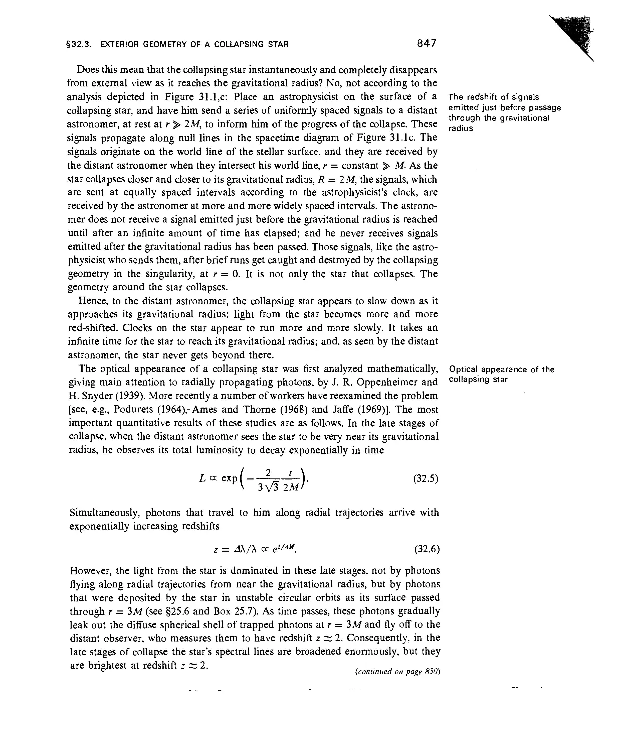
3.1 Exterior Geometry of a Collapsing Star 846
4. Collapse of a Star with Uniform Density and Zero Pressure 851
5. Spherically Symmetric Collapse with Internal Pressure Forces 857
6. The Fate of a Man Who Falls into the Singularity at r = 0 860
7. Realistic Gravitational Collapse—An Overview 862

CONTENTS
XVII
33, Black Holes 872
Why "Black Hole"?
34,
1.
2.
3.
4.
5.
6.
7.
872
The Gravitational and Electromagnetic Fields of a Black Hole 875
Mass, Angular Momentum, Charge, and Magnetic Moment 891
Symmetries and Frame Dragging 892
Equations of Motion for Test Particles 897
Principal Null Congruences 901
Storage and Removal of Energy from Black Holes 904
Reversible and Irreversible Transformations 907
Global Techniques, Horizons, and Singularity Theorems
1. Global Techniques Versus Local Techniques 916
916
2. "Infinity" in Asymptotically Flat Spacetime 917
3. Causality and Horizons 922
4. Global Structure of Horizons 924
5. Proof of Second Law of Black-Hole Dynamics 931
6. Singularity Theorems and the "Issue of the Final State"
934
Part VIII GRAVITATIONAL WAVES 941
35, Propagation of Gravitational Waves 943
1. Viewpoints 943
2. Review of "Linearized Theory" in Vacuum 944
3. Plane-Wave Solutions in Linearized Theory 945
4. The Transverse Traceless (TT) Gauge 946
5. Geodesic Deviation in a Linearized Gravitational Wave 950
6 Polarization of a Plane Wave 952
7. The Stress-Energy Carried by a Gravitational Wave 955
8. Gravitational Waves in the Full Theory of General Relativity 956
9. An Exact Plane-Wave Solution 957
10. Physical Properties of the Exact Plane Wave 960
1 1. Comparison of an Exact Electromagnetic Plane Wave with the Gravitational
Plane Wave 961
12. A New Viewpoint on the Exact Plane Wave 962
13. The Shortwave Approximation 964
14. Effect of Background Curvature on Wave Propagation 967
1 5. Stress-Energy Tensor for Gravitational Waves 969
36, Generation of Gravitational Waves 974
1.
2.
3.
4.
5.
6.
7.
8.
9.
10.
11.
The Quadrupole Nature of Gravitational Waves 974
Power Radiated in Terms of Internal Power Flow 978
Laboratory Generators of Gravitational Waves 979
Astrophysical Sources of Gravitational Waves: General Discussion 980
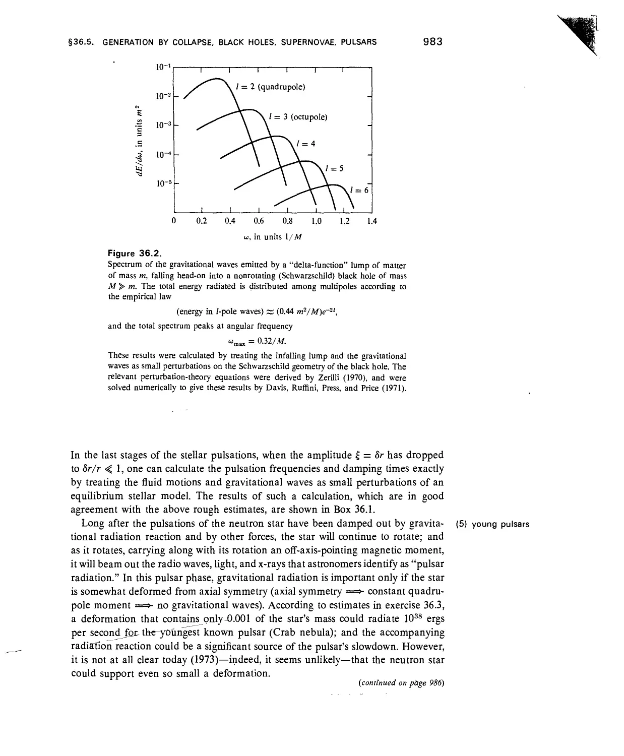
Gravitational Collapse, Black Holes, Supernovae, and Pulsars as Sources 981
Binary Stars as Sources 986
Formulas for Radiation from Nearly Newtonian Slow-Motion Sources 989
Radiation Reaction in Slow-Motion Sources 993
Foundations for Derivation of Radiation Formulas 995
Evaluation of the Radiation Field in the Slow-Motion Approximation 996
Derivation of the Radiation-Reaction Potential 1001
37,
Detection of Gravitational Waves 1004
1.1 Coordinate Systems and Impinging Waves 1004
2.1 Accelerations in Mechanical Detectors 1006
3.1 Types of Mechanical Detectors 1012

XVIII
GRAVITATION
4. Vibrating, Mechanical Detectors: Introductory Remarks 1019
5. Idealized Wave-Dominated Detector, Excited by Steady Flux of Monochromatic
Waves 1022
6. Idealized, Wave-Dominated Detector, Excited by Arbitrary Flux of
Radiation 1026
7. General Wave-Dominated Detector, Excited by Arbitrary Flux of
Radiation 1028
8. Noisy Detectors 1036
9. Nonmechanical Detectors 1040
10. Looking Toward the Future 1040
Part IX. EXPERIMENTAL TESTS OF GENERAL RELATIVITY 1045
38, Testing the Foundations of Relativity 1047
1.1 Testing is Easier in the Solar System than in Remote Space 1047
2.1 Theoretical Frameworks for Analyzing Tests of General Relativity 1048
3. Tests of the Principle of the Uniqueness of Free Fall: Eotvos-Dicke
Experiment 1050
4. Tests for the Existence of a Metric Governing Length and Time
Measurements 1054
5. Tests of Geodesic Motion: Gravitational Redshift Experiments 1055
6. Tests of the Equivalence Principle 1060
7. Tests for the Existence of Unknown Long-Range Fields 1063
39, Other Theories of Gravity and the Post-Newtonian Approximation 1066
1.1 Other Theories 1066
2.1 Metric Theories of Gravity 1067
3.1 Post-Newtonian Limit and PPN Formalism 1068
4. PPN Coordinate System 1073
5. Description of the Matter in the Solar System 1074
6. Nature of the Post-Newtonian Expansion 1075
7. Newtonian Approximation 1077
8. PPN Metric Coefficients 1080
9. Velocity of PPN Coordinates Relative to "Universal Rest Frame"
10. PPN Stress-Energy Tensor 1086
11. PPN Equations of Motion 1087
12. Relation of PPN Coordinates to Surrounding Universe 1091
13. Summary of PPN Formalism 1091
40, Solar-System Experiments 1096
1083
1.
2.
3.
4.
5.
6.
7.
8.
9.
10.
Many Experiments Open to Distinguish General Relativity from Proposed
Metric Theories of Gravity 1096
The Use of Light Rays and Radio Waves to Test Gravity 1099
"Light" Deflection 1 101
Time-Delay in Radar Propagation 1103
Perihelion Shift and Periodic Perturbations in Geodesic Orbits 1110
Three-Body Effects in the Lunar Orbit 1116
The Dragging of Inertial Frames 1117
Is the Gravitational Constant Constant? 1121
Do Planets and the Sun Move on Geodesies? 1 126
Summary of Experimental Tests of General Relativity 1131
Part X. FRONTIERS 1133
41, Spinors 1135
1. Reflections, Rotations, and the Combination of Rotations 1135
2. Infinitesimal Rotations 1140

CONTENTS xix
3. Lorentz Transformation via Spinor Algebra 1 142
4. Thomas Precession via Spinor Algebra 1 145
5. Spinors 1148
6. Correspondence Between Vectors and Spinors 1 150
7. Spinor Algebra 1151
8. Spin Space and Its Basis Spinors 1 156
9. Spinor Viewed as Flagpole Plus Flag Plus Orientation-Entanglement
Relation 1 1 57
10. Appearance of the Night Sky: An Application of Spinors 1 160
1 1. Spinors as a Powerful Tool in Gravitation Theory 1 1 64
42, Regge Calculus 1166
1. Why the Regge Calculus? 1166
2. Regge Calculus in Brief 1166
3. Simplexes and Deficit Angles 1 1 67
4. Skeleton Form of Field Equations 1 169
5. The Choice of Lattice Structure 1173
6. The Choice of Edge Lengths 1177
7. Past Applications of Regge Calculus 1 1 78
8. The Future of Regge Calculus 1 1 79
43, Superspace: Arena for the Dynamics of Geometry 1 180
1. Space, Superspace, and Spacetime Distinguished 1 180
2. The Dynamics of Geometry Described in the Language of the Superspace of
the C)£'s 1184
3. The Einstein-Hamilton-Jacobi Equation 1185
4. Fluctuations in Geometry 1190
44, Beyond the End of Time 1196
1. Gravitational Collapse as the Greatest Crisis in Physics of All Time 1 196
2. Assessment of the Theory that Predicts Collapse 1 198
3. Vacuum Fluctuations: Their Prevalence and Final Dominance 1202
4. Not Geometry, but Pregeometry, as the Magic Building Material 1203
5. Pregeometry as the Calculus of Propositions 1208
6. The Black Box: The Reprocessing of the Universe 1209
Bibliography and Index of Names 1221
Subject Index 1255

BOXES
1.1.
1.2.
1.3.
1.4.
1.5.
1.6.
1.7.
1.8.
1.9.
1.10.
1.11.
2.1.
2.2.
2.3.
2.4.
3.1.
3.2.
3.3.
4.1.
4.2.
4.3.
4.4.
4.5.
4.6.
5.1.
5.2.
5.3.
5.4.
5.5.
5.6.
Mathematical notation for events, coordinates,
and vectors. 9
Acceleration independent of composition. 1 6
Local Lorentz and local Euclidean geometry. 20
Time today. 28
Test for flatness. 30
Curvature of what? 32
Lorentz force equation and geodesic deviation
equation compared. 35
Geometrized units 36
Galileo Galilei. 38
Isaac Newton. 40
Albert Einstein. 42
Farewell to "ict. " 51
Worked exercises using the metric.
Differentials 63
Lorentz transformations 67
54
Lorentz force law defines fields, predicts mo-
motions. 72
Metric in different languages. 77
Techniques of index gymnastics. 85
Differential forms and exterior calculus in
brief. 91
From honeycomb to abstract 2-form. 102
Duality of 2-forms. 108
Progression of forms and exterior deriva-
derivatives. 1 1 5
Metric structure versus Hamiltonian or symplectic
structure. 126
Birth of Stokes' Theorem. 127
Stress-energy summarized. 131
Three-dimensional volumes. 135
Volume integrals, surface integrals, and Gauss's
theorem in component notation. 147
Integrals and Gauss's theorem in the language
of forms. 1 50
Newtonian hydrodynamics reviewed. 153
Angular momentum. 1 57
6.1.1 General relativity built on special relativity. 164
6.2.1 Accelerated observers in brief. 164
7.1. An attempt to describe gravity as a symmetric
tensor field in flat spacetime. 181
8.1. Books on differential geometry. 196
8.2. Elie Cartan. 198
8.3. Pictorial, abstract, and component treatments of
differential geometry. 199
8.4. Local tensor algebra in an arbitrary basis. 202
8.5. George Friedrich Bernhard Riemann. 220
8.6. Fundamental equations for covariant derivative
and curvature. 223
9.1. Tangent vectors and tangent space. 227
9.2. Commutator as closer of quadrilaterals. 236
10.1. Geodesies. 246
10.2. Parallel transport and covariant differentiation in
terms of Schild's ladder. 248
10.3. Covariant derivative: the machine and its compo-
components. 254
11.1. Geodesic deviation and curvature in brief. 266
11.2. Geodesic deviation represented as an
arrow 268
11.3. Arrow correlated with second derivative. 270
11.4. Newtonian and geometric analyses of relative
acceleration. 272
1 1.5. Definition of Riemann curvature tensor. 273
1 1.6. Geodesic deviation and parallel transport around
a closed curve as two aspects of same construc-
construction. 279
11.7. The law for parallel transport around a closed
curve. 281
12.1. Geodesic deviation in Newtonian spacetime.
293
12.2. Spacetimes of Newton, Minkowski, and Ein-
Einstein. 296
12.3. Treatments of gravity of Newton a la Cartan and
of Einstein. 297

XXII
GRAVITATION
15
15
15
16
16
16
16
.1
.2
.3
.1
.2
.3
.4
12.4. Geometric versus standard formulation of New-
Newtonian gravity. 300
13.1. Metric distilled from distances. 306
13.2. "Geodesic" versus "extremal world line." 322
13.3. "Dynamic" variational principle for geodesies.
322
14.1. Perspectives on curvature. 335
14.2. Straightforward curvature computation. 340
14.3. Analytical calculations on a computer. 342
14.4. Geodesic Lagrangian method shortens some cur-
curvature computations. 346
14.5. Curvature computed using exterior differential
forms (metric for Friedmann cosmology). 355
The boundary of a boundary is zero. 365
Mathematical representations for the moment of
rotation and the source of gravitation. 3 79
Other identities satisfied by the curvature. 381
Factor ordering and coupling to curvature in ap-
applications of the equivalence principle. 390
Pendulum clock analyzed. 394
Response of clocks to acceleration. 396
Ideal rods and clocks built from geodesic world
lines. 397
16.5. Gravity gradiometer for measuring Riemann cur-
curvature. 401
17.1.1 Correspondence principles. 412
17,2.1 Six routes to Einstein's geometrodynamic law
1 417
17.3. An experiment on prior geometry. 430
18.1. Derivations of general relativity from geometric
viewpoint and from theory of field of spin
two. 437
18.2. Gauge transformations and coordinate transfor-
transformations in linearized theory. 439
19.1.1 Mass-energy, 4-momentum, and angular mo-
I mentum of an isolated system. 454
19.2.1 Metric correction term near selected heavenly
I bodies. 459
20.1. Proper Lorentz transformation and duality rota-
rotation. 482
20.2. Transformation of generic electromagnetic field
tensor in local inertial frame. 483
21.1. Hamiltonian as dispersion relation. 493
21.2. Counting the degrees of freedom of the electro-
electromagnetic field. 530
22.1. Alternative thermodynamic potentials. 561
22.2. Thermodynamics and hydrodynamics of a perfect
fluid in curved spacetime. 564
22.3. Geometry of an electromagnetic wavetrain.
574
22.4. Geometric optics in curved spacetime. 578
22.5. Volume in phase space. 585
22.6. Conservation of volume in phase space. 586
23.1. I Mass-energy inside radius r. 603
23.2. I Model star of uniform density. 609
23.3. I Rigorous derivation of the spherically symmetric
1 line element. 61 6
24.1.1 Stellar configurations where relativistic effects are
I important. 61 9
24.2.1 Oscillation of a Newtonian star. 630
25.1. Mass from mean angular frequency and semima-
jor axis. 638
25.2. Motion in Schwarzschild geometry as point of
departure for major applications of Einstein's the-
theory. 640
25.3. Hamilton-Jacobi description of motion: natural
because ratified by quantum principle. 641
25.4. Motion in Schwarzschild geometry analyzed by
Hamilton-Jacobi method. 644
25.5. Killing vectors and isometries. 652
25.6. I Motion of a particle in Schwarzschild geome-
I try. 660
25.7. I Motion of a photon in Schwarzschild geome-
I try. 674
25.8. Equations of structure for a spherical star clus-
cluster. 683
25.9. Isothermal star clusters. 685
26.1. Eigenvalue problem and variational principle for
normal-mode pulsations. 695
26.2. Critical adiabatic index for nearly Newtonian
stars. 697
27.1.| Cosmology in brief. 704
27.2. The 3-geometry of hypersurfaces of homogene-
homogeneity. 723
27.3. Friedmann cosmology for matter-dominated and
radiation-dominated model universes. 734
27.4.1 A typical cosmological model that agrees with
I astronomical observations. 738
27.5. Effect of choice of Л and choice of closed or open
on the predicted course of cosmology. 746
27.6. Alexander Alexandrovitch Friedmann. 751
27.7. A short history of cosmology. 752
28.1. | Evolution of the quasar population. 767
29.1. Observational parameters compared to relativity
parameters. 773
29.2. Redshift of the primordial radiation. 779
29.3. Use of redshift to characterize distance and
time. 779

BOXES
29.4. Measurement of Hubble constant and decelera-
deceleration parameter. 785
29.5. Edwin Powell Hubble. 792
30.1. The mixmaster universe. 806
31.1.1 The Schwarzschild singularity: historical re-
I marks. 822
31.2.1 Motivation for Kruskal-Szerekes coordinates.
I 828
32.1. Collapsing star with Friedmann interior and Sch-
warschild exterior, 854
32.2. Collapse with nonspherical perturbations. 864
32.3. Collapse in one and two dimensions. 867
33,1.1 A black hole has no hair. 876
33.2.1 Kerr-Newman geometry and electromagnetic
I field. 878
33.3.1 Astrophysics of black holes. 883
33.4.1 The laws of black-hole dynamics. 887
33.5. Orbits in "equatorial plane" of Kerr-Newman
black hole. 911
34.1. Horizons are generated by nonterminating null
geodesies, 926
34.2. Roger Penrose. 936
34.3. Stephen W. Hawking. 938
35.1.| Transverse-traceless part of a wave. 948
36.1. Gravitational waves from pulsating neutron stars.
984
36.2. Analysis of burst of radiation from impulse event.
987
36.3. Radiation from several binary star systems. 990
37.1.1 Derivation of equations of motion of detec-
I tor. 1007
37.2.1 Lines of force for gravitational-wave accelera-
I tions. 1011
37.3. Use of cross-section for wave-dominated detec-
detector. 1020
37.4. Vibrating, resonant detector of arbitrary
shape. 1031
XXIII
37.5. Detectability of hammer-blow waves from astro-
physical sources. 1041.
37.6. Nonmechanical detector. 1043
38.1. I Technology of the 1970's confronted with rela-
I tivistic phenomena. 1048
38.2. Baron Lorand von Eotvos. 1051
38.3. Robert Henry Dicke. 1053
39.1. I The theories of Dicke-Brans-Jordan and of
I Ni. 1070
39.2. I Heuristic description of the ten
I post-Newtonian parameters. 1072
39.3. Post-Newtonian expansion of the metric coeffi-
coefficients. 1077
39.4. Summary of the PPN formalism. 1092
39.5. PPN parameters used in the literature: a transla-
translator's guide. 1093
40.1.1 Experimental results on deflection of light and
I radio waves. 1 104
40.2.1 Experimental results on radar time-delay. 1 109
40.3.1 Experimental results on perihelion preces-
I sion. 1112
40.4. Catalog of experiments. 1129
41.1. Spinor representation of simple tensors. 1 154
42.1. The hinges where "angle of rattle" is concen-
concentrated in two, three, and four dimensions. 1 1 69
42.2. Flow diagrams for Regge calculus. 1171
42.3. Synthesis of higher-dimensional skeleton geome-
geometries out of lower-dimensional ones. 1 1 76
43.1. Geometrodynamics compared with particle dy-
dynamics. 1181
44.1. Collapse of universe compared and contrasted
with collapse of atom. 1 197
44.2. Three levels of gravitational collapse. 1201
44.3. Relation of spin J to geometrodynamics. 1204
44.4. Bucket-of-dust concept of pregeometry. 1205
44.5. Pregeometry as the calculus of proposi-
propositions. 1211

FIGURES
1.1.
1.2.
1.3.
1.4.
1.5.
1.6.
1.7.
1.8.
1.9.
1.10.
1.11.
1.12.
2.1.
2.2.
2.3.
2.4.
2.5.
2.6.
2.7.
2.8.
2.9.
4.1.
4.2.
4.3.
4.4.
4.5.
4.6.
4.7.
5.1.
5.2.
5.3.
6.1.
6.2.
Spacetime compared with the surface of an
apple. 4
World-line crossings mark events. 6
Two systems of coordinates for same events. 7
Mere coordinate singularities. 1 1
Singularities in the coordinates on a 2-sphere.
12
The Roll-Krotkov-Dicke experiment. 14
Testing for a local inertial frame. 18
Path of totality of an ancient eclipse. 25
Good clock versus bad clock. 27
"Acceleration of the separation" of nearby geo-
geodesies. 31
Separation of geodesies in a 3-manifold. 31
Satellite period and Earth density. 39
From bilocal vector to tangent vector. 49
Different curves, same tangent vector. 50
Velocity 4-vector resolved into components. 52
A 1-form pierced by a vector. 55
Gradient as 1-form. 56
Addition of 1-forms. 57
Vectors and their corresponding 1-forms. 58
Lorentz basis. 60
The centrifuge and the photon. 63
Faraday 2-form. 100
Faraday form creates a 1-form out of 4-veloc-
ity. 104
Spacelike slices through Faraday. 106
Faraday and its dual. Maxwell. 107
Maxwell 2-form for charge at rest. 109
Mechanism of radiation. 1 1 1
Simple types of 1-form. 123
River of 4-momentum sensed by different 3-
volumes. 133
Aluminum ring lifted by Faraday stresses. 141
Integral conservation laws for energy-momen-
energy-momentum. 143
Hyperbolic motion. 167
World line of accelerated observer.
169
6.3. Hyperplanes orthogonal to curved world
line. 172
6.4. Local coordinates for observer in hyperbolic mo-
motion. 173
7.1. Congruence of world lines of successive light
pulses. 188
8.1. Basis vectors for Kepler orbit. 200
8.2. Covariant derivation. 209
8.3. Connection coefficients as aviator's turning coeffi-
coefficients. 212
8.4. Selector parameter and affine parameter for a
family of geodesies. 219
9.1. Basis vectors induced by a coordinate sys-
system. 231
9.2. Basis vectors and dual basis 1-forms. 232
9.3. Three representations of S'z. 241
10.1. Straight-on parallel transport. 245
10.2. Nearby tangent spaces linked by parallel trans-
transport. 252
11.1. One-parameter family of geodesies. 267
11.2. Parallel transport around a closed curve. 278
12.1. Coordinates carried by an Earth satellite. 298
13.1. Distances determine geometry. 309
13.2. Two events connected by more than one geo-
geodesic. 318
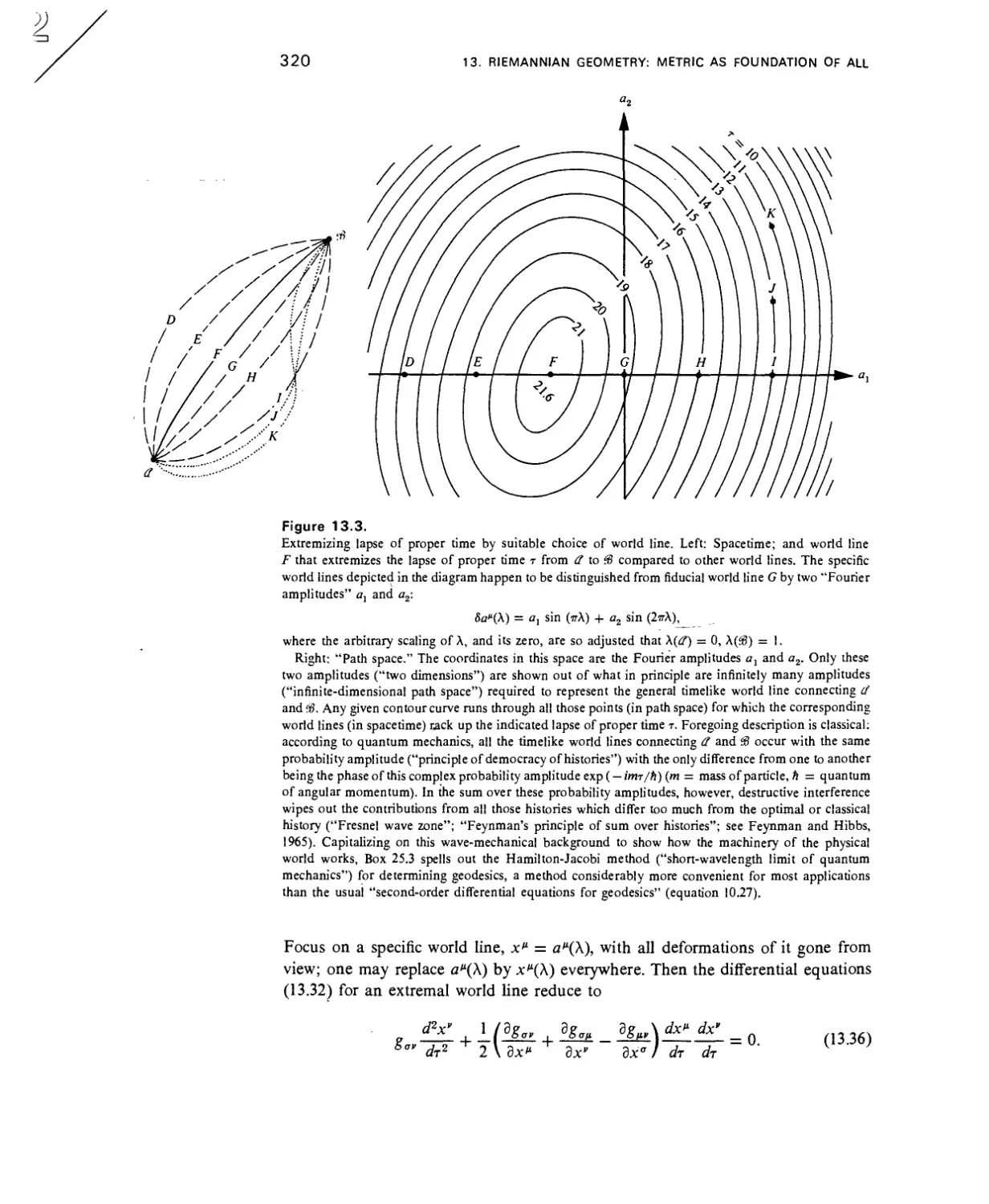
13.3. Coordinates in the truncated space of all his-
histories. 320
13.4. Proper reference frame of an accelerated ob-
observer. 328
15.1. The rotations associated with all six faces add to
zero. 372
18.1.1 Primitive detector for gravitational waves. 445
20.1. "World tube." 473
20.2. "Buffer zone." 477

FIGURES
XXV
21.1. Momentum and energy as rate of change of "dy-
"dynamic phase," 487
21.2. Building a thin-sandwich 4-geometry. 506
21.3. Extrinsic curvature. 511
21.4. Spacelike slices through Schwarzschild geome-
geometry. 528
21.5. Einstein thanks Mach. 544
21.6. Gaussian normal coordinates. 552
22.1. Geometric optics for a bundle of rays. 581
22.2. Number density of photons and specific inten-
intensity. 589
23.1.| Geometry within and around a star. 614
24.1.
24.2.
24.3.
First publications on black holes and neutron
stars. 622
Harrison-Wheeler equation of state for cold cata-
catalyzed matter and Harrison-Wakano-Wheeler stellar
models. 625
Collapse, pursuit, and plunge scenario. 629
25.1. Jupiter's satellites followed from night to
night. 63 7
25.2.1 Effective potential for motion in Schwarzschild
I geometry. 639
25.3. Cycloid relation between r and t for straight-in
fall. 664
25.4. Effective potential as a function of the tortoise
coordinate. 666
25.5. Fall toward a black hole as described by a comov-
ing observer versus a far-away observer. 667
25.6.1 Photon orbits in Schwarzschild geometry. 677
25.7. Deflection of a photon as a function of impact
parameter. 678
27.1. Comoving, synchronous coordinate system for
the universe. 71 6
27.2. Expanding balloon models an expanding uni-
universe. 719
27.3. Schwarzschild zones fitted together to make a
closed universe. 739
27.4. Friedmann cosmology in terms of arc parameter
time and hyperpolar angle. 741
27.5. Effective potential for Friedmann dynamics.
748
28.1.1 Temperature and density versus time for the
I standard big-bang model. 764
29.1. Redshift as an effect of standing waves. 776
29.2. Angle-effective distance versus redshift. 796
31.1.
31.2.
31.3.
Radial geodesies charted in Schwarzschild coor-
coordinates. 825
Novikov coordinates for Schwarzschild geome-
geometry. 82 7
Transformation from Schwarzschild to Kruskal-
Szekeres coordinates. 834
31.4.
31.5.
Varieties of radial geodesic presented in Sch-
Schwarzschild and Kruskal-Szekeres coordinates.
835
Embedding diagram for Schwarzschild geometry
at a moment of time symmetry. 837
Dynamics of the Schwarzschild throat. 839
31.6.
32.1. | Free-fall collapse of a star. 848
33.1.
33.2.
33.3.
34.1.
34.2.
34.3.
34.4
34.5.
34.6.
34.7.
34.8.
35.1
35.2
35.3.
36.1.
36.2.
36.3.
37.1.
37.2.
37.3.
37.4.
37.5.
38.1.
38.2.
38.3.
40.1.
40.2.
I Surface of last influence for collapsing star. 873
Black hole as garbage dump and energy
source. 908
Energy of particle near a Kerr black hole. 910
Future null infinity and the energy radiated in a
supernova explosion. 918
Minkowski spacetime depicted in coordinates that
are finite at infinity. 919
Schwarzschild spacetime . 920
Reissner-Nordstr^m spacetime depicted in coor-
coordinates that are finite at infinity. 921
Spacetime diagrams for selected causal relation-
relationships. 922
Black holes in an asymptotically flat space-
time. 924
The horizon produced by spherical collapse of a
star. 92 5
Spacetime diagram used to prove the second law
of black-hole dynamics. 932
I Plane electromagnetic waves.
Plane gravitational waves.
Exact plane-wave solution.
952
953
959
Why gravitational radiation is ordinarily weak.
976
Spectrum given off in head-on plunge into a
Schwarzschild black hole. 983
Slow-motion source. 997
Reference frame for vibrating bar detector.
1005
Types of detectors. 1013
Separation between geodesies responds to a
gravitational wave. 1014
Vibrator responding to linearly polarized radia-
radiation. 1022
Hammer blow of a gravitational wave on a noisy
detector. 103 7
The Pound-Rebka-Snider measurement of gravi-
gravitational redshift on the Earth. 1057
Brault's determination of the redshift of the D,
line of sodium from the sun. 1059
The Turner-Hill search for a dependence of proper
clock rate on velocity relative to distant mat-
matter. 1065
Bending of trajectory near the sun. 1 100
Coordinates used in calculating the deflection of
light. 1101

XXVI
GRAVITATION
40.3.1 Coordinates for calculating the relativistic time-
I delay. 1 106
40.4. Laser measurement of Earth-moon separation.
1130
41.1. Combination of rotations of 90° about axes that
diverge by 90°. 1 136
41.2. Rotation depicted as two reflections. 1 137
41.3. Composition of two rotations seen in terms of
reflections. 1 138
41.4. Law of composition of rotations epitomized in a
spherical triangle. 1 139
41.5. "Orientation-entanglement relation" between a
cube and its surroundings. 1 148
41.6. A 720° rotation is equivalent to no rotation.
1149
41.7. Spinor as flagpole plus flag. 1157
41.8. Direction in space represented on the complex
plane. 1161
42.1. A 2-geometry approximated by a polyhedron.
1168
42.2. Cycle of building blocks associated with a single
hinge. 1 1 70
43.1. Superspace in the simplicial approximation.
1182
43.2. Space, spacetime, and superspace. 1183
43.3. Electron motion affected by field fluctuations.
1190
44.1. Wormhole picture of electric charge. 1200
44.2. Gravitation as the metric elasticity of space.
1207
44.3. What pregeometry is not. 1210
44.4. Black-box model for reprocessing of universe.
1213
44.5. A mind full of geometrodynamics. 1219

ACKNOWLEDGMENTS
Deep appreciation goes to all who made this book possible. A colleague gives us
a special lecture so that we may adapt it into one of the chapters of this book. Another
investigator clears up for us the tangled history of the production of matter out of
the vacuum by strong tidal gravitational forces. A distant colleague telephones in
references on the absence of any change in physical constants with time. One student
provides a problem on the energy density of a null electromagnetic field. Another
supplies curves for effective potential as a function of distance. A librarian writes
abroad to get us an article in an obscure publication. A secretary who cares types
the third revision of a chapter. Editor and illustrator imaginatively solve a puzzling
problem of presentation. Repeat in imagination such instances of warm helpfulness
and happy good colleagueship times beyond count. Then one has some impression
of the immense debt we owe to over a hundred-fifty colleagues. Each face is etched
in our mind, and to each our gratitude is heartfelt. Warm thanks we give also to
the California Institute of Technology, the Dublin Institute for Advanced Studies,
the Institute for Advanced Study at Princeton, Kyoto University, the University of
Maryland, Princeton University, and the University of Texas at Austin for hospitality
during the writing of this book. We are grateful to the Academy of Sciences of
the U.S.S.R., to Moscow University, and to our Soviet colleagues for their hospitality
and the opportunity to become better acquainted in June-July 1971 with Soviet work
in gravitation physics. For assistance in the research that went into this book we
thank the National Science Foundation for grants (GP27304 and 28027 to Caltech;
GP17673 and GP8560 to Maryland; and GP3974 and GP7669 to Princeton); the
U.S. Air Force Office of Scientific Research (grant AF49-638-1545 to Princeton);
the U.S. National Aeronautics and Space Agency (grant NGR 05-002-256 to Caltech,
NSG 210-002-010 to Maryland); the Alfred P. Sloan Foundation for a fellowship
awarded to one of us (K.S.T.); and the John Simon Guggenheim Memorial Founda-
Foundation and All Souls College, Oxford, England, for fellowships awarded to another
of us (C.W.M.).

GRAVITATION

PART
SPACETIME PHYSICS
Wherein the reader is led, once quickly (§77),
then again more slowly, down the highways and
a few byways of Einstein's geometrodynamics—
without benefit of a good mathematical compass.

1
CHAPTER
GEOMETRODYNAMICS IN BRIEF
§1.1. THE PARABLE OF THE APPLE
One day in the year 1666 Newton had gone to the country,
and seeing the fall of an apple, as his niece told me, let himself
be led into a deep meditation on the cause which thus
draws every object along a line whose extension would pass
a/most through the center of the Earth.
VOLTAIRE A738)
Once upon a time a student lay in a garden under an apple tree reflecting on the
difference between Einstein's and Newton's views about gravity. He was startled
by the fall of an apple nearby. As he looked at the apple, he noticed ants beginning
to run along its surface (Figure 1.1). His curiosity aroused, he thought to investigate
the principles of navigation followed by an ant. With his magnifying glass, he noted
one track carefully, and, taking his knife, made a cut in the apple skin one mm
above the track and another cut one mm below it. He peeled off the resulting little
highway of skin and laid it out on the face of his book. The track ran as straight
as a laser beam along this highway. No more economical path could the ant have
found to cover the ten cm from start to end of that strip of skin. Any zigs and
zags or even any smooth bend in the path on its way along the apple peel from
starting point to end point would have increased its length.
"What a beautiful geodesic." the student commented.
His eye fell on two ants starting off from a common point P in slightly different
directions. Their routes happened to carry them through the region of the dimple
at the top of the apple, one on each side of it. Each ant conscientiously pursued

1. GEOMETRODYNAMICS IN BRIEF
Figure 1.1.
The Riemannian geometry of the spacetime of general relativity is here symbolized by the two-dimen-
two-dimensional geometry of the surface of an apple. The geodesic tracks followed by the ants on the apple's
surface symbolize the world line followed through spacetime by a free particle. In any sufficiently localized
region of spacetime, the geometry can be idealized as flat, as symbolized on the apple's two-dimensional
surface by the straight-line course of the tracks viewed in the magnifying glass ("local Lorentz character"
of geometry of spacetime). In a region of greater extension, the curvature of the manifold (four-dimen-
(four-dimensional spacetime in the case of the real physical world; curved two-dimensional geometry in the case
of the apple) makes itself felt. Two tracks d and <9, originally diverging from a common point 9, later
approach, cross, and go off in very different directions. In Newtonian theory this effect is ascribed to
gravitation acting at a distance from a center of attraction, symbolized here by the stem of the apple.
According to Einstein a particle gets its moving orders locally, from the geometry of spacetime right
where it is. Its instructions are simple: to follow the straightest possible track (geodesic). Physics is as
simple as it could be locally. Only because spacetime is curved in the large do the tracks cross. Geome-
trodynamics, in brief, is a double story of the effect of geometry on matter (causing originally divergent
geodesies to cross) and the effect of matter on geometry (bending of spacetime initiated by concentration
of mass, symbolized by effect of stem on nearby surface of apple).
Einstein's local view of
physics contrasted with
Newton's "action at a
distance"
Physics is simple only when
analyzed locally
his geodesic. Each went as straight on his strip of appleskin as he possibly could.
Yet because of the curvature of the dimple itself, the two tracks not only crossed
but emerged in very different directions.
"What happier illustration of Einstein's geometric theory of gravity could one
possibly ask?" murmured the student. "The ants move as if they were attracted
by the apple stem. One might have believed in a Newtonian force at a distance.
Yet from nowhere does an ant get his moving orders except from the local geometry
along his track. This is surely Einstein's concept that all physics takes place by
'local action.' What a difference from Newton's 'action at a distance' view of physics!
Now I understand better what this book means."
And so saying, he opened his book and read, "Don't try to describe motion
relative to faraway objects. Physics is simple only when analyzed locally. And locally

§1.2. SPACETIME WITH AND WITHOUT COORDINATES 5
the world line that a satellite follows [in spacetime, around the Earth] is already
as straight as any world line can be. Forget all this talk about 'deflection' and 'force
of gravitation.' I'm inside a spaceship. Or I'm floating outside and near it. Do I
feel any 'force of gravitation'? Not at all. Does the spaceship 'feel' such a force?
No. Then why talk about it? Recognize that the spaceship and I traverse a region
of spacetime free of all force. Acknowledge that the motion through that region
is already ideally straight."
The dinner bell was ringing, but still the student sat, musing to himself. "Let me
see if I can summarize Einstein's geometric theory of gravity in three ideas: A)
locally, geodesies appear straight; B) over more extended regions of space and time,
geodesies originally receding from each other begin to approach at a rate governed
by the curvature of spacetime, and this effect of geometry on matter is what we
mean today by that old word 'gravitation'; C) matter in turn warps geometry. The
dimple arises in the apple because the stem is there. I think I see how to put the
whole story even more briefly: Space acts on matter, telling it how to move. In turn,
matter reacts back on space, telling it how to curve. In other words, matter here,"
he said, rising and picking up the apple by its stem, "curves space here. To produce
a curvature in space here is to force a curvature in space there," he went on, as
he watched a lingering ant busily following its geodesic a finger's breadth away from
the apple's stem. "Thus matter here influences matter there. That is Einstein's
explanation for 'gravitation.'"
Then the dinner bell was quiet, and he was gone, with book, magnifying glass—and
apple.
Space tells matter how to
move
Matter tells space how to
curve
§1.2. SPACETIME WITH AND WITHOUT COORDINATES
Now it came to me: . . . the independence of the
gravitational acceleration from the nature of the falling
substance, may be expressed as follows: In a
gravitational field (of small spatial extension) things
behave as they do in a space free of gravitation. . . . This
happened in 1908. Why were another seven years required
for the construction of the general theory of relativity?
The main reason lies in the fact that it is not so easy to
free oneself from the idea that coordinates must have an
immediate metrical meaning.
ALBERT EINSTEIN [in Schilpp A949), pp. 65-67.]
Nothing is more distressing on first contact with the idea of "curved spacetime" than Problem: how to measure in
the fear that every simple means of measurement has lost its power in this unfamiliar curved spacetime
context. One thinks of oneself as confronted with the task of measuring the shape
of a gigantic and fantastically sculptured iceberg as one stands with a meter stick
in a tossing rowboat on the surface of a heaving ocean. Were it the rowboat itself
whose shape were to be measured, the procedure would be simple enough. One
would draw it up on shore, turn it upside down, and drive tacks in lightly at strategic
points here and there on the surface. The measurement of distances from tack to

У
1. GEOMETRODYNAMICS IN BRIEF
Figure 1.2.
The crossing of straws in a barn full of hay is a symbol for the world lines that fill up spacetime. By
their crossings and bends, these world lines mark events with a uniqueness beyond all need of coordinate
systems or coordinates. Typical events symbolized in the diagram, from left to right (black dots), are:
absorption of a photon; reemission of a photon; collision between a particle and a particle; collision
between a photon and a particle; another collision between a photon and a particle; explosion of a
firecracker; and collision of a particle from outside with one of the fragments of that firecracker.
Resolution: characterize
events by what happens
there
tack would record and reveal the shape of the surface. The precision could be made
arbitrarily great by making the number of tacks arbitrarily large. It takes more daring
to think of driving several score pitons into the towering iceberg. But with all the
daring in the world, how is one to drive a nail into spacetime to mark a point?
Happily, nature provides its own way to localize a point in spacetime, as Einstein
was the first to emphasize. Characterize the point by what happens there! Give a
point in spacetime the name "event." Where the event lies is defined as clearly and
sharply as where two straws cross each other in a barn full of hay (Figure 1.2). To
say that the event marks a collision of such and such a photon with such and such
a particle is identification enough. The world lines of that photon and that particle
are rooted in the past and stretch out into the future. They have a rich texture of
connections with nearby world lines. These nearby world lines in turn are linked
in a hundred ways with world lines more remote. How then does one tell the location
of an event? Tell first what world lines participate in the event. Next follow each

Figure 1.3.
Above: Assigning "telephone numbers" to events by way of a system of coordinates. To say that the
coordinate system is "smooth" is to say that events which are almost in the same place have almost
the same coordinates. Below: Putting the same set of events into equally good order by way of a different
system of coordinates. Picked out specially here are two neighboring events: an event named "i'" with
coordinates (л", л1) = G7.2. 22.6) and (л". лт) = ( 18.5. 51.4): and an event named ":?'" with coordinates
(.v". .v1) = G9.9. 20.1) and (x".x') = A8.4. 47.1). Events i' and :? are connected by the separation "vector"
f. (Precise definition of a vector in u curved spacetime demands going to the mathematical limit in
which the two points have nn indefinitely small separation [V-fold reduction of the separation ■/ — ;'].
and. in the resultant locally Hat space, multiplying the separation up again by the factor .Y[lim Л —» x:
"tangent space": "langent vector"']. Forego here that proper way o\' stating matters, and forego complete
accuracy: hence the quote around the word "vector".) In each coordinate system the separation vector
f is characterized by "components" (differences in coordinate values between '»' and r'):
<£'. t1) = G9.9 - 77.2. 20.1 - 22.6) = B.7. - 2.5).
(£\{T) = A8.4 - 18.5. 47.1 - 51.4) = (-0.1. -4.3).
See Bo\ 1.1 for further discussion of events, coordinates, and vectors.

8
1. GEOMETRODYNAMICS IN BRIEF
The name of an event can
even be arbitrary
Coordinates provide a
convenient naming system
Coordinates generally do not
measure length
Several coordinate systems
can be used at once
Vectors
of these world lines. Name the additional events that they encounter. These events
pick out further world lines. Eventually the whole barn of hay is catalogued. Each
event is named. One can find one's way as surely to a given intersection as the city
dweller can pick his path to the meeting of St. James Street and.Piccadilly. No
numbers. No coordinate system. No coordinates.
That most streets in Japan have no names, and most houses no numbers, illustrates
one's ability to do without coordinates. One can abandon the names of two world
lines as a means to identify the event where they intersect. Just as one could name
a Japanese house after its senior occupant, so one can and often does attach arbitrary
names to specific events in spacetime. as in Box 1.1.
Coordinates, however, are convenient. How else from the great thick catalog of
events, randomly listed, can one easily discover that along a certain world line one
will first encounter event Trinity, then Baker, then Mike, then Argus—but not the
same events in some permuted order?
To order events, introduce coordinates! (See Figure 1.3.) Coordinates are four
indexed numbers per event in spacetime; on a sheet of paper, only two. Trinity
acquires coordinates
(x°, x\ x2, x3) = G7,23,64,11).
In christening events with coordinates, one demands smoothness but foregoes every
thought of mensuration. The four numbers for an event are nothing but an elaborate
kind of telephone number. Compare their "telephone" numbers to discover whether
two events are neighbors. But do not expect to learn how many meters separate
them from the difference in their telephone numbers!
Nothing prevents a subscriber from being served by competing telephone systems,
nor an event from being catalogued by alternative coordinate systems (Figure 1.3).
Box 1.1 illustrates the relationships between one coordinate system and another, as
well as the notation used to denote coordinates and their transformations.
Choose two events, known to be neighbors by the nearness of their coordinate
values in a smooth coordinate system. Draw a little arrow from one event to the
other. Such an arrow is called a vector. (It is a well-defined concept in flat spacetime,
or in curved spacetime in the limit of vanishingly small length; for finite lengths
in curved spacetime, it must be refined and made precise, under the new name
"tangent vector," on which see Chapter 9.) This vector, like events, can be given
a name. But whether named "John" or "Charles" or "Kip," it is a unique, well-
defined geometrical object. The name is a convenience, but the vector exists even
without it.
Just as a quadruple of coordinates
(x°, x\ x2, x3) = G7,23,64,11)
is a particularly useful name for the event "Trinity" (it can be used to identify what
other events are nearby), so a quadruple of "components"
= A.2,-0.9,0,2.1)

Box 1.1 MATHEMATICAL NOTATION FOR EVENTS, COORDINATES, AND VECTORS
Events are denoted by capital script, one-letter Latin names such as e?, i?, (I', ?Я.
Sometimes subscripts are used: ^0, lflt $6.
Coordinates of an event if are denoted by /(;?), .v(f/1). v(tf), ;(&),
or by -A^), xl(&). .xH-P).
x3(<-?),
or more abstractly by x^) or xa(ii>),
where it is understood that Greek indices can take on any value 0, 1,
2. or3.
Time coordinate (when one of the four is picked to play this role) x°(^).
Space coordinates are xl(Lf), хЦ^Р), х3(?Р)
and are sometimes denoted by х'(У) or xkC?) or....
It is to be understood that Latin indices take on values 1, 2, or 3.
Shorthand notation: One soon tires of writing explicitly the functional depen-
dependence of the coordinates, х^(чР); so one adopts the shorthand notation xf>
for the coordinates of the event Lf, and x>
for the space coordinates. One even begins to think of x& as representing
the event У itself, but must remind oneself that the values of x°, xl, x2,
x3 depend not only on the choice of e? but also on the arbitrary choice
of coordinates!
Other coordinates for the same event •# may be denoted .v"(^) or just xa,
xa\rP) or just .va'.
x'\'f) or just x".
example: In Figure 1.3 (.v0,*1) = G7.2.22.6) and (x". .vT) = A8.5.51.4)
refer to the same event. The bars, primes, and hats distinguish one
coordinate system from another; by putting them on the indices rather
than on the x's, we simplify later notation.
Transformation from one coordinate system to another is achieved by the four
functions x%x<\ xK л--\ .v3),
хЦх".х\х-.х3),
л-2(.х°..х1,л--'..х3),
х\\л\х1,х'2.х3).
which are denoted more succinctly xa(.vs).
Separation vector* (little arrow) reaching from one event i? to neighboring event
L:P can be denoted abstractly by и or v or (. or f/1 — iP.
It can also be characterized by the coordinate-value differencest between
'?' and r1 (called "components" of the vector) f =x"{?P) — x"(£),
£," = xr>(':P) - x"(£).
Transformation of components of a vector from one coordinate system to another , -
is achieved bv partial derivatives of transformation equations £" = _^__£/i#
_' _ _ r.v'J
since |" = xa(iP) - .v"(-') = (?.v" ?.v/i)[.v'3(^) - .v'!(^)].f
Einstein summation convention is used here:
any index that is repeated in a product is automatically summed on
^. rxn
2-, ,-... и
*This definition of a vector is valid onlv in flat spacetime. The refined deliniiion ("tangent vector") in curved spacetime
i-, not ^pelled out here (see Chapter 9). but flat-geometry ideas apply with good approximation even in a curved geometry,
when the wo points are sufficiently elose.
t These formulas are preciselv accurate only when the region of spacetime under consideration is flat and when in addition
the coordinates are Lorentzian. Otherwise they are approximate—though ihey become arbitrarily good when the separation
between points and the length of the vector become arbitrarily small.

10
1. GEOMETRODYNAMICS IN BRIEF
Coordinate singularities
normally unavoidable
Continuity of spacetime
The mathematics of
manifolds applied to the
physics of spacetime
Dimensionality of spacetime
is a convenient name for the vector "John" that reaches from
= G7,23,64, 11)
to
(x°, jc1, a-2, x3) = G8.2,22.1,64.0, 13.1).
How to work with the components of a vector is explored in Box 1.1.
There are many ways in which a coordinate system can be imperfect. Figure 1.4
illustrates a coordinate singularity. For another example of a coordinate singularity,
run the eye over the surface of a globe to the North Pole. Note the many meridians
that meet there ("collapse of cells of egg crates to zero content"). Can't one do better?
Find a single coordinate system that will cover the globe without singularity? A
theorem says no. Two is the minimum number of "coordinate patches" required
to cover the two-sphere without singularity (Figure 1.5). This circumstance empha-
emphasizes anew that points and events are primary, whereas coordinates are a mere
bookkeeping device.
Figures 1.2 and 1.3 show only a few world lines and events. A more detailed
diagram would show a maze of world lines and of light rays and the intersections
between them. From such a picture, one can in imagination step to the idealized
limit: an infinitely dense collection of light rays and of world lines of infinitesimal
test particles. With this idealized physical limit, the mathematical concept of a
continuous four-dimensional "manifold" (four-dimensional space with certain
smoothness properties) has a one-to-one correspondence; and in this limit continu-
continuous, differentiable (i.e., smooth) coordinate systems operate. The mathematics then
supplies a tool to reason about the physics.
A simple countdown reveals the dimensionality of the manifold. Take a point f?
in an «-dimensional manifold. Its neighborhood is an и-dimensional ball (i.e., the
interior of a sphere whose surface has n — \ dimensions). Choose this ball so that
its boundary is a smooth manifold. The dimensionality of this manifold is (n — 1).
In this (n — l)-dimensional manifold, pick a point 2. Its neighborhood is an
(n — l)-dimensional ball. Choose this ball so that..., and so on. Eventually one
comes by this construction to a manifold that is two-dimensional but is not yet known
to be two-dimensional (two-sphere). In this two-dimensional manifold, pick a point
Ш,. Its neighborhood is a two-dimensional ball ("disc"). Choose this disc so that
its boundary is a smooth manifold (circle). In this manifold, pick a point ?t. Its
neighborhood is a one-dimensional ball, but is not yet known to be one-dimensional
("line segment"). The boundaries of this object are two points. This circumstance
tells that the intervening manifold is one-dimensional; therefore the previous mani-
manifold was two-dimensional; and so on. The dimensionality of the original manifold
is equal to the number of points employed in the construction. For spacetime, the
dimensionality is 4.
This kind of mathematical reasoning about dimensionality makes good sense at
the everyday scale of distances, at atomic distances A0~8 cm), at nuclear dimensions
A0~13cm), and even at lengths smaller by several powers often, if one judges by
the concord between prediction and observation in quantum electrodynamics at high

г = 2.2m
2.4m
г - 1.6/:
г = 1.8m
-' = — т
2.6m 2.8m 3.0m
Figure 1.4.
How a mere coordinate singularity arises. Above: A coordinate system becomes singular when the "cells
in the egg crate" are squashed to zero volume. Below: An example showing such a singularity in the
Schwarzschild coordinates r, / often used to describe the geometry around a black hole (Chapter 31).
For simplicity the angular coordinates в, <$> have been suppressed. The singularity shows itself in two
ways. First, all the points along the dotted line, while quite distinct one from another, are designated
by the same pair of (r. t) values: namely, r = 2m, t = cc. The coordinates provide no way to distinguish
these points. Second, the "cells in the egg crate," of which one is shown grey in the diagram, collapse
to zero content at the dotted line. In summary, there is nothing strange about the geometry at the dotted
line; all the singularity lies in the coordinate system ("poor system of telephone numbers"). No confusion
should be permitted to arise from the accidental circumstance that the / coordinate attains an infinite
value on the dotted line. No such infinity would occur if i were replaced by the new coordinate t. defined
ЬУ
(t/2m) = tan(//2m).
When / = эс, the new coordinate / is / = п-ni. The r, / coordinates still provide no way to distinguish
the points along the dotted line. They still give "cells in the egg crate" collapsed to zero content along
the dotted line.

Figure 1.5.
Singularities in familiar coordinates on the two-sphere can be eliminated by covering the sphere with
two overlapping coordinate patches. A. Spherical polar coordinates, singular at the North and South
Poles, and discontinuous at the international date line. B. Projection of the Euclidean coordinates of
the Euclidean two-plane, tangent at the North Pole, onto the sphere via a line running to the South
Pole; coordinate singularity at the South Pole. C. Coverage of two-sphere by two overlapping coordinate
patches. One, constructed as in B, covers without singularity the northern hemisphere and also the
southern tropics down to the Tropic of Capricorn. The other (grey) also covers without singularity all
of the tropics and the southern hemisphere besides.
Breakdown in smoothness of
spacetime at Pianck length
energies (corresponding de Broglie wavelength 10~16 cm). Moreover, classical general
relativity thinks of the spacetime manifold as a deterministic structure, completely
well-defined down to arbitrarily small distances. Not so quantum general relativity
or "quantum geometrodynamics." It predicts violent fluctuations in the geometry
at distances on the order of the Planck length,
L* = (fiG/c3I/2
= [A.054 x 10-27gcm2/sec)F.670 x 10~8 cm3/g sec2)]1/2 x
X B.998 X 1010 cm/sec)-3'2 A.1)
= 1.616 X 10-33 cm.
No one has found any way to escape this prediction. As nearly as one can estimate,
these fluctuations give space at small distances a "multiply connected" or "foamlike"
character. This lack of smoothness may well deprive even the concept of dimension-
dimensionality itself of any meaning at the Planck scale of distances. The further exploration
of this issue takes one to the frontiers of Einstein's theory (Chapter 44).
If spacetime at small distances is far from the mathematical model of a continuous
manifold, is there not also at larger distances a wide gap between the mathematical

§1.3. WEIGHTLESSNESS
13
idealization and the physical reality? The infinitely dense collection of light rays
and of world lines of infinitesimal test particles that are to define all the points of
the manifold: they surely are beyond practical realization. Nobody has ever found
a particle that moves on timelike world lines (finite rest mass) lighter than an electron.
A collection of electrons, even if endowed with zero density of charge (e+ and e~
world lines present in equal numbers) will have a density of mass. This density will
curve the very manifold under study. Investigation in infinite detail means unlimited
density, and unlimited disturbance of the geometry.
However, to demand investigatability in infinite detail in the sense just described
is as out of place in general relativity as it would be in electrodynamics or gas
dynamics. Electrodynamics speaks of the strength of the electric and magnetic field
at each point in space and at each moment of time. To measure those fields, it is
willing to contemplate infinitesimal test particles scattered everywhere as densely
as one pleases. However, the test particles do not have to be there at all to give
the field reality. The field has everywhere a clear-cut value and goes about its
deterministic dynamic evolution willy-nilly and continuously, infinitesimal test
particles or no infinitesimal test particles. Similarly with the geometry of space.
In conclusion, when one deals with spacetime in the context of classical physics,
one accepts A) the notion of "infinitesimal test particle" and B) the idealization
that the totality of identifiable events forms a four-dimensional continuous manifold.
Only at the end of this book will a look be taken at some of the limitations placed
by the quantum principle on one's way of speaking about and analyzing spacetime.
Difficulty in defining
geometry even at classical
distances?
No; one must accept
geometry at classical
distances as meaningful
§1.3. WEIGHTLESSNESS
"Gravity is a great mystery. Drop a stone. See it fall. Hear it hit. No one understands
why." What a misleading statement! Mystery about fall? What else should the stone
do except fall? To fall is normal. The abnormality is an object standing in the way
of the stone. If one wishes to pursue a "mystery," do not follow the track of the
falling stone. Look instead at the impact, and ask what was the force that pushed
the stone away from its natural "world line," (i.e., its natural track through space-
time). That could lead to an interesting issue of solid-state physics, but that is not
the topic of concern here. Fall is. Free fall is synonymous with weightlessness:
absence of any force to drive the object away from its normal track through space-
time. Travel aboard a freely falling elevator to experience weightlessness. Or travel
aboard a spaceship also falling straight toward the Earth. Or, more happily, travel
aboard a spaceship in that state of steady fall toward the Earth that marks a circular
orbit. In each case one is following a natural track through spacetime.
The traveler has one chemical composition, the spaceship another; yet they travel
together, the traveler weightless in his moving home. Objects of such different nuclear
constitution as aluminum and gold fall with accelerations that agree to better than
one part in 1OU, according to Roll, Krotkov, and Dicke A964), one of the most
important null experiments in all physics (see Figure 1.6). Individual molecules fall
in step, too, with macroscopic objects [Estermann, Simpson, and Stern A938)]; and
so do individual neutrons [Dabbs, Harvey, Paya, and Horstmann A965)], individual
.(continued on page-16)
Free fall is the natural state
of motion
All objects fall with the same
acceleration

/
14 1. GEOMETRODYNAMICS IN BRIEF
Figure 1.6.
Principle of the Roll-Krotkov-Dicke experiment, which showed that the gravitational accelerations of
gold and aluminum are equal to 1 part in 10" or better (Princeton, 1964). In the upper lefthand corner,
equal masses of gold and aluminum hang from a supporting bar. This bar in turn is supported at its
midpoint. If both objects fall toward the sun with the same acceleration of g = 0.59 cm/sec2, the bar
does not turn. If the Au mass receives a higher acceleration, g + Sg. then the gold end of the bar starts
to turn toward the sun in the Earth-fixed frame. Twelve hours laier the sun is on the other side, pulling
the other way. The alie mating torque lends itself to recognition against a background of noise because
of its precise 24-hour period. Unhappily, any substaniial mass nearby, such as an experimenter, located
at A/, will produce a torque that swamps the effect sought. Therefore the actual arrangement was as
shown in the body of the figure. One gold weight and two aluminum weights were supported at the
three corners of a horizontal equilateral triangle. 6 cm on a side (three-fold axis of symmetry, giving
zero response to all the simplest nonuniformities in the gravitational field). Also, the observers performed
all operations remotely to eliminate their own gravitational effects*. To detect a rotation of the torsion
balance as small as —lO"9 rad without disturbing the balance. Roll. Krotkov, and Dicke reflected a
very weak light beam from the optically flat back face of the quartz triangle. The image of the source
slit fell on a wire of about the same size as the slit image. The light transmitted past the wire fell on
a photomultiplier. A separate oscillator circuit drove the wire back and forth across the image at 3,000
hertz. When the image was centered perfectly, only even harmonics of the oscillation frequency appeared
in the light intensity. However, when the image was displaced slightly to one side, the fundamental
frequency appeared in the light intensity. The electrical output of the photomultiplier then contained
a 3,000-hertz component. The magnitude and sign of this component were determined automatically.
Equally automatically a proportional d.c. voltage was applied to the electrodes shown in the diagram.
It restored the torsion balance to its zero position. The d.c. voltage required to restore the balance to
its zero position was recorded as a measure of the torque acting on the pendulum. This torque was
Fourier-analyzed over a period of many days. The magnitude of the Fourier component of 24-hour
period indicated a ratio Sg/g = @.96 ± i.04) x 1O"U. Aluminum and gold thus fall with the same
acceleration, despite their important differences summarized in the table.
Ratios Al Аи
Number of neutrons „ .,
тт—z ; I 08 1.5
Number of proions
Mass of kinetic energy of K-electron
Rest mass of eleclron
Electrostatic mass-energy of nucleus
Mass of atom
The theoretical implications of this experiment will be discussed in greater detail in Chapters 16 and 38.
Braginsky and Panov A971) at Moscow University performed an experiment identical in principle
to that of Dicke-Roll-Krotkov, but with a modified experimental set-up. Comparing the accelerations
of platinum and aluminum rather than of gold and aluminum, they say that
< 1 X 10-12.
* Other perturbations had to be, and were, guarded against. A) A bit of iron on the torsion balance
as big as 10 cm on a side would have contributed, in the Earth's magnetic field, a torque a hundred
times greater than the measured torque. B) The unequal pressure of radiation on the two sides of a
mass would have produced an unacceptably large perturbation if the temperature difference between
these two sides had exceeded 10 °K. C) Gas evolution from one side of a mass would have propelled
it like a rocket. If the rate of evolution were as great as 10"8 g/day, the calculated force would have
been — 10 g cm/sec2, enough to affect the measurements. D) The rotation was measured with respect
to the pier that supported the equipment. As a guarantee that this pier did not itself rotate, it was anchored
to bed rock. E) Electrostatic forces were eliminated; otherwise they would have perturbed the balance.

15
\
Sun
//
Fused quartz fiber coated with a
thin aluminum film to eliminate
elecirostauc fields
Photo-
multiplier
Path of
return light
blocked by wire:
wire
oscillates rapidly
back and forth
across image
of slit
Telescope// /,
objective //,
Quartz triangle of torsion
balance: back face polished
to reflect light
Sun at | Ai
6 p.m.
Sun ai
6 \.м.

16
1. GEOMETRODYNAMICS IN BRIEF
electrons [Witteborn and Fairbank A967)] and individual mu mesons [Beall A970)].
What is more, not one of these objects has to see out into space to know how to
move.
Contemplate the interior of a spaceship, and a key, penny, nut, and pea by accident
or design set free inside. Shielded from all view of the world outside by the walls
of the vessel, each object stays at rest relative to the vessel. Or it moves through
the room in a straight line with uniform velocity. That is the lesson which experience
shouts out.
Forego talk of acceleration! That, paradoxically, is the lesson of the circumstance
that "all objects fall with the same acceleration." Whose fault were those accelera-
accelerations, after all? They came from allowing a groundbased observer into the act. The
Box 1.2 MATERIALS OF THE MOST DIVERSE COMPOSITION FALL WITH
THE SAME ACCELERATION ("STANDARD WORLD LINE")
Aristotle: "the downward movement of a mass of
gold or lead, or of any other body endowed with
weight, is quicker in proportion to its size."
Pre-Galilean literature: metal and wood weights
fall at the same rate.
Galileo: (I) "the variation of speed in air between
balls of gold, lead, copper, porphyry, and other
heavy materials is so slight that in a fall of 100
cubits [about 46 meters] a ball of gold would surely
not outstrip one of copper by as much as four
fingers. Having observed this, I came to the con-
conclusion that in a medium totally void of resistance
all bodies would fall with the same speed." B)
later experiments of greater precision "diluting
gravity" and finding same time of descent for
different objects along an inclined plane.
Newton: inclined plane replaced by arc of pendu-
pendulum bob; "time of fall" for bodies of different
composition determined by comparing time of
oscillation of pendulum bobs of the two materials.
Ultimate limit of precision in such experiments
limited by problem of determining effective length
of each pendulum: (acceleration) = Bт7/ре-
riodJ(length).
Lorand von Eotvos, Budapest, 1889 and 1922:
compared on the rotating earth the vertical defined
by a plumb bob of one material with the vertical
defined by a plumb bob of other material. The
two hanging masses, by the two unbroken threads
that support them, were drawn along identical
world lines through spacetime (middle of the labo-
laboratory of Eotvos!). If cut free, would they also
follow identical tracks through spacetime ("normal
world line of test mass")? If so, the acceleration
that draws the actual world line from the normal
free-fall world line will have a standard value, a.
The experiment of Eotvos did not try to test agree-
agreement on the magnitude of a between the two
masses. Doing so would have required (I) cutting
the threads and B) following the fall of the two
masses. Eotvos renounced this approach in favor
of a static observation that he could make with
greater precision, comparing the direction of a for
the two masses. The direction of the supporting
thread, so his argument ran, reveals the direction
in which the mass is being dragged away from its
normal world line of "free fall" or "weightless-
"weightlessness." This acceleration is the vectorial resultant
of (I) an acceleration of magnitude g, directed
outward against so-called gravity, and B) an ac-
acceleration directed toward the axis of rotation of
the earth, of magnitude w2 R sin в (w, angular ve-

§1.3. WEIGHTLESSNESS
м
push of the ground under his feet was driving him away from a natural world line.
Through that flaw in his arrangements, he became responsible for all those accelera-
accelerations. Put him in space and strap rockets to his legs. No difference!* Again the
responsibility for what he sees is his. Once more he notes that "all objects fall with
*"No difference" spelled out amounts to Einstein's A911) principle of the local equivalence between a
"gravitational field" and an acceleration: " We arrive at a very satisfactory interpretation of this law of
experience, if we assume that the systems К and K' are physically exactly equivalent, that is, if we assume
that we may just as well regard the system К as being in a space free from gravitational fields, if we then
regard К as uniformly accelerated. This assumption of exact physical equivalence makes it impossible for
us to speak of the absolute acceleration of the system of reference, just as the usual theory of relativity
forbids us to talk of the absolute velocity of a system; and it makes the equal falling of all bodies in a
gravitational field seem a matter of course."
locity; R, radius of earth; в, polar angle measured
from North Pole to location of experiment). This
centripetal acceleration has a vertical component
—w2i?sin2# too small to come into discussion.
The important component is w2 R sin в cos в, di-
directed northward and parallel to the surface of the
earth. It deflects the thread by the angle
horizontal acceleration
vertical acceleration
_ со2 R sin в cos в
g
= 34cm/sec29sinflcosfl
980 cm/sec2
= 1.7 x Ю-3 radian at 0 = 45°
from the straight line connecting the center of the
earth to the point of support. A difference, 8g, of
one part in 108 between g for the two hanging
substances would produce a difference in angle of
hang of plumb bobs equal to 1.7 x 10~n radian
at Budapest (в = 42.5°). Eotvos reported Sg/g less
than a few parts in 109.
Roll, Krotkov, and Dicke, Princeton, 1964. em-
employed as fiducial acceleration, not the 1.7 cm/sec2
steady horizontal acceleration, produced by the
earth's rotation at в = 45°, but the daily alternat-
alternating 0.59 cm/sec2 produced by the sun's attraction.
Reported |g(Au) - g(Al)\/g less than 1 X Ю1.
See Figure 1.6.
Braginsky and Panov, Moscow, 1971: like Roll,
Krotkov, and Dicke, employed Sun's attraction as
fiducial acceleration. Reported |g(Pt) — g(A\)\/g
less than 1 X Ю2.
Beall, 1970: particles that are deflected less by the
Earth's or the sun's gravitational field than a pho-
photon would be, effectively travel faster than light.
If they are charged or have other electromagnetic
structure, they would then emit Cerenkov radia-
radiation, and reduce their velocity below threshold in
less than a micron of travel. The threshold is at
energies around 103 me2. Ultrarelativistic particles
in cosmic-ray showers are not easily identified, but
observations of 1013 eV muons show that muons
are not "too light" by as much as 5 X Ю. Con-
Conversely, a particle P bound more strongly than
photons by gravity will transfer the momentum
needed to make pair production у —> P + P occur
within a submicron decay length. The existence of
photons with energies above 1013 eV shows that
e* are not "too heavy" by 5 parts in 109, fi* not
by 2 in 104, A, Z~, Q~ not by a few per cent.

18
1. GEOMETRODYNAMICS IN BRIEF
Figure 1.7.
"Weightlessness" as test for a local inertial frame of reference ("Lorentz frame"). Each spring-driven
cannon succeeds in driving its projectile, a steel ball bearing, through the aligned holes in the sheets
of lucite, and into the woven-mesh pocket, when the frame of reference is free of rotation and in free
fall ("normal world line through spacetime"). A cannon would fail (curved and ricocheting trajectory
at bottom of drawing) if the frame were hanging as indicated when the cannon went off ("frame drawn
away by pull of rope from its normal world line through spacetime"). Harold Waage at Princeton has
constructed such a model for an inertial reference frame with lucite sheets about 1 m square. The "fuses"
symbolizing time delay were replaced by electric relays. Penetration fails if the frame A) rotates, B)
accelerates, or C) does any combination of the two. It is difficult to cite any easily realizable device
that more fully illustrates the meaning of the term "local Lorentz frame."
Eliminate the acceleration by
use of a local inertial frame
the same acceleration." Physics looks as complicated to the jet-driven observer as
it does to the man on the ground. Rule out both observers to make physics look
simple. Instead, travel aboard the freely moving spaceship. Nothing could be more
natural than what one sees: every free object moves in a straight line with uniform
velocity. This is the way to do physics! Work in a very special coordinate system:
a coordinate frame in which one is weightless; a local inertial frame of reference.
Or calculate how things look in such a frame. Or—if one is constrained to a ground-
based frame of reference—use a particle moving so fast, and a path length so limited,
that the ideal, freely falling frame of reference and the actual ground-based frame
get out of alignment by an amount negligible on the scale of the experiment. [Given
a 1,500-m linear accelerator, and a 1 GeV electron, time of flight ~ A.5 X 105cm)/

§1.4. GEOMETRY IS LOCALLY LORENTZIAN
19
C X Ю10 cm/sec) = 0.5 X 1СГ5 sec; fall in this time ~~\gt2 = D90 cm/sec2)@.5 X
10~5 secJ ~ 10-8 cm.]
In analyzing physics in a local inertial frame of reference, or following an ant
on his little section of apple skin, one wins simplicity by foregoing every reference
to what is far away. Physics is simple only when viewed locally: that is Einstein's
great lesson.
Newton spoke differently: "Absolute space, in its own nature, without relation
to anything external, remains always similar and immovable." But how does one
give meaning to Newton's absolute space, find its cornerstones, mark out its straight
lines? In the real world of gravitation, no particle ever follows one of Newton's
straight lines. His ideal geometry is beyond observation. "A comet going past the
sun is deviated from an ideal straight line." No. There is no pavement on which
to mark out that line. The "ideal straight line" is a myth. It never happened, and
it never will.
"It required a severe struggle [for Newton] to arrive at the concept of independent
and absolute space, indispensible for the development of theory.... Newton's decision
was, in the contemporary state of science, the only possible one, and particularly the
only fruitful one. But the subsequent development of the problems, proceeding in a
roundabout way which no one could then possibly foresee, has shown that the resistance
of Leibniz and Huygens, intuitively well-founded but supported by inadequate argu-
arguments, was actually justified. ... It has required no less strenuous exertions subsequently
to overcome this concept [of absolute space]"
[A. EINSTEIN A954)].
What is direct and simple and meaningful, according to Einstein, is the geometry
in every local inertial reference frame. There every particle moves in a straight line
with uniform velocity. Define the local inertial frame so that this simplicity occurs
for the first few particles (Figure 1.7). In the frame thus defined, every other free
particle is observed also to move in a straight line with uniform velocity. Collision
and disintegration processes follow the laws of conservation of momentum and
energy of special relativity. That all these miracles come about, as attested by tens
of thousands of observations in elementary particle physics, is witness to the inner
workings of the machinery of the world. The message is easy to summarize: A)
physics is always and everywhere locally Lorentzian; i.e., locally the laws of special
relativity are valid; B) this simplicity shows most clearly in a local Lorentz frame
of reference ("inertial frame of reference"; Figure 1.7); and C) to test for a local
Lorentz frame, test for weightlessness!
Newton's absolute space is
unobservable. nonexistent
But Einstein's local inertial
frames exist, are simple
In local inertial frames,
physics is Lorentzian
§1.4. LOCAL LORENTZ GEOMETRY,
WITH AND WITHOUT COORDINATES
On the surface of an apple within the space of a thumbprint, the geometry is
Euclidean (Figure 1.1; the view in the magnifying glass). In spacetime, within a
limited region, the geometry is Lorentzian. On the apple the distances between point
and point accord with the theorems of Euclid. In spacetime the intervals ("proper
distance," "proper time") between event and event satisfy the corresponding theo-
theorems of Lorentz-Minkowski geometry (Box 1.3). These theorems lend themselves
{continued on page 23)
Local Lorentz geometry is the
spacetime analog of local
Euclidean geometry.

■И
20
1. GEOMETRODYNAMICS IN BRIEF
Box 1.3 LOCAL LORENTZ GEOMETRY AND LOCAL EUCLIDEAN GEOMETRY:
WITH AND WITHOUT COORDINATES
1. Local Euclidean Geometry
What does it mean to say that the geometry of
a tiny thumbprint on the apple is Euclidean?
A. Coordinate-free language (Euclid):
Given a line A6. Extend it by an equal
distance 6Z. Let $ be a point not on CtZ
but equidistant from (I and Z. Then
с 2—
■V'rt —
+
B.
(Theorem of Pythagoras; also other theo-
theorems of Euclidean geometry.)
Language of coordinates (Descartes):
From any point (! to any other point $
there is a distance s given in suitable (Eucli-
(Euclidean) coordinates by
If one succeeds in finding any coordinate
system where this is true for all points (I
and $ in the thumbprint, then one is guar-
guaranteed that (i) this coordinate system is
locally Euclidean, and (ii) the geometry of
the apple's surface is locally Euclidean.
II. Local Lorentz Geometry
What does it mean to say that the geometry of
a sufficiently limited region of spacetime in the
real physical world is Lorentzian?
A. Coordinate-free language (Robb 1936):
Let (iZ be the world line of a free particle.
Let 3 be an event not on this world line.
Let a light ray from Я? strike (!Z at the
event 2,. Let a light ray take off from such
an earlier event 9 along (IZ that it reaches
3. Then the proper distance sa,A (spacelike
separation) or proper time ratA (timelike
separation) is given by
2 —— 2
1 = 12-
х2= 10-
/
/
у
н н н н

§1.4. GEOMETRY IS LOCALLY LORENTZIAN
21
Proof of above criterion for local Lorentz
geometry, using coordinate methods in the
local Lorentz frame where particle remains
at rest:
raa2 = t2 - x2 = (t - x)(t + x)
В. Language of coordinates (Lorentz, Poincare,
Minkowski, Einstein):
From any event (I to any other nearby
event 3, there is a proper distance s^ or
proper time r^,,, given in suitable (local
Lorentz) coordinates by
If one succeeds in finding any coordinate
system where this is locally true for all
neighboring events (I and $, then one is
guaranteed that (i) this coordinate system
is locally Lorentzian, and (ii) the geometry
of spacetime is locally Lorentzian.
III. Statements of Fact
The geometry of an apple's surface is locally Eu-
Euclidean everywhere. The geometry of spacetime is
locally Lorentzian everywhere.
t + X
t - X
x°=4.
x°= 1-
_ ^
я)
v"j *О Г*- 00 ON
II II II II II

Box 1.3 [continued)
IV. Local Geometry in the Language of
Modern Mathematics
A. The metric for any manifold:
At each point on the apple, at each event
of spacetime, indeed, at each point of any
"Riemannian manifold." there exists a geo-
geometrical object called the metric tensor g.
It is a machine with two input slots for the
insertion of two vectors:
slot 1 slot 2
9( , )•
If one inserts the same vector и into both slots,
one gets out the square of the length of u:
g(u, u) = u2.
If one inserts two different vectors, и and v
(it matters not in which order!), one gets out
a number called the "scalar product of и on
v" and denoted и • v:
g(u, v) = g(v, u) = w v = v u.
The metric is a linear machine:
gBu + 3w, v) = 2g(u, v) + 3g(w, v),
g(u, av + bw) = ag(u, v) + bg(u, w).
Consequently, in a given (arbitrary) coordi-
coordinate system, its operation on two vectors can
be written in terms of their components as a
bilinear expression:
g(u, v) = gal3uav^
(implied summation on a, /?)
B.
The quantities gap = gpa (a and /8 running
from 0 to 3 in spacetime, from 1 to 2 on the
apple) are called the "components of д in the
given coordinate system."
Components of the metric in local Lorentz and
local Euclidean frames:
To connect the metric with our previous de-
descriptions of the local geometry, introduce
local Euclidean coordinates (on apple) or
local Lorentz coordinates (in spacetime).
a
/
/
/
Let f be the separation vector reaching from
A to ;tf. Its components in the local Eucli-
Euclidean (Lorentz) coordinates are
(cf. Box 1.1). Then the squared length of u^,
which is the same as the squared distance
from (! to:/}, must be (cf. I.B. and ll.B. above)
= W = (I1J + (I2J on apple
= -(I0J + (I1J + (I2J + (I3J
in spacetime.
Consequently, the components of the met-
metric are
Sn = %ii =
goo = -
£12 = &i = 0:
On aPPle' in
local Euclidean
coordinates;
ik = s
jk
in spacetime, in
local Lorentz
coordinates.
These special components of the metric in
local Lorentz coordinates are written here
and hereafter as g-a$ or rja/3, by analogy
with the Kronecker delta 8a/3. In matrix
notation:
= a
0
1
2
3
0
-1
0
0
0
1
0
1
0
0
2
0
0
1
0
3
0
0
0
1

§1.5. TIME
23
to empirical test in the appropriate, very special coordinate systems: Euclidean
coordinates in Euclidean geometry; the natural generalization of Euclidean coordi-
coordinates (local Lorentz coordinates; local inertial frame) in the local Lorentz geometry
of physics. However, the theorems rise above all coordinate systems in their content.
They refer to intervals or distances. Those distances no more call on coordinates
for their definition in our day than they did in the time of Euclid. Points in the
great pile of hay that is spacetime; and distances between these points: that is
geometry! State them in the coordinate-free language or in the language of coordi-
coordinates: they are the same (Box 1.3).
§1.5. TIME
Time is defined so that motion looks simple.
Time is awake when all things sleep.
Time stands straight when all things fall.
Time shuts in all and will not be shut.
Is, was, and shall be are Time's children.
0 Reasoning, be witness, be stable.
VYASA, the Mahabarata (ca. A.D. 400)
Relative to a local Lorentz frame, a free particle "moves in a straight line with
uniform velocity." What "straight" means is clear enough in the model inertial
reference frame illustrated in Figure 1.7. But where does the "uniform velocity" come
in? Or where does "velocity" show itself? There is not even one clock in the drawing!
A more fully developed model of a Lorentz reference frame will have not only
holes, as in Fig. 1.7, but also clock-activated shutters over each hole. The projectile
can reach its target only if it A) travels through the correct region in space and
B) gets through that hole in the correct interval of time ("window in time"). How
then is time defined? Time is defined so that motion looks simple!
No standard of time is more widely used than the day, the time from one high
noon to the next. Take that as standard, hov/ever, and one will find every good clock
or watch clashing with it, for a simple reason. The Earth spins on its axis and also
revolves in orbit about the sun. The motion of the sun across the sky arises from
neither effect alone, but from the two in combination, different in magnitude though
they are. The fast angular velocity of the Earth on its axis (roughly 366.25 complete
turns per year) is wonderfully uniform. Not so the apparent angular velocity of the
sun about the center of the Earth (one turn per year). It is greater than average
by 2 per cent when the Earth in its orbit (eccentricity 0.017) has come 1 per cent
closer than average to the sun (Kepler's law) and lower by 2 per cent when the
Earth is 1 per cent further than average from the sun. In the first case, the momentary
rate of rotation of the sun across the sky, expressed in turns per year, is approximately
366.25 - A + 0.02);
The time coordinate of a
local Lorentz frame is so
defined that motion looks
simple

24 1. GEOMETRODYNAMICS IN BRIEF
in the other,
366.25 - (I - 0.02).
Taking the "mean solar day" to contain 24 X 3.600 = 86,400 standard seconds, one
sees that, when the Earth is I per cent closer to (or further from) the sun than average,
then the number of standard seconds from one high noon to the next is greater
(or less) than normal by
0.02 (drop in turns per year) „, ллл
,-.,, — — 86,400 sec ~ 4.7 sec.
365.25 (turns per year on average)
This is the bookkeeping on time from noon to noon. No standard of time that varies
so much from one month to another is acceptable. If adopted, it would make the
speed of light vary from month to month!
This lack of uniformity, once recognized (and it was already recognized by the
ancients), forces one to abandon the solar day as the standard of time; that day
does not make motion look simple. Turn to a new standard that eliminates the motion
of the Earth around the sun and concentrates on the spin of the Earth about its
axis: the sidereal day, the time between one arrival of a star at the zenith and the
next arrival of that star at the zenith. Good! Or good, so long as one's precision
of measurement does not allow one to see changes in the intrinsic angular velocity
of the Earth. What clock was so bold as first to challenge the spin of the Earth for
accuracy? The machinery of the heavens.
Halley A693) and later others, including Kant A754), suspected something was
amiss from apparent discrepancies between the paths of totality in eclipses of the
sun, as predicted by Newtonian gravitation theory using the standard of time then
current, and the location of the sites where ancient Greeks and Romans actually
recorded an eclipse on the day in question. The moon casts a moving shadow in
space. On the day of a solar eclipse, that shadow paints onto the disk of the spinning
Earth a black brush stroke, often thousands of kilometers in length, but of width
generally much less than a hundred kilometers. He who spins the globe upon the
table and wants to make the shadow fall rightly on it must calculate back meticu-
meticulously to determine two key items: (I) where the moon is relative to Earth and sun
at each moment on the ancient day in question; and B) how much angle the Earth
has turned through from then until now. Take the eclipse of Jan. 14, a.d. 484, as
an example (Figure 1.8), and assume the same angular velocity for the Earth in
the intervening fifteen centuries as the Earth had in 1900 (astronomical reference
point). One comes out wrong. The Earth has to be set back by 30° (or the moon
moved from its computed position, or some combination of the two effects) to make
the Athens observer fall under the black brush. To catch up those 30° (or less, if
part of the effect is due to a slow change in the angular momentum of the moon),
the Earth had to turn faster in the past than it does today. Assigning most of the
discrepancy to terrestrial spin-down (rate of spin-down compatible with modern
atomic-clock evidence), and assuming a uniform rate of slowing from then to now

25
40-
B: Computed track if
length of day constant
Figure 1.B.
Calculated path of totality for the eclipse of January 14, a.d. 484 (left; calculation based on no spin-down
of Earth relative to its 1900 angular velocity) contrasted with the same path as set ahead enough to
put the center of totality (at sunrise) at Athens [displacement very close to 30°; actual figure of deceleration
adopted in calculations, 32.75 arc sec/(centuryJ]. This is "undoubtedly the most reliable of all ancient
European eclipses," according to Dr. F. R. Stephenson, of the Department of Geophysics and Planetary
Physics of the University of Newcastle upon Tyne, who most kindly prepared this diagram especially
for this book. He has also sent a passage from the original Greek biography of Proclus of Athens (died
at Athens a.d. 485) by Marinus of Naples, reading, "Nor were there portents wanting in the year which
preceded his death; for example, such a great eclipse of the Sun that night seemed to fall by day. For
a profound darkness arose so that stars even appeared in the sky. This happened in the eastern sky
when the Sun dwelt in Capricorn" [from Westermann and Boissonade A878)].
Does this 30° for this eclipse, logether with corresponding amounts for other eclipses, represent the
"right" correction? "Right" is no easy word. From one total eclipse of the sun in the Mediterranean
area to another is normally many years. The various provinces of the Greek and Roman worlds were
far from having a uniform level of peace and settled life, and even farther from having a uniform standard
of what it is to observe an eclipse and put it down for posterity. If the scores of records of the past
are unhappily fragmentary, even more unhappy has been the willingness of a few uncritical "investigators"
in recent times to rush in and identify this and that historical event with this and that calculated eclipse.
Fortunately, by now a great literature is available on the secular deceleration of the Earth's rotation,
in the highest tradition of critical scholarship, both astronomical and historical. In addition to the books
of O. Neugebauer A959) and Munk and MacDonald A960). the paper of Curott A966), and items cited
by these workers, the following are key items. (For direction to them, we thank Professor Otto Neuge-
Neugebauer—no relation to the other Neugebauer cited below!) For the ancient records, and for calculations
of the tracks of ancient eclipses, F. K. GinzelA882, 1883, 1884); for an atlas of calculated eclipse tracks,
Oppolzer A887) and Ginzel A899); and for a critical analysis of the evidence. P. V. Neugebauer A927,
1929, and 1930). This particular eclipse was chosen rather than any other because of the great reliability
of the historical record of it.

26
1. GEOMETRODYNAMICS IN BRIEF
Good clocks make spacetime
trajectories of free particles
look straight
Our choice of unit for
measuring time: the
geometrodynamic centimeter.
(angular velocity correction proportional to first power of elapsed time: angle cor-
correction itself proportional to square of elapsed time), one estimates from a correction
of
30° or 2 hours 1,500 years ago
the following corrections for intermediate times:
30° /102, or 1.2 min
30°/104, or 0.8 sec
150 years ago,
15 years ago.
Thus one sees the downfall of the Earth as a standard of time and its replacement
by the orbital motions of the heavenly bodies as a better standard: a standard that
does more to "make motion look simple." Astronomical time is itself in turn today
being supplanted by atomic time as a standard of reference (see Box 1.4, "Time
Today").
Look at a bad clock for a good view of how time is defined. Let t be time on
a "good" clock (time coordinate of a local inertial frame); it makes the tracks of
free particles through the local region of spacetime look straight. Let T(t) be the
reading of the "bad" clock; it makes the world lines of free particles through the
local region of spacetime look curved (Figure 1.9). The old value of the acceleration,
translated into the new ("bad") time, becomes
о =
£*- = A. (JL ^_
dt2 dt\dt dT/ dt2 dT
(dT\2
\dt)
d2x
dT2'
To explain the apparent accelerations of the particles, the user of the new time
introduces a force that one knows to be fictitious:
= — т
(dx\ ld2f
\dTl\dt2.
dt
A.2)
It is clear from this example of a "bad" time that Newton thought of a "good" time
when he set up the principle that "Time flows uniformly" (d2T/dt2 = 0). Time is
defined to make motion look simple!
The principle of uniformity, taken by itself, leaves free the scale of the time
variable. The quantity T = at + b satisfies the requirement as well as t itself. The
history of timekeeping discloses many choices of the unit and origin of time. Each
one required some human action to give it sanction, from the fiat of a Pharaoh to
the communique of a committee. In this book the amount of time it takes light to
travel one centimeter is decreed to be the unit of time. Spacelike intervals and
timelike intervals are measured in terms of one and the same geometric unit: the
centimeter. Any other decision would complicate in analysis what is simple in nature.
No other choice would live up to Minkowski's words, "Henceforth space by itself,
and time by itself, are doomed to fade away into mere shadows, and only a kind
of union of the two will preserve an independent reality."

§1.5. TIME
27
Figure 1.9.
Good clock (left) vs. bad clock (right) as seen in the maps they give of the same free particles moving
through the same region of spacetime. The world lines as depicted at the right give the impression that
a force is at work. The good definition of time eliminates such fictitious forces. The dashed lines connect
corresponding instants on the two time scales.
One can measure time more accurately today than distance. Is that an argument
against taking the elementary unit to be the centimeter? No, provided that this
definition of the centimeter is accepted: the geometrodynamic standard centimeter
is the fraction
1/(9.460546 X 1017) A.3)
of the interval between the two "effective equinoxes" that bound the tropical year
1900.0. The tropical year 1900.0 has already been recognized internationally as the
fiducial interval by reason of its definiteness and the precision with which it is known.
Standards committees have defined the ephemeris second so that 31,556,925.974 sec
make up that standard interval. Were the speed of light known with perfect precision,
the standards committees could have given in the same breath the number of
centimeters in the standard interval. But it isn't; it is known to only six decimals.
Moreover, the international centimeter is defined in terms of the orange-red wave-
wavelength of Kr86 to only nine decimals A6,507.6373 wavelengths). Yet the standard
second is given to 11 decimals. We match the standard second by arbitrarily defining
the geometrodynamic standard centimeter so that
9.4605460000 X 1017
such centimeters are contained in the standard tropical year 1900.0. The speed of
light then becomes exactly
9.4605460000 x 1017
31,556,925.974
geometrodynamic cm/sec.
A.4)
This is compatible with the speed of light, as known in 1967, in units of "international
cm/sec":
29,979,300,000 ± 30,000 international cm/sec.

Box 1.4 TIME TODAY
Prior to 1956 the second was defined as the frac-
fraction 1/86,400 of the mean solar day.
From 1956 to 1967 the "second" meant the
ephemeris second, defined as the fraction
1/C1,556,925.9747) of the tropical year
OOhOOmOOs December 31, 1899.
Since 1967 the standard second has been the
SI (Systeme International) second, defined as
9,192,631,770 periods of the unperturbed micro-
microwave transition between the two hyperfine levels
of the ground state of Cs133.
Like the foregoing evolution of the unit for the
time interval, the evolution of a time coordinate
has been marked by several stages.
Universal time, UTO, is based on the count of
days as they actually occurred historically; in other
words, on the actual spin of the earth on its axis;
historically, on mean solar time (solar position as
corrected by the "equation of time"; i.e., the faster
travel of the earth when near the sun than when
far from the sun) as determined at Greenwich
Observatory.
UT1, the "navigator's time scale," is the same
time as corrected for the wobble of the earth on
its axis (At ~ 0.05 sec).
UT2 is UT1 as corrected for the periodic fluc-
fluctuations of unknown origin with periods of one-
half year and one year (At ~ 0.05 sec; measured
to 3 ms in one day).
Ephemeris Time, ET (as defined by the theory
of gravitation and by astronomical observations
and calculations), is essentially determined by the
orbital motion of the earth around the sun.
"Measurement uncertainties limit the realization
of accurate ephemeris time to about 0.05 sec for
a nine-year average."
Coordinated Universal Time (UTC) is broadcast
on stations such as WWV. It was adopted interna-
internationally in February 1971 to become effective Jan-
January 1, 1972. The clock rate is controlled by atomic
clocks to be as uniform as possible for one year
(atomic time is measured to ~0.1 microsec in 1
min, with diffusion rates of 0.1 microsec per day
for ensembles of clocks), but is changed by the
infrequent addition or deletion of a second—called
a "leap second"—so that UTC never differs more
than 0.7 sec from the navigator's time scale, UT1.
THE TIMES
Wednesday
June 21 1972
Time suspended
for a second
Time will stand still throughout
the world for one second at mid-
midnight, June 30. All radio time
signals will insert a " leap second "
to bring Greenwich Mean Time into
line with the earth's loss of three
thousandths of a second a dav.
The signal from the Royal Green-
Greenwich Observatory to Broadcasting
House at midnight GMT A am
BST July 1) will be six short pip»
marking the seconds 55 to 60 inclu-
inclusive, followed bjr a lengthened sig-
signal at the following second to mark
the new minute.
The foregoing account is abstracted from J. A.
Barnes A971). The following is extracted from a
table (not official at time of receipt), kindly sup-
supplied by the Time and Frequency Division of the
U.S. National Bureau of Standards in Boulder,
Colorado.
Timekeeping capabilities of some familiar clocks
are as follows:
Tuning fork wrist watch A960),
1 min/mo.
Quartz crystal clock A921-1930),
1 /isec/day,
1 sec/yr.
Quartz crystal wrist watch A971),
0.2 sec/2 mos.,
1 sec/yr.
Cesium beam (atomic resonance, Cs133), A952-
1955),
0.1 /isec/day,
0.5 /isec/mo.
Rubidium gas cell (Rb87 resonance), A957),
0.1 /isec/day,
1-5 /isec/mo.
Hydrogen maser (I960),
0.01 ixsec/2 hr,
0.1 /isec/day.
Methane stabilized laser A969),
0.01 /isec/100 sec.

§1.6. CURVATURE
29
Recent measurements [Evenson et al. A972)] change the details of the foregoing
1967 argument, but not the principles.
§1.6. CURVATURE
Gravitation seems to have disappeared. Everywhere the geometry of spacetime is
locally Lorentzian. And in Lorentz geometry, particles move in a straight line with
constant velocity. Where is any gravitational deflection to be seen in that? For
answer, turn back to the apple (Figure 1.1). Inspect again the geodesic tracks of
the ants on the surface of the apple. Note the reconvergence of two nearby geodesies
that originally diverged from a common point. What is the analog in the real world
of physics? What analogous concept fits Einstein's injunction that physics is only
simple when analyzed locally? Don't look at the distance from the spaceship to the
Earth. Look at the distance from the spaceship to a nearby spaceship! Or, to avoid
any possible concern about attraction between the two ships, look at two nearby
test particles in orbit about the Earth. To avoid distraction by the nonlocal element
(the Earth) in the situation, conduct the study in the interior of a spaceship, also
in orbit about the Earth. But this region has already been counted as a local inertial
frame! What gravitational physics is to be seen there? None. Relative to the spaceship
and therefore relative to each other, the two test particles move in a straight line
with uniform velocity, to the precision of measurement that is contemplated (see
Box 1.5, "Test for Flatness"). Now the key point begins to appear: precision of
measurement. Increase it until one begins to discern the gradual acceleration of the
test particles away from each other, if they lie along a common radius through the
center of the Earth; or toward each other, if their separation lies perpendicular to
that line. In Newtonian language, the source of these accelerations is the tide-pro-
tide-producing action of the Earth. To the observer in the spaceship, however, no Earth
is to be seen. And following Einstein, he knows it is important to analyze motion
locally. He represents the separation of the new test particle from the fiducial test
particle by the vector £,k(k = 1,2, 3; components measured in a local Lorentz frame).
For the acceleration of this separation, one knows from Newtonian physics what
he will find: if the Cartesian z-axis is in the radial direction, then
Gm,.
dt2
Gm^
■t»;
A.5)
dt2
■V-
Proof: In Newtonian physics the acceleration of a single particle toward the center
of the Earth in conventional units of time is Gmcoav/r2, where G is the Newtonian
constant of gravitation, 6.670 X 10~8 cm3/g sec2 and wconv is the mass of the Earth
in conventional units of grams. In geometric units of time (cm of light-travel time).
Gravitation is manifest in
relative acceleration of
neighboring test particles

30
1. GEOMETRODYNAMICS IN BRIEF
Relative acceleration is
caused by curvature
the acceleration is Gmconv/c2r2. When the two particles are separated by a distance
£ perpendicular to r, the one downward acceleration vector is out of line with the
other by the angle £/r. Consequently one particle accelerates toward the other by
the stated amount. When the separation is parallel to r, the relative acceleration
is given by evaluating the Newtonian acceleration at r and at r + £, and taking the
difference (£ times d/dr) q.e.d. In conclusion, the "local tide-producing acceleration"
of Newtonian gravitation theory provides the local description of gravitation that
Einstein bids one to seek.
What has this tide-producing acceleration to do with curvature? (See Box 1.6.)
Look again at the apple or, better, at a sphere of radius a (Figure 1.10). The
separation of nearby geodesies satisfies the "equation of geodesic deviation,"
d4/ds°- + Rt = 0.
A.6)
Here R = I/a2 is the so-called Gaussian curvature of the surface. For the surface
of the apple, the same equation applies, with the one difference that the curvature
R varies from place to place.
Box 1.5 TEST FOR FLATNESS
1. Specify the extension in space L (cm or m)
and extension in time T (cm or m of light travel
time) of the region under study.
2. Specify the precision S£ with which one can
measure the separation of test particles in this
region.
3. Follow the motion of test particles moving
along initially parallel world lines through this
region of spacetime.
4. When the world lines remain parallel to the
precision S£ for all directions of travel, then one
says that "in a region so limited and to a precision
so specified, spacetime is flat."
example: Region just above the surface of the
earth, 100 m X 100 m X 100 m (space extension),
followed for 109m of light-travel time (Гсопу~
3 sec). Mass of Earth, mconv = 5.98 X 1027g,
m = @.742 X Ю-28 cm/g) X E.98 X Ю27 g) =
0.444 cm [see eq. A.12)]. Tide-producing accelera-
acceleration Лгого (relative acceleration in z-direction of
two test particles initially at rest and separated
from each other by 1 cm of vertical elevation) is
(d/dr)(m/r2) = -2m/r3
= -0.888 cm/F.37 x 108cmK
= -3.44 X 10-27cm-2
("cm of relative displacement per cm of light-
travel time per cm of light-travel time per cm of
vertical separation"). Two test particles with a ver-
vertical separation £* = 104 cm acquire in the time
t = 1011 cm (difference between time and proper
time negligible for such slowly moving test parti-
particles) a relative displacement
sr = ЧД*(ыД*
= 1.72 X Ю~27 cm-2A0n cmJ104 cm
= 1.72 mm.
(Change in relative separation less for other direc-
directions of motion). When the minimum uncertainty
S£ attainable in a measurement over a 100 m
spacing is "worse" than this figure (exceeds 1.72
mm), then to this level of precision the region of
spacetime under consideration can be treated as
flat. When the uncertainty in measurement is
"better" (less) than 1.72 mm, then one must limit
attention to a smaller region of space or a shorter
interval of time or both, to find a region of space-
time that can be regarded as flat to that precision.

§1.6. CURVATURE
Figure 1.10.
Curvature as manifested in the "acceleration of the separation" of two
nearby geodesies. Two geodesies, originally parallel, and separated by the
distance ("geodesic deviation") £0, are no longer parallel when followed
a distance 5. The separation is £ = £0 cos ф = £0 cos (s/a), where a is
the radius of the sphere. The separation follows the equation of simple
harmonic motion, <P£/ds2 + (I/a2) £ = 0 ("equation of geodesic devia-
deviation").
The direction of the separation vector, {, is fixed fully by its orthogon-
orthogonality to the fiducial geodesic. Hence, no reference to the direction of (
is needed or used in the equation of geodesic deviation: only the magni-
magnitude £ of ( appears there, and only the magnitude, not direction, of the
relative acceleration appears.
31
In a space of more than two dimensions, an equation of the same general form
applies, with several differences. In two dimensions the direction of acceleration of
one geodesic relative to a nearby, fiducial geodesic is fixed uniquely by the demand
that their separation vector, f, be perpendicular to the fiducial geodesic (see Figure
1.10). Not so in three dimensions or higher. There f can remain perpendicular to
the fiducial geodesic but rotate about it (Figure 1.11). Thus, to specify the relative
acceleration uniquely, one must give not only its magnitude, but also its direction.
The relative acceleration in three dimensions and higher, then, is a vector. Call
it "D2f /ds2" and call its four components "D4a/ds2." Why the capital Z>? Why
not "d^/ds2"? Because our coordinate system is completely arbitrary (cf. § 1.2). The
twisting and turning of the coordinate lines can induce changes from point to point
in the components £a of f, even if the vector f is not changing at all. Consequently,
the accelerations of the components d4a/ds2 sue generally not equal to the compo-
components D2£,a/ds2 of the acceleration!
How, then, in curved spacetime can one determine the components D2£a/ds2 of
the relative acceleration? By a more complicated version of the equation of geodesic
deviation A.6). Differential geometry (Part III of this book) provides us with a
geometrical object called the Riemann curvature tensor, "Riemann." Riemann is
(continued on page 34)
Curvature is characterized by
Riemann tensor
Figure 1.11.
The separation vector ( between two geodesies in a curved three-
dimensional manifold. Here ( can not only change its length from
point to point, but also rotate at a varying rate about the fiducial
geodesic. Consequently, the relative acceleration of the geodesies must
be characterized by a direction as well as a magnitude: it must be
a vector, D'2(/ds-.

Box 1.6 CURVATURE OF WHAT?
Nothing seems more attractive at first glance than
the idea that gravitation is a manifestation of the
curvature of space (A), and nothing more ridicu-
ridiculous at a second glance (B). How can the tracks
of a ball and of a bullet be curved so differently
if that curvature arises from the geometry of
space? No wonder that great Riemann did not give
the world a geometric theory of gravity. Yes, at
the age of 28 (June 10, 1854) he gave the world
the mathematical machinery to define and calcu-
calculate curvature (metric and Riemannian geometry).
Yes, he spent his dying days at 40 working to find
a unified account of electricity and gravitation. But
if there was one reason more than any other why
he failed to make the decisive connection between
gravitation and curvature, it was this, that he
thought of space and the curvature of space, not
of spacetime and the curvature of spacetime. To
make that forward step took the forty years to
special relativity A905: time on the same footing
as space) and then another ten years A915: gen-
general relativity). Depicted in spacetime (C), the
tracks of ball and bullet appear to have compara-
comparable curvature. In fact, however, neither track has
any curvature at all. They both look curved in (C)
only because one has forgotten that the spacetime
they reside in is itself curved—curved precisely
enough to make these tracks the straightest lines
in existence ("geodesies").
If it is at first satisfying to see curvature, and
curvature of spacetime at that, coming to the fore
in so direct a way, then a little more reflection
produces a renewed sense of concern. Curvature
with respect to what? Not with respect to the labo-
Photograph of stars
when sun (eclipsed
bv moon) lies »
as indicated
Photograph of stars
when sun swims
elsewhere
A. Bending of light by the sun depicted as a conse-
consequence of the curvature of space near the sun. Ray of
light pursues geodesic, but geometry in which it travels
is curved (actual travel takes place in spacetime rather
than space; correct deflection is twice that given by
above elementary picture). Deflection inversely propor-
proportional to angular separation between star and center of
sun. See Box 40.1 for actual deflections observed at time
of an eclipse.
[32]

ratory. The earth-bound laboratory has no simple
status whatsoever in a proper discussion. First, it
is no Lorentz frame. Second, even to mention the
earth makes one think of an action-at-a-distance
version of gravity (distance from center of earth
to ball or bullet). In contrast, it was the whole
point of Einstein that physics looks simple only
when analyzed locally. To look at local physics,
however, means to compare one geodesic of one
test particle with geodesies of other test particles
traveling A) nearby with B) nearly the same di-
directions and C) nearly the same speeds. Then one
can "look at the separations between these nearby
test particles and from the second time-rate of
change of these separations and the 'equation of
geodesic deviation' (equation 1.8) read out the
curvature of spacetime."
5 m
B. Tracks of ball and bullet through space as seen in
laboratory have very different curvatures.
Ball
C. Tracks of ball and bullet through spacetime, as re-
recorded in laboratory, have comparable curvatures.
Track compared to arc of circle: (radius) = (horizontal
distanceJ/8 (rise).
[33]

Riemann tensor, through
equation of geodesic
deviation, produces relative
accelerations
34
1. GEOMETRODYNAMICS IN BRIEF
the higher-dimensional analog of the Gaussian curvature R of our apple's surface.
Riemann is the mathematical embodiment of the bends and warps in spacetime.
And Riemann is the agent by which those bends and warps (curvature of spacetime)
produce the relative acceleration of geodesies.
Riemann, like the metric tensor g of Box 1.3, can be thought of as a family of
machines, one machine residing at each event in spacetime. Each machine has three
slots for the insertion of three vectors:
slot 1 slot 2 slot 3
I I I
Riemann ( , , ).
Choose a fiducial geodesic (free-particle world line) passing through an event i?,
and denote its unit tangent vector (particle 4-velocity) there by
и = dx/dr; components, и* = dxa/d.T.
A.7)
Choose another, neighboring geodesic, and denote by f its perpendicular separation
from the fiducial geodesic. Then insert и into the first slot of Riemann at 2, ( into
the second slot, and и into the third. Riemann will grind for awhile; then out will
pop a new vector,
Riemann (u, f, u).
The equation of geodesic deviation states that this new vector is the negative of
the relative acceleration of the two geodesies:
r2 + Riemann (u, f, u) = 0.
A.8)
The Riemann tensor, like the metric tensor (Box 1.3), and like all other tensors,
is a linear machine. The vector it puts out is a linear function of each vector inserted
into a slot:
Riemann (lu, aw + bv, 3r)
= 2 X a X 3 Riemann (u, w, r) + 2 X b X 3 Riemann (u, v, r). A.9)
Consequently, in any coordinate system the components of the vector put out can
be written as a "trilinear function" of the components of the vectors put in:
r = Riemann (u, v, w) -«=>- ra = RaBy& и& vy w8.
A.10)
(Here there is an implied summation on the indices /?, y, 6; cf. Box 1.1.) The
4x4x4x4 = 256 numbers Ла|8у8 are called the "components of the Riemann
tensor in the given coordinate system." In terms of components, the equation of
geodesic deviation states
dr2
dxh
~dT
A.8')

§1.6. CURVATURE
35
In Einstein's geometric theory of gravity, this equation of geodesic deviation Equation of geodesic
summarizes the entire effect of geometry on matter. It does for gravitation physics deviation is analog of Lorentz
what the Lorentz force equation, orce aw
D2xa
e
m
dr
A.11)
does for electromagnetism. See Box 1.7.
The units of measurement of the curvature are cm just as well in spacetime
as on the surface of the apple. Nothing does so much to make these units stand
out clearly as to express mass in "geometrized units":
Geometrized units
w(cm) = (G/c2)wconv(g)
= @.742 X КГ28 cm/g)wc
nv(g)-
A.12)
Box 1.7 EQUATION OF MOTION UNDER THE INFLUENCE OF A GRAVITATIONAL FIELD
AND AN ELECTROMAGNETIC FIELD, COMPARED AND CONTRASTED
Acceleration is defined for
one particle?
Acceleration defined how?
Acceleration depends on all
four components of the
4-velocity of the particle?
Universal acceleration for all
test particles in same
locations with same
4-velocity?
Driving field
Ostensible number of distinct
components of drivine
field
Actual number when allowance
is made for symmetries of
tensor
Names for more familiar of
these components
Electromagnetism
[Lorentz force, equation (/.//)]
Yes
Actual world line compared to
world line of uncharged
"fiducial" test particle
passing through same point
with same 4-velocitv.
Yes
No; is proportional to e/m
Electromagnetic field
4 x 4 = 16
3 electric
3 magnetic
Gravitation [Equation of
geodesic deviation A.8')]
No
Already an uncharged test
particle, which can't
accelerate relative to
itself! Acceleration
measured relative to a
nearby test particle as
fiduciary standard.
Yes
Yes
Riemann curvature tensor
4* = 256
20
6 components of local
Newtonian tide-producing
acceleration

Components of Riemann
tensor evaluated from relative
accelerations of slowly
moving particles
36
1. GEOMETRODYNAMICS IN BRIEF
This conversion from grams to centimeters by means of the ratio
G/c2 = 0.742 x lO8cm/g
is completely analogous to converting from seconds to centimeters by means of the
ratio
с =
9.4605460000 X Ю17 cm
31,556,925.974 sec
(see end of §1.5). The sun, which in conventional units has wconv = 1.989 x Ю33 g,
has in geometrized units a mass m = 1.477 km. Box 1.8 gives further discussion.
Using geometrized units, and using the Newtonian theory of gravity, one can
readily evaluate nine of the most interesting components of the Riemann curvature
tensor near the Earth or the sun. The method is the gravitational analog of deter-
determining the electric field strength by measuring the acceleration of a slowly moving
test particle. Consider the separation between the geodesies of two nearby and slowly
moving (v <c) particles at a distance r from the Earth or sun. In the standard, nearly
inertial coordinates of celestial mechanics, all components of the 4-velocity of the
Box 1.8 GEOMETRIZED UNITS
Throughout this book, we use "geometrized units,"
in which the speed of light c, Newton's gravita-
gravitational constant G, and Boltzman's constant к are
all equal to unity. The following alternative ways
to express the number 1.0 are of great value:
1.0 = с = 2.997930 • • • X Ю10 cm/sec
1.0 = G/c2 = 0.7425 X 10~28 cm/g;
1.0 = G/c4 = 0.826 X Ю-49 cm/erg;
1.0 = Gk/c4 = 1.140 X Ю5 cm/K;
1.0 = c2/Gxn = 3.48 X 1024 cm/gauss.
One can multiply a factor of unity, expressed in
any one of these ways, into any term in any equa-
equation without affecting the validity of the equation.
Thereby one can convert one's units of measure
from grams to centimeters to seconds to ergs to
.... For example:
Mass of sun = M@ = 1.989 x Ю33 g
= A.989 x 1033#)x (G/c2)
= 1.477 x Ю5 cm
= A.989 x 1033#)X (c2)
= 1.788 X 1054ergs.
The standard unit, in terms of which everything
is measured in this book, is centimeters. However,
occasionally conventional units are used; in such
cases a subscript "conv" is sometimes, but not
always, appended to the quantity measured:
= 1-989 X 1033 g.

§1.7. EFFECT OF MATTER ON GEOMETRY
37
fiducial test particle can be neglected except dx°/dr = 1. The space components of
the equation of geodesic deviation read
= 0.
A.13)
Comparing with the conclusions of Newtonian theory, equations A.5), we arrive at
the following information about the curvature of spacetime near a center of mass:
R
oib
m/r3 0 0
0 m/r3 0
0 0 -2m/r3
A.14)
(units cm). Here and henceforth the caret or "hat" is used to indicate the compo-
components of a vector or tensor in a local Lorentz frame of reference ("physical compo-
components," as distinguished from components in a general coordinate system). Einstein's
theory will determine the values of the other components of curvature (e.g.,
RxZie = —m/r3); but these nine terms are the ones of principal relevance for
many applications of gravitation theory. They are analogous to the components
of the electric field in the Lorentz equation of motion. Many of the terms not
evaluated are analogous to magnetic field components—ordinarily weak unless the
source is in rapid motion.
This ends the survey of the effect of geometry on matter ("effect of curvature
of apple in causing geodesies to cross"—especially great near the dimple at the top,
just as the curvature of spacetime is especially large near a center of gravitational
attraction). Now for the effect of matter on geometry ("effect of stem of apple in
causing dimple")!
§1.7. EFFECT OF MATTER ON GEOMETRY
The weight of any heavy body of known weight at a particular
distance from the center of the world varies according to the
variation of its distance therefrom; so that as often as it is
removed from the center, it becomes heavier, and when brought
near to it, is lighter. On this account, the relation of gravity to
gravity is as the relation of distance to distance from the center.
AL KHAZINT (Men, A.D. 1115), Book of the Balance of Wisdom
Figure 1.12 shows a sphere of the same density, p = 5.52 g/cm3, as the average
density of the Earth. A hole is bored through this sphere. Two test particles, A and
B, execute simple harmonic motion in this hole, with an 84-minute period. Therefore
their geodesic separation f, however it may be oriented, undergoes a simple periodic
motion with the same 84-minute period:
j = x or у or z.
A.15)

38 1. GEOMETRODYNAMICS IN BRIEF
Box 1.9 GALILEO GALILEI
Pisa, February 15, 1564—Arcetri, Florence, January 8, 1642
"In questions of science the authority
of a thousand is not worth the humble
reasoning of a single individual. "
GALILEO GALILEI A632)
"The spaces described by a body falling from rest
with a uniformly accelerated motion are to each other
as the squares of the time intervals employed in
traversing these distances."
GALILEO GALILEI A638)
Uffizi Gallery. Florence
"Everything that has been said before and imagined by other people [about the
tides] is in my opinion completely invalid. But among the great men who have
philosophised about this marvellous effect of nature the one who surprised me the
most is Kepler. More than other people he was a person of independent genius,
sharp, and had in his hands the motion of the earth. He later pricked up his ears
and became interested in the action of the moon on the water, and in other occult
phenomena, and similar childishness. "
GALILEO GALILEI A632)
"It is a most beautiful and delightful sight to behold [with the new telescope] the
body of the Moon . . . the Moon certainly does not possess a smooth and polished
surface, but one rough and uneven . . . full of vast protuberances, deep chasms
and sinuosities . . . stars in myriads, which have never been seen before and
which surpass the old, previously known, stars in number more than ten times. I
have discovered four planets, neither known nor observed by any one of the
astronomers before my time . . . got rid of disputes about the Galaxy or Milky
Way, and made its nature clear to the very senses, not to say to the
understanding . . . the galaxy is nothing else than a mass of luminous stars
planted together in clusters . . . the number of small ones is quite beyond
determination—the stars which have been called by every one of the astronomers
up to this day nebulous are groups of small stars set thick together in a wonderful
way."
GALILEO GALILEI IN SIDEREUS NUNCIUS A610)
"So the principles which are set forth in this treatise will, when taken up by
thoughtful minds, lead to many another more remarkable result; and it is to be
believed that it will be so on account of the nobility of the subject, which is
superior to any other in nature. "
GALILEO GALILEI A638)

§1.7. EFFECT OF MATTER ON GEOMETRY
39
t
84 min.
5.52 g/cm3
Figure 1.12.
Test particles A and В move up and down a hole bored through
the Earth, idealized as of uniform density. At radius r, a parti-
particle feels Newtonian acceleration
cT-r _ 1 cPr
dr- c2 di 2
G (mass inside radius r)
= "T2 ?
Consequently, each particle oscillates in simple harmonic mo-
motion with precisely the same angular frequency as a satellite,
grazing the model Earth, traverses its circular orbit:
u2(cm-2) = y.
= -J^ Pconv(g'/Cm3)-
Comparing this actual motion with the equation of geodesic deviation A.13) for
slowly moving particles in a nearly inertial frame, we can read off some of the The Riemann tensor inside
curvature components for the interior of this model Earth. tne Earth
DX
n ojo
л;
bib
" byb
Rib~b
0j
ог...
iX Oj/0
A ого
= D77P/3)
1
0
0
0
1
0
0
0
1
A.16)
This example illustrates how the curvature of spacetime is connected to the distribu-
distribution of matter.
Let a gravitational wave from a supernova pass through the Earth. Idealize the
Earth's matter as so nearly incompressible that its density remains practically un-
unchanged. The wave is characterized by ripples in the curvature of spacetime. propa-
propagating with the speed of light. The ripples will show up in the components R'ok(l
of the Riemann tensor, and in the relative acceleration of our two test particles.
The left side of equation A.16) will ripple; but the right side will not. Equation
A.16) will break down. No longer will the Riemann curvature be generated directly
and solely by the Earth's matter.
Nevertheless, Einstein tells us. a part of equation A.16) is undisturbed by the
Effect of gravitational wave
on Riemann tensor

J'Y;
40
waves: its trace
1. GEOMETRODYNAMICS IN BRIEF
Einstein tensor introduced
A.17)
Even in the vacuum outside the Earth this is valid; there both sides vanish [cf. A.14)].
More generally, a certain piece of the Riemann tensor, called the Einstein tensor
and denoted Einstein or G, is always generated directly by the local distribution
of matter. Einstein is the geometric object that generalizes Л6о, the lefthand side
Box 1.10 ISAAC NEWTON
Woolsthorpe, Lincolnshire, England, December 25, 1642-
Kensington, London, March 20, 1726
'The description of right lines and circles, upon which geometry
is founded, belongs to mechanics. Geometry does not teach
us to draw these lines, but requires them to be drawn."
[FROM P. 1 OF NEWTON'S PREFACE TO
THE FIRST A687) EDITION OF THE PRINCIPIA]
"Absolute space, in its own nature,
without relation to anything external, remains
always similar and immovable
"Absolute, true, and mathematical time,
of itself, and from its own nature, flows
equably without relation to anything external."
[FROM THE SCHOLIUM IN THE PRINCIPIA]
"I have not been able to discover the cause of those properties of gravity from
phenomena, and I frame no hypotheses; for whatever is not reduced from the
phenomena is to be called an hypothesis; and hypotheses . . . have no place in
experimental philosophy. . . . And to us it is enough that gravity does really exist,
and act according to the laws which we have explained, and abundantly serves to
account for all the motions of the celestial bodies, and of our sea. "
[FROM THE GENERAL SCHOLIUM ADDED AT THE END OF THE THIRD BOOK OF THE PRINCIPIA IN
THE SECOND EDITION OF 1713; ESPECIALLY FAMOUS FOR THE PHRASE OFTEN QUOTED FROM
NEWTON'S ORIGINAL LATIN. ■'HYPOTHESES NON FINGOr]
"And the same year [1665 or 1666] I began to think of gravity extending to the
orb of the Moon, and having found out. . . . All this was in the two plague years
of 1665 and 1666, for in those days I was in the prime of my age for invention,
and minded Mathematicks and Philosophy more than at any time since."
[FROM MEMORANDUM IN NEWTON'S HANDWRITING ABOUT HIS DISCOVERIES ON FLUXIONS. THE
BINOMIAL THEOREM. OPTICS, DYNAMICS, AND GRAVITY, BELIEVED TO HAVE BEEN WRITTEN
ABOUT 1714. AND FOUND BY ADAMS ABOUT 1887 IN THE "PORTSMOUTH COLLECTION" OF
NEWTON PAPERS]

§1.7. EFFECT OF MATTER ON GEOMETRY
41
of equation A.17). Like /?§q, Einstein is a sort of average of Riemann over all
directions. Generating Einstein and generalizing the righthand side of A.16) is a
geometric object called the stress-energy tensor of the matter. It is denoted 7". No
coordinates are need to define Einstein, and none to define T; like the Riemann
tensor, Riemann, and the metric tensor, g, they exist in the complete absence of
coordinates. Moreover, in nature they are always equal, aside from a factor of 8тг:
Einstein = G — %mT.
A.18)
Stress-energy tensor
introduced
"For hypotheses ought . . . to explain the properties of things and not attempt to
predetermine them except in so far as they can be an aid to experiments."
[FROM LETTER OF NEWTON TO I. M. PARDIES. 1672. AS QUOTED IN THE CAJORI NOTES AT THE
END OF NEWTON A687), P. 673]
"That one body may act upon another at a distance through a vacuum, without
the mediation of any thing else, by and through which their action and force may
be conveyed from one to another, is to me so great an absurdity, that I believe no
man, who has in philosophical matters a competent faculty of thinking, can ever
fall into it."
[PASSAGE OFTEN QUOTED BY MICHAEL FARADAY FROM LETTERS OF NEWTON TO RICHARD
BENTLY 1692-1693 AS QUOTED IN THE NOTES OF THE CAJORI EDITION OF NEWTON A687). P.
643]
"The attractions of gravity, magnetism, and electricity, reach to very sensible
distances, and so have been observed. . . ; and there may be others which reach
to so small distances as hitherto escape observation; . . . some force, which in
immediate contract is exceeding strong, at small distances performs the chemical
operations above-mentioned, and reaches not far from the particles with any
sensible effect."
[FROM QUERY 31 AT THE END OF NEWTON'S OPTICKS A730)]
"What is there in places almost empty of matter, and whence is it that the sun
and planets gravitate towards one another, without dense matter between them?
Whence is it that nature doth nothing in vain; and whence arises all that order and
beauty which we see in the world? To what end are comets, and whence is it that
planets move all one and the same way in orbs concentrick, while comets move all
manner of ways in orbs very excentrick; and what hinders the fixed stars from
falling upon one another?"
[FROM QUERY 28]
"He is not eternity or infinity, but eternal and infinite; He is not duration or space,
but He endures and is present. He endures forever, and is everywhere present; and
by existing always and everywhere. He constitutes duration and space. . . . And
thus much concerning God; to discourse of whom from the appearances of things,
does certainly belong to natural philosophy. "
[FROM THE GENERAL SCHOLIUM AT THE END OF THE PRINCIPIA A687)]

42
1. GEOMETRODYNAMICS IN BRIEF
Einstein field equation: how
matter generates curvature
Consequences of Einstein
field equation
This Einstein field equation, rewritten in terms of components in an arbitrary coordi-
coordinate system, reads
Gap = 8^V A.19)
The Einstein field equation is elegant and rich. No equation of physics can be
written more simply. And none contains such a treasure of applications and conse-
consequences.
The field equation shows how the stress-energy of matter generates an average
curvature (Einstein = G) in its neighborhood. Simultaneously, the field equation
is a propagation equation for the remaining, anisotropic part of the curvature: it
governs the external spacetime curvature of a static source (Earth); it governs the
generation of gravitational waves (ripples in curvature of spacetime) by stress-energy
in motion; and it governs the propagation of those waves through the universe. The
field equation even contains within itself the equations of motion ("Force =
Box 1.11
ALBERT EINSTEIN /
Ulm, Germany, /
March 14, 1879—'
Princeton, New Jersey,
April 18, 1955
Library of E. T. Hochschule. Zurich Acaderme des Sciences. Paris
\ SEAL: Courtesy of the Lewis and Rosa Strauss Foundation and Princeton University Press
Archives of California Institute of Technology

§1.7. EFFECT OF MATTER ON GEOMETRY
43
mass x acceleration") for the matter whose stress-energy generates the curvature.
Those were some consequences of G = %-nT. Now for some applications.
The field equation governs the motion of the planets in the solar system; it governs
the deflection of light by the sun; it governs the collapse of a star to form a black
hole; it determines uniquely the external spacetime geometry of a black hole ("a
black hole has no hair"); it governs the evolution of spacetime singularities at the
end point of collapse; it governs the expansion and recontraction of the universe.
And more; much more.
In order to understand how the simple equation G = 8777" can be so all powerful,
it is desirable to backtrack, and spend a few chapters rebuilding the entire picture
of spacetime, of its curvature, and of its laws, this time with greater care, detail,
and mathematics.
Thus ends this survey of the effect of geometry on matter, and the reaction of
matter back on geometry, rounding out the parable of the apple.
Applications of Einstein field
equation
"What really interests me is whether God had any choice in the creation of the
world"
EINSTEIN TO AN ASSISTANT. AS QUOTED BY G. HOLTON A971), P. 20
"But the years of anxious searching in the dark, with their intense longing, their
alternations of confidence and exhaustion, and the final emergence into the
light—only those who have experienced it can understand that"
EINSTEIN, AS QUOTED BY M. KLEIN A971). P. 1315
"Of all the communities available to us there is not one I would want to devote
myself to, except for the society of the true searchers, which has very few living
members at any time. . . "
EINSTEIN LETTER TO BORN. QUOTED BY BORN A971). P. 82
"/ am studying your great works and—when I get stuck anywhere—now have the
pleasure of seeing your friendly young face before me smiling and explaining"
EINSTEIN. LETTER OF MAY 2. 1920. AFTER MEETING NIELS BOHR
"As far as the laws of mathematics refer to reality, they are not certain; and as far
as they are certain, they do not refer to reality. "
EINSTEIN A921). P. 28
"The most incomprehensible thing about the world is that it is comprehensible. "
EINSTEIN. IN SCHILPP A949). P, 112

44
1. GEOMETRODYNAMICS IN BRIEF
EXERCISES Exercise 1.1. CURVATURE OF A CYLINDER
Show that the Gaussian curvature R of the surface of a cylinder is zero by showing that
geodesies on that surface (unroll!) suffer no geodesic deviation. Give an independent argu-
argument for the same conclusion by employing the formula R = l/p1p2, where p1 and p2 are
the principal radii of curvature at the point in question with respect to the enveloping
Euclidean three-dimensional space.
Exercise 1.2. SPRING TIDE VS. NEAP TIDE
Evaluate A) in conventional units and B) in geometrized units the magnitude of the Newton-
Newtonian tide-producing acceleration /?mOrlO(«7, n = 1,2,3) generated at the Earth by A) the
moon (mQom = 7.35 X Ю25 g, r = 3.84 x Ю10 cm) and B) the sun (wconv = 1.989 x Ю33 g,
r = 1.496 x 1013cm). By what factor do you expect spring tides to exceed neap tides?
Exercise 1.3. KEPLER ENCAPSULATED
A small satellite has a circular frequency ujcm) in an orbit of radius r about a central
object of mass m(cm). From the known value of o>, show that it is possible to determine
neither г nor m individually, but only the effective "Kepler density" of the object as averaged
over a sphere of the same radius as the orbit. Give the formula for a>2 in terms of this Kepler
density.
It is a reminder of the continuity of history that Kepler and Galileo (Box 1.9) wrote back
and forth, and that the year that witnessed the death of Galileo saw the birth of Newton
(Box 1.10). After Newton the first dramatically new synthesis of the laws of gravitation came
from Einstein (Box 1.11).
And what the dead had no speech for, when living.
They can tell you, being dead; the communication
Of the dead is tongued with fire beyond
the language of the living.
T. S. ELIOT, in LITTLE GIDDING A942)
/ measured the skies
Now the shadows I measure
Skybound was the mind
Earthbound the body rests
JOHANNES KEPLER, d. November 15, 1630.
He wrote his epitaph in Latin;
it is translated by Coleman A967), p. 109.
Ubi materia, ibi geometria.
JOHANNES KEPLER

PART
II
PHYSICS IN FLAT
SPACETIME
Wherein the reader meets an old friend. Special Relativity,
outfitted in new, mod attire, and becomes more
intimately acquainted with her charms.

CHAPTER
FOUNDATIONS OF
SPECIAL RELATIVITY
In geometric and physical applications, it always turns out that a
quantity is characterized not only by its tensor order,
but also by symmetry.
HERMAN WEYLA925)
Undoubtedly the most striking development of geometry during
the last 2,000 years is the continual expansion of the concept
"geometric object." This concept began by comprising only the
few curves and surfaces of Greek synthetic geometry; it was
stretched, during the Renaissance, to cover the whole domain of
those objects defined by analytic geometry; more recently, it has
been extended to cover the boundless universe treated by
point-set theory.
KARL MENGER. IN SCHILPP A949), P. 466.
§2.1. OVERVIEW
Curvature in geometry manifests itself as gravitation. Gravitation works on the
separation of nearby particle world lines. In turn, particles and other sources of
mass-energy cause curvature in the geometry. How does one break into this closed
loop of the action of geometry on matter and the reaction of matter on geometry?
One can begin no better than by analyzing the motion of particles and the dynamics
of fields in a region of spacetime so limited that it can be regarded as flat. (See
"Test for Flatness," Box 1.5).
Chapters 2-6 develop this flat-spacetime viewpoint (special relativity). The reader, Background assumed of
it is assumed, is already somewhat familiar with special relativity:* 4-vectors in reader
general: the energy-momentum 4-vector; elementary Lorentz transformations: the
Lorentz law for the force on a charged particle; at least one look at one equation ..«-
*For example, see Goldstein A959). Leighton A959), Jackson A962). or. for the physical perspective
presented geometrically. Taylor and Wheeler A966).

7
48
2. FOUNDATIONS OF SPECIAL RELATIVITY
in one book that refers to the electromagnetic field tensor F^; and the qualitative
features of spacetime diagrams, including such points as A) future and past light
cones, B) causal relationships ("past of," "future of," "neutral," or "in a spacelike
relationship to"), C) Lorentz contraction. D) time dilation, E) absence of a universal
concept of simultaneity, and F) the fact that the Г and I axes in Box 2,4 are
orthogonal even though they do not look so. If the reader finds anything new in
these chapters, it will be: (i) a new viewpoint on special relativity, one emphasizing
coordinate-free concepts and notation that generalize readily to curved spacetime
("geometric objects," tensors viewed as machines—treated in Chapters 2-4); or (ii)
unfamiliar topics in special relativity, topics crucial to the later exposition of gravita-
gravitation theory ("stress-energy tensor and conservation laws," Chapter 5; "accelerated
observers," Chapter 6).
Every physical quantity can
be described by a geometric
object
All laws of physics can be
expressed geometrically
§2.2. GEOMETRIC OBJECTS
Everything that goes on in spacetime has its geometric description, and almost every
one of these descriptions lends itself to ready generalization from flat spacetime to
curved spacetime. The greatest of the differences between one geometric object and
another is its scope: the individual object (vector) for the momentum of a certain
particle at a certain phase in its history, as contrasted to the extended geometric
object that describes an electromagnetic field defined throughout space and time
("antisymmetric second-rank tensor field" or, more briefly, "field of 2-forms"). The
idea that every physical quantity must be describable by a geometric object, and
that the laws of physics must all be expressible as geometric relationships between
these geometric objects, had its intellectual beginnings in the Erlanger program of
Felix Klein A872), came closer to physics in Einstein's "principle of general covari-
ance" and in the writings of Hermann Weyl A925), seems to have first been formu-
formulated clearly by Veblen and Whitehead A932), and today pervades relativity theory,
both special and general.
A. Nijenhuis A952) and S.-S. Chern A960,1966,1971)have expounded the mathe-
mathematical theory of geometric objects. But to understand or do research in geometro-
dynamics, one need not master this elegant and beautiful subject. One need only
know that geometric objects in spacetime are entities that exist independently of
coordinate systems or reference frames. A point in spacetime {"event") is a geometric
object. The arrow linking two neighboring events ("vector") is a geometric object
in flat spacetime, and its generalization, the "tangent vector," is a geometric object
even when spacetime is curved. The "metric" (machine for producing the squared
length of any vector; see Box 1.3) is a geometric object. No coordinates are needed
to define any of these concepts.
The next few sections will introduce several geometric objects, and show the roles
they play as representatives of physical quantities in flat spacetime.

§2.3. VECTORS
Vector vas
conceived as
arrow t?@ or Я - a
(not valid in
curved space)
Figure 2.1.
From vector as connector of two points to vector as derivative
("tangent vector"; a local rather than a bilocal concept).
Vector vM
conceived as
c№
dk
valid in curved space)
49
§2.3. VECTORS
Begin with the simplest idea of a vector (Figure 2.IB): an arrow extending from Ways of defining vector:
one spacetime event a ("tail") to another event 63 ("tip"). Write this vector as As arrow
"as
= $ - a (or a<$).
For many purposes (including later generalization to curved spacetime) other com-
completely equivalent ways to think of this vector are more convenient. Represent the
arrow by the parametrized straight line ?P(\) = U + Л($ — &), with Л = 0 the tail
of the arrow, and Л = 1 its tip. Form the derivative of this simple linear expression
for <?(k):
(d/d\)[a + \(@ -#)] = &- a = &(l)- $>@) = (tip) - (tail) = va#.
This result allows one to replace the idea of a vector as a 2-point object ("bilocal")
by the concept of a vector as a 1-point object ("tangent vector"; local):
v — (dtp/dX) _ B,1)
Example: if ^(т) is the straight world line of a free particle, parametrized by its
proper time, then the displacement that occurs in a proper time interval of one second
gives an arrow и = ^A) — ^@). This arrow is easily drawn on a spacetime diagram.
It accurately shows the 4-velocity of the particle. However, the derivative formula
и = dtP/dr for computing the same displacement A) is more suggestive of the
velocity concept and B) lends itself to the case of accelerated motion. Thus, given
a world line S?(t) that is not straight, as in Figure 2.2, one must first form d&'/dr,
and only thereafter draw the straight line ^@) + X(d^/dTH of the arrow и = dif/dr
to display the 4-velocity u.
As parametrized straight*)ine
As derivative of point along
curve

50
2. FOUNDATIONS OF SPECIAL RELATIVITY
3
Figure 2.2.
Same tangent vector derived from two very different curves. That parame-
parametrized straight line is also drawn which best fits the two curves at #0. The
tangent vector reaches from 0 to 1 on this straight line.
Components of a vector
Basis vectors
The reader may be unfamiliar with this viewpoint. More familiar may be the
components of the 4-velocity in a specific Lorentz reference frame:
, _ dx'
u> =
dr
B.2)
where
v1 = dxj/dt = components of "ordinary velocity,"
v2 = (v1J + (v"f + (vzJ.
Even the components B.2) of 4-velocity may seem slightly unfamiliar if the reader
is accustomed to having the fourth component of a vector be multiplied by a factor
/ = V— 1- If so, he must adjust himself to new notation. (See "Farewell to 'id,'"
Box 2.1.)
More fundamental than the components of a vector is the vector itself. It is a
geometric object with a meaning independent of all coordinates. Thus a particle
has a world line ^(т), and a 4-velocity и = dtP/dr, that have nothing to do with
any coordinates. Coordinates enter the picture when analysis on a computer is
required (rejects vectors; accepts numbers). For this purpose one adopts a Lorentz
frame with orthonormal basis vectors (Figure 2.3) e0, ev e2, and e3. Relative to
the origin в of this frame, the world line has a coordinate description
- в = x°(r)eQ
x3(r)e3 =
Expressed relative to the same Lorentz frame, the 4-velocity of the particle is
и = d^/dr = (dx"/dT)efl = u°eQ + uxex + u2e2 + u3e3. B.3)

§2.4. METRIC TENSOR
51
Box 2.1 FAREWELL TO "ict"
One sometime participant in special relativity will
have to be put to the sword: "x4 = ict." This
imaginary coordinate was invented to make the
geometry of spacetime look formally as little
different as possible from the geometry of Eu-
Euclidean space; to make a Lorentz transformation
look on paper like a rotation; and to spare one
the distinction that one otherwise is forced to make
between quantities with upper indices (such as the
components p* of the energy-momentum vector)
and quantities with lower indices (such as the
components/^ of the energy-momentum 1-form).
However, it is no kindness to be spared this latter
distinction. Without it, one cannot know whether
a vector (§2.3) is meant or the very different geo-
geometric object that is a 1-form (§2.5). Moreover,
there is a significant difference between an angle
on which everything depends periodically (a rota-
rotation) and a parameter the increase of which gives
rise to ever-growing momentum differences (the
"velocity parameter" of a Lorentz transformation;
Box 2.4). If the imaginary time-coordinate hides
from view the character of the geometric object
being dealt with and the nature of the parameter
in a transformation, it also does something even
more serious: it hides the completely different
metric structure (§2.4) of + + + geometry and
—I- + + geometry. In Euclidean geometry, when
the distance between two points is zero, the two
points must be the same point. In Lorentz-Min-
kowski geometry, when the interval between two
events is zero, one event may be on Earth and the
other on a supernova in the galaxy M31, but their
separation must be a null ray (piece of a light
cone). The backward-pointing light cone at a given
event contains all the events by which that event
can be influenced. The forward-pointing light cone
contains all events that it can influence. The multi-
multitude of double light cones taking off from all the
events of spacetime forms an interlocking causal
structure. This structure makes the machinery of
the physical world function as it does (further
comments on this structure in Wheeler and Feyn-
man 1945 and 1949 and in Zeeman 1964). If in
a region where spacetime is flat, one can hide this
structure from view by writing
(AsJ = (Ax1J + (Ax2J + (Ax3J + (Ax4J,
with x4 = ict, no one has discovered a way to
make an imaginary coordinate work in the general
curved spacetime manifold. If "x4 = ict" cannot
be used there, it will not be used here. In this
chapter and hereafter, as throughout the literature
of general relativity, a real time coordinate is used,
x° = t = ctconv (superscript 0 rather than 4 to
avoid any possibility of confusion with the imagi-
imaginary time coordinate).
The components wa of any other vector w in this frame are similarly defined as Expansion of vector in terms
the coefficients in such an expansion, of basis
w = waea.
Notice: the subscript a on ea tells which vector, not which component!
B.4)
§2.4. THE METRIC TENSOR
The metric tensor, one recalls from part IV of Box 1.3, is a machine for calculating
the squared length of a single vector, or the scalar product of two different vectors.

52
2. FOUNDATIONS OF SPECIAL RELATIVITY
4
Figure 2.3.
The 4-velocity of a particle in flat spacetime. The 4-velocity и is the unit vector
(arrow) tangent to the particle's world line—one tangent vector for each event on
the world line. In a specific Lorentz coordinate system, there are basis vectors of
unit length, which point along the four coordinate axes: e0, e,,e2, e3. The 4-velocity,
like any vector, can be expressed as a sum of components along the basis vectors:
и = u°e0 + u'e, + u2e2 + u3e3 = u"ea.
Metric defined as machine
for computing scalar
products of vectors
More precisely, the metric tensor g is a machine with two slots for inserting vectors
slot 1 slot 2
\ \
9( -. )•
Upon insertion, the machine spews out a real number:
B.5)
g(u, v) = "scalar product of и and v," also denoted и • v. B.6)
g(u, u) = "squared length of u," also denoted u2.
Moreover, this number is independent of the order in which the vectors are inserted
("symmetry of metric tensor"),
g(u, v) = g(v, u); B.7)
and it is linear in the vectors inserted
g(au + bv, w) = g(w, аи + bv) = ag(u, w) + bg{v, w). B.8)
Because the metric "machine" is linear, one can calculate its output, for any input,

§2.5. DIFFERENTIAL FORMS
53
as follows, if one knows only what it does to the basis vectors ea of a Lorentz frame.
A) Define the symbols ("metric coefficients") -qa$ by
7la0=g(ea,e0) = ea'e$. B.9)
B) Calculate their numerical values from the known squared length of the separation
vector f = Axaea between two events:
(AsJ = -(Ax0J + (Ax1J + (Ax2f + (Ax3f
= g(Axaea, Ах^вр) = AxaAx&g(ea, e^)
= AxaAxP-riap for every choice of Axa
-10 0 0
0 10 0
0 0 10
0 0 0 1
4
in any Lorentz frame.
B.10)
C) Calculate the scalar product of any two vectors и and v from
и • v = g(u, v) = g(uaea, u^
u- v = uau^t]a
= uau^g(ea, e$);
u3v3.
Metric coefficients
u2v2
B.11) Scalar products computed
from components of vectors
That one can classify directions and vectors in spacetime into "timelike" (negative
squared length), "spacelike" (positive squared length), and "null" or "lightlike" (zero
squared length) is made possible by the negative sign on the metric coefficient tj00.
Box 2.2 shows applications of the above ideas and notation to two elementary
problems in special relativity theory.
§2.5. DIFFERENTIAL FORMS
Vectors and the metric tensor are geometric objects that are already familiar from
Chapter 1 and from elementary courses in special relativity. Not so familiar, yet
equally important, is a third geometric object: the "differential form" or -form."
Consider the 4-momentum p of a particle, an electron, for example. To spell out
one concept of momentum, start with the 4-velocity, и = d9/d-т, of this electron
("spacetime displacement per unit of proper time along a straightline approximation
of the world line"). This is a vector of unit length. Multiply by the mass m of the
particle to obtain the momentum vector
p = mu.
But physics gives also quite another idea of momentum. It associates a de Broglie
wave with each particle. Moreover, this wave has the most direct possible physical
significance. Diffract this wave from a crystal lattice. From the pattern of diffraction,
one can determine not merely the length of the de Broglie waves, but also the pattern
in space made by surfaces of equal, integral phase ф = 7, ф = 8, ф = 9,.... This
The 1-form illustrated by de
Broglie waves

54
2. FOUNDATIONS OF SPECIAL RELATIVITY
Box 2.2 WORKED EXERCISES USING THE METRIC
Exercise: Show that the squared length of a test particle's 4-velocity и is — 1.
Solution: In any Lorentz frame, using the components B.2), one calculates as follows
u2 = g(u,u) = ипиРПар = -(и0J + (и1J + (и2J + (и3J
- 1 >'2 _,
- 1 _ ,.2 + 1 _ ,,2
Exercise: Show that the rest mass of a particle is related to its energy and momen-
momentum by the famous equation
(me2J = E2 - (pcf
or, equivalently (geometrized units!),
m2 = E2 -p2.
First Solution: The 4-momentum is defined byp = mu, where и is the 4-velocity
and m is the rest mass. Consequently, its squared length is
p2 = m2u2 = —m2
2 2 m2 , m2v2
тгиг = — +
1 _ „2 i _ ,,2 •
E2 p2
Second Solution: In the frame of the observer, where E and p are measured, the
4-momentum splits into time and space parts as
p° = E, p1e1 + p2e2 + p3e3 = p;
hence, its squared length is
P2=-E2+P2.
But in the particle's rest frame, p splits as
p° = m, p1=p2=p3 = 0;
hence, its squared length isp2 = — m2. But the squared length is a geometric object
defined independently of any coordinate system; so it must be the same by whatever
means one calculates it:
-p2 = m2 = E2 - p2.

§2.5. DIFFERENTIAL FORMS
55
/ Positive
/ sense
/of a
Figure 2.4.
The vector separation v = 9 — 9a between two neighboring events
9a and 9; a 1-form a; and the piercing of a by v to give the number
(a, v) = (number of surfaces pierced) = 4.4
D.4 "bongs of bell"). When a is made of surfaces of constant phase,
ф = 17, ф = 18, ф = 19,... of the de Broglie wave for an electron,
then {a, v) is the phase difference between the events 9a and 9. Note
that a is not fully specified by its surfaces; an orientation is also
necessary. Which direction from surface to surface is "positive"; i.e.,
in which direction does ф increase?
pattern of surfaces, given a name "Л," provides the simplest illustration one can
easily find for a 1-form.
The pattern of surfaces in spacetime made by such a 1-form: what is it good for?
Take two nearby points in spacetime, 9 and <3>0. Run an arrow v = 9 — $>0 from
^0 to в>. It will pierce a certain number of the de Broglie wave's surfaces of integral
phase, with a bong of an imaginary bell at each piercing. The number of surfaces
pierced (number of "bongs of bell") is denoted
Vector pierces 1 -form
1-form pierced ' L vector that pierces
in this example it equals the phase difference between tail (&0) and tip (Ф) of v,
(k, v) = ф(<?) - ф(?0).
See Figure 2.4.
Normally neither ^0 nor 9 will lie at a point of integral phase. Therefore one
can and will imagine, as uniformly interpolated between the surfaces of integral
phase, an infinitude of surfaces with all the intermediate phase values. With their
aid, the precise value of (k, v) = ф(^) — ф(^0) can be determined.
To make the mathematics simple, regard к not as the global pattern of de Broglie-
wave surfaces, but as a local pattern near a specific point in spacetime. Just as the
vector и = diP/dr represents the local behavior of a particle's world line (linear
approximation to curved line in general), so the 1-form к represents the local form
The 1-form viewed as family
of flat, equally spaced
surfaces

56
2. FOUNDATIONS OF SPECIAL RELATIVITY
к = rf<>, with three extra-
surfaces interleaved
to show its structure
more clearly
surface "— 1"
Figure 2.5.
This is a dual-purpose figure, (a) It illustrates the de Broglie wave 1-form к at an event 9a (family
of equally spaced, flat surfaces, or "hyperplanes" approximating the surfaces of constant phase), (b)
It illustrates the gradient d$ of the function </> (concept defined in §2.6), which is the same oriented
family of flat surfaces
к = d4>.
At different events, к = dtf> is different—different orientation of surfaces and different spacing. The
change in </> between the tail and tip of the very short vector v is equal to the number of surfaces of
d</> pierced by v, <d</>, v}; it equals -0.5 in this figure.
The 1-form viewed as linear
function of vectors
of the de Broglie wave's surfaces (linear approximation; surfaces flat and equally
spaced; see Figure 2.5).
Regard the 1-form Л as a machine into which vectors are inserted, and from which
numbers emerge. Insertion of v produces as output (k, v). Since the surfaces of
к are flat and equally spaced, the output is a linear function of the input:
(к, аи + bv) = a(k, u) + b(k, v).
B.12a)
This, in fact, is the mathematical definition of a 1-form: a 1-form is a linear, real-
valued function of vectors; i.e., a linear machine that takes in a vector and puts out
a number. Given the machine k, it is straightforward to draw the corresponding
surfaces in spacetime. Pick a point ^0 at which the machine is to reside. The surface
of Л that passes through ^0 contains points 9 for which (k, 9 — 90) = 0 (no bongs
of bell). The other surfaces contain points with (k,9 - $>0) = ±1, ±2, ±3,

§2.5. DIFFERENTIAL FORMS
57
Positive sense
Figure 2.6.
The addition of two 1-forms, a and 0, to produce the 1-form a. Required is a pictorial construction
that starts from the surfaces of a and 0, e.g., <a, 9 — 90) = • • • - 1, 0, 1, 2,..., and constructs those
of a = a + 0. Such a construction, based on linearity B.12b) of the addition process, is as follows.
A) Pick several vectors u, v,... that lie parallel to the surfaces of 0 (no piercing!), but pierce precisely
3 surfaces of a; each of these must then pierce precisely 3 surfaces of a:
{a, u> = <a + 0, u> = <a, i/> = 3.
B) Pick several other vectors w,... that lie parallel to the surfaces of a but pierce precisely 3 surfaces
of 0; these will also pierce precisely 3 surfaces of a. C) Construct that unique family of equally spaced
surfaces in which u, v,..., w,... all have their tails on one surface and their tips on the third succeeding
surface.
_
I Positive
I
sense
Sometimes 1-forms are denoted by boldface, sans-serif Latin letters with tildes
over them, e.g., k; but more often by boldface Greek letters, e.g., a, 0, a. The output
of a 1-form a, when a vector и is inserted, is called "the value of a on u" or "the
contraction of о with u."
Also, 1-forms, like any other kind of function, can be added. The 1-form aa + bp
is that machine (family of surfaces) which puts out the following number when a
vector и is put in:
(aa + b0,u) = a(a,u) + b@,u).
B.12b)
Figure 2.6 depicts this addition in terms of surfaces.
One can verify that the set of all 1-forms at a given event is a "vector space"
in the abstract, algebraic sense of the term.
Return to a particle and its de Broglie wave. Just as the arrow p = md^/dr
represents the best linear approximation to the particle's actual world line near ^0,
so the flat surfaces of the 1-form к provide the best linear approximation to the
curved surfaces of the particle's de Broglie wave, and к itself is the linear function
that best approximates the de Broglie phase ф near ^0:
Addition of 1-forms
+ terms of higher order in (^ —
B.13)

58
2. FOUNDATIONS OF SPECIAL RELATIVITY
В, В
\ Positive
Positive
\ .sense
\ of С
of D
Figure 2.7.
Several vectors, A, B, C, D, E, and corresponding 1-forms А, В, ё, D, E. The process of drawing U
corresponding to a given vector U is quite simple. A) Orient the surfaces of U orthogonal to the vector
U. (Why? Because any vector V that is perpendicular to U must pierce no surfaces of U
@ = U- V = <U, У» and must therefore lie in a surface of U.) B) Space the surfaces of U so that
the number of surfaces pierced by some arbitrary vector Y (e.g., Y = U) is equal to Y- U.
Note that in the figure the surfaces of в are, indeed, orthogonal to B; those of С are, indeed, orthogonal
to C, etc. If they do not look so, that is because the reader is attributing Euclidean geometry, not Lorentz
geometry, to the spacetime diagram. He should recall, for example, that because С is a null vector, it
is orthogonal to itself (С- С = 0), so it must itself lie in a surface of the 1-form C. Confused readers
may review spacetime diagrams in a more elementary text, e.g., Taylor and Wheeler A966).
Physical correspondence
between 1-forms and vectors
Actually, the de Broglie 1-form к and the momentum vector p contain precisely
the same information, both physically (via quantum theory) and mathematically.
To see their relationship, relabel the surfaces of к by Ь X phase, thereby obtaining
the "momentum 1-form""p. Pierce this 1-form with any vector v, and find the result
(exercise 2.1) that
pv = (p,Vy. B.14)
Mathematical correspondence
between 1-forms and vectors
In words: the projection of v on the 4-momentum vector p equals the number of
surfaces it pierces in the 4-momentum 1-form p. Examples: Vectors v lying in a
surface of p (no piercing) are perpendicular to p (no projection); p itself pierces
p2 = —m2 surfaces of p.
Corresponding to any vector p there exists a unique 1-form (linear function of
vectors) p defined by equation B.14). And corresponding to any 1-form p, there
exists a unique vector p defined by its projections on all other vectors, by equation
B.14). Figure 2.7 shows several vectors and their corresponding 1-forms.

§2.6. GRADIENTS AND DIRECTIONAL DERIVATIVES
59
A single physical quantity can be described equally well by a vector p or by the
corresponding 1-form p. Sometimes the vector description is the simplest and most
natural; sometimes the 1-form description is nicer. Example: Consider a 1-form
representing the march of Lorentz coordinate time toward the future—surfaces
x0 = ..., 7, 8, 9, The corresponding vector points toward the past [see Figure
2.7 or equation B.14)]; its description of the forward march of time is not so nice!
One often omits the tilde from the 1-form p corresponding to a vector p, and
uses the same symbol p for both. Such practice is justified by the unique correspond-
correspondence (both mathematical and physical) between p and p.
Exercise 2.1.
Show that equation B.14) is in accord with the quantum-mechanical properties of a de Broglie
wave,
ф = е'ф = exp [/'(* • x — at)].
EXERCISE
Gradient of a function as a
1-form
§2.6. GRADIENTS AND DIRECTIONAL DERIVATIVES
There is no simpler 1 -form than the gradient, "df" of a function/. Gradient a 1 -form?
How so? Hasn't one always known the gradient as a vector? Yes, indeed, but only
because one was not familiar with the more appropriate 1 -form concept. The more
familiar gradient is the vector corresponding, via equation B.14), to the 1-form
gradient. The hyperplanes representing df at a point S?o are just the level surfaces
of/itself, except for flattening and adjustment to equal spacing (Figure 2.5; identify
/here with ф there). More precisely, they are the level surfaces of the linear function
that approximates/in an infinitesimal neighborhood of 3?0.
Why the name "gradient"? Because df describes the first order changes in / in
the neighborhood of j?0:
f{9) =/(?„) + {df,9 - ^0> + (nonlinear terms).
B.15)
[Compare the fundamental idea of "derivative" of something as "best linear ap-
approximation to that something at a point"—an idea that works even for functions
whose values and arguments are infinite dimensional vectors! See, e.g., Dieudonne
(I960).]
Take any vector v, construct the curve lf(X) defined by 9>(\) — tP0 = \v; and
differentiate the function / along this curve:
B.16a)
B.16b)
э„/= (d/d\\=on<?(\)] = {df/dX),t.
The "differential operator,"
°v = ("/"^)atX = 0, along curve ?U) - :»>„ = \v?

U- *
Directional derivative
operator defined
60
2. FOUNDATIONS OF SPECIAL RELATIVITY
which does this differentiating, is called the "directional derivative operator along
the vector v." The directional derivative Э„/ and the gradient df are intimately
related, as one sees by applying Э„ to equation B.15) and evaluating the result at
the point cJ>0: -
dj = (df, d<?/d\) = (df, v). B.17)
This result, expressed in words, is: df is a linear machine for computing the rate
of change of/ along any desired vector v. Insert v into df, the output ("number
of surfaces pierced; number of bongs of bell") is Э„/—which, for sufficiently small
v, is simply the difference in/between tip and tail of v.
Basis 1-forms
§2.7. COORDINATE REPRESENTATION OF
GEOMETRIC OBJECTS
In flat spacetime, special attention focuses on Lorentz frames. The coordinates x°(<:P),
xl(?P), x2(^), x3(^) of a Lorentz frame are functions; so their gradients can be
calculated. Each of the resulting "basis 1-forms,"
uf = dxa.
B.18)
has as its hyperplanes the coordinate surfaces xa = const; see Figure 2.8. Conse-
Consequently the basis vector ea pierces precisely one surface of the basis 1-form wa,
Positive
Positive
sense
Figure 2.8.
The basis vectors and 1-forms of a particular Lorentz
coordinate frame. The basis 1-forms are so laid
out that

§2.7. COORDINATE REPRESENTATION OF GEOMETRIC OBJECTS 61
while the other three basis vectors lie parallel to the surfaces of w" and thus pierce
none:
0) = 8«fs. B.19)
(One says that the set of basis 1-forms {ш"} and the set of basis vectors {e^} are
the "duals" of each other if they have this property.)
Just as arbitrary vectors can be expanded in terms of the basis ea, v = vaea, so
arbitrary 1-forms can be expanded in terms of w^: Expansion of 1-form in terms
of basis
a = opwf*. B.20)
The expansion coefficients Og are called "the components of a on the basis ш&."
These definitions produce an elegant computational formalism, thus: Calculate Calculation and manipulation
how many surfaces of a are pierced by the basis vector ea; equations B.19) and of vector and 1-form
B.20) give the answer: components
<a, ea) = {opwf*, ea) = afi(w^, ea) = afi8^a;
i.e.,
{o,ea) = oa. B21a)
Similarly, calculate {wa, v) for any vector v = e^v^; the result is
{wa,v) = va. B.21b)
Multiply equation B.21a) by va and sum, or multiply B.21b) by aa and sum; the
result in either case is
{a, v) = aaua. B.22)
This provides a way, using components, to calculate the coordinate-independent
value of <a, v).
Each Lorentz frame gives a coordinate-dependent representation of any geometric
object or relation: v is represented by its components va; a, by its components aa;
a point!?, by its coordinates xa; the relation (a, v) = 17.3 by aaua = 17.3.
To find the coordinate representation of the directional derivative operator dv,
rewrite equation B.16b) using elementary calculus
=(A) =
A
va; see equation B.3)
the result is
Э„ = va д/дха. B.23) Directional derivative in terms
of coordinates
In particular, the directional derivative along a basis vector ea (components
ш B.24)
This should also be obvious from Figure 2.8.

D-
Components of gradient
62 2. FOUNDATIONS OF SPECIAL RELATIVITY
The components of the gradient l-form df which are denoted fa
df=f,a«>a<- B.25 a)
are calculated easily using the above formulas:
fa = (dfea) [standard way to calculate components; equation B.21a)]
= ^a/ [by relation B.17) between directional derivative and gradient]
= df/cxa [by equation B.24)].
Thus, in agreement with the elementary calculus idea of gradient, the components
of df are just the partial derivatives along the coordinate axes:
/„ = ef/cxa: i.e., df = (df/3xa) d.xa.
B.25 b)
(Recall: wa = dxa.) The formula df= (df/dxa) dxa suggests, correctly, that df is
a rigorous version of the "differential" of elementary calculus; see Box 2.3.
Other important coordinate representations for geometric relations are explored
in the following exercises.
EXERCISES
Derive the following computationally useful formulas:
Exercise 2.2. LOWERING INDEX TO GET THE 1-FORM
CORRESPONDING TO A VECTOR
The components ua of the l-form и that corresponds to a vector и can be obtained by
"lowering an index" with the metric coefficients г)а„:
Uo= -U°, Uk = Uk.
B.26a)
Exercise 2.3. RAISING INDEX TO RECOVER THE VECTOR
One can return to the components of и by raising indices.
u<* = •»)"%; B.26b)
the matrix Пт)а^П is defined as the inverse of llrjaj8ll, and happens to equal Hrjaj8ll:
Vaf>Vey = s"y'- VaP = Van for a11 «. P- B-27)
Exercise 2.4. VARIED ROUTES TO THE SCALAR PRODUCT
The scalar product of и with v can be calculated in any of the following ways:
UV = g(u, V) = UavSaH = "% = "aVe/i-
B.28)

§2.8. CENTRIFUGE AND THE PHOTON
63
Box 2.3 DIFFERENTIALS
The "exterior derivative" or "gradient" df of a
function / is a more rigorous version of the ele-
elementary concept of "differential."
In elementary textbooks, one is presented with
the differential dfa.% representing "an infinitesimal
change in the function/(!?)" associated with some
infinitesimal displacement of the point f?; but one
will recall that the displacement of i? is left arbi-
arbitrary, albeit infinitesimal. Thus df represents a
change in /in some unspecified direction.
But this is precisely what the exterior derivative
^represents. Choose a particular, infinitesimally
long displacement v of the point &. Let the dis-
displacement vector v pierce df to give the number
{df v) = dvf That number is the change of/ in
going from the tail of v to its tip. Thus df before
it has been pierced to give a number, represents
the change of/ in an unspecified direction. The
act of piercing df with v is the act of making
explicit the direction in which the change is to be
measured. The only failing of the textbook presen-
presentation, then, was its suggestion that dfw&s a scalar
or a number; the explicit recognition of the need
for specifying a direction v to reduce df to a. num-
number (df v) shows that in fact df is a 1-form, the
gradient of/
§2.8. THE CENTRIFUGE AND THE PHOTON
Vectors, metric, 1-forms, functions, gradients, directional derivatives: all these geo-
geometric objects and more are used in flat spacetime to represent physical quantities;
and all the laws of physics must be expressible in terms of such geometric objects.
As an example, consider a high-precision redshift experiment that uses the Moss-
Geometric objects in action:
bauer effect (Figure 2.9). The emitter and the absorber of photons are attached to example of centrifuge and
b r photon
Absorber at
time of emission
Absorber at time
of absorption
Emitter at time
of emission
Figure 2.9.
The centrifuge and the photon.
the rim of a centrifuge at points separated by an angle a, as measured in the inertial
laboratory. The emitter and absorber are at radius r as measured in the laboratory,
and the centrifuge rotates with angular velocity w. Problem: What is the redshift
measured,
- — vvabsorbed
e
d'/
emitted'/ emitted1
in terms of to, /\ and a?

64 2. FOUNDATIONS OF SPECIAL RELATIVITY
Solution: Let ue be the 4-velocity of the emitter at the event of emission of a
given photon; let ua be the 4-velocity of the absorber at the event of absorption;
and letp be the 4-momentum of the photon. All three quantities are vectors defined
without reference to coordinates. Equally coordinate-free are the photon, energies
Ee and Ea measured by emitter and absorber. No coordinates are needed to describe
the fact that a specific emitter emitting a specific photon attribute» to it the energy
Ee; and no coordinates are required in the geometric formula
Ee = -pue B.29)
for Ee. [That this formula works can be readily verified by recalling that, in the
emitter's frame, ue° = 1 and uj = 0; so
Ee = ~P«< = -Po = +P°
in accordance with the identification "(time component of 4-momentum) = (en-
(energy."] Analogous to equation B.29) is the purely geometric formula
Ea = -p- ua
for the absorbed energy.
The ratio of absorbed wavelength to emitted wavelength is the inverse of the
energy ratio (since E = hv = hc/X):
К _ Ee _ -P • ue
К Еа
This ratio is most readily calculated in the inertial laboratory frame
К ^Р\°-Р^^Р\°-Р'ие
(Here and throughout we use boldface Latin letters for three-dimensional vectors
in a given Lorentz frame; and we use the usual notation and formalism of three-
dimensional, Euclidean vector analysis to manipulate them.) Because the magnitude
of the ordinary velocity of the rim of the centrifuge, v = wr, is unchanging in time,
ue° and ua° are equal, and the magnitudes—but not the directions—of ue and ua
are equal:
ue° = ua° = (l- v2)~1/2, \ue\ = |««l = v/(l - v2I/2.
From the geometry of Figure 2.9, one sees that ue makes the same angle with p
as does ua. Consequently, p-ue=p-ua, and ^absorbedAemitted = *• There is no
redshift!
Notice that this solution made no reference whatsoever to Lorentz transforma-
transformations—they have not even been discussed yet in this book! The power of the geomet-
geometric, coordinate-free viewpoint is evident!

§2.8. CENTRIFUGE AND THE PHOTON 65
One must have a variety of coordinate-free contacts between theory and experiment in order EXERCISES
to use the geometric viewpoint. One such contact is the equation E = —p • и for the energy
of a photon with 4-momentum p, as measured by an observer with 4-velocity u. Verify the
following other points of contact.
Exercise 2.5. ENERGY AND VELOCITY FROM 4-MOMENTUM
A particle of rest mass m and 4-momentum p is examined by an observer with 4-velocity
u. Show that just as (a) the energy he measures is
E= -pu, B.31)
so (b) the rest mass he attributes to the particle is
m2 = -p2; B.32)
(c) the momentum he measures has magnitude
\p\ = [(p-uJ + (p#p)]1/2; B.33)
(d) the ordinary velocity v he measures has magnitude
M = y, B.34)
where \p\ and E are as given above; and (e) the 4-vector v, whose components in the
observer's Lorentz frame are
v° = 0, v> = (dx'/dt)tor particle = ordinary velocity,
is given by
y = P+ (*>">", B.35)
-pu
Exercise 2.6. TEMPERATURE GRADIENT
To each event 2. inside the sun one attributes a temperature T{2), the temperature measured
by a thermometer at rest in the hot gas there. Then TB) is a function; no coordinates are
required for its definition and discussion. A cosmic ray from outer space flies through the
sun with 4-velocity u. Show that, as measured by the cosmic ray's clock, the time derivative
of temperature in its vicinity is
dT/dr = duT = (dT, u). B.36)
In a local Lorentz frame inside the sun, this equation can be written
v> dT
dr dx" Vl - v2 dt VI - v2 dx> '
Why is this result reasonable?
B.37)

66
2. FOUNDATIONS OF SPECIAL RELATIVITY
Lorentz transformations: of
coordinates
Of basis vectors
§2.9. LORENTZ TRANSFORMATIONS
To simplify computations, one often works with the components of vectors and
1-forms, rather than with coordinate-free language. Such component manipulations
sometimes involve transformations from one Lorentz frame to another. The reader
is already familiar with such Lorentz transformations; but the short review in Box
2.4 will refresh his memory and acquaint him with the notation used in this book.
The key entities in the Lorentz transformation are the matrices ИЛа'^И and 11Л^а.И;
the first transforms coordinates from an unprimed frame to a primed frame, while
the second goes from primed to unprimed
— J1 а'л
B.38)
Since they go in opposite directions, each of the two matrices must be the inverse
of the other:
Aal Л/3 _ So' .
yi /3Jl у — ° Y'
Y
B.39)
From the coordinate-independent nature of 4-velocity, и = {dxa/dj)ea, one readily
derives the expressions
•а" =
«3 =
B.40)
for the basis vectors of one frame in terms of those of the other; and from other
geometric equations, such as
{a, v) = aaua = op.vP,
a = aawa = Op.wP',
Of basis 1-forms
Of components
one derives transformation laws
wa = A
if' = A
a/3 =
B.41)
B.42)
B.43)
One need never memorize the index positions in these transformation laws. One
need only line the indices up so that A) free indices on each side of the equation
are in the same position; and B) summed indices appear once up and once
down. Then all will be correct! (Note: the indices on Л always run "northwest to
southeast.")

Box 2.4 LORENTZ TRANSFORMATIONS
Rotation of Frame of Reference by Angle 0 in x-y Plane
s . 1
Slope s = tan в; sin в =
cos в =
.. У
/ = Г
л: = x cos б — _y sin в
у = Jsin0 +Jcos0
z = I
T= t
x = x cos в + у sin в
у = —л: sin б + у cos в
7= z
All signs follow from sign of this term. Positive by inspection of point Ф.
Combination of Two Such Rotations
s=
- Sls2
or
Boost of Frame of Reference by Velocity Parameter a in z-t Plane
Velocity /S = tanh a; sinh a =
P
A _ 02I/2 '
cosh a =
A _
= У
tan в = velocity /?
= tanh a
x,x
t = t cosh a + z sinh a
л: = x
yz=J
z = fsinh a + Jcosh a
t = t cosh a — z sinh a
x = x
У_ = У
z = —t sinh a + z cosh a
All signs follow from sign of this term. Positive because object at rest at z = 0
in rocket frame moves in direction of increasing z in lab frame.
Matrix notation: x* = A*-x", x'v = A"
ПЛ"-П =
cosh a 0 0 sinh a
0 10 0
0 0 10
sinh a 0 0 cosh a
. u\\\ =
cosh a 0 0 — sinh a
0 10 0
0 0 1 0
— sinh a 0 0 cosh a

Box 2.4 {continued)
Energy-momentum 4-vector Charge density-current 4-vector
E = £ cosh a + p" sinh a p = p cosh a + j" sinh a
p'=p'
py = py
f=jx
jv =jy
p* = E sinh a + p* cosh a j* = p sinh a + j* cosh a
Aberration, incoming photon:
_n A _ 02I/2 sin fl" • n -Px A -/S2I/2sin0
1 - /? cos в
COS0 =
-рг
E 1 - /? COS 0
tan @/2) = ee tan @/2)
- -P*
cos 0 = -4- =
1 + /S cos 0
cos 0 + В
/?COS0
tan @/2) = e~a tan @/2)
Combination of Two Boosts in Same Direction
a = a, + a,.
General Combinations of Boosts and Rotations
Spinor formalism of Chapter 41
Poincare Transformation
x" = Л"а.ха' + а".
Condition on the Lorentz part of this transformation:
ds* = г]*/}- d** dx"' = ds2 = %,Л^Л'р. dxa'
or Att)A = 7] (matrix equation, with Г indicating "transposed," or rows and columns
interchanged).
Effect of transformation on other quantities:
m" = A"a.ua' D-velocity)
pn _ A^^p"' D-momentum)
fit» — A*ta,A''p.Fa'P' (electromagnetic field)
еы = е^Л"в. (basis vectors);
ша' = Л^а/" (basis 1-forms);
и = еыиа' = е^и" = и (the 4-velocity vector).
"«' =
Pa- = Р*

§2.10. COLLISIONS
69
Exercise 2.7. BOOST IN AN ARBITRARY DIRECTION
An especially useful Lorentz transformation has the matrix components
EXERCISE
л", = л'-о = -
Л>'к = Л") = (у - \)п'пк + 5*,
А* „, = (same as Л"'^ but with fi replaced by — fi),
B.44)
where fi, и1, n2, and n3 are parameters, and u2 = (n1J + (n2J + (л3J = 1. Show (a) that
this does satisfy the condition Лтт\Л = tj required of a Lorentz transformation (see Box 2.4);
(b) that the primed frame moves with ordinary velocity fin as seen in the unprimed frame;
(c) that the unprimed frame moves with ordinary velocity — fin (i.e., v1' = —fin1, v2' = —fin2,
v3' = -fin3) as seen in the primed frame; and (d) that for motion in the z direction, the
transformation matrices reduce to the familiar form
B.45)
У
0
0
Ру
0
J
0
0
0
0
1
0
-Ру
0
0
У
ил*„,и =
У
0
0
Ру
0
J
0
0
0
0
1
0
Ру
0
0
У
§2.10. COLLISIONS
Whatever the physical entity, whether it is an individual mass in motion, or a torrent
of fluid, or a field of force, or the geometry of space itself, it is described in classical
general relativity as a geometric object of its own characteristic kind. Each such object
is built directly or by abstraction from identifiable points, and needs no coordinates
for its representation. It has been seen how this coordinate-free description translates
into, and how it can be translated out of, the language of coordinates and compo-
components, and how components in a local Lorentz frame transform under a Lorentz
transformation. Turn now to two elementary applications of this mathematical
machinery to a mass in motion. One has to do with short-range forces (collisions,
this section); the other, with the long-range electromagnetic force (Lorentz force law,
next chapter).
In a collision, all the change in momentum is concentrated in a time that is short
compared to the time of observation. Moreover, the target is typically so small, and
quantum mechanics so dominating, that a probabilistic description is the right one.
A quantity
Scattering of particles
da
\daL
dB
B.46)
gives the cross section (cm2) for scattering into the element of solid angle d£2 at
the deflection angle в; a more complicated expression gives the probability that the

ll
-"■ '-"-'Л
Conservation of
energy-momentum in a
collision
70
2. FOUNDATIONS OF SPECIAL RELATIVITY
original particle will enter the aperture di2 at a given polar angle в and azimuth
Ф and with energy E to E + dE, while simultaneously products of reaction also
emerge into specified energy intervals and into specified angular apertures. It would
be out of place here to enter into the calculation of such cross sections, though it
is a fascinating branch of atomic physics. It is enough to note that the cross section
is an area oriented perpendicular to the line of travel of the incident particle.
Therefore it is unaffected by any boost of the observer in that direction, provided
of course that energies and angles of emergence of the particles are transformed
in accordance with the magnitude of that boost ("same events seen in an altered
reference system").
Over and above any such detailed account of the encounter as follows from the
local dynamic analysis, there stands the law of conservation of energy-momentum:
Pk
original
particles, J
final
particles, К
B.47)
Out of this relation, one wins without further analysis such simple results as the
following. A) A photon traveling as a plane wave through empty space cannot split
(not true for a focused photon!). B) When a high-energy electron strikes an electron
at rest in an elastic encounter, and the two happen to come off sharing the energy
equally, then the angle between their directions of travel is less than the Newtonian
value of 90°, and the deficit gives a simple measure of the energy of the primary.
C) When an electron makes a head-on elastic encounter with a proton, the formula
for the fraction of kinetic energy transferred has three rather different limiting forms,
according to whether the energy of the electron is nonrelativistic, relativistic, or
extreme-relativistic. D) The threshold for the production of an (e+, e~) pair by a
photon in the field of force of a massive nucleus is 2me. E) The threshold for the
production of an (e+, e~) pair by a photon in an encounter with an electron at rest
is 4me (or 4me — e when account is taken of the binding of the e+e~e~ system in
a very light "molecule"). All these results (topics for independent projects!) and more
can be read out of the law of conservation of energy-momentum. For more on this
topic, see Blaton A950), Hagedorn A964), and Chapter 4 and the last part of Chapter
5 of Sard A970).

CHAPTER
THE ELECTROMAGNETIC
FIELD
The rotating armatures of every generator and every motor in this
age of electricity are steadily proclaiming the truth of the
relativity theory to all who have ears to hear.
LEIGH PAGE A941)
§3.1. THE LOREIMTZ FORCE AND
THE ELECTROMAGNETIC FIELD TENSOR
At the opposite extreme from an impulsive change of momentum in a collision (the
last topic of Chapter 2) is the gradual change in the momentum of a charged particle
under the action of electric and magnetic forces (the topic treated here).
Let electric and magnetic fields act on a system of charged particles. The accelera-
accelerations of the particles reveal the electric and magnetic field strengths. In other words,
the Lorentz force law, plus measurements on the components of acceleration of test
particles, can be viewed as defining the components of the electric and magnetic
fields. Once the field components are known from the accelerations of a few test
particles, they can be used to predict the accelerations of other test particles (Box
3.1). Thus the Lorentz force law does double service A) as definer of fields and B)
as predicter of motions.
Here and elsewhere in science, as stressed not least by Henri Poincare, that view
is out of date which used to say, "Define your terms before you proceed." All the laws
and theories of physics, including the Lorentz force law, have this deep and subtle
character, that they both define the concepts they use (here В and E) and make
statements about these concepts. Contrariwise, the absence of some body of theory,
law, and principle deprives one of the means properly to define or even to use concepts.
Any forward step in human knowledge is truly creative in this sense: that theory,
concept, law, and method of measurement—forever inseparable—are born into the
world in union.
Lorentz force as definer of
fields and predicter of
motions

72
3. THE ELECTROMAGNETIC FIELD
Box 3.1 LORENTZ FORCE LAW AS BOTH DEFINER OF FIELDS AND
PREDICTER OF MOTIONS
How one goes about determining the components
of the field from measurements of accelerations is
not different in principle for electromagnetism and
for gravitation. Compare the equations in the two
cases:
= — FapU^ in a Lorentz frame, A)
and
dj2 m
= —Яа„уЬи^^уиь in any coordinate system.
B)
To make explicit the simpler procedure for elec-
electromagnetism will indicate in broad outline how
one similarly determines all the components of
Ra/3ys f°r gravity. Begin by asking how many test
particles one needs to determine the three compo-
components of В and the three components of E in the
neighborhood under study. For one particle, three
components of acceleration are measurable; for a
second particle, three more. Enough? No! The
information from the one duplicates in part the
information from the other. The proof? Whatever
the state of motion of the first test particle, pick
one's Lorentz frame to be moving the same way.
Having zero velocity in this frame, the particle has
a zero response to any magnetic field. The electric
field alone acts on the particle. The three compo-
components of its acceleration give directly the three
components Ex, Ey, Ez of the electric field. The
second test particle cannot be at rest if it is to do
more than duplicate the information provided by
the first test particle. Orient the x-axis of the frame
of reference parallel to the direction of motion of
this second particle, which will then respond to
and measure the components By and Bz of the
magnetic field. Not so Bx\ The acceleration in the
^-direction merely remeasures the already once
measured Ex. To evaluate Bx, a third test particle
is required, but it then gives duplicate information
about the other field components. The alternative?
Use all N particles simultaneously and on the same
democratic footing, both in the evaluation of the
six Fa/3 and in the testing of the Lorentz force, by
applying the method of least squares. Thus, write
the discrepancy between predicted and observed
acceleration of the A"th particle in the form
C)
Take the squared magnitude of this discrepancy
and sum over all the particles
D)
In this expression, everything is regarded as known
except the six Fa/3. Minimize with respect to these
six unknowns. In this way, arrive at six equations
for the components of В and E. These equations
once solved, one goes back to C) to test the Lor-
Lorentz force law.
The 6x6 determinant of the coefficients in the
equation for the Fa/3 automatically vanishes when
there are only two test particles. The same line of
reasoning permits one to determine the minimum
number of test particles required to determine all
the components of the Riemann curvature tensor.

§3.1. LORENTZ FORCE AND ELECTROMAGNETIC FIELD TENSOR
73
The Lorentz force law, written in familiar three-dimensional notation, with
E = electric field, В = magnetic field, v = ordinary velocity of particle, p =
momentum of particle, e = charge of particle, reads
The three-dimensional version
of the Lorentz force law
(dp/dt) = e(E + v x B).
C.1)
Useful though this version of the equation may be, it is far from the geometric spirit
of Einstein. A fully geometric equation will involve the test particle's energy-mo-
energy-momentum 4-vector, p, not just the spatial part p as measured in a specific Lorentz
frame; and it will ask for the rate of change of momentum not as measured by
a specific Lorentz observer (d/dt), but as measured by the only clock present a priori
in the problem: the test particle's own clock {d/dj). Thus, the lefthand side of a
fully geometric equation will read
dp/dr = .
The righthand side, the Lorentz 4-force, must also be a frame-independent object.
It will be linear in the particle's 4-velocity u, since the frame-dependent expression
dp_
di
1
dp
- (£ + vxB) = e(u°E + uxB) C.2a)
is linear in the components of u. Consequently, there must be a linear machine Electromagnetic field tensor
named Faraday, or F, or "electromagnetic field tensor," with a slot into which one defmed
inserts the 4-velocity of a test particle. The output of this machine, multiplied by
the particle's charge, must be the electromagnetic 4-force that it feels: Geometrical version of
Lorentz force law ■
dp/dr = eF(u).
C.3)
By comparing this geometric equation with the original Lorentz force law (equa-
(equation 3.2a), and with the companion energy-change law
dp0
di
1
dE
1
■eE • v = eE ■ u,
C.2b)
one can read off the components of F in a specific Lorentz frame. The components
of dp/dj are dpa/dr, and the components of eF(u) can be written (definition of Fa/3!)
eFapU&. Consequently
dpa/dr = eFapuP C.4)
must reduce to equations C.2a,b). Indeed it does if one makes the identification
a = 0
a = 1
a = 2
a = 3
= 0
0
Ey
E,
/3= 1
0
-вг
в„
/3 = 2
£^
Z
0
-5.
0 =
£г
-В
вх
0
Components of
electromagnetic field tensor
C.5)

74
3. THE ELECTROMAGNETIC FIELD
More often seen in the literature are the "covariant components," obtained by
lowering an index with the metric components:
= Чау
C.6)
0
Е.т
Ey
Ez
— Ex
0
-вг
By
— E
вг
0
-вх
-E
-B
в,
0
C.7)
This matrix equation demonstrates the unity of the electric and magnetic fields.
Neither one by itself, E or B, is a frame-independent, geometric entity. But merged
together into a single entity, F = Faraday, they acquire a meaning and significance
that transcends coordinates and reference frames.
EXERCISE
Exercise 3.1.
Derive equations C.5) and C.7) for the components of Faraday by comparing C.4) with
C.2a,b), and by using definition C.6).
Examples of tensors
§3.2. TENSORS IN ALL GENERALITY
A digression is in order. Now on the scene are several different tensors: the metric
tensor g (§2.4), the Riemann curvature tensor Riemann (§1.6), the electromagnetic
field tensor Faraday (§3.1). Each has been defined as a linear machine with input
slots for vectors, and with an output that is either a real number, e.g., g(u, v), or
a vector, e.g., Riemann (u, v, w) and Faraday (u).
Should one make a distinction between tensors whose outputs are scalars, and
tensors whose outputs are vectors? No! A tensor whose output is a vector can be
reinterpreted trivially as one whose output is a scalar. Take, for example, Fara-
Faraday = F. Add a new slot for the insertion of an arbitrary 1-form a, and gears and
wheels that guarantee the output
F(o, u) = (a, F(u)} = real number.
C.8)
Then permit the user to choose whether he inserts only a vector, and gets out the
vector F(... ,u) = F(u), or whether he inserts a form and a vector, and gets out
the number F(a, u). The same machine will do both jobs. Moreover, in terms of
components in a given Lorentz frame, both jobs are achieved very simply:
F(..., u) is a vector with components /•
F(a, u) is the number <a, F(..., и)) =
C.9)

§3.2. TENSORS
75
By analogy, one defines the most general tensor H and its rank (£) as follows:
H is a linear machine with n input slots for n 1-forms, and m input slots for m vectors;
given the requested input, it puts out a real number denoted
Definition of tensor as linear
machine that converts
numbers ^
H(a, Л,..., р,и, у,..., IV).
C.10)
и 1-forms m vectors
For most tensors the output changes when two input vectors are interchanged,
Riemannia, u, v, w) ф Riemann(o, v, u, w), C.11)
or when two input 1-forms are interchanged.
Choose a specific tensor S, of rank Q) for explicitness. Into the slots of S, insert
the basis vectors and 1-forms of a specific Lorentz coordinate frame. The output
is a "component of S in that frame":
= S(wa, ojP, ey).
C.12) Components of a tensor
This defines components. Knowing the components in a specific frame, one can easily
calculate the output produced from any input forms and vectors:
S(a, p, v) = S(oawa, PpW1*, vyey) = aap&vyS{wa, ш&, ey)
— Sa/3 а о vy
C.13)
Tensor's machine action
expressed in terms of
components
And knowing the components of S in one Lorentz frame (unprimed), plus the
Lorentz transformation matrices ПЛ"^! and ПЛ^а-П which link that frame with
another (primed), one can calculate the components in the new (primed) frame. As
shown in exercise 3.2, one need only apply a matrix to each index of S, lining up
the matrix indices in the logical manner
S"'"'v =
C.14)
A slight change of the internal gears and wheels inside the tensor enables one
of its 1-form slots to accept a vector. All that is necessary is a mechanism to convert
an input vector n into its corresponding 1-form n and then to put that 1-form into
the old machinery. Thus, denoting the modified tensor by the same symbol S as
was used for the original tensor, one demands
Lorentz transformation of
components
S(a,n, v) — S(a,n, v);
or, in component notation
C-15)
C.15')
Modifying a tensor to accept
either a vector or a 1-form
int0 each slot
This is achieved if one raises and lowers the indices of S using the components of
the metric:
Sapy = ■QpuS'Wy, Sa"? = ij^S^y. C.16)
Raising and lowering indices
(See exercise 3.3 below.) By using the same symbol S for the original tensor and

76
3. THE ELECTROMAGNETIC FIELD
the modified tensor, one allows each slot to accept either a 1-form or a vector, so
one loses sight of whether S is a Q) tensor, or а (£) tensor, or a (g) tensor, or a (f)
tensor; one only distinguishes its total rank, 3. Terminology: an "upstairs index" is
called "contravariant"; a "downstairs" index is called "covariant." Thus in Sa/3r
"a" is a contravariant index, while "/?" and "y" are covariant indices.
Because tensors are nothing but functions, they can be added (if they have the
same rank!) and multiplied by numbers in the usual way: the output of the rank-3
tensor aS + bQ, when vectors u, v, w are put in, is
(aS + bQ)(u, v, w) = aS(u, v, w) + bQ(u, v, w).
C.17)
Several other important operations on tensors are explored in the following exercises.
They and the results of the exercises will be used freely in the material that follows.
EXERCISES
Exercise 3.2. TRANSFORMATION LAW FOR COMPONENTS OF A TENSOR
From the transformation laws for components of vectors and 1-forms, derive the transforma-
transformation law C.14).
Exercise 3.3. RAISING AND LOWERING INDICES
Derive equations C.16) from equation C.15') plus the law na = r)a/3n^ for getting the
components of the 1-form л from the components of its corresponding vector n.
Exercise 3.4. TENSOR PRODUCT
Given any two vectors и and v, one defines the second-rank tensor и ® v ("tensor product
of и with у") to be a machine, with two input slots, whose output is the number
(u ® v)(o, Л) = {a, w></t, v)
C.18)
when 1-forms a and Л are inserted. Show that the components of T = и ® v are the products
of the components of и and v:
Extend the definition to several vectors and forms,
(u ® v ® p ® w)(a, Л, n, <") = (а, и)(Л, v)(P, n)«", w),
and show that the product rule for components still holds:
S = u®v®p®w has components
C.19)
C.20)
C.21)
Exercise 3.5. BASIS TENSORS
Show that a tensor M with components M"^ys in a given Lorentz frame can be reconstructed
from its components and from the basis 1-forms and vectors of that frame as follows:
M = Maf>y*ea ® e0 ® шП ® es. C.22)
(For a special case of this, see Box 3.2.)

Box 3.2 THE METRIC IN DIFFERENT LANGUAGES
A. Geometric Language
g is a linear, symmetric machine with two slots for insertion of vectors. When vectors
и and v are inserted, the output of g is their scalar product:
g(u, v) = и • v.
B. Component Language
Щц, are the metric components. They are used to calculate the scalar product of two
vectors from components in a specific Lorentz frame:
и • v = T)IJ,llu"v".
С Coordinate-Based Geometric Language
The metric «у can be written, in terms of basis 1-forms of a specific Lorentz frame,
as
g = I? ш" ® ш" = 7j dx" ® dx"
[see equations B.18) and C.22)].
D. Connection to the Elementary Concept of Line Element
Box 2.3 demonstrated the correspondence between the gradient df of a function,
and the elementary concept df of a differential change of/ in some unspecified
direction. There is a similar correspondence between the metric, written as -ц^ dx"
® dx", and the elementary concept of "line element," written as ds2 = т\^ dx" dx".
This elementary line element, as expounded in many special relativity texts, repre-
represents the squared length of the displacement "dx"" in an unspecified direction. The
metric Tj^ dx" ® dx" does the same. Pick a specific infinitesimal displacement vector
f, and insert it into the slots of 7)д„ dx" ® dx". The output will be f 2 = ij^l"!*,
the squared length of the displacement. Before f is inserted, ij^, dx" ® dx" has the
potential to tell the squared length of any vector; the insertion off converts potenti-
potentiality into actuality: the numerical value of f 2.
Because the metric -ц^ dx" ® dx" and the line element ds2 = tj^ dx" dx" perform
this same function of representing the squared length of an unspecified infinitesimal
displacement, there is no conceptual distinction between them. One sometimes uses
the symbols ds2 to denote the metric; one sometimes gets pressed and writes it as
ds2 = -ц^ dx" dx", omitting the "®"; and one sometimes even gets so pressed as
to use nonbold characters, so that no notational distinction remains at all between
metric and elementary line element:
g = ds2 = ds2 = t}^ dx" dx".

78
3. THE ELECTROMAGNETIC FIELD
Exercise 3.6. Faraday MACHINERY AT WORK
An observer with 4-velocity и picks out three directions in spacetime that are orthogonal
and purely spatial (no time part) as seen in his frame, Let e-v e-,, e-3 be unit vectors in those
directions and let them be oriented in a righthanded way (ej • e2 X e-3 = +1 in three-di-
three-dimensional language). Why do the following relations hold?
e?• и = О, е- • er. = Sik.
What vectors are to be inserted in the two slots of the electromagnetic field tensor Faraday
if one wants to get out the electric field along e- as measured by this observer? What vectors
must be inserted to get the magnetic field he measures along ef.
The power of the geometric
view of physics
Example of electromagnetism
Transformation law for
electric and magnetic fields
§3.3. THREE-PLUS-ONE VIEW VERSUS GEOMETRIC VIEW
Great computational and conceptual power resides in Einstein's geometric view of
physics. Ideas that seem complex when viewed in the everyday "space-plus-time"
or  + 1" manner become elegant and simple when viewed as relations between
geometric objects in four-dimensional spacetime. Derivations that are difficult in
3 + 1 language simplify in geometric language.
The electromagnetic field is a good example. In geometric language, it is described
by a second-rank, antisymmetric tensor (-form") F, which requires no coordinates
for its definition. This tensor produces a 4-force on any charged particle given by
dp/dr = eF(u).
It is all so simple!
By contrast, consider the  + 1" viewpoint. In a given Lorentz frame, there is
an electric field E and a magnetic field B. They push on a particle in accordance
with
dp/dt = e(E + v x B).
But the values of p, E, v, and В all change when one passes from the given Lorentz
frame to a new one. For example, the electric and magnetic fields viewed from a
rocket ship ("barred" frame) are related to those viewed in the laboratory ("un-
("unbarred" frame) by
— E»,
В„ = Д.,
C.23)
(Неге "II" means component along direction of rocket's motion; "_L" means perpen-
perpendicular component; and /3J = dx'^^/dt is the rocket's ordinary velocity.) The
analogous transformation laws for the particle's momentum p and ordinary velocity

§3.4. MAXWELLS EQUATIONS 79
v, and for the coordinate time t, all conspire—as if by magic, it seems, from the
3 + 1 viewpoint—to maintain the validity of the Lorentz force law in all frames.
Not only is the geometric view far simpler than the 3 + 1 view, it can even derive
the 3 + 1 equations with greater ease than can the 3 + 1 view itself. Consider, for
example, the transformation law C.23) for the electric and magnetic fields. The
geometric view derives it as follows: A) Orient the axes of the two frames so their
relative motion is in the z-direction. B) Perform a simple Lorentz transformation
(equation 2.45) on the components of the electromagnetic field tensor:
£„ = Ez = Fm= A-3A^Fa0 = y2F30 + /32y2F03
= A - /32)y2F30 = F30 = EZ = £,„ 24)
EI = FT5 = AaTA^Fa$ = yFw + /3yF13 = y(Ex - ЦВу\
etc.
By contrast, the 3 + 1 view shows much more work. A standard approach is based
on the Lorentz force law and energy-change law C.2a,b), written in the slightly
modified form
d2x I - dt dx - dy - dz\
m ■ = £ I b, 1- U v в By —-— I, {?■*• J)
dr2 \ dr dr dr dr I
... (three additional equations)
It proceeds as follows (details omitted because of their great length!):
A) Substitute for the d2x/dr2, etc., the expression for these quantities in terms
of the d2x/dr2,... (Lorentz transformation).
B) Substitute for the d2x/dr2,... the expression for these accelerations in terms
of the laboratory E and В (Lorentz force law).
C) In these expressions, wherever the components dx/dr of the 4-velocity in the
laboratory frame appear, substitute expressions in terms of the 4-velocities
in the rocket frame (inverse Lorentz transformation).
D) In C.25) as thus transformed, demand equality of left and right sides for all
values of the dx/dr, etc. (validity for all test particles).
E) In this way arrive at the expressions C.23) for the E and В in terms of the
E and B.
The contrast in difficulty is obvious!
§3.4. MAXWELL'S EQUATIONS
Turn now from the action of the field on a charge, and ask about the action of a
charge on the field, or, more generally, ask about the dynamics of the electromagnetic

Magnetodynamics derived
from magnetostatics
Magnetodynamics and
magnetostatics unified in one
geometric law
80
3. THE ELECTROMAGNETIC FIELD
field, charge or no charge. Begin with the simplest of Maxwell's equations in a specific
Lorentz frame, the one that says there are no free magnetic poles:
Эх
Ъу
dz
C.26)
This statement has to be true in all Lorentz frames. It is therefore true in the rocket
frame:
дВх ЪВу дВ2 _
-_ т—г=~ т—tzt —
Эх Ъу Ъг
C.27)
For an infinitesimal Lorentz transformation in the x-direction (nonrelativistic ve-
velocity /3), one has (see Box 2.4 and equations 3.23)
Bx = Bx, By =
_Э_ = _Э_ пд_
Эх Эх P dt
г = Вг-
Ъу
ъ_
Ъу-
Ъ1
JL
Ъг
C.28)
C.29)
Substitute into the condition of zero divergence in the rocket frame. Recover the
original condition of zero divergence in the laboratory frame, plus the following
additional information (requirement for the vanishing of the coefficient of the
arbitrary small velocity /3):
ъвх
dt
ЪЕ,
Ъу
v _
= 0.
C.30)
Had the velocity of transformation been directed in the y- or z-directions, a similar
equation would have been obtained for ЪВу/Ъ1 or ЪВг/Ъ1. In the language of three-
dimensional vectors, these three equations reduce to the one equation
dt Э?
4
dt
Э?
C.31)
How beautiful that A) the principle of covariance (laws of physics are the same
in every Lorentz reference system, which is equivalent to the geometric view of
physics) plus B) the principle that magnetic tubes of force never end, gives
C) Maxwell's dynamic law for the time-rate of change of the magnetic field!
This suggests that the magnetostatic law V • В = 0 and the magnetodynamic law
ЪВ/Ъ1 + V x E = 0 must be wrapped up together in a single frame-independent,
geometric law. In terms of components of the field tensor F, that geometric law
must read
F«P,y + FPy,« + Fy«,p = °. C-32)
since this reduces to V • В = 0 when one takes a = 1, /3 = 2, у = 3; and it reduces
to ЪВ/Ы + V x E = 0 when one sets any index, e.g., a, equal to zero (see exercise
3.7 below). In frame-independent geometric language, this law is written (see §3.5,
exercise 3.14, and Chapter 4 for notation)

§3.5. WORKING WITH TENSORS 81
dF = 0, or, equivalently, V • *F = 0; C.33)
and it says, "Take the electromagnetic 2-form F (a geometric object defined even
in absence of coordinates); from it construct a new geometric object dF (called the
"exterior derivative of F"); dF must vanish. The details of this coordinate-free
process will be spelled out in exercise 3.15 and in §4.5 (track 2).
Two of Maxwell's equations remain: the electrostatic equation
V • E = 4тгр, C.34)
and the electrodynamic equation
dE/dt - V X В = -4irJ. C.35)
They, like the magnetostatic and magnetodynamic equations, are actually two Electrodynamics and
different parts of a single geometric law. Written in terms of field components, that electrostatics unified in one
, geometric law
law says
F^p = 4irJa, C.36)
where the components of the -current" J are
J° = p = charge density,
(J1, J2, J3) = components of current density.
Written in coordinate-free, geometric language, this electrodynamic law says
d*F = 4тг *J or, equivalently, V • F = 4irJ. C.38)
(For full discussion, see exercise 3.15 and §4.5, which is on Track 2.)
Exercise 3.7. MAXWELL'S EQUATIONS EXERCISE
Show, by explicit examination of components, that the geometric laws
Fae.y + Fffy<a + FyaS = 0, F-/»(/l = 4,7/°,
do reduce to Maxwell's equations C.26), C.31), C.34), C.35), as claimed above.
§3.5 WORKING WITH TENSORS
Another mathematical digression is needed. Given an arbitrary tensor field, S, of
arbitrary rank (choose rank = 3 for concreteness), one can construct new tensor Ways to produce new tensors
fields by a variety of operations. from old:
One operation is the gradient V. (The symbol d is reserved for gradients of scalars, Gradient
in which case ▼/= df, and for "exterior derivatives of differential forms;" a Track-2

82
3. THE ELECTROMAGNETIC FIELD
concept, on which see §4.5.) Like S, VS is a machine. It has four slots, whereas
S has three. It describes how S changes from point to point. Specifically, if one
desires to know how the number S(u, v, w) for fixed u, v, w changes under a
displacement f, one inserts u, v, w, f into the four slots of VS:
u, v, w, f) = d{S(u, v, w) with u, v, w fixed
~ + [value of S{u, v, w) at tip of f ]
— [value of S(u, v, w) at tail of f ].
In component notation in a Lorentz frame, this says
C.39)
VS(u, v, w, f) =
u*vf>w*
Contraction
Thus, the Lorentz-frame components of VS are nothing but the partial derivatives
of the components of S. Notice that the gradient raises the rank of a tensor by 1
(from 3 to 4 for S).
Contraction is another process that produces a new tensor from an old one. It
seals off ("contracts") two of the old tensor's slots, thereby reducing the rank by
two. Specifically, if Л is a fourth-rank tensor and M is obtained by contracting the
first and third slots of/?, then the output of M is given by (definition!)
Divergence
M(u, v)=Y, л(еа, и, ша, v).
а=0
C.40)
Here ea and wa are the basis vectors and 1-forms of a specific but arbitrary Lorentz
coordinate frame. It makes no difference which frame is chosen; the result will always
be the same (exercise 3.8 below). In terms of components in any Lorentz frame,
equation C.40) says (exercise 3.8)
M(U, V) =
so that
■* fJ.V CLfJ. V'
C.41)
Thus, in terms of components, contraction amounts to putting one index up and
the other down, and then summing on them.
Divergence is a third process for creating new tensors from old. It is accomplished
by taking the gradient, then contracting the gradient's slot with one of the original
slots:
(divergence of S on first slot) = V • S is a machine such that
▼ • S(u, v) = VS(w", u, v, ea) = Sa/3ytau>3vy; C.42)
i.e. V • S has components Sapya.

§3.5. WORKING WITH TENSORS 83
Transpose is a fourth, rather trivial process for creating new tensors. It merely Transpose
interchanges two slots:
N obtained by transposing second and third slots of S=>
N{u, v, w) = S(u, w, v). C.43)
Symmetrization and antisymmetrization are fifth and sixth processes for producing Symmetrization and
new tensors from old. A tensor is completely symmetric if its output is unaffected antisymmetrization
by an interchange of two input vectors or 1-forms:
S(u, v, w) = S(v, u, w) = S(v, w,u) = • • •. C.44a)
It is completely antisymmetric if it reverses sign on each interchange of input
S(u, v, w) = -S(v, u, w) = +S(v, w,u)= ■■■. C.44b)
Any tensor can be symmetrized or antisymmetrized by constructing an appropriate
linear combination of it and its transposes; see exercise 3.12.
Wedge product is a seventh process for producing new tensors from old. It is merely Wedge product
an antisymmetrized tensor product: given two vectors и and v, their wedge product,
the "bivector" и A v, is defined by Bivector
uAv = u0v—v<8u; C.45a)
similarly, the -form" a A p constructed from two 1-forms is 2-form
a A p=a ® p - p ® a. C.45b)
From three vectors u, v, w one constructs the "trivector" Trivector
BAirAwE(i(Air)AwEuA(irAiir)
= и ® v ® w + terms that guarantee complete antisymmetry
= u®v®w+v®w®u + w®u®v C.45c)
— v ® и ® w — и ® w ® v — w ® v ® u.
From 1-forms a, p, у one similarly constructs the -forms" a A p A y. The wedge
product gives a simple way to test for coplanarity (linear dependence) of vectors:
if и and v are collinear, so и = av, then
uAv = avAv = 0 (by antisymmetry of "Л").
If иг is coplanar with и and v so w = аи + bv ("collapsed box"), then
wAuAv = auAuAv+bvAuAv = O.
The symbol " Л " is called a "hat" or "wedge" or "exterior product sign." Its proper-
properties are investigated in Chapter 4.
Taking the dual is an eighth process for constructing new tensors. It plays a Dual
fundamental role in Track 2 of this book, but since it is not needed for Track 1,
its definition and properties are treated only in the exercises C.14 and 3.15).

84
3. THE ELECTROMAGNETIC FIELD
Because the frame-independent geometric notation is somewhat ambiguous (which
slots are being contracted? on which slot is the divergence taken? which slots are
being transposed?), one often uses component notation to express coordinate-inde-
coordinate-independent, geometric relations between geometric objects. For example,
— Л
0y,a
means "J is a tensor obtained by taking the divergence on the first slot of the tensor
S". Also,
Index gymnastics
means 'V is a vector obtained by A) constructing the tensor product F ® F of F
with itself, B) contracting F ® F on its first and third slots, and also on its second
and fourth, C) taking the gradient of the resultant scalar function, D) converting
that gradient, which is a 1-form, into the corresponding vector."
"Index gymnastics," the technique of extracting the content from geometric
equations by working in component notation and rearranging indices as required,
must be mastered if one wishes to do difficult calculations in relativity, special or
general. Box 3.3 expounds some of the short cuts in index gymnastics, and exercises
3.8-3.18 offer practice.
EXERCISES
Exercise 3.8. CONTRACTION IS FRAME-INDEPENDENT
Show that contraction, as defined in equation C.40), does not depend on which Lorentz
frame ea and w" are taken from. Also show that equation C.40) implies
(«/, v) =
Exercise 3.9. DIFFERENTIATION
(a) Justify the formula
d(uj}')/dr = (dujdr)v' + uJdv'/dr).
by considering the special case ц = 0, v = 1.
(b) Explain why
Exercise 3.10. MORE DIFFERENTIATION
(a) Justify the formula,
= lu^du^/dr),
by writing out the summation м"мд = rj^u^u" explicitly,
(b) Let 5 indicate a variation or small change, and justify the formula
(c) Compute
= ?

§3.5. WORKING WITH TENSORS 85
Box 3.3 TECHNIQUES OF INDEX GYMNASTICS
Equation Name and Discussion
•S"^ = S(ui", вр, ву) Computing components.
Sally = S(wa, w11, ey) Computing other components.
S = S^yC,, ® a/0 ® wy Reconstracting the rank-(J) version of S.
S = Saflyea ® ep ® ey Reconstructing the rank-(g) version of S. [Recall: one does
not usually distinguish between the various versions; see equa-
equation C.15) and associated discussion.]
S^y = У*5аду Raising an index.
5"ду = -г)д/з5у Lowering an index.
Mn — s"iw, Contraction of S to form a new tensor AT.
7Д„ = S"P J4V Tensor product of S with AT to form a new tensor T.
A2 = A"Aa Squared length of vector A produced by forming tensor product
A ® A and then contracting, which is the same as forming the
corresponding l-form>( and then piercing :A- — {A, A) = A"Aa.
rlafrl^'r = ^аУ ~^le matrix formed from the metric's "covariant components,"
111)о/311, is the inverse of that formed from its "contravariant
components," ll-rfll. Equivalently, raising one index of the
metric t)o/3 produces the Kronecker delta.
S"py = N"pty Gradient of N to form a new tensor S.
Rp = N"pa Divergence of N to form a new tensor Й.
Naij у = (Ч/зд^"") у = Ч/зд^"" v Taking gradients and raising or lowering indices are operations
that commute.
N"p-y = Naff Дт/"Т Contravariant index on a gradient is obtained by raising covari-
covariant index.
(RaMa) v = Ra yMa + RaMe у Gradient of a tensor product; says V(/? ® AT) =
Transpose (V/? ® AT) + Я ® VAT.
Gais — F\.atn = 2(^0 - Fpa) Antisymmetrizing a tensor F to produce a new tensor G.
Ha/s = Ftaff> = %,Fap + ffij Symmetrizing a tensor F to produce a new tensor H.
*4*0y = ^"Еда/зу Forming the rank-3 tensor that is dual to a vector (exercise
3.14).
*Fa/j = iF^'e^p Forming the antisymmetric rank-2 tensor that is dual to a given
antisymmetric rank-2 tensor (exercise 3.14).
*Ba = б^х'"'Ехдт Forming the 1-form that is dual to an antisymmetric rank-3
tensor (exercise 3.14).

86 3. THE ELECTROMAGNETIC FIELD
Exercise 3.11. SYMMETRIES
Let Au,, be an antisymmetric tensor so that Ацр = -Л„д; and let S"'' be a symmetric tensor
so that S"- = 5'1".
(a) Justify the equations A^S1"" = 0 in two ways: first, by writing out the sum explicitly
(all sixteen terms) and showing how the terms in the sum cancel in pairs; second, by giving
an argument to justify each equals sign in the following string:
(b) Establish the following two identities for any arbitrary tensor V^:
yu"A^ = у(v"" - V>'")A^ ^""V = j(V^+ v^s,,,.
Exercise 3.12. SYMMETRIZATION AND ANTISYMMETRIZATION
To "symmetrize" a tensor, one averages it with all of its transposes. The components of the
new, symmetrized tensor are distinguished by round brackets:
C.46)
(^ + K + K + K + v + VJ
One "antisymmetrizes" a tensor (square brackets) similarly:
C.47)
KUrt) = l-(^x + VvU + VXll, - VPuX - V^ - VXJ.
(a) Show that such symmetrized and antisymmetrized tensors are, indeed, symmetric and
antisymmetric under interchange of the vectors inserted into their slots:
(b) Show that a second-rank tensor can be reconstructed from its symmetric and antisym-
antisymmetric parts,
V>. = >V> + >V)> C-48)
but that a third-rank tensor cannot; V(af3y) and V[a/jy] contain together "less information"
than Va0T "Young diagrams" (see, e.g., Messiah [1961], appendix D) describe other symme-
symmetries, more subtle than these two, which contain the missing information.
(c) Show that the electromagnetic field tensor satisfies
Fiafi) = °' Fa0 = Flap]. C.49a)
(d) Show that Maxwell's "magnetic" equations
can be rewritten in the form
F[a0>y] = 0. C.49b)

§3.5. WORKING WITH TENSORS 87
Exercise 3.13. LEVI-CIVITA TENSOR
The "Levi-Civita tensor" с in spacetime is a fourth-rank, completely antisymmetric tensor:
c(n, u, v, w) changes sign when any two of the
vectors are interchanged.
Choose an arbitrary but specific Lorentz frame, with e0 pointing toward the future and with
ev e2, e3 a righthanded set of spatial basis vectors. The covariant components of с in this
frame are
c0123
= c(e0, e,, e2, e3) = + I. C.50b)
[Note: In an n-dimensional space, с is the analogous completely antisymmetric rank-n tensor.
Its components are
Ei2...n = «(*„ e2,..., en) = + 1, C.50c)
when computed on a "positively oriented," orthonormal basis «„..., en.]
(a) Use the antisymmetry to show that
£apys = ° unless a, /3, y, 5 are all different, C.50d)
_ fa-1 for even permutations of 0, I, 2, 3, and
■"■О1Г11Г21ГЗ ~ (- 1 for odd permutations. ^ ' e'
(b) Show that
(c) By means of a Lorentz transformation show that еа^т5 and е-д,^ have these same values
in any other Lorentz frame with eg pointing toward the future and with ej, ej, eg a
righthanded set. Hint: show that
£a/iySAsaA1ffA^yA^s = — det|yl"r|; C.50g)
from AT-r\A = Tj, show that det|i4",| = ±1; and verify that the determinant is +1 for trans-
transformations between frames with e0 and eg future-pointing, and with ev e._>, e3 and ej, ej,
e^ righthanded.
(d) What are the components of с in a Lorentz frame with past-pointing eg? with
lefthanded ej, ej, e5?
(e) From the Levi-Civita tensor, one can construct several "permutation tensors." In index
notation:
1 1
Rap ^= J_ Ro0\ _l_cap\pp . /-Э en: \
" liv=- л ° \iv\ — л* '/ivXp' ^J.JUl^
Ra ^^ &aQ = — RaPX — — caP^Pp Cl SOi ^
It- 1 lip f: М0Х С Мв^Р' VJ**^uJ/
J D D
Show that:
i+ 1 if a/8y is an even permutation
- 1 if a/3y is an odd permutation of fiv\, C.50k)
0 otherwise;

88 3. THE ELECTROMAGNETIC FIELD
1 if a/8 is an even permutation of fie,
1 if a/8 is an odd permutation of fie, C.501)
0 otherwise;
Exercise 3.14. DUALS
From any vector J, any second-rank antisymmetric tensor F(/"a/3 = F[a/j]), and any third-rank
antisymmetric tensor B(Ba/iy = Bla0y]), one can construct new tensors defined by
'Jafiy = J"^fiy, 47,/l = y*''"W *Ba = ^B^'4lira. C.51)
One calls *J the 'Ума/" of J, *F the dual of F, and "S the dual of B. [A previous and
entirely distinct use of the word "dual" (§2.7) called a set of basis one-forms {ша} dual
to a .se/ of basis vectors {ea} if (wa, e^) = 5"^. Fortunately there are no grounds for
confusion between the two types of duality. One relates sets of vectors to sets of 1-forms.
The other relates antisymmetric tensors of rank p to antisymmetric tensors of rank 4 — p.]
(a) Show that
"J = J, **F = -F, **B = B. C.52)
so (aside from sign) one can recover any completely antisymmetric tensor H from its dual
*H by taking the dual once again, **H. This shows that H and *H contain precisely the
same information.
(b) Make explicit this fact of same-information-content by writing out the components
mAa^ in terms of Aa, also 'F0 in terms of Fa^, also *Ba in terms of Ba^.
Exercise 3.15. GEOMETRIC VERSIONS OF MAXWELL EQUATIONS
Show that, iff is the electromagnetic field tensor, then ▼ • *F = 0 is a geometric frame-in-
frame-independent version of the Maxwell equations
Similarly show that ▼ • F = A-nJ (divergence on second slot of F) is a geometric version
of F"Pfi = 4тгУа.
Exercise 3.16. CHARGE CONSERVATION
From Maxwell's equations Fa^fi = A-nJa, derive the "equation of charge conservation"
J\a = 0. C.53)
Show that this equation does, indeed, correspond to conservation of charge. It will be studied
further in Chapter 5.
Exercise 3.17. VECTOR POTENTIAL
The vector potential A of electromagnetic theory generates the electromagnetic field tensor
via the geometric equation
F = —(antisymmetric part of ▼>*), C.54)
i.e.,
F^ = Av<li - А„. C.54')

§3.5. WORKING WITH TENSORS 89
(a) Show that the electric and magnetic fields in a specific Lorentz frame are given by
B = VxA, E= -dA/dt-VA°. C.55)
(b) Show that F will satisfy Maxwell's equations if and only if A satisfies
A""^ - A*ya = -AttJ". C.56)
(c) Show that "gauge transformations"
= .40LD + d<f>, Ф ■= arbitrary function, C-57)
leave F unaffected,
(d) Show that one can adjust the gauge so that
▼ •.4=0 ("Lorentz gauge"), C.58a)
ПА = -AmJ. C.58b)
Here □ is the wave operator ("d'Alembertian"):
ПА = Аа«феа. C.59)
Exercise 3.18. DIVERGENCE OF ELECTROMAGNETIC
STRESS-ENERGY TENSOR
From an electromagnetic field tensor F, one constructs a second-rank, symmetric tensor T
("stress-energy tensor," to be studied in Chapter 5) as follows:
C.60)
As an exercise in index gymnastics:
(a) Show that ▼ ■ T has components
(b) Manipulate this expression into the form
ГЛ = i [ - VV - у r"^,, + -W + W*)];' C-62)
note that the first term of C.62) arises directly from the second term of C.61).
(c) Use Maxwell's equations to conclude that
Г"'„= -F"aJa. C.63)

CHAPTER
ELECTROMAGNETISM AND
DIFFERENTIAL FORMS
The ether trembled at his agitations
In a manner so familiar that I only need to say.
In accordance with Clerk Maxwell's six equations
It tickled peoples' optics far away.
You can feel the way it's done.
You may trace them as they run—
dy by dy less d/8 by dz is equal KdX/dt . . .
While the curl of (X, Y, Z) is the
minus d/dt of the vector (a, b, c).
From The Revolution of the Corpuscle,
written by A. A. Robb
(to the tune of The Interfering Parrott)
for a dinner of the research students
of the Cavendish Laboratory
in the days of the old mathematics.
N §4.1. EXTERIOR CALCULUS
This chapter is all Track 2. It is
needed as preparation for
§§14.5 and 14.6 (computation
of curvature using differential
forms) and for Chapter 15
(Bianchi identities and
boundary of a boundary), but is
not needed for the rest of the
book.
Stacks of surfaces, individually or intersecting to make "honeycombs," "egg crates,"
and other such structures ("differential forms"), give unique insight into the geometry
of electromagnetism and gravitation. However, such insight comes at some cost in
time. Therefore, most readers should skip this chapter and later material that depends
on it during a first reading of this book.
Analytically speaking, differential forms are completely antisymmetric tensors;
pictorially speaking, they are intersecting stacks of surfaces. The mathematical
formalism for manipulating differential forms with ease, called "exterior calculus,"
is summarized concisely in Box 4.1; its basic features are illustrated in the rest of
this chapter by rewriting electromagnetic theory in its language. An effective way
to tackle this chapter might be to A) scan Box 4.1 to get the flavor of the formalism;
B) read the rest of the chapter in detail; C) restudy Box 4.1 carefully; D) get practice
in manipulating the formalism by working the exercises.*
(continued on page 99)
•Exterior calculus is. treated in greater detail than here by: Ё. Cartan A945); de Rham A955);
Nickerson, Spencer, and Steenrod A959); Hauser A970); Israel A970); especially Flanders A963,
relatively easy, with many applications); Spivak A965, sophomore or junior level, but fully in tune with
modern mathematics); H. Cartan A970); and Choquet-Bruhat A968a).

§4.1. EXTERIOR CALCULUS
91
Box 4.1 DIFFERENTIAL FORMS AND
EXTERIOR CALCULUS IN BRIEF
The fundamental definitions and formulas of exterior calculus are summarized here
for ready reference. Each item consists of a general statement (at left of page) plus
a leading application (at right of page). This formalism is applicable not only to
spacetime, but also to more general geometrical systems (see heading of each section).
No attempt is made here to demonstrate the internal consistency of the formalism,
nor to derive it from any set of definitions and axioms. For a systematic treatment
that does so, see, e.g., Spivak A965), or Misner and Wheeler A957).
A. Algebra I (applicable to any vector space)
1. Basis 1-forms.
a. Coordinate basis w' = dx'
(j tells which 1-form, not which component).
b. General basis w' = Vv dxk'.
An application
Simple basis 1-forms for analyzing Schwarzschild ge-
geometry around static spherically symmetric center of
attraction:
w° = A - 2m/r)l/2 dt;
w1 = A - 2m/r)-1/2 dr;
W2 = rd6;
ш3 = г sin в di>.
2. General p-form (or p-vector) is a completely anti-
antisymmetric tensor of rank (°) [or (g)]. It can be
expanded in terms of wedge products (see §3.5 and
exercise 4.12):
a = A aiii2...ipa/il Л a/i2 Л ••• Л wip
(Note: Vertical bars around the indices mean sum-
summation extends only over /x < i2 < ■ ■ ■ < ip.)
Two applications
Energy-momentum 1-form is of type a = агш1 or
p = -Edt +Pldx + pv dy + pz dz.
Faraday is a 2-form of type C = ji^^w11 A w" or in
flat spacetime
F = -Ez dt A dx - Ey dt A dy - Ez dt A dz
+ BTdy A dz + By dz A dx + Bz dx A dy

92 4. ELECTROMAGNETISM AND DIFFERENTIAL FORMS
Box 4.1 (continued)
3. Wedge product.
All familiar rules of addition and multiplication
hold, such as
(act + bp) A y = aa A y + bp A y,
(a A P) A y = a A (P A y) = a A p A y,
except for a modified commutation law between
a p-foim a and a ^-form /?:
a A p = (-l)Pop A a.
p чг ТГ p
Applications to 1-forms ct,p:
a A p = —p A a, a A a = 0;
a A p = (аш') A (pkwk) = а,въШ> A wk
4. Contraction of p-form on p-vector.
p v
A w{\ eh A • • • Л eh)
[=§ii-jP (See exercises 3.13 and 4.12)]
ft Aii-Лр
Four applications
a. Contraction of a particle's energy-momentum 1-form
p = pawa with 4-velocity и = иаеа of observer (a
1-vector):
— <p, u) = —paua = energy of particle.
b. Contraction of Faraday 2-form F with bivector
6^ Л A<5> [where 6^ = (<№/d\l)A\1 and A<5> =
(d.91d\2)A\2 are two infinitesimal vectors in a 2-sur-
face ^(\, X2), and the bivector represents the surface
element they span] is the magnetic flux Ф = (F, 6^
Л А9) through that surface element.
с More generally, a p-dimensional parallelepiped with
vectors av a2,..., ap for legs has an oriented volume
described by the "simple"p-veclor ax A a2 A • ■ ■ ap
(oriented because interchange of two legs changes its
sign). An egg-crate type of structure with walls made
from the hyperplanes of p different 1-forms a1,

§4.1. EXTERIOR CALCULUS
93
a2,..., a" is described by the "simple" p-form a1
A a2 A ■ • • Л ap. The number of cells of a1 Л
a2 A • • • Л ар sliced through by the infinitesimal
/7-volume а1 А a2 A
(а1 А а2 А
A apis
Л ар, а1 А a2 А
Aav).
d. The Jacobian determinant of a set of p functions
/к(хг,..., xn) with respect to p of their arguments
is
dx1
= det
дх2 ' ' ' ' дх*>
_ d(f\f2,..,p)
~ д(х\ х2,..., хР
5. Simple forms.
a. A simple р-(отт is one that can be written as
a wedge product of p 1-forms:
а = а А
А
Ay-
p factors
b. A simple /?-form а А р А ■ ■ ■ А у is repre-
represented by the intersecting families of surfaces
of a, p,..., у (egg-crate structure) plus a sense
of circulation (orientation).
Applications:
a. In four dimensions (e.g., spacetime) all 0-forms, 1-
forms, 3-forms, and 4-forms are simple. A 2-form F
is generally a sum of two simple forms, e.g., F =
— edt A dx + h dy A dz; it is simple if and only if
F A F = 0.
b. A set of 1-forms a, /?,..., у is linearly dependent
(one a linear combination of the others) if and
only if
a A p A ■■■ А у =0
(egg crate collapsed).
B. Exterior Derivative (applicable to any "differentiable manifold,
with or without metric)
1. d produces a (p + l)-form da from a p-forni a.
2. Effect of d is defined by induction using the

94 4. ELECTROMAGNETISM AND DIFFERENTIAL FORMS
Box 4.1 (continued)
(Chapter 2) definition of df, and / a function @-
form), plus
d(a Л /?) = da Л C + (-\y<x Л dp,
d2= dd = 0.
Two applications
d(a Л dP) = da Л d/?.
For the /?-form <p, with
<p = Фц1т1 | dx'1 Л ■ • • Л Ac'»,
one has (alternative and equivalent definition of dcp)
d<p = ефц^! Л dx11 Л • • ■ Л dx1».
С. Integration (applicable to any "differentiable manifold," with or
without metric)
1. Pictorial interpretation.
Text and pictures of Chapter 4 interpret fa (inte-
(integral of specified 1-form a along specified curve
from specified starting point to specified end point)
as "number of a-surfaces pierced on that route";
similarly, they interpret /<p (integral of specified
2-form ф over specified bit of surface on which
there is an assigned sense of circulation or "orien-
"orientation") as "number of cells of the honeycomb-like
structure ф cut through by that surface"; similarly
for the egg-crate-like structures that represent 3-
forms; etc.
2. Computational rules for integration.
To evaluate fa, the integral of a p-form
a = a|ilmip|(x\ ...,xn) dxu Л ■■■ A dxl",
over a/?-dimensional surface, proceed in two steps,
a. Substitute a parameterization of the surface,
into a, and collect terms in the form
a = a(X>) dX1 Л ■ ■. Л dX"
(this is a viewed as a p-form in the p-dimen-
sional surface);

§4.1. EXTERIOR CALCULUS
b. Integrate
j a = f a(X>) dX1 dX2 ...
using elementary definition of integration.
Example: See equations D.12) to D.14).
3. The differential geometry of integration.
Calculate fa for a /?-form a as follows.
a. Choose the /^-dimensional surface 5 over which
to integrate.
b. Represent 5 by a parametrization giving the
generic point of the surface as a function of the
parameters, ^(X1, X2,... X*>). This fixes the ori-
orientation. The same function with X1 <-> X2,
^(X2, X1,..., Xp), describes a different (i.e., op-
oppositely oriented) surface, —5.
с The infinitesimal parallelepiped
95
Л
л
AX?}
is tangent to the surface. The number of cells
of a it slices is
Л
L\
ЛХ1... АКР.
This number changes sign if two of the vectors
д*Р/дХк are interchanged, as for an oppositely
oriented surface.
d. The above provides an interpretation motivat-
motivating the definition
д9\
ЭХ*/
л
dX1 dX2...
This definition is identified with the computa-
computational rule of the preceding section (C.2) in
exercise 4.9.
An application
Integrate a gradient df along a curve, S?(X) from ??@)
to
J df= J (df, diP/dX) dX = J (df/dX) dX
e. Three different uses for symbol "d": First, light-
face d in explicit derivative expressions such as

96 4. ELECTROMAGNETISM AND DIFFERENTIAL FORMS
Box 4.1 (continued)
d/da, or df/da, or d^/da;.neither numerator nor
denominator alone has any meaning, but only
the full string of symbols. Second, lightface d
inside an integral sign; e.g., ffda. This is an
instruction to perform integration, and has no
meaning whatsoever without an integral sign;
"J"... d..." lives as an indivisible unit. Third,
sans-serif d; e.g., d alone, or df, or da. This is
an exterior derivative, which converts a /?-form
into a (p + l)-form. Sometimes lightface d is
used for the same purpose. Hence, d alone, or
df, or dx, is always an exterior derivative unless
coupled to an f sign (second use), or coupled
to a / sign (first use).
4. The generalized Stokes theorem (see Box 4.6).
a. Let dT be the closed /^-dimensional boundary
of a (p + l)-dimensional surface T. Let a be
a /?-form defined throughout T.
Then
a
[integral of /?-form a over boundary 9V equals
integral of (p + l)-form da over interior T\.
b. For the sign to come out right, orientations of
T and dT must agree in this sense: choose
coordinates y°, y1,... ,yp on a portion of T,
with y° specialized soy° < 0 in T, and y° = 0
at the boundary dT; then the orientation
Л
for T demands the orientation
Ъ9
Л ■■■ Л
for 9Г.
с. Note: For a nonorientable surface, such as a
Mobius strip, where a consistent and continuous
choice of orientation is impossible, more intri-
intricate mathematics is required to give a definition
of "9" for which the Stokes theorem holds.
Applications: Includes as special cases all integral theo-
theorems for surfaces of arbitrary dimension in spaces of
arbitrary dimension, with or without metric, generaliz-

§4.1. EXTERIOR CALCULUS 97
ing all versions of theorems of Stokes and Gauss. Exam-
Examples:
a. T a curve, dT its endpoints, a =/a 0-form (func-
(function):
Г df=f (df/dk)d\ = f /=/(i) -/@).
b. T a 2-surface in 3-space, dT its closed-curve bound-
boundary, v a 1-form; translated into Euclidean vector
notation, the two integrals are
Г dv = Г (V X v) • dS; Г v = Г v
<//.
с Other applications in §§5.8, 20.2, 20.3, 20.5, and
exercises 4.10, 4.11, 5.2, and below.
D. Algebra II (applicable to any vector space with metric)
1. Norm of a p-form.
p
Two applications: Norm of a 1-form equals its squared
length, Hall2 = a • a. Norm of electromagnetic 2-form
or Faraday: \\FII2 = B2 - E2.
2. Dual of a p-form.
a. In an л-dimensional space, the dual of a/?-form
a is the (n — /?)-form *a, with components
b. Properties of duals:
**a = (— l)p~1a in spacetime;
а Л *a = \\a\\2c in general.
с Note: the definition of с (exercise 3.13) entails
choosing an orientation of the space, i.e., decid-
deciding which orthonormal bases A) are "right-
handed" and thus B) have c(ev ..., en) = +1.
Applications
a. For / a 0-form, *f=fe, and //«/(volume) = /*/.
b. Dual of charge-current 1-form J is charge-current
3-form *J. The total charge Q in a 3-dimensional
hypersurface region 5 is
Q(S) = f
*J.

98
4. ELECTROMAGNETISM AND DIFFERENTIAL FORMS
Box 4.1 (continued)
Conservation of charge is stated locally by d*J = 0.
Stokes' Theorem goes from this differential conserva-
conservation law to the integral conservation law,
°=Ld*J=LtJ-
This law is of most interest when ЭТ = 52 — 5! con-
consists of the future 52 and past S1 boundaries of a
spacetime region, in which case it states Q(S2) =
QiSj); see exercise 5.2.
с Dual of electromagnetic field tensor F = Faraday is
*F = Maxwell. From the d*F = 4тг *J Maxwell
equation, find 4vQ = 4я/5 *J = fsd*F = fas *F.
Simple forms revisited.
a. The dual of a simple form is simple.
b. Egg crate of *a is perpendicular to egg crate
of a = а Л Р Л ••• Л // in this sense:
A) pick any vector V lying in intersection of
surfaces of a
B) pick any vector W lying in intersection of
surfaces of *a;
C) then V and W are necessarily perpendicu-
perpendicular: v-w = o.
Example: a = 3 dt is a simple 1-form in spacetime.
a. *a = — 3 dx Л dy Л dz is a simple 3-form.
b. General vector in surfaces of a is
V = Vxex
Vvey
Vzez.
x + Vey
с General vector in intersection of surfaces of *a is
W =
d. W- V = 0.

§4.2. ELECTROMAGNETIC 2-FORM AND LORENTZ FORCE 99
§4.2. ELECTROMAGNETIC 2-FORM AND LORENTZ FORCE
The electromagnetic field tensor, Faraday = F, is an antisymmetric second-rank
tensor (i.e., 2-form). Instead of expanding it in terms of the tensor products of basis
1-forms,
F =
dxa
the exterior calculus prefers to expand in terms of antisymmetrized tensor products
{"exterior products," exercise 4.1): Electromagnetic 2-form
expressed in terms of exterior
1 D1) products
dxa A
= dxa <8> dx? -
<8> dxa.
D.2)
Any 2-form (antisymmetric, second-rank tensor) can be so expanded. The symbol
"Л" is variously called a "wedge," a "hat," or an "exterior product sign"; and
dxa A dx13 are the "basis 2-forms" of a given Lorentz frame (see §3.5, exercise 3.12,
and Box 4.1).
There is no simpler way to illustrate this 2-form representation of the electromag-
electromagnetic field than to consider a magnetic field in the x-direction:
Fyz = ~Fzy = Bx>
F = Bx dy A dz.
D.3)
The 1-form dy = grad у is the set of surfaces (actually hypersurfaces) у = 18 (all
/, x, z),y = 19 (all /, x, z),y = 20 (all /, x, z), etc.; and surfaces uniformly interpolated
between them. Similarly for the 1-form dz. The intersection between these two sets
of surfaces produces a honeycomb-like structure. That structure becomes a -form"
when it is supplemented by instructions (see arrows in Figure 4.1) that give a "sense
of circulation" to each tube of the honeycomb (order of factors in the "wedge
product" of equation 4.2; dy A dz = —dz A dy). The 2-form F in the example
differs from this "basis 2-form" dy A dz only in this respect, that where dy A dz
had one tube, the field 2-form has Bx tubes.
When one considers a tubular structure that twists and turns on its way through
spacetime. one must have more components to describe it. The 2-form for the general
electromagnetic field can be written as
F = Exdx A dt + Eydy A dt + Ez dz A dt + Bx dy A dz
+ Bv dz A dx + Bz dx A dy
D.4)
F components, 6 basis 2-forms).
A 1-form is a machine to produce a number out of a vector (bongs of a bell as
the vector pierces successive surfaces). A 2-form is a machine to produce a number
out of an oriented surface (surface with a sense of circulation indicated on it: Figure
4.1, lower right). The meaning is as clear here as it is in elementary magnetism:
A 2-form as a honeycomb of
tubes with a sense of
circulation
A 2-form as a machine to
produce a number out of an
oriented surface

100
dz
&
&
0
0
0
0
0
0
0
0
0
0
/
/
dy Adz
77
77
737
77
BTdy A dz
Figure 4.1.
Construction of the 2-form for the electromagnetic field F = Bxdy A dz out of the 1-forms dy and
dz by "wedge multiplication" (formation of honeycomb-like structure with sense of circulation indicated
by arrows), A 2-form is a "machine to construct a number out of an oriented surface" (illustrated by
sample surface enclosed by arrows at lower right; number of tubes intersected by this surface is
I
F= 18;
"(this surface)
Faraday's concept of "magnetic flux"). This idea of 2-form machinery can be connected to the "tensor-
as-machine" idea of Chapter 3 as follows. The shape of the oriented surface over which one integrates
F does not matter, for small surfaces. All that affects fF is the area of the surface, and its orientation.
Choose two vectors, и and v, that lie in the surface. They form two legs of a parallelogram, whose
orientation (u followed by v) and area are embodied in the exterior product и A v. Adjust the lengths
of и and v so their parallelogram, и A v, has the same area as the surface of integration. Then
J F = J f = /T(u, v).
surface с/ Л v , • '
machinery idea
of this chapter.
[ГтасЫпегу idea
|_ of Chapter 3
Exercise: derive this result, for an infinitesimal surface и A v and for general F, using the formalism
of Box 4.1.

§4,2. ELECTROMAGNETIC 2-FORM AND LORENTZ FORCE
101
the number of Faraday tubes cut by that surface. The electromagnetic 2-form F
or Faraday described by such a "tubular structure" (suitably abstracted; Box 4.2)
has a reality and a location in space that is independent of all coordinate systems
and all artificial distinctions between "electric" and "magnetic" fields. Moreover,
those tubes provide the most direct geometric representation that anyone has ever
been able to give for the machinery by which the electromagnetic field acts on a
charged particle. Take a particle of charge e and 4-velocity
u=^f-ea. D.5)
Let this particle go through a region where the electromagnetic field is described
by the 2-form
F = Bxdy A dz
D.6)
of Figure 4.1. Then the force exerted on the particle (regarded as a 1-form) is the Lorentz force as contraction
contraction of this 2-form with the 4-velocity (and the charge); of electromagnetic 2-form
p = dp/dt = eF(u) = e(F, «>,
D.7)
as one sees by direct evaluation, letting the two factors in the 2-form act in turn
on the tangent vector u:
p = eBx{dy A dz, u)
= eBx{dy(dz,u)-dz{dy,u)}
= eBx{dy{dz, u*ez) - dz{dy,
or
ptt dx<* = eBxuz dy - eBxuv dz.
D.8)
Comparing coefficients of the separate basis 1-forms on the two sides of this equa-
equation, one sees reproduced all the detail of the Lorentz force exerted by the magnetic
field Bx:
dz
with particle's 4-velocity
dy
D.9)
By simple extension of this line of reasoning to the general electromagnetic field,
one concludes that the time-rate of change of momentum {1-form) is equal to the charge
multiplied by the contraction of the Faraday with the 4-velocity. Figure 4.2 illustrates
pictorially how the 2-form, F, serves as a machine to produce the 1-form, p, out
of the tangent vector, eu,
(continued on page 105)

102
4. ELECTROMAGNETISM AND DIFFERENTIAL FORMS
Box 4.2 ABSTRACTING A 2-FORM FROM THE CONCEPT OF "HONEYCOMB-
LIKE STRUCTURE," IN 3-SPACE AND IN SPACETIME
Open up a cardboard carton containing a dozen
bottles, and observe the honeycomb structure of
intersecting north-south and east-west cardboard
separators between the bottles. That honeycomb
structure of "tubes" ("channels for bottles") is a
fairly apt illustration of a 2-form in the context
of everyday 3-space. It yields a number (number
of tubes cut) for each choice of smooth element
of 2-surface slicing through the three-dimensional
structure. However, the intersecting cardboard
separators are rather too specific. All that a true
2-form can ever give is the number of tubes sliced
through, not the "shape" of the tubes. Slew the
carton around on the floor by 45 °. Then half the
separators run NW-SE and the other half run
NE-SW, but through a given bit of 2-surface fixed
in 3-space the count of tubes is unchanged. There-
Therefore, one should be careful to make the concept
of tubes in the mind's eye abstract enough that
one envisages direction of tubes (vertical in the
example) and density of tubes, but not any specific
location or orientation for the tube walls. Thus all
the following representations give one and the
same 2-form, a:
a = В dx Л dy;
a = BB dx) A U- dy\
(NS cardboards spaced twice as close as before;
EW cardboards spaced twice as wide as before);
(cardboards rotated through 45°);
_ a dx + /? dy у dx + 8 dy
= E /?I/2
(«5 - /?уI/2 («5 -
(both orientation and spacing of "cardboards"
changing from point to point, with all four
functions, a, /i, y, and 5, depending on
position).
What has physical reality, and constitutes the real
geometric object, is not any one of the 1-forms just
encountered individually, but only the 2-form a
itself. This circumstance helps to explain why in
the physical literature one sometimes refers to
"tubes of force" and sometimes to "lines of force."
The two terms for the same structure have this in
common, that each yields a number when sliced
by a bit of surface. The line-of-force picture has
the advantage of not imposing on the mind any
specific structure of "sheets of cardboard"; that is,
any specific decomposition of the 2-form into the
product of 1-forms. However, that very feature is
also a disadvantage, for in a calculation one often
finds it useful to have a well-defined representa-
representation of the 2-form as the wedge product of 1-forms.
Moreover, the tube picture, abstract though it
must be if it is to be truthful, also has this advan-
advantage, that the orientation of the elementary tubes
(sense of circulation as indicated by arrows in
Figures 4.1 and 4.5, for example) lends itself to
ready visualization. Let the "walls" of the tubes
therefore remain in all pictures drawn in this book
as a reminder that 2-forms can be built out of
1-forms; but let it be understood here and here-
hereafter how manyfold are the options for the indi-
individual 1-forms!
Turn now from three dimensions to four, and
find that the concept of "honeycomb-like struc-
structure" must be made still more abstract. In three
dimensions the arbitrariness of the decomposition
of the 2-form into 1-forms showed in the slant and
packing of the "cardboards," but had no effect on
the vertically ,of the "channels for the bottles"
("direction of Faraday lines of force or tubes of

§4.2. ELECTROMAGNETIC 2-FORM AND LORENTZ FORCE
103
force"); not so in four dimensions, or at least not
in the generic case in four dimensions.
In special cases, the story is almost as simple
in four dimensions as in three. An example of a
special case is once again the 2-form a = В dx
A dy, with all the options for decomposition into
1-forms that have already been mentioned, but
with every option giving the same "direction" for
the tubes. If the word "direction" now rises in
status from "tube walls unpierced by motion in
the direction of increasing z" to "tube walls un-
unpierced either by motion in the direction of in-
increasing z, or by motion in the direction of in-
increasing t, or by any linear combination of such
motions," that is a natural enough consequence of
adding the new dimension. Moreover, the same
simplicity prevails for an electromagnetic plane
wave. For example, let the wave be advancing in
the z-direction, and let the electric polarization
point in the x-direction; then for a monochromatic
wave, one has
x = Bv = £0cosw(z - t) = -F01 = F3
31,
and all components distinct from these equal zero.
Faraday is
F = FM dt A dx + F~, dz A dx
= Eo cos w(z — /) d(z — t) A dx,
which is again representable as a single wedge
product of two 1-forms.
Not so in general! The general 2-form in four
dimensions consists of six distinct wedge products,
F = F01 dt A dx + F02dt A dy + ■■■
+ F23 dy A dz.
It is too much to hope that this expression will
reduce in the generic case to a single wedge prod-
product of two 1-forms ("simple-form). It is not even
true that it will. It is only remarkable that it can
be reduced from six exterior products to two (de-
(details in exercise 4.1); thus,
F = /71 Л f1 + n2 A f2.
Each product /7* Л f' individually can be visual-
visualized as a honeycomb-like structure like those de-
depicted in Figures 4.1, 4.2, 4.4, and 4.5. Each such
structure individually can be pictured as built out
of intersecting sheets A-forms), but with such de-
details as the tilt and packing of these 1-forms ab-
abstracted away. Each such structure individually
gives a number when sliced by an element of
surface. What counts for the 2-form F, however,
is neither the number of tubes of n1 A fJ cut by
the surface, nor the number of tubes of n2 A f2
cut by the surface, but only the sum of the two.
This sum is what is referred to in the text as the
"number of tubes of F" cut by the surface. The
contribution of either wedge product individually
is not well-defined, for a simple reason: the de-
decomposition of a six-wedge-product object into
two wedge products, miraculous though it seems,
is actually far from unique (details in exercise 4.2).
In keeping with the need to have two products
of 1-forms to represent the general 2-form note
that the vanishing of dF ("no magnetic charges")
does not automatically imply that din1 A fJ) or
d(n2 A f2) separately vanish. Note also that any
spacelike slice through the general 2-form F (re-
(reduction from four dimensions to three) can always
be represented in terms of a honeycomb-like
structure ("simple" 2-form in three dimensions;
Faraday's picture of magnetic tubes of force).
Despite the abstraction that has gone on in see-
seeing in all generality what a 2-form is, there is no
bar to continuing to use the term "honeycomb-like
structure" in a broadened sense to describe this
object; and that is the practice here and hereafter.

Contract
with
ей
= 2
n + 2
n+2
n + 4
Figure 4.2.
The Faraday or 2-form F of the electromagnetic field is a machine to produce a 1-form (the time-rate
of change of momentum p of a charged particle) out of a tangent vector (product of charge e of the
particle and its 4-velocity u). In spacetime the general 2-form is the "superposition" (see Box 4.2) of
two structures like that illustrated at the top of this diagram, the tubes of the first being tilted and packed
as indicated, the tubes of the second being tilted in another direction and having a different pack-
packing density.

§4.3. ELECTROMAGNETISM IN TERMS OF FORMS
105
§4.3. FORMS ILLUMINATE ELECTROMAGNETISM, AND
ELECTROMAGNETISM ILLUMINATES FORMS
All electromagnetism allows itself to be summarized in the language of 2-forms,
honeycomb-like "structures" (again in the abstract sense of "structure" of Box 4.2)
of tubes filling all spacetime, as well when spacetime is curved as when it is flat.
In brief, there are two such structures, one Faraday = F, the other Maxwell = *F,
each dual ("perpendicular," the only place where metric need enter the discussion)
to the other, each satisfying an elementary equation:
dF = 0
("no tubes of Faraday ever end") and
d*F = 4n
D.10)
D.11)
("the number of tubes of Maxwell that end in an elementary volume is equal to
the amount of electric charge in that volume"). To see in more detail how this
machinery shows up in action, look in turn at: A) the definition of a 2-form; B)
the appearance of a given electromagnetic field as Faraday and as Maxwell; C)
the Maxwell structure for a point-charge at rest; D) the same for a point-charge
in motion; E) the nature of the field of a charge that moves uniformly except during
a brief instant of acceleration; F) the Faraday structure for the field of an oscillating
dipole; G) the concept of exterior derivative; (8) Maxwell's equations in the language
of forms; and (9) the solution of Maxwell's equations in flat spacetime, using a l-form
A from which the Lienard-Wiechert 2-form F can be calculated via F = dA.
A 2-form, as illustrated in Figure 4.1, is a machine to construct a number ("net
number of tubes cut") out of any "oriented 2-surface" B-surface with "sense of
circulation" marked on it):
/ number \
of tubes = Г
I cut / J~
surface
D.12)
For example, let the 2-form be the one illustrated in Figure 4.1
F = Bxdy A dz,
and let the surface of integration be the portion of the surface of the 2-sphere
x2 + y2 + z2 = a2, t = constant, bounded between в = 70° and в = 110° and
between <p = 0° and <p = 90° ("Atlantic region of the tropics"). Write
у = a sin в sin <p,
z = a cos в,
dy = a (cos в sin <p dd + sin в cos <p d<p),
dz = —asm6de,
dy Л dz = a2 sin20 cos <pdd Л dcp. D-13)
Preview of key points in
electromagnetism
A 2-form as machine for
number of tubes cut
Number of tubes cut
calculated in one example

106
'4. ELECTROMAGNETISM AND DIFFERENTIAL FORMS
Figure 4.3.
Spacelike slices through Faraday, the electromagnetic 2-form, a geometric object, a honeycomb of tubes
that pervades all spacetime ("honeycomb" in the abstract sense spelled out more precisely in Box 42).
The surfaces in the drawing do not look like a 2-form (honeycomb), because the second family of surfaces
making up the honeycomb extends in the spatial direction that is suppressed from the drawing. Diagram
A shows one spacelike slice through the 2-form (time increases upwards in the diagram). In diagram
B, a projection of the 2-form on this spacelike hypersurface gives the Faraday tubes of magnetic force
in this three-dimensional geometry (if the suppressed dimension were restored, the tubes would be tubes,
not channels between lines). Diagram С shows another spacelike slice (hypersurface of simultaneity for
an observer in a different Lorentz frame). Diagram D shows the very different pattern of magnetic tubes
in this reference system. The demand that magnetic tubes of force shall not end (V • В = 0), repeated
over and over for every spacelike slice through Faraday, gives everywhere the result дВ/dt = —VxE.
Thus (magnetostatics) + (covariance) —>- (magnetodynamics). Similarly—see Chapters 17 and 21—
(geometrostatics) + (covariance) —>- (geometrodynamics).
The structure dO Л dO looks like a "collapsed egg-crate" (Figure 1.4, upper right)
and has zero content, a fact formally evident from the vanishing of а А C =
—/? Л а when a and p are identical. The result of the integration, assuming constant
Bx, is
110° 90°
I F = a2Bx I sin20 dB I cos <p d<p
surface 70° "V
D.14)
It is not so easy to visualize a pure electric field by means of its 2-form F (Figure
4.4, left) as it is to visualize a pure magnetic field by means of its 2-form F (Figures
4.1, 4.2, 4.3). Is there not some way to treat the two fields on more nearly the same
footing? Yes, construct the 2-form *F (Figure 4.4, right) that is dual ("perpendicular";
Box 4.3; exercise 3.14) to F.

§4.3. ELECTROMAGNETISM IN TERMS OF FORMS .
107
Figure 4.4.
The Faraday structure
F = jFiu, dx" A dx" = jFol dt A dx + -iF10 dx A dt = Ex dx A dt
associated with an electric field in the x-direction, and the dual ("perpendicular") Maxwell honeycomb-
like 2-form
*F = \* Fv, rf*" л dx" = *F23 dx2 A dx3 = F01 dx2 A dx3 = F10 dx2 A dx3 = Exdy A dz.
Represent in geometric form the field of a point-charge of strength e at rest at
the origin. Operate in flat space with spherical polar coordinates:
ds2= -dr2 = g^dx^dx"
= -dt2 + dr2 + r2 dd2 + r2 sin20 dtp2.
D.15)
The electric field in the r-direction being Er = e/r2, it follows that the 2-form F
or Faraday is
F = j
» A dx" = -ETdt A dr = --Ldt Л dr.
D.16)
Its dual, according to the prescription in exercise 3.14, is Maxwell:
Maxwell = *F - e sin в dd A dtp,
Pattern of tubes in dual
structure Mexwell for
D.17) point-charge at rest
as illustrated in Figure 4.5.
Take a tour in the positive sense around a region of the surface of the sphere
illustrated in Figure 4.5. The number of tubes of *F encompassed in the route will
be precisely
/ number \ _ / solid \
\ of tubes/ \ angle /'
The whole number of tubes of *F emergent over the entire sphere will be 4тге, in
conformity with Faraday's picture of tubes of force.

9)
108
4. ELECTROMAGNETISM AND DIFFERENTIAL FORMS
Box 4.3 DUALITY OF 2-FORMS IN SPACETIME
Given a general 2-form (containing six exterior or wedge products)
F = Ex dx A dt + Ev dy A dt + ■ ■ ■ + Bz dx A dy,
one gets to its dual ("perpendicular") by the prescription
*F = -Bx dx A dt - ■■■ + Ev dz A dx + Ez dx A dy.
Duality Rotations
Note that the dual of the dual is the negative of the original 2-form; thus
**F = -Ex dx A dt- ■■■ -Bz dx A dy = -F.
In this sense * has the same property as the imaginary number i: ** = ii = — 1.
Thus one can write
e*a = cos a + *sina.
This operation, applied to F, carries attention from the generic 2-form in its simplest
representation (see exercise 4.1)
F = Ex dx A dt + Bx dy A dz
to another "duality rotated electromagnetic field"
e*aF = (Ex cos a — Bx sin a) dx A dt + (Bx cos a + Ex sin a)dy A dz.
If the original field satisfied Maxwell's empty-space field equations, so does the new
field. With suitable choice of the "complexion" a, one can annul one of the two
wedge products at any chosen point in spacetime and have for the other
(Bx2 +
dy A dz.
Field of a point-charge in
motion
How can one determine the structure of tubes associated with a charged particle
moving at a uniform velocity? First express *F in rectangular coordinates moving
with the particle (barred coordinates in this comoving "rocket" frame of reference;
unbarred coordinates will be used later for a laboratory frame of reference). The
relevant steps can be listed:
(a)
*F = e sin Odd A dy = -e(d cos 0) A dy;

§4.3. ELECTROMAGNETISM IN TERMS OF FORMS
109
Figure 4.5.
The field of 2-forms Maxwell = *F = e sin в dB Л d£ that
describes the electromagnetic field of a charge e at rest at the
origin. This picture is actually the intersection of *F with a
3-surface of constant time t; i.e., the time direction is sup-
suppressed from the picture.
(b)
(c)
_ x dy — у dx
tp = ^;
x1 + y*
cos в = —; —d(cos в) = _2 +^r(xrfx+j(/y + 2(/2 );
r r r6
(d) combine to find
*F = (e/73)(xdyA dz~ + yd!Л dx + Tdx Л dy)
D.18)
(electromagnetic field of point charge in a comoving Cartesian system; spherically
symmetric). Now transform to laboratory coordinates:
velocity parameter a
velocity /3 = tanh a
= cosh a,
= sinha
(a)
(b)
/ = / cosh а — x sinh a,
x = — t sinha + x cosh a,
y = y z = z;
7 = [(x cosh а — t sinh aJ + y2 + z2]1/2;
(c) *F = (e/r 3)[(x cosh а — t sinh a)dy Л dz + у dz A
(cosh a dx — sinh a <//) + z(cosh a dx — sinh a cfr) Л </у]; D.19)

110
4. ELECTROMAGNETISM AND DIFFERENTIAL FORMS
(d) compare with the general dual 2-form,
*F = Ez dy A dz + Evdz A dx + Ez dx A dy
+ Bx dt A dx + Bydt A dy + Bz dt A dz;
and get the desired individual field components
(e) f£x = (e/73)(x cosh a - / sinh a), Bx = 0,
lEy = (e/73)y cosh a, By = — (e/73)z sinh a,
[E, = (e/73)z cosh a, Bz = (e/73)y sinh a.
D20)
One can verify that the invariants
D.21)
D.22)
have the same value in the laboratory frame as in the rocket frame, as required.
Note that the honeycomb structure of the differential form is not changed when
one goes from the rocket frame to the laboratory frame. What changes is only the
mathematical formula that describes it.
How an acceleration causes
radiation
§4.4. RADIATION FIELDS
The Maxwell structure of tubes associated with a charge in uniform motion is more
remarkable than it may seem at first sight, and not only because of the Lorentz
contraction of the tubes in the direction of motion. The tubes arbitrarily far away
move on in military step with the charge on which they center, despite the fact that
there is no time for information "emitted" from the charge "right now" to get to
the faraway tube "right now." The structure of the faraway tubes "right now" must
therefore derive from the charge at an earlier moment on its uniform-motion,
straight-line trajectory. This circumstance shows up nowhere more clearly than in
what happens to the field in consequence of a sudden change, in a short time At,
from one uniform velocity to another uniform velocity (Figure 4.6). The tubes have
the standard patterns for the two states of motion, one pattern within a sphere of
radius r, the other outside that sphere, where r is equal to the lapse of time ("cm
of light-travel time") since the acceleration took place. The necessity for the two
patterns to fit together in the intervening zone, of thickness Ar = At, forces the field
there to be multiplied up by a "stretching factor," proportional to r. This factor is
responsible for the well-known fact that radiative forces fall off inversely only as
the first power of the distance (Figure 4.6).
When the charge continuously changes its state of motion, the structure of the
electromagnetic field, though based on the same simple principles as those illustrated
in Figure 4.6, nevertheless looks more complex. The following is the Faraday2-form

§4.4. RADIATION FIELDS
1 1 1
Figure 4.6.
Mechanism of radiation. J. J. Thomson's way to understand why the strength of an electromagnetic wave
falls only as the inverse first power of distance r and why the amplitude of the wave varies (for low
velocities) as sin в (maximum in the plane perpendicular to the line of acceleration). The charge was
moving to the left at uniform velocity. Far away from it, the lines of force continue to move as if this
uniform velocity were going to continue forever (Coulomb field of point-charge in slow motion). However,
closer up the field is that of a point-change moving to the right with uniform velocity A/r2 dependence
of strength upon distance). The change from the one field pattern to another is confined to a shell of
thickness Лт located at a distance r from the point of acceleration (amplification of field by "stretching
factor" r sin в Aft/At; see text). We thank C. Teitelboim for the construction of this diagram.
for the field of an electric dipole of magnitude p1 oscillating up and down parallel Field of an oscillating dipole
to the z-axis:
F = Exdx A dt + • • • + Bx dy A dz + ■ ■ ■ = real part of {/>/""-iut
[2 cosfl(-l - ^)dr A dt + sinfl (-1 - ^ - ^pjrdd A dt
gives £r
+ sin в {=!£- -^jdrAr d6]}
gives Ee
D.23)
gives Вф

112 4. ELECTROMAGNETISM AND DIFFERENTIAL FORMS
and the dual 2-form Maxwell = *F is
*F = -Bxdx A dt - ■ ■ ■ + Exdy A dz + ■■■ = real part of {/^e1""-1""
[sin0(-^-- — АЛ rsin6d<t> " "
gives Вф
\-'-^\rde A
r3 r-
gives ET
sin 0 (Д- - ^- - 0£-)r sin ЦЛ dr]}.
D.24)
gives Ee
Taking exterior derivative
§4.5. MAXWELL'S EQUATIONS
The general 2-form F is written as a superposition of wedge products with a
factor \,
A dx\
D.25)
because the typical term appears twice, once as Fxydx A dy and the second time
as Fyx dy A dx, with Fyx = — Fxy and dy A dx = —dx A dy.
If differentiation ("taking the gradient"; the operator d) produced out of a scalar
a 1 -form, it is also true that differentiation (again the operator d, but now generally
known under Cartan's name of "exterior differentiation") produces a 2-form out
of the general 1-form; and applied to a 2-form produces a 3-form; and applied to
a 3-form produces a 4-form, the form of the highest order that spacetime will
accommodate. Write the general/-form as
Ф = j
Adx"*A ... A dx«r
D.26)
where the coefficient Фаа af, like the wedge product that follows it, is antisym-
antisymmetric under interchange of any two indices. Then the exterior derivative of ф is
1 дфа1Я2 а
dxtt0
D.27)
Take the exterior derivative of Faraday according to this rule and find that it
vanishes, not only for the special case of the dipole oscillator, but also for a general
electromagnetic field. Thus, in the coordinates appropriate for a local Lorentz frame,
one has

§4.5. MAXWELL'S EQUATIONS
dF = d(Exdx Adt + ■■■ + Bxdy A dz + ■ ■ •)
1 1 3
dt+dx+dy+
dt dx дУ dz
+ • • • E more such sets of 4 terms each)....
D.28)
Note that such a term as dy A dy A dz is automatically zero ("collapse of egg-crate
cell when stamped on"). Collect the terms that do not vanish and find
dBx
f
+
dz
dEz 9£
dt dz dx
D-29)
Each term in this expression is familiar from Maxwell's equations
div В = V • В = О
and
curl E = VxE=-B.
Each vanishes, and with their vanishing Faraday itself is seen to have zero exterior
derivative:
dF = 0. D.30)
In other words, "Faraday is a closed 2-form"; "the tubes of F nowhere come to Faraday structure: tubes
an end." nowhere end
A similar calculation gives for the exterior derivative of the dual 2-form Maxwell
the result
d*F = d(-Bxdx A dt - ■■■ + Exdy A dz + • • •)
dx dy dz
dz
dx A dy A dz
— Jx dt A dy A dz
— Jydt A dz A dx
— Jz dt A dx A dy) = 47Г *J;
d*F = 4it *J.
Maxwell structure: density
of tube endings given by
D.31) charge-current 3-form

>J
114
4. ELECTROMAGNETISM AND DIFFERENTIAL FORMS
In empty space this exterior derivative, too, vanishes; there Maxwell is a closed
2-form; the tubes of *F, like the tubes of F, nowhere come to an end.
In a region where charge is present, the situation changes. Tubes of Maxwell
take their origin in such a region. The density of endings is described by the 3-form
*J = charge, a "collection of eggcrate cells" collected along bundles of world lines.
The two equations
dF = 0
and
d*F =
Duality: the only place in
electromagnetism where
metric must enter
summarize the entire content of Maxwell's equations in geometric language. The
forms F = Faraday, and *F — Maxwell, can be described in any coordinates one
pleases—or in a language (honeycomb and egg-crate structures) free of any reference
whatsoever to coordinates. Remarkably, neither equation makes any reference
whatsoever to metric. As Hermann Weyl was one of the most emphatic in stressing
(see also Chapters 8 and 9), the concepts of form and exterior derivative are metric-
free. Metric made an appearance only in one place, in the concept of duality
("perpendicularity") that carried attention from F to the dual structure *F.
Closed 2-form contrasted
with general 2-form
§4.6. EXTERIOR DERIVATIVE AND CLOSED FORMS
The words "honeycomb" and "egg crate" may have given some feeling for the
geometry that goes with electrodynamics. Now to spell out these concepts more
clearly and illustrate in geometric terms, with electrodynamics as subject matter,
what it means to speak of "exterior differentiation." Marching around a boundary,
yes; but how and why and with what consequences? It is helpful to return to functions
and 1-forms, and see them and the 2-forms Faraday and Maxwell and the 3-form
charge as part of an ordered progression (see Box 4.4). Two-forms are seen in this
box to be of two kinds: A) a special 2-form, known as a "closed" 2-form, which
has the property that as many tubes enter a closed 2-surface as emerge from it
(exterior derivative of 2-form zero; no 3-form derivable from it other than the trivial
zero 3-form!); and B) a general 2-form, which sends across a closed 2-surface a
non-zero net number of tubes, and therefore permits one to define a nontrivial 3-form
("exterior derivative of the 2-form"), which has precisely as many egg-crate cells
in any closed 2-surface as the net number of tubes of the 2-form emerging from
that same closed 2-surface (generalization of Faraday's concept of tubes of force
to the world of spacetime, curved as well as flat).
(continued on page 120)

§4.6. EXTERIOR DERIVATIVE AND CLOSED FORMS
115
Box 4.4 THE PROGRESSION OF FORMS AND EXTERIOR DERIVATIVES
0-Form or Scalar, f
An example in the context of 3-space and Newto-
Newtonian physics is temperature, T{x,y, z), and in the
context of spacetime, a scalar potential, ф(/, х, у, z).
From Scalar to 7-Form
Take the gradient or "exterior derivative" of a
scalar/to obtain a special 1-form, у = df. Com-
Comments: (a) Any additive constant included in/is
erased in the process of differentiation; the quan-
quantity n in the diagram at the left is unknown and
irrelevant, (b) The 1 -form у is special in the sense
that surfaces in one region "mesh" with surfaces
in a neighboring region ("closed 1-form"). (c) Line
integral J" $ df is independent of path for any class
of paths equivalent to one another under continu-
continuous deformation, (d) The 1-form is a machine to
produce a number ("bongs of bell" as each succes-
successive integral surface is crossed) out of a displace-
displacement (approximation to concept of a tangent
vector).
General 7-Form 0 = Ptt dxa
This is a pattern of surfaces, as illustrated in the
diagram at the right; i.e., a machine to produce
a number ("bongs of bell"; </?, u» out of a vector.
A 1-form has a reality and position in space inde-
independent of all choice of coordinates. Surfaces do
not ordinarily mesh. Integral ffi around indicated
closed loop does not give zero ("more bongs than
antibongs").
\ V*
\
From /-Form to 2-Form f = dp =
dx»
dx" Л dxa
f is a pattern of honeycomb-like cells, with a di-
direction of circulation marked on each, so stationed

116
4. ELECTROMAGNETISM AND DIFFERENTIAL FORMS
Box 4.4 (continued)
that the number of cells encompassed in the dotted
closed path is identical to the net contribution
(excess of bongs over antibongs) for the same path
in the diagram of p above. The "exterior deriva-
derivative" is defined so this shall be so; the generalized
Stokes theorem codifies it. The word "exterior"
comes from the fact that the path goes around the
periphery of the region under analysis. Thus the
2-form is a machine to get a number (number of
tubes, <f, и Л v)) out of a bit of surface (и Л v)
that has a sense of circulation indicated upon
it. The 2-form thus defined is special in this sense:
a rubber sheet "supported around its edges" by
the dotted curve or any other closed curve is
crossed by the same number of tubes when: (a)
it bulges up in the middle; (b) it is pushed down
in the middle; (c) it experiences any other continu-
continuous deformation. The Faraday or 2-form F of
electromagnetism, always expressible as F = dA
(A = 4-potential, a 1-form), also has always this
special property ("conservation of tubes").
0-Form to 7-Form to 2-Form? No!
Go from scalar/to 1-form у = df. The next step
to a 2-form a is vacuous. The net contribution of
the line integral fy around the dotted closed path
is automatically zero. To reproduce that zero result
requires a zero 2-form. Thus а = dy = ddf has
to be the zero 2-form. This result is a special in-
instance of the general result dd = 0.
General 2-Form a = —о„й dxa A
2
, with aap =
= —Or
Again, this is a honeycomb-like structure, and
again a machine to get a number (number of
tubes, {а, и A v)) out of a surface (u Л v) that
has a sense of circulation indicated on it. It is
general in the sense that the honeycomb structures
in one region do not ordinarily mesh with those

§4.6. EXTERIOR DERIVATIVE AND CLOSED FORMS
117
in a neighboring region. In consequence, a closed
2-surface, such as the box-like surface indicated
by dotted lines at the right, is ordinarily crossed
by a non-zero net number of tubes. The net num-
number of tubes emerging from such a closed surface
is, however, exactly zero when the 2-form is the
exterior derivative of a 1-form.
да,
From 2-Form to 3-Form // = da =
where dxy A dxa A dx^ = 3! dxiy <8> dxa <8>
This egg-crate type of structure is a machine to
get a number (number of cells <//, и A v A w»
from a volume (volume и A v A w within which
one counts the cells). A more complete diagram
would provide each cell and the volume of inte-
integration itself with an indicator of orientation
(analogous to the arrow of circulation shown for
cells of the 2-form). The contribution of a given
cell to the count of cells is +1 or — 1, according
as the orientation indicators have same sense or
opposite sense. The number of egg-crate cells of
// = da in any given volume (such as the volume
indicated by the dotted lines) is tailored to give
precisely the same number as the net number of
tubes of the 2-form a (diagram above) that emerge
from that volume (generalized Stokes theorem).
For electromagnetism, the exterior derivative of
Faraday or 2-form F gives a null 3-form, but the
exterior derivative of Maxwell or 2-form *F gives
477 times the 3-form *J of charge:
* J = p dx A dy A dz - Jx dt Л dy A dz
- Jvdt A dz A dx - J, dt A dx A dy.
Л dxa A dxP,

118 4. ELECTROMAGNETISM AND DIFFERENTIAL FORMS
Box 4.4 (continued)
From 7-Form to 2-Form to 3-Form? No!
Starting with a 1-form (electromagnetic 4-potential), construct its exterior deriva-
derivative, the 2-form F = dA {Faraday). The tubes in this honeycomb-like structure never
end. So the number of tube endings in any elementary volume, and with it the 3-form
dF = ddA, is automatically zero. This is another example of the general result that
dd = 0.
From 2-Form to 3-Form to 4-Form? No!
Starting with 2-form *F (Maxwell), construct its exterior derivative, the 3-form
477 *J. The cells in this egg-crate type of structure extend in a fourth dimension
("hypertube"). The number of these hypertubes that end in any elementary 4-vol-
ume, and with it the 4-form
dDir*J) = dd*F,
is automatically zero, still another example of the general result that dd = 0. This
result says that
+ + +
t дх ду dz
("law of conservation of charge"). Note:
dxa A dx13 A dxy A dxs = 4! dxla ® dx^ ® dx~* (8 dxs].
This implies dt A dx A dy A dz = e.
From 3-Form to 4-Form r = dv = "|tt^Yl dx& A dxa A dx^ A
dxh
This four-dimensional "super-egg-crate" type structure is a machine to get a number
(number of cells, <r, n А и A v A w)) from a 4-volume n А и A v A w.

§4.6. EXTERIOR DERIVATIVE AND CLOSED FORMS
119
From 4-Form to 5-Form? No!
Spacetime, being four-dimensional, cannot accommodate five-dimensional egg-crate
structures. At least two of the dx^'s in
dxa A dxt A dxy A dxs A dx1
must be the same; so, by antisymmetry of "Л," this "basis 5-form" must vanish.
Results of Exterior Differentiation, Summarized
0-form
1-form
2-form
3-form
4-form
5-form?
f
df
ddf=0
No!
A
F= dA
dF = ddA = 0
*
4ir*J
</Dt7 *J) =
F
= d
-- dd
*F
*F
V
= 0 т = dv fj
dr = 0 dpi = 0
New Forms from Old by Taking Dual (see exercise 3.14)
Dual of scalar/is 4-form: *f = fdx° A dx1 A dx2 A dx3 =fe.
Dual of 1-form J is 3-form: *J = J° dx1 A dx2 A dx3 - J1 dx2 A dx3 A dx°
+ J2 dx3 A dx° A dx1 - J3 dx° A dx1 A dx2.
Dual of 2-form F is 2-form: *F = F^e^^^ dx" A dx\ where
pap = ^
Dual of 3-form К is 1-form: *K = K012 dx3 - K123 dx° + K230 dx1 - K301 dx2,
where K*f>y = ^
Dual of 4-form L is a scalar: L = L0123 dx° A dx1 A dx2 A dx3;
• | _ г 0123 _ r
L — L. — — -ЦI23-
Note 1: This concept of duality between one form and another is to be distinguished
from the concept of duality between the vector basis ea and the 1-form basis cu*
of a given frame. The two types of duality have nothing whatsoever to do with each
other!

120 4. ELECTROMAGNETISM AND DIFFERENTIAL FORMS
Box 4.4 (continued)
Note 2: In spacetime, the operation of taking the dual, applied twice, leads back
to the original form for forms of odd order, and to the negative thereof for forms
of even order. In Euclidean 3-space the operation reproduces the original form,
regardless of its order.
Duality Plus Exterior Differentiation
Start with scalar ф. Its gradient d<p is a 1-form. Take its dual, to get the 3-form *dф.
Take its exterior derivative, to get the 4-form d*d(j>. Take its dual, to get the scalar
П<$>= —*d*d<$>. Verify by index manipulations that □ as defined here is the
wave operator; i.e., in any Lorentz frame, Пф = фуа = —(д2ф/дB) + V2<£.
Start with 1-form A. Get 2-form F = dA Take its dual *F = *dA, also a 2-form.
Take its exterior derivative, obtaining the 3-form d*F (has value 477 *J in electro-
magnetism). Take its dual, obtaining the 1-form *d*F = *d*dA = 4ttJ ("Wave
equation for electromagnetic 4-potential"). Reduce in index notation to
[More in Flanders A963) or Misner and Wheeler A957); see also exercise 3.17.]
§4.7. DISTANT ACTION FROM LOCAL LAW
Differential forms are a powerful tool in electromagnetic theory, but full power
requires mastery of other tools as well. Action-at-a-distance techniques ("Green's
functions," "propagators") are of special importance. Moreover, the passage from
Maxwell field equations to electromagnetic action at a distance provides a preview
of how Einstein's local equations will reproduce (approximately) Newton's 1/r2 law.
In flat spacetime and in a Lorentz coordinate system, express the coordinates of
particle A as a function of its proper time a, thus:
a* = a*{a), *f- = a'(a), i£Ef =#•(«)■ D32)
da da*
Dirac found it helpful to express the distribution of charge and current for a particle
of charge e following such a motion as a superposition of charges that momentarily

§4.7. DISTANT ACTION FROM LOCAL LAW 121
flash into existence and then flash out of existence. Any such flash has a localization World line of charge
in space and time that can be written as the product of four Dirac delta functions regarded as succession of
[see, for example, Schwartz A950-1951), Lighthill A958)]: flash-on, flash-off charges
8\х* - a") = 8[x° - a°(a)] 8[хг - a1 (a)] 8[x2 - a2(a)] 8[x3 - tf(a)]. D.33)
Here any single Dirac function 8(x) ("symbolic function"; "distribution"; "limit of
a Gauss error function" as width is made indefinitely narrow and peak indefinitely
high, with integrated value always unity) both A) vanishes for x фО, and B) has
the integral f±Z4x)dx = 1. Described in these terms, the density-current vector
for the particle has the value ("superposition of flashes")
da-
7" = e J 5 V - e'(«)]e"(«
The density-current D.34) drives the electromagnetic field, F. Write F = dA to
satisfy automatically half of Maxwell's equations (dF = ddA = 0):
= дА±_дА^
"a дх» дха
In flat space, the remainder of Maxwell's equations (d*F = 4v *J) become
or
Э дА"
D.36)
Make use of the freedom that exists in the choice of 4-potentials A" to demand
|41 = 0 D.37)
(Lorentz gauge condition; see exercise 3.17). Thus get
OAp = —4-nJp D.38) The electromagnetic wave
equation
The density-current being the superposition of "flashes," the effect (A) of this
density-current can be expressed as the superposition of the effects E of elementary
flashes; thus
А>Чх) = Г E[x - a(a)]a"(a) da, D.39) The solution of the wave
equation
where the "elementary effect" E ("kernel"; "Green's function") satisfies the equation
ПЕ(х) = -4т7 8\х). D.40)
One solution is the "half-advanced-plus-half-retarded potential,"
E(x) = HVapx"^). D.41)

122
4. ELECTROMAGNETISM AND DIFFERENTIAL FORMS
It vanishes everywhere except on the backward and forward light cones, where it
has equal strength. Normally more useful is the retarded solution,
R(x) =
BE(x)
10
if .y° > 0,
if x° < 0,
D.42)
which is obtained by doubling D.41) in the region of the forward light cone and
nullifying it in the region of the backward light cone. All electrodynamics (Coulomb
forces, Ampere's law, electromagnetic induction, radiation) follows from the simple
expression D.39) for the vector potential [see, e.g., Wheeler and Feynman A945)
and A949), also Rohrlich A965)].
EXERCISES
Exercise 4.1. GENERIC LOCAL ELECTROMAGNETIC FIELD
EXPRESSED IN SIMPLEST FORM
In the laboratory Lorentz frame, the electric field is E, the magnetic field B. Special cases
are: A) pure electric field (B = 0); B) pure magnetic field (E = 0); and C) "radiation field"
or "null field" (E and В equal in magnitude and perpendicular in direction). All cases other
than A), B), and C) are "generic." In the generic case, calculate the Poynting density of
flow of energy E X В/4тт and the density of energy (E2 + B2)/&n. Define the direction of
a unit vector n and the magnitude of a velocity parameter a by the ratio of energy flow
to energy density:
2EXB
n tanh 2a =
E2 + B2'
View the same electromagnetic field in a rocket frame moving in the direction of n with
the velocity parameter a (not 2a; factor 2 comes in because energy flow and energy density
are components, not of a vector, but of a tensor). By employing the formulas for a Lorentz
transformation (equation 3.23), or otherwise, show that the energy flux vanishes in the rocket
frame, with the consequence that Ё and В are parallel. No one can prevent the F-axis from
being put in the direction common to E and B. Show that with this choice of direction,
Faraday becomes
F = Ezdz A d7+ Bz dx A dy
(only two wedge products needed to represent the generic local field; "canonical representa-
representation"; valid in one frame, valid in any frame).
Exercise 4.2. FREEDOM OF CHOICE OF 1-FORMS IN CANONICAL
REPRESENTATION OF GENERIC LOCAL FIELD
Deal with a region so small that the variation of the field from place to place can be neglected.
Write Faraday in canonical representation in the form
F = dp, A dq1 + dp,, A dq",
where рл (A = I or //) and qA are scalar functions of position in spacetime. Define a
"canonical transformation" to new scalar functions of position pj and qx by way of the
"equation of transformation"
Pa dqA = dS + px dqA,
-rin*

§4.7. DISTANT ACTION FROM LOCAL LAW
123
v=df
("curl-free")
л r
j v
v= hdf
("rotation-free")
J V
(has rotation)
Figure 4.7.
Some simple types of 1-forms compared and contrasted.
where the "generating function" S of the transformation is an arbitrary function of the qA
and the qA:
dS = (dS/dqA) dqA + (dS/dqA) dqA.
(a) Derive expressions for the two /?A's and the two pj's in terms of S by equating
coefficients of dq', dq", dqT. dq" individually on the two sides of the equation of trans-
transformation.
(b) Use these expressions for the pA's and p/s to show that F = dpA A dqA and F =
dpA A dqA, ostensibly different, are actually expressions for one and the same 2-form in
terms of alternative sets of 1-forms.
Exercise 4.3. A CLOSED OR CURL-FREE 1-FORM IS A GRADIENT
Given a 1-form a such that da — 0, show that a can be expressed in the form a = df,
where/is some scalar. The 1-form a is said to be "curl-free," a narrower category of 1-form
than the "rotation-free" 1-form of the next exercise (expressible as a = h df), and it in turn
is narrower (see Figure 4.7) than the category of -forms with rotation" (not expressible
in the form a = hdf). When the 1-form a is expressed in terms of basis 1-forms dxa,
multiplied by corresponding components oa, show that "curl-free" implies a[a ^ = 0.
Exercise 4.4. CANONICAL EXPRESSION FOR A ROTATION-FREE 1-FORM
In three dimensions a rigid body turning with angular velocity w about the z-axis has
components of velocity vy = их, and vx = —uy. The quantity curl v = V x v has z-com-
ponent equal to 2w, and all other components equal to zero. Thus the scalar product of v
and curl v vanishes:
The same concept generalizes to four dimensions,
and lends itself to expression in coordinate-free language, as the requirement that a certain
3-form must vanish:
dv A v = 0.

124 4. ELECTROMAGNETISM AND DIFFERENTIAL FORMS
Any 1-form v satisfying this condition is said to be "rotation-free." Show that a 1-form is
rotation-free if and only if it can be written in the form
v = hdf,
where h and /are scalar functions of position (the "Frobenius theorem").
Exercise 4.5. FORMS ENDOWED WITH POLAR SINGULARITIES
List the principal results on how such forms are representable, such as
Ф, = i£ Л Vl + *„
and the conditions under which each applies [for the meaning and answer to this exercise,
see Lascoux A968)].
Exercise 4.6. THE FIELD OF THE OSCILLATING DIPOLE
Verify that the expressions given for the electromagnetic field of an oscillating dipole in
equations D.23) and D.24) satisfy dF = 0 everywhere and d*F = 0 everywhere except at
the origin.
Exercise 4.7. THE 2-FORM MACHINERY TRANSLATED
INTO TENSOR MACHINERY
This exercise is stated at the end of the legend caption of Figure 4.1.
Exercise 4.8. PANCAKING THE COULOMB FIELD
Figure 4.5 shows a spacelike slice, t = const, through the Maxwell of a point-charge at rest.
By the following pictorial steps, verify that the electric-field lines get compressed into the
transverse direction when viewed from a moving Lorentz frame: A) Draw a picture of an
equatorial slice (в = тг/2; t, г, ф variable) through Maxwell = -*F. B) Draw various space-
like slices, corresponding to constant time in various Lorentz frames, through the result-
resultant geometric structure. C) Interpret the intersection of Maxwell = *F with each Lorentz
slice in the manner of Figure 4.3.
Exercise 4.9. COMPUTATION OF SURFACE INTEGRALS
In Box 4.1 the definition
is given for the integral of a/?-form a over a ^-surface ^(Л1,... ,ЛР) in л-dimensional space.
From this show that the following computational rule (also given in Box 4.1) works: A)
substitute the equation for the surface,
into a and collect terms in the form
а = а(\1, ...,\")d\l A ••• Л dX";
B) integrate
Jа = J...Ja(\\...,\i>)d\1...d\i>
using the elementary definition of integration.

§4.7. DISTANT ACTION FROM LOCAL LAW 125
Exercise 4.10. WHITAKER'S CALUMOID, OR, THE LIFE OF A LOOP
Take a closed loop, bounding a 2-dimensional surface 5. It entraps a certain flux of Faraday
Фр = fsF ("magnetic tubes") and a certain flux of Maxwell Фы = fs*F ("electric tubes").
(a) Show that the fluxes Фр and Фы depend only on the choice of loop, and not on the
choice of the surface 5 bounded by the loop, if and only if dF = d*F = 0 (no magnetic
charge; no electric charge). Hint: use generalized Stokes theorem, Boxes 4.1 and 4.6.
(b) Move the loop in space and time so that it continues to entrap the same two fluxes.
Move it forward a little more here, a little less there, so that it continues to do so. In this
way trace out a 2-dimensional surface ("calumoid"; see E. T. Whitaker 1904) 9 = 9(a, b);
x" = x"(a, b). Show that the elementary bivector in this surface, I = Ъ9'/да А Ъ9'/ЪЪ
satisfies (F,Z) = 0 and <*F, X> = 0.
(c) Show that these differential equations for х>Ча, b) can possess a solution, with given
initial condition x*1 = х*{а, 0) for the initial location of the loop, if dF = 0 and d*F = 0
(no magnetic charge, no electric charge).
(d) Consider a static, uniform electric field F = —Exdt A dx. Solve the equations,
</% JT> = 0 and <*/% JT> = 0 to find the equation 9{a, b) for the most general calumoid.
[Answer: у = y(a), z = z(a), x = x(b), t = t(b),] Exhibit two special cases: (i) a calumoid
that lies entirely in a hypersurface of constant time [loop moves at infinite velocity; analogous
to super-light velocity of point of crossing for two blades of a pair of scissors]; (ii) a calumoid
whose loop remains forever at rest in the t, x, y, z Lorentz frame.
Exercise 4.11. DIFFERENTIAL FORMS AND HAMILTON IAN MECHANICS
Consider a dynamic system endowed with two degrees of freedom. For the definition of
this system as a Hamiltonian system (special case: here the Hamiltonian is independent of
time), one needs A) a definition of canonical variables (see Box 4.5) and B) a knowledge
of the Hamiltonian H as a function of the coordinates q1, q2 and the canonically conjugate
momenta plt p2. To derive the laws of mechanics, consider the five-dimensional space of
Pv P2' 91» <72> and '> and a curve ш this space leading from starting values of the five
coordinates (subscript A) to final values (subscript B), and the value
= J Pldq1 + p2dq*-H(p,q)dt = f
Л Л
f w
Л
of the integral / taken along this path. The difference of the integral for two "neigh-
"neighboring" paths enclosing a two-dimensional region 5, according to the theorem of Stokes
(Boxes 4.1 and 4.6), is
5/ = (fyW =z f dw
s
The principle of least action (principle of "extremal history") states that the representative
point of the system must travel along a route in the five-dimensional manifold (route with
tangent vector d&fdt) such that the variation vanishes for this path; i.e.,
dw(..., df?/di) = 0
B-form dw with a single vector argument supplied, and other slot left unfilled, gives the
1-form in 5-space that must vanish). This fixes only the direction of Af/dr, its magnitude
can be normalized by requiring {dt,d^/dt) = 1.
(a) Evaluate dw from the expression w = pf dq> — H dt,
(b) Set df/dt = q>(d&/dq>) + pftP/dp,) + l(d'f/dt), and expand dw{..., d&/dt) = 0 in
terms of the basis {dpjt dqk, dt}.

126
4. ELECTROMAGNETISM AND DIFFERENTIAL FORMS
Box 4.5 METRIC STRUCTURE AND HAMILTONIAN OR "SYMPLECTIC STRUCTURE"
COMPARED AND CONTRASTED
1. Physical application
2. Canonical structure
3. Nature of "metric"
4. Name for given coordinate
system and any other set of
four coordinates in which
metric has same form
5. Field equation for this metric
6. The four-dimensional manifold
7. Coordinate-free description of
the structure of this manifold
8. Canonical coordinates
distinguished from other
coordinates (allowable but
less simple)
Metric structure
Symplectic
structure
Geometry of spacetime
Hamiltonian mechanics
(...-...) = "ds2" = -dl ® di 0 = dp1A dq1 + dp2 A dq2
+ dx ® dx + dv ® dy
+ d: ® d:
Symmetric
Lorentz coordinate system
"мга/j = 0 (zero Riemann
curvature; flat spacetime)
Spacetime
Riemann = 0
Make metric take above form
(item 2)
Antisymmetric
System of "canonically" (or
"dynamically") conjugate
coordinates
dO = 0 ("closed 2-form";
condition automatically
satisfied by expression above).
Phase space
d0 = 0
Make metric take above form
(item 2) -
(c) Show that this five-dimensional equation can be written in the 4-dimensional phase
space of {q',pk} as
0(..., d9/dt) = dH,
where О is the 2-form defined in Box 4.5.
(d) Show that the components of O{..., d$>/dt) = dH in the {q',pk} coordinate system
are the familiar Hamilton equations. Note that this conclusion depends only on the form
assumed for 0, so that one also obtains the standard Hamilton equations in any other
phase-space coordinates {<f',pk} ("canonical variables") for which
О = dp\ A dq'1 + dp~2 A dq~2.
Exercise 4.12. SYMMETRY OPERATIONS AS TENSORS
We define the meaning of square and round brackets enclosing a set of indices as follows:
V = —
r(«i...«p> — „у
y

§4.7. DISTANT ACTION FROM LOCAL LAW 127
Box 4.6 BIRTH OF STOKES' THEOREM
Central to the mathematical formulation of electromagnetism are the theorems of
Gauss (taken up in Chapter 5) and Stokes. Both today appear together as one unity
when expressed in the language of forms. In earlier times the unity was not evident.
Everitt A970) recalls the history of Stokes' theorem: "The Smith's Prize paper set
by [G. C] Stokes [Lucasian Professor of Mathematics] and taken by Maxwell in
[February] 1854 ...
5. Given the centre and two points of an ellipse, and the length of the major axis,
find its direction by a geometrical construction.
6. Integrate the differential equation
(a2 - x2) dy2 + Ixydydx + (a2 - /) dx2 = 0.
Has it a singular solution?
7. In a double system of curves of double curvature, a tangent is always drawn at
the variable point P; shew that, as P moves away from an arbitrary fixed point Q,
it must begin to move along a generating line of an elliptic cone having Q for vertex
in order that consecutive tangents may ultimately intersect, but that the conditions
of the problem may be impossible.
8. If X, Y, Z be functions of the rectangular co-ordinates x, y, z, dS an element
of any limited surface, /, m, n the cosines of the inclinations of the normal at dS to
the axes, ds an element of the bounding line, shew that
the differential coefficients of X, Y, Z being partial, and the single integral being taken
all round the perimeter of the surface
marks the first appearance in print of the formula connecting line and surface
integrals now known as Stokes' theorem. This was of great importance to Maxwell's
development of electromagnetic theory. The earliest explicit proof of the theorem
appears to be that given in a letter from Thomson to Stokes dated July 2, 1850."
[Quoted in Campbell and Garnett A882), pp. 186-187.]

2)
128
4. ELECTROMAGNETISM AND DIFFERENTIAL FORMS
Here the sum is taken over all permutations it of the numbers 1,2,... ,p, and (— \y is
+ 1 or — 1 depending on whether the permutation is even or odd. The quantity V may have
other indices, not shown here, besides the set of p indices av a2,..., ap, but only this set
of indices is affected by the operations described here. The numbers тг1; тг2,..., тгр are the
numbers 1, 2,... ,p rearranged according to the permutation ■u. (Casesp = 2, 3 were treated
in exercise 3.12.) We therefore have machinery to convert any rank-/? tensor with components
Vai ap into a new tensor with components
Since this machinery Alt is linear, it can be viewed as a tensor which, given suitable argu-
arguments u, v,... ,w, a, p,..., у produces a number
(a) Show that the components of this tensor are
(Note: indices of S are
almost never raised or
lowered, so this notation
leads to no confusion.)
where
+ 1 if (<*!,... ,ap) is an even permutation of (/J1;...,/Jp),
— 1 if (<*!,.. ., ap) is an odd permutation of (Plt..., /Jp),
0 if (i) any two of the a's are the same,
0 if (ii) any two of the /J's are the same,
. 0 if (iii) the a's and /J's are different sets of integers.
Note that the demonstration, and therefore these component values, are correct in any
frame.
(b) Show for any "alternating" (i.e., "completely antisymmetric") tensor Aai ap = A[ai Др]
that
_L A
uYi-YpYp+i...Yp+,
V А
— Л|«1-«р1% YpV
The final line here introduces the convention that a summation over indices enclosed between
vertical bars includes only terms with those indices in increasing order. Show, consequently
or similarly, that
(c) Define the exterior ("wedge") product of any two alternating tensors by
(." A />Ai...Xp+, - Xb.XpXp.L.Jkp*, а|„1.../,р| P\n~.',\>
and similarly
'V'

§4.7. DISTANT ACTION FROM LOCAL LAW 1 29
Show that this implies equation C.45b). Establish the associative law for this product rule
by showing that
[(а Л Р) A Y]av..a^,+r
= [aA+@ A Y)]ai...a^>
and show that this reduces to the 3-form version of Equation C.45c) when a, 0, and у are
all 1-forms,
(d) Derive the following formula for the components of the exterior product of p vectors
(Ul A u2 A ■ ■ ■ A !/py»-°P = 8l]-f>(Uiy . .. (upY
= /?!ы1[а1ы2а2... up<"]

CHAPTER
STRESS-ENERGY TENSOR
AND CONSERVATION LAWS
The rest of this chapter is
Track 2.
It depends on no preceding
Track-2 material.
It is needed as preparation
for Chapter 20 (conservation
laws for mass and angular
momentum).
It will be extremely helpful in
all applications of gravitation
theory (Chapters 18-40).
§5.1. TRACK-1 OVERVIEW
"Geometry tells matter how to move, and matter tells geometry how to curve."
However, it will do no good to look into curvature (Part III) and Einstein's law
for the production of curvature by mass-energy (Part IV) until a tool can be found
to determine how much mass-energy there is in a unit volume. That tool is the
stress-energy tensor. It is the focus of attention in this chapter.
The essential features of the stress-energy tensor are summarized in Box 5.1 for
the benefit of readers who want to rush on into gravitation physics as quickly as
possible. Such readers can proceed directly from Box 5.1 into Chapter 6—though
by doing so, they close the door on several later portions of track two, which lean
heavily on material treated in this chapter.
§5.2. THREE-DIMENSIONAL VOLUMES AND DEFINITION
OF THE STRESS-ENERGY TENSOR
Spacetime contains a flowing "river" of 4-momentum. Each particle carries its
4-momentum vector with itself along its world line. Many particles, on many world
lines, viewed in a smeared-out manner (continuum approximation), produce a
continuum flow—a river of 4-momentum. Electromagnetic fields, neutrino fields,
mes.on fields: they too contribute to the river.
How can the flow of the river be quantified? By means of a linear machine: the
stress-energy tensor T.
Choose a small, three-dimensional parallelepiped in spacetime with vectors A,
В, С for edges (Figure 5.1). Ask how much 4-momentum crosses that volume in

§5.1. TRACK-1 OVERVIEW
131
Box 5.1 CHAPTER 5 SUMMARIZED
A. STRESS-ENERGY TENSOR AS A MACHINE
At each event in spacetime, there exists a stress-energy tensor. It is a machine that
contains a knowledge of the energy density, momentum density, and stress as
measured by any and all observers at that event. Included are energy, momentum,
and stress associated with all forms of matter and all nongravitational fields.
The stress-energy tensor is a linear, symmetric machine with two slots for the
insertion of two vectors: T(...,...). Its output, for given input, can be summarized
as follows.
A) Insert the 4-velocity и of an observer into one of the slots; leave the other slot
empty. The output is
/density of 4-momentum, \
"dp/dV" i.e., 4-momentum
per unit of three-dimensional volume,
as measured in observer's
Lorentz frame at event where
\7 is chosen
I
i.e., Тари& = Траи& = —(dpa/dV) for observer with 4-velocity ua.
B) Insert 4-velocity of observer into one slot; insert an arbitrary unit vector n into
the other slot. The output is
/component, "л • dp/dV", of
4-momentum density along the I
n direction, as measured in
observer's Lorentz frame
, n) = T(n, u)= -
C) Insert 4-velocity of observer into both slots. The output is the density of mass-
energy that he measures in his Lorentz frame:
77 ^ — /mass-energy per unit volume as measured\
\ in frame with 4-velocity и }
D) Pick an observer and choose two spacelike basis vectors, e,- and ek, of his Lorentz
frame. Insert et and ek into the slots of 7! The output is the j,k component of
the stress as measured by that observer:
Tjk = T(ef,ek) = Tkj = T(ek,e})
//-component of force acting
_ I from side xk — e to side xk + e,\
I across a unit surface area with
\ perpendicular direction ek
/^--component of force acting
I from side x} — e to side xj + e.
I across a unit surface area with
\ perpendicular direction e}

132 5. STRESS-ENERGY TENSOR AND CONSERVATION LAWS
Box 5.1 (continued)
B. STRESS-ENERGY TENSOR FOR A PERFECT FLUID
One type of matter studied extensively later in this book is a "perfect fluid." A perfect
fluid is a fluid or gas that A) moves through spacetime with a 4-velocity и which
may vary from event to event, and B) exhibits a density of mass-energy p and an
isotropic pressurep in the rest frame of each fluid element. Shear stresses, anisotropic
pressures, and viscosity must be absent, or the fluid is not perfect. The stress-energy
tensor for a perfect fluid at a given event can be constructed from the metric tensor,
g, the 4-velocity, u, and the rest-frame density and pressure, p and p:
T = (p +p)u ® и + pg, or Ta/3 = (p + p)uaup + pga/3.
In the fluid's rest frame, the components of this stress-energy tensor have the
expected form (insert into a slot of T, as 4-velocity of observer, just the fluid's
4-velocity):
= l(P+P)u"»p
p)ua
= -pua
i.e.,
also
0^ = — p = —(mass-energy density) = —dp°/dV,
'pitP = 0 = —(momentum density) = —dp'/dV;
Tjk = T(e,, ek) = p8jk = stress-tensor components.
С CONSERVATION OF ENERGY-MOMENTUM
In electrodynamics the conservation of charge can be expressed by the differential
equation
3(charge density)/3r + V • (current density) = 0;
i.e., J°o + V •/=(); i.e. Jaa = 0; i.e., V • J = 0. Similarly, conservation of
energy-momentum can be expressed by the fundamental geometric law
(Because T is symmetric, it does not matter on which slot the divergence is taken.)
This law plays an important role in gravitation theory.

§5.2. THREE-VOLUMES AND STRESS-ENERGY TENSOR
133
Figure 5.1.
The "river" of 4-momentum flowing through spacetime, and three different 3-volumes across which it
flows. (One dimension is suppressed from the picture; so the 3-volumes look like 2-volumes.) The first
3-volume is the interior of a cubical soap box momentarily at rest in the depicted Lorentz frame. Its
edges are Lez, Ley, Lez; and its volume l-form, with "positive" sense toward future ("standard
orientation"), is Z = L3 dt — — Vu( V = I? = volume as measured in rest frame; и = — dt = 4-velocity
of box). The second 3-volume is the "world sheet" swept out in time At by the top of a second cubical
box. The box top's edges are Lex and Lez\ and its volume l-form, with "positive" sense away from
the box's interior, in direction of increasing y, is Z = L? At dy = d Ато (в = L2 = area of box top;
a — dy — unit l-form containing world tube). The third 3-volume is an arbitrary one, with edges A,
В, С and volume l-form 2^ = tmPr
its positive sense (i.e., from its "negative side" toward its "positive side"). To calculate
the answer: A) Construct the "volume l-form"
E.1)
Mathematical representation
of 3-volumes
the parallelepiped lies in one of the l-form surfaces, and the positive sense across
the parallelepiped is defined to be the positive sense of the l-form Z. B) Insert
this volume l-form into the second slot of the stress-energy tensor T. The result is Momentum crossing a
3-volume calculated, using
(mome
„ega,i
empty j
slot
momentum crossing from
egative side toward positive side
)■
E.2)
stress-energy tensor
C) To get the projection of the 4-momentum along a vector w or l-form a, insert
the volume l-form Z into the second slot and w or a into the first:
T(w,Z) = wp
This defines the stress-energy tensor.
E.3)

9)
134
5. STRESS-ENERGY TENSOR AND CONSERVATION LAWS
The key features of 3-volumes and the stress-energy tensor are encapsulated by
the above three-step procedure. But encapsulation is not sufficient; deep under-
understanding is also required. To gain it, one must study special cases, both of 3-volumes
and of the operation of the stress-energy machinery.
Interior of a soap box:
Its volume 1-form
Its 4-momentum content
Its energy density
A Special Case
A soap box moves through spacetime. A man at an event iP0 on the box's world
line peers inside it, and examines all the soap, air, and electromagnetic fields it
contains. He adds up all their 4-momenta to get a grand total pboxat;fv How much
is this grand total? One can calculate it by noting that the 4-momentum inside the
box at S^q is precisely the 4-momentum crossing the box from past toward future
there (Figure 5.1). Hence, the 4-momentum the man measures is
Pboxat^o — '"(•••»
E.4)
where Z is the box's volume 1-form at ^0. But for such a soap box, Z has a
magnitude equal to the box's volume V as measured by a man in its momentary
rest frame, and the box itself lies in one of the hyperplanes of Z; equivalently,
Z = - Vu,
E.5)
where и is the soap box's 4-velocity at ^0 (minus sign because u, regarded as a
1-form, has positive sense toward the past, u0 < 0); see Box 5.2. Hence, the total
4-momentum inside the box is
E.6)
Pboxat^o =T(...,-VU)=- VT(. ..,!/),
or, in component notation,
The energy in the box, as measured in its rest frame, is minus the projection of
the 4-momentum on the box's 4-velocity:
= + VT^uaup = VT(u, </);
so
energy density
f measured in box's! =•-— = T(u, u).
1 rest frame
E.7)
Another Special Case
A man riding with the same soap box opens its top and pours out some soap. In
a very small interval of time At, how much total 4-momentum flows out of the box?

Box 5.2 THREE-DIMENSIONAL VOLUMES
A. General Parallelepiped
1. Edges of parallelepiped are three vectors A,
В, С One must order the edges; e.g., "A
is followed by В is followed by C."
в
(One dimension, that orthogonal
to the parallelepiped, is
suppressed here.)
2. Volume trivector is defined to be А Л В Л С It enters into the sophisticated
theory of volumes (Chapter 4), but is not used much in the elementary theory.
3. Volume 1-form is defined by 2^ = €1Ш/3уАаВ13Су. (А, В, С must appear here
in standard order as chosen in step 1.) Note that the vector "corresponding"
to I and the volume trivector are related by I = — *(A ABAC).
4. Orientation of the volume is defined to agree
with the orientation of its 1-form Z. More
specifically: the edges А, В, С lie in a hyper-
plane of !{{!, A) = (I, fl> = (I, C) = 0;
no "bongs of bell"). Thus, the volume itself
is one of Z's hyperplanes! The positive sense
moving away from the volume is defined to
be the positive sense of I. Note: reversing
the order of А, В, С reverses the positive
sense!
f
I
Positive sense
(One dimension, that along which С
extends, is suppressed here.)
5. The "standard orientation" for a spacelike 3-volume has the positive sense of
the 1-form I toward the future, corresponding toA,B,C forming a righthanded
triad of vectors.
B. 3-Volumes of Arbitrary Shape
Can be analyzed by being broken up into union of parallelepipeds.
C. Interior of a Soap Box (Example)
1. Analysis in soap box's rest frame. Pick an event on the box's world line. The
box's three edges there are three specific vectors А, В, С In the box's rest frame
they are purely spatial: A0 = B° = C° = 0. Hence, the volume 1-form has
components Si = 0 and

Box 5.2 (continued)
20 = -
= det
A1 A2 A3
в1 в2 в3
Cl C- C3
= A ' (B x C), in the standard notation of 3-dimensional vector analysis;
= + V (V — volume of box) if (A,B, C) are righthand ordered (positive
sense of Z toward future; standard orientation);
= —V(V= volume of box) if (А, В, С) are lefthand ordered (positive sense
of Z toward past).
2. This result reexpressed in geometric language: Let и be the box's 4-velocity
and V be its volume, as measured in its rest frame. Then either
Z = — Vu, in which case the "positive side" of the box's 3-surface is the future side,
and its edges are ordered in a righthanded manner—the standard orien-
orientation;
or else
Z = + Vu, in which case the "positive side" is the past side, and the box's edges
are ordered in a lefthanded manner.
D. 3-Volume Swept Out in Time At by Two-Dimensional Top
of a Soap Box (Example)
1. Analysis in box's rest frame: Pick an event on
box's world line. There the two edges of the
box top are vectors A and B. In the box's
rest frame, orient the space axes so that A
and В lie in the j,z-plane. During the lapse
of a proper time At, the box top sweeps out
a 3-volume whose third edge is и At (u =
4-velocity of box). In the box's rest-frame,
with ordering "A followed by В followed by
и At," the volume 1-form has components
So = 12 = 2*3 = 0, and
= —d At {d = area of box top) if {ex, A, B) are righthand ordered
= +d At (d = area of box top) if (ex,A, B) are lefthand ordered.
(Note: No standard orientation can be defined in this case, because Z can be
carried continuously into — Z by purely spatial rotations.)
2. This result reexpressed in geometric language: Let d be the area of the box
top as measured in its rest frame; and let a be a unit 1-form, one of whose
surfaces contains the box top and its 4-velocity (i.e., contains the box top's
"world sheet"). Orient the positive sense of a with the (arbitrarily chosen)
positive sense of the box-top 3-volume. Then
Г =d Ato.

§5.3. COMPONENTS OF STRESS-ENERGY TENSOR
137
To answer this question, consider the three-dimensional volume swept out during
At by the box's opened two-dimensional top ("world sheet of top"). The 4-momen- The top of a soap box:
turn asked for is the 4-momentum that crosses this world sheet in the positive sense
(see Figure 5.1); hence, it is
Pflowsout — ' (• • • ' *■ )'
E.8)
where Z is the world sheet's volume 1-form. Let d be the area of the box top, and Its volume 1-form
a be the outward-oriented unit 1-form, whose surfaces contain the world sheet (i.e.,
contain the box top and its momentary 4-velocity vector). Then
Z =аЛта
(see Box 5.2); so the 4-momentum that flows out during At is
Pnowsout = аЛгТ(..., a).
E.9)
E.10)
Its 4-momentum that flows
across
§5.3. COMPONENTS OF STRESS-ENERGY TENSOR
Like all other tensors, the stress-energy tensor is a machine whose definition and
significance transcend coordinate systems and reference frames. But any one ob-
observer, locked as he is into some one Lorentz frame, pays more attention to the
components of T than to T itself. To each component he ascribes a specific physical Physical interpretation of
significance. Of greatest interest, perhaps, is the "time-time" component. It is the stress-energy tensors
total density of mass-energy as measured in the observer's Lorentz frame:
components:
Гоо = —To°= T00 = 7"(e0, e0) = density of mass-energy
E.11) T00: energy density
(cf. equation 5.7, with the observer's 4-velocity и replaced by the basis vector e0 = u).
The "spacetime" components P° can be interpreted by considering the interior
of a soap box at rest in the observer's frame. If its volume is V, then its volume
1-form is Z = — Vu = + Vdt; and the ja-component of 4-momentum inside it is
p" = (dx",p) = T{dx\Z) = VT{dx*,dt) = VT"°.
Thus, the 4-momentum per unit volume is
p»/V= 7""°,
or, equivalently:
T00 = density of mass-energy
(units: g/cm3, or erg/cm3, or cm);
T'° = density of j-component of momentum
(units: g (cm/sec) cm, or cm").
E.12a)
E.13a)
E.13b) P°: momentum density
The components T"k can be interpreted using a two-dimensional surface of area
d, at rest in the observer's frame with positive normal pointing in the /^-direction.

138
5. STRESS-ENERGY TENSOR AND CONSERVATION LAWS
Tuk: energy flux
T'k: stress
During the lapse of time At, this 2-surface sweeps out a 3-volume with volume 1-form
Z = в At dxk (see Box 5.2). The ja-component of 4-momentum that crosses the
2-surface in time At is
/?" = 7"(Лс", Г) = a At 7"(dx", dxk) = в At T"k.
Thus, the flux of 4-momentum D-momentum crossing a unit surface oriented
perpendicular to ek, in unit time) is
>Vtf ^O
crossingsurfaceltoe, =
or, equivalently:
E.12b)
E.13c)
E.13d)
T°k = /^-component of energy fiux
(units: erg/cm2 sec, or cm");
T'k = j, к component of "stress"
= /^-component of flux of y-component of momentum
=y-component of force produced by fields and matter at xk — e acting
on fields and matter at xk + e across a unit surface, the perpendicular
to which is ek
(units: dynes/cm2, or cm").
(Recall that "momentum transfer per second" is the same as "force.")
The stress-energy tensor is necessarily symmetric, TaP = Л3"; but the proof of
this will be delayed until several illustrations have been examined.
§5.4. STRESS-ENERGY TENSOR FOR A SWARM
OF PARTICLES
Consider a swarm of particles. Choose some event 9 inside the swarm. Divide the
particles near 9 into categories, A = 1, 2,..., in such a way that all particles in
the same category have the same properties:
mU), rest mass;
uU), 4-velocity;
pU) = m{A)uU), 4-momentum.
Number-flux vector for
swarm of particles defined
Let NU) be the number of category-Л particles per unit volume, as measured in the
particles' own rest frame. Then the "number-flux vector" SU), defined by
, = NU
E.14)
has components with simple physical meanings. In a frame where category-Л parti-
particles have ordinary velocity vu), the meanings are:

§5.5. STRESS-ENERGY TENSOR FOR A PERFECT FLUID 139
% = NU)u°U) = NU) [1 - vUJ]- = number density; E.15a)
Number density in
particles' rest frame
su) = NU)UU) =
Lorentz contraction
factor for volume
= flux of particles.
E.15b)
Consequently, the 4-momentum density has components
and the flux of ja-component of momentum across a surface with perpendicular
direction е} is
= mU)NU)uti)uL)-
These equations are precisely the ja, 0 and \i,j components of the geometric, frame-
independent equation
TU) = mU)Nu)uU) ® uU) = pU) ® Su,
E.16)
The total number-flux vector and stress-energy tensor for all particles in the swarm
near 9 are obtained by summing over all categories:
E.17)
tensor for
swarm of particles
T =
§5.5. STRESS-ENERGY TENSOR FOR A PERFECT FLUID
There is no simpler example of a fluid than a gas of noninteracting particles ("ideal Ideal gas defined
gas") in which the velocities of the particles are distributed isotropically. In the
Lorentz frame where isotropy obtains, symmetry argues equality of the diagonal
space-space components of the stress-energy tensor,
1 xx 'yy 'zz 2-i
„ 211/2 Л
~ VU) > U -
2\1/2'
) )
(С
and vanishing of all the off-diagonal components. Moreover, E.19) represents a
product: the number of particles per unit volume, multiplied by velocity in the
x-direction (giving flux in the x-direction) and by momentum in the x-direction,

140
5. STRESS-ENERGY TENSOR AND CONSERVATION LAWS
giving the standard kinetic-theory expression for the pressure, p. Therefore, the
stress-energy tensor takes the form
Р О О О
О р О О
О 0 р О
О О О р
E.20)
in this special Lorentz frame—the "rest frame" of the gas. Here the quantity p has
nothing directly to do with the rest-masses of the constituent particles. It measures
the density of rest-plus-kinetic energy of these particles.
Rewrite E.20) in terms of the 4-velocity ua = A,0,0,0) of the fluid in the gas's
rest frame, and find
р
0
0
0
0
0
0
0
0
0
0
0
0
0
0
0
+
0
0
0
0
0
p
0
0
0
0
p
0
0
0
0
p
= PUaUP
Stress-energy tensor for ideal
gas or perfect fluid
Perfect fluid defined
or, in frame-independent, geometric language
T = pg + (p + p)u
u.
E.21)
Expression E.21) has general application. It is exact for the "ideal gas" just consid-
considered. It is also exact for any fluid that is "perfect" in the sense that it is free of
such transport processes as heat conduction and viscosity, and therefore (in the rest
frame) free of shear stress (diagonal stress tensor; diagonal components identical,
because if they were not identical, a rotation of the frame of reference would reveal
presence of shear stress). However, for a general perfect fluid, density p of
mass-energy as measured in the fluid's rest frame includes not only rest mass plus
kinetic energy of particles, but also energy of compression, energy of nuclear binding,
and all other sources of mass-energy [total density of mass-energy as it might be
determined by an idealized experiment, such as that depicted in Figure 1.12, with
the sample mass at the center of the sphere, and the test particle executing oscillations
of small amplitude about that location, with «2 = D77/3)p].
§5.6. ELECTROMAGNETIC STRESS-ENERGY
Faraday, with his picture of tensions along lines of force and pressures at right angles
to them (Figure 5.2), won insight into new features of electromagnetism. In addition
to the tension E2/8n (or В2/Ъчт) along lines of force, and an equal pressure at right
angles, one has the Poynting flux (E X B)/4tt and the Maxwell expression for the

§5.7. SYMMETRY OF THE STRESS-ENERGY TENSOR
141
Figure 5.2.
Faraday stresses at work. When the electromagnet is connected
to an alternating current, the aluminum ring flies into the air.
energy density, (E2 + J?2)/8t7. All these quantities find their places in the Maxwell
stress-energy tensor, defined by
E.22)
Stress-energy tensor for
electromagnetic field
Exercise 5.1.
Show that expression E.22), evaluated in a Lorentz coordinate frame, gives
T00 = (£2.И- Д2)/8т7, T°> = T'° = (EX В)'/4тт,
iB") + (E2 + B2M
EXERCISE
Pk =j-Г-(£'£*
E.23)
Show that the stress tensor does describe a tension (E2 + B2)/%rr along the field lines and
a pressure (E2 + В2)/%тг perpendicular to the field lines, as stated in the text.
§5.7. SYMMETRY OF THE STRESS-ENERGY TENSOR
All the stress-energy tensors explored above were symmetric. That they could not
have been otherwise one sees as follows.
Calculate in a specific Lorentz frame. Consider first the momentum density Proof that stress-energy
(components P°) and the energy flux (components Т°>). They must be equal because tensor is symmetric
energy = mass ("£ = Me2 = M")\
Toi = (energy flux)
= (energy density) x (mean velocity of energy flow)'
= (mass density) X (mean velocity of mass flow)'
= (momentum density) = T'°.
E.24)
Only the stress tensor T'k remains. For it, one uses the same standard argument
as in Newtonian theory. Consider a very small cube, of side L, mass-energy T°°L3,

142
5. STRESS-ENERGY TENSOR AND CONSERVATION LAWS
and moment of inertia ~Г°°/А With the space coordinates centered at the cube,
the expression for the z-component of torque exerted on the cube by its surround-
(-T**L2) (L/2) +
/>■-component/ lever
of force on I arm to
+x face l\+x face
T^L2) (-V2)
(y-component\/ lever
of force on V arm to
—x face Д— x face/
(L/2) - (T**L2) {-L/2)
/.x-component\/ lever
of force on arm to
+y face j\\-y face/
/л-componentW lever
of force on У arm to
— у face Д— у face]
Since the torque decreases only as L3 with decreasing L, while the moment of inertia
decreases as L5, the torque will set an arbitrarily small cube into arbitrarily great
angular acceleration—which is absurd. To avoid this, the stresses distribute them-
themselves so the torque vanishes:
jyx _ jxy
Put differently, if the stresses were not so distributed, the resultant infinite angular
accelerations would instantaneously redistribute them back to equilibrium. This
condition of torque balance, repeated for all other pairs of directions, is equivalent
to symmetry of the stresses:
Pk = 74 E.25)
Integral conservation law for
4-momentum:
£
T- d3l = 0
§5.8. CONSERVATION OF 4-MOMENTUM:
INTEGRAL FORMULATION
Energy-momentum conservation has been a cornerstone of physics for more than
a century. Nowhere does its essence shine forth so clearly as in Einstein's geometric
formulation of it (Figure 5.3,a). There one examines a four-dimensional region of
spacetime T bounded by a closed, three-dimensional surface ЭТ. As particles and
fields flow into T and later out, they carry 4-momentum. Inside T the particles
collide, break up, radiate; radiation propagates, jiggles particles, produces pairs. But
at each stage in this complex maze of physical processes, total energy-momentum
is conserved. The energy-momentum lost by particles goes into fields; the energy-
momentum lost by fields goes into particles. So finally, when the "river" of 4-mo-
4-momentum exits from T, it carries out precisely the same energy-momentum as it
carried in.
Restate this equality by asking for the total flux of 4-momentum outward across
Э V. Count inflowing 4-momentum negatively. Then "inflow equals outflow" means
"total outflow vanishes":

Э'Т = Э("Г2 -'T\) = S - S
(с)
Э'7" = 5 - S + :f
Figure 5.3. <e)
(a) A four-dimensional region of spacetime -7" bounded by a closed three-dimensional surface d'V. The
positive sense of 3'7' is defined to be everywhere outward (away from '7"). Conservation of energy-
momentum demands that every bit of 4-momentum which flows into '7" through ckV must somewhere
flow back out; none can get lost inside; the interior contains no "sinks." Equivalents, the total flux
of 4-momentum across Э'7" in the positive (outward) sense must be zero:
f
7» </:1.Г„ = 0.
Figures (b), (c). (d), and (e) depict examples to which the text applies this law of conservation of
4-momentum. All symbols T (or S) in these figures mean spacetime volumes (or spacelike 3-volumes)
with standard orientations. The dotted arrows indicate the positive sense of the closed surface Э'7' used
in the text's discussion of 4-momentum conservation. How ?T is constructed from the surfaces 5 and
rT is indicated by formulas below the figures. For example, in case (b), cT = Я, - S, means that c'V
is made by joining together <S., with its standard orientation and 5, with reversed orientation.

144
5. STRESS-ENERGY TENSOR AND CONSERVATION LAWS
Total flux of 4-momentum outward across a closed
three-dimensional surface must vanish.
E.26)
To calculate the total outward flux in the most elementary of fashions, approximate
the closed 3-surface dT by a large number of flat 3-volumes ("boiler plates") with
positive direction oriented outward (away from T). Then
Ptotalout = 2 T(..., IU)) = 0,
boiler plates Л
E.27)
where ZU) is the volume 1-form of boiler plate A. Equivalently, in component
notation
/'"totaJout —
E.27')
To be slightly more sophisticated about the calculation, take the limit as the number
of boiler plates goes to infinity and their sizes go to zero. The result is an integral
(Box 5.3, at the end of this section),
Special cases of integral
conservation law:
E.28)
Think of this (like all component equations) as a convenient way to express a
coordinate-independent statement:
Ptotalout =
E.29)
To be more sophisticated yet (not recommended on first reading of this book) and
to simplify the computations in practical cases, interpret the integrands as exterior
differential forms (Box 5.4, at the end of this section).
But however one calculates it, and however one interprets the integrands, the
statement of the result is simple: the total flux of 4-momentum outward across a
closed 3-surface must vanish.
Several special cases of this "integral conservation law," shown in Figure 5.3, are
instructive. There shown, in addition to the general case (a), are:
Case (b)
The closed 3-surface ЭТ is made up of two slices taken at constant time / of a specific
Lorentz frame, plus timelike surfaces at "infinity" that join the two slices together.
The surfaces at infinity do not contribute to $drTm d3la if the stress-energy tensor
dies out rapidly enough there. The boundary ЪТ of the standard-oriented 4-volume
T, by definition, has its positive sense away from T. This demands nonstandard

§5.8. CONSERVATION LAWS: INTEGRAL FORMULATION 145
orientation of S1 (positive sense toward past), as is indicated by writing ЪТ =
S2 — Sr; and it produces a sign flip in the evaluation of the hypersurface integral
0 _ £ т*и dzs _ _ С TaOdxdydz+ Г Та0 dx dy dz.
*W Jsl Js2
Because Ta0 is the density of 4-momentum, this equation says
(total 4-momentum in \ r 0 Total 4-momentum conserved
all of space at time tx} = \ У in time
/total 4-momentum in \ r ^ . , , ,
= I „ r- ■ I = \ Ta0 dx dy dz.
\all of space at time t2 ) Js
Case (с)
Here one wants to compare hypersurface integrals over 5 and 5, which are slices
of constant time, / = const and / = const in two different Lorentz frames. To form
a closed surface, one adds time-like hypersurfaces at infinity and assumes they do
not contribute to the integral. The orientations fit together smoothly and give a closed
surface _
dV = S - S + (surfaces at infinity)
only if one takes T = T2 — CV1—i.e., only if one uses the nonstandard 4-volume
orientation in eVv (See part A.1 of Box 5.3 for "standard" versus "non-standard"
orientation.) The integral conservation law then gives
0= ( T-d3I - f T-d3I,
Js Js
or, equivalently,
j T- d3l = (total 4-momentum p on 5)
S E-31)
= Г T- d3l = (total 4-momentum p on 5).
Js
This says that observers in different Lorentz frames measure the same total 4-mo-
4-momentum p. It does not mean that they measure the same components (pa ф ра);
rather, it means they measure the same geometric vector
PonS = Р"еа = PonS = Paea>
a vector whose components are connected by the usual Lorentz transformation law
Pa = Л"дрК E.32)
Total 4-momentum the same
in all Lorentz frames

146
5. STRESS-ENERGY TENSOR AND CONSERVATION LAWS
Total 4-momentum
independent of hypersurface
where measured
Case (d)
Here the contribution to the integral comes entirely from two arbitrary spacelike
hypersurfaces, SA and SB, cutting all the way across spacetime. As in cases (a) and
(b), the integral form of the conservation law says
роп5л=роп5в; E.33)
i.e., the total 4-momentum on a spacelike slice through spacetime is independent of
the specific slice chosen—so long as the energy-momentum flux across the "hypersur-
face at infinity" connecting SA and SB is zero.
Case (e)
Change with time of
4-momentum in a box equals
flux of 4-momentum across
its faces
This case concerns a box whose walls ostillate and accelerate as time passes. The
three-dimensional boundary ЪТ is made up of A) the interior 5 of the box, at an
initial moment of time t = constant in the box's initial Lorentz frame, taken with
nonstandard orientation; B) the interior 5 of the box, at t = constant in its final
Lorentz frame, with standard orientation; C) the 3-volume 5" swept out by the box's
two-dimensional faces between the initial and final states, with positive sense oriented
outward. The integral conservation law f-drT- d3l = 0 says
/total 4-momentum\ /total 4-momentum\
\in box at 5 / lin box at 5 /
_ /total 4-momentum that enters box through\
Vits faces between states 5 and 5 /
E.34)
§5.9. CONSERVATION OF 4-MOMENTUM:
DIFFERENTIAL FORMULATION
Differential conservation law
for 4-momentum: ▼ • T = 0
Complementary to any "integral conservation law in flat spacetime" is a "differential
conservation law" with identical information content. To pass back and forth between
them, one can use Gauss's theorem.
Gauss's theorem in four dimensions, applied to the law of 4-momentum conserva-
conservation, converts the surface integral of Tm into a volume integral of T"a a:
0 = j T"a d3la = J T^a dt dx dy dz.
E.35)
(See Box 5.3 for elementary discussion; Box 5.4 for sophisticated discussion.) If the
integral of Tm a is to vanish, as demanded, for any and every 4-volume 1Г, then
must itself vanish everywhere in spacetime:
а = 0; i.e., ▼ • T = 0 everywhere.
E.36)
(continued on page 152)

§5.9. CONSERVATION LAWS: DIFFERENTIAL FORMULATION
147
Box 5.3 VOLUME INTEGRALS, SURFACE INTEGRALS, AND
GAUSS'S THEOREM IN COMPONENT NOTATION
A. Volume Integrals in Spacetime
1. By analogy with three-dimensional space, the volume of a "hyperparallele-
piped" with vector edges А, В, С, D is
4-volume = п =
= det
A0 A1 A2 A3
B° B1 B2 B3
C° C1 C2 C3
D° D1 D2 D3
= *(A А В А С A D).
Here, as for 3-volumes, orientation matters; interchange of any two edges
reverses the sign of Q. The standard orientation for any 4-volume is the one
which makej Q positive; thus, e0 Л ех A e2 A e3 has standard orientation if
e0 points toward the future and ex, e2, e3 are a righthanded triad.
2. The "volume element" whose edges in a specific, standard-oriented Lorentz
frame are
Aa = {At, 0,0,0), Ba = @, Ax, 0,0), Ca = @,0, Ay, 0), D" = @,0,0, Az)
has a 4-volume, according to the above definition, given by
A4i2 = €0123 At Ax Ay Az = At Ax Ay Az.
3. Thus, the volume integral of a tensor S over a four-dimensional region T of
spacetime, defined as
M= Lim
5а1сеп1егогЛуо1игПе Of в),
number of\ /elementary\
elementary I I volumes il I
volumes I I in T /
can be calculated in a Lorentz frame by
Afpy = f Sapy dW = f Sapy dt dx dy dz.

l>
148
5. STRESS-ENERGY TENSOR AND CONSERVATION LAWS
Box 5.3 (continued)
B. Integrals over 3-Surfaces in Spacetime
1. Introduce arbitrary coordinates a, b, с on the
three-dimensional surface. The elementary
volume bounded by coordinate surfaces
a0 < a < a0 + Aa,
c0 < с < c0 + Ac
has edges
b0 < b < b0 + ЛЬ,
да ' db
so its volume 1-form is
dc
2. The integral of a tensor S over the 3-surface 5 thus has components
Эх" Эх" Эхх
sy dazy = I sv^-x
"s
P - J Л /3 " *y — J
da db dc
da db dc.
An equivalent formula involving a Jacobian is often used (see exercise 5.5):
С Gauss's Theorem Stated
1. Consider a bounded four-dimensional region
of spacetime T with closed boundary ЪТ.
Orient the volume 1-forms on 97" so that the
"positive sense" is away from T.
2. Choose a tensor field S. Integrate its diver-
divergence over T, and integrate it itself over дТ.
The results must be the same (Gauss's
theorem):
V. Positive sense
j Positive
I sense
f

§5.9. CONSERVATION LAWS: DIFFERENTIAL FORMULATION 149
D. Proof of Gauss's Theorem
1. The indices a and ft of Sapy "go along for a free ride," so one can suppress
them from the proof. Then the equation to be derived is
Г Syydt dx dydz = j Sy d3ly.
2. Since the integral of a derivative is just the original function, the volume integral
of S% is
Г S\dtdxdydz
•V
= Г S° dx dy dz - Г S° dx dy dz.
*up" "down"
~ "Down" '
3. The surface integral /эг S°d3I0 can be reduced to the same set of terms:
a. Use x, y, z as coordinates on ЭТ. On the "up" side, d3S0 must be positive
to achieve a "positive" sense pointing away from T", so (see part В above)
= €
°123
b. On the "down" side, d3Z0 must be negative, so
d3lo= -dxdydz.
с Hence,
Г S°d3I0 = f S°dxdydz-f S°dxdydz.
#Y "up" "down"
f
up" "down"
4. Equality is proved for the other components in the same manner. Adding
components produces the result desired:
Г Sytyd*B =
r '

FOR THE READER WHO HAS STUDIED CHAPTER 4
Box 5.4 I. EVERY INTEGRAL IS THE INTEGRAL OF A FORM.
II. THE THEOREM OF GAUSS IN THE LANGUAGE OF FORMS.
I. Every integral encountered in Chapter 5 can be interpreted as the integral of an
exterior differential form. This circumstance shows up in founold ,md threefold
integrals, for example, in the fact that
d4fi = e = *1 = £0123 dt A dx A dy A dz
and
xa A dx* A dxy
are basis 4- and 3-forms. (Recall: the indices afiy between vertical bars are to be
summed only over 0<a</?<y<3.)A more extensive glossary of notations is
found in С below.
II. Gauss's Theorem for a tensor integral in flat space reads
Г (▼ • S) d*fi = <f S-dl
for any tensor, such as S = Sapyea <8> w13 <8> ey (see Box 5.3 for component form).
It is an application of the generalized Stokes Theorem (Box 4.1), and depends on
the fact that the basis vectors ea and w13 of a global Lorentz frame are constants,
i.e., are independent of x. The definitions follow in A; the proof is in B.
A. Tensor-valued integrals can be defined in flat spaces because one uses constant
basis vectors. Thus one defines
J S • d3l = ea <8> ш* f S<y d3ly
for a tensor of the indicated rank. One justifies pulling basis vectors and forms outside
the integral sign because they are constants, independent of location in spacetime.
Each of the numbers fSapy d3ly (for a, /8 = 0, 1,2,3) is then evaluated by substi-
substituting any properly oriented parametrization of the hypersurface into the 3-form
Sapy d32y as described in Box 4.1 (arbitrary curvilinear parametrization in the part
of the calculation not involving the "free indices" a and fi). In other words,
S-d3I = ea <8> tut* <8> Sapyd3Iy is considered a "tensor-valued 3-form." Under
an integral sign, it is contracted with the hyperplane element tangent to the 3-surface
1, Л2, Л3) of integration to form the integral
Jacobian
determinant
Although constant basis vectors ea, w13 derived from rectangular coordinates are
essential here, a completely general parametrization of the hypersurface may be used.
B. The proof of Gauss's Theorem is a computation:

j S • d3l = ea <8> шр j Sapy d3Sy (ea, ш^ are constant)
= ea <8> ait f d(Sa^ d3Sy) (Stokes Theorem)
= f(r-s)d*a.
The missing computational step above is
yd3sy) =
(see below)
(merely notation)
dx" A d3ly
Here the first step uses d{d3ly) = 0 (which follows from e^-,, = const in flat
spacetime). The second step uses
dx" A d3ly = dy*l.
[Write the lefthand side of this identity as £ylll,X\ dx" л dx" л dx" л dx^ The оп1У
possible non-zero term in the sum over \iv\ is the one with ja < v < К all different
from p. The righthand side is the value of this term.]
C. Glossary of notations.
Charge density 3-form:
V =
A dxP A dx^/V..
d3!,.
Maxwell and Faraday 2-forms:
*F =
"tk
dxa A
Basis 2-forms:
Energy-momentum density 3-form:
dx"
(one way to label)
(dual way to label)
= *T;
dual on last index, (Т)"а/}у = T^epapy.
Angular momentum density 3-form:
S • d3l = leM Л е,Г
c
E\a&r

152
5. STRESS-ENERGY TENSOR AND CONSERVATION LAWS
(In the frame-independent equation ▼ • T = 0, one need not worry about which
slot of T to take the divergence on; the slots are symmetric, so either can be used.)
The equation ▼ • T = 0 is the differential formulation of the law of 4-momentum
conservation. It is also called the equation of motion for stress-energy, because it places
constraints on the dynamic evolution of the stress-energy tensor. To examine these
constraints for simple systems is to realize the beauty and power of the equation
▼ • T = 0.
§5.10. SAMPLE APPLICATIONS OF ▼ • 7 = 0
The equation of motion ▼ • T = 0 makes contact with the classical (Newtonian)
Newtonian fluid characterized equations of hydrodynamics, when applied to a nearly Newtonian fluid. Such a fluid
has low velocities relative to the Lorentz frame used, \v'\ < 1; and in its rest frame
its pressure is small compared to its density of mass-energy, p/p = p/pc2 < 1. For
example, the air in a hurricane has
by И < 1, p < p
Stress-energy tensor and
equation of motion for a
Newtonian fluid
! Application of V • T = 0 to
j an electrically charged,
! vibrating rubber block
\v>\ ~ 100 km/hour ~ 3,000 cm/sec ~ 10~7 с = 10~7 < 1,
I
P
1 atmosphere 106 dynes/cm2
10~3 g/cm3 10~3 g/cm3
= 109
cnr
sec2
10~12c2 = 10-12 4 1.
The stress-energy tensor for such a fluid has components
T°°=(p+ p)u°u° -p^p,
T°i =Т*° = (р + p)u°u' =: pv>,
Pk = (p + p)u'uk + p 8>k zz pv>vk + p 8>k;
and the equation of motion ▼ • T = 0 has components
("equation of continuity");
and
T'°,o + T'kik = d(pv>)/dt + d(Pv'vk)/dxk + др/дх' = о,
or, equivalently (by combining with the equation of continuity),
at
("Euler's equation").
E.37a)
E.37b)
E.37c)
E.38a)
E.38b)
Box 5.5 derives and discusses these results from the Newtonian viewpoint.
As a second application of ▼ • T = 0, consider a composite system: a block of
rubber with electrically charged beads imbedded in it, interacting with an electro-
electromagnetic field. The block of rubber vibrates, and its accelerating beads radiate
electromagnetic waves; at the same time, incoming electromagnetic waves push on
the beads, altering the pattern of vibration of the block of rubber. The interactions
shove 4-momentum back and forth between beaded block and electromagnetic field.

§5.10. APPLICATIONS OF ▼•Г= 0 153
Box 5.5 NEWTONIAN HYDRODYNAMICS REVIEWED
Consider a classical, nonrelativistic, perfect fluid. Apply Newton's law F= ma to
a "fluid particle"; that is, to a small fixed mass of fluid followed in its progress
through space:
— (momentum per unit mass) = (force per unit mass)
(force per unit volume) — (gradient of pressure)
(density) (density)
or
Translate from time-rate of change following the fluid to time-rate of change as
measured at a fixed location, finding
/rate of change \ /rate of change\ . , . . . . , .
/ ... . \ I ... \ /velocity\ /rate of change \
with time = with time at +1 n „.{)•[ ., ■■)
lf11 . a •, I 1 c ,, ■ I Vof fluid/ \ with position /
\iollowing fluid/ \ fixed location/ r
or
|l+(vV)v= -lyp B)
at p
or
dv{ 1
17 + v^Vk = ~ У''
(Latin indices run from 1 to 3; summation convention; upper and lower indices used
indifferently for space dimensions in flat space!) This is Euler's fundamental equation
for the hydrodynamics of a perfect fluid.
Two further equations are needed to complete the description of a perfect fluid.
One states the absence of heat transfer by requiring that the specific entropy (entropy
per unit mass) be constant for each fluid "particle":
4^ = 0, or |£+(vV> = 0. C)
dt at
The final equation expresses the conservation of mass:
^- + V • (pv) = 0, D)
or
^ + (pvk\k = 0;

1 54
5. STRESS-ENERGY TENSOR AND CONSERVATION LAWS
Box 5.5 (continued)
it is analagous in every way to the equation that expresses conservation of charge
in electrodynamics and that bears the same name, "equation of continuity."
The Newtonian stress-energy tensor, like its relativistic counterpart, is linked to
conservation of momentum and mass. Therefore examine the time-rate of change
of the density of fluid momentum, pvt, contained in a unit volume; thus,
d(pvi)/dt= -(pVivk)ik -pt.
E)
Momentum flows into the little volume element on the left ("force equals time-rate
of change of momentum") and out on the right; similarly at the other faces. Therefore
the righthand side of E) must represent the divergence of this momentum flux:
d(pvt)/dt = - TiKk.
Consequently, we take for the momentum flux itself
Tik = Tik = pVivk +
"push"
F)
G)
convection
For the momentum density, the Newtonian value is
7™ = Г10 = pvt. (8)
With this notation, the equation for the time-rate of change of momentum becomes
and with Г00 = p, the equation of continuity reads
ЭГ°"/Зх" = О. A0)
In conclusion, these Newtonian considerations give a reasonable approximation to
the relativistic stress-energy tensor:
pvl
pv'
pvlv
lv'
8ijp
(p + p)u°u° - p \{p + p)u°u'
(p + p)u°ul ■ (p + р)и1и> +
(П)

§5.10. APPLICATIONS OF V-r= 0 155
The 4-momentum of neither block nor field is conserved; neither ▼ • 7Jblock) nor
▼ • TJem field) vanishes. But total 4-momentum must be conserved, so
v * (TJbiock) + TJemfieid)) must vanish. E.39)
For a general electromagnetic field interacting with any source, ▼ • 7Jemfiel(j) has the
form
Afield),, = -F^Ja. E.40)
(This was derived in exercise 3.18 by combining Г'" v = 0 with expression 5.22 for
the electromagnetic stress-energy tensor, and with Maxwell's equations.) For our
beaded block, J is the 4-current associated with the vibrating, charged beads, and
F is the electromagnetic field tensor. The time component of equation E.40) reads
1 (em field), v~ ~r Jk — c J ,
/rate at which electric field E does work\
~~ \on a unit volume of charged beads /
For comparison, Т^ыосй.о IS tne rate at which the block's energy density changes
with time, — T$lock)i is the contribution of the block's energy flux to this rate of
change of energy density, and consequently their difference 7^,'оск) „ has the meaning
/rate at which mass-energy of block per
I unit volume increases due to actions
•Чьюсю," = I other than internal mechanical forces
\between one part of block and another/
Hence, the conservation law
(■Mem field) + Mblock)),!' = ^
says that the mass-energy of the block increases at precisely the same rate as the
electric field does work on the beads. A similar result holds for momentum:
П;тшф,,ек = -Fk"Jvek =-(J°E + Jx B)
E.43)
(Lorentz force per unit volume \
acting on beads /'
/rate at which momentum per unit volume \
7"fbiock),vek = I of block increases due to actions I; E.44)
\other than its own stresses /
so the conservation law
(^(em field) + '(block)), v = ®
says that the rate of change of the momentum of the block equals the force of the
electromagnetic field on its beads.

156
5. STRESS-ENERGY TENSOR AND CONSERVATION LAWS
Angular momentum defined
and its integral conservation
law derived
§5.11. ANGULAR MOMENTUM
The symmetry, P" = 7""'i, of the stress-energy tensor enables one to define a
conserved angular momentum JaP, analogous to the linear momentum pa. The
angular momentum is defined relative to a specific but arbitrary origin—an event
<2 with coordinates, in a particular Lorentz frame,
xa(<7) = aa.
The angular momentum about (I is defined using the tensor
E.45)
E.46)
(Note that xa — aa is the vector separation of the "field point" xa from the "origin"
d\ Tay is here evaluated at the "field point".) Because of the symmetry of T, }aPl
has vanishing divergence:
(xa - ac
E.47)
Consequently, its integral over any closed 3-surface vanishes
E.48)
{"integral form of the law of conservation of angular momentum").
The integral over a spacelike surface of constant time / is
Jap _ Jyapo dx dydz = J [(xa - аа)Г^° - (x*3 - а^)Га0] dx dy dz. E.49)
Recalling that Tp0 is momentum density, one sees that E.49) has the same form
as the equation "J = r X p" of Newtonian theory. Hence the name "total angular
momentum" for/a/3. Various aspects of this conserved angular momentum, including
the tie to its Newtonian cousin, are explored in Box 5.6.
EXERCISES
Exercise 5.2. CHARGE CONSERVATION
Exercise 3.16 revealed that the charge-current 4-vector J satisfies the differential conservation
law V • J =0. Write down the corresponding integral conservation law, and interpret it for
the four closed surfaces of Fig. 5.3.
Exercise 5.3. PARTICLE PRODUCTION
Inside highly evolved, massive stars, the temperature is so high that electron-positron pairs
are continually produced and destroyed. Let S be the number-flux vector for electrons and
positrons, and denote its divergence by
e = V • S.
E.50)

Box 5.6 ANGULAR MOMENTUM
A. Definition of Angular Momentum
(a) Pick an arbitrary spacelike hypersurface 5 and an arbitrary event d with
coordinates xa(d) = a". (Use globally inertial coordinates throughout.)
(b) Define "total angular momentum on S about d" to be
(c) If 5 is a hypersurface of constant time t, this becomes
juv _ f j,^dxdydz.
B. Conservation of Angular Momentum
(a) T*\, = 0 implies /"raa = 0.
(b) This means that У" is independent of the hypersurface S on which it is calculated
(Gauss's theorem):
[
(Note: 3T = (boundary of V) includes SA, SB, and timelike surfaces at spatial
infinity; contribution of latter dropped—localized source.)
C. Change of Point About Which Angular Momentum is Calculated
Let If be vector from d0 to dx: \f = af - aoa. Then
/""(about dj - /"'(about a0)
= -b* [ T*ad3Za + bv Г
Js Js
= -ЫР" + b'P*,
where i3" is total 4-momentum.

Box 5.6 (continued)
D. Intrinsic Angular Momentum
(a) Work, for a moment, in the system's rest frame, where
P° = M, P> = 0, xCM> = — f x'T00 d3x = location of center of mass.
Intrinsic angular momentum is defined as angular momentum about any event
(a0, xCM') on center of mass's world line. Its components are denoted S1'"' and work
out to be
S0' = 0, S'k = ('klSL,
where
S = j (x — xCM) X (momentum density) d3x
= "intrinsic angular momentum vector."
(b) Define "intrinsic angular momentum 4-vector" S^ to be that 4-vector whose
components in the rest frame are @, 5); then the above equations say
Up = Pp/M = 4-velocity of center of mass,
UnS<3 = 0. ._..
E. Decomposition of Angular Momentum into Intrinsic
and Orbital Parts
(a) Pick an arbitrary event d, whose perpendicular displacement from center-
of-mass world line is — Y", so
=0.
и = p/m

§5.11. ANGULAR MOMENTUM
(b) Then, by Part C, the angular momentum about d is
159
5"" (intrinsic) W (orbital)
(c) Knowing the angular momentum about d, and the 4-momentum (and hence
4-velocity), one can calculate the vector from d to the center-of-mass world line,
and the intrinsic angular momentum
are
Use Gauss's theorem to show that e is the number of particles created (minus the number
destroyed) in a unit four-dimensional volume of spacetime.
Exercise 5.4. INERTIAL MASS PER UNIT VOLUME
Consider a stressed medium in motion with ordinary velocity |v| < 1 with respect to a specific
Lorentz frame,
(a) Show by Lorentz transformations that the spatial components of the momentum density
E.51)
where
E.52)
and V" are the components of the stress-energy tensor in the rest frame of the medium.
Throughout the solar system Г56 > \ТЩ (see, e.g., discussion of hurricane in §5.10), so one
is accustomed to write T0' = T^v>, i.e., "(momentum density) = (rest-mass density) x (ve-
(velocity)". But inside a neutron star Г55 may be of the same order of magnitude as 7"**, so
one must replace "(momentum density) = (rest-mass density) x (velocity)" by equations
E.51) and E.52), at low velocities.
(b) Derive equations E.51) and E.52) from Newtonian considerations plus the equivalence
of mass and energy. (Hint: the total mass-energy carried past the observer by a volume V
of the medium includes both the rest mass 75 V and the work done by forces acting across
the volume's faces as they "push" the volume through a distance.)
(c) As a result of relation E.51), the force per unit volume required to produce an
acceleration dvk/dt in a stressed medium, which is at rest with respect to the man who applies
the force, is
F> = dT°>/dt =
'к dvk/dt.
E.53)

160
5. STRESS-ENERGY TENSOR AND CONSERVATION LAWS
This equation suggests that one call mjk the "inertial mass per unit volume" of a stressed
medium at rest. In general m'lk is a symmetric 3-tensor. What does it become for the special
case of a perfect fluid?
(d) Consider an isolated, stressed body at rest and in equilibrium (Ta^0 = 0) in the
laboratory frame. Show that its total inertial mass, defined by
= I т*> dx dy dz,
stressed
bodv
is isotropic and equals the rest mass of the body
Exercise 5.5. DETERMINANTS AND JACOBIANS
(a) Write out explicitly the sum defining d2S01 in
E.54)
E.55)
Thereby establish the formula
<PS.. =
d(a, b)
d(a, b)
- da db.
(Expressions such as these should occur only under integral signs. In this exercise one may
either supply an J... wherever necessary, or else interpret the differentials in terms of the
exterior calculus, da db —»- da Л db; see Box 5.4.) The notation used here for Jacobian
determinants is
д(а, b)
э/
да
Ч
да
э/
db
Ч
db
(b) By a similar inspection of a specific case, show that
dxa dx» dx
- da db dc.
(c) Cite a precise definition of the value of a determinant as a sum of terms (with suitably
alternating signs), with each term a product containing one factor from each row and
simultaneously one factor from each column. Show that this definition can be stated (in the
4x4 case, with the p X p case an obvious extension) as
det/f = det lU^II =
(d) Show that
(for a definition of
, see exercises 3.13 and 4.12).

§5.11. ANGULAR MOMENTUM 161
(e) Use properties of the 5-symbol to show that the matrix A'1 inverse to A has entries
i,A~1Ya given by
(f) By an "index-mechanics" computation, from the formula for det A in part (d) derive
the following expression for the derivative of the logarithm of the determinant
«#ln|deM| = traced" dA).
Here dA is the matrix WdAa,,\\ whose entries are 1-forms.
Exercise 5.6. CENTROIDS AND SIZES
Consider an isolated system with stress-energy tensor Г*"', total 4-momentum P", magnitude
of 4-momentum M = ( — P-PI/2, intrinsic angular momentum tensor SaP, and intrinsic
angular momentum vector Sa. (See Box 5.6.) An observer with 4-velocity ua defines the
centroid of the system, at his Lorentz time л:0 = t and in his own Lorentz frame, by
X>u(t) = {\/P°)\ xjT°°d3x in Lorentz frame where и = д$>/дх°. E.56)
This centroid depends on (i) the particular system being studied, (ii) the 4-velocity и of
the observer, and (iii) the time t at which the system is observed.
(a) Show that the centroid moves with a uniform velocity
dX'Jdt = Pi/P°, E.57)
corresponding to the 4-velocity
U = P/M. E.57')
Note that this -velocity of centroid" is independent of the 4-velocity и used in defining
the centroid.
(b) The centroid associated with the rest frame of the system (i.e., the centroid defined
with и = U) is called the center of mass; see Box 5.6. Let („ be a vector reaching from
any event on the center-of-mass world line to any event on the world line of the centroid
associated with 4-velocity u; thus the components of f „ in any coordinate system are
Ц = XI - X%. E.58)
Show that f u satisfies the equation
[(ft/** - Pa® - S^lup = 0. E.59)
[Hint: perform the calculation in a Lorentz frame where и = д'?/дх0.]
(c) Show that, as seen in the rest-frame of the system at any given moment of time, the
above equation reduces to the three-dimensional Euclidean equation
!u=-(vxS)/M, E.59')
where v = u/u° is the ordinary velocity of the frame associated with the centroid.
(d) Assume that the energy density measured by any observer anywhere in spacetime is

162 5. STRESS-ENERGY TENSOR AND CONSERVATION LAWS
non-negative (u • T- и > 0 for all timelike u). In the rest frame of the system, construct
the smallest possible cylinder that is parallel to S and that contains the entire system (Ta/3 = 0
everywhere outside the cylinder). Show that the radius r0 of this cylinder is limited by
r0 > \S\/M. _ E.60)
Thus, a system with given intrinsic angular momentum S and given mass M has a minimum
possible size rQm-m = \S\/M as measured in its rest frame.

CHAPTER
6
ACCELERATED OBSERVERS
The objective world simply is; it does not happen. Only to
the gaze of my consciousness, crawling upward along the life
line [world line] of my body, does a section of this world
come to life as a fleeting image in space
which continuously changes in time.
HERMAN WEYL A949. p. 116)
§6.1. ACCELERATED OBSERVERS CAN BE ANALYZED
USING SPECIAL RELATIVITY
It helps in analyzing gravitation to consider a situation where gravity is mocked
up by acceleration. Focus attention on a region so far from any attracting matter,
and so free of disturbance, that (to some proposed degree of precision) spacetime
there can be considered to be flat and to have Lorentz geometry. Let the observer
acquire the feeling that he is subject to gravity, either because of jet rockets strapped
to his legs or because he is in a rocket-driven spaceship. How does physics look
to him?
Dare one answer this question? At this early stage in the book, is one not too
ignorant of gravitation physics to predict what physical effects will be measured by
an observer who thinks he is in a gravitational field, although he is really in an
accelerated spaceship? Quite the contrary; special relativity was developed precisely
to predict the physics of accelerated objects—e.g., the radiation from an accelerated
charge. Even the fantastic accelerations
nuclear
v2/r ~ 1031 cm/sec2 ~ 1028 "earth gravities"
suffered by a neutron bound in a nucleus, and the even greater accelerations met
in high-energy particle-scattering events, are routinely and accurately treated within
Accelerated motion and
accelerated observers can be
analyzed using special
relativity

Box 6.1 GENERAL RELATIVITY IS BUILT ON SPECIAL RELATIVITY
A tourist in a powered interplanetary rocket feels
"gravity." Can a physicist by local effects convince
him that this "gravity" is bogus? Never, says Ein-
Einstein's principle of the local equivalence of gravity
and accelerations. But then the physicist will make
no errors if he deludes himself into treating true
gravity as a local illusion caused by acceleration.
Under this delusion, he barges ahead and solves
gravitational problems by using special relativity:
if he is clever enough to divide every problem into
a network of local questions, each solvable under
such a delusion, then he can work out all influ-
influences of any gravitational field. Only three basic
principles are invoked: special-relativity physics,
the equivalence principle, and the local nature of
physics. They are simple and clear. To apply them,
however, imposes a double task: A) take space-
time apart into locally flat pieces (where the prin-
principles are valid), and B) put these pieces together
again into a comprehensible picture. To undertake
this dissection and reconstitution, to see curved
dynamic spacetime inescapably take form, and to
see the consequences for physics: that is general
relativity.
the framework of special relativity. The theoretician who confidently applies special
relativity to antiproton annihilations and strange-particle resonances is not about
to be frightened off by the mere illusions of a rocket passenger who gullibly believed
the travel brochures advertising "earth gravity all the way." When spacetime is flat,
move however one will, special relativity can handle the job. (It can handle bigger
jobs too; see Box 6.1.) The essential features of how special relativity handles the
job are summarized in Box 6.2 for the benefit of the Track-1 reader, who can skip
the rest of the chapter, and also for the benefit of the Track-2 reader, who will find
it useful background for the rest of the chapter.
Box 6.2 ACCELERATED OBSERVERS IN BRIEF
An accelerated observer can carry clocks and measuring rods with him, and can
use them to set up a reference frame (coordinate system) in his neighborhood.
His clocks, if carefully chosen so their structures are affected negligibly by acceler-
acceleration (e.g., atomic clocks), will tick at the same rate as unaccelerated clocks moving
momentarily along with him:
(' time interval ticked off \
by observer's clocks as he I _
moves a vector displacement I ~~
f along his world line /
And his rods, if chosen to be sufficiently rigid, will measure the same lengths as

§6.1. ACCELERATED OBSERVERS VIA SPECIAL RELATIVITY 165
momentarily comoving, unaccelerated rods do. (For further discussion, see §16.4,
and Boxes 16.2 to 16.4.)
Let the observer's coordinate system be a Cartesian latticework of rods and clocks,
with the origin of the lattice always on his world line. He must keep his latticework
small:
■ __ /spatial dimensions \ ^ / the acceleration measured Y _ J_
V of lattice / Vby accelerometers he carries/ g'
At distances / away from his world line, strange things of dimensionless magnitude
gl happen to his lattice—e.g., the acceleration measured by accelerometers differs
from g by a fractional amount ~gl (exercise 6.7); also, clocks initially synchronized
with the clock on his world line get out of step (tick at different rates) by a fractional
amount ~gI (exercise 6.6). (Note that an acceleration of one "earth gravity" corre-
corresponds to
g'1 ~ 10~3 sec2/cm ~ 1018 cm ~ 1 light-year,
so the restriction / < \/g is normally not severe.)
To deduce the results of experiments and observations performed by an accelerated
observer, one can analyze them in coordinate-independent, geometric terms, and
then project the results onto the basis vectors of his accelerated frame. Alternatively,
one can analyze the experiments and observations in a Lorentz frame, and then
transform to the accelerated frame.
As deduced in this manner, the results of experiments performed locally (at
/ < \/g) by an accelerated observer differ from the results of the same experiments
performed in a Lorentz frame in only three ways:
A) There are complicated fractional differences of order gl < 1 mentioned above,
that can be made negligible by making the accelerated frame small enough.
B) There are Coriolis forces of precisely the same type as are encountered in
Newtonian theory (exercise 6.8). These the observer can get rid of by carefully
preventing his latticework from rotating—e.g., by tying it to gyroscopes that
he accelerates with himself by means of forces applied to their centers of
mass (no torque!). Such a nonrotating latticework has "Fermi-Walker trans-
transported" basis vectors (§6.5),
^L = u(a-e )-a(u-e ) A)
where и = 4-velocity, and a = du/dr = 4-acceleration.
C) There are inertial forces of precisely the same type as are encountered in
Newtonian theory (exercise 6.8). These are due to the observer's acceleration,
and he cannot get rid of them except by stopping his accelerating.

166
6. ACCELERATED OBSERVERS
The rest of this chapter is
Track 2,
It depends on no preceding
Track-2 material,
It is needed as preparation
for
A) the mathematical
analysis of gyroscopes
in curved spacetime
(exercise 19,2, §40,7),
and
B) the mathematical
theory of the proper
reference frame of an
accelerated observer
(§13.6).
It will be helpful in many
applications of gravitation
theory (Chapters 1B-40).
§6.2. HYPERBOLIC MOTION
Study a rocket passenger who feels "gravity" because he is being accelerated in flat
spacetime. Begin by describing his motion relative to an inertial reference frame.
His 4-velocity satisfies the condition u2 = — I. To say that it is fixed in magnitude
is to say that the 4-acceleration,
a = du/dr,
is orthogonal to the 4-velocity:
0 = (d/dr)( -1/2) = (d/dr) (у и ■ u) = a • u.
F.1)
F.2)
This equation implies that a0 = 0 in the rest frame of the passenger (that Lorentz
frame, where, at the instant in question, и = e0); in this frame the space components
of a* reduce to the ordinary definition of acceleration, a1 = d2xl/dt2. From the
components a11 = @; a1) in the rest frame, then, one sees that the magnitude of the
acceleration in the rest frame can be computed as the simple invariant
a" = a>tan = (d X/at ) as measured in rest frame-
Consider, for simplicity, an observer who feels always a constant acceleration g.
Take the acceleration to be in the x1 direction of some inertial frame, and take
x2 = x3 = 0. The equations for the motion of the observer in that inertial frame
become
dr
dr
I
dr
= a1
F.3)
Write out the three algebraic equations
"""„= -1,
и"дд = -u°a° + ulal = 0,
and
„ = g2.
Solve for the acceleration, finding
F.4)
These linear differential equations can be solved immediately. The solution, with
a suitable choice of the origin, reads
t = g'1 sinh gr, x = g x cosh jr.
F.5)
in spacetime diagram
Note that x2 - fi = g~2. The world line is a hyperbola in a spacetime diagram
("hyperbolic motion"; Figure 6.1). Several interesting aspects of this motion are

§6.2. HYPERBOLIC MOTION
167
Figure 6.1.
Hyperbolic motion. World line of an object that (or an ob-
observer who) experiences always a fixed acceleration g with
respect to an inertial frame that is instantaneously comoving
(different inertial frames at different instants'). The 4-acceler-
ation a is everywhere orthogonal (Lorentz geometry!) to the
4-velocity u.
treated in the exercises. Let the magnitude of the constant acceleration g be the
acceleration of gravity, g = 980 cm/sec2 experienced on earth: g ~ A03 cm/sec2)/
C X Ю10 cm/secJ = C X Ю7 sec • 3 X Ю10 cm/sec) = A light-year)-1. Thus the
observer will attain relativistic velocities after maintaining this acceleration for
something like one year of his own proper time. He can outrun a photon if he has
a head start on it of one light-year or more.
Exercise 6.1. A TRIP TO THE GALACTIC NUCLEUS
Compute the proper time required for the occupants of a rocket ship to travel the ~30,000
light-years from the Earth to the center of the Galaxy. Assume that they maintain an
acceleration of one "earth gravity" A03 cm/sec2) for half the trip, and then decelerate at
one earth gravity for the remaining half.
Exercise 6.2. ROCKET PAYLOAD
What fraction of the initial mass of the rocket can be payload for the journey considered
in exercise 6.1? Assume an ideal rocket that converts rest mass into radiation and ejects all
the radiation out the back of the rocket with 100 per cent efficiency and perfect collimation.
Exercise 6.3. TWIN PARADOX
(a) Show that, of all timelike world lines connecting two events (I and f/3, the one with the
longest lapse of proper time is the unaccelerated one. (Hint: perform the calculation in the
inertial frame of the unaccelerated world line.)
(b) One twin chooses to move from cf to <j? along the unaccelerated world .line. Show that
the other twin, by an appropriate choice of accelerations, can get from cf to ;ri in arbitrarily
small proper time.
(c) If the second twin prefers to ride in comfort, with the acceleration he feels never
exceeding one earth gravity, g, what is the shortest proper time-lapse he can achieve between
cf and $? Express the answer in terms of g and the proper time-lapse Лт measured by the
unaccelerated twin.
(d) Evaluate the answer numerically for several interesting trips.
EXERCISES

168
6. ACCELERATED OBSERVERS
Exercise 6.4. RADAR SPEED INDICATOR
A radar set measures velocity by emitting a signal at a standard frequency and comparing
it with the frequency of the signal reflected back by another object. This redshift measurement
is then converted, using the standard special-relativistic formula, into the corresponding
velocity, and the radar reads out this velocity. How useful is this radar set as a velocity-mea-
velocity-measuring instrument for a uniformly, accelerated observer?
(a) Consider this problem first for the special case where the object and the radar set are
at rest with respect to each other at the instant the radar pulse is reflected. Compute the
redshift 1 + z = ые/ы0 that the radar set measures in this case, and the resulting (incorrect)
velocity it infers. Simplify by making use of the symmetries of the situation.
(b) Now consider the situation where the object has a non-zero velocity in the momentary
rest frame of the observer at the instant it reflects the radar pulse. Compute the ratio of
the actual relative velocity to the velocity read out by the radar set.
Exercise 6.5. RADAR DISTANCE INDICATOR
Use radar as a distance-measuring device. The radar set measures its proper time т between
the instant at which it emits a pulse and the later instant when it receives the reflected pulse.
It then performs the simple computation Lo = т/2 and supplies as output the "distance"
Lo. How accurate is the output reading of the radar set for measuring the actual distance
L to the object, when used by a uniformly accelerated observer? (L is defined as the distance
in the momentary rest frame of the observer at the instant the pulse is reflected, which is
at the observer's proper time halfway between emitting and receiving the pulse.) Give a
correct formula relating Lo = т/2 to the actual distance L. Show that the reading Lo becomes
infinite as L approaches g~x, where g is the observer's acceleration, as measured by an
accelerometer he carries.
§6.3. CONSTRAINTS ON SIZE OF AN ACCELERATED FRAME
Difficulties in constructing
"the coordinate system of an
accelerated observer":
Breakdown in communication
between observer and events
at distance
/ > (acceleration)
It is very easy to put together the words "the coordinate system of an accelerated
observer," but it is much harder to find a concept these words might refer to. The
most useful first remark one can make about these words is that, if taken seriously,
they are self-contradictory. The definite article "the" in this phrase suggests that
one is thinking of some unique coordinate system naturally associated with some
specified accelerated observer, such as one whose world line is given in equation
F.5). If the coordinate system is indeed natural, one would expect that the coordi-
coordinates of any event could be determined by a sufficiently ingenious observer by sending
and receiving light signals. But from Figure 6.1 it is clear that the events composing
one quarter of all spacetime (Zone III) can neither send light signals to, nor receive
light signals from, the specified observer. Another half of spacetime suffers lesser
disabilities in this respect: Zone II cannot send to the observer, Zone IV cannot
receive from him. It is hard to see how the observer could define in any natural
way a coordinate system covering events with which he has no causal relationship,
which he cannot see, and from which he cannot be seen!
Difficulties also occur when one considers an observer who begins at rest in one
frame, is accelerated for a time, and maintains thereafter a constant velocity, at rest
in some other inertial coordinate system. Do his motions define in any natural way

§6.4. UNIFORMLY ACCELERATED OBSERVER
169
Figure 6.2.
World line of an observer who has undergone a brief period of
acceleration. In each phase of motion at constant velocity, an inertial
coordinate system can be set up. However, there is no way to reconcile
these discordant coordinates in the region of overlap (beginning at
distance g'1 to the left of the region of acceleration).
a coordinate system? Then this coordinate system A) should be the inertial frame
x" in which he was at rest for times x° less than 0, and B) should be the other
inertial frame x*' for times x0' > T in which he was at rest in that other frame.
Evidently some further thinking would be required to decide how to define the
coordinates in the regions not determined by these two conditions (Figure 6.2). More
serious, however, is the fact that these two conditions are inconsistent for a region
of spacetime that satisfies simultaneously x° < 0 and x0' > T. In both examples
of accelerated motion (Figures 6.1 and 6.2), the serious difficulties about defining
a coordinate system begin only at a finite distance g'1 from the world line of the
accelerated observer. The problem evidently has no solution for distances from the
world line greater than g~x. It does possess a natural solution in the immediate
vicinity of the observer. This solution goes under the name of "Fermi-Walker
transported orthonormal tetrad." The essential idea lends itself to simple illustration
for hyperbolic motion, as follows.
Natural coordinates
inconsistent at distance
/ > (acceleration)
accelerated observer
§6.4. THE TETRAD CARRIED BY A UNIFORMLY
ACCELERATED OBSERVER
An infinitesimal version of a coordinate system is supplied by a "tetrad," or "moving Orthonormal tetrad of basis
frame" (Cartan's "repere mobile"), or set of basis vectors e0-, ev, e2., e3- (subscript vectors carried by uniformly
tells which vector, not which component of one vector!) Let the time axis be the
time axis of a comoving inertial frame in which the observer is momentarily at rest.
Thus the zeroth basis vector is identical with his 4-velocity: e0- = u. The space axes
e2 and e3 are not affected by Lorentz transformations in the 1-direction. Therefore
take e2. and e3, to be the unit basis vectors of the all-encompassing Lorentz frame
relative to which the hyperbolic motion of the observer has already been described
in equations F.5): e2- = e2; e3, = e3. The remaining basis vector, er, orthogonal
to the other three, is parallel to the acceleration vector, er = g~la [see equation
F.4)]. There is a more satisfactory way to characterize this moving frame: the time
axis e0- is the observer's 4-velocity, so he is always at rest in this frame; and the

170
6. ACCELERATED OBSERVERS
other three vectors ev are chosen in such a way as to be A) orthogonal and B)
nonrotating. These basis vectors are:
(<?„.)" = (coshgr; sinhgr, 0, 0);
(er)" = (sinhfr; coshgr, 0, 0);
(e2y = @; 0, 1, 0);
{ezy = @; 0, 0, 1). F.6)
There is a simple prescription to obtain these four basis vectors. Take the four basis
vectors e0, ev e2, e3 of the original global Lorentz reference frame, and apply to
them a simple boost in the 1-direction, of such a magnitude that e^ comes into
coincidence with the 4-velocity of the observer. The fact that these vectors are all
orthogonal to each other and of unit magnitude is formally stated by the equation
•«• • <v = v,- F-7)
§6.5. THE TETRAD FERMI-WALKER TRANSPORTED BY
AN OBSERVER WITH ARBITRARY ACCELERATION
Orthonormal tetrad of
arbitrarily accelerated
observer: should be
"nonrotating"
"Nonrotating" means
rotation only in timelike
plane of 4-velocity and
4-acceleration
Mathematics of rotation in
3-space
Turn now from an observer, or an object, in hyperbolic motion to one whose
acceleration, always finite, varies arbitrarily with time. Here also we impose three
criteria on the moving, infinitesimal reference frame, or tetrad: A) the basis vectors
ец- of the tetrad must remain orthonormal [equation F.7)]; B) the basis vectors must
form a rest frame for the observer at each instant (e0- = и); and C) the tetrad should
be "nonrotating."
This last criterion requires discussion. The basis vectors of the tetrad at any proper
time т must be related to the basis vectors e0, ev e2, e3 of some given inertial frame
by a Lorentz transformation ец.(т) = Л"^.(т)ер. Therefore the basis vectors at two
successive instants must also be related to each other by a Lorentz transformation.
But a Lorentz transformation can be thought of as a "rotation" in spacetime. The
4-velocity i/, always of unit magnitude, changes in direction. The very concept of
acceleration therefore implies "rotation" of velocity 4-vector. How then is the re-
requirement of "no rotation" to be interpreted? Demand that the tetrad е^.(т) change
from instant to instant by precisely that amount implied by the rate of change of
и = e^, and by no additional arbitrary rotation. In other words, A) accept the
inevitable pseudorotation in the timelike plane defined by the velocity 4-vector and
the acceleration, but B) rule out any ordinary rotation of the three space vectors.
Nonrelativistic physics describes the rotation of a vector (components иг) by an
instantaneous angular velocity vector (components ы4). This angular velocity appears
in the formula for the rate of change of v,
{dvjdt) = (« X vL =
F.8)
For the extension to four-dimensional spacetime, it is helpful to think of the rotation

§6.5. FERMI-WALKER TRANSPORT
171
as occurring in the plane perpendicular to the angular velocity vector «. Thus rewrite
F.8) as
dvjdt = -Oikvk,
where
F.9)
F.10)
has non-zero components only in the plane of the rotation. In other words, to speak
of "a rotation in the A,2)-plane" is more useful than to speak of a rotation about
the 3-axis. The concept of "plane of rotation" carries over to four dimensions. There
a rotation in the (l,2)-plane will leave constant not only the v3 but also the v0
component of the velocity. The four-dimensional definition of a rotation is
dv"
di
with
F.11)
To test the appropriateness of this definition of a generalized rotation or infinitesimal
Lorentz transformation, verify that it leaves invariant the length of the 4-vector:
= 0.
F.12)
The last expression vanishes because i2"" is antisymmetric, whereas v v, is symme-
symmetric. Note also that the antisymmetric tensor i2"" ("rotation matrix"; "infinitesimal
Lorentz transformation") has 4x3/2 = 6 independent components. This number
agrees with the number of components in a finite Lorentz transformation (three
parameters for rotations, plus three parameters for the components of a boost). The
"infinitesimal Lorentz transformation" here must A) generate the appropriate Lor-
Lorentz transformation in the timelike plane spanned by the 4-velocity and the 4-accel-
eration, and B) exclude a rotation in any other plane, in particular, in any spacelike
plane. The unique answer to these requirements is
= a^u" - a'u»; i.e., О = а А и.
F.13)
Apply this rotation to a spacelike vector w orthogonal to и and a, (i/ • w = 0 and
a • w = 0). Immediately compute Q^"wv = 0. Thus verify the absence of any space
rotation. Now check the over-all normalization of •!?"" in equation F.13). Apply the
infinitesimal Lorentz transformation to the velocity 4-vector и of the observer. Thus
insert v" = u" in F.11). It then reads
Л/"/^т = а" = и"(а"м,) - a*{uvuv) — a».
This result is an identity, since и • и — — 1 and и • а = 0.
A vector v that undergoes the indicated infinitesimal Lorentz transformation,
dv»/dr = (u*a.v - u'a^v,, F.14)
is said to experience "Fermi-Walker transport" along the world line of the observer.
Mathematics of rotation in
spacetime
Fermi-Walker law of transport
for "nonrotating" tetrad of
basis vectors carried by an
accelerated observer

172
6. ACCELERATED OBSERVERS
Figure 6.3.
Construction of spacelike hyperplanes (dashed) orthogonal to
the world line (heavy line) of an accelerated particle at selected
moments along that world line. Note crossing of hyperplanes
at distance g~'(T) (time-dependent acceleration!) from the
world line.
The natural moving frame associated with an accelerated observer consists of four
orthonormal vectors, each of which is Fermi- Walker transported along the world line
and one of which is e<y = и (the 4-velocity of the observer). Fermi-Walker transport
of the space basis vectors ef can be achieved in practice by attaching them to
gyroscopes (see Box 6.2 and exercise 6.9).
Tetrad used to construct
"local coordinate system of
accelerated observer"
§6.6. THE LOCAL COORDINATE SYSTEM OF
AN ACCELERATED OBSERVER
Extend this moving frame or "infinitesimal coordinate system" to a "local coordinate
system" covering a finite domain. Such local coordinates can escape none of the
problems encountered in "hyperbolic motion" (Figure 6.1) and "briefly accelerated
motion" (Figure 6.2). Therefore the local coordinate system has to be restricted to
a region within a distance g'1 of the observer, where these problems do not arise.
Figure 6.3 illustrates the construction of the local coordinates ^. At any given proper
time т the observer sits at a specific event Ф(т) along his world line. Let the displace-
displacement vector, from the origin of the original inertial frame to his position S?(t), be
z(t). At SP(t) the observer has three spacelike basis vectors ег(т), е2-(т), е3-(т). The
point S?(t) plus those basis vectors define a spacelike hyperplane. The typical point
of this hyperplane can be represented in the form
x = £1'в1.(т) + ?ег(т) + £3'е3.(т) + z(t)
= (separation vector from origin of original inertial frame).
F.15)
Here the three numbers £*' play the role of Euclidean coordinates in the hyperplane.
This hyperplane advances as proper time unrolls. Eventually the hyperplane cuts
through the event ?PQ to which it is desired to assign coordinates. Assign to this event
as coordinates the numbers £°' = т, £*' given by F.15). Call these four numbers

§6,6. LOCAL COORDINATES FOR ACCELERATED OBSERVER
173
"coordinates relative to the accelerated observer." In detail, the prescription for the
determination of these four coordinates consists of the four equations
jc" = £*'[ек.(т)]" + z"(t), F.16)
in which the хц are considered as known, and the coordinates т, £*' are considered
unknowns.
At a certain distance from the accelerated world line, successive spacelike hyper-
planes, instead of advancing with increasing т, will be retrogressing. At this distance,
and at greater distances, the concept of "coordinates relative to the accelerated
observer" becomes ambiguous and has to be abandoned. To evaluate this distance,
note that any sufficiently short section of the world line can be approximated by
a hyperbola ("hyperbolic motion with acceleration g"), where the time-dependent
acceleration g(r) is given by the equation g2 = а"а^.
Apply the above general prescription to hyperbolic motion, arriving at the equa-
equations
x1 = (g-1 +
X2 = |2',
X3 = |3'.
F.17)
The surfaces of constant £°' are the hyperplanes with x°/x1 = tanh g£°' sketched in
Figure 6.4. Substitute expressions F.17) into the Minkowski formula for the line
element to find
ds2 = t^,, dx* dx"
= "A + gP
+
+
+ (d?J.
F.18)
Local coordinate system for
uniformly accelerated
observer
Figure 6.4.
Local coordinate system associated with an ob-
observer in hyperbolic motion (heavy black world
line). The local coordinate system fails for {'' less
than — g~K

174
6. ACCELERATED OBSERVERS
The coefficients of d£*' d£"' in this expansion are not the standard Lorentz metric
components. The reason is clear. The £"' do not form an inertial coordinate system.
However, at the position of the observer, £r = 0, the coefficients reduce to the
standard form. Therefore these "local coordinates" approximate a Lorentz coordinate
system in the immediate neighborhood of the observer.
EXERCISES
Exercise 6.6. CLOCK RATES VERSUS COORDINATE TIME
IN ACCELERATED COORDINATES
Let a clock be attached to each grid point, (I1', £-', £3') = constant, of the local coordinate
system of an accelerated observer. Assume for simplicity that the observer is in hyperbolic
motion. Use equation F.18) to show that proper time as measured by a lattice clock differs
from coordinate time at its lattice point:
p = 1 + g«»\
(Of course, very near the observer, at |1# <^ g, the discrepancy is negligible.)
Exercise 6.7. ACCELERATION OF LATTICE POINTS
IN ACCELERATED COORDINATES
Let an accelerometer be attached to each grid point of the local coordinates of an observer
in hyperbolic motion. Calculate the magnitude of the acceleration measured by the acceler-
accelerometer at (I1', |2', £3').
Exercise 6.8. OBSERVER WITH ROTATING TETRAD
An observer moving along an arbitrarily accelerated world line chooses not to Fermi-Walker
transport his orthonormal tetrad. Instead, he allows it to rotate. The antisymmetric rotation
tensor О that enters into his transport law
dea./dr = -Oea.
splits into a Fermi-Walker part plus a spatial rotation part:
F.19)
F.20)
ш = a vector orthogonal to 4-velocity и.
(a) The observer chooses his time basis vector to be e0. = u. Show that this choice is
permitted by his transport law F.19), F.20).
(b) Show that Q^R) produces a rotation in the plane perpendicular to и and w—i.e., that
и =0,
О,
(SB)
w = 0.
F.21)
(c) Suppose the accelerated observer Fermi-Walker transports a second orthonormal tetrad
ea... Show that the space vectors of his first tetrad rotate relative to those of his second tetrad
with angular velocity vector equal to w. Hint: At a moment when the tetrads coincide, show
that (in three-dimensional notation, referring to the 3-space orthogonal to the observer's world
line):
d{ef - ef.)/dr = a X ef.
F.22)

§6.6. LOCAL COORDINATES FOR ACCELERATED OBSERVER 175
(d) The observer uses the same prescription [equation F.16)] to set up local coordinates
based on his rotating tetrad as for his Fermi-Walker tetrad. Pick an event 2. on the observer's
world line, set т = 0 there, and choose the original inertial frame of prescription F.16) so
A) it comoves with the accelerated observer at 2, B) its origin is at 2, and C) its axes
coincide with the accelerated axes at 2. Show that these conditions translate into
r"@) = 0, ea.@) = ea. F.23)
(e) Show that near 2, equations F.16) for the rotating, accelerated coordinates reduce
to:
F.24)
(f) A freely moving particle passes through the event 2 with ordinary velocity v as
measured in the inertial frame. By transforming its straight world line x' = v'x" to the
accelerated, rotating coordinates, show that its coordinate velocity and acceleration there are:
= -oj - 2^'uV + 2iW. F.25)
Г t
inertial | Coriolis relativisitc
acceleration acceleration correction to
inertial acceleration
Exercise 6.9. THOMAS PRECESSION
Consider a spinning body (gyroscope, electron,...) that accelerates because forces act at its
center of mass. Such forces produce no torque; so they leave the body's intrinsic angular-
momentum vector S unchanged, except for the unique rotation in the и А а plane required
to keep S orthogonal to the 4-velocity u. Mathematically speaking, the body Fermi-Walker
transports its angular momentum (no rotation in planes other than и Л а):
dS/dr = (и Л a)-S. F.26)
This transport law applies to a spinning electron that moves in a circular orbit of radius
r around an atomic nucleus. As seen in the laboratory frame, the electron moves in the x,
/-plane with constant angular velocity, со. At time r = 0, the electron is at x = г, у = 0;
and its spin (as treated classically) has components
S°=0, S* = -^=b, S* = Q, Sz=-b.
V2 2
Calculate the subsequent behavior of the spin as a function of laboratory time. S^it). Answer:
5X = —-j= h (cos cor cos uyt + у sin cor sin coyr);
V2
Sy = —y= Ь (sin cor cos uyr — 7 cos cor sin coyr);
V2
1 1 F21)
5*=-ft; 5°= j=hvysmwyt;
v = ыг; у = A - v2yl/i.

0)
176 6. ACCELERATED OBSERVERS
Rewrite the time-dependent spatial part of this as
S* + iSy = JL[e-»<v-»<■>< + /A - 7)sin(«7r)elu/]. F.28)
V2
The first term rotates steadily in a retrograde direction with angular velocity
"Thomas = (У — 1)"
i F.29)
It is called the Thomas precession. The second term rotates in a righthanded manner for
part of an orbit @ < uyt < w) and in a lefthanded manner for the rest («• < uyt < 2т).
Averaged in time, it does nothing. Moreover, in an atom it is very small (y — 1 < 1). It
must be present, superimposed on the Thomas precession, in order to keep
S-u = S-u-S°ua = 0, F.30)
and
S2 = S2 - (S0J = ЗЙ2/4 = constant. F.31)
It comes into play with righthanded rotation when S-u is negative; it goes out of play when
S- и = 0; and it returns with lefthanded rotation when S • и turns positive.
The Thomas precession can be understood, alternatively, as a spatial rotation that results
from the combination of successive boosts in slightly different directions. [See, e.g., exercise
103 of Taylor and Wheeler A966).] For an alternative derivation of the Thomas precession
F.29) from "spinor formalism," see §41.4.

CHAPTER
INCOMPATIBILITY OF GRAVITY
AND SPECIAL RELATIVITY
§7.1. ATTEMPTS TO INCORPORATE GRAVITY
INTO SPECIAL RELATIVITY
The discussion of special relativity so far has consistently assumed an absence of
gravitational fields. Why must gravity be ignored in special relativity? This chapter
describes the difficulties that gravitational fields cause in the foundations of special
relativity. After meeting these difficulties, one can appreciate fully the curved-space-
time methods that Einstein introduced to overcome them.
Start, then, with what one already knows about gravity, Newton's formulation
of its laws:
d2xl/dt2 = -дФ/дх\ G.1)
= AvGp.
G.2)
These equations cannot be incorporated as they stand into special relativity. The
equation of motion G.1) for a particle is in three-dimensional rather than four-di-
four-dimensional form; it requires modification into a four-dimensional vector equation
for d2xfi/dr2. Likewise, the field equation G.2) is not Lorentz-invariant, since the
appearance of a three-dimensional Laplacian operator instead of a four-dimensional
d'Alembertian operator means that the potential Ф responds instantaneously to
changes in the density p at arbitrarily large distances away. In brief, Newtonian
gravitational fields propagate with infinite velocity.
One's first reaction to these problems might be to think that they are relatively
straightforward to correct. Exercises at the end of this section study some relatively
straightforward generalizations of these equations, in which the gravitational poten-
potential Ф is taken to be first a scalar, then a vector, and finally a symmetric tensor field.
Each of these theories has significant shortcomings, and all fail to agree with obser-
observations. The best of them is the tensor theory (exercise 7.3, Box 7.1), which, however,
This chapter is entirely
Track 2.
It depends on no preceding
Track-2 material.
It is not needed as
preparation for an,у later
chapter, but will be
helpful in Chapter 18 (weak
gravitational fields), and in
Chapters 38 and 39
(experimental tests and other
theories of gravity).
Newton's gravitational laws
must be modified into
four-dimensional, geometric
form
All straightforward
modifications are
unsatisfactory

178
7. INCOMPATIBILITY OF GRAVITY AND SPECIAL RELATIVITY
Best modification (tensor
theory in flat spacetime) is
internally inconsistent; when
repaired, it becomes general
relativity.
is internally inconsistent and admits no exact solutions. This difficulty has been
attacked in recent times by Gupta A954, 1957, 1962), Kraichnan A955), Thirring
A961), Feynman A963), Weinberg A965), Deser A970). They show how the flat-
space tensor theory may be modified within the spirit of present-day relativistic field
theory to overcome these inconsistencies. By this field-theory route (part 5 of Box
17.2), they arrive uniquely at standard 1915 general relativity. Only at this end point
does one finally recognize, from the mathematical form of the equations, that what
ostensibly started out as a flat-space theory of gravity is really Einstein's theory,
with gravitation being a manifestation of the curvature of spacetime. This book
follows Einstein's line of reasoning because it keeps the physics to the fore.
EXERCISES
EXERCISES ON FLAT-SPACETIME THEORIES OF GRAVITY
The following three exercises provide a solid challenge. Happily, all three require similar
techniques, and a solution to the most difficult one (exercise 7.3) is presented in Box 7.1.
Therefore, it is reasonable to proceed as follows, (a) Work either exercise 7.1 (scalar theory
of gravity) or 7.2 (vector theory of gravity), skimming exercise 7.3 and Box 7.1 (tensor theory
of gravity) for outline and method, not for detail, whenever difficulties arise, (b) Become
familiar with the results of the other exercise G.2 or 7.1) by discussing it with someone who
has worked it in detail, (c) Read in detail the solution to exercise 7.3 as presented in Box
7.1, and compare with the computed results for the other two theories, (d) Develop computa-
computational power by checking some detailed computations from Box 7.1.
Exercise 7.1. SCALAR GRAVITATIONAL FIELD, Ф
A. Consider the variational principle SI = 0, where
Г ф( dz" dzV
= -mJe \-^жж
G.3)
Here m = (rest mass) and za(X) = (parametrized world line) for a test particle in the scalar
gravitational field Ф. By varying the particle's world line, derive differential equations
governing the particle's motion. Write them using the particle's proper time as the path
parameter,
(A7a Л,/3
so that ua = dza/dr satisfies uau^a/3 = — 1.
B. Obtain the field equation for Ф(х) implied by the variational principle SI = 0, where
/ = f£ d*x and
£ = -
G.4)
Show that the second term here gives the same integral as that studied in part A (equa-
(equation 7.3).
Discussion: The field equations obtained describe how a single particle of mass m generates
the scalar field. If many particles are present, one includes in £ a term —/we* S4[x — z(r)] dr
for each particle.
C. Solve the field equation of part B, assuming a single source particle at rest. Also assume
that e* = 1 is an adequate approximation in the neighborhood of the particle. Then check
this assumption from your solution; i.e., what value does it assign to еф at the surface of
the earth? (Units with с = 1 are used throughout; one may also set G = 1, if one wishes.)

ч (к.
§7.1. GRAVITY BURSTS OUT OF SPECIAL RELATIVITY 179
D. Now treat the static, spherically symmetric field Ф from part С as the field of the sun
acting as a given external field in the variational principle of part A, and study the motion
of a planet determined by this variational principle. Constants of motion are available from
the spherical symmetry and time-independence of the integrand. Use spherical coordinates
and assume motion in a plane. Derive a formula for the perihelion precession of a planet.
E. Pass to the limit of a zero rest-mass particle in the equations of motion of part A.
Do this by using a parameter X different from proper time, so chosen that k* = dx^/dX
is the energy-momentum vector, and by taking the limit m —*- 0 with k° = ym = E remain-
remaining finite (so u° — у —*- os). Use these equations to show that the quantities q* = к*еф are
constants of motion, and from this deduce that there is no bending of light by the sun in
this scalar theory.
Exercise 7.2. VECTOR GRAVITATIONAL FIELD, ФM
A. Verify that the variational principle SI = 0 gives Maxwell's equations by varying Afi and
the Lorentz force law by varying 2м(т), when
Here F^v is an abbreviation for A, M — A^ „. Hint: to vary AJjc), rewrite the last term as
a spacetime integral by introducing a delta function S4[x — z(r)\ as in exercise 7.1, parts
A and B.
B. Define, by analogy to the above, a vector gravitational field Ф^ with GM, = Фv ^ — Фд „
using a variational principle with
(Note: if many particles are present, one must augment / by terms \m$(dz''/dT)(dzll./dr) dr +
m^J^dz^/dr) dr for each particle.) Find the "Coulomb" law in this theory, and verify that
the coefficients of the terms in the variational principle have been chosen reasonably.
C. Compute the perihelion precession in this theory.
D. Compute the bending of light in this theory (i.e., scattering of a highly relativistic
particle u° = у —*- oo), as it passes by the sun, because of the sun's ФM field.
E. Obtain a formula for the total field energy corresponding to the Lagrangian implicit
in part B. Use the standard method of Hamiltonian mechanics, with
£ is the Lagrangian density and L = f£ d3x is the Lagrangian. The corresponding Hamil-
Hamiltonian density (= energy density) is
Show that vector gravitational waves carry negative energy.
Exercise 7.3. SYMMETRIC TENSOR GRAVITATIONAL FIELD, h^, = hr/i
Here the action principle is, as for the vector field, SI = 0, with / = /field + Iparticie
interaction- •'particle is the Same as for the V^tOr field:
'particle =

180 7. INCOMPATIBILITY OF GRAVITY AND SPECIAL RELATIVITY
However, /field and /lnteraction are different:
ч [Note that
G.8b)
f — I A hyP'a —
'" 32irG\2 '*•"
"Note that
one h here
[js not an Л.
with
_ j
ltT*'d*x. G.9)
Here P" is the stress-energy tensor for all nongravitational fields and matter present. For
a system of point particles (used throughout this exercise),
P"(x) = Г т Щ^- ^-S4x - z(r)] dr. G.10)
J от от
A. Obtain the equations of motion of a particle by varying z"(t) in S(IpaTUck +
AmeracUon) = 0. Express your result in terms of the "gravitational force field"
rrap=j(hfatP + hrPa-haPtP) G.11)
derived from the tensor gravitational potentials Ад„ = й„д.
B. Obtain the field equations from S(/fleld + /lnteraction) = ^; express them in terms of
Discuss gauge invariance, and the condition A*"*a = 0.
С Find the tensor gravitational potentials йд„ due to the sun (treated as a point mass).
D. Compute the perihelion precession.
E. Compute the bending of light.
F. Consider a gravitational wave
h»> = A»> exp(ikaxa). G.13)
What conditions are imposed by the field equations? By the gauge condition
А"% = 0? G.14)
Show that, by further gauge transformations
that preserve the /)*""„ = 0 restrictions, further conditions
uaha» = 0, haa = 0 G.16)
can be imposed, where ua is a fixed, timelike vector. It is sufficient to consider the case,
obtained by a suitable choice of reference frame, where ua = A; 0,0,0) and &" = (со; О, О, со).
G. From the Hamiltonian density
X = й„,(Э£/ЭА„,) - £ G.17)
for the field, show that the energy density of the waves considered in part F is positive.
H. Compute T1" y for the stress-energy tensor of particles T1 that appears in the action
integral /. Does P „ vanish (e.g., for the earth in orbit around the sun)? Why? Show that
the coupled equations for fields and particles obtained from SI = 0 have no solutions.
(continued on page 187)

Box 7.1 AN ATTEMPT TO DESCRIBE GRAVITY BY A SYMMETRIC
TENSOR FIELD IN FLAT SPACETIME [Solution to exercise 7.3]
Attempts to describe gravity within the framework of special relativity would natu-
naturally begin by considering the gravitational field to be a scalar (exercise 7.1) as it
is in Newtonian theory, or a vector (exercise 7.2) by analogy to electromagnetism.
Only after these are found to be deficient (e.g., no bending of light in either theory;
negative-energy waves in the vector theory) would one face the computational
complexities of a symmetric tensor gravitational potential, h^ = /г„д, which has more
indices.
The foundations of the most satisfactory of all tensor theories of gravity in flat
spacetime are laid out at the beginning of exercise 7.3. The choice of the Lagrangian
made there (equations 7.8) is dictated by the demand that h^ be a "Lorentz covari-
ant, massless, spin-two field." The meaning of this demand, and the techniques of
special relativity required to translate it into a set of field equations, are customarily
found in books on elementary particle physics or quantum field theory; see, e.g.,
Wentzel A949), Feynman A963), or Gasiorowicz A966). Fierz and Pauli A939)
were the first to write down this Lagrangian and investigate the resulting theory.
The conclusions of the theory are spelled out here in the form of a solution to exercise
7.3.
A. Equation of Motion for a Test Particle (exercise 7.ЗА)
Carry out the integration in equation G.9), using the particle stress-energy tensor
of equation G.10), to find
'p+ i = 'particle + 'interaction = \ m / <V + K'^2' dj> W
where
z" = dz"/dr.
Then compute 8Ip + i, and find that the coefficient of the arbitrary variation in path
Sz^ vanishes if and only if
(V + Л„,)г'] -^haPJ"zP = 0.
Rewrite this equation of motion in the form
(V + К**2' + r^fit" = °. (?)
where Г^р is defined in equation G.11).
B1. Field Equations (exercise 7.3B)
Use /tield and /interaction >n tne forms given in equations G.8) and G.9); but for the
quickest and least messy derivation, do not use the standard Euler-Lagrange
equations. Instead, compute directly the first-order change 8i?f produced by a small

182
7. INCOMPATIBILITY OF GRAVITY AND SPECIAL RELATIVITY
Box 7.1 {continued)
variation Sha/3 of the field. For the second term of Cf, it is clear (by relabeling dummy
indices as needed) that varying each factor gives the same result, so the two terms
from the product rule combine:
A similar result holds for the first term of iff, in view of the identity a^b M>' = a^h*",
which holds for the "bar" operation of equations G.8); each side here is just й^„Ъ^"
— ^a^^b",,. Consequently,
-C277G) S£f = h'*-° ShrlSta - 2h ^
C)
Next use this expression in 5/field; and, by an integration by parts, remove the
derivatives from Sh^, giving
5/field = C2*G)
To find the coefficient of Sh^ in this expression, write (from equation 7.8c)
8А,/в = (8"в8,/,-уЧчвтГ)8Л,,,;
and then rearrange and relabel dummy (summation) indices to obtain
By combining this with 5/interaction = \T*" Sh^ d*x, and by using the symmetry
8hix, = Sh^> obtain
-A"'_„-" - Vhap,а^ + A"e>a'" + hva^ = \6vGT^. D)
The definition made in equation G.12) allows this to be rewritten as
B2. Gauge Invariance (exercise 7.3B, continued)
The symmetries,
of H1"^ imply an identity
analogous to F^" „M = 0 in electromagnetism.
Thus P" „ = 0 is required of the sources, just as is У д = 0 in electromagnetism
(exercise 3.16). These identities make the field equations D') too weak to fix Ад„

§7.1. GRAVITY BURSTS OUT OF SPECIAL RELATIVITY 183
completely. In particular, by direct substitution in equations D), one verifies that
to any solution one can add a gauge field
h (gauge) = 1+1
_ E)
I, (gauge) _ t it _ ~ ta
without changing P".
Let |д vanish outside some finite spacetime volume, but be otherwise arbitrary.
Then h^y and h^ = h^ + /iM,,(sause) both satisfy the source equation D) for the same
source Гм" and the same boundary conditions at infinity. We therefore expect them
to be physically equivalent.
By a specialization of the gauge analogous to the "Lorentz" specialization A" a = 0
of electromagnetism (equation 3.58a; exercise 3.17), one imposes the condition
A"% = 0. F)
This reduces the field equations D) to the simple d'Alembertian form
(see exercise 18.2). Here and henceforth we set G = 1 ("geometrized units").
C. Field of a Point Mass (exercise 7.3C)
For a static source, the wave equation G) reduces to a Laplace equation
The stress-energy tensor for a static point mass (equation 7.10) is Г00 = MS3(x) and
T"k = 0. Put this into the Laplace equation, solve for h^, and use equation G.8c)
to obtain h . The result is:
hoo = 2M/r; hOk = O; hik = SikBM/r) (8)
(see equation 18.15a).
D. Perihelion Precession (exercise 7.3D)
Direct substitution of the potential (8) into the equations of motion B) is tedious
and not very instructive. Variational principles are popular in mechanics because
they simplify such calculations. Return to the basic variational principle 5/p+i = 0
(equation 1), and insert the potential (8) for the sun. Convert to spherical coordinates
so oriented that the orbit lies in the equatorial (в = тт/2) plane:
Ip + i=fLdr; (9)
L = у m[-(l - 2Л/Г-1)/2 + A + IMr-1)^2 + г2ф2)]. A0)

184
7. INCOMPATIBILITY OF GRAVITY AND SPECIAL RELATIVITY
Box 7.1 (continued)
From the absence of explicit /-, ф-, and т-dependence in L, infer three constants
of motion: the canonical momenta
(this defines y) and
Pt=-my = dL/di
Рф = ma = dL/дф
(this defines a); and the Hamiltonian
H=x"(dL/dx")- L,
which can be set equal to — \m by appropriate normalization of the path parameter
т. From these constants of the motion, derive an orbit equation as follows: A)
calculate H = — \m in terms of г, г, ф, and /; B) eliminate / and ф in favor of the
constants у and a; C) as in Newtonian orbit problems, define и = M/r, and write
du и Mr M,. , - ..
— = T = - — = A+ 2u)r,
аф ф г~ф а
D) in H, eliminate r in favor of du/dф via the above equation, and eliminate r in
favor of u; E) solve for du/dф. The result is
(И)
Neglecting cubic and higher powers of и = GM/c2r ~~ A — y2) in this equation,
derive the perihelion shift. (For details of method, see exercise 40.4, with the у and
a of this box renamed Ё and Z, and with the у and fi of that exercise set equal
to 1 and 0.) The resulting shift per orbit is
Лф =
О([М/г0]2).
A2)
This is | the prediction of general relativity; and it disagrees with the observations
on Mercury (see Box 40.3).
E. Bending of Light (exercise 7.3E)
The deflection angle for light passing the sun is, on dimensional grounds, a small
quantity, Лф ~~ MQ/RQ ~~ 10~6; from the outset, one makes approximations based
on this smallness. A diagram of the photon trajectory, set in the x, z-plane, shows
that, for initial motion parallel to the z-axis, the deflection angle can be expressed
in terms of the final momentum as Лф = pjpz- Compute the final/^ by an integral
along the trajectory,
px=f (dpx/dz)dz,

§7.1. GRAVITY BURSTS OUT OF SPECIAL RELATIVITY
185
Px
P final
treating pz as essentially constant. This computation requires generalization of the
equation of motion B) to the case of zero rest mass. To handle the limit m —*- 0,
introduce a new parameter X = т/т; then p* = midz^/dj) = dz^/dX. Also define
Pfi = Ov + h )p", since this quantity appears simply in equation B) and agrees
with/» in the limit r —*- oo, where one will need to evaluate it. Then equation B)
reads, for any m, including m = 0,
On the righthand side here, since ha/B д is small, a crude approximation top^ suffices;
p1 = p2 = 0, p° = p3 = dz/dX = со = constant. Thus,
and
dX
1 dP 1
For the sun, /i00 = /i33 = 2M/r, and /i03 = 0 (equation 8), so
(pA - (PA - Г 2Mldz _2M
^Рз 'final *
final
+
43/2
For light grazing the sun, i = RQ, this gives Лф = AMQ/RQ radians = 1".75, which
is also the prediction of general relativity, and is consistent with the observations
(see Box 40.1).
F. Gravitational Waves (exercise 7.3F)
The field equations D) and gauge properties E) of the present flat-spacetime theory
are identical to those of Einstein's "linearized theory." Thus, the treatment of
gravitational waves using linearized theory, which is presented in §§18.2, 35.3, and
35.4, applies here.
G. Positive Energy of the Waves (exercise 7.3G)
Computing a general formula for 'X from equation G.17) is tedious, but it is sufficient
to consider only the special case of a plane wave (equation 7.13)—or better still,

Box 7.1 {continued)
a plane wave with only /i12 = h2l — f{z — t). Any gravitational wave can be con-
constructed as a superposition of such plane waves. First compute the Langrangian for
this case. According to equation G.8), it reads
Now the full content of the formula G.17) defining Ж is precisely the following:
start from the Lagrangian; keep all terms that are quadratic in time derivatives;
omit all terms that are linear in time derivatives; and reverse the sign of terms that
contain no time derivatives. The result is
3C = Q2*T\(h12fiY + (hl2i3)% A4)
which is positive.
H. Self-Inconsistency of the Theory (exercise 7.3H)
From equation G.10), find
dz* dz" 3 г4г / м j
But 84(x — z) depends only on the difference x* — z*, so — д/dz" can replace д/дх"
when acting on the 5-function. Noting that
rewrite T*\v as
7>' „ = -m f z^d/dr) S4[x - z(r)] dr = +m J f 54[x - z(t)] dr.
(The last step is obtained by an integration by parts.) Thus P" „ = 0 holds if and
only if г* = 0. But fM = 0 means that the gravitational fields have no effect on the
motion of the particle. But this contradicts the equation of motion B), which follows
from the theory's variational principle. Thus, this tensor theory of gravity is incon-
inconsistent. [Stated briefly, equation D) requires 7>" „ = 0, while equation B) excludes
it.]
The fact that, in this theory, gravitating bodies cannot be affected by gravity, also
holds for bodies made of arbitrary stress-energy (e.g., rubber balls or the Earth).
Since all bodies gravitate, since the field equations imply T^", = 0, and since this
"equation of motion for stress-energy" implies conservation of a body's total 4-mo-
mentum P* = JTM° dzx, no body can be accelerated by gravity. The Earth cannot
be attracted by the sun; it must fly off into interstellar space!
Straightforward steps to repair this inconsistency in the theory lead inexorably
to general relativity (see Box 17.2 part 5). Having adopted general relativity as
the theory of gravity, one can then use the present flat-spacetime theory as an
approximation to it ("Linearized general relativity"; treated in Chapters 18, 19, and
35; see especially discussion at end of §18.3).

§7.2. RED SHIFT FROM ENERGY CONSERVATION
187
§7.2. GRAVITATIONAL RED SHIFT DERIVED
FROM ENERGY CONSERVATION
Einstein argued against the existence of any ideal, straight-line reference system such
as is assumed in Newtonian theory. He emphasized that nothing in a natural state
of motion, not even a photon, could ever give evidence for the existence or location
of such ideal straight lines.
That a photon must be affected by a gravitational field Enstein A911) showed
from the law of conservation of energy, applied in the context of Newtonian gravita-
gravitation theory. Let a particle of rest mass m start from rest in a gravitational field g
at point d and fall freely for a distance h to point C3. It gains kinetic energy mgh.
Its total energy, including rest mass, becomes
m + mgh.
G.18)
Now let the particle undergo an annihilation at 3, converting its total rest mass
plus kinetic energy into a photon of the same total energy. Let this photon travel
upward in the gravitational field to (!. If it does not interact with gravity, it will
have its original energy on arrival at Ct. At this point it could be converted by a
suitable apparatus into another particle of rest mass m (which could then repeat
the whole process) plus an excess energy mgh that costs nothing to produce. To avoid
this contradiction of the principal of conservation of energy, which can also be stated
in purely classical terms, Einstein saw that the photon must suffer a red shift. The
energy of the photon must decrease just as that of a particle does when it climbs
out of the gravitational field. The photon energy at the top and the bottom of its
path through the gravitational field must therefore be related by
bottom =
+ gh) = £top(l + gconvVc2)-
G.19)
The drop in energy because of work done against gravitation implies a drop in
frequency and an increase in wavelength (red shift; traditionally stated in terms of
a red shift parameter, z = Л\/Х); thus,
+ z =
bottom
hv
top
^bottom
^top
= l+gh.
G.20)
The redshift predicted by this formula has been verified to 1 percent by Pound and
Snider A964, 1965), refining an experiment by Pound and Rebka A960).
§7.3. GRAVITATIONAL REDSHIFT IMPLIES
SPACETIME IS CURVED
Gravitational redshift derived
from energy considerations
An argument by Schild A960, 1962, 1967) yields an important conclusion: the
existence of the gravitational redshift shows that a consistent theory of gravity cannot
be constructed within the framework of special relativity.

2)
188
7. INCOMPATIBILITY OF GRAVITY AND SPECIAL RELATIVITY
A В
Figure 7.1.
Successive pulses of light rising from height r,, to height z2 = zt + h against the gravitational field of
the earth. The paths у,, and y2 must be exactly congruent, whether sloped at 45° (left) or having variable
slope (right).
Assume gravity is described
by an (unspecified) field in
flat spacetime . . .
Whereas Einstein's argument (last section) was formulated in Newtonian theory,
Schild's is formulated in special relativity. It analyzes gravitational redshift experi-
experiments in the field of the Earth, using a global Lorentz frame tied to the Earth's
center. It makes no demand that free particles initially at rest remain at rest in this
global Lorentz frame (except far from the Earth, where gravity is negligible). On
the contrary, it demands that free particles be accelerated relative to the Lorentz
frame by the Earth's gravitational field. It is indifferent to the mathematical nature
of that field (scalar, vector, tensor,...), but it does insist that the gravitational
accelerations agree with experiment. And, of course, it demands that proper lengths
and times be governed by the metric of special relativity.
Schild's argument proceeds as follows. Consider one observer at rest on the Earth's
surface at height zv and a second above the Earth's surface at height z2 = zx + h
(Figure 7.1). The observers may verify that they are at rest relative to each other
and relative to the Earth's Lorentz frame by, for instance, radar ranging to free
particles that are at rest in the Earth's frame far outside its gravitational field. The
bottom experimenter then emits an electromagnetic signal of a fixed standard
frequency ыь which is received by the observer on top. For definiteness, let the signal
be a pulse exactly TV cycles long. Then the interval of time* 5rbot required for the
emission of the pulse is given by 2irN = ыь 5rbot. The observer at the top is then
to receive these same N cycles of the electromagnetic wave pulse and measure the
time interval* 5rtop required. By the definition of "frequency," it satisfies 2-jtN =
ut 5rtop. The redshift effect, established by experiment (for us) or by energy conserva-
conservation (for Einstein), shows ut < ub; consequently the time intervals are different,
5rtop > 5rbot. Transfer this information to the special-relativity spacetime diagram of
the experiment (Figure 7.1). The waves are light rays; so one might show them as
traveling along 45° null lines in the spacetime diagram (Figure 7.1,A). In this
* Proper time equals Lorentz coordinate time for both observers, since they are at rest in the Earth's
Lorentz frame.

§7.4. RED SHIFT AS EVIDENCE FOR EQUIVALENCE PRINCIPLE
189
simplified but slightly inadequate form of the argument, one reaches a contradiction
by noticing that here one has drawn a parallelogram in Minkowski spacetime in
which two of the sides are unequal, rtop > rbot, whereas a parallelogram in flat
Minkowski spacetime cannot have opposite sides unequal. One concludes that special
relativity cannot be valid over any sufficiently extended region. Globally, spacetime,
as probed by the tracks of light rays and test particles, departs from flatness ("curva-
("curvature"; Parts III and IV of this book), despite the fine fit that Lorentz-Minkowski
flatness gives to physics locally.
Figure 7.1,B, repairs an oversimplification in this argument by recognizing that
the propagation of light will be influenced by the gravitational field. Therefore
photons might not follow straight lines in the diagram. Consequently, the world lines
Yj and y2 of successive pulses are curves. However, the gravitational field is static
and the experimenters do not move. Therefore nothing in the experimental setup
changes with time. Whatever the path yv the path y2 must be a congruent path
of exactly the same shape, merely translated in time. On the basis of this congruence
and the fact that the observers are moving on parallel world lines, one would again
conclude, if flat Minkowski geometry were valid, that rbot = rtop, thus contradicting
the observed redshift experiment. The experimenters do not need to understand the
propagation of light in a gravitational field. They need only use their radar apparatus
to verify the fact that they are at rest relative to each other and relative to the source
of the gravitational field. They know that, whatever influence the gravitational field
has on their radar apparatus, it will not be a time-dependent influence. Moreover,
they do not have to know how to compute their separation in order to verify that
the separation remains constant. They only need to verify that the round-trip time
required for radar pulses to go out to each other and back is the same every time
they measure it.
Schild's redshift argument does not reveal what kind of curvature must exist, or
whether the curvature exists in the neighborhood of the observational equipment
or some distance away from it. It does say, however, quite unambigously, that the
flat spacetime of special relativity is inadequate to describe the situation, and it
should therefore motivate one to undertake the mathematical analysis of curvature
in Part III.
This assumption is
incompatible with
gravitational redshift
Conclusion: spacetime is
curved
§7.4. GRAVITATIONAL REDSHIFT AS EVIDENCE FOR
THE PRINCIPLE OF EQUIVALENCE
Einstein A908,1911) elevated the idea of the universality of gravitational interactions
to the status of a fundamental principle of equivalence, that all effects of a uniform
gravitational field are identical to the effects of a uniform acceleration of the coordinate
system. This principle generalized a result of Newtonian gravitation theory, in which
a uniform acceleration of the coordinate system in equation G.1) gives rises to a
Principle of equivalence: a
uniform gravitational field is
indistinguishable from a
uniform acceleration of a
reference frame

190
7. INCOMPATIBILITY OF GRAVITY AND SPECIAL RELATIVITY
Gravitational redshift derived
from equivalence principle
supplementary uniform gravitational field. However, the Newtonian theory only
gives this result for particle mechanics. Einstein's principle of equivalence asserts
that a similar correspondence will hold for all the laws of physics, including Max-
Maxwell's equations for the electromagnetic field. . . ..
The rules of the game—the "scientific method"—require that experimental support
be sought for any new theory or principle, and Einstein could treat the gravitational
redshift as the equivalent of experimental confirmation of his principle of equival-
equivalence. There are two steps in such a confirmation: first, the theory or principle must
predict an effect (the next paragraph describes how the equivalence principle implies
the redshift); second, the predicted effect must be observed. With the Pound-Rebka-
Snider experiments, one is in much better shape today than Einstein was for this
second step. Einstein himself had to rely on the experiments supporting the general
concept of energy conservation, plus the necessity of a redshift to preserve energy
conservation, as a substitute for direct experimental confirmation.
The existence of the gravitational redshift can be deduced from the equivalence
principle by considering two experimenters in a rocket ship that maintains a constant
acceleration g. Let the distance between the two observers be h in the direction of
the acceleration. Suppose for definiteness that the rocket ship was at rest in some
inertial coordinate system when the bottom observer sent off a photon. It will require
time t = h for the photon to reach the upper observer. In that time the top observer
acquires a velocity v = gt = gh. He will therefore detect the photon and observe
a Doppler redshift z = v = gh. The results here are therefore identical to equation
G.20). The principle of equivalence of course requires that, if this redshift is observed
in an experiment performed under conditions of uniform acceleration in the absence
of gravitational fields, then the same redshift must be observed by an experiment
performed under conditions where there is a uniform gravitational field, but no
acceleration. Consequently, by the principle of equivalence, one can derive equation
G.20) as applied to the gravitational situation.
Equivalence principle implies
nonmeshing of local Lorentz
frames near Earth (spacetime
curvature!)
§7.5. LOCAL FLATNESS, GLOBAL CURVATURE
The equivalence principle helps one to discern the nature of the spacetime curvature,
whose existence was inferred from Schild's argument. Physics is the same in an
accelerated frame as it is in a laboratory tied to the Earth's surface. Thus, an
Earth-bound lab can be regarded as accelerating upward, with acceleration g, relative
to the Lorentz frames in its neighborhood.* Equivalently, relative to the lab and
the Earth's surface, all Lorentz frames must accelerate downward. But the downward
(radial) direction is different at different latitudes and longitudes. Hence, local
Lorentz frames, initially at rest with respect to each other but on opposite sides of
the Earth, subsequently fall toward the center and go flying through each other.
Clearly they cannot be meshed to form the single global Lorentz frame, tied to the
*This upward acceleration of the laboratory, plus equation F.18) for the line element in an accelerated
coordinate system, explains the nonequality of the bottom and top edges of the parallelograms in Fig-
Figure 7.1.

§7.5. LOCAL FLATNESS, GLOBAL CURVATURE
191
Earth, that was assumed in Schild's argument. This nonmeshing of local Lorentz
frames, like the nonmeshing of local Cartesian coordinates on a curved 2-surface,
is a clear manifestation of spacetime curvature.
Geographers have similar problems when mapping the surface of the earth. Over
small areas, a township or a county, it is easy to use a standard rectangular coordinate
system. However, when two fairly large regions are mapped, each with one coordi-
coordinate axis pointing north, then one finds that the edges of the maps overlap each
other best if placed at a slight angle (spacetime analog: relative velocity of two local
Lorentz frames meeting at center of Earth). It is much easier to start from a picture
of a spherical globe, and then talk about how small flat maps might be used as
good approximations to parts of it, than to start with a huge collection of small
maps and try to piece them together to build up a picture of the globe. The exposition
of the geometry of spacetime in this book will therefore take the first approach.
Now that one recognizes that the problem is to fit together local, flat spacetime
descriptions of physics into an over-all view of the universe, one should be happy
to jump, in the next chapter, into a broadscale study of geometry. From this more
advantageous viewpoint, one can then face the problem of discussing the relationship
between the local inertial coordinate systems appropriate to two nearby regions that
have slightly different gravitational fields.
There are actually two distinguishable ways in which geometry enters the theory
of general relativity. One is the geometry of lengths and angles in four-dimensional
spacetime, which is inherited from the metric structure ds2 of special relativity.
Schild's argument already shows (without a direct appeal to the equivalence princi-
principle) that the special-relativistic ideas of length and angle must be modified. The
modified ideas of metric structure lead to Riemannian geometry, which will be
treated in Chapters 8 and 13. However, geometry also enters general relativity
because of the equivalence principle. An equivalence principle can already be stated
within Newtonian gravitational theory, in which no concepts of a spacetime metric
enter, but only the Euclidean metric structure of three-dimensional space. The
equivalence-principle view of Newtonian theory again insists that the local standard
of reference be the freely falling particles. This requirement leads to the study of
a spacetime geometry in which the curved world lines of freely falling particles are
defined to be locally straight. They play the role in a curved spacetime geometry
that straight lines play in flat spacetime. This "affine geometry" will be studied in
Chapters 10-12. It leads to a quantitative formulation of the ideas of "соvariant
derivative" and "curvature" and even "curvature of Newtonian spacetime"!
Nonmeshing of local Lorentz
frames motivates study of
geometry
Two types of geometry
relevant to spacetime:
Riemannian geometry
(lengths and angles)
Affine geometry ("straight
lines" and curvature)

PART
III
THE MATHEMATICS OF
CURVED SPACETIME
Wherein the reader is exposed to the charms of a new temptress—
Modern Differential Geometry—and makes a decision:
to embrace her for eight full chapters; or,
having drunk his fill, to escape after one.

CHAPTER
8
DIFFERENTIAL GEOMETRY:
AN OVERVIEW
/ am coming more and more to the conviction that the necessity
of our geometry cannot be demonstrated, at least neither by, nor
for, the human intellect. . . . geometry should be ranked, not
with arithmetic, which is purely aprioristic, but with mechanics.
A817)
We must confess in all humility that, while number is a product
of our mind alone, space has a reality beyond the mind whose
rules we cannot completely prescribe. A830)
CARL FRIEORICH GAUSS
Concepts to be developed in
Part III:
§8.1. AN OVERVIEW OF PART III
Gravitation is a manifestation of spacetime curvature, and that curvature shows up
in the deviation of one geodesic from a nearby geodesic ("relative acceleration of
test particles"). The central issue of this part of the book is clear: How can one
quantify the "separation," and the "rate of change" of "separation," of two "geodesies"
in "curved" spacetime? A clear, precise answer requires new concepts.
"Separation" between geodesies will mean "vector." But the concept of vector as
employed in flat Lorentz spacetime (a bilocal object: point for head and point for
tail) must be sharpened up into the local concept of tangent vector, when one passes Tangent vector
to curved spacetime. Chapter 9 does the sharpening. It also reveals how the passage
to curved spacetime affects 1-forms and" tensors.
It takes one tool (vectors in curved geometry, Chapter 9) to define "separation"
clearly as a vector; it takes another tool (parallel transport in curved spacetime,
Chapter 10) to compare separation vectors at neighboring points and to define the
"rate of change of separation." No transport, no comparison; no comparison, no
meaning to the term "rate of change"! The notion of parallel transport founds itself

196
В. DIFFERENTIAL GEOMETRY: AN OVERVIEW
Geodesic
Covariant derivative
Geodesic deviation
Spacetime curvature
This chapter: a Track-1
overview of differential
geometry
on the idea of "geodesic," the world line of a freely falling particle. The special
mathematical properties of a geodesic are explored in Chapter 10. That chapter uses
geodesies to define parallel transport, uses parallel transport to define covariant
derivative, and—completing the circle—uses covariant derivative to describe geo-
geodesies.
Chapter 11 faces up to the central issue: geodesic deviation ("rate of change of
separation vector between two geodesies"), and its use in defining the curvature of
spacetime.
But to define curvature is not enough. The man who would understand gravity
deeply must also see curvature at work, producing relative accelerations of particles
in. Newtonian spacetime (Chapter 12); he must learn how, in Einstein spacetime,
distances (metric) determine completely the curvature and the law of parallel trans-
transport (Chapter 13); he must be the master of powerful tools for computing curvature
(Chapter 14); and he must grasp the geometric significance of the algebraic and
differential symmetries of curvature (Chapter 15).
Unfortunately, such deep understanding requires time—far more time than one
can afford in a ten-week or fifteen-week course, far more than a lone reader may
wish to spend on first passage through the book. For the man who must rush on
rapidly, this chapter contains a "Track-1" overview of the essential mathematical
tools (§§8.4-8.7). From it one can gain an adequate, but not deep, understanding
of spacetime curvature, of tidal gravitational forces, and of the mathematics of curved
spacetime. This overview is also intended for the Track-2 reader; it will give him
a taste of what is to come. The ambitious reader may also wish to consult other
introductions to differential geometry (see Box 8.1).
Box 8.1 BOOKS ON DIFFERENTIAL GEOMETRY
There are several mathematics texts that may be
consulted for a more detailed and extensive dis-
discussion of modern differential geometry along the
line taken here. Bishop and Goldberg A968) is the
no. 1 reference. Hicks A965) could be chosen as
a current standard graduate-level text, with
O'Neill A966) at the undergraduate level intro-
introducing many of the same topics without presuming
that the reader finds easy and obvious the current
style in which pure mathematicians think and
write. Auslander and MacKenzie A963) at a
somewhat more advanced level also allow for the
reader to whom differential equations are more
familiar than homomorphisms. Willmore A959) is
easy to read but presents no challenge, and leads
to little progress in adapting to the style of current
mathematics. Trautman A965) and Misner A964a,
1969a) are introductions somewhat similar to ours,
except for deemphasis of pictures; like ours, they
are aimed at the student of relativity. Flanders
A963) is easy and useful as an introduction to
exterior differential forms; it also gives examples
of their application to a wide variety of topics in
physics and engineering.

§8.2. TRACK 1 VERSUS TRACK 2
197
§8.2. TRACK 1 VERSUS TRACK 2:
DIFFERENCE IN OUTLOOK AND POWER
Nothing is more wonderful about the relation between Einstein's theory of gravity
and Newton's theory than this, as discovered by Elie Cartan A923, 1924): that both
theories lend themselves to description in terms of curvature; that in both this
curvature is governed by the density of mass-energy; and that this curvature allows
itself to be denned and measured without any use of or reference to any concept
of metric. The difference between the two theories shows itself up in this: Einstein's
theory in the end (or in the beginning, depending upon how one presents it!) does
define an interval between every event and every nearby event; Newton's theory
not only does not, but even says that any attempt to talk of spacetime intervals
violates Newton's laws. This being the case, Track 2 will forego for a time (Chapters
9-12) any use of a spacetime metric ("Einstein interval"). It will extract everything
possible from a metric-free description of spacetime curvature (all of Newton's
theory; important parts of Einstein's theory).
Geodesic deviation is a measurer and definer of curvature, but the onlooker is
forbidden to reduce a vector description of separation to a numerical measure of
distance (no metric at this stage of the analysis): what an impossible situation!
Nevertheless, that is exactly the situation with which Chapters 9-12 will concern
themselves: how to do geometry without a metric. Speaking physically, one will
overlook at this stage the fact that the geometry of the physical world is always
and everywhere locally Lorentz, and endowed with a light cone, but one will exploit
to the fullest the Galileo-Einstein principle of equivalence: in any given locality one
can find a frame of reference in which every neutral test particle, whatever its
velocity, is free of acceleration. The tracks of these neutral test particles define the
geodesies of the geometry. These geodesies provide tools with which one can do
much: define parallel transport (Chapter 10), define covariant derivative (Chapter
10), quantify geodesic deviation (Chapter 11), define spacetime curvature (Chapter
11), and explore Newtonian gravity (Chapter 12). Only after this full exploitation
of metric-free geodesies will Track 2 admit the Einstein metric back into the scene
(Chapters 13-15).
But to forego use of the metric is a luxury which Track 1 can ill afford; too little
time would be left for relativistic stars, cosmology, black holes, gravitational waves,
experimental tests, and the dynamics of geometry. Therefore, the Track-1 overview
in this chapter keeps the Einstein metric throughout. But in doing so, it pays a heavy
price: A) no possibility of seeing curvature at work in Newtonian spacetime (Chapter
12); B) no possibility of comparing and contrasting the geometric structures of
Newtonian spacetime (Chapter 12) and Einstein spacetime (Chapter 13), and hence
no possibility of grasping fully the Newtonian-based motivation for the Einstein field
equations (Chapter 17); C) no possibility of understanding fully the mathematical
interrelationships of "geodesic," "parallel transport," "covariant derivative," "cur-
"curvature," and "metric" (Chapters 9, 10, 11, 13); D) no possibility of introducing the
mathematical subjects "differential topology" (geometry without metric or covariant
Preview of Track-2
differential geometry
What the Track-1 reader will
miss

198
8. DIFFERENTIAL GEOMETRY: AN OVERVIEW
derivative, Chapter 9) and "affine geometry" (geometry with covariant derivative
but no metric, Chapters 10 and 11), subjects which find major application in modern
analytical mechanics [see, e.g., Arnold and Avez A968); also exercise 4.11 of this
book], in Lie group theory with its deep implications for elementary particle physics
[see, e.g., Hermann A966); also exercises 9.12, 9.13, 10.16, and 11.12 of this book],
in the theory and solution of partial differential equations [see, e.g., Sternberg A969)],
and, of course, in gravitation theory.
Geometry from three
viewpoints: pictorial, abstract,
component
§8.3. THREE ASPECTS OF GEOMETRY-
PICTORIAL, ABSTRACT, COMPONENT
Gain the power in §8.4 and Chapter 9 to discuss tangent vectors, 1-forms, tensors
in curved spacetime; gain the power in §8.5 and Chapter 10 to parallel-transport
vectors, to differentiate them, to discuss geodesies; use this power in §8.7 and Chapter
11 to discuss geodesic deviation, to define curvature; But full power this will
be only if it can be exercised in three ways: in pictures, in abstract notation, and
in component notation (Box 8.3). Elie Cartan (Box 8.2) gave new insight into both
Box 8.2 ELIE CARTAN, 1869-1951
Elie Cartan is a most remarkable figure in recent
mathematical history. One learns from his obitu-
obituary [Chern and Chevalley A952)] that he was born
a blacksmith's son in southern France, and proved
the value of government scholarship aid by rising
through the system to a professorship at the Sor-
bonne in 1912 when he was 43. At the age of 32
he invented the exterior derivative [Cartan A901)],
which he used then mostly in differential equations
and the theory of Lie groups, where he had al-
already made significant, contributions. He was
about fifty when he began applying it to geometry,
and sixty before Riemannian geometry specifically
was the object of this research, including his text
[Cartan A928)], which is still reprinted and worth
studying. Although universally recognized, his
work did not find responsive readers until he
neared retirement around 1940, when the "Bour-
baki" generation of French mathematicians began
to provide a conceptual framework for (among
other things) Cartan's insights and methods. This
made Cartan communicable and teachable as his
own writings never were, so that by the time of
his death at 82 in 1951 his influence was obviously
dominating the revolutions then in full swing in
all the fields (Lie groups, differential equations,
and differential geometry) in which he had prim-
primarily worked.
The modern, abstract, coordinate-free approach
to geometry, which is used extensively in this book,
is due largely to Elie Cartan. He also discovered
the geometric approach to Newtonian gravity that
is developed and exploited in Chapter 12.

§8.3. THREE ASPECTS OF GEOMETRY
199
Box 8.3 THREE LEVELS OF DIFFERENTIAL GEOMETRY
A) Purely pictorial treatment of geometry:
tangent vector is conceived in terms of the
separation of two points in the limit in which
the points are indefinitely close;
vectors are added and subtracted locally as in
flat space;
vectors at distinct points are compared by par-
parallel transport from one point to another;
this parallel transport is accomplished by a
"Schild's ladder construction" of geodesies
(Box 10.2);
diagrams, yes; algebra, no;
it is tied conceptually as closely as possible to
the world of test particles and measure-
measurements.
B) Abstract differential geometry:
treats a tangent vector as existing in its own
right, without necessity to give its break-
breakdown into components,
A = A°e0 + Axex + A2e2 + A3e3,
just as one is accustomed nowadays in elec-
tromagnetism to treat the electric vector E,
without having to write out its components;
uses a similar approach to differentiation
(compare gradient operator V of elementary
vector analysis, as distinguished from coor-
coordinate-dependent pieces of such an opera-
operator, such as д/Ъх, Ъ/Ъу, etc.);
is the quickest, simplest mathematical scheme
one knows to derive general results in differ-
differential geometry.
C) Differential geometry as expressed in the lan-
language of components:
is indispensible in programming large parts of
general relativity for a computer;
is convenient or necessary or both when one
is dealing even at the level of elementary
algebra with the most simple applications of
relativity, from the expansion of the Fried-
mann universe to the curvature around a
static center of attraction.
Newtonian gravity (Chapter 12) and the central geometric simplicity of Einstein's
field equations (Chapter 15), because he had full command of all three methods
of doing differential geometry. Today, no one has full power to communicate with
others about the subject who cannot express himself in all three languages. Hence
the interplay between the three forms of expression in what follows.
It is not new to go back and forth between the three languages, as witnesses the
textbook treatment of the velocity and acceleration of a planet in Kepler motion
around the sun. The velocity is written
v = vre-T
(8.1)
(The hats "-" on e-r and е-ф signify that these are unit vectors.) The acceleration
is
dv dvr
dv*
■ de-
de-
It
(8.2)
Planetary orbit as example of
three viewpoints

200
8. DIFFERENTIAL GEOMETRY: AN OVERVIEW
def/dt
к SK*i
e-
Sun
Figure 8.1.
A Keplerian orbit in the sun's gravitational field, as treated using the standard Euclidean-space version
of Newtonian gravity. The basis vectors themselves change from point to point along the orbit [equations
(8.3I. This figure illustrates the pictorial aspect of differential geometry. Later (exercise 8.5) it will illustrate
the concepts of "covariant derivative" and "connection coefficients."
The unit vectors are turning (Figure 8.1) with the angular velocity to = d^/dt; so
(8.3)
dt ~ T~ dt r
Thus the components of the acceleration have the values
and
a? =
dv*
~dT
■ d(p _ d I d(p\ dr d<p
v~dl-~d\r^) + 'dl~d7-
(8.4a)
(8.4b)
Here is the acceleration in the language of components; a was the acceleration
in abstract language; and Figure 8.1 shows the acceleration as an arrow. Each of
these three languages will receive its natural generalization in the coming sections
and chapters from two-dimensional flat space (with curvilinear coordinates) to
four-dimensional curved spacetime, and from spacetime to more general manifolds
(see §9.7 on manifolds).
Turn now to the Track-1 overview of differential geometry.

§8.4. TENSOR ALGEBRA IN CURVED SPACETIME
§8.4. TENSOR ALGEBRA IN CURVED SPACETIME
201
A) occurs in infinitesimal
neighborhood of an event
B) is same in curved
spacetime as in flat
To see spacetime curvature at work, examine tidal gravitational forces (geodesic Tensor algebra:
deviation); and to probe these forces, make measurements in a finite-sized laboratory.
Squeeze the laboratory to infinitesimal size; all effects of spacetime curvature become
infinitesimal; the physicist cannot tell whether he is in flat spacetime or curved
spacetime. Neither can the mathematician, in the limit as his domain of attention
squeezes down to a single event, 90.
At the event 6>0 (in the infinitesimal laboratory) both physicist and mathematician
can talk of vectors, of 1-forms, of tensors; and no amount of spacetime curvature
can force the discussion to change from its flat-space form. A particle at $>0 has a
4-momentum p, with squared length
p2 = p-p =g(p,p) = -m2.
The squared length, as always, is calculated by inserting p into both slots of a linear
machine, the metric g at 90. The particle also has a 4-acceleration a at ^„; and,
if the particle is charged and freely moving, then a is produced by the electromag-
electromagnetic field tensor F:
ma — eF(..., u).
In no way can curvature affect such local, coordinate-free, geometric relations. And
in no way can it prevent one from introducing a local Lorentz frame at <?0, and
from performing standard, flat-space index manipulations in it:
Р=раеа
p2 =
= рара,
таа =
But local Lorentz frames are not enough for the man who would calculate in
curved spacetime. Non-Lorentz frames (nonorthonormal basis vectors {ea}) often
simplify calculations. Fortunately, no effort at all is required to master the roles
of "index mechanics" in an arbitrary basis at a fixed event 90. The rules are identical
to those in flat spacetime, except that A) the covariant Lorentz components т)а/8 of
the metric are replaced by
Sap =^a-efi= g(ea, e0); (8.5)
C) rules for component
manipulation change slightly
when .using nonorthonormal
basis
Components of metric
B) the contravariant components -rfP are replaced by gaP, where
Hg«/3|| = llg^ir1 (matrix inverse);
i.e.,
_ x y.
~ a '
(8.6)
(8.6')
C) the Lorentz transformation matrix IW'^II and its inverse IM^II are replaced
by an arbitrary but nonsingular transformation matrix IIL"^!! and its inverse 1
_ \\Ta' 11—X-
IIXj oil ,
(8.7) Transformation of basis
(8.8)

Components of Levi-Civita -
tensor
202
8. DIFFERENTIAL GEOMETRY: AN OVERVIEW
D) in the special case of "coordinate bases," ea = д&'/дх", e^ =
La'0 =
(8.9)
and E) the Levi-Civita tensor e, like the metric tensor, has components that depend-
on how nonorthonormal the basis vectors are (see exercise 8.3): if e0 points toward
the future and ev e2, e3 are righthanded, then
= (-gI/2[«№,
(8.10a)
where [a/Sy5] is the completely antisymmetric symbol
4-1 if a/Sy5 is' an even permutation of 0123,
— 1 if a/Sy5 is an odd permutation of 0123,
0 if afiyS are not all different,
and where g is the determinant of the matrix llgai8ll
g = det\\ga0\\ =detllea-e/3ll.
(8.10b)
(8.11)
Read Box 8.4 for full discussion and proofs; work exercise 8.1 below for fuller
understanding and mastery.
Several dangers are glossed over in this discussion. In flat spacetime one often
does not bother to say where a vector, 1-form, or tensor is located. One freely moves
geometric objects from event to event without even thinking. Of course, the unwritten
rule of transport is: hold all lengths and directions fixed while moving; i.e., hold
all Lorentz-frame components fixed; i.e., "parallel-transport" the object. But in
Box 8.4 TENSOR ALGEBRA AT A FIXED EVENT IN AN ARBITRARY BASIS
A. Bases
Tangent-vector basis: Pick e0, ev e2, e3 at £?0 arbitrarily—but insist they be
linearly independent.
"Dual basis" for 1-forms: The basis {ea} determines a 1-form basis {»"} (its "dual
basis") by
[see equation B.19)].
Geometric interpretation (Figure 9.2): e2, e3, e0 lie parallel to surfaces of tu1;
ex pierces precisely one surface of tu1.
Function interpretation: (a/*, e$) = 5"^ determines the value of ш" on any vector
и = и^вр (number of "bongs of bell" as и pierces

§8.4. TENSOR ALGEBRA IN CURVED SPACETIME
203
^«■y
= ua
Special case: coordinate bases. Choose an arbitrary coordinate system \xa{9)}.
At ^0 choose ea = д^/дх" as basis vectors. Then the dual basis is uta = dxa.
Proof: the general coordinate-free relation (df v) = 3v/[equation B.17)], with
/= x" and if = ЪФ/дхР, reads
a0.
В. Algebra of Tangent Vectors and 1-Forms
The Lorentz-frame discussion of equations B.19) to B.22) is completely unchanged
when one switches to an arbitrary basis. Its conclusions:
expansion, и = eaua, a = oawa;
calculation of components, ua = (wa, u), aa = (a, ea>;
value of form on vector, <a, u> = aaua.
Application to gradients of functions:
expansion, df = fawa [defines f^];
calculation of components, fa = (df,ea) = 3ey[see equation B.17)].
Raising and lowering of indices is accomplished with ga/3 and ga& [equations
(8.5) and (8.6)]. Proof:
u, the 1-form corresponding to u, is denned by (u, v) = и • v for all v;
thus, ua = <S, ea> = и ■ ea = u^efi ■ ea =
inverting this equation yields u& = g^aua.
C. Change of Basis
The discussion of Lorentz transformations in equations B.39) to B.43) is applicable
to general changes of basis if one replaces IW'^II by an arbitrary but nonsingular
matrix IIL^II [equations (8.7), (8.8)]. Conclusions:
ша' =
va' =
ve =
When both bases are coordinate bases, then L^a, = дх^/дх*', Ld fi =
Proof:
dxa'
ip\ similarly e$ = ——g-ea:
дха дха

204 8. DIFFERENTIAL GEOMETRY: AN OVERVIEW
Box 8.4 (continued)
D. Algebra of Tensors _
The discussions of tensor algebra given in §3.2 [equations C.8) to C.22)] and in
§3.5 (excluding gradient and divergence) are unchanged, except that
and the components of the Levi-Civita tensor are changed from C.50) to (8.10)
[see exercise 8.3[.
Chief conclusions:
expansion, S = Safiyea ®ш^® wy;
components, Safiy = S(wa, ep, ey)\
raising and lowering indices, S^" = gmg"ySa$y;
change of basis, 5х',,,. = L*aL%,Lyv,Sa0y;
machine operation, S(a,u, v) = Safiyaau^vy;
tensor product, T = и ® v ■<=>■ TaP = uav&;
contraction, "M = contraction of Я on slots 1 and 3
wedge product, a A 0 has components a^fi" — fi^a"
Dual, *Jafiy = J\a0y, *Fa0 = iF»^,, *Ba =
E. Commutators (exercise 8.2; §9.6; Box 9.2)
If и and v are tangent vector fields, one takes the view that и = du and v = Э„,
and one defines
[u, v] = [Э„, Э„] = Э„ Э„ — Э„ ди.
This commutator is itself a tangent vector field.
Components in a coordinate basis:
Commutation coefficients of a basis:
Coordinate basis ("holonomic") ca^y = 0;
Noncoordinate basis ("anholonomic") some ca^y ф 0 (see exercise 9.9).

§8.4. TENSOR ALGEBRA IN CURVED SPACETIME
205
curved spacetime there is no global Lorentz coordinate system in which to hold
components fixed; and objects initially parallel, after "parallel transport" along
different curves cease to be parallel ("geodesic deviation"; Earth's meridians, parallel
at equator, cross at north and south poles). Thus, in curved spacetime one must
not blithely move a geometric object from point to point, without carefully specifying
how it is to be moved and by what route. Each local geometric object has its own
official place of residence (event f?0)'; it can interact with other objects residing there
(tensor algebra); but it cannot interact with any object at another event 2, until
it has been carefully transported from <3'0 to 2.
This line of reasoning, pursued further, leads one to speak of the "tangent space"
at each event, in which that event's vectors (arrows) and 1-forms (families of surfaces)
lie, and in which its tensors (linear machines) operate. One even draws heuristic
pictures of the tangent space, as in Figure 9.1 (p. 231).
Another danger in curved spacetime is the temptation to regard vectors as arrows
linking two events ("point for head and point for tail")—i.e., to regard the tangent
space of Figure 9.1 as lying in spacetime itself. This practice can be useful for heuristic
purposes, but it is incompatible with complete mathematical precision. (How is the
tangent space to be molded into a warped surface?) Four definitions of a vector
were given in Figure 2.1 (page 49): three definitions relying on "point for head
and point for tail"; one, "d<?/d\", purely local. Only the local definition is wholly
viable in curved spacetime, and even it can be improved upon, in the eyes of
mathematicians, as follows.
There is a one-to-one correspondence (complete "isomorphism") between vectors
и and directional derivative operators Э„. The concept of vector is a bit fuzzy, but
"directional derivative" is perfectly well-defined. To get rid of all fuzziness, exploit
the isomorphism to the full: define the tangent vector и to be equal to the corre-
corresponding directional derivative
u = du. (8.12)
(This practice, unfamiliar as it may be to a physicist at first, has mathematical power;
so this book will use it frequently. For a fuller discussion, see §9.2.)
\^ищй< i
Vectors and tensors must not
be moved blithely from point
to point
Tangent space defined
Definitions of vector in
curved spacetime:
A) as d€>/d\
B) as directional derivative
Exercise 8.1. PRACTICE WITH TENSOR ALGEBRA
Let /, x, y, z be Lorentz coordinates in flat spacetime, and let
r = (x2 + f + z2)U2, в = cos-^z/r), ф =
be the corresponding spherical coordinates. Then
e0 = df/dt, er = ЭеР/Эг, ев =
is a coordinate basis, and
_ d& _ ЪЧ?
вЬ ~ Э/ ' в'г - Ъг '
1 Ъ<?
г ев
еф = dif/дф
Эф
EXERCISES
is a noncoordinate basis.

206 8. DIFFERENTIAL GEOMETRY: AN OVERVIEW
(a) Draw a picture of ев, еф, е§, and e^ at several different points on a sphere of constant
Л г. [Answer for e9, e6 should resemble Figure 9.1.]
(b) What are the 1-form bases {uia} and {«/"} dual to these tangent-vector bases? [Answer:
o»° = dt. uir = dr, w" = eft?, шф = «/<>; «/" = dt. w' = dr, w' = rd9, шф = r sin в </<>.]
(c) What is the transformation matrix linking the original Lorentz frame to the spherical -
coordinate frame {eQ}? [Answer: nonzero components are
g- g-
LXT = sin в cos Ф, LTe = r cos в cos <>, L1 ф = -r sin в sin ф,
Ur = sin в sin ф, L"9 = r cos б sin <>, Lvф = r sin б cos <>.]
(d) Use this transformation matrix to calculate the metric components ga/3 in the spherical
coordinate basis, and invert the resulting matrix to get gae. [Answer:
goo = - 1, grr = 1, gee = r2, g00 = r2 sin2 в, all other ga/3 = 0.
g00 = — 1, g" = 1, f ** = r, ^ = r~2 sin 6, all other gaP = 0.]
(e) Show that the noncoordinate basis {ea} is orthonormal everywhere; i.e., that ga/5 =
ijoj8; i.e. that
(f) Write the gradient of a function/in terms of the spherical coordinate and noncoordi-
noncoordinate bases. [Answer:
(g) What are the components of the Levi-Civita tensor in the spherical coordinate and
noncoordinate bases? [Answer for coordinate basis:
Чтвф = -£roe0 = +ereo0 = • • • =г2%\пв,
е0твф _ _ег0вф _ +ег90О _ ... _ _r-2 sjn-l g]
Exercise 82. COMMUTATORS
Take the mathematician's viewpoint that tangent vectors and directional derivatives are the
same thing, и = Эи. Let и and v be two vector fields, and define their commutator in the
manner familiar from quantum mechanics
[u,v] = [du,dv] = dudv-dvdu. (8.13a)
(a) Derive the following expression for [u, v], valid in any coordinate basis,
[i/, v] = (uVv«<l3 - i^«Ve«- (8ЛЗЬ>
Thus, despite the fact that it looks like a second-order differential operator, [u, v] is actually
of first order—i.e., it is a tangent vector.
(b) For any basis {ea}, one defines the "commutation coefficients" c^ya and Cpya by
[вр,ву] = сруава; с^,, = g^/. (8.14)
Show that Cpya = cpya — 0 for any coordinate basis.

§8.5. PARALLEL TRANSPORT AND COVARIANT DERIVATIVE
207
(c) Calculate c^a for the spherical noncoordinate basis of exercise 8.1. [Answer: All vanish
except
Чф* = -с-фъ*= -cot0/r.]
Exercise 8.3. COMPONENTS OF LEVI-ClVITA TENSOR IN
NONORTHONORMAL FRAME
(a) Show that expressions (8.10) are the components of с in an arbitrary basis, with e0
pointing toward the future and ev e2, e3 right-handed. [Hints: A) Review the discussion
of с in Lorentz frames, given in exercise 3.13. B) Calculate ea/3y8 and ea#Y8 by transforming
from a local Lorentz frame {e^}, e.g.,
C) Show that these expressions reduce to
ea/iys = dctllL,llei/W, e = detllill
D) Show, from the transformation law for the metric components, that
ll = -1.
E) Combine these results to obtain expressions (8.10).]
(b) Show that the components of the permutation tensors [defined by equations C.50h)-
C.50j)] have the same values [equations C.50k)-C.50m)] in arbitrary frames as in Lorentz
frames.
Additional exercises on tensor algebra: exercises 9.3 and 9.4 (page 234).
§8.5. PARALLEL TRANSPORT, COVARIANT DERIVATIVE,
CONNECTION COEFFICIENTS, GEODESICS
The vehicle that carries one from classical mechanics to quantum mechanics is the
correspondence principle. Similarly, the vehicle between flat spacetime and curved
spacetime is the equivalence principle: "The laws of physics are the same in any
local Lorentz frame of curved spacetime as in a global Lorentz frame of flat space-
time." But to apply the equivalence principle, one must first have a mathematical
representation of a local Lorentz frame. The obvious choice is this: A local Lorentz
frame at a given event &'o is the closest thing there is to a global Lorentz frame at
that event; i.e., it is a coordinate system in which
Equivalence principle as
vehicle between flat
spacetime and curved
Local Lorentz frame:
mathematical representation
g^o) = V' (
and in which g^ holds as tightly as possible to т)^„ in the neighborhood of"Jo:
More tightly than this it cannot hold in general [g^^i^o) cannot be set to zero];
spacetime curvature forces it to change. [Combine §11.5 with equations (8.24) and
(8.44).]

Parallel transport defined
Covariant derivative defined
Gradient defined
Connection coefficients
defined
208
8. DIFFERENTIAL GEOMETRY: AN OVERVIEW
An obsen'er in a local Lorentz frame in curved spacetime can compare vectors
and tensors at neighboring events, just as he would in flat spacetime. But to make
the comparison, he must parallel-transport them to a common event. For him the
act of parallel transport is simple: he keeps all Lorentz-frame components fixed,
just as if he were in flat spacetime. But for a man without a local Lorentz frame—
perhaps with no coordinate system or basis vectors at all—parallel transport is less
trivial. He must either ask his Lorentz-based friend the result, or he must use a more
sophisticated technique. One technique he can use—a "Schild's ladder" construction
that requires no coordinates or basis vectors whatsoever—is described in §10.2 and
Box 10.2. But the Track-1 reader need not master Schild's ladder. He can always
ask a local Lorentz observer what the result of any given parallel transport is, or
he can use general formulas worked out below.
Comparison by parallel transport is the foundation on which rests the gradient
of a tensor field, V7. No mention of parallel transport was made in §3.5, where
the gradient was first denned, but parallel transport occurred implicitly: one denned
V7in such a way that its components were Tap y = дТар/дху [for T a Q) tensor];
i.e., one asked V7to measure how much the Lorentz-frame components of Г change
from point to point. But "no change in Lorentz components" would have meant
"parallel transport," so one was implicitly asking for the change in T relative to
what T would have been after pure parallel transport.
To codify in abstract notation this concept pf differentiation, proceed as follows.
First define the "covariant derivative" VUT of T along a curve £?(X), whose tangent
vector is и =
(8.16)
(See Figure 8.2 for the special case where T is a vector field v.) Then define 77
to be the linear machine, that gives VI#7'when и is inserted into its last slot:
■,«) = ▼„
(8.17)
The result is the same animal ("gradient") as was defined in §3.5 (for proof see
exercise 8.8). But this alternative definition makes clear the relationship to parallel
transport, including the fact that
▼„Г = 0
T is parallel-transported along и =
(8.18)
In a local Lorentz frame, the components of VT" are directional derivatives of
the components of T: T^ay. Not so in a general basis. If {e^)} is a basis that
varies arbitrarily but smoothly from point to point, and {wa{<!?)} is its dual basis,
then Vr = У(Г'8ае/8 <S> wa) will contain contributions from Ve^ and Vw", as well
as from VTPa = dT^a = 7*e>ya/?.
To quantify the contributions from Ve^ and Vw", i.e., to quantify the twisting,
turning, expansion, and contraction of the basis vectors and 1-forms, one defines
"connection coefficients":

§8.5. PARALLEL TRANSPORT AND COVARIANT DERIVATIVE 209
Figure 8.2.
Definition of the covariant derivative "Vuv" of a vector field v along a curve
with tangent vector и = d'S'/dK: A) choose a point ff(O) on the curve, at which to
evaluate Vuw. B) Choose a nearby point &(e) on the curve. C) Parallel-transport
v[9>(e)] along the curve back to ^@), getting the vector *■„[#(«)]. D) Take the
difference Sv = v{ff(e)] - v[&(P)]. E) Then Vuv is defined by
= Lim —= Lim
(->0 £ t—0
e ["Note reversal of /? and у to make the"]
;Y = <w , Vre/8> ^ differentiating index come last on Г J (819a)
(a component of change in e^, relative\
to parallel transport, along ey )'
and one proves (exercise 8.12) that
<VyW,efl>=-ra0r (8.19b)
In terms of these coefficients and
T\y = Vy T\ = д.Т*а = дуТ'„ (8.20)
the components of the gradient, denoted T^a;y, are Components of gradient in
arbitrary frame
1 a;y — l a,y T 1 /лу1 a 1 ay1 /л K°-^lJ
(see exercise 8.13). If the basis at the event where 77 is calculated were a local
Lorentz frame, the components of V7" would just be Tpa y. Because it is not, one
must correct this "Lorentz-frame" value for the twisting, turning, expansion, and
contraction of the basis vectors and 1-forms. The "ГТ" terms in equation (8.21)
are the necessary corrections—one for each index of T. The pattern of these correction
terms is easy to remember: A) " + " sign if index being corrected is up, " —" sign
if it is down; B) differentiation index (y in above case) always at end of Г; C)
index being corrected (ft in first term, a in second) shifts from T onto Г and gets
replaced on T by a dummy summation index (/a).

Components of covariant
derivative
Calculation of connection
coefficients from metric and
commutators
210
8. DIFFERENTIAL GEOMETRY: AN OVERVIEW
Knowing the components (8.21) of the gradient, one can calculate the components
of the covariant derivative ЧиТЪу a simple contraction into uy [see equation (8.17)]:
У„Г = (T$a.yuy)efi ® wa. (8.22)
When и is the tangent vector to a curve fP(\), и = diP/dX, one uses the notation
DT^JdX for the components of VUT:
r-[if basis is a coordinate basis so uy = dxy/dX]
(8.23)
Z3l = 7* «r±7* —
d\ - a-y ~ a;y d\
= (ТРау + "ГТ" corrections) dxy/dX
dxy
г,Л)
The ";" in T^a.y reminds one to correct T^ay with "ГТ" terms; similarly, the "D"
in DT^JdX reminds one to correct dT^JdX with "ГГ" terms.
This is all well and good, but how does one find out the connection coefficients
rapy for a given basis? The answer is derived in exercise 8.15. It says: A) take the
metric coefficients in the given basis; B) calculate their directional derivatives along
the basis directions
Kgfty d
t г=й i i r;
[if a coordinate basis, e = дф/дх", is being used]
(8.24a)
C) calculate the commutation coefficients of the basis [equations (8.14) in general;
c^y = 0 in special case of coordinate basis]; D) calculate the "covariant connection
coefficients"
(8.24b)
[these terms are 0 for
L coordinate basis .
E) raise an index to get the connection coefficients:
(8.24c)
[Note on terminology: a coordinate basis always has ca/8y = 0, and is sometimes called
holonomic; a noncoordinate basis always has some of its capy nonzero, and is
sometimes called anholonomic. In the holonomic case, the connection coefficients
are sometimes called Christoffel symbols.)
The component notation, with its semicolons, commas, D's, connection coefficients,
etc., looks rather formidable at first. But it bears great computational power, one
discovers as one proceeds deep into gravitation theory; and its rules of manipulation

§8.5. PARALLEL TRANSPORT AND COVARIANT DERIVATIVE
211
are simple enough to be learned easily. By contrast, the abstract notation (VT, У„Г,
etc.) is poorly suited to complex calculations; but it possesses great conceptual power.
This contrast shows clearly in the way the two notations handle the concept of
geodesic. A geodesic of spacetime is a curve that is straight and uniformly parame-
parametrized, as measured in each local Lorentz frame along its way. If the geodesic is
timelike, then it is a possible world line for a freely falling particle, and its uniformly
ticking parameter X (called "affine parameter") is a multiple of the particle's proper
time,'Л = ат + b. (Principle of equivalence: test particles move on straight lines in
local Lorentz frames, and each particle's clock ticks at a uniform rate as measured
by any Lorentz observer.) This definition of geodesic is readily translated into
abstract, coordinate-free language: a geodesic is a curve £?(X) that parallel-transports
its tangent vector и = d&'/dX along itself—
Vui/ = 0.
(8.25)
(See Figure 10.1.) What could be simpler conceptually? But to compute the geodesic,
given an initial event <3>0 and initial tangent vector u(£?0) there, one must use the
component formalism. Introduce a coordinate system xa{^), in which ua = dxa/dX,
and write the component version of equation (8.25) as
0 =
D{dxa/dX) d(dxa/dX)
dX
dX
{Г%
dX I dX
[see equation (8.23), with one less index on T); i.e.,
d2xa , „„ dx"
dX2
dX dX
= 0.
This geodesic equation can be solved (in principle) for the coordinates of the geodesic,
xa(X), when initial data [xa and dxa/dX at X = Xo] have been specified.
The geodesies of the Earth's surface (great circles) are a foil against which one
can visualize connection coefficients; see Figure 8.3.
The material of this section is presented more deeply and from a different view-
viewpoint in Chapters 10 and 13. The Track-2 reader who plans to study those chapters
is advised to ignore the following exercises. The Track-1 reader who intends to skip
Chapters 9-15 will gain necessary experience with the component formalism by
working exercises 8.4-8.7. Less important to him, but valuable nonetheless, are
exercises 8.8-8.15, which develop the formalism of covariant derivatives and con-
connection coefficients in a systematic manner. The most important results of these
exercises will be summarized in Box 8.6 (pages 223 and 224).
Geodesic and affine
parameter defined
(8.26) Geodesic equation
Exercise 8.4. PRACTICE IN WRITING COMPONENTS OF GRADIENT
Rewrite the following quantities in terms of ordinary derivatives (fy = 3ey= Yy/) and
"ГТ" correction terms: (a) T.y where Г is a function, (b) Ta.y where Г is a vector, (c) Ta.y
where Г is a 1-form. (d) Ta^t'.T [Answer:
T.y = Ту.
Та г та е
1 PS :-/ - ' ps .у
T".y = T" у
Гa
i цу
T — T —
ia.y — Jay
T
yip.
fa с _ Г il т-а
y' pS ' Sy' /З
/ +
EXERCISES

212
Figure 8.3.
The why of connection coefficients, schematically portrayed. The aviator pursuing his great circle route
from Peking to Vancouver finds himself early going north, but later going south, although he is navigating
the straightest route th'at is at all open to him (geodesic). The apparent change in direction indicates
a turning, not in his route, but in the system of coordinates with respect to which his route is described.
The vector v of his velocity (a vector defined not on spacetime but rather on the Earth's two-dimensional
surface), carried forward by parallel transport from an earlier moment to a later moment, finds itself
in agreement with the velocity that he is then pursuing; or, in the abstract language of coordinate-free
differential geometry, the covariant derivative Vvv vanishes along the route ("equation of a geodesic").
Though v is in this sense constant, the individual pieces of which the navigator considers this vector
to be built, v = v"ee + u*e0, are not constant.
In the language of components, the quantities v' and v* are changing along the route at a rate that
annuls the covariant derivative of v; thus "
▼„f = a = a*e0 + a?ee = 0,
0 = a* = — + r*mnvmv".
dt
In this sense the connection coefficients Г'тп serve as "turning coefficients" to tell how fast to "turn"
the components of a vector in order to keep that vector constant (against the turning influence of the
base vectors).
Alternatively, the navigator can use an "automatic pilot system" which parallel-transports its own base
vectors along the plane's route:
▼„<V = ▼„e*. = 0;
solid vectors at S become dotted vectors at Я?. Then the components of v must be kept fixed to achieve
a great-circle route,
dv'' _ difi' _ Q,
dt ~ dt ~ '
and the turning coefficients are used to describe the turning of the lines of latitude and longitude relative
to this parallel-transported basis:
The same turning coefficients enter into both viewpoints. The only difference is in how these coefficients
are used.

§8.5. PARALLEL TRANSPORT AND COVARIANT DERIVATIVE 213
Exercise 8.5. A SHEET OF PAPER IN POLAR COORDINATES
The two-dimensional metric for a flat sheet of paper in polar coordinates (г, в) is ds2 = dr2
+ r2 d$2—or, in modern notation, g = dr <8> dr + r2 d<j> <8> d$.
(a) Calculate the connection coefficients using equations (8.24). [Answer: Ггфф = — r;
Г^гф = Г^фг = I/r; all others vanish.]
(b) Write down the geodesic equation in (r, <f>) .coordinates. [Answer: d2r/d\2—
r(d<j>/d\J = 0; d2<j>/d\2 + Q./r)(dr/d\){d$/d\) = 0.]
(c) Solve this geodesic equation for r(X) and <f>(A), and show that the solution is a uniformly
parametrized straight line (x = r cos ф = оЛ + b for some a and b; у = r sin ф = j\ + к for
some у and k).
(d) Verify that the noncoordinate basis er = er = df/dr, еф = г~1еф г Э^/Эф,
wr = dr, ш~ф = г </ф is orthonormal, and that <ша, e^> = 8ag. Then calculate the connection
coefficients of this basis from a knowledge [part (a)] of the connection of the coordinate
basis. [Answer:
= r(d<t>, -Г2еф)
фг = г-1 + г-1 = 0;
г-1 + Г*фг = -г-1 + г-1 = 0;
similarly, Г*-^ = +\/г, Гг-фф = -1/r; all others vanish.]
(е) Consider the Keplerian orbit of Figure 8.1 and §8.3 as a nongeodesic curve in the
sun's two-dimensional, Euclidean, equatorial plane. In place of the old notation dv/dt, de-Jdt,
etc., use the new notation ▼„*, 1ve-T, etc. Then v = d^/dt is the tangent to the orbit, and
a = ▼„vis the acceleration. Derive equations (8.4) for aT and a* using component manipu-
manipulations and connection coefficients in the orthonormal basis.
Exercise 8.6. SPHERICAL COORDINATES IN FLAT SPACETIME
The spherical noncoordinate basis {e-a} of Exercise 8.1 was orthonormal, g^ = -q-a^, but
had nonvanishing commutation coefficients [part (c) of Exercise 8.2].
(a) Calculate the connection coefficients for this basis, using equations (8.24). [Answer:
all others vanish.]
(b) Write down expressions for V^e^ in terms of e^, and verify the correctness of these
expressions by drawing sketches of the basis vectors on a sphere of constant / and r. [Answer:
▼ie« = (cot 0/г)еь, Чфе-ф = - r~le-r - (cot в/г)её.
All others vanish.]
(c) Calculate the divergence of a vector, ▼ -A = Aa.~a, in this basis. [Answer.
= A\i + r-2(r2A')-r + (sin в)-\$т вА*)^ + А*л
_ дА! 1 д(г2А<) 1 3(sin в А») 1 ZA*
+г2 + h
▼ A
_
~~дГ+г2 дг + гsinB дв h rsm6~d$~'
This answer should be familiar from flat-space vector analysis.]
Exercise 8.7. SYMMETRIES OF CONNECTION COEFFICIENTS
From equation (8.24b), the symmetry of the metric, and the antisymmetry {сру1Л = —cy/3ll)

214 8. DIFFERENTIAL GEOMETRY: AN OVERVIEW
of the commutation coefficients, show that: ral/iy] = 0 (last two indices are symmetric) in
a coordinate basis: Г^)у = О (first two indices are antisymmetric) in a globally orthonormal
basis, g-afi = 7)aj8.
SYSTEMATIC DERIVATION OF RESULTS IN §8.5
Exercise 8.8. NEW DEFINITION OF V7 COMPARED WITH
OLD DEFINITION
The new definition of VTis given by equations (8.16) and (8.17). Use the fact that parallel
transport keeps local-Lorentz components fixed to derive, from (8.16), the Lorentz-frame
equation YUT = Tea yuye^ ® W. From this and equation (8.17), infer that the Lorentz-
frame components of VT are T®a y—which accords with the old definition of VT.
Exercise 8.9. CHAIN RULE FOR VUT
(a) Use calculations iff a local Lorentz frame to show that "▼„" obeys the standard chain
rule for derivatives:
▼.(/4 ® B) = (VJ)A ® В +/(▼„*) ® В + fA ® G,8). (8.27)
Here A and В are arbitrary vectors, 1-forms, or tensors; and/is an arbitrary function. [Hint:
assume for concreteness that A is a (J) tensor and В is a vector. Then this equation reads,
in Lorentz-frame component notation,
(b) Rewrite equation (8.27) in component notation in an arbitrary basis. [Answer: same
as (8.27'), except "," is replaced everywhere by ";". But note that/l5M5 =fsus, because the
function / "has no components to correct".]
Exercise 8.10. COVARIANT DERIVATIVE COMMUTES WITH
CONTRACTION
(a) Let S be a (|) tensor, Using components in a local Lorentz frame show that
▼„ (contraction on slots 1 and 2 of S) = (contraction on slots 1 and 2 of VUS). (8.28)
[Hint: in a local Lorentz frame this equation makes the trivial statement
)
а ',У а
Exercise 8.11. ALGEBRAIC PROPERTIES OF ▼
Use calculations in a local Lorentz frame to show that
▼«,+ *« = aVuS + b VVS (8.29)
for all tangent vectors u, v and numbers a, b; also that
▼e(S + M) = V^S + VUM (8.30)
for any two tensor fields S and M of the same rank; also that

§8.5. PARALLEL TRANSPORT AND COVARIANT DERIVATIVE 21 5
▼„w - Vwu = [u, иг], (8.31)
I Г commutator of и and w;~|
L discussed in exercise 8.2 J
for any two vector fields и and w.
Exercise 8.12. CONNECTION COEFFICIENTS FOR 1-FORM BASIS
Show that the same connection coefficients Га^у that describe the changes in {e^} from
point to point [definition (8.19a)] also describe the changes in {«/"}, except for a change
in sign [equation (8.19b)]. {Answer: A) (wa,eB) = 8"^ is a constant function @ or 1, de-
depending on whether a = /?). B) Thus, ▼y<a/°, ep) = de (W, e^) = 0. C) But (wa, ep) is
the contraction of w" <8> e^, so equation (8.28) implies 0 = Vy(contraction of w" <8> e^)
= contraction of [Vy(aia <8> e^)]. D) Apply the chain rule (8.27) to conclude 0 = contraction
of [(VyW) <8> ep + w" <8> (Уувр)] = <УуШа, ер) + <a/°, Vye^). E) Finally, use defini-
definition (8,19a) to arrive at the desired result, (8.19b).}
Exercise 8,13. "ГГ" CORRECTION TERMS FOR T^ay
Derive equation (8.21) for Tea.y in an arbitrary basis by first calculating the components
of ▼|#Г for arbitrary u, and by then using equation (8.17) to infer the components of
[Answer: A) Use the chain rule (8.27) to get
B) Write и in terms of its components, и = uyey; use linearity of Vu in и from equation
(8.29), to get ▼„ = иТЧу, and use this in ▼„Г:
▼„Г = иУ[Т\увр ®W+ Г*„(Тув/в) <8» ш" + Тваер % (▼уш")}.
C) Use equations (8.19a,b), rewritten as
▼v*/e = rV,«V ^0;»= -Г%?о;^, (8.32)
to put VUT in the form
V= «ЧТ\увр ®ша + Г^уТ^е^ ®W- Г'^Т^р <8» о;"}.
D) Rename dummy indices so that the basis tensor e^ <8> oi" can be factored out:
E) By comparison with
▼„Г =▼!■(...,... .и) = (Г^.уй^ ® ш",
read off the value of Tea.y.]
Exercise 8.14. METRIC IS COVARIANTLY CONSTANT
Show on physical grounds (using properties of local Lorentz frames) that
▼p = 0 (8.33)

7
216 8. DIFFERENTIAL GEOMETRY: AN OVERVIEW
or, equivalently, that ▼„</ = 0 for any vector u. Then deduce as a mathematical consequence
the obviously desirable product rule
▼„(>! • В) = (▼„>») • В + A • (VHfl).
[Answer: A) As discussed following equation (8.18), the components of ▼</ in a local Lorentz
frame are gM1,jO. Just useg for Tin that discussion. But these components all vanish by equation
(8.15b). Therefore equation (8.33) holds in this frame, and—as a tensor equation—in all
frames. B) The product rule is also a tensor equation, true immediately via components
in a local Lorentz frame. C) Prove the product rule also the hard way, to see where equation
(8.33) enters. Use the chain rule of exercise 8.9 to write
▼u(p ® A <» B) = CVug) ® A <8> В + g <8> (▼„>») ® В
+ g ® A ® (▼„«).
Use Equation (8.33) to drop one term, then contract, forming
A • В = contraction (g <8> A <8> B)
and the other inner products. Exercise 8.10 is used to justify commuting the contraction
with ▼„ on the lefthand side.]
Exercise 8.15. CONNECTION COEFFICIENTS
IN TERMS OF METRIC
Use the fact that the metric is covariantly constant [equation (8.33)] to derive equation (8.24b)
for the connection coefficients. Treat equation (8.24c) as a definition of Г^у in terms of
Г"^. [Answer: A) Calculate the components of ▼</ in an arbitrary frame:
о — 0 — V — Г f О — Г f V
= с —Г —Г
— 6а/3,у ' pay * а/ЗУ
thereby conclude that goj8)Y = 2-Г(а/3)у. (Round brackets denote symmetric part.) B) Construct
the metric terms in the claimed answer for -Гм/Зу:
~2 (8ppy + 8iiy0 — Spy?) = * (w3)y + ^*<муH ~ <
~2 I-' M/3Y + /3MY + MY/3 + ' У1ЧЗ ~ ' /3YM ~ ' Y
C) Infer from equation (8.31), with и and w chosen as two basis vectors (u = e^, w = ev)
that
cM/ep = [eM. в„] =
i.e.,
D) This, combined with step B) yields the desired formula for

§8.6. LOCAL LORENTZ FRAMES: MATHEMATICAL DISCUSSION 217
§8.6. LOCAL LORENTZ FRAMES:
MATHEMATICAL DISCUSSION
An observer falling freely in curved spacetime makes measurements in his local
Lorentz frame. What he discovers has been discussed extensively in Parts I and II
of this book. Try now to derive his basic discoveries from the formalism of the last
section.
Pick an event 90 on the observer's world line. His local Lorentz frame there is Local Lorentz frame:
a coordinate system xa{<?) in which
gap = ea-e,~^-j^ = Vap at <3>0 (8.35a)
(Lorentz metric at &0), and in which
3&,/»/3*" = 0 at 90 (8.35b)
(metric as Lorentz as possible near &0). [See equation (8.15).] In addition, by virtue
of equations (8.24),
Г'ру = 0 at 90 (8.36)
(no "correction terms" in covariant derivatives). Of course, the observer must be
at rest in his local Lorentz frame; i.e., his world line must be
x> = x\&0) = constant; x° varying. (8.37)
Query: Equations (8.35) to (8.37) guarantee that the observer is at rest in a local
Lorentz frame. Do they imply that he is freely falling? (They should!) Answer: Origin falls freely along a
Calculate the observer's 4-acceleration a = du/dj (notation of chapter 6) = Vuu geodesic
(notation of this chapter). His 4-velocity, calculated from equation (8.37) is
и = (dx°/dT)ea = (dx°/dT)e0 = e0; (8.38)
["because и and e0 bothYj
L have unit length J
so his 4-acceleration is
a = V и =
= 0 at Л. (8-39)
Thus, he is indeed freely falling (a = 0); and he moves along a geodesic (▼„!# = 0).
Query: Do freely falling particles move along straight lines {d2xa/di2 = 0) in the Freely falling particles move
observer's local Lorentz frame at <3>01 (They should!) Answer: A freely falling particle on strai9nt lines
experiences zero 4-acceleration
aparticle ~ 'uparticleUrparticle = ">
i.e., it parallel-transports its 4-velocity; i.e., it moves along a geodesic of spacetime

fij
218 8. DIFFERENTIAL GEOMETRY: AN OVERVIEW
with affine parameter equal to its proper time. The geodesic equation for its world
line, in local Lorentz coordinates, says
d2x<* _ pa dx" dx"
= 0 at »J>n.
0'
The particle's world line is, indeed, straight at 90.
Basis vectors at origin are Query: Does the freely falling observer Fermi-Walker-transport his spatial basis
Fermi-Walker transported vectors ef, i.e., can he attach them to gyroscopes that he carries? (He should be
able to!) Answer: Fermi-Walker transport (Box 6.2) would say
de,
v (
t
old
notation
t
new
notation
But и = e0, e0 • e,- = 0, and a = 0 for the observer; so Fermi-Walker transport in
this case reduces to parallel transport along e0: thus Voe,- = 0. This is, indeed, how
ey is transported through bJ0, because
▼oe, = f°joea = 0 at 90.
§8.7. GEODESIC DEVIATION AND
THE RIEMANN CURVATURE TENSOR
"Gravitation is a manifestation of spacetime curvature, and that curvature shows
up in the deviation of one geodesic from a nearby geodesic (relative acceleration
of test particles)." To make this statement precise, first quantify the "deviation" or
"relative acceleration" of neighboring geodesies.
Focus attention on a family of geodesies ^(X, ri); see Figure 8.4. The smoothly
varying parameter n ("selector parameter") distinguishes one geodesic from the next.
For fixed n, &(\, n) is a geodesic with affine parameter X and with tangent vector
и = д&/д\; (8.40)
thus ▼„!# = 0 (geodesic equation). The vector
(8.41)
measures the separation between points with the same value of X on neighboring
geodesies.
An observer falling freely along the "fiducial geodesic" n = 0 watches a test
particle fall along the "test geodesic" n = 1. The velocity of the test particle relative

§8.7. GEODESIC DEVIATION AND RIEMANN CURVATURE TENSOR
219
, \
\mmgk
= 0
Figure 8.4.
A family of geodesies s?(X, п). The selector parameter n tells "which" geodesic; the affine parameter
\ tells "where" on a given geodesic. The separation vector n = dtf/dn at a point 9(\, 0) along the
fiducial geodesic, n = 0, reaches (approximately) to the point ^(K, 1) with the same value of \ on the
test geodesic, и = 1.
to him he quantifies by Vun. This relative velocity, like the separation vector n,
is an arbitrary "initial condition." Not arbitrary, however, is the "relative accelera-
acceleration," ▼„ Vu л of the test particle relative to the observer (see Boxes 11.2 and 11.3).
It would be zero in flat spacetime. In curved spacetime, it is given by
Riemann curvature tensor
Vu Vun + Riemann (... ,u,n,u) = 0, (8.42) defined by relative
acceleration of geodesies
or, in component notation,
D2n"
= 0.
(8.43)
This equation serves as a definition of the "Riemann curvature tensor; " and it can
also be used to derive the following expressions for the components of Riemann Components of Riemann
in a coordinate basis:
(8.44)
дху
+ Г%УГ"„ - Г „,
г\

Effects of curvature
220
8. DIFFERENTIAL GEOMETRY: AN OVERVIEW
(For proof, read Box 11.4, Box 11.5. and exercise 11.3, in that order.) For a glimpse
of the man who first analyzed the curvature of spaces with three and more dimen-
dimensions, see Box 8.5.
Spacetime curvature causes not only geodesic deviation, but also route dependence
in parallel transport (parallel transport around a closed curve changes a vector or
tensor—Box 11.7); it causes covariant derivatives to fail to commute [equation
(8.44)]; and it prevents the existence of a global Lorentz coordinate system (§11.5).
At first sight one might think Riemann has 4x4x4x4 = 256 independent
components. But closer examination (§13.5) reveals a variety of symmetries
Symmetries of Riemann
(8.45)
Box 8.5 GEORG FRIEDRICH BERNHARD RIEMANN
September 17, 1826, Breselenz, Hanover—July 20, 1866,
Selasca, Lake Maggiore
With his famous doctoral thesis of 1851, "Founda-
"Foundations for a general theory of functions of a single
complex variable," Riemann founded one branch
of modern mathematics (the theory of Riemann
surfaces); and with his famous lecture of three
years later founded another (Riemannian geom-
geometry). These and other writings will be found in
his collected works, edited by H. Weber A953).
"The properties which distinguish space from
other conceivable triply-extended magnitudes are
only to be deduced from experience At every
point the three-directional measure of curvature
can have an arbitrary value if only the effective
curvature of every measurable region of space
does not differ noticeably from zero." [G. F. B.
Riemann, "On the hypotheses that lie at the foun-
foundations of geometry," Habilitationsvorlesung of
June 10, 1854, on entry into the philosophical
faculty of the University of Gottingen.]
Dying of tuberculosis twelve years later, occu-

§8.7. GEODESIC DEVIATION AND RIEMANN CURVATURE TENSOR
221
(antisymmetry on first two indices; antisymmetry on last two; symmetry under
exchange of first pair with last pair; vanishing of completely antisymmetric parts).
These reduce Riemann (in four dimensions) from 256 to 20 independent compo-
components.
Besides these algebraic symmetries, Riemann possesses differential symmetries
called "Bianchi identities,"
Rc
= 0,
(8.46) Bianchi identities
which have deep geometric significance (Chapter 15).
From Riemann one can form several other curvature tensors by contraction. The
easiest to form are the "Ricci curvature tensor,"
pied with an attempt at a unified explanation of
gravity and electromagnetism, Riemann commun-
communicated to Betti his system of characterization of
multiply-connected topologies (which opened the
door to the view of electric charge as "lines of force
trapped in the topology of space"), making use of
numbers that today are named after Betti but that
are identified with a symbol, Rn, that honors Rie-
Riemann.
"A more detailed scrutiny of a surface might
disclose that what we had considered an elemen-
elementary piece in reality has tiny handles attached to
it which change the connectivity character of the
piece, and that a microscope of ever greater mag-
magnification would reveal ever new topological com-
complications of this type, ad infinitum. The Riemann
point of view allows, also for real space, topologi-
topological conditions entirely different from those realized
by Euclidean space. I believe that only on the basis
of the freer and more general conception of geom-
geometry which had been brought out by the develop-
development of mathematics during the last century, and
with an open mind for the imaginative possibilities
which it has revealed, can a philosophically fruitful
attack upon the space problem be undertaken."
H. WeylA949, p. 91).
"But... physicists were still far removed from
such a way of thinking; space was still, for them,
a rigid, homogeneous something, susceptible of ho
change or conditions. Only the genius of Riemann,
solitary and uncomprehended, had already won its
way by the middle of the last century to a new
conception of space, in which space was deprived
of its rigidity, and in which its power to take part
in physical events was recognized as possible."
A. Einstein A934, p. 68).
Riemann formulated the first known model for
superspace (for which see Chapter 43), a super-
space built, however, not of the totality of all 3-
geometries with positive definite Riemannian met-
metric (the dynamic arena of Einstein's general
relativity), but of all conformally equivalent closed
Riemannian 2-geometries of the same topology, a
type of superspace known today as Teichmtiller
space, for more on Riemann's contributions to
which and the subsequent development of which,
see the chapters by L. Bers and J. A. Wheeler in
Gilbert and Newton A970).

Ricci curvature tensor
Scalar curvature
Einstein curvature tensor
Contracted Bianchi identities
222
8. DIFFERENTIAL GEOMETRY: AN OVERVIEW
R = Ra — Га — Га 4- Га ГР Га
'V — n nav — J цр,а J ita,i- + ' /За1 ц1- ~ ' Qv
I—{in a coordinate frame]
a. ("8 471
in a coordinate frame]
and the "scalar curvature,"
R = R\. (8.48)
But of much greater geometric significance is the "Einstein curvature tensor"
С^ = ^етРУК^1Егарв = R*t-±8*tR. (8.49)
Of all second-rank curvature tensors one can form by contracting Riemann, only
Einstein = G retains part of the Bianchi identities (8.46): it satisfies
.,, = 0.
(8.50)
For the beautiful geometric meaning of these "contracted Bianchi identities" ("the
boundary of a boundary is zero"), see Chapter 15.
Box 8.6 summarizes the above equations describing curvature, as well as the
fundamental equations for covariant derivatives.
EXERCISE
[The following exercises from Track 2 are appropriate for the Track-1 reader who wishes
to solidfy his understanding of curvature: 11.6, 11.9, 11.10, 13.7-11, and 14.3.]
Exercise 8.16. SOME USEFUL FORMULAS IN COORDINATE FRAMES
In any coordinate frame, define g to be the determinant of the matrix gaB [equation 8.11].
Derive the following relations, valid in any coordinate frame,
(a) Contraction of connection coefficients:
°Ра = (in
[Him: Use the results of exercise 5.5.]
(b) Components of Ricci tensor:
- (In V^g\a/1 -
(c) Divergence of a vector Aa or antisymmetric tensor FaP\
(8.51a)
(8.51b)
(8.51c)
(d) Integral of a scalar field ^ Over the proper volume of a 4-dimensional region *V:
J У ^(proper volume) = Г ^yf^gdtdxdydz. (8.5Id)

§8.7. GEODESIC DEVIATION AND RIEMANN CURVATURE TENSOR
223
[Hint: In a local Lorentz frame, ^(proper volume) = dtdx" df dz. Use a Jacobian to transfonn
this volume element to the given coordinate frame, and prove from the transformation law
_ Эх" Ъх"
ga() дха дх?
that the Jacobian is equal to V—g]
Box 8.6 COVARIANT DERIVATIVE AND CURVATURE: FUNDAMENTAL EQUATIONS
Entity
Covariant
Derivative
algebraic
properties
(Exercise 8.11)
chain rule
▼„ and
contraction
commute
* metric
covariantly
constant
Gradient
Connection
Coefficients
* Local Lorentz
frame at <f0
Parallel trans-
transport
Abstract notation
YUT = -7Ц. ..,..., u)
V™(SbV+ M) = VUS + VUM
▼uiv — ▼„,!/ = [o, w] for o, iv
both vector fields
YU{A ® В) = СЧцА) ® в + A ® (VUB)
▼u(contraction of S)
= (contraction of ▼„£)
vu, = o
▼r
Component notation
Т^а.уиУ = DTPjdX (u = dS>/d\)
T» (аиУ + bv<) = аТ»а.уиУ + ЬТ»а.уиУ
r"l^ = - Vе*/ [equation (8.34)]
2
HW;X = A-^BX + A%By,^
(SP га \ ц S? ( га ц\
а 'Ф а
jp — та . ра та _ pa та
1 a;y — 1 a,y ~ J цу1 а л ay1 ft
p<x &&№ P *
ay о дДу*
г _ i
Coordinate system with
S'^-i = 0

224
8. DIFFERENTIAL GEOMETRY: AN OVERVIEW
Box 8.6 {continued)
Entity
Geodesic
Equation
Riemann
Curvature
Tensor
Ricci Curvature
Tensor
* Curvature
Scalar
* Einstein
Curvature
Tensor
'Symmetries of
Curvature
Tensors
Bianchi
Identities
'Contracted
Bianchi
Identities
Geodesic
Deviation
Parallel
Transport
around closed
curve (§11.4)
Abstract notation
▼„" = 0
Riemann (<r. CAB) — <<r. ':il(A. B)C}
(not track-one formulas: see
Chapter II)
Ricci = contraction on slots
1 and 3 of Riemann
R = (contraction of Ricci)
G = Ricci - jgR
▼„ ▼„/» + Riemann (. .. , и. п, и) = О
SA + Riemann (.. . A, u, v) = 0
if u, v are edges of curve
Component notation
dix"/dK1 + rall,.{dx"/d\){dxl'/dX) = 0
in a coordinate basis
R *" ?x< a.*5
in coordinate frame
[see equation A1.13) for formula in non-
coordinate frame]
D Da pa pa i pa pfi
ntir — n par — ' ia\a ~ ' im.r "t" ' /3aJ nv
_ pa P0
1 fie1 im
in coordinate frame
R = Raa
Ga/1 = КаЦ ~ -^gafiR
Useful formulas for computing Gae (derived in §14.2):
G°o = -(*12i2 + «2323 + «3131),
G°, = R™12 + R°\3,
G\= -(R°-02+ R0303 + Л2323),
G\ = Rw20 + R1323, etc.
Ra/3y6 = "[а/!)[у8] = "[у«)М)' R[a/3ySl ~ ", Ra[fiy(\ = 0
Ra/3 = "<o^)- Ga0 = G(<t/J)
R"li[^;\) = °
G«.0 = 0
^if + К°,у^пУи* - О
8A° + R" mA<3u''vi = 0
*If metric is absent, these starred formulas cannot be formulated. All other formulas are valid in absence of metric.

CHAPTER
DIFFERENTIAL TOPOLOGY
In analytic geometry, many relations which are independent of
any frame must be expressed with respect to some particular
frame. It is therefore preferable to devise new methods—
methods which lead directly to intrinsic properties without any
mention of coordinates. The development of the topology of
general spaces and of the objects which occur in them, as well
as the development of the geometry of general metric spaces,
are steps in this direction.
KARL MENGER, in Schilpp A949), p. 467.
§9.1. GEOMETRIC OBJECTS IN METRIC-FREE,
GEODESIC-FREE SPACETIME
Curved spacetime without metric or geodesies or parallel transport, i.e., "differential
topology," is the subject of this easy chapter. It is easy because all the necessary
geometric objects (event, curve, vector, 1-form, tensor) are already familiar from
flat spacetime. Yet it is also necessary, because one's viewpoint must be refined when
one abandons the Lorentz metric of flat spacetime.
Events
This chapter is entirely Track 2.
It depends on no preceding
Track-2 material.
It is needed as preparation
for
A) Chapters 10-13
(differential geometry;
Newtonian gravity),
and
B) Box 30.1 (mixmaster
cosmology).
It will be helpful in
A) Chapter 14 (calculation
of curvature) and in
B) Chapter 15 (Bianchi
identities).
The primitive concept of an event 9 (Figure 1.2) needs no refinement. The essential 4
property here is identifiability, which is not dependent on the Lorentz metric struc-
structure of spacetime.

Metric is abandoned
Geometric concepts must be
refined
226
9. DIFFERENTIAL TOPOLOGY
Curves
Again no refinement. A "curve" ^(A) is also too primitive to care whether spacetime
has a metric—except that, with metric gone, there is no concept of "proper length"
along the curve. This is in accord with Newton's theory of gravity, where one talks
of the lengths of curves in "space," but never in "spacetime."
Vectors
Here refinement is needed. In special relativity one could dress primitive ("identifi-
("identifiable") events in enough algebraic plumage to talk of vectors as differences 9 — 2
between "algebraic" events. Now the plumage is gone, and the old bilocal ("point
for head and point for tail") version of a vector must be replaced by a purely local
version (§9.2). Also vectors cannot be moved around; each vector must be attached
to a specific event (§§9.2 and 9.3).
1-Forms
Almost no refinement needed, except that, with metric gone, there is no way to tell
which 1-form corresponds to a given vector (no way to raise and lower indices),
and each 1-form must be attached to a specific event (§9.4).
Tensors
Again almost no refinement, except that each slot of a tensor is specific: if it accepts
vectors, then it cannot accommodate 1-forms, and conversely (no raising and lower-
lowering of indices); also, each tensor must be attached to a specific event (§9.5).
§9.2. "VECTOR" AND "DIRECTIONAL DERIVATIVE"
REFINED INTO TANGENT VECTOR
Old definitions of vector
break down when metric is
abandoned
Flat spacetime can accommodate several equivalent definitions of a vector (§2.3):
a vector is an arrow reaching from an event ^0 to an event 20; it is the parameterized
straight line, ^(A) = &0 + X(S0 - &0) extending from $>0 at A = 0 to So at A = 1;
it is the rate of change of the point ^(A) with increasing A, <№/dk.
With Lorentz metric gone, the "arrow" definition and the "parametrized-straight
line" definition must break down. By what route is the arrow or line to be laid out
between ^0 and S01 There is no concept of straightness; all routes are equally straight
or bent.
Such fuzziness forces one to focus on the "rate-of-change-of-point-along-curve"

§9.2. TANGENT VECTOR AND DIRECTIONAL DERIVATIVE
227
Box 9.1 TANGENT VECTORS AND TANGENT SPACE
A tangent vector d^/dX is defined to be "the limit,
when N—>- oo, of N times the displacement of
9 as X ranges from 0 to l/N." One cannot think
of this final displacement di?/dX as lying in space-
time; fuzziness forbids (no concept of straightness).
Instead, one visualizes di?/dX as lying in a "tan-
"tangent plane" or "tangent space," which makes con-
contact with spacetime only at ^@), the event where
d9/dX is evaluated. All other tangent vectors at
^@)—e.g., d&/dp, d&/dT\, d&/d$—)ie, in this same
tangent space.
To make precise these concepts of tangent space
and tangent vector, one may regard spacetime as
embedded in a flat space of more than four di-
dimensions. One can then perform the limiting
process that leads to dtf/dX, using straight arrows
in the flat embedding space. The result is a higher-
dimensional analog of the figure shown above.
But such a treatment is dangerous. It suggests,
falsely, that the tangent vector d<?/dX and the
tangent space at ^0 depend on how the embedding
is done, or depend for their existence on the em-
embedding process. They do not. And to make clear
that they do not is one motivation for defining the
directional derivative operator "d/dX" to be the
tangent vector, rather than using Cartan's more
pictorial concept "d&/dX",
definition, d'S'/dX. It, under the new name "tangent vector," is explored briefly in
Box 9.1, and in greater depth in the following paragraphs.
Even "d&/dX" is a fuzzy definition of tangent vector, most mathematicians would
argue. More acceptable, they suggest, is this definition: the tangent vector и to a
curve S'iX) is the directional derivative operator along that curve
(9-1)
Tangent vector equals directional derivative operator? Preposterous! A vector
started out as a happy, irresponsible trip from ^0 to 20. It ended up loaded with
the social responsibility to tell how something else changes at 9Q. At what point
did the vector get saddled with this unexpected load? And did it really change its
character all that much, as it seems to have done? For an answer, go back and try
Best new definition: "tangent
vector equals directional
derivative operator"
и = d/dX

228
9. DIFFERENTIAL TOPOLOGY
Alternative definition,
и = dtf/dX, requires
embedding in flat space of
higher dimensionality
Refinement of d'P/dX into
d/dX
to redo the "rate-of-change-of-point" definition, d^/dX, in the form of a limiting
process:
0. Choose a curve <?(X) whose tangent vector diP/dX at X = 0 is desired.
1. Take the displacement of'? as X ranges from 0 to 1; that is not diP/dX.
2. Take twice the displacement of Ф as X ranges from 0 to \\ that is not df/dX.
TV. Take TV times the displacement of 9 as X ranges from 0 to 1 /TV; that is not
d9/dX.
oo. Take the limit of such displacements as TV—»- oo; that is dy'/dX,
This definition has the virtue that di?/dX describes the properties of the curve
not over the huge range from X = 0 to X = 1, where the curve might be doing wild
things, but only in an infinitesimal neighborhood of the point cf0 = £p@).
The deficiency in this definition is that no meaning is assigned to steps 1,2,...,
TV,..., so there is nothing, yet, to take the limit of. To make each "displacement
of "I" a definite mathematical object in a space where "limit" has a meaning, one
can imagine the original manifold to be a low-dimensional surface in some much
higher-dimensional flat space. Then ^A/TV) — ^@) is just a straight arrow connect-
connecting two points, i.e. a segment of a straight line, which, in general, will not lie in
the surface itself—see Box 9.1. The resulting mental picture of a tangent vector makes
its essential properties beautifully clear, but at the cost of some artifacts. The picture
relies on a specific but arbitrary way of embedding the manifold of interest (metric-
free spacetime) in an extraneous flat space. In using this picture, one must ignore
everything that depends on the peculiarities of the embedding. One must think like
the chemist, who uses tinkertoy molecular models to visualize many essential prop-
properties of a molecule clearly, but easily ignores artifacts of the model (colors of the
atoms, diameters of the pegs, its tendency to collapse) that do not mimic quantum-
mechanical reality.
Elie Cartan's approach to differential geometry, including the d<?/dX idea of a
tangent vector, suggests that he always thought of manifolds as embedded in flat
spaces this way, and relied on insights that he did not always formalize to separate
the essential geometry of these pictures from their embedding-dependent details.
Acceptance of his methods of calculation came late. Mathematicians, who mistrusted
their own ability to distinguish fact from artifact, exacted this price for acceptance:
stop talking about the movement of the point ifself, and start dealing only with
concrete measurable changes that take place within the manifold, changes in any
or all scalar functions/as the point moves. The limiting process then reads:
0. Choose a curve &(X) whose tangent vector at X = 0 is desired.
1. Compute the number/[^A)] —/[^@)], which measures the change in/as
the point ^(A) moves from ^0 = Фф) to So = &(l).
2. Compute 2{/[^(|)] —/[^@)]}, which is twice the change in/as the point
goes from ^@) to 9$).
TV. Compute N{f[&(\/N)] -Д&Ф)]}, which is TV times the change in/as the
point goes from ^@) to ^A/TV).

§9.2. TANGENT VECTOR AND DIRECTIONAL DERIVATIVE
229
oo. Same in the limit as N—»- oo: (change in/) = df/dX.
0. The vector is not itself the change in/ It is instead the operation d/dX, which,
when applied to/ gives the change df/dX, Thus
tangent vector = d/dX
[cf. definition (9.1)].
The operation d/dX clearly involves nothing but the last steps N—>- oo in this
limiting process, and only those aspects of these steps that are independent of/
But this means it involves the infinitesimal displacements of the point 9 and nothing
more.
One who wishes both to stay in touch with the present and to not abandon Cartan's
deep geometric insight (Box 9.1) can seek to keep alive a distinction between:
(A) the tangent vector itself in the sense of Cartan, the displacement d&/dX of
a point; and
(B) the "tangent vector operator," or "directional derivative operator," telling
what happens to a function in this displacement: (tangent vector operator)
= d/dX,
However, present practice drops (or, if one will, "slurs") the word "operator" in (B),
and uses the phrase "tangent vector" itself for the operator, as will be the practice
here from now on. The ideas (A) and (B) should also slur or coalesce in one's mind,
so that when one visualizes an embedding diagram with arrows drawn tangent to
the surface, one always realizes that the arrow characterizes an infinitesimal motion
of a point d^/dX that takes place purely within the surface, and when one thinks
of a derivative operator d/dX, one always visualizes this same infinitesimal motion
of a point in the manifold, a motion that must occur in constructing any derivative
df{<?)/dX. In this sense, one should regard a vector di?/dX = d/dX as both "a
displacement that carries attention from one point to another" and "a purely geo-
geometric object built on points and nothing but points."
The hard-nosed physicist may still be inclined to say "Tangent vector equals
directional derivative operator? Preposterous!" Perhaps he will be put at ease by
another argument. He is asked to pick an event ^0. At that event he chooses any
set of four noncoplanar vectors (vectors defined in whatever way seems reasonable
to him); he names them e0, ev e2, e3; and he uses them as a basis on which to
expand all other vectors at ^0:
и =
v = vaen
(9.2)
He is asked to construct the four directional derivative operators да = Эв along his
four basis vectors. As in flat spacetime, so also here; the same expansion coefficients
that appear in и = иаеа also appear in the expansion for the directional derivative:
Э„ = и" д„
= va Э„
(9.3)
Isomorphism between
directional derivatives and
vectors

230
9. DIFFERENTIAL TOPOLOGY
Tangent space defined
Hence, every relation between specific vectors at <j>0 induces an identical relation
between their differential operators:
и = aw + bv ■
ua = awa + bva
3„ = a 3» + b Э„.
(9.4)
There is a complete "isomorphism" between the vectors and the corresponding
directional derivatives. So how can the hard-nosed physicist deny the hard-nosed
mathematician the right to identify completely each tangent vector with its direc-
directional derivative? No harm is done; no answer to any computation can be affected.
This isomorphism extends to the concept "tangent space." Because linear relations
(such as du = a dw + b Э„) among directional derivatives evaluated at one and the
same point 9>0 are meaningful and obey the usual addition and multiplication rules,
these derivative operators form an abstract (but finite-dimensional) vector space
called the tangent space at ^0. In an embedding picture (Box 9.1) one uses these
derivatives (as operators in the flat embedding space) to construct tangent vectors
и = djf, v = d^f, in the form of straight arrows. Thereby one identifies the abstract
tangent space with the geometrically visualized tangent space.
§9.3. BASES, COMPONENTS, AND
TRANSFORMATION LAWS FOR VECTORS
Coordinate-induced basis
defined
An especially useful basis in the tangent space at an event ^0 is induced by any
coordinate system [four functions, x°(&), x\*?), x2(^), x3(&)]:
(9.5)
(/directional derivative alon'g the\
-r~o) = curve with constant (x1, x2, x3)
x\x\x3 Цпс} wjtjj parameter X = x° /at;v
e, =
Changes of basis:
transformation matrices
defined
Эх1'
e, =
Эх2'
dx3
(See Figure 9.1.)
A transformation from one basis to another in the tangent space at ^0, like any
change of basis in any vector space, is produced by a nonsingular matrix,
ea. = e»L<V; (9.6)
and, as always (including the Lorentz frames of flat spacetime), the components of
a vector must transform by the inverse matrix
ua =
{Гагр — Ra'
Ь pL у - О у,
I* IS -8s
(9.7)
(9.8)

§9.4. 1-FORMS
231
Figure 9.1.
The basis vectors induced, by a coordinate sys-
system, into the tangent space at each event. Here
a truncated, two-dimensional spacetime is shown
(two other dimensions suppressed), with coordi-
coordinates x(f) and <K^), and with corresponding
basis vectors Э/Эх and д/д\р.
This "inverse" transformation law guarantees compatibility between the expansions
и = ea.ua' and и = e^w^:
и =
= в „
In the special case of transformations between coordinate-induced bases, the
transformation matrix has a simple form:
x
ox" дха
(by usual rules of calculus),
so
L a. — FX /OX )atevent«"owheretangentspaceUes-
(9.9)
(Note: this generalizes the Lorentz-transformation law x13 = Л&ыха', which has the
differential form Л^а. = дх^/дх"'; also, it provides a good way to remember the
signs in the Л matrices.)
§9.4. 1-FORMS
When the Lorentz metric is removed from spacetime, one must sharpen up the
concept of a 1-form a by insisting that it, like any tangent vector u, be attached
to a spedfic event ^0 in spacetime. The family of surfaces representing a resides
in the tangent space at f?0, not in spacetime itself. The piercing of surfaces of a
by an arrow и to produce the number <a, u> ("bongs of bell") occurs entirely in
the tangent space.

9)
232
9. DIFFERENTIAL TOPOLOGY
Figure 9.2.
The basis vectors е„ and dual basis 1-forms w$ in the tangent space of an event if0. The condition
dictates that the vectors e2 and e3 lie parallel to the surfaces of a»1, and that et extend from one surface
of to1 to the next (precisely 1.00 surfaces pierced).
Notice that this picture could fit perfectly well into a book on X-rays and crystallography. There the
vectors в], e2, e3 would be the edges of a unit cell of the crystal; and the surfaces of a»1, w2, w3 would
be the surfaces of unit cells. Also, for an X-ray diffraction experiment, with wavelength of radiation
and orientation of crystal appropriately adjusted, the successive surfaces of w1 would produce Bragg
reflection. For other choices of wavelength and orientation, the surfaces of w2 or to3 would produce
Bragg reflection.
Given any set of basis vectors (e0, elt e2, e3} at an event ^0, one constructs the
Dual basis of 1-forms defined "dual basis" of 1-forms {w°, си1, ш2, ш3} by choosing the surfaces of w& such that
that
e> = e*e. (9.10)
Component-manipulation
formulas
See Figure 9.2. A marvelously simple formalism for calculating and manipulating
components of tangent vectors and 1-forms then results:
(definition of components of u), (9.11a)
(definition of components of a), (9.11b)
(way to calculate components of u), (9.11c)
(way to calculate components of a), (9.1 Id)
(way to calculate <a, i/> using (9.1 le)
components),
(transformation law for 1-form (9.1 If)
basis, corresponding to equation 9.6),
(transformation law for 1-form (9.1 lg)
components).
(Exercise 9.1 below justifies these equations.)
и - eaua
a = OpUj
ua = <ша
r, u> = oaua
Ш"' = i/p

§9.5. TENSORS
233
out
In the absence of a metric, there is no way to pick a specific 1-form и at an event Correspondence between
^0 and say that it corresponds to a specific tangent vector и at ^0. The correspond- vectors and 1-forms rubbed
ence set up in flat spacetime,
<й, v) = u- v for all v,
was rubbed out when "•" was rubbed out. Restated in component language: the
raising of an index, ua = rf^u^, is impossible because the rja^ do not exist; similarly,
lowering of an index, Up = т]раиа, is impossible.
The 1-form gradient df was introduced in §2.6 with absolutely no reference to
metric. Consequently, it and its mathematical formalism are the same here, without
metric, as there with metric, except that, like all other 1-forms, df now resides in
the tangent space rather than in spacetime itself. For example, there is no change
in the fundamental equation relating the projection of the gradient to the directional
derivative:
Gradient of a function
(9.12)
Г old notation for] j
[directional derivativej
[new notation;
recall и = du.j
Similarly, there are no changes in the component equations,
/a = 3a/=•„[/]
f,a =
(expansion of df in arbitrary
basis),
(way to calculate components
of
(9.13a)
(9.13b)
if {ea} is a coordinate basis,
except that they work in arbitrary bases, not just in Lorentz bases. And, as in Lorentz
frames, so also in general: the one-form basis {dxa} and the tangent-vector basis
{д/дха}, which are induced into a tangent space by the same coordinate system,
are the duals of each other.
(dxa,
(9.14)
(See exercise 9.2 for proofs.) Also, most aspects of Cartan's "Exterior Calculus" (parts
А, В, С of Box 4.1) are left unaffected by the removal of metric.
§9.5. TENSORS
A tensor S, in the absence of Lorentz metric, differs from the tensors of flat, Lorentz
spacetime in two ways. A) S must reside at a specific event £?0, just as any vector
or 1-form must. B) Each slot of S is specific; it will accept either vectors or 1-forms, Specificity of tensor slots
but not both, because it has no way to convert a 1-form и into a "corresponding

234 9. DIFFERENTIAL TOPOLOGY
vector" и as it sends и through its linear machinery. Thus, if S is a (I) tensor
(9.15)
(
t т t
t т t
insert 1-form here—I Mnsert vector here
insert vector here
then it cannot be converted alternatively to a (?) tensor, or a ($) tensor, or a (§) tensor
by the procedure of §3.2. In component language, the indices of S cannot be raised
and lowered.
Except for these two restrictions (attachment to a specific event; specificity of slots),
a tensor S is the same linear machine as ever. And the algebra of component
manipulations is the same:
Sapy = S(wa, eg, ey) (S, W, ep must all reside at same event) (9.16)
S = Sapyea О си? О uf, (9-17)
(9.18)
EXERCISES
Exercise 9.1. COMPONENT MANIPULATIONS
Derive equations (9.11c) through (9.1 lg) from (9.10), (9.11a, b), (9.6), (9.7), and (9.8).
Exercise 9.2. COMPONENTS OF GRADIENT, AND DUALITY OF
COORDINATE BASES
In an arbitrary basis, define f by the expansion (9.13a). Then combine equations (9.1 Id)
and (9.12) to obtain the method (9.13b) of computing^a. Finally, combine equations (9.12)
and (9.13b) to show that the bases {dxa} and {д/дх13} are the duals of each other.
Exercise 9.3. PRACTICE MANIPULATING TANGENT VECTORS
Let S?o be the point with coordinates (x = 0,y = \,z = 0) in a three-dimensional space;
and define three curves through 90 by
= (sin ?,«»?,?)*
9{p) = (sinh p, cosh p,p + p3).
(a) Compute {d/d\)f, (d/t%)f, and (d/dp)f for the function/= x2 - y2 + z2 at the point
90. (b) Calculate the components of the tangent vectors d/d\, d/dl, and d/dp at i?0, using
the basis {д/дх, д/ду, д/dz}.
Exercise 9.4. MORE PRACTICE WITH TANGENT VECTORS
In a three-dimensional space with coordinates (x,y,z), introduce the vector field v = y2
д/дх — x д/dz, and the functions/= xy, g = z3. Compute
(a) v[f] (c) v[fg] (e) v[f2 + g2]
Ф) v[g] (d) fv[g] - gv[f] (/) v{v[f]}

§9.6. COMMUTATORS AND PICTORIAL TECHNIQUES
235
Exercise 9.5. PICTURE OF BASIS 1-FORMS INDUCED BY COORDINATES
In the tangent space of Figure 9.1, draw the basis 1-forms tfy and d\ induced by the
i£, x-coordinate system.
Exercise 9.6. PRACTICE WITH DUAL BASES
In a three-dimensional space with spherical coordinates г, в, ф, one often likes to use, instead
of the basis д/дг, д/дв, д/дф, the basis
г дв'
ex =
1
ф г sin в дф '
(a) What is the 1-form basis {ш',ш',шф} dual to this tangent-vector basis? (b) On the
sphere r= 1, draw pictures of the bases {д/дг, д/дв, д/дф}, {ehehex}, {dr, d6, d<>},
and {wr, ш
§9.6. COMMUTATORS AND PICTORIAL TECHNIQUES
A vector u0 given only at one point ^0 suffices to compute the derivative uo[f] =
Э„ /, which is simply a number associated with the point !?0. In contrast, a vector
field и provides a vector i#(f?)—which is a differential operator du(9)—at each point
Ф in some region of spacetime. This vector field operates on a function/to produce
not just a number, but another function u[f] = Э„/. A second vector field v can
perfectly well operate on this new function, to produce yet another function
v{u[f)} = Э„(Э„/).
Does this function agree with the result of applying v first and then ui Equivalently,
does the "commutator"
= u{v[f}}-v{u[f]}
(9.19) Commutator defined
vanish?
The simplest special case is when и and v are basis vectors of a coordinate system,
и = д/дха, v = д/дхР. Then the commutator does vanish, because partial deriva-
derivatives always commute:
[д/дха,
Р дха - d°-f/dxa dxf> = 0.
But in general the commutator is nonzero, as one sees from a coordinate-based
calculation:
\u v]f= u*J-
1 ' J/ дх
Ж
- v<*
дх
, Э/\
дхЧ

236
9. DIFFERENTIAL TOPOLOGY
Commutator of two vector
fields is a vector field
Notice however, that the commutator [u, v], like и and v themselves, is a vector
field, i.e., a linear differential operator at each event:
Commutator as a "closer of
curves"
[и, v) = („[„/»] -
_
(9.20)
Such results should be familiar from quantum theory's formalism for angular mo-
momentum operators (exercise 9.8).
The three levels of geometry—pictorial, abstract, and component—yield three
different insights into the commutator. A) The abstract expression [u, v] suggests
the close connection to quantum theory, and brings to mind the many tools devel-
developed there for handling operators. But recall that the operators of quantum theory
need not be first-order differential operators. The kinetic energy is second order and
the potential is zeroth order in the familiar Schrodinger equation. Only first-order
operators are vectors. B) The component expression uav^ a — v"uP , valid in any
coordinate basis, brings the commutator into the reaches of the powerful tools of
index mechanics. C) The pictorial representation of [u, v] (Box 9.2) reveals its
fundamental role as a "closer of curves"—a role that will be important in Chapter
11 's analysis of curvature.
Commutators find application in the distinction between a coordinate-induced
basis, {ea} = {д/дха}, and a noncoordinate basis. Because partial derivatives always
commute,
= [д/дха, д/дх13] = 0 in any coordinate basis.
(9.21)
Box 9.2 THE COMMUTATOR AS A CLOSER OF QUADRILATERALS
A. Pictorial Representation in Flat Spacetime
1. For ease of visualization, consider flat space-
time, so the two vector fields u(&) and v{9)
can be laid out in spacetime itself.
2. Choose an event ?P0 where the commutator
[u, v] is to be calculated.
3. Give the names <3>х, <3>2, 9
2, 9Z,
Z 4 to the events
pictured in the diagram.
4. Then the vector &4 — &3, which measures
how much the four-legged curve fails to close,
can be expressed in a coordinate basis as

§9.6. COMMUTATORS AND PICTORIAL TECHNIQUES
237
B.
= [u,
e^0 - (uP,avaep)<F0 + errors
+ errors.
•-[terms such as vfi ^„u^u"ep
5. Notice that if и and v are halved everywhere, then [u, v] is cut down by a
factor of 4, while the error terms in the above go down by a factor of 8. Thus,
[u, v] represents accurately the gap in the four-legged curve ("quadrilateral")
in the limit where и and v are sufficiently short; i.e., [u, v] "closes the quadrila-
quadrilateral" whose edges are the vectors fields и and v..
Pictorial Representation in Absence of Metric,
or in Curved Spacetime with a Metric
x =
1. The same picture must work, but now one
dares not (at least initially) lay out the vector
fields in spacetime itself. Instead one lays out
two families of curves: the curves for which
иС?) is the tangent vector; and the curves for
which v(<?) is the tangent vector.
2. The gap "^4 — ^3" in the four-legged curve
can be characterized by the difference
/(^4) - f(f3) in the values of an arbitrary
function at £?4 and 93. That difference is, in
a coordinate basis,

238 9. DIFFERENTIAL TOPOLOGY
Box 9.2 (continued)
= [(f,ava\pup - (/>а),/Хк + "cubic errors"
= [(«"i>e,0 - ^""./з)9//9*"]*,, + "cubic errors"
= {[«, И|/]Ь0 + "cubic errors."
Here "cubic errors" are cut down by a factor of 8, while [u, v]fis cut down
by one of 4, whenever и and и are cut in half.
3. The result
+ "cubic errors"
says that [u, v] is a tangent vector at f?0 that describes the separation between
the points ^3 and 9'4. Its description gets arbitrarily accurate when и and v
get arbitrarily short. Thus, [u, v] closes the quadrilateral whose edges are the
projections of и and v into spacetime.
С Philosophy of Pictures
1. Pictures are no substitute for computation. Rather, they are useful for (a)
suggesting geometric relationships that were previously unsuspected and that
one verifies subsequently by computation; (b) interpreting newly learned
geometric results.
2. This usual noncomputational role of pictures permits one to be sloppy in
drawing them. No essential new insight was gained in part В over part A, when
one carefully moved the tangent vectors into their respective tangent spaces,
and permitted only curves to lie in spacetime. Moreover, the original picture
(part A) was clearer because of its greater simplicity.
3. This motivates one to draw "sloppy" pictures, with tangent vectors lying in
spacetime itself—so long as one keeps those tangent vectors short and occa-
occasionally checks the scaling of errors when the lengths of the vectors are halved.

§9.6. COMMUTATORS AND PICTORIAL TECHNIQUES
239
Conversely, if one is given a field of basis vectors ("frame field") (ea(^>)}, but one
does not know whether a coordinate system {x"^)} exists in which {ea} = {д/дха},
one can find out by a simple test: calculate all D X 3)/2 = 6 commutators [ea, e^];
if they all vanish, then there exists such a coordinate system. If not, there doesn't.
Stated more briefly, {ejty)} is a coordinate-induced basis if and only if[ea, e^] = 0
for all ea and e0. (See exercise 9.9 for proof; see § 11.5 for an important application.)
Coordinate-induced bases are sometimes called "holonomic." In an "anholonomic
basis" (noncoordinate basis), one defines the commutation coefficients сд„в by
V ev\ =
= с„
(9.22)
They enter into the component formula for the commutator of arbitrary vector fields
и and v:
[u, v] = (if[v*] - ф
(9.23)
Vanishing commutator: a test
for coordinate bases
Commutation coefficients
defined
(see exercise 9.10).
[ Warning! In notation for functions and fields, mathematicians and physicists often
use the same symbols to mean contradictory things. The physicist may write I when
considering the length of some critical component in an instrument he is designing,
then switch to l(T) when he begins to analyze its response to temperature changes.
Thus I is a number, whereas l(T) is a function. The mathematician, in contrast,
will write / for a function that he may be considering as an element in some
infinite-dimensional function space. Once the function is supplied with an argument,
he then contemplates Дх), which is merely a number: the value of/at the point
x. Caught between these antithetical rituals of the physics and mathematics sects,
the authors have adopted a clear policy: vacillation. Usually physics-sect statements,
like "On a curve ^(Л)...," are used; and the reader can translate them himself
into mathematically precise language: "Consider a curve G on which a typical point
is 6J = G(X); on this curve...." But on occasion the reader will encounter a pedan-
pedantic-sounding paragraph written in mathematics-sect jargon (Example: Box 23.3).
Such paragraphs deal with concepts and relationships so complex that standard
physics usage would lead to extreme confusion. They also should prevent the reader
from becoming so conditioned to physics usage that he is allergic to the mathematical
literature, where great advantages of clarity and economy of thought are achieved
by consistent reliance on wholly unambiguous notation.]
Physicists' notation vs.
mathematicians' notation
Exercise 9.7. PRACTICE WITH COMMUTATORS
Compute the commutator [e^.e^J of the vector fields
l
г sin (
EXERCISES
Express your result as a linear combination of e$ and

240 9. DIFFERENTIAL TOPOLOGY
Exercise 9.8. ANGULAR MOMENTUM OPERATORS
In Cartesian coordinates of three-dimensional Euclidean space, one defines three "angular-
momentum operators" (vector fields) Lf by
Draw a picture of these three vector fields. Calculate their commutators both pictorially and
analytically.
Exercise 9.9. COMMUTATORS AND COORDINATE-INDUCED BASES
Let и and v be vector fields in spacetime. Show that in some neighborhood of any given
point there exists a coordinate system for which
и = Э/Э.Х1, v = д/дх2,
if and only if и and v are linearly independent and commute:
[u, v] = 0.
First make this result plausible from the second figure in Box 9.2; then prove it mathe-
mathematically. Note: this result can be generalized to four arbitrary vector fields e0, e1; e2, e3.
There exists a coordinate system in which ea = д/дха if and only if e0, ev e2, e3 are linearly
independent and [е„, ej = 0 for all pairs е„, е„.
Exercise 9.10. COMPONENTS OF COMMUTATOR IN NON-COORDINATE BASIS
Derive equation (9.23).
Exercise 9.11. LIE DERIVATIVE
The "Lie derivative" of a vector field v(&) along a vector field i/(i?) is defined by
£uv=[u,v). (9.24)
Draw a space-filling family of curves (a "congruence") on a sheet of paper. Draw an arbitrary
vector v at an arbitrary point ;?„ on the sheet. Transport that vector along the curve through
ipQ by means of the "Lie transport law" £uv = 0, where и = d/dt is the tangent to the curve.
Draw the resulting vector v at various points 9{t) along the curve.
Exercise 9.12. A CHIP OFF THE OLD BLOCK
(a) Prove the Jacobi identity
[«/, [v, w]] + [v, [w, i/]] + [w, [u, v}] = 0 (9.25)
by picking out all terms of the form du dv 3W, showing that they add to zero, and arguing
from symmetry that all other terms, e.g., 3W ди д„ terms, must similarly cancel.
(b) State this identity in index form.
(c) Draw a picture corresponding to this identity (see Box 9.2).
§9.7. MANIFOLDS AND DIFFERENTIAL TOPOLOGY
Spacetime is not the only arena in which the ideas of this chapter can be applied.
Points, curves, vectors, 1-forms, and tensors exist in any "differentiable manifold."

§9.7. MANIFOLDS AND DIFFERENTIAL TOPOLOGY
241
Differentiable manifold
"defined"
Examples of differentiable
manifolds
Their use to study differentiable manifolds constitutes a branch of mathematics called
"differential topology"—hence the title of this chapter.
The mathematician usually begins his development of differential topology by
introducing some very primitive concepts, such as sets and topologies of sets, by
building a fairly elaborate framework out of them, and by then using that framework
to define the concept of a differentiable manifold. But most physicists are satisfied
with a more fuzzy, intuitive definition of manifold: roughly speaking, an л-dimen-
sional differentiable manifold is a set of "points" tied together continuously and
differentiably, so that the points in any sufficiently small region can be put into a
one-to-one correspondence with an open set of points of Rn. [Rn is the number space
of n dimensions, i.e., the space of ordered л-tuples (x1, x2,..., xn).] That corre-
correspondence furnishes a coordinate system for the neighborhood.
A few examples will convey the concept better than this definition. Elementary
examples (Euclidean 3-spaces, the surface of a sphere) bring to mind too many
geometric ideas from richer levels of geometry; so one is forced to contemplate
something more complicated. Let R3 be a three-dimensional number space with the
usual advanced-calculus ideas of continuity and differentiability. Points £ of R3 are
triples, £ = (£1; £2, £3), of real numbers. Let a ray 9 in R3 be any half-line from the
origin consisting of all £ of the form £ = Aij for some fixed i\ ф 0 and for all positive
real numbers Л > 0. (See Figure 9.3.) A good example of a differentiable manifold
then is the set S2 of all distinct rays. If/ is a real-valued function with a specific The manifold S2
value f{9) for any ray 9 [so one writes /: S2 —*- R: 9 —>- f(9)], it should be
intuitively (or even demonstrably) clear that we can define what we mean by saying
/ is continuous or differentiable. In this sense S2 itself is continuous and differen-
differentiable. Thus S2 is a manifold, and the rays 9 are the points of S2. There are many
other manifolds that differential topology finds indistinguishable from S2. The
simplest is the two-dimensional spherical surface B-sphere), which is the standard
representation of S2; it is the set of points £ ofR3 satisfying (|хJ + (£2J + (£зJ = 1-
Clearly a different point 9 ofS2 (one ray in R3) intersects each point of this standard
2-sphere surface, and the correspondence is continuous and differentiable in either
direction (ray to point; point to ray). The same is true for £ny ellipsoidal surface
in R3 enclosing the origin, and for any other surface enclosing the origin that has
Figure 9.3.
Three different representations of the differentiable manifold
S2. The first is the set of all rays emanating from the origin;
the second is the sphere they intersect; the third is an odd-
shaped, closed surface that each ray intersects precisely once.

■>)
The manifold T2
The manifold SOC) (rotation
group)
Affine geometry and
Riemannian geometry defined
242
9. DIFFERENTIAL TOPOLOGY
a different ray through each point of itself. They each embody the same global
continuity and differentiability concepts, and represent the same abstract differ-
entiable manifold S2, the 2-sphere. They, and the bundle of rays we started with,
all have the same geometric properties at this rudimentary level of geometry. A
two-dimensional manifold that has a different geometric structure at this level (a
different "differentiable structure") is the torus T2, the surface of a donut. There
is no way to imbed this surface smoothly in R3 so that a distinct ray lf £ S2 intersects
each of its points; there is no invertible and differentiable correspondence between
T2 and S2.
Another example of a manifold is the rotation group SOC), whose points & are
all the 3 X 3 orthogonal matrices of unit determinant, so & = \\Ptj\\ with ФТ<Э> = 1
and det if = 1. This is a three-dimensional space (one often uses the three Euler-
angle parameters in computations), where differential ideas (e.g., angular velocity)
are employed; hence, it is a manifold. So is the Lorentz group.
The differentiability of a manifold (i.e., the possibility of defining differentiable
functions on it) permits one to introduce coordinate systems locally, if not globally,
and also curves, tangent spaces, tangent vectors, 1-forms, and tensors, just as is done
for spacetime. But the mere fact that a manifold is differentiable does not mean
that such concepts as geodesies, parallel transport, curvature, metric, or length exist
in it. These are additional layers of structure possessed by some manifolds, but not
by all. Roughly speaking, every manifold has smoothness properties and topology,
but without additional structure it is shapeless and sizeless.
That branch of mathematics which adds geodesies, parallel transport, and curva-
curvature (shape) to a manifold is called affine geometry; that branch which adds a metric
is called Riemannian geometry. They will be studied in the next few chapters.
EXERCISES
EXERCISES ON THE ROTATION GROUP
As the exposition of differential geometry becomes more and more sophisticated in the
following chapters, the exercises will return time and again to the rotation group as an
example of a manifold. Then, in Box 30.1, the results developed in these exercises will
be used to analyze the "Mixmaster universe," which is a particularly important cosmological
solution to Einstein's field equation.
Before working these exercises, the reader may wish to review the Euler-angle parametri-
zation for rotation matrices, as treated, e.g., on pp. 107-109 of Goldstein A959).
Exercise 9.13. ROTATION GROUP: GENERATORS
Let UTl be three 3x3 matrices whose components are (Kt)mn = ttmn.
(a) Display the matrices Л\, (Л\)г, (Х{K, and (fk\L.
(b) Sum the series
8,@) =
(9.26)
Show that <Ях(в) is a rotation matrix and that it produces a rotation through an angle
в about the x-axis.

§9.7. MANIFOLDS AND DIFFERENTIAL TOPOLOGY 243
(c) Show similarly that йг(ф) = ехр(ЗГ3ф) and й„(х) = ехрEГ2Х) are rotation matrices,
and that they produce rotations through angles ф and x about the z- and j-axes,
respectively.
(d) Explain why 9 = &,г(ф)Ях(в)Яг(ф) defines the Euler-angle coordinates, ф, в, ф for
the generic element 9 £ 50C) of the rotation group.
(e) Let 6 be the curve 9 = Яг(г) through the identity matrix, <?@) = .1 € 50C). Show
that its tangent, (d&/dt)(O) = <?@) does not vanish by computing <?@)/12, where /12
is the function/12(^) = P12, whose value is the 12 matrix element of 9.
(f) Define a vector field e3 on 50C) by letting e3{9) be the tangent (at t = 0) to the
curve 6(t) = 9.z(t)9 through 9. Show that e3{9) is nowhere zero. Note: e3(9) is called
the "generator of rotations about the z-axis," because it points from 9 toward neigh-
neighboring rotations, €Lz(t)9, which differ from 9 by a rotation about the z-axis.
(g) Show that e3 = (д/Щ,ф.
(h) Derive the following formulas, valid for t < 1:
>) = $г(ф - г sin ф cot в)Ях(в + 1со&ф)Я;(ф + rsin^/sintf);
(i) Define e,^) and e2(^) to be the tangent vectors (at t = 0) to the curves 6(t)
and <?(') = ®v(t)9, respectively. Show that
Эф sin^ Эф
/
Э0 \ Эф sin^ Эф;
ej and e2 are the "generators of rotations about the x- and j-axes."
Exercise 9.14. ROTATION GROUP: STRUCTURE CONSTANTS
Use the three vector fields constructed in the last exercise,
(9-27)
вз-"э?'
as basis vectors for the manifold of the rotation group. The above equations express this
"basis of generators" in terms of the Euler-angle basis. Show that the commutation coefficients
for this basis are
independently of location 9 in the rotation group. These coefficients are also called the
structure constants of the rotation group.

CHAPTER
10
AFFINE GEOMETRY:
GEODESICS, PARALLEL TRANSPORT,
AND COVARIANT DERIVATIVE
Galilei's Principle of Inertia is sufficient in itself to prove
conclusively that the world is affine in character,
HERMANN WEYL
This chapter is entirely Track 2.
Chapter 9 is necessary
preparation for it.
It will be needed as
preparation for
A) Chapters 11-13
(differential geometry;
Newtonian gravity).
B) the second half of
Chapter 14 (calculation
of curvature), and
C) the details, but not the
message, of Chapter 15
(Bianchi identities).
Freely falling particles and
their clocks
§10.1. GEODESICS AND THE EQUIVALENCE PRINCIPLE
Free fall is the "natural state of motion," so natural, in fact, that the path through
spacetime of a freely falling, neutral test body is independent of its structure and
composition (the "weak equivalence principle" of Einstein, Eotvos, Dicke; see
Box 1.2 and §38.3).
Picture spacetime as filled with free-fall trajectories. Pick an event. Pick a velocity
there. They determine a unique trajectory.
Be more precise. Ask for the maximum amount of information tied up in each
trajectory. Is it merely the sequence of points along which the test body falls? No;
there is more. Each test body can carry a clock with itself (same kind of
clock—"good" clock in sense of Figure 1.9 —regardless of structure or composition
of test body). The clock ticks as the body moves, labeling each event on its trajectory
with a number: the time Л the body was there. Result: the free-fall trajectory is
not just a sequence of points; it is a parametrized sequence, a "curve" 9{\).
But is the parametrization unique? Not entirely. Quite arbitrary are A) the choice
of time origin, ^@); and B) the units (centimeters, seconds, furlongs,...) in which
clock time Л is measured. Hence, Л is unique only up to linear transformations
A0.1)

§10.2. PICTORIAL APPROACH
245
Figure 10.1.
A geodesic viewed as a rule for "straight-on parallel transport." Pick an event S?o and a tangent vector
и = d/dX there. Construct the unique geodesic !?(Л) that A) passes through e?0: 9@) = #"„; and B)
has и as its tangent vector there: (d&/d\\=0 = и. This geodesic can be viewed as a rule for picking
up и from S?@) and laying it down again at its tip, #"A), in as straight a manner as possible,
and for then picking it up and laying it down as straight as possible again at !?B),
etc. This sequence of "straight as possible," "tail-on-tip" transports gives meaning to the idea that
(«ft?/dX)x_1T and u= (<#Р/<Л)Х=О are "the same vector" at different points along the geodesic; or,
equivalently. that one has been obtained from the other by "straight-on parallel transport."
b ("new origin of clock time") is a number independent of location on this specific
free-fall trajectory, and a ("ratio of new units to old") is also.
In the curved spacetime of Einstein (and in that of Cartan-Newton, Chapter 12),
these parametrized free-fall trajectories are the straightest of all possible curves.
Consequently, one gives these trajectories the same name, "geodesies," that mathe-
mathematicians use for the straight lines of a.curved manifold; and like the mathematicians,
one uses the name "affine parameter" for the parameter Л along a free-fall geodesic.
Equation A0.1) then says "the affine parameter of a geodesic is unique up to linear
transformations."
The affine parameter ("clock time") along a geodesic has nothing to do, a priori,
with any jnetric. It exists even in the absence of metric (e.g., in Cartan-Newtonian
spacetime). It gives one a method for comparing the separation between events on
a geodesic ($ and в are "twice as far apart" as 91 and 2 if [Ля — Л^,] = 2[ЛЯ — Л,,]).
But the affine parameter measures relative separations only along its own geodesic.
It has no means of reaching off the geodesic.
The above features of geodesies, and others, are summarized in Figure 10.1 and
Box 10.1.
Geodesic defined as a
free-fall trajectory
Affine parameter defined as
clock time along free-fall
trajectory
§10.2. PARALLEL TRANSPORT AND COVARIANT
DERIVATIVE: PICTORIAL APPROACH
Two test bodies, initially falling through spacetime on parallel, neighboring geodesies,
get pushed toward each other or apart by tidal gravitational forces (spacetime
curvature). To quantify this statement, one must quantify the concepts of "parallel"
and "rate of acceleration away from each other." Begin with parallelism.

246
10. GEODESICS. PARALLEL TRANSPORT, AND COVARIANT DERIVATIVE
Box 10.1 GEODESICS
Geodesic in brief
Geodesic: in context of
gravitation physics
Give point, give tangent vector; get unique, affine-parametrized curve
("geodesic").
World line of a neutral test particle ("Einstein's geometric theory of
gravity"; also "Cartan's translation into geometric terms of Newton's
theory of gravity"):
A) "given point": some event on this world line;
B) "given vector": vector ("displacement per unit increase of parameter")
tangent to world line at instant defined by that event;
C) "unique curve": every neutral test particle with a specified initial
position and a specified initial velocity follows the same world line,
regardless of its composition and regardless of its mass (small; test
mass!; "weak equivalence principle of Einstein-Eotvos-Dicke");
D) "affine parameter": in Cartan-Newton theory, Newton's "universal
time" (which is measured by "good" clocks); in the real physical
world, "proper time" (as measured by a "good" clock) along a timelike
geodesic;
E) "parametrized curve": (a) affine parameter unique up to a transfor-
transformation of the form Л —*- d\ + b, where a and b are constants (no
arbitrariness along a given geodesic other than zero of parameter and
unit of parameter); or equivalently (b) given any three events d', $,
6 on the geodesic, one can find by well-determined physical con-
construction ("clocking") a unique fourth event Ф on the geodesic such
that (\9 — \e) is equal to (\л — \a); or equivalently (c) [differential
version] given a tangent vector with components {dxa/d\)a at
point Ct, one can find by physical construction (again "clocking")
"the same tangent vector" at point 6 with uniquely determined
components (dxa/d\)e (vector "equal"; components ordinarily not
equal because of twisting and turning of arbitrary base vectors be-
between a and G\
Comparison of vectors at
different events by parallel
transport
Consider two neighboring events (I and $ connected by a curve ^(Л). A vector
va lies in the tangent space at a, and a vector v# lies in the tangent space at $.
How can one say whether va and va are parallel, and how can one compare their
lengths? The equivalence principle gives an answer: an observer travels (using rocket
power as necessary) through spacetime along the world line ^(Л). Не carries the
vector va with himself as he moves, and he uses flat-space Newtonian or Minkows-
kian standards to keep it always unchanging (flat-space physics is valid locally

§10.2. PICTORIAL APPROACH
247
according to the equivalence principle!). On reaching event (9 the observer compares
his "parallel-transported vector" va with the vector vA. If they are identical, then
the original vector va was (by definition) parallel to v,A, and they had the same length.
(No metric means no way to quantify length; nevertheless, parallel transport gives
a way to compare length!)
The equivalence principle entered this discussion in a perhaps unfamiliar way,
applied to an observer who may be accelerated, rather than to one who is freely
falling. But one cannot evade a basic principle by merely confronting it with an
intricate application. (Ingenious perpetual-motion machines are as impossible as
simpleminded ones!) The equivalence principle states that no local measurement
that is insensitive to gravitational tidal forces can detect any difference whatsoever
between flat and curved spacetime. The spaceship navigator has an inertial guidance
system (accelerometers, gyroscopes, computers) capable of preserving an inertial
reference frame in flat spacetime; and in flat spacetime it can compute the attitude
and velocity of any object in the spaceship relative to a given inertial frame. The
purchaser may specify whether he wants a guidance computer programmed with
the laws of zero-gravity Newtonian mechanics, or with those of special-relativity
physics. Use this same guidance system—including the same computer program—in
curved spacetime. A vector is being parallel transported if the guidance system's
computer says it is not changing.
Will the result of transport in this way be independent of the curve used to link
(I and f$? Clearly yes, in gravity-free spacetime, since this is a principal performance
criterion that the purchaser of an inertial guidance system can demand of the
manufacturer. But in a curved spacetime, the answer is "NO!" If va agrees with
у after parallel transport along one curve, it need not agree with v$ after parallel
transport along another. Spacetime curvature produces discrepancies. But one is not
ready to study and quantify those discrepancies (Chapter 11), until one has developed
the mathematical formalism of parallel transport, which, in turn, cannot be done
until one has made precise the "flat-space standards for keeping the vector va always
unchanging" as it is transported along a curve.
The flat-space standards are made precise in Box 10.2. They lead to A) a "Schild's
ladder" construction for performing parallel transport; B) the concept "covariant
derivative," Vuv, of a vector field v along a curve with tangent u; C) the "equation
of motion" Vui/ = 0 for a geodesic, which states that "a geodesic parallel transports
its own tangent vector along itself;" and D) a link between the tangent spaces at
adjacent events (Figure 10.2).
Parallel transport defined
using inertial guidance
systems and equivalence
principle
Result of parallel transport
depends on route
Schild's ladder for performing
parallel transport; its
consequences
§10.3. PARALLEL TRANSPORT AND COVARIANT
DERIVATIVE: ABSTRACT APPROACH
From the "Schild's ladder" construction of Box 10.2, one learns the following
properties of spacetime's covariant derivative:
(continued on page 252)

248 10. GEODESICS, PARALLEL TRANSPORT, AND COVARIANT DERIVATIVE
Box 10.2 FROM GEODESICS TO PARALLEL TRANSPORT TO COVARIANT
DIFFERENTIATION TO GEODESICS TO ...
"Parallel transport" as *& A. Transport any sufficiently short stretch of a
defined by geodesies / curve в% (i.e., any tangent vector) parallel to
itself along curve tf$ to point iff as follows:
A*
S -rt 1. Take some point 9E along в'$ close to d.
/' Take geodesic %<Ж through % and <Ж. Take
/ any affine parametrization Л of ЙГ9£ and
/ define a unique point % by the condition
/ Х.л = |(Л:я: + Лд) ("equal stretches of time
/ in %9l and
2. Take geodesic that starts at (I and passes
through %, and extend it by an equal pa-
parameter increment to point 9.
^•й 3. Curve кЯЦЭ1 gives vector ^ЙГ as propagated
/' parallel to itself from в to 91 (for suffi-
/ ciently short iff*: and a9l). This construc-
^ tion certainly yields parallel transport in flat
/ spacetime (Newtonian or Einsteinian).
/ Moreover, it is local (vectors d%^ S^li^ etc.,
' "* very short). Therefore, it must work even in
' , curved spacetime. (It embodies the equival-
^^" ence principle.)

§10.2. PICTORIAL APPROACH
4. Repeat process over and over, and eventu-
eventually end up with 3% propagated parallel to
itself from 3 to $. Call this construction
"Schild's Ladder," from Schild's A970) sim-
similar construction. [See also Ehlers, Pirani,
and Schild A972).] Note that curve 3® need
not be a geodesic. There is no requirement
that 912 be the straight-on continuation of
391 similar to the geodesic requirement in
the "cross-brace" that 919 be the straight-on
continuation of 391.
5. Result of propagating 3% parallel to itself
from 3 to <8 depends on choice of world line
3® ("evidence of curvature of spacetime").
B. Ask how rapidly a vector field v is changing
along a curve with tangent vector и = d/dX.
The answer, dv/dX = Vuv = "rate of change
of v with respect to Л" = "covariant derivative
of v along u," is constructed by the following
obvious procedure: A) Take v at Л = Ло + е.
B) Parallel transport it back to Л = Ло. (З)
Calculate how much it differs from v there. D)
Divide by e (and take limit as e —*- 0):
= Lim !
е-» 01
+ e)]
ParaUel transported to \0
If и = d/dX is short compared to scale of inho-
mogeneities in the vector field v, then Vu v can
be read directly off drawing I, or, equally well,
off drawing II.
Л = Ло + 1
= л0
249
"Schild's Ladder"
"Covariant differentiation" as
defined by parallel transport
Л = Л„ + 1

250
10. GEODESICS, PARALLEL TRANSPORT, AND COVARIANT DERIVATIVE
Box 10.2 [continued)
"Symmetry" of covariant
differentiation
V.v-
= [u. v]
X.V
\
\
/
/
/
/
/
/
/
\ / '
\ /
X
/ \
/ \
\
\
\ 1
&
▼„u
^o)
Chain rule for covariant
differentiation
Additivity for covariant /
differentiation
Take two vector fields. Combine into one the
two diagrams for Vuv and Vvi/. Thereby dis-
discover that Vuv — Vvi/ is the vector by which
the v-u-v-u quadrilateral fails to close—i.e.
(see Box 9.2), it is the commutator [u, v]:
yuv - Vvu = [u, v].
Terminology: ▼ is said to be a "symmetric" or
"torsion-free" covariant derivative when Vuy
— Vvu = [u, v]. Other types of covariant de-
derivatives, as studied by mathematicians, have
no relevance for any gravitation theory based
on the equivalence principle.
D. The "take-the-difference" and "take-the-limit"
process used to define VOV "guarantees that it
obeys the usual rule for differentiating prod-
products:
scalar
.field
vector
.field
"derivative of/along
u," denoted 3u/in first
part of book; actually
equal to df/d\ if и = d/d\;
sometimes denoted ▼„/
(for proof, see exercise 10.2.)
E. In the real physical world, be it Newtonian or
relativistic, parallel transport of a triangle can-
cannot break its legs apart: A) А, В, С initially
such that A + В = С, B) А, В, С.each paral-
parallel transported with himself by freely falling
(inertial) observer; C) then A + В = С
always. Any other result would violate the
equivalence principle!

§10.2. PICTORIAL APPROACH
251
1. Consequence of this (as seen by following
through definition of covariant derivative,
and by noting that any vector и can be
regarded as the tangent vector to a freely
falling world line):
yu(v + w) = V> + Vuw
for any vector и and vector fields v and w.
2. Consequence of this, combined with sym-
symmetry of covariant derivative, and with
additivity of the "closer of quadrilaterals"
[u, v]:
(See exercise 10.1.) This can be inferred,
alternatively, from the equivalence princi-
principle: in a local inertial frame, as in special
relativity or Newtonian theory, the change
in v along и + п should equal the sum of
the changes along и and along n.
3. Consequence of above: choose л to be a
multiple of u; thereby conclude
F. The "Schild's ladder" construction process for
parallel transport (beginning of this box), ap-
applied to the tangent vector of a geodesic (exer-
(exercise 10.6) guarantees: a geodesic parallel trans-
transports its own tangent vector along itself.
Translated into covariant-derivative language:
iu = d/dX is a tangent\
I vector to a curve, and
K« = 0 /
(the curve is\
a eeodesic /'
Thus closes the circle: geodesic to parallel
transport to covariant derivative to geodesic.
Geodesies as defined by
parallel transport or covariant
differentiation

252
10. GEODESICS, PARALLEL TRANSPORT, AND COVARIANT DERIVATIVE
Covariant derivative: basic
properties
Symmetry: Vuv — Vvi/ = [u, v] for any vector fields и and v,
Chain rule: ▼„(/") =f7uv + v duf for any function f,
vector field v, and vector u;
Additivity:
+ w) = Vuv + Vuw for any vector
fields v and w, and vector u;
u+bnv = ayfuv + b Vnv for any vector
field v, vectors or vector fields и and n,
and numbers or functions a and b.
A0.2a)
A0.2b)
A0.2c)
A0.2d)
Figure 10.2.
The link between the tangent spaces at neighboring points, made possible by a parallel-transport law.
Choose basis vectors e1 and e2 at the event (!. Parallel transport them to a neighboring event я). (Schild's
ladder for transport of ej is shown in the figure.) Then any other vector v that is parallel transported
from (I to ii will have the same components at the two events (parallel transport cannot break the legs
of a triangle; see Box 10.2):
I—[same numerically as at (i\
п
v = v'e1 + v2e2 at d => v = vle1 + v-e2 at $.
t t t
-[parallel transported from (I to 33]
Thus, parallel transport provides a unique and complete link between the tangent space at (I and the
tangent space at $. It identifies a unique vector at $ with each vector at if in a way that preserves
all algebraic relations. Similarly (see §10.3), it identifies a unique 1-form at $ with each 1-form at 3,
and a unique tensor at $ with each tensor at a, preserving all algebraic relations such as <<x, v) = 19.9
and S(er, v, w) = 37 1.
Actually, all this is true only in the limit when d and $ are arbitrarily close to each other. When
& and $ are close but not arbitrarily close, the result of parallel transport is slightly different for different
paths; so the link between the tangent spaces is slightly nonunique. But the differences decrease by a
factor of 4 each time the afflne-parameter distance between (I and $ is cut in half; see Chapter 11.

§10.3. ABSTRACT APPROACH
253
Any "rule" V, for producing new vector fields from old, that satisfies these four
conditions, is called by differential geometers a "symmetric covariant derivative."
Such a rule is not inherent in the more primitive concepts (Chapter 9) of curves,
vectors, tensors, etc. In the arena of a spacetime laboratory, there are as many ways
of defining a covariant derivative rule ▼ as there are of rearranging sources of the
gravitational field. Different free-fall trajectories (geodesies) result from different
distributions of masses.
Given the geodesies of spacetime, or of any other manifold, one can construct
a unique corresponding covariant derivative by the Schild's ladder procedure of Box
10.2. Given any covariant derivative, one can discuss parallel transport via the
equation
dv/dk = yuv = 0
the vector field v is parallel transported
along the vector и = d/d\;
and one can test whether any curve is a geodesic via
Vuu = 0
the curve ^(Л) with tangent vector и = d/dX
parallel transports its own tangent vector и
^(Л) is a geodesic.
A0.4)
Thus a knowledge of all geodesies is completely equivalent to a knowledge of the
covariant derivative.
The covariant derivative V generalizes to curved spacetime the flat-space gradient
V. Like its flat-space cousin, it can be viewed as a machine for producing a number
(a, Vuv) out of a 1-form a, a vector u, and a vector field v. This machine viewpoint
is explored in Box 10.3. Note there an important fact: despite its machine nature,
V is not a tensor; it is a nontensorial geometric object.
In curved as in flat spacetime, ▼ can be applied not only to vector fields, but
also to functions, 1-form fields, and tensor fields. Its action on functions is defined
in the obvious manner:
▼/= df; ▼„/= 9u/= «[/] = (df, u).
A0.5)
Its action on 1 -form fields and tensor fields is defined by the curved-space generali-
generalization of equation C.39): VS is a linear machine for calculating the change in output
of S, from point to point, when "constant" (i.e., parallel transported) vectors are
inserted into its slots. Example: the gradient of a (?) tensor, i.e., of a 1-form field
a. Pick an event ^0; pick two vectors и and v in the tangent space at ^0; construct
from v a "constant" vector field v(i?) by parallel transport along the direction of
u, Vuv = 0. Then 7G is a (f) tensor, and Vua is а ф tensor defined at iP0 by
Ж
A0.3) Equation for parallel transport
Knowledge of all geodesies is
equivalent to knowledge of
covariant derivative
Covariant derivative
generalizes flat-space gradient
Action of covariant derivative
on functions, 1-forms, and
tensors
, u) =
±
A0.6)
where и = d/dX. This defines 7a and Vua, because it states their output for any
(continued on page 257)

254
10. GEODESICS, PARALLEL TRANSPORT, AND COVARIANT DERIVATIVE
Box 10.3 COVARIANT DERIVATIVE VIEWED AS A MACHINE;
CONNECTION COEFFICIENTS AS ITS COMPONENTS
A. The Machine View
1. The covariant derivative operator V, like most other geometric objects, can
be regarded as a machine with slots. There is one such machine at each event i^0
in spacetime. In brief, the machine interpretation of ▼ at &0 says
V( a . vpf), «) = <
First slot: insert
a 1-form a that
resides in the tan-
aent space at <?0
Second slot; insert Third slot: insert
a vector field v(?)
defined on a neigh-
neighborhood of S?o
a vector и that
resides in the
tangent space at f?0
A new vector:
"the covariant de-
derivative of the vec-
vector field v with
respect to u."
[Note: this slot notation for V serves no useful purpose except to emphasize the
"machine"-nature of V. This box is the only place it will be used.]
2. Geometrically, the output of the machine, (o,Vuv), is obtained as follows:
(a) Calculate the rate of change of v, Vuv, along the vector u; when и and v
are infinitesimally small, the calculation can be represented pictorially:
v at tip of u
v at tip of u, after
parallel transport back to tail
Vuv. a vector that resides
in the tangent space at s?0
(b) Count how many surfaces of the 1-form a are pierced by the vector
(piercing occurs in tangent space at t?0)
= -2.8.

§10.3. ABSTRACT APPROACH 255
This number is the output of the machine V, when a, v{9) and и are inserted into
its slots.
3. Another, equivalent, statement of covariant derivative as a machine. Leave first
slot empty (no mention of any l-form a); get a new vector field from original vector
field v.
▼( , у(П u) = yuv
empty
= "covariant derivative of vector field v along vector u."
4. A third machine operation. Leave first and third slots empty (no mention of
any l-form a; no mention of any vector и along which to differentiate); get a (})
tensor field from original vector field v:
empty empty
= "covariant derivative" or "gradient" of vector field v.
This tensor field, Vv, is the curved-space generalization of the flat-space Vv studied
in §3.5. It has two slots (the two left empty in its definition). Its output for given
input is
Vv( ,u) = V>
empty
5. Summary of the quantities defined above:
(a) ▼ is a covariant derivative operator; to get a number from it, insert a,
and u; the result is (a, Vuv).
(b) Vv is the gradient ofv; to get a number from it, insert a and u; the result
is (a, Vuv> [same as in (a)].
(c) ▼„ v is the covariant derivative of v along u; to get a number from it, insert
a; the result is <a, Vuv> [same as in (a) and (b)].
B. How V Differs from a Tensor
The machine V differs from a tensor in two ways. A) The middle slot of V will
not accept a vector; it demands a vector field—the vector field that is to be differ-
differentiated. B) V is not a linear machine (whereas a tensor must be linear!):

>)
256
10. GEODESICS, PARALLEL TRANSPORT, AND COVARIANT DERIVATIVE
Box 10.3 (continued)
П bu) = (aa, V6u»
= abf(a, -V» + ab(a, v) ▼„/
[this would be absent if ▼ were a]
linear machine. J
C. The "Connection Coefficients" as Components of V
Given a tensor S of rank (|), a basis of tangent vectors {ea} at the event s?0 where
S resides, and the dual basis of 1-forms {wa}, one defines the components of S
by
One defines the components of У similarly, except that for У one needs not only
a basis {ea} at the event 90, but also a basis {ejf)} at each event 9 in its neighbor-
neighborhood:
Гапу = components of У = У(ша, eJ9), ey)
= (ша,Уеер)
("a-component of change in basis vector ep, when\
in evaluating e^ one moves from tail to tip of ey/'
These components of ▼ are called the "connection coefficients" of the basis {ea}.
They are the "coordinate representation" of the covariant derivative operator У.
The covariant derivative operator У and the connection coefficients Г° provide
different mathematical representations of the same geometric animal? Preposterous!
The one animal runs from place to place and barks, or at least bites (takes difference,
for example, between vector fields at one place and at a nearby place). The other
animal, endowed with forty faces (see exercise 10.9) sits quietly at one spot. It would
be difficult for two animals to look more different. Yet they do the same jobs in any
world compatible with the equivalence principle: A) they summarize the properties
of all geodesies that go through the point in question; and, so doing, B) they provide
a physical means (parallel transport) to compare the values of vector fields and tensor
fields at two neighboring events.

§10.3. ABSTRACT APPROACH
257
given input vectors v and u. If v{*P) is not constrained to be "constant" along
и = d/dX, then (d/dX) (a, v) has contributions from both the change in v and the
change in a:
■jr {a, v) = Vu<a, v) = <Vua, v) + (a, V»
A0.7)
(see exercise 103).
Similarly, if S is a © tensor field, then its gradient VS is a Q) tensor field defined
as follows. Pick an event ^0; pick three vectors u, v, w, and a 1-form a in the tangent
space at 9^ turn v, w, and a into "constant" vector fields and a "constant" 1-form
field near ^0 by means of parallel transport (Tov = Vuw = Vua = 0 at ^0); then
define
VS(p, v, w, u) = (VuS)(a, v, w) = Vu[S(o, v, w)\
= du[S(a, v, w)\.
A0.8)
Exercise 10.1. ADDITIVITY OF COVARIANT DIFFERENTIATION
Show that the commutator ("closer of quadrilaterals") is additive:
[l#, V + W] = [U, V] + [if, W]\ [U + /I, V] — [if, V] + [Я, V].
Use this result, the additivity condition Vu(v + w) = Vuir + Vuiv, and symmetry of the
covariant derivative, Tuir — ▼„« = [if, v], to prove that
EXERCISES
Exercise 10.2. CHAIN RULE FOR COVARIANT DIFFERENTIATION
Use pictures, and the "take-the-difference-and-take-the-limit" definition of Vuir (Box 10.2)
to show that
▼»(» = f'7uv + v Эц[/]- (Ю-9)
Exercise 10.3. ANOTHER CHAIN RULE
Derive equation A0.7), using the "take-the-difference-and-take-the-limit" definitions of
derivatives. Hint: Before taking the differences, parallel transport a['f(X)] and v[s?(X)] back
from £P(X) to i?(Q).
Exercise 10.4. STILL ANOTHER CHAIN RULE
Show that, as in flat spacetime, so also in curved spacetime,
▼u(v ® w) = (Vuv) ® w + v ® (\w). A0.10)
Write down the more familiar component version of this equation in flat spacetime.
Solution to first part of exercise: Choose 1-forms a and p at the event i?0 in question,
and extend them along the vector и = d/dX by parallel transport, ~7up = Vua = 0. Then

258 10. GEODESICS. PARALLEL TRANSPORT, AND COVARIANT DERIVATIVE
[▼„(v ® w)](p. o)=4r [(* ® w)(p, o-)] (def of ▼„ on a tensor)
= — [(p, v){o. w)} (def of tensor product "®")
uA
dip, v) d(o, w\
= ———- (a, w) + (p, v) ———- (chain rule for derivatives)
= (p, V»<ct, w) + {p, v){a, Vuw)
(by equation 10.7 with p, a const)
= [(▼„*) <8 w](p, a) + [v® {VuwMp, a)
(def of tensor product "®").
Exercise 10.5. ONE MORE CHAIN RULE
Show, using techniques similar to those in exercise 10.4, that
▼„(a ® p ® v) = (Vua) ® p ® v + a ® (▼„p) ® v + a ® p ® (V^). A0.11)
Exercise 10.6. GEODESIC EQUATION
Use the "Schild's ladder" construction process for parallel transport (beginning of Box 10.2)
to show that a geodesic parallel transports its own tangent vector along itself (end of Box
10.2).
§10.4. PARALLEL TRANSPORT AND COVARIANT
DERIVATIVE: COMPONENT APPROACH
The pictorial approach motivates the mathematics; the abstract approach makes the
pictorial ideas precise; but usually one must use the component approach in order
to actually do complex calculations.
To work with components, one needs a set of basis vectors {ea} and the dual
set of basis 1-forms {wa}. In flat spacetime a single such basis suffices; all events
can use the same Lorentz basis. Not so in curved spacetime! There each event has
its own tangent space, and each tangent space requires a basis of its own. As one
travels from event to event, comparing their bases via parallel transport, one sees
the bases twist and turn. They must do so. In no other way can they accommodate
themselves to the curvature of spacetime. Bases at points ??0 and ^\, which are the
same when compared by parallel transport along one curve, must differ when
compared along another curve (see "Curvature"; Chapter 11).
To quantify the twisting and turning of a "field" of basis vectors {ea(^)} and
forms {ша(*Р)}, use the covariant derivative. Examine the changes in vector fields
along a basis vector e^, abbreviating
▼., = ▼„ (def of ▼„); A0.12)
and especially examine the rate of change of some basis vector: Урва. This rate
of change is itself a vector, so it can be expanded in terms of the basis:

§10.4. COMPONENT APPROACH 259
уреа = е„Г11ар (def of Г"а/3); A0.13) Connection coefficients
' ' "~^ defined
note reversal of order of a and /?!
and the resultant "connection coefficients" Г ^а13 can be calculated by projection on
the basis 1-forms:
<«". ▼„•«> = ^ V A0.14)
(See exercise 10.7; also Box 10.3.) Because the basis 1-forms are "locked into" the
basis vectors ((W, ea> = 8"a), these same connection coefficients Г"ар tell how the
1-form basis changes from point to point:
<Увш",еа)=-Г-'аВ. A0.16)
(See exercise 10.8.)
The connection coefficients do even more. They allow one to calculate the compo-
components of the gradient of an arbitrary tensor S. In a Lorentz frame of flat spacetime,
the components of VS are obtained by letting the basis vectors ea = д*Р/дха =
д/дха act on the components of S. Thus for a © tensor field S one finds that
VS has components SaBy s = —^~- [SaBy].
Not so in curved spacetime, or even in a non-Lorentz basis in flat spacetime. There
the basis vectors turn, twist, expand, and contract, so even if S were constant
(VS = 0), its components on the twisting basis vectors would vary. The connection
coefficients, properly applied, will compensate for this twisting and turning. As one
learns in exercise 10.10, the components of VS, called SaBy.s so that Components of the gradient
of a tensor field
VS = SaBy.sea <8> wB <8> щУ <S> a/5, A0.17)
can be calculated from those of S by the usual flat-space method, plus a correction
applied to each index (i.e., to each basis vector):
[" + " when correcting "up" indices] [interchange and sum 1
|_on index being correctedj
{differentiating index]
[" —" when correcting "down" indices
interchange and sum
on index being corrected
]—' \/
[differentiating]
Here
Ca = f, fW 1 = a Co (\r\ 1Q\
By,8 — C5L° fivj — в. By \i\j.i7j

260
10. GEODESICS, PARALLEL TRANSPORT. AND COVARIANT DERIVATIVE
Equation A0.18) looks complicated; but it is really very simple, once the pattern
has been grasped.
Just as one uses special notation, Sapr&, for the components of VS, so one
Components of the covariant introduces special notation, DSapy/dX, for components of the covariant derivative
'** '"'"' VUS along и = d/d\:
derivative of a tensor field
Chain rule for gradient
= (DSany/d\)e
a/?;
A0.20)
DSa
~dX
H-
+ correction terms)w5.
Since for any/
this reduces to
dX
/,«« = dj= df/dX
dX
- S'Plir*yy. A0.21)
The power of the component approach shows up clearly when one discusses chain
rules for covariant derivatives. The multitude of abstract-approach chain rules
(equations 10.2b, 10.7, 10.10, 10.11) all boil down into a single rule for components:
The gradient operation ";" obeys the standard partial-differentiation chain rule of
ordinary calculus. Example:
*—[ = / because / has no indices to correct]
(contract this with u*1 to get chain rule 10.2b). Another example:
A0.22a)
[= (aava) because aava has no free indices to correct]
(contract this with u11 to get chain rule 10.7). Another example:
<*aPp;
;iivy
A0.22c)
(contract this with u* to get chain rule 10.11). Another example: see Exercise A0.12)
below.
EXERCISES
Exercise 10.7. COMPUTATION OF CONNECTION COEFFICIENTS
Derive equation A0.14) for Г"а13 from equation A0.13).
Exercise 10.8. CONNECTION FOR 1-FORM BASIS
Derive equations A0.15) and A0.16), which relate ▼/8w>r to Г"ар, from equation A0.14).
Hint: use equation A0.7).

§10.4. COMPONENT APPROACH 261
Exercise 10.9. SYMMETRY OF CONNECTION COEFFICIENTS
Show that the symmetry of spacetime's covariant derivative (equation 10.2a) is equivalent
to the following symmetry condition on the connection coefficients:
(antisymmetric part of Г"а/}) = 1 (Г"а/} - Г^а)
у V (Ю.23)
[commutator of basis vectors]—'
As a special case, Г11а/3 is symmetric in a and fl when a coordinate basis (ea = д/дх") is used.
Show that in a coordinate basis this symmetry reduces the number of independent connection
coefficients at each event from 4 X 4 X 4 - 64 to 4 X 10 = 40.
Exercise 10.10. COMPONENTS OF GRADIENT
Derive equation A0.18) for the components of the gradient, Sa^y.s. Hint: Expand S in terms
of the given basis, and then evaluate the righthand side of
▼„S = ▼u(Sa/37ea <8 ш" ® аЛ),
for an arbitrary vector u. Use the chain rules A0.2b) and A0.11). By comparing the result
with
read off the components Sa^Ti.
Exercise 10.11. DIVERGENCE
Let Г be a ф tensor field, and define the divergence on its second slot by the same process
as in flat spacetime: ▼ ■ T — contraction of VT; i.e.,
(▼•Г)а = Та$.ж A0.24)
Write the components Ta^.^ in terms of Ta& g plus correction terms for each of the two
indices of Г.
[Answer:
ra% = r°% + Г%^ + Г^Г*'.]
Exercise 10.12. VERIFICATION OF CHAIN RULE
Let Sy be components of a Q) tensor field, and Mg7 be components of a (J) tensor field.
By contracting these tensor fields, one obtains a vector field Sa^YM^y. The chain rule for
the divergence of this vector field reads
Verify the validity of this chain rule by expressing both sides of the equation in terms of
directional derivatives (< e ) plus connection-coefficient corrections. Hint: the leftside becomes
by chain rule for directional derivati
1
ivative]

262
10. GEODESICS, PARALLEL TRANSPORT, AND COVARIANT DERIVATIVE
The right side has many more correction terms (three on Sa/iTa; two on M^y.a), but they
must cancel against each other, leaving only one.
Exercise 10.13. TRANSFORMATION LAW FOR CONNECTION COEFFICIENTS
Let {ea} and {e^.} be two different fields of basis vectors related by the transformation law
e^f) = L" .(tfOe^sP). A0.25)
Show that the corresponding connection coefficients are related by
Г«' — /a' f li 7 г Гр _i_ /a' r 11 (in 7f.\
iS'Y' — P iS У I11' д iS У' \i\j.4.yjj
standard transformation law
for components of a tensor
Exercise 10.14. POLAR COORDINATES IN FLAT 2-DIMENSIONAL SPACE
On a sheet of paper draw an (г, ф) polar coordinate system. At neighboring points, draw
the basis vectors e-T = д/or and е-ф = г'1 Э/Эф. (a) Use this picture, and Euclid's version
of parallel transport, to justify the relations
= 0,
-ei = 0,
(b) From these relations write down the connection coefficients, (c) Let A = ATe-T + ^
be a vector field. Show that its divergence, ▼ ■ A = Aa,-a = Л°а + I'"-ll-aA'1, can be calculated
using the formula
_ 1 ЪА* 1 Э(*уГ)
у ■ л — _ [_ -
г Зф г or
(which should be familiar to most readers).
§10.5. GEODESIC EQUATION
Geodesies—the parametrized paths of freely falling particles—were the starting point
of this chapter. From them parallel transport was constructed (Schild's ladder; Box
10.2); and parallel transport in turn produced the covariant derivative and its
connection coefficients. Given the covariant derivative, one recovered the geodesies:
they were the curves whose tangent vectors, и = dty/dk, satisfy Vuu = 0 (if is
parallel transported along itself).
Let a coordinate system {xa(?P)} be given. Let it induce basis vectors ea = д/дх"
into the tangent space at each event. Let the connection coefficients Гару for this
"coordinate basis" be given. Then the component version of the "geodesic equation"
▼uif = 0 becomes a differential equation for the geodesic xa(\):
Geodesic equation: abstract
version
О) «=-!? =
dxa д
dX dxa
components of и are ua =
dxa ,
dX '

§10.5. GEODESIC EQUATION
263
B) then components of Vuu = 0 are
8 (dxa\
~dx~A dXl
dX^* у
which reduces to the differential equation
d2xa , ra dXy dxP
dX2
dX dX
dX dX '
= 0.
A0.27) Component version
This component version of the geodesic equation gives an analytic method
("translation" of Schild's ladder) for constructing the parallel transport law from
a knowledge of the geodesies. Pick an event ^0 and set up a coordinate system in
its neighborhood. Watch many clock-carrying particles pass through (or arbitrarily
close to) 6>0. For each particle read off the values of d2xa/dX2 and dxa/dX at 6>0.
Insert all the data for many particles into equation A0.27), and solve for the connec-
connection coefficients. Do not be disturbed that only the symmetric part ofFayp is obtained
thereby; the antisymmetric part, Г\у^, vanishes identically in any coordinate frame!
(See exercise 10.9.) Knowing Г"у^ use them to parallel transport any desired vector
along any desired curve through ^0:
= 0
dx
A0.28)
How to construct parallel
transport law from
knowledge of geodesies
Exercise 10.15. COMPONENTS OF PARALLEL-TRANSPORT LAW
Show that equation A0.28) is the component version of the law for parallel transporting
a vector v along the curve 9(\) with tangent vector и = d6J/d\.
Exercise 10.16. GEODESICS IN POLAR COORDINATES
In rectangular coordinates on a flat sheet of paper, Euclid's straight lines (geodesies) satisfy
d2x/d\2 = d2y/d\2 = 0. Transform this geodesic equation into polar coordinates (x =
r cos ф, у = г sin Ф); and read off the resulting connection coefficients by comparison
with equation A0.27). These are the connection coefficients for the coordinate basis (Э/Эг,
Э/Эф). From them calculate the connection coefficients for the basis
EXERCISES
The answer should agree with the answer to part (b) of Exercise 10.14. Hint; Use such
relations as
!; = ▼„

264 10. GEODESICS. PARALLEL TRANSPORT. AND COVARIANT DERIVATIVE
Exercise 10.17. ROTATION GROUP: GEODESICS AND CONNECTION
COEFFICIENTS
[Continuation of exercises 9.13 and 9.14.] In discussing the rotation group, one must make
a clear distinction between the Euclidean space (coordinates x, y, r; basis vectors д/дх, д/ду,
c/dz) in which the rotation matrices act. and the group manifold SOC) (coordinates ф, в,
Ф; coordinate basis д/дф, д/дв, д/дф; basis of "generators" ev e2, e3), whose points & are
rotation matrices.
(a) Pick a vector
n = n* д/дх + n » д/ду + nz d/dz
in Euclidean space. Show that
#„(/) = exp[(nz:l\ + n»:l\ + n*K3)t] A0.29)
is a rotation matrix that rotates the axes of Euclidean space by an angle
t\n\ = t{(n*y + (n»f + («гJ]1/2
about the direction n, (:Tj are matrices defined in exercise 9.13.)
(b) In the group manifold SOC), pick a point (rotation matrix) 9>, and pick a tangent
vector и = Wea at 9. Let и be a vector in Euclidean space with the same components as
и has in SOC):
и = m^j + u2e2 + u3e3; и = и1 д/дх + и2 д/ду + u3 д/dz. A0.30)
Show that и is the tangent vector (at / = 0) to the curve
<?(/) = «„(О?. (Ю.31)
The curve <?(t) through the arbitrary point 9 with arbitrary tangent vector и = {d(£/dt)t = Q
is a very special curve: every point on it differs from 9 by a rotation $lu{t) about one and
the same direction u. No other curve in SOC) with "starting conditions" {9, u} has such
beautiful simplicity. Hence it is natural to decree that each such (£{t) is a geodesic of the
group manifold SOC). This decree adds new geometric structure to SOC); it converts SOC)
from a differentiable manifold into something more special: an affine manifold.
One has no guarantee that an arbitrarily chosen family of curves in an arbitrary manifold
can be decreed to be geodesies. Most families of curves simply do not possess the right
geometric properties to function as geodesies. Most will lead to covariant derivatives that
violate one or more of the fundamental conditions A0.2). To learn whether a given choice
of geodesies is possible, one can try to derive connection coefficients Га^у (for some given
basis) corresponding to the chosen geodesies. If the derivation is successful, the choice of
geodesies was a possible one. If the derivation produces inconsistencies, the chosen family
of curves have the wrong geometric properties to function as geodesies.
(c) For the basis of generators {ea} derive connection coefficients corresponding to the
chosen geodesies, C(t) = iHu(i)9, of SOC). Hint: show that the components ua = (wa, u)
of the tangent и = d€/dt to a given geodesic are independent of position <?(t) along the
geodesic. Then use the geodesic equation uu = 0, expanded in the basis {ea}, to calculate
the symmetric part of the connection Га(^у). Finally use equation A0.23) to calculate Г"[^У]-
[Answer:
where ca/3y is the completely antisymmetric symbol with £123 = +1. This answer is inde-
independent of location 9 in SOC)!]

CHAPTER
11
GEODESIC DEVIATION AND
SPACETIME CURVATURE
§11.1. CURVATURE, AT LAST!
Spacetime curvature manifests itself as gravitation, by means of the deviation of
one geodesic from a nearby geodesic (relative acceleration of test particles).
Let the geodesies of spacetime be known. Then the covariant derivative У and
its connection coefficients Га^у are also known. How, from this information, does
one define, calculate, and understand geodesic deviation and spacetime curvature?
The answer unfolds in this chapter, and is summarized in Box 11.1. To disclose the
answer one must A) define the "relative acceleration vector" Vu Vuii, which meas-
measures the deviation of one geodesic from another (§11.2); B) derive an expression
in terms of V or Гару for the "Riemann curvature tensor," which produces the
geodesic deviation (§11.3); C) see Riemann curvature at work, producing changes
in vectors that are parallel transported around closed circuits (§ 11.4); D) see Riemann
curvature test whether spacetime is flat (§11.5); and E) construct a special coordinate
system, "Riemann normal coordinates," which is tied in a special way to the Riemann
curvature tensor (§11.6).
This chapter is entirely
Track 2. Chapters. 9 and 10 are
necessary preparation for it.
It will be needed as
preparation for
A) Chapters 12 and 13
(Newtonian gravity;
Riemannian geometry).
B) the second half of
Chapter 14 (calculation
of curvature), and
C) the details, but not the
message, of Chapter 15
(Bianchi identities).
Overview of chapter
§11.2. THE RELATIVE ACCELERATION
NEIGHBORING GEODESICS
OF
Focus attention on a family of geodesies (Figure 11.1). Let one geodesic be distin- Geometry of a family of
guished from another by the value of a "selector parameter" n. The family includes geodesies:
not only geodesies n = 0, 1,2,... but also geodesies for all intervening values of Selector parameter

266
11. GEODESIC DEVIATION AND SPACETIME CURVATURE
Box 11.1 GEODESIC DEVIATION AND RIEMANN CURVATURE IN BRIEF
"Geodesic separation" n is displacement (tangent
vector) from point on fiducial geodesic to point on
nearby geodesic characterized by same value of
affine parameter X.
Geodesic separation changes with respect to X
(i.e., changes along the tangent vector и — d/dX)
at a rate given by the equation of geodesic deviation
▼u ▼„*» + Riemann (..., u, n, u) — 0 A)
(second-order equation; see §§1.6 and 1.7; Figures
1.10, 1.11, 1.12).
In terms of components of the Riemann tensor
the driving force ("tidal graviational force") is
Riemann (,.,,u,n,u) = еаЯа^уЬи^пУи&. B)
The components of the Riemann curvature ten-
tensor in a coordinate frame are given in terms of
the connection coefficients by the formula
+ Г
C)
This curvature tensor not only quantifies the
concept of "tidal gravitational force," but also
enters into Einstein's law, by which "matter tells
spacetime how to curve." That law, to be studied
in later chapters, takes the following operational-
computational form in a given coordinate system:
(a) Write down trial formula for dynamic evol-
evolution of metric coefficients g with time.
(b) Calculate the connection coefficients from
,.; D)
1 II'
dx* dxv
E)
(derived in Chapter 13).
(c) Calculate Riemann curvature tensor from
equation C).
(d) Calculate Einstein curvature tensor from
G = Ra -
uliv — lx iiav *y
TRa
F)
(geometric significance in Chapter 15).
(e) Insert into Einstein's equations (Chapter
17):
G^ = 0 (empty space),
G^ = 877-7^,, (when mass-energy is
present).
(f) Test whether the trial formula for the dy-
dynamic evolution of the geometry was cor-
correct, and, if not, change it so it is.
Affine parameter
Tangent vector
n. The typical point €> on the typical geodesic will be a continuous, doubly differen-
tiable function of the selector parameter n and the affine parameter X; thus
9 = 9(\, ri).
A1.1)
The tangent vector
и =
_
dX
(Cartan notation)
or
и = —— (notation of this book)
0Л
A1.2)
is constant along any given geodesic in this sense: the vector и at any point, trans-

§11.2. RELATIVE ACCELERATION OF NEIGHBORING GEODESICS
267
Figure 11.1.
One-parameter family of geodesies. The "selector parameter" n tells
which geodesic. The affine parameter X tells where on a given
geodesic. The two tangent vectors indicated in the diagram are u =
Э/ЭХ (Cartan: Э#УЭЛ) and n = д/дп (Cartan:
ported parallel to itself along the geodesic, arrives at a second point coincident in
direction and length with the и already existing at that point.
The "separation vector"
Separation vector
n =
Ъ<Э>
dn
(Cartan notation)
or
n = — (notation of this book)
dn
A1.3)
measures the separation between the geodesic n, regarded as the fiducial geodesic,
and the typical nearby geodesic, n + An (for small An), in the sense that
(An)n =
АпЩ-
дп
э
""ЭЙ"
measures the
change in
position
any
function
A1.4)
brought about by transfer of attention from the one geodesic to the other at a fixed
value of the affine parameter X. This vector is represented by the arrow '■MS in the
first diagram in Box 11.2.
(continued on page 270)

268
11. GEODESIC DEVIATION AND SPACETIME CURVATURE
Box 11.2 GEODESIC DEVIATION REPRESENTED AS AN ARROW
"Fiducial geodesic" n. Separation vector n An =
Ж2 leads from point LM on it, to point 2 with
same value of affine parameter X (timelike quan-
quantity) on neighboring "test geodesic" n + An.
\
В
n + An
X + AX
Parallel transport of 912 by "Schild's ladder con-
construction" (Box 10.2) to %<$ and £в. If the test
geodesic n + An had kept a constant separation
from the fiducial geodesic n, its tracer point would
have arrived at <Z at the value (Л — AX) of the
affine parameter, and at й> at (X + AX).
Actual location of tracer point of test geodesic at
values of the timelike affine parameter (Л — AX),
X, and (X + AX).
X - AX
Confrontation between actual course of tracer
point on test geodesic and "canonical course":
course it would have had to take to keep constant
separation from the tracer point moving along the
fiducial geodesic.

§11.2. RELATIVE ACCELERATION OF NEIGHBORING GEODESICS
269
Test geodesic same as before, except for uniform
stretchout in scale of affine parameter. Any meas-
measure of departure of the actual course of geodesic
from the canonical course ((Х2Щ, to be useful,
should be independent of this stretchout. Hence,
take as measure of geodesic deviation, not the
vector Й># alone, nor the vector d1?, but the
stretch-independent combination <52 = ($#) +
(d?P). Here the sign of addition implies that the
two vectors have been transported parallel to
themselves, before addition, to a common point
B in the diagram; Ж in the differential calculus
limit An —>- 0, AX —>- 0).
Alternative courses that the test geodesic of D
could have taken through 2 (families of geodesies
characterized by different degrees of divergence
from the left or convergence towards the right).
Tilt changes values of a$> (to a$>) and Ш (to Ш
individually, but not value of the sum d2 =
("lever principle").
Note that arrow ?/M is of first order in AX and
of first order in An; similarly for в<5>; hence the
combination d2 is of second order in AX and first
order in An. Conclude that the arrow d2/(AXJ(An)
is the desired measure of geodesic deviation in the
sense that:
size of mesh (ultimately to go to zero) cancels
out;
parameterization of test geodesic cancels out;
slope of test geodesic cancels out.
Give this arrow the name "relative-acceleration
vector"; and by examining it more closely (Box
11.3), discover the formula
d.2/(AXf(Ari) = Уи V>
for it.

270
11. GEODESIC DEVIATION AND SPACETIME CURVATURE
Relative-acceleration vector
Box 11.2 illustrates what it means to speak of geodesic deviation. One transports
the separation n An = LM2 parallel to itself along the fiducial geodesic. The tip of
this vector traces out the canonical course that the nearby tracer point would have
to pursue if it were to maintain constant separation from the fiducial tracer point.
The actual course of the test geodesic deviates from this "canonical" course. The
deviation, a vector (в<3> of Box 11.2), changes with the aflfine parameter (<?$> at d,
0 at 2,, СШ at $). The first derivative of this vector with respect to the aflfine parameter
is sensitive to the scale of parameterization along the test geodesic, and to its slope
(Box 11.2, F). Not so the second derivative. It depends only on the tangent vector
и of the fiducial geodesic, and on the separation vector n An. Divide this second
derivative of the deviation by An and give it a name: the "relative-acceleration
vector". Discover (Box 11.3) a simple formula for it
(relative-acceleration vector) = Vu ▼„я.
A1.5)
§11.3. TIDAL GRAVITATIONAL FORCES AND
RIEMANN CURVATURE TENSOR
With "relative acceleration" now defined, turn to the "tidal gravitational force" (i.e.,
"spacetime curvature") that produces it. Use a Newtonian analysis of tidal forces
Box 11.3 GEODESIC DEVIATION: ARROW CORRELATED WITH
SECOND COVARIANT DERIVATIVE
The arrow d2 in Box 11.2 measures, not the rate of change of the separation of
the test geodesic n + An from the "canonical course" d2$ as baseline, but the second
derivative:
I first derivative at X + -^- AX) = ▼„л =
I first derivative at Л AX) = ~4un =
- Ж®
AX An AX An'
ea - £<з> -а<з>
AX An
AX An
Transpose to common location X, take difference, and divide it by AX to obtain the
second covariant derivative with respect to the vector u; thus
_ _ _.
AX
[ioztt + (I j) vectors transported to
common location
(AXJ An (AXJ An
= "relative acceleration vector" for neighboring geodesies.

W
§11.3. TIDAL FORCES AND RIEMANN TENSOR
271
(left half of Box 11.4) to motivate the geometric analysis (right half of same box).
Thereby arrive at the remarkable equation
Tide-producing gravitational
A1.6) forces expressed in terms of
▼„▼„"
[▼», ▼„]« = 0.
f
a commutator
"relative ' "tide-producing
, acceleration" gravitational forces''
This equation is remarkable, because at first sight it seems crazy. The term
[▼„, Vu]u involves second derivatives of u, and a first derivative of ▼„:
=V ▼ u — ▼
A1.7)
It thus must depend on how и and n vary from point to point. But the relative
acceleration it produces, Vu Vun, is known to depend only on the values of ы and
n at the fiducial point, not on how ы and n vary (see Box 11.2, F). How is this
possible?
Somehow all derivatives must drop out of the tidal-force quantity [▼„, ▼„]«. One
must be able to regard [▼ ,▼ ]... as a purely local, algebraic machine with
three slots, whose output is a vector. If it is purely local and not differential, then
it is even linear (as one sees from the additivity properties of V), so it must be a
tensor. Give this tensor the name Riemann, and give it a fourth slot for inputting
a 1-form:
Riemann (..., C,A, B) = [VA, VeJC;
Riemann (a, C, A, B) = <a, [▼„, Ve ]C>.
This is only a tentative definition of Riemann. Before accepting it, one should
verify that it is, indeed, a tensor. Does it really depend on only the values of A,
В, С at the point of evaluation, and not on how they are changing there? The answer
(derived in Box 11.5) is "almost." It fails the test, but with a slight modification
it will pass. The modification is to replace the commutator [▼„, Ve] by the "curvature
operator"
where ▼ил 1S tne derivative along the vector [A,B] (commutator of A and B).
(*%(A, B) = [▼„, Ve] for the fields A = n and В = и of the geodesic-deviation
problem, because [n, u] = 0.) Then the modified and acceptable definition of the Riemann curvature tensor
Riemann curvature tensor is defined
Curvature operator defined
Riemann ( C,A, B) = <Я(А, В)С,
Riemann (а, С,А, В) = <ст, <Я(А, В)С).
A1.9)
То define Riemann thus, and to verify its tensorial character (exercise 11.2), does
not by any means teach one what curvature is all about. To understand curvature,
one must scrutinize Riemann from all viewpoints. That is the task of the rest of
this chapter.
(continued on page 275)

272
11. GEODESIC DEVIATION AND SPACETIME CURVATURE
Box 11.4 RELATIVE ACCELERATION OF TEST PARTICLES-
GEOMETRIC ANALYSIS PATTERNED ON NEWTONIAN ANALYSIS
Newtonian Analysis
Geometric Analysis
1. Consider a family of test-particle trajectories 1. Consider a family of test-particle trajectories
x'(t, ri) in ordinary, three-dimensional space: (geodesies), »P(\, ri), in spacetime: "Л" is affine-
"t" is time measured by particle's clock, or any parameter, i.e., time measured by particle's
clock; "л" is "selector parameter." clock; "и" is "selector parameter."
2. Equation of motion for each trajectory:
where Ф is Newtonian potential.
2. Geodesic equation for each trajectory:
Vuu = 0.
[Looks like first-order equation; is actually
second-order because the "u" being differen-
differentiated is itself a derivative, и = (д&/д\)п.]
3. Take difference between equations of motion 3. Take difference between geodesic equations for
for neighboring trajectories, n and n + An, and neighboring geodesies n and n + An, and take
take limit as An —>- 0—i.e., take derivative limit as An —>- 0—i.e., take covariant deriva-
derivative
4. When д/дп acts on second term, rewrite it as 4. There is no second term, so leave equation in
д г form
,dnjt \ dn )t dxk i
Thereby obtain
\dn/t\dt/n\ dt }n ЪхПх*

5. To obtain equation for relative acceleration, 5. To obtain equation for relative acceleration,
move (Э/Эл), through both of the (d/dt)n terms у„ УГип, move ▼„ through ▼„ and through the
(permissible because partial derivatives com- Э/ЭЛ of ы =
mute!): a. First step: In Vn Voii = 0, move Vn through
V,,. The result:
(±) (JL) (Щ
\dt)n\dt)n\dn/t
This is equivalent to
+ ■
-л* =0.
\ dt2 I дх> дхк
^'relative ~{_J iT'tide-producing 1
acceleration'j П gravitational forces'j
(▼» ▼» + [▼„, ▼»])« = 0.
commutator; must be included1
as protection against possibility
.that ▼. ▼. ф ▼. ▼,.
b. Second step: Move ▼„ through Э/ЭЛ of
ы = Э^/ЭЛ; i.e., write
[def. of li
■jdef. of л]
Why? Because symmetry of covariant
derivative says Vnii — Vuii = [n, u]
32 92 =0.
Эл' дХ] дпдХ дХдп
с Result:
УиУип +[▼„,▼„]« = 0
t i
"relative "tide-producing
i acceleration", gravitational forces";
, i.e.. "spacetime curvature",
Box 11.5 RIEMANN CURVATURE TENSOR
A. Definition of Riemann Motivated by
Tidal Gravitational Forces:
1. Tidal forces (spacetime curvature) produce relative acceleration of test particles
(geodesies) given by
У Уи„ + [V , ▼„]!! = 0. A)

274 11. GEODESIC DEVIATION AND SPACETIME CURVATURE
Box 11.5 [continued)
2. This motivates the definition
Riemann (...,C,A,B) = [▼„, VB]C. B)
L[empty slot for inserting a one-form]
B. Failure of this Definition
1. Definition acceptable only if Riemann (..., C,A, B) is a linear machine, inde-
independent of how А, В, С vary from point to point.
2. Check, in part: change variations of C, but not С itself, at event f?0:
tfarbitrary function except /(^0) = 1]
3. Does this change [▼^.▼e]C? Yes! Exercise 11.1 shows
C. Modified Definition of Riemann:
1. The term causing trouble, C0LD У[/Д в]/, can be disposed of by subtracting a
"correction term" resembling it from Riemann—i.e., by redefining
Riemann (...,C,A,B) = ®(A, B)C, C)
) = [УГА,УГВ]- У[А.В] D)
2. The above calculation then gives a result independent of the "modifying func-
function" /:
D. Is Modified Definition Compatible with Equation
for Tidal Gravitational Forces?
1. One would like to write ▼„ ▼„/! + Riemann (..., u, n, u) = 0.
2. This works just as well for modified definition of Riemann as for original defini-
definition, because

§11.3. TIDAL FORCES AND RIEMANN TENSOR
275
Щп, и) = [▼„, ▼„] - У[пм] = [▼„,▼„].
4= 0 because л = (Э/Зи)х an
и = C/ЭХ)В commute
Geodesic deviation and tidal forces cannot tell the difference between й(л, и)
and [▼„, ▼„], nor consequently between old and new definitions of Riemann.
E. Is Modified Definition Acceptable?
I.e., is Riemann (..., C, A, B) = €L{A, B)C a linear machine with output independ-
independent of how А, В, С vary near point of evaluation? YES! (See exercise 11.2.)
Take stock, first, of what one knows already about the Riemann curvature tensor.
A) Riemann is a tensor; despite the appearance of V in its definition A1.9), no
derivatives actually act on the input vectors A, B, and С B) Riemann is a (Q tensor;
its first slot accepts a 1 -form; the others, vectors. C) Riemann is determined entirely
by V, or equivalently by the geodesies of spacetime, or equivalently by spacetime's
parallel transport law; nothing but V and the input vectors and 1-form are required
to fix Riemann's output. D) Riemann produces the tidal gravitational forces that
pry geodesies (test-particle trajectories) apart or push them together; i.e., it charac-
tenzes the curvature of spacetime :
Tide-producing gravitational
fo.rces expressed in terms of
Riemann
▼„ ▼„л + Riemann (..., и, п, и) = 0.
A1.10)
(This "equation of geodesic deviation" follows from equations 11,6, 11.8, and 11,9,
and the relation [л, и] = 0.)
All these facets of Riemann are pictorial (e.g., geodesic deviation; see Boxes 11,2
and 11.3) or abstract (e.g., equations 11.8 and 11.9 for Riemann in terms of V).
Riemann's component facet, Components of Riemann
expressed in terms of
Ra$yi = Riemann (ша, e$, ey, es) = <a/a, fi?(ey, es) efi), A1.11) connection coefficients
is related to the component facet of У by the following equation, valid in any
coordinate basis {ea} = {д/дх"}\
дГа
'fly
dxs
1 „V-' %8 — 1 fiS1 P
A1,12)
(See exercise 11.3 for derivation, and exercise 11.4 for the extension to noncoordinate
bases,) These components of Riemann, with no sign of any derivative operator
anywhere, may leave one with a better feeling in one's stomach than the definition
A1.8) with its nondifferentiating derivatives!

276
11. GEODESIC DEVIATION AND SPACETIME CURVATURE
EXERCISES
Exercise 11.1. [▼„, Ve]C DEPENDS ON DERIVATIVES OF С
(Based on Box 11.5.) Let CXEW and C0LD be vector fields related by
I [
arbitrary function, except f(if0) = 1]
Show that
~ ''
OLD
Exercise 11.2. PROOF THAT Riemann IS A TENSOR
Show from its definition A1.8, 11.9) that Riemann is a tensor. Hint: Use the following
procedure,
(a) If/(^) is an arbitrary function, show that
=/<Я(А,В)С.
(b) Similarly show that
iH(fA,B)C =fti(A,B)C and $(A,fB)C = f<Jl(A,B)C.
(c) Show that ЩА, B)C is linear; i.e.,
&(A + a, B)C = ЩА, B)C + Ща, В)С,
ЩА,В + b)C = ЩА,В)С + <$(А,Ь)С;
ЩА,В)(С + с) = ЩА,В)С + ЩА,В)с.
(d) Now use the above properties to prove the most crucial feature of Ш(A, B)C: Modify
the variations (gradients) of A, B, and С in an arbitrary manner, but leave А, В, С unchanged
A
В
С
■A+aaea
■ В + baea
■ С + Се„
а"('/), ba(9), ca(f) arbitrary except
they all vanish at tP = #•„,
Show that this modification leaves Я(А, В)С unchanged at !?0,
(e) From these facts, conclude that Riemann is a tensor.
Exercise 11.3. COMPONENTS OF Riemann IN COORDINATE BASIS
Derive equation A1,12) for the components of the Riemann tensor in a coordinate basis.
[Solution;
„„ / „ s [standard way to 1
Л". = Riemann (wa, eR. ey,es) , , .
#7S ч p y " [.calculate components]
= <wa, Ш(ет es)ep) [by definition A1.9)]
▼ - ▼ ▼ Ле \ РУ definition AL8) Plus 1
▼« ▼« ▼7)e/3> [[^ ej = 0 in coord. basisJ
which reduces (upon using <tt<a, e^) = 5°^) to A1.12).]

§11.4. PARALLEL TRANSPORT AROUND A CLOSED CURVE
277
Exercise 11.4. COMPONENTS OF RIEMANN
IN NONCOORDINATE BASIS
In a noncoordinate basis with commutation coefficients cal3y defined by equation (9.22), derive
the following equation for the components of Riemann:
I\ /Э-ч/Л
Pa
pa pix p
' ixy1 /38 ~ '
pa
A1,13)
§11.4. PARALLEL TRANSPORT AROUND A CLOSED CURVE
Change in a vector due to
parallel transport around a
closed curve:
Related to geodesic deviation
What are the effects of spacetime curvature, and how can one quantify them? One
effect is geodesic deviation (relative acceleration of test bodies), quantified by equa-
equation A1.10). Another effect, almost as important, is the change in a vector caused
by parallel transport around a closed curve. This effect shows up most clearly in
the same problem, geodesic deviation, that motivated curvature in the first place.
The relative acceleration vector Vu Vu/i is also the change 8u in the vector и caused
by parallel transport around the curve whose legs are the vectors n and u:
▼„ ▼„л = 8u.
(See Box 11.6 for proof.) Hence, in this special case one can write
5u + Riemann (..., и, п, и) = 0.
The expected generalization is obvious: pick a closed quadrilateral with legs и Аа
and v Ab (Figure 11.2; Aa and Ab are small parameters, to go to zero at end of
discussion). Parallel transport the vector A around this quadrilateral. The resultant
change in A should satisfy the equation
ЬА + Riemann (... ,A,u Aa, v Ab) = 0; A1.14) Equation for change
or, equivalently,
or, more precisely,
Lim
utZo
8A + Aa Ab Я(и, v)A =0;
+ Riemann (...,A,u,v) = 0.
Aa Ab
A1.14')
A1.14")
The proof is enlightening, for it reveals the geometric origin of the correction term
▼[„„] in the curvature operator.
The circuit of transport (Figure 11.2) is to be made from two arbitrary vector
fields и Aa and v Ab. However, a circuit made only of these fields has a gap in it,
for a simple reason. The magnitude of и varies the wrong way from place to place.
The displacement и Aa that reaches, across at the bottom of the quadrilateral from
Derivation of equation for
change

— и Да
-vAb
v. и\ЛаЛЬ
before transport
Figure 11.2.
The change SA in a vector A as a result of parallel transport around
a closed curve. The edges of the curve are the vector fields и Ла and
v ЛЬ. plus the "closer of the quadrilateral" \v ЛЬ, и Ла\ = [v, и] Ла
ЛЬ (see Box 9.2),
one line of v's to another cannot make the connection at the top of the quadrilateral.
Similarly the v's vary the wrong way from place to place to connect the u's. To
close the gap and complete the circuit, insert the "closer of quadrilaterals" [v ЛЬ,
и Ла] = [v, и] Ла ЛЬ. (See Box 9.2 for why this vector closes the gap.)
With the route now specified, the vector A is to be transported around it. One
way to do this, "geometrical construction" by the method of Schild's ladder applied
over and over, is the foundation for planning a possible experiment. For planning
an abstract and coordinate-free calculation (the present line of action), introduce
a "fiducial field," only to take it away at the end of the calculation. Plan: Conceive
of A, not as a localized vector defined solely at the start of the trip, but as a vector
field (defined throughout the trip). Purpose: To provide a standard of reference
(comparison of A transported from the origin with A at the place in question).
Principle: The standard of reference will cancel out in the end. Procedure:
-5A = -
/Net change made in taking the vector A, originally localized at the \
start of the circuit, and transporting it parallel to itself ("mobile A")
around the closed circuit. This quantity cannot be evaluated until
completion of circuit because there is no preexisting standard of
\reference along the way. /
/A quantity subject to analysis for each leg of circuit individually. This \
new quantity is defined by introducing throughout the whole region
a vector field A(field), smoothly varying, and in agreement at starting
point with the original localized A, but otherwise arbitrary. This new
quantity is then given by Ameld) at starting point (same as и(localized)
\at starting point) minus д(тоЫ1е) at finish point (after transit). /
/Change inAitield> relative to.4(mobile) in the course of transport along \
specified leg. Value for any one leg depends on the arbitrary choice I
~~ 2.1 ofAmeld>, but this arbitrariness cancels out in end because of closure I
of circuit. /
= +
legs of
circui t

§11,4, PARALLEL TRANSPORT AROUND A CLOSED CURVE
279
/Change in>J(fleld) relative to the parallel-transported A (mobile> as standards
of reference, made up of contributions along following legs of Figure
11.2:
v ЛЬ, giving УуАше1® ЛЬ (on line displaced и Ла from start)
— v ЛЬ, giving — VvAitield> ЛЬ (on line through starting point)
— и Ла, giving — YuAitield) Ла (on line displaced v ЛЬ from start)
+ u Ла, giving VuAiMd> Ла (on line through starting point) .
У+[v, и] Ла ЛЬ, giving ▼[„.„]»(tield) Ла ЛЬ /
= (▼„ ▼. -▼„▼„ + ▼[..u]M(field) Ла ЛЬ
= Riemann (...,A(field), u, v) Ла ЛЬ = «(и, v)A imd> Ла ЛЬ. A1.15)
Profit: The curvature operator
Riemann (...,..., u, v) = Щи, v) = [▼„, ▼„] - V[u<v],
Box 11.6 GEODESIC DEVIATION AND PARALLEL TRANSPORT AROUND
CLOSED CURVE: TWO ASPECTS OF SAME CONSTRUCTION
Geodesic Deviation
n - Lim
(See Boxes 11.2 and 11.3)
В
Geodesic Deviation
Same result; different construction. To
simplify the connection with closed-curve
transport, change the tilt and dilate the
parametrization of geodesic "JU'A in A.
The result: B, where 9 and (I coincide.
From F of Box 11.2 one knows (ftf +
l№ = A$ + Ш—Le. ▼„ Уип is the

Box 11.6 (continued)
same for this family of geodesies as for the original family
▼ ym _ г !— I znzn
u "ц" — Lim {
4A -> о I (AXJ An
Лп -* 0 '
Also, to simplify discussion set An = AX = 1, and assume n and и are small enough
that one can evaluate ▼„ Vun without taking the limit:
▼„ ▼„л = №.
Parallel Transport Around Closed Curve, Performed by
Same Construction
Plan: Parallel transport the vector и AX = 201 counterclockwise around the curve
2 —*- 9 —>- £ —>- Ш. —>- 2. Execution: A) Call transported vector u(m) ("m"
for "mobile"). B) At 2, u(m) = Ш. C) At 9, u(m) = 92 because ФШ is a geodesic
and u(m) is its tangent vector. D) At £, u(m) = £Ж according to Schild's ladder of
the picture. E) At 9fc, i#(m) = ЖЙ because £ЖЙ is a geodesic and u(m) is now its
tangent vector. F) At 2, u(m) = £43 according to Schild's ladder. Result: The change
in u(m) is —48U. Had the curve been circuited in opposite direction (f —>- $> —>-
2 —>- <Ж —>- £), the change would have been
v "Мие^рагаЛеНгапвроНирп, outu, down-n, and — -ял ти ти"-
back along-i/tostartingpoint
applied to the vector field yi(fleld), gives the negative of the change in the localized
vector yi(locaUzed) (called д(тоЫ1е) during the phase of travel) on parallel transport
around the closed circuit. It does not give the change in AUield> on traversal of that
circuit, for Ameld> has the same value at the end of the journey as at the beginning.
Equation A1.14') expresses that change in terms of the conveniently calculated
differential operator, €L(u, v) = [▼„,▼„] — ▼[„,„]• Paradox: Neither wanted nor
evaluated is the change in the quantity АШе1д) acted on by this operator. Payoff:
Ostensibly differential in the character of its action on A, the operator Riemann
(...,..., u, v) = Щи, v) is actually local. Thus, replace the proposed smoothly
varying vector field Aiueld> by a quite different but also smoothly varying vector field
A (field, new) Then the tw0 fields need agree only at the one point in question for them
to give the same output Riemann (..., A, u, v) = Щи, v)A at that point. This one

§11.4. PARALLEL TRANSPORT AROUND A CLOSED CURVE
281
knows from the fact that 8A, the quantity calculated, has an existence and value
independent of the choice ofAiReld). This one can also verify by detailed calculation
(exercise 11.2). Power: Although they cancel out in their response to any change
of A with location, the several differentiations in the curvature operator respond
directly to the "rate of change of geometry with location" ("geodesic deviation").
Prolongation: The closed curve need not be a quadrilateral. The curvature operator
tells how a vector changes on parallel transport about small curves of arbitrary shape
(Box 11.7).
Exercise 11.5. COPLANARITY OF CLOSED CURVES EXERCISE
Let fx and f2 be the bivectors (see Box 11.7) for two small closed curves at the same event.
Show that the curves are coplanar if and only if f1 = af2 for some number a.
Box 11.7 THE LAW FOR PARALLEL TRANSPORT ABOUT A CLOSED CURVE
A. Special Case
Curve is closed quadrilateral formed by vector fields и and v.
1. Law says (in component form)
8Aa +
= 0.
A)
2. On what characteristics of the closed curve does this depend?
a. Notice that Л"^ = — Ла05у (antisymmetry in last two indices; obvious in
equation 11.12 for components; also obvious because reversing the direction
the curve is traversed—i.e., interchanging и and v—should reverse sign of 8A).
b. Equation A) contracts и ® v into these antisymmetric, last two indices.
The symmetric part of и ® v must give zero. Only the antisymmetric part,
uAv = ut%>v — v t%) и can contribute:
SA" +1'
A
= 0.
B)
3. This antisymmetric part is a "bivector." It is independent of the curve's shape;
it depends only on (a) the plane the curve lies in, and (b) the area enclosed by
the curve. [Although without metric "area" is meaningless, "relative areas at an
event in a given plane" have just as much meaning as "relative lengths at an

Box 11.7 (continued)
event along a given direction." Two vectors at the same event lie on the same
line if they are multiples of each other; their relative length in that case is their
ratio. Similarly, two small closed curves at the same event lie in the same plane
if their bivectors are multiples of each other (exercise 11.5); their relative area
in that case is the ratio of their bivectors.]
В. General Case
Arbitrary but small closed curve.
1. Break the curve down into a number
of quadrilaterals, all lying in the same
plane as the curve.
2. Traverse each quadrilateral once in the
same sense as the curve is to be tra-
traversed. Result: all interior edges get
traversed twice in opposite directions
(no net traversal); the outer edge (the
curve itself) gets traversed once.
3. Thus, 8A due to traversing curve is the sum of the 8A's from traversal of each
quadrilateral:
8Aa = -
' quadrilaterals
Vfor given quadrilateral
O •
Define the bivector f for the curve as the sum of the bivectors for its component
quadrilaterals:
f = ^
quadrilaterals
(add "areas"; keep plane the same).
4. Then
8A« + l
Л V)qu
quadrilateral
= 0.
C. Warning
This is valid only for closed curves of small compass: 8A doubles when the area
doubles; but the error increases by a factor ~23/2 [SA oc Aa Ab in calculation of
§11.4; but error az(AaJ Ab or Aa(AbJ].

§11.5. FLATNESS MEANS ZERO RIEMANN CURVATURE
283
§11.5. FLATNESS IS EQUIVALENT TO
ZERO RIEMANN CURVATURE
To say that space or spacetime or any other manifold is flat is to say that there
exists a coordinate system {xa(^)} in which all geodesies appear straight:
Flatness of a manifold
defined
xa(\) - a" + ba\.
A1.16)
(Example: Lorentz spacetime of special relativity, where test bodies move on such
straight lines.) They can appear so if and only if the connection coefficients in the
geodesic equation
dxv
d\2
d\ d\
= 0,
expressed in the same coordinate system, all vanish:
Г& = 0.
A1.17)
A1.18)
From the vanishing of these connection coefficients, it follows immediately (equation Flatness implies
11.12) that all the components of the curvature tensor are zero: Riemann = О
* V = о-
A1.19)
[Geometric restatement of A1.16) —>- A1.18) —у A1.19): For all geodesies to be
straight in a given coordinate system means that initially parallel geodesies preserve
their separation; the geodesic deviation is zero; and therefore the curvature vanishes.]
Is the converse true? Does zero Riemann curvature imply the existence of a
coordinate system in which all geodesies appear straight? Yes, as one sees by the
following construction.
Transport a vector parallel to itself from ^0 to S, and then back from 2 to ^0
along a slightly different route. It returns to its starting point with no alteration in
magnitude or direction, because Riemann everywhere vanishes. Therefore parallel
transport of a base vector e^ from S?o to 2, yields at 2 a base vector e^ that is
independent, both in magnitude and in direction, of the route of transportation (for
routes obtainable one from the other by any continuous sequence of deformations).
As for 2, so for all points of the manifold; and as for the one base vector e^, so
for a complete set of base vectors (fi = 0, 1,2,3): Parallel transport of a basis
(eap?0)} yields everywhere a field of frames ("frame field"), each base vector of
which suffers zero change (relative to the frame field) on parallel transport from
any point to any nearby point: thus,
▼e, = 0; A1.20)
or
Proof that Riemann = 0
implies flatness
▼,e, (=
= 0.
A1.21)
With the vanishing of these individual derivatives, there also vanishes the commuta-
commutator of any two basis-vector fields:
,, ev] = Ve, -
= 0 - 0 = 0.
A1.22)

284
11. GEODESIC DEVIATION AND SPACETIME CURVATURE
The gap in the quadrilateral of Figure 11.2 (there read "e^" for "u," "е„" for 'V")
closes up completely. Thereupon one can introduce coordinates x11, each of which
increases with a motion in the direction of the corresponding vector field; and with
appropriate scaling of these coordinates, one can write
A1.23)
(see exercise 9.9). With this coordinate basis in hand, one can employ the formula
▼ae« = eHrv A1.24)
Lorentz coordinates exist if
and only if Riemann = 0
Flatness does not imply
Euclidean topology
to calculate the connection coefficients. From the vanishing of the quantities on the
left, one concludes that all the connection coefficients on the right ("bending of
geodesies") must be zero; so spacetime is indeed flat.
Summary: Spacetime is flat—i.e., there exist "flat coordinates" in which Г^^ = 0
everywhere and geodesies are straight lines, xa(X) = a" + ba\—if and only if
Riemann = 0.
Note: In the spacetime of Einstein, which has a metric, one can choose (еД^0)}
in the above argument to be orthonormal, e^ ■ e,, = -ц^ at J?o. The resulting field
of frames will then be orthonormal everywhere, and the resulting coordinate system
will be Lorentz. Thus, in Einsteinian gravity the above summary can be rewritten:
spacetime is flat (there exists a Lorentz coordinate system) if and only if Riemann = 0.
Warning: Flatness does not necessarily imply Euclidean topology. Take a sheet
of paper. It is flat. Roll it up into a cylinder. It is still flat, intrinsically. The tracks
of geodesies over it have not changed. Distances between neighboring points have
not changed. Only the topology has changed, so far as an observer confined forever
to the sheet is concerned. (The "extrinsic geometry"—the way the sheet is embedded
in the surrounding three-dimensional space—has also changed; but an observer on
the sheet knows nothing of this, and it is not the subject of the present chapter.
See, instead §21.5.)
Take this cylinder. Bend it around and glue its two ends together, without changing
its flat intrinsic geometry. Doing so is impossible if the cylinder remains embedded
in flat, three-dimensional Euclidean space; perfectly possible if it is embedded in
a Euclidean space of 4 dimensions. However, embedding is unimportant to observers
confined to the cylinder, since all they ever measure is intrinsic geometry; so all
that matters to them is the topological identification of the two ends of the cylinder
with each other. The result is topologically a torus; but the tracks of geodesies are
still unchanged; the intrinsic geometry is flat; Riemann vanishes.
By analogy, take flat Minkowskii spacetime. Pick some'Lorentz frame, and in it
pick a cube 1010 light years on each side @ < x < 1010 light years; similarly for
у and z). Identify opposite faces of the cube so that a geodesic exiting across one
face enters across the other. The result is topologically a three-torus: a "closed
universe" with finite volume, with flat, Minkowskii geometry, and with a form that
changes not at all as Lorentz time t passes (no expansion, no contraction).

§11.6. RIEMANN NORMAL COORDINATES
§11.6. RIEMANN NORMAL COORDINATES
285
In curved spacetime one can never find a coordinate system with Га^у = 0 every-
everywhere. But one can always construct local inertial frames at a given event J?o; and
as viewed in such frames, free particles must move along straight lines, at least
locally—which means Га/Зу must vanish, at least locally.
A very special and useful realization of such a local inertial frame is a Riemann-
normal coordinate system. Pick an event 0>o and a set of basis vectors {ejfo)} to a realization of local inertial
be used there by an inertial observer. Fill spacetime, near^0, with geodesies radiating
out from ??0 like the quills of a hedgehog or porcupine. Each geodesic is determined
by its tangent vector v at J?o; and the general point on it can be denoted
Riemann normal coordinates:
Geometric construction of
Riemann normal coordinates
Taffine parameter;
L tells "where" on geodesic.
[Г tangent vector at J?o; "I
Ltells "which geodesic")
A1.25)
Actually, this gives more geodesies than are needed. One reaches the same point
after parameter length |Л if the initial tangent vector is 2v, as one reaches after
Л if the tangent vector is v:
]-\;
Thus, by fixing Л = 1 and varying v in all possible ways, one can reach every point
in some neighborhood of ??0. This is the foundation for constructing Riemann normal
coordinates. Choose an event <?. Find that tangent vector v at J?o for which <? =
S(\; v). Expand that v in terms of the chosen basis and give its components the
names jc":
= §{\;xaea).
A1.26)
The point <? determines jc" uniquely (if <? is near enough to J?o that spacetime
curvature has not caused geodesies to cross each other). Similarly, xa determines
<? uniquely. Hence, x" can be chosen as the coordinates of 9—its "Riemann-normal
coordinates, based on the event J?o and basis {ea(iP0)}."
Equation A1.26) summarizes Riemann-normal coordinates concisely. Other
equations, derived in exercise 11.9, summarize their powerful properties:
%o; A1.27)
A1.28)
Mathematical properties of
Riemann normal coordinates
+
A1.29)
If spacetime has a metric (as it does in actuality), and if the observer's frame at
^0 has been chosen orthonormal (ea • e^ = T)aj8), then

286
11. GEODESIC DEVIATION AND SPACETIME CURVATURE
*o) = 0.
у
A1.30)
A1.31)
A1.32)
Other mathematical
realizations of a local inertial
frame
ft (op \ _ p- (op \ _ p- (^ ). A1.32')
Here Jal3liLv are components of the Jacobi curvature tensor (see exercise 11.7).
Is this the only coordinate system that is locally inertial at i?0 (i.e., has Га^у = 0
there) and is tied to the basis vectors ea there (i.e., has д/дха = еа there)? No. But
all such coordinate systems (called "normal coordinates") will be the same to second
order:
xnew(^) = ^old^) + corrections of order (xgLDK.
Moreover, only those the same to third order,
■Xnew(^) = хо\л>(^) + corrections of order (xgLDL,
will preserve the beautiful ties A1.29) and A1.32) to the Riemann curvature tensor.
EXERCISES
Exercise 11.6. SYMMETRIES OF Riemann
(To be discussed in Chapter 13). Show that Riemann has the following symmetries:
Ra^ys = Ra/3[ys) (antisymmetric on last 2 indices) A1.33a)
R"[PyS] = 0 (vanishing of completely antisymmetric part) A1.33b)
Exercise 11.7. GEODESIC DEVIATION MEASURES ALL
CURVATURE COMPONENTS
The equation of geodesic deviation, written up to now in the form
Vu Vun + Riemann (..., и, п, и) = О
- &(n,u)u =0,
or
also lets itself be written in the Jacobi form Vu Vun + /(u, u)n = 0. Here /(u, v), the "Jacobi
curvature operator," is defined by
/(ii, v)n = 1 [Щп, u)v + Щп, v)u],
and is related to the "Jacobi curvature tensor" by
Jacobi (..., n, u, v) = /(u, v)n,
A1.34)
A1.35)

§11.6, RIEMANN NORMAL COORDINATES 287
which implies
J*,ap = /"„£„ = — (R"ar/3 + R^rpJ- A1.36)
(a) Show that У(в/5у) = 0 follows from Л"а/Зу = Л"а[/Зу].
(b) Show that by studying geodesic deviation (allowing arbitrary и and n in Vu Vun +
f(u, u)n = 0) one can measure all components of Jacobi.
(c) Show that Jacobi contains precisely the same information as Riemann. [Hint: show
that
this plus equation A1.36) for/"ra/3 proves "same information content".] Hence, by studying
geodesic deviation one can also measure all the components of Riemann.
(d) Show that the symmetry of R"lvaP] = 0 is essential in the equivalence between Jacobi
and Riemann by exhibiting proposed values for Л"„а/3 = -Л"г/За for which Л"[„а/3] ф 0,
and from which one would find J*pap = 0.
Exercise 11.8. GEODESIC DEVIATION IN GORY DETAIL
Write out the equation of geodesic deviation in component form in a coordinate system.
Expand all covariant derivatives (semicolon notation) in terms of ordinary (comma) deriva-
derivatives and in terms of fs to show all Г and Э terms explicitly.
Exercise 11.9. RIEMANN NORMAL COORDINATES IN GENERAL
Derive properties A1.27), A1.28), A1.29), A1,31), A1.32), and A1.32') of Riemann normal
coordinates. Hint: Proceed as follows.
(a) From definition A1.26), derive Cg?/3xa)9>o = ett.
(b) Similarly, from definition A1.26), show that each of the curves x" - ua\ (where the
v" are constants) is a geodesic through g?0, with affine parameter Л.
(c) Show that Гару(&0) = 0 by substituting x" = v"\ into the geodesic equation.
(d) Since the curves x" — v"\ are geodesies for every choice of the parameters v", they
provide not only a geodesic tangent и = (Э/ЭЛ) л, but also several deviation vectors
NM = (d/dva)x. Compute the components of these vectors in the Riemann normal coordi-
coordinate system, and substitute into the geodesic deviation equation as written in exercise 11.8.
(s) Equate to zero the coefficients of the zeroth and first powers of Л in the geodesic
deviation equation of part (d), using
which is a Taylor series for Г. In this way arrive at equation A1.29) for ГарУ11 in terms
of the Riemann tensor.
(f) From equations A1.28), A1.29), and (8.24) for the connection coefficients in terms
of the metric, derive equations A1.31), A1.32), and A1.32').
Exercise 11.10. BIANCHI IDENTITIES
Show that the Riemann curvature tensor satisfies the following "Bianchi identities"
The geometric meaning of these identities will be discussed in Chapter 15. [Hint: Perform
the calculation at the origin of a Riemann normal coordinate system.]

288 11. GEODESIC DEVIATION AND SPACETIME CURVATURE
Exercise 11.11. CURVATURE OPERATOR ACTS ON 1-FORMS
Let $?(u. v) be the operator #(u, v) = [Vu. У„] — V|u. „] when acting on 1-forms a (or other
tensors) as well as on tangent vectors. Show that
<u?(u, v)a, w} = -<a, #(u, v)w}.
Exercise 11.12. ROTATION GROUP: RIEMANN CURVATURE
[Continuation of exercises 9.13, 9.14, and 10.17.] Calculate the components of the Riemann
curvature tensor for the rotation group's manifold 50C); use the basis of generators {ea}.
[Answer:
Л%«а£ (H39)
where 5yf is the permutation symbol defined in equation C.501):
Note that this answer is independent of location & in the group manifold.]

CHAPTER
12
NEWTONIAN GRAVITY IN THE
LANGUAGE OF CURVED SPACETIME
The longest period of time for which a modern painting has hung
upside down in a public gallery unnoticed is 47 days. This
occurred to Le Bateau by Matisse in the Museum of Modern Art,
New York City. In this time 116,000 people
had passed through the gallery.
McWHIRTER AND McWHIRTER A971)
§12.1. NEWTONIAN GRAVITY IN BRIEF
The equivalence principle is not unique to Einstein's description of the facts of
gravity. What is unique to Einstein is the combination of the equivalence principle
and local Lorentz geometry. To return to the world of Newton, forget everything
discovered in the last century about special relativity, light cones, the limiting speed
of light, and proper time. Return to the "universal time" t of earlier centuries. In
terms of that universal time, and of rectangular, "Galilean" space coordinates,
Newtonian theory gives for the trajectories of neutral test particles
Ф (sometimes denoted - U) = Newtonian potential.
A2.2)
Customarily one interprets these equations as describing the "curved paths" x>(t)
along which test particles fall in Euclidean space (not spacetime). These curved paths
include circular orbits about the Earth and the parabolic trajectory of a baseball.
Cartan A923, 1924) asks one to abandon this viewpoint. Instead, he says, regard
these trajectories as geodesies [t(\), x>(\)] in curved spacetime. (This change of
viewpoint was embodied in Figures В and С of Box 1.6.) Since the "affinely ticking"
This chapter is entirely
Track 2. Chapters 9-11 are
necessary preparation for it.
It is not needed for any
later chapter, but it will be
helpful in
A) Chapter 17 (Einstein field
equations) and
B) Chapters 38 and 39
(experimental tests and
other theories of gravity).
Newtonian gravity: original
formulation
Newtonian gravity:
translation into language of
curved spacetime

290
12. NEWTONIAN GRAVITY IN LANGUAGE OF CURVED SPACETIME
Newtonian clocks carried by test particles read universal time (or some multiple,
X = at + b, thereof), the equation of motion A2.1) can be rewritten
dh
-0
dX2 "' dX2 ' dx'\d\
By comparing with the geodesic equation
d2xa/dX2 + ral3y(dx^/dX)(dx"'/dX) = 0,
one can read off the values of the connection coefficients:
Г>00 = дФ/дх>; all other ГаРу vanish.
A2.3)
A2.4)
And by inserting these into the standard equation A1.12) for the components of
the Riemann tensor, one learns (exercise 12.1)
all other Ra/3yS vanish.
Finally, the source equation for the Newtonian potential
= ^ Ф и =
one can rewrite with the help of the "Ricci curvature tensor"
Rap = R^aup (contraction of Riemann)
in the geometric form (exercise 12.2)
Roo = 4wp; all other Ra/3 vanish.
A2.5)
A2.6)
A2.7)
A2.8)
Equation A2.4) for Га0у, equation A2.5) for Ra0yS, equation A2.8) for Ra/3, plus
the law of geodesic motion are the full content of Newtonian gravity, rewritten in
geometric language.
It is one thing to pass quickly through these component manipulations. It is quite
another to understand fully, in abstract and pictorial terms, the meanings of these
equations and the structure of Newtonian spacetime. To produce such understanding,
and to compare Newtonian spacetime with Einsteinian spacetime, are the goals of
this chapter, which is based on the work of Cartan A923, 1924), Trautman A965),
and Misner A969a).
EXERCISES
Exercise 12.1. RIEMANN CURVATURE OF NEWTONIAN SPACETIME
Derive equation A2.5) for RapyS from equation A2.4) for Гарг
Exercise 12.2. NEWTONIAN FIELD EQUATION
Derive the geometric form A2.8) of the Newtonian field equation from A2.5) through A2.7).

§12.2. STRATIFICATION OF NEWTONIAN SPACETIME
§12.2. STRATIFICATION OF NEWTONIAN SPACETIME
291
Galileo and Newton spoke of a flat, Euclidean "absolute space" and of an "absolute
time," two concepts distinct and unlinked. In absolute space Newtonian physics took
place; and as it took place, absolute time marched on. No hint was there that space
and time might be two aspects of a single entity, a curved "spacetime"—until Einstein
made the unification in relativity physics, and Cartan A923) followed suit in New-
Newtonian physics in order to provide clearer insight into Einstein's ideas.
How do the absolute space of Galileo and Newton, and their absolute time, fit
into Cartan's "Newtonian spacetime"? The key to the fit is stratification; stratification
produced by the universal time coordinate t.
Regard t as a function (scalar field) defined once and for all in Newtonian space-
time
t =
A2.9)
Without it, spacetime could not be Newtonian, for "f" is every bit as intrinsic to
Newtonian spacetime as the metric "g" is to Lorentz spacetime. The layers of
spacetime are the slices of constant t—the "space slices"—each of which has an
identical geometric structure: the old "absolute space."
Adopting Cartan's viewpoint, ask what kind of geometry is induced onto each
space slice by the surrounding geometry of spacetime. A given space slice is endowed,
by the Galilean coordinates of §12.1, with basis vectors e;- = d/dxf; and this basis
has vanishing connection coefficients, Г>к1 = 0 [cf. equation A2.4)]. Consequently,
the geometry of each space slice is completely flat.
"Absolute space" is Euclidean in its geometry, according to the old viewpoint,
and the Galilean coordinates are Cartesian. Translated into Cartan's language, this
says: not only is each space slice (t = constant) flat, and not only do its Galilean
coordinates have vanishing connection coefficients, but also each space slice is en-
endowed with a three-dimensional metric, and its Galilean coordinate basis is orthonormal,
■e,- =
A2.10)
If the space slices are really so flat, where do curvature and geodesic deviation
enter in? They are properties of spacetime. Parallel transport a vector around a closed
curve lying entirely in a space slice; it will return to its starting point unchanged..
But transport it forward in time by At, northerly in space by Axk, back in time by
— At, and southerly by — Axk to its starting point; it will return changed by
i.e.,
8A° = О, 8А' = -RiMkA°(At)(Ax*) = j^^A°(At)(Axk). A2.11)
Geodesies of a space slice (Euclid's straight lines) that are initially parallel remain
The geometry of Newtonian
spacetime:
"Universal time" as a scalar
field
Space slices with Euclidean
geometry
Curvature acts in spacetime,
not in space slices

292
12. NEWTONIAN GRAVITY IN LANGUAGE OF CURVED SPACETIME
always parallel. But geodesies of spacetime (trajectories of freely falling particles)
initially parallel get pried apart or pushed together by spacetime curvature,
▼„ V + Я(л, и)и = 0,
or equivalently in Galilean coordinates:
n° = drfi/dt = 0 initially =»- n° = 0 always;
(see Box 12.1 and exercise 12.3).
A2.12a)
(Ш2Ь,
EXERCISE
Exercise 12.3. GEODESIC DEVIATION DERIVED
Produce a third column for Box 11.4, one that carries out the "geometric analysis" in
component notation using the Galilean connection coefficients A2.4) of Newtonian spacetime.
Thereby achieve a deeper understanding of how the geometric analysis parallels the old
Newtonian analysis.
§12.3. GALILEAN COORDINATE SYSTEMS
The Lorentz spacetime of special relativity has an existence and structure completely
independent of any coordinate system. But a special property of its geometry (zero
curvature) allows the introduction of a special class of coordinates (Lorentz coordi-
coordinates), which cling to spacetime in a special way
(c/dxa)
everywhere.
Galilean coordinates defined
By studying these special coordinate systems and the relationships between them
(Lorentz transformations), one learns much about the structure of spacetime itself
(breakdown in simultaneity; Lorentz contraction; time dilatation; ...).
Similarly for Newtonian spacetime. Special properties of its geometry (explored
in abstract later; Box 12.4) permit the introduction of special coordinates (Galilean
coordinates), which cling to spacetime in a special way
f) • (д/дхк) = 8jk;
Г>00 = ф . for some scalar field P, and all other fa/3y vanish.
To understand Newtonian spacetime more deeply, study the relations between these
Galilean coordinate systems.

Box 12.1 GEODESIC DEVIATION IN NEWTONIAN SPACETIME
Coordinate system for calculation: Galilean space
coordinates x> and universal time coordinate t.
General component form of equation:
D2na
dX2
+ Ra,.
t = 35 min.
dX
dX
Special conditions for this calculation: let the par-
particles' clocks (affine parameters) all be normalized
to read universal time, X = t. This means that the
separation vector
re = (Эдс«/Эи)х
between geodesies has zero time component,
n° = 0; i.e., in abstract language,
i.e., in geometric language, n lies in a space slice
(surface of constant t).
Evaluation of covariant derivative:
= 5 min.
Drf _ dna
DX dX
+
[0 unless /3 = 0
D2na d(Dna/dX)
dX2
dX
dx* _ dna
dX dX
-{6 unless jS is a space index (n° = 0)]
dx» d(Dna/dX) d2na d2na
Et dX dX
dX
[0 unless /3 = 0]_
| dt2 '
I—[since X = t]
-[0 unless fi is space index]
Evaluation of tidal accelerations:
dxs
dX
ny —— = 0 since R'oko and i?'oofc are only nonzero components.
dxs
dX
дх>дхк
{0 unless y is space index]
4for y a space index: 0 unless /3 = S = 0]
Resultant equation of geodesic deviation:
d2n° _ г, /agrees with result n° = 0 always, which \
dt2 \followed from choice X = t for all particles/
d2n>
~dT
J<p /agrees with Newton-type calculation\
i gxfc n ~ \in Box 11.4; see also exercise 12.3 /
_д2Ф

294 12. NEWTONIAN GRAVITY IN LANGUAGE OF CURVED SPACETIME
Point of principle: how can one write down the laws of gravity and properties
of spacetime in Galilean coordinates first (§12.1), and only afterward (here) come
to grip with the nature of the coordinate system and its nonuniqueness? Answer:
(a quotation from §3.1, slightly modified): "Here and elsewhere in science, as
emphasized not least by Henri Poincare, that view is out of date which used to say
'Define your terms before you proceed.' All the laws and theories of physics, includ-
including Newton's laws of gravity, have this deep and subtle character, that they both
define the concepts they use (here Galilean coordinates) and make statements about
these concepts."
The Newtonian laws of gravity, written in a Galilean coordinate system
x° = t, (д/дх>) • (д/дхк) = 8jk
make the statement 'T'oo = Ф;- and all other Га^у = 0" about the geometry of
spacetime. This statement in turn gives information about the relationships between
different Galilean systems. Let one Galilean system {xa($>)} be given, and seek the
most general coordinate transformation leading to another, {ха\^)}. The following
constraints exist: A) x°' = x° = t (both time coordinates must be universal time);
B) at fixed t (i.e., in a fixed space slice) both sets of space coordinates must be
Euclidean, so they must be related by a rotation and a translation:
x'" = Anxk + a'" A2.13a)
"-[translation]
—[rotation matrix, i.e., AriArl = 5rk,]
xk = Arkx'' - ak, with ak=Afka>'. ~ A2.13b)
The rotation and translation might, a priori, be different on different slices, Ayk =
Aj.k(t) and aj = a'(t); but C) they must be constrained by the required special form
of the connection coefficients. Calculate the connection coefficients in the new
coordinate system, given their form in the old. The result (exercise 12.4) is:
r>"Vk, = Г!"к,0, = ArlAvl (produces "Coriolis forces");
ял
xv - ak); A2.14)
" F
["centrifugal forces"]-1 "-["inertial forces"]
all other Г"'ру. vanish
("Euclidean" index conventions; repeated space indices to be summed even if both
are down; dot denotes time derivative). These have the standard Galilean form A2.4)
if and only if
An = 0, Ф' = Ф - akxk + constant. A2.15)
["Newtonian potential inT| [["Newtonian potential in!
L new coordinate system J L old coordinate system J

§12.3. GALILEAN COORDINATE SYSTEMS
295
These results can be restated in words: any two Galilean coordinate systems are
related by A) a time-independent rotation of the space grid (same rotation on each
space slice), and B) a time-dependent translation of the space grid (translation
possibly different on different slices)
Transformations linking
Galilean coordinate systems
[constant]
I l_[
A2.16)
time-dependent]
The Newtonian potential is not a function denned in spacetime with existence
independent of all coordinate systems. (There is no coordinate-free way to measure
it.) Rather, it depends for its existence on a particular choice of Galilean coordinates;
and if the choice is changed via equation A2.16), then Ф is changed:
Ф' = Ф — akxk.
A2.17)
Newtonian potential depends
on choice of Galilean
coordinate system
(By contrast, an existence independent of all coordinates is granted to the universal
time ((??) and the covariant derivative V.)
Were all the matter in the universe concentrated in a finite region of space and
surrounded by emptiness ("island universe"), then one could impose the global
boundary condition •
Ф —>- 0 as r = (xkxkI/2 —>- oo.
A2.18)
Absolute Galilean coordinates
defined
This would single out a subclass of Galilean coordinates ("absolute" Galilean coor-
coordinates), with a unique, common Newtonian potential. The transformation from one Transformations linking
absolute Galilean coordinate system to any other would be
absolute Galilean coordinate
systems
= Arkxk
v>'t
constant
rotation
constant
velocity
I constant
I displacementi
A2.19)
("Galilean transformation"). But, A) by no local measurements could one ever
distinguish these absolute Galilean coordinate systems from the broader class of
Galilean systems (to distinguish, one must integrate the locally measurable quantity
Ф . = Г'ю out to infinity); and B) astronomical data deny that the real universe
is an island of matter surrounded by emptiness.
It is instructive to compare Galilean coordinates and Newtonian spacetime as
described above with Lorentz coordinates and the Minkowskii spacetime of special
relativity, and with the general coordinates and Einstein spacetime of general rela-
relativity; see Boxes 12.2 and 12.3.
(continued on page 298)

Box 12.2 NEWTONIAN SPACETIME, MINKOWSKIIAN SPACETIME, AND EINSTEINIAN SPACETiME:
COMPARISON AND CONTRAST
Query
Newtonian space time
Minkowskiian spacetime
(special relativity)
Einsteinian spacetime
(general relativity)
WhaC a priori geometric structures
does spacetime possess?
What preferred coordinate systems
are present?
What is required to select out a
particular preferred coordinate
system?
Under what conditions is "if and i2
are simultaneous" well-defined?
Under what conditions is 'У and i2
occur at same point in space" well-
defined?
Under what conditions is "u and v,
at different events, point in same
direction" well-defined?
Under what conditions is "the
invariant distance between if and !2"
well-defined?
A) Universal time function /
B) Covariant derivative V
C) Spatial metric "•"; but spacetime
metric can not be defined
(exercise 12.10)
A) Galilean coordinates in general
B) Absolute Galilean coordinates in
an island universe (this case not
considered here)
A) A single spatial orientation, the
same throughout all spacetime
(three Euler angles)
B) The arbitrary world line of the
origin of space coordinates
(three functions of time)
In general; it is a coordinate-free
geometric concept
Only after choice of Galilean
coordinates has been made
Only if и and v are both spatial
vectors ({at, u> = (til, v) = 0); or
if they lie in the same space slice
and are arbitrary vectors; or if
there exists a preferred route
connecting their locations, along
which to compare them by parallel
transport
Only if'? and & lie in the same
space slice
A spacetime metric that is flat
(vanishing Riemann curvature)
Lorenlz coordinates
A) A single spatial orientation, the
same throughout all spacetime
(three Euler angles)
B) The location of the origin of
coordinates (four numbers)
C) The velocity of the origin of
space coordinates (three numbers)
Only after a choice of Lorentz frame
has been made; "simultaneity" depends
on the frame's velocity
Only after choice of Lorentz
coordinates has been made
Always
Always
A spacetime metric
In general, every coordinate system
is equally preferred (though in
special cases with symmetry there
are special preferred coordinates)
All four functions of position x"('f)
Only after arbitrary choice of lime
coordinate has been made
Only after arbitrary choice of space
coordinates has been made
Only if и and v lie at events
inrinitesimally close together; or
if there exists a preferred route
(e.g., a unique geodesic) connecting
their locations, along which to
compare them by parallel transport
Only if;? and i? are sufficiently
close together, or if there exists
a unique preferred world line (e.g.,
a geodesie) linking them, along
which to measure the distance

LT
§12.3. GALILEAN COORDINATE SYSTEMS
297
Box 12.3 NEWTONIAN GRAVITY A LA CARTAN, AND EINSTEINIAN GRAVITY:
COMPARISON AND CONTRAST
Property
Newton-Cartan
Einstein
Idea in brief (formulations of
the equivalence principle of
very different scope)
Idea even more briefly stated
Consequence (tested to one
part in 1011 by Roll-Krotkov-
Dicke experiment)
Another consequence
Consequence of way light rays
travel in real physical world?
Summary of spacetime structure
This structure expressed in
mathematical language
Laws of motion of free parti-
particles in a local, freely
falling, nonrotating frame are
identical to Newton's laws of
motion as expressed in a
gravity-free Galilean frame
Point mechanics simple in a
local inertial frame
Test particles of diverse
composition started with same
initial position and same
initial velocity follow the
same world line ("definition
of geodesic")
In every local region, there
exists a local frame ("freely
falling frame") in which all
geodesies appear straight (all
Г% = 0)
Disregarded or evaded. All
light rays have same velocity?
Speed depend on motion of
source? Speed depend on motion
of observer? Possible to move
fast enough to catch up with
a light ray? No satisfactory
position on any of these
issues
Stratified into spacelike
slices; geometry in each slice
Euclidean; each slice charac-
characterized by value of universal
time (geodesic parameter);
displacement of one slice with
respect to another not spec-
specified; no such thing as a
spacetime interval
Гап„\. yes: spacetime metric
Su,- no:
Г'о<) = |^-(/= 1,2.3);
ex'
all other Г"^ vanish
Laws of physics in a local,
freely falling, nonrotating
frame are identical with the
laws of physics as formulated
in special relativity in a
Lorentz frame
Everything simple in a local
inertial frame
Test particles of diverse
composition started with same
initial position and same
initial velocity follow the
same world line ("definition
of geodesic")
In every local region there
exists a local frame ("freely
falling frame") in which all
geodesies appear straight
(all Г%„ = 0)
Spacetime always and every-
everywhere has local Lorentz
character
No stratification. Well-
defined interval between every
event and every nearby event;
spacetime has everywhere local
Lorentz character, with one
local frame (specific space
and time axes) as good as
another (other space and time
axes); "homogeneous" rather
than stratified
raj% have no independent
existence; all derived from
Г- =g4il(
x1- ax" /
("metric theory of gravity")

298
12. NEWTONIAN GRAVITY IN LANGUAGE OF CURVED SPACETIME
EXERCISES
Figure 12.1.
The coordinate system carried by an orbital laboratory
as it moves in a circular orbit about the Earth.
Exercise 12.4. CONNECTION COEFFICIENTS FOR ROTATING,
ACCELERATING COORDINATES
Beginning with equation A2.4) for the connection coefficients of a Galilean coordinate system
{xa(&)}, derive the connection coefficients A2.14) of the coordinate system {xa'(&)} of
equations A2.13). From this, verify that A2.15) are necessary and sufficient for {xa'(&)} to
be Galilean.
Exercise 12.5. EINSTEIN'S ELEVATOR
Use the formalism of this chapter to discuss "Einstein's elevator"—i.e., the equivalence of
"gravity" to an acceleration of one's reference frame. Which aspects of "gravity" are equiva-
equivalent to an acceleration, and which are not?
Exercise 12.6. GEODESIC DEVIATION ABOVE THE EARTH
A manned orbital laboratory is put into a circular orbit about the Earth [radius of orbit = /■„,
angular velocity — и — (M/ro3I/t—why?]. An astronaut jetisons a bag of garbage and
watches it move along its geodesic path. He observes its motion relative to (non-Galilean)
space coordinates {хг{Ф)} which—see Figure 12.1—A) are Euclidean at each moment of
universal time [(д/дх1') • (д/дхк>) = Sjk], B) have origin at the laboratory's center, C) have
д/дх' pointing away from the Earth, D) have д/дх' and 3/3/' in the plane of orbit. Use
the equation of geodesic deviation to calculate the motion of the garbage bag in this coordi-
coordinate system. Verify the answer by examining the Keplerian orbits of laboratory and garbage.
Hints: A) Calculate Ra'p.y.y in this coordinate system by a trivial transformation of tensorial
components. B) Use equation A2.14) to calculate Г"'p.y at the center of the laboratory (i.e.,
on the fiducial geodesic).
§12.4. GEOMETRIC, COORDINATE-FREE FORMULATION
OF NEWTONIAN GRAVITY
To restate Newton's theory of gravity in coordinate-independent, geometric language
is the principal goal of this chapter. It has been achieved, thus far, with extensive
assistance from a special class of coordinate systems, the Galilean coordinates. To

§12.4. COORDINATE-FREE FORMULATION OF NEWTONIAN GRAVITY
299
climb out of Galilean coordinates and into completely coordinate-free language is
straightforward in principle. One merely passes from index notation to abstract
notation.
Example: Restate in coordinate-free language the condition Г°а^ = О of Galilean
coordinates.
Solution: Write Г°а/3 = — (Ygdt, ea>; the vanishing of this for all a means
V dt = 0 for all fi, which in turn means Vu dt = 0 for all u. In words: the gradient
of universal time is covariantfy constant.
By this process one can construct a set of coordinate-free statements about New-
Newtonian spacetime (Box 12.4) that are completely equivalent to the standard, non-
geometric version of Newton's gravitation theory. From standard Newtonian theory,
one can deduce these geometric statements (exercise 12.7); from these geometric
statements, regarded as axioms, one can deduce standard Newtonian theory (exercise
12.8).
Coordinate-free, geometric
axioms for Newton's theory
of gravity
Exercise 12.7. FROM NEWTON TO CARTAN
From the standard axioms of Newtonian theory (last part of Box 12.4) derive the geometric
axioms (first part of Box 12.4). Suggested procedure: Verify each of the geometric axioms
by a calculation in the Galilean coordinate system. Make free use of the calculations and
results in §12.1.
Exercise 12.8. FROM CARTAN TO NEWTON
From the geometric axioms of Newtonian theory (first part of Box 12.4) derive the standard
axioms (last part of Box 12.4). Suggested procedure: A) Pick three orthonormal, spatial basis
vectors (e,- with e,- • ek — Sjk) at some event ^0. Parallel transport each of them by arbitrary
routes to all other events in spacetime.
B) Use the condition S(i/, n)ej = 0 for all и and n [axiom C)] and an argument like
that in §11.5 to conclude: (a) the resultant vector fields в, are independent of the arbitrary
transport routes, (b) ▼«, = 0 for the resultant fields, and (c) [e;, ek] = 0.
C) Pick an arbitrary "time line", which passes through each space slice (slice of constant
t) once and only once. Parametrize it by t and select its tangent vector as the basis vector
e0 at each event along it. Parallel transport each of these eo's throughout its respective space
slice by arbitrary routes.
D) From axiom D) conclude that the resultant field is independent of the transport routes;
also show that the above construction process guarantees VJ-e0 = ▼ов)- = О.
E) Show that [ea, e^] = 0 for all pairs of the four basis-vector fields, and conclude from
this that there exists a coordinate system ("Galilean coordinates") in which ea = д/дха (see
§11.5 and exercise 9.9).
F) Show that in this coordinate system e; • ek = Sik everywhere (space coordinates are
Euclidean), and the only nonzero components of the connection coefficient are Г'оо; here
axioms F) and B) will be helpful.
G) From the self-adjoint property of the Jacobi curvature operator (axiom 7) show that
R'nkn = Rknm; show that in terms of the connection coefficients this reads Г'ппк = Гк,
OjO
oo j-
and from this conclude that there exists a potential Ф such that Г'т = Ф y
(8) Show that the geometric field equation (axiom 5) reduces to Poisson's equation
V20 = 4тгр.
(9) Show that the geodesic equation for free fall (axiom 8) reduces to the Newtonian
equation of motion d2x'/di2 + Ф j = 0.
(continued on page 302)
EXERCISES

300
12. NEWTONIAN GRAVITY IN LANGUAGE OF CURVED SPACETIME
Box 12.4 NEWTONIAN GRAVITY: GEOMETRIC FORMULATION
CONTRASTED WITH STANDARD FORMULATION
Geometric Formulation
Newton's theory of gravity and the properties of Newtonian spacetime can be derived
from the following axioms. (For derivation see exercise 12.8.)
A) There exists a function t called "universal time", and a symmetric covariant
derivative V (with associated geodesies, parallel transport law, curvature opera-
operator, etc.).
B) The 1-form dt is covariantly constant; i.e.,
Vu dt = 0 for all u.
[Consequence: if w is a spatial vector field (i.e., w lies everywhere in a surface of
constant t; i.e. (dt, w) = 0 everywhere), then Yuw is also spatial for every u,
(dt, Vuiv> = Vu (dt, w) - <VU dt, W) = 0.]
^ ' к J
[0 alwaysp Ц0 always]
C) Spatial vectors are unchanged by parallel transport around infinitesimal closed
curves; i.e.,
Щи, n)w = 0 if w is spatial, for every и and n.
D) All vectors are unchanged by parallel transport around infinitesimal, spatial,
closed curves; i.e.,
$(v, w) = 0 for every spatial v and w.
E) The Ricci curvature tensor, Rap = R11^, has the form
Ricci = A-np dt % dt,
where p is the density of mass.
F) There exists a metric " •" defined on spatial vectors only, which is compatible
with the covariant derivative in this sense: for any spatial w and v, and for
any и whatsoever,
Vu(w v) = (Vuw) ■ v + w (Vuv).
[Note: axioms A), B), and C) guarantee that such a spatial metric can exist;
see exercise 12.9.]

§12.4. COORDINATE-FREE FORMULATION OF NEWTONIAN GRAVITY
301
L
G) The Jacobi curvature operator /(и, л), defined for any vectors и, п, р by
, и)я],
(и, п)р = 1[
is "self-adjoint" when operating on spatial vectors; i.e.,
v [/(и, n)w] = w [/(и, я) if] for all spatial v, w,
and for any u, n.
(8) "Ideal rods" measure the lengths that are calculated with the spatial metric;
"ideal clocks" measure universal time t (or some multiple thereof); and "freely
falling particles" move along geodesies of V. [Note: this can be regarded as a
definition of "ideal rods," "ideal clocks," and "freely falling particles." A more
complete theory (e.g., general relativity; see §16.4) would predict in advance
whether a given physical rod or clock is ideal, and whether a given real particle
is freely falling.]
Note: For an alternative but equivalent set of axioms, see pp. 106-107 of Trautman
A965).
Standard Formulation
The following standard axioms are equivalent to the above.
A) There exist a universal time t, a set of Cartesian space coordinates x' (called
"Galilean coordinates"), and a Newtonian gravitational potential Ф.
B) The density of mass p generates the Newtonian potential by Poisson's equation,
-г = 4тгр.
дх> Эх'
C) The equation of motion for a freely falling particle is
+ = o
d!2 dx'
D) "Ideal rods" measure the Galilean coordinate lengths; "ideal clocks" measure
universal time.

302
12. NEWTONIAN GRAVITY IN LANGUAGE OF CURVED SPACETIME
Exercise 12.9. SPATIAL METRIC ALLOWED BY OTHER AXIOMS
Show that the geometric axioms A), B), and C) of Box 12.4 permit one to introduce a spatial
metric satisfying axiom F). Hint: Pick an arbitrary spatial basis {e,} at some event. Define
it to be orthonormal. e;- ek. = Sjk. Extend this basis through all spacetime by the method
used in A) of exercise 12,8. Define ey • ek = Sjk everywhere in spacetime for this basis. Then
prove that the resulting metric satisfies the compatibility condition of axiom F).
Exercise 12.10. SPACETIME METRIC FORBIDDEN BY OTHER AXIOMS
Show that in Newtonian spacetime it is impossible to construct a nondegenerate spacetime
metric g. defined on all vectors, that is compatible with the covariant derivative in the sense
that
(n, p) = g(Vun, p) + g(n, Vup).
A2.20)
Note: to prove this requires mastery of the material in Chapter 8 or 13; so study either 8
or 13 before tackling it. Hint: Assume that such a g exists. Show, by the methods of exercise
12.8, that in a Galilean coordinate system the spatial components gjk are independent of
position in spacetime. Then use this and the form of Ra/3yS in Galilean coordinates to prove
R;oko and — Roiko are not identical, a result that conflicts with the symmetries of the Riemann
tensor [eq. (8.45)] in a manifold with compatible metric and covariant derivative.
§12.5. THE GEOMETRIC VIEW OF PHYSICS:
A CRITIQUE
The principle of general
covariance has no forcible
content
Twentieth-century viewpoint
judges a theory by simplicity
of its geometric formulation
Einstein's theory of gravity is
simple; Newton's is complex
An important digression is in order.
"Every physical quantity must be describable by a (coordinate-free) geometric
object, and the laws of physics must all be expressible as geometric relationships
between these geometric objects." This view of physics, sometimes known as the
"principle of general covariance," pervades twentieth-century thinking. But does it
have any forcible content? No, not at all, according to one viewpoint that dates back
to Kretschmann A917). Any physical theory originally written in a special coordinate
system can be recast in geometric, coordinate-free language. Newtonian theory is
a good example, with its equivalent geometric and standard formulations (Box 12.4).
Hence, as a sieve for separating viable theories from nonviable theories, the principle
of general covariance is useless.
But another viewpoint is cogent. It constructs a powerful sieve in the form of a
slightly altered and slightly more nebulous principle: "Nature likes theories that are
simple when stated in coordinate-free, geometric language."* According to this
principle, Nature must love general relativity, and it must hate Newtonian theory.
Of all theories ever conceived by physicists, general relativity has the simplest, most
elegant geometric foundation [three axioms: A) there is a metric; B) the metric is
governed by the Einstein field equation G = 8яТ; C) all special relativistic laws
of physics are valid in local Lorentz frames of metric]. By contrast, what diabolically
'Admittedly, this principle is anthropomorphic: twentieth-century physicists like such theories and
even find them effective in correlating observational data. Therefore, Nature must like them too!

§12.5. GEOMETRIC VIEW OF PHYSICS: A CRITIQUE 303
clever physicist would ever foist on man a theory with such-a complicated geometric
foundation as Newtonian theory?
Of course, from the nineteenth-century viewpoint, the roles are reversed. It judged
simplicity of theories by examining their coordinate formulations. In Galilean
coordinates, Newtonian theory is beautifully simple. Expressed as differential equa-
equations for the metric coefficients in a specific coordinate system, Einstein's field
equations (ten of them now!) are horrendously complex.
The geometric, twentieth-century view prevails because it accords best with exper-
experimental data (see Chapters 38-40). In Chapter 17 it will be applied ruthlessly to
make Einstein's field equation seem compelling.

CHAPTER
13
RIEMANNIAN GEOMETRY:
METRIC AS FOUNDATION OF ALL
Philosophy is written in this great book (by which I mean the
universe) which stands always open to our view, but it cannot
be understood unless one first learns how to comprehend the
language and interpret the symbols in which it is written, and its
symbols are triangles, circles, and other geometric figures,
without which it is not humanly possible to comprehend even
one word of it; without these one wanders in a dark labyrinth.
GALILEO GALILEI A623)
С
This chapter is entirely Track 2.
Chapters 9-11 are necessary
preparation for it. It will be
needed as preparation for
A) the second half of
Chapter 14 (calculation
of curvature), and
B) the details, but not the
message, of Chapter 15
(Bianchi identities).
§13.6 (proper reference
frame) will be useful
throughout the applications of
gravitation theory (Chapters
18-40).
Constraints imposed on
spacetime by special relativity
§13.1. NEW FEATURES IMPOSED ON GEOMETRY BY
LOCAL VALIDITY OF SPECIAL RELATIVITY
Freely falling particles (geodesies) define and probe the structure of spacetime. This
spacetime is curved. Gravitation is a manifestation of its curvature. So far, so good,
in terms of Newton's theory of gravity as translated into geometric language by
Cartan. What is absolutely unacceptable, however, is the further consequence of
the Cartan-Newton viewpoint (Chapter 12): stratification of spacetime into slidable
slices, with no meaning for the spacetime separation between an event in one slice
and an event in another.
Of all the foundations of physics, none is more firmly established than special
relativity; and of all the lessons of special relativity none stand out with greater
force than these. A) Spacetime, far from being stratified, is homogeneous and
isotropic throughout any region small enough ("local region") that gravitational
tide-producing effects ("spacetime curvatures") are negligible. B) No local experi-
experiment whatsoever can distinguish one local inertial frame from another. C) The speed
of light is the same in every local inertial frame. D) It is not possible to give
frame-independent meaning to the separation in time ("no Newtonian stratifica-

§13.2. METRIC
305
tion"). E) Between every event and every nearby event there exists a frame-
independent, coordinate-independent spacetime interval ("Riemannian geometry").
F) Spacetime is always and everywhere locally Lorentz in character ("local Lorentz
character of this Riemannian geometry").
What mathematics gives all these physical properties? A metric: a metric that is
locally Lorentz (§§13.2 and 13.6). All else then follows. In particular, the metric
destroys the stratified structure of Newtonian spacetime, as well as its gravitational
potential and universal time coordinate. But not destroyed are the deepest features
of Newtonian gravity: A) the equivalence principle (as embodied in geodesic de-
description of free-fall motion, §§13.3 and 13.4); and B) spacetime curvature (as
measured by tidal effects, §13.5).
The skyscraper of vectors, forms, tensors (Chapter 9), geodesies, parallel transport,
covariant derivative (Chapter 10), and curvature (Chapter 11) has rested on crum-
crumbling foundations—Newtonian physics and a geodesic law based on Newtonian
physics. But with metric now on the scene, the whole skyscraper can be transferred
to new foundations without a crack appearing. Only one change is necessary: the
geodesic law must be selected in a new, relativistic way; a way based on metric
(§§13.3 and 13.4). Resting on metric foundations, spacetime curvature acquires
additional and stronger properties (the skyscraper is redecorated and extended),
which are studied in §13.5 and in Chapters 14 and 15, and which lead almost
inexorably to Einstein's field equation.
Metric: the instrument which
imposes the constraints
§13.2. METRIC
A spacetime metric; a curved spacetime metric; a locally Lorentz, curved spacetime
metric. This is the foundation of spacetime geometry in the real, physical world.
Therefore take a moment to recall what "metric" is in three contrasting languages.
In the language of elementary geometry, "metric" is a table giving the interval
between every event and every other event (Box 13.1 and Figure 13.1). In the
language of coordinates, "metric" is a set of ten functions of position, ^ (j:"), such
that the expression
As2 = -At2 = g^x") Ax* Ax" A3.1)
gives the interval between any event xa and any nearby event xa + Axa. In the
language of abstract differential geometry, metric is a bilinear machine,
д =-(...-...). to produce a number ["scalar product g(u, v) = (u • v)"] out of two
tangent vectors, и and v.
The link between the abstract, machine viewpoint and the concrete coordinate
viewpoint is readily exhibited. Let the tangent vector
f = Axaea = Axa(d/dxa)
represent the displacement between two neighboring events. The abstract viewpoint
gives
J.v- = f • f = ffflVe,, -IVe,.) = J.V Л.х'-д(еа. е,.)
|ii«i/w№(/ on page ill))
Metric described in three
languages

306
13. RIEMANNIAN GEOMETRY: METRIC AS FOUNDATION OF ALL
Box 13.1 METRIC DISTILLED FROM DISTANCES
Raw Data on Distances
Let the shape of the earth be described as in Figure 13.1, by giving distances between
some of the principal identifiable points: buoys, ships, icebergs, lighthouses, peaks,
and flags: points to a total of n = 2 X Ю7. The total number of distances to be
given is n(n — l)/2 = 2 x Ю14. With 200 distances per page of printout, this means
First Second Distance First
point point (Nautical miles) point
9,316,434 14,117,103 1410.316 9,316,434
9,316,434 14.117,104 1812.717 9,316,4^
9,316,434 14,117,105 1629.291 9.?1
Seco-
Pr
1012 pages weighing 6 g each, or 6 x Ю6 metric tons of data. With 6 tons per truck
this means 106 truckloads of data; or with one truck passing by every 5 seconds,
5 X Ю6 seconds or 2 months of night and day traffic to get in the data.
First Distillation: Distances to Nearby Points Only
Get distances between faraway points by adding distances covered on the elementary
short legs of the trip. Boil down the table of distances to give only the distance
between each point and the hundred nearest points. Now have 100 n = 2 X Ю9
distances, or 2 x 109/200 = 107 pages of data, or 60 tons of records, or 10 truckloads.
Second Distillation: Distances Between Nearby
Points in Terms of Metric
Idealize the surface of the earth as smooth. Then in any sufficiently limited region
the geometry is Euclidean. This circumstance has a happy consequence. It is enough
to know a few distances between the nearby points to be able to determine all the

§ 13.2. METRIC
307
1 —. т—
A3)
(Ю)
B0)
/B3)
distances between the nearby points. Locate point 2 so that A02) is a right triangle;
thus, A2J = A0J + B0J. Consider a point 3 close to 0. Define
and
xC) =
_yC) = B3) - B0).
Then the distance @3) does not have to be supplied independently; it can be
calculated from the formula*
@3J = [xC)]2 + [7C)]2.
Similarly for a point 4 and its distance @4) from the local origin 0. Similarly for
the distance (mn) between any two points m and n that are close to 0:
(mnf = [x(m) - x(n)f + [y(m) - y{ri)f.
Thus it is only needful to have the distance (\m) (from point 1) and Bm) (from
point 2) for each point m close to 0 (m = 3, 4,..., yV + 2) to be able to work out
*lf the distance @3) is given arbitrarily, the resulting four-vertex figure will burst out of the plane.
Regarded as a tetrahedron in a three-dimensional Euclidean space, it has a volume given by the formula
of Niccolo Fontana Tartaglia A500-1557). generalized today (Blumenthal 1953) to
/ volume of
/j-dimensional
simplex
spanned by
\(л + 1) points j
- /(-lr+'V7-1
~\ 2» ) n!
0
1
1
1
0
A0)-
1
@1)-
0
1
@2)- ...
A2J ...
1
(O/i)-
A/7)-
which reduces for three points to the standard textbook formula of Hero of Alexandria (a.d. 62 to
a.d. 150).
area = {s[s - @l)][s - @2)][s - A2)]}1'2.
2.v = @1) + @2) + A2).
for the area of a triangle. Conversely, if the four points are to remain in two-dimensional Euclidean
space, the tetrahedron must collapse to zero volume. This requirement supplies one condition on the
one distance @3). It simplifies the discussion of this condition to take @3) small and A02) to be a right
triangle, as above. However, the general principle is independent of .such approximations, and follows
directly from the extended Hero-Tartaglia formula. It is enough in a locally Euclidean or Lorent/. space
of n dimensions to have laid down (и + 1) fiducial points 0, 1.2 /i. and to know the distance of
every other point j, k,. . . from these fiducial points, in order to be able to calculate the distance of
these points /'. k. . . . from one another ("distances between nearby points in terms of coordinates": metric
as distillation of distance data).

308
13. RIEMANN1AN GEOMETRY: METRIC AS FOUNDATION OF ALL
Box 13.1 [continued)
its distance from every point n close to 0. The prescription to determine the
N(N — l)/2 distances between these N nearby points can be reexpressed to advan-
advantage in these words: A) each point has two coordinates, x and j; and B) the distance
is given in terms of these coordinates by the standard Euclidean metric; thus
(AsJ = (Axf + (AyJ.
Having gone this far on the basis of "distance geometry" (for more on which, see
Robb 1914 and 1936), one can generalize from a small region (Euclidean) to a large
region (not Euclidean). Introduce any arbitrary smooth pair of every-
everywhere-independent curvilinear coordinates xk, and express distance, not only in the
immediate neighborhood of the point 0, but also in the immediate neighborhood
of every point of the surface (except places where one has to go to another coordinate
patch; at least two patches needed for 2-sphere) in terms of the formula
ds2 = gjlc dx' dxk.
Thus out of the table of distances between nearby points one has distilled now five
numbers per point (two coordinates, x1, x2, and three metric coefficients, gn, g12 =
g21, and g22), down by a factor of 100/5 = 20 from what one had before (now 3
tons of data, or half a truckload).
Third Distillation: Metric Coefficients Expressed as Analytical
Functions of Coordinates
Instead of giving the three metric coefficients at each of the 2 x Ю7 points of the
surface, give them as functions of the two coordinates x1, x2, in terms of a power
series or an expansion in spherical harmonics or otherwise with some modest number,
say 100, of adjustable coefficients. Then the information about the geometry itself
(as distinct from the coordinates of the 2 x Ю7 points located on that geometry)
is caught up in these three hundred coefficients, a single page of printout. Goodbye
to any truck! In brief, metric provides a shorthand way of giving the distance between
every point and every other point—but its role, its justification and its meaning lies
in these distances and only in these many distances.

309
Brussels
Rejkjavik
Brussels
Cairo
Brussels
Vancouver
Honol
Lima
n Uiwn \U in
Dakar СоКчпК
Kashgar
Manila
Singapore
Auckland
Kyoto New
} York
Capetown
Figure 13.1.
Distances determine geometry. Upper left: Sufficiently great tidal forces, applied to the earth with tailored
timing, have deformed it to the shape of a tear drop. Lower left: This tear drop is approximated by
_ajx>lyhedron built out of triangles ("skeleton geometry"). The approximation can be made arbitrarily
good by making the number of triangles sufficiently great and the size of each sufficiently small. Upper
right: The geometry in each triangle is Euclidean: giving the three edge lengths fixes all the features
of the figure, including the indicated angle. Lower right: The triangles that belong to a given vertex,
laid out on a flat surface, fail to meet. The deficit angle measures the amount of curvature concentrated
at that vertex on the tear-drop earth. The sum of these deficit angles for all vertices of the tear drop
equals 4ir. This "Gauss-Bonnet theorem" is valid for any figure with the topology of the 2-sphere; for
the simplest figure of all, a tetrahedron, four vertices with a deficit angle at each of 180° are needed—3
triangles x 60° per triangle available = 180° deficit. In brief, the shape of the tear drop, in the given
skeleton-geometry approximation, is determined by its 50 visible edge lengths plus, say, 32 more edge
lengths hidden behind the figure, or a total of 82 edge lengths, and by nothing more ("distances determine
geometrylV'MetHc" leils the distance between every point and every nearby point. If volcanic action
""raises Rejkjavik, the distances between that Icelandic capital and nearby points increase accordingly:
distances again reveal shape. Conversely, that there is not a great bump on the earth in the vicinity
of Iceland, and that the earth does not now have a tear-drop shape, can be unambiguously established
by analyzing the pattern of distances from point to point in a sufficiently well-distributed network of
points, with no call for any observations other than measurements of distance.
_ - -;-_-Jjt Moscow
•Delhi
Deficit
angle
Mauritius
• Polygon laid out
flat fails to
close
• Gap measures
curvature
concentrated
at Cairo

310
13. RIEMANNIAN GEOMETRY: METRIC AS FOUNDATION OF ALL
Covariant components of
metric
"Line element" compared
with "metric as bilinear
machine"
Metric produces a
correspondence between
1-forms and tangent vectors
for the interval between those events; comparison with the coordinate viewpoint
[equation A3.1)] reveals
(standard equation for calculating components of a tensor).
Just as modern differential geometry replaces the old style "differential" df by
the "differential form" df (Box 2.3, page 63), so it also replaces the old-style "line
element"
ds2 = g^ dx" dx" = ("interval between x" and x" + dxa") A3.3)
by the bilinear machine ("metric tensor")
д = ds2 = g^ dx» 0 dxv. A3.4)
The output g(£, () of this machine, for given displacement-vector input, is identical
to the old-style interval. Hence, ds2 = g^ dx" <8> dxv represents the interval of an
unspecified displacement; and the act of inserting f into the slots of ds2 is the act
of making explicit the interval g{%, f) = g^, Ax"- Ax'' of an explicit displacement.
In curved spacetime with metric, just as in flat spacetime with metric (§2.5), a
particular 1-form и corresponds to any given tangent vector u:
и is defined by "<u, v) = g(u, v) for all v"
A3.5)
("representation of the same physical quantity in the two alternative versions of
vector and 1-form"; "corresponding representations" as (^)-tensor and as ф-tensor).
Example: the 1-form и corresponding to a basis vector и = еа has components
t
fstandard way
Lto compute u^_
[definition A3.5)H
= д(е„, e») = ?„«;
t
■—{equation A3.2)]
{by и = ej
Lowering indices
thus
is the 1-form ea corresponding to ea.
A3.6)
Also as in flat spacetime (§3.2), a tensor can accept either a vector or a 1-form into
any given slot
S(u, a, v) = S(u, a, v). A3.7)
Equivalently, in component language, the indices of a tensor can be lowered with
the covariant components of the metric
, еу) = gai
5Д = S(ea, w», ey) = S(ea, w», ey) = ^ у
i-[definition of S/y] ^-[Ъу equation A3.6)]
A3.8)

§13.2. METRIC 311
The basis vectors {ea} can be chosen arbitrarily at each event. Therefore the
corresponding components ga0 of the metric are quite arbitrary (though symmetric:
Sap = Spa)- But the mixed components ga0 are not arbitrary. In particular, equations
A3.5) and A3.7) imply
д(й, v) = д(и, v) = <B, v). A3.9)
Therefore one concludes that the metric tensor in mixed representation is identical Mixed and contravariant
with the unit matrix: components of metric
gae = д(ша, вр) = (ша, efi) = 8ар. A3.10)
This feature of the metric in turn fixes the contravariant components of the metric:
oCtlia — a<* — fia • ПЗ 1П
6 6 цр — op jS! V*^1/
•—["lowering an index" of ga*]
i.e.,
llg^ll is the matrix inverse of \\ga/}\\. A3.12)
This reciprocity enables one to undo the lowering of tensor indices (i.e., raise indices) Raising indices
with 2аР\
The last two paragraphs may be summarized in brief:
A) ga = Sae;
B) Wg^W = llg^ll;
C) tensor indices are lowered with ga/3;
D) tensor indices are raised with g"P.
In this formalism of metric and index shuffling, a big question demands attention: Metric must be locally
how can one tell whether the metric is locally Lorentz rather than locally Euclidean Lorentz
or locally something else? Of course, one criterion (necessary; not sufficient!) is
dimensionality—a locally Lorentz spacetime must have four dimensions. (Recall the
method of §1.2 to determine dimensionality.) Confine attention, then, to four-
dimensional manifolds. What else must one demand? One must demand that at
every event 9 there exist an orthonormal frame (orthonormal set of basis vectors
{e^}) in which the components of the metric have their flat-spacetime form
g4 =eye& = r,a/3 = diagonal (-1, 1,1,1). A3.14)
To test for this is straightforward (exercise 13.1). A) Search for a timelike vector
и (и • и < 0). If none exist, spacetime is not locally Lorentz. If one is found, then
B) examine all non-zero vectors v perpendicular to u. If they are all spacelike
(v • v > 0), then spacetime is locally Lorentz. Otherwise it is not.

312
13. RIEMANNIAN GEOMETRY: METRIC AS FOUNDATION OF ALL
EXERCISES
Exercise 13.1. TEST WHETHER SPACETIME IS LOCAL LORENTZ
Prove that the above two-step procedure for testing whether spacetime is locally Lorentz
is valid: i.e.. prove that if the procedure says "yes," then there exists an orthonormal basis
with ga$ — Чар at the event in question; if it says "no." then no such basis exists.
Exercise 13.2. PRACTICE WITH METRIC
A four-dimensional manifold with coordinates v, г, в. <J> has line element (old-style notation)
ds2 = -A - 2M/r) dv- + 2dv dr + r-{dB- + sin20 </ф2),
corresponding to metric (new-style notation)
ds2 = -A - 2M/r) dv ® dv + dv ® dr + dr ® dv + r2(d6 ® dd + sin20 </ф ® «/<>),
where M is a constant.
(a) Find the "covariani" components ga/3 and "contravariant" components ga/1 of the metric
in this coordinate system. [Answer: gvv = -A - 2M/r), gvr = grv = 1, gee = r2, g^ = r2
sin2 в- all other ga/3 vanish; gvr = grv = 1, g" = A - 2M/r), gee - r'2, g^ = r~2 siirW,
all other g"P vanish.]
(b) Define a scalar field I by
t = v - r - 2M\n[(r/2M) - 1].
What are the covariant and contravariant components (ua and и") of the 1-form и = dt?
What is the squared length и2 = и • и, of the corresponding vector? Show that и is timelike
in the region /• > 2M. [Answer: uv = 1, ur = -1/A - 2M/r), ив = иф = 0; uv = -1/A -
2M/r), ur = 0, «» = и* = 0; u2 - -1/A - 2M/r).]
(c) Find the most general non-zero vector w orthogonal to и in the region г > 2M. and
show that it is spacelike. Thereby conclude that spacetime is locally Lorentz in the region
г > 2M. [Answer: Since w и = wau" = —wj(\ - 2M/r), wv must vanish, but wr, we, u>0
are arbitrary, and w2 = A - 2M/r)w2 +
+ r~2 йп'2вкф2 > О.]
(d) Let t, г, в, <$> be new coordinates for spacetime. Find the line element in this coordinate
system. [Answer: This is the "Schwarzschild" line element
\ r I
dt2 +
dr*
1 - 2M/r
+ r2 de2 + г2 йп2в d<p2.]
(e) Find an orthonormal basis, for which g-a$ = rja/3 in the region r > 2M. [Answer:
e6 = A - 2М/Г)-1'2 д/dt, e- = (\ - 2M/rI/2 д/дг, е-в = г'1 д/дв, е^ = (r sin в)'1 д/дф.]
§13.3. CONCORD BETWEEN GEODESICS OF
CURVED SPACETIME GEOMETRY AND STRAIGHT
LINES OF LOCAL LORENTZ GEOMETRY
More could be said about the mathematical machinery and physical implications
of "metric," but an issue of greater urgency presses for attention. What has metric
(or spacetime interval) to do with geodesic (or world line of test particle)? Answer:

§13.3 GEODESIC AS STRAIGHT LINE OF LOCAL LORENTZ GEOMETRY
313
Local-Lorentz description of
straight lines
Two mathematical objects ("straight line in a local Lorentz frame" and "geodesic
of the over-all global curved spacetime geometry") equal to the same physical object
("world line of test particle") must be equal to each other ("condition of consist-
consistency"). As a first method to spell out this consistency requirement, examine the two
mathematical representations of the world line of a test particle in the neighborhood
of a given event ^0. The local-Lorentz representation says:
"Pick a local Lorentz frame at ^0. [As spelled out in exercise 13.3, such a local
Lorentz frame is the closest thing there is to a global Lorentz frame at ^0; i.e.,
it is a coordinate system in which
ga/зС^о) = Val} (flat-spacetime metric), A3.15a)
8ap,y<?o) = 0, A3.15b)
Sa/3,ys(^o) Ф 0 except in special cases, such as flat space.] A3.15c)
The world line in that frame has zero acceleration,
d2xa/dr2 = 0 at <3>0 ("straight-line equation"), A3.16)
where т is proper time as measured by the particle's clock."
The geodesic representation says
"In the local Lorentz frame, as in any coordinate frame, the world line satisfies Geodesic description of
the geodesic equation straight lines
d2xa/dT2
= 0
A3.17)
(т is an affine parameter because it is time as measured by the test particle's clock)."
Consistency of the two representations for any and every choice of test particle (any
and every choice of dxa/dr at ^0) demands
Condition of consistency.
Гару = О in local Lorentz
frame
= 0 in any local Lorentz frame [coordinate
system satisfying equations A3.15) at ^
A3.18)
i.e., it demands that every local Lorentz frame is a local inertial frame. (On local
inertial frames see §11.6.) In such a frame, all local effects of "gravitation" disappear.
That is the physical shorthand for A3.18).
One does not have to speak in the language of a specific coordinate system when
one demands identity between the geodesic (derived from the Га^у) and the straight
line of the local Lorentz geometry (g^). The local Lorentz specialization of coordi-
coordinates may be the most immediate way to see the physics ("no local effects of
gravitation"), but it is not the right way to formulate the basic mathematical re-
requirement in its full generality and power. The right way is to demand
= 0 ("compatibility of д and V").
Consistency reformulated:
▼sr = o.
A3.19)
Stated in the language of an arbitrary coordinate system, this requirement reads
— °Sa/3
—Г"
—0
A3.19')

314
13. RIEMANNIAN GEOMETRY: METRIC AS FOUNDATION OF ALL
expressed in terms of
metric
That this covariant requirement is fulfilled in every coordinate system follows from
its validity in one coordinate system: a local Lorentz frame. (The first term in this
equation, and the last two terms, are separately required to vanish in the local
Lorentz frame at point S?o—and required to vanish by the physics.) From Vej = 0,
one can derive both the abstract chain rule
Vu (v w) - (yuv) • w + v (Vuw)
A3.20)
(Exercise 13.4) and the following equations for the connection coefficients in any
frame in terms of A) the metric coefficients, gati = ea • e^, and B) the covariant
commutation coefficients
of that frame:
Cafiy =
Г*ру =
(definition of
= у (Smjs.y + &y,/? - SpyJ in апУ coordinate frame.
A3.21)
A3.22)
A3.23)
(See Exercise 13.4).
Equations A3.23) are the connection coefficients required to make the geodesies of
curved spacetime coincide with the straight lines of the local Lorentz geometry. And
they are fixed uniquely; no other choice of connection coefficients will do the job!
Summary: in curved spacetime with a local Lorentz metric, the following seemingly
different statements are actually equivalent: A) the geodesies of curved spacetime
coincide with the straight lines of the local Lorentz geometry; B) every local Lorentz
frame [coordinates with ga/3(^o) = Ча/з> Sap yO^o) = 0] is a local inertial frame
[Гару@>о) = О]; C) the metric and covariant derivative satisfy the compatibility
condition Vej = 0; D) the covariant derivative obeys the chain rule A3.20); E) the
connection coefficients are determined by the metric in the manner of equations
A3.23). A sixth equivalent statement, derived in the next section, says F) the
geodesies of curved spacetime coincide with world lines of extremal proper time.
EXERCISES
Exercise 13.3. MATHEMATICAL REPRESENTATION OF LOCAL
LORENTZ FRAME
By definition, a local Lorentz frame at a given event &0 is the closest thing there to a global
Lorentz frame. Thus, it should be a coordinate system with ^„(^0) = 4M»» and with as many
derivatives of g^ as possible vanishing at ;P0. Prove that there exist coordinates in which
= V and
= 0, but that
cannot vanish in general. Hence, such
coordinates are the mathematical representation of a local Lorentz frame. [Hint: Let {xa'(?P)}
be an arbitrary but specific coordinate system, and {x^)} be a local Lorentz frame, both

§13.4. GEODESICS AS WORLD LINES OF EXTREMAL PROPER TIME
315
with origins at 90. Expand the coordinate transformation between the two in powers of x*
xa =
+■■■■■,
and use the transformation matrix Ьа\ = дха'/дх" to get g^ifo)' g^,p(fo^ and g^pA&o)
in terms of ga,p, and its derivatives and the constants Ма^, N"^, Ра^гр- Show that whatever
ga,0, may be (so long as it is nonsingular, so ga'&' exists!), one can choose the 16 constants
Mall to make g^ = i)^v (ten conditions); one can choose the 4 X 10 = 40 constants Ny^
to make the 10 X 4 = 40
80
to make the 10 x 10 = 100 gltr<pa vanish.]
vanish; but one cannot in general choose the 4 X 20 =
Exercise 13.4. CONSEQUENCES OF COMPATIBILITY BETWEEN g AND ▼
(a) From the condition of compatibility Vjr = 0, derive the chain rule A3.20).
(b) From the condition of compatibility 'Vg = 0 and definitions A3.21) and A3.22), derive
equation A3.23) for the connection coefficients. [Answer. See exercise 8.15, p. 216.]
1 „
2R
§13.4. GEODESICS AS WORLD LINES OF
EXTREMAL PROPER TIME
In a local Lorentz frame, it is easy to distinguish a world line that is straight from
one that is not. Position the Lorentz frame and so orient it that the starting point
of the world line, S, lies at the origin and the end point, id, lies at x = 0, у = 0,
z = 0, t — T. As an example of a nonstraight world line, consider passage at uniform
velocity from d to point 9 with coordinates {\T; 0,0,|/?) and from there again with
uniform velocity to point ®. The lapse of proper time from start to finish ("length
of world line") is
т = (T2 - R2I/2.
Thus the lapse of proper time is diminished from its straight-line value, and dimin-
diminished moreover for any choice of R whatsoever, except for the zero or straight-line
value R = 0. As for this simple nonstraight curve, so also for any other nonstraight
curve: the lapse of proper time between d and <$ is less than the straight-line lapse
(Exercise 6.3). Thus, in flat spacetime, extremal length of world line is an indicator
of straightness.
Any local region of the curved spacetime of the real, physical world is Lorentz
in character. In this local Lorentz geometry, it is easy to set up Lorentz coordinates
and carry out the extremal-length analysis just sketched to distinguish between a
straight line and a nonstraight line:
т= Г dr= f (-v<fr*dx'I/2
(a maximum for straight line
as compared to any variant of |. A3.24)
the straight line
In flat spacetime, straight
lines have extremal length
Extremal length in curved
spacetime

316
13. RIEMANNIAN GEOMETRY: METRIC AS FOUNDATION OF ALL
Proof that curves of extremal
length are geodesies
Such a test for straightness can be carried out separately in each local Lorentz region
along the world line, or, with greater efficiency, it can be carried out over many
local Lorentz regions simultaneously, i.e., over a region with endpoints d and $
so widely separated that no single Lorentz frame can possibly contain them both.
To carry out the analysis, one must abandon local Lorentz coordinates. Therefore
introduce a general curvilinear coordinate system and find
т= Г dr = Г (-g^.
/an extremum for timelike world line that
is straight in each local Lorentz frame
along its path, as compared to any "nearby"
\ variant of this world line
A3.25)
In the real world, the path of extremal т, being straight in every local Lorentz frame,
must be a geodesic of spacetime.
Notice that the word "maximum" in equation A3.24) has been replaced by
"extremum" in the statement A3.25). When d and % are widely separated, they
may be connected by several different geodesies with differing lapses of proper
time (Figure 13.2). Each timelike geodesic extremizes т with respect to nearby de-
deformations of itself, but the extremum need not be a maximum. When several
distinct geodesies connect two events, the typical one is not a local maximum ("moun-
("mountain peak") but a saddle point ("mountain pass") in such a diagram as Figure 13.2
or 13.3.
Concord between locally straight lines (lines of extremal т) and geodesies of curved
spacetime demands that timelike geodesies have extremal proper length. If so, then
any curve x"(X) between tf (where Л = 0) and $ (where Л = 1) that extremizes т
should satisfy the geodesic equation. To test for an extremal by comparing times,
pick a curve suspected to be a geodesic, and deform it slightly but arbitrarily:
original curve, jc" = a"(A);
deformed curve, х" = а"(Л) + ба"(Л).
Along either curve the lapse of proper time is
r« r1/ dx* dx"\1/2
т= I dr = I I— gnV—г:—-г
^^ *^л \ ыЛ d
dX.
A3.26)
A3.27)
At fixed Л the metric coefficient
differs from one curve to the other by
8a«(X)} - gli,[
and the components dx"/dX of the tangent vector differ by
«Л «Л «Л
A3.28)
A3.29)

§13.4. GEODESICS AS WORLD LINES OF EXTREMAL PROPER TIME 317
These changes in g^ and dx"/d\, at fixed X, produce corresponding changes in the
lapse of proper time in equation A327):
(gJ
Integrate the first term by parts. Strike out the end-point terms, because both paths
must pass through в and $ (8a* = 0 at A = 0 and A = 1). Thus find
dai da*~\1/2
Here the/ff ("force terms") in the integrand are abbreviations for the four expressions
da?_ 1 dg^ da* da°_
,m 1 d 8a"~dX ~2 dx° ^ ^
_„ da^danlxl
Sys dX dX] L Syi
aX aXJ L dX aXJ
dX dX] L Syi dX
An extremum is achieved, and the first-order change 5т vanishes for every first-order
deformation 5a<7(A) from an optimal path x" = аст(А), when the four quantities^
that multiply the 8aa all vanish. Thus one arrives at the four conditions
fa(X) = 0 A3.32)
for the determination of an extremal world line. (An alternative viewpoint on the
extremization is spelled out in Figure 13.3.)
Sufficient these four equations are, but independent they are not, by reason of a
"bead argument" (automatic vanishing of 5т for any set of changes that merely slide
points, like beads, along an existing world line). The operation of mere "sliding of
beads" implies the trivial change
^ A3.33)
where h(X) is an arbitrary function of position along the world line ("more sliding
here than there"). Already knowing that this operation cannot change т, one is
guaranteed that the integrand in A3.30) must vanish when one inserts A3.33) for
8aa; and must vanish, moreover, whatever choice is made for the arbitrary "magni-
"magnitude of slide" factor h(X). This requirement implies and demands that the scalar
product fa dcP/dX must automatically vanish; or, otherwise stated,
Л^ = 0. A3.34)
The argument applies, and this equation holds, whether one is or is not dealing
with an optimal world line. An equation of this type, valid whether or not the world
line is an allowable track for a free test particle (track of extremal lapse of proper

318 13. RIEMANNIAN GEOMETRY; METRIC AS FOUNDATION OF ALL
time), is known as an identity. Equation A3.34), an important identity in the realm
of spacetime geodesies, is an appropriate forerunner for the Bianchi identities of
Chapter 15: the most important identities in the realm of spacetime curvature.
The freedom that exists to "slide Л-values along the world line" can be exploited
to replace the arbitrary parameter Л by the physically more interesting parameter
of proper time itself,
Figure 13.2.
Star oscillating back and forth through the plane of a disc galaxy, as an example of a situation where
two events (I and fitf can be connected by more than one geodesic. Upper left: The galaxy seen edge-on,
showing (dashed line) the path of the star in question, referred to a local frame partaking of and comoving
with the general revolution of the nearby "disc stars." Upper right: The effective potential sensed by
the star, according to Newtonian gravitation theory, is like that experienced by a ball which rolls down
one inclined plane and up another ("free fall toward galactic plane" with acceleration g = \ in the units
used here). The three central frames: Possible and impossible world lines for the star connecting two
given events d (plane of galaxy at t — 0) and Й? (plane of galaxy at t = 2). Right: Throw star up from
the galactic plane with enough velocity so that it just gets back to the plane at t = 2. Left: Throw it
up with half the velocity and it will come back in half the time (very contrary to behavior of a simple
harmonic oscillation, but in accord with galaxy's v-shaped potential!), thus being able to make two
excursions in the allotted time between d and !#. Center: A conceivable world line (conceivable with
rocket propulsion!) but not a geodesic. Bottom: Comparison of these and any other paths that allow
themselves to be approximated in the form
z = Oj sin (irt/2) + a2 sin Birt/2).
Here the two adjustable parameters, ax and a2, provide the coordinates in a two-dimensional "function
space" (approximation to the infinite-dimensional function space required to depict all conceivable world
lines connecting d and a); note comparison in right center frame between one-term Fourier approximation
and exact, parabolic law of free fall; similarly in left center frame, where the two curves agree too closely
to be shown separate on the diagram). Details: In the context of general relativity, take an arbitrary
world line that connects в and $, evaluate lapse of proper time, repeat for other world lines, and say
that a given world line represents a possible motion ("geodesic") when for it the proper time is an
extremum with respect to all nearby world lines. In the Newtonian approximation, the difference between
the lapse of proper time and the lapse (fffl — 1#) of coordinate time is all that comes to attention, in the
form of the "action integral" (on a "per-unit-mass basis")
r_
-
F/kineticX _ /potential^] ,
|Aenersy/ \ enersy /J
(maximum, or other extremum, in the proper time implies minimum, or corresponding other extremum,
in the action /). The integration gives
/ = (Л?/8) _ D|flllAr) + (v*4/2)
for |o2| < \ Ifljl (one-excursion motions), and for \a2\ > l Щ (two-excursion motions),
The one-excursion motion minimizes the action (maximizes the lapse of proper time). The two-excursion
motion extremizes the action but does not minimize it ("saddle point"; "mountain pass" in the topogra-
topography). Choquard A955) gives other examples of problems of mechanics where there is more than one
extremum. Morse A934) and Morse and Cairns A969) give a theorem connecting the number of saddles
of various types with the numbers of maxima and minima ("critical-point theorem of the calculus of
variations in the large").

Star»
Galaxy
^

320
13. RIEMANNIAN GEOMETRY: METRIC AS FOUNDATION OF ALL
Figure 13.3.
Extremizing lapse of proper time by suitable choice of world line. Left: Spacetime; and world line
F that extremizes the lapse of proper time т from в to <8 compared to other world lines. The specific
world lines depicted in the diagram happen to be distinguished from fiducial world line G by two "Fourier
amplitudes" ax and a2:
6а"(Л) = a, sin (яА) + аг sin BяА),
where the arbitrary scaling of Л, and its zero, are so adjusted that \(tf) = О, Л(й) = I.
Right: "Path space." The coordinates in this space are the Fourier amplitudes a, and a2. Only ihese
two amplitudes ("two dimensions") are shown out of what in principle are infinitely many amplitudes
("infinite-dimensional path space") required to represent the general timelike world line connecting (I
andfg. Any given contour curve runs through all those points (in path space) for which the corresponding
world lines (in spacetime) sack up the indicated lapse of proper time т. Foregoing description is classical:
according to quantum mechanics, all the timelike world lines connecting (t and S occur with the same
probability amplitude ("principle of democracy of histories") with the only difference from one to another
being the phase of this complex probability amplitude ехр( — г>ятД)(/я = mass of particle, ft = quantum
of angular momentum). In the sum over these probability amplitudes, however, destructive interference
wipes out the contributions from all those histories which differ too much from the optimal or classical
history ("Fresnel wave zone"; "Feynman's principle of sum over histories"; see Feynman and Hibbs,
1965). Capitalizing on this wave-mechanical background to show how the machinery of the physical
world works, Box 25.3 spells out the Hamilton-Jacobi method ("short-wavelength limit of quantum
mechanics") for determining geodesies, a method considerably more convenient for most applications
than the usual "second-order differential equations for geodesies" (equation 10.27).
Focus on a specific world line, jc" = а"(Л), with all deformations of it gone from
view; one may replace а"(Л) by х"(Л) everywhere. Then the differential equations
A3.32) for an extremal world line reduce to
dx* dx'
dr d-r
= 0.
A3.36)

§13.4. GEODESICS AS WORLD LINES OF EXTREMAL PROPER TIME
321
As an aside, note that the identity A3.34) now follows by one differentiation (with
respect to т) of the equation
dx" dx'
dr dr
+ 1=0.
A3.37)
Thus the identity is to be interpreted as saying that 4-velocity and 4-acceleration
are orthogonal for any world line, extremal or not. Now return to A3.36), raise an
index with g13", and thereby bring the equation for a straight line of local Lorentz
geometry into the form
dr2
dx"
Эх"
dx"
dx" I d-т dr
= 0.
A3.38)
Compare with the standard form of the equation for a geodesic in "premetric
geometry,"
d\2
+г'~%%-°-
A3.39)
Conclude that the geodesies of the premetric geometry will agree with the straight
lines of the local Lorentz geometry if and only if two conditions are satisfied: A)
the 40 connection coefficients Г&^ that define geodesies, covariant derivatives, and
parallel transport must be given in terms of the 10 metric coefficients g^ ("Einstein
gravitation potentials") by the equations A3.22) and A3.23) previously derived; and
B) the geodesic parameter Л must agree with the proper time т up to an arbitrary
normalization of zero point and an arbitrary but constant scale factor; thus
' " Л = ал + b.
(Nothing in the formalism has any resemblance whatsoever to the universal time
/ of Newton "flowing everywhere uniformly"; rather, there is a separate proper time
т for each geodesic). See Box 13.3 for another variational principle, which gives in
one step both the extremal world line and the right parametrization on that line.
With this step, one has completed the transfer of the ideas of curved-space
geometry from a foundation based on geodesies to a foundation based on metric.
The resulting geometry always and everywhere anchors itself to the principle of "local
Lorentz character," as the geometry of Newton-Cartan never did and never could.
Exercise 13.5. ONCE TIMELIKE, ALWAYS TIMELIKE
Show that a geodesic of spacetime which is timelike at one event is everywhere timelike.
Similarly, show that a geodesic initially spacelike is everywhere spacelike, and a geodesic
initially null is everywhere null. [Hint: This is the easiest exercise in the book!]
{continued on page 324)
EXERCISES

322
13. RIEMANNIAN GEOMETRY: METRIC AS FOUNDATION OF ALL
Box 13.2 "GEODESIC" VERSUS "EXTREMAL WORLD LINE"
Once the connection coefficients Г"^ have been
expressed in terms of Einstein's gravitational po-
potentials g^, by the equations A3.22) and A3.23),
as they are now and hereafter will be in this book
("Riemannian or metric geometry"), it is permis-
permissible and appropriate to subsume under the one
word "geodesic" two previously distinct ideas: A)
a parametrized world line that satisfies the geo-
geodesic equation
d-xa
dX2
dx* dxv
Л dX
and B) a world line that extremizes the proper
time (or, if spacelike, a curve that extremizes the
proper distance) between two events <? and $. The
one possible source of confusion is this, that A)
presupposes a properly parametrized curve (as was
essential, for example, in the Schild's ladder con-
construction employed for parallel transport in Chap-
Chapter 10), whereas B) cares only about the course
of the world line through spacetime, being in-
indifferent to what parametrization is used or
whether any parametrization at all is introduced.
This is not to deny the possibility of "marking in
afterward" along the extremal curve the most nat-
natural and easily evaluated of all parameters, the
proper time itself, whereupon the extremal curve
of B) satisfies the geodesic equation of A). Am-
Ambiguity is avoided by insisting on proper para-
parametrization: henceforth the word "curve" means
a parametrized curve, the word "geodesic" means
a properly parametrized geodesic.
Box 13.3 "DYNAMIC" VARIATIONAL PRINCIPLE FOR GEODESICS
If the principle of extremal length
•*r dx* dx'Vn .
т =
is indifferent to choice of parametrization ["dX" canceling out in A)] and if the
geodesic equation finds the proper parametrization a matter of concern, it is appro-
appropriate to search for another extremal principle that yields in one package both the
right curve and the right parameter. By analogy with elementary mechanics, one
expects that an equation of motion [the geodesic equation
d2x>i/dX2 + Г\р (dxa/dX)(dxl3/dX) = 0]
whose leading term has the form "jc" can be derived from a Lagrangian with leading
term "^x2" ("kinetic energy"; "dynamic" term). The simplest coordinate invariant
generalization of %x2 is
\g^(dx»/dX)(dxl'/dX).

§13.4. GEODESICS AS WORLD LINES OF EXTREMAL PROPER TIME 323
Thus one is led to try, in place of the "geometric" principle of extremal length, a
new "dynamic" extremal principle:
1 Л* dx* dx'
I = ll 8»-dx^\dx
B)
Г I dx"\ л
= J Li x",—— jdX = extremum
(replacement of square root in previous variational principle by first power). The
condition for an extremum, here as before [equations A3.30) to A3.32)] is annulment
of the so-called Euler-Lagrange "functional derivative"
0 _
_ /coefficient of 8x° in\
~ \ th itd f 81/
dX
or, written out in full detail,
8x" \ the integrand of 81/
C)
dL d dL K)
dx" dX д
**' . ЧЪ..Ъ« э,цд^ = 0;
E)
ba* dX2 2 \ dx* dx" dx° ) dX dX
or, after multiplication by the reciprocal metric,
d2xa
dX2 6 2 \ Эх" Эх' Эл;" / dX dX
which translates into the geodesic equation
d2xa ra dx* dx" _ n ,,,
~ж+1 "^x~dx-Q- F)
Thus, the new "dynamic" expression B) is indeed extremal for geodesic curves—
and, by contrast with proper length, A), it is extremal when and only when the
geodesic is affinely parametrized. [Its "Euler-Lagrange equations" F) remain satisfied
only under parameter changes Anew = aAold + b, which keep the parameter affine;
by contrast, the Euler-Lagrange equations A3.31) and A3.32) for the "principle of
extremal length" A) remain satisfied for any change of parameter whatsoever.]

324
13. RIEMANNIAN GEOMETRY: METRIC AS FOUNDATION OF ALL
Exercise 13.6. SPACELIKE GEODESICS HAVE EXTREMAL LENGTH
Show that any spacelike curve linking two events в and <S is a geodesic if and only if it
extremizes the proper length
[Hint: This is almost as easy as exercise 13.5 if one has already proved the analogous theorem
for timelike geodesies.]
Exercise 13.7. METRIC TENSOR MEASURED BY LIGHT SIGNALS AND
FREE PARTICLES [Kuchar]
(a) Instead of parametrizing a timelike geodesic by the proper time т, parametrize it by an
arbitrary parameter p,
т = F(n).
Write the geodesic equation in the /x-parametrization.
(b) Use now the coordinate time / as a parameter. Throw out a cloud of free particles
with different "velocities" i>' = dxi/dt and observe their "accelerations" a* = d2x'/dt2.
Discuss what combinations of the components of the affine connection Г1кХ one can measure
in this way. (Assume that no standard clocks measuring т are available!)
(c) Show that one can measure the conformal metric g^, i.e., the ratios of the components
of the metric tensor gtK to a given component (say, g00)
£« = ■**£„, Л = (-goo)-1,
using only the light signals moving along the null geodesies giKdx'dx" = 0.
(d) Combine now the results of (b) and (c). Assume that Г'кХ is generated by the metric
tensor by A3.22), A3.23), in the coordinate frame xl. Show that one can determine Л
everywhere, if one prescribes it at one event (equivalent to fixing the unit of time).
§13.5. METRIC-INDUCED PROPERTIES OF RIEMANN
In Newtonian spacetime, in the real, physical spacetime of Einstein—indeed, in any
manifold with covariant derivative—the Riemann curvature tensor has these sym-
symmetries (exercise 11.6):
(antisymmetry on last two indices) A3.40)
(vanishing of completely antisymmetric part). A3.41)
In addition, it satisfies a differential identity (exercise 11.10):
Symmetries of Riemann in
absence of metric
J?
[ya;€l =
("Bianchi identity")
A3.42)
New symmetries imposed by
metric
(see Chapter 15 for geometric significance).
When metric is brought onto the scene, whether in Einstein spacetime or elsewhere,
it impresses on Riemann the additional symmetry (exercise 13.8)

§13.5. METRIC-INDUCED PROPERTIES OF RIEMANN ' 325
Rapyi =-R[aj81y4 (antisymmetry on first two indices). A3.43)
This, together with A3.40) and A3.41), forms a complete set of symmetries for
Riemann; other symmetries that follow from these (exercise 13.10) are
Rapyt = Rysa/3 (symmetry under pair exchange), A3.44)
and
0 (vanishing of completely antisymmetric part). A3.45)
These symmetries reduce the number of independent components of Riemann from
4 X 4 X 4 x 4 = 256 to 20 (exercise 13.9).
With metric present, one can construct a variety of new curvature tensors from
Riemann. Some that will play important roles later are as follows.
A) The double dual of Riemann, -G = * Riemann* (analog of Maxwell = The curvature tensor
'Faraday), which has components
flap =_fai8/iPD pa — f — L f\<x/3fii> p pa П 3 461
" rs = 2 *"• 2 payS ~ 4°рсту«лд» (jj.to;
(exercise 13.11).
B) The Einstein curvature tensor, which is symmetric (exercise 13.11) Einstein tensor
A3.47)
C) The Ricci curvature tensor, which is symmetric, and the curvature scalar Ricci tensor
Curvature scalar
^, Rps = Rsp; R^RPp; A3.48)
which are related to the Einstein tensor by (exercise 13.12)
^ A3.49)
D) The Weyl conformal tensor (exercise 13.13) Weyl conformal tensor
C"yt = Ri*yS - 2d%RP\} + 18bly8finR. A3.50)
The Bianchi identity A3.42) takes a particularly simple form when rewritten in Bianchi identities
terms of the double dual <S:
€a/3ys.s=0 ("Bianchi identity") A3.51)
(exercise 13.11); and it has the obvious consequence
£/.0=0 ("contracted Bianchi identity"). A3.52)
Chapter 15 will be devoted to the deep geometric significance of these Bianchi
identities.

326
13. RIEMANNIAN GEOMETRY: METRIC AS FOUNDATION OF ALL
EXERCISES
Exercise 13.8. RIEMANN ANTISYMMETRIC IN FIRST
TWO INDICES
(a) Derive the antisymmetry condition A3.43). [Hint: Prove by abstract calculations that any
vector fields s, u, v, w satisfy 0 = 5?(u, v)(s-w) = s- [?i(u, v)w] + w [S?(u, v)s]. Then
from this infer A3.43).]
(b) Explain in geometric terms the meaning of this antisymmetry.
Exercise 13.9. NUMBER OF INDEPENDENT COMPONENTS
OF RIEMANN
(a) In the absence of metric, a complete set of symmetry conditions for Riemann is R"py& =
Ra0[yn and R"[/3y&] = 0. Show that in four-dimensional spacetime these reduce the number
of independent components from 4x4X4X4 = 256 to 4x4x6-4x4= 96-
16 = 80.
(b) Show that in a manifold of л dimensions without metric, the number of independent
components is
n3(n -
n2(n - l)(n - 2) n2(n
2(n2 -
A3.53)
(c) In the presence of metric, a complete set of symmetries is Ла/8у8 = Л[а/8][у8], and
Ла[/8у8] = 0. Show that in four-dimensional spacetime, these reduce the number of inde-
independent components to 6 X 6 — 4 X 4 = 36 — 16 = 20.
(d) Show that in a manifold of n dimensions with metric, the number of independent
components is
n(n -I)]2 n2(n-l)(n-2) n2(n2-
]2
J
12
A3.54)
Exercise 13.10. RIEMANN SYMMETRIC IN EXCHANGE OF PAIRS;
COMPLETELY ANTISYMMETRIC PART VANISHES
From the complete set of symmetries in the presence of a metric, /?a/gyS = R[a/3][ys] and
/?a[/8y8] = 0, derive: (a) symmetry under pair exchange, Ла/8у8 = Лува/8> and (b) vanishing
of completely antisymmetric part, Л[а/8у{] = 0. Then (c) show that the following form a
complete set of symmetries:
- R R — О ЛЗ 551
" лу5яб> "[aflyS] ~ "• \1J-}-})
Exercise 13.11. DOUBLE DUAL OF RIEMANN; EINSTEIN
(a) Show that -G = * Riemann* contains precisely the same amount of information as
Riemann, and satisfies precisely the same set of symmetries [A3.40), A3.41), A3.43) to
A3.45)].
(b) From the symmetries of -G, show that Einstein [defined in A3.47)] is symmetric
«7[,« = 0).
(c) Show that the Bianchi identities A3.42), when written in terms of -G, take the form
A3.51) ("vanishing divergence," ▼•€ =0).
(d) By contracting the Bianchi identities ▼ • -G = 0, show that G = Einstein has vanishing
divergence [equation A3.52)].
Exercise 13.12. RICCI AND EINSTEIN RELATED
(a) From the symmetries of Riemann, show that Ricci is symmetric
(b) Show that Ricci is related to Einstein by equation A3.49).
= 0).

§13.6. PROPER REFERENCE FRAME OF AN ACCELERATED OBSERVER
327
Exercise 13.13. THE WEYL CONFORMAL TENSOR
(a) Show that the Weyl conformal tensor A3.50) possesses the same symmetries [A3.40),
A3.41), A3.43) to A3.45)] as the Riemann tensor,
(b) Show that the Weyl tensor is completely "trace-free"; i.e., that
contraction of Ca/8yS on any pair of slots vanishes.
A3.56)
Thus, Ca/8yS can be regarded as the trace-free part of Riemann, and /?a/3 can be regarded
as the trace of Riemann. Riemann is determined entirely by its trace-free part Ca/8yS and
its trace Ла/3 [see equation A3.50), and recall R = R\].
(c) Show that in spacetime the Weyl tensor has 10 independent components.
(d) Show that in an я-dimensional manifold the number of independent components of
Weyl [defined by a modification of A3.50) that maintains A3.56)] is
2(n2 -
n2(n
n(n
12
• for n > 3, 0 for n < 3.
A3.57)
Thus, in manifolds of 1, 2, or 3 dimensions, the Weyl tensor is identically zero, and the
Ricci tensor completely determines the Riemann tensor.
Proper reference frame
described physical^
§13.6. THE PROPER REFERENCE FRAME OF
AN ACCELERATED OBSERVER
A physicist performing an experiment in a jet airplane (e.g., an infrared astronomy
experiment) may use several different coordinate systems at once. But a coordinate
system of special utility is one at rest relative to all the apparatus bolted into the
floor and walls of the airplane cabin. This "proper reference frame" has a rectangular
"x, y, z" grid attached to the walls of the cabin, and one or more clocks at rest
in the grid. That this proper reference frame is accelerated relative to the local
Lorentz frames, the physicist knows from his own failure to float freely in the cabin,
or, with greater precision, from accelerometer measurements. That his proper refer-
reference frame is rotating relative to local Lorentz frames he knows from the Coriolis
forces he feels, or, with greater precision, from the rotation of inertial-guidance
gyroscopes relative to the cabin walls.
Exercise 6.8 gave a mathematical treatment of such an accelerated, rotating, but
locally orthonormal reference frame in flat spacetime. This section does the same
in curved spacetime. In the immediate vicinity of the spatial grid's origin x ^ = 0
(region of spatial extent so small that curvature effects are negligible), no aspect
of the coordinate system can possibly reveal whether spacetime is curved or flat.
Hence, all the details of exercise 6.8 must remain valid in curved spacetime. Never-
Nevertheless, it is instructive to rediscuss those details, and some new ones, using the
powerful mathematics of the last few chapters.
Begin by making more precise the coordinate grid to be used. The following is
perhaps the most natural way to set up the grid.
A) Let т be proper time as measured by the accelerated observer's clock (clock at
center of airplane cabin in above example). Let!? = !?0(т) be the observer's world
line, as shown in Figure 13.4,a.
Six-step construction of
coordinate grid for proper
frame

328
13. RIEMANNIAN GEOMETRY: METRIC AS FOUNDATION OF ALL
и = ee
Figure 13:4.
The proper reference frame of an accelerated observer. Diagram (a) shows the observer's orthonormal
tetrad {ed} being transported along his world line 90(r) [transport law A3.60)]. Diagram (b) shows
geodesies bristling out perpendicularly from an arbitrary event ^0(.4) on the observer's world line. Each
geodesic is specified uniquely by A) the proper time т at which it originates, and B) the direction (unit
tangent vector n = d/ds = n'e/ along which it emanates). A given event on the geodesic is specified
by т, n, and proper distance j from the geodesic's emanation point; hence the notation
9 = S[r, n, s]
for the given event. The observer's proper reference frame attributes to this given event the coordinates
x>(g[r, n, s]) = sn>.
B) The observer carries with himself an orthonormal tetrad {e-} (Figure I3.4,a),
with
ee = и = d90/dr = D-velocity of observer) A3.58)
(ее points along observer's "time direction"), and with
(orthonormality).
A3.59)

§13.6. PROPER REFERENCE FRAME OF AN ACCELERATED OBSERVER
329
C) The tetrad changes from point to point along the observer's world line, relative Transport law for observer's
to parallel transport: tetrad
▼„e-= -O-ea, A3.60)
■f ив««евЛ" A3.61)
= "generator of infinitesimal Lorentz transformation."
This transport law has the same form in curved spacetime as in flat (§6.5 and
exercise 6.8) because curvature can only be felt over finite distances, not over
the infinitesimal distance involved in the "first time-rate of change of a vector"
(equivalence principle). As in exercise 6.8,
а = ▼„!# = D-acceleration of observer),
w =
angular velocity of rotation of spatial \
basis vectors e- relative to Fermi- 1,
A3.62)
Walker-transported vectors, i.e., I
relative to inertial-guidance gyroscopes/
и • а = и • w = 0.
If w were zero, the observer would be Fermi-Walker-transporting his tetrad
(gyroscope-type transport). If both a and w were zero, he would be freely falling
(geodesic motion) and would be parallel-transporting his tetrad, ▼„ej = 0.
D) The observer constructs his proper reference frame (local coordinate system) in
a manner analogous to the Riemann-normal construction of §11.6. From each
event ^0(t) on his world line, he sends out purely spatial geodesies (geodesies
orthogonal to и = dfd'Jdj), with affine parameter equal to proper length.
proper time; tells "
"starting point" of
geodesic
f|L
A3.63)
tangent vector to
geodesic at starting
point; tells "which"
geodesic
proper length along
geodesic from starting
point; tells "where"
on geodesic
(See Figure 13.4,b.) The tangent vector has unit length, because the chosen affine
parameter is proper length:
n = (d$/ds)s = 0; n* = (dx^/ds) along geodesic,
~27} = 1к* = L
A3.64)
E) Each event near the observer's world line is intersected by precisely one of the
geodesies S[t, n, s]. [Far away, this is not true; the geodesies may cross, either
because of the observer's acceleration, as in Figure 6.3, or because of the curva-
curvature of spacetime ("geodesic deviation").]

330
13. RIEMANNIAN GEOMETRY: METRIC AS FOUNDATION OF ALL
Connection coefficients along
observer's world line
F) Pick an event 9 near the observer's world line. The geodesic through it originated
on the observer's world line at a specific time т, had original direction n = n'>ej,
and needed to extend a distance .s before reaching cf. Hence, the four numbers
6, x\ Д
= (t, sn\ sn>, sr?)
A3.65)
are a natural way of identifying the event <?. These are the coordinates of 4?
in the observer's proper reference frame.
G) Restated more abstractly,
, n, s]) = sii' = sn-j = sn • e-.
A3.65')
In flat spacetime this construction process and the resulting coordinates xa(f?) are
identical to the process and resulting coordinates ia'(f) of exercise 6.8.
For use in calculations one wants not only the coordinate system, but also its metric
coefficients and connection coefficients. Fortunately, g-a$ and Га$у are needed only
along the observer's world line, where they are especially simple. Only a foolish
observer would try to use his own proper reference frame far from his world line,
where its grid ceases to be orthonormal and its geodesic grid lines may even cross!
(See §6.3.)
All along the observer's world line ^0(т), the basis vectors of his coordinate grid
are identical (by construction) to his orthonormal tetrad
д/дха = e-a,
and therefore its metric coefficients are
A3.66)
A3.67)
Some of the connection coefficients are determined by the transport law A3.60)
for the observer's orthonormal tetrad:
Thus
х = -а*£ all along 6>0{r).
A3.68)
Since О has the form A3.61) and the observer's 4-velocity and 4-acceleration have
components u^ = — 1, щ = 0, 05 = 0 in the observer's own proper frame, these
connection coefficients are
°66 = ^666 =
all along <?0(t). A3.69a)

§13.6. PROPER REFERENCE FRAME OF AN ACCELERATED OBSERVER 331
The remaining connection coefficients can be read from the geodesic equation for
the geodesies S[r, n, s] that emanate from the observer's world line. According to
equation A3.65), the coordinate representation of each such geodesic is
x\s) = т = constant, x'(s) = n's;
hence, d2xa/ds2 = 0 all along the geodesic, and the geodesic equation reads
и = ——- + 1 -Лу—z — = 1 ~ГкП'П".
ds2 py ds ds '
This equation is satisfied on the observer's world line for all spatial geodesies (all
n>) if and only if
Г«]к = Г%к = 0 all along 90{r). A3.69b)
The values A3.69) of the connection coefficients determine uniquely the partial
derivatives of the metric coefficients [see equation A3.19')]:
gififi = °> SJM = °>
£66,5 = -2ah £б,\* = ~4mw'
\ all along ^0(t); A3.70)
and these, plus the orthonormality condition £^[^0(т)] = rjaj8, imply that the Hne
element near the observer's world line is Metric of proper reference
frame, and its physical
ds2 = - A + 2asx>) dx& - 2(еЛ1х V) dxb dx> interpretation
A3.71)
Several features of this line element deserve notice, as follows.
A) On the observer's world line &0(т)—i.e., x> = 0—ds2 = rjaj8 dxa dx&.
B) The observer's acceleration shows up in a correction term to £55,
8gbb=-2a-x, A3.72a)
which is proportional to distance along the acceleration direction. For the flat-space-
time derivation of this correction term, see §6.6.
C) The observer's rotation relative to inertial-guidance gyroscopes shows up in
a correction term to #5;, which can be rewritten in 3-vector notation
8gb)e; = -x X « = +« X x. A3.72b)
D) These first-order corrections to the line element are unaffected by spacetime
curvature and contain no information about curvature. Only at second order,
О(\хЦ2), will curvature begin to show up.
E) In the special case of zero acceleration and zero rotation (a = w = 0), the
observer's proper reference frame reduces to a local Lorentz frame (ga/$ = rjaj8,
ra£y = 0) all along his geodesic world line! By contrast, the local Lorentz coordinate

332
13. RIEMANNIAN GEOMETRY: METRIC AS FOUNDATION OF ALL
systems constructed earlier in the book ("general" local Lorentz coordinates of §8.6,
"Riemann normal coordinates" of § 11.6) are local Lorentz only at a single event.
In the case of zero rotation and zero acceleration, one can derive the following
expression for the metric, accurate to second order in \x'\:
ds* = (-1 -
° dx*
A3.73)
[see, e.g., Manasse and Misner A963)]. Here Я$$у\ are the components of the
Riemann tensor along the world line x^ = 0. Such coordinates are called "Fermi
Normal Coordinates."
EXERCISES
Exerci*» 13.14. INERTIAL AND CORIOLIS FORCES
An accelerated observer studies the path of a freely falling particle as it passes through the
origin of his proper reference frame. If
v==(dx)/dxb)») A3.74)
is the particle's ordinary velocity, show that its ordinary acceleration relative to the observer's
proper reference frame is
dx*
[inertial acceleration]"
v)r.
A3.75)
[Coriolis acceleration]
relativistic correction 1
_to inertial acceleration]
Here a is the observer's own 4-acceleration, and u> is the angular velocity with which his
spatial basis vectors •; are rotating [see equations A3.62)]. [Him: Use the geodesic equation
at the point x> = 0 of the particle's trajectory. Note; This result was derived in flat spacetime
in exercise 6.8 using a different method.]
Exerci*» 13.15. ROTATION GROUP: METRIC
(Continuation of exercises 9.13, 9.14, 10.17 and 11.12). Show that for the manifold S0C)
of the rotation group, there exists a metric g that is compatible with the covariant derivative
T. Prove existence by exhibiting the metric components explicitly in the noncoordinate basis
of generators {•„}. [Answer:
= S
afi-
A3.76)
Restated in words: If one postulates that: A) the manifold of the rotation group is locally
Euclidean; B) the generators of infinitesimal rotations {•„} are orthonormal, *a' me = *>а$>
and C) {•„} obey the standard rotation-group commutation relations
then the resulting geodesies of SOQ) agree with the geodesies chosen in exercise 10.17.]

CHAPTER
14
CALCULATION OF CURVATURE
§14.1. CURVATURE AS A TOOL FOR
UNDERSTANDING PHYSICS
Elementary physics sometimes allows one to shortcircuit any systematized calculation
of curvature (frequency of oscillation of test particle; tide-producing acceleration
near a center of attraction; curvature of a closed 3-sphere model universe; effect
of parallel transport on gyroscope or vector; see Figures 1.1, 1.10, and 1.12, and
Boxes 1.6 and 1.7); but on other occasions a calculation of curvature is the quickest
way into the physics. This chapter is designed for such occasions. It describes three
ways to calculate curvature and gives the components of the Einstein curvature tensor
for a plane gravitational wave (Box 14.4, equation 5), for the Friedmann geometry
of the universe (Box 14.5), and for Schwarzschild geometry, both static (exercise
14.13) and dynamic (exercise 14.16). These and other calculations of curvature
elsewhere are indexed under "curvature tensors."
It is enough to look at an expression for a 4-geometry as complicated as
ds2 = -(
+ f/UL2)'3
(-z/LY~in dfi
+ (je
+ (x/3 "*
+ 31/2 ( f ^
X
A4Л)
This chapter is entirely Track 2.
Chapter 4 (differential forms)
and Chapter 10, 11, and 13
(differential geometry) are
necessary preparation for
§§14.5-14.6.
This chapter is needed as
preparation for Chapter IS
(Bianchi identities).
It will be helpful in many
applications of gravitation
theory (Chapters 23-40).

334
14. CALCULATION OF CURVATURE
Situations in which one must
compute curvature
"Standard procedure" for
computing curvature
Methods of displaying
curvature formulas
Computation of curvature
using a computer
[Harrison A959)] to realize that one might understand the physical situation better
if one knew what the curvature is; similarly with any other complicated expressions
for metrics that arise from solving Einstein's equations or that appear undigested
in the literature. In any such case, the appropriate method often is: curvature first,
understanding second.
Curvature is the simplest local measure of geometric properties (see Box 14.1).
Curvature is therefore a good first step toward a more comprehensive picture of
the spacetime in question.
One sometimes has an expression for a spacetime metric first, and then makes
calculations of curvature to understand it. But more often one makes calculations
of curvature, subject to specified conditions of symmetry in space and time, as an
aid in arriving at an expression for a physically interesting metric (stars, Chapters
23 to 26; model cosmologies, Chapters 27 to 30; collapse and black holes, Chapters
31 to 34; and gravitational waves, Chapters 35 to 37).
The basic "standard procedure for computing curvature" is illustrated in Box 14.2.
Two formulas in Box 14.2, derived previously, are used in succession. The first
(equations 1 and 2) has the form Г ~~ gdg and provides the Г*а/3- The other
(equation 3) has the form R ~ дГ + Г2 and gives the curvature components i?"raj8.
After the curvature components have been computed, there are helpful ways to
present the results. A) Form the Ricci tensor R^ = R"^,, and the scalar curvature
R = R*^. B) Form other invariants such as R*"a/3 R"?м„. C) Form components i?^
in a judiciously chosen orthonormal frame wa = La^ dxp, and D) display R^fc/n
as a 6 X 6 matrix (in four dimensions; a 3 X 3 matrix in three dimensions) where
[/IP] = [01], [02], [03], [23], [31], [12] labels the rows and [aft] labels the columns
(exercises 14.14 and 14.15). E) Last, but by far the most important for general
relativity, form the Einstein tensor G"; as described in §14.2.
The method of computation outlined above and described in more detail in Box
14.2 is used wherever it is quicker to employ a standard method than to learn or
invent a better method. The standard method is always preferable for the student
in a short course where physical insight has higher priority than technical facility.
It is, however, a dull method, better suited to computers than to people. Fve
algebra can be handled by a computer (see Box 14.3).
EXERCISES
Exercise 14.1. CURVATURE OF A TWO-DIMENSIONAL HYPERBOLOID
Compute the curvature of the hyperboloid t2 — x2 — y2 = T2 = const in 2 + 1 Minkowski
spacetime with ds32 — —dt2 + dx2 + dy2. First show that intervals within this two-dimen-
two-dimensional surface can be expressed inthe form ds2 = T\da2 + sinh2a d<$>2) by a suitable choice
of coordinates а, ф, on the hyperboloid. ~~~"
Exercise 14.2. RIEMANNIAN CURVATURE EXPRESSIBLE IN TERMS OF
RICCI CURVATURE IN TWO AND THREE DIMENSIONS
In two dimensions, there is only one independent curvature component, /?l2i2- Evidently
the single scalar quantity R must carry the same information. The two-dimensional identity
g,0 - g^Sva)'« established by noting that it is the only tensor formula giving
{continued on page 343)

§14.1. CURVATURE AS A TOOL FOR UNDERSTANDING PHYSICS
335
azimuth
Box 14.1 PERSPECTIVES ON CURVATURE
1. Historical point of departure: a curved line on
a plane. There is no way to define the curvature
of a line by measurements confined to ("intrinsic
to") the line itself. One needs, for example, the
azimuthal bearing в of the tangent vector relative
to a fixed direction in the plane, as a function of
proper distance s measured along the curve; thus,
в = e(s). Then curvature к and its reciprocal, the
radius of curvature p, are given by k(s) =
l/p(s) = d6{s)/ds. Alternatively, one can examine
departure, y, measured normally off from the tan-
tangent line as a function of distance x measured
along that tangent line; then к = 1/p = d2y/dx2.
2. This concept was later extended to a curved surface embedded in flat (Euclidean)
3-space. Departure, z, of the smooth curved surface from the flat surface tangent
to it at a given point is described in the neighborhood of that point by the quadratic
expression
z = — ax2 + bxy + — cy2.
Rotation of the axes by an appropriate angle a,
x = £ cos a -f rj sin a,
у = — £ sin a -f rj cos a,
reduces this expression to
with
Kl = 1/Pl
and
/c2 = l/p2
representing the two "principal curvatures" of the surface.
3. Gauss A827) conceived the idea of defining curvature by measurements confined
entirely to the surface ("society of ants"). From a given point cf on the surface,
proceed on a geodesic on the surface for a proper distance с measured entirely within
the surface. Repeat, starting at the original point but proceeding in other directions.

336
14. CALCULATION OF CURVATURE
Box 14.1 (continued)
Obtain an infinity of points. They define a "circle". Determine its proper circum-
circumference, again by measurements confined entirely to the surface. Using the metric
corresponding to the embedding viewpoint
ds2 = dz2 + d£2 + dtf2 (Euclidean 3-space)
(metric intrinsic\
to the curved ,
2-geometry /
one can calculate the result of such an "intrinsic measurement." One calculates that
the circumference differs from the Euclidean value, 2«, by a fractional correction
that is proportional to the square oft; specifically,
circumference \
1
P1P2
, (a
=dei
Note especially the first equality sign. Gauss did not conceal the elation he felt on
discovering that something defined by measurements entirely within the surface
agrees with the product of two quantities, Kj and к2, that individually demand for
their definition measurements extrinsic to the surface.
4. The contrast between "extrinsic" and "intrin-
"intrinsic" curvature is summarized in the terms,
(extrinsic curvature) = к = (к1 + K2)(cm-1),
/intrinsic or Gaussian\
\ curvature / J 2K '
(the latter being identical with half the scalar cur-
curvature invariant, R, of the 2-geometry). Draw a
3:4:5 triangle on a flat piece of paper; then curl
up the paper. The Euclidean 2-geometry intrinsic
to the piece of paper is preserved by this bending.
The Gaussian curvature intrinsic to the surface
remains unaltered; it keeps the Euclidean value
of zero (k2, non-zero; k1s zero; product, KjK2 =
zero). However, the extrinsic curvature is changed
from Kj + к2 = 0 to a non-zero value, к1 +
S. The curvature dealt with in this chapter is curvature intrinsic to spacetime; that
is, curvature defined without any use of, and repelling every thought of, any em-
embedding in any hypothetical higher-dimensional flat manifold (concept of Riemann,

§14.1. CURVATURE AS A TOOL FOR UNDERSTANDING PHYSICS
337
Clifford, and Einstein that geometry is a dynamic participant in physics, not some
God-given perfection above the battles of matter and energy).
6. The curvature of the geometry of spacetime imposes curvature on any spacelike
slice C-geometry; "initial-value hypersurface") through that spacetime (see "relations
of Gauss and Codazzi" in Chapter 21, on the initial-value problem of geometro-
dynamics).
7. Rotation of a vector transported parallel to
itself around a closed loop provides a definition
of curvature as useful in four and three as in two
dimensions. (In a curved two-dimensional geome-
geometry, at a point there is only one plane. Conse-
Consequently only one number is required to describe
the Gaussian curvature there. In three and four
dimensions, there are more independent planes
through a point and therefore more numbers are
required to describe the curvature.) In the dia-
diagram, start with a vector at position 1 (North Pole).
Transport it parallel to itself (position 2,3,...)
around a 90°-90°-90° spherical triangle. It arrives
back at the starting point (position 4) turned
through 90°:
/angle turned\
f Gaussian^ \through / (чг/2) _ 1
\curvature/ /area circum->
Vnavigated
A/8XW)
(positive; sense of rotation same as sense of cir-
circumnavigation).
8. Still staying for simplicity with a curved two-
dimensional manifold, describe the curvature of
the 2-surface as a 2-form ("box-like structure")
defined over the entire surface. The number of
boxes enclosed by any given route gives im-
immediately the angle in radians (or tenths or hun-
dredths of a radian, etc., depending on chosen
fineness of subdivision) turned through by a vector
carried parallel to itself around that route. The
contribution of a given box is counted as positive
or negative depending on whether the sense of the
arrow marked on it (see magnified view) agrees
or disagrees with the sense of circumnavigation of
the route.

338
14. CALCULATION OF CURVATURE
Box 14.1 (continued)
_ — — 5
9. Curvature 2-form for the illustrated surface of rotational symmetry ("pith hel-
helmet") with metric ds2 = da2 + r2(a) d<}>2 is
curvature =
*7 л
A)
(positive on crown of helmet, negative around brim, as indicated by sense of arrows
in the "boxes of the 2-form" shown at left). "Meaning" of r is illustrated by imbed-
imbedding the surface in Euclidean 3-space, a convenience for visualization; but more
important is the idea of a 2-geometry defined by measurements intrinsic to it, with
no embedding.
10. How lengths ("metric") determine curvature in quantitative detail is shown
nowhere more clearly than in this two-dimensional example, a model for "what is
going on behind the scene" in the mathematical calculations done in this chapter
with 1-forms and 2-forms in four-dimensional spacetime.
a. Net rotation in going around element of surface d<&<Md is 8 — 8 (no turn of
vector to left or to right in its transport along a meridian dd or Ш
b. Rotation of vector in going from d to <&, relative to coordinate system (directions
of meridians), is
(angle 8) =
arc
length
r(o
— r(o)
dr

§14.1. CURVATURE AS A TOOL FOR UNDERSTANDING PHYSICS
339
c. Rotation of vector in going from d to $ is similarly
(angle 8) = \^\ Лф.
d. Thus net rotation is:
e. Expressed as a form, this gives immediately equation A).
f. Ideas and calculations are more complicated in four dimensions, primarily
because one has to deal with different choices for the orientation of the surface
to be studied at the point in question.
11. Translation of these geometric ideas into the language of forms is most immediate
when one stays with this example of two dimensions. A sample vector A{ = (A1, A2)
carried around the boundary of an element of surface comes back to its starting
point slightly changed in direction:
/changed
\ in A* ) ~
B)
a. To be more specific, it is convenient to adopt as the basis 1-forms w^ = da
and w2 = rt/ф, and have Ax as the component of A along the direction of
increasing a, A2 as the component of A along the direction of increasing ф.
The matrix Й** is a rotation matrix, which produces a change in direction but
no change in length (zero diagonal components); thus here
'«HIJk "о
C)
In this example, ®,\ evidently represents the angle through which the vector
A turns on transport parallel to itself around the element of surface.
b. So far the rotation is "indefinite" because the size of the element of surface
has not yet been specified. It is most conveniently conceived as an elementary
parallelogram, defined by two vectors ("bivector"). Thus $*j, or, specifically,
the one element that counts, 4H\ (the "angle of rotation"), has to be envisaged
as a mathematical object (-form") endowed with two slots, into which these
two vectors are inserted to get a definite number (angle in radians). In the
example of the pith helmet, one has, from equation A)
i = _
Thus the #"„ in the text are called "curvature 2-forms,"
D)

340 14. CALCULATION OF CURVATURE
Box 14.1 (continued)
c. The text tells one how to read out of such expressions the. components of the
Riemann curvature tensor; for example here,
R}m = -R{m = (-l/rXcPr/da2) (coefficients of а/'1 Л ш2 or ш2 Л ш'1).
d. Generalizing to four dimensions, one understands by R"^^ the factor that one
has to multiply by three numbers to obtain a fourth. The number obtained
is the change (with reversed sign) that takes place in the ath component of
a vector when that vector is transported parallel to itself around a closed path,
defined, for example, by a parallelogram built from two vectors и and v. The
factors that multiply RapILf are A) the component of the vector A in the /fth
direction and B,3) the p.v component of the extension of the parallelogram,
(Wo* - u'v*). Thus
ЬАа = -Ка
Box 14.2 STRAIGHTFORWARD CURVATURE COMPUTATION
(Illustrated for a Globe)
The elementary and universally applicable method for computing the components
R^vap °f lhe Riemann curvature tensor starts from the metric components g^ in
a coordinate basis, and proceeds by the following scheme:
г~г% я—гг + гг
о у- Г »- Гм >_ Од
бдр ■* iiafi * a/3 " га/?'
The formulas required for these three steps are
""* ~ 2 \ Ъх» Ьха дх> Г У)
ар В rap' V**/
and
dm = ZJL **. J- Г11 Гр — Г11 Гр C\
ycta ri л ли "^ ра гр рв га' V /
ОХ 0Хн
The metric of the two-dimensional surface of a sphere of radius a is
ds2 = а*((Ю2 + sin20 df,2). D)
To compute the curvature by the standard method, use the formula for ds2 as a
table of gkl values. It shows that gee = a2, g90 = 0, g00 = a2sin20. Compute the six
possible different Г^ = FiUe (there will be 40 in four dimensions) from formula

§14.1. CURVATURE AS A TOOL FOR UNDERSTANDING PHYSICS
341
A). Thus
Л». =
= — a2sin0cos0
,o = 0,
E)
Raise the first index:
= -sintf cos в,
F)
Г\в = Г\ф = 0 =
и = Г
Choose a suitable curvature component (one that is not automatically zero by reason
of the elementary symmetry R^,^ = Щ^аЩ' n°r previously computed in another
form, as by R^ap = Ла^м„). In this two-dimensional example, there is only one
choice (compared to 21 such computations in four dimensions); it is
т>в _
Л 0(90 —
ъгв
0
ъгв
ф
g ,
рв гк гв гк
•* к*-1 фф~ *0
0»
= sin2fl - cos2fl + sin в cos в cot tf;
so
or
G)
Contraction gives the components of the Ricci tensor,
Л% = 0,
R% =
1,
and further contraction gives the curvature scalar
R = 2/a2.
A convenient orthonormal frame in this manifold is
we = adB, шф = a sin в tty.
(9)
A0)
(П)
More generally one writes uia = Lap dx13. To transform the curvature tensor to
orthonormal components in this simple but illuminating example of a diagonal
metric requires a single normalization factor for each index on a tensor. Thus
v'e = ave, иф = a sin в иф, v§ = a^Vg, иф = (a sin 8)~^ф. Similarly, from Л*0(90 =
sin20 one finds the components of the curvature tensor,
in the orthonormal frame.

342
14. CALCULATION OF CURVATURE
Box 14.3 ANALYTICAL CALCULATIONS ON A COMPUTER
Research in gravitation physics and general rela-
relativity is sometimes beset by long calculations, re-
requiring meticulous care, of such quantities as the
Einstein and Riemann curvature tensors for a
given metric, or the divergence of a given stress-
energy tensor, or the Newman-Penrose tetrad
equations under given algebraic assumptions.
Such calculations are sufficiently straightforward
and deductive in logical structure that they can be
handled by a computer. Since 1966, computers
have been generally taking over such tasks.
There are several computer languages in which
the investigator can program his analytic calcula-
calculations. The computer expert may wish to work in
a machine-oriented language such as LISP [see,
e.g., the work of Fletcher A966) and of Hearn
A970)]. However, most appliers of relativity will
prefer user-oriented languages such as REDUCE
[created by Hearn A970) and available for the
IBM 360 and 370, and the PDP 10 computers],
ALAM [created by D'Inverno A969) and available
on Atlas computers], CAMAL [created by Barton,
Bourne, and Fitch A970) and available on Atlas
computers], and FORMAC [created by Tobey et
al. A967) and available on IBM 7090, 7094, 360,
and 370]. For a review of activity in this area, see
Barton and Fitch A971). Here we describe only
FORMAC. It is the most widely available and
widely used of the languages; but it is probably
not the most powerful [see, e.g., D'Inverno A969)].
FORMAC is to analytic work what the earliest and
most primitive versions of FORTRAN were to
numerical work.
FORMAC manipulates algebraic expressions
involving: numerical constants, such as 1/3; sym-
symbolic constants, such as x or u; specific elementary
functions, such as sin (и) or exp (x); and symbolic
functions of several variables, such as f(x, u) or
g(u). For example, it can add ax + bx2 to 2x +
C + b)x2 and get (a + 2)x + C + 2b)x2; it can
take the partial derivative of x2uf(x, u) + cos (x)
with respect to x and get
2xuf(x, u) + x2u df(x, u)/dx — sin (x).
It can do any algebraic or differential-calculus
computation that a human can do—but without
making mistakes! Unfortunately, it cannot inte-
integrate analytically; integration requires inductive
logic rather than deductive logic.
PL/1 is a language that can be used simulta-
simultaneously with FORMAC or independently of it.
PL/1 manipulates strings of characters—e.g.,
"Z/lx29- + /." It knows symbolic logic; it can
tell whether two strings are identical; it can insert
new characters into a string or remove old ones;
but it does not know the rules of algebra or differ-
differential calculus. Thus, its primary use is as an ad-
adjunct to FORMAC (though from the viewpoint of
the computer system FORMAC is an adjunct of
PL/1).
FORMAC programs for evaluating Einstein's
tensor in terms of given metric components and
for doing other calculations are available from
many past users [see, e.g., Fletcher, Clemens,
Matzner, Thorne, and Zimmerman A967); Ernst
A968); Harrison A970)]. However, programming
in FORMAC is sufficiently simple that one ordi-
ordinarily does not have difficulty creating one's own
program to do a given task. If a difficulty does
arise, it may be because the analytic computation
exhausts the core of the computer. It is easy to
create an expression too large to fit in the core of
any existing computer by several differentiations
of an expression half a page long!
Users of FORMAC, confronted by core-
exhaustion, have devised several ways to solve
their problems. One is to remove unneeded parts
of the program and of the FORMAC system from
the core. Routines called PURGE and KILL have
been developed for this purpose by Clemens and
Matzner A967). Another is to create the answer
to a given calculation in manageable-sized pieces
and output those pieces from the computer's core
onto its disk. One must then add all the pieces
together—a task that is impossible using
FORMAC alone, or even FORMAC plus PL/1,
but a task that James Hartle has solved [see
Hartle and Thorne A974)] by using a combination
of FORMAC, PL/1, and IBM data-manipulation
routines called SORT.

§14.2. FORMING THE EINSTEIN TENSOR 343
R-iiiiap as a linear function of R, constructed from R and the metric alone, and with the correct
contracted value R1"^, = R- Establish a corresponding three-dimensional identity expressing
Rijkl in terms of the Ricci tensor Rjk and the metric.
Exercise 14.3. CURVATURE OF 3-SPHERE IN ORTHONORMAL FRAME
Compute the curvature tensor for a 3-sphere
ds2 = a2[dx2 + sin2x(de2 + sin20 d<$>2)] A42)
or for a 3-hyperboloid
ds2 = a2[dx2 + sinh2x(<#2 + sin20 d$2)}. A4.3)
Convert the coordinate-based components R*jkl to a corresponding orthonormal basis, R'jm
Display R^fci — R^ifcti as a 3 x 3 matrix with appropriately labeled rows and columns.
§14.2. FORMING THE EINSTEIN TENSOR
The distribution of matter in space does not immediately tell all details of the local
curvature of space, according to Einstein. The stress-energy tensor provides infor-
information only about a certain combination of components of the Riemann curvature
tensor, the combination that makes up the Einstein tensor. Chapter 13 described
two equivalent ways to calculate the Einstein tensor: A) by successive contractions Three ways to compute the
of the Riemann tensor Einstein tensor from the
Riemann tensor
*„, = *%,» * = *"*„„
<v = *„,-{ *„,л
[equations A3.48) and A3.49)]; B) by forming the dual of the Riemann tensor and
then contracting:
■G Ss = (*R*\ Л8 —f r\ix<>\ fpays
Gp' = <VS A4.5b)
[equations A3.46) and A3.47)]. A third method, usually superior to either of these,
is discovered by combining equations A4.5a,b):
[Note: in any frame, orthonormal or not, the permutation tensor 8s"al3lJil, has compo-
components
SSpa _ R Spa _
0 fill! — °p^ —
+ 1 if Spa is an even permutation
— 1 if Spa is an odd permutation of /fyt
0 otherwise;

344
14. CALCULATION OF CURVATURE
to see this, simply evaluate Sip0^„ using definition C.50h) and using the components
(8.10) of (-арц, and t^1".] Equation A4.6) for the Einstein tensor, written out explic-
explicitly, reads
G% = -(Rl\2 + R2323 + R3l31),
G\ = -(«0202 + R°\3 + R2323),
G\ = R°*12 + R0313,
A4.7)
G\ =
and every other component is given by a similar formula, obtainable by obvious
permutations of indices.
Standard method of
computing curvature is
wasteful
Ways to avoid "waste"
A) geodesic Lagrangian
method
B) method of curvature
2-forms
§14.3. MORE EFFICIENT COMPUTATION
If the answer to a problem or the result of a computation is not simple, then there
is no simple way to obtain it. But when a long computation gives a short answer,
then one looks for a better method. Many of the best-known applications of general
relativity present one with metric forms in which many of the components g^, r*aj3,
and R",a/3 are zero; for them the standard computation of the curvature (Box 14.2)
involves much "wasted" effort. One computes many Г"а^ that turn out to be zero.
One checks off many terms in a sum like —Г>1р^ГрЩ1 that are zero, or cancel with
others to give zero. Two alternative procedures are available to eliminate some of
this "waste." The "geodesic Lagrangian" method provides an economical way to
tabulate the Г*а0. The method of "curvature 2-forms" reorganizes the description
from beginning to end, and computes both the connection and the curvature.
The geodesic Lagrangian method is only a moderate improvement over the
standard method, but it also demands only a modest investment in the calculus of
variations, an investment that pays off in any case in other contexts in the world
of mathematics and physics. In contrast, the method of curvature 2-forms is efficient,
but demands a heavier investment in the mathematics of 1-forms and 2-forms than
anyone would normally find needful for any introductory survey of relativity. Anyone
facing several days' work at computing curvatures, however, would do well to learn
the algorithm of the curvature 2-forms.
§14.4. THE GEODESIC LAGRANGIAN METHOD
One normally thinks that the connection coefficients Г"а/3 must be known before
one can write the geodesic equation
*" + Г»айхахР = О.
A4.8)
(Here and below dots denote derivative with respect to the affine parameter, X.)
However, the argument can be reversed. Once the geodesic equations have been

§14.4. GEODESIC IAGRAN6IAN METHOO
345
written down, the connection coefficients can be read out of them. For instance,
oa the 2-sphete as treated in Box 14.2, the geodesic equations are
.2 _
= 0,
= 0.
A4.9(9)
A4.9*)
The first equation here shows that Г9^ = —sin в cos в; the second equation shows
that Г*фе = Гфвф = cot 0; and the absence of any further terms shows that all other
Fiik are zero.
The first essential principle is thus dear: an explicit writing out of the geodesic
equation is equivalent to a tabulation of all the connection coefficients /^a/3.
The second principle says more: one can write out the geodesic equation without
ever having computed the Г"а^. In order to arrive at the equations for a geodesic
(see Box 13.3), one need only recall that a geodesic is a parametrized curve that
A4.10)
in the sense
57 = 0.
Geodesic Lagrangian method
in 4 steps:
In practical applications of this variational principle, the first step is-ttrrewrite A) write / in simple form
equation A4.10) in the simplest possible form, inserting the specific values of g^ for
the problem at hand. If one's intereet-attaches to the geodesies themselves, one can
recognize many constants~6Tmotion even without carrying out any variations (see
Chaptei^-25-tfir'geodesic motion in Schwarzschild geometry, especially §25.2 on
conservation laws and constants of motion). For the purpose of computing the Г"а^,
one proceeds to vary each coordinate in turn, obtaining four equations. Next these
equations are rearranged so that their leading terms are Jc". In this form they must
be precisely the geodesic equations A4.8). Consequently, tiie^X^ areimniediately C) read off Г"
available as the coefficients in^ thesejau£-«^«rtidns. For the final step in computing
by lliis шеТпоЗТ one returns to the standard method and to formulas of
the type R ~ дГ + Г Г, treated in the standard way (Box 14.2); and as the need
arises for each Г in turn, one scans the geodesic equation to find it. The procedure
is best understood by following an example: Box 14.4 provides one.
B) vary / to get geodesic
equation
D) compute Rapy) etc. by
standard method
Exercise 14.4. EINSTEIN EQUATIONS FOR THE CLOSED FRIEDMANN
UNIVERSE CALCULATED BY USING THE GEODESIC
LAGRANGIAN METHOD
The line element of interest here is (see Chapter 27)
ds2 = -dfi + c?(t) [dx2 + sin2
+ sin20 #>2
(continued on page 348)
EXERCISE

346
14. CALCULATION OF CURVATURE
Box 14.4 GEODESIC LAGRANGIAN METHOD SHORTENS SOME
CURVATURE COMPUTATIONS
Aim: Compute the curvature for the line element
ds2 = L2(e2/? dx2 + e'2*3 df)-2dudv A)
where L and /8 are functions of и only. [This metric is discussed as an example of
a gravitational wave in §§35.9-35.12.]
Method: Obtain the /^a/3 from the geodesic equations as inferred from the varia-
variational principle A4.10), then compute Л"„а/з ~ дГ + Г2 as in Box 142.
Step 1. State the variational integral.
A4.10) requires 81 = D for
/ = jTy
Knmder-eoftsjd era tion^ equation
-uo]d\. B)
A world line that extremizes this integral is a geodesic.
Step 2: Vary the coordinates of the world line, one at a time, in their dependence
on X. First vary дг(Х), keeping fixed the functions /(X), м(Х), and v(X). Then
SI = J (LVjc) Sx d\= - J (ЬЯ&х)' Sx d\.
The requirement that 5/ = 0 for this variation (among others) gives
0 =
Varying у, и, v, in-the same way gives
0 =
ou
уй -2-
0 = О + ±
0 = "L
Step 3: Rearrange to get jc" leading terms. If this step is not straightforward, this
method will not save time, and the technique of either Box 142 or Box 14.5 will
be more suitable. In the example here, one quickly writes, using a prime for 9/9 и,
0 = x + 2{L-XL' + $')хй, (Зх)
0 = и.
(Зи)

§14.4. GEODESIC LAGRANGIAN METHOD 347
Step 3': Interpret these equations as a tabulation of Г^. Equations C) are the
standard equations for a geodesic,
Therefore it is enough to scan them to find the value of any desired Г. For instance
Г*уи must appear in the coefficient (Гхуи + Гхщ) = 2Гхуи of the уй term in the
equation for x. But no уй term appears in equation Cx). Therefore Гхуи is zero
in this example. Note that equations C) are simple, in the sense that they contain
few terms; therefore most of the F*afs must be zero. For instance, it follows from
equation (Зи) that all ten Гиа/3 are zero. The only non-zero /"s are Гххи = Гхих =
(I!' + P') from equation Cjc), Г\и = Г\у = (I!' - 0') from equation Cy),
and fvxx and fvyy from equation Cv).
Step 4: Compute each £"„„/?> etc- There is little relief from routine in systematically
applying equation C) from Box 14.2. One must list 21 components Л"„а/3 that are
not related by any of the symmetries Лдга/3 = Ra/3)l, = -R^ea, and compute each.
In the example here, one notes that fuaj3 = 0 implies Ruafiy = -Rvafiy = 0. There-
Therefore 15 of the list of 21 vanish at one swat. The list then is:
Rva/3y = - RUa/3y = °>
ихш
ихху ~~
ихуи ~~
D
иуиу
Куху =
~*
-R
-R
\их
V
хху
V
=
V
уху —
-(г
о,
\
v у .
уу)
. fv гх
1 XX1 XU
I fv fy
(^- - р"
D)
S4 /?)
Rnn = (L2e20)Rxyxy = 0.
One can now calculate the Einstein tensor via equation A4.7). In the example here,
however, it is equally simple to form first the Ricci tensor by the straightforward
contraction R^^p- Only ц = x and ft = у give any contribution, because no super-
superscript index can be a u, and no subscript a v. Thus one finds
Ruu = -[ p%
all other Ra/3 = 0,
and
R = 0. F)
From this last result, it follows that here the desired Einstein tensor is identical with
the Ricci tensor.

348
14. CALCULATION OF CURVATURE
(a) Set up the variational integral A4.10) for a geodesic in this metric, then successively
vary /, x. в, and <J> to obtain, after some rearrangement, four equations 0 = / + • • •, 0 =
X + • • •, etc. displaying the f's in the form of equation A4.8).
(b) Use this display as a table of 7"s to compute R'xiir and Rxefir, of which only R'xtx
and Яхвхв are non-zero (consequence of the complete equivalence of all directions tangent
to the хОф sphere).
(c) Convert to an orthonormal frame with w' = dt, wx = a d\, «/* = ?, w^ = ?, and list
R'xlx and Rx'xe- Explain why all other components are known by symmetry in terms of
these two.
(d) Calculate, using equations A4.7), all independent components of the Einstein ten-
tensor G11;. [Answer: See Box 14.5.]
§14.5. CURVATURE 2-FORMS
In electrodynamics the abstract notation
F = dA
saves space compared to the explicit notation
_ ЪАХ ЪА^
31 ~~ дх3 дх1'
p =дА1_дАк - - -■'
..., etc. (six equations);
there is no reason to shun similar economies in dealing with the dynamics of
Concepts needed for method geometry. Cartan introduced the decisive ideas, seen above, of differential forms
of curvature 2-forms (where a simple object replaces a listing of four components; thus, 0=0^ dx»),
and of the exterior derivative d. He went on A928,1946) to package the 21 compo-
components RufaB of the curvature tensor into six curvature 2-forms,
Regarded purely as notation, these 2-forms automatically produce a profit. They
cut down the weight of paper work required to list one's answer after one has it.
They also provide a route into deeper insight on "curvature as a geometric object,"
although that is not the objective of immediate concern in this chapter.
Cartan's exterior derivative d automatically effects many cancelations in the
calculation of curvature. It often cancels terms before they ever need to be evaluated.
Extension of Cartan's calculus from electromagnetism and other applications
(Chapter 4) to the analysis of curvature (this chapter) requires two minor additions
to the armament of forms and exterior derivative: A) the idea of a vector-valued
(or tensor-valued) exterior differential form; and B) a corresponding generalization

/z
§14.5. CURVATURE 2-FORMS
349
of the exterior derivative d. This section uses both these tools in deriving the key
formulas A4.18), A4.25), A4.31), and A4.32). Once derived, however, these formulas
demand no more than the standard exterior derivative for all applications and for
all calculations of curvature (§14.6 and Box 14.5).
The extended exterior derivative leads to nothing new in the first two contexts
to which one applies it: a scalar function (-form") and a vector field ("vector-valued
0-form"). Thus, take any function/ Its derivative in an unspecified direction is a
1-form; or, to make a new distinction that will soon become meaningful, a "scalar-
valued 1-form." Specify the direction in which differentiation is to occur ("fill in
the slot in the 1-form"). Thereby obtain the ordinary derivative as it applies to a
function
<<#«/> = Э„/
A4.11)
Extended exterior derivative:
A) acting on a scalar
Next, take any vector field v. Its covariant derivative in an unspecified direction B) acting on a vector
is a "vector-valued 1-form." Specify the direction и in which differentiation is to
occur ("fill in the slot in the 1-form"). Thereby obtain the covariant derivative
{dv, u> =
A4.12a)
This object too is not new; it is the covariant derivative of the vector v taken in
the direction of the vector u. When one abstracts away from any special choice of
the direction of differentiation u, one finds an expression that one has encountered
before, though not under its new name of "vector-valued 1-form." This expression
measures the covariant derivative of the vector v in an unspecified direction ("slot
for direction not yet filled in"). From a look at A4.12a), one sees that this extended
exterior derivative is applied to v, without reference to u, is
dv =
A4.12b)
Similarly, for any "tensor-valued 0-form" [i.e. ([}) tensor] S, dS = VS.
Before proceeding further with the exterior (soon to be marked as "antisymmetric")
differentiation of tensors, write down a formula (see exercise 14.5) for the exterior
(antisymmetric) derivative of a product of forms:
d(a A 0) = (da) A 0 + (-l)pa Л dp,
A4.13a)
where a is a /7-form and 0 is a q-form.
Now extend the exterior derivative from elementary forms to the exterior product C) defined in general
of a tensor-valued p-form S with any ordinary q-form, 0; thus,
d(S A 0) = dS A 0 + (-l)pS A d0.
A4.13b)
This equation can be regarded as a general definition of the extended exterior
derivative. For example, if S is a4ensor-valued 2-form, S = Sa^iyt[eaeedxy A dx*,
then equation A4.13b) says
dS =
A
A

350
14. CALCULATION OF CURVATURE
As another example, use A4.13b) to calculate d(uo), where и is a vector-valued
0-form (vector) and a is a scalar-valued 1-form A-form):
d(uo) = (du) А о + и do.
If one were following the practice of earlier chapters, one would have written и <8> о
where uo appears here, и ® do instead of и do, and ea ® ee instead of eae^.
However, to avoid overcom plication in the notation, all such tensor product symbols
are omitted here and hereafter.
Equations A4.12) and A4.13) do more than define the (extended) exterior deriva-
derivative d and provide a way to use it in computations. They also allow one to define
and calculate the antisymmetrized second derivatives, e.g., d2v. The relation
d2v = <3lv
where v is a vector will then introduce the "operator-valued" or "(})-tensor valued"
curvature 2-form #. The notation of the extended exterior derivative puts a new
look on the old apparatus of base vectors and parallel transport, and opens a way
to calculate the curvature 2-form ЧИ.
Let the vector field v be expanded in terms of some field of basis vectors ед;
thus
Definition of tv"r
Then the exterior derivative of this vector is
dv = de^v» + e^dv*.
Expand the typical vector-valued 1-form de ^ in the form
de,, = e,,w\,-
A4.14)
Here the "components" ш"^ in the expansion of de^ are 1-forms. Recall from
equation A0.13) that the typical w"А is related to the connection coefficients by
A4.15)
Therefore the expansion of the "vector" (really, "vector-valued 1-form") is
dv = e
Now differentiate once again to find
d2v = dea Л (dv
Л dva +
+
A4.16)
d2v*
- ш\ Л dv")
Л ша„и"
ш^а Л dva).
The simplifications made here use A) the equation A4.14), for a second time; and
B) the product rale A4.13a), which introduced the minus sign in the last term, ready

§14.5. CURVATURE 2-FORMS
351
to cancel the first term. Now consider the term d2v". Recall that any given compo-
component, for example, v3, is an ordinary scalar function of position (as contrasted to
v or e3 or ejU3). Therefore the standard exterior derivative (Chapter 4) as applied
to a scalar function is all that d can mean in d2v>1. But for the standard exterior
derivative applied twice, one has automatically d2v" = 0 (Box 4.1, B; Box 4.4). This
circumstance reduces the expansion for d2v to the form
Curvature 2-forms
d2v = e^vvv,
where the #"„ are abbreviations for the curvature 2-forms
#"„ = d(u*v + ш^а Л wav.
A4.17) A) in terms of d2v
A4.18) B) in terms of «/*„
Ordinarily, equation A4.18) surpasses in efficiency every other known method for
calculating the curvature 2-forms.
The remarkable form of equation A4.17) deserves comment. On the left appear
two d's, reminders that one has twice differentiated the vector field v. But on the
right, as the result of the differentiation, one has only the vector field v at the point
in question, undifferentiated. How v varies from place to place enters not one whit
in the answer. All that matters is how the geometry varies from place to place. Here
is curvature coming into evidence. It comes into evidence free of any special features
of the vector field v, because the operation d2 is an antisymmetrized covariant
derivative [compare equation A1.8) for this antisymmetrized covariant derivative
in the previously developed abstract language, and see Boxes 11.2 and 11.6 for what
is going on behind the scene expressed in the form of pictures]. In brief, the result
of operating on v twice with d is an algebraic linear operation on v; thus,
d2v =
Here <& is an abbreviation for the "(i)-tensor valued 2-form,'
A4.19)
A4.20)
If d is a derivative with a "slot in it" in which to insert the vector saying in what
direction the differentiation is to proceed, then the d2w of d2w = <3lw has two slots
and calls for two vectors, say, и and v. These two vectors define the plane in which
the antisymmetrized exterior derivative of A4.19) is to be evaluated (change in w
upon going around the elementary route defined by и and v and coming back to
its starting point; Boxes 11.6 and 11.7). To spell out explicitly this insertion of vectors
into slots, return first to a simpler context, and see the exterior derivative of a 1-form
(itself a 2-form) "evaluated" for a bivector и A v ("count of honeycomblike cells
of the 2-form over the parallelogram-shaped domain defined by the two vectors
и and v"), and see the result of the evaluation (exercise 14.6) expressed as a com-
commutator,
Tensor-valued curvature
2-form Й
(da, и Л v) = ди(а, v) - dv(a, и> - (a, [u,
A4.21)

352
14. CALCULATION OF CURVATURE
Relation of curvature 2-form
5? to curvature operator iit
Relation of $ to components
of Riemann
This result generalizes itself to a tensor-valued 1-form S of any rank in an obvious
way; thus,
(dS, и A vy = ▼„<£, v) - ▼„<£, </> - <S, [</, *]>■ A4.22)
Apply this result to the vector-valued 1-form S = dw. Recall the expression for
a directional derivative, (dw,u) = ▼„ил Thus find the result
(d2w, и Л v) = ▼„ Vvw - ▼„ ▼„iv - Vb
= Я (и, v) w,
,№
A4.23)
where $ (и, v) is the curvature operator defined already in Chapter 11 [equation
A1.8)]. The conclusion is simple: the (J)-tensor-valued 2-form Й of A4.19), evaluated
on the bivector ("parallelogram") и Л v, is identical with the curvature operator
$(«, v) introduced previously; thus
Л v) = U
A4.24)
Now go from the language of abstract operators to a language that begins to make
components show up. Substitute on the left the expression A4.20) and on the right
the value of the curvature operator from A1.11); and rewrite A4.24) in the form
e <8> ujv01ixv,u Л v) = e <8> Ш*R*vo.»uav®.
Compare and conclude that the typical individual curvature 2-form is given by the
formula
®\ = R\\ap\Wa Л ш* A4.25)
(sum over a, /?, restricted to a < /?; so each index pair occurs only once).
Equation A4.25) provides the promised packaging of 21 curvature components
into six curvature 2-forms; and equation A4.18) provides the quick means to calcu-
calculate these curvature 2-forms. It is not necessary to take the key calculational equations
A4.18) on faith, or to master the extended exterior derivative to prove or use them.
Not one mention of any d do they make except the standard exterior d of Chapter
4. These key equations, moreover, can be verified in detail (exercise 14.8) by working
in a coordinate frame. One adopts basis 1-forms wa = dxa. One goes on to use
w", = r»pXdxx from equation A4.15). In this way one obtains the "standard
formula for the curvature" [equation A1-12) and equation C) of Box 14.2] by
standard methods.
In summary, the calculus of forms and exterior derivatives reduces the
vafi
calculation to the
computation. Now look at the other link in the chain that leads from metric to
curvature. It used to be
a/3-

§14.5. CURVATURE 2-FORMS
353
It now reduces to the calculation of "connection 1-forms"; thus ■
w»,.
Two principles master this first step in the curvature computation: A) the symmetry
of the covariant derivative; and B) its compatibility with the metric. Condition A), Symmetry of covariant
symmetry, appears in hidden guise in the principle derivative
= 0.
derivative.
A426) A) expressed as d2? = О
Here the notation "<? for point" comes straight out of Cartan. He thought of a vector
as defined by the movement of one point to another point infinitesimally close to
it. To write d& was therefore to take the "derivative of a point" [make a construction
with a "point deleted" (tail of vector) and "point reinserted nearby" (tip of vector)].
The direction of the derivative rf in d? is indefinite. In other words, d& contains
a "slot." Only when one inserts into this slot a definite vector v does rf? give a
definite answer for Cartan's vector. What is that vector that d& then gives? It is
v itself. "The movement that is v tells the point 9 to reproduce the movement that
is v"; or in concrete notation,
(d3>, v) = v. A427)
Put the content of this equation into more formalistic terms. The quantity d3> is
a (})-tensor
d& = е^и/Г A428)
It is distinguished from the generic (J)-tensor
Г = ej^iv"
by the special value of its components
T\ = SV
In this sense it deserves the name of "unit tensor." Insert this tensor in place of
S into equation A4.22) and obtain the result
(d2<9>, и A v) = ▼„!/■ - Yvu - [u, v] = 0.
A4.29)
The zero on the right is a restatement of equation A0.2a) or of "the closing of the
vector diagram" in the picture called "symmetry of covariant differentiation" in Box
102. The vanishing of the righthand side for arbitrary и and v demands the vanish-
vanishing of d29 on the left; and conversely, the vanishing ofd2!? demands the symmetry
of the covariant derivative. The other principle basic to the forthcoming computa-
computations is "compatibility of covariant derivative with metric," as expressed in the form
d(u • v) = (du) • v + и • (dv).
A4.30)
It is essential here to ascribe to the metric (the "dot") a vanishing covariant deriva-
derivative; thus
«/(•) = o.

354
14. CALCULATION OF CURVATURE
B) expressed as
dtu" + ш"„ Л ш* = О
Compatibility of g and ▼
expressed as
Capitalize on the symmetry and compatibility of the covariant derivative by using
basis vectors (and where appropriate the basis 1-forms dual to these basis vectors)
in equations A4.26) and A4.30). Thus from
0 = d2y> = deu Л w» +
compute
О = d2y> =
= ед(ш"„ Л ш" + dou*),
and conclude that the coefficient of ед must vanish; or
0 = dw» + cu», Л uiv ("symmetry").
A4.31a)
Next, into A4.30) in place of the general и and v insert the specific ед and е„,
respectively, and find
%y.v = «V +
("compatibility"),
where
fiv — оца v fxva '
A4.31b)
A4.31c)
In equations A4.31) one has the connection between metric and connection forms
expressed in the most compact way.
Method of curvature 2-forms
in 4 steps:
A) select metric and frame
B) calculate connection
1-forms ы/"„
§14.6. COMPUTATION OF CURVATURE USING
EXTERIOR DIFFERENTIAL FORMS
The use of differential forms for the computation of curvature is illustrated in Box
14.5. This section outlines the method. There are three main steps: compute ш"„;
compute $"„; and compute G",,. More particularly, first select a metric and a frame.
Thereby fix the basis forms ш" = Z/a, dxa' and the metric components g^ in
ds2 = j^a/' ® W. Then determine the connection forms ш"„, and determine them
uniquely, as solutions of the equations
0 = dui» + ш"„ Л
Ид = ш А- Ш
OIXV *"* /If ' *"РЦ'
A4.31а)
A4.31Ь)
The "guess and check" method of finding a solution to these equations (described
and illustrated in Box 14.5) is often quick and easy. [Exercise A4.7) shows that a
solution always exists by showing that the Christoffel formula A4.36) is the unique
solution in coordinate frames.] It is usually most convenient to use an orthonormal
frame with g^ = т)д„ (or some other simple frame where g^ = const, e.g., a null
frame). Then dg^ = 0 and equation A4.31b) shows that ш ^ — —шГI. Therefore
there are only six w ^ for which to solve in four dimensions.
(continued on page 358)

§14.6. METHOD OF EXTERIOR DIFFERENTIAL FORMS 355
Box 14.5 CURVATURE COMPUTED USING EXTERIOR DIFFERENTIAL FORMS
(METRIC FOR FRIEDMANN COSMOLOGY)
The Friedmann metric
ds2 = -dt2 + a2(t)[dX2 + sin2x(d62 + sin26 d<j>2)]
(Box 27.1) represents a spacetime where each constant-г hypersurface is a three-
dimensional hypersphere of proper circumference 2ira(t). An orthonormal basis is
easily found in this spacetime; thus,
ds2 = —(w*J + (cuxJ + (a»*J + (u>&J,
where
w* = dt,
cux = adx,
ws = asinxde, A)
шф = a sin x sin в «/ф.
A. Connection Computation
Equation A4.31b) gives, since dg^ = dq^ = 0, just
B)
so there are only six 1-forms w^ to be found. Turn to the second basic equation
A4.31a). The game now is to guess a solution (because this is so often quicker than
using systematic methods) to the equations 0 = dW1 + ш"„ А ш" in which the cu"
and thus also dw» are known, and ш"„ are unknown. The solution ш"„ is known
to be unique; so guessing (if it leads to any answer) can only give the right answer.
Proceed from the simplest such equation. From cu1 = dt, compute
dwl = 0.
Compare this with do»' = — w'^ Л a»" or (since ш1; = —шц = 0, Ъуси^ = —ш^)
dw* = —ш\ Л шк = 0.
This equation could be satisfied by having ш\ <х cuk, or in more complicated ways
with cancelations among different terms, or more simply by ш\ = О. Proceed, not

356
14. CALCULATION OF CURVATURE
Box 14.5 (continued)
looking for trouble, until some non-zero wliv is required. From wx = ad\, find
dw x = a dt A dx
= (a/a)wl А wx = -(d/a)w* A wK
Compare this with
,/'
= -ujx^ A w»
= — u>xi Aw* —
A
— wx^ А
Guess that wx{ = {а/а)ш* from the first term; and hope the other terms vanish.
(Note that this allows ш'- Л ш* = — ш^ А ш* = ш^ А ш* = 0 in the duj1
equation.) Look at ш * = a sin x dB, and write
dw* = (а/а)ш1 A cus + a~1cotxtt'x Л w§
= — cusi Aw* — ws^ A w% — w^ A w&.
Guess, consistent with previously written equations, that
wsi = w'§ = {a/a)w\
Finally from
= (d/a)wl A w* + a'1 cot x wx A w*>
+ (a sin x) cot в ws A w&
= —w*i Aw1 — o»*£ Л wx — w*g A
deduce values of W'i, w*"^, and w^g. These are not inconsistent with previous
assumptions that terms like w9^ A w& vanish (in the dw9 equation); so one has
in fact solved dw^ = —w)Xv A w" for a set of connection forms w)Xv, as follows:
wk~t = w\ = (d/a)wk,
w • = —w X/j ^ a~ cot x w
C)
= cos в d$.
Of course, if these hit-or-miss methods of finding ш"„ do not work easily in some
problem, one may simply use equations A4.32) and A4.33).
= cos x sin в d(j>,

§14.6. METHOD OF EXTERIOR DIFFERENTIAL FORMS
357
B. Curvature Computation
The curvature computation is a straightforward substitution of ш"„ from equations
C) above into equation A4.34), which is
й"„ = duj*v + ш*а А wav.
This equation is short enough that one can write out the sum
+ ш{§ А шёх + ш'ф Л w*x
in contrast to the ten terms in the corresponding R = дГ + Г2 equation [equation
C) of Box 14.2]. Warning!: From a/x = (d/a)wx, do not cdmpute dw*^ = ;
(a/a)' ш1 А си*. Missing is the term (a/a)dwx. Instead write w*^ = (a/a)wx =
a d\, and then find dw^ = adt Л dx = (а/а)ш~г Л и>х. With elementary care,
then, in correctly substituting from C) for the ш"„ in the formula for $"„, one finds
and
'- = {а/а)ш* Л ш\
х~в = A + а2)а~2шх Л шё.
This completes the computation of the R"vap, since in this isotopic model universe,
all space directions in the orthonormal frame а»д are algebraically equivalent. One
can therefore write
0L\ = (а/а)ш* A wk,
Й? i = a (I + a )w A w ,
for the complete list of й"„. Specific components, such as
Rixix = й/а' Rtxie = °» etc->
or
are easily read out of this display of $"„.
С Contraction
From equations A4.7), find
Gu = +3a-2(l + a2), E a)
: G*\ Eb)
+ a2)}, Ec)
and
R = -G\ = 6[a~la + a~2(l + a2)}. F)

358
14. CALCULATION OF CURVATURE
C) calculate curvature
2-forms #*„
D) calculate components of
curvature tensors
If guessing is not easy, there is a systematic way to solve equations A4.31) in
an orthonormal frame or in any other frame in which dg^ = 0. Compute the
and arrange them in the format
dwa = -
А ш".
A4.32)
In this way display the 24 "commutation coefficients" см„а. These quantities enter
into the formula
Ш = —(c 4- С — С \ша
/if л V fiva ' fiav ^vafi/
A4.33)
to provide the six ш"„ (exercise 14.12).
Once the ш^ are known, one computes the curvature forms 5?"„ (again only six
in four dimensions, since Й"" = — fi?*1") by use of the formula
= div",, + ш»а A uiav.
A4.34)
Out of this tabulation, one reads the individual components of the curvature tensor
by using the identification scheme
* Д
A4.35)
The Einstein tensor (?"„ is computed by scanning the й"*1 display to find the
appropriate ^"а/3 components for use in formulas A4.7).
EXERCISES
Exercise 14.5. EXTERIOR DERIVATIVE OF A PRODUCT OF FORMS
Establish equation A4.13a) by working up recursively from forms of lower order to forms
of higher order. [Hints: Recall from equation D.27) that for a />-form
a = a
itill |
Л • • • Л dx"p,
the exterior derivative is defined by
da,u
"o A
Л • • • Л dxH.
Applied to the product a A fi of two 1-forms, this formula gives
d(a A 0) = d[(ax dx*) A {P^dx*)}
= <#[(ах/в„)(Лсх Л Лс*)]
дх"
dx" A dxx} А /8„ dx» - (ах dx*) A
= (da) A 0 - a A d0.
Extend the reasoning to forms of higher order.]
dx" A

§14.6. METHOD OF EXTERIOR DIFFERENTIAL FORMS 359
Exercise 14.6. RELATIONSHIP BETWEEN EXTERIOR DERIVATIVE
AND COMMUTATOR
Establish formula A4.21) by showing (a) that the righthand side is an algebraic linear function
of и and an algebraic linear function of v, and (b) that the equation holds when и and
v are coordinate basis vectors и = д/дхк, v = Ъ/дх1.
Exercise 14.7. CHRISTOFFEL FORMULA DERIVED FROM CONNECTION FORMS
In a coordinate frame W = dx", show that equation A4.31a) requires f^ = Г"ра, and
that, with this symmetry established, equation A4.3 lb) gives an expression for dg^/дх" which
can be solved to give the Christoffel formula
"--Mb+&-■&)■ <14J6)
Exercise 14.8. RIEMANN-CHRISTOFFEL CURVATURE FORMULA
RELATED TO CURVATURE FORMS
Substitute ш"„ = Г"„х dxx into equation A4.18), and from the result read out, according
to equation A4.25), the classical formula C) of Box 14.2 for the components Л"га/3.
Exercise 14.9. MATRIX NOTATION FOR REVIEW OF CARTAN
STRUCTURE EQUATIONS
Let e = (elt.. ., en) be a row matrix whose entries are the basis vectors, and let иЬе а
column of basis 1-forms a/". Similarly let й = На/"„Н and <A = 11$"„Н be square matrices
with 1-form and 2-form entries. This gives a compact notation in which de^ = evW^ and
eft? = e a/" read
de = eQ and eft? = eu, A4.37)
respectively.
(a) From equations A4.37) and d2*? = 0, derive equation A4.31a) in the form
0 = efco + S2 A to. A4.38)
[Solution: d2<?? = de А и + e efco = e(S2 A u + efco).]
(b) Compute d2e as motivation for definition A4.18), which reads
'A = da + Q A Q. A4.39)
(c) From </2<o = 0, deduce ЖЛи = 0 and then decompress the notation to get the
antisymmetry relation Л"[а/Зу] = О.
(d) Compute d€i from equation A4.39), and relate it to the Bianchi identity /?"„[а^.у] = 0.
(e) Let v = {v"} be a column of functions; so v = ev = e^v" is a vector field. Compute,
in compact notation, dv and d2v to show d2v = elAv (which is equation 14.17).
Exercise 14.10. TRANSFORMATION RULES FOR CONNECTION FORMS
IN COMPACT NOTATION
Using the notation of the previous exercise, write e' = eA in place of в^ = в„А''м; and
similarly <o' = Л~'<о, to represent a change of frame. Show that eft? = eus = e'us'. Substitute
e' = eA in de' = e'Q' to deduce the transformation law
Q' = A'WA + A'1 dA. A4.40)
Rewrite this in decompressed notation for coordinate frames with A"^ = Ъх'/сх^ as a
formula of the form Г"'„.£. = (?).

360
14. CALCULATION OF CURVATURE
Exercise 14.11. SPACE IS FLAT IF THE CURVATURE VANISHES (see §11.5)
If coordinates exist in which all straight lines (d2x"/d\2 = 0) are geodesies, then one says
the space is flat. Evidently all Г*а/3 and Л",,о/3 vanish in this case, by equation A4.8) and
equation C) in Box 14.2. Show conversely that, if fl? = 0, then such coordinates exist. Use
the results of the previous problem to find differential equations for a transformation A to
a basis e' where S2' = 0. What are the conditions for complete integrability of these equations?
[Note that dfK = Fk(x>/) ls completely integrable if d2fK = 0 modulo the original equations.]
Why will the basis forms w"' in this new frame be coordinate differentials w"' = dx"'?
Exercise 14.12. SYSTEMATIC COMPUTATION OF CONNECTION FORMS
IN ORTHONORMAL FRAMES
Deduce equation A4.32) by applying equation A4.21) to basis vectors, using equations (8.14)
to define c^". Then show that, in an orthonormal frame (or any frames with g^ = const),
equation A4.33) provides a solution of equations A4.31), which define «/"„. [Compare also
equation (8.24b).]
Exercise 14.13. SCHWARZSCHILD CURVATURE FORMS
Use the obvious orthonormal frame w1 = еф dt, wr = eA dr, ws = r dB, ы/* = г sin в </ф
for the Schwarzschild metric
ds2 = -е2ф dt2 + е2Л dr2 + r2(dd2 + sin20
A4.41)
in which Ф and Л are functions of r only; and compute the curvature forms Ж"; and the
Einstein tensor G"- by the methods of Box 14.5. [Answer: €iif = Ewl A wr, €Lli = Ёш* А
w°, #'« = Ecu* A w*, п** = Fw' A w*, <&& = ¥ш'ф A wf, ®.H = Fw"r А ш"д, with
A4.42)
E = -е-2Л(Ф" + Ф'2 - Ф'Л'),
E = - I е'2ЛФ\
r
and then
G\= -(F+2F),
g\= -(F+2E),
Ge§ = Gl= -(E+ E+ F),
A4.43)
Exercise 14.14. MATRIX DISPLAY OF THE RIEMANN-TENSOR COMPONENTS
Use the symmetries of the Riemann tensor to justify displaying its components in an ortho-
normal frame in the form
01
02
03
23
31
12
I
E
-HT
\
\
Я
F
1
A4.44)

§14.6. METHOD OF EXTERIOR DIFFERENTIAL FORMS
361
where the rows are labeled by index pairs /If = 01, 02, etc., as shown; and the columns aft,
similarly. Here E, F, and Я are each 3x3 matrices with (why?)
E=ET, F= FT,
where ET means the transpose of E.
trace H = 0,
A4.45)
Exercise 14.15. RIEMANN MATRIX WITH VANISHING
EINSTEIN TENSOR
Show that the empty-space Einstein equations G"; = 0 allow the matrix in equation A4.44)
to be simplified to the form
A4.46)
where now, in addition to the equality E = F that this form implies, the further conditions
trace E = 0, H = HT A4.47)
hold.
Exercise 14.16. COMPUTATION OF CURVATURE FOR A PULSATING
OR COLLAPSING STAR
Spherically symmetric motions of self-gravitating bodies are discussed in Chapters 26 and
32. A metric form often adopted in this situation is
ds2 = -е2ф dT2 + е2Л dR2 + r\dB2 + sin20
A4.48)
where now Ф, Л, and r are each functions of the two coordinates R and T. Compute the
curvature 2-forms and the Einstein tensor for this metric, using the methods of Box 14.5.
In the guessing of the a/",, most of the terms will already be evident from the corresponding
calculation in exercise 14.13. [Answer, in the obvious orthonormal frame wf = еф dT, wk =
ел dR, we = r dB, w* = r sin в dф:
®*к = Ewf A wk,
&fg = Ewf Лш' + Ншк Л ws,
®*ф = Ёш* Л ш'Ф + Ншк Л ы/*,
Ж*^ = Fwe Л ы/*,
®кё = Fwk Л ш'в - Нш* Л ш'\
'Лкф = Fwk Л ш* - Hwf Л ы/*,
which, in the matrix display of exercise 14.14, gives
IE . . ! .
A4.49)
RH" —
H
\ . -H
H
-H
F I
TR
Тф
M
A4.50)

362 14. CALCULATION OF CURVATURE
Here
E = е~2ф(Л + Л2 - ЛФ) - е-2Л(Ф" + Ф'2 - Ф'А'),
Ё=- е-2ф(г - гФ)-- е-2лг'Ф',
Н = -е-ф-л(г'- гФ'- г'Л), A4.51)
F=\(\ - г'2е~2Л + г2е'2ф),
F=- е~2фгЛ + - е-2л(г'Л' - г").
The Einstein tensor is
Gft= _Gff= F+2F,
Gtk - G*k - 2H,
°= /= ' _ A4-52)
Gkk= -BE+F),
G°S = G*$ = -(Е+Ё + F),
Gk, = Gki = G^ = 0.1
Exercise 14.17. BIANCHI IDENTITY IN rf$ = 0 FORM
Define the Riemann tensor as a bivector-valued 2-form,
A4.53)
and evaluate d€l to make it manifest that d^H = 0. Use
$»' = dw1" — ы/"а Л ш"а, A4.54)
which is derived easily in an orthonormal frame (adequate for proving </!$ = 0), or (as a
test of skill) in a general frame where Ж" = $.»ag<" and (why?) dg"" = -g"a(«'go/3)g/3r.
[Note: only wedge products between forms (not those between vectors) count in fixing signs
in the product rule A4.13) for d.]
Exercise 14.18. LOCAL CONSERVATION OF ENERGY AND MOMENTUM:
d*T = 0 MEANS ▼Г= О
Let the duality operator *, as defined for exterior differential forms in Box 4.1, act on the
forms, but not on the contravariant vectors, which appear when the stress-energy tensor T
or the Einstein tensor G is written as a mixed (\) tensor:
or
(a) Give an expression for *7"(or *G) expanded in terms of basis vectors and forms.

§14.6. METHOD OF EXTERIOR DIFFERENTIAL FORMS
(b) Show that
363
where d3Sv = tPia^y[uia A w13 A wy [see Box 5.4 and equations (8.10)].
(c) Compute d*T using the generalized exterior derivative rf; find that
d*T = в „
vy/\g\w° А ш1 А ш2 Л w3.

-2)
CHAPTER
15
BIANCHI IDENTITIES AND
THE BOUNDARY OF A BOUNDARY
This chapter is entirely Track 2.
As preparation, one needs to
have covered A) Chapter 4
(differential forms) and B)
Chapter 14 (computation of
curvature).
In reading it, one will be
helped by Chapters 9-11
and 13.
It is not needed as
preparation for any later
chapter, but it will be helpful
in Chapter 17 (Einstein field
equations).
Identities and conservation of
the source: electromagnetism
and gravitation compared:
§15.1. BIANCHI IDENTITIES IN BRIEF
Geometry gives instructions to matter, but how does matter manage to give instruc-
instructions to geometry? Geometry conveys its instructions to matter by a simple handle:
"pursue a world line of extremal lapse of proper time (geodesic)." What is the handle
by which matter can act back on geometry? How can one identify the right handle
when the metric geometry of Riemann and Einstein has scores of interesting features?
Physics tells one what to look for: a machinery of coupling between gravitation
{spacetime curvature) and source (matter; stress-energy tensor T) that will guarantee
the automatic conservation of the source (▼ • 7" = 0). Physics therefore asksjnathe-
matics: "What tensor-like feature of the geometry is automatically conserved?"
Mathematics comes back with the answer: "The Einstein tensor." Physics queries,
"How does this conservation come about?" Mathematics, in the person of Elie
Cartan, replies, "Through the principle that 'the boundary of a boundary is zero'"
(Box 15.1).
Actually, two features of the curvature are automatically conserved; or, otherwise
stated, the curvature satisfies two Bianchi identities, the subject of this chapter. Both
features of the curvature, both "geometric objects," lend themselves to representation
in diagrams, moreover, diagrams that show in action the principle that "the boundary
of a boundary is zero." In this respect, the geometry of spacetime shows a striking
analogy to the field of Maxwell electrodynamics.
In electrodynamics there are four potentials that are united in the 1-form A =
A^ dx*. Out of this quantity by differentiation follows the Faraday, F = dA. This

§15.1. BIANCHI IDENTITIES IN BRIEF
365
field satisfies the identity dF = 0 (identity, yes; identity lending itself to the definition dF = 0
of a conserved source, no).
In gravitation there are ten potentials (metric coefficients g ) that are united in
the metric tensor д = g^ dx" <8> dxv. Out of this quantity by two differentiations
follows the curvature operator
€L = je^ Л
dxa A
This curvature operator satisfies the Bianchi identity && = 0, where now "«/" is а Ш = О
generalization of Cartan's exterior derivative, described more fully in Chapter 14
(again an identity, but again one that does not lend itself to the definition of a
conserved source).
In electromagnetism, one has to go to the dual, *F, to have any feature of the dd*F = 0 plus Maxwell
field that offers a handle to the source, d*F = 4ет *J. The conservation of the equations ==»- d*J = О
source, d*J = 0, appears as a consequence of the identity dd*F = 0; or, by a
rewording of the reasoning (Box 15.1), as a consequence of the vanishing of the
boundary of a boundary.
(continued on page 370)
Box 15.1 THE BOUNDARY OF A BOUNDARY IS ZERO
A. The Idea in Its 1-2-3-Dimensional Form
Begin with an oriented cube or approximation to
a cube C-dimensional).
Its boundary is composed of six oriented faces,
each two-dimensional. Orientation of each face is
indicated by an arrow.
Boundary of any one oriented face consists of
four oriented edges or arrows, each one-dimen-
one-dimensional.
Every edge unites one face with another. No
edge stands by itself in isolation.
"Sum" over all these edges, with due regard to
sign. Find that any given edge is counted twice,
once going one way, once going the other.
Conclude that the one-dimensional boundary of
the two-dimensional boundary of the three-di-
three-dimensional cube is identically zero.

366
15. BIANCHI IDENTITIES AND THE BOUNDARY OF A BOUNDARY
Box 15.1 {continued)
B. The Idea in Its 2-3-4-Dimensional Form
Begin with an oriented four-dimensional cube or
approximation thereto. The coordinates of the
typical corner of the four-cube may be taken to
be (t0 ±\At, xQ±\ Ax, y0 ± \ Ay, z0 ± \ Az);
and, accordingly, a sample corner itself, in an
obvious abbreviation, is conveniently abbreviated
-) h- There are 16 of these corners. Less com-
complicated in appearance than the 4-cube itself are
its three-dimensional faces, which are "exploded
off of it" into the surrounding area of the diagram,
where they can be inspected in detail.
The boundary of the 4-cube is composed of eight
oriented hyperfaces, each of them three-dimen-
three-dimensional (top hyperface with extension Ax Ay Az,
for example; a "front" hyperface with extension
At Ay Az; etc.)
t = I/2 At

§15.1. BIANCHI IDENTITIES IN BRIEF 367
Boundary of any one hyperface ("cube") consists of six oriented faces, each
two-dimensional.
Every face (for example, the hatched face Ax Ay in the lower lefthand corner)
unites one hypersurface with another (the -cube side face" At Ax Ay in the lower
lefthand corner with the -cube top face" Ax Ay Az, in this example). No face stands
by itself in isolation. The three-dimensional boundary of the 4-cube exposes no
2-surface to the outside world. It is faceless.
"Sum" over all these faces, with due regard to orientation. Find any given face
is counted twice, once with one orientation, once with the opposite orientation.
Conclude that the two-dimensional boundary of the three-dimensional boundary
of the four-dimensional cube is identically zero.
C. The Idea in Its General Abstract Form
99 = 0 (the boundary of a boundary is zero).
D. Idea Behind Application to Gravitation and Electromagnetism
The one central point is a law of conservation (conservation of charge; conservation
of momentum-energy).
The other central point is "automatic fulfillment" of this conservation law.
"Automatic conservation" requires that source not be an agent free to vary
arbitrarily from place to place and instant to instant.
Source needs a tie to something that, while having degrees of freedom of its own,
will cut down the otherwise arbitrary degrees of freedom of the source sufficiently
to guarantee that the source automatically fulfills the conservation law. Give the
name "field" to this something.
Define this field and "wire it up" to the source in such a way that the conservation
of the source shall be an automatic consequence of the "zero boundary of a boundary."
Or, more explicitly: Conservation demands no creation or destruction of source inside
the four-dimensional cube shown in the diagram. Equivalently, integral of "creation
events" (integral of d*J for electric charge; integral of t/Tfor energy-momentum)
over this four-dimensional region is required to be zero.
Integral of creation over this four-dimensional region translates into integral of
source density-current (*J or *T) over three-dimensional boundary of this region.
This boundary consists of eight hyperfaces, each taken with due regard to orientation.
Integral over upper hyperface ("Ax Ay Az)" gives amount of source present at later
moment; over lower hyperface gives amount of souce present at earlier moment;
over such hyperfaces as "At Ax Ay" gives outflow of source over intervening period
of time. Conservation demands that sum of these eight three-dimensional integrals
shall be zero (details in Chapter 5).

368 15. BIANCHI IDENTITIES AND THE BOUNDARY OF A BOUNDARY
Box 15.1 (continued)
Vanishing of this sum of three-dimensional integrals states the conservation
requirement, but does not provide the machinery for "automatically" (or, in mathe-
mathematical terms, "identically") meeting this requirement. For that, turn to principle
that "boundary of a boundary is zero."
Demand that integral of source density-current over any oriented hyperface 'T
(three-dimensional region; "cube") shall equal integral of field over faces of this
"cube" (each face being taken with the appropriate orientation and the cube being
infinitesimal):
, С *. Г *. n Г Г /moment of\
4т7 I *J = I *F; 8w I T = I I I.
•V J9r Jr Jdr \ rotation /
Sum over the six faces of this cube and continue summing until the faces of all
eight cubes are covered. Find that any given face (as, for example, the hatched face
in the diagram) is counted twice, once with one orientation, once with the other
("boundary of a boundary is zero"). Thus is guaranteed the conservation of source:
integral of source density-current over three-dimensional boundary of four-dimen-
four-dimensional region is automatically zero, making integral of creation over interior of that
four-dimensional region also identically zero.
Repeat calculation with boundary of that four-dimensional region slightly dis-
displaced in one locality [the "bubble differentiation" of Tomonaga A946) and Schwin-
ger A948)], and conclude that conservation is guaranteed, not only in the four-di-
four-dimensional region as a whole, but at every point within it, and, by extension,
everywhere in spacetime.
E. Relation of Source to Field
One view: Source is primary. Field may have other duties, but its prime duty is
to serve as "slave" of source. Conservation of source comes first; field has to adjust
itself accordingly.
Alternative view: Field is primary. Field takes the responsibility of seeing to it
that the source obeys the conservation law. Source would not know what to do in
absence of the field, and would not even exist. Source is "built" from field. Conser-
Conservation of source is consequence of this construction.
One model illustrating this view in an elementary context: Concept of "classical"
electric charge as nothing but "electric lines of force trapped in the topology of a
multiply connected space" [Weyl A924b); Wheeler A955); Misner and Wheeler
A957)].
On any view: Integral of source density-current over any three-dimensional region
(a "cube" in simplified analysis above) equals integral of field over boundary of
this region (the six faces of the cube above). No one has ever found any other way
to understand the correlation between field law and conservation law.

§15.1. BIANCHI IDENTITIES IN BRIEF 369
F. Electromagnetism as a Model: How to "Wire Up" Source to Field
to Give Automatic Conservation of Source Via "ЗЭ = 0" in Its
2-3-4-Dimensional Form
Conservation means zero creation of charge (zero creation in four-dimensional
region J?).
Conservation therefore demands zero value for integral of charge density-current
over three-dimensional boundary of this volume; thus,
in the Track-1 language of Chapters 3 and 5. Equivalently, in the coordinate-free
abstract language of §§4.3-4.6, one has
0 = f d *J = [ *J,
where
*J = *J123 dx1 A dx2 A dx3 + Vo23 dx° A dx2 A dx3
+ V031 dx° A dx3 A dx1 + V012 dx° A dx1 A dx2
("eggcrate-like structure" of the 3-form of charge-density and current-density).
Fulfill this conservation requirement automatically ("identically") through the
principle that "the boundary of a boundary is zero" by writing 477 *J = d*F; thus,
4т7 Г *J = Г d*F = Г *F = 0
or, in Track-1 language, write 477/" = /""".„, and have
4т7 Г /" d3!^ = f F».t d3!^ = f F»« d*!^ = 0.
да дп ЭЭ№его!>
In other words, half of Maxwell's equations in their familiar flat-space form,
div E = V • E = 4т7р, curl В = V X В = Ё + 4irJ,
"wire up" the source to the field in such a way that the law of conservation of source
follows directly from "SSi? = 0."
G. Electromagnetism Also Employs "ЭЭ = 0" in its
1-2-3-Dimensional Form ("No Magnetic Charge")
Magnetic charge is linked with field via 4rrJmSLg = dF (see point F above for transla-
translation of this compact Track-2 language into equivalent Track-1 terms). Absence of

370 15. BIANCHI IDENTITIES AND THE BOUNDARY OF A BOUNDARY
Box 15.1 (continued)
any magnetic charge says that integral of Jmag over any 3-volume T is necessarily
zero; or ("integration by parts," generalized Stokes theorem)
0 = f dp = С F = (tOtal magnetic flux \
•V Jdr Vexiting through З'У/
In order to satisfy this requirement "automatically," via principle that "the boundary
of a boundary is zero," write F = dA ("expression of field in terms of 4-potential"),
and have
Г F = Г dA = Г А=0.
Jdr дГ ЭЭГ(гего!>
H. Structure of Electrodynamics in Outline Form
Duality
g
о
a
с
V
Differ
A (potential)
I
F (field;
t
dF = 0
Faraday]
(identity
on ЭЭ =
= dA »
based
0)
d'J = 0 or
("automatic"
■ *F (dual field; Maxwell)
\
d'F = 4v'J
I
d'J =0 (expressed as an
identity based
on 33 = 0)
▼ •J = 0
conservation of source)
In gravitation physics, one has to go to the "double dual" (two pairs of alternating
indices, two places to take the dual) <? = *R* of Riemann to have a feature of
the field that offers a handle to the source:
G = Tr-G = Einstein = 877 T = 877 X (density of energy-momentum).
The conservation of the source T = e/iTllpcu'' can be stated ▼ • T = 0. But bet
suited for the present purpose is the form (see Chapter 14 and exercise 14.18)

§15.1. BIANCHI IDENTITIES IN BRIEF
371
I. Structure of Geometrodynamics in Outline Form
Duality
(metric)
d (parallel transport; covariant derivative;
generalized exterior derivative)
d2 (curvature
operator)
0 (full Bianchi
identity;
based on
ЭЭ =0)
= 'Я* (double
dual)
■•G = 8тг*Г
d'G = 0 (contracted
Bianchi identity
based on ЭЭ = 0)
d'T = 0 or VT - 0
("automatic
conservation of source)
where
d*T =
d'G = 0 plus Einstein field
equation ==*- d*T = 0
This conservation law arises as a consequence of the "contracted Bianchi identity",
d*G = 0, again interpretable in terms of the vanishing of the boundary of a
boundary.

372
15. BIANCHI IDENTITIES AND THE BOUNDARY OF A BOUNDARY
Bianchi identity, d$ = 0,
interpreted in terms of
parallel transport around the
six faces of a cube.
Figure 15.1.
Combine rotations associated with each of the six faces of the illus-
illustrated 3-volume and end up with zero net rotation ("full Bianchi
identity"). Reason: Contribution of any face is measured by change
in a test vector A carried in parallel transport around the perimeter
of that face. Combine contributions of all faces and end up with each
edge traversed twice, once in one direction, once in the other direction
[boundary (here one-dimensional) of boundary (two-dimensional) of
indicated three-dimensional figure is zero]. Detail: The vector A,
residing at the indicated site, is transported parallel to itself over to
the indicated face, then carried around the perimeter of that face by
parallel transport, experiencing in the process a rotation measured by
the spacetime curvature associated with that face, then transported
parallel to itself back to the original site. To the lowest relevant order
of small quantities one can write
(change in A) = — Ay Az й(е„, ez) A
in operator notation; or in coordinate language,
-8A" = Rafyt(alx + Ax)AP Ay Az.
§15.2. BIANCHI IDENTITY <Ш = 0 AS A MANIFESTATION
OF "BOUNDARY OF BOUNDARY = 0"
Such is the story of the two Bianchi identities in outline form; it is now appropriate
to fill in the details. Figure 15.1 illustrates the full Bianchi identity, d$ = 0 (see
exercise 14.17), saying in brief, "The sum of the curvature-induced rotations associ-
associated with the six faces of any elementary cube is zero." The change in a vector A
associated with transport around the perimeter of the indicated face evaluated to
the lowest relevant order of small quantities is given by
-8A<* =
(at x + Ax)AP Ay Az.
A5.1)
The opposite face gives a similar contribution, except that now the sign is reversed
and the evaluation takes place at x rather than at x + Ax. The combination of the
contributions from the two faces gives
-A13 Ax Ay Az,
A5.2)

§15.3. MOMENT OF ROTATION: KEY TO BIANCHI IDENTITY 373
when Riemann normal coordinates are in use. In such coordinates, the vanishing
of the total — SAa contributed by all six faces implies
Here semicolons (covariant derivatives) can be and have been inserted instead of
commas (ordinary derivatives), because the two are identical in the context of
Riemann normal coordinates; and the covariant version A5.3) generalizes itself to
arbitrary curvilinear coordinates. Turn from an xyz cube to a cube defined by any
set of coordinate axes, and write Bianchi's identity in the form
(See exercise 14.17 for one reexpression of this identity in the abstract coordinate-
independent form, d$l = 0, and §15.3 for another.) This identity occupies much the
same place in gravitation physics as that occupied by the identity dF = ddA = 0
in electromagnetism:
§15.3. MOMENT OF ROTATION: KEY TO CONTRACTED
BIANCHI IDENTITY
The contracted Bianchi identity, the identity that offers a "handle to couple to the
source," was shown by Elie Cartan to deal with "moments of rotation" [Cartan
A928); Wheeler A964b); Misner and Wheeler A972)]. Moments are familiar in
elementary mechanics. A rigid body will not remain at rest unless all the forces acting
on it sum to zero:
]T F{i) = 0. A5.6)
Although necessary, this condition is not sufficient. The sum of the moments of these
forces about some point 9 must also be zero:
^ (S?(i) _ g?) Л F{i) = 0. A5.7)
Exactly what point these moments are taken about happily does not matter, and
this for a simple reason. The arbitrary point in the vector product A5.7) has for
coefficient the quantity 2tFw, which already has been required to vanish. The
situation is similar in the elementary cube of Figure 15.1. Here the rotation associated
with a given face is the analog of the force F{i) in mechanics. That the sum of these
rotations vanishes when extended over all six faces of the cube is the analog of the
vanishing of the sum of the forces F{i).
What is the analog for curvature of the moment of the force that one encounters
in mechanics? It is the moment of the rotation associated with a given face of the

374
15. BIANCHI IDENTITIES AND THE BOUNDARY OF A BOUNDARY
Net moment of rotation over
all six faces of a cube:
A) described
B) equated to integral of
source, f*T. over interior of
cube
cube. The value of any individual moment depends on the reference point "J.
However, the sum of these moments taken over all six faces of the cube will have
a value independent of the reference point 9, for the same reason as in mechanics.
Therefore 2? can be taken where one pleases, inside the elementary cube or outside
it. Moreover, the cube may be viewed as a bit of a hypersurface sliced through
spacetime. Therefore i? can as well be off the slice as on it. It is only required that
all distances involved be short enough that one obtains the required precision by
calculating the moments and the sum of moments in a local Riemann-normal
coordinate system. One thus arrives at a ^-independent totalized moment of rotation
(not necessarily zero; gravitation is not mechanics!) associated with the cube in
question.
Now comes the magic of "the boundary of the boundary is zero." Identify this
net moment of rotation of the cube, evaluated by summing individual moments of
rotation associated with individual faces, with the integral of the source density-
current (energy-momentum tensor *7") over the interior of the 3-cube. Make this
identification not only for the one 3-cube, but for all eight 3-cubes (hyperfaces) that
bound the four-dimensional cube in Box 15.1. Sum the integrated source density-
current *7"not only for the one hyperface of the 4-cube, but for all eight hyperfaces.
Thus have
source \
creation
4-cube \ d*T J
-1
3-boundary
of this 4-cube
/ source current-\
V density, *T )
3-cubes
I net moment of rotation \
I associated with speci-
\ ned cube /
/ moment of rotation
associated with specified
\ face of specified cube
A5.8)
eight six faces
bounding bounding
3-cubes given 3-cube
(zero!)
C) conserved
Let the moments of rotation, not only for the six faces of one cube, but for all the
faces of all the cubes, be taken with respect to one and the same point 4?. Recall
(Box 15.1) that any given face joins two cubes or hyperfaces. It therefore appears
twice in the count of faces, once with one orientation ("sense of circumnavigation
in parallel transport to evaluate rotation") and once with the opposite orientation.
Therefore the double sum vanishes identically (boundary of a boundary is zero!)
This identity establishes existence of a new geometric object, a feature of the curva-
curvature, that is conserved, and therefore provides a handle to which to couple a source.
The desired result has been achieved. Now to translate it into standard mathematics!

§15.4. CALCULATION OF THE MOMENT OF ROTATION
§15.4. CALCULATION OF THE MOMENT OF ROTATION
375
It remains to find the tensorial character and value of this conserved Cartan moment
of rotation that appertains to any elementary 3-volume. The rotation associated with D) evaluated
the front face Ay Azev A ez of the cube in Figure 15.1 will be represented by the
bivector
/rotation associated
Vwith front Ay Az face
A5.9)
located at ^,ront = (/ - \ At, x + Ax, у + % Ay, z + \ Az). This equation uses Rie-
mann normal coordinates; indices enclosed by strokes, as in |Aju|, are summed with
the restriction A < ju. The moment of this rotation with respect to the point 9 will
be represented by the trivector
moment of rotation \
associated with
front Ay Az face /
center
of front
face
-?)ЛехЛ
Ay Az. A5.10)
Here neither 9centerfront nor 9 has any well-defined meaning whatsoever as a vec-
vector, but their difference is a vector in the limit of infinitesimal separation, A9 =
^centerfront ~ ^ ■ With the back face a similar moment of rotation is associated,
with the opposite sign, and with ^centerfront replaced by !?centerback. In the difference
between the two terms, the factor 9 is of no interest, because one is already assured
it will cancel out [Bianchi identity A5.4); analog of IF{i) = 0 in mechanics]. The
difference ^Centerfront - ^centerback has the value Axex. Summing over all six faces,
one has
/net moment of \
I rotation associated
I with cube or hyper-
\ face Ax Ay Az /
ex Л ех Л eMRix^vz Ax Ay Az (front and back)
+ ey Л ех Л e^Xli\x Ay Az Ax (sides)
+ ez Л ех Л
Az Ax Ay (top and bottom). A5.11)
This sum one recognizes as the value (on the volume element ex A ey Л ег Ах
Ay Az) of the 3-form
е„ Л ех А
1 dx" A dxa A dx?.
Moreover this 3-form is defined, and precisely defined, at a point, whereas A5.11),
applying as it does to an extended region, does not lend itself to an analysis that
is at the same time brief and precise. Therefore forego A5.11) in favor of the 3-form.
Only remember, when it comes down to interpretation, that this 3-form is to be

376
15. BIANCHI IDENTITIES AND THE BOUNDARY OF A BOUNDARY
E) abstracted to give
F) abstracted to give
evaluated for the "cube" ex A ey A ez Ax Ay Az. Now note that the "trivector-
valued moment-of-rotation 3-form" can also be written as
/moment of
\rotation
\ =
/
Here
Л « = e л е Л e
= е„ dx°
dx" A dxa A dx*. A5.12)
A5.13)
is Cartan's ({) unit tensor. Also $ is the curvature operator, treated as a bivector-
valued 2-form:
$ = ex A e /?|Xwl|as| dxa A dx&. A5.14)
Using the language of components as in A5.11), or the abstract language intro-
introduced in A5.12), one finds oneself dealing with a trivector. A trivector can be left
a trivector, as, in quite another context, an element of 3-volume on a hypersurface
in 4-space can be left as a trivector. However, there it is more convenient to take
the dual representation, and speak of the element of volume as a vector. Denote
by * a duality operation that acts only on contravariant vectors, trivectors, etc. (but
not on forms). Then in a Lorentz frame one has *(e1 Л е2 Л е3) = e0; but
*(dx3) = dx3. More generally,
•(в, Л ex A ej = e,x/ee.
In this notation, the "vector-valued moment-of-rotation 3-form" is
A5.15)
or, in one more step,
(oTrotaln)
Here J32"T is a notation for basis 3-forms, as in Box 5.4; thus,
dx* A dxa A
A5.17)
(In a local Lorentz frame, dx1 A dx2 A dx3 = d320.)
Nothing is more central to the analysis of curvature than the formula A5.16).
It starts with an element of 3-volume and ends up giving the moment of rotation
in that 3-volume. The tensor that connects the starting volume with the final moment,
the "contracted double-dual" of Riemann. is so important that it deserves and
receives a name of its own, G = Einstein; thus
(Einstein)" = G"T = ■£?,<""• = {*R*)°*T. A5.18)
This tensor received attention in §§13.5 and 14.2, and also in the examples at the

§15.5 CONSERVATION OF MOMENT OF ROTATION FROM "ЭЭ = 0"
377
end of Chapter 14. In terms of Einstein, the connection between element of 3-vol-
3-volume and "vector-valued moment of rotation" is
/moment
Vof rotation/ ^ >o
A5.19)
The amount of "vector-valued moment of rotation" contained in the element of
3-volume d3S^ is identified by general relativity with the amount of energy-mo-
energy-momentum contained in that 3-volume. However, defer this identification for now.
Concentrate instead on the conservation properties of this moment of rotation. See
them once in the formulation of integral calculus, as a consequence of the principle
"ЭЭ = 0." See them then a second time, in differential formulation, as a consequence
of "</</ = 0."
§15.5. CONSERVATION OF MOMENT OF ROTATION SEEN
FROM "BOUNDARY OF A BOUNDARY IS ZERO"
The moment of rotation defines an automatically conserved quantity. In other words,
the value of the moment of rotation for an elementary 3-volume Ax Ay Az after the
lapse of a time At is equal to the value of the moment of rotation for the same
3-volume at the beginning of that time, corrected by the inflow of moment of rotation
over the six faces of the 3-volume in that time interval (quantities proportional to
Ay Az At, etc.) Now verify this conservation of moment of rotation in the language
of "the boundary of a boundary." Follow the pattern of equation A5.8), but translate
the words into formulas, item by item. Evaluate the amount of moment of rotation
created in the elementary 4-cube Q, and find
("creation of moment of \
/I г
rotation" in the elementary = J d*G\
4-cube of spacetime Q / t a
definition definition
Г d*G = J *G= f *(rf? Л <5?) =
step 1 step 2
the eight
3-cubes
that bound £2
I moment of rotation \
Г
? Л
associated with
, specified 3-cube j
step 3
eight bounding six faces hounding
3-cubes specified 3-cube
/ moment of rotation \
Г (;•/"' Л tf)
Ласе
associated with
specified face of
\ specified cube J
step 4
= 0. A5,20)
step 4
step 5
Conservation of net moment
of rotation:
A) derived from "ЭЭ = 0"

378
15. BIANCHI IDENTITIES AND THE BOUNDARY OF A BOUNDARY
Here step 1 is the theorem of Stokes. Step 2 is the identification established by A5.19)
between the Einstein tensor and the moment of rotation. Step 3 breaks down the
integral over the entire boundary Ъп into integrals over the individual 3-cubes that
constitute this boundary. Moreover, in all these integrals, the star • is treated as
a constant and taken outside the sign of integration. The reason for such treatment
is simple: the duality operation • involves only the metric, and the metric is locally
constant throughout the infinitesimal 4-cube over the boundary of which the inte-
integration extends. Step 4 uses the formula
d(cf A C$) — df A cJt + 'f A d$ = diP А €1 A5.21)
and the theorem of Stokes to express each 3-cube integral as an integral of? Л S
over the two-dimensional boundary of that cube. The culminating step is 5. It has
nothing to do with the integrand. It depends solely on the principle ЭЭ =0.
In brief, the conservation of moment of rotation follows from two circumstances.
A) The moment of rotation associated with any elementary 3-cube is by definition
a net value, obtained by adding the six moments of rotation associated with the
six faces of that cube. B) When one sums these net values for all eight 3-cubes
in A5.20), which are the boundary of the elementary 4-cube Q, one counts the
contribution of a given 2-face twice, once with one sign and once with the opposite
sign. In virtue of the principle that "the boundary of a boundary is zero," the
conservation of moment of rotation is thus an identity.
B) derived from "dd = 0"
§15.6. CONSERVATION OF MOMENT OF ROTATION
EXPRESSED IN DIFFERENTIAL FORM
Every conservation law stated in integral form lends itself to restatement in differ-
differential form, and conservation of moment of rotation is no exception. The calculation
is brief. Evaluate the generalized exterior derivative of the moment of rotation in
three steps, and find that it vanishes; thus:
d*G = d[*(d& A
= *[d(d& A
= *[d2& А
= 0
- &3> A d&]
step 1
step 2
step 3
Step 1 uses the relation d* = *d. The star duality and the generalized exterior
derivative commute because when d is applied to a contravariant vector, it acts as
a covariant derivative, and when * is applied to a covariant vector or 1-form, it
is without effect. Step 2 applies the standard rule for the action of d on a product
of tensor-valued forms [see equation A4.13b)]. Step 3 deals with two terms. The
first term vanishes because the first factor in it vanishes; thus, d2® = 0 [Cartan's
equation of structure; expresses the "vanishing torsion" of the covariant derivative;
see equation A4.26)]. The second term also vanishes, in this case, because the second
factor in it vanishes; thus, du = 0 (the full Bianchi identity). Thus briefly is conser-
conservation of moment of rotation established.

Box 15.2 THE SOURCE OF GRAVITATION AND THE MOMENT OF ROTATION:
THE TWO KEY QUANTITIES AND THE MOST USEFUL MATHEMATICAL
REPRESENTATIONS FOR THEM
Energy-momentum as source of
gravitation (curvature of space-
time)
Moment of rotation as automati-
automatically conserved feature of the
geometry
Representation as a vector-valued
3-form, a coordinate-independent
geometric object
Machine to tell how much energy-
momentum is contained in an
elementary 3-volume:
("dual of stress-energy tensor")
Machine to tell how much net
moment of rotation—expressed
as a vector—is obtained by add-
adding the six moments of rotation
associated with the six faces of
the elementary 3-cube:
*(«fip Л S?) = *G = efi°r <PIT
Representation as a (§)-tensor
(also a coordinate independent
geometric object)
Representation in language of
components (values depend on
choice of coordinate system)
Conservation law in language of
components
Conservation in abstract lan-
language, for the (|)-tensor
Conservation in abstract lan-
language, as translated into exterior
derivative of the dual tensor (vec-
(vector-valued 3-form)
Stress-energy tensor itself:
T = eJ"eT
T°T.T = 0
▼ • T = 0
d*T = 0
("dual of Einstein )
Einstein itself:
G = eGG"-eT
G".T = 0
▼ • G = 0
d*G = 0 or
Same conservation law expressed
in integral form for an element
of 4-volume Q
*L
(«ft!
(!)
i1 Л !)?)
f" Л fi?)
= 0 or
= 0 or
= 0
§15.7. FROM CONSERVATION OF MOMENT OF ROTATION TO
EINSTEIN'S GEOMETRODYNAMICS: A PREVIEW
Mass, or mass-energy, is the source of gravitation. Mass-energy is one component
of the energy-momentum 4-vector. Energy and momentum are conserved. The
amount of energy-momentum in the element of 3-volume dzl is
*T = eaT°TdzZT A5.22)
(see Box 15.2). Conservation of energy-momentum for an elementary 4-cube п
expresses itself in the form
•Л-. n
A5.23)
Einstein field equation
"derived" from demand that
(conservation of net moment
of rotation) => (conservation
of source)

380
15. BIANCHI IDENTITIES AND THE BOUNDARY OF A BOUNDARY
This conservation is not an accident. According to Einstein and Cartan, it is "auto-
"automatic"; and automatic, moreover, as a consequence of exact equality between
energy-momentum and an automatically conserved feature of the geometry. What
is this feature? It is the moment of rotation, which satisfies the law of automatic
conservation,
I;
*G = 0.
A5.24)
In other words, the conservation of momentum-energy is to be made geometric in
character and automatic in action by the following prescription: Identify the stress-
energy tensor (up to a factor 8w, or 8wG/c4, or other factor that depends on choice
of units) with the moment of rotation; thus,
'Я)= *G =
A5.25)
or equivalently (still in the language of vector-valued 3-forms)
/moment of\ = ^ = e,G<"d*2r = t*eaT»d*2T; A5.26)
\ rotation /
or, in the language of tensors,
G = eaG"TeT = ЪттеаТатет = 8яТ;
or, in the language of components,
GaT =
A5.27)
A5.28)
(Einstein's field equation; more detail, and more on the question of uniqueness, will
be found in Chapter 17; see also Box 15.3). Thus simply is all of general relativity
tied to the principle that the boundary of a boundary is zero. No one has ever
discovered a more compelling foundation for the principle of conservation of mo-
momentum and energy. No one has ever seen more deeply into that action of matter
on space, and space on matter, which one calls gravitation.
In summary, the Einstein theory realizes the conservation of energy-momentum as
the identity, "the boundary of a boundary is zero."
EXERCISES
Exercise 15.1. THE BOUNDARY OF THE BOUNDARY OF A 4-SIMPLEX
In the analysis of the development in time of a geometry lacking all symmetry, when one
is compelled to resort to a computer, one can, as one option, break up the 4-geometry into
simplexes [four-dimensional analog of two-dimensional triangle, three-dimensional tetrahe-
tetrahedron; vertices of "central simplex" conveniently considered to be at (/, x,y, z) = @,1,1,1),
@,1, -1, -1), @, -1,1, -1), @, -1,-1,1), E1/2,0,0,0), for example], sufficiently nu-
numerous, and each sufficiently small, that the geometry inside each can be idealized as flat
(Lorentzian), with all the curvature concentrated at the join between simplices (see discussion
of dynamics of geometry via Regge calculus in Chapter 42). Determine ("give a mathematical

§15.7. FROM MOMENT OF ROTATION TO GEOMETRODYNAMICS: A PREVIEW
381
Box 15.3 OTHER IDENTITIES SATISFIED BY THE CURVATURE
A) The source of gravitation is energy-momentum.
B) Energy-momentum is expressed by stress-
energy tensor (or by its dual) as a vector-valued
3-form ("energy-momentum per unit 3-volume").
C) This source is conserved (no creation in an
elementary spacetime 4-cube).
These principles form the background for the
probe in this chapter of the Bianchi identities. That
is why two otherwise most interesting identities
[Allendoerfer and Weil A943); Chern A955,1962)]
are dropped from attention. One deals with the
4-form
/T —
д й
/14
and
г
1 —
the
other
1
2|detg
with
the
4-form
Л (it)
+
L3
Я
10 '
Ч Я23).
B)
Both quantities are built from the tensorial "cur-
"curvature 2-forms"
C)
The four-dimensional integral of either quantity
over a four-dimensional region Q has a value that
A) is a scalar, B) is not identically equal to zero,
C) depends on the boundary of the region of
spacetime over which the integral is extended, but
D) is independent of any changes made in the
spacetime geometry interior to that surface (pro-
(provided that these changes neither abandon the con-
continuity nor change the connectivity of the 4-geom-
etry in that region). Property A) kills any
possibility of identifying the integral, a scalar, with
energy-momentum, a 4-vector. Property B) kills
it for the purpose of a conservation law, because
it implies a non-zero creation in Q.
Also omitted here is the Bel-Robinson tensor
(see exercise 15.2), built bilinearly out of the cur-
curvature tensor, and other tensors for which see, e.g.,
Synge A962).
One or all of these quantities may be found
someday to have important physical content.
The integral of the 4-form Г of equation B)
over the entire manifold gives a number, an inte-
integer, the so-called Euler-Poincare characteristic of
the manifold, whenever the integral and the inte-
integer are well-defined. This result is the four-dimen-
four-dimensional generalization of the Gauss-Bonnet integral,
widely known in the context of two-dimensional
geometry:
/ Riemannian scalar curvature \
I invariant (value 2/a2 g1/2 d''
\ for a sphere of radius a) J
■x.
This integral has the value Ъ-п for any closed,
oriented, two-dimensional manifold with the to-
topology of a 2-sphere, no matter how badly dis-
distorted; and the value 0 for any 2-torus, again no
matter how rippled and twisted; and other equally
specific values for other topologies.
description of") the boundary (three-dimensional) of such a simplex. Take one piece of this
boundary and determine its boundary (two-dimensional). For one piece of this two-dimen-
two-dimensional boundary, verify that there is at exactly one other place, and no more, in the book-
bookkeeping on the boundary of a boundary, another two-dimensional piece that cancels it
("facelessness" of the 3-boundary of the simplex).

1
382 15. BIANCHI IDENTITIES AND THE BOUNDARY OF A BOUNDARY
Exercise 15.2. THE BEL-ROBINSON TENSOR [Bel A958, 1959. 1962),
Robinson A959b), Sejnowski A973); see also Pirani A957)
and Lichnerowicz A962)].
Define the Bel-Robinson tensor by
Show that in empty spacetime this tensor can be rewritten as
W = *a,y.W + *.,.. V/ - Jgapgy*^^"^1- A5.30a)
Show also that in empty spacetime
7~%Yi;a = 0, A5.30b)
Ta/3yS is symmetric and traceless on all pairs of indices. A5.30c)
Discussion: It turns out that Einstein's "canonical energy-momentum pseudotensor" (§20.3)
for the gravitational field in empty spacetime has a second derivative which, in a Riemann-
normal coordinate system, is
/lyS ~~ ~£ ^a/lySJ- A5.31a)
Here Ta/3yS is the completely symmetric Bel-Robinson tensor, and Sa/3yS is defined by
Sa/3yS appears in the empty-space covariant wave equation
ARaflyS = -RaPyS.y» + RaPpaRyS»° + 2(RapyaRp"s" - RapSaRp"y") = 0, A5.31c)
where Л is a variant of the Lichnerowicz-de Rham wave operator [Lichnerowicz A964)],
when one rewrites this wave equation as
ПЛа/'= *V V = 2S[a V1- A5-31d>

PART
IV
EIIMSTEIIM'S GEOMETRIC
THEORY OF GRAVITY
Wherein the reader is seduced into marriage with the most elegant
temptress of all—Geometrodynamics—and learns from her
the magic potions and incantations that control the universe.

>«ay
CHAPTER
EQUIVALENCE PRINCIPLE AND
MEASUREMENT OF THE
'GRAVITATIONAL FIELD"
Rather than have one global frame with gravitational forces we
have many local frames without gravitational forces.
STEPHEN SCHUTZ A966)
§16.1. OVERVIEW
With the mathematics of curved spacetime now firmly in hand, one is tempted to
rush headlong into a detailed study of Einstein's field equations. But such temptation
must be resisted for a short time more. To grasp the field equations fully, one must Purpose of this chapter
first understand how the classical laws of physics change, or do not change, in the
transition from flat spacetime to curved (§§16.2 and 16.3); and one must understand
how the "gravitational field" (metric; covariant derivative; spacetime curvature; ...)
can be "measured" (§§16.4 and 16.5).
§16.2. THE LAWS OF PHYSICS IN CURVED SPACETIME
Wherever one is and whenever one probes, one finds that then and there one can
introduce a local inertial frame in which all test particles move along straight lines.
Moreover, this local inertial frame is also locally Lorentz: in it the velocity of light
has its standard value, and light rays, like world lines of test particles, are straight.
But physics is more, and the analysis of physics demands more than an account
solely of the motions of test particles and light rays. What happens to Maxwell's
equations, the laws of hydrodynamics, the principles of atomic structure, and all
the rest of physics under the influence of "powerful gravitational fields"?

Einstein's equivalence
principle
Equivalence principle as tool
to mesh nongravitational
laws with gravity
386
16. EQUIVALENCE PRINCIPLE AND MEASUREMENT OF GRAVITATIONAL FIELD
The answer is simple: in any and every local Lorentz frame, anywhere and anytime
in the universe, all the {nongravitational) laws of physics must take on their familiar
special-relativistic forms. Equivalently: there is no way, by experiments confined to
infinitesimally small regions of spacetime, to distinguish one local Lorentz frame
in one region of spacetime from any other local Lorentz frame in the same or any
other region. This is Einstein's principle of equivalence in its strongest form—a
principle that is compelling both philosophically and experimentally. (For the
relevant experimental tests, see §38.6.)
The principle of equivalence has great power. With it one can generalize all the
special relativistic laws of physics to curved spacetime. And the curvature need not
be small. It may be as large as that in the center of a neutron star; as large as that
at the edge of a black hole; arbitrarily large, in fact—or almost so. Only at the
endpoint of gravitational collapse and in the initial instant of the "big bang," i.e.,
only at "singularities of spacetime," will there be a breakdown in the conditions
needed for direct application of the equivalence principle (see §§28.3, 34.6, 43.3,
43.4, and chapter 44). Everywhere else the equivalence principle acts as a tool to
mesh all the nongravitational laws of physics with gravity.
Example: Mesh the "law of local energy-momentum conservation," ▼ • T = 0,
with gravity. Solution:
A) The law in flat spacetime, written in abstract geometric form, reads
▼ •Г = 0. A6.1a)
B) Rewritten in a global Lorentz frame of flat spacetime, it reads
T*\v = 0. A6.1b)
C) Application of equivalence principle gives same equation in local Lorentz frame
of curved spacetime:
" • = 0 at origin of local Lorentz frame.
A6.1c)
Because the connection coefficients vanish at the origin of the local Lorentz frame,
this can be rewritten as
v • = 0 at origin of local Lorentz frame.
A6.Id)
D) The geometric law in curved spacetime, of which these are the local-Lorentz
components, is
and its component formulation in any reference frame reads
Г"' = 0.
A6.10
Compare the abstract geometric law A6.le) in curved spacetime with the corre-
corresponding law A6.1a) in flat spacetime. They are identical! That this is not an accident
one can readily see by tracing out the above four-step argument for any other law

§16.2. THE LAWS OF PHYSICS IN CURVED SPACETIME 387
of physics (e.g., Maxwell's equation ▼ • F = 4itJ). The laws of physics, written in
abstract geometric form, differ in no way whatsoever between curved spacetime and
flat spacetime; this is guaranteed by, and in fact is a mere rewording of, the equiva-
equivalence principle.
Compare the component version of the law ▼ • T = 0, as written in an arbitrary
frame in curved spacetime [equation A6.1 f)], with the component version in a global
Lorentz frame of flat spacetime [equation A6.1b)]. They differ in only one way: the
comma (partial derivative; flat-spacetime gradient) is replaced by a semicolon
(covariant derivative; curved-spacetime gradient). This procedure for rewriting the
equations has universal application. The laws of physics, written in component form, "Comma-goes-to-semicolon"
change on passage from flat spacetime to curved spacetime by a mere replacement of ru'e
all commas by semicolons (no change at all physically or geometrically; change due
only to switch in reference frame from Lorentz to non-Lorentz!). This statement,
like the nonchanging of abstract geometric laws, is nothing but a rephrased version
of the equivalence principle.
The transition in formalism from flat spacetime to curved spacetime is a trivial
process when performed as outlined above. But it is nontrivial in its implications.
It meshes gravity with all the laws of physics. Gravity enters in an essential way
through the covariant derivative of curved spacetime, as one sees clearly in the
following exercise.
Exercise 16.1. HYDRODYNAMICS IN A WEAK GRAVITATIONAL FIELD EXERCISES
(a) In §18.4 it will be shown that for a nearly Newtonian system, analyzed in an appropriate
nearly global Lorentz coordinate system, the metric has the form
ds2 = _(l + 2Ф) dt2 + A - 2<P)(dx2 + dy2 + dz2) A6.2a)
where Ф is the Newtonian potential (-1 < Ф < 0). Consider a nearly Newtonian perfect
fluid [stress-energy tensor
Taf = (p + p)uau0 + pga0, p <p; A6.2b)
see Box 5.1 and §5.10] moving in such a spacetime with ordinary velocity
v' — dx'/dt^X. A6.2c)
Show that the equations T>"., = 0 for this system reduce to the familiar Newtonian law
of mass conservation, and the Newtonian equation of motion for a fluid in a gravitational
field:
dp dv> dv> дФ dp .,, , .
—- = -p—r, p = -p—г *-7, A6.3a)
dt P dx> V dt м Эх' дх> '
where d/dt is the time derivative comoving with the matter
A=z_ + viJL^. Aб.зь)
di~ dt dx' '

Factor-ordering problems and
coupling to curvature
388
16. EQUIVALENCE PRINCIPLE AND MEASUREMENT OF GRAVITATIONAL FIELD
(b) Use these equations to calculate the pressure gradient in the Earth's atmosphere as
a function of temperature and pressure. In the calculation, use the nonrelativistic relation
p = пмцм, where nM is the number density of molecules and \iM is the mean rest mass per
molecule; use the ideal-gas equation of state
p = nukT (/с = Boltzmann's constant);
and use the spherically symmetric form, Ф — —M/r, for the Earth's Newtonian potential.
If the pressure at sea level is 1.01 x 106 dynes/cm2, what, approximately, is the pressure
on top of Mount Everest (altitude 8,840 meters)? (Make a reasonable assumption about the
temperature distribution of the atmosphere.)
Exercise 16.2. WORLD LINES OF PHOTONS
Show that in flat spacetime the conservation law for the 4-momentum of a freely moving
photon can be written
Урр = 0. A6.4a)
According to the equivalence principle, this equation must be true also in curved spacetime.
Show that this means photons move along null geodesies of curved spacetime with affine
parameter Л related to 4-momentum by
p = d/dX
A6.4b)
In exercise 18.6 this result will be used to calculate the deflection of light by the sun.
§16.3. FACTOR-ORDERING PROBLEMS
IN THE EQUIVALENCE PRINCIPLE
On occasion in applying the equivalence principle to get from physics in flat space-
time to physics in curved spacetime one encounters "factor-ordering problems"
analogous to those that beset the transition from classical mechanics to quantum
mechanics.* Example: How is the equation C.56) for the vector potential of electro-
electrodynamics to be translated into curved spacetime? If the flat-spacetime equation is
written
-A"'^ + A^a = 4-nJ",
then its transition ("comma goes to semicolon") reads
A6.5)
However, if the flat-spacetime equation is written with two of its partial derivatives
interchanged
•For a discussion of quantum-mechanical factor-ordering problems, see, e.g., MerzbacherA961), pp.
138-39 and 334-35; also Pauli A934).

§16.3. FACTOR-ORDERING PROBLEMS IN EQUIVALENCE PRINCIPLE 389
then its translation reads
which can be rewritten
-Ла'"А + Л"./ + Л%Л" = Wa. A6.5')
(Ricci tensor appears as result of interchanging covariant derivatives; see exercise
16.3.) Which equation is correct—A6.5) or A6.5')? This question is nontrivial, just
as the analogous factor-ordering problems of quantum theory are nontrivial. For
rules-of-thumb that resolve this and most factor-ordering problems, see Box 16.1.
These rules tell one that A6.5') is correct and A6.5) is wrong (see Box 16.1 and
§22.4).
Exercise 16.3. NONCOMMUTATION OF COVARIANT DERIVATIVES EXERCISES
Let В be a vector field and S be a second-rank tensor field. Show that
S";ap = * V + * W A6.6a)
S^-ap = S^.pa + R>pfiaS" + R"pflaS»<>. A6.6b)
From equation A6.6a), show that
BWp = Bv.J* + R"^". A6.6c)
[Hint for Track-1 calculation: Work in a local Lorentz frame, where Гару = 0 but Гару%! ф 0;
expand the lefthand side in terms of Christoffel symbols and partial derivatives; and use
equation (8.44) for the Riemann tensor. An alternative Track-2 calculation notices that
Vp Vafl is not linear in ea, and that В*.а/3 are not its components; but, rather, that
«..«*)• A6.7)
{Third-rank tensor]
The calculation then proceeds as follows:
l-{
, (▼„•„)•▼*+•„•(▼*▼*)>
\0е„ ■ У В + УУЯ(..., ea,
Consequently
, [Yfi, Уа]Я> - В^Г'^ - Г
, [Ур, Уа]Я> -
in agreement with A6.6a). Note: because of slight ambiguity in the abstract notation, one
must think carefully about each step in the above calculation. Component notation, by
contrast, is completely unambiguous.]
(continued on page 392)

390 16. EQUIVALENCE PRINCIPLE AND MEASUREMENT OF GRAVITATIONAL FIELD
Box 16.1 FACTOR ORDERING AND CURVATURE COUPLING IN APPLICATIONS
OF THE EQUIVALENCE PRINCIPLE
The Problem
In what order should derivatives be written when applying the "comma-goes-to-
semicolon rule"? Interchanging derivatives makes no difference in flat spacetime,
but in curved spacetime it produces terms that couple to curvature, e.g., 22?a.[yjSI =
Ba.y/3 - Ba.py = R'^yB" for any vector field (see exercise 16.3). Hence, the
problem can be restated: When must the comma-goes-to-semicolon rule be augmented
by terms that couple to curvature?
The Solution
There is no solution in general, but in most cases the following types of mathematical
and physical reasoning resolve the problem unambiguously.
A. Mathematically, curvature terms almost always arise from the noncommutation of
covariant derivatives. Consequently, one needs to worry about curvature terms in
any equation that contains a double covariant derivative (e.g., — A^^ + A^J* =
4irJa); or in any equation whose derivation from more fundamental laws
involves double covariant derivatives (e.g. VUS = 0 in Example BC) below). But
one can ignore curvature coupling everywhere else (e.g., in Maxwell's first-order
equations).
B. Coupling to curvature can surely not occur without some physical reason. Therefore,
if one applies the comma-goes-to-semicolon rale only to physically measurable
quantities (e.g., to the electromagnetic field, but not to the vector potential), one
can "intuit" whether coupling to curvature is likely. Examples:
A) Local energy-momentum conservation. A coupling to curvature in the equa-
equations Ta^.j = 0—e.g., replacing them by Ta^.p = RapyST^us—would not
make sense at all. In a local inertial frame such terms as RapybTpyu& would
be interpreted as forces produced at a single point by curvature. But it should
not be possible to feel curvature except over finite regions (geodesic deviation,
etc.)! Put differently, the second derivatives of the gravitational potential
(metric) can hardly produce net forces at a point; they should only produce
tidal forces!

§16.3. FACTOR-ORDERING PROBLEMS IN EQUIVALENCE PRINCIPLE 391
B) Maxwell's equations for the electromagnetic field tensor. Here it would also
be unnatural to introduce curvature terms. They would cause a breakdown
in charge conservation, in the sense of termination of electric and magnetic
field lines at points where there is curvature but no charge. To maintain
charge conservation, one omits curvature coupling when one translates
Maxwell's equations C.32) and C.36) into curved spacetime:
Р*.р = Ш; Fap.y + Ffiy.a + Fyaip = 0.
Moreover, one continues to regard F as arising from a vector potential by
the curved-spacetime translation of C.54')
F — A — A
These points granted, one can verify that the second of Maxwell's equations
is automatically satisfied, and verify also that the first is satisfied if and only
if
-A^p + A*./ + R"^ = 4<nJa.
(See §22.4 for fuller discussion and derivation.)
C) Transport law for Earth's angular-momentum vector. If the Earth were in flat
spacetime, like any other isolated body it would parallel-transport its angu-
angular-momentum vector S along the straight world line of its center of mass,
▼US = 0 ("conservation of angular momentum"). When translating this
transport law into curved spacetime (where the Earth actually resides!), can
one ignore curvature coupling? No! Spacetime curvatures due to the moon
and sun produce tidal gravitational forces in the Earth; and because the Earth
has an equatorial bulge, the tidal forces produce a nonzero net torque about
the Earth's center of mass. (In Newtonian language: the piece of bulge nearest
the Moon gets pulled with greater force, and hence greater torque, than the
piece of bulge farthest from the Moon.) Thus, in curved spacetime one expects
a transport law of the form
▼uS = (Riemann tensor) X (Earth's quadrupole moment).
This curvature-coupling torque produces a precession of the Earth's rotation
axis through a full circle in the plane of the ecliptic once every 26,000 years
("general precession"; "precession of the equinoxes"; discovered by Hip-
parch us about 150 B.C.). The precise form of the curvature-coupling term
is derived in exercise 16.4.

392 16. EQUIVALENCE PRINCIPLE AND MEASUREMENT OF GRAVITATIONAL FIELD
Exercise 16.4. PRECESSION OF THE EQUINOXES
(a) Show that the transport law for the Earth's intrinsic angular momentum vector Sa in
curved spacetime is
-!£r = t"y4llllR''rytutu>u!. A6.8)
Here d/dr = и is 4-velocity along the Earth's world line; ^ is the Earth's "reduced quadru-
pole moment" (trace-free part of second moment of mass distribution), defined in the Earth's
local Lorentz frame by
i-ab = hi = 0, % = / P(x'xk - I r4jk) d3x; A6.9)
and Л",.7£ is the Riemann curvature produced at the Earth's location by the moon, sun, and
planets. [Hint: Derive this result in the Earth's local Lorentz frame, ignoring the spacetime
curvature due to the Earth. (In this essentially Newtonian situation, curvature components
Л'щ due to the Earth, sun, moon, and planets superpose linearly; "gravity too weak to be
nonlinear"). Integrate up the torque produced about the Earth's center of mass by tidal
gravitational forces ("geodesic deviation"):
/ acceleration at x', relative to center of mass (x> = 0), \
I produced by tidal gravitational forces but counterbalanced I
\ in part by Earth's internal stresses /
= -Лкбгбх' [see equation A.8')];
geodesic
deviation
/force per unit volume due to this\* |—mass density
acceleration, relative to center 1 ,
\ of mass / — P
/torque per unit volume relative\ _
\to center of mass / ;
/total torque about center\
\of mass /■
Put this expression into a form involving #jj, equate it to dSi/dr, and then reexpress it in
frame-independent, component notation. Tbe result should be equation A6.8).]
(b) Rewrite equation A6.8) in the Earth's local Lorentz frame, using the equation
R>m = д2Ф/дх> дхк
for the components of Riemann in terms of the Newtonian gravitational potential. (Newto-
(Newtonian approximation to Einstein theory. Track-2 readers have met this equation in Chapter
12; track-one readers will meet it in §17.4.)
(c) Calculate dS'/df using Newton's theory of gravity from the beginning. The answer
should be identical to that obtained in part (b) using Einstein's theory.
(d) Idealizing the moon and sun as point masses, calculate the long-term effect of the
spacetime curvatures that they produce upon the Earth's rotation axis. Use the result of part
(b), together with moderately accurate numerical values for the relevant solar-system param-
parameters. [Answer: The Earth's rotation axis precesses relative to the axes of its local Lorentz
frame ("precession of the equinoxes"; "general precession"); the precession period is 26,000
years. The details of the calculation will be found in any textbook on celestial mechanics.]

§16.4. RODS AND CLOCKS USED TO MEASURE SPACETIME INTERVALS
§16.4. THE RODS AND CLOCKS USED TO MEASURE
SPACE AND TIME INTERVALS
393
Turn attention now from the laws of physics in the presence of gravity to the nature
of the rods and clocks that must be used for measuring the length and time intervals
appearing in those laws.
One need not—and indeed must not!—postulate that proper length $ is measured
by a certain type of rod (e.g., platinum meter stick), or that proper time т is measured
by a certain type of clock (e.g., hydrogen-maser clock). Rather, one must ask the
laws of physics themselves what types of rods and clocks will do the job. Put
differently, one defines an "ideal" rod or clock to be one which measures proper "Ideal" rods and clocks
length as given by ds = (ga/3 dxa dxp)l/2 or proper time as given by dr = defined
(—gap dxa dx&I/2 (the kind of clock to which one was led by physical arguments
in §1.5). One must then determine the accuracy to which a given rod or clock is How ideal are real clocks?
ideal under given circumstances by using the laws of physics to analyze its behavior.
As an obvious example, consider a pendulum clock. If it is placed at rest on the A) pendulum clocks
Earth's surface, if it is tiny enough that redshift effects from one end to the other
and time dilation effects due to its swinging velocity are negligible, and if the
accuracy one demands is small enough that time variations in the local gravitational
acceleration due to Earth tides can be ignored, then the laws of physics report (Box
16.2) that the pendulum clock is "ideal." However, in any other context (e.g., on
a rocket journey to the moon), a pendulum clock should be far from ideal. Wildly
changing accelerations, or no acceleration at all, will make it worthless!
Of greater interest are atomic and nuclear clocks of various sorts. Such a clock B) atomic clocks
is analyzed most easily if it is freely falling. One can then study it in its local Lorentz
rest frame, using the standard equations of quantum theory; and, of course, one
will find that it measures proper time to within the'precision (At/t ~ 10~9 to 10~14)
of the technology used in its construction. However, one rarely permits his atomic
clock to fall freely. (The impact with the Earth's surface can be expensive!) Never-
Nevertheless, even when accelerated at " 1 g" = 980 cm/sec2 on the Earth's surface, and
even when accelerated at  g" in an airliner trying to avoid a midair collision
(Box 16.3), an atomic clock—if built solidly—will still measure proper time dr =
(—gap dx* dx&I/2 along its world line to nearly the same accuracy as if it were freely
falling. To discover this one can perform an experiment. Alternatively, one can
analyze the clock in its own "proper reference frame" (§13.6), with Fermi-Walker-
transported basis vectors, using the standard local Lorentz laws of quantum me-
mechanics as adapted to accelerated frames (local Lorentz laws plus an "inertial force,"
which can be treated as due to a potential with a uniform gradient.
Of course, any clock has a "breaking point," beyond which it will cease to function
properly (Box 16.3). But that breaking point depends entirely on the construction
of the clock—and not at all on any "universal influence of acceleration on the march
of time." Velocity produces a universal time dilation; acceleration does not.
The aging of the human body is governed by the same electromagnetic and C) human clocks
quantum-mechanical laws as govern the periodicities and level transitions in atoms
and molecules. Consequently, aging, like atomic processes, is tied to proper time
(continued on page 396)

394
16. EQUIVALENCE PRINCIPLE AND MEASUREMENT OF GRAVITATIONAL FIELD
Box 16.2 PROOF THAT A PENDULUM CLOCK AT REST
ON THE EARTH'S SURFACE IS IDEAL
That is, a proof that it measures the interval dr — (—gap dxa dx&I/2.
A. Constraint on the Pendulum
It must be so small that it cannot couple to the spacetime curvature—i.e., so small
that the Earth's gravitational field looks uniform in its neighborhood—and that
the velocity of its ball is totally negligible compared to the speed of light.
B. Coordinate System and Metric
A) General coordinate system: because the Earth's field is nearly Newtonian, one
can introduce the coordinates of "linearized theory" (§18.4; one must take
this on faith until one reaches that point) in which
ds2 = -A + 2<P)dt'2 + (I - 2<P)(dx'2 + dy'2 + dz'2),
where Ф is the Newtonian potential.
B) Put the origin of coordinates at the pendulum's equilibrium position, and
orient the jc',z'-plane so the pendulum swings in it.
C) Renormalize the coordinates so they measure proper length and proper time
at the equilibrium position
t = [1 + 2<P@)]1/2t', x> = [1 - 2Ф@)]1/2х>'.
Then near the pendulum (inhomogeneities in the field neglected!)

§16.4. RODS AND CLOCKS USED TO MEASURE SPACETIME INTERVALS 395
Ф = Ф@) + gz, g= "acceleration of gravity," A)
ds2 = -A + 2gz) dt2 + A - 2gz)(dx2 + dy2 + dz2). B)
C. Analysis of Pendulum Motion
A) Put the total mass m of the pendulum in its ball (negligible mass in its rod).
Let its rod have proper length /.
B) Calculate the 4-acceleration a = Vuu of the pendulum's ball in terms of
d2xa/dt2, using the velocity condition v <<< 1 and dt/dr zz 1:
a* = d2x/dr2 + r*m{dt/drJ = d2x/dt2 + Г*оо = d2x/dt2,
az = d2z/dr2 + r*m{dt/dTJ = d2z/dt2 + Г*оо = d2z/dt2 + g.
C) This 4-acceleration must be produced by the forces in the rod, and must be
directed up the rod so that (for x < / so g > d2z/dt2)
d2x/dt2 = a* = -{x/l)az = -(g/l)x. D)
D) Solve this differential equation to obtain
x = x0 cos (tVgJl). E)
E) Thus conclude that the pendulum is periodic in t, which is proper time at
the ball's equilibrium position (see equation 2). This means that the pendulum
is an ideal clock when it is at rest on the Earth's surface.
Note: The above analysis ignores the Earth's rotation; for an alternative analysis
including rotation, one can perform a similar calculation at the origin of the pendu-
pendulum's "proper reference frame" [§13.6; line element A3.71)]. The answer is the same;
but now "g" is a superposition of the "gravitational acceleration," and the "centrifu-
"centrifugal acceleration produced by Earth's rotation."

396
16. EQUIVALENCE PRINCIPLE AND MEASUREMENT OF GRAVITATIONAL FIELD
Box 16.3 RESPONSE OF CLOCKS TO ACCELERATION AND TO TIDAL GRAVITATIONAL FORCES
Consider an atomic clock with frequency stabilized
by some atomic or molecular process—for exam-
example, fixed by the "umbrella vibrations" of ammo-
ammonia molecules [see Feynman et. al. A964)]. When
subjected to sufficiently strong accelerations or
tidal forces, such a clock will cease to measure
proper time with its normal precision. Two types
of effects could lead to such departures from
"ideality":
A. Influence of the acceleration or tidal force on the
atomic process that provides the frequency stability.
Example: If tidal forces are significant over dis-
distances of a few angstroms (e.g., near a spacetime
"singularity" terminating gravitational collapse),
then they can and will deform an ammonia mole-
molecule and destroy the regularity of its umbrella
vibrations, thereby making useless any ammonia
atomic clock, no matter how constructed. Simi-
Similarly, if an ammonia molecule is subjected to ac-
accelerations of magnitude comparable to its internal
atomic accelerations (a ~ 1012"g" ~ 1015 cm/
sec2), which change in times of the order of the
"umbrella" vibration period, then it must cease to
vibrate regularly, and any clock based on its vibra-
vibrations must fail. Such limits of principle on the
ideality of a clock will vary from one atomic proc-
process to another. However, they are far from being
a limiting factor on clock construction in 1973.
Much more important today is:
B. Influence of the acceleration or tidal force on the
macroscopic structure of the clock—a structure dic-
dictated by current technology. The crystal oscillator,
which produces the periodic signal output, must
be locked to the regulating atomic process in some
way. The lock will be disturbed by moderate ac-
accelerations. The toughest task for the manufac-
manufacturer of aircraft clocks is to guarantee that precise
locking will be maintained, even when the aircraft
is maneuvering desperately to avoid collision with
another aircraft or with a missile. In 1972 a solidly
built rubidium clock will maintain its lock, with
no apparent degradation of stability
[At/t <- 10-l2(l sec/O1/2 for 1 sec < t < 103sec]
under steady-state accelerations up to 50 "g" or
more. But, because of the finite bandwidth of the
lock loop (typically Av <— 20 to 50 Hz), sudden
changes in acceleration will temporarily break the
lock, degrading the clock stability to that of the
unlocked crystal oscillator—for which an accelera-
acceleration a produces a change in frequency of about
(a/1 "g") X 10~9. But the lock to the rubidium
standard is restored quickly (St ~ 1 /Av), bring-
bringing the clock back to its normal highly stable
performance.* -
Tidal forces are so small in the solar system that
the clock manufacturer can ignore them. However,
a 1973 atomic clock, subjected to the tidal acceler-
accelerations near a spacetime singularity, should break
the "lock" to its atomic process long before the
tidal forces become strong enough to influence the
atomic process itself.
* For this information on the response of rubidium clocks
to acceleration, we thank H. P. Stratemeyer of General Radio
Company, Concord, Massachusetts.
Ideal rods and clocks
constructed from geodesic
world lines
as governed by the metric—though, of course, it is also tied to other things, such
as cigarette smoking.
In principle, one can build ideal rods and clocks from the geodesic world lines
of freely falling test particles and photons. (See Box 16.4.) In other words, spacetime
has its own rods and clocks built into itself, even when matter and nongravitational
fields are absent!

§16.4. RODS AND CLOCKS USED TO MEASURE SPACETIME INTERVALS
397
Box 16.4 IDEAL RODS AND CLOCKS BUILT FROM GEODESIC WORLD LINES*
The Standard Interval. A specific timelike inter-
interval—the interval between two particular neigh-
neighboring events d and $—is chosen as the standard
interval, and is assigned unit length. It is used to
calibrate a huge set of geodesic clocks that pass
through d.
Each geodesic clock is constructed and calibrated
as follows:
A) A timelike geodesic dG (path of freely falling
particle) passes through d.
B) A neighboring world line, everywhere parallel
to d6 (and thus not a geodesic), is constructed
by the method of Schild's ladder (Box 10.2),
which relies only on geodesies.
C) Light rays (null geodesies) bounce back and
forth between these parallel world lines; each
round trip constitutes one "tick."
D) The proper time lapse, т0, between ticks is
related to the interval d® by
where Nx and N2 are the number of ticks be-
between the events shown in the diagrams.
[Proof: see diagram at right.]
Spacetime is filled with such geodesic clocks.
Those that pass through d are calibrated as above
against the standard interval dlfi, and are used
subsequently to calibrate all other clocks they
meet.
e
to point 6
N2t0 = / + x
a x
In local Lorentz rest frame of geodesic clock:
OVoXM.t,)) = С - x)(l + x)
= /■--.v2= -(ff'fif
•Based on Marzke and Wheeler A964).

398
16. EQUIVALENCE PRINCIPLE AND MEASUREMENT OF GRAVITATIONAL FIELD
Box 16.4 {continued)
Any interval 92 along the world line of a geodesic
clock can be measured by the same method as was
used in calibration. The interval 92 can be time-
like, spacelike, or null; its squared length in all
three cases will be
(V>2J = -(N3t0)(N4t0)
To achieve a precision of measurement good to
one part in N, where N is some large number, take
two precautions:
A) Demand that the intervals a® and 92 be
sufficiently small compared to the scale of cur-
curvature of spacetime; or specifically,
RUB\a<$f 4 \/N
and
4 l/N,
where Л0"" and R(PQ) are the largest relevant
components of the curvature tensor in the two
regions in question.
B) Demand that the time scale, т0, of the geodesic
clocks employed be small compared to tf$ and
92 individually; thus,
т0 4 dS
т0 4 92/N.
The Einstein principle that spacetime is de-
described by Riemannian geometry exposes itself to
destruction by a "thousand" tests. Thus, from the
fiducial interval, в®, to the interval under meas-
measurement, 92, there are a "score" of routes of in-
tercomparison, all of which must give the same
value for the ratio 92/d<&. Moreover, one can
easily select out "fifty" intervals 92 to which the
same kind of test can be applied. Such tests are
not all items for the future.
Some 5 x 109 years ago, electrons arrived by
different routes at a common location, a given
atom of iron in the core of the earth. This iron
atom does not collapse. The Pauli principle of

§16.5. MEASUREMENT OF THE GRAVITATIONAL FIELD
399
exclusion keeps the electrons from all falling into
the K-orbit. The Pauli principle would not apply
if the electrons were not identical or nearly so.
From this circumstance it would appear possible
to draw an important conclusion (Marzke and
Wheeler). With each electron is associated a
standard length, its Compton wavelength, Л/тс.
If these lengths had started different, or changed
by different amounts along the different routes,
and if the resulting difference in properties were
as great as one part in
~E X Ю9 yr) X C X Ю7 sec/yr)
X E X Ю18 rev/sec) <- 1036,
by now this difference would have shown up, the
varied electrons would have fallen into the K-
orbit, and the earth would have collapsed, contrary
to observation.
The Marzke-Wheeler construction expresses an
arbitrary small interval 92,, anywhere in space-
time, in terms of the fiducial interval d®, an inter-
interval which itself may be taken for definiteness to
be the "geometrodynamic standard centimeter" of
§1.5. This construction thus gives a vivid meaning
to the idea of Riemannian geometry.
The M-W construction makes no appeal what-
whatsoever to rods and clocks of atomic constitution.
This circumstance is significant for the following
reasons. The length of the usual platinum meter
stick is some multiple, Nx{1?i2/me2), of the Bohr
atomic radius. Similarly, the wavelength of the
Kr86 line is some multiple, N2(hc/e2)(h2/mei), of
a second basic length that depends on the atomic
constants in quite a different way. Thus, if there
is any change with time in the dimensionless ratio
Ьс/е2 = 137.038, one or the other or both of these
atomic standards of length must get out of kilter
with the geometrodynamic standard centimeter. In
this case, general relativity says, "Stick to the geo-
geometrodynamic standard centimeter."
Hermann Weyl at first thought that one could
carry out the comparison of lengths by light rays
alone, but H. A. Lorentz pointed out that one can
dispense with the geodesies neither of test particles
nor of light rays in the measurement process, the
construction for which, however, neither Weyl nor
Lorentz supplied [literature in Marzke and
Wheeler A964)]. Ehlers, Pirani, and Schild A972)
have given a deeper analysis of the separate parts
played in the measurement process by the affine
connection, by the conformal part of the metric,
and by the full metric.
§16.5. THE MEASUREMENT OF THE GRAVITATIONAL FIELD
"I know how to measure the electromagnetic field using test charges; what is the
analogous procedure for measuring the gravitational field?" This question has, at
the same time, many answers and none.
It has no answers because nowhere has a precise definition of the term "gravita-
"gravitational field" been given—nor will one be given. Many different mathematical entities
are associated with gravitation: the metric, the Riemann curvature tensor, the Ricci
curvature tensor, the curvature scalar, the covariant derivative, the connection
coefficients, etc. Each of these plays an important role in gravitation theory, and
none is so much more central than the others that it deserves the name "gravitational
field." Thus it is that throughout this book the terms "gravitational field" and
"gravity" refer in a vague, collective sort of way to all of these entities. Another,
equivalent term used for them is the "geometry of spacetime."
The many faces of gravity,
and how one measures them

400
16. EQUIVALENCE PRINCIPLE AND MEASUREMENT OF GRAVITATIONAL FIELD
To "measure the gravitational field," then, means to "explore experimentally
various properties of the spacetime geometry." One makes different kinds of meas-
measurements, depending on which geometric property of spacetime one is interested
in. However, all such measurements must involve a scrutiny of the effects of the
spacetime geometry (i.e., of gravity) on particles, on matter, or on nongravitational
fields.
For example, to "measure" the metric near a given event, one typically lays out
a latticework of rods and clocks (local orthonormal frame, small enough that curva-
curvature effects are negligible), and uses it to determine the interval between neighboring
events. To measure the Riemann curvature tensor near an event, one typically studies
the geodesic deviation (relative accelerations) that curvature' produces between the
world lines of a variety of neighboring test particles; alternatively, one makes
measurements with a "gravity gradiometer" (Box 16.5) if the curvature is static or
slowly varying; or with a gravitational wave antenna (Chapter 37) if the curvature
fluctuates rapidly. To study the large-scale curvature of spacetime, one examines
large-scale effects of gravity, such as the orbits of planets and satellites, or the bending
of light by the sun's gravitational field.
But whatever aspect of gravity one measures, and however one measures it, one
is studying the geometry of spacetime.
EXERCISE
Exercise 16.5. GRAVITY GRADIOMETER
The gravity gradiometer of Box 16.5 moves through curved spacetime along an accelerated
world line. Calculate the amplitude and phase of oscillation of one arm of the gradiometer
relative to the other. [Hint: Perform the calculation in the gradiometer's "proper reference
frame" (§13.6), with Fermi-Walker-transported basis vectors. Use, as the equation for the
relative angular acceleration of the two arms,
i ,■>/..,., , о ч /Driving torque produced by\
2ml-(a + а/т0 + ыо-а) = I „• Ь
\ Riemann curvature /
where
2mi2 = (moment of inertia of one arm),
a = (angular displacement of one arm from equilibrium),
Цг + 2a = (angular separation of the two arms),
2ml2u02 = (torsional spring constant),
w0 = (angular frequency of free vibrations),
т0 = (decay time for free vibrations to damp out due to
internal frictional forces).
If f is the vector from the center of mass of the gradiometer to mass 1, then one has
/ curvature-produced
I acceleration of mass 1
relative to center of
\ gradiometer
\
1 _ / DHj \ _ _ о t
~ \ A* I geodesic ~ Ш"
I deviation
(continued on page 403)

§16.5. MEASUREMENT OF THE GRAVITATIONAL FIELD
401
Box 16.5 GRAVITY GRADIOMETER FOR MEASURING THE RIEMANN
CURVATURE OF SPACETIME
This gravity gradiometer was designed and built by Robert M. Forward and his
colleagues at Hughes Research Laboratories, Malibu, California. It measures the
Riemann curvature of spacetime produced by nearby masses. By flying a more
advanced version of such a gradiometer in an airplane above the Earth's surface,
one should be able to measure subsurface mass variations due to varying geological
structure. In an Earth-orbiting satellite, such a gradiometer could measure the
gravitational multipole moments of the Earth. Technical details of the gradiometer
are spelled out in the papers of Forward A972), and Bell, Forward, and Williams
A970). The principles of its operation are outlined below.
The gradiometer consists of two orthogonal arms
with masses m on their ends, connected at their
centers by a torsional spring. When the arms are
twisted out of orthogonal alignment, they oscillate.
A piezoelectric strain transducer is used to meas-
measure the oscillation amplitude.
Torsional spring

402
16. EQUIVALENCE PRINCIPLE AND MEASUREMENT OF GRAVITATIONAL FIELD
Box 16.5 {continued)
When placed near an external mass, M, the gra-
gradiometer experiences a torque: because of the gra-
gradient in the gravitational field of M (i.e., because
of the spacetime curvature produced by Af), the
Newtonian forces Fl and F2 are greater than F3
and F4; so a net torque pulls masses 1 and 2 to-
toward each other, and 3 and 4 toward each other.
[Note: the forces Fv F2, F3, F4 depend on whether
the gradiometer is in free fall (geodesic motion;
VHi# = 0) or is moving on an accelerated world
line. But the net torque is unaffected by accelera-
acceleration; acceleration produces equal Newtonian
forces on all four masses, with zero net torque.]
ut = 0
ut = Я-/4
When in operation the gradiometer rotates with
angular velocity и about its center. As it rotates,
the torques on its arms oscillate:
at ut = 0 net torque pushes 1 and 2 toward each
other;
at ut = 77/4 net torque is zero;
at ut = 77/2 net torque pushes 1 and 2 away from
each other.
The angular frequency of the oscillating torque is
2w. If 2w is set equal to w0 = (natural oscillation
frequency of the arms), the oscillating torque
drives the arms into resonant oscillation. The re-
resulting oscillation amplitude, in the 1970 prototype
of the gradiometer, was easily detectable for grav-
gravity gradients (Riemann curvatures) of magnitude
f
of
~ 1 X lO0 cm ~ .01 g/cm3
Riemann curvature produced by a two-kilometer
high mountain, idealized as a two-kilometer high
cube, at a distance of 15 kilometers. (Neglected
in this idealization are isostacy and any lowering
of density of Earth's crust in regions of mountain
uplift.)
For a mathematical analysis of the gradiometer,
see exercise 16.5.

§16.5. MEASUREMENT OF THE GRAVITATIONAL FIELD 403
/torque acting on mass l\
relative to center of
Igradiometer
The torque on mass 4 is identical to this (replace f by — f), so the total torque on arm
1-4 is twice this. The components Л^ц of Riemann can be regarded as components of
a 3 X 3 symmetric matrix. By appropriate orientation of the reference frame's spatial axes
(orientation along "principal axes" of fljteia), one can make R^ diagonal at some initial
moment of time
Ri6i6 Ф °> Ri6i6 Ф °' КШ(> Ф °> a11 others vanish.
Assume that Riemann changes sufficiently slowly along the gradiometer's world line that
throughout the experiment /?jaita remains diagonal and constant. For simplicity, place the
gradiometer in the x, /-plane, so it rotates about the £ axis with angular velocity ы ^ Ju0:
/Angle of arm l-4\ _
\ relative to x axis / ~
Show that the resultant equation of oscillation is
а + «/т0 + ы02а = —
and that the steady-state oscillations are
a=Im\ Y(Rib
[2uo(uo - 2w + i/2t0) J
Thus, for fixed ы (e.g., 2ы = ы0), by measuring the amplitude and phase of the oscillations,
one can learn the magnitude and sign of R^,^ — Rjfct,. The other differences, Д^а —
Rib"zb an<* Ribzb — Ribib can be measured by placing the gradiometer's rotation axis along the
x and у axes, respectively.]

CHAPTER
17
HOW MASS-ENERGY
GENERATES CURVATURE
The physical world is represented as a four-dimensional
continuum. If in this I adopt a Riemannian metric, and look for
the simplest laws which such a metric can satisfy, I arrive at the
relativistic gravitation theory of empty space. If I adopt in this
space a vector field, or the antisymmetrical tensor field derived
from it, and if I look for the simplest laws which such a field
can satisfy, I arrive at the Maxwell equations for free space.
. . . at any given moment, out of all conceivable constructions,
a single one has always proved itself absolutely
superior to all the rest . . .
ALBERT EINSTEIN A934, p. 18)
§17.1. AUTOMATIC CONSERVATION OF THE SOURCE AS
THE CENTRAL IDEA IN THE FORMULATION OF
THE FIELD EQUATION
Turn now from the response of matter to geometry (motion of a neutral test particle
This section derives the on a geodesic; "comma-goes-to-semicolon rule" for the dynamics of matter and
'Einstein field equation' fidds); and analyze the respOnse of geometry to matter.
Mass is the source of gravity. The density of mass-energy as measured by any
observer with 4-velocity и is
p = wT'u = иаТа^. A7.1)
Therefore the stress-energy tensor T is the frame-independent "geometric object"
that must act as the source of gravity.

§17.1. AUTOMATIC CONSERVATION OF SOURCE AS CENTRAL IDEA
405
This source, this geometric object, is not an arbitrary symmetric tensor. It must
have zero divergence
▼ •7 = 0, A72)
because only so can the law of conservation of momentum-energy be upheld.
Place this source, T, on the righthand side of the equation for the generation of
gravity. On the lefthand side will stand a geometric object that characterizes gravity.
That object, like T, must be a symmetric, divergence-free tensor; and if it is to
characterize gravity, it must be built out of the geometry of spacetime and nothing
but that geometry. Give this object the name "Einstein tensor" and denote it by
G, so that the equation for the generation of gravity reads
G = kT.
[_[*proportionality factor;]
L to be evaluated later J
A7.3)
(Do not assume that G is the same Einstein tensor as was encountered in Chapters
8, 13, 14, and 15; that will be proved below!)
The vanishing of the divergence ▼ • G is not to be regarded as a consequence
of ▼ • T = 0. Rather, the obedience of all matter and fields to the conservation law
▼ • T = 0 is to be regarded A) as a consequence of the way [equation A7.3)] they
are wired into the geometry of spacetime, and therefore B) as required and enforced
by an automatic conservation law, or identity, that holds for any smooth Riemannian
spacetime whatsoever, physical or not: ▼ • G = 0. (See Chapter 15 for a fuller
discussion and § 17.2 below for a fuller justification.) Accordingly, look for a symme-
symmetric tensor G that is an "automatically conserved measure of the curvature of
spacetime" in the following sense:
A) G vanishes when spacetime is flat.
B) G is constructed from the Riemann curvature tensor and the metric, and from
nothing else.
C) G is distinguished from other tensors which can be built from Riemann and
g by the demands (i) that it be linear in Riemann, as befits any natural
measure of curvature; (ii) that, like T, it be symmetric and of second rank;
and (iii) that it have an automatically vanishing divergence,
Equation describing how
matter generates gravity
must have form G = kT,
where T is stress-energy
tensor
Properties that the tensor G
must have
▼ • G = 0.
A7.4)
Apart from a multiplicative constant, there is only one tensor (exercise 17.1) that
satisfies these requirements of being an automatically conserved, second-rank tensor,
linear in the curvature, and of vanishing when spacetime is flat. It is the Einstein
curvature tensor, G, expressed in Chapter 8 in terms of the Ricci curvature tensor:
Proof that G must be the
Einstein curvature tensor of
Chapter 8
A7.5)

406
17. HOW MASS-ENERGY GENERATES CURVATURE
Evaluation of к (in G = кТ)
by comparing with
Newtonian theory of gravity
This quantity was given vivid meaning in Chapter 15 as the "moment of rotation
of the curvature" or, more simply, the "moment of rotation," constructed by taking
the double-dual
€ = * Riemann* A7.6a)
of the Riemann curvature tensor, and then contracting this double dual,
flV
fi&V
A7.6b)
In Chapter 15 the vanishing of ▼ • G was shown to follow as a consequence of the
elementary principle of topology that "the boundary of a boundary is zero."
To evaluate the proportionality constant к in the "Einstein field equation" G = кТ,
one can compare with the well-tested Newtonian theory of gravity. To facilitate the
comparison, examine the relative acceleration (geodesic deviation) of particles that
fall down a pipe inserted into an idealized Earth of uniform density p (Figure 1.12).
According to Newton, the relative acceleration is governed by the density; according
to Einstein, it is governed by the Riemann curvature of spacetime. Direct comparison
of the Newtonian and Einstein predictions using Newtonian coordinates (where
Suv ~ V^) reveals the relation
= Л Vo =
A7.7)
(See §1.7 for details of the derivation; see Chapter 12 for extensive discussion of
Newtonian gravity using this equation.) When applied to the Earth's interior, the
Einstein field equation G = /c7must thus reduce to Roo = 4-np. In component form,
the Einstein field equation reads
/-Ч ту 1 ту rw-i
Its trace reads
In consequence, it predicts
1
-R = R - 2R = кТ.
- goo7")
-1
which reduces to
J_;
A7.8)

§17.1. AUTOMATIC CONSERVATION OF SOURCE AS CENTRAL IDEA
407
when one recalls that for the Earth—as for any nearly Newtonian system—the
stresses Tjk are very small compared to the density of mass-energy Тю = p:
'oo
pressure dp
density dp
— (velocity of soundJ < 1.
The equation Rw = 4vp (derived by comparing relative accelerations in the Newton
and Einstein theories) and the equation Rqq = \кр (derived directly from the Einstein
field equation) can agree only if the proportionality constant к is 8я\
Thus, the Einstein field equation, describing the generation of curvature by
mass-energy, must read
G = 8яТ. A7.9)
The lefthand side ("curvature") has units cm, since a curvature tensor is a linear
machine into which one inserts a displacement (units: cm) and from which one gets
a relative acceleration (units: cm/sec2 ~ cm/cm2 ~ cm). The right-hand side also
has dimensions cm, since it is a linear machine into which one inserts 4-velocity
(dimensionless) and from which one gets mass density [units: g/cm3 — cm/cm3 —
cm; recall from equation A.12) and Box 1.8 that lg = (lg) X (G/c2) = (lg) X
@.742 x Ю8 cm/g) = 0.742 x Ю8 cm].
This concludes the simplest derivation of Einstein's field equation that has come
to hand, and establishes its correspondence with the Newtonian theory of gravity
under Newtonian conditions. That correspondence had to be worked out to deter-
determine the factor к = 8w on the righthand side of A7.9). Apart from this factor, the
central point in the derivation was the demand for, and the existence of, a unique
tensorial measure of curvature G with an identically vanishing divergence.
__
Result: "Einstein field
equation" G = 8itT
Exercise 17.1. UNIQUENESS OF THE EINSTEIN TENSOR
(a) Show that the most general second-rank, symmetric tensor constructable from Riemann
and g, and linear in Riemann, is
+
+
A7.10)
where a, b, and Л are constants.
(b) Show that this tensor has an automatically vanishing divergence if and only if
b = -\a.
(c) Show that, in addition, this tensor vanishes in flat spacetime, if and only if Л = 0—i.e.,
if and only if it is a multiple of the Einstein tensor Gap = Ra/1 — 2^£a,s- (Do not bother
to prove that V ■ G = 0; assume it as a result from Chapter 13.)
Exercise 17.2. NO TENSOR CONSTRUCTABLE FROM FIRST
DERIVATIVES OF METRIC
Show that there exists no tensor with components constructable from the ten metric coeffi-
coefficients ga/3 and their 40 first derivatives ga/3 д—except the metric tensor g, and products of
it with itself; e.g., g ® g. [Hint: Assume there exists some other such tensor, and examine
its hypothesized components in a local inertial frame.]
EXERCISES

408
17, HOW MASS-ENERGY GENERATES CURVATURE
Exercise 17.3. RIEMANN AS THE ONLY TENSOR CONSTRUCTABLE
FROM, AND LINEAR IN SECOND DERIVATIVES OF METRIC
Show that A) Riemann, B) g, and C) tensors (e.g., Ricci) formed from Riemann and
g but linear in Riemann, are the only tensors that (a) are constructable from the ten ga/3,
the 40 gal3tll, and the 100 ga/!ju., and (b) are linear in the gal3llv. [Hint: Assume there exists
some other such tensor, and examine its hypothesized components in an orthonormal,
Riemann-normal coordinate system. Use equations A1.30) to A1.32).]
Exercise 17.4. UNIQUENESS OF THE EINSTEIN TENSOR
(a) Show that the Einstein tensor, Ga/3 = Ra/3 — hRgap* 1S l^e only second-rank, symmetric
tensor that A) has components constructable solely from gaii, gaii д, ga^ д„; B) has components
linear in ga/3 ^,; C) has an automatically vanishing divergence, V - G = 0; and D) vanishes
in flat spacetime. This provides added motivation for choosing the Einstein tensor as the
left side of the field equation G = 8иТ.
(b) Show that, when condition D) is dropped, the most general tensor is G + Лд, where
Л is a constant. (See §17.3 for the significance of this.)
§17.2. AUTOMATIC CONSERVATION OF THE SOURCE:
A DYNAMIC NECESSITY
Einstein field equation
governs the evolution of
spacetime geometry
The answer G = 8w7 is now on hand; but what is the question? An equation has
been derived that connects the Einstein-Cartan "moment of rotation" G with the
stress-energy tensor T, but what is the purpose for which one wants this equation
in the first place? If geometry tells matter how to move, and matter tells geometry
how to curve, does one not have in one's hands a Gordian knot? And how then
can one ever untie it?
The story is no different in character for the dynamics of geometry than it is for
other branches of dynamics. To predict the future, one must first specify, on an
"initial" hypersurface of "simultaneity," the position and velocity of every particle,
and the amplitude and time-rate of change of every field that obeys a second-order
wave equation. One can then evolve the particles and fields forward in time by means
of their dynamic equations. Similarly, one must give information about the geometry
and its first time-rate of change on the "initial" hypersurface if the Einstein field
equation is to be able to predict completely and deterministically the future time-
development of the entire system, particles plus fields plus geometry. (See Chap-
Chapter 21 for details.)
If a prediction is to be made of the geometry, how much information has to be
supplied for this purpose? The geometry of spacetime is described by the metric
that is, by the ten functions gaj3 of location Ф in spacetime. It might then seem that
ten functions must be predicted; and, if so, that one would need for the task ten

§17.3. COSMOLOGICAL CONSTANT
409
equations. Not so. Introduce a new set of coordinates x" by way of the coordinate
transformations
xa =
and find the same spacetime geometry, with all the same bumps, rills, and waves,
described by an entirely new set of metric coefficients gje^).
It would transgress the power as well as the duty of Einstein's "geometrodynamic
law" G = 8w7 if, out of the appropriate data on the "initial-value hypersurface,"
it were to provide a way to calculate, on out into the future, values for all ten
functions gapi^)- To predict all ten functions would presuppose a choice of the
coordinates; and to make a choice among coordinate systems is exactly what the
geometrodynamic law cannot and must not have the power to do. That choice resides
of necessity in the man who studies the geometry, not in the Nature that makes the
geometry. The geometry in and by itself, like an automobile fender in and by itself,
is free of coordinates. The coordinates are the work of man.
It follows that the ten components Ga/3 = &irTaj3 of the field equation must not
determine completely and uniquely all ten components #д„ of the metric. On the
contrary, Gap = 8ягГа/3 must place only six independent constraints on the ten g^tf?),
leaving four arbitrary functions to be adjusted by man's specialization of the four
coordinate functions x"(?).
How can this be so? How can the ten equations Ga/3 = &irTa/3 be in reality only
six? Answer: by virtue of the "automatic conservation of the source." More specifi-
specifically, the identity Gap.p = 0 guarantees that the ten equations Ga/3 = 8vTa/3 contain
the four "conservation laws" Та& ;j8 = 0. These four conservation laws—along with
other equations—govern the evolution of the source. They do not constrain in any
way the evolution of the geometry. The geometry is constrained only by the six
remaining, independent equations in Ga/3 = 8ягГа/3.
When viewed in this way, the "automatic conservation of the source" is not merely
a philosophically attractive principle. It is, in fact, an absolute dynamic necessity.
Without "automatic conservation of the source," the ten Gap = %ъТар would place
ten constraints on the ten gap, thus fixing the coordinate system as well as the
geometry. With "automatic conservation," the ten Gap = 8wraj8 place four con-
constraints (local conservation of energy and momentum) on the source, and six con-
constraints on the ten gaj3, leaving four of the gaj3 to be adjusted by adjustment of the
coordinate system.
G = 8ttT must determine
only six metric components;
the other four are adjustable
by changes of .coordinates
G = 8т: Г leaves four
components of metric free
because it satisfies four
identities
0 == V • G = 8ctV • T
("automatic conservation of
source")
§17.3. COSMOLOGICAL CONSTANT
In 1915, when Einstein developed his general relativity theory, the permanence of Einstein's motivation for
the universe was a fixed item of belief in Western philosophy. "The heavens endure introducing a cosmological
from everlasting to everlasting." Thus, it disturbed Einstein greatly to discover
(Chapter 27) that his geometrodynamic law G = 8яТ predicts а иоирегтапеШ
universe; a dynamic universe; a universe that originated in a "big-bang" explosion,

410
17, HOW MASS-ENERGY GENERATES CURVATURE
or will be destroyed eventually by contraction to infinite density, or both. Faced
with this contradiction between his theory and the firm philosophical beliefs of the
day, Einstein weakened; he modified his theory.
The only conceivable modification that does not alter vastly the structure of the
theory is to change the lefthand side of the geometrodynamic law G = 8w7. Recall
that the lefthand side is forced to be the Einstein tensor, Ga/3 = Ra/3 — %Rga/3, by
three assumptions:
A) G vanishes when spacetime is flat.
B) G is constructed from the Riemann curvature tensor and the metric and
nothing else.
C) G is distinguished from other tensors that can be built from Riemann and
д by the demands A) that it be linear in Riemann, as befits any natural
measure of curvature; B) that, like T, it be symmetric and of second rank;
and C) that it have an automatically vanishing divergence, V • G = 0.
Denote a new, modified lefthand side by "G", with quotation marks to avoid
confusion with the standard Einstein tensor. To abandon V • "G" = 0 is impossible
on dynamic grounds (see § 17.2). To change the symmetry or rank of "G" is impossi-
impossible on mathematical grounds, since "G" must be equated to T. To let "G" be
nonlinear in Riemann would vastly complicate the theory. To construct "G" from
anything except Riemann and д would make "G" no longer a measure of spacetime
geometry and would thus violate the spirit of the theory. After much anguish, one
concludes that the assumption which one might drop with least damage to the beauty
and spirit of the theory is assumption A), that "G"^vanish when spacetime is flat.
But even dropping this assumption is painful: A) although "G" might still be in
some sense a measure of geometry, it can no longer be a measure of curvature;
and B) flat, empty spacetime will no longer be compatible with the geometrodynamic
law (G ф 0 in flat, empty space, where T = 0). Nevertheless, these consequences
were less painful to Einstein than a dynamic universe.
The only tensor that satisfies conditions B) and C) [with A) abandoned] is the
Einstein tensor plus a multiple of the metric:
= G
a/3
Ag
a/3
Einstein's field equation with
the cosmological constant
Why Einstein abandoned the
cosmological constant
(exercise 17.1; see also exercise 17.4). Thus was Einstein A917) led to his modified
field equation
G + Ад = 8яТ. A7.11)
The constant Л he called.the "cosmological constant"; it has dimensions cm 2.
The modified field equation, by contrast with the original, admits a static, un-
unchanging universe as one particular solution (see Box 27.5). For this reason, Einstein
in 1917 was inclined to place his faith in the modified equation. But thirteen years
later Hubble discovered the expansion of the universe. No longer was the cosmo-
cosmological constant necessary. Einstein, calling the cosmological constant "the biggest

§17.3. COSMOLOGICAL CONSTANT
411
A modern-day motivation for
the cosmological constant:
vacuum polarization
blunder of my life," abandoned it and returned to his original geometrodynamic
law, G = 8яТ [Einstein A970)].
A great mistake Л was indeed!—not least because, had Einstein stuck by his
original equation, he could have claimed the expansion of the universe as the most
triumphant prediction of his theory of gravity.
A mischievous genie, once let out of a bottle, is not easily reconfined. Many
workers in cosmology are unwilling to abandon the cosmological constant. They insist
that it be abandoned only after cosmological observations reveal it to be negligibly
small. As a modern-day motivation for retaining the cosmological constant, one
sometimes rewrites the modified field equation in the form
G = ЩТ + Т^ш], A7.12a)
T<VA-Q=-(A/&4T)g A7.12b)
and interprets TiVAC> as a stress-energy tensor associated with the vacuum. This
viewpoint speculates [Zel'dovich A967)] that the vacuum polarization of quantum
field theory endows the vacuum with the nonzero stress-energy tensor A7.12b), which
is completely unobservable except by its gravitational effects. Unfortunately, today's
quantum field theory is too primitive to allow a calculation of 7^^° from first
principles. (See, however, exercise 17.5.)
The mass-energy density that the cosmological constant attributes to the vacuum
is
p(vac> = jo/ac) = -M/8w_ A7.13)
If Л ф 0, it must at least be so small that р™АС> has negligible gravitational effects Observational limit on the
[|p(vAO| < p(matter)] wherever Newton's theory of gravity gives a successful account cosmological constant
of observations. The systems of lowest density to which one applies Newtonian theory
with some (though not great) success are small clusters of galaxies. Hence, one can
place the limit
|p
(VAC)| _
< p
(CLUSTER)
1Q-29 g/cm3 _ 1Q-57
on the value of the cosmological constant. Evidently, even if Л ф 0, A is so small
that it is totally unimportant on the scale of a galaxy or a star or a planet or a
man or an atom. Consequently it is reasonable to stick with Einstein's original
geometrodynamic law (G = 8w7; Л = 0) everywhere, except occasionally when
discussing cosmology (Chapters 27-30).
Why one ignores the
cosmological constant
everywhere except in
cosmology
Exercise 17.5. MAGNITUDE OF COSMOLOGICAL CONSTANT
(a) What is the order of magnitude of the influence of the cosmological constant on the
celestial mechanics of the solar system if Л ~~ 10~57 cm?
EXERCISE

412
17. HOW MASS-ENERGY GENERATES CURVATURE
(b) Show that the mass-energy density of the vacuum piVAC) = Л/8я- — 10~29 g/cm3,
corresponding to the maximum possible value of Л, agrees in very rough magnitude with
rest mass of an elementary particle . . , .
■ :—, . 5- X (gravitational fine-structure constant)
(Compton wavelength of particleK
— m m" — Ш—
~ (Л/wK ft ~ ft4
[Zel'dovich A967, 1968)]. This numerology is suggestive, but has not led to any believable
derivation of a stress-energy tensor for the vacuum.
§17.4. THE NEWTONIAN LIMIT
Just as quantum mechanics reduces to classical mechanics in the "correspondence
limit" of large actions, / > Й, so general relativity reduces to Newtonian theory in
the "correspondence limit" of weak gravity and low velocities. (On "correspondence
limits," see Вбх 17.1.) This section elucidates, in some mathematical detail, the
correspondence between general relativity and Newtonian theory. It begins with
"passive" aspects of gravitation (response of matter to gravity) and then turns to
"active" aspects (generation of gravity by matter).
Consider an isolated system—e.g., the solar system—in which Newtonian theory
is highly accurate. In order that special relativistic effects not be noticeable, all
Box 17.1 CORRESPONDENCE PRINCIPLES
A. General Remarks and
Specific Examples
1. As physics develops and expands, its unity is
maintained by a network of correspondence
principles, through which simpler theories
maintain their vitality by links to more sophis-
sophisticated but more accurate ones,
a. Physical optics, with all the new diffraction
and interference phenomena for which it
accounted, nevertheless also had to account,
and did account, for the old, elementary,
geometric optics of mirrors and lenses. Geo-
Geometric optics is recovered from physical
optics in the mathematical "correspondence
principle limit" in which the wavelength is
made indefinitely small in comparison with
all other relevant dimensions of the physical
system.
b. Newtonian mechanics is recovered from the
mechanics of special relativity in the mathe-
mathematical "correspondence principle limit" in
which all relevant velocities are negligibly
small compared to the speed of light.
с Thermodynamics is recovered from its suc-
successor theory, statistical mechanics, in the
mathematical "correspondence principle
limit" in which so many particles are taken
into account that fluctuations in pressure,

§17.4. THE NEWTONIAN LIMIT
particle number, and other physical quanti-
quantities are negligible compared to the average
values of these parameters of the system,
d. Classical mechanics is recovered from quan-
quantum mechanics in the "correspondence prin-
principle limit" in which the quantum numbers
of the quantum states in question are so
large, or the quantities of action that come
into play are so great compared to h, that
wave and diffraction phenomena make neg-
negligible changes in the predictions of standard
deterministic classical mechanics. Niels Bohr
formulated and took advantage of this cor-
correspondence principle even before any
proper quantum theory existed. He used it
to predict approximate values of atomic en-
energy levels and of intensities of spectral lines.
He also expounded it as a guide to all physi-
physicists, first in searching for a proper version
of the quantum theory, and then in elucidat-
elucidating the content of this theory after it was
found.
2. In all these examples and others, the newer,
more sophisticated theory is "better" than its
predecessor because it gives a good description
of a more extended domain of physics, or a
more accurate description of the same domain,
or both.
3. The correspondence between the newer theory
and its predecessor (a) gives one the power to
recover the older theory from the newer;
(b) can be exhibited by straightforward mathe-
mathematics; and (c), according to the historical rec-
record, often guided the development of the
newer theory.
B. Correspondence Structure of
General Relativity
1. Einstein's theory of gravity has as distinct limit-
limiting cases (a) special relativity; (b) the "linear-
413
Ш
ized theory of gravity"; (c) Newton's theory of
gravity; and (d) the post-Newtonian theory of
gravity. Thus, it has a particularly rich corre-
correspondence structure.
a. Correspondence with special relativity: Gen-
General relativity has two distinct kinds of corre-
correspondence with special relativity. The first is
the limit of vanishing gravitational field
everywhere (vanishing curvature); in this
limit one can introduce a global inertial
frame, set #д„ = т\ and recover completely
and precisely the theory of special relativity.
The second is local rather than global; it is
the demand ("correspondence principle";
"equivalence principle") that in a local iner-
inertial frame all the laws of physics take on
their special relativistic forms. As was seen
in Chapter 16, this puts no restrictions on the
metric (except that g^ = 7/д„ and £д„>а = О
in local inertial frames); but it places severe
constraints on the behavior of matter and
fields in the presence of gravity.
b. Correspondence with Newtonian theory: In
the limit of weak gravitational fields, low
velocities, and small pressures, general rela-
relativity reduces to Newton's theory of gravity.
The correspondence structure is explored
mathematically in the text of §17.4.
с Correspondence with post-Newtonian theory:
When Newtonian theory is nearly valid, but
"first-order relativistic corrections" might be
important, one often uses the "post-Newton-
"post-Newtonian theory of gravity." Chapter 39 expounds
the post-Newtonian theory and its corre-
correspondence with both general relativity and
Newtonian theory.
d. Correspondence with linearized theory: In the
limit of weak gravitational fields, but possi-
possibly large velocities and pressures (у ~ 1,
Tjk ~~ ?oo) general relativity reduces to the
"linearized theory of gravity". This corre-
correspondence is explored in Chapter 18.

414
17. HOW MASS-ENERGY GENERATES CURVATURE
Conditions which a system
must satisfy for Newton's
theory of gravity to be
accurate
"Newtonian coordinates"
defined
velocities in the system, relative to its center of mass and also relative to the Newto-
Newtonian coordinates, must be small compared to the speed of light
v 4 1. - --. A7.15a)
As a particle falls from the outer region of the system to the inner region, gravity
accelerates it to a kinetic energy \mv2 ~~ \тФ\тах. [Here Ф < 0 is Newton's gravita-
gravitational potential, so normalized that Ф(со) = О.] The resulting velocity will be small
only if
\Ф\ 4 1. A7.15b)
Internal stresses in the system also produce motion—e.g., sound waves. Such waves
have characteristic velocities of the order of \тг>/Т°°\1/2—for example, the speed
of sound in a perfect fluid is
v = (dp/dpI/2 ~~ (p/pI/2 ~~ \Т{'/Т00\1/2-
In order that these velocities be small compared to the speed of light, all stresses
must be small compared to the density of mass-energy
\TH\/Too= \T4\/p< 1. A7.15c)
When, and only when conditions A7.15) hold, one can expect Newtonian theory
to describe accurately the system being studied. Correspondence of general relativity
with Newtonian theory for gravity in a passive role then demands that the geodesic
world lines of freely falling particles reduce to the Newtonian world lines
d2x{/dt2 = -дФ/дх1.
A7.16)
Moreover, they must reduce to this form in any relativistic coordinate system where
the source and test particles have low velocities v < 1, and where coordinate lengths
and times agree very nearly with the lengths and times of the Newtonian coor-
coordinates—which in turn are proper lengths and times as measured by rods and clocks.
Thus, the relevant coordinates (called "Galilean" or "Newtonian" coordinates) are
ones in which
(weak gravitational field; nearly inertial coordinates; low velocities). In such a
coordinate system, the geodesic world lines of test particles have the form
,72Yi
dt2
dr2
= -Г\
= -Г
(since
dxa
dr dr
00
iOO
_ llf\{\ л **\
01,0
■^, 1 when |ЛА„| < 1 and |u»'| < 1)
(geodesic equation)
(since dt/dj 22 1 and \dxj/dj\ < 1)
(since g^ is j]^)
(equation for Га/Зу in terms of £а/3)У)
— ' ь
— 2
oo,i
/ all velocities small compared to с implies time \
derivatives small compared to space derivatives 1.
\—i.e., haj3>0 ~~ vh,
a/3,i
I

§17.4. THE NEWTONIAN LIMIT
415
These geodesic world Hnes do, indeed, reduce to those of Newtonian theory [equation
A7.16)] if one makes the identification
1
A7.18)
Together with the boundary conditions Ф(г = oo) = 0 and h^r = oo) = 0 (coor-
(coordinates Lorentz far from the source), this identification implies h^ = —2Ф; i.e.,
goo= —I — 2Ф for nearly Newtonian systems in Newtonian coordinates. A7.19)
Note that the correspondence tells one the form of h00 for nearly Newtonian
systems, but not the forms of the other components of the metric perturbation. In
fact, the other h^ could perfectly well be of the same order of magnitude as h00 ~ Ф,
without influencing the world lines of slowly moving particles, because they always
enter the geodesic equation multiplied by the small numbers v or v2, or differentiated
by t rather than by x\ The forms of the other h^ and their small corrections to
the Newtonian motion will be explored in Chapters 18, 39, and 40.
The relation g00 = — 1 — 2Ф is the mathematical embodiment of the correspondence
between general relativity theory and Newtonian theory for passive aspects of gravity.
Together with the "validity conditions" A7.15, 17.17), it is a foundation from which
one can derive all other aspects of the correspondence for "passive gravity," including
the relation
R* = ЪЧ/дх1
A7.20)
(exercise 17.6). Alternatively, all other aspects of this correspondence can be derived
by direct comparison of Newton's predictions with Einstein's. For example, to derive
equation A7.20), examine the relative acceleration of two test particles, one at xl + £*
and the other at xl. According to Newton
d2?
dt2
дФ
Эх*
d2xl
dt2
, дФ
ati'+J'
at*'
-Ъ2Ф
дх{ дх*
For comparison, Einstein predicts (equation of geodesic deviation)
L
Einstein gravity reduces to
Newton gravity only if, in
Newtonian coordinates,
fito = - 1 -2Ф
[by conditions A7.15) and A7.17)]
Direct comparison gives relation A7.20).
Turn now from correspondence for passive aspects of gravity to correspondence
for active aspects. According to Einstein, mass generates gravity (spacetime curva-
curvature) by the geometrodynamic law G = 8яТ Apply this law to a nearly Newtonian
system, and by the chain of reasoning that preceeds equation A7.8) derive the
relation
R00 = 4*p. A7.21)
The correspondence between
Einstein theory and Newton
theory for all "passive"
aspects of gravity
The Newtonian limit of the
Einstein field equation is

EXERCISES
416
17. HOW MASS-ENERGY GENERATES CURVATURE
Combine with the contraction of A7.20),
R°ooo =
t-
0
and thereby obtain Newton's equation for the generation of gravity by mass
V2<P = 4-np. A7.22)
Thus, Einstein's field equation reduces to Newton's field equation in the Newtonian
limit.
The correspondence between Newton and Einstein, although clear and straight-
straightforward as outlined above, is even more clear and straightforward when Newton's
theory of gravity is rewritten in Einstein's language of curved spacetime (Chapter
12; exercise 17.7).
Exercise 17.6. RAMIFICATIONS OF CORRESPONDENCE FOR GRAVITY IN
A PASSIVE ROLE
From the correspondence relation g00 = -1 - 2Ф, and from conditions A7.15) and A7.17)
for Newtonian physics, derive the correspondence relations
= дФ/дх1,
= дЧ/дхг дх>.
Exercise 17.7. CORRESPONDENCE IN THE LANGUAGE OF
CURVED SPACETIME [Track 2]
Exhibit the correspondence between the Einstein theory and Cartan's curved-spacetime
formulation of Newtonian theory (Chapter 12).
§17.5. AXIOMATIZE EINSTEIN'S THEORY?
Find the most compact and reasonable axiomatic structure one can for general
relativity? Then from the axioms derive Einstein's field equation,
G =
That approach would follow tradition. However, it may be out of date today. More
than half a century has gone by since November 25, 1915. For all that time the
equation has stood unchanged, if one ignores Einstein's temporary "aberration" of
adding the cosmological constant. In contrast the derivations have evolved and
become more numerous and more varied. In the beginning axioms told what equa-
There are many ways (Box tion is acceptable. By now the equation tells what axioms are acceptable. Box 17.2
17.2) to derive the Einstein sketches a variety of sets of axioms, and the resulting derivations of Einstein's
field equation .
equation.
(continued on page 429)

§17.5. AXIOMATIZE EINSTEIN'S THEORY? 417
Box 17.2 SIX ROUTES TO EINSTEIN'S GEOMETRODYNAMIC LAW
OF THE EQUALITY OF CURVATURE AND ENERGY DENSITY
("EINSTEIN'S FIELD EQUATION")
[Recommended to the attention of Track-1 readers are only route 1 (automatic
conservation of the source, plus correspondence with Newtonian theory) and
route 2 (Hilbert's variational principle); and even Track-2 readers are advised to
finish the rest of this chapter before they study route 3 (physics on a spacelike slice),
route 4 (going from superspace to Einstein's equation), route 5 (field of spin 2 in
an "unobservable flat spacetime" background), and route 6 (gravitation as an
elasticity of space that arises from particle physics).]
1. Model geometrodynamics after electrodynamics and treat "automatic conserva-
conservation of the source" and correspondence with the Newtonian theory of gravity
as the central considerations.
a. Particle responds in electrodynamics to field; in general relativity, to geometry.
b. The potential for the electromagnetic field is the 4-vector A (components A^).
The potential for the geometry is the' metric tensor g (components g^).
с The electromagnetic potential satisfies a wave equation with source term
D-current) on the right,
(dA,
\5x" Эх'
A)
so constructed that conservation of the source, j^ = 0, is automatic (conse-
(consequence of an identity fulfilled by the lefthand side). By analogy, the geometro-
dynamic potential must also satisfy a wave equation with source term (stress-
energy tensor) on the right,
А„ = ЪттТ^, B)
so constructed that conservation of the source, T^v — 0 (Chapter 16) is
"automatic." This conservation is automatic here because the lefthand side
of the equation is a tensor (the Einstein tensor; see Box 8.6 or Chapter 15),
built from the metric components and their second derivatives, that fulfills
the identity G^" = 0.
d. No other tensor which A) is linear in the second derivatives of the metric
components, B) is free of higher derivatives, and C) vanishes in flat spacetime,
satisfies such an identity.
e. The constant of proportionality (8w) is fixed by the choice of units [here
geometric; see Box 1.8] and by the requirement ("correspondence with Newto-
Newtonian theory") that a test particle shall oscillate back and forth through a
collection of matter of density p, or revolve in circular orbit around that
collection of matter, at a circular frequency given by аз2 = D^/3)p (Figure

418 17. HOW MASS-ENERGY GENERATES CURVATURE
Box 17.2 [continued)
1.12). The foregoing oversimplifies, and omits Einstein's temporary false turns,
but otherwise summarizes the reasoning he pursued in arriving at his field
equation. This reasoning is spelled out in more detail in the text of Chap-
Chapter 17.
2. Take variational principle as central.
a. Construct out of the metric components the only scalar that exists that A)
is linear in the second derivatives of the metric tensor, B) contains no higher
derivatives, and C) vanishes in flat spacetime: namely, the Riemann scalar
curvature invariant, R.
b. Construct the invariant integral,
*x. C)
с. Make small variations, Sg*1", in the metric coefficients g** in the interior of
the four-dimensional region Q, and find that this integral changes by the
amount
1 Г
D)
d. Demand that / should be an extremum with respect to the choice of geometry
in the region interior to Q (SI = 0 for arbitrary Sg^"; "principle of extremal
action").
e. Thus arrive at the Einstein field equation for empty space,
f. The continuation of the reasoning leads to the identity
Chapter 21, on the variational principle, gives more detail and takes up the
additional term that appears on the righthand side of E) when matter or fields
or both are present.
g. This approach goes back to David Hilbert A915). No route to the field equa-
equations is quicker. Moreover, it connects immediately (see the following section
here, 2') with the quantum principle of the "democracy of all histories" [Feyn-
man A942); Feynman and Hibbs A965)]. The variational principle is spelled
out in more detail in Chapter 21.
2'. An aside on the meaning of the classical action integral for the real world of
quantum physics.
a. A "history of geometry," H, is a spacetime, that is to say, a four-dimensional
manifold with four-dimensional —h + + Riemann metric that A) reduces on
one spacelike hypersurface ("hypersurface of simultaneity") to a specified
"initial value 3-geometry," A, with positive definite metric and B) reduces on

§17.5. AXIOMATIZE EINSTEIN'S THEORY?
419
another spacelike hypersurface to a specified "final value 3-geometry," B, also
with positive definite metric.
b. The classical variational principle of Hilbert, as reformulated by Arnowitt,
Deser, and Misner, provides a prescription for the dynamical path length, IH,
of any conceivable history H, classically allowed or not, that connects A and
В (see Chapter 21 for a fuller statement for what can and must be specified
on the initial hypersurface of simultaneity, and on the final one, and for
alternative choices of the integrand in the action principle).
с Classical physics says that a history H is allowed only if it extremizes the
dynamic path length / as compared to all nearby histories. Quantum physics
says that all histories occur with equal probability amplitude, in the following
sense. The probability amplitude for "the dynamic geometry of space to transit
from A to B" by way of the history H with action integral IH, and by way
of histories that lie within a specified infinitesimal range, ФН, of the history
H, is given by the expression
/probability amplitude \
to transit from A to
В by way of history H
and histories lying
within the range ФН
about H
\
~ exp (UH/h)№H.
F)
Here the normalization factor, N, is the same for all conceivable histories H,
allowed or not, that lead from A to В ("principle of democracy of histories").
The quantum of angular momentum, h = h/2ir, expressed in geometric units,
has the value
Ь = hconvG/c3 = {L*f,
G)
where L* is the Planck length, L* = 1.6 X 103cm.
d. The classically allowed history receives "preference without preference." That
history, and histories H that differ from it so little that 81 = IH— Iclass is only
of the order h and less, give contributions to the probability amplitude that
interfere constructively. In contrast, destructive interference effectively wipes
out the contribution (to the probability amplitude for a transition) that comes
from histories that differ more from the classically allowed history. Thus there
are quantum fluctuations in the geometry, but they are fluctuations of limited
magnitude. The smallness of Ь ensures that the scale of these fluctuations is
unnoticeable at everyday distances (see the further discussion in Chapters 43
and 44). In this sense classical geometrodynamics is a good approximation to
the geometrodynamics of the real world of quantum physics.
3. "Physics on a spacelike slice or hypersurface of simultaneity," again with electro-
magnetism as the model.
a. Say over and over "lines of magnetic force never end" and come out with
half of Maxwell's equations. Say over and over "lines of electric force end
The rest of this
chapter is Track
2. No previous
track-2 material
is needed as
preparation for
it, nor is it
necessary prep-
preparation for any
later chapter,
but it will be
helpful in Chap-
Chapter 21 (initial-
value equations
and variational
principle) and
in Chapter 39
(other theories
of gravity).

-2)
420
17. HOW MASS-ENERGY GENERATES CURVATURE
Box 17.2 {continued)
only on charge" and arrive at the other half of Maxwell's equations. Similarly,
say over and over
/ intrinsic \ / extrinsic \ / local density \
I curvature I + I curvature I = 167rjofmass-
\ scalar / \ scalar / \ energy /
(8)
and end up with all ten components of Einstein's equation. To "say over and
over" is an abbreviation for demanding that the stated principles hold on every
spacelike slice through every event of spacetime.
b. Spell out explicitly this "spacelike-slice formulation" of the equations of
Maxwell and Einstein. Consider an arbitrary point of spacetime, 9 ("event"),
and an arbitrary "simultaneity" S through 9 (hypersurface of simultaneity;
spacelike slice through spacetime). Magnetic lines of force run about through-
throughout S, but nowhere is even a single one of them permitted to end. Recall (§3.4)
that the demand "lines of magnetic force never end," when imposed on all
reference frames at 9 (for all choices of the "simultaneity" S), guarantees not
only V • В = 0, but also V x E + дВ/dt = 0. Similarly (§3.4) the demand
that "electric lines of force never end except on electric charge," V • E = 4ttJ°,
when imposed on all "simultaneities" through 9, guarantees the remaining
Maxwell equation V X В = дЕ/dt + 4ttJ.
с Each simultaneity S through 9 has its own slope and curvature. The possibility
of different slopes (different local Lorentz frames at 9) is essential for deriving
all of Maxwell's equations from the requirements of conservation of flux.
Relevant though the slope thus is, the curvature of the hypersurface S never
matters for the analysis of electromagnetism. It does matter, however, for any
analysis of gravitation modeled on the foregoing treatment of electromagne-
electromagnetism.
"Simultaneity" S (spacelike hypersurface or "slice
through spacetime") that cuts through event 9.
The "simultaneity" may be considered to be de-
defined by a set of "observers" a,b,c, .... Their
world lines cross the simultaneity orthogonally,
and their clocks all read the same proper time at
the instant of crossing. Another simultaneity
through 9 may have at 9 a different curvature or
a different slope or both; and it is defined by a
different band of observers, with other wrist
watches.

§17.5. AXIOMATIZE EINSTEIN'S THEORY?
421
d. "Mass-energy curves space" is the central principle of gravitation. To spell out
this principle requires one to examine in succession the terms "space" and
"curvature of space" and "density of mass-energy in a given region of space."
"Space" means spacelike hypersurface; or, more specifically, a hypersurface
of simultaneity S that includes the point 9 where the physics is under exami-
examination.
e. Denote by и the 4-vector normal to S at 9. Then the density of mass-energy
in the spacelike hypersurface 5 at 9 is
p =
(9)
in accordance with the definition of the stress-energy tensor given in Chap-
Chapter 5.
f. This density is a single number, dependent on the inclination of the slice one
cuts through spacetime, but independent of how curved one cuts this slice.
If it is to be equated to "curvature of space," that curvature must also be
independent of how curved one cuts the slice.
g. Conclude that the geometric quantity, "curvature of space," must A) be a single
number (a scalar) that B) depends on the inclination и of the cut one makes
through spacetime at 9 in constructing the hypersurface S, but C) must be
unaffected by how one curves his cut. The demand made here appears para-
paradoxical. One seems to be asking for a measure of curvature that is independent
of curvature!
h. A closer look discloses that three distinct ideas come into consideration here.
One is the scalar curvature invariant C).R of the 3-geometry intrinsic to the
hypersurface S at 9: "intrinsic" in the sense that it is defined by, and depends
exclusively on, measurements of distance made within the hypersurface. The
second is the "extrinsic curvature" of this 3-geometry relative to the 4-geometry
of the enveloping spacetime ("how curved one cuts his slice"; see Box 14.1
for more on the distinction between extrinsic and intrinsic curvature). The third
is the curvature of the four-dimensional spacetime itself, "normal to u," in
some sense yet to be more closely defined. This is the quantity that is inde-
independent of how curved one cuts his slice. It is the quantity that is to be
identified, up to a factor that depends on the choice of units, with the density
of mass-energy.

422
17. HOW MASS-ENERGY GENERATES CURVATURE
Box 17.2 {continued)
i. These three quantities are related in the following way:
/a correction term that (a)
depends only on the "ex-
"extrinsic curvature" KaB (Box
/scalar curvature invariant, \
C>.R, of the 3-geometry
intrinsic to the spacelike
hypersurface S, a quantity
dependent on "how curved
\ one cuts the slice" /
/a measure of the curvature \
of spacetime that depends
on the 4-geemetry of
the spacetime and on
the inclination и of the
spacelike slice S cut
through spacetime, but is
independent, by construc-
construction, of "how curved one
cuts the slice" /
I the Einstein curvature
I tensor of equation 8.49
\and Box 8.6
= 2
af3
14.1 and Chapter 21) of the
hypersurface relative to
the four-dimensional geometry
in which it is imbedded, and
(b) is so calculated (a
uniquely determinate calcu-
calculation) that the sum of this
correction term and i3)R is
independent of "how curved
one cuts his slice," and (c)
has the precise value
r Кf -
\(Ti
/a scalar quantity that \
(a) is completely denned \
by what has just been
said and (b) can there-
therefore be calculated in all
completeness by standard
differential geometry
\ (details in Chapter 21)
' a quantity interpreted in \
Track 2, Chapter 15, as the
"moment of rotation" asso-
associated with a unit element
of 3-volume located at 9
in the hypersurface orth-
\ ogonal to и
\
A0)
j. Conclude that the central principle, "mass-energy curves space," translates to
the formula
C)Д + (Tr Kf - Tr K2 = \6irp,
(H)

§17.5. AXIOMATIZE EINSTEIN'S THEORY? . 423
or, in shorthand form,
f\ _ / intrinsic \ / extrinsic \ _ / density of \
/ Vcurvature/ Vcurvature/ V mass-energy/
/moment оП
V rotation / Vcurvature/ ' Vcurvature/ Vmass-energy/
valid for every spacelike slice through spacetime at any arbitrary point 9.
k. All of Einstein's geometrodynamics is contained in this statement as truly as
all of Maxwell's electrodynamics is contained in the statement that the number
of lines of force that end in an element of volume is equal to 4w times the
amount of charge in that element of volume. The factor 16w is appropriate
for the geometric system of units in use in this book (density p in cm given
by G/c2 = 0.742 x Ю8 cm/g multiplied by the density peonv expressed in
the conventional units of g/cm3).
1. Reexpress the principle that "mass-energy curves space" in the form
Demand that this equation should hold for every simultaneity that cuts
through 9, whatever its "inclination" u.
m. Conclude that the coefficients on the two sides of A3) must agree; thus,
Gafi = ^ТаЦ' A4)
Einstein's equation in the language of components; or, in the language of
abstract geometric quantities,
G = 8*T. A5)
4. Going from superspace to Einstein's equation rather than from Einstein's equa-
equation to superspace.
a. A fourth route to Einstein's equation starts with the advanced view of geome-
geometrodynamics that is spelled out in Chapter 43. One notes there that the
dynamics of geometry unfolds in superspace. Superspace has an infinite
number of dimensions. Any one point in superspace describes a complete
3-geometry, C>-fe, with all its bumps and curvatures. The dynamics of geom-
geometry leads from point to point in superspace.
b. Like the dynamics of a particle, the dynamics of geometry lends itself to
distinct but equivalent mathematical formulations, associated with the names
of Lagrange, of Hamilton, and of Hamilton and Jacobi. Of these the most
convenient for the present analysis is the last ("H-J").
с In the problem of one particle moving in one dimension under the influence
of a potential V{x), the H-J equation reads
A6)

424 17. HOW MASS-ENERGY GENERATES CURVATURE
Box 17.2 {continued)
It has the solution
SE(x,t) = -Et + f [2m(E - K)]1/2 dx. A7)
Out of this solution one reads the motion by applying the "condition of
constructive interference,"
(one equation connecting the two quantities л: and t; for more on the condition
of constructive interference and the H-J method in general, see Boxes 25.3
and 25.4).
d. In the corresponding equation for the dynamics of geometry, one deals with
a function 5 = S(iS)b) of the 3-geometry. It depends on the 3-geometry itself,
and not on the vagaries of one's choice of coordinates or on the corresponding
vagaries in the metric coefficients of the 3-geometry,
ds2 = C>Smn d*m dx"
Smn
(C) to indicate 3-geometry omitted hereafter for simplicity). This function obeys
the H-J equation [the analog of A6)]
B0)
e. Out of this equation for the dynamics of geometry in superspace one can
deduce the Einstein field equation by reasoning similar to that employed in
going from A7) to A8) (Gerlach 1969).
f. It would appear that one must break new ground, and establish new founda-
foundations, if one is to find out how to regard the "Einstein-Hamilton-Jacobi equa-
equation" B0) as more basic than the Einstein field equation that one derives from
it. [Since done, by Hojman, Kuchaf, and Teitelboim A973 preprint).]
5. Einstein's geometrodynamics viewed as the standard field theory for a field of
spin 2 in an "unobservable flat spacetime" background.
a. This approach to Einstein's field equation has a long history, references to
which will be found in §7.1 and §18.1. (Further discussion of this approach
will be found in those two sections and in Box 7.1, exercise 7.3, and Box 18.1).
b. The following summary is quoted from Deser A970): "We wish to give a simple
physical derivation of the nonlinearity..., using a now familiar argument
-. . . leading from the linear, massless, spin-2 field to the full Einstein equa-
equations ....

§17.5. AXIOMATIZE EINSTEIN'S THEORY? 425
c. "The Einstein equations may be derived nongeometrically by noting that the
free, massless, spin-2 field equations,
+ Ч„АЭИ + Уацдцду - y^djp - цг/вЭ„Эв]фв/в = 0, B1)
whose source is the matter stress-tensor T^v, must actually be coupled to the
total stress-tensor, including that of the ф-field itself. That is, while the free-field
equations B1) are of course quite consistent as they stand, [they are not] when
there is a dynamic system's T^ as a source. For then the left side, which is
identically divergenceless, is inconsistent with the right, since the coupling
implies that 7^" „, as computed from the matter equations of motion, is no
longer conserved.
d. "To remedy this [violation of the principle of conservation of momentum and
energy], the stress tensor B)#А„ arising from the quadratic Lagrangian B)L
responsible for equation B1) is then inserted on the right.
e. "But the Lagrangian C)JL leading to these modified equations is then cubic,
and itself contributes a cubic C>#А„.
f. "This series continues indefinitely, and sums (if properly derived!) to the full
nonlinear Einstein equations, G^ ([calculated from] -qa/3 + фа/3) = — кТ^
[+ iirT^ in the geometric units and sign conventions of this book], which are
an infinite series in the deviation ф^ of the metric g^ from its Minkowskian
value Ч/1„.
g. Once the iteration is begun (whether or not а 7^„ is actually present), it must
be continued to all orders, since conservation only holds for the full series
„. Thus, the theory is either left in its (physically irrelevant) free linear
n=2
form B1), or it must be an infinite series."
h. For details, see Deser A970); the paper goes on A) to take advantage of a
well-chosen formalism B) to rearrange the calculation, and thus C) to "derive
the full Einstein equations, on the basis of the same self-coupling requirement,
but with the advantages that the full theory emerges in closed form with just
one added (cubic) term, rather than as an infinite series."
i. Deser summarizes the analysis at the end thus: "Consistency has therefore led
us to universal coupling, which implies the equivalence principle. It is at this
point that the geometric interpretation of general relativity arises, since all
matter now moves in an effective Riemann space of metric gA" = tj*" + №*.
. . . [The] initial flat 'background' space is no longer observable." In other
words, this approach to Einstein's field equation can be summarized as "cur-
"curvature without curvature" or—equally well—as "flat spacetime without flat
spacetime"!

426 17. HOW MASS-ENERGY GENERATES CURVATURE
Box 17.2 {continued)
6. Sakharov's view of gravitation as an elasticity of space that arises from particle
physics.
a. The resistance of a homogeneous isotropic solid to deformation is described
by two elastic constants, Young's modulus and Poisson's ratio.
b. The resistance of space to deformation is described by one elastic constant,
the Newtonian constant of gravity. It makes its appearance in the action
principle of Hilbert
B2)
-matter + Aieids)(-,?I/2 d*x = extremum.
с According to the historical records, it was first learned how many elastic
constants it takes to describe a solid from microscopic molecular models of
matter (Newton, Laplace, Navier, Cauchy, Poisson, Voigt, Kelvin, Born), not
from macroscopic considerations of symmetry and invariance. Thus, count the
energy stored up in molecular bonds that are deformed from natural length
or natural angle or both. Arrive at an expression for the energy of deformation
per unit volume of the elastic material of the form
e = A(Tt sJ + В Tr(s2). B3)
Here the strain tensor
-^A B4)
measures the strain produced in the elastic medium by motion of the typical
point that was at the location xm to the location xm + £m(x). The constants
A and В are derived out of microscopic physics. They fix the values of the
two elastic constants of the macroscopic theory of elasticity.
d. Andrei Sakharov A967) (the Andrei Sakharov) has proposed a similar micro-
microscopic foundation for gravitation or, as he calls it, the "metric elasticity of
space." He identifies the action term of Einstein's geometrodynamics [the first
term in B2)] "with the change in the action of quantum fluctuations of the
vacuum [associated with the physics of particles and fields and brought about]
when space is curved."
e. Sakharov notes that present-day quantum field theory "gets rid by a renor-
malization process" of an energy density in the vacuum that would formally
be infinite if not removed by this renormalization. Thus, in the standard
analysis of the degrees of freedom of the electromagnetic field in flat space,
one counts the number of modes of vibration per unit volume in the range

§17.5. AXIOMATIZE EINSTEIN'S THEORY?
427
of circular wave numbers from к to к + dk as B • Av/Z^k2 dk. Each mode
of oscillation, even at the absolute zero of temperature, has an absolute irre-
irreducible minimum of "zero-point energy of oscillation," \hv = \tick [the fluctu-
fluctuating electric field associated with which is among the most firmly established
of all physical effects. It acts on the electron in the hydrogen atom in supple-
supplement to the electric field caused by the proton alone, and thereby produces
most of the famous Lamb-Retherford shift in the energy levels of the hydrogen
atom, as made especially clear by Welton A948) and Dyson A954)]. The
totalized density of zero-point energy of the electromagnetic field per unit
volume of spacetime (units: cm4) formally diverges as
k3dk.
B5)
Equally formally this divergence is "removed" by "renormalization" [for more
on renormalization see, for example, Hepp A969)].
f. Similar divergences appear when one counts up formally the energy associated
with other fields and with vacuum fluctuations in number of pairs of electrons,
/i-mesons, and other particles in the limit of quantum energies large in com-
comparison with the rest mass of any of these particles. Again these divergences
in formal calculations are "removed by renormalization."
g. Removed by renormalization is a contribution not only to the energy density,
and therefore to the stress-energy tensor, but also to the total Lagrange function
£ of the variational principle for all these fields and particles,
I = f £ d4x = extremum.
B6)
h. Curving spacetime alters all these energies, Sakharov points out, extending
an argument of Zel'dovich A967). Therefore the process of "renormalization"
or "subtraction" no longer gives zero. Instead, the contribution of zero-point
energies to the Lagrangian, expanded as a power series in powers of the
curvature, with numerical coefficients A, B, ... of the order of magnitude of
unity, takes a form simplified by Ruzmaikina and Ruzmaikin A969) to the
following:
B7)
£(R) = Atifk3dk + Bfi^Rfkdk
+ ft[C(i4)RJ + DR^R
+ (higher-order terms).
[For the alteration in the number of standing waves per unit frequency in a
curved manifold, see also Berger A966), Sakharov A967), Hill in De Witt
A967c), Polievktov-Nikoladze A969), and Berger, Gauduchon, and Mazet
A971).]
i. Renormalization physics argues that the first term in B7) is to be dropped.
The second term, Sakharov notes, is identical in form to the Hilbert action

428
17. HOW MASS-ENERGY GENERATES CURVATURE
Box 17.2 (continued)
principle, equation C) above, with the exception that there the constant
that multiplies the Riemann scalar curvature invariant is — c3/16ttG (in con-
conventional units), whereas here it is Bhfk dk (in the same conventional units).
The higher order terms in B7) lead to what Sakharov calls "corrections ... to
Einstein's equations."
j. Overlooking these corrections, one evidently obtains the action principle of
Einstein's theory when one insists on the equality
(Newtonian \ _
constant of gravity/
\6irBti$kdk
B8)
With В a dimensionless numerical factor of the order of unity, it follows,
Sakharov argues, that the effective upper limit or "cutoff" in the formally
divergent integral in B8) is to be taken to be of the order of magnitude of
the reciprocal Planck length [see equation G)],
v cut off
(c3/ftGI/2 = \/L* = 1/1.6 X 10-33cm.
B9)
In effect Sakharov is saying A) that field physics suffers a sea change into
something new and strange for wavelengths less than the Planck length, and
for quantum energies of the order of tick^^u ~ 1028 eV or 10 g or more;
B) that in consequence the integral fk dk is cut off; and C) that the value
of this cutoff, arising purely out of the physics of fields and particles, governs
the value of the Newtonian constant of gravity, G.
k. In this sense, Sakharov's analysis suggests that gravitation is to particle physics
as elasticity is to chemical physics: merely a statistical measure of residual
energies. In the one case, molecular bindings depend on departures of mole-
molecule-molecule bond lengths from standard values. In the other case, particle
energies are affected by curvatures of the geometry.
1. Elasticity, which looks simple, gets its explanation from molecular bindings,
which are complicated; but molecular bindings, which are complicated, receive
their explanation in terms of Schrodinger's wave equation and Coulomb's law
of force between charged point-masses, which are even simpler than elasticity.
m. Einstein's geometrodynamics, which looks simple, is interpreted by Sakharov
as a correction term in particle physics, which is complicated. Is particle physics,
which is complicated, destined some day in its turn to unravel into something
simple—something far deeper and far simpler than geometry ("pregeometry";
Chapter 44)?

§17.6. EINSTEIN'S THEORY DISTINGUISHED BY "NO PRIOR GEOMETRY"
429
§17.6. "NO PRIOR GEOMETRY": A FEATURE DISTINGUISHING
EINSTEIN'S THEORY FROM OTHER THEORIES
OF GRAVITY
L
Whereas Einstein's theory of gravity is exceedingly compelling, one can readily
construct less compelling and less elegant alternative theories. The physics literature
is replete with examples [see Ni A972), and Thorne, Ni, and Will A971) for reviews].
However, when placed among its competitors, Einstein's theory stands out sharp
and clear: it agrees with experiment; most of its competitors do not (Chapters 38-40).
It describes gravity entirely in terms of geometry; most of its competitors do not.
It is free of any "prior geometry"; most of its competitors are not.
Set aside, until Chapter 38, the issue of agreement with experiment. Einstein's
theory remains unique. Every other theory either introduces auxiliary gravitational
fields [e.g., the scalar field of Brans and Dicke A961)], or involves "prior geometry,"
or both. Thus, every other theory is more complicated conceptually than Einstein's
theory. Every other theory contains elements of complexity for which there is no
experimental motivation.
The concept of "prior geometry" requires elucidation, not least because the
rejection of prior geometry played a key role in the reasoning that originally led
Einstein to his geometrodynamic equation G = %-nT. By "prior geometry" one means
any aspect of the geometry of spacetime that is fixed immutably, i.e., that cannot be
changed by changing the distribution of gravitating sources. Thus, prior geometry is
not generated by or affected by matter; it is not dynamic. Example: NordstremA913)
formulated a theory in which the physical metric of spacetime д (the metric that
enters into the equivalence principle) is generated by a "background" flat-spacetime
metric /7, and by a scalar gravitational field ф:
a/8
Safi =
(generation of ф by\
stress-energy /'
/construction of g\
\ from ф and rj I
A7.23a)
A7.23b)
In this theory, the physical metric g (governor of rods and clocks and of test-particle
motion) has but one changeable degree of freedom—the freedom in ф. The rest of
g is fixed by the flat spacetime metric ("prior geometry") rj. One does not remove
the prior geometry by rewriting Nordstram's equations A723) in a form
R = 24 ttT,
C*»u. = 0
v f > r /u- — -
[curvature scalar | T f г г„, , -,
constructed from дГ Lfe*rJ] LTW* tensor 1
j»j \o apj [constructed from g\
A7.24)
devoid of reference to rj and ф [Einstein and Fokker A914); exercise 17.8]. Mass
can still influence only one degree of freedom in the spacetime geometry. The other
degrees of freedom are fixed a priori—they are prior geometry. And this prior
geometry can perfectly well (in principle) be detected by physical experiments that
make no reference to any equations (Box 17.3).
Einstein's theory compared
with other theories of gravity
All other theories introduce
auxiliary gravitational fields
or prior geometry
"Prior geometry" defined
Nordstroms theory as an
illustration of prior geometry

430
17. HOW MASS-ENERGY GENERATES CURVATURE
Box 17.3 AN EXPERIMENT TO DETECT OR EXCLUDE CERTAIN TYPES OF PRIOR GEOMETRY
(Based on December 1970 discussions between Alfred Schild and Charles W. Misner)
Choose a momentarily static universe populated
with a large supply of suitable pulsars. The pulsars
should be absolutely regular, periodically emitting
characteristic pulses of both gravitational and
electromagnetic waves.
Two fleets of spaceships containing receivers are
sent out "on station" to collect the experimental
data. Admiral Weber's fleet carries gravitational-
wave receivers; Admiral Hertz's fleet, electromag-
electromagnetic receivers. The captain of each spaceship
holds himself "on station" by monitoring three
suitably chosen pulsars (of identical frequency)
and maneuvering so that their pulses always arrive
in coincidence. The experimental data he collects
consist of the pulses received from all other pul-
pulsars, which he is not using for station keeping, each
registered as coincident with or interlaced among
the reference (stationary) pulses. [For display pur-
purposes, the pattern produced by any single pulsar
can be converted to acoustic form. The reference
pulses can be played acoustically (by the data-
processing computer) on one drum at a fixed rate,
and the pulses from other pulsars can be played
on a second drum. A pattern of rythmic beats will
result.]
When the data fleet is checked out and tuned
up, each captain reports stationary patterns. Now
the experiment begins. One or more massive stars
are towed in among the fleet. The fleet reacts to
stay on station, and reports changes in the data
patterns. The spaceships on the outside edges of
the fleet verify that no detectable changes occur
at their stations; so the incident radiation from the
distant pulsars can be regarded as unaffected by
the newly placed stars. Data stations nearer the
movable stars report the interesting data.
What are the results?
In a universe governed by the laws of special
relativity (spacetime always flat), no patterns
change. (Weber's fleet was unable to get checked
out in the first place, as no gravitational waves
were ever detected from the pulsars). Neither stars,
nor anything else, can produce gravitational fields.
All aspects of the spacetime geometry are fixed a
priori (complete prior geometry!). There is no
gravity; and no light deflection takes place to make
Hertz's captains adjust their positions.
In a universe governed by Nordstrem's theory
of gravity (see text) both fleets get checked out—
i.e., both see waves. But neither fleet sees any
changes in the rhythmic pattern of beats. The stars
being towed about have no influence on either
gravitational waves or electromagnetic waves. The
prior geometry (/7) present in the theory precludes
any light deflection or any gravitational-wave
deflection.
In a universe governed by Whitehead's A922)
theory of gravity [see Will A971b) and references
cited therein], radio waves propagate along geo-
geodesies of the "physical metric" g, and get deflected
by the gravitational fields of the stars. But gravita-
gravitational waves propagate along geodesies of a flat
background metric /7, and are thus unaffected by
the stars. Consequently, Hertz's captains must ma-
maneuver to keep on station; and they hear a chang-
changing beat pattern between the reference pulsars and
the other pulsars. But Weber's fleet remains on
station and records no changes in the beat pattern.
The prior geometry (/7) shows itself clearly in the
experimental result.
In a universe governed by Einstein's theory,
both fleets see effects (no sign of prior geometry
because Einstein's theory has no prior geometry).
Moreover, if the fleets were originally paired, one
Weber ship and one Hertz at each station, they
remain paired. No differences exist between the
propagation of high-frequency light waves and
high-frequency gravitational waves. Both propa-
propagate along geodesies of g.

§17.7. A TASTE OF THE HISTORY OF EINSTEIN'S EQUATION
431
Mathematics was not sufficiently refined in 1917 to cleave apart the demands for
"no prior geometry" and for a "geometric, coordinate-independent formulation of
physics." Einstein described both demands by a single phrase, "general covariance."
The "no-prior-geometry" demand actually fathered general relativity, but by doing
so anonymously, disguised as "general covariance," it also fathered half a century
of confusion. [See, e.g., Kretschmann A917).]
A systematic treatment of the distinction between prior geometry ("absolute
objects") and dynamic fields ("dynamic objects") is a notable feature of Anderson's
A967) relativity text.
"No prior geometry" as a
part of Einstein's principle of
"general covariance"
Exercise 17.8. EINSTEIN-FOKKER REDUCES TO NORDSTR0M
The vanishing of the Weyl tensor [equation A3.50)] for a spacetime metric g guarantees
that the metric is conformally flat—i.e., that there exists a scalar field ф such that g = ф2/;,
where rj is a flat-spacetime metric. [See, e.g., Schouten A954) for proof.] Thus, the Einstein-
Fokker equation A7.24), C^^, = 0, is equivalent to the Nordstrem equation A7.23b). With
this fact in hand, show that the Einstein-Fokker field equation R = 2AtrT reduces to the
Nordstram field equation A7.23a).
EXERCISE
§17.7. A TASTE OF THE HISTORY OF EINSTEIN'S EQUATION
Nothing shows better what an idea is and means today than the battles and changes
it has undergone on its way to its present form. A complete history of general
relativity would demand a book. Here let a few key quotes from a few of the great
papers give a little taste of what a proper history might encompass.
Einstein A908): "We . . . will therefore in the following assume the complete physical
equivalence of a gravitational field and of a corresponding acceleration of the reference
system. . . . the clock at a point P for an observer anywhere in space runs A + Ф/с2)
times faster than the clock at the coordinate origin. ... it follows that light rays are
curved by the gravitational field. ... an amount of energy E has a mass E/c2."
Einstein and Grossmann A913): "The theory described here originates from the
conviction that the proportionality between the inertial and the gravitational mass of
a body is an exact law of nature that must be expressed as a foundation principle
of theoretical physics. ... An observer enclosed in an elevator has no way to decide
whether the elevator is at rest in a static gravitational field or whether the elevator
is located in gravitation-free space in an accelerated motion that is maintained by forces
acting on the elevator (equivalence hypothesis). ... In the decay of radium, for
example, that decrease [of mass] amounts to 1/10,000 of the total mass. If those changes
in inertial mass did not correspond to changes in gravitational mass, then deviations
of inertial from gravitational masses would arise that are far larger than the E6tv6s
experiments allow. It must therefore be considered as very probable that the identity
of gravitational and inertial mass is exact.

432 17. HOW MASS-ENERGY GENERATES CURVATURE
"The sought for generalization will surely be of the form
where к is a constant and Г^ is a contravariant tensor of the second rank that arises
out of the fundamental tensor g^,, through differential operations. ... it proved
impossible to find a differential expression for Г^,. that is a generalization of [Poisson's]
Лф, and that is a tensor with respect to arbitrary transformations. ... It seems most
natural to demand that the system of equations should be covariant against arbitrary
transformations. That stands in conflict with the result that the equations of the
gravitational field do not possess this property."
Einstein and Grossman A914): "In a 1913 treatment... we could not show general
covariance for these gravitational equations. [Origin of their difficulty: part of the
two-index curvature tensor was put on the left, to constitute the second-order part of
the field equation, and part was put on the right with T^ and was called gravitational
stress-energy. It was asked that lefthand and righthand sides transform as tensors, which
they cannot do under general coordinate transformations.]
Einstein A915a): "In recent years I had been trying to found a general theory of
relativity on the assumption of the relativity even of nonuniform motions. I believed
in fact that I had found the only law of gravitation that corresponds to a reasonably
formulated postulate of general relativity, and I sought to establish the necessity of
exactly this solution in a paper that appeared last year in these proceedings.
"A renewed analysis showed me that that necessity absolutely was not shown in
the approach adopted there; that it nevertheless appeared to be shown rested on an
error.
"For these reasons, I lost all confidence in the field equations I had set up, and
I sought for an approach that would limit the possibilities in a natural way. In this
way I was led back to the demand for the general covariance of the field equations,
from which I had departed three years ago, while working with my friend Grossmann,
only with a heavy heart. In fact we had already at that time come quite near to the
solution of the problem that is given in what follows.
"According to what has been said, it is natural to postulate the field equations of
gravitation in the form
since we already know that these equations are covariant with respect to arbitrary
transformations of determinant 1. In fact, these equations satisfy all conditionsuhaL
we have to impose on them. [Here R v is a piece of the Ricci tensor that Einstein
regarded as covariant.] . . .
"Equations B2a) give in the first approximation
=0
By this [condition] the coordinate system is still not determined, in the sense that for
this determination four equations are necessary." (Session of Nov. 4, 1915, published
Nov. 11.)
Einstein A915b): "In a recently published investigation, I have shown how a theory
of the gravitational field can be founded on Riemann's covariant theory of many-di-

х "(к
§17.7. A TASTE OF THE HISTORY OF EINSTEIN'S EQUATION 433
mensional manifolds. Here it will now be proved that, by introducing a surely bold
additional hypothesis on the structure of matter, a still tighter logical structure of the
theory can be achieved. ... it may very well be possible that in the matter to which
the given expression refers, gravitational fields play an essential part. Then 7"^ can
appear to be positive for the entire structure, although in reality only T^ + f^ is
positive, and T^ vanishes everywhere. We assume in the following that in fact the
condition T"^ = 0 is fulfilled [quite] generally.
"Whoever does not from the beginning reject the hypothesis that molecular [small-
scale] gravitational fields constitute an essential part of matter will see in the following
a strong support for this point of view.
"Our hypothesis makes it possible ... to give the field equations of gravitation in
a generally covariant form . . .
[where G^ is the Ricci tensor]." (Session of Nov. 11, 1915; published Nov. 18.)
Einstein A915c): "I have shown that no objection of principle stands in the way
of this hypothesis [the field equations], by which space and time are deprived of the
last trace of objective reality. In the present work I find an important confirmation
of this most radical theory of relativity: it turns out that it explains qualitatively and
quantitatively the secular precession of the orbit of Mercury in the direction of the
orbital motion, as discovered by Leverrier, which amounts to about 45" per century,
without calling on any special hypothesis whatsoever."
Einstein A915d; session of Nov. 25, 1915; published Dec. 2): "More recently I have
found that one can proceed without hypotheses about the energy tensor of matter when
one introduces the energy tensor of matter in a somewhat different way than was done
in my two earlier communications. The field equations for the motion of the perihelion
of Mercury are undisturbed by this modification....
"Let us put
Gim = — к
im
[where Gim is the Ricci tensor]." . . .
. . . these equations, in contrast to (9), contain no new condition, so that no other
assumption has to be made about the energy tensor of matter than obedience to the
energy-momentum [conservation] laws.
"With this step, general relativity is finally completed as a logical structure. The
postulate of relativity in its most general formulation, which makes the spacetime
coordinates into physically meaningless parameters, leads compellingly to a completely
determinate theory of gravitation that explains the perihelion motion of Mercury. In
contrast, the general-relativity postulate is able to open up to us nothing about the
nature of the other processes of nature that special relativity has not already taught.
The opinion on this point that I recently expressed in these proceedings was erroneous.
Every physical theory compatible with special relativity can be aligned into the system
of general relativity by means of the absolute differential calculus, without [general
relativity] supplying any criterion for the acceptability of that theory."
Hilbert A915): "Axiom I [notation changed to conform to usage in this book]. The

434 17. HOW MASS-ENERGY GENERATES CURVATURE
law of physical events is determined through a world function [Mie's terminology;
better known today as "Lagrangian"] L, that contains the following arguments:
and specifically the variation of the integral
' U-gf'd'x
must vanish for [changes in] every one of the 14 potentials gav, Aa. . . .
"Axiom II (axiom of general invariance). The world function L is invariant with
respect to arbitrary transformations of the world parameters [coordinates] x". . . .
"For the world function L, still further axioms are needed to make its choice
unambiguous. If the gravitation equations are to contain only second derivatives of
the potentials g", then L must have the form
L = R + LeIec,
where R is the invariant built from the Riemann tensor (curvature of the four-dimen-
four-dimensional manifold." (Session of Nov. 20, 1915.)
Einstein A916c): "Recently H. A. Lorentz and D. Hilbert have succeeded in giving
general relativity an especially transparent form in deriving its equations from a single
variation principle. This will be done also in the following treatment. There it is my
aim to present the basic relations as transparently as possible and in a way as general
as general relativity allows."
Einstein A916b): "From this it follows, first of all, that gravitational fields spread
out with the speed of light. . . . [plane] waves transport energy. . . . One thus gets . . .
the radiation of the system per unit time. . . .
24v 2-i \ эг3 / '
Hilbert A917): "As for the principle of causality, the physical quantities and their
time-rates of change may be known at the present time in any given coordinate system;
a prediction will then have a physical meaning only when it is invariant with respect
to all those transformations for which exactly those coordinates used for the present
time remain unchanged. I declare that predictions of this kind for the future are alL
uniquely determined; that is, that the causality principle holds in this formulation:
"From the knowledge of the 14 physical potentials g^v, Aa, in the present, all
predictions about the same quantities in the future follow necessarily and uniquely
insofar as they have physical meaning."

CHAPTER
18
WEAK GRAVITATIONAL FIELDS
The way that can be walked on is not the perfect way.
The word that can be said is not the perfect word.
LAO-TZU (~3rd century B.C.)
§18.1. THE LINEARIZED THEORY OF GRAVITY
Because of the geometric language and abbreviations used in writing them, Einstein's
field equations, G^ = 8-irT^, hardly seem to be differential equations at all, much
less ones with many familiar properties. The best way to see that they are is to apply
them to weak-field situations
S^ = V + V' IVI < !> A8Л)
e.g., to the solar system, where |АА„| ~ \Ф\ < MQ/RQ ~ 10; or to a weak gravita-
gravitational wave propagating through interstellar space.
In a weak-field situation, one can expand the field equations in powers of h^,
using a coordinate frame where A8.1) holds; and without much loss of accuracy,
one can keep only linear terms. The resulting formalism is often called "the linearized
theory of gravity," because it is an important theory in its own right. In fact, it is
precisely this "linearized theory" that one obtains when one asks for the classical
field corresponding to quantum-mechanical particles of A) zero rest mass and B)
spin two in C) flat spacetime [see Fierz and Pauli A939)]. Track-2 readers have
already explored linearized theory somewhat in §7.1, exercise 7.3, and Box 7.1. There
it went under the alternative name, "tensor-field theory of gravity in flat spacetime."
"Linearized theory of
gravity":
A) as weak-field limit of
general relativity
B) as standard
"field-theory" description of
gravity in "flat spacetime"

436
18. WEAK GRAVITATIONAL FIELDS
C) as a foundation for
"deriving" general relativity
Details of linearized theory:
A) connection coefficients
Just as one can "descend" from general relativity to linearized theory by linearizing
about flat spacetime (see below), so one can "bootstrap" one's way back up from
linearized theory to general relativity by imposing consistency between the linearized
field equations and the equations of motion, or, equivalently, by asking about: A)
the stress-energy carried by the linearized gravitational field h^; B) the influence
of this stress-energy acting as a source for corrections h{1\p to the field; C) the
stress-energy carried by the corrections ЛA>А„; D) the influence of this stress-energy
acting as a source for corrections Л121^,, to the corrections йA)А„; E) the stress-energy
carried by the corrections to the corrections; and so on. This alternative way to derive
general relativity has been developed and explored by Gupta A954, 1957, 1962),
Kraichnan A955), Thirring A961), Feynman A963a), Weinberg A965), and Deser
A970). But because the outlook is far from geometric (see Box 18.1), the details
of the derivation are not presented here. (But see part 5 of Box 17.2.)
Here attention focuses on deriving linearized theory from general relativity. Adopt
the form A8.1) for the metric components. The resulting connection coefficients
[equations (8.24b)], when linearized in the metric perturbation h^, read
A8.2)
The second line here introduces the convention, used routinely whenever one ex-
expands in powers of h^, that indices of h^ are raised and lowered using -q"" and
7)А„, not g11" and g . A similar linearization of the Ricci tensor [equation (8.47)] yields
R = Га — Г"
— — (h a 4- h a — h a — h ">
A8.3)
B) "gravitational potentials'
where
After a further contraction to form R =
equations, IG^ = ХбттТ^, read
i» one
A8.4)
: Einstein
The number of terms has increased in passing from R^ A8.3) to G^ = R^ —■
A8.5), but this annoyance can be counteracted by defining
A8.5)
A8.6)
and using a bar to imply a corresponding operation on any other symmetric tensor.

§18.1. THE LINEARIZED THEORY OF GRAVITY
437
Box 18.1 DERIVATIONS OF GENERAL RELATIVITY FROM GEOMETRIC
VIEWPOINT AND FROM SPIN-TWO VIEWPOINT, COMPARED
AND CONTRASTED
Einstein
derivation
Spin-2
derivation
Nature of primordial spacetime Not primordial; geometry is a "God-given" flat Lorentz
geometry? dynamic participant in physics spacetime manifold
Topology (multiple connected-
connectedness) of spacetime?
Vision of physics?
Starting points for this deri-
derivation of general relativity
Resulting equations
Resulting assessment of the
spacetime geometry from which
derivation started
View about the greatest single
crisis of physics to emerge
from these equations: complete
gravitational collapse
Laws of physics are local;
they do not specify the
topology
Dynamic geometry is the
"master field" of physics
1. Equivalence principle
(world lines of photons and
test particles are geo-
geodesies of the spacetime
geometry)
2. That tensorial conserved
quantity which is derived
from the curvature (Cartan's
moment of rotation) is to
be identified with the tensor
of stress-momentum-energy
(see Chapter 15).
Einstein's field equations
Fundamental dynamic partici-
participant in physics
Central to understanding the
nature of matter and the
Simply connected Euclidean
topology
This field, that field, and
the other field all execute
their dynamics in a flat-
spacetime manifold
1. Begin with field of spin
two and zero rest mass in
flat spacetime.
2. Stress-energy tensor built
from this field serves as a
source for this field.
Einstein's field equations
None. Resulting theory eradi-
eradicates original flat geometry
from all equations, showing it
to be unobservable
Unimportant or at most
peripheral
Thus G^ = R^ to first order in the h^, and Иц1. = h^, i.e., й„„ = й„„ - fr^h. With
this notation the linearized field equations become
-
V-
A8.7) C) linearized field equations
The first term in these linearized equations is the usual flat-space d'Alembertian,
and the other terms serve merely to keep the equations "gauge-invariant" (see Box

438
18. WEAK GRAVITATIONAL FIELDS
D) gauge conditions
E) field equations and metric
in Lorentz gauge
18.2). In Box 18.2 it is shown that, without loss of generality, one can impose the
"gauge conditions"
A8.8a)
**% = 0.
These gauge conditions are the tensor analog of the Lorentz gauge Aa a = 0 of
electromagnetic theory. The field equations A8.7) then become
-*„,/ = 16*7;,.
A8.8b)
The gauge conditions A8.8a), the field equations A8.8b), and the definition of the
metric
=
J -
A8.8c)
are the fundamental equations of the linearized theory of gravity written in Lorentz
gauge.
EXERCISES
Exercise 18.1. GAUGE INVARIANCE OF THE RIEMANN CURVATURE
Show that in linearized theory the components of the Riemann tensor are
л„
"р
"
a/3,/
A8.9)
Then show that these components are left unchanged by a gauge transformation of the form
discussed in Box 18.2 [equation Db)]. Since the Einstein tensor is a contraction of the
Riemann tensor, this shows that it is also gauge-invariant.
Exercise 18.2. JUSTIFICATION OF LORENTZ GAUGE
Let a particular solution to the field equations A8.7) of linearized theory be given, in an
arbitrary gauge. Show that there necessarily exist four generating functions |^(r, x') whose
gauge transformation [Box 18.2, eq. Db)] makes
Anew"a>a = 0
(Lorentz gauge).
Also show that a subsequent gauge transformation leaves this Lorentz gauge condition
unaffected if and only if its generating functions satisfy the sourceless wave equation
|tt,/3 _ Q
Exercise 18.3. EXTERNAL FIELD OF A STATIC, SPHERICAL BODY
Consider the external gravitational field of a static spherical body, as described in the body's
(nearly) Lorentz frame—i.e., in a nearly rectangular coordinate system 1/^,1 < 1, in which
the body is located at x = у = z = 0 for all t. By fiat, adopt Lorentz gauge,
(a) Show that the field equations A8.8b) and gauge conditions A8.8a) imply
Aqo = AM/(x2 + y2 + z2I/2, . hoj = hjk = 0,
лоо = Kx = Kv = Кг = 1M/(x2 + y2 + z2I/2, ha/3 = 0 if а ф fi,
where M is a constant (the mass of the body; see §19.3).

§18.1. THE LINEARIZED THEORY OF GRAVITY 439
Box 18.2 GAUGE TRANSFORMATIONS AND COORDINATE TRANSFORMATIONS
IN LINEARIZED THEORY
A. The Basic Equations of Linearized Theory, written in any coordinate system that
is nearly globally Lorentz, are A8.1) and A8.7):
g^ = V + K» IVI <l> 0)
-V,e" " VVе* + V", + Ka\ = 16* V B)
Two different types of coordinate transformations connect nearly globally Lorentz
systems to each other: global Lorentz transformations, and infinitesimal coordinate
transformations.
1. Global Lorentz Transformations:
x* = Л\,ха\ ^V^VV = Vr. Ca)
These transform the metric coefficients via
Thus, h^v—and likewise h^—transform like components of a tensor in flat
spacetime
K'p = Л\,А>^. Cb)
2. Infinitesimal Coordinate Transformations (creation of "ripples" in the coordi-
coordinate system):
**'($•) = хЦ9) + ¥{$>), Da)
where ^{9) are four arbitrary functions small enough to leave |/г^.„,| < 1.
Infinitesimal transformations of this sort make tiny changes in the functional
forms of all scalar, vector, and tensor fields. Example: the temperature T is
a unique function of position, Г(^); so when written as a function of coordinates
it changes
T(x* = a") = T(x" + £" = a") = Т(х" = a" - £")
= T(x" = a") - Г„$";
i.e., if |° = 0.001 sinCx1), and if T= cos2(x°), then
T = cos2(x0') + 0.002 sm(xr) cos(x0') sin(x0').

440
18. WEAK GRAVITATIONAL FIELDS
Box 18.2 {continued)
These tiny changes can be ignored in all quantities except the metric, where
tiny deviations from -q^ contain all the information about gravity. The usual
tensor transformation law for the metric
when combined with the transformation law Da) and with
reveals that
gp,a,(xa' = a") = r,pG + hpa(xa = a") - £p>a - ^p
+ negligible corrections ~ hpaaia and ~ Лра£%.
Hence, the metric perturbation functions in the new (х*') and old (x") coordinate
systems are related by
/.new _ /.old _ t _ t
p.' V V.' '*>/»'
Db)
whereas the functional forms of all other scalars, vectors, and tensors are unaltered,
to within the precision of linearized theory.
B. Gauge Transformations and Gauge Invariance. In linearized theory one usually
regards equation Db) as gauge transformations, analogous to those
A*ew = Л° + Ф ^ Ea)
of electromagnetic theory. The fact that gravitational gauge transformations do not
affect the functional forms of scalars, vectors, or tensors (i.e., observables) is called
"gauge invariance." Just as a straightforward calculation reveals the gauge invariance
of the electromagnetic field,
pnew /new jnew
/If f,!1 У-t9 —
Ф
fold
/IP'
Eb)
so a straightforward calculation (exercise 18.1) reveals the gauge invariance of the
Riemann tensor
new Pold
^pva$ — ^/lyafi-
F)
Such gauge invariance was already guaranteed by the fact that R^p are the
components of a tensor, and are thus essentially the same whether calculated in
an orthonormal frame g-^ = т^„, in the old coordinates where g^ = т^„ + hffi, or
in the new coordinates where gll, = т^„ + h*f.

§18.1. THE LINEARIZED THEORY OF GRAVITY 441
Like the Riemann tensor, the Einstein tensor and the stress-energy tensor are
unaffected by gauge transformations. Hence, if one knows a specific solution h^ to
the linearized field equations B) for a given T^", one can obtain another solution that
describes precisely the same physical situation (all observables unchanged) by the change
of gauge D), in which ^ are four arbitrary but small functions.
С Lorentz Gauge. One can show (exercise 18.2) that for any physical situation,
one can specialize the gauge (i.e., the coordinates) so that №аа = 0. This is the
Lorentz gauge introduced in §18.1. The Lorentz gauge is not fixed uniquely. The
gauge condition №aa = 0 is left unaffected by any gauge transformation for which
ia>% = o.
(See exercise 18.2.)
D. Curvilinear Coordinate Systems. Once the gauge has been fixed by fiat for a
given system (e.g., the solar system), one can regard h^ and h^ as components of
tensors in flat spacetime; and one can regard the field equations B) and the chosen
gauge conditions as geometric, coordinate-independent equations in flat spacetime.
This viewpoint allows one to use curvilinear coordinates (e.g., spherical coordinates
centered on the sun), if one wishes. But in doing so, one must everywhere replace
the Lorentz components of the metric, т^„, by the metric's components g^u&t in
the flat-spacetime curvilinear coordinate system; and one must replace all ordinary
derivatives ("commas") in the field equations and gauge conditions by covanant
derivatives whose connection coefficients come from g^ . See exercise 18.3 for an
example.
(b) Adopt spherical polar coordinates,
x = r sin 0 cos <f>, у = r sin в sin £, z = rcos6.
By regarding h^, and h^ as components of tensors in flat spacetime (see end of Box 18.2),
and by using the usual tensor transformation laws, put the solution found in (a) into the
form
Aoo = 4Л//1-, Thj = hjk = 0,
h _ 2M , _ 0 , _ 1M
where gap are the components of the flat-spacetime metric in the spherical coordinate
system
„ = r'~sin^- ёац „ , = 0 when а ф ft.
flat uai

Linearized theory and
electromagnetic theory
compared
Plane gravitational waves
442
18. WEAK GRAVITATIONAL FIELDS
Thereby conclude that the general relativistic line element, accurate to linearized order, is
ds2 = -A - IM/f) dt2 + A + 2M/r)(dr2 + r2 d62 + r2 sin20 dtf).
(c) Derive this general, static, spherically symmetric, Lorentz-gauge, vacuum solution to
the linearized field equations from scratch, working entirely in spherical coordinates. [Hint:
As discussed at the end of Box 18.2, -q^ in equation A8.8c) must be replaced by g^ :
and in the field equations and gauge conditions A8.8a, b), all commas (partial derivatives)
must be replaced by covariant derivatives, whose connection coefficients come from g^,nat.]
(d) Calculate the Riemann curvature tensor for this gravitational field. The answer should
agree with equation A.14).
§18.2. GRAVITATIONAL WAVES
The gauge conditions and field equations A8.8a, b) of linearized theory bear a close
resemblance to the equations of electromagnetic theory in Lorentz gauge and flat
spacetime,
,a — u>
"/ = 4-rrJ".
A8.10a)
A8.10b)
They differ only in the added index {№" versus A11, P*" versus У). Consequently,
from past experience with electromagnetic theory, one can infer much about linear-
linearized gravitation theory. — -
For example, the field equations A8.8b) must have gravitational-wave solutions.
The analog of the electromagnetic plane wave
A* = Ax(t - z), Ay = Ay(t - z), Az = 0, A0 = 0,
will be the gravitational plane wave
hxx = hxx(t - z), hxy = hxy(t - z), hyy = hyy(t - z),
A = A"* = 0 for all ц.
A8.11)
Although a detailed study of such waves will be delayed until Chapters 35-37, some
properties of these waves are explored in the exercises at the end of the next section.
How to analyze effects of
weak gravity on matter
§18.3. EFFECT OF GRAVITY ON MATTER
The effects of weak gravitational fields on matter can be computed by using the
linearized metric A8.1) and Christoffel symbols A8.2) in the appropriate equations
of motion—i.e., in the geodesic equation (for the motion of particles or light rays),
in the hydrodynamic equations (for fluid matter), in Maxwell's equations (for elec-
electromagnetic waves), or in the equation V • T = 0 for the total stress-energy tensor

§18.3. EFFECT OF GRAVITY ON MATTER
443
of whatever fields and matter may be present. Exercises 18.5, 18.6 and 18.7 provide
examples, as do the Newtonian-limit calculations in exercises 16.1 and 16.4, and
in §17.4. If, however, the lowest-order (linearized) gravitational "forces" (Chris-
toffel-symbol terms) have a significant influence on the motion of the sources of
the gravitational field, one finds that the linearized field equation A8.7) is inadequate,
and better approximations to Einstein's equations must be considered. [Thus emission
of gravitational waves by a mechanically or electrically driven oscillator falls within
the scope of linearized theory, but emission by a double-star system, or by stellar
oscillations that gravitational forces maintain, will require discussion of nonlinear
terms (gravitational "stress-energy") in the Einstein equations; see §§36.9 to 36.11.]
The above conclusions follow from a consideration of conservation laws associated
with the linearized field equation. Just as the electromagnetic equations A8.10a, b)
guarantee charge conservation
Г J°(t, x) dxdydz=Q = const,
all space
so the gravitational equations A8.8a, b) guarantee conservation of the total 4-mo- Conservation of 4-momentum
mentum and angular momentum of any body bounded by vacuum: and angular momentum in
linearized theory
Г" „ = 0.
J T*°(t, x) dx dy dz = P» = const;
body
J
=0,
- x*>Ta0) dx dy dz = JaP = const.
A8.12a)
A8.12b)
A8.13a)
A8.13b)
body
(See §5.11 for the basic properties of angular momentum in special relativity. The
angular momentum here is calculated relative to the origin of the coordinate system.)
Now it is important that the stress-energy components 7"'", which appear in the
linearized field equations A8.7) and in these conservation laws, are precisely the
components one would calculate using special relativity (with g^ = т}^„). As a result,
the energy-momentum conservation formulated here contains no contributions or
effects of gravity! From this one sees that linearized theory assumes that gravitational
forces do no significant work. For example, energy losses due to gravitational
radiation-damping forces are neglected by linearized theory. Similarly, conservation
lentmn Pvr~T6r each оТШе Bodies acting as sources of h^ means that each
body moves along a geodesic of т}^„ (straight lines in the nearly Lorentz coordinate
system) rather than along a geodesic of g^, = т^„ + h^. Thus, linearized theory can
be used to calculate the motion of test particles and fields, using g^ = tj^ + h^;
but to include gravitational corrections to the motion of the sources themselves—to
allow them to satisfy T1"., = 0 rather than Г*" ,, = 0—one must reinsert into the
field equations the nonlinear terms that linearized theory discards. (See, e.g., Chapter
20 on conservation laws; §§36.9-36.11 on the generation of gravitational waves and
radiation reaction; and Chapter 39 on the post-Newtonian approximation.)
Limit on validity of linearized
theory: gravity must not
affect motions of sources
significantly

1 b ^Щ-
444
18. WEAK GRAVITATIONAL FIELDS
The energy, momentum, and angular momentum radiated by gravitational waves
in linearized theory can be calculated by special-relativistic methods analogous to
those used in electromagnetic theory for electromagnetic waves [Fiertz and Pauli
A939)], but it will be more informative and powerful to use a fully gravitational
approach (Chapters 35 and 36).
EXERCISES
Exercise 18.4. SPACETIME CURVATURE FOR A PLANE
GRAVITATIONAL WAVE
Calculate the components of the Riemann curvature tensor [equations A8.9)] for the gravita-
gravitational plane wave A8.11). [Answer:
".rO.rO =
yz = + ^xzxz = ~ Ryzyz = ~ ~Q ("xx ~ "yy\tt>
l _
all other components vanish except those obtainable from the above by the symmetries
= RySa/1-
Exercise 18.5. A PRIMITIVE GRAVITATIONAL-WAVE DETECTOR
(see Figure 18.1)
Two beads slide almost freely on a smooth stick; only slight friction impedes their sliding.
The stick falls freely through spacetime, with its center moving along a geodesic and its ends
attached to gyroscopes, so they do not rotate. The beads are positioned equidistant (distance
\ I) from the stick's center. Plane gravitational waves [equation A8.11) and exercise 18.4].
impinging on the stick, push the beads back and forth ("geodesic deviation"; "tidal gravita-
gravitational forces"). The resultant friction of beads on stick heats the stick; and the passage of
the waves is detected by measuring the rise in stick temperature.* (Of course, this is not the
best of all conceivable designs!) Neglecting the effect of friction on the beads' motion,
calculate the proper distance separating them as a function of time. [Hints: Let f be the
separation between the beads; and let n = f/|f | be a unit vector that points along the stick
in the stick's own rest frame. Then their separation has magnitude I = ( ■ n. The fact that
the stick is nonrotating is embodied in a parallel-transport law for n, Vun = 0. ("Fermi-
Walker transport" of §§6.5,6.6, and 13.6 reduces to parallel transport, because the stick moves
along a geodesic with a = Vui/ = 0.) Thus,
dl/dr = ▼„(*• • n) = (▼„*•)• n_ _
d4/dr* = ▼„ ▼„(f • n) = (▼„ ▼„f) • n,
where т is the stick's proper time. But Vu Vuf is produced by the Riemann curvature of
the wave (geodesic deviation):
▼и ▼„{■ = projection along n of [ — Riemann (..., u, f, i#)].
(The geodesic-deviation forces perpendicular to the stick, i.e., perpendicular to n, are coun-
*This thought experiment was devised by Bondi [1957, 1965; Bondi and McCrea (I960)] as a means
for convincing skeptics of the reality of gravitational waves.

§18.4. NEARLY NEWTONIAN GRAVITATIONAL FIELDS
445
Gyroscope
Bead
Figure 18.1.
A primitive detector for gravitational waves, consisting of a
beaded stick with gyroscopes on its ends [Bondi A957)]. See
exercise 18.5 for discussion.
Gyroscope
terbalanced by the stick's pushing back on the beads to stop them from passing through
it—no penetration of matter by matter!) Thus,
d2i/d72 = —Riemann (..., u, (, u) • n = —Riemann (л, и, (, и).
Evaluate this acceleration in the stick's local Lorentz frame. Orient the coordinates so the
waves propagate in the z-direction and the stick's direction has components nz = cos в,
nx = sin# cos£, n" = sin# sin£. Solve the resulting differential equation for l(r).] [Answer:
I = l0 [ 1 + 1 (*„ - hj sin20 cos 2ф + 1 *,„ sin20 sin 2<<>],
where hjk are evaluated on the stick's world line (x = у = z = 0). Notice that, if the stick
is oriented along the direction of wave propagation (if в = 0), the beads do not move. In
this sense, the effect of the waves (geodesic deviation) is purely transverse. For further
discussion, see §§35.4 to 35.6.]
§18.4. NEARLY NEWTONIAN GRAVITATIONAL FIELDS
The general solution to the linearized field equations in Lorentz gauge [equations Retarded-integral solution of
A8.8a, b)] lends itself to expression as a retarded integral of the form familiar from linearized field equation
electromagnetic theory:
- С4т,Л'-\х-х'\,х')
x — x'
=Г
A8.14)
The gravitational-wave aspects of this solution will be studied in Chapter 36. Here
focus attention on a nearly Newtonian source: Too > |7)|, 70 > \Tjk\, and velocities Newtonian gravity as a limit
slow enough that retardation is negligible. In this case, A8.14) reduces to
of linearized theory
= hlk = О-
A8.15a)
/T (t x')
- ' / d3x' = Newtonian potential. A8.15b)
The corresponding metric A8.8c) is
ds- = -A + 2Ф) dt2 4- A - 2<P)(dx2 4- df 4- dz2) A8.15c)
~ _A _ 2M/r) dt2 4- A 4- 2M/r)(dx2 + df 4- dz2) far from source.

Bending of light and
gravitational redshift
predicted by linearized theory
446
18. WEAK GRAVITATIONAL FIELDS
The errors in this metric are: A) missing corrections of order Ф2 due to nonlinearities
of which linearized theory is oblivious; B) missing corrections due to setting hOj = 0
(these are of order hOj ~ Фи, where v ~ |Г0>|/70 is a typical velocity in the source);
C) missing corrections due to setting hjk = 0 [these are of order h)k ~ Ф(|7]*|/7"оо)].
In the solar system all these errors are ~102, whereas Ф ~ 10~6.
Passive correspondence with Newtonian theory demanded only that g00 =
-A + 2Ф); see equation A7.19). However, linearized theory determines all the
metric coefficients, up to errors of ~~Фи, ~~Ф2, and ~~Ф{\Т-)к\/Т^). This is sufficient
accuracy to predict correctly (fractional errors ~10~6) the bending of light and the
gravitational redshift in the solar system, but not perihelion shifts.
EXERCISES
Exercise 18.6. BENDING OF LIGHT BY THE SUN
To high precision, the sun is static and spherical, so its external line element is A8.15c) with
Ф = —M/r; i.e.,
ds2 = -A - IM/r) dt2 + A + 2M/r)(dx2 + dy2 + dz2) everywhere outside sun. A8.16)
A photon moving in the equatorial plane (z = 0) of this curved spacetime gets deflected
very slightly from the world line
x = t.
у = b = "impact parameter,"
= 0.
A8.17)
Calculate the amount of deflection as follows.
(a) Write down the geodesic equation A6.4a) for the photon's world line,
= о.
A8.18)
[Herep = d/d\* = D-momentum of photon) = (tangent vector to photon's null geodesic).]
(b) By evaluating the connection coefficients in the equatorial plane, and by using the
approximate values, \py\ < p° ~ p", of the 4-momentum components corresponding to the
approximate world line A8.17), show that
-2Mb . dx
dp' _
d\* ~ (x2
b2)
,3/2 •
(c) Integrate this equation forp', assumingpy = 0 atx = — oo (photon moving precisely
in x-direction initially); thereby obtain
„. . AM ,
p'(x = +oo) = --r-p'.
(d) Show that this corresponds to deflection of light through the angle
Лф = 4M/b = 1".75 (R@/b), A8.19)
where Re is the radius of the sun. For a comparison of this prediction with experiment,
see Box 40.1.

§18.4. NEARLY NEWTONIAN GRAVITATIONAL FIELDS 447
Exercise 18.7. GRAVITATIONAL REDSHIFT
(a) Use the geodesic equation for a photon, written in the form
dpjd\* - r'^pjt = 0,
to prove that any photon moving freely in the sun's gravitational field [line element A8.16)]
has dpn/d\X~^ 0; i-е.,
p0 = constant along photon's world line. A8.20)
(b) An atom at rest on the sun's surface emits a photon of wavelength \e, as seen in its
orthonormal frame. [Note:
hve = h/\e = (energy atom measures) = —p • f/e, A8.21)
where p is the photon's 4-momentum and ue is the emitter's 4-velocity.] An atom at rest
far from the sun receives the photon, and measures its wavelength to be \r. [Note: h/\r =
—p • ur] Show that the photon is redshifted by the amount
ИГ6. A8.22)
[Hint:uT = d/dt;ue = A - 2M/r)~in д/dt. Why?] For further discussion of the gravitational
redshift and experimental results, see §§7.4 and 38.5; also Figures 38.1 and 38.2.

CHAPTER
19
MASS AND ANGULAR MOMENTUM
OF A GRAVITATING SYSTEM
Metric far from a weakly
gravitating system, as a
power series in 1 /r.
A) derivation
§19.1. EXTERNAL FIELD OF A WEAKLY
GRAVITATING SOURCE
Consider an isolated system with gravity so weak that in calculating its structure
and motion one can completely ignore self-gravitational effects. (This is true of an
asteroid, and of a nebula with high-energy electrons and protons spiraling in a
magnetic field; it is not true of the Earth or the sun.) Assume nothing else about
the system—for example, by contrast with Newtonian theory, allow velocities to be
arbitrarily close to the speed of light, and allow stresses T'k and momentum densities
T°> to be comparable to the mass-energy density T00.
Calculate the weak gravitational field,
5fiv
A9.1)
A9.2)
produced by such a system [see "baired" version of equation A8.14)]. Restrict
attention to the spacetime region far outside the system, and expand h^ in powers
of x'/r = x'/\x\, using the relations
7> - |, - x'\,x'} = £n±[|L fv(, - г,дф - |x - x'lf, A9.3a)
+ ■■-, A9.3b)
+ ■-.. A9.3c)
r - \x - x
fv*' - r'2,
X>X
x>xk Cx>'xk' - r'2 Sjk)
\x - x'\ r + r2 r + 2 r3

§19.1. EXTERNAL FIELD OF A WEAKLY GRAVITATING SOURCE 449
Perform the calculation in the system's rest frame, where
pi = f T°i tPx = 0, A9.4a)
with origin of coordinates at the system's center of mass
fxiTood3x = 0. A9.4b)
The result, after a change of gauge to simplify h00 and hoj> is
B) result
A9.5)
(see exercise 19.1 for derivation.) Неге М and Sk are the body's mass and intrinsic
angular momentum.
M=fT°°d3x, A9.6a)
Sk = f ektmxiTm0 d*x. A9.6b)
The corresponding Newtonian potential is
Ф = ~ \ (Soo " Чоо) = - ~ + 0 Df)- A9.6c)
Conclusion: With an appropriate choice of gauge, Ф and g00 far from any weak How metric depends on
source are time-independent and are determined uniquely by the source's mass M; sYstem's mass Л/ and
gOj is time-independent and is fixed by the source's intrinsic angular momentum "9U r mo n um
S'\ but gjk has time-dependent terms (gravitational waves!) of 0(l/r).
The rest of this chapter focuses on the "imprints" of the mass and angular mo-
momentum in the gravitational field; the gravitational waves will be ignored, or almost
so, until Chapter 35.
Exercise 19.1. DERIVATION OF METRIC FAR OUTSIDE A WEAKLY EXERCISE
GRAVITATING BODY
(a) Derive equation A9.5). [Hints: A) Follow the procedure outlined in the text. B) When
calculating h00, write out explicitly the n = 0 and n = 1 terms of A9.2), to precision 0A/r2),
and simplify the n = 0 term using the identities
p* = IG-°°.x'.x*)i00 + (Tl>xk + Т1кх')л - j(Tlmx*xk)tm, A9.7a)
Tnxm = (т01х1хт~ ifv) +(т1кхкхт -±-TtmrA . A9.7b)

450
19. MASS AND ANGULAR MOMENTUM OF A GRAVITATING SYSTEM
(Verify that these identities follow from TaP p = 0.) C) When calculating hOm, write out
explicitly the n = 0 term of A9.2), to precision 0(l/r2), and simplify it using the identity
T°kx> + T°>xk = (T°°x'xk)fi + (T°lx>xk),.
A9.7c)
(Verify that this follows from 7""" p = 0.) D) Simplify h00 and hOm by the gauge transforma-
transformation generated by
J (Too + 7ц )
{2x'"x
'"xk'"
.(r-jx.-xi).^.
Here Г„/ denotes Г„,(Г - r,x').]
(b) Prove that the system's mass and angular momentum are conserved. [Note: Because
T"!3 fl = 0 (self-gravity has negligible influence), the proof is no different here than in flat
spacetime (Chapter 5).]
§19.2. MEASUREMENT OF THE MASS AND
ANGULAR MOMENTUM
For a weakly gravitating
system:
A) total mass M can be
measured by applying
Kepler's -2-3" law to
orbiting particles
The values of a system's mass and angular momentum can be measured by probing
the imprint they leave in its external gravitational field. Of all tools one might use
to probe, the simplest is a test particle in a gravitationally bound orbit. If the particle
is sufficiently far from the source, its motion is affected hardly at all by the source's
angular momentum or by the gravitational waves; only the spherical, Newtonian
part of the gravitational field has a significant influence. Hence, the particle moves
in an elliptical Keplerian orbit. To determine the source's mass M, one need only
apply Kepler's third law (perhaps better called "Kepler's 1-2-3 law"):
м =
и- v ■ ,J(sff;major axisK; i-e- w = *2а3-
orbital penod / \of ellipse /
2-n
A9.8)
The source's angular momentum is not measured quite so easily. One must use
a probe that is insensitive to Newtonian gravitational effects, but "feels" the off-
diagonal term,
goj = -2t'klSkxl/r3, A9.9)

§19.3. FULLY RELATIVISTIC SOURCES
451
in the metric A9.5). One such probe is the precession of the perihelion of a corevolv-
ing satellite, relative to the precession for a counterrevolving satellite. A gyroscope
is another such probe. Place a gyroscope at rest in the source's gravitational field.
By a force applied to its center of mass, prevent it from falling. As time passes,
the gOj term in the metric will force the gyroscope to precess relative to the basis
vectors д/дх>; and since these basis vectors are "tied" to the coordinate system, which
in turn is tied to the Lorentz frames at infinity, which in turn are tied to the "fixed
stars" (cf. §39.12), the precession is relative to the "fixed stars." The angular velocity
of precession, as derived in exercise 19.2, is
3E-jc)jc
A9.10)
One sometimes says that the source's rotation "drags the inertial frames near the
source," thereby forcing the gyroscope to precess. For further discussion, see §§21.12,
40.7, and 33.4.
B) total angular momentum
S can be measured by
examining the precession of
gyroscopes
Exercise 19.2. GYROSCOPE PRECESSION
Derive equation A9.10) for the angular velocity of gyroscope precession. [Hints: Place an
orthonormal tetrad at the gyroscope's center of mass. Tie the tetrad rigidly to the coordinate
system, and hence to the "fixed stars"; more particularly, choose the tetrad to be that basis
{e-a} which is dual to the following 1-form basis:
= [1 - BM/r)]1/2 dt +
x>, ш' = [1 + BM/r)]1/2 dx>. A9.11)
The spatial legs of the tetrad, e», rotate relative to the gyroscope with an angular velocity
ш given by [see equation A3.69)]
p g , ,
given by [see equation A3.69)]
EXERCISE
Consequently, the gyroscope's angular momentum vector L precesses relative to the tetrad
with angular velocity п = — to:
= /
A9.12)
Calculate Гщ for the given orthonormal frame, and thereby obtain equation A9.10) for п.]
§19.3. MASS AND ANGULAR MOMENTUM OF FULLY
RELATIVISTIC SOURCES
Abandon, now, the restriction to weakly gravitating sources. Consider an isolated,
gravitating system inside which spacetime may or may not be highly curved—a black
hole, a neutron star, the Sun,... But refuse, for now, to analyze the system's interior
or the "strong-field region" near the system. Instead, restrict attention to the weak

Metric far from any
gravitating system, as a
power series in \/r
Failure of volume integrals
for M and 5 when source
has strong internal gravity
452
19. MASS AND ANGULAR MOMENTUM OF A GRAVITATING SYSTEM
gravitational field far from the source, and analyze it using linearized theory in
vacuum. Expand h^, in multipole moments and powers of \/r; and adjust the gauge,
the Lorentz frame, and the origin of coordinates to simplify the resulting metric.
The outcome of such a calculation is a gravitational field identical to that for a weak
source [equation A9.5)]! (Details of the calculation are not spelled out here because
of their length; but see exercise 19.3.)
But before accepting this as the distant field of an arbitrary source, one should
examine the nonlinear effects in the vacuum field equations. Two types of nonlinear-
ities turn out to be important far from the source: A) nonlinearities in the static,
Newtonian part of the metric, which generate metric corrections
Sgoo = -2M7r2,
(see exercise 19.3 and §39.8), thereby putting the metric into the form
ds* = - 1^1 - — + — + 0 ^з
Я A9.13)
j jj к-
'
ЗЛ/2
2r2
B) a gradual decrease in the source's mass, gradual changes in its angular momen-
momentum, and gradual changes in its- "rest frame" to compensate for the mass, angular
momentum, and linear momentum carried off by gravitational waves (see Box 19.1,
which is best rgad only after finishing this section).
By measuring the distant spacetime geometry A9.13) of a given source, one cannot
discover whether that source has strong internal gravity, or weak. But when one
expresses the constants M and Sj, which determine £ш and goj, as integrals over
the interior of the source, one discovers a crucial difference: if the internal gravity
is weak, then linearized theory is valid throughout the source, and
M
= J Too d3x, S; = ftiklxk T10 d3x;
A9.14)
but if the gravity is strong, these formulas fail. Does this failure prevent one, for
strong gravity, from identifying the constants M and St of the metric A9.13) as
the source's mass and angular momentum? Not at all, according to the following
argument.
Consider, first, the mass of the sun. For the sun one expects Newtonian theory
to be highly accurate (fractional errors ~ MQ/RQ ~ 10); so one can assert that
the constant M appearing in the line element A9.13) is, indeed
M = J pd3x = f Tqq dzx = total mass.
But might this assertion be wrong? To gain greater confidence and insight, adopt
the viewpoint of "controlled ignorance"; i.e., do not pretend to know more than what
is needed. (This style of physical argument goes back to Newton's famous "Hypoth-
"Hypotheses non fingo," i.e. "I do not feign hypotheses.") In evaluating the volume integral
of Гад (usual Newtoman definition of M), one needs a theory of the internal structure

§19.3. FULLY RELATIVISTIC SOURCES
453
of the sun. For example, one must know that the visible surface layers of the sun
do not hide a massive central core, so dense and large that relativistic gravitational
fields \Ф\ ~ 1 exist there. If one makes use in the analysis of a fluid-type stress-energy
tensor 7"'", one needs to know equations of state, opacities, and theories of energy
generation and transport. One needs to justify the fluid description as an adequate
approximation to the atomic constitution of matter. One needs to assume that an
ultimate theory of matter explaining the rest masses of protons and electrons will
not assign an important fraction of this mass to strong (nonlinear) gravitational fields
on a submicroscopic scale. It is plausible that one could do all this, but it is also
obvious that this is not the way the mass of the sun is, in fact, determined by
astronomers! Theories of stellar structure are adjusted to give the observed mass;
they are not constructed to let one deduce the mass from nongravitational observa-
observations. The mass of the sun is measured in practice by studying the orbits of planets
in its external gravitational field, a procedure equivalent to reading the mass M off
the line element A9.13), rather than evaluating the volume integral JT00 dzx.
To avoid all the above uncertainties, and to make theory correspond as closely
as possible to experiment, one defines the "total mass-energy" M of the sun or any
other body to be the constant that appears in the line element {19.13) for its distant
external spacetime geometry. Similarly, one defines the body's intrinsic angular mo-
momentum as the constant 3-vector S appearing in its line element A9.13). Operationally,
the total mass-energy Л/is measured via Kepler's third law; the angular momentum
S is measured via its influence on the precession of a gyroscope or a planetary orbit.
This is as true when the body is a black hole or a neutron star as when it is the
sun.
What kind of a geometric object is the intrinsic angular momentum S? It is defined
by measurements made far from the source, where, with receding distance, spacetime
is becoming flatter and flatter (asymptotically flat). Thus, it can be regarded as a
3-vector in the "asymptotically fiat spacetime" that surrounds the source. But in what
Lorentz frame is S a 3-vector? Clearly, in the asymptotic Lorentz frame where the
line element A9.13) is valid; i.e., in the asymptotic Lorentz frame where the source's
distant "coulomb" ("M/r") field is static; i.e., in the "asymptotic rest frame" of the
source. Alternatively, one can regard S as a 4-vector, S, which is purely spatial
(S° = 0) in the asymptotic rest frame. If one denotes the 4-velocity of the asymptotic
rest frame by U, then the fact that S is purely spatial can be restated geometrically
as S • U = 0, or
S-P = 0, A9.15)
where
P = Mil = "total 4-momentum of source"
A9.16)
is still another vector residing in the asymptotically flat region of spacetime.
The total 4-momentum P and intrinsic angular momentum S satisfy conservation
laws that are summarized in Box 19.1. These conservation laws are valuable tools
in gravitation theory and relativistic astrophysics, but the derivation of these laws
(Chapter 20) does not compare in priority to topics such as neutron stars and basic
cosmology; so most readers will wish to skip it on a first reading of this book.
(comimied on page 456)
Definition of "total
mass-energy" M and
"angular momentum" S in
terms of external gravitational
field
5 as a geometric object in an
asymptotically flat region far
outside source
"Asymptotic rest frame" and
"total 4-momentum"
Conservation laws for total
4-momentum and angular
momentum

Box 19.1 TOTAL MASS-ENERGY, 4-MOMENTUM, AND ANGULAR
MOMENTUM OF AN ISOLATED SYSTEM
A. Spacetime is divided into A) the source's inte-
interior; which is surrounded by B) a strong-field
vacuum region; which in turn is surrounded by
C) a weak-field, asymptotically flat, near-zone re-
region; which in turn is surrounded by D) a weak-
field, asymptotically flat, radiation-zone region.
This box and this chapter treat only the asympto-
asymptotically flat regions. The interior and strong-field
regions are treated in the next chapter.
-o
OO
с
о
^ Ч •_ S
l
I
=5 5
mptot
near
j
с: о
'^ с
"я N
ptotic
iation
5 "=
^ 2
<
Interior
о
'So
00
■a
a
.2
-з~- У
Asymptotic rest frame
B. The asymptotic rest frame of the source is that
global, asymptotically Lorentz frame (coordinates
t, x, y, z) in which the distant, "coulomb" part of
the source's field is at rest (see diagram). The
asymptotic rest frame does not extend into the
strong-field region; any such extension of it would
necessarily be forced by the curvature into a highly
non-Lorentz, curvilinear form. The spatial origin
of the asymptotic rest frame is so adjusted that
the source is centered on it—i.e., that the distant
Newtonian potential is Ф = — M/(x2 + y2 4-
z2I72 + 0A /r3); i.e., that Ф has no dipole term,
D • x/r3, such as would originate from an offset
of the coordinates.
C. To the source one can attribute a total mass-energy M, a 4-velocity U, a total
4-momentum P, and an intrinsic angular momentum vector, S. The 4-vectors U, P,
and S reside in the asymptotically flat region of spacetime and can be moved about
freely there (negligible curvature => parallel transport around closed curves does not
change U, P, or S). The source's 4-velocity U is defined to equal the 4-velocity of
the asymptotic rest frame (U° = 1, U = 0 in rest frame). The total mass-energy M
is measured via Kepler's third (-2-3") law [equation A9.8)]. The total 4-momentum
is defined by P — MU. The intrinsic angular momentum S is orthogonal to the
4-velocity U, S- U = 0 (so S° = 0; S ф 0 in general in asymptotic rest frame); S
is measured via gyroscope precession or differential perihelion precession (§19.2).
In the asymptotic rest frame, with an appropriate choice of gauge (i.e., of ripples
in the coordinates), the slight deviations from flat-spacetime geometry are described
by the line element

Ш+ Ш
+ N 1 + — + Ц^г) 8>" + (gravitati°nal radiation terms) dx' dxk.
A)
D. Conservation of 4-momentum and angular mo-
momentum: Suppose that particles fall into a source
or are ejected from it; suppose that electromag-
electromagnetic waves flow in and out; suppose the source
emits gravitational waves. All such processes break
the source's isolation and can change its total 4-
momentum P, its intrinsic angular momentum S,
and its asymptotic rest frame. Surround the source
with a spherical shell 5, which is far enough out
to be in the asymptotically flat region. Keep this
shell always at rest in the source's momentary
asymptotic rest frame. By probing the source's
gravitational field near 5, measure its 4-momen-
4-momentum P and intrinsic angular momentum S as func-
functions of the shell's proper time т. An analysis given
in the next chapter reveals that the 4-momentum
is conserved, in the sense that
Interstellar debris falls into a black hole,
and gravitational waves emerge.
dPa r . /rate at which 4-momentum\
dr Js - ' \ flows inward through shell /
B)
where л is the unit outward normal to 5 and the integral is performed in the shell's
momentary rest frame. In words: the rate at which 4-momentum flows through the
shell, as measured in the standard special relativistic manner, equals the rate of change
of the source's gravitationally measured 4-momentum. Similarly, the angular momen-
momentum is conserved in the sense that
/rate at which angular \
—- = — Г ((■mxiTki)nl rf(area) = I momentum flows inward I , Ca)
dr ° \through the shell /
dS0 _ dUa _ I change required to keep S orthogonal to U\ \
~dV= ~ ~dV a = V'Fermi-Walker-transport law": cf. §§6.5, 13.6/' ( }
In these conservation laws Ta& is the total stress-energy tensor at the shell, including
contributions from matter, electromagnetic fields, and gravitational waves. The
gravitational-wave contribution, called TiGW)aP, is treated in Chapter 35.
Note: The conservation laws in the form stated above contain fractional errors
of order M/r (contributions from "gravitational potential energy" of infalling mate-
material), but such errors go to zero in the limit of a very large shell (r —*- oo).
Note: The formulation of these conservation laws given in the next chapter is
more precise and more rigorous, but less physically enlightening than the one here.
[455]

456
19. MASS AND ANGULAR MOMENTUM OF A GRAVITATING SYSTEM
EXERCISE
Exercise 19.3. GRAVITATIONAL FIELD FAR FROM A STATIONARY,
FULLY RELATIVISTIC SOURCE
Derive the line element A9.13) for the special case of a source that is time-independent
(%ij.v,t = 0)- This can be a difficult problem, if one does not proceed carefully along the
following outlined route. A) Initially ignore all nonlinearities in the Einstein field equations.
The field is weak far from the source. These nonlinearities will be absent from the dominant
terms. B) Calculate the dominant terms using linearized theory in the Lorentz gauge [equa-
[equations A8.8)], C) In particular, write the general solution to the vacuum, time-independent
wave equation A8,8b) in the following form involving n> = x'/r= (unit vector in radial
direction):
•(*)■
A9.17)
A'k =
B'ki = B{'kH.
(Round brackets denote symmetrization.) D) Then impose the Lorentz gauge conditions
ha& p = 0 on this general solution, thereby learning
A' = 0, A* = 0,
B'\S'k - 3n>nk) = 0,
_ Ъпкп1) = 0,
A9.18)
E) Write B'k as the sum of its trace 35, its traceless symmetric part S'k, and its traceless
antisymmetric part (these are its "irreducible parts"):
B>k = B8>k
t'klFL,
S» = 0,
A9,19)
Show that any tensor B'k can be put into such a form. Then show that the gauge conditions
A9.18) imply S'k = 0. F) Similarly show that any tensor B'kl that is symmetric on its first
two indices can be put into the form
Bjkl _
Ekm symmetric and traceless, i.e., Ekm = E(km), Ekk = 0, A9.20)
S'kl symmetric and traceless, i.e., S'kl = S{>kt\
S>jt — s'kk = S'ki = 0.
Then show that the gauge conditions A9,18) imply C> = -2A> and Ekm = S>ki = 0.
G) Combining all these results, conclude that
A9.21)
hik =
8>kAlnl - A>nk - Akn>

§19.4. A CLOSED UNIVERSE
457
Then use gauge transformations, which stay within Lorentz gauge, to eliminate В and A'
from hoj and hjk; so
A9.22)
*-«(*)■
(8) Translate the origin of coordinates so x'new = x'old — (B> + A')/A0; in the new coordinate
system hal3 has the same form as A9.22), but with B' + A' removed. From the resultant
hal3, construct the metric and redefine the constants A° and Fl to agree with equation A9.13).
(9) All linear terms in the metric are now accounted for. The dominant nonlinear terms
must be proportional to the square, (M/rJ, of the dominant linear term. The easiest way
to get the proportionality constant is to take the Schwarzschild geometry for a fully relativistic,
static, spherical source [equation C1.1)], by a change of coordinates put it in the form
ds2 = ~
(exercise 25.8), and expand it in powers of M/r.
f L {dx2 + df + dz2)
A9-23)
§19.4. MASS AND ANGULAR MOMENTUM OF
A CLOSED UNIVERSE
"There are no snakes in Ireland."
Statement of St. Patrick
after driving the snakes
out of Ireland (legend')
There is no such thing as "the energy (or angular momentum, or charge) of a closed
universe," according to general relativity, and this for a simple reason. To weigh
something one needs a platform on which to stand to do the weighing.
To weigh the sun, one measures the periods and semimajor axes of planetary orbits,
and applies Kepler's -2-3" law, M = u2a3. To measure the angular momentum,
S, of the sun (a task for space technology in the 1970's or 1980's!), one measures
the precession of a gyroscope in a near orbit about the sun, or one examines some
other aspect of the "dragging of inertial frames." To determine the electric charge
* Stokes A887) and other standard references deny this legend. In part 1 of Stokes the basic manuscript
references are listed, including especially codex manuscript Rawlinson B.512 in 154 folios, in double
columns, written by various hands in the fourteenth and fifteenth centuries (cf. Catalog! codicum
manuscriptorum Bibliothecae Bodleianae Partis Quintae Fasciculus Primus, Oxford, 1862, col. 728-732).
In this manuscript, folio 97b.1. line 14, reads in the translation of Stokes. Part 1. p. xxx: "as Paradise
is without beasts, without a snake, without a lion, without a dragon, without a scorpion, without a mouse,
without a frog, so is Ireland in the same manner without any harmful animal, save only the wolf. . ."
For a closed universe the
total mass-energy M and
angular momentum 5 are
undefined and undefinable

458
19. MASS AND ANGULAR MOMENTUM OF A GRAVITATING SYSTEM
Asymptotic flatness as the
key to the definability of M
and 5
of a body, one surrounds it by a large sphere, evaluates the electric field normal
to the surface at each point on this sphere, integrates over the sphere, and applies
the theorem of Gauss. But within any closed model universe with the topology of
a 3-sphere, a Gaussian 2-sphere that is expanded widely enough from one point
finds itself collapsing to nothingness at the antipodal point. Also collapsed to
nothingness is the attempt to acquire useful information about the "charge of the
universe": the charge is trivially zero. By the same token, every "surface integral"
(see details in Chapter 20) to determine mass-energy or angular momentum collapses
to nothingness. To make the same point in another way: around a closed universe
there is no place to put a test object or gyroscope into Keplerian orbit to determine
either any so-called "total mass" or "rest frame" or -momentum" or "angular
momentum" of the system. These terms are undefined and undefinable. Words, yes;
meaning, no.
Not having a defined 4-momentum for a closed universe may seem at first sight
disturbing; but it would be far more disturbing to be given four numbers and to
be told authoritatively that they represent the components of some purported
"total energy-momentum 4-vector of the universe." Components with respect to what
local Lorentz frame? At what point? And what about the change in this vector on
parallel transport around a closed path leading back to that strangely preferred
point? It is a happy salvation from these embarrassments that the issue does not
and cannot arise!
Imagine a fantastically precise measurement of the energy of a y-ray. The experi-
experimenter wishes to know how much this y-ray contributes to the total mass-energy
of the universe. Having measured its energy in the laboratory, he then corrects it
for the negative gravitational energy by which it is bound to the Earth. The result,
^corrected =
is the energy the photon will have after it climbs out of the Earth's gravitational
field. But this is only the first in a long chain of corrections for energy losses (redshifts)
as the photon climbs out of the gravitational fields of the solar system, the galaxy,
the local cluster of galaxies, the supercluster, and then what? These corrections show
no sign of converging, unless to £corrected = 0.
Quite in contrast to the charge-energy-angular-mom en turn facelessness of a closed
universe are the attractive possibilities of defining and measuring all three quantities
in any space that is asymptotically flat. One does not have to revolutionize present-
day views of cosmology to talk of asymptotically flat space. It is enough to note
how small is the departure from flatness, as measured by the departure of (—gooI/2
from unity, in cases of astronomical or astrophysical interest (Box 19.2). Surrounding
a region where any dynamics, however complicated, is going on, whenever the
geometry is asymptotically flat to some specified degree of precision, then to that
degree of precision it makes sense to speak of the total energy-momentum 4-vector
of the dynamic region, P, and its total intrinsic angular momentum, S. Parallel
transport of either around any closed curve in the flat region brings it back to its

§19.4. A CLOSED UNIVERSE
459
At shoulder of Venus 2 x Ю3 g
de Milo
At surface of Earth
At Earth's distance
from sun
At sun's distance from
center of galaxy
At distance of galaxy
from center of Virgo
cluster of galaxies
= 1.5 x 10-23cm 30 cm
6 X Ю27 g
2 X Ю33 g
2 x 10«g = 1.5 x 10I6cm
6 X Ю47 g = 4 X Ю19 cm
3 X 1025 cm
5 x 10~25
4 x Ю-1 cm 6.4 x Ю8 cm 6 x Ю0
1.5xl03cm 1.5xl0I3cm 1 x 10~8
2.5 x Ю22 cm 6 x Ю-7
1 x 10~6
Box 19.2 METRIC CORRECTION TERM NEAR SELECTED HEAVENLY BODIES
starting point unchanged. Moreover, it makes no difference how enormous are the
departures from flatness in the dynamic region (black holes, collapsing stars, intense
gravitational waves, etc.); far away the curvature will be weak, and the 4-momentum
and angular momentum will reveal themselves by their imprints on the spacetime
geometry.

CHAPTER
20
CONSERVATION LAWS FOR
4-MOMENTUM AND
ANGULAR MOMENTUM
We denote as energy of a material system in a certain state
the contribution of all effects (measured in mechanical units of
work) produced outside the system when it passes in an arbitrary
manner from its stete to e reference state which has been
defined ad hoc.
WILLIAM THOMPSON (later Lord Kelvin),
as quoted by Max von Laue in Schilpp A94S), p. 514.
All forms of energy possess inertia.
ALBERT EINSTEIN, conclusion
from his paper of September 26, 1905,
as summarized by von Laue in Schilpp A949), p. 523.
\ §20.1. OVERVIEW
Chapter 5 (stress-energy
tensor) is needed as
preparation for this chapter,
which in turn is needed as
preparation for the Track-2
portion of Chapter 36
(generation of gravitational
waves) and will be useful in
understanding Chapter 35
(propagation of gravitational
waves).
Chapter 19 expounded the key features of total 4-momentum P and total angular
momentum S for an arbitrary, gravitating system. But one crucial feature was left
unproved: the conservation laws for P and S (Box 19.1). To prove those conservation
laws is the chief purpose of this chapter. But other interesting, if less important,
aspects of P and S will be encountered along the route to the proof—Gaussian flux
integrals for 4-momentum and angular momentum; a stress-energy "pseudotensor"
for the gravitational field, which is a tool in constructing volume integrals for P
and S; and the nonlocalizability of the energy of the gravitational field.

§20.2. FLUX INTEGRALS FOR 4-MOMENTUM AND ANGULAR MOMENTUM
§20.2. GAUSSIAN FLUX INTEGRALS FOR
4-MOMENTUM AND ANGULAR MOMENTUM
461
In electromagnetic theory one can determine the conserved total charge of a source
by adding up the number of electric field lines emanating from it—i.e., by performing
a Gaussian flux integral over a closed 2-surface surrounding it:
Similarly, in Newtonian theory one can determine the mass of a source by evaluating
the Gaussian flux integral
B0.2)
These flux integrals work because the charge and mass of a source place indelible
imprints on the electromagnetic and gravitational fields that envelop it.
The external gravitational field (spacetime geometry) in general relativity possesses
similar imprints, imprints not only of the source's total mass-energy M, but also of
its total 4-momentum P and its intrinsic angular momentum S (see Box 19.1). Hence,
it is reasonable to search for Gaussian flux integrals that represent the 4-momentum
and angular momentum of the source.
To simplify the search, carry it out initially in linearized theory, and use Maxwell
electrodynamics as a guide. In electrodynamics the Gaussian flux integral for charge
follows from Maxwell's equations F"" „ = 4^7", plus the crucial fact that F"" is
antisymmetric, so that F0» д = F°> f.
Q=
4
Ait
4тт
[Gauss's theorem
d3x = 4-
m]—'
To find analogous flux integrals in linearized theory, rewrite the linearized field
equations A8.7) in an analogous form involving an entity with analogous crucial
symmetries. The entity needed turns out to be
+
- №т\ар).
B0.3)
As one readily verifies from this expression, it has the same symmetries as the
Riemann tensor
_ 0.
B0A)
Gaussian flux integrals for
charge and Newtonian mass
This entity, like /г"", transforms as a tensor under the Lorentz transformations of
linearized theory; but it is not gauge-invariant, so it is not a tensor in the general
relativistic sense.
defined

462
20. CONSERVATION LAWS FOR 4-MOMENTUM AND ANGULAR MOMENTUM
Linearized field equations in
terms of Hi""^
In terms of Я*""'/3, the linearized field equations A8.7) take on the much simplified
form
IG*" = Я"в ар = 16я-7^"; B0.5)
and from these, by antisymmetry of Яда"'3 in с and /?, follow the source conservation
laws of linearized theory,
1 TTitrrvR f\
Gaussian flux integrals in
linearized theory: A) for
4-momentum
B) for angular momentum
Generalization of Gaussian
flux integrals to full general
relativity
which were discussed back in §18.3. The same antisymmetry as yields these equations
of motion also produces a Gaussian flux integral for the source's total 4-momentum:
P" = f Г"° d3x = -i- Г №aW a
J 16^7 J '
1077
j cPx
Gauss's theorem]
B0.6)
Here the closed 2-surface of integration 5 must completely surround the source and
must lie in a 3-surface of constant time x°. The integral B0.6) for the source's energy
P°, which is used more frequently than the integrals for P\ reduces to an especially
simple form in terms of gaf3 = Tjaj8 + haf3:
B0.7)
(see exercise 20.1).
A calculation similar to B0.6), but more lengthy (exercise 20.2), yields a flux
integral for total angular momentum about the origin of coordinates:
= —f
а0> a - x'H'"'0' a + Я"'0' -
d2Sy
B0.8)
To evaluate the flux integrals in B0.6) to B0.8) (by contrast with the volume
integrals), one need utilize only the gravitational field far outside the source. Since
that gravitational field has the same form in full general relativity for strong sources
as in linearized theory for weak sources, the flux integrals can be used to calculate
P* and J*1" for any isolated source whatsoever, weak or strong:
in full general relativity
theory, for any isolated
source, when the closed
surface of integration 5
is in the asymptotically
£
flat region surrounding
the source, and when
asymptotically Minkows-
kian coordinates are used.
B0.9)

§20.2. FLUX INTEGRALS FOR 4-MOMENTUM AND ANGULAR MOMENTUM
463
Knowing P* and J"p, one can calculate the source's total mass-energy M and intrinsic Total mass-energy, center of
angular momentum S" by the standard procedure of Box 5.6: mass' and intrinsic angular
momentum
M=(-P»PII/2, B0.10)
(vector by which the source's asymptotic, \
"M/r", spherical field is displaced from I B0.11)
being centered on the origin of coordinates/
5p = T«
" YlijP" + Y>P»)P°/M.
B0.12)
Note especially that the integrands of the flux integrals B0.9) are not gauge-invari-
gauge-invariant. In any local inertial frame at an event S?o [g^o) = V' S^.ai^o) = °] they
vanish, since
= 0
™\a = 0;
= 0.
This is reasonable behavior; their Newtonian analog, the integrand Ф} = (gravita-
(gravitational acceleration) of the Newtonian flux integral B0.2), similarly vanishes in local
inertial frames.
Although the integrands of the flux integrals are not gauge-invariant, the total
integrals P11 D-momentum) and J*v (angular momentum) most assuredly are! They
have meaning and significance independent of any coordinate system and gauge.
They are tensors in the asymptotically flat region surrounding the source.
The spacetime must be asymptotically flat if there is to be any possibility of
defining energy and angular momentum. Only then can linearized theory be applied;
and only on the principle that linearized theory applies far away can one justify
using the flux integrals B0.9) in the full nonlinear theory. Nobody can compel a
physicist to move in close to define energy and angular momentum. He has no need
to move in close; and he may have compelling motives not to: the internal structure
of the sources may be inaccessible, incomprehensible, uninteresting, dangerous,
expensively distant, or frightening. This requirement for far-away flatness is a
remarkable feature of the flux integrals B0.9); it is also a decisive feature. Even
the coordinates must be asymptotically Minkowskian; otherwise most formulas in
this chapter fail or require modification. In particular, when evaluating the 4-momen-
4-momentum and angular momentum of a localized system, one must apply the flux integrals
B0.9) only in asymptotically Minkowskian coordinates. If such coordinates do not exist
(spacetime not flat at infinity), one must completely abandon the flux integrals, and
the quantities that rely on them for definition: the total mass, momentum, and angular
momentum of the gravitating source. In this connection, recall the discussion of § 19.4.
It described, in physical terms, why "total mass-energy" is a limited concept, useful
only when one adopts a limited viewpoint that ignores cosmology. (Compare "light
ray" or "particle," concepts of enormous value, but concepts that break down when
wave optics or wave mechanics enter significantly.)
Summary: Attempts to use formulas B0.9) in ways that lose sight of the Minkowski
boundary conditions (and especially simply adopting them unmodified in curvilinear
coordinates) easily and unavoidably produce nonsense.
Gaussian flux integrals valid
only in asymptotically flat
region of spacetime and in
asymptotically Minkowskian
coordinates

464
20. CONSERVATION LAWS FOR 4-MOMENTUM AND ANGULAR MOMENTUM
EXERCISES
Exercise 20.1. FLUX INTEGRAL FOR TOTAL MASS-ENERGY IN
LINEARIZED THEORY
Show that the flux integral B0.6) for P° reduces to B0.7). Then show that, when applied
to a nearly Newtonian source [line element A8.15c)]. it reduces further to the familiar
Newtonian flux integral B0.2).
Exercise 20.2. FLUX INTEGRAL FOR ANGULAR MOMENTUM IN
LINEARIZED THEORY
Derive the Gaussian flux integral B0.8) for У1'. [Hint: use the field equations B0.5) to show
16етсТ"° = (x»HfaOka)k - HWj - Я"оо"о; B0.13)
and then use Gauss's theorem to evaluate the volume integral of equation B0.8)].
Exercise 20.3. FLUX INTEGRALS FOR AN ARBITRARY STATIONARY SOURCE
(a) Use the flux integrals B0.9) to calculate P* and У* for an arbitrary stationary source.
For the asymptotically flat metric around the source, use A9.13), with the gravitational
radiation terms set to zero.
(b) Verify that the "auxiliary equations" B0.10) to B0.12) give the correct answer for this
source's total mass-energy M and intrinsic angular momentum S*.
§20.3. VOLUME INTEGRALS FOR 4-MOMENTUM
AND ANGULAR MOMENTUM
The full Einstein field
equations in terms of
Volume integrals for
4-momentum and angular
momentum in full general
relativity
It is easy, in linearized theory, to convert the surface integrals for P11 and У into
volume integrals over the source; one can simply trace backward the steps that led
to the surface integrals in the first place [equation B0.6); exercise 20.2]. How, in
full general relativity, can one similarly convert from the surface integrals to volume
integrals? The answer is rather easy, if one thinks in the right direction. One need
only put the full Einstein field equations into the form
#ма"/3,«/з = 16^Ц« B0.14)
analogous to equations B0.5) of linearized theory. Here H*"3 is to be defined in
terms of Ад„ = £д„ — т}д„ by equation B0.3), even deep inside the source where |АД„|
might be > 1. This form of the Einstein equations then permits a conversion of the
Gaussian flux integrals into volume integrals, just as in linearized theory:
d3x
Similarly,
= f (х"ГЙ - xTgg) cPx.
B0.15)
B0.16)

§20.3. VOLUME INTEGRALS FOR 4-MOMENTUM AND ANGULAR MOMENTUM
465
[Crucial to the conversion is the use of partial derivatives rather than covariant
derivatives in equations B0.14).] In these volume integrals, as throughout the pre-
ceeding discussion, the coordinates must become asymptotically Lorentz (g^ -> т]д„)
far from the source.
The form of T^t can be calculated by recalling that H1"*'? a/3 is a linearized
approximation to the Einstein curvature tensor B0.5). Define the nonlinear correc-
corrections by
16771^" = Hm"$ fl — 2C". B0.17)
(To calculate them in terms of £д„ or /гд„ = £д„ — т]д„ is straightforward but lengthy.
The precise form of these corrections will never be needed in this book.) Then
Einstein's equations read
Г""),
so that
= Г"" +
The quantity f"" is sometimes called a "stress-energy pseudotensor for the gravita-
gravitational field." The Einstein field equations B0.14) imply, because H/Ma"lia/B is anti-
antisymmetric in v and /?, that
= (Г
"'
= 0.
These equations are equivalent to T^'.„ = 0, but they are written with partial
derivatives rather than covariant derivatives—a fact that permits conversions back
and forth between volume integrals and surface integrals.
All the quantities H^3, 7>&, and f" depend for their definition and existence
on the choice of coordinates; they have no existence independent of coordinates;
they are not components of tensors or of any other geometric object. Correspond-
Correspondingly, the equations B0.14) to B0.19) involving T^t and f" have no geometric,
coordinate-free significance; they are not "covariant tensor equations." There is,
nevertheless, adequate invariance under general coordinate transformations to give
the values P» and 3*" of the volume integrals B0.15) and B0.16) geometric, coor-
coordinate-free significance in the asymptotically flat region far outside the source.
Although this invariance is hard to see in the volume integrals themselves, it is clear
from the surface-integral forms B0.9) that no coordinate transformation which
changes the coordinates only inside some spatially bounded region can influence
the values of the integrals. For coordinate changes in the distant, asymptotically
flat regions, linearized theory guarantees that under Lorentz transformations the
wrtegrais for?71 arlcTT^ will transform like special relativistic tensors, and that under
infinitesimal coordinate transformations (gauge changes) they will be invariant.
Because f"" are not tensor components, they can vanish at a point in one coordinate
system but not in another. The resultant ambiguity in defining a localized energy
density /00 for the gravitational field has a counterpart in ambiguities that exist in
f* ("stress-energy
pseudotensor") defined
B0.18) 7>£ defined
B0.19) Conservation law for
/» , ( , alia / gjj a[ с
coordinate-dependent objects

466
20. CONSERVATION LAWS FOR 4-MOMENTUM AND ANGULAR MOMENTUM
Other, equally
A)
good versions the formal definition of f"". It is clear that any quantities H£ffi which agree with
Telt- the original H*"*13 in the asymptotic weak-field region will give the same values as
H^a"P does for the P* and J*v surface integrals B0.9). One especially convenient
choice has been given by Landau and Lifshitz A962; §100), who define
LjuavB n-ufn-oB n-ai'n-uB {"lC\ "l(\\
■*-*тт = 3 S — S S , \Z,\j.z,\}\
where q*"' = (—£I/2£д". Landau and Lifshitz show that Einstein's equations can
be written in the form
+ >t*-i)' B0.21)
B) PA
where the Landau-Lifshitz pseudotensor components
C)
,-L eff
B0-22)
are precisely quadratic in the first derivatives of the metric. (Einstein also gave a
pseudotensor tEllv with this property, but it was not symmetric and so did not lead
to an integral for J^".) Because Я£?£0 has the same symmetries as H^""^ and equals
Huavp far from ^g source (exercise 20.4), and because the field equations B0.21)
in terms of Hiffi? have the same form as in terms of Яда"'3, it follows that
+ tf-0 B0.23a)
B0.23b)
B0.23c)
B0.23d)
has all the properties of the Jg£ introduced earlier in this section:
^Leff, = 0,
EXERCISE
Exercise 20.4. FORM OF Hg>f FAR FROM SOURCE
Show that the entities #£«£/* of equations B0.20) reduce to
region far outside the source.
B0.3) in the weak-field
§20.4. WHY THE ENERGY OF THE GRAVITATIONAL FIELD
CANNOT BE LOCALIZED
Consider an element of 3-volume dSv and evaluate the contribution of the "gravita-
"gravitational field" in that element of 3-volume to the energy-momentum 4-vector, using

§20.4. ENERGY OF GRAVITATIONAL FIELD CANNOT BE LOCALIZED
in the calculation either the pseudotensor /"" or the pseudotensor
the last section. Thereby obtain
p = e,/"' dlv
467
discussed in
or
P =
Right? No, the question is wrong. The motivation is wrong. The result is wrong.
The idea is wrong.
To ask for the amount of electromagnetic energy and momentum in an element
of 3-volume makes sense. First, there is one and only one formula for this quantity.
Second, and more important, this energy-momentum in principle "has weight." It
curves space. It serves as a source term on the righthand side of Einstein's field
equations. It produces a relative geodesic deviation of two nearby world lines that
pass through the region of space in question. It is observable. Not one of these
properties does "local gravitational energy-momentum" possess. There is no unique
formula for it, but a multitude of quite distinct formulas. The two cited are only
two among an infinity. Moreover, "local gravitational energy-momentum" has no
weight. It does not curve space. It does not serve as a source term on the righthand
side of Einstein's field equations. It does not produce any relative geodesic deviation
of two nearby world lines that pass through the region of space in question. It is
not observable.
Anybody who looks for a magic formula for "local gravitational energy-momen-
energy-momentum" is looking for the right answer to the wrong question. Unhappily, enormous
time and effort were devoted in the past to trying to "answer this question" before
investigators realized the futility of the enterprise. Toward the end, above all mathe-
mathematical arguments, one came to appreciate the quiet but rock-like strength of
Einstein's equivalence principle. One can always find in any given locality a frame
of reference in which all local "gravitational fields" (all Christoffel symbols; all Г*^)
disappear. No /"s means no "gravitational field" and no local gravitational field
means no "local gravitational energy-momentum."
Nobody can deny or wants to deny that gravitational forces make a contribution
to the mass-energy of a gravitationally interacting system. The mass-energy of the
Earth-moon system is less than the mass-energy that the system would have if the
two objects were at infinite separation. The mass-energy of a neutron star is less
than the mass-energy of the same number of baryons at infinite separation. Sur-
Surrounding a region of empty space where there is a concentration of gravitational
waves, there is a net attraction, betokening a positive net mass-energy in that region
of space (see Chapter 35). At issue is not the existence of gravitational energy, but
the localizability of gravitational energy. It is not localizable. The equivalence
principle forbids.
Look at an old-fashioned potato, replete with warts and bumps. With an orange
marking pen, mark on it a "North Pole" and an "equator". The length of the equator
is very far from being equal to 2-х times the distance from the North Pole to the
Why one cannot define a
localized energy-momentum
for the gravitational field

468
20. CONSERVATION LAWS FOR 4-MOMENTUM AND ANGULAR MOMENTUM
equator. The explanation, "curvature," is simple, just as the explanation, "gravita-
"gravitation", for the deficit in mass of the earth-moon system (or deficit for the neutron
star, or surplus for the region of space occupied by the gravitational waves) is simple.
Yet it is not possible to ascribe the deficit in the length of the equator in the one
case, or in mass in the other case, in any uniquely right way to different elements
of the manifold B-dimensional in the one case, 3-dimensional in the other). Look
at a small region on the surface of the potato. The geometry there is locally flat.
Look at any small region of space in any of the three gravitating systems. In an
appropriate coordinate system it is free of gravitational field. The over-all effect one
is looking at is a global effect, not a local effect. That is what the mathematics cries
out. That is the lesson of the nonuniqueness of the /""!
Total 4-momentum and
angular momentum for a
system of gravitating bodies
§20.5. CONSERVATION LAWS FOR TOTAL 4-MOMENTUM
AND ANGULAR MOMENTUM
Consider a system such as our galaxy or the solar system, which is made up of many
gravitating bodies. Some of the bodies may be highly relativistic (black holes; neutron
stars), while others are not. However, insist that in the regions between the bodies
spacetime be nearly flat (gravity be weak)—so flat, in fact, that one can cover the
entire system with coordinates which are (almost) globally inertial, except in a small
neighborhood of each body where gravity may be strong. Such coordinates can exist
only if the Newtonian gravitational potential, Ф ^z |(tj00 — g00), in the interbody
region is small:
^interbody ~ (Mass of system)/(radius of system) < 1.
The solar system certainly satisfies this condition @interbody ~ 10~7), as does the
Galaxy (<Pinterbody ~ Ю), as do clusters of galaxies (<P-interbody ~ 10~6); but the
universe as a whole does not @interbody ~ 0'
In evaluating volume integrals for the system's total 4-momentum, split its volume
into a region containing each body (denoted "A") plus an interbody region; and
neglect the pseudotensor contribution from the almost-flat interbody region:
B0.24a)
region
f
interbody
region
Because spacetime is asymptotically flat around each body, PA" is the 4-momentum
of body A as measured gravitationally by an experimenter near it. The integral of
7*° over the interbody region is the contribution of any gas, particles, or magnetic

§20.5. CONSERVATION LAWS FOR 4-MOMENTUM AND ANGULAR MOMENTUM
469
fields out there to the total 4-momentum. A similar breakup of the angular momen-
momentum reads
ji
system
УГ
I
interbody
region
- x'T*0) d3x.
B0.24b)
In operational terms, these breakups show that the total 4-momentum and angular
momentum of the system, as measured gravitationally by an experimenter outside it,
are sums of P* and •/"" for each individual body, as measured gravitationally by an
experimenter near it, plus contributions of the usual special-relativistic type from the
interbody matter and fields. This is true even if some of the bodies are hurtling through
the system with speeds near that of light; their gravitationally measured P* and
•/"" contribute, on an equal footing with anyone else's, to the system's total />" and
Surround this asymptotically flat system by a two-dimensional surface 5 that is
at rest in some asymptotic Lorentz frame. Then the 4-momentum and angular
momentum inside 5 change at a rate (as measured in 5's rest frame) given by
dP»
dt
and similarly
B0.25)
B0.26)
Rates of change of total
4-momentum and angular
momentum:
A) expressed as flux integrals
Although the pseudotensor f", in the interbody region and outside the system,
contributes negligibly to the total 4-momentum and angular momentum (by as-
assumption), its contribution via gravitational waves to the time derivatives dP^/dt
and djv/dt can be important when added up over astronomical periods of time.
Thus, one must not ignore it in the flux integrals B0.25), B0.26).
In evaluating these flux integrals, it is especially convenient to use the Landau-
Lifshitz form of Jg, since that form contains no second derivatives of the metric.
Thus set
where f£*L are given by equations B0.22). Only those portions of f £*L that die out
as 1/r2 or 1/r3 at large r can contribute to the flux integrals B0.25), B0.26). For
static solutions [дд„ ~ const. + O(l/r)]. t£"_L dies out as 1/r4. Hence, the only contri-
contributions come from dynamic parts of the metric, which, at these large distances, are
entirely in the form of gravitational waves. The study of gravitational waves in
Chapter 35 will reveal that when f£*L is averaged over several wavelengths, it
becomes a stress-energy tensor т(от^" for the waves, which has all the properties
one ever requires of any stress-energy tensor. (For example, via Einstein's equations

470
20. CONSERVATION LAWS FOR 4-MOMENTUM AND ANGULAR MOMENTUM
B) expressed as flux integrals
of T"" + r<GW>«"
^ jt contributes to the "background" curvature of the spacetime
through which the waves propagate.) Moreover, averaging /£*L over several wave-
wavelengths before evaluating the flux integrals B0.25), B0.26) cannot affect the values
of the integrals. Therefore, one can freely make in these integrals the replacement
eff —
= уд» +
thereby obtaining
dp»
~aT
dt
B0.27)
B0.28)
These are tensor equations in the asymptotically flat spacetime surrounding the
system. All reference to pseudotensors and other nontensorial entities has disap-
disappeared.
Equations B0.27) and B0.28) say that the rate of loss of 4-momentum and angular
momentum from the system, as measured gravitationally, is precisely equal to the rate
at which matter, fields, and gravitational waves carry off 4-momentum and angular
momentum.
This theorem is extremely useful in thought experiments where one imagines
changing the 4-momentum or angular momentum of a highly relativistic body (e.g.,
a rotating neutron star) by throwing particles onto it from far away [see, e.g., Hartle
A970)].
EXERCISE
Exercise 20.5. TOTAL MASS-ENERGY IN NEWTONIAN LIMIT
(a) Calculate f£?L for the nearly Newtonian metric
ds2 = -A + 2Ф) dt2 + A - 2Ф) Sjk dx' dxk
(see §18.4). Assume the source is slowly changing, so that time derivatives of Ф can be
neglected compared to space derivatives. [Answer:
Il-l = —(Ф }Ф к ~ у Sj**,i*,i)J B0.29)
(Note: t£L as given here is the "stress tensor for a Newtonian gravitational field"; cf. exercises
39.5 and 39.6.)
(b) Let the source of the gravitational field be a perfect fluid with
" = (p + р)и"и"
= (dx/dt)
2 ~

§20.6. EQUATIONS OF MOTION DERIVED FROM FIELD EQUATION 471
Let the Newtonian potential satisfy the source equation
Show that the energy of the source is
P° = j(T°°+ t°°)(-g)dax
I/2 +±pvi+±. РФ]^„^^ггI/2 dx dy dz B0.30)
rkineticM [[potential] [["proper 
[energy] [energy J [volumej
Lorentz
contraction
factor
+ higher-order corrections.
(c) Show that the "equations of motion" 7"£'Leffi>, = 0 reduce to the standard equations
A6.3) of Newtonian hydrodynamics.
§20.6. EQUATIONS OF MOTION DERIVED
FROM THE FIELD EQUATION
Consider the Einstein field equation
G = 8яТ B0.31)
under conditions where space is empty of everything except a source-free electro-
electromagnetic field:
^{ i) B0.32)
(cf. the expression for stress-energy tensor of the electromagnetic field in §5.6). To
predict from B0.31) how the geometry changes with time, one has to know how
the electromagnetic field changes with time. The field is expressed as the "exterior
derivative" of the 4-potential,
F = dA (language of forms)
or
dA dA
F = ^ (language of components), B0.33)
and the time rate of change of the field is governed by the Maxwell equation
d*F = 0
or
Я., = 0. B0.34)

472
20. CONSERVATION LAWS FOR 4-MOMENTUM AND ANGULAR MOMENTUM
Vacuum Maxwell equations
derived from Einstein field
equation
If it seems a fair division of labor for the Maxwell equation to predict the develop-
development in time of the Maxwell field and the Einstein equation to do the same for
the Einstein field, then it may come as a fresh surprise to discover that the Einstein
equation B0.31), plus expression B0.32) for the Maxwell stress-energy, can do both
jobs. One does not have to be given the Maxwell "equation of motion" B0.34). One
can derive it fresh from B0.31) plus B0.32). The proof proceeds in five steps (see
also exercise 3.18 and §5.10). Step one: The Bianchi identity V • G =0 implies
conservation of energy-momentum ▼•7 = 0. Step two: Conservation expresses
itself in the language of components in the form
0 = 8,7
B0.35)
Step three: Leaving the middle term unchanged, rearrange the first term so that,
like the last term, it carries a factor FaT. Thus in that first term let the indices v(S
of F"P be replaced in turn by от and by та, to subdivide that term into
г
faT 4. F*"* ? FT"
.a - F»a.r)F"
Step four: Combine the first and the last terms in B0.35) to give
g>\FVT.a + Fo,.r + Fn.,)F".
B0-36)
B0.37)
The indices on the derivatives of the field quantities stand in cyclic order. This
circumstance annuls all the terms in the connection coefficients Jraj8y when one writes
out the covariant derivatives explicitly. Thus one can replace the covariant derivatives
by ordinary derivatives. Moreover, these three derivatives annul one another identi-
identically when one substitutes for the fields their expressions B0.33) in terms of the
potentials. Consequently, nothing remains in the conservation law B0.35) except
the middle term, giving rise to four statements (ju = 0, 1,2, 3)
= 0
about the four quantities (/? = 0, 1,2, 3)
F"...
B0.38)
B0.39)
Step five: The determinant of the coefficients in the four equations B0.38) for the
four unknowns B0.39) has the value
= -(Е-В?
B0.40)

§20.6. EQUATIONS OF MOTION DERIVED FROM FIELD EQUATION
473
(see exercise 20.6, part i). In the generic case, this one function of the four variables
(t, x, y, z) vanishes on one or more hypersurfaces; but off any such hypersurface
(i.e., at "normal points" in spacetime) it differs from zero. At all normal points, the
solution of the four linear equations B0.38) with their nonvanishing determinant
gives identically zero for the four unknowns B0.39); that is to say, Maxwell's
"equations of motion"
FV'.V = 0
are fulfilled and must be fulfilled as a straight consequence of Einstein's field
equation B0.31)—plus expression 20.32 for the stress-energy tensor. Special cases
admit counterexamples (see exercise 20.8); but in the generic case one need not
invoke Maxwell's equations of motion; one can deduce them from the Einstein field
equation.
Turn from the dynamics of the Maxwell field itself to the dynamics of a charged
particle moving under the influence of the Maxwell field. Make no more appeal
to outside providence for the Lorentz equation of motion than for the Maxwell
equation of motion. Instead, to generate the Lorentz equation call once more on
the Einstein field equation or, more directly, on its consequence, the principle of
the local conservation of energy-momentum.
Keep track of the world line of the particle from t = t to t = t + At (Figure 20.1).
Generate a "world tube" around this world line. Thus, at each value of the time
coordinate t, take the location of the particle as center; construct a sphere of radius
£ around this center; and note how the successive spheres sweep out the desired
world tube. Construct "caps" on this tube at times t and t + At. The two caps,
together with the world tube proper, bound a region of spacetime in which energy
and momentum can be neither created nor destroyed ("no creation of moment of
rotation," in the language of the Bianchi identities, Chapter 15). Therefore the
energy-momentum emerging out of the "top" cap has to equal the energy-momen-
energy-momentum entering the "bottom" cap, supplemented by the amount of energy-momentum
carried in across the world-tube by the Maxwell field. Out of such an analysis, as
performed in flat spacetime, one ends up with the Lorentz equation of motion in
its elementary form (see Chapters 3 and 4),
Lorentz force equation
derived from the Einstein
field equation
p + Ap
Figure 20.1.
"World tube." The change in the 4-momentum of the
particle is governed by the flow of 4-momentum across
the boundary of the world tube.

474
20. CONSERVATION LAWS FOR 4-MOMENTUM AND ANGULAR MOMENTUM
A particle acted on by its
own electromagnetic field
("radiation damping")
Infinite self-energy of a point
particle
dp/dr = e(F, u) (language of forms)
or in curved spacetime, the Lorentz equation of motion in covariant form,
Vup = m Yuu = e{F, u) (form language)
or
-ffi
a dx* dx
"" dr
dr
■]-
eF«.
(component language). B0.41)
"One ends up with the Lorentz equation of motion"—but only after hurdling
problems of principle along the way. One would understand what a particle is if
one understood how to do the calculation of balance of energy-momentum with
all rigor! Few calculations in all of physics have been done in so many ways by
so many leading investigators, from Lorentz and his predecessors to Dirac and
Rohrlich [see Teitelboim A970, 1971) for still further insights]. Among the issues
that develop are two that never cease to compel attention. A) The particle responds
according to the Lorentz force law B0.41) to a field. This field is the sum of a
contribution from external sources and from the particle itself. How is the field
exerted by the particle on itself to be calculated? Insofar as it is not already included
in its effects in the "experimental mass" m in B0.41), this force is to be calculated
as half the difference between the retarded field and the advanced field caused by
that particle (see §36.11 for a more detailed discussion of the corresponding point
for an emitter of gravitational radiation). This difference is singularity-free. On the
world line, it has the following simple value [valid in general for point particles;
valid for finite-sized particles when and only when the particle changes its velocity
negligibly compared to the speed of light during the light-travel time across itself—
see, e.g., Burke A970)]
_ leldx» d3x*
3 Wt di3
dx
dr3 dr
■)■
B0.42)
Every acceptable line of reasoning has always led to expression B0.42). It also
represents the field required to reproduce the long-known and thoroughly tested
law of radiation damping. B) "Infinite self-energy." Around a particle at rest, or
close to a particle in an arbitrary state of motion, the field is e/r2 and the field energy
is
A/80 f (е/г2)Чттг2 dr = (e2/2)(r^n - c).
B0.43)
This expression diverges as r^ is allowed to go to zero. To hurdle this difficulty,
one arranges the calculation of energy balance in such a way that there always
appears the sum of this "self-energy" and the "bare mass." The two terms individ-
individually are envisaged as "going to infinity" as г^и goes to zero; but the sum is identified
with the "experimental mass" and is required to remain finite. Of course, no particle
is a classical object. A proper calculation of the energy has to be conducted at the
quantum level. There it is easier to hide from sight the separate infinities—but they

§20.6. EQUATIONS OF MOTION DERIVED FROM FIELD EQUATION
475
are still present, and promise to remain until the structure of a particle is understood.
Before one turns from the Maxwell and Lorentz equations of motion to a final
example (deriving the geodesic equations of motion for an uncharged particle), is
it not time to object to the whole program of "deriving an equation of motion from
Einstein's field equation"? First, is it not a pretensious parade of pomposity to say
it comes "from Einstein's field equation" (and even more, "from Einstein's field
equations") when it really comes from a principle so elementary and long established
as the law of conservation of 4-momentum? It cannot be contested that this conser-
conservation principle, in historical fact, came before geometrodynamics, just as it came
before electrodynamics and before the theories of all other established fields. How-
However, in no theory but Einstein's is this principle incorporated as an identity. Only
here does the conservation of energy-momentum appear as a fully automatic conse-
consequence of the inner working of the machinery of the world (energy density tied to
moment of rotation, and moment of rotation automatically conserved; see Chapter
17). Out of Einstein's theory one can derive the equation of motion of a particle.
Out of Maxwell's one cannot. Thus, nothing prevents one from acting on a charge
with an "external" force, over and above the Lorentz force, nor from tailoring this
force in such a way that the charge follows some prescribed world line ("engine-
driven source"). It makes no difficulties whatsoever for Maxwell's equations that
one has shifted attention from a world line that follows the Lorentz equation of
motion to one that does not. Quite the contrary is true in general relativity. To shift
from right world line (geodesic) to wrong world line makes the difference between
satisfying Einstein's field equation in the vicinity of that world line and being unable
to satisfy Einstein's field equation.
The Maxwell field equations are so constructed that they automatically fulfill and
demand the conservation of charge; but not everything has charge. The Einstein
field equation is so constructed that it automatically fulfills and demands the conser-
conservation of momentum-energy; and everything does have energy. The Maxwell field
equations are indifferent to the interposition of an "external" force, because that
force in no way threatens the principle of conservation of charge. The Einstein field
equation cares about every force, because every force is a medium for the exchange
of energy.
Electromagnetism has the motto, "I count all the electric charge that's here." All
that bears no charge escapes its gaze.
"I weigh all that's here" is the motto of spacetime curvature. No physical entity
escapes this surveillance.
Why, then, is the derivation of the geodesic equation of motion of an object said
to be based on "Einstein's geometrodynamic field equation" rather than on "the
principle of conservation of 4-momentum"? Because geometry responds by its
curvature to mass-energy in every form. Most of all, because geometry outside tells
about mass-energy inside, free of all concern about issues of internal structure
(violent motions, unknown forces, tortuously curved and even multiply-connected
geometry).
If one objection to the plan to derive the equation of motion of a particle "from
the field equation" has been disposed of, then the moment has come to deal with
Why one is justified to regard
equations of motion as
consequences of the Einstein
field equation

476
20. CONSERVATION LAWS FOR 4-MOMENTUM AND ANGULAR MOMENTUM
How one can avoid
complexities of particle
structure when deriving
equations of motion: the
"external viewpoint"
Derivation of geodesic
motion from Einstein field
equation:
A) derivation in brief
B) derivation with care
Coupling of curvature to
particle moments produces
deviations from geodesic
motion
the other natural objection: Is there not an inner contradiction in trying to apply
to a "particle" (implying idealization to a point) a field equation that deals with
the continuum? Answer: There is a contradiction in dealing with a point. Therefore
do not deal with a point. Do not deal with internal structure at all. Analyze the
motion by looking at the geometry outside the object. That geometry provides all
the handle one needs to follow the motion.
Already here one sees the difference from the derivation of the Lorentz equation
of motion as sketched out above. There A) no advantage was taken of geometry
outside as indicator of motion inside; B) a detailed bookkeeping was envisaged of
the localization in space of the electromagnetic energy; and C) this bookkeeping
brought up the issue of the internal structure of the particle, which could not be
satisfactorily resolved.
Now begin the analysis in the new geometrodynamic spirit. Surrounding "the
Schwarzschild zone of influence" of the object, mark out a "buffer zone" (Figure
20.2) that extends out to the region where the "background geometry" begins to
depart substantially from flatness. Idealize the geometry in the buffer zone as that
of an unchanging source merging asymptotically ("boundary $ of buffer zone") into
flat space. It suffices to recall the properties of the spacetime geometry far outside
an unchanging (i.e., nonradiating) source (exercise 19.3) to draw the key conclusion:
relative to this flat spacetime and regardless of its internal structure, the object
remains at rest, or continues to move in a straight line at uniform velocity (conserva-
(conservation of total 4-momentum; §20.5). In other words, it obeys the geodesic equation
of motion. If this is the result in a flash, then it is appropriate to go back a step
to review it, to find out what it means and what it demands.
When the object is absent and the background geometry alone has to be consid-
considered, then the geodesic is a well-defined mathematical construct. Moreover, Fermi-
Walker transport along this geodesic gives a well-defined way to construct a comoving
local inertial frame (see §13.6). Relative to this frame, the representative point of
the geodesic remains for all time at rest at the origin.
In what way does the presence of the object change this picture? The object
possesses an angular momentum, mass quadrupole moments, and higher multipole
moments. They interact with the tide-producing accelerations (Riemann curvature)
of the background geometry. Depending on the orientation in space of these mo-
moments, the interactions drive the object off its geodesic course in one direction or
another (see §40.9). These anomalies in the motion go hand in hand with anomalies
in the geometry. On and near the ideal mathematical geodesic the metric is Min-
kowskian. At a point removed from this geodesic by a displacement with Riemann
normal coordinates I1, £2, £3 (see §11.6), the metric components differ from their
canonical values ( — 1, 1, 1 ,1) by amounts proportional A) to the squares and
products of the £m and B) to the components of the Riemann curvature tensor
(tide-producing acceleration) of the background geometry. These second-order terms
produce departures from ideality in the buffer zone, departures that may be described
symbolically as of order
5 (metric) ~ r2 • R • (spherical harmonic of order two).
B0.44)

§20.6. EQUATIONS OF MOTION DERIVED FROM FIELD EQUATION
477
Figure 20.2.
"Buffer zone": the shell of space between в and S3, where the geometry is appropriately idealized as
the spherically symmetric "Schwarzschild geometry" of a localized center of attraction (the object under
study) in an asymptotically flat space. Inside <?: the "zone of influence" of the object. In the general
case where this object lacks all symmetry, the metric is found to depart more and more from ideal
"Schwarzschild character" as the exploration of the geometry is carried inward from c! (effect of angular
momentum of the object on the metric; effect of quadrupole moment; effect of higher moments). Outside
#: the "background geometry." As this geometry is explored at greater and greater distances outside
S3, it is found to depart more and more from flatness (effect of concentrations of mass, gravitational
waves, and other geometrodynamics).
Here r is the distance from the geodesic and R is the magnitude of the significant
components of the curvature tensor. The object produces not only the standard
"Schwarzschild" departure from flatness,
5(metric) ~ m/r,
B0.45)
which by itself (in a flat background) would bring about no departure from geodesic
motion, but also correction terms which may be symbolized as

Coupling of spin to curvature
478
and
20. CONSERVATION LAWS FOR 4-MOMENTUM AND ANGULAR MOMENTUM
S(metric) ~ (S/r2) (spherical harmonic of order one) B0.46)
5(metric) ~ (f/r3) (spherical harmonic of order two)
B0.47)
and higher-order terms. Here 5(cm2) is a typical component of the angular momen-
momentum vector or "spin"; /(cm3) is a representative component of the moment of inertia
or quadrupole tensor (see Chapter 36 for details), and higher terms have higher-order
coefficients.
The tide-producing acceleration generated by the surroundings of the object
("background geometry") acts on the spin of the object with a force of order RS
and pulls it away from geodesic motion with an acceleration of the order
acceleration (cm
fl(cirr2),S(cm2)
w(cm)
B0.48)
(see exercise 40.8). Otherwise stated, the surrounding and the spin both put warps
in the geometry, and these warps conspire together to push the object off track.
The sum of the relevant two perturbations in the metric is qualitatively of the
form
8g ~ r2R + S/r2.
The sum is least where r has a value of the order
and there it has the magnitude
Sg ~ (SRf2.
B0.49)
B0.50)
B0.51)
To "derive the geodesic equation of motion with some preassigned accuracy i"
may be defined to mean that the metric in the buffer zone is Minkowskian within
the latitude £. In the illustrative example, this means that (SRI/2 is required to
be of the order of £ or less. Nothing can be done about the value of R because
the background curvature Л is a feature of the background geometry. One can meet
the requirement only by imposing limits on the mass and moments of the object.
In the example, where the dominating moment is the angular momentum, one must
require that this parameter of the object be less in order of magnitude than the
limit
S ~ i2/R.
B0.52)
Evidently this and similar conditions on the higher moments are most easily satisfied
by demanding that the object have spherical symmetry E = 0, f = 0, higher

§20.6. EQUATIONS OF MOTION DERIVED FROM FIELD EQUATION
479
moments = 0). Then the perturbation in the metric, again disregarding angle factors
and indices, is qualitatively of the form
8g ~ r2R + m/r, B0.53)
and the buffer zone is best designed to bracket the minimizing value of r,
r9. B0.54)
The departure of the metric from Minkowskian perfection in the buffer zone is of
the order
Sg ~ (m2RI/3.
B0.55)
To achieve any preassigned accuracy £ for 8g, one must demand that the mass be
less than a limit of the order
m~~t3/2/R1/2.
B0.56)
No object of finite mass moving under the influence of a complex background
will admit a buffer zone where the geometry approaches Minkowskian values with
arbitrary precision, Therefore it is incorrect to say that such an object follows a
geodesic world line. It is meaningless to say that an object of finite rest mass follows
a geodesic world line. World line of what? If the object is a black hole, there is
no point inside its "horizon" (capture surface; one-way membrane; see Chapters
33 and 34) that is relevant to the physics going on outside. Geodesic world line within
what background geometry? It has no sense to speak of a geometry that "lies behind"
or is "background to" a black hole.
Turn from one motion of one object in one spacetime to a continuous one-param-
one-parameter family of spacetimes, with the mass m of the object being the parameter that
distinguishes one of these solutions of Einstein's field equation from another. Go
to the limit m = 0. Then the size of the buffer zone shrinks to zero and the departure
of the metric from Minkowskian perfection in the buffer zone also goes to zero.
In this limit ("test particle"), it makes sense to say that the object moves in a straight
line with uniform velocity in the local inertial frame or, otherwise stated, it pursues
a geodesic in the background geometry. Moreover, this background geometry is
well-defined: it is the limit of the spacetime geometry as the parameter m goes to
zero [see Infeld and Schild A949)]. In this sense, the geodesic equation of motion
follows as an inescapable consequence of Einstein's field equation.
The concept of "background" as limit of a one-parameter family of spacetimes
extends itself to the case where the object bears charge as well as mass, and where
the surrounding space is endowed with an electromagnetic field. This time the
one-parameter family consists of solutions of the combined Einstein-Maxwell equa-
equations. The charge-to-mass ratio e/m is fixed. The mass m is again the adjustable
parameter. In the limit when m goes to zero, one is left with A) a background
geometry, B) a background electromagnetic field, and C) a world line that obeys
The sense in which no body
can move on a geodesic of
spacetime
The sense in which test
particles do move on
geodesies of a background
geometry
Motion of a charged test
particle in curved spacetime

480
20. CONSERVATION LAWS FOR 4-MOMENTUM AND ANGULAR MOMENTUM
References on derivation of
equations of motion from
Einstein field equation
Quantum mechanical
limitations on the derivation
the general-relativity version of the Lorentz equation of motion in this background
as a consequence of the field equations [Chase A954)]. In contrast, a so-called
"unified field theory of gravitation and electromagnetism" that Einstein tentatively
put forward at one stage of his thinking, as a conceivable alternative to the combina-
combination of his standard 1915 geometrodynamics with Maxwell's standard electrody-
electrodynamics, has been shown [Callaway A953)] to lead to the wrong equation of motion
for a charged particle. It moves as if uncharged no matter how much charge is piled
on its back. If that theory were correct, no cyclotron could operate, no atom could
exist, and life itself would be impossible.
Thus the ability to yield the correct equation of motion of a particle has today
become an added ace in the hand of general relativity. The idea for such a treatment
dates back to Einstein and Grommer A927). Corrections to the geodesic equation
of motion arising from interaction between the spin of the object (when it has finite
dimensions) and the curvature of the background geometry are treated by Papa-
petrou A951) and more completely by Pirani A956) (see exercise 40.8). A book on
the subject exists [Infeld and Plebanski (I960)]. Section 40.9 describes how corrections
to geodesic motion affect lunar and planetary orbits. Some of the problems that
arise when the object under study fragments or emits a directional stream of radia-
radiation, and unresolved issues of principle, are discussed by Wheeler A961).
When one turns from the limit of infinitesimal mass to an object of finite mass,
no simpler situation presents itself then a system of uncharged black holes (Chapter
33). Everything about the motion of these objects follows from an application of
the source-free Einstein equation G = 0 to the region of spacetime outside the
horizons (see Chapter 34) of the several objects. The theory of motion is then
geometrodynamics and nothing but geometrodynamics.
It has to be emphasized that all the considerations on motion in this section are
carried out in the context of classical theory. In the real world of quantum physics,
the geometry everywhere experiences unavoidable, natural, zero-point fluctuations
(Chapter 43). The calculated local curvatures associated with these fluctuations at
the Planck scale of distances [L = (fiG/c3I/2 = 1.6 X 10~33cm] are enormous
[R ~ \/L2 ~ 0.4 X 1066 cm] compared to the curvature produced on much larger
scales by any familiar object (electron or star). No detailed analysis of the interaction
of these two curvatures has ever been made. Such an analysis would define a
smoothed-out average of the geometry over regions larger than the local quantum
fluctuations. With respect to this average geometry, the object will follow geodesic
motion: this is the expectation that no one has ever seen any reason to question—but
that no one has proved.
EXERCISES
Exercise 20.6. SIMPLE FEATURES OF THE ELECTROMAGNETIC FIELD
AND ITS STRESS-ENERGY TENSOR
(a) Show that the "scalar" - \/2FaBFa^ (invariant with respect to coordinate transforma-
transformations) and the "pseudoscalar" l/4Fa/3*F"^ (reproduces itself under a coordinate transfor-
transformation up to a ± sign, according as the sign of the Jacobian of the transformation is positive

§20.6. EQUATIONS OF MOTION DERIVED FROM FIELD EQUATION
481
or negative) have in any local inertial frame the values E2 — B2 and E • B, respectively ("the
two Lorentz invariarits" of the electromagnetic field).
(b) Show that the Poynting flux (E X B)/4ir is less in magnitude than the energy density
(E2 + В2)/8тг, save for the exceptional case where both Lorentz invariants of the field vanish
(case where the field is locally "null").
(c) A charged pith ball is located a small distance from the North Pole of a bar magnet.
Draw the pattern of electric and magnetic lines of force, indicating where the electromagnetic
field is "null" in character. Is it legitimate to say that a "null field" is a "radiation field"?
(d) A plane wave is traveling in the z-direction. Show that the corresponding electromag-
electromagnetic field is everywhere null.
(e) Show that the superposition of two monochromatic plane waves traveling in different
directions is null on at most a set of points of measure zero.
(f) In the "generic case" where the field (E, B) at the point of interest is not null, show
that the Poynting flux is reduced to zero by viewing the field from a local inertial frame
that is traveling in the direction of E X В with a velocity
v = tanh a,
where the velocity parameter a is given by the formula
t „ю (Poynting flux) 2\ExB\
tanh 2a = -— ■§■—:—r- = -== =jb-
(energy density) E2 + B2
B0.57)
B0.58)
(g) Show that all components of the electric and magnetic field in this new frame can
be taken to be zero except Ex and Bx.
(h) Show that the 4 x 4 determinant built out of the components of the field in mixed
representation, Fa^, is invariant with respect to general coordinate transformations. (Hint:
Use the theorem that the determinant of the product of three matrices is equal to the product
of the determinants of those three matrices.)
(i) Show that this determinant has the value - (E • BJ by evaluating it in the special local
inertial frame of (f).
(j) Show that in this special frame the Maxwell stress-energy tensor has the form
B0.59)
(Faraday tension along the lines of force; Faraday pressure at right angles to the lines of
force).
(k) In the other case, where the field is locally null, show that one can always find a local
inertial frame in which the field has the form E = @, F, 0), В = @,0, F) and the stress-energy
tensor has the value
-110 0
E2 + в;-
8,7
-1
0
0
0
0
-1
0
0
0
0
+ 1
0
0
0
0
+ 1
~
-11
0 0
0 0 0 0
(p for row, v for column).
B0.60)
A) Regardless of whether the electromagnetic field is or is not null, show that the Maxwell
stress-energy tensor has zero trace, Г"д = О, and that its square is a multiple of the unit
tensor,
T oJ v =75ГТ2К£ - В-)-+ (IE ■ В)-]
x
B0.61)

482
20. CONSERVATION LAWS FOR 4-MOMENTUM AND ANGULAR MOMENTUM
Exercise 20.7. THE STRESS-ENERGY TENSOR DETERMINES THE
ELECTROMAGNETIC FIELD EXCEPT FOR ITS COMPLEXION
(a) Given a non-zero symmetric 4x4 tensor Г"" which has zero trace Г"д = О and whose
square is a multiple, Л/4/(8стJ. of the unit matrix, show that, according as this multiple is
zero ("'null case") or positive, the tensor can be transformed to the form B0.60) or B0.59)
by a suitable rotation in 3-space or by a suitable choice of local inertial frame, respectively,
(b) In the generic (non-null) case in the frame in question, show that P" is the Maxwell
tensor of the "extremal electromagnetic field" £д1. with components
£<extremaD _ (W> Q, 0),
/{(extremal) _ (Q, Q^ Q).
B0.62)
Show that it is also the Maxwell tensor of the "dual extremal field" *£д„ with components
*£(extremaD _ (Q; Q> Q)f
• ^(extremal) _ щ Q, 0). B0.63)
(c) Recalling that the duality operation * applied twice to an antisymmetric second-rank
tensor B-form) in four-dimensional space leads back to the negative of that tensor, show
that the operator e'a ("duality rotation") has the value
e'a = (cos a) + (sin a)*.
B0.64)
(d) Show that the most general electromagnetic field which will reproduce the non-null
tensor P" in the frame in question, and therefore in any coordinate system, is
F —
B0.65)
(e) Derive a corresponding result for the null case. [The fieldF^ defined in the one frame
and therefore in every coordinate system by (d) and (e) is known as the "Maxwell square
root" of P"; £д(, is known as the "extremal Maxwell square root" of P"; and the angle
a is called the "complexion of the electromagnetic field." See Misner and Wheeler A957);
see also Boxes 20.1 and 20.2, adapted from that paper.]
Box 20.1 CONTRAST BETWEEN PROPER LORENTZ TRANSFORMATION
AND DUALITY ROTATION
Quantity
General proper
Lorentz transformation
Components of the Maxwell stress-energy tensor or
the "Maxwell square" of the field F
The invariants P — B2 and (£• Bf
The combination [(E2 - В"-J + BЕ-ВJ] =
[(£* + B2J - (IE x Bf\
Transformed
Unchanged
Unchanged
Duality
rotation
Unchanged
Transformed
Unchanged

§20.6. EQUATIONS OF MOTION DERIVED FROM FIELD EQUATION
483
Box 20.2 TRANSFORMATION OF THE GENERIC (NON-NULL)
ELECTROMAGNETIC FIELD TENSOR F = (E. B) IN
A LOCAL INERTIAL FRAME
Field values
At start
After simplifying
duality rotation
At start
After simplifying Lorentz
transformation
E,B
E and В parallel to each other
and parallel to x-axis
E and В perpendicular, and E
greater than В
E parallel to x-axis and В = О
Exercise 20.8. THE MAXWELL EQUATIONS CANNOT BE DERIVED FROM
THE LAW OF CONSERVATION OF STRESS-ENERGY WHEN
(ЕВ) = О OVER AN EXTENDED REGION
Supply a counter-example to the idea that the Maxwell equations,
/""';, = 0,
follow from the Einstein equation; or, more precisely, show that A) the condition that the
Maxwell stress-energy tensor should have a vanishing divergence plus B) the condition that
this Maxwell field is the curl of a 4-potential Ац can both be satisfied, while yet the stated
Maxwell equations are violated. [Hint: It simplifies the analysis without obscuring the main
point to consider the problem in the context of flat spacetime. Refer to the paper of Teitelboim
A970) for the decomposition of the retarded field of an arbitrarily accelerated charge into
two parts, of which the second, there called Г"'ц, meets the stated requirements, and has
everywhere off the worldline (Е- В) = 0, but does not satisfy the cited Maxwell equations.]
Exercise 20.9. EQUATION OF MOTION OF A SCALAR FIELD AS
CONSEQUENCE OF THE EINSTEIN FIELD EQUATION
The stress-energy tensor of a massless scalar field is taken to be
B0.66)
Derive the equation of motion of this scalar field from Einstein's field equation.

CHAPTER
21
VARIATIONAL PRINCIPLE
AND INITIAL-VALUE DATA
Whenever any action occurs in nature, the quantity of action
employed by this change is the least possible.
PIERRE MOREAU DE MAUPERTUIS A746)
In the theory of gravitation, as in all other branches of
theoretical physics, a mathematically correct statement of a
problem must be determinate to the extent allowed by the nature
of the problem; if possible, it must ensure the
uniqueness of its solution.
VLADIMIR ALEXANDROVITCH FOCK A959)
Things are es they are because they were as they were.
THOMAS GOLD A972)
Calculemus
G. W. LEIBNIZ
This chapter is entirely Track 2.
No earlier Track-2 material is
needed as preparation for it,
but Chapters 9-11 and 13-15
will be helpful. It is needed as
preparation for Box 30.1
(mixmaster universe) and for
Chapters 42 and 43.
§21.1. DYNAMICS REQUIRES INITIAL-VALUE DATA
No plan for predicting the dynamics of geometry could be at the same time more
mistaken and more right than this: "Give the distribution of mass-energy; then solve
Einstein's second-order equation,
G = UT,
B1.1)
for the geometry." Give the distribution of mass-energy in spacetime and solve for
the spacetime geometry? No. Give the fields that generate mass-energy, and their
> To Karel Kuchaf, Claudio Teitelboim, and James York go warm thanks for their collaboration in
the preparation of this chapter, and for permission to draw on the lecture notes of К. К. and to quote
results of K. K. [especially exercise 21.10] and of J. Y. [especially equations B1.87), B1.88), and B1.152)]
prior to publication elsewhere.

u~
§21.1. DYNAMICS REQUIRES INITIAL-VALUE DATA
485
time-rates of change, and give 3-geometry of space and its time-rate of change, all
at one time, and solve for the 4-geometry of spacetime at that one time? Yes. And
only then let one's equations for geometrodynamics and field dynamics go on to
predict for all time, in and by themselves, needing no further prescriptions from
outside (needing only work!), both the spacetime geometry and the flow of mass-
energy throughout this spacetime. This, in brief, is the built-in "plan" of geometro-
geometrodynamics, the plan spelled out in more detail in this chapter.
Contest the plan. Point out that the art of solving any coupled set of equations
lies in separating the unknowns from what is known or to be prescribed. Insist that
this separation is already made in B1.1). On the right already stands the source
of curvature. On the left already stands the receptacle of curvature in the form of
what one wants to know, the metric coefficients, twice differentiated. Claim therefore
that one has nothing to do except to go ahead and solve these equations for the
metric coefficients. However, in analyzing the structure of the equations to greater
depth [see Cartan A922a) for the rationale of analyzing a coupled set of partial
differential equations], one discovers that one can only make the split between "the
source and the receptacle" in the right way when one has first recognized the still
more important split between "the initial-value data and the future." Thus—to
summarize the results before doing the analysis—four of the ten components of
Einstein's law connect the curvature of space here and now with the distribution
of mass-energy here and now, and the other six equations tell how the geometry
as thus determined then proceeds to evolve.
In determining what are appropriate initial-value data to give, one discovers no
guide more useful than the Hilbert variational principle,
1 = f £d4x = f L(-gI/2 d4x = JL^(proper 4-volume) = extremum B1.2)
L{exercise 8.16]
or the Arnowitt-Deser-Misner ("ADM") variant of it (§21.6) and generalizations
thereof by Kuchaf (§21.9). Out of this principle one can recognize most directly
what one must hold fixed at the limits (on an initial spacelike hypersurface and
on a final spacelike hypersurface) as one varies the geometry (§21.2) throughout
the spacetime "filling of this sandwich," if one is to have a well-defined extremum
problem.
The Lagrange function L (scalar function) or the Lagrangian density £ =
(—gI/2L (quantity to be integrated over coordinate volume) is built of geometry
alone, when one deals with curved empty space, but normally fields are present as
well, and contribute also to the Lagrangian; thus,
L = L.
p.3)
field"
Give initial data, predict
geometry
Four of ten components of
Einstein equation are
conditions on initial-value
data
The variation of the field Lagrangian with respect to the typical metric coefficient
proves to be, of all ways, the one most convenient for generating (that is, for
calculating) the corresponding component of the symmetric stress-energy tensor of
the field (§21.3).
New view of stress-energy
tensor

486
21. VARIATIONAL PRINCIPLE AND INITIAL-VALUE DATA
Hamiltonian as a dispersion
relation
A computer, allowing for the effect of this field on the geometry and computing
ahead from instant to instant the evolution of the metric with time, imposes its own
ordering on the events of spacetime. In effect, it slices spacetime into a great number
of spacelike slices. It finds it most convenient (§21.4) to do separate bookkeeping
on A) the 3-geometry of the individual slices and B) the relation between one such
slice and the next, as expressed in a "lapse function" Лг and a 3-vector "shift func-
function" Wj.
The 3-geometry internal to the individual slice or "simultaneity" defines in and
by itself the three-dimensional Riemannian curvature intrinsic to this hypersurface;
but for a complete account of this hypersurface one must know also the extrinsic
curvature (§21.5) telling how this hypersurface is curved with respect to the envelop-
enveloping four-dimensional spacetime manifold.
In terms of the space-plus-time split of the 4-geometry, the action principle of
Hilbert takes a simple and useful form (§21.6).
In the most elementary example of the application of an action principle in
mechanics, where one writes
c*,t
1= Udx/dt,x,f)dt
B1.4)
and extremizes the integral, one already knows that the resultant "dynamic path
length" or "dynamic phase" or "action,"
S(x, t) = Г
B1.5)
is an important quantity, not least because it gives (up to a factor b) the phase of
the quantum-mechanical wave function. Moreover, the rate of change of this action
function with position is what one calls momentum,
p=dS(x,t)/dx; B1.6)
and the (negative of the) rate of change with time gives energy (Figure 21.1),
E= -dS(x,t)/dr, B1.7)
and the relation between these two features of a system of wave crests,
E=H[p,x),
B1-8)
call it "dispersion relation" or call it what one will, is the central topic of mechanics.
When dealing with the dynamics of geometry in the Arnowitt-Deser-Misner
formulation,* one finds it convenient to think of the specified quantities as being
* Historical remark. No one knew until recently what coordinate-free geometric-physical quantity really
is fixed at limits in the Hilbert-Palatini variational principle. In his pioneering work on the Hamiltonian
formulation of general relativity, Dirac paid no particular attention to any variational principle. He had
to generalize the Hamiltonian formalism to accommodate it to general relativity, introducing "first- and
second-class constraints" and generalizations of the Poisson brackets of classical mechanics. The work
of Arnowitt, Deser, and Misner, by contrast, took the variational principle as the foundation for the
whole treatment, even though they too did not ask what it is that is fixed at limits in the sense of

Figure 21.1.
Momentum and (the negative of the) energy viewed as rate of change
of "dynamic phase" or "action,"
*, 0 =
/extremum\ r''1 ,, ■ 4j /14
( va]ue of )jf (, Цх. *. 0 *, A)
with respect to position and time; thus,
SS = p8x - ESt. B)
The variation of the integral / with respect to changes of the history
along the way, 8x(t), is already zero by reason of the optimization
of the history; so the only change that takes place is
*S = Ы«мвшш = Цх,*,1)Ь + f
V.i'
dL
8L dt
= L St + f'+ ''' (~ Sx + — Sx) dt
Jx.t. \dx dx I
dL rx+jx'1 /dL d dc
= L St н Ax + I (
dx •> ■,. \ dx dt dx.
C)
[zero by reason ~| T
[of extremizationj
When one contemplates only a change Sx in the coordinates (x, t)
of the end point (change of history from 69 to 62.), one has Ax = Sx.
When one makes only a change St in the end point (change of history
from 6<f to 6S), one has Ax = (indicator of change from 9 to #) =
— xSt. For the general variation of the final point, one thus has
Ax = Sx — x St and
SS
dL 1 dL \
= —8x~(x—-L)8t.
dx \ dx /
One concludes that the "dispersion relation" is obtained by taking the relations [compare B) and
/ rate of change of \
I dynamic phase
\ with position
= (momentum) = p =
cL(x, x, t)
and
/rate of change of \
— (dynamic phase I = (energy) — E = i L.
/ ex
\vvith time
and eliminating x from them [solve E) for x and substitute that value of x into F)]; thus
E = H(p, x, t)
8S
—
dt
dS
—,
dx
D)
D)]
E)
F)
0)
(8)
Every feature of this elementary analysis has its analog in geometrodynamics.
a coordinate-free geometric-physical quantity. The great payoff of this work was recognition of the lapse
and shift functions of equation B1.40) as Lagrange multipliers, the coefficients of which gave directly
and simply Dirac's constraints. They did not succeed in arriving at a natural and simple time-coordinate,
but that goal has in the meantime been achieved in the "extrinsic time" of Kuchaf and York (§21.11).
However, the Arnowitt-Deser Misner approach opened the door to the "intrinsic time" of Sharp,
Baierlein, and Wheeler, where 3-geometry is fixed at limits, and 3-geometry is the carrier of information
about time; and this led directly to Wheeler's "superspace version" of the treatment of Arnowitt. Deser,
and Misner.

9)
488
21. VARIATIONAL PRINCIPLE AND INITIAL-VALUE DATA
Action viewed as dependent
on 3-geometry
Hamiltonian versus
super-Hamiltonian
the 3-geometry {3)b of the initial spacelike hypersurface and the 3-geometry {3)b of
the final spacelike hypersurface. One envisages the action integral as extremized
with respect to the choice of the spacetime that fills the "sandwich" between these
two faces. If one has thus determined the spacetime, one has automatically by that
very act determined the separation in proper time of the two hypersurfaces. There
is no additional time-variable to be brought in or considered. The one concept {3)h
thus takes the place in geometrodynamics of the two quantities x, t of particle
dynamics. The action S that there depended on x and t here depends on the
3-geometry of the face of the sandwich; thus,
S = S?3)b).
B1.9)
A change in the 3-geometry changes the action. The amount of the change in action
per elementary change in 3-geometry defines the "field momentum" w^ue conjugate
to the geometrodynamic field coordinate g{j, according to the formula
B1.10)
Comparing this equation out of the Arnowitt, Deser, and Misner (ADM) canonical
formulation of geometrodynamics (§21.7) with the expression for change of action
with change of endpoint in elementary mechanics,
8S = pSx - E8t,
B1.11)
one might at first think that something is awry, there being no obvious reference
to time in B1.10). However, the 3-geometry is itself automatically the carrier of
information about time; and B1.10) is complete. Moreover, with no "time" variable
other than the information that mb itself already carries about time, there is also
no "energy." Thus the "dispersion relation" that connects the rates of change of
action with respect to the several changes that one can make in the "field coordinates"
or 3-geometry takes the form
f(,f«&n) = 0, B1.12)
with the E-term of B1.8) equal to zero (details in §21.7). All the content of Einstein's
general relativity can be extracted from this one Hamiltonian, or "super-Hamilton-
"super-Hamiltonian," to give it a more appropriate name [see DeWitt A967a), pp. 1113-1118, for
an account of the contributions of Dirac, of Arnowitt, Deser, and Misner, and of
others to the Hamiltonian formulation of geometrodynamics; and see §21.7 and
subsequent sections of this chapter for the meaning and payoffs of this formulation].
The difference between a Hamiltonian and a super-Hamiltonian [see, for example,
Kramers A957)] shows nowhere more clearly than in the problem of a charged
particle moving in flat space under the influence of the field derived from the
electromagnetic 4-potential,^A(xa). The Hamiltonian treatment derives the equation
of motion from the action principle,

§21.1. DYNAMICS REQUIRES INITIAL-VALUE DATA
with
489
The super-Hamiltonian analysis gets the equations of motion from the action
principle
Here the super-Hamiltonian is given by the expression
2 + т,"' (p, + ^A
The variational principle gives Hamilton's equations for the rates of change
dxa/d\ = ЪХ/Ъра
and
dpp/dX = -дХ/дх1
From these equations, one discovers that % itself must be a constant, independent
of the time-like parameter X. The value of this constant has to be imposed as an
initial condition, % = 0 ("specification of particle mass"), thereafter maintained by
the Hamiltonian equations themselves. This vanishing of % in no way kills the partial
derivatives,
д'Х/дра and -BX/dxfi,
that enter Hamilton's equations for the rates of change,
dxa/d\ and dpp/d\.
Whether derived in the one formalism or the other, the equations of motion are
equivalent, but the covariance shows more clearly in the formalism of the super-
Hamiltonian, and similarly in general relativity.
Granted values of the "field coordinates" gij(x,y,z) (<3)-b) and field momenta
7rjj.ue(x,/, z) = SS/Sgfj compatible with B1.12), one has what are called "compatible
initial-value data on an initial spacelike hypersurface." One can proceed as described
in §21.8 to integrate ahead in time step by step from one spacelike hypersurface
to another and another, and construct the whole 4-geometry. Here one is dealing
with what in mathematical terminology are hyperbolic differential equations that
have the character of a wave equation.
In contrast, one deals with elliptic differential equations that have the character
of a Poisson potential equation when one undertakes in the first place to construct
the needed initial-value data (§21.9). In the analysis of these elliptic equations, it
Dynamic evolution of
geometry

490
21. VARIATIONAL PRINCIPLE AND INITIAL-VALUE DATA
Another choice of what to fix
at boundary hypersurface:
conformal part of 3-geometry
plus extrinsic time
Mach updated: mass-energy
there governs inertia here
proves helpful to distinguish in the 3-geometry between A) the part of the metric
that determines relative lengths at a point, which is to say angles ("the conformal
part of the metric") and B) the common multiplicative factor that enters all the
components of the gy at a point to determine the absolute scale of lengths at that
point. This breakdown of the 3-geometry into two parts provides a particularly simple
way to deal with two special initial-value problems known as the time-symmetric
and time-antisymmetric initial-value problems (§21.10).
The ADM formalism is today in course of development as summarized in §21.11.
In Wheeler's A968a) "superspace" form, the ADM treatment takes the 3-geometry
to be fixed on each of the bounding spacelike hypersurfaces. In contrast, York
(§21.11) goes back to the original Hilbert action principle, and discovers what it
takes to be fixed on each of the bounding spacelike hypersurfaces. The appropriate
data turn out to be the "conformal part of the 3-geometry" plus something closely
related to what Kuchaf A971a and 1972) calls the "extrinsic time." The contrast
between Wheeler's approach and the Kuchaf-York approach shows particularly
clearly when one A) deals with a flat spacetime manifold, B) takes a flat spacelike
section through this spacetime, and then C) introduces a slight bump on this slice,
of height €. The 3-geometry intrinsic to this deformed slice differs from Euclidean
geometry only to the second order in t. Therefore to read back from the full 3-geom-
3-geometry to the time ("the forward advance of the bump") requires in this case an
operation something like extracting a square root. In contrast, the Kuchaf-York
treatment deals with the "extrinsic curvature" of the slice, something proportional
to the first power off, and therefore provides what is in some ways a more convenient
measure of time [see especially Kuchaf A971) for the construction of "extrinsic time"
for arbitrarily strong cylindrical gravitational waves; see-also Box 30.1 on "time"
as variously defined in "mixmaster cosmology"]. York shows that the time-variable
is most conveniently identified with the variable "dynamically conjugate to the
conformal factor in the 3-geometry."
The initial-value problem of geometrodynamics can be formulated either in the
language of Wheeler or in the language of Kuchaf and York. In either formulation
(§21.9 or §21.11) it throws light on what one ought properly today to understand
by Mach's principle (§21.12). That principle meant to Mach that the "acceleration"
dealt with in Newtonian mechanics could have a meaning only if it was acceleration
with respect to the fixed stars or to something equally well-defined. It guided Einstein
to general relativity. Today it is summarized in the principle that "mass-energy there
governs inertia here," and is given mathematical expression in the initial-value
equations.
The analysis of the initial-value problem connected past and future across a
spacelike hypersurface. In contrast, one encounters a hypersurface that accommo-
accommodates a timelike vector when one deals (§21.13) with the junction conditions between
one solution of Einstein's field equation (say, the Friedmarm geometry interior to
a spherical cloud of dust of uniform density) and another (say, the Schwarzschild
geometry exterior to this cloud of dust). Section 21.13, and the chapter, terminate
with notes on gravitational shock waves and the characteristic initial-value problem
(the statement of initial-value data on a light cone, for example).

§21.2. HILBERT ACTION PRINCIPLE AND PALATINI METHOD OF VARIATION
491
§21.2. THE HILBERT ACTION PRINCIPLE AND
THE PALATINI METHOD OF VARIATION
Five days before Einstein presented his geometrodynamic law in its final and
now standard form, Hilbert, animated by Einstein's earlier work, independently
discovered A915a) how to formulate this law as the consequence of the simplest
action principle of the form B1.2-21.3) that one can imagine:
^geom ~
B1.13)
(Replace 1/16тг by c3/16wG when going from the present geometric units to conven-
conventional units; or divide by Ь ~ L*2 to convert from dynamic phase, with the units
of action, to actual phase of a wave function, with the units of radians). Here {4)R
is the four-dimensional scalar curvature invariant, as spelled out in Box 8.4.
This action principle contains second derivatives of the metric coefficients. In
contrast, the action principle for mechanics contains only first derivatives of the
dynamic variables; and similarly only derivatives of the type ЪАа/Ъх® appear in
the action principle for electrodynamics. Therefore one might also have expected
only first derivatives, of the form 3^„/Эхг, in the action principle here. However,
no scalar invariant lets itself be constructed out of these first derivatives. Thus, to
be an invariant, Lgeom has to have a value independent of the choice of coordinate
system. But in the neighborhood of a point, one can always so choose a coordinate
system that all first derivatives of the g^ vanish. Apart from a constant, there is
no scalar invariant that can be built homogeneously out of the metric coefficients
and their first derivatives.
When one turns from first derivatives to second derivatives, one has all twenty
distinct components of the curvature tensor to work with. Expressed in a local inertial
frame, these twenty components are arbitrary to the extent of the six parameters
of a local Lorentz transformation. There are thus 20 — 6 = 14 independent local
features of the curvature ("curvature invariants") that are coordinate-independent,
any one of which one could imagine employing in the action principle. However,
{4)R is the only one of these 14 quantities that is linear in the second derivatives
of the metric coefficients. Any choice of invariant other than Hilbert's complicates
the geometrodynamic law, and destroys the simple correspondence with the Newto-
Newtonian theory of gravity (Chapter 17).
Hilbert originally conceived of the independently adjustable functions of x,y, z, t
in the variational principle as being the ten distinct components of the metric tensor
in contravariant representation,^". Later Palatini A919) discovered a simpler and
more instructive listing of the independently adjustable functions: not the ten g?'
alone, but the ten g11" plus the forty Г%у of the affine connection.
To give up the standard formula for the connection Г in terms of the metric g
and let Г "flap in the breeze" is not a new kind of enterprise in mathematical physics.
Even in the simplest problem of mechanics, one can give up the standard formula
for the momentum p in terms of a time-derivative of the coordinate x and also let
Variational principle the
simplest route to Einstein's
equation
Scalar curvature invariant the
only natural choice

492
21. VARIATIONAL PRINCIPLE AND INITIAL-VALUE DATA
Idea of varying coordinate
and momentum
independently
Variation of connection is a
tensor
p "flap in the breeze." Then x{t) and p{t) become two independently adjustable
functions in a new variational principle,
= f'[ [pit)
— H(p(t),x(t), t) \dt = extremum.
B1.14)
Happily, out of the extremization with respect to choice of the function p(r), one
recovers the standard formula for the momentum in terms of the velocity. The
extremization with respect to choice of the other function, x(r), gives the equation
of motion just as does the more elementary variational analysis of Euler and La-
grange, where x(t) is the sole adjustable function. A further analysis of this equiva-
equivalence between the two kinds of variational principles in particle mechanics appears
in Box 21.1. In that box, one also sees the two kinds of variational principle as applied
to electrodynamics.
To express the Hilbert variational principle in terms of the /"£„ and gaB regarded
as the primordial functions of t, x, y, z, note that the Lagrangian density is
Lgeom(—gI/2 = A/16тг)D>Л(—gI/2 = (l/16?r)gaBRaB(—gI/2. B1.15)
Here, as in any spacetime manifold with an affine connection, one has (Chap-
(Chapter 14)
ав — ^ a\/3>
where
G/3
Г'
B1.16)
B1.17)
and every -Г is given in advance (in a coordinate frame) as symmetric in its two
lower indices. In order that the integral / of B1.2-21.3) should be an extremum,
one requires that the variation in / caused by changes both in the g?" and in the
/"s should vanish; thus,
0 = 5/ = (\/l6TT)fS[g«eRa/1(-g)V2}d*x + fS[Lueld(-g)V*]d*x. B1.18)
Consider now the variations of the individual factors in the first and second
integrals in B1.18). The variation of the first factor is trivial, 8gaB. In the variation
of the second factor, RaB, changes in the gaB play no part; only changes in the /"s
appear. Moreover, the variation 8Г\В is a tensor even though Г*в itself is not. Thus
in the transformation formula
J a/3 — M от
дха
дха
дхх
B1.19)
the last term destroys the tensor character of any set of Г$т individually, but subtracts
out in the difference 8Г*Т between two alternative sets of F's. Note that the variation
8RxaiiB of the typical component of the curvature tensor consists of two terms of
(continued on page 500)

§21.2. HUBERT ACTION PRINCIPLE AND PALATINI METHOD OF VARIATION
493
Box 21.1 RATE OF CHANGE OF ACTION WITH DYNAMIC COORDINATE
(= "MOMENTUM") AND WITH TIME, AND THE DISPERSION
RELATION (= "HAMILTONIAN") THAT CONNECTS THEM
IN PARTICLE MECHANICS AND IN ELECTRODYNAMICS
A. PROLOG ON THE PARTICLE-MECHANICS ANALOG
OF THE PALATINI METHOD
In particle mechanics, one considers the history x = x(t) to be adjustable be-
between the end points (x\ t') and (x, t) and varies it to extremize the integral / =
fL(x, x, t) dt taken between these two limits.
Expressed in terms of coordinates and momenta
(see Figure 21.1), the integral has the form
= f[px-H(p,x,t)]dt,
A)
x", t"
where x(t) is again the function to be varied and
p is only an abbreviation for a certain function of
x and x; thus, p = дЦх, х, t)/dx. Viewed in this
way, the variation, Sp(t), of the momentum is gov-
governed by, and is only a reflection of, the variation
8x(t).
1. Momentum Treated as Independently
Variable
There miraculously exists, however, quite another
way to view the problem (see inset). One can re-
regard x(t) and p(t) as two quite uncorrelated and
independently adjustable functions. One abandons
the formula p = dL(x, x, t)/dx, only to recover it,
or the equivalent of it, from the new "independ-
ent-coordinate-and-momentum version" of the
variation principle.
The variation of A), as defined and calculated in this new way, becomes
8I = p8x
Demand that the coefficient of Sp vanish and have the sought-for new version,
X =
dp

Box 21.1 {continued)
of the old relation, p — dL(x, x, t)/dx, between momentum and velocity. The van-
vanishing of the coefficient of 8x gives the other Hamilton equation,
/. о)
ox
equivalent in content to the original Lagrange equation of motion,
AlL_lL = o. D)
dt дх дх W
That p(t) in this double variable conception is—before the extremization!—a
function of time quite separate from and independent of the function x(r) shows
nowhere more clearly than in the circumstance thatp{t) has no end point conditions
imposed on it, whereas x' and x" are specified. Thus not only is the shape of the
history subject to adjustment in x,p, t space in the course of achieving the extremum,
but even the end points are subject to being slid along the two indicated lines in
the inset, like beads on a wire.
2. Action as Tool for Finding Dispersion Relation
Denote by S(x, t) the "action," or extremal value of /, for the classical history that
starts with (x\ t') and ends at (x, t) (= Ь times phase of de Broglie wave). To change
the end points to (x + Sx, t) makes the change in action
SS = p Sx. E)
Thus momentum is "rate of change of action with dynamic coordinate."
To change the end point to
(x + 8x,t + 8t) = ([x + x St] + [дх - x dt], t + dt) F)
makes the change in action
8S = p[8x- x8t} + L8t=p8x- HSt. G)
Thus the Hamiltonian is the negative of "the rate of change of action with time."
In terms of the Hamiltonian H = H{p, x), the "dispersion relation" for de Broglie
waves becomes
In the derivation of this dispersion relation, one can profitably short-cut all talk
of p(t) and x(t) as independently variable quantities, and derive the result in hardly

more than one step from the definition / = fL(x, x, t) dt. Similarly in electrody-
electrodynamics.
The remainder of this box best follows a first perusal of Chapter 21.
B. ANALOG OF THE PALATINI METHOD IN ELECTRODYNAMICS
In source-free electrodynamics, one considers as given two spacelike hypersurfaces
S' and S", and the magnetic fields-as-a-function-of-position in each, B' and B" (this
second field will later be written without the " superscript to simplify the notation).
To be varied is an integral extended over the region of spacetime between the two
hypersurfaces,
1.
Maxwell = / ^Maxwell d*X = - ^ f P"F^-gI/2 d*X.
Variation of Field on Hypersurface and Variation of Location
of Hypersurface are Cleanly Separated Concepts
in Electromagnetism
(9)
The electromagnetic field F is the physically relevant quantity in electromagnetism
(compare the 3-geometry in geometrodynamics). By contrast, the 4-potential A has
no direct physical significance. A change of gauge in the potentials,
leaves unchanged the field components
(compare the coordinate transformation that changes the g^ while leaving un-
unchanged the i3)b). The variation of the fields within the body of the sandwich is
nevertheless expressed most conveniently in terms of the effect of changes SA^ in
the potentials.
One also wants to see how the action integral is influenced by changes in the
location of the upper spacelike hypersurface ("many-fingered time"). Think of the
point of the hypersurface that is presently endowed with coordinates x,y, z, t{x,y, z)
as being displaced to x, y, z, t + St(x,y,z). Now renounce this use of a privi-
privileged coordinate system. Describe the displacement of the simultaneity in terms
of a 4-vector 5/i (not a unit 4-vector) normal to the hypersurface Z. The ele-
element of 4-volume 8S2 included between the original upper face of the sandwich
and the new upper face, that had in the privileged coordinate system the form
(—gI/2St(x,y,z)d3x, in the notation of Chapter 20 becomes
A0)
olJ = 5л" d J2.li = E/i • dAZ),
where the element of surface d3^^ already includes the previously listed factor
(-g)U2-

496 ■ 21. VARIATIONAL PRINCIPLE AND INITIAL-VALUE DATA
Box 21.1 {continued)
Counting together the influence of changes in the field values on the upper
hypersurface and changes in the location of that hypersurface, one has
= «'extremal = "A/16*) J F^'F^Sli • d3l)
upper X
■^AA^d3!,
upper X i
replace by
its equivalent
(SA,, — 5лаЛ„.„)
. ^ u. mat/
+ A/47Г) J /
4-volume4"
has to vanish
because integral has
, been extremized ,
Simplify this expression by arranging the coordinates so that the hypersurface
shall be a hypersurface of constant t, and so that lines of constant x, y, z shall be
normal to this hypersurface. Then it follows that the element of volume on that
hypersurface contains a single nonvanishing component, d320 = (—gI/2 d3x. The
antisymmetry of the field quantity F°" in its two indices requires that v be a spacelike
label, i = 1, 2, 3. The variation of the action becomes
((- 2) 1/2Fi0 1
add and subtract ——. A0St) A2)
l 4тг )л
2. Meaning of Field "Momentum" in Electrodynamics
Identify this expression with the quantity
8S = f 1тгш 5Л, d3x - J X Ш, A3)
where
~„ /"density of electromagnetic \ ,_ >1/2rio r\
'rW = T7" = I momentum dynamically canon-1 = = —
* \ ically conjugate to A" j

§21.2. HUBERT ACTION PRINCIPLE AND PALATINI METHOD OF VARIATION
497
is a simple multiple of the electric field and where
8S
/"density of
X = - Jg- = electromagnetic) = (l/16w)[JF'"JF^ + 4Fi0(Ai;X) -
\ Hamiltonian"
A5)
The concept of dynamic Hamiltonian density agrees with the usual concept of density
of electromagnetic energy, despite the very different context in which the two
quantities are derived and used. However, the canonical momentum тт*ш has nothing
directly whatsoever to do with the density of electromagnetic momentum as defined,
for example, by the Poynting vector, despite the confusing similarity in the standard
names for the two quantities. Note that there is no term 8A0 in A3); that is, тт°т = О.
3. Bubble Differentiation
The "bubble differentiation" with respect to
"many-fingered time" that appears in A5) was first
introduced by Tomonaga A946). One thinks of a
spacelike hypersurface 2г, a magnetic field В de-
defined as a function of position on this hypersurface
(by an observer on a world line normal to this
hypersurface), and a prescription S that carries one
from this information to a single number, the ac-
action. (Divided by ti, this action gives the phase of
the "wave function" or "probability amplitude"
for the occurrence of this particular distribution
of field values over this particular hypersurface.)
One goes to a second hypersurface S2 (see inset),
which is identical with 2V except in the immediate
vicinity of a given point. Take a distribution of
field values over S2 that is identical with the origi-
original distribution over Ег, "identity of location"
being defined by means of the normal. Evaluate
the difference, 8S, in the value of the dynamic
phase or action in the two cases. Divide this differ-
difference by the amount of proper 4-volume 8Q =
f(8n • d3Z) contained in the "bubble" between the
two hypersurfaces. Take the quotient, evaluate it
in the limit in which the size of the bubble goes
to zero, and in this way get the "bubble-time de-
derivative," 8S/8Q, of the action.

498 21. VARIATIONAL PRINCIPLE AND INITIAL-VALUE DATA
Box 21.1 (continued)
What does it mean to say that the action, S, besides depending on the hypersurface,
E, depends also on the distribution of the magnetic field, B, over that hypersurface?
The action depends on the physical quantity, В = V X A, not on the prephysical
quantity, A. Thus a change in gauge SAt = дХ/дх\ cannot make any change in S.
On the other hand, the calculated value of the change in S for this alteration in
A is
i
faction) = SS = fijSAi d3x
In order that there shall be no dependence of action on gauge, it follows that this
expression must vanish for arbitrary \(x,y, z), a result only possible if 5B", B) =
^(hypersurface, field on hypersurface) satisfies the identity
= 0. A7)
4. Hamilton-Jacobi "Propagation Law" for Electrodynamics
The "dispersion relation" or "Hamilton-Jacobi equation" for^ electromagnetism
relates A) the changes of the "dynamic phase" or "action" brought about by altera-
alterations in the dynamic variables A( (the generalization of the x of particle dynamics)
with B) the changes brought about by alterations in many-fingered time (the gener-
generalization of the single time / of particle dynamics); thus A5) translates into
~~ TiT = ~~o l"FT/ "^ /o \ ( X-4) A8)
8iJ 077 \0A I @77)
С DISPERSION RELATIONS FOR GEOMETRODYNAMICS AND
ELECTRODYNAMICS COMPARED AND CONTRASTED
Geometrodynamics possesses a direct analog of equation A7) ("action depends
on no information carried by the vector potential A except the magnetic field
В — V x A"), in an equation that says the action depends on no information carried
by the metric gtj on the "upper face of the sandwich" except the 3-geometry there,
C)b. It also possesses a direct analog of equation A8) ("dynamic equation for the
propagation of the action") with this one difference: in electrodynamics the field
variable В and the many-fingered time are distinct in character, whereas in geo-
geometrodynamics the "field" and the "many-fingered time" can be regarded as two
aspects of one and the same <3)-b:

с-
§21.2. HUBERT ACTION PRINCIPLE AND PALATINI METHOD OF VARIATION 499
D. ACTION PRINCIPLE AND DISPERSION RELATION ARE
ROOTED IN THE QUANTUM PRINCIPLE; FEYNMAN'S
PRINCIPLE OF THE DEMOCRATIC EQUALITY
OF ALL HISTORIES
For more on action principles in physics, see for example Mercier A953), Lanczos
A970), and Yourgrau and Mandelstam A968).
Newton A687) in the first page of the preface to the first edition of his Principia
notes that "The description of right lines ..., upon which geometry is founded,
belongs to mechanics. Geometry does not teach us to draw these lines, but requires
them to be drawn."
Newton's remark is also a question. Mechanics moves a particle along a straight
line, but what is the machinery by which mechanics accomplishes this miracle? The
quantum principle gives the answer. The particle moves along the straight line only
by not moving along the straight line. In effect it "feels out" every conceivable world
line that leads from the start, (*', /'), to the point of detection, (x", t"), "compares"
one with another, and takes the extremal world line. How does it accomplish this
miracle?
The particle is governed by a "probability amplitude to transit from (x1, t') to
(x", t")." This amplitude or "propagator," {x", t"\x', t'), is the democratic sum with
equal weight of contributions from every world line that leads from start to finish;
thus,
<jc", t"\x\ t') = Nf eu«/n $x. A5)
Here TV is a normalization factor, the same for all histories.
$x is the "volume element" for the sum over histories. For a "skeleton history"
defined by giving xn at tn = /0 + n At, one has "dx equal, up to a multiplicative
constant, to dxx dx2 ... dxN. When the history is defined by the Fourier coefficients
in such an expression as
x'(t" - t) + x"(t - t') _ . (t-0
«'> = (FT7j + ? *»sm m W=n'
the volume element, again up to a multiplicative factor, is dax da2....
Destructive interference in effect wipes out the contribution to the transition
probability from histories that differ significantly from the "extremal history" or
"classical history." Histories that are near that extremal history, on the other hand,
contribute constructively, and for a simple reason: a small departure of the first order
from the classical history brings about a change in phase which is only of the second
order in the departure.
In this elementary example, one sees illustrated why it is that extremal principles
play such a large part in classical dynamics. They remind one that all classical physics
rests on a foundation of quantum physics. The central ideas are A) the principle

500
21. VARIATIONAL PRINCIPLE AND INITIAL-VALUE DATA
Box 21.1 {continued)
of superposition of probability amplitudes, B) constructive and destructive interfer-
interference, C) the "democracy of all histories," and D) the probability amplitude associ-
associated with a history Я is е{1нП, apart from a normalizing factor that is a multiplicative
constant.
For more on the democracy of histories and the sum over histories see Feynman
A942, 1948, 1949, 1951, and 1955), and the book of Feynman and Hibbs A965);
also Hibbs A951), Morette A951), Choquard A955), Polkinghorne A955), Fujiwara
A962), and the survey and literature references in Kursunoglu A962); also reports
of Dempster A963) and Symanzik A963). This outlook has been applied by many
workers to discuss the quantum formulation of geometrodynamics, the first being
Misner A957) and one of the latest being Faddeev A971).
the form 8Гха/3 д and four terms of the form Г 8Г (indices being dropped for simplic-
simplicity). One coordinate system is as good as another in dealing with a tensor. Therefore
pick a coordinate system in which all the fs vanish at the point under study. The
terms Г 8Г drop out. In this coordinate system, the variation of the curvature is
expressed in terms of first derivatives of quantities like 8Г%0. One then need only
replace the ordinary derivatives by covariant derivatives to obtain a formula correct
in any coordinate system,
along with its contraction,
B1.20)
B1.21)
The third factor that appears in the variation principle is (—gI/2- Its variation
(exercise 21.1) is
. \_/ _pW2rr дрт"" A\Т1\
- Tl g) guv°g • D 1.44)
The other integrand, the Lagrange density Z-fleld, will depend on the fields present
and their derivatives, but will be assumed to contain the metric only as g"" itself,
never in the form of any derivatives of g"r.
In order for an extremum to exist, the following expression has to vanish:
A/16*)
B123)
= 0

§21.2. HUBERT ACTION PRINCIPLE AND PALATINI METHOD OF VARIATION
Focus attention on the term in B123) that contains the variations of Г,
A/16*)
501
and integrate by parts to eliminate the derivatives of the 8Г. To prepare the way
for this integration, introduce the concept of tensor density, a notational device widely Concept of tensor density
applied in general relativity. The concept of tensor density aims at economy. Without
this concept, one will treat the tensor
(see exercise 3.13) as having 44 = 256 components, and its covariant derivative as
having 45 = 1,024 components, of which one is
pa
1 2
pa
1 З
The symbol [afiyS], with values @, — 1, +1), introduces what is largely excess bag-
baggage, doing mere bookkeeping on alternating indices. Drop this unhandiness. Intro-
Introduce instead the non-tensor (—gI/2 and define for it the law of covariant differ-
differentiation,
(-gI/2;P = (-gI/2,P-r°ap(-gI/2. B1.24)
These four components take the place of the 1,024 components and communicate
all the important information that was in them.
Associated with the vectorуд is the vector density
!„ = (-gI/2U
with the tensor Гдг, the tensor density
and so on; the German gothic letter is a standard indicator for the presence of the
factor (—gI/2. On some occasions (see, for example, §21.11) it is convenient to
multiply the components of a tensor with a power of (—gI/2 other than 1. According
to the value of the exponent, the resulting assemblage of components is then called
a tensor density of this or that weight.
The law of differentiation of an ordinary or standard tensor density formed from
a tensor of arbitrary order,
a::- = (-gy*A~,
IS
(ЗГ).р = (ЗГ) р + (standard Г.. terms of a standard covariant
derivative multiplied into 9Г) — (К")Г°р.
The covariant derivative of a product is the sum of two terms: the covariant deriva-

502 21. VARIATIONAL PRINCIPLE AND INITIAL-VALUE DATA
tive of the first, times the second, plus the first times the covariant derivative of
the second.
Now return to the integral to be evaluated. Combine the factors gaP and (—gI/2
into the tensor density g. Integrate covariantly by parts, as justified by the rule
for the covariant derivative of a product. Get a "term at limits," plus the integral
-(I/I677)
This integral is the only term in the action integral that contains the variations of
the f's at the "interior points" of interest here. For the integral to be an extremum,
the symmetrized coefficient of 8Г*0 must vanish,
This set of forty equations for the forty covariant derivative ga/3 .x has only the zero
solution,
Be".x = 0. B1.25)
Thus the "density formed from the reciprocal metric tensor" is covariantly constant.
This simple result A) brings many simple results in its train: the covariant con-
constancy of B) (-gI/2, C) g*>, D) gafi, and E) ga/8. Of these, D) is of special interest
here, and B) is needed in proving it, as follows. Take definition B1.24) for the
covariant derivative of (—gI/2, and calculate the ordinary derivative that appears
in the first term from exercise 21.1. One encounters in this calculation terms of the
form 3ga^/3xx. Use B1.25) to evaluate them, and end up with the result
From this result it follows that the covariant derivative of the (J)-tensor density
(—gI/2 8^ is also zero. But this tensor density is the product of the tensor density
g"*3 by the ordinary metric tensor g0y. In the covariant derivative of this product
by xx, one already knows that the derivative of the first factor is zero. Therefore
the first factor times the derivative of the second must be zero,
and from this it follows that
= °- BI-26)
as was to be proven; or, explicitly,
9£g p Г" 9 Г" - О
Solve these equations for the Г 's, which up to now have been independent of the
gpy, and end up with the standard equation for the connection coefficients,
as required for Riemannian geometry.

§21.2. HUBERT ACTION PRINCIPLE AND PALATINI METHOD OF VARIATION
503
Similarly, equate to zero the coefficient of8gaP in the variation B1.23), and find
all ten components of Einstein's field equation, in the form
j_T identified in §21.3 with 
Lthe stress-energy tensor Ta0\
Among variations of the metric, one of the simplest is the change
9 = 9 4- 5? =: 9 4- i- 4- £
onew fip bfiv ' bfiv bfiv * ^fi',f ' ^v',n
brought about by the infinitesimal coordinate transformation
B128)
B1.29)
B1.30)
Although the metric changes, the 3-geometry does not. It does not matter whether
the spacetime geometry that one is dealing with extremizes the action principle or
not, whether it is a solution of Einstein's equations or not; the action integral / is
a scalar invariant, a number, the value of which depends on the physics but not Action unaffected by mere
at all on the system of coordinates in which that physics is expressed. This invariance chan9e m coordinatization
even obtains for both parts of the action principle individually (/geom and /Helds).
Therefore neither part will be affected in value by the variation B1.29). In other
words, the quantity
= A/1677)
d*X
'—[
B1.31)
"covariant integration by parts"]
must vanish whatever the 4-geometry and whatever the change £a. In this way, one
sees from a new angle the contracted Bianchi identities of Chapter 15,
= 0.
B1.32)
The "neutrality" of the action principle with respect to a mere coordinate trans-
transformation such as B1.29) shows once again that the variational principle—and with
it Einstein's equation—cannot determine the coordinates or the metric, but only the
4-geometry itself.
Exercise 21.1. VARIATION OF THE DETERMINANT OF THE METRIC TENSOR
Recalling that the change in the value of any determinant is given by multiplying the change
in each element of that determinant by its cofactor and adding the resulting products (exer-
(exercise 5.5) prove that
_ 1 / _\1/9~нк e_
and
Also show that
g = det lla"
and
EXERCISE

504
21. VARIATIONAL PRINCIPLE AND INITIAL-VALUE DATA
Lagrangian generates
stress-energy tensor
§21.3. MATTER LAGRANGIAN AND STRESS-ENERGY TENSOR
The derivation of Einstein's geometrodynamic law from Hilbert's action principle
puts on the righthand side a source term that is derived from the field Lagrangian.
In contrast, the derivation of Chapter 17 identified the source term with the stress-
energy tensor of the field. For the two derivations to be compatible, the stress-energy
tensor must be given by the expression
SL
field
ga/3Laeld>
or
se.
Field
B1.33a)
B1.33 b)
Electromagnetism as an
example
Contrast to stress-energy
tensor of "canonical field
theory"
What are the consequences of this identification?
By the term "Lagrange function of the field" as employed here, one means the
Lagrange function of the classical theory as formulated in flat spacetime, with the
flat-spacetime metric replaced wherever it appears by the actual metric, and with
the "comma-goes-to-semicolon rule" of Chapter 16 applied to all derivatives.
Were one dealing with a general tensorial field, the comma-goes-to-semicolon rule
would introduce, in addition to the derivative of the tensorial field with all its indices,
a number of F's equal to the number of indices. The presence of these F's in the
field Lagrangian would have unhappy consequences for the Palatini variational
procedure described in §21.2. No longer would the F's end up given in terms of
the metric coefficients by the standard formula B1.27). No longer would the geom-
geometry, as derived from the Hilbert-Palatini variation principle, be Riemannian. Then
what?
These troublesome issues do not arise in two well-known simple cases, a scalar
field and an electromagnetic field. In the one case, the field Lagrangian becomes
- т2ф2].
B1.34)
No connection coefficient comes in; the quantity being differentiated is a scalar. In
the other case, the field Lagrangian is built on first derivatives of the 4-potential
Ац. Therefore F's should appear, according to the standard rules for covariant
differentiation (Box 8.4). However, the derivatives of the A's appear, never alone,
but always in an antisymmetric combination where the F's cancel, making covariant
derivatives equivalent to ordinary derivatives:
A A A A
V\fl ll\V УЦ fi
B1.35)
In both cases, the differentiations of B1.33) to generate the stress-energy tensor
are easily carried out (exercises 21.2 and 21.3) and give the standard expressions
already seen [E.22) and E.23)] for Гд(, in one of these two cases in an earlier chapter.
Field theory provides a quite other method to generate a so-called canonical
expression for the stress-energy tensor of a field [see, for example, Wentzel A949)].

§21.4. SPLITTING SPACETIME INTO SPACE AND TIME
505
By the very manner of construction, such an expression is guaranteed also to satisfy
the law of conservation of momentum and energy, and by this circumstance it too
becomes useful in certain contexts. However, the canonical tensor is often not
symmetric in its two indices, and in such cases violates the law of conservation of
angular momentum (see discussion in §5.7). Even when symmetric, it may give a
quite different localization of stress and energy than that given by B1.33). Field
theory in and by itself is unable to decide between these different pictures of where
the field energy is localized. However, direct measurements of the pull of gravitation
provide injmnciple [see, for example, Feynman A964)] a means to distinguish
between alternative prescriptions for the localization of stress-energy, because gravi-
gravitation responds directly to density of mass-energy and momentum. It is therefore
a happy circumstance that the theory of gravity in the variational formulation gives
a unique prescription for fixing the stress-energy tensor, a prescription that, besides
being symmetric, also automatically satisfies the laws of conservation of momentum
and energy (exercises 212 and 21.3). [For an early discussion of the symmetrization
of the stress-energy tensor, see Rosenfeld A940) and Belinfante A940). A more
extensive discussion is given by Corson A953) and Davis A970), along with extensive
references to the literature.]
When one deals with a spinor field, one finds it convenient to take as the quantities
to be varied, not the metric coefficients themselves, but the components of a tetrad
of orthonormal vectors defined as a tetrad field over all space [see Davis A970) for
discussion and references].
Exercise 21.2. STRESS-ENERGY TENSOR FOR A SCALAR FIELD EXERCISES
Given the Lagrange function B1.34) of a scalar field, derive the stress-energy tensor for this
field. Also write down the field equation for the scalar field that one derives from this
Lagrange function (in the general case where the field executes its dynamics within the arena
of a curved spacetime). Show that as a consequence of this field equation, the stress-energy
tensor satisfies the conservation law, Ta^ = 0.
Exercise 21.3. FARADAY-MAXWELL STRESS-ENERGY TENSOR
Given the Lagrangian density —FlirF>"'/l6iT, reexpress it in terms of the variables A^ and
£M", and by use of B1.33) derive the stress-energy tensor as discussed in §5.6. Also derive
from the Lagrange variation principle the field equation Fa^ = 0 (curved spacetime,
but—for simplicity—a charge-free region of space). As a consequence of this field equation,
show that the Faraday-Maxwell stress-energy tensor satisfies the conservation law, Tap'-P = 0.
For a more ambitious project, show that any stress-energy tensor derived from a field
Lagrangian by the prescription of equation B1.33) will automatically satisfy the conservation
law 71.:* = 0.
§21.4. SPLITTING SPACETIME INTO SPACE AND TIME
There are many ways to "push forward" many-fingered time and explore spacetime
faster here and slower there, or faster there and slower here. However, a computer
is most efficiently programmed only when it follows one definite prescription. The

506
21. VARIATIONAL PRINCIPLE AND INITIAL-VALUE DATA
12
17
16
dx{ + N'dt' 15
Figure 21.2.
Building two 3-geometries into a thin sandwich 4-geometry, by interposing perpendicular connectors
between the two, with preassigned lengths and shifts. What would otherwise be flexible thereupon
becomes rigid. The flagged point illustrates equation B1.40).
Slice spacetime to compute
spacetime
Thin sandwich 4-geometry
successive hypersurfaces on which it gives the geometry are most conveniently
described by successive values of a time-parameter t. One treats on a different footing
the 3-geometries of these hypersurfaces and the 4-geometry that fills in between these
laminations.
The slicing of spacetime into a one-parameter family of spacelike hypersurfaces
is called for, not only by the analysis of the dynamics along the way, but also by
the boundary conditions as they pose themselves in any action principle of the form,
"Give the 3-geometries on the two faces of a sandwich of spacetime, and adjust
the 4-geometry in between to extremize the action."" "
There is no simpler sandwich to consider than one of infinitesimal thickness (Figure
21.2). Choosing coordinates adapted to the C + l)-space-time split, designate the
"lower" (earlier) hypersurface in the diagram as t = constant and the "upper" (later)
one as t + dt = constant (names, only names; no direct measure whatsoever of
proper time). Compare the two hypersurfaces with two ribbons of steel out of which
one wants to construct a rigid structure. To give the geometry on the two ribbons
by no means fixes this structure; for that purpose, one needs cross-connectors between
the one ribbon and the other. It is not even enough A) to specify that these connectors
are to be welded on perpendicular to the lower ribbon; B) to specify where each
is to be welded; and C) to give its length. One must in. addition tell where each
connector joins the upper surface. If the proper distances between tops of the
connectors are everywhere shorter than the distances between the bases of the
connectors, the double ribbon will have the curve of the cable of a suspension bridge;
if everywhere longer, the curve of the arch of a masonry bridge. The data necessary
for the construction of the sandwich are thus A) the metric of the 3-geometry of
the lower hypersurface,
gi}{t,x,y,z)dxidx', B1.36)
telling the (distanceJ between one point in that hypersurface and another; B) the
metric on the upper hypersurface,

§21.4. SPLITTING SPACETIME INTO SPACE AND TIME 507
gti(t + dt, x,y, z) dx* dx>; B1.37)
C) a formula for the proper length,
'lapse of \
proper time
between lower
and upper
\hypersurface /
of the connector that is based on the point (x,y, z) of the lower hypersurface; and
D) a formula for the place on the upper hypersurface,
= x* - N%x,y,z)dt,
B1.39)
where this connector is to be welded. Omit part of this information, and find the
structure deprived of rigidity.
The rigidity of the structure of the thin sandwich is most immediately revealed Metric of 4-geometry
in the definiteness of the 4-geometry of the spacetime filling of the sandwich, depends on lapse and shift of
д i с ,l • ,. i j j u n it ,\ л n j n connectors of the two
Ask for the proper interval ds or дт between xa = (t, xl) and xa + dxa = 3_aeometrjes
(t + dt, xl + dx*). The Pythagorean theorem in its 4-dimensional form
, 2 — /pr°Per distance \2 /proper time from \2
~~ \in base 3-geometry/ \lower to upper 3-geometry/
yields the result (see Figure 21.2).
ds2 = giAdx1 + Nl dt)(dx! + N1 dt) - (TVdtJ
B1.40)
Here as in B1.36) the gtj are the metric coefficients of the 3-geometry, distinguished
by their Latin labels from the Greek-indexed components of the 4-metric,
dxa
B1.41)
labeled here with a suffixD> to reduce the possibility of confusion. Comparing B1.41)
and B1.40), one arrives at the following construction of the 4-metric out of the Details of the 4-geometry
3-metric and the lapse and shift functions [Arnowitt, Deser, and Misner A962)]:
U D)„
600 60k
H bik
(NSNS -
Nk
B1.42)
The welded connectors do the job!
In B1.42), the quantities Nm are the components of the shift in its original primor-
primordial contravariant form, whereas the N( = gimNm are the covariant components, as
calculated within the 3-geometry with the 3-metric. To invert this relation,
дгм _ „ms дг
О S
B1.43)

О)
508
21. VARIATIONAL PRINCIPLE AND INITIAL-VALUE DATA
The components of the unit
normal
is to deal with the reciprocal 3-metric, a quantity that has to be distinguished sharply
from the reciprocal 4-metric. Thus, the reciprocal 4-metric is
B1.44)
D)„00 D) „От _Л/ДГ2\
D>g*0 (V" (Nk/N2) (gkm - NkNm/N2)
a result that one checks by calculating out the product
D)„ D)„/ЗУ _ D)X У
ba/3 5 — "a
according to the standard rules for matrix multiplication.
The volume element has the form
be0 dx1 dx2 dx3 = Ng1/2 dt dx1 dx2 dx3.
B1.45)
Welding the connectors to the two steel ribbons, or adding the lapse and shift
functions to the 3-metric, by rigidifying the 4-metric, also automatically determines
the components of the unit timelike normal vector/i. The condition of normalization
on this 4-vector is most easily formulated by saying that there exists a 1-form, also
called /i for the sake of convenience, dual to n, and such that the product of this
vector by this 1-form has the value
</!,/!>= -1.
This 1-form has the value
n = n0 dx^ = -Ndt + 0 + 0 + 0.
B1.46)
B1.47)
Only so can this 1 -form, this structure of layered surfaces, automatically yield a
value of unity, one bong of the bell, when pierced as in Figure 2.4 by a vector that
represents an advance of one unit in proper time, regardless of what x, y, and z
displacements it also has. Thus the unit timelike normal vector in covariant 1-form
representation necessarily has the components
«з = (-^,0,0,0)
B1.48)
Raise the indices via B1.44) to obtain the contravanant components of the same
normal, represented as a tangent vector; thus,
na = [(l/N),-(Nm/N)]. B1.49)
This result receives a simple interpretation on inspection of Figure 21.2. Thus the
typical "perpendicular connector" in the diagram can be said to have the components
(dt,-Nmdt)
and to have the proper length di = Ndt; so, ratioed down to a vector n of unit
proper length, the components are precisely those given by B1.49).

§21.5. INTRINSIC AND EXTRINSIC CURVATURE
§21.5. INTRINSIC AND EXTRINSIC CURVATURE
509
The central concept in Einstein's account of gravity is curvature, so it is appropriate
to analyze curvature in the language of the C + l)-space-time split. The curvature
intrinsic to the 3-geometry of a space like hypersurface may be defined and calculated
by the same methods described and employed in the calculation of four-dimensional
curvature in Chapter 14. Of all measures of the intrinsic curvature, one of the
simplest is the Riemann scalar curvature invariant i3)R (written for simplicity of
notation in what follows without the prefix, as R); and of all ways to define this
invariant (see Chapter 14), one of the most compact uses the limit (see exercise 21.4)
(at point \
К t , ) = Lim 18
under study/ e_*0
/ proper area of a surface (approximately \
4ire2 — a 2-sphere) defined as the locus of the
\ points at a proper distance e
477 6*
B1.50)
For a more detailed description of the curvature intrinsic to the 3-geometry,
capitalize on differential geometry as already developed in Chapters 8 through 14,
amending it only as required to distinguish what is three-dimensional from what
is four-dimensional. Begin by considering a displacement
= ег dxi
B1.51)
within the hypersurface. Here the e{ are the basis tangent vectors et = д/дх{ (in
one notation) or e{ = дф/дх1 (in another notation) dual to the three coordinate
1-forms dx\ Any field of tangent vectors A that happens to lie in the hypersurface
lets itself be expressed in terms of the same basis vectors:
A = eKA\
The scalar product of this vector with the base vector ef is
(A ■ в,) = A\eK • e,) = A% = A,.
B1.52)
B1.53)
Scalar curvature as measure
of area deficit
Now turn attention from a vector at one point to the parallel transport of the vector
to a nearby point.
A vector lying on the equator of the Earth and pointing toward the North Star,
transported parallel to itself along a meridian to a point still on the Earth's surface,
but 1,000 km to the north, will no longer lie in the 2-geometry of the surface of
the Earth. A telescope located in the northern hemisphere has to raise its tube to
see the North Star! The generalization to a three-dimensional hypersurface imbedded
in a 4-geometry is immediate. Take vector A, lying in the hypersurface, and transport
it along an elementary route lying in the hypersurface, and in the course of this
transport displace it at each stage parallel to itself, where "parallel" means parallel
with respect to the geometry of the enveloping 4-manifold. Then A will ordinarily

510
21. VARIATIONAL PRINCIPLE AND INITIAL-VALUE DATA
end up no longer lying in the hypersurface. Thus the "covariant derivative" of A
in the direction of the г-th coordinate direction in the geometry of the enveloping
spacetime (that is, the A at the new point diminished by the transported A) has
the form (see §10.4)
B1.54)
From parallel transport in
4-geometry to parallel
transport in 3-geometry
A new covariant derivative,
taken with respect to the
3-geometry
A special instance of this formula is the equation for the covariantly measured change
of the base vector em itself,
о —
iem —
B1.55)
In both B1.54) and B1.55) the presence of the "out-of-the-hypersurface component"
(eo-/i) B1.56)
is quite evident. Now kill this component. Project D)Vvl orthogonally onto the
hypersurface. In this way arrive at a parallel transport and a covariant derivative
that are intrinsic to the 3-geometry of the hypersurface. By rights this covariant
derivative should be written C)V; but for simplicity of notation it will be written
as V in the rest of this chapter, except where ambiguity might arise. To get the
value of the new covariant derivative, one has only to rewrite B1.54) with the suffix
D) replaced everywhere by aC), or, better, dropped altogether and with the "dummy
index" of summation /i = @,1,2,3) replaced by m = A,2, 3). However, it is more
convenient, following Israel A966), to turn from an expression dealing with contra-
variant components A1 of A to one dealing with covariant components A{ = (A' e().
Thus the covariant derivative of A in the direction of the г-th coordinate direction
in the hypersurface, calculated with respect to the 3-geometry intrinsic to the hyper-
hypersurface itself, has for its Л-th covariant component the quantity [see equation A0.18)]
jT.1, ij —
= eh
- АтГтМ (=Ah.ti for A in Z). B1.57)
Here the notation of the vertical stroke distinguishes this covariant derivative from
the covariant derivative taken with respect to the 4-geometry, as, for example, in
equations A0.17ff). The connection coefficients here for three dimensions, like those
dealt with earlier for four dimensions [see the equations leading from A4.14) through
A4.15)], allow themselves to be expressed in terms of the metric coefficients and
their first derivatives, and have the interpretation
<з)г = r —
mhi
mhi
B1.58)
From the connection coefficients in turn, one calculates as in Chapter 14 the full
Riemann curvature tensor C)Л*,тп of the 3-geometry intrinsic to the hypersurface.
Over and above the curvature intrinsic to the simultaneity, one now encounters
a concept not covered in previous chapters (except fleetingly in Box 14.1), the
extrinsic curvature of the 3-geometry. This idea has no meaning for a 3-geometry

§21.5. INTRINSIC AND EXTRINSIC CURVATURE
511
8n = -K(89)
9 + 89
Figure 21.3.
Extrinsic curvature measures the fractional shrinkage and deformation
of a figure lying in the spacelike hypersurface 2" that takes place when
each point in the figure is carried forward a unit interval of proper time
"normal" to the hypersurface out into the enveloping spacetime. (No
enveloping spacetime? No extrinsic curvature!) The extrinsic curvature
tensor is a positive multiple of the unit tensor when elementary displace-
displacements 89, in whatever direction within the surface they point, all experi-
encejhejame fractional shrinkage. Thus the extrinsic curvature of the
hypersurface illustrated in the figure is positive. The dashed arrow repre-
represents the normal vector n at the fiducial point 9 after parallel transport
to the nearby point 9 + 89.
conceived in and by itself. It depends for its existence on this 3-geometry's being
imbedded as a well-defined slice in a well-defined enveloping spacetime. It measures
the curvature of this slice relative to that enveloping 4-geometry (Figure 21.3).
Take the normal that now stands at the point 9 and, "keeping its base in the
hypersurface" 2, transport it parallel to itself as a "fiducial vector" to the point
9 + 89, and there subtract it from the normal vector that already stands at that
point. The difference, 8n, may be regarded in the appropriate approximation as a
"vector," the value of which is governed by and depends linearly on the "vector"
of displacement 89.
To obviate any appeal to the notion of approximation, go from the finite displace-
displacement 89 to the limiting concept of the vector-valued "displacement 1-form" d9 [see
equation 15.13]. Also replace the finite but not rigorously defined vector 8n by the
limiting concept of a vector-valued 1-form dn. This quantity, regarded as a vector,
being the change in a vector n that does not change in length, must represent a
change in direction and thus stand perpendicular to n. Therefore it can be regarded
as lying in the hypersurface 2. Depending linearly on d9, it can be represented
in the form _____
dn = -K{d&). B1.59)
Here the linear operator К is the extrinsic curvature presented as an abstract coor-
coordinate-independent geometric object. The sign of К as defined here is positive when
the tips of the normals in Figure 21.3 are closer than their bases, as they are, for
example, during the recontraction of a model universe, in agreement with the
conventions employed by Eisenhart A926), Schouten A954), and Arnowitt, Deser
and Misner A962), but opposite to the convention of Israel A966).
Into the slots in the 1-forms that appear on the lefthand and righthand sides of
B1.59), insert in place of the general tangent vector [which is to describe the general
Extrinsic curvature as an
operator

512
21. VARIATIONAL PRINCIPLE AND INITIAL-VALUE DATA
Gauss-Weingarten equation
for 4-transport in terms of
extrinsic curvature
local displacement, so far left open, as in the discussion following B.12a)] a very
special tangent vector, the basis vector eu for a displacement in the i-th coordinate
direction. Thus find B1.59) reading
= -К(е()=-К,>еи
B1.60)
where the AV are the components of the linear operator К in a coordinate represen-
representation. Take the scalar product of both sides of B1.60) with the basis vector em.
Recall (em • /i) = 0. Thus establish the symmetry of the tensor Kim, covariantly
presented, in its two indices:
ej = -e
B1.61)
see B1.55)]
A knowledge of the tensor Ki} of extrinsic curvature assists in revealing the changes
of the four vectors n, ev e2, e3 under parallel transport. Equation B1.60) already
tells how л changes under parallel transport. The change of em is to be read off
from B1.55) as a vector. It is adequate identification of this vector to know its scalar
product with each of four independent vectors: with the basis vectors ev e2, and
e3, or, more briefly, with es, in B1.58); and with the normal vector /i in B1.61).
Thus one arrives, following Israel A966), at what are known as the equations of
Gauss and Weingarten, in happy oversight of all change of notation in the interven-
intervening century:
/I
B1.62)
Knowing from this equation how each basis vector in S changes, one also knows
how to rewrite B1.54) for the change in any vector field A that lies in 2. The change
in both cases is expressed relative to a fiducial vector transported from a fiducial
nearby point. By the term "parallel transport" one now means "parallel with respect
to the geometry of the enveloping spacetime":
D)
n
(/I /I)
B1.63)
Of special importance is the evaluation of extrinsic curvature when spacetime is
sliced up into spacelike slices according to the plan of Arnowitt, Deser, and Misner
as described in §21.4. The 4-geometry of the thin sandwich illustrated in Figure
21.2, rudimentary though it is, is fully defined by the 3-metric on the two faces of
the sandwich and by the lapse and shift functions iVand N1. The normal in covariant
representation according to B1.47) has the components
(л0, nv n2, n3) = (-N,0,0,0).
B1.64)
The change in /i relative to "n transported parallel to itself in the enveloping
4-geometry," according to the definition of parallel transport, is

§21.5. INTRINSIC AND EXTRINSIC CURVATURE
(<//i)i = n{.k dxk
_ ГЭл}
513
B1.65)
dxk
Compare to the same change as expressed in terms of the extrinsic curvature tensor,
(Ai), = -Kik dxk.
Conclude that this tensor has the value
If „ ЛГD)Г Л/l
Kik - ~ni;k - —Л J ik - —"I
or, with the help of equations B1.42) and B1.44),
Kik = (l/N)li4)r0ik ~
1 j *. __ o*fc ") г тар
2Nldxk дхг dt pik J
B1.66)
Extrinsic curvature in terms
of shift and change of
B1.67) 3-metric
This is the extrinsic curvature expressed in terms of the ADM lapse and shift
functions [Arnowitt, Deser, and Misner A962)].
As an example, let X have the geometry of a 3-sphere
ds2 = a2[dx2 + sin2x(de2 + sin20 d$2)). B1.68)
Let the nearby spacelike slice in the one-parameter family of slices, the slice with
the label t + dt (only a label!) have a 3-metric given by the same formula with the
radius a replaced by a + da. The 4-geometry of the thin sandwich between these
two slices is completely undetermined until one gives the lapse and shift functions.
For simplicity, take the shift vector N* (see Figure 212) to be everywhere zero and
the lapse function at every point on 2 to have the same value N. The separation
in proper time between the two spheres is thus di = Ndt. Any geometric figure
located in X expands with time. The fractional increase of any length in this figure
per unit of proper time is the same in whatever direction that length is oriented,
and has the value
Extrinsic curvature of
expanding 3-sphere
/fractional increase \ , , , j, ^
/ „, , . I da 11 d(a2)
of length per unit = = ^—'-.
, Ь ,. / a di IN a2 dt
\of proper time /
B1.69)
The negative of this quantity, multiplied by the (\) unit tensor, 1 = d9, gives the
extrinsic curvature tensor in (\) representation,
К = — -r-r:—Z
1 1 d(a2)
IN a2 dt
1.
B1.70)

514
21. VARIATIONAL PRINCIPLE AND INITIAL-VALUE DATA
Basic forms for calculating
4-curvature
Gauss-Codazzi: 4-curvature in
terms of intrinsic 3-geometry
and extrinsic curvature
One confirms this result (exercise 21.5) by direct calculation of the components K{
using the ADM formula B1.67) as the starting point.
The Riemann curvature Rabcd = i3)Rabcd intrinsic to the hypersurface 2, together
with the extrinsic curvature K{j, give one information on the Riemann and Einstein
curvatures of the 4-geometry. In the calculation, it is not convenient to use the
coordinate basis,
basis vectors, basis 1-forms
e0 = dt, dt,
e{ = Э», dx\
because ordinarily the basis vector e0 does not stand perpendicular to the hypersur-
hypersurface (see Figure 21.2). Adopt a different basis but one that is still self-dual,
B1.71)
basis vectors, basis 1-forms,
en = n = N-\dt - Nm dj, wn = Ndt = (n- n)n
e% = d.v wl = dxl + Nl dt.
Also use Greek labels a = n, 1, 2, 3, instead of Greek labels a = 0, 1, 2, 3, to list
components.
Recall that curvature is measured by the change in a vector on transport around
a closed route; or, from equation A4.23),
(u, v)w =
w.
B1.72)
Let the vector transported be e{ and let the route be defined by e,- and ek. The
latter two vectors belong to a coordinate basis. Therefore the "route closes automati-
automatically", [e}, ek] = 0, and the final term in B1.72) drops out of consideration. Call
on B1.62) and B1.60) to find
C)Л
n
C)rs -
B1.73)
Evaluate similarly the term with indices у and к reversed, subtract from B1.73),
simplify, and find
-,, ek)e{ =
n
(/I /I)
B1.74)
The coefficients give directly the desired components of the curvature tensor
<*>*»„* = ™Rmm + (/i • n)-\Ki}K,r - К1кКГ) B1.75)
and
^R\jk = (n • n)-^Rniik =-(/!• n)~\Km - Kmj). B1.76)

§21.5. INTRINSIC AND EXTRINSIC CURVATURE
515
Equations B1.75) and B1.76) are known as the equations of Gauss and Codazzi
[for literature, see Eisenhart A926)]. It follows from B1.75) that the components
of the curvature of the 3-geometry will normally only then agree with the corre-
corresponding components of the curvature of the 4-geometry when the imbedding
happens to be accomplished at the point under study with a hypersurface free of
extrinsic curvature. The directly opposite situation is illustrated by the familiar
example of a 2-sphere imbedded in a flat 3-space, where the lefthand side of B1.75)
(with dimensions lowered by one unit throughout!) is zero, and the extrinsic and
intrinsic curvature on the right exactly cancel.
Important components of the Einstein curvature let themselves be evaluated from
the Gauss-Codazzi results. In doing the calculation, it is simplest to think of e{, e^
and ek as being an orthonormal tetrad, л being itself already normalized and
orthogonal to every vector in the hypersurface. Then, employing A4.7) and B1.75),
one finds
-G°o =
i4)R2323 + i4)R31
323
i3)R23
23
C)R31
+ (n • n)-\(K\K\ - K2K{) + ЩК2 - ЦК2)
+ {K\K\ - K\K3)}
Kf - Tr (If*)].
B1.77)
= 1R - 1 (/i • /I)
Here R is the 3-dimensional scalar curvature invariant and Tr stands for "trace of";
thus,
g^Kij = SijKi' = Ki B1.78)
and
Tr/f2 — (K2^. = KmK > = ?• Ksm? Ki}
B1.79)
Einstein curvature in terms of
extrinsic curvature
The result, though obtained in an orthonormal tetrad, plainly is covariant with
respect to general coordinate transformations within the spacelike hypersurface; and
it makes no explicit reference whatever to any time coordinate, in this respect
providing a coordinate-free description of the Einstein curvature.
The Einstein field equation equates B1.77) to %vp, where p is the density of
mass-energy. Expression B1.77) is the "measure of curvature that is independent
of how curved one cuts a spacelike slice." This measure of curvature is central to
the derivation of Einstein's field equation that is sketched in Box 17.2, item 3,
"Physics on a Spacelike Slice."
The other component of the Einstein curvature tensor that is easily evaluated by
A4.7) from the results at hand has the form
Gn _
= -{n-nT\K\l2 -
K3ll3 - K33ll),
B1.80)
Equation B1.77) is the
central Einstein equation,
"mass-energy fixes
curvature"
when referred to an orthonormal frame. One immediately translates to a form valid
for any frame ev e2, e3 in the hypersurface, orthonormal or not,
The other initial-value
G\ = -{n-nT^K^ - (ТгЛ%]. B1.81) equation

516
21. VARIATIONAL PRINCIPLE AND INITIAL-VALUE DATA
The Einstein field equation equates this quantity to 877 times the /-th covariant
component of the density of momentum carried by matter and fields other than
gravity.
The four components of the Einstein field equation so far written down will have
a central place in what follows as "initial-value equations" of general relativity. The
other six components will not be written out: A) the dynamics lets itself be analyzed
more simply by Hamiltonian methods; and B) the calculation takes work. It demands
that one evaluate the remaining type of object, й?(е^, п)е{. One step towards that
calculation will be found in exercise 21.7. Sachs does the calculation A964, equation
10) but only after specializing to Gaussian normal coordinates. These coordinates
presuppose a very special slicing of spacetime: A) geodesies issuing normally from
the spacelike hypersurface n = 0 cut all subsequent simultaneities n = constant
normally; and B) the n coordinate directly measures lapse of proper time, or proper
length, whichever is appropriate,* along these geodesies. In coordinates so special
it is not surprising that the answer looks simple:
dK,
ifc
Э/7
/Gaussian normah ,_, „,
\ coordinates /
Additional terms come into B1.82) when one uses, instead of the Gaussian normal
coordinate system, the coordinate system of Amowitt, Deser, and Misner. The ADM
coordinates are employed here because they allow one to analyze the dynamics as
one wants to analyze the dynamics, with freedom to push the spacelike hypersurface
ahead in time at different rates in different places ("many-fingered time"). Fischer
A971) shows how to evaluate and understand the geometric content of such formulas
in a coordinate-free way by using the concept of Lie derivative of a tensor field,
an introduction to which is provided by exercise 21.8.
* Here Sachs' equation A0) is generalized to the case where the unit normal n is not necessarily timelike.
Sachs used n = 3/3/.
EXERCISES
Exercise 21.4. SCALAR CURVATURE INVARIANT IN TERMS OF AREA DEFICIT
It being 10,000 km from North Pole to equator, one would have 62,832 km for the length
of the "equator" if the earth were flat, as contrasted to the actual ~40,000 km, a difference
reflecting the fact that the surface is curved up into closure. Turn from this "pre-problem"
to the actual problem, a 3-sphere
ds2 = a2[d\2 + sin2x(de2 + sin2» </ф2)].
Measure off from x = 0a 2-sphere of proper radius e = a\. Determine the proper area of
this 2-sphere as a function of x- Verify that relation B1.50) on the area deficit gives in the
limit e —>- 0 the correct result R = 6/a2. For a more ambitious exercise: A) take a general
(smooth) 3-geometry; B) express the metric near any chosen point in terms of Riemann's
normal coordinates as given in §11.6; C) determine the locus of the set of points at the
proper distance e to the lowest interesting power of e in terms of the spherical polar angles в
and ф (direction of start of geodesic of length e); D) determine to the lowest interesting
power of e the proper area of the figure defined by these points; and thereby establish B1.50)
[for more on this topic see, for example, Cartan A946), pp. 252-256].

§21.5. INTRINSIC AND EXTRINSIC CURVATURE . 517
Exercise 21.5. EXTRINSIC CURVATURE TENSOR FOR SLICE
OF FRIEDMANN GEOMETRY
Confirm the result B1.70) for the extrinsic curvature by direct calculation from formula
B1.67).
Exercise 21.6. EVALUATION 0?Ще}.ек)п
Evaluate this quantity along the model of B1.74) or otherwise. How can it be foreseen that
the coefficient of л in the result must vanish identically? Comparing coefficients of em, find
D)Дт„д and test for equivalence to equation B1.76).
Exercise 21.7. EVALUATION OF THE COMMUTATOR [e;, я]
The evaluation of this commutator is a first step toward the calculation of a quantity like
S?(e;-, п)ег. Expressing e;- as the differential operator д/дх', use B1.49) to represent n also
as a differential operator. In this way, show that the commutator in question has the value
Exercise 21.8. LIE DERIVATIVE OF A TENSOR (exercise provided by J. W. York, Jr.)
Define the Lie derivative of a tensor field and explore some of its properties. The Lie
derivative along a vector field я is a differential operator that operates on tensor fields T
of type (I), converting them into tensors £„Т, also of type (£). The Lie differentiation process
obeys the usual chain rule and has additivity properties [compare equations A0.2b, 10.2c,
10.2d) for the covariant derivative]. For scalar functions/ one has •*„/= /»[/] = f^n*. The
Lie derivative of a vector field и along a vector field v was defined in exercise 9.11 by
£uv = [i/, v\.
If the action of £„ on 1-forms is defined, the extension to tensors of general type will be
simple, because the latter can always be decomposed into a sum of tensor products of vectors
and 1-forms. If a is a 1-form and v is a vector, then one defines £„а to be that 1-form
satisfying
{£na, v) = n[(a, v)\ - <<х,[я,и]>
for arbitrary v.
(a) Show that in a coordinate basis
(b) Show that in a coordinate basis
where T is of type (§).
(c) Show that in (a) and (b), all partial derivatives can be replaced by covariant derivatives.
[Observe that Lie differentiation is defined independently of the existence of an affine
connection. For more information, see, for example, Bishop and Goldberg A968) and
Schouten A954)].
Exercise 21.9. EXPRESSION FOR DYNAMIC COMPONENTS OF THE
CURVATURE TENSOR (exercise provided by J. W. York, Jr.)
The Gauss-Codazzi equations can be viewed as giving 14 of the 20 algebraically independent
components of the spacetime curvature tensor in terms of the intrinsic and extrinsic geometry
of three-dimensional (non-null) hypersurfaces. In order to accomplish a space-plus-time
splitting of the Hilbert Lagrangian \Z—g^4)R, one must express, in addition, the remaining

518 21. VARIATIONAL PRINCIPLE AND INITIAL-VALUE DATA
6 components of the curvature tensor in an analogous manner. It is convenient for this
purpose to express all tensors as spacetime tensors, and to use Lie derivation in the direction
of the timelike unit normal field of the spacelike hypersurfaces as a generalized notion of
time differentiation. A number of preliminary results must be proven:
(b)
where уд„ is the metric of the spacelike hypersurface, expressed in the spacetime coordinate
basis, and a" = нх Vxh" is the curvature vector D-acceleration) of the timelike normal curves
whose tangent field is н". (Recall that u^a* = 0.)
(c) Prove that the extrinsic curvature tensor is given by
"др — ~ ~2 *i/>Vj" —
(d) The unit tensor of projection into the hypersurface is defined by
In terms of X show that one can write
"a;/3 = --Ka/3 ~ "a/3 ~ aa"/3>
where
and
(e) From the fact that н" is the unit normal field for a family of spacelike hypersurfaces,
show that <oa/3 = 0.
(f) The needed tools are now on hand. To obtain the result:
(i) Write down £UK^ (see exercise 21.8);
(ii) Insert this expression into the Ricci identity in the form
u« v, v^ur = u° vMvffK, + <4rp^«*«p;
(iii) Project the two remaining free indices into the hypersurface using ±, and show that
one obtains
XgXgM^K'K» = £uKaP + КауЦ
where C)Vee/8 = X J X ^ V^a,, can be shown to be the three-dimensional covariant derivative
of ap. In Gaussian normal coordinates, show that one obtains from this result
(g) Finally, in the construction of {i)R, one needs to show that
V,) + a^ = fT9 V> + аа1 = a*

§21.6. HILBERT ACTION PRINCIPLE AND ADM MODIFICATION THEREOF 519
Exercise 21.10. EXPRESSION OF {i)Rlnin IN TERMS OF EXTRINSIC
CURVATURE, PLUS A COVARIANT DIVERGENCE
(exercise provided by K. Kucha?)
Let a' be an arbitrary smooth set of four coordinates, not necessarily coordinated in any
way with the choice of the 1-parameter family of hypersurfaces.
(a) Show that
(b) Show that the covariant divergences
and
can be removed from this expression in such a way that what is left behind contains only
first derivatives of the unit normal vector n.
(c) Noting that the basis vectors e{ and n form a complete set, justify the formula
where to' is the 1-form dual to ev
(d) Noting that na..p,na' = 0 and
show that
H)Rlnin = (Tr/fJ - Tr/f2 plus a covariant divergence.
§21.6. THE HILBERT ACTION PRINCIPLE AND
THE ARNOWITT-DESER-MISNER MODIFICATION
THEREOF IN THE SPACE-PLUS-TIME SPLIT
For analyzing the dynamics, it happily proves unnecessary to possess the missing
formula for i4)Rnink. It is essential, however, to have the Lagrangian density,
16^geom = (-U)gI/2i4% B1.83)
in the Hilbert action principle as the heart of all the dynamic analysis. In the present
ADM A962) notation, this density has the form
]
(n-n)(TvK2 - (TvKf) + 2(n-n)^R\]
Kuchaf A971b; see also exercise 21.10) shows how to calculate a sufficient part of Drop a complete derivative
this quantity without calculating all of it. The difference between the "sufficient part" f rom the Hi|bert action
,....,„. . ... , ,. . . . „ principle to get the ADM
and the whole is a time derivative plus a divergence, a quantity of the form principle
a. B1.85)

520 21. VARIATIONAL PRINCIPLE AND INITIAL-VALUE DATA
When one multiplies B1.83) by dt dx1 dx2 dx3 and integrates to obtain the action
integral, the term B1.85) integrates out to a surface term. Variations of the geometry
interior to this surface make no difference in the value of this surface term. Therefore
it has no influence on the equations of motion to drop the term B1.85). The result
of the calculation (exercise 21.10) is simple: what is left over after dropping the
divergence merely changes the sign of the terms in Тг/f2 and (Тг/fJ in B1.84).
Thus the variation principle becomes
(extremum) = /modified = J £ modified d*x }
= A/16*г)/[Д + (#i-#i)((TrtfJ - TrK*)]Ngv* dt d*x + feriMsd*x.
This expression, rephrased, is the starting point for Arnowitt, Deser, and Misner's
analysis of the dynamics of geometry.
Two supplements from a paper of York A972b; see also exercise 21.9) enlarge one's
geometric insight into what is going on in the foregoing analysis. First, the tensor
of extrinsic curvature lets itself be defined [see also Fischer A971)] most naturally
in the form
К=-±£„д, B1.87)
where д is the metric tensor of the 3-geometry, n is the timelike unit normal field,
and £ is the Lie derivative as defined in exercise 21.8. Second, the divergence B1.85),
which has to be added to the Lagrangian of B1.86) to obtain the full Hilbert
Lagrangian, is
+ a*)],,, B1.88)
where the coordinates are general (see exercise 21.10), and
aa' = na'.p.nP' B1.89)
is the 4-acceleration of an observer traveling along the timelike normal n to the
successive slices.
§21.7. THE ARNOWITT, DESER, AND MISNER FORMULATION
OF THE DYNAMICS OF GEOMETRY
Dirac A959, 1964, and earlier references cited therein) formulated the dynamics of
geometry in a C + 1 )-dimensional form, using generalizations of Poisson brackets
and of Hamilton equations. Arnowitt, Deser, and Misner instead made the Hilbert-
Palatini variational principle the foundation for this dynamics. Because of its sim-
simplicity, this ADM A962) approach is followed here. The gravitational part of the
integrand in the Hilbert-Palatini action principle is rewritten in the condensed but
standard form (after inserting a 16w that ADM avoid by other units) as
= -gi; d**/dt -NX-
- 2 \чгЧЦ - 1N* Tr /7

§21.7. ADM FORMULATION OF DYNAMICS OF GEOMETRY
521
Here each item of abbreviation has its special meaning and will play its special part,
a part foreshadowed by the name now given it:
S(action)
7 true
^"geometrodynamic 1
field momentum" dyn-
dynamically conjugate to
the "geometrodynamic
Afield coordinate" g{j i
16w
; 17{> = g1/2(gi>'Ti К — Ki!) Momenta conjugate to the
dynamic gtj
B1.91)
(here the w<J of ADM is usually more convenient than w£ue); and
^true = #"(*&.*&,•) = ("super-Hamiltonian") = ЯГ/16«г;
#V'\&,-) = Г1/2 (тг/72 - у (Tr/7J) -
B1.92)
and
= 5Ci =
= ("supermomentum") = -
B1.93)
Here the covariant derivative is formed treating irik as a tensor density, as its
definition in B1.91) shows it to be (see §21.2). The quantities to be varied to
extremize the action are the coefficients in the metric of the 4-geometry, as follows:
the six gtj and the lapse function TV and shift function Л^; and also the six "geome-
trodynamic momenta," чт*>. То vary these momenta as well as the metric is A) to
follow the pattern of elementary Hamiltonian dynamics (Box 21.1), where, by taking
the momentum p to be as independently variable as the coordinate x, one arrives
at two Hamilton equations of the first order instead of one Lagrange equation of
the second order, and B) to follow in some measure the lead of the Palatini variation
principle of §21.2. There, however, one had 40 connection coefficients to vary,
whereas here one has come down to only six iri;. To know these momenta and the
3-metric is to know the extrinsic curvature. Before carrying out the variation, drop
the divergence — 2[ ]{ from B1.90), since it gives rise only to surface integrals
and therefore in no way affects the equations of motion that will come out of the
variational principle. Also rewrite the first term in B1.90) in the form
- (9/9O(£tfTi;) + wiy 9gj;/9/, B1.94)
and drop the complete time-derivative from the variation principle, again because
it is irrelevant to the resulting equations of motion. The action principle now takes
the form
extremum =
= /ADM/16w
The action principle itself, here as always, tells one what must be fixed to make
the action take on a well-defined value (if and when the action possesses an extre-
extremum). Apart from appropriate potentials having to do with fields other than geom-

522
21. VARIATIONAL PRINCIPLE AND INITIAL-VALUE DATA
Action principle says, fix
3-geometry on each face of
sandwich
What a 3-geometry is
Electromagnetism gives
example of momentum
conjugate to "field
coordinate"
etry, the only quantities that have to be fixed appear at first sight to be the values
of the six gy on the initial and final spacelike hypersurfaces. However, the ADM
action principle is invariant with respect to any change of coordinates x1, x2, x3
—*■ xT, x2, x3 within the successive spacelike slices. Therefore the quantities that
really have to be fixed on the two faces of the sandwich are the 3-geometries C)-b'
(on the initial hypersurface) and i3)h (on the final hypersurface) and nothing more.
In mathematical terms, a 3-geometry i3)b is the "equivalence class" of a set of
differentiable manifolds that are isometrically equivalent to each other under diffeo-
morphisms. In the terms of the everyday physicist, a 3-geometry is the equivalence
class of 3-metrics gtj(x,y, z) that are equivalent to one another under coordinate
transformations. In more homely terms, two automobile fenders have one and the
same 2-geometry if they have the same shape, regardless of how much the coordinate
rulings painted on the one may differ from the coordinate rulings painted on the
other.
To have in equation B1.95) an example of a field Lagrangian that is at the same
time physically relevant and free of avoidable complications, take the case of a
source-free electromagnetic field. It would be possible to take the field Lagrangian
to have the standard Maxwell value,
with
- B2)
= dAjdx» -
B1.96)
B1.97)
The variation of the Lagrangian with respect to the independent dynamic variables
of the field, the four potentials Aa, would then immediately give the four second-order
partial differential wave equations for these four potentials. However, to have instead
a larger number of first-order equations is as convenient for electrodynamics as it
is for geometrodynamics. One seeks for the analog of the Hamiltonian equations
of particle dynamics,
dx/dt = ЪН{х,р)/др,
dp/dt = -дН(х,р)/дх.
B1.98)
One gets those equations by replacing the Lagrange integral fL(x, x) dt by the
Hamilton integral j\px — H{x,p)\dt. Likewise, here one replaces the action inte-
integrand of B1.96) by what in flat spacetime would be
A/40
']•
B1.99)
In actuality, spacetime is to be regarded as not only curved but also sliced up into
spacelike hypersurfaces. This C + 1) split of the geometry made it desirable to split
the ten geometrodynamic potentials into the six gtj and the four lapse and shift
functions. Here one similarly splits the four AM into the three components A{ of the
vector potential and the scalar potential Ao = — <j> (with the sign so chosen that,
in flat spacetime in a Minkowski coordinate system, ф = A0). In this notation, the

§21.7. ADM FORMULATION OF DYNAMICS OF GEOMETRY
523
Lagrange density function, including the standard density factor (—D)gI/2 but
dropping a complete time integral (д/д1)(А{£1) that has no influence on the equations
of motion, is given by the formula
field =
= -(F* dAJdt +
+ &*&!) +
B1.100)
L
Lagrange density for
electromagnetism
Here use is made of the alternating symbol [ijk], defined as changing sign on the
interchange of any two labels, and normalized so that [123] = 1. Note that the
3-tensoreijfc and the alternating symbol [ijk] are related much as are the correspond-
corresponding four-dimensional objects in equation (8.10), so that one can write
B1.101)
The quantities $' are the components of the magnetic field in the spacelike slice.
They are not regarded as independently variable. They are treated as fully fixed
by the choice of the three potentials A-v The converse is the case for the components
£' of the electric field: they are treated like momenta, and as independently variable.
Extremizing the action with respect to the SK (exercise 21.11) gives the analog
of the equation dx/dt = p/m in particle mechanics, and the analog of the equation
Et = -ЪА-Jbt -
of flat-spacetime electrodynamics; namely,
-dAi/dt _ ф . _ Ng-V2gvg
= о.
B1.102)
B1.103)
Here the last term containing the shift functions M arises from the obliquity of
the coordinate system. ADM give the following additional but equivalent ways to
state the result B1.103):
B1.104)
= \ W {{[yVK-
They note that &' and $> are not directly the contravariant components of the fields
in the simultaneity I,
E = Е%, В = В% B1.105)
but the contravariant densities,
S> = g1/2E>, &V = g1/2B>.
B1.106)
Extremizing the action with respect to the three Ai (exercise 21.12) gives the
curved-spacetime analog of the Maxwell equations,
°f
BE/dt= V X B.
B1.107)

524
21. VARIATIONAL PRINCIPLE AND INITIAL-VALUE DATA
Divergence relation by
extremization with respect
to $
Action principle tells what to
fix at limits
At limits, fix not potentials
but magnetic field itself
The remaining potential, ф, enters the action principle at only one point. Extre-
mizing with respect to it gives immediately the divergence relation of source-free
electromagnetism.
= 0.
B1.108)
If an action principle tells in and by itself what quantities are to be fixed at the
limits, what lessons does B1.100) give on this score? One can go back to the example
of particle mechanics in Hamiltonian form, as in Box 21.1, and note that there the
momentum p could "flap in the breeze." Only the coordinate x had to be fixed at
the limits. Thus the variation of the action was
81= Sj[px - H{x,p)]dt B1.109)
= Г {[х - дН/др] dp + {d/dt){p Sx) + [-p - дН/дх] 8х} dt.
To arrive at a well-defined extremum of the action integral /, it was not enough
to annul the coefficients, in square brackets, of dp and 8x; that is, to impose Hamil-
Hamilton's equations of motion. It was necessary in addition to annul the quantities at
limits, p Sx; that is, to specify x at the start and at the end of the motion. Similarly
here. The quantities <f> and SK flap in the breeze, but the magnetic field has to be
specified on the two faces of the sandwich to allow one to speak of a well-defined
extremum of the action principle. Why the magnetic field, or the three quantities
BAj/dxi -
B1.110)
why not the three At themselves? When one varies B1.100) with respect to the At,
and integrates the variation of the first term by parts, as one must to arrive at the
dynamic equations, one obtains a term at limits
f
B1.111)
One demands that both these terms at limits must vanish in order to have a well-
defined variational problem. Go from the given vector potential to another vector
potential, Ai , by the gauge transformation
A{ =A{
8A: =
дХ/дх\
B1.112)
The magnetic-field components given by the three Aiatw differ in no way from those
listed in B1.110). Moreover the "variation at limits,"
Jsi8Aid3x = JsidX/dxid3x = -
B1.113)
is automatically zero by virtue of the divergence condition B1.108), for any arbitrary
choice of Л. Therefore the quantities fixed at limits are not the three A{ themselves
(mere potentials) but the physically significant quantities B1.110), the components
of the magnetic field. Moreover, the divergence condition S* { = 0 now becomes
the initial-value equation for the determination of the potential <f>.

L
§21.7. ADM FORMULATION OF DYNAMICS OF GEOMETRY
525
In the preceding paragraph one need only replace "the three A" by "the six gi}"
and "the components of the magnetic field" by "the 3-geometry C>-b" and "the
potential ф" by "the lapse and shift functions N and TV*" to pass from electro-
electrodynamics to geometrodynamics.
With this parallelism in view, turn back to the variational principle B1.95) of
general relativity in the ADM formulation. With the 3-geometry fixed on the two
faces of the sandwich, vary conditions in between to extremize the action, varying
in turn the тг<;, the gi;, and the lapse and shift functions. The geometrodynamic
momenta appear everywhere only algebraically in the action principle, except in
the term — 27Viw'J'lj.. Variation and integration by parts gives IN^&n*'. Collecting
coefficients of 5wtJ and annuling the sum of these coefficients, one arrives at one
of the several conditions required for an extremum,
B1.114)
ADM principle reproduces
formula for geometrodynamic
momentum
dgii/dt = 2ЛГ172 (*« - jft/Tr/i) + Ntii + Niti.
This result agrees with what one gets from equations B1.91) defining geometrody-
geometrodynamic momentum in terms of extrinsic curvature, together with expression B1.67)
for extrinsic curvature in terms of lapse and shift. The result B1.114) here is no
less useful than the result
dx/dt = дН(х,р)/др =р/т
in the most elementary problem in mechanics: it marks the first step in splitting
a second-order equation or equations into twice as many first-order equations.
Now vary the action with respect to the gtj and again, after appropriate integration Dynamic and initial-value
by parts and rearrangement, find the remaining first-order dynamic equations of equations out of ADM
general relativity [simplified by use of equations B1.116) and B1.117)],
= -Ng1'2
B1.115)
source terms arising from fields 1 '»
other than geometry, omitted here for
simplicity, but discussed by ADM A962)
Finally extremize the action B1.95) with respect to the lapse function TV and the
shift functions Nit and find the four so-called initial-value equations of general
relativity, equivalent to B1.77) and B1.81) or to Gan = %nTan; thus,
- A /16 w)af *(ffw, gij) = -
B1.116)
B1.117)

526
21. VARIATIONAL PRINCIPLE AND INITIAL-VALUE DATA
EXERCISES
Exercise 21.11. FIRST EXPLOITATION OF THE ADM VARIATIONAL PRINCIPLE
FOR THE ELECTROMAGNETIC FIELD
Extremize the action principle B1.100) with respect to the Si and derive the result B1.103).
Exercise 21.12. SECOND EXPLOITATION OF THE ADM VARIATIONAL
PRINCIPLE FOR THE ELECTROMAGNETIC FIELD
Extremize B1.100) with respect to the A{. and verify that the resulting equations in any
Minkowski-flat region are equivalent to B1.107).
Exercise 21.13. FARADAY-MAXWELL SOURCE TERM IN THE DYNAMIC
EQUATIONS OF GENERAL RELATIVITY
Evaluate the final indicated source terms in B1.115) from the Lagrangian B1.100) of Maxwell
electrodynamics, regarded as a function of the A, and the glf.
Exercise 21.14. THE CHOICE OF Ф DOESN'T MATTER
Prove the statement in the text that the dynamic development of the electric and magnetic
fields themselves is independent of the choice made for the scalar potential $(t,x,y,z) in
the analysis (a) in flat spacetime in Minkowski coordinates and (b) in general relativity,
according to equations B1.103), and B1,107) as generalized in exercise 21,12,
Exercise 21.15. THE CHOICE OF SLICING OF SPACETIME DOESN'T MATTER
Given a metric C)j-tj(x,y, z) and an extrinsic curvature K'\x,y, z) on a spacelike hypersurface
1, and given that these quantities satisfy the initial-value equations B1.116) and B1.117),
and given two alternative choices for the lapse and shift functions (Л', N{) and (TV + SN,
TVj + SNt), show that the curvature itself (as distinguished from its components in these two
distinct coordinate systems), as calculated at a point 9 a "little way" (first order of small
quantities) off the hypersurface, by way of the dynamic equations B1.114) and B1.115), is
independent of this choice of lapse and shift.
§21.8. INTEGRATING FORWARD IN TIME
In the Hamiltonian formalism of Amowitt, Deser, and Misner [see also the many
papers by many workers on the quantization of general relativity—primarily putting
Einstein's theory into Hamiltonian form—cited, for example, in references 1 and
2 of Wheeler A968)], the dynamics of geometry takes a form quite similar to the
Hamiltonian dynamics of geometry. There one gives x and p at a starting time and
integrates two first-order equations for dx/dt and dp/dt ahead in time to find these
dynamically conjugate variables at all future times. Here one gives appropriate values
of gy and w*' over an initial spacelike hypersurface and integrates the two first-order
equations B1.114) and B1.115) ahead in time to find the geometry at future times.
For example, one can rewrite the differential equations as difference equations
according to the practice by now familiar in modern hydrodynamics, and then carry
out the integration on an electronic digital computer of substantial memory capacity.

§21.В. INTEGRATING FORWARD IN TIME
527
Time in general relativity has a many-fingered quality very different from the
one-parameter nature of time in nonrelativistic particle mechanics [see, however,
Dirac, Fock, and Podolsky A932) for a many-time formalism for treating the relati-
vistic dynamics of a system of many interacting particles]. He who is studying the
geometry is free to push ahead the spacelike hypersurface faster at one place than
another, so long as he keeps it spacelike. This freedom expresses itself in the lapse
function N(t, x,y, z) at each stage, t, of the integration. Equations B1.114) and
B1.115) are not a conduit to feed out information on TV to the analyst. They are
a conduit for the analyst to feed in information on N. The choice of TV is to be made,
not by nature, but by man. The dynamic equations cannot begin to fulfill their
purpose until this choice is made. The "time parameter" t is only a label to distinguish
one spacelike hypersurface from another in a one-parameter family of hypersurface;
but TV thus tells the spacing in proper time, as it varies from place to place, between
the successive slices on which one chooses to record the time-evolution of the
geometry. A cinema camera can record what happens only one frame at a time,
but the operator can make a great difference in what that camera sees by his choice
of angle for the filming of the scene. So here, with the choice of slicing.
Another choice is of concern to the analyst, especially one doing his analysis on
a digital computer. He is in the course of determining, via B1.114-21.115) written
as difference equations, what happens on a lattice work of points, typified by
x = ..., 73,74, 75, 76,77,..., etc. He finds that the curvatures are developing most
strongly in a localized region in the range around x = 83 to x = 89. He wants to
increase the density of coverage of his tracer points in this region. He does so by
causing points at lesser and greater x values to drift into this region moment by
moment as t increases: t = ..., 122, 123, 124,.... He makes the tracer points at
lesser x-values start to move to the right (Nt positive) and points at greater x-values
move to the left (Л\ negative). In other words, the choice of the three shift functions
Nt(t, x,y, z) is just as much the responsibility of the analyst as is the choice of the
lapse function N. The equations will never tell him what to pick. He has to tell the
equations.
These options, far from complicating dynamic equations B1.114-21.115), make
them flexible and responsive to the wishes of the analyst in following the course
of whatever geometrodynamic process is in his hands for study.
The freedom that exists in general relativity in the choice of the four functions
N Nt, is illuminated from another side by comparing it with the freedom one has
in electrodynamics to pick the one function ${t, x,y, z), the scalar potential. In no
way do the dynamic Maxwell equations B1.103) and B1.107), as generalized in
exercise 21.12 determine <f>. Instead they demand that it be determined (by the
analyst) as the price for predicting the time-development of the vector potential Av
An altered choice of <j>(t, x,y, z) in its dependence on position and time means altered
results from the dynamic equations for the development of the three Ax in time and
space. However, the physically significant quantities, the electric and magnetic fields
themselves on successive hypersurfaces, come out the same (exercise 21.14) regardless
of this choice of ф. Similarly in geometrodynamics: an altered choice for the four
Lapse and shift chosen to .
push forward the integration
in time as one finds most
convenient
Same 4-geometry regardless
of lapse and shift options

528
21. VARIATIONAL PRINCIPLE AND INITIAL-VALUE DATA
F
Figure 21.4.
Some of the many ways to make distinct spacelike slices through
one and the same DL>, the complete Schwarzschild 4-geometry.
functions N, N{, means (a) an altered laying down of coordinates in spacetime, and
therefore (b) altered results for the intrinsic metric C)gj;- and extrinsic curvature KXI
of successive spacelike hypersurfaces, but yields the same 4-geometry D)-b (Figure
21.4) regardless of this choice of coordinatization (exercise 21.15).
Initial-value data: what is
freely disposable? and what
is thereby fixed?
§21.9. THE INITIAL-VALUE PROBLEM IN
THE THIN-SANDWICH FORMULATION
Given appropriate initial-value data, one can integrate the dynamic equations ahead
in time and determine the evolution of the geometry; but what are "appropriate
initial-value data"? They are six functions i3)gij(x,y, z) plus six more functions
1т{'(х,у, z) or Kl'(x,y, z) that together satisfy the four initial-value equations B1.116)
and B1.117). To be required to give coordinates and momenta accords with the
familiar plan of Hamiltonian mechanics; but to have consistency conditions or
"constraints" imposed on such data is less familiar. A particle moving in two-dimen-
two-dimensional space is catalogued by coordinates x, y, and coordinates px, pv; but a particle
forced to remain on the circle x2 + y2 = a2 satisfies the constraint xpx + ypv = 0.
Thus the existence of a "constraint" is a signal that the system possesses fewer degrees

§21.9. INITIAL-VALUE PROBLEM IN THE THIN-SANDWICH FORMULATION
529
of freedom than one would otherwise suppose. Fully to analyze the four "initial-
value" or "constraint" conditions B1.116) and B1.117) is thus to determine A) how
many dynamic degrees of freedom the geometry possesses and B) what these degrees
of freedom are; that is to say, precisely what "handles" one can freely adjust to
govern completely the geometry and its evolution with time. The counting one can
do today, with the conclusion that the geometry possesses the same count of true
degrees of freedom as the electromagnetic field. The identification of the "handles,"
or freely adjustable features of the dynamics, is less advanced for geometry than
it is for electromagnetism (Box 212), but most instructive so far as it goes.
By rights the identification of the degrees of freedom of the field, whether that
of Einstein or that of Faraday and Maxwell, requires nothing more than knowing
what must be fixed on initial and final spacelike hypersurfaces to make the appro-
appropriate variation principle well-defined. One then has the option whether A) to give
that quantity on both hypersurfaces or B) to give that quantity and its dynamic
conjugate on one hypersurface or C) to give the quantity on both hypersurfaces,
as in A), but go to the limit of an infinitely thin sandwich, so that one ends up
specifying the quantity and its time rate of change on one hypersurface. This third
"thin sandwich" procedure is simplest for a quick analysis of the initial-value
problem in both electrodynamics and geometrodynamics. Take electrodynamics first,
as an illustration.
Give the divergence-free magnetic field and its time-rate of change: on an arbitrary
smooth spacelike hypersurface in curved spacetime in the general case; on the
hypersurface t = 0 in Minkowski spacetime in the present illustrative treatment,
*@, x,y, z) given,
also given.
B1.118)
B1.119)
These quantities together contain four and only four independent data per space
point. How is one now to obtain the momenta w* Sl so that one can start
integrating the dynamic equations B1.103) and B1.107) forward in time? A) Find
a set of three functions Аг@, x,y, z) such that their curl gives the three specified
$*. That this can be done at all is guaranteed by the vanishing of the divergence
^SVjTTiowever, the choice of the Аг is not unique. The new set of potentials Ainew =
At + ЭЛ/Эх* with arbitrary smooth Л, provide just as good a solution as the original
A{. No matter. Pick one solution and stick to it. B) Similarly, find a set of three
Ai@,x,y, z) such that their curl gives the specified k\0, x,y, z), and resolve all
arbitrariness of choice by fiat. C) Recall that the electric field (negative of the field
momentum) is given by
= -At - дф/дх*
B1.120)
(formula valid without amendment only in flat space). The initial-value or constraint
equation Si t = 0 translates to the form
In electromagnetism, give
magnetic field and its rate of
change as initial data
B1.121)

Box 21.2 COUNTING THE DEGREES OF FREEDOM OF THE ELECTROMAGNETIC FIELD
A. First Approach: Number of
"Field Coordinates" per
Spacepoint
Superficial tally of the degrees of freedom of the
source-free electromagnetic field gives three field
coordinates At(x,y, z) per spacepoint on the initial
simultaneity I, plus three field momenta w^ =
wV4w [with it' = — S\x,y, z)] per spacepoint.
Closer inspection reveals that the number of
coordinate degrees of freedom per spacepoint is
not three but two. Thus the change in vector po-
potential At —>- A{ + dX/cx1 makes no change in
the actual physics, the magnetic field components,
& = у [ijk]{dAJdx' - дА;/дх*).
Moreover, though those components are three in
number, they satisfy one condition per spacepoint,
$* j = 0, thus reducing the effective net number
of coordinate degrees of freedom per spacepoint
to two.
The momentum degrees of freedom per space-
poin.t are likewise reduced from three to two by
the one condition per spacepoint Sl t = 0.
In curved spacetime, Fourier analysis is a less
convenient way of identifying the degrees of free-
freedom of the electromagnetic field [for such a Fou-
Fourier analysis, see Misner and Wheeler A957), es-
especially their Table X and following text] than
direct analysis in space, as above.
C. Another Alternative:
Analyze "Deformation of
Structure"
Still a third way to get a handle on the degrees
of freedom of a divergence-free field, whether 8
or (B, rests on the idea of deformation of structure
[diagram from Wheeler A964)]. Represent the
a.
B. Alternative Approach:
Count Fourier Coefficients
In textbooks on field theory [see, for example,
Wentzel A949)], attention focuses on flat space-
time. The electromagnetic field is decomposed by
Fourier analysis into individual running waves.
Instead of counting degrees of freedom per point
in coordinate space, one does the equivalent:
counts up degrees of freedom per point in wave-
number space. Thus for each (kx, kv, kz), there are
two independent states of polarization. Each state
of polarization requires for its description an am-
amplitude ("coordinate") and time-rate of change of
amplitude ("momentum") at the initial time, t'o.
Thus the number of degrees of freedom per point
in wave-number space is two for coordinates and
two for momenta, in accord with what one gets
by carrying out the count in coordinate space.
magnetic field by Faraday's picture of lines of
force (a) continuing through space without ever
ending, automatic guarantee that $' { is every-
everywhere zero. Insert "knitting needles" (b) into the
spaghetti-like structure of the lines of fcree and
move these needles as one will. Sliding the "knit-
"knitting needles" along a line of force causes no move-
movement of the line of force, (c) With the help of two
knitting needles perpendicular to each other and
to the line of force, one can give any given line
of force any small displacement one pleases per-
perpendicular to its length: again two degrees of free-
freedom per spacepoint. Granted any non-zero field
to begin with, no matter how small, one can build
it up by a sequence of such small deformations
to agree with any arbitrary field pattern of zero
divergence, no matter what its complexity and
strength may be.

§21.9. INITIAL-VALUE PROBLEM IN THE THIN-SANDWICH FORMULATION
531
Solve for ф. Then D) equation B1.120) gives the initial-value electric field, or
electrodynamic field momentum я-1 ~ — S\ required (along with the field coordinate
At) for starting the integration of the dynamic equations B1.103) and B1.107).
[Misner and Wheeler A957) deal with the additional features that come in when
the space is multiply connected. Each wormhole or handle of the geometry is able
to trap electric lines of force. The flux trapped in any one wormhole defines the
classical electric charge qw associated with that wormhole. One has to specify all
these charges once and for all in addition to the data B1.118) and B1.119) in order
to determine fully the dynamic evolution of the electromagnetic field. There is no
geometrodynamic analog to electric charge, according to Unruh A971).] E) In this
integration, the scalar potential <f> at each subsequent time step is not to be calculated;
it is to be chosen. Only when one has made this free choice definite do the dynamic
equations come out with definite results for the Ai and the я-1 or Si at these successive
steps.
In the thin-sandwich formulation of the initial-value problem of electrodynamics,
to summarize, one gives ®{ and $* (equivalent to (B on two nearby hypersurfaces).
One chooses the A{ and A{ with much arbitrariness to represent these initial-value
data. The arbitrariness having been seized on to give the initial A{ and At, there
is no arbitrariness left in the initial <j>. However, at all subsequent times the situation
is just the other way around. All the arbitrariness is sopped up in the choice of the
Ф, leaving no arbitrariness whatever in the three A{ (as given by the integration of
the dynamic equation).
The situation is quite similar in geometrodynamics. One gives the beginnings of
a 1 -parameter family of spacelike hypersurfaces; namely,
Scalar potential: fixed at
start; freely disposable later
In ADM treatment, give
3-geometry and its time-rate
of change
C>-b@) given,
B1.122)
given,
B1.123)
Then A) one picks a definite set of coordinates xl = (x,y, z) and in terms of those
coordinates finds the unique metric coefficients g^ix, y, z) that describe that 3-geom-
3-geometry. The existence of a solution is guaranteed by the circumstance that C>-b is a
Riemannian geometry. However, one could have started with different coordinates
and ended up with different metric coefficients for the description of the same
3-geometry. No matter. Pick one set of coordinates, take the resulting metric co-
coefficients, and stick to them as giving half the required initial-value data. B) Simi-
Similarly, to describe the 3-geometry C)b + C)h dt at the value of the parameter t + dt,
make use of coordinates x{ + xl dt and arrive at the metric coefficients g{j + g{j dt.
The arbitrariness in the x* having thus been resolved by fiat, and the C>-b being
given as definite initial physical data, the gtj are thereby completely fixed. C) Recall
that the components of the extrinsic curvature Ktj or the momenta ir{i are given
in terms of the g{j and g{j and the lapse and shift functions TV and N{ by B1.67)
or by B1.67) plus B1.91) or by B1.114). The four initial-value or "constraint"
equations B1.116) and B1.117) thus become four conditions for finding the four

532
21. VARIATIONAL PRINCIPLE AND INITIAL-VALUE DATA
Lapse and shift initially
determinate; thereafter freely
disposable
Counting initial-value data
quantities N, N(. One can shorten the writing of these conditions by introducing
the abbreviations
and
1
/"shift
Vanomaly"
B1.124)
B1.125)
(both for functions of x, y, z on the initial simultaneity). Then one has
C)R + уг/jV2 = 16w7nn = \6ттТпп B1.126)
for the one initial-value equation; and for the other three,
= --*■
B1.127)
In summary, one chooses the g{j and g.j with much arbitrariness (because of the
arbitrariness in the coordinates, not by reason of any arbitrariness in the physics)
to represent the given initial-value data, i3)h and C)h. The arbitrariness at the initial
time all having been soaked up in this way, one expects no arbitrariness to be left
in the initial N and N{ as obtained by solving B1.126) and B1.127). However, on
all later spacelike slices, the award of the arbitrariness is reversed. The lapse and
shift functions are freely disposable, but, with them once chosen, there is no arbi-
arbitrariness whatever in the six giS (and the six Ki} or -n^-as given by the integration
of the dynamic equations B1.114) and B1.115). The analogy with electrodynamics
is clear. There the one "gauge-controlled" function ф was fixed at the start by the
elliptic equation B1.121), but was thereafter free. Here the four lapse and shift
functions are fixed at the start by the four equations B1.126) and B1.127), but are
thereafter free.
Exercise 21.16 applies the initial-value equation B1.126) to analyze the whole
evolution in time of any Friedmann universe in which one knows the equation
p = p(p) connecting pressure with density. Exercise 21.17 looks for a variation
principle on the spacelike hypersurface I equivalent in content to the elliptic
initial-value equation B1.121) for the scalar potential <f>. Exercises 21.18 and 21.19
look for similar variation principles to determine the lapse and shift functions.
How many degrees of freedom, or how many "handles," are there in the specifica-
specification of the 4-geometry that one will obtain? The metric coefficients of the initial
3-geometry provided six numbers per space point. However, they were arbitrary to
the extent of a coordinate transformation, specified by three functions of position,
x = x(x',/, z'),
y=y(x',/,z'),
z = z(x',/, z').

§21.9. INITIAL-VALUE PROBLEM IN THE THIN-SANDWICH FORMULATION
533
The net number of quantities per space point with any physical information was
therefore 6 — 3 = 3. One can visualize these three functions as the three diagonal
components of the metric in a coordinate system in which gxi has been transformed
to diagonal form. Ordinarily it is not useful to go further and actually spell out the
analysis in any such narrowly circumscribed coordinate system.
Now think of the C>-b in question as imbedded in the D>-b that comes out of the
integrations. Moreover, think of thatD)-b as endowed with the lumps, bumps, wiggles,
and waves that distinguish it from other generic 4-geometries and that make Min-
kowski geometry and special cosmologies so unrepresentative. The C>-b is a slice in
that D)-b. It partakes of the lumps, bumps, wiggles, and waves present in all those
regions of the D>-b that it intersects. To the extent that the D>-b is generic, it does
not allow the C>-b to be moved to another location without becoming a different
C>-b. If one tries to push the C)h "forward in time" a little in a certain locality, leaving
it unchanged in location elsewhere, one necessarily changes the C)h. By this circum-
circumstance, one sees that the l3)b "carries information about time" [Sharp (I960); Baierl-
ein, Sharp, and Wheeler A962)]. Moreover, this "forward motion in time" demands
for its description one number per space point. It is possible to think of this number
in concrete terms by imagining an arbitrary coordinate system t, x, y, Y laid down
in the D>-b. Then the hypersurface can be conceived as defined by the value t =
t(x, y, I) at which it cuts the typical line x, y, Y. A forward movement carries it to
t(x,y, I) + St(x,y, Y), and changes shape and metric coefficients on C>-b accordingly.
It is usually better not to tie one's thinking down to such a concrete model, but
rather to recognize as a general point of principle A) that the location of the C>-b
in spacetime demands for its specification one datum per spacepoint, and B) that
this datum is already willy-nilly present in the three data per spacepoint that mark
anyC>&.
In conclusion, there are only two data per spacepoint in a C)h that really tell
anything about the D>-b in which it is imbedded, or to be imbedded (as distinguished
from where the C)b slices through that D)b). Similarly for the other C)b that defines
the other "face of the sandwich," whether thick or thin. Thus one concludes that
the specification of C>-b and C>-b actually gives four net pieces of dynamic information
per spacepoint about the D)h (all the rest of the information being "many-fingered
time," telling where the 3-geometries are located in that D>-b). According to this line
of reasoning, geometrodynamics has the same number of dynamic degrees of free-
freedom as electrodynamics. One arrives at the same conclusion in quite another way
through the weak-field analysis (§35.3) of gravitational waves on a flat spacetime
background: the same ranges of possible wave numbers as for Maxwell waves; and
for each wave number two states of polarization; and for each polarization one
amplitude and one phase (the equivalent of one coordinate and one momentum).
In electrodynamics in a prescribed spacetime manifold, one has a clean separation
between the one time-datum per spacepoint (when one deals with electromagnetism
in the context of many-fingered time) and the two dynamic variables per spacepoint;
but not so in the superspace formulation of geometrodynamics. There the two kinds
of quantities are inextricably mixed together in the one concept of 3-geometry.
Four pieces of
geometrodynamic information
per space point on initial
simultaneity

534
21. VARIATIONAL PRINCIPLE AND INITIAL-VALUE DATA
Problem in assuring
completeness and
consistency of initial data
The "thin sandwich
conjecture"
Turn from initial- and final-value data to the action integral that is determined
by A) these data and B) the principle that the action be an extremum,
/ — /
extremum
The action depends on the variables on the final hypersurface, according to the
formula
S = SB, B)
in electrodynamics, but according to the formula
S = S(i3)b)
B1.128)
B1.129)
in geometrodynamics. In each case, there are three numbers per spacepoint in the
argument of the functional (one in 2; two in a divergence-free magnetic field; three
in C>&).
This mixing of the one many-fingered time and the two dynamic variables in a
3-geometry makes it harder in general relativity than in Maxwell theory to know
when one has in hand appropriate initial value data. Give 2 and give $ and S3
on 2: that was enough for electrodynamics. For geometrodynamics, to give the six
gij(x,y, z) and the six gxfx,y, z) is not necessarily enough. For example, let the time
parameter t be a fake, so that dt, instead of leading forward from a given hypersur-
hypersurface 2 to a new hypersurface 2 + d2, merely recoordinatizes the present hypersur-
hypersurface:
»• xl - V dt,
+ «ш +
B1.130)
A first inspection may make one think that one has adequate data in the six gtj
and the six
Wli'
B1.131)
but in the end one sees that one has not both faces of the thin sandwich, as required,
but only one. Thus one must reject, as improperly posed data in the generic problem
of dynamics, any set of six gif that let themselves be expressed in the form B1.131)
[Belasco and Ohanian A969)].
Similar difficulties occur when the two faces of the thin sandwich, instead of
coinciding everywhere, coincide in a limited region, be it three-dimensional, two-
dimensional, or even one-dimensional ("crossover of one face from being earlier
than the other to being later"). Thus it is enough to have B1.131) obtaining even
on only a curved line in 2 to reject the six gi} as inappropriate initial-value data.
That one can impose conditions on the gi} and gi} which will guarantee existence
and uniqueness of the solution N(x, y, z), Nf(x,y, z) of the initial-value equations
B1.126) and B1.127) is known as the "thin-sandwich conjecture," a topic on which
there has been much work by many investigators, but so far no decisive theorem.

§21.10. TIME-SYMMETRIC AND -ANTISYMMETRIC INITIAL-VALUE PROBLEMS 535
To presuppose existence and uniqueness is to make the first step in giving mathe-
mathematical content to Mach's principle that the distribution of mass-energy throughout
space determines inertia (§21.12).
§21.10. THE TIME-SYMMETRIC AND
TIME-ANTISYMMETRIC INITIAL-VALUE PROBLEMS
Turn from the general initial-value problem to two special initial-value problems
that lend themselves to detailed treatment, one known as the time-symmetric ini-
initial-value problem, the other as the time-antisymmetric problem.
A 4-geometry is said to be time-symmetric when there exists a spacelike hypersur-
face 2 at all points of which the extrinsic curvature vanishes. In this case the three
initial value equations B1.127) are automatically satisfied, and the fourth reduces
to a simple requirement on the three-dimensional scalar curvature invariant,
R= 16wp. B1.132)
Still further simplifications result when one limits attention to empty space. Simplest
of all is the case of spherical symmetry in which B1.132) yields at once the full
Schwarzschild geometry at the moment of time symmetry (two asymptotically flat
spaces connected by a throat), as developed in exercise 21.20.
Consider a 3-geometry with metric
ds2 = g{1)ikdx4xk. B1.133)
Call it a "base metric." Consider another 3-geometry with metric
ds22 = ^{xi)ds2. B1.134)
Angles are identical in the two geometries. On this account they are said to be
conformally equivalent. The scalar curvature invariants of the two 3-geometries are
related by the formula [Eisenhart A926)]
R2 = -8f V^ + $-*Rv B1.135)
where
V^ = +/ = gl-i/2(d/dxi)[gv2gik(dHdxk)] B1.136)
Demand that the scalar curvature invariant R2 vanish, and arrive [Brill A959)] at
the "wave equation"
— " V^ - (R./Щ = 0 B1.137)
for the conformal correction factor ф. Brill takes the base metric to have the form
suggested by Bondi,
ds2 = e^^^idz2 + dp2) + p2 d<t>2, B1.138)

536
21. VARIATIONAL PRINCIPLE AND INITIAL-VALUE DATA
Wave amplitude determines
mass-energy: m = m(A)
"Time-antisymmetric"
initial-value data
and takes the conformal correction factor \p also to possess axial symmetry. In the
application:
qx(p, z) measures the "distribution of gravitational wave amplitude," assumed for
simplicity to vanish outside r = (p2 + z2I/2 = a;
A measures the "amplitude of the distribution of gravitational wave ampli-
amplitude";
ф(р, z) is the conformal correction factor, which varies with position at large
distances as 1 + (m/2r). The quantity m(cm) is uniquely determined by
the condition that the geometry be asymtotically flat. It measures the
mass-energy of the distribution of gravitational radiation.
The mass m of the gravitational radiation is proportional to A2 for small values of
the amplitude A. It is inversely proportional to the reduced wavelength A = (effective
wavelength/2^) that measures the scale of rapid variations in the gravitational wave
amplitude q^{p, z) in the "active zone." Thus the metric is dominated by wiggles,
proportional in amplitude to A, in the active zone, and at larger distances dominated
by something close to a Schwarzschild A + 2m/r) factor in the metric. When the
amplitude A is increased, a critical value is attained, A = AcHv at which m goes to
infinity and the geometry curves up into closure ("universe closed by its own content
of gravitational-wave energy"). Further analysis and examples will be found in
Wheeler A964a), pp. 399-451, also in Wheeler A964c).
Brill has carried out a similar analysis [Brill A961)] for the vacuum case of what
he calls time-antisymmetric initial-value conditions, sketched below as amended by
York A973). A) The initial slice is maximal, 1т К = 0. B) This slice is conformally
flat,
gii = V8Vr B1.139)
C) Work in the "base space" with metric 5{j- and afterwards transform to the geometry
B1.139). Three of the initial-value equations become
= 0.
B1.140)
To solve these equations, A) take any localized trace-free symmetric tensor Bkm;
B) solve the flat-space Laplace equation V2A = C/2) д2Вкт/дхк дхт for A;
C) define the six potentials Akm = Bkm + \A 8km; and D) calculate
B1.141)
д2Акт/дх1
that automatically satisfy B1.140) and give Tr Kbase = 0. Then Kl> = ^~10К^ше also
automatically satisfies these conditions, but now in the curved geometry B1.139).
The final initial-value equation becomes a quasilinear elliptic equation, in the flat
base space, for the conformal factor \p,
B1.142)
The asymptotic form of ф reveals that the mass of the wave is positive.

§21.10. TIME-SYMMETRIC AND -ANTISYMMETRIC INITIAL-VALUE PROBLEMS
537
In addition to the time-symmetric and time-antisymmetric cases, there are at least
two further cases where the initial-value problem possess special simplicity. One is
the case of a geometry endowed with a symmetry, as, for example, for the Friedmann
universe of Chapter 27 or the mixmaster universe of Chapter 30 or cylindrical
gravitational waves in the treatment of Kuchar A971a). One starts with a spacelike
slice on which the gi}- and тц have a special symmetry, and makes all future spacelike
slices in a way that preserves this symmetry. The geometry on any one of these
simultaneities, though almost entirely governed by these symmetry considerations,
still typically demands some countable number of parameters for its complete deter-
determination, such as the radius of the Friedmann universe, or the three principal radii
of curvature of the mixmaster universe. These parameters and the momenta conju-
conjugate to them define a miniphase space. In this miniphase space, the dynamics runs
its course as for any other problem of classical dynamics [see, for example, Box 30.1
and Misner A969) for the mixmaster universe; Kuchaf A971 a) and A972) for waves
endowed with cylindrical symmetry; and Gowdy A973) for waves with spherical
symmetry]. Even the evidence for the existence of many-fingered time, most charac-
characteristic feature of general relativity, is suppressed as the price for never having to
give attention to any spacelike slice that departs from the prescribed symmetry.
Finite dimensional dynamics
for geometries endowed with
high symmetry
Exercise 21.16. POOR MAN'S WAY TO DO COSMOLOGY
Consider a spacetime with the metric
ds2 = -dt2 + a2(t)[dx2 + sin2x(d92 + sin20 d<t>2)],
corresponding to a 3-geometry with the form of a sphere of radius a(t) changing with time.
Show that the tensor of extrinsic curvature as expressed in a local Euclidean frame of
reference is
К = -cr\da/dtI,
where 1 is the unit tensor. Show that the initial value equation B1.77) reduces to
F/a2)(da/dtJ + F/a2) = \6-np{a)
[for the value of the second term on the left, see exercise 14.3 and Boxes 14.2 and 14.5],
and explain why it is appropriate to write the term on the right as 6ao/a3 for a "dust-filled
model universe." More generally, given any equation of state, p = p(p), explain how one
can find p = p(a) from
d(pa3) = -p d(a3);
and how one can thus forecast the history of expansion and recontraction, a = a(t).
Exercise 21.17. THIN-SANDWICH VARIATIONAL PRINCIPLE FOR
THE SCALAR POTENTIAL IN ELECTRODYNAMICS
(a) Choose the unknown Um in the expression
EXERCISES
Sir8

538 21. VARIATIONAL PRINCIPLE AND INITIAL-VALUE DATA
in such a way that this expression, multiplied by the volume element gxl2 d3x, and integrated
over the simultaneity 2, is extremized by a <j>, and only by а ф, that satisfies the initial-value
equation B1.108) of electrodynamics.
(b) Show that the resulting variational principle, instead of having to be invented "out
of the blue," is none other than what follows directly from the action principle build on
the Lagrangian density B1.100) of electrodynamics (independent variation of <*> and the three
At everywhere between the two faces of a sandwich to extremize /, subject only to the prior
specification of the Аг on the two faces of the sandwich, in the limit where the thickness
of the sandwich goes to zero).
Exercise 21.18. THIN-SANDWICH VARIATIONAL PRINCIPLE FOR THE LAPSE
AND SHIFT FUNCTIONS IN GEOMETRODYNAMICS
(a) Extremize the action integral
/3 = / «Л - (Tr/CJ + Tr/C2 - 2T'nn]N
with respect to the lapse and shift functions, and show that one arrives in this way at the
four initial-value equations of geometrodynamics. It is understood that one has given the
six gtj and the six dg{j/dt on the simultaneity where the analysis is being done. The extrinsic
curvature is considered to be expressed as in B1.67) in terms of these quantities and the
lapse and shift. The energy density and energy flow are referred to a unit normal vector
n and three arbitrary coordinate basis vectors e{ within the simultaneity, as earlier in this
chapter, and the asterisk is an abbreviation for an omitted factor of 877.
(b) Derive this variational principle from the ADM variational principle by going to the
limit of an infinitesimally thin sandwich [see derivation in Wheeler A964)].
Exercise 21.19. CONDENSED THIN-SANDWICH VARIATIONAL PRINCIPLE
(a) Extremize the action /3 of the preceding exercise with respect to the lapse function N.
(b) What is the relation between the result and the principle that -geometry is a carrier
of information about time"?
(c) By elimination of N, arrive at a "condensed thin-sandwich variational principle" in
which the only quantities to be varied are the three shift functions Nt.
Exercise 21.20. POOR MAN'S WAY TO SCHWARZSCHILD GEOMETRY
On curved empty space evolving deterministically in time, impose the conditions A) that
it possess a moment of time-symmetry, a spacelike hypersurface, the extrinsic curvature of
which, with respect to the enveloping spacetime, is everywhere zero, and B) that this spacelike
hypersurface be endowed with spherical symmetry. Write the metric of the 3-geometry in
the form
ds2 = ^\7){d72 + 72 d62 + T2 sin2» d$2).
From the initial-value equation B1.127), show that the conformal factor^ up to a multiplica-
multiplicative factor must have the form \j/ = A + /и/27). Show that the proper circumference 2iif^2G)
assumes a minimum value at a certain value of 7, thus defining the throat of the 3-geometry.
Show that the 3-geometry is mirror-symmetric with respect to reflection in this throat in
the sense that the metric is unchanged in form under the substitution r' = m2/47. Find the
transformation from the conformal coordinate 7 to the Schwarzschild coordinate r.

§21.11. YORK'S "HANDLES" TO SPECIFY A 4-GEOMETRY 539
§21.11. YORK'S "HANDLES" TO SPECIFY A 4-GEOMETRY
On a simultaneity—or on the simultaneity—of extremal proper volume, give the
conformal part of the 3-geometry and give the two inequivalent components of the
dynamically conjugate momentum in order A) to have freely specifiable, but also
complete, initial-value data and thus B) to determine completely the whole generic
four-dimensional spacetime manifold. This in brief is York's extension A971, 1972b)
to the generic case of what Brill did for special cases (see the preceding section).
York and Brill acknowledge earlier considerations of Lichnerowicz A944) and Bruhat
A962 and earlier papers cited there on conformal geometry and the initial-value
problem). But why conformal geometry, and why pick such a special spacelike
hypersurface on which to give the four dynamic data per spacepoint?
Few solutions of Maxwell's equations are simpler than an infinite plane mon-
monochromatic wave in Minkowski's flat spacetime, and few look more complex when
examined on a spacelike slice cut through that spacetime in an arbitrary way, with
local wiggles and waves, larger-scale lumps and bumps, and still larger-scale general
curvatures. No one who wants to explore electrodynamics in its evolution with
many-fingered time can avoid these complexities; and no one will accept these
complexities of many-fingered time who wants to see the degrees of freedom of the
electromagnetic field in and by themselves exhibited in their neatest form. He will
pick the simplest kind of timelike slice he can find. On that simultaneity, there are
two and only two field coordinates, and two and only two field momenta per
spacepoint. Similarly in geometrodynamics.
When one wants to untangle the degrees of freedom of the geometry, as distinct
from analyzing the dynamics of the geometry, one therefore retreats from the three
items of information per spacepoint that are contained in a 3-geometry [or in any
other way of analyzing the geometrodynamics, as especially seen in the "extrinsic
time" formulation of Kuchar A971b and 1972)] and following York A) picks the
simultaneity to have maximal proper volume and B) on this simultaneity specifies
the two "coordinate degrees of freedom per spacepoint" that are contained in the
conformal part of the 3-geometry.
An element of proper volume g1/2 d3x on the spacelike hypersurface 2" undergoes,
in the next unit interval of proper time as measured normal to the hypersurface,
a fractional increase of proper volume [see Figure 21.3 and equations 21.59 and
21.66] given by
-Tr/f = _i-g-l/2Tr/7.
B1.143)
For the volume to be extremal this quantity must vanish at every point of 2. This
condition is satisfied in a Friedmann universe (Chapter 27) and in a Taub universe
(Chapter 30) at that value of the natural time-coordinate t at which the universe
switches over from expansion to recontraction. It is remarkable that the same
condition on the choice of simultaneity, 2", lets itself be formulated in the same
natural way,
Tr/f = 0 orTr/7 = 0, B1.144)
The degrees of freedom of
the geometry in brief
Pick hypersurface of extremal
proper volume

540
21. VARIATIONAL PRINCIPLE AND INITIAL-VALUE DATA
Case of open 3-geometry
Meaning of conformal
3-geometry
for a closed universe altogether deprived of any symmetry whatsoever. Alternatively,
one can deal with a spacetime that is topologically the product of an open 3-space
by the real line (time). Then it is natural to think of specifying the location in it
of a bounding spacelike 2-geometry 5 with the topology of a 2-sphere. Then one
has many ways to fill in the interior of 5 with a spacelike 3-geometry 2; but of
all these 2's, only the one that is extremal, or only the ones that are extremal, satisfy
B1.144).
Who is going to specify this 2-geometry with the topology of a 2-sphere? The
choice of that 2-geometry is not a matter of indifference. In a given 4-geometry,
distinct choices for the bounding 2-geometry will ordinarily give distinct results for
the extremizing 3-geometry, and therefore different choices for the "initial-value
simultaneity," 2. No consideration immediately thrusts itself forward that would
give preference to one choice of 2-geometry over another. However, no such infinity
of options presents itself when one limits attention to a closed 3-geometry. Therefore
it will give concreteness to the following analysis to consider it applied to a closed
universe, even though the analysis surely lets itself be made well-defined in an open
region by appropriate specification of boundary values on the closed 2-geometry that
bounds that open region. In brief, by limiting attention to a closed 3-geometry, one
lets the obvious condition of closure take the place of boundary conditions that are
not obvious.
York's analysis remains simple when his extrinsic time
т = ^-р-1/2Тг/7 =4-ТтК
3 3
has any constant value on the hypersurface, not only the value т = 0 appropriate
for the hypersurface of extremal proper volume.
On the simultaneity 2 specified by the condition of constant extrinsic time,
т = constant, begin by giving the conformal 3-geometry,
/the equivalence class of all those positive definite^
Riemannian three-dimensional metrics that are
equivalent to each other under A) diffeomorphism
(smooth sliding of the points over the mainfold to
new locations) or B) changes of scale that vary
smoothly from point to point, leaving fixed all
local angles (ratios of local distances), but /
\changing local distances themselves or C) both. /
The conformal 3-geometry is a geometric object that lends itself to definition and
interpretation quite apart from the specific choice of coordinate system and even
without need to use any coordinates at all. The conformal 3-geometry (on the
hypersurface 2 where т = constant) may be regarded much as one regards the
magnetic field in electromagnetism. The case of conformally flat 3-geometry,
=<з)< =
B1.145)
°base
B1.146)

§21.11. YORK'S "HANDLES" TO SPECIFY A 4-GEOMETRY
541
(with gybase = 8y), is analogous to those initial-value situations in electromagnetism
where the magnetic field is everywhere zero (the time-antisymmetric initial-value
problem of Brill); but now we consider the case of general rfygMe.
The six metric coefficients gtj of the conformal 3-geometry, subject to being
changed by change of the three coordinates x*, and undetermined at any one point
up to a common position-dependent multiplicative factor, carry 6 — 3 — 1 = 2
pieces of information per spacepoint. In this respect, they are like the components
of the divergenceless magnetic field $. The corresponding field momentum it {m oc &*
(Box 21.1, page 496) has its divergence specified by the charge density, and so also
carries
two pieces of information (in addition to the prescribed information
about the density of charge) per spacepoint. B1.147)
The comparison is a little faulty between the components of $ and the metric
coefficients. They are more like potentials than like components of the physically
relevant field.
The appropriate measure of the "field" in geometrodynamics is the curvature
tensor; but how can one possibly define a curvature tensor for a geometry that is
as rudimentary as a conformal 3-geometry? York A971) has raised and answered
this question. The Weyl conformal-curvature tensor [equation A3.50) and exercise
13.13] is independent [in the proper (|) representation], in spaces of higher dimen-
dimensionality, of the position-dependent factor $4 with which one multiplies the metric
coefficients, but vanishes identically in three-dimensional space (exercise 21.21). One
arrives at a non-zero conformally invariant measure of the curvature only when one
goes to one higher derivative (exercise 21.22). In this way, one comes to York's
curvature ДаЬ, here called Yab, a tensor density with these properties:
уаь _ у** (symmetric);
Yaa = 0 (traceless);
Yab]b = 0 (transverse);
Yat> invariant with respect to position-dependent
changes in the conformal scale factor,
уаь _ о when and only when the 3-geometry is conformally flat. B1.148)
Yab provides what York calls the pure spin-two representation of the 3-geometry
intrinsic to 2. It is the analog of the field #? of electrodynamics on the spacelike
initial-value simultaneity. It directly carries physical information about the conformal
3-geometry.
In addition to the conformal geometry <3)<, specified by the "potentials" gy/g1/3,
jind measured -by the Afield components" Yl>, one must also specify on Z the
corresponding conjugate momenta:
York's curvature tensor

542
21. VARIATIONAL PRINCIPLE AND INITIAL-VALUE DATA
The associated momenta
Unique solution for
conformal factor
~аь _ ^аь (symmetric); тг^ = 0 (traceless);
ъаЬл = О (transverse) in case there is no flow of energy in
space; otherwise
vabib = 87Г (density of flow of energy)";
two pieces of information (in addition to the prescribed information
about the flow of energy) per spacepoint. B1.149)
It might appear to be essential to specify with respect to which of the 3-geometries,
distinguished from one another by different values of the conformal factor one
calculates the covariant derivatives of tensor densities of weight 5/3 (see §21.2) in
B1.148) and B1.149). However, York has shown that the conditions B1.149) do not
in any way depend on the value of the conformal factor ^4.
These equations B1.149) for what York calls the "momentum density of weight
5/3,"
^ab _gl/3 ^ab-±.gabTTn), B1.150)
are linear, and therefore lend themselves to analysis by standard methods. It is a
great help in this enterprise that York A973a,b) has provided a "conformally invari-
invariant orthogonal decomposition of symmetric tensors on Riemannian manifolds" that
allows one to generate solutions of these requirements ("transverse traceless," "con-
"conformal Killing," and "trace" parts, respectively, measure deformation of conformal
part of geometry, mere recoordinatization, and change of scale). It is a further
assistance, as York notes, that one has the same ТтаЬ for an entire conformal equiva-
equivalence class of metrics; that is, for a given
8аЪ = 8-1/38а» B1Л51)
no matter how different the gab and ф themselves may be.
The conformal 3-geometry and the "momentum density of weight 5/3" once
picked, the remaining initial-value equation B1.116) then becomes the "scale"
equation,
for the determination of the conformal factor ^. Here V2 stands for the Laplacian
V2^ = g~1/2(d/dxa)g1/2gab(d^/dxb). B1.153)
It, like i3)R, M, and Q, refers to the base space. It is interesting that
V2 - p
is a conformally invariant wave operator, whereas V2 itself is not. The quantity M
in York's analysis is an abbreviation for
and
Q = 16^Pbase(= 16^*p =
B1.154a)
B1.154b)

§21.12. MACH'S PRINCIPLE AND THE ORIGIN OF INERTIA
543
One seeks a solution ф that is continuous over the closed manifold and everywhere
real and positive. When does such a solution^ of the elliptic equation B1.152) exist?
When is it unique? Always (when M > 0 and т ф 0), is the result of O'Murchadha
and York A973); see also earlier investigations of Choquet-Bruhat A972). Some of
the physical considerations that come into this kind of problem have been discussed
by Wheeler A964a, pp. 370-381).
§21.12. MACH'S PRINCIPLE AND THE ORIGIN OF INERTIA
In my opinion the genera/ theory of relativity can only solve this problem [of
inertia] satisfactorily if it regards the world as spatially self-enclosed.
ALBERT EINSTEIN A934), p. 52.
No violation of causality,
despite appearances
On June 25, 1913, two years before he had discovered the geometrodynamic law
that bears his name, Einstein A913b) wrote to Ernst Mach (Figure 21.5) to express
his appreciation for the inspiration that he had derived for his endeavors from Mach's
ideas. In his great book, The Science of Mechanics, Mach [A912), Chapter 2, section
6] had reasoned that it could not make sense to speak of the acceleration of a mass
relative to absolute space. Anyone trying to clear physics of mystical ideas would
do better, he reasoned, to speak of acceleration relative to the distant stars. But how
can a star at a distance of 109 light-years contribute to inertia in the here and the
now? To make a long story short, one can say at once that Einstein's theory
A) identifies gravitation as the mechanism by which matter there influences inertia
here; B) says that this coupling takes place on a spacelike hypersurface [in what
one, without a closer examination, might mistakenly think to be a violation of the
principle of causality; see Fermi A932) for a discussion and clarification of the similar
apparent paradox in electrodynamics; see also Einstein A934), p. 84: "Moreover
I believed that I could show on general considerations a law of gravitation invariant
in relation to any transformation of coordinates whatever was inconsistent with the
principle of causation. These were errors of thought which cost me two years of
excessively hard work, until I finally recognized them as such at the end of 1915"];
C) supplies in the initial-value equations of geometrodynamics a mathematical tool
to describe this coupling; D) demands closure of the geometry in space [one conjec-
conjectures; see Wheeler A959, 1964c) and Honl A962)], as a boundary condition on the
initial-value equations if they are to yield a well-determined [and, we know now,
a unique] 4-geometry; and E) identifies the collection of local Lorentz frames near
any point in this resulting spacetime as what one means quantitatively by speaking
of inertia at that point. This is how one ends up with inertia here determined by
density and flow of mass-energy there.
There are many scores of papers in the literature on Mach's principle, including An enormous literature
many—even one by Lenin (English translation, 1927)—one could call anti-Mach-
ian; and many of them make interesting points [see especially the delightful dialog
by Weyl A924a) on "inertia and the cosmos," and the article A957) and book A961)
of Sciama]. However, most of them were written before one had anything like the
understanding of the initial-value problem that one possesses today. Therefore no
{continued on page 546)

544
Figure 21.5.
Einstein's appreciation of Mach, written to Ernst Mach June 25, 1913, while Einstein was working hard
at arriving at the final November 1915 formulation of standard general relativity. Regarding confirmation
at a forthcoming eclipse: "If so, then your happy investigations on the foundations of mechanics, Planck's
unjustified criticism notwithstanding, will receive brilliant confirmation. For it necessarily turns out that
inertia originates in a kind of interaction between bodies, quite in the sense of your considerations on
Newton's pail experiment. The first consequence is on p. 6 of my paper. The following additional points
emerge: A) If one accelerates a heavy shell of matter S, then a mass enclosed by that shell experiences
an accelerative force. B) If one rotates the shell relative to the fixed stars about an axis going through
its center, a Coriolis force arises in the interior of the shell; that is, the plane of a Foucault pendulum
is dragged around (with a practically unmeasurably small angular velocity)." Following the death of
Mach, Einstein A916a) wrote a tribute to the man and his work. Reprinted with the kind permission
of the estate of Albert Einstein, Helen Dukas and Otto Nathan, executors.
■•«?' Я tl

546
21. VARIATIONAL PRINCIPLE AND INITIAL-VALUE DATA
Mach's principle updated and
spelled out
attempt will be made to summarize or analyze the literature, which would demand
a book in itself. Moreover, Mach's principle as presented here is more sharply
formulated than Einstein ever put it in the literature [except for his considerations
arguing that the universe must be closed; see Einstein's book A950), pp. 107-108];
and Mach would surely have disowned it, for he could never bring himself to accept
general (or even special) relativity. Nevertheless, it is a fact that Mach's principle—
that matter there governs inertia here—and Riemann's idea—that the geometry of
space responds to physics and participates in physics—were the two great currents
of thought which Einstein, by means of his powerful equivalence principle, brought
together into the present-day geometric description of gravitation and motion.
"Specify everywhere the distribution and flow of mass-energy and thereby deter-
determine the inertial properties of every test particle everywhere and at all times".
Spelled out, this prescription demands A) a way of speaking about "everywhere":
a spacelike hypersurface 2. Let one insist—in conformity with Einstein—B) that
it be a closed 3-geometry, and for convenience, not out of necessity, C) that т be
independent of position on 2. D) Specify this 3-geometry to the extent of giving
the conformal metric; without the specification of at least this much 3-geometry,
there would be no evident way to say "where" the mass-energy is to be located.
E) Give density pbase as a function of position in this conformal 3-geometry.
F) Recognize that giving the mass-energy only of fields other than gravity is an
inadequate way to specify the distribution of mass-energy throughout space. For-
malistically, to be sure, the gravitational fields does not and cannot make any
contribution to the source term that stands on the righthand side of Einstein's field
equation. However, the analysis of gravitational waves (Chapters 18 and 35) shows
that perturbations in the geometry of scale small compared to the scale of observation
have to be regarded as carrying an effective content of mass-energy. Moreover, one
has in a geon [Wheeler A955); Brill and Hartle A964); for more on gravitational-wave
energy, see §35.14] an object built out of gravitational waves (or electromagnetic
waves, or neutrinos, or any combination of the three) that holds itself together for
a time that is long in- comparison to the characteristic period of vibration of the
waves. It looks from a distance like any other mass, even though nowhere in its
interior can one put a finger and say "here is mass." Therefore it, like any other
mass, must have "its influence on inertia." But to specify this mass, one must give
enough information to characterize completely the gravitational waves on the simul-
simultaneity 2. For this, it is not enough merely to have given the two "wave-coordinates"
per spacepoint that one possesses in <3)<. One must give in addition G) the two
"wave-momenta" per spacepoint that appear in York's "momentum density of weight
5/3," ?ab; and at the same time, as an inextricable part of this operation, one must
(8) specify the density of flow of field energy. (9) Solve for the conformal factor
4*. A0) Then one has complete initial-value data that satisfy the initial-value equa-
equations of general relativity. A1) These data now known, the remaining, dynamic,
components of the field equation determine the 4-geometry into the past and the
future. A2) In this way, the inertial properties of every test particle are determined
everywhere and at all times, giving concrete realization to Mach's principle.
Much must still be done to spell out the physics behind these equations and to

§21.12. MACH'S PRINCIPLE AND THE ORIGIN OF INERTIA
547
see this physics in action. Some significant progress had already been made in this
direction before the present stage in one's understanding of the initial-value equa-
equations. Especially interesting are results of Thirring A918) and A921) and of Thirring
and Lense A918), discussed by Einstein A950) in the third edition of his book,
The Meaning of Relativity.
Consider a bit of solid ground near the geographic pole, and a support erected The Foucault pendulum
there, and from it hanging a pendulum. Though the sky is cloudy, the observer
watches the track of the Foucault pendulum as it slowly turns through 360°. Then
the sky clears and, miracle of miracles, the pendulum is found to be swinging all
the time on an arc fixed relative to the far-away stars. If "mass there governs inertia
here," as envisaged by Mach, how can this be?
Enlarge the question. By the democratic principle that equal masses are created
equal, the mass of the earth must come into the bookkeeping of the Foucault
pendulum. Its plane of rotation must be dragged around with a slight angular
velocity, wjpag, relative to the so-called "fixed stars." How much is w^ag? And how
much would u^^ be if the pendulum were surrounded by a rapidly spinning
spherical shell of mass M and radius RsbeU, turning at angular velocity wshell?
Einstein's theory says that inertia is a manifestation of the geometry of spacetime.
It also says that geometry is affected by the presence of matter to an extent propor-
proportional to the factor G/c2 = 0.742 x 10~28cm/g. Simple dimensional considerations
leave no room except to say that the rate of drag is proportional to a expression
of the form
The dragging of the inertial
frame
°drag
'shell, conv i,
r> "shell — K
shell
shell
'shell-
B1.155)
Here k is a numerical factor to be found only by detailed calculation. Lense and
Thirring [A918) and A921)], starting with a flat background spacetime manifold,
calculated in the weak-field approximation of Chapter 18 the effect of the moving
current of mass on the metric. Expressed in polar coordinates, the metric acquires
a non-zero coefficient g0(. Inserted into the equation of geodesic motion, this off-
diagonal metric coefficient gives rise to a precession. This precession (defined here
about an axis parallel to the axis of rotation, not about the local vertical) is given
by an expression of the form B1.155), where the precession factor k has the value
k = 4/3.
B1.156)
There is a close parallelism between the magnetic component of the Maxwell field
and the precession component of the Einstein field. In neither field does a source
at rest produce the new kind of effect when acting on a test particle that is also
at rest. One designs a circular current of charge to produce a magnetic field; and
a test charge, in order to respond to this magnetic field, must also be in motion.
Similarly here: no pendulum vibration means no pendulum precession. Moreover,
the direction of the precession depends on where the pendulum is, relative to the
rotating shell of mass. The precession factor k has the following values:

548
21. VARIATIONAL PRINCIPLE AND INITIAL-VALUE DATA
The "sum for inertia"
к = 4/3 for pendulum anywhere inside rotating
shell of mass;
к = 4/3 for pendulum at North or South pole;
к = —2/3 for pendulum just outside the rotating
shell at its equator.
B1.157)
This position-dependence of the drag, u^^, makes still more apparent the analogy
with magnetism, where the field of a rotating charged sphere points North at the
center of the sphere, and North at both poles, but South at the equator.
Whether the Foucault pendulum is located in imagination at the center of the
earth or in actuality at the North pole, the order of magnitude of the expected drag
is
0.44 cm 1 radian
"'drag
earth
"earth
earth
6 X 108 cm 13700 sec
B1.158)
~ 5 X Ю-14 rad/sec,
too small to allow detection, let alone actual measurement, by any device so far
built—but perhaps measurable by gyroscopes now under construction (§40.7). By
contrast, near a rapidly spinning neutron star or near a black hole endowed with
substantial angular momentum, the calculated drag effect is not merely detectable;
it is even important (see Chapter 33 on the physics of a rotating black hole).
The distant stars must influence the natural plane of vibration of the Foucault
pendulum as the nearby rotating shell of matter does, provided that the stars are
not so far away (r ~ radius of universe) that the curvature of space begins to
introduce substantial corrections into the calculation of Thirring and Lense. In other
words, no reason is apparent why all masses should not be treated on the same
footing, so that B1.158) more appropriately, if also somewhat symbolically, reads
m
shell
"plane of
vibration
of Foucault
pendulum
R
shell
"shell
+
т.,
'star"
2
far-away
"stars"
'"star"
""star"
B1.159)
Moreover, when there is no nearby shell of matter, or when it has negligible effects,
the plane of vibration of the pendulum, if experience is any guide, cannot turn with
respect to the frame defined by the far-away "stars." In this event wFoucauit must
be identical with u.t-, or the "sum for inertia,"
"star" '"universe
far-away "star"
"stars"
B1.160)
must be of the order of unity. Just such a relation of approximate identity between
the mass content of the universe and its radius at the phase of maximum expansion
is a characteristic feature of the Friedman model and other simple models of a closed
universe (Chapters 27 and 30). In this respect, Einstein's theory of Mach's principle
exhibits a satisfying degree of self-consistency.

§21.12. MACH'S PRINCIPLE AND THE ORIGIN OF INERTIA
549
At phases of the dynamics of the universe other than the stage of maximum
expansion, runiverse can become arbitrarily small compared to wuniverse- Then the
ratio B1.160) can depart by powers of ten from unity. Regardless of this circum-
circumstance, one has no option but to understand that the effective value of the "sum
for inertia" is still unity after all corrections have been made for the dynamics of
contraction or expansion, for retardation, etc. Only so can wFoucauit retain its inescap-
inescapable identity with w£ar.away stars. Fortunately, one does not have to pursue the theology
of the "sum for inertia" to the uttermost of these sophistications to have a proper
account of inertia. Mach's idea that mass there determines inertia here has its
complete mathematical account in Einstein's geometrodynamic law, as already
spelled outr-For—the first strong-field analysis of the dragging of the inertial
reference system in the context of relativistic cosmology, see Brill and Cohen A966)
and Cohen and Brill A967); see also §33.4 for dragging by a rotating black hole.
Still another clarification is required of what Mach's principle means and how
it is used. The inertial properties of a test particle are perfectly well-determined when
that particle is moving in ideal Minkowski space. "Point out, please," the anti-Ma-
chian critic says, "the masses that are responsible for this inertia." In answer, recall
that Einstein's theory includes not only the geometrodynamic law, but also, in
Einstein's view, the boundary condition that the universe be closed. Thus the section
of spacetime that is flat is to be viewed, not as infinite, but as part of a closed universe.
(For a two-dimensional analog, fill a rubber balloon with water and set it on a glass
tabletop and look at it from underneath). The part of the universe that is curved
acquires its curvature by reason of its actual content of mass-energy or—if animated
only by gravitational waves—by reason of its effective content of mass-energy. This
mass-energy, real or effective, is to be viewed as responsible for the inertial properties
of the test particle that at first sight looked all alone in the universe.
It in no way changes the qualitative character of the result to turn attention to
a model universe where the region of Minkowski flatness, and all the other linear
dimensions of the universe, have been augmented tenfold ("ten times larger balloon;
ten times larger face"). The curvature and density of the curved part of the model
universe are down by a factor of 100, the volume is up by a factor of 1,000, the
mass is up by a factor of 10; but the ratio of mass to radius, or the "sum for inertia"
(the poor man's substitute for a complete initial-value calculation) is unchanged.
Einstein acknowledged a debt of parentage for his theory to Mach's principle
(Figure 21.5). It is therefore onlyjustice that Mach's principle should in return today
owe its elucidation to Einstein's theory.
Minkowski geometry as limit
of a closed 3-geometry
Exercise 21.21.
WHY THE WEYL CONFORMAL CURVATURE
TENSOR VANISHES
How many independent components does the Riemann curvature tensor have in three-
dimensional space? How many does the Ricci curvature tensor have? Show that the two
tensors are related by the formula
EXERCISES

550 21. VARIATIONAL PRINCIPLE AND INITIAL-VALUE DATA
\ ~ Kgac)
with no need of any Weyl conformal-curvature tensor to specify (as in higher dimensions)
the further details of the Riemann tensor. Show that the Weyl tensor, from an n-dimensional
modification of equation A3.50) as in exercise 13.13, vanishes for n = 2.
Exercise 21.22. YORK'S CURVATURE
[York A971)]. (a) Define the tensor [Eisenhart A926)]
R R R + (&^
(b) Show that a 3-geometry is conformally flat when and only when Rabc = 0.
(c) Show that the following identities hold and reduce to five the number of independent
components of Rabc;
(d) Show that Yorks' curvature
Rabc + Rcab + Rbca — ®-
is conformally invariant and has the properties listed in equations B1.148).
Exercise 21.23. PULLING THE POYNTING FLUX VECTOR "OUT OF THE AIR"
From the condition that the Hamilton-Jacobi functional S(gtj, Am) (extremal of the action
integral) for the combined Einstein and Maxwell fields, ostensibly dependent on the six metric
coefficients gtj(x,y, z) and the three potentials Am(x, y, z), shall actually depend only on the
3-geometry of the spacelike hypersurface and the distribution of magnetic field strength on
this hypersurface, show that the geometrodynamic field momentum w*J' = SS/Sg^ satisfies
a condition of the form
*«ц = c[imn]SmSn,
and evaluate the coefficient с in this equation [Wheeler A968b)]. Hint: Note that the transfor-
transformation
x* —>- x* - £% g.} —>- gij + €4и + €ju
in no way changes the 3-geometry itself, and therefore the corresponding induced change
in S,
must vanish identically for arbitrary choice of the V(x,y,z), which measure the equivalent
of the sliding of a ruled transparent rubber sheet over an automobile fender.

If
§21.13. JUNCTION CONDITIONS
551
Exercise 21.24. THE EXTREMAL ACTION ASSOCIATED WITH THE HILBERT
ACTION PRINCIPLE DEPENDS ON CONFORMAL 3-GEOMETRY
AND EXTRINSIC TIME [K. Kuchar A972) and J. York A972)]
Show that the data demanded by the Hilbert action principle Sfi4)R(-^gI/2d*x = 0 on
each of the two bounding spacelike hypersurfaces consist of A) the conformal 3-geometry
C)< of the hypersurface plus B) the extrinsic time variable denned by
1
1
conveniently represented by the pictogram W, measured by one number per spacepoint,
and independent of the conformal factor in the metric of the 3-geometry. This done, explain
in a few words why in this formulation of geometrodynamics the Hamilton-Jacobi function
(ft times the phase of the wave function in the semiclassical or JWKB approximation) is
appropriately expressed in the form
S=
§21.13. JUNCTION CONDITIONS
The intrinsic and extrinsic curvatures of a hypersurface, which played such funda-
fundamental roles in the initial-value formalism, are also powerful tools in the analysis
of "junction conditions."
Recall the junction conditions of electrodynamics: across any surface (e.g., a
capacitor plate), the tangential part of the electric field, EH, and the normal part
of the magnetic field, B±, must be continuous; thus,
= (discontinuity in En)
= (EU on "+" side of surface) - (Eu on
surface)
-" side of
B1.161a)
B1.161b)
while the "jump" in the parts E± and BH must be related to the charge density (charge
per unit area) a, the current density (current per unit area) j, and the unit normal
to the surface я by the formulas
[Ex] = E\
[Bn] = fi,| -
= Ait} x /i.
B1.161c)
B1.16Ы)
Recall also that one derives these junction conditions by integrating Maxwell's
equations over a "pill box" that is centered on the surface.
Similar junction conditions, derivable in a similar manner, apply to the gravita-
gravitational field (spacetime curvature), and to the stress-energy that generates it.* Focus
"The original formulation of gravitational junction conditions stemmed from Lanczos A922, 1924).
The formulation given here, in terms of intrinsic and extrinsic curvature, was developed by Darmois A927),
Misner and Sharp A964), and Israel A966). For further references to the extensive literature, see Israel.
Junction conditions for
electrodynamics

552
21. VARIATIONAL PRINCIPLE AND INITIAL VALUE DATA
n = 1
S(n = 0)
Figure 21.6.
Gaussian normal coordinates in the neighborhood of a 3-surface X. The metric
in Gaussian normal coordinates has the form
ds2 = (n • л) dn2 + gtj dxi dx>
with n = d/Bn, (л • л) = — 1 if the surface is spacelike, and (л ■ л) = 1 if it is
timelike. (See exercise 27.2.) The extrinsic curvature of the surfaces л = constant
is Ky = —| Bgjj/дп, and the Einstein field equations written in  + 1" form are
B1.162).
Einstein equation in  + V
form
Surface stress-energy tensor
attention on a specific three-dimensional slice through spacetime—the 3-surface 2
on Figure 21.6. Let the surface be either spacelike [unit normal л timelike;
(л • л) = — 1 ] or timelike [л spacelike; (n- n) = + 1 ]. The null case will be discussed
later. As an aid in deriving junction conditions, introduce Gaussian normal coordi-
coordinates in the neighborhood of 2 [see the paragraph preceeding equation B1.82)]. In
terms of the intrinsic and extrinsic curvatures of 2 and of neighboring 3-surfaces
n = constant, the Einstein tensor and Einstein field equation have components
G\ = - у
- Tr(/f2)} = 8*
&, = <3»G',. + (л • n)-l{(Kl, - Sij Tr K\
B1.162a)
B1.162b)
'). B1.162c)
[See equations B1.77), B1.81), B1.76), and B1.82).]
Suppose that the stress-energy tensor Г"^ contains a "delta-function singularity"
at 2—i.e., suppose that 2 is the "world tube" of a two-dimensional surface with
finite 4-momentum per unit area (analog of surface charge and surface current in
electrodynamics). Then define the surface stress-energy tensor on 2 to be the integral
of 7*0 with respect to proper distance (л), measured perpendicularly through 2:
SaR = Lim
[•О'*!
B1.163)

§21.13. JUNCTION CONDITIONS
553
To discover the effect of this surface layer on the spacetime geometry, perform a Derivation of junction
"pill-box integration" of the Einstein field equation B1.162) conditions
Limfj
B1.164)
Examine the integral of G"p. If the 3-metric gtj were to contain a delta function
or a discontinuity at 2, then 2 would not have any well-defined 3-geometry—a
physically inadmissible situation, even in the presence of surface layers. Absence
of delta functions, 8(n), in gif means absence of delta functions in i3)R; absence of
discontinuities in g{j means absence of delta functions in K{j = — \giiin. Thus,
equations B1.162) when integrated say
n = 0 = 8kS\, B1.165a)
Gn{ dn = 0 = %vS\, B1.165b)
п)(у^ - 8ijTry) = SirS^, B1.165c)
J
j
J
where y',- is the "jump" in the components of the extrinsic curvature
у =[K] = (K on "л = +e side" of 2) - (K on "л = -е side" of 2) B1.166)
= К + - K~.
In the absence of a delta-function surface layer, the above junction conditions Junction conditions in
say, simply, that у = [К] = 0. In words: if one examines how 2 is embedded in absence of surface layers
the spacetime above its "upper"face, and how it is embedded in the spacetime below
its "lower" face, one must discover identical embeddings—i.e., identical extrinsic
curvatures K. Of course, the intrinsic curvature of 2 must also be the same, whether
viewed from above or below. More briefly:
(absence of surface layers) ^: ("continuity" of gtj and Ki}). B1.167)
If a surface layer is present, then 2 must be the world tube of a two-dimensional Junction conditions for a
layer of matter, and the normal to 2 must be spacelike, (л • n) = +1. The junction surface layer
conditions B1.165a,b) then have the simple physical meaning
the momentum flow is entirely in 2; ^
i.e., no momentum associated with the
surface layer flows out of 2; i.e., 2
is the world tube of the surface layer /
S(n,...) = 0
B1.168a)
which tells one nothing new. The junction condition B1.165c) says that the surface
stress-energy generates a discontinuity in the extrinsic curvature (different embedding
in spacetime "above" 2 than "below" 2), given by
7'y-S',Try =
B1.168b)
Of course, the intrinsic geometry of 2 must be the same as seen from above and
gtf continuous across 2.
11 (\Q\

554
21. VARIATIONAL PRINCIPLE AND INITIAL-VALUE DATA
Equation of motion for a
surface layer
Gravitational-wave shock
fronts
In analyzing surface layers, one uses not only the junction conditions B1.168a) to
B1.169), but also the four-dimensional Einstein field equation applied on each side
of the surface 2" separately, and also an equation of motion for the surface stress-
energy. The equation of motion is derived by examining the jump in the field
equation G\ = 8я-Г\ (equation 21.162b); thus [GnJ = ЩТ"{] says
and when reexpressed in terms of S™ by means of the junction condition B1.168b),
it says
Sim]m + [74"] = 0.
B1.170)
[For intuition into this equation of motion, see Exercises 21.25 and 21.26. For
applications of the "surface-layer formalism" see exercise 21.27; also Israel A966),
Kuchaf A968), Papapetrou and Hamoui A968).]
When one turns attention to junction conditions across a null surface 2, one finds
results rather different from those in the spacelike and timelike cases. A "pill-box"
integration of the field equations reveals that even in vacuum the extrinsic curvature
may be discontinuous. A discontinuity in K{j across a null surface, without any
stress-energy to produce it, is the geometric manifestation of a gravitational-wave
shock front (analog of a shock-front in hydrodynamics). For quantitative details see,
e.g., Pirani A957), Papapetrou and TrederA959, 1962), TrederA962), and especially
Choquet-Bruhat A968b).
That a discontinuity in the curvature tensor can propagate with the speed of light
is a reminder that all gravitational effects, like all electromagnetic effects, obey a
causal law. The initial-value data on a spacelike initial-value hypersurface uniquely
determine the resulting spacetime geometry [see the work of Cartan, Stellmacher,
Lichnerowicz, and Bruhat (also under the names Foures-Bruhat and Choquet-Bru-
Choquet-Bruhat) and others cited and summarized in the article of Bruhat A962)] but determine
it in a way consistent with causality. Thus a change in these data throughout a limited
region of the initial value 3-geometry makes itself felt on a slightly later hypersurface
solely in a region that is also limited, and only a little larger than the original region.
When one turns from classical dynamics to quantum dynamics, one sees new
reason to focus attention on a spacelike initial-value hypersurface: the observables
at different points on such a hypersurface commute with one another; i.e., are in
principle simultaneously observable.
Not every four-dimensional manifold admits a global singularity-free spacelike
hypersurface. Those manifolds that do admit such a hypersurface have more to do
with physics, it is possible to believe, than those that do not.
Even in a manifold that does admit a spacelike hypersurface, attention has been
given sometimes, in the context of classical theory, to initial-value data on a hyper-
hypersurface that is not spacelike but "characteristic," in the sense that it accomodates
null geodesies [see, for example, Sachs A964) and references cited there]. It is typical
in such situations that one can predict the future but not the past, or predict the
past but not the future.

§21.13. JUNCTION CONDITIONS 555
Children of.light and children of darkness is the vision of physics that emerges
from this chapter, as from other branches of physics. The children of light are the
differential equations that predict the future from the present. The children of
darkness are the factors that fix these initial conditions.
Exercise 21.25. EQUATION OF MOTION FOR A SURFACE LAYER EXERCISES
(a) Let и be the "mean 4-velocity" of the matter in a surface layer—so denned that an
observer moving with 4-velocity и sees zero energy flux. Let a be the total mass-energy per
unit proper surface area, as measured by such a "comoving observer." Show that the surface
stress-energy tensor can be expressed in the form
S = аи ® и + t, where (t ■ u) = 0, B1.171)
and where t is a symmetric stress tensor.
(b) Show that the component along и of the equation of motion B1.170) is
da/dr = -ои'ц + и{*л + U]{Pn], B1.172)
where d/dr = u. Give a physical interpretation for each term.
(c) Let as be that part of the 4-acceleration of the comoving observer which lies in the
surface layer 2. By projecting the equation of motion B1.170) perpendicular to u, show
that
са} = -Pia{'a\b + [Ta"]}, B1.173)
where Pja is the projection operator
Pja = gja + "i"a- B1.174)
Give a physical interpretation for each term of equation B1.182).
Exercise 21.26. THIN SHELLS OF DUST
For a thin shell of dust surrounded by vacuum ([T'n] = 0, t = 0), derive the following
equations
~" da/dr = -au\b, B1.175a)
a+ + e- = 0, B1.175b)
a+ - a" = Diro)n B1.175c)
Y - 8т7(т(ы ® и + jg\. B1.175d)
Here a+ and a~ are the 4-accelerations as measured by accelerometers that are fastened
onto the outer and inner sides of the shell, and g is the 3-metric of the shell. Show that
the first of these equations is the law of "conservation of rest mass."
Exercise 21.27. SPHERICAL SHELL OF DUST
Apply the formalism of exercise 21.25 to a collapsing spherical shell of dust [Israel A967b)].
For the metric inside and outside the shell, take the flat-spacetime and vacuum Schwarzschild
expressions (Chapter 23),

556 21. VARIATIONAL PRINCIPLE AND INITIAL VALUE DATA
ds2 = -dt2 + dr2 + r2(d92 + sin20 d<f>2) inside, B1.176a)
ds2 = - (l - ~-^j dt2 + , ^2М/г + r'ide' + sin2e *2) outside- B1.176b)
Let the "radius" of the shell, as a function of proper time measured on the shell, be
R=^-X (proper circumference of shell) = R(t). B1.176c)
Show that the shell's mass density varies with time as
а(т) = ix/4ttR2(t), ft = constant = "total rest mass"; B1.176d)
and derive and solve the equation of motion
ет-А-

CHAPTER
22
THERMODYNAMICS, HYDRODYNAMICS,
ELECTRODYNAMICS, GEOMETRIC
OPTICS, AND KINETIC THEORY
§22.1. THE WHY OF THIS CHAPTER
Astrophysical applications of gravitation theory are the focus of the rest of this book,
except for Chapters 41 -44. Each application—stars, star clusters, cosmology, collapse,
black holes, gravitational waves, solar-system experiments—can be pursued by itself
at an elementary level, without reference to the material in this chapter. But deep
understanding of the applications requires a prior grasp of thermodynamics, hydro-
hydrodynamics, electrodynamics, geometric optics, and kinetic theory, all in the context
of curved spacetime. Hence, most Track-2 readers will want to probe these subjects
at this point.
§22.2. THERMODYNAMICS IN CURVED SPACETIME*
Consider, for concreteness and simplicity, the equilibrium thermodynamics of a
perfect fluid with fixed chemical composition ("simple perfect fluid")—for example,
the gaseous interior of a collapsing supermassive star. The thermodynamic state of
a fluid element, as it passes through an event S?o, can be characterized by various
thermodynamic potentials, such as n, p, p, T, s, ц. The numerical value of each
potential at S?o is measured in the proper reference frame (§13.6) of an observer
who moves with the fluid element—i.e., in the fluid element's "rest frame." Despite
*For more detailed treatments of this subject see, e.g., Stueckelberg and Wanders A953), Kluitenberg
and de Groot A954), Meixner and Reik A959), and references cited therein: see also the references
on hydrodynamics cited at the beginning of §22.3, and the references on kinetic theory cited at the
beginning of §22.6.
This chapter is entirely Track 2.
No earlier Track-2 material is
needed as preparation for it,
but Chapter 5 (stress-energy
tensor) will be helpful.
§22.5 (geometric optics) is
needed as preparation for
Chapter 34 (singularities and
global methods). The rest of
the chapter is not needed as
preparation for any later
chapter; but it will be
extremely helpful in most
applications of gravitation
theory (Chapters 23-40).
Thermodynamic potentials
are defined in rest frame of
fluid

9)
558
22. THERMODYNAMICS, HYDRODYNAMICS,
AND KINETIC THEORY
Definitions of thermodynamic
potentials
Definition of "simple fluid"
Law of baryon conservation
this use of rest frame to measure the potentials, the potentials are frame-independent
functions (scalar fields). At the chosen event :У0, a given potential (e.g., n) has a
unique value n(i?0); so и is a perfectly good frame-independent function.
The values of n, p, p, T, s, jx measure the following quantities in the rest frame
of the fluid element:
n, baryon number density; i.e., number of baryons per unit three-dimensional
volume of rest frame, with antibaryons (if any) counted negatively.
p, density of total mass-energy; i.e., total mass-energy (including rest mass, ther-
thermal energy, compressional energy, etc.) contained in a unit three-dimensional
volume of the rest frame.
p, isotropic pressure in rest frame.
T, temperature in rest frame.
s, entropy per baryon in rest frame. (The entropy per unit volume is ns.)
^, chemical potential of baryons in rest frame [see equation B2.8) below].
The chemical composition of the fluid (number density of hydrogen molecules,
number density of hydrogen atoms, number density of free protons and electrons,
number density of photons, number density of 238U nuclei, number density of Л
hyperons...) is assumed to be fixed uniquely by two thermodynamic variables—e.g.,
by the total number density of baryons n and the entropy per baryon s. In this sense
the fluid is a "simple fluid." Simple fluids occur whenever the chemical abundances
are "frozen" (reaction rates too slow to be important on the time scales of interest;
for example, in a supermassive star except during explosive burning and except at
temperatures high enough for e~ — e+ pair production). Simple fluids also occur
in the opposite extreme of complete chemical equilibrium (reaction rates fast enough
to maintain equilibrium despite changing density and entropy; for example, in
neutron stars, where high pressures speed up all reactions). When one examines
nuclear burning in a nonconvecting star, or explosive nuclear burning, or pair
production and neutrino energy losses at high temperatures, one must usually treat
the fluid as "multicomponent." Then one introduces a number density и, and a
chemical potential /*, for each chemical species with abundance not fixed by n
and s. For further details see, e.g., Zel'dovich and Novikov A971).
The most fundamental law of thermodynamics—even more fundamental than the
"first" and "second" laws—is baryon conservation. Consider a fluid element whose
moving walls are attached to the fluid so that no baryons flow in or out. As the
fluid element moves through spacetime, deforming along the way, its volume V
changes. But the number of baryons in it must remain fixed, so
4(«П = 0. B2.1)
The changes in volume are produced by the flow of neighboring bits of fluid away
from or toward each other—explicitly (exercise 22.1)
dV/dr = (V-u)F,
B2.2)

§22.2. THERMODYNAMICS IN CURVED SPACETIME
559
where и = d/dr is the 4-velocity of the fluid. Consequently, baryon conservation
[equation B2.1)] can be reexpressed as
0 = Щ- + -2- 4r = V + «(▼ • u) = и • Vn + n( V • u) = V • (пи);
dr V dr
/Z.
i.e.,
V-S = 0,
S = nu = baryon number-flux vector
B2.3)
B2.4)
(see §5.4 and exercise 5.3.) Moreover, this abstract geometric version of the law must
be just as valid in curved spacetime as in flat (equivalence principle).
Note the analogy with the law of charge conservation, ▼ • J = 0, in electrody-
electrodynamics (exercise 3.16) and with the local law of energy-momentum conservation,
V • T = 0 (§§5.9 and 16.2). In a very deep sense, the forms of these three laws are
dictated by the theorem of Gauss (§5.9, and Boxes 5.3, 5.4).
The second law of thermodynamics states that, in flat spacetime or in curved, Second law of
entropy can be generated but not destroyed. Apply this law to a fluid element of thermodynamics
volume V containing a fixed number of baryons N. The entropy it contains is
S = Ns = nsV.
Entropy may flow in and out across the faces of the fluid element ("heat flow"
between neighboring fluid elements); but for simplicity assume it does not; or if
it does, assume that it flows too slowly to have any significance for the problem
at hand. Then the entropy in the fluid element can only increase:
d(nsV)/dr > 0 when negligible entropy is exchanged between
neighboring fluid elements;
i.e. [combine with equation B2.1)]
ds/dr > 0 (no entropy exchange).
B2.5)
So long as the fluid element remains in thermodynamic equilibrium, its entropy will
actually be conserved [" = " in equation B2.5)]; but at a shock wave, where equilib-
equilibrium is momentarily broken, the entropy will increase (conversion of "relative kinetic
energy" of neighboring fluid elements into heat). [For discussions of heat flow in
special and general relativity, see Exercise 22.7. For discussion of shock waves, see
Taub A948), de Hoffman and Teller A950), Israel A960), May and White A967),
Zel'dovich and Rayzer A967), Lichnerowicz A967, 1971), and Thorne A973a).]
The first law of thermodynamics, in the proper reference frame of a fluid element,
is identical to the first law in flat spacetime ("principle of equivalence"); and in
flat spacetime the first law is merely the law of energy conservation:
./energy in a volume element containing\ ... ч „ ,. .
d[ _ 6J, , л ,, °)= -pd(volume) + 7V(entropy);
\a fixed number. A, of baryons / r r-
Shock waves and heat flow
First law of thermodynamics

560
i.e.,
i.e.,
., AND KINETIC THEORY
22. THERMODYNAMICS. HYDRODYNAMICS,
d{PA/n) = -p d{A/n) + Td(As);
dp = — dn + nTds.
Query: what kind of a "d" appears here? For a simple fluid, the values of two
potentials, e.g., n and s, fix all the others uniquely; so any change in p must be
determined uniquely by the changes in n and s. It matters not whether the changes
are measured along the world line of a given fluid element, or in some other direction.
Thus, the "c/" in the first law can be interpreted as an exterior derivative
P + P
dp = — dn + nTds;
B2.6)
and the changes along a given direction in the fluid (along a given tangent vec-
vector v) can be written
У„р = (dp, v) = Z—£- (dn, v) + nT(ds, v)
n
Pressure and temperature
calculated from p(n, s)
Equation B2.6) lends itself to interpretation in two opposite senses: as a way to
deduce the density of mass-energy of the medium from information about pressure
(as a function of и and s) and temperature (as a function of и and s); and conversely,
as a way to deduce the two functions p(n, s) and T(n, s) from the one function p(n, s).
It is natural to look at the second approach first; who does not like a strategy that
makes an intellectual profit? Regarding p as a known (or calculable) function of
n and s, one deduces from B2.6)
P +
+ P _ /8p\
n \dn /s'
■4*).-
and thence pressure and temperature individually,
B2.7a)
B2.7b)
("two equations of state from one"). The analysis simplifies still further when the
fluid, already assumed to be everywhere of the same composition, is also everywhere

§22.2. THERMODYNAMICS IN CURVED SPACETIME
561
endowed with the same entropy per baryon, s, and is in a state of adiabatic flow
(no shocks or heat conduction). Then the density p = p(n, s) reduces to a function
of one variable out of which one derives everything (p,p,p) needed for the hydro-
hydrodynamics and the gravitation physics of the system (next chapter). Other choices
of the "primary thennodynamic potential" are appropriate under other circum-
circumstances (see Box 22.1).
If differentiation leads from p(n, s) to p(n, s) and T(n, s), it does not follow that
one can take any two functions p(n, s) and T(n, s) and proceed "backwards" (by
integration) to the "primary function", p(n, s). To be compatible with the first law
of thermodynamics B2.6), the two functions must satisfy the consistency requirement
["Maxwell relation"; equality of second partial derivatives of p]
(dP/ds)n = п\дт/дп\.
B2.7c)
Maxwell relation
Box 22.1 PRINCIPAL ALTERNATIVES FOR "PRIMARY THERMODYNAMIC POTENTIAL"
TO DESCRIBE A FLUID
Primary thermodynamic potential
and quantities on which it is most
appropriately envisaged to depend
"Secondary" thermodynamic quanti-
quantities obtained by differentiation of
primary with or without use of
Conditions under which convenient,
appropriate, and relevant
"Density"; total amount of mass-
energy (rest + thermal + ■ • ■) per
unit volume
P = p("> s)
in,s) = n[^-) -
n*'> = -l-
£±£/3,4
n \dnl.
Conditions of adiabatic flow (no
shocks or heat conduction), so'that s
stays constant along streamline
"Physical free energy"
a(n, Г) = - - Ts
n
p(n, T) = — л
Know or can calculate a (or the
"sum over states" of statistical me-
mechanics) for conditions of specified
volume per baryon and temperature
эг 1
"Chemical free energy"
p + P
f(P, T) = Z2LL _ Ts
\/n(p, T) = (df/dp)T
s(p,T)= -(Э//ЭГ),
Relevant for determining equilibrium
when pressure and temperature are
specified
"Chemical potential" ("energy to in-
inject" expressed on a "per baryon"
basis)
l/n(/»,j)= (Эм/Э/>),
ц(р, s) =
P + P
-P
When injection energy [= Fermi en-
energy for an ideal Fermi gas, relativis-
tic or not; see exercise 22.3] is the
center of attention

562
22. THERMODYNAMICS, HYDRODYNAMICS.
AND KINETIC THEORY
Chemical potential equals
"injection energy" at
fixed entropy per baryon and
total volume
The chemical potential /t is also a unique function of n and s. It is defined as
follows. A) Take a sample of the simple fluid in a fixed thermodynamic state (fixed
n and s). B) Take, separately, a much smaller sample of the same fluid, containing
8 A baryons in the same thermodynamic state as the large sample (same n and s).
C) Inject the smaller sample into the larger one, holding the volume of the large
sample fixed during the injection process. D) The total mass-energy injected,
= P X (volume of injected fluid) = p(8A/n),
plus the work required to perform the injection
_ /w°rk done against pressure of large sample \
injection - ^tQ open up space in it for the injected fluidj
injection
= /?(volume of injected fluid) = p(8A/n),
is equal to /t 8A:
= 8Mi
iajected
8A.
B2.8)
Stated more briefly: '
(total mass-energy required, per baryon, to "create"
inject a small additional amount of fluid into a given
sample, without changing s or volume of the sample
— p + P — /dp'
ЦЬу first law of thermodynamics B2.6)]
All the above laws and equations of thermodynamics are the same in curved
spacetime as in flat spacetime; and the same in (relativistic) flat spacetime as in
classical nonrelativistic thermodynamics—except for the inclusion of rest mass,
together with all other forms of mass-energy, in p and /t. The reason is simple: the
laws are all formulated as scalar equations linking thermodynamic variables that
one measures in the rest frame of the fluid.
Laws of hydrodynamics for
simple fluid without heat flow
or viscosity:
§22.3. HYDRODYNAMICS IN CURVED SPACETIME*
A simple perfect fluid flows through spacetime. It might be the Earth's atmosphere
circulating in the Earth's gravitational field. It might be the gaseous interior of the
Sun at rest in its own gravitational field. It might be interstellar gas accreting on-
onto a black hole. But whatever and wherever the fluid may be, its motion will be
governed by the curved-spacetime laws of thermodynamics (§22.2) plus the local
*For more detailed treatments of this subject see, e.g., Ehlers A961), Taub A971), Ellis A971),
Lichnerowicz A967), Cattaneo A971), and references cited therein; see also the references on kinetic
theory cited at the beginning of §22.6.

§22.3. HYDRODYNAMICS IN CURVED SPACETIME
563
law of energy-momentum conservation, ▼ • f = 0. The chief objective of this section A) Origins of laws
is to reduce the equation V • T = 0 to usable form. The reduction will be performed
in the text using abstract notation; the reader is encouraged to repeat the reduction
using index notation.
The stress-energy tensor for a perfect fluid, in curved spacetime as in flat (equival-
(equivalence principle!), is
T = (p + p)u <g> и + pg. B2.9)
(See §5.5.) Its divergence is readily calculated using the chain rule; using the "com-
"compatibility relation between g and V," Vg = 0; using the identity (▼/?) • g = Vp
(which one readily verifies in index notation); and using
0 = V • T = [V(P + p) • u]u + [(p + p) V • u]u + [(p + p)u] • Vu + (V/?) • g
I—[divergence on first slot]
= [▼«? + **P + (P + /»)▼ • "]" + (P+P) ▼„" + УР- B2Л0)
The component of this equation along the 4-velocity is especially simple (recall
that и • Уии = \ Уии2 = 0 because u2 = — 1):
0 = «•(▼' T) = -[VuP + Vup + (p +/0V-U] + Vu/7
= -▼„P - (p +/»)▼•!*.
Combine this with the equation of baryon conservation B2.3); the result is
dp (p + p) dn
— = — .
dr n dr
B> Local епег9У
B2.11a) conservation: adiabaticity of
f,ow
Notice that this is identical to the first law of thermodynamics B2.6) applied along
a flow line, plus the assumption that the entropy per baryon is conserved along a
flow line
ds/dr = 0.
B2.11b)
There is no reason for surprise at this result. To insist on thermodynamic equilibrium
and to demand that the entropy remain constant is to require zero exchange of heat
between one element of the fluid and another. But the stress-energy tensor B2.9)
recognizes that heat exchange is absent. Any heat exchange would show up as an
energy flux term in T (Ex. 22.7); but no such term is present. Consequently, when
one studies local energy conservation by evaluating и • (▼ • T) = 0, the stress-energy
tensor reports that no heat flow is occurring—i.e. that ds/dr = 0.
Three components of V • T = 0 remain: the components orthogonal to the fluid's
4-velocity. One can pluck them out of V • T = 0, leaving behind the component
along u, by use of the "projection tensor"
P = g
u
u.
B2.12)

Box 22.2 THERMODYNAMICS AND HYDRODYNAMICS FOR A SIMPLE
PERFECT FLUID IN CURVED SPACETIME
A. Ten Quantities Characterize the Fluid
Thermodynamic potentials all measured in rest
frame
n, baryon number density
p, density of total mass-energy
p, pressure
T, temperature
s, entropy per baryon
ц, chemical potential per baryon
Four components of the fluid 4-veIocity
B. Ten Equations Govern
the Fluid's Motion
Two equations of state
P = Pin, s),
T=T(n,s) (IX B)
subject to the compatibility constraint ("Max-
("Maxwell relation," which follows from first law of
thermodynamics)
First law of thermodynamics
dp =
P +
dn + nTds,
C)
which can be integrated to give p(n, s).
Equation for chemical potential
M = (P + P)/n, D)
which can be combined with p(n, s) andp(n, s)
to give ц(п, s).
Law of baryon conservation
dn/dr = Vun = — n V • u. E)
Conservation of energy along flow lines, which
(assuming no energy exchange between adja-
adjacent fluid elements) means "adiabatic flow"
ds/dr = 0 except in shock waves, where
ds/dr > 0. F)
[Shock waves are not treated in this book; see
Taub A948), de Hoffman and Teller A950),
Israel A960), May and White A967), Zel'do-
vich and Rayzer A967); Lichnerowicz
A967, 1971); and Thorne A973a).]
Euler equations
(p + p) Vuu = -(д + и <8> u)• Vp,
G), (8), (9)
which determine the flow lines to which и is
tangent.
Normalization of 4-velocity
uu = -\. A0)
C) Euler equation
(See exercise 22.4.) Contracting P with V ■ T = 0 [equation B2.10)] gives
(P +/>)▼„" = -P-(yp)=-[Vp + (▼/)"]• B2.13)
This is the "Euler equation" of relativistic hydrodynamics. It has precisely the same
form as the corresponding flat-spacetime Euler equation:
/ inertial mass \ / pressure gradient
I .4. \ / 4-acceleration\ I. . . c
per unit volume x ( . , j = - in the 3-surface
\ [exercise 5.4] / \ orthogonal to 4-velocity j
. B2.13')
The pressure gradient, not "gravity," is responsible for all deviation of flow lines
from geodesies.
Box 22.2 reorganizes and summarizes the above laws of thermodynamics and
hydrodynamics.

§22.3. HYDRODYNAMICS IN CURVED SPACETIME • 565
Exercise 22.1. DIVERGENCE OF FLOW LINES PRODUCES VOLUME CHANGES EXERCISES
Derive the equation dV/dr = (▼ • u)V [equation B2.2)] for the rate of change of volume
of a fluid element. [Hint: Pick an event &0, and calculate in a local Lorentz frame at &0
which momentarily moves with the fluid ("rest frame at &0").] [Solution: At events near
£"„ the fluid has a very small ordinary velocity u1 = dx!/dt. Consequently a cube of fluid
at <P0 with edges Ax = Ay = Az = L changes its edges, after time 8t, by the amounts
8(Ax) = [{dx/dt) Sf]at..(ront(ace-. - [{dx/dt) &
= (dv*/dx)L St,
8{Ay) = {dv"/dy)L8t,
8{Az) = {dv'/dz)L8t.
The corresponding change in volume is
8{Ax Ay Az) = {ди'/дх')Ь3 8t;
so the rate of change of volume is
dv/dt=
But in the local Lorentz rest frame at and near £"„ (where xa = 0), the metric coefficients
are guv = V + °(l*al2), and the ordinary velocity is u> = 0(|.va|); so
"° = "Г" = 7 fu а >м/2 = X + ^l^l2)-
qt (— v ax*1 ax i
u = ^L = vi + 0(\x
dr
Thus, the derivatives dV/dt and У(ди>/дх!) at 90 are
= uadV/dxa = uaVa = dV/dr
= У(Ъи>-/дх>) = V(dua/dxa) = Vua.a = K(V-i/). q.e.d.]
[Note that by working in flat spacetime, one could have inferred more easily that 3 V/dt —
dV/dr and dv'/дх' = ▼ • u; one would then have concluded dV/dr = (▼ • u)V; and one
could have invoked the equivalence principle to move this law into curved spacetime.]
Exercise 22.2. EQUATION OF CONTINUITY
Show that in the nonrelativistic limit in flat spacetime the equation of baryon conservation
B2.3) becomes the "equation of continuity"
Exercise 22.3. CHEMICAL POTENTIAL FOR IDEAL FERMI GAS
Show that the chemical potential of an ideal Fermi gas, nonrelativistic or relativistic, is (at
zero temperature) equal to the Fermi energy (energy of highest occupied momentum state)
of that gas.
Exercise 22.4. PROJECTION TENSORS
Show that contraction of a tangent vector В with the "projection tensor" P =g + и ® и
projects В into the 3-surface orthogonal to the 4-velocity vector u. [Hint: perform the

566 22. THERMODYNAMICS, HYDRODYNAMICS AND KINETIC THEORY
calculation in an orthonormal frame with e^ = u, and write В = Вае-а: then show that
P • В = B'e-j.] If n is a unit spacelike vector, show that P =g — n ® n is the corresponding
projection operator. Note: There is no unique concept of "the projection orthogonal to a
null vector." Why? [Hint: draw pictures in flat spacetime suppressing one spatial dimension.]
Exercise 22.5. PRESSURE GRADIENT IN STATIONARY GRAVITATIONAL FIELD
A perfect fluid is at rest (flow lines have x> = constant) in a stationary gravitational field
(metric coefficients are independent of л-°). Show that the pressure gradient required to
"support the fluid against gravity" (i.e., to make its flow lines be x> = constant instead of
geodesies) is
Evaluate this pressure gradient in the Newtonian limit, using the coordinate system and metric
coefficients of equation A8.15c).
Exercise 22.6. EXPANSION, ROTATION, AND SHEAR
Let a field of fluid 4-velocities u(&) be given.
(a) Show that ▼« can be decomposed in the following manner:
U*;P = "a/J + °аЦ + J6Fafi ~ aa"f» B2.15a)
where a is the 4-acceleration of the fluid
aa = ua.^u\ B2.15b).
в is the "expansion" of the fluid world lines
в = ▼ • и = иа.а, " B2.15c)
Pap is the projection tensor
PaP = gaP + UaUp, B2.15d)
oap is the shear tensor of the fluid
aa/3 =1(Ив.мР^ + u^P\) - J0Pa/J, ■ B2.15e)
and wap is the rotation 2-form of the fluid
^^{{u^P^-u^PW B2.15f)
(b) Each of the component parts of this decomposition has a simple physical interpretation
in the local rest frames of the fluid. The interpretation of the 4-acceleration a in terms of
accelerometer readings should be familiar. Exercise 22.1 showed that the expansion в = ▼ • и
describes the rate of increase of the volume of a fluid element,
в = (\/V){dV/dr). B2.15g)
Exercise 22.4 explored the meaning and use of the projection tensor P. Verify that in a local
Lorentz frame (g-^ = r}a/j, Га^ = 0) momentarily moving with the fluid (ua = Sa0), a-a^
and w-^5 reduce to the classical (nonrelativistic) shear and rotation of the fluid. [See, e.g.,
§§2.4 and 2.5 of Ellis A971) for both classical and relativistic descriptions of shear and
rotation.]

6:
§22.3. HYDRODYNAMICS IN CURVED SPACETIME 567
Exercise 22.7. HYDRODYNAMICS WITH VISCOSITY AND HEAT FLOW.*
(a) In §15 of Landau and Lifshitz A959), one finds an analysis of viscous stresses for a
classical (nonrelativistic) fluid. By carrying that analysis over directly to the local Lorentz
rest frame of a relativistic fluid, and by then generalizing to frame-independent language,
show that the contribution of viscosity to the stress-energy tensor is
7-Msc) _ _2va - tfP, B2.16a)
where tj > 0 is the "coefficient of dynamic viscosity"; f > 0 is the "coefficient of bulk viscosity";
and <7, в, P are the shear, expansion, and projection tensor of the fluid.
(b) An idealized description of heat flow in a fluid introduces the heat-flux 4-vector q
with components in the local rest-frame of the fluid,
о _ о 1 _ /energy per unit time crossing unit\
"' ' " \surface perpendicular to ej /'
By generalizing from the fluid rest frame to frame-independent language, show that the
contribution of heat flux to the stress-energy tensor is
T-(heat) = u®q + q®u. B2.16c)
Thereby conclude that, in this idealized picture, the stress-energy tensor for a viscous fluid
with heat conduction is
Га" = риаи^ + (р - $в)Ра1* - 2т)ста^ + qau^ + uaqt. B2.16d)
f (c) Define the entropy 4-vector s by
s = nsu + q/T. B2.16e)
By calculations in the local rest-frame of the fluid, show that
У , _ /rate of increase of entropy \ /rate at which heat and fluid \
\in a unit volume / Vcarry entropy into a unit volume/
_ /rate at which entropy is being \
Vgenerated in a unit volume /' t • )
Thereby arrive at the following form of the second law of thermodynamics:
▼ •s>0. B2.16g)
(d) Calculate the law of local energy conservation, и ■ ▼ • T = 0, for a viscous fluid with
heat flow. Combine with the first law of thermodynamics and with the law of baryon
conservation to obtain
T ▼ • s = ?02 + 2т)аО|3ааЗ - qa(TJT + aa). B2.16h)
Interpret each term of this equation as a contribution to entropy generation (example:
2r\aapOa!i describes entropy generation by viscous heating). [Note: The term qaaa is rela-
tivistic in origin. It is associated with the inertia of the flowing heat.]
(e) When one takes account of the inertia of the flowing heat, one obtains the following
generalization of the classical law of heat conduction:
q° = -кР'^Тр + Tap) B2.16i)
* Exercise supplied by John M. Stewart.

568
22. THERMODYNAMICS, HYDRODYNAMICS AND KINETIC THEORY
(Eckart 1940). Here к is the coefficient of thermal conductivity. Use this equation to show
that, for a fluid at rest in astationary gravitational field (Exercise 22.5),
B2.16J)
[Thus, thermal equilibrium corresponds not to constant temperature, but to the redshifted
temperature distribution 7"V — gOo = constant; Tolman A934a), p. 313.] Also, use the ideal-
idealized law of heat conduction B2.16i) to reexpress the rate of entropy generation as
ТУ ■ s = W2 + 2Voa/3o°« + {к
Та,,)
B2.16k)
[For further details about heat flow and for discussions of the limitations of the above
idealized description, see e.g., §4.18 of Ehlers A971); also Marie A969), Anderson A970),
Stewart A971), and papers cited therein.]
Electric and magnetic fields
Maxwell equations and
Lorentz force law
§22.4. ELECTRODYNAMICS IN CURVED SPACETIME
In a local Lorentz frame in the presence of gravity, an observer can measure the
electric and magnetic fields E and В using the usual Lorentz force law for charged
particles. As in special relativity, he can regard E and В as components of an
electromagnetic field tensor,
_ _f'}0 _
p)k _
he can regard the charge and current densities as components of a 4-vector Ja, and
he can write Maxwell's equations and the Lorentz force equation in the special
relativistic form,
FraJ = 0,
4 t*
(™[= mass of particle, q = charge, \
\ua = 4-v
-velocity, aa = 4-acceleration/
In any other frame these equations will have the same form, but with commas
replaced by semicolons
F^.p = 4vJa, B2.17a)
Ъф;у + F0y;a + Fyatf = °, B2.17b)
maa = F^qup. B2.17c)
These are the basic equations of electrodynamics in the presence of gravity. From
them follows everything else. For example, as in special relativity, so also here
(exercise 22.9), they imply the equation of charge conservation
Charge conservation
J*:a = 0;
B2.18a)

§22.4. ELECTRODYNAMICS IN CURVED SPACETIME
569
and for an electromagnetic field interacting with charged matter (exercise 22.10) they
imply vanishing divergence for the sum of the stress-energy tensors
7—«*);/J = 0.
B2.18b)
As in special relativity, so also here, one can introduce a vector potential A11. Vector potential
Replacing commas by semicolons in the usual special-relativistic expression for F*"
in terms of A11, one obtains
If all is well, this equation should guarantee (as in special relativity) that the Maxwell
equations B2.17b) are satisfied. Indeed, it does, as one sees in exercise 22.8. To derive
the wave equation that governs the vector potential, insert expression B2.19a) into
the remaining Maxwell equations B2.17a), obtaining
-AVp + A^p = 4vJa; B2.19b)
then commute covariant derivatives in the first term using the identity A6.6c), to
obtain
-Ла;% + A*.Ja + Л%Л* = 4vJa. B2.19b')
Finally, adopting the standard approach of special relativity, impose the Lorentz
gauge condition
A11. = 0, B2.19c) Lorentz gauge condition
thereby bringing the wave equation B2.19b') into the form
The "de Rham vector wave operator" Л which appears here is, apart from sign,
a generalized d'Alambertian for vectors in curved spacetime. Mathematically it is
more powerful than —Аа'^.^, and than any other operator that reduces to (minus)
the d'Alambertian in special relativity. [For a discussion, see de Rham A955).]
Although the electrodynamic equations B2.17a)-B2.19b) are all obtained from
special relativity by the comma-goes-to-semicolon rule, the wave equation B2.19d)
for the vector potential is not ("curvature coupling"; see Box 16.1). Nevertheless,
when spacetime is flat (so Ra^ = 0), B2.19d) does reduce to the usual wave equation
of special relativity.
Exercise 22.8. THE VECTOR POTENTIAL FOR ELECTRODYNAMICS
Show that in any coordinate frame the connection coefficients cancel out of both equations
B2.19a) and B2.17b), so they can be written
+
+
= 0.
B2.20a)
B2.20b)
EXERCISES

570 22. THERMODYNAMICS. HYDRODYNAMICS AND KINETIC THEORY
(In the language of differential forms these equations are F = dA, dF — 0.) Then use this
form of the equations to show that equation B2.19a) implies equation B2.17b), as asserted
in the text.
Exercise 22.9. CHARGE CONSERVATION IN THE PRESENCE OF GRAVITY
Show that Maxwell's equations B2.17a,b) imply the equation of charge conservation B2.18a)
when gravity is present, just as they do in special relativity theory. [Hints: Use the antisym-
antisymmetry of F"P; and beware of the noncommutation of the со variant derivatives, which must
be handled using equations A6.6). Alternatively, show that in coordinate frames, equation
B2.17a) can be written as
1 3 ,./ггтг.„Яч „ ,„ B2.17a')
igf Эх"
and B2.18a) as
J«.a =-}=-?-(V\&«) = 0, B2.18a')
Vjl da
and carry out the demonstration in a coordinate frame.]
Exercise 22.10. INTERACTING ELECTROMAGNETIC FIELD
AND CHARGED MATTER
As in special relativity, so also in the presence of gravity ("equivalence principle"), the
stress-energy tensor for an electromagnetic field is
t-(em) —J_(c p ц _ _L г Fn'9 1
a" ~ 4тг \ a" " 4 "' *a"/
Use Maxwell's equations B2.17a,b) in the presence of gravity to show that
3 = -Fa%. B2.22)
But FaPJp is just the Lorentz 4-force per unit volume with which the electromagnetic field
acts on the charged matter [see the Lorentz force equation B2.17c); also equation E.43)];
i.e., it is 7"<matter>«/3 ^ Consequently, the above equation can be rewritten in the form
B2.18b) cited in the text.
§22.5. GEOMETRIC OPTICS IN CURVED SPACETIME*
Radio waves from the quasar 3C279 pass near the sun and get deflected by its
gravitational field. Light rays emitted by newborn galaxies long ago and far away
propagate through the cosmologically curved spacetime of the universe, and get
focused (and redshifted) producing curvature-enlarged (but dim) images of the
galaxies on the Earth's sky.
* Based in part on notes prepared by William L. Burke at Caltech in 1968. For more detailed treatments
of geometric optics in curved spacetime, see, e.g., Sachs A961), Jordan, Ehlers, and Sachs A961), and
Robinson A961); also references discussed and listed in §41.11.

§22.5. GEOMETRIC OPTICS IN CURVED SPACETIME
571
These and most other instances of the propagation of light and radio waves are
subject to the laws of geometric optics. This section derives those laws, in curved
spacetime, from Maxwell's equations.
The fundamental laws of geometric optics are: A) light rays are null geodesies;
B) the polarization vector is perpendicular to the rays and is parallel-propagated
along the rays; and C) the amplitude is governed by an adiabatic invariant which,
in quantum language, states that the number of photons is conserved.
The conditions under which these laws hold are defined by conditions on three
lengths: A) the typical reduced wavelength of the waves,
_Л_ _ /"classical distance of closest approach for \
~~ 2-ir ~ \a photon with one unit of angular momentum"/'
B2.23 a)
as measured in a typical local Lorentz frame (e.g., a frame at rest relative to nearby
galaxies); B) the typical length £ over which the amplitude, polarization, and
wavelength of the waves vary, e.g., the radius of curvature of a wave front, or the
length of a wave packet produced by a sudden outburst in a quasar; C) the typical
radius of curvature $ of the spacetime through which the waves propagate,
typical component of Riemann as measured 1/2
in typical local Lorentz frame
B2.23b)
Geometric optics is valid whenever the reduced wavelength is very short compared
to each of the other scales present,
and
B2.23c)
so that the waves can be regarded locally as plane waves propagating through
spacetime of negligible curvature.
Mathematically one exploits the geometric-optics assumption, A < £ and А < Й,
as follows. Focus attention on waves that are highly monochromatic over regions
<£. (More complex spectra can be analyzed by superposition, i.e., by Fourier
analysis.) Split the vector potential of electromagnetic theory into a rapidly changing,
real phase,
в ~ (distance propagated)//*,
and a slowly changing, complex amplitude (i.e. one with real and imaginary parts),
A = Real part of{amplitude X eiS) = £{amplitude x eie).
Imagine holding fixed the scale of the amplitude variation, £, and the scale of the
spacetime curvature, $, while making the reduced wavelength, A, shorter and shorter.
The phase will get larger and larger @ ее I/A) at any fixed event in spacetime, but
the amplitude as a function of location in spacetime can remain virtually unchanged,
А г* н — [dominant part, 1 ["small corrections (deviations from 1
[.independent of AJ Lgeometric optics) due to finite wavelength]'
Overview of geometric optics
Conditions for validity of
geometric optics
The "two-length-scale'
expansion underlying
geometric optics

572
22. THERMODYNAMICS, HYDRODYNAMICS AND KINETIC THEORY
The vector potential in
geometric optics
Basic concepts of geometric
optics:
This circumstance allows one to expand the amplitude in powers of A:*
Amplitude = a + b + с + ....
t/ t
[independentT] ^[ссА] ЦссА2]
LofA J
[Actually, the expansion proceeds in powers of the dimensionless number
A/(minimum of £ and #) = X/L. B2.24)
Applied mathematicians call this a "two-length-scale expansion"; see, e.g., Cole
A968). The basic short-wavelength approximation here has a long history; see, e.g.,
Liouville A837), Rayleigh A912). Following a suggestion of Debye, it was applied
to Maxwell's equations by Sommerfeld and Runge A911). It is familiar as the WKB
approximation in quantum mechanics, and has many other applications as indicated
by the bibliography in Keller, Lewis, and Seckler A956). The contribution of higher
order terms is considered by Kline A954) and Lewis A958). See especially the book
of Froman and Froman A965).]
It is useful to introduce a parameter £ that keeps track of how rapidly various
terms approach zero (or infinity) as X/L approaches zero:
4, = »{(ад + £^ + e% + ■ ■ -)eie/'}. B2.25)
Any term with a factor en in front of it varies as (X/L)n in the limit of very small
wavelengths [в ее (X/L)'1; сд ее (X/LJ; etc.]. By convention, £ is a dummy expan-
expansion parameter with eventual value unity; so it can be dropped from the calculations
when it ceases to be useful. And by convention, all "post-geometric-optics correc-
corrections" are put into the amplitude terms b, c,...; none are put into в.
Note that, while the phase в is a real function of position in spacetime, the
amplitude and hence the vectors a, b, c,... are complex. For example, to describe
monochromatic waves with righthand circular polarization, propagating in the z
direction, one could set в = u(z — t) and a = 1/л/2а(ех + iey) with a real; so
V2
a{cos [«(z - t)]ex - sin [«(z - t)]ee}
The assumed form B2.25) for the vector potential is the mathematical foundation
of geometric optics. All the key equations of geometric optics result from inserting
this vector potential into the source-free wave equation AA = 0 [equation B2.19d)]
and into the Lorentz gauge condition ▼ 'A = 0 [equation B2.19c)]. The resulting
equations (derived below) take their simplest form only when expressed in terms
of the following:
"The equations fory* are linear. Therefore the analysis would proceed equally well assuming, instead
of an amplitude independent of A, a dominant term a oc A", with b oc A*+1, с ос А"+2, etc. The results
are independent of n. Choosing n = 1 would give field strengths FM, and energy densities Гм„ ос F2 oc
Л2/А2 ос constant as A —>- 0.

§22.5. GEOMETRIC OPTICS IN CURVED SPACETIME 573
"wave vector," к = V0; B2.26a) A) wave vector
"scalar amplitude," a = (a- aI/2 = (а"адI/2; B226b) B) scalar amplitude
"polarization vector," f = а/а = "unit complex vector along a". B2.26c) C) polarization vector
(Here a is the complex conjugate of a.) Light rays are defined to be the curves ^(A) D) light rays
normal to surfaces of constant phase в. Since к = V0 is the normal to these surfaces,
the differential equation for a light ray is
^ *). B2.26d)
Box 22.3, appropriate for study at this point, shows the polarization vector, wave
vector, surfaces of constant phase, and light rays for a propagating wave; the scalar
amplitude, not shown there, merely tells the length of the vector amplitude a. Insight
into the complex polarization vector, if not familiar from electrodynamics, can be
developed later in Exercise 22.12.
So much for the foundations. Now for the calculations. First insert the geometric- Derivation of laws of
optics vector potential B2.25) into the Lorentz gauge condition: geometric optics
0 = Л".„ = * {[j *Дв" + £**+...) + (** + **'+■•■). J eie/j. B2.27)
The leading term (order 1/e) says
к • a = 0 (amplitude is perpendicular to wave vector); B2.28)
or, equivalently
к • f = 0 (polarization is perpendicular to wave vector). B2.28')
The post-geometric-optics breakdown in this orthogonality condition is governed by
the higher-order terms [0A), 0(e), 0(e2),...] in the gauge condition B2.27); for
example, the 0A) terms say
к • b = i V • a.
Next insert the vector potential B2.25) into the source-free wave equation B2.19d):
0 = (AdRA)« = -jf-Pp + R^At
= s(P^***/,(fle + elf + e2ca+ ...)-2J-kl3(aa + elf+ •■■);j8
- |* V" + eba +■■■)- (aa +• ..)*/, + RW + • ■ -)]<>ie/e). B2.29)
Collect terms of order \/e- and 1/e (terms of order higher than 1/e govern post-
geometric-optics corrections):
(continued on page 576)

574
22. THERMODYNAMICS, HYDRODYNAMICS AND KINETIC THEORY
Box 22.3 GEOMETRY OF AN ELECTROMAGNETIC WAVE TRAIN
direction of propagation as
seen in local Lorentz frame
one wavelength, 2 ъХ,
as seen in local Loreniz frame
The drawing shows surfaces of constant phase, в = constant, emerging through the
"surface of simultaneity", t = 0, of a local Lorentz frame. The surfaces shown are
alternately "crests" @ = 1764л-, в = 1766л-, . . .) and "troughs" {в = 1765w, в =
\161it, ...) of the wave train. These surfaces make up a 1-form, к = ёв. The
"corresponding vector" к = V0 is the "wave vector." The wave vector is null,
к • к = 0, according to Maxwell's equations [equation B2.30)]. Therefore it lies in
a surface of constant phase:
/number of surfaces\ n
(pierced by к ) = <"*'*> = <*'*> = *' * = °'
But not only does it lie in a surface of constant phase; it is also perpendicular to
that surface! Any vector v in that surface must satisfy к • v = (k, v) = (t/в, v) = 0
because it pierces no surfaces.
Geometric optics assumes that the reduced wavelength A, as measured in a typical
local Lorentz frame, is small compared to the scale £ of inhomogeneities in the wave
train and small compared to the radius of curvature of spacetime, 6L. Thus, over
regions much larger than Л but smaller than £ or Й, the waves are plane-fronted

§22.5. GEOMETRIC OPTICS IN CURVED SPACETIME 575
and monochromatic, and there exist Lorentz reference frames (Riemann normal
coordinates). In one of these "extended" local Lorentz frames, the phase must be
в = kaxa + constant;
no other expression will yield V0 = k. The corresponding vector potential [equation
B2.25)] will be
A* = ftfa'1 exp[/(A • x — k°t)]} + ("post-geometric-optics corrections");
hence,
A:0 = 277/(period of wave) = lirv = и = (angular frequency),
\k\ = 27r/(wavelength of wave) = 1/Л = u,
к points along direction of propagation of wave.
At each event in spacetime there is a wave vector; and these wave vectors, tacked
end-on-end, form a family of curves—the "light rays" or simply "rays"—whose
tangent vector is k. The rays, like their tangent vector, lie both in and perpendicular
to the surfaces of constant phase.
The affine parameter Л of a ray (not to be confused with wavelength = 2чтЛ)
satisfies к = d/d\; therefore it is given by
A = t/k° + constant = t/u + constant,
where t is proper time along the ray as measured, not by the ray itself (its proper
time is zero!), but by the local Lorentz observer who sees angular frequency <o. Thus,
while и is a frame-dependent quantity and t is also a frame-dependent quantity,
their quotient t/ы when measured along the ray (not off the ray) is the frame-inde-
frame-independent affine parameter. For a particle it is possible and natural to identify the
affine parameter A with proper time т. For a light ray this identification is unnatural
and impossible. The lapse of proper time along the ray is identically zero. The
springing up of A to take the place of the vanished т gives one a tool to do what
one might not have suspected to be possible. Given a light ray shot out at event
(I and passing through event <S, one can give a third event в along the same null
world line that is twice as "far" from (I as <8 is "far," in a new sense of "far" that
has nothing whatever directly to do with proper time (zero!), but is defined by equal
increments of the affine parameter (At, — A,,; = A.rf — A</)- The "affine parameter"
has a meaning for any null geodesic analyzed even in isolation. In this respect, it
is to be distinguished from the so-called "luminosity distance" which is sometimes
introduced in dealing with the propagation of radiation through curved spacetime,
and which is defined by the spreading apart of two or more light rays coming from
a common source.
Maxwell's equations as explored in the text [equation B2.28')] guarantee that
the complex polarization vector f is perpendicular to the wave vector к and that,
therefore, it lies in a surface of constant phase (see drawing). Intuition into the
polarization vector is developed in exercise 22.12.

576
22. THERMODYNAMICS, HYDRODYNAMICS AND KINETIC THEORY
»(*)=
7a = О
■ к • к = 0 (wave vector is null);
B2,30)
4=0]
e./J + -*";/Jfle) = 0
2 ' /
=*- Ука = — —(V -/r)a (propagation equation for vector amplitude). B2.31)
These equations B2.30, 22.31) together with equation B2.28) are the basis from
which all subsequent results will follow. As a first consequence, one can obtain the
geodesic law from equation B2.30). Form the gradient of к • к = 0,
0 = (k%).a = 2k%.a,
and use the fact that k^ = в>/5 is the gradient of a scalar to interchange indices,
The main laws of geometric
optics:
0 =
The result is
▼л/г = О (propagation equation for wave vector).
B2.32)
A) Light rays are null
geodesies
Notice that this is the geodesic equation! Combined with equation B2.30), it is the
statement, derived from Maxwell's equations in curved spacetime, that light rays
are null geodesies, the first main result of geometric optics.
Turn now from the propagation vector к = V0 to the wave amplitude a = af,
and obtain separate equations for the magnitude a and polarization f. Use equation
B2.31) to compute
2a dka = 2a4ka = Vka2 = Vk(a • a) = a • \a + a -
a-a)= -a2V-/r;
so
дка = — — (V • к)а (propagation equation for scalar amplitude). B2.33)
Next write a = af in equation B2.31) to obtain
0 = Yk(af) + ±.D-k)af = aVkf + f\\a + у (▼ • Jr)e] = a

§22.5. GEOMETRIC OPTICS IN CURVED SPACETIME
577
or
= 0 (propagation equation for polarization vector).
B2.34)
This together with equation B228'), constitutes the second main result of geometric
optics, that the polarization vector is perpendicular to the rays and is parallel-propa-
parallel-propagated along the rays. It is now possible to see that these results, derived from
equations B2.30) and B2,31) are consistent with the gauge condition B2,28). The
vectors к and f, specified at one point, are fixed along the entire ray by their
propagation equations. But because both propagation equations are parallel-tran-
parallel-transport laws, the conditions к- к = 0, f • f = 1, and к• f = 0, once imposed on the
vectors at one point, will be satisfied along the entire ray.
The equation B2,33) for the scalar amplitude can be reformulated as a conserva-
conservation law. Since dk = (k • ▼), one rewrites the equation as (k • V)a2 + a2V • к = 0,
or
V • (a2k) = 0.
B2.35)
Consequently the vector a2k is a "conserved current," and the integral fa2k>1 d3Uд
has a fixed, unchanging value for each 3-volume cutting a given tube formed of
light rays. (The tube must be so formed of rays that an integral of a2k over the
walls of the tube will give zero.) What is conserved? To remain purely classical, one
could say it is the "number of light rays" and call a2k° the "density of light rays"
on an x° = constant hypersurface. But the proper correspondence and more concrete
physical interpretation make one prefer to call equation B2.35) the law of conserva-
conservation of photon number. It is the third main result of geometric optics. Photon number,
of course, is not always conserved; it is an adiabatic invariant, a quantity that is
not changed by influences (e.g., spacetime curvature, ~l/$2) which change slowly
($ > A) compared to the photon frequency.
Box 22.4 summarizes the above equations of geometric optics, along with others
derived in the exercises.
B) polarization vector is
perpendicular to ray and is
parallel propagated along ray
C) conservation of "photon
number"
Exercise 22.11. ELECTROMAGNETIC FIELD AND STRESS ENERGY
Derive the equations given in part D of Box 22.4 for F, E, B, and T.
EXERCISES
Exercise 22,12. POLARIZATION
At an event cf0 through which geometric-optics waves are passing, introduce a local Lorentz
frame with r-axis along the direction of propagation. Then к = w(e0 4- ег). Since the
polarization vector is orthogonal to k, it is f = /°(e0 4- e.) +f1ez +f-ey; and since
ff= 1, it has i/l|2 + |/2i2 = L
(a) Show that the component/0 of the polarization vector has no influence on the electric
and magnetic fields measured in the given frame; i.e., show that one can add a multiple
of к to f without affecting any physical measurements.
(continued on page 581)

578 22. THERMODYNAMICS, HYDRODYNAMICS AND KINETIC THEORY
Box 22.4 GEOMETRIC OPTICS IN CURVED SPACETIME
(Summary of Results Derived in Text and Exercises)
A. Geometric Optics Assumption
Electromagnetic waves propagating in a source-free region of spacetime are locally
plane-fronted and monochromatic (reduced wavelength Л < scale £ over which
amplitude, wavelength, or polarization vary; and А < 'Я = mean radius of curva-
curvature of spacetime).
B. Rays, Phase, and Wave Vector (see Box 22.3)
Everything (amplitude, polarization, energy, etc.) is transported along rays; and
the quantities on one ray do not influence the quantities on any other ray.
The rays are null geodesies of curved spacetime, with tangent vectors ("wave
vectors")k:
Vft* = 0.
The rays both lie in and are perpendicular to surfaces of constant phase, в =
const.; and their tangent vectors are the gradient of в:
In a local Lorentz frame, k° is the "angular frequency" and k°/2-n is the ordinary
frequency of the waves, and
n = k/k°
is a unit 3-vector pointing along their direction of propagation.
C. Amplitude and Polarization Vector
The waves are characterized by a real amplitude a and a complex polarization
vector f of unit length, f-f= 1. (Of the fundamental quantities в, к, a, f, all
are real except /. See exercise 22,12 for deeper understanding of f.)
The polarization vector is everywhere orthogonal to the rays, к • f = 0; and is
parallel-transported along them, 4kf = 0.
The propagation law for the amplitude is
da- --(V

§22.5. GEOMETRIC OPTICS IN CURVED SPACETIME 579
This propagation law is equivalent to a law of conservation of photons (classically:
of rays); a2k is the "conserved current" satisfying V • (a2k) = 0; and
(&-nn)~1fa2koy/\g[d3x is the number of photons (rays) in the 3-volume of
integration on any x° = constant hypersurface, and is constant as this volume
is carried along the rays.
The propagation law holds separately on each hypersurface of constant phase.
There it can be interpreted as conservation of a a2d, where d is a two-dimen-
two-dimensional cross-sectional area of a pulse of photons or rays. See exercise 22.13.
D. Vector Potential, Electromagnetic Field,
and Stress-Energy-Momentum
At any event the vector potential in Lorentz gauge is
A = K{aeief),
where 3& denotes the real part.
The electromagnetic field tensor is orthogonal to the rays, F • к = 0, and is given
by
F = Jk{iaeiek A f}.
The corresponding electric and magnetic fields in any local Lorentz frame are
E = Щiak V(projection of / perpendicular to &)},
В = их E, where и = к/ к0.
The stress-energy tensor, averaged over a wavelength, is
corresponding to an energy density in a local Lorentz frame of
T00 = (\/%-n)(ak°J
and an energy flux of
Toj _
^£L^g the rays (in n = k/k° direction) with the speed of
light. This is identical with the stress-energy tensor that would be produced by
a beam of photons with 4-momenta p = bk.
Conservation of energy-momentum V • T = 0 follows from the ray conservation
law V • (a2k) = 0 and the geodesic law 4kk = (k • V)/r = 0:
V • T = V • (a2k ® k) = [V • (a2k)]k + a2(k-Y)k = 0.

580 22. THERMODYNAMICS, HYDRODYNAMICS AND KINETIC THEORY
Box 22.4 (continued)
The adiabatic (geometric optics) invariant "ray number" a2k° or "photon number"
(вя-Й)^0 in a unit volume is proportional to the energy, (8w)~1a2(A:0J,
divided by the frequency, k°—corresponding exactly to the harmonic oscillator
adiabatic invariant E/w [Einstein A912), Ehrenfest A916), Landau and Lifshitz
(I960)].
E. Photon Reinterpretation of Geometric Optics
The laws of geometric optics can be reinterpreted as follows. This reinterpretation
becomes a foundation of the standard quantum theory of the electromagnetic field
(see, e.g., Chapters 1 and 13 of Baym A969)]; and the classical limit of that
quantum theory is standard Maxwell electrodynamics.
Photons are particles of zero rest mass that move along null geodesies of spacetime
(the null rays).
The 4-momentum of a photon is related to the tangent vector of the null ray (wave
vector) by p = bk. A renormalization of the affine parameter,
(new parameter) = A/Й) X (old parameter),
makes p the tangent vector to the ray.
Each photon possesses a polarization vector, f, which is orthogonal to its 4-mo-
4-momentum (p- f = 0), and which it parallel-transports along its geodesic world
line (ypf = 0).
A swarm of photons, all with nearly the same 4-momentum p and polarization
vector /(as compared by parallel transport), make up a classical electromagnetic
wave. The scalar amplitude a of the wave is determined by equating the
stress-energy tensor of the wave
T = f-a2k®k = ~^p®p
to the stress-energy tensor of a swarm of photons with number-flux vector S,
T = p ® S
[see equation E.18)]. The result:
or, in any local Lorentz frame,
umber density of photons
energy of one photon
a =

§22.5. GEOMETRIC OPTICS IN CURVED SPACETIME
581
(b) Show that the following polarization vectors correspond to the types of polarization
listed:
f — ex, linear polarization in x direction;
f = ey, linear polarization in у direction;
f = —j={ex + iey), righthand circular polarization;
f = —j=(ex — iey), lefthand circular polarization;
f = aex + /A — a2I/2ey, righthand elliptical polarization.
(c) Show that the type of polarization (linear,- circular; elliptical with given eccentricity
of ellipse) is the same as viewed in any local Lorentz frame at any event along a given ray.
[Hint: Use pictures and abstract calculations rather than Lorentz transformations and com-
component calculations.]
Exercise 22.13. THE AREA OF A BUNDLE OF RAYS
Write equation B2.31) in a coordinate system in which one of the coordinates is chosen
to be jc° = в, the phase (a retarded time coordinate).
(a) Show that g00 = 0 and that no derivatives д/дв appear in equation B2.33); so propa-
propagation of a can be described within a single в = constant hypersurface.
(b) Perform the following construction (see Figure 22.1). Pick a ray 60 along which a
is to be propagated. Pick a bundle of rays, with two-dimensional cross section, that (i) all
lie in the same constant-phase surface as <?0, and (ii) surround Go. (The surface is three-di-
4 Cross-sectional
area of bundle
Bundle has area d
lying perpendicular
to k.
(b)
Figure 22.1.
Geometric optics for a bundle of rays with two-dimensional cross section, all lying in a surface of constant
phase, в = const. Sketch (a) shows the bundle, surrounding a central ray <~0, in a spacetime diagram
with one spatial dimension suppressed. Sketch (b) shows the bundle as viewed on a slice of simultaneity
in a local Lorentz frame at the event ??0. Slicing the bundle turns each ray into a "photon"; so the
bundle becomes a two-dimensional surface filled with photons. The area d of this photon-filled surface
obeys the following laws (see exercises 22.13 and 22.14): A) d is independent of the choice of Lorentz
frame; it depends only on location 'jP0 along the ray в0. B) The amplitude a of the waves satisfies
da- = constant all along the ray t?0
("conservation of photon flux"). C) d obeys the "propagation equation" B2.36).

582 22. THERMODYNAMICS, HYDRODYNAMICS AND KINETIC THEORY
mensional, so any bundle filling it has a two-dimensional cross section.) At any event S?o,
in any local Lorentz frame there, on a "slice of simultaneity" x° = constant, measure the
cross-sectional area d of the bundle. (Note: the area being measured is perpendicular to
к in the three-dimensional Euclidean sense; it can be thought of as the region occupied
momentarily by a group of photons propagating along, side by side, in the к direction.) Show
that the area d is the same, at a given event '.?0, regardless of what Lorentz frame is used
to measure it; but the area changes from point to point along the ray t?0 as a result of the
rays' divergence away from each other or convergence toward each other:
dkd = (V-k)d. B2.36)
Then show that da2 is a constant everywhere along the ray €0 ("conservation of photon
flux"). [Hints: (i) Any vector ( connecting adjacent rays in the bundle is perpendicular to
k, because f lies in a surface of constant в and к ■ ( = <Л, (> = (dd, (> = (change in в
along f) = 0. (ii) Consider, for simplicity, a bundle with rectangular cross section as seen
in a specific local Lorentz frame at a specific event S?o [edge vectors v and w with v ■ w = 0
(edges perpendicular) and v e0 = w e0 = 0 (edges in surface of constant time) and
v • к = w к =0 (since edge vectors connect adjacent rays of the bundle)]. Show pictorially
that in any other Lorentz frame at S?o, the edge vectors are v' = v + ak and w' = w + /3k
for some a and /8. Conclude that in all Lorentz frames at 90 the cross section has identical
shape and identical area, and is spatially perpendicular to the direction of propagation
(k ■ v = к • w = 0). (iii) By a calculation in a local Lorentz frame show that dkd = (▼ • k)d.
(iv) Conclude from dka = -£(▼ ■ k)a that dk(tfa2) = 0.]
Exercise 22.14. FOCUSING THEOREM
The cross-sectional area d of a bundle of rays all lying in the same surface of constant phase
changes along the central ray of the bundle at the rate B2.36) (see Figure 22.1).
(a) Derive the following equation ("focusing equation") for the second derivative of dV2\
^ = ~ (|a|« + I Ък-к'У», B2.37)
where Л is affine parameter along the central ray (k = d/dX), and the "magnitude of the
shear of the rays", \a\, is defined by the equation
\a\2 = — k k"'-*3 - — (fc". J. B2.38)
[Hint: This is a vigorous exercise in index manipulations. The key equations needed in the
manipulations are d aka = (ka.a)d [equation B2.36)]; ka.pkP = 0 [geodesic equation B2.32)
for rays]; ka.fi = kfi.a [which follows from ka = в J; and the rule A6.6c) for interchanging
covariant derivatives of a vector.]
(b) Show that, in a local Lorentz frame where к = ш(е, + ez) at the origin,
I" I2 = т (*,,, - Kv? + CW2- B2-39)
Thus, \a\2 is nonnegative, which justifies the use of the absolute value sign.
(c) Discussion: The quantity \a\ is called the shear of the bundle of rays because it measures
the extent to which neighboring rays are sliding past each other [see, e.g., Sachs A964)].
Hence, the focusing equation B2.37) says that shear focuses a bundle of rays (makes
d2d1/2/dX2 < 0); and spacetime curvature also focuses' it if RafjkakP > 0, but defocuses it
if Ra/3 kakfi < 0. (When a bundle of toothpicks, originally circular in cross section, is squeezed
into an elliptic cross section, it is sheared.)

§22.6. KINETIC THEORY IN CURVED SPACETIME
583
(d) Assume that the energy density Гад, as measured by any observer anywhere in space-
time, is nonnegative. By combining the focusing equation B2.37) with the Einstein field
equation, conclude that
/2 /for any bundle of rays, all in the same\
2 < 0 [ surface of constant phase, anywhere in J
\spacetime
/
B2.40)
(focusing theorem). This theorem plays a crucial role in black-hole physics (§34.5) and in
the theory of singularities (§34.6).
§22.6. KINETIC THEORY IN CURVED SPACETIME*
The stars in a galaxy wander through spacetime, each on its own geodesic world
line, each helping to produce the spacetime curvature felt by all the others. Photons,
left over from the hot phases of the big bang, bathe the Earth, bringing with
themselves data on the homogeneity and isotropy of the universe. Theoretical
analyses of these and many other problems are unmanageable, if they attempt to
keep track of the motion of every single star or photon. But a statistical description
gives accurate results and is powerful. Moreover, for most problems in astrophysics
and cosmology, the simplest of statistical descriptions—one ignoring collisions—is
adequate. Usually collisions are unimportant for the large-scale behavior of a system
(e.g.; a galaxy), or they are so important that a fluid description is possible (e.g.,
in a stellar interior). _.
Consider, then, a swarm of particles (stars, or photons, or black holes, or . . .)
that move through spacetime on geodesic world lines, without colliding. Assume,
for simplicity, that the particles all have the same rest mass. Then all information
of a statistical nature about the particles can be incorporated into a single function,
the "distribution function" or "number density in phase space", 91.
Define 91 in terms of measurements made by a specific local Lorentz observer
at a specific event <?0 in curved spacetime. Give the observer a box with 3-volume
eVx (and with imaginary walls). Ask the observer to count how many particles, N,
are inside the box and have local-Lorentz momentum components p' in the range
pi _ 1 др} < pi < pi + 1 др1,
(He can ignore the particle energies p°; since all particles have the same rest mass
m, energy
p° = (w2 + p2I/2
Volume in phase space for a
group of identical particles
*For more detailed and sophisticated treatments of this topic, see, e.g., Tauber and Weinberg A961),
and Lindquist A966), Marie A969), Ehlers A971), Stewart A971), Israel A972). and references cited
therein. Ehlers A971) is a particularly good introductory review article.

584
22. THERMODYNAMICS. HYDRODYNAMICS AND KINETIC THEORY
Lorentz invariance of volume
in phase space
liouville's theorem
(conservation of volume in
phase space)
Number density in phase
space (distribution function)
is fixed uniquely by momentum.) The volume in momentum space occupied by the
N particles is Tp = Ap* Apv Apz\ and the volume in phase space is
'У = ГхТр. B2.41)
Other observers at f?0, moving relative to the first, will disagree on how much spatial
volume cVt and how much momentum volume cVp these same N particles occupy:
'Tx and T' depend on the choice of Lorentz frame.
B2.42)
However, all observers will agree on the value of the product f = 'Tx4rp ("volume
in phase space"):
The phase-space volume T occupied by a given set of N identical
particles at a given event in spacetime is independent B2.43)
of the local Lorentz frame in which it is measured.
(See Box 22.5 for proof.) Moreover, as the same N particles move through spacetime
along their geodesic world lines (and through momentum space), the volume f they
span in phase space remains constant:
The T occupied by a given swarm of N particles is
independent of location along the world line of the
swarm ("Liouville's theorem in curved spacetime").
B2.44)
(See Box 22.6 for proof.)
More convenient for applications than the volume -T in phase space occupied
by a given set of N particles is the "number density in phase space" ("distribution
function") in the neighborhood of one of these particles:
: = N/r.
B2.45)
On what does this number density depend? It depends on the location in space-
time, 9, at which the measurements are made. It also depends on the 4-momentum
p of the particle in whose neighborhood the measurements are made. But because
the particles all have the same rest mass, p cannot take on any and every value
in the tangent space at 9. Rather, p is confined to the "forward mass hyperboloid"
at <3>:
p2 = m2;
p lies inside future light cone.
Thus,
91 = 91
/ location, 9, \
\in spacetime/
D-momentum p, which must lie \
on the forward mass hyperboloid I
of the tangent space at 9 /_
B2.46)
Pick some one particle in the swarm, with geodesic world line f^(X) [X = (affine
parameter) = (proper time, if particle has finite rest mass)], and with 4-momentum

§22.6. KINETIC THEORY IN CURVED SPACETIME
585
Box 22.5 VOLUME IN PHASE SPACE
A. For Swarm of Identical Particles
with Nonzero Rest Mass
Pick an event ^0, through which passes a particle
named "John" with a 4-momentum named "Я".
In John's local Lorentz rest frame at <?0 ("barred
frame", S), select a small 3-volume, Тх = Ax Ay
Al, containing him. Also select a small -volume
in momentum space," V- = Apx Ap* Apz centered
on John's momentum, which is Px = P* =
Pz = 0. Focus attention on all particles whose world
lines pass through f- and which have momenta
p> in the range T- surrounding P? = 0.
Examine this bundle in another local Lorentz
frame ("unbarred frame", S) at #, which moves
with speed /? relative to the rest frame. Orient axes
so the relative motion of the frames is in the x
and x directions. Then the space volume t~x occu-
occupied in the new frame has Ay = Ay, Az = AJ (no
effect of motion on transverse directions), and
Ax = A — j82I/2 Ax (Lorentz contraction in lon-
longitudinal direction). Hence <Vt = (\- /?2I/2<F?
("transformation law for space volumes") or,
equivalently [since P° = w/(l - /?2I/2]:
Por _ mcy_ _ /constant, independent^
x x \of Lorentz frame /
A momentum-space diagram, analogous to the
spacetime diagram, depicts the momentum spread
for particles in the bundle, and shows that Apx =
Apx/{\ — /?2I/2. The Lorentz transformation
from S to S leaves transverse components of mo-
momenta unaffected; so Apv = Ap*, Apz = Apz.
Hence Гр = <F-/A - /?2I/2 ("transformation law
for momentum volumes"); or, equivalently
_ Ур _ /constant, independent^
P° ~ m ~ \of Lorentz frame /.'
Although the spatial 3-volumes tVx and V-
differ from one frame to another, and the momen-
momentum 3-volumes Tp and T- differ, the volume in
six-dimensional phase space is Lorentz-invariant:
T = CV-CV- — 'V <V
v — v xv p — v xv v
It is a frame-independent, geometric object!
B. For Swarm of Identical Particles
with Zero Rest Mass
Examine a sequence of systems, each with particles
of smaller rest mass and of higher velocity relative
to a laboratory. For every bundle of particles in
each system, POcVx, "Vp/P0, and TxTp are Lorentz-
invariant. Hence, in the limit as m —*- 0, as
j8 —*- 1, and as P° = w/(l - /?2I/2 —*- finite
value (particles of zero rest mass moving with
speed of light), Р°ГХ and Tp/P° and ГгУр are
still Lorentz-invariant, geometric quantities.

586
22. THERMODYNAMICS. HYDRODYNAMICS,
AND KINETIC THEORY
Box 22.6 CONSERVATION OF VOLUME IN PHASE SPACE
Examine a very small bundle of identical particles
that move through curved spacetime on neighbor-
neighboring geodesies. Measure the bundle's volume in
phase space, V (T = TxTp in any local Lorentz
frame), as a function of affine parameter X along
the central geodesic of the bundle. The following
calculation shows that
= 0
/"Liouville theorem in\
\ curved spacetime" /
Proof for particles of finite rest mass: Examine
particle motion during time interval 5т, using local
Lorentz rest frame of central particle. All velocities
are small in this frame, so
p> = mdx'/dt.
Hence (see pictures) the spreads in momentum
and position conserve Ax Apx, Ay Ap", and Al Apz;
dT _ 8(Ax Ay A7 Ар* Ар» Ар*)
~dT ~ dt
= 0.
But т = a\ + b for some arbitrary constants a and
b; so d'V/dk = 0.
Proof for particles of zero rest mass. Examine parti-
particle motion in local Lorentz frame where central
particle has P = P°(e0 + ex). In this frame, all
particles have pv<^p°, p" <^ p°, px = p° +
O([pv]2/P°) ~ P°. Since pa = dxa/d\ for appro-
appropriate normalization of affine parameters (see Box
22.4), one can write dx'/dt = p'/p°; i.e.,
dy _pv dz _ pz
~di~~P~b' ~d7~T°
1
_■ \ ,
[
f
Af
■11
Ax
7 = 0
Ax
(Ap'/2m)St
7= Si
Each particle moves with speed dx/dt proportional
to height in diagram —
dx/dt — p'/m,
and conserves its momentum, dpx/dt =: 0. Hence
the region occupied by particles deforms, but main-
maintains its area. Same is true for (y — p") and (z — рг).
f
St
Ap-\
Ax
'■:■■'■■'■;.
Ap-\
1
t = 0
t = 8:
Each particle ("photon") moves with dx/dt = 1 and
dpx/dt = 0 in the local Lorentz frame. Area and shape
of occupied region are preserved.

§22.6. KINETIC THEORY IN CURVED SPACETIME
587
Hence (see pictures) Ax Apx, Ay Apv, and Az Apz
are all conserved; and
dt
_ 8(Ax Ay Az Apx Apv Apz) _
St
= 0.
But / and the affine parameter X of central particle
are related by / = P°X [cf. equation A6.4)]; thus
d'V/dK = 0.
/
J
1-
-
Ay
Py
V'
'A
= St
Particle ("photon") speeds are proportional to height
in diagram
dy/dt = p»/P°,
and dpy/dt = 0. Hence, occupied region deforms but
maintains its area. Same is true of z — p".
p(X). Examine the density in phase space in this particle's neighborhood at each
point along its world line:
Calculate 9C(X) as follows: A) Pick an initial event ^@) on the world line, and a
phase-space volume V containing the particle. B) Cover with red paint all the
particles contained in T at ^@). C) Watch the red particles move through spacetime
alongside the initial particle. D) As they move, the phase-space region they occupy
changes shape extensively; but its volume T remains fixed (Liouville's theorem).
Moreover, no particles can enter or leave that phase-space region (once in, always
in; once out, always out; boundaries of phase-space region are attached to and move
with the particles). E) Hence, at any X along the initial particle's world line, the
particle is in a phase-space region of unchanged volume T, unchanged number of
particles N, and unchanged ratio 91 = N/V:
dX
= 0.
B2.47)
This equation for the conservation of 91 along a particle's trajectory in phase space
is called the "collisionless Boltzmann equation," or the "kinetic equation."
Photons provide an important application of the Boltzmann equation. But when
discussing photons one usually does not think in terms of the number density in
phase space. Rather, one speaks of the "specific intensity" /„ of radiation at a given
frequency v, flowing in a given direction, л, as measured in a specified local Lorentz
frame:
T ^(energy)
rf(time) rf(area) d(frequency) d(solid angle)'
B2.48)
Collisionless Boltzmann
equation (kinetic equation)

588
22. THERMODYNAMICS. HYDRODYNAMICS.
AND KINETIC THEORY
Distribution function for
photons expressed in terms
of specific intensity, /,
Invariance and conservation
of IJv3
(See Figure 22.2). A simple calculation in the local Lorentz frame reveals that
Л = h~\IJv\ B2.49)
where h is Planck's constant (see Figure 22.2). Thus, if two different observers at
the same or different events in spacetime look at the same photon (and neighboring
photons) as it passes them, they will see different frequencies v ("doppler shift,"
"cosmological red shift," "gravitational redshift"), and different specific intensities
/,.; but they will obtain identical values for the ratio I,/v3. Thus 1,,/v3, like 9i, is
invariant from observer to observer and from event to event along a given photon's
world line.
EXERCISES
Exercise 22.15. INVERSE SQUARE LAW FOR FLUX
The specific flux of radiation entering a telescope from a given source is defined by
F, = fl,dO, B2.50)
where integration is over the total solid angle (assumed < 4ir) subtended by the source on
the observer's sky. Use the Boltzmann equation (conservation of IJv3) to show that
F, oc (distance from source) for observers who are all at rest relative to each other in flat
spacetime.
Exercise 22.16. BRIGHTNESS OF THE SUN
Does the surface of the sun look any brighter to an astronaut standing on Mercury than
to a student standing on Earth?
Exercise 22.17. BLACK BODY RADIATION
An "optically thick" source of black-body radiation (e.g., the surface of a star, or the hot
matter filling the universe shortly after the big bang) emits photons iso tropically with a specific
intensity, as seen by an observer at rest near the source, given (Planck radiation law) by
/. = ■
2hv3
_ J '
B2.51)
Here T is the temperature of the source. Show that any observer, in any local Lorentz frame,
anywhere in the universe, who examines this radiation as it flows past him, will also see
a black-body spectrum. Show, further, that if he calculates a temperature by measuring the
specific intensity I, at any one frequency, and if he calculates a temperature from the shape
of the spectrum, those temperatures will agree..(Radiation remains black body rather than
being "diluted" into "grey-body.") Finally, show that the temperature he measures is red-
shifted by precisely the same factor as the frequency of any given photon is redshifted,
observed
_ / "observed \ fof a ;ven photon.
V «'„„,„„, /
B2.52)
•emitted
[Note that the redshifts can be "Doppler" in origin, "cosmological" in origin, "gravitational"
in origin, or some inseparable mixture. All that matters is the fact that the parallel-transport
law for a photon's 4-momentum, Ypp = 0, guarantees that the redshift >'Observed/''emitted 's
independent of frequency emitted.]

§22.6. KINETIC THEORY IN CURVED SPACETIME
589
%= \p\2a\p\aq
3-space volume Tx
3-momentum volume, with direction
of momentum vectors reversed for
ease of visualization (telescope as
an emitter, not a receiver!)
Figure 22.2.
Number density in phase space for photons, interpreted in terms of the specific intensity /„. An
astronomer has a telescope with filter that admits only photons arriving from within a small solid angle
AQ about the z-direction, and having energies between p° and p° + Ap°. The collecting area, d', of his
telescope lies in the x, _y-plane (perpendicular to the incoming photon beam). Let SN be the number
of photons that cross the area d in a time interval St. [All energies, areas, times, and lengths are measured
in the orthonormal frame ("proper reference frame; §13.6) which the astronomer Fermi-Walker
transports with himself along his (possibly accelerated) world line—or, equivalently, in a local Lorentz
frame momentarily at rest with respect to the astronomer.] The SN photons, just before the time interval
5/ begins, lie in the cylinder of area d and height 8z = St shown above. Their spatial 3-volume is thus
V, = d St. Their momentum 3-volume is Tp = (p0J Ap° AQ (see drawing). Hence, their number density
in phase space is
Ф - SN _ SN _ SN
~ rirp ~ d St(fJ(Ap°) AQ~ h3d St v2 Av AQ
where v is the photon frequency measured by the telescope (p° = hv).
The specific intensity of the photons, /„ (a standard concept in astronomy), is the energy per unit
area per unit time per unit frequency per unit solid angle crossing a surface perpendicular to the beam:
i.e.,
I, =
hvSN
a St Av AQ'
Direct comparison reveals 91 = h~4(I,,/v3).
Thus, conservation of 91 along a photon's world line implies conservation of /„/e3. This conservation
law finds important applications in cosmology (e.g., Box 29.2 and Ex. 29.5) and in the gravitational lens
effect (Refsdal 1964); see also exercises 22.15-22.17.
Exercise 22.18. STRESS-ENERGY TENSOR
(a) Show that the stress-energy tensor for a swarm of identical particles at an event cf0 can
be written as an integral over the mass hyperboloid of the momentum space at 90:
T =
d-Vp _ dp' dp* dp' .
in a local Lorentz frame.
B2.53)
B2.54)

о)
590 22. THERMODYNAMICS. HYDRODYNAMICS AND KINETIC THEORY
(Notice from Box 22.5 that d'V^p0 is a Lorentz-invariant volume element for any segment
of the mass hyperboloid.)
(b) Verify that the Boltzmann equation, d9l/d\ = 0, implies ▼ • T = 0 for any swarm
of identical particles. [Hint: Calculate ▼ • T in a local Lorentz frame, using the above
expression for T, and using the geodesic equation in the form Dp^/dX — 0.]
Exercise 22.19. KINETIC THEORY FOR NONIDENTICAL PARTICLES
For a swarm of particles with a wide distribution of rest masses, define
* = т^ь? B2-55)
where fx and Tp are spatial and momentum 3-volumes, and AN is the number of particles
in the region ТхТр with rest masses between m — Am/2 and m + Am/2. Show the following.
(a) I'/Vp Am is independent of Lorentz frame and independent of location on the world
tube of a bundle of particles.
(b) Ж can be regarded as a function of location 9 in spacetime and 4-momentum p inside
the future light cone of the tangent space at 9:
,). B2.56)
(c) Ж satisfies the collisionless Boltzmann equation (kinetic equation)
= 0 along geodesic trajectory of any particle. B2.57)
(d) % can be rewritten in a local Lorentz frame as
дг = Ш B2.58)
[(p°/m) Ax Ay Az][Ap° Ар* Ар« Ар*]'
(e) The stress-energy tensor at an event 9 can be written as an integral over the interior
of the future light cone of momentum space
Г"" = J (etpi'p')m-1 dp0 dp1 dp2 dp3 B2.59)
in a local Lorentz frame (Track-1 notation for integral; see Box 5.3);
T = J (g£/> <8> p)m~l*\ in frame-independent notation
= J (pip ® p)m~l dp0 Л dp1 Л dp2 Л dp3 B2.59')
in a local Lorentz frame (Track-2 notation; see Box 5.4).

PART
V
RELATIVISTIC STARS
Wherein the reader, armed
with the magic potions and powers
of Geometrodynamics, conquers the stars.

CHAPTER
23
SPHERICAL STARS
Preview of the rest of this
book
§23.1. PROLOG
Beautiful though gravitation theory may be, it is a sterile subject until it touches
the real physical world. Only the hard reality of experiments and of astronomical
observations can bring gravitation theory to life. And only by building theoretical
models of stars (Part V), of the universe (Part VI), of stellar collapse and black holes
(Part VII), of gravitational waves and their sources (Part VIII), and of gravitational
experiments (Part IX), can one understand clearly the contacts between gravitation
theory and reality.
The model-building in this book will follow the tradition of theoretical physics.
Each Part (stars, universe, collapse, . . .) will begin with the most oversimplified
model conceivable, and will subsequently add only those additional touches of
realism necessary to make contact with the least complex of actual physical systems.
The result will be a tested intellectual framework, ready to support and organize
the additional complexities demanded by greater realism. Greater realism will not
be attempted in this book. But the reader seeking it could start in no better place
than the two-volume treatise on Relativistic Astrophysics by Zel'dovich and Novikov
A971, 1974).
Begin, now, with models for relativistic stars. As a major simplification, insist
(initially) that all stars studied be static. Thereby exclude not only exploding and
pulsating stars, but even quiescent ones with stationary rotational motions. From
the static assumption, plus a demand that the star be made of "perfect fluid" (no Static stars must be spherical
shear stresses allowed!), plus Einstein's field equations, it probably follows that the
star is spherically symmetric. However, nobody has yet given a proof. [For proofs
under more restricted assumptions, see Avez A964) and Kunzle A971).] In the
absence of a proof, assume the result: insist that all stars studied be spherical as
well as static.

594
23. SPHERICAL STARS
§23.2. COORDINATES AND METRIC FOR A STATIC,
SPHERICAL SYSTEM
Metric for any static,
spherical system:
A) generalized from flat
spacetime
B) specialized to
"Schwarzschild form'
To deduce the gravitational field for a static spherical star—or for any other static,
spherical system—begin with the metric of special relativity (no gravity) in the
spherically symmetric form
ds°-= -dt2 + dr-
dQ2,
where
B3.1)
B3.2)
Try to modify this metric to allow for curvature due to the gravitational influence
of the star, while preserving spherical symmetry. The simplest and most obvious
guess is to allow those metric components that are already non-zero in equation
B3.1) to assume different values:
ds2 = -е2ф dt2 + e2A dr2 + R2 di22,
B3.3)
where Ф, Л, and R are functions of r only. (The static assumption demands
dg^/dt = 0.) To verify that this guess is good, use it in constructing stellar models,
and check that the resulting models have the same generality (same set of quantities
freely specifiable) as in Newtonian theory and as expected from general physical
considerations. An apparently more general metric
ds2 = -a2 dt2 - lab dr dt + c2 dr2 _+ R2 dQ2
B3.4)
actually is not more general in any physical sense. One can perform a coordinate
transformation to a new time coordinate t' defined by
еф dt' = adt + b dr.
B3.5)
By inserting this in equation B3.4), and by defining e2A = Ь2 + с2, one obtains the
postulated line element B3.3), apart from a prime on the t*
The necessity to allow for arbitrary coordinates in general relativity may appear
burdensome when one is formulating the theory; but it gives an added flexibility,
something one should always try to turn to one's advantage when formulating and
solving problems. The grt = 0 simplification (called a coordinate condition) in equa-
equation B3.3) results from an advantageous choice of the t coordinate. The r coordinate,
however, is also at one's disposal (as long as one chooses it in a way that respects
spherical symmetry; thus not r' = r + cos в). One can turn this freedom to advan-
advantage by introducing a new coordinate r'(r) defined by
r' = R(r).
B3.6)
*Of course, equation B3.5) only succeeds in defining a new time coordinate t' if it is integrable as
a differential equation for t'. By choosing the integrating factor e* to be just e* = a(r), one sees that
t' =. t + f[b(r)/a(r)] dr is the integral of B3.5); thus the required t' coordinate always exists, no matter
what the functions a(r), b(r). c(r), and R(r) in equation B3.4) may be.

§23.3. PHYSICAL INTERPRETATION OF SCHWARZSCHILD COORDINATES
595
With this choice of the radial coordinate, and with the primes dropped, equation
B3.3) reduces to
ds2 = -е2ф dt2 + е2Л dr2 + r2 dQ2, B3.7)
a line element with just two unknown functions, Ф(г) and A(r). This coordinate
system and metric have been used in most theoretical models for relativistic stars
since the pioneering work of Schwarzschild A916b), Tolman A939), and Oppen-
heimer and VolkoffA939). These particular coordinates are sometimes called "cur-
"curvature coordinates" and sometimes "Schwarzschild coordinates." The central idea
of these coordinates, in a nutshell, is (Schwarzschild /--coordinate) = (proper circum-
circumference),^.
For a more rigorous proof that in any static spherical system Schwarzschild
coordinates can be introduced, bringing the metric into the simple form B3.7), see
Box 23.3 at the end of this chapter.
C) derived more rigorously
Exercise 23.1. ISOTROPIC COORDINATES AND NEWTONIAN LIMIT
An alternative set of coordinates sometimes used for static, spherical systems is the "isotropic
coordinate system" (/, 1, в,ф). The metric in isotropic coordinates has the form
ds2 = -е2ф dt2 + e2*\dT2 +T2 dQ2\
B3.8)
with Ф and щ being functions of r.
(a) Exhibit the coordinate transformation connecting the Schwarzschild coordinates B3.7)
to the isotropic coordinates B3.8).
(b) From equation A6.2a) [or equivalently A8.15c)], show that, in the Newtonian limit,
the metric coefficient Ф of the isotropic line element becomes the Newtonian potential; and
ja becomes equal to — Ф. By combining with part (a), discover that Л = rd4>/dr in the
Newtonian limit.
§23.3. PHYSICAL INTERPRETATION OF
SCHWARZSCHILD COORDINATES
EXERCISE
In general relativity, because the use of arbitrary coordinates is permitted, the
physical significance of statements about tensor or vector components and other
quantities is not always obvious. There are, however, some situations where the
interpretation is almost as straightforward as in special relativity. The most obvious
example is the center point of a local inertial coordinate system, where the principle
of equivalence allows one to treat all local quantities (quantities not involving
spacetime curvature) exactly as in special relativity. Schwarzschild coordinates for
a spherical system turn out to be a second example.
One's first reaction when meeting a new metric should be to examine it, not in
order to learn about the gravitational field, for which the curvature tensor is more
The form of any metric can
reveal the nature of the
coordinates being used

596
23. SPHERICAL STARS
Geometric significance of the
Schwarzschild coordinates:
A) в, ф are angles on sphere
B) r measures surface area
of sphere
C) t has 3 special geometric
properties
D) description of a
"machine" to measure t
directly informative, but to learn about the coordinates. (Are they, for instance,
locally inertial at some point?)
The names given to the coordinates have no intrinsic significance. A coordinate
transformation V = в. г' = ф, в' = г, ф' = t is perfectly permissible, and has no
influence on the physics or the mathematics of a relativistic problem. The only thing
it affects is easy communication between the investigator who adopts it and his
colleagues. Thus the names trOfy for the Schwarzschild coordinates B3.7) provide
a mnemonic device pointing out the geometric content of the coordinates.* In
particular, the names в, ф are justified by the fact that on each two-dimensional
surface of constant r and t, the distance between two nearby events is given by
ds2 = r2 di22, as befits standard в, ф coordinates on a sphere of radius r. The area
of this two-dimensional sphere is clearly
A = j(rdB)(r sin в d(t>) = Airr2;
B3.9)
hence, the metric B3.7) tells how to measure the r coordinate that it employs. One
can merely measure (in proper length units) the area A of the sphere, composed
of all points rotationally equivalent to the point 9 for which the value r(^) is desired;
and one can then calculate
_ /proper area of sphere/4 V/2
Vthrough point Ф II'
B3.9')
The Schwarzschild coordinates have been picked for convenience, and not for the
ease with which one could build a coordinate-measuring machine. This makes it
more difficult to design a machine to measure t than machines to measure г, в, ф.
The geometric properties of t on which a measuring device can be based are:
A) the time-independent distances (dgap/dt = 0) between world lines of constant
г, в, ф; B) the orthogonality (gtT = gte = gt<t> = 0) of these world lines to the t =
constant hypersurfaces; and C) a labeling of these hypersurfaces by Minkowski
(special relativistic) coordinate time at spatial infinity, where spacetime becomes
flat. This labeling produces a constraint
Ф(оо) = О
B3.10)
in the metric B3.7). [Mathematically, this constraint is imposed by a simple rescaling
transformation t' = еф(хI, and by then dropping the prime.]
One "machine" design which constructs (mentally) such a t coordinate, and in
the process measures it, is the following. Observers using radar sets arrange to move
along the coordinate lines г,в,ф = const. They do this by adjusting their velocities
until each finds that the radar echos from his neighbors, or from "benchmark"
reference points in the asymptotically flat space, require the same round-trip time
at each repetition. Equivalently, each returning echo must show zero doppler shift;
*For an example of misleading names, consider those in the equation
ds2 = -e2*<«'> ^'2 + е2МП $12 + fl'2 (Л/2 + sin2 ,, ^2)>
which is equivalent to equation B3.7), but employs the coordinates t' = в, г' = ф, в' = г, ф' = t.

§23.4. DESCRIPTION OF MATTER INSIDE A STAR
597
it must return with the same frequency at which it was sent out. Next a master clock
is set up near spatial infinity (far from the star). It is constructed to measure proper
time—which, for it, is Minkowski time "at infinity"—and to emit a standard one-
Hertz signal. Each observer adjusts the rate of his "coordinate clock" to beat in time
with the signals he receives from the master clock. To set the zero of his "coordinate
clock," now that its rate is correct, he synchronizes with the master clock, taking
account of the coordinate time At required for radar signals to travel from the master
to him. [To compute the transit time, he assumes that for radar signals (Reflection —
'emission) = ('return ~ 'reflection) = At> so that the echo is obtained by time-inversion
about the reflection event. This time-reversal invariance distinguishes the time t in
the metric B3.7) from the more general t coordinates allowed by equation B3.4).]
Each observer moving along a coordinate line (г, в, ф = const.) now has a clock that
measures coordinate time t in his neighborhood.
The above discussion identifies the Schwarzschild coordinates of equation B3.7)
by their intrinsic geometric properties. Not only are r and t radial and time variables,
respectively (in that d/dr and д/dt are spacelike and timelike, respectively, and are
orthogonal also to the spheres defined by rotational symmetry), but they have
particular properties [4яг2 = surface area; dg^/dt = 0; d/dr • д/dt = grt = 0;
d/dt • d/dt = gn = — 1 at r = oo] that distinguish them from other possible coordi-
coordinate choices [r1 = f(r), t' = t + F(r)]. No claim is made that these are the only
coordinates that might reasonably be called r and t; for an alternative choice
("isotropic coordinates"), see exercise 23.1. However, they provide a choice that is
reasonable, unambiguous, useful, and often used.
Other coordinates are
possible, but Schwarzschild
are particularly simple
§23.4. DESCRIPTION OF THE MATTER INSIDE A STAR
To high precision, the matter inside any star is a perfect fluid. (Shear stresses are Material inside star to be
negligible, and energy transport is negligible on a "hydrodynamic time scale.") Thus, ldealized as perfect fluid
it is reasonable in model building to describe the matter by perfect-fluid parameters:
p = p{r) = density of mass-energy in rest-frame of fluid;
p = p(r) = isotropic pressure in rest-frame of fluid;
n = n(r) = number density of baryons in rest-frame of fluid; B3.11)
u^ = и^(г) = 4-velocity of fluid;
T"" = (p + />)w"w" + pg*1" = stress-energy tensor of fluid. B3.12)
(For Track-1 discussion, see Box 5.1; for greater Track-2 detail, see §§22.2 and 22.3.)
In order that the star be static, each element of fluid must remain always at rest
in the static coordinate system; i.e., each element must move along a world line
of constant г,в,ф; i.e., each element must have 4-velocity components
Parameters describing perfect
fluid:
A) P. P. n
B) и
ит = dr/dj = О,
в =
= dd/dT = 0,
* =
= d^/di = 0. B3.13a)

C) T
598
The normalization of 4-velocity,
— 1 = и • и =
then determines u*,
23. SPHERICAL STARS
ul = dt/di = е'ф,
= -е2фиЫК
и = е-фд/дГ,
B3.13b)
and this, together with the general form B3.12) of the stress-energy tensor and the
form B3.7) of the metric, determines Г"':
Г00 = ре--ф, Т" = ре~2Л, Твв = рг~2,
= О if а ф /3.
= pr~2 sin
B3.14)
Although these components of the stress-energy tensor in Schwarzschild coordi-
coordinates are useful for calculations, the normalization factors е'2ф, е'2Л, г'2, г'2 sin" в
make them inconvenient for physical interpretations. More convenient are compo-
components on orthonormal tetrads carried by the fluid elements ("proper reference
frames"; see §13.6):
Proper reference frame of
fluid
Components of и and T in
proper reference frame
_ d
Bt~ dr
1
еф
III
9
dt'
и
1
er eA
= ef>
P. ?f?
9 e
9r' *
ul = 1,
= ?i, = 7
1 9
^— A* OU
2>d>= P'
•*-
1
= r sin
9
? Эф'
0</ф;
B3.
B3.
B3.
B3.
15a)
15b)
15c)
15d)
Equation of state:
A) in general
B) idealized to
"one-parameter form'
P = P(n). P = P(n) .
See exercise 23.2 below.
The structure of a star—i.e., the set of functions Ф{г), Л{г), p{r), p(r), n{r)—is
determined in part by the Einstein field equations, С* = 8яТ'">, and in part by
the law of local conservation of energy-momentum in the fluid, Г*., = О. However,
these are not sufficient to fix the structure uniquely. Also necessary is the functional
dependence of pressure p and density p on number density of baryons n:
P = Pi"), P = Pin)-
B3.16)
Normally one cannot deduce p and p from a knowledge solely of и. One must know,
in addition, the temperature T or the entropy per baryon s; then the laws of
thermodynamics plus equations of state will determine all remaining thermodynamic
variables:
p = p{n, s), p = p(n, s), . . . .
(See §22.2 and Box 22.1 for full Track-2 discussions.) To pass from the given thermo-
thermodynamic knowledge, p(n, s) and р(и, s), to the desired knowledge, p(и) and р(и), one
needs information about the star's thermal properties, and especially about the way
in which energy-generation plus heat flow have conspired to distribute the entropy,
s = s(n):
Pi") = p[n, s(n)], p{ri) = p[n,

§23.4. DESCRIPTION OF MATTER INSIDE A STAR
599
There exist three important applications of the theory of relativistic stars: neutron
stars, white dwarfs, and supermassive stars (stars with M > 103A/o, which may exist
according to theory, but the existence of which has never yet been confirmed by
observation). In all three cases, happily, the passage from p = p(n, s), p(n, s), to
p = p{n), p = p{ri), is trivial.
Consider first a neutron star. Though hot by ordinary standards, a neutron star
is so cold by any nuclear-matter scale of temperatures that essentially all its thermal
degrees of freedom are frozen out ("degenerate gas"; "quantum fluid"). It is not
important that a detailed treatment of the substance of a neutron star is beyond
the capability of present theory (allowance for the interaction between baryon and
baryon; production at sufficiently high pressures of hyperons and mesons). The
simple fact is that one is dealing with matter at densities comparable to the density
of matter in an atomic nucleus B X Ю14 g/cm3) and higher. Everything one knows
about nuclear matter [see, for example, Bohr and Mottelson A969)] tells one that
it is degenerate, and that one can estimate in order of magnitude its degeneracy
temperature by treating it as though it were an ideal Fermi neutron gas. (In a normal
atomic nucleus, a little more than 50 per cent of all baryons are neutrons, the rest
are protons; in a neutron star, as many as 99 per cent are neutrons.) When approxi-
approximating the neutron-star matter as an ideal Fermi neutron gas, one considers the
neutrons to occupy free-particle quantum states, with two particles of opposite spin
in each occupied state, and a sharp drop from 100 per cent occupancy of quantum
states to empty states when the particle energy rises to the level of the "Fermi energy"
[for more on such an ideal Fermi gas, see Kittel, Section 19 A958); or at an intro-
introductory level, see Sears, Section 16-5 A953)]. In matter at nuclear density, the Fermi
energy is of the order
Justification for idealized
equation of state:
A) in neutron stars
^ Fermi
30 MeV or 3 x Ю11 K;
and at higher density the temperature required to unfreeze the degeneracy is even
greater. In other words, for matter at and above nuclear densities, already at zero
temperature the kinetic energy of the particles (governed by the Pauli exclusion
principle and by their Fermi energy) is a primary source of pressure. Nuclear forces
make a large correction to this pressure, but for T < 30 MeV = 3 x Ю11 K, energies
of thermal agitation do not.
A star, in collapsing from a normal state to a neutron-star state (see Chapter 24),
emits a huge flux of neutrinos at temperatures > 1010 K, and thereby cools to
Г<3х Ю11 К within a few seconds after formation. Consequently, in all neutron
stars older than a few seconds one can neglect thermal contributions to the pressure
and density; i.e., one can set
p(n, s) = p{n, s = 0) = p{n), p{n, s) = p(n, s = 0) = p(n).
A white dwarf is similar, except that here electrons rather than neutrons are the B) in white dwarfs
source of Fermi gas pressure and degeneracy. Typical white-dwarf temperatures
satisfy
Kl
permielectrons'

*3н
600
23. SPHERICAL STARS
C) in supermassive stars
the Fermi kinetic energy (Pauli exclusion principle), and not random kT energy,
is primarily responsible for the pressure and energy density; and one can set
p(n, s) = p(n, s = 0) = p(n), p(n, s) = p{n, s = 0) = p(«).
In a supermassive star (see Chapter 24), the situation is quite different. There
temperature and entropy are almost the whole story, so far as pressure and energy
density are concerned. However, convection keeps the star stirred up and produces
a uniform entropy distribution
s = const, independent of radius;
so one can write
p(n, s) = ps(n), p(n, s) = ps(n).
functions depending on
uniform entropy per baryon,
_s, in the star
и
In all three cases—neutron stars, white dwarfs, supermassive stars—one regards
the relations p(n) and p(w) as "equations of state"; and having specified them, one
can calculate the star's structure without further reference to its thermal properties.
EXERCISE
Exercise 23.2. PROPER REFERENCE FRAMES OF FLUID ELEMENTS
(a) Verify that equations B3.15a,b) define an orthonormal tetrad and its dual basis of 1-forms,
at each event in spacetime.
(b) Verify that the components of the fluid 4-velocity relative to these tetrads are given
by equations B3.15c). Why do these components guarantee that the tetrads form "proper
reference frames" for the fluid elements?
(c) Verify equations B3.15d) for the components of the stress-energy tensor.
§23.5. EQUATIONS OF STRUCTURE
The structure of a relativistic star is determined by five functions of radius r: the
metric functions Ф{г), Л(г), the pressure p(r), the density of mass-energy p(r), and
the number density of baryons, n(r). Hence, to determine the structure uniquely,
one needs five equations of structure, plus boundary conditions. Two equations of
structure, the equations of state p{ri) and p(w), are already in hand. The remaining
three must be the essential content of the Einstein field equations and of the law
of local energy-momentum conservation, T11". — 0.
One knows that the law of local energy-momentum conservation for the fluid
follows as an identity from the Einstein field equations. Without loss of information,
Five equations needed to
determine 5 stellar-structure
functions: Ф, A, p, p, n

§23.5. EQUATIONS OF STRUCTURE
601
one can therefore impose all ten field equations and ignore local energy-momentum
conservation. But that is an inefficient way to proceed. Almost always the equations
T^.y = 0 can be reduced to usable form more easily than can the field equations.
Hence, the most efficient procedure is to: A) evaluate the four equations Г*"., = О;
B) evaluate enough field equations (six) to obtain a complete set F + 4 = 10);
and C) evaluate the remaining four field equations as checks of the results of
A) and B).
The Track-2 reader has learned (§22.3) that the equations Г"'., = О for a perfect
Jluid take on an especially simple form when projected A) on the 4-velocity и of
the fluid itself, and B) orthogonal to a. Projection along и (м/1Г'"., = 0) gives the
local law of energy conservation B2.11 a),
dp , 4_ p + p dn
—■ = -(p + />)▼ * и = --г-
where и = d/di; i.e., т is proper time along the world line of any chosen element
of the fluid. For a static star, or for any other static system, both sides of this equation
must vanish identically (no fluid element ever sees any change in its own density).
Projection of T^.y = 0 orthogonal to и gives the reasonable equation
/lnertiaTmass
\per unit volume
■) X D-acceleration) = _/P^sure gradient, projected}
/ \ perpendicular to и /
i.e.,
perpendicula
[see equation B2.13)]. When applied to a static star, this equation tells how much
pressure gradient is needed to prevent a fluid element from falling. Only the radial
component of this equation has content, since the pressure depends only on r. The
radial component in. the Schwarzschild coordinate system says [see the line element
B3.7) and the 4-velocity components B3.13)],
(p +p)ur.,W = -{p+p)r\yUaW = -(p +р)Г°тОиои°
= (p + р)Ф<т = -pr
B3.17)
(Track-1 readers can derive this from scratch at the end of the section, exercise 23.3.)
In the Newtonian limit, Ф becomes the Newtonian potential (since g00 =
—е2ф s — 1 — 2Ф), and the pressure becomes much smaller than the mass-energy
density; consequently equation B3.17) becomes
Рф,г = -P,r-
B3.17N)
This is the Newtonian version of the equation describing the balance between
gravitational force and pressure gradient.
The pressure gradient that prevents a fluid element from falling appears in
Einstein's theory as the source of an acceleration. This acceleration, by keeping the
fluid element at a fixed r value, causes it to depart from geodesic motion (from
"fiducial world line"; from motion of free fall into the center of the star). Newtonian
The most efficient procedure
for solving Einstein equations
Equation of hydrostatic
equilibrium derived
Comparison of Newton and
Einstein views of hydrostatic
equilibrium

602
23. SPHERICAL STARS
Equation for Л derived
theory, on the other hand, views as the fiducial world line the one that stays at a
fixed r value. It regards the "gravitational force" as trying (without success, because
balanced by the pressure gradient) to pull a particle from a fixed-r world line onto
a geodesic world line. In the two theories the magnitudes of the acceleration, whether
"actually taking place" (Einstein theory) or "trying to take place" (Newtonian
theory), are the same to lowest order (but opposite in direction); so it is no surprise
that B3.17) and B3.17N) differ only in detail.
Turn next to the Einstein field equation. Here, as is often the case, the components
of the field equation in the fluid's orthonormal frame [equations B3.15a,b)] are
simpler than the components in the coordinate basis. One already knows the stress-
energy tensor T~a£ in the orthonormal frame [equation B3.15d)]; and Track-2 readers
have already calculated the Einstein tensor G~a^ (exercise 14.13; Track-1 readers will
face the task at the end of this section, exercise 23.4). All that remains is to equate
G~a£ to 8^7^. Examine first the 00 component of the field equations:
—2 —2 — 2Л —"
= r-\d/dr)[r{\ - е~2Л)] =
= iirp.
This equation becomes easy to solve as soon as one notices that it is a differential
equation linear in the quantity е~2Л; a bit of tidying up then focuses attention on
the quantity r(l — е~2Л). Give this quantity the name 2m(r) (so far only a name!);
thus,
2m = r(l - е~2Л); е2Л = A - гт/г).
In this notation the 00 component of the Einstein tensor becomes
2 dm(r)
B3.18)
"Mass-energy inside radius
r," m(r), defined
Integrate and find
m(r) = I 4яг2р dr + m@).
B3.19)
For the constant of integration m@), a zero value means a space geometry smooth
at the origin (physically acceptable); a non-zero value means a geometry with a
singularity at the origin (physically unacceptable: no local Lorentz frame at r = 0):
B3.20)
ds2 = [1 - гтфуг]'1 dr2 + r2{d62 + sin20 d<$>2)
ss -[r/2m@)] dr2 + r2(d62 + sin20 d<$>2) at r s 0 if m@) ф 0;
ds2 = [1 - (iirtyps2]-1 dr2 + r\dO2 + sm2e d<(>2)
~ dr2 + r2{d62 + sin20 d<p2) at r ss 0 if m@) = 0.
The quantity m(r), defined by equation B3.18) and calculated from equation
B3.19) with m@) = 0, is a relativistic analog of the "mass-energy inside radius r."
Box 23.1 spells out the analogy in detail.

§23.5. EQUATIONS OF STRUCTURE 603
Box 23.1 MASS-ENERGY INSIDE RADIUS r
The total mass-energy M of an isolated star is well-defined (Chapter 19). But not
well-defined, in general, is the distribution of that mass-energy from point to point
inside the star and in its gravitational field (no unique "gravitational stress-energy
tensor"). This was the crucial message of §20.4 (Track 2).
The message is -teue-in general. But for the case of a spherical star—and only
for that case—the message loses its bite. Spherical symmetry allows one to select
a distribution of the total mass-energy that is physically reasonable. In Schwarzschild
coordinates, it is defined by
"total mass-energy inside radius r" = m{r) = Г 4irr2pdr. A)
The fully convincing argument for this definition is found only by considering a
generalization of it to time-dependent spherically symmetric stars (pulsating, col-
collapsing, or exploding stars; see Chapters 26 and 32, and especially exercise 32.7).
For them one finds that the mass-energy in associated with a given ball of matter
(fixed baryon number) can change in time only to the extent that locally measurable
energy fluxes can be detected at the boundary of the ball. [Such energy fluxes could
be the power expended by pressure forces against the moving boundary surface,
or heat fluxes, or radiation (photon or neutrino) fluxes. But since spherically symme-
symmetric gravitational waves do not exist (Chapters 35 and 36), neither physical intuition
nor Einstein's equations require that problems of localizing gravitational-wave energy
be faced.] Thus the energy m is localized, not by a mathematical convention, but
by the circumstance that transfer of energy (with this definition of m) is detectable
by local measurements. [For the mathematical details of m(r, t) in the time-depend-
time-dependent case, see Misner and Sharp A964), Misner A965), and exercise 32.7.]
In addition to the critical "local energy flux" property of m(r) described above,
there are three further properties that verify its identification as mass-energy. They
are: A) Everywhere outside the star
/total mass-energy of star as measured from\
m{r) = M = ^Kepler,s third law for distant planets J; B)
see §23.6 for proof. B) For a Newtonian star, where "mass inside radius r" has a
unique meaning, m(r) is that mass. C) For a relativistic star, m{r) splits nicely into
"rest mass-energy" mo(r) plus "internal energy" U(r) plus "gravitational potential
energy" S2(r).
To recognize and appreciate the split
m(r) = mo(r) + U(r) + O(r), C)
proceed as follows. First split the total density of mass-energy, p, into a part цоп
due to rest mass—where ju0 is the average rest mass of the baryonic species pres-

604 23. SPHERICAL STARS
Box 23.1 [continued)
ent—and a part p — цоп due to internal thermal energy, compressional energy, etc.
Next notice that the proper volume of a shell of thickness dr is
D)
dr,
= Аъг\ел dr) = 4ят2A - 2m/r)~1/2 dr,
not 4яг2 dr. Consequently, the total rest mass inside radius r is
m0 = (Hn dT = f \vr\\ - Imlry
and the total internal energy is
U = f(p- Hri) dr = f^r2{\ - 1т/гуУ\р - jvO dr.
E)
F)
Subtract these from the total mass-energy, m; the quantity that is left must be
the gravitational potential energy,
Q = - f p[(l - 2m/r)~1/2 - W
Jo
^ — I (pm/rLwr2 dr.
t
■—[Newtonian limit, m/r ■< 1]
G)
(See exercise 23.7.)
Equation for Ф derived
Turn next to the rr component of the field equations:
G» = -r~2 + r~2e~2A + 2r~4~2A d<P/dr
Solving this equation for the derivative of Ф, and replacing e~2A by 1 — 2m/r, one
obtains an expression for the gradient of the potential Ф:
d<p m
dr r(r — 2m) '
This expression reduces to the familiar formula
d<P/dr = m/r2
in the Newtonian limit.
B3.21)
B3.2 IN)

§23.5. EQUATIONS OF STRUCTURE
605
In most studies of stellar structure, one replaces equation B3.17) by the equivalent
equation obtained with the help of B3.21),
dp _ (p + p)(m + 4vr3p)
dr r{r — 2m)
This is called the Oppenheimer-Volkoff (OV) equation of hydrostatic equilibrium.
Its Newtonian limit,
dp/dr = —pm/r2,
B3.22N)
is familiar.
Compare two stellar models, one relativistic and the other Newtonian. Suppose
that at a given radius r [determined in both cases by (proper area) = 4ят2], the two
configurations have the same values of p, p, and m. Then in the relativistic model
the pressure gradient is
dp
^(proper radial distance) eA dr
dp
_ (p + p){m
гЦ\- 2m/rI/2
In contrast, Newtonian theory gives for the pressure gradient
dp
^(proper radial distance)
dp_
dr
pm
г2
B3.23)
B3.23N)
Equation of hydrostatic
B3.22) equilibrium rewritten in
"OV" form
The relativistic expression for the gradient is larger than the Newtonian expression
A) because the numerator is larger (added pressure term in both factors) and
B) because the denominator is smaller [shrinkage factor A — 2m/rI/2]. Therefore,
as one proceeds deeper into the star, one finds pressure rising faster than Newtonian
gravitation theory would predict. Moreover, this rise in pressure is in a certain sense
"self-regenerative." The more the pressure goes up, the larger the pressure-correction
terms become in the numerator of B3.23); and the larger these terms become, the
faster is the further rise of the pressure as one probes still deeper into the star. The
geometric factor [1 — 2m(r)/r]1/2 in the denominator of B3.23) further augments
this regenerative rise of pressure towards the center. It is appropriate to summarize
the situation in short-hand terms by saying that general relativity predicts stronger
gravitational forces in a stationary body than does Newtonian theory. These forces,
among their other important effects, can pull certain white-dwarf stars and super-
massive stars into gravitational collapse under circumstances (see Chapter 24) where
Newtonian theory would have predicted stable hydrostatic equilibrium. As the most
elementary indication that a new factor has surfaced in the analysis of stability, note
that no star in hydrostatic equilibrium can ever have 2m(f)/r > 1 (see Box 23.2
for one illustration and §23.8 for discussion), a phenomenon alien to Newtonian
theory.
Now in hand are five equations of structure [two equations of state B3.16);
equation B3.19), expressing m(r) = \r{\ — е~2Л) as a volume integral of p; the source
Comparison of pressure
gradients in Newtonian and
relativistic stars
Equations of stellar structure
summarized

606
23. SPHERICAL STARS
equation B3.21) for Ф; and the OV equation of hydrostatic equilibrium B3.22)] for
the five structure functions p,p, n, Ф, A. If the theory of relativistic stars as outlined
above is well posed, then each of the remaining eight Einstein field equations
G-^ = 8ffl-ri/5 must be either vacuous ( = 0"), or must be a consequence of the
five equations of structure. This is, indeed, the case, as one can verify by straightfor-
straightforward but tedious computations.
To construct a stellar model, one needs boundary conditions as well as structure
equations. To facilitate the presentation of boundary conditions, the next section
will examine the star's external gravitational field.
EXERCISES
Exercise 23.3. LAW OF LOCAL ENERGY-MOMENTUM CONSERVATION
(for readers who have not studied Chapter 22)
Evaluate the four components of the equation Га/3;/3 = О for the stress-energy tensor B3.14)
in the Schwarzschild coordinate system of equation B3.7). [Answer: only T'P.p = 0 gives
a nonvacuous result; it gives equation B3.17).]
Exercise 23.4. EINSTEIN CURVATURE TENSOR
(for readers who have not studied Chapter 14)
Calculate the components of the Einstein curvature tensor, Gafi, in Schwarzschild coordinates.
Then perform a transformation to obtain G^/j, the components in the orthonormal frame
of equations B3.15a,b). [See Box 8.6, or Box 14.2 and equation A4.7).]
Exercise 23.5. TOTAL NUMBER OF BARYONS IN A STAR
Show that, if r = R is the location of the surface of a static star, then the total number of
baryons inside the star is
A = Г 4ъг2пел dr. B3.24)
[Hint: See the discussion ofm0 in Box 23.1.]
Exercise 23.6. BUOYANT FORCE IN A STAR
An observer at rest at some point inside a relativistic star measures the radial pressure-buoyant
force, Fbuoy, on a small fluid element of volume V. Let him use the usual laboratory tech-
techniques. Do not confuse him by telling him he is in a relativistic star. What value will he
find for Fbuoy, in terms of p,p, m, V, and dp/dri If he equates this buoyant force to an equal
and opposite gravitational force, F^^, what will Fgrav be in terms of p, p, m, V, and r? (Use
equation 23.22.) How do these results differ from the corresponding Newtonian results?
Exercise 23.7. GRAVITATIONAL ENERGY OF A NEWTONIAN STAR
Calculate in Newtonian theory the energy one would gain from gravity if one were to
construct a star by adding one spherical shell of matter on top of another, working from
the inside outward. Use Laplace's equation (г2Ф r) r = 4vr2p and the equation of hydrostatic
equilibrium p r = — рФ r to put the answer in the following equivalent forms:

§23.6. EXTERNAL GRAVITATIONAL FIELD
(energy gained from gravity) = — (gravitational potential energy)
= Г (ргФ гLот2 dr = Г {pm/rLmr2 dr
= _ _ ( (рФLттг2 dr = —\ (Ф г)Чт7Г2 dr
= 3 Г Airr2p dr.
607
§23.6. EXTERNAL GRAVITATIONAL FIELD
Outside a star the density and pressure vanish, so only the metric parameters Ф
and A = — \ In A — 2m/r) need be considered. From equation B3.19) one sees that
"the mass inside radius r," m{r), stays constant for values of r greater than R (outside
the star). Its constant value is denoted by M:
m(r) = M for r > R (i.e., outside the star).
B3.25)
By integrating equation B3.21) with p = 0 and m = M, and by imposing the
boundary condition B3.10) on Ф at r = oo ("normalization of scale of time at
r = oo"), one finds
= 1 in A - IM/r)
for r > R.
Consequently, outside the star the spacetime geometry B3.7) becomes
r)
B3.26)
B3.27)
This is called the "Schwarzschild geometry" or "Schwarzschild gratitational field"
or "Schwarzschild line element," because Karl Schwarzschild A916a) discovered it
as an exact solution to Einstein's field equations a few months after Einstein formu-
formulated general relativity theory.
In that region of spacetime, r > 2M, where the geometry is nearly flat, Newton's
theory of gravity is valid, and the Newtonian potential is
<p= -M/r for r > R, r > 2M.
B3.26N)
Spacetime outside star
possesses "Schwarzschild'
Consequently, M is the mass that governs the Keplerian motions of planets in the Total mass-energy of star
distant, Newtonian gravitational field—i.e., it is the star's "total mass-energy" (see
Chapters 19 and 20). Since the metric B3.27) far outside the star is precisely diagonal
(gtj = 0), the star's total angular momentum must vanish. This result accords with
the absence of internal fluid motions.

608 23. SPHERICAL STARS
§23.7. HOW TO CONSTRUCT A STELLAR MODEL
Equations of stellar structure The equations of stellar structure B3.16), B3.19), B3.21), B3.22), and associated
collected together boundary conditions (to be discussed below), all gathered together along with the
line element, read as follows.
Line Element
ds2 = -е2ф dt2
1 - 2m/r
= _(i _ m)dt2 + dr* + Л*>* + si^
\ r I 1 — 2M/r
r\d62 + sin20 d$2)
\±
2M/r
B3.27')
for r > R.
Mass Equation
m
= I 4ят2р dr, with m(r = 0) = 0.
B3.28a)
OV Equation of Hydrostatic Equilibrium
dp _ (p + p){m + 4vr3p)
dr
r(r - 2m)
, with/>(r = 0) = pc = central pressure. B3.28b)
Equations of State
P = Pi"),
P = Pin).
B3.28c)
B3.28d)
How to solve the equations
of stellar structure
Source Equation for Ф
d<P
~dr~
(m
— 2m)
with Ф(г = R) = -r- In A - 2M/R). B3.28e)
To construct a stellar model one can proceed as follows. First specify the equations
of state B3.28c,d) and a value of the central pressure, pc. Also specify an arbitrary
(later to be renormalized) value, Фо, for Ф(г = О). The boundary conditions
p(r = 0) = pc, Ф(г = 0) = Фо, m(r = 0) = 0 are sufficient to determine uniquely the
solution to the coupled equations B3.28). Integrate these coupled equations outward
from r = 0 until the pressure vanishes. [The OV equation, B3.28b), guarantees that
the pressure will decrease monotonically so long as the equations of state obey the

§23.7. HOW TO CONSTRUCT A STELLAR MODEL 609
reasonable restriction p > 0 for all/? > 0.] The point at which the pressure reaches
zero is the star's surface; the value of r there is the star's radius, R\ and the value
of m there is the star's total mass-energy, M. Having reached the surface, renormalize
Ф by adding a constant to it everywhere, so that it obeys the boundary condition
B3.28e). The result is a relativistic stellar model whose structure functions Ф, m,
p, p, n satisfy the equations of structure.
Notice that for any fixed choice of the equations of state p = p{ri), p = p{ri), the
stellar models form a one-parameter sequence (parameter pc). Once the central
pressure has been specified, the modelis determined uniquely.
The next chapter describes a variety of realistic stellar models constructed numer-
numerically by the above prescription. For an idealized stellar model constructed analyti-
analytically, see Box 23.2.
Exercise 23.8. NEWTONIAN STARS OF UNIFORM DENSITY EXERCISE
Calculate the structures of uniform-density configurations in Newtonian theory. Show that
the relativistic configurations of Box 23.2 become identical to the Newtonian configurations
in the weak-gravity limit. Also show that there are no mass or radius limits in Newtonian
theory.
(continued on page 612)
Box 23.2 RELATIVISTIC MODEL STAR OF UNIFORM DENSITY
For realistic equations of state (see next chapter), the equations of stellar structure
B3.28) cannot be integrated analytically; numerical integration is necessary. How-
However, analytic solutions exist for various idealized and ad hoc equations of state. One
of the most useful analytic solutions [Karl Schwarzschild A916b)] describes a star
of uniform density,
p = p0 = constant for all p. A)
It is not necessary to indulge in the fiction of "an incompressible fluid" to accept
this model as interesting. Incompressibility would imply a speed of sound,
v = (dp/dpI/2, of unlimited magnitude, therefore in excess of the speed of light,
and therefore in contradiction with a central principle of special relativity ("principle
of causality") that no physical effect can be propagated at a speed v > 1. (If a source
could cause an effect so quickly in one local Lorentz frame, then there would exist
another local Lorentz frame in which the effect would occur before the source had
acted!) However, that the part of the fluid in the region of high pressure has the
same density as the part of the fluid in the region of low pressure is an idea easy
to admit, if only one thinks of the fluid having a composition that varies from one

1 ■ .>
Box 23.2 [continued)
r value to another ("hand-tailored"). Whether one thinks along this line, or simply
has in mind a globe of water limited in size to a small fraction of the dimensions
of the earth, one has in Schwarzschild's model an instructive example of hydrostatics
done in the framework of Einstein's theory.
The mass equation B3.28a) gives immediately
m =
3 for r < R
M = Dтг/3)р0Л3 forr>i?J'
B)
from which follows the length-correction factor in the metric
^(proper^distance) = ^ =
C)
When for ease of visualization the space geometry (r, 4>) of an equatorial slice through
the star is viewed as embedded in a Euclidean 3-geometry (z, г, Ф) [see §23.8], the
"lift" out of the plane z = 0 is
_ S(R3/2MI/2[l - A - 2Мг2/Д3I/2] for r < R,
^ = ((i?3/2MI/2[l - A - 2M/RI/2] + [8M(r - 2M)]1/2 - [SM(R - 2M)]1/2
for r > R. D)
The knowledge of m(r) from B) allows the equation of hydrostatic equilibrium
B3.28b) to be integrated to give the pressure:
P =
- 2Mr2/R3I/2 - A - 2M/RI/2
for r < R.
E)
13A - 2M/RI/2 - A - 2Mr2/R3I/2
The pressure in turn leads via B3.28e) to the time-correction factor in the metric.
^(proper time) ф
. A - 2M/rI/2 for r > R
It
■ F)
Several features of these uniform-density configurations are noteworthy. A) For
fixed energy density, p0, the central pressure
Pc = Po
1 - A - 2M/RI/2
3A -2M/RY'2 - 1 J'
G)
increases monotonically as the radius, R, increases—and, hence, also as the mass,
M = Dw/3)poi?3, and the ratio ("strength of gravity")
2M/R = (8w/3)poi?2
(8)

increase. This is natural, since, as more and more matter is added to the star, a
greater and greater pressure is required to support it. B) The central pressure
becomes infinite when M, R, and 2M/R reach the limiting values
'\ (9)
A0)
(9/4)MUm =
BM/R\m = 8/9.
No star of uniform density can have a mass and radius exceeding these limits. These
limits are purely relativistic phenomena; no such limits occur in Newtonian theory.
C) Inside the star the space geometry (geometry of a hypersurface t = constant)
is that of a three-dimensional spherical surface with radius of curvature
a = C/8*rPo)i/2.
A1)
[See equation D), above.] Outside the star the (Schwarzschild) space geometry
is that of a three-dimensional paraboloid of revolution. The interior and exterior
geometries join together smoothly. All these details are shown in the following three
diagrams. There all quantities are given in the following geometric units (to convert
mass in g or density in g/cm3 into mass in cm or density in cm, multiply by
0.742 X 108 cm/g): lengths, in units C/8wpoI/2; pressure, in units p0; mass, in
units C/32wpoI/2.
t
20
10
-
-
M
— —^,
±_
1 to oo
1
\
= 0.-804
4
0.72
M =
: 0.636
—
at r
4
\
1 i i i i
= 0
-
Pressure
-
= 0.838 (critical)
1.0
t
:«o.5 -
M = 0.636-
M = 0.729-^
- M = 0.838 ^f
wj*?'
M =
У/
/
1
0.0828^
^^
<r _
Time
factor
1
1.5
1.5
t
CJ5<
1.0 -
0.5
1.0
0.5
i Ad"
Embedding ' Ap
(case M = 0.838) ' /<?

612
23. SPHERICAL STARS
Box 23.2 {continued)
The mass "after assembly" is what is called M. The mass of the same fluid,
dispersed in droplets at infinite separation, is called Mbefore in the following table.
'"before
М
Difference
(binding):
small
small
0.0882
0.0828
0.0054
0.894
0.636
0.258
1.0913
0.729
0.362
1.374
0.838 (critical)
0.536
Surface area of spheres, 4w2:
A) increases monotonically
from center of star
outward
§23.8. THE SPACETIME GEOMETRY FOR A STATIC STAR
For a highly relativistic star, the spacetime geometry departs strongly from Euclid-
Lorentz flatness. Consequently, there is no a priori reason to expect that the surface
area 4яг2, and hence also the radial coordinate r, will increase monotonically as
one moves from the center of the star outward. Fortunately, the equations of stellar
structure guarantee that r will increase monotonically from 0 at the star's center to
oo at an infinite distance away from the star, so long as p > 0 and so long as the
star is static (equilibrium).
The monotonicity of r can be seen as follows. Introduce as a new radial coordinate
proper distance, X, from the center of the star. By virtue of expression B3.27') for
the metric, i and r are related by
dr = ±A - 2m/rI/2 di.
B3.29)
Note that r is zero at the center of the star (where m oc r3), and note that r is always
nonnegative by definition. Therefore r must at first increase with i as one moves
outward from i = 0; r(l) can later reach a maximum and start decreasing only at
a point where 2m/r becomes unity [see equation B3.29)]. Such a behavior can and
does happen in a closed model universe, a 3-sphere of uniform density and radius
a, where
r(l) = a sin (I/a)
[see Chapter 27; especially the embedding diagram of Box 27.2(A)]. However, the
field equations demand that such a system be dynamic. Here, on the contrary,
attention is limited to a system where conditions are static. In such a system, the
condition of hydrostatic equilibrium B3.28b) applies. Then the pressure gradient
is given by an expression with the factor [1 — 2m(r)/r] in its denominator. If 2m/r
approaches unity with increasing i in some region of the star, the pressure gradient

§23.8. SPACETIME GEOMETRY FOR A STATIC STAR
613
there becomes so large that one comes to the point p = 0 (surface of the star) before
one comes to any point where 2m(r)/r might attain unit value. Moreover, after the
surface of the star is passed, m remains constant, m{r) = M, and 1m(r)/r decreases.
Consequently, 2m/r is always less than unity; and r(l) cannot have a maximum,
Q.E.D. (Details of the proof are left to the reader as exercise 23.9.)
Although the radii of curvature, r, and corresponding spherical surface areas, 4яг2,
increase monotonically from the center of a star outward, they do not increase at
the same rate as they would in flat spacetime. In flat spacetime the rate of increase
is given by dr/d(pxopex radial distance) = dr/dl = 1. In a star it is given by
dr/di = A — 2m/rI/2 < 1. Consequently, if one were to climb a long ladder
outward from the center of a relativistic star, measuring for each successive spher-
spherical shell its Schwarzschild r-value ("proper circumference"/2w), one would find
these r-values to increase surprisingly slowly.
This strange behavior is most easily visualized by means of an "embedding
diagram." It would be too much for any easy visualization if one were to attempt
to embed the whole curved four-dimensional manifold in some higher-dimensional
flat space. [See, however, Fronsdal A959) and Clarke A970) for a global embedding
in5 + 1 dimensions, and Kasner( 1921b) for a local embedding in 4 + 2 dimensions.
One can never embed a non-flat, vacuum metric (G^ = 0) in a flat space of 5
dimensions (Kasner, 1921c).] Therefore seek a simpler picture (Flamm 1916). Space
at one time in the context of a static system has the same 3-geometry as space at
another time. Therefore, depict 3-space only as it is at one time, t = constant.
Moreover, at any one time the space itself has spherical symmetry. Consequently,
one slice through the center, r = 0, that divides the space symmetrically into two
halves (for example, the equatorial slice, в = к/2) has the same 2-geometry as any
other such slice (any selected angle of tilt, at any azimuth) through the center.
Therefore limit attention to the 2-geometry of the equatorial slice. The geometry
on this slice is described by the line element
ds2 = [1 -
]'1 dr2 + r2 di?2.
B3.30)
Now one may embed this two-dimensional curved-space geometry in the flat geom-
geometry of a Euclidean three-dimensional manifold.
If the curvature of the two-dimensional slice is zero or negligible, the embedding
is trivial. In this event, identify the 2-geometry with the slice z = 0 of the Euclidean
3-space. Moreover, introduce into that 3-space the familiar cylindrical coordinates
z, r, 4>, that one employs for any problem with axial symmetry (see Fig. 23.1 and
Box 23.2 for more detail). Then one recognizes the flat two-dimensional slice as the
with z =- 0, with ф running from 0 to 2w, and
r from 0 to oo. One has identified the r and ф of the slice with the r and ф of the
Euclidean 3-space.
If the 2-geometry is curved, as it is when the equatorial section is taken through
a real star, then maintain the identification between the г, ф, of the slice and the
г, ф, of the Euclidean 3-geometry, but bend up the slice out of the plane z = 0 (except
at the origin, r = 0). At the same time, insist that the bending be axially symmetric.
In other words, require that the amount of the "lift" above the plane z = 0 shall
B) but increases more slowly
than in flat spacetime
Embedding of spacetime in a
flat space of higher
dimensionality
Construction of "embedding
diagram" for equatorial slice
through star

614
23. SPHERICAL STARS
Figure 23.1.
Geometry within (grey) and around (white) a star of radius R = 2.66M, schematically displayed. The
star is in hydrostatic equilibrium and has zero angular momentum (spherical symmetry). The two-
dimensional geometry
ds2 = [1 - 2m(r)/r] di2 + r2 d<f>2
of an equatorial slice through the star (в = ■n/l, t = constant) is represented as embedded in Euclidean
3-space, in such a way that distances between any two nearby points (r. <J>) and (r + dr, <> + d$) are
correctly reproduced. Distances measured off the curved surface have no physical meaning; points off
that surface have no physical meaning; and the Euclidean 3-space itself has no physical meaning. Only
the curved 2-geometry has meaning. A circle of Schwarzschild coordinate radius r has proper circum-
circumference 2wr (attention limited to equatorial plane of star, в = w/2). Replace this circle by a sphere of
proper area 4w2, similarly for all the other circles, in order to visualize the entire 3-geometry in and
around the star at any chosen moment of Schwarzschild coordinate time t. The factor [1 — 2m(r)/r]
develops no singularity as r decreases within r = 2M, because m(r) decreases sufficiently fast with decreas-
decreasing т.
be independent of ф, whatever may be its dependence on r. Thus the whole stofy-
of the embedding is summarized by the single function, the lift,
z = z{r) ("embedding formula").
The geometry on this curved two-dimensional locus in Euclidean space (a made-up
3-space; it has nothing whatever to do with the real world) is to be identical with
the geometry of the two-dimensional equatorial slice through the actual star; in other
words, the line elements in the two cases are to be identical. To work out this
requirement in mathematical terms, write the line element in three-dimensional
Euclidean space in the form
ds2 = dz2 + dr2 + r2 d<[>2. B3.31)
Restrict to the chosen locus ("lifted surface") by writing z = z(r) or dz = (dz/dr) dr.
Thus have
i- / J_/_ \ \. 9-1
B3.32)

§23.8. SPACETIME GEOMETRY FOR A STATIC STAR 615
on the two-dimensional locus in the 3-geometry, to be identified with
ds2 = [1 - гтОО/г]-1 dr2 + r2 d$2
in the actual star. Compare and conclude
+ 1 = [1 - 2m(r)lr\-\ B3.33)
This equation is information enough to find the lift as a function of r, thus,
fГ dr
0 hr-^- 1
11/2
everywhere,
B3.34a)
I2m(r)
z(r) = [8M(r - 2M)]1/2 + constant outside the star. B3.34b)
Outside the star this embedded surface is a segment of a paraboloid of revolution.
Its form inside the star depends on how the mass, m, varies as a function of r. Recall
that m{r) varies as Dw/3)pcr3 near the center of the star. Conclude that the embedded
surface there looks like a segment of a sphere of radius a = C/8wpcI/2; thus,
[a - z(r)f + r2 = a2 for r <a = C/8^pcI/2.
B3.34c)
In the special case of a star with uniform density (Box 23.2), the entire interior is
of the spherical form B3.34c); in the general case it is not. In all cases, because
r > 2m(r), equation B3.34a) produces a surface with z and r as monotonically
increasing functions of each other. This means that the embedded surface always
opens upward and outward like a bowl; it always looks qualitatively like Figure
23.1; it never has a neck, and it never flattens out except asymptotically at r = oo.
At the star's surface, even though the density may drop discontinuously to zero (p
finite inside when p = 0; p zero outside), the interior and exterior geometries will
join together smoothly [dz/dr, as given by equation B3.33), is continuous].
It must be emphasized that only points lying on the embedded 2-surface have
physical significance so far as the stellar geometry is concerned: the three-dimen-
three-dimensional regions inside and outside the bowl of Figure 23.1 are physically meaningless.
So is the Euclidean embedding space. It merely permits one to visualize the geometry
of space around the star in a convenient manner.
Description of embedded
surface
Exercise 23.9. GOOD BEHAVIOR OF г
Carry out explicitly the full details of the proof, at the beginning of this section, that 2m/r
is always less than unity and r is a monotonic function of i.
Exercise 23.10. CENTER OF STAR OCCUPIED BY IDEAL FERMI GAS AT
EXTREME RELATIVISTIC LIMIT
Opposite to the idealization of a star built from an incompressible fluid is the idealization
in which it is built from an ideal Fermi gas [ideal neutron star; see Oppenheimer and Volkoff
A939)] at zero temperature, so highly compressed that the particles have relativistic energies,
EXERCISES

616
23. SPHERICAL STARS
in comparison with which any rest mass they possess is negligible. In this limit, with two
particles per occupied cell of volume /r3 in phase space, one has
/number density\ = „ = B/A3Ltr f р'„гф = 8W73A3.
Vof fermions / Jo
/density of \ 2/A3Lw Г* ,2 ф = 2WCpT*/h\
\mass-energy/ Jo
and finally
P - ~
J energy \
Vper particle/ a(p/n
,/volume \ ~ d{\/n
Vper particle/
= 2*cpTV№ = p/3,
as if one were dealing with radiation instead of particles (pF = Fermi momentum; momen-
momentum of highest occupied state).
Box 23.3 RIGOROUS DERIVATION OF THE SPHERICALLY SYMMETRIC LINE ELEMENT
Section 23.2 gave a heuristic derivation of the
general spherically symmetric line element B3.7).
This box attempts a more rigorous derivation,
applicable to nonstatic systems, as well as static
ones.
Begin with a manifold M* on which a metric
ds2 of Lorentz signature is defined. Assume M*
to be spherically symmetric in the sense that to
any 3x3 rotation matrix A there corresponds a
mapping (rotation) of M4, also called A (A:M*
—*■ М*\9—*-А&), that preserves the lengths of
all curves. Further assumptions and constructions
will be numbered (i), (ii), etc., so one can see what
specializations are needed to get to the line ele-
element B3.7). Daggers (f) indicate assumptions that
are found inapplicable to some other physically
interesting situations.
For any point 9, form the set s = S(9>) =
{A9 £ M*\A € SOC)} of all points equivalent
to 9 under rotations. Assume (i)f that s is
a two-dimensional surface (except for center
points, where s is zero-dimensional), and (ii) that
the metric on s is that of a standard 2-sphere. Then
on s one will have
(ds2\ = R2{s)dQ2,
A)
where dQ2 is the standard metric of a unit sphere
(dQ2 = d62 + sin20 d$2 for some в, Ф, defined on
s), and where 2-nR is the circumference of s. If M2
is the set of all such surfaces s, then S:M* —>-
M2:9 —*- s = S(f) allows one to obtain, from
R:M2 —*- <&:s —*- R(s) [the "circumference"
function on M2 as defined by equation A)], a
corresponding function R:M*—*- СИ:&—>-
R{S(9)) on M* which in some cases can eventually
be used as a coordinate on M*. (Note: $ denotes
here the real numbers.)
Now assume (iii)f there is a spherically symme-
symmetric 4-velocity field u, defined so that if 9 = (?{т)
is one trajectory of и with и = d/di, then each
curve "J = A6(j) obtained by a rotation must also
be a trajectory of u. The orthogonal projection of
и onto any sphere s must then vanish, as there
are no rotation invariant non-zero vector fields on
2-spheres. Thus и is orthogonal to each s. Also,
if two trajectories of и start on some same sphere
s, so 6гф) = А62ф), then the same rotation Л will
always relate them, вг{т) = А62(т), since trajec-
trajectories are uniquely defined by any one point on
them. Then SF'1(t)) and S(<?2(t)) are both the
same curve in M2, whose tangent d/di one can
call also u; in this way one obtains a vector field
и on M2. Give each trajectory of и on M2 a differ-
different label r to define a function r(s) on M2. Denote
by r = r(S(&)) a corresponding function r on M*
with dr/dj = 0. Since functions and their gradi-
gradients on M* define corresponding quantities on M2,
inner products such as df • dg can be defined on
M2 by their values on M*\ thus, from the metric
on M* one obtains a metric on M2. Then by equa-

§23.8. SPACET1ME GEOMETRY FOR A STATIC STAR
617
(a) Write out the relativistic equation of hydrostatic equilibrium for a substance satisfying
the equation of state p = p/3.
(b) Show that there exists a well-defined analytic solution for the limiting case of infinite
central density, in which m(r)/r has the value 3/14.
(c) Find p(r), p(r), and n(r).
(d) Show that the number of particles out to any finite r-value is finite, despite the fact
that n(r) is infinite at the origin.
(e) Show that the 3-geometry has a "conical singularity" at r = 0.
(f) Make an "embedding diagram" for this 3-geometry ["lift" z{r) as a function of r from
B3.34)]. (Note that the conical singularity at r = 0, otherwise physically unreasonable, arises
because the density of mass-energy goes to infinity at that point. Note also that the calculated
mass of the system diverges to infinity as r —>- oo. In actuality with decreasing density the
FeTmTmolnentum falls from relativistic to nonrelativistic values, the equation of state changes
its mathematical form, and the total mass M converges to a finite value).
'^^^ЩЙ^^МЩ^ (
tion B3.5) or equivalently by drawing curves in
M2 orthogonal to the r = const, lines, and giving
each a different label t, one obtains coordinates
with g^= dr~ч/^=0. Both r and t labels were
assigned arbitrarily on the corresponding curves,
so it is clear that transformations t' = t'{t) and
r' = r'(r) are not excluded.
On one 2-sphere s in M4, on the t = 0 hypersur-
face, choose a set of в, ф coordinates by picking
the pole (9 = 0) and the prime meridian (<j> = 0)
arbitrarily. Then extend the definition of в,ф, over
the t = 0 hypersurface by requiring в and ф to be
constant on curves orthogonal to each 2-sphere s,
i.e., by demanding that (д/дг)вф be orthogonal to
each s at t = 0. Extend the definition of в and ф
to t -ф- 0 by requiring them to be constant on
curves with tangent u, so (д/д1)твф <х и. But each
s is a surface of constant r and t; so (Ъ/дв)Нф and
(д/дф)нв are tangent to s, while и ос (д/dt) is
orthogonal to each s. Consequently,
and
g» = (d/dt)- (д/дв) = 0
B)
C)
in the 1гвф coordinate system just constructed. The
vector (д/дг)(вф does not depend on the arbitrary
directions introduced in the original choice of в, ф
coordinates on one sphere s; it is invariant under
transformations в = в(в',ф'), ф = ф(в',ф'). But
nothing except в and ф introduced nonrotationally
invariant elements into the discussion; so (д/дг)(вф
must be a rotationally invariant vector field (un-
(unlike, say, д/дф); so it is, like u, orthogonal to each
2-sphere s. This invariance then gives
Втв = (д/дг)-(д/дв) = о, D)
gT<j> = (d/dr) • (д/дф) = о, E)
which, with gtT = 0 as previously established, gives
gtT = 0. The result is a line element of the form
B3.3). Further specialization, a change of radial
and time coordinates to R and T, where R is de-
defined by A) above and
Stt
еФ _ /integrating \
/tegra
vfactor
followed by a change of notation, leads to
Schwarzschild coordinates and the line element
B3.7)—though such a transformation is possible
(i.e., nonsingular) only where dR A dT ф 0:
(dR/btf , {dR/drf ^ n
(YRf =
Stt
If (iv)f spacetime is asymptotically flat, so
r —*- oo is a region where the metric can take on
its special relativity values, then the arbitrariness
in the t coordinate, t' = t'(t), can be eliminated
by requiring g(( = -lasr—*- oo. ThenC/3r)r6,0
is uniquely determined by natural requirements
(independent of the arbitrary в, ф, choices), and
whenever it is desired to make the further physical
assumption (v)f of a time-independent geometry,
this can be appropriately restated as dg^/dt = 0.

CHAPTER
24
PULSARS AND NEUTRON STARS;
QUASARS AND
SUPERMASSIVE STARS
Go, wond'rous creature, mount where Science guides.
Go, measure earth, weigh air, and state the tides;
Instruct the planets in what orbs to run.
Correct old time, and regulate the sun.
ALEXANDER POPE A733)
Types of stellar configurations
where relativity should be
important
§24.1. OVERVIEW
Five kinds of stellar configurations are recognized in which relativistic eflFects should
be significant: white dwarfs, neutron stars, black holes, supermassive stars, and
relativistic star clusters. The key facts about each type of configuration are summar-
summarized in Box 24.1; and the most important details are described in the text of this
chapter (white dwarfs in §24.2; neutron stars and their connection to pulsars in
§§24.2 and 24.3; supermassive stars and their possible connection to quasars and
galactic nuclei in §§24.4 and 24.5; and relativistic star clusters in §24.6; a detailed
discussion of black holes is delayed until Chapter 33).
The book Stars and Relativity by Zel'dovich and Novikov A971) presents a clear
and very complete treatment of all these astrophysical applications of relativistic
stellar theory. In a sense, that book can be regarded as a companion volume to
this one; it picks up, with astrophysical emphasis, all the topics that this book treats
with gravitational emphasis. This chapter is meant only to give the reader a brief
survey of the material to be found in Stars and Relativity.
(continued on page 621)

§24.1. OVERVIEW
619
Box 24.1. STELLAR CONFIGURATIONS WHERE RELATIVISTIC EFFECTS ARE IMPORTANT
[For detailed analyses and references on all these topics,
see Zel'dovich and Novikov A971).]
A. White Dwarf Stars
Are stars of about one solar mass, with radii
about 5,000 kilometers and densities about
106 g/cm3 ~ 1 ton/cm3; support themselves
against gravity by the pressure of degenerate
electrons; have stopped burning nuclear fuel,
and are gradually cooling as they radiate
away their remaining store of thermal energy.
Were observed and studied astronomically long
before they were understood theoretically.
Key points in history:
August 1926, Dirac A926) formulated Fermi-
Dirac statistics, following Fermi (February).
December 1926, R. H. Fowler A926) used
Fermi-Dirac statistics to explain the nature
of white dwarfs; he invoked electron de-
degeneracy pressure to hold the star out
against the inward pull of gravity.
1930, S. Chandrasekhar A931a,b) calculated
white-dwarf models taking account of spe-
special relativistic effects in the electron-de-
electron-degeneracy equation of state; he discovered
that no white dwarf can be more massive
than ~~1.2 solar masses ("Chandrasekhar
Limit").
1932, L. D. Landau A932) gave an elemen-
elementary explanation of the Chandrasekhar
limit.
1949, S. A. Kaplan A949) derived the effects
of general relativity on the mass-radius
curve for massive white dwarfs, and de-
deduced that general relativity probably in-
induces an instability when the radius be-
becomes smaller than 1.1 X 103km.
Role of general relativity in white dwarfs:
negligible influence on structure;
significant influence on stability, on pulsation
frequencies, and on form of mass-radius
curve near the Chandrasekhar limit (i.e., in
massive white dwarfs). Electron capture also
significant. See; e.g., Zel'dovich and Novi-
Novikov A971); Faulkner and Gribbin A968).
B. Neutron Stars
Are stars of about one solar mass, with radii
about 10 km and densities about 1014 g/cm3
(same as density of an atomic nucleus); are
supported against gravity by the pressure of
degenerate neutrons and by nucleon-nucleon
strong-interaction forces; are not burning nu-
nuclear fuel; the energy being radiated is the
energy of rotation and the remaining store of
internal thermal energy.
Theoretical calculations predicted their exist-
existence in 1934, but they were not verified to
exist observationally until 1968.
Key points in history:
1932, neutron discovered by Chadwick A932).
1933-34, Baade and Zwicky A934a,b,c) A)
invented the concept of neutron star; B)
identified a new class of astronomical ob-
objects which they called "supemovae"; C)
suggested that supernovae might be created
by the collapse of a normal star to form a
neutron star. (See Figure 24.1.)
1939, Oppenheimer and Volkoff A939) per-
performed the first detailed calculations of the
structures of neutron stars; in the process,
they laid the foundations of the general
relativistic theory of stellar structure as pre-
presented in Chapter 23. (See Figure 24.1.)
1942, Duyvendak A942) and Mayall and Oort
A942) deduced that the Crab nebula is a
remnant of the supernova observed by Chi-
Л

620
24. PULSARS. NEUTRON STARS; QUASARS. SUPERMASSIVE STARS
Box 24.1 {continued)
nese astronomers in a.d. 1054. Baade A942)
and Minkowskii A942) identified the
"south preceding star," near the center of
the Crab Nebula, as probably the (col-
(collapsed) remnant of the star that exploded
in 1054 (see frontispiece).
1967, Pulsars were discovered by Hewish et
al. A968).
1968, Gold A968) advanced the idea that
pulsars are rotating neutron stars; and sub-
subsequent observations confirmed this sug-
suggestion.
1969, Соске, Disney, and Taylor A969) dis-
discovered that the "south preceding star" of
the Crab nebula is a pulsar, thereby clinch-
clinching the connection between supemovae,
neutron stars, and pulsars.
Role of general relativity in neutron stars:
significant effects (as much as a factor of 2)
on structure and vibration periods;
gravitational radiation reaction may be the
dominant force that damps nonradial vi-
vibrations.
C. Black Holes
Are objects created when a star collapses to a
size smaller than twice its geometrized mass
(R < 2M ~ (M/MQ) X 3 km), thereby creat-
creating such strong spacetime curvatures that it
can no longer communicate with the external
universe (detailed analysis of black holes in
Chapters 33 and 34).
No one who accepts general relativity has found
any way to escape the prediction that black
holes must exist in our galaxy. This prediction
depends in no way on the complexity of the
collapse that forms the black holes, or on
unknown properties of matter at high density.
However, the existence of black holes has not
yet been verified observationally.
Key points in history:
1795, Laplace A795) noted that, according to
Newtonian gravity and Newton's corpuscu-
corpuscular theory of light, light cannot escape from
a sufficiently massive object (Figure 24.1).
1939, Oppenheimer and Snyder A939) calcu-
calculated the collapse of a homogeneous sphere
of pressure-free fluid, using general rela-
relativity, and discovered that the sphere cuts
itself off from communication with the rest
of the universe. This was the first calcula-
calculation of how a black hole can form (Figure
24.1).
1965, Beginning of an era of intensive theo-
theoretical investigation of black-hole physics.
Role of general relativity in black-hole physics:
No sensible account of black holes possible
in Newtonian theory. The physics of black
holes calls on Einstein's description of grav-
gravity from beginning to end.
D. Supermassive Stars
Are stars of mass between 103 and 109 solar
masses, constructed from a hot plasma of
density typically less than that in normal
stars; are supported primarily by the pressure
of photons, which are trapped in the plasma
and are in thermal equilibrium with it; burn
nuclear fuel (hydrogen) at some stages in their
evolution.
Theoretical calculations suggest (but not with
complete confidence) that supermassive stars
exist in the centers of galaxies and quasars,
and perhaps elsewhere. Supermassive stars
conceivably could be the energy sources for
some quasars and galactic nuclei. However,
astronomical observations have not yet
yielded definitive evidence about their exist-
existence or their roles in the universe if they do
exist.

§24.2. ENDPOINT OF STELLAR EVOLUTION
621
Key points in history:
1963, Hoyle and Fowler A963a,b) conceived
the idea of supermassive stars, calculated
their properties, and suggested that they
might be associated with galactic nuclei and
quasars.
1963-64, Chandrasekhar A964a,b) and
Feynman A964) developed the general
relativistic theory of stellar pulsations; and
Feynman used it to show that supermassive
stars, although Newtonian in structure, are
subject to a general-relativistic instability.
1964 and after, calculations by many workers
have elaborated on and extended the ideas
of Hoyle and Fowler, but have not pro-
produced any spectacular breakthrough.
Role of general relativity in supermassive stars:
negligible influence on structure, except in the
extreme case of a compact, rapidly rotating,
disc-like configuration [see Bardeen and
Wagoner A971); Salpeter and Wagoner
A971)].
significant influence on stability.
E. Relativistic Star Clusters
Are clusters of stars so dense that relativistic
corrections to Newtonian theory modify their
structure.
Theoretical calculations suggest that relativistic
star clusters might, but quite possibly do not,
form in the nuclei of some galaxies and qua-
quasars; if they do try to form, they might be
destroyed during formation by star-star colli-
collisions, which convert the cluster into super-
supermassive stars or into a dense conglomerate of
stars and gas. Astronomical observations have
yielded no definitive evidence, as yet, about
the existence of relativistic clusters.
Key points in history:
1965, Zel'dovich and Podurets A965) con-
conceived the idea of relativistic star clusters,
developed the theory of their structure
using general relativity and kinetic theory
(cf. §25.7), and speculated about their sta-
stability.
1968, Ipser A969) developed the theory of
star-cluster stability and showed (in agree-
agreement with the Zel'dovich-Podurets specula-
speculations) that, when it becomes too dense, a
cluster begins to collapse to form a black
hole.
Role of general relativity in star clusters:
significant effect on structure when gravita-
gravitational redshift from center to infinity ex-
exceeds zc = AK/X~~0.05.
induces collapse of cluster to form black hole
when central redshift reaches z. ^ 0.50.
§24.2. THE ENDPOINT OF STELLAR EVOLUTION
After the normal stages of evolution, stars "die" by a variety of processes. Some
stars explode, scattering themselves into the interstellar medium; others contract
into a white-dwarf state; and others—according to current theory—collapse to a
neutron-star state, or beyond, into a black hole. Although one knows little at present
about a star's dynamic evolution into its final state, much is known about the final
states themselves. The final states include dispersed nebulae, which are of no interest
here; cold stellar configurations, the subject of this section; and "black holes," the
subject of Part VII.
(continued on page 624)

JANUARY 15, 1934
PHYSICAL REVIEW
VOLUME 4 5
Proceedings
of the
American Physical Society
Minutes of the Stanford Meeting, Deckmbf.» 35-16, 1933
38. Supernovae and Cosmic Rays. W. Baadu, Mt.
Wilson Observatory, and F. Zwicky, California Institute
of Technology.—Supernovae flare up in every stellar system
(nebula) once in several centuries. The lifetime of a super-
supernova is about twenty days and its absolute brightness at
maximum may be as high as Afvi«=— 14U. The visible
radiation L, of a supernova is about 10е times the radiation
of our sun, that is, L, =3.78X10" ergs/sec. Calculations
indicate that the total radiation, visible and invisible, is
of the order Zr = 10TZ,=3.78x10" ergs/sec. The super-
supernova therefore emits during its life a total energy
3.78xl05J ergs. If supernovae initially are
quite ordinary stars of mass M< 10" g, ET/cx is of the
same order as M itself. In the supernova process mass in
bulk is annihilated. In addition the hypothesis suggests
itself that cosmic rays are produced by supernovae. Assuming
that in every nebula one supernova occurs every thousand
years, the intensity of the cosmic rays to be observed on
the earth should be of the order <r = 2 X10"' erg/cm» sec.
The observational values are about <r = 3Xl0~' erg/cm1
sec. (Millikan, Regener). With all reserve we advance the
view that supernovae represent the transitions from
ordinary stars into neutron stars, which in their final stages
consist of extremely closely packed neutrons.

TOME SECOND.
(So5)
ftussi lensiblcs a la distance qui nous er» se<
pare ; ct corobien its rloivent surpasscr ceux
que nous observons a la surface du solcil ?
! To us ccs corps devenus invisibles. sont a
/ la mem с place ом i!s otic etc observes, puts»
' qu'ils n'en ont point change, duraiit leurap-
i parition ; >1 existe done dans les espaces ce-
I lestes , des corps obscurs aussi considerables,
ec peut eire en aussi grand nombre, que lei
«toilet. Un astre lumtneux de шёлк deusite
que la tcrre. et dont le diametre $erait deux
cents cinquante fois plus grand que celui du
soleil , ne laisserait en vertu de son attrac-
attraction , parvenir aucun de ses rayons jusqu'a
nous; il est done possible que les plus grand*
corps lumineux de Tunivers, soient par cela
rocrat, invisibles. Uneetoile qui , sans etre de
cette grandeur, surpasserait coiisiderablement
le soleil ; affaiblirait sensiblement la vitesse
de la lumiere , et augtnenterait ainsi le ten due
de'son aberration. Cette difference dans I'aber*
ration des ctoiles ; un catalogue de celles qui
tie font que pa rail re , et leur position observed
au moment de leur eclat passager; la de*
termination de coutes les etoiles chapgeante»,
tme VL V
SEPTEMBER 1. 1939
PHYSICAL REVIEW VOLUME S6
On Continued Gravitational Contraction
J. R. Oppenheimer and H. Snyder
University of California, Berkeley, California
(Received July. 10, 1939)
When all thermonuclear sources of energy are exhausted a sufficiently heavy star will
collapse. Unless fission due to rotation, the radiation of mass, or the blowing off of mass by
radiation, reduce the star's mass to the order of that of the sun, this contraction will continue
indefinitely. In the present paper we study the solutions of the gravitational field equations
which describe this process. In I, general and qualitative arguments are given on the
behavior of the metrical tensor as the contraction progresses: the radius of the star ap-
approaches asymptotically its gravitational radius; light from the surface of the star is pro-
progressively reddened, and can escape over a progressively narrower range of angles. In II, an
analytic solution of the field equations confirming these general arguments is obtained for the
case that the pressure within the star can be neglected. The total time of collapse for an ob-
observer comoving with the stellar matter is finite, and for this idealized case and typical stellar
masses, of the order of a day:an external observer sees the star asymptotically shrinking to
its gravitational radius.

624
24. PULSARS. NEUTRON STARS: QUASARS. SUPERMASSIVE STARS
"Final state of stellar
evolution," and "cold,
catalyzed matter" defined
Equation of state for cold,
catalyzed matter
What does one mean in principle by the term "the final state of stellar evolution"?
Start with a star containing a given number, A, of baryons and let it evolve to
the absolute, burned-out end point of thermonuclear combustion (minimum mass-
energy possible for the Л-baryon system). If the normal course of thermonuclear
combustion is too slow, speed it up by catalysis. If an explosion occurs, collect the
outgoing matter, extract its kinetic energy, and let it fall back onto the system.
Repeat this operation as many times as needed to arrive at burnout (cold Fe56
for the part of the system under modest pressure; other nuclear species in the region
closer to the center; "cold matter catalyzed to the end point of thermonuclear
combustion" throughout). End up finally with the system in its absolutely lowest
energy state, with all angular momentum removed and all heat extracted, so that
it sits at the absolute zero of temperature and has zero angular velocity. Such a
"dead" system, depending upon its mass and prior history (two distinct energy
minima for certain ^-values), ends up as a cold stellar configuration (neutron star,
or "white" dwarf), or as a "dead" black hole.
The analysis of a cold stellar configuration demands an equation of state. The
temperature is fixed at zero; the nuclear composition in principle is specified
uniquely by the density; and therefore the pressure is also fixed uniquely once the
density has been specified [equation of state p(p) for "cold catalyzed matter"].
The white dwarfs and neutron stars observed by astronomers are not really built
of cold catalyzed matter. However, the matter in them is sufficiently near the end
point of thermonuclear evolution and sufficiently cold that it can be idealized with
fair accuracy as cold and catalyzed (see §23.4).
The equation of state, p(p), for cold catalyzed matter is shown graphically in
Figure 24.2. This version of the equation of state was constructed by Harrison and
Wheeler in 1958. Other versions constructed more recently [see Cameron A970)
and Baym, Bethe, and Pethick A971) for references] are almost identical to the
Harrison-Wheeler version at densities well below nuclear densities, p < 3 x Ю13
g/cm3. At nuclear and supernuclear densities, all versions differ because of differing
assumptions about nucleon-nucleon interactions. Along with the equation of state,
in Figure 24.2 are shown properties of the models of cold stars constructed from
this equation of state by integrating numerically the equations of structure B3.28).
The equation of state can be understood by following the transformations that
occur as a sample of cold catalyzed matter is compressed to higher and higher
densities. At each stage in the compression, each possible thermonuclear reaction
is to be catalyzed to its endpoint and the resultant thermal energy is to be removed.
When the sample is at zero pressure, it is a ball of pure, cold Fe56, since Fe56
is the most tightly bound of all nuclei. It has the density 7.86 g/cm3. As the sample
is compressed, its internal pressure is provided at first by normal solid-state forces;
but the atoms are soon squeezed so closely together that the electrons become quite
oblivious of their nuclei, and begin to form a degenerate Fermi gas. By the time
a density of p = 105 g/cm3 has been reached, valence forces are completely negligi-
negligible, the degenerate electron pressure dominates, and the compressibility index, у
(see legend for Figure 24.2), is 5/3, the value for a nonrelativistically degenerate
Fermi gas. Between 105 and 107 g/cm3, the pressure-providing electrons gradually

Equation of state
6 8 10 12
log10 p, g/cm3-
14
16 18
Stellar models
1.0 -
0.5-
1 1
-
-
: *ул
- п/15Л
, 1
1 1
H-W-W
\ ■?
14,
, I
1
П..
12Л
13.43
0
1 '
9 _*С
1г
13.25%
1 ,
1
8.38
V "
1\ :
О 1
а\ -
Л<:
V
У =
log10 R, km-
Figure 24.2.
The Harrison-Wheeler equation of state for cold matter at the absolute end point of thermonuclear
evolution, and the corresponding Harrison-Wakano-Wheeler stellar models. The equation of state is
exhibited in the form of a plot of "compressibility index,"
JL!!L
' dp
as a function of density of mass-energy, p. (Small у corresponds to easy compressibility.) The curve
is parameterized by the logarithm of the pressure, log10p, in units of g/cm3 [same units as p; note that
/?(g/cm3) = A/c2) x /j(dyne/cm2)]. The chemical composition of the matter as a function of density
is indicated as follows: Fe, Fe56 nuclei; A, nuclei more neutron rich than Fe56; e, electrons; n, free
neutrons; p, free protons.
The first law of thermodyjiamics [equation B2.6I, when applied to cold matter (zero entropy) says
dp/(p + p) = dn/n; i.e., ~~"
•«Pi-
MFe/56 ' \ ^0 p+pl
Here /iFe, the rest mass of an Fe56 atom, is the ratio between p + p ~ p and n/56 in the limit of zero
density. From this equation and a knowledge of p(p)—(see Figure)—one can calculate n(p).
The equilibrium configurations are represented by curves of total mass-energy, M, versus radius, R.
(Л is defined such that 4я-Л2 is the star's surface area.) The M(R) curve is parameterized by the logarithm
of the central density, log10pc, measured in g/cm3. Only configurations along two branches of the
curve are stable against small perturbations and can therefore exist in nature: the white dwarfs, with
log10pc < 8.38, and the neutron stars, with 13.43 < log10p,. < 15.78 (see Box 26.1).
For greater detail on both the equation of state and the equilibrium configurations, see Harrison,
Thome, Wakano, and Wheeler A965); also, for an updated table of the equation of state, see Hartle
and Thome A968).

626
24. PULSARS, NEUTRON STARS; QUASARS. SUPERMASSIVE STARS
become relativistically degenerate, and у approaches 4/3. Above p = 1.4 X 10"
g/cm3, the rest mass of 62 ¥еЩ nuclei, plus the rest mass of 44 electrons, plus the
rather large Fermi kinetic energy of 44 electrons at the top of the Fermi sea, exceeds
the rest mass of 56 Ni|| nuclei. Consequently, as the catalyzed sample of matter
is compressed past p = 1.4 X 107 g/cm3, the nuclear reaction
62 Fe56
26
compressed\
neutral atoms /
B4.1)
56 Ni6| (highly compressed\
Vneutral atoms /
Equilibrium configurations for
cold, catalyzed matter:
A) forms and stability
goes to its end point, with a release of energy. As the compression continues beyond
this point, the rising Fermi energy of the electrons induces new nuclear reactions
similar to B4.1), but involving different nuclei. In these reactions more and more
electrons are swallowed up to form new nuclei, which are more and more neutron-
rich. When the density reaches p = 3 X 10n g/cm3, the nuclei are so highly neutron-
rich (Y^|2) that neutrons begin to drip off them. The matter now becomes highly
compressible for a short time C X 10n < p < 4 X 10n), since most of the re-
remaining electrons are swallowed up very rapidly by the dripping nuclei. Above
p ~ 4 x 10n g/cm3 free neutrons become plentiful and their degeneracy pressure
exceeds that of the electrons. Further compression to p ~ 1013 g/cm3 completely
disintegrates the remaining nuclei, leaving the sample almost pure neutrons with
у = 5/3, the value for a nonrelativistically degenerate Fermi gas. Intermixed with
the neutrons are just enough degenerate electrons to prevent the neutrons from
decaying, and just enough protons to maintain charge neutrality. Compression
beyond p ~ 1013 g/cm3 pushes the sample into the domain of nuclear densities where
the physics of matter is only poorly understood. This Harrison-Wheeler version of
the equation of state ignores all nucleon-nucleon interactions at and above nuclear
densities; it idealizes matter as a noninteracting mixture of neutrons, protons, and
electrons with neutrons dominating; and it shows a compressibility index of 5/3 while
the neutrons are nonrelativistic, but 4/3 after they attain relativistic Fermi energies.
Other versions of the equation of state attempt to take into account the nucleon-
nucleon interactions in a variety of ways [see Cameron A970), Baym, Bethe, and
Pethick A971), and many references cited therein]. ~ "" ~
Corresponding to each value of the central density, pc, there is one stellar equilib-
equilibrium configuration. Equilibrium, yes; but is the equilibrium stable? Stability studies
(Chapter 26, especially Box 26.1) show that many of the models are unstable against
small radial perturbations, which lead to gravitational collapse. Only white-dwarf
stars in the range log10 pc < 8.4 and neutron stars in the range 13.4 < log10 pc < 15.8
are stable. Instability for the region of log10 pc values between 8.4 and 13.4 is caused
by a combination of A) relativistic strengthening of the gravitational forces, and
B) high compressibility of the matter due to electron capture and neutron drip by

§24.3. PULSARS
627
the atomic nuclei. Neutron stars are stable for a simple reason. Neutron-dominated
matter is so difficult to compress that even the relativistically strengthened gravita-
gravitational forces cannot overcome it. Above log10 pc ~ 15.8, the gravitational forces
become strong enough to win out over the pressure of the nuclear matter, and the
stars are all unstable. [See Gerlach A968) for the possibility—which, however, he
rates as unlikely—that there might exist a third family of stable equilibrium con-
configurations, additional to white dwarfs and neutron stars.]
The white-dwarf stars have masses below 1.2 MQ and radii between ~3000 and B) white-dwarf stars
~20,000 km. They are supported almost entirely by the pressure of the degenerate
electron gas. Relativistic deviations from Newtonian structure are only a fraction
of a per cent, but relativistic effects on stability and pulsations are important from
pc ?z 108 g/cm3 to the upper limit of the white-dwarf family at pc = 108-4 g/cm3 [see,
e.g., Faulkner and Gribbin A968)]. The properties of white-dwarf models are fairly
independent of whose version of the equation of state is used in the calculations.
The properties of neutron stars are moderately dependent on the equation of state C) neutron stars
used. However, all versions lead to upper and lower limits on the mass and central
density. The correct lower limits probably lie in the range
l3.4<logloPcinin< 14.0,
0.05 Me< Mmin < 0.2 MG;
B4.2)
the correct upper limits are probably in the range
15.0 <logloPcmax< 16.0,
0.5 MQ < Mmax < 3 MQ
B4.3)
[see Rhoades A971)]. Neutron stars typically have radii between ~6 km and ~100
km. Relativistic deviations from Newtonian structure are great, sometimes more than
50 per cent.
It appears certain that no cold stellar configuration can have a mass exceeding
~5 Мо [Rhoades A971)] A.2 MQ according to the Harrison-Wheeler equation of
state, Figure 24.2). Any star more massive than this must reduce its mass below
this limit if it is to fade away into quiet obscurity, otherwise relativistic gravitational D) black holes
forces will eventually pull it into catastrophic gravitational collapse past white-dwarf
radii, past neutron-star radii, and into a black hole a few kilometers in size (see
Part VII).
§24.3. PULSARS
Theory predicts that, when a star more massive than the Chandrasekhar limit of
1.2 Мо has exhausted the nuclear fuel in its core and has compressed its core to
white-dwarf densities, an instability pushes the star into catastrophic collapse. The

628
24. PULSARS, NEUTRON STARS; QUASARS, SUPERMASSIVE STARS
Birth of a neutron star by
stellar collapse
Dynamics of a newborn
neutron star
Neutron star as a pulsar
Pulsar radiation as a tool for
studying neutron stars
core implodes upon itself until nucleon-nucleon repulsion halts the implosion. The
result is a neutron star, unless the core's mass is so great that gravity overcomes
the nucleon-nucleon repulsion and pulls the star on in to form a black hole. Not
all the star's mass should become part of the neutron star or black hole. Much of
it, perhaps most, can be ejected into interstellar space by the violence that accom-
accompanies the collapse—violence due to flash nuclear burning, shock waves, and energy
transport by neutrinos ("stick of dynamite in center of star, ignited by collapse").
The collapsed core holds more interest for gravitation theory than the ejected
envelope. That core, granted a mass small enough to avoid the black-hole fate, will
initially be a hot, wildly pulsating, rapidly rotating glob of nuclear matter with a
strong, embedded magnetic field (see Figure 24.3). The pulsations must die out
quickly. They emit a huge flux of gravitational radiation, and radiation reaction
damps them in a characteristic time of -~1 second [see Wheeler A966); Thorne
A969a)]. Moreover, the pulsations push and pull elementary particle reactions back
and forth by raising and lowering the Fermi energies in the core's interior; these
particle reactions can convert pulsation energy into heat at about the same rate as
the pulsation energy is radiated by gravity. [See Langer and Cameron A969); also
§11.5 of Zel'dovich and Novikov A971) for details and references.]
The result, after a few seconds, is a rapidly rotating centrifugally flattened neutron
star with a strong (perhaps 1012 gauss) magnetic field; all the pulsations are gone.
If the star is deformed from axial symmetry (e.g., by centrifugal forces or by a
nonsymmetric magnetic field), its rotation produces a steady outgoing stream of
gravitational waves, which act back on the star to remove rotational energy. Whether
or not this occurs, the rotating magnetic field itself radiates electromagnetic waves.
They slow the rotation and transport energy into the surrounding, exploding gas
cloud (nebula). [See Pacini A968), Goldreich and Julian A968), and Ostriker and
Gunn A969) for basic considerations.]
Somehow, but nobody understands in detail how, the rotating neutron star beams
coherent radio waves and light out into space. Each time the beam sweeps past the
Earth optical and radio telescopes see a pulse of radiation. The light is emitted
synchronously with the radio waves, but the light pulses reach Earth earlier (~1
second for the pulsar in the crab nebula) because of the retardation of the radio
waves by the plasma along the way. This is the essence of the 1973 theory of pulsars,
accepted by most astrophysicists.
Although the mechanism of coherent emission is not understood, the pulsar
radiation can nevertheless be a powerful tool in the experimental study of neutron
stars. Anything that affects the stellar rotation rate, even minutely (fractional changes
as small as 10"9) will produce measurable irregularities in the timing of the pulses
at Earth. If the star's crust and mantle are crystalline, as 1973 theory predicts, they
may be subject to cracking, faulting, or slippage ("starquake") that changes the
moment of inertia, and thence the rotation rate. Debris falling into the star will also
change its rotation. Whichever the cause, after such a disturbance the star may rotate
differentially for awhile; and how it returns to rigid rotation may depend on such
phenomena as superfluidity in its deep interior. Thus, pulsar-timing data may
eventually give information about the interior and crust of the neutron star, and

629
100 km
Figure 24.3.
"Collapse, pursuit, and plunge scenario" [schematic from Ruffini and Wheeler A971b)].
w
A star with white-dwarf core (A), slowly rotating,
• evolves by straightforward astrophysics,
• arrives at the point of gravitational instability,
• collapses, and
• ends up as a rapidly spinning neutron-star pancake (B,B').
It then fragments (C) because it has too much angular momentum to collapse into a single stable
object. If the substance of the neutron-star pancake were an incompressible fluid, the fragmentation
would have a close tie to welbknown and often observed phenomena ("drop formation"). However,
the more massive a neutron star is, the smaller it is, so one's insight into this and subsequent stages
of the scenario are of necessity subject to correction or amendment. One can not today guarantee
that fragmentation takes place at all; nevertheless, fragmentation will be assumed in what follows.
The fragments dissipate energy and angular momentum via gravitational radiation.
One by one as they revolve they coalesce ("pursuit and plunge scenario").
1 In each such plunge a pulse of gravitational radiation emerges.
1 Fragments of debris fall onto the coalesced objects (neutron stars or black holes, as the case may
be), changing their angular momenta.
1 Eventually the distinct neutron stars or black holes or both unite into one such collapsed object with
a final pulse of gravitational radiation.
1 The details of the complete scenario differ completely from one evolving star to another, depending
on
• the mass of its core, and
• the angular momentum of this core.
An entirely different kind of picture therefore has to be drawn for altered values of these two
parameters.
Even for the values of these parameters adopted in the drawing, the present picture can at best possess
only qualitative validity.
Detailed computer analysis would seem essential for any firm prediction about the course of any selected
scenario.

Theory of the stability of
Newtonian stars
630
24. PULSARS, NEUTRON STARS; QUASARS, SUPERMASSIVE STARS
thence (by combination with theory) about its mass and radius. These issues are
discussed in detail in a review article by Ruderman A972) as well as in Zel'dovich
and Novikov A971).
§24.4. SUPERMASSIVE STARS AND
STELLAR INSTABILITIES
When a Newtonian star of mass M oscillates adiabatically in its fundamental mode,
the change in its radius, 8R, obeys a harmonic-oscillator equation,
M8R = -k8R,
B4.4)
with a "spring constant" к that depends on the star's mean adiabatic index Ft [recall:
Tj = (n/p)(dp/dn)consteniropy], on its gravitational potential energy J2, on the trace
/ = fpr2 dT of the second moment of its mass distribution, and on its mass M,
к = ЗМ(Г1 -
B4.5)
(See Box 24.2). If Г1 > 4/3 the Newtonian star is stable and oscillates; if Гх < 4/3
the star is unstable and either collapses or explodes, depending on its initial condi-
conditions and overall energetics. This result is a famous theorem in Newtonian stellar
theory—but it is relevant only for adiabatic oscillations.
Box 24.2 OSCILLATION OF A NEWTONIAN STAR
The following is a volume-averaged analysis of the lowest mode of radial oscillation.
Such analyses are useful in understanding the qualitative behavior and stability of
a star. [See Zel'dovich and Novikov A971) for an extensive exploitation of them.]
However, for precise quantitative results, one must perform a more detailed analysis
[see, e.g., Ledoux and Walraven A958); also Chapter 26 of this book].
1. Let M = star's total mass
R = star's radius
p = mean density = C/4tt)M/R3
p = mean pressure
T1 = mean adiabatic index = (й/^)(Э^/Эл)аШаЬаис
= (p/^')(9^/3p)adiabatic in Newtonian limit, where p = const. X n.
2. Then the mean pressure-buoyancy force Fbuoy and the counterbalancing gravita-
gravitational force /^.av in the equilibrium star are
= pM/R2 = Dir/3)p2R.

§24.4. SUPERMASSIVE STARS AND STELLAR INSTABILITIES
631
3. When the oscillating star has expanded or contracted so its radius is R + SR,
then its mean density will have changed to
p + 8p = C/4tt)M[R-3 + 8(R~3)] = p- 3(p/R) SR,
and its mean pressure will be
p + Sp=p + {p/p)T1 Sp=p- 3(T1p/R) SR.
The corresponding changes in the forces will be
= (
f )B
Consequently, the restoring force will be (recall: Fbuoy =
R
4. This restoring force produces an acceleration,
SFtw-SFlmar=-pSR.
Hence, the equation of motion for the oscillations is
SR = -3(T1 - 4/3)D-п-/3)р5Л,
corresponding to a "spring constant" к and angular frequency of oscillation w,
given by w2 = 4'тг(Г1 — 4/3)p, and к = Ми2.
5. A more nearly exact analysis (see exercise 39.7 for details, or Box 26.2 for an
alternative derivation) yields the improved formula
0 =/star's self-gravnationah =}_C 0dT=_}_ C_fP_drdr>
\energy / 2J 2 J \x - x'\
_ /trace of second moment of \ _ r 2 ,^
\ star's mass distribution / J
for the square of the oscillation frequency.
6. Note that Гг > 4/3 corresponds to stable oscillations; Г1 < 4/3 corresponds to
exponentially developing collapse or explosion.

Stability theory predicts
"engine-driven oscillations"
and quick death for stars of
M > 60MQ
Possible existence of
supermassive stars
Relativistic instabilities in a
supermassive star
632
24. PULSARS, NEUTRON STARS; QUASARS, SUPERMASSIVE STARS
In a real star no oscillation is precisely adiabatic. The oscillations in temperature
cause corresponding oscillations in the stellar opacity and in nuclear burning rates.
These insert energy into or extract energy from the gas vibrations.
All main-sequence stars thus far observed and studied have masses below 60 MQ.
For such small masses, theory predicts low enough temperatures that gas pressure
dominates over radiation pressure, and the adiabatic index is nearly that of nonrela-
tivistic gas, Ft zz 5/3. Such stars vibrate stably. The net effect of the oscillating
opacity and burning rate is usually to extract energy from the vibrations. Thus, they
damp. (The vibrations of Cepheid variable stars are a notable exception.)
No one has yet seen a main-sequence star with mass above about 60 MQ. This
is explained as follows. For masses above 60 MQ, the temperature should be so high
that radiation pressure dominates over gas pressure, and the adiabatic index Ft is
only slightly above the value 4/3 for pure radiation. Consequently the "spring
constant" of the star, although positive, is very small. On the inward stroke of an
oscillation, the central temperature rises, and nuclear burning speeds up. (The
nuclear burning rate goes as a very high power of the central temperature; for
example, in a massive star HCNO burning releases energy at a rate eHCN0 ^ Tcn.)
Because the spring constant is so small, the inward stroke lasts for a long time, and
the enhanced nuclear burning produces a significant excess of thermal energy and
pressure. Hence, on the outward stroke the star expands more vigorously than it
contracted ("engine"). Successive vibrations are driven to higher and higher ampli-
amplitudes. Eventually, calculations suggest, the star either explodes, or it ejects enough
mass by its vigorous vibrations to drop below the critical limit of M ~ 60 MQ. Hence,
stars of mass above 60 MQ should not live long enough that astronomers could have
a reasonable probability of discovering them.
Of course, this "engine action" does not prevent massive stars from forming, living
a short time, and then disrupting themselves. Such a possibility is particularly
intriguing for supermassive stars [M between 103 MQ and 109 MQ ~ 0.01 X (mass
of a galaxy)]. Although such stars may be exceedingly rare, by their huge masses
and huge release of explosive energy they might play an important role in the
universe. Moreover, it is conceivable that the oscillations of such stars, like those
of Cepheid variables, might be sustained at large amplitudes for long times (a million
years?), with nonlinear damping processes preventing their further growth.
Theory predicts that general relativistic effects should strongly influence the
oscillations of a supermassive star. The increase in "gravitational force," SF^^, acting
on a shell of matter on the inward stroke is greater in general relativity than in
Newtonian theory, and the decrease on the outward stroke is also greater. Conse-
Consequently the "effective index" Гг crit of gravitational forces is increased above the
Newtonian value of 4/3; thus,
/fractional increase in \
"pressure-like force of
gravity" per unit fractional
change in baryon-number
(density
= Л crit = D/3) + a(M/R) + O(M2/R2), B4.6)

§24.4. SUPERMASSIVE STARS AND STELLAR INSTABILITIES 633
where a is a constant of the order of unity that depends on the structure of the
star (see Box 26.2). To resist gravity, one has only the elasticity of the relativistic
material of the star:
/ fractional increase in \
"pressure-like resisting
force" per unit fractional
change in baryon number
\ density /
B4.7)
effective average
over star
The effective spring constant for the vibrations of the star is governed by the delicate
margin between these two indices:
/ contribution \
/ effective \ / c« , .. \ / contribution \
к = ( . I = of "elastic I - , . I
\ spring constant / \forces» / \ of gravity /
B4'8)
(derivation in Chapter 26). The relativistic rise in the effective index of gravity above
4/3 [equation B4.6)] brings on the transition from stability (positive k; vibration)
to instability (negative k; explosion or collapse) under conditions when one otherwise
would have expected stability. For supermassive stars, Fowler and Hoyle A964) show
that
.__ Г1 = 4/3
where f is a constant of order unity. As a newly formed supermassive star contracts
inward, heating up, but not yet hot enough to ignite its nuclear fuel, it approaches
nearer and nearer to instability against collapse. Unless burning halts the contraction,
collapse sets in at a radius RCTit given by
Г, = 4/3 + SW/MJ-1'* = rialt = 4/3 + aM/R;
i.e.,
R = (a/20(M/MQI/2 X (Schwarzschild Radius)
~ 104 x (Schwarzschild Radius) if M = 108 MQ.
The relativistic instability occurs far outside the Schwarzschild radius when the star
is very massive. Relativity hardly modifies the star's structure at all; but because
of the delicate balance between 5/^,.av and 6Fbuoy in the Newtonian oscillations (Box
24.2), tiny relativistic corrections to these forces can completely change the stability.
In practice, the story of a supermassive star is far more complicated than has been
indicated here. Rotation can stabilize it against relativistic collapse for a while. Temporary stabilization by
However, after the star has lost all angular momentum in excess of the critical value rotatfon

Possible scenarios for
evolution and death of a
supermassive star
634
24. PULSARS, NEUTRON STARS; QUASARS, SUPERMASSIVE STARS
JcHt = M2 ("extreme Kerr limit"; see Chapter 33), and after it has contracted to
near the Schwarzschild radius, rotation is helpless to stave off implosion. Depending
on its mass and angular momentum, the star may ignite its fuel before or after
relativistic collapse begins, and before or after implosion through the Schwarzschild
radius. When the fuel is ignited, it can wreak havoc, because even if the star is not
then imploding, its adiabatic index will be very near the critical one, and the burning
may drive oscillations to higher and higher amplitudes. These processes are so
complex that in 1973 one is far from having satisfactory analyses of them, but for
reviews of what is known and has been done, the reader can consult Fowler A966).
Thome A967), and Zel'dovich and Novikov A971).
The theory of stellar pulsations in general relativity is presented for Track-2 readers
in Chapter 26 of this book.
Supermassive stars as
possible energy sources for
quasars and galactic nuclei
Other possible energy
sources: dense star clusters;
black holes
§24.5. QUASARS AND EXPLOSIONS IN GALACTIC NUCLEI
Supermassive stars were first conceived by Hoyle and Fowler (I963a,b) as an expla-
explanation for explosions in the nuclei of galaxies. Shortly thereafter, when quasars were
discovered, Hoyle and Fowler quite naturally appealed to their supermassive stars
for an explanation of these puzzles as well. Whether galactic explosions or quasars
are driven by supermassive stars remains a subject of debate in astronomical circles
even as this book is being finished, in 1973. Hence, this book will avoid the issue
except for the following remark.
Whatever is responsible for quasars and galactic explosions must be a machine
of great mass (M ~ 106 to 1010 MQ) and small radius {light-travel time across the
machine, as deduced from light variations, is sometimes less than a day). The
machine might be a coherent object, i.e., a supermassive star; or it might be a dense
mixture of ordinary stars and much gas. Actually these two possibilities may not
be distinct. Star-star collisions in a dense cluster can lead to stellar coalescence and
the gradual building up of one or more supermassive stars [Sanders A970); Spitzer
A971); Colgate A967)]. Thus, at one stage in its life, a galactic nucleus or quasar
might be driven by collisions in a dense star cluster; and at a later stage it might
be driven by a supermassive star; and at a still later stage that star might collapse
to leave behind a massive black hole A06-109 Mo), but a black hole that is still
"live" and active (Chapter 33).
Relativistic star clusters
§24.6. RELATIVISTIC STAR CLUSTERS
The normal astrophysical evolution of a galactic nucleus is estimated [Sanders A970);
Spitzer A971)] to lead under some circumstances to a star cluster so dense that
general relativity influences its structure and evolution. The theory of relativistic
star clusters is closely related to that of relativistic stars, as developed in Chapter
23. A star is a swarm of gas molecules that collide frequently; a star cluster is a
swarm of stars that collide rarely. But the frequency of collisions is relatively unim-

§24.6. RELATIVISTIC STAR CLUSTERS 635
portant in a steady state. For the theory of relativistic star clusters, see: §25.7 of
this book; Zel'dovich and Podurets A965); Fackerell, Ipser, and Thome A969);
Chapter 12 of Zel'dovich and Novikov A971); and references cited there. A relativ-
relativistic star cluster is a latent volcano. No future is evident for it except to evolve with
enormous energy release to a massive black hole, either by direct collapse (possibly
a star at a time) or by first coalescing into a supermassive star that later collapses.

CHAPTER
25
THE "PIT IN THE POTENTIAL" AS THE
CENTRAL NEW FEATURE OF MOTION
IN SCHWARZSCHILD GEOMETRY
"Eccentric, intervolved, yet regular
Then most, when most irregular they seem;
And in their motions harmony divine"
MILTON.'1665
This chapter is entirely Track 2,
except for Figures 25.2 and
25.6. and Boxes 25.6 and 25.7
(pp. 639, 660, 674, and 677),
which Track-1 readers should
peruse for insight and flavor.
No earlier Track-2 material is
needed as preparation for it.
§25.2 (symmetries) is needed
as preparation for Box 30.2
(Mixmaster cosmology). The
rest of the chapter is not
essential for any later chapter,
but it will be helpful in
understanding
A) Chapters 31-34
(gravitational collapse
and black holes), and
B) Chapter 40 (solar-system
experiments).
Overview of this chapter
§25.1. FROM KEPLER'S LAWS TO THE EFFECTIVE POTENTIAL
FOR MOTION IN SCHWARZSCHILD GEOMETRY
No greater glory crowns Newton's theory of gravitation than the account it gives
of the principal features of the solar system: a planet in its motion sweeps out equal
areas in equal times; its orbit is an ellipse, with one focus at the sun; and the cube
of the semimajor axis, a, of the ellipse, multiplied by the square of the average
angular velocity of the planet in its orbit (w = 277/period) gives a number with the
dimensions of a length, the same number for all the planets (Box 25.1), equal to
the mass of the sun:
M = w2a3.
Exactly the same is true for the satellites of Jupiter (Figure 25.1), and of the Earth
(Box 25.1), and true throughout the heavens. What more can one possibly expect
of Einstein's theory of gravity when it in its turn grapples with this centuries-old
theme of a test object moving under the influence of a spherically symmetric center
of attraction? The principal new result can be stated in a single sentence: The particle
is governed by an "effective potential" (Figure 25.2 and §§25.5, 25.6) that possesses
not only A) the long distance —M/r attractive behavior and B) the shorter distance

§25.1. FROM KEPLER'S LAWS TO EFFECTIVE POTENTIAL
637
(angular momentumJ/''2 repulsive behavior of Newtonian gravitational theory, but
also C) at still shorter distances a pit in the potential, which A) captures a particle
that comes too close; B) establishes a critical distance of closest approach for this
black-hole capture process; C) for a particle that approaches this critical point
without crossing it, lengthens the turn-around time as compared to Newtonian
expectations; and thereby D) makes the period for a radial excursion longer than
the period of a revolution; E) causes an otherwise Keplerian orbit to precess; and
F) deflects a fast particle and a photon through larger angles than Newtonian theory
would predict.
The pit in the potential being thus the central new feature of motion in Schwarzs-
child geometry and the source of major predictions (Box 25.2), it is appropriate to
look for the most direct road into the concept of effective potential and its meaning
and application. In this search no guide is closer to hand than Newtonian mechanics.
Analytic mechanics offers several ways to deal with the problem of motion in a
central field of force, and among them are two of central relevance here: A) the
world-line method, which includes second-order differential equations of motion,
Lagrange's equations, search for constants of integration, reduction to first-order
equations, and further integration in rather different ways according as one wants
the shape of the orbit, в = #(/■), or the time to get to a given point on the world
line, / = t(r); and B) the wave-crest method, otherwise known as the "eikonal
method" or "Hamilton-Jacobi method," which gives the motion by the condition
of "constructive interference of wave crests," thus making a single leap from the
Hamilton-Jacobi equation to the motion of the test object. Both methods are em-
(continued on page 641)
A
East
East
Figure 25.1.
Jupiter's satellites, as followed from night to night with field glasses
or telescope, provide an opportunity to check for oneself the central
ideas of gravitation physics in the Newtonian approximation (dis-
(distances large compared to Schwarzschild radius). For the practically
circular orbits of these satellites, Kepler's law becomes Ml = u2r3
(-2-3 principle") and the velocity in orbit is/? = ur. Out of observa-
observations on any two of the quantities /?, M. u, r, one can find the other
two. (In the opposite limiting case of two objects, each of mass M,
going around their common center of gravity with separation r, one
has M = u-fijl. /} = ur/2). The configurations of satellites 1-IV of
Jupiter as given here for December 1964 (days 0.0, 1.0. 2.0, etc. in
"universal time." for which see any good dictionary or encyclopedia)
are taken from The American Ephemeris and Nautical Almanac for
1964 [U.S. Government Printing Office A962)].

638
25. PARTICLE MOTION IN SCHWARZSCHILD GEOMETRY
Box 25.1 MASS FROM MEAN ANGULAR FREQUENCY AND
SEMIMAJOR AXIS: M = w2a3
Appropriateness of Newtonian analysis shown by smallness of mass (or "half-
Schwarzschild radius" or "extension of the pit in the potential") as listed in last
column compared to the semimajor axis a in the next-to-last column. Basic data
from compilation of Allen A963).
Object
Planets
Mercury
Venus
Earth
Mars
Jupiter
Saturn
Uranus
Neptune
Pluto
Period* [days)
87.9686
224.700
365.257
686.980
4332.587
10759.20
30685
60188
90700
Major satellites of Jupiter
lo
Europa
Ganymede
Callisto
Two satellites
OSO5b
Moon
1.769 138
3.551 181
7.154 553
16.689 018
of Earth
95.6 min.
27.32
ш{ст'г)
275.8 X 109
107.95
66.41
35.31
5.599
2.255
0.7905
0.4030
0.2674 X 109
13.711 x 10"i6
6.831
3.391
1.454 x 106
3.65 x Ю-"
0.888 X 106
a{cm)
0.5791 X Ю13
1.0821
1.4960
22794
7.783
14.27
28.69
44.98
59.00 x Ю13
0.422 x 10"
0.671
1.070
1.883 X Ю11
6.916 x Ю8
3.84 x Ю10
u2a\cm)
1.477 x Ю5
1.477
1.477
1.477
1.478
1.477
1.476
1.478
1.469 x Ю5
141.3
141.0
140.8
141.1
0.442
0.446
'Sidereal period: time to make one revolution relative to fixed stars.
'Orbiting scientific observatory launched Jan. 22, 1969, to observe x-rays and ultraviolet radiation from the sun.
Perigee 531 km, apogee 560 km, above earth.
SOME TYPICAL MASSES AND TIMES IN CONVENTIONAL AND
GEOMETRIC UNITS. Conversion factor for mass,
G/c2 = 0.742 X 1O-28cm/g
Mass
MMB(g)
M(cm)
Conversion factor
sec.
Period
"conv (sec)
u (cm)
Galaxy
2.2 x Ю44
1.6 x 10i6
for time, с = 2.998 x
7 sec
6.28
2.09 x 10-i°
1 week
Sun
1.989 x Ю33
1.47 x 105
10i° cm/sec. One
1 min
1.046 x Ю-1
3.48 x Ю-12
1 month
Jupiter
1.899 x Ю30
112
sidereal year = 365.256 days or
; hr
1.75 x Ю-3
5.80 x Ю-"
7 year
Earth
5.977 x Ю27
0.444
3.1558 X Ю7
; day
7.28 X 10
2.42 x 10-w
1.04 x
3.46 x
2.39 x Ю-6
7.95 x Ю-17
1.99 x lO*7
6.63 x Ю-18

639
Figure 25.2.
Effective potential for motion of a test particle in the Schwarzschild
geometry of a concentrated mass M. Energy, in units of the rest mass
щ of the particle, is denoted E = E//x; angular momentum, Z = L/ц.
The quantity r denotes the Schwarzschild r coordinate. The effective
potential (also in units of ц) is defined by equation B5.16) or, equiva-
lently, by the equation
(see also §25.5) and has the value
V= [A - 2M/r)(\ + L2/r2)]1/2.
It represents that value of E at which the radial kinetic energy of
the particle, at r, reduces to zero (£-value that makes r into a "turning
point": V(r) = E. Note that one could equally well regard P*(r) as
the effective potential, and define a turning point by the condition
V2 = E2. Which definition one chooses depends on convenience, on
the intended application, on the tie to the archetypal differential
equation \x2 + V(x) = E, and on the stress one wishes to put on
correspondence with the effective potential of Newtonian theory).
Stable circular orbits are possible (representative point sitting at mini-
minimum of effective potential) onlyfor Z values in excess of 2\/3 M.
For any such fixed Z value, the motion departs slightly from circu-
circularity as the energy is raised above the potential minimum (see the
two heavy horizontal lines for Z = 3.75 M). In classical physics, the
motion is limited to the region of positive kinetic energy. In quantum
physics, the particle can tunnel through the region where the kinetic
energy, as calculated classically, is negative (dashed prolongations of
heavy horizontal lines) and head for the "pit in the potential" (capture
by black hole). Such tunneling is absolutely negligible when the center
of attraction has any macroscopic dimension, but in principle becomes
important for a black hole of mass 1017 g (or 101 cm) if such an
object can in principle exist.
The diagram at the right gives values of the minimum and maxi-
maximum of the potential as they depend on the angular momentum of
the test particle. The roots of Э V/br are given in terms of the "reduced
angular momentum parameter" V = Z/M = L/M\l by
1.04
1.02
1.00
0.98
0.96
0.94
0.92
I' I'' I
Last stable
circular orbit
i I I I Г
I I I I I I I I
10 15
-r/M-—
20 25 3
4 5 6
— L/M-*
1 + A - 12/Z.t2I/2>
£2 _ (L>2 + 36) + {V2 - 12)A - 12/Z.t2I/2
54
[= 8/9 forZ.' = A2I/2; 1 forZ.' = 4; (Z.t2/27) + A/3) + A/Lt2)
+ ... for^ —»- oo]
(plus root for maximum of the effective potential; minus root for
minimum: see exercise 25.18).

640
25. PARTICLE MOTION IN SCHWARZSCHILD GEOMETRY
Box 25.2 MOTION IN SCHWARZSCHILD GEOMETRY REGARDED AS A CENTRAL POINT OF
DEPARTURE FOR MAJOR APPLICATIONS OF EINSTEIN'S GEOMETRODYNAMICS
1. Newtonian effect of sun on planets and of earth
on moon and man.
2. Bending of light by sun.
3. Red shift of light from sun.
4. Precession of the perihelion of Mercury around
the sun.
5. Capture of a test object by a black hole as
simple exemplar of gravitational collapse.
6. Dynamics of Friedmann universe derived from
model of Schwarzschild "lattice universe." Lat-
Lattice universe is constructed from 120 or some
other magic number of concentrations of mass,
each mass in an otherwise empty lattice cell of
its own. Each lattice cell, though actually po-
polygonal, is idealized (see Wigner-Seitz approxi-
approximation of solid-state physics) as spherical. A
test object at the interface between two cells
falls toward the center of each [standard radial
motion in Schwarzschild geometry; see discus-
discussion following equation B5.27). Therefore the
two masses fall toward each other at a calcula-
calculable rate. From this simple argument follows the
entire dynamics of the closed 3-sphere lattice
universe, in close concord with the predictions
of the Friedmann model [see Lindquist and
Wheeler A957)].
7. Perturbations of Schwarzschild geometry, I.
Gravitational waves are incident on, scattered
by, and captured into a black hole. Waves with
wavelength short compared to the Schwarzs-
Schwarzschild radius can be analyzed to good approxi-
approximation by the methods of geometric optics (ex-
(exercises 35.15 and 35.16), as employed in this
chapter to treat the motions of particles and
photons. For longer wavelengths, there occur
important physical-optics corrections to this
geometric-optics idealization (see §35.8 and ex-
exercises 32.10, 32.11). Similar considerations
apply to electromagnetic and de Broglie waves.
8. Lepton number for an electron in its lowest
quantum state in the geometry ("gravitational
field of force") of a black hole is calculated to
be transcended (capture of the electron!) or not
according as the mass of this black hole is large
or small compared to a certain critical mass
Mte = M*2/me (~1017g or 10-ncm) [Hartle
A971, 1972); Wheeler A971b,c); Teitelboim
A972b,c)]. Similarly (with another value for the
critical mass) for conservation of baryon num-
number [Bekenstein A972a,b), Teitelboim A972a)].
To analyze "transcendence or not" one must
solve quantum-mechanical wave equations, of
which the Hamilton-Jacobi equation for parti-
particle and photon orbits is a classical limit. These
quantum wave equations contain effective po-
potentials identical—aside from spin-dependent
and wavelength-dependent corrections—to the
effective potentials for particle and photon mo-
motion.
9. Perturbations of Schwarzschild geometry, II.
Those small changes in standard Schwarzschild
black-hole geometry which remain stationary in
time describe the alterations in a "dead" black
hole that make it into a "live" black hole, one
endowed with angular momentum as well as
mass (see Chapter 33). To analyze such changes
in black-hole geometry, one must again solve
wave equations, but wave equations which are
now classical. Once more the wave equations
are closely related to the Hamilton-Jacobi
equation, and their effective potentials are close
kin to those for particle motion.

§25.1. FROM KEPLER'S LAWS TO EFFECTIVE POTENTIAL 641
ployed here in turn because each gives special insights. The Hamilton-Jacobi method
(Box 25.3) leads quickly to the major results of interest (Box 25.4), and it has a
close tie to the quantum principle. The world-line method (§§252, 25.3, 25.4) starts
with the geodesic equations of motion themselves. It provides a more familiar way
into the subject for a reader not acquainted with the Hamilton-Jacobi approach.
Moreover, in attempting to solve the geodesic equations of motion, one must analyze
symmetry properties of the geometry, an enterprise that continues to pay dividends
when one moves from Schwarzschild geometry to Kerr-Newman geometry (Chap-
(Chapter 33), and from Friedmann cosmology (Chapter 27) to more general cosmologies
(Chapter 30).
(continued on page 650)
Box 25.3 THE HAMILTON-JACOBI DESCRIPTION OF MOTION:
NATURAL BECAUSE RATIFIED BY THE QUANTUM PRINCIPLE
1. Purely classical (nonquantum).
2. Originated with William Rowan Hamilton out of conviction that mechanics is
similar in its character to optics; that the "particle world line" of mechanics is
an idealization analogous to the "light ray" of geometric optics. Localization
of energy of light ray is approximate only. Its spread is governed by wavelength
of light ("geometric optics"). Hamilton had glimmerings of same idea for parti-
particles: "quantum physics before quantum physics." The way that he and Jacobi
developed to analyze motion through the Hamilton-Jacobi function S(x, t)—to
take the example of a dynamic system with only one degree of freedom, x—
makes the leap from classical ideas to quantum ideas as short as one knows
how to make it. Moreover, the real world is a quantum world. Classical me-
mechanics isnot born out of a vacuum. It is an idealization of and approximation
to quantum mechanics.
3. Key idea is idealization to a particle wavelength so short that quantum-mechan-
quantum-mechanical spread or uncertainty in location of particle (or spread of configuration
coordinates of more complex system) is negligible. No better way was ever
discovered to unite the spirit of quantum mechanics and the precision of location
of classical mechanics.
4. CallHamiltonian#(/?, x) = p-/2m + V(x). Call energy of particle E. Then there
is no^way whatever consistent with the quantum principle to describe the motion
of the particle in space and time. The uncertainty principle forbids (sharply
denned energy AE —*- 0, in AE At > ti/2, implies uncertainty At —>- oo; also
Ap —>- 0 in Ap Ax > fi/2 implies Ax —>- oo). The quantum-mechanical wave
function is spread out over all space. This spread shows in the so-called semi-

642
25. PARTICLE MOTION IN SCHWARZSCHILD GEOMETRY
Box 25.3 {continued)
classical or Wentzel-Kramers-Brillouin ["WKB"; see, for example, Kemble
A937)] approximation for the probability amplitude function,
j, (jc л = (slowly varying
\ amplitude function
A)
Real part
Of *!>E
J \
J \J
/Л
V(x)
Kinetic energy
5. It is of no help in localizing the probability distribution that h = 1.054 X
10~27 gcm2/s [or h = A.6 X 103cmJ in geometric units] is very small com-
compared to the "quantities of action" or "magnitudes of the Hamilton-Jacobi
function, S" or "dynamic phase, S" encountered in most everyday applications.
6. It is of no help in localizing the probability distribution that this dynamic phase
obeys the simple Hamilton-Jacobi law of propagation,
B)
7. It is of no help in localizing the probability distribution that the solution of this
equation for a particle of energy E is extraordinarily simple,
S(x, t)= -Et
f {2m[E -
dx + 8
E
C)
(with 8E an arbitrary additive phase constant). The probability amplitude is still
spread all over everywhere. There is not the slightest trace of anything like a
localized world line, x = x(t).
8. To localize the particle, build a probability-
amplitude wave packet by superposing mono-
frequency (monoenergy) terms, according to a
prescription qualitatively of the form
х, t) = +я(х, t) +
, t) +
D)
Г\ /Л Г\
Monoenergy wave
Superposition of
monoenergy waves
to give wave packet

§25.1. FROM KEPLER'S LAWS TO EFFECTIVE POTENTIAL
643
Destructive interference takes place almost
everywhere. The wave packet is concentrated
in the region of constructive interference.
There the phases of the various waves agree;
thus
SE(x,t) = SE+AE(x,t).
E)
At last one has moved from a wave spread
everywhere to a localized wave and thence, in
the limit of indefinitely small wavelength, to
a classical world line. This one equation of
constructive interference ties together x and /
(locus of world line in x, t, diagram). Smooth
lines —20, —19, —18, etc. are wave crests of
\pE; dashed lines, wave crests for ^e+ae-
Shaded area is region of constructive interfer-
interference (wave packet). Black dots mark locus of
classical world line,
т ■
Lim
AE-*0
77:
AE
_ Г\/ Ъь \л On
9. The Newtonian course of the world line through spacetime follows at once from
this condition of constructive interference when one goes to the classical limit
(Й negligible compared to amounts of action involved; hence wavelength negli-
negligibly short; hence spread of energies AE required to build well-localized wave
packet also negligible); thus
AE
= 0
reduces to
dSE(x, t)
BE
= 0.

644 25. PARTICLE MOTION IN SCHWARZSCHILD GEOMETRY
Box 25.3 (continued)
This condition in turn" applied to expression C), gives the time required to travel
to the point x; thus,
dX , + <o = 0,
{B/m)[E-
where t0 is an abbreviation for the quantity
/0 = ddE/dE
("difference in base value of dynamic phase per unit difference of energy").
10. Not one trace of the quantum of action comes into this final Newtonian result,
for a simple reason: ft has been treated as negligible and the wavelength has
been treated as negligible. In this limit the location of the wave "packet" re-
reduces to the location of the wave crest. The location of the wave crest is precisely
what is governed by SE(x, t); and the condition of "constructive interference"
dSE(x, t)/BE = 0 gives without approximation the location of the sharply
defined Newtonian world line x = x(t).
11. Relevance in the context of motion in a central field of force? Quickest known
route to the concept of effective potential (Box 25.4).
Box 25.4 MOTION UNDER GRAVITATIONAL ATTRACTION OF A CENTRAL MASS
ANALYZED BY HAMILTON-JACOBI METHOD
A. Newtonian Theory of Gravitation
Hamiltonian H = Ц- + }£ + -2±— - - A)
2 2r2 2r2 sin2» r
(tildes over energy, momentum, etc., refer to test object of unit mass; test particle
of mass ц follows same motion with energy E = цЁ, momentum p = цр, etc.).
Equation of Hamilton-Jacobi for propagation of wave crests:
dS l(dS\2 1 (d§\2 1 /55\2 M B)
dt 2\dr) 2гЛдв/ + 2r2sin20\a<J>/ r'

§25.1. FROM KEPLER'S LAWS TO EFFECTIVE POTENTIAL 645
Box 25.4 (continued)
Solve by "method of separation of variables" with convention that V^= —o,
r*/~ PJ \1/2
J \ smW
(Check by substituting into Hamilton-Jacobi equation. Solution as sum of four
terms corresponding to the four independent variables goes hand in hand with
expression of probability amplitude in quantum mechanics as product of four
factors, because iS/h = ifiS/h is exponent in approximate expression for the
probability amplitude.)
Constructive interference of waves:
A) with slightly different £ values (impose "condition of constructive interfer-
interference" dS~ £,£(', г, в, ф)/ЪЁ = 0) tells when the particle arrives at a given r
(that is, gives relation between / and r);
B) with slightly different values of the "parameter of total angular momen-
momentum per unit mass," L (impose condition of constructive interference
dS~^z%(t, г,в,ф)/дЬ = 0) tells correlation between в and r (a major feature
of the shape of the orbit);
C) with slightly different values of the "parameter of azimuthal angular mo-
momentum per unit mass,"/?0 (impose condition д5/дрф = О) gives correlation
between в and ф,
sin в (sin2» - рф2/Ь2I/2
Planar character of the orbit.
Puzzle out the value of this last integral with the help of a table of integrals?
It is quicker and clearer to capture the content without calculation: the particle
moves in a plane. The vector associated with the angular momentum L stands
perpendicular to this plane. The projection of this angular momentum along
the z-axis is рф = L cos a (definition of orbital inclination, a). Straight line
connecting origin with particle cuts unit sphere in a point 9. As time runs on,
9 traces out a great circle on the unit sphere. The plane of this great circle
cuts the equatorial plane in a "line of nodes," at which "hinge-line" the two
planes are separated by a dihedral angle, a. The orbit of the point 9 is described
by x = r cos \p, у = r sin ty, z = 0 in a Cartesian system of coordinates in which
у runs along the line of nodes and in which x lies in the plane of the orbit.

646 25. PARTICLE MOTION IN SCHWARZSCHILD GEOMETRY
Box 25.4 [continued)
In a coordinate system in which у runs along the line of nodes and x lies in
the plane of the equator, one has:
r cos в = z = z cos a + x sin a = r cos ^ sin a;
r sin в cos ф = x = — z sin a + x cos a = r cos \p cos a;
r sin в sin £ = у = у = r sin тр.
Eliminate reference to the Cartesian coordinates and, by taking ratios, also
eliminate reference to r. Thus find the equation of the great circle route in
parametric form,
tan ф = tan ^/cos a
and
cos в = cos \p sin a.
Here increasing values of \p spell out successive points on the great circle.
Eliminate \p via the relation
sec2^ — tan2^ = 1
to find
£ - tan2<J, cos2a =
20
COS2»
or, more briefly,
sec ф = tan a tan в. E)
One verifies that ф as calculated from E) provides an integral of D), thus
confirming the physical argument just traced out. Moreover, the arbitrary
constant of integration that comes from D), left out for the sake of simplicity
from E), is easily inserted by replacing ф there by ф — ф0 (rotation of line of
nodes to a new azimuth). The kind of physics just done in tracing out the relation
between в and ф is evidently elementary solid geometry and nothing more. The
same geometric relationships also show up, with no relativistic corrections
whatsoever (how could there be any?!) for motion in Schwarzschild geometry.
Therefore it is appropriate to drop this complication from attention here and
hereafter. Let the particle move entirely in the direction of increasing в, not
at all in the direction of increasing ф; that is, let it move in an orbit of zero
angular momentum рф (total angular momentum vector Z inclined at angle
a = тг/2 to z-axis). Consequently the dynamic phase S (to be divided by ft to
obtain phase of Schrbdinger wave function when one turns from classical to
quantum mechanics) becomes
F)

§25.1. FROM KEPLER'S LAWS TO EFFECTIVE POTENTIAL
647
Shape of orbit:
whence
n dS й
U — —^r* — G —
dL
L dr/r
[2(E + M/r - L2/2r2)]1/2
r = L2/M
1 + e cos в '
Here e is an abbreviation for the eccentricity of the orbit,
e = A + 2EL2/M2I/2
G)
(8)
(9)
(greater than 1 for positive £, hyperbolic orbit; equal to 1 for zero E, parabolic
orbit; less than 1 for negative Ё, elliptic orbit). A constant of integration has
been omitted from (8) for simplicity. To reinstall it, replace в by в — в0 (rotation
of direction of principal axis in the plane of the orbit). Other features of the
orbit:
/ semimajor axis of \
\orbit when elliptic/
/ semiminor axis
\orbit when ellip
isof\
[iptic /
д _ L2/Af _ M
A0)
A1)
/"impact parameter" \
for hyperbolic orbit,
or "distance of closest
approach in
\ absence of deflection'/
/actual distance of\
\ closest approach /
/ angle of deflection \
\in hyperbolic orbit/
/differential scattering\
Vcross section /
(angular momentum per unit mass)
(linear momentum per unit mass)
z
V-/M
A + 2EL2/M2I/2 + 1
= 7г — 2 arccos(l/e)
= 2 arc tan [M/BEI/2L]
= 2 arc tan [M/2Eb];
A2)
A3)
A4)
da
du
2vbdb
2t7 sin в d9
M2
D£sin26>/2J
(Rutherford).
A5)

648 25. PARTICLE MOTION IN SCHWARZSCHILD GEOMETRY
Box 25.4 (continued)
Time as correlated with position:
л д$ Гт dr
°=j£=-t+i ТТ. „ т,^,,- A6>
Write
Г~ (-2Е)
r = —^^A -e cos u) A7)
to simplify the integration. Get
M
(u-esinu), A8)
/mean circular\ 2тг (-2£K/2 _ /M\1/2
\ frequency / (period) M \a3l
Here и is the so-called "mean eccentric anomaly" (Bessel's time parameter).
In terms of this quantity, one has also:
A-
sin и =
1 + e cos в '
cosM=1 ;
1 + e cos в
COSfl= COS"e
sin» =
1 — e cos и '
A - <?2I/2 sin и
1 — e cos и
x = r cos в = M (COS u _ ey B0)
(—2£)
j = rsinfl=(_2|I/2sinM. B1)
These expressions lend themselves to Fourier analysis into harmonic functions
of the time, with coefficients that are standard Bessel functions:
1 r57
J{Z) = gitesinu-nu) Jm; B2)
— IT
x/a=-—e+ ^ k-4k_1{ke)co%kict; B3)
= A — e2I/2 V k~1Jk_1(ke) sin koit B4)

§25.1. FROM KEPLER'S LAWS TO EFFECTIVE POTENTIAL 649
[for these and further formulas of this type, see, for example, Wintner A941),
Siegel A956), and Siegel and Moser A971)]. Via such Fourier analysis one is
in a position to calculate the intensity of gravitational radiation emitted at the
fundamental circular frequency w and at the overtone frequencies (see Chap-
Chapter 36).
B. Einstein's Geometric Theory of Gravitation
Connection between energy and momentum for a test particle of rest mass ц
traveling in curved space,
gaftPaPp + M2 = 0. B5)
Gravitation shows up in no way other than in curvature of the geometry, in
which the particle moves as free of all "real" force. Refer all quantities to basis
of a test object of unit rest mass by dealing throughout with p — р/ц. Also
write pa = dS/dxa. Thus Hamilton-Jacobi equation for propagation of wave
crests in Schwarzschild geometry (external field of a star; §23.6) becomes
dS\2 , 1 (d§\2
+
A - 2М/Г)
+ 1=0. B6)
Solve Hamiltori-Jacobi equation. As in Newtonian problem, simplify by eliminat-
eliminating all motion in direction of increasing ф. Thus set 0 = рф = dS/дф (dynamic
phase independent of <f) and have
S = -Et + Z* + f [E2 - A - mm + LVr2^2{X _driM/r). B7)
Find shape of orbit by "principle of constructive interference"; thus,
о - dS - в - Г .. ldr/r2 оъ
^*? J [E2 - A - 2M/r)(l ' '"-'^"' v '
[See equation B5.41) and associated discussion in text; also Figure 25.6.]
Find time to get to given r by considering "interference of wave crests" belonging
to slightly different^jcalues:
' + J IE2 - (] - 2M//-V1 4- l2lr2\V'2 (I - 2M//V ^ ^
2 _ (i _ 2M/r)(l + L2/r2)]1/2 A - 2M/r)
[See equation B5.32) and associated discussion in text; also Figure 25.5 and
exercise 25.15.]

650
25. PARTICLE MOTION IN SCHWARZSCHILD GEOMETRY
From symmetries to
conservation laws by:
A) Lagrangian or
Hamiltonian approach
B) Killing-vector approach
Killing vector, (, defined
§25.2. SYMMETRIES AND CONSERVATION LAWS
In analytic mechanics, one knows that symmetries of a Lagrangian or Hamiltonian
result in conservation laws. Exercises 25.1 to 25.4 describe how these general prin-
principles are used to deduce, from the symmetries of Schwarzschild spacetime, constants
of motion for the trajectories (geodesies) of freely falling particles in the gravitational
field outside a star. The same constants of motion are obtained in a different language
in differential geometry, where a "Killing vector" is the standard tool for the de-
description of symmetry. This section considers the general question of metric symme-
symmetries before proceeding to Schwarzschild spacetime.
Let the metric components g^v relative to some coordinate basis dxtt be independ-
independent of one of the coordinates xK, so
« = 0 for a = K.
B5.1)
This relation possesses a geometric interpretation. Any curve xa = ca(\) can be
translated in the xK direction by the coordinate shift AxK = e to form a "congruent"
(equivalent) curve:
xtt = ca(\) for а ф К and xK = cK(\) + e.
Let the original curve run from X = Xj to X = X2 and have length
Killing's equation derived
dk.
Then the displaced curve has length
d\.
But the coefficient of e in the integrand is zero. Therefore the length of the new
curve is identical to the length of the original curve: dL/de = 0.
The vector
f = d/dt = (д/дхк)
B5.2)
provides an infinitesimal description of these length-preserving "translations." It is
called a "Killing vector." It satisfies Killing's equation*
+
= 0
B5.3)
(condition on the vector field f necessary and sufficient to ensure that all lengths
are preserved by the displacement ef). This condition is expressed in covariant form.
♦Historical note: Wilhelm K. J. Killing, born May 10, 1847, in Burbach, Westphalia, died February
11, 1923 in MUnster, Westphalia; Professor of Mathematics at the University of MUnster, 1892-1920.
The key article that gives the name "Killing vector" to the kind of isometries considered here appeared
almost a century ago [Killing A892)].

§25.2. SYMMETRIES AND CONSERVATION LAWS
651
Therefore it is enough to establish it in the preferred coordinate system of B5.1)
in order to have it hold in every coordinate system. In that preferred coordinate
system, the vector field, according to B5.2), has components
Therefore the covariant derivative of this vector field has components
t _„£<*_
g „
rw)
~>a г»
vK — ■* uvK — ~Z~
""K ~ 2 \ Эх" т дхк
Ш) {25A)
One sees that £г„ is antisymmetric in the labels ju. and v, as stated in Killing's equa-
equation B5.3).
The geometric significance of a Killing vector is spelled out in Box 25.5.
From Killing's equation, ^.v) = 0, and from the geodesic equation Vpp = 0 for
the tangent vector p = d/dk to any geodesic, follows an important theorem: In any
geometry endowed with a symmetry described by a Killing vector field f, motion along
any geodesic whatsoever leaves constant the scalar product of the tangent vector with
the Killing vector:
pK = p • f = constant.
B5.5)
In verification of this result, evaluate the rate of change of the constant pK along
the course of the typical geodesic (affine parameter Л; result therefore as applicable
to light rays—with zero lapse of proper time—as to particles); thus,
dpK/d\ = (p"Q.,p' = (/>*.,/>% +
= 0.
B5.6)
p = d/dX = [iu =
B5.7)
Thus the affine parameter Л most usefully employed in the above analysis, when
it is concerned with a particle, is not proper time т but rather the ratio Л = т/ц.
When the metric g^ is independent of a coordinate xK, that coordinate is called
cyclic, and the corresponding conserved quantity, pK, is called the "momentum
conjugate to that cyclic coordinate" in a terminology borrowed from nonrelativistic
mechanics.
(continued on page 654)
Conservation of p • ( for
geodesic motion
Turn back from a general coordinate system to the coordinates of B5.1), where
the Killing vector field of the symmetry lets itself be written f = д/дхк. Then the
scalar- product of B5.5) becomes constant =ра£а = pa8aK = pK. The symmetry of
the geometry guarantees the conservation of the K-th covariant coordinate-based
component of the momentum.
On a timelike geodesic in spacetime, the momentum of a test particle of mass
ju. is
Terminology:
"cyclic coordinate,"
"conjugate momentum'

о)
652
25. PARTICLE MOTION IN SCHWARZSCHILD GEOMETRY
Box 25.5 KILLING VECTORS AND ISOMETRIES (Illustrated by a Donut)
A. On a given manifold (e.g., spacetime, or the donut
pictured here), in a given coordinate system, the
metric components are independent of a particular
coordinate xK. Example of donut:
ds2 =
(a-b cos вJ d<>>2;
gpr independent of xK = ф.
B. Translate an arbitrary curve 6 through the infinitesi-
infinitesimal displacement
ef = е(д/дхк) = е(д/дф), е < 1
to form a new curve G'. In coordinate language 6
is в = в(Х), ф = ф(Л); while 6" is в = в(Х), ф =
ф(Л) + е. (Translation of all points through Лф = е.)
Because dg^/дф = 0, the curves в and в' have the
same length (see text).
C. Pick a set of neighboring points d, iB, в, °D; and
translate each of them through ef to obtain points
d\ $', 6", Ф'. Since the length of every curve is
preserved by this translation, the distances between
neighboring points are also preserved:
(distance between d' and #?') =
(distance between d and $).
But geometry is equivalent to a table of all infinitesi-
infinitesimal distances (see Box 13.1). Thus the geometry of
the manifold is left completely unchanged by a trans-
translation of all points through ef. [This is the coordinate-
free version of the statement dg^/дф = 0.] One says
that f = д/дф is the generator of an "isometry" (or
"group of motions") on the manifold.
D. In general (see text), a vector field f(f) gener-
generates an isometry if and only if it satisfies Killing's
equation £,а;/5) = О.

§25.2. SYMMETRIES AND CONSERVATION LAWS
653
E. If f (9) generates an isometry (i.e. if f is a "Killing
vector"), then the curves
9(xK,alt ■ ■., oj
[parameterlj [[labels to tell 
Lon curve J |_"which" curvej
to which f is
"trajectories of the isometry.
F. The geometry is invariant under a translation of all
points of the manifold through the same AxK along
these trajectories [&(xK, av ..., an) —*- 9(xK +
, an); "finite motion" built up from many
"infinitesimal motions" ef.]
Three different trajectories
on a donut
Parameter on trajectories is xK =
G. This isometry is described in physical terms as fol-
follows. Station a family of observers throughout the
manifold. Have each observer report to a central
computer A) all aspects of the manifold's geometry
near him, and B) the distances and directions to all
neighboring observers (directions relative to "pre-
"preferred" directions that are determined by anisotro-
pies in the local geometry). Through each observer's
position passes a unique trajectory of the isometry.
Move each observer through the same fixed AxK
(e.g., AxK = 17) along his trajectory, leaving the
manifold itself unchanged. Then have each observer
report to the central computer the same geometric
information as before his motion. The information
received by the computer after the motion will be
identical to that received before the motion. There
is no way whatsoever, by geometric measurements,
to discover that the motion has occurred! This is the
significance of an isometry.

654
25. PARTICLE MOTION IN SCHWARZSCHILD GEOMETRY
EXERCISES
Exercise 25.1. CONSTANT OF MOTION OBTAINED FROM
HAMILTON'S PRINCIPLE
Prove the above theorem of conservation of pK = p- ( from Hamilton's principle (Box
13.3) •
J 2
as applied to geodesic paths. Recall: In this action principle, gH,. is to be regarded as a known
function of position, x, along the path; and the path itself, .V(X), is to be varied.
Exercise 25.2. SUPER-HAMILTONIAN FORMALISM
FOR GEODESIC MOTION
Show that a set of differential equations in Hamiltonian form results from varying p and
x» independently in the variational principle SI = 0, where
and
B5.9)
B5.10)
Show that the "super-Hamiltonian" Ж is a constant of motion, and that the solutions of
these equations are geodesies. What do the choices Ж = + \, Ж = 0, Ж = — £ju2, or Ж = — \
mean for the geodesic and its parametrization?
Exercise 25.3. KILLING VECTORS IN FLAT SPACETIME
Find ten Killing vectors in flat Minkowski spacetime that are linearly independent. (Restrict
attention to linear relationships with constant coefficients).
Exercise 25.4. POISSON BRACKET AS KEY TO CONSTANTS OF MOTION
Iff is a Killing vector, show that/>x = £ир^ commutes (has vanishing Poisson bracket) with
the Hamiltonian Ж of the previous problem, [Ж,рк] = 0, so dpK/d\ = 0. (Hint: Use a
convenient coordinate system.)
Exercise 25.5. COMMUTATOR OF KILLING VECTORS IS A KILLING VECTOR
Consider two Killing vectors, ( and /), which happen not to commute [as differential opera-
operators; i.e., the commutator of equations (8.13) does not vanish; consider rotations about
perpendicular directions as a case in point]; thus,
(a) Show that no single coordinate system can be simultaneously adapted, in the sense
of equation B5.1), to both the ( and /) symmetries (see exercise 9.9).
(b) Let/>j = p^,Pn =/у"> and/>f = />Д", and derive the Poisson-bracket relationship
[p^P-q] = — />£• In a geometry, the symmetries of which are related in this way, show that
Pl is also a constant of motion.
(c) In a coordinate system where f = (д/дхк), define Ж as in B5.10) and show from
[Ж,р^] = 0 that <" is a Killing vector.
Thus the commutator of two Killing vectors is itself a Killing vector.

§25.3. CONSERVED QUANTITIES FOR MOTION IN SCHWARZSCHILD GEOMETRY
655
Exercise 25.6. EIGENVALUE PROBLEM FOR KILLING VECTORS
Show that any Killing vector satisfies {^ = 0, and is an eigenvector with eigenvalue к = 0
of the equation
B5.11)
Find a variational principle (Raleigh-Ritz type) for this eigenvalue equation.
§25.3. CONSERVED QUANTITIES FOR MOTION
IN SCHWARZSCHILD GEOMETRY
Consider a test particle moving in the Schwarzschild geometry, described by the
line element
ds2 = -A -2M/r)dt2 +
dr2
A - 2M/r)
sin20
B5.12)
This expression for the geometry applies outside any spherically symmetric center
of attraction of total mass-energy M. It makes no difference, for the motion of the
particle outside, what the geometry is inside, because the particle never gets there;
before it can, it collides with the surface of the star—if the center of attraction is
a star, that is to say, a fluid mass in hydrostatic equilibrium. At each point throughout
such an equilibrium configuration, the Schwarzschild coordinate r exceeds the local
value of the quantity 2tn(r); see §23.8. Therefore the Schwarzschild coordinate R
of the surface exceeds 2M. Consequently, expression B5.12) applies outside any
equilibrium configuration, no matter how compact (r > R > 2M implies that one
need not face the issue of the "singularity" at r = 2M). The more compact the
configuration, however, the more of the Schwarzschild geometry the test particle
can explore. The ideal limit is not a star in hydrostatic equilibrium. It is a star that
has undergone complete gravitational collapse to a black hole. Then B5.12) applies
arbitrarily close to r = 2M. This idealization is assumed here ("black hole"), because
the analysis can then cover the maximum range of possible situations.
Wherever the test particle lies, and however fast it moves, project that point and
project that 3-velocity radially onto a sphere of some fixed r value, say, the unit
sphere r = 1. The point and the vector together define a point and a vector on the
surface of the unit sphere; and they in turn mark the beginning and define the totality
of a great circle. As the particle continues on its way, the radial projection of its
con_tinue_tojie_on that g^eat circle. To depart from the great circle on
one side or the other would be to give preference to the one hemisphere or the other
of the unit sphere, contrary to the symmetry of the situation.
Orient the coordinate system so that the radial projection of the orbit coincides
with the equator, в = тг/2, of the polar coordinates (see Box 25.4 for the spherical
trigonometry of a more general orientation of the orbit, and for eventual specializa-
Why attention focuses on
particle orbits around a black
hole
Choice of coordinates to
make particle orbit lie in
■'equator," в = я-/2

656
25. PARTICLE MOTION IN SCHWARZSCHILD GEOMETRY
Conserved quantities for
particle motion:
(D E
B) L
C)
tion to a polar orbit, in contrast to the equatorial orbit considered here). In polar
coordinates as so oriented, the particle has at the start, and continues to have, zero
momentum in the в direction; thus,
pe = dB/dk = 0.
The expression B5.12) for the line element shows that the geometry is unaffected
by the translations / —*- t + At, $ —>- <j> + Аф. Thus the coordinates / and ф are
"cyclic." The conjugate momenta po= —E and рф= ±L (L > 0) are therefore
conserved. This circumstance allows one immediately to deduce the major features
of the motion, as follows.
The magnitude of the 4-vector of energy-momentum is given by the rest mass
of the particle,
+ M2 = fPaPp + M2 = 0
or
E2
1
- 2M/r) A - 2M/r)
idrV L2
r) \d\) r2
2 =
B5.13)
B5.14)
D) E = E/ji
E) I == L/fL
Moreover, one knows from the equivalence principle that test particles follow the
same world line regardless of mass. Therefore what is relevant for the motion of
particles is not the energy and angular momentum themselves, but the ratios
Recall also
(energy per unit\
\ rest mass /
у . , /angular momentum\
L = L u, = I ° I.
Vper unit rest mass /
л = T/ (Proper time per\
\unit rest mass /
B5.15)
Effective potential V. and
equations for orbit when
Then B5.14) becomes an equation for the change of r-coordinate with proper time
in which the rest mass makes no appearance:
= £2 _
B5.16a)
Here
V(r) = [A - 2M/r)(l + L2/r2)]l/2 B5.16b)
is the "effective potential" mentioned in §25.1 and Figure 25.2 and to be discussed

§25.3. CONSERVED QUANTITIES FOR MOTION IN SCHWARZSCHILD GEOMETRY
657
in §25.5. For the rate of change of the other two relevant coordinates with proper
time, one has, assuming a "direct" orbit (dfr/dr > 0; рф = +L rather than — L),
and
dr /x dk
dt_ _ 1 dt_ _ p° _ g°°E _
L
r2
dr
d\
1 — 2M/r
B5.17)
B5.18)
Knowing r as a function of т from B5.16), one can find ф and t in their dependence
on т from B5.17) and B5.18). Symmetry considerations have in effect reduced the
four coupled second-order differential equations p^.^p" = 0 of geodesic motion to
the single first-order equation B5.16).
For objects of zero rest mass, it makes no sense to refer to proper time, and a
slightly different treatment is appropriate (§25.6).
Before looking, in §25.5, at the motions predicted by equations B5.16) to B5.18),
it is useful to analyze the physical significance of the constants p0 and рф, and to
identify other physically significant quantities whose values will be of interest in
studying these orbits. One calls E = —p0 the "energy at infinity"; and L = \рф\,
for equatorial orbits, the "total angular momentum." To justify these names, compare
them with standard quantities measured by an observer at rest on the equator of
the Schwarzschild coordinate system as the test particle flies past him in its orbit.
Let
Elocal=p° = <a/6,p> = <|gool1/2<
= \gOo\U2dt/dk = A - 2M/rf'*dt/dK
= \goo\U2P°
B5.19)
be the energy he measures in his proper reference frame, and let
p[
v^ = ^ =
ocal
r(d4>/d\)
B5.20)
-local
rE
local
be the tangential component of the ordinary velocity he measures. [Note: w" are
the basis one-forms of the observer's proper reference frame; see equations
B3.15a,b).] In terms of these locally measured quantities, the energy-at-infinity is
E=-Po= -gooP° = l£ool1/2£iocai = A " 2M/r)£local = constant. B5.21)
It therefore represents the locally measured energy Elocal, corrected by a factor
l£ool1/2- F°r any particle that flies freely (geodesic motion) from this observer to
r = oo, the correction factor reduces to unity, and Elocal (as measured by a second
observer, this time at infinity) becomes identical with E. Similarly the angular
momentum from B5.20) is
Interpretation of E as
"energy at infinity" and L as
"angular momentum"
= constant.
B5.22)

658
25. PARTICLE MOTION IN SCHWARZSCHILD GEOMETRY
This, like E = —p0, represents a quantity that is conserved, and whose interpretation
for r —>- oo on any orbit is familiar. Finally, recall that the total 4-momentum
of two colliding particles pl + p2 or (/>/iI + (p^J is conserved in a point collision
(at any r). Therefore the totals (£\ + (£J = (-po\ + (-poJ and {рф\ + (рфJ
are also conserved. One of the colliding particles may be on an orbit that could
never reach out to r = oo, but this makes no difference. This conservation principle
allows and forces one to take over the terms E = "energy at infinity" and L =
"angular momentum," valid for orbits that do reach to infinity, for an orbit that
does not reach to infinity.
EXERCISES
Exercise 25.7. RADIAL VELOCITY OF A TEST PARTICLE
Obtain a formula for the radial component of velocity v-r that an observer at r would measure
[see B5.20) for v^]. Express Еъы, v;, and v^ in terms of r and the constants E, рф.
Exercise 25.8. ROTATIONAL KILLING VECTORS FOR
SCHWARZSCHILD GEOMETRY
(a) Show that in the isotropic coordinates of exercise 23.1, the metric for the Schwarzschild
geometry takes the form
ds* = -A - M/27J(\ + M/27)~2dt2 + A + M/2r)\dr2 + 72 dQ2). B5.23)
(b) Exhibit a coordinate transformation that brings this into the form
ds2 = -A - M/27JA + M/27Г2 dt2 + A + M/27)\dx2 + df + dz2), B5.24)
with 7= {x2 +/ + z2)V2.
(c) Show that f x = y(d/dz) - z(d/dy) and similar vectors f „ and f г are each Killing
vectors, by verifying (see exercise 25.5c) that the Poisson brackets [ЯГ, LK] vanish for each
LK = p-{K, K= x, y, z.
(d) Show that (z = (с/Эф), r e; and show that for orbits in the equatorial plane Lz = рф,
Exercise 25.9. CONSERVATION OF TOTAL ANGULAR MOMENTUM
OF A TEST PARTICLE
Prove by a Poisson-bracket calculation that the total angular momentum squared, L2 =
p2 + (sin в)~2рф2 is a constant of motion for any Schwarzschild geodesic.
Exercise 25.10. SELECTING EQUATION BY SELECTING WHAT IS VARIED
Write out the integral / that is varied in B5.8) for the special case of the Schwarzschild
metric B5.12). What equation results from the demand SI = 0 if only ф(Л) is varied? If
only r(X)?
Exercise 25.11. MOTION DERIVED FROM SUPER-HAMILTONIAN
Write out the super-Hamiltonian B5.10) for the special case of the Schwarzschild metric.
Deduce from its form that/>0 and рф are constants of motion. Derive B5.14), B5.17), and
B5.18) from this super-Hamiltonian formalism.

§25.5. ORBITS OF PARTICLES
§254. GRAVITATIONAL REDSHIFT
659
The conservation law |gool1/2-£iOCai = constant (equation 2521), which is valid in this Law of "energy redshift"
form for any time-independent metric with goj= 0 and for particles with both zero ("gravitational redshift")
and non-zero rest mass, is sometimes called the "law of energy red-shift." It describes
how the locally measured energy of any particle or photon changes (is "red-shifted"
or "blue-shifted") as it climbs out of or falls into a static gravitational field. For
a particle of zero rest mass (photon or neutrino), the locally measured energy Elocel,
and wavelength \ocal (not to be confused with affine parameter!), are related by
^loeai = V^ioeai> where h is Planck's constant. Consequently, the law of energy
red-shift can be rewritten as
xiDcailgoor1/2 = constant.
B5.25)
A photon emitted by an atom at rest in the gravitational field at radius r, and received
by an astronomer at rest at infinity is red-shifted by the amount
Z = ЛК/Х = (Xrecelved - Xemitted)Aemitted = \goo(r)\~1/2 ~ I
z = A - 2Л/Л-)-1'2 - 1, B5.26)
z =r M/r in Newtonian limit. B5.26N)
Note that these expressions are valid whether the photon travels along a radial path
or not.
Exercise 25.12. REDSHIFT BY TIMED PULSES
Derive expression B5.26) for the photon redshift by considering two pulses of light emitted
successively by an atom at rest at radius r. [Hint: If Лтет is the proper time between pulses
as measured by the emitting atom, and Лтгес is the proper time separation as measured by
the observer at r = oo, then one can idealize Xem as Лтет and Xrec as Лтгес.]
EXERCISE
§25.5. ORBITS OF PARTICLES
Turn attention now from energy red-shift to the orbit of a particle in the Schwarzs-
child geometry. The position as a function of proper time follows upon solving
B5.16a),
f V\r) = E2, B5.16a)
B5.16b)
where V is the "effective potential" denned by
V\r) = A - 2M/r){\ + L2/r2)

660
25. PARTICLE MOTION IN SCHWARZSCHILD GEOMETRY
Qualitative features of orbits
diagnosed from
effective-potential diagram
and illustrated in Figure 25.2 and Box 25.6. The first diagram in Box 25.6 gives
V2{r) as a function of r. It is relevant even in the "domain inside the black hole"
(r < 2M), where V2 is negative (see Chapter 31). It serves as a model for, and is
closely related to, the "effective potential" B~2(r) used in §25.6 to analyze photon
orbits. The final diagram in Box 25.6 gives V(r) itself as a function of r. Energy
levels in this diagram or in Figure 25.2 can be interpreted as in any conventional
energy-level diagram. The difference in energy between two levels represents energy,
as measured at infinity, of the photon given off in the transition from the one level
to the other. Whether one plots V(r) or V2(r) as a function of r is largely a matter
of convenience. The important point is this: a value of r where V{r) becomes equal
to the available energy Ё, or V2{r) becomes equal to Ё2, is a turning point. A particle
that was moving to larger r values, once arrived at a turning point, turns around
and moves to smaller r values. Or when a particle moving to smaller r values comes
to a turning point, it reverses its motion and proceeds to larger r values. A turning
point is not a point of equilibrium. A stone thrown straight up does not sit at a
point of equilibrium at the top of its flight. However, when Ё — V(r), or E2 — V2^),
instead of having a single root, has a double root, then one does deal with a point
of equilibrium (only possible because of "centrifugal force" fighting against gravity).
When this equilibrium occurs at a minimum of V(r), it is a stable equilibrium; at
a maximum, an unstable equilibrium. Thus all the major features of the motion
in the r direction can be read from a plot of the effective potential as a function
of r (plot depends on value of Z) and from a knowledge of the E value (Figure
25.2, with further details in Box 25.6).
Box 25.6 QUALITATIVE FEATURES OF ORBITS OF A PARTICLE
MOVING IN SCHWARZSCHILD GEOMETRY
A. Equations Governing Orbit
(see text for derivation)
1. Effective-potential equation for radial part
of motion:
{dr/drf + P*(Z, r) = E2,
V2(L,r) = {\ -2M/r){\ +L2/r2),
Ё = (energy at infinity per unit rest mass),
L = (angular momentum per unit rest
mass).
2. Supplementary equations for angular and
time motion for "direct" orbit, dfy/dj > 0:
dfy/dj = Z/r2,
dt _ E
di 1 - 2M/r '
2 -
j/2
-I -
-
0
-
]Y2(Lr)
\ 1
\ (dr/drf
■ '"•: *''r.
. -V-'i - —r/M-—\
I
10 .
•С,
"Turning points" of orbit occur where
horizontal line of height E2 crosses V2

§25.5. ORBITS OF PARTICLES
661
B. Newtonian Limit, \E — 1|
Mir 4 1,I/r < 1
1,
1. Speak not about "energy-at-infinity per
unit rest mass," E = E/p = A - v2j~1/2,
but instead about the "nonrelativistic en-
energy per unit rest mass,"
e=-(E2-\)~E-\^-vJ.
2. Speak not about F^L, r) but instead about
the Newtonian effective potential,
,, M , L2
3. Rewrite effective-potential equation in the
form
a.
b.
4. From the effective-potential diagram and
the subsidiary equation d$/di = L/r2,
conclude that:
Particles with e > 0 (E > 1) come in
from r = oo along hyperbolic or pa-
parabolic orbits, are reflected off the
effective potential at e = VN[E2 = V2;
"turning point"; (dr/drf = 0], and
return to r = oo.
Particles with e < О (Ё < 1) move
back and forth in an effective potential
well between periastron (inner turning
point of elliptic orbit) and apastron
(outer turning point).
C. Relativistic Orbits
Use the effective-potential diagram of part A
(reproaucedTieTeTor various L), in the same
way one uses the Newtonian diagram of part
B, to deduce the qualitative features of the
orbits. The main conclusions are these.
(■;■(£■'■)
e > 0

662
Box 25.6 (continued)
1. Orbits with periastrons at r > M are Kep-
lerian in form, except for the periastron
shift (exercise 25.16; §40.5) familiar for
Mercury.
2. Orbits with periastrons at r < 10A/ differ
markedly from Keplerian orbits.
3. For L/M < 2\/3 there is no periastron;
any incoming particle is necessarily pulled
into r = 2M.
4. For 2\/3 < L/M < 4 there are bound
orbits in which the particle moves in and
out between periastron and apastron; but
any particle coming in from r = 00 (un-
(unbound; E2 > 1) necessarily gets pulled into
r=2M.
5. For V1 = L/M > 4, there are bound
orbits; particles coming in from r = 00
with
< V2 = A "
+
t2
_ 1 + VI - 12/L
reach periastrons and then return to r =
oo; but particles from r = oo with E2 >
Kmax2 get pulled into r = 2M.
There are stable circular orbits at the mini-
minimum of the effective potential; the mini-
minimum moves inward from r = oo for L =
oo to r = 6Л/ for V = L/M = 2 yX The
most tightly bound, stable circular orbit
(L/M =2УХ r = 6M) has a fractional
binding energy of
M~ E =\ -E=\ - ^f%/9 = 0.0572.
7. There are unstable circular orbits at the
maximum of the effective potential; the
maximum moves outward from r = 3Mfor
L = 00 to r = 6Л/ for L/M= 2V3. A
particle in such a circular orbit, if per-
perturbed inward, will spiral into r = 2M. If
perturbed outward, and if it has E2 > 1,
it will escape to r = 00. If perturbed out-
25. PARTICLE MOTION IN SCHWARZSCHILD GEOMETRY
1.04
1.02
1.00
0.98
0.96
0.94
П92
-
-
'T
, 1 , , , , 1 i i ,,
\
\
ft
V
Д
г
i £/л/ ^
\ 4.330 \
\ 4\\ :
^2 VI = 3.464 :
III-
0 5 10 15 20 25
— r/M—►
ward, and if it has E2 < 1, it will either
reach an apastron and then enter a spiral-
ing orbit that eventually falls into the star
(e.g., if 8Ё > 0, with unchanged angular
momentum); or it will move out and in
between apastron and periastron, in a sta-
stable bound orbit (e.g., if 8E < 0, again with
unchanged angular momentum).

§25.5. ORBITS OF PARTICLES
663
When one turns from qualitative features to quantitative results, one finds it
appropriate to write down explicitly the proper time At required for the particle
to augment its Schwarzschild coordinate by the amount Ar; thus (with the convention
that square roots may be negative or positive, V?= ±a)
dr
- A - 2Af/r)(l + L2/r2)
/2'
B5.27)
The integration is especially simple for a particle falling straight in, or climbing Radial orbits:
straight out, for then the angular momentum vanishes and the integral can be written
in an elementary form that applies (with the change т —>- t) even in Newtonian
mechanics,
-/*-/
dr
[2M/r - 2M/R]1'2'
B5.27')
Here R = 2А/Д1 — Ё2) is the radius at which the particle has zero velocity ("apas-
tron"). The motion follows the same "cycloid principle" that is so useful in nonrela-
tivistic mechanics (Figure 25.3). Thus, in parametric form, one has
= y(l + COST)),
Vl/2
= ^-h£b (TJ + sm4),
B5.28)
2 \2MI
with the total proper time to fall from rest at r = R into r = 0 given by the expression
(shorter by a factor l/\/2 than the time for fall under pull of the same mass,
distributed over a sphere of radius R; see dotted curve in Figure 25.3).
What about the Schwarzschild-coordinate time taken for a given motion? Take
equation B5.16a) for general motion (radial or nonradial), and where dr/dT appears,
replace it by
dr ^dr dt ^dr E g dr*
dr dt dT dt 1 - 2M/r dt '
Here r* is an abbreviation for a new "tortoise coordinate,"
B5.30)
'•=JW-
^
2M/r
2M
B5.31)
which was introduced by Wheeler A955) and popularized by Regge and Wheeler
A957). Thus find the equation
,2 __
+ V2 = E2.
B5.32)
A) "cycloidal" form of r(r)
for radial bound orbits
B) "tortoise" radial
coordinate as function of
coordinate time, r*(t)

664
25. PARTICLE MOTION IN SCHWARZSCHILD GEOMETRY
— Time—►
Figure 25.3.
A cycloid gives the relation between proper time and Schwarschild r coordinate for a test particle falling
straight in toward center of gravitational attraction of negligible dimensions. The angle of turn of the
wheel as it rolls on the base line and generates the cycloid is denoted by ij. In terms of this parameter,
one has
r= —A + cost)) (Schwarzschild r-coordinate)
R I R V^2
т = —I 1 (t) + sin-rj) (proper time)
(note difference in scale factors in expressions for r and for т). The total lapse of proper time to fall
from r=i?tor = 0isr = (ет/2)(Л3/2МI/2. The same cycloid relation and the same expression for
time to fall holds in Newton's nonrelativistic theory of gravitation, except that there the symbol т is
to be replaced by the symbol t (ordinary time). Were one dealing in Newtonian theory with the same
attracting mass M spread uniformly over a sphere of radius R, with a pipe thrust through it to make
a channel for the motion of the test particle, then that particle would execute simple harmonic oscillations
(dotted curve above). The angular frequency и of these vibrations would be identical with the angular
frequency of revolution of the test particle in a circle just grazing the surface of the planet, a frequency
given by Kepler's law M = ы2Л3. In this case, the time to fall to the center would be (ет/2)(Л3/МI/2,
longer by a factor 21/2 than for a concentrated center of attraction (concentrated mass: stronger accelera-
acceleration and higher velocity in the later phases of the fall). The expression for the Schwarzschild-coordinate
time t required to reach any point r in the fall under the influence of a concentrated center of attraction
is complicated and is not shown here (see equation 25.37 and Figure 25.5).
The same cycloidal relation that connects r with time for free fall of a particle also connects the radius
of the "Friedmann dust-filled universe" with time (see Box 27.1), except that there the cycloid diagram
applies directly, without any difference in scale between the two key variables:
(radius
3-:
coordinate time
identical with
proper time as
measured on dust ,
particle
= — (i) - sin i
m — V3 (for small 4).
The starting point of-rj is renormalized to time of start of expansion; see Lindquist and Wheeler A957)
for more on correlation between fall of particle and expansion of universe.
Here the effective potential is the same effective potential that one dealt with before,
V= [A - 2M/r){\ + Z2/r2)]1/2- B5.33)
Moreover, the E on the righthand side is the same E that appeared in the earlier
equation for (dr/drJ. Therefore the turning points and the qualitative description
of the motion are both the same as before. "A turning point is a turning point is

§25.5. ORBITS OF PARTICLES
665
the Schwarzschild radius
(r = 2Af)
a turning point." Right? Right about turning points; wrong about the conclusion.
The story has it that Achilles never could pass the tortoise. Whenever he caught C) details of the approach to
up with where it had been, it had moved ahead to a new location; and when he
got there, it was still further ahead; and so on ad infinitum. Imagine the race between
Achilles and the tortoise as running to the left and the expected point of passing
as lying at r = 2M. The r-coordinate has no inhibition about passing through the
value r = 2M. Not so r*, the "tortoise coordinate." It can go arbitrarily far in the
direction of minus infinity (corresponding to the infinitely many times when Achilles
catches up with where the tortoise was) and still r remains outside r = 2M:
r/2M
r'/2M
1.000001
-12.8155
1.0001
-8.2102
1.01
-3.5952
1.278465
0
2
2
5
6.386
10
12.303
10,000
10,009.210
It follows that there is a great difference between the description of the motion
in terms of the proper time т of a clock on the falling particle (r goes all the way
from r = R down to r = 0 in the finite proper time of 25.29) and a description of
the motion in terms of the Schwarzschild-coordinate time t appropriate for the
faraway observer (r* goes all the way from r* = R * down to r* = — oo; infinite
t required for this; but even in infinite time, as r* goes down to — oo, r is only brought
asymptotically down to г ~ 2М). Thus the second description of the motion leaves
out, and has no alternative but to leave out, the whole range of r values from r = 2M
down to zero: perfectly good physics, and physics that the falling particle is going
to see and explore, but physics that the faraway observer never will see and never
can see. If the tortoise coordinate did not exist, it would have to be invented. It
invests each factor ten of closer approach to r = 2M with the same interest as the
last factor ten and the next to come. It proportions itself in accord with the amount
of Schwarzschild-coordinate time available to the faraway observer to study these
more and more microscopic amounts of motion in more and more detail.
J4gunr25.4 shows the effective potential К of B5.33) and of Figure 25.2 replotted
as a function of the tortoise coordinate. The approach of Fto zero at r = 2M shows
up as an exponential approach of V to zero as r* goes to minus infinity. Thus in
moving "towards the black hole" (r = 2M, r* = — oo), the particle, as described
in coordinate time t, soon casts off any effective influence of any potential, and moves
essentially freely toward decreasing r*, in accordance with the equation
B5.34)
that is, "with the speed of light" (dr*/dt ~ — 1). This dependence of r* on t implies
at once an asymptotic dependence of r itself on Schwarzschild-coordinate time t,
of the form
r = 2M+ (constant x е'ь/2М). B5.35)
This result is independent of the angular momentum of the particle and independent
also of the energy, provided only that the energy-per-unit-mass Ё is enough to

666
25. PARTICLE MOTION IN SCHWARZSCHILD GEOMETRY
0.2
10
Figure 25.4.
Effective potential for motion in Schwarzschild geom-
geometry, expressed as a function of the tortoise coordinate,
for selected values of the angular momentum of the test
particle. The angular momentum L is expressed in units
Mp,, where M is the mass of the black hole and ц the
mass of the test particle. The effective potential (includ-
(including rest mass) is expressed in units ц; thus, V — V/ц.
The tortoise coordinate r* = r + 1M In (r/2M - 1) is
given in units M. . _ - -
surmount the barrier (Figure 25.4) of the effective potential-per-unit-mass V. (More
will be said on the approach to r = 2Л/ in Chapter 32, on gravitational collapse.)
To replace the asymptotic formula B5.35) by a complete formula requires one
to integrate B5.32); thus,
t =
Edr*
[E2 - V2]1'
= J \e2 - a -
dr
B5.36)
2M/r)(l + L2/r2)]1/2 A - 2M/r)'
The integration here is not easy, even for pure radial motion (L = 0), as is seen
in the complication of the resulting expression (Khun 1957):
t = \\-^-
2Mln
(R/2M - 1I/2 + tan (V2)
(R/2M- 1I/2 - tan(r)/2)
B5.37)
Here 7] is the same cycloid parameter that appears in equation B5.28) and Figure
25.3 (see the detailed plot in Figure 25.5 of the correlation between r and t, illustrat-

§25.5. ORBITS OF PARTICLES
667
t;
r/M 3
2
t, Schwarzschild time
0
10
15
20
25
30
—time/Л/—►
Figure 25.5.
Fall toward a Schwarzschild black hole as described (a) by a comoving observer (proper time т) and
(b) by a faraway observer (Schwarzschild-coordinate time t). In the one description, the point r = 0
is attained, and quickly [see equation B5.28)]. In the other description, r = 0 is never reached and even
r = 1M is attained only asymptotically [equations B5.35) and B5.37)]. The qualitative features of the
motion in both cases are most easily deduced by inspection of the "effective potential-per-unit-mass"
V in its dependence on r (Figure 25.2) when one is interested in proper time; or the same effective
potential V \n its dependence on the "tortoise coordinate" r* [Figure 25.4 and equation B5.31)] when
one is interested in Schwarzschild-coordinate time t.
ing the asymptotic approach to r = 2M). The difficulty in the integration for t, as
compared to the ease of the integration for т B5.28), has a simple origin. Only two
r-values appear in B5.27a) as special points when L is zero: the starting point, r = R,
where the velocity vanishes, and the point r = 0, where dr/dr becomes infinite. In
contrast B5.36), rewritten as
[1 - 2M/R]1/2 dr
t =
[2M/r - 2M/Rf'2 A - 2M/r)'
B5.36')
contains three special points: r = R, r = 0, and the added point with all the new
physics, r = 2M. To admit angular momentum is to increase the number of special
points still further, and to make the integral unmanageable except numerically or
qualitatively (via the potential diagram of Figure 25.4), or in terms of elliptic
functions [Hagihara A931)].
It is often convenient to abstract away from the precise value r = R at the start D) free-fall from r = oo
of the collapse. In this event, one deals with the limit R —*- oo. Then it is convenient
to displace the zero of proper time to the instant of final catastrophe. In this limit,
one has
~t/2M =~-B/J)(r/2AfK/2,
(Г/2МI'2 + 1
t/2M= -B/3)(r/2MK/2 - 2{r/2M)^2 + ln-
B5.38)
At very large negative time, the particle is far away and approaching only very
slowly. Then one can write
r = (9Мт2/2I/3 ~ (9М12/2)г
B5.39a)

668
25. PARTICLE MOTION IN SCHWARZSCHILD GEOMETRY
Nonradial orbits:
A) Fourier analysis
B) details of angular motion
whether one refers to coordinate time or to proper time. However, the final stages
of infall are again very different, when expressed in terms of proper time (т —>- 0,
r —»- 0), from what they are as expressed in terms of Schwarzschild-coordinate
time,
r/lM = 1 + 4e-&/3e-t/2il. B5.39b)
Turning from pure radial motion to motion endowed with angular momentum,
one has a situation where one would like to express the principal quantities of the
motion (components of displacement, velocity, and acceleration) in Fourier series
(in Schwarzschild-coordinate time), these being so convenient in the Newtonian limit
in analyzing radiation and perturbations of one orbit by another and tidal perturba-
perturbations of the moving particle itself by the tide-producing action of the center of
attraction. Any exact evaluation of these coefficients would appear difficult. For the
time being, the values of the Fourier amplitudes would seem best developed by
successive approximations starting from the Newtonian analysis (see Box 25.4 and
references cited there).
In connection with any such Fourier analysis, it is appropriate to recall that the
fundamental frequency alone appears, and all higher harmonics have zero amplitude,
when the motion takes place in an exactly circular orbit (opposite extreme from
the pure radial motion of L = 0). Therefore it is of interest to note (exercise 25.19)
that the circular frequency to of this motion, as measured by a faraway observer,
is correlated with the Schwarzschild r-value of the orbit by exactly the Keplerian
formula of non-relativistic physics:
co2r3 = M (exact; general relativity).
B5.40)
Turn now from the correlation between r and time to the correlation between
r and angle of revolution (ф in the analysis here; в in the Hamilton-Jacobi analysis
of Box 25.4; this difference in name is irrelevant in what follows). Return to equation
B5.16),
\dr)
2 _
+ V2(r) = E2,
and recall also equation B5.17)
dr
L
r2
Solve the second equation for dr, and substitute into the first to find
or equivalently, with и = M/r and D = Ъ/М = L/Mfi,
(du\2 E2 - A - 2m)A + V2u2)
\d<b/
V2
B5.41)
B5.42)

§25.5. ORBITS OF PARTICLES
669
Exercise 25.16 presents an alternative differential equation derived from this for-
formula, and uses it to obtain the following expression for the angle swept out by the
particle or planet, moving in a nearly circular orbit, between two successive points
of closest approach:
Лф =
(i-бм/д1'2'
B5.43)
The radial motion turns around from ingoing to outgoing, or from outgoing to
ingoing, whenever the quantity E2 — V2^), or E — V(r), plotted as a function of
r, undergoes a change of sign, and this as clearly here in the correlation between
r and ф as in the earlier correlation between r and time. Recall again the curves
of Figure 25.2 for V(r) as a function of r for selected Z values. From them one can
read out, without any calculation at all, the principal features of typical orbits (Box
25.6) obtained by detailed numerical calculation. Characteristic features are
A) circular orbit when Ё coincides with a minimum of the effective potential V(r),
B) precession when E is a little more than VMn,
C) temporary "orbiting" (many turns around the center of attraction) when E
is close to a maximum Vmax of the effective potential,
D) "capture into the black hole" when E exceeds Kmax.
A more detailed analysis appears in Box 25.6. [For explicit analytic calculation of
orbits in the Schwarzschild geometry, see Hagihara A931), Darwin A959 and 1961),
and Mielnik and Plebanski A962).]
For orbits of positive energy, no feature of the inverse-square force is better known
than the Rutherford scattering formula. It gives the "effective amount of target area"
presented by the center of attraction for throwing particles into a faraway receptor
that picks up everything coming off into a unit solid angle at a specified angle of
deflection 0:
da
M2
[4(E - 1) sin2<9/2]2
(Rutherford; nonrelativistic)
B5.44)
C) nearly circular orbits:
periastron shift
(derivation in equations 8 to 15 of Box 25.4). When one turns from the Newtonian
analysis to the general-relativity treatment, one finds two striking new features of
the scattering associated with the phenomenon of orbiting. A) The particles that
come off at a given angle of deflection 0 now include not only those that have really
been deflected by 0 (the only contribution in Rutherford scattering), but also those
that have been deflected by 0 + lit, 0 + 4w,... etc. (an infinite series of contribu-
contributions). B) These supplementary contributions, while finite in amount, and even finite
in amount "per unit range of 0," are not finite in amount when expressed "per
unit of solid angle dii = 2it sin 0 d0" in either the forward direction @ = 0) or
the backward direction @ = it). This circumstance produces no spectacular change
in the forward scattering, for that is already infinite in the nonrelativistic approxi-
approximation (infinity in Rutherford value ofda/dG as 0 = 0 is approached, arising from
D) qualitative features of
angular motion
Scattering of incoming
particles:
A) Rutherford
(nonrelativistic) cross
section
B) new features due to
relativistic gravity

670
25. PARTICLE MOTION IN SCHWARZSCHILD GEOMETRY
particles flying past with large impact parameters and experiencing small deflections;
see exercise 25.21). In contrast, the backward scattering, which was perfectly finite
in the Rutherford analysis, acquires also an infinity:
constant
sin<9
B5.45)
This concentration of scattering in the backward direction is known as a "glory."
The effect is most readily seen by looking at the brilliant illumination that surrounds
the shadow of one's plane on clouds far below A80° scattering of light ray within
waterdrop). It is also clearly seen in observations on the scattering of atoms by atoms
near 0 = 180°. No dwarf star, not even any neutron star, is sufficiently compact
to be out of the way of a high-speed particle trying to make such a 180° turn. Only
a black hole is compact enough to produce this effect.
Further interesting features of motion in Schwarzschild geometry appear in the
exercises below.
EXERCISES
Exercise 25.13. QUALITATIVE FORMS OF PARTICLE ORBITS
Verify the statements about particle orbits made in part С of Box 25.6.
Exercise 25.14. IMPACT PARAMETER
For a scattering orbit (i.e., unbound orbit), show that L = Eiijb, where b is the impact
parameter and vx the asymptotic ordinary velocity; also show that
1/2
b = l/(E2 - 1)
Draw a picture illustrating the physical significance of the impact parameter.
B5.46)
Exercise 25.15. TIME TO FALL TO r = 2/W
Show from equation B5.16) and the first picture in Box 25.6 that orbits (general L value!)
which approach r = 2M do so in a finite proper time, but (equation 25.32) an infinite
coordinate time t. For equilibrium stars, which must have radii R > 2M, the coordinate time
t to fall to the surface is finite, of course.
Exercise 25.16. PERIASTRON SHIFT FOR NEARLY CIRCULAR ORBITS
Rewrite equation B5.42) in the form
f A — 6ho)(h — uQJ — 2{u — uQK = (Ё2 —
B5.47)
Express the constant uQ = M/rQ in terms of L/M, and express Eo in terms of u0. Show for
a nearly circular orbit of radius r0 that the angle swept out between two successive periastra
(points of closest approach to the star) is
Лф = 2ттA - 6M/ro)-1/2.
Sketch the shape of the orbit for r0 = %M.
B5.48)

L
§25.5. ORBITS OF PARTICLES 671
Exercise 25.17. ANGULAR MOTION DURING INFALL
From equation B5.42), deduce that the total angle Лф swept out on a trajectory falling into
r = 0 is finite. The computation is straightforward; but the interpretation, in view of the
behavior of t(X) on the same trajectory (equation 2532 and exercise 25.15), is not. The
interpretation will be elucidated in Chapter 31.
Exercise 25.18. MAXIMUM AND MINIMUM OF EFFECTIVE POTENTIAL
Derive the expressions given in the caption of Figure 252 for the locations of the maximum
and the minimum of the effective potential as a function of angular momentum. Determine
also the limiting form of the dependence of barrier height on angular momentum in the
limit in which Z is very large compared to M.
Exercise 25.19. KEPLER LAW VALID FOR CIRCULAR ORBITS
From d$/dr of B5.17) and dt/dr of B5.18), deduce an expression for the circular frequency
of revolution as seen by a faraway observer; and from the results of exercise 25.18 (or
otherwise) show that it fulfills exactly the Kepler relation
u2r3 = M
for any circular orbit of Schwarzschild r-value equal to r, whether stable (potential minimum)
or unstable (potential maximum).
Exercise 25.20. HAMILTON-JACOBI FUNCTION
Construct the locus in the г, в diagram of points of constant dynamic phase S(t, г, в) = О
for t = 0 and for values Z = 4M, Ё = 1 (or for Z = 2^/3M, E = (8/9I/2, or for some other
equally simple set of values for these two parameters). Show that the whole set of surfaces
of constant 5 can be obtained by rotating the foregoing locus through one angle, then another
and another, and recopying or retracing. Interpret physically the principal features of the
resulting pattern of curves.
Exercise 25.21. DEFLECTION BY GRAVITY CONTRASTED WITH
DEFLECTION BY ELECTRIC FORCE
A test particle of arbitrary velocity /3 flies past a mass M at an impact parameter b so great
that the deflection is small. Show that the deflection is
8=~^+П- B5.49)
Derive the deflection according to Newtonian mechanics for a particle moving with the speed
of light. Show that B5.49) in the limit /3 —>- 1 is twice the Newtonian deflection. Derive
also (flat-space analysis) the contrasting formula for the deflection of a fast particle of rest
mass Ц and charge e by a nucleus of charge Ze,
-/32I/2- B5.50)
How feasible is it to rule out a "vector" theory of gravitation [see, for example, Brillouin
A970)], patterned after electromagnetism, by observations on the bending of light by the
sun? [Hint: To simplify the mathematical analysis, go back to B5.42). Differentiate once
with respect to ф to convert into a second-order equation. Rearrange to put on the left all
those terms that would be there in the absence of gravity, and on the right all those that
originate from the — 2u term (gravitation) in the factor A — 2u). Neglect the right-hand
side of the equation and solve exactly (straight-line motion). Evaluate the perturbing term

672
25. PARTICLE MOTION IN SCHWARZSCHILD GEOMETRY
on the right as a function of ф by inserting in it the unperturbed expression for м(ф). Solve
again and get the deflection.]
Exercise 25.22. CAPTURE BY A BLACK HOLE
Over and above any scattering of particles by a black hole, there is direct capture into the
black hole. Show that the cross section for capture is tb\M, with the critical impact parameter
6crit given by Z,crit/(£2 - ju2I/2. From the formulas in the caption of Fig. 25.2 or otherwise,
show that for high-energy particles this cross section varies with energy as
(photon limit for Ё—>- oo) and for low energies as
B5.51)
B5.52)
where /3 is the velocity relative to the velocity of light [Bogorodsky A962)].
§25.6. ORBIT OF A PHOTON, NEUTRINO, OR
GRAVITON IN SCHWARZSCHILD GEOMETRY
The concepts of "energy per unit of rest mass" and "angular momentum per unit
of rest mass" make no sense for an object of zero rest mass (photon, neutrino, even
the graviton of exercise 35.16). However, there is nothing about the motion of such
an entity that cannot be discovered by considering the motion of a particle of finite
rest mass /x and going to the limit /x —>- 0. In this limit the quantities
Orbits for particles of zero
rest mass:
E=E/fi
and
individually go to infinity; but the ratio
A) impact parameter defined
B) shape of orbit
/ angular \
^impact para-\ _ > _ \momentum/
/ ~ /li
\ meter
goes to the finite value
/linear \ (E2 - [i2I/2 (E2 - If'2
\ momentum/
Lim -4 = b.
д-о Е
B5.53)
B5.54)
In this limit, equation B5.41) for the shape of the orbit reduces at once to the simple
form

§25.6. ORBIT OF A PHOTON, NEUTRINO, OR GRAVITON
(±dr\2 1 - 2M/r _ \_
\r2 dJ + r2 b2'
or
/1 dr\2
B-2{r) = b~2,
or
tduV
\d$)
673
B5.55)
B5.56)
B5.57)
Whichever way the differential equation for the orbit is written, one term in it
depends on the choice of orbit (the term l/b2) the other on the properties of the
Schwarzschild geometry, but not on the choice of orbit. This second term defines
a kind of effective potential,
/ "effective \
{ potential for J =
\ photon" /
,_ 1 -2M/r
l= ,2
B5.58) C) effective potential
No attempt is made here to take the square root, as was done for a particle of finite
rest mass. There one took the root in order to have a quantity that reduced to the
Newtonian effective potential (plus the rest mass) in the nonrelativistic limit; but
for light (v = 1) there is no nonrelativistic limit. Therefore the effective potential
B5.58) is plotted directly in Box 25.7, and used there to analyze some of the principal
features of the orbits of a photon in Schwarzschild geometry.
On occasion it has proved useful to plot as a function of r, not the "effective
potential" of B5.58), but the "potential impact parameter B(r)" calculated from that
formula [see, for example, Power and Wheeler A957), ZeFdovich and Novikov
A971)]. This potential impact parameter has the following interpretation: A ray,
in order to reach^ the point r, must have an impact parameter b that is equal to
or less than B(r):
b < B{r) ("condition of accessibility").
B5.59)
D) critical impact parameter
A ray with zero impact parameter (head-on impact), or any impact parameter less
than bcrit = min[5(r)] = 3 y/3M, can get to any and all r values.
The beautifully simple "effective potential" defined by B5.58) is used in B5.56)
to determine_the__shape_of an orbit; thai is, the azimuth ф that the photon has when
it gets to a given r-value. In other connections, it can be equally interesting to know
when, or at what Schwarzschild coordinate time, the photon gets to a given r value.
More broadly, the geodesic of a photon, for which proper time has no meaning, E) affine parameter
admits of analysis from first principles by way of an affine parameter X, as contrasted
u ith the device of first considering a particle and then going to the limit /x —>- 0.
(continued on page 676)

674
25. PARTICLE MOTION IN SCHWARZSCHILD GEOMETRY
Box 25.7 QUALITATIVE ANALYSIS OF ORBITS OF A PHOTON
IN SCHWARZSCHILD GEOMETRY
A. Equations Governing Orbit
1. Effective-potential equation for radial part of motion:
B-\r) = r~2{\ - 2M/r);
b = (impact parameter).
2. Supplementary equations to determine angular and time motion:
d$/dX = 1/r2;
dt/dX = Ь~\\ - 2M/r)~x.
0.06 Af
ft.-2
0.04 W
1/27M2
0.02M-2 -
-
_
- в-2
0
/
/
2 '
^\
3 4
b
r/M-
! < 3V3
, >3\/3
1
- 6 -
—►
M
1
r
VJ
—.—
1
g
B. Qualitative Features of Orbits
(deduced from effective-potential diagram)
1. A zero-mass particle with b > 3 уДм, which falls in from r = oo, is "reflected
off the potential barrier" (periastron; b = B; dr/dX = 0) and returns to
infinity.
a. For b > 3 у/ЪМ, the orbit is a straight line, except for a slight deflection of
angle 4M/b (exercise 25.21; §40.3).
b. For 0 < b — 3 л/ЪМ < M, the particle circles the star many times ("un-
("unstable circular orbit) at r s 3M before flying back to r = oo.

§25.6. ORBIT OF A PHOTON, NEUTRINO, OR GRAVITON
675
2. A zero-mass particle with b < 3 \/3M, which falls in from r = oo, falls into
r = 2M (no periastron).
3. A zero-mass particle emitted from near r = 2M escapes to infinity only if
it has b < 3y/3M; otherwise it reaches an apastron and then gets pulled
back into r = 2M.
C. Escape Versus Capture as a Function of Propagation Direction
An observer at rest in the Schwarzschild gravitational field measures the ordi-
ordinary velocity of a zero-mass particle relative to his orthonormal frame [equa-
[equations B3.15)]:
\goo\v*dt/d\
S = (angle between propagation direction and radial direction)
= cos i>f = sin v$.
To be able to cross over the potential barrier, the particle must have b < 3
or v^2B2 < 27M2, or sin2 8 < 27M2/B2. This result, restated:
1. A particle ofzero^rest mass at r < 3Mwill eventually escape to infinity, rather
than be captured by a black hole at r = 2M if and only if vr is positive and
sin 6 < 3 \/3MB-\r).
2. A particle of zero rest mass at r > 3M will eventually escape to infinity if and
only if: A) vr is positive, or B) vr is negative and
sin 6 > 3 \f3MB-\r).
White, escape; black, to black hole;
directions in proper reference frame
ef = A - 2M/r)l/2 д/дг
I
-r/M-
10

676
25. PARTICLE MOTION IN SCHWARZSCHILD GEOMETRY
F) equations for orbit
G) scattering cross section
Return to the statement of the conservation laws B5.17) and B5.18) in the form
that makes reference to the affine parameter X but no reference to the rest mass
/x; thus
d-ф L
and
dX
dt _ E
d\ 1 - 2M/r
B5.60)
B5.61)
Recall that the course of a photon in a gravitational field is governed by its direction
but not by its energy. Therefore neither E nor L individually are relevant but only
their ratio, the impact parameter b = L/E of B5.54) and exercise 25.14. This
circumstance leads one to replace the affine parameter Л by a new affine parameter,
Xnew = LX, B5.62)
that is equally constant along the world line of the photon. In this notation (drop
the subscript "new" hereafter), the conservation laws take the form
dX
1
1
dt_ =
dX ~b{\ - IM/r)'
B5.63)
B5.64)
The statement that the world line of the photon is a line of zero lapse of proper
time,
dxa
ga/3
dX dX
= 0
leads to the "radial equation"
(dr.J
\dk)
B~\r) = b~2.
B5.65)
B5.66)
Here one encounters again the "effective potential" B~2(r) of B5.58). The present
fuller set of equations for the geodesic of a photon have the advantage that they
reach beyond space to a description of the world line in spacetime.
Return to space! Figure 25.6 shows typical orbits for a photon in Schwarzschild
geometry. Figure 25.7 shows angle of deflection as a function of impact parameter.
From the information contained in this curve, one can evaluate the contributions
to the differential scattering cross section
da
~dH
2
"branches"
2mb db
2w sin 9 d0
B5.67)
from the various "branches" of the scattering curve of Figure 25.7 [one turn around
the center of attraction, two turns, etc.; for more on these branches and the central

Figure 25.6.
The orbit of a photon in the "equatorial plane" of a black hole,
plotted in terms of the Schwarzschild coordinates r and ф, for selected
values of the turning point of the orbit, rTP/M = 2.99, 3.00 (unstable
circular orbit), 3.01, 3.5, 4, 5, 6, 7, 8, 9. The impact parameter is given
by the formula b = rTP(l — 2Af/rTP)~1/2. In none of the cases shown,
even for the inward plunging spiral, is the impact parameter less than
6crit = B7I/2 M, nor are any of these orbits able to cross the circle
r = 3 M. That only happens for orbits with b less than 6Ы1. For such
orbits there is no turning point; the photon comes in from infinity
and ends up at r = 0: straight in for b = 0 (head-on impact); only
after many loops near r = ЗЛ/, when b/M = B7I/2 — e, where e is
a very small quantity. Appreciation is expressed to Prof. R. H. Dicke
for permission to publish these curves, which he had a digital calcu-
calculator compute and plot out directly from the formula d2u/d<j>2 =
Зи2 — и, where и = M/r.
role of the deflection function в = 0(b) in the analysis of scattering, see, for example,
Ford and Wheeler A959a,b)]. For small angles the "Rutherford" part of the scatter-
scattering predominates. The major part of the small-angle scattering, and in the limit
в —*- 0 all of it, comes from large impact parameters, for which one has
<9 =
AM
B5.68)
(see exercises 25.21 and 25.24). It follows that the limiting form of the cross section
is
da _ DM\2
dQ \94
(small &).
B5.69)
Also, at в = tt one has a singularity in the differential scattering cross section, with
~thi character^ofXglory^see^discussion following equation B5.44)]. Writing down
the contributions of the several branches of the scattering function to the differential
cross section, and summing them, one has, near в = тг,
■SL = м A.75 + 0.0029 + О.ООООО55 + •••)= 1.75 м ^ . B5.70)
dii Tt — (9 - it — &
Thus, in principle, if one shines a powerful source of light onto a black hole, one
gets a direct return of a few photons from it. Equation B5.70) provides a means
to calculate the strength of this return. See exercise 2526.

2)
678
25. PARTICLE MOTION IN SCHWARZSCHILD GEOMETRY
3.577
0.577
0.0001
0.001
0.1
10 15
Figure 25.7.
Deflection of a photon by a Schwarzschild black hole, or by any spherically symmetric center of attraction
small enough not to block the trajectory of the photon. The accurate calculations (smooth curves) are
compared with formulas (dashed curves) valid asymptotically in the two limiting cases of an impact
parameter, b: A) very close to 6cril = VnM (many turns around the center of attraction); and B) very
large compared to bCTit (small deflection). The algorithm for the accurate calculation of the deflection
proceeds as follows (all distances being given, for simplicity, in units of the mass value, M). A) Choose
a value, r — R, for the Schwarzschild coordinate of the point of closest approach. B) Calculate the im-
impact parameter, b, from b2 = R3/(R - 2). C) Calculate Q from Q2 = (R - 2)(Л + 6). D) Determine
the modulus, k, of an "elliptic integral of the first kind" from sin20 = k2 — (Q — R + 6)/2Q. E) De-
Determine the so-called amplitude ф = фт1п of the same elliptic function from sn2umin = sin2<J>min =
B + Q - R)/F + Q - R). F) Then the total deflection is
в = 4(«/0[F(,r/2,<?) - £(Фт1п,<?)] - 77.
The values plotted here were kindly calculated by James A. Isenberg on the basis of the work of С G.
Darwin A959, 1961).
(8) gravitational lens effect
When the source of illumination, instead of being on the observer's side of the
black hole, is on the opposite side, then in addition to the "lens effect" experienced
by photons flying by with large impact parameter [literature too vast to summarize
here, but see, e.g., Refsdal A964)], and subsumed in equation B5.68), there is a
glory type of illumination (intensity ~ 1 /sin (9, with now, however, в close to zero)
received from photons that have experienced deflections в = 2тг, 4тг,.... This
illumination comes from "rings of brightness" located at impact parameters given
by b/M - 33/2 = 0.0065, 0.000012,.... Interesting though all these optical effects
are as matters of principle, they are, among all the ways to observe a black hole,
the worst; see part VI, C, of Box 33.3 for a detailed discussion.

§25.7. SPHERICAL STAR CLUSTERS
679
Exercise 25.23. QUALITATIVE FEATURES OF PHOTON ORBITS
Verify all the statements about orbits for particles of zero rest mass made in Box 25.7.
Exercise 25.24. LIGHT DEFLECTION
Using the dimensionless variable и — M/r in place of r itself, and ub = M/b in place of
EXERCISES
the impact parameter, transform B5.55) into the first-order equation
№J + о - •<
\d<t>/ v
and thence, by differentiation, into
=■*
B5.71)
B5.72)
(a) In the large-impact-parameter or small-и approximation, in which the term on the
right is neglected, show that the solution of B5.72) yields elementary rectilinear motion (zero
deflection).
(b) Insert this zero-order solution into the perturbation term Зи2 on the righthand side
of B5.72), and solve anew for и ("rectilinear motion plus first-order correction"). In this
way, verify the formula for the bending of light by the sun given by putting /? = 1 in equation
B5.49).
Exercise 25.25. CAPTURE OF LIGHT BY A BLACK HOLE
Show that a Schwarzschild black hole presents a cross section acapt = ПттМ2 for capture
of light.
Exercise 25.26. RETURN OF LIGHT FROM A BLACK HOLE
Show that flashing a powerful pulse of light onto a black hole leads in principle to a return
from rings of brightness located at b/M - 33/2 = 0.151, 0.00028, How can one evaluate
the difference in time delays of these distinct returns? Show that the intensity / of the return
(erg/cm2) as a function of the energy £0(erg/steradian) of the original pulse, the mass Af(cm)
of the black hole, the distance R to it, and the lateral distance r from the "flashlight" to
the receptor of returned radiation is
/-
R3rr
2b db
d&
E0M\
1.75 + 0.0029 + 0.0000055 + ■ ■ ■)
under conditions where diffraction can be neglected.
§25.7. SPHERICAL STAR CLUSTERS
By combining orbit theory, as developed in this chapter, with kinetic theory in curved
spacetime as developed in §22.6, one can formulate the theory of relativistic star
clusters.
Consider, for simplicity, a spherically symmetric cluster of stars (e.g., a globular Static, spherical star clusters:
cluster, but one so dense that relativistic gravitational effects might be important).

680
25. PARTICLE MOTION IN SCHWARZSCHILD GEOMETRY
A) foundations for analysis
B) solution of Vlasoff
equation
Demand that the cluster be static, in the sense that the number density in phase
space 91 is independent of time. (New stars, flying along geodesic orbits, enter a
fixed region in phase space at the same rate as "old" stars leave it.) Ignore collisions
and close encounters between stars; i.e., treat each star's orbit as a geodesic in the
spherically symmetric spacetime of the cluster as a whole.
With these idealizations accepted, one can write down a manageable set of equa-
equations for the structure of the cluster.* Since the cluster is static and spherical, so
must be its gravitational field. Consequently, one can introduce the same kind of
coordinate system ("Schwarzschild coordinates") as was used for a static spherical
star in Chapter 23:
ds2 = -е2ф dt2 + е2Л dr2 + r2 dQ2\ Ф = Ф(г), Л = Л(г). B5.73)
In the tangent space at each event in spacetime reside the momentum vectors of
the swarming stars. For coordinates in this tangent space ("momentum space"), it
is convenient to use the physical components of 4-momentum, p"—i.e., components
on the orthonormal frame
ш* = еф dt, w'T = ел dr, w§ = rd9,
= r sin
B5.74)
Then the number density of stars in phase space is a spherically symmetric, static
function
<% = 9L[r,pb,p'T, (рё2 + p*2I/2]. B5.75)
[SE is independent of t because the cluster is static; and independent of 9, ф, and
angle в = tan^*//>*) because of spherical symmetry.]
The functions describing the structure of the cluster, Ф, Л, and %, are determined
by the kinetic (also, in this context, called the Vlasoff) equation (§22.6)
d%/d\ = 0, i.e., % conserved along orbit
of each star in phase space;
B5.76a)
and by the Einstein field equations
= 8тг J
dp6 dp'Tdps dp*. B5.76b)
[The Vlasoff equation for Newtonian star clusters is treated by Ogorodnikov A965).
The above expression for the stress-energy tensor of a swarm of particles (stars) was
derived in exercise 22.18. Here, as in exercise 22.18, the particles (stars) are assumed
not all to have the same rest mass. Note that rest mass is here denoted ju, but in
Chapter 22 it was denoted т.]
To solve the Vlasoff equation, one need only note that % is conserved along stellar
orbits and therefore must be a function of the constants of the orbital motion. There
is a constant of motion corresponding to each Killing vector in the cluster's static,
spherical spacetime (see exercise 25.8):
"These equations were first derived and explored by Zel'dovich and Podurets A965).

§25.7. SPHERICAL STAR CLUSTERS 681
E = "energy at infinity" = -p • (д/dt) = -p0,
Lz = "z-component of angular momentum" = p • ( г = p • (д/дф) = рф,
Ly = "^-component of angular momentum" = p - (y, B5.77a)
Lx = ".^-component of angular momentum" = p • f x.
In addition, each star's rest mass
ц = (p62 - p'r2 - /2 - ^1/2 B5.77b)
is a constant of its motion. The general solution of the Vlasoff equation, then, has
the form
But this general solution is not spherically symmetric. For example, the distribution
function
corresponds to a cluster of stars with orbits all in the equatorial plane 9 =
it/2 {Ly = Lx = 0 for all stars in cluster). To be spherical the cluster's distribution
function must depend only on the magnitude
L = (Lx2 + L2 + L2f/2
of the angular momentum, and not on its direction (not on the orientation of a star's
orbital plane). Thus, the general spherical solution to the Vlasoff equation in a static,
spherical spacetime must-have the form
9L = F(E,LtV). B5.78)
To use this general solution, one must reexpress the constants of the motion E,
L, ц, in terms of the agreed-on phase-space coordinates (t, г, в, ф,р^,рг,р§,р*). The
rest mass of a star is given by B5.77b). The energy-at-infinity is obtained by red-
shifting the locally measured energy
E=-po = e*pK B5.79a)
For an orbit in the equatorial plane (pe = pe = ps = 0; Lx = Ly = 0), the total
angular momentum has the form
L = \LZ\ = \рф\ = \rp*\ = r X ("tangential" component of 4-momentum).
By symmetry, the equation L = r X ("tangential" component of p) must hold true
also for orbits in other planes; it must be perfectly general:
L = rpf, B5.79b)
pf= (tangential component of 4-momentum) = [(psJ + (p*J]1/2 B5.80)
(see exercise 25.9).

682
25. PARTICLE MOTION IN SCHWARZSCHILD GEOMETRY
C) "smeared-out"
Before solving the Einstein field equations, one finds it useful to reduce the
to stars
stress-energy tensor due stress-energy tensor to a more explicit form than B5.76b). The off-diagonal compo-
components T°> and Т~& (j ф k) all vanish because their integrands are odd functions of
p'. The integrands for the diagonal components Г66, T", and %T*S + T*$) are
independent of angle 0 = tan~x(/?*/ps) in the tangential momentum plane; so the
momentum volume element can be rewritten as
dp6dp'rdp'6 dp* —»- 2-np*dp*dp'rdp6.
Changing variables from (p^,pr,p6) to (р^,ц,р6) where
/* = [(/J - ip'r - (PfJ\1/2,
and recognizing that two values of pr (±p*) correspond to each value of ju, one
brings the volume element into the form
2чтр* dpf dp'rdp6 —>- Air(p*ц/р*) dpfdpbdii.
The diagonal components of T [equation B5.76b)] then read
p = 7*66 _ (totaj density of mass-energy)
= At, J
rpf
dpf dpb
B5.81a)
= 2т, f F{e*p\ rp*,
Pr = T" = (radial pressure)
= An § Р{ефрь, rpf, у)(р~гр*) dpfdpb ф,
+ T*&) = Tss = Г** = (tangential pressure)
t I
1 ! [by spherical symmetry] B5.81b)
pr] dp* dp6 djx,
B5.81c)
When performing these integrals, one must express pr in terms of the variables of
integration,
pr = [(p"Y — (p ) — nY'. B5.old)
D) solution of field equations The Einstein field equations for this stress-energy tensor and the metric B5.73),
after use of expressions A4.43) for Ga/5 and after manipulations analogous to those
for a spherical star (§23.5), reduce to
е2Л = A - 2m/r)~\ m = J 4тгг2р dr;
d<P
~d7
m + Airr3P.
B5.82a)
B5.82b)
r(r-2m) "
These equations, together with the assumed form F(E, L, ju) of the distribution

§25.7. SPHERICAL STAR CLUSTERS
683
function and the integrals B5.81) for p, Ря and P^ determine the structure of the
cluster. Box 25.8 gives an overview of these structure equations, and specializes them
for an isotropic velocity distribution. Box 25.9 presents and discusses the solution
to the equations for an isothermal star cluster (truncated Maxwellian velocity distri-
distribution).
Exercise 25.27. ISOTROPIC STAR CLUSTER
For a cluster with distribution function independent of angular momentum, derive properties
B.I to B.6 of Box 25.8.
Exercise 25.28. SELF-SIMILAR CLUSTER [See Bisnovatyi-Kogan and Zel'dovich
A969), Bisnovatyi-Kogan and Thome A970).]
(a) Find a solution to the equations of structure for a spherical star of infinite central density,
with the equation of state P = yp, where у is a constant @ < у < 1/3).
(b) Find an isotropic distribution function F(E,n) that leads to a star cluster with the
same distributions of p, P, m, and Ф as in the gas sphere of part (a). (See Box 25.8.) [Answer:
„ . . У2 1
'K~ 1 +6y + y2 27ГГ2'
е2Л = A - 2/и/г)-1 = A + 6y + y2)/(l + уJ,
е2Ф = BriyAl + y), В — const;
F =
A = const.]
Exercise 25.29. CLUSTER WITH CIRCULAR ORBITS
What must be the form of the distribution function to guarantee that all stars move in circular
orbits? Specialize the equations of structure to this case. Analyze the stability of the orbits
of individual stars in the cluster, using an effective-potential diagram. What conditions must
the distribution function satisfy if all orbits are to be stable? [See Einstein A939), Zapolsky
A968).]
EXERCISES
Box 25.8 EQUATIONS OF STRUCTURE FOR A SPHERICAL STAR CLUSTER
A. To Build a Model for a Star Cluster, Proceed as Follows
1. Specify the distribution function % = F(E,L,n), where
E = energy-at-infinity of a star,
L = angular momentum of a star,
ju = rest mass of a star.
2. Solve the following two integro-differential equations for the metric functions
m = \r{\ — е~2Л) and Ф of the line element

2)
"Л
Box 25.8 (continued)
ds2 = -е2ф dt2 + е2Л dr2 + r2 dQ2:
m = I 4тгг2р dr,
d-Ф _ m + 4vr3Pr
dr r(r — 2m) '
where
p =
rp
f) dpfdpb ф,
The integrations for p, P^ and Pr go over all positive p*, p6, ц for which
t _ ^2 > 0
B. If the Distribution Function is Independent
of Angular Momentum, Then
1. F=F(E,li).
2. The distribution of stellar velocities at each point in the cluster is isotropic.
3. p = 4ffff(ey, м)[0>6J - ju2]1'VJ Фб Ф-
4. The pressure is isotropic:
5. The total density of mass-energy p, the pressure P, and the metric functions
Ф and m = \r{\ — е~2Л) satisfy the equations of structure for a gas sphere
("star"),
m = jArrr2pdr,
d<P m + 4irr3P
dr
dP
dr
(p
r(r — 2m)
P)(m + 4trr3P)
r(r — 2m)
6. Thus, to every static, spherical star cluster with isotropic velocity distribution,
there corresponds a unique gas sphere that has the same distributions of
p, P, m, and Ф.
7. Conversely [see Fackerell A968)], given a gas sphere (solution to equations
of stellar structure for p, P, m, and Ф), one can always find a distribution
function F(E, ц) that describes a cluster with the same p, P, m, and Ф. But
for some gas spheres F is necessarily negative in part of phase space, and
is thus unphysical.

§25.7. SPHERICAL STAR CLUSTERS 685
Box 25.9 ISOTHERMAL STAR CLUSTERS
A. Distribution Function
1. In any relativistic star cluster, one might expect that occasional close en-
encounters between stars would "thermalize" the stellar distribution function.
This suggests that one study isotropic, spherical clusters with the Boltzmann
distribution function (tacitly assumed zero for p° = Ее~ф < ц0)
Here К is a. normalization constant, Г is a constant "temperature," and for
simplicity the stars are all assumed to have the same rest mass ju0.
2. In such a cluster, an observer at radius r sees a star of energy-at-infinity
E to have locally measured energy
pb = (rest mass-energy) + (kinetic energy) = ——^° 2 = Ее~ш. B)
Consequently, the stars in his neighborhood have a Boltzmann distribution
dN л
.,. ,o . , = S£ = К exp(—p /7L,) o(u — u0) C)
dup dAx dfx
with locally measured temperature
locW — le . rv
Thus, the temperature of the cluster is subject to identically the same red-
shift-blueshift effects as photons, particles, and stars that move about in the
cluster. (For a derivation of this same temperature-redshift law for a gas
in thermal equilibrium, see part (e) of exercise 22.7.)
3. Actually, the Boltzmann distribution A) can never be achieved. Stars with
E > ц0 are gravitationally unbound from the cluster and will escape. The
Boltzmann distribution presumes that, as such stars go zooming off toward
r = oo, an equal number of stars with the same energies come zooming in
from r = oo to maintain an unchanged distribution function. Such a situation
is clearly unrealistic. Instead, one expects the escape of stars to truncate the
distribution at some energy £max slightly less than щ0. The result, in idealized
form, is the "truncated Boltzmann distribution"
-ma*. E)
-max'

686
25. PARTICLE MOTION IN SCHWARZSCHILD GEOMETRY
Box 25.9 {continued)
B. Structure and Stability of Cluster Models
1. Models for star clusters with truncated Boltzmann distributions have been
constructed by Zel'dovich and Podurets A965), by Fackerell A966), and by
Ipser A969), using the procedure of Box 25.8. Ipser has analyzed the colli-
sionless radial vibrations of such clusters.
2. In general, these clusters form a 4-parameter family (A", T, щ0, EmaJ. Replace
the parameter К by the total rest mass of the cluster, Mo = jx0N, where N
is the total number of stars. Replace T by the temperature per unit rest
mass, T = Т/ц0. Replace Emax by the maximum energy per unit rest mass,
4Ш = -Emax/Mo- Then the clusters are parametrized by (Mo, f, щ0, £max).
When one now doubles ju0, holding Mo, T, Emax fixed (and thus halving the
total number of stars), all macroscopic features of the cluster remain un-
unchanged. In this sense ju0 is a "trivial parameter" and can henceforth be
ignored or changed at will. The total rest mass of the cluster Mo can be
regarded as a "scaling factor"; all dimensionless features of the cluster are
independent of it. For example, if pc is the central density of mass-energy
[equation B5.81a), evaluated at r = 0], then pcM02 is dimensionless and is
thus independent of Mo, which means that pc ex M0~2. Only two nontrivial
parameters remain: T and £max.
3. Consider as an instructive special case [Zel'dovich and Podurets A965)] the
one-parameter sequence with Emax = 1 — \T. The following figure, com-
computed by Ipser A969), plots for this sequence the fractional binding energy,
О = (МО-М)/МО
F)
(here M is total mass-energy); the square of the angular frequency for
collisionless vibrations (vibration amplitude ex е~ш) divided by central
density of mass-energy, w2/pc; and the redshift, zc, of photons emitted from
the center of the cluster and received at infinity. All these quantities are
dimensionless, and thus depend only on the choice of T = Т/ц0.
4. Notice that all models beyond the point of maximum binding energy
(zc > 0.5) are unstable against collisionless radial perturbations (u imagi-
imaginary; amplitude of perturbation ex eMt). When perturbed slightly, such
clusters must collapse to form black holes. (See Chapter 26 for an analysis
of the analogous instability in stars).
5. These results suggest an idealized story of the evolution of a spherical cluster
[Zel'dovich and Podurets A965); Fackerell, Ipser, and Thome A969)]. The

§25.7. SPHERICAL STAR CLUSTERS
687
л л
v.v
+0.02
+0.04
\
-
\ 1
\
\
\
\
\
\
\
\
\
\
\
\
\
\
= 0.05
?Nw Т = 0-Ю
1
1
ч
0.20
1
1
—
—
у ~
^^^^
Collapse
1
0.0
0.25
0.5
0.75
cluster would evolve quasistatically along a sequence of spherical equilibrium
configurations such as those of the figure. The evolution would be driven
by stellar collisions and by the evaporation of stars. When two stars collide
and coalesce, they increase the cluster's rest mass and hence its fractional
binding energy. When a star gains enough energy from such encounters to
escape from the cluster, it carries away excess kinetic energy, leaving the
cluster more tightly bound. Thus, both collisions and evaporation should
drive the cluster toward states of tighter and tighter binding. When the cluster
reaches the point, along its sequence, of maximum fractional binding energy,
it can no longer evolve quasistatically. Relativistic gravitational collapse sets
in: the stars spiral inward through the gravitational radius of the cluster
toward its center, leaving behind a black hole with, perhaps, some remaining
stars orbiting it.
It is tempting to speculate that violent events in the nuclei of some galaxies
and in quasars might be associated with the onset of such a collapse, or
with encounters between an already collapsed cluster (black hole) and
surrounding stars.
- 1.0
- 0.5
0.0
--0.5
1.0

CHAPTER
26
STELLAR PULSATIONS
r
This chapter is entirely
Track 2, but it neither depends
on nor prepares for any other
chapter.
The raison d'etre of this
chapter
§26.1. MOTIVATION
In relativistic astrophysics, as elsewhere in physics, most problems of deep physical
interest are too difficult and too complex to be solved exactly. They can be solved
only by use of approximation techniques. And of all approximation techniques, the
one that has the widest range of application is perturbation theory.
Perturbation calculations are typically long, tedious, and filled with complicated
mathematical expressions. Therefore, they are not appropriate for a textbook such
as this. Nevertheless, because it is so important that aspiring astrophysicists know
how to set up and carry out perturbation calculations in general relativity, the authors
have chosen to present one example in detail.
The example chosen is an analysis of adiabatic, radial pulsations of a nonrotating,
relativistic star. Two features of this example are noteworthy: A) it is sufficiently
complex to be instructive, but sufficiently simple to be presentable; B) in the results
of the calculation one can discern and quantify the relativistic instability that is so
important for modern astrophysics (see Chapter 24).
The calculation presented here is patterned after that of Chandrasekhar A964a,b),
which first revealed the existence of the relativistic instability. For an alternative
calculation, based on the concept of "extremal energy," see Appendix В of Harrison,
Thome, Wakano, and Wheeler A965); and for a calculation based on extremal
entropy, see Соске A965).
The authors are deeply indebted to Mr. Carlton M.' Caves, who found and corrected many errors in
the equations of this chapter and of a dozen other chapters.

§26.2. SETTING UP THE PROBLEM
§26.2. SETTING UP THE PROBLEM
689
The system to be analyzed is a sphere of perfect fluid, pulsating radially with very
small amplitude. To analyze the pulsations one needs (a) the exact equations gov-
erning the equilibrium configuration about which the sphere pulsates; (b) a coordi-
coordinate system for the vibrating sphere that reduces, for zero pulsation amplitude, to
the standard Schwarzschild coordinates of the equilibrium sphere; (c) a set of small
functions describing the pulsation (radial displacement and velocity, pressure and
density perturbations, first-order changes in metric coefficients), in which to linearize;
and (d) a set of equations governing the evolution of these "perturbation functions."
Setting up the analysis of
stellar pulsations
a. Equilibrium Configuration
The equations of structure for the equilibrium sphere are those summarized in §23.7. Equilibrium configuration of
It will be useful to rewrite them here, with a few changes of notation (use of subscript star
"o" to denote "unperturbed configuration"; use of Л = —\ In A — 2m/r) in place
of m in all equations; use of a prime to denote derivatives with respect to r):
ds2 = -е2ф- dt2 + е2Л- dr2 + r\dd2 + sin20 d<$>2), B6.1a)
л° = Yr(l ~ eUt) + 4l"rp°e2A°> B6ЛЬ)
Po'=-(Po+Po)*o', B6C)
Ф0'=-уA- <?л°) + Ь-пгро<?л°. B6.1 d)
b. Coordinates for Perturbed Configuration
-The gas sphere pulsates in a radial, i.e., spherically symmetric, manner. Conse-
Consequently, its spacetime geometry must be spherical. In Box 23.3 it is shown that for
any spherical spacetime, whether dynamic or static, one can introduce Schwarzschild
coordinates with a line element
ds2 = -e^dt2 + e2A
Ф = ФA, г),
Л = A(t, r).
B62) Coordinates for perturbed
configuration
One uses these coordinates for thejulsating^sphei&^ecause they reduce to the
the pulsations have zero amplitude.
с Perturbation Functions
When the pulsations have very small amplitude, the metric coefficients, Ф and A,
and the thermodynamic variables p, p, and n as measured in the fluid's rest frame

Perturbation functions
690
26. STELLAR PULSATIONS
have very nearly their unperturbed values. Denote by 8Ф, 8Л, Sp, Sp, and 5л the
perturbations at fixed coordinate locations:
<P(t, r) = Ф0(г) + 8<P(t, r), A(t, r) = A0{r) + SA(t, r),
P& r) = po(r) + Sp(t, r), p(t, r) = Po(r) + Sp(t, r), B6.3a)
n(t, r) = no(r) + Sn(t, r).
Besides 8Ф, 8Л, 8p, 8p, and 5л, one more perturbation function is needed to describe
the pulsations: the radial displacement £ of the fluid from its equilibrium position:
A fluid element located at coordinate radius r in the
unperturbed configuration is displaced to coordinate
radius r + £(r, 0 at coordinate time t in the vibrat-
vibrating configuration.
B6.3b)
To make the analysis of the pulsations tractable, all equations will be linearized in
the perturbation functions £, 8Ф, 8Л, 8p, 8p, and 5л.
How to derive equations
governing the, perturbation
functions
d. Equations of Evolution
The evolution of the perturbation functions with time will be governed by the
Einstein field equations, the local law of conservation of energy-momentum V • T =
0, and the laws of thermodynamics—all appropriately linearized. The analysis
from here on is nothing but a reduction of those equations to "manageable form."
Of course, the reduction will proceed most efficiently if one knows in advance what
form one seeks. The goal in this calculation and in most similar calculations is simple:
A) obtain a set of dynamic equations for the true dynamic degrees of freedom (only
the fluid displacement £ in this case; the fluid displacement and the amplitudes of
the gravitational waves in a nonspherical case, where waves are possible); and
B) obtain a set of initial-value equations expressing the remaining perturbation
functions (8Ф, 8Л, Sp, Sp, and 5л in this case) in terms of the dynamic degrees of
freedom (£).
Eulerian perturbations
defined
Lagrangian perturbations
defined
§26.3. EULERIAN VERSUS LAGRANGIAN PERTyRBATJONS
Before deriving the dynamic and initial-value equations, it is useful to introduce
a new concept: the "Lagrangian perturbation" in a thermodynamic variable. The
perturbations Sp, Sp, and 5л of equations B6.3) are Eulerian perturbations in p, p,
and л; i.e., they are changes measured by an observer who sits forever at a fixed
point (t, г, в, ф) in the coordinate grid. By contrast, the Lagrangian perturbations—
denoted Ар, Ар, and An—are changes measured by an observer who moves with

§26.4. INITIAL-VALUE EQUATIONS 691
the fluid; i.e., by an observer who would sit at radius r in the unperturbed configura-
configuration, but sits at r + £(?, r) in the perturbed configuration:
Ap(t, r) = p[t, r + £(t, r)] — po(r) B6.4a) Relation between Eulerian
e , ,t. and Lagrangian perturbations
AP(t, r) = p[t, r + t(t, r)] - po(r) B6.4b)
An(t, r) = n[t, r + £(t, r)] - no(r) B6Ac)
§26.4. INITIAL-VALUE EQUATIONS
a. Baryon Conservation
The law of baryon conservation, V • (пи) = О (§22.2), governs the evolution of Derivation of initial value
perturbations An and 5л in baryon number. By applying the chain rule to the equations:
divergence and using the relation и • Vn = Vun = dn/dr, one can rewrite the con- ^ a|7g" pe
servation law as
dn/dr = — n(V • u).
I [derivative of n along fluid world line]
In terms of An, the perturbation measured by an observer moving with the fluid,
this equation can be rewritten as
dAn
dr
= -n(Y-u). B6.5)
To reduce this equation further, one needs an expression for the fluid's 4-velocity.
It is readily derived from
' alongworldline
uT _ ldr/dr\ _ /dr\
1? ~ \dt/dr) ~ \di)t
(и'Jе2ф - (игJе2Л = 1.
The result to first order in £, SA, and 8Ф is
и* = е~ф = е~ф°(\ - 8Ф), ur = &-ф°. B6.6)
Using these components in equation B6.5), and using the relations
dr dxa' V--g
together with the vibrating metric B6.2), one reduces equation B6.5) to a relation
whose time integral is
An = -по{г-2е-л°(г2ел°£У + SA]. B6.7)

692
26. STELLAR PULSATIONS
This is the initial value equation for Лп in terms of the dynamic variable £. The
initial-value equation for 5л, which will not be needed later, one obtains by combin-
combining with equation B6.4c).
b. Adiabaticity
B) for pressure perturbations For adiabatic vibrations (negligible heat transfer between neighboring fluid ele-
Ap and Sp ments), the Lagrangian changes in number density and pressure are related by
Id \np\ „ _ n Лр
p Лп
definition of adia-"
batic index,
B6.8)
of adia-
*, Л J
Combining this adiabatic relation with equation B6.7) for Лп, and equation B6.4a)
for Sp in terms of Лр, one obtains the following initial-value equation for Sp:
Sp = -Г1р0[г-*е-л-(г*еЛ.& + 8Л] -
B6.9)
C) for density perturbations
Лр and Sp
с Energy Conservation
The local law of energy conservation [first law of thermodynamics; и • (V • 7") = 0;
see §§22.2 and 22.3] says that
dp_ _ (p + p) dn
dr n dr
Rewritten in terms of Lagrangian perturbations (recall: d/dr is a time derivative
as measured by an observer moving with the fluid), this reads
d Лр _ p + p d Лп
dr n dr
which has as its time integral (first-order analysis!)
Лр =
B6.10)
(The constant of integration is zero, because, when Лп = 0, Лр must also vanish.)
Combining this with equation B6.7) for Лп and equation B6.4b) for Sp in terms
of Лр, one obtains the following initial-value equation for Sp:
Sp = -(p0 + Ро)[г-Ч-Нг2еЧУ + Щ - &>„'.
B6.11)

§26.5. DYNAMIC EQUATION AND BOUNDARY CONDITIONS 693
d. Einstein Field Equations
Two of the Einstein field equations, when linearized, reduce to initial-value equations D) for metric perturbations
for the metric perturbations SA and 8Ф, The equations needed, expressed in an SA and 8Ф
orthonormal frame
w
= еф dt, w' = ел dr, ws = r dd, w* = r sin в d$, B6.12)
are G-ji = 8тг7#, and G%. = 8тг7^. The components of the Einstein tensor in this
orthonormal frame were evaluated in exercise 14.16:
I—[linearized]
Сй = 2(Л/г)е-(л + ф) = 2r-4~{A' + *>) SA; B6.13 a)
Gjf = 2(Ф'/г)е-2Л + г~2{е-2л - 1) B6.13b)
= (G^)o + 2r-!e-2A 8Ф' - ге-Ы'рг-Щ + г~2) 8Л.
L—[linearized]
The components of the stress-energy tensor, T-a^ = (p + p)u^u^ + frqap, as calcu-
calculated using the 4-velocity B6.6) [transformed into the form u- = — 1, щ = £ел°-ф°]
and using expressions B6.3 a) for p and p, reduce to
T-ri =-(Po+ Po)eA--*'i Tx=po + Sp. B6.14)
Consequently, the field equation G# = 8яТ#—after integration with respect to time
and choice of the constant of integration, so that 8Л = 0 when £ = 0—reduces to
SA = -4тг(р0 + Po)re24 = -(A'o + Ф'оI B6.15)
Ibis is the initial-value equation for SA. The field equation G^ = 8тг7^, after using
B6.15) to remove SA and B6.9) to remove Sp, and B6.1c) to remove Фо', reduces
to
8Ф' = -АттГ1Рог-1е2Л° + ф°{г2е-Н)' B6.16)
'г - 4,r(p0 + Po)]e24-
This is the initial-value equation for 8Ф.
§26.5. DYNAMIC EQUATION AND BOUNDARY CONDITIONS
The dynamic evolution of the fluid displacement £(f,r) is governed by the Euler Derivation of equation of
equation B2 13)" motion for fluid displacement
(p + p) X D-acceleration) = —(projection of Ур orthogonal to u). B6.17)
The 4-acceleration a = Vuii corresponding to the 4-velocity B6.6) in the metric B6.2)
has as its only non-zero, linearized, covariant component:
аг = Ф0' + 8Ф' + е2{л'-фУ1

694
26. STELLAR PULSATIONS
Boundary conditions on fluid
displacement
[The component at is trivial in the sense that it leads to an Euler equation that
duplicates B6.1c).] Combining this with p + p = p0 + p0 + Sp + Sp, with the radial
component p0' + Sp' for the projection ofVp, and with the zero-order equation of
hydrostatic equilibrium B6.1c), one obtains for the Euler equation
(ft, +
= Sp' - (Sp + 8р)Ф0' - (Po + p0) 8Ф'. B6.18)
This equation of motion is put into its most useful form by using the initial-value
equations B6.9), B6.11), and B6.16) to reexpress Sp, Sp, and 8Ф' in terms of £, and
by then manipulating terms extensively with the aid of the zero-order equations
of structure B6.1). The result is
Щ = (/>£')' +
B6.19)
where f is a "renormalized displacement function," and W, P, Q are functions of
radius determined by the structure of the equilibrium star:
W=(po+Po)r'
q =
B6.20)
B6.21a)
B6.21b)
B6.21c)
Equation B6.19) is the dynamic equation governing the stellar pulsations. [This
equation could be written in other forms; for instance, it could be multiplied by
W1 or any other non-zero factor, and terms could be regrouped. The form given
in equation B6.19) is preferred because it leads to a self-adjoint eigenvalue problem
for the oscillation frequencies, as indicated in Box 26.1.]
Not all solutions of the dynamic equation are acceptable. To be physically accept-
acceptable, the displacement function must produce noninfinite density and pressure
perturbations (Sp and Sp) at the center of the sphere, which means
finite or zero in limit as r
0
B6.22a)
[see B6.9) and B6.11)]; also, it must leave the pressure equal to zero at the star's
surface, which means
Ар = -Гхрог-геф°(гге-ф°%)' —>- 0 as r —>- R
[surface radius]—'
[see B6.8), B6.7), and B6.15)].
B622b)
Summary of theory of stellar
pulsations
§26.6. SUMMARY OF RESULTS
If an initial displacement of the fluid, £(t = 0, r), is specified subject to the boundary
conditions B6.22), then its subsequent evolution £(t, r) can be calculated by inte-

§26.6. SUMMARY OF RESULTS
695
grating the dynamic equation B6.19); and the form of the pressure, density, and
metric perturbations can be calculated from £(f, r) using the initial-value equations
B6.9), B6.11), B6.15), and B6.16).
Several important consequences of these results are explored in Boxes 26.1
and 262.
(continued on page 699)
Box 26.1 EIGENVALUE PROBLEM AND VARIATIONAL PRINCIPLE
FOR NORMAL-MODE PULSATIONS OF A STAR
Assume that the renormalized displacement function B6.20) has a sinusoidal time
dependence:
Then the dynamic equation B6.19) and boundary conditions B6.22) reduce to
an eigenvalue problem for the angular frequency и and amplitude f(r):
0)
Ba)
Bb)
Methods for solving this eigenvalue problem are catalogued and discussed by
Bardeen, Thome, and Meltzer A966). One method (but not the best for numerical
calculations) is the variational principle:
= 0,
f /r3 finite or zero as r —>- 0,
0 as r —>- R.
= extremal value of
Г {PV2-Q?)dr
J
C)
where f is varied over all functions satisfying the boundary conditions B). [See e.g.,
§12.3 of Mathews and Walker A965) for discussion of the equivalence between this
variational principle and the original eigenvalue problem.]
The absolute minimum value of expression C) is the squared frequency of the
fundamental mode of pulsation. If it is negative, the star is unstable (е~ш grows
exponentially in time). If it is positive, the star is stable against adiabatic, radial
perturbations. Therefore, since the denominator of expression C) is positive definite,
stability against'
adiabatic radial
perturbations
dr > 0 for all functions
{ satisfying B)
D)

i>
696
26. STELLAR PULSATIONS
Box 26.1 (continued)
By numerical solution of the eigenvalue equation A), the pulsation frequencies
have been calculated for a wide variety of models of neutron stars and supermassive
stars. Example: The figure gives a plot of pulsation frequency as a function of central
density for the lowest four normal modes of the Harrison-Wakano-Wheeler models
at the endpoint of stellar evolution. (Make a detailed comparison with Figure 24.2.)
These curves are based on calculations by Meltzer and Thorne A966), with correc-
corrections for the fundamental mode of massive white dwarfs by Faulkner and Gribbin
A968).
108 1010 1012 1014 1016 1018
-a
о
2
.о
I

§26.6. SUMMARY OF RESULTS 697
Box 26.2 THE CRITICAL ADIABATIC INDEX FOR NEARLY NEWTONIAN STARS
A. Fully Newtonian Stars
1. For a Newtonian star that pulsates sinusoidally, £ = £(r)e~i<ot, the dynamic
equation B6.19) reduces to
[/>or($/r)']' + Ъ(Г&01/гу - Ар'Цг + <o2po£ = 0. A)
2. If Г1 = 4/3 throughout the star, the physically acceptable solution [solution
satisfying boundary conditions B6.22)] for the fundamental mode of vibra-
vibration (mode with lowest value of w2) is
со2 = 0, £ = er, € = const. B)
Thus, for /\ = 4/3 the fundamental mode is "neutrally stable" and has
a "homologous" displacement function—independent of the star's equation
of state or structure.
3. If Г1 is allowed to differ slightly from 4/3 in an r-dependent way, then £(r)
will differ slightly from the homologous form:
£ = tr[l + r-dependent corrections of magnitude (Г1 — 4/3)].
Consequently, if one uses the homologous expression £ = er as a trial
function in the variational principle of Box 26.1, one will obtain w2 accurate
to О[(Г1 — 4/3J]. (Recall: first-order errors in trial function produce
second-order errors in value of variational expression.) The Newtonian limit
of the variational expression [equation C) of Box 26.1] becomes, with the
homologous choice of trial function,
со2 = (ЗЛ - 4)-2-g + О[(ЗЛ - 4J], C)
Г P^dr
where T1 is the pressure-averaged adiabatic index
rR
I po4irr2dr
D)

698 26. STELLAR PULSATIONS
Box 26.2 {continued)
By use of the Newtonian virial theorem for the nonpulsating star [equation
C9.21b) or exercise 23.7], one can convert equation C) into the form
со2 = C/\ - 4)|J?|//, E)
where i? is the star's self-gravitational energy and / = /(рог2Lят2 dr is the
trace of the second moment of its mass distribution (see Box 24.2 and exercise
39.6).
B. Nearly Newtonian Stars
1. When one takes into account first-order relativistic corrections (corrections
of order M/R), but ignores higher-order corrections, one can rewrite the
variational expression [equation C) of Box 26.1] in the form
CR rR
»0[/yV2 + C/\ - 4)(/-V)'](l + Ло + ЪФЛ dr - I FtJ dr
2 J0 ■ J0
Г por\\+ЪЛo + Фo+po/poft2dr
F)
where
Fo = %ттг*роро + %rmoPo + pom2, т, = f/r3 = (|/r)(l - Фо), G)
and mo(r) is the equilibrium mass inside radius r.
2. For a relativistic star with Гг — 4/3 of order M/R and with M/R < 1, the
homologous trial function £ = er will still be highly accurate. Equally accu-
accurate, and easier to work with, will be £ = сгеф° zz cr(l + Фо), which corre-
corresponds to r\ = € = constant. Its fractional errors will be of order M/r; and
the errors which it produces in u2 will be of order (M/RJ. By inserting this
trial function into the variational principle F) and keeping only relativistic
corrections of order M/R, one obtains
со2 = 3(Л - rialt)\B\/I. (8)
the adiabatic index Г1сгП is
Неге Гх is the pressure-averaged adiabatic index, and the critical value of
(9)

§26.6. SUMMARY OF RESULTS 699
with a a positive constant of order unity given by
A0)
Expressions (8) and (9) for the pulsation frequency and the adiabatic index
play an important role in the theory of supermassive stars (§24.4).
3. For alternative derivations of the above result, see Chandrasekhar A964a,b;
1965 c), Fowler A964, 1965), Wright A964).
Exercise 26.1. DRAGGING OF INERTIAL FRAMES BY A SLOWLY EXERCISE
ROTATING STAR
A fluid sphere rotates very slowly. Analyze its rotation using perturbation theory; keep only
effects and terms linear in the angular velocity of rotation. [Hints: A) Centrifugal forces
are second-order in angular velocity. Therefore, to first order the star is undeformed; its
density and pressure distributions remain spherical and unperturbed. B) Show, by symmetry
and time-reversal arguments, that one can introduce coordinates in which
ds2 = -е2ф dt2 + е2Л dr2 + r2[d62 + sin20 d<t>2] B6.23)
- 2(/-2 sin2fl)<o d<$> dt,
where
Ф = Ф{г), Л = Л(г), and ы = ы(г,в). B6.24)
Show that Ф = Фо and Л = Ло (no perturbations!) to first-order in angular velocity.
C) Adopt the following precise definition of the angular velocity i2(r,6):
Q = и*/и' = №M)movinSWiththefluid- B6-25)
Assuming uT = ив = О (i.e., rotation in the ф direction), calculate the 4-velocity of the fluid.
D) Use the Einstein field equations to derive a differential equation for the metric perturba-
perturbation ifi in terms of the angular velocity Q. E) Solve that differential equation outside the
star in terms of elementary functions, and express the solution for и(г,в) in terms of the
star's total angular momentum 5, as measured using distant gyroscopes (see Chapter 19).]
For the original analyses of this problem and of related topics, see Gurovich A965), Dorosh-
kevich, Zel'dovich, and Novikov A965), Hartle and Sharp A965), Brill and Cohen A966),
Hartle A967), Krefetz A967), Cohen and Brill A968), Cohen A968).

PART
VI
THE UNIVERSE
Wherein the reader, flushed with joy at his conquest of the
stars, seeks to control the entire universe, and is foiled by an
unfathomed mystery: the Initial Singularity.

CHAPTER
27
IDEALIZED COSMOLOGIES
From my point of view one cannot arrive, by way of theory, at any at least
somewhet relieble results in the field of cosmology, if one makes no use of the
principle of general relativity.
ALBERT EINSTEIN A949b, p. 684)
§27.1. THE HOMOGENEITY AND ISOTROPY
OF THE UNIVERSE
Astronomical observations reveal that the universe is homogeneous and isotropic
on scales of ~108 light years and larger. Taking a "fine-scale" point of view, one
sees the agglomeration of matter into stars, galaxies, and clusters of galaxies in
regions of size ~1 light year, ~106 light years, and ~3 X Ю7 light years, respec-
respectively. But taking instead a "large-scale" viewpoint, one sees little difference between
an elementary volume of the universe of the order of 108 light years on a side
centered on the Earth and other elementary volumes of the same size located
elsewhere.
Cosmology, summarized in its simplest form in Box 27.1, takes the large-scale
viewpoint as its first approximation; and as its second approximation, it treats the
fine-scale structure as a perturbation on the smooth, large-scale background. This
chapter B7) treats in detail the large-scale, homogeneous approximation. Chapter
28 considers such small-scale phenomena as the primordial formation of the ele-
elements, and the condensation of galaxies out of the primeval plasma during the
expansion of the universe. Chapter 29 discusses observational cosmology.
Evidence for the large-scale homogeneity and isotropy of the universe comes from
several sources. A) There is evidence in the distribution of galaxies on the sky and
in the distribution of their apparent magnitudes and redshifts [see, e.g., Hubble
A934b, 1936); Sandage A972a); Sandage, Tamman, and Hardy A972); but note the
papers claiming "hierarchic" deviations from homogeneity, which Sandage cites and
attacks]. B) There is evidence in the isotropy of the distribution of radio sources
on the sky [see, e.g., Holden A966), and Hughes and Longair A967)]. C) There
is evidence in the remarkable isotropy of the cosmic microwave radiation [see, e.g.,
Boughn, Fram, and Partridge A971)]. For a review of most of the evidence, see
Chapter 2 of Peebles A971).
r - - - - - (continued on page 711)
The universe: fine-scale
condensations contrasted
with large-scale homogeneity
Evidence for large-scale
homogeneity and isotropy

704
27. IDEALIZED COSMOLOGIES
Box 27.1 COSMOLOGY IN BRIEF
Uniform density. Idealize the stars and atoms as scattered like dust through the
heavens with an effective average density p of mass-energy everywhere the same.
Geometry homogeneous and isotropic. Idealize the curvature of space to be every-
everywhere the same.
Closure. Accept the term, "Einstein's geometric theory of gravity" as including
not only his field equation G = %irT, but also his boundary condition of closure
imposed on any solution of this equation.*
A three-sphere satisfies the three requirements of homogeneity, isotropy, and
closure, and is the natural generalization of the metric on a circle and a 2-sphere:
Spheres of selected
dimensionality
Visualized as embedded
in a Euclidean space of
one higher dimension*
Transformation from
Cartesian to polar
coordinates
Metric on S" expressed
in terms of these polar
coordinates
S1
S2
x2 + у2 = а2
x2 + y2 + z2 = a2
x2 + f + z2 + w2 = a2
x = a cos ф
у — a sin ф
x = a sin в cos ф
у = a sin в sin ф
z = a cos в
x = a sin x sin в cos ф
у = a sin x sin в sin ф
z = a sin x cos в
w = a cos в
ds2 = a2 di/,2
ds2 = a\dB2 + sin20 d$2
ds2 = a2[dx2 +
sin2x(<#2 + sin20 <Ц,2
•Excursion off the sphere is physically meaningless and is forbidden. The superfluous dimension is added to help the reason in
reasoning, not to help the traveler in traveling. Least of all does it have anything whatsoever to do with time.
The spacetime geometry is described by the metric
ds2 = -dt2 + a2{t)[dX2 + sm2x(d62 + sin20
A)
The dynamics of the geometry is known in full when one knows the radius a as
a function of the time t.
*"Thus we may present the following arguments against the conception of a space-infinite, and for
the conception of a space-bounded, universe:
. From the standpoint of the theory of relativity, the condition for a closed surface is very much
simpler than the corresponding boundary condition at infinity of the quasi-Euclidean stracture of the
universe.
. The idea that Mach expressed, that inertia depends upon the mutual action of bodies, is contained,
to a first approximation, in the equations of the theory of relativity; . . . But this idea of Mach's
corresponds only to a finite universe, bounded in space, and not to a quasi-Euclidean, infinite universe"
[Einstein A950), pp. 107-108].
Many workers in cosmology are skeptical of Einstein's boundary condition of closure of the universe,
and will remain so until astronomical observations confirm it.

§27.1. COSMOLOGY IN BRIEF 705
Einstein's field equation (doubled, for convenience), 26 = 16яТ, has its whole
force concentrated in its 00 (or U) component,
f. I An\L f.
—Л—Г\ Л j-= 16тгр B)
a2\dt I a2
[equation Ea) of Box 14.5]. This component of Einstein's equation is as central as
the component V • E = 4тгр of Maxwell's equations. It is described in the Track-2
Chapter 21 as the "initial-value equation" of geometrodynamics. There the two terms
on the left receive separate names: the "second invariant" of the "extrinsic curvature"
of a "spacelike slice" through the 4-geometry (tells how rapidly all linear dimensions
are being stretched from instant to instant); and the "intrinsic curvature" or three-
dimensional scalar curvature invariant l3)R of the "spacelike slice" (here a 3-sphere)
at the given instant itself.
The amount of mass-energy in the universe changes from instant to instant in
accordance with the work done by pressure during the expansion,
d Г /density of \ (volume)l _ _ (pressure) «/(volume). C)
L \mass-energy/ J
Today the pressure of radiation is negligible compared to the density of mass-energy,
and the righthand side of this equation ("work done") can be neglected. The same
was true in the past, one estimates, back to a time when linear dimensions were
about a thousand times smaller than they are today. During this "matter-dominated
phase" of the expansion of the universe, the product
/density of \x(volume)
\mass-energy/
-energy/
remained a constant,
p • 2тг2<?3 ^= M D)
Here the symbol Mean look like mass in the form of matter, and can even be called
mass; but one has to recall again (see §19.4) that the concept of total mass-energy
of a closed universe has absolutely no well-defined meaning whatsoever, not least
because there is no "platform" outside the universe on which to stand to measure
its attraction via periods of Keplerian orbits or in any other way. More convenient
than M, because more significant in what follows, is the quantity amax ("radius of
universe at phase of maximum expansion") defined by
<W = 4М/37Г. „ E)

706
27. IDEALIZED COSMOLOGIES
Box 27.1 {continued)
The decisive component of the Einstein field equation, in the terms of this notation,
becomes
6 /da\2 6
6 (da\2 6 6am
or
dt
F)
The first term in F) has the qualitative character of "kinetic energy" in an elementary
problem in Newtonian mechanics. The second term has the qualitative character
of a "potential energy,"
Zero
Total
KinetK / •
/
°max
I
|
I
A
(see diagram A), resulting from an inverse-square Newtonian force. Pursuing the
analogy, one identifies the " — 1" on the righthand side with the total energy in the
Newtonian problem. The qualitative character of the dynamics shows up upon an
inspection of diagram A. Values of the radius of the universe, a, greater than amax
are not possible. If a were to become greater than amax, the "potential energy" would
exceed the total "energy" and the "kinetic energy" of expansion would have to
become negative, which is impossible. Consequently the geometrodynamic system
can never be in a state more expanded than a = amBX. Starting in a state of small
a, (a < amax) and expanding, the universe has for each a value a perfectly definite
da/dt value. This velocity of expansion decreases as the expansion proceeds. It falls
to zero at the turning point a = amax. Thereafter the system recontracts.

§27.1. COSMOLOGY IN BRIEF
707
Lack of option is the striking feature of the dynamics. Granted a specific amount
of matter [specific M value in E)], one has at his disposal no free parameter what-
whatsoever. The value of amBX is uniquely specified by the amount of matter present,
and by nothing more. There is no such thing as an "adjustable constant of energy,"
such as there would have been in a traditional problem of Newtonian dynamics.
Where such an adjustable parameter might have appeared in equation F), there
appears instead the fixed number " — 1." This fixity is the decisive feature of a system
bound up into closure. Were one dealing with a collection of rocks out in space,
one would have a choice about the amount of dynamite one placed at their center.
With a low charge of explosive, one would find the rocks flying out for only a limited
distance before gravity halted their flight and brought them to collapse together
again. With more propellant, they would fly out with escape velocity and never
return. But no such options present themselves here, exactly because Einstein's
condition of closure has been imposed; and once closed, always closed. Collapse
of the universe is universal. This is simple cosmology in brief.
Einstein's unhappiness at this result was great. At the time he developed general
relativity, the permanence of the universe was a fixed item of belief in Western
philosophy. "The heavens endure from everlasting to everlasting." Yet the reasoning
that led to the fixed equation left open no natural way to change that equation or
its fantastic prediction. Therefore Einstein A917), much against his will, introduced
the least unnatural change he could imagine, a so-called cosmological term (§27.11),
the whole purpose of which was to avoid the expansion of the universe. A decade
later, Hubble A929) verified the predicted expansion. Thereupon Einstein aban-
abandoned the cosmological term, calling it "the biggest blunder of my life" [Einstein
A970)]. Thus ended the first great cycle of apparent contradiction to general relativity,
test, and dramatic vindication. Will one ever penetrate the mystery of creation? There
is no more inspiring evidence that the answer will someday be "yes" than man's
power to predict, and predict correctly, and predict against all expectations, so
fantastic a phenomenon as the expansion of the universe.
"Newtonian cosmology" provides an "equation of energy" similar to that of Einstein
cosmology, but fails to provide any clean or decisive argument for closure or for
the unique constant "—1." It considers the mass in any elementary spherical region
of space of momentary radius r, and the gravitational acceleration of a test particle
at the boundary of this sphere toward the center of the sphere; thus,
dt2
(mass)
(distanceJ
Dтг/3)рг3 4тгр
= -z—Г.
G)
Consider such imaginary spheres of varied radii drawn in the cosmological medium
with the same center. Note that doubling the radius doubles the acceleration. This
proportionality between acceleration and distance is compatible with a homogeneous

708
27. IDEALIZED COSMOLOGIES
Box 27.1 (continued)
deceleration of the expansion of the universe. Therefore define an expansion param-
parameter a* as the ratio between the radius of any one of these spheres now and the
radius of the same sphere at some fiducial instant; thus, a* = r/r0 is to be considered
as independent of the particular sphere under consideration. Write p = por%/r3,
where p0 is the density at the fiducial instant. Insert this expression for p into the
deceleration equation G), multiply both sides of the equation through by dr/dt,
integrate, and translate the result from an equation for dr/dt to an equation for
da*/dt, finding
/da*\2 (8wpo/3)
(__) - v и°/ ' = constant, (8)
\ at I a
in agreement with equation F), except for A) the trivial differences that arise because
a* is a dimensionless expansion ratio, whereas a is an absolute radius with the
dimensions of cm, and B) the all-important difference that here the constant is
disposable, whereas in standard Einstein geometrodynamics it has the unique ca-
canonical value " — 1." For more on Newtonian insights into cosmology, see especially
Bondi A961).
Free fall of a particle towards a Newtonian center of attraction according to
Newtonian mechanics gives an equation of energy of the same form as F), except
that the "radius of the universe," a, is replaced by distance, r, from the center of
—Time-
я-1
attraction. The solution of this problem of free fall is described by a cycloid (diagram
B; see also Figure 25.3 and Box 25.4), generated by rolling a circle of diameter amax
on a line through an ever increasing angle rj; thus,
(9)

§27.1. COSMOLOGY IN BRIEF 709
Immediately observable today is the present rate of expansion of the universe, with
every distance increasing at a rate directly proportional to the magnitude of that
distance:*
(velocity of recession\
of a galaxy /
——— - = = (Hubble "constant," #„) ~ 55 km/sec megaparsec
(distance to a galaxy) . ° ■
— l or- 1
18хЮ9уг 1.7xl028cm
/rate of increase of the \
Vradius of the universe itself/ da/dt
/rate of increase of the \ A0)
7
(radius of the universe) a
The Hubble time, H'1 ~ 18 x Ю9 yr (linearly extrapolated back to zero separation
on the basis of the expansion rate observed today, as illustrated in the diagram)
is predicted to be greater by a factor 1.5 or more (Box 27.3) than the actual time
back to the start of the expansion as deduced from the rate of the development
of stars (~10 X Ю9 yr). No such satisfactory concord between prediction and obser-
observation on this inequality existed in the 1940's. The scale of distances between galaxy
and galaxy in use at that time was short by a factor more than five. The error arose
from misidentifications of Cepheid variable stars and of HII regions, which are used
as standards of intensity to judge the distance of remote galaxies. The linearly
extrapolated time,
"""„,,, . ч (distance today)
(Hubble time) = J
(recession velocity today)'
back to the start of the expansion was correspondingly short by a factor more than
five. The Hubble time came out to be only of the order of 3 X Ю9 yr. This number
obviously violates the inequality
/~3 X Ю9 yr Hubble\ > { 5 /~10 X Ю9 yr; actual time\
Vtime /~ ' \ back to start of expansion/'
It implies a curve for dimensions as a function of time not bending down, as in
diagram B, but bending up. On some sides the proposal was made to regard the
actual curve as rising exponentially. Thus began an era of "theories of continuous
creation of matter," all outside the context of Einstein's standard geometrodynamics.
*H0 is predicted to be independent of the choice of galaxy insofar as local motions are unimportant,
and insofar as the difference between recession velocity now and recession velocity at the time when
the light was emitted is unimportant. The latter condition is well fulfilled by galaxies close enough to
admit of the necessary' measurement of distance, for they have redshifts only of the order of z ~ 0.1
and less (little lapse of time between emission of light and its reception on earth: therefore little change
in recession velocity between then and now; see §29.3 and Box 29.4 for a fuller analysis).

710
27. IDEALIZED COSMOLOGIES
Box 27.1 (continued)
This era ended when, for the first time, the distinction between stellar populations
of classes I and II was recognized and as a result Cepheid variables were correctly
identified, by Baade A952,1956) and when Sandage A958) discovered that Hubble
had misidentified as bright stars the HII regions in distant galaxies. Then the scale
of galactic distances was set straight. Thus ended the second great cycle of an
apparent contradiction to general relativity, then test, and then dramatic vindication.
The mystery of the missing matter marks a third cycle of doubt and test with the
final decision yet to come. It follows from equation B) that, if Einstein's closure
boundary condition is correct, then the density of mass-energy must exceed a certain
lower limit given by the equation
(H)
("critical amount of mass-energy required to curve up the geometry of the universe
into closure"). A Hubble expansion rate of Ho = 55 km/sec Megaparsec implies
a lower limit to the density of
Ph 877
8ir A.7 X
= 5 X 10-30 g/cm3
as compared to p ~ 2 x 10~31 g/cm3 of "luminous matter" observed in galaxies
(§29.6) and more being searched for today in the space between the galaxies.
A fuller treatment of cosmology deals with conditions back in the past corresponding
to redshifts of 10,000 or more and dimensions 10,000 times less than they are today,
when radiation could not be neglected, and even dominated (§27.10). It also considers
even earlier conditions, when anisotropy oscillations of the geometry of the universe
as a whole (analogous to the transformation from a cigar to a pancake and back
again) may conceivably have dominated (Chapter 30). More broadly, it takes, up the
evolution of the universe into its present state (Chapter 28) and the present state
and future evolution of the universe (Chapter 29). The present chapter examines
the basic assumptions that underlie the simple standard cosmology thus traced out,
and §27.11 examines what kinds of qualitative changes would result if one or another
of these assumptions were to be relaxed.

§27.2. STRESS-ENERGY CONTENT OF UNIVERSE—FLUID IDEALIZATION
711
§27.2. STRESS-ENERGY CONTENT OF THE UNIVERSE-
THE FLUID IDEALIZATION
By taking the large-scale viewpoint, one can treat galaxies as "particles" of a "gas"
that fills the universe. These particles have internal structure (stars, globular clusters,
etc.); but one ignores it. The "particles" cluster on a small scale (clusters of galaxies
of size <3 x Ю7 light years); but one ignores the clustering. To simplify calculations,
one even ignores the paniculate nature of the "gas" [though one can take it into
account, if one wishes, by adopting a kinetic-theory description; see §22.6 for kinetic
theory, and Ehlers, Geren, and Sachs A968) for its application to cosmology]. One
removes the paniculate structure of the gas from view by treating it in the perfect-
fluid approximation. Thus, one characterizes the gas by a 4-velocity, и (the 4-velocity
of an observer who sees the galaxies in his neighborhood to have no mean motion),
by a density of mass-energy, p (the smoothed-out density of mass-energy seen in the
frame with 4-velocity u; this includes the rest mass plus kinetic energy of the galaxies
in a unit volume, divided by the volume), and by a pressure p (the kinetic pressure
of the galaxies). The stress-energy tensor for this "fluid of galaxies" is the familiar
one
The rest of this chapter, except
for Box 27.4, is Track 2.
No earlier track-2 material is
needed as preparation for it,
but it is needed as preparation
for Chapter 29 (Present state
and future evolution of the
universe).
Idealization of matter in
universe as a perfect fluid
("fluid of galaxies")
T = (p + p)u <8> и + др,
B7.1)
where д is the metric tensor.
Astronomical observations reveal that the rest-mass density of the galaxies is much Large-scale conditions in
greater than their density of kinetic energy. The typical ordinary velocities of the universe today:
galaxies—and of stars in them—relative to each other are
~ 200 km/sec ~ 10.
B7.2)
Consequently, the ratios of kinetic-energy density and of pressure to rest-mass den- A) kinetic energy and
sity are pressure of stars and
= Y<^2> = io-6
= j<^2>io-6
B7.3)
galaxies
At least, these are the ratios today. Very early in the life of the universe, conditions
must have been quite different.
The total density of mass-energy, p, is thus very nearly the rest-mass density of B) density of mass in
the galaxies, prm. Astronomical observations yield for prm today galaxies
prm > 2 X Ю-31 g/cm3
B7.4)
(see §29.6).

712
27. IDEALIZED COSMOLOGIES
C) cosmic-ray density
D) density of intergalactic
gas
E) magnetic fields
F) radiation density
The cosmic microwave
radiation
Not all the matter in the universe is tied up in galaxies; there is also matter in
cosmic rays, with an averaged-out density of mass-energy
3g/cm3, B7.5)
Pcr
<
and, perhaps, gas in intergalactic space with
Pig
B7.6)
[Delineating more sharply the value of pig is one of the most important goals of
current cosmological research. For a review of this question as of 1971, see "The
mean mass density of the universe," pp. 56-120 in Peebles A971).] These sources
of mass density, and the associated pressures, one can lump together with the galaxies
into the "cosmological fluid," with stress-energy tensor B7.1).
Not all the stress-energy in the universe is in the form of matter. There are also
magnetic fields, with mean energy density that almost certainly does not exceed the
limit
Рша^Ю5!
B7.7)
(corresponding to Bavg < 10~6 G), and radiation (electromagnetic radiation, neutrino
radiation, and perhaps gravitational radiation) totaling, one estimates,
Prad ~ Ю-33
B7.8)
The magnetic fields will be ignored in this chapter; they are unimportant for large-
scale cosmology, except perhaps very near the "big-bang beginning" of the uni-
universe—if they existed then. However, the radiation cannot be ignored, for it plays
a crucial role.
Most of the radiation density is in the form of "cosmic microwave radiation,"
which was discovered by Penzias and Wilson A965) [see also Dicke, Peebles, Roll,
and Wilkinson A965)], and has been studied extensively since then [for a review,
see Partridge A969)]. The evidence is very strong that this cosmic microwave radia-
radiation is a remnant of the big-bang beginning of the universe. This interpretation will
be accepted here.
The cosmic microwave radiation has just the form one would expect if the earth
were enclosed in a box ("black-body cavity") with temperature 2.7K. The spectrum
is a Planck spectrum with this temperature, and the radiation is isotropic [Boughn,
Fram, and Partridge A971)]. Consequently, its pressure and density of mass-energy
are given by the formula,
Pmlcrowave ~ •'/'microwave — a'
= 4 X Ю4 g/cm3.
B7.9)
Thermodynamic considerations (§27.10) suggest that the universe should also be
filled with neutrino radiation and perhaps gravitational radiation that have Planck
spectra at approximately the same temperature (~3K). However, they are not
detectable with today's technology.

Lr
§27.3. GEOMETRIC IMPLICATIONS OF HOMOGENEITY AND ISOTROPY
713
To high accuracy (< 300 km/sec) the mean rest frame of the cosmic microwave
radiation near Earth is the same as the mean rest frame of the galaxies in the
neighborhood of Earth [Boughn, Fram and Partridge A971)]. Consequently, the
radiation can be included, along with the matter, in the idealized cosmological fluid.
Summary: From the large-scale viewpoint, the stress-energy of the universe can
be idealized as a perfect fluid with 4-velocity u, density of mass-energy p, pressure
p, and stress-energy tensor
и + pg.
B7.10)
The 4-velocity и at a given event Ф in spacetime is the mean 4-velocity of the galaxies
near 9; it is also the 4-velocity with which one must move in order to measure an
isotropic intensity for the cosmic microwave radiation. The density p is made up
of material density (rest mass plus negligible kinetic energy of galaxies; rest mass
plus kinetic energy of cosmic rays; rest mass plus thermal energy of intergalactic
gas—all "smeared out" over a unit volume), and also of radiation energy density
(electromagnetic radiation, neutrino radiation, gravitational radiation). The pressure
p, like the density p, is due to both matter and radiation. Today the pressure of
the-^aatter is much less than its mass-energy density,
/'matter < Pmatter todaV>
B7.11a)
but this strong inequality cannot have held long ago. Always the pressure of the
radiation is J its mass-energy density:
Eradiation = 3-Pradiationalways-
B7.11b)
Summary of fluid idealization
of matter in universe
§27.3. GEOMETRIC IMPLICATIONS OF HOMOGENEITY
AND ISOTROPY
This chapter will idealize the universe to be completely homogeneous and isotropic.
This idealization places tight constraints on the geometry of spacetime and on the
motion of the cosmological fluid through it. In order to discover these constraints,
one must first give precise mathematical meaning to the concepts of homogeneity
and isotropy.
Homogeneity means, roughly speaking, that the universe is the same everywhere
at a given moment of time. A given moment of what time? Whose time? This is
the crucial question that the investigator asks.
In Newtonian theory there is no ambiguity about the concept "a given moment
of time." In special relativity there is some ambiguity because of the nonuniversality
of simultaneity, but once an inertial reference frame has been specified, the concept
becomes precise. In general relativity there are no global inertial frames (unless
spacetime is flat); so the concept of "a given moment of time" is completely ambigu-
ambiguous. However, another, more general concept replaces it: the concept of a three-
dimensional spacelike hypersurface. This hypersurface may impose itself on one's
Spacelike hypersurface as
generalization of "moment of
time"

714
27. IDEALIZED COSMOLOGIES
"Homogeneity of universe"
defined in terms of spacelike
hypersurfaces
"Isotropy of universe"
defined
Isotropy implies fluid world
lines orthogonal to
homogeneous hypersurfaces
attention by reason of natural symmetries in the spacetime. Or it may be selected
at the whim or convenience of the investigator. He may find it more convenient
to explore spacetime here and there than elsewhere, and to push the hypersurface
forward accordingly ("many-fingered time"; the dramatically new conception of time
that is part of general relativity). At each event on a spacelike hypersurface, there
is a local Lorentz frame whose surface of simultaneity coincides locally with the
hypersurface. Of course, this Lorentz frame is the one whose 4-velocity is orthogonal
to the hypersurface. These Lorentz frames at various events on the hypersurface
do not mesh to form a global inertial frame, but their surfaces of simultaneity do
mesh to form the spacelike hypersurface itself.
The intuitive phrase "at a given moment of time" translates, in general relativity,
into the precise phrase "on a given spacelike hypersurface." The investigator can
go further. He can "slice up" the entire spacetime geometry by means of a "one-
parameter family" of such spacelike surfaces. He can give the parameter that
distinguishes one such slice from the next the name of "time." Such a one-parameter
family of slices through spacetime is not required in the Regge calculus of Chapter
42. However, such a "slicing" is a necessity in most other practical methods for
analyzing the dynamics of the geometry of the universe (Chapters 21, 30, and 43),
The choice of slicing may dissolve away the difficulties of the dynamic analysis or
may merely recognize those difficulties. The successive slices of "moments of time"
may shine with simplicity or may only do a tortured legalistic bookkeeping for the
dynamics. Which is the case depends on whether the typical spacelike hypersurface
is distinguished by natural symmetries or, instead, is drawn arbitrarily.
Homogeneity of the universe means, then, that through each event in the universe
there passes a spacelike "hypersurface of homogeneity" (physical conditions identical
at every event on this hypersurface). At each event on such a hypersurface the
density, p, and pressure, p, must be the same; and the curvature of spacetime must
be the same.
The concept of isotropy must also be made precise. Clearly, the universe cannot
look isotropic to all observers. For example, an observer riding on a 1020 eV cosmic
ray will see the matter of the universe rushing toward him from one direction and
receding in the opposite direction. Only an observer who is moving with the cosmo-
logical fluid can possibly see things as isotropic. One considers such observers in
defining isotropy:
Isotropy of the universe means that, at any event, an observer who is "moving with
the cosmological fluid" cannot distinguish one of his space directions from the others
by any local physical measurement.
Isotropy of the universe actually implies homogeneity; of this one can convince
oneself by elementary reasoning (exercise 27.1).
Isotropy guarantees that the world lines of the cosmological fluid are orthogonal
to each hypersurface of homogeneity. This one sees as follows. An observer "moving
with the fluid" can discover by physical measurements on which hypersurface
through a given event conditions are homogeneous. Moreover, he can measure his
own ordinary velocity relative to that hypersurface. If that ordinary velocity is
nonzero, it provides the observer with a way to distinguish one space direction in

§27.4. COMOVING. SYNCHRONOUS COORDINATES FOR THE UNIVERSE
715
his rest frame from all others—in violation of isotropy. Thus in an isotropic universe,
where the concept of "observer moving with the fluid" makes sense, each such
observer must discover that he is at rest relative to the hypersurface of homogeneity.
His world line is orthogonal to that hypersurface.
L
Exercise 27.1. ISOTROPY IMPLIES HOMOGENEITY
Use elementary thought experiments to show that isotropy of the universe implies homoge-
homogeneity.
EXERCISE
Construction of a "comoving,
synchronous" coordinate
system for the universe
§27.4. COMOVING, SYNCHRONOUS COORDINATE
SYSTEMS FOR THE UNIVERSE
The results of the last section enable one to set up special coordinate systems in
the spacetime manifold of an isotropic model universe (Figure 27.1). Choose a
hypersurface of homogeneity S7. To all the events on it assign coordinate time, tv
Lay out, in any manner desired, a grid of space coordinates (jc1, x2, x3) on S7.
"Propagate" these coordinates off S7 and throughout all spacetime by means of the
world lines of the cosmological fluid. In particular, assign to every event on a given
world line the space coordinates (jc1, x2, x3) at which that world line intersects 57.
This assignment has a simple consequence. The fluid is always at rest relative to
the space coordinates. In other words, the space coordinates are "comoving"; they
are merely labels for the world lines of the fluid. For the time coordinate t of a
given event 9, use the lapse of proper time, / dr, of 9 from 57, as measured along
the fluid world line that passes through 9, plus tt ("standard of time" on the initial
hypersurface 57); thus,
along world line of fluid
B7.12)
The surfaces t = constant of such a coordinate system will coincide with the hyper-
surfaces of homogeneity of the universe. This one sees by focusing attention on
observations made by two different observers, A and B, who move with the fluid
along different world lines. At coordinate time tt (on 57) the universe looks the same
to В as to A. Let A and В make observations again after their clocks have ticked
away the same time interval At. Homogeneity of the initial hypersurface 57, plus
the deterministic nature of Einstein's field equations, guarantees that A and В will
again see identical physics. (Identical initial conditions on 57, plus identical lapses
of proper time during which Einstein's equations govern the evolution of the universe
near A and B, guarantee identical final conditions.) Therefore, after time lapse At,
A and В are again on the same hypersurface of homogeneity—albeit a different

716
27. IDEALIZED COSMOLOGIES
This fluid / -^^LJi^YA •A priece of Ле h£per"
element carries L , ,Г~Г/ surface ' = *
the label
(д:1, д:2, д:3) = '< + л III II I j U-L_ World lines of particles of
(9, 2, 136) L+2 I И II I I I JZ^=^ the fluid with spatial grid
attached to them ("comoving")
A piece of the initial hyper-
hypersurface 57, with arbitrary
coordinate grid on it
Figure 27,1.
Comoving, synchronous coordinate system for the universe, as constructed in §27.4 of the text. Key
features of such a coordinate system are as follows (see §§27.4 and 27.5). A) The spatial coordinates
move with the fluid, and the time coordinate is proper time along the fluid world lines; i.e., the coordinate
description of a particular fluid world line is
(x1, x2, x3) = constant, x°—.t — r + constant.
T
| ["proper time measured"!
|_along world line J
B) Any surface of constant coordinate time is a hypersurface of homogeneity of the universe. Every
such hypersurface is orthogonal to the world lines of all particles of the fluid. C) The spatial grid on
some initial hypersurface S, is completely arbitrary. D) If ytj dx{ dx> is the metric on the initial
hypersurface in terms of its arbitrary coordinates (with уц a function of л:1, х2, x3), then the metric of
spacetime in terms of the comoving, synchronous coordinate system is
ds2 = -dt2 + а2О)Уц dxi dxK
Thus, the entire dynamics of the geometry of the universe is embodied in a single function of time,
a(i) = "expansion factor"; while the shape (but not size) of the hypersurfaces of homogeneity is embodied
in the spatial 3-metric уц dxi dxK
one from 57, where they began. By virtue of definition B7.12) of coordinate time,
the time coordinate at the intersection of B's world line with this new hypersurface
is t = tj + At, and similarly for A. Moreover, observers A and В were arbitrary.
Consequently the new hypersurface of homogeneity, like 57, is a hypersurface of
constant coordinate time, q.e.d.
Because the hypersurfaces of homogeneity are given by t =' constant, the basis
vectors д/дх* at any given event 9 are tangent to the hypersurface of homogeneity
that goes through that event. On the other hand, the time basis vector, д/dt, is tangent
to the world line of the fluid through 9, since that world line has x{ = constant
along it. Consequently, orthogonality of the world line to the hypersurface guarantees
orthogonality of д/dt to д/дх*:
= 0toii= 1,2,3.
B7.13a)

§27.4. COMOVING. SYNCHRONOUS COORDINATES FOR THE UNIVERSE
717
The time coordinate has another special property: it measures lapse of proper
time along the world lines of the fluid. Because of this, and because д/dt is tangent
to the world lines, one can write
д/dt =
B7.13b)
where и is the 4-velocity of the "cosmological fluid." The 4-velocity always has unit
length,
(9/90'C/90= -1-
B7.13c)
Conditions B7.13a,c) reveal that, in the comoving coordinate frame [where
a^a —. (д/дха)' (д/дх*3)], the line element for spacetime reads
ds2 = -dt2 + gijdxidxK
B7.14)
Any coordinate system in which the line element has this form is said to be
"synchronous" A) because the coordinate time t measures proper time along the
lines of constant x% (i.e., gtt = — 1), and B) because the surfaces t = constant are
(locally) surfaces of simultaneity for the observers who move with xl = constant
[i.e., gti = (д/dt)' (д/дхг) = О]; it is also called a "Gaussian normal coordinate
system" (c/ Figure 21.6).
A hypersurface of homogeneity, t = constant, has a spatial, three-dimensional
geometry described by equation B7.14) with dt = 0:
-'on hypersurface of homogeneity
= [£«]< = const dxidx>.
B7.15)
To know everything about the 3-geometry on each of these hypersurfaces is to know
everything about the geometry of spacetime.
Form of the line element in
this coordinate system
Exercise 27.2. SYNCHRONOUS COORDINATES IN GENERAL
In an arbitrary spacetime manifold (not necessarily homogeneous or isotropic), pick an initial
spacelike hypersurface Sr, place an arbitrary coordinate grid on it, eject geodesic world lines
orthogonal to it, and give these world lines the coordinates
(x1, x2, x3) = constant, x° = t = tj + т,
where т is proper time along the world line, beginning with т = 0 on Sr. Show that in this
coordinate system the metric takes on the synchronous (Gaussian normal) form B7.14),
EXERCISE

718
27. IDEALIZED COSMOLOGIES
Proof that, aside from an
over-all "expansion factor."
all homogeneous
hypersurfaces in the universe
have the same 3-geometry
§27.5. THE EXPANSION FACTOR
To determine the 3-geometry, da2 = g^t, xk) dxl dx>, of each of the hypersurfaces
of homogeneity, split the problem into two parts: A) the nature of the 3-geometry
on an arbitrary initial hypersurface (dealt with in next section); and B) the evolution
of the 3-geometry as time passes, i.e., as attention moves from the initial hypersur-
hypersurface to a subsequent hypersurface, and another, and another,... (dealt with in this
section).
Assume that one knows the initial 3-geometry—i.e., the coefficients in the space
part of the metric,
xk), B7.16)
on the initial hypersurface 57—in its arbitrary but explicitly chosen coordinate system.
What form will the metric coefficients gik(t, xk) have on the other hypersurfaces of
homogeneity? This question is easily answered by the following argument; Consider
two adjacent world lines, d and $, of the cosmological fluid, with coordinates
(x1, x2, x3) and (x1 + Ax1, x2 + Ax2, x3 + Ax3). At time tt (on surface 57) they are
separated by the proper distance
Aa(tl) = (Yij Ax1
B7.17)
At some later time t (on surface 5), they will be separated by some other proper
distance Aa(t). Isotropy of spacetime guarantees that the ratio of separations
Ao(t)/Ao(t[) will be independent of the direction from d to $ (no shearing motion
of the fluid). For any given direction, the additivity of small separations guarantees
that Aa(i)/Aa{tj) will be independent of Aa(tj). Thus Ao{i)/Ao{tj) must be the same
for all pairs of world lines near a given world line. Finally, homogeneity guarantees
that this scalar ratio will be independent of position on the initial surface S7—i.e.,
independent of x1, x2, x3. Define a(t) to be this spatially constant ratio,
a(t) = Aa{t)/Aa{ti).
B7.18)
Thus, a(t) is the factor by which the separations of world lines expand between time
tj and time t. In other words, the function a(t) is a universal "expansion factor,"
or "scale factor."
By combining equations B7.17) and B7.18), one obtains for the separation of
adjacent world lines at time t
Aa(t) = аA)[у^(хк) Ахг Ах>]1/2.
B7.19)
B720)
This corresponds to the spatial metric at time t,
da2 = a2(t)yij(xk) dxl dx>,
and to the spacetime metric,
ds2 = -dt2 + a2(t)yij(xk) dxl dx>.

и
§27.5. THE EXPANSION FACTOR
719
Figure 27.2.
Inflation of a balloon covered with pennies as a model for the expansion of the universe.
Each penny A may well consider itself to be the center of the expansion because the distance
from A to any neighbor В от С increases the more the more remote that neighbor was
to begin with ("the Hubble relation"). The pennies themselves do not expand (constancy
of sun-Earth distance, no expansion of a meter stick, no increase of atomic dimensions).
The spacing today between galaxy and galaxy (~ 106 lyr) is roughly ten times the typical
dimension of a galaxy (~ 105 lyr).
Notice that the coefficients Уц(хк) describe the shape not only of the initial
hypersurface, but also of all other hypersurfaces of homogeneity. All that changes
in the geometry from one hypersurface to the next is the scale of distances. All
distances between spatialgrid points (fluid world lines) expand by the same factor
a(t), leaving the shape of the hypersurface unchanged. This is a consequence of
homogeneity and isotropy; and it is precisely true only if the model universe is
precisely homogeneous and isotropic.
Of all the disturbing implications of "the expansion of the universe," none is more
upsetting to many a student on first encounter than the nonsense of this idea. The
universe expands, the distance between one cluster of galaxies and another cluster
expands, the distance between sun and earth expands, the length of a meter stick
expands, the atom expands? Then how can it make any sense to speak of any
expansion at all? Expansion relative to what? Expansion relative to nonsense! Only
later does he realize that the atom does not expand, the meter stick does not expand,
the distance between sun and earth does not expand. Only distances between clusters
of galaxies and greater distances are subject to the expansion. Only at this gigantic
scale of averaging does the notion of homogeneity make sense. Not so at smaller
distances. No model more quickly illustrates the actual situation than a rubber
balloon with pennies affixed to it, each by a drop of glue. As the balloon is inflated
(Figure 27.2) the pennies increase their separation one from another but not a single
one of them expands! [For mathematical detail see, e.g., Noerdlinger and Petrosian
A971).]
What expands in the
universe, and what does not

720
27. IDEALIZED COSMOLOGIES
EXERCISE
Exercise 27.3. ARBITRARINESS IN THE EXPANSION FACTOR
How much arbitrariness is there in the definition of the expansion factor a(iI Civilization
A started long ago at time tA. For it, the expansion factor is
/ proper distance between
I two particles of the "cos-
\ mological fluid" at time t
I proper distance between
I same two particles
\ at time tA
Subsequently men planted civilization В at time tB on a planet in a nearby galaxy, [At this
time, the expansion factor aA had the value aA(tB)}. Civilization В defines the expansion factor
relative to the time of its own beginning:
/ proper distance between
I two particles of the "cos-
\ mological fluid" at time t
I proper distance between
I the same two particles
\ at time tB
_
~ в
At two subsequent events, С and D, of which both civilizations are aware, they assign to
the universe in their bookkeeping by no means identical expansion factors,
Show that the relative expansion of the model universe in passing from stage С to stage
D in its evolution is nevertheless the same in the two systems of bookkeeping:
aA(tD) _ /relative expansion\ _ aB(tD)
aA(tc) ~ Vfrom С to D I ~ aB(tc) '
§27.6. POSSIBLE 3-GEOMETRIES FOR
A HYPERSURFACE OF HOMOGENEITY
Riemann tensor for
homogeneous, isotropic
hypersurfaces
Turn now to the 3-geometry yxi dxK dx' for the arbitrary initial hypersurface 57. This
3-geometry must be homogeneous and isotropic. A close scrutiny of its three-dimen-
three-dimensional Riemann curvature must yield no "handles" to distinguish one point on 57
from any other, or to distinguish one direction at a given point from any other.
"No handles" means that l3)Riemann must be constructed algebraically from pure
numbers and from the only "handle-free" tensors that exist: the 3-metric y%i and

§27.6. 3-GEOMETRIES FOR HOMOGENEOUS HYPERSURFACES
721
the three-dimensional Levi-Civita tensor eijk. (All other tensors pick out preferred
directions or locations.) One possible expression for i3)Riemann is
{3>Rijkl = K(yikyn -
; К = "curvature parameter" = constant. B721)
TriaTSna~error-sooHbeoBvmce оде that this is the only expression that both has the
correct symmetries for a curvature tensor and can be constructed solely from con-
constants, ytj, and eijk. Hence, this must be the 3-curvature of 5r. [One says that any
manifold with a curvature tensor of this form is a manifold of "constant curvature."]
As one might expect, the metric for S{ is completely determined, up to coordinate Metric for homogeneous,
transformations, by the form B7.21) of its curvature tensor. (See exercise 27.4 below), isotropic hypersurfaces: three
With an appropriate choice of coordinates, the metric reads (see exercise 27.5 below), ^^^SS ^
curva^re
da2 = yw dx* dx1 = A^Vx2 + sm2x{d92 + sin20 d<t>2)] if К > О,
da2 = Yy dx* dx1 = d\2 + x2(d62 + sin20 d<t>2) if К = 0, B7.22)
da2 = ^ dx* dx> = (-JCrVx2 + sbh2x(d62 + sin20 d$2)] if К < 0.
Absorb the factor K~1/2 or (—K)~1/2 into the expansion factor a(t) [see exercise
27.3], and define the function
2 = sin x, if к = K/\K\ = +1 ("positive spatial curvature"),
S^X, tfk = K=Q ("zero spatial curvature"),
I = sinh x. if к = K/\K\ = -1 ("negative spatial curvature").
Thus write the full spacetime geometry in the form
ds2 = -dt2 + a2@Yij dx* dx1,
Yy dx* dx> = dX2 + 22{d62 + sin20 d$2),
and the 3-curvatures of the homogeneous hypersurfaces in the form
{3%m = [k/aKt)foikyfi - уиУ}к].
The curvature parameter K, after this renormalization, is evidently
К = k/a2(t).
B7.23)
B7.24)
B7.25a)
B7.25b)
Why is the word "renormalization" appropriate? Previously a(t) was a scale factor Significance of normalization
describing expansion of linear dimensions relative to the linear dimensions as they of the exPansion factor
stood at some arbitrarily chosen epoch; but the choice of that fiducial epoch was
a matter of indifference. Now a(t) has lost that arbitrariness. It has been normalized
so that its value here and now gives the curvature of a spacelike hypersurface of
homogeneity here and now. Previously the factor a(t) was conceived as dimensionless.
Now it has the dimensions of a length. This length is called the "radius of the model
universe" when the curvature is positive. Even when the curvature is negative one
sometimes speaks of a(t) as a "radius." Only for zero curvature does the normaliza-

722
27. IDEALIZED COSMOLOGIES
tion of a(t) still retain its former arbitrariness. Thus, for zero-curvature, consider
two choices for a(t), one of them a(t), the other a(t) = 2a(t). Then with x = гХ> one
can write proper distances in the three directions of interest with perfect indifference
in either of two ways:
/proper distance\
I in the direction I = a{t) d\ = a(t) d\,
\ of increasing x /
/proper distance \
I in the direction I = a(t)xdd = a(t)\dO,
\ of increasing в /
/ proper distance \
I in the direction I = a(t)\ sin в d<$> = a(i)x sin в dfy,
\of increasing ф f
No such freedom of choice is possible when the model universe is curved, because
then the x's in the last two lines are replaced by a function, sin x or sinh x, that
is not linear in its argument.
Despite the feasibility in principle of determining the absolute value of the
"radius" a{t) of a curved universe, in practice today's accuracy falls short of what
is required to do so. Therefore it is appropriate in many contexts to continue to
regard a(t) as a factor of relative expansion, the absolute value of which one tries
to keep from entering into any equation exactly because it is difficult to determine.
This motivation will account for the way much of the analysis of expansion is carried
out in what follows, with calculations arranged to deal with ratios of a values rather
than with absolute a values.
Box 27.2 explores and elucidates the geometry of a hypersurface of homogeneity.
EXERCISES
Exercise 27.4. UNIQUENESS OF METRIC FOR 3-SURFACE
OF CONSTANT CURVATURE
Let Yj,- and yir be two sets of metric coefficients, in coordinate systems {x'} and {**'}>
have Riemann curvature tensors [derived by equations (8.22) and (8.42)] of the constant-
curvature type B7.21). Let it be given in addition that the curvature parameters К and K'
are equal. Show that y{i and yVf, are related by a coordinate transformation. [For a solution,
see §8.10 of Robertson and Noonan A968), or §§10 and 27 of Eisenhart A926).]
Exercise 27.5. METRIC FOR 3-SURFACE OF CONSTANT CURVATURE
(a) Show that the following metric has expression B7.21) as its curvature tensor
B7.26)*
•With this choice of spatial coordinates, the spacetime metric reads
+ [1 + \K(x> + f + z*)f
This is often called the "Robert son-Walker line element," because Robertson A935,1936) and Walker
A936) gave the first proofs that it describes the most general homogeneous and isotropic spacetime
geometry.

§27.6. 3-GEOMETRIES FOR HOMOGENEOUS HYPERSURFACES
723
(b) By transforming to spherical coordinates (R, в, ф) and then changing to a Schwarzs-
child radial coordinate Bwr = "proper circumference"), transform this metric into the form
do2 =
dr2
1 - Кг2
r\d92 + sin20 d<t>2).
{2121)
(c) Find a further change of radial coordinate that brings the metric into the form B722).
Exercise 27.6. PROPERTIES OF THE 3-SURFACES
Verify all statements made in Box 27.2.
Exercise 27.7. ISOTROPY IMPLIES HOMOGENEITY
Use the contracted Bianchi identity i3)Giklk = 0 (where the stroke indicates a covariant
derivative based on the 3-geometry alone) to show A) that i3)VK = О in equation B7.21),
and therefore to show B) that direction-independence of the curvature [isotropy; curvature
of form B7.21)] implies and demands homogeneity (K constant in space).
(continued on page 726)
Box 27.2 THE 3-GEOMETRY OF HYPERSURFACES OF HOMOGENEITY
A. Universe with Positive Spatial
Curvature '"Spatially Closed
Universe")
Metric of each hypersurface is
da2 = a2[dx2 + sin2X(de2
sin20
A)
То visualize this 3-geometry, imagine embed-
embedding it in a four-dimensional Euclidean space
(such embedding possible here; not possible for
general three-dimensional manifold; only four
freely disposable functions [w, x,y, z] of three vari-
variables [a, P, y] are at one's disposal to try to repro-
reproduce six prescribed functions [gmn(a, /?, y)] of those
same three variables).
The embedding is achieved by
w = a cos x, z = a sin x cos в,
x = a sin x sin в cos ф, B)
у = a sin x sin в sin ф,
since it follows that
da2 == dw2 + dx2 + dy~ + dz2
= a2[dX2 + sin2x(<#2 + sin20 d<p2)]. C)
Typical point
with </> = -a
Typical point
with </> = 0
A 3-surface of positive curvature embedded in four-dimen-
four-dimensional Euclidean space. One rotational degree of freedom is
suppressed by setting Ф = 0 and v ("slice through pole," 3-
sphere in 4-space looks like a 2-sphere in 3-space).

Box 27.2 {continued)
Equations B) for the embedded surface imply
that
W2 + X2 + y2 + Z2 _ fl2. D)
i.e., the surface is a 3-dimensional sphere in 4-
dimensional Euclidean space.
To verify homogeneity and isotropy, one need
only notice that rotations in the four-dimensional
embedding space can move any given point [any
given (w, x,y, z) on the 3-sphere] and any given
direction at that point into any other point and
direction—while leaving unchanged the line ele-
element
da2 = dw2 + dx2 + dy2 + dz2.
The above equations and the picture show that
A) The 2-surfaces of fixed x (which look like cir-
circles in the picture, because one rotational de-
degree of freedom is suppressed) are actually
2-spheres of surface area Aita2 sin2x; and (в, ф)
are standard spherical coordinates on these
2-spheres.
B) As x ranges from 0 to it, one moves outward
from the "north pole" of the hypersurface,
through successive 2-spheres ("shells") of area
4wa2 sin2x B-spheres look like circles in pic-
picture). The area of these shells increases rapidly
at first and then more slowly as one ap-
approaches the "equator" of the hypersurface,
X = w/2. Beyond the equator the area de-
decreases slowly at first, and then more rapidly
as one approaches the "south pole", (x = w;
area = 0).
C) The entire hypersurface is swept out by
0 < X < *,
0 < в < it,
0 < Ф < 2w
(ф is cyclic; ф = 0 is same as ф = lit);
its 3-volume is
V = J (a d\){a sin x d6)(a sin x sin 9 dф)
= J Aita2 sin2x(a dx) = 2it2az. E)
B. Universe with Zero Spatial
Curvature ("Spatially Flat Universe")
Metric of each hypersurface is
da2 = a2[dx2 + X2{de2 + sin20
]. F)
This is a perfectly flat, three-dimensional, Eucli-
Euclidean space described in spherical coordinates. In
Cartesian coordinates
x = a\ sin в cos ф,
у = ax sin в sin ф, G)
z = ax cos 9,
the metric is
da2 = dx2 + dy2 + dz2. (8)
The entire hypersurface is swept out by
0 < x < oo,
0 < в < it, (9)
0 < Ф < 2w;
and its volume is infinite.
C. Universe with Negative Spatial
Curvature ("Spatially open
Universe")
Metric of each hypersurface is
da2 = a2[dx2 + sinh2x(<#2 + sin20 </ф2)]. A0)
This 3-geometry cannot be embedded in a four-
dimensional Euclidean space; but it can be em-
embedded in a flat Minkowski space
da2 = -dw2 + dx2 + dy2 + dz2. A1)
To achieve the embedding, set
w = a cosh x, z = a sinh x cos в,
x = a sinh x sin в cos ф, A2)
у = a sinh x sin 9 sin ф;
insert this into equation A1), and thereby obtain
A0).
Equations A2) for the embedded surface imply
that
w2-x2-y2-z2 = a2; A3)
i.e., the surface is a three-dimensional hyperboloid
in four-dimensional Minkowski space. (It has the

Typical point
with ф = ir
Typical point
with ф = 0
A 3-surface of negative curvature embedded in four-dimen-
four-dimensional Minkowski space. One rotational degree of freedom is
suppressed by setting ф = 0 and w ("slice through pole"; 3-
hyperboloid in 4-space looks like 2-hyperboloid in 3-space).
same form as a mass hyperboloid in momentum
space; see Box 22.5.)
To verify homogeneity and isotropy, one need
only notice that "Lorentz transformations" in the
embedding space can move any given point on the
3-hyperboloid and any direction through that
point into any other point and direction—while
leaving unchanged the line element
da2 = -dw2 + dx2 + dy2 + dz2.
The above equations and the picture show that
A) The 2-surfaces of fixed x (which look like cir-
circles in the picture because one rotational de-
degree of freedom is suppressed) are actually
2-spheres of surface area 4wa2 sinh2x; and (в,
ф) are standard spherical coordinates on these
2-spheres.
B) As x ranges from 0 to oo, one moves outward
from the (arbitrarily chosen) "pole" of the
hypersurface, through successive 2-spheres
("shells") of ever increasing area 4wa2 sinh2x-
For large x> surface area increases far more
rapidly than it would if the hypersurface were
flat
(proper surface area) _ A
4w (proper distanceJ 4w I2
sinh2x
A4)
\2l/a/
The entire hypersurface is swept out by
0<x< oo,
0 < Ф < lit
(ф is cyclic; ф = 0 is same as ф = 2w).
The volume of the hypersurface is infinite.
D. Nonuniqueness of Topology
Warning: Although the demand for homogeneity
and isotropy determines completely the local geo-
geometric properties of a hypersurface of homogene-
homogeneity up to the single disposable factor K, it leaves
the global topology of the hypersurface undeter-
undetermined. The above choices of topology are the most
straightforward. But other choices are possible.
This arbitrariness shows most simply when the
hypersurface is flat (k = 0). Write the full space-
time metric in Cartesian coordinates as
ds2 = -dt2 + a2(t)[dx2 + dy2 + dz2]. A6)
Then take a cube of coordinate edge L
0 <x< L, 0 <y< L, 0 < z< L,
and identify opposite faces (process similar to roll-
rolling up a sheet of paper into a tube and gluing
its edges together; see last three paragraphs of
§11.5 for detailed discussion). The resulting geom-
geometry is still described by the line element A6), but
now all three spatial coordinates are "cyclic," like
the ф coordinate of a spherical coordinate system:
(t, x, y, z) is the same event as
(t,x + L,y+ L,z + L).
The homogeneous hypersurfaces are now -tor-
uses" of finite volume
V = a3L3,
analogous to the 3-toruses which one meets under
the name "periodic boundary conditions" when
analyzing electron waves and acoustic waves in
solids and electromagnetic waves in space.
Another example: The 3-sphere described in
part A above (case of "positive curvature") has the
same geometry, but not the same topology, as the
manifold of the rotation group, SOC) [see exer-
exercises 9.12, 9.13, 10.16, and 11.12]. For detailed
discussion, see for example Weyl A946), Coxeter
A963), and Auslander and MarkusX1959)..

726
27. IDEALIZED COSMOLOGIES
§27.7. EQUATIONS OF MOTION FOR THE FLUID
After the above analysis of any one hypersurface of homogeneity, return to the
dynamics of the universe. Examine, first, the evolution of the fluid, as governed by
the law V • T = 0.
Recall (§22.3 and 23.5) that for a perfect fluid the equations of motion split into
two parts. The component along the 4-velocity, и • (V • T) = 0, reproduces the first
law of thermodynamics
(d/dr)(PV) = -p(dV/dr),
B7.28a)
Euler equation is vacuous for
a homogeneous universe
where V is the volume of any fluid element. The part orthogonal to the 4-velocity,
(g + и <8> u) • (V • T) = 0, gives the force equation ("Euler equation")
(p + p) X D-acceleration) = -(component of Vp orthogonal to u). B7.28b)
For a static star (§23.5) the first law of thermodynamics was vacuous, but the force
equation was crucial. For a homogeneous universe, the converse is true; the force
equation is vacuous (no accelerations), but the first law of thermodynamics is crucial.
To see that the force equation is vacuous, notice that isotropy guarantees the
vanishing of both sides of equation B7.28b). If either side were nonzero at any event
9, it would distinguish a direction in the homogeneous hypersurface at 9.
In applying the first law of thermodynamics B7.28a) to cosmology, divide the
density and pressure into contributions due to matter and contributions due to
radiation: -
P = Pm+
P=Pm+ Pr
B7.29)
"Equations of state" for
matter and radiation
First discuss the density of mass-energy. Today pm(> 10~31 g/cm3) dominates over
pr(~10~33 g/cm3). Matter did not always dominate. Therefore, one cannot set pr = 0.
Now discuss the pressure. During that epoch of the universe when pressure was
significant cosmologically, pr dominated o\tr pm. Consequently, one can neglect pm
at all times, and one can use the "equation of state" for radiation, pr = ^pr, to write
p =
B7.30)
Energy exchange between
matter and radiation is
negligible
When B7.30) is inserted into the first law of thermodynamics B7.28a), it yields the
result
(d/dr)(PmV) + (d/dr)(PrV) = - ±PrdV/dr.
B7.31)
One cannot integrate this equation until one knows how mass-energy is fed back
and forth between matter and radiation—i.e., until one knows another relationship
between pmV and prV. All estimates indicate that, except in the first few seconds
of the life of the universe, the energy exchanged between radiation and matter was

§27.7. EQUATIONS OF MOTION FOR THE FLUID
727
negligible compared to pmKand pTVindividually (see §28.1). Under these conditions,
First law of thermodynamics
used to express densities of
B7.32a) radiation and matter in terms
of expansion factor
and
equation B7.31) can be split into two parts:
(d/dr)(PmV) = 0,
(d/dr)(PrV) + 1 Pr </ V/dr = 0. B7.32b)
The solutions are simple:
PmV= constant (conservation of matter) B7.33a)
and
ргу*/з _ const _ Pr^ у / constanCy of number\ B7.33b)
■(■ V of photons /
energy hc/X of
one photon, up
to a factor of
proportionality
Now what is VI It is the volume of any fluid element. It has the value
V= а3^2 sine Ax Ав Аф
for a fluid element with edges Ax, Ав, Аф. Here x> #> Ф are constant along each
world line of the fluid (comoving coordinates). Therefore the element of hyperspher-
ical solid angle 22 sin 9 Ax Ав Аф (or pseudohyperspherical solid angle for the model
of an open universe) is constant throughout all time for any fluid element. Therefore
the volume of the fluid element grows in direct proportion to the cube of the
expansion parameter a; thus,
V/a3 = constant.
Combining this result with the constancy of pmV and prV4/3, one sees that
pma3 = constant, p/r4 = constant. B7.34)
Let p^, be the density of matter today, pro be the density of radiation today, and
a0 be the expansion factor for the universe today. Then, at any time in the past,
Pi!) = Pr,
and
a\t)
+ Pn
e*@
B7.35 a)
B7.35b)

728
27. IDEALIZED COSMOLOGIES
These results were based on two key claims, which will be justified in detail later
(Chapter 28): the claim that in the epoch when pressure was important^ was much
smaller than/?r; and the claim that exchange of mass-energy between radiation and
matter was always negligible (except in the first few seconds after the "creation").
Evaluation of the Einstein
field equation for a
homogeneous universe:
§27.8. THE EINSTEIN FIELD EQUATION
Once the time evolution of the expansion factor, a(t), is known, one can read off
the time evolution of the density and pressure directly from equations B7.35). The
density and pressure, in turn, determine how the expansion proceeds in time, via
Einstein's field equations. Thus the field equations "close the logic loop" and give
one a closed mathematical system from which to determine all three quantities, a(t),
p(t) and P(t).
One can readily calculate the components of the Einstein tensor for the model
universe using the orthonormal basis one-forms,
dd, шф = a{t)S sin в </ф. B7.36)
B7.37a)
B7.37b)
The result [see equations E) of Box 14.5] is
"xx
' liV
= 0 if
v.
B7.37c)
(With foresight, one will notice ahead of time that isotropy guarantees the equality
^xx = 6ц = G^, and similar equalities for the Riemann tensor; and one will
calculate only Gxx, the component that is most easily calculated.)
The basis one-forms, «/', w*, шв, ш*, are the orthonormal basis carried along
by an observer who moves with the "cosmological fluid." Consequently, Тц is the
mass-energy density, p, that he measures; Г« is the pressure,/>; 7}j vanishes, because
he sees no energy flux (no momentum density); and Тц vanishes for i ф j because
he sees no shear stresses:
Tti = P.
Г-- = 0 when /* ф v.
B7.38а)
B7.38Ь)
B7.38с)
Equate the Einstein ("moment of rotation") tensor of equations B7.37) to the
stress-energy tensor of equations B7.38). And if one insists, include the so-called
"Л-term" or "cosmological term" in the field equations [Einstein A970): "the biggest
blunder of my life"). Thus obtain two nonvacuous field equations. The first is an

§27.B. THE EINSTEIN FIELD EQUATION
729
"initial value equation," which relates at to a and p at any initial moment of time:
к Л
la А2 к Л 8ет
\ a I а2 Ъ 3
B7.39a) A) initial value equation
omit
The second is a "dynamic equation," which gives the second time-derivative of the
expansion factor, and thereby governs the dynamic evolution away from the initial
moment of time,
— + J^
omit
B7.39b) B) dynamic equation
If B7.39b) is to be compared with anything in Newtonian mechanics, it is to be
compared with an equation for acceleration (equation of motion), and in the same
spirit B7.39a) is to be compared with a first integral of the equation of motion;
that is, an equation of energy. In accordance with this comparison, note that one
only has to differentiate B7.39a) and combine it with the relation satisfied by the
pressure,
("law of conservation of energy") to get the acceleration equation B7.39b). Without
any loss of information, one can therefore ignore the "acceleration equation" or
"dynamic equation" B7.39b) henceforth, and work with the analog of an energy
equation or what is more properly known as an "initial-value equation" (details of
initial-value problem for Track-2 readers in Chapter 21).
What shows up here in the limited context of Friedmann cosmology is appropri-
appropriately viewed in the wider context of general geometrodynamics. Conservation of
energy plus one field equation have just been seen to reproduce the other field
equations. Conversely, by accepting both field equations, one can derive the law
of conservation of energy in the form just stated. Thus, the very act of writing the
field equation G = 8яТ (or, if one insists upon the "cosmological term,"
G + Ад = 8етГ)
omit
was encouraged by and founded on the automatic vanishing of the divergence ▼ • G
(or the vanishing of the divergences of G and g), because one knew to begin with
that energy and momentum are conserved, V • T = 0. It is not surprising, then, that
there should be a redundancy between the conservation law, V • T = 0, and the
field equations. Neither is it surprising in the dynamics of the Friedmann universe
that one can use what is here the one and only interesting component of the conser-
conservation law, plus the one and only interesting initial value component (G# component)
of the field equations, to obtain the one and only interesting dynamic component
(Gjj component) of the field equations.
Why the dynamic equation is
superfluous
Side remarks about initial
value equations, dynamic
equations, and Bianchi
identities in more general
contexts

730
27. IDEALIZED COSMOLOGIES
Differential equation for
expansion factor
In a similar way, in more general problems that lack symmetry, one can always
eliminate some of the dynamic field equations, but when gravitational radiation is
present, one cannot eliminate them all. The dynamic field equations that cannot
. be eliminated, even in principle, govern the propagation of the gravitational waves.
No gravitational waves are present in a perfectly homogeneous and isotropic cos-
mological model; its high degree of symmetry—in particular, its spherical B-sphere!)
symmetry about x = 0—is incompatible with gravitational waves.
Now turn back from general dynamics to Friedmann cosmology. To determine
the time evolution of the expansion factor, a, insert into the initial-value equation
B7.39a) the expression for the density of mass-energy given in B7.35a), and arrive
at an equation ready for integration,
k_
a2
Л
fx4
omit
B7.40)
When one has completed the integration of this equation for a = a(t), one turns
back to equation B7.35a,b) to get p(t) and p(t), and to expression B7.24) to get
the geometry,
ds2 = -dt2 + a2(t)[dx2 + Z2(<®2 + sin20 d$2)], B7.41)
thus completing the solution of the problem.
§27.9. TIME PARAMETERS AND THE
HUBBLE CONSTANT
Three choices of time
parameter for universe:
A) proper time, t
B) expansion factor, a
To the analysis of this dynamic problem, many investigators have contributed over
the years, beginning with Friedmann himself in 1922. They discovered, among other
results, that there are three natural choices of time variable, the one of greatest utility
depending on the application that one has at hand.
First is t, the original time variable. This quantity gives directly proper time elapsed
since the start of the expansion. This is the time available for the formation of
galaxies. It is also the time during which radioactive decay and other physical
processes have been taking place.
Second is a(t), the expansion factor, which grows with time, which therefore serves
to distinguish one phase of the expansion from another, and which consequently
can be regarded as a parametric measure of time in its own right. The ratio of a(t)
at two times gives the ratio of the dimensions of the universe (cube root of volume)
at those two times. It also gives the ratio A + z) of wavelengths at those two times
(see §29.2). A knowledge of the red shift, z, experienced in time past by radiation
received today is equivalent to a knowledge of a(t)/a0, where a0 is the expansion
factor today. Specifically, radiation coming in with z = 999 is radiation coming in
from a time in the history of the universe when it had 10~3 of its present dimensions
and 10~9 of its present volume. During the interval of time while the expansion

§27.9. TIME PARAMETERS AND THE HUBBLE CONSTANT 731
parameter is increasing from a to a + da, the lapse of proper time, according to
B7.40), is
dt =
dt = \-k + (8w/3)a2P(a) + (Л/3)а2]1/2"
omit
In terms of a as a new time parameter, it follows from this formula that the metric
takes the form [Hughston A969)]
omit
Third is f\{t), the "arc-parameter measure of time." During the interval of time C) arc parameter,
dt, a photon traveling on a hypersphere of radius a(i) covers an arc measured in
radians equal to
di, = B7.44)
a(t)
When the model universe is open instead of closed, the same parameter lets itself
be defined. Only the words "hypersphere" and "arc" have to be replaced by the
corresponding words for a flat hypersurface of homogeneity (k = 0) or a hyperbol-
oidal hypersurface (k = — 1). In all three cases, the "arc parameter" is defined by
the integral of this expression from the start of the expansion:
"■ '=Jf!r p745)
thus small values of the "arc parameter time," tj, mean early times; and larger values
mean later times. In terms of this "arc-parameter measure of time," the metric takes
the form
ds2 = a2G>)[-<V + dx2 + S2{d62 + sin20 df)\. B7.46)
Let a photon start at the "North Pole" of the 3-sphere (x = 0; any в and ф) at
the "arc parameter time" tj = -qv Then, by the "arc parameter time" tj = tj2, the
photon has traveled to a new point on the hypersphere and encountered a new set
of particles of the "cosmological fluid." They lie at the hyperpolar angle
X = V2 ~ Vv
When one makes a spacetime diagram on a piece of paper to show what is happening
when an effect propagates from one point to another in the universe, one finds it
most convenient to take A) the space coordinate to be x (the life histories of distinct
particles of the "cosmological fluid" thus being represented by distinct vertical lines),
and B) the time coordinate to be tj (so that photons are described by lines inclined
at ±45°). No time parameter is more natural to use than ij when one is tracing

732
27. IDEALIZED COSMOLOGIES
Hubble constant and
Hubble time
out the course of null geodesies. For an example, see the treatment of the cosmologi-
cal redshift in §29.2. It also turns out that it is simpler analytically (when Л is taken
to be zero) to give a = a(-q) and t = ?(tj) than to give a directly as a function of
time. Thus one gets the connection between the dimension a and the "arc-parameter
time" 7j from the formula
da
-ко2
(Л/3)а4]1/2-
omit
B7.47)
From a knowledge of the dimension a as a function of this time parameter, one
immediately gets proper time itself in terms of this time parameter, from the formula
dt = a(-q) dt].
B7.48)
An equation B7.40) for the expansion factor and a choice of parameters for
marking out time have now set the stage for a detailed analysis of idealized cosmol-
cosmology, and some of the relevant questions have even been asked: How does the
characteristic dimension, a, of the geometry (radius of 3-sphere, in the case of closure)
change with time? What is the spacetime geometry? How do geodesies, especially
null geodesies, travel in this geometry? However, additional questions are equally
important: Is the expansion of the universe decelerating and, if so, how fast? How
do density and pressure of matter and radiation vary with time? And finally, for
the simplest and most immediate tie between theory and observation, what is the
expansion rate?
In speaking of expansion rate, one refers to the "Hubble constant," the fractional
rate of increase of distances,
B7.49)
a(t)
which is normally evaluated today Я(today) = #0, but is in principle defined as
a function of time for every phase of the history of the universe. The reciprocal
of Я is the "Hubble time," H'1. This quantity represents the time it would have
taken for the galaxies to attain their present separations, starting from a condition
of infinite compaction, if they had maintained for all time their present velocities
("time for expansion with dimensions linearly extrapolated back to the start"). For
the conversion from astrophysical to geometric units and to years, take the currently
accepted value, Ho = 55 km/sec megaparsec (Box 29.4), as an illustration:
„ 55 km/sec
0 ~ B99,793 km/sec)C.0856 X Ю24 cm or 3.2615 X 10е yr of time)
= 0.59 X 10~28 per cm of light-travel time
or 5.6 X 10~n fractional expansion per yr, B7.50)
H'1 = 1.7 X Ю28 cm of light-travel time or 18 X Ю9 yr.

§27.10. FRIEDMANN COSMOLOGY OF A CLOSED UNIVERSE
733
§27.10. THE ELEMENTARY FRIEDMANN COSMOLOGY
OF A CLOSED UNIVERSE
Take the simplest cosmological model, an isotropic homogeneous closed universe
with A = 0, and trace out its features in all detail in the two limiting cases where
matter dominateTand where-radiatiaiLjdoininates-jnLe term "Friedmann universe"
is used here for both cases, although the matter-dominated model is sometimes
referred to as the Friedmann universe and the radiation-dominated one as the
Tolman universe. In this analysis, it will be appropriate to let the variable a(t)
represent the radius of the universe, as measured in cm, because only by reference
to this radius does one have the tool in hand to discuss all the interesting geometric
effects that in principle lend themselves to observation. After this discussion, it will
be enough, in dealing with other models, to summarize their principal parts and
comment on their differences from this simple model, without repeating the full
investigation. Any reference to an open universe or any so-called "cosmological
constant" or its effects will therefore be deferred to a brief final section, §27.11. There
the variable a(t) will sometimes be taken to represent only a parameter of relative
expansion, as is appropriate for discussions reaching out only to, say, z = 0.1, where
global geometric issues are not taken up.
Rewrite the controlling component B7.40) of Einstein's field equation in the form
Ida
\di
da\*
dt/
= -1.
B7.51)
According as one neglects the radiation term or the matter term in this equation,
the equation idealizes to
dt
= -1,
/27.52; matter \
Vdominates /
Features of a closed
Friedmann universe with
Л = 0:
A) radius as function of time
or
(da\2 _ a*l _ _i
\dt) a2 ~
/27.52; radiation \
vdominates /
In both cases, the problem lends itself to comparison to the problem of particle
motion in Newtonian mechanics with "total energy" — 1 and with an "effective
potential energy" of the qualitative form shown in diagram A of Box 27.1—apart
from minor differences in shape according as the potential goes as — I/a or as — I/a2.
The principal features of the solution are collected in Box 27.3.
It is a striking feature of the radiation-dominated era of the early Friedmann
universe that the density of the radiation depends on time according to a simple
universal law,
Pr = 3/32w?2 B7.53)
(final line and final column of Box 27.3). This circumstance may someday provide
(continued on page 736)
B) early era, when radiation
dominates: types of
radiation

734
27. IDEALIZED COSMOLOGIES
Box 27.3 SOLUTIONS FOR THE ELEMENTARY FRIEDMANN
COSMOLOGY OF A CLOSED UNIVERSE IN THE TWO LIMITING CASES IN WHICH
A) MATTER DOMINATES AND RADIATION IS NEGLIGIBLE. AND
B) RADIATION DOMINATES AND MATTER IS NEGLIGIBLE
Idealization for
dynamics of 3-sphere
Matter dominated
Radiation dominated
Model relevant when?
Effective "potential" in
(-У
Xdtl
+ V(d) = - 1
Value of constant in this "potential"
in terms of conditions at some
standard epoch
Solution of dynamic equation ex-
expressed parametrically in terms of
"arc parameter" tj (radians of arc
distance on 3-sphere covered by a
photon travelling ever since start
of expansion)
Range of tj from start of expansion
to end of recontraction
Nature of curve relating radius a to
time t
Hubble time
back into past to redshift z ~ 10,000;
through today and through phase
of maximum expansion, and re-
contraction down to dimensions
~ 10,000-fold smaller than today
V(a)= --
-cost,)
2w (one trip around the universe)
cycloid
0 -
very early phase of expansion, for
redshifts z ~ 1,000 and greater;
and corresponding phase in late
stages of recontraction; not di-
directly relevant today.
V(a)= --
.2 8w .
Q = QID
■^ о "то
a = a sin tj
= a*(l - cosrj)
•n (gets only as far as antipodal point
of universe)
semicircle
(da/Л) (da/dn)
sinrj
COST)

§27.10. FRIEDMANN COSMOLOGY OF A CLOSED UNIVERSE
735
Idealization for
dynamics of 3-sphere
Matter dominated
Radiation dominated
Inequality between Hubble or "ex-
"extrapolated" time and actual time
back to start of expansion
Я-* > 1.5/
Я > It
Density of mass-energy
This density expressed in terms of
Hubble expansion rate
Inequality satisfied by density
Analysis of magnification of distant
galaxy by curvature of intervening
space
Pm. =
Pm =
ЧпахО -COST,K
3ff2 2
8w 1 + cost)
Ml
§29.5 and Figure 29.2
_ ЗЯ2 1
T 8w cos^ij
^ ЗЯ2
§29.5
Limiting form of law of expansion
for early times
а = otj
а = Ba'ty/2
Other features of expansion at early
times
8
Pm =
(8wa3/3)
1 _ ЗЯ2
Я = a'r,2 = It
3 ЗЯ2

736 27. IDEALIZED COSMOLOGIES
a tool to tell how many kinds of radiation contributed to pr in the early universe;
or, in other words, to learn about field physics from observational cosmology. Express
the density of radiation in the form
Pr(cm-) = 1 Pr,conv(erg/cm3) = ^L^J. B7.54)
It would be surprising if electromagnetism made the sole contribution to the radiation
density, since the following additional mechanisms are available to sop up thermal
energy from a violently radiating source:
electromagnetic radiation (already considered), fem = 8;
gravitational black body radiation, fg = 8;
neutrino plus antineutrino radiation of the electron-
neutrino type [its contribution depends on the chemical
potential of the neutrinos, on which see Brill and
Wheeler A957); a zero value is assumed here for that
potential], /e, = 7;
neutrino plus antineutrino radiation of the muon-
neutrino type [with the same assumptions as for ve's], f^ = 7;
pairs of positive and negative electrons produced out
of the vacuum when temperatures are of the order of
T = mc2/k = 0.59 X Ю10 К and higher, evaluated in
the approximation in which these particles are treated
as overwhelmingly more numerous than the unpaired
electrons that one sees today, fe+e~ = 14;
other particles such as mesons created out of the vac-
vacuum when temperatures are two orders of magnitude
higher (~1012 K), and baryon-antibaryon pairs created
out of the vacuum when temperatures are of the order
of МО" К and higher, /„+„_ ,/„...;
sum of these/-values, f. B7.55)
As the expansion proceeds and temperatures drop below 1013 K, then 1012, then
1010, the various particle pairs presumably annihilate and disappear [see, however,
Alfven and Klein A962), Alfven A971), Klein A971), and Omnes A969)]. One is
left with the radiations of zero rest mass, and only these radiations, contributing
to the specific heat of the vacuum. At the phases of baryon-antibaryon and electron-
positron annihilation, the thermal gravitational radiation present has already effec-
effectively decoupled itself from the matter, according to all current estimates. Therefore
the energy set free by annihilation of matter and antimatter is expected to pour
at first into the other two carriers of energy: neutrinos and electromagnetic radiation.
However, the neutrinos also decouple early (after baryon-antibaryon annihilation;
before full electron-positron annihilation), because the mean free path for neutrinos

§27.10. FRIEDMANN COSMOLOGY OF A CLOSED UNIVERSE
737
rises rapidly with expansion. The energy of the subsequent annihilations goes almost
exclusively into electromagnetic radiation. Thus the temperatures of the three radia-
radiations at the present time are expected to stand in the order
T > T > T
em 'r ' * a'
B.7.56)
Гет has been measured to be 2.7 K; Tv is calculated to be D/11I/3 Tem = 1.9 K,
and Tg has been calculated to be 1.5 К [Matzner A968)] in a model where gravitons
decouple during an early, quark-dominated era.
Decoupled radiation, once in a Planck spectrum, remains in a Planck spectrum
(see Box 292). Expansion leaves constant the product prideC0Upled я4 or the product
^decoupledfl4> Compare the temperature of this particular radiation now to the
temperature of the same radiation at any chosen fiducial time tud after its era of
decoupling. Find
«now
•'r.now —
B7.57)
Here z represents the red shift of any "tracer" spectral line, given off at the fiducial
time, and observed today, relative to the standard wavelength of the same transition
as observed in the laboratory.
If the three radiations could be catalyzed into thermodynamic equilibrium, then
all radiations could be treated on the same footing during the radiation-domi-
radiation-dominated era of cosmology. Their individual / values could be added directly to give
/=8 + 8 + 7 + 7 = 30. Temperature and time would then be connected by the
formula
(Г/1010 KJ{t/\ sec) = 1.19.
This formula together with B7.57) implies the relation
B7.58a)
B7.58b)
This relation concerns two radiations: A) the actual electromagnetic radiation with
Planck spectrum (a continuum); and B) the redshift and time of emission of a "tracer
radiation" (a line spectrum). A measured departure from this relation could serve
as one potential (indirect) indication that, in accordance with standard theory,
neutrinos and gravitational radiation today are cooler than electromagnetic radiation.
Turn now from the radiation-dominated era of cosmology to the matter-dominated
era. Numbers sometimes elicit more response from the imagination than formulas.
Therefore idealize to a matter-dominated cosmology, and for the moment arbitrarily
adopt 20 x Ю9 yr and 10 x Ю9 yr as Hubble time and actual time, respectively,
back to the start of the expansion. It is certain that future work will show both
numbers to require revision, but probably not by more than a factor 2, in the opinion
of observational cosmologists. Since any judgment on the best numbers is subject
C) later era, when matter
dominates

738 27. IDEALIZED COSMOLOGIES
to uncertainty, one can pick the numbers to be simple as well as reasonable. From
Box 27.3, one then deduces the present value of the arc parameter time tj,
QmaxO -COST]J
20 X Ю9 lyr _ H^_ _ 2 sin 7]
ЮхЮМуг t amax ( • }
-y* 0) - sin tj)
or
7) = 1.975 (or 113.2°) B7.60)
(arc traveled by a photon on the 3-sphere from the start of the expansion to today.)
This fixed, all other numbers emerge as shown in Box 27.4.
Box 27.4 A TYPICAL COSMOLOGICAL MODEL COMPATIBLE WITH
ASTRONOMICAL OBSERVATIONS AND WITH EINSTEIN'S
CONCEPTION OF COSMOLOGY (Л = 0; Universe Closed)
Radius at phase of maximum expansion, 18.94 x Ю9 lyr;
Time from start to maximum, 29.76 x Ю9 yr;
Time from start to final recontraction, 59.52 x Ю9 yr;
Time from start to today (adopted value), 10 X Ю9 yr;
Radius today, 13.19 x Ю9 lyr;
Hubble time today (adopted value), 20 X Ю9 yr;
Hubble expansion rate today, 49.0 km/sec Megaparsec;
Deceleration parameter today, q0
[equation B9.1b)] 1.7
Density today C/8тга02) + C#02/8т7), G.67 + 3.33) x Ю~58 cm'2
- 11.00 X 10-58cm-2
or 14.8 X 10~30 g/cm3;
Volume today, 2т72а03, 38.3 x Ю84 cm3;
Density at maximum C/8тга2) + Ctf 2/8тг), C.70 + 0.00) x Ю8 cm~2
= 5.0 x Ю-30 g/cm3;
Volume at maximum, 114 X lO^cm3;
Rate of increase of radius today, 13.19 x Ю9 lyr/20 x Ю9 yr
= 0.66 lyr/yr;
Rate of increase of volume today, 1.82 X Ю68 cm3/sec;
Amount of matter, 5.68 x Ю56 g;
Equivalent number of solar masses, 2.86 X Ю23;
Equivalent number of baryons, 3.39 x Ю80.
Fraction visible today 0.74
It must be emphasized that these numbers do not deserve the title of "canonical,"
however convenient that adjective may be for describing them; they can at most
be called illustrative.

Figure 27.3.
Many Schwarzschild zones are fitted together to make a closed uni-
universe. This universe is dynamic because a test particle at the interface
between two zones rises up against the gravitational attraction of each
and falls back under the gravitational attraction of each. Therefore
the two centers themselves have to move apart and move back to-
together again. The same being true for all other pairs of centers, it
follows that the lattice universe itself expands and recontracts, even
though each Schwarzschild geometry individually is viewed as static.
This diagram is taken from Lindquist and Wheeler A957).
If every five seconds a volume of space is added to the universe, a volume
equivalent to a cube 105 lyr (= 0.95 X 1023cm) on an edge, about equal to the
volume occupied by the Milky Way, where does that volume make its entry? Rather
than look for an answer, one had better reexamine the question. Space is not like
water. The outpouring of fresh water beneath the ocean at the Jesuit Spring off
Mount Desert Island can be detected and measured by surrounding the site with
flowmeters. There is no such thing as a flowmeter to tell "how fast space is streaming
past." The very idea that "space flows" is mistaken. There is no way to define a
flow of space, not least because there is no way to measure a flow of space. Water,
yes; space, no. Life is very different for the flowmeter, according as it is stationary
or moving with respect to the water. For a particle in empty space, however, physics
is indistinguishable regardless of whether the particle is at rest or moves at high
velocity relative to some chosen inertial frame. To try to pinpoint where those cubic
kilometers of space get born is a mistaken idea, because it is a meaningless idea.
One can get a fresh perspective on what is going on in expansion and recontraction
by turning from a homogeneous isotropic closed universe to a Schwarzschild lattice
closed universe. [Lindquist and Wheeler A957)]. In the former case, the mass is
idealized as distributed uniformly. In the latter, the mass is concentrated into 120
identical Schwarzschild black holes. Each is located at the center of its own cell,
of dodecahedral shape, bounded by 12 faces, each approximately a pentagon; and
space is empty. The dynamics is easy to analyze in the approximation in which each
lattice cell is idealized as spherical, a type of treatment long familiar in solid-state
physics as the "Wigner-Seitz approximation" (references in Lindquist and Wheeler).
In this approximation, the geometry inside each lattice cell is treated as having
exactly the Schwarzschild character (Figure 27.3); a test particle placed midway
between black hole A and black hole В rises against the attraction of each, and
ultimately falls back toward each, according to the law developed in Chapter 25
[equation B5.28) with a shift of я- in the starting point for defining tj],
D) "Where is the new space
created during
expansion?"—a
meaningless question
= A(i -cost,),
R( R
2 \2M
1/2
B7.61)
(tj - sin tj).
Accordingly, the two masses in question must fall toward each other; and so it is
with all the masses. One comes out in this way with the conclusion that the lattice

740
27. IDEALIZED COSMOLOGIES
E) causal isolation of various
regions of universe from
each other
universe follows the same law of expansion and recontraction as the Friedmann
universe to an accuracy of better than 4 per cent [Lindquist and Wheeler; Wheeler
A964a), pp. 370-381]. Now ask again the same meaningless question about where
the cubic kilometers of space pour into the universe while it is expanding, and where
they pour out while it is recontracting. Receive a fuller picture why the question
is meaningless. Surrounding each center of mass, the geometry is and remains the
Schwarzschild geometry (until eventually the black holes come so close together that
they coalesce). The situation inside each cell is therefore static. Moreover, the
interface between cell and cell is defined in imagination by a sprinkling of test
particles so light that they have no influence on the geometry or its dynamics. The
matchup between the geometry in one cell and the next is smooth ("tangency
between the two geometries"). There is nothing abnormal whatsoever in the space-
time on and near the interface. One has as little right to say those cubic kilometers
are "created".here as anywhere else. To speak of the "creation" of space is a bad
way of speaking, and the original question is a bad question. The right way of
speaking is to speak of a dynamic geometry. So much for one question!
In charting the dynamics of the geometry of a Friedmann universe, one often
finds that it simplifies things to take as space coordinate the hyperpolar angle x>
measured from some chosen world line (moving with the "cosmological fluid") as
standard of reference; and to take as time coordinate the arc-parameter measure
of time, T), as illustrated in Figure 27.4.
Inspection of the (x, Tj)-diagram makes it clear that photons emitted from matter
at one point cannot reach, in a limited time, any matter except that which is located
in a limited fraction of the 3-sphere. In a short time t, according to Box 27.3, a
photon can cover an arc distance on the 3-sphere equal only to tj = Bt/a*I/2.
Moreover, what is true of photons is true of other fields, forces, pressures, energies
and influences: they cannot reach beyond this limit. Evidently the 3-sphere at time
t is divided into a number of "zones,"
N =
/number of
V
zones
/hyperspherical solid \
e/
\angle of entire 3-sphere^
/hyperspherical solii
\ angle of one zone
2я-2
Зя- /а*\3/2
25/2
1£л
КГ) '
B7.62)
effectively decoupled one from the other. As time goes on, there are fewer separate
zones, and ultimately every particle has been subjected to influences from every other
particle in the model universe.
EXERCISES
Exercise 27.8. MATTER-DOMINATED AND RADIATION-DOMINATED REGIMES
OF FRIEDMANN COSMOLOGY
Derive the results listed in the last two columns of Box 27.3, except for the focusing properties
of the curved space.

§27.10. FRIEDMANN COSMOLOGY OF A CLOSED UNIVERSE
Final collapse
741
2
u
-C
a.
<n
- О
s«
"o
c_
Z
A r
Ц
Maximum in
expansion J
/
Big(Bang
Final collapse
17/2
N-Pol
/
U.
U
3-spl
о
/
Maximum
expansion
BigjBang
w/2
— X-
w/2
A О
Figure 27.4.
Use of "arc parameter" tj as a time coordinate and hyperpolar angle x as a space coordinate to describe
travel of a photon (±45° line) in a Friedmann universe that is matter-dominated (center) or radiation-
dominated (right). The burst of photons is emitted from the "JV-pole" of the 3-sphere at a time very
little after the big bang, and the locus of the cloud of photons at subsequent stages of the expansion
and recon traction is indicated by sections of the 3-sphere in the diagrams at the left. The matter-dominated
Friedmann universe appears to be a reasonable model for the physical universe, except when its
dimensions have fallen to the order of one ten-thousandth of those at maximum expansion or less
("radiation regime"). .
Exercise 27.9. TRANSITION FROM RADIATION-DOMINATED REGIME TO
MATTER-DOMINATED REGIME
Including both the radiation and the matter terms in equation B7.51), restate the equation
in terms of the arc parameter tj (with dq = dt/a) as independent variable, and integrate to
find
a = («шах/2) - \(amj2f + a*2] cos (i, + 5),
' = (вшв/2)ч - [(<W/2J + a*2]1/2[sin (ч + в)- sin 5],
where
5 = arc tan [a7(amax/2)].
B7.63)
B7.64)
B7.65)
(a) Verify that under appropriate conditions these expressions reduce at early times to
a "circle" relation between radius and time and to a "cycloid" relation later.

742
27. IDEALIZED COSMOLOGIES
(b) Assign to a*2 the value aoamax/10,000 (why?) and construct curves for the dimensionless
measures of density,
(Pm Л
bg,,
Pr
+Pr)
as a function of the dimensionless measure of time,
>°g10 C/amax)-
What conclusions emerge from inspecting the logarithmic slope of these curves?
Exercise 27.10. THE EXPANDING AND RECONTRACTING
SPHERICAL WAVE FRONT
An explosion takes place at the "jV-pole" of the matter-dominated Friedmann model universe
at the value of the "arc parameter time" tj = •п/Ъ, when the radius of the universe has reached
half its peak value. The photons from the explosion race out on a spherical wave front.
Through what fraction of the "cosmological fluid" has this wave front penetrated at that
instant when the wave front has its largest proper surface area?
§27.11. HOMOGENEOUS ISOTROPIC MODEL UNIVERSES
THAT VIOLATE EINSTEIN'S CONCEPTION
OF COSMOLOGY
Open Friedmann universe
with Л = 0:
A) expansion factor as
function of time
B) early stage—same as for
closed universe
It violates Einstein's conception of cosmology (Box 27.1)—though not the equations
of his theory—to replace the closed 3-sphere of radius a by the open hyperboloidal
geometry of equation B7.22) with the same scale length a. Even so, the results of
Box 27.3 continue to apply in the two limiting regimes of matter-dominated and
radiation-dominated dynamics when the following changes are made. A) Change
the constant — 1 on the righthand side of the analog of a "Newtonian energy
equation" to +1, thus going over from a bound system (maximum expansion) to
an open system (forever expanding). B) Replace A — costj) by (coshrj — 1), sinrj
by sinh tj, cos tj by cosh tj, and (tj — sin tj) by (sinh tj — tj). C) The range of the "arc
parameter" tj now extends from 0 to oo, and the curve relating "radius" a to time
t changes from cycloid or circle to an ever-rising curve. D) The listed inequalities
on the Hubble time (as related to the actual time of expansion) and on the density
(as related to ЗЯ^/втг) no longer hold. E) The formulas given in Box 27.3 for
conditions at early times continue to hold, for a simple reason: at early times the
curvature of spacetime "in the direction of increasing time" [the extrinsic curvature
F/a2)(da/dtJ as it appears in Box 27.1, equation B)] is overwhelmingly more
important than the curvature within any hypersurface of homogeneity, ±6/a2 (the
intrinsic curvature); therefore it makes no detectable difference at early times whether
the sign is plus or minus, whether the space is closed or open, or whether the
geometry of space is spherical or hyperboloidal.
Why doesn't it make a difference? Not why mathematically, but why physically,
doesn't it make a difference in early days whether the space is open or closed?

§27.11. MODEL UNIVERSES WITH к < О or Л ф. О
743
Because photons, signals, pressures, forces, and energies cannot get far enough to
"smell out" the difference between closure and openness. The "zones of influence"
of B7.62) are too small for any one by itself to sense or to respond significantly
to any difference between a negative space curvature — 6/a2 and a positive space
curvature +6/a2. Therefore the simple power-law time-dependence of the density
of the mass-energy of radiation given in Box 27.3 for a closed universe holds equally
well in the earliest days of a radiation-dominated, open, isotropic model universe;
thus,
Pr = Ъ/Ъг-пР. B7.66)
Only at a later stage of the expansion, when the "extrinsic curvature" term [equation
B), Box 27.1], F/a2)(da/dtJ (initially varying as 1.5r2, according to Box 27.3) has
fallen to a value of the same order of magnitude as the "intrinsic curvature" term
±6/a2 (initially varying as ±3a*~1t~1), does the sign of the intrinsic curvature begin
to matter. Only then do the differences in rate of expansion begin to show up that
distinguish the open model universe from the closed one.
The open model goes on expanding forever. Therefore the density of mass-energy,
whether matter-dominated and proportional to amax/a3, or radiation-dominated and
proportional to a*2/a4, or some combination of the two, A) ultimately falls to a level
that is negligible in comparison with the intrinsic curvature, —6/a2, and B) thereafter
can be neglected. Under these circumstances, the only term left to balance the
intrinsic curvature is the extrinsic curvature. The important component of the field
equation (after removal from all terms of a common factor 3) now reads
dt
B7.67)
For a closed universe, the two terms (one sixth the extrinsic curvature and one sixth
the intrinsic curvature) have the same sign, and any equation like B7.67) leads to
an impossibility. Here, however, rather than impossibility, one has the remarkably
simple solution
B7.68)
and the corresponding metric
ds2 = -dt2
Write
a = t,
t2[dx2 + sinh2X(de2
r = t sinh x>
'new = t cosh X.
B7.69)
B7.70)
and find that B7.69), solution as it is of Einstein's empty-space field equation, is
identical with the Lorentz-Minkowski metric of flat spacetime,
C) late stage—expansion
forever
ds2 = -dt2nevr + dr2 + r2{d62 + sin20 d$2
B7.71)
(see Box 27.2C). This geometry had acquired the flavor of an expanding universe

ТАЛ
27. IDEALIZED COSMOLOGIES
Homogeneous cosmologies
with Л ф 0:
A) equation for evolution of
expansion factor
B) qualitative features of
evolution
because the cosmological fluid, too thinly spread to influence the dynamics of the
geometry, and serving only to provide marker points, was flying out in all directions
[for a fuller discussion of this "expanding Minkowski universe," see, for example,
Chapter 16 of Robertson and Noonan A968)]. The typical spacelike hypersurface
of homogeneity looks to have a curved 3-space geometry, and does have a curved
geometry (instrinsic curvature), because the slice B7.70) through flat spacetime is
itself curved (extrinsic curvature).
Turn now to a second violation of Einstein's conception of cosmology: a cosmolog-
cosmological term in the field equation B7.39),
B7.72)
In analyzing the implications of this broadened equation, turn attention from the
"radius" a(t) itself, which was the focus of interest in the previous section, §27.10,
on Friedmann cosmology. Recognize that present measurements have not yet pro-
provided a good, direct handle on the absolute dimension a(t) of the universe. However,
they do give good figures for the redshift z and therefore for the ratio between a
at the time of emission and a = aB now,
aja = 1 + z
B7.73)
For any comparison with observations designed to fix limits on к (Einstein value:
к = +1) and on Л (expected to be zero), it is therefore appropriate to rewrite the
foregoing equations so that they refer as much as possible only to ratios. Thus one
rephrases B7.72) as the "generalized Friedmann equation,"
Here the quantity
B7.74)
B7.75)
acts as an "effective potential" for the dynamics of the expansion. The constant term
Ko represents one sixth of the intrinsic curvature of the model universe today. Its
negative, — KB, plays the role of an "effective energy" in the generalized Friedmann
equation (Box 27.5). All the qualitative features of the cosmology can be read off
from the curve for the effective potential as a function of (a/a0) and from the value
of*,.
For a quantitative analysis, the log-log diagram of Figure 27.5 is often more useful
than the straight linear plot of V against (a/a0) of Box 27.5.
All the limiting features shown in the varied types of cosmology have been
encountered before in the analysis of the elementary Friedmann cosmology (big bang
out of a configuration of infinite compaction; reaching a maximum expansion at
a turning point, or continued expansion to a Minkowski universe; recollapse to

§27.11. MODEL UNIVERSES WITH * < 0 or Л ф О
745
infinite density) or lend themselves to simple visualization (static but unstable
Einstein universe; "hesitation" model; "turnaround" model), except for the even
more rapid expansion that occurs when A is positive and the dimension a has
surpassed a certain critical value. In this expansion, a eventually increases as
exp [(Л/3I/2?] irrespective of the openness or closure of the universe (k = 0, ±1).
This expansion dominates every other feature of the cosmology. Therefore, in dis- C) de Sitter universe
cussing it, it is appropriate to suppress every other feature of the cosmology, take the
density of matter to be negligible, and take к = 0 (hypersurfaces of homogeneity
endowed with flat 3-space geometry). In this limit, one has the following empty-space
solution of Einstein's field equation with cosmological constant:
ds2 = -dt2 + a2e2(A/3)UH[dx2
B7.76)
This "de Sitter universe" [de Sitter A917a,b)] may be regarded as a four-dimensional
surface,
-(z0J + (z1J + (z2J + (z3J + (z4J = 3/Л, B7.77)
in a five-dimensional space endowed with the metric
(dsJ = -(dz0J + (dz1J + (dz2J + (dz3J + (dz*J. B7.78)
The correctness of this description may be checked directly by making the substitu-
substitutions
z° = C/ЛI/2 sinh
у (Л/3I/2еШз)ина2х2,
z* = (З/ЛI'-2 cosh [(Л/3I/2?] - - (Л/3I/2еШзI/%2х2,
2
z1 = а/л/3)ичх sin в cos ф,
B7.79)
z3 = авеШзI/\ cos в.
Because of its beautiful group-theoretical properties and invariance with respect to
5 X 4/2 = 10 independent rotations, the de Sitter geometry has been the subject
of scores of mathematical investigations. The physical implications of a cosmology
following the de Sitter model are described for example by Robertson and Noonan
A968, especially their §16.2). The de Sitter model is the only model obeying Ein-
Einstein's equations (with Л -ф 0) which A) continually expands and B) looks the same
to any observer who moves with the cosmological fluid, regardless of his position
or his time. Any model of the universe satisfying condition B) is said to obey the
so-called "perfect cosmological principle." This phrase arose in the past in studying
models that lie outside the framework of general relativity, models in which matter
is envisaged as continuously being created, and to which the name of "steady-state
universe" has been given. Any such model has been abandoned by most investigators A) steady-state model
today, not least because it gives no satisfactory account of the 2.7 К background
radiation.
{continued on page 748)
Other non-Einsteinian
cosmologies:

746
27. IDEALIZED COSMOLOGIES
Box 27.5 EFFECT OF VALUE OF COSMOLOGICAL CONSTANT AND
OF INTRINSIC CURVATURE OF MODEL UNIVERSE "TODAY"
ON THE PREDICTED COURSE OF COSMOLOGY
The "effective potential" Kin the generalized Friedmann equation B7.74) is repre-
represented schematically here as a function of the expansion ratio a/a0. The diagram
illustrates the influence on the cosmology of A) the cosmological constant Л (deter-
(determines the behavior of the effective potential at large values of a/a0; see dashed
curves) and B) the value adopted for Ko = (one sixth of the intrinsic curvature of
3-space at the present epoch). The value of the quantity — KB determines the "effec-
"effective energy level" and is shown in the diagram as a horizontal line. The difference
between this horizontal line and the effective potential determines (a da/dtJ.
Regions where this difference is negative are inaccessible. From the diagram one
can read off the histories of 3-space on the facing page.
{da/dt)
I Einstein static \
I universe; Л > 0,1
\A" > 0; unstable/
\
'—Ko level which gives\
hesitation" solution I
for Л > 0 /
= 0)
— Ko level to give
nonsingular
"turn-around"
\solution, Л > 0, Ko > 0,
The diagram is schematic, not quantitative. Representative values might be AC0DV = 0
or ±3 X 10-28 g/cm3; Pmoconv = lO^Og/cm3 or PmO;COnv = 108 g/cm3; and
(a-1 da/dtJ = H2 = A/20 x 109yrJ or 3.8 X 10~29 g/cm3. At small values of
a/a0 the cosmological term — (Л/3)(а/а0J is negligible. Not negligible at small values
of (a/a0) is the difference between a model universe curved only by the density of
matter (the dashed curve in the diagram) and one curved also by a density of
radiation (the full curve). The different dependence of "radius" and density on time
at early times in these two cases of a matter-dominated cosmology and a radiation-
dominated cosmology is spelled out in the last part of Box 27.3, giving in the one
case p = l/бя-?2 and in the other p = 3/32тг?2.

§27.11. MODEL UNIVERSES WITH к < 0 or Л ф. О
747
Intrinsic curvature
of space today
Cosmology
Hyperbolic;
Ko negative
negative
Universe starts in a condition of infinite density. It ex-
expands to a maximum extent (or minimum density) governed
by the value of Л. It then recontracts at an ever increasing
rate to a condition of infinite density.
Hyperbolic;
Ko negative
Universe starts in a condition of infinite density. It ex-
expands. Ultimately the rate of expansion reaches a steady
rate, da/dt = 1. The 4-geometry is Minkowski flat spacetime.
Only the curvature of the spacelike slices taken through this
flat 4-geometry gives the 3-geometry its hyperbolic character
[see equation B7.70)].
Closed;
Ko positive
Standard Friedmann cosmology: expansion from infinite
compaction to a finite radius and recontraction and collapse.
Closed;
Ko positive
negative
Qualitatively same as foregoing. Quantitatively a slightly
smaller radius at the phase of maximum expansion and a
slightly shorter time from start to end.
Closed;
Ko positive
Л more positive than a certain
critical value: Л > Л.^,
"Summit" of "effective potential" is reduced to a value
slightly less than — Ko. The closed universe once again starts
its expansion from a condition of infinite compaction. This
expansion once again slows down as the expansion proceeds
and then looks almost as if it is going to stop ("moment of
hesitation"). However, the representative point slowly passes
over the summit of the potential. Thereafter the expansion
gathers more and more speed. It eventually follows the ex-
exponential law
a = constant X exp [(Л/3I/2/].
Closed;
Ko positive
Л positive and exactly equal
to the critical value, Л = Лсг11,
that puts the "summit of the
potential" into coincidence
with -K
Situation similar to that of a pencil with its tip dug into
the table and provided with just enough energy to rise
asymptotically in infinite time to the vertical position. Uni-
Universe starts from a compact configuration and expanding
approaches a certain radius ("Einstein radius", aE) according
to a law of the form
a = aE— constant X exp ( — at).
Or (Einstein's original proposal, when he thought that the
universe is static, and added the "cosmological term,"
against his will, to the field equation to permit a static uni-
universe) the representative point sits forever at the "summit of
the effective potential" (Einstein universe). Aside from con-
contradicting present-day evidence on expansion, this configura-
configuration has the same instability as does a pencil trying to stand
on its tip. The least disturbance will cause it to "fall" either
way, toward collapse or toward accelerating expansion, in
the expansion case ultimately approaching the law
a = constant X exp [M/3I/2/].
Closed;
Ko positive
Л less positive than the
critical value:
0 < Л < Hcrit(Kj
Motion on the large a side of the "potential barrier." Far
back in the past the model universe has enormous dimen-
dimensions, but is also contracting with enormous rapidity, in
approximate accord with the formula
a = constant X ехр[-(Л/3I/2/].
The radius a reaches a minimum value and thereafter the
universe reexparids ("turn-around solution"), ultimately ap-
approaching the asymptotic law
a = constant X exp [(Л/3I/2/].

748
27. IDEALIZED COSMOLOGIES
Figure 27.5. (facing page)
Log-log plot of the effective potential V\d) of equation B7.75) and Box 27.5 as it enters the generalized
Friedmann equation
Horizontally is given the expansion ratio referred to (a ao)today = 1 as standard of reference. Vertically
is given the value of V(a/a0) in the geometric units of cm. The supplementary scale at the right translates
to — (c2/G)C/8w)K(a/a0) as an equivalent density, expressed in g/cm3. The contribution of radiation
density to the effective potential is indicated by the wavy line in the diagram. It is normalized to a value
of the radiation densiiy today of pw = 103 g/cm3 and has a logarithmic slope of two. The contribution
of matter density to the "effective potential" has a logarithmic slope of unity. Two choices are made
for it, corresponding to a density of matter today of pmo = 100 g/cm3 and pmo = 10s g/cm3 (dashed
lines in the diagram). The total effective potential in the two cases is also indicated in the diagram:
a heavy line for the case ри = 10og,'cm3 (no cosmological term included) and a light line for the
case p^ = 10Sg/cm3. In this second case, a cosmological term is included, with the cosmological
constant given by C/8ir)(yl/3) = 10~29g/cm3. The line describing the contribution of this term has a
negative slope of magnitude two (dashed line). The horizontal or "level line" is drawn for a value of
the Hubble expansion rate today. #0, equal to 1/B0 X Ю9 years). The vertical separation on the log
plot between the potential curve and the level line gives the ratio — V/H2. This ratio as evaluated at
any time / has the value a2(l)/a2 + K0H;2, where a = da/dl. As evaluated "today" (a/a0 = 1) this ratio
has the value 1 + KOH~'Z. Knowing the Hubble expansion rate HI today, and knowing (or trying
a certain set of parameters for) the potential curve, one can therefore deduce from the spread between
the two the value of 1 + К0Щ2, hence the value of K0H;2, hence the present value. Ko, of the curvature
factor. As an example, consider the case of the low-density universe (heavy line) and read off "today's"
value, 1 + K0H~2 = 0.223. From this follows Ko — —0.777 H2 (open or hyperbolic universe), hence
k = -1 and a0 = (k/K0)u2 = A/0.777I/2 20 X Ю9 yr = 22.7 X Ю9 yr. For the high-density model
universe, with pM = 10~28g/cm3, one similarly finds 1 + K0H;2 = 24.5, hence Ko = + 23.5 H2, hence
k = +\ (closed universe) and a0 = (k/K0)in = A/23.5I'2 20 x Ю9 yr = 4.12 x 109yr. Expansion
stops, if and when it stops, at that stage when the ratio — V/H2 between the potential and the level
line, or a\l)/a2 + K0H;2, falls from its "present value" of 1 + К0Щ2 to 0 + K0H;2\ that is, from 0.223
to —0.777 in the one case, and from 24.5 to 23.5 in the other case. This log-log plot should be replaced
by the linear plot of Box 27.5 when Л < 0.
B) hierarchic model
However great a departure it is from Einstein's concept of cosmology to give any
heed to a cosmological constant or an open universe, it is a still greater departure
to contemplate a "hierarchic model" of the universe, in which clusters of galaxies,
and clusters of clusters of galaxies, in this part of the universe are envisaged to grade
off in density with distance, with space at great distances becoming asymptotically
flat [Alfven and Klein A962), Alfven A971), Klein A971), Moritz A969), de Vau-
couleurs A971), Steigman A971)]. The viewpoint adopted here is expressed by Oskar
Klein in these words, "Einstein's cosmology was adapted to the discovery by Hubble
that the observed part is expanding; the so-called cosmological postulate has been
used as a kind of an axiomatic background which, when analyzed, makes it appear
that this expansion is shared by a very big, but still bounded system. This implies
that our expanding metagalaxy is probably just one of a type of stellar objects in
different phases of evolution, some expanding and some contracting."

§27.11. MODEL UNIVERSES WITH * < 0 or Л ф О
749
102
Ю-зо _cj J_ V(
"/ лр G 8w
Ю-28
io-27
10-26
Ю-25
Ю-24
The contrast between the hierarchic cosmology and Einstein's cosmology [Einstein
A931) advocates a closed Friedmann cosmology] appears nowhere more strongly
than here, that the one regards asymptotically flat spacetime as a requirement; the
other, as an absurdity. "Only the genius of Riemann, solitary and uncomprehended,"
Einstein A934) puts it, "had already won its way by the middle of the last century
to a new conception of space, in which space was deprived of its rigidity, and in
which its power to take part in physical events was recognized as possible." That
statement epitomizes cosmology today.

750
27. IDEALIZED COSMOLOGIES
But today's view of cosmology, as dominated by Einstein's boundary condition
of closure (k = +1) and his belief in Л = 0, need not be accepted on faith forever.
Einstein's predictions are clear and definite. They expose themselves to destruction.
Observational cosmology will ultimately confirm or destroy them, as decisively as
it has already destroyed the 1920 belief in a static universe and the 1948 steady-state
models (see Box 27.7 on the history of cosmology).
EXERCISES
Exercise 27.11. ON SEEING THE BACK OF ONE'S HEAD
Can a being at rest relative to the "cosmological fluid" ever see the back of his head by
means of photons that travel all the way around a closed model universe that obeys the
Friedmann cosmology and has a non-zero cosmological constant (see the entries in Box 27.3
for the case of a zero cosmological constant)?
Exercise 27.12. DO THE CONSERVATION LAWS FORBID THE PRODUCTION OF
PARTICLE-ANTIPARTICLE PAIRS OUT OF EMPTY SPACE BY
TIDAL GRAVITATION FORCES?
Find out what is wrong with the following argument: "The classical equations
are not compatible with the production of pairs, since they lead to the identity Tj3.^ = 0.
Let the initial state be vacuum, and let Ta/3 and its derivative be equal to zero on the
hypersurface t = const or t = — со. It then follows from T/.^ — 0, that the vacuum is always
conserved." [Answer: See Zel'dovich A970, 1971, 1972). Also see §30.8.]
Exercise 27.13. TURN-AROUND UNIVERSE MODEL NEGLECTING
MATTER DENSITY
If turn-around (minimum radius) occurs far to the right (large a) of the maximum of the
potential V(a) in equation B7.75), the matter terms will be negligible. Let p^ = pro = 0.
Then (what signs of к, Л are needed for turn-around?), solve to show that Л = 3(amin)~2,
H— (ат^)'г tanh 0/amin) near turnaround (t = 0) and that the deceleration parameter
q= -(l/H2a)(d2a/dt2) has the value
q =
-1.
Exercise 27.14. "HESITATION" UNIVERSE
Neglect radiation in equation B7.75) but assume Ko and Л to be chosen so that the universe
spent a very long time with a{t) near ah (ah measures location of highest point of the barrier,
or the size of the universe at which the universe is most sluggish). Choose ah = ао/Ъ to
produce an abnormally great number of quasar redshifts near z = 2 [as Burbidge and
Burbidge A969a,b) believe to be the case, though their opinion is not shared by all observers].
Show (a) that the density of matter now would account for only 10 per cent of the value
of Щ = (d/a)low in equation B7.75) ["missing matter", i.e., Ko and Л terms, account for
90 per cent], (b) that ah ~ 201/2Я^1, and (c) that the deceleration parameter denned in the
previous exercise, as evaluated "today", has the value q0—— 13/10.

§27.11. MODEL UNIVERSES WITH k< 0 or Л ф. О
751
Exercise 27.15. UNIVERSE OPAQUE TO BLACK-BODY RADIATION AT
A NONSINGULAR PAST TURN-AROUND REQUIRES
IMPOSSIBLE PARAMETERS
From a plot like that in Box 27.5, construct a model of the universe that contains 2.7 К
black-body radiation at the present, but, with к = +1 and A > 0, had a past turn-around
(minimum radius) at which the blackbody temperature reached 3,000 К where hydrogen
would be ionized. Try to use values of H'1 and p^ that are as little as possible smaller
than presently accepted values.
Box 27.6 ALEXANDER ALEXANDROVITCH FRIEDMANN
St. Petersburg, June 17, 1888—Leningrad, September 15, 1925
Graduated from St. Petersburg University, 1909;
doctorate, 1922; 1910, mathematical assistant in
the Institute of Bridges and Roads; 1912, lecturer
on differential calculus in the Institute of Mines;
1913, physicist in the Aerological Institute of
Pavlov; dirigible ascent in preparation for observ-
observing eclipse of the sun of August 1914; volunteer
in air corps on war front near Osovets, 1914; head
of military air navigation service, 1916-1917; pro-
professor of mechanics at Perm University, 1918; St.
Petersburg University, 1920; lectures in hydrody-
hydrodynamics, tensor analysis; author of books, Experi-
Experiments in the Hydromechanics of Compressible Liq-
Liquids and The World as Space and Time, and the
path-breaking paper, On the Curvature of Space,
1922; a director of researches in the department
of theoretical meteorology of the Main Geophysi-
Geophysical Laboratory, Leningrad, and, from February
1925 until his death of typhoid fever seven months
later, director of that Laboratory; with L. V. Keller
"introduced the concept of coupling moments, i.e.,
mathematical expectation values for the products
of pulsations of hydrodynamic elements at differ-
different points and at different instants ... to elucidate
the physical structure of turbulence" [condensed
from Polubarinova-Kochina A963), which also
contains a bibliography of items by and about
Friedmann].

752 27. IDEALIZED COSMOLOGIES
Box 27.7 SOME STEPS IN COSMOLOGY ON THE WAY TO WIDER
PERSPECTIVES AND FIRMER FOUNDATIONS [For general reference on
the history of cosmology, see among others Munitz A957), Nesr A964),
North A965), Peebles A971), Rindler A969), and Sciema A971); and
especially see Peebles and Sciama for bibliographical references to
modern developments listed below in abbrevieted form.]
A. Before the Twentieth Century
Concepts of very early Indian cosmology [summarized by Zimmer A946)]: "One
thousand mahayugas—4,320,000,000 years of human reckoning—constitute a single
day of Brahma, a single kalpa. ... I have known the dreadful dissolution of the
universe. I have seen all perish, again and again, at every cycle. At that terrible
time, every single atom dissolves into the primal, pure waters of eternity, whence
all originally arose."
Plato, ca. 428 to ca. 348 в.с. [from the Timaeus, written late in his life, as translated
by Cornford A937)]: "The world [universe] has been fashioned on the model of
that which is comprehensible by rational discourse and understanding and is always
in the same state. . . . this world came to be ... a living creature with soul and
reason. ... its maker did not make two worlds nor yet an indefinite number; but
this Heaven has come to be and is and shall be hereafter one and unique. ... he
fashioned it complete and free from age and sickness. ... he turned its shape
rounded and spherical... It had no need of eyes, for nothing visible was left outside;
nor of hearing, for there was nothing outside to be heard. ... in order that Time
might be brought into being, Sun and Moon and five other stars—'wanderers,' as
they are called—were made to define and preserve the numbers of Time. . . . the
generation of this universe was a mixed result of the combination of Necessity and
Reason ... we must also bring in the Errant Cause. . . . that which is to receive
in itself all kinds [all forms] must be free from all characters [all form] .... For
this reason, then, the mother and Receptacle of what has come to be visible and
otherwise sensible must not be called earth or air or fire or water . . . but a nature
invisible and characterless, all-receiving, partaking in some very puzzling way of
the intelligible, and very hard to apprehend."
Aristotle, 384-322 в.с. [from On the Heavens, as translated by Guthrie A939)]:
"Throughout all past time, according to the records handed down from generation
to generation, we find no trace of change either in the whole of the outermost heaven
or in any one of its proper parts. . . . the shape of the heaven must be spherical. . . .
From these considerations [motion invariably in a straight line toward the center;
regularity of rising and setting of stars; natural motion of earth toward the center
of the universe] it is clear that the earth does not move, neither does it lie anywhere
but at the center. . . . the earth . . . must have grown in the form of a sphere. This
[shape of segments cut out of moon at time of eclipse of moon; and ability to see

§27.11. BRIEF HISTORY OF COSMOLOGY 753
in Egypt stars not visible in more northerly lands] proves both that the earth is
spherical and that its periphery is not large . . . Mathematicians who try to calculate
the circumference put it at 400,000 stades [1 stade = 600 Greek feet = 606 English
feet; thus 24.24 X Ю7 ft/F0802 ft/nautical mile) = 39,900 nautical miles—the
oldest recorded calculation of the earth's circumference, and reportedly known to
Columbus—85 per cent more than the true circumference, 60 x 360 = 21,600
nautical miles]."
Aristotle [from the Metaphysics, as translated by Warrington A956)]: "Euxodus
[of Cnidos, 408-355 B.C.] supposed that the motion of the sun and moon involves,
in each case, three spheres. ... He further assumed that the motion of the planets
involves, in each case, four spheres. . . . Calippus [of Cyzicus, flourished 330 в.с]
. . . considered that, in the light of observation, two more spheres should be added
to the sun, two to the moon, and one more to each of the other planets."
Eratosthenes, 276-194 в.с. [a calculation attributed to him by Claudius Ptolemy,
who observed at Alexandria from 127 to 141 or 151 a.d., in his Almagest, I, §12;
see the translation by Taliaferro A952)]:
(Maximum distance of moon from earth) = F4^) (radius of earth);
(Minimum distance of sun from earth) = A,160) (radius of earth).
Abu 'All al-Husain ibn 'Abdallah ibn Slim, otherwise known as Avicenna, 980-1037;
physician, philosopher, codifier of Aristotle, and one of the most influential of those
who preserved Greek learning and thereby made possible its transmission to me-
mediaeval Europe [quoted in Nasr A964), p. 225]: "Time is the measure of motion."
From the Rasa'il, a~51-treatise encyclopedia, sometimes known as the Koran after
the Koran, of the Ikhwan al-Safa' or Brothers of Sincerity, whose main center was
at Basra, Iraq, roughly a.d. 950-1000 [as quoted by Nasr A964), p. 64; see p. 78
for a list of distances to the planets (in terms of Earth radii) taken from the Rasa'il,
as well as sizes of planets and the motions of rotation of the various Ptolemaic
carrier-spheres]: Space is "a form abstracted from matter and existing only in the
consciousness."
Abu Raihan al-BIrunl, 973-1030, a scholar, but concerned also with experiment,
observation, and measurement, who calculated the circumference of the Earth from
measurements he made in India as 80,780,039 cubits (about 4 per cent larger than
the value accepted today), and gave a table of distances to the planets [as quoted
in Nasr A964), pp. 120 and 130]: "Both [kinds of eclipses] do not happen together
except at the time of the total collapse of the universe."
Etiene Tempier, Bishop of Paris, in 1277, to settle a controversy then dividing much
of the French theological community, ruled that one could not deny the power of
God to create as many universes as He pleases.
Roger Bacon, 1214-1294, in his Opus Majus A268), gave the diameter of the sphere
that carries the stars, on the authority of Alfargani, as 130,715,000 Roman miles

754 27. IDEALIZED COSMOLOGIES
Box 27.7 {continued)
[mile equal to 1,000 settings down of the right foot]; the volume of the sun, 170
times that of the Earth; first-magnitude star, 107 times; sixth-magnitude, 18 times
Earth.
Nicolas Cusanus, 1401-1464 [from Of Learned Ignorance A440), as translated by
Heron A954)]: "Necessarily all parts of the heavens are in movement. ... It is
evident from the foregoing that the Earth is in movement. . . the world [universe],
its movement and form . . . will appear as a wheel in a wheel, a sphere in a sphere
without a center or circumference anywhere. ... It is now evident that this Earth
really moves, though to us it seems stationary. In fact, it is only by reference to
something fixed that we detect the movement of anything. How would a person
know that a ship was in movement, if... the banks were invisible to him and he
was ignorant of the fact that water flows?"
Nicolaus Copernicus, February 19, 1473, to May 24, 1543 [from De Revolutionibus
Orbium Coelestrwn A543), as translated by Dobson and Brodetsky A947)]: "I was
induced to think of a method of computing the motions of the spheres by nothing
less than the knowledge that the mathematicians are inconsistent in these investiga-
investigations. . . . they cannot explain or observe the constant length of the seasonal year.
. . . some use only concentric circles, while others eccentrics and epicycles. . . . Nor
have they been able thereby to discern or deduce the principal thing—namely the
shape of the universe and the unchangeable symmetry of its parts. . . .
"I found first in Cicero that Nicetas had realized that the Earth moved. Afterwards
I found in Plutarch [~a.d. 46-120] . . . 'The rest hold the Earth to be stationary,
but Philolaus the Pythagorean [born ~480 B.C.] says that she moves around the
(central) fire on an oblique circle like the Sun and Moon. Heraclides of Pontus
[flourished in 4th century в.с] and Ecphantus the Pythagorean also make the Earth
to move, not indeed through space but by rotating round her own center as a wheel
on an axle from West to East.' Taking advantage of this I too began to think of
the mobility of the Earth. . . .
"Should we not be more surprised if the vast Universe revolved in twenty-four
hours, than that little Earth should do so? ... Idle therefore is the fear of Ptolemy
that Earth and all thereon would be disintegrated by a natural rotation. . . . That
the Earth is not the center of all revolutions is proved by the apparently irregular
motions of the planets and the variations in their distances from the Earth. . . . We
therefore assert that the center of the Earth, carrying the Moon's path, passes in
a great orbit among the other planets in an annual revolution round the Sun; that
near the Sun is the center of the Universe; and that whereas the Sun is at rest, any
apparent motion of the Sun can be better explained by motion of the Earth. . . .
Particularly Mars, when he shines all night, appears to rival Jupiter in magnitude,
being distinguishable only by his ruddy color; otherwise he is scarce equal to a star
of the second magnitude, and can be recognized only when his movements are

§27.11. BRIEF HISTORY OF COSMOLOGY
755
carefully followed. All these phenomena proceed from the same cause, namely
Earth's motion. . . . That there are no such phenomena for the fixed stars proves
their immeasurable distance, compared to which even the size of the Earth's orbit
is negligible and the parallactic effect unnoticeable."
Thomas Digges, 1546-1595 [in a Perfit Description of the Caelestiall Orbes accord-
according to the most aundente doctrine of the Pythagoreans, latelye reuiued by Copernicus
and by Geometricall Demonstrations approued A576), the principal vehicle by which
Copernicus reached England, as quoted in Johnson A937)]: "Of whiche lightes
Celestiall it is to bee thoughte that we onely behoulde sutch as are in the inferioure
partes of the same Orbe, and as they are hygher, so seeme they of lesse and lesser
quantity, euen tyll our sighte beinge not able farder to reach or conceyue, the greatest
part rest by reason of their wonderfuU distance inuisible vnto vs."
Giordano Bruno, born ca. 1548, burned at the stake in the Campo dei Fiori
in Rome, February 17, 1600 [from On the Infinite Universe and Worlds, written on
a visit to England in 1583-1585, as translated by Singer A950)]: "Thus let this surface
be what it will, I must always put the question, what is beyond? If the reply is
NOTHING, then I call that the VOID or emptiness. And such a Void or Emptiness
hath no measure and no outer limit, though it hath an inner; and this is harder
to imagine than is an infinite or immense universe. . . . There are then innumerable
suns, and an infinite number of earths revolve around those suns, just as the seven
we can observe revolve around this sun which is close to us."
Johann Kepler established the laws of elliptic orbits and of equal areas A609),
and established the connection between planetary periods and semimajor axes A619).
Galileo Galilei observed the satellites of Jupiter and realized they provided support
for Copernican theory, and interpreted the Milky Way as a collection of stars A610).
In 1638 he wrote:
"Salvati. Now what shall we do, Simplicio, with the fixed stars? Do we want to
sprinkle them through the immense abyss of the universe, at various distances from
any predetermined point, or place them on a spherical surface extending around
a center of their own so that each of them will be at the same distance from that
center?
"Simplicio. I had rather take a middle course, and assign to them an orb described
around a definite center and included between two spherical surfaces . . ."
Isaac Newton A687): "Gravitation toward the sun is made up out of the gravita-
gravitations toward the several particles of which the body of the sun is composed, and
in receding from the sun decreases accurately as the inverse square of the distances
as far as the orbit of Saturn, as evidently appears from the quiescence of the aphelion
of the planets."
Isaac Newton [in a letter of Dec. 10, 1692, to Richard Bentley, quoted in Munitz
A957)]: "If the matter of our sun and planets and all the matter of the universe
were evenly scattered throughout all the heavens, and every particle had an innate
gravity toward all the rest, and the whole space throughout which this matter was

756 27. IDEALIZED COSMOLOGIES
Box 27.7 (continued)
scattered was but finite, the matter on the outside of this space would, by its gravity,
tend toward all the matter on the inside and, by consequence, fall down into the
middle of the whole space and there compose one great spherical mass. But if the
matter was evenly disposed throughout an infinite space, it could never convene
into one mass; but some of it would convene into one mass and some into another,
so as to make an infinite number of great masses scattered at great distances from
one to another throughout all that infinite space. And thus might the sun and fixed
stars be formed."
Christiaan Huygens, 1629-1695 [in his posthumously published Cosmotheoros
A698)]: "Seeing then that the stars . . . are so many suns, if we do but suppose
one of them [Sirius, the Dog-star] equal to ours, it will follow [details, including
telescope directed at sun; thin plate; hole in it; comparison with Sirius] . . . that
his distance to the distance of the sun from us is as 27,664 to 1. ... Indeed it seems
to me certain that the universe is infinitely extended."
Edmund Halley A720): "If the number of the Fixt Stars were more than finite,
the whole superficies of their apparent Sphere [i.e., the sky] would be luminous"
[by today's reasoning the same temperature as the surface of the average star; this
is known today as Olber's paradox, or the paradox of P. L. de Cheseaux A744) and
Heinrich Wilhelm Matthias Olbers A826)].
Thomas Wright of Durham A750): "To . . . solve the Phaenomena of the Via
Lactea . . . granted . . . that the Milky Way is formed of an infinite number of small
Stars . . . imagine a vast infinite gulph, or medium, every way extended like a plane,
and inclosed between two surfaces, nearly even on both sides. . . . Now in this space
let us imagine all the Stars scattered promiscuously, but at such an adjusted distance
from one another, as to fill up the whole medium with a kind of regular irregularity
of objects. [Considering its appearance] "to an eye situated . . . anywhere about the
middle plane" ... all the irregularity we observe in it at the Earth, I judge to be
entirely owing to our Sun's position . . . and the diversity of motion . . . amongst
the stars themselves, which may here and there . . . occasion a cloudy knot of stars."
Immanuel Kant, 1724-1804 A755): "It was reserved for an Englishman, Mr. Wright
of Durham, to make a happy step ... we will try to discover the cause that has
made the positions of the fixed stars come to be in relation to a common plane. . . .
granted . . . that the whole host of [the fixed stars] are striving to approach each
other through their mutual attraction . . . ruin is prevented by the action of the
centrifugal forces ... the same cause [centrifugal force] . . . has also so directed
their orbits that they are all related to one plane. . . . [The needed motion is calcu-
calculated to be] one degree [or less] in four thousand years; . . . careful observers . . .
will be required for it. ... Mr. Bradley has observed almost imperceptible displace-
displacements of the stars" [known from later work to be caused by aberration (effect of
observer velocity) rather than real parallax (effect of position of observer)].

§27.11. BRIEF HISTORY OF COSMOLOGY
757
С
Asks for the first time how a very remote galaxy would appear: "circular if its
plane is presented directly to the eye, and elliptical if it is seen from the side or
obliquely. The feebleness of its light, its figure, and the apparent size of its diameter
will clearly distinguish such a phenomenon when it is presented, from all the stars
that are seen single. . . . this phenomenon . . . has been distinctly perceived by
different observers [who] . . . have been astonished at its strangeness. . . . Analogy
thus does not leave us to doubt that these systems [planets, stars, galaxies] have
been formed and produced . . . out of the smallest particles of the elementary matter
that filled empty space."
Goes on to consider seriously "the successive expansion of the creation [of planets,
stars, galaxies] through the infinite regions of space that have the matter for it. ...
attraction is just that universal relation which unites all the parts of nature in one
space. It reaches, therefore, to ... all the distance of nature's infinitude."
Johann Heinrich Lambert, 1728-1777 A761): "The fixed stars obeying central
forces move in orbits. The Milky Way comprehends several systems of fixed stars. . . .
Each system has its center, and several systems taken together have a common center.
Assemblages of their assemblages likewise have theirs. In fine, there is a universal
center for the whole world round which all things revolve." [First spelling out of
a "hierarchical model" for the universe, later taken up by C. V. I. Charlier and by
H. Alfven and O. Klein A962); see also O. Klein A966 and 1971)].
Auguste Comte A835) concluded that it is meaningless to speak of the chemical
composition of distant stars because man will never be able to explore them; "the
field of positive philosophy lies wholly within the limits of our solar system, the
study of the universe being inaccessible in any positive sense."
The first successful determination of the parallax [1 second of parallax: 1 pc =
3.08 X Ю18 cm = 3.26 lyr] of any star was made in 1838 (for a Centauri by Hen-
Henderson, for a Lyrae by Struve, and for 61 Cygni by Bessel).
B. The Twentieth Century .
Derivation by James Jeans in 1902 of the critical wavelength that separates short-
wavelength acoustical modes of vibration of a hot primordial gas and longer wave-
wavelength modes of commencement of gravitational condensation of this gas. Applica-
Application of these considerations by P. J. E. Peebles and R. H. Dicke in 1968 to explain
why globular star clusters have masses of the order of 105Л/о.
Investigations of cosmic rays from first observation by V. F. Hess and
W. Kolhorster in 1911-1913 to date; determination that the energy density in
interstellar space (in this galaxy) is about 1 eV/cm3 or 10~12 erg/cm3, comparable
to the density of energy of starlight, to the kinetic energy of clouds of ionized
interstellar gas, averaged over the galaxy, and to the energy density of the interstellar

758
27. IDEALIZED COSMOLOGIES
Box 27.7 {continued)
magnetic field (~10~5 gauss). In connection with this equality, see especially
E. Fermi A949).
Discovery by Henrietta Leavitt in 1912 that there is a well-defined relation between
the period of a Cepheid variable and its absolute luminosity.
First determination of the radial velocity of a galaxy by V. M. Slipher in 1912:
Andromeda approaching at 200 km/sec. Thirteen galaxies investigated by him by
1915; all but two receding at roughly 300 km/sec.
Albert Einstein A915d): Interpreted gravitation as a manifestation of geometry;
gave final formulation of the law that governs the dynamic development of the
geometry of space with the passage of time.
Albert Einstein A917): Idealized the universe as a 3-sphere filled with matter at
effectively uniform density; the radius of this 3-sphere could not be envisaged as
static without altering his standard 1915 geometrodynamic law; for this reason
Einstein introduced a so-called "cosmological term," which he later dropped as "the
biggest blunder" in his life [Gamow A970)].
Formulation by W. de Sitter in 1917 of a cosmological model in which A) the
universe is everywhere isotropic (and therefore homogeneous) and B) the universe
does not change with time, so that the mean density of mass-energy and the mean
curvature of space are constant, but in which perforce C) a cosmological term
("repulsion") of the Einstein type has to be added to balance the attraction of the
matter. Observation by de Sitter that he could obtain another static model by
removing all the matter from the original model, but that the Л-term would cause
test particles to accelerate away from one another.
From 1917 to 1920, debate about whether spiral nebulae are mere nebulous objects
(Harlow Shapley) or are "island universes" or galaxies similar to but external to
the Milky Way (H. D. Curtis).
Discovery by Harlow Shapley in 1918, by mapping distribution of about 100
globular clusters of this Galaxy A04 to 106 stars each) in space that center is in
direction of Sagittarius (present value of distance from sun ~10 kpc).
Independent derivation of evolving homogeneous and isotropic cosmological
models [also leading to the relation v = H- (distance)] by A. Friedmann in 1922
and G. Lemaitre in 1927, with Lemaitre tieing in his theoretical analysis with the
then-ongoing Mt. Wilson work, to become the "father of the big-bang cosmology".
(Universe, however, taken to expand smoothly away from Einstein's static Л > 0
solution in Lemaitre's original paper).
Remark by H. Weyl in 1923 that test particles in de Sitter model will separate
at a rate given by a formula of the form v = #• (distance).
In 1924, resolution of debate about nature of spiral nebulae by Edwin P. Hubble
with Mount Wilson 100-inch telescope; discovery of Cepheid variables in Andromeda
and other spiral nebulae, and consequent determination of distances to these nebulae.

§27.11. BRIEF HISTORY OF COSMOLOGY 759
Determination by Jan Oort in 1927 of characteristic pattern of radial velocities
of stars near sun,
8vr = Ar cos 2(в - S),
showing that: A) axis of rotation of stars in Milky Way is perpendicular to disc;
B) sun makes a complete revolution in ~ 108 yr; and C) the effective mass pulling
on the sun required to produce a revolution with this period is of the order ~ 1044 g
or —1011Afo.
Age of a uranium ore as established from lead-uranium ratio: greatest value found
up to 1927, 1.3 X Ю9 yr (A. Holmes and R. W. Lawson). Age of the lead in the
"average" surface rocks of the earth as calculated from time required to produce
this lead from the uranium in the same surface rocks, 2 X Ю9 yr to 6 x Ю9 yr. Age
of elemental uranium as estimated by Rutherford from time required for U235 and
U238 to decay from assumed roughly equal ratio in early days to known very unequal
ratio today, ~3 X 109 yr.
Establishment by Hubble in 1929 that out to 6 x Ю6 lyr the velocity of recession
of a galaxy is proportional to its distance.
Note by A. S. Eddington in 1930 that Einstein Л > 0 static universe is unstable
against any small increase or decrease in the radius of curvature.
Recommendation from Einstein in 1931 hereafter to drop the so-called cosmolog-
ical term.
Proposal by Einstein and de Sitter in 1932 that one tentatively adopt the simplest
assumption that Л = 0, that pressure is negligible, and that the reciprocal of the
square of the radius of curvature of the universe is neither positive nor negative
(spherical or hyperbolic universe) but zero ("cosmologically flat"), thus leading to
the relation p = 3#2/8w (in geometric units).
Evidence uncovered by Grote Reber in 1934 for the existence of a discrete radio
source in Cygnus; evidence for this source, Cygnus A, firmed up by J. S. Hey, S. J.
Parsons, and J. W. Phillips in 1946; six other discrete radio sources, including
Taurus A and Centaurus A, discovered by J. G. Bolton in 1948.
Discovery by E. A. Milne and W. H. McCrea in 1934 of close correspondence
between Newtonian dynamics of a large gas cloud and Einstein theory of a dynamic
universe, with the scale factor of the expansion satisfying the same equation in both
theories, so long as pressure is negligible.
Demonstration by H. P. Robertson and by A. G. Walker, independently, in 1935
that the Lemaitre type of line element provides the most general Riemannian
geometry compatible with homogeneity and isotropy.
Classification of nebulae as spiral, barred spiral, elliptical, and irregular by Hubble
in 1936.
First detailed theory of thermonuclear energy generation in the sun, H. A. Bethe,
1939.

г
760 27. IDEALIZED COSMOLOGIES
Box 27.7 (continued)
Reasoning by George Gamow in 1946 that matter in the early universe was dense
enough and hot enough to undergo rapid thermonuclear reaction, and that energy
densities were radiation-dominated.
Proposal of so-called "steady-state cosmology" by H. Bondi, T. Gold, and
F. Hoyle in 1948, lying outside the framework of Einstein's standard general rela-
relativity, with "continuous creation of matter" taking place throughout the universe,
and the mean age of the matter present being equal to one third of the Hubble
time.
Prediction by R. A. Alpher, H. A. Bethe, and G. Gamow in 1948 that the black-
body radiation that originally filled the universe should today have a Planck spec-
spectrum corresponding to a temperature of 25 K. Independent conception of same idea
by R. H. Dicke in 1964 and start of an experimental search for this primordial
cosmic-fireball radiation. Discovery of unwanted and unexpected 7 cm background
radiation in 1965 by A. A. Penzias and R. W. Wilson with a temperature of about
3.5 K; immediate identification of this radiation by Dicke, P. J. E. Peebles, P. G.
Roll, and D. T. Wilkinson as the expected relict radiation.
Radio sources Taurus A, Virgo A, and Centaurus A tentatively and, as it later
proved, correctly identified with the Crab Nebula and with the galaxies NGC 4486
and NGC 5128 by J. G. Bolton, G. J. Stanley, and О. В. Slee in 1949.
Analysis by Lemaitre in 1950 of big-bang expansion approaching very closely the
Einstein static universe (Л > 0) and then, at first slowly, subsequently more and
more rapidly, going into exponential expansion.
Discovery by Walter Baade in 1952 that there are two types of Cepheid variables
with different period-luminosity relations; consequent increase in Hubble distance
scale by factor of about 2.6, and a corresponding increase in the original value
(roughly 2 x Ю9 yr) of the Hubble time, H~\
Identification of radio source Cygnus A by W. Baade and R. Minkowski in 1954
with the brightest member of a faint cluster of galaxies, contrary to the then widely
held view that the majority of radio sources lie within the Milky Way. Determination
of redshift in the optical spectrum of SX/X = z — 0.057 by Minkowski, implying for
Cygnus A a distance of 170 Mpc and a radio luminosity of 1045 erg/sec, 107 times
the radio power and ten times the optical power of a normal galaxy.
Resolution of radio source Cygnus A in 1956 into two components symmetrically
located on either side of the optical galaxy, the first indication that most radio sources
are double. Still unsolved is the mystery of the explosion or other mechanism that
caused this and other double sources.
Calculation by G. R. Burbidge in 1956 of the kinetic energy in the electrons giving
off synchrotron radiation in a radio galaxy and the energy of the magnetic field
that holds these electrons in orbit; minimization of the sum of these two energies;

§27.11. BRIEF HISTORY OF COSMOLOGY
761
determination that this minimum is of the order of 1060 ergs (energy of annihilation
of half a million suns) for Hercules A, for example.
Solar system determined to have an age of 4.55 X Ю9 yr or more from relative
abundances of pb204-206-207 and U235>238 in meteorites and oceanic sediments by
С Patterson in 1956; and by others in 1965 and 1969 from evidence on the processes
Rb87 —>- Sr87 and K40 —t- A40 in meteorites.
Discovery by Allen Sandage in 1958 that what Hubble had identified in distant
galaxies as bright stars were H II regions, clumps of hot stars surrounded by a plasma
ionized by stars, and consequent upping of Hubble's distance scale by a further factor
of about 2.2.
Estimation by Jan Oort in 1958, from luminosity of other galaxies, that matter
in galaxies contributes to the density of mass-energy in the universe roughly
3 x 10~31g/cm3 [see Peebles A971) for updated analysis], this being one or two
orders of magnitude less than that called for by Einstein's concept that the universe
is curved up into closure, and thereby giving rise to "the mystery of the missing
matter," the focus of much present-day research.
Discovery of celestial (nonsolar) X-rays in 1962 by Giacconi, Gursky, Paolini, and
Rossi. Majority of sources in plane of the Milky Way, presumably local to this galaxy,
as is the Crab nebula. Extragalactic sources include the radio galaxy Virgo A and
the quasar 3C273.
Revised C-catalog" of radio sources published in 1962 by A. S. Bennett, con-
containing 328 sources, nearly complete in coverage between declinations —5° and
+90° for sources brighter than 9 flux units (9 x Ю6 watt/m2Hz) at 178 MHz.
Identification of the first quasistellar object (QSO) by Maarten Schmidt at Mt.
Palomar in 1963: radio-position determination of 3C273 to better than 1 second
of arc by С Hazard, M. B. Mackey, and A. J. Shimmins in 1962, followed by
Schmidt's taking an optical spectrum of the star-like source and, despite all pre-
presumptions that it was a star in this galaxy, trying to fit it, and succeeding, with a
redshift of the magnitude (unprecedented for a "star") of SX /X = z — 0.158. Distance
implied by Hubble relation, 1.5 X Ю9 lyr; optical brightness, 100 times brightest
known galaxy. Largest redshift of any QSO known in 1972, z - 2.88 DC05.34;
С R. Lynds). Such a source detectable even if it had a redshift of 3; but no QSO's
known in 1972 with such redshifts. See Box 28.1.
Reasoning by Dennis Sciama in 1964 [see also Sciama A971)] that intergalactic
hydrogen can best escape observation if at a temperature between 3 x Ю5 К and
106 K. With as many as 10 protons and 10 electrons per cm3 and a temperature
lower than 3 x Ю5 K, the number density of neutral atoms would be great enough
and the resulting absorption of Lyman a from a distant galaxy (z = 2) would be
strong enough to show up, contrary to observation.
In 1964 J. E. Gunn and B. A. Peterson, E. J. Wampler, and others determined
that, at a temperature greater than 106 K, the intensity of 0.25 keV or 50 A x-rays

762 27. IDEALIZED COSMOLOGIES
Box 27.7 (continued)
from intergalactic space would be too high to be compatible with the observations.
Emphasis by Wheeler A964a) that the dynamic object in Einstein's general
relativity is 3-geometry, not 4-geometry, and that this dynamics, both classical and
quantum, unrolls in the arena of superspace.
Discovery by Sandage in 1965 of quasistellar galaxies (radio-quiet QSO's).
Discovery by E. M. Burbidge, G. R. Burbidge, C. R. Lynds, and A. N. Stockton
in 1965 of a QSO, 3C191, with numerous absorption lines, implying the coexistence
of several redshifts in one spectrum.
Fraction (by mass) of matter converted to helium in early few minutes of universe
nearly independent of the relative numbers of photons and baryons, over a 106 range
in values of this number ratio, so long as the universe at 1010 К is still radiation-
dominated. Value of this plateau helium abundance (following earlier work of
others) first accurately calculated as 27 per cent by P. J. E. Peebles in 1966 and
by R. V. Wagoner, W. A. Fowler, and F. Hoyle in 1967.
Proposal by С W. Misner in 1968 to consider as an important part of early
cosmology the anisotropy vibrations of the geometry of space previously brought
to attention by E. Kasner and by I. M. Khalatnikov and E. Lifshitz. [Misner's hope
to account naturally in this way for the otherwise so puzzling homogeneity of the
universe was later dashed.]
Proof on the basis of standard general relativity by S. W. Hawking, G. F. R.
Ellis, and R. Penrose in 1968 and 1969 [see also related work of earlier investigators
cited in Chapter 44] that a model universe presently expanding and filled with matter
and radiation obeying a physically acceptable equation of state must have been
singular in the past, however wanting in symmetry it is today.
Discovery of pulsars in 1968 by Hewish, Bell, Pilkington, Scott, and Collins, and
their interpretation as spinning neutron stars (see Chapter 24).
"No poet, nor artist of any art, has his complete meaning alone. His
significance, his appreciation, is the appreciation of his relation to the dead poets
and artists. You cannot value him alone; you must set him, for contrast and
comparison, among the dead . . . when a new work of art is created . . .
something . . . happens simultaneously to all the works of art which preceded it.
The existing monuments form an ideal order among themselves, which is modified
by the introduction of the new (the really new) work of art among them."
T. S. ELIOT A920).

^Ш|
CHAPTER
28
EVOLUTION OF THE UNIVERSE
INTO ITS PRESENT STATE
Cosmology. . . restrains the aberrations of the mere
undisciplined imagination.
ALFRED NORTH WHITEHEAD A929. p. 21)
§28.1. THE "STANDARD MODEL" OF THE UNIVERSE
Evolution of universe
according to "standard hot
big-bang model":
Since the discovery of the cosmic microwave radiation in 1965, extensive theoretical
research has produced a fairly detailed picture of how the universe probably evolved
into its present state. This picture, called the "standard hot big-bang model" of the
universe, is sketched in the present chapter, and its main features appear in Figure
28.1. Gravitation dominates the over-all expansion; but otherwise most details of
the evolution are governed much less by gravitation than by the laws of thermody-
thermodynamics, hydrodynamics, atomic physics, nuclear physics, and high-energy physics.
This fact, and the existence of three excellent recent books on the subject [Sciama
A971); Peebles A972); Zel'dovich and Novikov A974)], encourage brevity here.
The past evolution of the universe is qualitatively independent of the nature of
the homogeneous hypersurfaces (k = — 1, 0, or +1) and qualitatively independent
of the cosmological constant, since the contributions of к and Л to the evolution
are not important in early stages of the history (small а/а0) [see equation B7.40)
and Figure 27.5]. One crucial assumption underlies the standard hot big-bang model: A) initial state
that the universe "began" in a state of rapid expansion from a very nearly homoge-
homogeneous, isotropic condition of infinite (or near infinite) density and temperature.
During the first second after the beginning, according to this analysis, the temper-
temperature of the universe was so high that there was complete thermodynamic equilib-

764
28. EVOLUTION OF THE UNIVERSE INTO ITS PRESENT STATE
Time /. sec Now A2 x I09 yrs.)
10- 104 10е 10ч 10l" I01- 10" 10"
Pairs recombine
neutrinos decouple
Primordial г
elements form
A i—A
T Galaxies!
I form |
Now
Transition from 1»
i radiation dominance И | ,
to matter dominance] Plasma ' .
recombines Most distant
„. quasar observed
Matter and radiation (г ~ 3)
in thermal equilibrium
Figure 28.1.
Evolution of the universe into its present state, according to the standard hot big-bang
model. The curves are drawn assuming
р„ = 5х Ю-30 g/cm3, pro = 10~33 g/cm3, к = 0;
but for other values of p^, pro, and к within the limits of observation, the curves are virtually
the same (see exercise 28.1). See text and Box 28.1 for detailed discussion of the processes
described at the bottom of the figure. [This figure is adapted from Dicke, Peebles, Roll,
and Wilkinson A965).]
B) thermal equilibrium,
decay of particles,
recombination of pairs
@ < t < 10 sec.)
C) decoupling and free
propagation of gravitons
and neutrinos (t < 1 sec.)
rium between photons, neutrinos, electrons, positrons, neutrons, protons, various
hyperons and mesons, and perhaps even gravitons (gravitational waves) [see, e.g.,
Kundt A971) and references cited therein]. However, by the time the universe was
a few seconds old, its temperature had dropped to about 1O10 К and its density was
down to ~105 g/cm3; so all nucleon-antinucleon pairs had recombined, all hyperons
and mesons had decayed, and all neutrinos and gravitons had decoupled from
matter. The universe then consisted of freely propagating neutrinos, and perhaps
gravitons, with black-body spectra at temperatures Г~ 1О10 K, plus electron-posi-
electron-positron pairs in the process of recombining, plus electrons, neutrons, protons, and
photons all in thermal equilibrium at Г~ 1010 K.
Since that early state, the gravitons (if present) and neutrinos have continued

§2B.1. THE "STANDARD MODEL" OF THE UNIVERSE
765
to propagate freely, maintaining black-body spectra; but their temperatures have
been redshifted by the expansion of the universe in accordance with the law
Г ос I/a
B8.1)
(Box 29.2). Consequently, today their temperatures should be roughly 3 K, and they
should still fill the universe. Unfortunately, today's technology is far from being able
to detect such a "sea" of neutrinos or gravitons. However, if and when they can
be detected, they will provide direct observational information about the first one
second of the life of the universe!
As the universe continued to expand after the first few seconds, it entered a period
lasting from / ~ 2 seconds to / ~ 1,000 seconds (Г~ 1010 to ~109 К, р ~ 10+5 to
10 g/cm3), during which primordial element formation occurred. Before this
period, there were so many high-energy protons around that they could blast apart
any atomic nucleus (e.g., deuterium or tritium or He3 or He4) the moment it formed;
after this period, the protons were too cold (had kinetic energies too low) to penetrate
each others' coulomb barriers, and all the freely penetrating neutrons from the
earlier, hotter stage had decayed into electrons plus protons. Only during the short,
crucial period from /~2 seconds to /— 1,000 seconds were conditions right for
making elements. Calculations by Gamow A948), by Alpher and Hermann A948a,b;
1950), by Fermi and Turkevitch A950), by Peebles A966), and by Wagoner, Fowler,
and Hoyle A967) reveal that about 25 per cent of the baryons in the universe should
have been converted into He4 (alpha particles) during this period, and about 75
per cent should have been left as H1 (protons). Traces of deuterium, He3, and Li
should have also been created, but essentially no heavy elements. All the heavy
elements observed today must have been made later, in stars [see, e.g., Fowler A967)
or Clayton A968)]. Current astronomical studies of the abundances of the elements
give some support for these predictions; but the observational data are not yet very
conclusive [see, e.g., Danziger A968) and pp. 268-275 of Peebles A971)].
After primordial element formation, the matter and radiation continued to interact
thermally through frequent ionization and recombination of atoms, keeping each
other at the same temperature. Were the temperatures of radiation and matter not
locked together, the radiation would cool more slowly than the matter (for adiabatic
expansion, TT a I/a, but Tm °c I/a2). Thus thermal equilibrium was maintained only
by a constant transfer of energy from radiation to matter. But the heat capacity
of the radiation was far greater than that of the matter. Therefore the energy transfer
had a negligible effect on pr, pT, and Tr It held up the temperature of the matter
(Tm= TT) without significantly lowering the temperature of the radiation. On the
other hand, the total mass-energy of matter was and is dominated by rest mass.
Therefore the energy transfer had negligible influence on pm. [This circumstance
justifies the approximation of ignoring energy transfer when passing from equation
B7.31) to B7.32).]
When the falling temperature reached a few thousand degrees (a/a0 ~ 10~3,
p ~ 10~20 g/cm3, / ~ 105 years), two things of interest happened: the universe ceased
to be radiation-dominated and became matter-dominated [pm = pmo(ao/aK came
to exceed pr = pro(ao/aL]; and the photons ceased to be energetic enough to keep
D) primordial element
formation
B sec. < t < 1,000 sec.)
E) thermal interaction of
matter and radiation
A,000 sec. < t < 105
years)
F) plasma recombination
and transition to matter
dominance (t ~ 1O5 yrs.)

G) subsequent propagation
of photons (t > 105 yrs.)
(8) condensation of stars,
galaxies and clusters A0s
yrs. < i < 109 yrs.)
766
28. EVOLUTION OF THE UNIVERSE INTO ITS PRESENT STATE
hydrogen atoms ionized, so the electrons and protons quickly recombined. That these
two events were roughly coincident is a result of the specific, nearly conserved value
that the entropy per baryon has in our universe:
= entropy per baryon
(number of photons in universe)
(number of baryons in universe)
108.
Why the universe began with this value of s, rather than some other value (e.g.
unity), nobody has been able to explain.
Recombination of the plasma at / ~ 105 years was crucial, because it brought an
end to the interaction and thermal equilibrium between radiation and matter ("de-
("decoupling"). Thereafter, with very few free electrons off which to scatter, and with
Rayleigh scattering off atoms and molecules unimportant, the photons propagated
almost freely through space. Unless energy-releasing processes reionized the inter-
galactic medium sometime between a/a0 ~ 10 and a/a0 ~ 0.1, the photons have
been propagating freely ever since the plasma recombined. Even if reionization
occurred, the photons have been propagating freely at least since a/a0 ~0.1.
The expansion of the universe has redshifted the temperature of the freely propa-
propagating photons in accordance with the equation Га I/a (see Box 29.2). As a
consequence, today they have a black-body spectrum with a temperature of 2.7 K.
They are identified with the cosmic microwave radiation that was discovered in 1965,
and they give one direct information about the nature of the universe at the time
they last interacted with matter (a/a0 ~ 10, / ~ 105 years if reionization did not
occur; a/a0 ~ 0.1, / ~ 5 X Ю8 years if reionization did occur.)
Return to the history of matter. Before plasma recombination, the photon pressure
("elasticity of the cosmological fluid") prevented the uniform matter B5 per cent
He4, 75 per cent H) from condensing into stars, galaxies, or clusters of galaxies.
However, after recombination, the photon pressure was gone, and condensation could
begin. Small perturbations in the matter density, perhaps dating back to the begin-
beginning of expansion, then began to grow larger and larger. Somewhere between
a/a0 ~ 1/30 and a/a0 ~ 1/10 A08 years < / < 109 years) these perturbations began
developing into stars, galaxies, and clusters of galaxies. Slightly later, at a/a0 ~ 1/4,
quasars probably "turned on," emitting light which astronomers now receive at Earth
(see Box 28.1).
EXERCISE
Exercise 28.1. UNCERTAINTY IN EVOLUTION
Current observations, plus the assumption of complete homogeneity and isotropy at the
beginning of expansion, plus the assumption that the excess of leptons over antileptons is
less than or of the order of the excess of baryons over antibaryons, place the following limits
on the cosmological parameters today:
Matter density today = p^,, between 10~28 and 2 x Ю1 g/cm3;
к = 0 or +1 or - 1;
temperature of electromagnetic radiation today = 2.7 +0.1K.
Total radiation density [observed photons, plus neutrinos and gravitons that presumably
originated in big bang in thermal equilibrium with photons] = pro, between 0.7 x Ю3
and 1.2 x 103 g/cm3. .
(continued on page 769)

§2B.1. THE "STANDARD MODEL" OF THE UNIVERSE
767
>«K
Box 28.1 EVOLUTION OF THE QUASAR POPULATION
That the large-scale, average properties of the universe are changing markedly with
time one can infer from quasar data. In brief, there appear to have been about 50
times more quasars in the universe at a redshift z ^ 2 than at z ^ 0.5; and there
may well have been fewer, or none, at redshifts z > 3. (On the use of redshift to
characterize time since the big bang, see Box 29.3.) In greater detail, Schmidt A972)
gives the following analysis of the data:*
1. Schmidt assumes from the outset that quasar redshifts are cosmological in origin
[redshift = (Hubble constant) X (distance); §29.2]. The evidence for this is
a. Observational: Some quasars are located in clusters of galaxies [as evidenced
both by position on sky and by quasar having same redshift as galaxies in
cluster; see Gunn A971)]. Since the evidence for the cosmological distance-
redshift relation for galaxies is overwhelming (Boxes 29.4 and 29.5), the
redshifts of these particular quasars must be cosmological.
b. Theoretical: Observed quasar redshifts of z ~ 1 to 3 cannot be gravitational
in origin; objects with gravitational redshifts larger than z ^ 0.5 are unstable
against collapse (see Chapters 24 and 26 and Box 25.9). Nor are the quasar
redshifts likely to be Doppler; how could so massive an object be accelerated
to v zz 1 without complete disruption? The only remaining possibility is a
cosmological redshift. For this reason, opponents of the cosmological hypothe-
hypothesis usually feel pressed to invoke in the quasars a breakdown of the laws of
physics as one understands them today. [See, e.g., Arp A971) and references
cited therein. These references also describe evidence against the cosmological
assumption, evidence that a few prominent investigators find compelling, but
that most do not as of 1972.]
2. Schmidt then asks how many quasars, N, there were in the universe at a time
corresponding to the redshift z, and with absolute luminosity per unit frequency,
£„B,500 A) at the wavelength 2500 A as measured in the quasar's local Lorentz
frame.
3. The data on quasars available in 1972 are not at all sufficient to determine
N[z, £,,B,500 A)] uniquely. But they are sufficient to show unequivocally that:
a. There must have been evolution; N(z, Lr) cannot be independent of z.
b. The evolution cannot have resided primarily in the luminosities: the total
number of quasars,
iVtot(z)= 2 N(Z>LJ
L,B,5O0A)
must have changed markedly with time (with z).
* Our version of Schmidt's A972) argument is oversimplified. The reader interested in greater precision
should consult his original paper.

Box 28.1 (continued)
с. If the evolution was primarily in the total number, Ntot(z), i.e., if the changes
in the relative luminosity distribution at 2,500 A
were negligible, and if the universe today is characterized by a0 = q0 = 1 (see
Chapter 29 for notation), then the data show
Ntat(z = 2) ~ 50Nm(z = 0.5).
This steep increase in number as one goes backward in time—and all other
basic features of the observed quasar redshift and magnitude distributions for
z < 2—can be fit in a universe with <j0 = q0 = 1 by either of the evolution
laws
ли*) a 0 + zf>
Here t0 is the current age of the universe and / was the age at redshift z.
d. These evolution laws, when extrapolated beyond a redshift zs2 and when
combined with the observed relative luminosity function/(z, Lv) for quasars
near apparent magnitude 18, predict that an observer on Earth should see the
following fractions of nineteenth and twentieth-magnitude quasars to have
redshifts greater than 2.5:
evolution law
fraction with z > 2.5
m = 19 m = 20 "
A + zf
12% 14%
In 1972 about 30 quasars fainter than m = 18.5 are known, and of these only
1 C%) has z > 2.5. This shows, in Schmidt's words, "that the density law
A + zf cannot persist beyond a redshift of around 2.5." Schmidt regards the
105<«o-o/to jaw (which becomes nearly constant at z > 2.5) to be also in
apparent conflict with the observations, but he says that "further spectroscopic
work on faint quasars is needed to confirm this suspicion."
One reason for caution is the difficult problem of removing "observational selection
effects" from the data. Schmidt, Sandage, and others have independently searched
for selection effects that might produce an artificial apparent decrease in the number
of quasars at z > 2.5. None have been found. In the words of Sandage A972d) "The
apparent cutoff in quasar redshifts near z = 2.8 [has been] examined for selection
effects that could produce it artificially. If the cutoff is real, it may be the time of
the birth of the first quasars, although the suggested redshift is unexpectedly small.
At z = 3 in a q0 = 1 universe, the look-back time is 89 per cent of the Friedmann
age. Assessment of the observational selection effects shows that none are positively
established that could produce the cutoff artificially."

§28.3. WHAT "PRECEDED" THE INITIAL SINGULARITY? 769
(The uncertainties taken into account in pw are uncertainty about whether quadrupole
moments at early times were sufficient to create gravitons at the full level corresponding
to thermal equilibrium, and uncertainty about the number and statistical weights of particle
species in equilibrium at the time gravitons decoupled.) Use the equations in §27.10 to
calculate the uncertainties in the evolutionary history (Figure 28.1) caused by these uncer-
uncertainties in the present state of the universe.
§28.2. STANDARD MODEL MODIFIED FOR
PRIMORDIAL CHAOS
The standard hot big-bang model is remarkably powerful and accords well with
observations (primordial helium abundances; existence, temperature, and isotropy
of cosmic microwave radiation; homogeneity and isotropy of universe in the large;
close accord between age of universe as measured by expansion and ages of oldest
stars;...). However, in 1972 it encounters apparent difficulty with one item: the
origin of galaxies. In a universe that is initially homogeneous and isotropic it is not
clear that random fluctuations will give rise (after plasma recombination) to pertur-
perturbations in the density of matter of sufficient amplitude to condense into galaxies.
The perturbations that eventually form galaxies might have to reside in the initial,
exploding state of the universe. [See ZePdovich and Novikov A974) for detailed
review and discussion; see also references cited in §30.1.]
Is it reasonable to assume a small amount of initial inhomogeneity? Is it not much
more reasonable to assume either perfect homogeneity (one extreme) or perfect chaos
(the other extreme)?
Thus, if perfect initiarhomogeneity turns out to be incompatible with the origin What if the universe began
of galaxies, it is attractive to try "perfect initial chaos"—i.e., completely random chaotic?
initial conditions, with a full spectrum of fluctuations in density, entropy, and local
expansion rate [Misner A968, 1969b)]. It is conceivable, but far from proved, that
during its subsequent evolution such a model universe will quickly smooth itself
out by natural processes (Chapter 30) such as "Mixmaster oscillations," neutrino-
induced viscosity [see, e.g., Matzner and Misner A971)], and gravitational curva-
curvature-induced creation of particle pairs [Zel'dovich A972)]. Will one be left, after
a few seconds or less, with a nearly homogeneous and isotropic, Friedmann universe,
containing just enough remaining perturbations to condense eventually into galaxies?
Theoretical calculations have not yet been carried far enough to give a clear answer.
Of course, after the initial chaos subsides, if it subsides, such a model universe will
evolve in accord with the standard big-bang model of the last section.
§28.3. WHAT "PRECEDED" THE INITIAL SINGULARITY?
No problem of cosmology digs more deeply into the foundations of physics than
the question of what "preceded" the "initial state" of infinite (or near infinite) density,
pressure, and temperature. And, unfortunately, no problem is farther from solution
in 1973.

The initial singularity and
quantum gravitational effects
770
28. EVOLUTION OF THE UNIVERSE INTO ITS PRESENT STATE
General relativity predicts, inexorably, that even if the "initial state" was chaotic
rather than smooth, it must have involved a spacetime "singularity" of some sort
[see Hawking and Ellis A968); also §34.6 of this book]. And general relativity is
incapable of projecting backward through the singularity to say what "preceded"
it. Perhaps only by coming to grip with quantum gravitational effects (marriage of
quantum theory with classical geometrodynamics) will one ever reach a clear under-
understanding of the initial state and of what, if anything, "preceded" it [see Misner
A969c), Wheeler A971c)]. For further discussion of these deep issues, see §§34.6,
43.4, the final section of Box 30.1, and Chapter 44.
Cosmologies that violate
general relativity
§28.4. OTHER COSMOLOGICAL THEORIES
This book confines attention to the cosmology of general relativity. If one were to
abandon general relativity, one would have a much wider set of possibilities, includ-
including A) the steady-state theory [Hoyle A948); Bondi and Gold A948)], which has
not succeeded in accounting for the cosmic microwave radiation or in explaining
observed evolutionary effects in radio sources and quasars [Box 28.1]; B) the Klein-
Alfven "hierarchic cosmology" of matter in an asymptotically flat spacetime [Alfven
and Klein A962), Alfven A971), Klein A971), Moritz A969), de Vaucouleurs A971)],
which disagrees with cosmic-ray and gamma-ray observations [Steigman A971)];
and the Brans-Dicke cosmologies [Dicke A968), Greenstein A968a,b), Morganstern
A973)], which are qualitatively the same and quantitatively almost the same as the
standard hot big-bang model. However, no motivation or justification is evident for
abandoning general relativity. The experimental basis of general relativity has been
strengthened substantially in the past decade (Chapters 38-40); and the standard
big-bang model of the universe predicted by general relativity accords remarkably
well with observations—far better than any other model ever proposed!

CHAPTER
29
PRESENT STATE AND FUTURE
EVOLUTION OF THE UNIVERSE
§29.1. PARAMETERS THAT DETERMINE THE FATE
OF THE UNIVERSE
Will the universe continue to expand forever; or will it slow to a halt, reverse into
contraction, and implode back to a state of infinite (or near infinite) density, pressure,
temperature, and curvature? The answer is not yet known for certain. To discover
the answer is one of the central problems of cosmology today.
The only known way to discover the answer is to measure, observationally, the
present state of the universe; and then to calculate the future evolution using
Einstein's field equations. The field equations have already been solved in §§27.10
and 27.11. From those solutions one reads off the following correlation between the
present state of the universe and its future.
If A = 0 [in accord with Einstein's firmly held principle of simplicity]".
Expansion forever -«=*- negative or zero spatial curvature for hypersurfaces of
homogeneity, i.e., k/a02 < 0 ("open" or "flat");
Recontraction -*=»- positive spatial curvature for homogeneous hypersurfaces,
i.e., k/a02 > 0 ("closed").
If A ^0:
Expansion forever -*=s
Recontraction -*=»- A < A.
if k<0,
r2 if к > 0;
crif
Evidently three parameters are required to predict the future: the cosmological
constant, A; the curvature parameter today for the hypersurface of homogeneity,
k/a02; and the density of matter today, p^. (To extrapolate into the past, as was
done in the last chapter, one needs, besides these quantities, the radiation density
today, pro. But pro is so small now and is getting smaller so fast (pr oc a~4; pm oc a'3)
that it can have no influence on the decision between the possibilities just listed.
This chapter is entirely
Track 2. Chapter 27 (idealized
cosmological models) is needed
as preparation for it. but this
chapter is not needed as
preparation for any later
chapter.
Expansion forever vs.
recontraction of universe
Parameters required to
predict future of universe:
A) "relativity parameters"
Л к/а*. Рпв

B) "observational
parameters" Ho. q0, a0
772
29. PRESENT STATE AND FUTURE EVOLUTION OF THE UNIVERSE
The task of predicting the future, then, reduces to the task of measuring the "rela-
"relativity parameters" Л, k/a02, and p^.
In tackling this task, observational cosmologists prefer to replace the three "rela-
"relativity parameters," which have immediate significance for relativity theory, by
parameters that are more directly observable. One parameter close to the observa-
observations is the Hubble expansion rate today, i.e., the "Hubble constant,"
H0 = (at/aH. B9.1a)
Another is the dimensionless "deceleration parameter" today, q0, defined by
q°~ a
a H*
a/);
And a third is the dimensionless "density parameter," today,
4vPmo
0=
B9.1b)
B9.1c)
C) relationship between The relationships between these three "observational parameters" and the three
relativity parameters and "relativity parameters" A, k/a02, and p^ (together making six "cosmological param-
observational parameters
eters") can be calculated by combining definitions B9.1) with the Einstein field
equations B7.39), which, evaluated today, say
k i A i 8gp
2 I I """>'
= -Ho2 -
B9.2)
By combining these equations, one finds the relationships shown in Box 29.1, where
the implications of several values of a0 and q0 are also shown.
EXERCISE
Exercise 29.1. IMPLICATIONS OF PARAMETER VALUES
Derive the results quoted in Box 29.1.
§29.2. COSMOLOGICAL REDSHIFT
One of the key pieces of observational data used in measurements of Ho, q0, and
Observed features of a0 is the cosmological redshift: spectral lines emitted by galaxies far from Earth and
cosmological redshift received at Earth are found to be shifted in wavelength toward the red. For example,
the [O II]\3727 line, when both emitted and observed in an Earth-bound laboratory,
has a wavelength of 3727 A. However, when it is emitted by a star in the galaxy

§29.1. PARAMETERS THAT DETERMINE FATE OF UNIVERSE
773
Box 29.1 OBSERVATIONAL PARAMETERS COMPARED TO RELATIVITY PARAMETERS
A. Relativity Parameters
1. Matter density today,
2. Curvature of hypersurface of homogeneity
today,
3. Cosmological constant,
4. Radiation density today, pm (unimportant
for the present dynamics of the universe,
and therefore ignored in this chapter)
С Observational Parameters in Terms
of Relativity Parameters
#02 = (8n/3)Pmo - к/а* + A/3,
Dv/3)Pmo - Л/3
4
B. Observational Parameters
1. Hubble constant (Hubble expansion rate
today),
2. Deceleration parameter,
3. Density parameter,
(W3)Pmo -
A/3 '
- к/а* + Л/3 •
A)
B)
C)
D. Relativity Parameters in Terms
of Observational Parameters
Pnu, = C/417)Я„Ч,
* = ЯДЗа0 -q0- 1),
Л = 3H0\a0 - q0).
E. Implications of Specific Parameter Values
D)
E)
F)
1. A = 0 (in accord with Einstein's point of view) if and only if a0 = q0
2. Sign of Л is same as sign of a0 — q0.

774 29. PRESENT STATE AND FUTURE EVOLUTION OF THE UNIVERSE
Box 29.1 (continued)
3. If Л = 0
(a) q. > ± ~ Pmo > Pcrit = f Я„2 ~ к > 0 (Positive curvature;)
z ew \ closed universe /
-*=»- universe will eventually recontract;
,,4 1 3 „о _ i л /zero curvature;\
(b) q0 = у ■*-»" Рж»= Pcrit = 8^яо2 -«- * = ° („ш„ universe j
==*- universe will expand forever;
!^n^~ -A ui^v ^ л /negative curvature;
2 crlt 8w ° V open universe
==*- universe will expand forever.
4. If Л фО
,.. > JLc i i\ i- > о /positive curvature;\
U"' 3 Kq° ' V'dosed" universe /'
and in this case,
a0 — q0 ^ —2\ao ^~э—) ■*=>' universe will expand forever,
1 / q + 1\3
ao ~ qo < —2\ao ~ "^j—) ■*=>' universe will eventually recontract;
CM — — ( 4- ]^ A-— fl /zero curvature;\
°l?0 ^ "*==>" ~ V'flat" universe /'
and in this case,
<70 ^ ?o ■*=>' universe will expand forever,
a0 < q0 -*=»- universe will eventually recontract;
/ ч ^ 1 / 1ч i ^ n /negative curvature;
(c) <j <- —(a + 1) -*==>- к < 0 I
0 3 V'open" universe
and in this case,
ao ^ ?0 ■*=>' universe will expand forever,
a0 < q0 -*=»- universe will eventually recontract.

и
§29.2. COSMOLOGICAL REDSHIFT
775
3C295 (presumably with the same wavelength, Xem = 3727 A) and received at Earth,
it is measured here to have the wavelength Xrec = 5447 A. The fractional change
in wavelength is
z = (\rec - \J)/Xm = 0.4614 for 3C 295. B9.3)
The cosmological redshift is observed to affect all spectral lines alike, and not
only lines in the visible spectrum. Thus, the 21-cm line of hydrogen, with 400,000
times the wavelength of the central region of the visible, undergoes a redshift that
agrees (within the errors of the measurements) with the redshifts of lines in the visible
for recession velocities of the order of v ~ 0.005, according to observation of thirty
objects by Dieter, Epstein, Lilley, and Roberts A962) and further observations by
Roberts A965).
No one has ever put forward a satisfactory explanation for the cosmological
redshift other than the expansion of the universe (see below). The idea has been
proposed at various times by various authors that some new process is at work ("tired
light") in which photons interact with atoms or electrons on their way from source
to receptor, and thereby lose bits and pieces of their energy. Ya. B. Zel'dovich A963)
gives a penetrating analysis of the difficulties with any such ideas:
Why redshift cannot be due
to "tired light"
A) "If the energy loss is caused by an interaction with the intergalactic matter, it is
accompanied by a transfer of momentum; that is, there is a change of the direction
of motion of the photon. There would then be a smearing out of images; a distant
star would be seen as a disc, not a point, and that is not what is observed." B) "Let
us suppose that the photon decays, у —*- у' + к, giving up a small part of its energy
to some particle, k. It follows from the conservation laws that к must move in the
direction of the photon (this, by the way, avoids a smearing out), and must have zero
rest mass. Because of the statistical nature of the process, however, some photons would
lose more energy than others, and there would be a spectral broadening of the lines,
which is also not observed."
C) If there does exist any such decay process, then simple arguments of special
relativity that Zel'dovich attributes to M. P. Bronshtein, and spells out in detail,
demand the relationship
/ probability per \ /a universal constant with\
I second of = Vtbe dimensions sec /
\ "photon decay"/ (frequency of photon in sec)
"Thus," Zel'dovich concludes, "if the decay of photons is possible at all, those in radio
waves must decay especially rapidly! This would mean that the Maxwell equation for
a static electric field would have to be changed.... There is no experimental indication
of such effects: the radio-frequency radiation from distant sources is transmitted to
us not a bit more poorly than visible light, and the red shift measured in different
parts of the spectrum is exactly the same .... Thus, suggestions that there is an
explanation of the red shift other than Friedmann's fail completely."

776
29. PRESENT STATE AND FUTURE EVOLUTION OF THE UNIVERSE
Emission:
atom excites л-node standing wave;
universe small. a{te) = aem;
wavelengths small. \{ie) = \fm.
Reception:
universe larger, a(tT) = arec;
wavelengths larger, \(tr) = Are(
number of nodes in standing
wave unchanged;
n = constant =
Figure 29.1.
Redshift as an effect of standing waves. The ratio of wavelengths, Arec/Aem, is identical with the ratio
of dimensions, arec/aem in any closed spherically symmetrical (Friedmann) model universe. The atom
excites an n-node standing wave in the universe. The number n stays constant during the expansion.
Therefore wavelengths increase in the same proportion as the dimensions of the universe. One sees
immediately in this way that the redshift is independent of all such details as A) why the expansion
came about (spherical symmetry, but arbitrary equation of state); B) the rate—uniform or nonuni-
form—at which it came about; and C) the distance between source and receptor at emission, at reception,
or at any time in-between. The reasoning in the diagram appears to depend on the closure of the universe
(standing waves; к = +1 rather than 0 or — 1). That closure is not required for this simple result is
seen from the further analysis given in the text.
Derivation of redshift
formula:
л /expansion\
\ factor /
Not the least among the considerations that lead one to accept the general recession
of the galaxies as the explanation for the redshift is the circumstance that this general
recession was predicted [Friedmann A922)] before the redshift was observed [Hubble
A929)].
The cosmological redshift is easily understood (Figure 29.1) in terms of the
standard big-bang model for the universe. A detailed analysis focuses attention on
three processes: emission of the light, propagation of the light through curved
spacetime from emitter to receiver, and reception of the light. Emission and reception
occur in the proper reference frames (orthonormal tetrads) of the emitter and
receiver; they are special-relativistic phenomena. Propagation, by contrast, is a
general-relativistic process; it is governed by the law of geodesic motion in curved
spacetime.
In calculating all three processes—emission, propagation, and absorption—one

6:
§29.2. COSMOLOGICAL REDSHIFT 777
needs a coordinate system. Use the coordinates (/, x, в, ф) or (-q, x, в, ф) introduced
in Chapter 27; and orient the space coordinates in such a way that the paths of
the light rays through the coordinate system are simple. This is best done by putting
the origin of the coordinate system (x = 0) at the Earth. Then the emitting galaxy
will lie at some "radius" xe and some angular position (ве, фе). The cosmological
line element
ds2 = -dt2 + a2{t)[dx2 + 22{d62 + sin20 dф2)]
= a2{j])[-dt]2 + dx2 + 22{de2 + sin20 dф2)], B9.4a)
sinx if к = +1,
X if к = 0, B9.4b)
sinhx if к = —1,
2 =
is spherically symmetric about x = 0 (i.e., about the Earth) whether к = — 1, 0, or
+1. Consequently, the geodesies (photon world lines) that pass through both Earth
and the emitting galaxy must all be radial
в = ве, ф = фе, x = X@- B9.5)
(One who wishes to forego any appeal to symmetry can examine the geodesic
equation in the (/, x, #, ф) coordinate system, and discover that if d6/d\ =
dф/dX = 0, then d4/dX2 = d^/dX2 = 0. Consequently a geodesic that is initially
radial will always remain radial.)
Consider, now, emission. A galaxy at rest (moving with the "cosmological fluid")
at (xe, ве, фе) emits two successive crests, A and B, of a wave train toward Earth
at coordinate times tAe and tBe. It has been arranged that proper time as measured
on the galaxy is the same as coordinate time (t = т + const, was part of the con-
construction process for the coordinate system in §27.4). Consequently the period of
the radiation as seen by the emitter is Pem = teB — teA; and the wavelength is the
same as the period when geometrized units are used:
Km = 'eB ~ 'eA- B9-6)
Next examine propagation. Wave crests A and В propagate along null geodesies.
This fact enables one to read the world lines of the wave crests, Хд@ and Хв(О>
directly from the line element B9.4): ds2 = 0 guarantees that a(t) d\= — dt ( —, not
+, because the light propagates toward the Earth at x = 0). Consequently, the world
lines are
Xe ~ ХаС ог Ч) = 4 - VeA = J a 1 dt> B9-7)
Xe - Хв(' ОГ Ч) = 4 - VeB = Г a~l dL
Finally, examine reception. The receiver on Earth moves with the "cosmological
fluid," just as does the distant emitter. (Ignore the Earth's "peculiar motion" relative

778
29. PRESENT STATE AND FUTURE EVOLUTION OF THE UNIVERSE
to the fluid—motion around the sun, motion around center of our Galaxy, etc.;
it can be taken into account by an ordinary Doppler correction.) Thus, for receiver
as for emitter, proper time is the same as coordinate time, and
K« = tTB-tTA, B9.8)
where trB and trA are the times of reception of the successive wave crests.
Now combine equations B9.6), B9.7), and B9.8) to obtain the redshift. The
receiver is at x = 0. Therefore equations B9.7) say
0 = Xe- f'V1*,
rt,s
0 = Xe- a'1 dt.
Subtract these equations from each other to obtain
/'гВ С *тЛ
a'1 dt- J a'1 dt
B9.9)
~ '
eA .
and combine with B9.6) and B9.8) to discover
a{tr) a(te)'
i.e.,
= a(tr)/a(te)-l.
B9.10)
B9.11)
These redshift equations confirm the simple result of Figure 29.1: As the light
ray propagates, its wavelength (as measured by observers moving with the "fluid")
increases in direct proportion to the linear expansion of the universe. The ratio of
the wavelength to the expansion factor, X/a, remains constant. For important applica-
applications of this result, see Boxes 29.2 and 29.3.
EXERCISES
Exercise 29.2. ALTERNATIVE DERIVATION OF REDSHIFT
Notice that the only part of the line element that is relevant for the light ray is
ds2 = -dt2 + a2(t)dx2,
since dd = d<t> = 0 along its world line (spherical symmetry!). Regard the light ray as made

Box 29.2 COSMOLOGICAL REDSHIFT OF THE PRIMORDIAL RADIATION
As an important application of the redshift for-
formula
X/a = constant A)
[equation B9.10)], consider the radiation emerging
from-tbe-hoL big bang. Because it is initially in
thermal equilibrium with matter, this primordial
radiation initially has a Planck black-body spec-
spectrum. Subsequent interactions with matter cannot
change the spectrum, because the matter remains
in thermal equilibrium with the radiation so long
as interactions are occurring. The cosmological
redshift can and does change the spectrum, how-
however. It was shown in exercise 22.17, using kinetic
theory, that radiation with a Planck spectrum as
viewed by one observer has a Planck spectrum as
viewed by all observers; but the observed temper-
temperature is redshifted in precisely the same manner
as the frequency of an individual photon is red-
shifted. Consequently, as seen by observers at rest
in the "fluid," the temperature of the primordial
radiation is redshifted
Гос I/a.
B)
This is true after plasma recombination, when the
radiation and matter are decoupled, as well as
before recombination, when they are interacting.
And it is true not only for the primordial photons
but also for thermalized neutrinos and gravitons
emerging from the hot big bang.
There is another way to derive the redshift
equation B). Combine the equation
pr ее Г4 C)
for the energy density of black-body radiation in
terms of temperature, with the equation
pr oc (volume)-4/3 ос (а3)~4/3 ос сГ
D)
for the decrease of energy density with adiabatic
expansion.
Box 29.3 USE OF REDSHIFT TO CHARACTERIZE DISTANCES AND TIME
Distance: When discussing objects within the
Earth's cluster of galaxies, astronomers typically
describe distances in units of lightyears or parsecs.
But when dealing with more distant objects (gal-
(galaxies, quasars, etc.), astronomers find it more con-
convenient to describe distance in terms of what is
actually observed: redshift. For example, the
statement "the galaxy 3C 295 is at a redshift of
0.4614" means that C 295 is at that distance
from Earth [given by equation B9.16)] which cor-
corresponds to a redshift of z = 0.4614."
Time: When discussing events that occurred dur-
during the last few 109 years, astronomers usually
measure time in units of years. Example: "The
solar system condensed out of interstellar gas
4.6 X Ю9 years ago" [see Wasserburg and Burnett
A968)]. But when dealing with events much nearer
the beginning of the universe, all of which have
essentially the same age, of about 12 x Ю9 years,
astronomers find it more convenient to describe
time in terms of redshift. Example: "The primor-
primordial plasma recombined at a redshift of 1,000"
means that "If a photon had been emitted at the
time of plasma recombination, and had propa-
propagated freely ever since, it would have experienced
a total redshift between then and now of
z = 1,000." Equivalently, since 1 + z = (ao/a) [see
equation B9.11)], "the plasma recombined when
the universe was a factor of 1 + z ^ 1,000 smaller
than it is today." [Application: In Figure 28.1,
where the past evolution of the universe is sum-
summarized, one can freely replace the horizontal
scale a/a0 by 1/A + z), and thereby see that pri-
primordial element formation occurred at a redshift
of z гг 109.) The conversion from redshift units to
time units is strongly dependent on the parameters
Pmo, pn, and k/a02 [see §§27.10 and 27.11; also
equation B9.15)].

780
29. PRESENT STATE AND FUTURE EVOLUTION OF THE UNIVERSE
of photons with 4-momenta p. From the geodesic equation (or, for the reader who has studied
chapter 25, from arguments about Killing vectors), show that
рх = р-(д/дх)
is conserved along the photon's world line. Use this fact, the fact that a photon's 4-momentum
is null, p- p = 0, and the equation E = —p • и for the energy measured by an observer
with 4-velocity i/, to derive the redshift equation B9.11).
Exercise 29.3. REDSHIFT OF PARTICLE DE BROGLIE WAVELENGTHS
A particle of finite rest mass jn moves along a geodesic world line through the expanding
cosmological fluid. Let
= (p-pI/2 =
A - V2I'2
be the spatial 4-momentum of the particle as measured by observers at rest in the fluid.
(The ordinary velocity they measure in their proper reference frames is v.) The associated
"de Broglie wavelength" of the particle is Л = h/p.
(a) Show that this de Broglie wavelength is redshifted in precisely the same manner as
a photon wavelength:
X/a = constant.
(b) Employing this result, show that, for the molecules of an ideal gas that fills the universe,
their mean kinetic energy decreases in inverse proportion to a2 when the gas is nonrelativistic
and (like photon energies) in inverse proportion to a when the gas is highly relativistic.
§29.3. THE DISTANCE-REDSHIFT RELATION;
MEASUREMENT OF THE HUBBLE CONSTANT
Derivation of distance-redshift
relation
Equation B9.11) expresses the redshift in terms of the change in expansion factor
between the event of emission and the event of reception. For "nearby" emitters
(emitters at distances much less than \/H0> the "Hubble length") it is more conven-
convenient to express the redshift in terms of the distance between the emitter and Earth.
That distance ("present distance") is defined on the hypersurface of homogeneity
that passes through Earth today, since that hypersurface agrees locally with the
surface of simultaneity of the receiver today, and it is also, locally, a surface of
simultaneity for any observer moving today with the "cosmological fluid."
The distance between emitter and observer today [the distance along the spatial
geodesic of constant (/, в, ф) connecting (t^ О, ве, фе) and (t^ xe, 0e> Фе)] can be read
directly from the line element B9.4):
I = a(tT)(Xe - Xr) = a{tr)xe-
Using expression B9.9) for xe, one finds
= a(tr)f'a-1dt.
B9.12)
B9.12')

x 6,
§29.3. DISTANCE-REDSHIFT RELATION; MEASUREMENT OF Ho 781
In the recent past, a(t) was given by
a(t) = a{tr) + (att)tr(t - tr) + 1 (att)tr(/ - trf
(att)t(/ - tf
1 B9.13)
= a(tr)[l + H0(t - tT) - \q0H0\t - trf +•••],
where definitions B9.1) for the Hubble constant Ho and the deceleration parameter
q0 have been used. Putting this expression into equation B9.12') and integrating,
one finds for the distance the expression
i = (tr- te) + ±H0(tr - tef + ...
or, equivalently,
tr-te = l-±Hol*+.--. B9.14)
The redshift [equation B9.11)] can be expressed as a power series in tr — te by using
equation B9.13):
= a(tr) - a(te) = a(tr)[H0(tr - te) + \q0H0\tr - tef + • • •]
a(te) a(tJl-H0(tr-te)+...}
= H0(tr - te) + hA\ + \qo)(tr - tef + ....
Combining this with equation B9.14) for tr - te in terms of I, one finally obtains
z = Hol+ 1A + qo){Hol? + О([Н01П B9.16)
This is the "distance-redshift relation" for the standard big-bang model of the uni-
universe.
By comparing this distance-redshift relation with astronomical observations (see Measurement of Hubble
Box 29.4, which is best read after the next section), Allan Sandage A972a) obtains constant Ho
a Hubble constant of
Ho = 55 ± 1 km sec Mpc; B9.17)
i.e.,
H'1 = A8 ± 2) x Ю9 years. B9.18)
(Note: 1 Mpc = one Megaparsec is 3.26 x Ю6 light years, or 3.08 X Ю24 cm.) The
uncertainty of ±7 km sec Mpc quoted here is the "one-sigma" statistical uncer-
uncertainty associated with the distance-redshift data. Systematic errors, not now under-
understood, might be somewhat larger; but the true value of Ho almost certainly is within
a factor 2 of Sandage's value, 55 km sec Mpc.

782
29. PRESENT STATE AND FUTURE EVOLUTION OF THE UNIVERSE
Value of critical density
Note that, if Л = 0, then the "critical density" marking the dividing line between
a "closed" universe and an "open" universe—i.e., between eventual recontraction
and expansion forever—is
10-3Og/cm3.
B9.19)
(As described in Box 29.1, p > pcrit ■<=>- "closed" ■<=>- recontraction; p < pcrit ■<=>-
"open" ■<=>- expansion forever.) Comparison with the actual density will be de-
delayed until §29.6.
The distance measurements are not accurate enough to yield useful information
about the deceleration parameter, q0.
§29.4. THE MAGNITUDE-REDSHIFT RELATION;
MEASUREMENT OF THE DECELERATION PARAMETER
Apparent magnitude defined
Derivation of
magnitude-redshift relation
Information about q0 is best obtained by comparing the apparent magnitudes of
galaxies with their redshifts.
In astronomy one defines the apparent (bolometric) magnitude, m, of an object
by the formula
m = -2.5 log10(S/2.52 x 10-5ergcnr2 sec)
= —2.5 log10S + constant,
B9.20)
where S is the flux of energy (energy per unit time per unit area) that arrives at
Earth from the object. [Of course, one cannot measure the flux over the entire
wavelength range 0 < Л < oo; so one distinguishes various apparent magnitudes
(mv, mB, mv,...) corresponding to fluxes in various wavelength ranges ("U" =
"ultraviolet"; "B" = "blue"; "V" = "visual"). However, these subtleties are too far
from gravitation physics to be treated here.]
Calculate the apparent magnitude for a galaxy of intrinsic luminosity L and
redshift z. To simplify the calculation, put the emitter at the origin of the space
coordinates (x<, = 0); and put the Earth at (xr, в^ фг). (Note the reversal of locations
compared to redshift calculation of §29.2.) On Earth, place a photographic plate
of area A perpendicular to the incoming light. Then at time tr the plate is a tiny
segment of a spherical two-dimensional surface (/ = tr,x = хт> в anc* Ф vary) about
the emitting galaxy. The total area of the 2-sphere surrounding the galaxy is
A = Ma{tr)S{Xr)f.
B9.21)
Therefore, the ratio of the area of the plate to the area of the 2-sphere is given
by
A A
£L = —.—d _. B9.22)
The plate catches a fraction A/ A of the energy that pours out through the 2-sphere.

§29.4. MAGNITUDE-REDSHIFT RELATION; MEASUREMENT OF q0 783
If there were no redshift, the power crossing the entire 2-sphere at time tr would
be precisely the luminosity of the emitter at time te. However, the redshift modifies
this result in two ways. A) The energy of each photon that crosses the 2-sphere is
smaller, as measured in the local Lorentz frame of the fluid there, than it was as
measured by the emitter:
Erec/Eem = Aem/Arec = 1/A + z). B9.23)
B) Two photons with the same в and ф, which are separated by a time Atr as
measured by an observer stationary with respect to the "cosmological fluid" at the
2-sphere, were separated by a shorter time Ate as measured by the emitter:
Atr/Ate = Xr/Xe =l+z. B9.24)
The luminosity, L, as measured at the source, is the sum of the energies EemJ of
the individual photons (labeled with the index J) emitted in a time interval Ate,
divided by Ate:
emJ. B9.25)
The power that crosses the 2-sphere a time tr — te later, as measured by the fluid
at the 2-sphere, is
^ЕтеЫ, B926)
where the summation runs over the same set of photons.
Combining equations B9.23) to B9.26), one sees that the power crossing the
2-sphere is
P = L/{\ + zf.
Of this, a fraction,
A AL
РР=
z)a{tr)S{Xr)f
crosses the photographic plate; so the flux measured at the Earth is
'
where R is the "radius of curvature" of the 2-sphere surrounding the emitter and
passing through the receiver at the time of reception,
R = a0I{Xr - Xe) =
a0 sinh (xr - Xe) if *= -1,
ao[Xr ~ Xj if к = 0, B9.28)
a0 sin (Xr - Xe) if к = +1

784
29. PRESENT STATE AND FUTURE EVOLUTION OF THE UNIVERSE
[recall: \e is 0 according to the present conventions, and a0 = a(tr)]. The correspond-
corresponding apparent magnitude [equation B9.20)] is
m = + 5 Iog10[(l + z)R] - 2.5 log10L + constant.
B9.29)
In order to relate the apparent magnitude to the redshift of the emitter, one must
express the quantity R in terms of z. From equation B9.7) for the photon propagation
(with sign reversed because positions of receiver and emitter have been reversed),
one knows that
B,зо,
and from equation B9.11) one knows that
z = a{tr)/a{te)-\.
Hence
Equations D) to F) of Box 29.1, and B7.40), determine the function dt/da in terms
of a/a(tr) and the constants Ho, q0, a0. By inserting that result into equation B9.31)
and integrating, one obtains xr — Xe m terms of the redshift z and the cosmological
parameters Ho, q0, a0:
Xr - Xe =
г1+г
1 L WO
+ 1o-
The 2-sphere radius of curvature R is obtained by inserting this expression into the
equation „ _!
[equation B9.28), with a0 evaluated by equation E) of Box 29.1].
Equations B9.29) and B9.32) determine the apparent magnitude, m, in terms of
redshift, z.
For the case of vanishing cosmological constant (a0 = q0; Л = 0), the integral
B9.32a) can be expressed in terms of elementary functions, yielding
Result for magnitude-redshift
relation
R =
l - 1A
so that
qo)z + 6>(z2)]
B9.33)
m = 5 log10 [1 - q0 + qoz + (q0 - l)Bqoz + 1I/2] - 2.5 log10 L + const.
= 5 log10 z + 1.086A - qo)z + O{z*) - 2.5 log10 L + const. B9.34)
for z < 1.

§29.4. MAGNITUDE-REDSHIFT RELATION; MEASUREMENT OF q0
785
L
(Note: the factor 1.086 is actually 2.5/ln 10.) A power-series solution for nonzero
A (for a0 jt q0) reveals a dependence on a0 only at O(z2) and higher:
R ~ H~xz\ 1 — —A + qo)z + (corrections of O(z2) depending on a0 and q0) \,
B9.35 a)
m ~ 5 log10 z + 1.086A - qo)z + O(z2) - 2.5 log10 L + const. B9.35b)
Sheldon A971) gives the exact solution for Л ji 0 in terms of the Weierstrass elliptic
function. Refsdal et al. A967) tabulate and plot the exact solution.
By comparing the theoretical magnitude-redshift relation B9.35b) with observa- Measurement of deceleration
tions of the brightest galaxies in 82 clusters, Allan Sandage A972a,c,d) obtains the Parameter- <?„
following value for the deceleration parameter:
?e=1.0±0.5, if a0 = qo(i.c. Л = 0).
B9.36)
(Note: 0.5 is the "one-sigma" uncertainty. Sandage estimates with 68 per cent con-
confidence that 0.5 < q0 < 1.5, and with 95 per cent confidence that 0 < q0 < 2—
providing unknown evolutionary effects are negligible.) The observations leading
to this result and the uncertainties due to evolutionary effects are described in Box
29.4. Box 29.5 gives a glimpse of Edwin Hubble, the man who laid the foundations
for such cosmological measurements.
(continued on page 794)
Box 29.4 MEASUREMENT OF HUBBLE CONSTANT AND
DECELERATION PARAMETER
I. Hubble Constant, Ho
A. Objective: To measure the constant Ho by comparing observational data with
the distance-redshift relation
z = Hol+ 1A + qo)(Hoiy + O{[H0if).
Here I is distance from Earth to source today; and z is redshift of source
as measured at Earth.
B. Key Difficulty: This distance-redshift relation does not apply to stars in our
Galaxy: the Galaxy is gravitationally bound and therefore is impervious to
the universal expansion. Nor does the distance-redshift relation apply to the
separations between our Galaxy and nearby galaxies (the "local group");
gravitational attraction between our Galaxy and its neighbors is so great it
perturbs their motions substantially away from universal expansion. Only on

786 29. PRESENT STATE AND FUTURE EVOLUTION OF THE UNIVERSE
Box 29.4 (continued)
scales large enough to include many galaxies (scales where each galaxy or
cluster of galaxies can be thought of as a "grain of dust," with the grains
distributed roughly homogeneously)—only on such large scales should the
distance-redshift relation hold with good accuracy. But it is very difficult to
obtain reliable measurements of the distances I to galaxies that are so far
away!
C. Procedure by which Ho has been measured [Sandage and Tamman, as summar-
summarized in Sandage A972a)]:
1. Cepheid variables are pulsating stars with pulsation periods (as measured
by oscillations in light output) that are very closely correlated with their
luminosities L—or, equivalently, with their absolute (bolometric) magni-
magnitudes, M:
/apparent magnitude star would have were it at a\
~ \distance of 10 parsecs = 32.6 light years / A)
= -2.5 log10 (L/3.0 X 1035 erg sec)
[see equation B9.20).] By measurements within our Galaxy, astronomers
have obtained the "period-luminosity relation" for cepheid variables.
2. Cepheid variables are clearly visible in galaxies as far away as ~4 Mpc
D Megaparsecs = 4 x Ю6 parsecs). In each such galaxy one measures the
periods of the cepheids; one then infers their absolute magnitudes M from
the period-luminosity relation; one measures their apparent magnitudes
m; and one then calculates their distances I from Earth using the relation
m-M=51ogl0(V10pc). B)
By this means one obtains the distances I to all galaxies within ~4 Mpc
of our own. Unfortunately, such galaxies are too close to participate cleanly
in the universal expansion. (They include only the "local group," the "M81
group," and the "south polar group.") Thus, one must push the distance
scale out still farther before attempting to measure Ho.
3. Galaxies of types Sc, Sd, Sm, and Ir within ~4 Mpc contain huge clouds
of ionized hydrogen, which shine brightly in "Ha light." These clouds,
called "H II regions," exhibit a very tight correlation between diameter
D of the H II region and luminosity L of the galaxy (or, equivalently,
between D and absolute magnitude of galaxy, M). In fact, for a given
galaxy luminosity L, the fractional spread in H II diameters is o(AD/D)
=s 0.12. Using (a) the distances (<4 Mpc) to these galaxies as determined
via cepheid variables, (b) the apparent magnitudes of the galaxies, and
(c) the angular diameters of H II regions in the galaxies, one calculates

L
§29.4. MAGNITUDE-REDSHIFT RELATION; MEASUREMENT OF q0
787
the actual HII diameters D and galaxy luminosities L, and thereby obtains
the "diameter-luminosity relation" D(L).
4. H II regions are large enough to be seen clearly in galaxies as far away
as ~60 Mpc. By measuring the H II angular diameters a = D/l and
galaxy apparent (bolometric) magnitudes
m
= -2.51ogl0(-
L/4nl2
,52 х Ю~5 erg cm sec"
C)
and by combining with the diameter-luminosity relation, one obtains the
distances I to all galaxies of types Sc, Sd, Sm, and Ir which possess H II
regions and lie within ~60 Mpc of Earth. Unfortunately, this is still not
far enough away for local motions to be negligible compared with the
universal expansion.
Within ~60 Mpc reside enough galaxies of type Sc I for one to discover
that their luminosities (absolute magnitudes) are rather constant (difference
in L from one Sc I galaxy to another <50 per cent). Using the distances
to such Sc I galaxies, as measured via HII regions, and using measurements
of their apparent magnitudes, one calculates their universal absolute
magnitude (measured photographically) to be Mpg = —21.2.
The Sc I galaxy МЮ1 at a distance I ~ 3 Mpc from Earth,
as photographed with the 200-inch telescope. (Courtesy of
Hale Observatories)

788
29. PRESENT STATE AND FUTURE EVOLUTION OF THE UNIVERSE
Box 29.4 (continued)
6. One then examines all known Sc I galaxies with distances greater than
~70 Mpc. For each, one measures the apparent magnitude and compares
it with the universal absolute magnitude to obtain the distance X from
Earth. And for each, one measures the redshift z = ЛЛ/Л of the spectral
lines. From the resulting redshift-distance relation—and taking into ac-
account the statistical uncertainties in all steps leading up to it—Sandage
and Tamman (work carried out in 1965-1972) obtain the value
Ho = dz/dl = 55 ± 7 (km/sec) Mpc'1 = 1/[A8 ± 2) X 109 years]. [For
a review see Sandage A972a).] The quoted error is purely statistical. Sys-
Systematic errors are surely larger—but they almost surely do not exceed a
factor 2 [i.e., 30 < Ho < 110 (km/sec) Mpc].
-1.2 -
-1.6 -
£ -2.0 -
-2.4 -
14
15
16
Magnitude-redshift relation for Sc I galaxies at distances > 70 Mpc. Solid line is
a least-squares fit to the data; dotted line has the theoretical slope of 5. [From
Sandage and Tamman.]
II. Deceleration Parameter, q0.
A. Objective: To measure the constant q0 by comparing observational data with
the magnitude-redshift relation:
m = 5 log10 z + 1.086A - qo)z + O(z2) - 2.5 log10 L + const. D)

§29.4. MAGNITUDE-REDSHIFT RELATION; MEASUREMENT OF q0
789
[Note: This relation is valid even if the cosmological constant is nonzero, i.e.,
even if a0 jt q0. Dependence on a0 occurs only at O(z2) and higher.]
B. Key Difficulty: One must use data for objects with the same absolute lumin-
luminosity L ("standard candles"). But one cannot measure L at distances great
enough for the effects of q0 to show up.
C. The Search for a Standard Candle: One obvious choice for the standard candle
would be Sc I galaxies, since they were found to all have nearly the same
L (see above). But they are not bright enough to be seen at distances great
enough for effects of q0 to show up. An alternative choice, quasars, are bright
enough to be seen at very large redshifts (z as large as ~3). But their absolute
luminosities have enormous scatter—or so one infers from the failure of
quasars to fall on a straight line, even at small z, in the magnitude-redshift
diagram. The best choice is the brightest type of object that has small scatter
in L. Sandage A972a,b,c) chooses the brightest galaxy in "recognized regular
clusters of galaxies." Such clusters are composed predominately of E-type
galaxies, and the brightest members are remarkably similar from one cluster
The E-type galaxy M87 at a distance X — 11 Mpc from Earth,
as photographed with the 200-inch telescope. (Courtesy of Hale
Observatories)
to another (scatter in L is ~25 per cent). The similarity shows up in their
spectra and in the very precise straight lines they give when one plots angular
diameter versus redshift (next page), or apparent magnitude versus redshift
(next page), or angular diameter versus apparent magnitude.

Box 29.4 (continued)
-0.5
-1.0
<S -1-5
о
j
-2.0
-2.5
\
-
-
—
0
_ •
3"
1
о ЗС 295
\^
°OrC
с
200 inch
48 inch
1
>
1
10"
1
4
#
30"
1
<
i i
100"
1
\
1
300"
1
-
-
-
-
Virgo
Л "
1
- 0.333
- 0.100
- 0.033
- 0.010
- 0.003
0.4
1.2 2.0
Log10 0(sec)
Angular diameter versus redshift
for brightest galaxy in recognized
regular clusters. From Sandage
A972a,b). [These data are not suffi-
sufficiently precise to yield useful in-
information about q0 and o0; but
improvements in 1973 may bring
the needed precision; see §29.5.]
-0.4
-0.8
-1.2
-1.6
-2.0
-2.4
Brightest galaxy
_ in 82 clusters
-
-
/
• 1 1
if*\
гг* •
1
X-
-
-
i i
10
12
14
16
18
20
Magnitude versus redshift for brightest
galaxy in recognized regular clusters.
V26 — Kv - Av is the apparent magni-
magnitude with certain corrections taken into
account. The line plotted corresponds to
oo = q0 - 1 (straight line of slope 5).
From Sandage A972a).

§29.4. MAGNITUDE-REDSHIFT RELATION; MEASUREMENT OF q0
791
L
D. Procedure by which q0 has been measured [Sandage {1972a,c)\.
1. Data on magnitude versus redshift have been gathered for the brightest
galaxy in 82 recognized regular clusters (see above).
2. The data, when fitted with a straight line, show a slope of
dm/dlog10z = 5.150 ± 0268 (rms),
by comparison with a theoretical slope of 5.
3. The data, when fitted to the theoretical relation
m = 5 log10 z + 1.086A - qo)z + O(z2) + const,
E)
F)
[with the correct O(z2) and higher terms included; see equations B9.29),
B9.32), and B9.34)] yield
9o=l±0.5(one-sigma)| = = Q
= 1 ± 1 (two-sigma)j ° 4oK '
G)
The data are inadequate to determine a0 and q0 simultaneously. [The O(z2)
terms, which depend on a0, play a significant role in the fit to the data.
For a graphical depiction of their theoretical effects see Figure 2 of Refsdal
et. al A967).]
E. Evolutionary uncertainties
1. Sandage's fit of data to theory assumes that the luminosities of his "stand-
"standard candles" are constant in time. If, because of evolution of old stars
and formation of new ones, his galaxies were to dim by 0.09 magnitudes
per 109 years, then galaxies 109 light-years away, which one sees as they
were 109 years ago, would be 0.09 magnitudes brighter intrinsically than
identical nearby galaxies. Correction for this effect would lower the most
probable value of q0 from 1 to 0 [Sandage A972c)].
2. Knowledge of the evolution of galaxies in 1972 is too rudimentary to
confirm or rule out such an effect. [See references cited by Sandage
A972c).]

792
29. PRESENT STATE AND FUTURE EVOLUTION OF THE UNIVERSE
Box 29.5 EDWIN POWELL HUBBLE
November 20, 1889, Marshfield Missouri-
September 28, 1953, Pasadena, California
Edwin Hubble, at age 24, earned a law degree
from Oxford University and began practicing law
in Louisville, Kentucky. After a year of practice
he became fed up and, in his own words, "chucked
the law for astronomy, and I knew that even if
I were second-rate or third-rate it was astronomy
that mattered." He chose the University of Chi-
Chicago and Yerkes Observatory as the site for his
astronomy education, and three years later A917)
completed a Ph.D. thesis on "Photographic Inves-
Investigations of Faint Nebulae."
When Hubble entered astronomy, it was sus-
suspected that some nebulae lie outside the Galaxy,
but the evidence was exceedingly weak. During
the subsequent two decades, Hubble, more than
anyone else, was responsible for opening to man's
purview the extragalactic universe. Working with
the 60-inch and 100-inch telescopes at Mount Wil-
Wilson, Hubble developed irrefutable evidence of the
extragalactic nature of spiral nebulae, elliptical
nebulae, and irregular nebulae (now called gal-
galaxies). He devised the classification scheme for
galaxies which is still in use today. He systematized
the entire subject of extragalactic research: deter-
determining distance scales, luminosities, star densities,
and the peculiar motion of our Galaxy; and ob-
obtaining extensive evidence that the laws of physics
outside the Galaxy are the same as near Earth (in
Hubble's words: "verifying the principle of the
uniformity of nature"). He discovered and quan-
quantified the large-scale homogeneity of the universe.
And—his greatest triumph of all!—he discovered
the expansion of the universe.
The details of Hubble's pioneering work are best
sketched in his own words:
"Extremely little is known of the nature of nebulae; and no classification has yet
been suggested. . . . The agreement [between the velocity of escape from a spiral
nebula and that from our galaxy] is such as to lend some color to the hypothesis
that the spirals are stellar systems at distances to be measured
often in millions of light years. "
A920; Ph.D. THESIS; PUBLICATION DELAYED 3 YEARS BY WORLD WAR I)
This box is based largely on the biography of Hubble by Mayall A970).

§29.4. MAGNITUDE-REDSHIFT RELATION; MEASUREMENT OF q0 793
"The present investigation [using Cepheid variables for the first time as an
indicator of distances beyond the Magellanic clouds] identifies NGC 6822 as an
isolated system of stars and nebulae of the same type as the Magellanic clouds.
although somewhat smaller and much more distant. A consistent structure is thus
reared on the foundation of the Cepheid criterion, in which the dimensions,
luminosities, and densities, both of the system [NGC 6822] as a whole and its
separate members, are of orders of magnitude which are thoroughly familiar. The
distance is the only quantity of a new order. The principle of the uniformity of
nature thus seems to rule undisturbed in this remote region of space. "
A925)
"Critical tests made with the 100-inch reflector, the highest resolving power
available, show no difference between the photographic images of the so-called
condensations in Messier 33 and the images of ordinary galactic stars. . . . The
period-luminosity relation is conspicuous among the thirty-five Cepheids and
indicates a distance about 8.1 times that of the Small Magellanic Cloud. Using
Shapley's value for the latter, the distance of the spiral
is about 263.000 parsecs."
A926a)
"[To the present paper A926b)] is prefaced a general classification of nebulae
. . . the various types [of extragalactic nebulae] are homogeneously distributed
over the sky. . . . The data are now available for deriving a value for the order of
the density of space. This is accomplished by means of the formulae for the
numbers of nebulae to a given limiting magnitude and for the distance in terms of
the magnitude. [The result is]
_ p = 1.5 X 10~31 grams per cubic centimeter.
This must be considered as a lower limit, for loose material scattered between the
systems is entirely ignored. The mean density of space can be used to determine
the dimensions of the finite but boundless universe of general reletivity . . .
R = 2. -4= = ■ • • =2.7 x Ю10 parsecs. "
V4trk Vp I1926b)
"The data . . . indicate a linear correlation between distances and velocities [for
extragalactic nebulae]. Two solutions have been made, one using the 24 nebulae
individually, the other combining them into 9 groups according the proximity in
direction and distance. The results are . . . 24 objects: К = 465 ± 50 km/sec per
106 parsecs; 9 groups: К = 513 ± 60 km/sec per 106 parsecs. . . . The
outstanding feature, however, is the possibility that the velocity-distance relation
may represent the de Sitter effect, and hence that numerical data may be
introduced into discussions of the general curvature of space. "
A929)*
•Hubble's value of К (the "Hubble constant") was later revised downward by the work
of Baade and Sandage; see section titled The Hubble Time in Box 27.1.

Box 29.5 (continued)
"The velocity-distance relation is re-examined with the aid of 40 new
velocities. . . . The new data extend out to about eighteen times the distance
available in the first formulation of the velocity-distance relation, but the form of
the relation remains unchanged except for [Shapley's JO per cent]
revision of the unit of distance. "
A931). WITH M. L. HUMASON
"Many ways of producing such effects [redshifts in extragaiactic nebulae] are
known, but of them all, only one will produce large redshifts without introducing
other effects which should be conspicuous but actually are not found. This one
known permissible explanation interprets redshifts as due
to actual motion away from the observer."
A934a)
"We now have a hasty sketch of some of the general features of the observable
region as a unit. The next step will be to follow the reconnaissance with a
survey—to repeat carefully the explorations with an eye to accuracy and
completeness. The program, with its emphasis on methods, will be a tedious
series of successive approximations. "
A934b)
Most of the remainder of Hubble's career was Mountain; and Hubble's student, Alan Sandage,
dedicated to this "tedious series of successive ap- began using it in a continuation of Hubble's quest
proximations." Shortly before Hubble's death the into the true nature of the universe. (See Box
200-inch telescope went into operation at Palomar 29.4).
EXERCISES Exercise 29.4. m(z) DERIVED USING STATISTICAL PHYSICS
Derive the magnitude-redshift relation using a statistical description of the photon distribution
[cf. eq. B2.49) and associated discussion].
Exercise 29.5. DOPPLER SHIFT VERSUS COSMOLOGICAL REDSHIFT
(a) Consider, in flat spacetime, a galaxy moving away from the Earth with velocity v, and
emitting light that is received at Earth. Let the distance between Earth and galaxy, as
measured in the Earth's Lorentz frame at some specific moment of emission, be r; and let
the Doppler shift of the radiation when it is eventually received be z = ЛЛ/Л. Show that
the flux of energy S received at the Earth is related to the galaxy's intrinsic luminosity L
by
B9.37)
-zf
[Track-2 readers will find it most convenient to use the statistical formalism of equation
B2.49).]
(b) Compare this formula for the flux with formula B9.27), where the redshift is of
cosmological origin. Why is the number of factors of 1 + z different for the two formulas?
[Mathematical answer: equation F.28a) of Ellis A971).]

§29.5. SEARCH FOR "LENS EFFECT" OF THE UNIVERSE
795
§29.5. SEARCH FOR "LENS EFFECT" OF THE UNIVERSE
Curved space should act as a lens of great focal length. The curving of light rays
has little effect on the apparent size of nearby objects. However, distant galaxies—
galaxies from a quarter of the way up to halfway around the universe—are expected
to have greatly magnified angular diameters [Klauder, Wakano, Wheeler, and Willey
A959)]. To see a normal galaxy at such a distance by means of an optical telescope
seems out of the question. However, radio telescopes resolve features in quasistellar
sources and other radiogalaxies at redshifts of z = 2 or more. Moreover, paired radio
telescopes at intercontinental distances (for example, Goldstone, California, and
Woomera, Australia) resolve distant sources to better than 0".001 or 4.8 X Ю"9
radians or 15 lightyears for an object at a distance of 3 X Ю9 lightyears (Euclidean
geometry temporarily being assumed). A radio telescope in space paired with a radio
telescope on earth will be able to do even better on angular resolution. Will one
be able to find any fiducial distance characteristic of any one class of objects that
will serve as a natural standard of length, for very great distances (z = 2 to z = 3)
as well as for galaxies closer at hand? Perhaps not. However, it would seem unwise
to discount this possibility, with all the advantages it would bring, in view of the
demonstrated ability of skilled observers to find regularities elsewhere where one
had no right to expect them in advance.
Let L denote the actual length of a fiducial element (if any be found) in a galaxy;
and let 89 (radians!) denote the apparent length of the object, idealized as perpendi-
perpendicular to the line of sight, as seen by the observer. The ratio of these two quantities
defines the "angle effective distance" of the source,
(angle effective distance) = raed = L/89.
B9.38a)
In flat space and for objects with zero relative velocity, this distance is to be identified
with the actual distance, r, to the source or with the actual time of flight, t, of light
from source to observer. The situation is changed in an expanding universe.
To calculate the angle effective distance as a function of redshift, place the Earth
(receiver) at xr = 0; and place the object under study (emitter) at xe- Let the fiducial
length L lie on the sphere at \e (perpendicular to line of sight), and let it run from
ве to ве + 89 [one end of fiducial element at (xe, 9e, фе); other at (x,,, 9e + 8в, фе)].
Then
and
= [a{tT)Z{xe -
i.e. [see equation B9.28), with xr and xe reversed],
The hope for a fiducial length
in distant objects
Angle effective distance
defined
'aed =
+
no 19U\ An9le effective distance as
(Z^BD) function of redshift
Here R is given as a function of redshift of source, z, and cosmological parameters
Ho, q0, a0, by equations B9.32) in general, or by B9.33) if Л = 0. [Equation B9.38b)
is modified if the beam preferentially traverses regions of low mass density ("vacuum
between the galaxies"); see equation B2.37) and Gunn A967).]

9)
796
29. PRESENT STATE AND FUTURE EVOLUTION OF THE UNIVERSE
rAED, IO9 light years
Figure 29.2.
Angle effective distance versus redshift for two typical cosmo-
Iogical models—one open @ < oo = q0 < I); the other closed
(o0 = q0 = I); both with zero cosmological constant; both with
H-1= 18 x I09Iyr.
Angle effective distance as a
tool for determining whether
universe is closed
Figure 29.2 shows angle effective distance as a function of redshift for a few
selected choices of the relevant parameters. It is evident that the angle effective
distance has a maximum for a redshift roughly of the order z ~~ 1, provided that
the universe is closed. However, there is a big difference if the universe is open
(Figure 29.2). The rapid improvements taking place in radio astronomy make
increasingly attractive the possibility it provides for testing whether the universe is
closed, as Einstein argued it should be [Einstein A950), pp. 107-108]. Moreover,
even with optical telescopes, in 1973 one may be on the verge of measuring q0 by
studies of angle effective distance: preliminary studies [Sandage A972b)] suggest that
the optical size of the brightest E-type galaxies may be a usable fiducial length.
Measurements of mean mass
density of universe:
A) luminous matter in
galaxies
§29.6. DENSITY OF THE UNIVERSE TODAY
It is exceedingly difficult to measure the mean density p^ of the universe today.
A large amount of matter may be in forms that astronomers have not yet managed
to observe (intergalactic matter, black holes, etc.). Therefore, the best one can do
is to add up all the luminous matter in galaxies and regard the resulting number
as a lower limit on p^. Even adding up the luminous matter is a difficult and risky
task, so difficult that even today no analysis is more definitive than the classic work
of Oort A958). [See, however, the very detailed review of the problem in Chapter
4 of Peebles A971)]. Oort's result is
~ B X lO"" g/cm*){Hj55 km sec Mpc-1)*, B9.39)
corresponding to
a0 > 0.02
(independent of the value of Ho).
B9.40)

§29.7. PRESENT KNOWLEDGE OF COSMOLOGICAL PARAMETERS
797
As an example (albeit an atypical one) of the danger inherent in any such estimate,
Oort points to the Virgo cluster of galaxies. If the Virgo cluster is not gravitationally
bound, then its ~2,500 galaxies will go flying apart, destroying any semblance of
a cluster, in about one billion years. If it is gravitationally bound, then the mean
velocity of its galaxies relative to each other, when combined with the virial theorem,
yields an estimate of the cluster's total mass. That estimate is 25 times larger than
the value one gets by Oort's method of adding up the luminous mass of the cluster.
Although one has no definitive evidence for or against large amounts of matter
(enough to close the universe) in intergalactic space, one has tentative indirect limits:
A) If Л = 0 (in accord with Einstein), then ao = q0; so Sandage's value of q0 <
1—stretched to q0 < 10 under the most wild of assumptions about galaxy evolu-
evolution—implies
Pig < КГ28 g/cm3 (c0 = qo< 10).
B) Gott and Gunn A971) point out that, if the density of gas in intergalactic space
were >10~30 g/cm3 (i.e., if <r0 were >0.1), one would expect gas falling into the
Coma cluster of galaxies to form a shock wave, which would emit large amounts
of X-rays. From the current X-ray observations, one can place a limit on the amount
of such infalling matter—and therefrom a limit
Pit< 10-3og/cm3 (<re<0.1)
on the density of gas in intergalactic space. But these limits, like others obtained
in other ways [see Chapter 4 of Peebles A971) for a review] are far from definitive;
they depend too much on theoretical calculations to make one feel fully comfortable.
B) matter in intergalactic
space
§29.7. SUMMARY OF PRESENT KNOWLEDGE ABOUT
COSMOLOGICAL PARAMETERS
The best data available in 1973 [equations B9.18), B9.36), B9.40)] reveal
Я, = A8±2)x 109 years,
q0 = 1 ± 0.5 (one-sigma) if a0 = qo(A = 0),
a0 > 0.02,
B9.41)
for the observational parameters of the universe. These numbers are inadequate to
reveal whether the universe is closed or open, and whether it will continue to expand
forever or will eventually slow to a halt and recontract.
If one is disappointed in this lack of knowledge, one can at least be consoled by
the following. A) There is excellent agreement between theory and observation for
the linear (low-z) parts of the distance-redshift, magnitude-redshift, and angular
diameter-redshift relations (Box 29.4). B) There is remarkably good agreement
between (a) the age of the universe A8 billion years if q0 = a0 < 1; 12 billion years
if q0 = a0 = |) as calculated from the measured value of Ho; (b) the ages of the
Summary of observational
parameters of universe
Some quantitative triumphs
of cosmology

798
29. PRESENT STATE AND FUTURE EVOLUTION OF THE UNIVERSE
The bright prospects for
observational cosmology
oldest stars (~10 X Ю9 years) as calculated by comparing the theory of stellar
evolution with the properties of the observed stars; (c) the time (~9 billion years)
since nucleosynthesis of the uranium, thorium, and plutonium atoms that one finds
on Earth, as calculated from the measured relative abundances of various nucleides;
and (d) the ages D.6 billion years) of the oldest meteorites and oldest lunar rock
samples, as calculated from measured relative abundances of other nucleides. For
further detail see, e.g., Sandage A968, 1970), Wasserburg et at. A969), Wasserburg
and Burnett A968), and Fowler A972). C) Observations of the cosmic microwave
radiation and measurements of helium abundance are now capable of giving direct
information about physical processes in the universe at redshifts z > 1 (Chapter 28).
D) One may yet find "fiducial lengths" in radio sources, visible out to z > 1, with
which to measure q0 and a0 by the angle-effective-distance method (§29.5). E) The
enigmas of the nature of quasars and of their peculiar distribution with redshift (great
congregation at z ~ 2; absence at z > 3) may yet be cracked and may yield, in the
process, much new information about the origin of structure in the universe
(Box 28.1). F) The next decade may well bring as many great observational surprises,
and corresponding new insights, as has the last decade.
EXERCISES
Exercise 29.6. SOURCE COUNTS
Suppose that one could find (which one cannot) a family of light or radio sources that
A) are all identical with intrinsic luminosities L, B) are distributed uniformly throughout
the universe, and C) are born at the same rate as they die so that the number in a unit
comoving coordinate volume is forever fixed.
(a) Show that the number of such sources N(z) with redshifts less than z, as observed
from Earth today, would be
N(z) = (constant)
qo):
B9.42)
(b) Show that the number of sources N(S) with fluxes greater than S as observed at Earth
today would be
= (constant)
/ I и 2\
-^)
3/2
^)
2 \1/2
)
B9.43)
= z2 + O(z3)
first-order correction
independent of q0 and a,
[Answer: See §15.7 of Robertson and Noonan A968).]
Exercise 29.7. COSMIC-RAY DENSITY (Problem devised by Maarten Schmidt)
Suppose the universe has contained the same number of galaxies indefinitely into the past.
Suppose further that the cosmic rays in the universe were created in galaxies and that a
negligible fraction of them have been degraded or lost since formation. Derive an expression
for the average density of energy in cosmic rays in the universe today in terms of: A) the
number density of galaxies, Л^, today; and B) the nonconstant rate, dE/dz, at which the
average galaxy created cosmic-ray energy during the past history of the universe. [At redshift
z in range dz, the average galaxy liberates energy (dE/dz) dz into cosmic rays.]

§29.7. PRESENT KNOWLEDGE OF COSMOLOGICAL PARAMETERS 799
Exercise 29.8. FRACTION OF SKY COVERED BY GALAXIES
Assume that the redshifts of quasars are cosmological. Let the number of galaxies per unit
physical volume in the universe today be No, and assume that no galaxies have been created
or destroyed since a redshift of >7. Let D be the average angular diameter of a galaxy.
Calculate the probability that the light from a quasar at redshift z, has passed through at
least one intervening galaxy during its travel to Earth. [For a detailed discussion of this
problem, see Wagoner A967).]

CHAPTER
30
ANISOTROPIC AND
INHOMOGENEOUS COSMOLOGIES
This chapter is entirely Track 2.
The main text requires no
special preparation, although
Chapters 27-29 would be
helpful.
Box 30.1 contains more
technical sections: ideal
preparation for it would be
Chapters 4, 9-14, 21, and
27-29, plus §25.2; minimal
preparation would be
exercises 9.13, 9.14, and
25.2, Chapter 21 through
§21.8, and §§27.8, 27.11,
and 29.2.
Chapter 30 is not needed as
preparation for any later
chapter.
Motivation for studying
inhomogeneous and
anisotropic cosmologies: Why
is universe so uniform?
§30.1. WHY IS THE UNIVERSE SO HOMOGENEOUS
AND ISOTROPIC?
The last three chapters studied the Friedmann cosmological models and the relatively
satisfactory picture they give of the universe and its evolution. This chapter describes
less simplified cosmological models, and uses them to begin answering the question,
"Why are the very simple Friedmann models satisfactory?" This question is intended
to probe more deeply than the first, obvious answer—namely, that the models are
satisfactory because they do not contradict observations. Accepting the agreement
with observations, we want to understand why the laws of physics should demand
(rather than merely permit) a universe that is homogeneous and isotropic to high
accuracy on large scales. Because this question cannot be answered definitively in
1972, many readers will prefer to omit this chapter on the first reading and return
to it only after they have surveyed the major results in other areas such as black
holes (Chapter 33), gravitational waves (Chapters 35-37), and solar-system experi-
experiments (Chapter 40).
The approach described here to the question "Why is the universe so highly
symmetric?" is to ask Einstein's equations to describe what would have happened
if the universe had started out highly irregular.
The first step in this approach is to ask what would have happened if the universe
had started a little bit irregular. This problem can be tackled by analyzing small
perturbations away from the high symmetry of the Friedmann models. Such an
analysis is most fruitful in its discussion of the beginnings of galaxy formation, and

§30.2. KASNER MODEL FOR AN ANISOTROPIC UNIVERSE
801
in its ability to relate small upper limits on the present-day anisotropy of the
microwave background radiation to limits on density and temperature irregularities
that might have existed ten billion years ago, when the radiation was emitted. These
studies are described so well in the book by Zel'dovich and Novikov A974) [see
also Field A973), Peebles A969), Peebles and Yu A970), Jones and Peebles A972),
and references cited therein] that we omit them here.
Another approach is to allow large deviations from the symmetry of the Friedmann
universes, but to put the asymmetries into only a few degrees of freedom.
§30.2. THE KASNER MODEL FOR
AN ANISOTROPIC UNIVERSE
The prototype for cosmological models with great asymmetry in a few degrees of Kasner metric: an example of
freedom is the Kasner A921a) metric, an anisotropic model
ds2 = -dt2 + fl^dx2 + t2p*df + t2»sdz2,
C0.1)
which was first studied as a cosmological model by Schucking and Heckmann A958).
In this metric the pi are constants satisfying
Pi+P2+P3 = (PiJ + (P2J + (РзJ = 1-
C0.2)
Each t = constant hypersurface of this cosmological model is a flat three-dimensional
space. The world lines of constant x, y, z are timelike geodesies along which galaxies
or other matter, treated as test particles, can be imagined to move. This model
represents an expanding universe, since the volume element
is constantly increasing. But it is an anisotropically expanding universe. The separa-
separation between two standard (constant x,y, z) observers is tpi Ax if only their x-coor-
dinates differ. Thus, distances parallel to the x-axis expand at one rate, ix oc tpx,
while those along the j-axis can expand at a different rate, i2 oc tP2. Most remarkable
perhaps is the fact that along one of the axes distances contract rather than expand.
This contraction shows up mathematically in the fact that equations C0.2) require
one of them's, say pt, to be nonpositive:
-\<Pi<0.
C0.3)
As a consequence, in a universe of this sort, if black-body radiation were emitted
at one time t and never subsequently scattered, later observers would see blue shifts
near one pair of antipodes on the sky and red shifts in most other directions. In
terms of this example, the fundamental cosmological question is why the Friedmann
metrics should be a more accurate approximation to the real universe than is this
Kasner metric.
universe

802
30. ANISOTROPIC AND INHOMOGENEOUS COSMOLOGIES
Kasner model with matter
becomes isotropic in "old
age"
Anisotropy energy
Adiabatic cooling of
anisotropy
§30.3. ADIABATIC COOLING OF ANISOTROPY
In seeking an answer, ask a question. Ask, in particular, what would become of a
universe that starts out near t = 0 with a form described by the Kasner metric of-
equation C0.1). This metric is an exact solution of the vacuum Einstein equation
G = 0. It approximates a situation where the matter terms in the Einstein equations
are negligible by comparison with typical non-zero components of the Riemann
tensor. Schiicking and Heckmann A958) give solutions with matter included as
a pressureless fluid. In this situation, the curvature of empty spacetime dominates
both the geometry and the expansion rate at early times, t —*■ 0; but after some
characteristic time tm the matter terms become more important, and the metric
reduces asymptotically to the homogeneous, isotropic model with к = 0.
This example illustrates the possibility that the universe might achieve a measure
of isotropy and homogeneity in old age, even if it were born in a highly irregular
state. Whether the symmetry of our universe can be explained along these lines is
not yet clear in 1972. The model universe just mentioned is only a hint, especially
since the critical parameter tm can be given any value whatsoever.
The standard Einstein general-relativity physics of this model can be described
in other language (Misner, 1968) by ascribing to the anisotropic motions of empty
spacetime an "effective energy density" p^^, which enters the Goo component of
the Einstein equation on an equal footing with the matter-energy density, and
thereby helps to account for the expansion of the universe:
"matter/
C0.4)
The anisotropy energy density is found to have an equation of state
a 'V1 = (volume),
while
Pmatter
= (volume)"*.
For pressureless matter у = 1; for a radiation fluid у = 4/3; for a nonrelativistic
ideal gas у = 5/3).
This arrangement of the Einstein equation allows one to think of the anisotropy
motions as being adiabatically cooled by the expansion of the universe, just as the
thermal motions of an ideal gas would be. Since the adiabatic index for homogeneous
anisotropy is у = 2, the anisotropy will be the dominant source of "effective energy"
in a highly compressed state, whereas the matter will dominate in an expanded state.
§30.4. VISCOUS DISSIPATION OF ANISTROPY
The model universe sketched above can be further elaborated by introducing dissi-
pative mechanisms that convert anisotropy energy into thermal energy. Suppose that

§30.5. PARTICLE CREATION IN AN ANISOTROPIC UNIVERSE
803
such an anisotropic universe were filled at one time with thermal radiation. If the
radiation were collisionless or nearly so, the quanta moving parallel to the contracting
x-axis would get blueshifted and would develop an energy distribution corresponding
to a high temperature. The quanta moving parallel to the other (expanding) axes
would be redshifted to an energy distribution corresponding to a low temperature.
Any collisions taking place between these two systems of particles would introduce
a "thermal contact" between them, and would transfer energy from the hot system
to the cold one, with a corresponding large production of entropy. This provides
an irreversible dissipative process, which decreases p^so and increases Pracgaaon
relative to the values they would have had under conditions of adiabatic expansion.
[For further details, see, e.g., Matzner and Misner A972).]
It is possible that both the adiabatic cooling of anisotropy and the dissipation
of anisotropy by its action on a gas of almost collisionless quanta have played
significant roles in the evolution of our universe. In particular, neutrinos above 1010 К
may have undergone sufficient v-e scattering to have provided strong dissipation
during the first few seconds of the life of the universe.
§30.5. PARTICLE CREATION IN
AN ANISOTROPIC UNIVERSE
Adiabatic cooling and viscous dissipation might not be the chief destroyers of
anisotropy in an expanding universe. More powerful still might be another highly
dissipative process, which might occur at still earlier times, very near the initial
"singularity." This is a process of particle creation which was first treated by DeWitt
A953), then explored by-Parker A966 and 1969) for isotropic cosmologies and finally
by Zel'dovich A970) in the present context of anisotropic cosmologies. In this process
one again turns to the Kasner metric for the simplest example, but now quantum-
mechanical considerations enter the picture. One realizes that not only would real
quanta propagating in different directions be subject to red shifts and blue shifts,
but that virtual quanta must be considered as well. Vacuum fluctuations (zero-point
oscillations) entail a certain minimum number of virtual quanta, which are subject
to the redshifting and blueshifting action of the strong gravitational fields. Virtual
quanta that are blueshifted sufficiently violently can materialize as real particles,
thanks to their energy gain. In this context "sufficiently violently" means not adia-
batically.
In an adiabatic expansion, the number of particles does not change, although the
energy of each one does. This adiabatic limit is just the geometric-optics approxima-
approximation to wave equations, which was discussed in §22,5. There one saw that, if spacetime
were not flat on the scale of a wavelength, then the wave equation could not be
replaced by a particle description with conserved particle numbers. Thus, the adia-
adiabatic limit (geometric-optics approximation) is violated in the conditions of high
curvature near the singularity at the beginning of the universe.
By studying wave equations in the Kasner background metric, Zel'dovich and
Starobinsky A971) find quantitatively the consequences of the failure of the adia-
Creation of particles by
anisotropy of expansion

804
30. ANISOTROPIC AND INHOMOGENEOUS COSMOLOGIES
Anisotropy might have created
the matter content of our
universe, damping itself out
in the process
batic approximation near the singularity. Classically, the amplitudes of waves at
frequencies comparable to the Hubble constant for any given epoch increase faster
than a simple blue-shift calculation would imply (amplification through parametric
resonance). Quantum-mechanically, the same ..amplification, applied to zero-point
oscillations, leads to the creation of particle-antiparticle pairs. The calculations indi-
indicate that this effect is very strong at the characteristic time tq = \fGhfc5 ~ 10~43
sec. (All calculations performed thus far are inadequate when the effect becomes
strong, thus for t < tq).
For the creation of massless particles, it is essential that an anisotropically ex-
expanding universe be postulated (except for scalar particles, for which particle creation
occurs already in the Friedmann universe, unless the particle satisfies the conformal-
invariant wave equation). The isotropic Friedmann universes are all conformally
flat, so that solutions of the wave equation for a field of zero rest mass can be given
in terms of solutions for flat-space wave equations where there is no particle creation.
There is some particle creation even in the isotropic Friedmann universe when the
particle has finite rest mass and low energy. However, the particle-creation process
normally uses anisotropy energy as the energy supply that it converts into radiation
energy.
The pioneering work by Parker and Zel'dovich suggests that one should study
in detail cosmological models in which the initial conditions are a singularity, and
in which quantum effects near the time t = tq dissipate all anisotropies and simulta-
simultaneously give rise to the matter content of the model. This program of research, which
is in its infancy, seems to require extrapolating laws of physics down to the very
natural looking but preposterously small dimension ^Gti/c5 ~ 10~43 sec, or equiv-
alently y/Gh/c3 ~ lO3 cm.
Inhomogeneous cosmological
models:
A) with spherical symmetry
B) with (rather symmetric)
gravitational waves
C) near a singularity, with
few or no symmetries
§30.6. INHOMOGENEOUS COSMOLOGIES
The model universes considered above were all homogeneous although anisotropic.
It is also crucial to study inhomogeneous cosmological models, in which the metric
has a nontrivial dependence on the space coordinates. One class of such models is
spherically symmetric universes, where the matter density, expansion rate, and all
other locally measurable physical quantities have spherical symmetry about some
preferred origin. Models of this sort were first considered by Lemaitre A933a,b),
Tolman A934b), and Datt A938), and were also treated by Bondi in 1947. These
models provide a means for studying density perturbations of large amplitude.
A recent tool is making it possible to study large-amplitude, spatially varying
curvature perturbations of other symmetries; this tool is the Gowdy A971, 1973)
metrics. These metrics, which are exact solutions of the Einstein equations, represent
closed universes with various topologies (S3, S1 X S2, Г3) containing gravitational
waves. The wave form in these solutions is essentially arbitrary, but all the waves
propagate along a single preferred direction and have a common polarization.
A rather different approach to understanding the behavior of inhomogeneous and
anisotropic solutions of the Einstein equations has been developed by Khalatnikov,

§30.7. THE MIXMASTER UNIVERSE
805
Lifshitz, and their colleagues. Rather than truncate the Einstein theory by limiting
attention to specialized situations where exact solutions can be obtained, they have
sought to study the widest possible class of solutions, but to describe their behavior
only in the immediate neighborhood of the singularity. These studies give a greatly
enhanced significance to some of the exact solutions, by showing that phenomena
found in them are in fact typical of much broader classes of solutions.
Thus, in the first large class of solutions studied [Lifshitz and Khalatnikov A963)],
it was found that near the singularity solutions containing matter showed no features
not already found in the vacuum solutions. Furthermore, space derivatives in the
Einstein equations became negligible near the singularity in these solutions, with
the consequence that a metric of the Kasner form [equation C0.1)] described the
local behavior of spacetime near the singularity, but with a different set ofp{ values
possible at each point of the singular hypersurface. Subsequently, broadened studies
of solutions near a singularity [Belinsky and Khalatnikov A970)] showed that the
mixmaster universe [Misner A969b); Belinsky, Khalatnikov, and Lifshitz A970)] is
a still better homogeneous prototype for singularity behavior than the Kasner metric.
§30.7. THE MIXMASTER UNIVERSE
The simplest example of a mixmaster universe is described in Box 30.1. It shows Mixmaster universe:
how, near the singularity, the Kasner exponents pi can become functions of time.
The result is most simply described in terms of the Khalatnikov-Lifshitz param- A) "anisotropy oscillations'
eter u: explained in terms of
Pl = -и/A + u+ и2),
~?2 = 0 + ")/(! + u + )>
p3 = иA + и)/A + и + и2).
Kasner model
C0.5)
As one extrapolates backward in time toward the singularity, one finds that the
expansion rates in the three principal directions correspond to those of the Kasner
metric of equation C0.1), with pt values corresponding to some fixed и parameter.
In these mixmaster models, however, the metric is not independent of the space
coordinates (the spacelike hypersurfaces can, for instance, have the same 3-sphere
topology as the closed Friedmann universes).
The Kasner-like behavior at fixed и can persist through many decades of volume
expansion before effects of the spatial derivatives of the metric come into play. The
role then played by the space curvature is brief and decisive. The expansion is
converted from a type corresponding to a parameter value и = u0 to a type corre-
corresponding to the value и = — u0 (which is equivalent, under a relabeling of the axes,
to the value и = u0 — 1). Extrapolating still farther back toward the singularity, one
finds a previous period with и = u0 — 2. Throughout an entire sequence и = u0,
u0 — 1, u0 — 2, u0 — 3,..., with u0 > 1, nearly the entire volume expansion is due
to expansion in the 3-direction, whereas the 1- and 2-directions change very little,
alternating at each step between expansion and contraction. Sufficiently far in the
past, however, such a sequence leads to a value of и between 0 and 1. This value

806
30. ANISOTROPIC AND INHOMOGENEOUS COSMOLOGIES
B) as a prototype for generic
behavior near
singularities
Are there any other generic
types of behavior near
singularities?
can be interpreted as the starting point for another, similar sequence, through the
transformation и —*- I/u, which interchanges the names of axes 2 and 3.
The extrapolation of the universe's evolution back toward the singularity at t = 0
therefore shows an extraordinarily complex behavior, in which similar but not
precisely identical sequences of behavior are repeated infinitely many times. In terms
of a time variable which is approximately log (log t~l), these behaviors are quasi-
periodic. In the generic example to which the Khalatnikov-Lifshitz methods lead,
one has a metric whose asymptotic behavior near the singularity is at each point
of the singular hypersurface described by a mixmaster-type behavior, but with the
principal axes of expansion changing their directions as well as their roles (as
characterized by the и parameter) at each step, and with the mixmaster parameters
spatially variable. [For more details see Belinsky, Lifshitz, and Khalatnikov A971),
and Ryan A971, 1972).]
It is not yet A972) known whether there are important solutions or classes of
solutions relevant to the cosmological problem, with asymptotic singularity behavior
not described by the Khalatnikov-Lifshitz generic case. The difficulty in reaching
a definitive assessment here is that Khalatnikov and Lifshitz use essentially local
methods, confined to a single coordinate patch, whereas the desired assessment poses
an essentially global question. The global approaches (described in Chapter 34) have
not, however, provided any comparable description of the nature of the singularity
whose necessity they prove. One attempt to bridge these differences in technique
and content is the work by Eardley, Liang, and Sachs A972).
(continued on page 815)
Box'30.1
THE MIXMASTER
COSMOLOGY
The Mixmaster Cosmology is a valuable example.
As described in §30.7, it shows a singularity be-
behavior which illustrates most of the features of the
most general examples known. In particular, it
shows how properties of empty space reminiscent
of an elastic solid become evident near the cos-
cosmological singularity.
The mathematical path to this example, as given
in this box, also illustrates several important tech-
techniques in using the variational principles for the
Einstein equations to elucidate the solution of
these equations. The Mixmaster example can also
be used to provide simple examples of superspace
ideas and of quantum formulations of the laws of
gravity [Misner A972 a)].
A Generalized Kasner Model
Two generalizations must be implemented in order
to progress from the Kasner example C0.1) of a
cosmological singularity to the Mixmaster exam-
example. The first is to allow a more general time-
dependence while preserving some of the sim-
simplicity of the conditions C0.2) on the exponents/^.
Note that these exponents satisfy, e.g., p2 =
dlng22/dlng. Therefore one is led to parametrize
the 3 X 3 spatial metric as
ft, = e>*(e*% A)
or equivalently, (In g)tj = 2a Stj + 2£i;., where /3i;-
is a traceless 3x3 symmetric matrix, and the
exponential is a matrix power series, so det e2^ = 1
and
Vg = e3". B)
For the purposes of this paragraph only, define

§30.7. THE MIXMASTER UNIVERSE
807
detg. Then from equations A)
and B), one computes
so the one Kasner condition
C)
Pi = trace p^ = 1 + -г- trace (dji/da)
is an identity in view of trace /?i;- = 0. The second
condition on the Kasner exponents is trace (p2) =
1, and becomes (dp^/daf = 6 by equation C).
This is not an identity, but a consequence of
the Einstein equations in empty space. For the
(Bianchi Type I) metric
ds2 = -dt2 + е?а(е?% dxi dx>, D)
and in the case when /?i;- is diagonal, the Einstein
equations are,
and
dt
together with a redundant equation involving Tkk
and the equation TOk = 0. [The stress components
here refer to an orthonormal frame with basis
1-forms w* = ea(e^)ijdx>.] From equation E) one
immediately derives
PaBisod) =
G)
as a formula for the effectiveness of Type I anisot-
ropy in contributing to the Hubble constant H =
da/dt on a basis comparable to matter energy,
as in equation C0.4). Similarly, for equation F)
in the case of fluid matter (isotropic pressures), the
stress terms vanish, and one obtains Рз^^п^ =
const., as in the equation following C0.4). The
Kasner condition Up? = 1 or (dfi^/daf = 6 fol-
follows from equation E) whenever T00 < P^so-
In the diagonal case, /?y has only two independ-
independent components, and it is convenient at times to
define them explicitly by the parameterization
Pu = P++ V30_,
/322 = /3+- у/Ър_, (8)
/833 = -20+.
For these the Kasner condition (dpif/daf = 6
becomes
(dp+/daf + (dpjdaJ = 1.
(9)
The p± are related to the Kasner exponents p{ or
the и parameter of equations C0.5) by
4-1
A0)
= - у V3(l + 2и)A + и + и2)'1.
Introducing Space Curvature
The first step in generalizing the Kasner metric has
focused attention on the "velocity" J3' = (d/3+/da,
dp_/da) which is a derivative of anisotropy with
respect to expansion. The effects of matter or, as
will soon appear, space curvature can change the
magnitude lljB'll from the Kasner value of unity.
The second step of generalization is to introduce
space curvature. This one achieves in a simple
example by retaining the metric components of
equation A), but employing them in a non-holo-
nomic basis. Use the basis vectors introduced in
exercises 9.13 and 9.14 on the rotation group
SOC), whose dual 1-forms are
a1 = cos \p d6 + sin \p sin в d4>,
a2 = sin \p d6 — cos \p sin в d$,
(П)
a3 =
cos6
to form the metric
ds2 = -N2dt2 + е2"^)^', A2)
where TV, a, and p{j are functions of t only. When

808
30. ANISOTROPIC AND INHOMOGENEOUS COSMOLOGIES
Box 30.1 (continued)
a — 0 = p{j, the three-dimensional space metric
here reduces to the one studied in exercise 13.15,
which is the metric of highest symmetry on the
group space SOC). The simply connected covering
space has the 3-sphere topology, and is obtained
by extending the range of the Euler angle ^ to give
it a 4w period [SUB) or spin \ covering of the
rotation group]. With N = 1, \a = ea, and /?i;- = 0,
one obtains from equation A2) the same metric
(in different coordinates) as that treated in exercise
14.4 and in Chapter 27 in discussions of the closed
Friedmann cosmological model. A non-zero value
for Ptj allows the 3-sphere to have a different cir-
circumference on great circles in each of 3 mutually
orthogonal principal directions, thus destroying its
isotropy but not its homogeneity.
Let us consider only the case with /?4; diagonal,
as in equation (8). Then the Г00 Einstein equation
becomes (with TV = 1 as a time-coordinate condi-
condition)
3(d2 - /V - /L2) + \
where only the term
3tfIX = 1 e~2a trace
A3)
A4)
is different from equation E). This term [see equa-
equation B1.92)] is the scalar curvature of a three-
dimensional slice, t = const [which has symmetry
properties known as "Bianchi Type IX" for the
metric of equations A1) and A2)]. If equation A3)
is interpreted in terms of an anisotropy energy
density contributing, with T00, to the volume ex-
expansion d2, then there are not only kinetic energy
terms /?2 [as in equations E) and G)], but also a
potential energy term. This term shows that nega-
negative scalar curvature, which can be produced by
anisotropy (/? ф 0), is equivalent to a positive po-
potential (or "internal") energy, and suggests that
empty space has properties with analogies to an
elastic solid and resists shear strains. The more
detailed analysis which follows shows that, near
the singularity, the scalar curvature is always neg-
negligible when positive.
Negative curvatures, however, arise in this
closed universe from large shear (/?) deformations
near the singularity and become large enough to
reverse one Kasner shear motion [и-value, etc.;
equation A0)] and change it to another.
These conclusions and further details of the
time-evolution of the "Mixmaster" metric A1, 12)
require, in principle, the study of all the Einstein
equations, not just equation A3) for Г00. As de-
described in Chapter 21, however, this Г00 constraint
equation is central, and actually contains implicitly
the full content of the Einstein equations when
formulated properly.
Variational Principles
One adequate formulation, adopted here, involves
treating equation A3) not as an energy equation
(involving velocities), but as a Hamiltonian (in-
(involving momenta). Take the Einstein variational
principle B1.15) in ADM form B1.95) and carry
out the space integration, using
J а1 Л а2 Л a3 = j sin в d<j> Л dB Л cfy = DwJ,
to obtain the action integral in the form
When introducing the specific form A) and (8) for
g{j, it is convenient also to parameterize the diago-
diagonal matrix ti\ as follows:
A6)
with
6P\ = P+
6P22=P+
A7)

§30.7. THE MIXMASTER UNIVERSE
[see equation (8)]. The result is
/ = Jp+ dp+ + p_ dP_ + pa da
Ne" r 9 9 9
~2bT[~Pa+P++P-
- 24тг2е6аCЯ1Х)] dt.
This is cleaned up for further study as follows.
Write
A8)
where
V = V(/3) = -±- trace A - 2е~2Р + e4^) A9)
so F@) = 0; and adjust the zero of a (a —'■*■
a - a0) so that e2a —*- (бтг)^2". Then the metric
is
ds2 = -N2 dt2 + Fw)-
and the variational integral is
iio*iy', B0)
with
= fp+dp++p_df3_+pada
- C7г/2I/2Мг3аЯГ dt,
2% = -p2 + p2 + pj + e*°(V-l). B2)
One demands SI = Ofor arbitrary independent var-
variations of p±, pa, P±, a, N to obtain the Einstein
equations. From varying N, one obtains the funda-
fundamental constraint equation ОС = О [which would
reduce to the vacuum version of equation A3)
when the momenta are replaced by velocities (via
equations obtained by varying them's) if the coor-
coordinate condition TV = 1 were imposed.]
ADM Hamiltonian
The standard ADM prescription for reducing this
variational principle to canonical (Hamiltonian)
form is to choose one of the field variables or
momenta as a time-coordinate, and solve the con-
809
straint for its conjugate Hamiltonian. Here an ob-
obvious and satisfactory choice is to set t = a, and
solve % = 0 for
= -Pa = lP+2 +P-2 + е*"(У- \)Г2.
B3)
The a equation [vary/?a in equation B1)] is
a = -&n/2)V*Ne-3apa B4)
and shows that the choice a = t (so a = 1) re-
requires
B5)
The reduced, canonical, variational principle
which results when equation B3) is used to elimi-
eliminate pa reads S/red = 0 with
4*i = fp+ dp+ + />_ dp_ - ЯАОМ da B6)
and must be supplemented by equation B5).
Super-Hamiltonian
A more convenient approach here is one .more
closely related to the Dirac Hamiltonian methods
than those of ADM. Note, however, that one does
not remove the arbitrariness in the lapse function
by taking it to be some specified function N(t) of
the coordinates. Instead the procedure adopted
here is to eliminate N from the variational princi-
principle B1) by choosing it (coordinate condition!) to
be some chosen function of the field variables and
momenta, N= N («,/?+,/'„,/'+). Any such choice,
inserted in equation B1), leaves a variational inte-
integral in canonical Hamiltonian form. The content
of this new variational principle becomes equiva-
equivalent to the original one only when supplemented
by the constraint
ОС = 0,
B7)
which can no longer be derived from the varia-
variational principle. [The other Euler-Lagrange equa-
equations for these two principles differ only by terms
proportional to 0C, and thus are equivalent when

810
30. ANISOTROPIC AND INHOMOGENEOUS COSMOLOGIES
Box 30.1 (continued)
% = 0 is imposed on the initial conditions.] The
choice
TV = B/ЗтгI/2е3а
B8)
is obvious and convenient. It makes OC become a
super-Hamiltonian in the resulting variational
principle
/ = fp+ dp+ + p_ dp^ +pada- X d\, B9)
where t = X has been written to label the specific
time-coordinate choice that equation B8) implies.
Mixmaster Dynamics
If matter terms with no additional degrees of free-
freedom are included, the super-Hamiltonian in equa-
equation B9) is modified simply. For an example,
choose
r66 = -т°о =
C0)
for the energy density of matter in a frame with
time-axis во = N~\d/dt). The two terms represent
a nonrelativistic perfect fluid (p oc V'1) and a
radiation fluid (p oc F~4/3), respectively, and lead
to
( }
This Hamiltonian, with its simple quadratic mo-
momentum dependence, differs in only two ways
from the Hamiltonians of elementary mechanics,
namely, A) in the sign of the p2 term and B) in
the detailed shape of the "potential" term as func-
function of a and /?+, the study of which reduces to
a study of the function V(P). Hamuton's equa-
equations, from varying a, P+, pa, and p± in equation
B9), yield
d2p±
d\2
др±
др
and
d2a
dX2
= +
da
= 2e4a(V-
C3)
Thus the sign of the pa2 term causes a to accelerate
toward (rather than away from) higher values of
the "potential" terms e*»(K- 1) + ще3а + Ге2а.
When | V\ <^ 1 (small anisotropy), equation C3) is
identical to its form in the isotropic Friedmann
model, and allows a deceleration only when a is
large enough that the positive curvature term
(— e4") dominates over matter (fie3") and radiation
(Ге2"). Near the singularity (a —*- — oo), the
positive curvature term is always negligible
compared to radiation and matter.
For studies of the singularity behavior, it is
sufficient to study the simplified super-Hamilton-
super-Hamiltonian
IX - -p2 + p+2 + pJ + e*° V(p), C4)
since the other terms obviously vanish for a —*-
— oo. This form retains only the Fterm in 3RIX =
|e~2a(l — V), which dominates when the cur-
curvature of this closed universe becomes negative,
F> 1. If the term in V(@) were also negligible,
then X = —p2 + p+2 + P-2 would make each
pa, p± constant, giving the Kasner behavior with
= pjpa = const
and \dfi/da\2 = 1 as expected (since matter and
curvature have been neglected). To proceed fur-
further, a study of V(P) is required, based on equa-
equations A9) and (8), and their immediate conse-
consequence:
V(p) = 1 <
cos
C5)
+ 1 +-|e4^(cosh4V3/L - 1).
One finds that V(P) is a. positive definite "potential
well" which has the same symmetries as an equi-

§30.7. THE MIXMASTER UNIVERSE
811
lateral triangle in the /?+/?_ plane. Near the origin,
/?± = 0, the equipotentials are circles, since
V(P) = 8@+2 + /3J) + 0(P3). C6)
For large /? values, one finds
and
— oo,
+oo,
C7)
C8)
These two asymptotic forms, together with the
triangular symmetry, give a complete asymptotic
description of V(fl), as sketched in the figure,
where on successive levels separated by Aft = 1,
the potential V increases by a factor of e8 =
3 X Ю3.
"Bounce" Interrupts Kasner-like Steps
Toward the Singularity
The dominant feature of the V(/3) potential is
evidently its steep (exponential) triangular walls,
with equation C7) representing the typical one for
study. Under the influence of this potential wall,
the evolution of this model universe is governed
by the super-Hamiltonian
2X ~ -Pa2 + p+2
C9)
If a —»- -oo with dpjda > 1/2 [recall dfi+/da
= const., \dfl/da\ = 1, when the last term in C9)
is small], then the potential term grows and will
eventually become large enough to influence the
motion. A simple "Lorentz" transformation, sug-
suggested by the superspace metric (coefficients of the
Some equipotentials, K(/?) = constant, are shown for
the function defined in equation C5). Equipotentials
near the origin of the /?-plane are closed curves for
V < 1 and are omitted here.

812
30. ANIS0TROPIC AND INHOMOGENEOUS COSMOLOGIES
Box 30.1 (continued)
quadratic in the momenta) simplifies the compu-
computation further. Set
j exp (-
and find
2% = -p2 + p+2
D0)
For this super-Hamiltonian both pa and p_ are
constants of motion, whereas the /?+-Hamiltonian,
p+2 + |e~4^+, represents a simple bounce against
a one-dimensional potential wall with the initial
and final values of p+ different only in sign. The
behavior of the anisotropy parameters /?± near the
singularity thus consists of a simple Kasner step
(where dfijda = const., with the dfl+/da > |, or
conditions equivalent by symmetry, satisfied rela-
relative to one of the three walls), followed by a
bounce against that wall, beginning a new Kasner
step with other Kasner parameters. [The most de-
detailed description of this behavior and its relation
to more general cosmological models can be found
in Belinsky, Khalatnikov, and Lifshitz A970)—see
also the briefer report, Khalatnikov and Lifshitz
A970)—using quite different methods. For de-
detailed developments by Hamiltonian methods,
which supercede the partial Lagrangian methods
of Misner A969b), see Misner A970, 1972a), and
Ryan A972a,b).]
Steady-State, Quasiperiodic Infinity of
"Bounces" Approaching the Singularity
Some comprehensive features of the singularity
behavior, involving many Kasner-like steps, can
be exhibited by another transformation of the
parameter space (superspace) of the metric field.
The transformation introduces a "radial" t-
coordinate out from the origin of a/?± space, while
respecting the metric properties of this superspace
implied by the form of the super-Hamiltonian.
Thus one defines (for any constant a0)
and finds
21C — e~2t
a0 -
K-p,2
- a
f}+
/L
+
= ё cosh I,
= ё sinh f cos Ф,
= ё sinh f sin ф,
p^ + Рф2 sinh-Ч) ^
D1)
h e2teiaV\.
D2)
The advantage of this transformation is that in the
limit t —*■ oo (a —*■ — oo, singularity) the po-
potential terms become, in first approximation, inde-
independent of f. Thus equation C7) gives, for one
potential wall,
- 8e* (si
sinh f cos ф + у cosh
0]
D3)
For t —*- oo this expression evidently tends to
either zero or infinity, depending on the sign of
the expression in parentheses. Therefore define the
asymptotic potential walls by
tanh f + — sec ф = О
D4)
in the sector \ф — n\ < ti/Ъ, and equivalent for-
formulae in which ф is replaced by ф ± Bw/3) for
the other sides of the triangle. Consequently, an
asymptotic approximation to the super-Hamil-
super-Hamiltonian is
2X = e~2\-p2
p2 sinhf
, ф)],
D5)
where K'(f, Ф) vanishes inside the asymptotic walls
D4) and equals + oo outside. Because the remain-
remaining /-dependence is a common factor in D5), a
simple change of independent variable e~2t dX =
dk' in equation B9)—equivalent to the choice
N = B/3wI/2<r2t exp [3(a0 - ё cosh f)] D6)

§30.7. THE MIXMASTER UNIVERSE
in place of equation B8)—gives a new super-
Hamiltonian %' = e2t% with the variational
integral
f - %' dk'. D7)
/ = fpt dt +Pid$+ рф
In the asymptotic approximation where
2%' = -p2 + p? + p2 sinh-2f + V$, ф), D8)
one immediately sees that pt is a constant of mo-
motion, and that the "bouncing" of the £ф values
within the asymptotic potential walls is a station-
stationary, quasi-periodic process in this time-coordinate
X' (or t, since dt/dX' = —pt = const). [More de-
detailed studies based on this asymptotic super-
Hamiltonian show that the motion is even ergodic,
with £ф approaching arbitrarily close to any given
value infinitely many times as t —*- oo; see Chitre
A972a).]
Summary
One has found the singularity behavior in this
Mixmaster example to be extraordinarily active.
In the simple Kasner singularity, two axes col-
collapse, but the thirdls stretched in a simple tidal
deformation accompanied by volume compres-
compression. But in the Mixmaster example, every such
collapse attempt is defeated by the high negative
curvature it implies. Or rather it is diverted to
another attempt as compression continues in-
inexorably, but the tidal deformations attempt first
one configuration, then another, in an infinitely
recurring probing of all possible configurations.
Speculations on Time and the Singularity
The cosmological singularity (in all examples
where its character is not known to be unstable)
involves infinite curvature and infinite density.
One's abhorence of such a theoretical prediction
is particularly heightened by the correlative pre-
prediction that these infinities occurred at a finite
proper time in the past, and would—if they
813
recur—occur again at some finite proper time in
the future. The singularity prediction would be
more tolerable if the infinite densities could be
removed to the infinitely distant past. The universe
could then, as now, find its natural state to be one
of expansion, so every finite density will have been
experienced at some suitably remote past time, but
infinite density becomes a formal abstraction never
realized in the course of evolution.
To push infinite curvature out of the finite past
might be achieved in two ways. It is not known
which, if either, works. One way is to change the
physical laws which require the singularity, chang-
changing them perhaps only in obvious and desirable
ways, such as stating the laws of gravity in a proper
quantum language. Computations of quantum ge-
geometry are not yet definitive, however, and some
(perhaps inadequate) approximations [Misner
A972a)] do not remove the singularity problem.
Another way to discard the singularity is to
accept the mathematics of the classical Einstein
equations, but reinterpret it in terms of an infinite
past time. There are, of course, simple and utterly
inadequate ways to do this by arbitrary coordinate
transformations such as t = In т which change a
т = 0 singularity into one at t = — oo. But an
arbitrary coordinate is without significance. The
problem is that the singularity occurs at a finite
proper time in the past, and proper time is the most
physically significant, most physically real time we
know. It corresponds to the ticking of physical
clocks and measures the natural rhythms of actual
events. To reinterpret finite past time as infinite,
one must attack proper time on precisely these
grounds, and claim it is inadequately physical. On
a local basis, where special relativity is valid, no
challenge to the physical significance of proper
time can succeed. It is on a more global scale that
the physical primacy of proper time needs to be
reviewed.
"The cosmological singularity occurred ten
thousand million years ago." In this statement,
take time to mean the proper time along the world
line of the solar system, ephemeris time. Then the
statement would have a most direct physical sig-

814
30. ANISOTROPIC AND INHOMOGENEOUS COSMOLOGIES
Box 30.1 (continued)
nificance if it meant that the Earth had completed
1010 orbit,s about the sun since the beginning of
the universe. But proper time is not that closely
tied to actual physical phenomena. The statement
merely implies that those 5 X Ю9 orbits which the
earth may have actually accomplished give a
standard of time which is to be extrapolated in
prescribed ways, thus giving theoretical meaning
to the other 5 X Ю9 years which are asserted to
have preceeded the formation of the solar system.
A hardier standard clock changes the details of
the argument, but not its qualitative conclusion.
To interpret 1010 years in terms of SI (Systeme
Internationale) seconds assigns a past history con-
containing some 3 X Ю27 oscillations of a hyperfine
transition in neutral Cesium. But again the critical
early ticks of the clock (needed to locate the
singularity in time by actual physical events) are
missing. The time needed for stellar nucleo-
nucleosynthesis to produce the first Cesium disqualifies
this clock on historical grounds, and the still earlier
high temperatures nearer the singularity would
have ionized all Cesium even if this element had
predated stars.
Thus proper time near the singularity is not a
direct counting of simple and actual physical
phenomena, but an elaborate mathematical
extrapolation. Each actual clock has its "ticks"
discounted by a suitable factor—3 X Ю7 seconds
per orbit from the Earth-sun system, 1.1 X 10~10
seconds per oscillation for the Cesium transition,
etc. Since no single clock (because of its finite size
and strength) is conceivable all the way back to
the singularity, a statement about the proper time
since the singularity involves the concept of an
infinite sequence of successively smaller and
sturdier clocks with their ticks then discounted and
added. "Finite proper time," then, need not imply
that any finite sequence of events was possible. It
may describe a necessarily infinite number of
events ("ticks") in any physically conceivable his-
history, converted by mathematics into a finite sum
by the action of a non-local convergence factor,
the "discount" applied to convert "ticks" into
"proper time."
Here one has the conceptual inverse of Zeno's
paradox. One rejects Zeno's suggestion that a sin-
single swing of a pendulum is infinitely complicated—
being composed of a half period, plus a quarter
period, plus 2~" ad infinitum—because the terms
in his infinite series are mathematical abstractions,
not physically achieved discrete acts in a drama
that must be played out. By a comparable stand-
standard, one should ignore as a mathematical abstrac-
abstraction the finite sum of the proper-time series for
the age of the universe, if it can be proved that
there must be an infinite number of discrete acts
played out during its past history. In both cases,
finiteness would be judged by counting the num-
number of discrete ticks on realizable clocks, not by
assessing the weight of unrealizable mathematical
abstractions.
Whether the universe is infinitely old by this
standard remains to be determined. The quantum
influences, in particular, remain to be calculated.
The decisive question is whether each present-
epoch event is subject to the influence of infinitely
many previous discrete events. In that case statisti-
statistical assumptions (large numbers, random phases,
etc.) could enter in stronger ways into theories of
cosmology. The Mixmaster cosmological model
does have an infinite past history in this sense,
since each "bounce" from one Kasner-like motion
to another is a recognizable cosmological event,
of which infinitely many must be realized between
any finite epoch and the singularity.

§30.8. HORIZONS AND THE ISOTROPY OF THE MICROWAVE BACKGROUND
815
§30.8. HORIZONS AND THE ISOTROPY OF
THE MICROWAVE BACKGROUND
The fundamental cosmological question—"Must a universe that is born chaotic
necessarily become as homogeneous and isotropic as our universe is, and do so before
life evolves?"—entails one further issue. This issue is horizons. As was discussed in
§27.10, at any given epoch in the expansion of a Friedmann universe (e.g., the present
epoch), there may be significant portions of the universe from which no light signal
or other causally propagating influence will have yet reached Earth in the time
available since the initial singularity. "If we should live so long," the question would
arise, "will the new portions of the universe which first come into view during the
next ten billion years look statistically identical to the neighboring portions which
are already being seen?"
Fortunately, this question need not be posed only for the future. It can be asked
as of some past time, and the answer then is yes. Microwave background radiation
arrives at the earth from all directions in the sky with very nearly the same tempera-
temperature. [The data of Boughn, Fram, and Partridge A971) and of Conklin A969) show
"ЛТ/Т-< 0.004.] The plasma that emitted the microwave radiation coming to earth
from one direction in the sky had not been able, before the epoch of emission, to
communicate causally with the plasma emitting the radiation that arrives from other
directions. If one adopts a Friedmann model of the universe, then different sectors
of the microwave sky are disjoint from each other in this sense if they are separated
from each other by more than 30°, even if the microwaves were emitted as recently
as z = 7. (The critical angle is much smaller if the microwaves were last scattered
at z = 1,000.) From this, one concludes that the foundations for the homogeneity
and isotropy of the universe were laid long before the universe became approximately
Friedmann, for if statistical homogeneity and isotropy of the universe had not already
been achieved at the longest wavelengths earlier, these horizon limitations would
have prevented any further synchronization of conditions over large scales while
the universe was in a nearly Friedmann state, and small amplitude A0%) deviations
from isotropy should be observed now.
The mixmaster universe received its name from the hope that it could contribute
to the solution of this problem. The very large и values that occur sporadically an
infinite number of times near the singularity in a mixmaster universe give a geometry
close to that of the Kasner model with pl = 1, p2 = p3 = 0. This model can be
written in the form
Horizons in a Friedmann
universe
Observed isotropy of
microwave radiation proves
foundations for homogeneity
were laid before universe
became Friedmann-like
What made the universe
homogeneous and isotropic?
A) Mixmaster oscillations?—
probably not
= e^i-dr,2 + dx2) + df + dz2,
C0.6)
where tj = In t. If this metric is converted into a closed-universe model by inter-
interpreting x, y, z as angle coordinates each with period 4ет, then one sees that a light
ray can circumnavigate the universe in the x-direction in a time interval Ац = 4ет,
which corresponds to a volume expansion by a factor V—gi/V—#2 = e4*'■ Unfor-
Unfortunately, a quantitative analysis of the degree and frequency with which the mix-
mixmaster universe achieves this specific Kasner form suggests that the horizon breaking

816
30. ANISOTROPIC AND INHOMOGENEOUS COSMOLOGIES
B) particle creation near
singularity?
is inadequate to explain the present state of the universe [Doroshkevich, Lukash,
and Novikov A971); Chitre A972)]. It may turn out that particle creation near the
singularity can solve this horizon question, as well as provide for the dissipation
of anisotropy. Hope is provided by the fact that particle creation, when described
in purely classical terms, has some acausal appearances, even though it is a strictly
causal process at the quantum level [Zel'dovich A972)].

PART
VII
GRAVITATIONAL COLLAPSE
AND BLACK HOLES
Wherein the reader is transported to the land of black holes, and
encounters colonies of static limits, ergospheres,
and horizons—behind whose veils are hidden gaping,
ferocious singularities.

CHAPTER
31
SCHWARZSCHILD GEOMETRY
§31.1. INEVITABILITY OF COLLAPSE FOR
MASSIVE STARS
There is no equilibrium state at the endpoint of thermonuclear evolution for a star
containing more than about twice the number ofbaryons in the sun (A > Атах ~ 2AQ).
This is one of the most surprising—and disturbing—consequences of the discussion
in Chapter 24. Stated differently: A star with A > Amax ~ 2AQ must eject all but
Amax of its baryons—e.g., by nova or supernova explosions—before settling down
into its final resting state;-otherwise there will be no final resting state for it to settle
down into.
What is the fate of a star that fails to eject its excess baryons before nearing the
endpoint of thermonuclear evolution? For example, after a very massive supernova
explosion, what will become of the collapsed degenerate-neutron core when it
contains more than Amax baryons? Such a supercritical mass cannot explode, since
it is gravitationally bound and it has no more thermonuclear energy to release. Nor
can it reach a static equilibrium state, since there exists no such state for so large
a mass. There remains only one alternative; the supercritical mass must collapse
through its "gravitational radius," r = 2M, leaving behind a gravitating "black hole"
in space.
The phenomenon of collapse through the gravitational radius, as described by
classical general relativity, will be the subject of the next chapter. However, before
tackling it, one must understand more fully than heretofore the Schwarzschild
spacetime geometry, which surrounds black holes and collapsing stars as well as
static stars.
This chapter will concern itself with two topics that, at first sight, appear to be
disconnected. One is the_fall of a test particle in a preexisting Schwarzschild geom-
geometry, which is regarded as static, but can also be visualized as all that remains of
a star that underwent collapse some time ago. The second topic is the physical
This chapter, on
Schwarzschild geometry, is
key preparation for
understanding gravitational
collapse (next chapter) and
black holes (following
chapter)

820
31. SCHWARZSCHILD GEOMETRY
character of this geometry, regarded in and by itself. For the exploration of this
geometry, the test particle serves as the best of all explorers. But the test particle
may also be regarded in another light. It can be viewed as a rag-tag johnny-come-
lately piece of the matter of the falling star. Regarded in this way, it provides the
simplest of all illustrations of an asymmetryjn the distribution of mass of acollapsing
star. That this asymmetry irons itself out will therefore give one some preliminary
insight into how more complicated asymmetries also iron themselves out. In brief,
the motion of the test particle and the dynamics of the Schwarzschild geometry (for
this geometry will prove to be dynamic), two apparently different problems, have
the happy ability to throw light on each other.
§31.2. THE NONSINGULARITY OF
THE GRAVITATIONAL RADIUS
The Schwarzschild line
element becomes singular at
r = 2/W ("gravitational
radius")
The Schwarzschild spacetime geometry
\ r I
1 - 2M/r
appears to behave badly near r = 2M; there gtt becomes zero, and gn becomes
infinite. However, one cannot be sure without careful study whether this pathology
in the line element is due to a pathology in the spacetime geometry itself, or merely
to a pathology of the (t, г, в, ф) coordinate system near r = 2M. (As an example of
a coordinate-mcluced patHoiogy, consider the neighborhood of в = 0 on one of the
invariant spheres, t = const and r = const. There g00~ becomes zero because the
coordinate system behaves badly; however, the intrinsic, coordinate-independent
geometry of the sphere is well-behaved there. For another example, see Figure 1.4.
The worrisome region of the Schwarzschild geometry, r = 2M, is called the "grav-
"gravitational radius," or the "Schwarzschild radius," or the "Schwarzschild surface,"
or the "Schwarzschild horizon," or the "Schwarzschild sphere." It is also called the
"Schwarzschild singularity" in some of the older literature; but that is a misnomer,
since, as will be shown, the spacetime geometry is not singular there.
To determine whether the spacetime geometry is singular at the gravitational
radius, send an explorer in from far away to chart it. For simplicity, let him fall
freely and radially into the gravitational radius, carrying his orthonormal tetrad with
him as he falls. His trajectory through spacetime ["parabolic orbit"; radial geodesic
of metric C1.1)] is
\3/2
)
2M
3 \2M
2M)
(r/2MI/2
C1.2)
(r/2MI/2 -
+ constant.
[See §25.5 and especially equation B5.38) for derivation and discussion.] One obtains
the r coordinate of the explorer in terms of the proper time measured on a clock

§31.2. NONSINGULARITY OF THE GRAVITATIONAL RADIUS
821
he carries, г(т), by inverting the first equation; one finds his r coordinate in terms
of coordinate time, lit), by inverting the second equation.
Of all the features of the traveler's trajectory, one stands out most clearly and
disturbingly: to reach the gravitational radius, r = 2M, requires a finite lapse of
proper time, but an infinite lapse of coordinate time:
r/2M = 1 - (t + constant)/2M
r/2M = 1 + constant X exp (—t/2M)
when near r = 2M;
in limit as t —»-
C13)
oo.
(see Fig. 25.5.) Of course, proper time is the relevant quantity for the explorer's
heart-beat and health. No coordinate system has the power to prevent him from
reaching r = 2M. Only tniTcoordinate-indepenclent geometry of spacetime could
possibly do that; and equation C1.3) shows it does not!
Let the explorer approach and reach r = 2M, then. What spacetime geometry does
he measure there? Is it singular or nonsingular? Restated in terms of measurements,
do infinite tidal gravitational forces tear the traveler apart and crusliTiinvas he
approaches r = 2M, or does he feef "only finite tidal forces which in principle his
body can witMSiid?
The tidal forces felt by the explorer as he passes a given radius r are measured
by the components of the Riemann curvature tensor with respect to his orthonormal
frame there (equation of geodesic deviation). To calculate those curvature compo-
components at r, proceed in two steps. A) Calculate the components, not in the traveler's
frame, but rather in the "static" orthonormal frame
wf = I 1 -
._^w-, „,.=,*,«♦= ^
C1.4a)
located at the event through which he is passing; the result [obtainable from equa-
equations A4.50) and A4.51) by setting е2Ф = е~2Л = 1 - 2M/r] is
C1.4b)
all other Ru$y% vanish except those obtainable
from the above by symmetries of Riemann.
B) Calculate the components in the explorer's frame by applying to the "static-
frame" components C1.4b) the appropriate transformation—forr >.2M, a Lorentz
boost in the e- direction with ordinary velocity vr; for r < 2M, not a "boost," but
a transformation given by the standard boost formula (Box 2.4) with vr > 1. Here
=
dr/dt
(-gttI/2dt \-2M/r
2M\1/2
)
C1.5)
The amazing result (a consequence of special algebraic properties of the Schwarzs-
child geometry, and somewhat analogous to what happens—or, rather, does not hap-
An infalling observer reaches
r = 2M in finite proper time
but infinite coordinate time

822
31. SCHWARZSCHILD GEOMETRY
pen—to the components of the electromagnetic field, E and B, when they are both
parallel to a boost) is this: all the components of Riemann are left completely
unaffected by the boost. If e- is the traveler's radial basis vector, and е- = и is
his time basis vector, then
= M/r\
C1.6)
The infalling observer does
not feel infinite tidal forces at
r=2M
Thus, the spacetime
geometry is well behaved at
r = 2M, but the coordinate
system is pathological
(See exercise 31.1.)
The payoff of this calculation: according to equations C1.6), none of the compo-
components of Riemann in the explorer's orthonormal frame become infinite at the
gravitational radius. The tidal forces the traveler feels as he approaches r = 2M are
finite; they do not tear him apart—at least not when the mass Mis sufficiently great,
because at r = 2M the typical non-zero component i?^g of the curvature tensor
is of the order 1 /M2. The gravitational radius is a perfectly well-behaved, nonsingular
region of spacetime, and nothing there can prevent the explorer from falling on
inward.
By contrast, deep inside the gravitational radius, at r = 0, the traveler must
encounter infinite tidal forces, independently of the route he uses to reach there.
One says that "/• = 0 is a physical singularity of spacetime." To see this, one need
only calculate from equation C1.4b) or C1.6) the "curvature invariant":
C1.7)
Box 31.1 THE "SCHWARZSCHILD SINGULARITY": HISTORICAL REMARKS
Although Eddington A924) was the first to con-
construct a coordinate system that is nonsingular at
r = 2M, he seems not to have recognized the sig-
significance of his result. Lemaitre A933c, especially
p. 82) appears to have been the first to recognize
that the so-called "Schwarzschild singularity" at
r = 2M is not a singularity. He wrote, "La singu-
larite du champ de Schwarzschild est done une
singularite fictive, analogue a celle qui se presen-
tait a l'horizon du centre dans la forme originale
de l'univers de de Sitter". He also provided a
coordinate system to go through r = 2M. How-
However, his coordinate system, like Eddington's, cov-
covered only half of the Schwarzschild geometry:
regions I and II of Figure 31.3. Synge A950) was
the first to discover the incompleteness in the Ed-
Eddington and Lemaitre coordinate systems, and to
provide coordinates that cover the entire geometry
(regions I, II, III, IV of Figure 31.3). Fronsdal
A959), unaware of Synge's work, rediscovered the
global structure of the Schwarzschild geometry by
means of embedding diagrams and calculations.
The coordinate system that provides maximum
insight into the Schwarzschild geometry is the one
generally known as the Kruskal-Szekeres coordi-
coordinate system. It was constructed independently by
Kruskal A960) and by Szekeres A960).

§31.3. BEHAVIOR OF SCHWARZSCHILD COORDINATES AT r = 2M 823
In every local Lorentz frame this will be a sum of products of curvature components, At r = 0 the curvature is
and it will have the same value 4SM2/r6. Thus, in every local Lorentz frame, ii
including the traveler's, Riemann will have one or more infinite components as
r —>- 0; i.e., tidal forces will become infinite.
Exercise 31.1. TIDAL FORCES ON INFALLING EXPLORER EXERCISE
(a) Carry out the details of the derivation of the Riemann tensor components C1.6).
(b) Calculate, roughly, the critical mass Afcrit such that, if M > Mcrit the explorer's body
(a human body made of normal flesh and bones) can withstand the tidal forces at r = 1M,
but if M < Mciit his body is mutilated by them. [Answer: Mcrit ~ IOOOA/q. Evidently, if
M ~~ MQ the physicist should transform himself into an ant before taking the plunge! For
details see §32.6.1
§31.3. BEHAVIOR OF SCHWARZSCHILD
COORDINATES AT r = 2M
Since the spacetime geometry is well behaved at the gravitational radius, the singular Nature of the coordinate
behavior there of the Schwarzschild metric components, gtt = -A - 2M/r) and pathology at r = 2/W:
gn = A — 2M/r)~\ must be due to a pathology there of the Schwarzschild coordi-
coordinates t, г, в, ф. Somehow one must find a way to get rid of that pathology—i.e., one
must construct a new coordinate system from which the pathology is absent. Before
doing this, it is helpful to understand better the precise nature of the pathology, i
The most obvious pathology at r = 2M is the reversal there of the roles of t and ;,A) f and r reverse roles as
r as timelike and spacelike coordinates. In the region r > 2M, the t direction, д/dt, j timelike and spacelike
is timelike (gtt < 0) and the r direction, д/dr, is spacelike (#„. > 0); but in the region •
r < 2M, д/dt is spacelike (gtt > 0) and д/dr is timelike (#„. < 0).
What does it mean for r to "change in character from a spacelike coordinate to
a timelike one"? The explorer in his jet-powered spaceship prior to arrival at r = 2M
always has the option to turn on his jets and change his motion from decreasing
r (infall) to increasing r (escape). Quite the contrary is the situation when he has
once allowed himself to fall inside r = 2M. Then the further decrease of r represents
the passage of time. No command that the traveler can give to his jet engine will
turn back time. That unseen power of the world which drags everyone forward
willy-nilly from age twenty to forty and from forty to eighty also .drags the rocket
in from time coordinate r = 2M to the later value of the time coordinate r = 0.
No human act of will, no engine, no rocket, no force (see exercise 31.3) can make
time stand still. As surely as cells die, as surely as the traveler's watch ^ticks away
"the unforgiving minutes," with equal certainty, and with never one halt along the
way, r drops from 2Л/ to 0.
At r = 2M, where r and t exchange roles as space and time coordinates, gu vanishes
while gn is infinite. The vanishing of gtt suggests that the surface r = 2M, which

824
31. SCHWARZSCHILD GEOMETRY
B) the region r = 2M.
— oo < f < + эо is
two-dimensional rather
than three
appears to be three-dimensional in the Schwarzschild coordinate system (—oo<t<
+ co, 0 < в < 7T, 0 < $ < 2ъ) has zero volume and thus is actually only two-di-
two-dimensional, or else is null; thus.
I
I
г = 2.tf
C1.8)
(r=2M,t = const)
The divergence of gn at r = 2M does not mean that r = 2M is infinitely far from
all other regions of spacetime. On the contrary, the proper distance from r = 2M
to a point with arbitrary r is
f
2M
•{r(r - 2M)]1/2 + 2Mln \(r/2M -
/2 + (r/2MI/2\
when r > 2M,
-2Mcor1[r1/2/BM -
- [rBM - r)]1/2
when r < 2M,
C1.9)
C) radial geodesies reveal
that the regions r = 2/W,
t = ±oo are "finite"
parts of spacetime
which is finite for all 0 < r < oc.
Just how the region r < 2M is physically connected to the region r > 2M can
be discovered by examining the radial geodesies of the Schwarzschild metric. Focus
attention, for concreteness, oiTthe~trajectory of a test particle that gets ejected from
the singularity at r = 0, flies radially outward through r = 2M, reaches a maximum
radius rmax ("top of orbit") at proper time т = 0 and coordinate time t = 0, and
then falls back down through r = 2M to r = 0. The solution of the geodesic equation
for such an orbit was derived in §25.5 and described in Figure 25.3. It has the "cycloid
form" (with the parameter 7j running from — tr to + it),
1
t = 2Mb
(rmax/2M - II/2 + tan (tj/2)
\- max' ^ / ■ ~~— vi/ *
(rmax/2M - \f2 - tan (tj/2)
■ 1/2 ■"
C1.10a)
C1.10b)
C1.10c)
Figure 31.1 plots this orbit in the r, ^-coordinate plane (curve F-F'-F"), along with
several other types of radial geodesies.
Every radial geodesic except a "set of geodesies of measure zero" crosses the
gravitational radius at t = +oo (or at t = — oo, or both), according to Figure 31.1
and the calculations behind that figure (exercises for the student! See Chapter 25).
One therefore suspects that all the physics at r = 2M is consigned to t = ±oo by
reason of some unhappiness in the choice of the Schwarzschild coordinates. AJ)etter_
coordinate system, one begins to believe, will take these two "points at infinity" and

825
_L A',B',D',F'
M
(at / = oo)
IX
w
i\\
\
В"/
/
\5
Figure 31.1.
Typical radial geodesies of the Schwarzschild geometry, as charted in Schwarzschild coordinates (sche-
(schematic). FF'F" [see equations C1.10)] is the timelike geodesic of a test particle that starts at rest at r = 5.2M
and falls straight in, arriving in a finite proper time at the singularity r = 0 (zig-zag marking). The
unhappiness of the Schwarzschild coordinate system shows in two ways: A) in the fact that / goes to
oo partway through the motion; and B) in the fact that / thereafter decreases as т (not shown) continues
to increase. The course of the same trajectory prior to / = 0 may be constructed by reflecting the diagram
in the horizontal axis ("time inversion"). The time-reversed image of F" marks the ejection of the test
particle from the singularity. AA'A" is a timelike geodesic which comes in from r = + 00. BB'B" is the
null geodesic travelled by a photon that falls straight in (no summit; never at rest!). DD'D" is a spacelike
radial geodesic. So is CC, but E'E" is timelike. Neither of the latter two ever succeed in crossing r — 2M.
(Unanswered questions about these geodesies will answer themselves in Figure 31.4, where the same
world lines are charted in a "Kruskal-Szekeres diagram").
Described mathematically via equation C1.10), the geodesic F"(I
. FF'F" starts with ejection
at
it flies outward with increasing proper time т, but decreasing coordinate time, /, until it reaches the
gravitational radius
r = 1M at / = — oo, т=— I ""** I cos1 1 i — rmax I 1 J ;
it then continues to fly on outward, but with coordinate time now increasing from / = — oo, until it
reaches its maximum radius
r = rmax at / = 0, т = 0 (event F in diagram);
it then falls inward, with / continuing to increase, until it crosses the gravitational radius again
(event F' in diagram);
and it finally falls on in with decreasing / (but, of course, still increasing т) to
(Г \1/2/Г
(event F" in diagram).

826
31. SCHWARZSCHILD GEOMETRY
spread them out into a line in a new (rnevi, fnew)-plane; and will squeeze the "line"
(r = 2M, t from —oo to +oo) inj^a_iingle_p^in^iaah^_^neiK,Jnew)-plane. One is
the more prepared to accept this tentative conclusion and act on it because one has
already seen (equation 31.8) that the region covering the (в, ф) 2-sphere at r = 2M,
and extending from t = — oo to t = + oo, has zejpjDjropervolurne. What timelier
indication could one want that the "line" r = 2M, — oo < t < oo, is actually a point?
Novikov coordinates:
A) how constructed
B) line element
§31.4. SEVERAL WELL-BEHAVED COORDINATE SYSTEMS
The well-behaved coordinate system that is easiest to visualize is one in which the
radially moving test particles of equations C1.10) remain always at rest ("comoving
coordinates"). Such coordinates were first used by Novikov A963). Novikov attaches
a specific value of his radial coordinate, R*, to each test particle as it emerges from
the singularity of infinite tidal forces at r = 0, and insists that the particle carry that
value of R* throughout its "cycloidal life"—up through r = 2M to r = rmax, then
back down through r = 2M to r = 0. For definiteness, Novikov expresses the R*
value for each particle in terms of the peak point on its trajectory by
R* = (rmax/2M -
C1.11)
As a time coordinate, Novikov uses proper time т of the test particles, normalized
so т = 0 at the peak of the orbit. Every particle in the swarm is ejected in such
a manner that it arrives at the summit of its trajectory (r = rmax, т = 0) at one and
the same value of the Schwarzschild coordinate time; namely, at t = 0.
Simple though' they may be conceptually, the Novikov coordinates are related
to the original Schwarzschild coordinates by a very complicated transformation: A)
combine equations C1.10b) and C1.11) to obtain 7j(r, R*); B) combine 7j(r, R*) with
C1.10a) and C1.11) to obtain r(T, R*); C) combine tj(t, R*) with C1.10c) and C1.11)
to obtain г(т, R*). The resulting coordinate transformation, when applied to the
Schwarzschild metric C1.1), yields the line element
sin20
C1.12a)
{"Schwarzschild geometry in Novikov coordinates".) Неге г is no longer a radial
coordinate; it is now a metric function rij, R*) given implicitly by
—— - •+- (R*2 + 1)
2M~~{ + }12М R*2+l
,2 -11/2
+ (R*2 +
C1.12b)
Figure 31.2 shows the locations of several key regions of Schwarzschild spacetime
in this coordinate system. The existence of two distinct regions with r = 0 (singulari-
(singularities) and two distinct regions with r —>- oo (asymptotically flat regions; recall that
4w2 = surface area!) will be discussed in §31.5.

Figure 31.2.
The Novikov coordinate system for Schwarzschild
spacetime (schematic). The dashed curves are curves of
constant r (recall: Atti2 = surface area about center of
symmetry). The region shaded gray is not part of
spacetime; it corresponds to r < 0, a region that cannot
be reached because of the singularity of spacetime at
r = 0. Notice that the "line" (r = 2M, — oo <
/ < + oo) of the Schwarzschild coordinate diagram
(Figure 31.1) has been compressed into a point here,
in accordance with the discussion at the end of §31.3.
Although Noyikoy'scoordinate system is_very _simple_conceptually, the mathe- \ ,\ \v-v •-.; •- ,- :
matical expressions for the metric, components in it are rather unwieldy. Simpler,
more usable expressions have been obtained "in a different coordinate system
("Kruskal-Szekeres coordinates") by Kruskal (I960), and independently by Szekeres
A960). - — ,-■■
Kruskal and Szekeres use a dimensionless radial coordinate it and a dimensionless Kruskal-Szekeres coordinates
time coordinate v related to the Schwarzschild r and t by r~~~~~^ ~ ZZZl
и = (r/2M -
/4M cosh (Г/4М) 1
j
v = (r/2M - lI/2er/iMsinh(t/4M) j
и = A - r/2MI/2er/iMsinh (t/4M) 1
v = A - r/2MI/2er/iMcosh (t/4M)\
when r > 2M,
when r < 2M.
C1.13a)
C1.13b)
(Motivation for imfocfficirig~STIch coordinates is given in Box 31.2.) By making this
change of coordinates in the Schwarzschild metric C1.1), one obtains the following
line element:
ds°- = C2M3/r)e-r/2M( - dv2 + du2)
sin2
C1.14a)
("Schwarzschildgeometry in Kruskal-Szekeres coordinates"). Неге г is to be regarded
as a function of и and v denned implicitly by
(r/2M- \)er/2M = ir - v2
[cf. equations C1.13)].
C1.14b)
(continued on page 833)

-ш
828
31. SCHWARZSCHILD GEOMETRY
Box 31.2 MOTIVATION FOR KRUSKAL-SZEKERES COORDINATES'
A. EDDINGTON-FINKELSTEIN COORDINATES
The motivation for the Kruskal-Szekeres system begins by introducing a different
coordinate system, first devised by Eddington A924) and rediscovered by Finkelstein
A958). Eddington and Finkelstein use as the foundation of their coordinate system,
not freely falling particles as did Novikov, but freely falling photons. More par-
particularly, they introduce coordinates U and V, which are labels for outgoing and
ingoing, radial, null geodesies. The geodesies are given by
ds2 = 0 = -A - 2M/r) dt2 + A - 2Л///-)-1 dr2.
Equivalently, outgoing geodesies are given by U = const, where
U=t-r*;
and ingoing geodesies are given by V = const, where
V=t + r*.
Here r* is the "tortoise coordinate" of §25.5 and Figure 25.4:
r* = r + 2M\n\r/2M- 1|.
(la)
(lb)
(lc)
ingoing Eddington-Finkelstein Coordinates—Adopt r and V as
coordinates in place of r and t
The Schwarzschild metric becomes.
ds2 = -A - 2M/r) dV2 + 2 dVdr + r2 dU2.
The radial light cone, ds2 = 0, has one leg
dV/dr = 0,
and the other leg
dV _ 2
dr ~ 1 - 2M/r '
From this, and this alone, one can infer all features of the drawing.
•This box is based on Misner A969a).
B)
Ca)
Cb)

§31.4. SEVERAL WELL-BEHAVED COORDINATE SYSTEMS
829
I, V
r = 1M is world line
of outgoing photons
Light cone
Ingoing Eddington-Finkelstein coordinates (one rotational degree of freedom
is suppressed; i.e., в is set equal tow/2). Surfaces of constant V, being ingoing
null surfaces, are plotted on a 45-degree slant, just as they would be in flat
spacetime. Equivalently, surfaces of constant
7= V - r= t + 2Mln\r/2M- l|
are plotted as horizontal surfaces.
Outgoing Eddington-Finkelstein Coordinates—Adopt r and U as
coordinates in place of r and t
The Schwarzschild metric becomes
ds2 = -A - 2M/r) dU2 - 2 dUdr + r2 dQ2.
D)

J У
830
31. SCHWARZSCHILD GEOMETRY
Box 31.2 {continued)
The radial light cone, ds2 = 0, has one leg
dl'/dr = 0,
and the other leg
dU _ 2
dr 1 - 2M/r '
From this, and this alone, one can infer all features of the drawing.
r = 2A/ is world line
of infalling photons
Outgoing Eddington-Finkelstein coordinates (one rotational degree of free-
freedom is suppressed). (Surfaces of constant U, being outgoing null surfaces,
are plotted on a 45-degree slant, just as they would be in flat spacetime.)
Ea)
Eb)

§31.4. SEVERAL WELL-BEHAVED COORDINATE SYSTEMS
831
Notice that both Eddington-Finkelstein coordinate systems are better behaved at
the gravitational radius than is the Schwarzschild coordinate system; butjhey_are-
not fully well-behaved. The outgoing coordinates (U, г, в, ф) describe in a non-
pathological manneTlhe ejection of particles outward from r = 0 through r = 2M;
but theirjiesraptiaiuifjnfallj^^
scnjgtiojugiscen_,b.yJSchwatzschDd coordinates (Figure 31.1). Similarly, the ingoing
coordinates ( V, г, в, <j>) describe well thermfalToTa particle through r = 2M, but they
give a pathological description of outgoing trajectories. Moreover, the contrast
between the two diagrams seems paradoxical: in one the gravitational radius is made
up of world lines of outgoing photons; in the other it is made up of world lines
of ingoing photons! To resolve the paradox, one must seek another, better-behaved
coordinate system. [But note: because the ingoing Eddington-Finklestein coordinates
describe infall so well, they are used extensively in discussions of gravitational
collapse (Chapter 32) and black holes (Chapters 33 and 34).]
B. TRANSITION FROM EDDINGTON-FINKELSTEIN
TO KRUSKAL-SZEKERES
Perhaps one would obtain a fully well-behaved coordinate system by dropping
r from view and using U, V, as the two coordinates in the radial-time plane. The
resulting coordinate system is related to Schwarzschild coordinates by [see equations
AI
V- U = 2r*, Fa)
V+ U = 2t; Fb)
and the line element in terms of the new coordinates reads
ds2 = -A - 2M/r)dUdV+
G)
exp [(V - U)/4M] = exp (r*/2M) = (r/2M - 1) exp (r/2M),
Contrary to one's hopes, this coordinate system is pathological at r = 2M.
Second thoughts about the construction reveal the trouble: the surfaces U =
constant (outgoing null surfaces) used in constructing it are geometrically well-
defined, as are the surfaces V = constant (ingoing null surfaces); but the way of
labeling them is not. Any relabeling, u = F( U) and v = G(V), will leave the surfaces
unchanged physically. What one needs is a relabeling that will get rid of the singular
factor 1 — 2M/r in the line element G). A successful relabeling is suggested by the
equation
(8)

Box 31.2 [continued)
which follows from equations Fa) and (lc). Experimenting with this relation quickly
reveals that the relabeling
(9a)
(9b)
и= -е-р/4Я = -С/2Л/-
v~e+V/4M = (r/2M- l)i/
wiU remove the offending 1 — 2M/r from the metric coefficients. In terms of these
new coordinates, the line element reads
ds2 = -C2M3/r)e-r/2Mdvdu + r2(d62 + sin20
A0a)
Here r is still defined by 4^-r2 = surface area, but it must be regarded as a function
of 1; and u:
(г/2Л/ - \)er/2M = -uv.
A0b)
One can readily verify that this equation determines r uniquely (recall: r > 0!) in
terms of the product «T> [details in Misner A969a)].
The coordinates, u, V, which label the ingoing and outgoing null surfaces, are null
coordinates; i.e.,
д/ди • д/ди = g~~ = 0, д/dv -d/dv = g~~ = 0
[see equation A0a)]. If one is not accustomed to working with null coordinates, it
is helpful to replace и and v by spacelike and timelike coordinates, и and v (Kruskal-
Szekeres coordinates!) defined by
so that
u = ~(v-u) = (r/2M - lI/2eT/4Mcosh (t/4M),
v=~(v + u) = (r/2M - l)l/2eT/4M sinh (t/4M),
dv2 — du2 = dvdu.
(lla)
(lib)
A2)
In terms of these coordinates, the line element has the Kruskal form C1.14), which
is fuUy well-behaved at the gravitational radius.
Although the Kruskal-Szekeres line element is well behaved at r = 2M, the
transformation A1) from Schwarzschild to Kruskal-Szekeres is not; it becomes
meaningless (u and v "imaginary") when one moves from r > 2M to r < 2M. Of
course, this is a manifestation of the pathologies of Schwarzschild coordinates. By
trial and error, one readily finds a new transformation, to replace A1) at r < 2M,
leading from Schwarzschild to Kruskal-Szekeres coordinates:
и = A - r/2MI/2eT/iM sinh (t/4M),
v = A - r/2MI/2eT/4M cosh (t/4M).
(lie)
(lid)

§31.5. KRUSKAL DIAGRAMS
833
§31.5. RELATIONSHIP BETWEEN KRUSKAL-SZEKERES
COORDINATES AND SCHWARZSCHILD COORDINATES
In the Kruskal-Szekeres coordinate system, the singularity r = 0 is located at Kruskal-Szekeres coordinates
V2 _ „2 _ i Thus there are actually two singularities, not one; both reveal that Schwarzschild
spacetime has two "r = 0
singularities" and two
v = +A + u2I/2 and v = —A + u2I/2 correspond to r = 0! C1.15) "r—>- аз exterior regions"
This is not the only surprise that lies hidden in the Kruskal-Szekeres line element
C1.14). Notice also that/- > 2Af(the region of spacetime far outside the gravitational
radius) is given by u2 > v2. Thus there are actually two exterior regions*; both
and и < — |u| correspond to r > 2ЛЯ
C1.16)
How can this be? When the geometry is charted in Schwarzschild coordinates,
it contains one singularity and one exterior region; but when expressed in Kruskal-
Szekeres coordinates, it shows two of each. The answer must be that the Schwarzs-
Schwarzschild coordinates cover only part of the spacetime "manifold; they must be only a
local coordinate patch on the full manifold. Somehow, by means of the coordinate
transformation that leads to Kruskal-Szekeres coordinates, one has analytically
extended the limited Schwarzschild solution for the metric to cover all (or more
nearly all) of the manifold.
To understand this covering more clearly, transform back from Kruskal-Szekeres
coordinates to Schwarzschild coordinates (see Figure 31.3). The transformation
equations, as written down in C1.13) were valid only for the quadrants и > |u|
[equation C1.13a)] andi; > \u\ [equation C1.13b)] of Kruskal coordinates. Denote
these quadrants by the numerals I and II; and denote the other quadrants by III
and IV (see Figure 31.3). In the other quadrants, one can also transform the Kruskal-
Szekeres line element C1.14) into the Schwarzschild line element C1.1); but slightly
different transformation equations are needed. One easily verifies that the following
sets of transformations work:
(I)
(H)
(III)
(IV)
и = (r/2M - l)i/2er/4A/ cosh
v = (r/2M - l)!/V/4if sinh (t/4M)'
и = A - r/2MI/2er/iM sinh (t/4M)
v = A - r/2MI/2eT/*Mcosh(t/4M)'
u= -(r/2M- lI/2eT/iMcosh(t/4M)
v = -{r/2M - lI/2er/*Msinh(t/4M)'
и = -A - r/2MI/2eT/iM sinh (t/4M)
v = -A - r/2M)V2eT/iM cosh (t/4M)'
Transformation between
C1.17a) Schwarzschild coordinates
and Kruskal-Szekeres
coordinates
C1.17b)
C1.17c)
C1.17d)
•The global structure of the Schwarzschild geometry, including the existence of two singularities and
two exterior regions, was first discovered by Synge A950). See Box 31.1.

?■*•**
834
31. SCHWARZSCHILD GEOMETRY
Schwarzschild
patches
— v
Kruskal-Szekeres
V>
Figure 31.3.
The transformation of the Schwarzschild vacuum geometry between Schwarzschild and Kruskal-Szekeres
coordinates. Two Schwarzschild coordinate patches I, II, and III, IV (illustrated in the upper and lower
portions of Figure 31.5,a) are required to cover the complete Schwarzschild geometry, whereas a single
Kruskal-Szekeres coordinate system suffices. The Schwarzschild geometry consists of four regions I, II,
III, IV. Regions I and III represent two distinct, but identical, asymptotically flat universes in which
r > 2M; while regions II and IV are two identical, but time-reversed, regions in which physical singulari-
singularities (r = 0) evolve. The transformation laws that relate the Schwarzschild and Kruskal-Szekeres coordi-
coordinate systems to each other are given by equations C1.17) and C1.18). In the Kruskal-Szekeres u,u-plane,
curves of constant r are hyperbolae with asymptotes и — ±v, while curves of constant t are straight
lines through the origin.
Two Schwarzschild
coordinate patches are
required to cover all of
spacetime
The inverse transformations are
(r/2M - \)eT/2M =u2 - v2 in I, II, III, IV;
f AM tanrr^/u) in I and III,
~
[ AM
in II and IV.
C1.18a)
C1.18b)
These coordinate transformations are exhibited graphically in Figure 31.3. Notice
that two Schwarzschild coordinate patches, I, II, and III, IV, are required to cover
the entire Schwarzschild geometry; but a single Kruskal coordinate system suffices.
Schwarzschild patch I, II, is divided into two regions—region I, which is outside
the gravitational radius (/• > 2M), and region II, which is inside the gravitational
radius (r < 2M). Similarly, Schwarzschild patch III, IV, consists of an exterior
region (III) and an interior region (IV).

§31.5. KRUSKAL DIAGRAMS
835
(a) (b)
Schwarzschild Kruskal-Szekeres
Figure 31.4.
(a) Typical radial timelike (A, E, F), lightlike E), and spacelike (C, D) geodesies of the Schwarzschild
geometry, as seen in the Schwarzschild coordinate system (schematic only). This is a reproduction of
Figure 31.1.
(b) The same geodesies, as seen in the Kruskal-Szekeres coordinate system, and as extended either to
infinite length or to the singularity of infinite curvature at r = 0 (schematic only).
system
Equations C1.18) reveal that the regions of constant r (constant surface area) are
hyperbolae with asymptotes и = ±v in the Kruskal-Szekeres diagram, and that
regions of constant t are straight lines through the origin.
Several radial geodesies of the complete Schwarzschild geometry are depicted in Properties of the
the Kruskal-Szekeres coordinate system in Figure 31.4. Notice how much more\ Kruskal-Szekeres coordinate
reasonable the geodesic curves look in Kruskal-Szekeres coordinates than
Schwarzschild coordinates. Notice also that radial, lightlike geodesies (paths of radial')
light rays) are 45-degree lines in the Kruskal-Szekeres coordinate system. This can
be seen from the Kruskal-Szekeres line element C1.14), for which du = ±dv guar- ;
antees ds = 0. Because of this 45-degree property, the radial light cone in a i4
Kruskal-Szekeres diagram has the sameform as in the space-time diagramHofspecial
relativity. Any radial curve that points "generally upward" (i.e., makes an angle of
less than 45 degrees with the vertical, v, axis) is timelike; and curves that point
"generally outward" are spacelike. This property enables a Kruskal-Szekeres diagram
to exhibit easily the causality relation between one event in spacetime and another
(see exercises 31.2 to 31.4).

836
31. SCHWARZSCHILD GEOMETRY
EXERCISES
Exercise 31.2. NONRADIAL LIGHT CONES
Show that the world line of a photon traveling nonradially makes an angle less than 45
decrees with the vertical t,>-axis of a Kruskal-Szekeres coordinate diasram. From this, infer
that particles with finite rest mass, traveling nonradially or radially, must always move
"generally upward" (angle less than 45 degrees with vertical y-axis).
Exercise 31.3. THE CRACK OF DOOM
Use a Kruskal diagram to show the following.
(a) If a man allows himself to fall through the gravitational radius r = 2A/, there is no
way whatsoever for him to avoid hitting (and being killed in) the singularity at r = 0.
(b) Once a man has fallen inward through r = 2A/, there is no way whatsoever that he
can send messages out to his friends at r > 2A/, but he can still receive messages from them
(e.g., by radio waves, or laser beam, or infalling "CARE packages").
Exercise 31.4. HOW LONG TO LIVE?
Show that once a man falling inward reaches the gravitational radius, no matter what he
does subsequently (no matter in what directions, how long, and how hard he blasts his rocket
engines), he will be pulled into the singularity and killed in a proper time of
T < Tmax = "nM = 1.54 X \0-5(M/MQ) seconds.
C1.19)
[Hint: The trajectory of longest proper time lapse must be a geodesic. Use the mathematical
tools of Chapter 25 to show that the geodesic of longest proper time lapse between r = 2A/
and r = 0 is the radial geodesic C1.10a), with rmax = 2A/, for which the time lapse is ттМ]
Exercise 31.5. EDDINGTON-FINKELSTEIN AND KRUSKAL-SZEKERES COMPARED
Use coordinate diagrams to compare the ingoing and outgoing Eddington-Finkelstein coor-
coordinates of Box 31.2 with the Kruskal-Szekeres coordinates. Pattern the comparison after that
between Schwarzschild and Kruskal-Szekeres in Figures 31.3 and 31.4.
Exercise 31.6. ANOTHER COORDINATE SYSTEM
Construct a coordinate diagram for the U, V, в, ф coordinate system of Box 31.2 [equations
F) and G)]. Show such features as A) the relationship to Schwarzschild and to Kruskal-
Szekeres coordinates; B) the location of r = 2M; and C) radial geodesies.
§31.6. DYNAMICS OF THE SCHWARZSCHILD GEOMETRY
What does the Schwarzschild geometry look like? This question is most readily
answered by means of embedding diagrams analogous to those for an equilibrium
star (§23.8; Figure 23.1; and end of Box 23.2) and for Friedmann universes of
positive and negative spatial curvature [equations B7.23) and B7.24) and Box 27.2].
Examine, first, the geometry of the spacelike hypersurface v = 0, which extends
from и = + oo (r = oo) into и = 0 (r = 2M) and then out to и = — oo (r = oo).
In Schwarzschild coordinates this surface is a slice of constant time, t = 0 [see
equation C1.18b)]; it is precisely the surface for which an embedding diagram was
calculated in equation B3.34b). The embedded surface, with one degree of rotational
freedom suppressed, is described by the paraboloid of revolution
T=2M+T2/8M
C1.20)

Figure 31.5.
(a) The Schwarzschild space geometry at the "moment of time" t = v = 0, with one degree of rotational
freedom suppressed @ = w/2). To restore that rotational freedom and obtain the full Schwarzschild
3-geometry, one mentally replaces the circles of constant? = (x2 + J2I'2 with spherical surfaces of area
АтгТ2. Note that the resultant 3-geometry becomes flat (Euclidean) far from the throat of the bridge in
both directions (both "universes").
(b) An embedding of the Schwarzschild space geometry at "time" t = v = 0, which is geometrically
identical to the embedding (a), but which is topologically different. Einstein's field equations fix the
local geometry of spacetime, but they do not flx its topology; see the discussion at end of Box 27.2.
Here the Schwarzschild "wormhole" connects two distant regions of a single, asymptotically flat universe.
For a discussion of issues of causality associated with this choice of topology, see Fuller and Wheeler
A962).
in the flat Euclidean space with metric
da2 = dr2 + dz2 + r2 dl2.
C1.21)
(See Figure 31.5.)
Notice from the embedding diagram of Figure 31.5,a, that the Schwarzschild

n
838
31. SCHWARZSCHILD GEOMETRY
The 3-surface v = t — 0 is a
"wormhole" connecting two
asymptotically flat universes,
or two different regions of
one universe
Schwarzschild geometry is
dynamic in regions r < 2M
Time evolution of the
wormhole." creation;
expansion; recontraction; and
pinch-off
Communication through the
wormhole is impossible: it
pinches off too fast
geometry on the spacelike hypersurface t = const consists of a bridge or "wormhole"
connecting two distinct, but identical, asymptotically flat universes. This bridge is
sometimes called the "Einstein-Rosen bridge" and sometimes the "Schwarzschild
throat" or the "Schwarzschild wormhole." If one so wishes, one can change the
topology of the Schwarzschild geometry by connecting the two asymptotically flat
universes together in a region distant from the Schwarzschild throat [Fuller and
Wheeler A962); Fig. 31.5b]. The single, unique universe then becomes multiply
connected, with the Schwarzschild throat providing one spacelike path from point
d to point $, and the nearly flat universe providing another. For concreteness, focus
attention on the interpretation of the Schwarzschild geometry, not in terms of
Wheeler's multiply connected single universe, but rather in terms of the Einstein-
Rosen double universe of Figure 31.5,a.
One is usually accustomed to think of the Schwarzschild geometry as static.
However, the static "time translations," t —>- t + At, which leave the Schwarzschild
geometry unchanged, are time translations in the strict sense of the words only in
regions I and III of the Schwarzschild geometry. In regions II and IV,
t —*- t + At is a spacelike motion, not a timelike motion (see Fig. 31.3). Conse-
Consequently, a spacelike hypersurface, such as the surface t = const of Figure 31.5,a,
which extends from region I through и = v = 0 into region III, is not static. As
this spacelike hypersurface is pushed forward in time (in the + v direction of the
Kruskal diagram), it enters region II, and its geometry begins to change.
In order to examine the time-development of the Schwarzschild geometry, one
needs a sequence of embedding diagrams, each corresponding to the geometry of
a spacelike hypersurface to the future of the preceding one. But how are the hyper-
hypersurfaces to be chosen? In Newtonian theory or special relativity, one chooses hyper-
hypersurfaces of constant time. But in dynamic regions of curved spacetime, no naturally
preferred time coordinate exists. This situation forces one to make a totally arbitrary
choice of hypersurfaces to use in visualizing the time-development of geometry, and
to keep in mind how very arbitrary that choice was.
Figure 31.6 uses two very different choices of hypersurfaces to depict the time-
development of the Schwarzschild geometry. (Still other choices are shown in Figure
21.4.) Notice that the precise geometry of the evolving bridge depends on the
arbitrary choice of spacelike hypersurfaces, but that the qualitative nature of the
evolution is independent of the choice of hypersurfaces. Qualitatively speaking, the
two asymptotically flat universes begin disconnected, with each one containing a
singularity of infinite curvature (r = 0). As the two universes evolve in time, their
singularities join each other and form a nonsingular bridge. The bridge enlarges,
until it reaches a maximum radius at the throat of r = 2M (maximum circumference
of 4ttM; maximum surface area of I677M2). It then contracts and pinches off, leaving
the two universes disconnected and containing singularities (r = 0) once again. The
formation, expansion, and collapse of the bridge occur so rapidly, that no particle
or light ray can pass across the bridge from the faraway region of the one universe
to the faraway region of the other without getting caught and crushed in the throat
as it pinches off. (To verify this, examine the Kruskal-Szekeres diagram of Figure
31.3, where radial light rays move along 45-degree lines.)

§31.6. DYNAMICS OF THE SCHWARZSCH1LD GEOMETRY
839
у ^
г- ,
^ D
с
X у
w—y/—A'<a
^**
\
/
,
\
-А
^ У
Г'
£>'
с
ч—*'
Spacelike slices
History
A-B-C-D-E-F-G
History
A-W-X-D-Y-Z-G
Figure 31.6. - - - -
Dynamical evolution of the Einstein-Rosen bridge of the vacuum Schwarzschild geometry (schematic).
Shown here are two sequences of embedding diagrams corresponding to two different ways of viewing
the evolution of the bridge—History A-B-C-D-E-F-G, and History A-W-X-D-Y-Z-G. The embedding
diagrams are skeletonized in that each diagram must be rotated about the appropriate vertical axis in
order to become two-dimensional surfaces analogous to Figure 31.5,a. [Notice that the hypersurfaces
of which embedding diagrams are given intersect the singularity only tangentially. Hypersurfaces that
intersect the singularity at a finite angle in the u,u-plane are not shown because they cannot be embedded
in a Euclidean space. Instead, a Minkowski space (indefinite metric) must be used, at least near r = 0.
For an example of an embedding in Minkowski space, see the discussion of a universe with constant
negative spatial curvature in equations B7.23) and B7.24) and Box 27.2C] Figure 21.4 exhibits embed-
embedding diagrams for other spacelike slices in the Schwarzschild geometry.
From the Kruskal-Szekeres diagram and the 45-degree nature of its radial light
rays, one sees that any particle that ever finds itself in region IV of spacetime must
have been "created" in the earlier singularity; and any particle that ever falls into
region II is doomed to be crushed in the later singularity. Only particles that stay
forever in one of the asymptotically flat universes I or III, outside the gravitational
radius (r > 2M), are forever safe from the singularities.
Some investigators, disturbed by the singularities at r = 0 or by the "double-uni-
"double-universe" nature of the Schwarzschild geometry, have proposed modifications of its
topology. One proposal is that the earlier and later singularities be identified with
each other, so that a particle which falls into the singularity of region II, instead
of being destroyed, will suddenly reemerge, being ejected, from the singularity of
region IV. One cannot overstate the objections to this viewpoint: the region r = 0
is a physical singularity of infinite tidal gravitation forces and infinite Riemann
curvature. Any particle that falls into that singularity must be destroyed by those
Creation and destruction in
the singularities
Nonviable proposals for
modifying the topology of
Schwarzschild spacetime

840
31. SCHWARZSCHILD GEOMETRY
forces. Any attempt to extrapolate its fate through the singularity using Einstein's
field equations must fail; the equations lose their predictive power in the face of
infinite curvature. Consequently, to postulate that the particle reemerges from the
earlier singularity is to make up an ad hoc mathematical rule, one unrelated to
physics. It is conceivable, but few believe it true, that any object of finite mass will
modify the geometry of the singularity as it approaches r = 0 to such an extent
that it can pass through and reemerge. However, whether such a speculation is correct
must be answered not by ad hoc rules, but by concrete, difficult computations within
the framework of general relativity theory (see Chapter 34).
A second proposal for modifying the topology of the Schwarzschild geometry is
this: one should avoid the existence of two different asymptotically flat universes
by identifying each point (v,и.в,ф) with its opposite point (— v, —и,в,ф) in the
Kruskal-Szekeres coordinate system. Two objections to this proposal are: A) it pro-
produces a sort of "conical" singularity (absence of local Lorentz frames) at (v, u) =
@,0), i.e., at the neck of the bridge at its moment of maximum expansion; and
B) it leads to causality violations in which a man can meet himself going backward
in time.
One good way for the reader to become conversant with the basic features of
the Schwarzschild geometry is to reread §§31.1-31.4 carefully, reinterpreting every-
everything said there in terms of the Kruskal-Szekeres diagram.
EXERCISES
Exercise 31.7. SCHWARZSCHILD METRIC
IN ISOTROPIC COORDINATES
(a) Show that, rewritten in the isotropic coordinates of Exercise 23.1, the Schwarzschild metric
reads
ds2=~
and derive the transformation
+wl[dr2
M/27J
s[n~
C! 22)
C1.23)
between the two radial coordinates.
(b) Which regions of spacetime (I, II, III, IV; see Figure 31.3) are covered by the isotropic
coordinate patch, and which are not?
(c) Calculate and construct an embedding diagraMTbrTfilTsp^celikrtypersTrrfatt: j =-©-,
0 < F< oo.
(d) Find a coordinate transformation that interchanges the region near 7 = 0 with the
region near 7= oo, while leaving the metric coefficients in their original form.
Exercise 31.8. REISSNER-NORDSTR0M GEOMETRY
(a) Solve the Einstein field equations for a spherically symmetric, static gravitational field
ds2 = -е2Ш dt2 + е2ЛМ dr2 + r2(d92 + sin2

§31.6. DYNAMICS OF THE SCHWARZSCHILD GEOMETRY 841
with no matter present, but with a radial electric field В = 0, E=f(r)e- in the static
orthonormal frame
wl = e* dt, w"r = e* dr, ws = rdB, w* = rsin
Use as a source in the Einstein field equations the stress-energy of the electric field. [Answer:
C1.24a)
Ci.24b)
This is called the "Reissner A916)-Nordstram A918) metric".]
(b) Show that the constant Q is the total charge as measured by a distant observer (r > 2M
and г > Q), who uses a Gaussian flux integral, or who studies the coulomb-force-dominated
orbits of test charges with charge-to-mass ratio e/ju > M/Q. What is the charge-to-mass ratio,
in dimensionless units, for an electron? Show that the constant M is the total mass as measured
by a distant observer using the Keplerian orbits of electrically neutral particles.
(c) Show that for Q > M, the Reissner-Nordstrem coordinate system is well-behaved from
r — oo down to г = 0, where there is a physical singularity and infinite tidal forces.
(d) Explore the nature of the spacetime geometry for Q < M, using all the techniques
of this chapter (coordinate transformations, Kruskal-like coordinates, studies of particle
orbits, embedding diagrams, etc.).
[Solution: see Graves and Brill A960); also Fig. 34.4 of this book.]
(e) Similarly explore the spacetime geometry for Q = M. [Solution: see Carter A966b).]
(f) For the case of a large ratio of charge to mass [Q > M as in part (c)], show that the
region near г = 0 is unphysical. More precisely, show that any spherically symmetric distri-
distribution of charged stressed matter that gives rise to the fields C1.24) outside its boundary
must modify these fields for r < r0 = Q2/2M. [Hint: Study the quantity m(r) defined in
equations B3.18) and C2.22h), noting its values deduced from equation C1.24), on the one
hand, and from the appropriate Einstein equation within the matter distribution, on the other
hand. See Figure 26 of Misner A969a) for a similar argument.]

n ■■-'•>
CHAPTER
GRAVITATIONAL COLLAPSE
Now, here, you see, it takes all the running you can do, to keep in the same
place. If you want to get somewhere else, you must run twice as fast as that.
The Red Queen, in Through the Looking Glass.
LEWIS CARROLL A871)
§32.1. RELEVANCE OF SCHWARZSCHILD GEOMETRY
The story that unfolded in the preceeding chapter was fantastic! One began with
the innocuous looking Schwarzschild line element
ds2 = - (l - Щ) dt2 + dr* + r\dB2 + sin20 d4>2), C2.1)
\ r I 1 — 2M/r
which was derived originally as the external field of a static star. One asked what
happens if the star is absent; i.e., one probed the nature of the Schwarzschild
geometry when no star is present to generate it. One might have expected the
geometry to be that of a point mass sitting at r = 0. But it was not. It turned out
to represent a "wormhole" connecting two asymptotically flat universes. Moreover,
the wormhole was dynamic. It was created by the "joining together" of two "r = 0"
singularities, one in each universe; it expanded to a maximum circumference of 4nM;
it then recontracted and pinched oflf, leaving the two universes disconnected once
again, each with its own "r = 0" singularity.
The roles and relevance of As a solution to Einstein's field equations, this expanding and recontracting
the Schwarzschild geometry wormhole must be taken seriously. It is an exact solution; and it is one of the simplest
of all exact solutions. But there is no reason whatsoever to believe that such worm-
holes exist in the real universe! They can exist only if the expanding universe,
~ 10 X Ю9 years ago, was "born" with the necessary initial conditions—with "r = 0"

§32.2. BIRKHOFFS THEOREM
843
Schwarzschild singularities ready and waiting to blossom forth into wormholes. There
is no reason at all to believe in such pathological initial conditions!
Why, then, was so much time and effort spent in Chapter 31 on understanding
the Schwarzschild geometry? A) Because it illustrates clearly the highly non-
Euclidean character of spacetime geometry when gravity becomes strong;
B) because it illustrates many of the techniques one can use to analyze strong
gravitational fields; and most importantly C) because, when appropriately truncated,
it is the spacetime geometry of a black hole and of a collapsing star—as well as
of a wormhole.
This chapter explores the role of the Schwarzschild geometry in gravitational
collapse; the next chapter explores its role in black-hole physics.
§32.2. BIRKHOFF'S THEOREM
That the Schwarzschild geometry is relevant to gravitational collapse follows from
Birkhoff's A923) theorem: Let the geometry of a given region of spacetime A) be
spherically symmetric, and B) be a solution to the Einstein field equations in vacuum.
Then that geometry is necessarily a piece of the Schwarzschild geometry. The external
field of any electrically neutral, spherical star satisfies the conditions of Birkhoff's
theorem, whether the star is static, vibrating, or collapsing. Therefore the external
field must be a piece of the Schwarzschild geometry.
Birkhoff's theorem is easily understood on physical grounds. Consider an equilib-
equilibrium configuration that is unstable against gravitational collapse and that, like all
equilibrium configurations (see §23.6), has the Schwarzschild geometry as its external
gravitational field. Perturb this equilibrium configuration in a spherically symmetric
way, so that it begins to collapse radially. The perturbation and subsequent collapse
cannot affect the external gravitational field so long as exact spherical symmetry
is maintained. Just as Maxwell's laws prohibit monopole electromagnetic waves, so
Einstein's laws prohibit monopole gravitational waves. There is no possible way for
any gravitational influence of the radial collapse to propagate outward.
Not only is Birkhoff's theorem easy to understand, but it is also fairly easy to
prove. Consider a spherical region of spacetime. Spherical symmetry alone is suffi-
sufficient to guarantee that conditions (i), (ii), and (iii) of Box 23.3 are satisfied, and
thus to guarantee that one can introduce Schwarzschild coordinates
ds2 = -е2ф dt2 + е2Л dr2
sin20
Ф = <P(t, r), and A = A(t, r).
C2.2)
[See Box 23.3 for proof; and notice that: A) for generality one must allow gtt = —е2ф
and gn = е2Л to be positive or negative (no constraint on sign!); B) at events where
the gradient of the "circumference function" r is zero or null, Schwarzschild coor-
coordinates cannot be introduced. The special case (VrJ = 0 is treated in exercise 32.1.]
The uniqueness of the
Schwarzschild geometry:
Birkhoff's theorem
The physics underlying
Birkhoff's theorem
Proof of Birkhoff's theorem

844
32. GRAVITATIONAL COLLAPSE
Impose Einstein's vacuum field equation on the metric C2.2), using the orthonormal
components of the Einstein tensor as derived in exercise 14.16:
G-ti = r~2(\ ~ е~2Л) + 2(Л,г/г)е-2Л = 0, C2.3a)
GVr = G-ri = 2(A,t/r)e'^ + <t>) = 0, C2.3b)
G» = 2(Ф,г/г)е~2Л + r~2(e~2A - 1) = 0, C2.3c)
G-e'e = Gfa = +(Ф,ТТ + Ф,2 - Ф,ГЛ,Г + Ф,т/г - Л,г/г)е~2Л
- (Л и + Л/ - ЛЬФ <)е-2Ф = 0. C2.3d)
Equation C2.3b) guarantees that Л is a function of r only, and equation C2.3a)
then guarantees that A has the same form as for the Schwarzschild metric:
A = -y In |1 - 2M/r\.
C2.4a)
Equations C2.3c,d) then become two equivalent equations for <P(t,r)—equivalent
by virtue of the Bianchi identity, ▼ • G = 0—whose solution is
= ylnll -2M/H +/@-
C2.4b)
Here/is an arbitrary function. Put expressions C2.4) into the line element C2.2);
thereby obtain
ds2 = -e2f{t)(l - —) dt2 + ^ + r2(d62 + sin20 d^2).
\ r I 1 — 2M/r
Then redefine the time coordinate
t _ [ e№ dt
new ~ J '
and thereby bring the line element into the Schwarzschild form
r2(d62 -
dt2
1 — 2M/r
Conclusion: When the spacetime surrounding any object has spherical symmetry
and is free of charge, mass, and all fields other than gravity, then one can introduce
coordinates in which the metric is that of Schwarzschild. Conclusion restated in
coordinate-free language: the geometry of any spherically symmetric vacuum region
of spacetime is a piece of the Schwarzschild geometry (Birkhoff's theorem). Q.E.D.
EXERCISE
Exercise 32.1. UNIQUENESS OF REISSNER-NORDSTR0M
GEOMETRY [Track 2]
Prove the following generalization of Birkhoff's theorem. Let the geometry of a given region
of spacetime A) be spherically symmetric, and B) be a solution to the Einstein field equations

§32.2. BIRKHOFFS THEOREM 845
with an electromagnetic field as source. Then that geometry is necessarily a piece of the
Reissner-Nordstram geometry [equation C124b)] with electric and magnetic fields, as meas-
measured in the standard static orthonormal frames
E = (Qe/r2)e-r, В = (Qm/r2)eh Q = {Q2 + Qm2)i/2.
[Hints: A) First consider regions of spacetime in which (VrJ ф 0, using the same methods
as the text uses for BirkhofFs theorem. The result is the Reissner-Nordstrem solution.
B) Any region of dimensionality less than four, in which (▼rJ = 0 (e.g., the Schwarzschild
radius), can be treated as the join between four-dimensional regions with (VrJ ф 0. More-
Moreover, the geometry of such a region is determined uniquely by the geometry of the adjoining
four-dimensional regions ("junction conditions"; §21.13). Since the adjoining regions are
necessarily Reissner-Nordstram (step 1), then so are such "sandwiched" regions. C) Next
consider four-dimensional regions in which Vr = dr is null and nonzero. Show that in such
regions there exist coordinate systems with
ds2 = -2* drdt + r2{de2 + sin20 d<j>2),
where Ч' = ^(r, /). Show further that the Ricci tensor for this line element has an orthonor-
malized component
R»t = Vr2,
whereas the stress-energy tensor for a spherically symmetric electromagnetic field has
SwTis = Ътг(тьь - ^gssT^j = Q2/r\ Q = const.
These quantities, R$$ and 8wTjj, must be equal (Einstein's field equation) but cannot be
because of their different r-dependence. Thus, an electromagnetic field cannot generate
regions with dr ф 0, dr*dr■"= 0. D) Finally, consider four-dimensional regions in which
dr = 0. Denote the constant value of r by a, and show that any event can be chosen as
the origin of a locally well-behaved coordinate system with
ds2 = a2(-dr2 + e2Kdz2 + dO2
\ = \(t, z), \(t = 0, z) = 0, \(t = 0, z) = 0.
[Novikov-type coordinate system; see §31.4.] Show that, in the associated orthonormal frame,
spherical symmetry demands
E = {Qja2)eh В = {QJa2)eh Q = (Q2 + Qm2?'2,
and that the Einstein field equations then require Q = a and ex = cos т, so that
ds2 = QX-dr2 + cos2? dz2 + dO2 + sin20 d<j>2).
E) This solution of the field equations [sometimes called the "Bertotti A959)-Robinson A959a)
Electromagnetic Universe," and explored in this coordinate system by Lindquist (I960)] is
actually the throat of the Reissner-Nordstrem solution for the special case Q = M. Verify
this claim by performing the following coordinate transformation on the Reissner-Nordstrom
throat region [equation C1.24b) with Q = M and \r — Q\ < Q]:
r - Q = Qe~z cos т, t = Qe* tan?.

846
32. GRAVITATIONAL COLLAPSE
F) Thus, each possible case leads either to no solution at all, or to a segment of the
Reissner-Nordstrom geometry, q.e.d.] Note: The missing case. CVrJ = 0, in the text's proof
of BirkhorTs theorem, is resolved by noting that, for O = 0, steps C) and D) above lead
to no solutions at all. We thank G. F. R. Ellis for pointing out the omission of the case
J = 0 in the preliminary version of this book.
Gravitational collapse
analyzed by examining the
stars exterior, Schwarzschild
geometry
§32.3. EXTERIOR GEOMETRY OF A COLLAPSING STAR
Consider a star that is momentarily static, but will subsequently begin to collapse.
Its space geometry at the initial moment of Schwarzschild coordinate time, t = 0,
has two parts: in the exterior, vacuum region (r > R > 2M), it is the Schwarzschild
geometry (Birkhoff's theorem!); but in the star's interior, it is some other, totally
different geometry. Whatever the interior geometry may be, it has an embedding
diagram at time t = 0 which is qualitatively like that of Figure 23.1. (For discussion
and proof of this, see §23.8.) Notice that the star's space geometry is obtained by
discarding the lower universe of the full Schwarzschild geometry (Figure 31.5,a), and
replacing it with a smooth "bowl" on which the matter of the star is contained.
To follow the subsequent collapse of this star in the Schwarzschild coordinate
system, or in the Kruskal-Szekeres coordinate system, or in an ingoing Eddington-
Finkelstein coordinate system, one can similarly discard that part of the coordinate
diagram which lies inside the star's surface, and keep only the exterior Schwarzschild
region. (See Figure 32.1.) In place of the discarded interior Schwarzschild region,
one must introduce some other coordinate system, line element, and diagram that
correctly describe the interior of the collapsing star.
From truncated coordinate diagrams (such as Figures 32.1,a,b,c), one can readily
discover and understand the various peculiar features of collapse through the gravi-
gravitational radius.
A) No matter how stiff may be the matter of which a (spherical) star is made,
once its surface has collapsed within the gravitational radius, the star will continue
to collapse until its surface gets crushed in the singularity at r = 0. This one discovers
by recalling that the star's surface cannot move faster than the speed of light, so
its world line must always make an angle of less than 45 degrees with the u-axis
of the Kruskal-Szekeres diagram.
B) No signal (e.g., photon) emitted from the star's surface after it collapses inside
the gravitational radius can ever escape to an external observer. Rather, all signals
emitted from inside the gravitational radius get caught and destroyed by the collapse
of the surrounding geometry into the singularity at r = 0 as space "pinches off"
around the star.
C) Consequently, an external observer can never see the star after it passes the
gravitational radius; and he can never see the singularity that terminates its col-
collapse—unless he chooses to fall through the gravitational radius himself and pay
the price of death for the knowledge gained.
The gravitational radius as a
point of no return, and the
"crushing" at r = 0

§32.3. EXTERIOR GEOMETRY OF A COLLAPSING STAR
847
Does this mean that the collapsing star instantaneously and completely disappears
from external view as it reaches the gravitational radius? No, not according to the
analysis depicted in Figure 31.1,c: Place an astrophysicist on the surface of a
collapsing star, and have him send a series of uniformly spaced signals to a distant
astronomer, at rest at r > 2M, to inform him of the progress of the collapse. These
signals propagate along null lines in the spacetime diagram of Figure 31.1c. The
signals originate on the world line of the stellar surface, and they are received by
the distant astronomer when they intersect his world line, r = constant > M. As the
star collapses closer and closer to its gravitational radius, R = 2M, the signals, which
are sent at equally spaced intervals according to the astrophysicist's clock, are
received by the astronomer at more and more widely spaced intervals. The astrono-
astronomer does not receive a signal emitted just before the gravitational radius is reached
until after an infinite amount of time has elapsed; and he never receives signals
emitted after the gravitational radius has been passed. Those signals, like the astro-
astrophysicist who sends them, after brief runs get caught and destroyed by the collapsing
geometry in the singularity, at r = 0. It is not only the star that collapses. The
geometry around the star collapses.
Hence, to the distant astronomer, the collapsing star appears to slow down as it
approaches its gravitational radius: light from the star becomes more and more
red-shifted. Clocks on the star appear to run more and more slowly. It takes an
infinite time for the star to reach its gravitational radius; and, as seen by the distant
astronomer, the star never gets beyond there.
The optical appearance of a collapsing star was first analyzed mathematically,
giving main attention to radially propagating photons, by J. R. Oppenheimer and
H. Snyder A939). More recently a number of workers have reexamined the problem
[see, e.g., Podurets A964), Ames and Thome A968) and Jaffe A969)]. The most
important quantitative results of these studies are as follows. In the late stages of
collapse, when the distant astronomer sees the star to be very near its gravitational
radius, he observes its total luminosity to decay exponentially in time
Lccexp(—V—I
V Зл/3 2М/
C2.5)
Simultaneously, photons that travel to him along radial trajectories arrive with
exponentially increasing redshifts
z = A\/\ ос
C2.6)
The redshift of signals
emitted just before passage
through the gravitational
radius
However, the light from the star is dominated in these late stages, not by photons
flying along radial trajectories from near the gravitational radius, but by photons
that were deposited by the star in unstable circular orbits as its surface passed
through r = 3M(see §25.6 and Box 25.7). As time passes, these photons gradually
leak out the diffuse spherical shell of trapped photons at r = ЪМ and fly off to the
distant observer, who measures them to have redshift z ~ 2. Consequently, in the
late stages of collapse the star's spectral lines are broadened enormously, but they
are brightest at redshift z zz 2. .
° (continued on page 850)
Optical appearance of the
collapsing star

I Л/
49
48
47
46
45
44
43
42
41
40
39
38
37
36
35
- A
oq
5|
i
i
f
т = 34.2 /И**»
II
-
-
-
-
-
-
i
i
b
V 7 = 33.3.U
\
L
\/r = 32.4Л/
\
\
л T ■
\
1
1 1
т = 30.8.W
= 47.7.1/
2
-г/Л/-
\s
\iV-1 = 37.9.W
0 0.5 1.0 1.5 2.0 2.5 3.0
(a) Schwarzschild (b) Kruskal-Szekeres
Figure 32.1.
The free-fall collapse of a star of initial radius /?s = Ю Mas depicted alternatively in (a) Schwarzschild
coordinates, (b) Kruskal-Szekeres coordinates, and (c) ingoing Eddington-Finkelstein coordinates (see
Box 31.2). The region of spacetime inside the collapsing star is grey, that outside it is white. Only
the geometry of the exterior region is that of Schwarzschild. The curve separating the grey and white
regions is the geodesic world line of the surface of the collapsing star (equations [31.10] or [32.10] with
rmax = /?j = 10 M). This world line is parameterized by proper time, т, as measured by an observer
who sits on the surface of the star; the radial light cones, as calculated from ds2 = 0, are attached to it.
Notice that, although the shapes of the light cones are not all the same relative to Schwarzschild
coordinates or relative to Eddington-Finkelstein coordinates, they are all the same relative to Kruskal-
Szekeres coordinates. This is because light rays travel along 45-degree lines in the u,u-plane (dv — ±du),
but they travel along curved paths in the г.г-plane and r, K-plane.
The Kruskal-Szekeres spacetime diagram shown here is related to the Schwarzschild diagram by
equations C1.13) plus a translation of Schwarzschild time: t —*-t + 42.8 M. The Eddington-Finklestein
diagram is related to the Schwarzschild diagram by
V - t + r* = t + r + 2 Mln |r/2 M - 1|
(see Box 31.2).
It is evident from these diagrams that the free-fall collapse is characterized by a constantly diminishing
radius, which drops from R — 10 M to R = 0 in a finite and short comoving proper time interval,
4t = 35.1 M. The point R — 0 and the entire region r = 0 outside the star make up a physical "singular-
"singularity" at which infinite tidal gravitational forces—according to classical, unquantized general relativity—can
and do crush matter to infinite density (see end of §31.2; also §32.6).

849
32
2 4 6 8
(c) Eddington-Finkelstein
10
r/M
The Eddington-Finkelstein diagram depicts a series of photons emitted radially from the surface of
the collapsing star, and received by an observer at r = #initlal = 10 M. The observer eventuaJly-receives
all photons emitted radially from outside the gravitational radius; all photons emitted after the star passes
through its gravitational radius eventually get pulled into the singularity at r = 0; and any photon emitted
radially at the gravitational radius stays at the gravitational radius forever.
Non-free-fall collapse is similar to the collapse depicted here. When pressure gradients are present,
only the detailed shape of the world line of the star's surface changes.

850
32. GRAVITATIONAL COLLAPSE
Notice how short is the characteristic e-folding time for the decay of luminosity
and for the radial redshift:
Here
rchar = 2M~ 1 x IQ-5(M/MQ) sec
_ /light-travel time across a flat-space \
\distance equal to the gravitational radius/
fp. denotes one solar mass.
C2.7)
EXERCISE
The rest of this chapter is
Track 2. No. previous Track-2
material is needed as
preparation for it, but it is
needed as preparation for
A) the Track-2 part of
Chapter 33 (black holes), and
B) Chapter 34 (singularities
and global methods).
Exercise 32.2. REDSHIFTS DURING COLLAPSE
(a) Let a radio transmitter on the surface of a collapsing spherical star emit monochromatic
waves of wavelength \e: and let a distant observer, at the same 0, ф, as the transmitter, receive
the waves. Show that at late times the wavelength received varies as
Лгес/\еш ос e'/4Jf C2.8a)
[equation C2.6)], where t is proper time as measured by the distant observer.
(b) [Track 2] Use kinetic theory for the outgoing photons (conservation of density in phase
space: Liouville's theorem; §22.6) to show that the energy flux of the radiation received
(ergs/cm2 sec) varies as
o-t/M
C2.8b)
(c) Suppose that nuclear reactions at the center of the collapsing star generate neutrinos
of energy Ee, and that these neutrinos flow freely outward (negligible absorption in star).
Show that the energy of the neutrinos received by a distant observer decreases at late times
as
C2.9a)
Erec/Ee ос е-"**,
(d) Show that the flux of neutrino energy dies out at late times as
f (x e-(/2Jf
C2.9b)
(e) Explain in elementary terms why the decay laws C2.8a) and C2.9a) for energy are
the same, but the decay laws C2.8b) and C2.9b) for energy flux are different.
(f) Let a collapsing star emit photons from its surface at the black-body rate
— - Л <; v ,nn Photons \ /surface area\ /temperature\3
d7 -\1JX1U cm2 sec Ks/ x Vof star / Vof surface / -
Let a distant observer count the photons as they pass through his sphere of radius r > M.
Let him begin his count (time t = 0) when he sees (via photons traveling radially outward)
the center of the star's surface pass through the radius г = ЪМ. Show that, in order of
magnitude, the time he and his associates must wait, until the last photon that will ever
get out has reached them, is
= (Л//Л/о)[8 X Ю-" + 5 x Ю loglo(TnM/M0)] seconds,
C2.9c)
where Tn is the star's surface temperature in units of 10u K.

§32.4. COLLAPSE WITH UNIFORM DENSITY AND ZERO PRESSURE
851
§32.4. COLLAPSE OF A STAR WITH UNIFORM DENSITY
AND ZERO PRESSURE
When one turns attention to the interior of a collapsing star and to the precise world
line that its surface follows in the Schwarzschild geometry, one encounters rather
complicated mathematics. The simplest case to treat is that of a "star" with uniform
density and zero pressure; and, indeed, until recently that was the only case which
had been treated in detail. The original—and very complete—analysis of the collapse
of such a uniform-density "ball of dust" was given in the classic paper of Oppen-
heimer and Snyder A939). More recently, other workers have discussed it from
slightly different points of view and using different coordinate systems. The ap-
approach taken here was devised by Beckedorff and Misner A962).
Because no pressure gradients are present to deflect their motion, the particles
on the surface of any ball of dust must move along radial geodesies in the exterior
Schwarzschild geometry. For a ball that begins at rest with finite radius, R = R{,
at time t = 0, the subsequent geodesic motion of its surface is given by equations
C1.10):
R = (Ri/2)(\ + cost)), C2.10a)
t = 2Mln
{RJ2M-
tan(T)/2)
(Ri/2M-
2M(Ri/2M- 1)
- tan(Tj/2)
sinrj)].
C2.10b)
The collapse, from rest, of a
uniform-density ball of
"dust":
A) world line of ball's
surface in exterior
Schwarzschild
coordinates
Here R is the Schwarzschild radial coordinate (i.e., 4kR2 is the star's surface area)
at Schwarzschild time t. This world line is plotted in Figure 32.1 for Rt = 10M, in
terms of Schwarzschild coordinates, Kruskal-Szekeres coordinates, and Eddington-
Finkelstein coordinates. The proper time read by a clock on the surface of the
collapsing star is given by equation C1.10b):
т = (Л?/8МI/2(т) + sinrj).
C2.10c)
Note that the collapse begins when the parameter tj is zero (R = Rit t = т = 0);
and it terminates at the singularity (R = 0, tj = nr) after a lapse of proper time, as
measured on any test particle falling with the dust, equal to
At = 77(K?/8AO1/2.
It is interesting, though coincidental, that this is precisely the time-lapse required
for free-fall collapse to infinite density in Newtonian theory [see equation B5.27'),
assee4ated discussion].
What is the behavior of the interior of the ball of dust as it collapses? A variety
of different interiors for pressureless dust can be conceived (exercise 32.8). But here
attention focuses on the simplest of them: an interior that is homogeneous and
isotropic everywhere, except at the surface—i.e., an interior locally identical to a
dust-filled Friedmann cosmological model (Box 27.1). Is the Friedmann interior to
be "open" (k = -1), "flat" (k = 0), or "closed" (k = +1)? Only the closed case
B) interior of ball is identical
to a portion of a closed
Friedmann universe

852
32. GRAVITATIONAL COLLAPSE
is appropriate, since one has already demanded [equation C2.10)] that the star be
at rest initially (initial rate of change of density equals zero; "moment of maximum
expansion").
Using comoving hyperspherical coordinates, x, в, Ф, f°r the star's interior, and
putting the origin of coordinates at the star's center, one can write the line element
in the interior in the familiar Friedmann form
C2.11)
ds2 = -dr2 + a2(T)[dx2 + sm2x(de2 + sin20
Here а(т) is given by the familiar cycloidal relation,
costj),
C2.12)
C) the join between
Friedmann interior and
Schwarzschild exterior
and the density is given by
p = Cam/S
= C/8™m2)[i(l + cost,)] C2.13)
[see equations A), (9), D), and E) of Box 27.1, with т, replaced by т, + it).
There is one possible difficulty with this interior solution. In the cosmological case,
the solution was homogeneous and isotropic everywhere. Here homogeneity and
isotropy are broken at the star's surface—which lies at some radius
X = Xo C2.14)
for all т, as measured in terms of the hyperspherical polar angle x, a comoving
coordinate (first picture in Box 27.2). At that surface (i.e., three-dimensional world
tube enclosing the star's fluid) the interior Friedmann geometry must match smoothly
onto the exterior Schwarzschild geometry. If the match cannot be achieved, then
the Friedmann line element C2.11) cannot represent the interior of a collapsing star.
An example of a case in which the matching could not be achieved is an interior
of uniform and nonzero pressure, as well as uniform density. In that case there would
be an infinite pressure gradient at the star's surface, which would blow oflfthe outer
layers of the star, and would send a rarefaction wave propagating inward toward
its center. The uniform distribution of density and pressure would quickly be de-
destroyed.
For the case of zero pressure, the match is possible. As a partial verification of
the match, one can examine the separate and independent predictions made by the
interior and exterior solutions for the star's circumference, С = 2шЯ, as a function
of proper time т at the star's surface. The external Schwarzschild solution predicts
the cycloidal relation,
С = 2nR = 2w(ft/2)(l + cost,),
C2.15)
i)
т =
[equations C2.10)]. The interior Friedmann solution predicts a similar cycloidal
relation:

§32.4. COLLAPSE WITH UNIFORM DENSITY AND ZERO PRESSURE
С =
853
= 2тг(—am sinxo)(l + costj),
T = -2am(V + sini)-
The two predictions agree perfectly for all time if and only if
R{ = an sin xo,
M = yflm sin3x0-
C2.16)
C2.17a)
C2.17b)
A more complete verification of the match is given in exercise 32.4.
For further insight into this idealized model of gravitational collapse, see Box 32.1.
Exercise 32.3. EMBEDDING DIAGRAMS AND PHOTON PROPAGATION
FOR COLLAPSING STAR
Verify in detail the features of homogeneous collapse described in Box 32.1.
Exercise 32.4. MATCH OF FRIEDMANN INTERIOR
TO SCHWARZSCHILD EXTERIOR
The Einstein field equations are satisfied on a star's surface if and only if the intrinsic and
extrinsic geometries of the surface's three-dimensional world tube are the same, whether
measured on its interior or on its exterior (see §21.13 for proof and discussion). Verify that
for the collapsing star discussed above, the intrinsic and extrinsic geometries match at the
join between the Friedmann interior and the Schwarzschild exterior. [Hints: (a) Use т;, в, ф,
as coordinates on the world tube of the star's surface, and show that the intrinsic geometry
has the same line element
ds2 = я2(т,)[-Л,2
C2.18a)
whether measured in the Schwarzschild exterior or in the Friedmann interior, (b) Show that
the extrinsic curvature of the world tube has the same components
Kt>t> =
Ф = к,ф = о,
-a(T/)sinx0cosx0.
C2.18b)
whether measured in the Schwarzschild exterior or in the Friedmann interior.]
Exercise 32.5. STARS THAT COLLAPSE FROM INFINITY
(a) Patch together a truncated Schwarzschild geometry and the geometry of a truncated "flat"
(k = 0), dust-filled Friedmann universe to obtain a model of a star that collapses from rest
at an infinite initial radius. [Hint: The world line of the star's surface in the Schwarzschild
geometry is given by equations C1.2).]
(b) Similarly patch together a truncated Schwarzschild geometry and the geometry of a
truncated "open" (k = — 1), dust-filled Friedmann universe to obtain a star which collapses
from infinity with finite initial inward velocity.
(continued on page 857)
EXERCISES

854
32. GRAVITATIONAL COLLAPSE
Box 32.1 AN IDEALIZED COLLAPSING STAR
WITH FRIEDMANN INTERIOR
AND SCHWARZSCHILD EXTERIOR
(See §32.4 and exercises 32.3 and 32.4
for justification of the results
described here.)
Initial State
A) Take a Friedmann universe of radius a = am at its moment of maximum expansion,
7) = 0; and slice off and discard the region x0 < X < w> where x0 1S some angle less
than w/2. B) Take a Schwarzschild geometry of mass M = (am/2) sin3 x0 at the
moment t = 0; and slice off and discard the region г < R{ = am sin Xo- C) Glue
the remaining pieces of Friedmann and Schwarzschild geometry together smoothly
along their cut surfaces. The resultant object will be a momentarily static star of
uniform density pi = 3/(87ram2), of mass M= (am/2)sin3x0, and of radius Rt =
am sin xo-
Subsequent Evolution
Release this star from its intial state, and let it collapse in accord with Einstein's
field equations. The interior, truncated Friedmann universe and the exterior, truncated
Schwarzschild geometry will evolve just as though they had never been cut up and
patched together; and this evolution will preserve the smoothness of the match
between interior and exterior!
Details of the Collapse
Probe the details of the collapse using sequences of embedding diagrams (histories
ABCD and AWXY), and using photons that propagate radially outward (photons
a, /?, y, 5, c). The example shown here has x0 = 096 and R{/M = 2/sin2x0 = 3.

Exterior
(Kruskal-
Szekeres)
Interior
(Friedmann)
V = it
tj = о
0.96 =
History of Collapse as Probed
by Hypersurfaces ABCD:
A) Initial configuration, A — A' — A", is that
constructed by cutting and sewing at times
7) = t = 0.
B) Each subsequent configuration has as its inte-
interior a slice of constant Friedmann time tj.
C) The interior remains always a spherical cup of
half-angle XoJ but it contracts from radius
R = R{ = am sin Xo to R = 0 as time increases.
D) The matter in the star is all crushed simultane-
simultaneously to infinite density when R reaches zero,
and the external Schwarzschild "funnel" de-
develops a cusp-like singularity at that point.
E) As time increases further, this cusp pulls the
region r < 2M of the funnel into r = 0 so fast , ...... . ... • ,
° , These embedding diagrams must be rotated about the vertical
that the outward-traveling photon 5 is gobbled axes in order t0 become 2-dimensional surfaces analogous to
Up and Crushed. Figure 23.1.

Box 32.1 {continued)
History as Probed by Hypersurfaces AWXY
A) Initial configuration, A — A' — A'', is again
that constructed by cutting and sewing at
7) = t = 0.
B) Subsequent hypersurfaces are very different
from 7) = const.
C) As time passes, a neck develops in the geom-
geometry just outside the surface of the star.
D) This neck becomes tighter and tighter and then
pinches off, leaving the star completely iso-
isolated from the rest of the universe, and leaving
a deadly cusp-like singularity in the exterior
geometry where the star used to be.
E) The isolated star, in its own little closed uni-
universe, continues to contract until it is crushed
to infinite density, while the external geometry
begins to develop another neck and the cusp
quickly gobbles up photon 5.
The extreme difference between histories ABCD and AWXY dramatizes the
"many-fingered time" of general relativity. The hypersurface on which one explores
the geometry can be pushed ahead faster in time in one region, at the option of
the party of explorers. Thus whether one region of the star collapses first, or another,
or the entire star collapses simultaneously, is a function both of the spacetime
geometry and of the choice of slicing. The party of explorers has this choice of
slicing at their own control, and thus they themselves to this extent govern what
kind of spacelike slices they will see as their exploration moves forward in time.
The spacetime geometry that they slice, however, is in no way theirs to control or
to change. To the extent that their masses are negligible and they serve merely as
test objects, they have no influence whatsoever on the spacetime. It was fixed
completely by the specification of the initial conditions for the collapse. In brief,
spacetime is four-dimensional and slices are only three-dimensional (and in the —
pictures here look only two-dimensional or one-dimensional). Any one set of slices
captures only a one-sided view of the whole story. To see the entire picture one
must either examine the dynamics of the geometry as it reveals itself in varied choices
of the slicing or become accustomed to visualizing the spacetime geometry as a whole.

§32.5. SPHERICAL COLLAPSE WITH PRESSURE
857
§32.5. SPHERICALLY SYMMETRIC COLLAPSE WITH
INTERNAL PRESSURE FORCES
So far as the external gravitational field is concerned, the only difference between
a freely collapsing star and a collapsing, spherically symmetric star with internal
pressure is this: that the surfaces of the two stars move along different world lines
in the exterior Schwarzschild geometry. Because the exterior geometry is the same
in both cases, the qualitative aspects of free-fall collapse as described in the last section
can be carried over directly to the case of nonnegligible internal pressure.
An important and fascinating question to ask is this: can large internal pressures
in any way prevent a collapsing star from being crushed to infinite density by infinite
tidal gravitational forces? From the Kruskal-Szekeres diagram of Figure 32.1,b, it
is evident that, once a star has passed inside its gravitational radius (R < 2M), no
internal pressures, regardless of how large they may be, can prevent the star's surface
from being crushed in a singularity. The surface must move along a time-like world
line, and all such world lines inside r = 1M hit r = 0. Although there is no such
theorem now available, one can reasonably conjecture that, if the surface of a
spherical configuration is crushed in the r = 0 singularity, the entire interior must
also be crushed.
The details of the interior dynamics of a spherically symmetric collapsing star
with pressure are not so well-understood as the exterior Schwarzschild dynamics.
However, major advances in one's understanding of the interior dynamics are now
being made by means of numerical computations and analytic analyses [see Misner
A969a) for a review]. In these computations and analyses, no new features (at least,
no unexpected ones) have been encountered beyond those that occurred in the simple
uniform-density, free-fall collapse of the last section.
Spherical collapse with
pressure is qualitatively the
same as without pressure
Exercise 32.6. GENERAL SPHERICAL COLLAPSE: METRIC
IN COMOVING COORDINATES
Consider an inhomogeneous star with pressure, undergoing spherical collapse. Spherical
symmetry alone is enough to guarantee the existence of a Schwarzschild coordinate system
(f, г, в, ф) throughout the interior and exterior of the star [see equation C2.2) and preceding
discussion]. Label each spherical shell of the star by a parameter a, which tells how many
baryons are contained interior to that shell. Then r(a, t) is the world line of the shell with
label a. The expression for these world lines can be inverted to obtain a(t, r), the number
of baryons interior to radius r at time t. Show that there exists a new time coordinate t(t, r),
such that the line element C2.2), rewritten in the coordinates G, а, в, ф), has the form
C2.19a)
C2.19b)
Ф~ = 0G, a), r = r(t, а), Г = Г(Т, а).
These are "comoving, synchronous coordinates" for the stellar interior.
EXERCISES

858 32. GRAVITATIONAL COLLAPSE
Exercise 32.7. ADIABATIC SPHERICAL COLLAPSE: EQUATIONS
OF EVOLUTION [Misner and Sharp A964)]
Describe the interior of a collapsing star by the comoving, synchronous metric C2.19), by
the number density of baryons n, by the total density of mass-energy p, and by the pressure
p. The 4-velocity of the star's fluid is
ы = е-*с/г7. C2.20)
since the fluid is at rest in the coordinate system. Let a dot denote a proper time derivative
as seen by the fluid—e.g.,
and let a prime denote a partial derivative with respect to baryon number,—e.g.
п' = (дп/даO.
Denote by U the rate of change of (l/2u) x (circumference of shell), as measured by a
man riding in a given shell:
U=r; C2.21a)
and denote by m(t, a) the "total mass-energy interior to shell a at time 7:
m(t,a)= Г Amr2p(t,ayda. C2.21b)
•'o
(See Box 23.1 for discussion of this method of localizing mass-energy.) Assume that the
collapse is adiabatic (no energy flow between adjacent shells; stress-energy tensor entirely
that of a perfect fluid).
(a) Show that the equations of collapse [baryon conservation, B2.3); local energy conser-
conservation, B2.11a); Euler equation, B2.13); and Einstein field equations (ex. 14.16)] can be
reduced to the following eight equations for the eight functions Ф~, Г, r, n, p, p, U, m:
(dynamic equation for r); C2.22a)
(dynamic equation for n); C2.22b)
except at a shock front, where adiabaticity
breaks down (dynamic equation for p); *■
Ш + l^r P- (dynamic equation for U); C2.22d)
p + p r' rl
p = p(n, p) (equation of state); C2.22e)
Ф' — —p'/(p + p), $ = 0 at star's surface (source equation for Ф~); C2.22f)
m' = 4vr2pr', m = 0 at a = 0, (source equation for w); C2.22g)
Г = sign(r')(l + U2 - 2m/rI/2 (algebraic equation for Г). C2.22h)
(b) The preceding equations are in a form useful for numerical calculations. [For particular
numerical solutions and for the handling of shocks, see May and White A966).] For analytic
work it is often useful to replace C2.22b) by
n = Г7DwV), C2.22b')
(nr2
p
p +
r =
Y
p
II-
u
ft
n
U'
r'
Г2

§32.5. SPHERICAL COLLAPSE WITH PRESSURE 859
and C222d) by
m = -4ш2Ри. C2.22d')
Derive these equations.
(c) Explain why equations C2.22g) and C2.22d') justify the remarks made in Box 23.1
about localizability of energy.
Exercise 32.8. ANALYTIC SOLUTIONS FOR PRESSURE-FREE COLLAPSE
[Tolman A934b); Datt A938)]
Show that the general solution to equations C222) in the case of zero pressure can be
generated as follows.
(a) Specify the mass inside shell a, m{a); by equation C2.22d'), with p = 0, it will not
change with time t.
(b) Assume that all the dust particles have rest masses ц that depend upon radius, щ(я);
so
p = pn. C2.23a)
(c) Calculate Г from the equation
Г = т'/ц; C223b)
it will be independent of 7.
(d) Specify an initial distribution of circumference 2ят as function of a, and solve the
dynamic equation
to obtain the subsequent evolution of r(J, a). Notice that this equation has identically the
same form as in Newtonian theory!
(e) Calculate the remaining quantities of interest from the algebraic equations
ds2 = -di2 + (r' da/ГJ + r2 dQ2, C2.23d)
p = цп = m'/DwrV), C2.23e)
$ = 0, U=dr/d7. C2.23f)
[Note: In this solution, successive "shells" may pass through each other, producing a surface
of infinite density as they do (r' —*- 0 where m' ф 0), since there is no pressure built up
to stop shell crossing. When this happens, the coordinate system becomes pathological (a
no longer increases monotonically outward), but spacetime remains well-behaved. The surface
of infinite density (I) produces negligible tidal forces on neighboring dust particles; and B)
like the surface layers of §21.13, it is an idealization that gets smeared down to finite density
by finite pressure.]
Exercise 32.9. COLLAPSE WITH UNIFORM DENSITY
Recover the Friedmann-Schwarzschild solution for collapse with uniform density and zero
pressure by specifying appropriate forms for m(a) and r(a) in the prescription of exercise
32.8. In the interior of the star, give the dust particles nonzero rest masses, ц = constant ф 0;
in the exterior give them zero rest masses, ц = 0 ("imaginary dust particles" in vacuum).
Reduce the resulting metric C2.23 d) to that of Friedmann inside the star, and to that of
Novikov for the Schwarzschild geometry outside the star [equations C1.12)].

860
32. GRAVITATIONAL COLLAPSE
The effect of tidal forces on
the body of a man falling
into the r = 0 singularity:
Stage 1: body resists
deformation; stresses build up
§32.6. THE FATE OF A MAN WHO FALLS INTO
THE SINGULARITY AT r = 0
Consider the plight of an experimental astrophysicist who stands on the surface of
a freely falling star as it collapses to R = 0.
As the collapse proceeds toward R = 0, the various parts of the astrophysicist's
body experience different gravitational forces. His feet, which are on the surface
of the star, are attracted toward the star's center by an infinitely mounting gravita-
gravitational force; while his head, which is farther away, is accelerated downward by a
somewhat smaller, though ever rising force. The difference between the two acceler-
accelerations (tidal force) mounts higher and higher as the collapse proceeds, finally be-
becoming infinite as R reaches zero. The astrophysicist's body, which cannot withstand
such extreme forces, suffers unlimited stretching between head and foot as R drops
to zero.
But this is not all. Simultaneous with this head-to-foot stretching, the astrophysicist
is pulled by the gravitational field into regions of spacetime with ever-decreasing
circumferential area, A-nr2. In order to accomplish this, tidal gravitational forces must
compress the astrophysicist on all sides as they stretch him from head to foot. The
circumferential compression is actually more extreme than the longitudinal stretch-
stretching; so the astrophysicist, in the limit R —*- 0, is crushed to zero volume and
indefinitely extended length.
The above discussion can be put on a mathematical footing as follows.
There are three stages in the killing of the astrophysicist: A) the early stage, when
his body successfully resists the tidal forces; B) the intermediate stage, when it is
gradually succumbing; and C) the final stage, when it has been completely over-
overwhelmed.
During the early stage, one can analyze the tidal forces by means of the equation
of geodesic deviation, evaluated in the astrophysicist's orthonormal frame wT, ш",
w\ ш* (see §31.2). In this frame, the nonvanishing components of the Riemann
curvature tensor are given by equations C1.6):
R-TyTh = -2МДЗ,
Rre-Ti =
= M/r\
C2.24a)
The equation of geodesic deviation says that two freely moving particles, momentarily
at rest in the astrophysicist's local inertial frame, and separated by the 3-vector
must accelerate apart with a relative acceleration given by
D4>/d,2 = -rImZ* = -4rAk

ж
§32.6. GORE AT THE SINGULARITY 861
Using the components C2.24a) of the curvature tensor, one sees that
= -{М/г3)£ё, C2.24b)
To apply these equations to the astrophysicist's body, idealize it (for simplicity)
as a homogeneous rectangular box of mass /i =r 165 pounds ^ 75 kg, of length
I ^ 70 inches г: 1.8 m in the e- direction, and of width and depth w г: 10 inches
г: 0.2 m in the e$ and e^ directions. Then calculate the stresses that must be set
up in this idealized body to prevent its particles from moving along diverging (and
converging) geodesies.
From the form of equations C2.24), it is evident that the principal directions of
the stress will be e-, eg, and e^ (i.e., in the e-, eg, e^ basis, the stress tensor will
be diagonal). The longitudinal component of the stress, at the astrophysicist's center
of mass, can be evaluated as follows. A volume element of his body with mass ф,
located at a height h above the center of mass (distance h measured along e-
direction) would accelerate with a = BM/r3)h away from the center of mass, if it
were allowed to move freely. To prevent this acceleration, the astrophysicist's muscles
must exert a force
dF= adn = BM/r3)h ф.
This force contributes to the stress across the horizontal plane (e^ Л е^ plane)
through the center of mass. The total force across that plane is the sum of the forces
on all mass elements above it (which is also equal to the sum of the forces on the
mass elements below it):
F=f
•Won above plane)
_ 1 /iMi
The stress is this force divided by the cross-sectional area w2, with a minus sign
because it is a tension rather than a pressure:
4 w2r3 ~ 1л л ш (r/1 кт)з cm2
The components of the stress in the e$ and e^ directions at the center of mass
are, similarly,
(Recall that one atmosphere of pressure is 1.01 x Ю6 dynes/cm2.)

862
32. GRAVITATIONAL COLLAPSE
Stage 2: body gives way;
man dies
Stage 3: body gets crushed
and distended
The human body cannot withstand a tension or pressure of > 100 atmospheres
~ 108 dynes/cm2 without breaking. Consequently, an astrophysicist on a freely
collapsing star of one solar mass will be killed by tidal forces when the star's radius
is R ~ 200 km > 2M= 3 km.
By the time the star is much smaller than its gravitational radius, the baryons
of the astrophysicist's body are moving along geodesies; his muscles and bones have
completely given way. In this final stage of collapse, the timelike geodesies are curves
along which the Schwarzschild "time"-coordinate, t, is almost constant [cf. the nar-
narrowing down of the light cones near r = 0 in Figure 32.1,a; also equation C1.2) in
the limit r < 2M]. The astrophysicist's feet touch the star's surface at one value of
t—say t = tf—while his head moves along the curve t = th> tf. Consequently, the
length of the astrophysicist's body increases according to the formula
*astroph
~ t,
cc (T|
collapse
C2.26a)
Here т = [—fR\gn.\1/2dr + constant] is proper time as it would be measured by
the astrophysicist if he were still alive, and TcoUapse is the time at which he hits r = 0.
The gravitational field also constrains the baryons of the astrophysicist's body to
fall along world lines of constant в and ф during the final stages of collapse. Conse-
Consequently, his cross-sectional area decreases according to the law
(T
coUapse
C2.26b)
By combining equations C2.26a,b), one sees that the volume of the astrophysicist's
body decreases, during the last few moments of collapse, according to the law
astroph
гastroph" astroph
cc (V
coUapse
— t\
C2.26c)
This crushing of matter to infinite density by infinitely large tidal gravitational
forces can occur not only on the surface of the collapsing star, but also at any other
point along the r = 0 singularity outside the surface of the star. Hence, any foolish
rocketeer who ventures below the radius r = 2 A/ of the external gravitational field
is doomed to destruction.
For further discussion of spacetime singularities, and of the possibility that quan-
quantum gravitational effects might force a reconsideration of the singularities predicted
by classical gravitation theory, see Chapter 30, §34.6, and Chapter 44.
Review of spherical collapse
§32.7. REALISTIC GRAVITATIONAL COLLAPSE—
AN OVERVIEW
Instability, implosion, horizon, and singularity; these are the key stages in the
spherical collapse of any star. Instability: The star, having exhausted its nuclear fuel,
and having contracted slowly inward, begins to squeeze its pressure-sustaining
electrons or photons onto its atomic nuclei; this softens the equation of state, which
induces an instability [see, e.g., §§10.15 and 11.4 of Zel'dovich and Novikov A971)

§32.7. NONSPHERICAL GRAVITATIONAL COLLAPSE
863
for details]. Implosion: Within a fraction of a second the instability develops into
a full-scale implosion; for realistic density distributions, the stellar core falls rapidly
inward on itself, and the outer envelopes trail along behind [see, e.g., the numerical
calculations of Colgate and White A966), Arnett A966,1967), May and White A966),
and Ivanova, Imshennik, and Nadezhin A969)]. Horizon: In the idealized spherical
case, the star's surface falls through its gravitational radius ("horizon"; end of
communication with the exterior; point of no return). From the star's vantage point
this happens after a finite, short lapse of proper time. But from an external vantage
point the star requires infinite time to reach the horizon, though it becomes black
exponentially rapidly in the process [e-folding time ~ M~ 1O~5(M/M0)sec]. The
result is a "black hole", whose boundary is the horizon (gravitational radius), and
whose interior can never communicate with the exterior. Singularity: From the star's
interior vantage point, within a short proper time interval Лт ~ M ~ IO~5(M/MQ) sec
after passing through the horizon, a singularity is reached (zero radius, infinite
density, infinite tidal gravitational forces).
Does this basic picture—instability, implosion, horizon, singularity—have any
relevance for real stars? Might complications such as rotation, nonsphericity, mag-
magnetic fields, and neutrino fluxes alter the qualitative picture? No, not for small initial
perturbations from sphericity. Perturbation theory analyses described in Box 32.2
and exercise 32.10 show that realistic, almost-spherically symmetric collapse, like
idealized collapse, is characterized by instability, implosion, horizon; and Penrose
A965b; see §34.6) proves that some type of singularity then follows.
Highly nonspherical collapse is more poorly understood, of course. Nevertheless,
a number of detailed calculations and precise theorems point with some confidence
to two conclusions: A) horizons (probably) form when and only when a mass M gets A) horizon
compacted into a region whose circumference in EVERY direction is 6 < 4тгМ (Box
32.3); B) the external gravitational field of a horizon (black hole), after all the "dust"
and gravitational waves have cleared away, is almost certainly the Kerr-Newman
generalization of the Schwarzschild geometry (Chapter 33). If so, then the external
field is determined uniquely by the mass, charge, and angular momentum that went
"down the hole." (This nearly proved theorem carries the colloquial title "A black
hole has no hair.")
The interior of the horizon, and the endpoint (if any) of the collapse are very
poorly understood today. The various possibilities will be reviewed in Chapter 34.
That a singularity occurs one can state with much certainty, thanks to theorems of
Penrose, Hawking, and Geroch. But whether all, only some, or none of the collapsing
matter and fields ultimately encounter the singularity one does not know.
Summary of 1 972
knowledge about realistic,
nonspherical collapse:
B) black hole
C) singularity
Exercise 32.10. PRICE'S THEOREM FOR A SCALAR FIELD
[See Price A971, 1972a), also Thome A972),
for more details than are presented here.]
A collapsing spherical star, with an arbitrary nonspherical "scalar charge distribution,"
generates an external scalar field Ф. The vacuum field equation for Ф is ПФ = Ф.аа = 0.
Ignore the back-reaction of the field's stress-energy on the geometry of spacetime.
(continued on page 868)
EXERCISES

864
32. GRAVITATIONAL COLLAPSE
Box 32.2 COLLAPSE WITH SMALL NON-SPHERICAL PERTURBATIONS
[based on detailed calculations by Richard H. Price A971, 1972a,b)].
A. Density Perturbations
1. When star begins to collapse, it possesses a
small nonspherical "lump" in its density distri-
distribution.
2. As collapse proceeds, lump grows larger and
larger [instability of collapse against small per-
perturbations—a phenomenon well known in
Newtonian theory; see, e.g., Hunter A967); Lin,
Mestel, and Shu A965)].
3. The growing lump radiates gravitational waves.
4. Waves of short wavelength (X < M), emitted
from near horizon (r — 2M < M), partly prop-
propagate to infinity and partly get backscattered
by the "background" Schwarzschild curvature
of spacetime. Backscattered waves propagate
into horizon (surface of black hole; gravita-
gravitational radius) formed by collapsing star.
5. Waves of long wavelength (X > M), emitted
from near horizon (r — 2M < M), get fully
backscattered by spacetime curvature; they
never reach out beyond г ~ ЪМ; they end up
propagating "down the hole."
6. Is lump on star still there as star plunges
through horizon, and does star thereby create
a deformed (lumpy) horizon? Yes, according to
calculations.
7. But external observers can only learn about
existence of "final lump" by examining defor-
deformation (quadrupole moment) in final gravita-
gravitational field. That final deformation in field does
not and cannot propagate outward with infinite
speed (no instantaneous "action at a distance").
It propagates with speed of light, in form of
gravitational waves with near-infinite wave-
wavelength (infinite redshift from edge of horizon to
any external radius). Deformation in final field,
like any other wave of long wavelength, gets
fully backscattered by curvature of spacetime
at r < ЪМ; it cannot reach external observers.
External observers can never learn of existence
Collapse depicted in ingoing
Eddington-Finkelstein coordinates

§32.7. NONSPHERICAL GRAVITATIONAL COLLAPSE
865
of final lump. Final external field is perfectly
spherical, lump-free, Schwarzschild geometry!
8. Even in region of backscatter BM < r < 3M),
final external field is lump-free. Backscattered
waves, carrying information about existence of
final lump, interfere destructively with outgoing
waves carrying same information. Result is de-
destruction of all deformation in external field
and in horizon!
9. Final black hole is a Schwarzschild black hole!
B. Perturbations in Angular Momentum
1. When star begins to collapse, it possesses a
small, nonzero intrinsic angular momentum
("spin") S.
2. As collapse proceeds, S is conserved (except for
a tiny, negligible change due to angular mo-
momentum carried off by waves; that change is
proportional to square of amplitude of waves,
i.e., to square of amplitude of perturbations in
star, i.e., to S2).
3. Consequently, external field always and every-
everywhere carries imprint of angular momentum S
(on imprints, see Chapter 19). There is no need
for that imprint to propagate outward from
near horizon. Moreover, it could not so propa-
propagate even if it tried, because of the conservation
law for 5" (absence of dipole gravitational
waves; see §§36.1 and 36.10).
4. Hence, the final external field is that of an
undeformed, slowly rotating black hole:
ds2 = - 1 -
С. Perturbations in Electromagnetic Field
1. Star possesses a magnetic field generated by
currents in its interior, and an electric field due
to an arbitrary internal charge distribution; and
electromagnetic radiation is emitted by its hot
matter. For simplicity, S is assumed zero.
2. Evolution of external electromagnetic field is
similar to evolution of perturbations in external
gravitational field. Distant observer can never
learn "final" values of changeable quantities
(magnetic dipole moment, electric dipole mo-
moment, quadrupole moments, . . .). Final values
try to propagate out from horizon, carried by
electromagnetic waves of near-infinite wave-
wavelength. But they cannot get out: spacetime cur-
curvature reflects them back down the hole; and
they superpose destructively with their outgoing
counterparts, to produce zero net field.
3. By contrast with all other quantities, which are
changeable, the electric monopole moment
(total flux of electric field; equal to Ait times-
total electric charge) is conserved. It neverj
changes from before star collapses, through the.
collapse stage, into the quiescent black-hole
stage.
4. Hence, the final external electromagnetic field
is a spherically symmetric coulomb field
E = (Q/r2)e-l as measured by static
В = 0 j observer (г, в, ф, constant);
and the final spacetime geometry is that of
Reissner and Nordstrom (charged black hole;
see exercises 31.8 and 32.1):
1 — 2M/r
Schwarzschild geometry
4Ssin6
rotational imprint, see exercise
26.1; also Chapter 19.
Here the polar axis has been oriented along S.
dr2
- 2M/r + Q2/r2)

866
32. GRAVITATIONAL COLLAPSE
Box 32.2 (continued)
D. Generalization; Price's Theorem
1. Let the star generate a "zero-rest-mass, integer-
spin field." ["Zero rest mass" refers to the
quantized particles associated with the classical
field. Classically it means the field has a Cou-
Coulomb-law A/r) fall off at large distances. The
spin also is a property of the quantized parti-
particles; classically it is most easily visualized as
describing the symmetries of a monochromatic
plane wave under rotations about the direction
of propagation; see §35.6. A scalar field has
spin zero; an electromagnetic field has spin one;
Einstein's gravitational field has spin two; ....
Of such fields, only gravitational (s = 2) and
electromagnetic (s = 1) are known to exist in
the real universe. See, e.g., Dirac A936), Gard-
ing A945), Bargmann and Wigner A948), Pen-
rose A965a), for further discussion.]
2. Let the spin-i field be sufficiently weak that its
stress-energy perturbs the star's external,
Schwarzschild geometry only very slightly.
3. Resolve the external field into spherical har-
harmonics (scalar spherical harmonics for 5 = 0;
vector spherical harmonics for s = 1; tensor
spherical harmonics for s > 2); and label the
spherical harmonics by the usual integer I (I =
0 for monopole; i = 1 for dipole; I = 2 for
quadrupole; etc.).
4. All multipole fields with I < s are conserved
during the collapse (theorem from classical ra-
radiation theory). A scalar field (s = 0) conserves
nothing. The electromagnetic field (s = 1) con-
conserves only its monopole parts (electric Cou-
Coulomb field, and vanishing magnetic Coulomb
field). The gravitational field (s = 2) conserves
its monopole part (with imprint equal to mass),
and its dipole parts (with imprints measuring
the angular momentum, and the standard grav-
gravitational dipole moment—which vanishes if
coordinate system is centered on star).
5. For I > s, and only for I > s, radiation is pos-
possible (scalar waves can have any multipolarity;
electromagnetic waves must be dipole and
higher; gravitational waves must be quadrupole
and higher; see §36.1).
6. Price's theorem states that, as the nearly spheri-
spherical star collapses to form a black hole, all things
that can be radiated (all multipoles I > s) get
radiated completely away—in part "off to in-
infinity"; in part "down the hole" ("what is per-
permitted is compulsory"). The final field is char-
characterized completely by its conserved quantities
(multipole moments with I < s).
7. For proof of Price's theorem in the case of a
scalar field, see exercise 32.10.
E. Generalization to Nonclassical Fields
See Hartle A971, 1972) and Teitelboim A972b,c)
for neutrino fields; Bekenstein A972a,b) and
Teitelboim A972a) for pion fields.

§32.7. NONSPHERICAL GRAVITATIONAL COLLAPSE
867
Box 32.3 COLLAPSE IN ONE AND TWO DIMENSIONS
A. The Question
To produce a black hole (horizon from which
nothing can emerge), must one compact matter
strongly in all three spatial dimensions, to circum-
circumferences 6" < 47rM(quasispherical compaction); or
is it sufficient to compact only in one or two di-
dimensions?
B. The Answer for One Dimension
Consider, as an example readily generalized, the
gravitational collapse of a spheroid of dust (zero
pressure). Let the spheroid be highly Newtonian
(r >» 2M) in its initial, momentary state of rest;
and let it be slightly flattened (oblate). In Newto-
Newtonian theory, any homogeneous, nonrotating
spheroid of dust remains homogeneous as it col-
collapses; but its deformations grow [see, e.g., Lin,
Mestel, and Shu A965) for details]. Hence, the
spheroid of interest implodes to form a pancake
of infinite density but finite mass per unit surface
area. The final kinetic energy of the dust particles
is roughly equal to their final potential energy:
1 2 M
2 F72,7)
M = mass of spheroid,
G — circumference of final pancake.
Consequently, so long as Gp.it > 2 A/, the collapse
velocities remain much smaller than light, and the
gravitational energy remains much smaller than
the rest mass-energy. This means that for G Pit >
2Л/, the Newtonian analysis is an excellent ap-
approximation to general relativity all the way down
to the pancake endpoint. Hence, no horizon can
form, hardly any gravitational waves are emitted,
and the whole story is exceedingly simple and fully
Newtonian. However, since the pancake endpoint
is not a singularity of spacetime (see the remarks
at end of exercise 32.8), the evolution can proceed
beyond it; and as G contracts to <AirM, the evolu-
tion will become very complicated and highly rel-
ativistic (see the "collapse, pursuit, and plunge
scenario" of Figure 24.3).
C. The Answer for Two Dimensions
Consider, as an example not so readily general-
generalized, the gravitational collapse of a homogeneous
prolate spheroid of dust, initially highly Newto-
Newtonian. Such a spheroid collapses to form a thin
"thread" or "spindle" [see Lin, Mestel, and Shu
A965)]. Assume that the spheroid is still Newto-
Newtonian when its threadlike state is reached. It
then has a length i, a mass per unit length
X = M/l <^ 1, and a rapidly contracting equato-
equatorial radius R < i. Subsequently, each segment of
the thread collapses radially as though it were part
of an infinite cylinder. [Ignore the instability of
breakup into "beads"; see, e.g., Hunter A967),
Chandrasekhar A968).] The radial collapse veloc-
velocity approaches the speed of light and the gravita-
gravitational energy approaches the rest mass-energy
only when the thread has become exceedingly
thin, R < /?CTit ~ I exp (- 1/4Л). At this stage,
relativistic deviations from Newtonian collapse
come into play. Thorne A972) and Morgan and
Thome A973) have analyzed the relativistic effects
using an idealized infinite-cylinder model. The
results are very different from either the spherical
case or the pancake case. The collapsing cylinder
emits a large flux of gravitational waves; but they
are powerless to halt the collapse. The collapse
proceeds inward to a thread-like singularity, without
the creation of any horizon (no black hole!).
D. Objection to the Answer, a Reply,
and a Conjecture
One can object that the collapses of both pancake
and cylinder can be halted short of their endpoints,
especially that of the pancake. As the thickness of

868
32. GRAVITATIONAL COLLAPSE
Box 32.3 {continued)
the pancake approaches zero, the vertical pull of
gravity remains finite, but the pressure gradient
caused by any finite pressure goes to infinity.
Hence, pressure halts the collapse. Subsequently
the rim of the pancake contracts toward the relativ-
istic regime &/2ъ < 2Л/. In the collapse of a
cylinder according to Newtonian theory, with a
pressure-density relation p ее рУ, the gravitational
acceleration ag and pressure-buoyancy accelera-
acceleration ap vary as
ag = -2k/R,
Hence, for у > 1 (the most common realistic case)
pressure halts the collapse, but for у < 1 it does
not. Whether this is true also after the relativistic
domain is reached, one does not yet know.
Actually, the ability of pressure to halt the col-
collapse is of no importance to the issue of black holes
and horizons. The important thing is that in oblate
collapse with final circumference 6 > 4тгМ, and
also in prolate collapse with final thread length
I > 1M, no horizons are created. This, coupled
with the omnipresent horizons in nearly spherical
collapse (Box 32.2) suggests the following conjec-
conjecture [Thorne A972)]: Black holes with horizons
form when and only when a mass M gets compacted
into a region whose circumference in EVERY direc-
direction is в < 4itM. (Like most conjectures, this one
is sufficiently vague to leave room for many differ-
different mathematical formulations!)
(a) Resolve the external field into scalar spherical harmonics, using Schwarzschild coor-
coordinates for the external Schwarzschild geometry:
Ф = У —*t(t, r)Y, @,ф). C2.27a)
Show that the vacuum field equation reduces to
where r' is the "tortoise coordinate" of §25.5 and Figure 25.4:
r* = r + 2M in (r/2M - 1).
,32,7b,
C2.27c)
Notice that C2.27b) is a flat-space, one-dimensional wave equation with effective potential
Part of this effective potential [X(X + \)/r2] is the "centrifugal barrier," and part [2M/r] is
due to the curvature of spacetime. Notice the similarity of this effective potential for scalar
waves, to the effective potentials for particles and photons moving in the Schwarzschild
geometry,
= 0 -
(Boxes 25.6 and 25.7). The scalar-wave potential, like the photon potential, is positive for
all r > 2M. It rises, from 0 at r = 2M, to a barrier summit; then falls back to 0 at r = oo.

§32.7. NONSPHERICAL GRAVITATIONAL COLLAPSE 869
(b) Show that there exist no physically acceptable, static scalar-wave perturbations of a
Schwarzschild black hole. [More precisely, show that all static solutions to equation C2.27b)
become infinite at either the horizon {r = 2M, r* = — oo) or at radial infinity.] This suggests
that somehow the black hole formed by collapse must divest itself of the star's external scalar
field before it can settle down into a quiescent state.
(c) The general solution to the wave equation C2.27b) can be written in terms of a Fourier
transform. For waves that begin near the horizon, propagate outward, and are partially
transmitted and partially reflected ("rightward-propagating waves"), show that the general
solution is
¥,('.0 = A(k)Rlk(r')e-m dk, C2.28a)
where
d*Rk/dr'* = [-fc2 + Кей(г)]Я<, C2.28b)
Rlk = eikT' + rfe~ikT' as r* —»- - oo,
/?i = 7g»e'*r* as r* —»- oo. C2.28c)
Show that the "reflection and transmission coefficients for rightward-propagating waves,"
Г[т and Tf1, have the following asymptotic forms for \k\ < \/M (short wave number; long
wavelength):
a
<» = - 1 + o2M/Vt, 7(,f = ^-j-p-ClM/Jk)'-1-' C2.28d)
produces complete reflection and complete 'no transmission
destructive interference in limit к—*- 0; in limit к —*- 0; see
see Box 32.2 for detailed discussion of ,Box 32.2 ,
consequences
where о and ft are constants of order unity. Give a similar analysis for waves that impinge
on a Schwarzschild black hole from outside ("leftward-propagating waves").
(d) Show that, as the star collapses into the horizon, the world line of its surface in {t, r')
coordinates is
r' = R\t) = -t - R* exp (-Г/2М) + const., C2.29a)
where R* is related to the magnitude a of the surface's 4-acceleration (a > 0 for outward
4-acceleration) by
Ro' = (8M/e)[l + l6Ma^Ma + (м2а2 + {У'2]}- C2.29b)
Thus, the world line of the surface appears to become null near the horizon (r + r' = V =
constant); of course, this is due to pathology of the coordinate system there. Show, further,
that the scalar field on the star's surface (K= constant) must vary as
*« = Qio + Qne-U/4>1, U=t- r\ C2.29c)
when the star is approaching the horizon (r —*- oo, r' —*- — oo, U —*- oo), in order that
the rate of change of Ф( be finite as measured on the star's surface. Notice that Qi0 is the
"final value" of the scalar field on the star's surface. It can be regarded as an outgoing wave
with zero wave number (infinite wavelength); and, consequently, it gets completely and

870 32. GRAVITATIONAL COLLAPSE
destructively reflected by the effective potential [see equation C2.28d): also Box 32.2]. Conclu-
Conclusion: All multipoles of the scalar field die out at finite r* as t —>- oo. (Price's theorem for
a scalar field.) For a more detailed analysis, including the rates at which the multipoles die
out. see Price A971, 1972a) or Thome A972).
Exercise 32.11. NEWMAN-PENROSE "CONSTANTS"
[See Press and Bardeen A971), Bardeen and Press A972),
and Piir A971) for more details than are presented here.]
Wheeler A955) showed that Maxwell's equations for an X-pole electromagnetic field residing
in the Schwarzschild geometry can be reduced to the wave equation
_ 2AM 1A + 1) C23О)
r I r2
[electromagnetic analogue of C2.27b)]. After this equation has been solved, the components
of the electromagnetic field can be obtained by applying certain differential operators to
(a) Show that the general solution to the electromagnetic wave equation C2.30) for dipole
(X = 1) fields, with outgoing-wave boundary conditions at r* —>- + oo, has the form
where
U = t — r* is "retarded time", and
n,2. C2.31b)
When spacetime is flat (M = 0), this solution becomes
%=f1XV)+f1{V)/r. C2.3 IN)
[The \/r fall-off of the radiation field//(£/) has been factored out of 4^; see the scalar-wave
function C2.27a).] The terms /^(t/)/r2 + . . . , which are absent in flat spacetime, are
attributable to backscatter of the outgoing waves by the curvature of spacetime. They are
sometimes called the "tail" of the waves.
(b) Show that the general static dipole field has the form C2.31a) with
(/o)static = °; (/i)static = D = diPole moment;
(/Static = | MD;....
(c) Consider a star (not a black hole!) with a dipole field that is initially static. At time
t = 0, let the star suddenly change its dipole moment to a new static value D'. Equations
C2.31b) demand that^ be conserved ["Newman-Penrose {1965) constant"]. Hence, f2 will
always exhibit a value, \MD, corresponding to the old dipole moment; it can never change
to \MD'. This is a manifestation of the tail of the waves that are generated by the sudden
change in dipole moment. To understand this tail effect more clearly, and to discover an
important flaw in the above result, evaluate the solution C2.31) for retarded time U > 0,
using the assumptions
A) field has static form C2.32) for В < 0,
C2.33)
B)/1 = £'for U >0.

§32.7. NONSPHERICAL GRAVITATIONAL COLLAPSE
Put the answer in the form
jMD
871
-Д)(-1) Чя+1)£ , 0(M MU\
s Щ-п + oy-rT'—r-)- C2-34>
(The terms neglected are small compared to those kept for all V/r, so long as r> M.)
Evidently, so long as the series converges the Newman-Penrose "constant" (coefficient of
1/r2) remembers the old D value and is conserved, as claimed above. Show, however, that
the series diverges for U > 2r—i.e., it diverges inside a sphere that moves outward with
asymptotically \ the speed of light. Thus, the Newman-Penrose "constant" is well-defined and
conserved only outside the "\-speed-of-light cone."
(d) Sum the series in C2.34) to obtain a solution valid even for U > 2r.
-El 3 MD' 2M(D' - D) (t7 + 3r)
r 2 r2 r ({7+ 2rJ
new static
solution
"tail term"
= the series C2.34) for U < 2r (domain of convergence of that series)
r 2
C2.35)
MtML) for и>г>м.
Ur r3 I
From this result conclude that at fixed r and late times the electromagnetic field becomes
asymptotically static, and the Newman-Penrose "constant" assumes the new value \MD'
appropriate to the new dipole moment.
и
U:

CHAPTER
33
BLACK HOLES
A luminous star, of the same density as the Earth, and whose diameter should be
two hundred and fifty times larger than that of the Sun, would not, in
consequence of its attraction, allow any of its rays to arrive at us; it is therefore
possible that the largest luminous bodies in the universe may, through this cause,
be invisible.
P. S. LAPLACE A798)
§33.1. WHY "BLACK HOLE"?
A dialog explaining why Sagredus. What is all this talk about "black holes"? When an external observer
black holes deserve their watches a star collapse, he sees it implode with ever-increasing speed, until
the relativistic stage is reached. Then it appears to slow down and become
"frozen," just outside its horizon (gravitational radius). However long the
observer waits, he never sees the star proceed further. How can one reasonably
give the name "black hole" to such a frozen object, which never disappears
from sight?
Salvatius. Let us take the name "black hole" apart. Consider first the blackness.
Surely nothing can be blacker than a black hole. The very redshift that makes
the collapsing star appear to freeze also makes it darken and become black.
In the continuum approximation, where one ignores the discreteness of
photons, the intensity of the radiation received by distant observers decreases
exponentially as time passes, L cc exp (— t/Ъ \/ЗЛ/), with an exceedingly short
e-folding time
т = 3 y/3M = B.6 X Ю-5 sec)(M/M0).
Within a fraction of a second, the star is essentially black. Discreteness of
photons makes it even blacker. The number of photons emitted before the
star crosses its horizon is finite, so the exponential decay cannot continue
For a more detailed exposition of the foundations of "black-hole physics," see DeWitt and DeWitt
A973).

§33.1. WHY THE NAME "BLACK HOLE"?
873
forever. Eventually—only IO~3(M/MQ) seconds after the star begins to dim'
(see exercise 32.2)—the last photon that will ever get out reaches the distant
observers. Thereafter nothing emerges. The star is not merely "essentially
black"; it is "absolutely black."
Sagredus. Agreed. But it is the word "hole" that concerns me, not "black." How
can one possibly regard the name "hole" as appropriate for an object that
hovers forever just outside its horizon. True, absence of light makes the object
invisible. But couldn't one always see it by shining a flashlight onto its surface?
And couldn't one always fly down to its surface in a rocket ship and scoop
up a few of the star's baryons? After all, as seen from outside the baryons
at its surface will never, never, never manage to fall into the horizon!
Salvatius. Your argument sounds persuasive. To test its validity, examine the collapse
of a spherically symmetric system, using the ingoing Eddington-Finkelstein
diagram of Figure 33.1. Let a family of external observers shine their flash-
flashlights onto the star's surface, as you have suggested. Let the surface of the
star be carefully silvered so it reflects back all light that reaches it. Initially
(low down in the spacetime diagram of Figure 33.1) the ingoing light beams
Figure 33.1.
Spherical gravitational collapse of a star to form a black hole, as viewed in ingoing
Eddington-Finkelstein coordinates. The "surface of last influence," SE, is an ingoing null
surface that intersects the horizon in coincidence with the surface of the collapsing star.
After an external observer, moving forward in time, has passed through the surface of
last influence, he cannot interact with and influence the star before it plunges through
the horizon. Thus, one can think of the surface of last influence as the "birthpoint" of
the black hole. Before passing through this surface, the external observer can say his
flashlight is probing the shape of a collapsing star; afterwards, he can regard his signals
as probes of a black hole. For further discussion, see text.

874 33. BLACK HOLES
reach the star's surface and are reflected back to the flashlights with no
difficulty. But there is a critical point—an ingoing radial null surface $L—
beyond which reflection is impossible. Photons emitted inward along й reach
the star just as it is passing through its horizon. After reflection these photons
Яу "outward" along the horizon, remaining forever at r = 1M. Other photons,
emitted inward after the flashlight has passed through %, reach the surface
of the star and are reflected only after the star is inside its horizon. Such
photons can never return to the shining flashlights. Once inside the horizon,
they can never escape. Thus, the total number of photons returned is finite
and is subject to the same blackness decay law as is the intrinsic luminosity
of the star. Moreover, if the observers do not turn on their flashlights until
after they pass through the null surface 9L, they can never receive back any reflec-
reflected photons! Evidently, flashlights are of no help in seeing the "frozen star."
Sagredus. I cannot escape the logic of your argument. Nevertheless, seeing is not
the only means of interacting with the frozen star. I have already suggested
swooping down in a rocket ship and stealing a few baryons from its surface.
Similarly, one might let matter fall radially inward onto the frozen star. When
the matter hits the star's surface, its great kinetic energy of infall will be
converted into heat and into outpouring radiation.
Salvatius. Thus it might seem at first sight. But examine again Figure 33.1. No
swooping rocket ship and no infalling matter can move inward faster than
a light ray. Thus, if the decision to swoop is made after the ship passes through
the surface 9L, the rocket ship has no possibility of reaching the star before
it plunges through the horizon; the rocket and pilot cannot touch the star,
sweep up baryons, and return to tell their tale. Similarly, infalling matter
to the future of % can never hit the star's surface before passing through the
horizon. The surface % is, in effect, a "surface of last influence." Once anybody
or anything has passed through %, he or it has no possibility whatever of
influencing or interacting with the star in any way before it plunges through
the horizon. Thus, from a "causal" or "interaction" standpoint, the collapsing
star becomes a hole in space at the surface 9L. This hole is not black at first.
Radiation from the collapsing star still emerges after % because of finite
light-propagation times, just as radiation still reaches us today from the hot
big-bang explosion of the universe. But if an observer at radius r > 1M waits
for a time 2r after passing through % (time for % to reach horizon, plus time
for rays emitted at R ~ ЪМ to get back to observer), then he will see the
newly formed hole begin to turn black; and within a time At ~ A0~3
seconds)(M/Me) thereafter, it will be completely black.
Sagredus. You have convinced me. For all practical purposes the phrase "black hole"
is an excellent description. The alternative phrases "frozen star" and "col-
"collapsed star," which I find in the pre-1969 physics literature, emphasize an
optical-illusion aspect of the phenomenon. Attention must be directed away
from the star that created the black hole, because beyond the surface of last
influence one has no means to interact with that star. The star is irrelevant

§33.2. GRAVITATIONAL AND ELECTROMAGNETIC FIELDS OF A HOLE
875
to the subsequent physics and astrophysics. Only the horizon and its external
spacetime geometry are relevant for the future. Let us agree to call that
horizon the "surface of a black hole," and its external geometry the "gravita-
"gravitational field of the black hole."
Salvatius. Agreed.
§33.2. THE GRAVITATIONAL AND ELECTROMAGNETIC
FIELDS OF A BLACK HOLE
The collapse of an electrically neutral star endowed with spherical symmetry pro-
produces a spherical black hole with external gravitational field described by the
Schwarzschild line element
= -A -2M/r)dt2 +
dr2
1 - 2M/r
r2(d62
C3.1)
The surface of the black hole, i.e., the horizon, is located at r = 2M = (gravitational
radius). Only the region on and outside the black hole's surface, r > 2M, is relevant
to external observers. Events inside the horizon can never influence the exterior.
The gravitational collapse of a realistic star (nonspherical, collapse with small but
nonzero net charge of one sign or the other) produces a black hole somewhat different
from the simple Schwarzschild hole. For collapse with small charge and small
asymmetries, perturbation-theory calculations (Box 32.2) predict a final black hole
with external field determined entirely by the mass M, charge Q, and intrinsic angular
momentum S of the collapsing star. For fully relativistic collapse, with large asym-
asymmetries and possibly a large charge, the final black hole (if one forms) is also
characterized uniquely by M, Q, and S- This is the conclusion that strongly suggests
itself in 1972 from a set of powerful theorems described in Box 33.1.
Why M, Q, and S should be the complete governors of the final external field
of the black hole, one can understand heuristically as follows. Of all quantities
intrinsic to any isolated source of gravity and electromagnetism, only M, Q, and
S possess (and are defined in terms of) unique, conserved imprints in the distant
external fields of the source (conserved Gaussian flux integrals; see Box 19.1 and
§20.2). When a star collapses to form a black hole, its distant external fields are
forced to~maintain unchanged the imprints of M, Q, and S. In effect, M, Q, and
5 provide anchors or constraints on the forms of the fields. Initially other constraints
are produced by the distributions of mass, momentum, stress, charge, and current
inside the star. But ultimately the star plunges through a horizon, cutting itself off
causally from the external universe. (The nonpropagation of long-wavelength waves
through curved spacetime plays a key role in this cutoff; see Box 32.2.) Subsequently,
the only anchors remaining for the external fields are the conserved imprints of M,
Q, and S. Consequently, the external fields quickly settle down into unique shapes
corresponding to the given M, Q, and S. Of course, the settling down involves
dynamic changes of the fields and an associated outflow of gravitational and electro-
The structure of a black hole
is determined uniquely by its
mass M, charge .Q, and
intrinsic angular momentum, S
Heuristic explanation of the
M-Q-S uniqueness

876
33. BLACK HOLES
Box 33.1 A BLACK HOLE HAS NO "HAIR'
The following theorems come close to proving that
the external gravitational and electromagnetic fields
of a stationary black hole (a black hole that has
settled down into its "final" state) are determined
uniquely by the hole's mass M, charge Q, and intrin-
intrinsic angular momentum S—i.e., the black hole can
have no "hair" (no other independent characteris-
characteristics). For a detailed review, see Carter A973).
I. Stephen Hawking A971b, 1972a): A station-
stationary black hole must have a horizon with
spherical topology; and it must either be static
(zero angular momentum), or axially sym-
symmetric, or both.
II. Werner Israel A967a, 1968): Any static black
hole with event horizon of spherical topology
has external fields determined uniquely by its
mass M and charge Q; moreover, those exter-
external fields are the Schwarzschild solution if
Q = 0, and the Reissner-Nordstram solution
(exercises 31.8 and 32.1) if Q ф 0 (both special
cases of Kerr-Newman; see §33.2).
III. Brandon Carter A970): "All uncharged, sta-
stationary, axially symmetric black holes with
event horizons of spherical topology fall into
disjoint families not deformable into each
other. The black holes in each family have
external gravitational fields determined
uniquely by two parameters: the mass M and
the angular momentum S." (Note: the "Kerr
solutions"—i.e., "Kerr-Newman" with Q = 0
—form one such family; it is very likely
that there are no others, but this has not been
proved as of December 1972. It is also likely
that Carter's theorem can be extended to the
case with charge; but this has also not yet
been done.)
IV. Conclusions made by combining all three the-
theorems:
(a) All stationary black holes are axially sym-
symmetric.
(b) All static (nonrotating) black holes are
characterized uniquely by M and Q, and
ha.ve the Reissner-Nordstrem form.
(c) All uncharged, rotating black holes fall '
into distinct and disjoint families, with
each black hole in a given family charac-
characterized uniquely by M and S. The Kerr
solutions form one such family. There
may well be no other family.
V. Remarks and Caveats:
(a) The above statements of the theorems are
all somewhat heuristic. Each theorem
makes several highly technical assump-
assumptions, not stated here, about the global
properties of spacetime. These assump-
assumptions seem physically reasonable and in-
innocuous, but they might not be.
(b) Progress in black-hole physics is so rapid
that, by the time this book is published,
there may well exist theorems more pow-
powerful than the above, which really prove
that "a black hole has no hair."
(c) For insight into the techniques of "global
geometry" used in proving the above the-
theorems and others like them, see Chapter
34; for greater detail see the forthcoming
book by Hawking and Ellis A973).
(d) For analyses which show that a black hole
cannot exert any weak-interaction forces
caused by the leptons which have gone
down it, see Hartle A971,1972) and Tei-
telboim (I972b,c). For similar analyses
which show absence of strong-interaction
forces from baryons that have gone down
the hole, see Bekenstein A972a,b) and
Teitelboim A972a).

§33.2. GRAVITATIONAL AND ELECTROMAGNETIC FIELDS OF A HOLE
877
magnetic waves. And, of course, the outflowing waves carry off mass and angular
momentum (but not charge), thereby leaving M and 5 changed. And, of course,
the external fields must then readjust themselves to the new Л/and S. But the process
will quickly converge, producing a black hole with specific final values of M, Q,
and 5 and with external fields determined uniquely by those values.
The problem of calculating the external fields for given M, Q, and 5 and their
given imprints, is analogous to the problem of Plateau—to calculate the shape of
a soap film anchored to a wire of given shape.* One calculates the shape of the
soap film by seeking a surface of minimum area spanning the bent wire. The
condition of minimum area leads to a differential equation describing the soap film,
which must be solved subject to the constraint imposed by the shape of the wire.
To calculate the external fields of a black hole, one can extremize the "action
integral" /($ + £) ^/—gdix for interacting gravitational and electromagnetic fields
(see Chapter 21) subject to the anchored-down imprints of M, Q, and 5 at radial
infinity, and subject to the existence of a physically nonsingular horizon (no infinite
curvature at horizon!). Extremizing the action is equivalent to solving the coupled
Einstein-Maxwell field equations subject to the constraints imprinted by M, Q, and
5. and the existence of the horizon. The derivation of the solution and the proof
of its uniqueness are much too complex to be given here. (See references cited in
Box 33.1.) However, the solution turns out to be the "Kerr-Newman geometry" and
its associated electromagnetic field.f
Written in the t, г, в, ф coordinates of Boyer and Lindquist A967) (generalization Details of black-hole structure:
of Schwarzschild coordinates), the Kerr-Newman geometry has the form
Variational principle for
black-hole structure
ds2 = - 4 [dt - a sin20 d<$>]2 +
[(r2 + a2) dt? - a dtf
C3.2)
A) metric ("Kerr-Newman
geometry")
where
A = r2 - 2Mr + a2 + Q2,
p2 =
a = S/M= angular momentum per unit mass.
C3.3a)
C3.3b)
C3.4)
The corresponding electromagnetic field tensor, written as a 2-form (recall: dxa A
= dxa <8> dxt* - dx$ <8> dxa) is
F = Qp~\r2 - a2 cos20) dr A [dt - a sin20 tft>]
+ 2Qp-*ar cos в sin Ode A [(r2 + a2) d<t> - a dt].
C3.5)
*On the problem of Plateau see, e.g., Courant A937), Darboux A941), or p. 157 of Lipman Bers
A952).
tThe uncharged (Q = 0) version was first found as a solution to Einstein's vacuum field equations
by Kerr A963). The charged generalization was first found as a solution to the Einstein-Maxwell field
equations by Newman, Couch, Chinnapared, Exton, Prakash, and Torrence A965). Only later was the
connection to black holes discovered; see Box 33.1.
B) electromagnetic field

878 33. BLACK HOLES
Expressions C3.2) for the metric and C3.5) for the electromagnetic field are
sufficiently long to be somewhat frightening. Therefore, it is helpful to develop some
qualitative insight into them and into their implications before attempting detailed
computations with them. Boxes 33.2, 33.3, and 33.4 develop qualitative insight by
presenting, without derivation, a summary of the key features of the Kerr-Newman
geometry and a summary of the physics and astrophysics of black holes. The re-
remainder of this chapter is a Track-2 justification and derivation of some, but not
all, of the results cited in Boxes 33.2-33.4.
(continued on page 891)
Box 33.2 KERR-NEWMAN GEOMETRY AND ELECTROMAGNETIC FIELD
I. Equations for metric and electromagnetic field
A. Parameters appearing in equations:
M = mass, Q = charge, a = S/M = angular momentum per unit mass, all
as measured by their standard imprints on the distant fields.
B. Constraint on parameters:
The Kerr-Newman geometry has a horizon, and therefore describes a black
hole, if and only if M2 > Q2 + a2. It seems likely that in any collapsing body
which violates this constraint, centrifugal forces and/or electrostatic repulsion
will halt the collapse before a size ~M is reached; see equation C3.56).
С Limiting cases:
Q = 0, Kerr A963) geometry;
5 = 0, Reissner-Nordstram geometry and electromagnetic field
(exercises 31.8 and 32.1);
Q = S = 0, Schwarzschild geometry;
M2 = Q2 + a2 "Extreme Kerr-Newman geometry."
D. Boyer-Lindquist A967) coordinates (t, r, 0, ф—generalization of Schwarzs-
Schwarzschild coordinates; black hole rotates in ф direction):
ds2 = -{A/p2)[dt - a sin20 dф]2 + (sin20/p2)[(r2 + a2) dф - a dt]2
Л = r2 - 2Mr + a2 + Q2, p2 = r2 + a2 cos20. B)
F = Qp~\r2 - a2 cos20) dr A [dt - a sin20 d<j>]
+ 2Qp~4ar cos 0 sin 0 dd A [(r2 + a2) d^ - a dt].
E. Kerr coordinates [ V, r, 0, ф—generalization of ingoing Eddington-Finkelstein
coordinates; {V,0, ф) = constant is an ingoing, "radial," null geodesic; black
hole rotates in ф direction]:
Relationship to Boyer-Lindquist:

§33.2. PRINCIPAL FEATURES OF HOLES
879
Nu^i^^m^^^L
dV=dt + (r2 + a2)(dr/A),
d$ = d<p + a(dr/A). D)
ds2 = - [1 - p-\2Mr - Q2)] dV2 + 2 dr dV + p2 dff1
+ p~2[(r2 + a2J - Aa2 sin20] sin20 dj>2 - 2a sin20 </ф dr E)
- 2ap~2BMr - Q2) sin20 d^dV.
F = Qp-4[(r2 - a2 cos20) dr A dV - 2a2r cos в sin в dO A dV F)
-a sin20(r2 - a2 cos2^) dr A i/ф + 2ar(r2 + a2) cos ^ sin в d6 A d%\.
II. Properties of spacetime geometry
A. Symmetries (§33.4):
The metric coefficients in Boyer-Lindquist
coordinates are independent of t and Ф,
and in Kerr coordinates are independent
of V and ф. Thus the spacetime geometry
is "time-independent" (stationary) and ax-
~ ially symmetric. The "Killing vectors"
(§25.2) associated with these two sym-
symmetries are (д/д1\в>ф = (д/дУ)гвг and
(Э/Эф)(>г>в = (д/дфХг<в.
B. Dragging of inertial frames and static limit
(§33.4):
1. The "dragging of inertial frames" by
the black hole's angular momentum
produces a precession of gyroscopes
relative to distant stars. By this preces-
precession one defines and measures the an-
angular momentum of the black hole (see
§§19.2 and 19.3).
2. The dragging becomes more and more
extreme the nearer one approaches the
horizon of the black hole. Before the
horizon is reached, at a surface de-
scribed by
r = ro(8)
- Q2 - a2 cos20, G)
the dragging becomes so extreme that
no observer can possibly remain at rest
there (i.e., be "static") relative to the
distant stars. At and inside this surface
(called the "static limit"), all observers
with fixed r and в must orbit the black
hole in the same direction in which the
hole rotates:
Q = d$/dt
a sin в —
(г2 + a2) sin в - у/Аа sin20
(> 0 for а = S/M > 0 and г < г0).
No matter how hard an observer, at
fixed (r, 0) inside the static limit, blasts
his rocket engines, he can never halt his
angular motion relative to the distant
stars.
3. The mathematical foundation for the
above statement is this: world lines of
the form (r, 0, ф) = constant [tangent
vector ex 3/3/ = "Killing vector in time
direction"] change from being timelike
outside the static limit to being space-
like inside it. Therefore, on and inside
the static limit, no observer can remain
at rest.
С Horizon (§33.4):
1. The horizon is located at
2.
- Q2 - a2. (8)
As with the Schwarzschild horizon of
a nonrotating black hole, so also here,
particles and photons can fall inward
through the horizon; but no particle or

880
33. BLACK HOLES
Box 33.2 {continued)
photon can emerge outward through it.
3. The horizon is "generated" by outgoing
null geodesies (outgoing photon world
lines).
D. Ergosphere (§33.4):
1. The "ergosphere" is the region of space-
time between the horizon and the
static limit. It plays a fundamental role
in the physics of black holes (Box 33.3;
§33.7).
2. The static limit and the horizon touch
at the point where they are cut by
the axis of rotation of the black hole
@ = 0, я-); they are well-separated else-
elsewhere with the static limit outside the
horizon, unless a = 0 (no rotation).
When a = 0, the static limit and hori-
horizon coincide; there is no dragging of
inertial frames; there is no ergosphere.
Qualitative representation of horizon, ergosphere, and static
limit [adapted from Ruffini and Wheeler A971b)],
E. Singularity in Boyer-Lindquist coordi-
coordinates:
1. For a nonrotating black hole, the
Schwarzschild coordinates become sin-
singular at the horizon. One manifestation
of the singularity is the infinite amount
of coordinate time required for any
particle or photon to fall inward
through the horizon, t —*- oo as
r —*- 2M. One way to remove the sin-
singularity (Eddington-Finkelstein way) is
to replace t by a null coordinate
V=t + r + 2M\n \r/2M - 1|
attached to infalling photons [so
(д/дг)увф is vector tangent to photon
world lines].
2. For a rotating black hole, the Boyer-
Lindquist coordinates, being generali-
generalizations of the Schwarzschild coordi-
coordinates, are also singular at the horizon.
It requires an infinite coordinate time
for any particle or photon to fall in-
inward through the horizon, t —*- oo as
r —>- r+. But that is not all. The drag-
dragging of inertial frames forces particles
and photons near the horizon to orbit
the black hole with .1? = й7ф/Л > О.
Consequently, for a particle falling
through the horizon (r —>- r+), just as
t —*- oo, so also ф —>- oo (infinite
twisting of world lines around horizon).
3. To remove the coordinate singularity,
one must perform an infinite compres-
compression of coordinate time, and an infinite
untwisting in the neighborhood of the
horizon. Kerr coordinates achieve this
by replacing t with a null coordinate V,
and ф with an untwisted angular coor-
coordinate ф:
dV=dt + (r2 + a2)(dr/A),
Aф = d$ + a(dr/A).
Both of the new coordinates are at-
attached to the world lines of a particular
family of infalling photons; C/3r)^9-
is the field of vectors tangent to the
world lines of this family of photons
(ingoing principal null congruence;
§33.6).

§33.2. PRINCIPAL FEATURES OF HOLES
F. Spacetime diagram:
1. A spacetime diagram in Kerr coordi-
coordinates looks much Шее an Eddington-
Finkelstein diagram for the Schwarzs-
child geometry. In both cases, one plots
the surfaces of constant V not as hori-
horizontal planes, but as "backward light
cones" (5-degree surfaces"), because
they are generated by the world lines
of ingoing photons. Equivalently, one
plots surfaces of constant 7= V — r as
horizontal planes.
2. The key differences between a Kerr
diagram and an Eddington-Finkektein
diagram are: (a) Because the Kerr-
Newman geometry is not spherical, a
Kerr diagram with one rotational de-
degree of freedom suppressed loses infor-
information about the geometry. Kerr dia-
diagrams are usually made for the
equatorial "plane," в = -п/2. (b) Just as
the horizon pulls the light cones inward,
so the dragging of inertial frames tilts
the light cones in the direction of in-
increasing ф, for a > 0 and r = constant,
(c) The ingoing edge of a light cone
(dr/dV~=- — <x) does not tilt toward in-
increasing ф; the transformation from
Boyer-Lindquist coordinates to Kerr
coordinates untwists the tilt with de-
decreasing r, which would otherwise be
produced by "frame dragging."
3. The shapes of the light cones reveal the
special features of the static limit and
horizon. At the static limit, a vertical
world line [г, в, ф constant; C/3 V)r e^
= (d/dt)r04, = tangent vector] lies on
the light cone. At the horizon the light
cones tilts fully inward, except for a
single line of tangency to the horizon.
Notice that the line of tangency has
d$/dV = a/(r+2 + а2) ф 0. Equiva-
Equivalently, the outgoing null geodesies,
which generate the horizon, twist about
it ("barber-pole-twist")—yet another
manifestation of the dragging of inertial
frames.
881
Kerr diagram for equatorial slice
@ = it/2) through the spacetime of an
"extreme Kerr" black hole (Q = 0, a = M).
View from above showing the shapes of
the light cones as a function of radius

882
33. BLACK HOLES
Box 33.2 (continued)
4. The Kerr diagram, like the Eddington-
Finkelstein diagram, describes infall
through the horizon in a faithful, non-
singular way.
5. [The term "Kerr diagram" is a misno-
misnomer. Kerr has not published such dia-
diagrams himself, though nowadays others
construct such diagrams using his coor-
coordinate system. Penrose is the originator
and greatest exploiter of such diagrams
(see, e.g., Penrose, 1969). But several
other types of diagrams bear Penrose's
name, so it would be confusing to name
them all after him.]
G. Maximal analytic extension of Kerr-New-
man geometry:
1. When one abstracts the Schwarzschild
geometry away from all sources (Chap-
(Chapter 31), one discovers that it describes
an expanding and recontracting bridge,
connecting two different universes. But
in the context of black holes, only half
of the Schwarzschild geometry (regions
I and II) is relevant. The other half
(regions III and IV) gets fully replaced
by the interior of the star that collapsed
to form the black hole. Because only a
Surface of
collapsing star
part of the Schwarzschild geometry
comes into play, ingoing Eddington-
Finkelstein coordinates—which de-
describe I and II well, but III and IV
badly—are well-suited to black-hole
physics.
2. Similarly, when one abstracts the Kerr-
Newman geometry away from all sour-
sources, one discovers that it describes a
much larger, and more complex space-
time manifold than one might ever
have suspected. This "maximum ana-
analytic extension" of the Kerr-Newman
geometry has been analyzed in de-
detail by Boyer and Lindquist A967)
and by Carter A966a, 1968a). But it is
totally irrelevant to the subject of black
holes, for two reasons. First, as with
Schwarzschild, the star that collapsed to
form the black hole replaces most of the
inward extension of the Kerr-Newman
manifold. Second, even outside the star,
the Kerr-Newman geometry does not
properly represent the true geometry at
early times. At early times the star has
not got far down the road to collapse.
Gravitational moments of the star arise
from mountains or prominences or tur-
turbulence or other particularities that
have not yet gone into the meat grinder.
The geometry departs from flatness A)
by a term that varies for large distances
as mass divided by distance, and B) by
another term that varies as angular mo-
momentum divided by the square of the
distance and multiplied by a spherical
harmonic of order one, but also C) by
higher-order terms proportional to
higher-order mass moments multiplied
by higher spherical harmonics. These
higher-order terms normally will devi-
deviate at early times from the correspond-
corresponding terms in the mathematical analysis
of the Kerr-Newman geometry—
though the deviations will die out as
time passes. For a system endowed with
spherical symmetry, no such higher-
order terms do occur or can occur.
Therefore the geometry outside is

§33.2. PRINCIPAL FEATURES OF HOLES
Schwarzschild in character at all stages
of the collapse. However, when the sys-
system lacks spherical symmetry, the ge-
geometry outside initially departs from
Kerr-Newman character. Only well after
the collapse occurs (asymptotic future),
and in the region at and outside the hori-
horizon, is the Kerr-Newman geometry a
faithful descriptor of a black hole. This
region is described in a nonsingular
manner by Kerr coordinates and Kerr
diagrams; and it is the only region that
this book will explore.
H. Test-particle orbits
See §§33.5-33.8 and Box 33.5.
III. Properties of electromagnetic field (§33.3):
A. Far from the black hole, where spacetime
is nearly flat, in the usual spherical
orthonormal frame {w* = dt, wr = dr,
(Vs = rdB, шф = rsin0tfy>), the electric
and magnetic fields have dominant com-
components
Е-Я-
B-T = -Щ- cos в,
= -iVsin0.
гл
883
These reveal that
Q = charge of black hole,
Ж = Qa = magnetic dipole moment of
black hole.
B. Notice that the gyromagnetic ratio, y =
(magnetic moment)/(angular momentum),
is equal to Q/M = (charge/mass), just as
for an electron!
С Notice that the value of the magnetic mo-
moment, like all other features of the black
hole, is determined uniquely by the hole's
mass, charge, and angular momentum:
<Dl = QS/M. This illustrates the theorem
(Box 33.1) that a black hole has no "hair."
D. Other electric and magnetic moments are
nonzero, but are determined uniquely by
M, S, and Q.
E. Near the black hole, the curvature of
spacetime deforms the electric and mag-
magnetic fields produced by the charged, rota-
rotating black hole. For a mathematical de-
description of this deformed field, see Cohen
and Wald A971); for a diagrammatic rep-
representation, Hanni and Ruffini A973).
Box 33.3 THE ASTROPHYSICS OF BLACK HOLES
Black holes in nature should participate in astro-
physical processes that are as varied as those for
stars. By searching for observable phenomena as-
associated with these processes, astronomers have a
good chance of discovering the first black hole
sometime during the 1970's. This box lists some
possible astrophysical processes, and a few rele-
relevant references.
I. Mechanisms of Formation
A. "Direct, in isolation": A massive star(M >
3MO) collapses, almost spherically, pro-
producing a collapsed neutron-star core that
is too massive to support itself against
gravity. Gravity pulls the core on inward,
producing a horizon and black hole. [May

884
Box 33.3 (continued)
and White A966, 1967); Chapter 32 of this
book.]
B. "Indirect, in isolation": "Collapse, pursuit,
and plunge scenario" depicted in Figure
24.3 [Ruffini and Wheeler A971b).]
С "In the thick of things": Stars collected
into a dense cluster (e.g., the nucleus of
a galaxy) exchange energy. Some acquire
energy and move out into a halo. Others
lose energy and make a more compact
cluster. This process of segregation con-
continues. The cluster becomes so compact
that collisions ensue and gas is driven off.
The gas moves toward the center of the
gravitational potential well. Out of it new
stars form. The process continues. Eventu-
Eventually star-star collisions may become suffi-
sufficiently energetic and inelastic that the cen-
centers of the colliding stars coalesce. In this
way supermassive objects may be built up
and may evolve. Ultimately A) many
"small" stars may collapse to form "small"
' black holes (M~MO); B) one or more
supermassive stars may collapse to form
huge black holes (M~ 104Mo to 109Mo);
C) the entire conglomerate of stars and gas
and holes may become so dense that it
collapses to form a single gigantic hole.
[Sanders A970), Spitzer A971), Lynden-
Bell A967, 1969), Colgate A967), §§24.5,
24.6,25.7 of this book.]
D. "Primordially": Perturbations in the initial
density distribution of the expanding uni-
universe may produce collapse, resulting in
"primordial black holes." Those holes
would subsequently grow by accretion of
radiation and matter. By today all such
holes might have grown into enormous
objects [M~1017Mo; Zel'dovich and
Novikov A966)]; but some of them might
have avoided such growth and might be
as small as 10~5 grams [Hawking A971a)].
33. BLACK HOLES
II. How many black holes are there in our galaxy
today?
Peebles A972) has given an excellent review
of this issue and of prospects for finding black
holes in the near future. He says "a good
fraction of the mass of the disc of our galaxy
was deposited [long ago] in stars capable of
collapsing to black holes.... The indication is
that the galaxy's disk may contain on the
order of 109 black holes."
III. "Live" black holes versus "dead" black holes
A. A Schwarzschild black hole is "dead" in
the sense that one can never extract from
it any of its mass-energy. One aspect of
this "deadness"—the fact that a Schwarzs-
Schwarzschild black hole is stable against small
perturbations—is essential A) to the iden-
identification of a black hole with the ultimate
"ground state" of a large mass, and B) to
any assertion that general relativity theory
predicts the possible existence of black
holes. [For a proof of stability see Vish-
veshwara A970). The problem was formu-
formulated, and most of the necessary tech-
techniques developed, by Regge and Wheeler
A957), with essential contributions also by
Zerilli A970a).] Thus a small pulse of gravi-
gravitational (or other) radiation impinging on
a Schwarzschild black hole does not initi-
initiate a transition of the black hole into a
very different object or state.
B. A Kerr-Newman black hole—which is ro-
rotating or charged or both—is not dead.
The rotational and electromagnetic contri-
contributions to the mass-energy can be extracted.
(See §§33.7 and 33.8 for mathematical de-
details.) Thus, such black holes are "live";
they can inject energy into their surround-
surroundings. By a suitable arrangement of external
apparatus, one can trigger an exponen-
exponentially growing energy release [Press and
Teukolsky A972).] But for a perturbed

§33.2. PRINCIPAL FEATURES OF HOLES
black hole in isolation, the release is al-
always "controlled" and damped; i.e., Kerr
black holes are stable in any classical con-
context [Press and Teukolsky A973)].
C. Most objects (massive stars; galactic nu-
nuclei; ...) that can collapse to form black
holes have so much angular momentum
that the holes they produce should be
"very live" (a nearly equal to M; S nearly
equal to M2). [Bardeen A970a).]
D. By contrast, it is quite probable (but far
from certain) that no black hole in the
universe has substantial charge—i.e., that
all black holes have Q <^ M. A black hole
with Q ~ M(say, Q > 0 for concreteness)
would exert attractive electrostatic forces
on electrons, and repulsive electrostatic
forces on protons, that are larger than the
hole's gravitational pull by the factor
(electrostatic force) _ eQ e
885
(gravitational force) fiM
Here e is the electron charge and fi is the
electron (or proton) mass. Such huge
differential forces are likely to pull in
enough charge from outside the hole to
neutralize it.
E. But one has learned from the "unipolar
induction process" for neutron stars [Gold-
reich and Julian A968)] that charge neu-
neutralization can sometimes be circum-
circumvented. Whether any black-hole process
can possibly prevent neutralization one
does not know in 1972.
IV. Interaction of a black hole with its environ-
environment
A. Gravitational pull: A black hole exerts a
gravitational pull on surrounding matter
and stars. The pull is indistinguishable, at
radii r > M, from the pull of a star with
the same mass.
B. Accretion and emission of x-rays and y-
rays: Gas surrounding a black hole gets
pulled inward and is heated by adiabatic
compression, by shock waves, by turbu-
turbulence, by viscosity, etc. Before it reaches
the horizon, the gas may become so hot
that it emits a large flux of x-rays and
perhaps even y-rays. Thus, accreting mat-
matter can convert a black hole into a glowing
"white" body [for a review of the litera-
literature, see Novikov and Thome A973)].
Accretion from a nonrotating gas cloud
tends to decrease the angular momentum
of a black hole [preferential accretion of
particles with "negative" angular momen-
momentum; Doroshkevich A966), Godfrey
A970a)]. But the gas surrounding a hole
is likely to be rotating in the same direc-
direction as the hole itself, and to maintain
S~M2 [more precisely, S =r 0.998M2;
Thome A973b)].
C. A lump of matter (an "asteroid" or a
"planet" or a star) falling into a black hole
should emit a burst of gravitational waves
as it falls. The total energy radiated is
£~0.01;ii(|u/M), where ц is the mass of
the object. [Zerilli A970b); Davis, Ruffini,
Press, and Price A971); Figure 36.2 of this
book.]
D. An object in a stable orbit around a black
hole should spiral slowly inward because
of loss of energy through gravitational ra-
radiation, until it reaches the most tightly
bound, stable circular orbit. It should then
fall quickly into the hole, emitting a "last-
gasp burst" of waves. The total energy
radiated during the slow inward spiral is
equal to the binding energy of the last
stable circular orbit:
F — и — F
^-■radiated ~ r ^last orbit
_ f0.0572jU. for Schwarzschild hole,
~ l0.4235jii for Kerr hole with
S= M2,Q = 0.
Here fi is the rest mass of the captured
object. [Box 33.5.] The total energy in
the last-gasp burst is £~0.01^(^/Л/) if
ju < M. [Fig. 36.2.]

886
33. BLACK HOLES
Box 33.3 (continued)
E. When matter falls down a black hole, it
can excite the hole's external spacetime
geometry into vibration. The vibrations
are gradually converted into gravitational
waves, some of which escape, others go
down the hole. [PressA97l,Goebel( 1972).]
These vibrations are analogous to an
"incipient gravitational geon" [Wheeler
A962); Christodoulou A971)]—except that
for a vibrating black hole the background
Kerr geometry holds the vibration energy
together (prevents it from propagating
away immediately), whereas in a geon it
is curvature produced by the "vibration
energy" itself that prevents disruption.
F. By a non-Newtonian, induction-zone (i.e.,
nonradiative) gravitational interaction, a
black hole gradually transfers its angular
momentum to any non-axially-symmetric,
nearby distribution of matter or fields.
[Hawking A972a); Ipser A971), Press
A972), Hawking and Hartle A972).]
G. A star or planet falling into a large black
hole will get torn apart by tidal gravita-
gravitational forces. If the tearing occurs near but
outside the horizon, it may eject a blob of
stellar matter that goes out with relativis-
tic velocity ("tube-of-toothpaste effect").
Moreover, the outgoing jet may extract a
substantial amount of rotational energy
from the hole's ergosphere—i.e., the hole
might throw it off with a rest mass plus
kinetic energy in excess of the rest mass
of the original infalling object. [Wheeler
A971d); §§33.7 and 33.8.]
H. The magnetic field lines of a charged black
hole may be anchored to surrounding
plasma, may get wound up as the hole
rotates, and may shake, twitch, and excite
the plasma.
V. Collisions between black holes
A. Two black holes can collide and coalesce;
but there is no way to blast a black hole
apart into several black holes [Hawking
A972a); exercise 34.4].
B. When two black holes collide and coalesce,
the surface area of the final black hole
must exceed the sum of the surface areas
of the two initial black holes ("second
law of black-hole dynamics"; Hawking
A971a,b); Box 33.4; §34.5). This constraint
places an upper limit on the amount of
gravitational radiation emitted in the colli-
collision. For example, if all three holes are of
the Schwarzschild variety and the two ini-
initial holes have equal masses M/2, then
alJ > Щ2(М/2)Г
so the energy radiated is
^radiated < M - M/уД = 0.293М
VI. Where and how to search for a black hole [For
a detailed review, see Peebles A971)]:
A. When it forms, by the burst or bursts of
gravitational radiation given off during
formation [Figure 24.3].
B. In a binary star system: black-hole compo-
component optically invisible, but may emit
x-rays and y-rays due to accretion; visible
component shows telltale Doppler shifts
[Hoyle, Fowler, Burbidge, and Burbidge
A964); Zel'dovich and Guseynov A965);
Trimble and Thome A969); Pringle and
Rees A972); Shakura and Sunyaev
A973)]. The velocity of the visible compo-
component and the period give information on
the mass of the invisible component. If

§33.2. PRINCIPAL FEATURES OF HOLES
mass of this invisible component is four
solar masses or more, it cannot be an ordi-
ordinary star, because an ordinary star of that
mass would have DK = 64 times the lu-
luminosity of the sun. Neither can it be a
white dwarf or a neutron star because ei-
either object, so heavy, would instantly col-
collapse to a black hole. Therefore, it is attrac-
attractive—though not necessarily compelling
[see Trimble and Thome A969)]—to iden-
identify the invisible object as a black hole.
С [But one must not expect to see any no-
noticeable gravitational lens action from a
black hole in a binary system: if it taxed
the abilities of astronomers for decades to
see the black disc of Mercury, 4,800 km
in diameter, swim across the great face of
the sun, little hope there is to see a black
hole with an effective radius of only ~3
km, enormously more remote, occult a
companion star. Significant lens action re-
requires that the lens (black hole) be sepa-
separated by a normal interstellar distance
from the star it focuses; whence the impact
parameter of the focused rays is more than
a stellar radius, so the lens .action is not
more than that of a normal star. Moreover,
887
even with 109 black holes in the galaxy,
only one per year would pass directly be-
between the Earth and a more distant star,
and produce significant lens action
(Refsdal, 1964). Chance of watching the
right spot on the sky at the right time with
a sufficiently strong telescope: nil!]
D. At the center of a globular cluster, where
a black hole may settle down, attract nor-
normal stars to its vicinity, and thereby pro-
produce a cusp in the distribution of light
from the cluster. [Cameron and Truran
A971), Peebles A971).]
E. In the nucleus of a galaxy, including even
the Milky Way, where a single huge black
hole (M ~ 104 to 108Mo) might sit as an
end-product of earlier activity of the ga-
galactic nucleus. Such a hole will emit gravi-
gravitational waves, light, and radio waves as
it accretes matter. Much of the light may
be converted into infrared radiation by
surrounding dust. The black hole may also
produce jets and other nuclear activity.
[Lynden-Bell A969), Lynden-Bell and
Rees A971), Wheeler A97Id), Peebles
A971).]
Box 33.4 THE LAWS OF BLACK-HOLE DYNAMICS
The black-hole processes described in Box 33.3 are governed by the standard laws
of physics: general relativity, plus Maxwell electrodynamics, plus hydrodynamic,
quantum mechanical, and other laws for the physics of matter and radiation. From
these standard laws of physics, one can derive certain "rules" or "constraints," which
all black-hole processes must satisfy. Those rules have a power, elegance, and
simplicity that rival and resemble the power, elegance, and simplicity of the laws
of thermodynamics. Therefore, they have been given the analogous name "the laws
of black-hole dynamics" (Israel 1971). This box states two of the laws of black-hole

888
33. BLACK HOLES
Box 33.4 (continued)
dynamics and some of their ramifications. Two additional laws, not discussed here,
have been formulated by Bardeen. Carter, and Hawking A973).
I. The First and Second Laws of Black-Hole Dynamics.
A. The first law.
1. Like the first law of thermodynamics, the first law of black-hole dynamics
is the standard law of conservation of total energy, supplemented by the
laws of conservation of total momentum, angular momentum, and charge.
For detailed discussions of these conservation laws, see Box 19.1 and
Chapter 20.
2. Specialized to the case where matter falls down a black hole and gravita-
gravitational waves pour out, the first law takes the form depicted and discussed
near the end of Box 19.1.
3. Specialized to the case of infalling electric charge, the first law says that
the total charge Q of a black hole, as measured by the electric flux emerging
from it, changes by an amount equal to the total charge that falls down
the hole,
AQ = ^thatfallsin-
4. Specialized to the case where two black holes collide and coalesce (example
given in Box 33.3), the first law says: (a) Let P1 and P2 be the 4-momenta
of the two black holes as measured gravitationally, when they are so
well-separated that they have negligible influence on each other. (P1 and
P2 are 4-vectors in the surrounding asymptotically flat spacetime.) Simi-
Similarly, let Jx and J2 be their total angular-momentum tensors (not intrinsic
angular-momentum vectors!) relative to some arbitrarily chosen origin of
coordinates, ^0, in the surrounding asymptotically flat spacetime (Jj and
J2 contain orbital angular momentum, as well as intrinsic angular mo-
momentum; see Box 5.6.). (b) Let P3 and J3 be the similar total 4-momentum
and angular momentum of the final black hole, (c) Let PT and JT be the
total 4-momentum and angular momentum radiated as gravitational waves
during the collision and coalescence. Then
-я„
= J1+J2- JT
[Note: to calculate the mass and intrinsic angular momentum of the final
black hole from a knowledge of P3 and J3, follow the prescription of Box
5.6. In that prescription, the world line of the final black hole is that world
line, in the distant asymptotically Lorentz coordinates, on which the hole's
distant spherical field is centered.

§33.2. PRINCIPAL FEATURES OF HOLES 889
B. The second law [expounded and applied by Hawking A971b, 1972a)].
When anything falls down a black hole, or when several black holes collide
and coalesce or collide and scatter, or in any other process whatsoever involv-
involving black holes, the sum of the surface areas (or squares of "irreducible
masses"—see equation 3 below) of all black holes involved can never decrease.
(See §34.5 for proof.) This is the second law of black-hole dynamics.
II. Reversible and Irreversible Transformations; Irreducible Mass
[Christodoulou A970); Christodoulou and Ruffini A971)—results derived inde-
independently of and simultaneously with Hawking's discovery of the second law.]
A. Consider a single Kerr-Newman black hole interacting with surrounding
matter and fields. Its surface area, at any moment of time, is given in terms
of its momentary mass M, charge Q, and intrinsic angular momentum per
unit mass a = S/M by
A = 4v[r+2 + a2] = 4v[(M + yJM2 - Q2 - a2J + a2] A)
(exercise 33.12). Interaction with matter and fields may change M, Q, and
a in various ways; M can even be decreased—i.e., energy can be extracted
from the black hole! [Penrose A969); §33.7.] But whatever may be the
changes, they can never reduce the surface area A. Moreover, if any change
in M, Q, and a ever increases the surface area, no future process can ever
reduce it back to its initial value.
B- Thus, one can classify black-hole processes into two groups.
1. Reversible transformations change M, Q, or a or any set thereof, while
leaving the surface area frxed. They can be reversed, bringing the black
.Jhole back to its original state.
2. Irreversible transformations change M, Q, or a or any set thereof, and
increase the surface area in the process. Such a transformation can never
be reversed. The black hole can never be brought back to its original state
after an irreversible transformation.
С Examples of reversible transformations and of irreversible transformations
induced by infalling particles are presented in §§33.7 and 33.8.
D. The reversible extraction of charge and angular momentum from a black hole
Jecrease in Q and a holding A fixed) necessarily reduces the black hole's
mass (energy extraction!). By the time all charge and angular momentum
have been removed, the mass has dropped to a final "irreducible value" of
, .,,, 41/, /mass of Schwarzschild
M. = (A/16itI/2 = '
ir ~ ( f > ~ Ulack hole of surface area A
).

890
33. BLACK HOLES
Box 33.4 (continued)
E. Expressed in terms of this final, irreducible mass, the initial mass-energy of
the black hole (with charge Q and intrinsic angular momentum S) is
s2
4Mir2
C)
[This formula, derived by Christodoulou and Ruffini, may be obtained by
combining equations A), B), and 5 = Ma].
F. Thus, one can regard the total mass-energy of a black hole as made up of an
irreducible mass, an electromagnetic mass-energy, and a rotational energy. But
one must resist the temptation to think of these contributions as adding
linearly. On the contrary, they combine in a way [equation C)] analogous
to the way rest mass and linear momentum combine to give energy, E2 =
m2 +p2.
G. Contours of constant M/Mir are depicted below in the "charge-angular
momentum plane." Black holes can exist only in the interior of the region
depicted (Q2 + a2 < M2). [Diagram adapted from Christodoulou A971).]
м = 2M

§33.3. MASS, ANGULAR MOMENTUM, CHARGE, AND MAGNETIC MOMENT
891
чшу
H. Since a black hole's irreducible mass is proportional to the square root of
its surface area, one can restate the second law of black-hole dynamics as
follows:
In black-hole processes the sum of the squares of the irreducible masses of
all black holes involved can never decrease.
§33.3. MASS, ANGULAR MOMENTUM, CHARGE,
AND MAGNETIC MOMENT
It is instructive to verify that the constants M, Q, and a, which appear in equations
C3.2)-C3.5) for the Kerr-Newman geometry and electromagnetic field, are actually
the black hole's mass, charge, and angular momentum per unit mass, as claimed
above.
Mass and angular momentum are defined by their imprints on the spacetime
geometry far from the black hole. Therefore, to calculate the mass and angular
momentum, one can expand the line element C3.2) in powers of \/r and examine
the leading terms:
Ш
Г i + о (-)] [dr2 + r\de2 + sin20 ,
C3.6)
The examination is facilitated by transforming to asymptotically Lorentz coordi-
coordinates— x = r sin в cos ф, у = r sin в sin ф, z = r cos в:
C3.6')
-4 \[dx2 + dy2 + dz2].
Direct comparison with the "standard form" [equation A9.13)] of the metric far from
a stationary rotating source reveals that A) the parameter M is, indeed, the mass
of the black hole; and B) the intrinsic angular momentum vector of the black hole
is
S =
д/dz = (aM)
(f . P°lar axis).
\of Boyer-Lindquist coordinates /
C3.7)
The rest of this chapter is
Track 2. To be prepared for it,
one needs to have covered the
Track-2 part of Chapter 32
(gravitational collapse). In
reading it, one will be helped
greatly by Chapter 25 (orbits in
Schwarzschild geometry). The
rest of this chapter is needed
as preparation for Chapter 34
(singularities and global
methods).
The metric far outside a
black hole: imprints of mass
and angular momentum
The charge is defined for the black hole, as for any source, by a Gaussian flux
integral of its electric field over a closed surface surrounding the hole. The electric

892
33. BLACK HOLES
The electromagnetic field far field in the asymptotic rest frame of the black hole has as its orthonormal components
outside a black hole:
£; = ET = FTt = Q/r* + 0(l/r3),
A) electric field
4), C3.8)
= Еф/г sin в = Fet/r sin 0 = 0.
B) magnetic field
Hence, the electric field is purely radial with a Gaussian flux integral of 4ctQ, which
reveals Q to be the black hole's charge.
A similar calculation of the dominant components of the magnetic field reveals
C3.9)
= 0.
This is a dipole magnetic field, and from it one immediately reads off the value
C) magnetic dipole moment Ж = Qa = (Q/M)S = (charge/mass) X (angular momentum) C3.10)
"b["gyromagnetic ratio"]
Nonspherical shape of hole's
geometry ■
for the magnetic moment of the black hole.
Just as the rotation of the black hole produces a magnetic field, so it also produces
nonspherical deformations in the gravitational field of the black hole [see Hernandez
A967) for quantitative discussion]. But those deformations, like the magnetic mo-
moment, are not freely specifiable. They are determined uniquely by the mass, charge,
and angular momentum of the black hole.
§33.4. SYMMETRIES AND FRAME DRAGGING
Killing vectors for the
Kerr-Newman geometry
The metric components C3.2) of a Kerr-Newman black hole are independent of
the Boyer-Lindquist time coordinate t and angular coordinate ф. This means (see
§25.2) that
= (Э/ЭОГ,М and ({ф) =
C3.11)
are Killing vectors associated with the stationarity (time-translation invariance) and
axial symmetry of the black hole. The scalar products of these Killing vectors with
themselves and each other are

§33.4. SYMMETRIES AND FRAME DRAGGING
893
= gtt = ~
Л - аЧш2в\
)-('-^)- <*■"•>
a sin20 (Л - г2 - a2) BMr - Q2)a sin20
S @) ' S @) —
[(г2 + а2J - 4a2sin20] sin20
, C3.12b)
C3.12c)
Since Killing vectors are geometric properties of spacetime, with existence inde-
independent of any and all coordinate systems, their scalar products also have coor-
coordinate-free meaning. It so happens (not by chance, but by careful choice of coordi-
coordinates!) that the Boyer-Lindquist metric components gtt, gt<f>, andg00 are equal to these
coordinate-independent scalar products. Thus gtt, gt<j>, and g^ can be thought of
as three scalar fields which embody information about the symmetries of spacetime.
By contrast, the metric coefficients gn = p2/A and gee = p2 carry no information
at all about the symmetries.* They depend, for their existence and values, on the
specific Boyer-Lindquist choice of coordinates.
Any observer who moves along a world line of constant (г, в) with uniform angular Stationary observers
velocity sees an unchanging spacetime geometry in his neighborhood. Hence, such
an observer can be thought of as "stationary" relative to the local geometry. If and
only if his angular velocity is zero, that is, if and only if he moves along a world Static observers
line of constant (г, в, ф), will he also be "static" relative to the black hole's asymptotic
Lorentz frame (i.e., relative to the "distant stars").
The precise definition of "angular velocity relative to the asymptotic rest frame"
—or simply "angular velocity"—is
Angular velocity and
4-velocity of a stationary
observer
dfy/d-т
dt/dr
C3.13a)
(see exercise 33.2). In terms of Q, the Killing vectors, and the scalar products of
Killing vectors, the 4-velocity of a stationary observer is
и = и\Ъ/Ы + Qd/дф) =
+
+
C3.13b)
'@)
(-gtt -
A stationary observer is static if and only if п vanishes.
The stationary observers at given г, в cannot have any and every angular velocity.
Only those values of п are allowed for which the 4-velocity и lies inside the future
light cone—i.e., for which
«"«> + ^f^Ф)J = gtt + tag* +
<
"This is not quite true. Kerr-Newman spacetime possesses, in addition to its two Killing vectors, also
a "Killing tensor" which is closely linked to the Boyer-Lindquist coordinates r and в. See Walker and
PenroseA970); also §33.5.

Frame dragging, static limit,
and ergosphere
894 33. BLACK HOLES
Thus, the angular velocities of stationary observers are constrained by
where
■ = w — л/аз* — P.Jp, j
nm v Stt' офф'
C3.14)
C3.15a)
C3.15b)
C3.16)
and it is assumed that S/M = a > 0. The following features of these limits are
noteworthy. A) Far from the black hole, one has /•fimin = —1 and ri2max = +1,
corresponding to the standard limits imposed by the speed of light in flat spacetime.
B) With decreasing radius, i?min increases ("dragging of inertial frames"). Finally,
when gtt reaches zero, i.e., at
r = ro@) = M +
- Q2 - a2 cos20,
C3.17)
i?min becomes zero. At and inside this surface, all stationary observers must orbit
the black hole with positive angular velocity. Thus, static observers exist outside and
only outside r = го(в). For this reason r = го(в) is called the "static limit"; see Box
33.2. C) As one moves through the static limit into the "ergosphere," one sees the
allowed range of angular velocities become ever more positive (ever more "frame
dragging"). At the same time, one sees the allowed range narrow down, until finally,
at the horizon
r= r+ =
- Q2 - a2,
C3.18)
the limits i?min and i?max coalesce (w2 = gtt/g^. Thus, at the horizon there are no
stationary observers. All timelike world lines point inward. There is no escape from
the black hole's "pull."
Further features of stationary observers and "frame dragging" are explored in
the exercises.
EXERCISES
Exercise 33.1. KERR DESCRIPTION OF KILLING VECTORS
(a) Use the transformation law from Boyer-Lindquist coordinates to Kerr coordinates
[equation D) of Box 33.2] to show that
-, C3.19a)
C3.19b)
C3.19c)
fw = (Э/Эф),1Г>, =
Verify explicitly by examining metric components that
ivv = itf> %уф = %t<p
in accordance with equations C3.19a,b).

§33.4. SYMMETRIES AND FRAME DRAGGING 895
(b) Show that for a stationary observer (world line of constant г, в), the angular velocity
expressed in terms of Kerr coordinates is
Q = d<j>/dt = d^/dV = u*/u7,
so that the entire discussion of stationary observers in terms of Kerr coordinates is identical
to the discussion in terms of Boyer-Lindquist coordinates. Differences between the coordinate
systems show up only when one moves along world lines of changing r. Reconcile this
fact with the fact that both coordinate systems use the same coordinates (г, в) but different
time and aximuthal coordinates (t, ф versus V, ф).
Exercise 33.2. OBSERVATIONS OF ANGULAR VELOCITY
An observer, far from a black hole and at rest in the hole's asymptotic Lorentz frame, watches
(with his eyes) as a particle moves along a stationary (nongeodesic) orbit near the black
hole. Let Q — d$/dt be the particle's angular velocity, as denned and discussed above. The
distant observer uses his stopwatch to measure the time required for the particle to make
one complete circuit around the black hole (one complete circuit relative to the distant
observer himself; i.e., relative to the hole's asymptotic Lorentz frame).
(a) Show that the circuit time measured is Iv/h. Thus, Q can be regarded as the particle's
"angular velocity as measured from infinity."
(b) Let the observer moving with the particle measure its circuit time relative to the
asymptotic Lorentz frame, using his eyes and a stopwatch he carries. Show that his answer
for the circuit time must be
{8 1Q& °%^/2 C3-20)
^—["redshift factor"]
Exercise 33.3. LOCALLY NONROTATING OBSERVERS
(Bardeen 1970b)
(a) Place a rigid, circular mirror ("ring mirror") at fixed (г, в) around a black hole. Let an
observer at (г, в) with angular velocity Q emit a flash of light. Some of the photons will
get caught by the mirror and will skim along its surface, circumnavigating the black hole
in the positive-ф direction. Others will get caught and will skim along in the negative-ф
direction. Show that the observer will receive back the photons from both directions simulta-
simultaneously only if his angular velocity is
i2 = ш(г,в) = expression C3.16).
Thus in this case, and only in this case, can the observer regard the +ф and — ф directions
as equivalent in terms of local geometry. Put differently, in this case and only in this case
is the observer "nonrotating relative to the local spacetime geometry." Thus, it is appropriate
to use the name "locally nonrotating observer" for an observer who moves with the angular
velocity Q = u(r, в).
(b) Associated with the axial symmetry of a black hole is a conserved quantity,
рф = p • f (<s), for geodesic motion. This quantity for any particle—whether it is moving along
a geodesic or not—is called the "component of angular momentum along the black hole's
spin axis," or simply the particle's "angular momentum." (See §33.5 below.) Show that of
all stationary observers at fixed (г, в), only the "locally nonrotating observer" has zero angular
momentum. [Note: Bardeen, Press, and Teukolsky A972) have shown that the "locally
nonrotating observer" can be a powerful tool in the analysis of physical processes near a
black hole.]

I
896 33. BLACK HOLES
Exercise 33.4. ORTHONORMAL FRAMES OF LOCALLY
NONROTATING OBSERVERS
(a) Let spacetime be filled with world lines of locally nonrotating observers, and let each
such observer carry an orthonormal frame with himself. Show that the spatial orientations
of these frames can be so chosen that their basis 1-forms are
fti gj** = (g^)U2(d<> - «dt), ^
w'r =(P/Au2)dr, w» de
More specifically, show that these 1-forms are orthonormal and that the dual basis has
д/di = и = 4-velocity of locally nonrotating observer. C3.22)
Show that и = — ш' is a rotation-free field of 1-forms [dw1 Л ш'=0; exercise 4.4].
(b) One sometimes meets the mistaken notion that a "locally nonrotating observer" is
in some sense locally inertial. To destroy this false impression, verify that: (i) such an observer
has nonzero 4-acceleration,
a = rmej = i ▼ In \gtl - «*gw|; C3.23)
(ii) if such an observer carries gyroscopes with himself, applying the necessary accelerations
at the gyroscope centers of mass, he sees the gyroscopes precess relative to his orthonormal
frame C3.21) with angular velocity
„(preeess) = Г._..е. ^ _
C3.24)
[Hints: See exercise 19.2, equation A3.69), and associated discussions. The calculation of
the connection coefficients is performed most easily using the methods of differential forms;
see §14.6.]
Exercise 33.5. LOCAL LIGHT CONES
Calculate the shapes of the light cones depicted in the Kerr diagram for an uncharged (Q = 0)
Kerr black hole (part II.F of Box 33.2). In particular, introduce a new time coordinate
~t=V-r C3.25)
for which the slices of constant? are horizontal surfaces in the Kerr diagram. Then the Kerr
diagram plots t vertically, r radially, and ф azimuthally, while holding в = it/2 ("equatorial
slice through black hole").
(a) Show that the light cone emanating from given 7, г, ф has the form
2M/r
1 + 2M/r v A + 2M/rJ 1 + 2M/r
(b) Show that the light cone slices through the surface of constant radius along the curves
dr/dT= 0, d$/d7= J2min and J2max, C3.26b)
where Q^^ and J2max are given by expressions C3.15a,b) (minimum and maximum allowed
angular velocities for stationary observers).
(c) Show that at the static limit, r = ro(ir/2), the light cone is tangent to a curve of constant
г, в, ф.

§33.5. EQUATIONS OF MOTION FOR TEST PARTICLES 897
(d) Show that the light cone slices the surface of constant Ф along the curves
4 = 0, ^=-land1-2M/r. C3.26c)
dt dt 1 + 2M/r
(e) Show that the light cone is tangent to the horizon.
(f) Make pictures of the shapes of the light cone as a function of radius.
(g) Describe qualitatively how the light cone must look near the horizon in Boyer-Lindquist
coordinates. (Note: it will look "crazy" because the coordinates are singular at the horizon.)
§33.5. EQUATIONS OF MOTION FOR TEST PARTICLES
[Carter A968a)]
Let a test particle with electric charge e and rest mass ц move in the external fields
of a black hole. Were there no charge down the black hole, the test particle would
move along a geodesic (zero 4-acceleration). But the charge produces an electromag-
electromagnetic field, which in turn produces a Lorentz force on the particle: ца = eF- u. (Here
и is the particle's 4-velocity, and a = Vui/ is its 4-acceleration.)
The geodesic equation, a = 0, for the uncharged case is equivalent to Hamilton's
equations
dx"/d\ = дОС/др^, dp/dX = -дОС/дх», C3.27 a)
where \ is an affine parameter so normalized that
d/d\ = p = 4-momentum, C3.27b)
and where
% = "super-Hamiltonian" = у #у?„ C3.27c)
(see exercise 25.2). Similarly (see exercise 33.6) the Lorentz-force equation, jua =
eF • u, for the charged case is equivalent to Hamilton's equations written in terms
of position x11 and "generalized momentum" w :
dxf/dX = ЪХ/dir^, d-njdk = -д9С/дх*. C3.28a)
The form of the superhamiltonian ОС, in terms of the metric coefficients at the Superhamiltonian for a
particle's location, g^(xa), and the particle's charge e and generalized momentum charged test particle in any
electromagnetic field in
"V curved spacetime
*" = у £"'(*„ " Ч>> " *U C3.28b)
[See §7.3 of Goldstein A959) for the analogous superhamiltonian in flat spacetime.]

898
33. BLACK HOLES
Vector potential for a charged
black hole
"Constants of motion" for a
charged test particle moving
around a charged black hole:
A) "energy at infinity" E
B) "axial component of
angular momentum" Lz
The first of Hamilton's equations for this superhamiltonian reduces to
p" = D-momentum) = dx^/dX = тг" - еЛ" C3.29a)
(value of тг*1 in terms of p*1, e, and A11); the second, when combined with the first,
reduces to the Lorentz-force equation
C3.29b)
[pv, not uv because"] J
X = т/ц J
For a Kerr-Newman black hole, the vector potential in Boyer-Lindquist coordi-
coordinates can be put in the form
A = -%{dt - asm2ed<S>),
P2
C3.30)
as one verifies by checking that
dA =l(A0a-Aa^)dxa
reduces to the Faraday 2-form of equation C3.5).
There is good reason for going through all this formalism, rather than tackling
head-on the Lorentz-force equation in its most elementary coordinate version,
d2xa , ra
dX2
dX dX
The Hamiltonian formalism enables one to discover immediately two constants of
the motion; the elementary Lorentz-force equation does not. The key point is that
the components A^ of A [equation C3.30)] and the components g* of the metric
[inverse of g^ of equation C3.2); see C3.35)] are independent of t and ф
(stationarity and axial symmetry of both the electromagnetic field and the space time
geometry). Consequently, the superhaimltonian is also independent of t and ф; and
therefore Hamilton's equation
dirJdX = -дХ/дха
guarantees that wt and ттф are constants of the motion.
Far from the black hole, where the vector potential vanishes and the metric
becomes
ds2 = -dt2 + dr2 + r2(d62 + sin20 </ф2),
the constants of the motion become
■*t=Pt= -P* = -energy,
_ _ ф — /projection of angular momentum\
"V — Рф — P — ^ aiong black hole's rotation axis /'

§33.5. EQUATIONS OF MOTION FOR TEST PARTICLES 899
Thus it is appropriate to adopt the names and notation
E = ("energy at infinity") = -itt = -{pt + eAt), C3.31a)
/"axial component of angular\
Lz = I momentum", or simply I = тгф = рф + еАф C3.31b)
\ "angular momentum" /
for the constants of the motion — <nt and w0.
A third constant of the motion is the particle's rest mass C) rest mass
ц = ]p\ = (-g^PaPeI'2. C3.31c)
In general, four constants of the motion are needed to determine uniquely the
orbit of a particle through four-dimensional spacetime. If the black hole were to
possess an additional symmetry—e.g., if it were spherical, rather than merely axially
symmetric—then automatically there would be a fourth constant of the motion. But
in general, black holes are not spherical; so test-particle motion around a black hole
possesses only three obvious constants. It is rather remarkable, then, that a constant
turns out to exist. It was discovered by Carter A968a), using Hamilton-Jacobi
methods. As of 1973, nobody has given a cogent geometric explanation of why this
fourth constant should exist—although hints of an explanation may be found in
Carter A968c) and Walker and Penrose A970).
Carter's "fourth constant" of the motion, as derived in exercise 33.7, is D) "&"
2=pe2 + cos2e[a2(n2 - E2) + sin~2eLz2]. C3.3Id)
The constant of the motion
X = 2 + (Lz - aEJ, C3.3le)
obtained by combining 2, Lz, and E, is often used in place of 2. Whereas 2 can be
negative, X is always nonnegative:
X = pe2 + {Lz - aE sin2eJ/sm26 + а2ц2 cos20
> 0 everywhere
= 0 only for case of photon (ju = 0) moving along polar axis (в = 0, w).
The contravariant components of the test particle's 4-momentum, pa = dxa/d\,
are readily expressed in terms of the constants E, Lz, ц, 2, by combining equations
C3.31) with the metric coefficients C3.2) and the components of the vector potential
C3.30). The result is
p2 dO/dk = Л/в, C3.32a) Equations of motion for
.— „ charged test particles
p2dr/d\=\TR, C3.32b)
p2 dcj>/d\ = -(aE - Lz/sm26) + (a/A)P, C3.32c)
p2 dt/dX = -a(aEsin20 - LZ) + (r2 + a^A^P. C3.32d)

900
33. BLACK HOLES
Here p2 = r2 + a2 cos20 as denned in equation C3.3b), and the functions в, R, P
are denned by
9 = 2, - cos20 [a2(ix2 - E2) + L//sin20],
P = E(r2 + a2) - Lza - eQr,
R = P2- A[p2r2 + {Lz - aEf + 2].
C3.33a)
C3.33b)
C3.33c)
When working in Kerr coordinates (to avoid the coordinate singularity at the
horizon), one must replace equations C3.32c) and C3.32d) by
P2dV/dk = -a(aEsin20 - LZ) + (r2 + a2)A~\VR + P), C3.32c')
= -(aE- Lz/sm26)
P).
C3.32d')
[These follow from C3.32) and the transformation between the two coordinate
systems—see equations D) of Box 33.2.] In the above equations, the signs of y/R
and V^can be chosen independently; but once chosen, they must be used consis-
consistently everywhere.
Applications of these equations of motion will play a key role in the rest of this
chapter.
EXERCISES
Exercise 33.6. SUPERHAMILTONIAN FOR CHARGED-PARTICLE MOTION
Show that Hamilton's equations C3.28a) for the Hamiltonian C3.28b) reduce to equation
C3.29a) for the value of the generalized momentum, and to the Lorentz force equation
C3.29b). [Hint: Use the relation (fa%y),M = 0.]
Exercise 33.7. HAMILTON-JACOBI DERIVATION OF EQUATIONS OF MOTION
[Based on Carter A968a)]
Derive the first-order equations of motion C3.32) for a charged particle moving in the external
fields of a Kerr-Newman black hole. Use the Hamilton-Jacobi method [Boxes 25.3 and 25.4
of this book; also Chapter 9 of Goldstein A959)], as follows.
(a) Throughout the superhamiltonian X of equation C3.28b), replace the generalized
momentum -na by the gradient bS/bxa of the Hamilton-Jacobi function.
(b) Write down the Hamilton-Jacobi equation [generalization of equation B) of Box 25.4]
in the form
(c) Show that the metric components ga& for a Kerr-Newman black hole in Boyer-Lind-
quist coordinates are given by

§33.6. PRINCIPAL NULL CONGRUENCES ' 901
(d) Use these metric components and the components C3.30) of the vector potential to
bring the Hamilton-Jacobi equation C3.33) into the concrete form
(e) Solve this Hamilton-Jacobi equation by separation of variables. [Hint: Because the
equation has no explicit dependence on Л, ф, or t, the solution must take the form
S sJjpj^X_- Et + Ьгф + Sr(r) + Se@), C3.36a)
where the values of the "integration constants" follow from dS/d\ = -0i\ dS/dt = w,,
dS/дф = 1гф. Insert this assumed form into C3.35) and solve for Sr(r) and SeF) to obtain
Sr = J A'1 \f~Rdr, Se = J Ve d6, C3.36b)
where R(r) and в{в) are the functions defined in equation C3.33). Notice that the constant
S arises naturally as a "separation-of-variables constant" in this procedure. It was in this
way that Carter originally discovered 2-, following Misner's suggestion that he seek analogies
to a constant in Newtonian dipole fields (Corben and Stehle, 1960, p. 209).]
(f>-Sy successively netting -Э5/Э[Д_+ {Lz - aE)% dS/гц2, dS/dE, and dS/dLz to zero,
obtain the following equations describing the test-particle orbits:
~, C3.37a)
=
\/e
J Ve J aVr
aVr
J sin4 \/в J A\/R
(g) By differentiating these equations and combining them, obtain the equations of motion
C3.32) cited in the text,
(h) Derive equations C3.31) for E, Lz, fi, and 3. by setting dS/dxa = -na = pa + eAa.
§33.6. PRINCIPAL NULL CONGRUENCES
Two special families of photon trajectories "mold themselves into" the Kerr-Newman Principal null congruences for
geometry in an especially harmonious way. They are called the "principal null the spacetime geometry of a
congruences" of the geometry. ("Congruence" is an elegant word that means "space-

902
33. BLACK HOLES
Significance of the principal
null congruences
filling family of curves.") These congruences are the solutions to the test-particle
equations of motion C3.32) with
[i = 0 (zero rest mass; photon),
e = 0 (zero charge on photon),
/a permissible value for LA
Lz = aE sin20 only because dB/d\ turns
C3.38a)
C3.38b)
C3.38c)
to be zero
2. = -{Ьг - aEf = -a2E2cos4. C3.38d)
For these values of the constants of motion, the equations of motion C3.32) reduce
to
ke = dB/d\ = 0, C3.39a)
kT = dr/d\ = ±E (" + " for outgoing photons, C3.39b)
"-" for ingoing),
k* = d4>/d\ = aE/A, C3.39c)
k{ = dt/dX = (r2 + a2)E/A. C3.39d>_
In what sense are these photon trajectories more interesting than others? A) They
mold themselves to the spacetime curvature in such a way that, if Ca/3yS is the Weyl
conformal tensor (§13.5), and *Ca/3yS = «^„C^"'^ is its dual, then
= o.
C3.40)
[This relationship implies that the Kerr-Newman geometry is of "Petrov-Pirani type
D" and that these photon trajectories are "doubly degenerate, principal null con-
congruences." For details of the meanings and implications of these terms see, e.g., §8
of Sachs A964), or Ehlers and Kundt A962), or the original papers by Petrov A954,
1969) and Pirani A957).] B) By suitable changes of coordinates (exercise 33.8), one
can bring the Kerr-Newman metric into the form
where Я is a scalar field and ka are the components of the wave vector for one
of the principal null congruences (either one; but not both!). [This was the property
of the Kerr-Newman metric that led to its original discovery (Kerr, 1963). For further
detail on metrics of this form, see Kerr and Schild A965).] C) In Kerr coordinates
(Box 33.2), the ingoing principal null congruence is
r =
— EX, в = const,
Ij
Ф = const,
arbitrary normalization
factor; can be removed
by redefinition of \
V= const. C3.42a)

§33.6. PRINCIPAL NULL CONGRUENCES
903
These ingoing photon world lines are the generators of the conical surface V = const,
in the Kerr diagram of Box 33.2. D) The only kind of particle that can remain forever
at the horizon is a photon with world line in the outgoing principal null congruence
(exercise 33.9). Such photon world lines are "generators" of the horizon (dotted
curves with a "barber-pole twist" in Kerr diagram of Box 332). They have angular
velocity
_ dcj> _ d%
~ dt~ dV
2 + a2 2M2 - Q2 + 2M(M2 - a2 - Q2I/2 '
C3.42b)
Exercise 33.8. KERR-SCHILD COORDINATES EXERCISES
(a) Show that in Kerr coordinates the ingoing null congruence C3.39) has the form C3.42a).
Also show that the covariant components of the wave vector—after changing to a new affine
parameter Xnew = Xold£—are
£<in) = 0, £<in) = 0, № = a sin20, № = -1. C3.43)
Ф v
(b) Introduce new coordinates t, x, y, z, denned by
x + iy = (r + ia)e^ sinB, z = rcosB, 7= V — r; C3.44a)
and show that in this "Kerr-Schild coordinate system" the metric takes the form
ds2 = (tjo/3 + 2Hk^k№) dx" dxe, C3.44b)
where __ _ _ __
Mr - \Q2
H r2 + a2(z/rJ'
i-(in) a a _ r(x dx + у dy) — a(x dy — у dx) zdz
" ~ r2 + a2 r
For the transformation to analogous coordinates in which
-dt.
C3.44c)
C3.44d)
see, e.g., Boyer and Lindquist A967).
Exercise 33.9. NULL GENERATORS OF HORIZON
(a) Show that in Kerr coordinates the outgoing principle null congruence is described by
the tangent vector
d\
d\
A
£ C3.45)
Л
(b) These components of the wave vector become singular at the horizon (Д = 0), not
because of a singularity in the coordinate system—the coordinates are well-behaved!—but
because of poor normalization of the affine parameter. For each outgoing geodesic, let Ao

904
33. BLACK HOLES
be a constant, defined as the value of J at the event where the geodesic slices the hypersurface
V = 0. Then renormalize the affine parameter for each geodesic
C3.46)
Show that the resulting wave vectors
are well-behaved as one approaches the horizon; and show that the geodesies on the horizon
have the form
в = const., r = r+ = const., ф = 2a\, V = 2{r+2 + a2)\. C3.47)
(c) Show that these are the only test-particle trajectories that remain forever on the horizon.
[Hint: Examine the light cone.]
When a small object falls
down a large hole:
A) energy radiated is
negligible compared to
object's rest mass
B) hole's mass, charge, and
angular momentum
change by AM = E,
AQ = e. AS = L,
§33.7. STORAGE AND REMOVAL OF ENERGY
FROM BLACK HOLES [Penrose A969)]
When an object falls into a black hole, it changes the hole's mass, charge, and
intrinsic angular momentum (first law of black-hole dynamics; Box 33.4). If the
infalling object is large, its fall produces much gravitational and electromagnetic
radiation. To calculate the radiation emitted, and the energy and angular momentum
it carries away—which are prerequisites to any calculation of the final state of the
black hole—is an enormously difficult task. But if the object is very small (size of
object < size of horizon; mass of object < mass of hole), and has sufficiently small
charge, the radiation it emits in each circuit around the hole is negligible. For
example, for gravitational radiation
(energy emitted per circuit) (rest mass of object)
(rest mass of object) (mass of hole)
C3.48)
[see §36.5; also Bardeen, Press, and Teukolsky A972)]. Because the energy emitted
is negligible, radiation reaction is also negligible, and the object moves very nearly
along a test-particle trajectory. In this case, application of the first law of black-hole
dynamics is simple and straightforward.
Consider, initially, a small object that falls directly into the black hole from far
away. According to the first law, it produces the following changes in the mass,
charge, and angular momentum of the black hole:
AM = E = ("energy at infinity" of infalling object), C3.49a)
AQ = e = (charge of infalling object), C3.49b)
., _ _ /component of object's angular momentum\
z \on black hole's rotation axis /

- (COt6,
= (L2 -
„ССКф
L 2I/2
JLZ,
)LZ,
C3.49d)
C3.49e)
C3.49f)
§33.7. STORAGE AND REMOVAL OF ENERGY 905
The infalling object will also change the direction of S. In the black hole's original
asymptotic Lorentz frame, its initial angular momentum vector points in the z-direc-
tion,
(^i)initial = S, (-^initial = ^' (^initial = 0-
Consequently, only the z-component of angular momentum of the infalling object
can produce any significant change in the magnitude of S. But the x- and ^-com-
^-components, Lx and Ly, can change the direction of S. If the object has negligible speed
~~aHnfimty, then it produces the changes (exercise 33.10):
ASX = Lx = - (sin ф
ASV = LV = (cosnjr
A(SX2 + 5„2I/2
Here a subscript "oo" means the value of a quantity at a point on the orbit far
-irom tr^j^ackjiolejat "infinity").
Consider, next, a more complicated process, first conceived of by Penrose A969):
A) Shoot a small object A into the black hole from outside with energy-at-infinity
EA, charge eA, and axial component of angular momentum LzA. B) When the object
is deep down near the horizon, let it explode into two parts, В and C, each of which
subsequently moves along a new test-particle trajectory, with new constants of the
motion eB and ec, EB and Ec, LzB and LzC. C) So design the explosion that object
В falls down the hole and gets captured, but object С escapes back to radial infinity.
What will be the changes in mass, charge, and angular momentum of the black
hole? According to the first law of black-hole dynamics,
(total energy that distant observers s
fall inward past themselves minus
total energy that they see reemerge
= EA- Ec.
Similarly, AQ = eA — ec and AS = LzA — LzC. Not unexpectedly, these changes can
be written more simply in terms of the constants of motion for object B, which went
down the hole. View the explosion "A —*- В + С" in a local Lorentz frame down
near the hole, which is centered on the explosive event. As viewed in that frame,
the explosion must satisfy the special relativistic laws of physics (equivalence princi-
principle!). In particular, it must obey charge conservation
*л = ев + eC C3.50a)
and conservation of total 4-momentum
vP^/immediatelybeforeexplosion — \Рв "•" Pc/immediately after explosion"

906
33. BLACK HOLES
Changes in M. Q, S for any
nonradiative black-hole
process
Extraction of energy from a
black hole by processes in
the ergosphere
Moreover, conservation of 4-momentum p and charge e implies also conservation
of generalized momentum n = p — eA,
nA=pA- eAA = pB+ pc-
ec)A = nB
n
c;
and hence also conservation of the components of generalized momentum along
the vectors 3/3? and Э/Эф,
Ec,
= L
zB
zC,
C3.50b)
C3.50c)
(conservation of "energy-at-infinity" and "axial component of angular momentum"
in explosion). Combining these conservation laws with the expressions
AM=EA- Ec,
one obtains
AQ = eA- ec, and AS = LzA - LzC,
AM=EB, AQ = eB, AS = LzB. C331)
This result restated in words: the changes in mass, charge, and angular momentum
are equal to the "energy-at-infinity," charge, and "axial component of angular
momentum" that object В carries inward across the horizon, even though В may
have ended up on a test-particle orbit that does not extend back to radial infinity!
Straightforward extensions of the above thought experiment produce this general-
generalization: In any complicated black-hole process that involves infalling, colliding, and
exploding pieces of matter that emit negligible gravitational radiation, the total changes
in mass, charge, and angular momentum of the black hole are
(sum of values of energy-at-infinity, E,
for all objects which cross the horizon—with
E evaluated for each object at event of crossing^
/similar sum, of charges, e, for\
\all objects crossing horizon /'
AQ =
/similar sum of axial components of angular \
~ \momentum, Lz, for all objects crossing horizon/"
C3.52a)
C3.52b)
C3.52c)
This result is not at all surprising. It is precisely what one might expect from the
most naive of viewpoints. Not so expected, however, is the following consequence
[Penrose A969)]: By injecting matter into a black hole in a carefully chosen way, one
can decrease the total mass-energy of the black hole—i.e., one can extract energy from
the hole.
For uncharged infalling objects, the key to energy extraction is the ergosphere
[hence its name, coined by Ruffini and Wheeler A971 a) from the Greek word "zpyov"
for "work"]. Outside the ergosphere, the Killing vector f(() = 3/3? is timelike, as
is the 4-momentum p of every test particle; and therefore E — —p • f (() is necessarily
positive. But inside the ergosphere (between the horizon and the static limit), f(()

§33.8. REVERSIBLE AND IRREVERSIBLE PROCESSES
907
is spacelike, so for certain choices of timelike momentum vector (certain orbits of
uncharged test particles), E = —p • f(() is negative, whereas for others it is positive.
The orbits of negative E are confined entirely to the ergosphere. Thus, to inject an
uncharged object with negative E into the black hole—and thereby to extract energy
from the hole—one must always change its E from positive to negative and therefore
also change its orbit, after it penetrates into the ergosphere. Of course, this is not
difficult in principle—and perhaps not even in practice; see Figure 33.2.
For a charged object, electromagnetic forces alter the region where there exist
orbits of negative energy-at-infinity. If the charges of object and hole have opposite
sign, then the hole's electromagnetic field pulls inward on the object, giving it more
kinetic energy when near the hole than one would otherwise expect. Thus, — p • f(()
becomes an overestimate of E,
E=-(p- eA)
= -p •
eQrj£;
C3.53)
0 if eQ < O]
orbits with E < 0 exist in a region somewhat larger than the ergosphere. If,
on the other handr^and Q have the same sign, then orbits with E < 0 are confined
to a region smaller than the ergosphere. For given values e, Q, and rest mass ц, The "effective ergosphere"
the region where there exist orbits with E < 0 is called the "effective ergosphere." for charged-particle processes
Exercise 33.10. ANGULAR MOMENTUM VECTOR FOR INFALLING PARTICLE
Derive equations C3.49d,e,f) for the components Lx and Ly of the orbital angular momentum
of a particle falling into a black hole. Assume negligible initial speed, E2 - fi2 ~ 0.
EXERCISE
§33.8. REVERSIBLE AND IRREVERSIBLE TRANSFORMATIONS
[Christodoulou A970), Christodoulou and Ruffini A971)]
Take a black hole of given mass M, charge Q, and angular momentum S. By injection
of small objects, make a variety of changes in M, Q, and S. Can one pick an arbitrary
desired change, AM, AQ, and AS, and devise a process that achieves it? Or are there
limitations?
The second law of black-hole dynamics (nondecreasing surface area of black hole;
Box 33.4; proof in §34.5 of next chapter) provides a strict limitation.
Then can all values within that limitation be achieved—and can that limitation
be discovered by a direct examination of test-particle orbits?
The answer is yes; and, in fact, the limitation was discovered by Christodoulou
A970) and Christodoulou and Ruffini A971) from an examination of test-particle
orbits, independently of and simultaneously with Hawking's A971) discovery of the
second law of black-hole dynamics.

V
908
Figure 33.2.
An advanced civilization has constructed a rigid framework around a black hole, and has built a huge
city on that framework. Each day trucks carry one million tons of garbage out of the city to the garbage
dump. At the dump the garbage is shoveled into shuttle vehicles which are then, one after another,
dropped toward the center of the black hole. Dragging of inertial frames whips each shuttle vehicle
into a circling, inward-spiraling orbit near the horizon. When it reaches a certain "ejection point," the
vehicle ejects its load of garbage into an orbit of negative energy-at-infinity, £gaj.bage < 0. As the garbage
flies down the hole, changing the hole's total mass-energy by AM = £garija€e ejected < °.the shuttle vehicle
recoils from the ejection and goes flying back out with more energy-at-infinity than it took down
^vehicle out ^vehicle + garbagedown ^garbageejected
"^ vehicle + garbage down"
The vehicle deposits its huge kinetic energy in a giant flywheel adjacent to the garbage dump; and the
flywheel turns a generator, producing electricity for the city, while the shuttle vehicle goes back for another
load of garbage. The total electrical energy generated with each round trip of the shuttle vehicle is
(Energy per trip) = EvMcle out - (rest mass of vehicle)
= (£vehicle + garbage down ~ ^garbage ejected) ~ (reSt maSS of Vehicle)
= (rest mass of vehicle + rest mass of garbage — AM) — (rest mass of vehicle)
= (rest mass of garbage) + (amount, — AM, by which hole's mass decreases).
Thus, not only can the inhabitants of the city use the black hole to convert the entire rest mass of their
garbage into kinetic energy of the vehicle, and thence into electrical power, but they can also convert
some of the mass of the black hole into electrical power!

§33.B. REVERSIBLE AND IRREVERSIBLE PROCESSES
909
To derive the limitation of nondecreasing surface area from properties of test- Properties of test-particle
particle orbits, one must examine what values of energy-at-infinity, E, are allowed orbits:
at a given location (г, в) outside a black hole. Equations C3.32a,b), when combined,
yield the value of E in terms of a test particle's location (г, в), rest mass ц, charge
e, axial component of angular momentum Lz, and momenta/?7 = dr/d\,pe = dO/dk
in the r and в directions:
aE2 -
E =
13+ V/32 - ay
where
a = (r2 + a2J — Aa2 sin20 > 0 everywhere outside horizon, C3.54b)
/3 = {Lza + eQr){r2 + a2) - Lza A, C3.54c)
Y = (Lxa + eQrf - A{LJ%\xvBf - ix2 Ар2 - p4^'J + А(рвJ]. C3.54d)
£asfunction of
r 0 pT
(One must take the positive square root, + V/?2 — «Y> rather than the negative
square root; positive square root corresponds to 4-momentum pointing toward
future; while negative square root corresponds to past-pointing 4-momentum; see
Figure 33.3.)
Several features of the energy equation C3.54) are noteworthy. A) For orbits in B) effective potential
the equatorial "plane," в = it/2 andpe = 0, the energy equation yields an effective
potential for radial motion (Box 33.5). B) Orbits of negative E must have /J < 0
and у > 0—which can be achieved only if Lza < 0 and/or eQ < 0. Thus, one cannot
decrease the mass of a black hole without simultaneously decreasing the magnitude
of its charge or angular momentum or both. C) For an orbit at given (г, в), with given
e and Lz, £ is a minimum if pT = рв = ц = 0. Put differently, the rest mass and the
r- and B-components of momentum always contribute positively to E.
By injecting an object into a black hole, produce small changes
C) negative E requires
1га < 0 and/or eQ < 0
SM = E, SQ = e, SS = Lz,
in its mass, charge, and angular momentum. For given changes in Q and S, what Changes in black-hole
range of changes in M is possible? Clearly SM can be made as large as one wishes properties due to injection of
by making the rest mass ц sufficiently large. But there will be a lower limit on SM.
That limit corresponds to the minimum value of E for given e and Lz. The orbit
of minimum E crosses the horizon (otherwise no changes in M, Q, S would occur!),
so one can evaluate E there. At the horizon, as anywhere, a minimum for E is
achieved if ц = pT = pe = 0. Inserting these values and r = r+ (so A = 0) into
equations C3.54), one finds
Lza + eQr+
C3.55)

910
33. BLACK HOLES
1.25
Positive-root states
0.75
-2.5 -1.5
Positive-root
states of |"-;
negative
enerev
Negative-root
states of
positive
. - energy
+ -0.75
Negative-root states of negative energy
J-U,
J— 1.25
■I.25
г = ЗЛ//2
Figure 33.3.
Energy-at-infinity £ allowed for a particle of angular momentum Ls and rest mass ц, which is A) in
the "equatorial plane" в = ■nfl, B) at radius r = ЗЛ//2, C) of an uncharged {Q = 0) extreme-Kerr
(S = M2) black hole. E is here plotted against Z... "Seas" of "positive and negative root" states are
shown. The positive root states have energies-at-infinity given by equations C3.54)
E =
and have 4-momentum vectors pointing into the future light cone. The negative root states (states of
Dirac's "negative energy sea") have energies at infinity given by
E =
and have 4-momentum vectors pointing into the past light cone. In the gap between the "seas" no orbits
exist (forbidden region). The gap vanishes at the horizon r — M (infinite redshift of local energy gap,
2ji, gives zero gap in energy-at-infinity). [Figure adapted from Christodoulou A971).]
A) limit on 8M for given SQ
and SS
B) preservation of the
horizon
corresponding to changes in the black-hole properties of
aSS + r+QSQ /absolute minimum value of\
SM>
a2
(absolute minimum value of \
SM for given 55 and SQ )' ( ' '
Notice an important consequence [Bardeen A970a)]: if the black hole is initially
of the "extreme Kerr-Newman" variety, with M2 = a2 + Q2, so that one might fear
a change which makes M2 < a2 + Q2 and thereby destroys the horizon, one's fears
are unfounded. Equation C3.56) then demands (since r+ = M and S = Ma)
MSM> aSa+ Q SQ;
so M2 remains greater than or equal to a2 + Q2, and the horizon is preserved.

C?
§33.8. REVERSI8LE AND IRREVERSIBLE PROCESSES
911
Box 33.5 ORBITS OF TEST PARTICLE IN "EQUATORIAL PLANE"
OF KERR-NEWMAN BLACK HOLE
Radial motion is governed by energy equation C3.54) with в = рв = 0:
P+ ■
aE2 - 2pE
= 0; E =
- aYo + <xr\p*f
a, /J, Yo are functions of r and of constants of motion,
cc = (r2 + a2J - Aa2 > 0,
P = {Lza + eQr)(r2 + a2) - LzaA,
Yo = {Lza + eQrJ - AL2 - ti2r2A;
pT = (radial momentum) is
pT = dr/dk.
A)
Ba)
Bb)
Bc)
C)
Thus, equation A) is an ordinary differential equation for dr/dX.
Qualitative features of the radial motion can be read off an effective-potential
diagram. The effective potential V(r) is the minimum allowed value of £ at radius r:
V(r) =
V/?2 - «To
As in the Schwarzschild case (Figure 25.2), the allowed regions for a particle of
energy-at-infinity E are the regions with V(r) < E; and the turning points (pr =
dr/dX = 0) occur where V{r) = E.
Stable circular orbits occur at the minima of V(r). By examining V(r) closely, one
finds that for uncharged black holes the innermost stable circular orbit (most tightly
bound orbit) has the characteristics here tabulated [table adapted from Ruffini and
Wheeler A971b)].
Charac-
Characteristic
r/.M
E/lL
(ll - E)/lL =
"fractional
binding"
Newtonian
{Figure 25.2)
0
— 00
+ 00
Schwarzschild
{a = Q - 0)
(Figure 25.2)
6
2V2/3
0.0572
Extreme Kerr
(a2 = M-. Q = 0)
{see figure)
[Bardeen {1970a)]
if Lza > 0 if Ца < О
1 9
\'\fl 5/C VI)
0.4226 0.0377
22/C VI)

912
33. BLACK HOLES
Box 33.5 (continued)
For a charged extreme Kerr-Newman black hole (M2 = Q2 + a2, Q ■£ 0 and a ■£ 0)
stable circular orbits with 100 per cent binding (E = 0) are achieved in the limit
н-оо, ^^O(soa
Q
м
M), and - • ^
— oo.
[Christodoulou and Ruffini A971)].
The effective potential for an uncharged, extreme Kerr black hole (a = M) is
shown in the figure [figure adapted from Ruffini and Wheeler A971b)]. For detailed
diagrams of orbits in the equatorial plane, see de Felice A968). For many interesting
properties of orbits that are not confined to the equatorial plane, see Wilkins A972).
-2.4
15.0

L
§33.В. REVERSIBLE AND IRREVERSIBLE PROCESSES 913
The general limit C3.56) on the change in mass can be rewritten in an alternative
form [Christodoulou A970), Christodoulou and Ruffini A971)]:
5Mir > 0, C3.57)
where
_ 1
Mir = j y/r+2 + a2 =j[(M+ VM2 - Q2 - a2) 2 + a2]l/2 (ЗЗ.бв)'' C) irreducible mass
is the "irreducible mass" of the black hole. Equation C3.57) states that no black-hole
transformation produced by the injection of small lumps of matter can ever reduce
the irreducible mass of a black hole. This result is actually a special case of the second
law of black-hole dynamics, since the surface area of a black hole is
A = 16wMir2 C3.59)
(Exercise 33.12).
Equation C3.58) can be combined with a = S/M and inverted to yield
№ = (мь + -ГГгJ + -7T7T- C3-6°)
["irreducible con- у electromagnetic con- ["rotational con- 1
Ltribution to massj |tribution to mass , Ltribution to massj
A black-hole transformation that holds fixed the irreducible mass is reversible; D) reversible and irreversible
one that increases it is irreversible. The derivation of equation C3.56) revealed that transformations
the only injection processes that actually achieve the minimum possible value for
5M(and thus make SMlT = 0) are those with ц = pT = pe = 0 at the horizon, r = r+.
Restated in words: To produce a reversible transformation by injecting an object
into a black hole, one must A) give the object a rest mass ц extremely small compared
to its charge € or axial component of angular momentum Lz,
ц/е4 1 and/or ц2/Ь2 < 1;
and B) set the object down "extremely gently" (pT = pe = 0), extremely close to
the horizon (r = r+). This does not sound too difficult until one recalls that objects
with/7r = рв = О at the horizon must be moving outward with the speed of light,
and that the nearer one approaches the horizon as one sets down the object, the
greater one's danger of "slipping" and getting swallowed!
Clearly, any actual injection process will depart somewhat from irreversibility.
Reversibility is an idealized limit, approachable but not attainable.

914
33. BLACK HOLES
EXERCISES Exercise 33.11. IRREDUCIBLE MASS IS IRREDUCIBLE
Show that condition C3.56) is equivalent to 5,V/ir > 0.
Exercise 33.12. SURFACE AREA OF A BLACK HOLE
Show that the surface area of the horizon of the Кегг-Newman geometry [area of surface
r — r+ and t = const (Воуег-Lindquist coordinates) or V = const (Kerr coordinates)] is
16<гЛ/,Д
Exercise 33.13. ANGULAR VELOCITY OF A BLACK HOLE
A general theorem [Hartle A970) for relativistic case; Ostriker and Gunn A969) for nonrela-
tivistic case] says that, if one injects angular momentum into a rotating star while holding
fixed all other contributions to its total mass-energy (contributions from entropy and from
baryonic rest mass), then the injection produces a change in total mass-energy given by
c, , /angular velocity of star\ ■
S(mass-energy) = I . .... 5(anaular momentum).
v b}> Vat point of injection / v "
C3.61)
By analogy, if one injects an angular momentum SS into a rotating black hole while holding
fixed all other contributions to its total mass-energy (contributions from irreducible mass
and from charge), one identifies the coefficient Qh in the equation
SM = Qh SS
as the angular velocity of the hole:
(a) Show that the angular velocity of a black hole is equal to
r, a
C3.62)
C3.63)
Notice that this is precisely the angular velocity of photons that live forever on the horizon
[equation C3.42b); "barber-pole twist" of null generators of horizon].
(b) Show that any object falling into a black hole acquires an angular velocity (relative
to Воуег-Lindquist coordinates) of .12 = d<j>/dt = Qh in the late stages, as it approaches the
horizon. (Recall that the horizon is a singularity of the Воуег-Lindquist coordinates. This
is the reason that every object, regardless of its Lz, E, e, ц, <2, can approach and does approach
Exercise 33.14. SEPARATION OF VARIABLES FOR WAVE EQUATIONS
This chapter has studied extensively the motion of small objects in the external fields of
black holes. Of almost equal importance, but not so well-understood yet because of its
complexity, is the evolution of weak electromagnetic and gravitational perturbations
("waves") in the Кегг-Newman geometry. Just as one had no a priori reason to expect a
"fourth constant" for test-particle motion in the Кегг-Newman geometry, so one had no
reason to expect separability for Maxwell's equations, or for the wave equations describing
gravitational perturbations—or even for the scalar wave equation Cty= — ^ tt" = 0. Thus
it came as a great surprise when Carter A968c) proved separability for the scalar wave
equation, and later when Teukolsky A972, 1973) separated both Maxwell's equations and
the wave equations for gravitational perturbations.

ч 6.
§33.В. REVERSIBLE AND IRREVERSIBLE PROCESSES 915
Show that separation of variables for the scalar-wave equation in the (uncharged) Kerr
geometry yields solutions of the form
4, = (r2 + a2)~V2ulm(r)Sml(- ma, cos flyw—fl, C3.64a)
where m and 1 are integers with 0 < \m\ < I; Sml is a spheroidal harmonic [see Meixner
and Scharfke A954)]; and ulm satisfies the differential equation
-d2u/dr*2 + Vu = 0. C3.64b)
In order to put the equation in this form, define a Regge-Wheeler A957) "tortoise"-type
radial coordinate r* by
dr* = A'\r2 + a2) dr, C3.64c)
and find an effective potential V{r*) given by
V= -U- ™ A* + [(m - u>aJ + S](r2 + a2)~2 Л
СЗЗ 64Н)
+ l(Mr - a2){r2 + а2)'3 Л + 3a2(r2 + a2)-* A2. '
In this radial equation S is a constant (analog of Carter's constant for particle motion),
given in terms of m and I by
2 = л , - m2- \ ,= [eigenfunction of spheroidal harmonic;]
' Lsee Meixner and Scharfke A954) J' ^
[These details of the separated solution were derived by Brill et al. A972). For studies of
the interaction between fields and Kerr black holes—studies performed using the above
solution, and using analogous solutions to the electromagnetic and gravitational wave
equations—see Bardeen, Press, and Teukolsky A972), Misner A972b), Teukolsky A972), Ipser
A971), Press and Teukolsky A973), and Chrzanowski and Misner A973).]

CHAPTER
34
GLOBAL TECHNIQUES, HORIZONS,
AND SINGULARITY THEOREMS
This chapter is entirely
Track 2. §22.5 (geometric
optics) and the Track-2 portions
of Chapters 32 and 33
(collapse and black holes) are
necessary preparation for it. It
is not needed as preparation
for any later chapter.
Local techniques of analyzing
spacetime physics contrasted
with global techniques
§34.1. GLOBAL TECHNIQUES VERSUS LOCAL TECHNIQUES
Until the 1960's, computations in gravitation theory used local techniques almost
exclusively: the Einstein field equation describes how the stress-energy tensor T at
a given event generates curvature G at that same event (local physics). When reduced
to differential equations for the metric coefficients, 6 = 8яТ relates ga/3, 3ga/3/3x'1,
and d2ga/3/dx>idx'' at each given event to Tys at that same event (local equation).
The solution of these differential equations is effected, on a computer or in any
initial-value-type analysis, by integrating forward in time from event to event to
event (local integration). The nongravitational laws of physics are obtained by
invoking the equivalence principle in a local Lorentz frame at each individual event
in spacetime. To build up an understanding of the global structure of spacetime,
one performs local computations near each event, and then patches the local results
together to form a global picture. Why this great reliance on local analyses? Because
the laws of gravitation physics take on particularly simple forms when stated locally.
That gravitation physics is also subject to powerful and simple global laws, physi-
physicists did not realize until the mid 1960's. But since 1963, studies of black holes and
of singularities have revealed global laws and global properties of spacetime that
rival in their simplicity and elegance even the (local) equivalence principle. An
example is the second law of black-hole dynamics: "In an isolated system, the sum
of the surface areas of all black holes can never decrease." As a result, there has
developed a powerful body of knowledge and techniques for analyzing directly the
global properties of spacetime.
To give a full treatment of global techniques would require many chapters.
Fortunately, a full treatment is being published, almost simultaneously with this
book, by Hawking and Ellis A973). Because Hawking and Ellis are much better
qualified to write on this subject than are we (Misner, Thome, and Wheeler), we
have chosen to not write a "competitive" treatment. Instead, we give in this chapter
only a brief taste of the subject—enough of a taste to make the reader acquainted
with the types of techniques involved and several of the most important results, but

§34.2. "INFINITY" IN ASYMPTOTICALLY FLAT SPACETIMES
917
not enough to give him a working knowledge of the subject. The topics we have
chosen to treat are those that contact most closely the rest of this book: properties
of "infinity" in an asymptotically flat spacetime (§34.2); causality and horizons
(§§34.3 and 34.4); a proof of the second law of black-hole dynamics (§34.5); and
theorems about the evolution of singularities in spacetime (§34.6). For greater detail
on global techniques, one can consult not only the book of Hawking and Ellis A973),
but also review articles by Geroch A971), by Penrose A968a, 1972), and by Hawking
A973), the thesis of Godfrey A970b), and the more specialized papers cited in the
body of this chapter.
" IN ASYMPTOTICALLY FLAT SPACETIMES
When performing calculations in asymptotically flat spacetime, one often must
examine the asymptotic forms of fields (e.g., the metric, or the curvature tensor, or
the electromagnetic field) "at infinity." For example, the mass and angular momen-
momentum of an isolated system are determined by the asymptotic form of the metric
(Chapter 19). It is rarely sufficient to examine asymptotic forms near "spatial infin-
infinity." For example, if one wishes to learn how much mass was carried away by
gravitational and electromagnetic waves during a supernova explosion, one must
examine the asymptotic form of the metric not just at "spatial infinity," but at
"future null infinity" (see Figure 34.1).
Penrose A964, 1965 a) has developed a powerful body of mathematical technique
for studying asymptotic properties of spacetime near "infinity." The key to his
technique is a "conformal transformation" of spacetime, which brings "infinity" in
to a finite radius and thereby converts asymptotic calculations into calculations at
"finite points." Penrose's technique also provides rigorous definitions of several types
of "infinity" that one encounters in asymptotically flat spacetimes.
The details of Penrose's technique are not of importance to the rest of this chapter.
However, this chapter will refer frequently to the various types of "infinity" defined
by Penrose. In heuristic terms, they are as follows (see Figure 34.2a).
/+ = "future timelike infinity":
the region t —»- + oo at finite radius r
(region toward which timelike lines extend).
/~ = "past timelike infinity":
the region t —»- — oo at finite radius r
(region from which timelike lines come),
/o = "spacelike infinity":
the region r —*- oo at finite time t
(region toward which spacelike slices extend).
$+ = "future null infinity":
the region t + r —*- oo at finite t — r
(region toward which outgoing null lines extend).
S~ = "past null infinity":
the region t — r —»- — oo at finite t + r
(region from which ingoing null lines come).
Note: $ is a script /, and is sometimes given the name "scri."
References on global
techniques
Motivation for studying
properties of spacetime near
infinity
Specific regions of infinity:
/+. /°, Г. 3+. 3~

^Supernova explosion begins
^Star begins to collapse
Star
Figure 34.1.
Measurement of the mass-energy radiated as gravitational and electromagnetic
waves by a supernova explosion in asymptotically flat spacetime, The mass-energy
radiated equals the mass (A/be[ore) of the presupernova star, minus the mass (M^J
of the neutron star and nebula after the explosion:
'"radiated — '"before '"after'
To measure MbtlOTe, one can gamine the asymptotic form (in suitable coordinates)
of £00 at spatial infinity
*oo — — ' т
■ + O\ —
oo, / = constant,
But to measure M^^ in the same way, one must wait, at any fixed r, until the
radiation has flowed entirely past that point:
asr-
... , /constant value sufficiently large\
-*■ oo with t - r = I ,, J 6).
Vto be inside the burst of waves/
Put differently, to measure MMeT one must examine the asymptotic form of £00
not at "spatial infinity," but rather at "future null infinity,"
Coordinate diagrams for
exhibiting structure of infinity
It is often useful, in visualizing the asymptotic structure of spacetime, to introduce
coordinates that attribute finite coordinate values to infinity. For example, in flat
spacetime one can transform from the usual spherical coordinates t, г, в, <j>, with
ds2 = -dt2 + dr2 + r2{d62 + sin20
to new spherical coordinates ф, £, в, ф, with
C4.1)

Lr
§34.2. "INFINITY" IN ASYMPTOTICALLY FLAT SPACETIMES
919
""%
г
r>
Г
\
(a) (b)
Figure 34.2.
Flat, "Minkowski" spacetime as depicted (a) in the usual spherical coordinates t, г, в, ф of a global
Lorentz frame, and (b) in the spherical coordinates of equations C4.2). The five regions of infinity—/+,
/~, I", 9+, }-—are shown in each coordinate diagram. In both coordinate systems, radial null lines
make angles of 45° with the vertical axis, and nonradial null lines make angles less than 45° [see equations
C4.1) and C4.2c)]. See exercise 34.1 for further detail.
ds2 =
t + r= tany
-dxp2 +
sin20
C4.2а)
C4.2Ь)
C4.2с)
The resulting ф, £ coordinate diagram (Figure 34.2b) depicts /+, /~, /°, ^+, S~ more
clearly than does the usual t, r, coordinate diagram.
As another example, replace the Kraskal-Szekeres coordinates v, и, в, ф for
Schwarzschild spacetime by new coordinates ф, £, в, <j>:
u= tany
v - u= tanyO// -
C4.3a)
C4.3b)
A - r/2M)er/2M = v2 - u2 = tany^ + £) tany^ - |), C4.3c)
ds2 =
32M3
r2(d62 + sin20 d<t>2). C4.3d)
The resulting coordinate diagram (Figure 34.3) depicts clearly the causal connections
between the horizons, the singularities, and the various regions of infinity.

920
34. GLOBAL TECHNIQUES. HORIZONS. AND SINGULARITY THEOREMS
/+ r = 0 singularity /+
/ r = 0 singularity
Figure 34.3.
Schwarzschild spacetime as depicted in the \^. {, в, 6
coordinates of equations C4.3). This coordinate diagram
should be compared with the Kruskal-Szekeres coordi-
coordinate diagram (Figure 31.3). In both diagrams, radial null
geodesies are 45° lines. Each of the asymptoiically flat
regions (one on each side of the "wormhole" of Figure
31.5a) has its own set of infinities /+. /", /°. .1*, and
У". See exercise 34.2 for justification of this diagram.
EXERCISES
Exercise 34.1. FLAT SPACETIME IN ^, £, в. ф COORDINATES
(a) Derive equation C4.2c) from C4.1) and C4.2a,b).
(b) Show that the regions /+, /~, /°, i+, and S~ of flat spacetime are located at
/+: ф = чг, £ = 0,
= 0, £ = w,
C4.4)
S~". Ф — J = — 41, —7Г < 1^ + £ < 7Г.
[see equations C4.2)]. These are the regions depicted in Figure 34.2.
(c) Show that in flat spacetime, in a ty, £ coordinate diagram (Figure 34.2), radial null
lines make angles of 45° with the vertical axis, and nonradial null lines make angles of less
than 45°.
Exercise 34.2. SCHWARZSCHILD SPACETIME IN ф, £, в. ф COORDINATES
(a) Derive equations C4.3c,d) from C4.3a,b) and the Kruskal-Szekeres equations C1.14).
(b) Use equations C4.3) to justify the precise form of the coordinate diagram in Fig-
Figure 34.3.
Exercise 34.3. REISSNER-NORDSTROM SPACETIME
(a) Show that there exists a coordinate system in which the Reissner-Nordstrem geometry
with 0 < \Q\ < M (exercises 31.8 and 32.1) has the form
ds2 = F\-d
F =
sin2» dф2),
r = r(& 0,
C4.5)
and in which the horizons and infinities are as shown in Figure 34.4. [Note: This is a very
difficult exercise unless one has in hand the solution to exercise 31.8(d). For solution, see
Carter A966b).]
(b) Use Figure 34.4 to deduce that the Reissner-Nordstram geometry describes a "worm-
hole" or bridge, connecting two asymptotically flat spacetimes, which: (i) expands to a state
of maximum circumference; (ii) recontracts toward a state of minimum circumference, and
in the process disconnects its outer regions from the two /°'s (spatial infinity) and reconnects
them to a pair of r = 0 singularities; (Hi) bounces; (iv) reexpands, and in the process

§34.2. "INFINITY" IN ASYMPTOTICALLY FLAT SPACETIMES
921
p
p
p
Figure 34.4.
Reissner-Nordstrem spacetime
-(-"♦■£)
-
dr2
sin20 d<$>2)
l-2M/r+ Q2/r2
with 0 < \Q\ < M, as depicted in a new (if>, {,
в, ф) coordinate system where the line element
has the form
ds2 = Я(-^2 + dg2) + r\dS2 + sin20 d<$>2).
(see exercise 34.3.) This coordinate diagram re-
repeals the global structure of the geometry, in-
including its singularities at r = 0, its horizons at
r = r+ = M + y/M2 - Q2
(which limit communication with j* and <T), the
null surfaces at
r = r_ = M - VM2 - Q2
(which limit communication with the singulari-
singularities), and the various asymptotically flat infinities,
/+, /-, /°, У+, and }'. From this diagram one
can read off the "causal structure" of the geome-
geometry—i.e., the abilities of various regions to com-
communicate with each other. For detailed discussion
of the geometry, see Graves and Brill A960)
and Carter A966b). For discussions of collaps-
collapsing charged stars, for which this geometry is
the external gravitational field, see Novikov
A966a,b), de la Cruz and Israel A967), and Bar-
deen A968).
disconnects its "outer regions" from the two singularities and reconnects them to a pair of
/°'s in two new asymptotically flat universes; (v) slows its expansion to a halt;
(vi) recontracts toward a state of minimum circumference, and in the process disconnects
its outer regions from the two /°'s and reconnects them to a new pair of r = 0 singularities;
etc. ad infinitum.

922
34. GLOBAL TECHNIQUES, HORIZONS, AND SINGULARITY THEOREMS
Note: if < ft1, if < ~.
if ^ it, if <$ £\
but i? £
Note: $ is a spacelike slice which
extends from /° in to r — 2M,
but does not inc'ude r = 2M.
У+E) does not include the
leftmost horizon; but J*E)
is the leftmost horizon.
(a) (b)
Figure 34.5,
Spacetime diagrams illustrating various causal relationships. Diagram (a) is a hypo-
hypothetical spacetime; diagram (b) is Schwarzschild spacetime (see Figure 34.3). In
both diagrams, null lines have slopes of 45°.
§34.3. CAUSALITY AND HORIZONS
Restriction of discussion to
asymptotically flat,
time-oriented manifolds
Definitions of several
causality concepts
Turn now to global* techniques for analyzing black holes. The goals of the discussion
will be A) to define the concept of horizon (this section), B) to deduce global
geometric properties of horizons (next section), and C) to prove the second law of
black-hole dynamics (following section). The entire discussion will be confined to
spacetime manifolds that A) contain at least one asymptotically flat region ("the
external universe"; region "outside black holes"), and B) are "time-oriented." By
"time-oriented" one means that at each event in spacetime a distinct choice has been
made as to which light cone is the future cone and which is the past, and moreover
that this choice is continuous from event to event throughout spacetime.
The discussion begins with definitions of a variety of causal relationships between
events and regions of spacetime (see Figure 34.5).
Definition: 9 < 2 or equivalently 2 > 9 ("the event 9 precedes the event 2";
"the event 2 follows the event 9") means that there exists at least
one smooth, future-directed timelike curve that extends from 9 to 2.
Definition: A causal curve 6{\) is any smooth curve that is nowhere spacelike—i.e.,
that is timelike or null or "zero" [в{\) = some fixed 9, for all X] or
some admixture thereof.
Definition: 9 < 2 or equivalently 2 > 9 ("the event 9 causally precedes the event
•Global, but not fully global; the "universe" of §§34.3-34.5 is asymptotically flat; no account is taken
here of possible closure or collapse of the universe or of their consequences.

§34.3. CAUSALITY AND HORIZONS
923
2"; the event 2 causally follows the event 9") means that there exists
at least one future-directed causal curve that extends from 9 to 2.
Definition: J~(9), called the causal past of 9, is the set of all events that causally
precede 9—i.e., J~(9) = {2\ 2 < 9).
Definition: J+(9), called the causal future of 9, is the set of all events that causally
follow 9—i.e., J+(9) ~{2\2>9).
Definition: If 5 is a region of spacetime—e.g., a segment of a spacelike hyper-
surface—then J~(S) (the causal past of S) is the set of all events that
causally precede at least one event in 5—i.e.,
J-(S) = {2\2 < 9 for at least one 9 £ S].
Definition: Similarly, J+(S) (the causal future of S) is the set of all events that
causally follow at least one event in 5—i.e.,
/+(S) = {2\ 2 > 9 for at least one 9 £ 5}.
Definition: J+(S) is the boundary of J+(S),
J-(S) is the boundary ofJ~(S).
Definition: One defines the future of 9, I+(9); the past of 9, I~(9); the future
ofS, I+(S); the past ofS, r(S); the boundary of the future ofS, /+E);
and the boundary of the past of S, I~(S) in precisely the same manner
as above, except that the phrase "causally precede" is replaced by
"precede," and "causally follow" is replaced by "follow." Example:
/+E) = {2\2 > 9 for at least one 9 £ 5}.
Not all these definitions are needed in the following discussion; but the literature
on global methods uses these concepts so extensively that the reader should be
familiar with them.
Focus attention on a specific spacetime manifold, and in that manifold select out
a specific asymptotically flat region. [In the external field of a star, there is but one
asymptotically flat region. In the vacuum Schwarzschild geometry without source
(Figure 34.3), there are two. In the Reissner-Nordstrom geometry without source
(Figure 34.4), there are infinitely many different asymptotically flat regions.] The
selected asymptotically flat region ("external universe") has one future timelike
infinity /+, one past timelike infinity /~, one spacelike infinity /°, one future null
infinity У+, and one past null infinity 9~. It may also possess black holes, which
form by stellar collapse, and which collide, coalesce, accrete matter, and generally
wreak havoc in their immediate vicinities. The surfaces of all black holes ("future
horizons") separate the external universe, which can send signals out to S+, from
the black-hole interiors, which cannot. One thus has the definition:
Definition: The totality (or "union") of all future horizons (surfaces of all black
holes) is the region J~(9+)—i.e., it is the boundary of the domain
J~(#+) that can send future-directed causal curves out to future null
infinity.
Definition: surfaces of black
holes; future
horizons—J~D+)

924
34. GLOBAL TECHNIQUES, HORIZONS. AND SINGULARITY THEOREMS
Surface of a
black hole at
"time" S,
I/
Surface of a
-black hole at
"time" 52
Figure 34.6.
Black holes in an asymptotically flat spacetime (schematic spacetime diagram).
J~(9+) is the "external universe"—i.e., the region which can send causal curves
to future null infinity. j~(9*), the greyish region, is the boundary of the "external
universe"—i.e., it is the union of all future horizons. At the "time" of spacelike
slice Sj, there are no black holes in the universe. Between S, and S2 two stars
collapse to form black holes. The two closed 2-surfaces, in which S2 intersects J'(i*)
are the horizons of those black holes at "time" S,. Between S2 and S3, the two
original black holes collide and coalesce, while a third black hole is being formed
by stellar collapse.
[Similarly, one can define the totality of all past horizons to be J+(#~). But past
horizons are of little interest for astrophysics. Whereas gravitational collapse pro-
produces future horizons in a quite natural manner, past horizons must be primordial
in origin—i.e., they must be postulated as initial structure in the origin of the universe
[Novikov A964), Ne'eman A965)]. There is no good reason to believe that the
universe began with or should have begun with such strange initial structure.]
Any given spacelike slice 5 through spacetime will intersect J~{3+) in a number
of disjoint, closed, two-dimensional surfaces. Each such 2-surface is the horizon of
a single black hole at the "moment of time" 5. See Figure 34.6.
Penrose's theorem on the
structure of J~D+) (future
horizons)
§34.4. GLOBAL STRUCTURE OF HORIZONS
The union of all future horizons, J~($+), has an especially simple global geometric
structure, as follows.
THEOREM [Penrose A968a)]: J~(#+) is generated by null geodesies that have no
future end points. Stated more precisely (see Figure 34.7):
A) Definition: The "generators" of J~($+) are null geodesies which
(at least for some finite lapse of affine parameter) lie in 7~(У+).

§34.4. GLOBAL STRUCTURE OF HORIZONS
925
Once it enters
j~(9+), a generator —
never leaves j~(9*)
nor passes through
a caustic nor crosses
any other generator
"Through each non-caustic
event <? passes one and only
one generator
J-(f)*)
-Caustic. Here generators enter J~($+)
from J-(i+)
Figure 34.7.
The future horizon J'(i*_) produced by the spherical gravitational collapse of a
star. This horizon "illustrates the global geometric structure of J~(fl+) as spelled out
in Penrose's theorem (§34.4 of text). In this special case, there is only one caustic.
In general there will be many.
B) Theorem: When followed into the past, a generator may (but
does not have to!) leave j~(#+). Each event at which a generator
leaves is called a "caustic" of 7~(У+). When a generator leaves,
it goes into J~(#+).
C) Once a generator, being followed into the future, enters J~{$+)
from J~(#+) at a caustic, it can never thereafter leave j~(#+),
nor can it ever intersect another generator. [Generators can
intersect only at the "caustics," where they enter j~($+).]
D) Through each noncaustic event of J~(#+) there passes one and
(aside from normalization of amne parameter) only one genera-
This theorem is proved in Box 34.1.
For a Schwarzschild black hole, the generators of 7~(i+) are the world lines of
radially outgoing photons at the gravitational radius [r = 2M, в and Ф constant,

926
34. GLOBAL TECHNIQUES, HORIZONS. AND SINGULARITY THEOREMS
и = +v, dotted line on horizon in Figure 32.1(c)]. For a Kerr-Newman black hole,
the generators of j~(.i+) are the "barber-pole-twist" null geodesies of Box
33.2(F)—i.e., they are those members of the outgoing principal null congruence that
lie on the horizon, r = r+ (§33.6; exercise 33.9). But the theorem is more general.
It refers to any black hole—dynamic or static; accreting matter, or coalescing with
a neighboring black hole, or existing alone in isolation—in any time-oriented,
asymptotically flat spacetime.
(continued on page 931)
Box 34.1 HORIZONS ARE GENERATED BY NONTERMINATING
NULL GEODESICS (Penrose 1968a)
A. Lemma: If A) t^X) is a causal, future-directed curve
from event if to event 2, B) e'2(X) is a causal, fu-
future-directed curve from event 2 to event $, and
C) <9> <^ tf {f is not in the past of 5?), then вх and
(?2 are null geodesies, and their tangent vectors coin-
coincide (aside from normalization) at event 2.
Proof*:
1. Suppose that в1 were not a null geodesic, or c?2
were not a null geodesic, or both. Then some-
somewhere along 6X U 62 there would be a timelike
segment, or a nongeodesic null segment, or both,
a. If 6x U в2 contained a timelike segment, then
a slight deformationf of t'l U G2 would pro-
produce a smooth curve CJ3 from fiP to # which
is everywhere timelikej—contradicting the as-
assumption lf <^ '$.
Timelike
segment
of <?, U c-2
*The proof utilizes some elementary concepts of point-set topology:
see, e.g., Wallace A963) or Kelley A955).
f One can always deform any curve in any spacetime manifold by
a small amount in any direction one wishes, without running into
singularities or into other boundaries of the manifold. This is possible
because a manifold by definition is open. In physical terms, spacetime
is open because each event in spacetime must possess a local Lorentz
neighborhood which also lies in spacetime.
JOne can convince oneself of this, and of similar claims made later
in the proof, by arguments using local Lorentz frames. In the literature
on global geometry, claims such as this are rarely substantiated—
though each author is always convinced that he could do so if forced
to by a skeptic. Unfortunately, to substantiate such claims with rigor-
rigorous arguments would lengthen and complicate the discussion enor-
enormously and would tend to obscure the simplicity of the underlying
ideas.

§34.4. GLOBAL STRUCTURE OF HORIZONS
b. If 6г U S2 contained a nongeodesic null seg-
segment 6 reaching from event S to event $,
then, when compared to neighboring curves
between d and S, в would not have stationary
length. This means that some curves from S
to Ъ would have larger squared length—i.e.,
would be spacelike—while others would have
smaller squared length—i.e., would be time-
timelike. Thus, a slight deformation of 6 would
produce a timelike segment from S to $. Then
a further deformation of 6X U 62, as described
in (a) above, would produce a smooth timelike
curve from 9 to #, contradicting 9 <% !%.
Thus, the supposition is wrong; i.e., both вг and
62 must be null geodesies.
2. Suppose that the tangent vectors of 6X and G2
did not agree at their join point, 2. Then one
could "round off the corner" at $,, producing a
timelike segment there. One could then further
deform 6X U 6?2~as in (la) above, to produce a
smooth timelike curve from 9 to #—contradict-
#—contradicting 9 <^ 6L. Thus, the supposition is wrong; i.e.,
the tangent vectors must agree at 2. q.e.d.
927
Timelike
segment
Timelike

■?)
928
34. GLOBAL TECHNIQUES, HORIZONS, AND SINGULARITY THEOREMS
Box 34.1 (continued)
B. Lemma: If a £ J'{.1+) and fif? £ J-(.f+), then <T<< tf.
Proof: Assume d < !»?.
1. Then there exists a timelike curve from в to $.
2. A slight deformation of that curve which keeps
it still timelike will make it link an arbitrary event
& in some sufficiently small neighborhood $[[cf]
to an arbitrary event 'A in some small s£[w>].
3. Pick <$ to lie in J-(9+). Then join the timelike
curve from 2 to <A onto a causal curve from 'A
to У+. The resulting curve, when smoothed in a
neighborhood of the join, becomes a causal curve
from any arbitrary 2 £ %\в\ to У+.
4. The existence of such curves implies that Щ<2] С
/~(У+), and hence that <? £ /~(У+)—in contra-
contradiction to the original hypotheses.
Conclusion:
$. q.e.d.
С Lemma: Let i?(X) be a causal curve that intersects
J~($+) at some event $). Then when followed into
the past from <8,£(X) forever lies inJ-(i+) U J-{4+).
Proof:
1. Pick an arbitrary event d on f(X), with <?<$.
2. Construct an arbitrarily small neighborhood
3. A small deformation of 6, between d and <Э,
produces a timelike curve "P from some event
9 e[f] to 0.
4. Since S3 £ J~($+), a slight deformation of Ф,
keeping it still timelike, produces a curve <£ from
9 to some event 2 £ 7"(У+). <? can then be pro-
prolonged, remaining causal, until it reaches У+. The
result is a causal curve from 9 to У+. Hence,
9 € 7-(^+).
5. But 9 was in an arbitrarily small neighborhood
%\S\ Hence, S must also be in J~(#+) or else
in its boundary, j~{<l+). q.e.d.
to Г
10.1*

§34.4. GLOBAL STRUCTURE OF HORIZONS
929
D. Theorem [Penrose A968a)]: j~{#+) is generated by
null geodesies which have no future endpoints. [See
text of §34.4 for more detailed statement of theo-
theorem.]
Proof:
1. Pick an arbitrary event 9 in J~{$+). Prove as
follows that through 9 there passes a future-di-
future-directed null geodesic which lies in j~{4+):
a. Construct an arbitrary neighborhood Щ9]. [If
j~(#+) happens somewhere to encounter a
singularity of spacetime, then Щ9] must be
chosen small enough to keep the singularity
outside it.]
b. In Щ9] П J~(#+), construct a sequence of
events {9t} which converges to the event 9.
с For each i, construct a causal curve 6{ extend-
extending from 9i to У+.
d. Let 2г be the intersection of <?4 with Щ9], the
boundary of Щ9]. Since Щ&] is a compact set,
the sequence 2{ must have a limit point, 2.
e. Because there exist causal curves from events
9{ arbitrarily near 9 to events 2i arbitrarily
near 2, there must be a causal curve from 9
to 2. Call that curve 6.
f. Since 2 is a limit point of a sequence of events
in J~(#+), 2, either lies in J~(#+), or else lies
dlTifr boundary J~($+), or both. Suppose
2 <£ J-(#+).
i. Then some small neighborhood Щ2] is
contained entirely in J~($+).
ii. Construct a causal curve from 9 to У+ by
going from 9 to 2 along the causal curve
G, then from 2 along a timelike curve to
some event $ £ Щ2], and then from $ to
У+ along a causal curve—and by smooth-
smoothing at the join points 2 and $.
iii. Since this curve from 9 to У+ has a time-
like segment, it can be deformed smoothly,
while being kept causal, so that it reaches
any desired event 5 in some small neigh-
neighborhood 9['[&]. But this means that
SZ'[9] С У-(У+), hence that 9 <£ J'{^)—
which contradicts the original definition
of 9.
Conclusion: £ € J'(.f+).
Cannot occur!

930
34. GLOBAL TECHNIQUES, HORIZONS, AND SINGULARITY THEOREMS
Box 34.1 (continued)
g. By Lemma - B, since 9 £ J~{$+) and
й £ J~D+), then 9 4 ~7- But e is a future-
directed causal curve from 9 to 2. Conse-
Consequently, by Lemma A, G is a null geodesic.
h. Since the curve в intersects J~($+) at 2, be-
between 9 and £? it must everywhere lie in
J-{9+) U J~{3+) [Lemma C]. Apply the rea-
reasoning of (f) above, with & replaced by an
arbitrary point on 6 between 9 and 2.
Thereby conclude that, everywhere between 9
and 2, G lies in j~D+).
Summary: Through every event 9 £ J~(#+) there
passes a null geodesic G which, when followed into
the future from 9, lies in J~{$+). This null geodesic
is called a "generator" ofJ-(#+).
2. Follow the generator 6 from 9 to 2 and then
onward still further. Can it ever leave /~(У+)? No!
For suppose it did leave, at some event 9' £
a. Repeat the entire construction of step 1, with
9' replacing 9, to conclude that there is a null
geodesic 6' С j~{$+) extending into the
causal future from 9' to some event 2'.
b. By Lemma B, since »J> £ J'(^+) and 2' £
J-{$+\ 9 4 2'.
с Then by Lemma A the null geodesic G from
9 to 9' and the null geodesic G' from 9' to
2' have tangents that coincide at 9' (aside
from normalization). Thus, with a renormal-
ization of affine parameter, G' becomes the
prolongation of G—which means that G does
not leave /~(У+) at 9'.
Conclusion: Once a generator, being followed into
the future, enters J~($+), it can never thereafter
leave J~(#+).
3. Figure 34.7 provides an example of how a null
geodesic, being following into the future, can
enter J~{3+) and become a generator. Lemma С
guarantees that, when a null geodesic enters
J~(#+), it enters from J~C+).
в cannot
do this

§34.5. PROOF OF SECOND LAW OF BLACK-HOLE DYNAMICS
931
4. As indicated by the example of Fig. 34.7, at a
"caustic" [entry point of generators onto J~($+)]
generators can cross each other. Follow a genera-
- —tor gAo thtcausaUiilurtftom its entry point onto
J~(#+). Can it ever again cross another generator?
No. For suppose that at an event 9 the generator
6 were to cross another generator <z>.
a. To the causal future of 9, both generators
always lie in J~{$+). Thus, events d and S of
the picture are in J~($+).
b. Since 9 is to the causal future of the caustic
where 6 enters /~(У+), there exists an event
2 € J~{3+) П e to the causal past of 9.
с Since 2 € J~(#+) and 3 £ J~(#+), 2 ^ #
[Lemma B].
d. Lemma A, applied to the curves 6 from 2 to
9, and Ф from 9 to S, then guarantees that
the tangent vectors ue and uv coincide at 9
(aside from normalization), and that therefore
(aside from normalization) the geodesies в and
Ф are identical. This contradicts the supposition
that в and Ф are different generators which
cross at 9.
Conclusion: Once a generator has entered J~($+),
it can never thereafter cross any other generator.
§34.5. PROOF OF SECOND LAW OF BLACK-HOLE DYNAMICS
[Hawking A971b, 1972a, 1973)]
All the tools are now in hand for a proof of the second law of black-hole dynamics.
Consider the union of all future horizons, j~(ff+), in an asymptotically flat space-
time, as depicted in Figure 34.8. Divide up the null-geodesic generators of J~{3+)
into a large number of infinitesimal bundles, and give each bundle an identifying
number, K. As one moves from past toward future along j~($+), one occasionally
sees new bundles of generators created in "caustics" of the 3-surface J~{H+). The
caustic sources of new generators are created by such processes as the infall of matter
through the horizon (example: bundle #42 in Figure 34.8), and the collision and
coalescence of two black holes (example: bundle #29). But each bundle, once
created, can never be destroyed (no termination of null generators as one moves
from past toward future).
Proof of second law of
black-hole dynamics:

932
34. GLOBAL TECHNIQUES, HORIZONS, AND SINGULARITY THEOREMS
Figure 34.8.
Schematic spacetime diagram used in proving the
second law of black-hole dynamics. See text for
details of the proof, and see Figure 34.6 for
physical interpretation of the diagram.
Focus attention on a specific bundle of generators—bundle # K. At a specific event
cf along that bundle, let various observers, moving with various velocities, measure
its (two-dimensional) cross-sectional area dK(^?). As shown in Figure 22.1, exercise
22.13, and exercise 22.14: A) the cross-sectional area SK(9) is independent of the
velocity of the observer who measures it—i.e., dK{9) depends only on location 9
along the bundle; and B) dK changes from event to event along the bundle in a
manner governed by the "focusing theorem"
Proof assumes nonnegative
energy density
d\K2
if the energy density Г55, as measured
< 0 by all observers along the bundle, is
nonnegative.
C4.6)
Here \K is affine parameter along the bundle. Assume—in accord with all physical
experience and the best assessments of modern physics—that energy density Г55 can
never be negative. (This assumption underlies the second law of black-hole dynamics.
If it were ever found to be invalid, then one would have to abandon the second law.)
Suppose that d£K1/2/d\K were negative at some event 9 along the bundle. Then,
according to the focusing theorem, d£K1/2/d\K would always remain at least as

§34.5. PROOF OF SECOND LAW OF BLACK-HOLE DYNAMICS
933
negative as its value at ^—and, hence, after a lapse of affine parameter given by
AX,
< ( £
C4.7)
aK1/2 would
go to zero. At the point where <2KV2 reaches zero, adjacent null
geodesies in the bundle cross each other, giving rise to events in J~{3+) through
which pass more than one null geodesic generator. But this violates Penrose's theorem
on the global structure of horizons (§34.4).
Thus either the supposition of negative ddK1/2/d\K is wrong; or else ddKx/2/d\K
goes negative, but then, before the generators get a chance to cross [before the finite
lapse C4.7) of affine parameter], the generators hit a singularity and cease to exist.
To prove the second law of black-hole dynamics, one must assume that no singularity
is hit by the horizon, and thereby conclude that d£K1/2/d\K never goes negative.
Hawking A971b, 1972a) makes an alternative assumption which implies ddK1/2/d\K
> 0: Hawking assumes that spacetime is "future asymptotically predictable. "In essence
this means that spacetime possesses no "naked singularities"—i.e., no singularities
visible from У+. (Naked singularities could influence the evolution of the external
universe; and, therefore, unless one knew the laws of physics governing singularities—
which one does not—they would prevent one from predicting the future in the
external universe.)
Under either assumption (no naked singularities; or horizon never hits a singular-
singularity), one concludes that
ddK1/2/d\K is nonnegative everywhere along bundle K.
C4.8)
Cr
Proof assumes that horizon
never hits a singularity (no
naked singularities)
This result says that the cross-sectional area SK of each bundle can never decrease
as one moves toward the future along J~{3+). Since new bundles can be created,
but old ones can never be destroyed as one moves toward the future, the total Precise formulation of
cross-sectional area of j~($+) cannot decrease toward the future. Equivalently, (see second law
Figure 34.8), if Sx and S2 are spacelike hypersurfaces with 52 everywhere to the
future of Sv then the cross-sectional area of J~($+) at its intersection with S2, <Z(S2),
cannot be less than the cross-sectional area at Sx, <fEi). This is the second law of
black-hole dynamics, reformulated in more precise language than that of Chapter
33, and finally proved.
Exercise 34.4. A BLACK HOLE CAN NEVER BIFURCATE [Hawking A972a)]
Make plausible the theorem that no matter how hard one "zaps" a black hole, and no matter
what one "zaps" it with, one can never make it bifurcate into two black holes. [Hint: By
drawing pictures, make it plausible that, at any bifurcation point, some null geodesic genera-
generators o{j~{!l+) must leave J~{Ji+) as one follows them into the future—in violation of Penrose's
theorem (§34.4). Assume that the surface of each hole is topologically a 2-sphere. Note: The
same argument, time-reversed, shows that if two black holes coalesce, generators enter/~(/+)
from J'(.1+) at the coalescence point: and the surface area of the horizon increases.]
EXERCISE

934
34. GLOBAL TECHNIQUES, HORIZONS, AND SINGULARITY THEOREMS
Overview of theorems on
singularities
Singularity defined
Trapped surface defined
§34.6. THEOREMS ON SINGULARITIES, AND THE
"ISSUE OF THE FINAL STATE"
Just as global techniques are powerful tools in the analysis of horizons, so they also
are-powerful in the analysis of spacetime singularities. In fact, it was the proof of
Penrose's A965b) pioneering theorem on singularities that gave birth to global
techniques for studying spacetime.
For a detailed introduction to the global analysis of singularities, one can read
the book of Hawking and Ellis A973). Now that the reader has had a taste of global
techniques, attention here will focus on a qualitative description of results:
How does gravitational collapse terminate? Is the singularity at the end point of
spherical collapse typical, or can asymmetries remove it? That singularities are very
general phenomena, and cannot be wished away, has been known since 1965, thanks
to theorems on singularities proved by Penrose, Hawking, and Geroch. [For a full
list of references, see Hawking and Penrose A969) or Hawking and Ellis A973).]
Before examining the theorems on singularities, one must make precise the concept
of a singularity. This is not easy, as Geroch A968) has emphasized in a long treatise
on the wide variety of pathologies that can occur in spacetime manifolds. However,
after vigorous efforts by many people, Schmidt A970) finally produced a definition
that appears to be satisfactory. Put in heuristic terms, Schmidt's highly technical
definition goes something like this. In a spacetime manifold, consider all spacelike
geodesies (paths of "tachyons"), all null geodesies (paths of photons), all timelike
geodesies (paths of freely falling observers), and all timelike curves with bounded
acceleration (paths along which observers are able, in principle, to move). Suppose
that one of these curves terminates after the lapse of finite proper length (or finite
affine parameter in the null-geodesic case). Suppose, further, that it is impossible
to extend the spacetime manifold beyond that termination point—e.g., because of
infinite curvature there. Then that termination point, together with all adjacent
termination points, is called a "singularity." (What could be more singular than the
cessation of existence for the poor tachyon, photon, or observer who moves along
the terminated curve?)
Another concept needed in the singularity theorems is that of a trapped surface.
This concept, devised by Penrose A965b), is motivated by a close examination of
the two-dimensional, spherical surfaces (r, t) = const, inside the horizon of the
Schwarzschild geometry. These surfaces signal the nearness of a singularity (r = 0)
by this property: light rays emitted from one of these surfaces in the perpendicular
outward direction (i.e., outgoing, orthogonal, null geodesies) converge toward each
other as they propagate; and inward light rays perpendicular to the 2-surface also
converge. Penrose gives the name "trapped surface" to any closed 2-surface, spherical
or not, that has this property. In Schwarzschild spacetime, the convergence of light
rays, both outgoing and ingoing, can be attributed to the "intense pull of gravity,"
which sucks the photons into the singularity. That this might also be true in asym-
asymmetric spacetimes is suggested by the Hawking-Penrose A969) theorem [the most
powerful of a wide class; see Hawking and Penrose A969) for references to others;
and see Boxes 34.2 and 34.3 for introductions to Hawking and Penrose]:

§34.6. THEOREMS ON SINGULARITIES
935
A spacetime M necessarily contains incomplete, inextendable timelike or null geo-
geodesies (and is thus singular in the Schmidt sense) if, in addition to Einstein's equations,
the following four conditions hold: A) M contains no closed timelike curves (reason-
(reasonable causality condition); B) at each event in M and for each unit timelike vector u,
the stress-energy tensor satisfies
(reasonable energy condition); C) the manifold is "general" (i.e., not too highly
symmetric) in the sense that every timelike or null geodesic with unit tangent и passes
through at least one event where the curvature is not lined up with it in a specific
way:
rf"r"S Ф 0 at some point on the geodesic.
D) the manifold contains a trapped surface.
All these conditions, except the trapped surface, seem eminently reasonable for
any physically realistic spacetime! Note, especially, that the energy condition can
be violated only if, as measured by some local observer in his proper frame, the
total energy density E is negative or the principal pressures (eigenvalues of stress
tensor) Р4 are so negative that
The Hawking-Penrose
theorem on singularities
The relevance of the Hawking-Penrose theorem for collapse follows from the
general expectation that, in the real universe, trapped surfaces will always exist just
below all future horizons, J~($+). (Exceptions, such as the Kerr metric with a = M,
are probably a "set of measure zero.") Since horizons and accompanying trapped
surfaces are necessarily produced by slightly nonspherical collapse (Box 32.2), and
since they probably also result from moderately deformed collapse (§32.7), such
collapse presumably produces singularities—or a violation of causality, which is also
a rather singular occurrence!
If the singularities are really such a general feature of collapse, then the exact
nature of the singularity is of life-and-death importance to anyone who falls through
a horizon! Here one is on very shaky ground. Although the main results and
conjectures described up to now in this section will probably survive all future
research, opinions about the nature of the singularities are likely to change several
times more before the whole story is in. Hence, it is safe only to describe the
possibilities, not to attempt to judge them.
Possibility 1
The singularity at the endpoint of a realistic collapse is a region of infinite tidal
gravitational forces (infinite curvature), which crushes the collapsing matter to infinite
density. Examples: the very special, homogeneous crushing of the Oppenheimer-
Snyder A939) spherical collapse (§32.4); also the very special inhomogeneous but
spherical crushing described by Podurets A966); also the special inhomogeneous,
(continued on page 940)
Relevance of the
Hawking-Penrose theorem for
gravitational collapse
The nature of the singularity
at the endpoint of realistic
collapse: 4 possibilities

936
34. GLOBAL TECHNIQUES, HORIZONS. AND SINGULARITY THEOREMS
Box 34.2 ROGER PENROSE: Born August 8, 1931, Colchester, Essex, England
Roger Penrose started "out as an algebraic geom-
geometer. However, while at Cambridge from 1952-55
and again from 1957-60, his interest in general
relativity was aroused by Hermann Bondi and
Dennis Sciama. Because of his pure mathematical
background, his approach to the subject was
different from those which had been adopted hith-
hitherto. He was particularly interested in the global
light-cone structure of spacetime and in the equa-
equations of zero rest-mass fields, both of which are
preserved under conformal transformations. He
exploited this conformal invariance to give an
elegant and powerful treatment of gravitational
radiation in terms of a null surface 3+ at infinity.
More recently this interest has led him to develop
the theory of twistors, which are the spinors corre-
corresponding to the conformal group of Minkowski
space. These offer a new and very promising ap-
approach to the quantization of spacetime.
His interest in conformal geometry also led him
to study the properties of the causality relation-
relationships between points of spacetime. These in turn
led him to the theorems on the occurrence of sin-
singularities in spacetime, which are probably the
most important predictions of general relativity,
since they seem to imply that spacetime has a
beginning or an end.
"If spacetime is considered from the point of view of its conformal structure
only, points at infinity can be treated on the same basis as finite points"
[PENROSE, IN INFELD A964)]
"The argument will be to show that the existence of a trapped surface implies—
irrespective of symmetry—that singularities necessarily develop"
[PENROSE A965b)]
"While the quantum effects of gravitation are normally thought to be significant
only when curvatures approach /O33 cm'1, all our local physics is based on the
Poincare group being a good approximation of a local symmetry group at
dimensions greater than /0~13 cm. Thus, if curvatures ever even approach
/013 cm'1, there can be little doubt but that extraordinary local effects are likely
to take place"
[HAWKING AND PENROSE A969)]

§34.6. THEOREMS ON ^.
937
"We are thus presented with what is perhaps the most fundamental unanswered
question of general-relativistic collapse theory, namely: does there exist a "cosmic
censor" who forbids the appearance of naked singularities, clothing each one in an
absolute event horizon?"
[PENROSE A969)]
"Under normal circumstances, general relativity can, for practical purposes,
remain remarkably apart—almost aloof—from the rest of physics. At a space-time
singularity, the very reverse must surely be the case!"
"I do not believe that a real understanding of the nature of elementary particles
can ever be achieved without a simultaneous deeper understanding of the nature
of spacetime itself. But if we are concerned with a level of phenomena for which
such an understanding is not necessary—and this will cover almost all of
present-day physics—then the smooth manifold picture presents an
(unreasonably!) excellent framework for the discussion of phenomena."
"The most important single lesson of relativity theory is, perhaps, that space
and time are not concepts that can be considered independently of one another
but must be combined together to give a four-dimensional picture of phenomena:
the description in terms of spacetime"
[PENROSE A968a)]
"If a formalism enables one to treat myriads of non-existent types of universe,
then (effectively) it contains 'arbitrary parameters.' only special values of which
will correspond to the world as it actually is. In the ordinary approach to
spacetime as a pseudo-Riemannian differentiable manifold, the dimension of the
manifold and the signature of the metric are two such arbitrary parameters. "
"As we localize the position of a particle, it jumps essentially along the null
cone. Other particles are produced, which leap backward and forward essentially
along null directions.without apparent regard for continuity, heeding only the
positions of the'null cones themselves and "topology" only in the respect in
which this term is applied to the structure of graphs"
[PENROSE A966)]
"My own view is that ultimately physical laws should find their most natural
expression in terms of essentially combinatorial principles, that is to say, in terms
of finite processes such as counting or other basically simple manipulative
procedures. Thus, in accordance with such a view, should emerge some form of
discrete or combinatorial spacetime"
[PENROSE. IN KLAUDER A972)]
"Complex numbers are ... a very important constituent of the structure of
physical laws. The twistor theory carries this further in suggesting that complex
numbers may also be very basically involved in defining the nature of spacetime
itself."
[PENROSE AND MACCALLUM A973)]
"It is thus very tempting to believe that a link between spacetime curvature and
quantum processes may be supplied by the use of twistors. Then, roughly
speaking, it is the continual slight 'shifting' of the interpretations of the quantum
(twistor) operators which results in the curvature of spacetime"
[PENROSE A968b)]

938
34. GLOBAL TECHNIQUES. HORIZONS. AND SINGULARITY THEOREMS
Box 34.3 STEPHEN W. HAWKING: Born January 8, 1942, Oxford, England
As a research student of Dennis Sciama's in Cam-
Cambridge, Stephen Hawkins's early interest in rela-
relativity theory centered mainly on the question of
spacetime singularities. With Ellis, he showed that
a large class of homogeneous cosmological models
must be singular. Then, encouraged by work of
Penrose on the singularities arising in gravitational
collapse, he developed new techniques which, in
a series of papers in the Royal Society of London
during 1966-67, established the important result
that any plausible general-relativistic cosmology
must be singular.
The major portion of his later research has been
concerned with black holes. He devised a series
of arguments of great ingenuity which, together
with the work of Israel and Carter, established to
all intents and purposes the result that (vacuum)
black holes in general relativity are described by
Kerr metrics, that topologies other than spherical
cannot occur, and that a certain limit on the en-
energy emitted when two black holes congeal into
one must be satisfied.
Some of this work has had substantial pure
mathematical interest (e.g., singularity theorems),
some of it is concerned with astrophysics (e.g.,
work with Taylor on helium production in the big
bang), some with observations (work with Gibbons
on the possibility of black holes in binary star
systems) and even experimental developments
(with Gibbons on gravitational-wave detectors). In
such scope is exhibited not only a considerable
insight, depth, and versatility, but also the gift of
an extraordinary determination to overcome se-
severe physical handicaps, to seek out and compre-
comprehend the truth.
"The observed isotropy of the microwave background indicates that the universe
is rotating very little if at all. . . . This could possibly be regarded as an
experimental verification of Mach's Principle"
[HAWKING A969)]
"Undoubtedly, the most important results are the theorems . . . on the
occurrence of singularities. These seem to imply either that the general theory of
relativity breaks down or that there could be particles whose histories did not exist
before (or after) a certain time. The author's own opinion is that the theory
probably does break down but only when quantum gravitational
effects become important."
"Although we have omitted the singular points from the definition of spacetime,
we can still recognize the 'holes' left where they have been cut out by the
existence of incomplete geodesies. "

§34.6. THEOREMS ON SINGULARITIES
939
"A good physical theory should not only correctly describe the currently
experimental knowledge, but should also predict new results which can be tested
by experiment, the further the predictions from the original experiments, the
greater the credit to the theory if they are found to be correct. Thus observations
of whether or not singularities actually occurred, would provide a powerful test of
the general theory of relativity in strong fields"
[HAWKING A966a))
"The construction of gravitational radiation detectors may open up a whole new
field of 'gravitational astronomy' which could be as fruitful as radio astronomy has
been in the last two decades. . . . Black hole collisions . . . would be much more
effective in converting rest-mass energy into radiation than nuclear reactions,
which can re/ease only about 1 per cent of the rest-mass energy. In addition.
black holes formed by collisions of smaller black holes can undergo further
collisions, re/easing more energy, whereas matter that has been fully processed by
nuclear reactions cannot yield any more energy by the same means. . . . we are
witnessing something really cataclysmic at the centre of our galaxy"
[HAWKING A972b)]
"One might suggest that prior to the present expansion there was a collapsing
phase. In this, local inhomogeneities grew large and isolated singularities occurred.
Most of the matter avoided the singularities and reexpanded to give the present
observed universe."
"■ft seems that we should draw a surface around regions where the radius of
curvature is less than, say, /O~16 cm. On our side of this surface, a manifold
picture of spacetime would be appropriate, but we have no idea what structure
spacetime would have on the other side"
[HAWKING AND ELLIS A968)]
"Presumably it would be necessary to consider quantum effects in very strong
fields. However, these would not become important until the radius of curvature
became of the order of /O~14 cm. which for practical purposes is pretty singular. "
"The view has been expressed that singularities are so objectionable that if the
Einstein equations were to predict their occurrence, this would be a compulsive
reason for modifying them. However, the real test of a physical theory is not
whether its predicted results are aesthetically attractive but whether they agree
with observation. So far there are no observations which would show that
singularities do not occur"
[HAWKING A966b)]
"It is shown that a stationary black hole must have a topologica/ly spherical
boundary and must be axisymmetric if it is rotating. These results, together with
those of Israel and Carter, go most of the way toward establishing the conjecture
that any stationary black hole is a Kerr solution"
[HAWKING A972a)]
"The fact that we have observed the universe to be
isotropic is only a consequence of our existence. "
[COLLINS AND HAWKING A973)]

940
34. GLOBAL TECHNIQUES. HORIZONS, AND SINGULARITY THEOREMS
Will quantization of
spacetime save the universe
from singularities?
"Kasner-like" crushing of Lifschitz and Khalatnikov A963a,b); also, most impor-
importantly, the very general "mixmaster" crushing (Chapter 30), discovered in the homo-
homogeneous case by Misner A969b) and by Belinsky and Khalatnikov A969a), and
analyzed in the inhomogeneous case by Belinsky and Khalatnikov A969b, 1970)
and-by Khalatnikov and Lifschitz A970). The mixmaster singularities—and only
they among all explicitly known singularities—appear to be generic in this sense:
if one perturbs slightly but arbitrarily the initial conditions of a spacetime that
evolves a mixmaster singularity, then the resultant perturbed spacetime will also
evolve a mixmaster singularity. Because of this, the prevalent opinion today A973)
is that realistic collapse probably produces, inside the horizon, a mixmaster singular-
singularity. But that opinion might change tomorrow.
Possibility 2
The singularity is a region of spacetime in which timelike or null geodesies terminate,
not because of infinite tidal gravitational forces or infinite crushing, but because
of other, more subtle pathologies. Example: "Taub-NUT space" [see Misner and
Taub A968)]. For other examples created specially to exhibit various pathologies,
see Geroch A968).
Possibility 3
The singularity may be sufficiently limited in "size" and influence that all or most
of the collapsing matter successfully avoids it. The matter cannot then explode back
outward through the horizon that it went down; the horizon is a one-way membrane
and will not let anything back out. Instead, the matter may reach a stage of maximum
but finite contraction, and then reexplode into some other region of spacetime
(multiply connected spacetime topology; "wormhole"). Analytical solutions for
collapsing, charged spheres do reexplode in this manner [Novikov A966); de la Cruz
and Israel A967); Bardeen A968); see Figure 34.4]. Such a process requires that
the "exploding" end of the wormhole be built into the initial conditions of the
universe, with mass and angular momentum (as measured by Keplerian orbits and
frame dragging) precisely equal to those that go down the black-hole end. This seems
physically implausible. So does the "explosion."
Other Possibilities
Various combinations of the above.
If, as one suspects today, the singularities are of a very physical, infinite-curvature
type, then one must face up to John Wheeler's A964a) "issue of the final state" in
its most raw and disturbing form. Wheeler, when faced with the issue, argues that
infinite-curvature singularities signal a breakdown in classical general relativity—a
breakdown forced by the onset of quantum gravitational phenomena (see Chapter
44). Whether quantization of gravity will actually save spacetime from such singu-
singularities one cannot know until the "fiery marriage of general relativity with quantum
physics has been consummated" [Wheeler A964a); see also Misner A969c), and the
last section of Box 30.1].

PART
VIM
GRAVITATIONAL WAVES
Wherein the reader voyages on stormy seas of curvature ripples,
searching for the ripple-generating storm gods, and battles
through an electromagnetic and thermal fog that allows only
uncertain visibility upon those seas.

__
CHAPTER
35
PROPAGATION OF
GRAVITATIONAL WAVES
Born: "/ should like to put to Herr Einstein a question, namely, how quickly the
action of gravitation is propagated in your theory. That it happens with the speed
of light does not elucidate it to me. There must be a very complicated
connection between these ideas. "
Einstein: "It is extremely simple to write down the equations for the case when
the perturbations that one introduces in the field are infinitely small. Then the g's
differ only infinitesimally from those that would be present without the
perturbation. The perturbations then propagate with the same velocity as light."
Born: "But for great perturbations things are surely very complicated?"
Einstein: "Yes, it is a mathematically complicated problem. It is especially
difficult to find exact solutions of the equations, as the equations are nonlinear."
Excerpts from discussion after Einstein's Fall 1913 lecture in Vienna on "The present position of the
problem of gravitation," already two years before he had the final field equations [EINSTEIN. 1913a]
§35.1. VIEWPOINTS
Study one idealization after another. Build a catalog of idealizations, of their prop-
properties, of techniques for analyzing them. This is the only way to come to grips with
so complicated a subject as general relativity!
Spherical symmetry is the idealization that has dominated most of the last 12
chapters. Together with the idealization of matter as a perfect fluid, and of the
universe as homogeneous, it has yielded insight into stars, into cosmology, into
gravitational collapse.
Turn attention now to an idealization of an entirely different type, one independent
of any symmetry considerations at all: the idealization of a "gravitational wave."
Just as one identifies as "water waves" small ripples rolling across the ocean, so
one gives the name "gravitational waves" to small ripples rolling across spacetime.
We are deeply indebted to Mr. James M. Nester, who found and corrected many errors in the equations
of this chapter and of a dozen others throughout the book.
Gravitational waves
compared to water waves on
ocean:

A) approximate nature of a
wave
B) local viewpoint vs.
large-scale viewpoint
944
35. PROPAGATION OF GRAVITATIONAL WAVES
Ripples of what? Ripples in the shape of the ocean's surface; ripples in the shape
(i.e., curvature) of spacetime. Both types of waves are idealizations. One cannot,
with infinite accuracy, delineate at any moment which drops of water are in the
waves and which are in the underlying ocean: Similarly, one cannot delineate
precisely which parts of the spacetime curvature are in the ripples and which are
in the cosmological background. But one can almost do so; otherwise one would
not speak of "waves"!
Look at the ocean from a rowboat. Waves dominate the seascape. Changes in
angle and level of the surface occur every 30 feet or less. These changes propagate.
They obey a simple wave equation
Now get more sophisticated. Notice from a spaceship the large-scale curvature of
the ocean's surface—curvature because the Earth is round, curvature because the
sun and the moon pull on the water. As waves propagate long distances, this
curvature bends their fronts and changes slightly their simple wave equation. Also
important over large distance are nonlinear interactions between waves, interaction
with the wind, Coriolis forces due to the Earth's rotation, etc.
Spacetime is similar. Propagating through the universe, according to Einstein's
theory, must be a complex pattern of small-scale ripples in the spacetime curvature,
ripples produced by binary stars, by supernovae, by gravitational collapse, by
explosions in galactic nuclei. Locally ("rowboat viewpoint") one can ignore the
interaction of these ripples with the large-scale curvature of spacetime and their
nonlinear interaction with each other. One can pretend the waves propagate in flat
spacetime; and one can write down a simple wave equation for them. But globally
one cannot. The large-scale curvature due to quiescent stars and galaxies will produce
redshifts and will deform wave fronts; and the energy carried by the waves them-
themselves will help to produce the large-scale curvature. This chapter treats both view-
viewpoints, the local (§§35.2-6), and the global (§§35.7-15).
Linearized theory of
gravitational waves:
§35.2. REVIEW OF "LINEARIZED THEORY" IN VACUUM
Idealize, for awhile, the gravitational waves of our universe as propagating through
flat, empty spacetime (local viewpoint). Then they can be analyzed using the "lin-
"linearized theory of gravity," which was introduced in Chapter 18.
Linearized theory, one recalls, is a weak-field approximation to general relativity.
The equations of linearized theory are written and solved as though spacetime were
flat (special-relativity viewpoint); but the connection to experiment is made through
the curved-space formalism of general relativity.
More specifically, linearized theory describes gravity by a symmetric, second-rank
tensor field h^. In the standard ("Lorentz," or Hilbert) gauge, this field satisfies
the "gauge" or "subsidiary" conditions (coordinate conditions)
A) Lorentz gauge condition
A"» = 0.
C5.1a)

§35.3. PLANE-WAVE SOLUTIONS IN LINEARIZED THEORY 945
(Here, and throughout linearized theory, indices of h^ are raised and lowered with
the Minkowski metric т;ау8.) In this gauge the propagation equations for vacuum
gravitational fields are the familiar wave equations
М„ = Лм„>а" = 0. C5.1b) B) propagation equation
Spacetime is really curved in linearized theory, although equations C5.1) are
written and solved as though it were not. The global inertial frames of equations
C5.1) are only almost inertial. In them the metric components are actually
g,f = V + V + °AЛ,]2); C5-2а>* C
and the "metric perturbation" h^ is related to the "gravitational field" h^, by
h = haa= -h= -haa. C5.2b)
The metric C5.2a) governs the motion of test particles, the propagation of light,
etc., in the usual general-relativistic manner.
Recall the origin of the equations C5.1) that govern h^. The subsidiary conditions
hf a = 0 were imposed by specializing the coordinate system; and the Einstein field
equations in vacuum then reduced to Oh^ = 0.
Actually, as was shown in Box 18.2, the coordinates of linearized theory are not
fully fixed by the conditions h* a = 0. There remains an ambiguity embodied in
further "gauge changes" (infinitesimal coordinate transformations), £ which satisfy D) residual gauge freedom
a restrictive condition _
W = ° C5-3a>
in order to preserve conditions C5.1a). Then
**new = **old + f C5.3b)
is the coordinate transformation and
is the gauge change. All this was derived and discussed in Chapter 18.
§35.3. PLANE-WAVE SOLUTIONS IN LINEARIZED THEORY
The simplest of all solutions to the linearized equations h^J1 = h^a = 0 is the
monochromatic, plane-wave solution, Monochromatic, plane wave
«)]. C5.4a)
•A more nearly rigorous treatment defines h^ = g^ — т\^, and puts the small corrections O^h^]
into the field equations:

Plane wave has two degrees
of freedom in amplitude (two
polarizations)
946
35. PROPAGATION OF GRAVITATIONAL WAVES
Here £[ ] means that one must take the real part of the expression in brackets;
while Лд„ {amplitude) and k^ {wave vector) are constants satisfying
kak" = 0 {к a null vector),
{A orthogonal to к)
Amka = 0
C5.4b)
C5.4c)
[consequences of h^. aa — 0 and h"a = 0, respectively; see C5.10) below for the true
physics associated with this wave, the curvature tensor]. Clearly, this solution de-
describes a wave with frequency
« = k° =
к?У>\
C5.5)
which propagates with the speed of light in the direction {l/k°){kz, ky, kz).
At first sight the amplitude А^„ of this plane wave appears to have six independent
components (ten, less the four orthogonality constraints A^k" = 0). But this cannot
be right! As Track-2 readers have learned in Chapter 21, the gravitational field in
general relativity has two dynamic degrees of freedom, not six. Where has the
analysis gone astray?
One went astray by forgetting the arbitrariness tied up in the gauge freedom C5.3).
The plane-wave vector
£*= -/"Cexp (/*„;<:«),
C5.6)
with four arbitrary constants C, generates a gauge transformation that can change
arbitrarily four of the six independent components of A^,. One gets rid of this
arbitrariness by choosing a specific gauge.
Transverse-traceless (TT)
gauge:
A) for plane wave
§35.4. THE TRANSVERSE TRACELESS (TT) GAUGE
Select a 4-velocity и—not at just one event, but the same и throughout all of
spacetime (special-relativistic viewpoint!). By.a specific gauge transformation (exer-
(exercise 35.1), impose the conditions
C5.7a)
= 0.
These are only three constraints on A^, not four, because one of them—k
= 0—is already satisfied C5.4c). As a fourth constraint, use a gauge transformation
(exercise 35.1) to set
= 0.
C5.7b)
One now has eight constraints in all, Amua = Amk" = Aaa = 0, on the ten
components of the amplitude; and the coordinate system (gauge) is now fixed rigidly.
Thus, the two remaining free components of A^, represent the two degrees of freedom
(two polarizations) in the plane gravitational wave.

§35.4. THE TRANSVERSE TRACELESS GAUGE
947
It is useful to restate the eight constraints Amua = Amka = A*^ = 0 in a Lorentz
frame where u° = 1, u' = 0, and in a form where ka does riot appear explicitly:
^o = О,
Ш = °.
н„ = о.
i.e., only the spatial components
hjk are nonzero;
i.e., the spatial components are
divergence-free;
i.e., the spatial components are
trace-free.
C5.8a)
C5.8b)
C5.8c)
(Here and henceforth repeated spatial indices are to be summed, even if both are
down; e.g., hkk = 2l=1hkk.) Notice that, since h = hf — hkk = 0, there is no dis-
distinction between h^ and h^ in this gauge.
Turn attention now away from plane waves to arbitrary gravitational waves in
linearized theory. Any electromagnetic wave can be resolved into a superposition
of plane waves, and so can any gravitational wave. For each plane wave in the
superposition, introduce the special gauge C5.8). Note that the gauge conditions
are all linear in h^. Therefore the arbitrary wave will also satisfy conditions C5.8).
Thus arises the theorem: Pick a specific global Lorentz frame of linearized theory
{i.e., pick a specific A-velocity u). In that frame {where u" = 8), examine a specific
gravitational wave of arbitrary form. One can always find a gauge in which h^ satisfies
the constraints C5.8). Moreover, in this gauge only the hjk are nonzero. Therefore,
one need only impose the six wave equations
□V = к
ljk,a —
C5.9)
Any symmetric tensor satisfying constraints C5.8) [but not necessarily the wave
equations C5.9)] is called a transverse-traceless {TT) tensor—transverse because it
is purely spatial {hOfL = 0) and, if thought of as a wave, is transverse to its own
direction of propagation {hiU = h^k, = 0); traceless because hkk = 0. The most
general purely spatial tensor S^ can be decomposed [see Arnowitt, Deser, and Misner
A962) or Box 35.1] into a part Sff, which is "transverse and traceless"; a part
Sfj = \{8%jfkk — fi}), which is "transverse" {Sfu = 0) but is determined entirely by
one function/giving the trace of S{Skk = V2/); and a part Sfj = Sfj + Sfti, which
is "longitudinal" and is determined by the vector field 5f. In linearized theory Af;-
is a purely gauge part of h^, whereas hfj and hff are gauge-invariant parts of h^.
The special gauge in which h^ reduces to its transverse-traceless part is called the
TT or transverse-traceless gauge. The conditions C5.8) defining this gauge can be
summarized as
V =
C5.8d)
As exercise 35.2 illustrates, only pure waves (and not more general solutions of the
linearized field equations with source, Oh^,, = —16^7^,,) can be reduced to TT
gauge.
B) for any wave
Decomposition of spatial
tensors

948 35. PROPAGATION OF GRAVITATIONAL WAVES
Curvature tensor in TT gauge In the TT gauge, the time-space components
of the Riemann curvature tensor have an especially simple form [see equation A8.9)
and exercise 18.4]:
C5.10)
p 1 uTT
^jOkO — j njk,W
Recall that the curvature tensor is gauge-invariant (exercise 18.1). It follows that
йдг cannot be reduced to still fewer components than it has in the TT gauge.
Box 35.1 describes methods to calculate /z^J from a knowledge of йдг in some
other gauge.
Box 35.1 METHODS TO CALCULATE "TRANSVERSE-TRACELESS PART" OF A WAVE
Problem: Let a gravitational wave Лдг(?, х>) in an
arbitrary gauge of linearized theory be known.
How can one calculate the metric perturbation
hfflt, x>) for this wave in the transverse-traceless
gauge?
Solution I (valid only for waves; i.e., when
Пйдг = 0). Calculate the components RjOko of
Riemann in the initial gauge; then integrate
equation C5.10)
"jk.OO — ~
A)
to obtain hjk. When the wave is monochromatic,
hnv = ЬцЛх1)е~ш'>then the solution of A) has the
simple form
h]? = 2«-2Д,Око.
B)
Solution 2 (valid only for plane waves). "Project
out" the TT components in an algebraic manner
using the operator
C)
Here
pik = sjk ~ nink-
4 = kk/\k\
is the unit vector in the direction of propagation.
Verify that Pjk is a projection operator onto the
transverse plane:
Then the transverse part of hjk is Р,хЛмРтк (or in
matrix notation, PhP); and the TT part is this
quantity diminished by its trace:
Щ = Pfi
hTT=
D)
(index notation),
(matrix notation). D')
The sequence of operations that gives Aleuts two
parts out of h^. The first part cut out is
which is transverse but is built from its own trace,
hT = Tr (PhP) = Tr (Ph) = Plmhml.

§35.4. THE TRANSVERSE TRACELESS GAUGE
949
Exercise 35.1. TRANSFORMATION OF PLANE WAVE TO TT GAUGE
Let a plane wave of the form C5.4) be given, in some arbitrary gauge of linearized theory.
Exhibit explicitly the transformation that puts it into the TT gauge. [Hint: Work in a Lorentz
frame where the 4-velocity u" of the TT gauge is u° = 1, u> = 0. Solve for the four constants
С of the generating function C5.6) by demanding that йд, satisfy the TT constraints C5.7).]
EXERCISES
Exercise 35.2. LIMITATION ON EXISTENCE OF TT GAUGE
Although the metric perturbation h^ for any gravitational wave in linearized theory can be
put into the TT form C5.8), nonradiative h^'s cannot. Consider, for example, the external
field of a rotating, spherical star, which cannot be written as a superposition of plane waves:
The second part cut out of йц is the longitudinal
part
Ul* — U P P h
* )k "jk *■ jl* тк'Чт
= ninkhn + nfnthlk - n^n^htj; F)
hL = h- PhP F')
or
Solution 3 (general case). Fourier analyze any
symmetric array htj = JAi;(fc, 0 exp (ikmxm) d3k,
and apply the formulas D) from solution 2 to each
Fourier component individually. But note that in
this case one can write the projection operator in
the direction-independent form ;
or
,k = Sik ~ "у? d>
ntnm = — ax Э„
G)
(8)
(provided the formulas are written with all A's
standing on the right), since dt = ikt under the
Fourier integral. Of course the operation 1/V2 can
be evaluated by other methods, e.g., by Green's
functions, as well as by Fourier analysis. [The
quantity 4> = V~2/ stands for the solution \p of the
Poisson equation V2\p = /.] The advantage of this
method is its power in certain analytic computa-
computations (see, e.g., below).
Gauge Transformations. The change in h^ due
to a gauge transformation is
«V = -C^ + bji,). (9)
The transverse part of this change is
PjiPkJthJ = -PnPkJ?iim + djt) = o. (io)
To verify this formula for a plane wave (solution
2), note that dl = i\k\nl and Pjtnt = 0. To verify
the same result in general, use equation G) to give
the result
Thus both /iff of equation D), and hfj of equation
E) are gauge-invariant:
= 0.
A2)
In empty space (T^ = 0), both h\j and another
gauge-invariant quantity hOk (discussed in exercise
35.4) vanish, by virtue of the field equations.

950
35. PROPAGATION OF GRAVITATIONAL WAVES
1M
г
h
2M
Slx"
г
r=(x2 ■
[see equation A9.5)]. Here M is the star's mass and 5 is its angular momentum. Show that
this cannot be put into TT gauge. [Hint; Calculate Rmo and from it, by means of C5.10),
infer hJkT. Then calculate ROryz in both the original gauge and the new gauge, and discover
that they disagree—not only by virtue of the mass term, but also by virtue of the angular-
momentum term.]
Exercise 35.3. A CYLINDRICAL GRAVITATIONAL WAVE
Го restore one's faith, which may have been shaken by exercise 35.2, one can consider the
radiative solution whose only nonvanishing component h^ is
hzz = 44 cos(ut)J0(uy/x2 + y2),
where Jo is the Bessel function. This solution represents a superposition of ingoing and
outgoing cylindrical gravitational waves. For this gravitational field calculate Rmo, and from
it infer hJkT. Then calculate several other components of RapyS (e.g., Rxyxy) in the original
gauge and in TT gauge, and verify that the answers are the same.
Exercise 35.4. NON-TT PARTS OF METRIC PERTURBATION [Track 2]
From Box 35.1 establish the formula hT = T~2(hkk u - hklkl); then verify the gauge invari-
ance of hT directly, by showing that hkkjt — hklkl is gauge-invariant. Use Sh^ = £у + £Ai,
Show similarly that the quantities hok defined by
are gauge-invariant. Show from the gauge-invariant linearized field equations A8.5) that
V2hT= -16vT°°,
V%k= -16irTok,
so hT and hok must vanish for waves in empty space.
§35.5. GEODESIC DEVIATION IN A LINEARIZED
GRAVITATIONAL WAVE
Action of a gravitational wave
on separation of two test
particles
The oscillating curvature tensor of a gravitational wave produces oscillations in the
separation between two neighboring test particles, A and B. Examine the oscillations
from the viewpoint of A. Use a coordinate system {"proper reference frame of A"),
with spatial origin x> = 0, attached to A's world line (comoving coordinates); with
coordinate time equal to A's proper time (x® = т on world line x' = 0); and with
orthonormal spatial axes attached to gyroscopes carried by A ("nonrotating frame").
This coordinate system, appropriately specialized, is a local Lorentz frame not just
at one event ^0 on A's geodesic world line, but all along A's world line:
ds2 = -dx'0' + % dx'dxk + O(\x>\2)dx'adx^.
C5.11)

§35.5. GEODESIC DEVIATION IN A LINEARIZED WAVE 951
[Proof: such a "proper reference frame" was set up for accelerated particles in
Track 2's §13.6. The line element A3.71) derived there, when specialized to particle
A (a* = 0 because A falls freely; «* = 0 because the spatial axes are attached to
gyroscopes) reduces to the above form, as in equation A3.73).]
As the gravitational wave passes, it produces an oscillating curvature tensor, which
wiggles the separation vector n reaching from particle A to particle B:
D2n'/dr2 = -R'mnk = -RmnK C5.12)
The components of the separation vector are nothing but the coordinates of
particle B, since particle A is at the origin of its own proper reference frame; thus,
rO = xj - xA\ = xB>.
Moreover, at x> = 0 [where the calculation C5.12) is being performed], the Г\ц
vanish for all x6; so df^/dr also vanish. This eliminates all Christoffel-symbol
corrections in D2n'/DT2, Hence, equation C5.12) reduces to
d2xj/dr2 = -RmxBk. C5.13)
There is a TT coordinate system that, to first order in the metric perturbation hfkT,
moves with particle A and with its proper reference frame. To first order in A?J,
the TT coordinate time t is the same as proper time т, and RjJk0 = R]oko- Hence,
equation C5.13) can be rewritten
d2xj/dt2 = -R%koxBk = ±{d2h%/dt2)xBk. C5.14)
Suppose, for concreteness, that the particles are at rest relative to each other before
the wave arrives (xj = xm)> when hjg = 0). Then the equation of motion C5.14)
can be integrated to yield
xJ(j) = xmtf\sik + Ufi\ C5.15)
L z Jat position оЫ
This equation describes the wave-induced oscillations of B's location, as measured
in the proper reference frame of A.
Turn to the special case of a plane wave. Suppose the test-particle separation lies Transverse character of
in the direction of propagation of the wave. Then the wave cannot affect the separa- relative accelerations
tion; there is no oscillation:
*£W a bj?kk = 0.
Only separations in the transverse direction oscillate; the wave is transverse not only
in its mathematical description (Ajjf), but also in its physical effects (geodesic deviation)!

952
35. PROPAGATION OF GRAVITATIONAL WAVES
EXERCISE Exercise 35.5. ALTERNATIVE CALCULATION OF RELATIVE OSCILLATIONS
Introduce a TT coordinate system in which, at time t = 0, the two particles are both at rest.
Use the-geodesic equation to show that subsequently they both always remain at rest in the
7Tcoordinates. despite the action of the wave. This means that the contravariant components
of the separation vector are always constant in the TT coordinate frame:
n' = xB> — xA' = const.
Call this constant xB@/. Transform these components to the comoving orthonormal frame;
the answer should be equation C5.15).
§35.6. POLARIZATION OF A PLANE WAVE
Polarization of gravitational
waves:
A) States of linear
polarization, " + "
and "X"
Geodesic deviation in the transverse direction provides a means for studying and
characterizing the polarizations of plane waves.
Consider a plane, monochromatic wave propagating in the z direction. In the TT
gauge the constraints AJJ = 0, hffj = ikfrT? = 0, and h]$ = 0 reveal that the only
nonvanishing components of AJJ are
C5.16)
The amplitudes A+ and Ax represent two independent modes of polarization.
As for electromagnetic plane waves (Figure 35.1), so also for gravitational plane
waves (Figure 35.2), one can resolve a given wave into two linearly polarized
components, or, alternatively, into two circularly polarized components.
2/777
B/7 4" 1O7
(*•♦«-
Displacement, 5x,
•
•
t
for polarization
t
Figure 35.1.
Plane Electromagnetic Waves.
Polarization vector: ep
Vector Potential
Л =
Acceleration of a test charge:
a = (?/m)£ = (q/m)(-dA/dt)
= JR[ico(G/m)/4 g-*«f-»)e l
Displacement of charge relative
to inertia! frame:
Sx:
— *M . ^ ^P I

§35.6. POLARIZATION OF A PLANE WAVE
953
For linearly polarized waves, the unit polarization vectors of electromagnetic theory
are ex and ey. A test charge hit by a plane wave with polarization vector ex oscillates
in the x-direction relative to an inertial frame; and similarly for ey. By analogy,
the unit linear-polarization tensors for gravitational waves are
e+ = ex ® ex - ey
ex = ex <8> ey + ey
C5.17a)
C5.17b)
The plane wave C5.16), when Ax = 0, has polarization e+ and can be rewritten
hjk = &{A+e-ia(t-!)e+jk}. C5.18)
Its effect in altering the geodesic separation between two test particles depends on
the direction of their separation. To see the effect in all directions at once, consider
a circular ring of test particles in the transverse (x,y) plane, surrounding a central
particle (Figure 35.2). As the plane wave C5.18) (polarization e+) passes, it deforms
what was a ring as measured in the proper reference frame of the central particle
into an ellipse with axes in the x and у directions that pulsate in and out:
OooooO 0 OOooooO 0 00
etc. By contrast (Figure 35.2), a wave of polarization ex deforms the ring at a
45-degree angle to the x and/ directions: O<9<?<9OO^OO etc.
For circularly polarized waves, the unit polarization vectors of electromagnetic
theory are
V2
e, =
r(«,"
C5.19)
B) States of circular
polarization
- z)
2/!77
(In 4-
Deformation of a ring of test particles
0
О
Figure 35.2.
Plane Gravitational Waves. Polarization tensor:
ep
Metric perturbation:
Tidal acceleration between two test particles:
D2n-,
Separation between two test particles:
Position of test particle В in proper reference
frame of test particle A. (In drawing, A is the
central particle and В is any peripheral particle):
r 1 —
Лв —
- oe ePfkxao) I

Spin-2 character of
gravitational field and its
relation to symmetries of
waves
954
35. PROPAGATION OF GRAVITATIONAL WAVES
Similarly, the unit circular polarization tensors of gravitation theory are
eR =
t
/ex),
eL =
W
C5.20)
A test charge hit by an electromagnetic wave of polarization eR moves around and
around in a circle in the righthanded direction (counterclockwise for a wave propa-
propagating toward the reader); for eL it circles in the lefthanded (clockwise) direction
(see Figure 35.1). Similarly (Figure 352), a gravitational wave of polarization eR
rotates the deformation of a test-particle ring in the righthanded direction,
о о О О Ъ ^ <=> о
while a wave of eL rotates it in the lefthanded direction. The individual test particles
in the ring rotate in small circles relative to the central particle. However, just as
the drops in an ocean wave do not move along with the wave, so the particles on
the ring do not move around the central particle with the rotating ellipse.
Notice from Figure 35.2 that, at any moment of time, a gravitational wave is
invariant under a rotation of 180° about its direction of propagation. The analogous
angle for electromagnetic waves (Figure 35.1) is 360°, and for neutrino waves it
is 720°. This behavior is intimately related to the spin of the zero-mass particles
associated with the quantum-mechanical versions of these waves: gravitons have
spin 2, photons spin 1, and neutrinos spin 1/2. The classical radiation field of a
spin-5 particle is always invariant under a rotation of 360°/5 about its propagation
direction.
A radiation field of any spin 5 has precisely two orthogonal states of linear
polarization. They are inclined to each other at an angle of 90°/5; thus, for a
neutrino field, with 5 = \, the two states are distinguished as |f > and |^> (spin
up and spin down; 180° angle). For an electromagnetic wave 5 = 1 and two ortho-
orthogonal states of polarization are ex and ey (90° angle). For a gravitational wave 5 = 2,
and two orthogonal states are e+ and ex D5 ° angle).
EXERCISES
Exercise 35.6. ROTATIONAL TRANSFORMATIONS FOR POLARIZATION STATES
Consider two Lorentz coordinate systems, one rotated by an angle в about the z direction
relative to the other:
t' = t, x' = x cos в + у sin 9, у' = у cos в — х sin в,
C5.21)
Let |f > and ||> be quantum-mechanical states of a neutrino with spin-up and spin-down
relative to the x direction; and similarly for |f> and \\'~>. Let ex, ey, ex; e^ be the unit
polarization vectors in the two coordinate systems for an electromagnetic wave traveling in
the z-direction; and similarly e+, ex, e+-, ex. for a gravitational wave in linearized theory.
Derive the following transformation laws:
C5.22)
ex. = x y;
e+. = e+ cos 26 + ex sin 29;
lf> = -
л,
ey. = — ex sin в + еу cos в;
ex. = — e+ sin 29 + ex cos 20.

§35.7. STRESS-ENERGY CARRIED BY A GRAVITATIONAL WAVE
955
What is the generalization to the linear-polarization basis states for a radiation field of
arbitrary spin 5?
Exercise 35.7. ELLIPTICAL POLARIZATION
Discuss elliptically polarized gravitational waves in a manner analogous to the discussion
of linearly and circularly polarized waves in Figure 35.2.
§35.7. THE STRESS-ENERGY CARRIED BY
A GRAVITATIONAL WAVE
Exercise 18.5 showed that in principle one can build detectors which extract energy
from gravitational waves. Hence, it is clear that the waves must carry energy.
Unfortunately, to derive and justify an expression for their energy requires a
somewhat more sophisticated viewpoint than linearized theory. Such a viewpoint
will be developed later in this chapter (§§35.13 and 35.15). But for the benefit of
Track-1 readers, the key result is stated here.
In accordance with the discussions in §§19.4 and 20.4, the stress-energy carried
by gravitational waves cannot be localized inside a wavelength. One cannot say
whether the energy is carried by the crest of a wave, by its trough, or by its "walls."
However, one can say that a certain amount of stress-energy is contained in a given
"macroscopic" region (region of several wavelengths' size), and one can thus talk
about a tensor for an effective smeared-out stress-energy of gravitational waves,
). In a (nearly) inertial frame of linearized theory, 7"^w> is given by
T"(GW) = ^
"' 3277
C5.23)
where < > denotes an average over several wavelengths and hj^ means the (gauge-
invariant) transverse-traceless part of h^, which is simply hjk in the TT gauge.
Another formula for T{£™, valid in any arbitrary gauge, with h ф 0, h* a ф 0, and
чОц
0 is
This stress-energy tensor, like any other, is divergence-free in vacuum
r(GW)/;_ = 0; C5.24)
and it contributes to the large-scale background curvature (which linearized theory
ignores) just as any other stress-energy does:
C5.25)
In writing here the term r(^w) for the effective smeared-out energy density of the
gravitational wave, one is foregoing any further insertion of the gravitational wave
into the Einstein equation. Otherwise one might end up counting twice over the
Approximate localization of
energy in a gravitational
wave
Effective stress-energy tensor
for gravitational waves:
A) expressed in terms of
metric perturbations
slJbJect t0 conservation
law
role as source of
background curvature

йё?
D) for a plane,
monochromatic wave
956
35. PROPAGATION OF GRAVITATIONAL WAVES
contribution of the same wave to the background curvature of space, even though
expressed in very different formalisms.
According to equation C5.23), the stress-energy tensor for the plane wave,
*„, = *{(A+e+fiP +
C5.26)
is
Conditions for validity of
gravitational-wave formalism
+ \AX\2).
C5.27)
Notice that the background radius of curvature 61- (ignored by linearized theory),
and the mean reduced wavelength Л (= wavelength/27r) and amplitude d of the
gravitational waves satisfy
typical magnitude of components of -
a"-/K2 if r«Jw) is chief source of background curvature,
Tf™
a2/*2 if p™> is not chief source.
Consequently, the dimensionless numbers d and К/61 are related by
a < X/6L.
C5.28)
Thus, the whole concept of a small-scale ripple propagating in a background of
large-scale curvature breaks down, and the whole formalism of this chapter becomes
meaningless, if the dimensionless amplitude of the wave approaches unity. One must
always have в < / as well as Л < 61 if the concept of a gravitational wave is to make
any sense!
§35.8. GRAVITATIONAL WAVES IN THE FULL THEORY
OF GENERAL RELATIVITY
Nonlinear effects in
gravitational waves:
A) radiation damping
B) refraction
Curving up of the background spacetime by the energy of the waves is but one
of many new effects that enter, when one passes from linearized theory to the full,
nonlinear general theory of relativity.
In linearized theory one can consider a localized source of gravitational waves
(e.g., a vibrating bar) in steady oscillation, radiating a strictly periodic wave. But
the exact theory insists that the energy of the source decrease secularly, to counter-
counterbalance the energy carried off by the radiation (energy conservation; gravitational
radiation damping; see §§36.8 and 36.11). This makes an exactly periodic wave
impossible, though a very nearly periodic one can certainly be emitted [Papapetrou
A958); Arnowitt, Deser, and Misner as reported by Misner A964b)].
In the real universe there are spacetime curvatures due not only to the energy
of gravitational waves, but also, and more importantly, to the material content of
the universe (planets, stars, gas, galaxies). As a gravitational wave propagates through
these curvatures, its wave fronts change shape ("refraction"), its wavelength changes

§35.9. AN EXACT PLANE-WAVE SOLUTION
957
(gravitational redshift), and it backscatters off the curvatures to some extent. If the
wave is a pulse, the backscatter will cause its shape and polarization to keep changing
and will produce "tails" that spread out behind the moving pulse, traveling slower
than light [see exercise 32.10; also Riesz A949), DeWitt and Brehme A960), DeWitt
and DeWitt A964a), Kundt and Newman A968), Couch et. al. A968)]. However, so
long as в < 1 and K/^L < 1, these effects will be extremely small locally. They can
only build up over distances of the order of $—and sometimes not even then. Thus,
locally, linearized theory will remain highly accurate.
Even in an idealized universe containing nothing but gravitational waves, back-
scatter and tails are produced by the interaction of the waves with the background
curvature that they themselves produce.
If the reduced wavelength Л = Х/2тг and the mass-energy m of a pulse of waves
satisfy Л < т, it is possible (in principle) to focus the pulse into a region of size
r < m, whereupon a part of the energy of the pulse will undergo gravitational
collapse to a singularity, leaving behind a black hole [see Ruffini and Wheeler A970),
and pp. 7-24 of Christodoulou A971)]. Short of a certain critical strength, no part
of the pulse undergoes such a collapse. But it does undergo a time delay before
reexpanding. This time delay is definable and measurable in the asymptotically flat
space, far from the domain where the energy a little earlier underwent temporary
focusing into dimensions of order Л.
All these effects can be analyzed in general relativity theory using approximation
schemes which, in first order, are similar to or identical to linearized theory. Later
in this chapter (§§35.13-35.15), one such approximation scheme will be developed.
But first it is helpful to study an exact solution that exhibits some of these effects.
§35.9. AN EXACT PLANE-WAVE SOLUTION
Any exact gravitational-wave solution that can be given in closed mathematical form
must be highly idealized; otherwise it could not begin to cope with the complexities
outlined above. Consequently, mathematically exact solutions are useful for peda-
pedagogical purposes only. However, pedogogy should not be condemned: it is needed
not only by students, but also by veteran workers in the field of relativity, who
even today are only beginning to develop intuition into the nonlinear regime of
geometrodynamics!
From the extensive literature on exact solutions, we have chosen, as a compromise
between realism and complexity, the following plane wave [Bondi et. al. A959), Ehlers
and Kundt A962)]:
C) redshift
D) backscatter
E) tails
F) self-gravitational
attraction
The rest of this chapter is
Track 2. No earlier Track-2
material is needed as
preparation for it, but
Chapter 20 (conservation laws)
and §22.5 (geometric optics)
will be found to be helpful. It
is not needed as preparation
for any later chapter.
Exact plane-wave solution of
vacuum field equation:
ds2 = L V" dx3 + e-W dy2) + dz2 - dt2
= L°-(e2P dx2 + e-*f> dy2) - du dv.
C5.29a) A) form of metric
Here
и = t — z, v = t + z,
L = Ци), [i = P(u).
C5.29b)

958
35. PROPAGATION OF GRAVITATIONAL WAVES
B) generation of
"background factor" L
by "wave factor" /?
C) linearized limit
D) special case: a
plane-wave pulse
The forms that the functions L(u) ("background factor") and C(u) ("wave factor")
can take are determined by the vacuum field equations. In the null coordinate system
u, v. x, y, the only component of the Ricci tensor that does not vanish identically
is (see Box 14.4, allowing for the difference in coordinates. 2uthere = vhere)
Ruu = -2L-\L"
C5.30)
where the prime denotes d/du. Thus, Einstein's equations in vacuum read
L" + (PT-L = 0. C5.31)
("effect of wave factor on background factor")
The linearized version of this equation is L" = 0, since (/?'J is a second-order
quantity. Therefore the solution corresponding to linearized theory is
L = 1, fi(u) arbitrary but small.
The corresponding metric is
ds2 = A + 2p) dx°- + A - 2p) dy2 + dz2 - dt2,
= p(t - z). C5.32)
Notice that this is a plane wave of polarization e+ propagating in the z-direction.
(See exercise 35.10 at end of §35.12 for the extension to a wave possessing both
polarizations, e+ and ex.)
Return attention to the exact plane wave, and focus on the case where the "wave
factor" fi(u) is a pulse of duration IT, and |/?'| < \/T throughout the pulse. Then
the exact solution (Figure 35.3) is: A) for и < —T (flat spacetime; pulse has not
yet arrived),
/? = 0, 1 = 1;
C5.33 a)
B) for — T < и < +T(interior of pulse),
/3 = fi{u) is arbitrary, except that |/?'| < \/T,
L(u) = 1 - f {f [Ц'{Щ? du} du +
C) for и > T (after the pulse has passed),
т
-T
т т
f {p'fdu Г {p'f
т
{
C5.33b)
C5.33c)
Before discussing the physical interpretation of this exact solution, one must come
to grips with the singularity in the metric coefficients at и = a > T. (There L = 0,
so gxx = gyy = 0.) Is this a physical singularity like the region r = 0 of the
Schwarzschild geometry, or is it merely a coordinate singularity as r = 2M is in
Schwarzschild coordinates (Chapters 31, 32, and 33)? The only nonzero compo-
components of the Riemann tensor for the metric C5.29) are (see Box 14.4)

Lr
§35.9. AN EXACT PLANE-WAVE SOLUTION
959
Figure 35.3.
Spacetime diagram and pulse profile for an exact plane-wave solution to Einstein's
vacuum field equations. The metric has the form
ds2 = L?(e2ls dx2 + «r2" df) + dz2 - dt2.
The "wave factor" /?(«) = /?(r - z) (short-scale ripples) and the "background fac-
factor" L(u) = L(t — z) (large-scale bending of the background geometry by the
effective mass-energy of the "ripply" gravitational wave) are shown in the drawing
and are given analytically by equations C5.33).
•— = T*** - Р" - 2{L'/LW,
C5.34)
К ui/u = T-^uu + Р + ^V^ /^)Р •
Moreover, these components both vanish in any extended region where /8 = 0. Thus,
spacetime is completely flat in regions where the "wave factor" vanishes—which is E) spacetime is flat outside
everywhere outside the pulse! In particular, spacetime is flat near и = a, so the the pulse
singularity there must be a coordinate singularity, not a physical singularity. To
eliminate this singularity, one can perform the coordinate transformation
v
vi i ~y2
<3535)
throughout the region to the future of the pulse (u > T), where
ds2 = A - u/af(dx2 + dy2) - du dv.
C5.36a)

960
35. PROPAGATION OF GRAVITATIONAL WAVES
EXERCISES
In the new X, Y, U, V. coordinates the metric has the explicitly flat form
ds2 = dX2 + dY2 - dUdV for U = и > Т. C5.36b)
Exercise 35.8. GLOBALLY WELL-BEHAVED COORDINATES FOR PLANE WAVE
[based on Ehlers and Kundt A962)]
Find a coordinate transformation similar to C5.35), which puts the exact plane-wave solution
C5.29a), C5.31), into the form
ds2 = dX2 + dYn- - dUdV+ (X2 - Y2)FdU2,
F= F(U) completely arbitrary.
C5.37)
This coordinate system has the advantage of no coordinate singularities anywhere; while
the original coordinate system has the advantages of an easy transition to linearized theory,
and easy interpretation of the action of the wave on test particles.
Exercise 35.9. GEODESIC COMPLETENESS FOR PLANE-WAVE MANIFOLD
[based on Ehlers and Kundt A962)]
Prove that the coordinate system (X, Y, U, V) of exercise 35.8 completely covers its spacetime
manifold. More specifically, show that every geodesic can be extended in both directions
for an arbitrarily large affine-parameter length without leaving the X, Y, U, V coordinate
system. (This property is called geodesic completeness.) [Hint: Choose an arbitrary event and
an arbitrary tangent vector d/d\ there. They determine an arbitrary geodesic. Perform a
coordinate transformation that leaves the form of the metric unchanged and puts d/d\ either
in the (U, V) = constant 2-surface, or in the X, ?) = constant 2-surface. Verify that the two
coordinate systems cover the same region of spacetime. Then analyze completeness ofd/d\'s
geodesic in (X, Y, U, V) coordinates.]
§35.10. PHYSICAL PROPERTIES OF THE EXACT PLANE WAVE
Flatness outside
gravitational-wave pulses is
unusual
Action of exact
gravitational-wave pulse on
test particles:
Spacetime is completely flat both before the arrival of the plane-wave pulse
(u < —T) and after it has passed (u > T). This is the message of the last paragraph.
Complete flatness outside the pulse is very atypical for gravitational waves in the
full, nonlinear general theory of relativity. It occurs in this example only because
the wave fronts (surfaces of constant и and v, i.e., constant z and /) are perfectly
flat 2-surfaces. If the wave fronts were bent (e.g., spherical), the energy carried by
the pulse would produce spacetime curvature outside it.
To see nonlinear effects in action, turn from the flat geometry outside the pulse
to the action of the pulse on freely falling test particles. Consider a family of particles
that are all at rest in the original t,x,y,z coordinate system (world lines: [x,y, z]
= constant) before the pulse arrives. Then even while the pulse is passing, and after
it has gone, the particles remain at rest in the coordinate system. (This is true for
any metric, such as C5.29a), with gOll = -8°^, for then Г*м = 0, so x" = S"ot +
const, satisfies the geodesic equation.)

§35.11. ELECTROMAGNETIC AND GRAVITATIONAL PLANE WAVES COMPARED
961
Two particles whose separation is in the direction of propagation of the pulse
(z-direction) have not only constant coordinate separation, Ax = Ay = 0 and Az ф 0;
they also have constant proper separation, As = £гг1/2 Az = Az. Hence, the exact
plane wave is completely transverse, like a plane wave of linearized theory.
Neighboring particles transverse to the propagation direction, (Ax ф 0, Ay ф 0,
Az = 0) have a proper separation that wiggles as the pulse passes:
As = L(t -
^z L[(\ +
C5.38)
Superimposed on the usual linearized-theory type of wiggling, due to the "wave
factor" /8, is a very small net acceleration of the particles toward each other, due
to the "background factor" L [note the form of L(u) in Figure 35.3]. This is an
acceleration of almost Newtonian type, caused by the gravitational attraction of the
energy that the gravitational wave carries between the two particles. The total effect
of all the energy that passes is to convert the particles from an initial state of relative
rest, to a final state of relative motion with speed
where
yfinai = dAs/dt = d(L As^/dt = -Asja,
As% = [(AxJ + (AyJ]1/2 = (initial particle separation).
C5.39)
[Recall: Linitial = 1, Lfinal = 1 - u/a - 1 - (/ - г)/a; equation C5.33).]
Precisely the same effect can be produced by a pulse of electromagnetic waves
(§35.11).
§35.11. COMPARISON OF AN EXACT ELECTROMAGNETIC
PLANE WAVE WITH THE GRAVITATIONAL
PLANE WAVE
Consider the metric
ds2 = L2(u)(dx2 + dy2) - du dv,
{" = J
C5.40)
A) transverse character of
relative accelerations
B) gravitational attraction
due to energy in pulse
which is always flat if it satisfies the vacuum Einstein equations (R^ = 0 or L" = 0),
and therefore cannot represent a gravitational wave. In this metric the electromag- An electromagnetic
netic potential plane-wave pulse
A =Aa dx* = A(u) dx C5.41)
satisfies Maxwell's equations for arbitrary A(u). It represents an electromagnetic
plane wave analogous to the gravitational plane wave of the last few sections. The
only nonzero field components of this wave are
— ' '•^•» ^tx — *"гх — '
C5.42)

962
35. PROPAGATION OF GRAVITATIONAL WAVES
Electromagnetic plane wave
and gravitational plane wave
produce same gravitational
attractions
so the electric vector oscillates back and forth in the лг-direction, the magnetic vector
oscillates in the r-direction, and the wave propagates in the r-direction. The stress-
energy tensor in x,y, u, v, coordinates has only
Tuu = (А«
C5.43)
nonzero.
The Maxwell equations are already satisfied by the potential C5.41) in the back-
background metric C5.40), as the reader can verify. In order to make that metric itself
equally acceptable, one need only impose the Einstein equations G^ = 8тгГд„. They
read [see equation C5.30) with /8 = 0]
L" + D7r7uu)L = 0.
C5.44)
This has exactly the form of the equation L" + (fi'fL = 0 for the gravitational
plane wave. Consequently, the relative motions of uncharged test particles produced
by the "background factor" L{u) are the same whether L{u) ф 1 is produced by
the stress-energy of an electromagnetic wave, or by a corresponding gravitational
wave with
Jgravwave
C5.45)
The analogy can be made even closer. Decrease the wavelength of the waves,
while holding (/?'J/4тг and {A'f/AuL2 fixed:
= <(A'f/4*L2) = const; Л
0.
In the limit of very small wavelength (i.e., from a viewpoint whose characteristic
length is >A), the two solutions are completely indistinguishable. Their metrics are
identical (A —*- 0 and <(y8'J> = const, imply y8 —*- 0), and their jigglings of test
particles are too small to be seen. Only their curving up of spacetime (L ф 1) and
the associated gravitational pull of their energy are detectable.
Exact gravitational plane
waves reexamined in the
language of "short-wave
approximation":
A) ripples vs. background
§35.12. A NEW VIEWPOINT ON THE EXACT PLANE WAVE
The above comparison suggests a viewpoint that was sketched briefly in the intro-
introduction to this chapter and in §35.8. Think of the exact gravitational plane-wave
solution [Figure 35.3; equations C5.29) and C5.33)] as ripples in the spacetime
curvature, described by у8(м), propagating on a very slightly curved background
spacetime, characterized by L(u). The most striking difference between the back-
background and the ripples is not in the magnitude of their spacetime curvatures, but
in their characteristic lengths. The ripples have characteristic length
Л = (typical reduced wavelength, Х/2тг, of waves);
C5.46)
the background has characteristic length ("radius of curvature of background
geometry")

§35.12. NEW VIEWPOINT ON EXACT PLANE WAVE 963
^~|L/LT/2insidewave~l/l£1. C5.47)
Recall that X is somewhat smaller than the pulse length, IT. Recall also that
|/?T| < 1. Conclude that the characteristic lengths of the "wave factor" and the
"background factor" differ greatly:
X < Я. C5.48)
This difference in scales enables one to separate out the background from the ripples.
The ripples are very much smaller in scale (X < Щ than the background. Never-
Nevertheless the local curvature in a ripple is correspondingly larger than the background
curvature [equations C5.30), C5.34)]; thus,
(•" uxu)background = v^ uyu)background = ~>- I'-' '■IЛ ,
(^«sJwaves = "(* Waves = ~P" ~ №'l/* ~ Щ*Щ C5.49)
One is reminded of the mottled surface of an orange!
The metric for the background of the gravitational plane wave is the same as
for the electromagnetic one [equation C5.40)]:
ds2 = gfj dx» dx" = L\dx9- + dy9-) - du dv. C5.50)
By comparison with equation C5.29a), one sees that the metric for the full spacetime
(background plus ripple) is
ds2 = (g»> + V)dx" dx">
K* =-hn = 2y8, all other й„, = О. C5.52)
(Recall, in the region where /8 ф 0, L is very nearly 1.) One can think of the ripples B) propagation of ripples in
as a transverse, traceless, symmetric tensor field h^ analogous to the electromagnetic background
field A^, propagating in the background geometry. Just as the electromagnetic field
produces the background curvature via
Guu = -2L"/L = 8tt7uu,
so the gravitational-wave ripples h^ produce the background curvature via equation
C5.31), which one can rewrite as
G™ = -2L"/L = 8^7™. C5.53)
Here
t(eff) —JLr/?M2 — _i_/, и П5 541 C) effective stress-energy
'« ==4тг(^) -32^V«V« V>**> tensor for ripples
is the "effective stress-energy tensor" for the gravitational waves. Notice that it agrees,
except for averaging, with the expression C5.23) that was written down without
justification in §35.7.

964
35. PROPAGATION OF GRAVITATIONAL WAVES
EXERCISE
Exercise 35.10. PLANE WAVE WITH TWO POLARIZATIONS PRESENT
The exact plane-wave solution C5.29) has polarization e+. Construct a similar solution,
containing two arbitrary amplitudes, P(u) and у(и), for polarizations e+ and ex. Extend the
discussions of §§35.9-35.12 to this solution.
§35.13. THE SHORTWAVE APPROXIMATION
The remainder of this chapter extends the above viewpoint in a rigorous manner
to very general gravitational-wave solutions. This extension is called the "shortwave
formalism"; it was largely devised by Isaacson A968a,b), though it was built on
foundations laid by Wheeler A964a) and by Brill and Hartle A964). Versions that
are even more rigorous have been given in the W.K.B. or geometric-optics limit by
Choquet-Bruhat A969), and by MacCallum and Taub A973).
Consider gravitational waves propagating through a vacuum background space-
time. As in §35.7, let $ be the typical radius of curvature of the background; let
Л and в be the typical reduced wavelength (Х/2тг) and amplitude of the waves;
and demand both d < 1 and X/m < 1. The background curvature might be due
entirely to the waves, or partly to waves and partly to nearby matter and nongravi-
tational fields.
The analysis uses a coordinate system closely "tuned" to spacetime in the sense
that the metric coefficients can be split into "background" coefficients plus perturba-
perturbations
Foundations for shortwave
formalism:
A) <g, A. and a defined
B) demand that a 4, 1 and
Л/Й 4 1
C) split of metric into
background plus
perturbation; "steady
coordinates"
о = а'® 4- h
Ofiv о[iv ^ iiv
with these properties: A) the amplitude of the perturbation is
h^ < (typical value of g™) • (?;
B) the scale on which g® varies is > *&
ifla < (typical value of g®)/$;
C) the scale on which h^ varies is ~~X
h^ a ~ (typical value of h^/X.
C5.55)
C5.56a)
C5.56b)
C5.56c)
D) Split of Ricci curvature
tensor
Such coordinates are called "steady."
A rather long computation (exercise 35.11) shows that the Ricci tensor for an
expanded metric of the form C5.55) is
C5.57)
fi + 4"№ + Rt(h) + error.
? a/x2 a°-/x2 a3/*2

§35.13. SHORTWAVE APPROXIMATION
965
Here a marker (d/A2, etc.) has been placed under each term to show its typical
order of magnitude; i?®' is the Ricci tensor for the background metric g®'; and
{*1 and Rl® are expressions defined by
= у(-V " Via"
C5.58a)
- hma) -
C5.58b)
In these expressions and everywhere below, indices are raised and lowered with g®,',
and an upright line denotes a covariant derivative with respect to g®' (whereas in
Chapter 21 it denoted covariant derivative with respect to. 3-geometry).
At the heart of the shortwave formalism is its method for solving the vacuum
field equations R^ = 0. One begins by selecting out of expression C5.57) the part
linear in the amplitude of the wave d, and setting it equal to zero. The action of
the waves to curve up the background is a nonlinear phenomenon (linearized theory
shows no sign of it); so i?®' cannot be linear in d. Hence, in expression C5.57),
R{*l(h) is the only linear term, and it must vanish by itself
R™(h) = 0. C5.59a)
[Of course h^ may contain nonlinear correction terms—call themy^,,—of order d2,
which must not be constrained by this linear equation. They will be determined
by C5.59c), below.]
One next splits the remainder of R^ into a part that is free of ripples—i.e., that
varies only on scales far larger than Л ("coarse-grain viewpoint"), and a second part
that contains the fluctuations. This split can be accomplished by averaging over
several wavelengths (see exercise 35.14 for a precise treatment of the averaging
process, also see Choquet-Bruhat A969) for a class of solutions where such averaging
is not required):
C5.59b)
Split of vacuum field
equations into "wave part"
(cc</) plus "coarse-grain
part" (cc^2 and smooth on
scale A) plus "fluctuational
corrections" (cc^?2 and ripply
on scale A)
d2/K2
+ Rf,(h) - <R%(h)> + error = 0 Г;;"""! C5.59c)
d2/x2 d2/x2 dz/*2 L
"nonlinear cor-1
rection to A J
That's all there is to it!—except for reducing the equations to manageable form,
and a fuller interpretation of the physics. Physicai interpretation of the
Begin with the interpretation. three parts of field equations:

966
35. PROPAGATION OF GRAVITATIONAL WAVES
A) propagation of waves Equation C5.59a) is an equation for the propagation of the gravitational
waves h^,.
B) production of background Equation C5.59b) shows how the stress-energy in the waves creates the background
curvature by energy of curvature. It can be rewritten in the more suggestive form
waves; 7"JJj,w) defined
Л
» = 877 7«JW) in vacuum,
C5.60)
C) nonlinear self-interaction
of waves
where
C5.61)
is the stress-energy tensor for the gravitational waves. Now one sees the origin of
the statement in §35.7, that the stress-energy of gravitational waves is well-defined
only in a smeared-out sense.
Finally, equation C5.59c) shows how the gravitational waves h generate nonlinear
corrections j to themselves (wave-wave scattering, harmonics of the fundamental
frequency, etc.). These higher-order effects will not be investigated in this chapter.
EXERCISE
Exercise 35.11. CONNECTION COEFFICIENTS AND CURVATURE
TENSORS FOR A PERTURBED METRIC
In a specific coordinate frame of an arbitrary spacetime, write the metric coefficients in
covariant representation in the form
p- = ?(B) + h
C5.62a)
(At the end of the calculation, one can split h^ into two parts, h^v —*■ h^v + j\v; and out
of this split obtain the formulas used in the text.) Assume that the typical components of
h^v are much less than those of g™; so one can expand Christoffel symbols and curvature
tensors in AtfJ>. Raise and lower indices of h^ with g®>; and denote by a "" covariant
derivatives relative to g®> ancj j,y a "." covariant derivatives relative to g^.
(a) Here g^ and g*> can be thought of as two different metrics coexisting in the spacetime
manifold. Show that the difference between the corresponding covariant derivatives, ▼ —
▼(B) = S—indeed, the difference between any two covariant derivatives!—is a tensor with
components
[Hint: See part В of Box 10.3.]
(b) Show that
= g®'*" - A"" + h^h/ -
.C5.62b)
C5.62c)
and also that
C5.62c')

§35.14. EFFECT OF BACKGROUND CURVATURE ON WAVE PROPAGATION 967
(c) By calculating in a local Lorentz frame of g®> and then transforming back to the
original frame, show that
S'py = уГЧ^/пу + h«yw ~ A*yb). C5-62d>
S'pylt + S'nS^t - S'^S^y, C5.62e)
e i fil] 'w + S'^S^ - S'^S^ C5.62f)
(d) Show that expression C5.62f) reduces to
*0» = *<*» + Rf*(h) + *%w + ■■■ C5-62g)
where R{1) and R{2) are defined by equations C5.58).
§35.14. EFFECT OF BACKGROUND CURVATURE
ON WAVE PROPAGATION
Focus attention on the propagation equation R^l(h) = 0. As in linearized theory,
so also here, the propagation is studied more simply in terms of
h^h^-^hgf}, C5.63) V defined
than in terms of h^. Rewritten in terms of h^, R$(h) = 0 says
Г a , а(в>Га/з _ ?A a , у d(b) Zap _ у d(b) Г a — n /■>« £.a\ Propagation equation for
Vl« +8^ J/»« 2Лфм + 2Л^ 2^«(Л) -°- (i5'64) waves on curved background
[To obtain this, invert equation C5.63) obtaining h^ = h^ — \gf}h; insert this into
C5.58a) and equate to zero; then commute covariant derivatives using the identity
A6.6b); finally contract to obtain an expression for h]a" and substitute that back
in.]
The propagation equation C5.64) can be simplified by a special choice of gauge.
An infinitesimal coordinate transformation Specialization to "Lorentz
gauge"
C5.65a)
induces a first-order change in the functional forms of the metric coefficients given
by
Vnew(*enew) = Vold^new) - 2%W) C5.65Ь)
[analog of the gauge transformation of linearized theory, equation C5.3c); see
exercise 35.12]. By an appropriate choice of the four functions £**, one can enforce
the four "Lorentz gauge conditions"
Via = 0 C5.66)

968
35. PROPAGATION OF GRAVITATIONAL WAVES
Coupling of waves to Ricci
tensor can be ignored
Propagation equation in
Lorentz gauge and its realm
of validity
Lists of effects absent from
and contained in propagation
equation
in the new coordinate system (exercise 35.13). This choice of gauge is analogous
to that of linearized theory. It makes the second and third terms in the propagation
equation vanish. (For additional gauge conditions of the -1ТТ" type, see exercise
35.13.)
The last term of the propagation equation. — 2Л(^/гг)а, vanishes to within the
precision of the analysis, for this reason: attention has been confined to vacuum;
so the only source of a nonvanishing Ricci tensor is the stress-energy carried by
the gravitational waves themselves [equation C5.60)]; hence R{^ ~ (?2/К2 and
л<В)а<А>а ~ tf3/-*2- C5.67)
This is of the same order as Rfl(h). the third-order correction to the Ricci tensor,
which is far below the precision of the analysis. For consistency in the analysis it
will therefore be neglected.
Summary of this section thus far: by choosing a gauge where hf\a = 0, and by
discarding terms of higher order than the precision of the analysis, one obtains the
vacuum propagation equation
— П
C5.68)
subject to the Lorentz gauge condition
Vе = 0.
are
Equation C5.68) is accurate to first order in the amplitude [corrections octf"
embodied in equation C5.59c)]; and its accuracy is independent of the ratio
as one sees from equations C5.59). Thus, it can be applied whenever the waves are
weak, even if the wavelength is large!
All nonlinear interactions of the wave with itself are neglected in this first-order
propagation equation. Absent is the mechanism for waves to scatter off each other
and off the background curvature that they themselves produce. Also absent are
any hints of a change in shape of pulse due to self-interaction as a pulse of waves
propagates. There are no signs of the gravitational collapse that one knows must
occur when a mass-energy m of gravitational waves gets compressed into a region
of size <m. To see all these effects, one must turn to corrections of second order
in a and higher [e.g., equations C5.59c) and C5.60)].
Actually contained in the propagation equation are all effects due to the linear
action of the background curvature on the propagating wave. These effects are
explored, for short wavelengths (A/$ < 1) and for nearly flat wave fronts, in
exercises 35.15-35.17 at the end of the chapter. The effects considered include a
gravitational redshift of gravitational radiation and gravitational deflection of the
direction of propagation of gravitational radiation, identical to those for light; and
also a rotation of the polarization tensor. When the wavelength is not small (Л/Й
not < 1), the propagation equation includes a back-scatter of the gravitational waves
off the background curvature and a resultant pattern of wave "tails" analogous to
that explored in exercise 32.10 [see, e.g., Couch et al. A968), Price A971a), Bardeen
and Press A972), Unt and Keres A972)].

§35.15. STRESS-ENERGY TENSOR FOR GRAVITATIONAL WAVES
969
Exercise 35.12. GAUGE TRANSFORMATIONS IN A CURVED BACKGROUND EXERCISES
(a) Show that the infinitesimal coordinate transformation C5.65a) induces the change
C5.65b) in the functional form of the metric perturbation.
(b) Discuss the relationship between this gauge transformation and the concept of a Killing
vector (§25.2).
Exercise 35.13. TRANSVERSE-TRACELESS GAUGE FOR GRAVITATIONAL
WAVES PROPAGATING IN A CURVED BACKGROUND
(a) Show that, in vacuum in a curved background spacetime, the gauge condition й^а = О
is preserved by transformations whose generator satisfies the wave equation ^/J}"a = 0.
(b) Locally (over distances much smaller than Щ linearized theory is applicable; so there
exists such a transformation which makes [see equations C5.7b) and C5.8a)]
h = 0 + error,
hmua = 0 + error.
C5.69)
Here u" is a vector field that is as nearly covariantly constant as possible (uaj/3 = 0); i.e.,
it is a constant vector in the inertial coordinates of linearized theory; and the errors are
small over distances much less than $. Show that h = 0 can be imposed globally along with
пт1а = О; i.e., show that, if it is imposed on an initial hypersurface, the propagation equation
C5.68) preserves it.
(c) Show that in general, the background curvature prevents any vector field from being
covariantly constant (u"^ ~ иа/<Я at best); and from this show that hmua = 0 cannot be
imposed globally along with A/*!a = 0.
§35.15. STRESS-ENERGY TENSOR FOR GRAVITATIONAL WAVES
Turn now to an evaluation of the effective stress-energy tensor 7^w) of equation
C5.61). The evaluation requires averaging various quantities over several wave-
wavelengths. Useful rules for manipulating quantities inside the averaging brackets < >
are the following (see exercise 35.14 for justification).
A) Covariant derivatives commute; e.g., (h h^^) = (h ^„|да>. The fractional
errors made by freely commuting are ~(A/$J, well below the inaccuracy of the
computation.
B) Gradients average out to zero; e.g., ((h^h^)^) = 0. Fractional errors made
here are <A/$.
C) As a corollary, one can freely integrate by parts, flipping derivatives from one
h to the other; e.g., {h ^,a/3> = {-h^h^}.
A straightforward but long calculation using these rules, using equation C5.58b)
for R{®(h), using definition C5.63) of h^, using the propagation equation C5.64),
and using the definition C5.61) of Tf™\ yields (Rl2)(h)) = 0, and
r£W = гГ <*./>i,*e/V " T*i A " 2*e/>i/> W>>- C5°)
This is the result quoted in equation C5.23'), except that there one used an inertial
The averaging process
involved in "coarse-grain'
viewpoint
Evaluation of effective
stress-energy tensor for
gravitational waves, 7"*Jj,w)

970
35. PROPAGATION OF GRAVITATIONAL WAVES
Accuracy of expression
for ™
Properties of
coordinate system of linearized theory, where covariant derivatives and ordinary
derivatives are the same. In a gauge where h^w = 0, the last term vanishes. When,
in addition, h^ is traceless (see exercise 35.13), the second term vanishes; and there
remains only
T<GW) _
1 ..„ —
32тг
v)
C5.70')
These expressions for the effective stress-energy of a gravitational wave have
fractional errors of order S, due to the neglect of second-order corrections to h^;
they also have fractional errors of order К/'Л, due to the averaging process, which
makes no sense when Л approaches 5? in magnitude. Since d < Л/й? C5.28), the
dominant errors in r(^W) are ~Л/$.
To this accuracy, the stress-energy tensor for gravitational waves is on an equal
footing with any other stress-energy tensor. It plays the same role in producing
background curvature; and it enters into conservation laws in the same way. For
example, one can show, either by direct calculation or from the identity G(B)l"'ill = 0,
that
_ о + error,
C5.71)
where the error ~(A/$)G'<GW)'£Y$) is negligible in the shortwave approximation.
Some of the properties of 7^GW) have already been explored in §35.7. Further
properties are explored in exercises 35.18 and 35.19.
EXERCISES
Exercise 35.14. BRILL-HARTLE AVERAGE
Isaacson A968b) introduces the following averaging scheme, which he names "Brill-Hartle
averaging."
(a) In the small region, of size several times X, where the averaging occurs, there will
be a unique geodesic of g*> connecting any two points 6" and 2P; so given a tensor E{6")
at 9", one can parallel transport it along this geodesic to fP, getting there a tensor E@")^g,.
(b) Let/(#", <3>) be a weighting function that falls smoothly to zero when 9" and & are
separated by many wavelengths, and such that
C5.72)
(c) Then the average of the tensor field E(p") over several wavelengths about the point
9 is
d*x:
C5.73)
(i) Show that there exists an entity gjf )a'(#\ <?'), whose primed index transforms as a tensor
at <3" and whose unprimed index transforms as a tensor at &>, such that (for E second rank)
E (tf'} — gtB)p'rrGtov'jr t ,Fpf\ C5 74)
This entity is called the "bivector of geodesic parallel displacement"; see DeWitt and Brehme
A960) or Synge A960a).

§35.15. STRESS-ENERGY TENSOR FOR GRAVITATIONAL WAVES 971
(ii) Rewriting expression C5.73) in coordinate language as
, x')gf"'(x, x')E^Ax')f(x, x')yj-g™{x') d*x', C5.73')
derive the three averaging rules cited at the beginning of §35.15. [For solution, see Appendix
of Isaacson A968b).]
Exercise 35.15. GEOMETRIC OPTICS
Develop geometric optics for gravitational waves of small amplitude propagating in a curved
background. Pattern the analysis after geometric optics for electromagnetic waves (§22.5).
In particular, let h^ have an amplitude that varies slowly (on a scale 1 < €i) and a phase
в that varies rapidly {в-а ~ I/A). Expand the amplitude in powers of X/l, so that
Here « is a formal expansion parameter, actually equal to unity, which reminds one that
the terms attached to en are proportional to (A/$)n. Define the following quantities (with
Л*„ denoting the complex conjugate of A^):
"wave vector": ка = в а C5.76a)
A V/2
уЛ*„Л*"] C5.76b)
"polarization": <?„„ = AJA. C5.76c)
By inserting expression C5.75) into the gauge condition C5.66) and the propagation equation
C5.68), derive the fundamental equations of geometrical optics as follows.
(a) The rays (curves perpendicular to surfaces of constant phase) are null geodesies; i.e.
kaka = 0, C5.77a)
Kvk» = 0. C5.77b)
(b) The polarization is orthogonal to the rays and is parallel transported along them;
e^k« = 0, C5.77c)
W*e = °- C5-77d>
(c) The scalar amplitude decreases as the rays diverge away from each other in accordance
with
A«*e = -J*ete^ C5-77e>
1-e"' (A2ka)ta = 0 ("conservation of gravitons"). C5.77f)
(d) The correction B^ to the amplitude obeys
ВцсМ" = '^/ш'а> C5.77g)
In accordance with exercise 35.13, specialize the gauge so that h = 0, i.e.,
e' = 0. C5.771)

972 35. PROPAGATION OF GRAVITATIONAL WAVES
Then show that the stress-energy tensor C5.70') for lhe waves is
*" = 55^ f »■ C5.77j)
This has the same form as the stress-energy tensor for a beam of particles with zero rest
mass (see §5.4). Show explicitly that r(GW)*V = 0.
Exercise 35.16. GRAVITONS
Show that geometric optics, as developed in the preceding exercise, is equivalent to the
following: "A graviton is postulated to be a particle of zero rest mass and 4-momentum
p, which moves along a null geodesic (^p = 0). It parallel transports with iiself (Vpe — 0)
a transverse (e • p =0) traceless (eaa = 0) polarization tensor e. Geometric optics is the
theory of a stream of such gravitons moving through spacetime." Exhibit the relationship
between the quantities in this version of geometric optics and the quantities in the preceding
version (e.g., p = bk, where Ь is Planck's reduced constant h/2ir).
Exercise 35.17. GRAVITATIONAL DEFLECTION
OF GRAVITATIONAL WAVES
Show that gravitational waves of short wavelength passing through the solar system experi-
experience the same redshift and gravitational deflection as does light. (One should be able to
infer this directly from exercise 35.15.)
Exercise 35.18. GAUGE INVARIANCE OF ^
Show that the stress-energy tensor Tf^ of equation C5.70) is invariant under gauge trans-
transformations of the form C5.65).
Exercise 35.19. 7^w> EXPRESSED AS THE AVERAGE OF
A STRESS-ENERGY PSEUDOTENSOR
Calculate the average over several wavelengths of the Landau-Lifshitz stress-energy pseu-
dotensor [equation B0.22)] for gravitational waves with Л/Й < 1. The result should be equal
to rj°w). [Hint: Work in a gauge where h/la = h = 0, to simplify the calculation.]
Exercise 35.20. SHORTWAVE APPROXIMATION FROM
A VARIATIONAL VIEWPOINT
Readers who have studied the variational approach to gravitation theory in Chapter 21 may
find attractive the following derivation of the basic equations of the shortwave approximation.
It was devised, independently, by Sandor Kovacs and Bernard Schutz, and by Bryce DeWitt
(unpublished, 1971). MacCallum and Taub A973) give a "non-Palatini" version,
(a) Define
&., = g™ + V> V = V - \g™h' ;C5.78a)
\ytL ^—nf-a(fi _l }i fi \ C5.78b)
Raise and lower indices on h^ and W*py with the background metric. Using the results
of exercise 35.11, derive the following expression for the Lagrangian of the gravitational
field:
_ I 1/2 _ /perfect divergence\ /corrections of order \ /35 7gc\
= Тб7(~^ + \of form д£а/дха ) U3/A2, Rfja, and smaller/' ( ' '

§35.15. STRESS-ENERGY TENSOR FOR GRAVITATIONAL WAVES 973
where
i _(Rbivs urn iirR 11 m lirR 41 V * 7
[Hint: recall that
for any Ba.] Drop the corrections of order tf3/*2 from £; and, knowing in advance that
the field equations will demand Rf® ~ в2/*2, drop also the corrections of order Rfld.
Knowing that a perfect divergence contributes nothing in an extremization calculation, drop
the divergence term from £. Then £' is the only remaining part of £.
(b) Extremize I = f£'d4x by the Palatini method (§21.2); i.e., abandon (temporarily)
definition C5.78b) of И^у, and extremize / with respect to independent variations of
W^py = W»yli, Л"' = Л"*, and ggj = gfty Show that extremization with respect to И/"у8у
leads back to equation C5.78b) for W*py in terms ofh^. Show that extremization with respect
to A*, when combined with equations C5.78a,b), leads to the propagation equation for
gravitational waves C5.64). Show that extremization with respect to g'8''"', when combined
with equations C5.78a,b) and with the propagation equation C5.64), and when averaged
over several wavelengths, leads to
where T{™) [s given by equation C5.70). [Warning: The amount of_algebra in this exercise
is enormous, unless one chooses to impose the gauge conditions h = ha^t/j = 0 from the
outset.]

CHAPTER
36
GENERATION OF
GRAVITATIONAL WAVES
Matter is represented by curvature, but not every curvature does represent matter;
there may be curvature "in vacuo."
G. LEMAITRE in Schilpp A949), p. 440
Generation of gravitational
waves analyzed by
electromagnetic analog
§36.1. THE QUADRUPOLE NATURE OF GRAVITATIONAL WAVES
Masses in an isolated, nearly Newtonian system move about each other. How much
gravitational radiation do they emit?
For an order-of-magnitude estimate, one can apply the familiar radiation formulas
of electromagnetic theory, with the replacement e2 —*■ — m2, which converts the
static coulomb law into Newton's law of attraction. This procedure treats gravity
as though it were a spin-one (vector) field, rather than a spin-two (tensor) field;
consequently, it introduces moderate errors in numerical factors and changes angular
distributions. But it gives an adequate estimate of the total power radiated.
In electromagnetic theory, electric-dipole radiation dominates, with a power output
or "luminosity," L, given (see §4.4 and Figure 4.6) by
■^electric dipole = B/3 )б О
for a single particle with acceleration a and dipole moment changing as d = ex = ea;
■^electric dipole = B/3) «
for a general system with dipole moment d. [Geometric units: luminosity in cm of
mass-energy per cm of light travel time; charge in cm, e = (G1/2/c2)econv = B.87 X
105cm/esu) x D.8 x 10~10esu) = 1.38 X 10~34cm, acceleration in cm of distance
per cm of time per cm of time. For conventional units, with e in esu or (g cm3/sec2I/2,

§36.1. THE QUADRUPOLE NATURE OF GRAVITATIONAL WAVES
975
insert a factor с 3 on the right and get L in erg/sec]. The gravitational analog of Why gravitational waves
the electric dipole moment is the mass dipole moment cannot be dipolar
d = 2 mAXA-
particles A
Its first time-rate of change is the total momentum of the system,
d=
= P
particles Л
The second time-rate of change of the mass dipole moment has to vanish because
of the law of conservation of momentum, d = p = 0. Therefore there can be no mass
dipole radiation in gravitation physics.
The next strongest types of electromagnetic radiation are magnetic-dipole and
electric-quadrupole. Magnetic-dipole radiation is generated by the second time-
derivative of the magnetic moment, [i. Here again the gravitational analog is a
constant of the motion, the angular momentum,
li = ^ (position of A) X (current due to A) = ^ га X (mvA) = J>
so it cannot radiate. Thus, there can be no gravitational dipole radiation of any sort.
When one turns to quadrupole radiation, one finally gets a nonzero result (see
Figure 36.1). The power output predicted by electromagnetic theory,
L _1л2 = 1л n
■^electricquadrupole — лп *£ — ЛП *^ik*£jk>
Qik =
= Qik in much other literature). has as its gravitational counterpart
■^mass quadrupole = "F \* )=T\')t'jt)i
fjk =
AjxAk ~ у 8д r/J = fp (xjXk - - Sjkr2j
d3x.
C6.1) Gravitational-wave power
output expressed in terms of
"reduced quadrupole
moment" of source
C6.2)
Formula C6.1) contains the correct factor of 1/5, which comes from tensor calcula-
calculations (see §36.10), instead of the incorrect factor 1/20 suggested by the electromag-
electromagnetic analog; and the righthand side of C6.1) has been averaged ("< >") over several
characteristic periods of the source to accord with one's inability to localize the energy
of gravitational radiation inside a wavelength.

1&|
w
/
Source
Receptor
easme
Loose =
difference in time
of travel to receptor;
gives rise to
difference in phase
8e e
Conclusion:
(amplitude),,., = (amplitude),or2
.sinS\
j
(и/, cos в)
(luminosity) ~~(f'J
Figure 36.1.
Why gravitational radiation is ordinarily weak. In brief, contributions to the amplitude of the outgoing
wave from the mass dipole moments of the separate masses cancel, (m,a, + m2a2)/r = 0 (principle that
action equals reaction).
(a) Radiation from an accelerated charge (see §4.4 and Figure 4.6).
(b) Representation of the field at the great distance r in terms of the typical rotating-vector diagram
of electrical engineering; however, here, for ease of visualization, the vertical projection of the rotating
vector gives the observed field (usual dipole-radiation field produced by a charge in circular orbit).
(c) Corresponding rotating-vector diagram for gravitational radiation, based on the simplified model
of the gravitation field as a spin-one or vector field (to be contrasted with its true tensor character; hence
details of angular distribution and total radiation as given by this simple diagram are not correct; but
order of magnitude of luminosity is correct).
(d) The two masses m, and m2 that hold each other in orbit give equal and opposite contributions
to the amplitude of the outgoing wave because of the principle that action equals reaction. (In electro-
electromagnetic radiation from a hydrogen atom, the corresponding radiation amplitudes do not cancel:
eelecaelec + eprotaprot ~ WW Ф °)"
(e) In a better approximation, one has to allow for the difference in time of arrival at the receptor
of the effects from the two masses. The two vectors that formerly opposed each other exactly are now
drawn inclined, at the phase angle 89. The amplitude of the resulting field goes as f, where f is the
reduced quadrupole moment; and the luminosity is proportional to f2.

§36.1. THE QUADRUPOLE NATURE OF GRAVITATIONAL WAVES 977
Notation: There is no ambiguity about the definition of the "second moment of
the mass distribution " as it appears throughout the physics and mathematics literature
d3x.
Nor is there any ambiguity about how one constructs the moment of inertia tensor
З^ from this second moment of the mass distribution:
^ = 8fk trace (Iab) - Ijk =fp(r2 8}k - x}xk) d*x.
The moments that characterize a source radiating quadrupole gravitational radiation
are here taken, equally unambiguously, to be the "trace-free part of the second
moment of the mass distribution":
** = /,* " у «* trace (Iab) = Ijk - | SjkI = f р(х}хк - 1 Sjkr2) d*x. C6.3)
This notation is adopted because it simplifies formulas, it simplifies calculations, it
meshes well with much of the literature of gravitational-wave theory [e.g. Peters
A964), Peres and Rosen A964)], and it is easy to remember. Another name for the
quantities fjk is reduced quadrupole moment. This terminology makes clear the
distinction between the quantities used here and the three-times-larger quantities
that are called quadrupole moments in the standard text of Landau and Lifshitz
A962) and in the literature on nuclear quadrupole moments, and the 3/2-times-larger
quantities used in the theory of spherical harmonics:
/Landau and Lifshitz; also \ _ Г qz2 _ лд
\nuclear quadrupole moments/ J
Г /3 1 \
Qzz (theory of spherical harmonics) = J p( —z2 - —r2jd3x,
/reduced quadrupole moment;\
fzz I unambiguous measure of I = J p\z2 — —r2\d3x.
\source strength adopted here/
Thus the fjk notation has the merit of circumventing the existing ambiguity in the
literature.
That electromagnetic radiationis predominantly dipolar (spherical-harmonic index Why gravitational waves are
/ = 1), and gravitational radiation is quadrupolar (/ = 2) are consequences of a ordinarily quadrupolar
general theorem. Consider a classical radiation field, whose associated quantum
mechanical particles have integer spin S, and zero rest mass. Resolve that radiation
field into spherical harmonics—i.e., into multipole moments. All components with
I < S will vanish; in general those with I > S will not; and this is independent of
the nature of the source! [See, e.g., Couch and Newman A972).] Since the lowest
nonvanishing multipoles generally dominate for a slowly moving source (speeds < c),
electromagnetic radiation (S = 1) is ordinarily dipolar (/ = S = 1), while gravita-

978
36. GENERATION OF GRAVITATIONAL WAVES
tional radiation (S = 2) is ordinarily quadrupolar (/ = S = 2). Closely connected
with this theorem is the "topological fixed-point theorem" [e.g., Lifshitz A949)],
which distinguishes between scalar, vector, and tensor fields. For a scalar disturbance,
such as a pressure wave, there is no difficulty in having a spherically symmetric
source. Thus, over a sphere of a great radius r, there is no difficulty in having a
pressure field that everywhere, at any one time, takes on the same value/?. In contrast,
there is no way to lay down on the surface of a 2-sphere a continuous vector field,
the magnitude of which is non-zero and everywhere the same ("no way to comb
smooth the hair on the surface of a billiard ball"). Likewise, there is no way to lay
down on the surface of a 2-sphere a continuous non-zero transverse-traceless 2x2
matrix field that differs from one point to another at most by a rotation. Topology
thus excludes the possibility of any spherically symmetric source of gravitational
radiation whatsoever.
§36.2. POWER RADIATED IN TERMS OF INTERNAL
POWER FLOW
Expression C6.1) for the power output can be rewritten in a form that is easier to
use in order-of-magnitude estimates. Notice that the reduced quadrupole moment
is
/mass of that part of \ /size of \2
Vsystem which moves,
X
Vsystem/ _ MR2
Ts
(time for masses to move from\3
one side of system to other /
/nonspherical part\
M{R/Tf \of kinetic energy /
Gravitational-wave power
output in terms of internal
power flow of source
f
^i
nternal =
/power flowing from one
= ^
Qf
)=
C6.4)
Consequently, equation C6.1) says that the power output in gravitational waves
("luminosity") is roughly the square of the internal power flow
(^internal) '
C6.5)
If this equation seems crazy (who but a fool would equate a power to the square
of a power?), recall that in geometrized units power is dimensionless. The conversion
factor to conventional units is
Lo = c5/G = 3.63 x Ю59 erg/sec = 2.03 x 105Moc2/sec.
C6.6)
One may freely insert this factor of Lo = 1 wherever one wishes in order to feel
more comfortable with the appearance of the equations. For example, one can
rewrite equation C6.5) in the form
^internal/
C6.7)

§36.3. LABORATORY GENERATORS OF GRAVITATIONAL WAVES
979
In applying the equation LGW ~ (LinternalJ, one must be careful to ignore those
internal power flows that cannot radiate at all, i.e., those that do not accompany
a time-changing quadrupole moment. For example, in a star the internal power flows
associated with spherical pulsation and axially symmetric rotation must be ignored.
Conservation of energy guarantees that radiation reaction forces will pull down
the internal energy of the system at the same rate as gravitational waves carry energy
away (see Box 19.1). The characteristic time-scale for radiation reaction to change
the system markedly is
Treact ~ [l/(rate at which energy is lost)] X [energy in motions that radiate]
~ [1/LGW] X [(^internal) X (characteristic period T of internal motions)]
~ (Anternaj/^GW)^- (VAnternal)^ C6.8)
Consequently, radiation reaction is important in one characteristic period only if the
system achieves the enormous internal power flow
Anternal> A, = 3-63 xlO*> ergs/sec =1!
Characteristic time-scale for
radiation-reaction effects
§36.3. LABORATORY GENERATORS
OF GRAVITATIONAL WAVES
As a laboratory generator of gravitational waves, consider a massive steel beam of
radius r = 1 meter, length / = 20 meters, density p = 7.8 g/cm3, mass M = 4.9 X
10s g D90 tons), and tensile strength t = 40,000 pounds per square inch or
3 x Ю9 dyne/cm2. Let the beam rotate about its middle (so it rotates end over end),
with an angular velocity w limited by the balance between centrifugal force and
tensile strength
w = (8t/p/2I/2 = 28 radians/sec.
The internal power flow is
г2х Ю18 erg/sec s= 1Q-41LO.
The order of magnitude of the power radiated is
■'GW
A0-41JIo ~ 10-23 erg/sec.
C6.9)
(An exact calculation using equation C6.1) gives 2.2 x 10~22 erg/sec; see Exercise
36.1.) Evidently the construction of a laboratory generator of gravitational radiation
Ts^an unattractive enterprise in the absence of new engineering or a new idea or
both.
To rely on an astrophysical source and to build a laboratory or solar-system
detector is a more natural policy to consider. Detection will be discussed in the next
chapter. Here attention focuses on astrophysical sources. ' -
Power output from a rotating
steel beam

980
36. GENERATION OF GRAVITATIONAL WAVES
EXERCISE
Exercise 36.1. GRAVITATIONAL WAVES FROM ROTATING BEAM
A long steel beam of length / and mass M rotates end over end with angular velocity to.
Show that the power it radiates as gravitational waves is
45
C6.10)
Use this formula to verify that the rod described in the text radiates 2.2 X Ю~22 ergs/sec.
§36.4. ASTROPHYSICAL SOURCES OF GRAVITATIONAL WAVES:
GENERAL DISCUSSION
Consider a highly dynamic astrophysical system (a star pulsating and rotating wildly,
or a collapsing star, or an exploding star, or a chaotic system of many stars). If its
mass is M and its size is R, then according to the virial theorem (exercise 39.6) its
kinetic energy is ~~M2/R. The characteristic time-scale for mass to move from one
side of the system to the other, T, is
Power output from violent
astrophysical sources, in
terms of mass and radius
Upper limit on power output
R
R
(mean velocity (M/RI/2 \M
C6.11a)
(~ time of free fall; ~ time to turn one radian in Kepler orbit; see Chapter 25).
Consequently, the internal power flow is
■^internal
(kinetic energy) /M2\/M\1/2 (M\5/2
/M2\/M\1/2 (M\5/2
C611b)
The gravitational-wave output or "luminosity" is the square of this quantity, or
iGW ~ {M/RfL0. C6.11c)
(If the system is rather symmetric, or if only a small portion of its mass is in motion,
then its quadrupole moment does not change much, and the estimate of LGW must
be reduced accordingly. The wave amplitude goes down in proportion to the fraction
of the mass in motion, and the power is reduced in proportion to the square of
that fraction.)
Clearly, the maximum power output occurs when the system is near its gravitational
radius; and because nothing, not even gravitational waves, can escape from inside
the gravitational radius, the maximum value of the output is ~~L0 = 3.63 X №59
ergs/second, regardless of the nature of the system!
Actually, the above derivation of this limit and of equation C6.11c) uses approxi-
approximations to general relativity that break down near the gravitational radius. [Velocities
small compared to light are required in deriving the standard formula C6.1) for

§36.5. GENERATION BY COLLAPSE, BLACK HOLES, SUPERNOVAE, PULSARS
981
LGW (see §36.7); nearly Newtonian fields are required for the virial theorem argu-
arguments of C6.11a), as well as for the LGW formula.] Nevertheless, in rough order
of magnitude, equation C6.11c) is valid to quite near the Schwarzschild radius, say,
R ~ 3M; and inside that point gravity is so strong that no system can resist collapse
for an effective length of time much longer than T ~ M.
The time required for radiation-reaction forces to affect a system substantially
[equation C6.8)] is of the order
T (l II XT (R/M\5/2T П6 1Ы1
react ^^ \ о' internal-' ^^ \ / / ' ^jy.i *u/
where Г is the characteristic time C6.11a) of rotation or free fall. (Note how one
inserts and removes the factor Lo = 1 at will!) Consequently, the effect of radiation
reaction, as integrated over one period, is unimportant except when the system is near
its gravitational radius.
When a system such as a pulsating star is settling down into an equilibrium state,
the radiation reaction will damp its internal motions. On the other hand, when the
system, like a binary star system, is far from any state of equilibrium, then loss of
energy (and angular momentum) to radiation under certain circumstances may speed
up the angular velocity or speed up the internal motions and augment the radiation.
Radiation reaction in
astrophysical sources
§36.5. GRAVITATIONAL COLLAPSE, BLACK HOLES,
SUPERNOVAE, AND PULSARS AS SOURCES
Since LGW ~ (M/RML0, the most intense gravitational waves reaching Earth must
come from a dynamic, deformed system near its gravitational radius (LGVV drops
by a factor 100,000 with each increase by 10 of Rl). The scenario of Figure 24.3
gives an impression of some of the dynamic processes that not only may happen
but probably must happen. The sequence of events sketched out there includes pulses
of gravitational radiation interspersed with intervals of continuous radiation of
gradually increasing frequency. Pulse number one comes at the time of the original
collapse of a star with white-dwarf core to a pancake-shaped neutron star. The details
of what then goes on will differ enormously depending on the original mass and
angular momentum of this "pancake." In the illustration, this pancake fragments
into a constellation of corevolving neutron stars, which then one by one undergo
"pursuit and plunge."
Whether in this kind of scenario or otherwise, perhaps the most favorable source
of gravitational radiation is a star (the original very temporary "pancake" or one
of the fragments therefrom) collapsing through its gravitational radius in a highly
nonspherical manner. Such a star should terminate life with a last blast of gravita-
gravitational waves, which carry off a sizeable fraction of its rest mass. Thus an order-of-
magnitude estimate gives
(energy radiated) = I LGW
dt
/time during which \
0 \peak luminosity occurs/ C6.12)
Gravitational waves from:
A) stellar collapse and
formation of a black hole
LM = M.

B) the fall of debris into a
black hole
C) collisions of black holes
D) supernova explosions
982
36. GENERATION OF GRAVITATIONAL WAVES
(Whether the energy radiated is 0.9M, or 0.1Л/, or 0.01M is not known for certain
today; but it must lie in this range of orders of magnitude.) The radiation should
be weak at low frequencies; it should rise to a peak at a frequency a little smaller
than \/M; and it should cut off sharply for circular frequencies above w ~ \/M.
Matter ("debris"; see Figure 24.3) falling into a black hole can also be a significant
source of gravitational waves. The infalling matter will radiate only weakly when
it is far from the gravitational radius; but as it falls through the gravitational radius
(between r ~ 4Af and r = 2M), it should emit a strong burst. If m is the mass of
an infalling lump of matter and M is the total mass of the black hole, then the total
energy in the final burst is
Radiated ~»'2/Л/, C6.13)
and it comes off in a time ~~M with a power output of LGW ~ (m/MJL0. (See
exercise 36.2.) Actually, this is an extremely rough estimate of the energy output.
In the limit where the infalling lump is small in both size and mass [(size of lump) <
(gravitational radius of black hole); m < M; "delta-function lump"], one can
perform an exact calculation of the spectrum and energy radiated by treating the
lump and the waves as small perturbations on the Schwarzschild geometry of the
black hole. The foundations for such a treatment were given by Zerilli A970b).
Zerilli's formula was corrected and applied to the case of head-on impact by Davis,
Ruffini, Press, and Price A971). They predict the spectrum of Figure 36.2 and the
total energy output
■'radiated
= 0.0104w2/Af
C6.14)
for m < M and (size of lump) < M.
A collision between black holes should also produce a strong burst of gravitational
waves—through such collisions are probably very rare!
Not quite so rare, but still not common, are supernova explosions (about one per
galaxy per 100 years). According to current theory as verified by pulsar observations,
a supernova is triggered by the collapse of the core of a highly evolved star (see
§24.3). The collapse itself and the subsequent wild gyrations of the collapsed core
(neutron star) should produce a short, powerful burst of gravitational waves. The
characteristics of the burst, as estimated with formulas C6.11), and assuming large
departures from sphericity, are
(energy radiated) ~ (neutron-star binding energy)
~ M2/R ~ O.lAf ~ 1053 ergs,
(mean frequency) ~ 1/Г ~ (M/R3I/2 ~ 0.03ЛГ1 ~ 3000 Hz, C6.15)
(power output) ~ {M/RfL0 ~ 10-5Lo ~ 3 x Ю54 ergs/sec,
/ time for gravitational \
radiation to damp the
motion if turbulence, = т ~ M{M/R)-'i ~ 0.1 sec ~ 300 periods.
heat conduction, and other
effects do not damp it
\sooner /

§36.5. GENERATION BY COLLAPSE, BLACK HOLES, SUPERNOVAE, PULSARS
983
Is
С
.S
1U
Ю-2
ю-3
10-4
io-5
1
-
-
1
1 1 1 1 1
\ / = 2 (quadrupole)
^— "Д\ / = 3 (octupole)
i i i i »i
0.2 0.4 0.6 0.8
u, in units I/A/
1.0
1.2 1.4
Figure 36.2.
Spectrum of the gravitational waves emitted by a "delta-function" lump of matter
of mass от, falling head-on into a nonrotating (Schwarzschild) black hole of mass
M >> от. The total energy radiated is distributed among multipoles according to
the empirical law
(energy in /-pole waves) г; @.44 nfi/M)e~21,
and the total spectrum peaks at angular frequency
"шах = 0.32/W.
These results were calculated by treating the infalling lump and the gravitational
waves as small perturbations on the Schwarzschild geometry of the black hole. The
relevant perturbation-theory equations were derived by Zerilli A970), and were
solved numerically to give these results by Davis, Ruffini, Press, and Price A971).
In the last stages of the stellar pulsations, when the amplitude £ = Sr has dropped
to Sr/r < 1, one can calculate the pulsation frequencies and damping times exactly
by treating the fluid motions and gravitational waves as small perturbations of an
equilibrium stellar model. The results of such a calculation, which are in good
agreement with the above rough estimates, are shown in Box 36.1.
Long after the pulsations of the neutron star have been damped out by gravita-
gravitational radiation reaction and by other forces, the star will continue to rotate; and
as it rotates, carrying along with its rotation an off-axis-pointing magnetic moment,
it will beam out the radio waves, light, and x-rays that astronomers identify as "pulsar
radiation." In this pulsar phase, gravitational radiation is important only if the star
is somewhat deformed from axial symmetry (axial symmetry =»- constant quadru-
quadrupole moment =>- no gravitational waves). According to estimates in exercise 36.3,
a deformation that contains onlyX).001 of the star's mass could radiate IO38 ergs
per seconcHbc thc^youngest known pulsar (Crab nebula); and the accompanying
radiation reaction could be a significant source of the pulsar's slowdown. However,
it is not at all clear today A973)—indeed, it seems unlikely—that the neutron star
could support even so small a deformation.
(continued on puge 986)
E) young pulsars

Box 36.1 GRAVITATIONAL WAVES FROM PULSATING NEUTRON STARS
The table given here, taken from Thorne A969a), shows vari-
various characteristics of the quadrupoie oscillations of several
typical neutron-star models. Note that the gravitational waves
emitted by the most massive models (I) have frequencies
v - \/Tn ~ 3,000 Hz, B) last for a time of ~\ second, C)
damp out the stellar vibrations after only ~ 1,000 oscillations,
and D) carry off a total energy of ~A054 ergs) X (SR/RJ,
where SR/R is the initial fractional amplitude of vibration
of the star's surface.
These results are not based on the nearly Newtonian slow-
motion formalism of this chapter [equation C6.1), §§36.7 and
36.8], because that formalism is invalid here: the reduced wave-
wavelength of the radiation, Л ~ 15 km for waves from the most
massive star, is not large compared to the star's gravitational
radius, 2M~ 6 km; and the star's internal gravitational field is
not weak (M/R as large as 0.29). Consequently, these results
were derived using an alternative technique, which is valid for
rapid motions and strong internal fields, but which assumes
small perturbations away from the equilibrium stellar model.
See Thorne A969a) and papers cited therein for details.
Equation
of state
H-W
H-W
Vy
Vy
1
Pc
(g cm
3 X
6 X
5.15 X
3 X
-.3)
10"
1015
10"
10t5
M/Mo
0.405
0.682
0.677
1.954
QUAORUPOLE
2M/R
0.0574
0.240
0.159
0.580
n
0
0
1
2
3
0
1
0
1
2
PULSATIONS OF
[msec)
1.197
0.3109
0.1713
0.1179
0.0938
0.6991
0.2358
0.3777
0.1556
0.1026
т„
[sec)
13.
0.19
0.28
1.3
24.
1.7
11.
0.22
1.6
2.6
NEUTRON
rn/Tn
11000
610
1600
11000
250000
2400
47000
600
10000
25000
STARS
{(bR/Rf)
(ergs)
7.8 x 10s"
2.8 x Ющ
3.6 X Ю51
2.6 X Ю50
8.9 x Ю48
5.7 x 10й
6.0 x 10м
1.7 x 10м
1.5 X 10й4
5.2 X 10м
Power
«•W//?J>
[ergs sec1)
1.2 X Ю™
2.9 X 10й
2.6 x 10й2
3.9 x Ю5"
7. x Ю47
7. x 10:'2
1.1 X 10sn
1.6 x 1055
1.9 x 10м
4.0 x 10м
(«Я/Я)
{Яг/г)с
+ 7.4
+ 5.2
- 14.
+ 55.
-350.
+ 1.4
- 38.
+ 1.9
- 2.1 .
+ 2.9 :
6в,/Мс
+ 3.1
+ 3.7
- 3.3
+ 5.9
-24.
+ 1.3
- 4.7
+ 3.1
- 0.66
+ 0.40

The columns in the table have the following meanings.
Equation of state: the equation of state p(p) used in con-
constructing the equilibrium stellar model and in calculating the
adiabatic index from у = [(p + p)/p] dp/dp; H-W is the
Harrison-Wheeler equation of state in the tabular form given
by Hartle and Thorne A968), Table 1; Vy is the Levinger-
Simmons-Tsuruta-Cameron Vy equation of state in the tabu-
tabular form given by Hartle and Thorne A968), Table 2.
pc: central density of total mass-energy for the equilibrium
stellar model.
M/Mo: total mass-energy of the equilibrium model (i.e.,
the mass that governs distant Keplerian orbits), in units of
the sun's mass.
2M/R - 2GM/Rc2: ratio of the gravitational radius of the
equilibrium model to its actual radius (radii are defined by
4itR'2 = surface area).
n: the "order" of the pulsational normal mode under study
(for all models given here, n is also the number of nodes in
the radial relative eigenfunction, Sr/r.). Note: n = 0 is the
fundamental (quadrupole) mode.
Tn = 2w/con: the pulsation period of the quasinormal mode
measured in milliseconds.
тп: the damping time for the amplitude of the normal mode
measured in seconds.
тп/Тп = соптп/2тг. the number of pulsation periods required
for the amplitude to drop by a factor of l/e.
Em/({8R/RJ)\ energy of pulsation of the star, divided by
the square of the relative amplitude of radial motion of the
star's surface averaged over its surface.
Pov/er/((8R/RJ): the power radiated as gravitational
waves, divided by the averaged square of the relative ampli-
amplitude at the star's surface.
(8R/R)(8r/r)c~l: relative amplitude of radial motion at the
star's surface divided by relative amplitude at the star's center.
80а/8вс = 8фа/8фс: amplitude of the angular displacement
of the star's fluid at its surface divided by the same amplitude
at its center.
[985]

986
36. GENERATION OF GRAVITATIONAL WAVES
Of the sources discussed in this section, most are "impulsive" rather than continu-
continuous (star collapsing through gravitational radius; debris falling into a black hole;
collision between black holes; supernova explosion). They give rise to bursts of
gravitational waves. An order-of-magnitude method of analyzing such bursts is
spelled out in Box 36.2.
It is difficult and risky to pass from the above description of processes that should
generate gravitational waves to an estimate of the characteristics of the waves that
actually bathe the earth. For such an estimate, made in 1972 and subject to extensive
revision as one's understanding of the universe improves, see Press and Thome
A972).
EXERCISES
Exercise 36.2. GRAVITATIONAL WAVES FROM MATTER FALLING
INTO A BLACK HOLE
A lump of matter with mass m falls into a black hole of mass M. Show that a burst of
gravitational waves is emitted with duration ~~M and power LGW ~ (m/MJL0, so that the
total energy radiated is given in crude order of magnitude by equation C6.13).
Exercise 36.3. GRAVITATIONAL WAVES FROM A
VIBRATING NEUTRON STAR
Idealize a neutron star as a sphere of incompressible fluid of mass M and radius R, with
structure governed by Newton's laws of gravity. Let the star pulsate in its fundamental
quadrupole mode. Using Newtonian theory, calculate: the angular frequency of pulsation,
to; the energy of pulsation £puls; the quantity §<?2), which, according to equation C6.1),
is the power radiated in gravitational waves, Z.GW; and the enfolding time, т = Epxlls/Lov/,
for radiating away the energy of the pulsations. Compare the answers with equations C6.15)—
which are based on a much cruder approximation—and with the results in Box 36.1, which
are based on much better approximations. [For solution, see Table 13 of Wheeler A966).]
Exercise 36.4. PULSAR SLOWDOWN
The pulsar NPO532 in the Crab Nebula has a period of О.ОЗЗ seconds and is slowing down
at the rate dP/dt = 1.35 X Ю sec/yr. Assuming the pulsar is a typical neutron star,
calculate the rate at which it is losing rotational energy. If this energy loss is due primarily
to gravitational radiation reaction, what is the magnitude of the star's nonaxial deformation?
[For solution, see Ferrari and Ruffini A969); for a rigorous strong-field analysis, see Ipser
A970).]
§36.6. BINARY STARS AS SOURCES
Binary stars as sources of
gravitational waves:
The most numerous sources of weak gravitational waves are binary star systems.
Moreover, roughly half of all stars are in binary or multiple systems [see, for example,
the compilation of Allen A962)]. According to Kepler's laws, two stars of masses
m1 and w2 that circle each other have angular frequency « and separation a coupled
to each other by the formula
= Wj + m2 = M.

Box 36.2 ANALYSIS OF BURSTS OF RADIATION FROM IMPULSE EVENTS*
Elec tromagne tism
Gravitation
Typical moment relevant for radiation
Its Fourier transform
Name for this quantity
Time decomposition of total radiative energy
loss AE
Decomposition of ЛЕ according to circular
frequency
Integrand nearly constant with respect to
<o from <o = 0 up to a critical value of <o,
beyond which radiation falls off very fast
— d AE/doi for u < ucrit
Zero frequency moment that enters this formula
Rewrite of - d AE/du
Total energy of pulse
d,{t)
'«@
c~3fd2(u>) du
«cm ~ I/A
~(ex Avtl + e2 Avt2)
~(e Avf/c3
-This/At
Gc-3/?2(u) du>
«cm ~ I/A
~Gc-5?2@)
^(«Kinetic Energy»)tt
•Box adapted from pp. 113 and 114 of Wheeler A962).
As sample applications of this analysis, Wheeler A962) cites the following:
Parameter
Mass
Velocity
Energy
Fraction assumed
relevant to radia-
radiative moment
Time integral of
this moment
— *v F »
— «К.£.»„
«К.Е.»„/С2
dE G/«K.E.»It\2
da c\c2)
At
Аи — l/Ai
^■radiated
Assumed distance
to detector
AE/4i7r-
One atomic-nucleus fission
of 180 MeV
4 X 10-22 g
1.2 x 109cm/s
2.9 x 10-* erg
1
2.9 x 10"> erg
3.2 x 10-25 g
iiv in-" er§
£.J A 1U ——
rad/s
10-2' s
102' rad/s
10-46 erg
103cm
Ю-53 erg/cm2
Fission bomb yield
1 7 kilotons at
10% efficiency
104g
4 x Ю8 cm/s
7 x Ю20 erg
0.1
7 x Ю19 erg
0.08 g
11 v 10o Г^
rad/s
10-8s
108 rad/s
10-'2 erg
103cm
109 erg/cm2
Meteorite striking
earth at escape
velocity
109g
11 x 105cm/s
6 x 1020 erg
1
6 X lO20 £rg
0.67 g
i о x io~18 r^
rad/s
Ю-3 s
103 rad/s
10-15 erg
109cm
10-34 erg/cm2
Explosion of star
when 1O~4 of
mass is released
2 x 1033 g
4 x 108 cm/s
1.8 x 1050 erg
0.1
1.8 x 1049erg
2 x Ю28 g
9 v 1038 еГ^
rad/s
104s
10-» rad/s
1035 erg
1023 cm
10-'2 erg/cm2
The reader might find it informative to extend this table to the bursts of waves
emitted by A) debris falling into a black hole, B) collisions between two black holes,
and C) a supernova explosion in which a star of two solar masses collapses to nuclear
densities, ejecting half its mass in the process.

988 36. GENERATION OF GRAVITATIONAL WAVES
In this motion the kinetic energy is
1 . , 1 m.m2
(kinetic energy) = — —(potential energy) = .
The power that they radiate as gravitational waves can be estimated roughly as the
square of the circulating power, L ~ w X (kinetic energy); thus,
A) power output
B) effects of radiation
reaction
where ц = mlm2/M is the familiar reduced mass, and M = ml + m2 is the total
mass of this binary system.
An exact calculation based on equation C6.1) gives a result larger than this by
a factor ~30: for a binary system of semimajor axis a and eccentricity e, the power
output averaged over an orbital period is
C6.16a)
C6.16b)
[See exercise 36.6 at end of §36.8; also Peters and Mathews A963).]
As the binary system loses energy by gravitational radiation, the stars spiral in
toward each other (decrease of energy; tightening of gravitational binding). For
circular orbits the energy, E = —^чп^т^/а = —^iM/a, decreases as
_32
GW 5 a5 J v"/~0'
where/(e) is the dimensionless "correction function,"
dE/dt = \/2(iiM/a2)(da/dt)
32
32
--Law- -T
Consequently, the evolution of the orbital radius is given by the formula
a = aa{\ - t/T0f\ C6.17a)
where a0 = atoday and
—) =
'today
256
C6.17b)
Thus, unless nongravitational forces intervene, the two stars will spiral together in
a time т0 (spiral time). For an elliptical orbit, the eccentricity also evolves. Radiation
is emitted primarily at periastron. Therefore the braking forces of radiation reaction
act there with greatest force. This effect deprives the stars of some of the kinetic
energy of the excursions in their separation ("radial kinetic energy"). In consequence,
the orbit becomes more nearly circular. [See Peters and Mathews A963) for detailed
calculations.!

§36.7. FORMULAS FOR RADIATION FROM SLOW-MOTION SOURCES
989
The calculated power output, flux at Earth, and damping times are shown in Box
36.3 for several known binary stars and several interesting hypothetical cases. Notice
that in the most favorable known cases the period is a few hours; the damping time
is the age of the universe (could the absence of better cases be due to radiation
reaction's having destroyed them?); the output of power in the form of gravitational
waves is ~1030 to 1032 ergs/sec (approaching the light output of the sun, 3.9 x Ю33
ergs/sec); and the calculated flux at the Earth is ~10~10 to 10~12 ergs/sec (too small
to detect in 1973, but perhaps not too small several decades hence; see Chap-
Chapter 37).
The hypothetical cases in Box 36.3 illustrate the general relations for astrophysical
systems that were derived in §36.4—namely, that only as the system approaches
its gravitational radius can LGW approach Lo, and only then can damping remove
nearly the whole energy in a single period.
C) particular binaries
observed by astronomers
§36.7. FORMULAS FOR RADIATION FROM NEARLY
NEWTONIAN SLOW-MOTION SOURCES
Turn now from illustrative astrophysical sources to rigorous formulas valid for a
wide variety of sources. One such formula has already been written down,
C6.1)
but it has not yet been derived, nor has its realm of validity been discussed.
This formula for the power output is actually valid for any "nearly Newtonian,
slow-motion source"—more particularly, for any source in which
(size of source)/(reduced wavelength of waves) < 1, C6.18a)
iNewtonian potential! < (size of source)/(reduced wavelength), C6.18b)
| typical stressesl (size of source)
(mass density) (reduced wavelength)
C6.18c)
It is not valid, except perhaps approximately, for fast-motion or strong-field sources.
Moreover, there is no formalism available today which can handle effectively and
in general the fast-motion case or the strong-field case.
The rest of this chapter is devoted to a detailed analysis of gravitational waves
from nearly Newtonian, slow-motion sources. But the analysis (Track 2; §§36.9-
36.11) will be preceded by a Track-1 summary in this section and the next.
For any source of size R and mean internal velocity v, the characteristic reduced
wavelength (A = Х/2-п) of the radiation emitted is А ~ (amplitude of mo-
tions)/y < R/v. Consequently the demand C6.18a) that R/X be < 1 [i.e., that the
source be confined to a small region deep inside the near (nonradiation) zone]
enforces the slow-motion constraint
The "nearly Newtonian,
slow-motion approximation'
for analyzing sources of
gravitational waves
v<\.

Box 36.3 GRAVITATIONAL RADIATION FROM
Type of system
Solar System (Sun +
Jupiter)
Typical resolved
binaries from
compilation of
Van de Kamp A958)
Typical eclipsing
binaries from
compilation of
Gaposhkin A958)
Favorable cases from
compilation of
Braginsky A965)
Hypothetical
binaries (neutron
stars or black holes)
Name
Solar
System
i) Cas
{ Boo
Sirius
Fu 46
/SLyr
UWCMa
/? Per
WUMa
UV Leo
V Pup
i Boo
YY Eri
SW Lac
WZSge
104km
103 km
102km
10 km
Period
11.86 yr.
480 yr.
149.95 yr.
49.94 yr.
13.12 yr.
12.925 day
4.395 day
2.867 day
0.33 day
0.6 day
1.45 day
0.268 day
0.321 day
0.321 day
81 min
12.2 sec
0.39 sec
12.2 msec
0.39 msec
SEVERAL
mx
Mo
1.0
0.94
0.85
2.28
0.31
19.48
40.0
4.70
0.76
1.36
16.6
1.35
0.76
0.97
0.6
1.0
1.0
1.0
1.0
BINARY STAR
m2
~Мэ~
9.56 x Ю-
0.58
0.75
0.98
0.25
9.74
31.0
0.94
0.57
1.25
9.8
0.68
0.50
0.83
0.03
1.0
1.0
1.0
1.0
SYSTEMS*
Distance
from earth
(pc)
Earth is in
near zone
5.9
6.7
2.6
6.5
330
1470
30
110
68
390
12
42
75
100
1000
1000
1000
1000
Spiral timeb
2.5 X IO23 yr
9.5 X 1024
3.8 x IO23
7.2 x 102i
3.2 x IO21
7.0 x 1011
8.2 x 10я
3.2 x 10u
6.2 x 10я
1.0 x 1010
2.3 x 10я
2.0 x 10я
6.6 x 10я
3.5 x 10я
1.1 X 10я yr
3.2 yr
2.8 hr
1.0 sec
0.10 msec
'•GW
{ergs/sec)
5.2 x 10"'
5.6 X 10"'
3.6 X 1012
1.1 x Ю15
3.6 X 10"
0.057 x 10™
49. x Ю30
0.014 x Ю3"
0.47 x IO30
0.63 x Ю3"
65. x 1030
3.2 x Ю3"
0.42 x Ю30
1.5 x Ю3"
0.5 x IO3"
3.25 x Ю4'
3.25 x Ю46
3.25 x Ю51
3.25 x Ю56
Flux at
earth
[erg/sec cm2}
1.4
6.7
1.3
7.1
0.0004
0.019
0.013
0.032
0.012
0.36
18.
0.20
0.21
0.04
2.7
2.7
2.7
2.7
—
x ю-2я
x ю-28
x io~24
x io-26
x ю-11
x ю-11
x Ю-"
x Ю"
x 10-"
x ю-"
x io-u
x ю-11
x ю-11
x ю-"
x io-3
x io2
x io7
x io12
"Based on tables by Braginsky A965) and by Ruffini and Wheeler A971b).
bThe spiral time, т0> as given by equation C6.17b) is the time for the two slars to spiral into each other if no nongravitalional forces intervene.

§36.7. FORMULAS FOR RADIATION FROM SLOW-MOTION SOURCES
991
These related conditions, v < 1 and R < X, are satisfied by all presently conceived
laboratory generators of gravitational waves. No one has seen how to bring a
macroscopic mass up to a speed v ~ 1. These conditions are also satisfied by every
gravitationally bound, nearly Newtonian system. Thus, for such a system of mass
M, the condition for gravitational binding, \M\? < M2/R guarantees that
v < (M/RI/2 < 1.
The conditions M/R < R/X and \pk\/T°° < R/X are satisfied by all nearly
Newtonian sources of conceivable interest. Typical sources (e.g. binary stars) have
M \Pk\
yoo
(virial theorem). In those rare cases where (M/R or \Pk\/T00) > R/X (e.g., a mar-
marginally stable, slowly vibrating star), the motion is so very slow that the radiation
will be too weak to be interesting.
For any nearly Newtonian slow-motion system, there is a spacetime region deep
inside the near zone (r < A), but outside the boundary of the source (r > R), in
which vacuum Newtonian gravitation theory is nearly valid. An observer in this
Newtonian region can measure the Newtonian potential Ф and can expand it in
powers of 1/r:
• •), where n> = x'/r. C6.19a)
Definitions of mass, dipole
moment, and reduced
quadrupole moment for a
slow-motion source
He can then give names to the coefficients in this expansion:
Л/= "total mass-energy" = "active gravitational mass";
df = "dipole moment" [if he chooses the origin of coordinates C6.19b)
carefully, he can make dj = 0];
i-k = "reduced quadrupole moment" [because the system is nearly
Newtonian, fjk is given
by expression C6.3)].
As this Newtonian potential reaches out into the radiation zone, the static portions
of it ( — M/r — djn'/r2) maintain their Newtonian form, unchanged. But the dynamic
part (—%tjkn'nk/r3) ceases to be describable in Newtonian terms. As retardation
effects become noticeable (at increasing r values), it gradually changes over into
outgoing gravitational waves, which must be described in the full general theory
of relativity, or in linearized theory, or in the "shortwave" approximation of §35.13.
If one chooses to use linearized theory in the radiation zone, and if one imposes
the transverse-traceless gauge there (ИЦ = 0, hj? = 0, Щ£к = 0), then the gravita-
gravitational waves take the form [derived later as equation C6.47)]
Properties of gravitational
waves in terms of reduced
quadrupole moment:
hj? = — iJkT{t -r) + corrections of order Г-^ ^
- r)l. C6.20) A) the wave field hj?

992
36. GENERATION OF GRAVITATIONAL WAVES
Here ij£ is the second time-derivative of the transverse-traceless part of the quad-
rupole moment (transverse to the radial direction; see §35.4); thus,
tt _ p i p xp
jk — rjaTabrbk ~ ~y r)k
= (8аъ ~ паЩ) (projection operator),
па = xa/r (unit radial vector).
C6.21)
The effective stress-energy tensor for these outgoing waves (§35.7) has the same form
as for a swarm of zero-mass particles traveling radially outward with the speed of
light; at large distances its components of lowest nonvanishing order are
B) effective stress-energy
tensor
T<GW) —
J 00 — ~
_ 1 / 1.TT UTT \
— 22^7 \njk,On)k,O/
'TTlTT\
}k T jk /
C6.22)
C) total power radiated
where < > denotes an average over several wavelengths. (Recall that one cannot
localize the energy more closely than a wavelength!) The total power crossing a
sphere of radius r at time t is
= f
=Uiik{t - r)tjk(t -
C6.23)
D) density of angular
momentum
(See exercise 36.9.) This is the formula with which this chapter began: equation
C6.1).
The wave fronts are not precisely spherical. For example, for a binary star system
the wave fronts in the equatorial plane must be spirals. This means that there is
a tiny nonradial component of the momentum flux, which decreases in strength as
1/r3. Associated with this nonradial momentum is an angular momentum density
(angular momentum relative to the system's center, r = 0), which drops off as 1/r2
[Peters A964), as corrected by DeWitt A971), p. 286]:
*<-6иА im n +9nfkmn n i n). C6.24)
The integral of this quantity over a sphere is the total angular momentum being
transported outward per unit time,
E) total angular momentum
radiated
-dJf/dt =
C6.25)
(See exercise 36.9.)

§36.8. RADIATION REACTION IN SLOW-MOTION SOURCES 993
§36.8. RADIATION REACTION IN SLOW-MOTION SOURCES*
The conservation laws discussed in Box 19.1 and derived in §20.5 guarantee that
the source must lose energy and angular momentum at the same rate as the gravita-
gravitational waves carry them off. The agent that produces these losses is a tiny component
of the spacetime curvature inside the source, which reverses sign if one changes from
a (realistic) outgoing-wave boundary condition at infinity to the opposite (unrealistic)
ingoing-wave condition. These "radiation-reaction" pieces of the curvature can be
described in Newtonian language when the source obeys the nearly Newtonian,
slow-motion conditions C6.18).
The dynamical part of the Newtonian potential, in its "standard form"
Outgoing-wave boundary
condition gives rise to a
Newtonian-type
radiation-reaction potential
+ ^OA-4); equation C6.18),
has no retardation in it. (Newtonian theory demands action at a distance!) Conse-
Consequently, there is no way whatsoever for the standard potential to decide, at large
radii, whether to join onto outgoing waves or onto ingoing waves. Being undecided,
it takes the middle track of joining onto standing waves (half outgoing, plus half
ingoing). But this is not what one wants. It turns out (see §36.11) that the join can
be made to purely outgoing waves if and only if Ф is augmented by a tiny "radia-
"radiation-reaction" potential
/ft /ft
standard Newtonian theory
i /ft(react)
5 dt5
C6.26a)
C6.26b)
If, instead, one sets Ф = #standard — <2><react), the potential will join onto purely ingoing
waves.
In order of magnitude, the radiation-reaction potential is
#(react) _ J_ (MR2
A
C6.27)
Consequently, near the source it is tiny compared to the standard Newtonian
potential [a factor (R/AM — v5 smaller!]. However, at the inner boundary of the
radiation zone (r ~ A), it is of the same order of magnitude as the dynamic, quadru-
pole part of the standard potential.
The radiation-reaction part of the Newtonian potential plays the same role as
a producer of accelerations that any other part of the Newtonian potential does.
Any particle in the Newtonian region experiences a gravitational acceleration given
= "*, = "S
tandard,,'
"The ideas and formalism described in this section were devised by Burke A970), Thome A969b),
and Chandrasekhar and Esposito A970). Among the forerunners of these ideas were the papers of Peters
A964), and Peres and Rosen A964).
Form and magnitude of the
radiation-reaction potential
Effects of the potential:
A) radiation-reaction
accelerations

B) loss of energy and
angular momentum
Radiation-reaction potential
for electromagnetic waves
994
36. GENERATION OF GRAVITATIONAL WAVES
Inside the source, this acceleration leads to energy and angular momentum losses
given by
dE/dt = J pajVj
and
dJj/dt = /£i
C6.29a)
C6.29b)
(Неге р is the density, Vj is the velocity, and ay as above is the acceleration of the
matter in the source.) Standard Newtoman theory conserves the energy and angular
momentum. Therefore only the reaction part of the potential can produce losses:
dE/dt = -J f&bf^Vj d3x,
C6.30)
dfj/dt= -
A straightforward calculation (exercise 36.5) using expression C6.26b) for the reac-
reaction potential yields, for the time-averaged losses,
dE/dt =-j(tjktjk),
dJi/dt= -\tiu(ikaiai
C6.31)
Notice that these results agree with the energy and angular momentum carried
off by the radiation as given by equations C6.1) and C6.25). The agreement is an
absolute imperative. The laws of conservation of total energy and angular momen-
momentum demand it.
A slow-motion electromagnetic system emitting electric dipole radiation has a
radiation-reaction potential
_ 0,
C6.32)
which is completely analogous to <2><react) of gravitation theory [see, e.g., Burke A971)].
However, attention does not usually focus on this potential and the reaction forces
it produces. Instead, it focuses on the reaction force in a special case: that of an
isolated charge being accelerated by nonelectromagnetic forces. For such a charge,
the reaction force is
/•(React) _ 2 2- C6.33)
No such formula is relevant to gravitation theory, because there is no such thing
as a gravitationally isolated, radiating particle (i.e., one accelerated by forces that
have no coupling to gravity).

§36.9. FOUNDATIONS FOR DERIVATION OF RADIATION FORMULAS
995
Exercise 36.5. ENERGY AND ANGULAR MOMENTUM LOSSES DUE TO EXERCISES
RADIATION REACTION
Derive equations C6.31) for the rate at which gravitational radiation damping saps energy
and angular momentum from a slow-motion source. Base the derivation on equations C6.26b)
and C6.30).
Exercise 36.6. GRAVITATIONAL WAVES FROM BINARY STAR SYSTEMS
Apply the full formalism of §§36.7 and 36.8 to a binary star system with circular orbits.
Calculate the angular distribution of the gravitational waves; the total power radiated; the
total angular momentum radiated; the radiation-reaction forces; and the loss of energy and
angular momentum due to radiation reaction. Compare the answers with the results quoted
in §36.6. [For further details of the solution, see Peters and Mathews A963).]
§36.9. FOUNDATIONS FOR DERIVATION OF
RADIATION FORMULAS
Turn now from the formulas for radiation from a nearly Newtonian system in slow
motion to a derivation of these formulas. Initially (this section) work in the full
general theory of relativity without any approximations—not even that of slow
motion. Impose only the constraint that the source be isolated, and that spacetime
become asymptotically flat far away from it.
Use a coordinate system that becomes asymptotically Lorentz as rapidly as space-
time curvature permits, when one moves radially outward from the source toward
infinity. Everywhere in this coordinate system, even inside the source, which may
be relativistic, define
V = g»v ~ V»
C6.34)
The rest of this chapter is
Track 2. Chapter 20
(conservation laws) is needed
as preparation for it. It will be
helpful in Chapter 39
(post-Newtonian formalism),
but is not needed as
preparation for any other
chapters.
Derivation of formula for the
gravitational-wave field
produced by a slow-motion
source:
The h^ are clearly not the components of a tensor. Neither is т)м„ the true metric
tensor. Nevertheless, one is free to raise and lower indices on Ам„ with т)м„ and to
define
)м„
A,, = AM,-i-i
= haa =
C6.35) A) definition of
Moreover, one can always specialize the coordinates so that the four conditions
V,e = 0 C6.36)
are exactly satisfied everywhere, including the interior of the source.
With these definitions and conventions, h^v becomes the gravitational field of
linearized theory far from the source, and also inside the source if gravity is weak
there. But if the interior gravity is strong (|/гм„| not < 1), h^ in the interior has no
connection whatsoever to linearized theory.

996
36. GENERATION OF GRAVITATIONAL WAVES
B) field equations in terms
of Л„.
C) philosophy of controlled
ignorance
D) integral formulation of
field equations
The exact Einstein field equations can be written in terms of A"*1 as [cf. §20.3;
in particular, combine equations B0.14), B0.18), and B0.3); and impose the coordi-
coordinate condition C6.36)]
C6.37)
+
where T** are the components of stress-energy tensor, and f" are quantities
(components of the "stress-energy pseudotensor for the gravitational field") that are
of quadratic order and higher in A'". Recall the "philosophy of controlled ignorance"
expounded in §19.3. One is so ignorant that nowhere does one ever write down an
explicit expression for t"" in terms of Aa/3; and this ignorance is so controlled that
one will never need such an expression in the calculations to follow! More specifi-
specifically, the strength of the outgoing wave is proportional to the integral of a compli-
complicated expression over the interior of a system where "gravitational stresses" may
be comparable to material stresses, \t'k\ ~~ \T'k\. No matter. All that will count for
the radiation is the quadrupole part of the field. Moreover, that quadrupole moment
is empirically definable by purely Newtonian measurements in the Newtonian region
A) well inside the wave zone, but B) well outside the surface of the source. One
does not have to know the inner workings of a star to define its mass (influence
on Kepler orbits outside) nor does one have to know those inner workings to define
its quadrupole moment as sensed externally.
Einstein's equations C6.37), augmented by an outgoing-wave boundary condition,
are equivalent to the integral equations
A
C6.38)
where
x - x-\ =
all space
|l/2
11/2
> - x>f , d3x' = dx1' dx2' dxs',
and the subscript "ret" means the quantity is to be evaluated at the retarded
spacetime point
{t' = t-\x-x'\,xf).
These are integral equations because the unknowns, A'*", appear both outside and
inside the integral (inside they are contained in P"). Notice that in passing from
the wave equations C6.37) to the integral equations C6.38), one has cavalierly
behaved as though A'1" were fields in flat spacetime. This is certainly not true; but
the mathematical manipulations are valid nevertheless!—and the integral equations
C6.38) are valid for any field point (t,x>), even inside the source.
E) specialization to slow
motion
§36.10. EVALUATION OF THE RADIATION FIELD IN
THE SLOW-MOTION APPROXIMATION
Thus far the analysis has been exact. Now it is necessary to introduce the slow-motion
assumption of §36.7: R < A.

(?
§36.10. DERIVATION OF RADIATION FIELD
997
"Gravitational source"
[Region of size L, where
/"' gives significant
contribution to
integral C6.38)]
Material source
[Region of size
R, where Гд" ф 0]
Figure 36.3.
A slow-motion source radiating gravitational waves. The origin of spatial coordinates is located inside
the source. The size of the source, R, is very small compared to a reduced wavelength, R < A. Significant
contributions to the retarded integral C6.38) for A"' come only from a region of size L — R < A
surrounding the source, because outside the source—but in the near zone (R < r 4, A)—the "stress-energy
pseudotensor" t"' dies out as 1/r4 (see exercise 36.7).
In the radiation zone, f' ceases to die out as 1/r4, and begins to die out as 1/r2; it is trying to describe
(but cannot, really, without appropriate averaging) the stress-energy carried by the gravitational waves.
If the source has been emitting waves long enough, contributions from the radiation zone to the retarded
integral C6.38) may be nonnegligible:
[for r > A
\ -~ / ['"Ir
Г may have significant contri- TJ
[butions from large r' J
Such contributions are ignored in the text, in calculations of the radiated waves, because they have nothing
whatsoever to do with the emission process itself. Rather, they are part of the propagation process treated
in the last chapter. They include the background curvature produced by the stress-energy of the waves,
scattering of waves off the background curvature, wave-wave scattering, etc.; and they are totally negligible
in the neighborhood of the source itself (r < 1,000 A, for example) because a slow-motion source radiates
so very weakly.
Place the origin of spatial coordinates inside the source, as shown in Figure 36.3.
For slow-motion systems, the only significant contributions to the retarded integrals
C6.38) come from deep inside the near zone (from a region of size L ~ R < Л;
see Figure 36.3). Confine attention to "field points" (points of observation) x> far
outside this "source region,"

F) calculation of h'k in
radiation zone
G) specialization to nearly
Newtonian sources
998
36. GENERATION OF GRAVITATIONAL WAVES
\x\ = r > L > |x'|, C6.39a)
and expand the retarded integral C6.38) in powers of x'/r—in just the same manner
as was done in §19.1. (Such an expansion is justified by and requires the slow-motion
assumption, A/R ~~ A/L < 1.) The result is
i"'(?, x)=- f
r J
', t - r)
x', t - /•)] d3x'
', t - r)
', t - r)] d3x'\.
J
C6.40)
Of the ten components of A"", only the six spatial ones, hik, are of interest, since
only they are needed in projecting out the transverse-traceless radiation field A JJ.
The spatial components are expressed by equations C6.40) in terms of integrals over
the "stress distribution" Tik + tih. It will be convenient, in making comparisons with
Newtonian theory, to reexpress A >k in terms of integrals over the "energy distribu-
distribution" T00 + t00. One can make the conversion with the help of the exact equations
of motion Г"".„ = О, which have the special form
G*"" +
= 0
C6.41)
in the coordinate system being used [see equations C6.36) and C6.37); also the
discussion in §20.3]. Applying these relations twice in succession, one obtains the
identity
(T°° + Г>,оо = "(^Oi + 'OiUo = -iTl° + 'iO),oi
= +(Ttm + ttm\ml. _ _ __ .
From this and the elementary chain rule for differentiation, it follows that
[(f 00 + /OOJjcijc*]^ = (ГЫ + (lm)MX'xh
= [(Tlm + tlm)x>xk]ml - 2[(Tl> + tl>)xk + (Tlk + tik)x>]tl
+ 2(T'k + Pk),
whence
where
= J
, x)
t, x)]x>xk d3x.
C6.42a)
C6.42b)
Now introduce the nearly Newtonian assumption. It guarantees that gravitation
contributes only a small fraction of the total energy:
(M/R)T°° 4 T00;
hence
Ijk(t) = j T00(t, x)x'xk d3x. C6.42b')
The quantity Ijk thus represents the second moment of the mass distribution.

§36.10. DERIVATION OF RADIATION FIELD
999
By combining equations C6.42) and C6.40), and by noting that inside the source
~ \*jtt1c\ ~ Г00|Ф|, one obtains
t0 hJk
[negligible by assumptions C6.18)]—J
Actually, what one wants are hj£, not h>k. They can be obtained by first lowering (8) conversion, by projection,
indices, using т\1т = Slm, and then projecting out the TT part using the projection t hJ
operator for radially traveling waves:
Plm = hm ~ ntnm- nt = x4r C6.44)
(see Box 35.1). (Because hjk and hjk differ only in the trace, they have the same
TT parts). The result is
where
C6.45b)
This is not the best form in which to write the answer, because an external observer
cannot measure directly the second moment of the mass distribution, Ijk. Fortunately,
(9) reexpression of hj£ in
terms of reduced
one can replace Ijk by the reduced quadrupole moment,
fjk = I.k - 18jkI = J(T°° + /00) (xlx* _ 15,fcr2) d*x, C6.46) quadrupole moment
and write
C6.47)
This is allowed because the TT parts of Ijk and fjk are identical (exercise 36.8).
The reduced quadrupole moment fjk has a well-defined, elementary physical
significance for an observer confined to the exterior of the source. In the near zone
(r < Л), but outside the source so that vacuum Newtonian theory is very nearly valid,
the Newtonian potential is
ф=-
1иоо=
= _ r
- Iaoo = _ ^Aoo + I*) = - |(A00 + h»)
T»
all space
\x - x'\
[see equation C6.38)]. Any nearly Newtonian, slow-motion source satisfies
|,oo

1000 36. GENERATION OF GRAVITATIONAL WAVES
[recall: tafi ~ (Ф Jf ~ Т00\Ф\]. Hence, one can write
C6.48)
\x-x'\
Expanding \x — xT1 in powers of l/r, one obtains
Ф = -I —
M
7
djX>
7~
зу*«
Ir < Л, but r nevertheA
I for
less large enough that I
vacuum Newtonian
\ theory is valid
I. C6.49 a)
where
M = (total mass-energy of source) = J T00 d3x,
dj = (dipole moment of source) = J Т°°х> dx3, C6.49b)
fjk = (reduced quadrupole moment of source) = expression C6.46).
Thus, the quantities fik, whose second time-derivatives determine the radiation field
by equation C6.47), are precisely the components of the star's reduced quadrupole
moment, as measured by an observer who explores its Newtonian potential Ф deep inside
the near zone (r < Л) ("empirical quadrupole moment.").
The final answer C6.47) for the radiation field in termsof fj^ was quoted in the
summary of results given in §36.7. Also quoted there were expressions for the
effective stress-energy tensor of the radiation and for the energy and angular mo-
momentum radiated [equations C6.22) to C6.25)]. Those expressions can be derived
using the formalism of the shortwave approximation. (See exercise 36.9.)
EXERCISES
Exercise 36.7. MAGNITUDE OF P"
Consider a slow-motion source of gravitational waves. Show that far from the source, but
in the near zone (Л < r < A) the components of the "stress-energy pseudotensor" f' die
out as l/r4, but in the radiation zone (r > A) they die out only as l/r2.
Exercise 36.8. PROOF THAT THE TRANVERSE TRACELESS PARTS OF .
tjk AND ljk ARE IDENTICAL
Prove by direct computation that the TT parts of Ijk C6.42b) and fjk C6.46) are identical,
no matter where the observer is who does the TT projection (i.e., no matter what the unit
vector л in the projection operator may be).
Exercise 36.9. ENERGY AND ANGULAR MOMENTUM RADIATED
(a) For the gravitational waves in asymptotically flat spacetime described by equation C6.47),
calculate the smeared-out stress-energy tensor 7**w) of equation C5.23). [Answer: equation
C6.22).]

§36.11. DERIVATION OF RADIATION-REACTION POTENTIAL
1001
(b) Perform the integrals of equations C6.23) and C6.25) to obtain the total power and
angular momentum radiated. [Hint: Derive and use the following averages over a sphere
± f П;
= -i- Ei;. S
Here л = х/|х| is the unit radial vector.]
kt + Sik 8,, + Su 8ik).
6ь
§36.11.
DERIVATION OF THE RADIATION-REACTION
POTENTIAL
Turn, finally, to a derivation of the radiation-reaction results quoted in §36.8. The
analysis starts with the solution C6.43) for the spatial part of the radiation field
in the original (i.e., not 7T) gauge:
C6.50)
Although this solution was originally derived by discarding all terms that die out
faster than l/r, it is in fact an exact solution to the vacuum field equations hik aa = 0
of linearized theory. This means that it is valid in the intermediate and near zones
(r < Л, but r > R) as well as in the radiation zone.
Were one to replace the outgoing-wave condition by an ingoing-wave condition
at infinity, the exact solution C6.50) for hik would get replaced by
Thus, in order to delineate the effects of the outgoing-wave boundary condition,
one can write the exact solution in the form
C6.51)
and then focus attention on the effects of the sign of «.
In the near zone (r < Л), but outside the nearly Newtonian source, this solution
for hjk, as expanded in powers of r, becomes
S, = 2 [St -
«/»
f
f
- .
- ],
,36.52a,
where
Derivation of formula for the
radiation-reaction potential:
A) formula for hlk anywhere
outside source, with
either outgoing or
ing0ing w9aves9
l2>
""
= d4jk(t)/dt\

1002
36. GENERATION OF GRAVITATIONAL WAVES
C) h00 and hoj in near zone
calculated by gauge
conditions
D) plucking out the
radiation-reaction
potentials from Ла/8
The corresponding forms of hoj and /?00 can be generated from this by the gauge
conditions lij*л = 0; i.e., by hj00 = hjkk and Лооо = hou. The results are:
_ Г
- 2 | -
- с
№
1
Ъ1™хкг 4ipck-2'
хкг2Г
+ (static terms not associated with radiation);
C6.52b)
-
(Здс'дс
'дс*-г»
Д»)
Д
>k ~ IT "
■ 8*)
4lr 5!
+ (static and time-linear terms not associated with radiation).
The leading term in these expressions rises as I//-3 when one approaches the source:
2Cxb:fc - r2 8*)
'oo •
_ 6tjkn>nk
It is precisely the leading term in the dynamic, quadrupole part of the Newtonian
potential, Ф = —%h00 = — \h00. All other terms without «'s in front of them are
corrections to the Newtonian potential. They produce effects like the perihelion shift
of Mercury that in no way deplete the energy and angular momentum of the system.
The terms with «'s are associated with radiation reaction. Pluck the leading ones
out and call them "reaction potentials":
,, ...„, 1
4k
/T(react) ~_ rD)yfc _ *■
11 Oj — о *■ jkл i r
2, t/Q\ 1 ,*\
C6.53)
The corresponding metric perturbations /ia/3 = /ia/3 —\hx\afi are
ereact) =
(,
~
C6.54)
These reaction potentials in the near zone are understood most clearly by a change
of gauge that brings them into Newtonian form. Set

§36.11. DERIVATION OF RADIATION-REACTION POTENTIAL
1003
h
with
conversion of
radiation-reaction
potentials to Newtonian
gauge
So = " j
C6-55)
Then in the new gauge
jCr
C6.56)
This gauge is ideally suited to a Newtonian interpretation, since in it the geodesic
equation for slowly moving particles has the form
d2xi/dt2 = .
+
(terms not sensitive to \
\outgoing-wave condition/
with
_ _ 1 /,(react) _ 1
C6.58)
Thus, the leading radiation-reaction effects (with fractional errors ~ [Л//-]2) can
be described in the near zone of a nearly Newtonian source by appending the term
$1$!х'хк to the Newtonian potential. The resulting formalism and a qualitative
version of the above derivation were presented in §36.8.

CHAPTER
37
DETECTION OF
GRAVITATIONAL WAVES
/ often say that when you can measure what you are speaking about, and
express it in numbers, you know something about it; but when you cannot
measure it, when you cannot express it in numbers, your knowledge is of a
meagre and unsatisfactory kind: it may be the beginning of knowledge, but you
have scarcely, in your thoughts, advanced to the stage of science,
whatever the matter may be.
WILLIAM THOMSON. LORD KELVIN [A889), p. 73]
Linearized description of
gravitational waves
propagating past Earth
§37.1. COORDINATE SYSTEMS AND IMPINGING WAVES
The detector is even easier to analyze than the generator or the transmission when
one deals with gravitational waves within the framework of general relativity. Man's
potential detectors all He in the solar system, where gravity is so weak and spacetime
so nearly flat that a plane gravitational wave coming in remains for all practical
purposes a plane gravitational wave. (Angle of deflection of wave front passing Hmb
of sun is only 1!' 75.) Moreover, the nearest source of significant waves is so far away
that, for all practical purposes, one can consider the waves as plane-fronted when
they reach the Earth. Consequently, as they propagate in the z-direction past a
detector, they can be described to high accuracy by the following transverse-traceless
Hnearized expressions
Metric perturbation: AJJ = -AJJ1 = A+(l ~ z)' h% = h7x = АЛ ~ z), C7.1a)
Riemann tensor: RxOx0 = -
= -±A+(t-z),
1 -
2
C7.1b)

§37.1. COORDINATE SYSTEMS AND IMPINGING WAVES
1005
Figure 37.1.
The proper reference frame of a vibrating-bar detector. The bar hangs by -a wire
from a cross beam, which is supported by vertical posts (not shown) that are
embedded in the Earth. Consequently, the bar experiences a 4-acceleration given,
at the moment when this diagram is drawn, by a = g(d/dz), where g is the "local
acceleration of gravity" (g — 980 cm/sec2). Later, the spatial axes will have rotated
relative to the bar ("Foucoult-pendulum effect" produced by Earth's rotation), so
the components of a but not its magnitude will have changed.
The proper reference frame relies on an imaginary clock and three imaginary
gyroscopes located at the bar's center of mass (and shown above in a cut-away
view). Coordinate time is equal to proper time as measured by the clock, and the
directions of the spatial axes д/дх"' are attached to the gyroscopes. The forces that
prevent the gyroscopes from falling in the Earth's field must be applied at the
centers of mass of the individual gyroscopes (no torque!).
Stress-energy:
+
timeavg.'
C7.1c)
(See exercise 37.1.)
To analyze most easily the response of the detector to these impinging waves,
use not the TT coordinate system {xa} (which is specially "tuned" to the waves),
but rather use coordinates {xa} specially "tuned" to the experimenter and his
detector. The detector might be a vibrating bar, or the vibrating Earth, or a loop
of tubing filled with fluid (see Figures 37.1 and 37.2). But whatever it is, it will
have a center of mass. Attach the spatial origin, x> = 0, to this center of mass; and
attach orthonormal spatial axes, д/дх', to (possibly imaginary) gyroscopes located
at this spatial origin (Figure 37.1). If the detector is accelerating (i.e., not falling
freely), make the gyroscopes accelerate with it by applying the necessary forces at
their centers of mass (no torque!). Use, as time coordinate, the proper time x® = т
measured by a clock at the spatial origin. Finally, extend these locally defined
coordinates xa throughout all spacetime in the "straightest" manner possible. (See
Proper reference frame of a
detector

1006
37. DETECTION OF GRAVITATIONAL WAVES
Track 2's §13.6 for full details.) The metric in this "proper reference frame of the
detector" will have the following form
ds2 = -A + 2alXi)(dxb¥ + % dy) dx* + O(\x>\2) dx« dx&. C1.2) - .
[equation A3.71) with ul = 0]. Here a-j are the spatial components of the detector's
4-acceleration. (Since a must be orthogonal to the detector's 4-velocity, a6 vanishes.)
Notice that, except for the acceleration term in g^ ("gravitational redshift term";
see §38.5 and exercise 6.6), this reference frame is locally Lorentz.
EXERCISES
Exercise 37.1. GENERAL PLANE WAVE IN TT GAUGE
Show that the most general linearized plane wave can be described in the transverse-traceless
gauge of linearized theory by expressions C7.1). [Hint: Express the plane wave as a superpo-
superposition (Fourier integral) of monochromatic plane waves, and describe each monochromatic
plane wave by expressions C5.16). Use equations C5.10) and C5.23) to calculate Ra^yi
and \
Exercise 37.2. TEST-PARTICLE MOTION IN PROPER REFERENCE FRAME
Show that a slowly moving test particle, falling freely through the proper reference frame
of equation C7.2), obeys the equation of motion (geodesic equation)
d^x'/dt2 = -a; + Офск\).
Thus, one can interpret — a;» as the "local acceleration of gravity" (see caption of Fig-
Figure 37.1).
§37.2. ACCELERATIONS IN MECHANICAL DETECTORS
Equations of motion for a
mechanical detector
The proper reference frame of equation C7.2) is the closest thing that exists to the
reference frame a Newtonian physicist would use in analyzing the detector. In fact,
it is so nearly Newtonian that (according to the analysis of Box 37.1) the equations
of motion for a mechanical detector, when written in this proper reference frame, take
their standard Newtonian form and can be viewed and dealt with in a fully Newtonian
manner, with one exception: the gravitational waves produce a driving force of non-
Newtonian origin, given by the familiar expression for geodesic deviation „
ld2x^
/force per unit mass (i.e., acceleration) . .» ;.
of a particle at x> relative to detector's ]= (—— J
\ center of mass at x> = 0 '
C7.3)
due to waves
~ V^JofcoJduetowav
Xk
To use this equation, and to calculate detector cross sections later, one must know
the components of the curvature tensor Ra$y%, and of the waves' stress-energy tensor,
r(-G.w), in the detector's proper reference frame. One cannot calculate Ra$yi directly

§37.2. ACCELERATIONS IN MECHANICAL DETECTORS 1007
Box 37.1 DERIVATION OF EQUATIONS OF MOTION FOR
A MECHANICAL DETECTOR
Consider a "mass element" in a mechanical detector (e.g., a cube of aluminum one
millimeter on each edge if the detector is the bar of Figure 37.1; or an element
of fluid with volume 1 mm3 if the detector is the tube filled with fluid shown in
part h of Figure 37.2). This mass element gets pushed and pulled by adjacent matter
and electromagnetic fields, as the medium of the detector vibrates or flows or does
whatever it is supposed to do. Let
/ 4-force per unit mass exerted on mass-element \
.; ~\by adjacent matter and by electromagnetic fields/ ^ '
This 4-force per unit mass gives the mass element a 4-acceleration Vuu = /; or,
in terms of components in the detector's proper reference frame, /' = Du'/dr.
Assume that the mass element has a very small velocity (v < 1) in the detector's
proper reference frame (i.e., relative to the detector's center of mass). Then, ignoring
terms of O(v2), O(\x'\2), and O(\x>\v), one has [see equation C7.2)]
d't/dr = m° = 1 - a-x> = 1 -a-x, B)
and
/' = d2x'/dT2 + Г>-ациаи& = (d2x>/d? + Г>м)A - 2a • x). C)
Exercise 37.3 calculates Г'^ to precision of O(|jcj'|). Inserting its result and rearrang-
rearranging terms, one finds that
d2x>/d~t2 = A + 2a - x)f> - a\\ + a • x) - R]mxk D)
("equation of motion for mass element").
Examine this equation, first from the viewpoint of an Einsteinian physicist, and
then from the viewpoint of a Newtonian physicist.
The Einsteinian physicist recognizes d2x'/dt2 as the "coordinate acceleration" of
the mass element—but he keeps in mind that, to precision of O(\x'\2), coordinate
lengths and proper lengths are the same [see equation C7.2)]. The coordinate
acceleration d2x'/dt2 has three causes: A) the externally applied force,
A + 2a ■ x)f> = (^V^2)externaHOrce Ea)
(the origin of the a • л: correction is simply the conversion between coordinate time

1008
37. DETECTION OF GRAVITATIONAL WAVES
Box 37.1 (continued)
and proper time); B) the "inertial force" due to the acceleration of the reference
frame,
/inertial force
Eb)
(see exercise 37.4 for explanation of the a* x correction); and C) a "Riemann
curvature force," which will include Riemann curvature due to local, Newtonian
gravitational fields (fields of Earth, sun, moon, etc.), plus Riemann curvature due
to the impinging gravitational waves,
tonfields
** = (d2X>/d?)
curvature
Ec)
(linear superposition because all gravitational fields in the solar system are so weak).
This "Riemann curvature force" is not, of course, "felt" by the mass element; it
does not produce any 4-acceleration. Rather, like the inertial force, it originates in
the choice of reference frame: The spatial coordinates x' measure proper distance
and direction away from the detector's center of mass; and Riemann curvature tries
to change this proper distance and direction ("relative acceleration;" "geodesic
deviation").
A Newtonian physicist views the equation of motion D) in a rather different
manner. Having been told that the spatial coordinates x} measure proper distance
and direction away from the detector's center of mass, he thinks of them as the
standard Euclidean spatial coordinates of Newtonian theory. He then rewrites
equation D) in the form
= F> -
where
j _ /Newtonian force per unit mass\
\ acting on mass element /
= A + la• x)f> - a\\ +a-x)- (
F)
G)
The Newtonian physicist is free to express F> in a form more familiar than trn's.
He can ignore the subtleties of the a • x "redshift effects" because A) they are small
\a\a ■ x)\ ~ \/>(a • x)\ <
(8)
and B) they are steady in time, and therefore—by contrast with the equally small
wave-induced forces—they cannot excite resonant motions of the detector. Also, he

§37.2. ACCELERATIONS IN MECHANICAL DETECTORS
1009
can separate the "inertial acceleration," —a>, into a contribution from the local
acceleration of gravity at the detector's center of mass, — (дФ/дх>)х;=0, plus a
contribution — a'absriute due to acceleration of the detector relative to the "absolute
space" of Newtonian theory. Finally, he can rewrite the Riemann curvature due
to Newtonian gravity in the familiar form R'^ = д2Ф/дх> дхк. The net result is
F' =
— a
absolute
,дФ\
w/,
at mass element
[total Newtonian force per unit]
Lmass acting on mass element J
Г Newtonian force per unit mass exerted by 1
Ladjacent matter and by electromagnetic fields]
["inertial force per unit mass due to acceleration 1
|_of detector relative to Newtonian absolute space J
Г = -(дФ/дх>)х!=0 - (д2Ф/дх> дхк)хк 1
L= Newtonian gravitational acceleration J
(9)
Conclusion: The equation of motion for a mass element of a mechanical detector,
when written in the detector's proper reference frame, has the standard Newtonian
form F), with standard Newtonian driving forces (9), plus a driving force due to
the gravitational waves given by
(d2x'/dl2)due
A0)
from the metric coefficients gi/5 of expression C7.2); to do so one would need the
unknown corrections of О(\х>\2). However, one can easily obtain K^^ and r(£w)
from the corresponding components in the TT coordinate frame [equations C7.1)]
by applying the transformation matrix ||9jca/9*''ll. То make the transformation
trivial, orient the TT coordinate frame so that, to a precision of O^h^l) < 1, it
coincides with the detector's proper reference frame near the detector's center of
mass at the moment of interest, t = t = 0. Then the transformation matrix will be
corrections due to
ripples in spacetime
caused by waves
+ 0(a]X>)
"redshift Л
„corrections]
O(\a\l).
C7.4)
L
corrections due to relative
velocity of frames resulting
/rom detector's acceleration
The acceleration the detector experiences is typically
\a\ = one "Earth gravity" = 980 cm/sec2 ~ 1/(light-year).

Description of waves in frame
of detector
Explicit form of accelerations
due to waves
This analysis is valid only for
"small" detectors [L < A)
1010
37. DETECTION OF GRAVITATIONAL WAVES
Therefore to enormous precision ||Зха/Эл:'1|| =
tjje same jn t{je tw0 reference frames:
1
2A+
T<GW) _ I
and components of tensors are
r<GW> =
time avg.
C7.5)
[see equation C7.1)].
Combining equations C7.3) and C7.5), one obtains for the wave-induced
accelerations relative to the center of mass of the detector
due to waves
C7.6)
V^Vdue
= 0.
to waves
These expressions, like the equation of geodesic deviation, are valid only over regions
small compared to one wavelength. Second derivatives of the metric (i.e., the compo-
components of the Riemann tensor) give a poor measure of geodesic deviation and of
wave-induced forces over regions of size L > Л. Thus, to analyze large detectors
(L > Л), one must abandon the "local mathematics" of the curvature tensor and
replace it by "global mathematics"—e.g., an analysis in the TT coordinate frame
using the metric components h^. For an example, see exercise 37.6.
All detectors of high sensitivity that have been designed up until now A973) are
small compared to a wavelength, and therefore can be analyzed using the techniques
of Newtonian physics and the driving forces of equations C7.6).
It is useful to develop physical intuition for the driving forces, —Ri^x*, produced
by waves of various polarizations. Figure 35.2 is one aid to such intuition; Box 37.2
is another. [The reader may find it interesting to examine, compare, and reconcile
them!]
EXERCISES
Exercise 37.3. CONNECTION COEFFICIENTS IN J
PROPER REFERENCE FRAME
(a) Calculate Га0у for the metric C7.2), ignoring corrections of O(\x'\). [Answer: Equations
A3.69) with ul - 0.]
(b) Calculate Л'646 using the standard formula (8.44), and leaving spatial derivatives of
the connection coefficients unevaluated because of the unknown corrections of O(|jc'|) in
Г'а^. [Answer: R>m = Г'66Д - aW.]
(c) Use the answer to part (b) to evaluate the OQx'l) corrections to Г'^. [Answer:
akxk)
O(\xk\*).]
C7.7)

§37.2. ACCELERATIONS IN MECHANICAL DETECTORS
1011
Box 37.2 LINES OF FORCE FOR GRAVITATIONAL-WAVE ACCELERATIONS
A. Basic Idea
Consider a plane wave propagating in the f direc-
direction. Discuss it entirely in the proper reference
frame of a detector. The relative accelerations due
to the wave are entirely transverse. Relative to the
center of mass of the detector (origin of spatial
coordinates) they are
A)
cPz/d? = 0.
Notice that these accelerations are divergence-free.
Consequently they can be represented by "lines
of force," analogous to those of a vacuum electric
field. At a value of t — z where Ax = 0 (so polari-
polarization is entirely e+), the lines of force are the
hyperbolas shown here [sketch (a)]. The direction
of the acceleration at any point is the direction of
the arrow there; the magnitude of the acceleration
is the density of force lines. Since acceleration is
proportional to distance from center of mass, the
force lines get twice as close together when one
moves twice as far away from the origin in a given
direction. When A+ is positive, the arrows on the
force lines are as shown in (a); when it is negative,
they are reversed. As \A+\ increases, the force lines
move in toward the origin so their density goes
up; as \A+\ decreases, they move out toward in-
infinity so their density goes down.
For polarization ex the force lines are rotated
by 45° from the above diagram. For intermediate
polarization (values of t - z where A+ and Ax are
both nonzero), the diagram is rotated by an inter-
intermediate angle [sketch (b)]
(a) Force lines for Ax = 0, A+ > 0
.0 = iarctan(ix/i+).
B)

1012
Box 37.2 {continued)
В. Three-Dimensional Diagram
At each value of t — i, the wave-produced accel-
accelerations have a specific polarization [orientation
angle ф0 of sketch (b)] and a specific amplitude
(density of lines of force). Draw the lines of force
in a three-dimensional (x,y, z) diagram for fixed
t. Then as time passes the over-all diagram will
remain unchanged in form, but will propagate
with the speed of light in the f direction.
Sketch (c) shows such a diagram for righthand
circularly polarized waves of unchanging ampli-
amplitude. Note: The authors are not aware of diagrams
such as these [(a), (b), (c) above] and their use in
analyzing detector response prior to William H.
Press A970).
37. DETECTION OF GRAVITATIONAL WAVES
(c)
Exercise 37.4. WHY THE a • x?
Explain the origin of the a • x correction in equation Eb) of Box 37.1. [Hint: Take the
viewpoint of an observer at rest at the spatial origin who watches two freely falling particles
respond to the inertial force. At time t = 0, put one particle at the origin and the other
at x>. As time passes, the separation of the particles in their common Lorentz frame remains
fixed; so there develops a Lorentz contraction from the viewpoint of the observer at x' = 0.]
Exercise 37.5. ORIENTATION OF POLARIZATION DIAGRAM 5
Derive equation B) of Box 37.2.
§37.3. TYPES OF MECHANICAL DETECTORS
Eight types of mechanical Figure 37.2 shows eight different types of mechanical detectors for gravitational
detectors: waves. (By "mechanical detector" is meant a detector that relies on the relative

о-
Earth
Laser beam
—о
Moon
(a) Oscillations in Earth-moon
separation (see exercise 37.7)
(c) Oscillations in Earth's
crust [see Dyson A969)]
(e) Normal-mode vibrations
of an elastic square,
or hoop, or tuning fork
[see Douglass A971)]
ЛЛ
(b) Normal-mode vibrations
of earth and moon [see
Weber A968)]
(d) Normal-mode vibrations
of an elastic bar [see
Weber A969) and
references cited therein]
(f) Angular accelerations of
rotating bars ["Heterodyne
detector": see Braginsky,
Zel'dovich, and Rudenko A969)]
Driving machine
(g) Angular accelerations
of driven oscillators
[SakharovA969)]
Figure 37.2.
Various types of gravitational-wave detectors.
(h) Pumping of fluid in a rotating loop of
pipe [Press A970)]. The pipe rotates
with the same angular velocity as the
waves; so the position of the pipe in
the righthand polarized lines of force
remains forever fixed

1014
37. DETECTION OF GRAVITATIONAL WAVES
motions of matter. Nonmechanical detectors are described in §37.9, near end of this
chapter.) These eight detectors, and others, can be analyzed easily using the force-line
diagrams of Box 37.2. A qualitative discussion of each of the eight detectors is given
below. (A full quantitative analysis for each one would entail experimental techni-
technicalities" for which general relativity is irrelevant, and which are beyond the scope
of this book. However, some quantitative details are spelled out in §§37.5-37.8.)
A) freely falling bodies
1. The Relative Motions of Two Freely Falling Bodies
As a gravitational wave passes two freely falling bodies, their proper separation
oscillates (Figure 37.3). This produces corresponding oscillations in the redshift and
round-trip travel times for electromagnetic signals propagating back and forth
between the two bodies. Either effect, oscillating redshift or oscillating travel time,
could be used in principle to detect the passage of the waves. Examples of such
detectors are the Earth-Moon separation, as monitored by laser ranging [Fig.
37.2(a)]; Earth-spacecraft separations as monitored by radio ranging; and the
separation between two test masses in an Earth-orbiting laboratory, as monitored
by redshift measurements or by laser interferometry. Several features of such
detectors are explored in exercises 37.6 and 37.7. As shown in exercise 37.7, such
detectors have so low a sensitivity that they are of little experimental interest.
Figure 37.3.
Time of round-trip travel between two geodesies responds to oscillations in the
curvature of spacetime (diagram is schematic only; symbolic of a laser pulse sent
from the Earth to a corner reflector on the Moon and back at a time when a very
powerful, long-wavelength gravitational wave passes by; the wave would have to
be powerful because a direct measure of distance to better than 10 cm is difficult,
and such precision produces a much less sensitive indicator of waves than the
vibrations in length [10~14 cm or less] of a Weber bar; see exercise 37.7). The
geodesies are curved toward each other in regions where the relevant component
of the Riemann curvature tensor, call it Дй*б> has one S1gn! and curved away from
each other in regions where it has the opposite sign. The diagram allows one to
see at a glance the answer to an often expressed puzzlement: Is not any change
in round-trip travel time mere trumpery flummery? The metric perturbation, Sh^,
of the wave changes the scale of distances slightly but also correspondingly changes
the scale of time. Therefore does not every possibility of any really meaningful
and measurable effect cancel out? Answer: A) The widened separation between
the geodesies is not a local effect but a cumulative one. It does not arise •from the
local value of Sh^ directly or even from the local value of the curvature. It arises
from an accumulation of the bending process over an entire half-period of the
gravitational wave. B) The change in separation of the geodesies is a true change
in proper distance, and shows up in a true change in proper time (see "ticks" on
the world line of one of the particles). See exercise 37.6. Note: When one investi-
investigates the separation between the geodesies, not over a single period, as here, but
over a large number of periods, he finds a cumulative, systematic, net slow bending
of the rapidly wiggling geodesies toward each other. This small, attractive acceler-
acceleration is evidence in gravitation physics of the effective mass-energy carried by the
gravitational waves (see Chapter 35).

§37.3. TYPES OF MECHANICAL DETECTORS
2. Normal-Mode Vibrations of the Earth and Moon
1015
A gravitational wave sweeping over the Earth will excite its quadrupole modes of B) Earth and Moon
vibration, since the driving forces in the wave have quadrupole spatial distributions
[see Fig. 37.2(b)]. The fundamental quadrupole mode of the Earth has a period of
54 minutes, while that of the moon has a period of 15 minutes. Thus, the Earth
and Moon should selectively pick out the 54-minute and 15-minute components of
any passing wave train. Section 37.7 will analyze quantitatively the interaction
between the wave and solid-body vibrations. By comparing that analysis with
seismometer studies of the Earth's vibrations, Weber A967) put the first observational
limit ever on the cosmic flux of gravitational waves:
_ d flux
d frequency
< 3 X Ю7 erg cm sec Hz at v = 3.1 X 10~4 Hz. C7.8)
3. Oscillations in the Earth's Crust
If the neutron star in a pulsar is slightly deformed from axial symmetry, its rotation C) Earth's crust
will produce gravitational waves. The period of the waves is half the period of the
pulsar (rotation of star through 180° produces one period of waves)—i.e., it should
range from 0.017 sec for NP0532 (Crab Pulsar) to 1.87 sec. for NP0527. Such a
wave train cannot excite the 54-minute quadrupole vibration or any of the other
normal, low-frequency modes of vibration of the Earth. The kind of vibrations it
can excite allow themselves in principle to be described in the language of normal
modes. However, they are clearly and more conveniently envisaged as vibrations
of localized regions of the Earth; or, more particularly, vibrations of the Earth's
crust.
Dyson A969) has analyzed the response of an elastic solid, such as the Earth,
to an incident, off-resonance gravitational wave. He shows that the response depends
on irregularities in the elastic modulus for shear waves, and that it is strongest at
a free surface [Figure 37.2(c)]. For the fraction of gravitational-wave energy crossing
a flat surface that is converted into energy of elastic motion of the solid, he finds
the expression
(fraction) = (877Gp/u2)(s/cK X
+ cos20 + (s/v) sin20]. C7.9)
Here s and v are the velocities of shear waves and compressive waves, respectively,
and# is the angle between the direction of propagation of the waves and the normal
to the surface. Considering a flux of 2 x 10~5 erg/cm2 sec (an optimistic but con-
conceivable value for waves from a pulsar) incident horizontally (в = яг/2; "divergent"
factor |cos 0I cancels out in calculation!), and taking s to be 4.5 X Ю5 cm/sec and
со to be 6 rad/sec, he calculates that the 1-Hz horizontal displacement produced
in the surface has an amplitude of £0 ~ 2 X Ю7 cm, too small by a factor of the
order of 103 to be detected against background seismic noise. He points to the
possibilities of improvements, especially via resonance (elastic waves reflected back
and forth between two surfaces; Antarctic ice sheet).

D) elastic bar
1016 37. DETECTION OF GRAVITATIONAL WAVES
4. Normal-Mode Vibrations of an Elastic Bar
As of 1972, the most often-discussed type of detector is the aluminum bar invented
by Joseph Weber A960, 1961) [see Figures 37.1 and 37.2(d)]. Weber's bars are
cylindrical in shape, with length 153 cm, diameter 66 cm, and weight 1.4 X 106g.
Each bar is suspended by a wire in vacuum and is mechanically decoupled from
its surroundings. Around its middle are attached piezoelectric strain transducers,
which couple into electronic circuits that are sensitive to the bar's fundamental
end-to-end mode of oscillation (frequency v = 1,660 Hz). When a gravitational wave
hits the bar broadside, as shown in Figure 37.2(d), the relative accelerations carried
by the wave will excite the fundamental mode of the bar. As of 1972, Weber observes
sudden, simultaneous excitations in two such bars, one at the University of Maryland,
near Washington, D.C.; the other at Argonne National Laboratory, near Chicago
[see Weber A969, 1970a,b)]. No one has yet come forward with a workable explana-
explanation for Weber's coincidences other than gravitational waves from outer space.
However, the history of physics is rich with instances where supposedly new effects
had to be attributed in the end to long familiar phenomena. Therefore it would
seem difficult to rate the observed events as "battle-tested." To achieve that con-
confidence rating would seem to require confirmation with different equipment, or under
different circumstances, or both; experiments to provide that confirmation are now
A972) underway. If one makes this tentative assessment, one can be excused for
expressing at the same time the greatest admiration for the experimental ingenuity,
energy, and magnificent persistence that Joseph Weber has shown in his more than
decade-long search for the most elusive radiation on the books of physics.
Mechanical detectors of the above four types represent systems on which meas-
measurements have been made; so practical difficulties and realizable noise levels can be
estimated properly. In the continuing search for improved methods, more elaborate
detectors are being studied, and in 1972 one can list a number of interesting pro-
proposals, as below. For these it is hard to know how much development would be
required in order to achieve the desired performance.
E) elastic bodies of other
shapes
5. Normal-Mode Vibrations of Elastic Bodies of Other Shapes
The "bar" of a Weber detector need not be cylindrical in shape. For a discussion
of a detector with the shape of a hollow square, a hoop, or a tuning fork, see Douglass
A971); such a detector might allow its fundamental frequency to be adjusted for
the most favorable response, with given mass, or given maximum dimension, or both.
Sections 37.4 and 37.7 and exercises 37.9 to 37.12 analyze in detail the operation of
a "vibrating-bar" detector of arbitrary shape. See also Douglass and Tyson A971).
F) rotating bars
("heterodyne detector")
6. Angular Accelerations of Rotating Bars
All the potential detectors described thus far respond in the most obvious of manners
to the tidal accelerations of a gravitational wave: relative distances oscillate in and

§37.3. TYPES OF MECHANICAL DETECTORS 1017
out. But the tidal accelerations contain, in addition to a length-changing component,
also a tangential, rotation-producing component. In picture (a) of Box 37.2, the
length-changing component dominates near the x and у axes, whereas the rotation-
producing component dominates half-way between the axes. Vladimir B. Braginsky
was the first to propose a detector that responds to the rotation-producing accelera-
accelerations [see Braginsky, Zel'dovich, and Rudenko A969); Braginsky and Nazarenko
A971)]. It consists of two metal rods, oriented perpendicular to each other, and
rotating freely with angular velocity co0 in their common plane [see Fig. 37.2(f)].
(The rotation is relative to the gyroscopes of the proper reference frame of the
detector; equivalently, it is relative to the Lorentz frame local to the detector.) Let
monochromatic gravitational waves of angular frequency со = 2co0 (change of phase
per unit of time equals twice the angular velocity at which the pattern of lines of
force turns) impinge broadside on the rotating rods. The righthand circularly polar-
polarized component of the waves will then rotate with the rods; so their orientation in
its lines-of-force diagram will remain forever fixed. With the orientation of Fig.
37.2(f), rod A will undergo angular acceleration, while rod В will decelerate. The
experimenter can search for the constant relative angular acceleration of the two
rods (constant so long as the angle between them does not depart significantly from
90°). Better yet, the experimenter can (all too easily) adjust the rotation rate co0
so it does not quite match the waves' frequency со. Then for|w0/|co — 2co0| rotations,
rod A will accelerate and В will decelerate; then will follow |co0/|co — 2co0| rotations
in which A decelerates and В accelerates, and so on (frequency beating). The
experimenter can search for oscillations in the relative orientation of the rods. One
need not worry about the lefthand polarized waves marring the experiment. Since
they do not rotate with the rods, their angular accelerations average out over one
cycle.
Such a device is called a "heterodyne detector" by Braginsky. He envisages that
such detectors might be placed in free-fall orbits about the Earth late in the 1970's.
Heterodyne detectors would work most efficiently for long monochromatic wave
trains such as those from pulsars; but even for short bursts of waves they may be
more sensitive than vibrating bars [see Braginsky and Nazarenko A971)].
7. Angular Accelerations of Driven Oscillators
Andrei D. Sakharov A969) has proposed a different type of detector for the angular G) rotation of driven
accelerations of a gravitational wave. Instead of two rotating bars, it consists of two oscillators
identical, driven oscillators, initially parallel and nonrotating, but oscillating out of
phase with each other. Each oscillator experiences angular accelerations in one
direction at one phase of a passing wave, and in the opposite direction at the next
phase, but the torques do not cancel out. When the oscillator is maximally distended,
it experiences a greater torque (acceleration oc length; torque cc length2) than when
it is maximally contracted. Consequently, if the driven oscillations have the same
angular frequency as a passing, monochromatic wave, and if the phases are as shown
in Figure 37.2(g), then oscillator A will receive an angular acceleration in the right-
hand direction, while В receives an angular acceleration in the lefthand direction.

1018
37. DETECTION OF GRAVITATIONAL WAVES
(8) fluid in pipe
8. Pumping of Fluid in a Rotating Loop of Pipe
A third type of detector that responds to angular accelerations has been described
by William Press A970). This detector would presumably be far less sensitive than
others, and therefore not worth constructing; but it is intriguing in its novel design;
and it illustrates features of gravitational waves ignored by other detectors. Press's
detector consists of a loop of rotating pipe, containing a superfluid. The shape of
the pipe and its constant rotation rate are chosen so that the gravitational waves
will pump the fluid around inside the pipe. One conceivable pipe design (a bad
one to build in practice, but an easy one to analyze) is shown in Fig. 37.2(h). Note
that use is made of the variation in tidal acceleration along the direction of propaga-
propagation of the wave as well as perpendicular to that direction. To analyze the response
of the fluid to a righthand circularly polarized wave, one can mentally place the
rotating pipe in the three-dimensional line-of-force diagram of Box 37.2(c).
EXERCISES
Exercise 37.6. RELATIVE MOTION OF FREELY FALLING BODIES AS A
DETECTOR OF GRAVITATIONAL WAVES
[see Figures 37.2(a) and 37.3.]
Consider two test bodies initially at rest with respect to each other in flat, empty spacetime.
(The case where other, gravitating bodies are nearby can be treated without too much more
difficulty; but this exercise concerns only the simplest example!) A plane, nearly monochro-
monochromatic gravitational wave, with angular frequency u> and polarization e+, impinges on the
bodies, coming from the — z direction. As shown in exercise 35.5, the bodies remain forever
at rest in those TT coordinates that constituted the bodies' global inertial frame before the
wave arrived. Calculate, for arbitrary separations {Ax, Ay, Az) of the test bodies, the redshift
and the round-trip travel time of photons going back and forth between them. Compare
the answer, for large Ax, Ay, Az, with the answer one would have obtained by using (without
justification!) the equation of geodesic deviation. Physically, why does the correct answer
oscillate with increasing separation? Discuss the feasibility and the potential sensitivity of
such a detector using current technology. »
Exercise 37.7. EARTH-MOON SEPARATION AS A
GRAVITATIONAL-WAVE DETECTOR
In the early 1970's one can monitor the Earth-moon separation using laser ranging to a
precision of 10 cm, with successive observations separated by at least one round-trip travel
time. Suppose that no oscillations in round-trip travel time are observed except those (of
rather long periods) to be expected from the Earth-moon-sun-planets gravitational interac-
interaction. What limits can one then place on the energy flux of gravitational waves that pass
the Earth? The mathematical formula for the answer should yield numerically
3
Flux < 1O1S erg/cm2 sec for 0.3 cycle/sec < v < 1 cycle/day, C7.10a)
corresponding to a limit on the mass density in gravitational waves of
Density < 10-13 g/cm3. C7.10b)
Why is this an uninteresting limit?

§37.4. VIBRATING DETECTORS: INTRODUCTORY REMARKS
1019
§37.4. VIBRATING, MECHANICAL DETECTORS:
INTRODUCTORY REMARKS
The remainder of this chapter (except for§37.9) gives a detailed analysis of vibrating,
mechanical detectors (Earth; Weber bar; "bars" with complex shapes; and so on).
The details of the analysis and its applications depend in a crucial way on the
values of two dimensionless numbers: A) the ratio tgw/t0, where
/characteristic time scale for changes in \
GW ~~ \gravitational-wave amplitude and spectrum/'
/e-folding time for detector vibrations (in\
т0 = normal mode of interest) to die out as
\a result of internal damping
C7.11a)
C7.11b)
and B) the ratio Е^ЪтМоп/кТ, where
"^vibration
(mean value of detector's vibration energy (in\
normal mode of interest) while waves are
passing and driving detector
C7.12a)
The rest of this chapter is
Track 2. No earlier track-2
material is needed as
preparation for it, nor is it
needed for any later chapter.
, _ /Boltzman s\ /detector s \
kT=\ I X I I
\ constant / \ temperature/
(Mean energy in normal mode\
of interest when gravitational I.
waves are not exciting it /
C7.12b)
When tgw > т0, the detector views the radiation as having a "steady flux," and it
responds with steady-state vibrations; when tgw << т0 (short burst of waves), the
waves deal a "hammer blow" to the detector. When Е-^Ът&иоп > kT, the driving force
of the waves dominates over the detector's random, internal, Brownian-noise forces
("wave-dominated detector"); when Ё^ътааоп < кТ, the driving force of the waves
must compete with the detector's random, internal, Brownian-noise forces ("noisy
detector").
Sections 37.5 to 37.7 deal with wave-dominated detectors (£V!bl.ation > kT). The
key results of those sections are summarized in Box 37.3, which appears here as
a quick preview (though it may not be fully understandable in advance). Section
37.8 treats noisy detectors.
Warning: Throughout the rest of this chapter prime attention focuses on the
concept of cross section. This is fine for a first introduction to the theory of detectors.
But cross section is not the entire story, especially when one wishes to study the
detailed wave-form of the radiation. And sometimes (e.g., for the detector of Figure
37.2a), it is none of the story. A first-rate experimenter designing a new detector
will not deal primarily in cross sections any more than a radio engineer will in
"Ttesigmhgra newTadio telescope. Attention will also focus heavily on the bandwidth
(continued on page 1022)
Definitions: "steady flux,"
"hammer-blow waves,"
"wave-dominated detector,"
"noisy detector"
Design of detectors requires
much more than the concept
of cross section

1020
37. DETECTION OF GRAVITATIONAL WAVES
Box 37.3 WAYS TO USE CROSS SECTION FOR WAVE-DOMINATED DETECTORS
To Calculate Rate at which
Detector Extracts Energy from
a Steady Flux of Radiation
(TGW ^ To)
1. Frequency distribution of radiation arbitrary:
/steady rate at which detector extractsN
\energy from gravitational waves '
= I • Ft.{v) • <r(i-) dv
erg/cm2 sec Hz cm2 Hz
2. Frequency spread of radiation small
compared to line width of detector:
o(i>)(detector)
.(^17 (source)
■' / Steady rate at which \
I detector extracts energy I
\from gravitational wavesy
= "("source) JO-",) dv = OF
3. Frequency spread of .radiation large
compared to line width of detector:
/steady rate a.t- which detector extracts\
\energy from gravitational waves /
т)
erg/cm2 sec Hz "resonance
integral", cm2 Hz
F,) (source)

§37,4, VIBRATING DETECTORS: INTRODUCTORY REMARKS
1021
B. To Calculate Total Energy Deposited
in Detector by any Pessing Wave train
I. If frequency distribution of radiation is arbitrary.
/total energyN r
{ deposited ) = J J,.. , ^ £
erg/cm'2 Hz cm2' • -Hz t
2. If frequency spread of radiation is small
eompared to line width of detector
("monochromatic waves"):
o(p)(detector)
(.9^ (source)
ш.' /total energyN _
, • •" I depbsited I ~ •
.••"'("«„„re.) f(s?)di,= off-
rg/c
3. If frequency spread of radiation is large
compared to line width'of detector
(as it must be for h,ammer-blow
radiation, where •"
(total qnergy deposited) =
(^/"detector) / °(") d"
erg/cm- Hz cm- Hz,
"resonance
intearal"
Wave
amplitude
- Time
SourceП
(source)
etect,
tor
o(^)(detector)

1022
37. DETECTION OF GRAVITATIONAL WAVES
Incoming
waves
Figure 37,4,
An idealized detector (vibrator) responding to
linearly polarized gravitational waves.
Polarization
directions
of the antenna, and on other, more detailed characteristics of its response, on
coupling of the antenna to the displacement sensor, on response characteristics of
the sensor, on antenna noise, on sensor noise, and so on. For an overview of these
issues, and for discussions of detectors for which the concept of cross section is useless,
see, e.g., Press and Thorne A972).
§37.5. IDEALIZED WAVE-DOMINATED DETECTOR,
EXCITED BY STEADY FLUX OF
MONOCHROMATIC WAVES
Idealized detector: oscillator
driven by a steady flux of
monochromatic waves:
A) derivation of equation of
motion
Begin with the case of a wave-dominated detector {Е^ъга&оп ^ kT) being driven by
a steady flux of radiation (tgw > т0). Deal at first, not with a solid bar of arbitrary
shape, but rather with the idealized detector of Figure 37.4: an oscillator made of
two masses M on the ends of a spring of equilibrium length 2L. Let the detector
have a natural frequency of vibration to0 and a damping time т0 > l/«0, so tnat
its equation of motion (in the detector's proper reference frame) is
+ £/т0 + со^£ = driving acceleration.
C7.13)
Let gravitational waves of polarization e+ and angular frequency со impinge on the
detector from the — f direction; and let the polar angles of the detector relative to
. the wave-determined x,y, f-axes be в and <J>.
The incoming waves are described by equations C7.1) with the amplitude
Лх =0, A+ = a+е-;"«-г>. C7.14)
(Here and throughout one must take the real part of all complex expressions.)

§37.5. IDEALIZED DETECTOR, DRIVEN BY STRONG, STEADY FLUX
1023
Assume that the detector is much smaller than a wavelength, so that one can set
z ~ i = 0 throughout it. Then the tidal accelerations produced by the wave
\dt2)
d2y\
dF)
due to wave
due to wave
have as their component along the oscillator
ач _xd4 у d*y i d4 _ i
= - ju2a+Le-iaisin20 со$2ф.
Consequently, the equation of motion for the oscillator is
Z.2
I + £/т0
е~и sin26» cos 2<f>.
C7.15)
The driving force varies as cos 2<j> because of the "spin-2" nature of gravitational
waves: a rotation through 180° in the transverse plane leaves the waves unchanged;
a rotation through 90 ° reverses the phase. The sin20 term results from the transverse
nature of the waves [one factor of sin в to account for projection onto the detector's
direction], plus their tidal-force nature [another factor of sin в to account for (relative
force) cc (distance in transverse plane)].
The straightforward steady-state solution of the equation of motion C7.15) is
—и>2A+Ь sin20 cos 2<J>
-=—z ъ
м* - «o + toAo
C7.16)
When the incoming waves are near resonance with the detector, |w ± co0| < 1/т0,
the oscillator is excited to large amplitude. Otherwise the excitation is small. Focus
attention henceforth on near-resonance excitations; then equation C7.16) can be
simplified (note: co0 is positive, but со may be negative or positive):
sin20 cos 2<f>
e-4
- «o + 2-sgn(w)//T0
C7.16')
One measure of the detector's usefulness is its cross section for absorbing gravita-
gravitational-wave energy. The steady-state vibrational energy in a detector with the above
amplitude and with 2 masses M is
= 2 • -• M-
+- sin40
C7.17)
B) oscillator amplitude as
function of frequency and
orientation

1024
37. DETECTION OF GRAVITATIONAL WAVES
This energy is being dissipated internally at a rate £vibration/To- ^ one ignores
reradiation of energy as gravitational waves (a negligible process!), one can equate
the dissipation rate to the rate at which the detector absorbs energy from the
incoming waves—which in turn equals the "cross section" a times the incoming flux:
C) cross sections for
polarized radiation
D) cross sections for
unpolarized radiation
Consequently, near resonance (|ы ± co0| < co0), the cross section for interception of
gravitational-wave energy is
2ттМЬ2(щ2/т0) sin40 cos22<f>
(M - co0J + A/2т0J :
for polarized radiation. C7.18)
This expression applies to monochromatic radiation. However, experience with many
other kinds of waves has taught that one often has to deal with a broad continuum
of frequencies, with the "bandwidth" of the incident radiation far greater than the
width of the detector resonance (see Box 37.3). Under these conditions, the relevant
quantity is not the cross section itself, but the "resonance integral" of the cross section,
J adv = J
resonance
= 2ттМЬ2ы02 sin40 cos22<f>,
for polarized radiation.
C7.19)
Before examining the magnitude of this cross section, scrutinize its directionality
(the "antenna-beam pattern"). The factor of sin40 cos22<J> refers to linearly polarized,
e+ radiation (see Figure 37.4). For the orthogonal mode of polarization, ex, cos22<|>
is to be replaced by sin22<|>; and for unpolarized (incoherent mixture) radiation or
circularly polarized radiation, the cross section is the average of these two expres-
expressions; thus
sin4fl
- co0J + (l/2r0J
for unpolarized radiation. C7.20)
Notice that this unpolarized cross section is peaked, with half-width 33°, about the
equatorial plane of the detector. Averaged over all possible directions of incoming
waves, the cross section is
<°>alldirections = T I ° sin ^ ^ = 7TCmax
15
C7.21)
for unpolarized radiation.
(|«| - co0J + (l/2r0J
One can rewrite the above cross sections in several suggestive forms. For example,
on resonance, the cross section C7.21) reads
(°)alldirections —
AM
15 2тг/со0

§37.5. IDEALIZED DETECTOR, DRIVEN BY STRONG, STEADY FLUX
1025
Recall that со0т0 defines the "Q" of a detector, \/Q = (fraction of energy dissipated
per radian of oscillation). Note that 2tt/w0 is the wavelength Xo of resonant radiation.
Finally, denote by rg = 4M the gravitational radius of the detector. In terms of these
three familiar quantities, find for the cross section the formula
<°)aiidirections _ (CT°ss section for absorbing waves on resonance)
BZ.J ("geometric" cross section of detector)
= Dтг2/15)(гЛ0)е for ^Polarized radiation
on resonance.
C722)
Magnitude of cross sections
for any resonant detector
This relation holds in order of magnitude for any resonant detector. It shows starkly
that gravitational-wave astronomy must be a difficult enterprise. How large could
you make the factor rg/X0, given a reasonable budget? Weber's 1970 detectors have
2LettJve ~ 1 meter, rg =: @.74 X Ю~28 cm/g) X (Ю6 g) =: 10~22 cm, u0 = со0/2тг =
1,660 Hz, Xo =; 200 km, rg/X0 ~ \ x 10~29, т0 ~ 20 sec, g=;2x Ю5; so that
-"Weber ■
3 X 10~20 cm2 on resonance.
C723)
What flux of gravitational-wave energy would have to be incident to excite a cold Flux required to excite a
detector (~0° K) into roughly steady-state vibrations with a vibration energy of Weber-type detector
(Boltzmann's constant) x (room temperature) ~4x 10~14 erg? The vibrator, if
cooled enough to be wave-dominated, dissipates its energy at the rate £уц,га11оп/т0
— 2 x 10~15 erg/sec. The incident flux has to make up this loss, at the rate
r(oGow)a ~ 2 x 10-15 erg/sec,
C7.24a)
implying an incident flux of the order of 2 x 10~15/3 x Ю~20 ~ 105 erg/cm2 sec.
Moreover, this flux has to be concentrated in the narrow range of resonance
v =; к0 ± 1/4тгт0 = A660 ± 0.004) Hz.
C7.24b)
By anybody's standards, this is a very high flux of gravitational radiation for such
a small bandwidth (~107 erg/cm2 sec Hz, as compared to the flux of blackbody
gravitational radiation, %vv2kT/c2 = 3 x 10~27 erg/cm2 sec Hz, that would corre-
correspond to Planck equilibrium at the same temperature; the large factor of difference
is a direct reflection of the difference in rate of damping of the oscillator by friction
and by gravitational radiation).
Equation C7.22) makes it seem that an optimal detector must have a large Q.
This is not necessarily so. Recall that the bandwidth, Лиз г; uo/Q, over which the
cross section is large, decreases with increasing Q. When an incoming steady flux
of waves of bandwidth Aw > co0/Q = 1/т0 and of specific flux
F/erg/cm2 sec Hz)
drives the detector, it deposits energy at the rate
A large Q is not necessarily
optimal

1026
37. DETECTION OF GRAVITATIONAL WAVES
/rate of deposit\ dE с „ , „, ч Г ,
I r I = = I Fva dv = Fj,(y0) I a dv.
\0f energy / dt Jresonlma. т Resonance
Ijfor radiation with
Lbandwidth Av > 1/т0
Consequently, the relevant measure of detector effectiveness will be the integral of
the cross section over the resonance,/a dv C7.19). (See next section.) This frequency-
integrated cross section is independent of the detector's Q, so one must use more
sophisticated reasoning (e.g., signal-to-noise theory) in deciding whether a large Q
is desirable. (See §37.8).
Response of idealized
detector to an arbitrary,
non-monochromatic flux:
A) derivation
§37.6. IDEALIZED, WAVE-DOMINATED DETECTOR,
EXCITED BY ARBITRARY FLUX OF RADIATION
Let plane-polarized waves of polarization e+ but arbitrary spectrum [equation C7.1)
with Ax = 0] impinge on the idealized detector of Figure 37.4. Then the equation
of motion for the detector is the same as for monochromatic waves [equation C7.15)],
but with — o}2d+e~iat replaced by A+:
£/т0
= |i+L sin20 cos 2ф.
C7.26)
[By now one is fully accustomed to the fact that all analyses of detectors (when the
detector is much smaller than the wavelength of the waves) are performed in the
proper reference frame, with coordinates t,x,y,z. Henceforth, for ease of eyesight,
abandon the "hats" on these "proper coordinates," and denote them as merely t, x,
Fourier-analyze the waves and the detector displacement,
A+(t) = B*)- j АМе~ш,
and conclude from equation C7.26) that
? =
C7.27a)
C7.27b)
со2 — co02 + /ы/т0
This Fourier amplitude is negligible unless |ы ± co0| < co0; consequently, without loss
of accuracy, one can rewrite it as

§37.6. IDEALIZED DETECTOR DRIVEN BY STRONG, VARYING FLUX
1027
1
-j uqA+L sin20 cos 2<j>
И - to0 + у sgn(co)//r0
C7.28)
[Compare with the steady-state amplitude C7.16').]
Ask how much total energy is deposited in thedetector by the gravitational waves.
Do not seek an answer by examining the amplitude of the vibrations, £(f), directly;
since that amplitude is governed by both internal damping and the driving force
of the waves, it does not reflect directly the energy deposited. To get the total energy
deposited, integrate over time the force acting on each mass multiplied by its velocity:
/total energy\ f+°°-./l ,,r r • ia
I , ;—, I = 21 — МЛ, L sin20 cos.
Vdeposited / J_«, j \2 +
\ deposited
[2 masses
\
j
t
■-[
velocity of each mass]
[force on each mass]
Use Parseval's theorem (one of the most powerful tools of mathematical physics!)
to replace the time integral by a frequency integral
Then use equation C7.28) to rewrite this entirely in terms of the wave amplitude
/total energy\ __ f+x [2tt(wo2/to)ML2 sin40 cos22<j>"
Vdeposited
-L v (м-co0J +
- C7-29)
The first term in this expression is precisely the cross section for monochromatic
waves, derived in the last section C7.18). The second term has an equally simple
interpretation: the total energy that the gravitational waves carry past a unit surface
area of detector is
^(ergs/cm2) = J pow) dt = f-±-A+2 dt
C7.30)
16тг
= /'
8
■dv
(Parseval's theorem again!). Consequently, the energy per unit frequency interval,
per unit area carried by the waves is
C7.31)
[for — oo < v < +oo; double this for 0 < v < +oo, a convention we use for the
rest of this chapter]. This is 2w times the second term in C7.29).
Combining equations C7.18), C729), and C7.31), then, one finds
/total energy\ r ,.,_.. ,
Vdeposited / J "y '
C7.32)
B) answer—
(!ner9y ,)
Vdeposited/

1028
37. DETECTION OF GRAVITATIONAL WAVES
How one can measure
energy deposited
This is the total energy deposited, regardless of the spectrum of the waves, and regardless
of whether they come in a steady flux for a long time, or in a short burst, or in
any other form. It is perfectly general—so long as the detector is wave-dominated
(^vibration ^ kT) while the waves are driving it.
How can an experimenter measure the total energy deposited? He cannot measure
it directly, in general, but he can measure a quantity equal to it: the total energy
that goes into internal damping, i.e., into "friction." Energy is removed by "friction"
at a rate £уц,Гаиоп/то' when the vibration energy is much greater than kT (during
period of wave-dominance). Therefore, the experimenter can measure
C7.33)
integrate over the period that Е^Ьтайоп > kTf
In the special case of "hammer-blow waves" (tgw = duration of waves < т0), the
vibration energy is driven "instantaneously" from ~/c7"to a peak value,
> kT, and then decays exponentially back to ~AT; thus
/total energy\ _ J_
\ deposited / то-о
Oration* «
- ^vibration
for hammer-blow waves.
When the waves are steady for a long period of time (tgw
flux
т0), with specific
F, = ^AGW (ergs/cm2 sec Hz),
then the energy will be deposited at a constant rate
(dE/dt) = (total energy deposited)/TGW;
and equation C7.32) can be rewritten ,.
/rate of deposit\ г . ч „ , ч . ,,,„.
( - ) = °(v)Fv dv, for steady waves (tgw > т0). C7.35)
\oi energy / •>
Equations C7.32) and C7.35) are the key equations for application of the concept
of cross section to realistic situations. They are applicable not only to polarized
radiation, but also to unpolarized radiation and to radiation coming in from all
directions, if one merely makes sure to use the appropriate cross section [equation
C7.20) or C7.21) instead of C7.18)]. For examples of their application, see Box 37.3.
§37.7. GENERAL WAVE-DOMINATED DETECTOR,
EXCITED BY ARBITRARY FLUX OF RADIATION
The cross sections of the idealized spring-plus-mass detector can be put into a form
more elegant than equations C7.18) to C7.21)—a form that makes contact with many

§37.7. GENERAL DETECTOR DRIVEN BY STRONG, VARYING FLUX
1029
branches of physics, and is valid for any vibrating resonant detector whatsoever.
Introduce the "Einstein /(-coefficients," which describe the rate at which a unit Cross sections reexpressed in
amount of detector energy is lost to internal damping and to reradiation of gravita- terms of "Einstein
. bJ ^ 6 5 ^-coefficients"
tional waves:
_ /rate at which energy is dissipated internally
Hi" energy in oscillations of detector
_ / rate at which energy is reradiated \
w \ energy in oscillations I
) = —, C7.36a)
C7.36b)
For the idealized detector of Figure 37.4, the standard formula C6.1) for the emission
of gravitational waves yields
(power reradiated) = §M2Z.2<S2>Umeavi,
(see exercise 37.8). Consequently
C7.37)
C7.38)
One can use these relations tto rewrite the detector cross sections in terms of A^ss,
AGvf, and the reduced wavelength
Л = I/to C7.39)
of the radiation. For example, the cross section C7.21)—now with со > 0—is
1
(°) all directions ~ л77 i,, ,,\
i. (CO — Wo)
for unpolarized C7.40)
(recall the assumption
co0 in all cross-section formulas) and the corre-
corresponding integral over the resonance is
/ <°>
aiidirections
dv = y
for polarized radiation. C7.41)
These expressions for the cross section are comprehensive in their application. They
apply to any vibrating, resonant, gravitational-wave detector whatsoever, as one sees
from the "detailed balance" calculation of exercise 37.9, and from the dynamic
calculations of exercise 37.10. They also apply, with obvious changes in statistical
factors and notation, to compound-nucleus reactions in nuclear physics ("Breit-Wig-
ner formula"; see Blatt and Weisskopf, pp. 392-94,408-10,555-59), to the absorption
of photons by atoms and molecules, to reception of electromagnetic waves by a
television antenna, etc. Equation C7.41) says in effect, "Calculate the rate at which
the oscillator is damped by emission of gravitational radiation; multiply that rate
by the geometric factor familiar in all work with antennas, |^A02, and immediately
obtain the resonance integral of the cross section. The result is expressed in geometric
Generality of the ^-coefficient
formalism

юзо
37. DETECTION OF GRAVITATIONAL WAVES
Scattering of radiation by
detector
units (cm). To get the resonance integral in conventional units, multiply by the
conversion factor с = 3 X 1010 cm Hz.
The 'dynamic analysis' of the idealized masses-on-spring detector, as developed
in the last section, is readily extended to a vibrating detector of arbitrary shape
(Earth; Weber's bar; an automobile fender; and so on). The extension is carried
out in exercise 37.10 and its main results are summarized in Box 37.4.
Part of the energy that goes into a detector is reradiated as scattered gravitational
radiation. For any detector of laboratory dimensions with laboratory damping
coefficients, this fraction is fantastically small. However, in principle one can envisage
a larger system and conditions where the reradiation is not at all negligible. In such
an instance one is dealing with scattering. No attempt is made here to analyze such
scattering processes. For a simple order-of-magnitude treatment, one can use the same
type of Breit-Wigner scattering formula that one employs to calculate the scattering
of neutrons at a nuclear resonance or photons at an optical resonance. A still more
detailed account will analyze the correlation between the polarization of the scattered
radiation and the polarization of the incident radiation. The kind of formalism useful
here for gravitational radiation with its tensor character will be very much like that
now used to treat polarization of radiation with a spin-1 character. Here notice
especially the "Madison Convention" [Barschall and Haeberli A971)] developed by
the collaborative efforts of many workers after experience during many years with
a variety of conflicting notations. Considering the way in which the best notation
that is available today for spin-1 radiation was evolved, one can only feel that it
is too early to canonize any one notation for describing the scattering parameters
for an object that is scattering gravitational radiation.
EXERCISES
Exercise 37.8. POWER RERADIATED
The idealized gravitational wave detector of Figure 37.4-vibrates with angular frequency
w. Show that the power it radiates as gravitational waves is given by equation C7.37).
Exercise 37.9. CROSS SECTIONS CALCULATED
BY DETAILED BALANCE
Use the principle of detailed balance to derive the cross sections C7.41) for a vibrating,
resonant detector of any size, shape, or mass (e.g., for the vibrating Earth, or Weber's vibrating
cylinder, or the idealized detector of Figure 37.4). [Hints: Let the detector be in thermal
equilibrium with a bath of blackbody gravitational waves. Then it must be losing energy
by reradiation as rapidly as it is absorbing it from the waves. (Internal damping can be ignored
because, in true thermal equilibrium, energy loss by internal damping will match energy
gain from random internal Brownian forces.) In detail, the balance of energy in and out
reads [with /„ = "specific intensity," equation B2.48)]
= yo)]b
iackbody
J <<J>
a,idirectionS
— ^ow X (Energy in normal mode of detector).
Solve for f<<j> dv, using the familiar form of the Planck spectrum and the fact that gravita-
gravitational waves have two independent states of polarization.] Note: Because detailed balance

§37.7. GENERAL DETECTOR DRIVEN BY STRONG, VARYING FLUX 1031
Box 37.4 VIBRATING, RESONANT DETECTOR OF ARBITRARY SHAPE
A. Physical Characteristics of Detector
1. Detector is a solid object (Earth, Weber bar, automobile fender, . . .) with
density distribution p(x) and total mass M = fp d3x.
2. Detector has normal modes of vibration. The nth normal mode is character-
characterized by:
со„ = angular frequency;
(e-folding time for vibration energy \
to decay as result of internal damping/ "'
un(x) = eigenfunction (defined here to be dimensionless and real).
The eigenfunctions un are orthonormalized, so that
fpun-umd3x = M8nm. B)
3. During a normal-mode vibration with Е^ЪгМоп > kT, a mass element origi-
originally at x receives the displacement
8x = | = ип(х)$пе-1а*'-1/\ (За)
^constant amplitude]
the density at fixed л: changes by
Sp = — V • (рип)®п<?-'и»'-'/т», Cb)
and the moment of inertia tensor oscillates
Цк = iin)lk®nriaJ-t/T*- Cc)
Here Iin)jk is the "moment of inertia factor for the nth normal mode":
= j p(ujxk + unkx>) d3x D)
[dimensions: mass X length, multiply by $n (length) to get Ijk].
The corresponding "reduced quadrupole factor for the nth normal mode" is
■i = т L j r a\
T(n)jk — I(n)jk -3 1(n)ll °jk- \->)

1032 37. DETECTION OF GRAVITATIONAL WAVES
Box 37.4 (continued)
B. Cross Sections for Detector (exercise 37.10)
1. For polarized radiation with propagation direction n and polarization ten-
tensor e:
hjk = A(t-n- x)ejk,
ejknk = О, еи = 0, ejkejk = 2; F)
'~4 V (М-сопJ+"A/2тпJ' <7a)
/_ j_, I (n)jk jk 2 /tu\
°n ™v =  77 wn ■ \'4)
resonance
2. For unpolarized radiation (random mixture of polarizations) with propaga-
propagation direction n, cross sections are
(8a)
4 M (|со|-сопJ + A/2тпJ'
i w (^(n)jfc) 2 ^Qu\
°n «" = T IT wn • (°b)
Here ^^fc is the transverse-traceless part of f(n)jk (transverse and traceless
relative to the propagation direction и):
~ \P trace (Pi(n)), Pjk. = Sjk - njnk. (9)
(See Box 35.1)
3. Cross sections for unpolarized radiation, averaged over all directions, are
<an(")>alldirections = y/^fl^i _ u ^+^D rtJ2' ^1Oa^
Г 1 J
J <on>aUdlrecUonsrf"=2-wA2y4GW, A0Ь)
where the Einstein A coefficients are
^diss=l/V (И)
^gw = — <n)'fc con4. A2)

§37.7. GENERAL DETECTOR DRIVEN BY STRONG, VARYING FLUX
1033
C. Spectrum Radiated by an Aperiodic Source (exercise 37.11)
It is instructive to compare these formulas with expressions for the radiation
emitted by an aperiodic source.
1. Fourier-analyze the reduced quadrupole factor of the source
/+00
1^)е~ш do:.
— 00
2. Then the total energy per unit frequency (v > 0) radiated over all time, into
a unit solid angle about the direction n, and with polarization tensor e, is
A3a)
[compare with equations G)]. Summed over polarizations, this is
=
dvdO 2
ТТ|2Ш6
A3b)
[compare with equations (8)]. Here v > 0.
3. The total energy radiated per unit frequency, integrated over all directions,
still with v > 0, is
dE/dv = — > f,t 2cob
A4)
[compare with equations A0)—A2)].
can be applied to any kind of resonant system in interaction with any kind of thermal bath
of radiation or particles, equations C7.40) and C7.41), with appropriate changes of statistical
factors, have wide generality.
Exercise 37.10. NORMAL-MODE ANALYSIS OF VIBRATING,
RESONANT DETECTORS
Derive all the results for vibrating, resonant detectors quoted in Box 37.4. Pattern the
derivation after the treatment of the idealized detector in §37.6. [Guidelines: (a) Let the
detector be driven by the polarized waves of equation F), Box 37.4; and let it be wave-dom-
wave-dominated (^Vibration ^ kT). Show that the displacements Sx = !(*, /) of its mass elements are
described by
C7.42a)

1034
37. DETECTION OF GRAVITATIONAL WAVES
where the time-dependent amplitude for the nth mode satisfies the driven-oscillator equation
К + Khn + <Sn = RnC), C7.42b)
and where the curvature-induced drivins term is
Rn(t)= -Rmf(p/M)uJX"d3x
C7.42c)
(See Box 37.4 for notation.)
(b) Fourier-analyze the amplitudes of the detector and waves,
Bn(t) = B<Г1
A(t) = B*)/2 J А(о:)е-Ш do:,
C7.42d)
C7.42e)
and solve the equation of motion C7.42b,c) to obtain, in the neighborhood of resonance,
1 -7,,
Д. =
у //тя
for Iw ± i
C7.42f)
(c) Calculate the total energy deposited in the detector by integrating
I Щ ,1 = Г (Force per unit volume) • (Velocity) d3x dt.
Thereby obtain
/energy deposited in\ = L(I e) Г Лвп dt.
Vnth normal mode / 4 l ); ' J
(d) Apply Parseval's theorem and combine with expression C7.42f) to obtain
/energy deposited in\ = r ? 43
Vnth normal mode / J " '
where an is giyen by equation Ga) of Box 37.4, and (for -oo < и < +oo)
C7.44)
(e) Show that ^„(v) is the total energy per unit area per unit frequency carried by the
waves past the detector.
(f) Obtain all the remaining cross sections quoted in Box 37.4 by appropriate manipula-
manipulations of this cross section. Use the mathematical tools for projecting out and integrating
"transverse-traceless parts," which were developed in Box 35.1 and exercise 36.9.
Exercise 37.11. SPECTRUM OF ENERGY RADIATED BY A SOURCE
Derive the results quoted in the last section of Box 37.4.

§37.7. GENERAL DETECTOR DRIVEN BY STRONG, VARYING FLUX 1035
Exercise 37.12. PATTERNS OF EMISSION AND ABSORPTION
The elementary dumbbell oscillator of Figure 37.4, initially unexcited, has a cross section
for absorption of unpolarized gravitational radiation proportional to sin4f?, and when excited
radiates with an intensity also proportional to sin4# (Chapter 36). The patterns of emission
and absorption are identical. Any other dumbbell oscillator gives the same pattern, apart
from a possible difference of orientation. Consider a nonrotating oscillator of general shape
undergoing free vibrations in a single nondegenerate (and therefore nonrotatory) mode, or
excited from outside by unpolarized radiation.
(a) Show that its pattern of emission is identical with its pattern of absorption. [Hint: Make
the comparisons suggested in the last few parts of Box 37.4.]
(b) Show that this emission pattern (= absorption pattern), apart from three Euler angles
that describe the orientation of this pattern in space, and apart from a fourth parameter
that determines total intensity, is uniquely fixed by a single ("fifth") parameter.
(c) Construct diagrams for the pattern of intensity for the two extreme values of this
parameter and for a natural choice of parameter intermediate between these two extremes.
(d) Define the parameter in question in terms of a certain dimensionless combination of
the principal moments of the reduced quadrupole tensor.
Exercise 37.13. MULTIMODE DETECTOR
Consider a cylindrical bar of length very long compared to its diameter. Designate the
fundamental mode of end-to-end vibration of the bar as "n = 1," and call the mode with
n — 1 nodes in its eigenfunction the "nth mode." Show that the cross section for the inter-
interception of unpolarized gravitational waves at the nth resonance, integrated over that reso-
resonance, and averaged over direction, is given by the formula [Ruffini and Wheeler A971b)]
I,
a(v)dv = v' „ for n odd (zero for even n), C7.45)
nth 15^ С П
resonance;
random
where v is the speed of sound in the bar expressed in the same units as the speed of light,
c; and M is the mass of the bar (geometric units; multiply the righthand side by the factor
G/c = 2.22 x 108 cm2 Hz/g when employing conventional units). Show that this expression
gives fadv = 1.0 x 10~21 cm2 Hz for the lowest mode of Weber's bar. Multimode detectors
are A973) under construction by William Fairbank and William Hamilton, and by David
Douglass and John A. Tyson.
Exercise 37.14. CROSS SECTION OF IDEALIZED MODEL OF EARTH FOR
ABSORPTION OF GRAVITATIONAL RADIATION
The observed period of quadrupole vibration of the earth is 54 minutes [see, e.g., Bolt A964)
or Press A965) for survey and bibliography]. To analyze that mode of vibration, with all
due allowance for elasticity and the variation of density in the earth, is a major enterprise.
Therefore, for a first estimate of the cross section of the 'earth for the absorption of quadrupole
radiation, treat it as a globe of fluid of uniform density held in the shape of a sphere by
gravitational forces alone (zero rigidity). Let the surface be displaced from r = a to
r = a + ааР2(соьв), C7.46a)
where в is polar angle measured from the North Pole and a is the fractional elongation
of the principal axis. The motion of lowest energy compatible with this change of shape
is described by the velocity field
yov, ^ = az C7.46b)
(zero divergence, zero curl).

1036
37. DETECTION OF GRAVITATIONAL WAVES
(a) Show that the sum of the kinetic energy and the gravitational potential energy is
E = -C/5)(M2/a)(l - a2/5) + C/20)Л/а2а2. C7.46c)
(b) Show that the angular frequency of the free quadrupole vibration is
w = A6т7/15I/2р1/2. C7.46d)
(c) Show that the reduced quadrupole moments are
ixx = iyy = -Ma2a/5, izz = 2Ma2a/5. C7.46e)
(d) Show that the rate of emission of vibrationa! energy, averaged over a period, is
-{dE/dty = C/125)M2a4u6apeak2.
C7.46f)
(e) Show that the exponential rate of decay of energy by reason of gravitational wave
damping, or "gravitational radiation line broadening," is
AQW =
C7.46g)
(f) Show that the resonance integral of the absorption cross section for radiation incident
from random directions with random polarization is
J
re
dv = (^
C7.46h)
(g) Evaluate this resonance integral. Note: This model of a globe of fluid of uniform
density would imply for the earth, with average density 5.517 g/cm3, a quadrupole vibration
period of 94 min, as compared to the observed 54 min; and a moment of inertia B/5)Ma2
as compared to the observed 0.33Afa2. Ruffini and Wheeler A971b) have estimated correction
factors for both effects and give for the final resonance integral ~5 cm2 Hz.
§37.8. NOISY DETECTORS
When the bandwidth of the incoming waves is large compared to the resonance
width of the detector, the waves deposit a total energy in the detector given by
(total energy deposited) = I o?fv dv = $~„(у = v0) I a dv.
[ergs]J [erg ст-Щг'1}^ [cm2HzP
Extraction of small signal
from large noise—general
remarks
At least, this is so if the detector is wave-dominated (i.e., if E^^^^ > kf while
waves act; i.e., if initial amplitude of oscillation, produced by Brownian forces, is
too small to interfere constructively or destructively with the amplitude due to waves).
Unfortunately, all experiments today A973) are faced with noisy detectors. Nobody
has yet found waves so strong, or constructed a detector so sensitive, that the detector
is wave-dominated. Consequently, a key experimental task today is to pick a small
signal out of large noise. Many techniques for doing this have been developed and
used in a variety of fields of physics, as well as in astronomy, psychology and
engineering [see, e.g., Davenport and Root A958), Blackman and Tukey A959), and

§37.В. NOISY DETECTORS
1037
Figure 37.5.
Detection of hammer-blow gravitational waves with a noisy detector. Detection of
even a weak pulse is possible if the time of the pulse is short enough. The amplitude
й?„ of the detector's vibrations changes by an amount ~S8™S (At/rnI/2 during a
time interval At, due to thermal fluctuations (random-walk, Brownian-noise forces).
Depicted in the inset is a change in amplitude produced by a burst of waves of
duration rGW arriving out of phase with the detector's thermal motions (energy
extracted by waves!). The waves are detectable because
even though A\3n\ •< S8™s.
references given there]. The key point is always to find some feature of the signal
that is statistically more prominent than the same feature of the noise, plus a
correlation to show that it arises from the expected signal source and not from
elsewhere ("protection from systematic error"). Thus to detect steady gravitational
waves from a pulsar, one might seek to define very precisely two numbers <Лг2>
and ((N + SJ) = <Лг2> + <5'2>, where Wand S1 are the noise and signal amplitudes
respectively. A long series of observations (with the pulsar out of the antenna beam)
gives one value of <Лг2>. Another equally long series of observations, interspersed
with the first series, will be expected in zeroth approximation to give the same value
of <Лг2>. In the next approximation one recognizes and calculates the influence of
normal statistical fluctuations. In an illustrative example, theory, confirmed by
statistical tests of other parameters drawn from the same data, guarantees that the
fluctuations are less than 10~5<N2> with 95 per cent confidence (only 5 per cent
chance of exceeding 10~5<N2>; this limit is set by time and money, not by absolute
limitations of physics). Let the second series of observations be carried out only at
times when the pulsar is in the antenna beam. Let it give
{(N*) + <52>}2dseries = A + 7.3 x 10-5){<iV2>}lstser.es.
„Then in first approximation one can say that (S2) lies with 95 per cent confidence
in the limits G.3 ± 1.0) X Ю^2).
Many conceivable sources of gravitational radiation produce bursts rather than
a steady signal strength (Figure 37.5). Thus one is led to ask in what features
"hammer-blow radiation" (tGw < т0) differs from noise. The "Brownian motion"
noise in the detector may be thought of as arising from large numbers of small
Rate-of-change of detector
amplitude as a tool for
extracting burst signals from
thermal noise

1038
37. DETECTION OF GRAVITATIONAL WAVES
Description of thermal noise
in resonant detector
(molecular) energy exchanges with a heat bath. The calculations below estimate the
typical rate of change of amplitude that a series of such molecular "knocks" can
produce in a detector, and compare it with the rapid amplitude change produced
by a "hammer-blow" pulse of radiation. The calculations show that sudden thermally
induced changes, even of very small amplitude, are rare. Thus sudden changes are
a suitable feature for the observations to focus on. The actual detection of pulses
requires a more extended analysis, however, which goes beyond the estimates made
below. Such an analysis would calculate the probabilities that rare events (sudden
changes in amplitude) occur by chance (i.e., due to thermal fluctuations) in specified
periods of time, the still smaller probabilities that they occur in coincidence between
two or more detectors, and the correlations with postulated sources.
Consider a realistic detector of the type described in Box 37.4. But examine it
at a time when it is not radiation-dominated. Then its motions are being driven
by internal Brownian forces (thermal fluctuations), and perhaps also by an occasional
burst of gravitational waves. Focus attention on a particular normal mode (mode
"л"), and describe that mode's contribution to the vibration of the detector by the
vector field
Since un is dimensionless with mean value unity (/ри„2 d3x = M), the complex
number ®n(?) is the mass-weighted average of the amplitudes of motion of the
detector's mass elements. This amplitude changes slowly with time (rate < wn) as
a result of driving by Brownian forces; but averaged over time it has a magnitude
corresponding to a vibration energy of kT:
<£
vibratio
n> = 2 (}
= I Mon2<l«J2> =
C7.48)
i.e.,
arms
Jn
C7.49)
Example: for Weber's detector (M~ 103kg, w0 ~ 104/sec), the fundamental mode
at room temperature has
_ n x us x Ш-» x boo «,y/. _ cm
u \ 106 g X Ю8 sec /
One's hope for detecting weak hammer-blow radiation lies not in an examination
of the detector's vibration amplitude (or energy), but in an examination of its rate
of change (Figure 37.5). The time-scale for large Brownian fluctuations in amplitude
(|Лйу ~ й?™), when the detector is noisy, is the same as the time scale rn for internal
forces to damp the detector, when it is driven to Е^ЬтМоп > kT. Thus, the amplitude
@n does a "random walk" under the influence of Brownian forces, with the mean time
for "large walks" (|43J ~ iS™s) being At sr тп. The change in iSn over shorter times
At is smaller by the "\/yfR factor," which always enters into random-walk processes:

§37.8. NOISY DETECTORS
1039
C7.51)
гтг _ I number of vibration cycles in time тп \1/2 _ / rn \1/:
\ number of vibration cycles in time At I \At)
-,> = ejr (ALf2 = (Jfcrf2 (AY/2 during _ 52r
\t_/ \Mo2/ \t_/ time At
Now suppose that "hammer-blow" radiation (burst of duration At = tgw < тп)
strikes the detector, producing a change 4$|,GW) in the detector's amplitude. This
change in amplitude, because it comes so quickly, A) superposes linearly on any
change in amplitude produced in the same time interval by the action of Brownian-
motion forces; and B) is therefore independent in value of the presence or absence
of Brownian-motion forces, i.e., independent of all thermal agitation. Therefore
j<g(Gw) (a quantity with both magnitude and phase!) is identical to what it would
have been if the detector were at zero temperature:
Effect of a burst of waves on
a noisy, resonant detector
fan(v)dy;
energy that would
be deposited if
detector were at
zero temperature
For hammer-blow radiation, bandwidth of
radiation is always > bandwidth of detector;
see Box 37.4
i.e.,
C7.53)
This wave-induced change in amplitude will be distinguishable from thermal changes
only if it is significantly bigger than the thermal changes C7.52) expected during
the same length of time tgw:
> <|Л^егта»|> during time tgw
equivalently: Fv(un/2ir)
criteria for
detectability
C7.54)
Of course, if one is equipped only to measure the magnitude of the detector's
amplitude or energy, and not its phase, these criteria for detectability are not quite
sufficient. The wave-induced change in squared amplitude (proportional to change
in energy) will depend on the relative phases of the initial amplitude and amplitude
change
*For a fuller derivation and discussion of this formula, see, e.g.. Braginsky A970). Two key points
covered there are: A) a statistical version of the formula, which describes the probability that in time
At the amplitude will change by a given amount, from a given initial value; and B) quantum-mechanical
corrections, which come into play in the limit as т„ —*■ ос. but which are unimportant for detectors
of the early 1970's.
Criteria for detectability of
burst

1040
37. DETECTION OF GRAVITATIONAL WAVES
|2 _
Ways to improve sensitivity
of detector
Non-mechanical detectors
The future of
gravitational-wave astronomy
tf «пиы>
_ |<y}(mitiaD|2
if in phase
~ 0 if phase difference is ±тг/2
~ -2|0(,jIlUial)P<8jGW)| if phase difference is -n.
C7.55)
Thus, only a burst that arrives in phase with the initial motion of the detector or
with reversed phase will be measurable. But for such a burst, the criteria C7.54)
are sufficient.
Equations C7.54) make it clear that there are three ways to improve the sensitivity
of vibratory detectors to hammer-blow radiation: A) increase the detector's integrated
cross-section [which can be done only by increasing the rate y4GW at which it reradiates
gravitational waves; see equations A0b) and (lib) of Box 37.4]; B) cool the detector;
C) increase the detector's damping time.
Box 37.5 applies the above detectability criteria to some detectors that seem
feasible in the 1970's, and to some bursts of waves predicted by theory. The conclu-
conclusions of that comparison give one hope!
To be complete, the above discussion should have analyzed not only noise in the
detector, but also the noise in the sensor which one uses to measure the amplitude
of the detector's displacements. However, the theory of displacement sensors is
beyond the scope of this book. For a brief discussion and for references, see Press
and Thome A972).
§37.9. NON-MECHANICAL DETECTORS
When gravitational waves flow through matter, they excite it into motion. Such
excitations are the basis for all detectors described thus far. But gravitational waves
interact not only with matter; they also interact with electromagnetic fields; and
those interactions can also be exploited in detectors. One of the most promising
detectors that may be built in the future, one designed by Braginsky and Menskii
A971), relies on a resonant interaction between gravitational waves and electro-
electromagnetic waves. It is described in Box 37.6.
§37.10. LOOKING TOWARD THE FUTURE
As this book is being written, it is not at all clear whether the experimental results
of Joseph Weber constitute a genuine detection of gravitational waves. (See §37.4,
part 4.) But whether they do or not, gravitational-wave astronomy has begyji, and
seems to have a bright future. The technology of 1973 appears sufficient for the
construction of detectors that will register waves from a star that collapses to form
a black hole anywhere in our galaxy (Box 37.5); and detectors of the late 1970's
and early 1980's may well register waves from pulsars and from supernovae in other
galaxies. The technical difficulties to be surmounted in constructing such detectors
are enormous. But physicists are ingenious; and with the impetus provided by Joseph
Weber's pioneering work, and with the support of a broad lay public sincerely
interested in pioneering in science, all obstacles will surely be overcome.

§37.10. LOOKING TOWARD THE FUTURE
1041
G
й
Box 37.5 DETECTABILITY OF HAMMER-BLOW WAVES
FROM ASTROPHYSICAL SOURCES: TWO EXAMPLES
(The following calculations are accurate only to
within an order of magnitude or so)
A. Waves from a Star of Ten Solar Masses Collapsing to Form
a Black Hole; 1972 Detector with 1975 (?) Sensor
1. Predicted characteristics of radiation:
(intensity at Earth) = t
4'n-(distanceJj'
~B x Ю5 ergs/cm2 Hz) [(distance to center of galaxy)/(distance)]2,
(frequency of waves) = v ~ 103 Hz,
(bandwidth of waves) = Av ~ 103 Hz,
(duration of burst) = tgw ~ 10~3 sec to 10 sec.
2. Detector properties: A Weber bar, vibrating in its fundamental mode, with
t
M = 106 g, Jadv= 101 cm2 Hz (exercise 37.13),
v0 = wo/2tt = 1,660 Hz, T = 3 К (liquid Helium temperature),
т0 = 20 seconds,
B x 1-37 X Ю-16 x 3 ers
= /
= 3 X 105 cm,
-Г7Г7 rpz, 5 )
106 g X Ю8 sec /
= C x Ю5 cm)A0-3/20I/2 = 2 x 10~17 cm,
during At = 10~3 sec,
= 2 x Ю6 cm, during At = 0.1 sec.
3. Effect of waves [equation C7.53)]:
2 x 2 x Ю5 x 10-21 ergs\1/2 center of Galaxy
106 x Ю8 sec
\
distance
= 2 x 10~15 cm
distance to \
I center of Galaxy I
\ distance /
4. Conclusion: Gravitational waves from a massive star collapsing to form a
black hole anywhere in our galaxy are readily detectable, if'one can construct
a "sensor" to measure changes in vibration amplitudes of magnitude
<10~15 cm on time scales <0.1 seconds. This does appear to be feasible
with 1972 technology; see Press and Thome A972).

Box 37.5 {continued)
В. Waves from a Supernova Explosion in the Virgo Cluster of
Galaxies; a Detector that might be constructable by late 1970's
or early 1980s
1. Predicted characteristics of radiation:
О.ОЗМп
(intensity at Earth) = F,,
4тгA1 megaparsecsJ*'
~4 x 10~"J ergs/cm'^ Hz,
(frequency of waves) = v ~ 103 Hz,
(bandwidth of waves) ~ v ~ 103 Hz,
(duration of burst) = tgw ~ 0.3 sec, or tgw ~ 2 x Ю sec*
2. Detector: A Weber-type bar made not of metal, but of a 1,000-kg monocrys-
tal of quartz, cooled to a temperature of 3 x 10~3 K. (For such a monocrys-
tal, it is thought that the damping time would increase in inverse proportion
to temperature, т0 ее l/T.) Estimated properties of such a detector:
M ~ 106 g, Jadv= 10-21 cm2 Hz (same as for Weber bar),
v0 = wo/2tt ~ 1,500 Hz, T = 3 X 10~3 K;
т0 ~ 106 sec,
«Г " BХи.0Хе10Х^^'ГЗеГ8Г " ' X >°-в -•
10-i6 cm)(°-3or206Xl0I/2 =
f 6 x 10-20 cm,
or
. 5 x 10~21 cm.
3. Effect of waves [equation C7.53)]:
= 3 X 10~19 cm.
-e
sec
4. Conclusion: Gravitational waves are detectable from a supernova in the
Virgo cluster, if one can construct a sensor to measure changes in vibration
amplitudes of magnitude < 10~19 cm on time scales of <0.1 seconds; and
if one can construct a detector with the above characteristics.
*For the duration of waves from a supernova explosion, two time scales appear to be relevant: A) the
time required for the final stages of the collapse of the white-dwarf core to a neutron star or a neutron-star
pancake, т ~ (dimensions of neutron star)/(speed of sound in nuclear matter) ~ 2 x 10 sec ("pulse
of gravitational radiation"); and B) the time required for a vibrating neutron star to lose its energy
of vibration by gravitational radiation ("damped train of waves"), r ~ 0.3 sec.

LT
§37.10. LOOKING TOWARD THE FUTURE
1043
Box 37.6 A NONMECHANICAL DETECTOR OF GRAVITATIONAL WAVES
[Braginsky and Menskii A971)]
The Idea in Brief
(see diagram at right)
A toroidal waveguide contains a monochromatic
train of electromagnetic waves, traveling around
and around it. Gravitational waves propagate per-
perpendicular to the plane of the torus. If the circuit
time for the EM waves is twice the period of the
gravitational waves, then one circularly polarized
component of the gravitational waves will stay
always in phase with the traveling EM waves.
Result: a resonance develops. In one region of the
EM wave train, gravitational tidal forces always
"push" the waves forward {blue shift!) in another
region the tidal forces "push" backward {red
shift!). An EM frequency difference builds up
linearly with time; a phase difference builds up
quadratically.
Outline of Quantitative Analysis
1. Let waveguide fall freely in an Earth orbit.
Orient axes of waveguide's proper reference
frame (= local Lorentz frame) so A) wave-
waveguide lies in i,j-plane, and B) gravitational
waves propagate in £ direction.
2. Let gravitational waves have amplitudes
A+ - iAx = **-«««-»> A)
[Recall: t~t,z^z; i.e., proper frame and TT
coordinates almost agree.] Then in plane of
waveguide (z = 0),
1
B)
3. Consider two neighboring parts of the
EM wave, one at <p = a + \ut; the other at
$ = a + da + lut. Treat them as photons.
Each moves along a null jeodesic, except for
и = (angular frequency of gravitational waves) = (rate
of change of phase of waves with time) = (two times
angular velocity with which pattern of "lines of force"
rotates)
r — (radius of torus), is adjusted so the speed of propa-
propagation of EM waves in waveguide is v = \ur.
• at = 0
A (redshift)
В (blueshift)
i at = w/2
A (redshift)
В (blueshift)
[EM waves propagate counterclockwise; gravitational
line-of-force diagram rotates counterclockwise; they
stay in phase.]

1044
37. DETECTION OF GRAVITATIONAL WAVES
Box 37.6 {continued)
the deflective guidance of the wave guide. Thus,
their wave vectors к satisfy
▼** =
/deflective "acceleration"
V of waveguide
C)
and the difference 8k = VnAr between the wave
vectors of the two parts of the wave (difference
measured via parallel transport) satisfies the
equation
Vkd/c = VkVn/c = [Vfc, ▼„]* + Vn Vkk D)
= Riemann (... ,k,k,n) + VnVkAr
[deflective acceleration of wave guide]-^
The waveguide influences the direction of
propagation of the waves, but not their fre-
frequency. Thus only Riemann enters into the 0
component of the above equation:
к«8к\к = я6у.к'«к*пУ. E)
4. Let fc° = ue be the angular frequency of the
electromagnetic wave. The direction of the
space component к of the propagation 4-vector
is along the purely spatial vector n; so
А:6 = ые, k= (vue/r8a)n, nb = 0. F)
Use these relations to rewrite equation E) as
(" °we/"Omovingwithphotons
= (юв/г8а)К%п*п1 G)
5. Combine the expression for л in the spacetime
diagram with equations B) and G), and with
the world line <p = a + \ut for the photons, to
obtain
ue/dt )m0Vingwith photons
2a) 5a. (8)
6. Integrate over time and over a to obtain
«. = "eo [ 1 - \<lv (sin 2a)(«r)(«?)]. (9)
Spacetime
diagram
t
(vector connecting\
photons /
= г 5a (- sin ф eI + cos ф ev)

PART
IX
EXPERIMENTAL TESTS
OF GENERAL RELATIVITY
Wherein the reader is tempted by a harem of charming
gravitation theories (and some not so charming), is saved from
his foolish passions by an army of experiments, cleaves unto his
faithful spouse, Geometrodynamics, vows to lead an honest life
hereafter, and becomes a True Believer.

CHAPTER
38
TESTING THE FOUNDATIONS
OF RELATIVITY
Provando e riprovando
(Verify the one and disprove the other)
GALILEO
§38.1. TESTING IS EASIER IN THE SOLAR SYSTEM
THAN IN REMOTE SPACE
For the first half-century of its life, general relativity was a theorist's paradise, but
an experimentalist's hell. No theory was thought more beautiful, and none was more
difficult to test.
The situation has changed. In the last few years general relativity has become
one of the most exciting and fruitful branches of experimental physics. A half-century
late, the march of technology has finally caught up with Einstein's genius—not only
on the astronomical front, but also in laboratory experiments.
On the astronomical front, observers search for phenomena in which relativity
is important, and study them: cosmology, pulsars, quasars, gravitational waves, black
holes. Unfortunately, in pulsars and quasars, and in the sources of cosmological
radiation and gravity waves, gravitational effects are tightly interwoven with the local
hydrodynamics and local plasma physics. There is little hope of separating the several
effects sufficiently sharply to get clean tests of the nature of gravity. Instead, astro-
astrophysicists must put the laws of gravity into their calculations along with all the other
laws of physics and the observational data; and they must then seek, as output,
information about the doings of matter and fields "way out there."
Thus, for clean tests of general relativity one turns to the laboratory—but to a
laboratory that is much larger today than formerly: a laboratory that includes the
entire solar system.
Clean tests of general
relativity are currently
confined to solar system

Capabilities of technology in
1970's
1048
38. TESTING THE FOUNDATIONS OF RELATIVITY
In the solar system all relativistic effects are tiny. Nonetheless, some of them are
measurable with a precision, in the 1970's, of one part in 1,000 of their whole
magnitude or better (see Box 38.1).
§38.2. THEORETICAL FRAMEWORKS FOR ANALYZING TESTS
OF GENERAL RELATIVITY
There are now possible many experiments for testing general relativity. But most
of them are expensive; very expensive. They involve atomic clocks flown on space-
Box 38.1 TECHNOLOGY OF THE 1970s CONFRONTED WITH RELATIVISTIC PHENOMENA
Quantity to
be measured
Angular separation of
two sources on the sky
Distance between two
bodies in solar system
Difference in lapse of
proper time between
two world lines in solar
system
Magnitude of
relativistic effects
Precision of a one-day
measurement in the early 197Q's
Solar deflection of starlight
A) if light ray grazes edge of Sun,
I ".75
B) if light ray comes in perpendicular
to Earth-sun line,
0".004
(a) With optical telescope, ~1"
(b) Angular separation of two quasars with
radio telescope (differential
measurement from day to day, not
absolute measurement)
in 1970, ~0".l
in mid 1970's, ~0".001
(a) Perihelion shift per Earth year
A) for Mercury, 120 km
B) for Mars, 15 km
(b) Relativistic time delay for radio waves
from Earth, past limb of sun, to Venus
(one way),
1 x lO'4 sec = 30 km
(c) Periodic relativistic effects in
Earth-moon separation
A) in general relativity,
100 cm
B) in Jordan-Brans-Dicke theory,
100 cm; (840 cm)/B + u)
(a) Separation of another planet (Mercury,
Venus, Mars) from Earth, by bouncing
radar signals off it,
-0.3 km
(b) Separation of a radio transponder (on
another planet or in a space craft) from
Earth, by measuring round-trip radio
travel time,
~3 x Ю"8 sec = 10 m = 0.01 km
(c) Earth-moon separation by laser ranging,
~10cm
(a) Clock on Earth vs. clock in
synchronous Earth orbit,
At/t ~ 6 x Ю0
(b) Clock on Earth vs. clock in orbit about
sun,
At/t ~ Ю-8
Stability of a hydrogen maser clock,
At/t ~ 103 for t up to
one year

§38.2. THEORETICAL FRAMEWORKS FOR ANALYZING TESTS
1049
Theoretical frameworks for
analyzing gravitation
experiments:
craft; radar signals bounced off planets; radio beacons and transponders landed on
planets or orbited about them; etc. Because of the expense, it is crucial to have as
good a theoretical framework as possible for comparing the relative values of various
experiments—and for proposing new ones, which might have been overlooked.
Such a framework must lie outside general relativity. It must scrutinize the foun-
foundations of Einstein's theory. It must compare Einstein's theory with other viable
theories of gravity to see which experiments can distinguish between them. It must
be a "theory of theories."
At present, in 1973, there are two different frameworks in broad use. One, devised A) Dicke framework
largely by Dicke A964b),* assumes almost nothing about the nature of gravity. It is
used to design and discuss experiments for testing, at a very fundamental level, the
nature of space time and gravity. Within it, one asks such questions as: Do all bodies
respond to gravity with the same acceleration? Is space locally isotropic in its intrinsic
properties? What are the theoretical implications of local isotropy? What types of
fields, if any, are associated with gravity: scalar fields, vector fields, tensor fields,
affine fields? Although some of the experiments that tackle these questions will be
discussed below, this book will not attempt a detailed exposition of the Dicke
framework.
The second framework in broad use is the "parametrized post-Newtonian (PPN) B) PPN framework
formalism." It has been developed to higher and higher levels of sophistication by
Eddington A922), Robertson^A962), Schiff A962, 1967), Nordtvedt A968b, 1969),
Will A971c), and Will and Nordtvedt A972).
The PPN formalism is an approximation to general relativity, and also to a variety
of other contemporary theories of gravity, called "metric theories." It is a good
approximation whenever, as in the solar system, the sources of the field gravitate
weakly (\Ф\/с2 < 1) and move slowly (v2/c2 < 1). The PPN formalism contains a
set of ten parameters whose values differ from one theory to another. Solar-system
experiments (measurements of perihelion shift, light deflection, etc.) can be regarded
as attempts to measure some of these PPN parameters, and thereby to determine
which metric theory of gravity is correct—general relativity, Brans-Dicke A961)-
Jordan A959) theory, one of Bergmann's A968) scalar-tensor theories, one of
Nordstrom's theories, Whitehead's A922) theory, or something else. [For reviews of
Nordstrom and Whitehead, see Whitrow and Morduch A965), Will A971b), and Ni
A972). For a significant nonmetric theory, see Cartan A920) and Trautman A972).]
Chapter 39 will discuss the concept of a metric theory of gravity and will construct
the PPN formalism; and then Chapter 40 will use the PPN formalism to analyze
the systematics of the solar system, and to discuss a variety of past and future
experiments that distinguish between various metric theories of gravity. But first,
as a prelude to those topics, this chapter will examine experiments that test the
foundations of general relativity—foundations on which most other metric theories
also rest. For a more detailed discussion of most of these experiments, see Dicke
A964b).
*See Thome and Will A971), or Will A972), for expositions of both frameworks and a comparison
of them.

1050
38. TESTING THE FOUNDATIONS OF RELATIVITY
The rest of this chapter is
Track 2.
No earlier Track-2 material is
needed as preparation for it,
but Chapter 7
(incompatibility of gravity
and special relativity) will be
helpful.
This chapter is not needed as
preparation for any later
chapter, but it will be helpful
in Chapters 39 and 40 (other
theories; PPN formalism;
experimental tests).
Eotvos-Dicke experiment to
test uniqueness of free fall
§38.3. TESTS OF THE PRINCIPLE OF THE UNIQUENESS
OF FREE FALL: EOTVOS-DICKE EXPERIMENT
One fundamental building block common to Einstein's theory of gravity and to
almost all other modern theories is the principle of "uniqueness of free fall":* "The
world line of a freely falling test body is independent of its composition or structure."
By "test body" is meant an electrically neutral body, small enough that A) its
self-gravitational energy, as calculated using standard Newtonian theory, can be
neglected compared to its rest mass (M/R < 1), and B) the coupling of its multipole
moments to inhomogeneities of the gravitational field can be neglected.f
The uniqueness of free fall permits one to regard spacetime as filled with a set
of curves, the test-body trajectories, which are unique aside from parametrization.
Through each event, along each timelike or null direction in spacetime, there passes
one and only one test-body trajectory. Describe these trajectories mathematically:
that is a central imperative of any theory of gravity.
When translated into Newtonian language, the uniqueness of free fall states that
any two test bodies must fall with the same acceleration in a given external gravita-
gravitational field. Experimental tests of this principle search for differences in acceleration
from one body to another. The most precise experiments to date are of a type devised
by Baron Lorand von Eotvos (Box 38.2), redesigned and pushed to much higher
precision by the Princeton group of Robert H. Dicke (Box 38.3), and extended with
modifications by the Moscow group of Vladimir B. Braginsky. (See Figure 1.6 and
Box 1.2 for experimental details.)
These Eotvos-Dicke experiments are "null experiments." They balance the accel-
acceleration of one body against the acceleration of another, and look for tiny departures
from equilibrium. The reason is simple. Null experiments typically have much higher
precision than experiments measuring the value of a nonzero quantity.
Eotvos, Pekar, and Fekete A922) checked to an accuracy of 5 parts in 109 that
the Earth imparts the same acceleration to wood, platinum, copper, asbestos, water,
magnalium (90% Al, 10% Mg), copper sulphate, and tallow. Renner A935) checked,
to 7 parts in 1010, the Earth's acceleration of platinum, copper, bizmuth, brass, glass,
ammonium fluoride, and an alloy of 30% Mg, 70% Cu. Dicke, and later Braginsky,
chose to use the sun's gravitational acceleration rather than the Earth's, since the
alternation in the direction of the sun's pull every 12 hours lends itself to amplifica-
amplification by resonance. (See Figure 1.6.) Roll, Krotkov, and Dicke A964) reported an
*R. H. Dicke calls this principle "The weak equivalence principle." We prefer to avoid} confusion
with the equivalence principle (Chapter 16).
fin general relativity, one often uses an alternative definition of test body, which places no constraint
on the self-gravitational energy [abandon condition A) while retaining B)]. Such a definition is preferable,
in principle, because the theory of matter has not been developed sufficiently to decide whether (and
no objective test has ever been proposed to decide whether), gravitational energy at the subnuclear scale
is a small fraction, a large fraction, or the entirety of the rest mass. But for present purposes a definition
constraining test bodies to have M/R < 1 is preferable for two reasons. First, most theories of gravity
that currently "compete" with Einstein's (a) agree with the principle of uniqueness of free fall when
the macroscopic, Newtonian, self-gravitational energy is neglected {M/R < 1), but (b) violate that
principle when macroscopic, Newtonian self-gravitational energy is taken into account See §40.9 for
details. Second, the test bodies used in the E5tv5s-Dicke experiment have M/R so small that their
macroscopic, Newtonian, self-gravitational energies are, in fact, negligible (M/R ~~ EWKr/M~ 10~27).

§38.3. EOTVOS-OICKE EXPERIMENT
1051
agreement of 1 part in 1011 between the sun's acceleration of aluminum and gold,
while Braginsky and Panov A971) reported agreement to 1 part in 1012 for aluminum
and platinum.
From this agreement, one can infer the response of neutrons, protons, electrons,
virtual electron-positron pairs, nuclear binding energy, and electrostatic energy to
the sun's gravity. Gold is 60% neutrons, while aluminum is only 50% neutrons.
Therefore even from the 1964 results one could conclude that neutrons and protons
must have the same acceleration to within [0.6 — 0.5 = 0.1] parts in 1011 = 1 part
in 1010. Similarly, electrons must accelerate the same as nucleons to 2 parts in 107;
virtual pairs (being more abundant in gold than in aluminum) must accelerate the
same to 1 part in 104; nuclear binding energy, to 1 part in 107; and electrostatic
energy to 3 parts in 109.
This accuracy of testing gives one confidence in the principle of the uniqueness
'' '-I (continued on page 1054)
Theoretical implications of
Eotvos-Dicke experiment
Box 38.2 BARON LORAND VON EOTVOS
Budapest, July 27, 1 848—Budapest, April 8, 1919
Eotvos (pronounced ut'vush) studied at Heidelberg with Kirchhoff, Helmholtz, and
Bunsen and at Konigsberg with Neumann and Richelot. His 1870 Heidelberg Ph.D.
thesis dealt with an issue of relativity: can the motion of a light source relative to
an "ether" be detected by comparing the light intensities in the direction of the
motion and in the opposite direction?
Studies of his at the same time resulted in the Eotvos law of capillarity, (surface
tension) ss 2.12 (TCTit — J)/(specific volumeJ/3. EStvos, made professor of physics
at Budapest in 1872, concentrated on gravity from 1886 onward. He developed and
extended the original Michell-Cavendish torsion balance, which measured not only
Ф xx and Ф xy (where Ф is the gravitational potential) but also Ф xz and Ф yz, all to
a precision destined to be unexcelled for decades. He showed that the so-called "ratio
between gravitational mass and inertial mass" cannot vary from material to material
by more than 5 parts in 109. He investigated the paleomagnetism of bricks and other
ceramic objects, and studied the shape of the earth. He served (June 1894—January
1895) as minister of public instruction and religious affairs (a cabinet position held
in earlier years by his father). He founded a school which trained high-school
teachers, to whose leavening influence one can give some of the credit for such
outstanding scientists as von Karman, von Neuman, Teller, and Wigner. He served
one year as rector of the University of Budapest.
"/ can never forget the moment when my train rushed into the railroad station of
Heidelberg along the banks of the Neckar. . . I cannot forget my happiness that
now I could breathe the same air as those men of science whose fame attracted
me there."
[EOTVOS IN 1887. AS QUOTED IN FEJER AND MIKOLA A918). P. 259]

1052
38. TESTING THE FOUNDATIONS OF RELATIVITY
Box 38.2 (continued)
Photograph by A. Szekely 1913
"Insofar as it is permitted on the basis of a few experiments, we can therefore
declare that fi, that is, the weakening of the Earth's attraction through the
intervening compensator quadrants, is less than one part in 5 X 10w. . . . the
absorption (of gravity) by the entire earth along a diameter Fs less than about one
part in 800.
"We have carried out a series of observations which surpassed all previous ones in
precision, but in no case could we discover any detectable deviation from the law
of proportionality of gravitation and inertia."
[EOTVOS. PEKAR. AND FEKETE A922).]
"Science shall never find that formula by which its necessary character could be
proved. Actually science itself might cease if we were to find the clue to the
secret."
[EOTVOS, PRESIDENTIAL ADDRESS TO THE HUNGARIAN ACADEMY OF SCIENCES, 189D,
AS QUOTED IN FEJER AND MIKOLA A918). P. 280.]
"We should consider it as one of the most astonishing errors of the present pge
thet so many people listen to the words of pseudoprophets who, in place of the
dogmas of religion, offer scientific dogmas with medieval impatience but without
historical justification."
[EOTVOS, 1877, AS QUOTED IN FEJER AND MIKOLA A918), P. 280.]

§38.3. EOTVOS-DICKE EXPERIMENT
1053
Box 38.3 ROBERT HENRY DICKE May 6. 1916, St. Louis, Missouri
Cyrus Fogg Brackett Professor of Physics at Princeton University
During 1941-1946, Dicke was a leader in replacing
the outmoded concept of lumped circuit elements
by a new microwave analysis based on symmetry
considerations, conservation laws, reciprocity rela-
relations, and the scattering matrix—concepts that led,
among others, to the lock-in amplifier and the
microwave radiometer. Searching for a means to
reduce the Doppler width of spectral lines for
precision measurements, Dicke discovered recoil-
less radiation in atomic systems held in a box or
in a buffer gas. This development led to A) the
discovery of the basic idea of the gas-cell atomic
clock and B) a much more precise measurement
of the gyromagnetic ratio of electrons in the Is and
2s levels of hydrogen and of the hyperfine struc-
structure of atomic hydrogen.
A fundamental paper by Dicke in 1954 set forth
the theory of coherent radiation processes and of
the superradiant state, and laid the foundation for
the future development of the laser and the maser,
to which he also contributed. His patent no.
2,851,652 (filed May 21, 1956) was the first disclo-
disclosure of a device for the generation of infrared
radiation by a coherent process, and supplied the
first suggestion for combining the use of an etalon
resonator with an amplifying gas.
Beginning in the 1960's, Dicke brought his talent
for precision measurement to the service of experi-
experimental cosmology, and with his collaborators: A)
checked the equivalence principle with the up-
to-then unprecedented accuracy of 1 part in 1011;
B) determined the solar oblateness; and C) sug-
suggested that the primordial cosmic-fireball radia-
radiation, a tool for seeing deeper into the past history
of the universe than has ever before been possible,
should be observable, and therefore should be
hunted down and found.
"For want of a better term, a gas which is radiating strongly because of coherence
will be called 'superradiant.'... As the system radiates it passes to states of
lower m with r unchanged—to the 'superradiant' region m ~ 0"
A954)
"Possibilities are examined for the excitation of optical
'superradiant' states of gas"
A957)

2>
1054
38. TESTING THE FOUNDATIONS OF RELATIVITY
Box 38.3 {continued)
"A 'gravitational oblateness' of [the sun of] 5 X 10 3 would require the
abandonment of Einstein's purely geometrical theory of gravitation. . . . Such a
flattening [of the sun] could be understood as the effect of a rather rapidly rotating
interior. . . . The answer appears to be that in the past, and to this day. the solar
corona with its magnetic field has acted as a brake on the surface of the sun"
A964a)
"New measurements of the solar oblateness have given a value for the fractional
difference of equatorial and polar radii of E.0 ±0.7) x 10~s"
[DICKE AND GOLDENBERG A967)]
"[The universe must] have aged sufficiently for there to exist elements other than
hydrogen. It is well-known that carbon is required to make physicists"
A961)
"The question of the constancy of such dimension/ess numbers is to be settled
not by definition but by measurements"
[BRANS AND DICKE A961)]
"The geophysical data lead to an upper limit of 3 parts in /013 per year on the
rate of change of the fine-structure constant"
[DICKE AND PEEBLES A962)]
Experimental evidence for
existence of a metric
§38.4. TESTS FOR THE EXISTENCE OF A METRIC GOVERNING
LENGTH AND TIME MEASUREMENTS, AND
PARTICLE KINEMATICS
Special relativity, general relativity, and all other metric theories of gravity assume
the existence of a metric field and predict that this field determines the rates of ticking
of atomic clocks and the lengths of laboratory rods by the familiar relation — dr2 =
The experimental evidence for a metric comes largely from elementary particle
physics. It is of two types: first, experiments that measure time intervals directly,
e.g., measurements of the time dilation of the decay times of unstable particles;*
second, experiments that reveal the fundamental role played by the Lorentz group
in particle kinematics and elsewhere in particle physics.f To cast out the metric tensor
entirely would leave one with no theoretical framework adequate for interpreting
such experiments.
*For a 2 per cent test of time dilation with muons of A - i^)'U2 ~ 12 in a storage ring, see Farley,
Bailey, Brown, Giesch, Jostlein, van der Meer, Picasso, and Tannenbaum A966). For earlier time-dilation
experiments see Frisch and Smith A963); Durbin, Loar, and Havens A952); and Rossi and Hall A941).
fSee p. 18 of Lichtenberg A965) for a discussion of Lorentz invariance, spin and statistics, the TCP
theorem, and relevant experiments.

§38.5. GRAVITATIONAL REDSHIFT EXPERIMENTS
1055
Notice what particle-physics experiments do and do not tell one about the metric
tensor, g. First, they do not guarantee that there exist global Lorentz frames, i.e.,
coordinate systems extending throughout all of spacetime, in which ga/8 = 7ja/8.
However, they do suggest that at each event 9 there exist orthonormal frames with
e;(f) • e^{9) = i\ap, which are related to each other by Lorentz transformations.
These orthonormal frames provide one with a definition of the inner product between
any two vectors at a given event—and, thereby, they define the metric field.
Second, particle experiments do not guarantee that freely falling particles move
along geodesies of the metric field, i.e., along straight lines in local Lorentz frames.
(Here, in §§38.4 and 38.5, the phrase "local Lorentz frame" means a "normal" co-
coordinate system at an event 9, in which ga/}(9) = т;а/8 and ga/}y(9) = 0. The term
"inertial frame" is avoided because no assertions are made, yet, about test-body
motion.) In particular, one does not know from elementary-particle experiments
whether the local Lorentz frames in the laboratory are freely falling (so they fly
up from the center of the earth and then fall back with Newtonian acceleration
g = 980 cm/sec2), whether they are forever at rest relative to the laboratory walls,
or whether they undergo some other type of motion. All one is led to believe is
that a metric determines the nature of the spacetime intervals (dr2 = — £м„ dx* dx")
measured by atomic clocks, that the various local Lorentz frames in the laboratory
therefore move with uniform velocity relative to each other (they are connected by
Lorentz transformations), and that electric and magnetic fields and the energies and
momenta of particles undergo Lorentz transformations in the passage from one local
Lorentz frame to another.
Third, elementary particle experiments do suggest that the times measured by
atomic clocks depend only on velocity, not on acceleration. The measured squared
interval is ds2 = ga^ dxa dx&, independently of acceleration (until the acceleration
becomes so great it disturbs the structure of the clock; see §16.4 and Box 16.3).
Equivalently, but more physically, the time interval measured by a clock moving
with velocity v' relative to a local Lorentz frame is
= i-Vafi dxadxPI/2 = [1 - (vxJ - (vvJ - (v*J]1/2dt,
C8.1)
independently of the clock's acceleration d2x'/dt2. If this were not so, then particles
moving in circular orbits in strong magnetic fields would exhibit different decay rates
than freely moving particles—which they do not [Farley et ah A966)].*
§385. TESTS OF GEODESIC MOTION:
GRAVITATIONAL REDSHIFT EXPERIMENTS
Particle experiments do not
guarantee existence of global
Lorentz frames, or geodesic
motion for test particles
Particle experiments do
suggest proper tim'e is
independent of acceleration
The uniqueness of free fall, as tested by the Dicke-Eotvos experiments, implies that
spacetime is filled with a family of preferred curves, the test-body trajectories. There
*The experiment of Farley etal. is a 2 percent check of acceleration-independence of the muon decay
rate for energies E/m = A — u2)""v/2 ~ 12 and for accelerations, as measured in the muon rest frame,
of a = 5 x 10-'° cm/sec2 = 0.6 cm.

1056
38. TESTING THE FOUNDATIONS OF RELATIVITY
Physical meaning of a
comparison between
test-body trajectories and
geodesies of metric
Pound-Rebka-Snider redshift
experiment as a test of
geodesic motion
is also another family of preferred curves, the geodesies of the metric fir. It is tempting
to identify these geodesies with the test-body trajectories. Einstein's geometric theory
of gravity makes this identification ("equivalence principle"). One might conceive
of theories that reject this identification. What is the experimental evidence on this
point?
In order to see what kinds of experiments are relevant, it is helpful to elucidate
the physical significance of the geodesies.
A geodesic of д is most readily identified locally by the fact that it is a straight
line in the local Lorentz frames. Put differently, a body's motion is unaccelerated
as measured in a local Lorentz frame if and only if the body moves along a geodesic
of д. Hence, to determine whether test-body trajectories are geodesies, one must
compare experimentally the motion of the spatial origin of a local Lorentz frame
(as defined by atomic-clock readings) with the motion of a test body (material
particle).
It is easy to study experimentally the motions of test bodies; relative to an earth-
bound laboratory, they accelerate downward with g = 980 cm/sec2; and this accel-
acceleration can be measured at a given location on the Earth to a precision of 1 part
in.106.
Unfortunately, it is much more difficult to measure the motion of a local Lorentz
frame, once again as defined by atomic-clock readings. The only direct experimental
handle one has on this today, with sufficient precision to be interesting, is gravita-
gravitational redshift experiments. (See §§7.2-7.5 and §25.4 for theoretical discussions of
the gravitational redshift in the framework of general relativity.)
The redshift experiment of highest precision is that of Pound and Rebka A960),
as improved by Pound and Snider A965); see Figure 38.1. It used the Mossbauer
effect to measure the redshift of 14.4 keV gamma rays from Fe57. The emitter and
absorber of the gamma rays were placed at rest at the bottom and top of a tower
at Harvard University, separated by a height h = 74 feet = 22.5 meters. The meas-
measured redshift agreed, to 1 percent precision, with the general relativistic prediction
of
AX/X = gh = 2.5 X Ю-15.
C8.2)
This result tells one that the local Lorentz frames are not at rest relative to the
Earth's surface; rather, they are accelerating downward with the same acceleration,
g, as acts on a free particle (to within 1 percent precision). To arrive at this conclusion,
one analyzes the experiment in the laboratory reference frame, where everything
(the experimental apparatus, the Earth, the Earth's gravitational field) is static.
Relative to the laboratory a local Lorentz frame, momentarily at rest, accelerates
downward (horizontal accelerations being ruled out by symmetry) with some un-
unknown acceleration a. Equivalently, the laboratory accelerates upward (in +z direc-
direction) with acceleration a relative to the local Lorentz frame. Consequently, the
spacetime metric in the laboratory frame has the standard form
ds2 = -A + laz) dP + dx2 + df + dz2 + O(\x>\2) dx
C8.3)

u Counter—VU
Main
absorber
J U.
73'
J u:
Mylar tube-
for He
Source-monitor
unit
-Penthouse floor
4th fl. gr. 69.55'
3d fl.
2d fl.
1st fl. gr. 33.70'
Counter for inverted
operation (~<-'u + " j)
Figure 38.1.
The experiment of Pound and Rebka A959) and Pound and Snider A965) on the gravitational redshift
of photons rising 22.5 meters against gravity through a helium-filled tube in a shaft in the Jefferson
Physical Laboratory of Harvard University. The source of Co57 had an initial strength greater than a
curie. The 14.4 keV gamma rays had to pass in through an absorber enriched in Fe51 to reach the
large-window proportional counters. Both source and absorber were placed in temperature-regulated
ovens. The velocity of the source consisted of two parts: one steady (uM), to put the center of the emission
line on the part of the transmission curve that is nearly straight; and the other alternating between +Vj
and — Vj. to sweep the transmission curve in this straight region; similarly when the steady velocity was
— vM. The departure from symmetry between the two cases +v3l and —Vj, allows one to determine the
offset uD (effect of gravitational redshift) from the zero-gravity case of stationary emitter and stationary
absorber. The final result for the redshift was @.9990 ± 0.0076) times the value 4.905 x 10"3 of2gh/c2
predicted from the principle of equivalence (difference between "up" experiment and "down" experi-
experiment). Diagrams adapted from Pound and Snider A965).
\ Source velocity
( "м ~ v j)

1058
38. TESTING THE FOUNDATIONS OF RELATIVITY
which Track-2 readers have met in §§6.6 and 13.6; and Track-1 readers have met
and used in Box 16.2. Moreover, in the laboratory frame the metric is static, gravity
is static, and the experimental apparatus is static. Therefore the crest of each electro-
electromagnetic wave that climbs upward must follow a world line t(z) identical in form
to the world lines of the crests before and after it; thus,
wave crest #0: t = to(z),
wave crest # 1: t = to(z) + At,
wave crest #n: t = to(z) + n At.
[Here, as in Schild's argument (§7.3) that redshift implies spacetime curvature, no
assumption is made about the form of the wave-crest world lines to(z); see Figure
7.1.] Hence, expressed in coordinate time, the interval between reception of successive
wave crests is the same as the interval between emission. Both are At. But the atomic
clocks of the experiment (Fe57 nuclei) are assumed to measure proper time At =
(—gap Axa Ax&I/2, not coordinate time. Thus
^received _ ^"received
0 + azreceived)
Vmitted
At.
emitted
0 + ^emitted) At
= 1 + a(z,
received
- Z,
emitted/
i.e.,
Other redshift experiments
theoretical prediction based on assumptions
(/) that atomic clocks measure At = (—gapAxa Ax13I''2;
(ii) that electromagnetic radiation has the form of a
wave train;
(//7) that local Lorentz frames accelerate downward
with acceleration a relative to the laboratory.
C8.4)
Direct comparison with the experimental result C8.2) reveals that local Lorentz
frames in an Earthbound laboratory accelerate downward with the same acceleration
g as acts on a test particle (to within 1 per cent precision).
[The above discussion is basically a reworked version of Schild's proof (§7.2) that
the redshift experiment implies spacetime is curved. After all, how could ipacetime
possibly be flat if Lorentz frames in Washington, Moscow, and Peking all accelerate
toward the Earth's center with g = 980 cm/sec2?]
Of all redshift experiments, the Pound-Rebka-Snider experiment is the easiest to
interpret theoretically, because it was performed in a uniform gravitational field.
Complementary to it is the experiment by Brault A962), which measured the redshift
of the sodium D1 line emitted on the surface of the sun and received at Earth (Figure
38.2). To a precision of 5 per cent, he found a redshift of GMq/RqC2, where Mo and
Rq are the mass and radius of the sun. This is just the redshift to be expected if

Cr
Movable
output slit
Plane
SratinS Photo current
Solar ^y
radiation
0.8 г
'i
E
ел
•a
0.6 -
0.4
?
-
*
д-
-г
A
[ _ ^ I
Theoretical -L
Redshift of sodium Di Y
coming from the sun
© Center
A Limb
l 1 1
50 100
-Slit oscillation amplitude in mA-
150
Figure 38.2.
The measurement by Brault A962) of the redshift of the D, line of sodium gives 1.05 ± 0.05 of the
gravitational redshift predicted by general relativity. This strong line, in contrast to the weak lines used
by earlier investigators A) is emitted high in the sun's atmosphere, above the regions strongly disturbed
by the pressure and convective shifts, and yet lower than the chromosphere, and B) comes closer to
standing up cleanly above the background than any other line in the visible spectrum. Brault built a
new photoelectric spectrometer (upper diagram), with its slit vibrated mechanically back and forth across
a narrow region of the spectrum, to define the position of the line peak A) electronically, B) independently
of subjective judgment, and C) with a precision greater by a factor of the order often than that afforded
by conventional visual methods. The slit is considered set on a line when its mean position is such that
the photomultiplier current contains no signal at the frequency of the modulation. The redshift measured
in this way is corrected for orbital motion and for rotation of the sun and the Earth to give the points
in circles and triangles in the lower diagram. Extrapolation to zero vibration of the slit gives the cited
number for the redshift. Figure adapted from thesis of Brault A962).

1060
38. TESTING THE FOUNDATIONS OF RELATIVITY
the local Lorentz frames, at each point along the photon trajectory, fall in step with
freely falling test bodies.*
In summary, redshift experiments reveal that, to a precision of several percent,
the local Lorentz frames at the Earth's- surface and near the sun are unaccelerated
relative to freely falling test bodies. Equivalently, test bodies move along straight
lines in the local Lorentz frames. Equivalently, the test-body trajectories are geodesies
of the metric д.
Tests of the equivalence
principle:
A) geodesic motion
B) physical laws are locally
Lorentz-invariant
C) laws do not vary from
event to event
§38.6. TESTS OF THE EQUIVALENCE PRINCIPLE
Of all the principles at work in gravitation, none is more central than the equivalence
principle. As enunciated in §16.2, it states: "In any and every local Lorentz frame,
anywhere and anytime in the universe, all the (nongravitational) laws of physics must
take on their familiar special-relativistic forms."
That test bodies move along straight lines in local Lorentz frames (geodesic
motion) is one aspect of the equivalence principle. Other aspects are the universality
of Maxwell's equations
= 4тг7а and F , v + FRya + Fyna = 0
C8.5)
in all local Lorentz frames; the universality of the law of local energy-momentum
conservation
= 0;
C8.6)
and the universality of the values of the dimensionless constants that enter into the
local laws of physics:
1
_ _ /electromagnetic
137.0360 ... ~ Vstructure constant
= 1.00138...,
^electron
C8.7)
proton
m
proton
1836.12...'
etc.
(Attention here is confined to dimensionless constants, since only they are independ-
independent of one's arbitrary choice of units of measure.)
If one focuses attention on a given event and asks about invariance of the form
of the physical laws [equations C8.5), C8.6), etc.] from one Lorentz frame to another,
one is then in the province of special relativity. Here a multitude of experiments
verify the equivalence principle (see §38.4).
If one asks about variations in the form of the laws from one event to another,
one opens up a Pandora's box of possibilities that one hardly dares to contemplate.
However, no experimental evidence has ever given the slightest warrant to consider
any such "departure from democracy" in the action of the laws of physics. Moreover,
astronomical observations provide strong evidence that the laws of physics are the
*For a review of other, less-precise redshift experiments, see Bertotti, Brill, and Krotkov A962).

L
§38.6. TESTS OF THE EQUIVALENCE PRINCIPLE
1061
same in distant stellar systems as in the solar system, and the same in distant galaxies
as in our own Galaxy. (See, in Box 29.5, Edwin Hubble's expressions of joy upon
discovering this.)
Constancy of the dimensionless "constants" from event to event can be tested to
high precision, if one assumes constancy of the physical laws. Dirac A937, 1938),
Teller A948), Jordan A955, 1959), Gamow A967), and others have proposed that
the fine-structure "constant" ae might be a slowly varying scalar field, perhaps
governed by a cosmological equation. However, rather stringent limits on such
variations follow from data on the fine-structure splitting of the spectral lines of
quasars and radio galaxies. For the quasar 3C 191 with redshift z = 1.95, Bahcall,
Sargent, and Schmidt A967) find aeCC 191)/ae(Earth) = 0.97 ± 0.5. With a cos-
cosmological interpretation of the quasar redshift, this corresponds to a limit
(l/ae)(dae/dt) < 1/1011 years. An even tighter limit has been obtained from radio-
galaxy data, where there is no question about the interpretation of the redshift.
Bahcall and Schmidt A967) measured fine-structure splitting in five radio gal-
galaxies with z zz 0.20, corresponding to an emission of light 2 x Ю9 years ago.
They obtained ae(z = 0.20)/ae(Earth) = 1.001 ± 0.002, which yields the limit
\(l/ae)(dae/dt)\ < 1/Ю12 years.
Dyson A972) points out that comparison of the rate of beta decay of Re187 in
times past (via osmium-rhenium abundance ratios in old ores) with the rate of
beta-decay today provides a means to check on any possible variation of ae with
time more sensitive than redshift data and more sensitive than any changes in rates
of alpha decay and fission between early times and now. He summarizes the available
data on Re187 and arrives at the limit
„ - \(l/ae)(dae/dt)\ < 5/1015 years.
For further evidence of the constancy of the fundamental constants see Minkowski
and Wilson A956), Dicke A959a,b), Dicke and Peebles A962b).
Spatial variations of ae, mneatron/mpToton, and other "constants" in the solar system
can be sought by means of Eotvos-type experiments. The reasoning [by Dicke A969)]
leading from such experiments to limits on any spatial variation of the constants
is indirect. It recalls the reasoning used in standard treatises on polar molecules to
deduce the acceleration of a polarizable molecule pulled on by an inhomogeneous
electric field. It proceeds as follows.
Suppose one of the dimensionless "constants," "a," depends on position. This will
lead to a position-dependence of the total mass-energy of a laboratory test body.
For example, if ae depends on position, then the coulomb energy of an atomic
nucleus will also (£coul ос е4 ос ае2; 8М/ЕсШ = 2 8ae/ae). One can calculate the
change in a test body's mass-energy when it is moved from x" to *" + &x" by
assuming no change at all in the body's structure during its displacement:
D) fundamental constants do
not vary from event to
event
Eotvos-type experiments as
tests for spatial variation of
fundamental constants
Ш = (9M/3«)fixedstructureO«/3*«
C8.8)
After the displacement, a weakening of internal forces (due, e.g., to a decrease of a)

1062 38. TESTING THE FOUNDATIONS OF RELATIVITY
may cause a change in structure, but that change will be accompanied by a con-
conversion of internal potential energy into internal kinetic energy, which conserves M.
Now consider the following thought experiment [an elaboration of the argument
by which Einstein first derived the gravitational redshift (§7.2)]: Take n particles,
each with mass-energy ц. Make the particles with a structure such that a negligible
fraction of ц is associated with the "constant" of interest, a:
A/nYJdn/da) = 0. C8.9)
Place these particles at a height Л in a (locally) uniform Newtonian field. Combine
them together there, releasing binding energy EB(h), to form a composite body of
mass
M=nn-EB(h) C8.10)
which depends in a significant manner on the "constant" a,
(l/M)(dM/da)jtO. C8.11)
Lower this body, and the released binding energy tied up in a little bag, a distance
Sh. The total force acting is (in Newtonian language)
F=Ma + EB(h)g. C8.12)
Here g is acceleration experienced by the type of mass-energy that is independent
of a when it is in free fall. In contrast, "free" fall of the assembled body M is not
really free fall, because of the supplementary "polarization force" pulling on this
object. Hence the assembled body in "free" fall experiences an acceleration, a, a
little different from g. However, the mass that is accelerated is precisely M, and
therefore the force required to produce this acceleration is given by the product Ma.
The energy gained in lowering the body and the bag is
£(down) = F8h = Ma8h + EB(h)g8h.
Put this energy in the bag.
At h — 8h use some of the energy from the bag to pull the body apart into its
component particles. The energy required is
EJh - Sh) = пц- M(h - Sh) = пц - M(h) + Ш^£.8h
da dh
B da dh
so an energy
Ebag = EB(h) + £(down) - EB(h - Sh)
C8.13)
is left in the bag. Use this energy to raise the n particles and the bag back up to

и
§38.7. TESTS FOR EXISTENCE OF LONG-RANGE FIELDS
1063
height h. Assume total energy conservation, so that there will be no extra energy and
no deficit when the n particles and bag have returned to the original state back
at height h. This means that £bag must be precisely the right amount of energy to
do the raising:
C8.14)
C8.15)
g [M+ EB(h)]g8h.
Combining expressions C8.13) and C8.14) for Ebag, discover that
а — г =
1 BMdq
M да dh
Thus, under the assumption of total energy conservation (no perpetual-motion
machines!), a spatial dependence of a physical "constant" a will lead to the anomaly
C8.15) in the acceleration of a body whose mass depends on a.
Coulomb energy, which is proportional to ae2, amounts in a gold nucleus to 0.4
per cent of the mass, and to 0.1 per cent in an aluminum nucleus. Hence, a spatial
variation in ae should lead to a fractional difference in the gravitational accelerations
of these two nuclei equal to
dh ~
da.
dh
< 1 x
1 X 10~9 cm/sec2 = 1 X 10-30/cm
C8.16)
at the Earth due to the sun.
Here use is made of the limit A X Ю1) from Dicke's experiment (§38.3), and the
acceleration g = 0.6 cm/sec2 due to the sun at Earth.
Notice that this says the gradient of In ae is less than 1 X 10~9 the gradient of
the Newtonian potential!
§38.7. TESTS FOR THE EXISTENCE OF UNKNOWN
LONG-RANGE FIELDS
Whether or not one accepts the assumption that test bodies move on geodesies of
the metric, it remains conceivable that previously unknown long-range fields (fields
with /r" fall-off at large distances) are somehow associated with gravity.
If "new" long-range fields (not metric, not electromagnetic) do exist, waiting to
be discovered, then there are two ways by which they could influence matter. First,
they could couple directly to matter, producing, for example, slight deviations from Direct vs. indirect coupling
geodesic motion (deviations smaller than the limits of §38.5), or slight dependences
of masses of particles on position (dependences smaller than the limits of §38.6).
Second (and harder to detect), they could couple indirectly to matter by being mere
Possible existence of new
long-range fields associated
with gravity

0)
1064
38. TESTING THE FOUNDATIONS OF RELATIVITY
Experimental limits on
direct-coupling fields:
A) Hughes-Drever
experiment
B) ether-drift experiments
participants in field equations that determine the geometry of spacetime. This section
will describe tests for direct-coupling effects. Theories with fields that couple indi-
indirectly will be described in Box 39.1, and tests for such fields will be discussed in
Chapter 40.
Dicke A964b), using his framework for analyzing tests of gravitation theories
(§38.2), has shown that several null experiments place stringent limits on unknown,
direct-coupling, long-range fields.
One of these experiments is the "Hughes-Drever Experiment" [Hughes, Robinson,
and Beltran-Lopez A960); Drever A961)]. It can be thought of as a search for a
symmetric second-rank tensor field ha/i that produces slight deviations of test-body
trajectories from geodesies of the metric ga/3. Unless one's experiments happen to
be made in a region of spacetime where ha^ is a constant multiple of ga/3 ("mere
rescaling of all lengths and times by a constant factor"), this tensor field must produce
anisotropies in the properties of spacetime—which, in turn, will cause anisotropies
in the inertial mass of a nucleon, and in turn will cause in an atomic nucleus relative
shifts of degenerate energy levels with different magnetic quantum numbers. The
Hughes-Drever experiment places stringent limits on such shifts, and thereby on
a possible tensor field /ia/3. To quote Dicke A964, p. 186), "If two [tensor] fields are
present with the one strongly anisotropic in a coordinate system chosen to make
the other isotropic, the strength of [direct] coupling to one must be only of the order
of 102 that of the other.... [Moreover], on the moving Earth with ever-changing
velocity, anisotropy would be expected at some season." From the experiments of
Hughes and Drever, then, one concludes that there is not the slightest evidence for
the presence of a second tensor field. For further details see Dicke and Peebles
A962a).
Another series of experiments, called "ether-drift experiments," places stringent
limits on any unknown, long-range vector field that couples directly to mass-energy.
One can imagine such a field of cosmological origin. Being cosmological, the 4-vector
would most naturally be expected to point in the same direction as the 4-vector
и of the "cosmological fluid" (identical with the time direction e0 of a frame in
which the cosmic microwave radiation is isotropic). The 4-vector of the new field
would then have spatial components in any other frame. In principle an observer
could use them to discern his direction of motion and speed relative to the mean
rest frame of the universe. The ether-drift experiments search for effects of such
a field.
For example, the experiment of Turner and Hill A964) searches for a dependence
of clock rates on such a vector field, by examining the transverse Doppler'shift as
a function of direction for an emitter on the rim of a centrifuge and a receiver at
its center (Figure 38.3). If there is any effect, it would most naturally be expected
to have the form
^rate of clock moving relative \
Uo universe with speed /3 /
/rate of clock at rest\
\relative to universe/
= 1
a smaii constant. C8.17)

Cr
§38.7. TESTS FOR EXISTENCE OF LONG-RANGE FIELDS
Figure 38.3.
The experiment of Turner and Hill A964) looks for a dependence of proper
clock rate (the clock being a Co5r source placed near the rim of the centrifuge)
on velocity relative to the distant matter of the universe; or, in operational terms,
relative to a "new local field" described by a 4-vector. The 14.4 keV gamma
rays from the Co57 already experience a second-order Doppler shift of 1.3 parts
in 1013. One searches for an additional shift y/?2 where /j = и + v(ex cos at +
ev sin oit) is the velocity* relative to the frame in which the scalar field is purely
timelike. The transmission of the gamma rays through the Fe5" absorber will
drop linearly with any such additional shift, and will be noted as a drop in
the counting rate of the Nal crystal. The source was 10 cm from the axis of
rotation and the centrifuge turned at 15,000 rpm. The value of у deduced from
the experiment was A ± 4) x 10~5.
1065
A clock at the center of the centrifuge has /3 = и = иех, whereas one on the rim
has /3 = и + v(ex cos cot + ey sin cot). Thus, the shift between rim and disk should
vary with position
ЛХ/Х = —Av/v = — 2ymucosu? + usual transverse shift.
The data of Turner and Hill, using the Mossbauer effect, show that
|Y| < 4 X Ю-5.' C8.18)
Hence, a cosmological vector field, if present, has only a weak direct coupling to
matter.
For further discussion of these experiments and references on others like them,
see Dicke A964b).

CHAPTER
39
OTHER THEORIES OF GRAVITY
AND THE POST-NEWTONIAN
APPROXIMATION
Role of alternative gravitation
theories as foils for
experimental tests
Criteria for viability of a
theory:
A) self-consistency
§39.1. OTHER THEORIES
Among all bodies of physical law none has ever been found that is simpler or more
beautiful than Einstein's geometric theory of gravity (Chapters 16 and 17); nor has
any theory of gravity ever been discovered that is more compelling.
As experiment after experiment has been performed, and one theory of gravity
after another has fallen by the wayside a victim of the observations, Einstein's theory
has stood firm. No purported inconsistency between experiment and Einstein's laws
of gravity has ever surmounted the test of time.
Query: Why then bother to examine alternative theories of gravity? Reply: To
have "foils" against which to test Einstein's theory.
To say that Einstein's geometrodynamics is "battle-tested" is to say it has won
every time it has been tried against a theory that makes a different prediction. How
then does one select new antagonists for decisive new trials by combat?
Not all theories of gravity are created equal. Very few, among the multitude in
the literature, are sufficiently viable to be worth comparison with general relativity
or with future experiments. The "worthy" theories are those which satisfy three
criteria for viability: self-consistency, completeness, and agreement with past experi-
experiment.
Self-consistency is best illustrated by describing several theories that fail this test.
The classic example of an internally inconsistent theory is the spin-two field theory
of gravity [Fierz and Pauli A939); Box 7.1 here], which is equivalent to linearized
general relativity (Chapter 18). The field equations of the spin-two theory imply
that all gravitating bodies move along straight lines in global Lorentz reference
frames, whereas the equations of motion of the theory insist that gravity deflects

§39.2. METRIC THEORIES OF GRAVITY
1067
bodies away from straight-line motion. (When one tries to remedy this inconsistency,
one finds oneself being "bootstrapped" up to general relativity; see route 5 of Box
17.2.) Another self-inconsistent theory is that of Kustaanheimo A966). It predicts
zero gravitational redshift when the wave version of light (Maxwell theory) is used,
and nonzero redshift when the particle version (photon) is used.
Completeness: To be complete a theory of gravity must be capable of analyzing B) completeness
from "first principles" the outcome of every experiment of interest. It must therefore
mesh with and incorporate a consistent set of laws for electromagnetism, quantum
mechanics, and all other physics. No theory is complete if it postulates that atomic
clocks measure the "interval" di = (—ga/3 dxa dx^)in constructed from a particular
metric. Atomic clocks are complex systems whose behavior must be calculated from
the fundamental laws of quantum theory and electromagnetism. No theory is com-
complete if it postulates that planets move on geodesies. Planets are complex systems
whose motion must be calculated from fundamental laws for the response of stressed
matter to gravity. For further discussion see §§16.4, 20.6, and 40.9.
Agreement with past experiment: The necessity that a theory agree, to within several
standard deviations, with the "four standard tests" (gravitational redshift, perihelion
shift, electromagnetic-wave deflection, and radar time-delay) is obvious. Equally
obvious but often forgotten is the need to agree with the expansion of the universe
(historically the ace among all aces of general relativity) and with observations at
the more everyday, Newtonkn level. Example: Birkhoff's A943) theory predicts the
same redshift, perihelion shift, deflection, and time-delay as general relativity. But
it requires that the pressure inside gravitating bodies equal the total density of
mass-energy, p = p; and, as a consequence, it demands that sound waves travel with
the speed of light. Of course, this prediction disagrees violently with experiment.
Therefore, Birkhoff's theory is not viable. Another example: Whitehead's A922)
theory of gravity was long considered a viable alternative to Einstein's theory,
because it makes exactly the same prediction as Einstein for the "four standard tests."
Not until the work of Will A971b) was it realized that Whitehead's theory predicts
a time-dependence for the ebb and flow of ocean tides that is completely contradicted
by everyday experience (see §40.8).
C) agreement with past
experiment
§39.2. METRIC THEORIES OF GRAVITY
Two lines of argument narrow attention to a restricted class of gravitation theories,
called metric theories.
The first line of argument constitutes the theme of the preceding chapter. It
examined experiment after experiment, and reached two conclusions: A) spacetime
possesses a metric; and B) that metric satisfies the equivalence principle (the standard
special relativistic laws of physics are valid in each local Lorentz frame). Theories
of gravity that incorporate these two principles are called metric theories.* In brief,
Chapter 38 says, "For any adequate description of gravity, look to a metric theory."
Why attention focuses on
metric theories of gravity
*For a slightly narrower definition of metric theories, see Thorne and Will A971).

1068
39. OTHER THEORIES OF GRAVITY AND POST-NEWTONIAN APPROXIMATION
How metric theories differ
Exception: Cartan's A922b, 1923) theory ["general relativity plus torsion"; see
Trautman A972)] is nonmetric, but agrees with experiment and is experimentally
indistinguishable from general relativity with the technology of the 1970's.
The second line of argument pointing to metric theories begins with the issue of
completeness (preceding section). To be complete, a theory must incorporate a
self-consistent version of all the nongravitational laws of physics. No one has found
a way to incorporate the rest of physics with ease except to introduce a metric, and
then invoke the principle of equivalence. Other approaches lead to dismaying
complexity, and usually to failure of the theory on one of the three counts of
self-consistency, completeness, and agreement with past experiment. All the theories
known to be viable in 1973 are metric, except Cartan's. [See Ni A972b); Will A972).]
In only one significant way do metric theories of gravity differ from each other:
their laws for the generation of the metric. In general relativity theory, the metric
is generated directly by the stress-energy of matter and of nongravitational fields.
In Dicke-Brans-Jordan theory (Box 39.1, p. 1070), matter and nongravitational fields
generate a scalar field ф; then ф acts together with the matter and other fields to
generate the metric. Expressed in the language of §38.7, ф is a "new long-range
field" that couples indirectly to matter. As another example, a theory devised by
Ni A970, 1972) (Box 39.1) possesses a flat-space metric rj and a universal time
coordinate t ("prior geometry"; see §17.6); rj acts together with matter and nongrav-
nongravitational fields to generate a scalar field ф; and then rj, t, and ф combine to create
the physical metric g that enters into the equivalence principle.
All three of the above theories—Einstein, Dicke-Brans-Jordan, Ni—were viable
in the summer of 1971, when this section was written. But in autumn 1971 Ni's
theory, and many other theories that had been regarded as viable, were proved by
Nordtvedt and Will A972) to disagree with experiment. This is an example of the
rapidity of current progress in experimental tests of gravitation theory!
Henceforth, in this chapter and the next, attention will be confined to metric
theories of gravity and their comparison with experiment.
§39.3. POST-NEWTONIAN LIMIT AND PPN FORMALISM
Weak-field, slow-motion The solar system, where experiments to distinguish between metric theories are
expansion of a metric theory performed, has weak gravity,
Ф\ = |Newtonian potential! < 10;
moreover, the matter that generates solar-system gravity moves slowly
П = (p - Po)/Po =
umt baryon "mass" density/~
C9.1a)
v2 = (velocity relative to solar-system center of massJ < 10 C9.1b)
and has small stress and internal energies
\Tjk\/p0 = (stress divided by baryon "mass" density) < 10, C9.1c)
C9.1d)

§39.3. POST-NEWTONIAN LIMIT AND PPN FORMALISM
1069
[Here the baryon "mass" density p0, despite its name, and despite the fact it is
sometimes even more misleadingly called "density of rest mass-energy," is actually
a measure of the number density of baryons n, and nothing more. It is defined as
the product of n with some standard figure for the mass per baryon, ju0, in some
well-defined standard state; thus,
C9. le)
Post-Newtonian
approximation
Consequently, the analysis of solar-system experiments using any metric theory of
gravity can be simplified, without significant loss of accuracy, by a simultaneous
expansion in the small parameters \Ф\, v2, \Tjk\/p0, and 77. Such a "weak-field,
slow-motion expansion" gives: A) flat, empty spacetime in "zero order"; B) the
Newtonian treatment of the solar system in "first order"; and C) post-Newtonian
corrections to the Newtonian treatment in "second order".
The* formalism of Newtonian theory plus post-Newtonian corrections is called the
"post-Newtonian approximation." Each metric theory has its own post-Newtonian
approximation- Despite the great differences between metric theories themselves,
their post-Newtonian approximations are very similar. They are so similar, in fact,
that one can construct a single post-Newtonian theory of gravity, devoid of any
reference to indirectly coupling fields (ф in Dicke-Brans-Jordan; //, t, and ф in Ni;
see Box 39.1), that contains the post-Newtonian approximation of every conceivable
metric theory as a special c#se. This all-inclusive post-Newtonian theory is called ppn formalism
the "Parametrized Post-Newtonian (PPN) Formalism." It contains a set of parameters
(called "PPN parameters") that can be specified arbitrarily. One set of values for
these parameters makes the PPN formalism identical to the post-Newtonian limit
of general relativity; another set of values makes it the post-Newtonian limit of
Dicke-Brans-Jordan theory, etc.
Subsequent sections of this chapter present a version of the PPN formalism devised
by Clifford M. Will and Kenneth Nordtvedt, Jr. A972). [See also Will A972).] This
version, containing ten PPN parameters, encompasses as special cases nearly every
metric theory of gravity known to the authors. The few exceptions [Whitehead A922)
and theories reviewed by Will A973)] all disagree with experiment. One can include
them in the PPN formalism by adding additional terms and parameters.
The ten parameters are described heuristically in Box 39.2, for the convenience
of readers who would skip the full details of the formalism (§§39.4-39.12).
How accurate is the PPN formalism? Or, stated more precisely, how accurately
does the post-Newtonian approximation agree with the metric theory from which
it comes? In the solar system, where \Ф\, v2, \Tik\/pg, and П are all < 10~6, the
post-Newtonian approximation makes fractional errors of < 10~6 in quantities of
post-Newtonian order, and fractional errors of < 10~~12 in quantities of Newtonian
order. For example, it misrepresents the deflection of light by < 10~6 X (post-New-
(post-Newtonian deflection) ~ 10~6 seconds of arc. And it ignores relativistic deformations of
the Earth's orbit of magnitude < 10~12 X (one astronomical unit) ~ 10 centimeters.
Clearly, there is no need in the 1970's to use higher-order corrections to the post-
Newtonian approximation; and hence no need to construct a "parametrized post-
post-Newtonian framework." However, in the words of Shapiro A971b): "If one
projects from the achievements in the last decade, it is not unreasonable to "predict
(continued on page 1072)
Accuracy of PPN formalism
in solar system

1070 39. OTHER THEORIES OF GRAVITY AND POST-NEWTONIAN APPROXIMATION
Box 39.1 THE THEORIES OF DICKE-BRANS-JORDAN AND OF NI
A. Dicke-Brans-Jordan
References: Brans and Dicke A961); Jordan A959). [Notes: This is the special
case 7] = — 1 of Jordan's theory. An alternative mathematical representation
of the theory is given by Dicke A962).]
Fields associated with gravity:
Ф, a long-range scalar field;
g, the metric of spacetime (from which are constructed the covariant derivative
V and the curvature tensors, in the usual manner).
Equations by which these fields are determined:
The trace of the stress-energy tensor generates ф via the curved-spacetime wave
equation
Оф = ф-а.а = 87Г Г,
3 + 2w
where w is the dimensionless "Dicke coupling constant."
The stress-energy tensor and ф together generate the metric (i.e., the spacetime
curvature) via the field equations
G8tt ~, (
„я — lr.a Л
G«fi
Ф
where Gaji is the Einstein tensor.
Variational principle for these equations:
- и(ф_аф-а/Ф) + \(>-nL){-g)^d*x = 0,
where R is the scalar curvature and L is the matter Lagrangian.
Equivalence principle is satisfied:
The special-relativistic laws of physics are valid, without change, in the local
Lorentz frames of the metric g.
Consequence: the scalar field does not exert any direct influence on matter;
its only role is that of participant in the field equations that determine the
geometry of spacetime- It is an "indirectly coupling field" in the sense of §38.7.
This theory is self-consistent, complete, and for w > 5 in "reasonable" accord (two
standard deviations or better) with all pre-1973 experiments.
B. Ni
References: Ni A970, 1972)
Fields associated with gravity:
//, a flat "background metric" ("prior geometry" in sense of §17.6). There exist,

§39.3. POST-NEWTONIAN LIMIT AND PPN FORMALISM 1071
by assumption, coordinate systems ("background Lorentz frames") in which
everywhere at once i^ = — 1, T)oj = 0, and i\-]k = 8jk.
t, a scalar field called the "universal time coordinate" ("prior geometry" in sense
of §17.6), which is so "tuned" to the background metric that
where "|" denotes covariant derivative with respect to //.
This means there exists a background Lorentz frame (the "rest frame of the
,• universe") in which *0 = t.
ф, a scalar field called the "scalar gravitational field".
g, the metric of spacetime (from which are constructed the covariant derivative
V and the curvature tensors, in the usual manner).
Equations by which these fields are determined:
The stress-energy of spacetime generates the scalar gravitational field ф via the
wave equation
Ф, rj, and t together determine the metric of spacetime through the algebraic
relation
g = e-^rj + (е~2ф - e2*) dt <S> eft.
Note: In the "rest frame of the universe" that is presupposed in this theory,
this metric reduces to
*2 = £«/» dxa dx* = -e2* dt2 + e'^dx2 + dy2 + dz2).
Variational principle for the field equation for ф:
= 0,
where L is the matter Lagrangian.
Equivalence principle is satisfied:
The special-relativistic laws of physics are valid, without change, in the local
Lorentz frames of the spacetime metric g.
Consequence: Ф, rj, and t do not exert any direct influence on matter; they are
"indirectly coupling fields" in the sense of §38.7.
This theory is self-consistent and complete. If the solar system were at rest in the
"rest frame of the universe", the theory would agree with all experiments to
date—except, possibly, the expansion of the universe. But the motion of the
solar system through the universe leads to serious disagreement with experiment
(Will and Nordtvedt 1972; §40.8).

1072
39. OTHER THEORIES OF GRAVITY AND POST-NEWTONIAN APPROXIMATION
Box 39.2 HEURISTIC DESCRIPTION OF THE TEN PPN PARAMETERS
Para-
Parameter
What it measures, relative to general relativity*
Value in Value in Value in
General Dicke-Brans- Ni's
Relativity Jordan Theory* Theory0
How much space curvature (gjk) is produced by unit rest mass?
/? How much nonlinearity is there in the superposition law for
gravity (£,„,)?
/Sj How much gravity (g00) is produced by unit kinetic energy
How much gravity (g00) is produced by unit gravitational potential
energy (p0UI
How much gravity (gm) is produced by unit internal energy (po/7)?
How much gravity (g^) is produced by unit pressure (pI
How much more gravity (g00) is produced by radial kinetic energy
[|po(i'-rJJ—i.e., kinetic energy of motion toward obser-
observer—than by transverse kinetic energy?
How much more gravity (g00) is produced by radial stress [r-t-f]
than by transverse stress?
How much dragging of inertial frames (goj) is produced by unit
momentum (povyi
How much easier is it for momentum (pov) to drag inertial frames
radially (toward the observer) than in a transverse direction?
1 +
2 +
3 + 2w
4 + 2u
I + 2u
4 + 2u
I
1 + "
2 + ш
0
10 + 7u
14 + 7u
"These heurisiic descripiions are based on equations C9.23).
bFor expositions of ihese theories see Box 39.1. For derivaiion of iheir PPN values and of PPN values for oiher iheories, see Ni A972).
that in the 1980's techniques will be available to detect second-order effects olgeneral
relativity. At that point the ratio of theoretical to experimental relativists may take
a sharp turn downwards."
Actually, there are a few exceptions to the claim that the post-Newtonian approxi-
approximation suffices for the 1970's. These exceptions occur where the external universe
impinges on and influences the solar system. For example, gravitational waves
propagating into the solar system from distant sources (Chapters 35-37) are ignored
by every post-Newtonian approximation and by the PPN framework. They must
be treated using a full metric theory or a weak-field, "fast-motion" approximation

§39.4. PPN COORDINATE SYSTEM
1073
to such a theory. Similarly, time-dependence of the "gravitational constant" (§40.8),
induced in some theories by expansion of the universe, is beyond the scope of the
PPN formalism, as is the expansion itself.
The PPN formalism is used not only in interpreting experimental tests of gravita-
gravitation theories, but also as a powerful tool in theoretical astrophysics. By specializing
all the PPN parameters to unity, except f = i\ = 0, one obtains the post-Newtonian
approximation to Einstein's theory of gravity. This post-Newtonian approximation
can then be used (and has been used extensively) to calculate general relativistic
corrections to such phenomena as the structure and stability of stars.*
Applications of PPN
formalism to astrophysics
Historical and Notational Notes
The earliest parametrizations of the post-Newtonian approximation were performed,
and used in interpreting solar system experiments, by Eddington A922), Robertson
A962), and SchiffA962, 1967). However, they dealt solely with the vacuum gravita-
gravitational field outside an isolated, spherical body (the sun). Nordtvedt A968b, 1969)
devised the first full PPN formalism, capable of treating all aspects of the solar
system; he treated the sun, planets, and moon as made from "gases" of point-particles
(atoms) that interact gravitationally and clectromagnetically. Will A971c) later used
techniques devised by Chandrasekhar A965a) to modify Nordtvedt's formalism, so
that it employs a stressed, continuous-matter description of celestial bodies. The
version of the formalism presented herer_deyised_by_Will and Nordtvedt A972),
-gene~raTizeTalTprevious versions to acquire "post-Galilean invariance" [see Chandra-
sekhar and Contopolous A967)]. The most detailed and up-to-date review article
on the PPN formalism is Will A972).
In the literature of post-Newtonian physics and the PPN formalism, the Newtonian
potential is described traditionally not by Ф, but by
C9.2)
History and notation of PPN
formalism
To avoid confusion, this chapter and the next will use U, although the rest of the
book uses Ф.
Turn now to a detailed, Track-2 exposition of the PPN formalism.
§39.4. PPN COORDINATE^SYSTEWI
—- ~ EXPOSITION OF PPN
The PPN formalism covers the solar system (or whatever system is being analyzed) FORMALISM:
with coordinates (t, xj) = (t, x>) that are as nearly globally Lorentz as possible: Coordinate system
gap =
ю-6.
C9.3)
*See. e.g.. a long series of papers by Chandrasekhar and his associates in the Astrophysical Journal,
beginning with Chandrasekhar (I965a.b,c).

1074
39. OTHER THEORIES OF GRAVITY AND POST-NEWTONIAN APPROXIMATION
The rest of this chapter is
Track 2. No earlier Track-2
material is needed as
preparation for it, but the
following will be helpful:
A) Chapter 7 (incompatibility
of gravity and special
relativity)
B) §17.6 (no prior geometry);
C) §§36.9-36.11 (generation
of gravitational waves); and
D) Chapter 38 (tests of
foundations).
This chapter is not needed as
preparation for any later
chapter, but it will be helpful
in Chapter 40 (solar-system
tests)
Description of matter
(In this sense the PPN formalism is like linearized theory; see Chapter 18.) The
velocity of the coordinate system (i.e., 4-velocity of its spatial origin) is so chosen
that the solar system is approximately at rest in these coordinates. (Whether the
center of mass of the solar system is precisely at rest, or is moving with some low
velocity v < (MQ/RQI/2 ~ 10 ~ 300 km/sec, is a matter for the user of the
formalism to decide. For more on the options, see §§39.9 and 39.12.)
The PPN coordinates provide one with a natural  + 1" split of spacetime into
space plus time. That split is conveniently treated using the notation of three-dimen-
three-dimensional, flat-space vector analysis—even though spacetime and the three-dimensional
hypersurfaces *° = constant are both curved. The resultant three-dimensional for-
formalism will look more like Newtonian theory than like general relativity—as, indeed,
one wishes it to; after all, one's goal is to study small relativistic corrections to
Newtonian theory!
§39.5. DESCRIPTION OF THE MATTER
IN THE SOLAR SYSTEM
Relative to the PPN coordinates, the matter of the solar system (idealized as a
stressed medium) has a coordinate-velocity field
Vj = dx/dx0.
C9.4)
Choose an event 9, and in its neighborhood transform to an orthonormal frame
that moves with the matter there. Orient the spatial axes ej of this comoving frame
so that they coincide as accurately as possible with the PPN coordinate axes. (This
requirement will be made more precise in §39.10.) In the orthonormal comoving
frame, define the following quantities, which describe the state of the matter:
(density of total mass-energy) = p;
(baryon "mass" density) = p0
_/number density \ /standard rest mass per baryon, цо,\
= \of baryons, n / X Vfor matter in some standard state /'
(specific internal energy density) = П = (р — ро)/ро;
(components of stress tensor) = >,« = e4- • T- ef
(pressure) =p = — (t- + t--y + t--z)
= (average of stress over all directions).
C9.5a)
C9.5b)
C9.5c)
C9 id)
S
__ C9.5e)
Anisotropies (i.e., shears) in the stress are important only in planets such as the
Earth; and even there they are dominated by the isotropic pressure:
tV] =
[corrections < 1].
C9.6)

LT
§39.6. NATURE OF THE POST-NEWTONIAN EXPANSION
1075
For many purposes, especially inside the sun, one can ignore the anisotropies, thereby
approximating the solar-system matter as a perfect fluid.*
The isotropic part of the radiation field gives a significant contribution to the
pressure, p, and the density of internal energy, р0П, inside the sun. However, the
anisotropic radiation flux is ignored in the stress-energy tensor. This approximation
is allowable because in the sun the outward energy flux carried by radiation is less
than 10~15 of the internal energy density p0IJ; in planets it is even less.
§39.6. NATURE OF THE POST-NEWTONIAN EXPANSION
For any gravitationally bound configuration such as the solar system, the Newtonian
approximation imposes limits on the sizes of various dimensionless physical quanti-
quantities (see exercise 39.1):
e2 = maximum value of Newtonian potential U
>-values-aftywftere of U, v2,p/p0, \tV]\/p0, П.
C9.7)
(The Newtonian potential at the center of the sun is e2 ~ 10. The values ofp/po,
ty/Po, and П there are also ~10, and they are much smaller elsewhere. The orbital
velocities of the planets are all less than 100 km/sec = 3 X Ю, so v2 < 10~7.)
Moreover, changes with time of all quantities at fixed xf are due primarily to the
motion of the matter. As a result, time derivatives are small by O(c) compared to
space derivatives,
dA/dt
dA/dxj
Vj\ < e for any quantity A,
C9.8)
Relative magnitudes of
expansion parameters
although not in the radiation zone, where outgoing gravitational waves flow (dis-
(distance > one light year from Sun). Consequently, the radiation zone must be excluded
from the analysis when one makes a post-Newtonian expansion. To treat it requires
different techniques, e.g., those of Chapter 36.
Conditions 39.7 and 39.8 suggest that one expand the metric coefficients in powers Rules of the expansion
of the small parameter e, treating U, v2, p/p0, ttj/p0, and 77 as though they were
all of O(t2) (often they are smaller!), and treating time derivatives as O(t) smaller
than space derivatives.
In this "post-Newtonian" expansion, terms odd in e (i.e., terms such as
po(x', t)Vj(x', t) M 3
— d6x' v ~ f.6
R
x — x
C9.9)
whose total number of v's and C/9/)'s is odd) change sign under time reversal,
"In the solar system, post-Newtonian corrections due to anisotropic stresses are so much smaller than
other post-Newtonian corrections that there is no hope of measuring them in the 1970's. For this reason,
elsewhere in the literature (but not in this book) the PPN formalism treats all stresses at the post-New-
post-Newtonian level as isotropic pressures, thereby setting to zero the PPN parameter rj of §§39.8-39.11.

1076
39. OTHER THEORIES OF GRAVITY AND POST-NEWTONIAN APPROXIMATION
Expanded form of metric
whereas terms even in e do not. Time reversal (x° = — x°) also changes the sign
of gojigoj = -gojX but leaves goo and gjk unchanged. Therefore, goj must contain
only terms odd in t; whereas g00 and gjk must contain only even terms. (Actually,
this ceases to be the case when radiation damping enters the picture. In the real
world-one always insists on outgoing-wave boundary conditions. But time reversal
converts outgoing waves to ingoing waves; so an extra sign change is required to
convert back to out. Therefore, radiation damping terms in the near-zone metric
are even in e for gOj, but odd for g00 and gjk. However, radiation damping does
not come into play until order e5 beyond Newtonian theory—see Chapter 36—so
it will be ignored here.)
The form of the expansion is already known through Newtonian order (see §17.4,
with Ф replaced by — U): Newtonian gravity is only obtained when one demands
that
goo= -1 +2U+ [terms < e4],
g0j = [terms < e3],
gij = Sy + [terms < e2].
C9Л0)
The stated limits on the higher-order corrections are dictated by demanding that
the space components of the geodesic equation agree with the Newtonian equation
of motion:
dt2
d2Xj
Ih2
= -г*
dx°
dxa
C9.11)
dr dr ap dt dt
"ЛH - 2F'0kVk ~ f'klVkVl
/j + terms of order {tgOk/, t2gki,j}-
One would get the wrong Newtonian limit if gok were O(t) or greater, and if gkl — 8kl
were 0A) or greater.
The above pattern continues on to all orders in the expansion. Thus in the geodesic
equation, and also in the law of local conservation of energy-momentum Га/3;/3 = О,
goo always goes hand-in-hand with cgOk and c2gjk (see exercise 39.2). Therefore, the
post-Newtonian expansion has the form summarized in Box 39.3.
EXERCISES
Exercise 39.1. ORDERS OF MAGNITUDE IN GRAVITATIONALLY
BOUND SYSTEMS
Use Newtonian theory to derive conditions C9.7) for any gravitationally bound system. [Hint:
Such concepts as orbital velocities, the speeds of sound and shear waves, the virial theorem,
and hydrostatic equilibrium are relevant]
Exercise 39.2. PATTERN OF TERMS IN POST-NEWTONIAN EXPANSION
Verify the statements in the paragraph following equation C9.11). In particular, suppose
that one wishes to evaluate the coordinate acceleration, d2Xj/dt2, to accuracy twUj for some

§39.7. NEWTONIAN APPROXIMATION
1077
integer N. Show that this undertaking requires a knowledge of g^ to accuracy €2lf+2, of
g0k to t2"*1, and of g,^ to t21*. Also suppose that one knows Г00 to accuracy p^2", Toi to
p^2**1, and P" to р,,*2* [see, e.g., equations C9.13) for N = 0 and C9.42) for ЛГ = 2].
Show that to calculate ГОа.а with accuracy «2JV+1pOj an<^ ^'a-a w'1^ accuracy €2JV+2p0j,
one must know g00 to tw+2, gok to г2", and gjk to t2". This dictates the pattern of Box
39.3.
§39.7. NEWTONIAN APPROXIMATION
At Newtonian order the metric has the form C9.10); and the 4-velocity and stress- Newtonian approximation
energy tensor have components, relative to the PPN coordinate system,
u°= +1 + O(c2), u* = v, + O(£3);
= Po+ O(Pot2), TV = Pov-, + O(Pot3),
= t№ + povjVk
C9.12)
C9.13)
(see exercise 39.3). Two sets of equations govern the structure and evolution of the
solar system. A) The Einstein field equations. As was shown in §18.4, and also in
§17.4, in the Newtonian limit Einstein's equations reduce to Laplace's equation
C9.14a)
which has the "action-at-a-distance" solution
C9.14b)
Box 39.3 POST-NEWTONIAN EXPANSION OF THE METRIC COEFFICIENTS
Level of approximation
(and papers expanding general
relativity to this level)
Order or value of terms
Soo So/
flat, empty spacetime
Newtonian approximation
post-Newtonian approximation
[(Fock A959): Chandrasekhar A965a)]
post-post-Newtonian approximation
[Chandrasekhar and Nutku A969)]
radiation damping
[Chandrasekhar and Esposito A970)]
-1 ° sik
2V 0 0
+ terms ~ €4 + terms ~ €3 + terms — <
+ terms ~ €6 + terms ~~ e5 + terms ~ <
+ terms ~ t'
+ terms
+ terms

1078
39. OTHER THEORIES OF GRAVITY AND POST-NEWTONIAN APPROXIMATION
B) The law of local energy-momentum conservation, Ta^.^ = 0. The time compo-
component of this law reduces to the conservation of rest mass
dpjdt + д(роо})/дх, = 0 + fractional errors of 0{t2); C9.15a)
and the space components reduce to Newton's second law of motion, "F = ma":
p0 dvf/dt = po(dU/dXj) - dt-k/dxk + fractional errors of O(e2), C9.15b)
d/dt = (time derivative following the matter) = д/dt + vk д/дхк C9.16)
(see exercise 39.3).
Equations C9.14)-C9.16), together with equations of state describing the planetary
and solar matter, are the foundations for all Newtonian calculations of the structure
and motion of the sun and planets. Notice that the internal energy density р0П
nowhere enters into these equations. It is of no importance to Newtonian hydrody-
hydrodynamics. It matters for the sun's thermal-energy balance; but that is irrelevant here.
EXERCISES
Exercise 39.3. NEWTONIAN APPROXIMATION
(a) Derive equations C9.13) for the components of the stress-energy tensor in the PPN
coordinate frame. [Hint: In the rest frame of the matter ("comoving orthonormal frame")
Тм= p = p0 + 0(«2), r6j = 0, T-jk = tjf.; see equations C9.5). Lorentz-transform these
components by a pure boost with ordinary velocity — vf to obtain Ta/3.]
(b) Show that, in the PPN coordinate frame, TOa.a = 0 reduces to equation C9.15a), and
T>a.a = 0, when combined with C9.15a), reduces to equation C9.15b).]
Exercise 39.4. A USEFUL FORMULA
Derive from equations C9.15) the following useful formula, valid for any function f(x,t):
~JPo{x, t)flx, t) cPx = J Po(x, t) ЩИ d*x
+ fractional errors of 0(«2).
C9.17)
Here both integrals are extended over all of space; and df/dt is the derivative following
the matter C9.16).
Exercise 39.5. STRESS TENSOR FOR NEWTONIAN GRAVITATIONAL FIELD
Define a "stress tensor for the Newtonian gravitational field U" as follows:
C9.18)
Show that the equations of motion for the matter C9.15b) can be rewritten in the forms
dv,
dt
dx>
-(tjk + tjk) + fractional errors of O(t2),
(Povj),t + Qtk + Цк + Povivk),k = ° + fractional errors of O(«2).
C9.19)
C9.19')

§39.7. NEWTONIAN APPROXIMATION 1079
Exercise 39.6. NEWTONIAN VIRIAL THEOREMS
(a) From equation C9.19') show that
d2ljk/dt2 = 2 J(xjk + t]k + povjVk) d3x + fractional errors of O(t2), C9.20a)
where Ijk is the second moment of the system's mass distribution,
x,xk d3x.
This is called the "time-dependent tensor virial theorem."
(b) From this infer that, if < longtime denotes an average over a long period of time,
then
(/ (t,k + t]k + povjVk) d3x^ngtime = О (J Poe4 d*x). C9.20b)
This is called the "tensor virial theorem."
(c) By contraction of indices and use of equations C9.18), C9.14a), and C9.5e), derive
the (ordinary) virial theorems:
~d2l/dt2 = JPov2 d3x - J~p0Ud3x + 3 J*/j d3x + fractional errors of O(e2), C9.21a)
where / is the trace of the second moment of the mass distribution
and
/kinetic\ /gravitational , / pressure \
Venergy/ \energy / \ integral/
Exercise 39.7. PULSATION FREQUENCY FOR NEWTONIAN STAR
Use the ordinary, time-dependent virial theorem C9.21a) to derive the following equation
for the fundamental angular frequency of pulsation of a nonrotating, Newtonian star:
Ш2 = nf - 4) |star's self-gravitational energy|
1 (trace of second moment of star's mass distribution)'
= _ /pressure-weighted average\ _ /7\/> d3x
1 ~ \of adiabatic index ) = fpd*x " (ММ.Ъ)
In the derivation assume that the pulsations are "homologous"—i.e., that a fluid element
with equilibrium position x> (relative to center of mass x> = 0) gets displaced to x> + £>(x, t),
where
£' = (small constantjx'e"'"'.
Assume nothing else. Notes: A) The result C9.22) was derived differently in Box 26.2
and used in §24.4. B) The assumption of homologous pulsation is fully justified if
I/1! - 4/31 = constant 4, 1: see Box 26.2. C) The result C9.22) is readily generalized to slowly

1080
39. OTHER THEORIES OF GRAVITY AND POST-NEWTONIAN APPROXIMATION
rotating Newtonian stars; see, e.g., Chandrasekhar and Lebovitz A968). It can also be
generalized to nonrotating post-Newtonian stars using general relativity (Box 26.2). or using
the PPN formalism for any metric theory [Ni A973)]. And it can be generalized to slowly
rotating, post-Newtonian stars [see, e.g., Chandrasekhar and Lebovitz A968)].
Post-Newtonian corrections to
metric:
A) rules governing forms
B) construction of
corrections
§39.8. PPN METRIC COEFFICIENTS
The post-Newtonian corrections ka/} to the metric coefficients ga/3 are calculated,
in any metric theory of gravity, by lengthy manipulations of the field equations.
(See, e.g., exercise 39.14 near the end of this chapter for general relativity.) But
without ever picking some one theory, and without ever writing down any set of
field equations, one can infer the forms of the post-Newtonian corrections ka/3. Their
forms are fixed by the following constraints: A) They must be of post-Newtonian
order (k00 ~ e4, kOj ~ e3, ktj ~ e2). B) They must be dimensionless. C) k00 must
be a scalar under rotations, kOj must be components of a 3-vector, and kjk must
be components of a 3-tensor. D) The corrections must die out at least as fast as
1/r far from the solar system, so that the coordinates become globally Lorentz and
spacetime becomes flat at r = oo. E) For simplicity, one can assume that the metric
components are generated only by p0, p0IJ, t$,p, products of these with the velocity
Vj, and time-derivatives of such quantities;* but not by their spatial gradients. [This
assumption of simplicity is satisfied by all metric theories examined up to 1973,
except Whitehead A922) and theories reviewed by Will A973)—which disagree with
experiment.] Note the further justification for this assumption in exercise 39.8.
Begin with the corrections to the spatial components, ktj ~ e2. There are only two
functionals of p0, p, П, 1%, «,-, that die out at least as fast as 1/r, are dimensionless,
are O(e2), and are second-rank, symmetric 3-tensors; they are
C9.23a)
Thus, ktj must be k{j = 2y 8UU + 2Гиг), for some constant "PPN parameters" у and
Г. By an infinitesimal coordinate transformation [xiNEW = xiOhD + ^ ^x/Sjcj, with
X(x, t) = —fpo(x', t)\x — x'\ dzx'] one can set Г = 0, thereby obtaining
klf =
2yU)
5C9.23b)
"One allows for time derivatives because retarded integrals contain such terms when expanded to
post-Newtonian order; thus,
• po(x', t - \х - х'\)
\х - х'\
(Рх' =
x\ t) dpo(x', t)
dt
\<Px'.
However, it turns out that, with a suitable choice of coordinates ("gauge"), all time-odd retarded terms
[e.g., J(dpo/dt) cPx] vanish, except at "the post5/2-Newtonian order" and at higher orders of approxima-
approximation; there they lead to radiation damping (see Box 39.3). For example, JCpo/3/) (Px = (d/dt)fp0 (Px
vanishes by virtue of the conservation of baryon number.

Lr
§39.8. PPN METRIC COEFFICIENTS
1081
Next consider kOj ~ e3. Trial and error yield only two vector functional that die
out as \/r or faster, are dimensionless, and are O(e3). They are
C9.23c)
wiix, о =
Thus, кщ must be a linear combination of these, involving unknown constants (PPN
parameters) Л1 and A2:
So; = *и=-у
C9.23e)
Finally consider kM ~ e4. Trial and error yields a variety of terms, which can all
be combined together with the Newtonian part of g00 to give
goo= -1 +2£/+A:00= -
where
a(x,t) = J -2i-^
-№-ii9, C9.23f)
^^^
,0Г
C9.23g)*
d*x>. C9.231)
Also, /3, /?j, /32, /S3, /34, f, т) are unknown constants (PPN parameters). Elsewhere
in the literature the term — т)Ф in g00 is ignored (see footnote on p. 1075).
Yet another term is possible: one could have set
g00 = [value in equation C9.23f)]
C9.24)
where I is another PPN parameter. [It can be shown, using the Newtonian equations
C9.14)-C9.16), that this expression dies out as \/r far from the solar system.] If
* WARNING: Throughout the literature the notation Ф is used where we use ¥ for the functional
C9.23g), and <> is used for our ij/. We are forced to violate the standard notation to avoid confusion
with the Newtonian potential Ф = - U. However, we urge that nobody else violate the standard notation!

1082
39. OTHER THEORIES OF GRAVITY AND POST-NEWTONIAN APPROXIMATION
Rigidity of coordinate system
Summary of PPN metric and
parameters
such a 2 term had been included, then one could have removed it by making the
infinitesimal coordinate transformation
,-0 _ v0 у С Ро(Х ' '
" new — x old t \
\x — x'
■d3x'
C9.25)
(see exercise 39.9). Thus, there is no necessity to include the 2 term.
The absence of the S term from g00 means that the time coordinate has been
fixed rigidly up through post-Newtonian order:
x° has uncertainties only of O(RO(.5) ~ 10~14 seconds. C9.26a)
The space coordinates are also fixed rigidly through post-Newtonian order:
x' has uncertainties only of O(RQc4) ~ 0.1 cm, C9.26b)
because any transformation of the form
^new = x'oid + position-dependent terms of O(t2Ro)
would destroy the form C9.23 b) of the space part of the metric.
In summary, for almost every metric theory of gravity yet invented, accurate
through post-Newtonian order the metric coefficients have the form C9.23). One
theory is distinguished from another by the values of its ten "post-Newtonian
parameters" /?, /Jj, /?2, /?3, /?4, y, f, tj, A1 and A2. These are determined by comparing
the field equations of the given theory with the form C9.23) of the post-Newtonian
metric. The parameter values for general relativity and for several other theories
are given in Box 39.2, along with a heuristic description of each parameter.
EXERCISES
Exercise 39.8. ABSENCE OF "METRIC-GENERATES-METRIC" TERMS IN
POST-NEWTONIAN LIMIT
In writing down the post-Newtonian metric corrections, one might be tempted to include
terms that are generated by the Newtonian potential acting alone, without any direct aid
from the matter. After all, general relativity and other metric theories are nonlinear; so the
two-step process (matter) —*- U —*- (post-Newtonian metric corrections) seems quite
natural. Show that such terms are not needed, because the equations C9.14)—C9.16) of the
Newtonian approximation enable one to reexpress them in terms of direct integrals over
the matter distribution. In particular, show that |
^
C9.27)
where Vj and Щ are defined by equations C9.23c,d); also show that
г [дЩх\ 0/Эх/рЩх\ О/Эдс/1
J \х - х'\
x, t)f + 4,
x — x
.ш C9.28)

§39.9. VELOCITY OF PPN COORDINATE FRAME
1083
Note that the terms on the righthand sides of C9.27) and C9.28) are already included in
the expressions C9.23e,f) for goj and g^,.
Exercise 39.9. REMOVAL OF 2 TERM FROM дж
Show that the coordinate transformation C9.25) removes the 2 term from the metric
coefficient g00 of equation C9.24), as claimed in the text.
Exercise 39.10. VERIFICATION OF FORMS OF POST-NEWTONIAN
CORRECTIONS
Verify the claims in the text immediately preceding equations C9.23a,b,c,f).
§39.9. VELOCITY OF PPN COORDINATES RELATIVE TO
£ "UNIVERSAL REST FRAME"
Thus far it has been assumed tacitly that the center of mass of the solar system
is at rest in the PPN coordinate system. Is this really a permissible assumption? Put
differently, can one always so adjust the PPN coordinate system that its origin moves
with any desired velocity (e.g., that of the solar system); or is the PPN coordinate
system rigidly and irrevocably attached to some "universal rest frame"?
In general relativity, the geometry of curved spacetime picks out no preferred
coordinate frames (except in cases with special symmetry). Therefore, one expects
the velocity of the PPN coordinate frame to be freely specifiable. Put differently,
one expects the entire PPN formalism, for general relativity, to be invariant under
Lorentz transformations of the PPN coordinates [combined, perhaps, with "in-
"infinitesimal coordinate transformations" to maintain the gauge conditions that the
"' and "Ujk" terms of C9.24) and C9.23a) be absent]. By contrast, in Ni's theory
of gravity (Box 39.1) the geometry of spacetime always picks out a preferred coordi-
coordinate frame: the "rest frame of the universe." One would not be surprised, in this
case, to find the PPN coordinate frame rigidly attached to the universal rest frame.
The above intuition is correct, according to calculations by Will A97Id) and by
Will and Nordtvedt A972). When dealing with general relativity and other theories
with little or no "prior geometry," one can freely specify the velocity of the PPN
coordinate system (at some initial instant of time). But for theories like Ni's, with
a preferred "universal rest frame" ("preferred-frame theories"), only in the preferred
frame can the post-Newtonian metric assume the form derived in the last section
[equations C9.23)]. This restriction on the PPN metric does not mean that one is
confined, in preferred-frame theories, to perform all calculations in the universal
rest frame. Rather, it means that for such theories the PPN metric requires generali-
generalization to take account of coordinate-frame motion relative to the universal rest frame.
The required generalization can be achieved by subjecting the PPN metric C9.23)
to A) a Lorentz boost from the preferred frame {*old) to a new ^^N frame {4Ew},
which moves with velocity w, plus B) a change of gauge designed to keep the metric
coefficients as simple as possible. The boost-plus-gauge-change is [Will and Nordt-
Nordtvedt A972)]
Preferred-frame theories of
gravity
Generalization of PPN metric
to moving frames

1084
Final form of metric
39. OTHER THEORIES OF GRAVITY AND POST-NEWTONIAN APPROXIMATION
1
'NEW
+ yC
H')w + \ l + У*'
'old = 'new(i + у и-2 + I и-4) + (l + I,
'NEW
Fnew*'1'
C9.29a)
- 1) w,
4 NEW
), C9.29b)
C9.29c)
[Л^оГе: One insists, in the spirit of the post-Newtonian approximation, that the velocity
w of the new PPN frame relative to the universal rest frame be no larger than the
characteristic internal velocities of the system:
•t—[gauge change]
' •'■new) = ~ J PoC'nEW' -CNEw)I-cNEW ~ •'■NEwl " ^NEW-
M < «J
C9.30)
This change of coordinates produces corresponding changes in the velocity of the
matter
1
FOLD — j, — FNEW
"'OLD
C9.31)
A long but straightforward calculation (exercise 39.11) yields the following compo-
components for the metric in the new PPN coordinates. [Note: The subscripts NEW are
here and hereafter dropped from the notation.]
gjk = fi,.fc(l + 2yU) + O(£4), C9.32a)
go, = ~ \ Л1V, ~ у *2 Щ + («2 " у «i) w, U - a2wk Ukj + O(«5), C9.32b)
g00 = -1 + W - 2/3U2 + 4^ - la - 7i9
+ (a2 + a3 - a1)w2U+ Ba3 - ajwtf - «2wj
Here alt a2, and a3 are certain combinations of PPN parameters
«! = 7 Л1 + A2 - 4y - 4,
a2 = J2+f-l,
a3 = 4^ - 2y - 2 - f.
C9.32c)
C9.33a)
C9.33b)
C9.33c)
The "gravitational potentials" £/, 1^, Wjt У, в, and Ф appearing here are to be
calculated in the new, "moving" PPN coordinate system by the same prescriptions

§39.9. VELOCITY OF PPN COORDINATE FRAME 1085
as one used in the universal rest frame. Thus, their functional forms are the same
as previously, but their values at any given event are different (see exercise 39.11):
U(x, t)= [ Po{X'l) d3x'; C9.34a)
J \x - x I
)=CP^)v^d3xl. C934b)
J \x — x I
^ ok*-*r«y,-*/)*v. C934c)
| P4p/Po; C9.34d)
VV C9.34e)
'»(*'. 0 - I Vll(*'> ol {xf - x/)(xk - xk')
j^-^ d*x\ C9.34f)
The quantity Ujk is the gravitational potential defined in equation C9.23a):
C9.34g)
Notice that the velocity w of the PPN coordinate system relative to the universal
rest frame appears explicitly in the PPN metric only if one or more of the coefficients
av a2, a3, is nonzero. Thus, theories with аг = a2 = a3 = 0 (e.g., general relativity)
possess no preferred universal rest frame in the post-Newtonian limit; all their PPN
frames are "created equal." By contrast, theories with at least one of av a2, a3,
nonzero (e.g., Ni's theory) do possess a preferred frame.
The generalized form C9.32) of the PPN metric, by virtue of the process used
to construct it, is invariant under a Lorentz boost plus a gauge adjustment ["Post- Post-Galilean invariance
Galilean transformation"; see Chandrasekhar and Contopolous A967)]:
1 / i \
-<4*NBW). C935)
1 3 \ / 1 o\
•Z-P + 7Г P I 'NEW + I ' + ^T P" I •'■NEW * P
Z о / \ Z /
+ (y ^2 + $ 1 - 1 H * VNEWX + 0(<%EW + £4
Of course, it is also invariant under spatial rotations.

1086
39. OTHER THEORIES OF GRAVITY AND POST-NEWTONIAN APPROXIMATION
EXERCISE
Exercise 39.11. TRANSFORMATION TO MOVING FRAME
Show that the change of coordinates C9.29) changes the PPN metric coefficients from the
form C9.23) to the form C9.32). [Hints: A) Keep firmly in mind the fact that the potentials
U, Vj, Щ, d', and ч> are not scalar fields. Each coordinate system possesses its own potentials.
For example, by using equations C9.29) in the integral for U0LD, one finds
— Г
— I T
j3yi
Г" ""'O
JWi WkX,)k\
'NEW N
B) The law of baryon conservation C9.44) may be useful]
§39.10. PPN STRESS-ENERGY TENSOR
The motion of the solar system is governed by the equations Га^;/8 = О. Before
studying them, one must calculate the post-Newtonian corrections to the stress-energy
tensor in the PPN coordinate frame. This requires a transformation from the comov-
ing, orthonormal frame wa, where
= Po{\ + П),
6'' = 0, T'k = fa
C9.37)
to the coordinate frame. One can effect this transformation in two stages: stage 2
is a transformation
шъ = [1 - U+ O(c4)] dt
= [A + yU) Sj
jk
jU+ a2wkUkj
dxk + O(t5) dt,
C9.38a)
C9.38b)
between the coordinate frame and an orthonormal frame attached to it; stage 1 is
a pure Lorentz transformation (boost) between the two orthonormal frames wa and
ша. The 4-velocity of this boost is minus the 4-velocity of the matter, which has
components ?
u> = VjU°, u° = 1 + у v2 + U + O(c4) in coord, frame; C9.39)
u' = vju°,
O(c4),
in ws frame. C9.40)
Combining the boost, which has ordinary velocity/Sj = — vj, with the transformation
C9.38), and then inverting, one obtains the result (exercise 39.12)

§39.11. PPN EQUATIONS OF MOTION
dxa = Аалшр,
Л°л=1+1
{(jjp — orthonormal comoving basis,
\dxa — PPN coordinate basis;
U+ OU4),
B
(«2 - у «i) w,£/ -
1087
Transformation from rest
frame of matter to PPN
coordinate frame
C9.41)
This transformation, when applied to the stress-energy tensor C9.37) yields, in the Stress-energy tensor in
PPN coordinate frame, coordinate frame
T00 = Po(l + n+v2
T* = po(l + П + v2
T* = t-k(l - 2yU) + Po(l
2U)Vjvk
C9.42a)
C9.42b)
C9.42c)
Exercise 39.12. THE TRANSFORMATION BETWEEN COMOVING FRAME
AND PPN FRAME
Carry out the details of the derivation of the transformation matrix C9.41); and in the process
calculate the correction of O(e4) to A\
EXERCISE
§39.11. PPN EQUATIONS OF MOTION
The post-Newtonian corrections to the Newtonian equations of motion C9.15) and
C9.16) are derived from the law of conservation of baryon number (poua).a = 0,
and from the law of conservation of local energy-momentum, TaP;/3 = 0. The
simplest of the equations of motion is the conservation of baryon number. Its exact
expression is (poua).a = (l/V-~g)(V--gPoua),a = 0- Define a new quantity
C9.43)

1088
39. OTHER THEORIES OF GRAVITY AND POST-NEWTONIAN APPROXIMATION
Law of baryon conservation
Law of energy conservation
Post-Newtonian Euler
equation
[see C9.39) for u°, and C9.32) for the metric]. Then rest-mass conservation takes
on the same form as at the Newtonian order C9.15a), except now it is more accurate:
errors of
C9.44)
The next simplest equation of motion is TOa.a = 0. Straightforward evaluation,
using the metric of equations C9.32) and the stress-energy tensor of equations C9.42),
yields
[Po(l
2U)\t + [Po(l +Л+и* + 2U)Vj
+ Cy - 2)PoU>t + Cy - 3)P
^). C9.45)
By subtracting equation C9.44) from this, and using the Newtonian equations of
motion C9.15) and C9.16) to simplify several terms where the Newtonian approxi-
approximation is adequate, one obtains
Po dn/dt + t]kvi<k = 0 + errors of 0(po/5).
C9.46)
Notice that this is nothing but the first law of thermodynamics (local energy conser-
conservation) with energy flow through the matter being neglected. (Neglecting energy
flow was justified in §39.5.) This first law of thermodynamics is actually a post-New-
post-Newtonian equation in the context of hydrodynamics, rather than a Newtonian equation,
because IT does not affect the hydrodynamic motion at Newtonian order (see §39.7).
The last of the equations of motion, T'a.a = 0, reduces to the post-Newtonian
Euler equation
7T " р'
Ы1 + 3yU)]'k - '*>* (у
'2 г 2 * 2 г
~ Wi\t + yP*tG Л1 + A2)vk + (a, - 2a3)wk]VkJ
C9.47)
tf
- IaiH-. v + i(a2 + a3 - a^ - B/3 - 2)U
Partial derivatives are denoted by commas; d/dt is the time-derivative following the
matter [equation C9.16)].
Equations C9.44), C9.46), and C9.47) are a complete set of equations-of motion
at the post-Newtonian order.

§39.11. PPN EQUATIONS OF MOTION 1089
Exercise 39.13. EQUATIONS OF MOTION EXERCISES
Carry out the details of the derivation of the equations of motion C9.44), C9.46), and C9.47).
As part of the derivation, calculate the following values of the Christoffel symbols in the
PPN coordinate frame:
), Г\ = - Utl
V = yU,t Sik + \
\ Ww + I Л2%,ю + (у «i - «2) w<iU,v
7*9 + j(«i - «2
- 1
Here square brackets on tensor indices denote antisymmetrization, and round brackets denote
symmetrization. As part of the derivation, it may be useful to prove and use the relations
X(/, x) = - J Po(t, x')|x - x'| d^x', C9.49a)
Xtjk= SjkU+ Uik, C9.49b)
" X.« =Ъ-Ц + О(е5), C9.49c)
wlkji = ^№,fl- C9.50)
Here x is the function originally defined in equation C9.29c).
Exercise 39.14. POST-NEWTONIAN APPROXIMATION TO GENERAL RELATIVITY
Perform a post-Newtonian expansion of Einstein's field equations, thereby obtaining the
values cited in Box 39.2 for the PPN parameters of general relativity. The calculations might
best follow the approach of Chandrasekhar A965a): Set ga/j = ija/3 + ha/3, and assume
*„, = O(e2) + O(e4), hoj = O(e3), hjk = O(e2). C9.51)
Choose the space and time coordinates so that the four "gauge conditions"
h; = O^/Ro)
with h = h^ = -hoo + hu C9.52)
are satisfied.
(a) Show that the spatial gauge conditions are the post-Newtonian approximations to those
C5.1a) used in the study of weak gravitational waves, but that the temporal gauge condition
is not.

1090 39. OTHER THEORIES OF GRAVITY AND POST-NEWTONIAN APPROXIMATION
(b) Use these gauge conditions and the post-Newtonian limit in equations (8.24) and (8.47)
to obtain for the Ricci tensor, accurate to linearized order,
Л L/, ■ _|_ OU*/R.2) R = -h + OU4/R.2) C9.53a)
Л0> = — J Kj,mm ~ 4" ^OO.OJ + O(ta/RQ2). C9.53Ь)
(c) Combine these with the Newtonian form C9.13) of the stress-energy tensor, and with
equation C9.27), to obtain the following metric coefficients, accurate to linearized order:
Лоо = 2U+ k00 + O(e6), hol= -jVj-jWj+ O(e5),
unknown post-Newtonian correction] C9.54)
Here U, Vj, and Wj are to be regarded as defined by equations C9.34a,b,c). By comparing
these metric coefficients with equations C9.32), discover that
7=1, At=\, A2=\ C9.55)
for general relativity.
(d) With this knowledge of the metric in linearized order, one can carry out the analysis
of §39.10 (using у = A1 = A2 = 1 throughout), to obtain the post-Newtonian corrections to
the stress-energy tensor [equation C9.42) with 7=1].
(e) Calculate, similarly, the post-Newtonian corrections to the Ricci tensor component Roo,
uslne8a/3 = Чо/з + hap, using ha/3 as given in equations C9.54), and using the gauge conditions
C9.52). The answer should be
Лоо = ( - U - I A:oo - U2) + 4UU_mm + O(i6/Ro2). C9.56)
(f) Evaluate the Einstein equation Roo — 8т7(Г00 — igooT), accurate to post-Newtonian
order, and solve it to obtain the post-Newtonian metric correction
/c00 = -W2 + 4% C9.57)
where ^ is given by equation C9.43d) with /?х = /J2 = /83 = /84 = 1. By comparing with
C9.58)
equations C9.32c) and C9.34d), discover that
for general relativity.
(g) Knowing the full post-Newtonian metric, and the full post-Newtonian stress-energy
tensor, one can carry out the calculations of §39.11 (using у = /J = /Jx = /J2 = /J3 = /J4 =
Ax = A2 = 1, ? = rj = 0) to obtain the post-Newtonian equations of motion for the matter
[equations C9.44), C9.46), and C9.47)].

§39.13. SUMMARY OF PPN FORMALISM
§39.12. RELATION OF PPN COORDINATES TO
SURROUNDING UNIVERSE
1091
One crucial issue remains to be clarified: What is the orientation of the PPN coordi-
coordinate system relative to the surrounding universe? More particularly: Does the PPN
coordinate system rotate relative to the "fixed stars on the sky;" or is it "rigidly
attached" to them, in some sense? In order to answer this question, imagine using
the PPN formalism to analyze the solar system. Make no assumptions about the
solar system's velocity through the PPN coordinate frame. Then, as one moves
outward from the Sun, past the Earth's orbit, past Pluto's orbit, and on out toward
interstellar space, one sees the PPN coordinate frame become more and more
Lorentz in its global properties [ga/3 = t)a/} + 0(Me/r)]. Thus, far from the solar
system the PPN coordinates become a "Lorentz frame moving through the galaxy."
This means, of course, that the spatial axes of the PPN coordinate frame behave
as though they were attached to gyroscopes far outside the solar system. Equivalently:
The PPN coordinate system Fermi-Walker-transports its spatial axes through the
spacetime geometry of the galaxy and universe.
Solar system's PPN
coordinate frame is attached
to a local Lorentz frame of
Galaxy
§39.13. SUMMARY OF PPN FORMALISM
The PPN formalism, as constructed in this chapter, is summarized in Box 39.4. Much
of the recent literature uses a different set of PPN parameters than are used in this
book; for a translation from one parameter set to the other, see Box 39.5.
Exercise 39.15. MANY-BODY SYSTEM IN POST-NEWTONIAN LIMIT
OF GENERAL RELATIVITY
Consider, in the post-Newtonian limit of general relativity, a system made up of many
gravitationally interacting bodies with separations large compared to their sizes (example:
the solar system). Idealize each body to be spherically symmetric, to be free of internal
motions, and to have isotropic internal stresses, t^ = 8jkp. Let the world line of the center
of body A, in some chosen PPN coordinate frame, be xA(t); and let the (coordinate) velocity
of the center of body A be
vA(t) = dxjdt.
C9.59a)
The total mass-energy of body A as measured in its neighborhood (rest mass-energy plus
internal energy plus self-gravitational energy) is given by
MA
= J (\ + П - -i Ute]t\ rf(rest mass) + 0(MAt%
C9.59b)
where UselI is the body's own Newtonian potential (no contributions from other bodies),
and 'YA is the interior of the body.
(continued on page 1094)
EXERCISE

1092 39. OTHER THEORIES OF GRAVITY AND POST-NEWTONIAN APPROXIMATION
Box 39.4 SUMMARY OF THE PPN FORMALISM
I. Variables
po(x, t): baryon "mass" density (§39.3), as measured in rest frame
I7(x, t): specific internal energy (dimensionless; §39.3), as measured in rest frame
tft{x, t): components of stress referred to orthonormal axes of rest frame
Vj(x, t): coordinate velocity of matter (i.e., rest frame) relative to PPN coordinates
U(x, t), У(х, t), d{x, t), ч){х, t), Vj(x, t), Wj(x, t), Ujk(x, t): gravitational potentials
y, /S, /?!, ji2, ji3, /?4, Ax, A2, f, tj: parameters whose values distinguish one theory
from another (see Box 39.2)
w: velocity of PPN coordinate frame relative to "universal rest frame" [relevant
only for theories with nonzero a,, a2, or a3; see eq. C9.33)].
II. Equations governing evolution of these variables
p0: conservation of rest mass, equation C9.44)
IJ: first law of thermodynamics, equation C9.46)
t$: determined in terms of p0, П, and other material variables (chemical composi-
composition, strains, etc.) by equations of state and the usual theory of a stressed
medium—which is not discussed here
v}: equations of motion ("F = ma"), equations C9.47)
U, % а, Ф, V-, Wj, Ujk: source equations C9.34) .. —--
HI. Quantities to be calculated from these variables
goo(x, t), goj(x, t), gjk(x, t): these components of metric in PPN coordinate frame
are expressed in terms of gravitational potentials by equations C9.32)
u°(x, t), u'(x, t): these components of matter 4-velocity in PPN coordinate frame
are given by equations C9.39)
T°°(x, t), T°>(x, t), T>k(x, t): these components of stress-energy tensor in PPN
coordinate frame are given by equations C9.42)
IV. Relation between rest frame, PPN coordinates, and the universe
1. Orthonormal basis wa of rest frame, where ty are defined, is related to RPN
coordinate basis dxa by equations C9.41)
2. Far from the sun, the PPN coordinates become asymptotically Lorentz; i.e.,
they form an inertial frame moving through the spacetime geometry of the
galaxy and the universe.
3. Gives no account of expansion of universe or of cosmic gravitational waves
impinging on solar system.

§39.13. SUMMARY OF PPN FORMALISM 1093
Box 39.5 PPN PARAMETERS USED IN LITERATURE: A TRANSLATOR'S GUIDE
The original "point-particle version" of the PPN formalism [Nordtvedt A968b)], and
the original "perfect-fluid version" [Will A971c)] used different sets of PPN param-
parameters. This book has adopted Will's set, and has added the parameter tj character-
characterizing effects of anisotropic stresses. More recently, Will and Nordtvedt have jointly
adopted a revised set of parameters, described below.
A. Translation Table
Will-Nordtvedt Revised parameters in Revised parameters in
л revised parameters* notation of this bookb notation of Nordtvedt A968b)c
al
<*3
fl
f*
и -
1 Ax
4ft
W-
+ A2-
42 + f
-2y-
f
(-2Д2-
Дз-
04-
-4y-
__ 1
- 2 -
. 3y
1
у
- 4
■f
- 1
8 A - 4y - 4
a"' - 1
4a" - a'" - 2y - 1
<*"' - x
2/3 - a' - 1
absent
absent
"Revised parameters are used by Will and Nordtvedt A972), Nordtvedt and Will A972), Will A972), and Ni A973).
ьNotation of this book is used by Will A971a,b,c,d). Ni A972), and Thome, Ni, and Will A971).
cNordtvedt's original "point-particle" parameters were used by Nordtvedt A968b, 1970, 1971a,b).
B. Significance of Revised Parameters
a,, a2, a3 measure the extent of and nature of "preferred-frame effects"; see §39.9.
Any theory of gravity with at least one a nonzero is called a preferred-frame theory.
?i> f 2» ?3» ?4> аз measure the extent of and nature of breakdowns in global conser-
conservation laws. A theory of gravity possesses, at the post-Newtonian level, all 10 global
conservation laws D for energy-momentum, 6 for angular momentum; see Chapters
19 and 20) if and only if f, = f2 = f3 = f4 = a3 = 0. See Will A971d), Will and
Nordtvedt A972), Will A972), for proofs and discussion. Any theory with f, = f2
= f3 = f4 = a3 = 0 is called a conservative theory.
In general relativity and the Dicke-Brans-Jordan theory, all a's and f 's vanish.
Thus, general relativity and Dicke-Brans-Jordan are conservative theories with no
preferred-frame effects.

1094 39. OTHER THEORIES OF GRAVITY AND POST-NEWTONIAN APPROXIMATION
(a) Show that, when written in the chosen PPN coordinate frame, this expression for
MA becomes
MA = Jf Po A.+ П.+ I v/ + 3 U - j Usei[) rf3x + О(Мд£4). C9.59c)
Use equations C9.43), C9.44), and C9.46) to show that MA is conserved as the bodies move
about, dMJdt = 0.
(b) Pick an event (/, x) outside all the bodies, and at time / denote
rA = *a ~ x< глв = xA- xB, rA = \rA\, rAB = \rAB\. C9.59d)
Show that the general-relativistic, post-Newtonian metric C9.32) at the chosen event has
the form
B 2 ^) + O(c% C9.60a)
А ГА I
Y^^P} °(<5)- C9-60b)
£00= -1 +-!ZT--2Z~
А ГА х А
-2 2 S ^^ + °(<6)- C90c)
[Hint: From the Newtonian virial theorem C9.21a), applied to body A by itself in its own
rest frame, conclude that
Г Up-LPou Л^х = O(MAt% C9.61)
\л\ 2 I
where the integral is performed in the PPN frame.]
(c) Perform an infinitesimal coordinate transformation,
'OLD — 'NEW "T Zj Z ' 0LD ~ XNEW' (.J^.OZJ
Z А ГА
to bring the metric C9.60) into the standard form originally devised by Einstein, Infeld, and
Hoffman A938), and by Eddington and Clark A938):
O(£4), C9.63a)
a W >
M
Soj = -4 2 — vA) + O(i% C9.63b)
А ГЛ
goo = ~ 1 + 2 2j ~ 2Bj~r~) + 3 2j ^
Л '4 У А ГЛ ' A A
-2 2 S МдМд - -^F + °(£б)> C9.63с)
А ВфЛ ГАГАВ <*t

и-
§39.13. SUMMARY OF PPN FORMALISM 1095
where x [equation C9.49a)] is given by
X = - £ MArA.
A
(d) The equations of motion for the bodies can be obtained in either of two ways: by
performing a volume integral of the Euler equation C9.48) over the interior of each body;
or by invoking the general arguments of §20.6. The latter way is the easier. Use it to conclude
that any chosen body К moves along a geodesic of the metric obtained by omitting the terms
A = К from the sums in C9.63). Show that the geodesic equation for body К reduces to
d2xK dvr v-, MA
df dt афк Л гак L B^K rBK
ГАК
А фК ' AK
+ 1 у у r M*Mc
2 АфКСфА А ГАКГСА3
Equations C9.63) and C9.64) are called the Einstein-Infeld-Hoffman ("EIH") equations for
the geometry and evolution of^a many-body system. They are used widely in analyses of
planetary orbits in the solar system. For example, the Caltech Jet Propulsion Laboratory uses
them, in modified form, to calculate ephemerides for high-precision tracking of planets and
spacecraft. The above method of deriving the EIH equations and metric was devised by
Fock A959). For a similar calculation in the Dicke-Brans-Jordan theory, see Estabrook
A969); and for a derivation of the analogous many-body equations in the full PPN formalism,
see Will A972).

CHAPTER
40
SOLAR-SYSTEM EXPERIMENTS
This chapter analyzes
experiments using PPN
formalism
Complexity of solar system's
spacetime geometry
§40.1. MANY EXPERIMENTS OPEN TO DISTINGUISH
GENERAL RELATIVITY FROM PROPOSED
METRIC THEORIES OF GRAVITY
No audience will show up for a fight if in everyone's eyes the challenger has zero
chance to win. No battle-hungry promoter desperately trying to finance the fight
can afford to put into the ring against the champion any but the best contender
that he can find. Against Einstein's metric theory of gravity, the judgment of the
day (as §39.2 showed) leaves one no option except to put up another theory of gravity
that is also metric (or metric plus torsion).
To put on a contest, then, is to design and perform an experiment that distinguishes
general relativity from some not completely implausible metric theory of gravity.
This chapter describes such experiments—some already performed; some to be
performed in the future—and analyses their significance using the PPN formalism
of Chapter 39.
In most of the experiments to be described, one investigates the motion of the
moon, planets, spacecraft, light rays, or gyroscopes through the spacetime geometry
of the solar system. That spacetime geometry is very complicated. It includes the
spherical fields of the sun and all the planets, nonspherical fields due Ho their
quadrupolar and higher-order deformations, and fields due to their momentum and
angular momentum. Moreover, the spacetime geometry results—or at least in the
post-Newtonian formalism it is viewed as resulting—from a nonlinear superposition
of all these fields.*
* Of course, from the point of view of Einstein's full general relativity theory, all that legalistically
counts is the one and only curved-spacetime geometry of the real physical world. All these "individual
fields" are mere bookkeepers' discourse, and they are best abandoned (they cease to be useful) when
one passes from the post-Newtonian limit to the full Einstein theory.

§40.1. EXTERNAL FIELD OF SUN
1097
Fortunately for this discussion, several of the most important experiments are free
of almost all these complications. The effects they measure are associated entirely
with the spherical part of the sun's gravitational field. A description of these experi-
experiments will come first (§§40.2-40.5), and then attention will turn to experiments that
are more complex in principle.
To discuss central-field experiments, one needs an expression for the external
gravitational field of an idealized, isolated, static, spherical sun. In general relativity,
such a gravitational field is described by the Schwarzschild line element,
ds2
=_L_ 1Щ
\ r
1 - 2MQ/r
But this line element is not what one wants, for two reasons: A) it is "too accurate";
B) it is written in the "wrong" coordinate system.
Why too accurate? Because it is simple only when unperturbed and unmodified;
whereas some modified theories show up new effects that are so complex they are
tractable only in the post-Newtonian approximation. Why wrong coordinate system?
Because physicists, astronomers, and other celestial mechanics have adopted the
fairly standard convention of using "isotropic coordinates" rather than "Schwarzs-
"Schwarzschild coordinates" when analyzing the solar system. Example: post-Newtonian
expansions, including the PPN formalism of Chapter 39, almost always use isotropic
coordinates. Another example: the relativistic ephemeris for the solar system, pre-
prepared by the Caltech Jet Propulsion Laboratory [Ohandley et al. A969); Anderson
A973)] and used extensively throughout the world, employs isotropic coordinates.
Modify the Schwarzschild line element, then. First transform to isotropic coordi-
coordinates (Exercise 31.7); then expand the metric coefficients in powers of MQ/r, to
post-Newtonian accuracy. Thereby obtain
ds2 = - Г1 - 2 ^ + 2 (—V] dt2 + Г1 + 2 ^ j [dr2 + r\dd2 + sin20 d$2)]
Г мл D01)
+ 2 —- [dx2 + dy2 + dz2].
Idealization of geometry
that of isolated, static,
spherical sun:
A) in Schwarzschild
coordinates
to
B) in isotropic coordinates
Here г, в, Ф are related to x, y, z in the usual manner:
r = (x2 + / + z2I/2, в = tan- \z/(x> + /I/2], <> = tan-4//*); D0.2)
and r is the new, "isotropic" radial coordinate, not to be confused with the
Schwarzschild r. (The reader who has not studied §39.6 will discover in the next
section why one keeps terms of order MQ2/r2 in g00 but not in gjk.) Note: this post-
Newtonian expression for the metric is a special case of the result derived in
exercise 19.3.
If one calculates the gravitational field of the same source (the sun) in the same
post-Newtonian approximation in other metric theories of gravity, one obtains a
very similar result:

C) in PPN formalism
D) including preferred-frame
effects
1098
ds2=-\l-2^ + 2p[^\ \dt2
40. SOLAR-SYSTEM EXPERIMENTS
2y ^] [dr2 + r2(dd2
^][dx2 + df + dz2\
D0.3)
(see exercise 40.1). Here у and /8 are two of the ten PPN parameters described in
Box 39.2. Recall from that box that у measures "the amount of space curvature
produced by unit rest mass," while /8 measures "the amount of nonlinearity in the
superposition law for g00." These heuristic descriptions find their mathematical
counterparts in the above form for the idealized metric surrounding a spherically
symmetric center of attraction.
By measuring the parameter у to high precision, one can distinguish between
general relativity (y = 1) and the Dicke-Brans-Jordan theory [y = A + «)/B + «),
where « is the "Dicke coupling constant"]; see Box 39.2. But general relativity and
Dicke-Brans-Jordan predict the same value for /8 (/8 = 1). This identity does not
mean that /8 is unworthy of measurement. A value /8 ф 1 is predicted by other
theories [see Ni A972)]; so measurements of /8 are useful in distinguishing such
theories from general relativity.
Actually, the above form D0.3) for the sun's metric is not fully general. In any
theory with a preferred "universal rest frame" (e.g., Ni's theory; Box 39.1), there
are additional terms in the metric due to motion of the sun relative to that preferred
frame (exercise 40.1):
ds2 = (expression40.3) + (a2 + «3 - «,) — и>2 dt2 + 2 (a2 - \- «j)— w,-dx> dt
-a2 \—2-x>xk - -f-(x>xk ~-^r2 8jkX\ wf dtB dxk + wk dt). D0.3')
In these "preferred-frame terms" /Q = /й- = fpr2 d3x is the trace of the second
moment of the sun's mass distribution;
ttl = 1AX + A2 - Ay - 4,
a3 = 4^ - 2y - 2 - $
}
are combinations of PPN parameters; and w is the sun's velocity (= velocity of
coordinate system) relative to the preferred frame. (Theories such as general relativity
and Dicke-Brans-Jordan, which possess no preferred frame, have ax = a2 = a3 = 0,
and therefore have no preferred-frame terms in the metric.) For ease of exposition,
all equations and calculations in this chapter will ignore the preferred-frame terms;
but the consequences of those terms will be discussed and references analyzing them
will be cited.

§40.2. USE OF LIGHT RAYS AND RADIO WAVES TO TEST GRAVITY
1099
Exercise 40.1. PPN METRIC FOR IDEALIZED SUN [Track 2]
Show that for an isolated, static, spherical sun at rest at the origin of the PPN coordinate
system, the PPN metric C9.32) reduces to expressions D0.3), D0.3')- As part of the reduction,
show that the sun's total mass-energy is given by
D0.4)
EXERCISES
= / °Po(l
[Warning: One must not look at this formula and immediately think: "The contribution of
rest mass is fpo4vr2 dr, the contribution of gravitational energy is /2/82р0£/4ят2 dr, etc."
Rather, in making any such interpretation one must remember that A) spacetime is curved,
so 4ят2 dr is not proper volume as measured by physical meter sticks; also B) virial theorems
(exercise 39.6) and other integral theorems can be used to change the form of the integrand.
For further discussion see exercises 40.9 and 40.10 below.]
§40.2. THE USE OF LIGHT RAYS AND RADIO WAVES
TO TEST GRAVITY
In the Newtonian limit, planetary and spacecraft orbits are strongly influenced by
gravity; but light propagation and radio-wave propagation (at "infinite" velocity)
are not influenced at all. For this reason, experimental studies of orbits are beset
by the problem of separating the relativistic effects from much larger standard
Newtonian effects. By contrast, experimental studies of light and radio-wave propa-
propagation do not contend with any such overpowering Newtonian background. Not
surprisingly, they are to date A973) the clearest and most definitive of the solar-
system experiments.
Mathematically, the parameter that distinguishes a light ray from a planet is its
high speed. In the geodesic equation, the magnitude of the velocity determines which
metric coefficients can influence the motion. Consider, for example, a weak, static
field iap - Чар + ha/3, and a particle at (x,y, z) = (r, 0,0) moving with velocity
(vx, vy, vz) = @, v, 0); see Figure 40.1. Here the effect of gravity on the trajectory
of the particle can be characterized by the quantity
/curvature of trajectory in 3-dimensional,\ _ /radius of curvature\-1
\ nearly Euclidean, space
_ d2x
dy2 dy
\ _
/ \ of trajectory /
_ dr d (dr dx\_ 1 d (ux\ 1 dux
dy dr\dy dr) u^drXu") (uvf dr
A - v2
dxa
= -Гхо
1 ,
„-2
dr dr
Fl — ГХ
л., U 1
_ \_
~ ~ 2
(и"J
dx°
dt dt
vv
(V* ~ H0xJV ' + \\hVV,x ~ hxy,yj-
Light rays and radio waves
give "clean" tests of
relativity

1100
40. SOLAR-SYSTEM EXPERIMENTS
Sun
Here the trajectory as described
in isotropic coordinates has
(radius of curvature)
Figure 40.1.
The bending of the trajectory of a test body at
its point of closest approach to the sun, as a
function of its 3-velocity. (See text for computa-
computation and discussion.)
Light rays are governed
solely by Newtonian potential
and PPN parameter у
Reexpressed in spherical coordinates, in the terminology of the idealized solar line
element D0.3), this formula says
D0.5)
= -(MQ/r2)(v-2 + у)
for a particle at its point of closest approach to the sun. (Compare with exercise
25.21.) Note that here у is a PPN parameter; it is not A - и2)72.
Notice what happens as one boosts the velocity of the particle. For slow velocities
[v2 ~ (post-Newtonian expansion parameter e2) г MQ/RQ], the Newtonian part of
Aoo dominates completely; and the tiny post-Newtonian corrections come equally
from the e4 part of Aoo, the e3 part of hoj, and the e2 part of hjk. [This was the
justification for expanding Aoo to O(e4), hOj to 0(£3), and hjk to O(e2) in the post-
Newtonian limit; see §39.6.] But as v increases, the ordering of the terms changes.
In the high-u regime (v ~ 1 > e2), the bending of the trajectory has become almost
imperceptible because of the high forward momentum of the particle and the short
time it receives transverse momentum from the sun. What bending is left is due
to the e2 (Newtonian) part of Aoo, and the e2 (post-Newtonian) part of hjk. Nothing
else can have a significant influence. Notice, moreover, that—even when one allows
for "preferred-frame" effects—these dominant terms,
hoo = 2U= 2MQ/r and hjk = 2yUdjk = 2y(MQ/r) Sjk,
depend only on the Newtonian potential U= —Ф and the PPN parameter y.
This is a special case of a more general result: Aside from fractional corrections
ofe2< 10~6, relativistic effects on light and radio-wave propagation are governed
entirely by the Newtonian potential U and the PPN parameter y. These relativistic
effects include the gravitational redshift (discussed in the last chapter; independent

§40.3. LIGHT DEFLECTION
1101
of у), the gravitational deflection of light and radio waves (discussed below; depend-
dependent on y), and the "relativistic time-delay" (discussed below; dependent on y).
§40.3. "LIGHT" DEFLECTION
Consider a light or radio ray coming into a telescope on Earth from a distant star Light deflection:
or quasar. Do not assume, as in the usual discussion (exercises 18.6 and 25.24), that
the ray passes near the sun. The deflection by the sun's gravitational field will
probably be measurable, in the middle or late 1970's, even when the ray passes far
from the sun! [The calculation that follows is due to Ward A970), but Shapiro A967)
first derived the answer.]
Orient the PPN spherical coordinates of equation D0.3) so that the ray lies in A) derivation
the "plane" в = тг/2. By symmetry, if it starts out in this plane far from the Earth,
it must lie in this plane always. Let the incoming ray enter the solar system along
the line Ф = 0; and let the Earth be located at r = rE, ф = фЕ when the ray reaches
it. (See Figure 40.2.) One wishes to calculate the angle a between the incoming light
ray and the center of the sun, as measured in the orthonormal frame (e;, e^) of
an observer on Earth. If the sun had zero mass (flat, Euclidean space), a would
be it — ф-Е (see Figure 40.2). However, the sun produces a deflection: a = ■n — фЕ
+ да. The deflection angle 5a is the true objective of the calculation.
In the calculation, ignore the Earth's orbital and rotational motions. They lead
to aberration, for which correction can be made by the usual formula of special
relativity (Lorentz transformation in the neighborhood of the telescope.) Also ignore
deflection of the light ray due to the Earth's gravitational field (deflection angle ~
2Мв/Дв~0".0003), which might be detectable in the late 1970's.
a — ст — <j>E + Sa
Figure 40.2.
Coordinates used in the text for calculating the deflec-
deflection of light. Notice that in this diagram ф increases
in the clockwise direction.

1102 40. SOLAR-SYSTEM EXPERIMENTS
As the first step in calculating the deflection angle, determine the trajectory of
the ray in the r, ф-plane. This can be calculated either using the geodesic equation,
or using the eikonal method of geometric optics (Hamilton-Jacobi method; §22.5
and Box 25.4). The result of such a calculation (exercise 40.2) is an equation con-
connecting r with ф; thus,
A = sin ф + (L±jBo A _ ms ф) D0 6)
r b
r
Notice that b has a simple geometric interpretation: far from the sun, the ray
trajectory is ф = b/r + O(MQb/r2). Consequently, b is the impact parameter in the
usual sense of classical scattering theory (see Figure 402). The ray makes its closest
approach to the sun (assuming it is not intercepted by the Earth first) at the PPN
coordinate radius
.*[, _<l+J^b]~k D0.7,
Thus, b can also be thought of as the radius of the ray's "perihelion."
Notice that the ray returns to r = oo, not at an angle ф = it, but rather at
ф(г = oo) = 7г + 2A + y)Mo/b. D0.8a)
Thus, the total deflection angle is
(angle of total deflection) = 2A + y)MQ/b
= 1A + y)i"J5 for a ray that D0'8b)
just grazes the sun.
But this is not the quantity of primary interest. Rather, one seeks the position
of the star as seen by an astronomer on Earth. The angle a = тг — фЕ + 8a between
the sun and the star as measured by the astronomer is given by (see Figure 40.2)
_ и* _ Г(
E
tanGr — фЕ + 8a) = —
A + yMQ/r) dr/dX JE = [~d7
~dim\E
where u& = dx^/dX are the components of a tangent to the ray at the Earth. By
inserting into this equation expression D0.6) for the trajectory of the ray, one obtains
5a sin<>E + [A + y)MQ/b]{\ -
tan ©p — — —
/>E+ [A + y)M0/fc]sin</>E D0.10)
- [A + y)M0/fc](l - cos4>E)/cos2</>E.

§40.4. TIME-DELAY IN RADAR PROPAGATION
Thus, the deflection angle measured at the Earth is
A + y)MQ
Sa= -
Cos«)=
A + у)Мф/1
1103
1/2 B) formula for deflection
. D0.11) angle
It ranges from zero when the ray comes in opposite to the sun's direction (a = тг),
through the value
A + y)MQ/rE = 1A + yH".0041
D0.12)
when the ray comes in perpendicular to the Earth-Sun line (a = w/2), to the "classi-
"classical value" of ^A + y) x 1".75 when the ray comes in grazing the sun's limb.
All experiments to date A972) have examined the case of grazing passage. The
experimental results are stated and discussed in Box 40.1. They show that the PPN
parameter у has its general relativistic value of 1 to within an uncertainty of about
20 percent.
By the middle or late 1970's, measurements of the deflection of radio waves from
quasars should determine у to much better than 1 percent. Also, by that time radio
astronomers may be making progress toward setting up high-precision coordinates
on the sky using very long baseline interferometry. If so, they will have to use
equation D0.11) to compensate for the "warping" of the coordinates caused by the
sun's deflection of radio waves in all regions of the sky, not just near the solar limb.
Experimental measurements
of deflection
Exercise 40.2. TRAJECTORY OF LIGHT RAY IN SUN'S GRAVITATIONAL FIELD EXERCISE
Derive equation D0.6) for the path of a light ray in isotropic coordinates D0.3) in the sun's
"equatorial plane." Use one or more of three alternative approaches: A) direct integration
of the geodesic equation (the hardest approach!); B) computation based on the three integrals
of the motion
к • к = 0, к • (д/dt) = к0, к- (д/дф) = кф = -Ьк0;
к = d/dk — tangent vector to geodesic
(see §§25.2 and 25.3); C) computation based on the Hamilton-Jacobi method (Box 25.4),
which for photons (zero rest mass) reduces to the "eikonal method" of geometric optics
(see §22.5).
§40.4. TIME-DELAY IN RADAR PROPAGATION
Another effect of spacetime curvature on electromagnetic waves is a relativistic delay
in the round-trip travel time for radar signals. It was first pointed out by Shapiro
A964); see also Muhleman and Reichley A964, 1965).
(continued on page 1106)
Radar time delay:

Box 40.1 DEFLECTION OF LIGHT AND RADIO WAVES BY SUN: EXPERIMENTAL RESULTS
Eclipse Measurements
Until 1968 every experiment measured the deflection of star-
starlight during total eclipse of the sun. The measurements were
beset by difficulties such as poor weather, optical distortions
due to temperature changes, and the strange propensity of
eclipses to attain maximum time of totality in jungles, in the
middles of oceans, in deserts, and in arctic tundras. Lists of
all the results and references are given by Bertotti, Brill and
Krotkov A962), and by Kluber A960). Dicke A964b) sum-
summarizes the results as follows:
"The analyses [of the experimental data] scatter from a
deflection at the limb of the sun of 1.43 seconds of arc to
2.7 seconds [compared to a general relativistic value of 1.75
seconds]. The scatter would not be too bad if one could be-
believe that the technique was free of systematic errors. It ap-
appears that one must consider this observation uncertain to
at least 10 percent, and perhaps as much as 20 percent." This
result corresponds to an uncertainty in у of 20 to 40 percent.
Measurements on the Deflection of Radio Waves
Each October 8 the sun, as seen from the Earth, passes in
front of the quasar 3C279. By monitoring the angular separa-
separation between 3C279 and a nearby quasar 3C273, radio as-
astronomers can measure the deflection by the sun of the 3C279
radio waves. The monitoring uses radio interferometers. [See
references cited in table for discussion of the technique.]
Technology of the early 1970's should permit measurements
to a precision 0.001 seconds of arc or better, if the two ends
of the interferometer are separated by several thousand kilo-
kilometers ("transcontinental" or "transworld" baseline). But as
of 1971 the only successful experiments were less ambitious:
they used baselines of less than 10 kilometers. A summary
of these pre-1971, short-baseline results is shown in the table.
- - 2°
\
1°
0 075 I'.'O
Scale of light
deflections
Observed light deflections (mean of two instruments) of the 15 best measured
stars within 2°.5 of the sun's center in the total solar eclipse of September
21, 1922 at Wallal, Western Australia, as determined by Campbell and
Trumpler A928). The arrows represent in size and direction the observed
light deflections relative to the reference stars E° to 10° from the sun's
center). (See Box 1.6 for Einstein's description of the deflection in terms of
the curvature of geometry near the sun).

The 90-foot (background) and 130-foot (foreground) radio interferometer
system at Caltech's Owens Valley Radio Observatory. These were used by
Seielstadt, Sramek, and Weiler A970) in their pioneering measurement of
the deflection of quasar radio waves by the sun. During the experiment the
two antennas were separated by 1.07 kilometers. (Photo by Alan Moffet.)
Dates of
observation
Sept. 30-Oct. 15
1969
Oct. 2-Oct. 10
1969
Oct. 2-Oct. 12
1970
Sept. 30-Oct. 15
1970
Observatory
Owens Valley
(Caltech)
Goldstone
(Caltech-JPL)
National Radio
Astronomy
Observatory
(USA)
Mullard Radio
Astronomy
Observatory
(Cambridge Univ.)
Experimenters
and
reference
Seielstadt,
Sramek,
Weiler A970)
Muhleman,
Ekers,
Fomalont A970)
Sramek A971)
Hill A971)
Number of
telescopes
and separations
2,
1.07 km
2,
21.56 km
3,
0.80 km, 1.90 km,
2.70 km
3,
0.66 km, 1.41 km
Wave
lengths
3.1 cm
12.5 cm
11.1 cm,
3.7 cm
11.1 cm,
6.0 cm
Experimental results^
I Observed \
i \deflection)
2 ( &nstein \
\predictioni
1.01
1.04
0.90
1.07
Formal
standard
error
±0.12
±0.05
±0.05
±0.17
One-
sigma
error
±0.12
+ 0.15
-0.10
±0.05
±0.17
"Here I
ihe solar
of ihe cenainty i . , .
uncertain lies. The experimeniers estimate a probability of 68 perceni that the lrue result is wiihin "lo" of their measured value; a probabilily of 95 percent that it is within o"; etc.
[1105]

1106
40. SOLAR-SYSTEM EXPERIMENTS
nitter .. ' -f
Transmitter
•-с
I-
Beam path used in computation ( у =
—/— ; Re,
/ Actual beam path
Beam path used in computation ( у = b = const.)
Reflector
Sun
Figure 40.3.
Diagram, in the PPN coordinate system, for
the calculation of the relativistic time delay.
A) foundations for
calculation; Fermat's
principle
B) details of calculation
Let a radar transmitter on Earth send a radio wave out to a reflector elsewhere
in the solar system, and let the reflector return the wave to Earth. Calculate the
round-trip travel time, as measured by a clock on Earth. For simplicity of calculation,
idealize both Earth and reflector as nonrotating and as at rest in the static, spherical
gravitational field of the Sun. At the end of the calculation, the effects of rotation
and motion will be discussed separately. Also ignore time dilation of the transmitter's
clock due to the Earth's gravitational field; it is easily corrected for, and it is so
small that it will not come into play in these radar experiments before the middle
or late 1970's. The gravitational effects of the other planets on the radio waves are
too small to be discernible in the foreseeable future, unless the beam grazes the
limb of one of them. However, the effects of dispersion in the solar wind and corona
are discernible and must be corrected for. These corrections will not be discussed
here, since they are free of any general-relativistic influence.
The calculation of the round-trip travel time can be simplified by using a general-
relativistic version of Fermat's principle: In any static field (gOj = 0, ga/30 = 0)
consider all null curves between two points in space, x' = a' and x' = b'. Each such
null curve, xj(t), requires a particular coordinate time interval At to get from a1 to
b'. The curves of extremal At are the null geodesies of spacetime. The proof of this
theorem is outlined in exercise 40.3.
Because of Fermat's principle, the lapse of coordinate time between transmission
of the radar beam and reflection at the reflector, ?та, is the same for a straight path
in the PPN coordinates as for the slightly curved path which the beam actually
follows. (The two differ by a fractional amount AtrvJtTK ~ (angle of deflec-
deflectionJ < 10~12, which is far from discernable.) Hence, in the computation one can
ignore the gravitational bending of the beam.
Adopt Cartesian PPN coordinates with the sun at the origin; the transmitter, sun,
and reflector in the z = 0 "plane"; and the transmitter-reflector line along the x
direction (see Figure 40.3). The transmitter is at (x,y) = (—a^ b) in the PPN coordi-
coordinates, and the reflector is at {x,y) = (aR, b). Recall that for a null ray ds2 = 0 =

§40.4. TIME-DELAY IN RADAR PROPAGATION
1107
£00 dt2 — gxx dx2. It follows that the lapse of coordinate time between transmission
and reflection is
,
Integration yields
,TR = aR + aT
y)MQ
The lapse of coordinate time in round-trip travel has twice this magnitude. The
lapse of proper time measured by an Earth-based clock is
D0.14)
ГАй «■ ?Ae /apje of time on an Earth-based clock, aside from corrections for the orbital
and rotational motion of the Earth, for the orbital motion of the reflector, for
dispersion of radiation traversing the solar wind and corona, and for time dilation
in the Earth's gravitational field.
Any reader is reasonable who objects to the form D0.14) in which the time-delay
has been written. The quantities aR, a^ and b are coordinate positions in the PPN
coordinate system, rather than numbers the astronomer can measure directly. They
differ from coordinate positions in other, equally good coordinate systems by
amounts of the order oFMo ~ 1.5 km. The objection is not mathematical in its origin.
The quantities aR, a^ and b are perfectly well-defined [with post-post-Newtonian
uncertainties of order b(MQ/bJ < 10~6 km], because the PPN coordinate system
is perfectly well-defined. But they are not quantities which the experimenter can
measure directly, with precision anywhere near that required to test the relativistic
terms in the time-delay formula D0.14).
In practice, fortunately, the experimenter does not need to measure aR, a^ or b
with high precision. Instead, he checks the time-delay formula by measuring the
changes in At as the Earth and reflector move in their orbits about the Sun; Le.,
he measures At as a function of Earth-based time т. Notice that when the beam
is passing near the sun (b < aR, b < aT; but db/dr > daR/dT and db/dr > daT/dr
because the Earth's and reflector's orbits are nearly circular), the change of b in
the In term of D0.14) dominates all other relativistic corrections to the Newtonian
delay; consequently (using db/dr ~ 10 km/sec for typical experiments)
dAr /Constant NewtonianX
dr \ part /
1.5
10 km\
sec /
D0.15)
30
C) formula for delay
D) comparison with
experiment
day

E) experimental result for у
1108
40. SOLAR-SYSTEM EXPERIMENTS
Such differential shifts in round-trip travel time—which rise as the Earth-reflector
line moves toward the Sun and falls as it moves away—are readily observable.
In practice, in order to obtain precisions better than about 20 percent in the
determination of the parameter у by time-delay measurements, one must carefully
collect'and analyze data for a large fraction of a year—from a time when the beam
is far from the sun (b ~~ ат ~ 108 km), to the time of superior conjunction {b ~ RQ
~ 106 km), and on around to a time of distant beam again. Such a long "arc" of
data is needed to determine the reflector's orbit with high precision, and to take
full advantage of the slow, logarithmic falloff of At with b D0.14). When the beam
is far from the sun (b > RQ), the simplifying assumptions behind equation D0.15)
are not valid; and the relativistic time-delay gets intertwined with the orbital motions
of the Earth and the reflector. The analysis then remains straightforward, but its
details are so complex that one resorts to numerical integrations on a computer to
carry it out. Because the orbital motions enter, the time-delay data then contain
information about other metric parameters (/3 is the dominant one) in addition to y.
The experimental results as of 1971 are described in Box 40.2. They yield a value
for the PPN parameter у that is more accurate than the value from light and
radio-wave deflection experiments:
у =1.02 ±0.08. D0.16)
Future experiments using spacecraft may improve the precision of у to ±0.001 or
better.
EXERCISE
Exercise 40.3. FERMAT'S PRINCIPLE
Prove Fermat's principle for a static gravitational field. [Hint: The proof might proceed as
follows. Write down the geodesic equation in four-dimensional spacetime using an affine
parameter X. Convert from the parameter X to coordinate time t, and use ds2 = 0 to obtain
d2xk
S)k d]2 + 1 )l
^_dx^__ r gja^i^i dh/dX2 dxk _
dt dt >°° g00 dt dt + (dt/dXJ8ik dt ~ "
Combine with the time part of the geodesic equation
d2t/d\2
and use the expression for the Christoffel symbols in terms of the metric to obtain
d2xk 1 dx^^L _ 0 _ gjk *
dt dt ' ik g00
y>l-k ~
Then notice that this is a geodesic equation with affine parameter t in a three-dimensional
manifold with metric yjk. The familiar extremum principle for this geodesic is
5 f * (yjk dx' dxkf'2 = S Г dt = 0,
which is precisely Fermat's principle!]

§40.4. TIME-DELAY IN RADAR PROPAGATION
1109
Box 40.2 RADAR TIME DELAY IN THE SOLAR SYSTEM
EXPERIMENTAL RESULTS
Two types of experiments have been performed to
measure the relativistic effects [proportional to
Kl + y); equation D0.14)] in the round-trip radar
travel time in the solar system. In one type {"pas-
{"passive" experiment) the reflector is the surface of the
planet Venus or the planet Mercury. In the other
type {"active" experiment) the "reflector" is elec-
-irorrnr-cqtripment on-troare-ar spacecraft that re-
receives the signal and transmits it back to Earth
\"transponder"). Passive experiments suffer from
noise due to topography of the reflecting planet
(earlier radar return from mountain tops than
from valley floors), and they suffer from weakness
of the returned signal. Active experiments suffer
from buffeting of the spacecraft by solar wind,
_buffeting_by fluctuations iar solar radiation pres-
pressure, and buffeting by leakage from gas jets ("out-
gassing"). Experiments of the future will solve
these problems by placing a transponder on the
surface of a planet or on a "drag-free" (buffeting-
free) spacecraft. But experiments of the present
and future must both contend with fluctuating
time delays due to" dispersion in the fluctuating
solar wind and corona. Fortunately, these are
smaller than the relativistic effects, except when
The Mariner VI spacecraft (mock-up), which was the reflector
in a 1970 measurement of ^A + y) by radar time delay [photo
courtesy the Caltech Jet Propulsion Laboratory].
the beam passes within 2 or 3 solar radii of the
sun.
The results of experiments performed before
1972 are listed in the table.
Dates of
observation
November 1966
to
August 1967
1967
through
1970
October 1969
to
January 1971
Radar
telescopes
Haystack (MIT)
Haystack (MIT),
and
Arecibo (Cornell)
Deep Space
Network
(NASA)
Reflector
Venus and
Mercury
Venus and
Mercury
Mariner VI
and VII
spacecraft
Experimenters
and
reference
Shapiro A968)
Shapiro, Ash, et al.
A971).
Anderson, et al.
A971)
Wave
length
3.8 cm
3.8 cm,
and
70 cm.
14 cm.
Experimental result*
/Observed}
\ delay ) c
/Einstein \ standard
\predictionl error
0.9
1.015 ±0.02
1.00 ±0.014
One-
sigma
error
±0.2
±0.05
±0.04
•Here (observed delay)/(Einstein prediction) is lhe value of J(l + y) obtained by fining the observational data, Jt(t), to a more sophisticated
version of the PPN prediction D0.14). This more sophisticated version includes the graviiational influences of all the planets on the orbits of
reflector and Earth: also lhe effect of the moon on the Earth's orbil and the effect of the Earth's rotation on the iravel lime; also, to as good
an extent as possible, the delay due to dispersion in the solar corona and wind. "Formal standard error" and "one-sigma error" are defined
in the lable in Box 40.1. . . . _ .

1110
40. SOLAR-SYSTEM EXPERIMENTS
Perihelion shift for geodesic
orbits around spherical sun,
ignoring preferred-frame
effects
§40.5. PERIHELION SHIFT AND PERIODIC PERTURBATIONS
IN GEODESIC ORBITS
The light-deflection and time-delay experiments both measured y. To measure other
PPN parameters, one must examine the effects of gravity on slowly moving bodies;
this was the message of §40.2.
Begin with the simplest of cases: the geodesic orbit of a test body in the sun's
spherical gravitational field, ignoring all gravitational effects of the planets, of solar
oblateness, and of motion relative to any preferred frame. The PPN metric then
has the form D0.3):
■+
D0.3)
^1 [dr2 + r\dB2 + sin20
Orient the coordinates so the test body moves in the equatorial "plane" в = тг/2;
and calculate the shape г(Ф) of its nearly Keplerian, nearly elliptical geodesic orbit.
The result, accurate to order MQ/r beyond Newtonian theory, is
r =
- e2)a
+ecos[(l -
where a and e are constants of integration, and 8ф0 is defined by
D0.17)
y
3 a(l - e2)
in general relativity.
D0.18)
(For derivation, see exercise 40.4.)
Notice that, if 5ф0 were zero—as it is in the Newtonian limit—then the orbit D0.18)
would be an ellipse with semimajor axis a and eccentricity e (see Box 25.4). The
constant 8ф0 merely makes the ellipse precess: for r to go through a complete circuit,
from perihelion to aphelion to perihelion again, A — 5фо/2тг)ф must change by 2тг;
so ф must change by 2тг + 8ф0. Thus, the perihelion shifts forward by an angle 8ф0
with each circuit around the ellipse.
Relative to what does the perihelion shift? A) Relative to the PPN cooldinate
system; B) relative to inertial frames at the outskirts of the solar system (since the
PPN coordinates are tied to those frames; see §39.12); C) relative to a frame
determined by the "fixed stars in the sky" (since the inertial frames at the outskirts
of the solar system, inertial frames elsewhere in our galaxy, and inertial frames in
our cluster of galaxies should not rotate significantly relative to each other); D)
relative to the perihelia of (other) planets, which themselves are shifting at calculable
rates that decrease as one moves outward in the solar system from Mercury to Venus
to Earth to....

§40.5. PERIHELION SHIFT IN GEODESIC ORBITS
1111
The perihelion shift is not the only relativistic effect contained in the orbital motion
for a test body. There are other effects, but they are all periodic rather than cumula-
cumulative with time; so, with the limited technology of the pre-space-age era, it was
impossible to detect them. But the technology of the 1970's is bringing them within
reach. Moreover, many space-age experiments are necessarily of short duration
(< one orbit)—particularly those involving spacecraft and transponders landed on
planets. For these, the periodic perturbations in an orbit are of almost as much
experiinfinlaL«alue_as_ the^umulative perihelion shift. The periodic effects are not
obvious in the PPN orbital equation D0.17); it looks like the simplest of precessing
ellipses. But the quantities the observer measures directly are not a, e, and 5ф0.
Instead, he measures the time evolution of round-trip radar travel times, /к(т), and
of angular positions on the sky [0о(т), Ф0(тI- То compute these quantities is perfectly
straightforward in principle, but in practice is a very complex task. The calculations
predict relativistic effects periodic with the frequency of the orbit and all its har-
harmonics. The amplitudes of these effects, for the lower harmonics, must obviously
be of the order of MQ ~ 1 km ~ 10 jusec ~ 0".01 arc on the sky. (The distance
MQ = 1.48 km is the characteristic length for all relativistic effects in the sun's
spherical field!)
The most favorable orbits for experimental tests of the perihelion shift and of
periodic effects are those that go nearest the sun and have the highest eccentricity
[see equation D0.18)]—the orbits of Mercury, Venus, Earth, Mars, and the asteroid
Icarus. But how does one know that these orbits are geodesies? After all, planets
are not "test bodies"; they themselves produce nonnegligible curvature in spacetime.
It turns out (see §40.9 for full discussion) that there should exist tiny deviations from
geodesic motion, but they are too small to compete with the perihelion shift or with
the periodic effects discussed above, at least for these five bodies.
Extensive astronomical observations of planetary orbits, dating back to the mid-
nineteenth century and aided by radar since 1966, have yielded accurate values for
planetary perihelion shifts (accurate to ±0.4 seconds of arc per century for Mercury).
From the data, which are summarized and discussed in Box 40.3, one obtains the
value
i {+^ D0.19a)
for the ratio of observed relativistic shift to general relativistic prediction. Combining
this result with the radar-delay value for у D0.16), one obtains a value
Periodic perturbations in
geodesic orbits
Comparison of theory with
planetary orbits
- -ft;
D0.19b) Experimental result for /8
for the PPN parameter /3. (Recall: /3 measures the "amount of nonlinearity in the
superposition law for gOo")
The periodic effects in the planetary orbits have not yet A973) been studied
experimentally.
The above discussion and Box 40.3 have ignored the motion of the solar system
relative to the preferred frame (if one exists); i.e., they have ignored the terms D0.3')

1112
40. SOLAR-SYSTEM EXPERIMENTS
Box 40.3 PERIHELION SHIFTS; EXPERIMENTAL RESULTS
Relativistic corrections to Newtonian theory are
not the only cause of shift in the perihelion of a
planetary orbit. Any departure of the Newtonian
gravitational field from its idealized, spherical,
inverse-square-law form also produces a shift.
Such nonsphericities and resulting shifts are
brought about by A) the gravitational pulls of
other planets, and B) deformation of the sun
("solar oblateness"; "quadrupole moment"). In
addition, when the primary data are optical posi-
positions of planets on the sky (right ascension and
declination as functions of time), there is an ap-
apparent perihelion shift caused by the precession
of the Earth's axis ("general precession"; observer
not on a "stable platform"; see exercise 16.4).
The perihelion shifts due to a general precession
and to the gravitational pulls of other planets can
be calculated with high precision. But in 1973
there is no fully reliable way to determine the solar
quadrupole moment. It is conventional to quantify
the sun's quadrupole moment by a dimensionless
pararneter /2, which appears in the following ex-
expression for the Newtonian potential,
■_MQ\ , V
U ■■
The Haystack radar antenna, which Irwin Shapiro and his
group have used to collect extensive data on the systematics
of the inner part of the solar system. Those data are rapidly
becoming the most important source of information about
perihelion shifts. (Picture courtesy of Lincoln Laboratories,
MIT.)
If the sun were rotating near breakup velocity, J2
would be near 1. Very careful measurements of
the optical shape of the sun [Dicke and Golden-
berg A967)] show a flattening, which suggests J2
may be near 3 X 10~5.
The total perihelion shift produced by relativity
plus solar quadrupole moment is (see exercise
40.5)
2 -
- e2)'
Note that relativistic and quadrupole shifts have
different dependences on the semimajor axis a and
ecentricity e of the orbit. This difference in depen-
dependence allows one to obtain values for both the
quadrupole moment parameter J2, and the PPN
parameter JB — /3 + 2y) by combining measure-
measurements of 8ф for more than one planet.
The experimental results, as of 1972, are as
follows.

§40,5. PERIHELION SHIFT IN GEODESIC ORBITS
1113
I. Data for Mercury from optical studies [Clemence A943, 1947)]*
(general relativity with no solar oblateness predicts 43.03"/century)
Quantity
(a) Total observed shift per century
(b) Contribution to shift caused by observer not being in an inertial frame far from
the sun ("general precession" as evaluated in 1947)
(c) Shift per century produced by Newtonian gravitation of other planets
(d) Residual shift per century to be attributed to general relativity plus
solar oblateness
(e) Residual shift if one uses the 1973 value for the "general precession"
(f) Corresponding value of \p (see above)
Value
5599".74±0".41
5025".645 ± 0".50
531".54±0".68
42".56 ± 0".94
41".4±0".90
\o = 0.96 ± 0.02
1970 Results of Shapiro A970, 1971a,b), Shapiro et al. A972)
(a) Values of Xp obtained by reanalyzing all the world's collection of optical data,
and combining it with radar data
(b) Value of Jt obtained by comparing the observed shifts for Mercury and Mars
( (Ммегсш, = LOO ± 0,01
U^Mars = 107 ±0.10
Л < 3 х Ю-
III. Theoretical implications of Shapiro's results
(a) Value of B - /3 + 2y)/3
(b) Value of /3 obtained by combining with у from time delay experiments
[equation D0.16)]
-0,10
-0.2
•Clemence A947) notes, "The observations cannot be made in a Newtonian frame of reference. They are referred to the moving equinox,
that is, they are affected by the precession of the equinoxes, and the determination of the precessional motion is one of the most difficult problems
of observational astronomy, if not the most difficult. In the light of all these hazards, it is not surprising that a difference of opinion could exist
regarding the closeness of agreement between the observed and theoretical motions,"
in the sun's metric. When one takes account of these terms, one finds an additional
contribution to the perihelion shift, given for small eccentricities e < 1 by
1/2
if.
= -«i^-— wQ-a2^[{w-Pf-{W-Qf]
w •
D0.20)
Perihelion shift due to
preferred-frame forces
[see Nordtvedt and Will A972)]. Here MQ, £2& and wo are the sun's mass, self-gravi-
self-gravitational energy, and rotational angular velocity; w is the sun's velocity relative to
the preferred frame; a and e are the semimajor axis and eccentricity of the orbit;
P is the unit vector pointing from the sun to the perihelion; and Q is a unit vector
orthogonal to P and lying in the orbital plane. Comparison with observations for

1114
40. SOLAR-SYSTEM EXPERIMENTS
Experimental result for a3
The future of orbital
experiments
Mercury—and combination with limits on a, and a2 discussed below [equations
D0.46b) and D0.48)]—yields the limit
w-Q
' 200 km/sec
< 2 x 10-5.
D0.21a)
Since the velocity of the sun around the Galaxy is ~200 km/sec, and the peculiar
motion of the Galaxy relative to other nearby galaxies is ~200 km/sec, a value
w ~ 200 km/sec is reasonable. Moreover, there is no reason to believe that w and
Q are orthogonal, so one is fairly safe in concluding
= |4/3, - 2y - 2 - fl < 2 X 10
-5
D0.21b)
This is a stringent limit on theories that possess universal rest frames. For example,
with great certainty it rules out a theory devised by Coleman A971), which has
/3 = у = 1, but a3 = -4; see Ni A972).
Looking toward the future, one cannot expect data on orbits of spacecraft to give
decisive tests of general relativity, despite the high precision (~10 meters in 1972)
with which spacecraft can be tracked. Spacecraft are buffeted by the solar wind.
They respond to fluctuations in this wind and in the pressure of solar radiation,
and respond also to "outgassing" from leaky jets. Unless one can develop excellent
"drag-free" or "conscience-guided" spacecraft, one must therefore continue to rely
on planets as the source of data on geodesies. However, planetary data themselves
can be greatly improved in the future by placing radar transponders on the surfaces
of planets or in orbit about them, by improvements in radar technology, and by
the continued accumulation of more and more observations.
EXERCISES
Exercise 40.4. DERIVATION OF PERIHELION SHIFT IN PPN FORMALISM
[See exercise 25.16 for a derivation in general relativity, accurate when gravity is strong (IM/r
as large as |) but the orbital eccentricity is small. The present exercise applies to any "metric
theory" and to any eccentricity, but it assumes gravity is weak BM/r < 1) and ignores motion
relative to any universal rest frame.] Derive equation D0.17) for the shape of any bound
orbit of a test particle moving in the equatorial plane of the PPN gravitational field D0.3).
Keep only "first-order" corrections beyond Newtonian theory (first order in powers of M@/r).
[Sketch of solution using Hamilton-Jacobi theory (Box 25.4): A) Hamilton-Jacobi equation,
referred to a test body of unit mass, is
?. » .
B) Solution to Hamilton-Jacobi equation is
S= -Et + U
l/2
D0.22)
*

§40.5. PERIHELION SHIFT IN GEODESIC ORBITS 1115
where post-post-Newtonian corrections have been discarded. In discarding post-post-New-
post-post-Newtonian corrections, recall that Ё is the conserved energy per unit rest mass and L is the angular
momentum per unit rest mass (see Box 25.4). Consequently one has the order-of-magnitude
relations
1 - E2 ~ (velocity of test bodyJ ~ MQ/r
and
(MQ/LJ ~ (MQ/rvJ ~ MQ/r.
C) The shape of the orbit is determined by the "condition of constructive interference,"
dS/dl = 0:
D) This integral is readily evaluated in terms of trigonometric functions. For a bound orbit
(Ё < 1), the integral is
where
1 - e2 = (—УA - E2)\\'+'2(\ + y)(l - E2) - 2&VB - p + 2YI D0.23)
1-22
1
оф0 = у {2. —
E) Straightforward manipulations bring this result into the form of equations D0.17) and
D0.18).]
Exercise 40.5. PERIHELION SHIFT FOR OBLATE SUN
(a) The Newtonian potential for an oblate sun has the form
U = ^L[\-j2^-l^j -y D0.24)
where J2 is the "quadrupole-moment parameter." One knows that/2 < 3 x Ю. Show that
if an oblate sun is at rest at the origin of the PPN coordinate system, the metric of the
surrounding spacetime [equations C9.32)] can be put into the form
+ Г1 + 2y -^2-1 [dr2 + r2(d92 + sin2^ d$2)) D0.25)
+ corrections of post-post-Newtonian magnitude.

1116
40. SOLAR-SYSTEM EXPERIMENTS
(b) Let a test particle move in a bound orbit in the equatorial plane. Use Hamilton-Jacobi
theory to show that its orbit is a precessing ellipse [equation D0.17)] with a precession per
orbit given by
5ф0 = ^ _„" °,; + h _„," °.w D0.26)
For the significance of this result, see Box 40.3.
The rest of this chapter is
Track 2. No earlier Track-2
material is needed as
preparation for it, but the
following will be helpful:
A) Chapter 6 (accelerated
observers);
B) §17.6 (no prior geometry);
and
C) Chapters 3B and 39 (tests
of foundations; other
theories; PPN formalism).
It is not needed as prepara-
preparation for any later chapter.
3-body effects in lunar orbit:
A) theory
B) prospects for
measurement
§40.6. THREE-BODY EFFECTS IN THE LUNAR ORBIT
The relativistic effects discussed thus far all involve the spherical part of the sun's
external gravitational field, and thus they can probe only the PPN parameters /?
and у plus the "preferred-frame" parameters alt a2, and a3. Attempts to measure
other PPN parameters can focus on three-body interactions (discussed here), the
dragging of inertial frames by a rotating body (§40.7), anomalies in the locally
measured gravitational constant (§40.8), and deviations of planetary and lunar orbits
from geodesies (§40.9).
There is no better place to study three-body interactions than the Earth-moon
orbit. The pulls of the Earth, the moon, and the sun all contribute. Perturbations
in the motion of Earth and moon about their common center of gravity can be
measured with high precision using laser ranging (earth-moon separation measured
to ~ 10 cm in early 1970's) and using a radio beacon on the moon's surface (angular
position on sky potentially measurable to better than 0".001 of arc).
Over and above any Newtonian three-body interactions, the Earth and the sun,
acting together in a nonlinear manner, should produce relativistic perturbations in
the lunar orbit that are barely within the range of this technology. These effects
depend on the familiar parameters у (measuring space curvature) and /? [measuring
amount of nonlinear superposition, (f/Earth + Usunf, in g00]. In addition, they
depend on /?2, which regulates the extent to which the sun's potential, £/sun, acting
inside the Earth, affects the strength of the Earth's gravitational pull, causing it to
vary as the Earth moves nearer and farther from the sun. These effects are expected
to depend also on f, Alt and A2, which regulate the extent to which the Earth's orbital
momentum and anisotropies in kinetic energy (caused by the sun) gravitate.
Bromberg A958), Baierlein A967), and Krogh and Baierlein A968) have calculated
the three dominant three-body effects in the Earth-moon orbit using general relativity
and the Dicke-Brans-Jordan theory. These effects are noncumulative and have
amplitudes of ~ 100 cm, ~20 cm, and ~10 cm. The 100-cm effect [which was
originally discovered by de Sitter A916)] is known to depend only on y. The precise
dependence of the other effects on the PPN parameters is not known.
The prospects for measuring these effects in the 1970's are dim; they are masked
by peculiarities in the orbit of the moon that have nothing to do with relativity.

§40.7. THE DRAGGING OF INERTIAL FRAMES
§40.7. THE DRAGGING OF INERTIAL FRAMES
1117
The experiments discussed thus far study the motion of electromagnetic waves,
spacecraft, planets, and asteroids through the solar system. An entirely different type Gyroscope precession:
of experiment measures changes in the orientation of a gyroscope moving in the
gravitational field of the Earth. This experiment is particularly important because
it can measure directly the "dragging of inertial frames" by the angular momentum
of the Earth.
It is useful, before specializing to a rotating Earth, to derive a general expression
for the precession of a gyroscope in the post-Newtonian limit. (Track-1 readers, and
others who have not studied Chapters 6 and 39, may have difficulty following the
derivation. No matter. It is the answer that counts!)
Let Sa be the spin of the gyroscope (i.e., its angular momentum vector), and let A) general analysis
ua be its 4-velocity. The spin is always orthogonal to the 4-velocity, Saua = 0 (see
Box 5.6). Assume that any nongravitationalforces acting on the gyroscope are applied
at its center of mass, so that there is no torque in its proper reference frame. Then
the gyroscope will "Fermi-Walker transport" its spin along its world line (see §6.5):
a = Vuu = 4-acceleration.
D0.27)
The objective of the calculation is to write down and analyze this transport equation
in the post-Newtonian limit.
The gyroscope moves relative to the PPN coordinate grid with a velocity v} =
dx'/dt = dxj/dt. Assume that v} < e, where e is the post-Newtonian expansion
parameter (e2 ^ MQ/RQ). As the gyroscope moves, it carries with itself an orthonor-
mal frame e-a, which is related to the PPN coordinate frame by a pure Lorentz boost,
plus a renormalization of the lengths of the basis vectors [transformation C9.41)].
The spin is a purely spatial vector E° = 0) in this comoving frame; its length
(S]SjI/2 remains fixed (conservation of angular momentum); and its direction is
regulated by the Fermi-Walker transport law.
The basis vectors e-a of the comoving frame are not Fermi-Walker transported,
by contrast with the spin. Rather, they are tied by a pure boost (no rotation!) to
the PPN coordinate grid, which in turn is tied to an inertial frame far from the
solar system, which in turn one expects to be fixed relative to the "distant stars."
Thus, by calculating the precession of the spin relative to the comoving frame,
D028)
?j, relative to
one is in effect evaluating the spin's angular velocity of precession,
a frame fixed on the sky by the distant stars.
Calculate
eh
= yu(S■ e,) = (TBS) • e, + S • (Т„в,) = S • ▼„ej. D029)
Here use is made of the fact that Vu S is in the и direction [equation D0.27)] and

1118
40. SOLAR-SYSTEM EXPERIMENTS
is thus orthogonal to ej. The quantity S* ^ej is readily evaluated in the PPN
coordinate frame. In the evaluation, one uses as metric coefficients [equations C9.32)]
the expressions
m =-\ +2U+ O(e*), gik = Sjk(l + 2yU)
2 2 \ frame terms /
D0.30)
one takes as the components of ej and S [obtained via the transformation C9.41)]
the expressions
ef =v,+
ef = A - yU) Sjk + 1 vkvt + 0{t%
So = ViSj + O(c3S}),
Sk = A - yU)St + j vkVjS< + O(c*S});
D0.31)
and one uses the relation
B) general PPN formula for
precession
C) specialization: Thomas
precession
D0.32)
where af (assumed < UJ) are the components of the 4-acceleration. One finds (see
exercise 40.6) for the precession of the spin the result
dS}/dT = S- Уие- = Sk[vlsak] + golkJ] - By + !)%£/*]].
Rewritten in three-dimensional vector form this result becomes
dS/dr = Я X S, D0.33 a)
D0.33b)
D0.33c)
In this final answer it does not matter whether the 3-vectors entering into Я are
evaluated in the coordinate frame or in the comoving orthonormal frame, since e*
and d/dxs differ only by corrections of order c2.
Equations D0.33) describe in complete generality at the p ost - Newt onian^ level of
approximation the precession of the gyroscope spin S relative to the comoving ortho-
normal frame that is rotationally tied to the distant stars.
For an electron with spin 5 in orbit around a proton, only the first term, —\v x a,
is present (no gravity). This term leads to the Thomas precession, which plays an
important role in the fine structure of atomic spectra [see, e.g., Ruark and Urey
A930)]. For other ways of deriving the Thomas precession, see exercise 6.9 and §41.4.
The Thomas precession comes into play for a gyroscope on the surface of the
Earth (a = Newtonian acceleration of gravity), but not for a gyroscope in a freely
moving satellite.

§40.7. THE DRAGGING OF INERTIAL FRAMES
1119
If one ignores the rotation of the Earth and preferred-frame effects, and puts the D) specialization: precessions
PPN coordinate frame at rest relative to the center of the Earth, then gOj vanishes
and Я is given by
due to acceleration and
Earth's Newtonian
potential
Я = v x[- ja + (y + y)v
= yv X Vf/ for gyroscope on Earth's surface
+ y)»'XVf/for gyroscope in orbit.
D0.34)
The general-relativistic term (y + \)v x VU is caused by the motion of the gyroscope
through the Earth's curved, static spacetime geometry. Notice that it depends solely
on the same parameter у as is tested by electromagnetic-wave experiments. In order
of magnitude, for a gyroscope in a near-Earth, polar orbit,
° ~ T
2
^V 4^§) ~ 8 seconds of arc per year.
RI \к%I
D0.35)
The general-relativistic precession |v x Vf/was derived by W. de Sitter A916) for
the "Earth-moon gyroscope" orbiting the sun. Eleven years later L. H. Thomas A927)
derived the special relativistic precession — \v x a for application to atomic physics.
The Earth's rotation produces off-diagonal terms, gOj, in the PPN metric (exer-
(exercise 40.7):
D0.36)
Here / is the Earth's angular momentum. These off-diagonal terms contribute an
amount
Я = --i
<40,7)
to the precession of the gyroscope. Notice that this contribution, unlike the others,
is independent of the linear velocity of the gyroscope. One can think of it in the
following way.
The gyroscope is rotationally at rest relative to the inertial frames in its neighbor-
neighborhood. It and the local inertial frames rotate relative to the distant galaxies with the
angular velocity Я because the Earth's rotation "drags" the local inertial frames
along with it. Notice that near the north and south poles the local inertial frames
rotate in the same direction as the Earth does (Я parallel to/), but near the equator
they rotate in the opposite direction (Я antiparallel to /; compare Я with the
magnetic field of the Earth!). Although this might seem paradoxical at first, an
analogy devised by Schiff makes it seem more reasonable.* Consider a rotating, solid
sphere immersed in a viscous fluid. As it rotates, the sphere will drag the fluid along
with it. At various points in the fluid, set down little rods, and watch how the fluid
•This analogy can be made mathematically rigorous; see footnote on p. 255 of Thome A971); see
also, §21.12 on Mach's principle.
E) specialization: precession
due to Earth's rotation

1120
40. SOLAR-SYSTEM EXPERIMENTS
rotates them as it flows past. Near the poles the fluid will clearly rotate the rods
in the same direction as the star rotates. But near the equator, because the fluid
is dragged more rapidly at small radii than at large, the end of a rod closest to
the sphere is dragged by the fluid more rapidly-than the far end of the rod. Conse-
Consequently, the rod rotates in the direction opposite to the rotation of the sphere.
In order of magnitude, the precessional angular velocity caused by the Earth's
rotation is
F) prospects for measuring
precession
0.1 seconds of arc per year.
D0.37')
Both this precession, and the larger one [equation D0.35)] due to motion through
the Earth's static field, may be detectable in the 1970's. Equipment aimed at detecting
them via a satellite experiment is now A973) under construction at Stanford Univer-
University; see Everitt, Fairbank, and Hamilton A970); also O'Connell A972).*
The gyroscope precession produced by motion of the Earth relative to the preferred
frame (if any) is too small to be of much interest.
* The dragging of inertial frames by a rotating body plays important roles elsewhere in gravitation
physics, e.g., in the definition of angular momentum for a gravitating body (§19.2), and in black-hole
physics (Chapter 33). The effect was first discussed and calculated by Thirring and Lense A918). More
recent calculations by Brill and Cohen A966) of idealized situations where the effect may be large give
insight into the mechanism of the effect. See also the discussion of Mach's principle in §21.12.
EXERCISES
Exercise 40.6. PRECESSIONAL ANGULAR VELOCITY
Derive equations D0.33) for the precession of a gyroscope in the post-Newtonian limit. Base
the derivation on equations D0.29)-D0.32).
Exercise 40.7. OFF-DIAGONAL TERMS IN METRIC ABOUT THE EARTH
Idealize the Earth as an isolated, rigidly rotating sphere with angular momentum /. Use
equations C9.34b,c) and C9.27) to show that (in three-dimensional vector notation)
V= Vft = W=
_Ify r/r3
D0.38)
outside the Earth, in the Earth's PPN rest frame. From this, infer equation D0.36).
Exercise 40.B. SPIN-CURVATURE COUPLING
Consider a spinning body (e.g., the Earth or a gyroscope or an electron) moving through
curved spacetime. Tidal gravitational forces produced by the curvature of spacetime act on
the elementary pieces of the spinning body. These forces should depend not only on the
positions of the pieces relative to the center of the object, but also on their relative velocities.
Moreover, the spin of the body,
S = Г (pr X v) d(volume) in comoving orthonormal frame,
is a measure of the relative positions and velocities of its pieces. Therefore one expects the
spin to couple to the tidal gravitational forces—i.e., to the curvature of spacetime—producing

§40.8. IS THE GRAVITATIONAL CONSTANT CONSTANT? 1 121
deviations from geodesic motion. Careful solution of the PPN equations of Chapter 39 for
general relativity reveals [Papapetrou A951), Pirani A956)] that such coupling occurs and
causes a deviation of the worldline from the course that it would otherwise take; thus,
Evaluate, in order of magnitude, the effects of the supplementary term on planetary orbits
in the solar system.
[Answer: They are much too small to be detected. However, there are two other material
places to look for the effect: A) when a rapidly spinning neutron star, or a black hole endowed
with substantial angular momentum enters the powerful tidal field of another neutron star
or black hole; and B) when an individual electron, or the totality of electrons in the "Dirac
sea of negative energy states," enter a still more powerful tidal field (late phase of gravita-
gravitational collapse). Such a tidal field, or curvature, pulls oppositely on electrons with the two
opposite directions of spin [Pirani A956); DeWitt A962), p. 338; Schwinger A963a,b)] just
as an electric field pulls oppositely on electrons with the two opposite signs of charge
["vacuum polarization"; see especially Heisenberg and Euler A936)]. In principle, the tidal
field pulling on the spin of an electron need not be due to "background" spacetime curvature;
it might be due to a nearby massive spinning object, such as a "live" black hole (chapter
33) ["gravitational spin-spin coupling"; O'Connell A972)].
§40.8. IS THE GRAVITATIONAL CONSTANT CONSTANT?
The title and subject of this section are likely to arouse confusion. Throughout this
book one has used geometrized units, in which G = с = 1. Therefore, one has locked
oneself into a viewpoint that forbids asking whether the gravitational constant
changes from event to event.
False! One can perfectly well ask the question in the context of G = с = 1, if
one makes clear what is meant by the question.
In §§1.5 and 1.6, с was defined to be a certain conversion factor between centi-
centimeters and seconds; and G/c2 was denned to be a certain conversion factor between
grams and centimeters. These definitions by fiat do not guarantee, however, that
a Cavendish experiment* to measure the attraction between two bodies will yield
Force = —Gm1m2/r2 = — mxm2/r2.
If general relativity correctly describes classical gravity, and if the values of the
conversion factors G and с have been chosen precisely right, then any Cavendish
experiment, anywhere in the universe, will yield "Force = — mxm2/r2'\ But if the
* See any standard textbook for a description of Cavendish experiments. By his original version of
the experiment, with two separated spheres suspended by fine wires, Henry Cavendish A798) inferred
the mass and hence the density of the Earth. He reported: "By a mean of the experiments made with
the wire first used, the density of the Earth comes out 5.48 times greater than that of water; and by
a mean of those made with the latter wire it comes out the same; and... the extreme results do not
differ from the mean more than 0.38, or 1/14 of the whole." The most precise method of measuring
С today [Rose et at. A969)] gives Cc = F.674 ± .004) x 10~8 cm3/g sec2 (one standard deviation).

1122
40. SOLAR-SYSTEM EXPERIMENTS
"Cavendish gravitational
constant," Gc, defined
Changes of Gc with time
Spatial variations in Gc
Dicke-Brans-Jordan theory, or almost any other metric theory gives the correct
description of gravity, the force in the Cavendish experiment will depend on where
and when the experiment is performed, as well as on mv m2, and r. To discuss
Cavendish experiments as tests of gravitation theory, then, one must introduce a
new "proportionality factor
Gc = GCavendish = ("Cavendish gravitational constant"), D0.40)
which enters into the Newtonian force law
Force = —Gcm1m2/r2.
D0.41)
This Cavendish constant will be unity in general relativity, but in most other metric
theories it will vary from event to event in spacetime.
In some theories, such as Dicke-Brans-Jordan, the Cavendish constant is deter-
determined by the distribution of matter in the universe. As a result, the expansion of
the universe changes its value:
1 dGc / 0.1 to 1 \ -1
Gc dt \ age of universe / 1010 or 1011 years
[see, e.g. Brans and Dicke A961)]. A variety of observations place limits on such
time variations. Big time changes in Gc during the last 4.6 billion years would have
produced marked effects on the Earth, the sun, and the entire solar system. The
expected geophysical effects have been summarized and compared with observations
by Dicke and Peebles A965). It is hard to draw firm conclusions because of the
complexity of the geophysics involved, but a fairly certain limit is
(l/Gc)(dGc/dt) < 1/1010 years (geophysical).
D0.42a)
Eventually, high-precision measurements of the orbital motions of planets will yield
a better limit. For the present, planetary observations show
(l/Gc)(dGc/dt) < 4/1010 years (planetary orbits)
D0.42b)
[Shapiro, Smith, et al. A971)]. These limits are tight enough to begin to be interesting,
but not yet tight enough to disprove any otherwise viable theories of gravity.
If Gc is determined by the distribution of matter in the universe, then it should
depend on where in the universe one is, as well as when. In particular, as one moves
from point to point in the solar system, closer to the Sun and then fartrfer away,
one should see Gc change. Indeed this is the case in most metric theories of gravity,
though not in general relativity. Analyses of Cavendish experiments using the PPN
formalism reveal spatial variation in Gc given by
AGC = -2Gc(p + y-p2-l)U
D0.43)
[Nordtvedt A970, 1971a); Will A971b)].
The amplitude of these variations along the Earth's elliptical orbit is AGC/GC ~
100, if P + у — /32 — 1 ~ 1. This is far too small to measure directly in the

§40.8. IS THE GRAVITATIONAL CONSTANT CONSTANT?
1123
1970's. Despite great ingenuity and effort, the most accurate experiments measuring
the value of Gc have precisions in 1972 no better than 1 part in 104 [see Beams
A971)]. Experiments to search for yearly variations in Gc on Earth without measuring
the actual value ("null-type experiments") can surely be performed with better
precision than 1 in 104—but not with precisions approaching 1 in 1010. On the other
_hand,jWj>ec?.cpnseq!uences of a spatial variation of Gc in the solar system are almost
certainly measurable (see §40.9 below).
In Ni's theory of gravity (Box 39.1), and other two-tensor or vector-tensor theories
like it, where the prior geometry picks out a preferred "universal rest frame," the
Cavendish constant Gc can depend on velocity relative to the preferred frame. For
Cavendish experiments with two equal masses separated by distances large compared
to their sizes, Gc varies as
i
«з "
D0.44)
[Will A971b)]. Here v is the velocity of the Cavendish apparatus relative to the
preferred frame, and n is the unit vector between the two masses. For experiments
where one body is a massive sphere (e.g., the Earth), and the other is a small object
on the sphere's surface, Gc varies as
Dependence of Gc on
velocity
-y«20 - 3I/MR2)(v nf
D0.44')
[Nordtvedt and Will A972)]. Неге М and R are the mass and radius of the sphere,
and
1 = f {рг2Цттг2 dr
is the trace of the second moment of its mass distribution. Consequences of these
effects for planetary orbits have not yet been spelled out, but consequences for
Earthbound experiments have.
Think of a Cavendish experiment in which one mass is the Earth, and the other Anomalies in Earth tides due
is a gravimeter on the Earth's surface. The gravimeter gives a reading for the "local t0 anisotropies m Gc:
acceleration of gravity,"
As the Earth turns, so the unit vector n between its center and the gravimeter rotates,
Gc and hence g will fluctuate with a period of 12 sidereal hours and an amplitude
1
Неге вт is the minimum, as the Earth rotates, of the angle between v (constant
vector) and n (rotating vector). (Note: we have used the value I/MR2 ~ 0.5 for the
Earth.) These fluctuations will produce tides in the Earth of the same type as are

1124
40. SOLAR-SYSTEM EXPERIMENTS
A) experimental value of a2
B) experimental disproof of
Whitehead theory
Anomalies in Earth rotation
rate due to dependence of Gc
on velocity
produced by the moon and sun. As of 1972, gravimeter measurements near the
Earth's equator show no sign of any anomalous 12-sidereal-hour effects down to
an amplitude of ~10~9 [Will A971b)]. Consequently,
|a2|1/2ucos0m = \A2 +
- l|1/2ucos0m < 6 X 10~5
20 km/sec. D0.46a)
Using a rough estimate of v ~ 200 km/sec for the-Earth's veleeity-relative-to-the
universal rest frame, and вт < 60° for the angle between v and the Earth's equatorial
plane, one obtains the rough limit
= \A2
0.03.
D0.46b)
[This limit does not affect the three theories in Box 39.1; of them, only Ni's theory
has prior geometry and a universal rest frame; and it predicts isotropic effects in
AGC/GC [equation D0.44)], but no anisotropic effects. However, other theories with
universal rest frames—e.g. Papapetrou's A954a,b,c) theory—are ruled out by this
limit; see Ni A972), Nordtvedt and Will A972).]
Whitehead's theory of gravity (which is a two-tensor theory with a rather different
type of prior geometry from Ni's) predicts that the galaxy should produce velocity-
independent anisotropies in Gc. These, in turn, would produce Earth tides with
periods of 12 sidereal hours and amplitudes of
Ag/g ~ 2 X 10 ~ 100 X
/experimental limit
\such amplitudes
[Will A971b)]. The absence of such tides proves Whitehead's theory to be incor-
incorrect—a feat of disproof beyond the power of all redshift, light-deflection, time-delay,
and perihelion-shift measurements. (For all these "standard experiments," the
predictions of Whitehead and Einstein are identical!)
Equation D0.44') predicts a periodic annual variation of the Cavendish constant
on Earth, as the Earth moves around the sun:
_ /velocity of Earth \ /velocity of sun relative\ _
~ Vrelative to sun / \to preferred frame / E
h>2 +
+ 2w
(^Gc/Gc)averagedover = Ща2 + «з - аЛ(
of Earth ' ' '
[varies sinusoidally with period of one year
D0.47)
This annual variation, assuming all PPN parameters are of order unity, is 1,000 times
larger than the one produced by the Earth's motion in and out through the sun's
gravitational potential [equation D0.43)]. In response to this changing Cavendish
constant, the Earth's self-gravitational pull should change, and the Earth should
"breathe" inward (greater pull) and outward (relaxed pull). The resulting annual
variations in the Earth's moment of inertia should produce annual changes in its
rotation rate w (changes in "length of day" as measured by atomic clocks):
0.11 —a2 + a3 — aAw

§40.8. IS THE GRAVITATIONAL CONSTANT CONSTANT?
1 125
[Nordtvedt and Will A972)]. Comparison with the measured annual variations of
rotation rate (all of which geophysicists attribute to seasonal changes in the Earth's
atmosphere) yields the following limit
= <0.2.
D0.48)
[See Nordtvedt and Will A972)]. This limit rules out several preferred-frame theories
of gravity, including that of Ni (Boxes 39.1 and 392).
The experimental results D0.21), D0.46), and D0.48), when combined, place the
following very rough limits on any theory that possesses a Universal rest frame:
= |7 Ax + A2 - 4y - 4| < 0.2,
= |A, + f- 1| <0.03,
= |4& -2Y-2-?|<2x Ю-5.
D0.49)
Experimental value of
§«2 + «з - «i
These limits completely disprove all theories with preferred frames that have been
examined to date except one devised by Will and Nordtvedt [see Ni A972);
Nordtvedt and Will A972)].
In some theories of gravity, the result of a Cavendish experiment depends on the Dependence of Gc on
chemical composition and internal structure of the test bodies (exercises 40.9 and chemical composition
40.10). Kruezer A968) has performed the most accurate search for such effects to
date. He finds that Gc is the same for fluorine and bromine to a precision of
Gc(bromine) — (Jc(fluorine)
< 5 X 10-5.
D0.50)
Exercise 40.9. CAVENDISH CONSTANT FOR IDEALIZED SUN
Idealize the sun as a static sphere of perfect fluid at rest at the origin of the PPN coordinates.
Then its external gravitational field has the form D0.3), with MQ given by D0.4). Conse-
Consequently, a test body of mass m, located far away at radius r, is accelerated by a gravitational
force
Force = -mMo/r2. D0.51a)
(a) Calculate the mass of the sun, M, in the sense of the amount of energy required to
construct it by adding one spherical shell of matter on top of another, working from the
inside outward. [Answer:
M
= Г °Po(l + П + 3yULirr2dr -if °PoU4i7r2dr
rest mass + internal energy gravitational potential energy
= f*°Po[\ + Л + (зу - I) £/]4*r* dr.] D0.51b)
(b) Use the virial theorem [equation C9.2lb)] to rewrite equation D0.4) in the form
Mo=f ° Po [
+
+
+ J
4^2 dr.
D0.51 c)
EXERCISES

1126
40. SOLAR-SYSTEM EXPERIMENTS
(с) Combine the above equations with the definition
Force = - GcmM/r2
of the Cavendish constant for r far outside the sun, to obtain
/mass of sun as defined by its effect in
V bending world line of a faraway test particle
Gc = /mass-energy as defined by applying law of
I conservation of energy to the steps in the
\construction of the sun
D0.5 Id)
D0.52)
jD/?2 + /?4 - 6y
Unless ft3 = 1, and 4fi2 + Д, - 6y + 1 = 0 (as they are, of course, in Einstein's theory),
Gc will depend on the sun's internal structure! Specialize equation D0.52) to "conservative
theories of gravity (Box 39.5), and explain why the result is what one would expect from
equation D0.43).
Exercise 40.10. CAVENDISH CONSTANT FOR ANY BODY
Extend the analysis of exercise 40.9 to a source that is arbitrarily stressed and has arbitrarv
shape and internal velocities (subject to the constraints v2 4, 1, I'jftl/Po <£ I, U ^ l, П <£ 1,
of the post-Newtonian approximation). Assume that the body is at rest relative to the
universal rest frame. Show that Gc depends on the internal structure of the source unless
2^-^=1, 4/92 + /94-бу= -1, /83=1, f = 0, ч=0. D0.53)
Of course, these PPN constraints are all satisfied by Einstein's theory.
§40.9. DO PLANETS AND THE SUN MOVE
ON GEODESICS?
Crucial to solar-system experiments is the question of whether the sun and the planets
move on geodesies of spacetime. This question is complicated by the contributions
to the spacetime curvature made by the moving body itself.
To elucidate the question—and to obtain an answer in the framework of general
relativity—consider an "Einstein elevator" type of argument. The astronomical object
under consideration has an outer boundary, and each point on this boundary
describes a world line. These world lines define a world tube. Some distance outside
of this world tube construct a "buffer zone" as in §20.6. Tailor its inner and outer
dimensions, according to the mass and moments of the object and the curvature
of the enveloping space ("strength of the tide-producing force of the external gravi-
gravitational field"), in such a way that the departure с (cf. §20.6) of the metric from
flatness in this buffer zone takes on values equal at most to twice the extremal
achievable value e^^ (a minimum with respect to variations in r, a maximum
The sense in which general
relativity predicts geodesic
motion for planets and sun

(к
§40.9. DO PLANETS AND THE SUN MOVE ON GEODESICS?
1127
Deviations from geodesic
motion:
with respect to variations in direction; in other words, a minimax). Then, apart from
errors of order cextrem, the object can be regarded as moving in an asymptotically
flat space. The law of conservation of total 4-momentum applies. It assures one that
the object moves in a (locally) straight line with uniform velocity. Consider, next,
a "background geometry" that agrees just outside the buffer zone with the actual
geometry to accuracy Сех^щ or better, but that inside is a source-free solution of
Einstein's field equation. Then, to an accuracy governed by the magnitude of «e^em,
the locally straight line along which the astronomical object moves will be a geodesic
of this background geometry.
Insofar as one can give any well-defined meaning to the departure of the actual
motion from this geodesic (a task complicated by the fact that the background
geometry does not actually exist!), one can calculate this departure by making use
of the PPN formalism or some other approximation scheme [see, e.g., Taub A965)].
This deviation springs ordinarily in substantial measure, and sometimes almost
wholly, from a coupling between the Riemann curvature tensor of the external field A) due to curvature coupling
and the multipole moments of the astronomical object (angular momentum associ-
associated with rotation; quadrupole and higher moments associated with deformation;
see, e.g., exercises 40.8 and 16.4). This coupling is important for the Earth-moon
system, but one need not use relativity to calculate it; Newtonian theory does the
job to far greater accuracy than needed—or would, if one understood the interiors
of the Earth and the moon well enough! For the planets and sun, the effect is
negligible. (Exercise: use Newtonian theory to prove so!).
Thus, in general relativity as applied to the solar system, one can approximate
the orbit of the sun, the Earth-moon mass center, and each other planet, as a geodesic
of that "background spacetime geometry" which would exist if its own curvature
effects were absent. This is the approach used to analyze the perihelion shift for
planets in §40.5 in the context of general relativity, and to derive in exercise 39.15
the post-Newtonian "many-body equations of motion."
In most other metric theories of gravity, including the Dicke-Brans-Jordan theory,
there are substantial departures from geodesic motion. The "Einstein elevator"
argument fails in these theories because spacetime is endowed not only with a metric,
but also with a long-range field that couples indirectly (cf. §§38.7 and 39.2) to
massive, gravitating bodies.
This phenomenon is best understood in terms of Dicke's argument about the
influence of spatial variations of the fundamental constants on experiments of the
Eotvos-Dicke type (see §38.6). In a theory where the Cavendish gravitational constant
Gc depends on position (as it does not and cannot in general relativity), a body
with significant self-gravitational energy ^av must fall, in a perfectly uniform
external Newtonian gravitational field, with an anomalous acceleration:
B) due to spatial
dependence of
gravitational constant
(Nordtvedt effect)
/acceleration of\ /acceleration
\ massive body / \test body
M\ dGc
D0.54)
MGr

1128
40. SOLAR-SYSTEM EXPERIMENTS
[see equation C8.15)]. In Dicke-Brans-Jordan theory, Gc is essentially the reciprocal
of the scalar field; and it contains a small part that is proportional to the Newtonian
potential, U [equation D0.43) with the appropriate values of the parameters from
Box 39.2]. As a result, the sun falls with an acceleration smaller by one part in 106
than the acceleration of a test body; Jupiter falls with an acceleration one part in
109 smaller; and the Earth, one part in 1010 smaller. Translated into relativistic
language: the scalar field, by influencing the gravitational self-energy of a massive
body, produces deviations from geodesic motion.
One can use the full PPN formalism of Chapter 29 to calculate the motion of
massive bodies in any metric theory of gravity. Nordtvedt A968b) and Will A971a)
have done this. They find that a massive body at rest in a uniform external field
experiences a (Newtonian-type) PPN coordinate acceleration given by
dU
dt2
where Ejk is a quantity depending on the body's structure:
Eik = SSk\l - G Ax - 3y -
It рЛЪ
>k 2J I
- B/? + 2/?2 - Зу + Л, - 2)^i,
YYl ) YYl
D0.55)
E _
grav -
Nordtvedt effect in
Earth-moon orbit
Here m is the body's total mass-energy, S2jk is the "Chandrasekhar potential-energy
tensor," and EWKr is the body's self-gravitational energy. [Note: Dicke's method of
calculating the anomalous acceleration D0.54) breaks down in theories that are not
"conservative" (Box 39.5).]
In general relativity, the combinations of PPN coefficients appearing in Ejk vanish;
so Ejk = Sjk, and the body falls with the usual acceleration—i.e., it moves along
a geodesic. But in most other theories of gravity Ejk ф Sjk; the body does not move
on a geodesic; and its acceleration may even be in a different direction than the
gradient of the Newtonian potential!
This predicted departure from geodesic motion is called the "Nordtvedt effect."
' The possibility of such an effect was first noticed in passing by Dicke A964c), but
was discovered independently and explored in great detail by Nordtvedt A968a,b).
The Nordtvedt effect in a theory other than general relativity produces a number
of phenomena in the solar system that are potentially observable. [See Nordtvedt
A971b) for an enumeration and references.] The effect most suitable for a test is
a "polarization" of the Earth-moon orbit due to the fact that the moon should fall
toward the sun with a greater acceleration than does the Earth. This "polarization"
results in an eccentricity in the orbit that points always toward the Sun and has
the amplitude

§40.9. DO PLANETS AND THE SUN MOVE ON GEODESICS?
Sr
= 84о[зу + 40 - 7 4 - 1B0 + 202 - Зу + Л, - 2)]cm
in Ni's theory (Boxes 39.1 and 392)
meters in Dicke-Brans-Jordan theory (Boxes 39.1 and 39.2)
in Einstein's theory.
1129
D0.56)
= 67 meters
8.4
2 + w
= 0
Box 40.4 CATALOG OF EXPERIMENTS
Type of experiment
Description of experiment
Where discussed
I. Tests of foundations of
general relativity
II. Post-Newtonian
("solar-system") .__-
experiments
III. Cosmological
observations
IV. Gravitational-Wave
experiments
1. Tests of uniqueness of free fall (E5tv5s-Dicke-Braginsky §38.3; Figure 1.6;
experiments Box 1.1
2. Tests for existence of metric (time dilation of panicle de-
decays; role of Lorentz group in panicle kinematics; etc.) §38.4
3. Searches for new, direct-coupling, long-range fields (Hughes-
Drever experiment; ether-drift experiments) §38.7; Figure 38.3
4. Gravitational redshift experiments §38.5; Figures 38.1
and 38.2; §§7.2,
7.3, and 7.4
5. Constancy, in space and time, of the nongravitational phys-
physical constants §38.6
1. Deflection of light and radio waves by Sun §40.3; Box 40.1'
2. Relativistic delay in round-trip travel time for radar beams
passing near Sun §40.4; Box 40.2
3. Perihelion shifts and periodic perturbations in planetary
orbits §40.5; Box 40.3
4. Three-body effects in the Lunar orbit §40.6
5. Precession of gyroscopes ("geodetic precession" and preces-
precession due to dragging of inertial frames by Earth's rotation) §40.7
6. Spatial variation of the Cavendish gravitational constant in
the solar system §§40.8 and 40.9
7. Dependence of the Cavendish gravitational constant on the
chemical composition of the gravitating body §40.8
8. Earth tides with sidereal periods §40.8
9. Annual variations in Earth rotation rate §40.8
10. Periodicities in Eanh-Moon separation due to breakdown of
geodesic motion §40.9
1. Change of Cavendish gravitational constant with time in
solar system §40.8
2. Large-scale features of universe (expansion, isotropy, homo-
homogeneity; existence and properties of cosmic microwave Chapters 27-30;
radiation; ...) especially Chapter 29
3. Agreement of various measures of age of universe (age from
expansion; ages of oldest stars: age of solar system) §29.7
Existence of waves; propagation speed; polarization
properties;...
Chapters 35-37;
especially Chapter 37

о
§40.10. SUMMARY OF EXPERIMENTAL TESTS OF GENERAL RELATIVITY ' 1 131
Figure 40.4. (facing page)
Measuring the separation between earth and moon by determining the time-delay (about 2.5 sec) between
the emission of light from a laser on the earth and the return of this light to the earth. A key element
in the program is a corner reflector, the first of which was landed on the moon July 20, 1969, by the
Apollo 11 flight crew. In November 1971, there were three such reflectors on the moon: two American,
and one French-built and Soviet-landed. A pulsed ruby laser projects a beam out of the 107-inch reflecting
telescope of the McDonald Observatory of the University of Texas, on Mount Locke, 119 miles east
of El Paso. This beam makes a spot of light on the moon's surface about 3.2 km in diameter. Laser
light is bounced straight back to the earth by the "laser ranging retroreflectors" (LR3). Each consists
of an aluminum panel of 46 cm by 46 cm with 100 fused silica corner cubes each 3.8 cm in diameter.
The first reflector ever set up appears in the first inset, near the lunar landing module. It is tilted with
respect to the landscape of the moon. The photograph was made shortly before astronauts Neil A.
Armstrong and Edwin E. Aldrin, Jr., took off for the earth. The second inset is a photograph made
by D. G. Currie of the field of view in the guiding eyepiece of the McDonald 107-inch telescope in
an interval when the laser was not firing at the Apollo 11 site. One guides the telescope to Tranquility
Base (small circle) by aligning fiducial marks on more visible moonscape features. In November 1971,
the LR? experiment and continuing rime-of-fiight measurements were the responsibility of the National
Aeronautics and Space Administration and a Lunar Retroreflecting Ranging Team of representatives
from several centers of research. One of the members of this team, Carroll Alley, of the University of
Maryland, is hereby thanked for his kindness in providing the photographs used in this montage. Thanks
to this NASA work, the distance between the laser source on the earth and the reflectors on the moon
is known with an accuracy now better than half a meter. The astronauts left behind on the moon not
only LR3 and a seismometer and other equipment, but also a plaque: "We came in peace for all
mankind."
By the mid 1970's, lunar laser-ranging data will probably be able to determine the
amplitudes of this polarization to a precision of one meter or better [see Bender
et al. A971); also Figure 40.4].
§40.10. SUMMARY OF EXPERIMENTAL TESTS
OF GENERAL RELATIVITY
No longer is general relativity "a theorist's Paradise, but an experimentalist's Hell."
It is now a Paradise for all—as one can see quickly by perusing the catalog of
experiments given in Box 40.4 on page 1129. Moreover, general relativity has
emerged from each of its tests unscathed—a remarkable 1973 tribute to the 1915
genius of Albert Einstein.

PART
X
FRONTIERS
Wherein the reader—who, during a life of continued variety for
forty chapters {besides the Preface), was eight chapters a
mathematician, four times enticed {once by an old friend), four
chapters a cosmologist, and four chapters a transported
astrophysicist in the land of black holes, and who at last
inherited a wealth of experiments, lived honest, and became a
True Believer—now ventures forth in search of new
frontiers to conquer.

CHAPTER
41
SPINORS
§41.1. REFLECTIONS, ROTATIONS, AND
THE COMBINATION OF ROTATIONS
Spinors and their applications in relativity grew out of the analysis of "rotations,"
first in space, then in spacetime. Take a cube (Figure 41.1). Rotate it about one
axis through 90°. Then pick another axis at right angles to the first. About it rotate
the cube again through 90°. In this way the cube is carried from the orientation
marked "Initial" to that marked "Final." How can one make this net transformation
in a single step, with a single rotationTJn, other words, whatsis the law for the
—-combination UfTotations?
Were rotations described by vectors, then one could apply the law of combination
of vectors. The resultant of two vectors of the same magnitude (90°) separated by
a right angle, is a single vector that A) lies in the same plane and B) has the
magnitude 21/2 X 90° = 127.28°. Both predictions are wrong. To turn the cube from
initial to final orientation in a single turn, A) take an axis running from the center
through the vertex A and B) rotate through 120°.
_^ _3&at-Jc©mp«tati©Trat'aIglmtEm can ever reproduce a law of combination of
rotations apparently so strange? On the evening of October 16, 1843, William Rowan
Hamilton was walking with his wife along the Royal Canal in Dublin when the
answer leaped to his mind, the fruit of years of reflection. With his knife he then
and there carved on a stone on Broughai» Bridge the formulas*
~~^ i2 = j2 = k2 = ijk = -1,
This chapter is entirely
Track 2. No earlier Track-2
material is needed as
preparation for it, nor is it
needed as preparation for any
later chapter.
The problem of combining
rotations
*In the same city on June 21, 1972 President Eamon de Valera told one of the authors that, while
in jail one evening in 1916, scheduled to be shot the next morning, he wrote down the formula of which
he was so fond, P =j2 = k2 = ijk= — 1.

Initial Final
Figure 41.1.
Rotation about the vertical axis through 90°, followed by rotation about the horizontal axis through
90°, gives a net change m orientation that can be achieved by a single rotation through 120° about
an axis emergent from the center through the corner Л.
which in today's notation,
0 1
1 0
o, =
0 -i
1 0
= У,
0 -1
= /*, D1.1)
Rotation operators:
A) defined '
B) as tools in combining
rotations
take the form
a/ = o* = o* = 1,
axav = — ayax = iaz (and cyclic permutations).
D1.2)
To any rotation is associated a quantity (Hamilton's "quaternion;" today's "spin
matrix" or "spinor transformation" or "rotation operator")
R = cos (9/2) — i sin @/2)(ox cos a + a cos /? + az cos y),
"D1.3)
where в is the angle of rotation and a, /?, у are the angles between the axis of rotation
and the coordinate axes. A rotation described by Rx followed by a rotation described
by R2 gives a net change in orientation described by the single rotation
R3 = R2RV D1.4)
This is Hamilton's formula for the combination of two rotations (steps towsntir-
by Euler in 1776; obtained by Gauss in 1819 but never published by him).
In the example in Figure 41.1,
/^(rotation by в = 90ft*bout z;axis^= A - iat)/21/2,
^(rotation by в = 90° about x-axis) = A - йтг)/21/г,— - -
and the product of the two is
= A - iax + iav - ioz)/2
= cos 60° - /sin60°(

§41.1. REFLECTIONS AND THE COMBINATION OF ROTATIONS
1137
Figure 41.2.
Reflection in the plane MPQ carries A to B.
Reflection in the plane NPQ carries В to C. The
combination of the two reflections in the two
planes separated by the angle в/2 produces the
same end result (transformation from A to C) as
rotation through the angle в about the line PQ.
According to Hamilton's rule D1.3), this result implies a net rotation through 120°
aboitt a line that makes equal angles with the x-axis, the /-axis, and the z-axis, in
conformity with what one already saw in Figure 41.1 (axis of rotation running from
center of cube through the corner A).
What one has just done in the special example one can do in the general case:
obtain the parameters 93, a3, /?3, y3 of the net rotation (four unknowns!) by identify-
identifying the four coefficients of the four Hamilton units 1, — iax, —iav, —ioz on both
sides of the equation R3 = R2RV In this way one arrives at the four prequaternion
formulas of Olinde Rodrigues A840) for the combination of the two rotations.
Why do half-angles put in an appearance? And what is behind the law of combi-
combination of rotations? The answer to both questions is the same: a rotation through
the angle в about a given axis may be visualized as the consequence of successive
reflections in two planes that meet along that axis at the angle 0/2 (Figure 41.2).
Two rotations therefore imply four reflections. However, it can be arranged that
reflections no. 2 and no. 3 take place in the same plane, the plane that includes
the two axes of rotation. Then reflection no. 3 exactly undoes reflection no. 2. By
now there remain only reflections no. 1 and no. 4, which together constitute one
rotation: the net rotation that was desired (Figures 41.3 and 41.4).
The rotation
R = cos (9/2) — i sin @/2)(ox cos a + ay cos /? + az cos y)
D1.3)
is undone by the inverse rotation
R'1 = cos (в/2) + / sin (в/2)(ах cos a + <xy cos /? + az cos y). D1.3')
Thus the product of the two rotation operators
RR'1 = R~!R = 1 D1.5)
is an operator, the unit operator, that leaves unchanged everything that it acts on.
The reciprocal R'1 of the combination R = R2RX of two rotations is
R'1 = R^Rz1
(reverse order of factors!), as one verifies by substitution into D1.5).
D1.5')
Geometric reason that half
angles appear in rotation
operators
Algebraic properties of
rotation operators

1138
41. SPINORS
Figure 41.3.
Composition of two rotations seen in terms of reflections. The first rotation (for instance, 90° about
OZ in the example of Figure 41.1.) is represented in terms of reflection 1 followed by reflection 2 (the
planes of the two reflections being separated by 90°/2 = 45° in the example). The second reflection
appears as the resultant of reflections 3 and 4. But the reflections 2 and 3 take place in the common
plane ZOX. Therefore one reflection undoes the other. Thus the sequence of four operations 1234
collapses to the two reflections 1 and 4. Their place in turn is taken by a single rotation about the axis
OA.
The conjugate transpose, M*, of a matrix M is obtained by taking the conjugate
complex of every element in the matrix and then interchanging rows and columns.
By direct inspection of matrix expressions D1.1) one sees that o* = ax, a* = ay,
a* = az. Such matrices are said to be Hermitian. The conjugate transpose of the
product M = PQ of two matrices is the product M* = Q*P* of the individual
conjugate transposed matrices taken in the reverse order. For the rotation matrix
written down above, note that R* = R'1. Such a matrix is said to be unitary. The

§41.1. REFLECTIONS AND THE COMBINATION OF ROTATIONS
1139
Figure 41.4.
Law of composition of rotations epitomized by
a spherical triangle in which each of the three
important angles represents half an angle of ro-
rotation.
determinant of a unitary matrix may be seen to have absolute value unity from
the following line of argument:
1 = det (unit matrix) = det (RR'1)
= det (RR*) = det R det R*
= |det R\2.
D1.6)
In actuality the determinant of the rotation spin matrix is necessarily unity ("uni-
modular matrix") as shown in the following exercises
Exercise 41.1. ELEMENTARY FEATURES OF THE ROTATION MATRIX
Write equation D1.3) in the form
R{8) = cos (8/2) - ism(8/2)((r-n),
and establish the following properties:
(a) (a ■ лJ = 1 = unit matrix;
(b) tr (a • n) = 0 (tr means "trace," i.e., sum of diagonal elements);
(c) \R, (a • n)] = R(a • ri) - (a • n)R = 0;
"t [commutator]
(d) i| =_!«,.„)*. D1.7)
[Note that if one thinks of в as increasing with angular velocity w, so d8/dt = w = constant,
then this last equation reads
-i(<r-to)« D1.7")
EXERCISES
dt
where to = ton.]

Infinitesimal rotations
1 140 41. SPINORS
Exercise 41.2. ROTATION MATRIX HAS UNIT DETERMINANT
Recall from exercise 5.5 that for any matrix M one has
rf[ln (det Л/)] = \r{M-xdM)
and use this to show that det R in D1.7) is constant, and therefore equal to (det R )e _ 0 = 1.
§41.2. INFINITESIMAL ROTATIONS
A given rotation can be obtained by performing in turn two rotations of half the
magnitude, or four rotations of a fourth the magnitude, or eight of an eighth the
magnitude, and so on. Thus one arrives in the limit at the concept of an infinitesimal
rotation described by the spin matrix
R=l-(i/2)(oxd6]
yz
av d9zx
az d6xv
)
or
Here the quantities
R= 1 - (id6/2)(<r-n).
d0vz = -dBzv = nxde = cos a d0,
dezx = ~dexz = nvd6 = cos /? d0,
d6xy = -d0yx = nzd0 = cos у dB,
D1.8)
D1.9)
are the components of the infinitesimal rotation in the three indicated planes. An
infinitesimal rotation in the (x,/)-plane through the angle dOxy transforms the vector
л: = (x,y, z) into a new vector with changed components x' and y' but with un-
unchanged component z' = z. More generally, the infinitesimal rotation D1.8) con-
considered in this same "active" sense* produces the transformation
with
x' = x - (dexv)y - (dexz)z,
/= -i^vz)x + у - (devz)z,
z' = -{d0zx)x - (d6zv)y + z.
D1.10)
Representation of a 3-vector Spinor calculus provides an alternative (and shorthand!) means to calculate the
as a spin matrix foregoing effect of a rotation on a vector. Associate with the vector x the spin matrix
X = xax + yav + zaz = (x • <r),
D1.11)
* An "active" transformation changes one vector into another, while leaving unchanged the underlying
reference frame (if there is one). By contrast, a "passive" transformation leaves all vectors unchanged,
but alters the reference frame. All transformations in previous chapters of this book were passive.

§41.2. INFINITESIMAL ROTATIONS 1141
and with the vector x' a corresponding spin matrix or quaternion X'. Then the effect
of the rotation is summarized in the formula
Rotation of a 3-vector
X—»- X' = RXR*. D1.12) described in spin-matrix
language
Test this formula for the general infinitesimal rotation D1.10). It reads
(*' • a) = [1 - (i d6/2)(<r • n)](x • a)[l + (i d6/2)(<T • и)]
or^tgjhe first order in the quantity dO,
(*' • a) = (x • a) + (i d6/2)[(x - a)(<x • и) - (a • n)(x • a)]. D1.13)
The product of spin matrices A = (a • <x) and В = (* • a) built from two distinct
vectors a and * is
AB = (a - a)(b • <t) = axbxax2 + axbvaxay + . . . ,
or, according to D1.2),
AB = (a • b) + i(a Xb)-<r. D1.14)
Employ this formula to evaluate the right-hand side of D1.13). In the square brackets,
the terms in (x • и) have opposite signs and cancel. In contrast, the terms in (и х x)
have the same sign. They combine to cancel the factor 2 in (dO/2). End up with
or
*' = [1 + (d9)nx]x D1.15)
in agreement with D1.10), as was to be shown.
A finite rotation about a given axis can be considered as the composition of
infinitesimal rotations about that axis. To see this composition in simplest form, Composition of finite rotation
rewrite the spin matrix D1.8) associated with the general infinitesimal rotation as from infinitesimal rotations
R(d6) = e-iidem°-n) D1.16)
(exponential function defined by its power-series expansion). Note that (<r • и) com-
commutes (a) with unity and (b) with itself, and in addition (c) has a unit square.
Therefore the calculation of the exponential function proceeds no differently here,
for spin matrices, than for everyday algebra. The composition of the spin matrices
for infinitesimal rotations about an unchanging axis proceeds by adding exponents,
to give
R(9) = e-i{e/2*°-B), D1.17)
which can also be obtained immediately from equation D1.7). This expression can
be put in another form by developing the power series; thus,

1142
41. SPINORS
RF) = 2 A //>!)(- iBo- n/
evenp
= cos (9/2) - i sin (9/2)(a • и)
n) 2 (\/p\)(-W/2y
oddp
D1.18)
in agreement with the expression D1.3) originally given for a spinor transformation.
The effect of one infinitesimal rotation after another after another ... on a vector
is given by
X' = R(d6) . . . R(de)XR*{d6) . . . R*(d6),
with the consequence that even for a finite rotation R = RF) one is correct in
employing the formula
X' = RXR*. D1.19)
EXERCISE
Exercise 41.3. MORE PROPERTIES OF THE ROTATION MATRIX
Show that for X = x • a one has the commutation relation
\{o • n), X] = 2i(n Xx)-a.
Use this to obtain, from equation D1.19) in the form X = RX0R* [where Xo is constant,
while RF) is given by equation D1.17)], the formula
-^ (x • a) = (n X x) • a.
Why is this equivalent to the standard definition
for the angular velocity? Reverse the argument to show that equation D1.7') correctly defines
the rotation R(t) resulting from a time-dependent angular velocity to(r), even though the
simple solution R = exp [ — \it{a • to)] of this equation can no longer be written when to is
not constant.
§41.3. LORENTZ TRANSFORMATION VIA SPINOR ALGEBRA
4-vectors and Lorentz Generate a rotation by two reflections in space? Then why not generate a Lorentz
transformations in spin-matrix transformation by two reflections in spacetime? If for this purpose one has to turn
from a real half-angle between the two planes of reflection to a complex half-angle,
that development will come as no surprise; nor will it be a surprise that one can
language

§41.3. LORENTZ TRANSFORMATION VIA SPINOR ALGEBRA 1 143
still represent the effect of the Lorentz transformation by a matrix multiplication
of the form
*—>- X' = LXL*. D1.20)
Here the "Lorentz spin transformation matrix" £ is a generalization of the rotation
matrix, R. Also the "coordinate-generating spin matrix" X is now generalized from
D1.11) to
X=t + (x-a) D1.21)
or
t + z x - iy\\
X =
x + iy t — z
D1.22)
It is demanded that this matrix be Hermitian
X = X*. D1.23)
Then and only then are the coordinates (t, x,y, z) real. The conjugate transpose of
the transformed spin matrix must also be Hermitian—and is:
(X')*= (LXL*)*
= (L*)*(X)*(L)* = LXL* = X'. D1.24)
Therefore the new coordinates (t\ x',y', z') are guaranteed to be real, as desired.
This reality requirement is a rationale for the form of the spin-matrix transformation
D1.20), with L appearing on one side of X and L* on the other.
A Lorentz transformation is defined by the circumstance that it leaves the interval
invariant:
Г'2 _ X'2 _ y>2 _ z,2 _ B _ X2 _ y2 _ Z2 D1.25)
Note that the determinant of the matrix X as written out above has the value
det X = t2 - x2 - y2 - z2. D1.26)
Consequently the requirement for the preservation of the interval may be put in
the form
detA" = detA' D1.27)
or
(det L) (det *) (det L*) = det X. D1.28)
This requirement is fulfilled by demanding
detL=l D1.29)
[itJs_nQi_a,4Jsefui generalization to multiply every element of £ here by a common
phase factor eiS, and therefore multiply det L by e2iS, because the net effect of this
phase factor is nil in the formula X' = LXL*].

1144
41. SPINORS
Infinitesimal Lorentz
transformations
Composition of finite Lorentz
transformations from
infinitesimal transformations
The spin matrix associated with a rotation, whether finite or infinitesimal, already
satisfied the condition det L = 1 [proved in exercise D1.2)]. This condition, being
algebraic, will continue to hold when the real angles dOyz, dOzx, dOxy, are replaced
by complex angles, dOyz + idax, d9zx + iday, dBxy + i daz. The spin-transformation
matrix acquires in this way a total of six parameters, as needed to describe the general
infinitesimal Lorentz transformation. Thus the spin matrix for the general infinitesi-
infinitesimal Lorentz transformation can be put in the form
L = 1 - (i/2)(ax d6yz
+ (l/2)(ax dax
= 1 - (/ d0/2)(o • n) + (a ■ da/2).
oy dBzx + az d6xy)
ay day + az daz)
D1.30)
The effect of this transformation upon the coordinates is to be read out from the
formula
X —>- X' = LXL*
or
t> + (a • x') = [1 - (/ de/2)(o ■ n) + (a • da/2)]
X [t + (a • *)][! + (i d9/2)(a • n) + (a • da/2)]
D1.31)
Employ equation D1.14) for (a • A)(a • B) to reduce the right side to the form
t + (a • x) + (a • da)t + d6(n X x) • a + (x • da).
Now compare coefficients of 1, ax, oy and ae, respectively, on both sides of the
equation, and find
t' = t + (x-da)
D1.32)
x' = x + t da + d6(n X x),
in agreement with the conventional expression for an infinitesimal Lorentz transfor-
transformation or "boost" of velocity da, in active form, as was to be shown.
The composition of such infinitesimal Lorentz transformations gives a finite
Lorentz transformation. The result, however, can be calculated easily only when all
infinitesimal transformations commute. Thus assume that dB and da are in a fixed
ratio, so
dr
dr
are constants, with т a parameter. Then integration with respect to т (composition
of infinitesimal transformations) gives a finite transformation L = exp[—\ha •
(« + id)]. For т = 1, so 9n = «т, а = at, this reads
L = exp [(a - i9n) • a/2].
D1.33)
In the special case of a pure boost (no rotation; в = 0), the exponential function
is evaluated along the lines indicated in D1.18), with the result
L = cosh (a/2) + (na • a) sinh (a/2).
D1.34)

§41.4. THOMAS PRECESSION VIA SPINOR ALGEBRA 1145
Here na = a/a is a unit vector in the direction of the boost. The corresponding
Lorentz transformation itself is evaluated from the formula
X' = LXL*
or
t' + (x'-a) = [cosh a/2 + (na • a) sinh a/2][t + (x • a)]
X [cosh a/2 + (wa • a) sinh a/2]. ^
Simplify with the help of the relations
cosh2(a/2) + sinh2(a/2) = cosh a,
2 sinh (a/2) cosh (a/2) = sinh a,
and ?
(na ■ o)(x • o)(na • a) = 2(/ia ■ x)(na • a) - (na - na)(x • a),
and on both sides of the equation compare coefficients of 1 and a, to find
t' = (cosh a)t + (sinh a)(na • x),
x' = [(sinh a)nat + (cosh a)(na • x)na] ("in-line part of transformation")
+ [x — (x ■ na)na] ("perpendicular part of л: unchanged").
In this way one verifies that the quantity a is the usual "velocity parameter,"
connected with the velocity itself by the relations
A -/?2)-1/2 = cosh a,
"'"/8(l-/82)-1/2 = sinha, D1.37)
/3 = tanha.
That velocity parameters add for successive boosts in the same direction shows
nowhere more clearly than in the representation D1.33) of the spin-transformation
matrix:
L(a2)L(ax) = exp [a2(na • a)/2] exp [a^ ■ a)/2] = exp [(a2 + ai)(na ■ a)/2]
= Ца2 + aj). D1.38)
Turn from this special case, and ask how to get the resultant of two arbitrary Lorentz
transformations, each of which is a mixture of a rotation and a boost. No simpler
method offers itself to answer this question than to use formula D1.33) together
with the equation
L(resultant) = L2LV D1.39)
§41.4. THOMAS PRECESSION VIA SPINOR ALGEBRA
A spinning object, free of all torque, but undergoing acceleration, changes its
direction as this direction is recorded in an inertial frame of reference. This is the

■2)
1146
41. SPINORS
Origin of Thomas precession:
composition of two boosts is
not a pure boost
Derivation of Thomas
precession using spin
matrices
Thomas precession [see exercise 6.9 and first term in equation D0.33b)]. This preces-
precession accounts for a factor two in the effective energy of coupling of spin and orbital
angular momentum of an atomic electron. In a nucleus it contributes a little to the
coupling of the spin and orbit of a nucleon. The evaluation of the Thomas precession
affords an illustration of spin-matrix methods in action.
The precession in question can be discussed quite without reference either to
angular momentum or to mass in motion. It is enough to consider a sequence of
inertial frames of reference S(t) with these two features. A) To whatever point the
motion has taken the mass at time t, at that point is located the origin of the frame
S(t). B) The inertial frame S(t + dt) at the next succeeding moment has undergone
no rotation with respect to the inertial frame S(t), as rotation is conceived by an
observer in that inertial frame. However, it has undergone a rotation ("Thomas
precession") as rotation is conceived and defined in the laboratory frame of reference.
How is it possible for "no rotation" to appear as "rotation"? The answer is this:
one pure boost, followed by another pure boost in another direction, does not have
as net result a third pure boost; instead, the net result is a boost plus a rotation.
This idea is not new in kind. Figure 41.1 illustrated how a rotation about the z-axis
followed by a rotation about the x-axis had as resultant a rotation about an axis
with not only an x-component and a z-component but also a j-component. What
is true of rotations is true of boosts: they defy the law for the addition of vectors.
Let the frame So coincide with the laboratory frame, and let the origin of this
laboratory frame be where the moving frame is at time t. Let S(t) be a Lorentz
frame moving with this point at time t. Let one pure boost raise its velocity relative
to the laboratory from /3 to /3 + dfi. The resulting final configuration cannot be
reached from So by a pure boost. Instead, first turn So relative to the laboratory
frame ("rotation R associated with the Thomas precession") and then send it by
a simple boost to the final configuration. Only one choice of this rotation will be
right to produce match-up. Thus, distinguishing the spin matrices for pure boosts
and pure rotations by the letters В and R, one has the relation
B(fi + dfi)R(icdt) = "B(dfi)"B(fi)
D1.40)
out of which to find the angular velocity « of the Thomas precession. The quotation
marks in "B(dfi)" carry a double warning: A) the velocity of transformation that
boosts S(t) to S(t + dt) is not (fi + dfi) - fi = dfi (law of vector addition—or
subtraction—not applicable to velocity), and B) "B(dfi)" does not appear as a pure
boost in the laboratory frame. It appears as a pure boost only in the comoving frame.
Take care of the second difficulty first. It is only a difficulty because the formalism
for combination of transformations, R3 = R2Ri, as developed in §41.1 presupposes
all operations Rt, R2,. . . , to be defined and carried out in the laboratory reference
frame. In contrast, the quantity "B(dfi)" is understood to imply a pure boost as
defined and carried out in the comoving frame. Such an operation can be fitted
into the formalism as follows. A) Undo any velocity that the object already has.
In other words apply the operator B~\fi). Then the object is at rest in the laboratory
frame. Then apply the necessary small pure boost, 5(acomovlng dr), where acomovlng

§41.4. THOMAS PRECESSION VIA SPINOR ALGEBRA 1147
is the acceleration as it will be sensed by the object and dr is the lapse of proper
time as it will be sensed by the object. At the commencement of this brief acceleration
the object is at rest relative to the laboratory. What is a pure boost to it is a pure
boost relative to the laboratory. It is also a pure boost in the spin-matrix formalism.
Then transform back from laboratory to moving frame. Thus have the relation
Г = B(/3)B(acomovinsdT)B-\(i). D1.41)
The equation for the determination of the Thomas precession now reads
B(fi + <фЩа dt) = B(p)B(acomovillg dr) D1.42)
or, with all unknowns put on the left,
t R(a dt)B-\acomovillg dr) = B~\fi + <ф)Вф). D1.43)
The first task, to replace the erroneous value of the velocity change (dji) by a correct
value («comoving ^T)> *s now made part of the problem along with the evaluation of
the Thomas precession itself.
Principles settled, the calculation proceeds by inserting the appropriate expressions
for all four factors in D1.43), and evaluating both sides of the equation to the first
order of small quantities, as follows:
1 - (i dtit + dra) • a/2 = [cosh (a'/2) - (wa, • a) sinh (a'/!)]
X [cosh {a/2) + (wa • a) sinh (a/2)]. D1.44)
Here a and na are the velocity parameter and unit vector that go with the velocity
P; a' = a + da, and n^ = na + dna, go with /3 + dfi. Develop the righthand side
of D1.44) by the methods of calculus, writing a' = a + da and na. = na + dna, and
applying the rule for the differentiation of a product. Equate coefficients of —a/2
and — ia/2 on both sides of the equation. Thus find
«comoving d-r = (da)na + (sinh a) dna D1.45)
and
« dt — [2 sinh2(a/2)] dna X na. D1.46) Angular velocity of Thomas
precession
The one expression gives the change of velocity as seen in a comoving inertial frame.
The other gives the precession as seen in the laboratory frame. For low velocities
the expression for the Thomas precession reduces to
« = aX/3/2. D1.47)
Here a is the acceleration. Only the component perpendicular to the velocity /3 is
relevant for the precession.
For an elementary account of the importance of the Thomas precession in atomic
physics, see, for example, Ruark and Urey A930).

2)
1148
41. SPINORS
Figure 41.5.
"Orientation-entanglement relation" between a cube and the
walls of a room. A 360° rotation of the cube entangles the
threads. A 720° rotation might be thought to entangle them
still more—but instead makes it possible completely to disen-
disentangle them.
Orientation-entanglement
relation
Spinor defined
§41.5. SPINORS
Paint each face of a cube a different color. Then connect each corner of the cube
to the corresponding corner of the room with an elastic thread (Figure 41.5). Now
rotate the cube through 2v = 360°. The threads become tangled. Nothing one can
do will untangle them. It is impossible for every thread to proceed on its way in
a straight line. Now rotate the cube about the same axis by a further 2-n. The threads
become still more tangled. However, a little work now completely straightens out
the tangle (Figure 41.6). Every thread runs as it did in the beginning in a straight
line from its corner of the cube to the corresponding corner of the room. More
generally, rotations by 0, ±4тт, ±8w, . . . , leave the cube in its standard "orienta-
"orientation-entanglement relation" with its surroundings, whereas rotations by ±2it, ±6it,
± \0чт,. . . , restore to the cube only its orientation, not its orientation-entanglement
relation with its surroundings. Evidently there is something about the geometry of
orientation that is not fully taken into account in the usual concept of orientation;
hence the concept of "orientation-entanglement relation" or (briefer term!) "version"
(Latin versor, turn). Whether there is also a detectable difference in the physics
(contact potential between a metallic object and its metallic surroundings, for exam-
example) for two inequivalent versions of an object is not known [Aharonov and Susskind
A967)].
In keeping with the distinction between the two inequivalent versions of an object,
the spin matrix associated with a rotation,
R = cos (9/2) - i(n • a) sin (в/2),
D1.48)
reverses sign on a rotation through an odd multiple of 2it. This sign change never
shows up in the law of transformation of a vector, as summarized in the formula
X' - RXR*
D1.49)
(two factors R; sign change in each!). The sign change does show up when one turns
from a vector to a 2-component quantity that transforms according to the law
£—»-£' = R£. D1.50)

1149
Figure 41.6.
An object is connected to its surroundings by elastic threads as in Figure 41.5. (Eight are shown here;
any number could be used.) Rotating the object through 720° and then following the procedure outlined
(Edward McDonald) in frames 2-8 (with the object remaining fixed), one finds that the connecting threads
are left disentangled, as in frame 9 (lower right).
Such a quantity is known as a spinor. A spinor reverses sign on a 360° rotation.
It therefore provides a reasonable means to keep track of the difference between
the two inequivalent versions of the cube. More generally, with each orientation-
entanglement relation between the cube and its surroundings one can associate a
different value of the spinor £. Moreover, there is nothing that limits the usefulness
of the spinor concept to rotations. Also, for the general combination of boost and
rotation, one can write
£—*-£' = ££ D1.51)
Lorentz transformation of a
spinor

1150
41. SPINORS
Second type of spinor
When the boost and rotation are both infinitesimal, the explicit form of this trans-
transformation is simple:
' = [1 - (i de/2){n • a\ + (dp/2)
or, according to D1.1),
+ —(-i
D1.52)
For any combination of a boost in the z-direction of any magnitude and a finite
rotation about the z-axis, one has
П
0
0
D1.53)
To keep track of the two components of the spinor, it is convenient and customary
to introduce a label (capital Roman letter near beginning of alphabet) that takes
on the values 1 and 2; thus D1.51) becomes
= ьл
D1.54)
The spinor has acquired a significance of its own through one's having pulled
out half of the transformation formula
X' = LXL*.
D1.55)
To be able to recover this formula, one requires the other half as well. It contains
the conjugate complex of the Lorentz transformation. Therefore introduce another
spinor 7j that transforms according to the law
т\'ь =1ьут\* D1.56)
[U = 1,2; V = 1,2; dots and capital letters near the end of the alphabet are used
to distinguish components that transform according to the conjugate complex (no
transpose!) of the Lorentz spin matrix].
Vector regarded as a
Hermitian second-rank spinor form
§41.6. CORRESPONDENCE BETWEEN VECTORS
AND SPINORS
To go back from spinors to vectors, note that the spin matrix X in D1.55) has the
(t + z) (x - iy)
(x + iy) (t - z)
л-11 xl4
\X2i X24'
D1.57)

с?
§41.7. SPINOR ALGEBRA
1151
where the labels receive dots or no dots according as they are coupled in D1.55)
to L* or to L. That equation of transformation becomes
X'AtJ =
D1.58)
(transpose obtained automatically by ordering of indices; thus LFy, not L*^v). The
coefficients in this transformation are identical with the coefficients in the law for
the transformation of a "second-rank spinor with one index undotted and the other
dotted:"
D1-59)
In this sense one can say that "a 4-vector transforms like a second-rank spinor."
To be completely explicit about this connection between a 4-vector and a second-rank
spinor^ note from D1.57) the relations
D1.60)
A1 — x°
X12 = xl
X2i = x1
X22 = x°
+
—
+
x3,
ix2,
ix2,
X3.
In a more compact form, one has
XAtr =[t
D1.61)
where a0 is the unit matrix. This equation tells immediately how to go from the
components of a 4-vector, or -index tensor," to the components of the correspond-
corresponding ,1-spinor" (one undotted and one dotted index).
With each real 4-vector xa is associated a 1,1-spinor that is Hermitian in the sense
that
xau=x~ua D1.62)
An example of a Hermitian 1,1-spinor is provided by D1.61). The concept of >
Hermiticity can be stated in other words, and more generally. Associated with any yv,yV-spinors and Hermiticity
JV,JV-spinor Ф with components ^гЛ^-^ is the conjugate complex spinor Ф with
UyAv..Axj D1.63)
An N,N-spinoT is said to be Hermitian when it is equal to its conjugate complex.
§41.7. SPINOR ALGEBRA
Equation D1.53) showed the component I'1 of a spinor rising exponentially with
a boost in proportion to the factor el/2&*, and the other component, £'2 falling
exponentially. If from two spinors £ and f, there is to be any quantity constructed Spinor algebra:
which is unaffected in value by the boost, it must be formed out of such products

1152
41. SPINORS
A) елв, еАВ defined
as l1^2 and ^f1. One can restate this product prescription in other language.
Introduce the alternating symbols eAB and eAB such that e12 = e12 = 1 and
B) raising and lowering
spinor indices
C) scalar products of spinors
EAB _ _EBA
D1.64)
the only other nonvanishing components being e21 = e21 = — 1. Define the lower-
label spinor £A in terms of the upper-label spinor £А by the equation
with the inverse
iB =
Then the scalar product of one spinor by another is defined to be
D1.65)
D1.66)
D1.67)
The value of this scalar product is unaffected by any boost or rotation or combination
thereof:
D) the mapping between
vectors and 1,1-spinors
= (det
= idc-
D1.68)
The proof uses the fact that the expression LbdebaLac A) vanishes when D = C,
and B) reduces to the determinant of L (unity!) or its negative when D = 1, С = 2,
or D = 2, С = 1. Note that the scalar product iAlA is the negative of the scalar
product iAlA. The value of the scalar product of a spinor with itself is automatically
zero ("built-in null character of a spinor").
The components of a vector with upper index have been expressed in terms of
the components of a 1,1-spinor with upper indices
D1.69)
and a similar correlation holds between vector and 1,1-spinor with lower indices;
thus,
AU-
D1.70)
E) о*1 defined and related
to a,,
Here the "associated basic spin matrices" have the components
„u. .
0 AU —
£BAEVU>
D1.71)

§41.7. SPINOR ALGEBRA
1153
or, explicitly,
1
0
■10
ll
ll;
l
0
0 -i
1 О
1 О
О -1
for ju = 0,
for ju = 1,
for ju = 2,
for ju = 3.
D1.72)
The same type of multiplication law holds for these matrices, (axJ = (avJ =
(a'J = 1, axav = -avax = их*, etc., as for the matrices ax, oy, стг of D1.2). Be-
Between the "basic spin matrices," a , and the "associated basic spin matrices," o1*,
the following orthogonality and normalization relations obtain:
= -2 Si
and
AUnv . _
ли
= -2 8'.
D1.73)
D1.74)
One can use these relations to "go back from a quantity expressed as a 1,1-spinor
('spinor equivalent of a vector') to the same quantity expressed directly as a vector
(first-rank tensor)." Thus, multiply through D1.61) on both sides by — \о"Ау, sum
over the spinor indices, and employ D1.74) to find the contravariant components
of the vector,
D1.75)
D1.76)
An iV-index tensor Tlets itself be expressed in spinor language ("spinor equivalent F) the mapping between
of the tensor") by a generalization of D1.61) or D1.70); thus, for a mixed tensor rank-Л/ tensors and
.... , , yV,yV-spinors
of third order, one has
Similarly from D1.70) and D1.73) one finds the covariant components,
T .BVCW _ „a .„ BVn CWj-
1AU — " AV°0 "y 2a
and the converse relation
1a ~ \~ Y/ a ° BV° CWJAU
Box 41.1 gives the spinor representation of several simple tensors.
D1.77)
D1.78)

1154
41. SPINORS
Box 41.1 SPINOR REPRESENTATION OF CERTAIN SIMPLE TENSORS IN
THE CONTEXT OF A LOCAL LORENT2 FRAME
Quantity
Tensor language
Spinor language
General 4-vector
Real 4-vector (example:
4-momentum)
Null 4-vector
Future-pointing real null 4-vector
(such as 4-momentum of a
photon)
x" (four complex numbers)
x" = x" (four real numbers)
%fix"x^ = 0
Xй = X"
П^х'х» = О
x° > 0
D complex numbers)
xav _ (xva) B real components.
I distinct complex component)
detA''"' = 0 [see D1.57)]; hence
there exist two spinors £A and щи
such that XAi' = fV-
There exists a spinor £* (two com-
complex numbers, unique up to a
common multiplicative phase_ fac-
factor eil) such that XA" = i\t)°
Past-pointing real null 4-vector
x" < 0
Real bivector or 2-form (such as
Maxwell field)
i*m (subscript implying Fa/1
— Fpa: six distinct real
components)
There exists a symmetric spinor ф^
(three distinct complex compo-
components фи, ф12, ф22) such_ that
Real 2-form dual to foregoing real
2-form
'FAVBV = - Ъ
(duality for 2-form corresponds to
multiplication of spinor флв
by -0
Real fourth-order tensor with sym-
symmetries of Weyl conformal curva-
curvature tensor; that is, with symme-
symmetries of Riemann curvature tensor
and with additional requirement
of vanishing Ricci tensor ("empty
space;" "vacuum Riemann
tensor")
•а/з-уа = Qa/ffl-ya» (antisymmetric in
first two indices; antisymmetric in
last two indices; symmetric against
interchange of first pair with sec-
second pair) C"[jlys] = 0 B0 algebrai-
algebraically distinct components, as for
the Riemann tensor, reduced to 10
by the further vacuum condition:)
С%„„ = 0
There exists a completely symmetric
spinor 4>ABCD w'tn five distinct
complex components,
^1222
^2222
such that CAL,BivwDx = _
f
In some treatises on spinor analysis, the factor (—%)N in equations like D1.78)
is eliniinated by the following double prescription: A) insert into the matrices a^
and a11 a factor 1/V2 not included above; and B) use for the standard metric not
diag 7^„ = (—1, 1,1, 1) as above, but A, —1,-1, —1). This prescription was not
adopted here A) because the introduction of l/y/l in the matrices ax, ay, az would
put them out of line with the Pauli matrices as used for many years throughout

§41.7. SPINOR ALGEBRA
1155
Quantity
Tensor language
Spinor language
Fully developed Riemann curvature
tensor (space where matter is
present)
<{а/г)[уа1>
л«[/гуа) = 0 B0 algebraically dis-
distinct components)
Each physical quantity is described
by a geometric object. Every local
physical quantity is described by a
mathematical quantity that trans-
transforms under a proper local Lor-
entz transformation as an "irre-
"irreducible representation of the
group LT+ of proper Lorentz
transformations."
Each local physical quantity is de-
described by a tensor with its own
rank and specific symmetry
properties.
There exists a completely symmetric
spinor трлвсо ("Weyl" or "confor-
mal" part of curvature, or part of
nonlocal origin) and a scalar Л
(measure of trace of part of curva-
curvature of local origin) and a spinor
флвиг = фив*иЬ = (ф)лвм
(measure of trace-free part of cur-
curvature of local origin; last of the
three irreducible parts of the cur-
curvature tensor) such that
= 4'ABCDeUVeWX
+
In order to provide the required fi-
finite irreducible representation of
L1+ to represent a local physical
quantity, the associated spinor
must be completely symmetric in
all of its undotted indices, and
also completely symmetric in all
its dotted indices [Gel'fand A963)].
atomic and nuclear physics, and B) because a positive definite metric within a
spacelike hypersurface has the advantage of naturalness for the analysis of the
initial-value problem of geometrodynamics and for the definition of what one means
by a 3-geometry. The price of the factor (—$)** is paid here for these advantages.
Conventions that avoid this price are preferable for extensive spinor computations;
see, e.g., Pirani A965) or Penrose A968a).

Linear independence of
spinors
Basis spinors and spinor
mates
1 156 41. SPINORS
§41.8. SPIN SPACE AND ITS BASIS SPINORS
The "space" of elementary spinors is two-dimensional. Therefore it is spanned by
any two linearly independent spinors XA and цА. Moreover, it is easy to diagnose
a pair of spinors for possible linear dependence, that is, for existence of a relation
of the form pA = const XA. In this event, the scalar product of pA with XA, like the
scalar product of XA with XA D1.67) automatically vanishes. Therefore a nonvan-
ishing scalar product
XaV.a ф 0
D1.79)
is a necessary and sufficient condition for the linear independence of two spinors.
The general 4-vector lets itself be represented as a linear combination of four basis
vectors. Similarly the general spinor lets itself be represented as a linear combination
of two basis spinors:
ыл = X£A + p)A. D1.80)
Here it is understood that the term "basis spinor" implies that £A and t\A satisfy
the normalization condition
= 1 (= -
D1.81)
From this condition one derives simple expressions for the expansion coefficients
in D1.80):
ju = iAu>A (= -uB£B). D1.82)
Inserting these expansion coefficients back into D1.80) will reproduce any arbitrarily
chosen spinor uA. In other words, the following equation has to be an identity in
the components of uB:
uA = e^<oB = (fV - v4B)uB. D1.83)
From this circumstance, it follows that the components of the two basic spinors are
linked by the equations
Given two basis spinors £A and т\А, one can get two equally good basis spinors by
writing
ы _ ы
^ new ^ '
VAnew = VA + «f*. D1.85)
with a any real or complex constant, as one checks at once by substitution into D1.81)
or D1.84). The most general "spinor mate" to a given spinor £A, satisfying the
normalization condition D1.81), has this form D1.85).

Lr
§41.9. SPINOR VIEWED AS FLAGPOLE PLUS FLAG
1157
Figure 41.7.
Spinor represented by A) "flagpole" [Penrose terminology; track of pulse of light;
null vector 69] plus B) "flag" [arrow (s? —»-) flashed onto surface of moon by
laser pulse from earth or, in expanded view in the inset above, a flag itself, substi-
substituted for the arrow] plus C) the orientation-entanglement relation between the flag
and its surroundings [symbolized by strings drawn from comers of flag to surround-
surroundings]. When the spinor itself is multiplied by a factor peia, the components of the
null vector (flagpole) are multiplied by the factor p2 and the flag is rotated through
the angle 2a about the flagpole.
§41.9. SPINOR VIEWED AS FLAGPOLE PLUS FLAG PLUS
ORIENTATION-ENTANGLEMENT RELATION
How can one visualize a spinor? Aim the laser, pull the trigger, and send a megajoule Geometric representation of a
pulse from the here and now (event 6) to the there and then (event "P: center of sPinor:
the crater Aristarchus, 400,000 km from 6 in space, and 400,000 km from 6 in
light-travel time). The laser has been designed to produce, not a mere spot of light,
but an illuminated arrow. Following Roger Penrose, speak of the null vector в&
as a "flagpole," and of the illuminated arrow as a "flag." A spinor (Figure 41.7)
consists of this combination of A) null flagpole plus B) flag plus C) the orientation-

1158
41. SPINORS
A) null vector (flagpole), plus
B) bivector (flag) and its
orientation-entanglement
relation
entanglement relation between the flag and its surroundings. "Rotate the flag" by
repeatedly firing the laser, with a bit of rotation of the laser about its axis between
one firing and the next. When the flag has turned through 360° and has come back
to its original direction, the spinor has reversed sign. A rotation of the flag about
the flagpole through any even multiple of 2w restores the spinor to its original value.
One goes from a spinor £, a mathematical object with two complex components
i1 and £2, to the geometric object of "flagpole plus flag plus orientation-entanglement
relation" in two steps: first the pole, then the flag. Thus, go from the spinor £A to
the real null 4-vector of the "pole" by way of the formula
XAir =
or
(x - iy)
(t — z)
D1.86)
D1.87)
The matrix on the right has its first row identical up to a factor £V£2 with its second
row. Therefore the determinant of the matrix on the right vanishes. So also for the
left. Therefore the 4-vector 6У = (t, x,y, z) is a null vector. One "stretches" this
vector by a factor p2 when one multiplies the spinor £A by the nonzero complex
number Л = peia (p, a real); however, the vector is unchanged in direction. The
4-vector is also unaffected by the choice of the angle a. In other words, this null
4-vector is uniquely fixed by the spinor; but the spinor is not fixed with all uniqueness
by the 4-vector. To a given 4-vector corresponds a whole family of spinors. They
differ from one another by a multiplicative phase factor of the form eia ("flag
factor").
Looking further to see the influence of the flag factor showing up, turn from a
real vector (four components) generated out of the spinor £A to a real bivector (six
components) generated out of the same spinor:
fABUV = ^B
ju—>-AU; v
D1.88)
That this quantity has no more than six distinct components (f" = — Fvii) follows
from interchanging A with В and U with V, and noting the resultant change in sign
on the righthand side of D1.88). To unfold the meaning of this bivector, look in
D1.88) for every appearance of the alternating factor eab. Wherever such a factor
appears, insert the expression D1.84) for this factor in terms of the starting spinor
iA and insert the additional spinor i\A that is needed, along with £A, to supply a
basis for all spinors. In this way, find
f.ABVt =
D1.89)
' - y"x'.

Lr
§41.9. SPINOR VIEWED AS FLAGPOLE PLUS FLAG
1 159
Thus the 2,2-spinor built from £A represents a bivector constructed out of the two
4-vectors x and y. Of these, the first is the "real null vector of the flagpole," already
seen to be determined uniquely by the spinor £A. The second vector,
YAt} = £V
D1-90)
is also determined by £A, but not uniquely, because the "spinor mate," t)A, to £A
is not unique. Go from one choice of mate, i)A, to a new choice of mate (equation
41.85),
A D1.91)
Then the real 4-vector y? goes to the new real 4-vector
/"new
=/"+(«+«)*"•
D1-92)
Were the 4-vector у unique, there would project out from the flagpole, not a flag
but an arrow. The range of values open for the real constant a + a makes one arrow
into many arrows, all coplanar; hence the flag of Penrose. Otherwise stated, the
choice of a spinor £A fixes no individual arrow, but does fix the totality of the
collection of arrows, and thus uniquely specifies the flag.
The 4-vector у (and with it ynew) is orthogonal to the null 4-vector x,
xy =
i° + vAi°) = 0,
D1.93)
and spacelike,
VY=- ^
D1-94)
("unit length of flag").
Multiplication of the spinor £A by the "flag factor" eia rotates the flag about the
fiagpok-by trre~angle~2a, because the spinor mate, i}A, of £A is multiplied by the
factor e~ia [see the normalization condition D1.81)]. These changes alter the vector
у to a rotated vector yrot, with
/rot
rot
— e2iotA~U
e-2ia
vA~i
sin
ya cos 2a + za sin 2a.
D1.95)
Here the 4-vector z shares with the vector у these properties: it is A) real,
B) spacelike, C) of unit magnitude, D) orthogonal to the null 4-vector x of the
flagpole, and E) uniquely specified by the original spinor iA up to the additive real
Rotation of flag about
fla9Pole

1160
41. SPINORS
Equations relating spinor,
flagpole, and flag
multiple (a + a) of x. In addition, z and у are orthogonal. Thus у and z provide
basis vectors in the two-dimensional space in which—to overpictorialize—the "tip
of the flag" undergoes its rotation.
Recapitulate by returning to the laser pulse. Two numbers, such as the familiar
polar angles в (angle with the z-axis) and <> (azimuth around z-axis from л-axis)
tell the direction of its flight. A third number, r, gives the distance to the moon
and also the travel time for light to reach the moon. A fourth number, an angle
yp, tells the azimuth of the illuminated arrow shot onto the surface of the moon,
this azimuth to be measured from the ee direction (where \p = 0), around the flagpole
in a righthanded sense. Then the spinor associated with the flagpole plus flag (rotated
arrow) is
sm(e/2)el*/2+i*/2
D1.96)
according to the conventions adopted here [see D1.87)]. The mate -qA to this spinor,
unique up to an additive multiple of £A, is
\ij2/
cos @/2 )е
The 4-vector of the flagpole determined by £A is found from D1.87):
D1.97)
D1.98)
To determine the flag itself, one requires, in addition to xa, the unit spacelike 4-vector
ya, normal to xa, and unique up to an additive real multiple of xa. This vector is
evaluated by use of D1.90) and has the form
f
0 \
I cos в cos ф cos i// + sin ф sin yp
[ cos в sin ф cos \p — cos ф sin \p
— sin в cos yp
D1.99)
From these expressions for x1* and/'', one calculates the components of the tyvector
("flag") /""' = x*y' - у"х" by simple arithmetic.
§41.10. APPEARANCE OF THE NIGHT SKY:
AN APPLICATION OF SPINORS
Attention has gone here to extracting all four pieces of information contained in
a spinor: separation in time (equal to separation in space), direction in space, and

Cr
§41.10. APPEARANCE OF NIGHT SKY ANALYZED BY SPINORS
1161
Figure 41.8.
Representation of a direction in space (one of the stars of the Big Dipper, regarded
as a point on the celestial sphere) as a point in the complex f plane (f = ratio
J2/!1 of spinor components) by stereographic projection from the South Pole.
rotation about that direction. Turn now to an application where not all that informa-
information is needed. Look at the night sky and ask A) how to describe its appearance
and B) how to change that appearance. As one way to describe its appearance, give
the direction of each star. Abandon any concern about the distance of the star, and
any concern about any rotation i// about the flagpole. In other words, the complex
factor
common to I1 and £2 drops from attention. All that is left as significant is the ratio
f of these spinor components:
f = £2/£! = tan @/2)e4 D1.100)
To give the one complex number f ("stereographic coordinate;" Figure 41.8) for
each star in the sky is to catalog the pattern of the stars.
Let the observer change his stance. The celestial sphere appears to rotate. Or let
him rocket past his present location in the direction of the North Star with some
substantial fraction of the velocity of light. To him all that portion of the celestial
sphere is opened out, as if by a magnifying glass. To compensate, the remaining
stars are packed into a smaller angular compass. Any such rotation or boost or
combination of rotation and boost being described in spinor language by a transfor-
transformation of the form
Spinors used to analyze
"Lorentz transformations" of
appearance of night sky
Ы
_ tA tB
D1.101)

1 162 41. SPINORS
implies a transformation of the complex stereographic coordinate of any given star
of the form
v £new L 2^ + L 1 D
>i nv , n '
5 new 2» "r" *- 1
In the special case of a boost in the z-direction with velocity parameter a (velocity
/J = tanh a), the off-diagonal components L1, and L21 vanish. The magnification
of the overhead sky then expresses itself in the simple formula
*new c *
or
4>new = <»'
tan @new/2) = e° tan (в/2). D1.103)
Contrary to this prediction and false expectation, no magnification at all is
achieved of the regions around the North Star by moving with high velocity in that
direction. On the contrary, any photon coming in from a star a little off that direction,
with a little transverse momentum, keeps that transverse momentum in the new
frame; but its longitudinal momentum against the observer is augmented by his
motion. Thus the ratio of the momenta is decreased, and the observed angle relative
to the North Star is also decreased. The consequence is not magnification, but
diminution ("looking through the wrong end of a telescope"). The correct formula
is not D1.103) but
tan @new/2) = e~a tan @/2) D1.104)
(reversal of the sign of a). The reason for this correction is not far to seek. The
spinor analysis so far had dealt with an outgoing light pulse, and a 4-vector with
positive time component. That feature was built into the formula adopted to tie
the spinor to the 4-vector,
r\ + {r-a) = X= \\£А£Ч. D1.105)
In contrast the 4-vector that reaches back to the origin of an incoming photon has
a time component that is negative (or, alternatively, sign-reversed space compo-
components)! For any null 4-vector with negative time component, one employs instead
of D1.105) the formula
X=-\\£*£*\\. (SH.106)
It is enough to mention here this point of principle without going through the details
that give the altered sign for a in D1.104). From now on, to preserve the previous
arithmetic, change the problem. Deal, not with incoming photons, but with outgoing
photons. Replace the receiving telescope by the projector of a planetarium. It projects
out into space a separate beam of light for each star of the Big Dipper and also
one for the North Star itself. Let an observer move in the positive z-direction with
velocity parameter a. In his frame of reference the beams actually will be widened
out in full accord with D1.103).
"The magnification process changes the size of the Big Dipper but not its shape."

§41.10. APPEARANCE OF NIGHT SKY ANALYZED BY SPINORS
1163
This statement is at the same time true and false. It is true of the Dipper and of
any other constellation to the extent that the angular dimensions of that constellation
can be idealized to be small compared to the entire compass of the sky. It is false
in the sense that any well-rounded projected constellation, however small it may
appear to an observer at rest with respect to the eartk, can always be so "opened
out" by the observer putting on any sufficiently high velocity, the observer still being
near the earth, that the constellation encompasses a major fraction of the sky.
That the "Lorentz-transformation-induced magnification" of a small object does
not change its shape can be seen in three ways. A) Stereographic projection (Figure
41.8) and "fractional linear transformation" D1.102) are both known to leave all
angles unchanged ["conformal invariance;" see for example Penrose A959)] and
known even to turn every old circle into a new circle. B) Consider a given star,
M, in the constellation and immediate neighbors, L and N, just below it and just
above5it in the count of the members of that constellation. Consider the flagpole
pointed at M and the flag pointed first from M to L, then from M to N. The flag
has turned-about the flagpole through an angle yp. The two corresponding spinors
therefore differ by a phase factor e't/2. They differ in no other way. After an arbitrary
Lorentz transformation they still differ by the phase factor eK^n, and in no other
way. The angle between the arcs ML and MN on the celestial sphere therefore
remains at its original value ^ after the Lorentz transformation (again conformal
invariance of patterns on the celestial sphere!). C) An even more elementary calcu-
calculation shows that infinitesimal arc lengths on the unit celestial sphere in the direction
of increasing в and arc lengths in the direction of increasing ф are magnified in
the same proportion, thus leaving unchanged the angle between arc and arc (confor-
(conformal invariance). Thus, consider a photon shot out from the planetarium projector
to a point on the celestial sphere ("planetarium version of a Big-Dipper star") with
inclination в to the z-axis, as seen by an observer at rest relative to the earth. From
the standard laws of transformation of angles in a Lorentz transformation ("aberra-
("aberration"; Box 2.4), one has for the sine of the transformed angle
. й A - I2I72 .
sin 0new = - - - sin i
new 1 — /J cos в
D1.107)
Lorentz transformations leave
angles on sky unchanged
("conformal invariance")
and (by differentiating the expression for the cosine of the transformed angle)
D1.108)
From these expressions it follows at once that the inclination, relative to a meridian
line, on the transformed celestial sphere is identical to the direction, relative to the
same meridian line, on the original celestial sphere:
tan
) =
SUl fl
)
inclination/
<#?„
dQ
I original \
= tan(. ,.° . )
\ inclination/
D1.109)
(again conformal invariance!).

1164
41. SPINORS
So much for the elementary spinor and what it has to do with a null vector, with
a "flagpole" pointed to the celestial sphere, and with rotation of a "flag" about such
a flagpole.
§41.11.. SPINORS AS A POWERFUL TOOL IN
GRAVITATION THEORY
Spinor formalism in curved
spacetime
Spinors needed when
analyzing fermions in
gravitational fields
Equivalence of spinor and
tensor formalisms
Just as vectors, tensors, and differential forms are easily generalized from flat space-
time to curved, so are spinors.
Each event f? in curved spacetime possesses a tangent space. In that tangent space
reside and operate all the vectors, tensors, and forms located at ЧР. The geometry
of the tangent space is Lorentzian ("local Lorentz geometry at ^"), since the scalar
product of any two vectors и and v at 9, expressed in an orthonormal frame at
"I, is
u- v = g(u,v) = 7j-/5MaiA
Thus, there is no mathematical difference between the tangent space at 9 on the
one hand, and flat spacetime on the other. Whatever mathematical can be done
in the one can also be done in the other. In particular, the entire formalism of spinors,
developed originally in flat spacetime, can be carried over without change to the tangent
space at the arbitrary event 9 in curved spacetime.
Let it be done. Now spinors reside at every event in curved spacetime; and at
each event one can translate back and forth between spinor language and tensor
language, using the equations (valid in orthonormal frames) of §§41.6 and 41.7.
Spinors in curved spacetime are an indispensible mathematical tool, when one
wishes to study the influence of gravity on quantized particles of half-integral spin
(neutrinos, electrons, protons, . . .). Consider, for example, Hartle's A971) proof that
a black hole cannot exert any long-range, weak-interaction forces on external matter
(i.e., that a black hole has no "weak-interaction hair"). His proof could not function
without a spinor description of neutrino fields in curved spacetime. Similarly for
Wheeler's A97 lb) analysis of the quasibound states of an electron in the gravitational
field of a small black hole (gravitational radius ~10~13 cm): it requires solving the
Dirac equation for a spin-| particle in the curved spacetime geometry of Schwarzs-
child. For a detailed discussion of the Dirac equation in curved spacetime see, e.g.,
Brill and Wheeler A957).
To use the mathematics of spinors, one need not be dealing with quantum theory
or with particles of half-integral spin. The spinor formalism is perfectly applicable
in situations where only integral-spin entities (scalars, vectors, tensors) are in view,
and where in fact, the spinor formalism is fully equivalent to the tensor formalism
that pervades earlier chapters of this book. Equations D1.77) and D1.78) provide
the translation from one formalism to the other, once an orthonormal frame has
been chosen at each event in spacetime.
Certain types of problems in gravitation theory are far more tractable in the
language of spinors than in the language of tensors. Examples are as follows.

G
§41.11. SPINORS AS A POWERFUL TOOL IN GRAVITATION THEORY 1 165
A) Geometric Optics
(the theory of "null congruences of geodesies")
Here spinors make almost trivial the lengthy tensor algebra needed in derivations
of the "focusing theorem" [equation B2.37)]; and they yield an elegant, simple
formalism for discussing and calculating how, with increasing affine parameter, a
bundle of rays alters its size ("expansion"), its shape ("shear"), and its orientation
("rotation"). See, e.g., Sachs A964), Pirani A965), or Penrose A968a) for a review
and the original references.
Applications of spinor
formalism in classical
gravitation theory
B) Radiation Theory in Curved Spacetime
(both gravitational and electromagnetic)
Spinors provide the most powerful of all formalisms for decomposing radiation fields
into spherical harmonics and for manipulating their decomposed components. See,
for example, Price's A972a,b) analysis of how a perturbed Schwarzschild black hole
radiates away all its radiatable perturbations, be they electromagnetic perturbations,
gravitational perturbations, or perturbations in a fictitious field of spin 17; see,
similarly, the analysis by Fackerell and Ipser A972) and by Ipser A971) of electro-
electromagnetic perturbations of a Kerr black hole, and the analysis by Teukolsky A972)
of gravitational perturbations of a Kerr hole. Spinors also yield an elegant and
powerful analysis of the /r" expansion of a radiation field flowing out from a
source into asymptotically flat space. Among its results is a "peeling theorem," which
describes the algebraic properties of the coefficients in a 1/r expansion of the
Riemann tensor. See, e.g., Sachs A964) or Pirani A965) for reviews and original
references.
C) Algebraic Properties of Curvature Tensors
The spinor formalism is a more powerful method than any other for deriving the
"Petrov-Pirani algebraic classification of the conformal curvature tensor," and for
proving theorems about algebraic properties of curvature tensors. See, e.g., Sachs
A964) or Pirani A965) or Penrose A968a) for reviews and references.
Of course, the spinor formalism, like any formalism, has its limitations. For
"exampIeTmany of the elementary problems of gravitation theory, and a large fraction
of the most difficult ones, would be more difficult in the language of spinors than
in the language of tensors! But for certain classes of problems, especially those where
null vectors play a central role, spinors are a most valuable tool.
Cartan gave spinors to the world's physics and mathematics. His text (American
edition, 1966) is an important reference to the subject.

CHAPTER
42
REGGE CALCULUS
This chapter is entirely Track 2.
As preparation for it. Chapter
21 (variational principle and
initial-value formalism) is
needed. It is not needed as
preparation for any later
chapter, though it will be
helpful in Chapter 43
(dynamics of geometry).
The need for Regge calculus
as a computational tool
§42.1. WHY THE REGGE CALCULUS?
Gravitation theory is entering an era when situations of greater and greater com-
complexity must be analyzed. Before about 1965 the problems of central interest could
mostly be handled by idealizations of special symmetry or special simplicity or both.
The Schwarzschild geometry and its generalizations, the Friedmann cosmology and
its generalizations, the joining together of the Schwarzschild geometry and the
Friedmann geometry to describe the collapse of a bounded collection of matter, the
vibrations of relativistic stars, weak gravitational waves propagating in an otherwise
flat space: all these problems and others were solved by elementary means.
But today one is pressed to understand situations devoid of symmetry and not
amenable to perturbation theory. How do two black holes alter in shape, and how
much gravitational radiation do they emit when they collide and coalesce? What
are the structures and properties of the singularities at the endpoint of gravitational
collapse, predicted by the theorems of Penrose, Hawking, and Geroch? Can a
Universe that begins completely chaotic smooth itself out quickly by processes such
as inhomogeneous mixmaster oscillations?
To solve such problems, one needs new kinds of mathematical tools—and in
response to this need, new tools are being developed. The "global methods" of
Chapter 34 provide one set of tools. The Regge Calculus provides another* [Regge
A961); see also pp. 467-500 of Wheeler A964a)].
Approximation of smooth
geometries by skeleton
structures
§42.2. REGGE CALCULUS IN BRIEF
Consider the geodesic dome that covers a great auditorium, made of a multitude
of flat triangles joined edge to edge and vertex to vertex. Similarly envisage space-
time, in the Regge calculus, as made of flat-space "simplexes" (four-dimensional

§42.3. SIMPLEXES AND DEFICIT ANGLES
1167
item in this progression: two dimensions, triangle; three dimensions, tetrahedron;
four dimensions, simplex) joined face to face, edge to edge, and vertex to vertex.
To specify the lengths of the edges is to give the engineer all he needs in order to
know the shape of the roof, and the scientist all he needs in order to know the
geometry of the spacetime under consideration. A smooth auditorium roof can be
approximated arbitrarily closely by a geodesic dome constructed of sufficiently small
triangles. A smooth spacetime manifold can be approximated arbitrarily closely by
a locked-together assembly of sufficiently small simplexes. Thus the Regge calculus,
reaching beyond ordinary algebraic expressions for the metric, provides a way to
analyze physical situations deprived, as so many situations are, of spherical symme-
symmetry, and systems even altogether lacking in symmetry.
If the designer can give the roof any shape he pleases, he has more freedom than
the anajyst who is charting out the geometry of spacetime. Given the geometry of
spacetime up to some spacelike slice that, for want of a better name, one may call
"now," one has no freedom at all in the geometry from that instant on. Einstein's
geometrodynamic law is fully deterministic. Translated into the language of the
Regge calculus, it provides a means to calculate the edge lengths of new simplexes
from the dimensions of the simplexes that have gone before. Though the geometry
is deterministically specified, how it will be approximated is not. The original
spacelike hypersurface ("now") is approximated as a collection of tetrahedrons joined
together face to face; but how many tetrahedrons there will be and where their
vertices will be placed is the option of the analyst. He can endow the skeleton more
densely with bones in a region of high curvature than in a region of low curvature
to get the most "accuracy profit" from a specified number of points. Some of this
freedom of choice for the lengths of the bones remains as one applies the geometro-
geometrodynamic law in the form given by Regge A961) to calculate the future from the
past. This freedom would be disastrous to any computer program that one tried
to write, unless the programmer removed all indefiniteness by adding supplementary
conditions of his own choice, either tailored to give good "accuracy profit," or
otherwise fixed.
Having determined the lengths of all the bones in the portion of skeletonized
spacetime of interest, one can examine any chosen local cluster of bones in and
by themselves. In this way one can find out all there is to be learned about the
geometry in that region. Of course, the accuracy of one's findings will depend on
the fineness with which the skeletonization has been carried out. But in principle
that is no limit to the fineness, or therefore to the accuracy, so long as one is working
in the context of classical physics. Thus one ends up with a catalog of all the bones,
showing the lengths of each. Then one can examine the geometry of whatever
spacelike surface one pleases, and look into many other questions besides. For this
purpose one has only to pick out the relevant bones and see how they fit together.
Role of Einstein field
equation in fixing the
skeleton structure
§42.3. SIMPLEXES AND DEFICIT ANGLES
Figure 42.1 recalls how a smoothly curved surface can be approximated by flat
triangles. All the curvature is concentrated at the vertices. No curvature resides at

1168
42. REGGE CALCULUS
Figure 42.1.
A 2-geometry with continuously varying curvature can be approximated arbitrarily closely by a polyhedron
built of triangles, provided only that the number of triangles is made sufficiently great and the size of
each sufficiently small. The geometry in each triangle is Euclidean. The curvature of the surface shows
up in the amount of deficit angle at each vertex (portion ABCD of polyhedron laid out above on a
flat surface).
Deficit angle as a
skeletonized measure of
curvature:
A) in two dimensions
B) in n (or four) dimensions
the edge between one triangle and the next, despite one's first impression. A vector
carried by parallel transport from A through В and С to D, and then carried back
by another route through С and В to A returns to its starting point unchanged in
direction, as one sees most easily by laying out this complex of triangles on a flat
surface. Only if the route is allowed to encircle the vertex common to А, В, С, and
D does the vector experience a net rotation. The magnitude of the rotation is equal
to the indicated deficit angle, 5, at the vertex. The sum of the deficit angles over
all the vertices has the same value, 4w, as does the half-integral of the continuously
distributed scalar curvature (l2)R = 2/a2 for a sphere of radius a) taken over the
entirety of the original smooth figure,
skeleton
geometry
actual smooth
geometry
i2)R (/(surface) = Am.
D2.1)
Generalizing from the example of a 2-geometry, Regge calculus approximates a
smoothly curved л-dimensional Riemannian manifold as a collection of л-dimen-
sional blocks, each free of any curvature at all, joined by (n — 2)-dimensional regions
in which all the curvature is concentrated (Box 42.1). For the four-dimensional
spacetime of general relativity, the "hinge" at which the curvature is concentrated
has the shape of a triangle, as indicated schematically in the bottom row of Figure
42.2. In the example illustrated there, ten tetrahedrons have that triangle in common.
Between one of these tetrahedrons and the next fits a four-dimensional simplex.
Every feature of this simplex is determined by the lengths of its ten edges. One
of the features is the angle a between one of the indicated tetrahedrons or "faces"
of the simplex and the next. Thus a represents the angle subtended by this simplex

§42.4. SKELETON FORM OF FIELD EQUATIONS
1169
Box 42.1 THE HINGES WHERE THE CURVATURE IS CONCENTRATED IN THE
"ANGLE OF RATTLE" BETWEEN BUILDING BLOCKS IN A SKELETON MANIFOLD
Dimensionality of manifold
Elementary flat-space
building block:
Edge lengths to define it:
Hinge where cycle of such
blocks meet with a deficit
angle or "angle of rattle" 8:
Dimensionality of hinge:
I
"Content" of such a hinge:
2
triangle
3
vertex
0
1
3
tetrahedron
4
edge
1
length /
4
simplex
5
triangle
2
area Л
Contribution from all hinges
within a given small region
to curvature of manifold:
Continuum limit of this quantity
expressed as an integral over
the same small region:
region
at the hinge. Summing the angles a for all the simplexes that meet on the given
hinge 92.^1, and subtracting from 2ir, one gets the deficit angle associated with that
hinge. And by then summing the deficit angles in a given small л-volume with
appropriate weighting (Box 42.1), one obtains a number equal to the volume integral
of the scalar curvature of the original smooth л-geometry. See Box 42.2.
§42.4. SKELETON FORM OF FIELD EQUATIONS
Rather than translate Einstein's field equations directly into the language of the
skeleton calculus, Regge turns to a standard variational principle from which Ein-
Einstein's law lets itself be derived. It says (see §§21.2 and 43.3) adjust the 4-geometry
throughout an extended region of spacetime, subject to certain specified conditions
on the boundary, so that the dimensionless integral (action in units of h\),
I = (c3/16t7/jG) f R(-gI/2 d*x, D2.2)
is an extremum. This statement applies when space is free of matter and electromag-
Einstein-Hilbert variational
principle reduced to skeleton
form

Figure 42.2.
Cycle of building blocks associated with a single hinge. Top row, two dimensions: left, schematic
association of vertices S, If, ф, Т, W with "hinge" at the vertex 9; right, same, but with elementary
triangles indicated in full. Middle row, three dimensions: left, schematic; right, perspective representation
of the six tetrahedrons that meet on the "hinge" lf2. Bottom row, four dimensions; shown only
schematically. The five vertices y'&'JKS^i1 belong to one simplex, a four-dimensional region throughout
the interior of which space is flat. The five vertices y'U&ln'S belong to the next simplex; and so on around
the cycle of simplexes. The two simplexes just named interface at the tetrahedron уЧ2$Ф, inside which
the geometry is also flat. Between that tetrahedron and the next, ФЯ'АВ, there is a certain hyperdihedral
angle a subtended at the "hinge" ??&$. The value of this angle is completely fixed by the ten edge
lengths of the intervening simplex е?!2<йч>£. This dihedral angle, plus the corresponding dihedral angles
subtended at the hinge 'f^'.i by the other simplexes of the cycle, do not in general add up to 2v. The
deficit, the "angle of rattle" or deficit angle S, gives the amount of curvature concentrated at the hinge
92'A. There is no actual rattle or looseness of fit, unless one tries to imbed the cycle into an over-all
flat four-dimensional space (analog of "stamping on" the collection of triangles, and seeing them open
out by the amount of the deficit angle, as indicated in inset in Figure 42.1).
netic fields,- a simplification that will be made in the subsequent discussion to keep
it from becoming too extended. When in addition all lengths are expressed in units
of the Planck length 8
L* =
= 1.6 x 10-33cm,
D2.3)
and the curvature integral is approximated by its expression in terms of deficit angles,
Regge shows that the statement SI = 0 (condition for an extremum!) becomes
н
r) 8
AhSh = 0.
hinges
hSh
D2.4)

L
§42.4. SKELETON FORM OF FIELD EQUATIONS
1171
Box 42.2 FLOW DIAGRAMS FOR REGGE CALCULUS
A skeleton 4-geometry is completely determined by all its edge lengths. From the
edge lengths one gets the integrated curvature by pursuing, for each hinge in the
4-geometry, the following flow diagram:
hinge
cycle of blocks
swinging on this hinge
one of these blocks
the two tetrahedral "faces" that set this block off from
the blocks before and after it in the cycle of blocks
1
angle a between these two faces fixed by
the block's n(n — l)/2 edge lengths
1
deficit angle at the given hinge is
S = 2tt — ^ a
■"blocks swinging
on that hinge
contribution to integrated curvature
(Box 42.1) is 5 times area of hinge
One finds it natural to apply this analysis in either of two ways. First, one can probe
a given 4-geometry (given set of edge lengths!) in the sense
edge lengths
curvature

1172
42. REGGE CALCULUS
Box 42.2 {continued)
Second—and this is the rationale of Regge calculus—one can use the skeleton
calculus to deduce a previously unknown 4-geometry from Einstein's geometrody-
namic law, proceeding in the direction
initial conditions
translated into
information about
some of the edge lengths
Einstein's equations
expressed as con-
conditions on the
curvature (deficit
angle of each hinge)
fix remainder of the
edge lengths (apart
from natural options
in fineness of zoning)
In the changes contemplated in this variational principle, certain edge lengths are
thought of as being fixed. They have to do with the conditions specified at the
boundaries of the region of spacetime under study. It is not necessary here to enter
into the precise formulation of these boundary conditions, fortunately, since some
questions of principle still remain to be clarified about the precise formulation of
boundary conditions in general relativity (see §21.12). Rather, what is important
is the effect of changes in the lengths of the edges of the blocks in the interior of
the region being analyzed, as they augment or decrease the deficit angles at the
various hinges. In his basic paper on the subject, Regge A961) notes that the typical
deficit angle Sh depends in a complicated trigonometric way on the values of numer-
numerous edge lengths ip. However, he proves (Appendix of his paper) that "quite re-
remarkably, we can carry out the variation as if the Sh were constants," thus reducing
the variational principle to the form ,
н
hinges
D2.5)
Here the change in area of the A-th triangle-shaped hinge, according to elementary
trigonometry, is
И, = у
1p SIp

§42.5. THE CHOICE OF LATTICE STRUCTURE
1173
In this equation 6ph is the angle opposite to the p-th edge in the triangle. Conse-
Consequently, Einstein's equations in empty space reduce in skeleton geometry to the form
D2.7)
hinges that
havethe
given edge
p in common
one equation for each edge length in the interior of the region of spacetime being
analyzed.
G
Einstein field equation
reduced to skeleton form
§42.5. THE CHOICE OF LATTICE STRUCTURE
Two questions arise in the actual application of Regge calculus, and it is not clear
that either has yet received the resolution which is most convenient for practical
applications of this skeleton analysis: What kind of lattice to use? How best to
capitalize on the freedom that exists in the choice of edge lengths? The first question
is discussed in this section, the second in the next section.
It might seem most natural to use a lattice made of small, nearly rectangular
blocks, the departure of each from rectangularity being conditioned by the amount
and directionality of the local curvature. However, such building blocks are "floppy."
One could give them rigidity by specifying certain angles as well as the edge lengths.
But then one would lose the cleanness of Regge's prescription: give edge lengths,
and give only edge lengths, and give each edge length freely and independently,
in order to define a geometry. In addition one would have to rederive-the Regge
equations, including new equations for the determination of the new angles. There-
Therefore one discards the quasirectangle in favor of the simplex with its 5 • 4/2 = 10 edge
lengths. This decided, one also concludes that even in flat spacetime the simplexes
cannot all have identical edge lengths. Two-dimensional flat space can be filled with
identical equilateral triangles, but already at three dimensions it ceases to be possible
to fill out the manifold with identical equilateral tetrahedrons. One knows that a
given carbon atom in diamond is joined to its nearest neighbors with tetrahedral
bonds, but a little reflection shows that the cell assignable to the given atom is far
from having the shape of an equilateral tetrahedron.
Synthesis would appear to be a natural way to put together the building blocks:
first make one-dimensional structures; assemble these into two-dimensional struc-
structures; these, into three-dimensional ones; and these, into the final four-dimensional
structure. The one-dimensional structure is made of points, 1, 2, 3,..., alternating
with line segments, 12, 23, 34,.... To start building a two-dimensional structure,
pick up a second one-dimensional structure. It might seem natural to label its points
Г, 2', 3',..., etc. However, that labeling would imply a cross-connection between
1 and Г, between 2 and 2', etc., after the fashion of a ladder. Then the elementary
cells would be quasirectangles. They would have the "floppiness" that is to be
excluded. Therefore relabel the points of the second one-dimensional structure as
Ц', 2\', Ъ\', etc. The implication is that one cross-connects 2|' with points 2 and 3
of the original one-dimensional structure, etc. One ends up with something like the
The choice of lattice structure:
A) avoiding floppiness
B) necessity for unequal
edge lengths
C) construction of two-
dimensional structures

J>
1174
42. REGGE CALCULUS
D) 3-D structures built from
2-D structures by
"method of blocks"
E) 3-D structures from 2-D
by "method of spheres"
girder structure of a bridge, fully rigid in the context of two dimensions, as desired.
The same construction, extended, fills out the plane with triangles. One now has
a simple, standard two-dimensional structure. One might mistakenly conclude that
one is ready to go ahead to build up a three-dimensional structure: the mistake
lies in the tacit assumption that the flat-space topology is necessarily correct.
Let it be the problem, for example, to determine the development in time of a
3-geometry that has the topology of a 3-sphere. This 3-sphere is perhaps strongly
deformed from ideality by long-wavelength gravitational waves. A right arrangement
of the points is the immediate desideratum. Therefore put aside for the present any
consideration of the deformation of the geometry by the waves (alteration of edge
lengths from ideality). Ask how to divide a perfect 3-sphere into two-dimensional
sheets. Here each sheet is understood to be separated from the next by a certain
distance. At this point two alternative approaches suggest themselves that one can
call for brevity "blocks" and "spheres."
A) Blocks. Note that a 3-sphere lets itself be decomposed into 5 identical, tetra-
tetrahedron-like solid blocks E vertices; 5 ways to leave out any one of these vertices!)
Fix on one of these "tetrahedrons." Select one vertex as summit and the face through
the other three vertices as base. Give that base the two-dimensional lattice structure
already described. Introduce a multitude of additional sheets piled above it as evenly
spaced layers reaching to the summit. Each layer has fewer points than the layer
before. The decomposition of the 3-geometry inside one "tetrahedron" is thereby
accomplished. However, an unresolved question remains; not merely how to join
on this layered structure in a regular way to the corresponding structure in the
adjacent "tetrahedrons"; but even whether such a regular joinup is at all possible.
The same question can be asked about the other two ways to break up the 3-sphere
into identical "tetrahedrons" [Coxeter A948), esp. pp. 292-293: 16 tetrahedrons
defined by a total of 8 vertices or 600 tetrahedrons defined by a total of 120 vertices].
One can eliminate the question of joinup of structure in a simple way, but at the
price of putting a ceiling on the accuracy attainable: take the stated number of
vertices E or 8 or 120) as the total number of points that will be employed in the
skeletonization of the 3-geometry (no further subdivision required or admitted).
Considering the boundedness of the memory capacity of any computer, it is hardly
ridiculous to contemplate a limitation to 120 tracer points in exploratory calculations!
B) Spheres. An alternative approach to the "atomization" of the 3-sphere begins
by introducing on the 3-sphere a North Pole and a South Pole and the hyperspherical
angle x (x = 0 at tne ^lTSI pole, x = it at the second, x = it/2 at the equator; see
Box 27.2). Let each two-dimensional layer lie on a surface of constant x (x equal
to some integer times some interval Ax). The structure of this 2-sphere is already
to be regarded as skeletonized into elementary triangles ("fully complete Buckminster
Fuller geodesic dome"). Therefore the number of "faces" or triangles F, the number
of edge lengths E, and the number of vertices V must be connected by the relation
of Euler:
F- E
-(a topology-dependent
\number or "Euler character
"/
_ B for 2-sphere,
for 2-torus.
D2.8)
It follows from this relation that it is impossible for each vertex to sit at the center

§42.5. THE CHOICE OF LATTICE STRUCTURE
1175
of a hexagon (each vertex the point of convergence of 6 triangles). This being the
case, one is not astonished that a close inspection of the pattern of a geodesic dome
shows several vertices where only 5 triangles meet. It is enough to have 12 such
5-triangle vertices among what are otherwise all 6-triangle vertices in order to meet
the requirements of the Euler relation:
n 5-triangle vertices
V — n 6-triangle vertices
F=(V- л)F/3) + лE/3) triangles
E = (V - n)F/2) + nE/2) edges D2.9)
V = (V - л)F/6) + п vertices
2 = F-E+V=n/6 Euler characteristic
n = 12
Among all figures with triangular faces, the icosahedron is the one with the smallest
number of faces that meets this condition E-triangle vertices exclusively!)
If each 2-surface has the pattern of vertices of a geodesic dome, how is one dome
to be joined to the next to make a rigid skeleton 3-geometry? Were the domes
imbedded in a flat 3-geometry, rigidity would be no issue. Each dome would already
be rigid in and by itself. However, the 3-geometry is not given to be flat. Only by
a completely deterministic skeletonization of the space between the two 2-spheres
will they be given rigidity in the context of curved space geometry. A) Not by running
a single connector from each vertex in one surface to the corresponding vertex in
the next ("floppy structure"!) B) Not by displacing one surface so each of its vertices
comes above, or nearly above, the center of a triangle in the surface "below." First,
the numbers of vertices and triangles ordinarily will not agree. Second, even when
they do, it will not give the structure the necessary rigidity to connect the vertex
of the surface above to the three vertices of the triangle below. The space between
will contain some tetrahedrons, but it will not be throughout decomposed into
tetrahedrons. C) A natural and workable approach to the skeletonization of the
3-geometry is to run a connector from each vertex in the one surface to the corre-
corresponding vertex in the next, but to flesh out this connection with additional structure
that will give rigidity to the 3-geometry: intervening vertices and connectors as
illustrated in Box 42.3.
In working up from the skeletonization of a 3-geometry to the skeletonization
of a 4-geometry, it is natural to proceed similarly. A) Use identical patterns of points
in the two 3-geometries. B) Tie corresponding points together by single connectors.
C) Halfway, or approximately halfway between the two 3-geometries insert a whole
additional pattern of vertices. Each of these supplementary vertices is "dual" to and
lies nearly "below" the center of a tetrahedron in the 3-geometry immediately above.
D) Connect each supplementary vertex to the vertices of the tetrahedron immediately
above, to the vertices of the tetrahedron immediately below, and to those other
supplementary vertices that are its immediate neighbors. E) In this way get the edge
lengths needed to divide the 4-geometry into simplexes, each of rigidly defined
dimensions.
F) 4-D structures built from
3-D structures

1176
42. REGGE CALCULUS
Box 42.3 SYNTHESIS OF HIGHER-DIMENSIONAL SKELETON GEOMETRIES OUT OF
LOWER-DIMENSIONAL SKELETON GEOMETRIES
A) One-dimensional structure as alternation of
points and line segments. B) Two-dimensional
structure (a) "floppy" (unacceptable) and (b) rigid-
ified (angles of triangles fully determined by edge
lengths). When this structure is extended, as at
right, the "normal" vertex has six triangles hinging
on it. However, at least twelve 5-triangle vertices
of the type indicated at в are to be interpolated
if the 2-geometry is to be able to close up into
a 2-sphere. C) Skeleton 3-geometry obtained by
filling in between the skeleton 2-geometry...
a® ... $96 ...ёФ... and the similar structure
... a'®'... ^'9'G'... ё'Ф'... as follows, (a) In-
Insert direct connectors such as 99' between
corresponding points in the two 2-geometries. (b)
Insert an intermediate layer of "supplementary
vertices" such as S&WVWVC Each of these
supplementary vertices lies roughly halfway be-
between the center of the triangle "above" it and the
center of the corresponding triangle "below" it. (c)
Connect each such "supplementary vertex" with
its immediate neighbors above, below, and in the
same plane, (d) Give all edge lengths, (e) Then
the skeleton 3-geometry between the two 2-ge-
2-geometries is rigidly specified. It is made up of five
types of tetrahedrons, as follows. A) "Right-
through blocks," such as 99'Ш (six of these
hinge on 99' when 9 is a normal vertex; five,
when it is a 5-fold vertex, such as indicated by <2
at the upper right). B) "Lower-facing blocks," such
as а®9?Г. C) "Lower-packing blocks," such as
й9Ш. D, 5) Corresponding "upper-facing blocks"
and "upper-packing blocks" (not shown). The
number of blocks of each kind is appropriately
listed here for the two extreme cases of a 2-geom-
2-geometry that consists (a) of a normal hexagonal lattice
extending indefinitely in a plane and (b) of a lat-
lattice consisting of the minimum number of 5-fold
vertices ("type a vertices") that will permit close-
up into a 2-sphere.

§42.6. THE CHOICE OF EDGE LENGTHS
1177
2-geometry of upper
{or lower) face
Hexagonal pattern
of triangles
Icosahedron
made of triangles
Its topology Infinite 2-plane
Vertices on upper face V
Nature of these vertices 6-fold
Edge lengths on upper facf 3 V
Triangles on upper face 2V
Number of "supplementary vertices" 2V
2-sphere
12
5-fold
\V= 30
20
20
Outer facing blocks
Outer packing blocks
Right through blocks
Inner packing blocks
Inner facing blocks
4
2V
3V
bV
3V
2V
20
30
60
30
20
С
С
§42.6. THE CHOICE OF EDGE LENGTHS
So much for the lattice structure of the 4-geometry; now for the other issue, the
freedom that exists in the choice of edge lengths. Why not make the simplest choice
and let all edges be light rays? Because the 4-geometry would not then be fully
determined. The geometry ^aj8(jC) differs from the geometry Х(х^) g^ix11), even
though the same points that are connected by light rays in the one geometry are
also connected by light rays in the other geometry.
If none of the edges is null, it is nevertheless natural to take some of the edge
lengths to be spacelike and some to be timelike. In consequence the area A of the
triangle in some cases will be real, in other cases imaginary. In 3-space the parallelo-
parallelogram (double triangle) spanned by two vectors В and С is described by a vector
2A =BxC
perpendicular to the two vectors. One obtains the magnitude of A from the formula
4A2 = B2C2- (B-CJ.
In 4-space, let В and С be two edges of the triangle. Then, as in three dimensions,
2A is dual to the bivector built from В and С In other words, if В goes in the t
direction and С in the z direction, then A is a bivector lying in the {x,y) plane.
Consequently its magnitude A is to be thought of as a real quantity. Therefore the
appropriate formula for the area A is (Tullio Regge)
4A2 = (B ■ CJ - B2C2.
D2.10)
The quantity A is real when the deficit angle 8 is real. Thus the geometrically
important product AS is also real.
The choice of edge lengths:
A) choose some timelike,
others spacelike

1178
42. REGGE CALCULUS
B) choose timelike lengths
comparable to spacelike
lengths
C) why some lengths must
be chosen arbitrarily
Deficit angles in terms of
edge lengths
When the hinge lies in the (x,y) plane, on the other hand, the quantity A is purely
imaginary. In that instance a test vector taken around the cycle of simplexes that
swing on this hinge has undergone change only in its z and / components; that is,
it has experienced a Lorentz boost; that is, the deficit angle 5 is also purely imaginary.
So again the product AS is a purely real quantity.
Turn now from character of edge lengths to magnitude of edge lengths. It is
desirable that the elementary building blocks sample the curvatures of space in
different directions on a roughly equal basis. In other words, it is desirable not to
have long needle-shaped building blocks nor pancake-shaped tetrahedrons and
simplexes. This natural requirement means that the step forward in time should be
comparable to the steps "sidewise" in space. The very fact that one should have
to state such a requirement brings out one circumstance that should have been
obvious before: the "hinge equations"
binges h that
have edgep
in common
6\cotan0p,, =
= 1,2,...),
D2.7)
though they are as numerous as the edges, cannot be regarded as adequate to
determine all edge lengths. There are necessarily relations between these equations
that keep them from being independent. The equations cannot determine all the
details of the necessarily largely arbitrary skeletonization process. They cannot do
so any more than the field equations of general relativity can determine the coordi-
coordinate system. With a given pattern of vertices (four-dimensional generalization of
drawings in Box 42.3), one still has (a) the option how close together one will take
successive layers of the structure and (b) how one will distribute a given number
of points in space on a given layer to achieve the maximum payoff in accuracy
(greater density of points in regions of greater curvature). To prepare a practical
computer program founded on Regge calculus, one has to supply the machine not
only with the hinge equations and initial conditions, but also with definite algorithms
to remove all the arbitrariness that resides in options (a) and (b).
Formulas from solid geometry and four-dimensional geometry, out of which to
determine the necessary hyperdihedral angles a and the deficit angles S in terms
of edge lengths and nothing but edge lengths, are summarized by Wheeler A964a,
pp. 469, 470, and 490) and by С Y. Wong A971). Regge A961) also gives a formula
for the Riemann curvature tensor itself in terms of deficit angles and number of
edges running in a given direction [see also Wheeler A964a, p. 471)].
Past applications of Regge
calculus
§42.7. PAST APPLICATIONS OF REGGE CALCULUS
Wong A971) has applied Regge calculus to a problem where no time development
shows itself, where the geometry can therefore be treated as static, and where in
addition it is spherically symmetric. He determined the Schwarzschild and Reissner-
Nordstrem geometries by the method of skeletonization. Consider successive spheres

§42.8. THE FUTURE OF REGGE CALCULUS
1179
surrounding the center of attraction. Wong approximates each as an icosahedron.
The condition
<з>л = 16 J energy density\
Von the 3-space/
(§21.5) gives a recursion relation that determines the dimension of each icosahedron
in terms of the two preceding icosahedra. Errors in the skeleton representation of
the exact geometry range from roughly 10 percent to less than 1 percent, depending
on the method of analysis, the quantity under analysis, and the fineness of the
subdivision.
Skeletonization of geometry is to be distinguished from mere rewriting of partial
differential equations as difference equations. One has by now three illustrations Partial skeletonization
that ощ can capitalize on skeletonization without fragmenting spacetime all the way
to the level of individual simplexes. The first illustration is the first part of Wong's
work, where the time dimension never explicitly makes an appearance, so that the
building blocks are three-dimensional only. The second is an alternative treatment,
also given by Wong, that goes beyond the symmetry in t to take account of the
symmetry in в and ф. It divides space into spherical shells, in each of which the
geometry is "pseudo-flat" in much the same sense that the geometry of a paper cone
is flat. The third is the numerical solution for the gravitational collapse of a spherical
star by May and White A966), in which there is symmetry in в and ф, but not in
r or t. This zoning takes place exclusively in the r, f-plane. Each zone is a spherical
shell. The difference as compared to Regge calculus (flat geometry within each
building block) is the adjustable "conicity" given to each shell. The examples show
that the decision about skeletonizing the geometry in a calculation is ordinarily not
"whether" but "how much."
§42.8. THE FUTURE OF REGGE CALCULUS
In summary, Regge's skeleton calculus puts within the reach of computation prob- Hopes for the future
lems that in practical terms are beyond the power of normal analytical methods.
It affords any desired level of accuracy by sufficiently fine subdivision of the space-
time region under consideration. By way of its numbered building blocks, it also
offers a practical way to display the results of such calculations. Finally, one can
hope that Regge's truly geometric way of formulating general relativity will someday
make the content of the Einstein field equations (Cartan's "moment of rotation";
see Chapter 15) stand out sharp and clear, and unveil the geometric significance
of the so-called "geometrodynamic field momentum" (analysis of the boundary-value
problem associated with the_yariatkmal problem of general relativity in Regge
calculus see §2Т.12)Г

CHAPTER
43
SUPERSPACE: ARENA FOR
THE DYNAMICS OF GEOMETRY
Traveler, there are no paths.
Paths are made by walking.
ANTONIO MACHADO A940)
This chapter is entirely Track 2.
Chapter 21 (initial-value
formalism) is needed as
preparation for it. In reading it,
one will be helped by Chapter
42 (Regge calculus). It is not
needed as preparation for any
later chapter, but it will be
helpful in Chapter 44 (vision of
the future).
Superspace is the arena for
geometrodynamics
§43.1. SPACE, SUPERSPACE, AND SPACETIME
DISTINGUISHED
Superspace [Wheeler A964a), pp. 459 ff] is the arena of geometrodynamics. The
dynamics of Einstein's curved space geometry runs its course in superspace as the
dynamics of a particle unfolds in spacetime. This chapter gives one simple version
of superspace, and a little impression of alternative versions of superspace that also
have their uses. It describes the classical dynamics of geometry in superspace in terms
of the Hamilton-Jacobi principle of Boxes» 25.3 and 25.4. No version of mechanics
makes any shorter the leap from classical dynamics to quantum. Thus it provides
a principle ("Einstein-Hamilton-Jacobi or EHJ equation") for the propagation of
wave crests in superspace, and for finding where those wave crests give one the
classical equivalent of constructive interference ("envelope formation"). In this way
one finds the track of development of 3-geometry with time expressed as a sharp,
thin "leaf of history" that slices through superspace. The quantum principleSreplaces
this deterministic account with a fuzzed-out leaf of history of finite thickness. In
consequence, quantum fluctuations take place in the geometry of space that dominate
the scene at distances of the order o£-the Planck length, L* = (hG/c3I/2 = 1.6 x
10~33 cm, and less. The present survey simplifies by considering-only jhfLdynamics
of curved empty space. When sources are present and are to be taken into accountr
supplementary terms are to be added, some of the literature on which is listed.
In all the difficult investigations that led in the course of half a century to some
understanding of the dynamics of geometry, both classical and quantum, the most

§43.1. SPACE, SUPERSPACE, AND SPACETIME DISTINGUISHED
1181
Box 43.1 GEOMETRODYNAMICS COMPARED WITH
Concept
Dynamic entity
Descriptors of momentary
configuration
Classical history
History is a stockpile of
configurations?
t
Dynamic arena
Particle dynemics
Particle
x, t("event")
x = x(t)
Yes. Every point on world
line gives a momentary
configuration of particle
Spacetime (totality of all
points x, t)
PARTICLE DYNAMICS
Geometrodynamics
Space
CI& (-geometry")
ШЬ (-geometry")
Yes. Every spacelike
slice through <4)-& gives
a momentary configura-
configuration of space
Superspace (totality of all
C)£'s)
difficult point was also the simplest: The dynamic object is not spacetime. It is space.
The geometric configuration of space changes with time. But it is space, three-di-
three-dimensional space, that does the changing (see Box 43.1).
Space will be treated here as "closed" or, in mathematical language, "compact,"
either because physics adds to Einstein's second-order differential equations the
requirement of closure as a necessary and appropriate boundary condition [Einstein
A934, p. 52; 1950); Wheeler A959; 1964c). H6nl A962); see also §21.12] or because
that requirement simplifies the mathematical analysis, or for both reasons together.
One can approximate a smooth, closed 3-geometry by a skeleton 3-geometry built
out of tetrahedrons, as indicated schematically in Figure 43.1 (see Chapter 42 on
the Regge calculus). Specify the 98 edge-lengths in this example to fix all the features
of the geometry; and fix these 98 edge-lengths by giving the location of a single
point in a space of 98 dimensions. This 98-dimensional manifold, this "truncated
superspace," goes over into superspace [Wheeler A964a), pp. 453, 459, 463, 495]
in the idealization in which the tracer points increase in density of coverage without
limit. Accounts of superspace with more mathematical detail are given by DeWitt
A967a,b), Wheeler A970), and Fischer A970).
Let the representative point move from one location to a nearby location, either
in truncated superspace or in full superspace. Then all edge-lengths alter, and the
3-geometry of Figure 43.1 moves as if alive. No better illustration can one easily
supply of what it means to speak of the "dynamics of space."
The term -geometry" makes sense as well in quantum geometrodynamics as
in classical theory. So does superspace. But spacetime does not. Give a 3-geometry,
and give its time rate of change. That is enough, under typical circumstances (see
Chapter 21) to fix the whole time-evolution of the geometry; enough in other words,
to determine the entire four-dimensional spacetime geometry, provided one is
3-geometry is the dynamic
object
Finite-dimensional "truncated
superspace"

1182
43. SUPERSPACE: ARENA FOR THE DYNAMICS OF GEOMETRY
Superspace
Figure 43.1.
Superspace in the simplicial approximation. Upper left, space (depicted as two-dimensional but actually
three-dimensional). Upper right, simplical approximation to space. The approximation can be made
arbitrarily good by going to the limit of an arbitrarily fine decomposition. The curvature at a typical
location is measured by a deficit angle. This angle is completely determined by the edge lengths (Lv
Z-2, . . . Ls in the figure) of the simplexes that meet at that location. When there are 98 edge lengths
altogether in the simplicial representation of the geometry, then this geometry is completely specified
by a single point in a 98-dimensional space (lower diagram; "superspace").
The concept of spacetime is
incompatible with the
quantum principle
considering the problem in the context of classical physics. In the real world of
quantum physics, however, one cannot give both a dynamic variable and its time-rate
of change. The principle of complementarity forbids. Given the precise 3-geometry
at one instant, one cannot also know at that instant the time-rate of change of the
3-geometry. In other words, given the geometrodynamic field coordinate, one cannot
know the geometrodynamic field momentum. If one assigns the intrinsic 3-geometry,
one cannot also specify the extrinsic curvature.
The uncertainty principle thus deprives one of any way whatsoever to predict,
or even to give meaning to, "the deterministic classical history of space evolving

§43.1. SPACE, SUPERSPACE, AND SPACETIME DISTINGUISHED
1183
in time." No prediction ofspacetime, therefore no meaning for spacetime, is the verdict
of the quantum principle. That object which is central to all of classical general
relativity, the four-dimensional spacetime geometry, simply does not exist, except
in a classical approximation.
These considerations reveal that the concepts of spacetime and time are not
primary but secondary ideas in the structure of physical theory. These concepts are
valid in the classical approximation. However, they have neither meaning nor
application under circumstances where quantum geometrodynamic effects become
important. Then one has to forego that view of nature in which every event, past,
present, or future, occupies its preordained position in a grand catalog called
"spacetime," with the Einstein interval from each event to its neighbor eternally
established. There is no spacetime, there is no time, there is no before, there is no
after. The question of what happens "next" is without meaning.
That^spacetime is not the right way does not mean there is no right way to describe
the dynamics of geometry consistent with the quantum principle. Superspace is the
key to one right way to describe the dynamics (see Figure 43.2).
Space
Spacetime
Figure 43.2.
Space, spacetime, and superspace. Upper left: Five sample configurations, A, B, C, D, E, attained by
space in the course of its expansion and recontraction. Below: Superspace and these five sample
configurations, each represented by a point in superspace. Upper right: Spacetime. A spacelike cut, like
A, through spacetime gives a momentary configuration of space. There is no compulsion to limit attention
to a one-parameter family of slices, A, B, C, D, E through spacetime. The phrase "many-fingered time"
is a slogan telling one not to so limit one's slices, and B' is an example of this freedom in action. The
3-geomemes B' and A, B, C, D, £, like all 3-geometries obtained by all spacelike slices whatsoever through
the given classical spacetime, lie on a single bent leaf of history, indicated in the diagram, and cutting
its thin slice through superspace. A different spacetime, in other words, a different solution of Einstein's
field equation, means a different leaf of history (not indicated) slicing through superspace.

1 184
43. SUPERSPACE: ARENA FOR THE DYNAMICS OF GEOMETRY
THE DYNAMICS OF GEOMETRY DESCRIBED
IN THE LANGUAGE OF THE SUPERSPACE
OF THE
Spacetime is a classical leaf
of history slicing through
superspace
§43.2.
Given a spacetime, one can construct the corresponding leaf of history slicing through
superspace. Conversely, given the leaf of history, one can reconstruct the spacetime.
Consider the child's toy commonly known as "Chinese boxes." One opens the
outermost box only to reveal another box; when the second box is opened, there
is another box, and so on, until eventually there are dozens of boxes scattered over
the floor. Or conversely the boxes can be put back together, nested one inside the
other, to reconstitute the original package. The packaging of C)£i's into а {4)Ъ is much
more sophisticated. Nature provides no monotonic ordering of the C)£i's. Two of the
dynamically allowed mb's, taken at random, will often cross each other one or more
times. When one shakes the D)£i apart, one therefore gets enormously more {3)h's
"spread out over the floor" than might have been imagined. Conversely, when one
puts back together all of the C)£i's lying on the leaf of history, one gets a structure
with a rigidity that might not otherwise have been foreseen. This rigidity arises from
the infinitely rich interleaving and intercrossing of clear-cut, well-defined C)£i's one
with another.
In summary: A) Classical geometrodynamics in principle constitutes a device, an
algorithm, a rule for calculating and constructing a leaf of history that slices through
superspace. B) The C)£i's that lie on this leaf of history are YES 3-geometries; the
vastly more numerous C)&'s that do not are NO 3-geometries. C) The YES C)&'s
are the building blocks of the {i)b that is classical spacetime. D) The interweaving
and interconnections of these building blocks give the {i)h its existence, its dimen-
dimensionality, and its structure. E) In this structure every {3)b has a rigidly fixed location
of its own. F) In this sense one can say that the "many-fingered time" of each
3-geometry is specified by the very interlocking construction itself. Baierlein, Sharp
and Wheeler A962) say a little more on this concept of -geometry as carrier of
information about time."
How different from the textbook concept of spacetime! There the geometry of
spacetime is conceived as constructed out of elementary objects, or points, known
as "events." Here, by contrast, the primary concept is 3-geometry, in abstracto, and
out of it is derived the idea of event. Thus, A) the event lies at the intersection
of such and such C)£i's; and B) it has a timelike relation to (earlier or later than,
or synchronous with) some other C)£i, which in turn C) derives from the intercrossings
of all the other C)&'s. 5
When one turns from classical theory to quantum theory, one gives up the concept
of spacetime, except in the semiclassical approximation. Therefore, one gives up any
immediate possibility whatsoever of defining the concept, normally regarded as so
elemental, of an "event." The theory itself, however, here as always [Bohr and
Rosenfeld A933)], defines in and by itself, in its own natural way, the procedures-
in-principle for measuring all those quantities that are in principle measurable.
Quantum theory upsets the sharp distinction between YES 3-geometries and NO

§43.3. THE EINSTEIN-HAMILTON-JACOBI EQUATION
1185
3-geometries. It assigns to each 3-geometry not a YES or a NO, but a probability Probability amplitude for
amplitude, . 3-geometry
ф = ф(®Ь). D3.1)
This probability amplitude is highest near the classically forecast leaf of history and
falls off steeply outside a zone of finite thickness extending a little way on either
side of the leaf.
Were one to take, instead of a physically relevant probability amplitude function,
a typical solution of the relevant wave equation, one would have to expect to see
not one trace of anything like classical geometrodynamics. The typical probability
amplitude function is spread all over superspace. No surprise! Already in classical
theory one has to reckon with a Hamilton-Jacobi function,
S = S({3)b),
D3.2)
spread out over superspace. Moreover, this "dynamic phase function" of classical
geometrodynamics gives at once the phase of ф, according to the formula
D3.3)
флз)Ъ) = ( slowlv varying \
Vamplitude function/
indication enough that ф and S are both unlocalized.
Dynamics first clearly becomes recognizable when sufficiently many such spread- Wave packet recovers
out probability amplitude functions are superposed to build up a localized wave classical geometrodynamics
packet, as in the elementary examples of Boxes 25.3 and 25.4; thus,
ф = с1ф1 + с2ф2
D3.4)
Constructive interference occurs where the phases of the several individual waves
agree:
= S2(mh) = ■ ■ ■. D3.5)
This is the condition that distinguishes YES 3-geometries from NO 3-geometries.
It is the tool for constructing a leaf of history in superspace. It is the key to the
dynamics of geometry. Moreover, it is an equation that says not one word about
the quantum principle. It is not surprising that the equation of constructive interfer-
interference in D3.5) makes the leap from classical theory to quantum theory the shortest.
§43.3. THE EINSTEIN-HAMILTON-JACOBI EQUATION
Should one write down a differential equation for the Hamilton-Jacobi function
S(<3)-£>), solve it, and then analyze the properties of the solution? The exact opposite
is simpler: look at the properties of the solution, and from that inspection find out
what equation the dynamic phase or action S must satisfy.

1 186 43. SUPERSPACE: ARENA FOR THE DYNAMICS OF GEOMETRY
Hilberts' principle of least action reads
6w) J<4R(-gI/2 d4x = extremum. D3.6)
After" one separates off complete derivatives in the integrand, what is left [see
equations B1.13) and B1.95)] becomes
Arue =
+ Щ~ш [у (Tr /7J - Tr (/72)] + 2Л^) d*x. D3.7)
In D3.7), but not in D3.6), g stands for the determinant of the three-dimensional
metric tensor, gi}, and R for the scalar curvature invariant of the 3-geometry; the
suffix C) is omitted for simplicity. The integral is extended from A) a spacelike
hypersurface on which a 3-geometry is given with metric g^{x,y, z) to B) a spacelike
hypersurface on which a 3-geometry is given with metric gK?'{x,y,z). Whatever is
adjustable in the chunk of spacetime between is now to be considered as having
been adjusted to extremize the integral. Therefore the value of the integral /ADM
becomes a functional of the metrics on the two hypersurfaces and nothing more.
Next, holding fixed the metric £ц(х,у, z) on the earlier hypersurface, change
slightly or even more than slightly the metric on the later hypersurface. Solve the
new variation problem and get a new value of/ADM. Proceeding further in this way,
for each new g{j" one gets a new value of /ADM. Call the functional /ADM of the
metric defined in this way "Hamilton's principal function," or the "action" or the
"dynamic path length,*" S(gy(*,.y, z)) of the "history of geometry" that connects
the two given 3-geometries. The double prime suffix is dropped from g{j" here and
hereafter to simplify the notation. One knows from other branches of mechanics
that the quantity defined in this way, S(gy), when it exists, even though it is a special
solution, nevertheless is always a solution of the Hamilton-Jacobi equation. Jacobi
could look for more general solutions, but Hamilton already had one!
For D3.7) to be an extremal with respect to variations of the lapse N and the
shift components N{, it was necessary (see Chapter 21) that the coefficients of these
four quantities should vanish; thus,
2~1/2[у(Тг/7J - Tr/72] + gWR = 0 D3.8)
and s
* "„ = 0. D3.9)
In the expression for the extremal value of the action, only one term, the first, is
left:
S(g(x,y, z)) = 1^ ^ = /'* W dgij/dt} d*x. D3.10)
n't)
♦Actually S = Хдвм = \6'7TS^lle = 16?r (true dynamic path length).

§43.3. THE EINSTEIN-HAMILTON-JACOBI EQUATION
1187
The effect of a slight change, Sg^, in the 3-metric at the upper limit is therefore
easy to read off:
D3.11)
The language of "functional derivative" [see, for example, Bogoliubov and Shirkov
A959)] allows one to speak in terms of a derivative rather than an integral:
8S
D3.12)
The "field momenta" acquire a simple meaning: they give the rate of change of
the action with respect to the continuous infinitude of "field coordinates," gy(-X,/, z).
(Here the x, y, z, as well as the / and j, serve as mere labels.)
Although the phase function S appears to depend on all six metric coefficients
gi} individually, it depends in actuality only on that combination of the gtj which
is locked to the 3-geometry. To verify this point, express a particular 3-geometry
C)£i throughout one local coordinate patch in terms of one set of coordinates xp
by one set of metric coefficients gpq. Reexpress the same 3-geometry in terms of
coordinates x" shifted by the small amount £p,
jcp = x*> -
D3.13)
To keep the 3-geometry the same, that is, to keep unchanged the distance ds from
one coordinate-independent point to another, the metric coefficients have to change:
Spq Spq "■"
W
D3.14)
Let the phase function S (or in quantum mechanics, let the probability amplitude
Ф) be considered to be expressed as a functional of the metric coefficients gn(x),
gl2(x),..., g33(x). Changes 8gpq(x) in these coefficients alter the H-J phase function
and the probability amplitude by the amounts
= f(8S/8gpg)8gpgd*x,
D3.15)
according to the standard definition of functional derivative. Therefore the coordi-
coordinate change produces an ostensible change in the dynamic path length or phase
5 given by
D3.16)
= -2f(8S/8Spg)lgZpd*x.
Geometrodynamic
momentum as rate of change
of dynamic path length with
respect to 3-geometry of
terminal hypersurface
Action depends on
3-geometry, not on metric
coefficients individually
This change must vanish if S is to depend on the 3-geometry alone, and not on

1188
43. SUPERSPACE: ARENA FOR THE DYNAMICS OF GEOMETRY
Law of propagation of wave
crests in superspace
the coordinates in terms of which that 3-geometry is expressed; and must vanish,
moreover, for arbitrary choice of the £p. From this condition, one concludes
0.
D3.17)
pq I \q
Likewise, one finds three equations on the wave function \p itself, as distinguished
from its phase S/h; thus,
8ф
=0-
D3.18)
But D3.17), by virtue of D3.12), is identical with D3.9). In this sense D3.9) merely
verifies what one already knew had to be true: the classical Hamilton-Jacobi function
S (like the probability amplitude function \p of quantum theory) depends on 3-ge-
3-geometry, not on individual metric coefficients, and not on choice of coordinates.
All the dynamic content of geometrodynamics is summarized in the sole remaining
equation D3.8), which takes the form
0
6
-1/2
[h
8S SS
pqors
bprogs
= 0.
D3.19)
This is the Einstein-Hamilton-Jacobi equation, first given explicitly in the literature
by Peres A962) on the foundation of earlier work by himself and others on the
Hamiltonian formulation of geometrodynamics. This equation tells how fronts of
constant S ("wave crests") propagate in superspace.
That the one EHJ equation D3.19) contains as much information as all ten
components of Einstein's field equation has been demonstrated by Gerlach A969).
The central point in the analysis is the principle of constructive interference, and
the main requirement for a proper treatment of this point is the concept of a
completely parametrized solution of the EHJ equation.
The problem of a particle moving in two-dimensional space, as treated by the
Hamilton-Jacobi method in Boxes 25.3 and 25.4, required for complete analysis a
solution containing two distinct and independently adjustable parameters, the energy
per unit mass, Ё, and angular momentum per unit mass, L; thus
S(r,6,t; E,L)= -Et + LB
- A - 2A//r)(l
_
8(E,L). } D3.20)
Here the additive phase <5(£, Z) is required if one is to be able to arrange for the
particle to arrive at a given r-value at a specified t value and at a specified value
of в. One thinks of superposing four probability amplitudes, as in D3.4), with
dynamic phases, 5, given by D3.20) and the parameters taking on, respectively, the
following four sets of values: (E, I); (£ + ЛЁ, Z); (Ё, Z + AZ); and (Ё + AE,
L + AL). The principle of constructive interference leads to the conditions

LT
§43.3. THE EINSTEIN-HAMILTON-JACOBI EQUATION
dS/дЕ = 0,
dS/dl = 0.
1189
D321)
The points in the spacetime (г, в, t) that satisfy these conditions are the YES points;
they lie on the world line. The ones that don't are the NO points.
The desired solution of the EHJ equation D3.19) contains not two parameters
(plus an additive phase, <5, depending on these two parameters), but an infinity of
parameters, and even a continuous infinity of parameters. Thus the parameters are
not to be designated as a,, a2,...; Px, /?2> • • • (parameters labeled by a discrete index),
but as
a(u, v, w)
and
/?(m, v, w)
(two parameters "labeled" by three continuous indices и, и, w). Accidentally omit
one of this infinitude of parameters? How could one ever hope to know that what
purported to be a complete solution of the EHJ equation was not in actuality
complete? Happily Gerlach provides a procedure to test the parameters for com-
completeness.
Granted completeness, Gerlach goes on to show that the "leaf of history in
superspace" or collection of 3-geometries that satisfy the conditions of constructive
interference,
8S(™b; g(u, v, w), 0(u, v, w))
8a
= 0,
D3.22)
5/3
= 0,
is identical with the leaf of history, or equivalent 4-geometry, given by the ten
components of Einstein's geometrodynamic law.
From the Hamilton-Jacobi equation for a problem in elementary mechanics, it
is a short step to the corresponding Schroedinger equation; similarly in geometro-
dynamics. No one has done more than Bryce DeWitt to explore the meaning and
consequences of this "Einstein-Schroedinger equation" [DeWitt A967a,b)]. One of
the most interesting consequences is the existence of a conserved current in super-
space, analogous to the conserved current
that one encounters in the Klein-Gordon wave equation for a particle of spin zero.
It is an unhappy feature of this Einstein-Schroedinger wave equation that it
contains second derivatives; so one has to specify both the probability amplitude,
and the normal derivative of the probability amplitude, on the appropriate "super-
Condition of constructive
interference gives classical
"leaf of history" or
spacetime

1 190 43. SUPERSPACE: ARENA FOR THE DYNAMICS OF GEOMETRY
hypersurface" in superspace, in order to be able to predict the evolution of this state
function elsewhere in superspace. One suggested way out of this situation—it is at
least an inconvenience, possibly a real difficulty—has been proposed by Leutwyler
A968): impose a natural boundary condition that reduces the number of independent
solutions from the number characteristic of a second-order equation to the number
characteristic of a first-order equation. Another way out is to formulate the dynamics
quite differently, in the way proposed by Kuchaf (see Chapter 21), in which the
resulting equation is of first order in the variable analogous to time.
The exploration of quantum geometrodynamics is simplified when one treats most
of the degrees of freedom of the geometry as frozen out, by imposition of a high
degree of symmetry. Then one is left with one, two. or three degrees of freedom
(see Chapter 30, on mixmaster cosmology), or even infinitely many, and is led to
manageable problems of quantum mechanics [Misner A972a, 1973)].
§43.4. FLUCTUATIONS IN GEOMETRY
Of all the remarkable developments of physics since World War II, none is more
impressive than the prediction and verification of the effects of the vacuum fluctua-
fluctuations in the electromagnetic field on the motion of the electron in the hydrogen atom
(Figure 43.3). That development made it impossible to overlook the effects of such
fluctuations throughout all physics and, not least, in the geometry of spacetime itself.
Figure 43.3.
Symbolic representation of motion of electron in hydrogen atom as affected by fluctuations
in electric field in vacuum ("vacuum" or "ground state" or "zero-point" fluctuations). The
electric field associated with the fluctuation, Et(t) = $Ех(а)е~1*1 doi, adds to the stajic
electric field provided by the nucleus itself. The additional field brings about in the most
elementary approximation the displacement Ax = $(e /таг)Ех(а)е~ш da. The average
vanishes but the root mean square ((AxJ) does not. In consequence the electron feels
an effective atomic potential altered from the expected value V(x,y, z) by the amount
AV(x,y, 2) = j {{Axfy V>V(x,y, z).
The average of this perturbation over the unperturbed motion accounts for the major part
of the observed Lamb-Retherford shift ЛЕ = (AV(x,y,z)) in the energy level. Con-
Conversely, the observation of the expected shift makes the reality of the vacuum fluctuations
inescapably evident.

§43.4. FLUCTUATIONS IN GEOMETRY 1191
From the zero-point fluctuations of a single oscillator to the fluctuations of the
electromagnetic field to geometrodynamic fluctuations is a natural order of progres-
progression.
A harmonic oscillator in its ground state has a probability amplitude of Fluctuations for oscillator and
for electromagnetic field
\ 1ТП /
to be displaced by the distance x from its natural classical position of equilibrium.
In this sense, it may be said to "resonate" or "fluctuate" between locations in space
ranging over a region of extent
Ax - (fi/muI/2. D3.24)
The electromagnetic field can be treated as an infinite collection of independent
"field oscillators," with amplitudes £v £2, When the Maxwell field is in its state
of lowest energy, the probability amplitude—for the first oscillator to have amplitude
£1? and simultaneously the second oscillator to have amplitude £2, the third £3, and
so on—is the product of functions of the form D3.23), one for each oscillator. When
the scale of amplitudes for each oscillator is suitably normalized, the resulting infinite
product takes the form
<K£i> £2' • • •) = Nexp [—(£x2 + £22 + • • •)]• D3.25)
This expression gives the probability amplitude \p for a configuration B(x>y, z) of
the magnetic field that is described by the Fourier coefficients £1? £2, One can
forgo any mention of these Fourier coefficients if one desires, however, and rewrite
D3.25) directly in terms of the magnetic field configuration itself [Wheeler A962)]:
One no longer speaks of "the" magnetic field, but instead of the probability of this,
that, or the other configuration of the magnetic field, even under circumstances, as
here, where the electromagnetic field is in its ground state. [See Kuchaf A970) for
a similar expression for the "ground state" functional of the linearized gravitational
field.]
It is reasonable enough under these circumstances that the configuration of greatest
probability is B(x,y,:) = 0. Consider for comparison a configuration where the
magnetic field is again everywhere zero except in a region of dimension L. There
let the field, subject as always to the condition div В = 0, be of the order of magni-
magnitude AB. The probability amplitude for this configuration will be reduced relative
to the nil configuration by a factor exp ( — /). Here the quantity / in the exponent
is of the order (AB)-L4/hc. Configurations for which / is large compared to 1 occur
with negligible probability. Configurations for which / is small compared to 1 occur
with practically the same probability as the nil configuration. In this sense, one can

1192
43. SUPERSPACE: ARENA FOR THE DYNAMICS OF GEOMETRY
say that the fluctuations in the magnetic field in a region of extension L are of the
order of magnitude
(ticI'2
ЛВ
L2
D3.27)
In other words, the field "resonates" between one configuration and another with
the range of configurations of significance given by D3.27). Moreover, the smaller
is the region of space under consideration, the larger are the field magnitudes that
occur with appreciable probability.
Still another familiar way of speaking about electromagnetic field fluctuations gives
additional insight relevant to geometrodynamics. One considers a measuring device
responsive in comparable measure to the magnetic field at all points in a region
of dimension L. One asks for the effect on this device of electromagnetic disturbances
of various wavelengths. A disturbance of wavelength short compared to L will cause
forces to act one way in some parts of the detector, and will give rise to nearly
compensating forces in other parts of it. In contrast, a disturbance of a long wave-
wavelength Л produces forces everywhere in the same direction, but of a magnitude too
low to have much effect. Thus the field, estimated from the equation
/energy of electromagnetic \
/ . , , л . i /energy of one quantum\
[ wave of wavelength л in a I ~ I „ OJ , ? I
\ , • r i л ч / \of wavelength Л /
\domain of volume кл / °
or
or
Fluctuations in geometry
dominate at the Planck scale
of distances
В
(he)
1/2
Л2
D3.28)
is very small if Л is large compared to the domain size L. The biggest effect is caused
by a disturbance of wavelength Л comparable to L itself. This line of reasoning leads
directly from D3.28) to the standard fluctuation formula D3.27).
Similar considerations apply in geometrodynamics. Quantum fluctuations in the
geometry are superposed on and coexist with the large-scale, slowly varying curvature
predicted by classical deterministic general relativity. Thus, in a region of dimension
L, where in a local Lorentz frame the normal values of the metric coefficieAs will
be —1, 1, 1, 1, there will occur fluctuations in these coefficients of the order
D3.29)
fluctuations in the first derivatives of the gik's of the order
D3.30)

§43.4. FLUCTUATIONS IN GEOMETRY . 1193
and fluctuations in the curvature of space of the order
4Л~^|™. D3.31)
Here
L* - (Щ-Y2 = 1.6 X Ю-33 cm D3.32)
\ сл I
is the so-called Planck length [Planck A899)].
It is appropriate to look at orders of magnitude. The curvature of space within
and near the earth, according to classical Einstein theory, is of the order
R~ i£. p~@.7x 10-28c
~ 4 x 1СГ28 cm-2.
This quantity has a very direct physical significance. It measures the "tide-producing
component of the gravitational field" as sensed, for example, in a freely falling
elevator or in a spaceship in free orbit around the earth. By comparison, the quantum
fluctuations in the curvature of space are only
AR ~ 10~33 cm~2, D3.34)
even in a domain of observation as small as 1 cm in extent. Thus the quantum
fluctuations in the geometry of space are completely negligible under everyday
circumstances.
Even in atomic and nuclear physics the fluctuations in the metric,
10-33cm _ 10_25
8 10~8 cm
and
are so small that it is completely in order to idealize the physics as taking place
in a flat Lorentzian spacetime manifold.
The quantum fluctuations in the geometry are nevertheless inescapable, if one
is to believe the quantum principle and Einstein's theory. They coexist with the
geometrodynamic development predicted by classical general relativity. The fluctua-
fluctuations widen the narrow swathe cut through superspace by the classical history of
the geometry. In other words, the geometry is not deterministic, even though it looks
so at the everyday scale of observation. Instead, at a submicroscopic scale it "reson-
"resonates" between one configuration and another and another. This terminology means
no more and no less than the following: A) Each configuration {3)b has its own
probability amplitude^ = 6(i3)b). B) These probability amplitudes have comparable
magnitudes for a whole range of 3-geometries included within the limits D3.29) on

1194
43. SUPERSPACE: ARENA FOR THE DYNAMICS OF GEOMETRY
either side of the classical swathe through superspace. C) This range of 3-geometries
is far too variegated on the submicroscopic sale to fit into any one 4-geometry, or
any one classical geometrodynamic history. D) Only when one overlooks these
small-scale fluctuations (—10~33cm) and examines the larger-scale features of the
3-geometries do they appear to fit into a single space-time manifold, such as comports
with the classical field equations.
These small-scale fluctuations tell one that something like gravitational collapse
is taking place everywhere in space and all the time; that gravitational collapse is
in effect perpetually being done and undone; that in addition to the gravitational
collapse of the universe, and of a star, one has also to deal with a third and, because
it is constantly being undone, most significant level of gravitational collapse at the
Planck scale of distances.
EXERCISES
Exercise 43.1. THE ACTION PRINCIPLE FOR A FREE PARTICLE
IN NONRELATIVISTIC MECHANICS
Taking as action principle I = fL dt = extremum, with specified x\ t' and x", t" at the two
limits, and with L = \m{dx/dfJ, find A) the extremizing history x = x(t) and B) the dynam-
dynamical path length or action S(x", t"; x', t') = /extremum in its dependence on the end points.
Also C) write down the Hamilton-Jacobi equation for this problem, and D) verify that S(x, t;
x', t') satisfies this equation. Finally, imagining the Hamilton-Jacobi equation not to be
known, E) derive it from the already known properties of the function S itself.
Exercise 43.2. THE ACTION FOR THE HARMONIC OSCILLATOR
The kinetic energy is \m(dx/dtJ and the potential energy is \mu>2x2. Carry through the
analysis of parts A), B), C), D) of the preceding exercise. Partial answer:
wjco (x2 + x'2) cos co(r — /") — 2xx'
~ 2 sin co(r - t')
Verify that dS/дх gives momentum and —dS/dt gives energy.
Exercise 43.3. QUANTUM PROPAGATOR FOR HARMONIC OSCILLATOR
Show that the probability amplitude for a simple harmonic oscillator to transit from x', t'
to x", t" is
lx" t"- x' t'\
_ / /жо у/2 imu>[(x + х'2) cos co(r" - t') — 2x"x'\
\2i:ih sin co(/" — t')j 2h sin co(/" — t') '
and that it reduces for the case of a free particle to
1/2 im(x" - xf
exp-r-^ —.
v 2h(t" - t')
Note that one can derive all the harmonic-oscillator wave functions from the solution by
use of the formula
", /"; x\ О = ^ un(x")un\x') exp iEn{? - t")

§43.4. FLUCTUATIONS IN GEOMETRY 1195
Exercise 43.4. QUANTUM PROPAGATOR FOR FREE
ELECTROMAGNETIC FIELD
In flat spacetime, one is given on the spacelike hypersurface t = t' the divergence-free
magnetic field B'(x,y, z) and on the spacelike hypersurface t = t" the divergence-free
magnetic field B"(x,y, z). By Fourier analysis (reducing this problem to the preceding
problem) or otherwise, find the probability amplitude to transit from B' at f to B" at t".
Exercise 43.5. HAMILTON-JACOBI FORMULATION
OF MAXWELL ELECTRODYNAMICS
Regard the four components^ of the electromagnetic 4-potential as the primary quantities;
split them into a space party4j and a scalar potential <J>. A) Derive from the action principle
(in flat spacetime)
= (\/$ir)f(E2 - B2)d4x,
by splitting off an appropriate divergence, an expression qualitatively similar in character
to D3.7). B) Show that the appropriate quantity to be fixed on the initial and final spacelike
hypersurface is not really At itself, but the magnetic field, defined by В = curl A. C) Derive
the Hamilton-Jacobi equation for the dynamic phase or action S{B, S) in its dependence
on the choice of hypersurface S, and the choice of magnetic field В on this hypersurface,
SS 1 . DQ2/5S\2
8G ~ 8ъ 8tt \Sa) '
The quantity on the left is Tomonaga's "bubble time" derivative [Tomonaga A946); see also
Box 21.1].
LT
6b

CHAPTER
44
BEYOND THE END OF TIME
"Heaven wheels above you
Displaying to you her eternal glories
And still your eyes are on the ground"
DANTE
The world "stands before us as a great, eternal riddle"
EINSTEIN A949a)
§44.1. GRAVITATIONAL COLLAPSE AS THE GREATEST
CRISIS IN PHYSICS OF ALL TIME
This chapter is entirely Track
2. No previous Track-2 material
is needed as preparation for it,
but Chapter 43 will be helpful.
The universe starts with a big bang, expands to a maximum dimension, then recon-
tracts and collapses: no more awe-inspiring prediction was ever made. It is prepos-
preposterous. Einstein himself could not believe his own prediction. It took Hubble's
observations to force him and the scientific community to abandon the concept of
a universe that endures from everlasting to everlasting.
Later work of Tolman A934a), Avez (I960), Geroch A967), and Hawking and
Penrose A969) generalizes the conclusion. A model universe that is closed, that obeys
Einstein's geometrodynamic law, and that contains a nowhere negative density of
mass-energy, inevitably develops a singularity. No one sees any escape frpm the
density of mass-energy rising without limit. A computing machine calculating ahead
step by step the dynamical evolution of the geometry comes to the point where it
can not go on. Smoke, figuratively speaking, starts to pour out of the computer.
Yet physics surely continues to go on if for no other reason than this: Physics is
by definition that which does go on its eternal way despite all the shadowy changes
in the surface appearance of reality.
The Marchon lecture given by J. A. W. at the University of Newcastle-upon-Tyne, May 18, 1971,
and the Nuffield lecture given at Cambridge University July 19, 1971, were based on the material
presented in this chapter.

LT
§44.1. GRAVITATIONAL COLLAPSE: THE GREATEST CRISIS IN PHYSICS
1197
Some day a door will surely open and expose the glittering central mechanism
of the world in its beauty and simplicity. Toward the arrival of that day, no develop-
development holds out more hope than the paradox of gravitational collapse. Why paradox?
Because Einstein's equation says "this is the end" and physics says "there is no end."
Why hope? Because among all paradigms for probing a puzzle, physics proffers none
with more promise than a paradox.
No previous period of physics brought a greater paradox than 1911 (Box 44.1).
Rutherford had just been forced to conclude that matter is made up of localized
positive and negative charges. Matter as so constituted should undergo electric
collapse in ~10~17 sec, according to theory. Observation equally clearly proclaimed
that matter is stable. No one took the paradox more seriously than Bohr. No one
worked around and around the central mystery with more energy wherever work
was possible. No one brought to bear a more judicious combination of daring and
conserVativeness, nor a deeper feel for the harmony of physics. The direct opposite
The paradox of collapse:
physics stops, but physics
must go on
The 1911 crisis of electric
collapse
Box 44.1 COLLAPSE OF UNIVERSE PREDICTED BY CLASSICAL THEORY, COMPARED
AND CONTRASTED WITH CLASSICALLY PREDICTED COLLAPSE OF ATOM
System
Atom G577)
Universe A970's)
Dynamic entity
Nature of classi-
classically predicted
collapse
One rejected "way
out"
Another proposal
for a "cheap way
out" that has to
be rejected
How this proposal
violates principle
of causality
A major new consider-
consideration introduced
by recognizing
quantum principle
as overarching or-
organizing principle
of physics
System of electrons
Electron headed toward point-center of
attraction is driven in a finite time
to infinite energy
Give up Coulomb law of force
"Accelerated charge need not radiate"
Coulomb field of point-charge cannot re-
readjust itself with infinite speed out
to indefinitely great distances to
sudden changes in velocity of charge
Uncertainty principle; binding too close
to center of attraction makes zero-point
kinetic energy outbalance potential
energy: consequent existence of a
lowest quantum state: can't radiate
because no lower state available to
drop to
Geometry of space
Not only matter but space itself arrives
in a finite proper time at a condition
of infinite compaction
Give up Einstein's field equation
"Matter cannot be compressed beyond a
certain density by any pressure, how-
however high
Speed of sound cannot exceed speed of
light; pressure cannot exceed density
of mass-energy
Uncertainty principle; propagation of
representative wave packet in super-
space does not lead deterministically
to a singular configuration for the
geometry of space; expect rather a
probability distribution of outcomes,
each outcome describing a universe
with a different size, a different set of
particle masses, a different number of
particles, and a different length of
time required for its expansion and
recontraction.

1 1 98 44. BEYOND THE END OF TIME
of harmony, cacophony, is the impression that comes from sampling the literature
of the 'teens on the structure of the atom. A) Change the Coulomb law of force
between electric charges? B) Give up the principle that an accelerated charge must
radiate? There was little inhibition against this and still wilder abandonings of the
well-established. In contrast, Bohr held fast to these two principles. At the same
time he insisted on the importance of a third principle, firmly established by Planck
in quite another domain of physics, the quantum principle. With that key he opened
the door to the world of the atom.
Great as was the crisis of 1911, today gravitational collapse confronts physics with
its greatest crisis ever. At issue is the fate, not of matter alone, but of the universe
itself. The dynamics of collapse, or rather of its reverse, expansion, is evidenced not
by theory alone, but also by observation; and not by one observation, but by
observations many in number and carried out by astronomers of unsurpassed ability
and integrity. Collapse, moreover, is not unique to the large-scale dynamics of the
universe. A white dwarf star or a neutron star of more than critical mass is predicted
to undergo gravitational collapse to a black hole (Chapters 32 and 33). Sufficiently
many stars falling sufficiently close together at the center of the nucleus of a galaxy
are expected to collapse to a black hole many powers of ten more massive than
the sun. An active search is under way for evidence for a black hole in this Galaxy
(Box 33.3). The process that makes a black hole is predicted to provide an experi-
experimental model for the gravitational collapse of the universe itself, with one difference.
For collapse to a black hole, the observer has his choice whether A) to observe from
a safe distance, in which case his observations will reveal nothing of what goes on
inside the horizon; or B) to follow the falling matter on in, in which case he sees
the final stages of the collapse, not only of the matter itself, but of the geometry
surrounding the matter, to indefinitely high compaction, but only at the cost of his
own early demise. For the gravitational collapse of a closed model universe, no such
choice is available to the observer. His fate is sealed. So too is the fate of matter
and elementary particles, driven up to indefinitely high densities. The stakes in the
crisis of collapse are hard to match: the dynamics of the largest object, space, and
the smallest object, an elementary particle—and how both began.
§44.2. ASSESSMENT OF THE THEORY THAT
PREDICTS COLLAPSE
No one reflecting on the paradox of collapse ("collapse ends physics"; "dollapse
cannot end physics") can fail to ask, "What are the limits of validity of Einstein's
geometric theory of gravity?" A similar question posed itself in the crisis of 1911.
The Coulomb law for the force acting between two charges had been tested at
distances of meters and millimeters, but what warrant was there to believe that it
holds down to the 10~8 cm of atomic dimensions? Of course, in the end it proves
to hold not only at the level of the atom, and at the 10~13 cm level of the nucleus,
but even down to 5 X 10~15 cm [Barber, Gittelman, O'Neill, and Richter, and Bailey
et al. A968), as reviewed by Farley A969) and Brodsky and Drell A970)], a striking

§44.2. ASSESSMENT OF THE THEORY THAT PREDICTS COLLAPSE
1199
example of what Wigner A960) calls the "unreasonable effectiveness of mathematics
in the natural sciences."
No theory more resembles Maxwell's electrodynamics in its simplicity, beauty,
and scope than Einstein's geometrodynamics. Few principles in physics are more
firmly established than those on which it rests: the local validity of special relativity
(Chapters 2-7), the equivalence principle (Chapter 16), the conservation of momen-
momentum and energy (Chapters 5, 15 and 16), and the prevalence of second-order field
equations throughout physics (Chapter 17). Those principles and the demand for
no "extraneous fields" (e.g., Dicke's scalar field) and "no prior geometry" (§17.6)
lead to the conclusion that the geometry of spacetime must be Riemannian and
the geometrodynamic law must be Einstein's.
To say that the geometry is Riemannian is to say that the interval between any
two nearby events С and D, anywhere in spacetime, stated in terms of the interval
AB bdtween two nearby fiducial events, at quite another point in spacetime, has
a value CD/AB independent of the route of intercomparison (Chapter 13 and Box
16.4). There are a thousand routes. By this hydraheaded prediction, Einstein's theory
thus exposes itself to destruction in a thousand ways (Box 16.4).
Geometrodynamics lends itself to being disproven in other ways as well. The
geometry has no option about the control it exerts on the dynamics of particles and
fields (Chapter 20). The theory makes predictions about the equilibrium configura-
configurations and pulsations of compact stars (Chapters 23-26). It gives formulas (Chapters
27-29) for the deceleration of the expansion of the universe, for the density of
mass-energy, and for the magnifying power of the curvature of space, the tests of
which are not far off. It predicts gravitational collapse, and the existence of black
holes, and a wealth of physics associated with these objects (Chapters 31-34). It
predicts gravitational waves (Chapters 35-37). In the appropriate approximation,
it encompasses all the well-tested predictions of the Newtonian theory of gravity
for the dynamics of the solar system, and predicts testable post-Newtonian corrections
besides, including several already verified effects (Chapters 38-40).
No inconsistency of principle has ever been found in Einstein's geometric theory
of gravity. No purported observational evidence against the theory has ever stood
the test of time. No other acceptable account of physics of comparable simplicity
and scope has ever been put forward.
Continue this assessment of general relativity a little further before returning to
the central issue, the limits of validity of the theory and their bearing on the issue
of gravitational collapse. What has Einstein's geometrodynamics contributed to the
understanding of physics?
First, it has dethroned spacetime from a post of preordained perfection high above
the battles of matter and energy, and marked it as a new dynamic entity participating
actively in this combat.
Second, by tying energy and momentum to the curvature of spacetime, Einstein's
theory has recognized the law of conservation of momentum and energy as an
automatic consequence of the geometric identity that the boundary of a boundary
is zero (Chapters 15 and 17).
Third, it has recognized gravitation as a manifestation of the curvature of the
Battle-tested theory of
gravitation
New view of nature flowing
from Einstein's
geometrodynamics

1200
44. BEYOND THE END OF TIME
Electric charge as lines of
force trapped in the topology
of space
geometry of spacetime rather than as something foreign and "physical" imbedded
in spacetime.
Fourth, general relativity has reinforced the view that "physics is local"; that the
analysis of physics becomes simple when it connects quantities at a given event with
quantities at immediately adjacent events.
Fifth, obedient to the quantum principle, it recognizes that spacetime and time
itself are ideas valid only at the classical level of approximation; that the proper
arena for the Einstein dynamics of geometry is not spacetime, but superspace; and
that this dynamics is described in accordance with the quantum principle by the
propagation of a probability amplitude through superspace (Chapter 43). In conse-
consequence, the geometry of space is subject to quantum fluctuations in metric coefficients
of the order
Sg
(Planck length, L* = (f)G/c3I/2 = 1.6 x 10~33cm)
(linear extension of region under study)
Sixth, standard Einstein geometrodynamics is partial as little to Euclidean topology
as to Euclidean geometry. A multiply connected topology provides a natural de-
description for electric charge as electric lines of force trapped in the topology of a
multiply connected space (Figure 44.1). Any other description of electricity postulates
a breakdown in Maxwell's field equations for the vacuum at a site where charge
Figure 44.1.
Electric charge viewed as electric lines of force trapped in the topology of a multiply connected space
[for the history of this concept see reference 36 of Wheeler A968a)]. The wormhole or handle is envisaged
as connecting two very different regions in the same space. One of the wormhole mouths, viewed by
an observer with poor resolving power, appears to be the seat of an electric charge. Out of this region
of 3-space he finds lines of force emerging over the whole 4v solid angle. He may construct a boundary
around this charge, determine the flux through this boundary, incorrectly apply the theorem of Gauss
and "prove" that there is a charge "inside the boundary." It isn't a boundary. Someone caught within
it—to speak figuratively—can go into that mouth of the wormhole, through the throat, out me other
mouth, and return by way of the surrounding space to look at his "prison" from the outside. Lines
of force nowhere end. Maxwell's equations nowhere fail. Nowhere can one place a finger and say,
"Here there is some charge." This classical type of electric charge has no direct relation whatsoever
to quantized electric charge. There is a freedom of choice about the flux through the wormhole, and
a specificity about the connection between one charge and another, which is quite foreign to the charges
of elementary particle physics. For ease of visualization the number of space dimensions in the above
diagram has been reduced from three to two. The third dimension, measured off the surface, has no
physical meaning—it only provides an extra dimension in which to imbed the surface for more convenient
diagrammatic representation. [For more detail see Misner and Wheeler A957), reprinted in Wheeler
A962)].

§44.2. ASSESSMENT OF THE THEORY THAT PREDICTS COLLAPSE 1201
is located, or postulates the existence of some foreign and "physical" electric jelly
imbedded in space, or both. No one has ever found a way to describe electricity
free of these unhappy features except to say that the quantum fluctuations in the
geometry of space are so great at small distances that even the topology fluctuates,
makes "wormholes," and traps lines of force. These fluctuations have to be viewed,
not as tied to particles, and endowed with the scale of distances associated with
particle physics (~10~13 cm) but as pervading all space ("foam-like structure of
geometry") and characterized by the Planck distance (~10~33 cm). Thus a third type
of gravitational collapse forces itself on one's attention, a collapse continually being
done and being undone everywhere in space: surely a guide to the outcome of
collapse at the level of a star and at the level of the universe (Box 442).
i
Box 44.2 THREE LEVELS OF GRAVITATIONAL COLLAPSE
1. Universe
2. Black hole
3. Fluctuations at the Planck scale of distances
Recontraction and collapse of the universe is a kind of mirror image of the "big
bang," on which one already has so much evidence.
Collapse of matter to form a black hole is most natural at two distinct levels:
(a) collapse of the dense white-dwarf core of an individual star (when that core
exceeds the critical mass, ~1MO or 2MO, at which a neutron star is no longer a
possible stable end-point for collapse) and (b) coalescence one by one of the stars
in a galactic nucleus to make a black hole of mass up to 106Mo or even 109Mo.
In either case, no feature of principle about matter
falling into the black hole is more interesting than the
option that the observer has (symbolized by the branch-
branching arrow in the inset). He can go along with the infall-
ing matter, in which case he sees the final stages of - [".
collapse, but only at the cost of his own demise. Or he ,; -
can stay safely outside, in which case even after in- •,., ,.'. ,■
definitely long time he sees only the first part of the
collapse, with the infalling matter creeping up more and
more slowly to the horizon.
In the final stages of the collapse of a closed model universe, all black holes present
are caught up and driven together, amalgamating one by one. No one has any way
to look at the event from safely outside; one is inevitably caught up in it oneself.
Collapse at the Planck scale of distances is taking place everywhere and all the
time in quantum fluctuations in the geometry and, one believes, the topology of
space. In this sense, collapse is continually being done and undone, modeling the
undoing of the collapse of the universe itself, summarized in the term, "the reproc-
reprocessing of the universe" (see text).

1202
44. BEYOND THE END OF TIME
Is matter built out of
geometry?
The richness of the physics
of the vacuum
§44.3. VACUUM FLUCTUATIONS: THEIR PREVALENCE
AND FINAL DOMINANCE
If Einstein's theory thus throws light on the rest of physics, the rest of physics also
throws light on geometrodynamics. No point is more central than this, that empty
space is not empty. It is the seat of the most violent physics. The electromagnetic
field fluctuates (Chapter 43). Virtual pairs of positive and negative electrons, in effect,
are continually being created and annihilated, and likewise pairs of mu mesons, pairs
of baryons, and pairs of other particles. All these fluctuations coexist with the
quantum fluctuations in the geometry and topology of space. Are they additional
to those geometrodynamic zero-point disturbances, or are they, in some sense not
now well-understood, mere manifestations of them?
Put the question in other words. Recall Clifford, inspired by Riemann, speaking
to the Cambridge Philosophical Society on February 21,1870, "On the Space Theory
of Matter" [Clifford A879), pp. 244 and 322; and A882), p. 21], and saying, "I hold
in fact A) That small portions of space are in fact of a nature analogous to little
hills on a surface which is on the average flat; namely, that the ordinary laws of
geometry are not valid in them. B) That this property of being curved or distorted
is continually being passed on from one portion of space to another after the manner
of a wave. C) That this variation of the curvature of space is what really happens
in that phenomenon which we call the motion of matter, whether ponderable or
etherial. D) That in the physical world nothing else takes place but this variation,
subject (possibly) to the law of continuity." Ask if there is a sense in which one
can speak of a particle as constructed out of geometry. Or rephrase the question
in updated language: "Is a particle a geometrodynamic jxciton?" What else is there
out of which to build a particle except geometry itself? And what else is there to
give discreteness to such an object except the quantum principle?
The Clifford-Einstein space theory of matter has not been forgotten in recent years.
"In conclusion," one of the authors wrote a decade ago [Wheeler A962)], "the vision
of Riemann, Clifford, and Einstein, of a purely geometric basis for physics, today
has come to a higher state of development, and offers richer prospects—and presents
deeper problems—than ever before. The quantum of action adds to this geometro-
geometrodynamics new features, of which the most striking is the presence of fluctuations
of the wormhole type throughout all space. If there is any correspondence at all
between this virtual foam-like structure and the physical vacuum as it has come
to be known through quantum electrodynamics, then there seems to be no escape
from identifying these wormholes with 'undressed electrons.' Completely different
from these 'undressed electrons,' according to all available evidence, are the electrons
and other particles of experimental physics. For these particles the geometrodynamic
picture suggests the model of collective disturbances in a virtual foam-like vacuum,
analogous to different kinds of phonons or excitons in a solid.
"The enormous factor from nuclear densities ~1014g/cm3 to the density of field
fluctuation energy in the vacuum, ~1094g/cm3, argues that elementary particles
represent a percentage-wise almost completely negligible change in the locally violent
conditions that characterize the vacuum. ['A particle A014 g/cm3) means as little

L
§44.4. PREGEOMETRY AS THE MAGIC BUILDING MATERIAL
1203
to the physics of the vacuum (lO^g/cm3) as a cloud A0~6g/cm3) means to the
physics of the sky A0~3 g/cm3),'] In other words, elementary particles do not form
a really basic starting point for the description of nature. Instead, they represent
a first-order correction to vacuum physics. That vacuum, that zero-order state of
affairs, with its enormous densities of virtual photons and virtual positive-negative
pairs and virtual wormholes, has to be described properly before one has a funda-
fundamental starting point for a proper perturbation-theoretic analysis,"
"These conclusions about the energy density of the vacuum, its complicated
topological character, and the richness of the physics which goes on in the vac-
vacuum, stand in no evident contradiction with what quantum electrodynamics has to
say about the vacuum. Instead the conclusions from the 'small distance' analysis
A0~33 cm)—sketchy as it is—and from 'larger distance' analysis A0~n cm) would
seem to [be able] to reinforce each other in a most natural way.
"The most evident shortcoming of the geometrodynamic model as it stands is this,
that it fails to supply any completely natural place for spin| in general and for the
neutrino in particular."
Attempts to find a natural place for spin \ in Einstein's standard geometrodynamics
(Box 44.3) founder because there is no natural way for a change in connectivity to
take place within the context of classical differential geometry.
A uranium nucleus undergoing fission starts with one topology and nevertheless
ends up with another topology. It makes this transition in a perfectly continuous
way, classical differential geometry notwithstanding.
There are reputed to be two kinds of lawyers. One tells the client what not to
do. The other listens to what the client has to do and tells him how to do it. From
the first lawyer, classical differential geometry, the client goes away disappointed,
still searching for a natural way to describe quantum fluctuations in the connectivity
of space. Only in this way can he hope to describe electric charge as lines of electric
force trapped in the topology of space. Only in this way does he expect to be able
to understand and analyze the final stages of gravitational collapse. Pondering his
problems, he comes to the office of a second lawyer, with the name "Pregeometry"
on the door. Full of hope, he knocks and enters. What is pregeometry to be and
say? Born of a combination of hope and need, of philosophy and physics and
mathematics and logic, pregeometry will tell a story unfinished at this writing, but
full of incidents of evolution so far as it goes.
No place in
geometrodynamics for
change of topology; therefore
turn to "pregeometry"
§44.4. NOT GEOMETRY, BUT PREGEOMETRY, AS THE
MAGIC BUILDING MATERIAL
An early survey (Box 44.4) asked whether geometry can be constructed with the
help of the quantum principle out of more basic elements, that do not themselves
have any specific dimensionality.
The focus of attention in this 1964 discussion was "dimensionality without dimen-
dimensionality." However, the prime pressures to ponder pregeometry were and remain
(cominued on page 1206)

1204
44. BEYOND THE END OF TIME
Box 44.3 THE DIFFICULTIES WITH ATTEMPTS TO FIND A NATURAL PLACE
FOR SPIN | IN EINSTEIN'S STANDARD GEOMETRODYNAMICS
"It is impossible" [Wheeler A962)] "to accept any
description of elementary particles that does not
have a place for spin \. What, then, has any purely
geometric description to offer in explanation of
spin \ in general? More particularly and more im-
importantly, what place is there in quantum geomet-
geometrodynamics for the neutrino—the only entity of
half-integral spin that is a pure field in its own
right, in the sense that it has zero rest mass and
moves with the speed of light? No clear or satisfac-
satisfactory answer is known to this question today. Un-
Unless and until an answer is forthcoming, pure geo-
geometrodynamics must be judged deficient as a basis
for elementary particle physics."
A later publication [Wheeler A968a)] takes up
this issue again, noting that, "A new world opens
out for analysis in quantum geometrodynamics.
The central new concept is space resonating be-
between one foamlike structure and another. For this
multiple-connectedness of space at submicroscopic
distances no single feature of nature speaks more
powerfully than electric charge. Yet at least as
impressive as charge is the prevalence of spin \
throughout the world of elementary particles."
Repeating the statement that "It is impossible
to accept any description of elementary particles
that does not have a place for spin \" the article
adds to the discussion a new note: "Happily, the
concept of spin manifold has come to light, not
least through the work of John Milnor [see Lich-
nerowicz A961a,b,c) and A964); Milnor A962),
A963), and A965a,b); Hsiang and Anderson
A965); Anderson, Brown, and Peterson A966a,b);
and Penrose A968a)]. This concept suggests a new
and interesting interpretation of a spinor field
within the context of the resonating microtopology
of quantum geometrodynamics, as the nonclassical
two-valuedness [Pauli's standard term for spin; see,
for example, Pauli A947)] that attaches to the prob-
probability amplitude for otherwise identical 3-geome-
3-geometries endowed with alternative 'spin structures.'"
More specifically: "One does not classify the
closed orientable 3-manifold of physics completely
when one gives its topology, its differential struc-
structures, and its metric. One must tell which spin
structure it has." [On a 3-geometry with the topol-
topology of a 3-sphere, one can lay down a continuous
field of triads (a triad consisting of three orthonor-
mal vectors). Any other continuous field of triads
can be deformed into the first field by a continuous
sequence of small readjustments. One says that the
3-sphere admits only one "spin structure," a po-
potentially misleading standard word for what could
just as well have been called a "triad structure."
In contrast, a 3-sphere with n handles or worm-
holes admits 2" "spin structures" (continuous fields
of triads) inequivalent to one another under any
continuous sequence of small readjustments what-
whatsoever, and distinguished from one another in any
convenient way by n "descriptors" wv w2, . . . . ,
wk, . . . . wn.] It is natural in quantum geometro-
geometrodynamics to expect "separate probability ampli-
amplitudes for a 3-geometry with descriptor wk = +1
and for an otherwise identical 3-geometry with
descriptor wk = — 1. Does this circumstance imply
that quantum geometrodynamics supplies all the
machinery one needs to describe fields of spin \
in general and the neutrino field in particular? . . .
That is the only way that has ever turned up within
the framework of Einstein's general relativity and
Planck's quantum principle. Is this the right path?
It is difficult to name any question more decisive
than this in one's assessment of 'everything as
geometry.'"
Why not spell out these concepts, reduce them
to practice, and compare them with what one
knows about the behavior of fields of spin \1 There
is a central difficulty in this enterprise. It assumes
and demands on physical grounds that the topol-
topology of the 3-geometry shall be free to change from
one connectivity to another. In contrast, classical
differential geometry says, in effect, "Once one
topology, always that topology." Try a question
like this, "When a new handle develops and the
number of descriptors rises by one, what boundary
condition in s'uperspace connects the probability

amplitude ф for 3-geometries of the original topol-
topology with the probability amplitudes ф+ and ip_ for
the two spin structures of the new topology?"
Classical differential geometry not only gives one
no help in answering this question; it even forbids
one to ask it. In other words, one cannot even get
the enterprise "on the road" for want of a natural
mathematical way to describe the required change
in topology. The idea is therefore abandoned here
and now that 3-geometry is "the magic building
material of the universe." In contrast, pregeometry
(see text), far from being endowed with any frozen
topology, is to be viewed as not even possessing
any dimensionality.
L
С
J
Box 44.4 "A BUCKET OF DUST"-AN EARLY ATTEMPT TO FORMULATE
i THE CONCEPT OF PREGEOMETRY [Wheeler A964a)]
"What line of thought could ever be imagined as
leading to four dimensions—or any dimensionality
at all—out of more primitive considerations? In
the case of atoms one derives the yellow color of
the sodium D-lines by analyzing the quantum
dynamics of a system, no part of which is ever
endowed with anything remotely resembling the
attribute of color. Likewise any derivation of the
four-dimensionality of spacetime can hardly start
with the idea of dimensionality."
"Recall the notion of a Borel set. Loosely speak-
speaking, a Borel set is a collection of points ("bucket
of dust") which have not yet been assembled into
a manifold of any particular dimensionality. . . .
Recalling the universal sway of the quantum prin-
principle, one can imagine probability amplitudes for
the points in a Borel set to be assembled into
points with this, that, and the other dimensional-
dimensionality. . . . More conditions have to be imposed on
a given number of points—as to which has which
for a nearest neighbor—when the points are put
together in a five-dimensional array than when
these same points are arranged in a two-dimen-
two-dimensional pattern. Thus one can think of each dimen-
dimensionality as having a much higher statistical weight
than the next higher dimensionality. On the other
hand, for manifolds with one, two, and three di-
dimensions, the geometry is too rudimentary—one
can suppose—to give anything interesting. Thus
Einstein's field equations, applied to a manifold
of dimensionality so low, demand flat space; only
when the dimensionality is as high as four do
really interesting possibilities arise. Can four,
therefore, be considered to be the unique dimen-
dimensionality which is at the same time high enough
to give any real physics and yet low enough to
have great statistical weight?
"It is too much to imagine that one has yet made
enough mistakes in this domain of thought to
explore such ideas with any degree of good judg-
judgment."
Consider a handle on the geometry. Let it thin
halfway along its length to a point. In other words,
let the handle dissolve into two bent prongs that
touch at a point. Let these prongs separate and
shorten. In this process two points part company
that were once immediate neighbors. "However
sudden the change is in classical theory, in quan-
quantum theory there is a probability amplitude func-
function which falls off in the classically forbidden
domain. In other words, there is some residual
connection between points which are ostensibly
very far away (travel from one 'tip' down one
prong, then through the larger space to which
these prongs are attached, and then up the other
prong to the other tip). But there is nothing dis-
distinctive in principle about the two points that have
happened to come into discussion. Thus it would
seem that there must be a connection . . . between
every point and every other point. Under these
conditions the concept of nearest neighbor would
appear no longer to make sense. Thus the tool
disappears with the help of which one might oth-
otherwise try to speak [unambiguously about dimen-
dimensionality."

1206
44. BEYOND THE END OF TIME
Sakharov: gravitation is the
"metric elasticity of space"
The stratification of space
Comparison with everyday
elasticity
two features of nature, spin \ and charge, that speak out powerfully from every part
of elementary particle physics.
A fresh perspective on pregeometry comes from a fresh assessment of general
relativity. "Geometrodynamics is neither as important or as simple as it looks. Do
not make it the point of departure in searching for underlying simplicity. Look
deeper, at elementary particle physics." This is the tenor of interesting new consider-
considerations put forward by Sakharov [the Sakharov] A967) and summarized under the
heading, "Gravitation as the metric elasticity of space," in Box 17.2. In brief, as
elasticity is to atomic physics, so—in Sakharov's view—gravitation is to elementary
particle physics. The energy of an elastic deformation is nothing but energy put into
the bonds between atom and atom by the deformation. The energy that it takes
to curve space is nothing but perturbation in the vacuum energy of fields plus
particles brought about by that curvature, according to Sakharov. The energy
required for the deformation is governed in the one case by two elastic constants
and in the other case by one elastic constant (the Newtonian constant of gravity)
but in both cases, he reasons, the constants arise by combination of a multitude
of complicated individual effects, not by a brave clean stroke on an empty slate.
One gives all the more favorable reception to Sakhorov's view of gravity because
one knows today, as one did not in 1915, how opulent in physics the vacuum is.
In Einstein's day one had come in a single decade from the ideal God-given Lorentz
perfection of flat spacetime to curved spacetime. It took courage to assign even one
physical constant to that world of geometry that had always stood so far above
physics. The vacuum looked for long as innocent of structure as a sheet of glass
emerging from a rolling mill. With the discovery of the positive electron [Anderson
A933)], one came to recognize a little of the life that heat can unfreeze in "empty"
space. Each new particle and radiation that was discovered brought a new accretion
to the recognized richness of the vacuum. Macadam looks smooth, but a bulldozer
has only to cut a single furrow through the roadway to disclose all the complications
beneath the surface.
Think of a particle as built out of the geometry of space; think of a particle as
a "geometrodynamic exciton"? No model—it would seem to follow from Sakharov's
assessment—could be less in harmony with nature, except to think of an atom as
built out of elasticity! Elasticity did not explain atoms. Atoms explained elasticity.
If, likewise, particles fix the constant in Einstein's geometrodynamic law (Sakharov),
must it not be unreasonable to think of the geometrodynamic law as explaining
particles?
Carry the comparison between geometry and elasticity one stage deeper (Fig$44.2).
In a mixed solid there are hundreds of distinct bonds, all of which contribute to
the elastic constants; some of them arise from Van der Waal's forces, some from
ionic coupling, some from homopolar linkage; they have the greatest variety of
■strengths; but all have their origin in something so fantastically simple as a system
of positively and negatively charged masses moving in accordance with the laws
of quantum mechanics. In no way was it required or right to meet each complication
of the chemistry and physics of a myriad of bonds with a corresponding complication
of principle. By going to a level of analysis deeper than bond strengths, one had

§44.4. PREGEOMETRY AS THE MAGIC BUILDING MATERIAL
1207
Two
elastic
constants
Atomic and
molecular
bonds
Dynamic
system of
+ and — charged
masses
/
/
/
Figure 44.2.
Elasticity and geometrodynamics, as viewed at three levels of analysis. A hundred years
of the study of elasticity did not reveal the existence of molecules, and a hundred years
of the study of molecular chemistry did not reveal Schrodinger's equation. Revelation
moved upward in the diagram, not downward.
emerged into a world of light, where nothing but simplicity and unity was to be
seen.
Compare with geometry. The vacuum is animated with the zero-point activity
of distinct fields and scores of distinct particles, all of which, according to Sakharov,
contribute to the Newtonian G, the "elastic constant of the metric." Some interact
via weak forces, some by way of electromagnetic forces, and some through strong
forces. These interactions have the greatest variety of strengths. But must not all
these particles and interactions have their origin in something fantastically simple?
And must not this something, this "pregeometry," be as far removed from geometry
as the quantum mechanics of electrons is far removed from elasticity?
If one once thought of general relativity as a guide to the discovery of pregeometry,
nothing might seem more dismaying than this comparison with an older realm of
physics. No one would dream of studying the laws of elasticity to uncover the
principles of quantum mechanics. Neither would anyone investigate the work-hard-
work-hardening of a metal to learn about atomic physics. The order of understanding ran not
Work-hardening A cm) —»- dislocations A0~4 cm) —»- atoms A0~8 cm),
but the direct opposite,
Atoms A0~8 cm) —»- dislocations A0~4 cm) —»- work-hardening A cm)

1208
44. BEYOND THE END OF TIME
One had to know about atoms to conceive of dislocations, and had to know about
dislocations to understand work-hardening. Is it not likewise hopeless to go from
the "elasticity of geometry" to an understanding of particle physics, and from particle
physics to the uncovering of pregeometry? Must not the order of progress again
be the direct opposite? And is not the source of any dismay the apparent loss of
guidance that one experiences in giving up geometrodynamics—and not only geo-
metrodynamics, but geometry itself—as a crutch to lean on as one hobbles forward?
Yet there is so much chance that this view of nature is right that one must take
it seriously and explore its consequences. Never more than today does one have
the incentive to explore pregeometry.
Search for the central
principle of pregeometry
§44.5. PREGEOMETRY AS THE CALCULUS OF PROPOSITIONS
Paper in white the floor of the room, and rule it off in one-foot squares. Down on
one's hands and knees, write in the first square a set of equations conceived as able
to govern the physics of the universe. Think more overnight. Next day put a better
set of equations into square two. Invite one's most respected colleagues to contribute
to other squares. At the end of these labors, one has worked oneself out into the
door way. Stand up, look back on all those equations, some perhaps more hopeful
than others, raise one's ringer commandingly, and give the order "Fly!" Not one
of those equations will put on wings, take off, or fly. Yet the universe "flies."
Some principle uniquely right and uniquely simple must, when one knows it, be
also so compelling that it is clear the universe is built, and must be built, in such
and such a way, and that it could not possibly be otherwise. But how can one discover
that principle? If it was hopeless to learn atomic physics by studying work-hardening
and dislocations, it may be equally hopeless to learn the basic operating principle
of the universe, call it pregeometry or call it what one will, by any amount of work
in general relativity and particle physics.
Thomas Mann A937), in his essay on Freud, utters what Niels Bohr would surely
have called a great truth ("A great truth is a truth whose opposite is also a great
truth") when he says, "Science never makes an advance until philosophy authorizes
and encourages it to do so." If the equivalence principle (Chapter 16) and Mach's
principle (§21.9) were the philosophical godfathers of general relativity, it is also
true that what those principles do mean, and ought to mean, only becomes clear
by study and restudy of Einstein's theory itself. Therefore it would seem reasonable
to expect the primary guidance in the search for pregeometry to come from a
principle both philosophical and powerful, but one also perhaps not destined to be
wholly clear in its contents or its implications until some later day.
Among all the principles that one can name out of the world of science, it is difficult
to think of one more compelling than simplicity; and among all the simplicities of
dynamics and life and movement, none is starker [Werner A969)] than the binary
choice yes-no or true-false. It in no way proves that this choice for a starting principle
is correct, but it at least gives one some comfort in the choice, that Pauli's "nonclassi-
cal two-valuedness" or "spin" so dominates the world of particle physics.

§44.6. THE REPROCESSING OF THE UNIVERSE
1209
С
It is one thing to have a start, a tentative construction of pregeometry; but how
does one go on? How not to go on is illustrated by Figure 44.3. The "sewing machine"
builds objects of one or another definite dimensionality, or of mixed dimensionalities,
according to the instructions that it receives on the input tape in yes-no binary code.
Some of the difficulties of building up structure on the binary element according
to this model, or any one of a dozen other models, stand out at once. A) Why
N = 10,000 building units? Why not a different N1 And if one feeds in one such
arbitrary number at the start, why not fix more features "by hand?" No natural
stopping point is evident, nor any principle that would fix such a stopping point.
Such arbitrariness contradicts the principle of simplicity and rules out the model.
B) Quantum mechanics is added from outside, not generated from inside (from the
model itself). On this point too the principle of simplicity speaks against the model.
C) The passage from pregeometry to geometry is made in a too-literal-minded way,
with no appreciation of the need for particles and fields to appear along the way.
The model, in the words used by Bohr on another occasion, is "crazy, but not crazy
enough to be right."
Noting these difficulties, and fruitlessly trying model after model of pregeometry
to see if it might be free of them, one suddenly realizes that a machinery for the
combination of yes-no or true-false elements does not have to be invented. It already
exists. What else can pregeometry be, one asks oneself, than the calculus of proposi-
propositions? (Box 44.5.)
A first try at a pregeometry
built on the principle of
binary choice
A more reasonable picture:
pregeometry is the calculus
of propositions
§44.6. THE BLACK BOX: THE REPROCESSING
OF THE UNIVERSE
No amount of searching has ever disclosed a "cheap way" out of gravitational
collapse, any more than earlier it revealed a cheap way out of the collapse of the
atom. Physicists in that earlier crisis found themselves in the end confronted with
a revolutionary pistol, "Understand nothing—or accept the quantum principle."
Today's crisis can hardly force a lesser revolution. One sees no alternative except
to say that geometry fails and pregeometry has to take its place to ferry physics
through the final stages of gravitational collapse and on into what happens next.
No guide is evident on this uncharted way except the principle of simplicity, applied
to drastic lengths.
Whether the whole universe is squeezed down to the Planck dimension, or more
or less, before reexpansion can begin and dynamics can return to normal, may be
irrelevant for some of the questions one wants to consider. Physics has long used
the "black box" to symbolize situations where one wishes to concentrate on what
goes in and what goes out, disregarding what takes place in between.
At the beginning of the crisis of electric collapse one conceived of the electron
as headed on a deterministic path toward a point-center of attraction, and unhappily
destined to arrive at a condition of infinite kinetic energy in a finite time. After the
advent of quantum mechanics, one learned to summarize the interaction between
(coniimted on page 1213)
The role of the black box in
physics

1210
Figure 44.3.
"Ten thousand rings"; or an example of a way to think of the connection between pregeometry and
geometry, wrong because it is too literal-minded, and for other reasons spelled out in the text. The vizier
[story by Wheeler, as alluded to by Kilmister A971)*] speaks: "Take N= 10,000 brass rings. Take an
automatic fastening device that will cut open a ring, loop it through another ring, and resolder the joint.
Pour the brass rings into the hopper that feeds this machine. Take a strip of instruction paper that is
long enough to contain N(N — l)/2 binary digits. Look at the instruction in the (Jk)-lh location on this
instruction tape (j,k = 1, 2,..., N; j < k). When the binary digit at that location is 0, it is a signal to
leave the y-th ring disconnected from the k-\h ring. When it is 1, it is an instruction to connect that
particular pair of rings. Thread the tape into the machine and press the start button. The clatter begins.
Out comes a chain of rings 10,000 links long. It falls on the table and the machine stops. Pour in another
10,000 rings, feed in a new instruction tape, and push the button again. This time it is not a one-dimen-
one-dimensional structure that emerges, but a two-dimensional one: a Crusader's coat of mail, complete with neck
opening and sleeves. Take still another tape from the library of tapes and repeat. Onto the table thuds
a smaller version of the suit of mail, this time filled out internally with a solid network of rings, a
three-dimensional structure. Now forego the library and make one's own instruction tape, a random
string of 0's and l's. Guided by it, the fastener produces a "Christmas tree ornament," a collection of
segments of one-dimensional chain, two-dimensional surfaces, and three-, four-, five-, and higher-di-
higher-dimensional entities, some joined together, some free-floating. Now turn from a structure deterministically
fixed by a tape to a probability amplitude, a complex number,
■Xtape) = ф(п12, п13, пы, ,"дг-1,дг) ("(,-= 0,1), 0)
defined over the entire range of possibilities for structures built of 10,000 rings. Let these probability
amplitudes nor be assigned randomly. Instead, couple together amplitudes, for structures that differ from
each other by the breaking of a single ring, by linear formulas that treat all rings on the same Footing.
The separate i^'s, no longer entirely independent, will still give non-zero probability amplitudes for
"Christmas tree ornaments." Of greater immediate interest than these "unruly" parts of the structures
are the following questions about the smoother parts: A) In what kinds of structures is the bulk of
the probability concentrated? B) What is the dominant dimensionality of these structures in an appropri-
appropriate correspondence principle limit? C) In this semiclassical limit, what is the form taken by the dynamic
law of evolution of the geometry?" No principle more clearly rules out this model for pregeometry than
the principle of simplicity (see text).
•Wheeler's story about the vizier and whai the vizier had to say about superspace was told at the May 18, 1970,
Gwatt Seminar on lhe Bearings of Topology upon General Relativity. Minister's A971) published article alludes to
the unpublished siory, but does not actually contain it.

§44.6. THE REPROCESSING OF THE UNIVERSE 1211
Box 44.5 "PREGEOMETRY AS THE CALCULUS OF PROPOSITIONS"
A sample proposition taken out of a standard text on logic selected almost at random
reads [Kneebone A963), p. 40]
[X —>- ((X —>- X) —>- Y)\ & (X —>- Z) eq (X V Y V Z) &
(X V Y V Z) & (X V Y V Z) & (X V Y V Z).
The symbols have the following meaning:
A, Not A;
i Л V 5, Л or В or both ("Л ye/ B");
A & B, A and fi;
A—>-B, A implies В ("if /4, then 5");
A-<—*- В, В is equivalent to A ("B if and only if A").
Propositional formula §1 is said to be equivalent ("eq") to propositional formula
Щ if and only if &-«—>-Щ is a tautology. The letters A, B, etc., serve as connectors
to "wire together" one proposition with another. Proceeding in this way, one can
construct propositions of indefinitely great length.
A switching circuit [see, for example, Shannon A938) or Hohn A966)] is isomor-
phic to a proposition.
Compare a short proposition or an elementary switching circuit to a molecular
collision. No idea seemed more preposterous than that of Daniel Bernoulli A733),
that heat is a manifestation of molecular collisions. Moreover, a three-body encounter
is difficult to treat, a four-body collision is more difficult, and a five- or more molecule
system is essentially intractable. Nevertheless, mechanics acquires new elements of
simplicity in the limit in which the number of molecules is very great and in which
one can use the concept of density in phase space. Out of statistical mechanics in
this limit come such concepts as temperature and entropy. When the temperature
is well-defined, the energy of the system is not a well-defined idea; and when the
energy is well-defined, the temperature is not. This complementarity is built ines-
inescapably into the principles of the subject. Thrust the finger into the flame of a match
and experience a sensation like nothing else on heaven or earth; yet what happens
is all a consequence of molecular collisions, early critics notwithstanding.
Any individual proposition is difficult for the mind to apprehend when it is long;
and still more difficult to grasp is the content of a cluster of propositions. Neverthe-
Nevertheless, make a statistical analysis of the calculus of propositions in the limit where
the number of propositions is great and most of them are long. Ask if parameters
force themselves on one's attention in this analysis A) analogous in some small
measure to the temperature and entropy of statistical mechanics but B) so much

1212 44. BEYOND THE END OF TIME
Box 44.5 (continued)
more numerous, and everyday dynamic in character, that they reproduce the contin-
continuum of everyday physics.
Nothing could seem so preposterous at first glance as the thought that nature is
built on a foundation as ethereal as the calculus of propositions. Yet, beyond the
push to look in this direction provided by the principle of simplicity, there are two
pulls. First, bare-bones quantum mechanics lends itself in a marvelously natural
way to formulation in the language of the calculus of propositions, as witnesses not
least the book of Jauch A968). If the quantum principle were not in this way already
automatically contained in one's proposed model for pregeometry, and if in contrast
it had to be introduced from outside, by that very token one would conclude that
the model violated the principle of simplicity, and would have to reject it. Second,
the pursuit of reality seems always to take one away from reality. Who would have
imagined describing something so much a part of the here and now as gravitation
in terms of curvature of the geometry of spacetime? And when later this geometry
came to be recognized as dynamic, who would have dreamed that geometrodynamics
unfolds in an arena so ethereal as superspace? Little astonishment there should be,
therefore, if the description of nature carries one in the end to logic, the ethereal
eyrie at the center of mathematics. If, as one believes, all mathematics reduces to
the mathematics of logic, and all physics reduces to mathematics, what alternative
is there but for all physics to reduce to the mathematics of logic? Logic is the only
branch of mathematics that can "think about itself."
"An issue of logic having nothing to do with physics" was the assessment by many
of a controversy of old about the axiom, "parallel lines never meet." Does it follow
from the other axioms of Euclidean geometry or is it independent? "Independent,"
Bolyai and Lobachevsky proved. With this and the work of Gauss as a start, Riemann
went on to create Riemannian geometry. Study nature, not Euclid, to find out about
geometry, he advised; and Einstein went on to take that advice and to make geometry
a part of physics.
"An issue of logic having nothing to do with physics" is one's natural first assess-
assessment of the startling limitations on logic discovered by Godel A931), Cohen A966),
and others [for a review, see, for example, Kac and Ulam A968)]. The exact opposite
must be one's assessment if the real pregeometry of the real physical world indeed
turns out to be identical with the calculus of propositions.
"Physics as manifestation of logic" or "pregeometry as the calculus of proposition^"
is as yet [Wheeler A971a)] not an idea, but an idea for an idea. It is put forward
here only to make it a little clearer what it means to suggest that the order of progress
may not be
physics —»- pregeometry
but
pregeometry —*- physics.

О
§44.6. THE REPROCESSING OF THE UNIVERSE
1213
Figure 44.4.
The "black-box model" applied A) to the scattering of an electron by a center of attraction
and B) to the collapse of the universe itself. The deterministic electron world line of classical
theory is replaced in quantum theory by a probability amplitude, the wave crests of which
are illustrated schematically in the diagram. The catastrophe of classical theory is replaced
in quantum theory by a probability distribution of outputs. The same diagram illustrates
the "black-box account" of gravitational collapse mentioned in the text. The arena of the
diagram is no longer spacetime, but superspace. The incident arrow marks no longer a
classical world line of an electron through spacetime, but a classical "leaf of history of
geometry" slicing through superspace (Chapter 43). The wave crests symbolize no longer
the electron wave function propagating through spacetime, but the geometrodynamic wave
function propagating through superspace. The cross-hatched region is no longer the region
where the one-body potential goes to infinity, but the region of gravitational collapse where
the curvature of space goes to infinity. The outgoing waves describe no longer alternative
directions for the new course of the scattered electron, but the beginnings of alternative
new histories for the universe itself after collapse and "reprocessing" end the present cycle.
center of attraction and electron in a "black box:" fire in a wave-train of electrons
traveling in one direction, and get electrons coming out in this, that, and the other
direction with this, that, and the other well-determined probability amplitude (Figure
44.4). Moreover, to predict these probability amplitudes quantitatively and correctly,
it was enough to translate the Hamiltonian of classical theory into the language of
wave mechanics and solve the resulting wave equation, the key to the "black box."
A similar "black box" view of gravitational collapse leads one to expect a "proba-
"probability distribution of outcomes." Here, however, one outcome is distinguished from
another, one must anticipate, not by a single parameter, such as the angle of scatter-
scattering of the electron, but by many. They govern, one foresees, such quantities as the
size of the system at its maximum of expansion, the time from the start of this new
cycle to the moment it ends in collapse, the number of particles present, and a
thousand other features. The "probabilities" of these outcomes will be governed by
a dynamic law, analogous to A) the Schrodinger wave equation for the electron,
or, to cite another black box problem, B) the Maxwell equations that couple together,
at a wave-guide junction, electromagnetic waves running in otherwise separate wave
guides. However, it is hardly reasonable to expect the necessary dynamic law to
spring forth as soon as one translates the Hamilton-Jacobi equation of general
relativity (Chapter 43) into a Schrodinger equation, simply because geometrody-
namics, in both its classical and its quantum version, is built on standard differential
geometry. That standard geometry leaves no room for any of those quantum fluc-
fluctuations in connectivity that seem inescapable at small distances and therefore also
inescapable in the final stages of gravitational collapse. Not geometry, but pregeom-
etry, must fill the black box of gravitational collapse.
Probability distribution of the
outcomes of collapse

1214
44. BEYOND THE END OF TIME
"Reprocessing" the universe
Little as one knows the internal machinery of the black box, one sees no escape
from this picture of what goes on: the universe transforms, or transmutes, or transits,
or is reprocessed probabilistically from one cycle of history to another in the era
of collapse.
However straightforwardly and inescapably this picture of the reprocessing of the
universe would seem to follow from the leading features of general relativity and
the quantum principle, the two overarching principles of twentieth-century physics,
it is nevertheless fantastic to contemplate. How can the dynamics of a system so
incredibly gigantic be switched, and switched at the whim of probability, from one
cycle that has lasted 1011 years to one that will last only 106 years? At first, only
the circumstance that the system gets squeezed down in the course of this dynamics
to incredibly small distances reconciles one to a transformation otherwise so unbe-
unbelievable. Then one looks at the upended strata of a mountain slope, or a bird not
seen before, and marvels that the whole universe is incredible:
mutation of a species,
metamorphosis of a rock,
chemical transformation,
spontaneous transformation of a nucleus,
radioactive decay of a particle,
reprocessing of the universe itself.
All conservation laws
transcended in the collapse
of the universe
If it cast a new light on geology to know that rocks can be raised and lowered
thousands of meters and hundreds of degrees, what does it mean for physics to think
of the universe as being from time to time "squeezed through a knothole," drastically
"reprocessed," and started out on a fresh dynamic cycle? Three considerations above
all press themselves on one's attention, prefigured in these compressed phrases:
destruction of all constants of motion in collapse;
particles, and the physical "constants" themselves, as the
"frozen-in part of the meteorology of collapse;"
"the biological selection of physical constants."
The gravitational collapse of a star, or a collection of stars, to a black hole
extinguishes all details of the system (see Chapters 32 and 33) except mass and charge
and angular momentum. Whether made of matter or antimatter or radiation, whether
endowed with much entropy or little entropy, whether in smooth motion or^haotic
turbulence, the collapsing system ends up as seen from outside, according to all
indications, in the same standard state. The laws of conservation of baryon number
and lepton number are transcended [Chapter 33; also Wheeler A971b)]. No known
means whatsoever will distinguish between black holes of the most different prove-
provenance if only they have the same mass, charge, and angular momentum. But for
a closed universe, even these constants vanish from the scene. Total charge is
automatically zero because lines of force have nowhere to end except upon charge.
Total mass and total angular momentum have absolutely no definable meaning
whatsoever for a closed universe. This conclusion follows not least because there

G
§44.6. THE REPROCESSING OF THE UNIVERSE
1215
is no asymptotically flat space outside where one can put a test particle into Keplerian
orbit to determine period and precession.
Of all principles of physics, the laws of conservation of charge, lepton number,
baryon number, mass, and angular momentum are among the most firmly estab-
established. Yet with gravitational collapse the content of these conservation laws also
collapses. The established is disestablished. No determinant of motion does one see
left that could continue unchanged in value from cycle to cycle of the universe.
Moreover, if particles are dynamic in construction, and if the spectrum of particle
masses is therefore dynamic in origin, no option would seem left except to conclude
that the mass spectrum is itself reprocessed at the time when "the universe is
squeezed through a knot hole." A molecule in this piece of paper is a "fossil" from
photochemical synthesis in a tree a few years ago. A nucleus of the oxygen in this
air is a fossil from thermonuclear combustion at a much higher temperature in a
star a few 109 years ago. What else can a particle be but a fossil from the most
violent event of all, gravitational collapse?
That one geological stratum has one many-miles long slope, with marvelous
linearity of structure, and another stratum has another slope, is either an everyday
triteness, taken as for granted by every passerby, or a miracle, until one understands
the mechanism. That an electron here has the same mass as an electron there is
also a triviality or a miracle. It is a triviality in quantum electrodynamics because
it is assumed rather than derived. However, it is a miracle on any view that regards
the universe as being from time to time "reprocessed." How can electrons at different
times and places in the present cycle of the universe have the same mass if the
spectrum of particle masses differs between one cycle of the universe and another?
Inspect the interior of a particle of one type, and magnify it up enormously, and
in that interior see one view of the whole universe [compare the concept of monad
of Leibniz A714), "The monads have no window through which anything can enter
or depart"]; and do likewise for another particle of the same type. Are particles
of the same pattern identical in any one cycle of the universe because they give
identically patterned views of the same universe? No acceptable explanation for the
miraculous identity of particles of the same type has ever been put forward. That
identity must be regarded, not as a triviality, but as a central mystery of physics.
Not the spectrum of particle masses alone, but the physical "constants" themselves,
would seem most reasonably regarded as reprocessed from one cycle to another.
Reprocessed relative to what? Relative, for example, to the Planck system of units,
L* = (fiG/c3I/2 = 1.6 X 1СГ33ст,
T* = (fiG/c5I/2 = 5.4 x lCT44sec,
M* = {hc/Gy/2 = 2.2 x 1СГ5 g,
the only system of units, Planck A899) pointed out, free, like black-body radiation
itself, of all complications of solid-state physics, molecular binding, atomic constitu-
constitution, and elementary particle structure, and drawing for its background only on the
simplest and most universal principles of physics, the laws of gravitation and black-
body radiation. Relative to the Planck units, every constant in every other part of
physics is expressed as a pure number.
Three hierarchies of fossils:
molecules, nuclei, particles
Reason for identity in mass
of particles of the same
species?
Reprocessing of physical
constants

1216
44. BEYOND THE END OF TIME
No pure numbers in physics are more impressive than Ьс/e2 = 137.0360 and the
so-called "big numbers" [Eddington A931, 1936, 1946); Dirac A937, 1938); Jordan
A955, 1959); Dicke A959b, 1961, 1964b); Hayakawa A965a,b); Carter A968b)]:
~10SO particles in the universe,*
/radius of universe at\*
1028 cm \maximum expansion/
10~12 cm /"size" of an elementary\ '
\ particle /
e2 (electric forces)
-1040~
-1040
GmM (gravitational forces)
-1020
("size" of an elementary\
particle /
(W/c3y/2 (Planck length)
/number of photons\
\in universe /
/number of baryons\ '
\in universe /
Values of physical constants
as related to the possibilities
for life
Some understanding of the relationships between these numbers has been won
[Carter A968b)]. Never has any explanation appeared for their enormous magnitude,
nor will there ever, if the view is correct that reprocessing the universe reprocesses
also the physical constants. These constants on that view are not part of the laws
of physics. They are part of the initial-value data. Such numbers are freshly given
for each fresh cycle of expansion of the universe. To look for a physical explanation
for the "big numbers" would thus seem to be looking for the right answer to the
wrong question.
In the week between one storm and the next, most features of the weather are
ever-changing, but some special patterns of the wind last the week. If the term
"frozen features of the meteorology" is appropriate for them, much more so would
it seem appropriate for the big numbers, the physical constants and the spectrum
of particle masses in the cycle between one reprocessing of the universe and another.
A per cent or so change one way in one of the "constants," tic/e2, will cause all
stars to be red stars; and a comparable change the other way will make fell stars
be blue stars, according to Carter A968b). In neither case will any star like the sun
be possible. He raises the question whether life could have developed if the deter-
determinants of the physical constants had differed substantially from those that charac-
characterize this cycle of the universe.
Dicke A961) has pointed out that the right order of ideas may not be, here is
the universe, so what must man be; but here is man, so what must the universe
•Values based on the "typical cosmological model" of Box 27.4; subject to much uncertainty, in the
present state of astrophysical distance determinations, not least because the latitude in these numbers
is even enough to be compatible with an open universe.

§44.6. THE REPROCESSING OF THE UNIVERSE
1217
be? In other words: A) What good is a universe without awareness of that universe?
But: B) Awareness demands life. C) Life demands the presence of elements heavier
than hydrogen. D) The production of heavy elements demands thermonuclear
combustion. E) Thermonuclear combustion normally requires several 109 years of
cooking time in a star. F) Several 109 years of time will not and cannot be available
in a closed universe, according to general relativity, unless the radius-at-maximum-
expansion of that universe is several 109 light years or more. So why on this view
is the universe as big as it is? Because only so can man be here!
In brief, the considerations of Carter and Dicke would seem to raise the idea of
the "biological selection of physical constants." However, to "select" is impossible
unless there are options to select between. Exactly such options would seem for the
first time to be held out by the only over-all picture of the gravitational collapse
of the universe that one sees how to put forward today, the pregeometry black-box
model of the reprocessing of the universe.
Proceeding with all caution into uncharted territory, one must nevertheless be
aware that the conclusions one is reaching and the questions one is asking at a given
stage of the analysis may be only stepping stones on the way to still more penetrating
questions and an even more remarkable picture. To speak of "reprocessing and
selection" may only be a halfway point on the road toward thinking of the universe
as Leibniz did, as a world of relationships, not a world of machinery. Far from being
brought into its present condition by "reprocessing" from earlier cycles, may the
universe in some strange sense be "brought into being" by the participation of those
who participate? On this view the concept of "cycles" would even seem to be
altogether wrong. Instead the vital act is the act of participation. "Participator" is
the incontrovertible new concept given by quantum mechanics; it strikes down the
term "observer" of classical theory, the man who stands safely behind the thick glass
wall and watches what goes on without taking part. It can't be done, quantum
mechanics says. Even with the lowly electron one must participate before one can
give any meaning whatsoever to its position or its momentum. Is this firmly estab-
established result the tiny tip of a giant iceberg? Does the universe also derive its meaning
from "participation"? Are we destined to return to the great concept of Leibniz,
of "preestablished harmony" ("Leibniz logic loop"), before we can make the next
great advance?
Rich prospects stand open for investigation in gravitation physics, from neutron
stars to cosmology and from post-Newtonian celestial mechanics to gravitational
waves. Einstein's geometrodynamics exposes itself to destruction on a dozen fronts
and by a thousand predictions. No predictions subject to early test are more en-
entrancing than those on the formation and properties of a black hole, "laboratory
model" for some of what is predicted for the universe itself. No field is more pregnant
with the future than gravitational collapse. No more revolutionary views of man
and the universe has one ever been driven to consider seriously than those that come
out of pondering the paradox of collapse, the greatest crisis of physics of all time.
Alt of these endeavors are based on the belief that existence should have a
completely harmonious structure. Today we have /ess ground than ever before for
allowing ourselves to be forced away from this wonderful belief.
EINSTEIN A934)
Black hole as 'laboratory'
model for collapse of
universe

What is now proved was once only imagin'd.
WILLIAM BLAKE
••••
•
••••
••••
• •••
••••
• •••
•
• •••
••••
••••
••••
••••
••••
••••
••••
••••
••••
•••••
•••••
• ••••
•••••
•
•••••
•••••■
We will first understand
How simple the universe is
When we realize
How strange it is.
ANON.
To some one who could grasp the
universe from a unified standpoint,
the entire creation would appear
as a unique truth and necessity.
J. D'ALEMBERT
Yo ho, it's hot.,. the sun is not
A place where we could live
But here on earth there 'd be no life
Without the light it gives
H.ZARET
Probable-Possible, my black hen.
She lays eggs in the Relative When.
She doesn't lay eggs in the Positive Now
Because she's unable to postulate How.
F. WINSOR
From A Space Child's Mother Goose.
© 1956. 1957. 1958 by Frederick Winsor and Marian Parry.
by permission of Simon and Schuster.
(Sur I'air de "J'ai rendez-vous avec vous,"
chanson de Georges Brasseus)
Le Rayonnement dipolaire
. On sait qu'il n'est pas pour nous
C'est pour Maxwell, oui mais Maxwell on s'en fout
Tout est r'latif apres tout
Un argument qu'on revere
Celui de Synge pour dire le tout
Nous promet le quadrupolaire
Tout est r'latif apres tout
Les sources quasi stellaires
Disparaissent comme dans un trou
Dans le Schwarzschild, oui mais Schwarzschild on s'en fout
Tout est r'latif apres tout
Aux solutions singulieres
On prefere et de beaucoup
Une metrique partout regu/iere
Tout est r'latif apres tout
Les physiciens nucleaires
Comme Us nous aiment pas beaucoup
Y gardent tout Uric, oui mais le fric on s'en fout
Tout est r'latif apres tout
Les experiences de Weber
Le gyroscope, ca coutent des sous
Celles de pensees sont moins cheres
Tout est r'latif apres tout
M. A. TONNELAT
Reprinted with the kind permission of M. A. Tonnelat.

"Omnibus ex nihil ducendis sufficit unum!"
(One suffices to create Everything of nothing!)
GOTTFRIED WILHELM VON LEIBNIZ
(Sur I'air de Aupres de ma blonde)
Dans les jardins d'Asnieres
La science a refleuri
Tous les savants du monde
Apportent leurs ecrits
Refrain:
Aupres de nos ondes
Qu i/ fait bon. fait bon. fait bon
Aupres de nos ondes
Qu'il fait bon rever
Tous les savants du monde
Apportent leurs ecrits
Loi gravitationnelle
Sans tenseur d'energie
Loi gravitationnelle
Sans tenseur d'energie
De ravissants mode/es
Pour la cosmologie
De ravissants modeles
Pour la cosmologie
Pour moi ne m'en faut guere
Car j'en ai un j'oli
Pour moi ne m'en faut guere
Car j'en ai un joli
II est dans ma cerve/le
Void топ manuscrit
Le champ laisse des plumes
Aux bosses de I'espace-temps
En prendrons quelques unes
Pour decrire le mouvement
С CATTANEO, J. GEHENIAU
M. MAVRIDES, and M. A. TONNELAT
Reprinted with the kind permission of the authors.
When Arthur Evans began this excavation
neither he nor anyone knew that he
would uncover an unknown world.
PAT (Mrs. Hypatia Vourloumis
at Knossos A971))
And as imagination bodies forth
The form of things unknown, the poet's pen
Turns them to shapes, and gives to airy nothing
A local habitation and a name.
SHAKESPEARE
••••
••••
••••
••••
••••
••••
••••
••••
•
Geometrodynamics
Bianchi
identity and
boundary
of a
boundary
Einstein's \ /Black
geometrodynamic4 ' n°les
law
Gravitational
collapse
Gravitational
waves
Post-
Newtonian
celestial
mechanics
•
••••
••••
••••
••••
••••
••••
Appreciation and farewell to our patient reader.
••••
••••
■•*•••
••••

BIBLIOGRAPHY AND
INDEX OF NAMES
This bibliography, like that of Synge A960b), merely provides points of entry into the literature,
which is far too extensive for a comprehensive listing. For more extensive bibliographies of certain
segments of the literature, see, for example, Lecat A924), Boni, Russ, and Laurence A960), Chick
A960, 1964), and Combridge A965). Citations are sometimes not to the earliest publication, but
to a later and more accessible source. For ease of reference, conference and summer-school
proceedings are cited both under editors' names and under the more familiar place names
(Brandeis, Les Houches, Varenna, etc.). Persons mentioned in the text without explicit biblio-
bibliographical reference are also indexed here. Most doctoral dissertations in the United States are
available from University Microfilms, Inc., Ann Arbor, Mich. 48106. Appreciation is expressed
to Gregory Cherlin for preparing the initial version of this bibliography, to Nigel Coote for
numerous subsequent amendments, and to colleagues without whose help some of the most
elusive, and most important, of these references would have escaped capture.
Adler, R., M. Bazin, and M. Schiffer, 1965, Introduction to
General Relativity, McGraw-Hill, New York, [endpapers]
Aharonov, Y., and L. Susskind, 1967, "Observability of the sign
change of spinors under 2тг rotations," Phys. Rev. 158,
1237-1238. [§41.5]
Ahrens, L. H., F. Press, and S. K. Runcorn, eds., 1964, Physics
and Chemistry of the Earth, Pergamon Press, London.
Cited under Bolt 1964.
al Biruni, Abu Raihan. cited by name in Box 27.7.
Aldrin, E. E., Jr., cited by name in Fig. 40.4.
Alfven, H., 1971, "Plasma physics applied to cosmology," Phys.
Today 24 (Feb. 1971), 28-33. [§§27.10, 27.11, 28.4]
Alfven, H., and O. Klein, 1962. "Matter-antimatter annihila-
annihilation and cosmology," Ark. Fys. 23, 187-194. [§§27.10,27.11,
28.4, Box 27.7]
al Khazini, 1115, Book of the Balance of Wisdom, partially
edited and translated by N. Khanikoff in J. Am. Oriental
Soc. 6A860), 25-38. [§1.7]
Allen, C. W., 1963, Astrophysical Quantities, University of
London, Athlone Press, London. [§36.6, Box 25.1, end-
endpapers]
Allendoerfer, C, and A. Weil, 1943, "The Gauss-Bonnet theo-
theorem for Riemannian polyhedra," Trans. Am. Math. Soc.
53, 101-129. [Box 15.3]
Alley, С. О., cited by name in Fig. 40.4. See also Bender et
al. 1971.
Alpher, R. A., cited by name in Box 27.7.
Alpher, R. A., and R. С Herman 1948a, "Evolution of the
universe," Nature 162, 774-775. [§28.1]
Alpher, R. A., and R. С Herman, 1948b, "On the relative
abundance of the elements," Phys. Rev. 74, 1737-1742.
[§28.1]
Alpher, R. A., and R. С Herman, 1950, "Theory of the origin
and relative-abundance distribution of the elements." Rev.
Mod Phys. 22. 153-213. [§28.1]
American Ephemeris and Nautical Almanac for 1964, 1962, U.S.
Government Printing Office, Washington, D.C. [Fig. 25.1]
Ames, W. L., and K. S. Thome, 1968, "The optical appearance
of a star that is collapsing through its gravitational radius,"
Astrophys. J. 151, 659-670. [§32.3]
Anderson, С D., 1933, "The positive electron," Phys. Rev. 43,
491-494.[§44.4]

1222
GRAVITATION
Anderson, D. W., E. H. Brown, Jr., and F. P. Peterson, 1966a,
"Spin cobordism," Bull. Am. Math. Soc. 72, 256-260. [Box
44.3]
Anderson, D. W., E. H. Brown, Jr., and F. P. Peterson, 1966b,
"SU-cobordism, КО-characteristic numbers, and the
Kervaire invariant," Ann. Math. 83. 54. [Box 44.3]
Anderson. J. D., 1973, "Lectures on physical and technical
problems posed by precision radio tracking." in Bertotti
1973. [§40.1]
Anderson, J. D., P. B. Esposito, W. L. Martin, and D. O.
Muhleman, 1971, "Measurements of the general relativis-
tic time delay with data from Mariners 6 and 7," in Davies
1971, pp. 111-135. [Box 40.2]
Anderson, J. L., 1967, Principles of Relativity Physics, Aca-
Academic Press, New York. [§17.6, endpapers]
Anderson, J. L., 1970, "Relativistic Boltzmann theory and the
Grad method of moments," in Carmeli, Fickler, and
Witten 1970, pp. 109-124. [Ex. 22.7]
Anonymous, source of quotation at end of Chapter 44: found
on beach at Rincon, Puerto Rico, March 21, 1973.
Aristotle, ca. 330 B.C., Physics, ed. by W. D. Ross, Clarendon
Press, Oxford A950). [Box 1.2] See also Guthrie 1939,
Warrington 1956.
Armstrong, N. A., cited by name in Fig. 40.4.
Arnett, W. D., 1966, "Gravitational collapse and weak inter-
interactions," Can. J. Phys. 44, 2553-2594. [§32.7]
Arnett, W. D., 1967, "Mass dependence in gravitational col-
collapse of stellar cores," Can. J. Phys. 45, 1621-1641. [§32.7]
Arnold, V. I., and A. Avez. 1968, Ergodic Problems of Classical
Mechanics, W. A. Benjamin, New York. [§8.2]
Arnowitt, R., cited by name in §§21.1, 35.8, Box 17.2.
Arnowitt, R., S. Deser, and С W. Misner, 1962, "The dynamics
of general relativity," in Witten 1962, pp. 227-265. [§§21.1,
' 21.4, 21.5, 21.6, 21.7, 21.8, 35.4]
Arp, H., 1971, "Observational paradoxes in extragalactic as-
astronomy," Science 174, 1189-1200. [Box 28.1]
Ash, M. E: See Shapiro, Ash, et. al. 1971,- Shapiro, Smith, et.
al. 1971, Shapiro et. al. 1972.
Auslander, L., and R. E. Mackenzie, 1963, Introduction to
Differentiable Manifolds, McGraw-Hill, New York. [Box
8.1]
Auslander, L., and L. Markus, 1959, Flat Lorenti 3-Manifolds,
American Mathematical Society, Providence, R.I. [Box
27.2]
Avez, A., 1960, "Proprietes globales des espace-temps period-
iques clos," Acad. des Sci., Paris, Comptes Rend. 250,
3583-3587. [§44.1]
Avez, A., 1964, "Le ds2 de Schwarzschild parmi les ds2 station-
naires," Ann. Inst. Henri Poincare Al, 291-300. [§23.1]
Avez, A. See also Arnold and Avez 1968.
Avicenna, cited by name in Box 27.7.
Baade, W., 1942, "The Crab Nebula," Astrophys. J. 96, 188-
198. [Box 24.1]
Baade, W., 1952, Report to Commission 28 of I.A.U., Rome,
September 1952. [Box 27.1]
Baade, W., 1956. "The period-luminosity relation of the ceph-
eids," Pub. Astron. Soc. Pacific, 28, 5-16. [Box 27.1]
Baade, W., cited by name in Box 27.7.
Baade, W., and F. Zwicky, 1934a, "Cosmic rays from super-
novae," Proc. Nat. Acad Sci. U.S. 20, 259-263. [Box 24.1]
Baade. W.. and F. Zwicky, 1934b, "On supernovae," Proc. Nat.
Acad Sci. U.S. 20, 254-259. [Box 24.1]
Baade, W., and F. Zwicky, 1934c. "Supernovae and cosmic
rays," Phys. Rev. 45, 138. Abstract of paper presented at
Stanford meeting of Amer. Phys. Soc, Dec. 15-16, 1933.
[Box 24.1]
Bacon, R.. 1268, Opus Majus, J. H. Bridges, ed., Clarendon
Press, Oxford, Епг. Vols. 1 and 2, 1897; vol. 3. 1900. [Box
27.7]
Bahcall, J. N.. W. L. W. Sargent, and M. Schmidt, 1967, "An
analysis of the absorption spectrum of 3C191," Astrophys.
J. 149, 11-15. [§38.6]
Bahcall, J. N., and M. Schmidt, 1967, "Does the fine-structure
constant vary with cosmic time?" Phys. Rev. Lett. 19,
1294-1295. [§38.6]
Baierlein, R. F., 1967, "Testing general relativity with laser
ranging to the moon," Phys. Rev. 162, 1275-1288. [§40.6]
Baierlein, R. F., cited by name in §21.1. See also Krogh and
Baierlein 1968.
Baierlein, R. F., D. H. Sharp, and J. A. Wheeler, 1962,
"Three-dimensional geometry as carrier of information
about time," Phys. Rev. 126, 1864-1865. [§§21.9, 43.2]
Bailey, J. See Farley et al. 1966.
Bailey, J., W. Bartl, G. von Bochmann, R. С A. Brown, F.
J. M. Farley, H. Jostlein, E. Picasso, and R. W. Williams,
1968, "Precision measurement of the anomalous magnetic
moment of the muon," Phys. Lett. 28B, 287-289. [§44.2]
Bardeen, J. M., 1968, "General relativistic collapse of charged
dust (abstract)," Bull. Am. Phys. Soc. 13, 41. [§34.6, Fig.
34.4]
Bardeen, J. M., 1970a, "Kerr metric black holes," Nature 226,
64-65. [§33.8, Boxes 33.3,-33.5]
Bardeen, J. M., 1970b, "A variational principle for rotating
stars in general relativity," Astrophys. J. 162, 71-95. [Ex.
33.3]
Bardeen, J. M. See also Press and Bardeen 1971.
Bardeen, J. M., B. Carter, and S. W. Hawking, 1973, "The four
laws of black-hole mechanics," Commun. Math. Phys., in
press. [Box 33.4]
Bardeen, J. M., and W. H. Press, 1972, "Radiation fields in
the Schwarzschild background," J. Math. Phys. 14, 7-19.
[§35.14, Ex. 32.11]
Bardeen, J. M., W. H. Press, and S. A. Teukolsky, 1972, "Rota-
"Rotating black holes: locally nonrotating frames, energy ex-
extraction, and scalar synchrotron radiation," Astrophys. J.
178, 347-369. [§33.7, Ex. 33.3, 33.14]
Bardeen, J. M., K. S. Thome, and D. W. Meltzer, 1966, "A
catalogue of methods for studying the normal medes of
radial pulsation of general-relativistic stellar models,"
Astrophys. J. 145, 505-513. [Box 26.1]
Bardeen, J. M., and R. V. Wagoner, 1971, "Relativistic disks,
I: Uniform rotation," Astrophys. J. 167, 359-423. [Box 24.1]
Barger, R. L. See Evenson et. al. 1972.
Bargmann, V., and E. P. Wigner, 1948, "Group theoretical
discussion of relativistic wave equations,'" Proc. Nat. Acad.
Sci. U.S. 34, 211-222. [Box 32.2]
Barnes, J. A., 1971, "A non-mathematical discussion of some
basic concepts of precise time measurement," in Tracer
on Frequency 2, No. 2 (Tracor Industrial Instruments,
Austin, Texas). [Box 1.4]

BIBLIOGRAPHY AND INDEX OF NAMES
1223
Barschall, H. H. and W. Haeberli, 1971. "The Madison con-
convention," pp. xxv-xxix in Polarization Phenomena in Nu-
Nuclear Reactions, Univ. of Wisconsin Press, Madison. [§37.7]
Bartl, W. See Bailey et al. 1968.
Barton, D., S. R. Bourne, and J. P. Fitch, 1970, "An algebra
system," Comput. J. 13, 32-39. [Box 14.3]
Barton, D., and J. P. Fitch, 1971, "General relativity and the
application of algebraic manipulative systems," Comm.
Assoc. Comput. Machinery 14, 542-547. [Box 14.3]
Battelle Rencontres, Seattle 1967. See DeWitt and Wheeler
1968.
Baym, G., 1969, Lectures on Quantum Mechanics, W. A.
Benjamin, New York. [Box 22.4]
Baym, G., H. A. Bethe, and С J. Pethick, 1971, "Neutron star
matter," Nuclear Phys A. 175, 225-271. [§24.2]
Bazin, M. See Adler, Bazin, and Schiffer 1965.
Beall, E. F., 1970, "Measuring the gravitational interaction of
elementary particles," Phvs. Rev. D 1, 961-978. [§1.3, Box
1.2]
Beams, J. W., 1971, "Finding a better value for G," Phys.
Today 24 (May 1971), 35-40. [§40.8]
Beams, J. W. See also Rose et at. 1969.
Beckedorff, D. L., and С W. Misner, 1962, unpublished; see
D. L. BeckedorfFs A. B. Senior Thesis, Princeton Univer-
University. [§32.4]
Bekenstein, J., 1972a, "Nonexistence of baryon number for
static black holes," Phys. Rev. D 5, 1239-1246. [Boxes 25.2,
32.2, 33.1]
Bekenstein. J., 1972b, "Nonexistence of baryon number for
static black holes, II," Phys. Rev. D 5, 2403-2412. [Boxes
25.2, 32.2, 33.1]
Bel, L., 1958, "Sur la radiation gravitationelle," Acad Sci.,
Paris, Comptes Rend. 247,Л094-1096. [Ex. 15.2]
Bel, L., 1959, "Introduction d'un tenseur du quatrieme ordre,"
Acad. Sci., Paris, Comptes Rend. 248, 1297-1300. [Ex. 15.2]
Bel; L., 1962, "La radiation gravitationelle," in CNRS 1962,
pp. 119-126. [Ex. 15.2]
Belasco, E. P.. and H. C. Ohanian, 1969, "Initial conditions
in general relativity: Lapse and shift formulation," J.
Math. Phys. 10, 1503-1507. [§21.9]
Belinfante, F., 1940, "On the current and the density of the
electric charge, the energy, the linear momentum, and the
angular momentum of arbitrary fields," Physica 7, 449-
474. [§21.3]
Belinsky, V. A. See also Ryan 1972b.
Belinsky, V. A., and I. M. Khalatnikov, 1969a, "On the nature
of the singularities in the general solution of the gravita-
gravitational equations," Zh. Eksp. & Teor. Fiz. 56. 1700-1712.
Enalish translation in Sou. Phvs.—JETP 29, 911-917
[§34.6]
Belinsky, V. A., and I. M. Khalatnikov, 1969b. "General solu-
solution of the gravitational equations with a physical singu-
singularity,- Zh. Eksp. & Teor. Fiz. 57, 2163-2175. English
translation in Sov. Phvs.—JETP 30. 1174-1180 A970).
[§34.6]
Belinsky, V. A., and 1. M. Khalatnikov, 1970. "General solution
of the gravitational equations with a physical oscillatory
singularity," Zh. Eksp. & Teor. Fiz. 59, 314-321. English
translation in Sov. Phvs.—JETP32, 169-172. [§§30.6, 34.6]
Belinskv. V. A., 1. M. Khalatnikov. and E. M. Lifshitz. 1970.
"Oscillatory approach to a singular point in the relativistic
cosmology," Usp. Fiz. Nauk 102, 463-500. English transla-
translation in Advances in Physics 19, 525-573. [§30.6, Box
30.1]
Belinsky, V. A., E. M. Lifshitz, and 1. M. Khalatnikov, 1971,
"Oscillatory mode of approach to a singularity in homo-
homogeneous cosmological models with rotating axes," Zh.
Eksp. & Teor. Fiz. 60. 1969-1979. English translation in
Sov. Phys.—JETP 33, 1061-1066 A97Г). [§§30.7, 34.6]
Bell, С. С, R. L. Forward, L. R. Miller, T. D. Beard, and T.
M. Baran, 1969, "Static gravitational gradient field detec-
detection with a rotating torsional gradiometer," in NASL 1969.
[Box 16.5]
Bell, С. С, R. L. Forward, and H. P. Williams, 1970, "Simu-
"Simulated terrain mapping with the rotating gravity gradiome-
gradiometer, in W. T. Kattner, ed., Advances in Dynamic Gravime-
try, Instrument Society of America, Pittsburgh, 115-129.
[Box 16.5]
Bell, S. J., cited by name in Box 27.7. See also Hewish et al.
1968.
Beltran-Lopez, V. B. See Hughes, Robinson, and Beltran-
Lopez 1960.
Bender, P. L., R. H. Dicke, D. T. Wilkinson, С. О. Alley, D. G.
Currie, J. E. Faller, J. D. Mulholland, E. С Silverberg,
H. E. Plotkin, W. M. Kaulla, and G. J. E. McDonald,
1971. "The lunar laser-ranging experiment," in Davies
1971. [§40.9]
Bennett, A. S., cited by name in Box 27.7.
Bentley, R., cited by name in Box 27.7.
Berger, B. K., D. M. Chitre, V. E. Moncrief, and Y. Nutku,
1972, "Hamiltonian formulation of spherically symmetric
gravitational fields," Phys. Rev. D 5, 2467-2470. [§21.10]
Berger, M., 1966, "Sur les spectres d'une variete Rieman-
nienne," Acad. Sci Paris, Comptes Rendus 263, 13-16. [Box
17.2 part 6]
Berger, M., P. Gauduchon, and E. Mazet, 1971, Le Spectre
d'une variete riemannienne, Springer, Berlin and New
York. [Box 17.2 part 6]
Bergmann, P. G., 1942, Introduction to the Theory of Relativity,
Prentice-Hall, New York, [endpapers]
Bergmann, P. G., 1968, "Comments on the scalar-tensor the-
theory," Int. J. Theor. Phys. 1, 25-36. [§38.2]
Bern, Switzerland, 1955, Jubilee of Relativity Theory, confer-
conference held July 11-16, 1955; see Mercier and Kervaire
1956.
Bernoulli, D., 1733, Hydrodynamica, chapter 10, Archives of
Academy of Science. Leningrad; summarized in С. С.
Gillispie, ed.. Dictionary of Scientific Biography, Scribners,
New York. vol. 2, 1970. [Box 44.5]
Bers. L., 1952, "Singularities of minimal surfaces," in Proceed-
Proceedings of the International Congress of Mathematicians,
Cambridge. Mass., 1950, American Mathematical Society,
Providence. R.I. [§33.2]
Bers. L.. cited by name in Box 8.5.
Bertotti, В., 1959, "Uniform electromagnetic field in the theory
of general relativity," Phys. Rev. 116, 1331-1333. [Ex. 32.1]
Bertotti, В., ed., 1973, proceedings of Course 56 of the Interna-
International School of Physics Enrico Fermi, dealing with exper-
experimental tests of relativjstic gravitation theories, Academic
Press. New York, in press.

1224
GRAVITATION
Bertotti, В.. D. R. Brill, and R. Krotkov, 1962, "Experiments
on gravitation," in Witten 1962. [§38.5. Box 40.1]
Bessel, F. W., cited by name in Box 27.7.
Bethe. H. A., cited by name in Box 27.7. See also Baym, Bethe.
and Pethick 1971.
Birkhoff. G. D.. 1923. Relativity and Modern Physics. Harvard
University Press. Cambridge, Mass. [§32.2]
Birkhoff, G. D., 1943, "Matter, electricity and gravitation in
flat spacetime," Proc. Nat. Acad. Sci. U.S. 29, 231-239.
[§39.1]
Bishop, R. L., and S. I. Goldberg, 1968, Tensor Analysis on
Manifolds, Macmillan, New York. [Box 8.1, Ex. 21.8]
Bisnovatyi-Kogan, G. S., and K. S. Thome, 1970, "Relativistic
gas spheres and clusters of point masses with arbitrarily
large central redshifts: Can they be stable?" Astrophys. J.
160, 875-885. [Ex. 25.28]
Bisnovatyi-Kogan, G. S., and Ya. B. Zel'dovich, 1969, "Models
of clusters of point masses with great central redshift,"
Aslrofizika 5, 223-234. English translation in Astrophys. 5,
105-109. [Ex. 25.28]
Blackman, R. В., and J. W. Tukey, 1959, The Measurement of
Power Spectra, from the Point of View of Communications
Engineering, Dover, New York. [§37.8]
Blake, W., quoted at end of Chapter 44
Blaton, J., 1950, "On a geometrical interpretation of energy
and momentum conservation in atomic collisions and
disintegration processes," Kgl. Danske Videnskab. Sels.,
Mat.-fys. Medd. 24, no. 20. [§2.10]
Blatt, J. M., and V. F. Weisskopf, 1952, Theoretical Nuclear
Physics, Wiley, New York. [§37.7]
Blumenthal, L. M., 1953, Theory and Applications of Distance
Geometry, Clarendon Press, Oxford, England. [Box 13.1]
Bochmann, G. von. See Bailey el al. 1968.
Bogoliubov, N. N., and D. V. Shirkov, 1959, Introduction to
the Theory of Quantized Fields, Interscience (now a divi-
division of Wiley), New York. [§43.3]
Bogorodskii, A. F., 1962, Uravneniya Polya Einsteina i ikh
Primeneniye и Astronomii (Einstein's Field Equations and
Their Application in Astronomy), Kiev Univ. Press, USSR.
[Ex. 25.22]
Bohr, A., and B. R. Mottleson, 1969, Nuclear Structure, Vol.
I: Single-Particle Motion, W. A. Benjamin, New York.
[§23.4]
Bohr, N., 1918, "On the quantum theory of line spectra," Mem.
Acad R. Sci. & Lett. Danemark 4, no. 1, parts 1-2; part
1 reprinted in Van der Waerden 1967, pp. 95-137. [Box
17.1]
Bohr, N., cited by name in Preface, §§44.1, 44.5, Box 17.1
Bohr, N., and L. Rosenfeld, 1933, "Zur Frage der Messbarkeit
der elektromagnetischen FeldgrSssen," Kgl. Danske
Videnshab. Sels. Mat.-fys. Medd. 12, no. 8. [§43.2]
Boissonade, J. F. See Westerman and Boissonade 1878.
Bolt, B. A., 1964, "Recent information of the earth's interior
from studies of mantle waves and eigenvibrations," in
Ahrens, Press, and Runcorn 1964, pp. 55-119. [Ex. 37.14]
Bolton, J. G., cited by name in Box 27.7.
Bondi, H., 1947, "Spherically Symmetrical Models in General
Relativity," Mon. Not. R. Astron. Soc. 107, 410-425. [§30.6]
Bondi, H., 1957, "Plane gravitational waves in general relativ-
relativity," Nature 179, 1072-1073. [Ex. 18.5, Fig. 18.1]
Bondi, H., 1961, Cosmology, 2d ed., Cambridge Univ. Press.
Cambridge. Eng. [Box 27.1]
Bondi. H.. 1965. "Some special solutions of the Einstein equa-
equations." in Trautman, Pirani. and Bondi 1965. pp. 375-459.
- esp. p. 431. [Ex. 18.5]
Bondi, H., cited by name in §21.10, Boxes 27.7, 34.2. See also
Trautman, Pirani, and Bondi 1965.
Bondi. H., and T. Gold, 1948, "The steady-state theory of the
expanding universe," Mon. Not. R. Astron. Soc. 108, 252-
270. [§28.4]
Bondi, H., and W. H. McCrea, 1960, "Energy transfer by
gravitation in Newtonian theory," Proc. Cambridge Phil.
Soc. 56, 410-413. [Ex. 18.5]
Bondi, H., F. A. E. Pirani, and I. Robinson, 1959, "Gravita-
"Gravitational waves in general relativity, III: Exact plane waves,"
Proc. R. Soc. London A 251, 519-533. [§35.9]
Boni, N., M. Russ, and D. H. Laurence, 1960, A Bibliographical
Check List and Index to the Published Writings of Albert
Einstein, Pageant Books. Paterson, N.J., cited in preface
of present bibliography; based on earlier bibliography of
M. С Shields in Schilpp 1949.
Born, M., 1971, The Born-Einstein letters: Correspondence Be-
Between Albert Einstein and Max and Hedwig Born from 1916
to 1955 with Commentaries by Max Born, translated by
Irene Born, Walker, New York. [Box 1.11]
Born, M., cited by name in Box 17.2
Boughn, S. P., D. M. Fram, and R. B. Partridge, 1971, "Iso-
tropy of the microwave background at 8-millimeter
wavelength," Astrophys. J. 165, 439-444. [§§27.1, 27.2. 30.8]
Bourbaki, N., cited by name in Box 8.2; pseudonym for
an organization of French mathematicians who, since
1939, have nearly completed the first ten Books of a
projected larger work: Elements de Mathematique, Her-
Hermann, Paris.
Bourne, S. R. See Barton, Bourne, and Fitch 1970.
Boyer, R. H., and R. W. Lindquist, 1967, "Maximal analytic
extension of the Kerr metric," J. Math. Phys. 8, 265-281.
[§33.2, Box 33.2, Ex. 33.8]
Braginsky, V. В., 1965, "Gravitational radiation and the pros-
prospect of its experimental discovery," Usp. Fiz. Nauk 86,
433-446. English translation in Sou. Phys.—Vspekhi 8,
513-521. [Box 36.3]
Braginsky, V. В., 1970, Fizicheskie Eksperimenli s Probnimi
Telami (Physics Experiments With Test Bodies), Nauka,
Moscow, Russia. English translation published as NASA-
TT F-762, available from National Technical Information
Service, Springfield, Va. [§37.8] ,
Braginsky, V. В., А. В. Manukin, and M. Yu. Tikhonov, 1970,
"Investigation of dissipative ponderomotive effects of
electromagnetic radiation," Zh. Eksp. & Teor. Fiz. 58,
1549-1552, English translation in Sov. Phys.—JETP 31,
829-830. [§37.8]
Braginsky, V. В., and M. B. Menskii, 1971, "High-frequency
detection of gravitational waves," Zh. Eksp. & Teor. Fiz.
Pis'ma 13, 585. English translation in Sov. Phys.—JETP
Lett. 13, 417-419. [§37.9, Box 37.6]
Braginsky, V. В., and V. S. Nazarenko, 1971, "On the detection
of gravitational radiation from some astronomical sources
with the heterodyne detector," in Davies 1971, pp. 45-46.
[§37.3]

BIBLIOGRAPHY AND INDEX OF NAMES
1225
Braginsky, V. В., and V. I. Panov, 1971, "Verification of the
equivalence of inertial and gravitational mass," Zh. Eksp.
& Teor. Fiz. 61, 873-879. English translation in Sov.
Phys.—JETP 34, 464-466. [§§38.3, 40.9, Box 1.2]
Braginsky, V. В., Ya. B. Zel'dovich, and V. N. Rudenko, 1969,
"Reception of gravitational radiation of extraterrestrial
origin," Zh. Eksp. & Teor. Fiz. Pis'ma 10, 437-441. Eng-
English translation in Sov. Phys.—JETP Lett. 10, 280-283.
[§37.3, Fig. 37.2]
Brandeis Summer Institute in Theoretical Physics: 1964, see
Trautman, Pirani, and Bondi 1965; 1968, see Chretian,
Deser, and Goldstein 1969.
Brans, C, cited by name in §§40.1, 40.6, 40.9.
Brans, C, and R. H. Dicke, 1961, "Mach's principle and a
relativistic theory of gravitation," Phys. Rev. 124, 925-935.
Reprinted in Dicke 1964b. [§§17.6, 28.4, 38.2, 39.2, 40.8,
Boxes 38.3, 39.1]
BrasseUT, Georges, quoted in Fig. 44.5.
Brault, J. W., 1962, The Gravitational Redshift in the Solar
Spectrum, doctoral dissertation, Princeton Univ. Abstract,
"Gravitational Redshift of Solar Lines," in Bull. Amer.
Phys. Soc. 8, 28 A963). [§38.5, Fig. 38.2]
Brehme, R. W. See DeWitt and Brehme 1960.
Bressanone, Italy: 1970 summer school sponsored by Centro
Interzionale Matematico Estivo. See Cattaneo 1971.
Brill, D. R., 1959, "On the positive definite mass of the Bondi-
Weber-Wheeler time-symmetric gravitational waves,"
Ann. Phys. (USA) 7, 466-483. [§21.10]
Brill, D. R., 1961, General Relativity: Selected Topics of Current
Interest, report SUI61-4, Physics Department, State Uni-
University of Iowa, Iowa City, Iowa (multilithed); summar-
summarized in DeWitt and DeWitt 1964b, pp. 431-432; published
as Brill 1964. [§21.10]
Brill, D. R., 1964, "General relativity: selected topics of
current interest," Suppl. Nuovo Cimento 2, 1-56. See
Brill 1961.
Brill, D. R. See also Bertotti, Brill, and Krotkov 1962, Cohen
and Brill 1967 and 1968, and Graves and Brill 1960.
Brill, D. R., P. L. Chrzanowski, С M. Pereira, E. D. Fackerell,
and J. R. Ipser, 1972, "Solution of the scalar wave equa-
equation in a Kerr background by separation of variables,"
Phys. Rev. D 5, 1913-1915. [Ex. 33.14]
Brill, D. R., and J. M. Cohen, 1966, "Rotating masses and their
effect on inertial frames," Phys. Rev. 143, 1011-1015.
[§§21.12, 40.7, Ex. 26.1]
Brill, D. R., and J. B. Hartle, 1964, "Method of self-consistent
field in general relativity and its application to the gravita-
gravitational geon." Phys. Rev. В 135, 271-278. [§§21.12, 35.13]
Brill, D. R., and J. A. Wheeler, 1957, "Interaction of neutrinos
and aravitational fields," Rev. Mod. Phys. 29, 465-479.
[§§27Л0, 41.11]
Brillouin, L., 1970, Relativity Reexamined, Academic Press,
New York. [Ex. 25.21]
Brodetsky, S. See Dobson and Brodetsky 1947.
Brodsky, S. J., and S. D. Drell, 1970, "The present status of
quantum electrodynamics," in Ann. Rev. Nuclear Sci. 20,
147-194. [§44.2]
Bromberg, V. A., 1958, "Relativistic corrections in the theory
of the motion of the moon," Bull. Inst. Theor. Astron.,
Akad Nauk SSSR 6, 733-756. [§40.6]
Bronshtein, M. P., cited by name in §29.2.
Brown, E. H., Jr. See Anderson, Brown, and Peterson 1966a
and 1966b.
Brown, R. С A. See Bailey et al. 1968 and Farley et al. 1966.
Bruhat, Y., 1962, "The Cauchy problem," in Witten 1962.
[§§21.11,21.13]
Bruhat, Y. See also Choquet-Bruhat, Y., and Foures-
Bruhat, Y.
Bruno, G. See Singer 1950.
Bunsen, R. W., cited by name in Box 38.2.
Burbidge, E. M., cited by name in Box 27.7. See also Burbidge
and Burbidge 1969a and 1969b and Hoyle et al. 1964.
Burbidge, G. R., cited by name in Box 27.7. See also Hoyle
et al. 1964.
Burbidge, G. R., and E. M. Burbidge, 1969a, "Red-shifts of
quasi-stellar objects and related extragalactic systems,"
Nature 222, 735-741. [Ex. 27.14]
Burbidge, G. R., and E. M. Burbidge, 1969b, "Quasi-stellar
objects—a progress report," Nature 224, 21-24. [Ex. 27.14]
Burke, W. L., 1970, "Runaway solutions: remarks on the
asymptotic theory of radiation damping," Phys. Rev. A 2,
1501-1505. [§20.6]
Burke, W. L., 1971, "Gravitational radiation damping of slowly
moving systems calculated using matched asymptotic ex-
expansions," J. Math. Phys. 12, 402-418. [§36.8]
Burke, W. L., cited by name in §22.5.
Burnett, D. S. See Wasserburg and Burnett 1968.
Cairns, S. S., ed., 1965, Differential and Combinatorial Topol-
Topology, Princeton Univ. Press, Princeton, N.J.
Cairns, S. S. See also Morse and Cairns 1969.
Callaway, J., 1953, "The equations of motion in Einstein's new
unified field theory," Phys. Rev. 92, 1567-1570. [§20.6]
Callippus, cited by name in Box 27.7.
Caltech-JPL conference on experimental tests of gravitational
theories, November 1970. See Davies 1971.
Cameron, A. G. W., 1970, "Neutron stars," Ann. Rev. Astron.
& Astrophys. 8, 179-208. [§24.2]
Cameron, A. G. W., See also Langer and Cameron 1969, and
Truran and Cameron 1971.
Cameron, A. G. W., and J. Truran, 1971, work cited by Peebles
1971. [Box 33.3]
Campbell, D. B. See Shapiro, Ash, et al. 1971 and Shapiro et
al. 1972.
Campbell, L., and Garnett. W., 1882, Life of James Clerk
Maxwell, Macmillan, London. [Box 4.6]
Campbell, W. W., and R. J. Trumpler, 1928. "Observations
made with a pair of five-foot cameras on the light-deflec-
light-deflections in the suns gravitational field at the total solar
eclipse of September 21, 1922." Lick Obs. Bull. 13, 130-
160. [Box 40.1]
Carmeli, M., S. I. Fickler, and L. Witten, 1970, Relativity,
Plenum, New York. [§40.7]
Carroll, L. See Dodgson, С L.
Cartan, Ё., 1901, "Sur quelques quadratures dont l'element
differentiel contient des fonctions arbitrages," Bull. Soc.
Math. France 29, 118-130. [Box 8.2]

1226
GRAVITATION
Cartan, Ё.. 1922a. "Sur les equations de la gravitation de
Einstein,"/ Math. Pures Appl. 1, 141-203."[§21.1]
Cartan. Ё., 1922b, "Sur une generalisation de la notion de
courbure de Riemann et les espaces a torsion," Acad. Sci.,
Paris, Comptes Rend. 174.593-595. [§§38.2. 39.2]
Cartan, Ё., 1923, "Sur les varietes a connexion affine et la
theorie de la relativite generalisee (premiere partie)," Ann.
EcoleNorm. Sup. 40. 325-412. [§§8.2. 12.1, 12.2, 38.2, 39.2]
Cartan, Ё., 1924, "Sur les varietes a connexion affine et la
theorie de la relativite generalisee (suite)," Ann. Ecole
Norm. Sup. 41, 1-25. [§§8.2, 8.3, 12.1]
Cartan, Ё., 1925, La Geometrie des Espaces de Riemann. Me-
Memorial des Sciences Mathematiques, Fascicule IX,
Gauthier-Villars, Paris, France. [§14.5]
Cartan, Ё., 1928 and 1946, Lecons sur la Geometrie des Espaces
de Riemann. Gauthier-Villars. Paris. France. [§§14.5, 15.3,
Box 8.2, Ex. 21.4. endpapers]
Cartan, Ё., 1935. La Methode du Repere Mobile, la Theorie des
Groupes Continus el les Espaces Generalisees, Hermann,
Paris, France. [§6.4]
Cartan, Ё., 1945, "Les systemes differentiels exterieurs et leurs
applications geometriques," Exposes de Geometrie 14,
Hermann, Paris. France. [§4.1]
Cartan, Ё., 1946. See Cartan 1928.
Cartan, Ё., 1966, Theory of Spinors, M.I.T. Press, Cambridge,
Mass. [§41.11]
Cartan, Ё., cited by name in §§9.1, 13.1, 13.4, 15.1, Boxes 10.1,
12.3, Ex. 12.7, 12.8.
Cartan, H., 1970, Formes Differentiels, Hermann, Paris, France.
[§4-1]
Carter, В., 1966а, "Complete analytic extension of the sym-
symmetry axis of Kerr's solution of Einstein's equations,"
Phys. Rev. 141, 1242-1247. [Box 33.2]
Carter, В., 1966b, "The complete analytic extension of the
Reissner-Nordstrom metric in the special case e2 = m2,"
Phys. Lett. 21, 423-424. [Fig. 34.4, Ex. 31.8, 34.3]
Carter, В., 1968а, "Global structure of the Kerr family of
gravitational fields," Phys. Rev. 174, 1559-1571. [§33.5,
Box 33.2, Ex. 33.7]
Carter, В., 1968b, "Large numbers in astrophysics and cos-
cosmology," unpublished preprint, Institute of Theoretical
Astronomy, Cambridge, Eng. [§44.6]
Carter, В., 1968с, "Hamilton-Jacobi and Schrodinger separable
solutions of Einstein's equations," Commun. Math. Phys.
10, 280-310. [§33.5]
Carter, В., 1970, "An axisymmetric black hole has only two
degrees of freedom," Phys. Rev. Lett. 26, 331-333. [Box
33.1]
Carter, В., 1973, "Properties of the Kerr metric," in DeWitt
and DeWitt 1973. [Box 33.1]
Carter, В., cited by name in Box 34.3. See also Bardeen, Carter,
and Hawking 1973.
Cattaneo, C, ed., 1971, Relativistic Fluid Dynamics, proceed-
proceedings of a summer school sponsored by Centro Inter-
nazionale Matematico Estivo, Bressanone, Italy, June
1970, Edizione Cremonese, Rome. [§22.3]
Cattaneo, C, quoted at end of Chap. 44.
Cauchy, A. L., cited by name in Box 17.2.
Cavendish, H., 1798, "Experiments to determine the density
of the Earth"' (read June 21, 1798). Phil. Trans. R. Soc.
London. Part II A798), pp. 469-526. [§40.8]
Caves, С. М., cited by name in §26.1.
Chadwick, J., 1932. "Possible existence of a neutron." Nature
129. 312. [Box 24.1]
Chandrasekhar, S., 1931a, "The density of white dwarf stars.'"
Phil. Mag. 11. 592-596. [Box 24.1]
Chandrasekhar. S.. 1931b, "The maximum mass of ideal white
dwarfs," Astrophys. J. 74, 81-82. [Box 24.1]
Chandrasekhar, S.. 1964a. "Dynamical instability of gaseous
masses approaching the Schw-arzschild limit in general
relativity," Phys. Rev. Lett. 12. 114-116 and 437-438.
[§26.1. Boxes 24.1. 26.2]
Chandrasekhar, S.. 1964b. ''The dynamical instability of gase-
gaseous masses approaching the Schwarzschild limit in general
relativity," Astrophys. J. 140, 417-433. [§26.1, Boxes 24.1,
26.2]
Chandrasekhar, S., 1965a, "The post-Newtonian equations of
hydrodynamics in general relativity," Astrophys. J. 142,
1488-1512. [§39.3, Box 39.3, Ex. 39.14]
Chandrasekhar, S., 1965b, "The post-Newtonian effects of
general relativity on the equilibrium of uniformly rotating
bodies, I: The Maclaurin spheroids and the virial theo-
theorem," Astrophys. J. 142, 1513-1518. [§39.3, Box 39.3]
Chandrasekhar, S., 1965c, "The stability of gaseous masses for
radial and non-radial oscillations in the post-Newtonian
approximation of general relativity," Astrophys. J. 142,
1519-1540. [§39.3, Box 26.2]
Chandrasekhar, S., 1968, Hydrodynamic and Hydromagnetic
Stability, Clarendon Press, Oxford. See especially §108.
[Box 32.3] ,__...
Chandrasekhar, S., and G. Contopolous, 1967, "On a post-
Galilean transformation appropriate to the post-
Newtonian theory of Einstein, Infeld, and Hoffmann,"
Proc. R. Soc. London A 298, 123-141. [§39.3, 39.9]
Chandrasekhar, S., and F. P. Esposito, 1970, "The 2'/2-post-
Newtonian equations of hydrodynamics and radiation
reaction in general relativity," Astrophys. J. 160, 153-180.
[§36.8, Box 39.3]
Chandrasekhar, S., and N. R. Lebovitz, 1968, "The pulsations
and the dynamical stability of gaseous masses in uniform
rotation," Astrophys. J., 152, 267-291. [Ex. 39.7]
Chandrasekhar, S., and Y. Nutku, 1969, "The second post-
Newtonian equations of hydrodynamics in general relativ-
relativity," Astrophys. J. 158, 55-80. [Box 39.3]
Chapel Hill 1957, Conference on the Role of Gravitation in
Physics, Jan. 18-23, 1957. See DeWitt 1957. J
Chase, D. M., 1954, "The equations of motion of charged test
particles in general relativity," Phys. Rev. 95, 243-246.
[§20.6]
Cherlin, G., cited by name in introduction to this bibliography.
Chern, S.-S., 1955, "On curvature and characteristic classes of
a Riemann manifold," Hamburg Abh. 20, 117-126. [Box
15.3]
Chern, S.-S., 1960, Geometric Structures on Manifolds, collo-
colloquium lectures, Amer. Math. Soc, Providence, R.I. [§2.2]
Chern, S.-S., 1962, "Geometry of a quadratic differential

BIBLIOGRAPHY AND INDEX OF NAMES
1227
form," J. Soc. Indust. & Appl. Math. 10, 751-755, also in
H. P. Robertson January 27, 1903-August 26, 1961, In
Memoriam, Soc. Indust. and Applied Math., Philadelphia
1963, pp. 13-17. [Box 15.3]
Chern, S.-S., 1966, "The geometry of G-structures." Bull. Am.
Math. Soc. 72, 167-219. [§2.2]
Chern, S.-S., 1971, "Differential geometry: its past and its
future," in Proceedings of the International Congress of
Mathematicians, Nice, September 1970, Gauthier-Villars,
Paris, pp. 41-53. [§2.2]
Chern, S.-S., and С Chevalley, 1952, "Elie Cartan and his
mathematical work," Bull. Am. Math. Soc. 58, 217-250.
[Box 8.2]
Chevalley, C. See Chern and Chevalley 1952.
Chick, H. J., 1960, Theory of Gravitation 1920-Present (Bibli-
(Bibliography), Report LMS-2328 of Los Alamos Scientific
Laboratory, Los Alamos, New Mexico, cited in preface
of present bibliography.
Chick, H. J., 1964, Theory of Gravitation 1959-1963 (Bibliog-
(Bibliography), Report LMS-3099 of Los Alamos Scientific Labo-
Laboratory, Los Alamos, New Mexico, cited in preface of
present bibliography.
Chinnapared, R. See Newman el al. 1965.
Chitre, D. M., 1972a, Investigations of the Vanishing of a Hori-
Horizon for Bianchi Type IX (Mixmaster) Universe, doctoral
dissertation, Univ. of Maryland. [§30.8]
Chitre, D. M., 1972b, "High-frequency sound waves to elimi-
eliminate a horizon in the mixmaster universe," Phys. Rev. D
6, 3390-3396. [§30.8]
Chitre, D. M. See also Berger et al. 1972.
Chiu, H.-Y., and W. F. Hoffman, eds., 1964, Gravitation and
Relativity, W. A. Benjamin, New York.
Choquard, P., 1955, "Traitement semi-classique des forces
generates dans la representation de Feynman," Helv. Phys.
Acta 28, 89-157. [Box 21.1, Fig. 13.2]
Choquet-Bruhat, Y., 1968a, Geometrie differentielle et systemes
exterieurs, Monographies Universitaires de Mathema-
tiques no. 28, Dunod, Paris, France. [§4.1]
Choquet-Bruhat, Y., 1968b, "Espace-temps Einsteiniens
generaux, chocs gravitationels," Ann. Inst. Henri Poincare
8, 327-338. [§21.13]
Choquet-Bruhat, Y., 1969, "Construction de solutions radia-
tives approchees des equations d'Einstein," Commun.
Math. Phys. 12, 16-35. [§35.13]
Choquet-Bruhat, Y., 1972, "Probleme des contraintes sur une
variete compacte," Acad. Sci. Paris, Comptes Rend. A 274,
682-684; fuller account in "Global solutions of the equa-
equations of constraint in general relativity, on open and closed
manifolds." Gen. Rel. & Grav. 1973, in press. [§21.1]
Choquet-Bruhat, Y. See also Bruhat, Y., and Foures-
Bruhat, Y.
Chretien, M., S. Deser, and J. Goldstein, eds.. 1969, Brandeis
Summer Institute 1968, Astrophysics and General Relativity,
Gordon and Breach, New York.
Christodolou, D., 1970, "Reversible and irreversible trans-
transformations in black-hole physics," Phys. Rev. Lett. 25,
1596-1597. [§33.8, Box 33.4]
Christodolou, D., 1971. Investigations in Gravitational Collapse
and the Physics of Black Holes, doctoral dissertation,
Princeton Univ. [§35.8. Boxes 33.3. 33.4, Fig. 33.3]
Christodolou, D., and R. Rufflni, 1971, "Reversible trans-
transformations of a charged black hole," Phys. Rev. D 4,
3552-3555. [§33.8, Boxes 33.4, 33.5]
Chrzanowski, P. L., and С W. Misner, 1973, "Geodesic syn-
synchrotron radiation in the Kerr geometry by the method
of asymptotically factorized Green's functions," technical
report of the Dept. of Physics and Astronomy, University
of Maryland. [§33.8]
Chrzanowski, P. L. See also Brill et al. 1972.
Cincinnati 1969, Relativity Conference in The Midwest, June
2-6, 1969, Cincinnati, Ohio. See Carmeli, Fickler, and
Witten 1970.
Clark, G. See Eddington and Clark 1938.
Clarke, С J. S., 1970, "On the global isometric embedding of
pseudo-Riemannian manifolds," Proc. Roy. Soc. London
A 314, 417-428. [§23.8]
Clayton, D., 1968, Principles of Stellar Evolution and Nucleo-
Nucleosynthesis, McGraw-Hill, New York. [§28.1]
Clemence, G. M., 1943, "The motion of Mercury, 1765-1937,"
Astron. Papers Am. Ephemeris 11, 1-221. [Box 40.3]
Clemence, G. M., 1947, "The relativity effect in planetary
motions," Rev. Mod. Phys. 19, 361-364. [Box 40.3]
Clemens, R. See also Fletcher et al. 1967.
Clemens, R., and R. Matzner, 1967, Technical Report no. 635
of the Univ. of Maryland Department of Physics and
Astronomy. [Box 14.3]
Clifford, W. K., 1879, Lectures and Essays, L. Stephen and
F. Pollock, eds., Macmillan, London, I, 244 and 322.
[§44.3]
Clifford, W. K., 1882, Mathematical Papers, R. Tucker, ed.,
Macmillan, London. [§44.3]
CNRS, 1962, Les Theories relativistes de la gravitation, Edition's
du Centre National de la Recherche Scientifique, Paris,
France. Same as Royaumont 1959.
Соске, W. J., 1965, "A maximum-entropy principle in general
relativity and the stability of fluid spheres," Ann. Inst.
Henri Poincare A 2, 283-306. [§26.1]
Соске, W. J., H. J. Disney and D. J. Taylor, 1969, "Discovery
of optical signals from pulsar NP0532," Nature 221,
525-527. [Box 24.1]
Codazzi, D., cited by name in §21.5.
Cohen, J. M., 1968, "Angular momentum and the Kerr
metric," J. Math. Phys. 9, 905-906. [Ex. 26.1]
Cohen, J. M. See also Brill and Cohen 1966.
Cohen, J. M., and D. Brill, 1966, "Rotating masses and their
effect on inertial frames," Phys. Rev. 143, 1011-1015.
[§21.12]
Cohen, J. M., and D. R. Brill, 1968, "Further examples of
'Machian effects' of rotating bodies in general relativity,"
Nuovo Cim. 56B, 209-219. [Ex. 26.1]
Cohen, J. M.. and R. M. Wald, 1971, "Point charge in the
vicinity of a Schwarzschild black hole," J. Math. Phys. 12,
1845-1849. [Box 33.1]
Cohen, P., 1966, Set Theory and the Continuum Hypothesis,
W. A. Benjamin, New York. [Box 44.5]
Cole, J., 1968, Perturbation Methods in Applied Mathematics,
Ginn-Blaisdell, Waltham. Mass. [§22.5]
Coleman, С J., 1971, "A simple relativistic theory of gravita-
gravitation," J. Phys. /4 4, 611-616. [§40.5]
Coieman, J. A., 1967, Early Theories of the Universe, New
American Library, New York. [§1.7]

1228
GRAVITATION
Colgate, S. A., 1967, "Stellar coalescence and the multiple-
supernova interpretation of quasi-stellar sources," Astro-
Astrophys. J. 150, 163-192. [§24.5. Box 33.3]
Colgate, S. A., and R. H. White. 1966, "The hydrodynamic
behavior of supernovae explosions," Astrophys. J. 143,
626-681. [§32.7]
Collins, С. В., and S. W. Hawking, 1973, "Why is the universe
isotropic?" Astrophys. J. 180, 317-334. [Box 34.3]
Collins, R. A., cited by name in Box 27.7. See also Hewish et
al. 1968.
Combridge, J. Т., 1965. Bibliography of Relativity and Gravita-
Gravitation Theory 1921-1937, Kings College, London, cited in
preface of present bibliography.
Comte, A., 1835, Cours dephilosophie positive. Paris. [Box 27.7].
Conklin, E. K., 1969, "Velocity of the Earth with respect to
the cosmic background radiation," Nature 222, 971-972.
[§30.8]
Contopolous, G. See Chandrasekhar and Contopolous 1967.
Coote, N., cited by name in introduction to this bibliography.
Copenhagen 1971, Sixth International Conference on General
Relativity and Gravitation, held in Copenhagen, July
1971; portions of the proceedings appear as articles in Gen.
Rel. Grav., especially vol. 3, 1972.
Copernicus, N. See Dobson and Brodetsky 1947.
Corben, H. C. and P. Stehle, 1960, Classical Mechanics, 2d
ed., Wiley, New York. [Ex. 33.7]
Cornell University, 1965, Summer Seminar on Applied Mathe-
Mathematics, arranged by the American Mathematical Society.
Proceedings (vols. 8-10 in Lectures in Applied Mathe-
Mathematics series) published as Ehlers 1967.
Cornford, F. M., 1937, Plato's Cosmology: The Timaeus of
Plato, Humanities Press, New York. [Box 27.7]
Corson, E. M., 1953, Introduction to Tensors, Spinors, and
Relativistic Wave-Equations, Hafner, New York. [§21.3]
Couch, W. E. See also Newman et al. 1965.
Couch, W. E., and E. T. Newman, 1972, "Generalized
Lienard-Wiechart fields," J. Math. Phys. 13, 929-931.
[§36.1]
Couch, W. E., R. J. Torrence, A. I. Janis, and E. T. Newman,
1968, "Tail of a gravitational wave," J. Math. Phys. 9,
484-496. [§§35.8, 35.14]
Courant, R., 1937, "Plateau's problem and Dirichlet's princi-
principle," Ann. Math. U.S. 38, 679-724. [§33.2]
Coxeter, H. S. M., 1963, Regular Polytopes. 2d ed., Macmillan,
New York. [§42.5, Box 27.2]
Curott, D. R., 1966, "Earth deceleration from ancient solar
eclipses," Astron. J. 71, 264-269. [Fig. 1.8]
Currie, D. G., cited by name in Fig. 40.4. See also Bender et
al. 1971.
Curtis, H. D., cited by name in Box 27.7.
Cusanus, N. See Heron 1954.
Dabbs, J. W. Т., J. A. Harvey, D. Paya, and H. Horstmann,
1965, "Gravitational acceleration of free neutrons," Phys.
Rev. В 139, 756-760. [§1.3]
D'Alembert, J., quoted at end o/Chap. 44.
Danielson, B. L. See Evenson et al. 1972.
Dante Alighieri. Paradise, translated by Philip H. Wicksteed,
1921, Dent, London, England. [Epigraph to Chap. 44]
Danziger. I. J.. 1970, "The cosmic abundance of helium," Ann.
Rev. Astron. Astrophys., 8, 161-178. [§28.1]
Darboux, G., 1941. Lecons sur la Theorie Generate des Surfaces,
Part I, Gauthier-Villars, Paris, France. [§33.2]
Darmois, G., 1927. Les equations de la gravitation einsteinienne.
Memorial des sciences mathematiques XXV, Gauthier-
Villars, Paris. [§21.13]
Darwin, C, 1959. "The gravity field of a particle. 1," Proc. R.
Soc. London A 249,~180-194. [§25.5, Fig. 25.7]
Darwin, C, 1961. "The gravity field of a particle. II." Proc.
R. Soc. London A 263, 39-50. [§25.5, Fig. 25.7]
Datt, В., 1938, "Uber eine Klasse von Losungen der Gravita-
tionsgleichungen der Relativitat," Z. Physik 108, 314-321.
[§30.6, Ex. 32.8]
Davenport, W. В., and W. L. Root, 1958, An Introduction to
the Theory of Random Signals and Noise. McGraw Hill,
New York, [§37.8]
Davies, R. W., ed., 1971, Proceedings of the Conference on
Experimental Tests of Gravitational Theories, November
11-13, 1970, California Institute of Technology, J.P.L.
Technical Memorandum, 33-499.
Davis, M., R. Ruffini, W. H. Press, and R. H. Price, 1971,
"Gravitational radiation from a particle falling radially
into a Schwarzschild black hole," Phys. Rev. Lett. 27,
1466-1469. [§§33.7, 36.5, Box 33.3, Fig. 36.2]
Davis, W. R., 1970, Classical Theory of Particles and Fields and
the Theory of Relativity, Gordon and Breach, New York.
[§21.3, endpapers]
Day, G. W. See Evenson et al. 1972.
de Broglie, M. See Einstein 1912.
Debye, P. J. W., cited by name in §22.5.
De Cheseaux, P. L., 1744, Traite de la comete qui a paru en
decembre 1743, Paris; the relevant material is in the Ap-t
pendix. [Box 27.7]
De Felice, F., 1968, "Equatorial geodesic motion in the gravi-
gravitational field of a rotating source," Nuovo Cimento В 57,
351-388. [Box 33.5]
Defoe, D., 1722, The Fortunes and Misfortunes of the Famous
Moll Flanders, reprinted by Fine Editions Press, Cleveland,
1953. [epigraph to Part X]
De Groot, S. R. See Kluitenberg and de Groot 1954.
De Hoffmann, F., and E. Teller, 1950, "Magneto-hydro-
dynamic shocks," Phys. Rev. 80, 692-703. [§22.2, Box 22.2]
De la Cruz, V., and W. Israel, 1967, "Gravitational bounce,"
Nuovo Cimento A 51, 744-760. [§34.6, Fig. 34.4]
De Lange, F. G. See Refsdal, Stabell, and de Lang$ 1967.
Dempster, J. R. H., 1963, Feynman Quantization in Field The-
Theory: Topology of Commutators and Functional Repre-
Representation of States, doctoral dissertation, Princeton Uni-
University. [Box 21.1]
De Rham, G., 1955, Varieles Differentiables, Herman, Paris.
[§§4.1, 22.4]
Deser. S., 1970, "Self-interaction and gauge invariance," Gen.
Rel. & Grav. 1, 9-18. [§§7.1, 18.1, Box. 17.2 part 5]

BIBLIOGRAPHY AND INDEX OF NAMES
1229
Deser, S., cited by name in §§21.1, 35.8, Box 17.2, part 2'. See
also Arnowitt, Deser, and Misner 1962 and Chretien,
Deser, and Goldstein 1969.
Deser, S., and K. W. Ford, eds., 1965, Lectures on General
Relativity; 1964 Brandeis Summer Institute in Theoretical
Physics I, Prentice-Hall, Englewood Cliffs, N.J. Same as
Trautman, Pirani, and Bondi 1965.
De Sitter, W., 1916, "On Einstein's theory of gravitation and
its astronomical consequences," Mon. Not. R. Astron. Soc.
77, 155-184 and 481. [§§40.6, 40.7]
De Sitter, W., 1917a, "On the relativity of inertia: Remarks
concerning Einstein's latest hypothesis," Proc. Kon. Ned.
Akad. Wet. 19, 1217-1225. [§27.11]
De Sitter, W., 1917b, "On the curvature of space," Proc. Kon.
Ned. Akad Wet. 20, 229-243. [§27.11]
De Sitter, W., cited by name in §30.3, Box 27.7.
Deutsch, A. J., and W. B. Klemperer, eds., 1962, Space Age
Astronomy, Academic Press, New York.
De Valera, E., cited by name in §41.1.
De Vaucouleurs, G., 1971, "The large-scale distribution of
galaxies and clusters of galaxies," Astron. Soc. Pacific Publ.
83, 113-143. [§27.11]
DeWitt, B. S., 1953, "Pair production by a curved metric,"
Phys. Rev. 90, 357. [§30.5]
DeWitt, B. S., 1962, "The quantization of geometry," in Witten
1962. [Ex. 40.8]
DeWitt, B. S., 1967a, "Quantum theory of gravity, I," Phys.
Rev. 160, 1113-1148. [§§21.1,43.1,43.3]
DeWitt, B. S., 1967b. "Quantum theory of gravity, II; The
manifestly covariant theory." Phys. Rev. 162, 1195-1239.
[§§43.1, 43.3]
DeWitt, B. S., 1967c, "Quantum theory of gravity, III; Appli-
Application of the covariant theory," Phys. Rev. 162, 1239-1256.
[Box 17.2 part 6h]
DeWitt, B. S., 1971, Lectures on Relativity—Stanford, Fall 1971
(unpublished manuscript). [§36.7]
DeWitt, B. S., cited by name in Ex. 35.20. See also DeWitt and
DeWitt 1964a, 1964b, and 1973.
DeWitt, B. S., and R. W. Brehme, 1960, "Radiation damping
in a gravitational field," Ann. Phys. (U.S.A.) 9, 220-259.
[§35.8, Ex. 35.14]
DeWitt, C, ed. 1957, Conference on the Role of Gravitation
in Physics, Proceedings, W.A.D.C. Technical Report
57-216; ASTIA Document No. AD118180, Wright Air
Development Center, Wright-Patterson Air Force Base,
Ohio.
DeWitt, С See also Morette, С
DeWitt, C, and B. S. DeWitt, 1964a, "Falling charges," Physics
1, 3-20. [§35.8]
DeWitt, C, and B. S. DeWitt, eds., 1964b, Relativity, Groups,
and Topology, Gordon and Breach, New York. [§38.2]
DeWitt. C, and B. S. DeWitt, eds., 1973, Black Holes, Pro-
Proceedings of 1972 session of Ecole d'ete de physique theo-
rique. Gordon and Breach, New York. [§33.1]
DeWitt, С, Е. Schatzman, and P. Veron, eds., 1967, High-
Energy Astrophysics, Vol. Ill, Gordon and Breach, New
York. [§24.4]
DeWitt, C, and J. A. Wheeler, eds., 1968, Battelle Rencontres:
1967 Lectures in Mathematics and Physics, W. A.
Benjamin, New York.
Dicke, R. H., 1954, "Coherence in spontaneous radiation proc-
processes," Phys. Rev. 93, 99-110. [Box 38.3]
Dicke, R. H., 1957, "Coherence and the quantum," J. Opt. Soc.
Am. 47, 527. [Box 38.3]
Dicke, R. H., 1959a, "Dirac's cosmology and the dating of
meteorites," Nature 183, 170-171. [§38.6]
Dicke, R. H., 1959b, "New research on old gravitation," Sci-
Science 129, 621-624. [§§38.6, 40.9, 44.6]
Dicke, R. H., 1961, "Dirac's cosmology and Mach's principle,"
Nature 192, 440-441. [§§38.6, 44.6, Box 38.3]
Dicke, R. H., 1962, "Mach's principle and invariance under
transformation of units," Phys. Rev. 125, 2163-2167. Re-
Reprinted in Dicke 1964b. [Box 39.1]
Dicke, R. H., 1964a, "The sun's rotation and relativity," Nature
202, 432-435. [Box 38.3]
Dicke, R. H., 1964b, The Theoretical Significance of Experi-
Experimental Relativity, Gordon and Breach, New York; also in
DeWitt and DeWitt 1964a. [§§38.2, 38.7, 44.6, Box 40.1]
Dicke, R. H., 1964c, "Remarks on the observational basis of
general relativity," in Chiu and Hoffman 1964, pp. 1-16.
[§40.9]
Dicke, R. H., 1968, "Scalar-tensor gravitation and the cosmic
fireball," Astrophys. J., 152, 1-24. [§28.4]
Dicke. R. H., 1969, Gravitation and the Universe, American
Philosophical Society, Philadelphia. [§§38.6, 40.9]
Dicke, R. H., cited by name in §§10.1, 38.3, 38.5, 40.1, 40.6,
40.9, Box 27.7. See also Bender et al. 1971, Brans and
Dicke 1961, and Roll, Krotkov, and Dicke 1964.
Dicke, R. H., and H. M. Goldenberg, 1967, "Solar oblateness
and general relativity," Phys. Rev. Lett. 18, 313-316.
[Boxes 38.3, 40.3]
Dicke, R. H., and P. J. E. Peebles, 1962a, "Significance of
spatial isotropy," Phys. Rev. 127, 629-631. Reprinted in
Dicke 1964b. [§38.7]
Dicke, R. H., and P. J. E. Peebles, 1962b, "Cosmology and
the radioactive decay ages of terrestrial rocks and meteor-
meteorites," Phys. Rev. 128, 2006-2011. [§38.6, Box 38.3]
Dicke. R. H., and P. J. E. Peebles, 1965, "Gravitation and space
science," Space Sci. Rev. 4, 419-460. [§40.8]
Dicke. R. H., P. J. E. Peebles, P. G. Roll, and D. T. Wilkinson,
1965, "Cosmic-black-body radiation," Astrophys. J. 142,
414-419. [§§27.2, 28.1]
Dieter, N. H., E. E. Epstein, A. E. Lilley, and M. S. Roberts,
1962, "A radio and optical investigation of extragalactic
redshifts," Astron. J. 67, 270-27'1. [§29.2]
Dieudonne, J.. 1960, Foundations of Modern Analysis, Aca-
Academic Press, New York. [§2.6]
Digges, Т., cited by name in Box 27.7.
d'lnverno. R. A., 1969, "ALAM—Atlas Lisp algebraic manipu-
manipulator." Comput. J. 12, 124-127. [Box 14.3]
Dirac. P. A. M., 1926, "On the theory of quantum mechanics,"
Proc. R. Soc. London A 112, 661-677. [Box 24.1]
Dirac. P. A. M., 1-936, ''Relativistic wave equations," Proc. R.
Soc. London A 155, 447-459. [Box 32.2]
Dirac. P. A. M., 1937, "The cosmological constants," Nature
139. 323. [§§38.6. 44.6]

1230
GRAVITATION
Dirac. P. A. M., 1938, "New basis for cosmology." Proc. R.
Soc. London A 165. 199-208. [§§38.6, 44.6] ~
Dirac. P. A. M., 1959, 'Fixation of coordinates in the Hamil-
tonian theory of gravitation." Phvs. Rev. 114, 924-930.
[§21-7]
Dirac, P. A. M. 1964, Lectures on Quantum Mechanics. Belfer
Graduate School of Science Monograph Series Number
Two. Yeshiva University, New York. [§21.7]
Dirac. Paul A. M., Festschrift on the occasion of his 70th
birthday, Aug. 8, 1972. See Salam and Wigner 1972.
Dirac, P. A. M.. cited by name in §§20.6. 21.1. Box 4.4.
Dirac, P. A. M., V. A. Fock. and B. Podolskv. 1932, "On
quantum electrodynamics," Phys. Z. Sowjetunion 2.
468-479. [§21.8]
Dobson. J. F., and S. Brodetsky. 1947. Nicolaus Copernicus's
De Revolutionibus (translation of Preface and Book I).
Royal Astronomical Society. London. [Box 27.7].
Dodgson, С L., 1871, Through the Looking Glass. Macmillan,
London. [Epigraph to Chap. 32]
Doroshkevich, A. G., 1966, "Change of the angular momentum
of a star during accretion." Astron. Zhur. 43, 105-107.
Terrible English translation in Sou. Astron.—A. J. 10,
83-84. [Box 33.3]
Doroshkevich, A. G., V. N. Lukash, and I. D. Novikov, 1971,
"Impossibility of mixing in the Bianchi type IX cosmo-
logical model," Zh. Eksp. & Teor. Fiz. 60, 1201-1205.
English translation in Sou. Phvs.—JETP 33, 649-651.
[§30.8]
Doroshkevich, A. G., Ya. B. Zel'dovich, and 1. D. Novikov,
1965, "Gravitational collapse of nonsymmetric and rota-
rotating masses," Zh. Eksp. & Teor. Fiz. 49, 170-181. English
translation in Sou. Phys.—JETP 22, 122-130. [Box 33.3,
Ex. 26.1]
Douglas, K. N.. 1. Robinson. A. Schild. E. L. Schiicking,
J. A. Wheeler, and N. J. Woolf, eds., 1969, Quasars and
High-Energy Astronomy, Proceedings of the Second Texas
Symposium on Relativistic Astrophysics. Gordon and
Breach, New York.
Douglass, D. H., Jr., 1971. "Properties of 'hollow square' gravi-
gravitational wave detectors," in Davies 1971. [§37.3, Fig. 37.2]
Douglass, D. H., Jr., cited by name in Ex. 37.13.
Douglass, D. H., Jr., and J. A. Tyson, 1971, "New class of
gravitational-wave detectors," Nature 229, 34-36. [§37.3]
Drabkin, I. E., and S. Drake, 1960, Galileo Galilei on Motion and
on Mechanics, translations with introductions and notes,
University of Wisconsin Press, Madison, Wise. [Box 1.2]
Drake, S. See Drabkin and Drake 1960.
Drell, S. D. See Brodsky and Drell 1970.
Drever, R. W., 1961, "A search for anisotropy of inertial mass
usina a free precession technique," Phil. Mag. 6, 683-687.
[§38Л]
Dunford, N. and J. T. Schwartz, 1958, Linear operators, pp.
467-471, Interscience (now a division of Wiley), New
York. Cited under Lefschetz 1949.
Durbin, R. P., H. H. Loar, and W. W. Havens, Jr., 1952, "The
lifetimes of the pi-plus and pi-minus mesons," Phys. Rev.
88, 179-183. [§38.4]
Duyvendak, J. J. L., 1942, "Further data bearing on the identi-
identification of the Crab Nebula with the supernova of a.d.
1054. Part I: The ancient oriental chronicles," Proc. Astron.
Soc. Pacific 54, 91-94. [Box 24.1]
Dyce, R. B. See Shapiro, Ash, et al. 1971 and Shapiro et al.
1972.
Dyson. F. J., 1954. Advanced Quantum Mechanics, multilitho-
graphed lecture notes. Physics Department. Cornell Uni-
University. [Box 17.2 part 6]
Dyson. F. J., 1967. "Time variation of the charge of the pro-
proton." Phys. Rev. Lett. 19, 1291-1293. [§37.3^ Fig. 37.2]
Dyson. F. J., 1969, "Seismic response of the Earth to a gravita-
gravitational wave in the 1-Hz band," Aslrophvs. J. 156, 529-540.
[§37.3, Fig. 37.2]
Dyson, F. J.. 1972. "The fundamental constants and their time
variation." in Salam and Wigner 1972. [§38.6]
Eardley. D., E. Liang, and R. Sachs, 1972, "Velocity-dominated
singularities in irrotational dust cosmologies," J. Math.
Phys. 13, 99-107. [§30.7]
Eckart, C, 1940, "The thermodynamics of irreversible proc-
processes, III: Relativistic theory of the simple fluid," Phys.
Rev., 58, 919-924. [Ex. 22.7]
Ecphantus, cited by name in Box 27.7.
Eddington, A. S., 1922, The Mathematical Theory of Relativity,
Cambridge Univ. Press, Cambridge, Eng. [§§38.2, 39.3]
Eddington, A. S., 1924, "A comparison of Whitehead's and
Einstein's formulas," Nature 113, 192. [Boxes 31.1, 31.2]
Eddington, A. S., 1931, "Preliminary note on the masses of the
electron, the proton, and the universe," Proc. Cambridge
Phil. Soc. 27, 15-19. [§44.6]
Eddington, A. S., 1936, Relativity Theory of Protons and Elec-
Electrons, Cambridge Univ. Press, Cambridge, Eng. [§44.6]
Eddington, A. S., 1946, Fundamental Theory, Cambridge Univ.
Press, Cambridge, Eng. [§44.6]
Eddington, A. S., cited by name in Box 27.7.
Eddington, A., and G. Clark, 1938, "The problem of л bodies
in general relativity theory," Proc. Roy. Soc. A 166, 465-
475. [Ex. 39.15]
Ehlers, J., 1961, "Contributions to the relativistic mechanics of
continuous media," Akad. Wiss. Lit. Mainz Abh. Math.-
Nat. Kl., 793-837. [§22.3]
Ehlers, J., ed., 1967, Relativity Theory and Astrophysics: I,
Relativity and Cosmology; II, Galactic Structure; III,
Stellar Structure, American Mathematical Society, Provi-
Providence, R.I.
Ehlers, J., 1971, "General relativity and kinetic theory," in
Sachs 1971. [§22.6, Ex. 22.7, endpapers]
Ehlers, J. See also Jordan, Ehlers, and Sachs 1961.
Ehlers, J., P. Geren, and R. K. Sachs, 1968, "Isotropic solutions
of the Einstein-Liouville equations," J. Math. Phys. 9,
1344-1349. [§27.2]
Ehlers, J., and W. Kundt, 1962, "Exact solutions of the gravita-
gravitational field equations," in Witten 1962. [§§33.6, 35.9, Ex.
35.8, 35.9]
Ehlers, J., F. A. E. Pirani, and A. Schild, 1972, "The geometry
of free-fall and light propagation," in O'Raifeartaigh 1972,
pp. 63-84. [Boxes 10.2, 16.4]
Ehrenfest, P.. 1916, "On the adiabatic changes of a system in
connection with the quantum theory," Amsterdam Acad,
Proc. 19, 576-597. [Box 22.4]

BIBLIOGRAPHY AND INDEX OF NAMES
1231
Einstein, A., 1905, "Zur elektrodynamik bewegter Кбгрег,"
Ann. Phys. (Germany) 17, 891-921. [Box 1.5]
Einstein, A., 1908, "Uber das Relativitatsprinzip und die aus
demselben gezogenen Folgerungen," Jarb. Radioakt. 4,
411-462. [§§7.4, 17.7]
Einstein, A., 1911, "Uber den Einfluss der Schwerkraft auf die
Ausbreitung des Lichtes," Ann. Phys. (Germany) 35, 898-
908, English translation in Lorentz et al. 1923. [§§1.3, 7.2,
7.4, 10.1, 16.2]
Einstein, A. ' 1912, "Si Ton modifie la longueur du pen-
dule . . . ," p. 450 in P. Langevin and M. de Broglie, eds.,
La theorie du rayonnement et les quanta, Gauthier-Villars,
Paris, 1912. [Box 22.4]
Einstein, A., 1913a, "Zum gegenwartigen Stand des Gravita-
tionsproblems," Phys. Z. 14, 1249-1262, discussion 1262-
1266. [Epigraph to Chap. 35]
Einstein, A., 1913b, letter to Ernst Mach dated June 26. [§21.12,
Fig. 21.5]
Einstein, A., 1915a, "Zur allgemeinen Relativitatstheorie,"
Preuss. Akad. Wiss. Berlin, Sitzber., 778-786 (published
November 11). [§17.7]
Einstein, A. 1915b, "Zur allgemeinen Relativitatstheorie
(Nachtrag)," Preuss. Akad. Wiss. Berlin, Sitzber, 799-801
(published November 18). [§17.7, Box 27.8]
Einstein, A., 1915c. "Erklarung der Perihelbewegung des
Merkur aus der allgemeinen Relativitatstheorie," Preuss.
Akad, Wiss. Berlin, Sitzber. 47, 831-839 (published No-
November 25). [§17.7]
Einstein, A., 1915d, "Die Feldgleichungen der Gravitation,"
Preuss. Akad Wiss. Berlin, Sitzber, 844-847 (published
December 2). [§17.7, Box 27.7]
Einstein, A., 1916a, "Ernst Mach," Phys. Z. Sowjetunion 17,
101-104. [Fig. 21.5]
Einstein. A,, 1916b, "Naherungsweise Integration der Feld-
Feldgleichungen der Gravitation," Preuss, Akad Wiss. Berlin,
Sitzber 688-696. [§17.7]
Einstein, A., 1916c, "Hamiltonsches Prinzip und allgemeine
Relativitatstheorie," Preuss. Akad. Wiss. Berlin, Sitzber,
1111-1116. [§17.7]
Einstein, A., 1917, "Kosmologische Betrachtungen zur allge-
allgemeinen Relativitatstheorie," Preuss. Akad, Wiss, Berlin,
Sitzber, 142-152, reprinted in English in Lorentz et al.
1923. [§17.3, Boxes 27.1, 27.7]
Einstein, A,, 1921, "Geometry and Experience," address to
Prussian Academy of Sciences, Berlin, Jan. 27, 1921; pub-
published in Sidelights on Relativity, Mathuen, London, 1922.
[Box 1.11]
Einstein, A,, 1931, "Zum kosmologischen Problem der allge-
allgemeinen Relativitatstheorie," Preuss, Akad, Wiss. Berlin,
Sitzber, 235-237. [§27.11]
Einstein, A,, 1934, Essays in Science, Philosophical Library,
New York, Translated from Mein Weltbild, Querido Ver-
lag, Amsterdam, 1933, [Epigraph to Chap. 17, §§21.12.
27Л1, 27.12,43.1,44.6, Box 8.5]
Einstein, A., 1939, "On a stationary system with spherical
symmetry consisting of many gravitating masses," Ann.
Math. (U.SA.) 40, 922-936. [Ex. 25.29]
Einstein, Albert, Festschrift, in commemoration of his seven-
seventieth birthday, March 14, 1949; Rev. Mod Phys. 21 (July
1949), 343-540.
Einstein, A., 1949a, introduction to Schilpp 1949. [Preface,
Epigraph to Chap. 44, §1.2]
Einstein, A., 1949b, "Reply to criticisms," in Schilpp 1949.
[Epigraph to Chap. 27]
Einstein, A., 1950, The Meaning of Relativity, 3d ed., Princeton
Univ. Press, Princeton, N.J. [§21.12, 29.5, 43.1, Box 27.1,
endpapers]
Einstein, A., 1954, preface to Concepts of Space, M. Jammer,
ed., Harper, New York, p. xv. [§1.3]
Einstein, A., 1970, quoted by G. Gamow in My World Line,
Viking Press, New York A970), p. 44. [§§17.3, 27.8, Box
27.1]
Einstein, A., citedby name in §§1.1, 1.6, 7.1, 7.2, 7.4, 10.1, 12.1,
12.2, 17.3, 20.6, Boxes 12.2, 12.3, 27.7. See also Lorentz
et al. 1923, Born 1971, Holton 1971, Klein 1971.
Einstein, A., and A. D. Fokker, 1914, Ann. Phys. (Germany),
44, 321. [§17.6]
Einstein, A., and J. Grommer, 1927, "Allgemeine Rela-
Relativitatstheorie und Bewegungsgesetze," Sitzber. Deut.
Akad. Wiss. Berlin, Kl. Math. Phys. Tech. 2-13, 235-245.
[§20.6]
Einstein, A., and M. Grossmann, 1913, "Entwerf einer ver-
allgemeinerten Relativitatstheorie und einer Theorie der
Gravitation," Zeit, Math. Phys. 62, 225-261. [§17.7]
Einstein, A., and M. Grossmann, 1914, "Kovarianzeigen-
schaften der Feldgleichungen der auf die verallgemeinerte
Relativitatstheorie gegriindeten Gravitationstheorie," Zeit.
Math. Phys. 63, 215-225. [§17.7]
Einstein, A,, L. Infeld, and B, Hoffmann, 1938, "The gravita-
gravitational equations and the problem of motion," Ann, Math.
39, 65-100, [Ex, 39.15]
Eisenhart, L. P., 1926, Riemannian Geometry. Princeton Univ.
Press, Princeton, N.J. [§§21.5, 21.12, Ex. 27.4, endpapers]
Ekers, R. D. See Muhleman, Ekers, and Fomalont 1970.
Eliot, T, S., 1920, "Tradition and individual talent," in The
Sacred Wood; Essays on Poetry and Criticism, Methuen,
London, [Box 27,7]
Eliot, T. S., 1942, Little Gidding, Faber and Faber, London.
[§1.7]
Ellis, G. F. R., 1971, "Relativistic cosmology," in Sachs 1971.
[§22.3, Ex. 22.6, 29.5]
Ellis., G. F. R., cited by name in Boxes 27.7, 34,3, Ex, 32.1.
See also Hawking and Ellis 1968 and 1973, and Stewart
and Ellis 1968.
Eotvos, R. V,, 1889, "Uber die Anziehung der Erde auf ver-
schiedene Substanzen," Math. Naturw. Ber, aus Ungarn 8,
65-68. [Box 1,2]
Eotvos, R, V,, cited by name in §§10,1, 38.3, 38,5, 40.9.
Eotvos, R, V,, D, Pekar, and E, Fekete, 1922, "Beitrage zum
Gesetze der Proportionalitat von Tragheit und Gravimt,"
Ann. Phys. (Germany) 68, 11-66, [§§10,1, 38,3, 40,9, Boxes
1,2,38.2]
Epstein, E, E. See Dieter et al. 1962,
Ernst, F. J,, 1968, 090 FORMAC subroutines: Exterior cal-
calculus," repon number PORS 1IT-9, Illinois Institute of
Technology, [Box 14,3]

1232
GRAVITATION
Esposito, F. P. See Chandrasekhar and Esposito 1970.
Esposito, P. B. See Anderson el al. 1971.
ESRO Conference on Space Physics, Interlaken, Switzerland,
September 4, 1969. See Ruffini and Wheeler 1971b.
Estabrook, F. В., 1969, "Post-Newtonian л-body equations of
the Brans-Dicke theory," Astrophys. J. 158, 81-83. [Ex.
39.15]
Estermann, I,, О. С Simpson, and O. Stern, 1938, "The free
fall of molecules," Phys. Rev. 53, 947-948. [§1.3]
Eudoxus, cited by name in Box 27,7,
Euler, H, See Heisenberg and ЕЫег 1936,
Euler, L,, 1760, "Demonstratio theorematis Fermatiani omnem
numerum esse summam quatuor quadratorum," Novi
Comment, Petrop. 5, 93, Opera 12, 369ff, [§41.1]
Evenson, K, M,, J, S, Wells, F, R, Petersen, B, L, Danielson,
G, W, Day. R, L, Barger, and J, L, Hall, 1972, "Speed
of light from direct frequency and wavelength measure-
measurements of the methane-stabilized laser", Phys. Rev. Letters
29, 1346-1349. [§1,5]
Everitt, С W, F,, 1970, "Maxwell as a student," preprint,
Stanford University, Stanford, Calif, [Box 14,6]
Everitt, С W, F,, W, M, Fairbank, and W, O, Hamilton, 1970,
"General relativity experiments using low-temperature
techniques," in Carmeli, Fickler, and Witten 1970, pp.
145-159, [§40,7]
Exton, A, See Newman et al. 1965,
Fackerell, E, D,, 1966, Relativistic Stellar Dynamics, unpub-
unpublished Ph.D. thesis, University of Sydney, [Box 25,9]
Fackerell, E. D., 1968, "Relativistic stellar dynamics," Astro-
Astrophys. J. 153, 643-660. [Box 25.8]
Fackerell, E. D. See also Brill et al. 1972.
Fackerell, E. D., and J. R. Ipser, 1972, "Weak electromagnetic
fields around a rotating black hole," Phys. Rev. D5,
■ 2455-2458. [§41.11]
Fackerell, E. D., J. R. Ipser, and K. S. Thome, 1969, "Rela-
"Relativistic star clusters," Comments Astrophvs. & Space Phys.
1, 134-139. [§24.6, Box 25.9]
Fadeev, L. D., 1971, "Symplectic structure and quantization
of the Einstein gravitation theory," in Actes du Congres
International des Mathematiciens, Nice 1-10 Septembre
1970, Gauthier-Villars, Paris, III, 35-40. [Box 21.1]
Fairbank, W. M. cited by name in Ex. 37.13. See also Everitt,
Fairbank, and Hamilton 1970, Witteborn and Fairbank
1967, and Witteborn, Knight, and Fairbank 1967.
Faller, J. E. See Bender et al. 1971.
Faraday, M., cited by name in §5.6.
Farley, F. J. M., 1969, "The status of quantum electrodynam-
electrodynamics," Nuovo Cimento 1, Numero Speciale, 59-86. [§44.2]
Farley, F. J. M. See also Bailey et al. 1968.
Farley, F. J. M., J. Bailey, R. С A. Brown, M. Giesch,
H. J6stlein, S. van der Meer, E. Picasso, and M. Tannen-
baum, 1966, "The anomolous magnetic moment of the
negative muon," Nuovo Cimento 45, 281-286. [§38.4]
Farnsworth, D., J. Fink, J. Porter, and A. Thomson, eds., 1972,
Methods of Local and Global Differential Geometry in Gen-
General Relativity, Springer, Berlin.
Faulkner, J., and J. R. Gribbin, 1968, "Stability and radial
vibration periods of the Hamada-Salpeter white-dwarf
models," Nature 218, 734-735. [§24.2, Boxes 24.1, 26.1]
Fejer, L., and S. Mikola, eds., 1918, "Baro Eotvos Lorand
Ftizet," Matem. Fiz. Lapok27, Nos. 6-7, Oct.-Nov., kindly
translated into English for use here by Rev, Stanley Jaki.
[Box 38.2]
Fekete, E, See Eotvos, Pekar, and Fekete 1922,
Fermi, E,, 1922, "Sopra i fenomeni che awengono in vicinanza
di una linea oraria," Atti Accad Naz. Lincei Cl. Sci. Fis.
Mat. & Nat. 31, 184-187, 306-309, [§6,3]
Fermi, E,, 1932, "Quantum theory of radiation," Rev. Mod.
Phys. 4, 87-132, [§21,12]
Fermi, E., 1949, "On the origin of the cosmic radiation," Phys.
Rev. 75, 1169-1174, [Box 27,7],
Fermi, E,, and A, Turkevich, 1950, unpublished work described
in Alpher and Herman 1950, pp. 194ff, [§28,1]
Ferrari, A., and R, Ruffini, 1969, "Theoretical implications of
the second time derivative of the period of the pulsar NP
0532," Astrophys. J. Letters 158, L71-L75, [Ex, 36,4]
Feynman, R, P., 1942, The Principle of Least Action in Quantum
Mechanics, doctoral dissertation, Princeton University,
[Boxes 17,2, 21,1]
Feynman, R, P., 1948, "Spacetime approach to nonrelativistic
quantum mechanics," Rev. Mod. Phys. 20, 367-387, [Box
21,1]
Feynman, R, P., 1949, "Spacetime approach to quantum elec-
electrodynamics," Phys. Rev. 76, 769-789, [Box 21.1]
Feynman, R, P., 1951, "The concept of probability in quantum
mechanics," in Neyman 1951, p, 533, [Box 21,1]
Feynman, R. P., 1955, "Slow electrons in polar crystals," Phys.
Rev. 97, 660-665. [Box 21.1]
Feynman, R. P., 1963, Lectures on Gravitation, unpublished
lecture notes prepared by F. B. Morinigo and W. G.
Wagner, Calif. Institute of Technology. [§7.1, Box 7.1,
§18.1]
Feynman, R. P., 1964, unpublished work cited in Fowler 1964.
[Box 24.1]
Feynman, R. P. See also Wheeler and Feynman 1945 and
Wheeler and Feynman 1949.
Feynman, R. P., and A. R. Hibbs, 1965, Quantum Mechanics
and Path Integrals, McGraw-Hill, New York. [§21.1, Fig.
13.3, Boxes 17.2, 21.1]
Feynman, R. P., R. B. Leighton and M. Sands, 1964, The
Feynman Lectures on Physics, Addison-Wesley, Reading,
Mass. [§21.3, Box 16.3]
Fickler, S. I. See Carmeli, Fickler, and Witten 1970.
Field, G., 1973, "The origin of galaxies," in A. and M. Sand-
age, eds., Stars and Stellar Systems, IX: Galaxies and the
Universe, Univ. of Chicago Press, Chicago (in press).
[§30.1] *
Fierz, M., and W. Pauli, 1939, "Relativistic wave equations for
particles of arbitrary spin in an electromagnetic field,"
Proc. Я Soc. London A 173, 211-232. [§§18.1, 18.3, 39.1,
Box 7.1]
Fierz, M., and V. F. Weisskopf, 1960, Theoretical Physics in
the 20th Century: A Memorial Volume to Wolfgang Pauli,
Interscience, New York.
Fink, J. See Farnsworth et al. 1972.
Finkelstein, D., 1958, "Past-future asymmetry of the gravita-
gravitational field of a point particle," Phys. Rev. 110, 965-967.
[Box 31.2]

BIBLIOGRAPHY AND INDEX OF NAMES
1233
Fischer, A. E., and J. B. Marsden, 1972, "The Einstein equa-
equations of evolution—A geometric approach," J. Math. Phys.
13, 546-568. [§§21.5,21.6]
Fischer, A. E., 1970, "The theory of superspace," in Carmeli,
Fickler, and Witten 1970. [§43.1]
Fitch, J. P. See Barton and Fitch 1971 and Barton, Bourne,
and Fitch 1970.
Flamm, L., 1916, "Beitrage zur Einsteinschen Gravita-
tionstheorie," Physik. Z. 17, 448-454. [§23.8]
Flanders, H., 1953, "Development of an extended exterior
differential calculus," Trans. Am. Math. Soc. 75, 311-326.
[§14.5, Ex. 14.9, 14.10]
Flanders, H., 1963, Differential Forms With Applications to the
Physical Sciences, Academic Press, New York. [§4.1, Boxes
4.4, 8.1]
Fletcher, J. G., 1966, "GRAD Assistant—a program for sym-
symbolic algebraic manipulation and differentiation." Com-
mifa. Assoc. Comput. Machinery 9, 552-553. [Box 14.3]
Fletcher, J. G., R. Clemens, R. Matzner, K. S. Thome, and
B. A. Zimmerman, 1967, "Computer programs for calcu-
calculating general-relativistic curvature tensors," Astrophys. J.
Lett. 148, L91-L92. [Box 14.3]
Fock, V. A., 1959, The Theory of Space, Time, and Gravitation,
Pergamon, New York, translated by N. Kemmer. [Box
39.3. Ex. 39.15, Epigraph to Chap. 21, endpapers]
Fock, V. A., chief editor, 1968. Abstracts, Fifth International
Conference on Gravitation and the Theory of Relativity,
Publishing House of Tbilisi University, Tbilisi, USSR.
Fock. V. A. See also Dirac, Fock. and Podolsky 1932.
Fokker, A. D., 1965, Time and Space, Weight and Inertia,
Pergamon Press, London, [endpapers]
Fokker. A. D. See Einstein and Fokker 1914.
Fomalont, E. B. See Muhleman. Ekers, and Fomalont 1970.
Ford. K. VV. See Deser and Ford 1967.
Ford, K. W., and J. A. Wheeler, 1959a, "Application of semi-
classical scattering analysis," Ann. Phvs. (U.S.A.) 7, 287-
322. [§25.6]
Ford, K. W., and J. A. Wheeler, 1959b. "Semiclassical descrip-
description of scattering," Ann. Phys. (U.S.A.) 7, 259-286. [§25.6]
Forman, F. See Gittelman et al. 1968.
Forward, R. L., 1972, "Geodesy with orbiting gravity gradi-
ometers," in The Use of Artificial Satellites for Geodesy,
Geophysical Monograph Series, vol. 15, American Geo-
Geophysical Union, Washington, 239-243. [Box 16.5]
Foures-Bruhat, Y. See Bruhat, Y., and Choquet-Bruhat, Y.
Fowler, R. H., 1926. "Dense matter," Mon. Not. R. Astron. Soc.
87, 114-122. [Box 24.1]
Fowler. W. A., 1964, "Massive stars, relativistic polytropes, and
gravitational radiation," Rec. Mod. Phvs. 36, 545-555 and
1104. [Boxes 24.1, 26.2]
Fowler, W. A.. 1966. "The stability of supermassive stars."
Astrophys. J. 144, 180-200. [§24.4, Box 26.2]
Fowler. W. A., 1967, Nuclear Astrophysics. American Philo-
Philosophical Society, Philadelphia, Penn. [§28.1]
Fowler. W. A.. 1972. "New observations and old nucleocosmo-
chronologies." in Reines 1972. [§29.7]
Fowler. W. A. Cited by name in Box 27.7. See also Hoyle and
Fowler 1963a and 1963b. Hoyle et al. 1964. and Wagoner.
Fowler, and Hoyle 1967.
Fowler, W. A., and F. Hoyle, 1964, "Neutrino processes and
pair formation in massive stars and supernovae," Astro-
Astrophys. J. Supp. 9, 201-319. [§24.4]
Fram. D. M. See Boughn, Fram. and Partridge 1971.
Friedmann, A., 1922, "Uber die Kriimmung des Raumes."
Z. Phys. 10, 377-386. [§§14.1, 27.9, 29.2, Boxes 14.5, 27.6]
Friedmann, A., cited by name in §§30.3, 42.1, Boxes 27.6, 27.7.
Frisch, D. H., and J. H. Smith, 1963, "Measurement of the
relativistic time dilation using mu-mesons," Am. J. Phys.
31, 342-355. [§38.4]
Froman, N., and P. O. Froman, JWKB approximation: contri-
contributions to the theory, North-Holland, Amsterdam, 1965.
[§22.5]
Froman, P. O. See Froman and Froman 1965.
Fronsdal, C, 1959, "Completion and embedding of the
Schwarzschild solution," Phys. Rev. 116, 778-781. [§23.8,
Box 31.1]
Fujiwara, I., 1962, "The correspondence principle, I," in Pro-
Proceedings of the Physics Seminar in Trondheim, no. 3, Nor-
dita, Copenhagen, Denmark. [Box 21.1]
Fuller, R. W., and J. A. Wheeler, 1962, "Causality and multi-
multiply-connected space-time," Phvs. Rev. 128, 919-929.
[§31.6, Fig. 31.5]
Galilei, G., 1592, De Motu, unpublished work written at the
University of Pisa, 1589-1592; translation in Drabkin and
Drake 1961. p. 48. [Box 1.2]
Galilei, G., 1610, Sidereus Nuncius, Translated by E. S. Carlos,
The Sidereal messenger, Rivingtons, London, 1880. [Boxes
1.9, 27.7]
Galilei. G., 1623, // Saggiatore, Accademia dei Lincei, Rome,
[epigraph, Chap. 13]
Galilei, G., 1632, Dialogo dei due massimi sistemi del mundp,
Landini, Florence. Translation by S. Drake, Galileo Gali-
Galilei—Dialogue Concerning the Two Chief World Systems—
Ptolemaic and Copernican, Univ. of California Press,
Berkeley and Los Angeles, 1953. [Box 1.9]
Galilei, G., 1638, Discorsi e dimostriazioni matematiche intorno
a due nuove scienze, Elzevir, Leiden. Translation by
H. Crew and A. de Salvio, Dialogues Concerning Two
New Sciences, Macmillan, New York, 1914; reprinted by
Dover, New York, 1954. [Boxes 1.2, 1.9, 27.7]
Galilei, G., cited by name in §12.2, quoted in epigraph of
Chap. 38.
Gamow, G., 1948, "The evolution of the universe," Nature 162,
680-682. [§28.1]
Gamow, G., 1967, "Electricity, gravity, and cosmology," Phys.
Rev. Lett. 19, 759-761. [§38.6]
Gamow, G.. 1970, Л/г World Line, Viking Press, New York.
[Box 27.7]
Gamow, George, March 4, 1904-August 20. 1968, Memorial
volume. See Reines 1972.
Gaposchkin. S., 1958. "The eclipsing binaries." Handbuch der
Physik 50. 225-242. [Box 36.3]
Girding. L.. 1945. '■Relativistic wave equations for zero rest
mass." Proc. Cambridge Phil. Soc. 41, 49-56. [Box 32.2]
Garnett. W. See Campbell and Garnett 1882.
Gauduchon. P. See Berger. Gauduchon, and Mazet 1971.
Gasiorowizc. S.. 1966. Elementary Particle Physics, Wiley. New
York. [Box 7.1]

1234
GRAVITATION
Gauss, К. F., 1817, letter to Olbers in his Werke, VIII, 177.
[Epigraph to Chap. 8]
Gauss. К. Е. 1830, letter to Bessel in his Werke, VIII, 201.
[Epigraph to Chap. 8]
Gauss, K. F., 1827, "Disquisitiones generales circa superficies
curvas," in Karl Friedhch Gauss Werke, IV, 217-258;
English translation by J. С Morehead and A. M. Hilte-
beitel, General Investigations of Curved Surfaces of 1827
and 1825, reprinted by Raven Press. New York. 1965.
[§§5.9.22.2. Boxes 5.3, 5.4, 14.1]
Gauss, K. F., cited by name in §41.1.
Geheniau, J., quoted at end of Chap. 44.
Geren, P. See Ehlers, Geren, and Sachs 1968.
Gerlach, U., 1968, "The equation of state at supranuclear
densities and the existence of a third family of superdense
stars," Phys. Rev. 172, 1325-1330. [§24.2]
Gerlach, U., 1969, "Derivation of the ten Einstein field equa-
equations from the semiclassical approximation to quantum
geometrodynamics," Phys. Rev. 177, 1929-1941. [§43.3,
Box 17.2 part 4]
Geroch, R. P., 1967, Singularities in the Spacetime of General
Relativity: Their Definition, Existence, and Local Charac-
Characterization, doctoral dissertation, Princeton University.
[§§32.7, 44.1, Epigraph to Chap. 34]
Geroch, R. P., 1968, "What is a singularity in general relativ-
relativity?" Ann. Phys. (U.S.A.) 48, 526-540. [§34.6]
Geroch, R. P., 1971, "Spacetime structure from a global view-
viewpoint," in Sachs 1971. [§34.1]
Geroch, R. P., cited by name in §§32.7, 42.1, Box 34.1.
Giacconi, R., cited by name in Box 27.7.
Gibbons, J. J., cited by name in Box 34.3.
Giesch, M. See Farley et al. 1966.
Gilbert, R. P.. and R. Newton, 1970, Analytic Methods in
Mathematical Physics, Gordon and Breach, New York.
[Box 8.5]
Gillispie, С. С. See Bernoulli 1733.
Ginzel, F. K.. 1882, "Astronomische Untersuchungen liber
Finsternisse, I: Uber die zwischen 26 und 103 nach
Chr. stattgefundenen Sonnenfinsternisse im Allgemeinen
and die Finsterniss des Plutarch ins besonders," Sitzber.
Kais. Akad. Wiss. Wien Math.-Nat. Kl. 8511, 663-747.
[Fig. 1.8]
Ginzel, F. K., 1883, "Astronomische Untersuchungen liber
Finsternisse, II: Grundlagen aus historischen Sonnenfin-
sternissen zur Ableitung empirischer Correctionen der
Mondbahn," Sitzber. Kais. Akad. Wiss. Wien Math.-Nat.
Kl. 8811, 629-755. [Fig. 1.8]
Ginzel, F. K., 1884, "Astronomische Untersuchungen liber
Finsternisse, III: Ermittlung empirischer Correction der
Bahn des Mondes," Sitzber. Kais. Akad. Wiss. Wien
Math.-Nat. Kl. 8911. [Fig. 1.8]
Ginzel, F. K., 1899, Spezieller Kanon der Sonnen- und Mond-
finsternissejur das Landergebiet der Klassischen Altertum-
wissenschaften und den Zeitraum von 900 vor Chr. bis 600
nach Chr., Mayer, Berlin. [Fig. 1.8]
Godfrey, В. В., 1970а, "Mach's principle, the Kerr metric, and
black-hole physics," Phys. Rev. D I, 2721-2725. [Box 33.3]
Godfrey, В. В., 1970b, A Survey of the Mathematical Properties
of Static, Axisymmetric Vacuum Spacetimes. doctoral dis-
dissertation, Princeton University- [§34.1]
Goebel, С J., 1972, "Comments on the 'vibrations' of a black
hole," Astrophys. J. 172, L95-L96. [Box 33.3]
Godel. K., 1931, "Uber formal unentscheidbare Satze der
Principia Mathematica und verwandte Systeme I,"
Monatsh. Math. Phys. 38, 173-198, English translation by
B. Meltzer, On Formally Undecidable Propositions, with an
introduction by R. O. Braithwaite. Basic Books, New
York, 1962: outlined and discussed in Nagel and Newman
1958. [Box 44.5]
Gold, Т., 1968. "Rotating neutron stars as the origin of the
pulsating radio sources," Nature 218, 731-732. [Box 24.1]
Gold, Т., 1972, oral remark to J. A. Wheeler. [Epigraph to
Chap. 21]
Gold, Т., cited by name in Box 27.7. See also Bondi and Gold
1948.
Goldberg, S. I. See Bishop and Goldberg 1968.
Goldenberg, H. M. See Dicke and Goldenberg 1967.
Goldreich, P. and W. H. Julian, 1968, "Pulsar electrodynam-
electrodynamics," Astrophys. J. 157, 869-880. [§24.3, Box 33.3]
Goldstein, H., 1959, Classical Mechanics, Addison-Wesley,
Reading, Mass. [§§2.1, 9.7, 33.5, Ex. 33.7]
Goldstein, J. See Chretien, Deser, and Goldstein 1969.
Gott, J. R., Ill, and J. E. Gunn, 1971, "The Coma Cluster as
an X-ray source: Some cosmological implications," Astro-
Astrophys. J. Lett. 169, 13-15. [§29.6]
Gowdy, R. H., 1971, "Gravitational waves in closed universes,"
Phys. Rev. Lett. 27, 826-829, and erratum p. 1102. [§30.6]
Gowdy, R. H., 1973, "Vacuum spacetimes with two-parameter
spacelike isometry groups and compact invariant hyper-
surfaces: Topologies and Boundary conditions," Univer-
University of Maryland technical report 73-089 (unpublished).
[§§21.10, 30.6]
Gratton, L., ed., 1966, High-Energy Astrophysics, Academic
Press, New York.
Graves, J. C, and D. R. Brill, 1960, "Oscillatory character of
Reissner-Nordstrom metric for an ideal charged worm-
hole," Phys. Rev. 120, 1507-1513. [Fig. 34.4, Ex. 31.8]
Greenstein, G. S., 1968a, "Brans-Dicke Cosmology," Astro-
Astrophys. Letters, 1, 139-141. [§28.4]
Greenstein, G. S., 1968b, "Brans-Dicke Cosmology, II," Ap.
Space Set, 2, 157-165. [§28.4]
Gribbin, J. R. See Faulkner and Gribbin 1968.
GR«, International Conferences on General Relativity and
Gravitation. See Berne 1955 (GR0), Chapel Hill 1957
(GR1), Royaumont 1959 (GR2), Jablonna 1962 (GR3),
London 1965 (GR4), Tbilisi 1968 (GR5), Copenhagen
1971 (GR6). *
Grommer, J. See Einstein and Grommer 1927.
Grossmann, M. See Einstein and Grossman 1913 and 1914.
Gunn, J. E., 1967, "On the propagation of light in inhomo-
geneous cosmologies: I, Mean effects," Astrophys. J. 150,
737-753. [§29.5]
Gunn, J. E., 1971, "On the distances of the quasistellar ob-
objects," Astrophys. J. Letters, 164, L133-L118. [Box 28.1]
Gunn, J. E. Cited by name in Box 27.7. See also Gott and Gunn
1971, Ostriker and Gunn 1969.

BIBLIOGRAPHY AND INDEX OF NAMES
1235
Gupta, S. N., 1954, "Gravitation and electromagnetism," Phys.
Rev. 96, 1683-1685. [§§7.1, 18.1]
Gupta, S. N., 1957, "Einstein's and other theories of gravita-
gravitation," Rev. Mod. Phys. 29, 337-350. [§§7.1, 18.1]
Gupta, S. N., 1962, "Quantum theory of gravitation," in Recent
Developments in General Relativity, Pergamon, New York,
pp. 251-258. [§§7.1, 18.1]
Gurovich, V. Ts., 1965, "The gravitational field of rotating
superdense configurations," Astron. Zhur. 42, 974-976.
English translation in Sov. Astron.—A.J. 9, 750-751. [Ex.
26.1]
Gursky, H., cited by name in Box 27.7.
Guseynov, О. Н. See Zel'dovich and Guseynov 1965.
Guthrie, W. К. С, trans., 1939, Aristotle's On the Heavens,
Harvard Univ. Press, Cambridge, Mass. [Box 27.7]
Haeberli, W. See Barschall and Haeberli 1971.
Hagedorn, R., 1964, Relativistic Kinematics, W. A. Benjamin,
l^ew York. [§2.10]
Hagihara, Y., 1931, "Theory of the relativistic trajectories in
a gravitational field of Schwarzschild," Japan. J. Astron.
Geophys., 8, 67-175. [§25.5]
Hall, D. B. See Rossi and Hall 1941.
Hall, J. L., 1972. See Evenson et al. 1972.
Halley, E., 1693, "Emendationes ac notal in vetustas Ablatenii
observationes astronomicas cum restitutione tabularum
lunisolarum," Roy. Soc, London, Phil. Trans. 17, 913.
[§1-5]
Halley, E. 1720, "Of the infinity of the sphere of fix'd stars"
and "Of the number, order, and light of the fix'd stars,"
Roy. Soc. London, Phil. Trans. 31, 22-24 and 24-26. [Box
27.7]
Hamilton, W. O., cited by name in Ex. 37.13. See also Everitt,
Fairbank, and Hamilton 1970.
Hamilton, W. R., cited byname in §41.1 Boxes 17.2, 25.3.
Hamoui, A. See Papapetrou and Hamoui 1967 and 1968.
Hanni, R. S., and R. Ruffini, 1973, paper in preparation. [Box
33.2]
Hardy, E. See Sandage, Tamman, and Hardy 1972.
Harrison, В. К., 1959, "Exact three-variable solutions of the
field equations of general relativity," Phys. Rev. 116,
1285-1296. [§14.1]
Harrison, B. K., K. S. Thome, M. Wakano, and J. A. Wheeler,
1965, Gravitation Theory and Gravitational Collapse, Univ.
of Chicago Press, Chicago. [§26.1, Fig. 24.2]
Harrison, В. К., and J. A. Wheeler, 1958, "The Harrison-
Wheeler equation of state," first presented in Onzieme
Conseil de Physique Solvav: La Structure et Involution de
I'univers, Editions Stoops, Brussels, 1959; presented in
greater detail in Harrison et al. 1965. [§24.2, Fig. 24.2]
Harrison. G. H., 1970, "A Compact Method for Symbolic
Computation of the Riemann Tensor." M. S. thesis. Tech.
Report. Dept. of Physics and Astronomy. Univ. of Mary-
Maryland. College Park. [Box 14.3]
Hartle, J. В., 1967, "Slowly rotating relativistic stars, 1: Equa-
Equations of structure," Astrophys. J. 150. 1005-1029. [Ex. 26.1]
Hartle. J. В., 1970, "Slowly rotating relativistic stars, IV: Rota-
Rotational energy and moment of inertia for stars in differen-
differential rotation." Astrophys. J. 161, 111-118. [§20.5. Ex. 33.13]
Hartle, J. В., 1971, "Long-range neutrino forces exerted by
Kerr black holes," Phvs. Rev. D 3, 2938-2940. [§41.11,
Boxes 25.2, 32.2, 33.1]'
Hartle, J. В., 1972, "Can a Schwarzschild black hole exert
long-range neutrino forces?" in Klauder 1972. [Boxes 25.2,
32.2,33.1]
Hartle, J. B. See also Brill and Hartle 1964, Hawking and
Hartle 1972.
Hartle, J. В., and D. H. Sharp 1965, "Variational principle for
the hydrostatic equilibrium of a relativistic, rotating fluid,"
Phys. Rev. Lett. 15, 909-911. [Ex. 26.1]
Hartle, J. В., and K. S. Thorne, 1968, "Slowly rotating relativ-
relativistic stars, II: Models for neutron stars and supermassive
stars," Astrophys. J. 153, 807-834. [Box 36.1, Fig. 24.2]
Hartle, J. В.. and K. S. Thorne, 1974. "Slowly rotating rela-
relativistic stars, VII: Emission of gravitational waves due to
quasiradial pulsation." Astrophys. J., in preparation. [Box
14.3]
Harvey, J. A. See Dabbs et al. 1965.
Hauser, W., 1970, "On the fundamental equations of electro-
magnetism," Am. J. Phys. 38, 80-85. [§4.1]
Havens, W. W., Jr. See Durbin, Loar, and Havens 1952.
Hawking, S. W., 1966a, "Singularities and the geometry of
space-time" Adams Prize Essay, Cambridge University,
Cambridge, England. [Box 34.3]
Hawking, S. W., 1966b, "The occurrence of singularities in
cosmology," Proc. R. Soc. London A 294, 511-521. [Box
34.3]
Hawking, S. W.. 1969, "On the rotation of the Universe,"
Observatory 89, 38-39. [Box 34.3]
Hawking, S. W.. 1971a, "Gravitationally collapsed objects of
very low mass," Mon. Not. R. Astron. Soc. 152, 75-78. [Box
33.3]
Hawking, S. W., 1971b, "Gravitational radiation from colliding
black holes," Phys. Rev. Lett. 26, 1344-1346. [§34.5. Boxes
33.1, 33.4, Ex. 34.4]
Hawking, S. W., 1972a, "Black holes in general relativity."
Commun. Math. Phys. 25. 152-166. [§34.5. Boxes 33.1. 33.3.
33.4, 34.3, Ex. 34.4]
Hawking. S. W.. 1972b. "Gravitational Radiation: The Theo-
Theoretical Aspect." Contemp. Phys. 13. 273-282. [Box 34.3]
Hawking, S. W., 1973, "The Event Horizon," in DeWitt and
DeWitt 1973. [§§34.1, 34.5]
Hawking, S. W.. cited by name in §§32.7, 42.1, Box 27.7. See
also Bardeen, Carter, and Hawking 1973 and Collins and
Hawking 1973.
Hawking, S. W.. and G. F. R. Ellis, 1968, "The cosmic black-
body radiation and the existence of singularities in our
universe," Astrophys. J. 152. 25-36. [§28.3. Box 34.3]
Hawking. S. W.. and G. F. R. Ellis. 1973. The Large Scale
Structure of Space-time. Cambridge Univ. Press, Cam-
Cambridge. Eng. [§§34.1. 34.6. Box 33.1. endpapers]
Hawking, S. W.. and J. B. Hanle. 1972. "Energy and angular
momentum flow into a black hole," Commun. Math. Phys.
27, 283-290. [Box 33.3]
Hawking. S. W.. and R. Penrose. 1969, "The singularities of
gravitational collapse and cosmology.. Proc. R. Soc. Lon-
London A 314, 529-54S. [§§34.6, 44.1]"

1236
GRAVITATION
Hayakawa, S., 1965a. "Cosmological interpretation of the weak
forces." Prog. Theor. Phys. 33, 538-539. [§44.6]
Hayakawa. S.. 1965b, "Atomism and cosmology." Prog. Theor.
Phys. Supp.. special number, Yukawa thirtieth anniversary
issue, 532-541. [§44.6]
Hazard, C, cited byname in Box 27.7.
Hearn, A. C, 1970. "A program for symbolic algebraic com-
computation," in Proceedings of SHARE XXXIV. 4.470-4.481.
[Box 14.3]
Heckmann, O. See Schucking and Heckmann 1958.
Heisenberg, W., and H. Euler, 1936, "Folgerungen aus der
Diracschen Theorie des Positrons," Z. Phys. 98, 714-732.
[Ex. 40.8]
Helmholtz, H. L. F., cited by name in Box 38.2.
Henderson, Т., cited by name in Box 27.7.
Hepp, K., 1969, Theorie de la renormalisation, Springer, Berlin.
[Box 17.2 part 6]
Herman, R. С See Alpher and Herman 1948a.b and 1950.
Hermann, R., 1966, Lie Groups for Physicists, W. A. Benjamin,
New York. [§8.2]
Hernandez, W. C, Jr., 1967, "Material sources for the Kerr
metric," Phys. Rev. 159, 1070-1072. [§33.3]
Heron (Hero of Alexandria), 1899, Heronis Alexandrini Opera
Omnia, Teubner, Leipzig; also in G. Sarton, A History of
Science, Harvard Univ. Press, Cambridge, Mass., 1952, I,
73. [Box 13.1]
Heron, G., trans., 1954, Nicolas Cusanus's Of Learned Igno-
Ignorance, Yale Univ. Press, New Haven, Conn. [Box 27.7]
Hertz, G. L., cited by name in Box 17.3.
Hewish, A., cited by name in Box 27.7.
Hewish, A., S. J. Bell, J. D. H. Pilkington, P. F. Scott, and
R. A. Collins, 1968, "Observation of a rapidly pulsating
radio source," Nature 217, 709-713. [Box 24.1]
Hey, J. S., cited by name in Box 27.7.
Hibbs, A. R., 1951, "Quantum mechanics," in M. Kac, Proba-
Probability and Related Topics in Physical Science, Interscience,
New York, pp. 205-221. [Box 21.1]
Hibbs, A. R. See also Feynman and Hibbs 1965.
Hicks, N. J., 1965, Notes on Differential Geometry, Van Nos-
trand, Princeton, N.J. [Box 8.1, endpapers]
Hilbert, D., 1915, "Die Grundlagen der Physik," Konigl. Gesell.
d. Wiss. Gottingen, Nachr., Math.-Phys. Kl, 395-407; see
also Math. Annalen 92 A924), 1-32. [§§17.7, 21.2, Box
17.2]
Hilbert, D., 1917, "Die Grundlagen der Physik (Zweite Mit-
teilung)," Konigl Gesell. d. Wiss. Gdttingen, Nachr.,
Math.-Phys. KL, 53-76. [§17.7]
Hilbert, D., cited by name in §21.1.
Hill, H. A. See Turner and Hill 1964.
Hill, J. M., 1971, "A Measurement of the gravitational deflec-
deflection of radio waves by the sun," Mon. Not. R. Astron. Soc,
154, 7P-11P. [Box 40.1]
Hill, Т., 1967, unpublished work referred to in DeWitt 1967c.
[Box 17.2 part 6]
Hiltebei'tel, A. M. See Gauss 1827
Hipparchus, cited by name in Box 16.1.
Hlavaty, Vaclav, Festschrift on the occasion of his 70th birth-
birthday, Jan. 27, 1964. See Hoffmann 1966.
Honl. H., 1962, "Allgemeine Relativitatstheorie und Machsches
Prinzip." in Physikertagung Wien, Physik Verlag. Mos-
bach/Baden, Germany. [§§21.12, 43.1]
Hoffmann, В., ed., 1966, Perspectives in Geometry and Relativ-
Relativity: Essays in Honor of Vaclav Hlavaty. Indiana Univ.
Press. Bloomington.
Hoffman, B. See also Einstein, Infeld. and Hoffman 1938.
Hoffman, W. F. See Chiu and Hoffman 1964.
Hohn F. E., 1966, Applied Boolean Algebra: An Elementary
Introduction, 2d ed., Macmillan, New York. [§44.5]
Holden, D. J.. 1966, "An investigation of the clustering of radio
sources," Mon. Not. R. Astron. Soc, 133. 225-228. [§27.1]
Holdridge, D. B. See Ohandley et al., 1969.
Holmes, A., cited by name in Box 27.7.
Holton, G., 1965, personal communication, London. [Preface]
Holton. G., \91\, Einstein. The Life and Times, by R. W. Clark,
book review, New York Times Book Review, September
5, 1-20. [Box 1.11]
Holton, G. See also Kollros 1956.
Horstmann, H. See Dabbs et al. 1965
Hoyle, F., 1948, "A new model for the expanding universe,"
Mon. Not. R. Astron. Soc. 108, 372-382. [§28.4]
Hoyle, F., cited by name in Box 27.7. See also Fowler and Hoyle
1964 and Wagoner, Fowler, and Hoyle 1967.
Hoyle, F., and W. A. Fowler, 1963a, "On the nature of strong
radio sources," Mon. Not. Я Astron. Soc. 125, 169-176.
[§24.5, Box 24.1]
Hoyle, F., and W. A. Fowler, 1963b, "Nature of strong radio
sources," Nature 197, 533-535. [§24.5, Box 24.1]
Hoyle, F., W. A. Fowler, G. R. Burbidge, and E. M. Burbidge,
1964, "On relativistic astrophysics," Astrophys. J. 139,
909-928. [Box 33.3]
Hsiang, W.-C, and B. J." Sanderson, 1965, "Twist-spinning
spheres in spheres," Illinois J. Math. 9, 651-659. [Box 44.3]
Hubble, E. P., 1920, "Photographic investigations of faint
nebulae" (Ph.D. thesis), Pub. Yerkes Obs., 4, 69-85. [Box
29.5]
Hubble, E. P., 1925, "NGC 6822, a remote stellar system,"
Astrophys. J. 62, 409-433. [Box 29.5]
Hubble, E. P., 1926a, "A spiral nebula as a stellar system:
Messier 33," Astrophys. J. 63, 236-274. [Box 29.5]
Hubble, E. P., 1926b, "Extra-galactic nebulae," Astrophys. J.
64, 321-369. [Box 29.5]
Hubble, E. P., 1929, "A relation between distance and radial
velocity among extragalactic nebulae," Proc. Nat. Acad.
Sci. U.S. 15, 169-173. [§§27.9, 29.2, Boxes 27.1, 29.5]
Hubble, E. P., 1934a, Red-shifts in the spectra of nebulae
(Halley Lecture), Clarendon Press, Oxford, Eng, [Box
29.5]
Hubble, E. P., 1934b, "The distribution of extra-galactic nebu-
nebulae," Astrophys. J. 79, 8-76. [§27.1, Box 29.5]
Hubble, E. P., 1936, "Effects of redshifts on the distribution
of nebulae," Astrophys. J. 84, 517-554. [§27.1]
Hubble, E. P., cited by name in §17.3, Boxes 27.7, 29.5. See
also Mayall 1970.
Hubble, E. P., and M. L. Humason, 1931, "The velocity-
distance relation among extra-galactic nebulae," Astro-
Astrophys. J. 74, 43-80. [Box 29.5]

BIBLIOGRAPHY AND INDEX OF NAMES
1237
Hughes, R. G., and M. S. Longair, 1967, "Evidence of the
isotropy of faint radio sources," Mon. Not. R. Astron. Soc.
135, 131-137. [§27.1]
Hughes, V. W., H. G. Robinson, and V. B. Beltran-Lopez,
1960, "Upper limit for the anisotropy of inertial mass from
nuclear resonance experiments," Phys. Rev. Lett. 4, Ъ42-
344. [§38.7]
Hughston, L., 1969, "Multifluid cosmologies," Astrophys. J.
158, 987-989. [§27.9]
Humason, M. L. See Hubble and Humason 1931.
Huneke, J. С See Wasserburg, Schramm, and Huneke 1969.
Hunter, C, 1967, "Fragmentation," in Ehlers 1967, pp. 169-
194. [Boxes 32.2, 32.3]
Huygens, C, 1698, Cosmotheoros, The Hague. English transla-
translation, The Celestial Worlds Discovered or, Conjectures Con-
Concerning the Inhabitants, Plants and Productions of the
Worlds in the Planets, London, also 1698. [Box 27.7]
Imshennik, V. S. See Ivanova, Imshennik, and Nadezhin 1969.
Infeld, Leopold, 1962, volume dedicated to him in connection
with his 60th birthday, Feb. 8, 1958: Recent Developments
in General Relativity, Pergamon Press, Oxford, and
PWN—Polish Scientific Publishers, Warsaw.
Infeld, L., ed., 1964, Conference Internationale sur les theories
relativistes de la gravitation, Gauthier-Villars, Paris,
France.
Infeld, L. See also Einstein, Infeld, and Hoffman 1938.
Infeld, L., and J. Plebanski, 1960, Motion and Relativity, Per-
Pergamon, New York. [§20.6, endpapers]
Infeld, L., and A. Schild, 1949, "On the motion of test par-
particles in general relativity," Rev. Mod. Phys. 21, 408-413.
[§20.6]
Ingalls, R. P. See Shapiro, Ash et al. 1971, Shapiro, Smith et
al. 1971, Shapiro et al. 1972.
Ipser, J. R., 1969, "Relativistic, spherically symmetric star clus-
clusters, III: Stability of compact isotropic models," Astrophys.
J. 158, 17-43. [Boxes 24.1, 25.9]
Ipser, J. R., 1970. "Gravitational radiation from slowly rotat-
rotating, fully relativistic stars," Astrophys. J. 166, 175-196.
[Ex. 36.4]
Ipser, J. R., 1971, "Electromagnetic test fields around a Kerr-
metric black hole," Phys^Rev. Lett. 27, 529-531. [§41.11,
Ex. 33.14, Box 33.3]
Ipser, J. R. See also Brill et al. 1972, Fackerell and Ipser 1972,
and Fackerell, Ipser, and Thome 1969.
Ipser, J. R., and K. S. Thome, 1968, "Relativistic, spherically
symmetric star clusters, I: Stability theory for radial per-
perturbations," Astrophys. J. 154, 251-270. [Box 24.1]
Isaacson, R. A., 1968a, "Gravitational radiation in the limit of
high frequency, 1: Thejmeai-appfoxirnafion and geometri-
-___caLepA^ HhjTTKfv. 166. 1263-1271. [§35.13]
Isaacson, R. A., 1968b, "'Gravitational radiation in the limit
of high frequency, II: Nonlinear terms and the effective
stress tensor," Phvs. Rev. 166. 1272-1280. [§35.13, Ex.
35.14]
lsenberg, J. A., cited by name in Figure 25.7.
Israel, W.. 1960, "Relativistic theory of shock waves." Proc.
Roy. Soc. A 259, 129-143. [§22.2, Box 22.2]
Israel, W., 1966, '"Singular hypersurfaces and thin shells in
general relativity," Nxiovo Cimenlo 44 B, 1-14, and correc-
correction in 48 B, 463. [§§21.5, 21.13]
Israel, W., 1967a, "Event horizons in static vacuum space-
times," Phys. Rev. 164, 1776-1779. [Box 33.1]
Israel, W., 1967b, "Gravitational collapse and causality," Phys.
Rev. 153, 1388-1393. [Ex. 21.27]
Israel, W., 1968, "Event horizons in static electrovac space-
times," Commun. Math. Phys. 8, 245-260. [Box 33.1]
Israel, W., 1970, Differential Forms in General Relativity, Com-
Communications of the Dublin Institute for Advanced Studies,
series A, no. 17. [§4.1]
Israel, W., 1971, personal communication. [Box 33.4]
Israel, W., 1972, "The relativistic Boltzman Equation," in
O'Raifeartaigh 1972, pp. 201-241. [§22.6]
Israel, W., cited by name in Box 34.3. See also de la Cruz and
Israel 1967.
Ithaca 1965. See Cornell University 1965 or Ehlers 1967.
Ivanova, L. N., V. S. Imshennik, and D. K. Nadezhin, 1969,
"Investigations into the dynamics of supernova explo-
explosions," Sci. Inf. Astron. Council USSR Acad. Sci. 13, 3-93.
[§32.7]
Jablonna 1962, Relativistic Theories of Gravitation, proceedings
of a conference held in Warsaw and Jablonna, July 1962,
edited by L. Infeld, Pergamon Press, Oxford, 1964.
Jackson, J. D., 1962, Classical Electrodynamics, Wiley, New
York. [§2.1]
Jacobi, K. G. J., cited by name in Box 17.2.
Jaffe, J.. 1969, "Collapsing objects and the backward emission
of light," Ann. Phys. U.S.A. 55, 374-390. [§32.3]
Janis, A. 1. See Couch et al. 1968.
Jauch, J., 1968, Foundations of Quantum Mechanics, Addison-
Wesley, Reading, Mass. [Box 44.5]
Jeans, J., cited by name in Box 27.7.
Jones, B. T. J., and P. J. E. Peebles, 1972, "Chaos in Cos-
Cosmology," Comm. Astrophys. Space Sci. 4, 121-128. [§30.1]
Jostlein, H. See Bailey et al. 1968 and Farley et al. 1966.
Johnson, F. R., 1937, Astronomical Thought in Renaissance
England, John Hopkins Press, Baltimore, [Box 27.7]
Jordan, P., 1955, Schwerkraft und Weltall, Vieweg und Sohn,
Braunschweig. [§§38.6, 44.6]
Jordan, P., 1959, "Zum gegenwartigen Stand der Diracschen
kosmologischen Hypothesen," Z. Phvs. 157, 112-121.
[§§38.2, 38.6, 44.6, Box 39.1]
Jordan, P., cited by name in §§40.1, 40.6, 40.9.
Jordan, P., J. Ehlers, and R. Sachs, 1961, "Exact solutions of
the field equations of general relativity, II: Contributions
to the theory of pure gravitational radiation," (in German)
Akad Wiss. Lit. Mainz Abh. Math.-Nat. Kl. 1, 3-60. [§22.5]
Julian, W. H. See Goldreich and Julian 1968.
Jurgens. R. F. See Shapiro, Ash et al. 1971.
Kac, M.. and S. Ulam, 1968, Mathematics and Logic: Retrospect
and Prospects, Praeger. New York; abridged paperback
edition by Pelican Books, Harmondsworth, Middlesex,
1971. [Box 44.5]
Kant, I., 1754. "Whether the earth has undergone an alteration
of its axial rotation," Wochemliche Frag- und Anzeigungs-
Nachrichten, Kanter. K6nigsberg. mid-June issue [§1.5]
Kant, 1.. 1755, Allgemeine Naturgeschiclne und Theories des
Himmels, oder Versuch von der Verfassung und dem Mecli-
anischen Vrsprunge des ganzen Welt gebdudes nach Лен-
wnischen Grundsdtzen- Abgeltandelt. Petersen, Konigsberg
and Leipzig. Translation by W. Hastie. with introduction

1238
GRAVITATION
by M. K. Munitz, Universal Satural History and Theory
of the Heavens. Univ. of Michigan Press. Ann Arbor. 1964.
[Box 27.7]
Kaplan, S. A.. 1949a, "Sverkhplotnve' zvezdy ('Superdense'
stars)." Sankovy Zapiski (Sci. Notes Univ. Lwow) 15.
109-115. [Box 24.1]
Kaplan, S. A.. 1949b. "O krugovykh orbitakh v teorii tyago-
teniya Einshteina (On circular orbits in Einsiein's theory
of gravitation)," Zh. Eksp. & Teor. Fi:. 19, 951-952. [Box
24.1]
Kasner, E.. 1921a, "Geometrical theorems on Einstein's cos-
mological equations," Am. J. Math. 43, 217-221. [§30.2]
Kasner, E.. 1921b. "Finite representation of the solar gravita-
gravitational field in a space of six dimensions." Am. J. Math
43, 130-133. [§23.8]
Kasner. E., 1921c, "The impossibility of Einsiein fields im-
immersed in fiat space of five dimensions." Am. J. Math 43,
126-129. [§23.8]
Kasner, E.. cited by name in Boxes 27.7; 30.1.
Kaula, W. M. See Bender et al. 1971.
Keller, J. В., R. M. Lewis, and B. D. Seckler, 1956, "Asymp-
"Asymptotic solution of some diffraction problems," Commun.
Pure & Appl. Math. 9, 207-265. [§22.5]
Keller, L. V., cited by name in Box 27.6.
Kelley, J. L.. 1955, General Topology, Van Nostrand, New
York. [Box 34.2]
Kelvin. See Thomson, W.. Lord Kelvin.
Kemble, E. C. 1937, The Fundamental Principles of Quantum
Mechanics, McGraw-Hill, New York. Later editions avail-
available in paperback. [Box 25.3]
Keres, P. See Unt and Keres 1972.
Kepler, J., 1609, Astronomia nova amoXoytjTos, seu Physica
coelestis tradita comentariis de motibus stellae Martis,
Prague. [Box 27.7]
Kepler, J., 1619. De Harmonice Mundi, Augsburg. [Box 27.7]
Kerr, R. P., 1963, "Gravitational field of a spinning mass as
an example of algebraically special metrics," Phys. Rev.
Lett. 11, 237-238. [§§33.2, 33.6, Box 33.2]
Kerr, R. P., and A. Schild, 1965, "A new class of vacuum
solutions of the Einstein field equations," in Proceedings
of the Galileo Galilei Centenary Meeting on General Rela-
Relativity, Problems of Energy and Gravitational Waves, G.
Barbera, ed., Comitato Nazionale per le Manifestazione
Celebrative, Florence, pp. 222-233. [§33.6]
Khalatnikov, I. M., cited by name in Box 27,7. See also Belinsky
and Khalatnikov 1969a, 1969b, and 1970, Belinsky,
Khalatnikov, and Lifshitz 1970, Belinsky, Lifshitz, and
Khalatnikov 1971, Lifshitz and Khalatnikov 1963a and
1963b, and Ryan 1972b.
Khalatnikov, I. M.. and E. M, Lifshitz, 1970, "General cosmo-
logical solutions of the gravitational equations with a
singularity in time," Phys. Rev. Lett, 24, 76-79. [§34.6, Box
30.1]
Khuri, N., 1957, unpublished calculation quoted in Lindquist
and Wheeler 1957. [§25,5]
Killing, W., 1892, "Uber die Grundlagen der Geometrie," J.
Reine Angew. Math. 109, 121-186. [§25.2]
Kilmister. С W., 1971, "More about the King and the Vizier,"
Gen. Relativity & Grav. 2. 35-36. [Fig. 44.3]
Kirchhoff, G.-R.. cited by name in Box 38.2.
Kittel, C, 1958. Elementary Statistical Physics, Wiley, New
York. [§23.4] '-
Klauder, J.. ed., 1972, Magic Without Magic: John Archibald
Wheeler, W. H. Freeman, San Francisco.
Klauder, L. Т., Jr., M. Wakano, J. A. Wheeler, and R. Willey,
1959, "Kinematics of a spherical isotropic uniform uni-
universe," in Onzieme Conseil de Physique Solvay: La Struc-
Structure et revolution de I'univers, Editions Stoops, Brussels,
Belgium. [§29.5]
Klein, F., 1872, "Erlangerprogram: Vergleichende Betrachtun-
gen tiber neuere geometrischen Forschungen," translation
in Bull. Amer. Math. Soc. 2, 215-249, 1893. [§2.2]
Klein, M. J., 1971, Einstein: The Life and Times, by R. W.
Clark, book review, Science, 174, 1315-1316. [Box 1.11]
Klein, O., 1966, "Boundary conditions and general relativity"
in A. de-Shalit, H. Feshbach, and L. Van Hove, eds.,
Preludes in Theoretical Physics in Honor of V. F. Weiss-
kopf, North Holland, Amsterdam, pp. 23-26. [Box 27.7]
Klein, O., 1971, "Arguments concerning relativity and cosmol-
cosmology," Sc/елсе 171, 339-345. [§§27.10, 27.11, Box 27.7]
Klein, O. See also Alfven and Klein 1962.
Klemperer, W. B. See Deutsch and Klemperer 1962.
Kline, M., 1954, "Asymptotic solution of linear hyperbolic
partial-differential equations," J. Rat. Mech. & Anal. 3,
315-342. [§22.5]
Klttber, H. V., 1960, "The determination of Einstein's light-
deflection in the gravitational field of the sun," Vistas in
Astronomy 3, 41-11, London, Pergamon Press. [Box 40.1]
Kluitenberg, G. A., and S.- R.deGroot, 1954, "Relativistic
thermodynamics of irreversible processes, III." Physica
20, 199-209. [§22.2]
Kneebone, G. Т., 1963, Mathematical Logic and the Founda-
Foundations of Mathematics: An Introductory Survey, Van Nos-
Nostrand, Princeton, N. J. [Box 44.5]
Knight, L. V. See Witteborn, Knight, and Fairbank 1967.
Kollros, L., 1956, in Carl Seelig, ed. Яе//е Zeit- Dunkle
Zeit—In Memoriam Albert Einstein, Europa, Zurich. We
thank Professor G. Holton for this quotation, [preface]
Kovacs, S., cited by name in ex. 35.20.
Kraichnan, R. H., 1955, "Special-relativistic derivation of gen-
generally со variant gravitation theory," Phys. Rev. 55, 111 8—
1122. [§§7.1, 18.1]
Kramers, H. A., 1957, Quantum Mechanics, North Holland
Pub. Co., Amsterdam, Holland. Translated from the Ger-
German by D. ter Haar. [§21.1] J
Krefetz, E., 1967, "The equilibrium of slowly rotating configu-
configurations in the post-Newtonian approximation: Corrections
to Clairaut's equations," Astrophys. J. 148, 589-612. [Ex.
26,1]
Kretschmann, E, 1917, "Uber den physikalischen Sinn der
Relativitatspostulate, A, Einsteins neue und seine ur-
sprungliche Relativitatstheorie," Ann. Phys. (Germany) 53,
575-614. [§§12.5, 17,6]
Kreuzer, L. B,, 1968, "Experimental measurement of the

BIBLIOGRAPHY AND INDEX OF NAMES
1239
equivalence of active and passive gravitational mass,"
Phys. Rev. 169, 1007-1012. [§40.8]
Krogh, C, and R. Baierlein, 1968, "Lunar laser ranging and
the Brans-Dicke theory," Phys. Rev. 175, 1576-1579.
[§40.6]
Krotkov, R. See Bertotti, Brill, and Krotkov 1962 and Roll,
Krotkov, and Dicke 1964.
Kruskal, M. D,, 1960, "Maximal extension of Schwarzschild
metric," Phys. Rev. 119, 1743-1745. [§31.4, Box 31,1]
Kuchaf, K., 1968, "Charged shells in general relativity and
their gravitational collapse," Czech J. Phys, В 18, 435-463,
[§21.13]
Kuchaf, K., 1970, "Ground state functional of the linearized
gravitational field," J. Math. Phys. 11, 3322-3334. [§43.4]
Kuchaf, K., 1971a, "Canonical quantization of cylindrical
gravitational waves," Phys. Rev. D 4, 955-986. [§§21.1,
21.10]
Kuchaf, K., 1971b, "Gravitational action functional reex-
pressed by means of intrinsic and extrinsic curvature,"
unpublished lecture given in the course Relativity at
Princeton University. [§§21.6, 21.11, Ex. 21.10]
Kuchaf, K., 1972, "A bubble-time canonical formalism for
geometrodynamics," J, Math. Phys. 13, 768-781. [§§21.1,
21.10, 21.11, Ex. 21.24]
Kuchaf, K,, cited by name in §21.1, Ex. 13.7. 21.10.
Kuhlthau, A. R. See Rose et al. 1969.
Kundt, W., 1971, "Cosmological density fluctuations during
Hadron stage," in Sachs 1971, pp. 365-372. [§28.1]
Kundt, W. See also Ehlers and Kundt 1962.
Kundt, W., and E. T. Newman, 1968, "Hyperbolic differential
equations in two dimensions," J. Math. Phys. 9, 2193-2210.
[§§35.8, 38.8]
Kiinzle, H. P., 1971, "On the Spherical Symmetry of a Static
Perfect Fluid," Commun. Math. Phys. 20, 85-100. [§23.1]
Kuper, C. G., and A. Peres, eds., 1971, Relativity and Gravita-
Gravitation, Gordon and Breach, New York,
Kursunoglu, В., 1962, Modern Quantum Theory, W. H. Free-
Freeman, San Francisco. [Box 21.1]
Kustaanheimo, P., 1966, "Route dependence of the gravita-
gravitational red shift," Phys. Lett. 23, 75-77. [§39.1]
Lagrange, J. L., cited by name in Box 17.2.
Lamb, W. E., Jr., and R. С Retherford, 1947, "Fine structure
of the hydrogen atom by a microwave method," Phys.
Rev. 72, 241-243. [Fig. 43.3, Box 17.2 part 6]
Lambert, J. H., 1761, Kosmologischen Briefe, Augsburg; see his
The System of the World, translated, with modifications,
from the French by J. Jacque, London, 1800; reprinted
in part in Munitz 1957. [Box 27.7]
Lanczos, K., 1922, "Bemerkungzurde Sitterschen Welt." Phys.
Z. 23, 539-543. [§21.13]
Lanczos, K., 1924. "Flachenhafte Verteilung der Materie in der
Einsteinschen Gravitationstheorie." Ann. Phys. (Germany)
74, 518-540. [§21.13]
Lanczos, K., 1970. The Variational Principles of Mechanics,
Univ. of Toronto Press, Toronto, 4th ed. [Box 21.1]
Landau. L. D., 1932, "On the theory of stars." Phys. Z.
Sowjetunion 1, 285-288. [Box 24.1]
Landau, L, D., and E. M. Lifshitz, 1959, Fluid Mechanics,
Pergamon Press, London, [Ex. 22.7]
Landau, L, D., and E. M, Lifshitz, 1960, Mechanics, Addison-
Wesley, Reading, Mass. [Box 22,4]
Landau, L. D., and E. M. Lifshitz, 1962, The Classical Theory
of Fields, translated by M, Hamermesh, Addison-Weslev,
Reading, Mass. [§§20.3, 20.5, 36.1, endpapers]
Landau, L. D. and E. M, Lifshitz, 1971, The Classical Theory
of Fields, 3d rev. English ed., Addison-Wesley, Reading,
Massachusetts, and Pergamon, London, [endpapers]
Langer, W, D., and A. G, W. Cameron, 1969, "Effects of
hyperons on the vibrations of neutron stars," Astrophvs.
& Space Sci. 5, 213-253, [§24.3]
Lao-tzu, 3d century в.с. Тао Те Ching, Poem 1. Translated as
The Way of Life, R. B. Blakney, New American Library,
1955; translation revised by Janet Ten Broeck, [Epigraph
to Chap. 18]
Langevin, P. See Einstein 1912.
Laplace, P. S., 1795, Le Systeme du monde, vol. II, Paris. Pub-
Published in English as The System of the World, W. Flint,
London, 1809. [Fig. 24,1, Box 24.1, Epigraph to chap. 33]
Laplace, P. S., cited by name in Box 17,2.
Lascoux, J., 1968, "Perturbation theory in quantum field theory
and homology," in DeWitt and Wheeler 1968, 354-419.
[Ex. 4.5]
Laurence, D. H. See Boni, Russ, and Laurence 1960,
Lawson. R. W., cited by name in Box 27.7.
Leavitt, H., cited by name in Box 27.7.
Lebovitz, N. R. See Chandrasekhar and Lebovitz 1968,
Lecat, M., 1924, "Bibliographic de la relativite," Lamertine,
Bruxelles, cited in preface of present bibliography.
Ledoux, P., and Th. Walraven, 1958, "Variable stars." Hand-
buch der Physik 51, S, Fliigge ed., Springer-Verlag. Berlin,
pp. 353-604. [Box 24.2]
Lefschetz, S. 1949, Introduction to Topology, Princeton Univ.
Press, Princeton, N.J. For a fuller account of fixed-point
theorems, see Dunford and Schwartz 1958. [§36,1]
Leibniz, G. W., 1714, La Monadologie. English translation
available in several books; parts included in P, P. Wiener,
ed., Leibniz Selections, Scribners, New York, 1951. [§44.6]
Leibniz, G. W., 1961, untitled essay in his Philosophischen
Schriften, vol. 7, ed. by С J. Gerhardu 01ms Verlagsbuch-
handlung, Hildesheim, p. 200. [Epigraph to Chap, 21]
Leibniz, G. W., quoted at end o/Chap. 44.
Leighton, R. В., 1959, Principles of Modern Physics, McGraw-
Hill, New York. [§2.1]
Leighton, R. B. See also Feynman, Leighton. and Sands I9M.
Lemaitre, G., 1933a, "Formation of nebulae in the expanding
universe," Acad. Sci., Paris. Coiitpies Rend. /*•*. It*-*
1087. [§30.6]
Lemaitre. G.. 1933b, "Spherical condensations in the expand-
expanding universe," Acad. Sci., Paris, Comptes Rend /«ft. W
904. [§30.6]
Lemaitre. G.. 1933c. "L'univers en expansion." Ann. .Var. So
Bruxelles I A53, 51-85. [Box 31.1]
Lemaitre. G.. 1949. cited in Schilpp 1949, p. 440. llp
to Chap. 36]

1240
GRAVITATION
Lemahre. G., cited by name in Box 27.7.
Lenin. V. I., 1927. Materialism and Empiriocriticism: Critical
Comments on a Reactionary Philosophy, International
Publications, New York, 2d English ed. of Materializm'
i Empiriokrititsizm': Kriticheskia Zametki ob' Odnoi
Reaktsionnoi Filosofii, Zveno Press, Moscow, 1909. [§21.12]
Lense. J. See Thirring and Lense4918.
Les Houches. France. Ecole d'ete de physique theorique: 1963.
see DeWitt and DeWitt 1964b; 1966, see DeWitt, Schatz-
man, and Veron 1967 (third volume of three); 1972, see
DeWitt and DeWitt 1973.
Leutwyler. H., 1968. "Boundary conditions for the state func-
functional in the quantum theory of gravity," in DeWitt and
Wheeler 1968, pp. 309-317. [§43.3]
Lewis. R. M., 1958, "Asymptotic expansion of steady-state
solutions of symmetric hyperbolic linear differential equa-
equations," J. Rat. Mech. & Math. 7, 593-641. [§22.5]
Lewis, R. M. See also Keller, Lewis, and Seckler 1956.
Liang, E. See Eardley, Liang, and Sachs 1972.
Lichnerowicz, A., 1944, "L'integration des equations de la
gravitation relativiste et le probleme des n corps," J. Math.
Pures & Appl. 23, 37-63. [§21.11]
Lichnerowicz, A., 1955, Theories relativistes de la gravitation
et de I'electromagnetisme, Masson, Paris, [endpapers]
Lichnerowicz, A., 1961a, "Anticommutateur du champ spino-
riel en relativity generale," Acad Sci., Paris, Comptes
Rend. 252, Ъ1Ь1-Ъ1Ы. [Box 44.3]
Lichnerowicz, A., 1961b, "Anticommutateur pour le champ
correspondant au spin 3/2 sur un espace d'Einstein,"
Acad. Sci., Paris, Comptes Rend. 253, 940-942. [Box 44.3]
Lichnerowicz, A., 1961c, "Theorie de Petiau-Duffin-
Kemmeren," Acad. Sci., Paris, Comptes Rend 253, 983-
985. [Box 44.3]
Lichnerowicz, A., 1962, "Radiations en relativite generate,"
especially "Le tenseur de superenergie," in CNRS 1962,
pp. 93-106. [Ex. 15.2]
Lichnerowicz, A., 1964, "Propagateurs, commutateurs, et anti-
commutateurs en relativite generale," in DeWitt and
DeWitt 1964. [Box 44.3, Ex. 15.2]
Lichnerowicz, A., 1967, Relativistic Hydrodynamics and Mag-
netohydrodynamics; Lectures on the Existence of Solutions,
W. A. Benjamin, New York. [§§22.2, 22.3, Box 22.2]
Lichnerowicz, A., 1971, "Ondes des choc, ondes infinitesimales
et rayons en hydrodynamique et magnetohydrodynamique
relativistes," in Cattaneo 1971, pp. 88-203. [§22.2, Box
22.2]
Lichtenberg, D. В., 1965, Meson and Baryon Spectroscopy,
Springer-Verlag, New York. [§38.4]
Lifshitz, E, M., cited by name in Box 27.7. See also Belinsky,
Khalatnikov, and Lifshitz 1970, Belinsky, Lifshitz, and
Khalatnikov 1971, Khalatnikov and Lifshitz 1970, and
Landau and Lifshitz, 1959, 1960, 1962, and 1971.
Lifshitz, E. M., and I. M. Khalatnikov, 1963a, "Investigations
in relativistic cosmology," in Advances in Physics 12, 185-
249; translated from the Russian by J. L. Beeby. [§§30.6,
34.6]
Lifshitz, E. M., and I. M. Khalatnikov, 1963b, "Problems of
relativistic cosmology," Usp. Fi:. Nauk 80, 391-438. Eng-
English translation in Sov. Phys. — Uspekhi 6, 495-522. 1964.
[§§30.6. 34.6]
Lifshitz, E. M., and I. M. Khalatnikov, 1970, "Oscillatory-
approach to singular point in the open cosmological
model," Zh. Eksp. & Teor. Fiz. Pis'ma., II, 200-203. Eng-
English translation in Sou. Phys.—JETP Lett. 11, 123-125
A971).
Lighthill, M. J., 1958, Introduction to Fourier Analysis and
Generalized Functions, Cambridge University Press, Cam-
Cambridge, England. [§4.7]
Lilley, A. E. See Dieter et al. 1962.
Lin, С. С. L. Mestel, and F. H. Shu, 1965. "The gravitational
collapse of a uniform spheroid," Astrophys. J. 142, 1431-
1446. [Boxes 32.2, 32.3]
Lindquist, R. W.. 1960, The Two-Body Problem in Geometro-
dynamics, doctoral dissertation, Princeton University,
Princeton, N.J. [Ex. 32.1]
Lindquist, R. W., 1966, "Relativistic transport theory," Ann.
Phys. (USA) 37, 487-518. [§22.6]
Lindquist, R. W. See also Boyer and Lindquist 1967.
Lindquist, R. W., and J. A. Wheeler, 1957, "Dynamics of a
lattice universe by the Schwarzschild cell method," Rev.
Mod Phys. 29, 432-433. [§27.10, Box 25.2, Fig. 25.3. 27.3]
Liouville, J., 1837, "Second memoire sur le deVeloppement des
fonctions ou parties des fonctions en series " Liou-
ville's J. de Math. Pures et Appliquees 2, 16-35.
[§22.5]
Loar, H, H. See Durbin, Loar, and Havens 1952.
London 1965, International Conference on Relativistic Theo-
Theories of Gravitation, King's College, University of London,
July 1965. Proceedings multilithed in 2 volumes by King's
College.
Longair, M. S. See Hughes and Longair 1967.
Lorentz, H. A., cited by name in §20.6 and Box 16.4.
Lorentz, H. A., A. Einstein, H. Minkowski, and H. Weyl, 1923.
The Principle of Relativity: A Collection of Original Mem-
Memoirs, Methuen, London. Paperback reprint, Dover, New
York.
Lowry, R. A. See Rose et al. 1969.
Lukash, V. N. See Doroshkevich, Lukash, and Novikov 1971.
Lurie, D., and N. Mukunda, eds., 1963, Proceedings of Seminar
on Unified Theories of Elementary Particles, University of
Rochester report URPA-11, Rochester, N.Y.
Lynden-Bell, D., 1967, "Statistical mechanics of violent relaxa-
relaxation in stellar systems," Mon. Not. R. Astron. Soc. 136,
101-121. [Box 33.3]
Lynden-Bell, D., 1969, "Galactic nuclei as collapsed ojd qua-
quasars," Nature 223, 690-694. [Box 33.3]
Lynden-Bell, D., and M. Rees, 1971, "On quasars, dust, and
the galactic center," Mon. Not. R. Astron. Soc. 152, 461-
475. [Box 33.3]
Lynds, C. R., cited by name in Box 27.7.
MacCallum, M. A. H. See Penrose and MacCallum 1973.
MacDonald, G. J. F. See Bender et al. 1971 and Munk and
MacDonald 1960.
Mach, E., 1912, Die Mechanik in Ihrer Entwicklung Historisch-

BIBLIOGRAPHY AND INDEX OF NAMES
1241
Kritisch Dargestelh, Brockhaus, Leipzig. English transla-
translation by T. J. McCormack, published in 1960 as The Sci-
Science of Mechanics with an mtroduction by Karl Menger,
Open Court, La Salle, 111. [§§21.1, 21.12]
Mach, E., cited by name in Box 27.1.
Machado, A., 1940, "Proverbios у cantares XXIX," in his
Obras, Editorial Seneca, Mexico, pp. 235-236. [Epigraph
to Chap. 43]
MacKenzie, R. E. See Auslander and MacKenzie 1963.
Mackey, M. В., cited by name in Box 27.7.
Manasse, F. K., and С W. Misner, 1963, "Fermi Normal
Coordinates and Some Basic Concepts in Differential
Geometry," J. Math. Phys. 4, 735-745. [§13.6]
Mandelstam, S. See Yourgrau and Mandelstam 1968.
Mann, Т., 1937, Freud, Goethe, Wagner, Knopf, New York.
Essay on Freud published originally as Freud und die
Zukunft (Vortrag Gehalten in Wien am 8 Mai 1936 zur
Feier von Sigmund Freuds 80 Geburtstag), Bormann-
Fischer, Wien A936). [§44.5]
Manukin, A. B. See Braginsky, Manukin, and Tikhonov 1970.
Marconi, G. W., cited by name in Preface.
Marinus of Naples, cited by name in Fig. 1.8.
Markus, L. See Auslander and Markus 1959.
Marie, C, 1969, "Sur l'etablissement des equations de l'hydro-
dynamique des fluides relativistes dissipatifs, I et II," Ann.
Inst. Henri Poincare, 10, 67-126 and 127-194. [§22.6, Ex.
22.7]
Marsden, J. B. See Fischer and Marsden 1972.
Martin, W. L. See Anderson et al. 1971.
Marzke, R. F., and J. A. Wheeler, 1964, in Chiu and Hoffman
1964. [Box 16.4]
Mathews, J. See also Peters and Mathews 1963.
Mathews, J., and R. Walker, 1965, Mathematical Methods of
Physics, W. A. Benjamin, New York. [Box 26.1]
Matzner, R. A., 1968, "The present temperature of primordial
black-body gravitational radiation," Astrophys. J. 154,
1123-1125. [§27.10]
Matzner, R. A. See also Clemens and Matzner 1967 and
Fletcher et al. 1967.
Matzner, R. A., and С W. Misner, 1972, "Dissipative effects
in the expansion of the universe," Astrophys. J. 171, 415-
432. [§§28.2, 30.4]
Maupertuis, P. L. M. de, 1746, "Recherche des loix du mouve-
ment," Acad. R. Sci. Berlin. [Epigraph toChap. 21]
Mavrides, M., quoted at end o/Chap. 44.
Maxwell, J. C, cited by name in Preface, Box 4.6.
May, M., and R. H. White, 1966, "Hydrodynamic calculations
of general-relativistic collapse," Phys. Rev. 141, 1232-1241.
[§§32.7, 42.7, Box 33.3, Ex. 32.7]
May, M., and R. H. White, 1967, "Stellar dynamics and gravi-
gravitational collapse," Meth. Computat. Phys. 73, 219-258.
[§22.2, Boxes 22.2, 33.3]
Mayall, N. U., 1970, "Edwin Powell Hubble," Biograph. Mem.
Nat. Acad. Sci, 41, 176-214. [Box 29.5]
Mayall, N. U., and Oort, J. H., 1942, "Further data bearing
on the identification of the Crab Nebula with the super-
supernova of 1054 a.d., part II: The astronomical aspects."
Proc. Astron. Soc. Pacific 54, 95-104. [Box 24.1]
Mazet, E See Berger, Gauduchon, and Mazet 1971.
McCrea, W. H., cited by name in Box 27.7. See also Bondi and
McCrea 1960.
McDonald, E., cited by name in Fig. 41.6.
McVittie, G. C, 1956, General Relativity and Cosmology,
Chapman and Hall, London, [endpapers]
McWhirter, N., and R. McWhirter, 1971, The Guinness Book
of Records, Guinness Superlatives, Ltd., Enfield, Middle-
Middlesex [Chap. 12 epigraph]
Meer, S. van der. See Farley et al. 1966.
Meixner, J., and H. G. Reik, 1959, "Thermodynamik der irre-
versiblen Prozesse," Handbuch der Physik, 3, Teil 2, 413-
505. [§22.2]
Meixner, J., and F. W. Schafke, 1954, Mathieusche Funktionen
und Spharoidfunktionen, Springer-Verlag, Berlin, Ger-
Germany. [Ex. 33.14]
Melbourne, W. G. See Ohandley et al. 1969.
Meltzer, D. W. See Bardeen, Thome, and Meltzer 1966.
Meltzer, D. W., and K. S. Thome, 1966, "Normal modes of
radial pulsation of stars at the end point of thermonuclear
evolution," Astrophys. J. 145, 514-543. [Box 26.1]
Menger, Karl, 1949, see Schilpp 1949, pp. 466-467. [Epigraph
to Chap. 2, Epigraph to Chap. 9]
Menskii, M. B. See Braginsky and Menskii 1971.
Mercier, A., 1953, Analytical and Canonical Formalism in
Physics, North-Holland, Amsterdam, Holland. Paperback
reprint, Dover, New York, 1963. [Box 21.1]
Mercier, A., and M. Kervaire, 1956, Jubilee of Relativity The-
Theory, proceedings of a conference in Bern, Switzerland, July
11-16, 1955, Birkhauser, Bern.
Merzbacher, E., 1961, Quantum Mechanics, Wiley. New York.
[§16.3]
Messiah, A., 1961, Quantum Mechanics, translated from the
French by G. M: Temmer, North-Holland, Amsterdam,
Holland. [Ex. 3.12]
Mestel, L. See Lin, Mestel, and Shu 1965.
Mielnik, В., and J. Plebanski, 1962, "A study of geodesic
motion in the field of Schwarzschild's solution," Acra
Phys. Polon. 21, 239-268. [§25.5]
Mikola, S. See Fejer and Mikola 1918.
Milne, E. A., cited by name in Box 27.7.
Milnor, J., 1962, "A survey of cobordism theory," Enseigne-
ment Math. 8, 16-23. [Box 44.3]
Milnor, J., 1963, "Spin structures on manifolds," Enseignement
Math. 9, 198-203. [Box 44.3]
Milnor, J., 1965a, "On the Stiefel-Whitney numbers of complex
manifolds and of spin manifolds," Topology 3, 223-230.
[Box 44.3]
Milnor, J., 1965b, "Remarks concerning spin manifolds," in
Cairns 1965, p. 55. [Box 44.3]
Milton, J., 1665, Paradise Lost, Book V, Lines 623-625, in The
Complete Poems of John Milton, Union Library Associa-
Association of New York, 1936. [Epigraph to Chap. 25]
Minkowski, H., 1908, address delivered at the 80th Assembly
of German Natural Scientists and Physicians, Cologne.
English translation, "Space and time," in The Principle of
Relativity, Dover. New York. 1923. [§1.5]
Minkowski, H. See also Loreniz et al. 1923.

1242
GRAVITATION
Minkowski. R., 1942, "The Crab Nebula," Astropkys. J. 96.
199-213. [Box 24.1]
Minkowski, R., cited by name in Box 27.7.
Minkowski, R.. and 6. С Wilson. 1956, "Proportionality of
nebular redshifts to wave length," Astrophys. J. 123, 373-
376. [§38.6]
Misner, С W., 1957. "Feynman quantization of general rela-
relativity," Rev. Mod Phys. 29, 497-509. [Box 21.1]
Misner, С W., 1964a, "Differential geometry and differential
topology," in DeWitt and DeWitt 1964b, pp. 881-929.
[Box 8.1]
Misner, С W., 1964b. "Waves, Newtonian fields, and coordi-
coordinate functions," in lnfeld 1964. [§35.8]
Misner, С W., 1965, "Relativistic equations for spherical grav-
gravitational collapse with escaping neutrinos," Phrs. Rev.
B137, 1360-1364. [Box 23.1]
Misner, С W., 1968, "The isotropy of the universe," Astrophys.
J. 151, 431-457. [§§28.2, 30.3]
Misner, C. W., 1969a, "Gravitational collapse," in Chretien,
Deser, and Goldstein 1969, vol I. [§§12.1, 32.5, Boxes 8.1,
31.2, Ex. 31.8, endpapers]
Misner, С W., 1969b, "Mixmaster universe," Phys. Rev. Lett.
22, 1071-1074. [§§21.10, 28.2, 30.6, 34.6. Box 30.1]
Misner, С W., 1969c, "Absolute zero of time," Phys. Rev. 186,
1328-1333. [§§28.3, 34.6]
Misner, С W., 1970, "Classical and quantum dynamics of a
closed universe," in Carmeli, Fickler, and Witten 1970, pp.
55-79. [Box 30.1]
Misner, С W., 1972a, "Minisuperspace," in Klauder 1972.
[§43.3, Box 30.1]
Misner, С W., 1972b, "Stability of Kerr black holes against
scalar perturbations," Bull. Am. Phys. Soc. (II) 17, 472.
[Ex. 33.14]
Misner, С W., 1973, "A minsuperspace example: The Gowdy
T3 cosmology," Caltech Orange Aid Preprint. Submitted
to Phys. Rev. [§43.3]
Misner, С W., cited by name in §§2l.l, 35.8, Boxes 17.2 part
2', 17.3, 27.7. See also Arnowitt, Deser, and Misner 1962,
Beckedorff and Misner 1962, Chrzanowski and Misner
1973, Manasse and Misner 1963, and Matzner and Misner
■ 1972.
Misner, С W., and D. H. Sharp, 1964, "Relativistic equations
for adiabatic, spherically symmetric gravitational col-
collapse," Phys. Rev. В 136, 571-576. [§§21.13, 22.2, Ex. 32.7,
Box 23.1]
Misner, С W., and A. H. Taub, 1968, "A singularity-free empty
universe," Zh. Eksp. & Tear. Fiz. 55, 233. English original
in Sov. Phys.—JETP 28, 122, 1969. [§§32.5, 34.6]
Misner, С W., and J. A. Wheeler, 1957, "Classical physics as
geometry: Gravitation, electromagnetism, unquantized
charge, and mass as properties of curved empty space,"
Ann. Phys. (U.S.A.) 2, 525-603, reprinted in Wheeler 1962.
[§§20.6, 21.8, 21.9, Fig. 44.1, Boxes 4.1, 4.4, 15.1, 21.2, Ex.
20.7]
Misner, С W., and J. A. Wheeler, 1972, "Conservation laws
and the boundary of a boundary," in Shelest 1972, pp.
338-351. [§15.3]
Moffet, A., cited by name in Box 40.1.
Miller, C, 1952, The Theory of Relativity, Oxford Univ. Press,
London: 2d ed.. 1972. [endpapers]
M0ller, C, ed., 1962, Evidence for Gravitational Theories, Aca-
Academic Press, New York.
Moncrief, V. E, See Berger et at 1972.
Morduch, G. E, See Whitrow and Morduch 1965.
Morehead. J. С See Gauss 1827.
Morette, C, 1951, "On the definition and approximation of
Feynman's path integrals," Phys. Rev. 81, 848-852. [Box
21.1]
Morette, С See also DeWitt, С
Morgan, Т., and K. S. Thorne, 1973, in preparation. [Box 32.3]
Morganstern, R. E., 1973, "Observational constraints imposed
by Brans-Dicke cosmologies," Phys. Rev. D 7, 1570-1579.
[§28.4]
Moritz, В. К., 1969, A Study of the General Relativistic Dy-
Dynamics of the Klein-Alfven Cosmology, doctoral disser-
dissertation, University of Maryland [§27.11, §28.4]
Morse, M., 1934, The calculus of variations in the large, Ameri-
American Mathematical Society, Providence, R.I. [Fig. 13.2]
Morse, M., and S. S. Cairns, 1969, Critical Point Theory in
Global Analysis and Differential Topology: an Introduction,
Academic Press, New York. [Fig. 13.2]
Moser, J. K. See Siegel and Moser 1971.
Mottleson, B. R. See Bohr and Mottleson 1969.
Muhleman, D. O. See Anderson et al. 1971.
Muhleman, D. O., R. D. Ekers, and E. B. Fomalont, 1970,
"Radio interferometric test of the general relativistic light
bending near the sun," Phys. Rev. Lett. 24, 1377-1380.
[Box 40.1]
Muhlemann, D. O., and P. Reichley, 1964, "Effects of general
relativity on planetary radar distance measurements," JPL
Space Programs Summary 4, no. 37-29, p. 239. [§40.4]
Muhlemann, D. O., and P. Reichley, 1965, "General relativistic
effects on radar propagation," JPL Space Programs Sum-
Summary 4, no. 37-31, p. 342. [§40.4]
Mukunda, N. See Lurie and Mukunda 1963.
Mulholland. J. D. See Bender et al. 1971 and Ohandley et al.
1969.
Munitz, M. K., 1957, Theories of the Universe, Free Press, New
York. [Box 27.7]
Munk, W. H., and G. J. F. MacDonald, 1960, The Rotation
of the Earth; a Geophysical Discussion, Cambridge Uni-
University Press, Cambridge, England. [Fig. 1.8]
Nadezhin, D. K. See Ivanova, lmshennik, and Nadezhin 1969.
Nagel, E., and J. R. Newman, 1958, Godel's Proof, New York
Univ. Press, New York.
NASL, 1969, Proceedings of the 1969 Symposium on Unconven-
Unconventional Inertia! Sensors (U) Vol. I, Naval Applied Science
Laboratory, Brooklyn, New York.
Nasr, H., 1964, Three Muslim sages: Avicenna, Suhrawardi, Ibn
Arabi, Harvard University Press, Cambridge, Mass. [Box
27.7]
Navier, L., cited by name in Box 17.2 part 6.
Nazarenko, V. S. See Braginsky and Nazarenko 1971.
Ne'eman, Y., 1965, "Expansion as an energy source in quasi-
stellar radio sources," Astrophys. J. 141, 1303-1305. [§34.3]
Nester, J. M., cited by name in §35.1.

BIBLIOGRAPHY AND INDEX OF NAMES
1243
Neugebauer, O., 1959, Greek Horoscopes, with H. B. van
HOsen, American Philosophical Society, Philadelphia, Pa.
[Fig. 1.8]
Neugebauer, P. V., 1927, "Zilr astronomischen Chronologie,"
Astron. Nachr. 230, 57-64. [Fig. 1.8]
Neugebauer, P. V., 1929, Astronomische Chronologie, 2 vols,
De Gruyter, Berlin. [Fig. 1.8]
Neugebauer, P. V., 1930, "Schoch Todesanzeige," Astron.
Nachr. 237, 221-224. [Fig. 1.8]
Neugebauer, P. V., and C. Schoch, 1930, "Zflr astronomischen
Chronologie, II," Astronomische Abhandlungen. Ergan-
zungshefte zu den Astron. Nachrichten 8, no. 2, 24-32. [Fig.
1.8]
Newman, E. T. See also Couch and Newman 1972, Couch et
al. 1968, and Kundt and Newman 1968.
Newman, E. Т., E. Couch, K. Chinnapared, A. Exton,
A. Prakash, and R. Torrence, 1965, "Metric of a rotating,
charged mass," J. Math. Phys. 6, 918-919. [§33.2]
Newman, E. Т., and R. Penrose, 1965, 0 exact gravita-
tionally-conserved quantities," Phys. Rev. Lett. 15, 231-
233. [Ex. 32.11]
Newman, J. R. See Nagel and Newman 1958.
Newton, I., 1687, Philosophiae naturalis principia mathematica,
1st ed., Streater, London; final ed., in English translation
by A. Motte, 1729, revised by A. Cajori, Sir Isaac Newton's
Mathematical Principles of Natural Philosophy and His
System of the World, Univ. of California Press, Berkeley
and Los Angeles, 1934; paperback, 1962. [Boxes 1.10,21.1,
27.7]
Newton, 1., 1730, Opticks, or a Treatise of the Reflection, Re-
Refraction, Inflection, & Colours of Light, 4th ed.; reprint,
ed. by D. H. D. Roller, Dover, New York, 1952. [Box 1.10]
Newton, I., cited by name in §§1.1, 1.3, 12.1, 12.2, Boxes 1.2,
12.2, 12.3, 12.6, Ex. 12.7, 12.8, 13.4, 17.2 part 6.
Newton, R. See Gilbert and Newton 1970.
Neyman, J., 1951, Proceedings of the Second Berkeley Sympo-
Symposium on Mathematical Statistics and Probability, Univ. of
California Press, Berkeley, Calif.
Ni, W.-T., 1970, work reported by K. S. Thorne at the NASA-
ESRO conference on experimental tests of gravitation
theories, California Institute of Technology, November
1970; see Thorne, Ni, and Will 1971. [§39.2, Box 39.1]
NtrWr-Тг, -19?2rThTOretical frameworks for testing relativistic
gravity, IV: A compendium of metric theories of gravity
and their post-Newtonian limits." Astrophys. J. 176. 769-
796. [§§17.6, 38.2, 39.2, 40.1, 40.5, 40.8. Boxes 39.1, 39.2.
39.5]
Ni, W.-T. See also Thorne, Ni. and Will 1971.
Ni, W.-T, 1973, "Relativistic stellar stability, an empirical
approach." Astrophys. J. 181, 939-956. [Box 39.5, Ex. 39.7]
Nicetas, cited by name in Box_2ZIL_ —'
___Nick«rson. H. K.rDTCTSpencer, and N. E. Steenrod, 1959,
Advanced Calculus, Van Nostrand, Princeton. New Jersey.
[§4.1]
Nijenhuis, A., 1952, "Theory of the geometric object," disser-
dissertation, Amsterdam. [§2.2]
Nizer, L., 1972, quoted in the New York Times February 7,
1972. [Epigraph to Chap. 40]
Noerdlinger, P. D., and V. Petrosian, 1971, "The effect of
cosmological expansion on self-gravitating ensembles of
particles," Astrophys. J. 168, 1-9. [§27.5]
Noonan, T. W. See Robertson and Noonan 1968.
Nordstrom, G., 1913, "Zur Theorie der Gravitation vom
Standpunkt des Relativitatsprinzips," Ann. Phys. (Ger-
(Germany) 42, 533-554. [§17.6]
Nordstrom, G., 1918, "On the energy of the gravitational field
in Einstein's theory," Proc. Kon. Ned. Akad Wet. 20,
1238-1245. [Ex. 31.8]
Nordstrom, G., cited by name in §§38.2, 42.7.
Nordtvedt, K., 1968a, "Equivalence principle for massive bod-
bodies, 1: Phenomenology," Phys. Rev. 169, 1014-1016.
[§§38.2, 40.9]
Nordtvedt, K., 1968b, "Equivalence principle for massive bod-
bodies, II: Theory," Phys. Rev. 169, 1017-1025. [§§38.2, 39.3,
40.9, Box 39.5]
Nordtvedt, K., Jr., 1969, "Equivalence principle for massive
bodies including rotational energy and radiation pres-
pressure," Phys. Rev., 180, 1293-1298. [§§38.2, 39.3]
Nordtvedt, K., 1970, "Solar system E6tvos experiments,"
Icarus 12, 91-100. [§40.8, Box 39.5]
Nordtvedt, K., 1971a, "Equivalence principle for massive bod-
bodies, IV: Planetary bodies and modified E6tvos-type exper-
experiments," Phys. Rev. D 3, 1683-1689. [§§40.8, 40.9, Box
39.5]
Nordtvedt, K.., 1971b, in Davies 1971, pp. 32-37. [§§39.5, 40.9.
Box 39.5]
Nordtvedt, K.., Jr. See also Will and Nordtvedt 1972.
Nordtvedt, K., Jr., and С. М. Will, 1972, "Conservation laws
and preferred frames in relativistic gravity, 11: Experi-
Experimental evidence to rule out preferred-frame theories of'
gravity," Astrophys. J. 177, 775-792. [§§39.2,40.5,40.8, Box
39.5]
North, J. D., 1965, The Measure of the Universe, Clarendon
Press, Oxford. [Box 27.7]
Novikov, 1. D., 1963, doctoral dissertation, Shternberg Astro-
Astronomical Institute, Moscow. [§31.4]
Novikov, 1. D., 1964. "Delayed explosion of a part of the
Friedmann universe, and quasars," Astron. Zh. 41, 1075-
1083. English translation in Sou. Astron.-Astron. J. 8, 857-
863. [§34.3]
Novikov, I. D., 1966a, "Change of relativistic collapse into
anticollapse and kinematics of a charged sphere," Zh.
Eksp. & Tear. Fiz. Pis'ma 3, 223-227. English trans-
translation in Sov. Phys.—JETP Lett. 3, 142-144. [§34.6, Fig.
34.4]
Novikov, 1. D., 1966b. "The replacement of relativistic gravita-
gravitational contraction by expansion, and the physical singu-
singularities during contraction," Astron. Zh, 43, 911-918. Eng-
English translation in Sov. Astron.—A. J. 10. 731-737. [§34.6.
Fig. 34.4]
Novikov. 1. D. See also Doroshkevich, Lukash. and Novikov
1971, Doroshkevich, Zel'dovich. and Novikov 1965, and
Zel'dovich and Novikov 1966. 1971, and 1974.
Novikov. 1. D.. and K. S. Thorne, 1973, "Astrophysics of black
holes." in DeWitt and DeWitt 1973, pp. 343-450. [Box
33.3]

1244
GRAVITATION
Nutku, Y. See Berger et al. 1972 andChandrasekhar and Nutku
1969.
O'Connell, R. F., 1972, "Present status of the theory of the
relativistic gyroscope experiment," Gen. Rel & Grav. 3,
123-133. [§40.7, Ex. 40.8]
Ogorodnikov, K. F., 1965, Dynamics of Stellar Systems, ed. by
A. Beer. Macmillan. New York. [§25.7]
Ohandley, D. A., D. B. Holdridge. W. G. Melbourne, and
J. D. Mulholland, 1969, J. P. L. Development Ephemeris No.
69, J.P.L. Technical report 32-1465, Caltech Jet Propulsion
Laboratory, Pasadena. [§40.1]
Ohanian, H. С See Belasco and Ohanian 1969.
Olbers. H. W. M., 1826. '-Liber die Durchsichtigkcit des Welt-
raumes" Bode Jahrbuch; HO; substantially the same article
in Bibliotheque Universelle for February 1826, and in
Edinburgh New Philosophical Journal for April-October
1826, 141. [Box 27.7]
Omnes, R. L., 1969, "Possibility of matter-antimatter separa-
separation at high temperature," Phys. Rev. Lett. 23, 38-40.
[§27.10]
O'Murchadha, N., and J. W. York, Jr., 1973, personal commu-
communication; see also O'Murchadha, N., "Existence and
uniqueness of solutions of the Hamiltonian constraint of
general relativity," doctoral dissertation, Princeton Univ.,
February 5, 1973. [§21.11]
O'Neill, В., 1966, Elementary Differentia! Geometry, Academic
Press, New York. [Box 8.1]
Oort, J. H., 1958, "Distribution of galaxies and the density of
the universe," in Onzieme Conseil de Physique Solvay; La
Structure et revolution de I'univers, Editions Stoops, Brus-
Brussels, Belgium. [§29.6]
Oort, J. H., 1970, "Matter far from the galactic plane associated
with spiral arms," in Spiral Structure of our Galaxy, Basel,
Switzerland, 29 Aug.-4 Sep. 1969, D. Reidel, Dordrecht,
Netherlands. [§28.2]
Oort, J. H., cited by name in Box 27.7, See also Mayall and
Oort 1942.
Oppenheimer, J. R., and H. Snyder, 1939, "On continued
gravitational contraction," Phys. Rev. 56, 455-459. [§§32.3,
32.4,34.6, Fig. 24.1, Box 24.1]
Oppenheimer, J. R., and G. Volkoff, 1939, "On massive neu-
neutron cores," Phys. Rev. 55, 374-381. [§23.2, Fig. 24.1, Box
24.1, Ex. 23.10]
Oppolzer, Th. V., 1887, "Canon der Finsternisse," Math-
Naturwiss. Cl. d. Akad der Wiss. Denkschriften 52, Wien.
[Fig. 1.8]
O'Raifeartaigh, L, ed., 1972, General Relativity, Papers in
Honor of J. L. Synge, Oxford Univ. Press, London.
Ostriker, J. P., and J. E. Gunn, 1969, "On the nature of pulsars,
I: Theory," Astrophys. J. 157, 1395-1417. [§24.3, Ex. 33.13]
Pacini, F.. 1968, "Rotating neutron stars, pulsars, and super-
supernova remnants," Nature 219, 145-146. [§24.3]
Page, L., 1941, lecture at Dec. 17 meeting of the American
Institute of Electrical Engineers, New York. [Epigraph to
Chap. 3]
Palatini, A., 1919, "Deduzione invariantiva delle equazioni
gravitazionali dal principio di Hamilton," Rend. Circ. Mat.
Palermo 43, 203-212. [§21.2]
Palatini, A., cited by name in §§21.1, 21.2.
Panov, V. 1. See Braginsky and Panov 1971.
Paolini, F., R., cited by name in Box 27.7.
Papanastassiou, D, A., and G. J. Wasserburg, 1969, "Initial
strontium isotopic abundances and the resolution of small
time differences in the formation of planetary objects,"
Earth & Planetary Sci. Lett. 5, 361-376. [Box 29.3]
Papapetrou, A., 1951, "Spinning test-particles in general rela-
relativity, 1," Proc. R. Soc. London A 209, 248-258. [§20.6, Ex.
40.8]
Papapetrou, A., 1954a, "Eine neue Theorie des Gravita-
tionsfeldes, 1." Math. Nachr. 12, 129-141. [§40.8]
Papapetrou. A., 1954b, "Eine neue Theorie des Gravita-
tionsfeldes, 11." Math. Nachr. 12, 143-154. [§40.8]
Papapetrou, A.. 1954c, "Eine Theorie des Gravitationsfeldes
mit einer Feldfunktion," Z. Phys. 139, 518-532. [§40.8]
Papapetrou, A., 1958, "Uber zeit abhangige Losungen der
Feldgleichungen der allgemeinen Relativitatstheorie."
Ann. Phys. (Germany) 2, 87-96. [§35.8]
Papapetrou, A., and A. Hamoui, 1967, "Surfaces caustiques
degenerees dans la solution de Tolman: La singularite
physique en relativity generate," Ann. Inst. Henri Poincare
A 6, 343-364. [Ex. 32.7]
Papapetrou, A., and A. Hamoui, 1968, "Couches simples de
matieres en relativite generate," Ann. Inst. Henri Poincare
A 9, 179-211. [§21.13]
Papapetrou, A., and H. Treder, 1959, "Das Sprungproblem
erster Ordnung in der allgemeinen Relativitatstheorie,"
Math. Nachr. 20, 53-66. [§21.13]
Papapetrou, A., and H. Treder, 1962, "Shock waves in general
relativity," in lnfeld 1962, pp. 351-360. [§21.13]
Paris 1967, Fluides et Champs Gravitationnel en relativite ge-
generate, Colloques Internationaux du CNRS, no. 170, orga-
organize au College de France.du 19 au 23 juin 1967, Editions
du Centre National de la Recherche Scientifique, 1969.
Parker, H. M. See Rose et al. 1969.
Parker, L., 1966, Particle Creation in the Expanding Universe,
Ph.D. thesis, Harvard University, unpublished. [§30.5]
Parker, L., 1969, "Quantized fields and particle creation in
expanding universes, I," Phys. Rev. 183, 1057-1068.
[§30.5]
Parker, L., 1972, "Particle Creation in Isotropic Cosmologies,"
Phys. Rev. Lett. 28, 705-708. [§30.5]
Parsons, S. J., cited by name in Box 27.7.
Partridge, R. В., 1%9, "The primeval fireball today," Am. Sci.
57, 37-74. [§27.2]
Partridge, R. B. See also Boughn, Fram, and Partridge 1971.
Pauli, W., 1921, "Relativitatstheorie," in Enzyklopadie der
Mathematischen Wissenschaften, II, 539-775, Teubner,
Leipzig, Germany. [Preface] J
Pauli, W., 1934, "Die allgemeinen Prinzipien der Wellen-
mechanik," Handbuch der Physik 24, Part 1, 2d ed.
[§16.3]
Pauli, W., 1947, Exclusion Principle and QuaniUnrMechanics,
1945 Nobel prize lecture, Editions Grisson, Neuchatel,
Switzerland. Related discussion in Fierz and Weisskopf
1960. [Box 44.3]
Pauli, W., ed., 1955, Niels Bohr and the Development of Physics,
McGraw-Hill, New York.
Pauli, W., 1958, Theory of Relativity, Pergamon Press, London.
English translation by Gerard Field of Pauli 1921 with
supplementary notes A956) by the author, [endpapers]

BIBLIOGRAPHY AND INDEX OF NAMES
1245
Pauli, Wolfgang, Memorial volume. See Fierz and Weisskopf
1960.
Pauli, W., cited by name in Preface. See also Fierz and Pauli
1939.
Paya, D. See Dabbs et al. 1965.
Peebles, P. J. E., 1966, "Primordial He abundance and fireball,
II," Astrophys. J. 146, 542-552. [§28.1]
Peebles, P. J. E., 1969, "Cosmology," Proc. Roy. Astron. Soc.
Canada, 63, 4-31. [§30.1]
Peebles, P. J. E., 1971, Physical Cosmology, Princeton Univ.
Press, Princeton, N.J. [§§27.1, 27.2, 28.1, 29.6, Box 27.7]
Peebles, P. J. E., 1972, "Gravitational collapse and related
phenomena from an empirical point of view, or, black
holes are where you find them," Gen. Rel. & Grav. 3,
63-82. [Box 33.3]
Peebles, P. J. E. Cited by name in Box 27.7. See also Dicke
and Peebles 1962a, 1962b, and 1965, Dicke et al. 1965, and
Jones^and Peebles 1972.
Peebles, P. J. E., and J. T. Yu, 1970, "Primeval adiababic
perturbation in an expanding universe," Astrophys. J. 162,
815-836. [§30.1]
Pekar, D. See EotvOs, Pekar, and Fekete 1922.
Penrose, R., 1959, "The apparent shape of a relativistically
moving sphere," Proc. Cambridge Phil. Soc. 55, 137-139.
[§41.10]
Penrose, R., 1964, "Conformal treatment of infinity," in
DeWitt and DeWitt 1964b. [§34.2]
Penrose, R., 1965a, "Zero rest-mass fields including gravitation:
Asymptotic behavior," Proc. R. Soc. London A 284, 159-
203. [§34.2, Box 32.2]
Penrose, R., 1965b, "Gravitational collapse and space-time
singularities," Phys. Rev. Lett. 14, 57-59. [§§32.7,34.6, Box
34.2]
Penrose, R., 1966, "An analysis of the structure of spacetime,"
Adams Prize Essay. [Box 34.2]
Penrose, R., 1968a, "Structure of spacetime," in DeWitt and
Wheeler 1968. [§§34.1, 34.4, 41.7, 41.11, Boxes 34.1, 34.2,
44.3]
Penrose, R., 1968b, "Twistor quantization and the curvature
of spacetime," Int. J. Theor. Phys. 1, 61-99. [Box 34.2]
Penrose, R., 1969, "Gravitational collapse: The role of general
relativity," Nuovo Cimento 1, special number, 252-276.
[§33.7, Boxes 33.2, 33.4, 34.2]
Penrose, R., 1972, "Techniques of differential topology in rela-
relativity," in Farnsworth et al. A972). [§34.1]
Penrose, R., cited by name in §§32.7, 41.9, 42.1, Box 27.7, Fig.
41.7. See also Hawking and Penrose 1969, lnfeld 1964,
Klauder 1964, Newman and Penrose 1965, and Walker
and Penrose 1970.
Penrose, R., and M. A. H. MacCallum, 1973, "Twistor Theory:
An approach to the quantization of fields and spacetime,"
Physics Reports 6C, no. 4, 242-315. [Box 34.2]
Penzias, A. A., cited by name in Box 27.7.
Penzias, A. A., and R. W. Wilson, 1965, "A measurement of
excess antenna temperature at 4080 Mc/s," Astrophvs. J.
142, 419-421. [§27.2]
Pereira, С. М. See Brill et al. 1972.
Peres, A., 1962, "On the Cauchy problem in general relativity,
II," Kuovo Cimento 26, 53-62. [§43.3]
Peres, A., and N. Rosen, 1964, "Gravitational radiation damp-
damping of nongravitational motion," Ann. Phys. (U.S.A.) 10,
94-99. [§§36.1, 36.8]
Peters, P. C, 1964, "Gravitational radiation and the motion of
two point masses," Phys. Rev. В 136, \114-m2. [§§36.1,
36.7, Ex. 36.9]
Peters, P. C, and J. Mathews, 1963, "Gravitational radiation
from point masses in a Keplerian orbit," Phys. Rev. 131,
435-440. [§36.6, Ex. 36.6]
Peterson, B. A., cited by name in Box 27.7.
Peterson, F. P. See Anderson, Brown, and Peterson 1966a and
1966b.
Peterson, F. R. See Evenson et al. 1972.
Pethick, С J. See Baym, Bethe, and Pethick 1971.
Petrosian, V. See Noerdlinger and Petrosian 1971.
Petrov, A. Z., 1954, Reports of the State University of Kazan
114, book 8, 55. [§33.6]
Petrov, A. Z., 1969, Einstein Spaces, Pergamon, New York.
[§33.6]
Petrov, Aleksei Zinoveivich, Memorial volume. See Shelest
1972.
Pettengill, G. H. See Shapiro, Ash et al. 1971, Shapiro, Smith
et al. 1971, and Shapiro et al. 1972.
Philolaus, cited by name in Box 27.7.
Phillips, J. W., cited by name in Box 27.7.
Picasso, E. See Bailey et al. 1968 and Farley et al. 1966.
Piir, I. 1., 1971, "Maxwell equations in the Schwarzschild grav-
gravitational field" (in Russian), Izv. Akad Nauk Estonian
S. S. R., Fiz. Mat, 20, 413-419. [Ex. 32.11]
Pilkington, J. D., cited by name in Box 27.7. See also Hewish
et al. 1968.
Pirani, F. A. E., 1956, "On the physical significance of the
Riemann tensor," Ada Phys. Pol. 15, 389-405. [§20.6, Ex. •
40.8]
Pirani, F. A. E., 1957, "Invariant formulation of gravitational
radiation theory," Phys. Rev. 105, 1089-1099. [§§21.13,
33.6, Ex. 15.2]
Pirani, F. A. E., 1965, "Introduction to gravitational radiation
theory," in Trautman, Pirani, and Bondi 1965, pp. 249-
373. [§§41.7, 41.11, endpapers]
Pirani, F. A. E. See also Bondi, Pirani, and Robinson 1959,
Ehlers, Pirani, and Schild 1972, and Trautman, Pirani, and
Bondi 1965.
Pittsburgh 1970, Regional Conference on Relativity, July
13-17, 1970. See Farnsworth et al. 1972.
Planck, M., 1899, "Uber irreversible Strahlungsvorg'ange,"
Sitzungsber. Deut. Akad Wiss. Berlin, Kl. Math.—Phys.
Tech., 440-480. [§§43.4, 44.6]
Plato. See Cornford 1937.
Plebanski, J. See lnfeld and Plebanski 1960 and Mielnik and
Plebanski 1962.
Plotkin, H. E. See Bender et al. 1971.
Plutarch, cited by name in Box 27.7.
Podolsky. B. See Dirac, Fock, and Podolsky 1932.
Podurets. M. A., 1964, "Asymptotic behavior of the optical
luminosity of a star in gravitational collapse in terms of
general relativity theory," Astron. Zhur. 41. 1090-1096,
English translation in Sou. Astron.—A. J. 8, 868-873
A965). [§32.3]
Podurets, M. A., 1966, "The character of the singularity in the
gravitational collapse of a star," Dokl Akad. Nauk SSSR

1246
GRAVITATION
167, 1025-1027. English translation in Sou. Pk—Doklady
11, 275-276. [§34.6. Ex. 32.3]
Podurets. M. A. See also Zel'dovich and Podurets 1965.
Poincare. H. cited by name in §§3.1. 12.3.
Poisson, S.. cited by name in Box 17.2 part 6.
Polievktov-Nikoladze. N. M.. 1969. "On the theory of the
gravitational field," Zlt. Eksp. & Tear. Fiz. 57. 2010-2020.
English translation in Sov. Phys.— JETP 30 A970). 1089-
1095. [Box 17.2 part 6]
Polkinghorne. J. C, 1955. "On the Feynman principle," Proc.
R. Soc. London A 230, 272-276. [Box 21.1]
Polubarinova-Kochina, P. Ya., 1963. "Alexander Alexandro-
vitch Friedmann (In memory of A. A. Friedmann).'' Usp.
Fiz. Nauk. 80, 345-352. English translation in Sov.
Phys.—Uspekhi. XX, 467-472 0964). [Box 27.6]
Pope, A.. 1733, Essay on Man, London [Epigraph to Chap. 24]
Porter, J. See Farnsworth et al. 1972.
Pound, R. V., and G. A. Rebka. 1960, "Apparent weight of
Photons." Phys. Rev. Lett. 4, 337-341. [§§7.2, 7.4,38.5, Fig.
38.1]
Pound, R. V., and J. L. Snider, 1964, "Effect of gravity on
nuclear resonance," Phys. Rev. Lett. 13, 539-540. [§§7.2,
7.4]
Pound, R. V., and J. L. Snider, 1965, "Effect of gravity on
gamma radiation," Phys. Rev. В 140, 788-803. [§§7.2. 38.5,
Fig. 38.1]
Power, E. A., and J. A. Wheeler, 1957, "Thermal geons." Rev.
Mod Phys. 29, 480-495. [§25.6]
Prakash, A. See Newman et al. 1965.
Press, F., 1965, "Resonant vibrations of the Earth," Sci. Ameri-
American 213, no. 5, 28-37. [Ex. 37.14]
Press, F. See also Ahrens, Press, and Runcorn 1964.
■Press, W. H.. 1970, unpublished work described in part in Press
and Thome 1972. [§37.3, Fig. 37.2, Box 37.2]
Press. W. H.. 1971. "Long wave trains of gravitational waves
from a vibrating black hole," Astrophys. J. Lett. 170, 105-
108. [Box 33.3]
Press, W. H.. 1972, "Time evolution of a rotating black hole
immersed in a static scalar field," Astrophys. J. 175, 243-
252. [Ex. 33.14, Box 33.3]
Press, W. H. See also Bardeen and Press 1972, Bardeen, Press,
and Teukolsky 1972, and Davis et al. 1971.
Press, W. H., and J. M. Bardeen, 1971, "Nonconservation of
the Newman-Penrose conserved quantities," Phys. Rev.
Lett. 27, 1303-1306. [Ex. 32.11]
Press, W. H., and S. A. Teukolsky, 1972, "Floating orbits, super-
radiant scattering and the black-hole bomb," Nature 238,
211-212. [Box 33.3]
Press, W. R, and S. A. Teukolsky, 1973, "Perturbations of a
rotating black hole, II: Dynamical stability of the Kerr
metric," Astrophys. J., in press. [Box 33.3, Ex. 33.14]
Press, W. H., and K. S. Thorne, 1972, "Gravitational-wave
astronomy," Ann. Rev. Astron. Astrophys. 10, 335-374.
[§§36.5, 37.4, 37.8, Box 37.5]
Price, R. H., 1971, Nonspherical Perturbations of Relativistic
Gravitational Collapse, doctoral dissertation, California
Institute of Technology. [Ex. 32.10, Box 32.2]
Price. R. H.. 1972a. "Nonspherical perturbations of relativistic
gravitational collapse. 1: Scalar and gravitational perturba-
perturbations." Plus. Rev., D5, 2419-2438. [§§35.14. 41.11. Ex.
32.10. Box 32.2]
Price. R. H.. 1972b. "Nonspherical perturbations of relativistic
gravitational collapse. 11: Integer-spin, zero-rest-mass
fields." Phys. Rev.. D5, 2439-2454. [§41.11. Box 32.2]
Price. R. H. See also Davis et al. 1971.
Pringle. J. E., and M. J. Rees, 1972. "Accretion disc models
for compact X-ray sources," Astron. Astrophys. 21, 1-9.
[Box 33.3]
Proclus of Athens, cited by name in Fig. 1.8.
Ptolemy, С See Taliaferro 1952.
Ramsey. N. F.. 1972, "History of atomic and molecular stand-
standards of frequency and time," I.E.E.E. Trans. 1M-21. 90-98.
[Box 16.3]
Rayleigh. Lord. 1912, "On the propagation of waves through
a stratified medium, with special reference to the question
of reflection." Proc. R. Soc. London A 86, 207-226. [§22.5]
Rayzer. Yu. P. See Zel'dovich and Rayzer 1967.
Reber, G., cited by name in Box 27.7.
Rebka, G. A. See Pound and Rebka 1960.
Rees, M. See Lynden-Bell and Rees 1971 and Pringle and Rees
1972.
Refsdal. S., 1964, "The gravitational lens effect." Mon. Not. R.
Astron. Soc. 128, 295-306. [§25.6. Fig. 22.2. Box 33.3]
Refsdal, S., R. Stabell, and F. G. de Lange, 1967, "Numerical
calculations on relativistic cosmological models," Mem.
Roy. Astron. Soc, 71, 143-248. [§29.4, Box 29.4]
Regge, Т., 1961, "General relativity without coordinates."
Nuovo Cimento 19, 558-571. [§§42.1, 42.2, 42.4, 42.6]
Regge, Т., and J. A. Wheeler; 1957, "Stability of a Schwarzs-
child singularity," Phys. Rev. 108, 1063-1069. [§25.5, Box
33.3]
Reichley, P. See Muhlemann and Reichley 1964 and 1965.
Reik, H. G. See Meixner and Reik 1959.
Reines, F., ed., 1972, Cosmology, Fusion, and Other Matters.
Univ. of Colorado Press. Boulder.
Reissner, H., 1916, "Uber die Eigengravitation des elektrischen
Feldes nach der Einsteinschen Theorie," Ann. Phys. (Ger-
(Germany) 50, 106-120. [Ex. 31.8]
Reissner, H., cited by name in §42.7.
Retherford, R. С See Lamb and Retherford 1947.
Rhoades, С. Е. J., 1971, Investigations in the Physics of Neutron
Stars, doctoral dissertation, Princeton University. [§24.2]
Richelot, cited by name in Box 38.2.
Riemann, G. F. В., achievements and picture in Box 8.5; for
collected works, see Weber 1953.
Riesz, M., 1949, "L'integrale de Riemann-Liouville et le prob-
leme de Cauchy," Acta Math. 81, 1-223. [§35.8]
Rindler, W., 1969, Essential Relativity: Special, General, ami
Cosmological, Van Nostrand, New York. [Box 27.7]
Robb, A. A., 1914, A Theory of Time and Space, Cambridge
Univ. Press, Cambridge, Eng. [Box 13.1]
Robb, A. A., 1936, Geometry of Time and Space, Cambridge
Univ. Press, Cambridge, Eng. Rev. ed. of Robb 1914.
[Boxes 1.3, 13.1]

BIBLIOGRAPHY AND INDEX OF NAMES
1247
Robb, A. A., quoted, epigraph of Chap. 4.
Roberts, M. S., 1965, 1-cm. hydrogen measurements of
NGC5668, a relatively distant galaxy," Astrophys. J. 142,
148-153. [§29.2]
Roberts, M. S. See also Dieter et al. 1962.
Robertson, H. P., 1935, "Kinematics and world structure,"
Astrophys. J. 82, 248-301. [Ex. 27.5]
Robertson, H. P., 1936, "Kinematics and world structure,"
Astrophys. J. 83, 187-201, 257-271. [Ex. 27.5]
Robertson, H. P., 1962, "Relativity and cosmology," in Deutsch
and Klemperer 1962, pp. 228-235. [§§38.2, 39.3]
Robertson, H. P., cited by name in §30.3, Box 27.7.
Robertson, H. P., and T. W. Noonan, 1968, Relativity and
Cosmology, W. B. Saunders, Philadelphia. [§27.11, Ex.
27.4, 29.6, endpapers]
Robinson, H. G. See Hughes, Robinson, and Beltran-Lopez
1960.
Robinsdh, 1., 1959a, "A solution of the Maxwell-Einstein
equations," Bull. Acad Polon. Sci. 7, 351-352. [Ex. 32.1]
Robinson, I., 1959b, unpublished report at Colloque Interna-
Internationale sur les Theories Relativistes de la Gravitation,
Abbaye de Royaumont. [Ex. 15.2]
Robinson, 1., 1961, "Null Electromagnetic Fields," J. Math.
Phys., 2, 290-291. [§22.5]
Robinson, 1., A. Schild, and E. Schiicking, eds., 1965, Quasi-
stellar Sources and Gravitational Collapse, The University
of Chicago Press, Chicago.
Robinson, I. See also Bondi, Pirani, and Robinson 1959,
Douglas et al. 1969.
Rohrlich, F., 1965, Classical Charged Particles; Foundations of
Their Theory, Addison-Wesley, Reading, Mass. [§4.7]
Rohrlich, F., cited by name in §20.6.
Roll, P. G., cited by name in Box 27.7. See also Dicke et al.
1965.
Roll, P. G., R. Krotkov, and R. H. Dicke, 1964, "The equiva-
equivalence of inertial and passive gravitational mass," Ann.
Phys. (U.S.A.) 26, 442-517. [§§1.3, 10.1, 38.3, Fig. 1.6, Box
1.2]
Root, W. L. See Davenport and Root 1958.
Rose, R. D., H. M. Parker, R. A. Lowry, A. R. Kuhlthau, and
J. W. Beams, 1969, "Determination of the gravitational
constant G, Phys. Rev. Lett. 23, 655-658. [§40.8]
Rosen, Nathan, Festschrift on The occasion of his 60th birth-
birthday, March 22, 1969. See Kuper and Peres 1971.
Rosen, N. See also Peres and Rosen 1964.
Ro.senfeld, L., 1940, "Sur le tenseur d'impulsion-energie,"
Mem. Acad R. Belg. Sci. 18, no. 6. [§21.3]
Rosenfeld, L. See also Bohr and Rosenfeld 1933.
Rossi, В., cited by name in Box 27.7.
Rossi, В., and D. B. Hall, 1941, "Variation of the rate of decay
of mesotrons with momentum," Phvs. Rev. 59, 223-228.
[§38.4]
Royaumont 1959, Les Theories relativistes de la gravitation,
Actes du Colloque International, organize a Royaumont,
du 21 au 27 juin 1959, Centre National de la Recherche
Scientifique. Paris, 1962.
Ruark, A. E., and H. С Urey, 1930, Atoms. Molecules, and
Quanta. McGraw-Hill. New York. [§§40.7. 41.4]
Rudenko, V. N. See Braginsky, Zel'dovich, and Rudenko 1969.
Ruderman, M., 1972, "Pulsars: Structure and dynamics," Ann.
Rev. Astron. Astrophys. 10, 427-476. [§24.3]
Ruffini, R. See Christodolou and Ruffini 1971; Davis et al.
1971; Ferrari and Ruffini 1969; and Hanni and Ruffini
1973.
Ruffini, R., and J. A. Wheeler, 1970, "Collapse of wave to
black hole," Bull. Am. Phys. Soc. 15, 76. [§35.8]
Ruffini, R., and J. A. Wheeler, 1971a, "Introducing the black
hole," Phys. Today 24, 30-36. [§33.7]
Ruffini, R., and J. A. Wheeler, 1971b, "Relativistic cosmology
and space platforms," in Proceedings of the Conference on
Space Physics, European Space Research Organization,
Paris, France, pp. 45-174. [Boxes 33.2,33.3,33.5~ 36.3, Fig.
24.3, Ex. 37.13. 37.14]
Runcorn, S. K. See Ahrens, Press, and Runcorn 1964.
Runge, J. See Sommerfeld and Runge 1911.
Russ, N. See Boni, Russ, and Laurence 1960.
Rutherford, E., cited by name in Preface, §44.1.
Ruzmaikin, A. A. See Ruzmaikina and Ruzmaikin 1969.
Ruzmaikina, T. V., and A. A. Ruzmaikin, 1969, "Quadratic
corrections to the Lagrangian density of the gravitational
field and the singularity," Zh. Eksp. & Tear. Fiz. 57, 680-
685. English translation in Sov. Phys.—JETP 30, 372-374.
[Box 17.2 part 6]
Ryan, M. P., Jr., 1971, "Qualitative cosmology: Diagrammatic
solutions for Bianchi type IX universes with expansion,
rotation, and shear, 11: The general case," Ann. Phys. 68,
541-555. [§30.7]
Ryan. M. P., Jr., 1972a, Hamiltonian Cosmology, Springer,
Berlin, Germany. [§30.7, Box 30.1]
Ryan, M. P., Jr., 1972b, "The oscillatory regime near the singu-
singularity in Bianchi type-lX universes," Ann. Phys. (U.S.A.)
70, 301-322. (Includes a report of work by V. A. Belinsky
and I. M. Khalatnikov. [§30.7, Box 30.1]
Sachs. R. K., 1961, "Gravitational waves in aeneral relativity,
Vl: The outgoing radiation condition," Proc. R. Soc. Lon-
London A 264, 309-338. [§22.5]
Sachs, R. K., 1964, "Gravitational radiation." in DeWitt and
DeWitt 1964. [§§21.5, 21.13, 33.6, 41.11, Ex. 22.14, end-
endpapers]
Sachs, R. K., ed., 1971, General Relativity and Cosmology,
proceedings of course 47 of the International School of
Physics "Enrico Fermi", Academic Press. [§§27.2, 34.1,
40.7]
Sachs, R. K. See also Eardley, Liang, and Sachs 1972, Ehlers,
Geren, and Sachs 1968, and Jordan, Ehlers, and Sachs
1961.
Sakharov. A. D., 1967, "Vacuum quantum fluctuations in
curved space and the theory of gravitation." Doklady
Akad. Sank S.S.S.R. 177, 70-71. English translation in
Sov. Phys. Doklady 12, 1040-1041 A968). [§44.4. Box 17.2
part 6]
Sakharov, A. D., 1969, unpublished work cited by Braginsky
and Nazarenko 1971. [§37.3. Fig. 37.2]
Salam. A., and E. P. Wigner, eds., 1972, Aspects of Quantum
Theory. Cambridge Univ. Press. Cambridge, Eng.
Salpeter. E. E. and R. V. Wagoner. 1971, "Structure of rela-
relativistic disks," Asirophys.J. 164. 557-568. [Box 24.1]

1248
GRAVITATION/-
Sandage, A., 1958. "Current problems in the extragalactic
distance scale." Astrophys. J. 127. 513-526. [Box 27.1]
Sandage. A.. 1968, "The time scale for creation," in L. Woltjer,
ed., Galaxies and the Universe. Columbia Univ. Press. New
York, pp. 75-112. [§29.7]
Sandage. A., 1970. "Main-sequence photometry, color-
magnitude diagrams, and ages for the globular clusters
МЗ, М13, M15, and M92," Astrophts. }. 162, 841-870.
[§29.7]
Sandage, A., 1972a, "Distances to galaxies: the Hubble con-
constant, the Friedmann time, and the edge of the world."
in Proceedings of the Symposium on the Galaxy and the
Distance Scale, Essex. England, in press. [§§27.1, 29.3.
29.4, Box 29.4]
Sandage, A., 1972b, "The redshift-distance relation, 1. Angular
diameter of first-ranked cluster galaxies as a function of
redshift: the aperture correction to magnitudes," Astro-
Astrophys. J. 173, 485-500. [§29.5, Box 29.4]
Sandage, A.. 1972c, "The redshift-distance relation, 11. The
Hubble diagram and its scatter for first-ranked cluster
galaxies: a formal value for q0" Astrophvs. J. 178, 1-24.
[§29.4, Box 29.4]
Sandage, A., 1972d, "The redshift-distance relation, 111. Pho-
Photometry and the Hubble diagram for radio sources and
the possible turn-on time for QSO's," Astrophys. J. 178,
25-44. [§29.4, Boxes 28.1, 29.4]
Sandage, A., cited by name in Boxes 27.7, 29.5.
Sandage, A., G. A. Tamman, and E. Hardy, 1972, "Limits on
the local deviation of the universe from a homogeneous
model," Astrophys. J. 172, 253-263. [§27.1]
Sanders, R., 1970, "The effects of stellar collisions in dense
stellar systems," Astrophys. J. 162, 791-809. [§§24.5, 24.6,
Box 33.3]
Sanderson, B. J. See Hsiang and Sanderson 1965.
Sands, M. See Feynman, Leighton, and Sands 1964.
Sard, R. D., 1970, Relativistic Mechanics, W. A. Benjamin,
New York. [§2.10]
Sargent, W. L. W. See Bahcall, Sargent, and Schmidt 1967.
Schafke, F. W. See Meixner and Schafke 1954.
Schatzman, E. See DeWitt, Veron, and Schatzman 1967.
Schiff, L. I., 1962. "General relativity: Theory and ex-
experiment," J. Indust. & Appl. Math 10, 795-801. [§§38.2,
39.3]
Schiff, L. I., 1967, "Comparison of theory and observation in
general relativity," in Ehlers 1967. [§§38.2, 39.3]
Schiffer, M. See Adler, Bazin, and Schiffer 1965.
Schild, A., 1960, "Time," Texas Quarterly, 3, no. 3, 42-62.
[§7-3]
Schild, A., 1962, "Gravitational theories of the Whitehead type
and the principle of equivalence," in Miller 1962. [§§7.3,
38.5]
SchUd, A., 1967, "Lectures on General Relativity Theory," in
Ehlers 1967, pp. 1-105. [§7.3, endpapers]
Schild, A., 1970, "Tearing geometry to pieces: More on con-
formal geometry," unpublished lecture at Jan. 19 Prince-
Princeton University relativity seminar. [Box 10.2]
Schild, A., cited by name in §10.3, Box 17.3, Ex. 10.6. See also
Douglas et al. 1969, Ehlers, Pirani, and Schild 1972, Infeld
and Schild 1949, Kerr and Schild 1965, and Robinson,
Schild, and Schucking 1965.
Schilpp, P. A., ed.. 1949, Albert Einstein: Philosopher-Scientist.
Library of Living Philosophers, Evanston. 111.; source of
quotations from A. Einstein, K. Menger, and M. von
Laue. [Box 1.11, epigraphs to §1.2, Chaps. 2. 9]
Schmidt, B. G.. 1971, "A new definition of singular points in
general relativity," Сел. Rel. Grav. 1, 269-280. [§34.6]
Schmidt. M., 1972. "Statistical studies of the evolution of ex-
extragalactic radio sources, 1. Quasars," Astrophvs. J. 176,
273-287. [Box 28.1]
Schmidt. M. Cited by name in Box 27.7, Ex. 29.7. See also
Bahcall, Sargent, and Schmidt 1967 and Bahcall and
Schmidt 1967.
Schoch, С See Neugebauer and Schoch 1930.
Schouten. J. A.. 1954, Ricci-calculus, Springer, Berlin, Ger-
Germany. [§21.5, Ex. 17.8, 21.8, endpapers]
Schramm. D. N. See Wasserburg, Schramm. and Huneke 1969.
Schr6dinger, E., 1950, Space-Time Structure, Cambridge Univ.
Press, England, [endpapers]
Schucking, E. See also Douglas et al. 1969 and Robinson.
Schild, and Schucking 1965.
Schucking, E., and O. Heckmann, 1958, "World models," in
Onzieme Conseil de Physique Solvay, Editions Stoops,
Brussels, pp. 149-158. [§§30.2, 30.3]
Schutz, В., cited by name in Ex. 35.20.
Schutz, S., 1966, statement in January 1966 final examination
in course in relativity, Princeton University. [Epigraph to
Chap. 16]
Schwartz, J. T. See Dunford and Schwartz 1958.
Schwartz, L., 1950-1951, Theorie des distributions, vols. 1 and
2, Hermann, Paris. [§4.7]
Schwarzschild, K., 1916a, "Uber das Gravitationsfeld eines
Massenpunktes nach der Einsteinschen Theorie," Sitzber.
Deut.Akad. Wiss. Berlin, Kl. Math.-Phys. Tech., 189-196.
[Preface, §§14.1, 23.6]
Schwarzschild, K., 1916b, "Uber das Gravitationsfeld einer
Kugel aus inkompressibler Flussigkeit nach der Einstein-
Einsteinschen Theorie," Sitzber. Deut. Akad. Wiss. Berlin, Kl.
Math.-Phys. Tech., 424-434. [§23.2, Box 23.2]
Schwarzschild, K., cited by name in §§42.1, 42.7.
Schwinger, J., 1948, "Quantum electrodynamics, 1: A covariant
formulation," Phys. Rev. 74, 1439-1461. [Box 15.1]
Schwinger, J., ed., 1958, Selected Papers on Quantum Electro-
Electrodynamics, Dover, New York.
Schwinger, J., 1963a, "Energy and momentum density in field
theory," Phys. Rev. 130, 800-805. [Ex. 40.8]
Schwinger, J., 1963b, "Quantized gravitational field," Phys.
Rev. 130, 1253-1258. [Ex. 40.8]
Sciama, D. W., 1957, "Inertia," Sci. American 196, цо. 2, 99-
109. [§21.12]
Sciama, D. W., 1961, The Unity of the Universe, Anchor, New
York. [§21.12]
Sciama, D. W., 1971, Modern Cosmology, Cambridge Univ.
Press, Cambridge, Eng. [§28.1, Box 27.7]
Sciama, D. W., cited by name in Boxes 34.2, 34.3.
Scott, P. F., cited by name in Box 27.7. See also Hewish et al.
1968.
Sears, F. W., 1953, An Introduction to Thermodynamics, the
Kinetic Theory of Gases, and Statistical Mechanics, Addi-
son-Wesley, Reading, Mass. [§23.4]

BIBLIOGRAPHY AND INDEX OF NAMES
1249
Seattle 1967, Battelles Rencontres. See DeWitt and Wheeler
1968.
Seckler, B. D. See Keller, Lewis, and Seckler 1956.
Seelig, C, ed., 1956. See Kollros 1956.
Seielstad, G. A., R. A. Sramek, and K. W. Weiler, 1970,
"Measurement of the deflection of 9.602-GHz radiation
from 3C279 in the solar gravitational field," Phys. Rev.
Lett. 24, 1373-1376. [Box 40.1]
Sejnowski, T. J., 1973, personal communication. [Ex. 15.2]
Shakespeare, W., quoted at end o/Chap. 44.
Shakura, N. I., and R. A. Sunyaev, 1973, "Black holes in binary
systems: Observational appearance," Astron. Astrophys. 24,
337-355. [Box 33.3]
Shannon, C, 1938, "A symbolic analysis of relay and switching
circuits," Trans. Am. Inst. Elect. Eng. 57, 713-723. [§44.5]
Shapiro, I. I., 1964, "Fourth test of general relativity," Phys.
Rev. Lett. 13, 789-791. [§40.4]
Shapiro, II1., 1967, "New method for the detection of light
deflection by solar gravity," Science 157, 806-808. [§40.3]
Shapiro, I. I., 1968, "Fourth test of general relativity: prelimi-
preliminary results," Phys. Rev. Lett. 20, 1265-1269. [§40.4, Box
40.2]
Shapiro, I. I., 1970, results reported at Third Cambridge Con-
Conference on Experimental Relativity, New York City, June
1970. [Box 40.3]
Shapiro, 1. 1., 1971a. "Testing general relativity: pi ogress,
problems, and prospects," in Davies, 1971, pp. 136-147.
[Box 40.3]
Shapiro, 1. 1., 1971b. "Testing general relativity: progress,
problems, and prospects," lecture at Sixth International
Conference on Gravitation and Relativity, published by
NORDITA (Copenhagen) in multilith form for distribu-
distribution at conference, also published in Gen. Rel. Grav. 3,
135-148 A972). [§39.3, Box 40.3]
Shapiro, I. I., M. E. Ash, D. B. Campbell, R. B. Dyce, R. P.
Ingalls, R. F. Jurgens, and G. H. Pettengill, 1971, "Fourth
test of general relativity: New radar result," Phys. Rev.
Lett. 26, 1132-1135. [Box 40.2]
Shapiro, I. I., W. B. Smith, M. E. Ash, R. P. Ingalls,. and G. H.
Pettengill, 1971, "Gravitational constant: Experimental
bound on its time variation," Phys. Rev. Lett. 26, 27-30.
[§40.8]
Shapiro, 1. 1., G. H. Pettengill, M. E. Ash, R. P. Ingalls, D. B.
Campbell, and R. B. Dyce, 1972, "Mercury's perihelion
advance: determination by radar," Phys. Rev. Lett. 28,
1594-1597. [Box 40.3]
Shapley, H., cited by name in Box 27.7.
Sharp, D. H., 1960, "One- and two-surface formulations of the
boundary-value problem for Einstein-Maxwell theory and
for 'already unified' field theory," Physics A. B. senior
thesis, Princeton University, unpublished; deposited in
Fine Library, Princeton University. [§21.9]
Sharp, D. H., cited by name in §21.1. See also Baierlein, Sharp,
and Wheeler 1962, Hartle and Sharp 1965, and Misner and
Sharp 1964.
Sheldon. S. E., 1971, "A complete redshift-magnitude for-
formula," Astron. J. 76, 751-755. [§29.4]
Shelest, V. P., ed., 1972, Grauitatsiya: Problem! i Perspektivi:
pamyati Alekseya Zinovievicha Petrova posvashaetsva,
Naukova Dumka, Kiev.
Shields, M. С See Boni, Russ, and Laurence 1960.
Shimmins, A. J., cited by name in Box 27.7.
Shirkov, D. V. See Bogoliubov, N. N.
Shu, F. H. See Lin, Mestel, and Shu 1965.
Siegel, C. L., 1956, Vorlesungen iiber Himmelsmechanik,
Springer, Berlin. [Box 25.4]
Siegel, С L., and J. K. Moser, 1971, Lectures on Classical
Mechanics, translated by С I. Kalme, Springer, Berlin and
New York, 1971. [Box 25.4]
Silverberg, E. С See Bender et al. 1971.
Simpson, О. С See Estermann, Simpson, and Stern 1938.
Singer, D. W., 1950, Giordano Bruno, His Life and Thought
with Annotated Translation of His Work, On the Infinite
Universe and Worlds, Abelard-Schuman, New York. [Box
27.7]
Slee, О. В., cited by name in Box 27.7.
Slipher, V. M., cited by name in Box 27.7.
Smith, J. H. See Frisch and Smith 1963.
Smith, W. B. See Shapiro, Smith et al. 1971.
Snider, J. L. See Pound and Snider 1964 and 1965.
Snyder, H. See Oppenheimer and Snyder 1939.
Soding, P., J. Bartels, A. Barbaro-Galtieri, J. E. Enstrom, T. A.
Lasinski, A. Rittenberg, A. H. Rosenfeld, T. G. Trippe,
N. Barash-Schmidt, С Bricman, V. Chaloupka, and
M. Roos, 1972, "Review of particle properties," Physics
Letters, 39B, 13. [endpapers]
Solvay 1958, Onzieme Conseil de Physique Solvay, held at the
lnstituts Solvay, Brussels; proceedings: La Structure et
revolution de I'univers, Editions Stoops, Brussels, Belgium.
Sommerfeld, A., and J. Runge, 1911, "Anwendung der Vektor-
rechnung auf die Grundlagen der geometrischen Optik,"
Ann. Phys. (Germany) 35, 277-298. [§22.5]
Spencer, D. С See Nickerson, Spencer, and Steenrod 1959. .
Spitzer, L., Jr., 1971, "Dynamical evolution of dense spherical
star systems," in Semaine d'etnde sur les noyeaux des gal-
galaxies 1970 (Pontificae Academiae Scientarum Scripta Varia
no. 35). [§§24.5, 24.6, Box 33.3]
Spivak, M., 1965, Calculus on Manifolds, W. A. Benjamin, New
York. [§4.1, Box 4.1]
Sramek, R. A., 1971, "A measurement of the gravitational
deflection of microwave radiation near the sun, 1970 Oc-
October," Astrophys. J. Lett. 167, L55-L60. [Box 40.1]
Sramek, R. A. See also Seielstad, Sramek, and Weiler 1970.
St. Patrick. See Stokes 1887.
Stabell, R. See Refsdal, Stabell, and de Lange 1967.
Stanley, G. J., cited by name in Box 27.7.
Starobinsky, A. A. See Zel'dovich and Starobinsky 1971.
Steenrod, N. E. See Nickerson, Spencer, and Steenrod 1959.
Stehle, P. See Corben and Stehle 1960.
Steigman, G., 1971, "Antimatter and cosmology," in Sachs
1971, pp. 373-382. [§§27.11, 28.4]
Stephenson, F. R., contributed Fig. 1.8.
Stern. O. See Estermann, Simpson, and Stern 1938.
Sternberg, S., 1969, Celestial Mechanics, W. A. Benjamin, New
York. [§8.2]
Steuckelberg, E. С G.. and G. Wanders, 1953, "Thermo-
dynamique en relativite general." Helv. Phys. Act., 26,
307-316. [§22.2]
Stewart, J. M., 1971. Son-Equilibrium Relaiivistic Kinetic The-
Theory, lecture notes in Physics 10, Springer-Verlag, Berlin.
[§22.6, Ex. 22.7]

1250
GRAVITATION
Stewart. J. M., cited by name in §22.3.
Stewart, J. M.. and G. F. R. Ellis. 1968, "Solutions of Einstein's
equations for a fluid which exhibiis local rotational sym-
symmetry." J. Math. Phys. 9, 1072-1082. [Ex. 32.1]
Stockton, A. N., cited by name in Box 27.7.
Stokes, G. C. cited by name in Box 4.6.
Stokes, W., 1887, The Tripartite Life of St. Patrick With Other
Documents Relating to That Saint, Her Majesty's Station-
Stationery Office, London. [§19.4]
Stratimyer, H., cited b\4 name in Box 16.3.
Struve, F. G. W., cited by name in Box 27.7.
Sunyaev, R. A. See Shakura and Sunyaev 1973.
Susskind, L. See Aharonov and Susskind 1967.
Symanzik, K., 1963, "Aspects of Euclidean field theory and
Feynman path integrals," in Lurie and Mukunda 1963.
[Box 21.1]
Synge, J. L., 1950, "The gravitational field of a particle," Proc.
R. Irish Acad A 53, 83-114. [§31.5, Box 31.1]
Synge, J. L., 1960a, "On certain identities connected with the
Einstein tensor," Proc. R. Irish Acad A 61, 29-36. [Ex.
35.14]
Synge, J. L., 1960b, Relativity: The Genera! Theory, North-
Holland, Amsterdam, [endpapers]
Synge, J. L., 1962, "Tensorial integral conservation laws
in general relativity," in CNRS 1962, pp. 75-83. [Box
15.3]
Synge, John Lighton, Festschrift on the occasion of his 75th
birthday, March 23, 1972. See O'Raifeartaigh 1972.
Szekeres, G., 1960, "On the singularities of a Riemannian
manifold," Publ. Mat. Debrecen 7, 285-301. [§31.4 Box
31.1]
Taliaferro, R. C, trans. 1952, Ptolemy, The Almagest, in Great
Books of the Western World, Encyclopedia Brittanica, Inc.,
Chicago, 111., Volume 16. [Box 27.7]
Tamman, G. A., cited by name in Box 29.4. See also Sandage,
Tamman, and Hardy 1972.
Tannenbaum, M. See Farley et al. 1966.
Tartaglia, N. F., 1560, General Trattato dei Numeri et Misnre,
Cited in Enzyklopadie der Mathematischen Wissenschaften,
vol. Ill, part i, p. 1056, Leipzig 1914. [Box 13.1]
Taub, A. H., 1948, "Relativistic Rankine-Hugonoit equations,"
Phys. Rev., 74, 328-334. [§22.2, Box 22Г2]
Taub, A. H., 1965, "Equations of motion of test particles," in
London 1965. [§40.9]
Taub, A. H., 1971, "Relativistic Hydrodynamics," Studies in
Applied Mathematics—Math. Assoc. Amer. Studies in Math.
7, 150-180. [§22.3]
Taub, A. H. See also Misner and Taub 1968.
Tauber, G. E., and J. W. Weinberg, 1961, "Internal state of
a gravitating gas," Phys. Rev. 122, 1342-1365. [§22.6]
Taylor, D. J., cited by name in Box 34.3. See also Соске and
Taylor 1969.
Taylor, E. F., and J. A. Wheeler, 1966, Spacetime Physics,
W. H. Freeman, San Francisco, Calif. [§2.1, Fig. 2.7, Ex.
6.9]
Tbilisi, USSR, 1968. Fifth International Conference on Gravi-
Gravitation and the Theory of Relativity, Tbilisi State Univer-
University, August 1968. See Fock 1968.
Technion 1969, International Seminar on Relativity and Gravi-
Gravitation held at Technion City. Israel, in July 1969. in honor
of the 60th birthday of Professor Nathan Rosen. See
Kuper and Peres 1971.
Teitelboim. C, 1970, "Splitting of the Maxwell tensor: radia-
radiation reaction without advanced fields." Pltvs. Rev. D 1,
1572-1582. [§20.6. Ex. 20.8]
Teitelboim, C, 1971, "Radiation reaction as a retarded self-
interaction." Phys. Rev. D 4, 345-347. [§20.6]
Teitelboim, C, 1972a. "Nonmeasurability of the baryon num-
number of a black hole," Nuovo Cimento Lett., II, no. 3,
326-328. [Box 25.2, Boxes 32.2, 33.1]
Teitelboim, C, 1972b, "Nonmeasurability of the lepton num-
number of a black hole," Nuovo Cimento, II3, 397-400. [Boxes
25.2, 33.1]
Teitelboim, C, 1972c, "Nonmeasurability of the Quantum
Numbers of a Black Hole," Phys. Rev. D 5, 2941-2954
[Boxes 25.2. 32.2, 33.1]
Teitelboim. C, cited by name in §21.1, Fig. 4.6.
Teller, E., 1948, "On the change of physical constants," Phys.
Rev. 73, 801-802. [§38.6]
Teller, E., cited by name in Box 38.2. See also De Hoffman and
Teller 1950.
Tempier, Ё., cited by name in Box 27.7.
Teukolsky. S. A., 1972. "Rotating black holes: Separable wave
equations for gravitational and electromagnetic perturba-
perturbations," Phys. Rev. Lett. 29, 1114-1118. [§41.11, Box 33.3,
Ex. 33.14]"
Teukolsky, S. A., 1973, "Perturbations of a rotating black hole,
I." Fundamental equations for gravitational, electro-
electromagnetic, and neutrino-field perturbations," Astrophys. J.,
in press. [Ex. 33.14]
Teukolsky, S. A. See also Bardeen. Press, and Teukolsky 1972
and Press and Teukolsky 1972 and 1973.
Texas Symposia on Relativistic Astrophysics: 1963, see Robin-
Robinson, Schild, and Schiicking 1965 and Harrison et al. 1965:
1964, see Douglas et al. 1969; 1972, see Trans. N.Y. Acad.
Sci.
Thirring, H., 1918, "Uber die Wirkung rotierender ferner
Massen in der Einsteinschen Gravitationstheorie," Phvs.
Z. 19, 33-39. [§21.12]
Thirring, H., 1921, "Berichtigung zu meiner Arbeit: "Uber die
Wirkung rotierender ferner Massen in der Einsteinschen
Gravitationstheorie," Phys. A. 22, 29-30. [§21.12]
Thirring, H., and J. Lense, 1918, "Uber den Einfluss der
Eigenrotation der Zentralk6rper auf die Bewegung der
Planeten und Monde nach der Einsteinschen Gravita-
Gravitationstheorie," Phys. Z. 19, 156-163. [§§21.12, 40.7]
Thirring, W. E., 1961, "An alternative approach tc| the theory
of gravitation," Ann. Phys. (U.S.A.) 16, 96-117. [§§7.1.
18.1]
Thomas, L. H., 1927, "The kinematics of an electron with an
axis," Phil. Mag. 3, 1-22. [§§40.7, 41.4, Ex. 6.9]
Thomson, A. See Farnsworth et al. 1972.
Thomson, J. J., 1907, Electricity and Matter, Archibald Con-
Constable, London, Chapter III. [Fig. 4.6]
Thomson, J. J., cited by name in Fig. 4.6.
Thomson, W., Lord Kelvin, 1889, Popular Lectures and Ad-
Addresses, Vol. I, Macmillan, London. [Epigraph to Chap.
37]
Thomson, W., Lord Kelvin, 1904, Baltimore Lectures on Mo-

BIBLIOGRAPHY AND INDEX OF NAMES
1251
lecular Dynamics and the Wave Theory of Light, C. J. Clay,
London. [Preface]
Thomson, W., Lord Kelvin, cited by name in Box 17.2, quoted
in epigraph of Chap. 20.
Thome, K. S., 1967, "The general relativistic theory of stellar
structure and dynamics," in DeWitt, Schatzman, and
Veron 1967, pp. 259-441. [§24.4, endpapers]
Thorne, K. S., 1969a, "Nonradial pulsation of general-
relativistic stellar models, 111: Analytic and numerical
results for neutron stars," Astrophys. J. 158, 1-16. [§24.3,
Box 36.1]
Thome, K. S., 1969b, "Nonradial pulsation of general-relati-
vistic stellar models, IV: The weak-field limit," Astrophys.
J. 158, 997-1019. [§36.8, Box 36.1]
Thorne, K. S., 1971, "Relativistic stars, black holes, and gravi-
gravitational waves," in Sachs 1971, pp. 238-283. [§40.7]
Thorne^ K. S., 1972, "Nonspherical gravitational collapse, a
short review," in Klauder 1972, pp. 231-258. [Box 32.3,
Ex. 32.10]
Thorne, K. S., 1973a. "Relativistic shocks: The Taub adiabat,"
Astrophys. J. 179, 897-907. [§22.2, Box 22.2] '
Thorne, K. S., 1973b, "Black-hole models for compact x-ray
sources," Astrophys. J., in press. [Box 33.3]
Thorne, K. S. See also Ames and Thorne 1968, Bardeen,
Thorne, and Meltzer 1966, Bisnovatyi-Kogan and Thome
1970, Fackerell, lpser, and Thorne 1969, Fletcher et al.
1967, Harrison et al. 1965, Hartle and Thorne 1968 and
1974, lpser and Thorne 1968, Meltzer and Thorne 1966,
Morgan and Thome 1973, Novikov and Thome 1973,
Press and Thorne 1972, and Trimble and Thorne 1969.
Thorne, K. S., W. T. Ni, and С. М. Will, 1971, "Theoretical
frameworks for testing relativistic gravity. A review," in
Davies 1971, pp. 10-31. [§r7.6, Box 39.5]
Thorne, K. S., and С. М. Will. 1971, "Theoretical frameworks
for texting relativistic gravity, 1: Foundations," Astrophys.
J. 163, 595-610. [§§38.2, 39.2]
Tikhonov, M. Yu. See Braginsky, Manukin. and Tikhonov
1970.
Tobey, R. G., et al. 1967, PL/1 Formac Interpreter, Users Ref-
Reference Manual IBM Controlled Program Library 360D
03.3004, Hawthorne, N.Y. [Box 14.3]
Tolman, R. C, 1934a, Relativity, Thermodynamics, and Cos-
Cosmology, Clarendon Press, Oxford. [§44.1, Ex. 22.7, end-
endpapers]
Tolman, R. C, 1934b, "Effect of inhomogeneity on cosmologi-
cal models," Proc. Nat. Acad. Sci. U.S. 20, 169-176. [§30.6,
Ex. 32.8]
Tolman, R. C, 1939, "Static solutions of Einstein's field equa-
equations for spheres of fluid," Phys. Rev. 55, 364-373. [§23.2,
Ex. 23.9]
Tomonaga, S., 1946, "On a relativistically invariant formulation
of the quantum theory of wave fields," Prog. Theor. Phys.
1, 27-42, reprinted in Schwinger 1958. [Boxes 15.1, 21.1,
Ex. 43.5]
Tonnelat, M. A., quoted at end of Chap. 44.
Torrence, R. J. See Couch et al 1968 and Newman et al. 1965.
Trautman, A., 1965, "Foundations and! current problems of
general relativity theory," in Trautman, Pirani, and Bondi
1965. [§12.1, Boxes 8.1. 12.4, endpapers]
Trautman, A., 1972, "On the Einstein-Cartan equations, 1,"
Bulletin de VAcademie Polonaise des Sciences (math, astr.,
phys.) 20, 185-190. [§§38.2, 39.2]
Trautman, A., F. A. E. Pirani, and H. Bondi, 1965, Lectures
on General Relativity, Brandeis 1964 Summer Institute on
Theoretical Physics, vol. 1, Prentice-Hall, Englewood
Cliffs, NJ.
Treder, H. J., 1962, Gravitative Stosswellen, Nichtanalytischen
Wellenlosungen der Einsteinschen Gravitationsgleichungen,
Akademie-Verlag, Berlin. [§21.13]
Treder, H. J. See also Papapetrou and Treder 1959 and 1962.
Trimble, V. L., and K. S. Thome, 1969, "Spectroscopic binaries
and collapsed stars," Astrophys. J. 156, 1013-1019. [Box
33.3]
Trumpler, R. J. See Campbell and Trumpler 1928.
Truran, J. See Cameron and Truran 1971.
Truran, J., and A. G. W. Cameron, 1971, "Evolutionary models
of nucleosynthesis in the galaxy," Astrophys. & Space Sci.
14, 179-222. [Box 33.3]
Tukey, J. W. See Blackman and Tukey 1959.
Turkevich, A. See Fermi and Turkevich 1950.
Turner, К. С, and H. A. Hill, 1964, "New experimental limit
on velocity-dependent interactions of clocks and distant
matter," Phys. Rev. В 134, 252-256. [§38.7, Fig. 38.3]
Tyson, J. A., cited by name in Ex. 37.13. See also Douglass and
Tyson 1971.
Ulam, S. See Kac and Ulam 1968.
Unruh, W. G., 1971, "Dirac particles and geometrodynamical
charge in curved geometries," doctoral dissertation, phys-
physics, Princeton University. [§21.9]
Unt, V., and P. Keres, 1972. "Tails of waves in the Schwarzs-
child field" (in Russian), Izv. Akad Nauk Estonian S.S.R.,
Fiz. Mat., 21, 17-30. [§35.14]
Urey, H. С See Ruark and Urey 1930.
Van de Kamp, P., 1958, "Visual binaries," Ann. Phys. (U.S.A.)
50, 187-224. [Box 36.3]
Van der Waerden, B. L.. 1967, Sources of Quantum Mechanics,
North-Holland, Amsterdam, Holland. Reprinted in 1968
by Dover, New York.
Varenna, International School of Physics "Enrico Fermi," or-
organized at Varenna on Lake Como by the Italian Physical
Society; 1961, see Miller 1962; 1965, see Gratton 1966;
1969, see Sachs 1971; 1972, see Bertotti 1973.
Vatican 1970, Study Week on the Nuclei of Galaxies, April
13-18, 1970, at the Vatican; proceedings published in
Semain d'etude sur les noyeaux des galaxies, Pontificae
Academiae Scientarum Script Varia no. 35, 1971.
Veblen, O., and J. H. С Whitehead, 1932, The Foundations
of Differential Geometry, Cambridge Univ. Press, Cam-
Cambridge. Eng. Reprinted 1953. [§2.2]
Veron, P. See DeWitt, Schatzman, and Veron 1967.
Vishveshwara, С V., 1970, "Stability of the Schwarzschild
Metric." Phys. Rev. D 1, 2870-2879. [Box 33.3]
Volkoff, G. See Oppenheimer and Volkoff 1939.
Voltaire, Francois Marie Arouet de, 1738, Elements de Philoso-
phie de Newton, Pt. 3. chap. Ill; reprinted in vol. 5 of
Oevres de Voltaire, Bacquenois, Paris, 1836. [epigraph W
§1.1]
von Karman, Т., cited bv name in Box 38.2.

1252
GRAVITATION
von Kluber, H.. 1960, The determination of Einstein's light
deflection in the gravitational field of the sun." in Beer
1960. pp. 47-77. [Box 40.1]
von Oppolzer, T. R., 1887, "Canon der Finsternisse.'" Sitzber.
Kais. Akad. YViss. IVien Math.—Sat. Л7. 52. i-xviii, 1-321.
[Fig. 1.8]
von Neumann. J.. cited by name in Box 38.2.
Vourloumis, Hypatia, 1971, statement made at Knossos, May
1971, while serving as guide on Swan's Hellenic tour.
Quoted at end of Chap. 44.
Vyasa, about 400 a.d., The Mahabharata. translated from the
Sanskrit by P. Lai, Writers Workshop, Calcutta. [Epigraph
to §1.5]
Waage, H., cited by name in Fig. 1.7.
Wagoner. R. V., 1967, "Some effects of an intervening galaxy
on the radiation from very distant objects," Astrophys. J.
149, 465-480, [Ex, 29.8]
Wagoner, R, V., cited by name in Box 27.7. See also Bardeen
and Wagoner 1971 and Salpeter and Wagoner 1971.
Wagoner, R. V., W. A. Fowler, and F. Hoyle, 1967, "On the
synthesis of elements at very high temperatures," Astro-
Astrophys. J. 148, 3-49. [§28.1]
Wakano, M. See Harrison et a]. 1965 and Klauder et al 1959.
Wald, R. M., 1971. See Cohen and Wald 1971.
Walker, A. G., 1932, "Relative coordinates," Proc. R. Soc.
Edinburgh 52, 345-353. [§6.3]
Walker, A. G., 1936, "On Milne's theory of world-structure,"
Proc. London Math. Soc. 42, 90-127. [Ex. 27.5]
Walker, A. G. cited by name in §30.3, Box 27.7.
Walker, M., and R. Penrose, 1970, "On quadratic first integrals
of the geodesic equations for type [22] spacetimes," Com-
mun. Math. Phys. 18, 265-274. [§§33.4, 33.5]
, Walker, R. See Mathews and Walker 1965.
Wallace, A. H., 1957, An Introduction to Algebraic Topology,
Pergamon, London. [Box 34.1]
Walraven, Th. See Ledoux and Walraven 1958.
Wampler, E. J., cited by name in Box 27.7.
Wanders, G. See Steuckelberg and Wanders 1953.
Ward, W., 1970, "General-relativistic light deflection for the
complete celestial sphere," Astrophys. J. 162, 345-348.
[§40.3]
Warrington, J., trans. 1956, Aristotle's Metaphysics, E. P. Dut-
ton, New York. [Box 27.7]
Wasserburg, G. J. See Papanastassiou and Wasserburg 1969.
Wasserburg, G. J., and D. S. Burnett, 1968, "The status of
isotopic age determinations on iron and stone meteorites,"
in P. M. Millman, ed., Meteorite Research, Reidel, Dor-
Dordrecht, Holland, pp. 467-479. [§29.7, Box 29.3]
Wasserburg, G. J., D. N. Schramm, and J. С Huneke, 1969,
"Nuclear chronologies for the galaxy,"' Astrophys. J. 157,
L91-L96. [§29.7]
Weber, H., ed., 1953, B. Riemann: Gesammelte Mathemattsche
Werke, 2d ed., paperback reprint, Dover, New York. The
Habilitationsvorlesung of 1854 was translated into English
by W. K. Clifford, Nature, 8, 14 A873). [Box 8.5]
Weber, J., 1960, "Detection and generation of gravitational
waves," Phys. Rev. 117, 307-313. [§37.3]
Weber, J., 1961, General Relativity and Gravitational Waves,
Wiley-Interscience, New York. [§37.3, endpapers]
Weber. J.. 1967, "Gravitational radiation," Phys. Rev. Lett. 18,
498-501. [§37.3, Fig. 37.2]
Weber, J., 1969, "Evidence for discovery of gravitational radia-
radiation," Phys. Rev. Lett. 22, 1320-1324., [§§37.3. 37.10. Fig.
37.2]
Weber. J., 1970a, "Gravitational radiation experiments," Phys.
Rev. Lett. 24. 276-279. [§§37.3, 37.10]
Weber. J.. 1970b, "Anisotropy and polarization in the gravita-
gravitational-radiation experiments," Phys. Rev. Lett. 25, 180-
184. [§§37.3, 37.10]
Weber, J., cited by name in Preface, Box 17.3.
Weil. A. See Allendoerfer and Weil 1943.
Weiler, K. W. See Seielstad, Sramek, and Weiler 1970.
Weinberg, J. W. See Tauber and Weinberg 1961.
Weinberg, S., 1965, "Photons and gravitons in perturbation
theory: Derivation of Maxwell's and Einstein's equations,"
Phys. Rev. В 138, 988-1002. [§§7.1, 18.1]
Weinberg, S., 1972, Gravitation and Cosmology: Principles and
Applications of the General Theory of Relativity, Wiley,
New York, [endpapers]
Weingarten, J., cited by name in §21.5.
Weisskopf, V. F. See Blatt and Weisskopf 1952 and Fierz and
Weisskopf 1960.
Wells, J. S. See Evenson et al. 1972.
Welton, T. A., 1948, "Some observable effects of the quan-
quantum-mechanical fluctuations of the electromagnetic field,"
Phys. Rev. 74,. 1157-1167. [Box 17.2 part 6]
Wentzel, G., 1949, Quantum Theory of Fields, lnterscience,
New York. [§21.3, Boxes 7.1, 21.2]
Werner, F. G., 1969, private remark to J. A. Wheeler on June
3 at the Cincinnati, Ohio, Relativity Conference in the
Midwest. [§44.5]
Westermann, A. and J. F. Boissonade, eds. 1878. "Marini vita
Prodi," xxxvii, in Dioginis Laertii de Clarorum Philoso-
phorttm, II, Paris, p. 169. [Fig. 1.8]
Weyl, H., 1922, Space-Time-Matter, translated by H. L. Brose,
Methuen, London, [endpapers]
Weyl, H., 1924a, "Massentr'agheit und Kosmos: Ein Dialog,"
Naturwissenschaften 12, 197-204. [§21.12]
Weyl, H., 1924b, Was 1st Materie, Springer, Berlin, Germany.
[Box 15.1]
Weyl, H., 1925, "Theorie der Darstellung kontinuierlichen
halb-einfacher Gruppen durch lineare Transformationen,
I," Math. Z, 23, 271-309. [§2.2, Epigraph to Chap. 2]
Weyl, H., 1937, lectures at Princeton University. [§4.5]
Weyl, H., 1946, Classical Groups: Their Invariants and Repre-
Representation, Princeton Univ. Press, Princeton, N.J., 2d ed.
[Box 27.2] >
Weyl, H., 1949, Philosophy of Mathematics and Natural Science.
Princeton Univ. Press, Princeton, N.J., p. 116. [Epigraph
to Chap. 6, Box 8.5]
Weyl, H,, cited by name in §4.5, Boxes 16.4, 27.7, quoted in
epigraph of Chap. 10. See also Lorentz et al. 1923.
Wheeler, J. A., 1955, "Geons," Phys, Rev. 97, 511-536,
[§§21.12,25.5, Box 15,1, Ex. 32,11]
Wheeler, J, A., 1959, "View that the distribution of mass and
energy determines the metric," in Onzieme Conseil de
Physique Solvay: La Structure et devolution de I'univers,
Editions Stoops, Brussels, Belgium. [§§21.12, 43.1]

BIBLIOGRAPHY AND INDEX OF NAMES
1253
Wheeler, J. A., 1961, "Geometrodynamics and the problem of
motion," Rev. Mod. Phys. 33, 63-78. [§20.6]
Wheeler, J. A., 1962, Geometrodynamics, Academic Press, New
York. [§§43.4, 44.3, Fig. 44.1, Boxes 33.3, 36.2, 44.3]
Wheeler J. A., 1964a, "Geometrodynamics and the issue of the
final state," in DeWitt and DeWitt 1964b. [§§27.10, 21.11,
34.6, 35.13, 42.6, 43.1, Boxes 27.7, 44.4, Ex. 21.18]
Wheeler, J. A., 1964b, "Gravitation as geometry, II," in Chiu
and'Hoffman 1964. [§15.3]
Wheeler, J. A., 1964c, "Mach's principle as boundary condition
for Einstein's equations," in Chiu and Hoffman 1964, pp.
303-349. [§§21.10, 21.12, 43.1]
Wheeler, J. A., 1966, "Superdense stars," in Annual Review
Astron. and Astrophys. Vol. 4, L. Goldberg, ed., Palo Alto,
Calif, pp. 393-432.'[§24.3, Ex. 36.3]
Wheeler, J. A., 1968a, "Superspace and the nature of quantum
geometrodynamics," in DeWitt and Wheeler 1968. [§§21.1,
21.8, Box 44.3]
Wheeler, J. A., 1968b, Einstein's Vision, Springer, Berlin. Con-
Contained in part in Wheeler 1968a. [§§21.8, 21.12, Ex. 21.23]
Wheeler, J. A., 1970, "Superspace," in Gilbert and Newton
1970, pp. 335-378. [§43.1]
Wheeler, J. A., 1971a, notebook entry, "Pregeometry and the
calculus of propositions," 9:10 a.m., April 10; seminar, De-
Department of Mathematics, Kings College, London, May
10; letter to L. Thomas, "Pregeometry and propositions,"
June 11, unpublished. [Box 44.5]
Wheeler, J. A., 1971b, "Transcending the law of conservation
of leptons," in Atti del Convegno Internationale sul Tema:
The Astrophysical Aspects of the Weak Interactions; Qua-
derno N. 157, Accademia Nazionale dei Lincei, Roma, pp.
133-164. [§§41.11, 44.6, Box 25.2]
Wheeler, J. A., 1971c, "From Mendeleev's atom to the col-
collapsing star," 189-233 in Atti'del Convegno Mendeleeviano,
Accademia delle Scienze, Torino; reprinted in Trans. New
YorkAcad Sci., 33, 745-779 A971). See also Wyler 1971.
[§28.3, Box 25.2]
Wheeler, J. A., 1971d, "Mechanisms for jets," in Study week
on nuclei of galaxies, Pontificiae Academiae Scientarum
Scripta Varia no. 35, 539-567. [Box 33.3]
Wheeler, John Archibald, Festschrift on the occasion of his
sixtieth birthday, July 9, 1971. See Klauder 1972.
Wheeler, J. A., cited by name in §21.1, Box 8.5. See also Baier-
lein. Sharp, and Wheeler 1962, Brill and Wheeler 1957,
DeWitt and Wheeler 1968, Douglas et al. 1969, Ford and
Wheeler 1959a and 1959b, Fuller and Wheeler 1962, Har-
Harrison et al. 1965, Harrison and Wheeler 1958, Klauder et
al. 1959, Lindquist and Wheeler 1957, Marzke and
Wheeler 1964, Misner and Wheeler 1957 and 1972, Power
and Wheeler 1957, Regge and Wheeler 1957, Ruffini and
Wheeler 1970, 1971a, and 1971b, and Taylor and Wheeler
1966.
Wheeler, J. A., and R. P. Feynman, 1945, "Interaction with
the absorber as the mechanism of radiation," Rev. Mod
Phys. 17, 157-181. [§4.7, Box 2.1]
Wheeler, J. A., and R. P. Feynman, 1949, "Classical electro-
electrodynamics in terms of direct inter-particle action," Rev.
Mod. Phys. 21, 425-434. [§4.7, Box 2.1]
White, R. H. See Colgate and White 1966 and May and White
1966 and 1967.
Whitehead, A. N.. 1922, The Principle of Relativity, Cambridge
Univ. Press, Cambridge, Eng. [§§38.2, 39.1, 39.3, 39.8, Box
17.3]
Whitehead, A. N., 1929, The Function of Reason, Princeton
Univ. Press, Princeton, N.J. [Epigraph to Chap. 28]
Whitehead, J. H. С See Veblen and Whitehead 1932.
Whitrow, G. J., and G. E. Morduch, 1965, "Relativistic theories
of gravitation, a comparative analysis with particular ref-
reference to astronomical tests, in Vistas in Astronomy 6,
1-67. [§38.2]
Whittaker, E. R., 1904, "On an expression of the electro-
electromagnetic field due to electrons by means of two scalar
potential functions," Proc. R. Soc. London 1, 367-372. [Ex.
4.10]
Wigner, E. P., 1960, "The unreasonable effectiveness of mathe-
mathematics in the natural sciences," Commun. Pure & Appl.
Math. 13, 1-14, reprinted in Symmetries and Reflections:
Scientific Essays of Eugene P. Wigner, W. J. Moore and
M. Scriven, eds., Indiana Univ. Press, Bloomington, Ind.,
1967. [§44.2]
Wigner, E. P., cited by name in Box 38.2. See also Bargmann
and Wigner 1948 and Salam and Wigner 1972.
Wilkins, D., 1972, "Bound geodesies in the Kerr metric," Phys.
Rev. D 5, 814-822. [Box 33.5]
Wilkinson, D. Т., cited by name in Box 27.7. See also Bender
et al. 1971 and Dicke et al. 1965.
Will, С. М., 1971a, "Relativistic gravity in the solar system,
I: Effect of an anisotropic gravitational mass on the
earth-moon distance," Astrophys. J. 165, 409-412. [Box
39.5]
Will, С. М., 1971b, "Relativistic gravity in the solar system,
II: Anisotropy in the Newtonian gravitational constant,"
Astrophys. J. 169, 141-156. [§§38.2, 39.1, 40.8, Boxes 17,3,
39.5]
Will, С. М., 1971c, "Theoretical frameworks for testing rela-
relativistic gravity, II: Parametrized post-Newtonian hydro-
hydrodynamics, and the Nordtvedt effect," Astrophys. J. 163,
611-628. [§§38.2, 39.3, 40.9, Box 39.5]
Will, С. М., 197Id, "Theoretical frameworks for testing rela-
relativistic gravity. III: Conservation laws, Lorentz invariance,
and values of the PPN parameters," Astrophys. J. 169,
125-140. [§39.9, Box 39.5, Ex. 39.15]
Will, С. М., 1972. "The theoretical tools of experimental gravi-
gravitation," Caltech Orange-Aid Preprint 289, to be published
in Bertotti 1973. [§§38.2, 39.3, Box 39.5]
Will, С. М., 1973, "Relativistic gravity in the solar system, III:
Experimental disproof of a class of linear theories of
gravitation," Astrophys. J., in press. [§§39.3, 39.8]
Will, С. М. See also Nordtvedt and Will 1972, Thorne, Ni,
and Will 1971, and Thorne and Will 1971.
Will, С M., and K. Nordtvedt, Jr., 1972, "Conservation laws
and preferred frames in relativistic gravity, 1: Preferred-
frame theories and an extended PPN formalism," Astro-
Astrophys. J. 177, 151-114. [§§38.2, 39.2, 39.3, 39.9, 40.8, Boxes
39.1, 39.5]
Willey. R. See Klauder et al. 1959.
Williams, R. W. See Bailey et al. 1968.
Willmore. T. J.. 1959, An Introduction to Differential Geometry,
Clarendon Press. Oxford, [Box 8.1]
Wilson, О. С See Minkowski and Wilson 1956.
Wilson. R. W,, cited by name in Box 27.7. See also Penzias and
Wilson 1965.

1254
GRAVITATION
Winsor. F.. quoted at end o/Chap. 44.
Wintner. A.. 1941. Analytical Foundations of Celestial Me-
Mechanics, Princeton Univ. Press, Princeton, N.J. [Box 25.4]
Witteborn. F. C, and W. M. Fairbank, 1967. "Experimental
comparison of the gravitational force on freely falling
electrons and metallic electrons." Phvs. Rev. Lett. 19.
1049-1052. [§1.3]
Witteborn. F. C, L. V. Knight, and W. M. Fairbank, 1965.
"Use of low-temperature techniques to measure gravita-
gravitational forces on charged particles," in Proceedings of the
9th International Conference on Low-Temperature Physics,
Columbus 1964. Plenum Press, New York, 1965, part B,
pp. 1248-1252. [§1.3]
Witten. L., ed.. 1962. Gravitation: An Introduction to Current
Research, Wiley. New York.
Witten. L. See also Carmeli, Fickler, and Witten 1970,
Wong, C.-Y., 1971. "Application of Regge calculus to the
Schwarzschild and Reissner-Nordstrom geometries at the
moment of time-symmetry," J. Math, Phys. 12, 70-78.
[§§42.6, 42.7]
Woolf, N. See Douglas et al, 1969.
Wright, J. P., 1964, "General relativistic instability," Phvs. Rev.
В 136, 288-289. [Box 26.2]
Wright, Т., 1750, An Original Theory or New Hypothesis of the
Universe, H. Chapelle, London. Reprinted in Munitz 1957.
[Box 27.7]
Wyler, J. A. (pseudonym), 1971, "Rasputin, science, and the
transmogrification of destiny," preprint bearing the
Princeton University seal.
York. J. W., Jr., 1971, "Gravitational degrees of freedom and
the initial-value problem," Phys. Rev. Lett. 26, 1656-1658.
[§§21.11, 21.12, Ex. 21.22]
York, J. W., Jr., 1972a, personal communication. [Ex. 21.8,
21.9. 21.24]
York. J. W., Jr.. 1972b, "The role of conformal 3-geometry in
the dynamics of gravitation," Phys. Rev. Letters 28, 1082-
1085. [§§21.6, 21.11. Ex. 21.24]
York, J. W., Jr., 1973a, "Conformally invariant orthogonal
decomposition of symmetric tensors on Riemannian man-
manifolds and the initial-value problem of general relativity,"
J. Math. Phys. 14, in press. [§21.11]
York, J. W., Jr., 1973b, personal communication. [§§21.10,
21.11]
York, J. W., Jr., cited by name in §21.1, Ex. 21.8, 21.9. See also
O'Murchadha and York 1973.
Yourgrau, W., and S. Mandelstam, 1968, Variational Principles
in Dynamics and Quantum Theory, W. B. Saunders, Phila-
Philadelphia, Pa. [Box 21.1]
Yu, J. T. See Peebles and Yu 1970.
Zapolsky, H. S., 1968, "Can the redshift of quasistellar objects
be gravitational?" Astrophys. J. Lett. 153, 163-169. [Ex.
25.29]
Zaret, H., quoted at end of Chap. 44.
Zeeman, E. C, 1964, "Causality implies the Lorentz group,"
J. Math. Phys. 5, 190-493. [Box 2.1]
Zel'dovich, Ya. В., 1963. "The theory of the expanding universe
as originated by A. A. Friedmann," Usp. Fiz. Nauk, 80,
357-390. English translation in Sou. Phys.—Uspekhi. 6,
475-494 A964). [§29.2]
Zel'dovich, Ya. В., 1967, "Cosmological constant and elemen-
elementary particles," Zh. Eksp. & Teor. Fiz. Pis'ma 6, 883-884.
English translation in Soc. Phys.—JETP Lett. 6, 316-317,
[§17.3. Ex. 17.5, Box 17.2 part 6]
Zel'dovich, Ya. В.. 1968. "The cosmological constant and the
theory of elementary particles." Vsp. Fiz. \ank 95. 209-
230. English translation in Sov. Phys. —Uspekhi 11, 381-
393. [Ex~ 17.5]
Zel'dovich, Ya. В., 1970, "Particle production in cosmology,"
Zh. Eksp. Teor. Fiz.—Pis'ma 12, 443-447. English transla-
translation in Sov. Ph\s.—JETP Lett. 12, 307-311. [§30.5, Ex.
27.12]
Zel'dovich, Ya. В.. 1971. "Particle creation by gravitational
fields in collapse and singularities," Coinin. Astrophys. &
Space Phys. 3, 179-184. [Ex. 27.12]
Zel'dovich, Ya. В., 1972, "Creation of particles and antiparti-
cles in an electric and gravitational field." in Klauder 1972,
pp. 277-288. [§30.8. Ex. 27.12]
Zel'dovich. Ya. B. See also Bisnovatyi-Kogan and Zel'dovich
1969, Braginsky. Zel'dovich, and Rudenko 1969, and
Doroshkevich, Zel'dovich. and Novikov 1965.
Zel'dovich, Ya. В., and О. Н. Guseynov, 1965, "Collapsed stars
in binaries," Astrophys. J. 144, 840-841. [Box 33.3]
Zel'dovich, Ya, В., and 1. D. Novikov, 1966, "The hypothesis
of cores retarded during expansion and the hot cosmo-
cosmological model," Astron. Zh. 43, 758-760. English transla-
translation in Soy. Astron.— A. J. 10, 602-603. [Box 33.3]
Zel'dovich, Ya. В., and 1. D. Novikov, 1971, Relativistic Astro-
Astrophysics, Vol. I: Stars and Relativity, Univ. of Chicago
Press, Chicago, 111. [§§22.2, 23,1,24. l'. 24.3,24.4, 24.6, 25.6,
32.1, Boxes 24.1, 24.2]
Zel'dovich, Ya. В., and 1. D. Novikov, 1974, Relativistic Astro-
Astrophysics, Vol. II: The Universe and Relativity, Univ. of
Chicago Press, Chicago, 111., in press. [§§23.1, 28.1, 28.2,
30.1]
Zel'dovich, Ya. В., and M. A. Podurets, 1965, "The evolution
of a system of gravitationally interacting point masses."
Astron. Zh. 42, 963-973. English translation in Sov. As-
Astron.—A. J. 9, 742-749 A966). [§§24.6, 25.7, Boxes 24.1.
25.9]
Zel'dovich, Ya. В., and Yu. P. Rayzer, 1967, Physics of Shock
Waves and High-temperature Hydrodynamic Phenomena,
Academic Press, New York. [§22.2, Box 22.2]
Zel'dovich, Ya. В., and A. A. Starobinsky, 1971, "Particle
production and vacuum polarization in an anisotropic
gravitational field," Zh. Eksp. Teor. Fiz. 61, 2161-2175.
English translation in Sov. Phys.—JETP 34, 1159-1166
A972). [§30.5]
Zeno, cited by name in Box 30.1; see A. Grflnbaum, 1967.
Modern Science and Zeno's Paradoxes, We^eyan Univ.
Press, Middletown, Conn.
Zerilli, F, J., 1970a, "Effective potential for even-parity
Regge-Wheeler gravitational perturbation equations,"
Phys. Rev. Lett. 24, 737-738. [Box 33.3]
Zerilli, F. J., 1970b, "Gravitational field of a particle falling
in Schwarzschild geometry analyzed in tensor harmon-
harmonics," Pins. Rev. D 2, 2141-2160. [§36.5, Fig. 36.2, Box
33.3]
Zimmer, H., 1946, Myths and Symbols in Indian Art and Civili-
Civilization, Bollingen Foundation, Washington, D.C; paper-
paperback reprint, Harper and Row, New York, 1962. [Box 27.7]
Zimmerman, B. A. See Fletcher et al. 1967.
Zwicky, F, See Baade and Zwicky 1934a and 1934b.

SUBJECT INDEX
Aberration
formulas for, 68
in light-deflection experiments, 1101
Absolute space of Newtonian theory, 19,
40, 29If
Absolute time of Newtonian theory, 291f
Abundances of elements, 765
Accelerated observer in curved spacetime,
327-332. See also Proper reference
frame
Accelerated observer in flat spacetime,
163-175
measuring equipment of, 164-165
problems of principle in defining
coordinate system of, 168-169
constraints on size of frame, 168-169
tetrad Fermi-Walker transported with,
169-172
local coordinate system of, 172-176
with rotating tetrad, 174f
Acceleration
gravity mocked up by, 163ff
equivalent to gravitational field. See
Equivalence principle
special relativity adequate to analyze,
163ff
of neutron in nucleus, 163
constant in comoving frame, for
hyperbolic motion, 166-167
4-acceleration always orthogonal to
4-velocity. 166
See also Fermi-Walker transport
Acceleration, "absolute," and the
equivalence principle, 17
Acceleration, relative. See Geodesic
deviation
Accretion of gas onto a black hole. 885
Action. See Dynamical path length
Action principle. See Variational principle
Action at a distance, gravitational, 4
Newton's stricture against, 41
derived from local law, 120
Active vs. passive transformations, 1140
Adiabatic index defined, 692
Advanced fields, and radiation reaction, 474
Advanced potential, 121
After, undefined term in quantum
geometrodynamics, 1183
Affine connection. See Connection,
Covariant derivative
Affine geometry
characterized, 191, 242
in extenso. Chap. 10
See also specific concepts, such as
Covariant derivative, Connection
coefficients
Affine parameter, defined, 211, 244ff
of geodesic, 244-246
effect of changing, on geodesic deviation,
269
variational principle adapted to, 322-323
in geometric optics, 575
Alternating symbol, in spinor analysis,
defined, 1152. See also Levi-Civita
tensor. Permutation tensor
Alternating tensor. See Permutation tensor
Ampere's law. from electromagnetic
4-potential, 122
Angle-effective distance vs. redshift. 795f
Angular integrals, useful formulas, 1001
Angular momentum in curved spacetime.
for an isolated source
defined by way metric approaches
flatness
in exienso, chapter 19
in linearized theory. 448-451
in general. 453ff
as geometric object residing in
" asymptotically flat region. 453
no meaning of, for closed universe, 457ff
contribution of interbody matter and
fields to, 468
total unambiguous, despite contribution
of pseudotensor to, 470
Gaussian flux integral for, 460-464
volume integral for, 460-466
measured by satellite-orbit precession,
451, 454,457
measured by gyroscope precession, 451,
454, 457
measured by frame dragging, 451. 457
conservation laws for, 455. 468-471
for Kerr-Newman black hole, 891
Angular momentum in Hat spacetime
density of. 151, 156f
total, 156-159
decomposition of total into intrinsic and
orbital, 158f
conservation of, 156f
intrinsic, sets lower limit to size, 162
parallel transport of, and Thomas
precession, 175-176
Angular momentum in Newtonian theory,
flux integral for, 470
Angular momentum operators, 240
Angular momentum, orbital, for test
particles
in SchwarzsL'hild geometry. 656ff
in Kerr-Newman geometry. 898f
Angular velocity
extended to four dimensions, 170f
rot.um» tetrad, vs. Fermi-Walker tetrad
174f
in context of spinor analysis, 1139, 1142
Angular velocity of orbital motion in
Kerr-Newman geometry, 893ff
Anholonomie basis.04. 210. 239
AniMiiropy energy. 802, 807
•■\ntis\mnietrization. of tensor. 83

1256
GRAVITATION
Asymptotically fiat spacetime geometry. 453
form of, in linearized theory. 448ff
form of far from stationary fully
relativistic source, 456f
key to defining mass and angular
momentum. 457ff
in evaluation of Gaussian flux integral,
462f
 weigh all that's here," 475
conformal treatment of infinity, 917-921
Automatic conservation of source, 404.
408f, 417. See also Bianchi identities
В
Background geometry
defined by limiting procedure, 479-480.
See also Gravitational waves, shortwave
formalism of
Backscatter of waves off curvature. 864f,
869ff, 957
Bar operation
in linearized theory, 436ff
in shortwave formalism, 967
Baryons
number density of, 558
mass density of. 1069, 1074
conservation law for. See under
Conservation laws
Base metric, in time-symmetric initial-value
problem, 535
Basis forms
3- and 4-forms for volume integrals, 150
2-forms and dual labeling thereof, 151
Basis 1-forms
dual to basis vectors, 60f, 202f, 232, 234
as coordinate gradients, 60ff
transformation laws for, 68, 203
connection coefficients for, 209. 215, 258f
Basis vectors, 50
in extenso, 201-207
as differential operators, 229f
dual to basis 1-forms. 60ff, 232
transformation laws for, 68, 201, 203,
230f
commutation coefficients for, 204
connection coefficients for, 209, 258f
coordinate vs. general basis, 201-203
coordinate basis, 230f
See also Proper reference frame, tetrad
Bell bongs, 55 f, 60, 99. 202, 231
Bertotti-Robinson electromagnetic universe,
845
Betti numbers, characterize connectivity,
221
Bianchi identities
stated, 22 If, 224, 325f
proved, 287
model for, in geodesic identity, 318
expressed in terms of curvature 2-form,
362
in terms of boundary of a boundary,
Chap. 15
as automatically fulfilled conservation
law, 405
required because geometrodynamic law-
must not predict coordinates. 409
applied to equations of motion, 473
from coordinate-neutrality of Hilbert-
Palatini variational principle, 503
Big Dipper, shape unaffected by velocity of
observer, 1160-1164
Binary star
black holes as members of. 886f
generation of gravitational waves by,
986. 988ff. 995
Binding eneray of orbits around black
holes. 885, 911
BirkhofTs theorem
for Schwarzschild geometry, 843f
for Reissner-Nordstrem geometry, 844ff
Bivector
defined, 83
in surface of Whitaker's calumoid, 125
Black body. See under Radiation
Black hole, 884-887
in extenso, Chap. 33
brief summary of properties, 620
history of knowledge of, 620, 623
why deserve their name, 872-875
Kerr-Newman geometry as unique
external field, 863, 875-877, esp. 876
"hair on," 43, 863, 876
baryon number transcended by, 876
lepton number transcended by. 640, 876
astrophysical aspects of, 883-887
mechanisms of formation, 883-884
gravitational waves from collapse that
forms, 1041
dynamical processes, 884ff
can never bifurcate, 933
collision and coalescence of, 886, 924,
939
gravitational waves from hole-hole
collisions, 886, 939, 982
interactions with matter, 885f
Cygnus X-l as an examplar of, ix
gravitational waves from matter falling
into, 885, 904, 982f, 986
change of parameters of hole due to
infall of particles, 904-910, 913
extraction of energy from, 906, 908
experimental tests of general relativity
using, 1047
See also Black-hole dynamics, laws of;
Collapse, gravitational;
Kerr-Newman geometry;
Schwarzschild geometry
Black-hole dynamics, laws of, 887f. See also
Second law of black-hole dynamics
Boost, 67ff
Boundary
of a boundary, route to Bianchi
identities, Chap. 15
of a boundary is zero, 364-370
automatically conserve's Cartan's
moment of rotation, 377-378
of the boundary of a 4-simplex. 380-381
Boundary operator, 96
Boyer-Lindquist coordinates. 877-880
Brackets, round and square, define
symmetry, 126
Bragg reflection,- related to 1-forms, 232
Brans-Dicke theory of gravity. See
Gravitation, theories of:
Dicke-Brans-Jordan theory
Brill-Hartle averaging process. 970
Brownian forces, 1038
Bubble-time derivative, 497
Buffer zone, in analysis of departures from
geodesic motion, 476-480
Buoyant force, 606
Calumoid, Whitaker's. related to flux
integrals, 125
Canonical structure, metric and symplectic
structure, 126
Canonical variables, in Hamiltonian
mechanics, 125
Cartan structure equations, 359
Carter's fourth constant, 899
Causal relationships in flat spacetime,
48, 51
Causal structure of curved spacetime, 922ff
future horizons, 923-924
global structure of horizons, theorems
about, 924-925
global structure of horizons, analysis of,
926-931
See also Global techniques, Horizons
Causality, principle of, and the mechanism
of radiation, 110
Caustics, of a horizon, 925
Cavendish experiment, 112If
Cavendish gravitational constant, 112 Iff
dependence on velocity relative to
"preferred universal rest frame."
1123-1124
dependence on chemical composition of
gravitating bodies, 1125
variations in, cause deviations from
geodesic motion, 1127-1128
Center of mass, 161
Centrifugal forces, 294
Centrifuge, in idealized redshift experiment,
63f
Centroid, 161 j
Cepheid variable stars
pulsation of, 632
period-luminosity relation discovered, 758
as distance indicators, 786
confused with HII regions in Hubble's
work, 709
confusion resolved by Baade, 710, 760
Chain rule
abstract, 314-315
for covariant derivative, 252, 257f, 260f
Chandrasekhar limit, 619

SUBJECT INDEX
1257
Charge
evaluated from flux integral, 98
of closed universe, meaningless integral
for, 457-458
as measured by tubes of force, in 2-form
representation, 107
as lines of force trapped in the topology
of space, 221, 368, 1200f
Charge conservation. See Conservation
laws, charge
Charge density-current
4-vector, Lorentz transformation of, 68
dual representations 88, 97f
3-form, 113f, 151
Dirac's representation, for particle in
arbitrary motion, 120f
Chemical potential. See under
Thermodynamics
Chines^ historical records of Crab
supernova, ii.
Classical mechanics, correspondence with
quantum mechanics, 413
Classical theory, conceives of geometry and
fields as measureable, 13
Clock "paradox," 167
Clocks
bad vs. good, 26-27
stability of, 28, 1048
ideal
defined, 393
in Newton-Cartan theory, 301
built on geodesies, 396-399
specific types of, 28, 393-396
influence of acceleration on, 164f, 327,
396
influence of tidal forces on, 396
as tools in parametrization of geodesies,
246
infinite sequence of, needed as one
approaches a singularity, 813f
Closed form, 114. See also Forms,
differential
Closure of universe. See Cosmological
models
Clusters of galaxies
origin of, 766, 769f
Virgo as source of gravitational waves,
1042
Cold, catalyzed matter, 624-626
Collapse, gravitational
in one and two dimensions, 867f
of a spherical shell of dust, 555-556
of a spherical star
analyzed by examining exterior
geometry, 846-850, 857
redshift of radiation from. 847, 849f.
872
decay of luminosity of. 847, 850. 872
surface of last influence. 873f
Eddington-Finklestein diagram for,
849, 864, 873
Kruskal diagram for. 848, 855
embedding diagrams for. 855f
comovins coordinates for. 857
equations governing adiabatic collapse,
858f
models with zero pressure, 859
models with zero pressure and uniform
density, 851-856, 859
realistic, 862f, 883 f
triggering of, in late stages of stellar
evolution, 627, 862
collapse, pursuit, and plunge scenario,
629
evolution of small perturbations from
spherical symmetry, 864-866
Price's theorem, 866
gravitational waves emitted during,
1041
inevitability of, for massive stars, 819
in a dense star cluster, 884
creation of Kerr-Newman black hole
by, 882-883
at three levels: universe, black hole,
quantum fluctuations, 1201
issue of the final state, 940, 1196f
black box model of, 1209, 1213-1217
importance of and philosophical
implications of, 437, 1196f
Collapsed star. See Neutron star, Black
hole
Collisions of particles in flat spacetime, 19,
69f
Comma-goes-to-semicolon rule, 387-392.
See also Equivalence principle
Commutation, of observables on spacelike
hypersurface, 554
Commutation coefficients of basis vectors,
204, 243, 314
calculated by exterior derivative of basis
1-forms, 358f
for rotation group, 243
Commutator
of tangent vectors, 204, 206f, 235-240
Jacobi identity for. 240
as closer of quadrilaterals, 236, 278
pictorial representation of, 236-237
for rotation group, 332
for normal and tangent to spacelike slice,
517
of covariant derivatives, 276, 389ff
Compatibility of metric and covariant
derivative, 313ff, 353f
Complexion, of electromagnetic field, 108,
482
Component manipulations. See Index
manipulations
Component notation, to remove ambiguity
of slots, 84
Components
of vectors, introduced, 8-10, 50-51
of 1-forms. introduced. 61
of tensors, introduced. 75
of curvature tensor, introduced. 34. 37.
40. 42
See uho Index manipulations
Concepts of physics, defined by theory
itself. 71f
Conduction of heat, 567
Conformal curvature tensor. See under
Curvature, formalism of
Conformal part of 3-geometry, in York's
formulation of initial-value problem,
540-541
Conformal transformation of infinity. See
under Infinity
Connection, measured by light signals and
free particles, 324
See also Covariant derivative
Connection coefficients
summarized, 223
as components of covariant derivative,
208f, 256, 261-262
calculated from metric and commutators,
210,216,314
symmetries of, 213-214
transformation law for, 262
specialized to a coordinate basis
called "Christoffel symbols," 210
contraction of, in terms of metric, 222
formula for, from Palatini variational
principle, 502
unique, to make geodesies agree with
straight lines of local Lorentz
geometry, 314f
illustrated by great-circle navigation, 212
specific cases of
for plane, in polar coordinates, 213,
263
for flat 3-2eometry, polar coordinates.
213
for 2-sphere, 341, 345
for rotation group, 264
for Riemann normal coordinates, 286f
for Newton-Cartan spacetime, 29If,
294, 298
for proper reference frame of
accelerated observer, 33Of
Connectivity
at small distances, 221
of spacetime, in classical differential
geometry, 1204-1205
charge as trapped lines of force, 221, 368
1200f
See also Topology
Conservation laws
equivalence of differential and integral
formulations of, 146
baryon number. 558f. 563ff
applied to pulsating stars, 69If
applied to collapsing stars, 858
in PPN formalism, Ш88
electric charge, 369f
differential formulation of. 88, 568, 570
integral formulation from differential
via Stokes theorem, 98, 156
■as consequence of dd = 0, 118
energv -momentum( V • Г = 0)
tested in elementary particle physics. 19
in flat spacetime. 132. 146, 152-155
integral formulation in flat spacetime
142-146

1258
GRAVITATION
Conservation laws (continued)
transition to curved spacetime. 386f.
390
to be interpreted as automatic, via
"wiring up" to geometry, 364.
367f, 371, 404-407
in terms of generalized exterior
derivative, 362f
various mathematical representations
for, 379
total mass-energy and 4-momentum of a
gravitating source, 455. 468-471
for test-particle motion
related to Killing vector field, 651
related to Hamilton's principle, 654
in Schwarzschild geometry. 655-658
in any spherical, static geometry, 681
in Kerr metric and electromagnetic
field. 898f
Constants, fundamental
listed, endpapers
limits on deviations from constancy,
1061-1063
Constraint, as signaling reduced number of
degrees of freedom, 528f
Constraints, first and second class, in
Dirac's formulation of
geometrodynamics, 486
Constructive interference
as shortest leap from quantum to
classical, 1185
in particle mechanics and in
geometrodynamics, compared, 1186f
behind Hamilton-Jacobi formulation of
mechanics and geometrodynamics,
423f
Continuity, equation of, 152ff, 565
"Continuous-creation," 745, 750, 770
Contraction of tensor. 82
Contravariant components, 76, 201-207, 312
Controlled ignorance, philosophy of, 452f,
996
Convection, in supermassive stars, 600
Coordinate patch, concept introduced,
10-12
Coordinate systems
nature of, deducible from metric, 595f
of accelerated observers, 172-176
asymptotically Minkowskiian, 463
Boyer-Lindquist, 877-880
comoving, for collapsing star, 857
comoving, for universe, 715ff
curvilinear, in linearized theory, 441
Eddington-Finklestein, 828-831, 849
Euclidean, 22f
Fermi normal, 332
Galilean, 289, 291-298, 414
Gaussian normal, 516, 518, 715ff
isotropic, for Schwarzschild geometry,
840
isotropic, for static, spherical system, 595
Kerr, 879f
Kerr-Schild, 903
Kruskal-Szekeres, 827, 831-836
local Lorentz, 207
Lorentz, 22f
Minkowski. same as Lorentz
Novikov, 826f
of post-Newtonian formalism, 1073f,
1082-1087, 1089. 1091, 1097
Regge-Wheeler, same as Tortoise
Riemann normal. 285ff, 329-332
Schwarzschild. for Schwarzschild
geometry. 607
Schwarzschild. for static, spherical
systems. 597
Schwarzschild, for pulsating star, 689
for any spherical system, 616f
' Tortoise, for Schwarzschild geometry,
663. 665-666
Coordinates, 5-10
canonical, in context of differential forms
and symplectic structure, 125f
must not be predicted by
geometrodynamic law, 409
rotation and translation of, in
Newton-Cartan theory, 294f
preferred, in Newton, Minkowskii, and
Einstein spacetime, 296
Coordinate singularities. See Singularities,
coordinate
Coplanarity, test for, 281
Coriolis forces, 165, 175, 294, 327, 332
Correspondence, between 1-forms and
vectors, 310. See also Vectors; Forms,
differential
Correspondence principles, 412f
Cosmic censorship. 937
Cosmic gravitational-wave background, 712,
736f, 764f
Cosmic microwave radiation, 712f, 764ff
prediction of by Gamow et ai, 760
isotropy of, 703
existence of, refutes steady-state
cosmological model, 770
incompatible with "turnaround universe,"
751
Cosmic neutrino background, 712, 736f,
764f
Cosmic rays, 757
evolution of mean density of, 798
observations refute Klein-Alfven
cosmological models, 770
Cosmological constant, 410ff
Einstein's invention and retraction of,
410f, 707, 758
influence on evolution of universe, 747,
771, 774
Cosmological models
anisotropic, Chap. 30
Brans-Dicke, 770
closure of universe
related to Mach's principle, 543, 549
as boundary condition, 1181
de Sitter, 745, 758
Einstein static universe, 746f, 750, 758f
flat, closed, static 3-torus model, 284
Friedmann
discovery of, by Friedmann and
Lemaitre. 751. 758
assumption of homogeneity and
isotropy. 703, 713
assumption of perfect-fluid
stress-energy tensor, 71 If
assumed equation of state. 713. 726
implications of homogeneity and
isotropy. 714f, 720ff
isotropy implies homogeneity, 715. 723
coordinate system constructed, 715fT
expansion factor introduced, 718
arbitrariness in expansion factor, 720ff
expansion factor renormalized, 721 f
possible 3-geometries for homogeneous
hypersurfaces. 720-725
curvature parameter К = к/а-. 721
line element, various forms for. 72Iff,
731, 759
embedding diagrams, 723, 725
topology not unique, 725
first law of thermodynamics for. 726ff
assumption that matter and radiation
exchange negligible energy, 726ff,
765
assumption that pressure of mafter can
always be neglected, 726, 728
density and pressure expressed in terms
of expansion factor, 727
Einstein tensor for, 728
orthonormal frames attached to matter.
728
initial-value equation (for a,,2), 744
dynamic equation (for a,tt), 729
dynamic equation derivable from
initial-value equation plus first law
of thermodynamics, 729
time parameters: t, a, rj, 730-732
observer's parameters vs. relativity
parameters, 77 Iff
implications of parameter values for
future of universe, 747, 771, 773f
dynamics of early stage independent of
к (unaffected by closure), 742f
critical density for closure of universe
if Л = 0, 782
small perturbations of, 800f
See also Hubble constant, Density
parameter, Deceleration parameter
Friedmann, closed (k — + 1, Л — 0)
in extenso, 733-742
track-1 overview, 704-711
Einstein's arguments favoring closure,
704 5
critical density for closure, 710, 782
geometry of 3-sphere hypersurfaces,
704, 721, 723f
radius of, defined, 704
radius of maximum expansion, 705
embedding diagram, 723f
volume of, 724
topology not unique, 725
first law of thermodynamics applied to,
705, 726ff

SUBJECT INDEX
1259
initial-value equation for, 537, 705f,
729, 733
effective potential for evolution of, 706
inevitability of recollapse, 707
solutions of field equations for, 734f
radiation-dominated era, 733-737, 740ff
matter-dominated era, 733fT, 738-742
coordinate diagram for, 741
concrete numbers for a typical model,
738
propagation of signals around universe,
741, 750
causal isolation of various regions from
each other, 740ff
mocked up by Schwarzschild-lattice
universe, 739f
compared with Newtonian
cosmological models, 707f
Friedmann, flat and open (k = 0,
4= -1; Л = 0)
geometry of homogeneous
hypersurfaces, 721, 724f
embedding diagram, 724f
topology not unique, 725 ,
Solutions of field equations for, 742
radiationrdominated era, 742f
matter-dominated era, 743f
Friedmann, plus cosmological constant
(k = 0, ±1; Л f 0)
initial-value equation (for a,B), 744
effective potential for evolution of, 744,
746, 748f
dynamical evolution of, 744-747
special cases of, 745ff, 750f
hesitation universe, 750
hierarchic (island) universe, 748f, 770
inhomogeneous, Chap. 30
inhomogeneous Gowdy models, 804
inhomogeneous but spherical models,
804
Kasner model, 801, 8O5ff
Klein-Alfven model, 748, 770
mixmaster, 805-814
Newtonian, 707f, 759
primordial chaos in big-bang models,
769, 802ff
in extenso, Chap. 30
primordial black holes produced by,
884
See also Isotropy and homogeneity of
universe, possible explanations of
Schwarzschild lattice universe, 739f
steady-state universe, 745, 750, 770
turnaround universe, 750f
See also Cosmology: history of universe
according to "standard big-bang
model"
Cosmology:
expansion of universe
prediction of by Friedmann, de Sitter,
and Weyl, 758, 776
discovery of by Hubble, 759, 792-794
removed motive for cosmological term,
410-411
was greatest prediction of Einstein*s
theory, 411
what expands and what does not, 719,
739
"Where is the new space added?" 719,
739
will Universe recontract? 747, 771, 774
See also Hubble expansion rate
history of man's ideas and knowledge of
the universe, 752-762
history of the universe according to the
"standard big-bang model"
in extenso, Chap. 28
initial singularity, 769f
what "preceded" initial singularity?
769
possible roles of primordial chaos, 769,
8O3f, 816. See also Cosmological
models: primordial chaos
complete thermal equilibrium at
r << 1 second, 736, 763f
decoupling of gravitational waves and
neutrinos, 736, 764
recombination of pairs, 736f, 764
thermal interaction of matter and
radiation during expansion, 765f
transition from matter dominance to
radiation dominance, 74If, 765f
condensation of stars, galaxies, and
clusters of galaxies, 766, 769, 800
past history not much affected by к
(by geometry of hypersurfaces),
742f, 763
expansion forever vs. recontraction,
747, 771, 774
observational probes of standard model,
780-798
summary of, 797f
distance-redshift relation, derivation of,
780f
distance-redshift relation, observational
data, 781, 785-788, 792ff. See also
Hubble expansion rate
magnitude-redshift relation, derivations
of, 782-785, 794
magnitude-redshift relation,
observational data, 788-791
angle-effective distance vs. redshift
("lens effect of universe"), 795f
source counts (number-flux relation),
798
mean mass density of universe, 7 lOff,
796f
comparison of temperature, redshift,
and emission times for cosmic
background radiations, 737
abundances of elements, 765
comparison of ages deduced by various
methods, 797f
evolution of quasar population, 767f,
770
experimental tests of general relativity
using cosmological observations,
1047 .
observed properties of universe
homogeneity on large scales, 703, 815
isotropy on large scale, 703, 801, 815
rotation, observational limits on, 939
cosmological expansion, 772, 775f,
785-788, 793f
age deduced from expansion rate, 709f,
797
ages of oldest stars, 709, 797f
ages of rocks and meteorites, 759, 761,
798
deceleration parameter, 785, 788-791 •
density parameter, 796f
mean density of luminous matter, 7 lOf,
761
mean density of cosmic rays, 712, 757,
798
mean density of intergalactic matter,
712, 761f, 797
mean density in electromagnetic
radiation, 712
energy and pressure in kinetic motions
of galaxies and stars, 711
abundances of elements, 765
entropy per baryon, 766
quasar population, evolution of, 767f,
770
"fine-scale" structure, 703
See also Cosmic microwave radiation,
Hubble expansion rate
speculations about initial and final states
of universe, 707, 1209, 1213-1217
Coulomb field, "pancaking" of, for fast
charged particle, 124
Coulomb force, from electromagnetic
4-potential, 122
Coupling of fields to matter, direct vs.
indirect, 1063f
Covariance, general. See General
covariance
Covariant components of a tensor, 76,
201-207,312
Covariant derivative
fundamental equations summarized,
223-224
defined by parallel transport, 208, 249
pictorialized, 209, 212
algebra of, 250-261
chain rule for, 214, 250, 252, 257f, 260f
symmetry of ("no torsion"), 250, 252,
353f
additivity of, 252
commutes with contraction, 214
compatibility with metric, 215f, 313ff,
353f
noncommutation of two covariant
derivatives, 389ff
as a machine with slots, 253ff
is not a tensor, 253, 255f
connection coefficients as its components,
210, 256, 26If
rotation 1-forms constructed from, 349ff,
359f
semicolon notation for, introduced, 210

1260
GRAVITATION
Covariant derivative (continued)
component calculations of. 215
of tensor densiiies, 50If
in a hypersurface, 510
regarded as a gravitational field, 387
See also Connection coefficients; Parallel
transport; Rotation coefficients
Crab nebula, ii, 619f. 760
Cross section
collisional, 69
Lorentz transformation of. 70
Crystallography, related to 1-forms, 232
Current 4-vector. See Charge
density-current
Cun'ature, constant, 3-geometries of.
720-725
Curvature, formalism of
fundamental equations, summarized,
223-224
Bel-Robinson (tidal) tensor, 38If
conformal (Weyl) tensor
introduced, 325, 327
principal null congruences of, 902
Petrov-Pirani algebraic classification of,
1165
spinor representation of, 1154f
in Nordstrem-Einstein-Fokker theory
of gravity, 429, 431
vanishes in 3 dimensions, 550
Einstein tensor
introduced, 222, 325f
track-1 equations summarized, 224
as trace of double dual of Riemann,
325f, 376
formula for mixed components in
terms of Riemann components,
343f
in terms of intrinsic and extrinsic
curvature, 515
interpreted as moment of rotation,
373-377
contracted Bianchi identity
("conservation of Einstein"), 325,
377ff
conservation of, from boundary of a
boundary, 377ff
uniqueness of, 405, 407f
cun'ature 2-form, 348-363
picture of, for 2-sphere, 337
picture of, for pith helmet, 338
cun'ature operator В
introduced, 271
regarded as bivector-valued 2-form,
" 376-380
as twice-applied exterior derivative, 351
as machine-with-slots, 35If
in context of Newton-Cartan theory,
299
extrinsic curvature of a hypersurface,
511-516
contrasted with intrinsic curvature, 336,
421
operator for, 511
tensor for, 512
from Lie derivative of metric. 520
Gauss-Codazzi relations, 514ff
Gaussian curvature of a 2-surface, 30. 44,
336f
intrinsic curvature of a hypersurface, 509f
invariants of Riemann, 491
. Jacobi cun'ature tensor, 286f
Jacobi cun'ature operator, 286
in context of Newton-Cartan theory,
299, 301
principal radii of curvature for a
2-surface, 44, 335f
Riemann tensor
component formulas for, summarized,
224, 266
component formula for in
non-coordinate basis, 277
Riemann, matrix display of
components of, 36Of
elementary introduction to, 31, 34-37,
39
in extenso track-1 treatment (metric
present), 218-224
in extenso, in absence of metric,
270-288
in extenso, properties induced by
introduction of metric, 324-327
defined by parallel transport around
closed curve, 277-282
proof of tensor character, 276
defined by geodesic deviation, 29-37,
218f, 270-277, 287
relation to curvature operator, 274ff
relation to noncommuting covariant
derivatives, 389ff
relation to curvature 2-form, 352
as machine with slots, 271, 274f
symmetries of, 35, 220ff, 286, 324f
number of independent components,
326
invariants of, 491
in 2 and 3 dimensions: deducible from
Ricci tensor. 334, 343, 550
Bianchi identities, 22If, 224, 325f. See
also Bianchi identities
only tensor from, and linear in, second
derivatives of metric, 408
wave equation for, 382
dynamic components of, 517f
spinor representation of, 1154f
in Newton-Cartan spacetime, 290, 302
in linearized theory, 438
Riemann tensor, double dual of, 325f,
343, 371,376
Ricci tensor, 222, 325f
in Newton-Cartan theory, 290, 300
scalar curvature
introduced, 222, 325
in terms of area deficit, 516
for a 3-surface, 422f
Gauss-Bonnet integral of, 309, 381
in Hilbert action principle, 418, 491
Weyl tensor. See Conformal tensor
York's curvature, 541, 550
Cun'ature, methods of calculating
in extenso, Chap. 14
analytical, on a computer, 342
straightforward method, from connection
and its derivative, 340f
mixed components of Einstein expressed
explicitly in terms of Riemann
components, 343f
geodesic Lagrangian method, 344-348
via 2-forms,"theory, 348-354
via 2-forms, method, 354-362
ways to display results, 334, 360f
"Curvature coupling" in equivalence
principle, 389-392
Curvature of spacetime
modeled by surface of apple. 4f
implied by gravitational red shift, 187ЙГ
generation of, by mass-energy, 37-44,
Chap. 17
measured by geodesic deviation, 29-37,
195f, 270-275
procedure-in-principle to measure, 72
measured by gravity gradiometer,
400-403
coupling to physics in equivalence
principle, 389-392
coupling to moments of a macroscopic
object, 39If, 476-480, 1120f
can be great locally even if average is
near zero, 220
See also Geodesic deviation, Tidal forces,
Spacetime geometry
"Curvature parameter" of Friedmann
cosmologies, 721
Curvature tensors for specific manifolds
gravitational wave, exact, plane, 346f, 444
gravitational wave, linearized, 948
linearized theory, any metric, 438
Friedmann cosmology, 345, 348, 355ff,
537, 728
Newton-Cartan spacetime, 290
Newtonian sp'here of uniform density,
39f
Newtonian spherical vacuum field, 37
Schwarzschild metric, 82 Iff
spherical, dynamic line element, 36If
spherical, static line element in
Schwarzschild coordinates, 360f
3-hyperboloid, 343, 721
3-sphere, 343, 721
3-surface of "constant curvature," 721
2-hyperboloid, 334
2-sphere, 30, 341 §
2-surface of revolution, 339f
world tube of a collapsing star's surface,
853
Curvature. See also Bianchi identities;
Gauss-Weingarten equations;
Gauss-Codazzi equations
Curve, in context of differential topology,
226
Curves, congruence of, 240
Cutoff, related to Planck length, 428
Cycloidal motion

SUBJECT INDEX
1261
for radial geodesies m Schwarzschild
geometry, 664
for test particle in field of a Newtonian
point mass, 708
for radius of closed Friedmann
cosmology, 708
for surface of a pressure-free collapsing
star, 852
"d," three usages of this differential
symbol. 95-96
d'Alembertian operator. See Wave
operators
Day, length of, 23-26, 1124f
de Rham operator. See Wave operators
de Broglie wave, 53, 55-59
de Sitter universe, 745, 758
Deceleration parameter of universe
denned, 772
relationship to other cosmological
parameters, 771-773
determinant of whether universe will
recontract, 774
magnitude-redshift relation for
measuring, 782-785, 794
observational data on, 785, 788-791
Deficit angles, 309, 1167ff
Deflection of light, gravitational,
pictorial explanation of, 32
early Einstein words on, 431
calculated in linearized theory, 184f, 446
calculated in Schwarzschild coordinates,
679
calculated in PPN formalism, 110 Iff
post-post-Newtonian corrections -to, 1069
magnitude of, compared with current
technology, 1048, 1101
experimental results on, 1104f
in flat-space theories of gravity, 179, 184f
Deflection of particles by a central field,
671, 1099f
Degenerate electron gas. See White-dwarf
matter
Degenerate neutron gas. See Neutron-star
matter
Degrees of freedom, counting of, for
geometrodynamics and
electrodynamics, 529-533
Delta, Kronecker, 22
Delta function, Dirac, 121
Democracy of histories, 418-419
Density of universe. See under Cosmology:
observed properties of the universe
"Density parameter" of universe, 772, 796f
Derivative, covariant. See Covariant
derivative
Derivative, directional. See Directional
derivative
Derivative, following fluid, 153, 1078
Detailed balance, principle of, 1028ff, 1033,
1035f
Determinant
derivative of, 160-161
and Jacobian, 160-161
Deviation, geodesic. See Geodesic deviation
DeWitt equation, 1189. See also
Emstem-Schrodmger equation
Dicke-Brans-Jordan theory of gravity. See
under Gravitation, theories of
Dicke-Eotvos experiment See Eotvos-Dicke
experiment
Dicke's framework for analyzing
experiments, 1049, 1064
Differentiable manifold. See Manifold,
differentiable
Differentiable structure, 242
Differential conservation law, equivalence
to integral conservation law, 146
Differential forms. See Forms, differential
Differential geometry
overview of, 194-198
track-1 treatment of, Chap. 8
track-2 treatment of, Chaps. 9-11, 13-15
texts on, 196
three levels of: pictorial, abstract,
components, 198-200
Cartan's contributions to, 198
applications of, listed, 198
See also Differential topology, Affine
geometry, Riemannian geometry,
and specific concepts, such as
Metric, Connection, Forms
"Differential," of differential calculus,
rigorous version of, 62
interpreted as a 1-form, 63
interpreted as/>-form, 160-161
Differential topology, 197f, Chap. 9, esp.
240-243. See also specific concepts, e.g.,
Manifold, Lie derivative
Dimensionality, 10, 12
Dirac brackets, 486, 520
Dirac delta function, 121
Dirac equation, in Schwarzschild geometry,
1165
Directional derivative
of a function along a vector, 59-60
operator for, 61
as a tangent vector, 227-230
Disks, rapidly rotating, in general relativity,
621
Dispersion relations obtained from
Hamiltonians, 486f, 494, 498
Distance, proper. See Interval, Lorentz
Distance-redshift relation. See under
Cosmology: observational probes of
standard model
Distances, as raw material of metric, 306-309
Distant action. See Action at a distance
Distant stars, inertial influence of. See
Mach's principle
Distribution. See Dirac delta function
Distribution function, 583f, 590
Divergence of a vector or tensor, 82, 213,
222, 261
Divergences, in theory of particles and
fields, 426-428
Double star. See Binary star
Dragging of inertial frames
in PPN formalism, 1117-1120
by Earth's rotation, 1119f
by a slowly rotating star, 699
in Kerr-Newman geometry, 879ff, 893-896
prospects to measure, 1120
See also Mach's principle
Dual bases, 60f, 119, 202, 232
Duality operation on forms, vectors, and
tensors
on forms, 88, 97f, 108, 119, 151
on simple forms, expressed in terms of
perpendicularity, 98
application to electromagnetism, 88, 97f,
114
double dual of Riemann, 371, 376
not to be confused with duality of bases,
119
special star operation that does not act
on forms, 376-380
Duality rotation of electromagnetic field,
108, 482f
Dynamical path length
in elementary mechanics, 486-487
as proportional to phase of wave
function, 486
in superspace formulation of
geometrodynamics, 419, 1186
See also Variational principle
Earth
atmosphere and gravity, 388
crust, as detector of gravitational waves,
1013, 1015
general precession (precession of rotation
axis), 391, 392, 1112, 1113
gravitational multipole moments, 401
mass, radius, density. See endpapers
motion relative to cosmic microwave
radiation, 713
particles oscillating in hole bored
through, 39
rotation of, drags inertial frames, 1119f.
See also Day
satellite orbits used to deduce mass, 638
shape as described by collection of
distances, 306-309
subsurface mass variations, 401
tides, as experimental test of general
relativity, 1123f
vibrations of, as detector for gravitational
waves, 1013, 1015, 1035f
Eccentricity of an elliptical orbit, 647
Eclipses, 24-26, 1104
Eddington-Finklestein coordinates, 828-831,
849
Eddington-Finklestein diagrams, 829, 830,
849, 864, 873
Effective potentials
for test particles in Schwarzschild
geometry, 639, 656, 659-662

1262
GRAVITATION
Effective potentials (continued)
for charged test particles in equatorial
plane of Kerr-Newman hole. 911
for waves in Schwarzschild geometry,
868, 870
for scalar waves in Kerr geometry. 915
for radius of Friedmann universe. 706.
744. 746. 748f
for oscillations of mixmaster universe.
809ff
Einstein. See under Curvature, formalism of
E1H equations of motion, 1091, 1094-1095
Eikonal method, 1102
Einstein A coefficients. 1029
Einstein's elevator. 298. See also
Equivalence principle
Einstein field equation. 431-434
elementary introduction to, 4Iff
integral equation equivalent to. 995-996
variational principles for. See under
Variational principles
derivations of
in extenso. Chap. 17, esp. 406, 416-482
from automatic conservation of source,
379f, 417
from Hilbert's action principle, 418
from physics on a spacelike slice,
419-423
from spin-2 field theory, 424f. 437
from superspace analysis, 423f
from "metric elasticity of space," 4261T
modified by cosmological term, 410-412
correspondence with Newtonian theory,
412-416
and collapse, 1198-1199
See also Geometrodynamics
Einstein-Infeld-Hoffman equations of
motion, 1091, 1094-1095
Einstein-Rosen bridge, 837fT
Einstein-Schrodinger equation, 1189f
Einstein static universe, 746. 747, 750, 758f
Einstein summation convention, 9
Einstein tensor. See under Curvature,
formalism of
Einstein's theory of gravity. See General
relativity
Elasticity, 426-428
Electrodynamics
in flat spacetime, in extenso, Chap. 3
in curved spacetime, in extenso, 385-391,
568-570
in language of forms, in extenso, Chap. 4
in language of spinors, 1154, 1165
in terms of boundary of a boundary,
365-370
in geometric optics limit. See Geometric
optics
canonical formulation of, as a guide to
geometrodynamics, 496f, 522fT
analog of Palatini variational method in,
495-498
three-plus-one view versus geometric
view, 78-79
deduced from vector potential, 122
deduced from electrostatics plus
covariance, 81
lines of force never end. as core principle
of. 420
analogies and comparisons with
geometrodynamics, 35, 348. 364.
367-370
See also Initial-value problem. Integrating
forward in time
Electromagnetic field
descriptions of and equations governing
electric and magnetic fields, 73f
Lorentz transformation of, 78f
dual of electromagnetic field tensor.
Maxwell
introduced. 88. 105
egg-crate picture of. 107. 109
divergence vanishes, 88
exterior derivative gives charge density
and current. 113f
vector potential, 88f, 120, 569
wave equation for, 89, 120, 388-391,
569
electromagnetic field tensor (or 2-form),
Faraday
as machinery to produce force from
4-velocity, 73, 101, 104
components of, 73-74
expressed in terms of exterior products
99
egg-crate pictures of, 99f, 104, 106, 107,
111
"canonical representation" of, 122
special cases of pure electric, pure
magnetic, and null, 122
generic case reduced to simplest form,
122, 483
Maxwell's equations for, in component
notation, 80f, 568
divergence gives charge density and
current, 81, 88
exterior derivative vanishes, 112f, 117
invariants, 110, 480-483
field momentum, 496f, 522fT
stress-energy tensor, 140f
divergence vanishes, 89
complexion, 108, 482
calumoid, 125
Lorentz force, 71fT, 101, 104, 568
Maxwell's equations, 80f, 568. See also
Maxwell's equations
Lorentz transformations, 78f, 108fT, 482f
Electromagnetic field produced by specific
sources
oscillating dipole, 111-112
point charge, 107-111, 121f
Electron
quasibound in field of small black hole,
1164
spinning, Thomas precession of, 175-176
Electron capture, in white-dwarf matter,
619
Elementary-particle experiments as tests of
relativity theory, 1054f, 1060. See also
under Conservation laws, energy-
momentum
Elements, abundances of. 765
Elevator, 431. See also Uniqueness of free
fall, Tide-producing acceleration
Embedding diagrams
general discussion, 613
for a static, spherical star. 613-615. 617
for Schwarzschild geometry. 837. 839, 528
for a spherical, collapsing star, 855-856
for Friedmann cosmological models, 723,
725
Energy-at-infinity
in Schwarzschild geometry, 656ff
in Kerr-Newman geometry, 898f, 910
Energy in mechanics, as time rate of
change of action, 486-487
Energy of a particle, expressed as — p-u.
65
Energy-momentum
4-vector, 51, 53f. 68
density of
revealed by stress-energy tensor, 131
3-form for, 151
of gravitational field
nonlocalizable in generic case, 466fT
precisely localizable only for spherical
systems, 603-604, 858f
localizable only to within a wavelength
for gravitational waves, 955f,
964-966, 969f
total, of a gravitating source
in terms of asymptotic gravitational
field, Chap. 19
expressed as a flux integral, 461-464
expressed as a volume integral,
464-466
conservation of. See under Conservation
laws
Entropy. See under Second law of
thermodynamics
E6tv6s-Dicke experiments, 14-17, 1050-1055
early Einstein words on, 431
implications for constancy of
fundamental constants, 1061-1063
for massive (self-gravitating) bodies,
1127-1131
Ephemeris for solar system (J.P.L.), 1095,
1097
Ephemeris second, 28
Equation of structure, Cartan's, 378
Equations of motion
derived from Einstein field equation,
42-43,471-480
for bodies separated by distances large
compared to their sizes
"EIH" (post-Newtonian) for spherical
bodies, 1091, 1094-1095
deviations from geodesic motion,
1120-1121, 1128
Equations of state
for nuclear and white-dwarf matter,
. 624-626
for "cosmological fluid," 713, 726

SUBJECT INDEX
1263
Equinoxes, precession of, 391f, 1112f
Equivalence principle
enunciated, 386f, 1060
Einstein's 1911 formulation of, 17
bridge from special relativity to general
relativity, 164, Chap. 16, 207
out of spin-2 field theory, 425
in Newton-Cartan theory, 297
basis for afflne parameter, 211, 250
factor-ordering problems m, 388-391
role in metric theories, 1067f
tests of, 187-190, 1054-1063
weak equivalence principle. See
Uniqueness of free fall
Ergosphere, 880
Ether, 1051, 1064f
Euclidean geometry, 19-22
contrasted with Lorentz geometry, 51
Euler pngles, 243
Euler relation, on vertices, edges, faces,
1175
Euler equation of hydrodynamics
in flat spacetime, 152f
in curved spacetime, 564
in PPN formalism, 1088
applied to a pulsating star, 693-694
applied to a collapsing star, 858
Eulerian perturbations, 690-691
Events, 6, 9f
identifiability as key, 225
as classical, not valid quantum concept,
1184
Expansion of universe. See under
Cosmology
"Expansion," of a bundle of null rays, 582,
1165
"Expansion," of a congruerice~6f world
lines, 565f
Experimental tests of general relativity
in extenso, Chaps. 38, 39, 40
Beall test of uniqueness of free fall, 17
black holes, 1047
catalogued, 1129
constancy of fundamental constants,
1061-1063
cosmological observations used for, 707,
1047, 1061, 1067
deflection of electromagnetic waves by
sun, 1048, 1069, esp. 1101-1105
"de Sitter effects" in Earth-moon orbit,
1116, 1119
Earth's failure to collapse, 398f
Earth's rotation rate, periodicities in,
1124-1125
Earth tides due to galaxy and to motion
relative to preferred frame,
1123-1124
E6tv6s-Dicke experiment. See
Eotvos-Dicke experiments
ether-drift experiments, 1064-1065
expansion of universe, 707
geophysical observations, 1061, 1123-1125
gyroscope precession, 1117-1120
gravitational (Cavendish) constant,
variations of. See under Cavendish
gravitational constant
gravitational waves, 1047, 1072
Hughes-Drever experiment, 1064
isotropy of space, 1064
Kreuzer experiment, 1125
laser ranging to moon, 1048, 1130-1131
lunar orbit, 1048, 1116, 1119, 1127,
1128-1131
Newtonian experiments, 1067
Nordtvedt effect, 1128-1131
null experiments, 1050, 1064
perihelion shift, esp. 1110-1116
planetary orbits, deviations from geodesic
motion, 1111, 1126-1131
planetary orbits, periodic effects in, 1069,
1111
Pound-Rebka-Snider experiment,
1056-1058
preferred-frame effects, 1098, 1113-1114
pulsars used for, 1047
quasars used for, 1047, 1048, 1061, 1101,
1103, 1104-1105
radar time delay, 1048, 1103, esp.
1106-1109
redshift, gravitational See Redshift,
gravitational
redshift, due to "ether drift," 1064-1065
singularities in spacetime, existence of, 939
Turner-Hill experiment, 1064-1065
See also Parametrized post-Newtonian
formalism, Dicke's framework for
analyzing experiments, Experimental
tests of special relativity
Experimental tests of special relativity,
1054-1055
Exterior calculus
introduction to and detailed summary of,
91-98
application to electromagnetism, Chap. 4
largely unaffected by presence or absence
of metric, 233
extended to vector- and tensor-valued
forms, 348-363
See also specific concepts, e.g., Forms,
differential; Exterior derivative;
Stokes theorem
Exterior derivative
introduced, for scalar fields, 93f
as operation to augment the order of a
form, 114-120
applied twice in succession, automatically
gives zero, 116, 118
results of, 119
extended to vector- and tensor-valued
forms, 348-363, Chap. 15
Exterior product. See Wedge product
External field of a gravitating source. See
Asymptotically fiat spacetime geometry
Extrema, number of, 318
Extreme Kerr-Newman geometry, as
limiting case of Kerr-Newman, 878
Extremization, of integral for proper time,
316-324
Extrinsic curvature. See under Curvature,
formalism of
Extrinsic time, of Kuchaf and York, 487,
490
Factor-ordering problems, 388-391
Faraday. See under Electromagnetic field
Faraday stresses, 140f, 481
Fast-motion approximation, 1072-1073
Fermat's principle in a static gravitational
field, 1106, 1108
Fermi energy, m neutron stars and white
dwarfs, 599-600
Fermi gas, ideal, 565, 599
Fermi normal coordinates, 332
Fermi-Walker transport, 165, 170f, 1117
Feynman's sum over histories, 320, 419, 499f
Field equations. See Einstein field
equations
Fields, long range (i.e., zero rest mass)
spin of, deduced from transformation
laws for polarization of waves, 954
radiation fields must have / > 5, 866, 977
role in slightly nonspherical collapse of a
star, 866
direct coupling vs. indirect coupling,
1063-1064
direct coupling, experimental searches
for, 1063-1065
indirect coupling, 1068, 1069
Final state of stellar evolution, 624. See
also White dwarfs, Neutron stars,
Black holes
Fine-structure constant, electromagnetic,
constancy of, 399, 1061
First law of thermodynamics
general formulation for a simple fluid,
559-560
for a fluid in adiabatic flow, 563
in PPN formalism, 1088
role in laws of hydrodynamics, 564
application to pulsating stars, 692
application.to collapsing stars, 858
application to closed Friedmann universe,
705, 726ff
Fixed-point theorem, 978
Flatness
test for, 30
equivalent to zero Riemann curvature,
283-284
does not imply Euclidean topology, 284
local, accompanied by global curvature,
190-191
of space slices in Newton-Cartan
spacetime, 291-295
Flatness, asymptotic. See Asymptotically
fiat spacetime
Flat spacetime. See Special relativity;
Lorentz geometry
"Foamlike" character of space, 419, 480,
1190-1194, 1202
Fluctuations, See Quantum fluctuations

1264
GRAVITATION
Fluid. See Hydrodynamics
Flux of particles. See Number-flux vector
Flux of energy, defined, 782
Focusing
of null rays, 582f, 932, 1165
See also Lens effect
4-Force, Lorentz, 73
Forms, differential
list of all definitions and formulas, 91-98.
Note: this list is not indexed here,
since it itself is organized like an
index!
machinery for working with, illustrated in
context of electromagnetism, Chap. 4
as intersecting stacks of surfaces. 99-120
ordered progression of A-form,
2-form, . . .). 114-120
closed forms distinguished from general
forms, 114-119
operations on. See Duality, Exterior
derivative, Integration
1-forms
motivated, 53, 55f
defined, 56f
illustrated, 55-58
"corresponding" tangent vector, 58f,
62, 310
pictorial addition of, 57
basis. See Basis 1-forms
algebra of, for general basis, 202-203
in metric-free context, 226, 231-233
closed, 123
curl-free, 123
rotation-free, 123-124
with rotation, 123
2-forms
as machines to construct "number of
tubes" from oriented surface,
105-107
simple, 103
general, expressible as sum of two
simple 2-forms, 103, 122f
basis 2-forms, in direct and dual
labeling, 151
used in description and calculation of
curvature, 337-340, 348-363
vector-valued and tensor-valued forms,
348-363 and chapter 15
Four-momentum. See under
Energy-momentum
Four-vector. See Vector
Four-velocity. See Velocity 4-vector
Friedmann cosmologies. See under
Cosmological models
Frobenius theorem, on rotation-free
1-forms, 124
Frozen star. See Black hole
"Future of." See Causal relationships
Galaxies
classification of, 786f, 789, 793, 795
origin of, 766, 769f
evolution of, 791
distribution of, homogeneity vs.
hierarchy. 703
fraction of sky covered by, 799
nuclei of
explosions in. 634
black holes in. 887
relativistic star clusters in, 634. 687
Galaxy. The (Milky Way), 756-761
metric correction at. 459
oscillations of star through disc, analyzed,
318-319
Galilean coordinates, 289. 291-298. 414
Gamma-ray observations, as tests of
cosmological models, 770
Gauge transformations and invariance
in electromagnetism. 89
in linearized gravitation theory (flat-space
spin-2 theory), 180, 182f, 440f, 463
in perturbations of curved spacetime.
967ff
See also Lorentz gauge
Gauss-Bonnet theorem, for 2-sphere
topology, 309
Gauss-Codazzi relations. 514ff
Gauss-Weingarten equations, for
4-transport
in terms of extrinsic curvature, 512
Gaussian flux integrals
for energy-momentum and angular
momentum, 460-464
for charge, 461
Gaussian normal coordinate system, 552,
717
Gauss's theorem, 148-151
as special case of generalized Stokes
theorem, 97
applied to conservation of
energy-momentum, 146, 152
General covariance, principle of, 80, 43 If
General relativity
epitomized briefly, 130 (line 1), 164, 190f,
266, 289
foundations developed in detail. Chaps.
16, 17
See also Einstein field equation,
Equivalence principle, Experimental
tests of general relativity,
Geometrodynamics
Generating function, for transformation
from one canonical representation of a
2-form to another, 122-123
Geodesies
track-1 introduction to, 211
track-2 treatment, in absence of metric,
244-247
affine parametrization of, 244-246
as straight-on parallel transport, 245
as straight lines of local Lorentz
geometry, 312-315, 321-324
as curves of extremal proper length,
314-321,324
"dynamic" variational principle for, 322f
one-parameter family of, 265-267
can't change from timelike to null or
spacelike en route, 321
simple examples
great circle on sphere, 21 If
straight line on plane, in polar
coordinates. 213
of specific manifolds. See under the
manifold of interest
as world lines of freely falling particles.
4, 196
as tools for building ideal rods and
clocks, 396-399
Geodesic deviation
elementary introduction to. 29-37
double role: defines curvature, predicts
motion, 72
equation of, presented in track-1
language, 218ff
equation of, derived, 265-275
in spacetime of Newton-Cartan, 272f, 293
in gravitational-wave detector. 444-445,
950-955, 101 If
Geodesic equation 211, 262ff
Geodesic motion
experimental tests of, 1055-1060
departures from. See under Equations
of motion
Geodesic separation vector. 265-270
Geometric objects, 48
absolute vs. dynamic, and "no prior
geometry," 431
spinor representation of, 1154f
See also specific objects, e.g., Vectors,
Forms, Connection
Geometric units
introduced, 27ff, 36
factors of conversion to and from, 36,
638, end papers
Geometric optics
as limiting case of physical optics. 412
in extenso, for electromagnetic waves,
570-583
basic references on, 570n.
conditions for validity of, 571
two-length-scale expansion underlying,
571-572
basic concepts of, 571-582
summarized, 578-580
affine parameter of ray, 575
angular frequency, 575
bundle of rays, 581-582
electric field, 579
magnetic field, 579 3
phase, 571, 572, 574-575
photons, 580, 581
polarization vector, 573, 574-575, 577,
578, 581
scalar amplitude, 573
rays, 573, 574-575
stress-energy tensor, 579
wave vector, 573, 574-575
laws of
described qualitatively, 571
summarized in detail, 578-580

SUBJECT INDEX
1265
photon interpretation of, 580
derived from wave equation and
Lorentz gauge condition for vector
potential, 573, 576-577
post-geometric optics corrections, 572f,
8O3f
in spinor language, 1165
examples of applications of, 570
geometry of a bundle of rays, 581-582
focusing equation, 582f
breakdown of, related to pair creation,
803-804
Geometrodynamics (dynamics of geometry)
ideas of, in brief, 4f
built-in plan: initial data plus time
evolution, 408f, 484f
some history of, 486-488
analogies with electrodynamics, 364,
{367-370
causal propagation of effects in, 554
Arnowitt, Deser, Misner formulation of
in brief, 486-490
action principle in, 521
geometrodynamic field momenta for,
521
3-geometry fixed at surfaces in, 522
split of variables made by, 525-526
electrodynamic analog, 522-524
Dirac formulation of, 520
subject to standard quantum
indeterminism, 1182
illustrated in action, for Schwarzschild
geometry, 528
See also Einstein field equation, General
relativity, Initial value, Integrating
forward in time
Geometry. See specific types:"Spacetime,
Euclidean, Lorentz, Differential, Affine,
Riemannian, Prior. See also Curvature
Geon, 886
Global techniques of analyzing spacetime
structure
in extenso, Chap. 34
basic references on, 916-917
examples of, 926-931
attempt to combine with local methods,
806
See also Infinity, regions of, in
asymptotically flat spacetime; Causal
structure of spacetime; Singularities
in spacetime
Globular clusters, 757
black holes in, 887
"Glory," in particle scattering, 670
Gowdy metrics, 804
Gradient
of a scalar, in flat spacetime, 59f
of a tensor, in flat spacetime, 81f
in a curved manifold, 208-212, 259-261
See also Exterior, derivative
Gradiometer, gravity, 400-403
Gravitation, 13, 163-164
local description in terms of
tide-producing acceleration, 29-37
Gravitation-matter "coupling loop," in brief,
5,37
Gravitation, theories of
catalogs of, 429
criteria for viability of, 1066-1067
Berginann's scalar-tensor theories, 1049
BirkhofFs, 1067
Cartan's (general relativity plus torsion),
1049, 1068
Cartan-Newton. See Newton-Cartan
theory of gravity
Coleman's, 1114
completeness of, 1067, 1068
conservative, 1093
Dicke-Brans-Jordan, 1048f, 1068f, esp.
1070, 1093, 1098, 1122, 1127, 1129
cosmological models in, 770
general relativity, foundations of, Chaps.
16, 17
Kustaanheimo's, 1067
linearized. See Linearized theory of
gravity
metric. See Metric theories of gravity
metric, not encompassed by the
10-parameter PPN formalism, 1069
Newtonian. See Newton-Cartan theory of
gravity
Ni's, 1068f, esp. 1070f, 1083, 1098, 1123,
1129
Nordstrem's, 429ff 1049
Papapetrou's, 1124
post-Newtonian. See Post-Newtonian
approximation; Post-Newtonian
formalism, parametrized
preferred-frame, 1083, 1093, 1098,
1123-1125
prior-geometric, 429-431, 1068, 1070-1071
self-consistency of, 1066-1067
spin-0 field, in fiat spacetime, 178f
spin-1 field, in fiat spacetime, 179
spin-2 field, in fiat spacetime. See
Linearized theory of gravity
Whitehead's, 430, 1049, 1067, 1069, 1124
Gravitational collapse. See Collapse,
gravitational
Gravitational constant
value of, 29, endpapers
measurement of, 1121, 1123
as measure of "metric elasticity of
space," 426-428
See also Cavendish gravitational constant
"Gravitational field" in general relativity
theory
as term with many meanings and none,
399f
spacetime geometry as, 399-400
metric as, 399f
covariant derivative and connection
coefficients as, 387, 399-400
Riemann curvature as, 399-403
contribution of, to standard stress-energy
tensor, specifically excluded, 131
Gravitational lens effect, 589, 887
Gravitational mass, 431
Gravitational potential. See under
Newton-Cartan theory, Post-Newtonian
formalism
Gravitational radiation reaction. See
Gravitational waves; radiation reaction
Gravitational radius, 820-826. See also
Horizon, Black hole, Schwarzschild
geometry, Kerr-Newman geometry
Gravitational-wave detectors
conceivable types of
Earth-moon separation, 1013, 1014,
1018
normal-mode vibrations of Earth and
moon, 1013, 1015
oscillations of Earth's crust, 1013, 1015
normal-mode vibrations of an elastic
bar, 1013, 1016, 1025, 1035, 1038
normal-mode vibrations of general
elastic bodies, 1013, 1016, 1025,
1028-1035, 1041-1042
angular accelerations of rotating bars
("heterodyne detector"), 1013,
1016-1017
angular accelerations of driven
oscillators, 1013, 1017
pumping of fluid in a rotating pipe,
1013, 1018
idealized vibrator B masses on a
spring), 1022-1028
beads on stick, 444f
nonmechanical detectors, 1040
electromagnetic waves in a toroidal
wave guide, 1043-1044
methods of analyzing (for mechanical
detectors small compared to
wavelength)
proper reference frame of detector,
1005-1006, 1010, 1012
dynamic analysis: Newtonian equation
of motion plus wave driving
forces, 1006-1009
driving forces of waves, 1006, 1009,
1010
line-of-force diagram, 1011-1012
method of detailed balance, 1028,
1029-1030, 1033
for noisy detector, 1019, 1036-1040
detailed analysis of
two freely falling bodies, 1018
idealized vibrator (two masses on a
spring), 1022-1028
any resonant vibrator, analyzed by
detailed balance, 1030, 1033
any resonant vibrator, analyzed by
dynamic method, 1031-1034
noisy resonant vibrator (extraction of
signal from noise), 1036-1040
Earth vibrating in quadrupole mode,
1035-1036
electromagnetic waves in a toroidal
wave guide, 1043-1044
cross sections
limits on usefulness of concept of cross
section. 1019, 1022

1266
GRAVITATION
Gravitational-wave detectors (continued)
summary of ways to use. for
wave-dominated detectors.
Ю20-Ю21
used to calculate total energy deposited
in detector, 1027, 1028
use of, for noisy detectors. 1038-1039
related to emission patterns. 1032-1033.
1035
for idealized vibrator, 1024. 1025
for any resonant, mechanical detector.
1025, 1029, 1032
for a Weber bar, 1025
for a Weber bar in multimode
operation, 1035
for Earth in fundamental quadrupole
mode. 1036
thermally noisy detectors
extraction of small signal from noise,
1036-1040
sensitivity of, to hammer-blow waves,
1039
ways to improve sensitivity, 1040
sensors for monitoring displacements,
1041, 1042
prospects for the future, 1040ff
Gravitational waves
exact solutions
cylindrical wave, 950
plane waves with one state of
polarization, 957-963. See also
Plane gravitational waves
plane waves with two polarization
states, 964
experimental tests of general relativity
using, 1047. 1072
generation by slow-motion, weak-field
sources •
nonexistence of monopole and dipole
waves, 974-978
waves are predominantly quadrupolar,
975-978
assumptions underlying formulas, 989,
991
formula for metric perturbation, 991
formulas for emitted flux of energy
and angular momentum, 992
formulas for total output of energy and
angular momentum, 975, 992
formulas for radiation reaction in
source, 993-994
formulas for spectrum in various
polarization states, 1033, 1035
formulas specialized to impulse events,
987
order-of-magnitude formulas for,
978-979, 980-981
derivation of formulas, 995-1003
role of "gravitational stresses" in
generation, 996-998
generation by strong-field sources,
techniques for calculating
particle falling into black hole, by
perturbations of Schwarzschild
metric. 982. 983
vibrations of a relativistic star, by
perturbations of equilibrium stellar
structure, 984-985
rotation of a deformed relativistic star,
by perturbations of spherical
stellar structure. 986
initial-value solutions for, 536
intensity and spectrum of waves that
bathe Earth, estimate of. 986
linearized theory of
in extenso, 944-955
Lorentz gauge condition. 944-945
propagation equation. 945
gauge transformations that maintain
Lorentz gauge. 945
plane-wave solutions, 945-946, 949,
1004-1005
transverse-traceless gauge 946-950
methods to calculate transverse-traceless
part. 948-949
Riemann tensor, 948
geodesic deviation, 950-955, 1011-1012
relative accelerations are purely
transverse, 951
polarization, 952-955
Fourier analysis of, 1026, 1027
specific flux of, 1027
monopole and dipole waves absolutely
forbidden, 977, 978
nonlinear interaction of waves with
themselves
nonexistence of precisely periodic
waves, 956
self-gravitational attraction, 957, 968
wave-wave scattering, 968
propagation through curved spacetime
analogy with water waves on ocean,
993-994
refraction of wave fronts (deflection of
rays) by background curvature,
956, 968, 972
gravitational redshift of frequency,
956-957, 968
backscatter off curvature, 957, 864-865,
869-871
tails due to interaction with
background curvature, 957,
864-865, 869-871
shock fronts, 554
shortwave formalism for, 964-973. See
also Gravitational waves:
shortwave formalism
propagation equation, 967-968
stress-energy tensor, 969-970. See also
Gravitational waves: stress-energy
tensor for
geometric optics formalism, 971-972
propagation of polarization tensor, 968,
971
spinor formalism for, 1165
See also Gravitational waves: nonlinear
interaction of waves with
themselves
radiation reaction
order-of-magnitude formulas for. 979,
981
formalism for calculating, in wreak-
field, slow-motion sources, 993ff.
lOOlff
linked to outgoing-wave condition, 993.
1001-1002
forbids existence of exactly periodic
waves, 956
damping of neutron-star vibrations by,
620, 628, 984f
evolution of binary-star orbits due to,
988
shortwave formalism
"steady" coordinates, 964
expansion parameters of, 964
assumptions underlying, 964
expansion of Ricci tensor, 964-965
coarse-grain viewpoint vs. fine-grain
viewpoint, 965
propagation equation, 967-968
gauge freedom, 967-969
Lorentz gauge, 968
transverse-traceless gauge, 969
stress-energy tensor, 969-970. See also
Gravitational waves: stress-energy
tensor
Brill-Hartle averaging process, 970
geometric optics specialization, 971-972
variational principle used to derive,
972-973
sources of
astrophysical sources,
order-of-magnitude formulas for,
980-981
big-bang origin of universe, 712,
736-737, 764-765
gravitational collapse of a star, 628,
629, 1041
supernova explosions, 982, 1040, 1042
explosion of a star, 987
collapses and explosions in Virgo
cluster of galaxies, 1042
vibrations of neutron star, 982-986
rotation of a deformed neutron star
(young pulsar), 628f, 983, 986, 1040
binary stars, 986, 988-990, 995
fall of matter into a black hole, 885,
982, 983, 986
collision and coalescence of black „
holes, 886, 939, 982
vibrations of a black hole, 886
rotating steel beam, 979-980
fission of an atomic nucleus, 987
atomic bomb, 987
meteorite striking earth, 987
stress-energy tensor for
elementary summary of, 955-956
expressed in terms of metric
perturbations, 969

SUBJECT INDEX
1267
expression for in traceless Lorentz
gauge, 970
gauge invariance of, 972
expressed as an average of stress-energy
pseudotensor, 972
divergence vanishes, 970
as source for background curvature of
spacetime, 966, 973
for geometric-optics waves, 972
for waves in nearly flat spacetime,
955-956
for exact plane wave, 963
Gravitons, 972
Gravity gradiometer, 400-403
Group. See Rotation group; Lorentz group
Group of motions, 652-653. See also
Killing vector fields
Gyroscopes
employed in definition of Fermi-Walker
transport, 165
employed in constructing proper
reference frame, 327, 33Of
precession of, as experimental test of
general relativity, 1117-1120
See also Dragging of inertial frames
Gyromagnetic ratio, of Kerr-Newman black
hole, 883, 892
H
НИ regions in galaxies, 710, 761, 786f
Hair on a billiard ball, 978
Hair on a hole. See Kerr-Newman
geometry, uniqueness of
"Hammer-blow waves" defined, 1019
Hamilton-Jacobi theory, 486ff, 641-649
relation to quantum theory, 641-643
for harmonic oscillator, 1194
for free particle, 1194
for test-particle motion
in Newtonian M/r potential, 644-649
in Schwarzschild gravitational field, 649
in Kerr-Newman gravitational and
electromagnetic fields, 900-901
deflection of light by sun, in PPN
formalism, 1102f
perihelion shift in PPN formalism,
1114f
for electrodynamics, 1195
for geometrodynamics in superspace,
423f, 1180-1190
Hamiltonian
contrasted with super-Hamiltonian, for
charged particle in field, 488-489
electromagnetic, 497
for test-particle in Newtonian \/r
potential, 644
See also Super-Hamiltonian
Hamiltonian, ADM, applied to mixmaster
cosmology, 809
Hamiltonian dynamics,
in the language of forms, 125-126
symplectic structure of, 126
Hamilton's principle for geodesic motion,
654
Harrison-Wheeler equation of state, 625
Harrison-Wakano-Wheeler stellar models,
625ff, 696
Hat product See Wedge product
Heat flow in general relativity
references on, 559
heat-flux 4-vector, 567
law of thermal conductivity, 567
in a stationary gravitational field, 568
Hilbert's variational principle. See
Variational principle, Hilbert's
Histories,
space of, 318-319
democracy of, 320
sum over, 320, 419, 499f
"History of geometry," denned, 418-419
Holonomic basis, 204, 210, 239
Homologous pulsations of a star, 697, 1079
Honeycomb structure. See Forms
Horizons, in black-hole physics
definition of, 923-924
global structure of (theorem), 924-925
global structure analyzed, 926-931
caustics of, 925
generators of, 903-904, 925, 929-931, 932
created by gravitational collapse, 862,
863, 867, 924
for Kerr-Newman geometry, 879ff
angular velocity of, 914
area of, 889, 914
generators of, 903f
Horizons, in cosmology, 815f
in Friedmann cosmologies, 740ff, 815
Hubble expansion rate, 709f
history of knowledge of, 709-710,
758-761
expressed in terms of expansion factor
a (t), 732
distance-redshift relation used in
measuring, 780-781
relationship to other cosmological
parameters, 771-773
See also under Cosmological models,
Cosmology
Hughes-Drever experiment, 1064
Hydrodynamics
Newtonian, in absence of gravity, 152ff
Newtonian, in presence of gravity, 387f,
1077-1080
post-Newtonian. See under PPN
formalism
general relativistic
basic references, 562n, 568
for a simple fluid with no heat flow or
viscosity, 562-563
for a fluid with viscosity and heat flow,
567-568
volume changes related to divergence
of flow lines, 565
gradient of 4-velocity resolved into
4-acceleration. expansion, relation.
and shear, 566
Euler equation, 564
equilibrium in a stationary
gravitational field, 566, 568
interaction of charged matter with an
electromagnetic field, 570
See also Thermodynamics, laws of
Hydrostatic equilibrium
in any stationary gravitational field, 566
in static, spherical star, 601-602, 605
Oppenheimer-Volkoff equation of, 605
buoyant force, 606
Hyperbolic motion of an accelerated
observer, 166ff, 173f
Hypersurface, spacelike. See Spacelike slice
I
Imaginary time coordinate not used. 51
Ideal gas, 139f
Impact parameter
for hyperbolic, Newtonian orbit, 647
for hyperbolic orbit in Schwarzschild
field, 670
for photon in Schwarzschild field, 672
for photon in PPN formalism, HOlf
Identity, as automatically fulfilled
conservation law, 405
Index, contravariant and covariant, 76
Index manipulations
in global Lorentz frames. 85
in curved, Riemannian manifolds.
201-204, 223f
in affine manifolds, 225f
in linearized theory, 436
Induction, from electromagnetic 4-potential,
122
Inertia, 460
Inertial forces, 165, 332
in Newton-Cartan theory, 294
Inertial frames, dragging of. See Dragging
of inertial frames.
Inertial guidance. 247
Inertial mass. 159f. 431. 1051
Inertial reference frame, local (= local
Lorentz frame if orthonormal
coordinates are used), 18f
defined by uniform velocity of free test
particles, 23
used in analysis of tide-producing
acceleration, 29-37
mathematical representation of. See
Ricmann normal coordinates
See also Lorenu frame, local
Infinitesimal Lorenu transformation. See
Lorenu transformation, infinitesimal
Infinity, region* of, in asymptotically flat
spaccnme
/•, / . Г. *', * dclined. 917-918
«informal irjn\formaiions of, 919-921
936
confi>rmjll> transformed coordinate
diagram». 914 921

1268
GRAVITATION
Initial-value data
as uniquely determining future, Hilbert
on, 434
mystery- of what fixes them, 555
formulation of, on characteristic
hypersurface. 554
Initial-value data for geometrodynamics
in extenso, Chap. 21
required for dynamics, 484-485
compatible on spacelike slice, 489-490
on characteristic surface, 490
thin-sandwich conjecture, 534
count of, 529-533
time and dynamic data mixed in
3-geometry, 533
improperly posed data, 534-535
separation of time and dynamic data, 533
York's formulation of
sketched, 490
on hypersurface of zero or constant
extrinsic time, 539-540
gives conformal 3-geometry, 540-541
gives York's curvature, 541
gives conjugate York momenta, 542
Initial-value equations for
geometrodynamics, 515-516, 519, 525,
531-535
Initial-value problem for geometrodynamics
York's formulation of
wave equation for conformal factor,
542
existence and uniqueness of solutions,
543
thin-sandwich formulation of
as option in specifying data, 529
electrodynamic analog, 529
as guide in counting degrees of
freedom, 529-533
as guide to geometrodynamics, 529-531
time-symmetric case, 490
formulated, 535
role of base metric in, 535
gravitational wave amplitude in, 536
wave equation for conformal
correction factor, 535
time-antisymmetric case, 490
formulated, 536
wave equation for conformal
correction factor, 536
mass of wave is positive, 536
other symmetric cases
Friedmann universe, 537, 705f, 727f,
744
mixmaster universe, 537, 806-811
waves with cylindrical symmetry, 537
waves with spherical symmetry, 537
pulsating star, 691-694
as route to cosmology, 537
See also Geometrodynamics, Integrating
forward in time
Initial-value theory for electrodynamics,
523 f, 526, 529ff. See also
Electrodynamics, Integrating forward
in time
Injection energy. 561, 562
Integral conservation law, 146
Integrating forward in time
geometrodynamic equation
statement of initial data in, 526-527
options in choice of lapse and shift,
527-528
compared to electrodynamics, 527-528
Maxwell's equations
statement of initial data in, 527
options in choice of potential, 527
as guide to geometrodynamics, 527
See also Electrodynamics,
Geometrodynamics, Initial value
Integration
of differential forms, 94-97, 150f
of tensors, in track-1 language, 147ff
See also Stokes' theorem, Gauss's
theorem, Volume
Interference, constructive and destructive,
419, 423f, 1185-1187
Interferometry, used to measure deflection
of radio waves by sun, 1104-1105
Intergalactic matter, mean density of, 712,
761f
Interval, Lorentz, 19-23
Intrinsic curvature. See under Curvature,
formalism of
Intrinsic time of Sharp, Baierlein, and
Wheeler, 487, 490
Invariants
of electromagnetic field, 110, 480-483
of Riemann tensor, 491
Irreducible mass of a black hole, 889f, 913
Isolated system, 454
Isometry, 652-653. See also Killing vector
fields
Isostasy, 402
Isothermal star clusters, 685ff
Isotropic coordinates
for a star, 595
for Schwarzschild geometry, 840
in post-Newtonian approximation, 1097
Isotropy and homogeneity of universe
in extenso, Chap. 30
man could not exist in an anisotropic
universe, 939
adiabatic cooling of anisotropy, 802
viscous dissipation of anisotropy, 769,
802-803
pair creation by anisotropy energy, 769,
803-804
See also Cosmological models; Cosmology
Isotropy implies homogeneity, 715, 723
Jacobi identity, for commutators, 240
Jacobian, 93, 148, 160f
Jacob's ladder. See Schild's ladder
Jeans instability, 757
Junction conditions, 490
from electrodynamics as guide, 551
relevant components of Einstein field
equation, 552
surface stress-energy tensor, 552-553
intrinsic geometry continuous, 553
extrinsic curvature may jump, 554
across null surface, 554
and motion of surface layer, 555
applied to collapsing shell of dust,
555-556
applied to surface of a collapsing star,
852-853
Jupiter, motion of satellites, 637
К
K'ai-feng observatory, ii
Kasner cosmological model, 801, 8O5ff
Keplerian orbits in Newtonian field of a
point mass, 647-649
analyzed using Hamilton-Jacobi theory,
644-649
effective potential for, 661
"Kepler density" from satellite period, 44
Kepler's laws,
discovery by Kepler, 755
-2-3" law, 39, 450, 457
Kernel, of wave operator, 121
Kerr coordinates, 879f
Kerr diagram, 881
Kerr geometry, as limiting case of
Kerr-Newman, 878
Kerr-Newman geometry and
electromagnetic field
history of, 877n
parameters of (M, Q, S, or a), 878
limiting cases (Schwarzschild,
Reissner-Nordstram, Kerr, extreme
Kerr-Newman), 878
uniqueness as external field of a black
hole
heuristic explanation of uniqueness,
875, 877
theorems implying uniqueness, 876,
938, 939
implications for realistic gravitational
collapse, 863
Boyer-Lindquist coordinates
metric, 877, 878
electromagnetic field tensor, 877, 878
vector potential, 898
pathology of, at horizon, 880
Kerr coordinates
electromagnetic field tensor, 879
metric, 879 3
transformation between Kerr and Boyer-
Lindquist coordinates, 879f
Kerr-Schild coordinates, 903
stationary observers, 893-894
locally nonrotating observers, 895-896
Кегг diagram for, 881
maximal analytic extension of, 882
Killing vectors, 879, 892ff
Killing tensor, 893
principal null congruences, 901-904

SUBJECT INDEX
1269
light cones, 891, 896-897
electromagnetic-field structure, 877ff, 883,
892
magnetic dipole moment, 883, 892
multipole moments of, 883, 892
horizon, 879ff
null generators of, 903-904
area of, 889, 914
angular velocity of, 914
rotational properties
intrinsic angular momentum vector,
891
gyromagnetic ratio, 883, 892
static limit, 879ff, 894
ergosphere, 880
dragging of inertial frames, 879ff,
893-896
dynamic properties
role as endpoint of gravitational
4 collapse, 882-883
stability against small perturbations,
884-885
change of M, Q, S when particles fall
into horizon, 904-910, 913
reversible and irreversible
transformations of, 889-890
rotational energy of, 890
electromagnetic energy of, 890
irreducible mass, 889-890, 913
test-particle motion in,
super-Hamiltonian for, 897
energy-at-inflnity, 898-899, 910
axial component of angular
momentum, 898-899
rest-mass of particle, 899
Carter's fourth constant of the motion,
2, or X, 899 _-- —
equations of motion in separated form,
899-900, 901
Hamilton-Jacobi derivation of
equations of motion, 900-901
orbits in equatorial plane, 911-912
effective potential for equatorial
motion, 911
binding energy of last stable circular
orbit, 885, 911
wave propagation in, 914-915
Kerr-Schild coordinates, 903
Killing vector fields, 650-653
associated conservation laws for
test-particle motion, 651
commutator of is Killing vector, 654
eigenvalue problem for finding, 654
for flat spacetime, 654
for spherically symmetric manifolds, 658
for Kerr-Newman geometry, 879, 892ff
Killing's equation, 650
Killing tensor field, 893n
Kinetic theory in curved spacetime
in extenso, 583-590
basic laws
Liouville's theorem for noninteracting
particles in curved spacetime, 584,
586-587, 590
collisionless Boltzmann equation
(kinetic equation), 587, 590.
specialized to photons, 587-589
basic concepts
mass hyperboloid, 585
momentum space, 583ff, 590
phase space, 584f, 590
volume in phase space, 584-587, 590
distribution function (number density
in phase space) defined, 583f, 590
applications, 583
elementary expression for pressure,
139-140
stress-energy tensor as integral over
momentum space, 589f
photons, 587ff
relativistic star clusters, 679-687
computation of optical appearance of a
collapsing star, 850
Klein-Alfven cosmology, 748, 770
Kronecker delta, 22
Kruskal diagrams, 528, 834f, 839, 848, 855
Kruskal-Szekeres coordinates for
Schwarzschild geometry, 828-832
metric in, 827
relationship to Schwarzschild coordinates,
833-835
Lagrangian perturbations, 690-691
Lamb-Retherford shift, principal
mechanism, 1190
Landau-Lifshitz pseudotensor. See
Pseudotensor
Laplace operator, vs. d'Alembertian, 177
Lapse function
as Lagrange multiplier, 487
metric interval as fixed by, 507
со variant and contravariant forms of,
507-508
award of arbitrariness in, reversed, 532
variational principle for, 538
Laser ranging to moon, 1048, 1130f
Lattice. See Clocks; Rods
Laws of physics in curved spacetime,
384-393. See also specific laws, e.g.,
Kinetic theory, Hydrodynamics,
Conservation laws
Leap second, 28
Least action, principle of
applied in elementary Hamiltonian
mechanics, 125-126
related to extremal time, 315-324
Lens effect, 589, 795f, 887
Levi-Civita tensor
in flat spacetime, 87f
orientation of, 87f
in general basis, 202, 207
in spherical coordinates, 206
Lie derivative
of a vector, 240
of a tensor, 517
independent of any affine connection,
517
Lie groups, 198
Lie transport law, 240
Light, bending of. See Deflection of light.
Light cone
characterization of advanced and
retarded potentials, 122
Newton-Cartan vs. Einstein difference,
297
See also Causal relationships
Line element. See Metric
Lines of force
relation to honeycomb structure. 102
never end, as core of Maxwell's
equations, 420
diagram for gravitational waves. 101 If
Linearized theory of gravity (same as
Spin-2 theory in flat spacetime)
equivalence of the two theories spelled
out, 435
presentation from spin-2 viewpoint.
179-186
presentation as linearized limii of
general relativity. Chap. 18, 448-451.
461-464, 944-955
sketched, 435
bar operation. 436-438
field equations, 437-43X. 46 It
formula for metric, 438
gauge transformations, 43S 441
gauge invariance of Kiemunn
curvature, 438
Lorentz gauge, 438. 441
global Lorenu transformations 4.V1
curvilinear coordinates. 441
effect of gravity on matter and
photons, 442-444
self-inconsistency of. ISO. IK6, 44.1t
complete repair of, leads to ccncr.il
relativity, 186. 4MI
partial repair for »lo»-motion sworn*
leads to Newumun tnd
post-New Ionian formalism*.
1073-1078. IOW
applications
external field of »uuc sphcrujl гчч1\.
438
external field of «n> «.mac, 44S 4M,
461-464
bending of light, rcdthiil. pcuhch.-n
advance. 18Ж 4*.
gravitational w«\tv 1*4. 44?. 444|
944-955. Srr «*(<•■ mmJrt
Gra
Liouvillc's theorem. 5M *Ш ««».
Local рпумо rs iimpk ph>t*v 4 l>
29f "
Local inerual fr*m«. Srr IwfUii luwt.
local
Local Lorenu fume Ktt I ««caw fitn-.c,
local
Locally nonrouung Pt*fr.rrv *•*« »л
Lorenu contract**». 4*

1270
GRAVITATION
Lorentz force law
compared equation of geodesic
deviation, 35
formulated, in flat spacetime, 73
energy change associated with, 73
double role: defines fields and predicts
motions, 71-74
in language of forms, 101-104
in language of energy-momentum
conservation, 155
in curved spacetime, 201, 568
for a continuous medium, 570
derived from Einstein's field equations,
473-475
in three languages, 474
Lorentz frame, local
closest to global Lorentz frame, 207
mathematical representations of, 217f,
285ff, 314f
straight lines are geodesies of curved
spacetime, 312-324
evidences for acceleration relative to, 327
used to analyze redshift experiments,
1056-1060
See also Inertial frame, local
Lorentz gauge. See Gauge transformations
and invariance
Lorentz geometry, global, 19-23
contrasted with Euclidean geometry, 51
spacetime possesses, if and only if
Rlemann vanishes, 284
Lorentz group, 242
Lorentz invariance, experimental tests of,
1054f
Lorentz transformations, 66-69
key points, 67f
matrix description of, 66
way to remember index positions, 66
velocity parameter in. 67
boost, 67, 69
rotation in a coordinate plane, 67
infinitesimal
antisymmetric matrix for, 171
generator of, 329
special case: boost along coordinate
axis, 80
in spin-matrix language, 1142-1145
velocity parameter, 1145
post-Newtonian limit of, 1086
used to annul Poynting flux. 122
See also Rotations
Lowering indices. See Index manipulations
Lunar orbit, experimental tests of general
relativity using, 1048, 1116. 1119,
1127-1131
M
Machine with slots. See under Covariant
derivative, Metric, Tensor
Mach's principle, 490, 543-545
acceleration relative to distant stars, 543
and York's formulation of initial-value
problem, 546
gives inertia here in terms of mass there,
546
and Foucault pendulum, 547
and dragging of inertial frames. 547.
See also Dragging of inertial frames
dragging analoaous to magnetic effect,
548"
inertial influence of distant stars, 548
sum-for-inertia in, 549
"flat" space as part of closed space in,
549
Magnetic flux, from integration of
Faraday, 99-101
Magnetic poles, absence of. 80
Magnetostatics. plus covariance. gives
magnetodynamics. 80, 106
"Magnitude, absolute," defined. 786
"Magnitude, apparent." defined, 782
Magnitude-redshift relation. See under
Cosmology, observational probes of
standard model
Manifold, diflerentiable, 10. 13, 241ff
Many-fingered time, and arbitrariness in
slice through spacetime, 713f, 1184
Mass
active vs. passive. See Cavendish
gravitational constant
center of, 161
experimental, finite, as difference
between two infinities, 474-475
inertial, density of, 159f
inertial vs. gravitational, 431, 1051 See
also Uniqueness of free fall
"Mass-energy inside radius r," 602ff, 858f
Mass-energy, density of. See Stress-energy
tensor
Mass-energy, total, of an isolated,
gravitating system (= "active
gravitational mass")
denned by rate metric approaches
flatness
in extenso, Chap. 19
in linearized theory, 448-450
in general, 453, 455
no meaning of, for closed universe,
457-459
as geometric object residing in
asymptotically flat spacetime, 453
measured via Kepler's 1-2-3 law, 450,
457, 636ff
contribution of gravitational field to, 467
not localizable in generic case, 466ff
precisely localizable only for spherical
systems, 603f, 8O3f
localizable to within a wavelength for
gravitational waves, 955f, 964ff,
969f
conservation law for, 455, 468-471
See also under Energy-momentum
Mass hyperboloid, 585
Matter in universe, luminous, mean density
of, 71 Of, 761
Matrix, inverse, explicit expression for, 161.
See also Jacobian, Determinant
Maxima, number of, 318
Maximal analytic extension of a geometry,
882
Maxwell, dual 2-form representation of
electromagnetic field, introduced. 105.
See under Electromagnetic field
Maxwell energy density, 140-141
Maxwell's equations
component version in flat spacetime, 80f
geometric version, 88-89
in language of forms, 112-114
solution for particle in an arbitrary state
of motion, 121-122
in curved spacetime, 391, 568
for vector potential, 569
deduced from "lines of force end only
on charge," 79-81
derived from physics on a spacelike slice,
419-420
derived from stress-energy and Einstein
field equation, 471-473
and conservation of energy-momentum,
483
nowhere failing, 1200
See also Electrodynamics, Lorentz force
law
Mean eccentric anomaly, 648
Measurability of geometry and fields in
classical theory, 13
Measurement, possibilities defined by
theory, 1184
Measuring rods. See Rods
Mercury, perihelion precession of. See
Perihelion shift
Meshing of local Lorentz frames, 190-191
Metric
distilled from distances, 306-309
descriptions
summarized, 77, 305, 310f
as machine with slots, 22, 51-53, 77,
305, 310f
in component language, 77, 310f
in terms of basis 1-forms, 77, 310
as line element, 77, 305, 310
introduced and defined, 22
components of
in arbitrary basis, 201, 31 Of
in Euclidean coordinates, 22
in Lorentz coordinates, 22, 53
determinant of components
defined, 202
differentiated, gives contraction of
connection coefficients, 222 5
variation of, 503
computation of connection coefficients
from, 210, 216
compatibility with covariant derivative,
313ff, 353f
structure, and symplectic structure, 126
enters electromagnetism only in concept
of duality, 105, 114
role in spacetime of general relativity
measured by light signals and free
particles, 324

SUBJECT INDEX
1271
as "gravitational field," 399-400
test for local Lorentz character,
311-312
components not all predicted by
geometrodynamic law, 409
role in Newton-Cartan spacetime, 300,
302
coefficients in specific manifolds and
frames. See specific manifolds, e.g.,
Sphere, 3-dimensional;
Schwarzschild geometry, or
coordinate systems, e.g., Kerr-Schild
coordinates
Metric elasticity of space, 426-428
Metric theories of gravity, 1067ff
experiments to test whether the correct
theory is metric, Chap. 38, 1067
PPN formalism as approximation to,
1069
Microwave radiation. See Cosmic
microwave radiation.
Minima, number of, 318
Minkowski geometry. See Lorentz geometry
Missing matter, "mystery of," 710. See also
under Cosmology
Mixmaster universe, 805-814.
Mixmaster oscillations damp chaos, 769
Mobius strip, 96
Moment of inertia tensor defined, 977
Moment of rotation
as meaning of Einstein curvature,
373-377
conservation of, 378fT, 473
"Moment of time" means "spacelike
hypersurface," 713-714, 1184
Momentum, in mechanics, as space rate of
change of action, 486-487 - -
Momentum field, electromagnetic, 497f, 524
Momentum space, 583ff, 590
Momentum vector. See Energy-momentum
4-vector
Moon
effect on tides, 44
shadow on Earth, 24-26
laser ranging to, 1048, 1130f
orbit of, tests of general relativity using,
1048, 1116, 1119, 1127-1131
separation from Earth as
gravitational-wave detector, 1013f,
1018
Morse theory, 318
Mossbauer effect, 63, 1056, 1057
Motion. See Equations of motion
Moving frame. See Tetrad
Multicomponent fluid, 558
Multipole expansion of Newtonian
potential, 991
Multipole moments of Kerr-Newman black
hole, 883, 892
N
Near zone for radiation theory, 997,
999-1000
Neutral stability, 697
"Neutral relationship to." See Causal
relationships
Neutrinos
emitted in stellar collapse, 599
transport energy in collapsing star, 628
redshift when emitted by a collapsing
star, 850
from big-bang, 712, 736-737, 764-765
damp anisotropy of expansion, 803
formalism for analyzing in curved
spacetime, 1164
Neutron-star matter, 599
idealized as simple fluid, 558
equations of state for, 624-626
Neutron stars, 619f, 622
models for, 625-627
mass limits, 627
rotation of, 628
as source of gravitational waves, 983,
986, 1040
pulsation of, 628
as source of gravitational waves,
982-986
stability of 626-627, 696
creation by stellar collapse, 627-629
Newman-Penrose constants, 870f
Newton-Cartan theory of gravity
contrasted with Einstein's theory, 3ff, 197,
245, 297f, 302f
incompatibility with special relativity,
177, 304
standard Newtonian formulation of
in brief, 177, 301
as approximation to general relativity,
412-416
as approximation to metric theories of
gravity, 1077f, 1097
useful formulas and computational
techniques, 1078f
virial theorems, 1079
stress tensor for Newtonian
gravitational field, 1078f
Cartan's curved-spacetime formulation of
in exlenso, Chap. 12
in brief, in language of Galilean
coordinates, 289f
in brief, in coordinate-free language,
300f
transition between languages, 298f
transition between Newton formulation
and Cartan formulation, 289f, 299
Noise, extraction of signals from, 1036ff. See
also Gravitational-wave detectors
Nonlocalizability of gravitational energy.
See under Mass-energy, total;
EnergyTmomentum; Pseudotensor
Nonorientable surface, 96
Nordstrom's theories of gravity. See under
Gravitation, theories of
Nordtvedt effect, 1128-1131
Norm of a^-form, 97
Normal, unit normal in terms of lapse and
shifi. 508
Normal coordinate system, 1055
Nothing, as foundation of everything
Leibniz on, 1219
geometrodynamics as early model for
1202-1203
calculus of propositions as a laier model
for, 1209, 1211-1212
Novikov coordinates, 826f
Nuclear burning in stars
drives pulsational instability, 632
HCNO cycle, 632
catalyzed to endpoint, 624-626
formulation of thermodynamics in
presence of, 558
Number-flux vector
introduced, 138-139
for photons in geometric optics limit,
580
Number-flux relation, in cosmology, 798
Number space, 241
Nuclear matter. See Neutron-star matter
Nucleosynthesis in big bang, 760, 762
Null experiments, 1050, 1064
Observational cosmology, Chap. 29. See
under Cosmology
One-form. See under Forms, differential
Optics. See Geometric optics
Olber's paradox, 756
Oppenheimer-Volkoff equation of
hydrostatic equilibrium, 605
Oppenheimer-Snyder model for collapsing
star, 851-856
Orbit, See Keplerian orbits. Planetary orbits.
See also geometry in which the
orbits occur, e.g., Schwarzschild
geometry
Orientation
of space, embodied in duality operation.
97
of forms
1-form, illustrated, 55
2-form, illustrated, 100, 104. 107, 109.
116
3-form, 117
of volumes, 133, 135f, 147-150
relative, of domain and its boundary. %
Pair production
by photon, 70
at high lemperatures, 558
by tidal gravitational forces. 7.4), 7<W.
8O3f, 816
damps anisotropie» of geometry 7M
8O3f
Pairs
free-fall of, experimenPl leM. 10Я
in early stages of standard сочпоМкк-
model. 736f, 764

1272
GRAVITATION
Parallax, 757
Parallel transport
in brief, 208f
in extenso, 245-263
equation of, summarized. 224
illustrated, 209, 212
See also Fermi-Walker transport
Parallelepiped, trivector and 1-form
representation of, 133. 135-136
Parametrization, of geodesic, 244-246
Parametrized post-Newtonian formalism
history of, 1049, 1073
described qualitatively, 1049, 1068f, 1072f
summary of technical details, 1092
notation, 1073f, 1092f
accuracy and realm of validity, 1069,
1072f, 1075
metric theories encompassed by and not
encompassed by, 1069
parameters
described qualitatively. 1069, 1072
denned precisely, 1080f
translated from one convention to
another, 1093
values for several theories, 1072
parameters, experimental limits on
y, 1103, 1105, 1108f
/3, 1111, 1113
«з = 4/3, - 2y - 2 -J, 1114
a2- 4, + f- 1, 1124
«3 = 4/3, -2y- 2 -f, 1125
foundations of
coordinates of, 1073f, 1082-1087, 1089,
1091, 1097
expansion parameters and their
magnitudes in the solar system,
1068, 1075
radiation, zone excluded from, 1075
time derivatives small compared to
space derivatives. 1075
shear stresses typically negligible, 1074f
expansion procedure, 1075ff
metric coefficients, pattern of, 1076f,
1080, 1100
description of matter
thermodynamic functions in, 1074f
velocity of matter, 1073f, 1086
transformation between coordinate
frame and rest frame of matter,
1087
stress-energy tensor, 1086f
matter generates gravity
gravitational potentials (functions
appearing in metric), 1080f, 1085
nonlinear superposition of gravitational
fields, 1096
identities relating potentials to each
other, 1082, 1089
metric coefficients, precise form of,
1084f
Christoffel symbols, 1089
equations of motion for matter, 1087ff
baryon (rest mass) conservation, 1088
energy conservation law, 1088
Euler equation. 1088
post-Galilean transformations, and
invariance, 1085
velocity of coordinate frame relative to
universal preferred frame, 1083f,
1098, 1114
applications of
total mass-energy of a body calculated,
1091. 109< 1099, 1125f
gravitational field of isolated, spherical
sun, 1097ff
gravitational field of sun with
quadrupole moment, 1115
gravitational field of rotating Earth,
1119
why high-speed particle moiion probes
only the parameter y, 1099ff
propagation of light and radio waves,
1099-1109
deflection of electromagnetic waves by
sun, HOlff
radar time-delay in sun's gravitational
field, 1103, 1106-1109
many-body ("EIH") equations of
motion, 1091, 1094f
equation of motion for a spinning
body, 1120f
perihelion shift, 1110-1116
three-body effects in lunar orbit, 1116
precession of a gyroscope, 1117-1120
Cavendish gravitational constant
derived, 1125f
Partial differential equations,
applications of differential geometry to,
198
rationale of analyzing, 485
Particle-physics experiments as tests of
special relativity, 1054f, 1060. See also
under Conservation laws.
Particles, See Pairs; Conservation laws
Passive vs. active transformations, 1140
"Past of." See Causal relationships
Path integral. See Feynman's sum over
histories
Pauli principle, as test of Riemannian
geometry, 398-399
"Peeling theorem," in radiation theory,
1165
Perfect cosmological principle, 745
Perfect fluid
defined, 132, 140
stress-energy tensor for, 132, 140
See also Hydrodynamics
Perihelion shift, 391f
for nearly circular orbits in exact
Schwarzschild geometry, 670
in post-Newtonian limit of general
relativity, 1110-1116
in PPN formalism, 1110-1116
in linearized (spin-2) theory, 183f, 446
in spin-0 and spin-l theories of gravity,
179
observational data on, 1112f
. Einstein on, 433
Permutation tensor (same as alternating
tensor), 126. 128f, 207, 343
Perturbation theory for spacetime geometry
general formalism
connection coefficients in terms of
metric perturbation, 966-967
curvature tensors in terms of metric
perturbations, 966-967
action principle for metric
perturbations, in vacuum, 972f
gauge transformations, 967ff
stress-energy of metric perturbations in
shortwave limit, 969
applications
shortwave approximation for
gravitational waves, 964-973
pulsation of relativistic stars, 688-699
slow rotation of a star, 699
to Friedmann cosmology. 800f
to collapsing star, 844ff
stability analyses of Schwarzschild and
Kerr holes, 884f
Petrov-Pirani classification of spacetimes,
902
Phase, of de Broglie wave, 53-55
Phase, in geometric optics, 57 If, 574f
Phase space, 126, 584f, 590
Photons
splitting, forbidden for plane wave. 70
world lines of, 388
kinetic-theory description of, 587-589
in geometric optics, 580
Physical optics, correspondence with
geometric optics, 412
Piercing of surfaces, of a form, 55f, 60, 99,
202,231
Piezoelectric strain transducer, 401
Pit in the potential, 636-637
Planck length
defined, 10
relevance to fluctuations in geometry, 10,
1180, 1192ff
Plane electromagnetic waves in curved
spacetime, 961-962
Plane gravitational waves, exact
form of metric, 957
field equations and solution fbr a pulse
of waves, 958-959
linearized limit of, 958
Riemann curvature of, 959
global structure of spacetime, 958-960
effect on test particles, 960-961
comparison with exact electromagnetic
plane wave, 961-963 g
stress-energy of, 963
in language of shortwave approximation,
962-963
Plane gravitational waves in linearized
theory, 945f, 949, 1004ff
Planetary orbits
periodic relativistic effects in, 1009, 1011
deviations from geodesic motion, 1111,
1126-1131
See also Keplerian orbits, Perihelion shift

SUBJECT INDEX
1273
Plateau, problem of, 877
Poincare transformation, 68
Positive sense. See Orientation
Poisson bracket, 654
generalized, 486
Poisson's equation for Newtonian
gravitational potential, 290, 299, 301
Polarization of a gravitational wave
tensors denned 953f, 971
plane (linear), 952f
circular, 953f
elliptical, 955
compared with that of an electromagnetic
wave, 952-954
rotational transformation of states, 954
parallel transport of, in geometric-optics
limit, 971
line-of-force diagram, 1011-1012
Polarization of a neutrino, 954
Polarization of radiation fields with
arbitrary spin, 954-955
Polarization vector for electromagnetic
waves, 573 ff, 577f, 581
Post-Galilean transformations, 1085
Post-Newtonian approximation to general
relativity, 1069
obtained from PPN formalism, 1073
derived by post-Newtonian expansion of
field equations, 1089f
stellar structure and stability analyzed
using, 1073
many-body ("EIH") equations of motion,
1091, 1094f
See also Parametrized post-Newtonian
formalism
Post-Newtonian expansion procedure,
1075fT. See also Parametrized
post-Newtonian formalism.—
Post-post-Newtonian approximation, 1069,
1077
Post5/2-Newtonian approximation and its
relationship to radiation damping, 1077
Potentials, effective. See Effective potentials
Pound-Rebka-Snider experiment, 1056ff
Poynting flux, 122, 140f, 481, 550
Precession
of perihelion. See Perihelion
of spin axis. See under Spinning body
Precession component, of Einstein field, 547
Preferred-frame theories of gravity, 1083,
1093, 1098, 1123ff
Preferred-frame effects, experiments to
search for, 1098, 1113f
Pregeometry, 1203-1212 passim
as calculus of propositions, 1208-1209,
1211-1212
Pressure, in stress-energy tensor for a
perfect fluid, 132
Price's theorem, 863, 866
Primordial fireball. See Cosmic microwave
radiation
Principal null congruences of Weyl tensor
defined, 902
for Kerr-Newman geometry, 901-904
Prior geometry, 429fT, 1068, 1070f
Probability amplitude
for a history, 419
phase of, given by action, 486, 491
Projection operator for transverse-traceless
part of a tensor, 948
Projection tensors, 565f
Propagator, mentioned, 120
Proper distance. See Interval, Lorentz
Proper reference frame of an accelerated
(or unaccelerated) observer
constructed, 327-332
metric, 33If
connection coefficients, 33Of
inertial and Coriolis forces, 332
applied to definition of thermodynamic
potentials, 557f
applied to analysis of gravitational-wave
detector, 1005-1010, 1012
Proper time. See Interval, Lorentz
Pseudotensors of stress-energy for
gravitational field, 465f
do not localize gravitational energy, 466f
order of magnitude of, 996, 999f
used in analyzing generation of
gravitational waves, 996-999
for waves, averaging gives stress-energy
tensor, 972
Pulsars
discovery of, 620, 762
theory of, 628, 630
timing data as a probe of neutron-star
structure, 628, 630
experimental tests of general relativity
using, 1047
in idealized experiment on "prior
geometry," 430
See also Neutron stars
Q of an oscillator, 1025
Quadrupole-moment parameter for sun, J2,
1112f, 1115
Quadrupole moment, 977
coupling to curvature produces
departures from geodesic motion,
476-480
precession of spin axis, 391 f
reduced, 977
as integral over mass distribution, 975,
977
as trace-free part of second moment of
mass distribution, 977
as coefficient in 1/r expansion of
Newtonian potential, 991
and generation of gravitational waves,
975, 991-994
Quantum fluctuations
in electromagnetic field, 427, 1190f
in geometry of spacetime, 419, 480,
1190-1194, 1202
and zero-point energy of particles and
fields, as responsible for gravity,
426ff
Quantum geometrodynamics
commutation of observables in, on
spacelike hypersurface, 554
ideas of Penrose and Hawking on, 936,
938, 940
See also Pair production, Quantum
fluctuations
Quantum theory
angular momentum commutators, 236
general operators, 236
correspondence principle, 413
particle self-energies, 474f
Quantum propagator, 1194
Quasars, 76If
distances to, controversy over, 767
evolution of population, 767f, 770
models for energy source, 634-635, 687
use in experimental tests of general
relativity, 1047f, 1061, 1101, 1103ff
Quaternions. See Spin matrices
Radiation, description of spectrum, 588
specific intensity /„ defined, 587, 589
specific flux F, defined, 1025
flux F defined, 782
conservation of IJv3 (Liouville's
theorem), 587-588
redshift of temperature of black-body
radiation, 588
Radiation, electromagnetic
pictorial explanation of 1/r behavior,
HOf
and causality, 110
of oscillating dipole, 111-112
Radiation, gravitational. See Gravitational
waves
Radiation reaction, 474, 993f
Radiation zone, 997
Radar time delay in Sun's gravitational
field, 1048, 1103, esp. 1106-1109
Radio sources, cosmic, 759-762
isoiropy on sky, 703
See also Quasars
Radius of closed Friedmann universe, 704f
Raising indices. See Index manipulations
Rays, in geometric optics, 573ff, 58If
Redshift, cosmological
independent of wavelength, 775
"tired light" does not explain, 775
derivations
from standing waves, 776
from wave-crest emission, propagation,
and reception, 777f
using symmetry-induced constant of
geodesic motion, 777, 780
used to characterize distances and times
in universe, 779
contrasted with Doppler shift, 794
of particle energies and de Broglie waves,
780

1274
GRAVITATION
Redshifi (continued)
of cosmic microwave radiation, 764-765,
779
in anisotropic cosmology. 801
See also under Cosmology
Redshift
Doppler. 63f, 794
due to ''ether drift," 1064f
of radiation from a collapsing star, 847,
849f. 872
Redshift, gravitational, for gravitational
waves, 956f. 968
Redshift, gravitational, for photons
compared with 1970 clock technology.
1048
experimental results, 1058. 1060
Pound-Rebka-Snider experiment.
1056-1058
in solar spectum, 1058-1060
equivalence principle tested by, 189f,
1056
geodesic motion tested by, 1055-1060
implies spacetime is curved, 187-189
derivation
from energy conservation, 187
from geodesic equation in generic
static metric, 657, 659
in linearized theory, 446f
Redshift, gravitational, for temperature.
568, 685
Redshift parameter, z, denned, 187
Regge-Wheeler radial coordinate, See
Tortoise coordinate
Reference system. See Coordinate system,
Inertial frame, Lorentz frame, Proper
reference frame
Regge calculus,
surveyed. Chap. 42
suitable for low-symmetry
geometrodynamics, 1166
geometry determined by lengths. 1167
simplexes and deficit angles, 1167-1169
skeleton geometry, 1169
hinges, 1169 '
continuum limit of, 1169
blocks associated with one hinge, 1170
variational principle for
geometrodynamics, 1170
flow diagram for, 1171-1172
initial-value data in, 1172
Einstein's geometrodynamic law,
expressed in, 1173
choice of lattice structure, 1173-1177
supplementary vertices in, 1176
facing, packing, and right-through blocks,
1176
count of faces, 1177
choice of edge lengths, 1177-1178
applications and future of, 1178-1179
Reissner-Nordstram geometry
derivation of metric, 840-841
Kruskal-like coordinates for, 841
coordinates with infinity conformally
transformed, 920
global structure of, 920-921
throat for Q = Л/ identical to
Bertoiti-Robinson universe. 845
uniqueness of (Birkhoff-iype theorem),
844IT
as limiting case of Kerr-Newman. 878
Reversible and irreversible transformations
in black-hole physics. 889f
Relative acceleration. See Geodesic
deviation
Relativity. See Special relativity; General
relativity
Renormalization of zero-point energy of
particles and fields, 426ff
"Reprocessing" of universe, 1209,
1213-1217
Retarded fields and radiation reaction. 474
Retarded potential, 121
Ricci curvature. See under Curvature,
formalism of
Ricci rotation coefficients. See Connection
coefficients
Ricci rotation 1-forms. See Rotation
1-forms.
Riemann. See under Curvature,
formalism of
Riemann normal coordinates, 285ff.
480-486
Riemannian geometry
characterized, 242, 304f
track-1 treatment of, Chap. 8
track-2 treatment of, Chap. 13
Riemann's founding of, 220
of apple, is locally Euclidean, 19-21
of spacetime, is locally Lorentzian, 19-23
See also specific concepts, such as Metric,
Connection
Robertson-Walker line element, 722, 759
Rods, 301, 393, 396-399
Roll-Krotkov-Dicke experiment, See
Eotvos-Dicke experiments
Rotation
as stabilizer of stars, 633f
rigid-body, 123f
of universe, limits on, 939
"Rotation"
of a field of 1-forms, 123f
of a field of 4-velocities, 566
of rays, in spinor language, 1165
Rotation group, 50C), manifold of
generators. 242-243, 264
structure constants, 243, 332
geodesies and connection, 264, 332
Riemann curvature, 288
metric, 332
isometric to 3-sphere, 725
used in constructing mixmaster
cosmological model, 807
Rotation matrices. See Spin matrices
Rotation 1-forms «*„ 350-354, 360
matrix notation for, 359
See also Covariant derivative, Connection
coefficients
Rotation operators. See Spin matrices
Rotations
in coordinate plane, 67
composition of. 1135-1138
Rodrigues formula. 1137
represented as two reflections. 1137ff
half-angles arise from reflections. 1137
infinitesimal, 170f, 1140IT
Rutherford scattering. 647, 669
relativistic corrections to, 669f
Saddle points, number of, 318
Sakharov view of gravitation, 426-428
Scalar field
stress-energy tensor, 483
equation of motion, from Einstein's field
equation, 483
propagation in Schwarzschild geometry,
863, 868ff
Scalar product of vectors, 22, 52f, 62
Scalar-tensor theories of gravity. See under
Gravitation, theories of
Schild's argument for curvature, 187-189
Schild's ladder,
described, 249
applications, 251-253. 258, 263, 268, 278
Schwarzschild coordinates
for any static, spherical system, 597
for Schwareschild geometry. 607
pathology at gravitational radius, 11,
823-826
for a pulsating star, 689
Schwarzschild geometry, 822
in extenso, Chaps. 25, 31
as limiting case of Kerr-Newman, 878
BirkhofTs theorem for, 843-844
derivation from
full field equations, 607
initial-value equation, 538
coordinate systems and reference frames
Schwarzschild coordinates, 607,
823-826
isotropic coordinates, 840
Novikov coordinates, 826-827
ingoing Eddington-Finklestein
coordinates, 312, 828f, 849
outgoing Eddington-Finklestein
coordinates, 829ff
Kruskal-Szekeres coordinates, 827,
831-836. See also
Kruskal-Szekeres coordinates
tortoise coordinate, 663, 665f.
coordinates with infinity conformally
transformed, 919f
orthonormal frames, 821
Riemann curvature, 82Iff
structure and evolution
Einstein-Rosen bridge (wormhole),
837ff, 842f
topology, 838ff
not static inside gravitational radius,
838
evolution, 838ff, 842

SUBJECT INDEX
1275
embedding diagrams, 528, 837, 839
diagram of causal structure, 920
singularities. See Singularities of
Schwarzschild geometry
singularities at r = 0. See under
Singularities,
explored by radially infalling observer,
820-823
destruction of all particles that fall inside
gravitational radius, 836, 839, 860-862
test-particle motion in
in extenso, Chap. 25
analyzed using Hamilton-Jacobi theory,
649
analyzed using symmetry-induced
constants of the motion, 656-672
orbit lies in a "plane," 645f, 655
conserved quantities for, 656
angular momentum, 656ff
erjfcrgy-at-infinity, 656ff
effective potential for radial part of
motion, 639, 656, 659-662
qualitative description of orbits, 662
radial orbits, details of, 663-668,
820-823, 824-826, 835
nonradial orbits, details of, 668
circular orbits, stability of, 662
binding energy of last stable circular
orbit, 885, 911
periastron shift for nearly circular
orbits, 670
scattering cross section, 669f
deflection angle, 671
photon motion in
shape of orbit, 673, 677
effective potential for radial part of
motion, 673f, 676
qualitative description of, 674f
impact parameter, 672
critical impact parameter for capture,
673
escape versus capture as a function of
propagation direction, 675
scattering cross section, 676-679
capture cross section, 679
wave propagation in
effective potentials for, 868, 870
scalar field, analyzed in detail, 863,
868ff
electromagnetic field, Newman-Penrose
constants, 870f
fields of zero rest mass, integer spin,
866
Dirac equation in, 1164
perturbations of
high-frequency, analyzed by geometric
optics, 640
wave equations for, related to
Hamilton-Jacobi equation, 640
stability against small, 884
applications
as external field of a static star. 607
as exterior of a collapsing star, 846-850
matched to Friedmann geometry to
produce model for collapsing star,
851ff
many Schwarzschild solutions joined in
lattice to form closed universe,
739f
Schwarzschild lattice universe, 73 9f
Schwarzschild radius. See Gravitational
radius
Schwarzschild surface. See Gravitational
radius
Schwarzschild's uniform-density stellar
model, 609-612
Second, changing definitions of, 23-29
Second law of black-hole dynamics, 93 Iff
formulated with assumptions ignored,
889, 891
reversible and irreversible
transformations, 889f, 907-910, 913
used to place limits on gravitational
waves from hole-hole collisions, 886
Second law of thermodynamics, 563, 567f
Second moment of mass distribution,
defined, 977
Selector parameter
defined, 265-266
used in analysis of geodesic deviation.
Chap. 11
"Self-energy," infinite, 474
"Self-force," 474
Semicolon notation for covariant derivative,
210
Semimajor axis of an elliptic orbit, 647
"Sense." See Orientation
Separation vector, 29ff, 218f, 265-270
"Shear"
of a congruence of world lines, 566
of a bundle of null rays, 582
in spinor language, 1165
Shear stress
idealized away for perfect fluid, 140
produced by viscosity, 567
in PPN formalism, 1074, 1075n
Shell crossing, 859
Shift function
as Lagrange multiplier, 487
metric interval as fixed by, 507
covariant and contravariant forms of,
507f
award of arbitrariness in, reversed, 532
two variational principles for, 538
Shock waves
hydrodynamic, 559, 564, 628
in spacetime curvature, 554
Signature, of metric, 311
Simple fluid, defined, 558
Simplex, 307, 38Of. 1167ff
Simultaneity
in Newion, Minkowskii, and Einstein
spacetime, 296
as term for spacelike slice. See Spacelike
slice
Singularities, coordinate, 10-12
illustrated by Schwarzschild coordinates,
11, 823ff
Singularities in geometry of spacetime
definitions of, 934
theorems on creation of, 934ff, 936, 938,
762
structures of, 935, 940, 804ff
cosmic censorship vs. naked singularities,
937
in Schwarzschild geometry,
and evolution of the geometry, 838f
remote possibility that infalling objects
might destroy, 840
and spherical gravitational collapse of
a star, 846, 860ff
Mixmaster, 805-813
is generic, 806, 940
changing standards of time near, 813f
initial, of the universe, 769f
what "preceded" it? 769f
prospects for understanding, 707
should one worry about singularities?
Misner's viewpoint, 813f
Thome's neutrality
Wheeler's viewpoint, 1196ff
unphysical, due to overidealization
surface layers, 552-556
shell crossings, 859
Signals, extraction of from noise, 1036-1038
Size
related to angular momentum, 162
of accelerated frame, 168f
Skeleton geometry, 309, 1169
Skeleton history, 499
Slicing of spacetime, 506. See also
Spacelike slice
"Slot" in machine concept of tensor. See
Tensor
Solar system, 752-756
ephemeris for (J.P.L.), 1095, 1097
relativistic effects in, magnitude of, 1048,
1068
Nordtvedt effect in, 1128
See also Earth, Moon, Planetary orbits,
Sun, Experimental tests of general
relativity
Space
Newtonian absolute, 19, 40, 29If
foamlike structure and quantum
fluctuations, 1204
not spacetime, as the dynamic object, 1181
See also Manifold, Differential geometry,
Differential topology, Affine
geometry, Riemannian geometry
Space theory of matter, 1202-1205
Source counts in cosmology, 798
Spacecraft, used to test general relativity.
1108f, 1114
"Spacelike relationship to." See Causal
relationships
Spacelike slice
as "moment of time" in spacetime, 713f
as the dynamic object in superspace,
423 f, 1181
geometrodynamics and electrodynamics
derived from physics on, 419-423

1276
GRAVITATION
Spacelike slice (continued)
See also Embedding diagrams, Initial
value. Three-geometries
Spacetime geometry
Newtonian. See Newton-Cartan theory of
gravity.
Minkowskiian (Loreniz). See Lorentz
geometry
Ensteinian
modeled by apple, 4
Riemannian character tested by
stability of Earth, 398f
curvature of, implied by gravitational
red shift, 187ff
stratification denied by locally Lorentz
character of physics, 304f
viewed as a "gravitational field," 399f
as dynamic participant in physics, 337
response to matter, as heart of general
relativity, 404
as classical approximation, 118If
as classical leaf slicing through
superspace, 1184
See also General Relativity,
Geometrodynamics, Curvature of
spacetime . •
Newtonian, Minkowskiian, and
Einsteinian, compared and
contrasted, 296, 437
Special relativity
briefly outlined, 47-48
spelled out, Chaps. 2-6
does not take in gravitation, Chap. 7
local validity as central feature of curved
spacetime, 304f
See also specific concepts, e.g.,
Electromagnetic field, Lorentz
transformations
Specific intensity, denned, 587, 589
Specific flux, defined, 1025
Sphere, 2-dimensional (S2)
two coordinate patches to cover, 12
topology of, 24 If
metric on, 340
Riemann tensor of, 341
Sphere, 3-dimensional (S3)
volume of, 724
hyperspherical coordinates and metric
for, 723f
Riemann curvature tensor, 721
embedding diagram, 723
compared with spheres of lower
dimensionality, 704
isometric to manifold of rotation group,
725
Spherical symmetry, Killing vectors for, 658
Spherical systems, static
Schwarzschild coordinates for, 594-597
isotropic coordinates for, 595
orthonormal frames for, 598
rigorous derivation of line element, 616f
curvature tensors for, 360f
Spherical systems, dynamic
Schwarzschild coordinates for, 616f, 689
curvature tensors for, 361f
BirkhofTs theorem for, 883f
Spin, as nonclassical two-valuedness. 1204
Spin matrices
in law of combination of rotations, 1136
as quaternions or rotation operators, 1136
Hermitian conjugate of. 1138
algebraic properties, 1137-1142
and 3-vectors. 1140f
and 4-vectors, 1142f
associated spin matrices. 1152f
multiplication law for, 1153
Spinning body
equation of motion for, 1120f
transport law for spin
Fermi-Walker, in absence of curvature
coupling, 165, 176f, 1117
modified by curvature coupling. 39If
spin precessions
"general," 39If
Thomas, 175f, 1118, 1145ff
frame-dragging, 1119f
due to space curvature ("geodetic"),
1119f
Spindown of black holes, 886
Spinors
general account, Chap. 41
and orientation-entanglement relation,
1148ff
defined by their law of transformation,
1148ff
conjugate complex, 1150
with dotted indices, 1150
correspondence with vectors, 1150ff
of higher rank, 1151
algebra of, 1151-1155
spinor equivalent of tensors, 1153f
spin space and basis spinors, 1156
flagpole plus flag plus
orientation-entanglement relation,
1157-1160
in curved spacetime, 1164
analyze appearance of night sky,
1160-1164
as tool in gravitation theory, 1164f
Standard candle, 789
Standard hot big-bang cosmological model.
See under Cosmology
Star clusters, relativistic, 621, 635
creation by evolution of a galactic
nucleus, 634
analysis of structure, 679-683
equations of structure summarized, 683f
relativistic instability in, 621, 686f
collapse of, 884
possible roles in quasars and galactic
nuclei, 634, 687
specific models
with purely circular orbits, 683
self-similar, 683
isotropic, 683f
isothermal, spherical, 685ff
Star operations. See Duality
Starquake, 628
Stars, evolution into final state, 621, 624.
627-629
Stars, Newtonian
equations of structure. 601-602, 605ff
gravitational energy, 606-607
uniform-density model, 609
pulsation theory
dynamical analysis, 697f
virial-theorem analysis, 1079f
volume-averaged analysis, 630f
Stars, relativistic. nonrotating
structure
in extenso, Chaps. 23, 24
equations of structure summarized,
608-609, 689
must be spherical, 593
Schwarzschild coordinate system. 597
isotropic coordinate system, 595
curvature tensors for, 360f
Newtonian limit of gravitational
potentials, 595
parameters describing matter, 597-600
proper reference frame of fluid, 598
equations of structure derived, 600-606
Newtonian limit of equations of
structure, 601-602, 605ff
mass-energy inside radius r, 602ff
must have 2m/r< 1, 605, 612f, 615
total number of baryons, 606
external gravitational field. See
Schwarzschild geometry,
monotonicity of r, 612-613, 615
embedding diagrams for, 613-615, 617
specific models
how to construct, 608f
Schwarzschild's uniform-density model,
609-612
Fermi-gas model with pc = oo, 615ff
numerical models for white dwarfs and
neutron stars, 625 ff, 696
radial pulsation of
dynamic analysis, 688-699
boundary conditions for, 694
eigenvalue problem for normal modes,
695f
Newtonian limit, 697f
post-Newtonian limit, 698f, 1080
stability of
critical adiabatic index for radial
pulsations, 697ff
pulsational instability in massive stars,
632
relativistic instability, 605, 697fF
See also under White-dwarf stirs,
Neutron stars, Supermassive stars
collapse of. See Collapse, Gravitational
nonradial pulsation of, 984f
Stars, relativistic, rotating
slowly rotating, spherical stars, 699
rapidly rotating disks, 621
stabilizing effects of rotation, 633f
Stars. See also Binary stars, Cepheid
variable stars, Neutron stars,
Supermassive stars, White dwarfs

SUBJECT INDEX
1277
Static limit, 879ff, 894
Stationary gravitational field
hydrostatic equilibrium in, 566
thermal equilibrium in, 568
Steady coordinates, 964
"Steady flux of waves," defined, 1019
Steady-state cosmology, 745, 750, 770
Stokes theorem, generalized, 96f, 127
content in pictures, 117
Gauss's theorem as special case, 97, 150f
applications, 96f, 125, 378
Stress. See Stress-energy tensor
Stress-energy pseudotensor. See
Pseudotensor
Stress-energy tensor
summarized, 131-132
in extenso, Chap. 5
as machine to reveal energy density,
momentum density, and stress, 13If
phy$cal interpretation of components,
137f
symmetry of, 141-142
vanishing divergence, 152
as functional derivative of Lagrangian,
485, 5O3ff
specific form for
nearly Newtonian fluid, 152, 154
perfect fluid, 132, 140
viscous fluid with heat flowing through
it, 567
stressed medium with no heat flow,
1086f
swarm of particles (kinetic theory),
138f, 589f, 680, 682
spherical star cluster, 680, 682
photons in geometric optics limit, 579f
geometric-optics waves, 579
electromagnetic field, 139-140, 480ff
scalar field, 504f
gravitational field in spin-2 theory, 425
gravitational field in general relativity.
Does not exist; see Pseudotensor
Structure
Cartan's equation of, 378
constants, of rotation group, 243
deformation of, 530
differentiable, 242
symplectic, of Hamiltonian mechanics,
125-126
See also Global techniques, Horizons
Sum-for-inertia. See Mach's principle
Sum over histories. See Feynman's sum
over histories
Summation convention, Einstein's, 9
Sun
mass deduced from planetary orbits, 638.
endpapers
quadrupole moment, 1112f, 1115f, 1053f
gravitational field in PPN formalism.
1097ff
velocity relative to Galaxy, local group,
and universe, 1114
effect on tides, 44
observed redshift of light from, 1058ff
radiation flux negligible compared to
pressure, 1075
See also under Experimental tests of
general relativity
Super-Hamiltonian
contrasted with Hamiltonian, 488f
for test-particle motion
in electromagnetic field, 488f
in gravitational field, 654
in combined electromagnetic and
gravitational fields, 897f
for mixmaster cosmology, 809-813
Supermassive stars, 620f, 634
convection in, 600
entropy constant in, 600
adiabatic index in, 633
pulsational instability in, 632-633
relativistic instability in, 605, 620, 633f
rotation as a stabilizer, 633-634
possible roles in quasars and galactic
nuclei, 634
See also Neutron stars, White dwarfs
Supernova, 619, 622
Crab nebula created by, ii, 619f
theoretical scenario for, 628
as source of gravitational waves, 982, 987,
1040, 1042
Superspace, 1180-1183
as starting point for Einstein's
geometrodynamic law, 423
quantum fluctuations, 1180
spread-out wave versus wave packet,
1185
conserved probability current in, 1189
truncated, skeleton version, 1181
mixmaster version ("minisuperspace"),
806
of 2-geometries, 221
Surface integral. See Integration
Surface of last influence, 873f
Symmetry of tensor, indicated by round or
square bracket, 126
Symmetry operations as tensors, 126,
128-129
Symmetries, more subtle than symmetry
and antisymmetry, 86
Symmetries of spacetime. See Killing vector
fields
Symmetrization, of tensor, 83
Synchronous coordinate system, 717. See
also Gaussian normal coordinate
system
Systeme International (SI) second. 28
Tails of waves in curved spacetime. 957.
864f. 869ff
Tangent space. 205. 227-231
at neighboring points, linked. 246f. 252
Tangent vector. See Vector, tangent.
Taub-NUT space. 940
TCP, experimental tests of. 1054
Teichmilller space, 221
Temperature. See Thermodynamics
Temperature, redshift of, 568, 588, 685
Tensors
summaries of formalism for manipulating
in global Lorentz frame, 85
m manifold without metric, 233f
in curved manifold with metric, 203f,
223f
machine-with-slots definition, 22, 74ff,
131, 133f, 233f, 310f
ambiguity of slots removed by component
notation, 84
rank, defined, 75f, 234
components of
in Lorentz frame, 75f
in general frame, 201-204, 312
operations on, introduced in global
Lorentz frame
indices, raising and lowering, 75-76
addition, 76
multiplication by scalar, 76
tensor product, 76
basis tensors, 76
gradient, 81-82, 84
contraction, 82, 84
divergence, 82
transpose, 83
symmetrization, antisymmetrization.
83, 85f, 126
wedge product, 83
duality, 85, 87, 88
integration, I47ff
algebraic operations extended to general
frames, 201-207, 233f
covariant derivative introduced, 208ff,
257-261
Lie derivative introduced, 517
spinor representation of, 1153-1155
Tensors, first rank. See Vectors, Forms,
1-forms
Tensors, second-rank symmetric,
decomposition of, 947
Tensors, completely antisymmetric. See
Forms, differential
Tensor density, 50If
"Test body," defined, 1050n
Tests of general relativity. See Experimental
tests of general relativity
Test particle, freely falling, defines geodesic
196
Test particles
three needed to explore Lorentz force, 72
more needed to explore Riemann
curvature, 72
Tetrad
carried by a uniformly accelerated
observer. 169-170
in Fermi-Walker transport, 170-171
carried by accelerated observer, 328-332
Tetrahedron. 307. 309
Theories of gravitation. See Gravitation,
theories of
Thermal conductivity. See Heat conduction

1278
GRAVITATION
Thermal equilibrium in a stationary
gravitational field. 568
Thermodynamics
in exienso, 557-562
basic references. 557n, 568
basic concepts defined
simple fluid, 558
multicomponent fluid, 558
baryon number density. 558
density of total mass-energy, 558
chemical potential. 558, 561, 562
entropy per baryon. 558
entropy 4-vector, 567
temperature, 508
heat-flux 4-vector. 567
pressure, 558
primary thermodynamic potential, 561
physical free energy, 561
chemical free energy, 561
equations of state, 560
adiabatic index, 692
viscosity coefficients, 567
laws and equations of
law of heat conduction, 559
Maxwell relations, 561, 564
See also Conservation laws, baryons;
First law of thermodynamics;
Second law of thermodynamics;
Equation of state
extension of formalism when nuclear
burning occurs, 558
some applications and processes
injection energy, 561f
shock waves, 559
pair production at high temperatures,
558
chemical potential for an ideal Fermi
gas, 565
See also Hydrodynamics
Thin-sandwich conjecture, 534
Thomas precession, 175-176, 1118, 1146f
Three-geometry
of initial and final spacelike
hypersurfaces, 488
as carrier of information about time, 488,
533
fixed at surface in ADM formulation, 522
conform al
in York's formulation of initial-value
problem, 540-541
pure spin-2 representation via York
curvature, 541
YES vs. NO vs. quantum probability for,
1184f
See also Initial value, Spacelike slice
Three-plus-one split of spacetime, 486, 505
sandwiches and rigidification, 506
via 3-metric plus lapse and shift, 506-507
4-metric vs. 3-metric in, 508
choice of slicing doesn't matter, 526
Tidal forces, 823, 860ff. See also Curvature
of spacetime, Geodesic deviation
Tides, produced by sun and moon, 38, 44
391f
Time
standards of, 23-29
defined so motion looks simple, 23-29
end of, in gravitational collapse, Chap. 44
many-fingered, 495, 498, 527
proper. See Interval
imaginary coordinate for, not used. 51
Newtonian universal, 40, 299
See also Bubble-time derivative, Clocks.
Day
Time dilation, experimental tests of, 1054f
Tired light, 775
Tolman universe, 733
Topology, point-set, 241. 926n
Topology of spacetime
various possibilities for Schwarzschild
geometry. 837-840
various possibilities for Friedmann
cosmological models, 725
Einstein vs. flat space views of, 437
See also Differential topology
Torque of sun and moon on Earth, 391-392
Torsion
not present in affine connection if
equivalence principle is valid, 250
vanishes in Riemannian geometry, 378
possible incorporation into general
relativity, 1049, 1068
Tortoise coordinate, 663, 665-666
Torus, three-dimensional, 284, 725
Transformations
active vs. passive, 1140
of tensors, 201-204
of connection coefficients, 262
of spinors, 1149f
Transpose of tensor, 83
Transverse-traceless gauge
in linearized theory, 946-950
in a curved background, 969
Trapped surface. 934, 936
Trivector, defined, 83
Tubes of force, 102, 114
Twin "paradox," 167
Two-length-scale expansion, 571 f
Twistors, 937
Two-form. See under Forms, differential
U
Unified theory of electricity and gravitation,
Riemann's unsuccessful search for, 32,
221
Uniqueness of free fall ("weightlessness,"
"weak equivalence principle"), 13-19,
197. 1050-1054
formulation of this book, 1050
Einstein's 1908 formulation, 5
contained in Einstein's 1911 equivalence
principle, 17
experimental tests of 13-17, 1051-1054.
See also Eotvos-Dicke experiment
Universal Time (UT0, UTl, UT2), 28
Universe. See Cosmological models,
Cosmology
V
Variational principles for spin-0. spin-l,
and spin-2 theories of gravity in flat
spacetime, 178-181
Variational principles for test particle motion
extremal proper time, 314-324
"dynamic" principle, 322f
Variational principles for geometrodynamics
Hilbert's, 434
in exienso, Chap. 21
in brief, 418, 485
what fixed at limits, 485
scalar curvature as integrand in, 491,
519
grounded in quantum character of
physics, 499f
in space-plus-time split. 519f
put into ADM form, 520
Sakharov renormalization of, 426
Hilbert's, by Palatini's method
sketched, 491
analogy with mechanics, 491-495
analogy with electrodynamics, 495-498
connection as independently variable
in, 492
Arnowitt, Deser, Misner
in simplest form. 521
exploited, 526
specialized to mixmaster cosmology,
8O8f
thin-sandwich, for lapse and shift, 538
in shortwave approximation, 927f
in Regge calculus, 1170
in superspace formulation, 1186
Vector, tangent
introduced, 8-13
definitions of
as arrow. 49
as parametrized straight line, 49
as derivative of point, 49, 205, 226-229
as directional derivative operator, 205,
227-230
manipulations summarized. See under
Tensor
formalism of, in global Lorentz frames,
timelike, null, and spacelike, 53
defining directional derivative, 59f
correspondence to 1-form, 58ff
from 1-form by raising index, 62
test for linear dependence, 83
transition to curved spacetime, 201-207,
230f 5
commutator, 204
formula for determining components of,
232
transformation laws for, 230ff
comparison by parallel transport, 245-263
correspondence of, with spinors, 1150ff
covariant components from spinor
analysis, 1153
Vector, ^-vector, 91
Vectors, three-dimensional (spatial),
introduced, 64