/


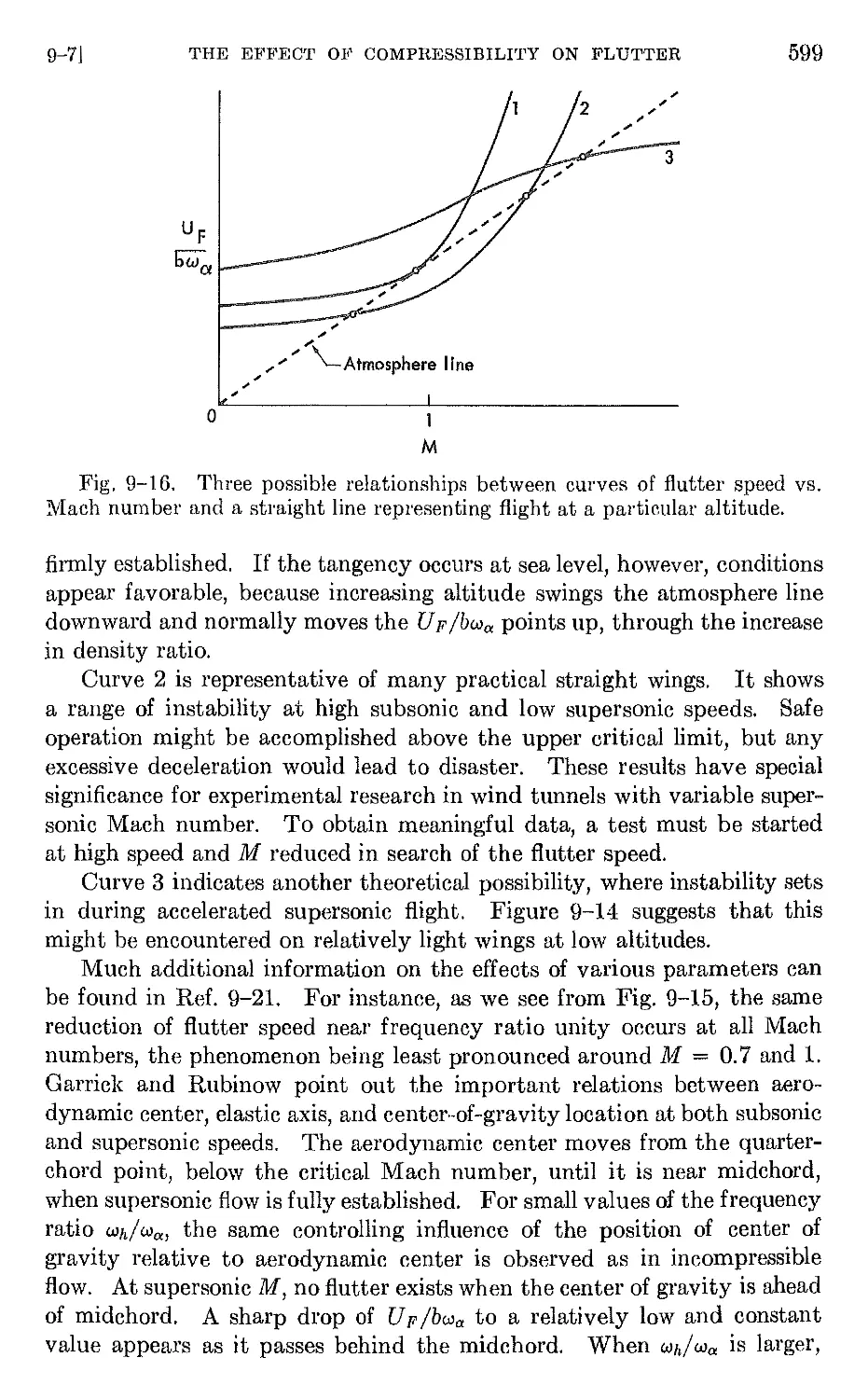


Автор: Bisplinghoff R.L. Halfman R.L. Ashley H.
Теги: physics aeroelasticity
ISBN: 0-486-69189-6
Год: 1983


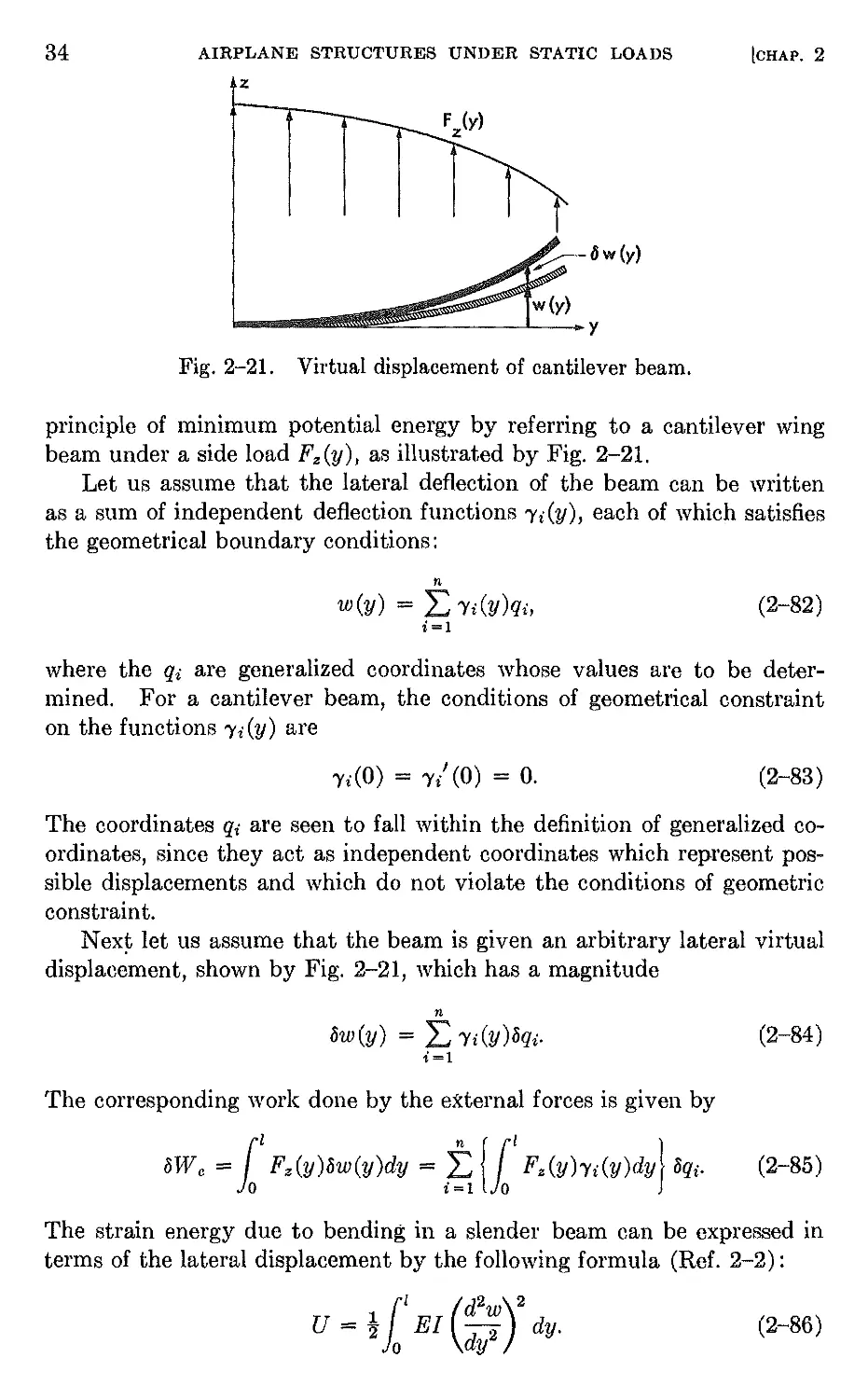
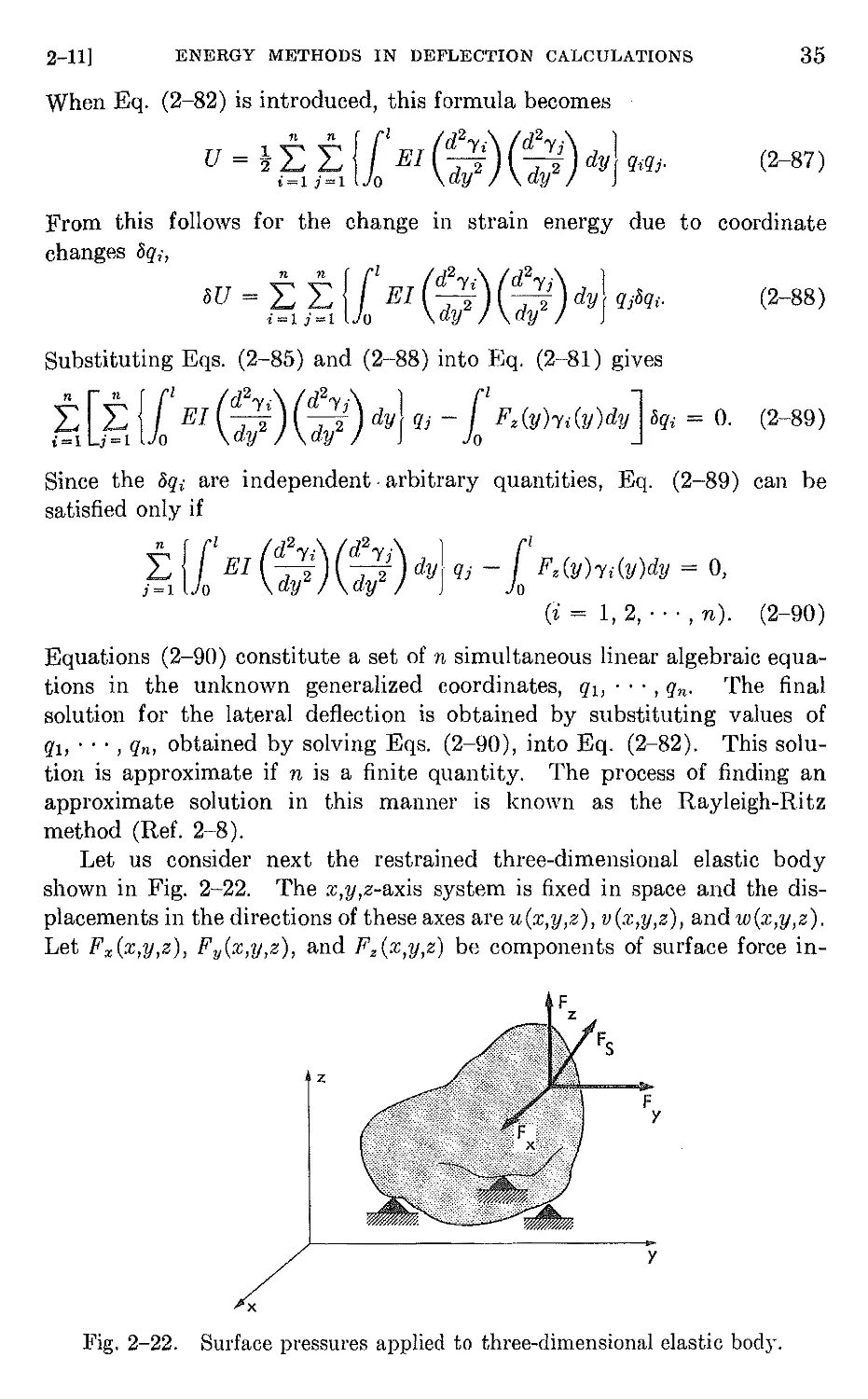
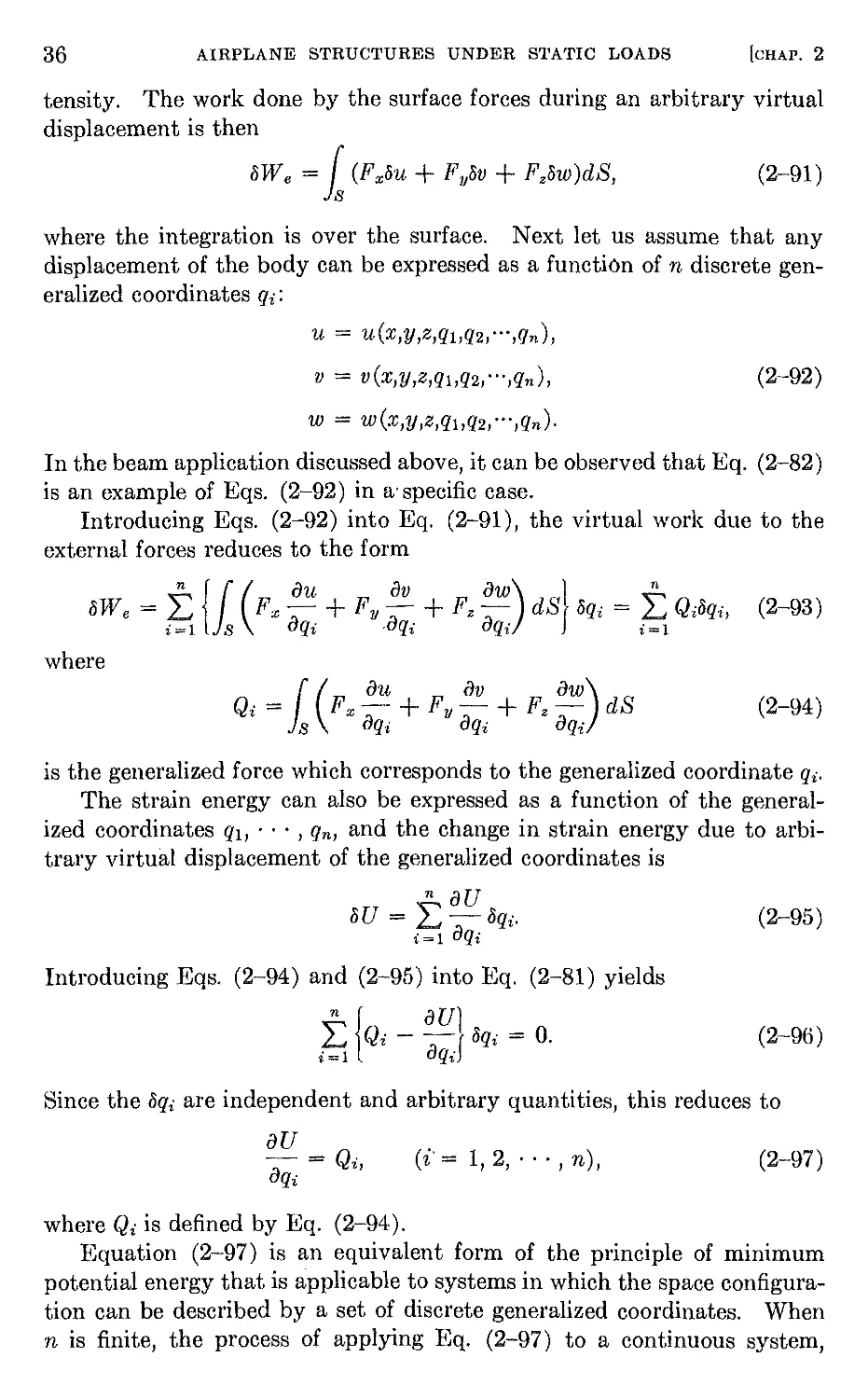
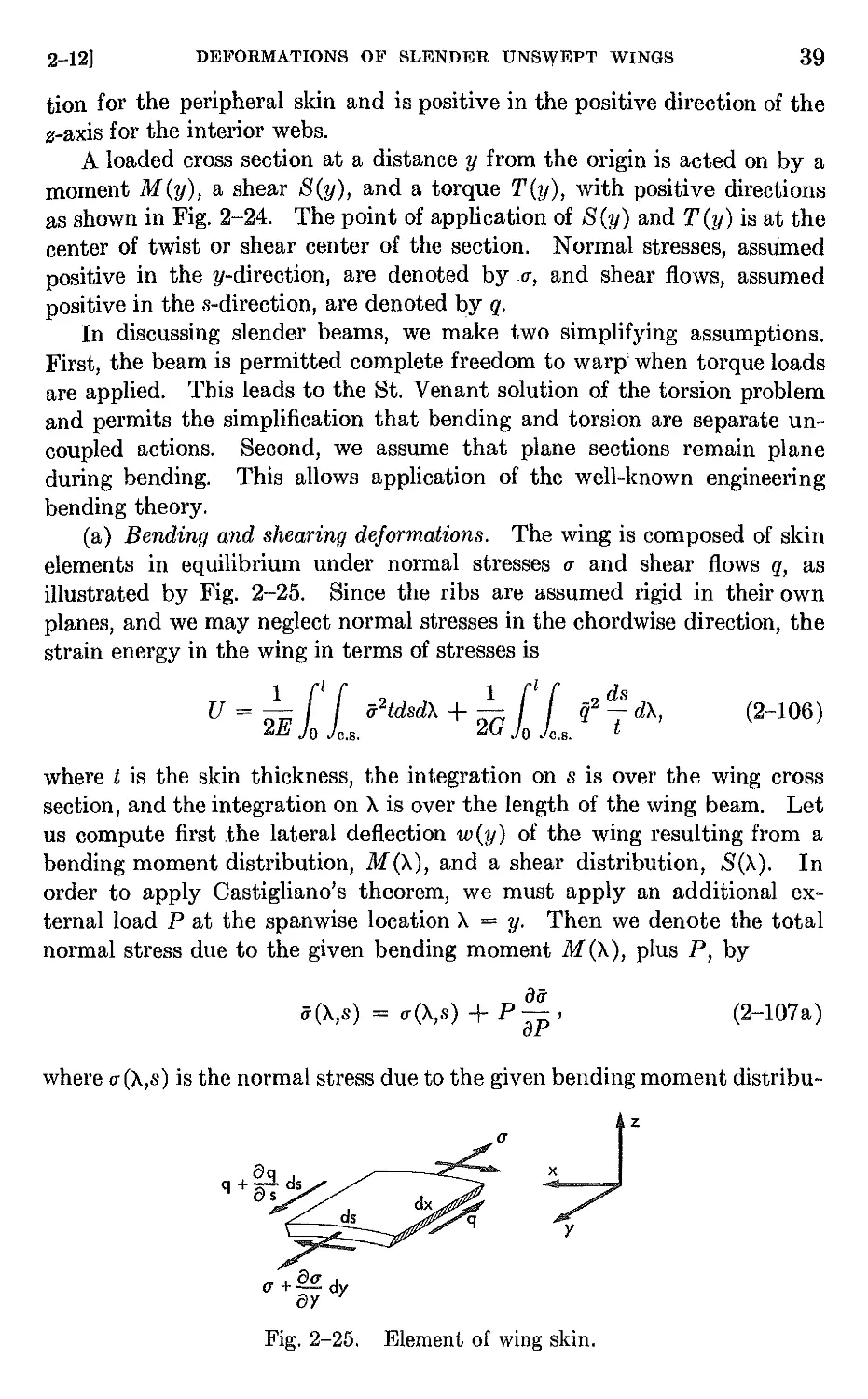
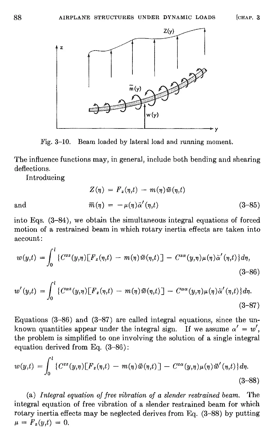
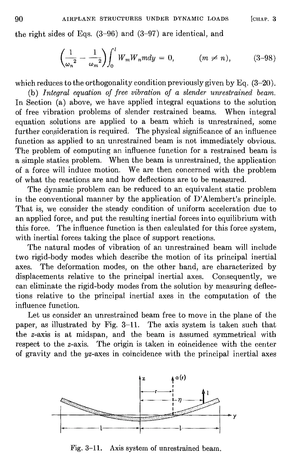
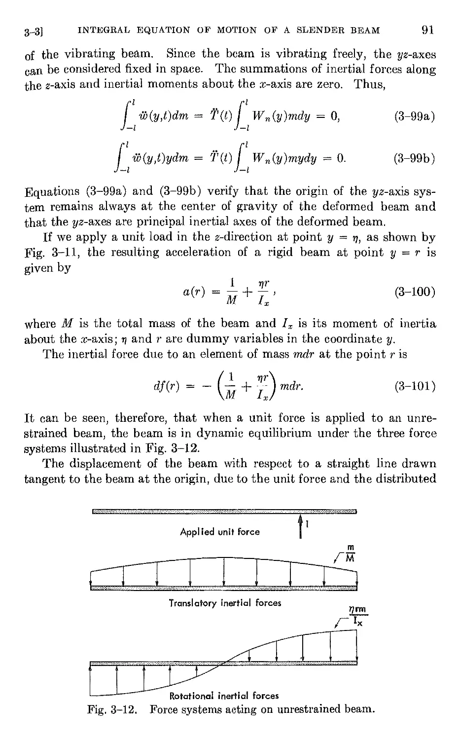
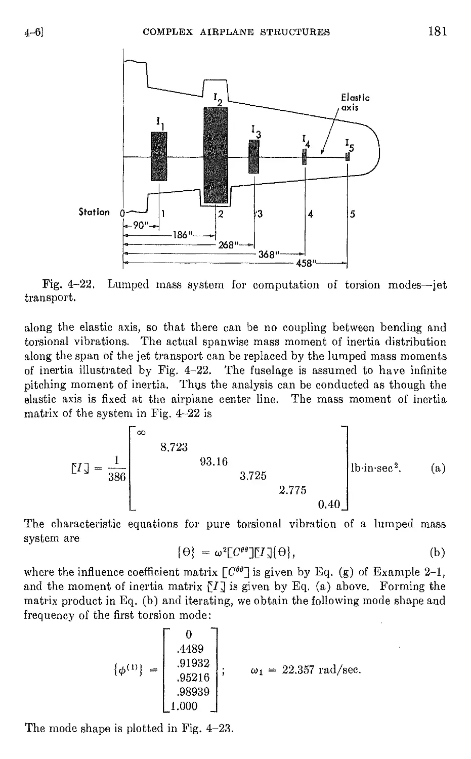
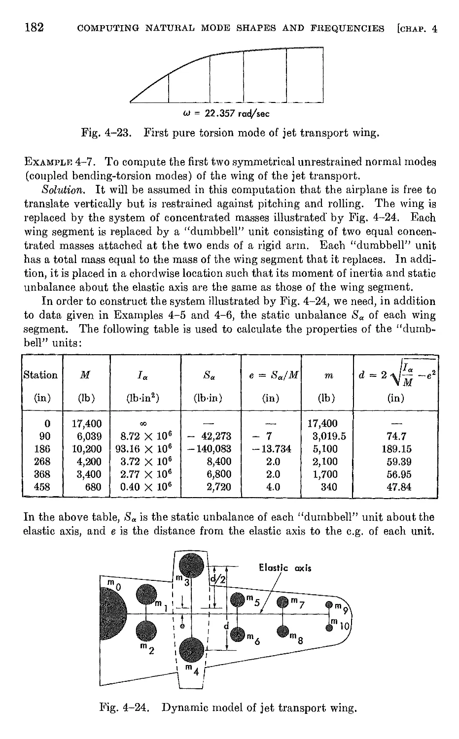
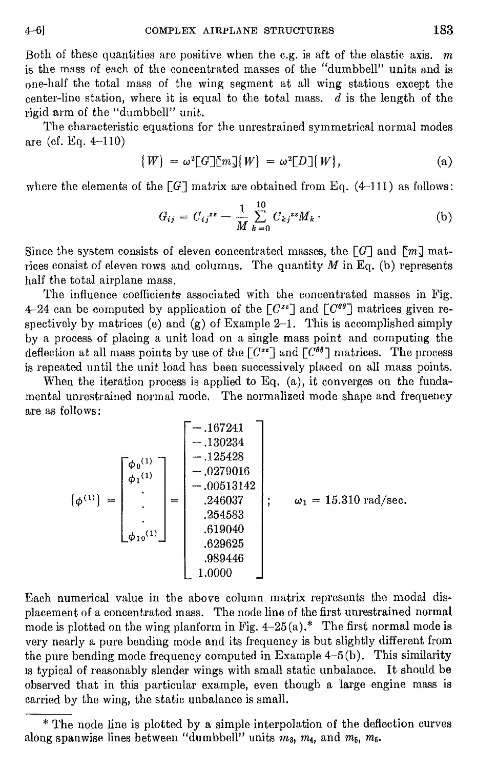
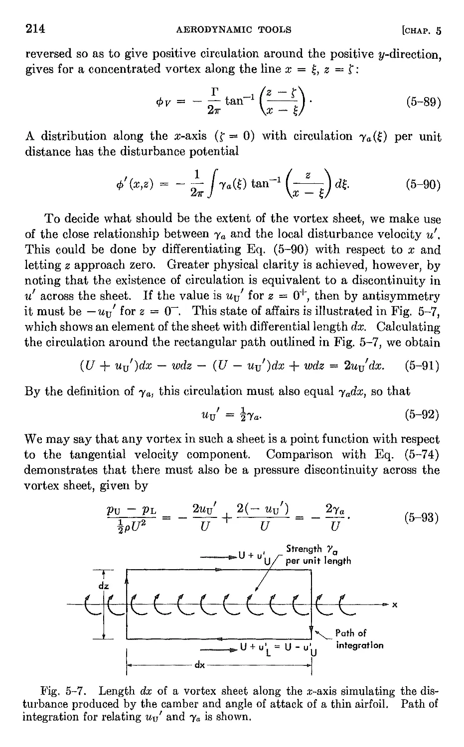
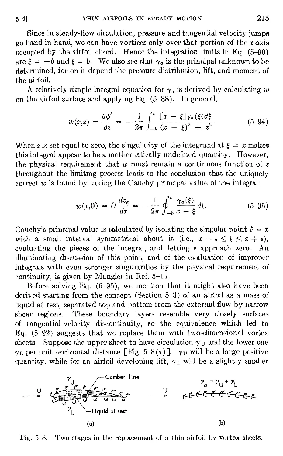
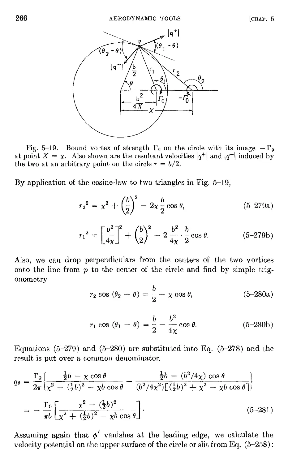
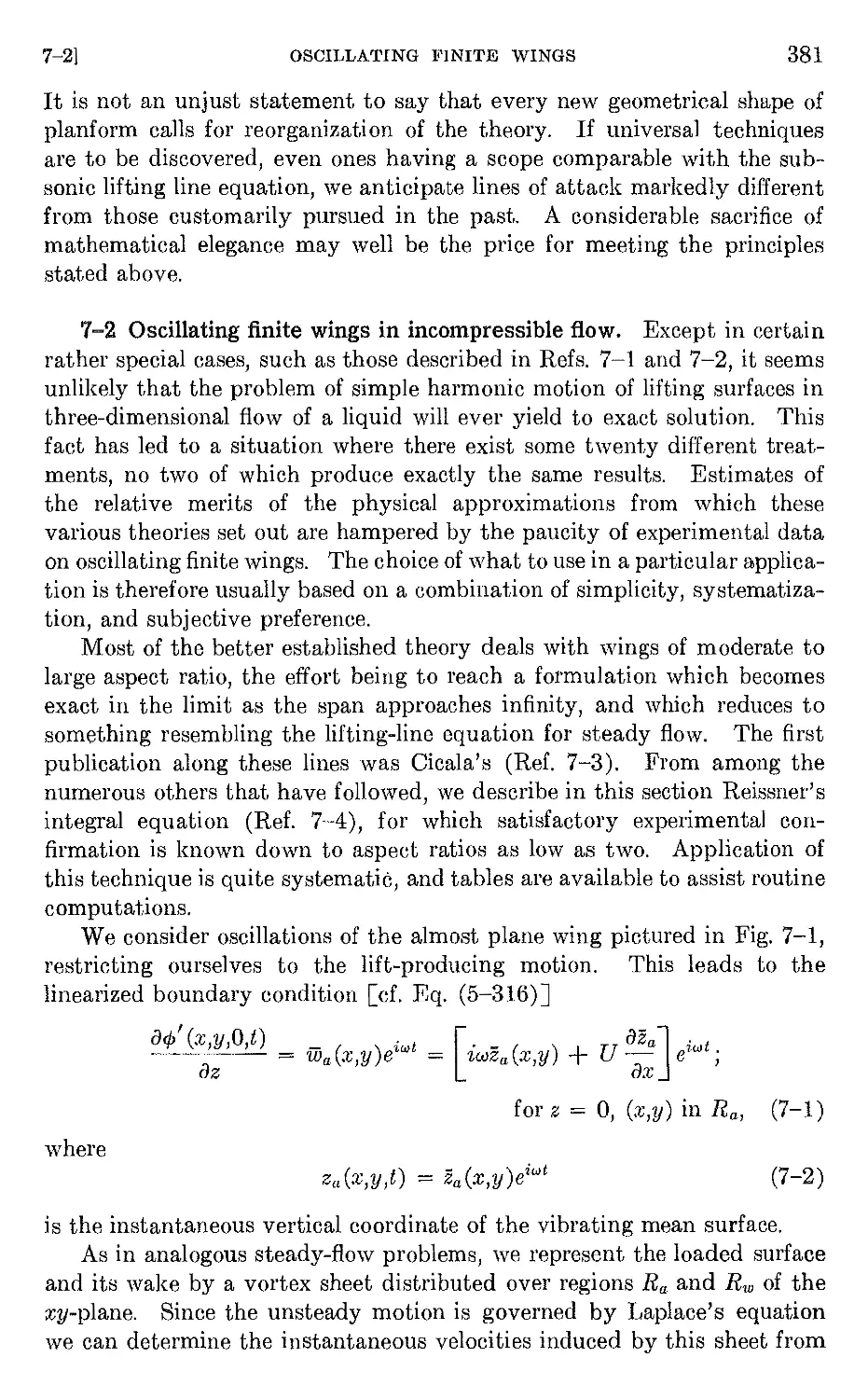
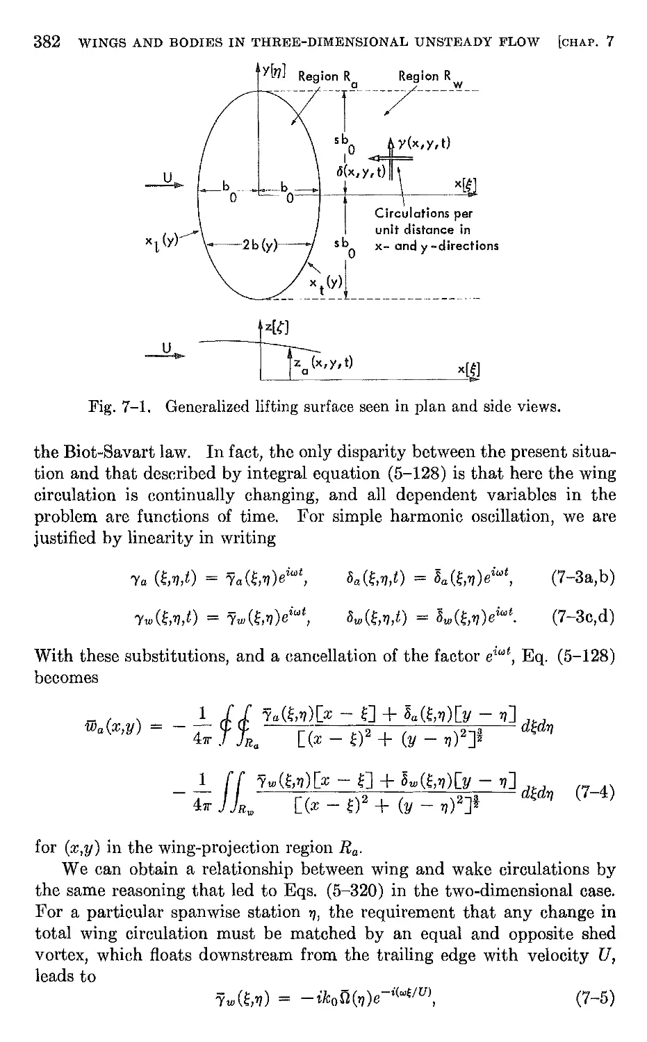
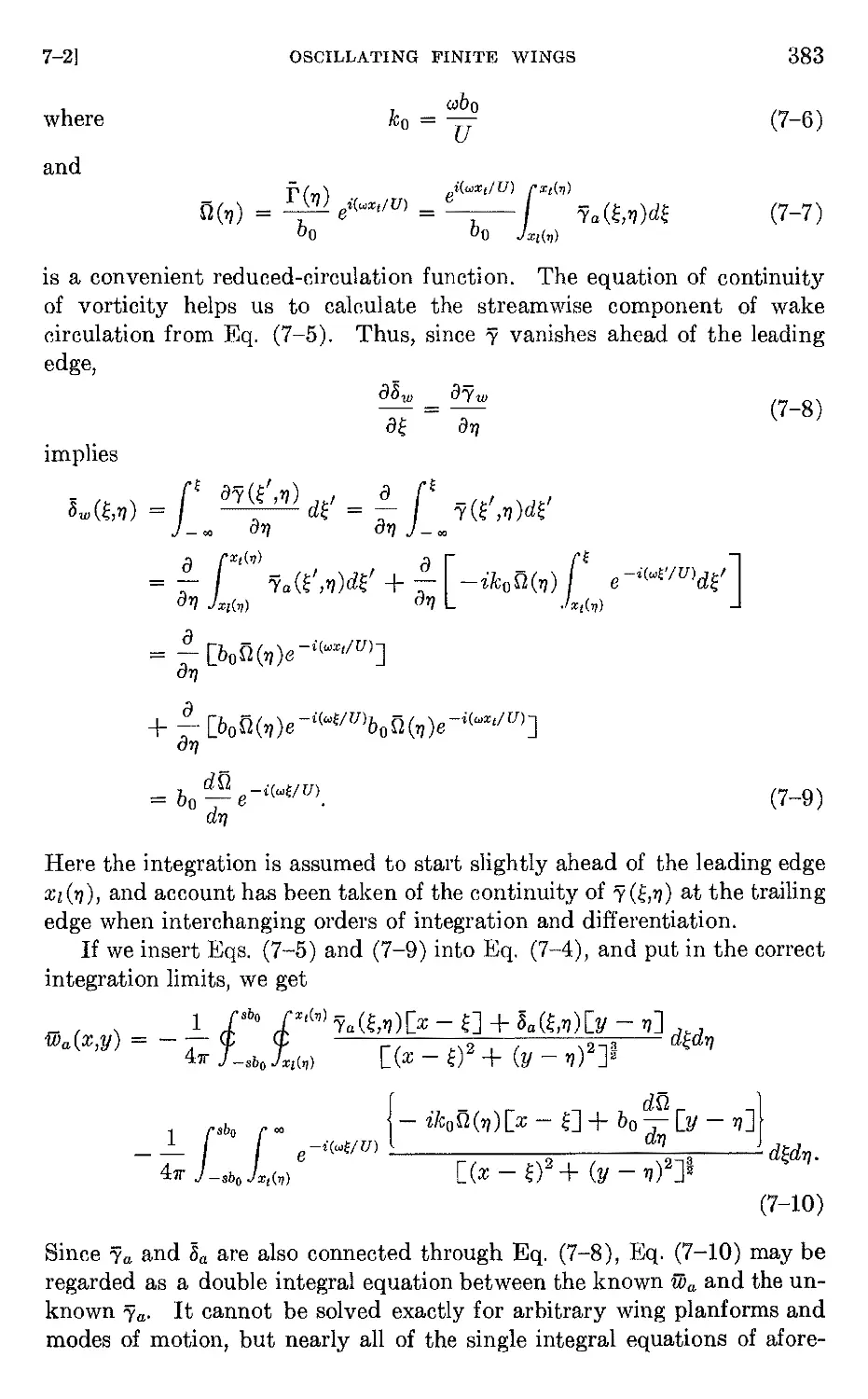
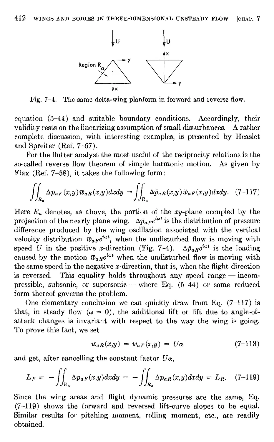
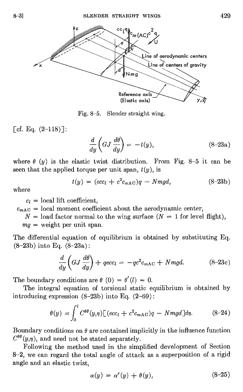
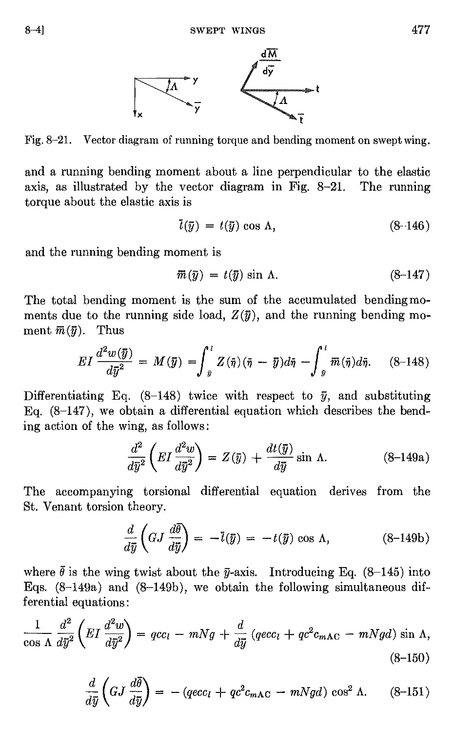
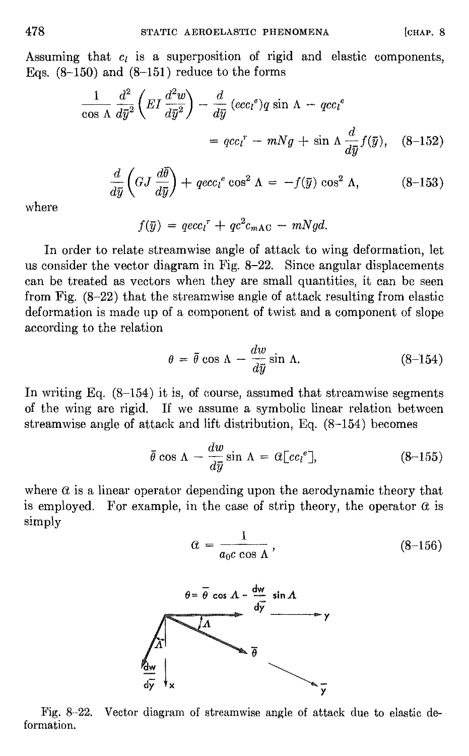
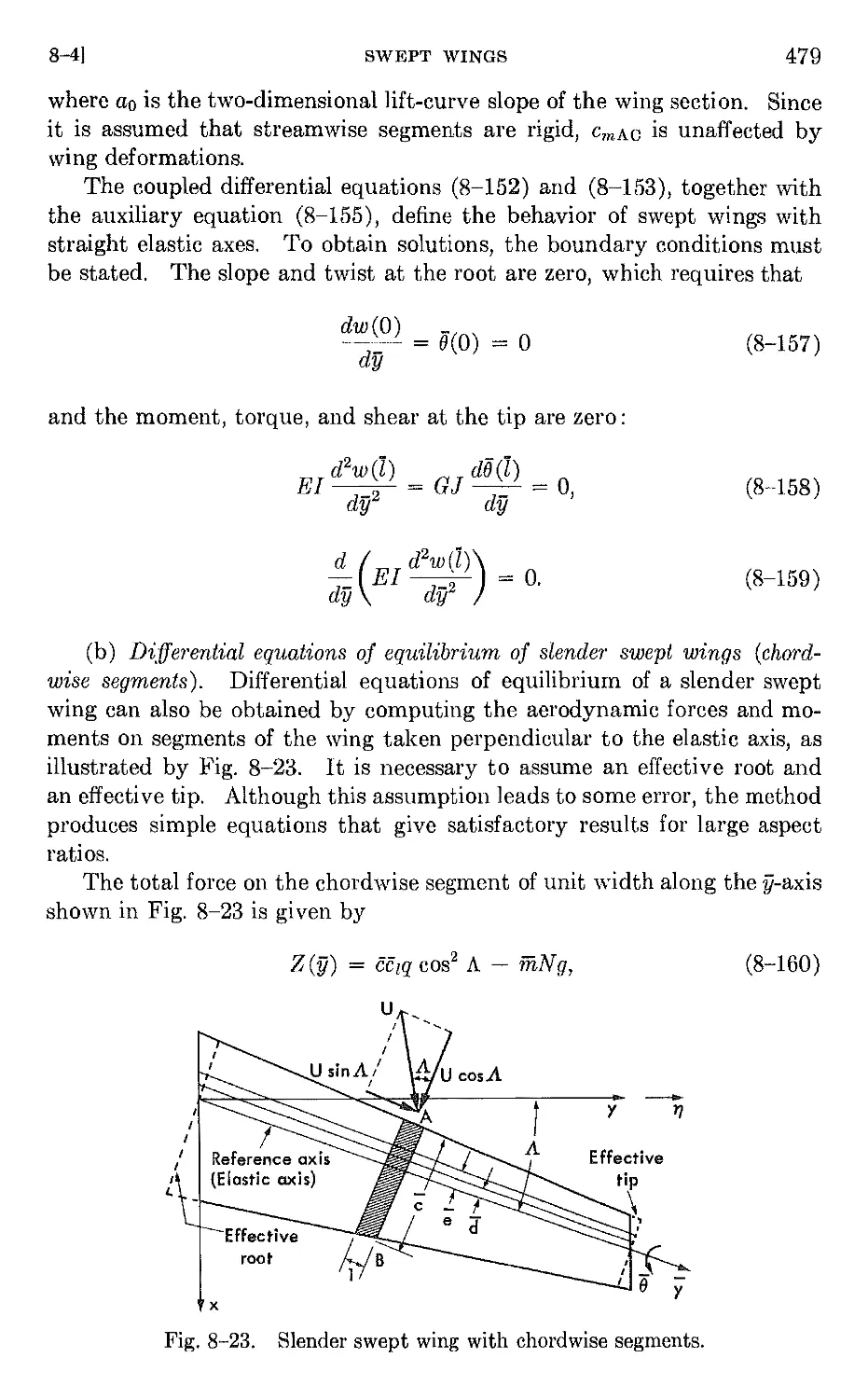
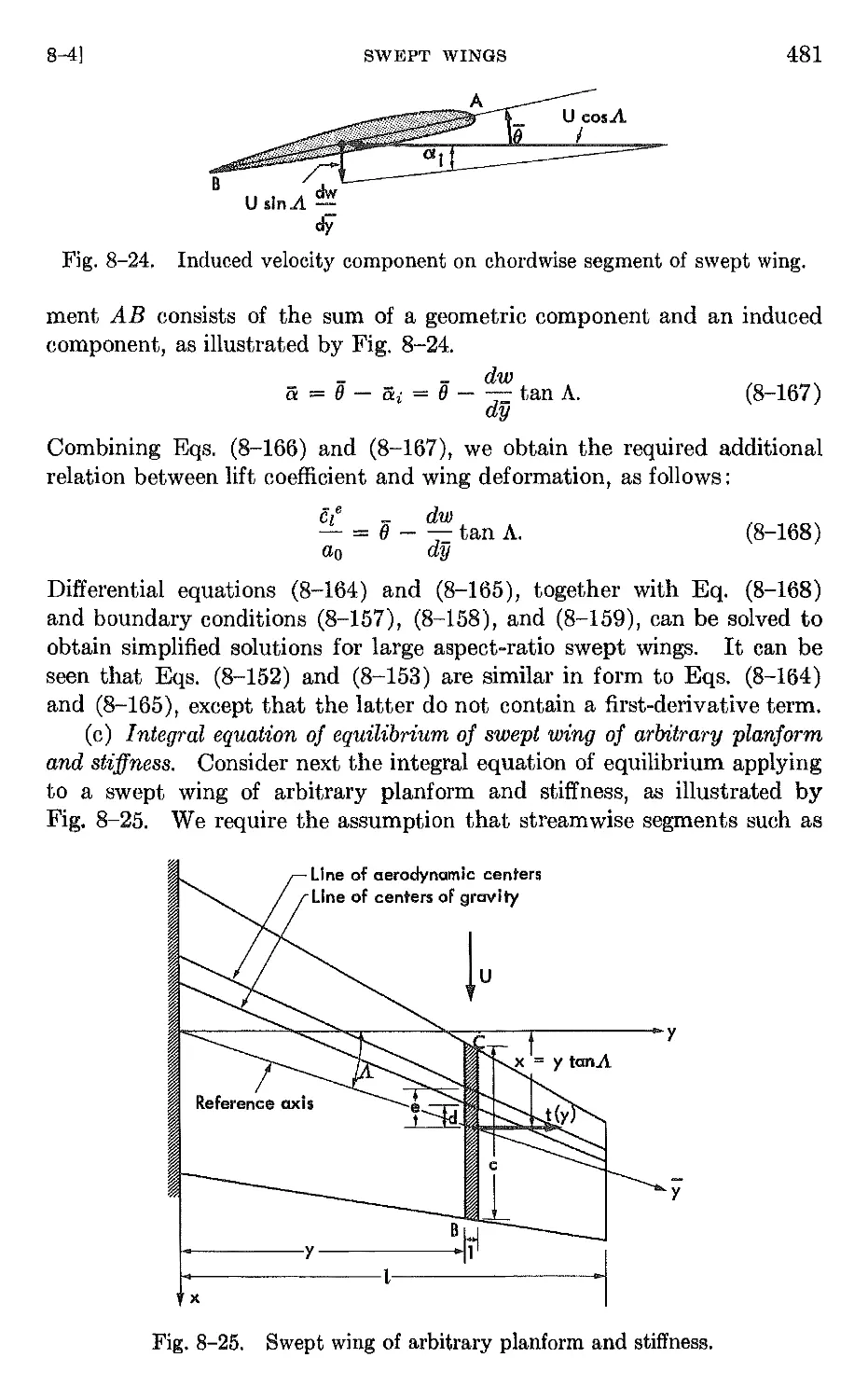
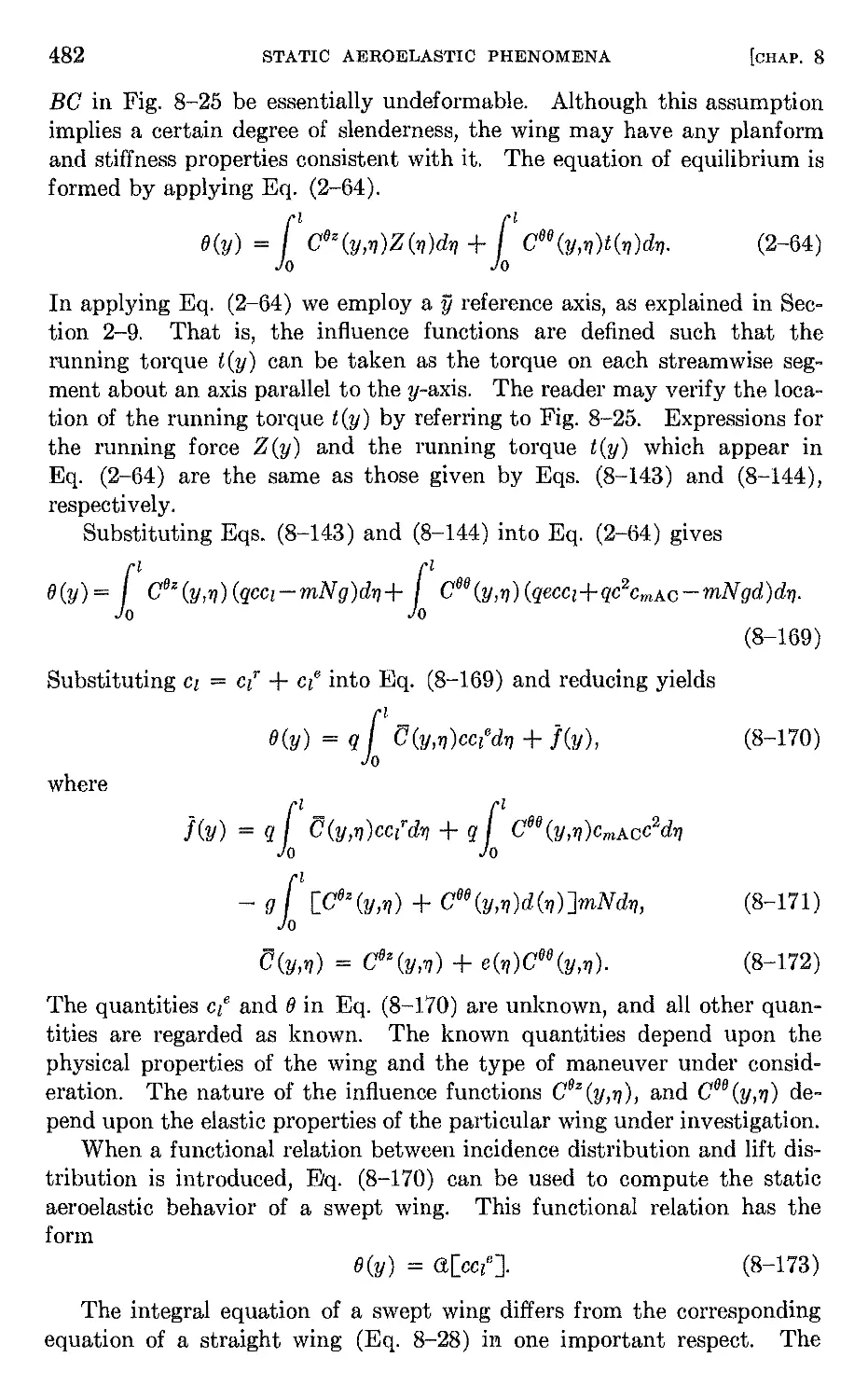
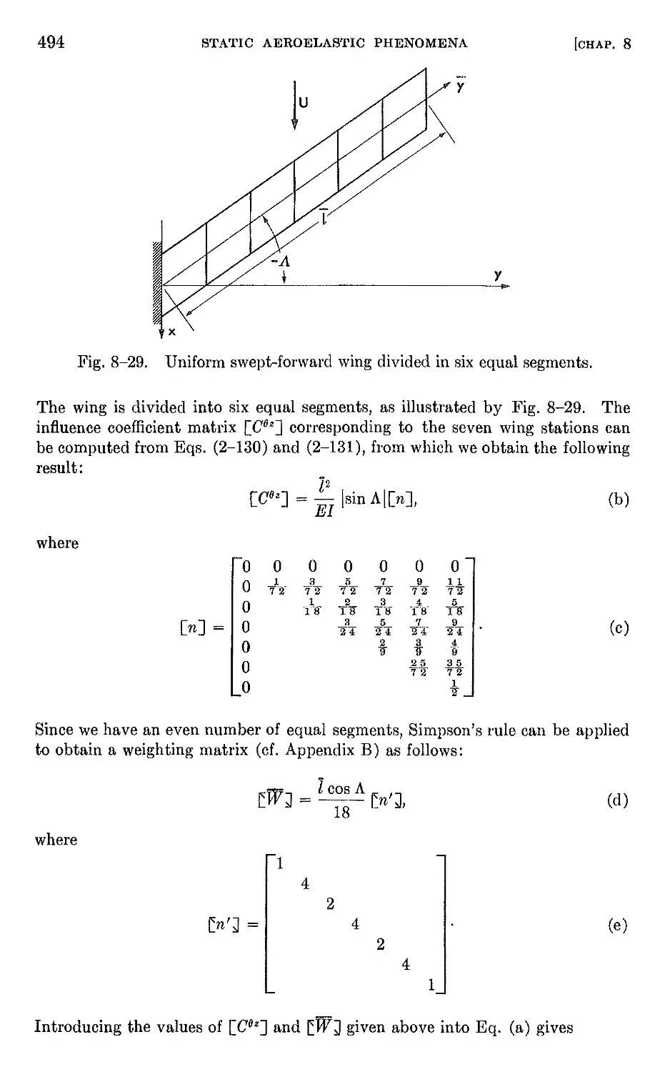
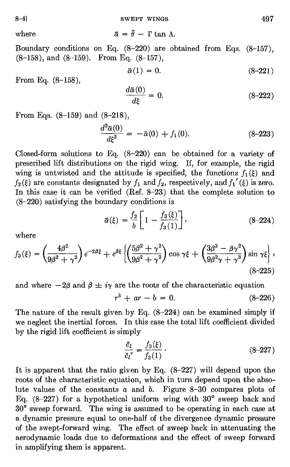
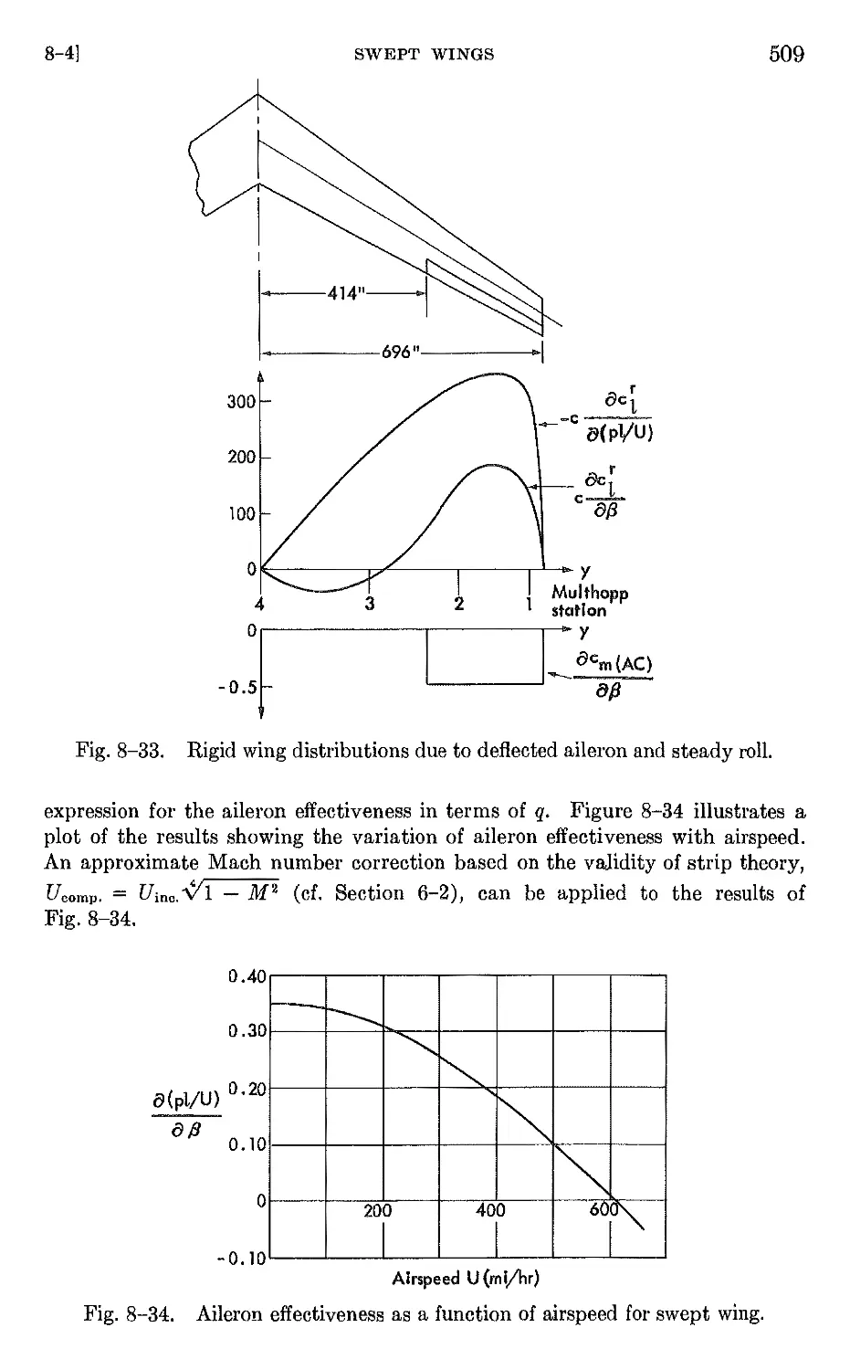
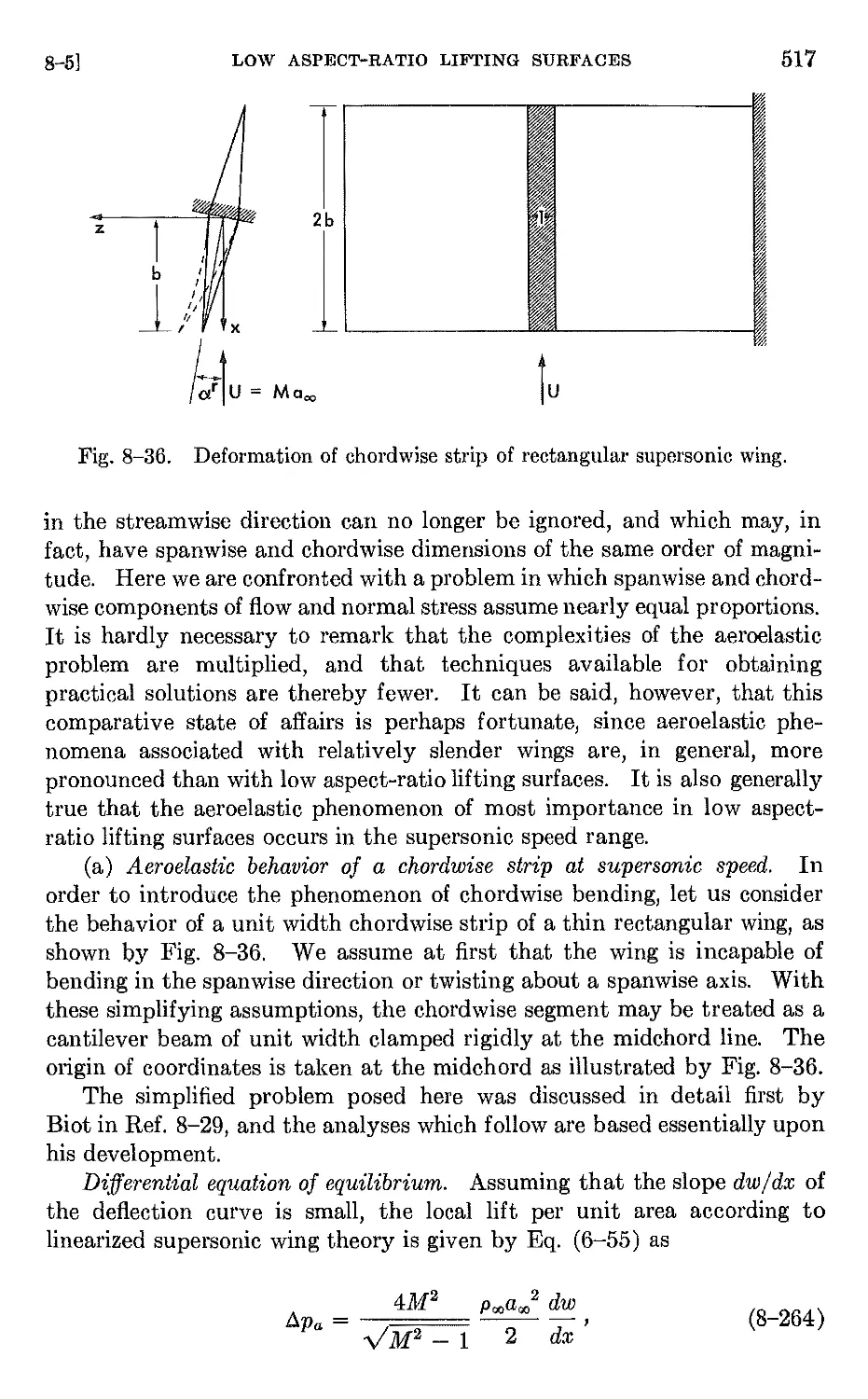
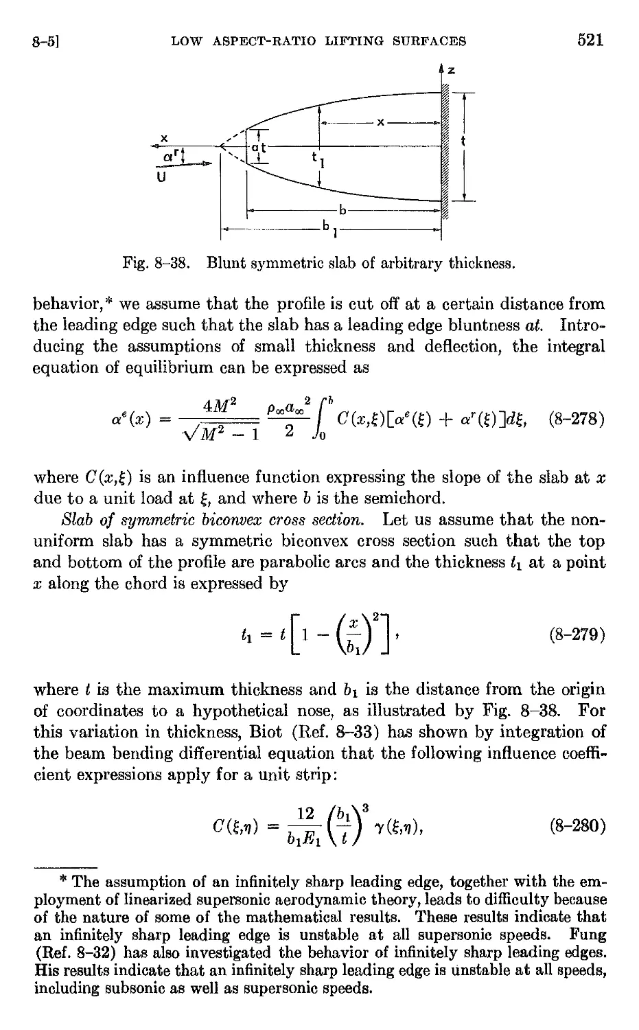
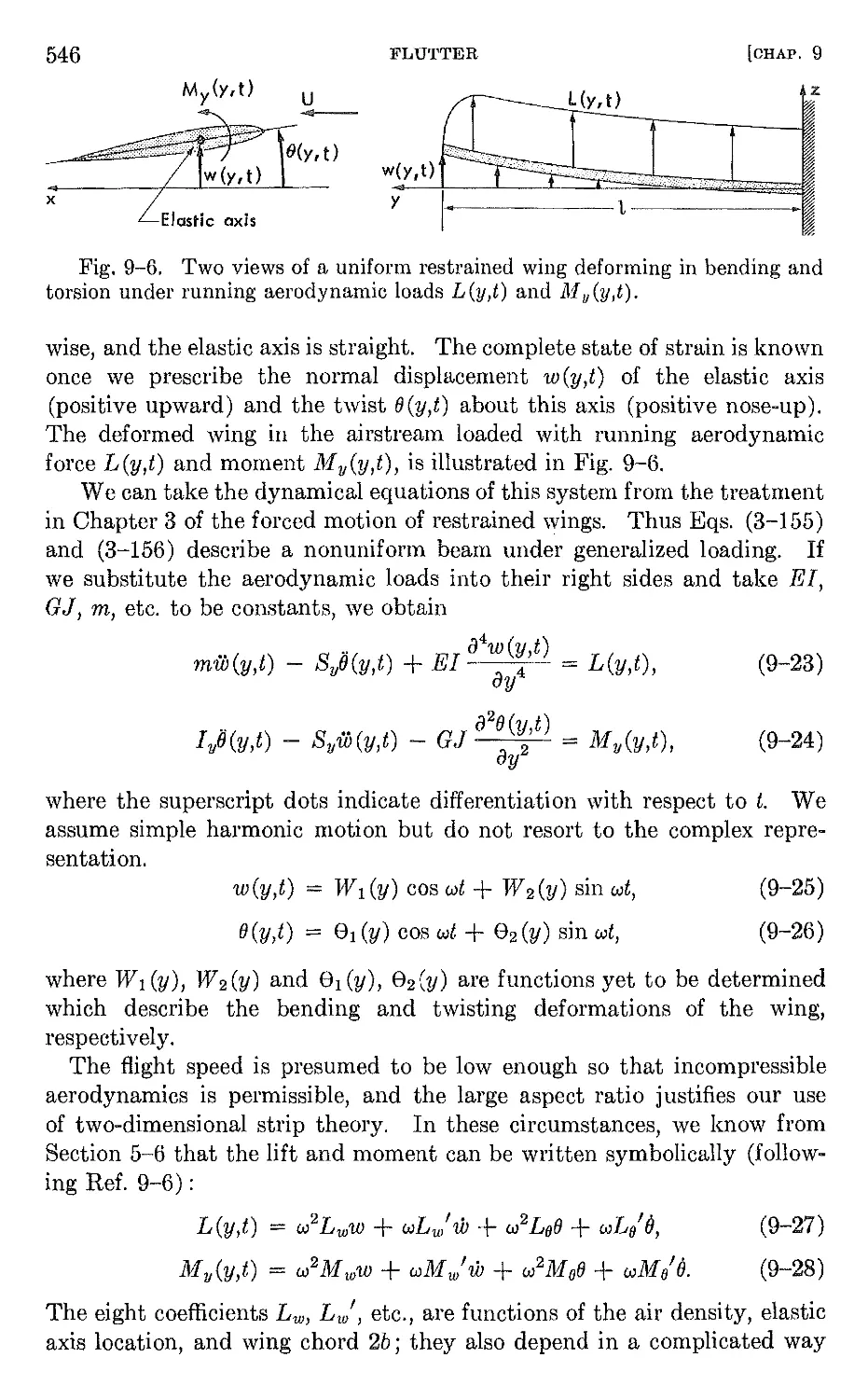
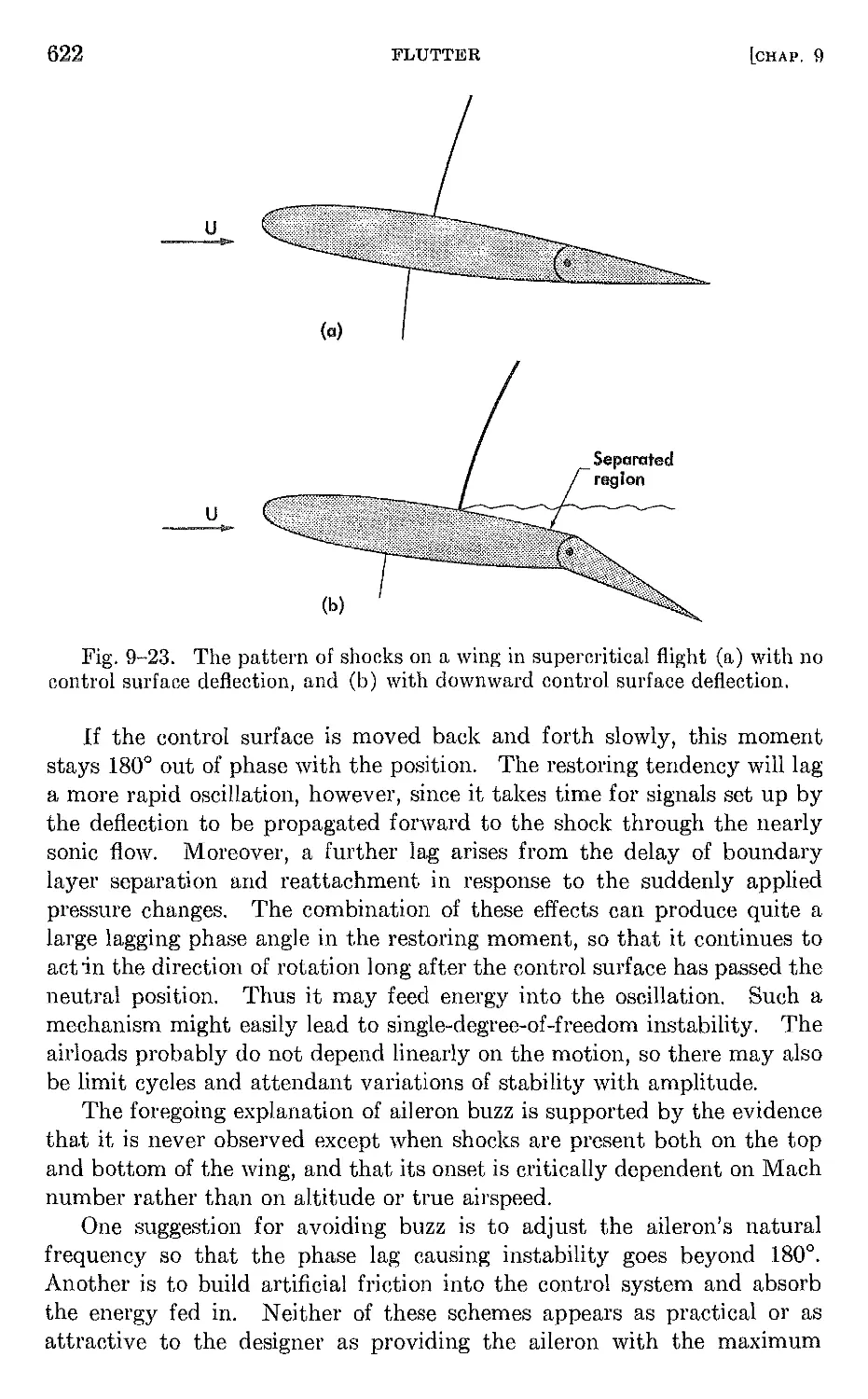
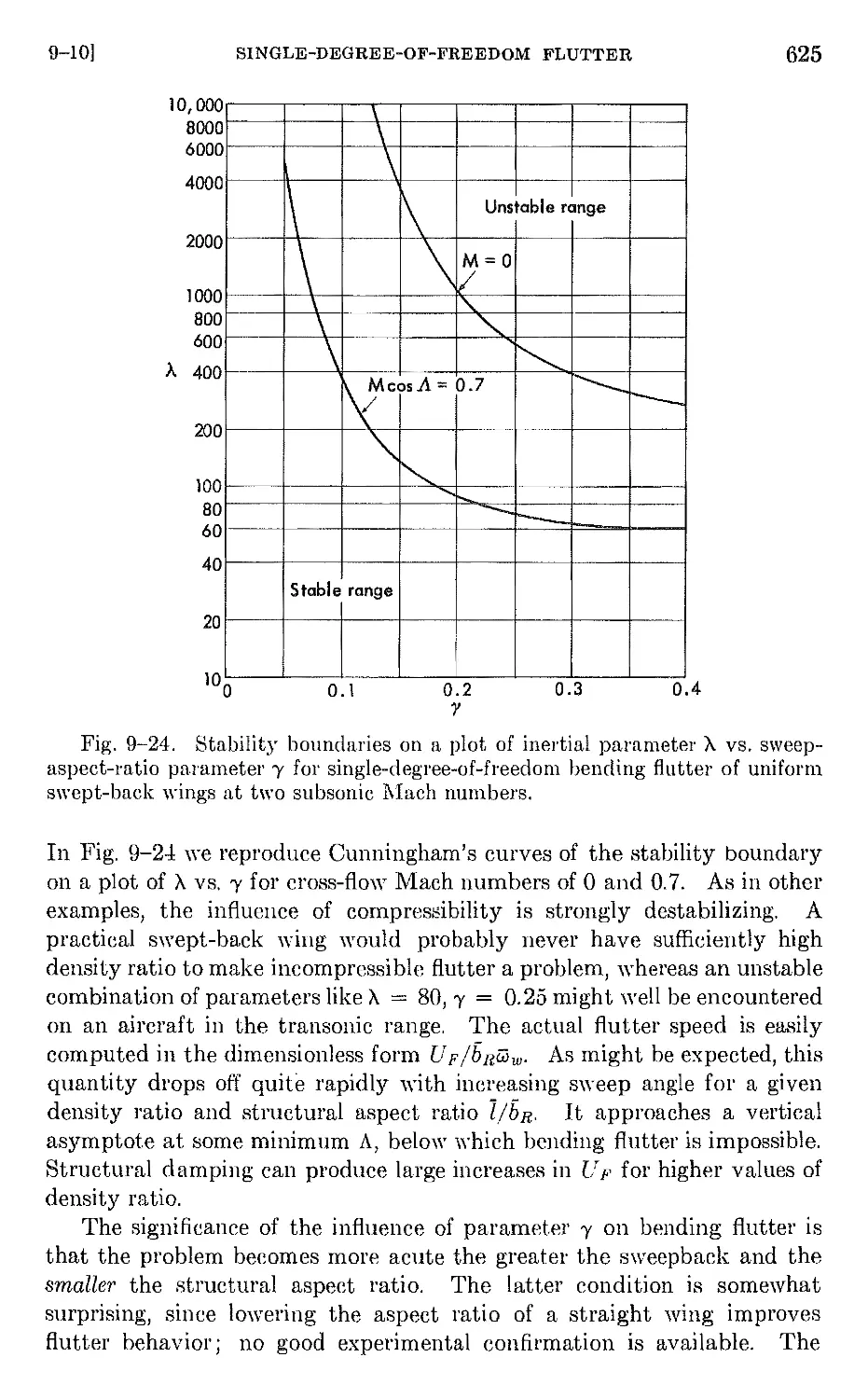
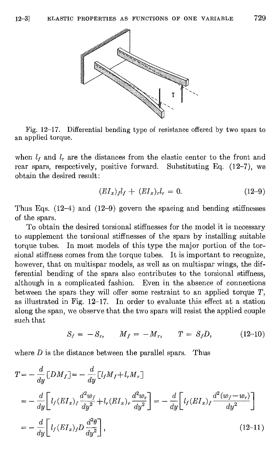
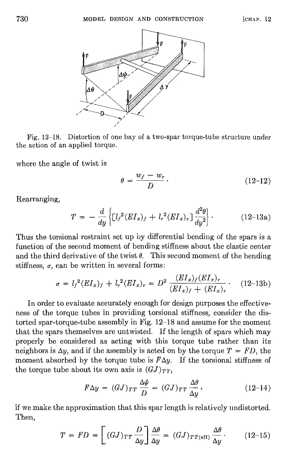
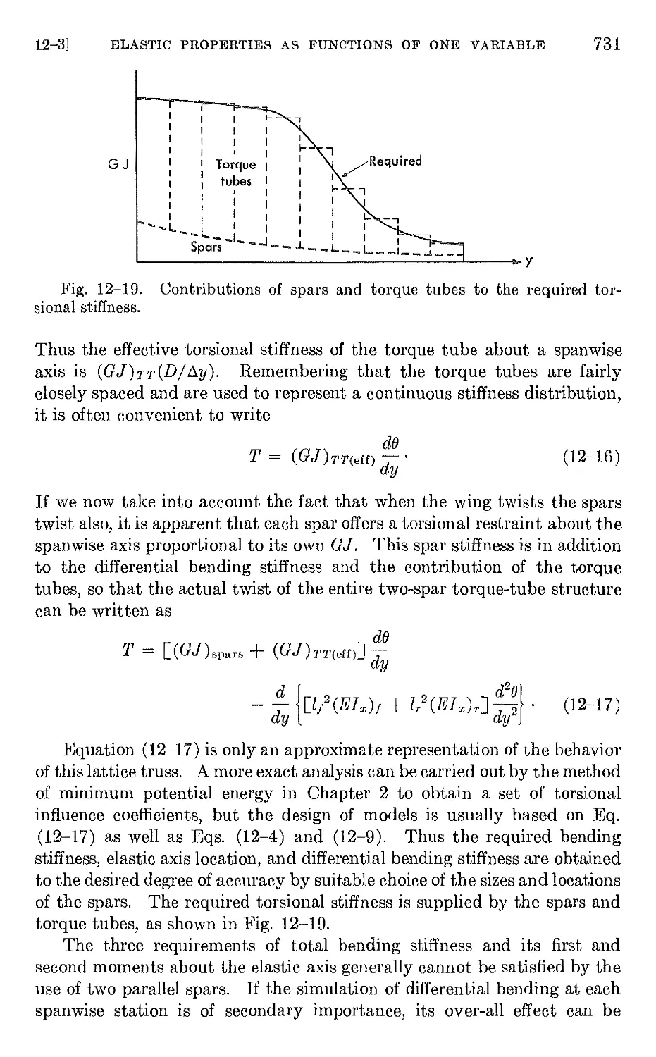
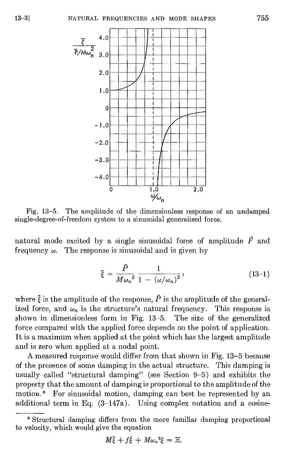
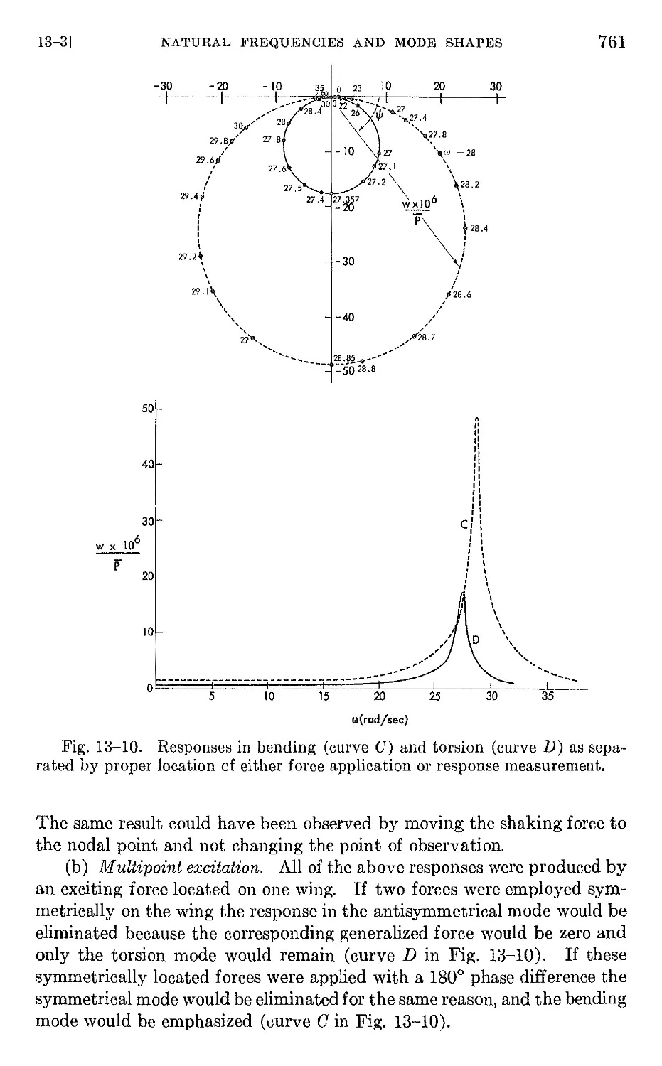
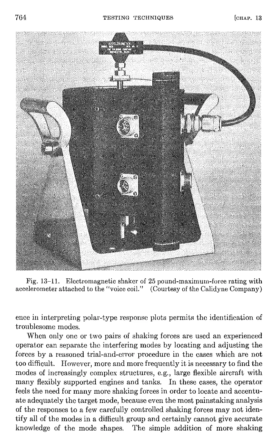
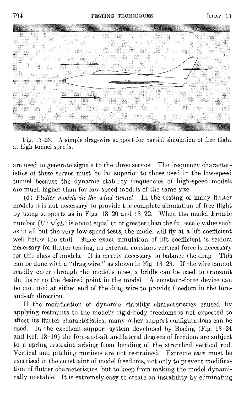
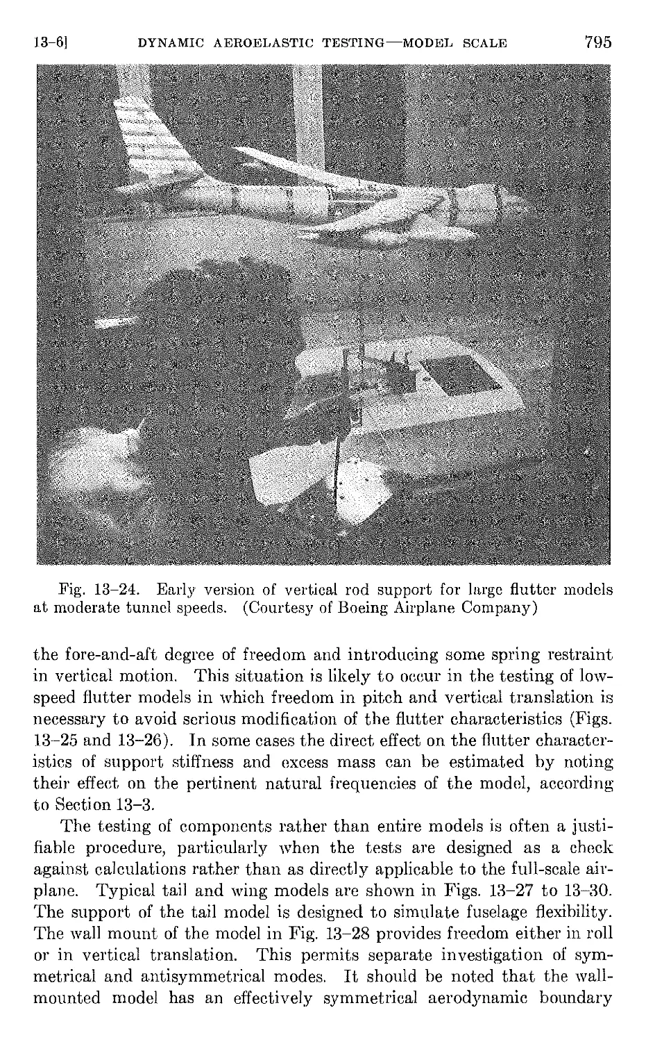
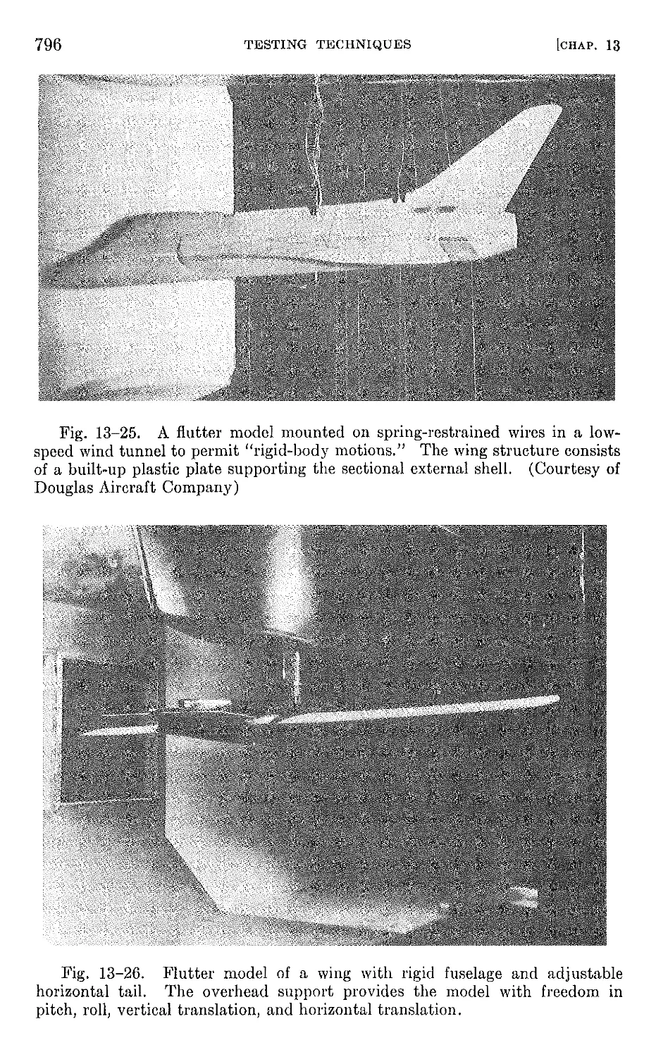
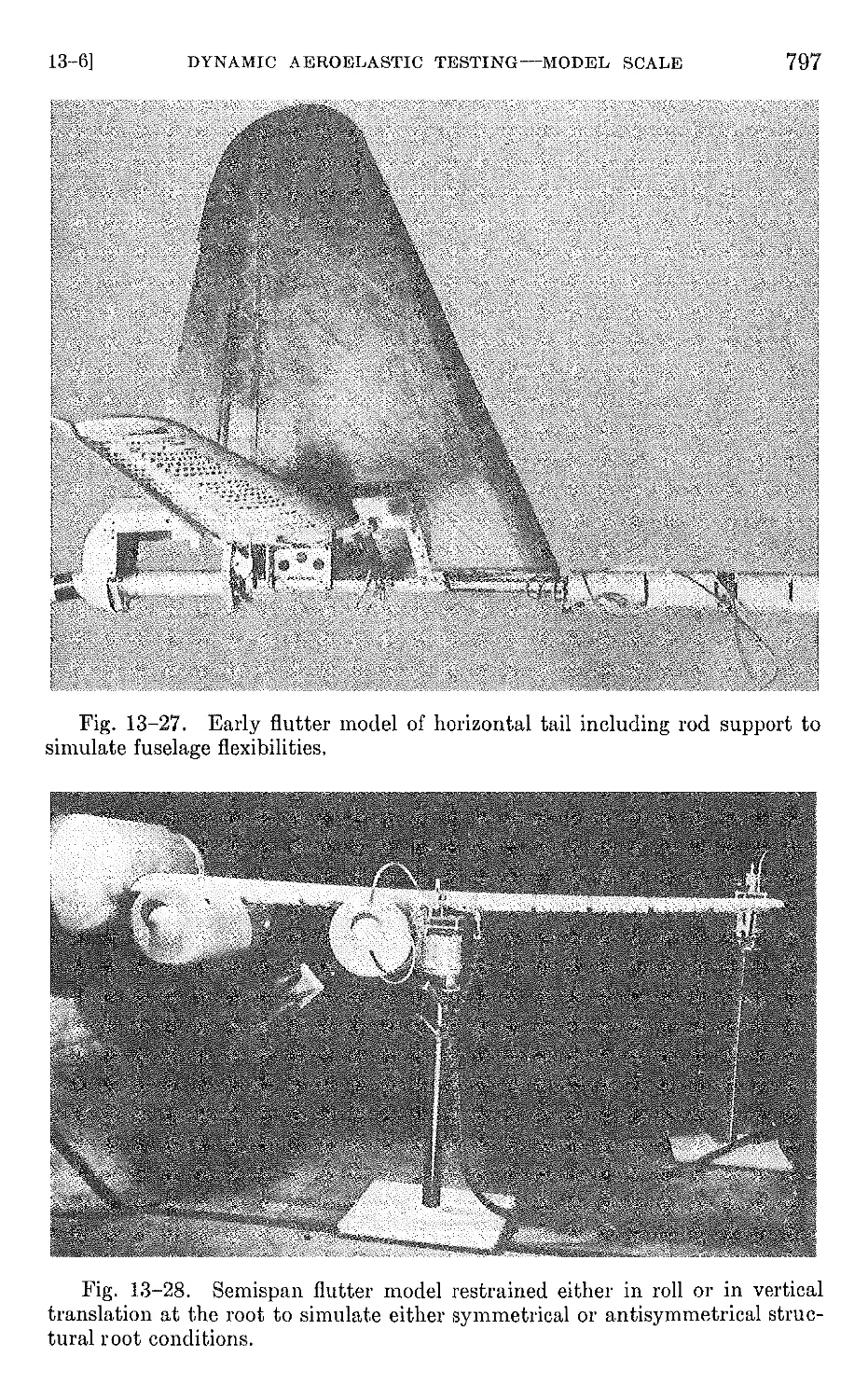
Текст
DOVER BOOKS ON PHYSICS
METHODS OF QUANTUM FIELD THEORY IN STATISTICAL PHYSICS, AA Abrikosov
et al. (63228-8) $12.95
ELECTRODYNAMICS AND CLASSICAL THEORY OF FIELDS AND PARTICLES, A.O. Barut.
(64038-8) $9.95
DYNAMIC LIGHT SCATTERING: WITH ApPLICATIONS TO CHEMISTRY, BIOLOGY, AND
PHYSICS, Bruce J. Berne and Robert Pecora. (41155-9) $17.95
QUANTUM THEORY, David Bohm. (65969-0) $15.95
ATOMIC PHYSICS (8TH EDITION), Max Born. (65984-4) $14.95
EINSTEIN'S THEORY OF RELATIVITY, Max Born. (60769-0) $9.95
INTRODUCTION TO HAMILTONIAN OPTICS, H.A Buchdahl. (67597-1) $10.95
MATHEMATICS OF CLASSICAL AND QUANTUM PHYSICS, Frederick W. Byron, Jr.
and Robert W. Fuller. (67164-X) $18.95
MECHANICS, J.P. Den Hartog. (60754-2) $13.95
INVESTIGATIONS ON THE THEORY OF THE BROWNIAN MOVEMENT, Albert Einstein.
(60304-0) $5.95
THE PRINCIPLE OF RELATIVITY, Albert Einstein, et al. (60081-5) $7.95
THE PHYSICS OF WAVES, William C. Elmore and Mark A Heald. (64926-1)
$14.95
THERMODYNAMICS, Enrico Fermi. (60361-X) $7.95
INTRODUCTION TO MODERN OPTICS, Grant R. Fowles. (65957-7) $13.95
DIALOGUES CONCERNING Two NEW SCIENCES, Galileo Galilei. (60099-8) $9.95
GROUP THEORY AND ITS ApPLICATION TO PHYSICAL PROBLEMS, Morton
Hamermesh. (66181-4) $14.95
ELECTRONIC STRUCTURE AND THE PROPERTIES OF SOLIDS: THE PHYSICS OF THE
CHEMICAL BOND, Walter A Harrison. (66021-4) $19.95
SOLID STATE THEORY, Walter A Harrison. (63948-7) $14.95
PHYSICAL PRINCIPLES OF THE QUANTUM THEORY, Werner Heisenberg.
(60113-7) $8.95
ATOMIC SPECTRA AND ATOMIC STRUCTURE, Gerhard Herzberg. (60115-3) $7.95
AN INTRODUCTION TO STATISTICAL THERMODYNAMICS, Terrell L. Hill. (65242-4)
$13.95
EQUILIBRIUM STATISTICAL MECHANICS, E. Atlee Jackson (41185-0) $9.95
OPTICS AND OPTICAL INSTRUMENTS: AN INTRODUCTION, B.K. Johnson. (60642-2)
$8.95
THEORETICAL SOLID STATE PHYSICS, VOLS. I & II, William Jones and Norman
H. March. (65015-4, 65016-2) $33.90
THEORETICAL PHYSICS, Georg Joos, with Ira M. Freeman. (65227-0) $24.95
THE VARIATIONAL PRINCIPLES OF MECHANICS, Cornelius Lanczos. (65067-7)
$14.95
A GUIDE TO FEYNMAN DIAGRAMS IN THE MANy-BODY PROBLEM, Richard D.
Mattuck. (67047-3) $12.95
(continued on back flap)
AEROELASTICITY
AEROELASTICITY
Raymond L. Bisplinghoff
Holt Ashley
Robert L. Halfman
DOVER PUBLICATIONS, INC.
MINEOLA, NEW YORK
Copyright
Copyright @1955 by Addis on- Wesley Publishing Company, Inc.
Copy tight @ renewed 1983 by Raymond L. Bisplinghoff, Holt Ashley and
Robert L. Halfman.
All rights reserved under Pan American and International Copyright
Conventions.
Published in Canada by General Publishing Company, Ltd., 30 Lesmill
Road, Don Mills, Toronto, Ontario.
Bibliographical Note
This Dover edition, first published in 1996, is a corrected republication
of the work first published by Addison-Wesley Publishing Company,
Cambridge, Mass., 1955. The authors have provided a number of corrections
for the Dover edition.
Library of Congress Cataloging-in-Publication Data
Bisplinghoff, Raymond L.
Aeroelasticity / Raymond L. Bisplinghoff, Holt Ashley, Robert L. Halfman.
p. cm.
Corrected republication of the work originally published: Cambridge,
Mass. : Addison-Wesley, 1955.
Includes bibliographical references and index.
ISBN 0-486-69189-6 (pbk.)
1. Aeroelasticity. I. Ashley, Holt. II. Halfman, Robert L. III. Title.
TL574.A37B5397 1996
629. 132'362-dc20 96-5412
CIP
Manufactured in the United States. of America
Dover Publications, Inc., 31 East 2nd Street, Mineola, N.Y. 11501
PREFACE
The objective of the authors in writing Aeroelasticity has been to provide
both a textbook for advanced engineering students and a reference book for
practicing engineers. In selecting material for the book it was the authors'
conviction that not only the practical aspects of aeroelasticity should be
treated, but also the aerodynamic and structural tools upon which these
rest. Accordingly, the book divides roughly into two halves; the first deals
with the tools and the second with applications of the tools to aeroelastic
phenomena. The authors' convictions concerning a need for further treat-
ment of the tools do not stem from a feeling that they are inadequately
treated elsewhere but rather from the realization that they are not treated
from the point of view of the aeroelastician.
The first chapter emphasizes the role of aeroelasticity among the aero-
nautical sciences and its influence on modern design. Chapters 2, 3, and 4
are concerned with the deformation behavior of airplane structures under
static and dynamic loads. These three chapters comprise the total treat-
ment of the structural tools. The aerodynamic tools are treated in Chap-
ters 5, 6, and 7. The reader will observe that although steady-state aero-
dynamics is discussed briefly, the primary emphasis is on unsteady phe-
nomena. Chapter 8 brings together for the first time the aerodynamic and
structural tools and treats the subject of static aeroelasticity. Problems
of static aeroelasticity are characterized by the absence of the independent
variable time, and they are introduced first because of their simplicity.
Chapter 9 is concerned with flutter and Chapter 10 with dynamic response
phenomena. Whereas the former entails essentially a harmonic dependence
of the motion on time, the latter includes a class of problems in which the
motion of the system may vary in a transient manner with time. Chapters
11 and 12 treat, respectively, the important subjects of aeroelastic model
theory and model design and construction; the final chapter is concerned
with experimental techniques for studying aeroelastic phenomena. Al-
though the space devoted to experimental methods is relatively small, it is
not the authors' intention to imply that experimental tools and techniques
in aeroelasticity are of minor importance in the solution of practical
problems. Indeed, aeroelastic phenomena encountered at the forefront of
modern design often do not yield to analytical methods, and if solutions
are to' be obtained within a reasonable length of time the employment of
experimental methods is absolutely necessary.
The authors have endeavored to write each chapter by progressing from
the easy to the hard. Thus the engineering instructor who seeks to use this
book as an elementary text in aeroelasticity will find that his purpose is
served by merely using the first parts of selected chapters. For example, the
book may be used as an introductory text in aeroelasticity for senior or
graduate students in aeronautical engineering by using Chapter 1 and the
v
Vi
PREFACE
first parts of Chapters 2,3, 5 J 8, and 9. The mathematical prerequisites for
an understanding of these portions of the book are the mathematics courses
included in the usual engineering curriculum, through differential equations.
The latter course should have at least an introduction to the notions of
partial derivatives and partial differential equations. An introductory
laboratory course in experimental aeroelasticity can be based upon Chap-
ters 11 J 12, and 13. Advanced courses in aeroelasticity may be based upon
the latter parts of Chapters 2, 3, 5 J 8 J and 9, as well as Chapters 4, 6, 7,
and 10. In general, the mathematical prerequisites for an understanding
of the complete book include a course in advanced calculus in addition to
the courses mentioned above.
The practicing engineer who uses the book for reference purposes will
find that the authors have attempted to present applications of funda-
mentals instead of the compendium of standard tabular methods which
may be in current favor. Although many numerical examples are included,
it is unlikely that the practicing engineer will often find the particular
::>roblem that he is concerned with at the moment. However, it is hoped
that the illustrative examples will always be of some value to the reader
in perceiving how the fundamental tools may be applied to his case.
The authors arranged the material content of the book and the outlines
of each chapter in close cooperation. Then each author worked on certain
chapters independently, with R. L. Bisplinghoff concentrating on the
structural tools, H. Ashley on the aerodynamic tools, and R. L. Halfman
on the experimental aspects. Finally, the applications to aeroelastic
phenomena were prepared jointly and the entire manuscript was worked
over by the. three authors to ensure continuity.
. Acknowledgement is due a great many people who' aided in bringing
the book to completion. Professor Eric Reissner's counsel is gratefully
acknowledged. A 1J.umber of M.LT. staff members and former students
read portions of thl manuscript and offered valuable advice and criticism.
These include Professors Shatswell Ober, James Mar, Theodore Pian,
Morton Finston, and Leon Trilling of the M.LT. Department of Aero-
nautical Engineering; Garabed Zartarian, Hua Lin, John McCarthy,
Kenneth Foss, and Robert Staley of the Aeroelastic and Structures Re-
search Laboratory at M.I.T.; Mr. M. J. Turner of the Boeing Airplane Co.,
Mr. H. C. Johnson of the Glenn L. Martin Company, Professor H. C.
Martin of the University of Washington, and Professor K. Washizu of the
University of Tokyo. The numerical examples were worked out by Mr.
John Martuccelli and Mr. Yechiel Shulman of the Aeroelastic and Struc-
tures Research Laboratory. The authors express their sincere apprecia-
tion to all of these people, and to Miss Nancy Ladd for so ably performing
the seemingly endless chore of typing and preparing the manuscript.
R.L.B., H.A., R.L.B:.
Cambridge, Mass.
February, 1955.
CONTENTS
CHAPTER 1. INTRODUCTION TO AEROELASTICITY 1
1-1 Definitions . 1
1-2 Historical background . 3
1-3 Ihfluence of aeroelastic phenomena on design 7
1-4 Comparison of wing critical speeds 13
CHAPTER.2. DEFORMATIONS OF AIRPLANE STRUCTURES UNDER STATIC
LOADS 15
2-1 Introduction 15
2-2 Elastic properties of structures 17
2-3 Deformation due to several forces. Influence coefficients 17
2-4 Properties of influence coefficients 21
2-5 Strain energy in terms of influence coefficients . 23
2-6 Deformations under distributed forces. Influence functions 23
2-7 Properties of influence functions 26
2-8 The simplified elastic airplane. 27
2-9 Deformations 'Of airplane wings 28
2-10 Integration by weighting matrices 30
2-11 Energy methods in deflection calculations 33
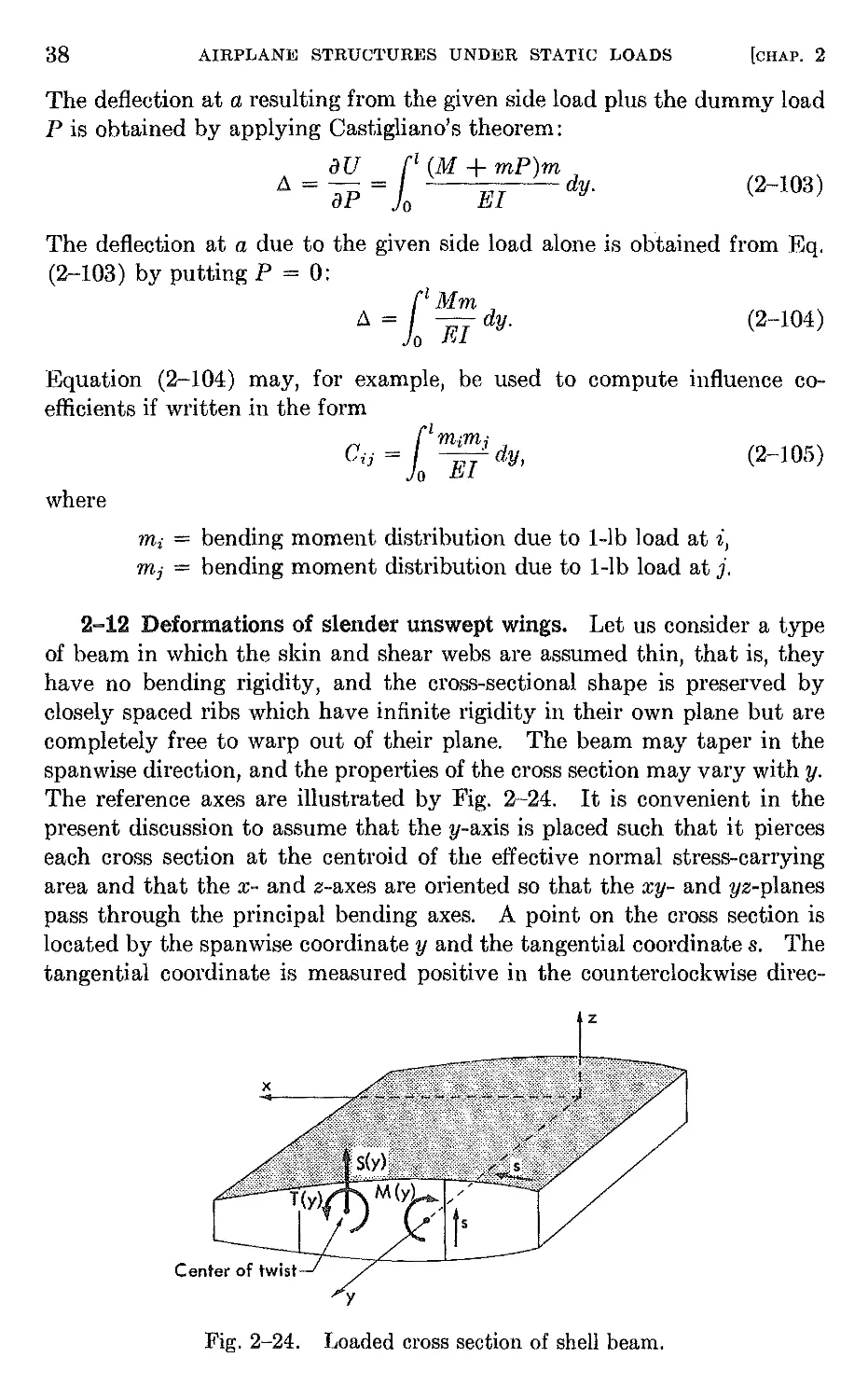
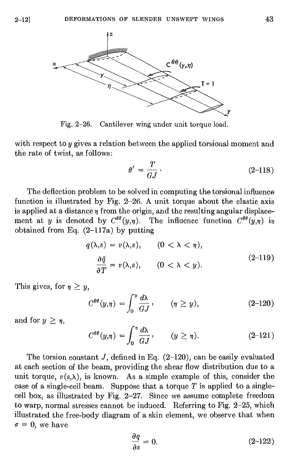
2-12 Deformations of slender unswept wings . 38
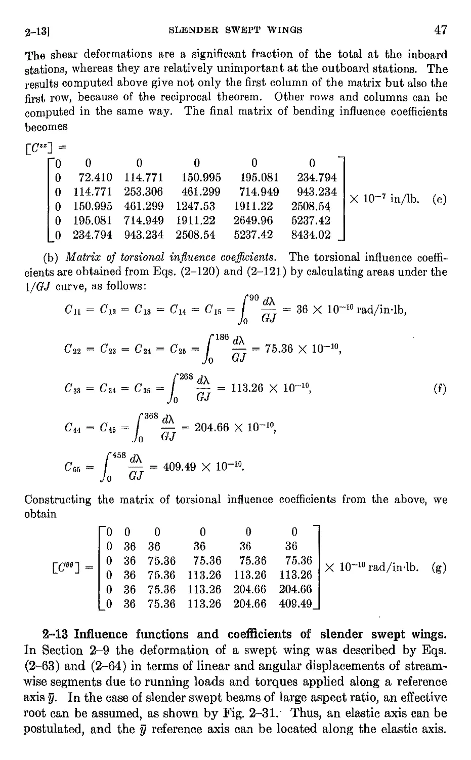
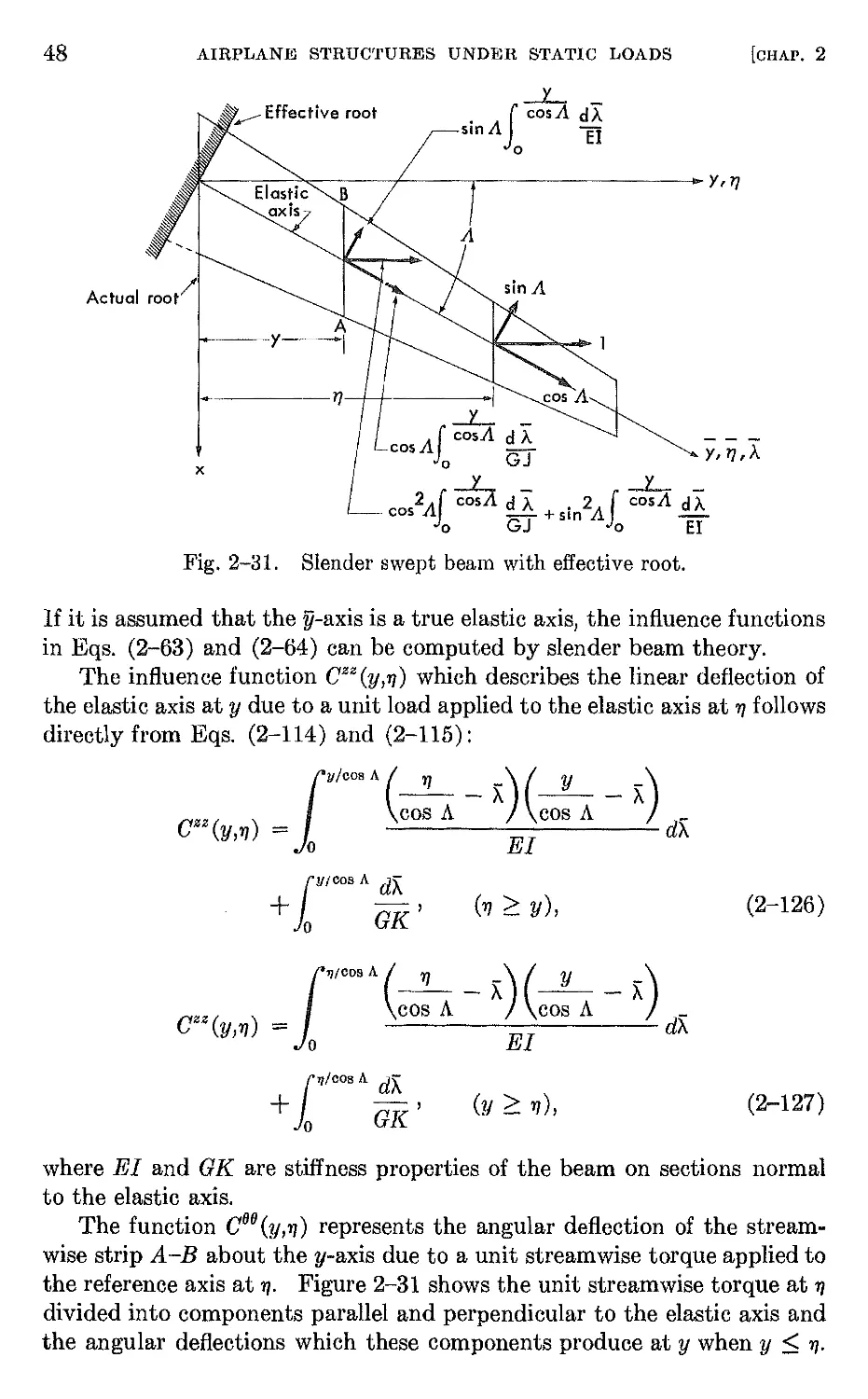
2-13 Influence functions and coefficients of slender swept wings 47
2-14 Deformations and influence coefficients of low aspect. ratio wings 49
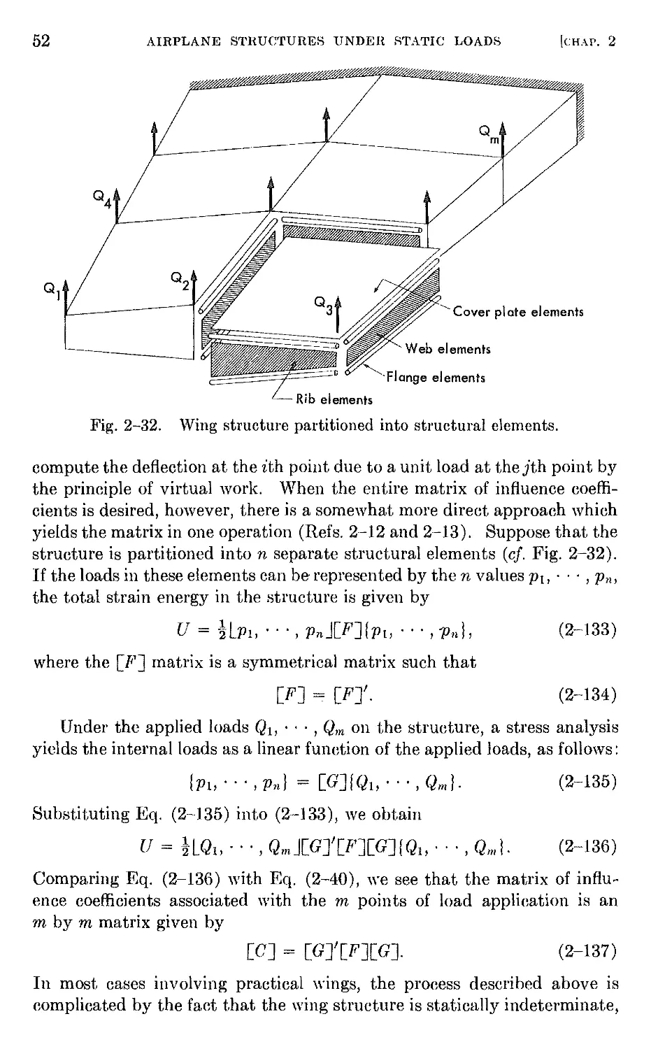
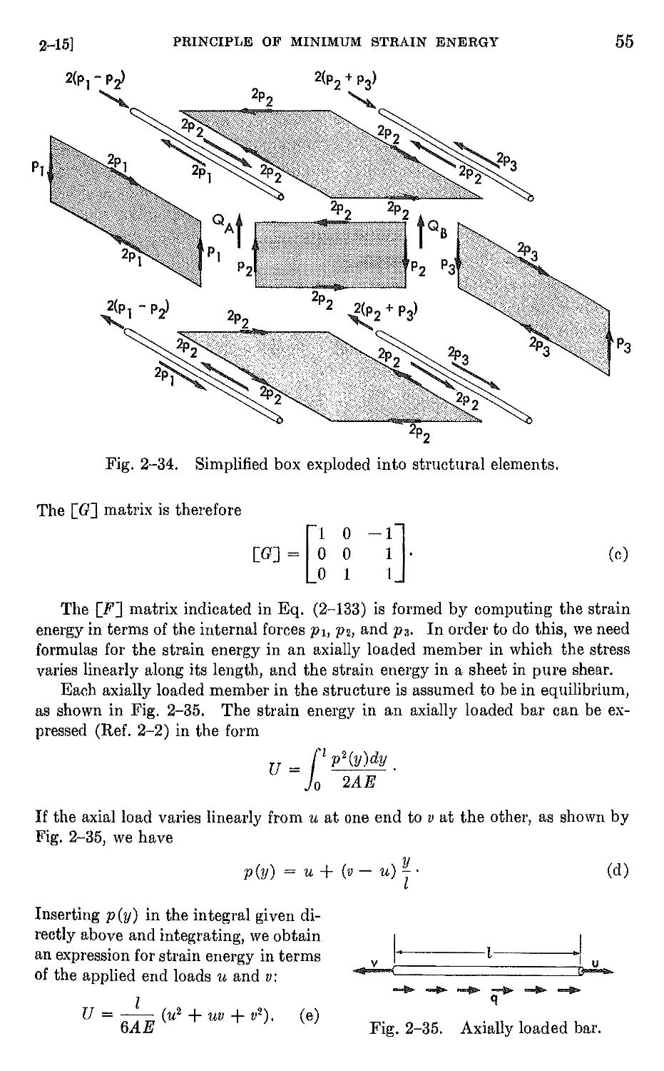
2-15 Influence coefficients of complex built-up wings by the principle of
minimum strain energy 51
2-16 Influence coefficients of complex built-up wings by the principle of
minimum potential energy. . 57
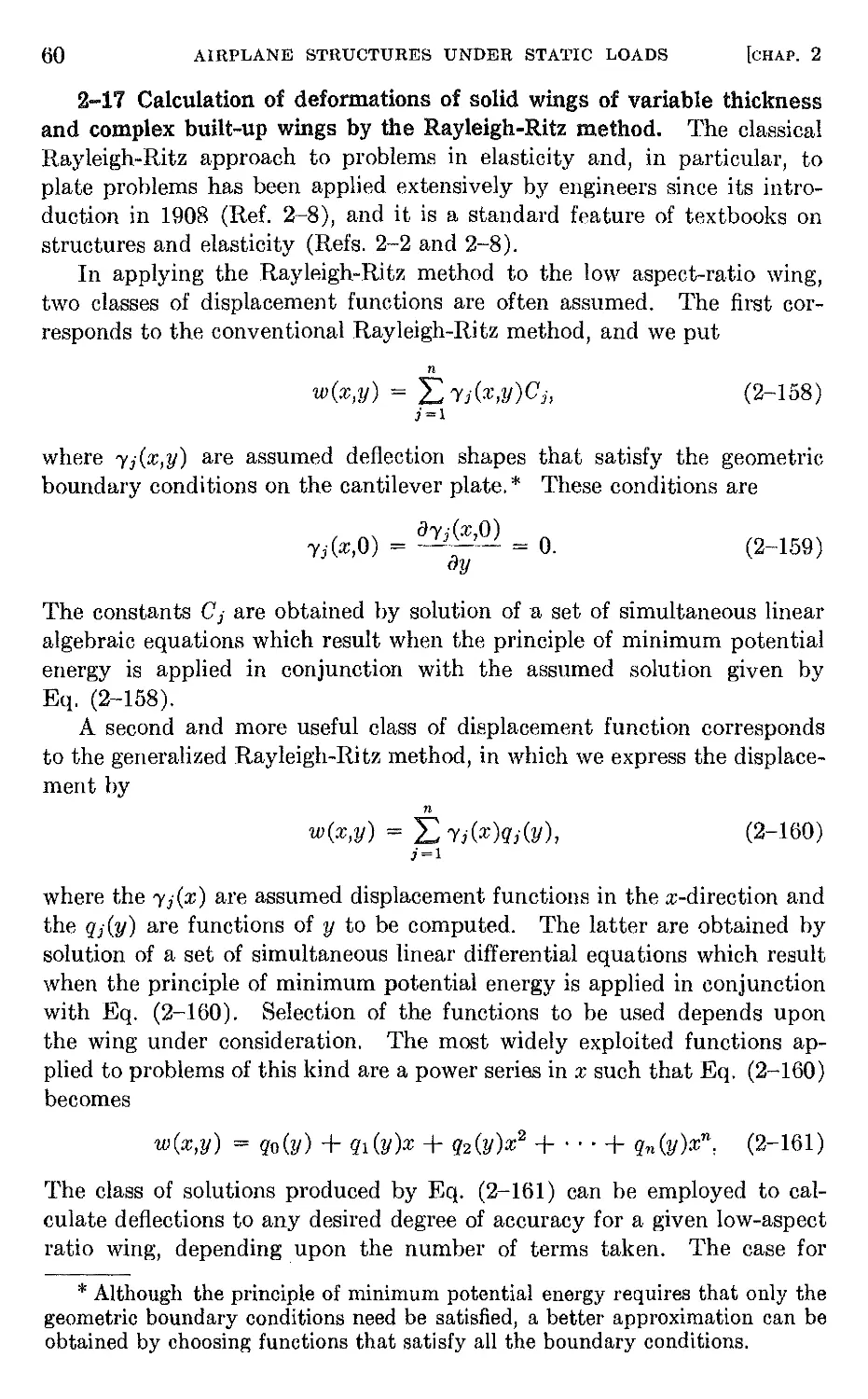
2-17 Calculation of deformations of solid wings of variable thickness
and complex built-up wings by the Rayleigh-Ritz method 60
CHAPTER 3. DEFORMATIONS OF AIRPLANE STRUCTURES UNDER DYNAMIC
M M
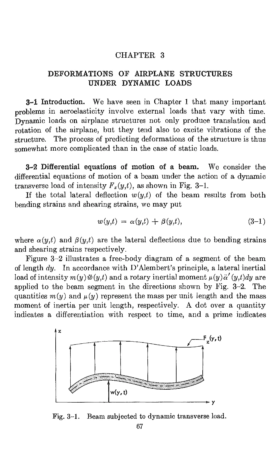
3-1 Introduction 67
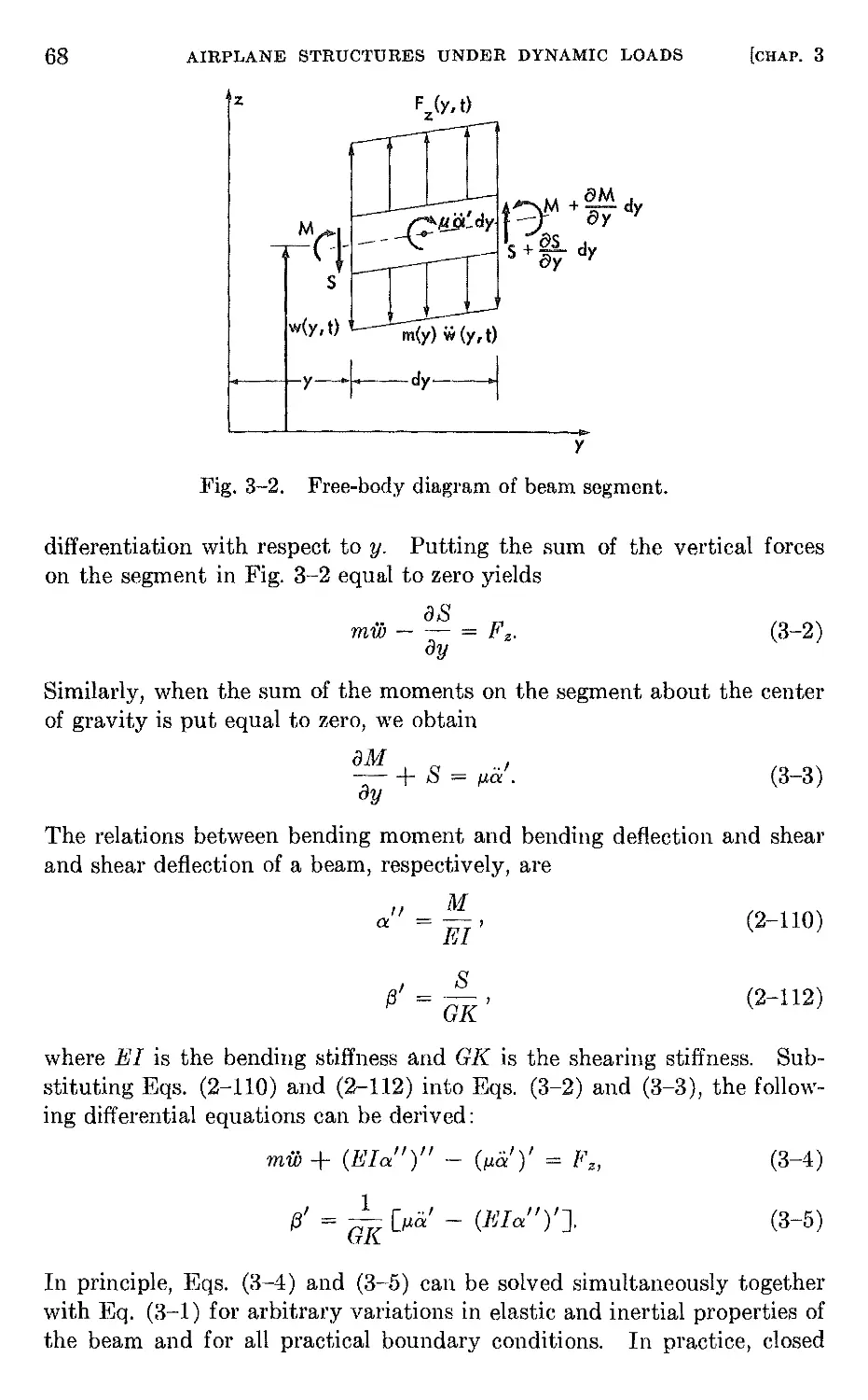
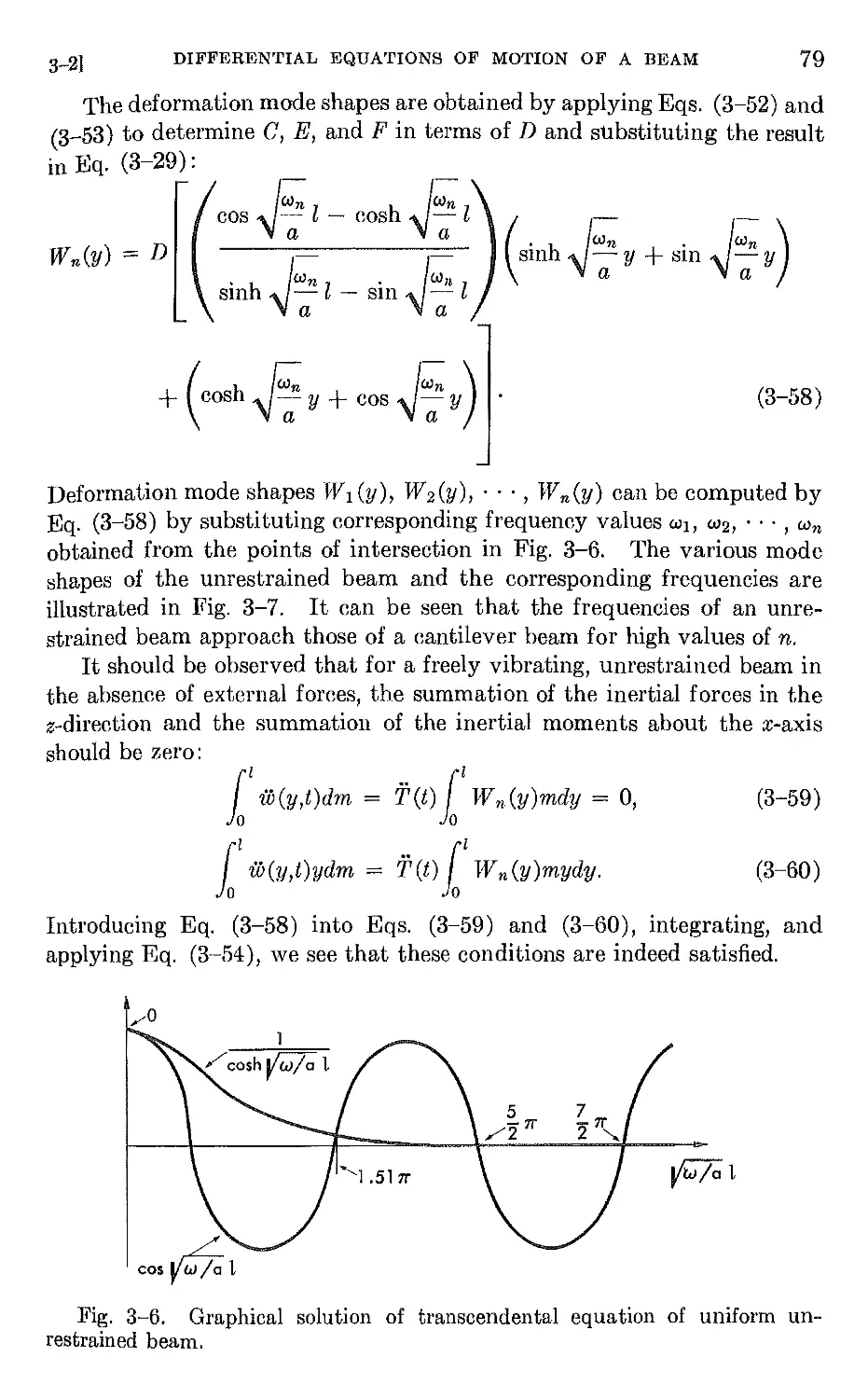
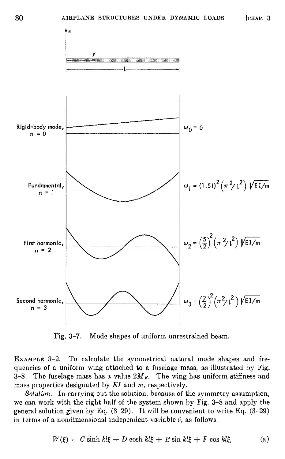
3-2 Differential equations of motion of a beam 67
3-3 Integral equation of motion of a slender beam 87
3-4 Dynamic equilibrium of slender rotating beams in bending 95
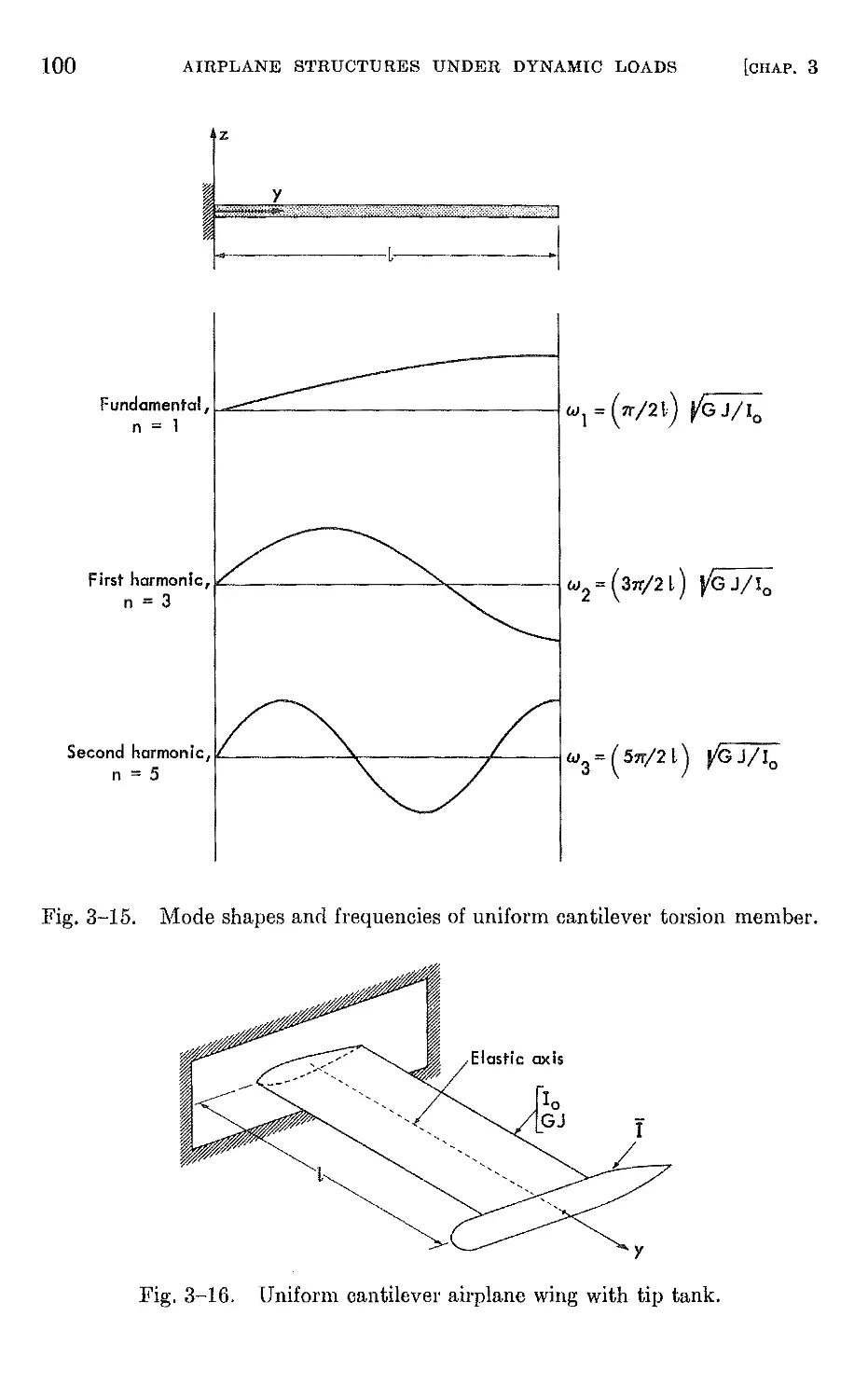
3-5 Dynamic eguilibrium of slender beams in torsion . 98
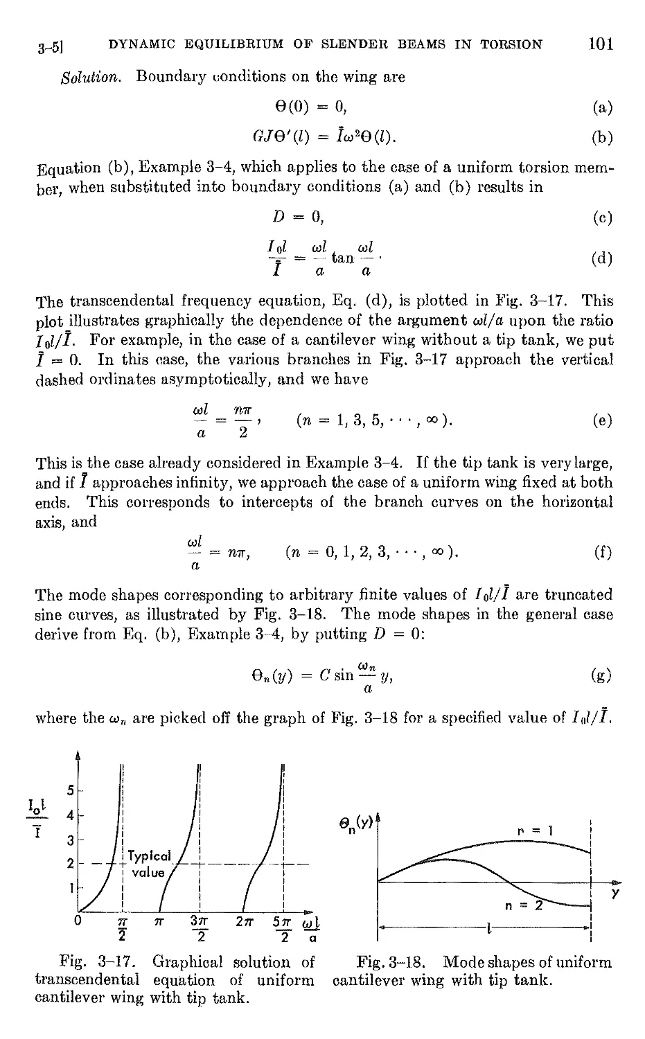
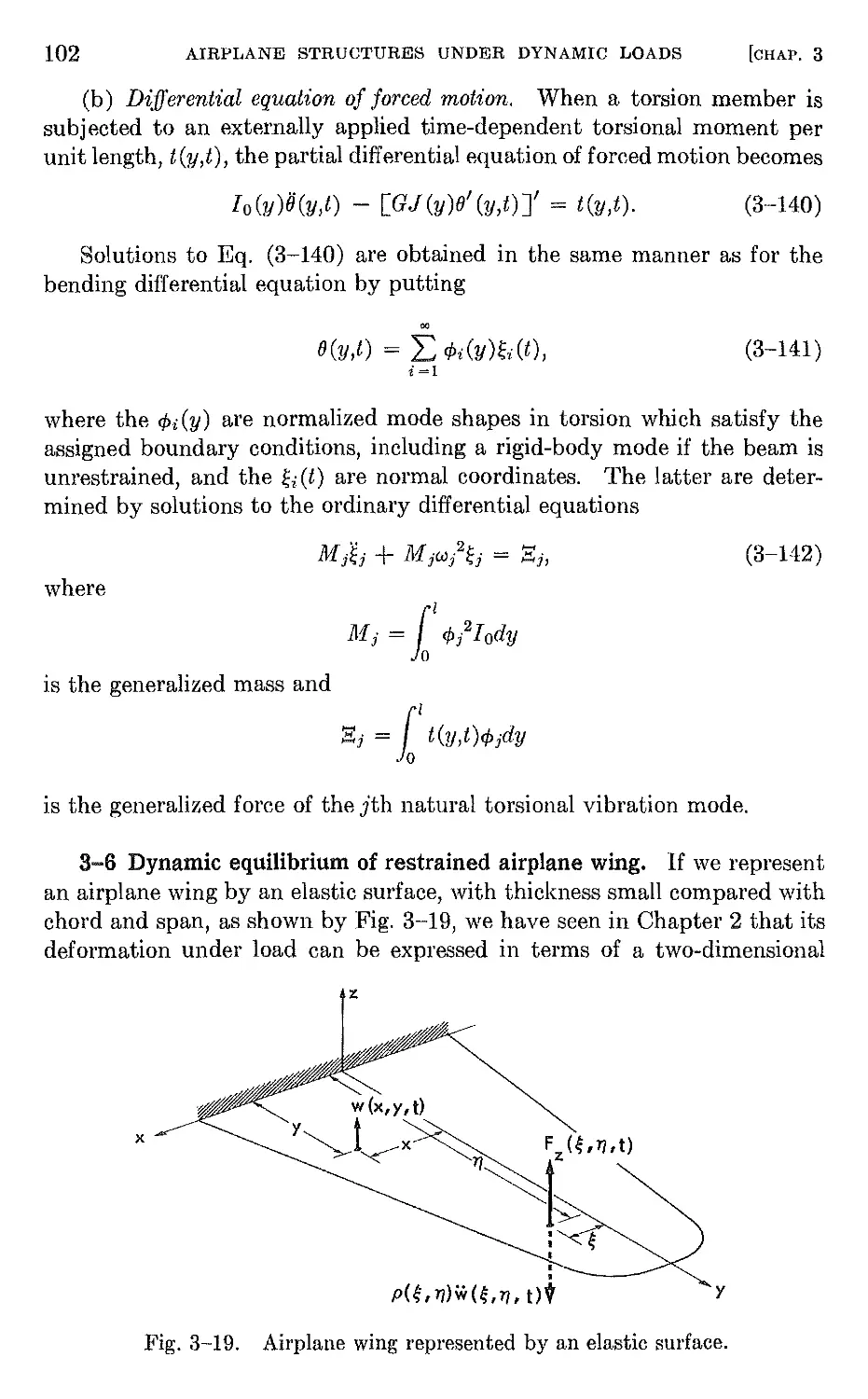
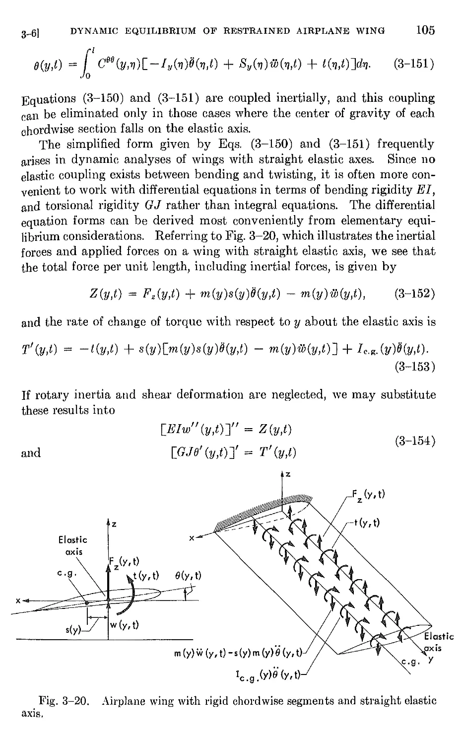
3-6 Dynamic equilibrium of restrained airplane wing . 102
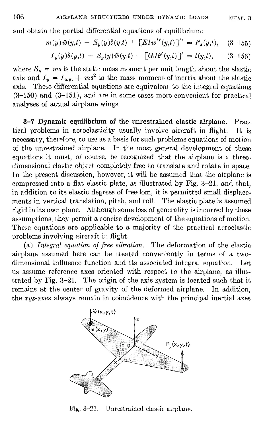
3-7 Dynamic equilibrium of the unrestrained elastic airplane. 106
3-8 Energy methods . 114
3-9 Approximate methods of solution to practical problems . 124
3-10 Approximate solutions by the Rayleigh Ritz method . 125
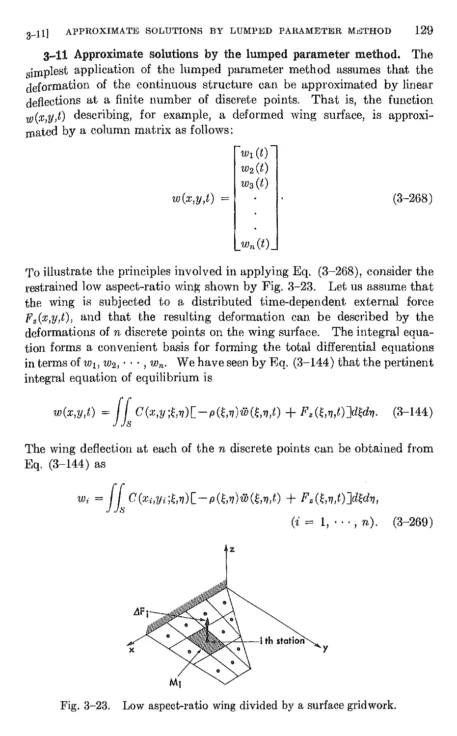
3-11 Approximate solutions by the lumped parameter method 129
CHAPTER 4. ApPROXIMATE METHODS OF COMPUTING NATURAL MODE
SHAPES AND FREQUENCIES 132
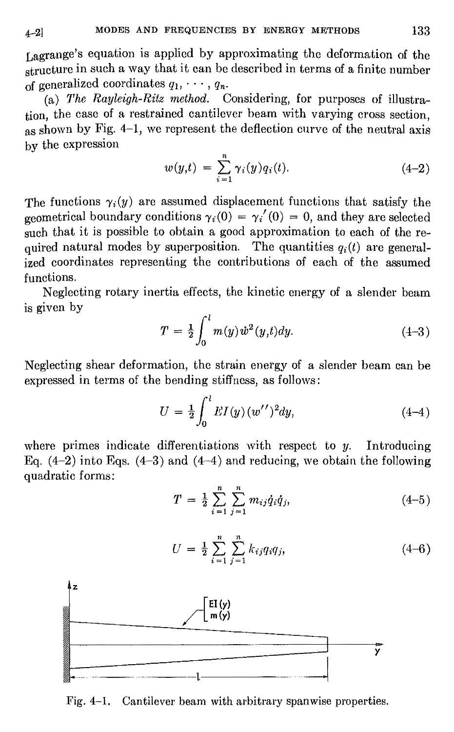
4-1 Introduction . 132
4-2 Natural modes and frequencies by energy methods 132
4-3 Natural mode shapes and frequencies derived from the integral
equation . 146
VlI
Vlll
CONTENTS
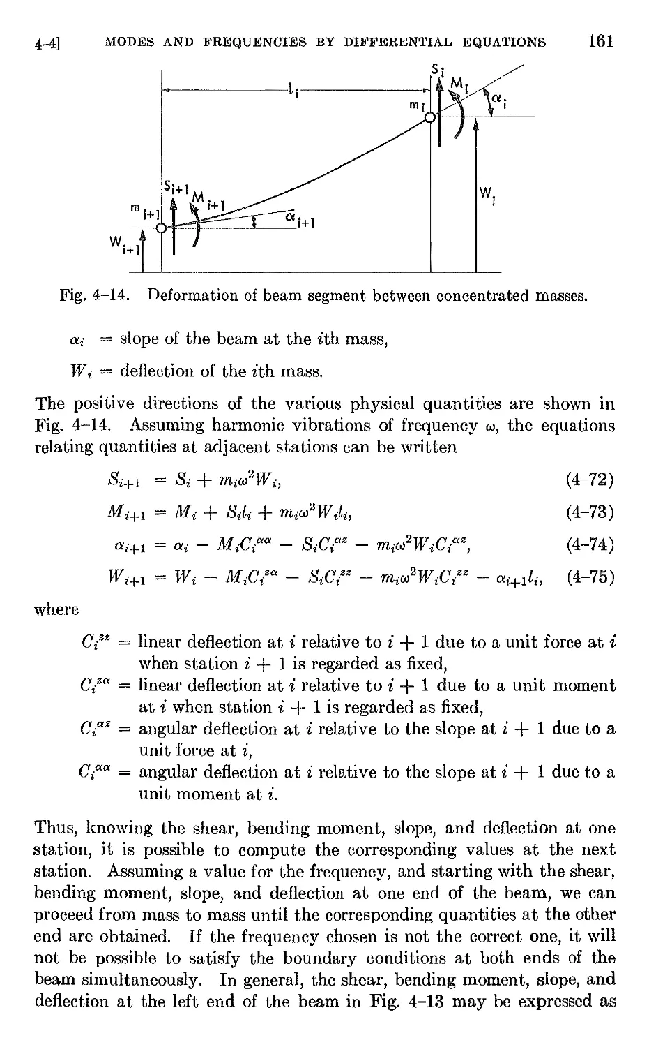
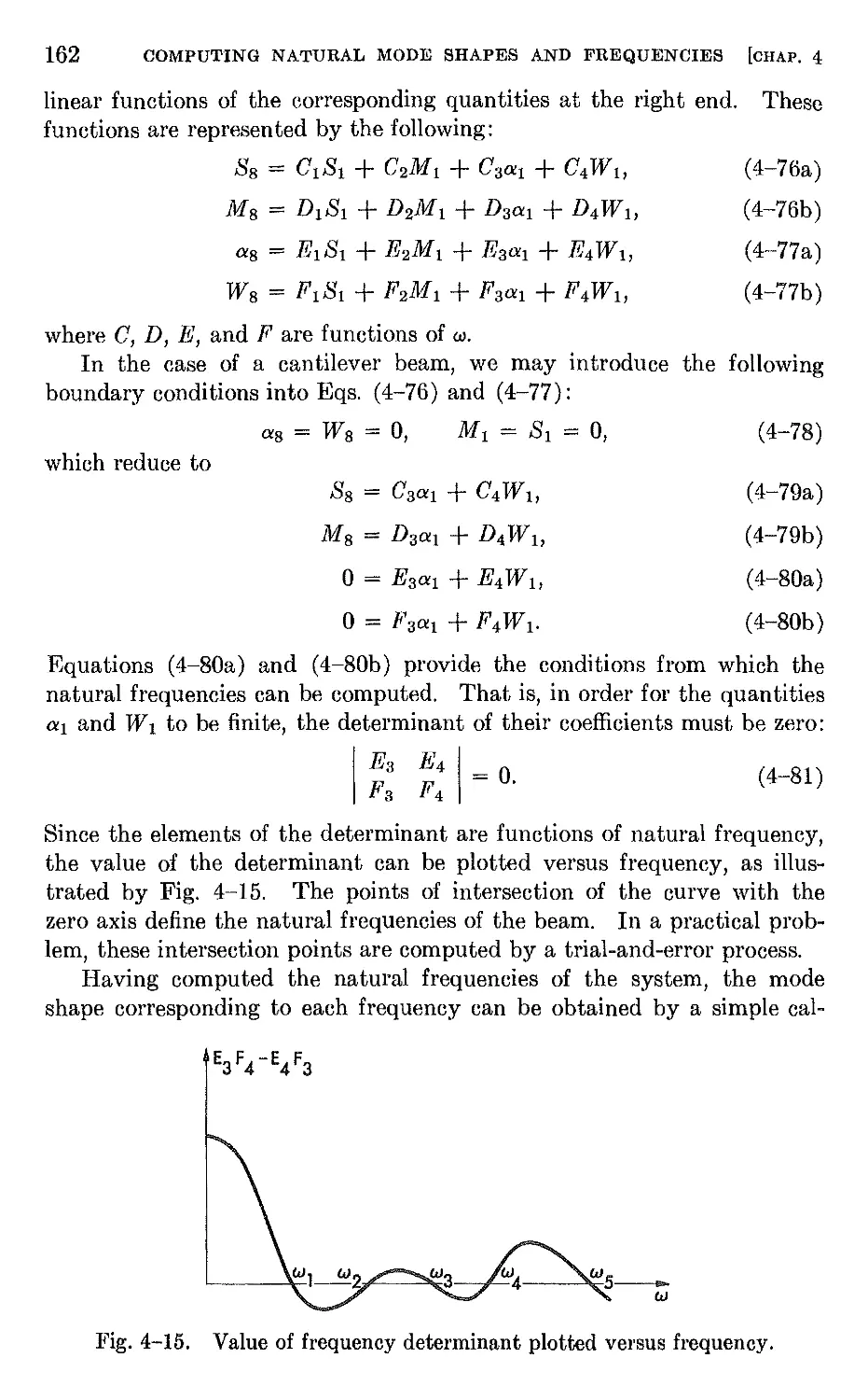
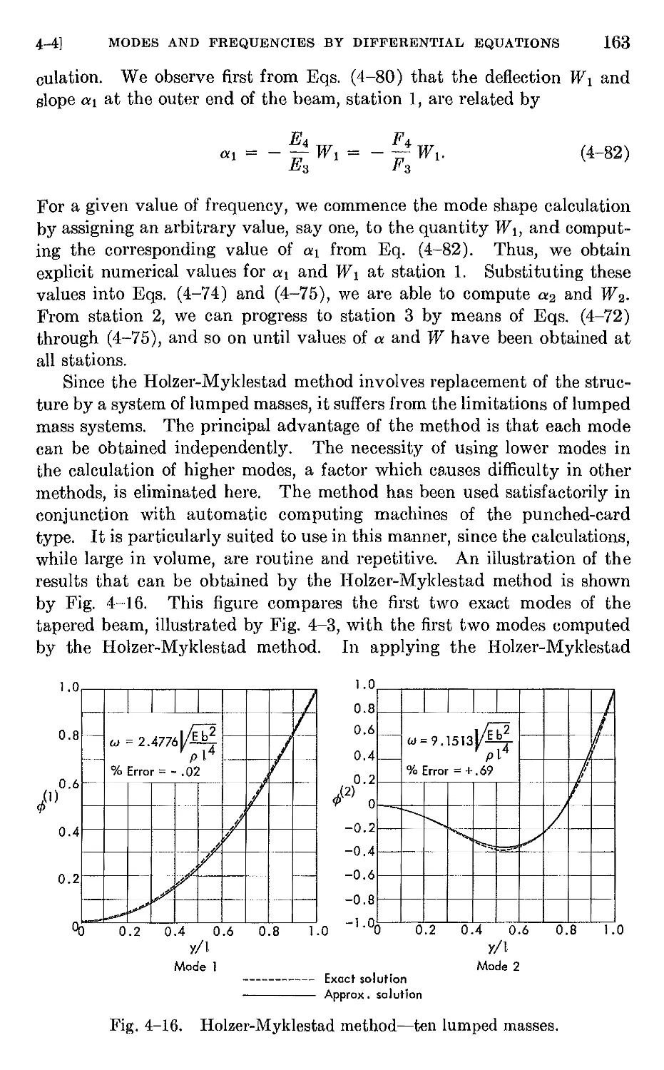
4-4 Natural mode shapes and frequencies derived from the differential
equation. .159
4-5 Solution of characteristic equations . . 164
4-6. Natural modes and frequencies of complex airplane structures 172
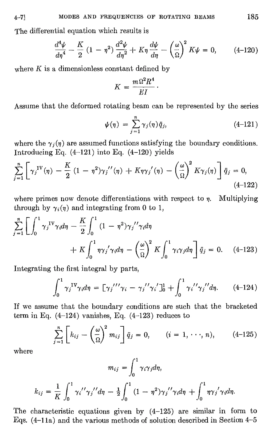
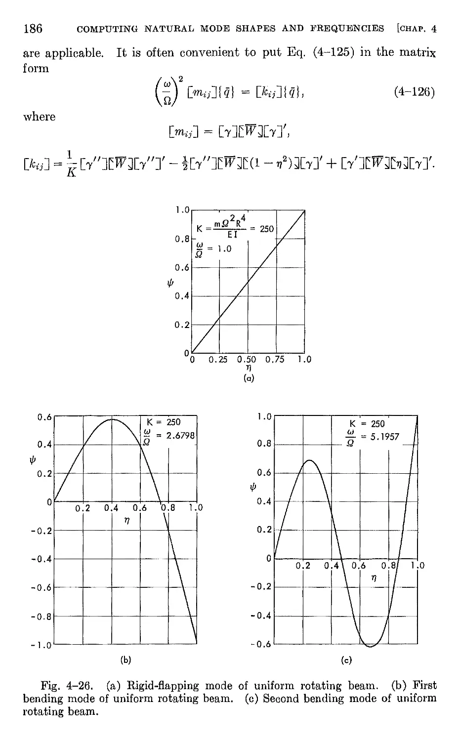
4-7 Natural modes and frequencies of rotating beams 184
CHAPTER 5. AERODYNAMIC TOOLS: TWO- AND THREE-DIMENSIONAL IN
COMPRESSIBLE FLOW . 188
5-1 Fundamentals: the concept of small disturbances. " 188
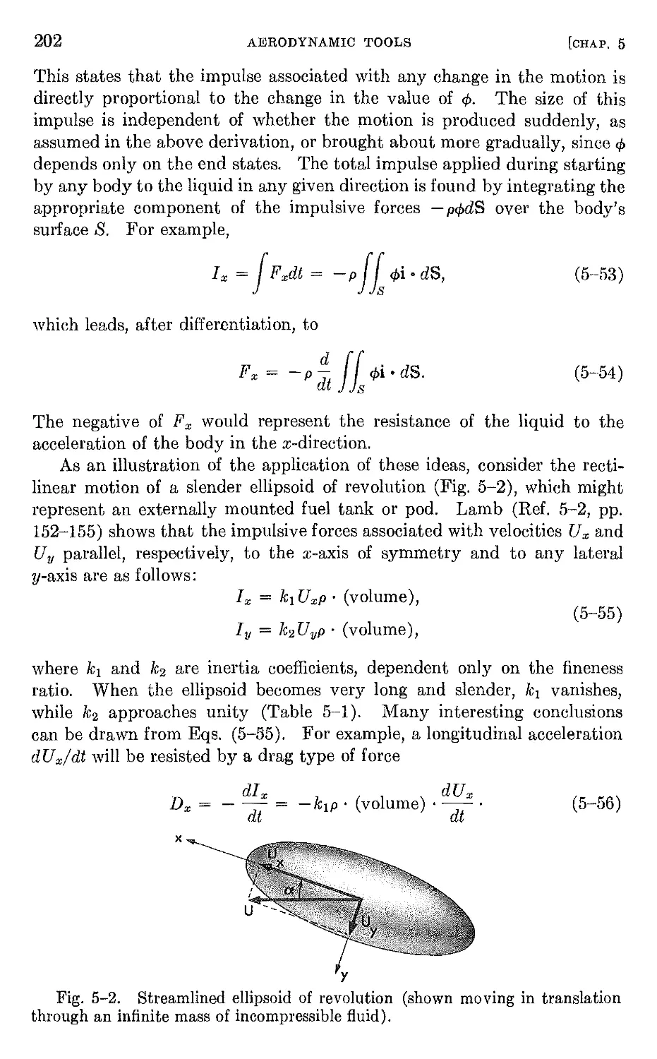
5-2 Properties of incompressible flow with and without circulation 200
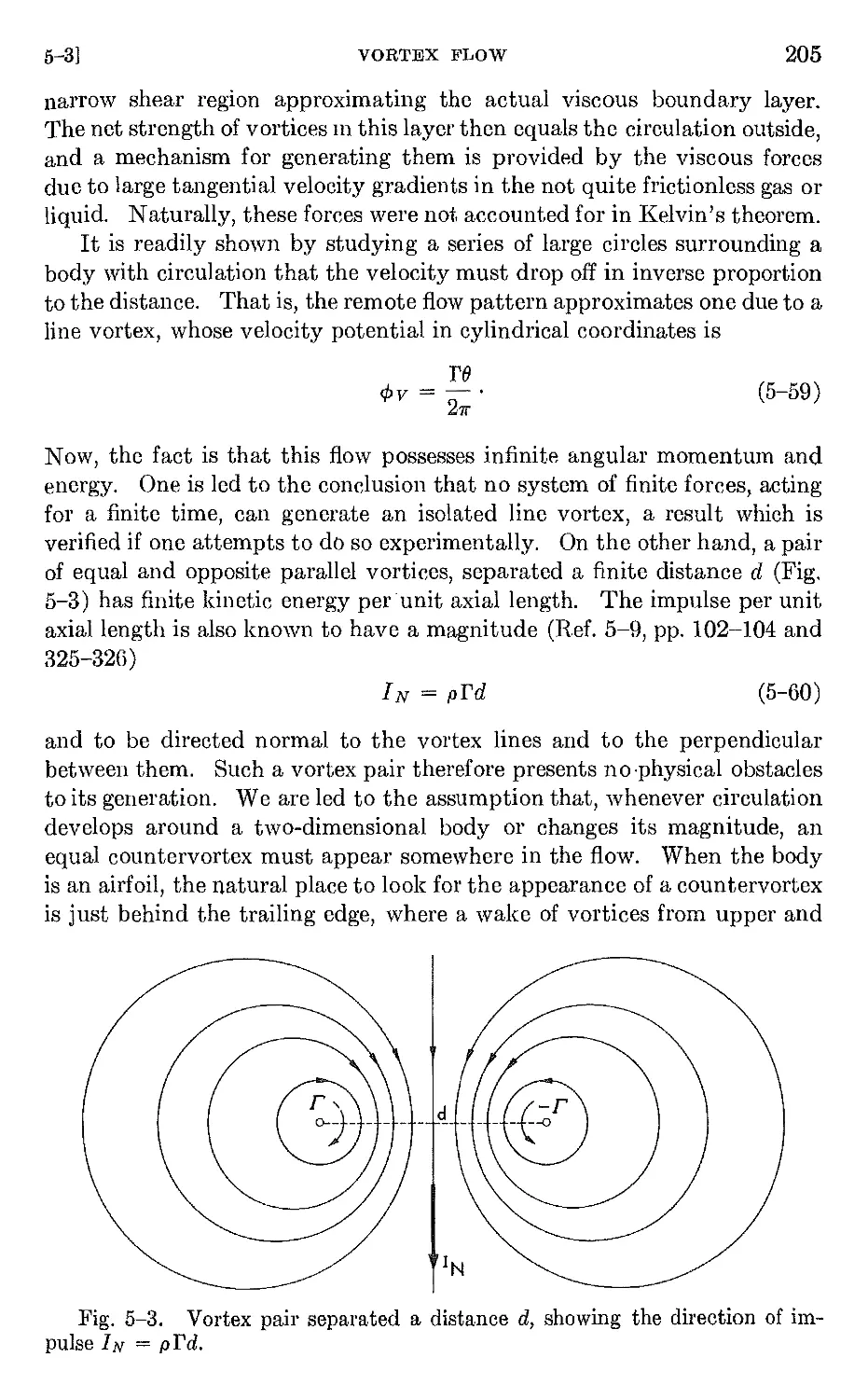
5-3 Vortex flow . 204
5-4 Thin airfoils in steady motion. 208
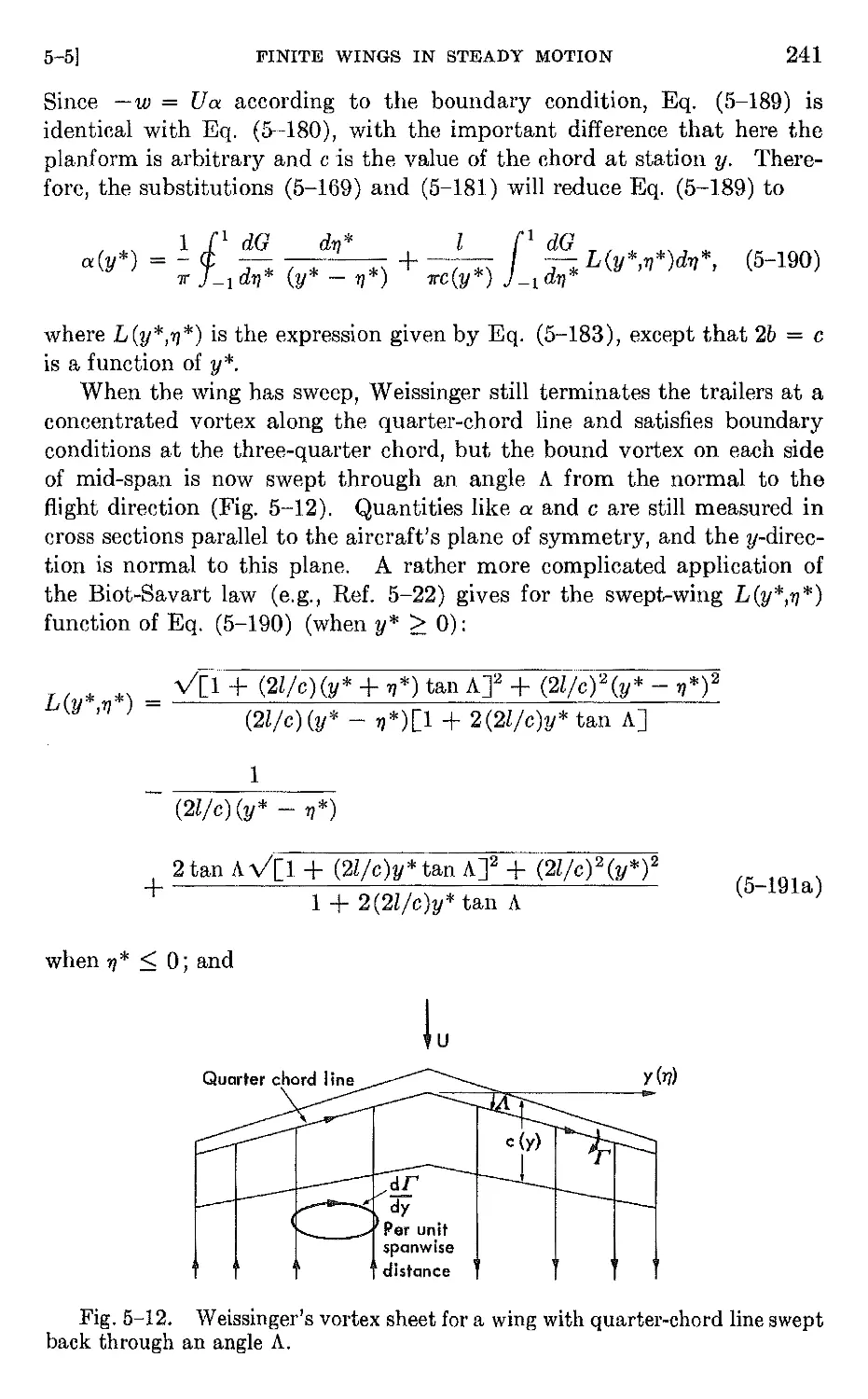
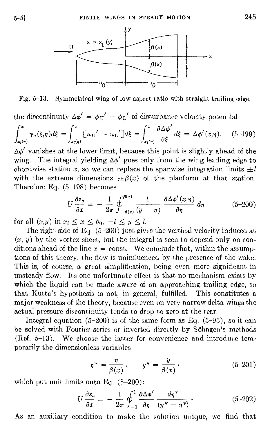
5-5 Finite wings in steady motion.. 221
5-6 Thin airfoils oscillating in incompressible flow.. .,. 251
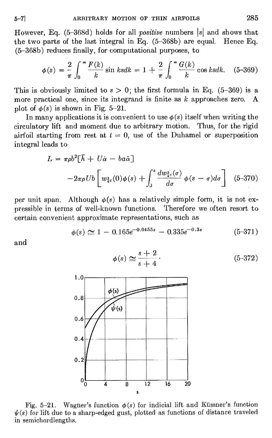
5-7 Arbitrary motion of thin airfoils in incompressible flow; the gust
problem . 281
CHAPTER 6. AERODYNAMIC TOOLS: COMPRESSIBLE FLOW . 294
6-1 Introduction " . 294
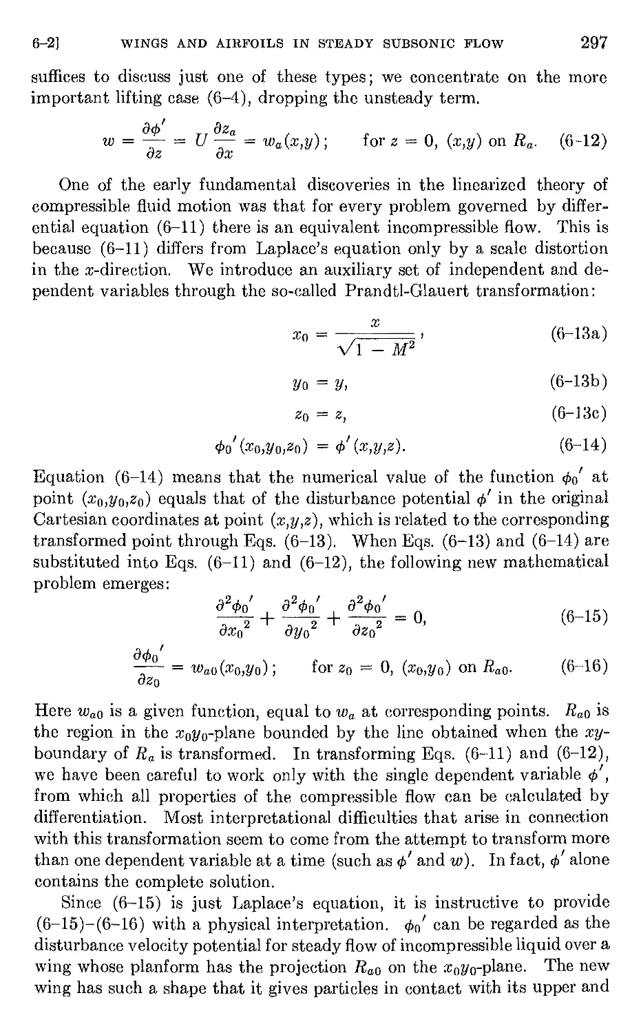
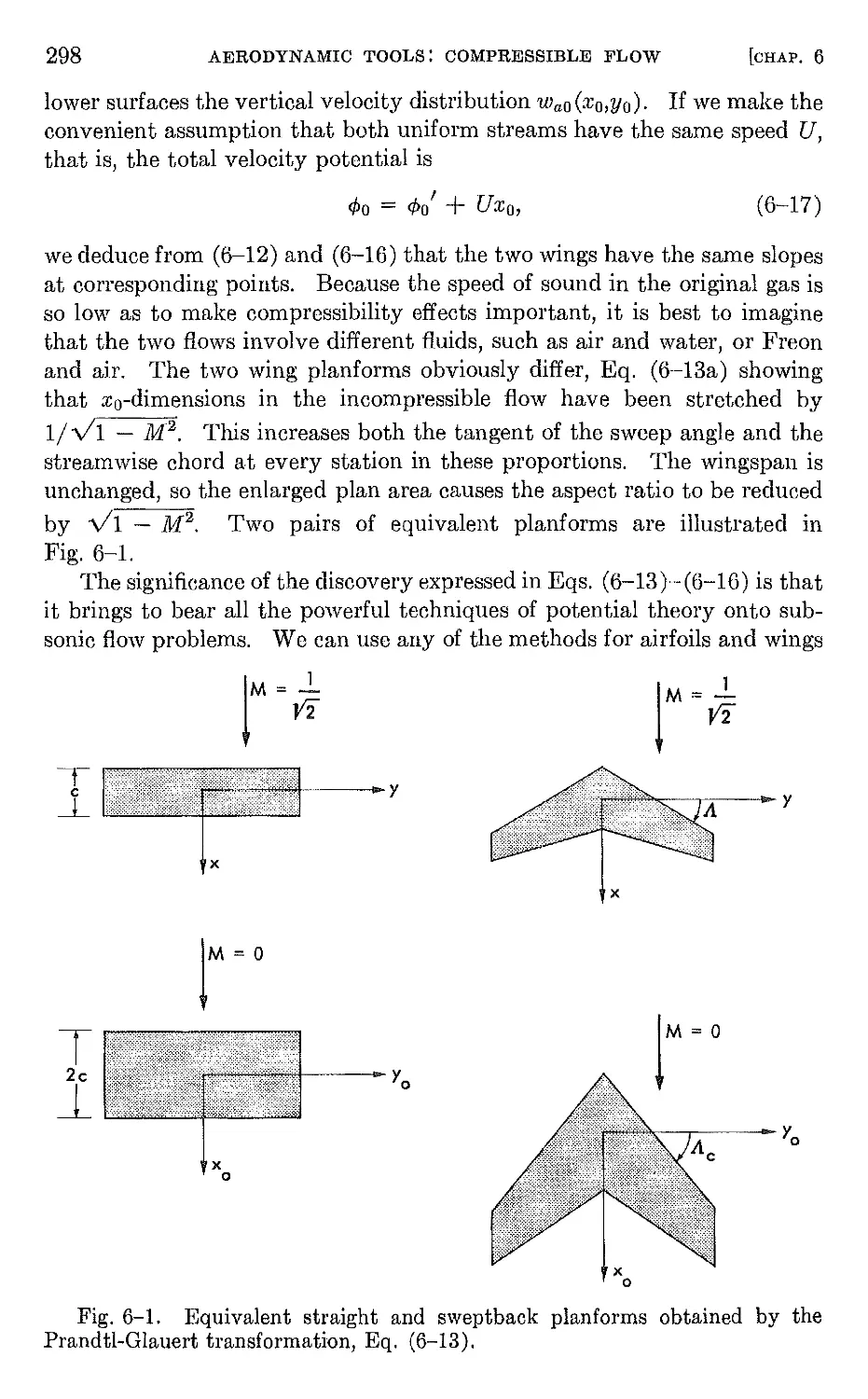
6-2 Wings and airfoils in steady subsonic flow; the Prandtl-Glauert
transformation , . . 296
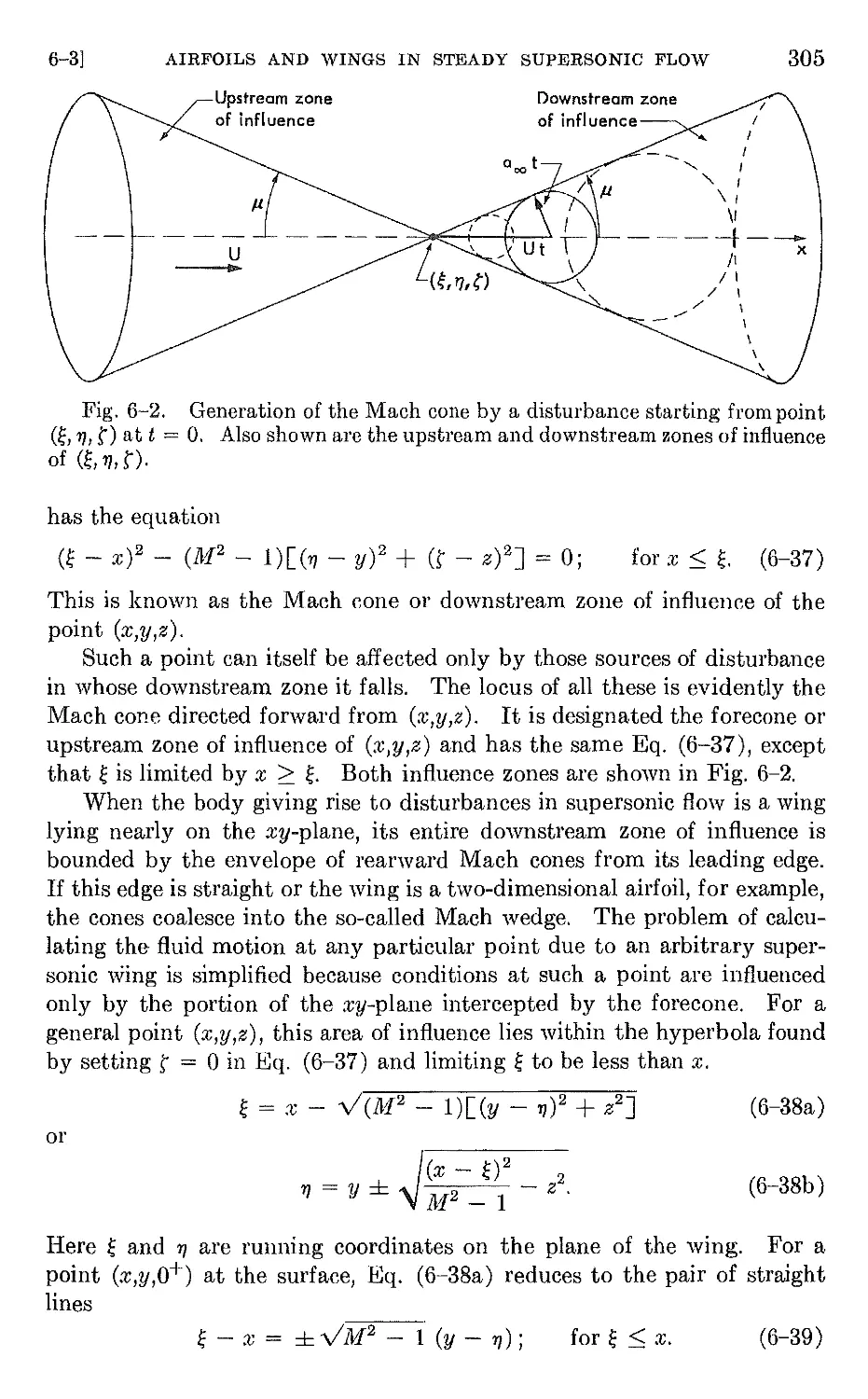
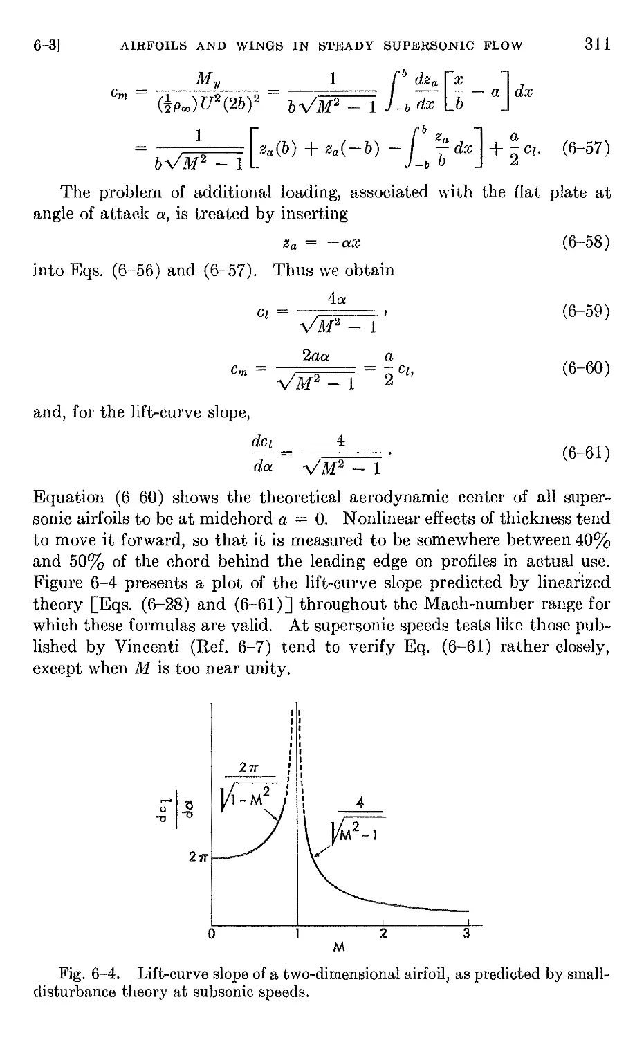
6-3 Airfoils and wings in steady supersonic flow 303
6-4 Oscillating airfoils in subsonic flow 317
6-5 Arbitrary small motions of airfoils in subsonic flow 332
6-6 Oscillating airfoils at supersonic speeds . 353
6-7 Indicial airfoil motions in supersonic flow 367
6-8 Unsteady motion of airfoils at Mach number one 375
CHAPTER 7. WINGS AND BODIES IN THHEE-DIMENSIONAL UNSTEADY FLOW 380
7-1 Introduction 380
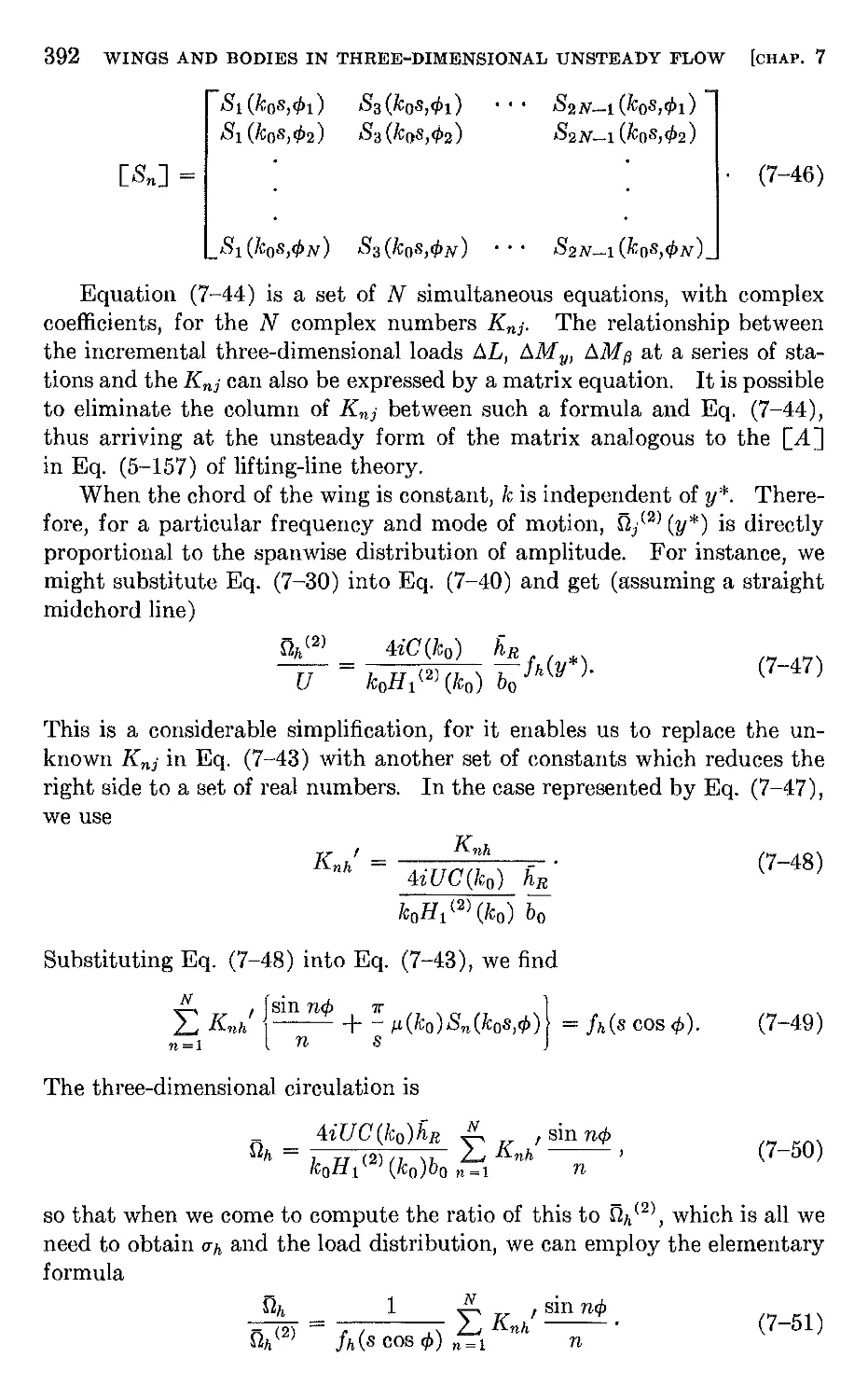
7-2 Oscillating finite wings in incompressible flow . 381
7-3 The influence of sweep 394
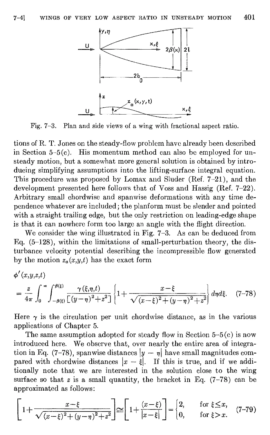
7-4 Wings of very low aspect ratio in unsteady motion 400
7-5 The influence of compressibility on oscillating wings of finite span 405
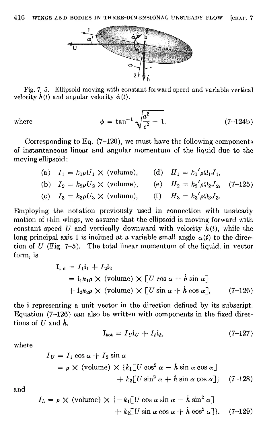
7-6 Unsteady motion of nonlifting bodies 414
CHAPTER 8. STATIC AEROELASTIC PHENOMENA 421
8-1 Introduction 421
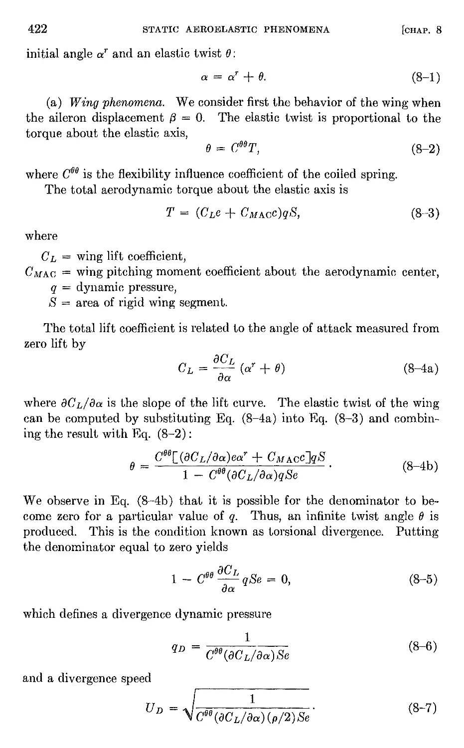
8-2 Twisting of simple two-dimensional wing with aileron 421
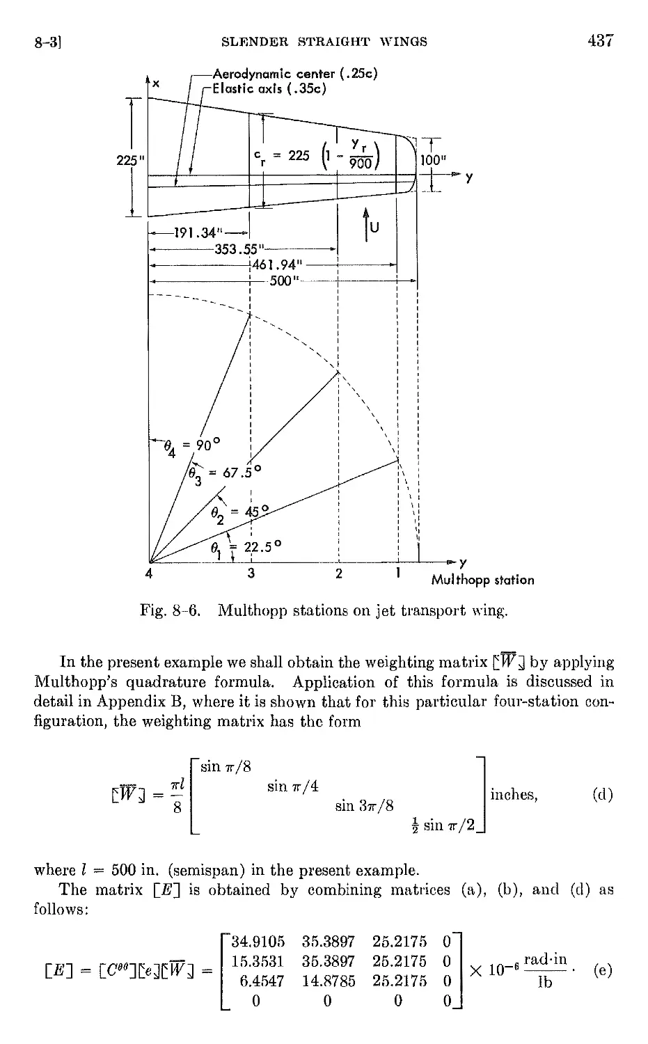
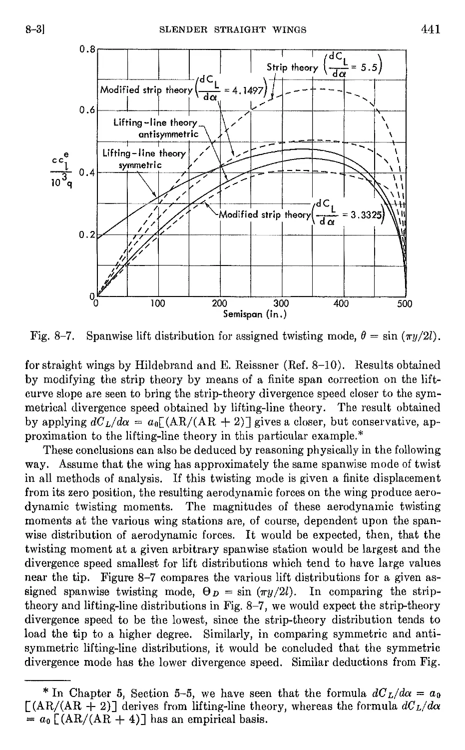
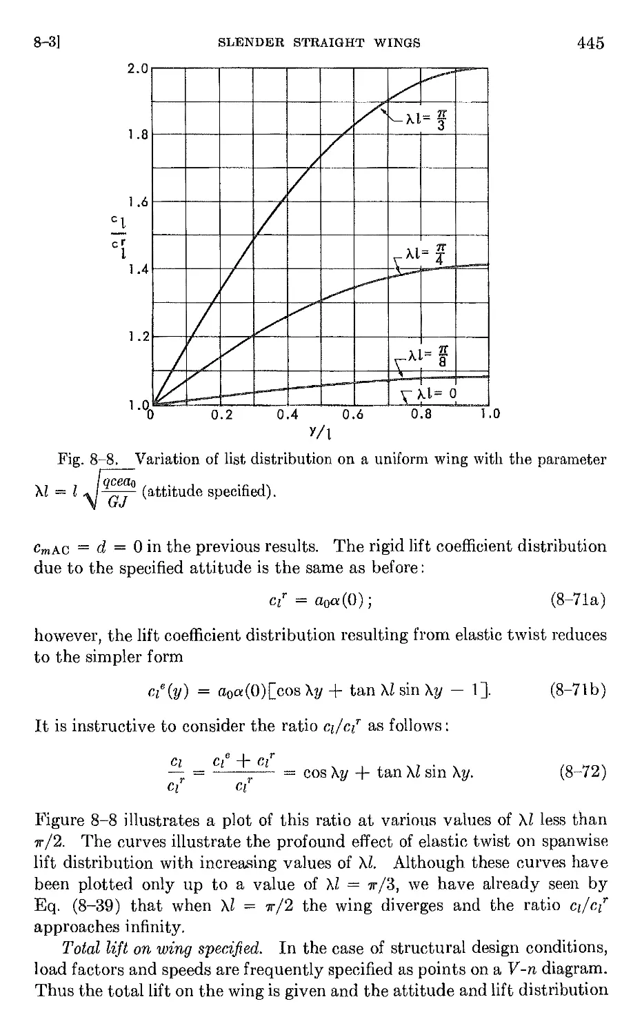
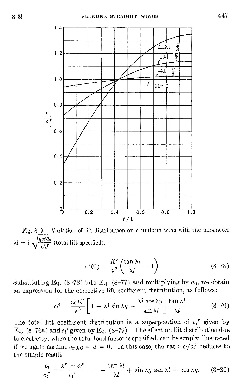
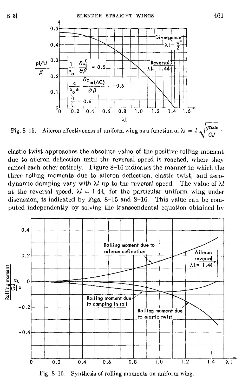
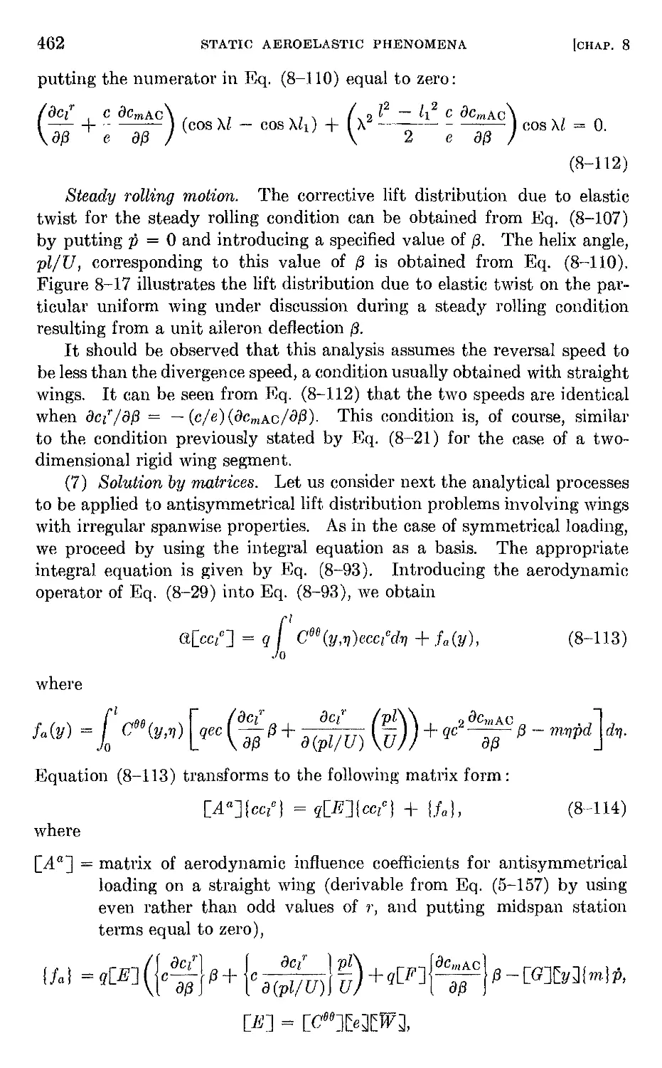
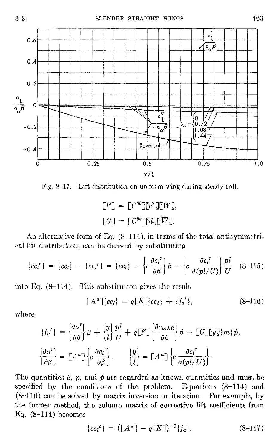
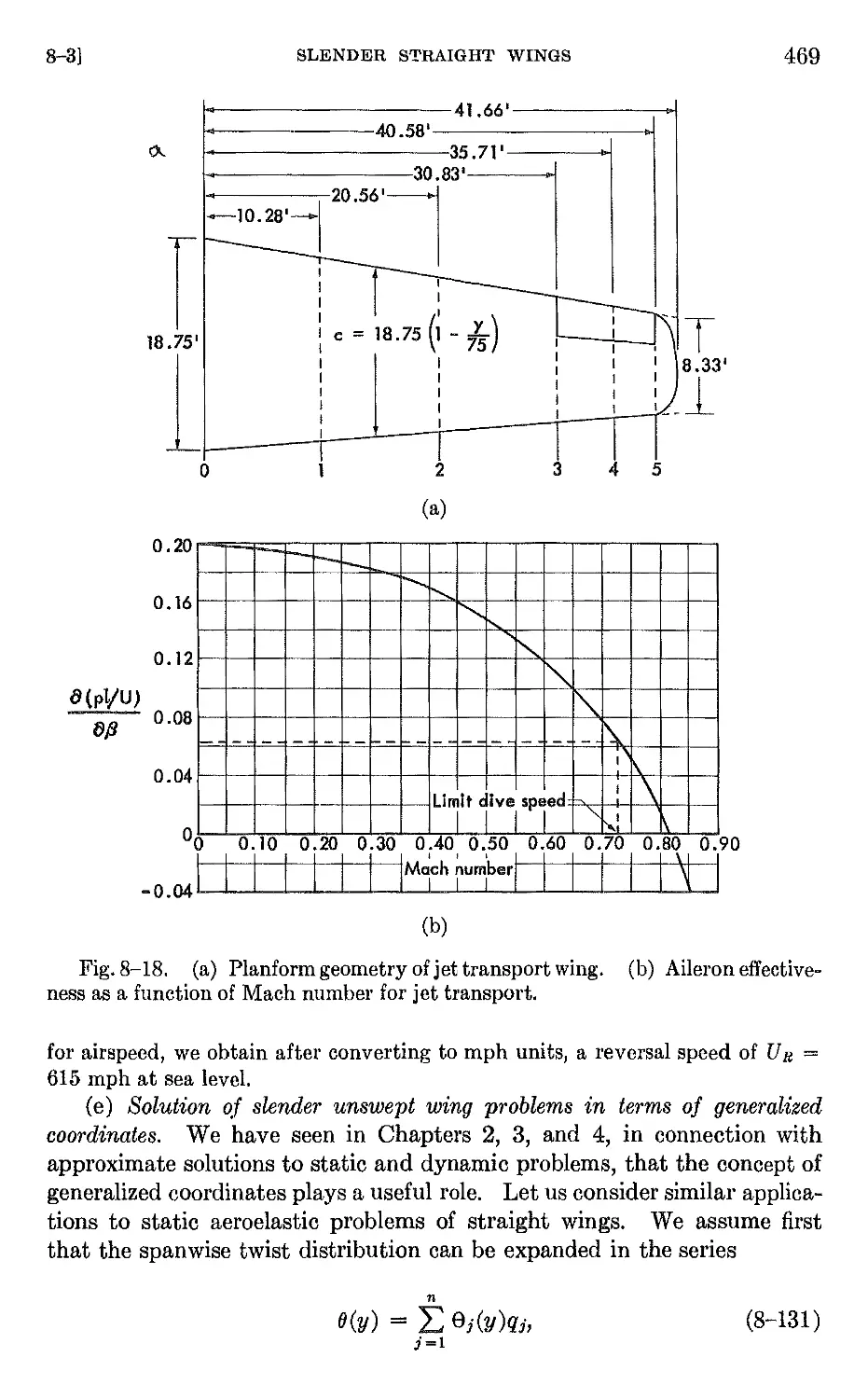
8-3 Slender straight wings . 427
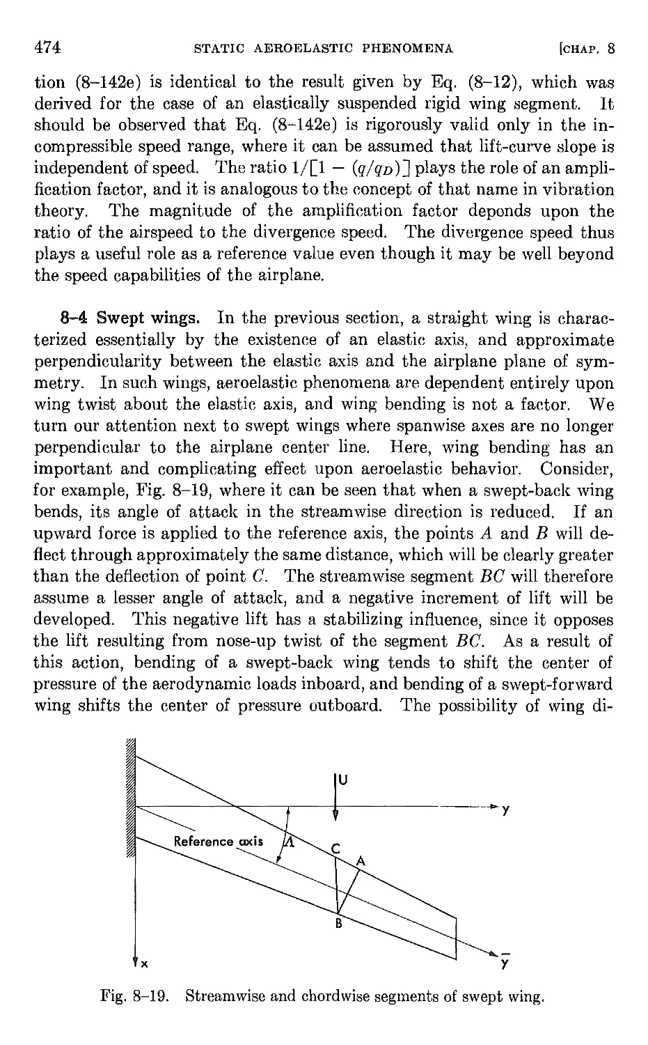
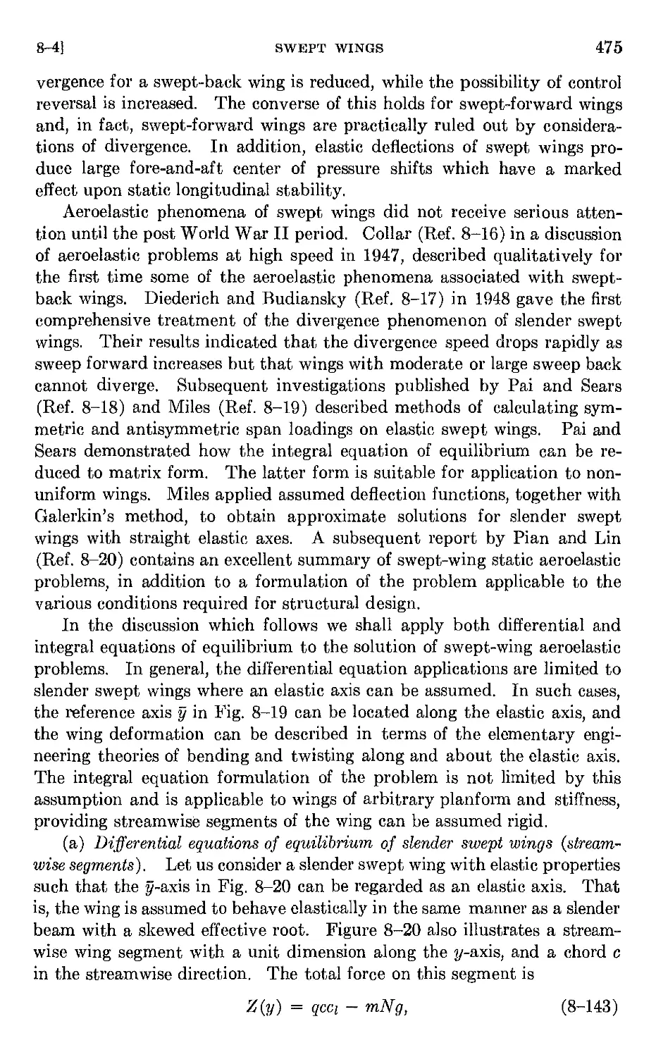
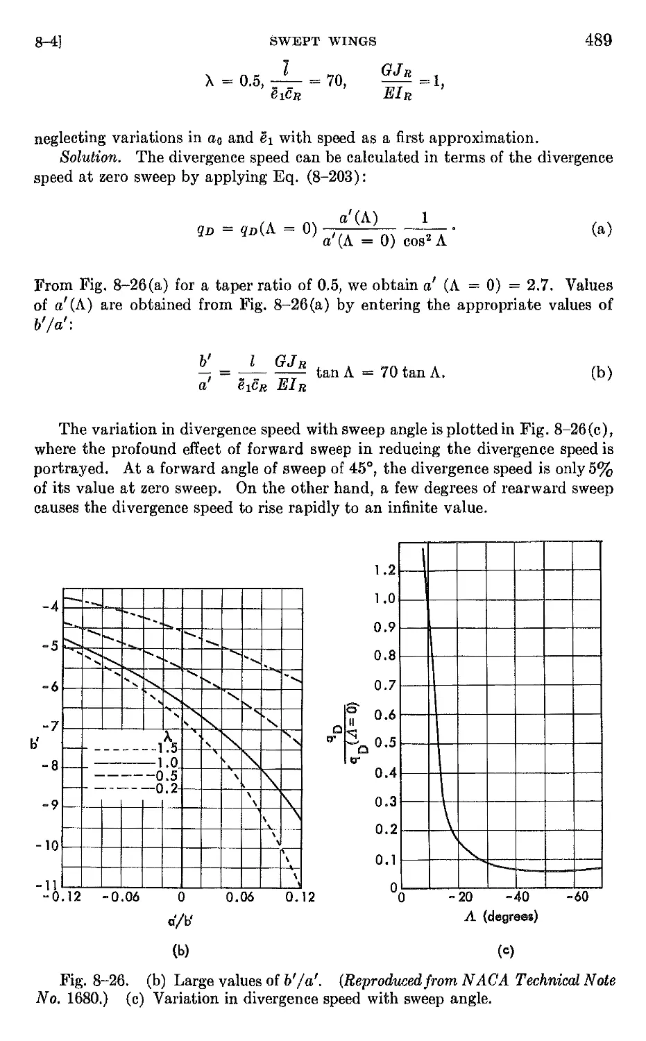
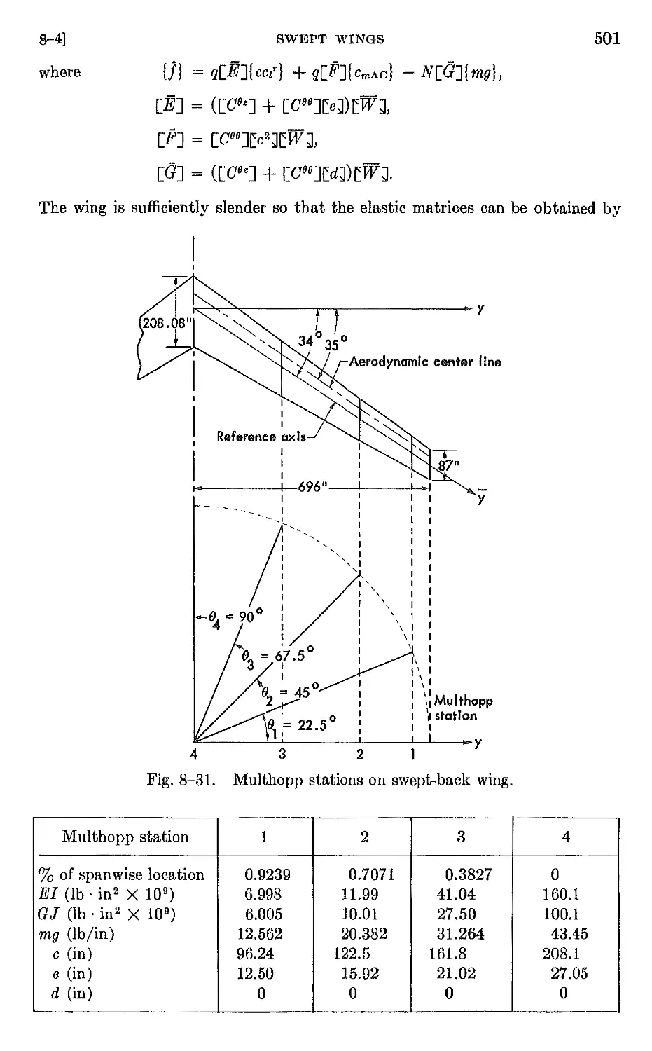
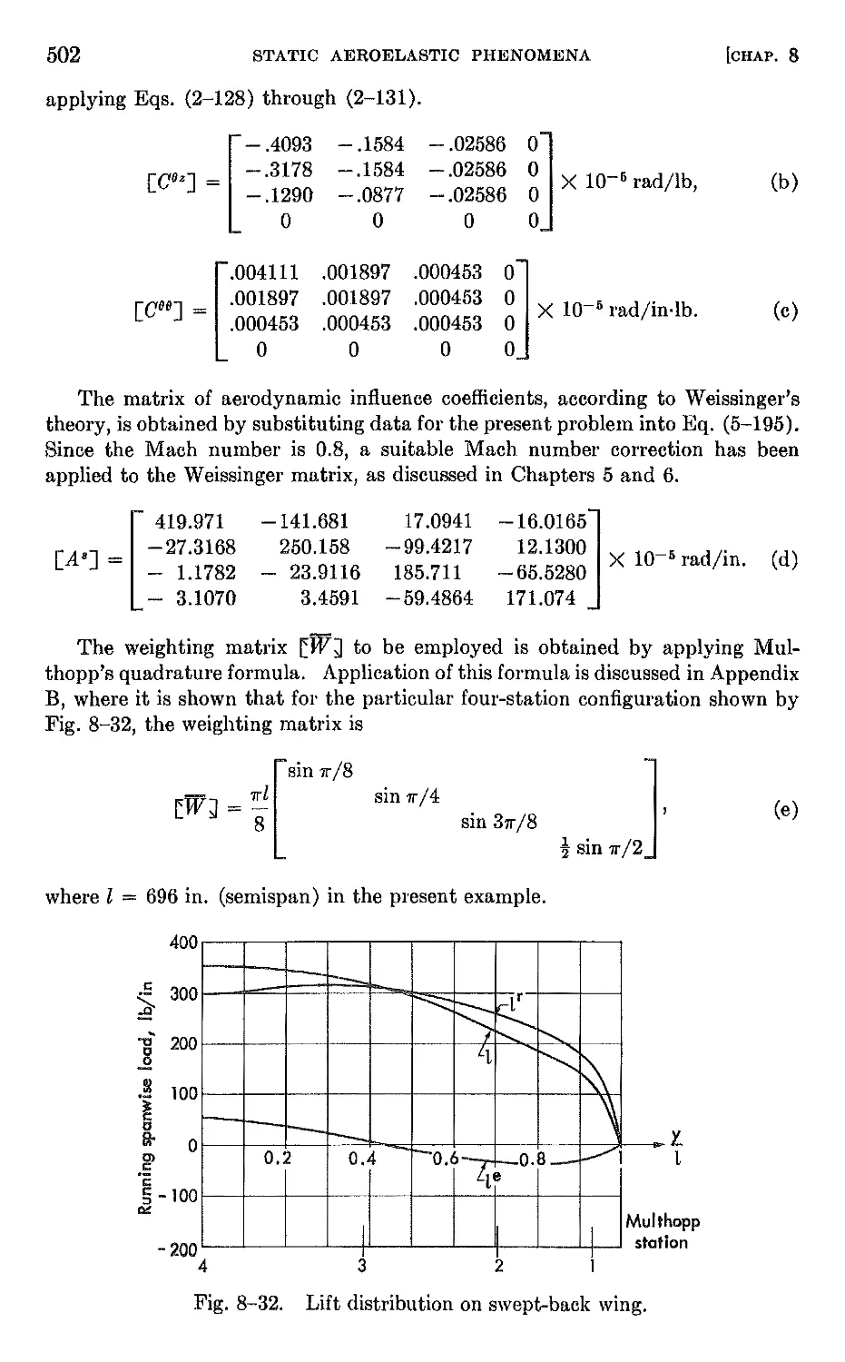
8-4 Swept wings 474
8-5 Low aspect-ratio lifting surfaces of arbitrary planform and stiffness 516
CHAPTER 9, FLUTTER 527
9-1 Introduction. The nature of flutter 527
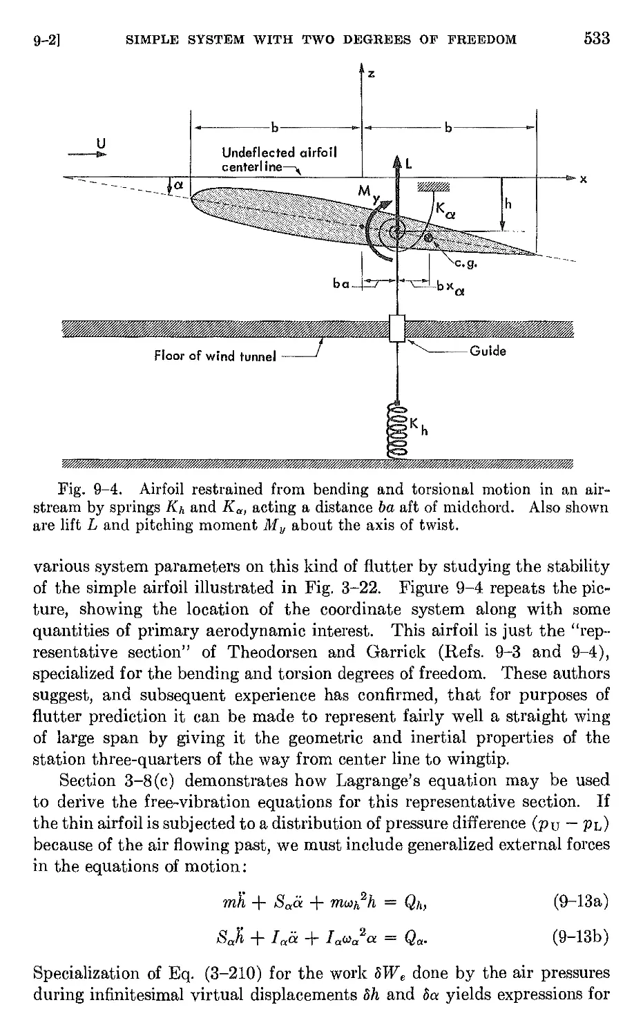
9-2 Flutter of a simple system with two degrees of freedom 532
9-3 Exact treatment of the bending-torsion flutter of a uniform canti-
lever wing 545
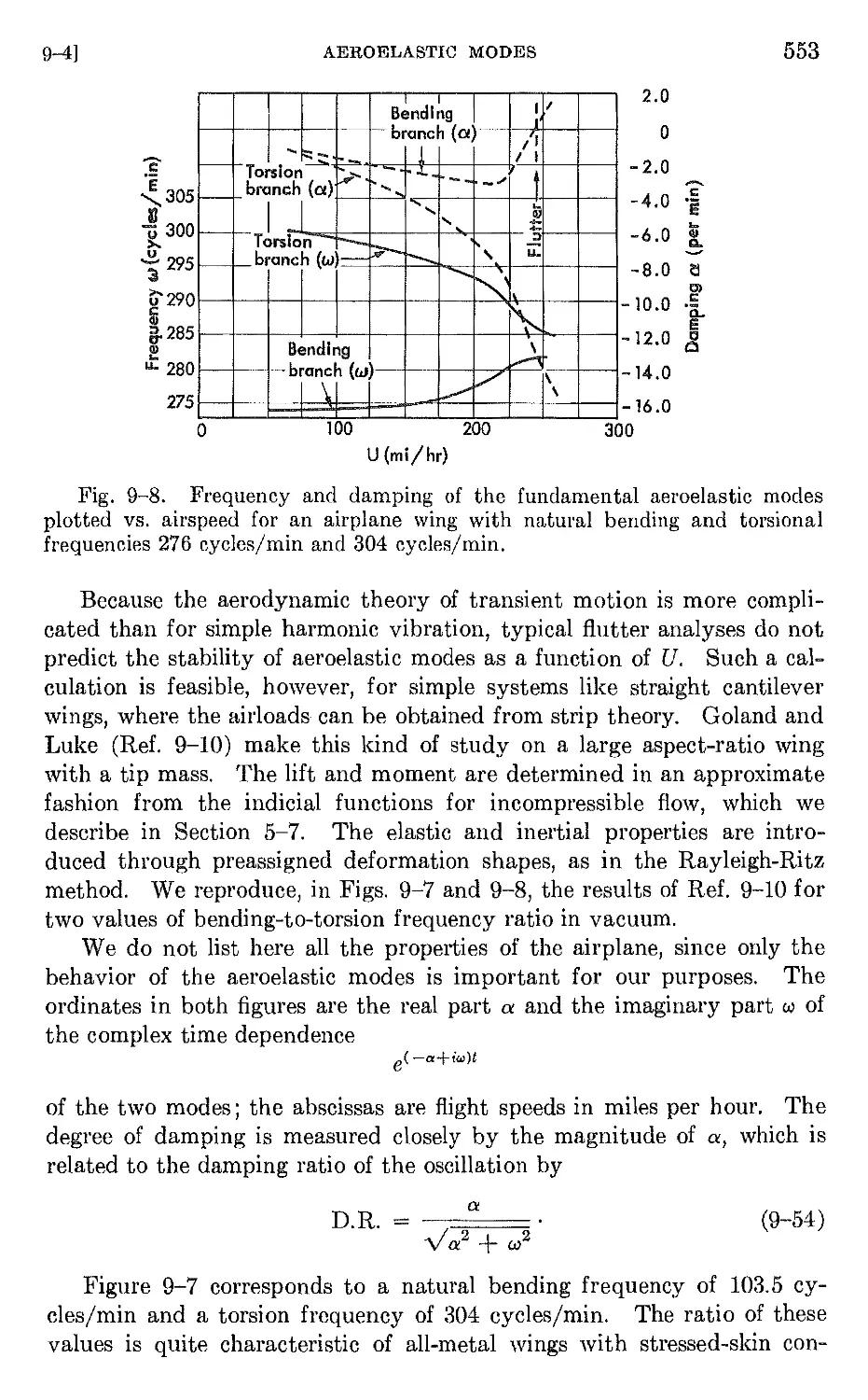
9-4 Aeroelastic modes . 551
9-5 Flutter analysis by assumed-mode methods 555
9-6 Inclusion of finite span effects in flutter calculations 590
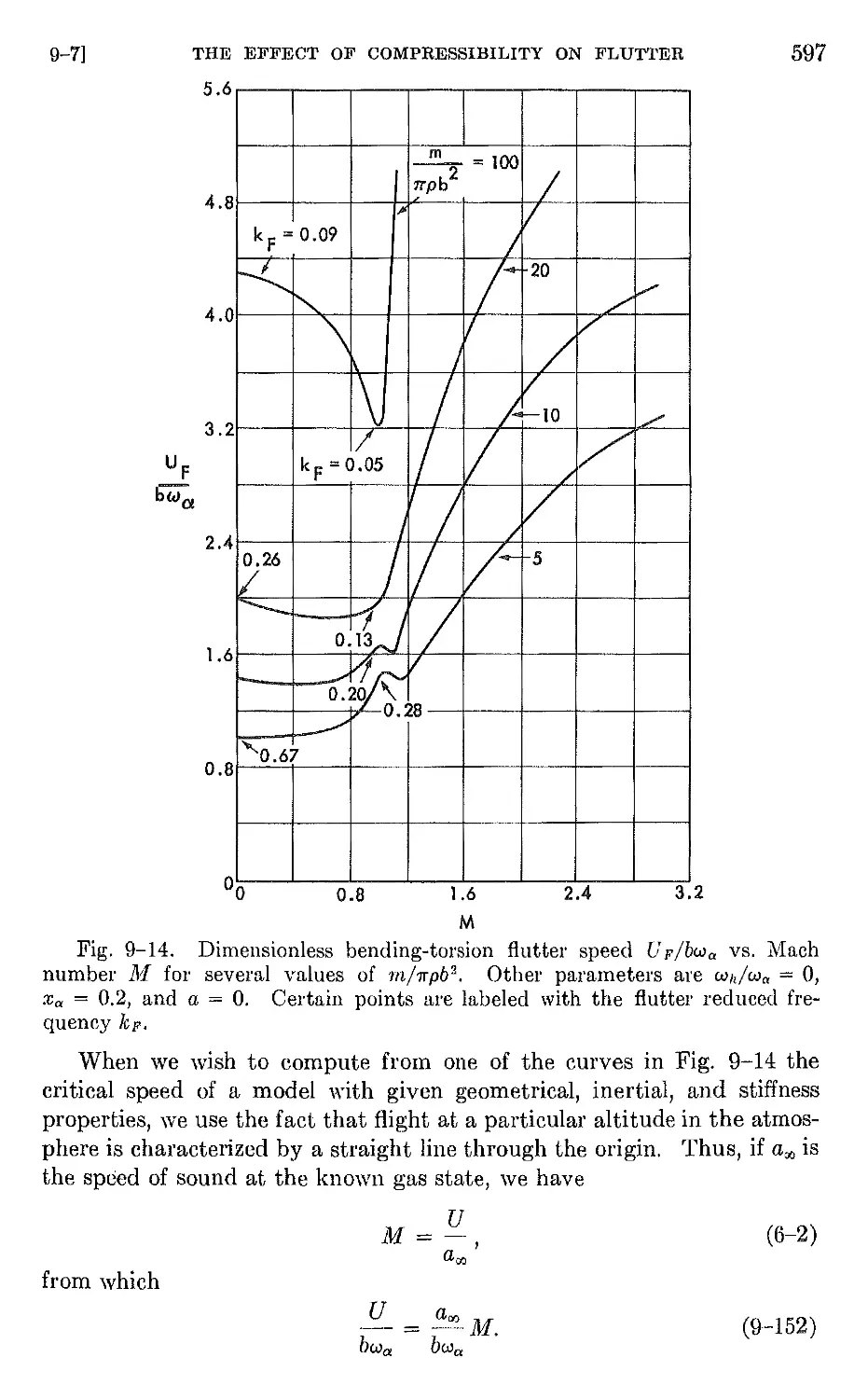
9-7 The effect of compressibility OIl flutter . 595
CONTENTS IX
9-8 Flutter of swept wings. 604
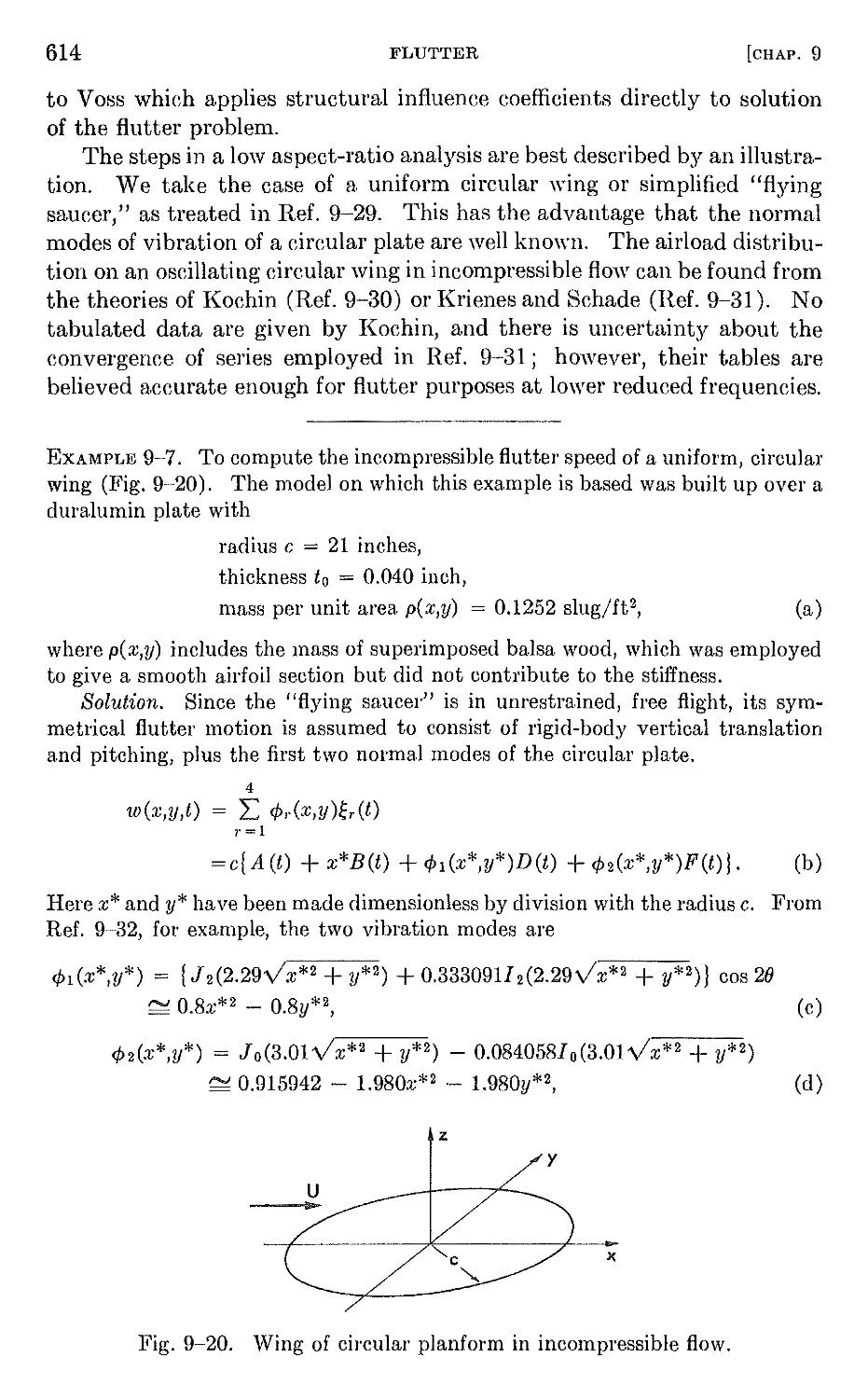
9-9 Wings of low aspect ratio . 613
9-10 Single-degree-of-freedom flutter 617
9-11 Certain other interesting types of flutter 626
CHAPTER 10. DYNAMIC RESPONSE PHENOMENA. 632
10-1 Introduction 632
10-2 Equations of disturbed motion of an elastic airplane 633
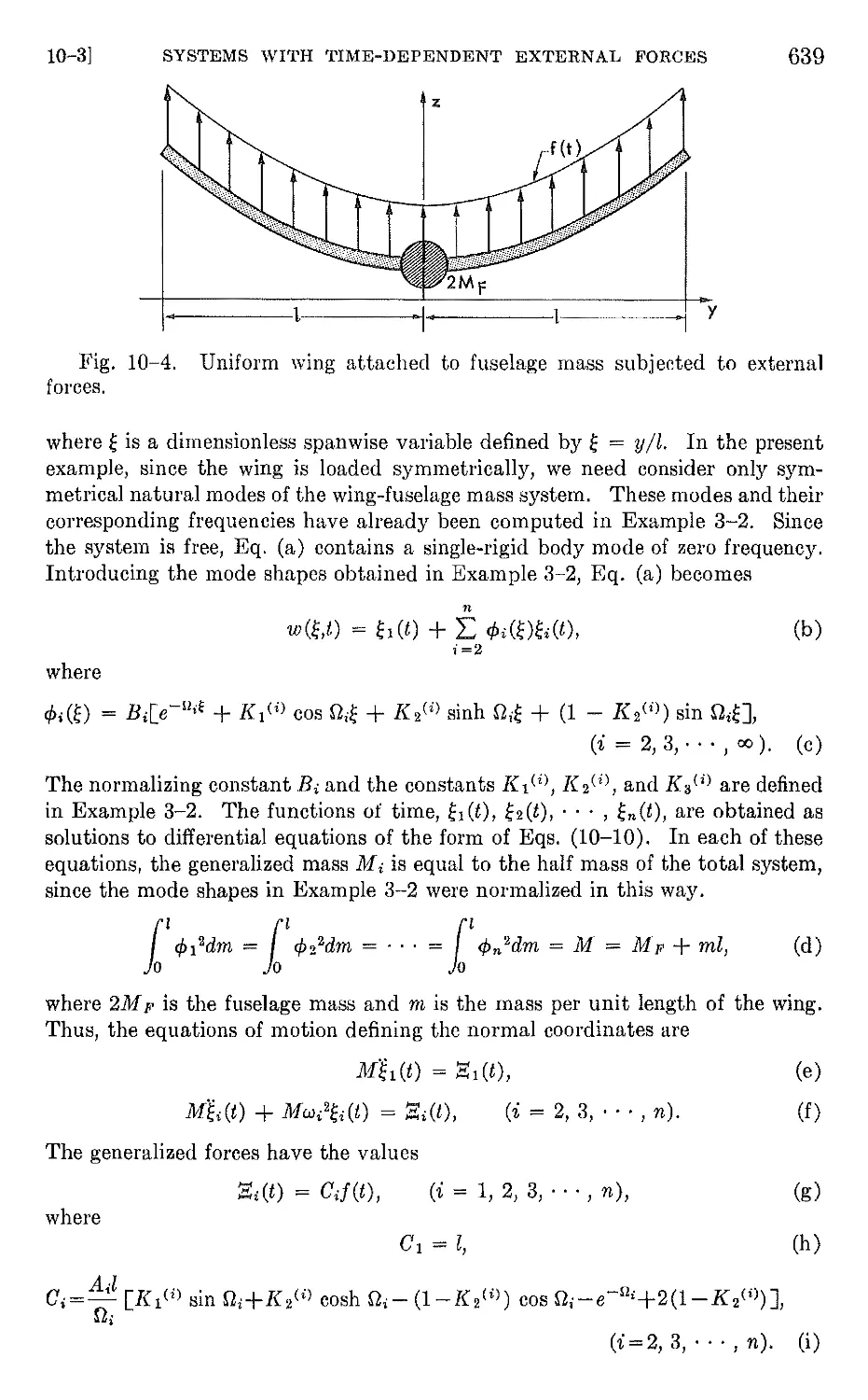
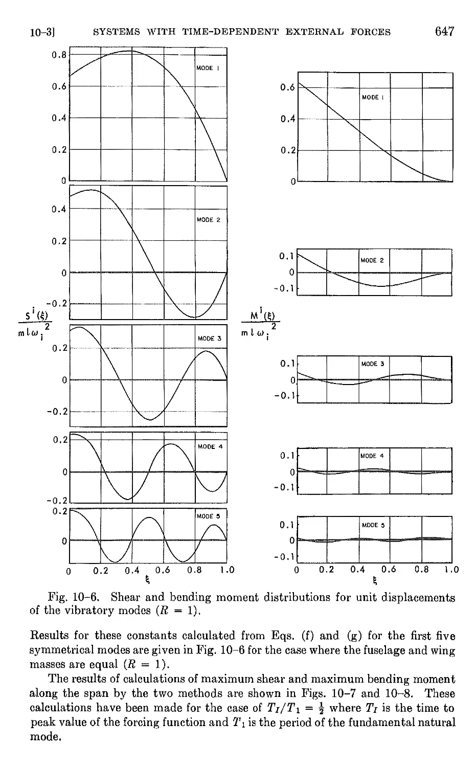
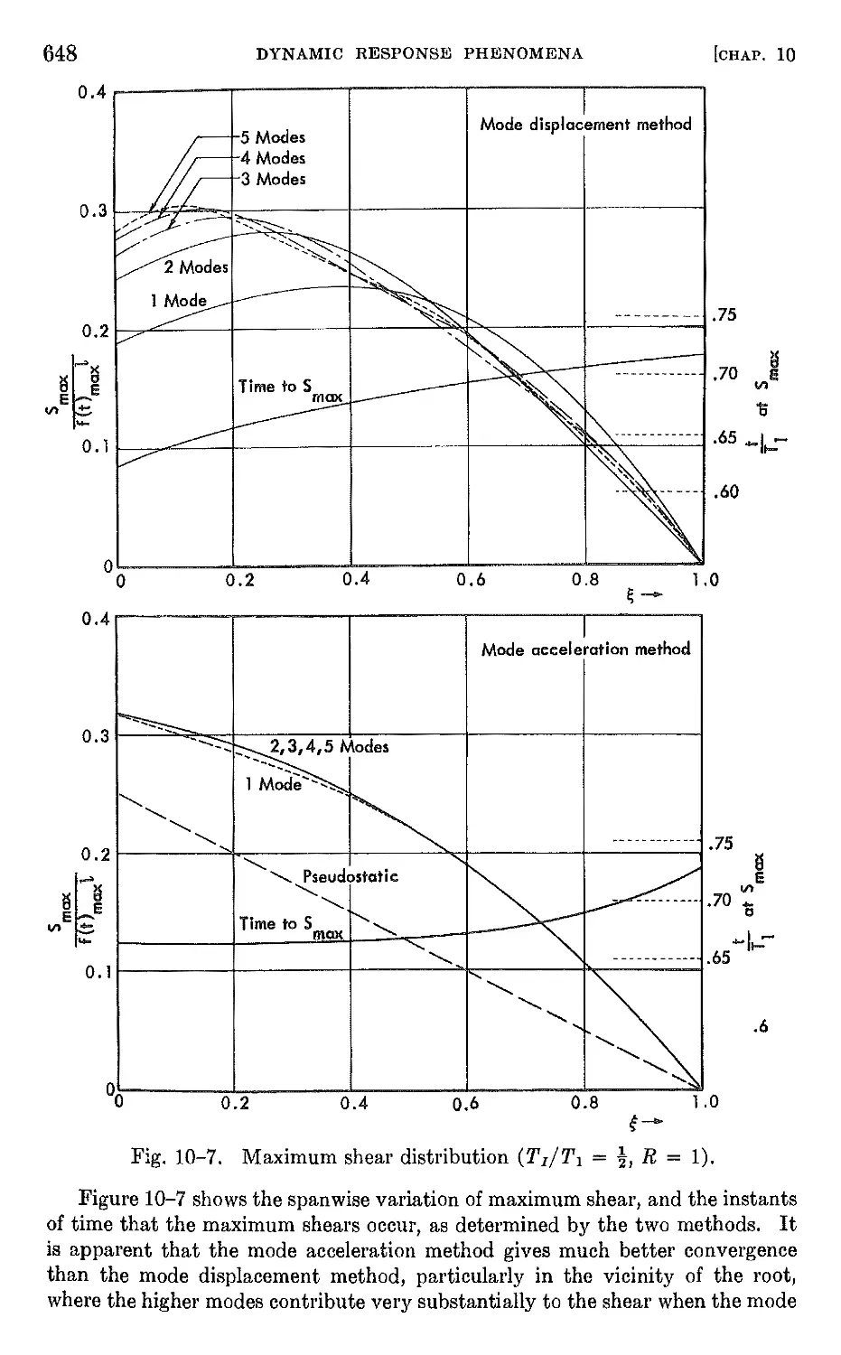
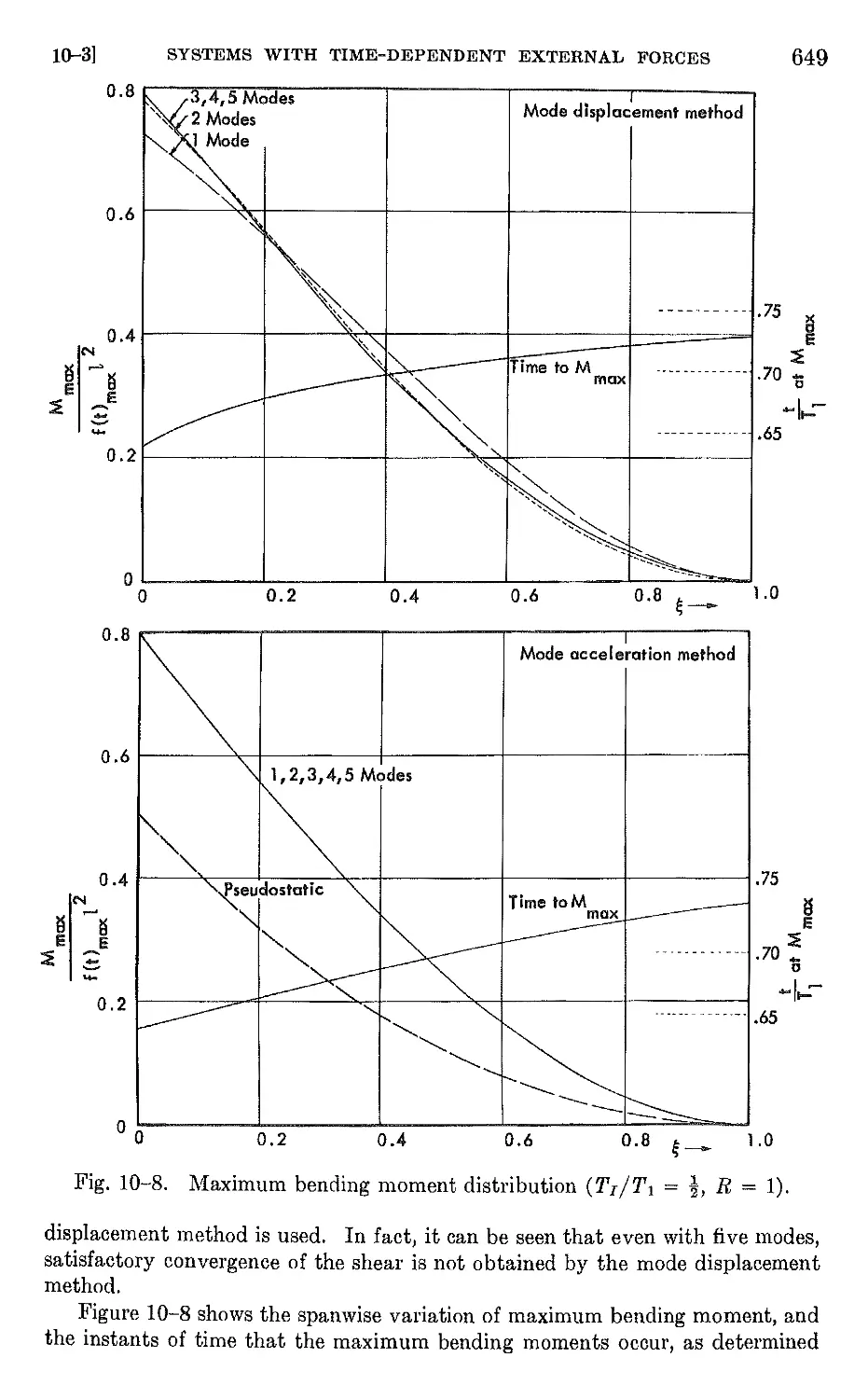
10-3 Systems with prescribed time-dependent external forces 635
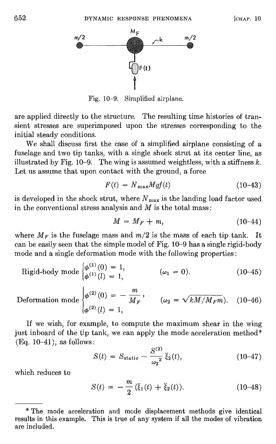
10-4 Transient stresses during landing 650
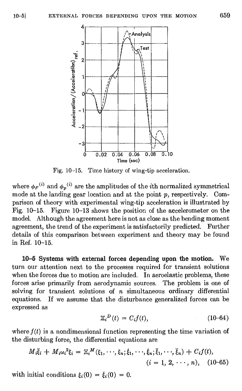
10-5 Systems with external forces depending upon the motion. 659
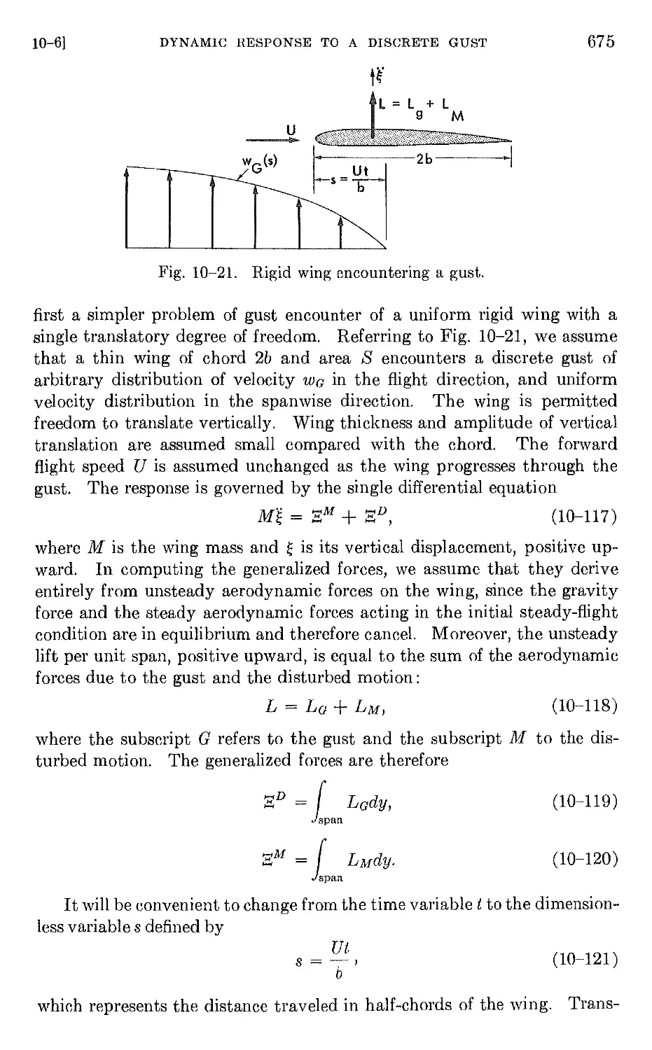
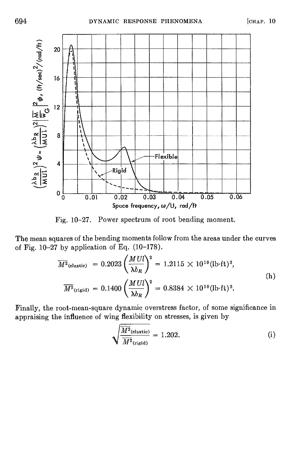
10-6 Dynamic response to a discrete gust. 673
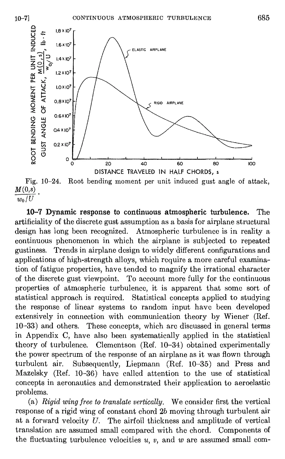
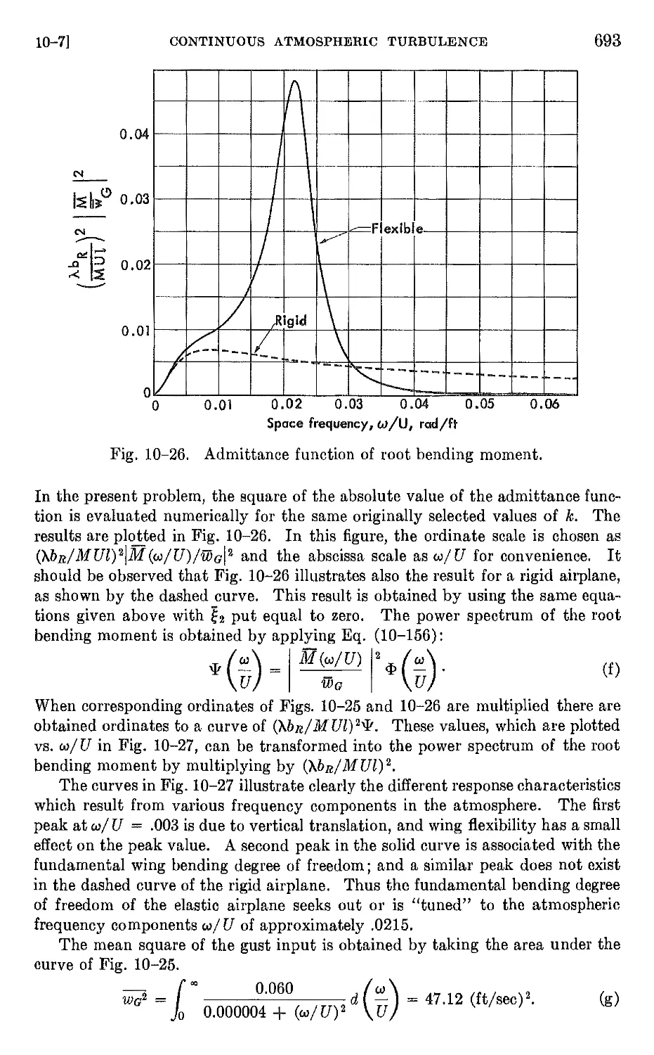
10-7 Dynamic response to continuous atmospheric turbulence. 685
CHAPTER 11. AEROELASTIC MODEL THEORY 695
11-1 Introduction . . 695
11-2 Dimensional concepts . 695
11-3 Equations of motion 698
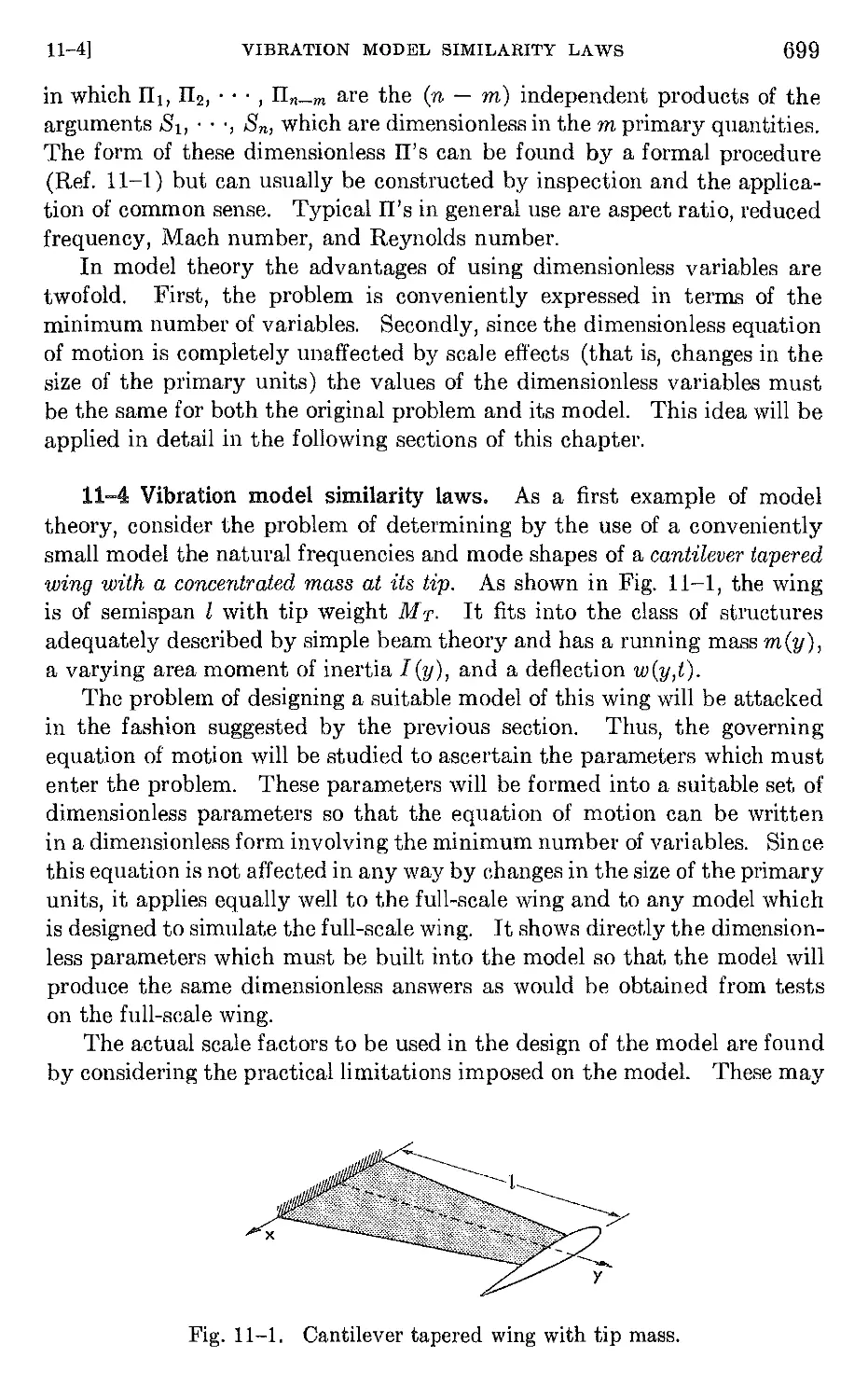
11-4 Vibration model similarity laws 699
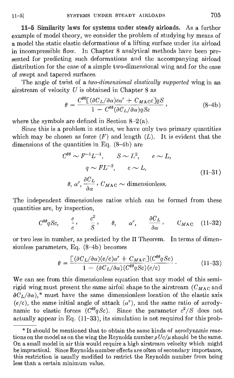
11-5 Similarity laws for systems under steady airloads 705
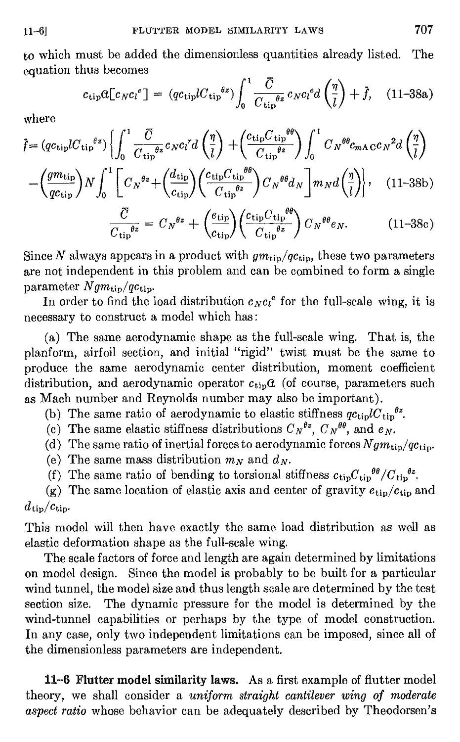
11-6 Flutter model similarity laws. 707
11-7 The unrestrained flutter model 712
11-8 The dynamic stability model. 715
CHAPTER 12. MODEL DESIGN AND CONSTRUCTION 717
12-1 Introduction 717
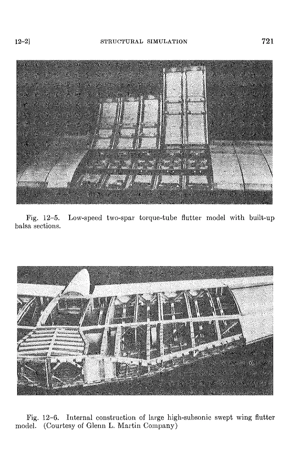
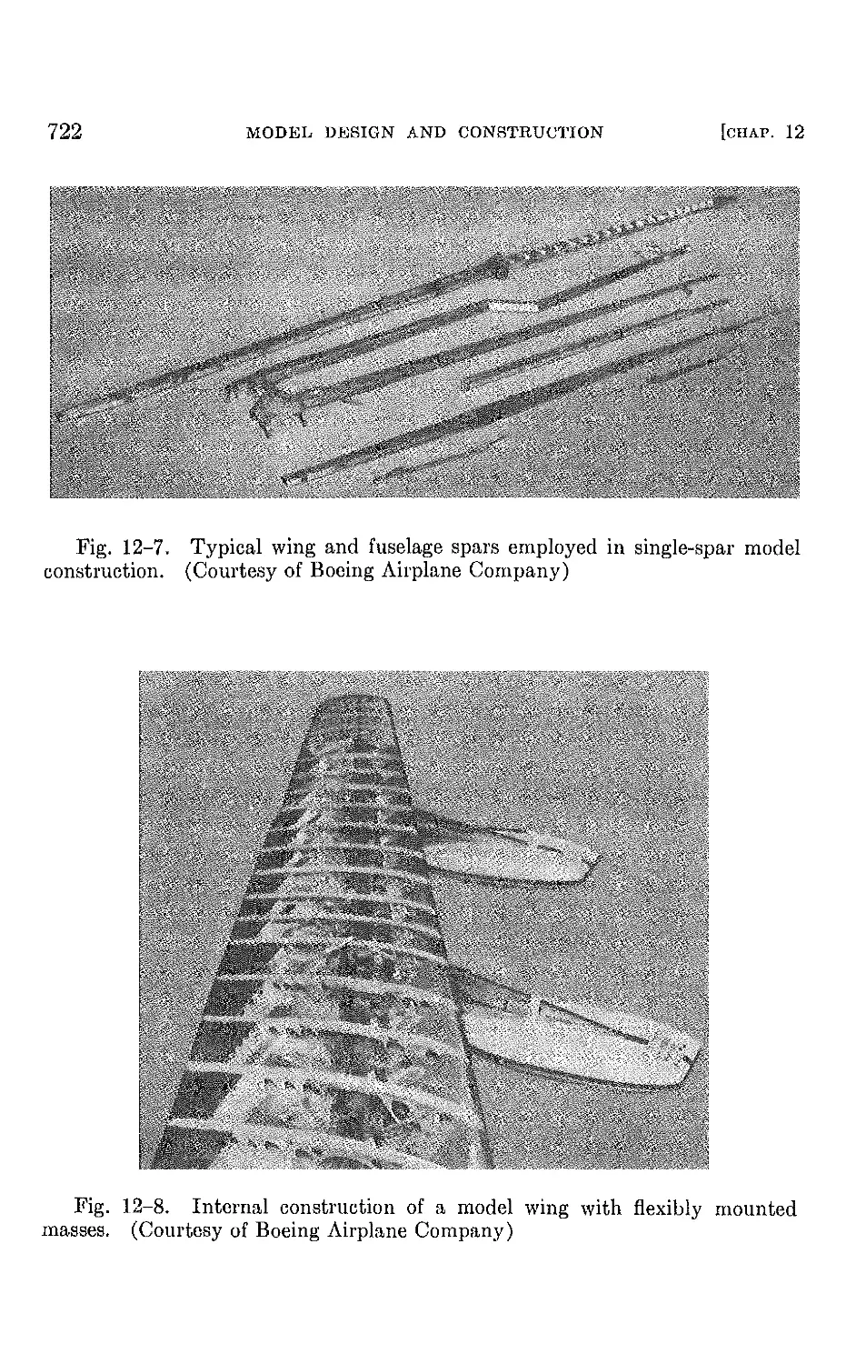
12-2 Structural simulation 718
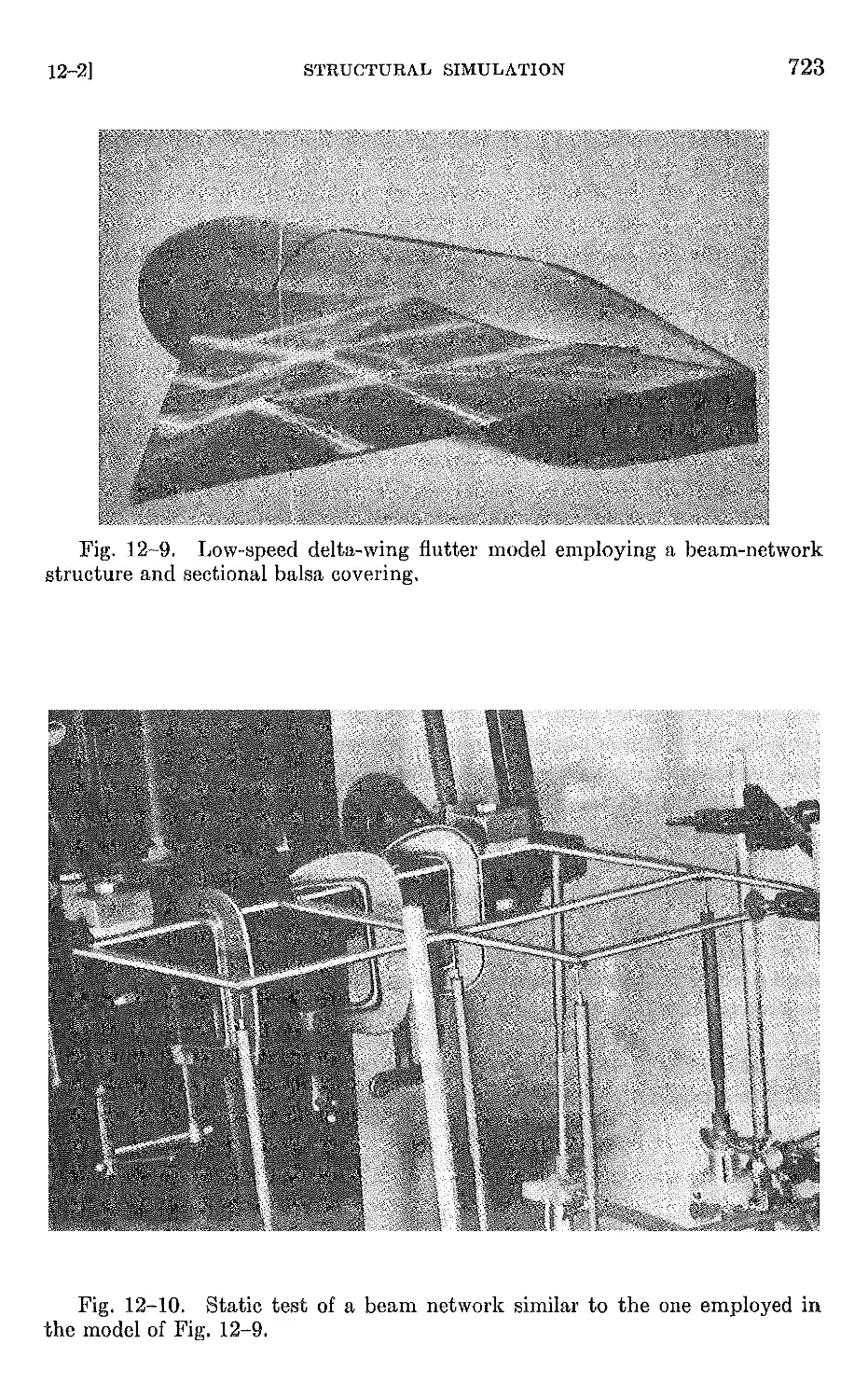
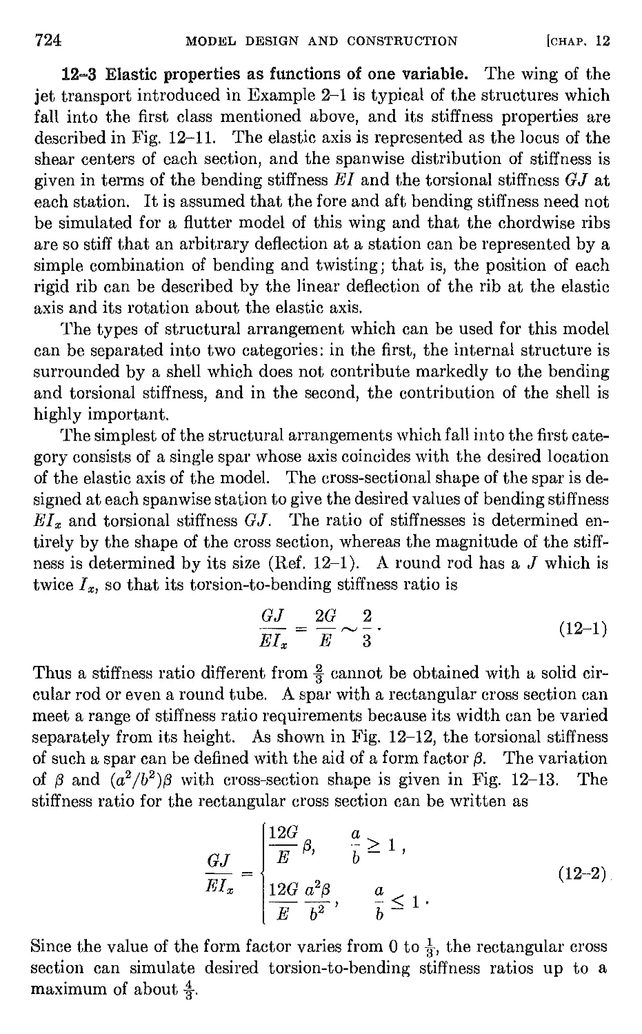
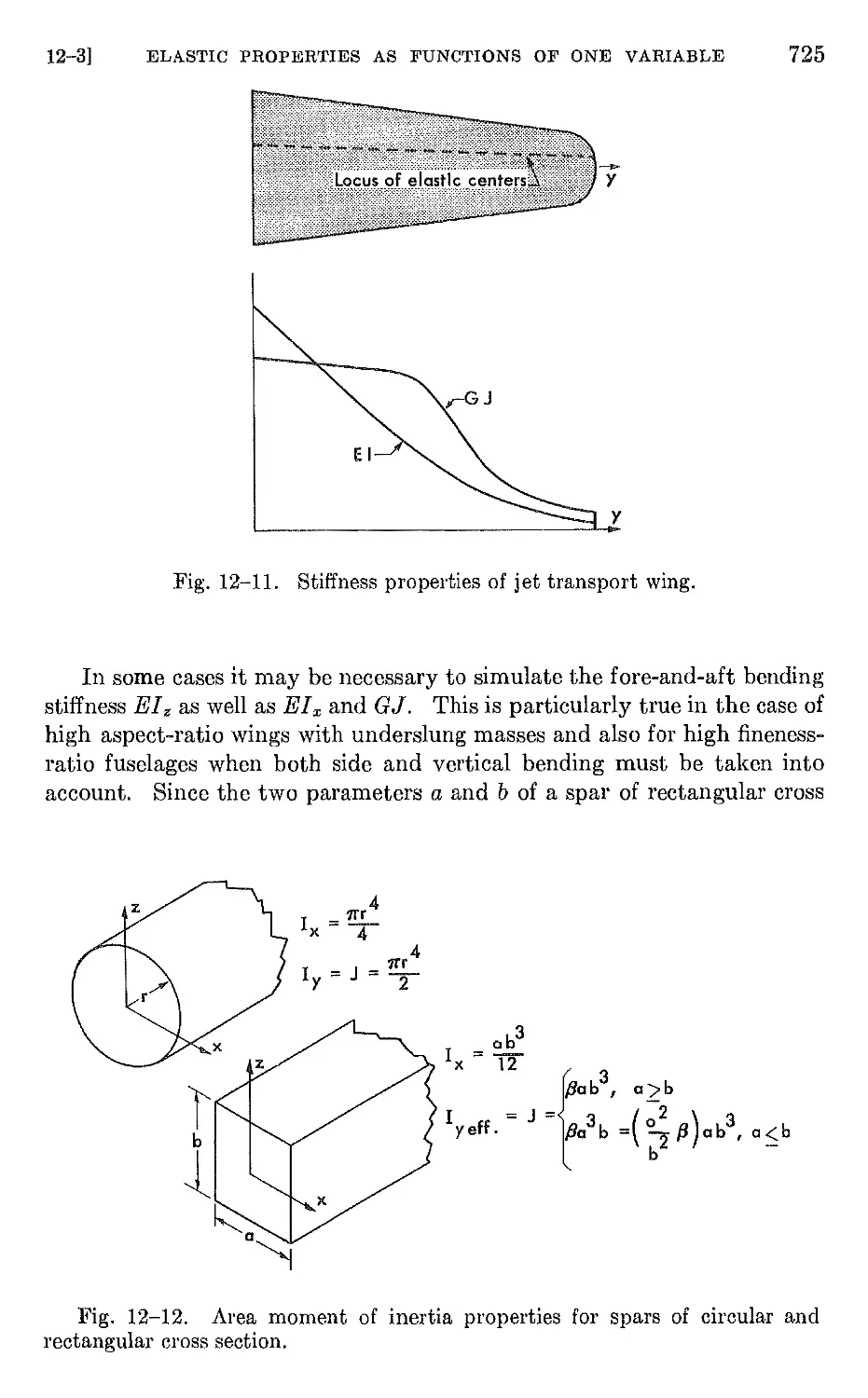
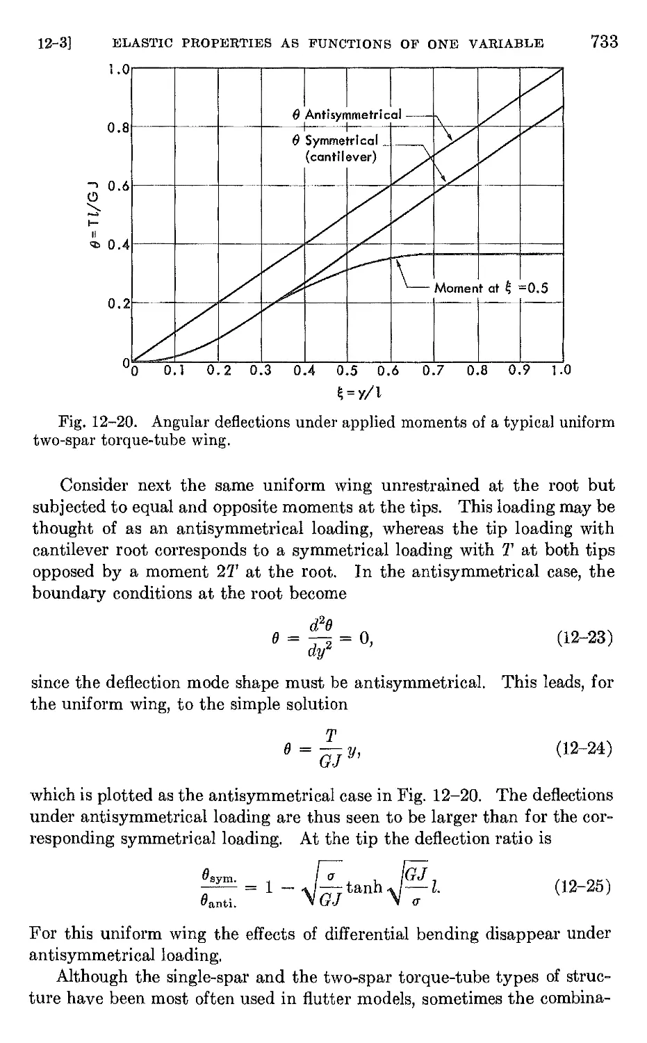
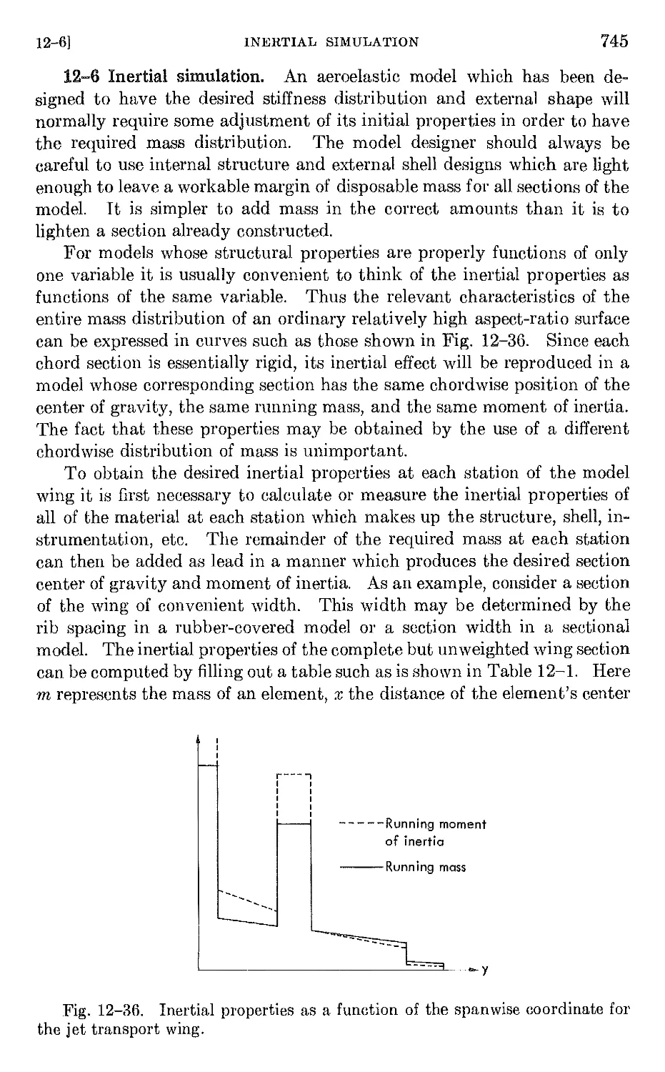
12-3 Elastic properties as functions of one variable . 724
12-4 Elastic properties as functions of two variables 735
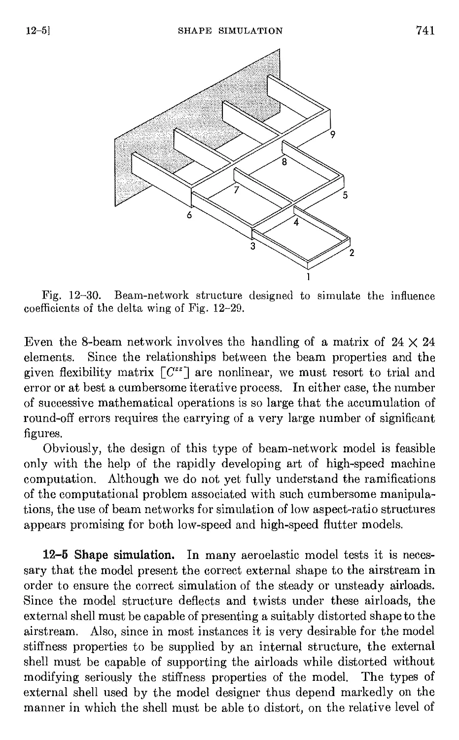
12-5 Shape simulation 741
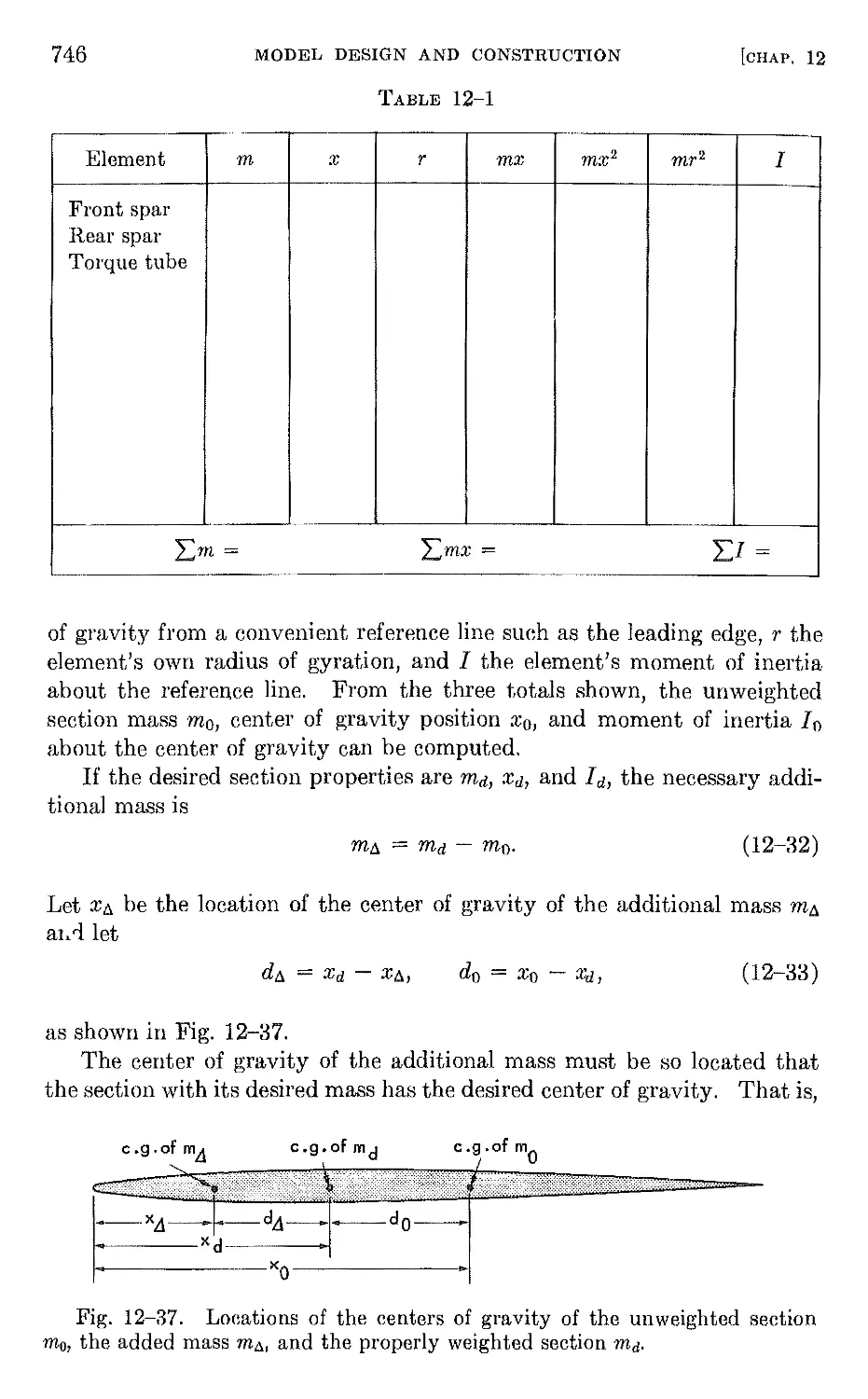
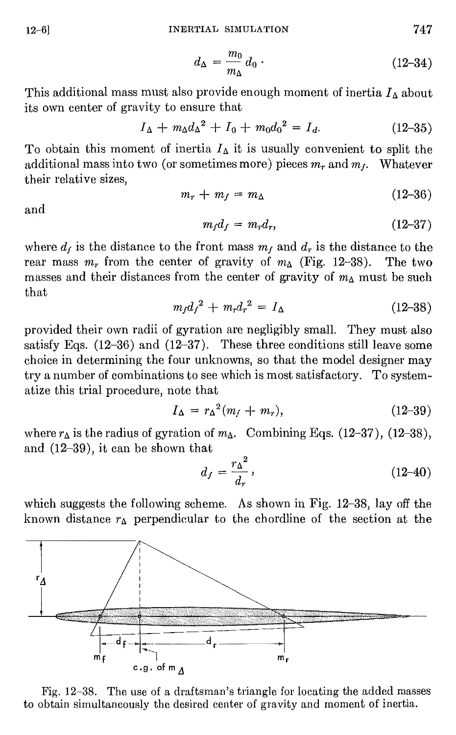
12-6 Inertial simulation. 745
CHAPTER 13. TESTING TECHNIQUES 749
13-1 Introduction 749
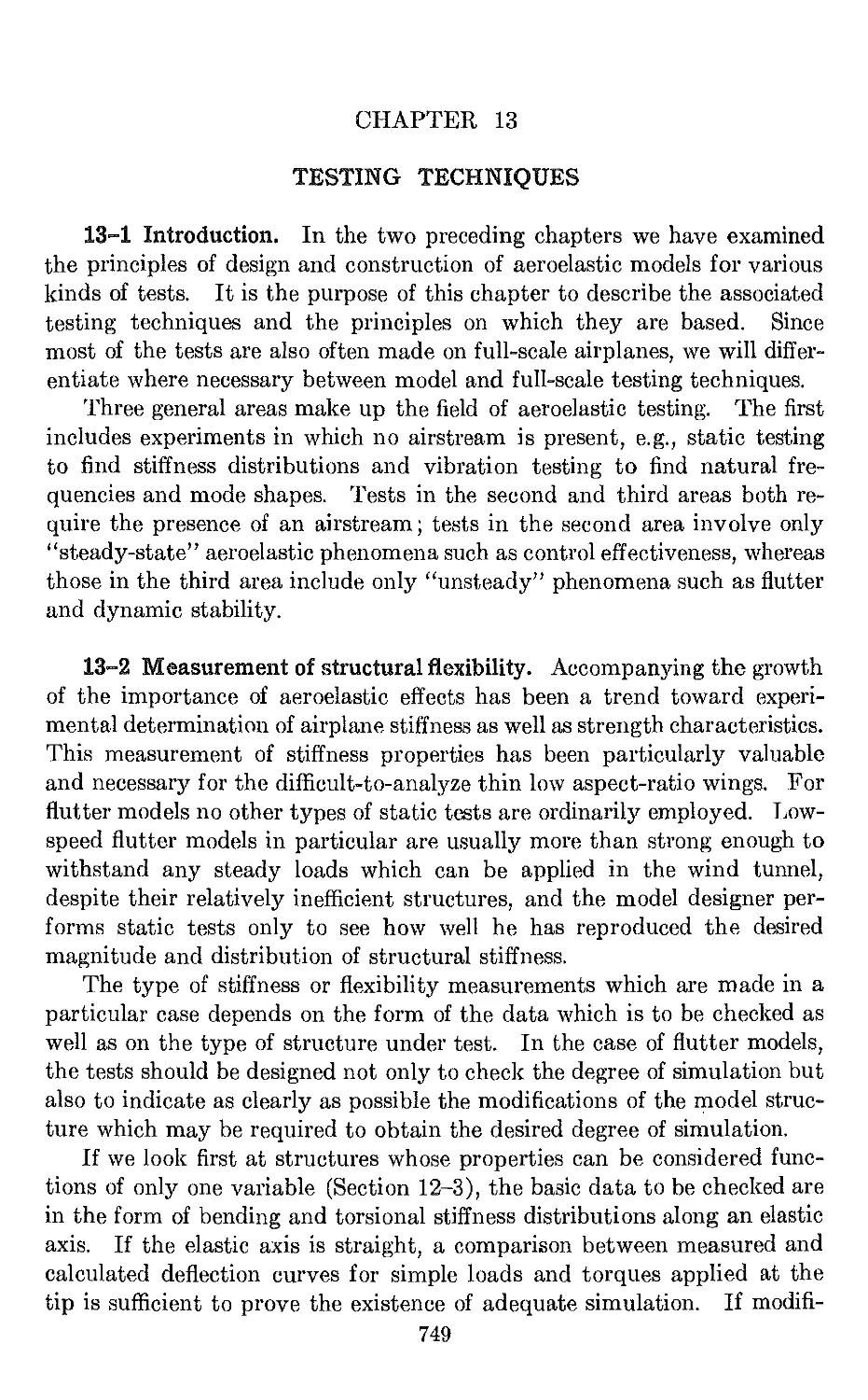
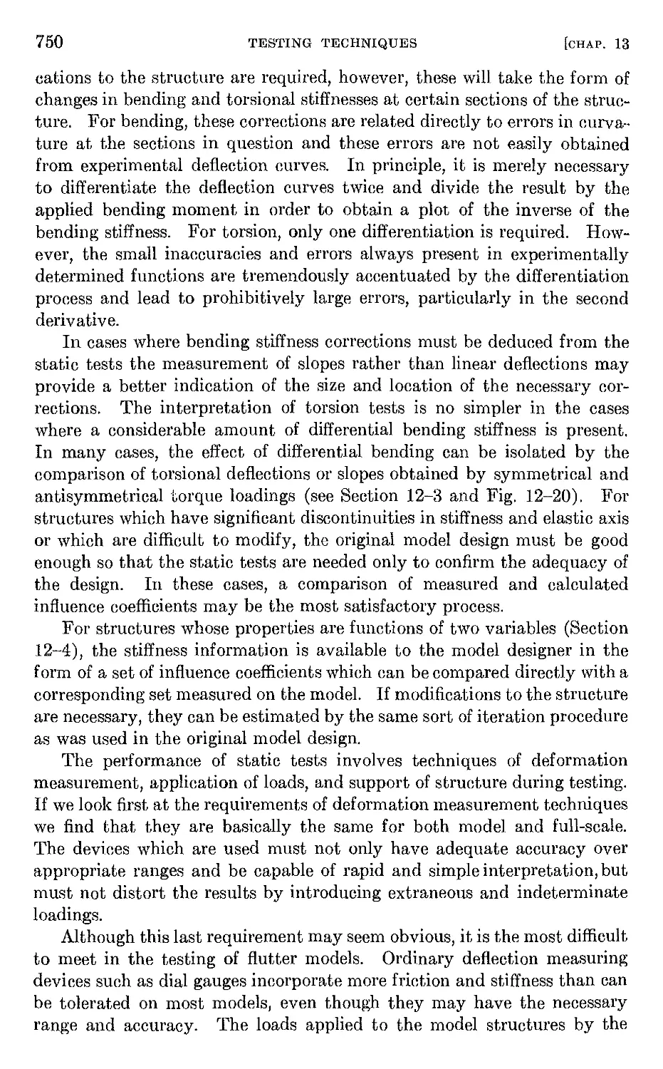
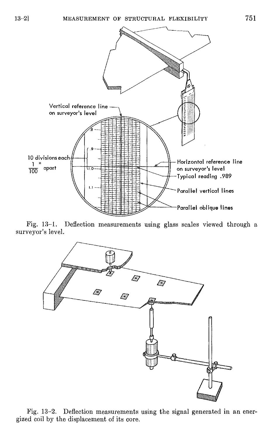
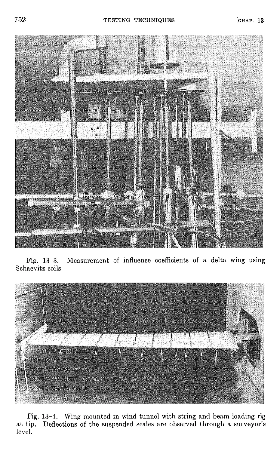
13-2 Measurement of structural flexibility 749
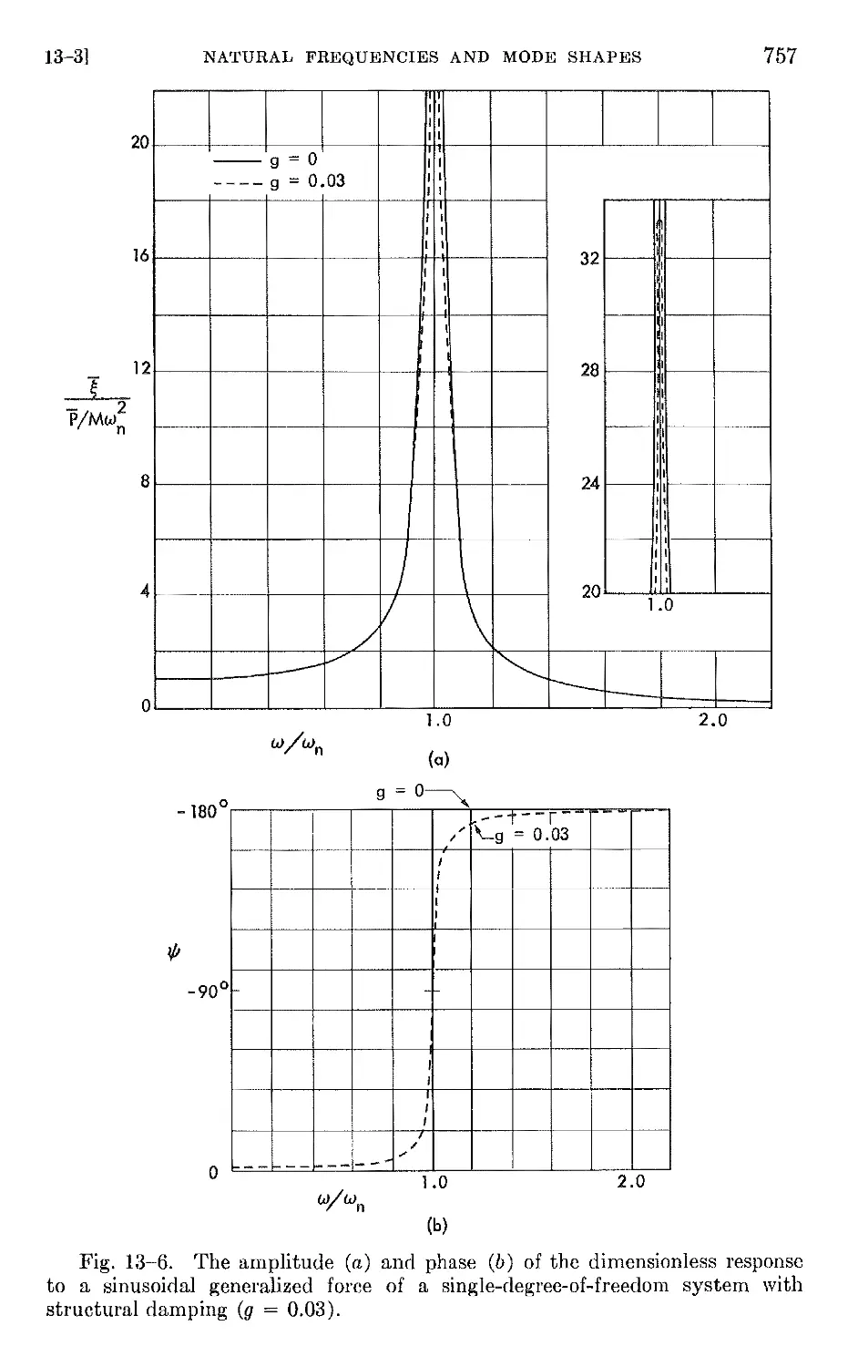
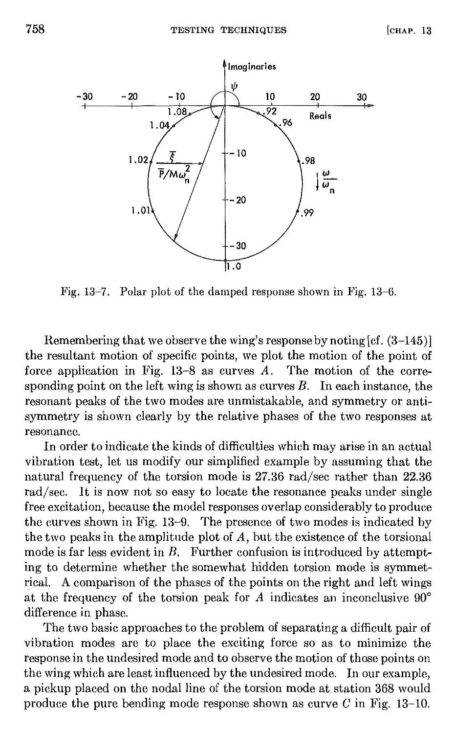
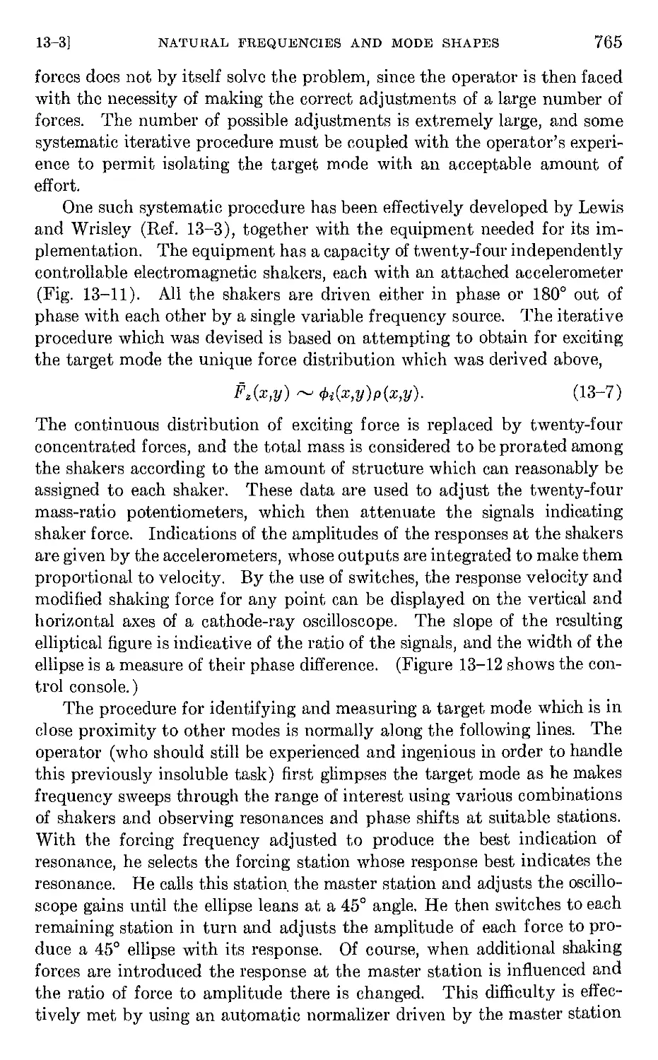
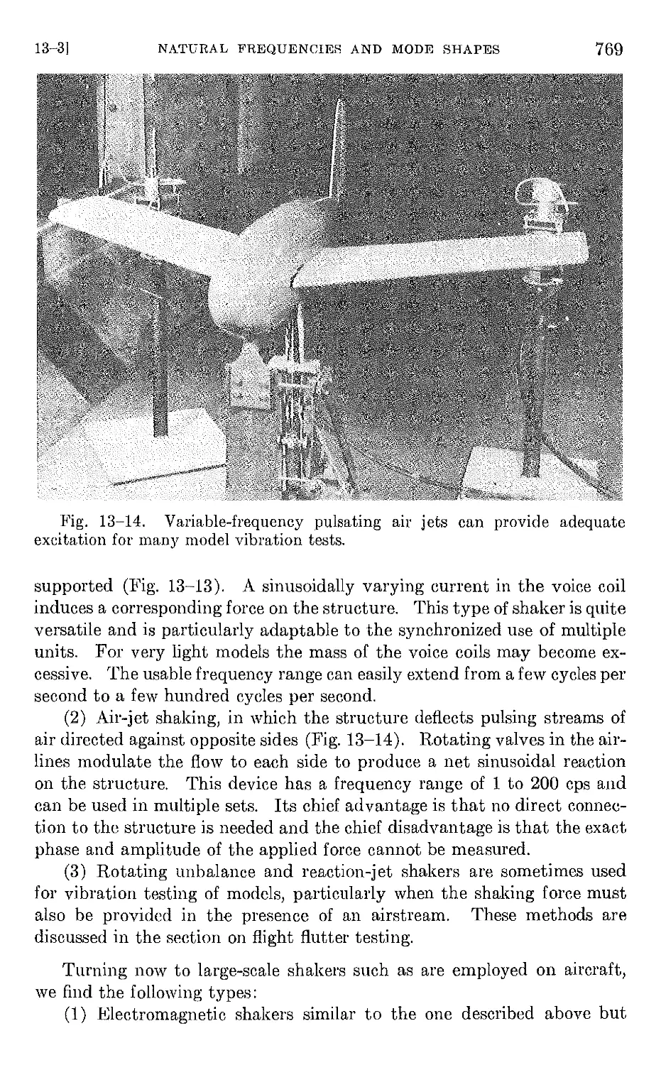
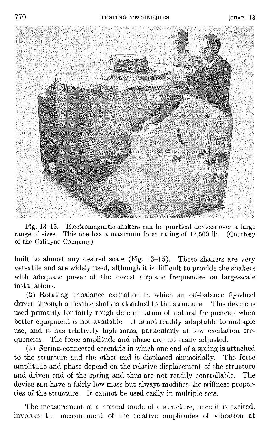
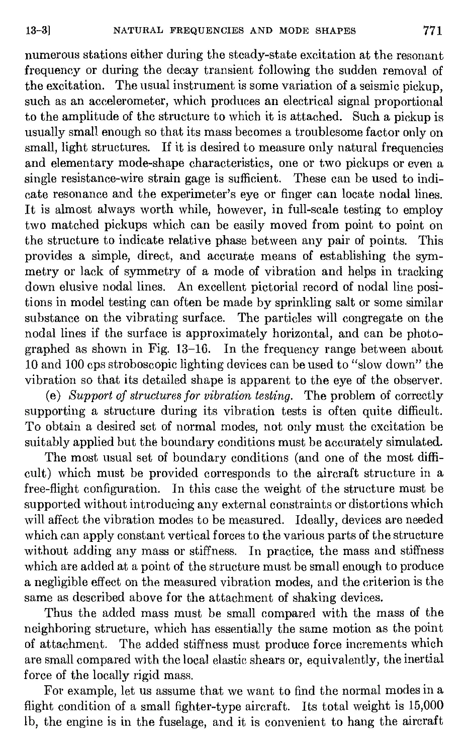
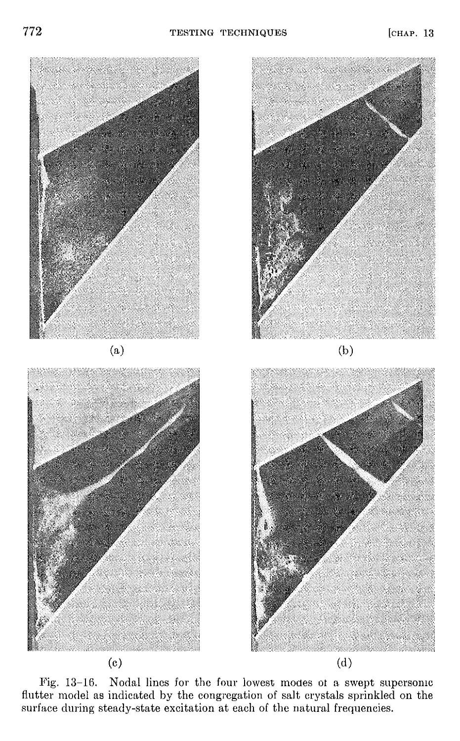
13-3 Measurement of natural frequencies and mode shapes 753
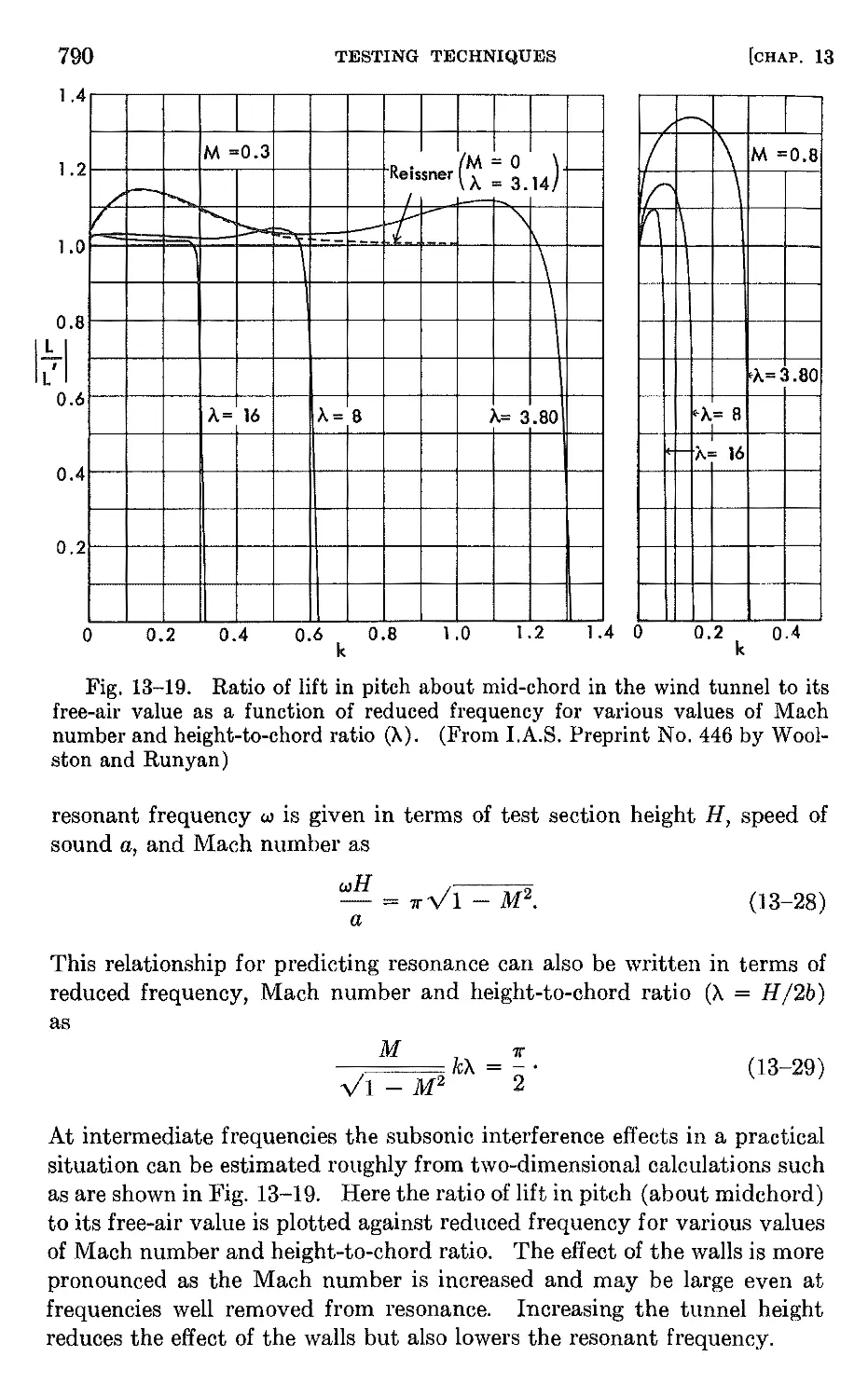
13-4 Steady-state aeroelastic testing 779
13-5 Dynamic aeroelastic testing - full scale 781
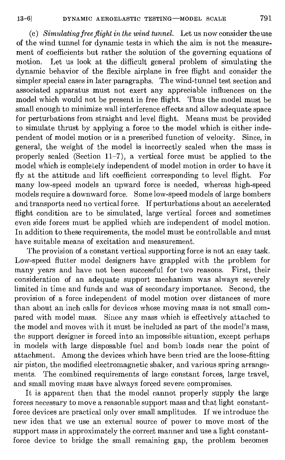
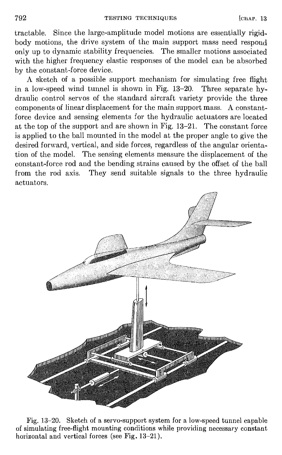
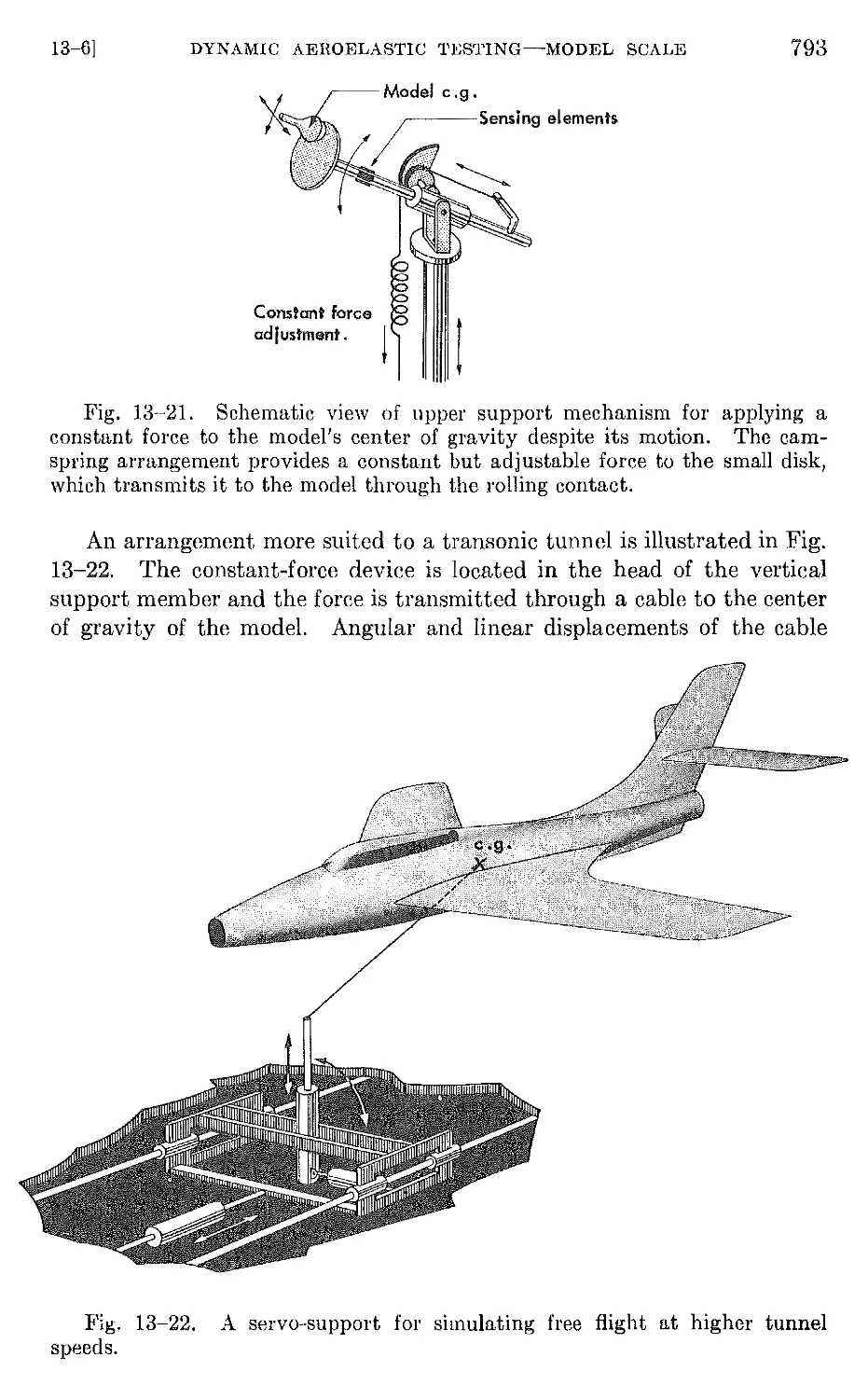
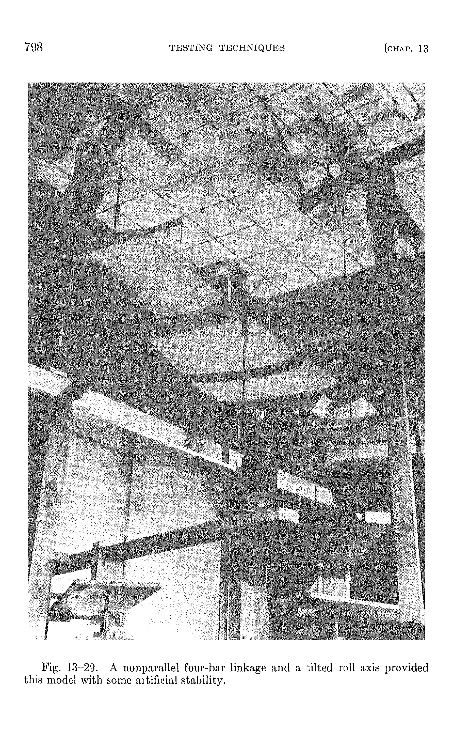
13-6 Dynamic aeroelastic testing- model scale 787
ApPENDICES. MATHEMATICAL TOOLS . 803
A Matrices . 805
B Integration by weighting numbers 809
C Linear systems 813
REFERENCES 827
AUTHOR INDEX 851
SUBJECT INDEX 855
CHAPTER 1
INTRODUCTION TO AEROELASTICITY
1-1 Definitions. The term aeroelasticity has been applied by aero-
nautical engineers to an important class of problems in airplane design.
It is often defined as a science which studies the mutual interaction between
aerodynamic forces and elastic forces, and the influence of this interaction
on airplane design. Aeroelastic problems would not exist if airplane struc-
tures were perfectly rigid. Modern airplane structures are very flexible,
and this flexibility is fundamentally responsible for the various types of
aeroelastic phenomena. Structural flexibility itself may not be objection-
able; however, aeroelastic phenomena arise when structural deformations
induce additional aerodynamic forces. These additional aerodynamic
forces may produce additional structural deformations which will induce
still greater aerodynamic forces. Such interactions may tend to become
smaller and smaller until a condition of stable equilibrium is reached, or
they may tend to diverge and destroy the structure.
The term aeroelasticity, however, is not completely descriptive, since
many important aeroelastic phenomena involve inertial forces as well as
aerodynamic and elastic forces. We shall apply a definition in which the
term aeroelasticity includes phenomena involving interactions among
inertial, aerodynamic, and elastic forces, and other phenomena involving
interactions between aerodynamic and elastic forces. The former will be
referred to as dynamic and. the latter as static aeroelastic phenomena.
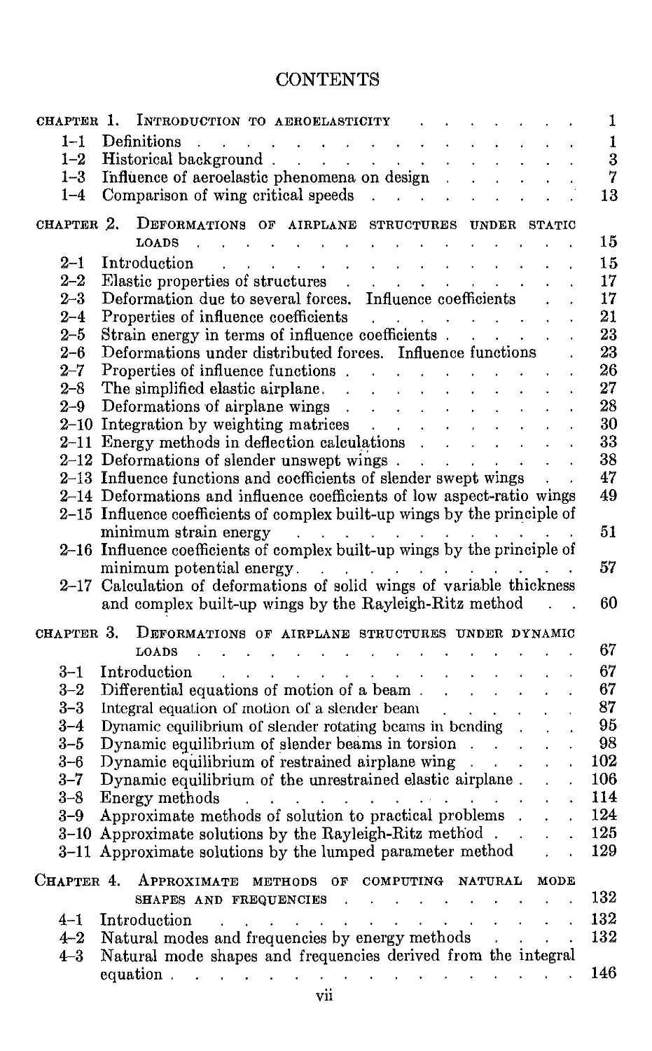
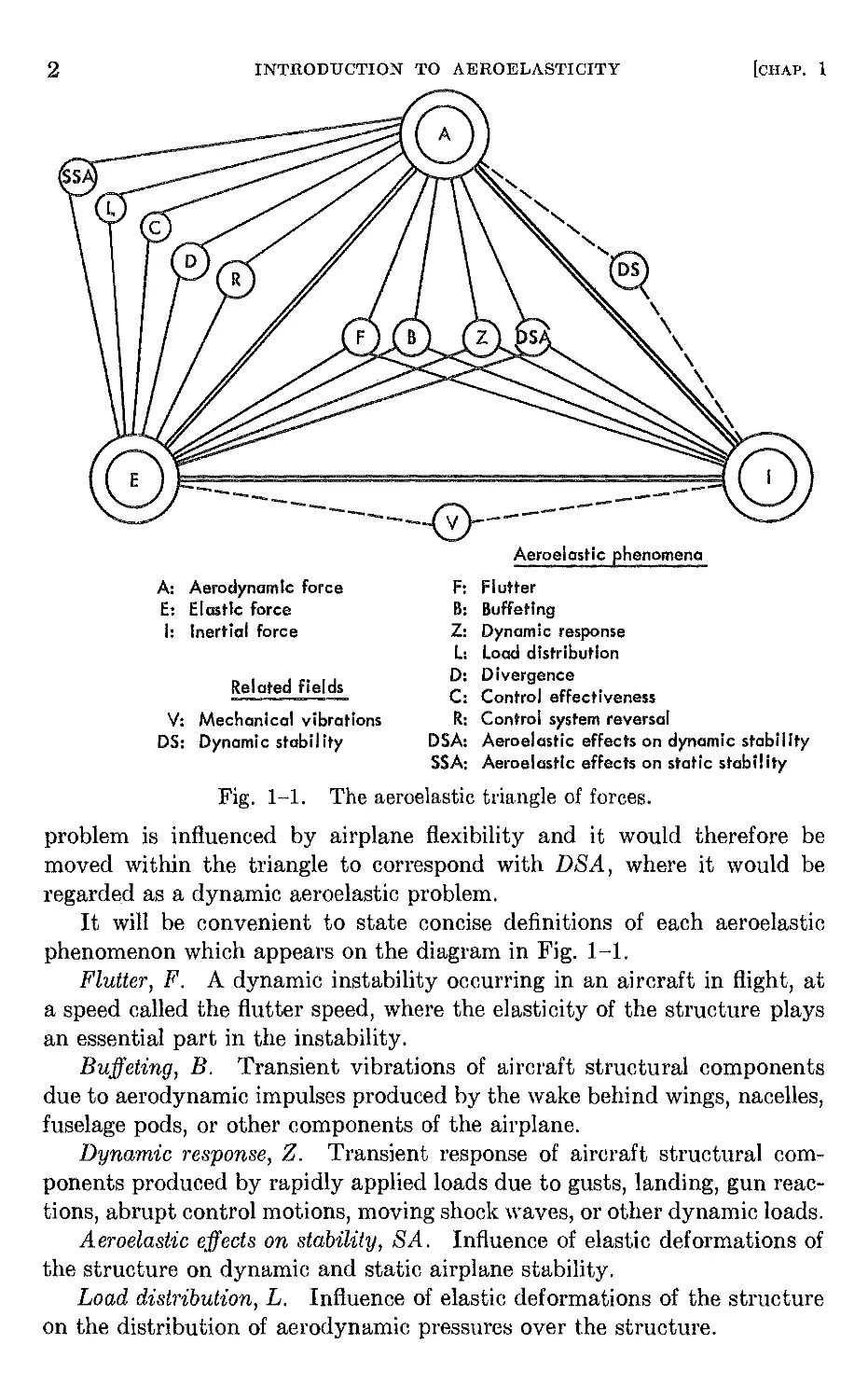
Collar (Ref. 1-1) has ingeniously classified problems in aeroelasticity
by means of a triangle of forces. Referring to Fig. 1-1, the three types of
forces, aerodynamic, elastic, and inertial, represented by the symbols A, E,
and I, respectively, are placed at the vertices of a triangle. Each aeroelas-
tic phenomenon can be located on the diagram according to its relation to
the three vertices. For example, dynamic aeroelastic phenomena such as
flutter, F, lie within the triangle, since they involve all three types of forces
and must be bonded to all three vertices. Static aeroelastic phenomena
such as wing divergence, D, lie outside the triangle on the upper left side,
since they involve only aerodynamic and elastic forces. Although it is
difficult to define precise limits on the field of aeroelasticity, the classes of
problems connected by solid lines to the vertices in Fig. 1-1 are usually
accepted as the principal ones. Of course, other borderline fields can be
placed on the diagram. For example, the fields of mechanical vibrations,
V, and rigid-body aerodynamic stability, DB, are connected to the vertices
by dotted lines. It is very likely that in certain cases the dynamic stability
1
2
INTRODUCTION TO AEROELASTICITY
[CHAP. 1
"
,
'-',
'.....
@{
\
\
\
\
\
\
\
\
- - --- -
- - - -
-.._-- --
Aeroelastic phenomena
F: Flutter
B: Buffeting
Z: Dynamic response
L: Load distribution
D: Divergence
C: Control effectiveness
R: Control system reversal
DSA: Aeroelastic effects on dynamic stability
SSA: Aeroelastlc effects on static stability
Fig. 1-1. The aeroelastic triangle of forces.
problem is influenced by airplane flexibility and it would therefore be
moved within the triangle to correspond with DSA, where it would be
regarded as a dynamic aeroelastic problem.
It will be convenient to state concise definitions of each aeroelastic
phenomenon which appears on the diagram in Fig. 1-1.
Flutter, F. A dynamic instability occurring in an aircraft in flight, at
a speed called the flutter speed, where the elasticity of the structure plays
an essential part in the instability.
Buffeting, B. Transient vibrations of aircraft structural components
due to aerodynamic impulses produced by the wake behind wings, nacelles,
fuselage pods, or other components of the airplane.
Dynamic response, Z. Transient response of aircraft structural com-
ponents produced by rapidly applied loads due to gusts, landing, gun reac-
tions, abrupt control motions, moving shock waves, or other dynamic loads.
Aeroelastic effects on stability, SA. Influence of elastic deformations of
the structure on dynamic and static airplane stability.
Load distribution, L. Influence of elastic deformations of the structure
on the distribution of aerodynamic pressures over the structure.
A: Aerodynamic force
E: Elastic force
I: Inertial force
Related fields
V: Mechanical vibrations
DS: Dynami c stabi I ity
1-21
HISTORICAL BACKGROUND
3
Divergence, D. A static instability of a lifting surface of an aircraft in
flight, at a speed called the divergence speed, where the elasticity of the
lifting surface plays an essential role in the instability.
Control effectiveness, C. Influence of elastic deformations of the struc-
ture on the controllability of an airplane.
Control system reversal, R. A condition occurring in flight, at a speed
called the control reversal speed, at which the intended effects of displacing
a given component of the control system are completely nullified by elastic
deformations of the structure.
1-2 Historical background. Problems in aeroelasticity did not attain
the prominent role that they now play until the early stages of World
War II. Prior to that time, airplane speeds were relatively low and the
load requirements placed on aircraft structures by design criteria specifica-
tions produced a structure sufficiently rigid to preclude most aeroelastic
phenomena. As speeds increased, however, with little or no increase in
load requirements, and in the absence of rational stiffness criteria for de-
sign, aircraft designers encountered a wide variety of problems which we
now classify as aeroelastic problems.
Although aeroelastic problems have occupied their current prominent
position for a relatively short period, they have had some influence on air-
plane design since the beginning of powered flight. Perhaps the first
designer to be affected was Professor Samuel P. Langley of the Smithsonian
Institution. In the light of modern knowledge, it seems likely that the
unfortunate wing failure which wrecked Langley's machine on the Potomac
River houseboat in 1903 could be described as wing torsional divergence.
In going over the arguments put forward at the time, the best explanation
of what happened (Ref. 1-2) was given by Griffith Brewer (Ref. 1-3), one
time president of the Royal Aeronautical Society. Brewer described the
phenomenon which wrecked the Langley monoplane in the same way as
we describe wing torsional divergence today. Langley's misfortune oc-
curred shortly before the Wright Brothers made the first sustained heavier-
than-air flight.
Perhaps the success of the Wright biplane and the failure of the Langley
monoplane was the original reason for the strong predilection for biplanes
in the early days of airplane design. The technical arguments of biplane
versus monoplane, which were prevalent for so many years, were un-
doubtedly influenced by the lack of a rational torsional stiffness criterion
for monoplane wings. Although a number of externally braced mono-
planes were constructed by the French and Germans prior to World War I,
the monoplane as a military machine ceased to exist in 1917, and it was not
until the mid-thirties that designers ventured to build high-performance
monoplane military aircraft.
4
INTRODUCTION TO AEROELASTICITY
[CHAP. I
Q,)
,.D
S
o
,.D
<::>
<::>
'<ji
-........
<::>
Q,)
b.O
<:'3
0-<
"1:!
.:::
<:'3
p:j
CjI
,-j
on
if:
1-2]
HISTORICAL BACKGROUND
5
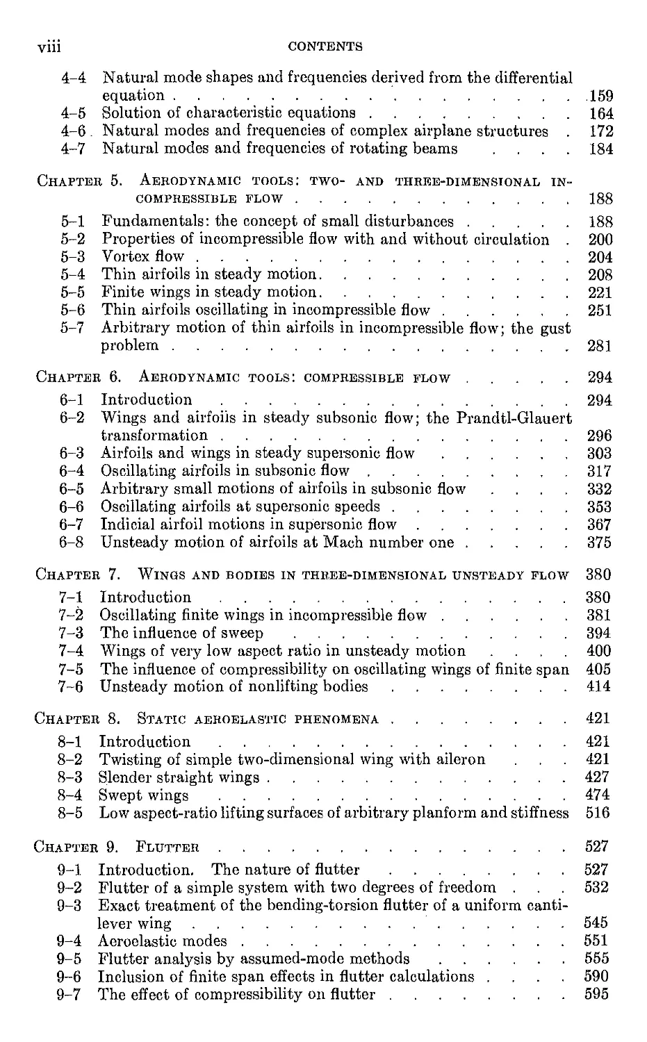
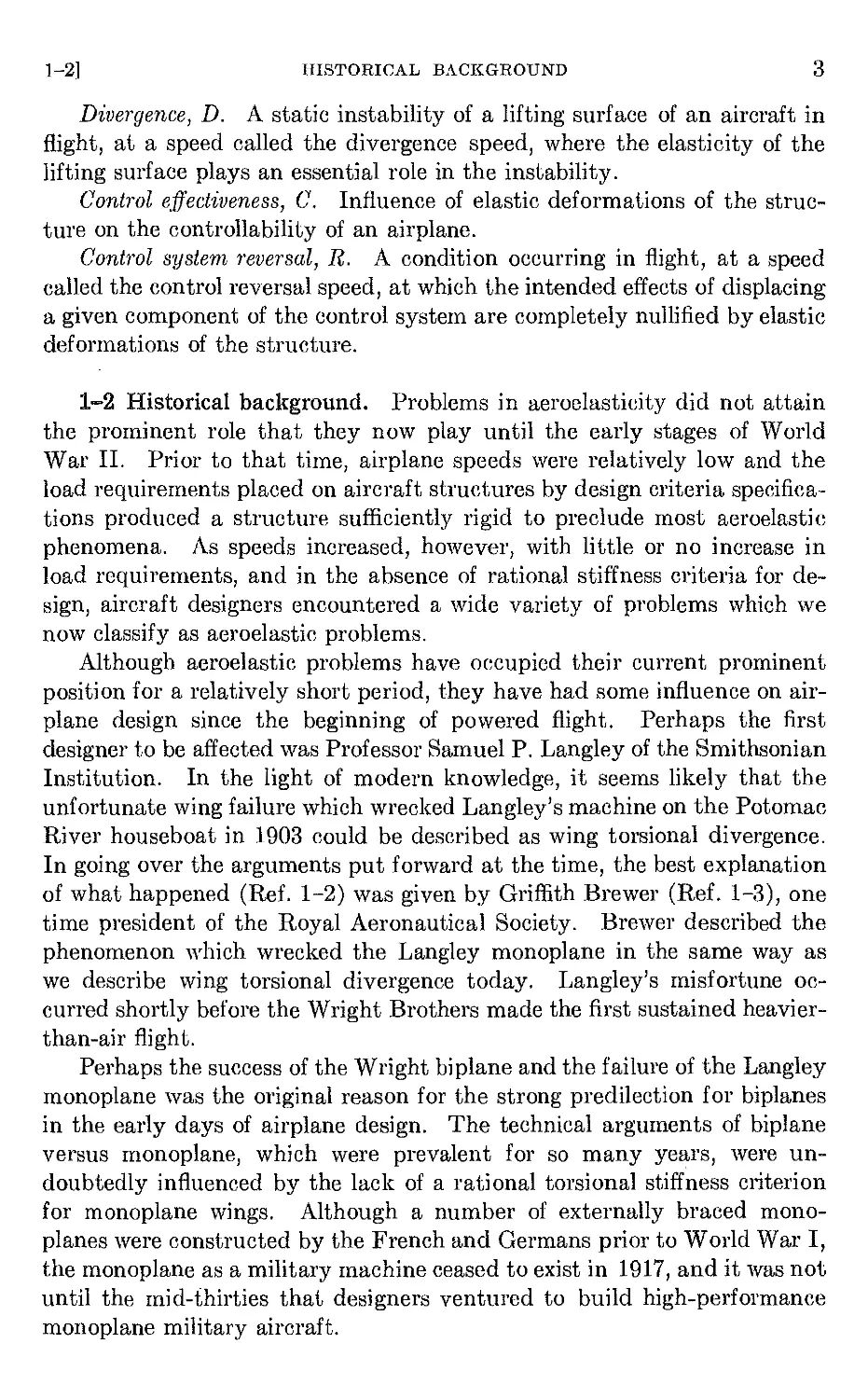
The most widespread early aeroelastic problem in the days when mili-
tary aircraft were almost exclusively biplanes was the tail flutter problem.
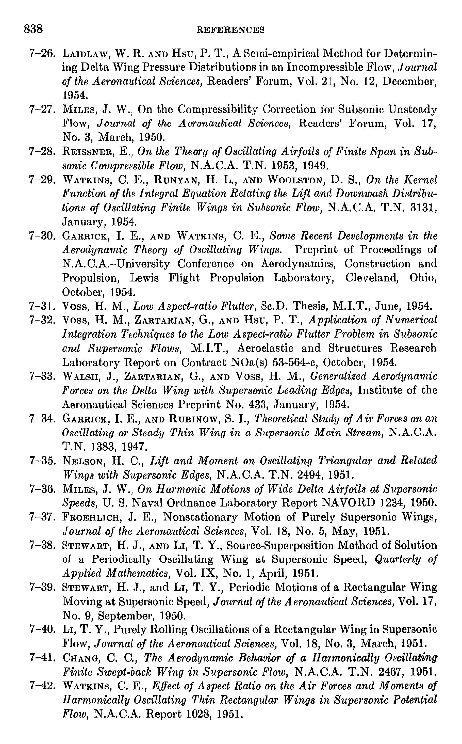
One of the first documented cases of flutter occurred on the horizontal tail
of the twin-engined Handley Page 0/400 bomber, shown by Fig. 1-2, at
the beginning of World War 1. Lanchester and Bairstow were asked to
investigate the cause of violent oscillations of the fuselage .and tail surfaces.
They discovered (Refs. 1-4 and 1-5) that the fuselage and tail had two
principal low-frequency modes of vibration. In one mode, the left and
right elevators oscillated about their hinges 180 0 out of phase. This was
possible because the elevators were not attached to the same torque tube,
but were connected by a relatively weak spring provided by the long control
cables through which each individual elevator was connected to the stick.
In the second mode, the fuselage oscillated in torsion. The possibility of a
self-excited oscillation involving coupling between the modes was diagnosed
as the cause of the vibrations. One of the proposed remedial measures was
that of connecting both elevators to the same torque tube. A second
epidemic of tail flutter due to the same cause was experienced by the DH-9
airplane in 1917, and a number of lives were lost before it was cured. The
cure was identical to that applied to the Handley Page airplane, and a
torsionally stiff connection between elevators has been a design feature in
airplanes ever since.
Aeroelastic wing problems appeared when designers abandoned biplane
construction with its interplane bracing and relatively high torsional
rigidity, in favor of monoplane types. The latter often had insufficient
torsional rigidity, and flutter, loss of aileron effectiveness; and deformation
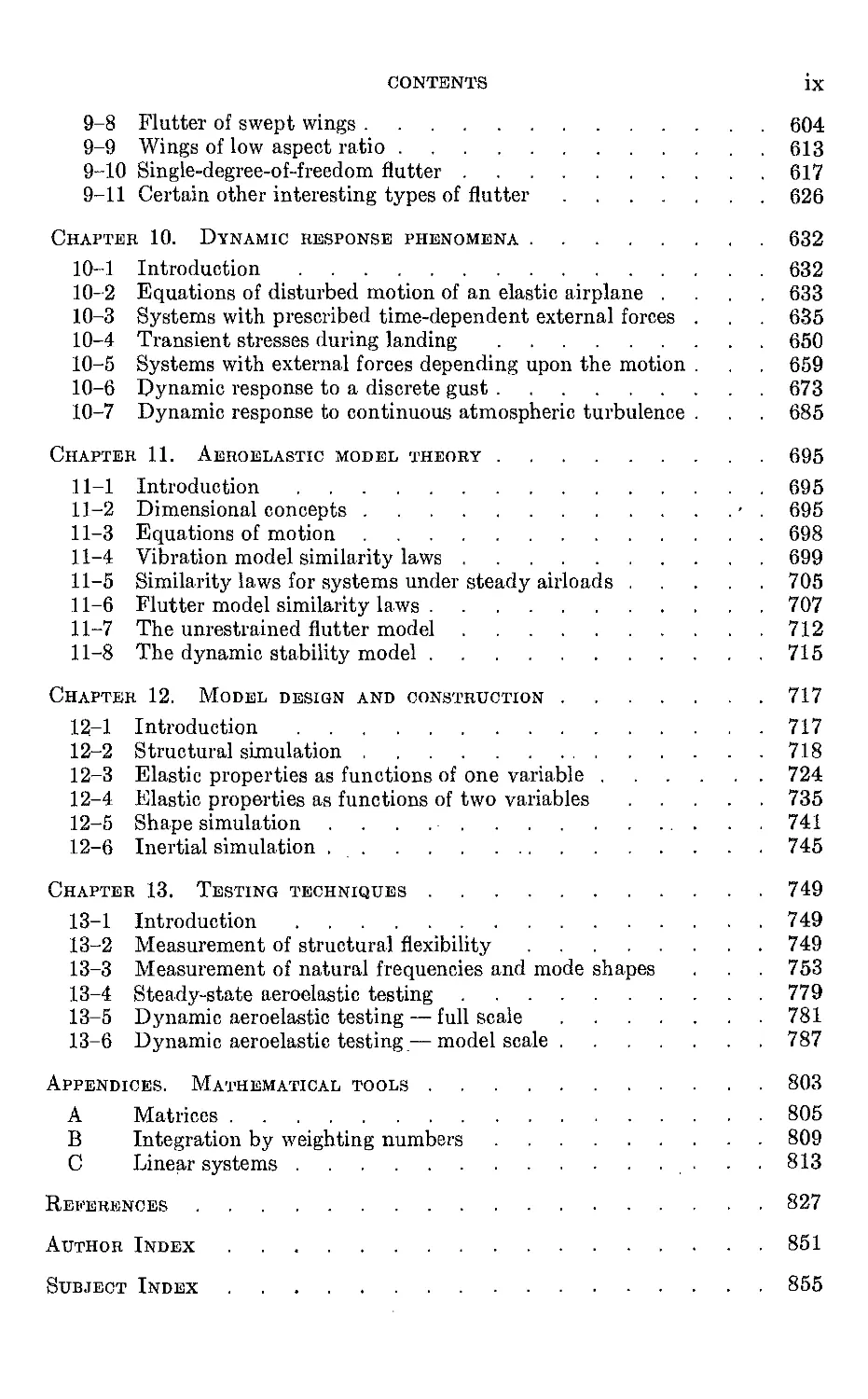
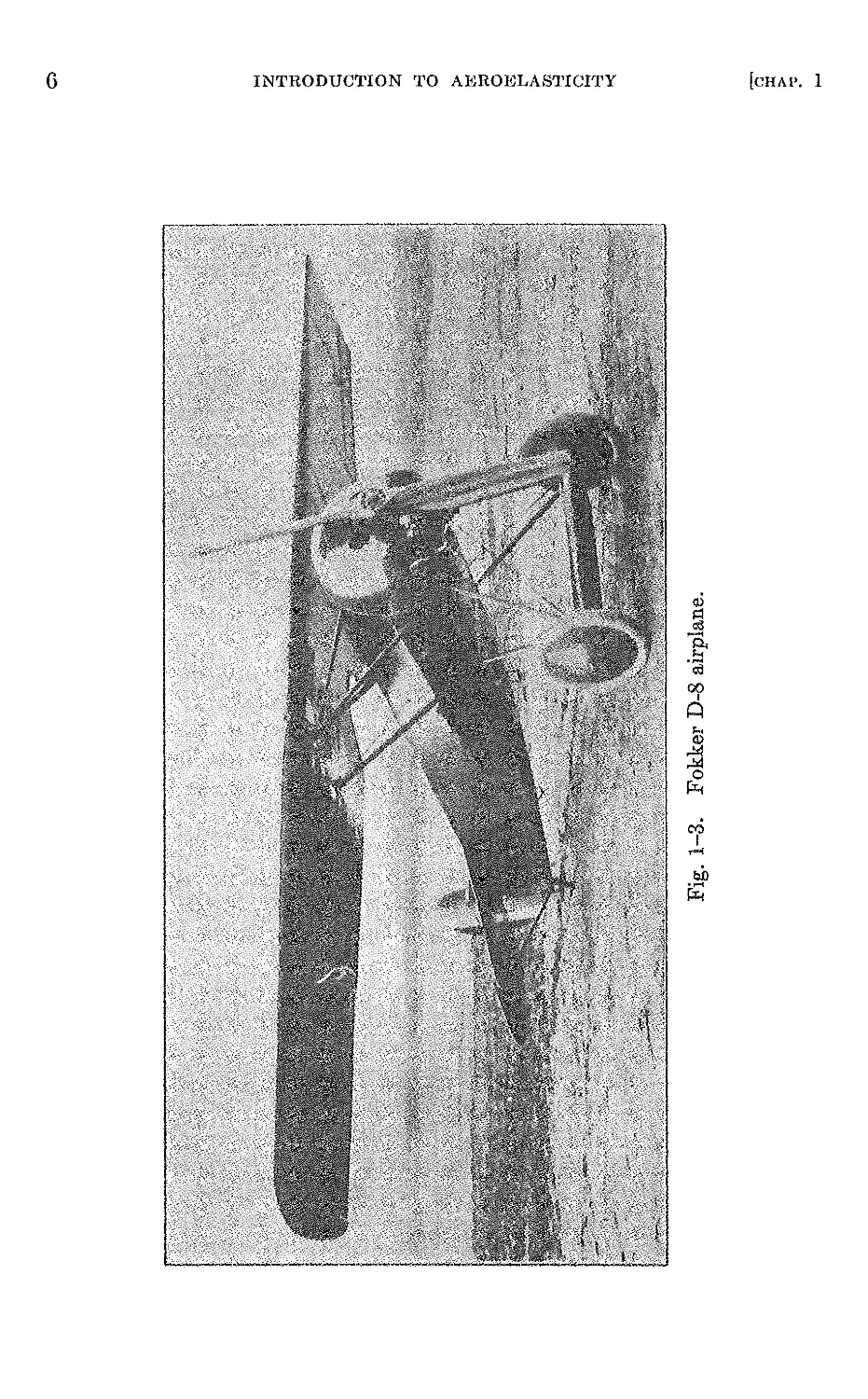
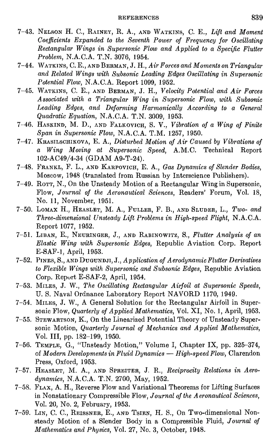
effects on load distribution resulted. An early example of this kind arose
during World War I in the development of the Fokker D-8 airplane shown
in Fig. 1-3. In the initial design of this airplane, which was a high-wing
cantilever monoplane, the torsional stiffness was determined by a criterion
which had been applied to biplanes. The D-8 was put into production
because of its superior performance, and was not in combat more than a
few days before wing failures repeatedly occurred in high-speed dives. Since
the best pilots and squadrons were receiving them first, it appeared possible
that the flower of the German Air Corps would be wiped out. Mter a
period in which the Army engineers and the Fokker Company each tried
to place the responsibility on the other, the Army conducted static strength
tests on half a dozen wings and found them sufficiently strong to support
the required ultimate factor of 6. This produced a serious' dilemma, and
it was clearly up to Anthony Fokker to discover the cause or cease produc-
tion on the D-8. Static tests were undertaken by the Fokker Company,
and this time, deflections were carefully measured from tip to tip. In
Folcker's words (Ref. 1-6), the following conclusions were drawn: "I dis-
covered that with increasing load, the angle of incidence at the wing tips
increased perceptibly. It suddenly dawned on me that this increasing
6
INTRODUCTION TO AEROELASTICITY
[CHAP. 1
<V
e-
.-
t'3
O?
;...
<V
o
,...
b1)
if:
1-3]
INFLUENCE OF AEROELASTIC PHENOMENA ON DESIGN
7
angle of incidence was the cause of the wing's collapse, as logically the load
resulting from the air pressure in a steep dive would increase faster at the
wing tips than at the middle. The resulting torsion caused the wings to
collapse under the strain of combat maneuvers." This seems to be the first
documented case where static aeroelastic effects at a fairly high speed
produced a redistribution in airload such that failure resulted.
In later experience with the D-8, subsequent to the war, U. S. Army
Air Corps engineers at McCook Field, Dayton, Ohio, observed a violent
but nondestructive case of wing bending-aileron flutter. This was cured
by statically balancing the ailerons about the hinge line, a technique which
seems to have been pointed out first by Baumhauer and Koning (Ref. 1-7)
in 1922. Several of the monoplane racers of the 1920's and 1930's experi-
enced forms of wing-aileron flutter; and mass balancing was a commonly
applied cure and preventive measure.
The period of development of the cantilever monoplane seems to have
been the period in which serious research in aeroelasticity commenced. In
the earliest days of monoplane design, aeroelastic problems were overcome
by cut-and-try methods. A theory of wing-load distribution and wing
divergence was first presented in 1926 by Hans Reissner (Ref. 1-8). A
theory of loss of lateral control and aileron reversal was published six years
later by Roxbee Cox and Pugsley (Ref. 1-9) in 1932. The mechanism of
potential flow flutter was understood sufficiently well for design use by
1935, largely through the early efforts of Glauert (Ref. 1-10), Frazer and
Duncan (Ref. 1-11), Kussner (Ref. 1-12), and Theodorsen (Ref. 1-13).
However, few designers were able to comprehend the theories in the early
papers and the majority were reluctant to trust mathematicians to compute
sizes of structural members to preclude aeroelastic effects.
1-3 Influence of aeroelastic phenomena on design. Aeroelastic phe-
nomena in modern high-speed aircraft have profound effects upon the design
of structural members and somewhat lesser but nonetheless important
effects upon mass distribution, lifting surface planforms; and control system
design.
Flutter. Flutter has perhaps the most far-reaching effects of all aero-
elastic phenomena on the design of high-speed aircraft. Modern aircraft
are subject to many kinds of flutter phenomena. The classical type of
flutter is associated with potential flow and usually, but not necessarily,
involves the coupling of two 01' more degrees of freedom. The nonclassical
type of flutter, which has so far been difficult to analyze on a purely
theoretical basis, may involve separated flow, periodic breakaway and
reattachment of the flow, stalling conditions, and various time-lag effects
between the aerodynamic forces and the motion. Preventive measures
and cures usually involve either increased stiffness or decreased coupling
by adjustments in mass distribution, or a combination of both. The most
8
INTRODUCTION TO AEROELASTICITY
[CHAP. . 1
important stiffness parameter affected by flutter considerations is wing
torsional stiffness. It is not uncommon for the flutter condition to control
the selection of wing skin thickness. Of course, wing structural design is
controlled by either a strength or a stiffness criterion. For example, if the
torsion carrying structure of a wing is designed by a stiffness requirement,
the wing would probably consist of a structure which carries its normal
stresses in the wing skin with a minimum of stringers and flanges. This
type of wing structure would require several spanwise webs in order to
stabilize the heavily loaded cover skin. For a wing designed initially by
strength considerations to carry a given load factor, it is obvious that a
higher torsional stiffness and hence a higher flutter speed will result if the
ratio of stiffener area to skin area is reduced to a minimum. In addition,
the use of higher strength alloys, which have no corresponding increase in
modulus of elasticity, tends to make flutter more critical for wings designed
for strength only.
Heavy mass items in the wing are often located by considerations of
optimum conditions for flutter prevention. For example, a given mass
distribution may require higher wing stiffness and hence higher wing
structural weight to prevent flutter than some other mass distribution. For
this reason, analytical and model studies are often made in the design stages
in order to determine the optimum mass distribution for flutter prevention.
Wing planform and aspect ratio also have significant effects on flutter
characteristics. Decreases in wing aspect ratio and increases in sweep
tend to raise flutter speeds, whereas increases in aspect ratio and decreases
in sweep, including sweep forward, reduce flutter speeds.
Flutter considerations may affect control surface design in the deter-
mination of aerodynamic and mass balance, hinge location, and the degree
of irreversibility required in the actuating system.
Buffeting. A serious buffeting phenomenon confronting designers is
encountered by fighter aircraft during pull-ups to C Lmax at high speed.
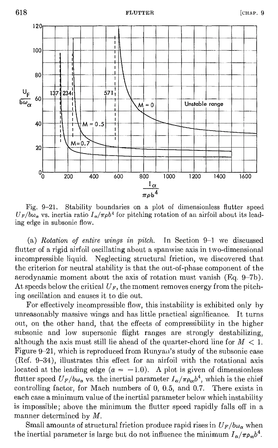
This often results in rugged transient vibrations in the tail due to aero-
dynamic impulses from the wing wake. The principal problems are those
of reducing the severity of these vibrations, and the provision of adequate
strength. Designing for strength is very difficult. The problem of pre-
dicting dynamic stresses due to a given buffeting condition is still unsolved
analytically. The principal obstacle has been a lack of knowledge of the
properties of the wake behind a stalled wing. Designers have alleviated
their buffeting problems up to the present time largely by proper positioning
of the tail assembly and by clean aerodynamic design.
Dynamic loads problems. This class of aeroelastic problem has its
primary influence on structural design. In the prediction of design loads
on an airplane structure in an accelerated condition, it is usually assumed
that the airplane is perfectly rigid. Structural components designed by
loads computed on this basis may fail due to a dynamic overstress. External
1-31
INFLUENCE OF AEROELASTIC PHENOMENA ON DESIGN
9
loads that are rapidly applied not only cause translation and rotation of the
airplane as a whole, but tend to excite vibrations of the structure. The
additional inertial forces associated with these vibrations produce the
dynamic overstress. Dynamic stresses are usually manifested in the form
of increased bending and torsional stresses in the wing and fuselage beams.
The design of these beams must take account of dynamic stresses by
increasing the normal and shear carrying areas. Perhaps the two most
important dynamic response problems have been the gust and landing
problems. The gust condition is usually the controlling strength condition
in large aircraft. Aeroelastic effects may have an important influence on
gust design conditions. For example, the designer can expect that the
dynamic response of a straight wing in the gust condition may produce
wing bending moments at the root 15% to 20% greater than those calcu-
lated on the assumption of a rigid wing. Response of a slender flexible
swept wing when a gust is encountered is a matter of considerable practical
interest, particularly in the case of large high-speed aircraft. Elastic
deformations and vibratory response of the wing have important and com-
plicating effects upon the load distribution. Load distributions predicted
on the assumption of a rigid wing are often too much in error to be useful,
and swept-wing designers are compelled to consider the principal aero-
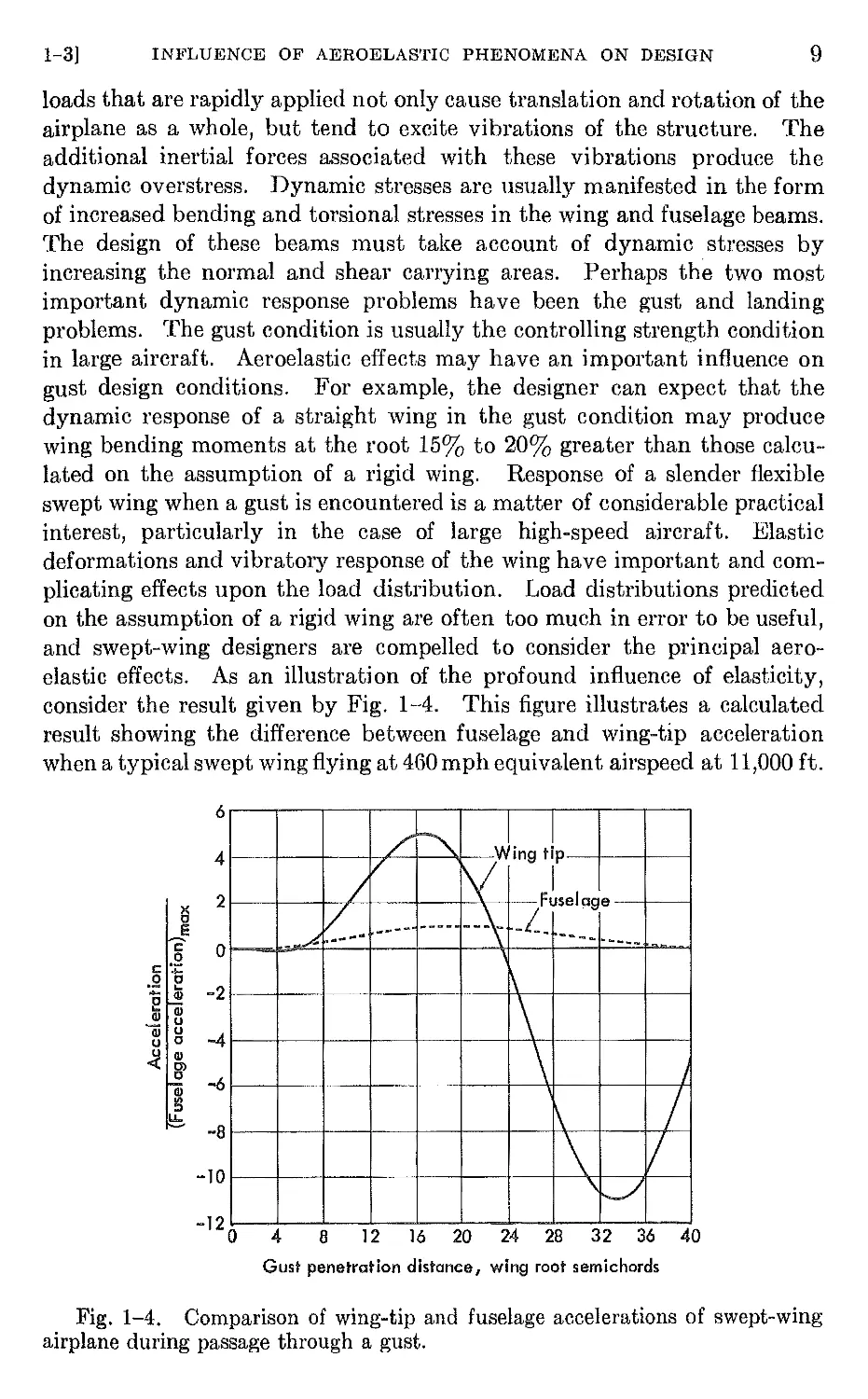
elastic effects. As an illustration of the profound influence of elasticity,
consider the result given by Fig. 1-4. This figure illustrates a calculated
result showing the difference between fuselage and wing-tip acceleration
when a typical swept wing flying at 460 mph equivalent airspeed at 11,000 ft.
6
4
2
e
!: 0
0
!: .-
o t;
.- ... -2
t; <I)
... C1I
0 -4
.:J. C1I
0>
C -6
C1I
'"
::I
u..
-8
-10
/ j. j
mg tip
V L,oge
/
/ ....--- --- - L
../. .............. - -- ---... ...--...
-
\
\
\ I
\ /
\ /
\ J
8 12 16 20 24 28 32 36 40
- 12 0 4
Gust penetration distance, wing root semichords
Fig. 1-4. Comparison of wing-tip and fuselage accelerations of swept-wing
airplane during passage through a gust.
10
IN'.rRODUCTION TO AEROELASTICITY
[CHAP. 1
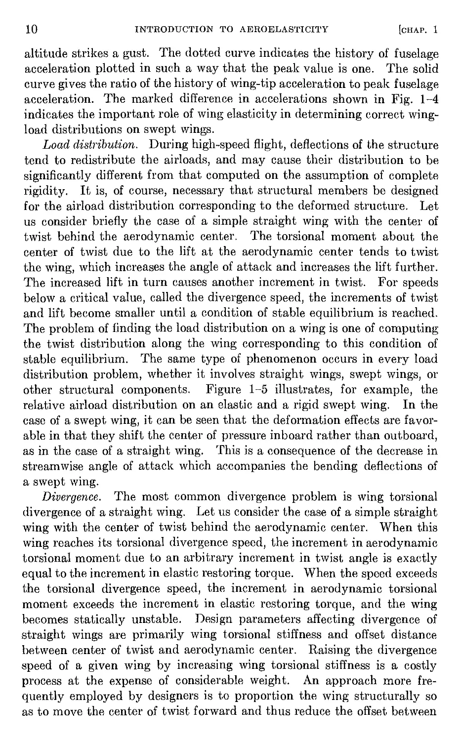
altitude strikes a gust. The dotted curve indicates the history of fuselage
acceleration plotted in such a way that the peak value is one. The solid
curve gives the ratio of the history of wing-tip acceleration to peak fuselage
acceleration. The marked difference in accelerations shown in Fig. 1-4
indicates the important role of wing elasticity in determining correct wing-
load distributions on swept wings.
Load distribution. During high-speed flight, deflections of the structure
tend to redistribute the airloads, and may cause their distribution to be
significantly different from that computed on the assumption of complete
rigidity. It is, of course, necessary that structural members be designed
for the airload distribution corresponding to the deformed structure. Let
us consider briefly the case of a simple straight wing with the center of
twist behind the aerodynamic center. The torsional moment about the
center of twist due to the lift at the aerodynamic center tends to twist
the wing, which increases the angle of attack and increases the lift further.
The increased lift in turn causes another increment in twist. For speeds
below a critical value, called the divergence speed, the increments of twist
and lift become smaller until a condition of stable equilibrium is reached.
The problem of finding the load distribution on a wing is one of computing
the twist distribution along the wing corresponding to this condition of
stable equilibrium. The same type of phenomenon occurs in every load
distribution problem, whether it involves straight wings, swept wings, or
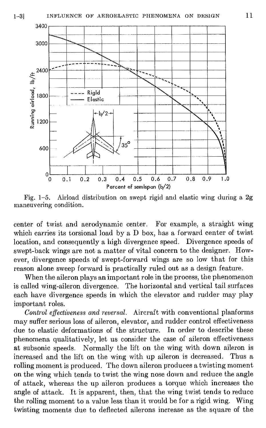
other structural components. Figure 1-5 illustrates, for example, the
relative airload distribution on an elastic and a rigid swept wing. In the
case of a swept wing, it can be seen that the deformation effects are favor-
able in that they shift the center of pressure inboard rather than outboard,
as in the case of a straight wing. This is a consequence of the decrease in
stream wise angle of attack which aeeompanies the bending deflections of
a swept wing.
Divergence. The most common divergence problem is wing torsional
divergence of a straight wing. Let us consider the case of a simple straight
wing with the center of twist behind the aerodynamic center. When this
wing reaehes its torsional divergence speed, the increment in aerodynamic
torsional moment due to an arbitrary increment in twist angle is exactly
equal to the increment in elastic restoring torque. When the speed exceeds
the torsional divergence speed, the increment in aerodynamic torsional
moment exceeds the increment in elastic restoring torque, and the wing
becomes statically unstable. Design parameters affecting divergence of
straight wings are primarily wing torsional stiffness and offset distance
between center of twist and aerodynamic center. Raising the divergence
speed of a given wing by increasing wing torsional stiffness is a costly
process at the expense of considerable weight. An approach more fre-
quently employed by designers is to proportion the wing structurally so
as to move the center of twist forward and thus reduce the offset between
1-3]
INFLUENCE OF AEROELASTIC PHENOMENA ON DESIGN
11
3400
600
--- -
---
........ '"
......
---- ---- --- .
....
.......... '..
......
'" ......
.. ..
---- Rigid " '.....
...
- Elastic " ",
,
.....b/2- "'"
f-- " \
\
t-- ..... .
, ..
t-- '> .£ \\
- / 350 \\
- \
- \
I
3000
.... 2400
....
"-
...a
..
"U
g 1800
.!:::
c
(J)
c:
1200
0<:
o
o 0.1 0.2 0.3 0.4 0.5 0.6 0.7 0.8 0.9 1.0
Percent af semispan (b/2)
Fig. 1-5. Airload distribution on swept rigid and elastic wing during a 2g
maneuvering condition.
center of twist and aerodynamic center. For example, a straight wing
which carries its torsional load by a D box, has a forward center of twist
location, and consequently a high divergence speed. Divergence speeds of
swept-back wings are not a matter of vital concern to the designer. How-
ever, divergence speeds 'of swept-forward wings are so low that for this
reason alone sweep forward is practically ruled out as a design feature.
When the aileron plays an important role in the process, the phenomenon
is called wing-aileron divergence. The horizontal and vertical tail surfaces
each have divergence speeds in which the elevator and rudder may play
important roles.
Control effectiveness and reversal. Aircraft with conventional planforms
may suffer serious loss of aileron, elevator, and rudder control effectiveness
due to elastic deformations of the structure. In order to describe these
phenomena qualitatively, let us consider the case of aileron effectiveness
at subsonic speeds. Normally the lift on the wing with down aileron is
increased and the lift on the wing with up aileron is decreased. Thus a
rolling moment is produced. The down aileron produces a twisting moment
on the wing which tends to twist the wjng nose down and reduce the angle
of attack, whereas the up aileron produces a torque which increases the
angle of attack. It is apparent, then, that the wing twist tends to reduce
the rolling moment to a value less than it would be for a rigid wing. Wing
twisting moments due to deflected ailerons increase as the square of the
12
INTRODUCTION TO AEROELASTICITY
[CHAP. 1
12
'0 8
..2 g>
Q) C
> t:
g>2
.- Q)
(54: 4
'"
Mach number
r Aileron reversal
speed
o
o 0.2 0.4 0.6 0.8 1.0
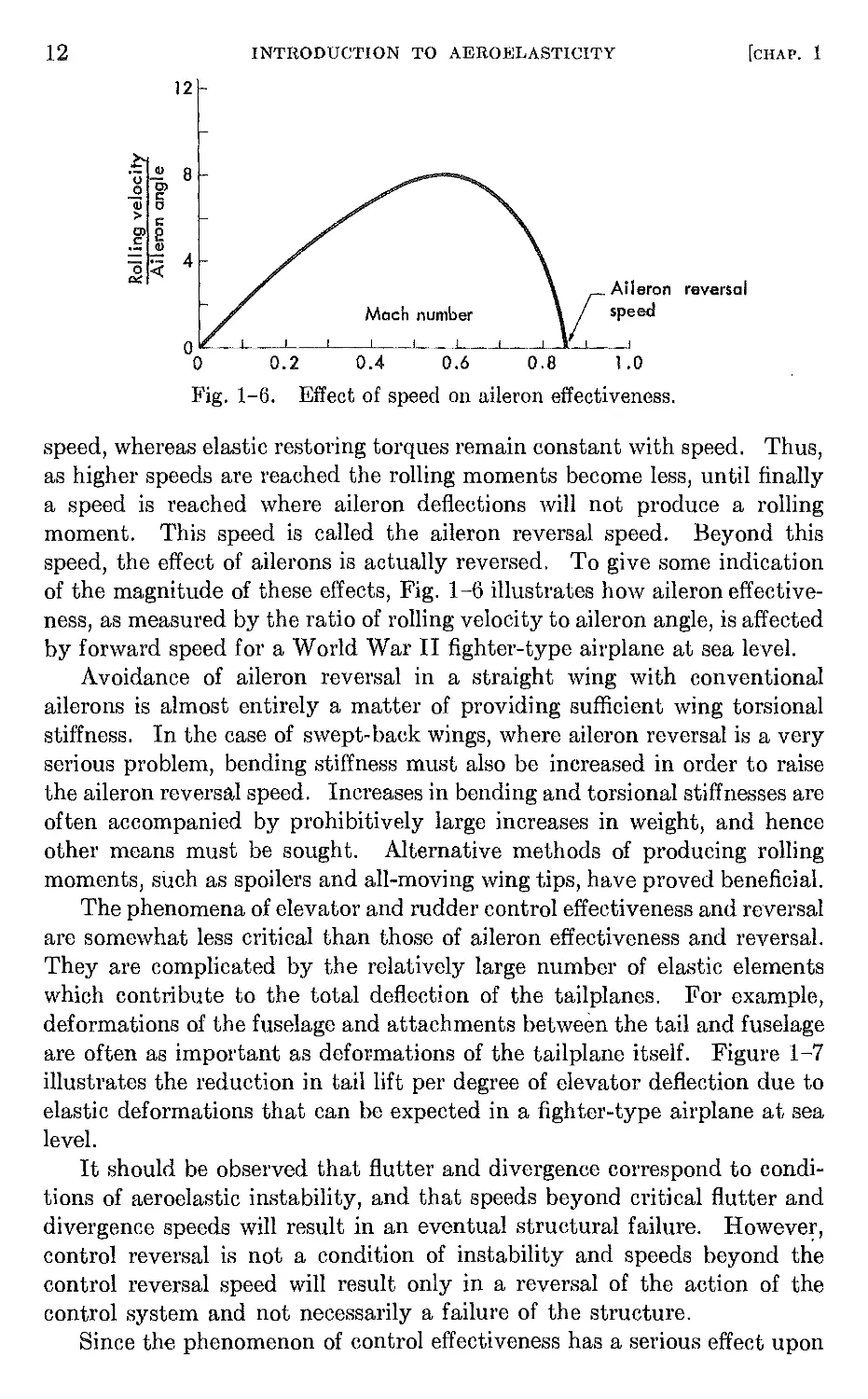
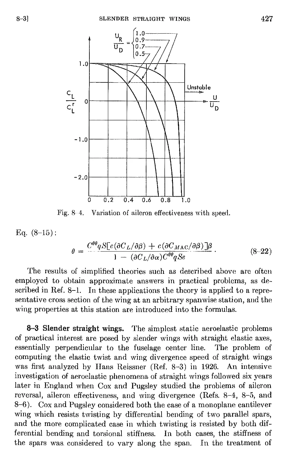
Fig. 1-6. Effect of speed on aileron effectiveness.
speed, whereas elastic restoring torques remain constant with speed. Thus,
as higher speeds are reached the rolling moments become less, until finally
a speed is reached where aileron deflections will not produce a rolling
moment. This speed is called the aileron reversal speed. Beyond this
speed, the effect of ailerons is actually reversed. To give some indication
of the magnitude of these effects, Fig. 1-6 illustrates how aileron effective-
ness, as measured by the ratio of rolling velocity to aileron angle, is affected
by forward speed for a World War II fighter-type airplane at sea level.
Avoidance of aileron reversal in a straight wing with conventional
ailerons is almost entirely a matter of providing sufficient wing torsional
stiffness. In the case of swept-back wings, where aileron reversal is a very
serious problem, bending stiffness must also be increased in order to raise
the aileron reversal speed. Increases in bending and torsional stiffnesses are
often accompanied by prohibitively large increases in weight, and hence
other means must be sought. Alternative methods of producing rolling
moments, such as spoilers and all-moving wing tips, have proved beneficial.
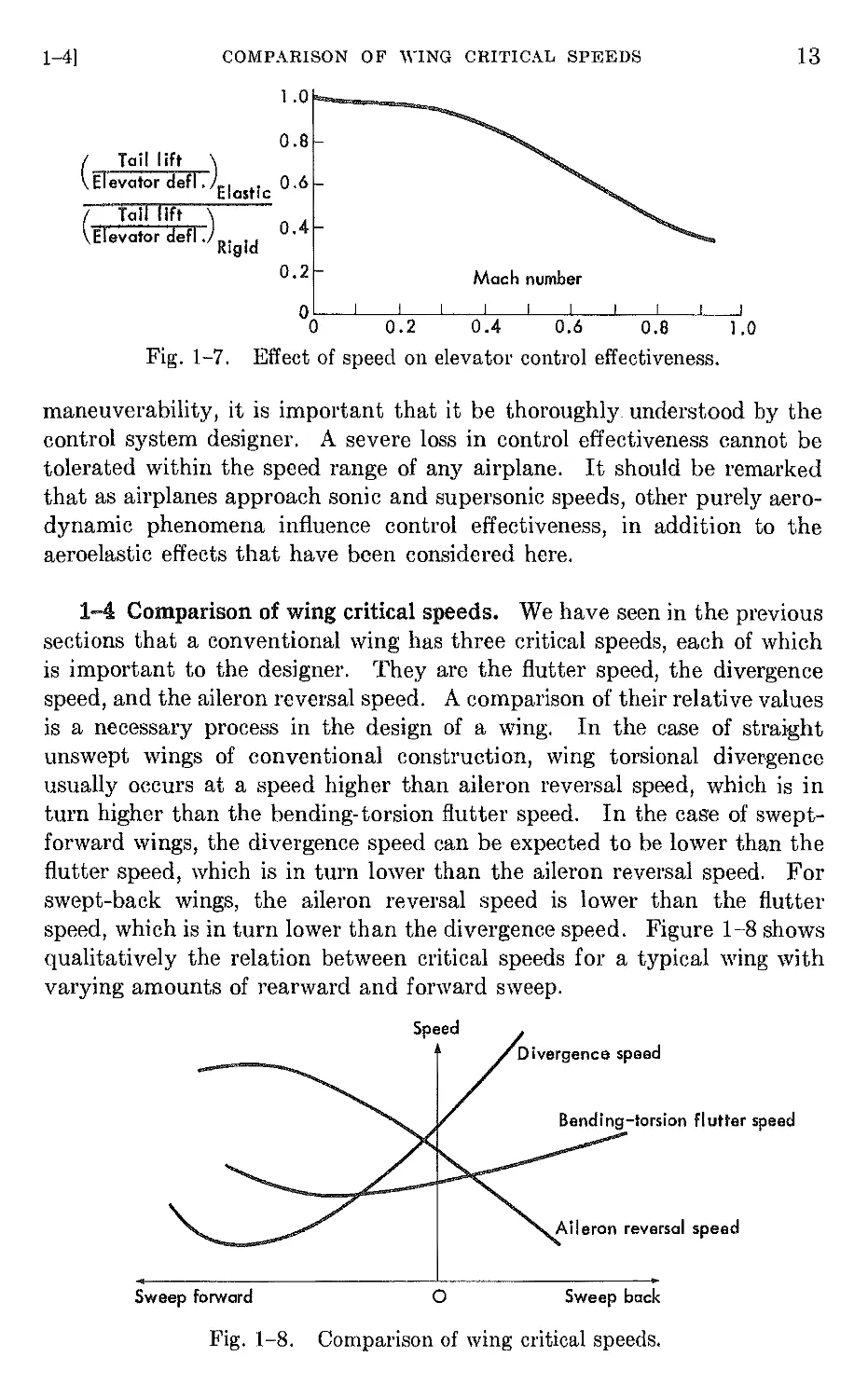
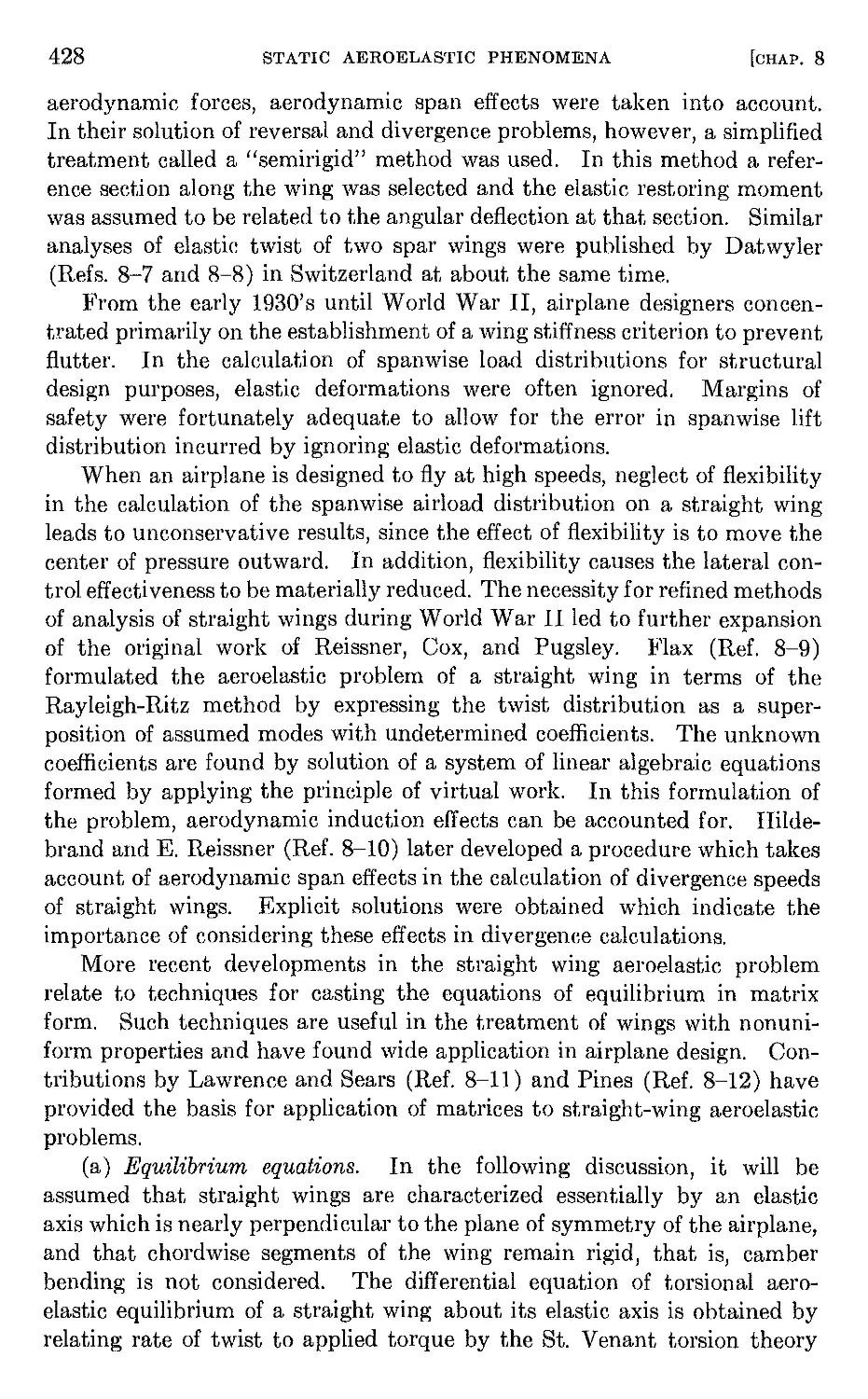
The phenomena of elevator and rudder control effectiveness and reversal
are somewhat less critical than those of aileron effectiveness and reversal.
They are complicated by the relatively large number of elastic elements
which contribute to the total deflection of the tailplanes. For example,
deformations of the fuselage and attachments between the tail and fuselage
are often as important as deformations of the tailplane itself. Figure 1-7
illustrates the reduction in tail lift per degree of elevator deflection due to
elastic deformations that can be expected in a fighter-type airplane at sea
level.
It should be observed that flutter and divergence correspond to condi-
tions of aeroelastic instability, and that speeds beyond critical flutter and
divergence speeds will result in an eventual structural failure. Howeve ,
control reversal is not a condition of instability and speeds beyond the
control reversal speed will result only in a reversal of the action of the
control system and not necessarily a failure of the structure.
Since the phenomenon of control effectiveness has a serious effect upon
1-4]
COMPARISON OF WING CRITICAL SPEEDS
13
1.0
0.8
( Tail lift )
E l evatordef l . EI t . 0.6
as Ie
( Tall 11ft )
E l evator d ef l . Rigid 0.4
0.2
Mach number
Fig. 1-7.
0.2 0.8
Effect of speed on elevator control effectiveness.
°0
1.0
maneuverability, it is important that it be thoroughly understood by the
control system designer. A severe loss in control effectiveness cannot be
tolerated within the speed range of any airplane. It should be remarked
that as airplanes approach sonic and supersonic speeds, other purely aero-
dynamic phenomena influence control effectiveness, in addition to the
aeroelastic effects that have been considered here.
1-4 Comparison of wing critical speeds. We have seen in the previous
sections that a conventional wing has three critical speeds, each of which
is important to the designer. They are the flutter speed, the divergence
speed, and the aileron reversal speed. A comparison of their relative values
is a necessary process in the design of a wing. In the case of straight
unswept wings of conventional construction, wing torsional divergence
usually occurs at a speed higher than aileron reversal speed, which is in
turn higher than the bending-torsion flutter speed. In the case of swept-
forward wings, the divergence speed can be expected to be lower than the
flutter speed, which is in turn lower than the aileron reversal speed. For
swept-back wings, the aileron reversal speed is lower than the flutter
speed, which is in turn lower than the divergence speed. Figure 1-8 shows
qualitatively the relation between critical speeds for a typical wing with
varying amounts of rearward and forward sweep.
Sweep forward
o
Sweep back
Fig. 1-8. Comparison of wing critical speeds.
14
INTRODUCTION '1'0 AEROELASTICITY
[CHAP. 1
Q)
s:::
03
........
s:l.
I-<
......
03
J:..
.,.j1
I
..-i
I
bO
r£:
CHAPTER 2
DEFORMATIONS OF AIRPLANE STRUCTURES
UNDER STATIC LOADS
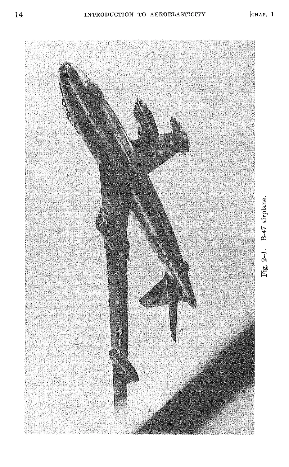
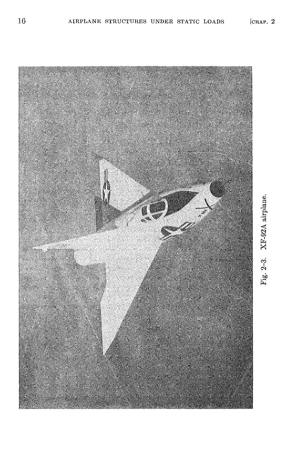
2-1 Introduction. Modern airplanes vary widely in geometric shape.
On the one hand, we find high-aspect ratio wings which resemble slender
beams, and on the other, low-aspect ratio delta wings which resemble
plates. The Boeing B-47 airplane, illustrated in Fig. 2-1, is an example of
the former, and the Convair XF -92A in Fig. 2-3 provides an excellent
example of the latter. The fuselage may be long and slender, or it may be
nonexistent, as in the case of a flying wing. The arrangements and types
of load-carrying members also differ widely. As aircraft are put to wider
uses, it is natural to expect larger differences among their geometric and
structural configurations.
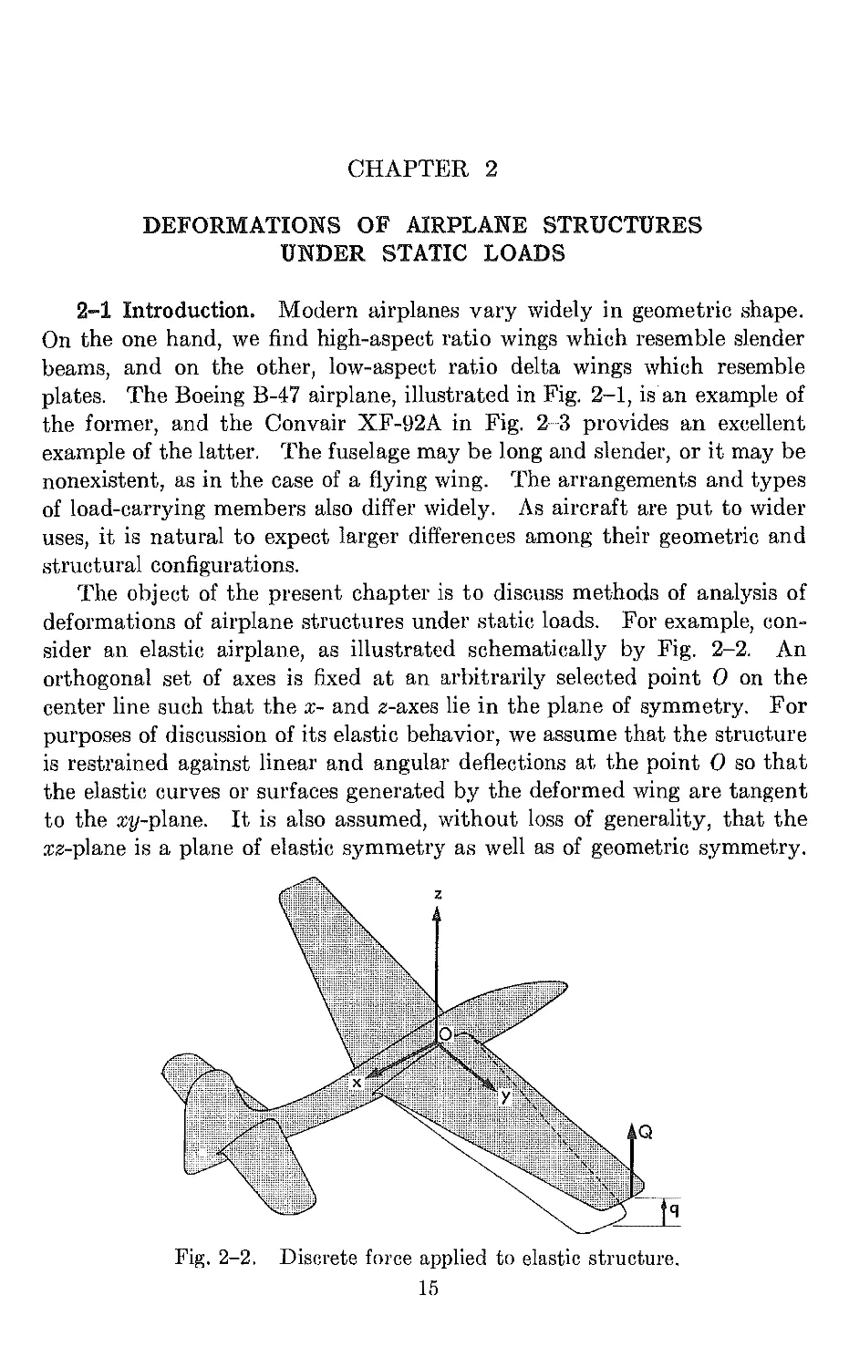
The object of the present chapter is to discuss methods of analysis of
deformations of airplane structures under static loads. For example, con-
sider an elastic airplane, as illustrated schematicaUy by Fig. 2-2. An
orthogonal set of axes is fixed at an arbitrarily selected point 0 on the
center line such that the x- and z-axes lie in the plane of symmetry. For
purposes of discussion of its elastic behavior, we assume that the structure
is restrained against linear and angular deflections at the point 0 so that
the elastic curves or surfaces generated by the deformed wing are tangent
to the xy-plane. It is also assumed, without loss of generality, that the
xz-plane is a plane of elastic symmetry as well as of geometric symmetry.
Fig. 2-2. Discrete force applied to elastic structure.
15
16
AIRPLANE STRUCTURES UNDER STATIC LOADS
[CHAP. 2
<15
>=:
«!
......
r-.
.....
<:'3
<r;
a>
Ix:
I
M
2-3]
DEFORMATION DUE TO SEVERAL FORCES
17
2-2 Elastic properties of structures. In this book it will be assumed
that the aircraft structures under consideration are perfectly elastic. That
is, when external forces are removed the structure resumes its initial form.
Experiments on aircraft structures have indicated that within certain limits
an applied force, Q, and its resulting deflection, q, as illustrated by Fig. 2-2,
are related by
q = CQ,
(2-1 )
where C is a constant of proportionality.
linearly related and the loaded structure
system.
In thin-skin aircraft structures elastic buckling may produce a dis-
continuity in the force-deflection diagram even though the materials which
make up the structure are stressed at a relatively low level. We shall
assume that the elastic behavior of our structures is defined in the range
below the point of elastic buckling. Although this assumption is not
restrictive for structures with thick skins, as in the case of military aircraft,
its validity may require examination when applied to aeroelastic problems
involving thin-skin structures.
A consequence of Eq. (2-1) is that the work done by the external force
during application is transformed completely into strain energy in the
structure. That is,
Thus force and deflection are
may be referred to as a linear
U = !Qq,
(2-2 )
where U denotes the strain energy.
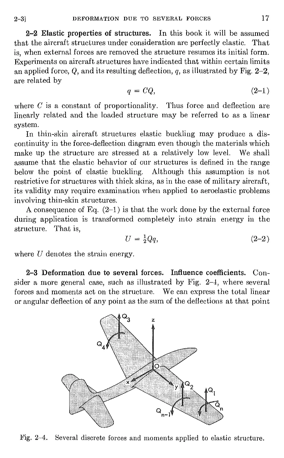
2-3 Deformation due to several forces. Influence coefficients. Con-
sider a more general case, such as illustrated by Fig. 2-4, where several
forces and moments act on the structure. We can express the total linear
or angular deflection of any point as the sum of the deflections at that point
Fig. 2-4. Several discrete forces and moments applied to elastic structure.
18
AIRPLANE STRUCTURES UNDER STATIC LOADS
[CHAP. 2
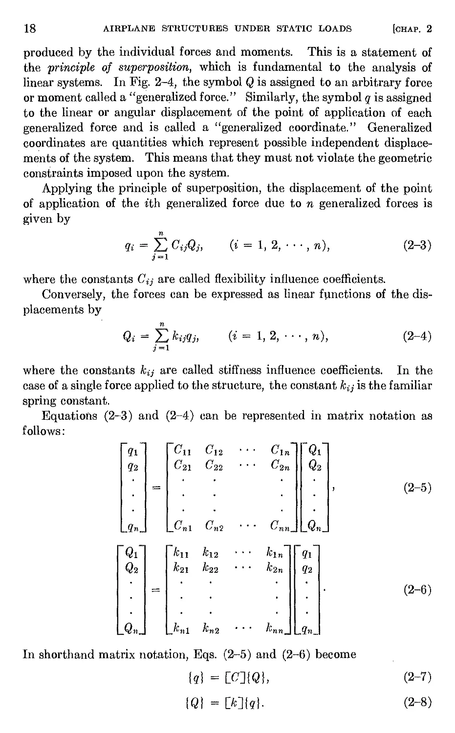
produced by the individual forces and moments. This is a statement of
the principle of superposition, which is fundamental to the analysis of
linear systems. In Fig. 2-4, the symbol Q is assigned to an arbitrary force
or moment called a "generalized force." Similarly, the symbol q is assigned
to the linear or angular displacement of the point of application of each
generalized force and is called a "generalized coordinate." Generalized
coordinates are quantities which represent possible independent displace-
ments of the system. This means that they must not violate the geometric
constraints imposed upon the system.
Applying the principle of superposition, the displacement of the point
of application of the ith generalized force due to n generalized forces is
given by
n
qi = I: CijQj,
j=l
( i = 1 2 ... n )
" , ,
(2-3 )
where the constants C ij are called flexibility influence coefficients.
Conversely, the forces can be expressed as linear fllnctions of the dis-
placements by
n
Q . - "Jr.. q .
- L...J " J J,
j=l
( i = 1 2 ... n )
" , ,
(2-4 )
where the constants k ij are called stiffness influence coefficients. In the
case of a single force applied to the structure, the constant k ij is the familiar
spring constant.
Equations (2-3) and (2-4) can be represented in matrix notation as
follows:
ql C ll C 12 C 1n Ql
q2 C 21 C 22 C 2n Q2
= (2-5)
qn C n1 C n2 Cnn Qn
Ql k ll k 12 kIn ql
Q2 k 21 k 22 k 2n q2
- (2-6)
Qn k n1 k n2 k nn qn
In shorthand matrix notation, Eqs. (2-5) and (2-6) become
Iq} = [CJIQI,
IQ} = [kJlq}.
(2-7)
(2-8)
2-3]
DEFORMATION DUE TO SEVERAL FORCES
19
The representation of sets of linear equations in matrix notation is fre-
quently useful in manipulating the equations and in indicating orderly
processes for carrying out numerical calculations. Matrix methods are
widely used in aeroelasticity, but a knowledge of only a few of the elemen-
tary rules of matrix algebra is sufficient for most purposes. Appendix A
develops these rules, and Ref. 2-1 is an excellent source of more complete
information.
The square array of numbers, [CJ, called the matrix of flexibility influ-
ence coefficients, is related mathematically to the matrix of stiffness influ-
ence coefficients, [k]. If the set of linear equations, Eq. (2-7), is solved
for the Q's as linear functions of the q's, the set of linear equations given by
Eq. (2-8) is obtained. This process is known as matrix inversion (Ap-
pendix A) and is represented symbolically by
[kJ = [CJ-l,
(2-9)
where the matrix [leJ is said to be the reciprocal of the matrix [C].
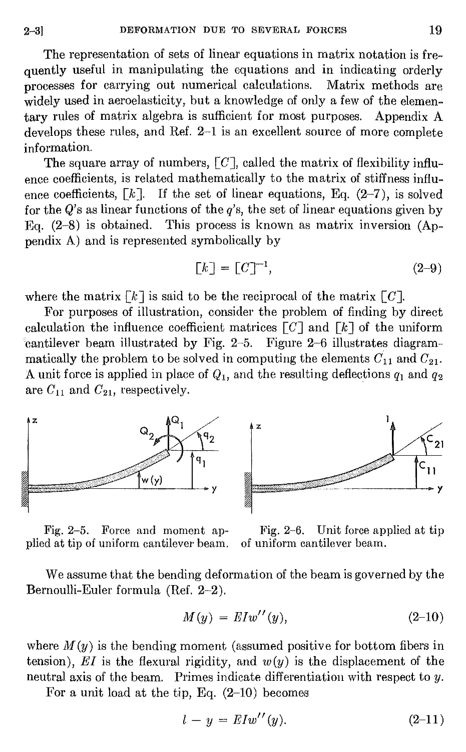
For purposes of illustration, consider the problem of finding by direct
calculation the influence coefficient matrices [CJ and [kJ of the uniform
cantilever beam illustrated by Fig. 2-5. Figure 2-6 illustrates diagram-
matically the problem to be solved in computing the elements C ll and C 21 .
A unit force is applied in place of Ql, and the resulting deflections ql and q2
are C ll and C 2 1, respectively.
z
:z;
y
y
Fig. 2-5. Force and moment ap-
plied at tip of uniform cantilever beam.
Fig. 2-6. Unit force applied at tip
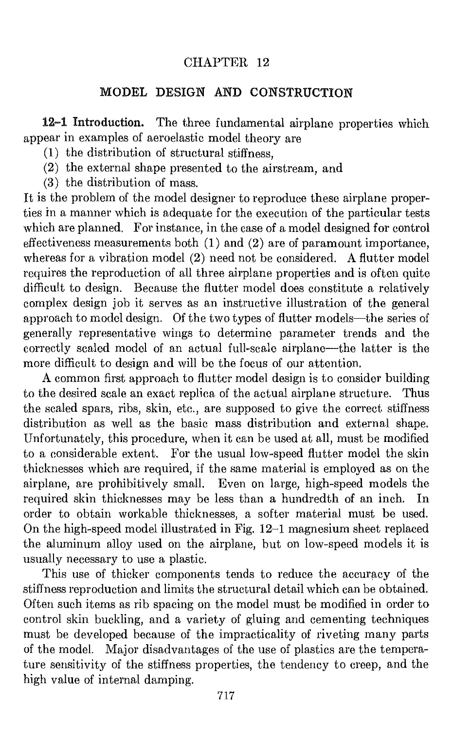
of uniform cantilever beam.
We assume that the bending deformation of the beam is governed by the
Bernoulli-Euler formula (Ref. 2-2).
M(y) = Elw" (y),
(2-10)
where M(y) is the bending moment (assumed positive for bottom fibers in
tension), E I is the flexural rigidity, and w (y) is the displacement of the
neutral axis of the beam. Primes indicate differentiation with respect to y.
For a unit load at the tip, Eq. (2-10) becomeB
l - y = Elw" (y).
(2-11 )
20
AIRPLANE STRUCTURES UNDER STATIC LOADS
[CHAP. 2
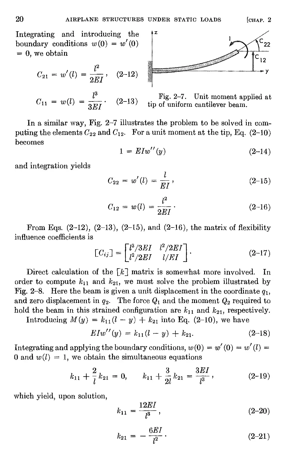
Integrating and introducing the
boundary conditions w(O) = w' (0)
= 0, we obtain
z
y
%
l2
C 21 = w' (l) = 2El ' (2-12)
C 11 = w(l)
l3
--.
3El
(2-13)
Fig. 2-7. Unit moment applied at
tip of uniform cantilever beam.
In a similar way, Fig. 2-7 illustrates the problem to be solved in com-
puting the elements C 22 and C 12 . For a unit moment at the tip, Eq. (2-10)
becomes
1 = Elw fl (y)
(2-14)
and integration yields
I Z
C 22 = w (l) = EI '
(2-15)
l2
C 12 = w(l) = - .
2EI
(2-16)
From Eqs. (2-12), (2-13), (2-15), and (2-16), the matrix of flexibility
influence coefficients is
[ l3 13E I Z2 12E I ]
[C ij ] = l2/2EI llEl .
(2-17 )
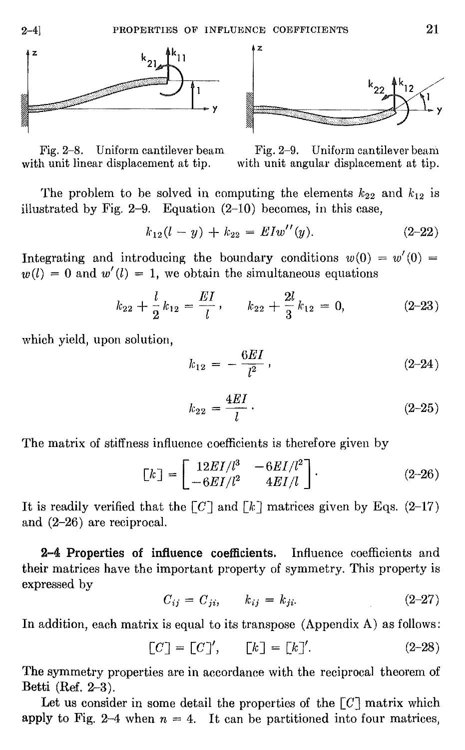
Direct calculation of the [k] matrix is somewhat more involved. In
order to compute k 11 and k 21 , we must solve the problem illustrated by
Fig. 2-8. Here the beam is given a unit displacement in the coordinate Q1,
and zero displacement in Q2. The force Ql and the moment Q2 required to
hold the beam in this strained configuration are k ll and k 2b respectively.
Introducing M(y) = le ll (l - y) + k 21 into Eq. (2-10), we have
Elw" (y) = k ll (l - y) + k 21 . (2-18)
Integrating and applying the boundary conditions, w(O) = WI (0) = w' (l) =
o and w(l) = 1, we obtain the simultaneous equations
2 3 3El
Jell + l k 21 = 0, le ll + 2l k 21 = T' (2-19)
which yield, upon solution,
12EI
k 11 = r'
(2-20)
6EI
k 21 = - [2 .
(2-21 )
2-4J
21
z
PROPERTIES OF INFLUENCE COEFFICIENTS
z
k 21 k j 1
Fig. 2-8. Uniform cantilever beam
with unit linear displacement at tip.
%
y
/'
y
Fig. 2-9. Uniform cantilever bean1
with unit angular displacement at tip.
The problem to be solved in computing the elements k 22 and k 12 is
illustrated by Fig. 2-9. Equation (2-10) becomes, in this case,
k 12 (l - y) + k 22 = Elw" (y). (2-22)
Integrating and introducing the boundary conditions w(O) = w/ (0) =
w(l) = 0 and w/ (l) = 1, we obtain the simultaneous equations
l BI
k 22 + '2 k 12 = T '
which yield, upon solution,
k 12 =
4EI
k 22 = - .
l
2l
k 22 + - k 12 = 0,
3
(2-23 )
BEl
--,
l2
(2-24 )
(2-25 )
The matrix of stiffness influence coefficients is therefore given by
[ 12EIIZ3
[Ie] = -6Elll z
-6El l l2 J .
4EIIl
(2-26 )
It is readily verified that the [CJ and [kJ matrices given by Eqs. (2-17)
and (2-26) are reciprocal.
2-4 Properties of influence coefficients. Influence coefficients and
their matrices have the important property of symmetry. This property is
expressed by
C i ;, = C;'i,
ICi;' = k ji .
(2-27)
In addition, each matrix is equal to its transpose (Appendix A) as follows:
(2-28)
[CJ = [CJ/,
[k] = [k]'.
The symmetry properties are in accordance with the reciprocal theorem of
Betti (Ref. 2-3).
Let us consider in some detail the properties of the [CJ matrix which
apply to Fig. 2-4 when n = 4. It can be partitioned into four matrices,
22
AIRPLANE STRUCTURES UNDER STATIC LOADS
[CHAP. 2
each containing different types of influence coefficients, as follows:
C OOt C oa C Oa
12 I 13 14
C oo : C Oa C oa
22 I 23 24
,
-------------+-------------
I
c 31 ao c 32 ao ! c 33 aa c 34 aa
C ao C ao : C aa C aa
41 42 I 43 44
C OO
11
C oo
21
[C] =
(2-29)
The four different types of elements are
Cijoo = linear deflection at i due to unit force at j,
Cit a = angular deflection at i due to unit moment at j,
Ci/a = linear deflection at i due to unit moment at j,
cija o = angular deflection at i due to unit force at j.
In order for the [C] matrix to be symmetrical, the following reciprocal
relations must hold:
cjo = cjl O ,
(2-30)
(2-31 )
(2-32)
C. .aa = C ..aa
tJ J '
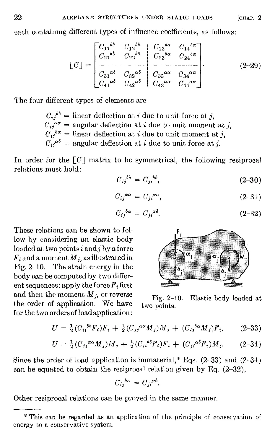
These relations can be shown to fol-
low by considering an elastic body
loaded at two points i andj by a force
F i and a moment M j, as illustrated in
Fig. 2-10. The strain energy in the
body can be computed by two differ-
ent sequences: apply the force F i first
and then the moment M j, or reverse
the order of application. We have
for the two orders of load application:
U = !(CiiOOFi)Fi + !(CjjaalIJj)Mj + (ci/allJj)F iJ
C oa - C ao
ij - ji .
Fig. 2-10. Elastic body loaded at
two points.
U = !(CjjaaMj)M j + !(CjoFi)F i + (CjiaoFi)1I1j.
(2-33 )
(2-34)
Since the order of load application is immaterial, * Eqs. (2-33) and (2-3-1)
can be equated to obtain the reciprocal relation given by Eq. (2-32),
c..oa = c..ao
J Jt .
Other reciprocal relations can be proved in the Ijame manner.
* This can be regarded as an application of the principle of conservation of
energy to a conservative system.
2.,..6]
DEFORMATIONS UNDER DISTRIBUTED FORCES
23
2-6 Strain energy in terms of influence coefficients. In the applica-
tion of energy theorems to aeroelastic systems, formulas for strain energy
in terms of influence coefficients are useful. Referring to Fig. 2-4, we have
the following expression for strain energy:
n
U = ! L Qiqi.
i =1
(2-35 )
The introduction of Eq. (2-3) into Eq. (2-35) results in an expression for
the strain energy in terms of the flexibility influence coefficients and the
external loads,
n n
U = ! L L CijQiQj.
i =1 j=1
(2-36 )
Similarly, by introducing Eq. (2-4) into Eq. (2-35), we obtain an expres-
sion for strain energy in terms of stiffness influence coefficients and dis-
placements,
n n
U = ! L L kijqiqj.
i=l i=l
(2-37 )
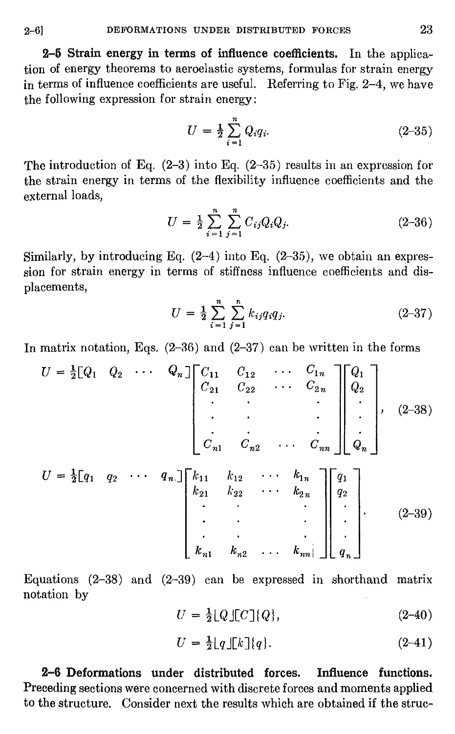
In matrix notation, Eqs. (2-36) and (2-37) can be written in the forms
U = ![Ql Q2 . . . Qn] C ll C 12 GIn Ql
C 21 C 22 G 2n Q2
(2-38 )
G nI G n2 G nn Qn
U = ![ql q2 . . . qn.] leu k 12 kIn ql
lc 21 k 22 k 2n q2
(2-39 )
k nl k n2 knnl qn
Equations (2-38) and (2-39) can be expressed 111 shorthand matrix
notation by
[J = !LQJeC] {Q j, (2-40 )
U = !LqJ[lc]{qJ. (2-41)
2-6 Deformations under distributed forces. Influence functions.
Preceding sections were concerned with discrete forces and moments applied
to the structure. Consider next the results which are obtained if the struc-
24
AIRPLANE STRUCTURES UNDER STATIC LOADS
[CHAP. 2
> 4
rj
z
z
,\Z{y)
%
y
y
Fig. 2-11. Uniform cantilever
beam loaded by distributed side load.
y
J
TJ
Fig. 2-12. Uniform
beam loaded by unit load.
cantilever
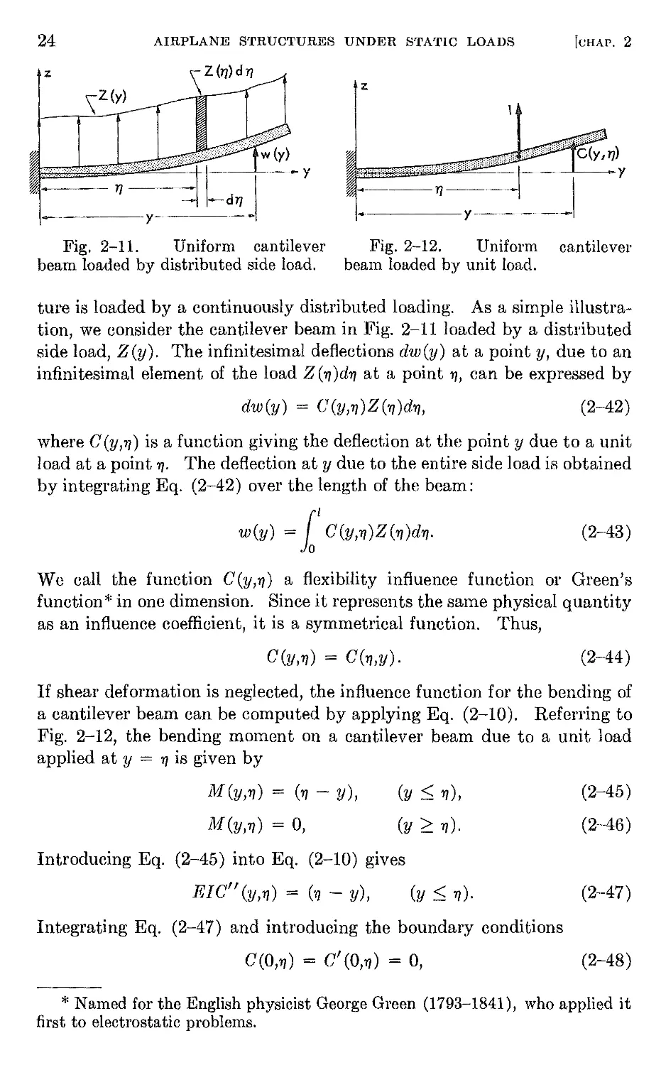
ture is loaded by a continuously distributed loading. As a simple illustra-
tion, we consider the cantilever beam in Fig. 2-11 loaded by a distributed
side load, Z(y). The infinitesimal deflections dw(y) at a point y, due to an
infinitesimal element of the load Z('I'/)d'l'/ at a point '1'/, can be expressed by
dw(y) = C(y,'I'/)Z('I'/)d'l'/,
(2-42 )
where C(y,'I'/) is a function giving the deflection at the point y due to a unit
load at a point '1'/. The deflection at y due to the entire side load is obtained
by integrating Eq. (2-42) over the length of the beam:
w(y) = 1 1 C(y,TJ)Z('I'/)d'l'/. (2-43)
We call the function C (y,TJ) a flexibility influence function or Green's
function * in one dimension. Since it represents the same physical quantity
as an influence coefficient, it is a symmetrical function. Thus,
C(y,'I'/) = C(TJ,Y).
(2-44)
If shear deformation is neglected, the influence function for the bending of
a cantilever beam can be computed by applying Eq. (2-10). Referring to
Fig. 2-12, the bending moment on a cantilever beam due to a unit load
applied at Y = TJ is given by
M(y,'I'/) = ('1'/ - y),
M(y,'I'/) = 0,
(y < '1'/),
(y > TJ).
(2-45 )
(2-46)
Introducing Eq. (2-45) into Eq. (2-10) gives
E I C" (y, TJ) = ('I] - y), (y < '1'/).
(2-47)
Integrating Eq. (2-47) and introducing the boundary conditions
C(O,'I'/) = C'(O,TJ) = 0, (2-48)
* Named for the English physicist George Green (1793-1841), who applied it
first to electrostatic problems.
2-61
DEFORMATIONS UNDER DISTRIBUTED FORCES
25
C(y, YJ)
YJ
. 1
y
Fig. 2-13. Plot of the influence function, C(Y,TJ).
we obtain the influence function of a uniform beam for the range y < 1/:
y2
C(y,1/) = 6EI (31/ - V),
(y < 1/).
(2-49 )
Introducing Eq. (2-46) into (2-10), we obtain
EIC" (y,1/) = 0,
(y > 1/).
(2-50 )
Integrating Eq. (2-50) and evaluating the constants of integration by
putting y = '11 in Eq. (2-49), with the resultant requirements that
'11 3
C(TJ,1/) = 3EI '
1/2
C f ('11,1/) = 2EI '
(2-51 )
we obtain
'11 2
C(y,1/) = 6EI (3y - 1/),
(y > '11).
(2-52 )
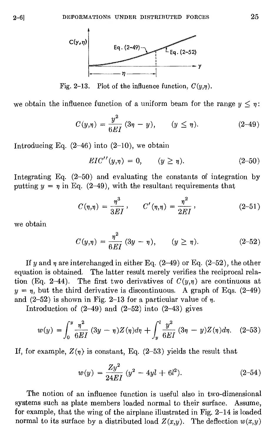
If y and 1/ are interchanged in either Eq. (2-49) or Eq. (2-52), the other
equation is obtained. The latter result merely verifies the reciprocal rela-
tion (Eq. 2-44). The first two derivatives of C(y,1/) are continuous at
y = 1/, but the third derivative is discontinuous. A graph of Eqs. (2-49)
and (2-52) is shown in Fig. 2-13 for a particular value of 1/.
Introduction of (2-49) and (2-52) into (2-43) gives
l y 2 t y2
w(y) = 0 6 1 (3y - 1/)Z(1/)d1) + Jy 6El (31/ - y)Z(1/)dTJ.
(2-53 )
If, for example, Z(TJ) is constant, Eq. (2-53) yields the result that
Zy2
w(y) = 24El (y2 - 4yl + 6Z 2 ).
(2-54 )
The notion of an influence function is useful also in two-dimensional
systems such as plate members loaded normal to their surface. Assume,
for example, that the wing of the airplane illustrated in Fig. 2-14 is loaded
normal to its surface by a distributed load Z (x,y). The deflection w(x,y)
26
AIRPLANE STRUCTURES UNDER STATIC LOADS
[CHAP. 2
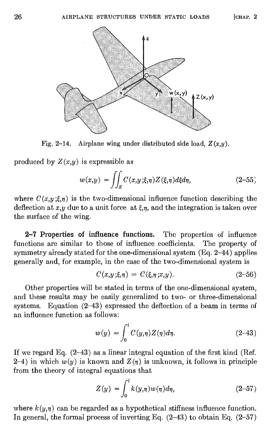
Fig. 2-14. Airplane wing under distributed side load, Z(x,y).
produced by Z (x,y) is expressible as
w(x,y) = 11 C(x,Y; ,rr)Z( ,rr)d drr,
(2-55
where C (x,y ; ,rr) is the two-dimensional influence function describing the
deflection at x,y due to a unit force at ,rr, and the integration is taken over
the surface of the wing.
2-7 Properties of influence functions. The properties of influence
functions are similar to those of influence coefficients. The property of
symmetry already stated for the one-dimensional system (Eq. 2-44) applies
generally and, for example, in the case of the two-dimensional system is
C(x,Yj ,rr) = C( ,rr;x,y).
(2-56 )
Other properties will be stated in terms of the one-dimensional system,
and these results may be easily generalized to two- or three-dimensional
systems. Equation (2-43) expressed the deflection of a beam in terms of
an influence function as follows:
w(y) = 1 1 C(y,rr)Z(7])d7].
(2-43)
If we regard Eq. (2-43) as a linear integral equation of the first kind (Ref.
2-4) in which w(y) is known and Z (rr) is unknown, it follows in principle
from the theory of integral equations that
Z(y) = 1/ k(y,rr)w(rr)drr, (2-57)
where k (y,7]) can be regarded as a hypothetical stiffness influence function.
In general, the formal process of inverting Eq. (2-43) to obtain Eq. (2-57)
2-8]
THE SIMPLIFIED ELASTIC AIRPLANE
27
is formidable. But in a practical problem this process does not have to be
carried out in functional form, and our principal need here is a recognition
of the dual relation between Eqs. (2-43) and (2-57).
The strain energy of a continuously loaded one dimensional system can
be expressed in the form
u = t 1 1 Z(y)w(y)dy.
(2-58 )
Substituting Eq. (2-43), we obtain an expression for the strain energy in
terms of the flexibility influence function and the distributed load,
U = t 1 1 Z(y) 1 1 C(y,rJ)Z(?J)drJdy.
(2-59 )
Similarly, if Eq. (2-57) is substituted in Eq. (2-58), the strain energy can
also be expressed by
U = ! 1 1 w(y) 1 1 k(Y,rJ)w(rJ)drJdy. (2-60)
2-8 The simplified elastic airplane. Because of the complexity of air-
craft structures, it is usually necessary to introduce simplifying assumptions
in order to compute their elastic properties. In many cases, the wings, the
fuselage, and the horizontal and vertical tails can be regarded as beams
rigid in cross sections perpendicular to their lengthwise direction. In such
cases, the airplane becomes a collection of beams which can be represented
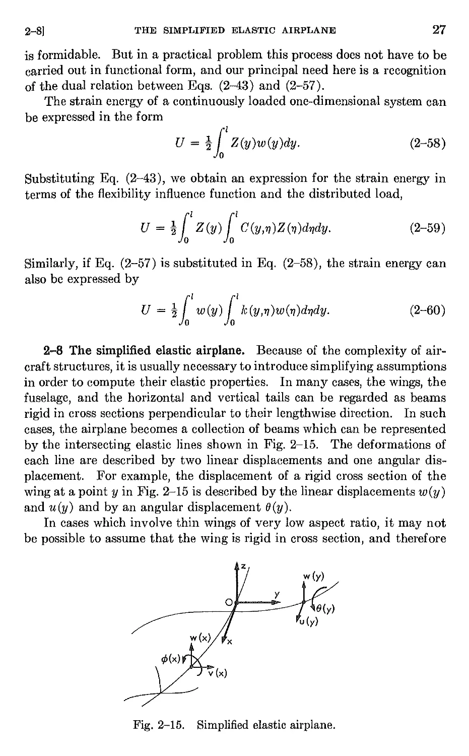
by the intersecting elastic lines shown in Fig. 2-15. The deformations of
each line are described by two linear displacements and one angular dis-
placement. For example, the displacement of a rigid cross section of the
wing at a point y in Fig. 2-15 is described by the linear displacements W (y)
and u(y) and by an angular displacement ()(y).
In cases which involve thin wings of very low aspect ratio, it may not
be possible to assume that the wing is rigid in cross section, and therefore
z
o
y
Fig. 2-15. Simplified elastic airplane.
28
AIRPLANE STRUCTURES UNDER STATIC LOADS
[CHAP. 2
z
w{x,y)
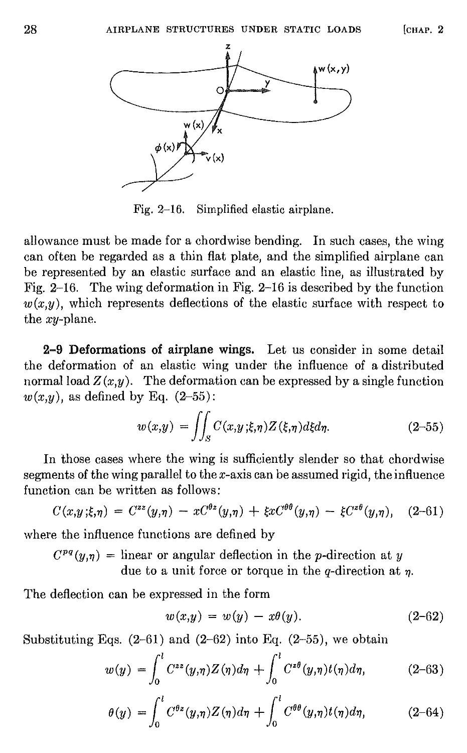
Fig. 2-16. Simplified elastic airplane.
allowance must be made for a chordwise bending. In such cases, the wing
can often be regarded as a thin flat plate, and the simplified airplane can
be represented by an elastic surface and an elastic line, as illustrated by
Fig. 2-16. The wing deformation in Fig. 2-16 is described by the function
w(x,y), which represents deflections of the elastic surface with respect to
the xv-plane.
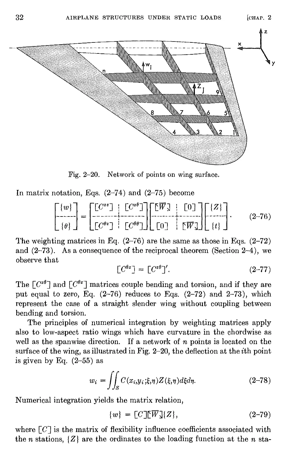
2-9 Deformations of airplane wings. Let us consider in some detail
the deformation of an elastic wing under the influence of a distributed
normal load Z (x,y). The deformation can be expressed by a single function
w(x,y), as defined by Eq. (2-55):
w(x,y) = /1 C(X,y; ,l1)Z( ,l1)d dl1. (2-55)
In those cases where the wing is sufficiently slender so that chordwise
segments of the wing parallel to the x-axis can be assumed rigid, the influence
function can be written as follows:
C(X,Y; ,l1) = CZZ(Y,l1) - xC 9z (y,11) + xC99(Y,11) - cz9(Y,11), (2-61)
where the influence functions are defined by
cpq (y,l1) = linear or angular deflection in the p-direction at y
due to a unit force or torque in the q-direction at 11.
The deflection can be expressed in the form
w(x,y) = w(y) - xO(y). (2-62)
Substituting Eqs. (2-61) and (2-62) into Eq. (2-55), we obtain
w(y) = 1 1 c zz (Y,l1)Z ('rJ)dl1 + 1 1 c z9 (y,1l)t(11)dl1, (2-63)
O(y) = 1 1 C 9Z (Y,11)Z(1l)dl1 + 1 1 C 99 (Y,11)t(11)drJ, (2-64)
2-9]
DEFORMATIONS OF AIRPLANE WINGS
29
where
Z(rJ) = 1 Z( ,l1)d ,
chord
t(rJ) = - r Z( ;IJ)d .
Jchord
(2-65 )
(2-66 )
In deriving Eqs. (2-63) and (2-64), the effects of chordwise drag loads on
the wing have been neglected. Equations (2-63) and (2-64) apply in
general to the case of unswept or swept wings with structural discontinuities.
The principal elastic effects of sweep and structural discontinuities are to
couple the bending and torsional actions. It should be observed that the
assumption of rigidity along segments parallel to the x-axis becomes less
valid with increasing angles of sweep. The error involved seems to be small
for slender wings with angles of sweep up to about 45°.
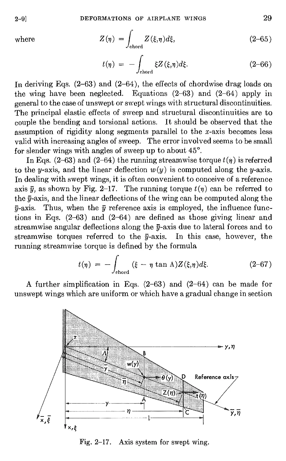
In Eqs. (2-63) and (2-64) the running streamwise torque t(i1) is referred
to the y-axis, and the linear deflection w (y) is computed along the y-axis.
In dealing with swept wings, it is often convenient to conceive of a reference
axis y, as shown by Fig. 2-17. The running torque t(1}) can be referred to
the y-axis, and the linear deflections of the wing can be computed along the
y-axis. Thus, when the y reference axis is employed, the influence func-
tions in Eqs. (2-63) and (2-64) are defined as those giving linear and
streamwise angular deflections along the y-axis due to lateral forces and to
streamwise torques referred to the y-axis. In this case, however, the
running streamwise torque is defined by the formula
t(1}) = _ 1 ( - 1} tan A)Z( ,l1)d .
chord
(2-67 )
A further simplification in Eqs. (2-63) and (2-64) can be made for
unswept wings which are uniform or which have a gradual change in section
Y,l1
y
Ref en
T/
t
Y,T/
x,
Fig. 2-17. Axis system for swept wing.
30
AIRPLANE STRUCTURES UNDER STATIC LOADS
[CHAP. 2
o
, ' ::::::": ('>:: ' ." "" . " X:" ""'i{""" ,".. i;\.: . f:}.::,:"'\....
.....H X............HH ....w.
4¥tt-- - - - <: :::: - - - - - - - --<" % ':.
""" "''''{::",::::,:,::"""",,':'''''''''''''' ,.,."..... p .. p
Elastic axis .
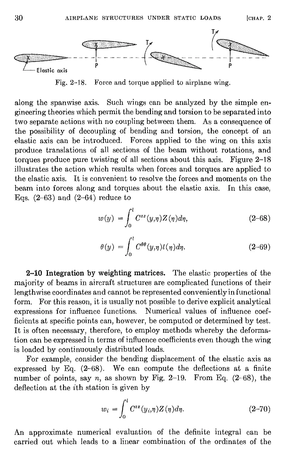
Fig. 2-18. Force and torque applied to airplane wing.
along the spanwise axis. Such wings can be analyzed by the simple en-
gineering theories which permit the bending and torsion to be separated into
two separate actions with no coupling between them. As a consequence of
the possibility of decoupling of bending and torsion, the concept of an
elastic axis can be introduced. Forces applied to the wing on this axis
produce translations of all sections of the beam without rotations, and
torques produce pure twisting of all sections about this axis. Figure 2-18
illustrates the action which results when forces and torques are applied to
the elastic axis. It is convenient to resolve the forces and moments on the
beam into forces along and torques about the elastic axis. In this case,
Eqs. (2-63) and (2-64) reduce to
w(y) = 1 1 CZZ(Y,rJ)Z(rJ)drJ, (2-68)
{}(y) = 1 1 Coe(Y,rJ)t(rJ)drJ.
(2-69)
2-10 Integration by weighting matrices. The elastic properties of the
majority of beams in aircraft structures are complicated functions of their
lengthwise coordinates and cannot be represented conveniently in functional
form. For this reason, it is usually not possible to derive explicit analytical
expressions for influence functions. Numerical values of influence coef-
ficients at specific points can, however, be computed or determined by test.
It is often necessary, therefore, to employ methods whereby the deforma-
tion can be expressed in terms of influence coefficients even though the wing
is loaded by continuously distributed loads.
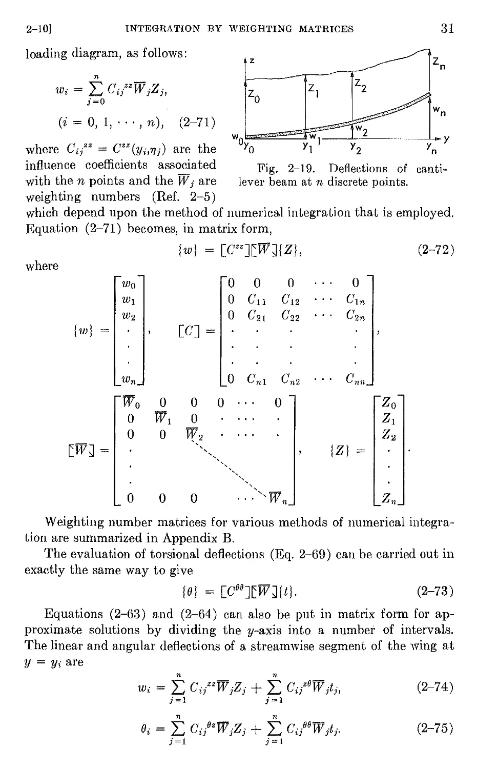
For example, consider the bending displacement of the elastic axis as
expressed by Eq. (2-68). We can compute the deflections at a finite
number of points, say n, as shown by Fig. 2-19. From Eq. (2-68), the
deflection at the ith station is given by
Wi = [I C ZZ (Yi,1])Z(rJ)drJ.
(2-70)
An approximate numerical evaluation of the definite integral can be
carried out which leads to a linear combination of the ordinates of the
2-10]
INTEGRATION BY WEIGHTING MATRICES
31
where Ci/z = C Zz (Yi,rlj) are the
influence coefficients associated
with the n points and the W j are
weighting numbers (Ref. 2-5)
which depend upon the method of numerical integration that is employed.
Equation (2-71) becomes, in matrix form,
loading diagram, as follows:
z
n
Wi = L Ci/z W jZ j ,
j=O
Zo
(i = 0, 1, . . . , n), (2-71 )
w......
Oy
o
Zn
Zl
Z2
W J
Y1
Y Y
n
Fig. 2-19. Deflections of canti-
lever beam at n discrete points.
(wI = [czzJ W J{ZL
where
Wo
WI
W2
000
o C ll C 12
o C 21 C 22
(wI =
[C] =
W n
o C n1 C n2
W o 0
o W I
o 0
o 0 0
o
W ?
" -
"
,
"'" """"
o . . . " W n
W J =
o 0
(2-72)
o
C 1n
C 2n
C nn
Zo
Zl
Zz
(ZI =
Zn
Weighting number matrices for various methods of numerical integra-
tion are summarized in Appendix B.
The evaluation of torsional deflections (Eq. 2-69) can be carried out in
exactly the same way to give
(eJ = [C08] W J(tl.
(2-73)
Equations (2-63) and (2-64) can also be put in matrix form for ap-
proximate solutions by dividing the y-axis into a number of intervals.
The linear and angular deflections of a streamwise segment of the wing at
y = Yi are
n n
Wi = L Ci/z W jZj + L Ci/O W jtj,
j=1 j=I
(2-74)
n n
" 0 - "08-
ei = L.J Cij zWJ.z j + L.J Cij W jtj.
j=l j=l
(2-75)
32
AIRPLANE STRUCTURES UNDER STATIC LOADS
[CHAP. 2
y
Fig. 2-20. Network of points on wing surface.
In matrix notation, Eqs. (2-74) and (2-75) become
t I_] = m -H : J t rH;J t!{m .
(2-76)
The weighting matrices in Eq. (2-76) are the same as those in Eqs. (2-72)
and (2-73). As a consequence of the reciprocal theorem (Section 2-4), we
observe that
[C OZ ] = [C Zo ]',
(2-77)
The [cz O ] and [COZ] matrices couple bending and torsion, and if they are
put equal to zero, Eq. (2-76) reduces to Eqs. (2-72) and 2-73), which
represent the case of a straight slender wing without coupling between
bending and torsion.
The principles of numerical integration by weighting matrices apply
also to low-aspect ratio wings which have curvature in the chordwise as
well as the spanwise direction. If a network of n points is located on the
surface of the wing, as illustrated in Fig. 2-20, the deflection at the ith point
is given by Eq. (2-55) as
Wi = 11 C(Xi,Yi; ,l1)Z( ,l1)d dl1. (2-78)
Numerical integration yields the matrix relation,
{w} = [C] W {Z},
(2-79)
where [C] is the matrix of flexibility influence coefficients associated with
the n stations, {Z} are the ordinates to the loading function at the n sta-
2-111
ENERGY METHODS IN DEFLECTION CALCULATIONS
33
tions, and W is a matrix of weighting numbers. The form of the W
matrix depends) of course) on the scheme of numerical integration that is
employed.
2-11 Energy methods in deflection calculations. Energy methods
find wide use in aeroelastic problems in the determination of deformation
shapes under static and dynamic loads and in the calculation of influence
functions and coefficients.
(a) Deflections by the principle of minimum potential energy. The
principle of minimum potential energy, a useful tool in computing dis-
placements of conservative elastic systems, is based on the principle of
virtual work (Ref. 2-3). The principle of virtual work) applied to deform-
able bodies) can be stated as follows:
If a body is in equilibrium ltnder the action of prescribed external
forces, the work (virtual work) done by these forces in a small additional
displacement compatible with the geometric constraints (virtual displace-
ment) is equal to the change in strain energy.
The principle of virtual work can be stated in the mathematical form
oWe = oU,
(2-80)
where oWe is the virtual work done by the external forces and oU is the
change in strain energy resulting from a small virtual displacement of the
body.
The principle of minimum potential energy, applicable only to con-
servative systems, can be derived by transposing Eq. (2-80):
o U - oWe = 0 (U - V e) = O.
(2-81)
The principle of minimum potential energy, expressed mathematically
by Eq. (2-81), can be stated as follo\vs:
Among all possible deformation configurations compatible with the
geometric constraints, the configuration which satisfies the equations of
equilibrium is the one which minimizes the potential energy, U - We.
The principle of minimum potential energy finds two principal uses
in deflection analyses. The first application is the derivation of exact
differential, integral, or algebraic equations of equilibrium, and the sec-
ond, approximate solutions to deflection problems of continuous systems
which are difficult to solve by exact methods.
(b) The principle of minimum potential energy applied to continuous
systems; Rayleigh-Ritz method. We shall illustrate the application of the
34
AIRPLANE STRUCTURES UNDER STATIC LOADS
[CHAP. 2
z
y
Fig. 2-21. Virtual displacement of cantilever beam.
IS w (y)
principle of minimum potential energy by referring to a cantilever wing
beam under a side load Fz (y), as illustrated by Fig. 2-21.
Let us assume that the lateral deflection of the beam can be written
as a sum of independent deflection functions "(i(Y), each of which satisfies
the geometrical boundary conditions:
n
w(y) = :E "Ii (y)gi,
i=l
(2-82)
where the gi are generalized coordinates whose values are to be deter-
mined. For a cantilever beam, the conditions of geometrical constraint
on the functions 'Yi(y) are
'Yi(O) = "1/ (0) = o.
(2-83)
The coordinates gi are seen to fall within the definition of generalized co-
ordinates, since they act as independent coordinates which represent pos-
sible displacements and which do not violate the conditions of geometric
constraint.
Nex let us assume that the beam is given an arbitrary lateral virtual
displacement, shown by Fig. 2-21, which has a magnitude
n
ow(y) = :E "Ii (y)ogi.
i=l
(2-84)
The corresponding work done by the external forces is given by
oWe = (I Fz(y)ow(y)dy = i2 { t Fz(Yhi(Y)d y f l agi.
Jo t=l Jo
(2-85 )
The strain energy due to bending in a slender beam can be expressed in
terms of the lateral displacement by the following formula (Ref. 2-2):
t ( d Z W ) 2
U = ! Jo EI dy2 dy.
(2-86)
2-11]
ENERGY METHODS IN DEFLECTION CALCULATIONS
When Eq. (2-82) is introduced, this formula becomes
35
n n {1 1 ( d2-y " ) ( d2-y , ) 1
u = t t; J 0 EI dy2 dy; d Y j qiqj.
From this follows for the change in strain energy due to coordinate
changes oqi,
n n { r ( d 2 -y , ) ( d2-y , ) 1
oU = i :; Jo EI dy2 dy'; dy j qjoqi.
Substituting Eqs. (2-85) and (2-88) into Eq. (2-81) gives
n [ n {1 1 ( d2-y , ) ( d2"( , ) 1 1 1 ]
[; 0 EI dy2 d y 2 J d Y j qj - 0 Fz(yhi(y)dy 8qi = O.
Since the oqi are independent, arbitrary quantities, Eq. (2-89)
satisfied only if
i;, [[ EI e: i ) e» d Y ) qj - [F,(Yhi(Y)dY = 0,
(i = 1,2, . . . , n).
(2-87 )
(2-88 )
(2-89)
can be
(2-90 )
Equations (2-90) constitute a set of n simultaneous linear algebraic equa-
tions in the unknown generalized coordinates, ql,"', qn. The final
solution for the lateral deflection is obtained by substituting values of
qb . . . , qn, obtained by solving Eqs. (2-90), jnto Eq. (2-82). This solu-
tion is approximate if n js a finite quantity. The process of finding an
approximate solution in this manner is known as the Rayleigh-Ritz
method (Ref. 2-8).
Let us consider next the restrained three-dimensional elastic body
shown in Fig. 2-22. The x,y,z-axis system is fixed in space and the dis-
placements in the directions of these axes are u(x,y,z), v(x,y,z), and w(x,y,z).
Let Fx(x,y,z), Fy(x,y,z), and Fz(x,y,z) be components of surface force in-
:z;
F
y
y
x
Fig. 2-22. Surface pressures applied to three-dimensional elastic body.
36
AIRPLANE STRUCTURES UNDER STATIC LOADS
[CHAP. 2
tensity. The work done by the surface forces during an arbitrary virtual
displacement is then
oWe = 1 (Fx ou + Fyov + Fzow)dS, (2-91)
where the integration is over the surface. N ext let us assume that any
displacement of the body can be expressed as a function of n discrete gen-
eralized coordinates qi:
u = u(x,y,z,ql,q2,"',qn),
V = v(x,y,z,ql,q2,''',qn),
W = w(x,y,z,ql,q2,"',qn)'
In the beam application discussed above, it can be observed that Eq. (2-82)
is an example of Eqs. (2-92) in a'specific case.
Introducing Eqs. (2-92) into Eq. (2-91), the virtual work due to the
external forces reduces to the form
(2-92)
n {1 ( au av aw ) 1 n
oWe = L F x - + F y - + Fz - dS f oqi = L Qioqi,
i=l s aqi ,aqi aqi i=l
(2-93 )
where
Qi = { ( F x a'u, + F y + Fz aw ) dS
} s aqi aqi aqi
is the generalized force which corresponds to the generalized coordinate qi.
The strain energy can also be expressed as a function of the general-
ized coordinates ql, . . . , qn, and the change in strain energy due to arbi-
trary virtual displacement of the generalized coordinates is
(2-94 )
n aU
oU = L -oqi.
i=l aqi
Introducing Eqs. (2-94) and (2-95) into Eq. (2-81) yields
n { a Ul
L Qi - - f oqi = o.
i=l aqi
(2-95 )
(2-96 )
Since the oqi are independent and arbitrary quantities, this reduces to
aU
-;- = Qi,
uqi
( i' = 1 2 ... n )
" , ,
(2-97 )
where Qi is defined by Eq. (2-94).
Equation (2-97) is an equivalent form of the principle of minimum
potential energy that is applicable to systems in which the space configura-
tion can be described by a set of discrete generalized coordinates. When
n is finite, the process of applying Eq. (2-97) to a continuous system,
2-111
ENERGY METHODS IN DEFLECTION CALCULATIONS
37
called the Rayleigh-Ritz method, leads to approximate solutions. If n
is increased without limit, it is possible for the equilibrium equations
given by Eq. (2-97) to yield an .exact solution.
(c) Deflections by Castigliano's theorem. Castigliano's theorem provides
a method for computing deflections from the strain energy when the latter
is expressed as a function of the applied loads. When Eq. (2-36) is dif-
ferentiated with respect to Qi, we obtain
au a ( n n ) n
Q ' = Q ' ! CijQiQj = CijQj.
u u =l,=l 3=1
(2-98)
Combining Eqs. (2-98) with Eq. (2-3), we obtain the mathematical
statement of Castigliano's theorem:
au
qi = aQi .
(2-99)
Castigliano's theorem states that the partial derivative with respect to
one of the loads of the strain energy, expressed as a function of the applied
loads, yields the deflection of the structure at the point of application and
in the direction of that load.
To demonstrate Castigliano's theorem as a means of computing beam
deflections, let us consider the problem of computing the deflection of the
point a due to an arbitrary side load on a cantilever beam, as shown by
Fig. 2-23. We apply an additional dummy load P at the point a at which
we seek the deflection . If the bending moment distribution due to a
1-lb load at a is given by m, then, by the principle of superposition, the
bending moment distribution due tc
a load P at a is given by mP. The
strain energy due to normal strains
in a slender beam can. be expressed
in terms of the applied bending
moment distribution M by the fol- "
lowing formula (Ref. 2-2):
z
y
1 -2
U = 1 I dy.
(2-100)
Fig. 2-23. Cantilever beam under
arbitrary side load.
The strain energy due to the given side load plus the dummy load P is
obtained by substituting
M = M (y) + mP
(2-101)
into Eq. (2-100):
1 1 (M + mp)2
U = 0 2EI dy.
(2-102)
38
AIRPLANE STRUCTURES UNDER STATIC LOADS
[CHAP. 2
The deflection at a resulting from the given side load plus the dummy load
P is obtained by applying Castigliano's theorem:
= aU = 1 1 (M + mP)m d y .
ap 0 EI (2-103)
The deflection at a due to the given side load alone is ohtained from Eq.
(2-103) by putting P = 0:
6 = 1 1 7 dy.
Equation (2-104) may, for example, be used
efficients if written in the form
tmimj
C ij = Jo EI dy,
(2-104 )
to compute influence co-
(2-105 )
where
mi = bending moment distribution due to l-lb load at i,
mj = bending moment distribution due to l-lb load at j.
2-12 Deformations of slender unswept wings. Let us consider a type
of beam in which the skin and shear webs are assumed thin, that is, they
have no bending rigidity, and the cross-sectional shape is preserved by
closely spaced ribs which have infinite rigidity in their own plane but are
completely free to warp out of their plane. The beam may taper in the
spanwise direction, and the properties of the cross section may vary with y.
The reference axes are illustrated by Fig. 2-24. It is convenient in the
present discussion to assume that the y-axis is placed such that it pierces
each cross section at the centroid of the effective normal stress-carrying
area and that the x- and z-axes are oriented so that the xy- and yz-planes
pass through the principal bending axes. A point on the cross section is
located by the spanwise coordinate y and the tangential coordinate 8. The
tangential coordinate is measured positive in the counterclockwise direc-
Fig. 2-24. Loaded cross section of shell beam.
2-12]
DEFORMATIONS OF SLENDER UNSWEPT WINGS
39
tion for the peripheral skin and is positive in the positive direction of the
z-axis for the interior webs.
A loaded cross section at a distance y from the origin is acted on by a
moment M(y), a shear S(y), and a torque T(y), with positive directions
as shown in Fig. 2-24. The point of application of S (y) and T (y) is at the
center of twist or shear center of the section. Normal stresses, assumed
positive in the y direction, are denoted byu, and shear flows, assumed
positive in the s direction, are denoted by q.
In discussing slender beams, we make two simplifying assumptions.
First, the beam is permitted complete freedom to warp when torque loads
are applied. This leads to the St. Venant solution of the torsion problem
and permits the simplification that bending and torsion are separate un-
coupled actions. Second, we assume that plane sections remain plane
during bending. This allows application of the well-known engineering
bending theory.
(a) Bending and shearing deformations. The wing is composed of skin
elements in equilibrium under normal stresses u and shear flows q, as
illustrated by Fig. 2-25. Since the ribs are assumed rigid in their own
planes, and we may neglect normal stresses in the chordwise direction, the
strain energy in the wing in terms of stresses is
1 1 1 [ 1 1 1 [ ds
U = - u 2 tdsdA + - il - dA
2E 0 c.s. 2G 0 C.8. t '
(2-106 )
where t is the skin thickness, the integration on s is over the wing cross
section, and the integration on X is over the length of the wing beam. Let
us compute first .the lateral deflection w(y) of the wing resulting from a
bending moment distribution, M (A), and a shear distribution, SeA). In
order to apply Castigliano's theorem, we must apply an additional ex-
ternal load P at the spanwise location A = y. Then we denote the total
normal stress due to the given bending moment M(A), plus P, by
au
u(A,s) = u(A,s) + P ap ,
(2-107a)
where u (A,s) is the normal stress due to the given bending moment distribu-
a
z
y
q+
ds
Fig. 2-25. Element of wing skin.
40
AIRPLANE STRUCTURES UNDER STATIC LOADS
[CHAP. 2
tion M (X) and au / ap is the normal stress distribution due to P = 1 located
at X = y. Similarly, the total shear flow is denoted by
0-
q(X,s) = q(X,s) + P a '
(2-107b)
where q(X,s) is the shear flow due to the given shear distribution SeX), and
aqlaP is the shear flow due to P = 1 located at X = y.
Substituting Eqs. (2-107a) and (2-107b) into Eq. (2-106), the total
strain energy due to the given bending moment and shear distributions plus
the dummy load Pis.
1 1 1 [ [ aU J 2
U = 2E 0 C.8. O"(X,s) + P aP tdsdX
1 (I i [ aq J 2 ds
+ 2G Jo C.8. q(X,s) + P aP t dX.
(2-107c)
Differentiating with respect to P and setting P = 0, the lateral deflection
w (y) becomes
1 t [ au 1 t [ aq ds
w(y) = E Jo C.s. O"(X,s) aP tdsdX + G Jo C.s. q(X,s) aP t dX. (2-108)
The first term in Eq. (2-108) represents the bending deflection, which
we denote by a (y) :
a(y) = ; 11£.s. u(X,s) :; tdsdX.
If we assume, for example, that the engineering theory of beam bending
can be applied, the normal stresses are represented by
(2-109a)
M(X)z
u(X,s) = - I '
{ y - X
au - -z,
-= I'
aP 0
,
(y > X))
(y < X),
(2-109b)
where I is the area momeilt of inertia of the cross section about the x-axis.
Substituting Eqs. (2-1 09b) into Eq. (2-109a) results in
( ) = (Y M (X ) (y - X) d
a y Jo E I X.
(2-109c)
Differentiation of Eq. (2-109c) twice with respect to y produces the follow-
ing relation between beam bending moment and curvature:
" M
a =-.
EI
(2-110)
2-12]
DEFORMATIONS OF SLENDER UNSWEPT WINGS
41
The second term in Eq. (2-108) represents the shearing deflection,
which we denote by f3 (y) :
1 i l [ vij ds
(3(y) = - q(A,S) - - dA.
G 0 C.s. fJP t
If we assume that the shear flow distribution due to S = 1 is denoted by
u(X,s), then
(2-111a)
q(A,S) = SU(A,S),
fJij _ J U (A,S),
fJP - l 0,
(y > X),
(y < A).
(2-111b)
Substituting Eqs. (2-111b) into Eq. (2-111a) gives
t'SdA
(3(y) = Jo GK '
(2-111c)
where
K = 1
[ 2 ds
u-
C.8. t
is a shearing constant of the beam cross section defined in terms of the shear
flow distribution due to a unit shear force. The quantity GK in Eq.
(2-111c) is termed the shearing rigidity of the beam. Differentiating
Eq. (2-111c) with respect to y gives a relation between the shear and the
first derivative of the shearing deflection, as follows:
/ S
f3 =-.
GK
(2-112)
(b) Influence functions and coefficients. Influence functions taking both
bending and shearing deformations into account can be computed from
Eq. (2-108). For example, to compute C ZZ (y,"7) by applying the engineering
theory of beam bending, we put
U(A,S) = "7 - A (0 < A < "7),
--z
I '
fJii y-X (0 < A < V),
- z,
fJP I
and
q(A,S) = U(A,S), (0 < A < 'YJ),
fJij (0 < A < y),
fJP = U(A,S),
(2-113a)
(2-113b)
42
AIRPLANE STRUCTURES UNDER STATIC LOADS
[CHAP. 2
into Eq. (2-108). For the case of 'f/ > y, this yields
{Y ('f/ - X) (y - X) (Y dX
CZZ(y,'f/) = Jo EI dX + Jo GK '
('f/ > V), (2-114)
and for the case of y > 'f/,
C ZZ ( ) = (" ('f/ - X)(y - X) dX + 1 " ,
y,'f/ Jo EI 0 GK
Influence coefficients can be obtained from Eqs. (2-114) and (2-115) by
introducing explicit numerical values for y and 'f/.
(c) Torsional deformation and influence function. If, during the applira-
tion of torsional moments, the beam is free to warp, the strain energy is due
entirely to shear stresses, as follows:
(y > 'f/). (2-115)
1 i l l ds
u = - il -- dX.
2G 0 e.s. t
(2-116)
By applying Castigliano's theorem in the same manner as for the bending
problem, the angle of twist of the beam due to a given distribution of
applied torque, T(X), can be expressed as
1 1 1 1 aij ds
O(y) = -.- q(X,s) - - dX,
G 0 e.s. aT t
(2-1l7a)
where q(X,s) is the shear flow distribution due to the applied torques and
aij/ aT is the shear flow distribution due to a unit torque T = 1 applied at
the spanwise station X = y.
If we assume that the shear flow distribution due to T = 1 is denoted
by veX,s), then
q(X,s) = T(x)v(X,s),
aij = { VeX,s),
aT 0,
(y > X),
(y < X).
(2-117b)
Substituting Eqs. (2-117b) into Eq. (2-117a) gives
( ) _ i ll T(X)dX
o y - ,
o GJ
(2-117c)
where
1
J=
1 2ds
v -
c.s. t
is the torsion constant of the beam cross section. The quantity GJ is
termed the torsional stiffness of the beam. Differentiating Eq. (2-117c)
2-121
DEFORMATIONS OF SLENDER UNSWEPT WINGS
43
z
Fig. 2-26. Cantilever wing under unit torque load.
with respect to y gives a relation between the applied torsional moment and
the rate of twist, as follows:
! T
(J =-.
GJ
(2-118)
The deflection problem to be solved in computing the torsional influence
function is illustrated by Fig. 2-26. A unit torque about the elastic axis
is applied at a distanc 'f/ from the origin, and the resulting angular displace-
ment at y is denoted by COfJ(y,'f/). The influence function CfJ()(y,'f/) is
obtained from Eq. (2-117a) by putting
q("A,s) = v("A,s), (0 < "A < 'f/),
aq
- = V ( "A S )
aT "
(0 < "A < v).
(2-119)
This gives, for 'f/ > y,
(Y d"A
C()()(y,'f/) = Jo GJ '
('f/ > V),
(2-120 )
and for y > 'f/,
l YJd "A
Coo(y,'f/) = 0 GJ '
(y 'f/).
(2-121 )
The torsion constant J, defined in Eq. (2-120), call be easily evaluated
at each section of the beam, providing the shear flow distribution due to a
unit torque, v(s,"A), is known. As a simple example of this, . consider the
case of a single-cell beam. Suppose that a torque T is applied to a single-
cell box, as illustrated by Fig. 2-27. Since we assume complete freedom
to warp, normal stresses cannot be induced. Referring to Fig. 2-25, which
illustrated the free-body diagram of a skin element, we observe that when
(J' = 0, we have
aq
- =0.
as
(2-122)
44
AIRPLANE STRUCTURES UNDER STATIC LOADS
[CHAP. 2
4 %1
q! ,) dA J 1.
-.
q
Fig. 2-27. Torque applied to single cell box.
Equation (2-122) tells us that the shear flow q around a single cell box is
constant.
Referring to Fig. 2-27 and equating the applied torque to the moments
of the applied shear flows about an arbitrary point, we obtain
T = f qrds.
(2-123)
Since q is constant around the section, Eq. (2-123) reduces to the result
known as Bredt's formula,
T = 2Aq,
(2-124)
where A is the cross-sectional area of the cell.
Putting this result into Eq. (2-120), we obtain a formula for the torsion
constant of a single-cell section:
4A 2
J = -. (2-125)
f s
In computing the torsional rigidity of a multi cell box, we must compute
the shear flow distribution in a statically indeterminate system due to the
unit torque. Methods for accomplishing this are well known and may be
found, for example, in Ref. 2-10.
(d) Elastic axis. We have derived formulas in Parts (a) and (b) above
for computing bending and torsional flexibility influence coefficients of
beams with straight elastic axes. In order to use these results) it is necessal'Y
to know the location of the elastic axis. The elastic axis is located by
drawing a span wise line through the shear centers of .the cross sections of
the beam. The shear center of each cross section is computed by establish-
ing the point in the plane of the section at which a sheal' force can be applied
to the section without producing afate of twist of the section. Methods for
computing the shear center location of multi cell beams may be found in
Refs. 2-2 and 2-10. Tests of full-scale wings and of models are frequently
employed as a means of determining elastic axis locations for aeroelastic
studies.
2-12]
DEFORMATIONS OF SLENDER UNSWEPT WINGS
45
EXAMPLE 2-1. To calculate the influence coefficients of the wing of a jet transport.
The planform of the wing is illustrated by Fig. 2-28. The elastic axis is straight
and perpendicular to the root at 35% of the chord. The curves of bending
rigidity El, torsional rigidity GJ, and shearing rigidity GK have been computed
and are plotted in Fig. 2-29. It is desired to calculate the five by five matrices of
bending and torsional influence coefficients at wing stations 90, 186, 268, 368,
and 458.
Solution.
(a) Matrix of bending influence coefficients. The bending influence coefficients
are obtained by a numerical evaluation of Eqs. (2-114) and (2-115). Exnandinll
487"
370"
L Elastic axis
(35% C)
1 . - 186"
i== Fuselage t.
I I
L I- -""--Jet nacelle
500"
Fig. 2-28.
Wing planfofm of typical jet transport.
-0 0 0
I
I
0 0 I
0
X )(
x
::.:: -,
0 0 w
30 3.0 7
25 2.5 6
20 2.0 5
15 1.5 4
3
10 1.0
2
5 0.5 1
0 0 0 100 200 300 400 500
Wing station (inches)
Fig. 2-29. Bending, torsional, and shear stiffness curves.
46
AIRPLANE STRUCTURES UNDER STATIC LOADS
[CHAP. 2
Eq. (2-115) and putting Y = Yi and 1} = Yj, we obtain an expression for the
bending influence coefficient Cij, as follows:
FYi d"A (Yi"Ad)., . FYi "A 2 d"A FYi d"A
Cij = YiYjJo EI - (Yi + Yj) Jo El + Jo El + Jo GK '
(Yi 2:: Yj).
(Ii.)
Putting Y j = 90, we can, for example, compute the first column of the bending
influence coefficient matrix from the following formula:
1 90 d)., 1 90 "Ad"A 1 90 "A2d"A 1 90 d"A
Cil = 90Yi - - (Yi + 90) - + - + - ,
o EI 0 El 0 El 0 GK
(b)
where Yi = 90, 186, 268, 368, and 458. The definite integrals can be evaluated by
plotting 1/El, "A/El, "A2/El, and 1/GK, as shown by Fig. 2-30, and taking the
areas under the curves to the left of Sta. 90. A planimeter may be used, but the
trapezoidal rule is easy to apply and usually provides sufficient accuracy. Eval-
uating the areas under the curves, we get for Co,
Co = (.44126Yi - 4.369) X 10- 7 + 37.07 X 10- 7 ,
(c)
where the first term is due to the normal strains and the second term due to the
shear strains. Putting Yi equal to 90, 186, 268, 368, and 458, we get
C ll = 35.3445 X 10- 7 + 37.07 X 10- 7 = 72.410 X 10- 7 in/lb,
C 2l = 77.7054 X 10- 7 + 37.07 X 10- 7 = 114.771 X 10- 7 ,
C al = 113.889 X 10- 7 + 37.07 X 10- 7 = 150.955 X 10- 7 , (d)
C 41 = 158.015 X 10- 7 + 37.07 X 10- 7 = 195.081 X 10- 7 ,
C n = 197.728 X 10- 7 + 37.07 X 10- 7 = 234.794 X 10- 7 .
<0 0
0 00 -Co
0 .....
..... 0
..... .....
x x
........ x x
..... ........ ........ ........
LU ..... .....
N "" 0
.-< ::>
- - - -
10 20
9 18
8 8 16 4
7 7 14 3.5
6 6 12 3
5 5 10 2.5
4 4 8 2
3 3 6 1.5
4 1 1
2 2 E1
1 1 2 0.5
A
0 0 0 0 100 200 400 500
Fig. 2-30. Plots of integrands involved in influence coefficient calculations.
2-13]
SLENDER SWEPT WINGS
47
The shear deformations are a significant fraction of the total at the inboard
stations, whereas they are relatively unimportant at the outboard stations. The
results computed above give not only the first column of the matrix but also the
first row, because of the reciprocal theorem. Other rows and columns can be
computed in the same way. The final matrix of bending influence coefficients
becomes
[czzJ =
0 0 0 0 0 0
0 72.410 114.771 150.995 195.081 234.794
0 114.771 253.306 461.299 714.949 943.234 X 10- 7 in/lb. (e)
0 150.995 461.299 1247.53 1911.22 2508.54
0 195.081 714.949 1911.22 2649.96 5237.42
0 234.794 943.234 2508.54 5237.42 8434.02
(b ) Matrix of torsional influence coefficients. The torsional influence coeffi-
cients are obtained from Eqs. (2-120) and (2-121) by calculating areas under the
l/GJ curve, as follows:
1 90 d'A .
Cll = C 12 = C 13 = C 14 = C 15 = - = 36 X 10- 10 rad/m'lb,
o GJ
1 186 d'A
C 22 = C 23 = C 24 = C 25 = - = 75.36 X 10- 10 ,
o GJ
1 268 d'A
C 33 = C 34 = C 35 = - = 113.26 X lO- lO ,
o GJ
£ 368 d'A
C 44 = C 45 = - = 204.66 X 10- 10 ,
.0 GJ
1 458 d'A
C 55 = - = 409.49 X lO- lO .
o GJ
(f)
Constructing the matrix of torsional influence coefficients from the above, we
obtain
0 0 0 0 0 0
0 36 36 36 36 36
[CooJ = 0 36 75.36 75.36 75.36 75.36 X 10- 10 rad/in.lb. (g)
0 36 75.36 113.26 113.26 113.26
0 36 75.36 113.26 204.66 204.66
0 36 75.36 113.26 204.66 409.49
2-13 Influence functions and coefficients of slender swept wings.
In Section 2-9 the deformation of a swept wing was described by Eqs.
(2-63) and (2-64) in terms of linear and angular displacements of stream-
wise segments due to running loads and torques applied along a reference
axis y. In the case of slender swept beams of large aspect ratio, an effective
root can be assumed, as shown by Fig. 2-31.' Thus, an elastic axis can be
postulated, and the y reference axis can be located along the elastic axis.
48
AIRPLANE STRUCTURES UNDER STATIC LOADS
[CHAP. 2
:..---- Effective root
f --L. -
. cosA dA.
Sin A Ei
o
Actual root/
Y/TJ
x
..I cos A
--L- _
i cosA d A
cos A 0 G J Y / TJ, A.
J ..L. - J --L- -
2 A cosA d A . 2 cosA d "-
cos ./1 _ + sin A _
o GJ 0 EI
Slender swept beam with effective root.
Fig. 2-31.
If it is assumed that the y-axis is a true elastic axis, the influence functions
in Eqs. (2-63) and (2-64) can be computed by slender beam theory.
The influence function CZZ(Y,71) which describes the linear deflection of
the elastic axis at Y due to a unit load applied to the elastic axis at 71 follows
directly from Eqs. (2-114) and (2-115):
j Y/COS A ( _ ) ( -.JL _ )
CZZ ( ) _ cos A cos A d -
y,rj - 0 EI A
l Y / COS A d
+ 0 GK '
(rJ > V),
(2-126 )
CZZ ( ) _ l /COS A ( - ) ( - ) _
y,rj - 0 EI dA
l /COS A d
+ 0 GK '
(y > rj),
(2-127)
where EI and GK are stiffness properties of the beam on sections normal
to the elastic axis.
The function C 88 (y,rj) represents the angular deflection of the stream-
wise strip A-B about the y-axis due to a unit stream wise torque applied to
the reference axis at 71. Figure 2-31 shows the unit stream wise torque at 71
divided into components parallel and perpendicular to the elastic axis and
the angular deflections which these components produce at y when y < rj.
2-14]
LOW ASPECT-RATIO WINGS
49
The function Coo (Y,"f/) is the resultant component of twist about the y-axis:
00 ' / _ l Y/cOS A ( cos 2 A sin 2 A ) _
C (Y,"f/) - 0 GJ + EI dX, ("f/ 2:: V), (2-128)
where EI and GJ are stiffness properties of the beam on sections normal to
the elastic axis. It can also be seen that
00 _ l 'l'f/ cOS A ( cos 2 A sin 2 A ) _
C (y,1]) - 0 GJ + EI dX, (y 2:: 1]). (2-129)
Finally, C Oz (y,1]) is the angular deflection of the streamwise strip A-B
about the y-axis due to a unit load applied to the reference axis at 1]:
l v/cDs A ( _ -X )
o ( . cos A -
C Z y, 1]) = - S1l1 A dX,
o EI
1 'l/C08 A ( _ -X )
o . cos A -
C Z(y,1]) = - S111 A 0 EI dX,
(1] > V),
(2-130)
(y 2:: "f/).
(2-131 )
Using the reciprocal relation given by Eq. (2-32), the influence function
C Z (J(y,1]) is obtained from C OZ (y,1]) by interchanging y and "f/:
c zO (y,1]) = C OZ (1],y). (2-132)
2-14 Deformations and influence coefficients of low aspect-ratio wings.
In dealing with explicit methods of predicting structural deformations, we
have so far confined our remarks to slender wings 'which can be treated by
the engineering beam theory. Modern configuration trends in high-speed
aircraft design, however, have been away from slender wings and towards
low aspect-ratio surfaces of the type exemplified by the wing of the XF-92A
airplane, illustrated in Fig. 2-3. The problem of predicting the elastic
properties of low aspect-ratio surfaces for aeroelastic analyses presents
exceptional difficulties and requires the expenditure of considerable time
and effort in order to arrive at useful and accurate results.
Analyses of low aspect-ratio surfaces are significantly different from
analyses of long slender wings in at least two important respects. First,
the root restraint plays a much more important role in the deformations
and, hence, must be accounted for more rigorously. This stipulation
applies primarily to root restraint against warping, which has a profound
effect upon the twisting action of the wing (Ref. 2-11). Second, camber
bending of the surface may become a significant component in the defor-
mation. As a result, the wing may behave in a manner similar to a plate
with elastic curvature of appreciable magnitude in two directions. In
recent years, considerable effort has been expended in deriving methods of
analysis of deformations of both built-up and solid low aspect-ratio wings.
50
AIRPLANE STRUCTURES UNDER STATIC LOADS
[CHAP. 2
The intensive demand for low drag,. low aspect-ratio, supersonic lifting
surfaces has resulted in a continuous decrease in thickness ratio. Structural
design trends accompanying this thickness ratio reduction have been. to-
wards thicker cover skins and multiple webs. The ultimate limit of this
process is, of course, the completely solid wing. In an effort to reduce drag
to an absolute minimum, supersonic missile designers have frequently
employed solid lifting and control surfaces.
In general, it can be said that deformation analyses of low aspect-ratio
wings can be divided into three fundamentally different methods of ap-
proach. The first method, which applies essentially to built-up wings, was
described by Levy in 1947 (Ref. 2-12). This approach views the structure
as an assemblage of a finite number of elastic components. Each com-
ponent is placed in equilibrium and the forces acting on the various com-
ponents are regarded as the unknown quantities. If the structure is
statically determinate, the internal forces can be computed from the equa-
tions of equilibrium and the deflections can be obtained by applying
Castigliano's theorem. If the structure is statically indeterminate, the
correct internal force system must be obtained by application of the
principle of minimum strain energy. Application of the latter is equivalent
to imposing the requirement that the deforination of each member be
,
compatible with the deformation of every other member. Subsequent
papers by Lang and Bisplinghoff (Ref. 2-13), Langefors (Ref. 2-14), and
Wehle and Lansing (Ref. 2-15) have made further contributions to Levy's
method of approach. These contributions have consisted largely of
methods for casting the problem in matrix form and improved techniques
for solution.
The second method, which also applies essentially to built-up wings, is
similar to the first in that it views the structure as an assemblage of inter-
connected elastic components. But in this method the deformations of the
various discrete components of the structure are regarded as the unknown
quantities, instead of the forces on the components. The deformation of
each elastic component is required to be compatible with the deformation
of every other component. The correct deformation pattern is obtained
by applying the principle of minimum potential energy. Such an applica-
tion is equivalent to the requirement that every component of the structure
should be in static equilibrium. This method is sometimes called .the
method of direct stiffness calculation. Contributors to this method of
approach have included Schuerch (Ref. 2-16), Levy (Ref. 2-17), and
Turner, Clough, Martin, and Topp (Ref. 2-18).
A third method of approach applies to both built-up and solid wings.
It consists of applying the principle of minimum potential energy in the
form of either the Rayleigh-Ritz or the generalized Rayleigh-Ritz method.
In these methods the space configuration of the deformed elastic surface is
taken as a superposition of assumed deformation modes. The contribution
2-151
PRINCIPLE OF MINIMUM STRAIN ENERGY
51
of each assumed mode is obtained by application of the principle of mini-
mum potential energy. The basic contributions to this method of approach
hava been made primarily by Reissner and Stein (Ref. 2-19) and Fung
(Ref. 2-20).
Although the present chapter is devoted primarily to analysis, it
should be remarked that structural models can be employed as a means of
obtaining influence coefficients in many instances where analysis is not
deemed sufficiently reliable. As a result of the widely different structural
arrangements which are currently being developed, structural models will
undoubtedly be used more extensively in the future. Faithful model
reproductions are expensive, however, and take considerable time to con-
struct. Moreover, they tend to become obsolete due to design changes if
they are constructed too early in the airplane program. These factors, as
well as others which relate to structural models, are discussed at greater
length in Chapters 12 and 13.
2-15 Influence coefficients of complex built-up wings by the principle
of minimum strain energy. An airplane structure, no matter what shape
it may assume, is fundamentally a group of elastic elements joined together
to form a system that is often statically indeterminate. The structure
can usually be idealized so that it consists of structural elements such as
axially loaded flange elements, shear panels, or other types of elementary
members whose strain energy can be computed in terms of internal stresses.
This idealization is essentially a process of replacing a continuous system
by an equivalent lumped parameter system. The success of the method is
largely due to the ability of the analyst to replace the actual structure by a
simple idealized structure which retains the essential features of the actual
structure. For example, it is common practice in the analysis of slender
monocoque structures with thin cover sheets to consider the axial-load and
shear-carrying capacities of the cover sheet separately. Thus, the axial-
load carrying contribution of the cover sheet is handled by lumping the
various portions of the cross-sectional area of the cover sheets with that of
the neighboring spar caps and other axial reinforcements. This practice is
based on the assumption that the stress in the cover sheet in the direction
perpendicular to the spar caps and axial reinforcements is negligible. For
high-aspect ratio wings with relatively little taper or sweep and with bul1c-
heads and ribs perpendicular to the beam axis, this implicit assumption is
nearly satisfied. In a multispar delta wing or other wing of low aspect
ratio, the selection of a direction of negligible stress in the cover sheet is
no longer possible (Ref. 2-17). Thus, in a low aspect-ratio wing, it is
desirable to consider the load-carrying ability of the cover sheet both in the
direction parallel to the spars and in a transverse direction.
Suppose, for example, that we wish to compute the influence coefficients
associated with m points on the structure illustrated in Fig. 2-32. We can
52
AIRPLANE STRUCTURES UNDEH Rl'ATIC LOADS
[CHAP. 2
Q]
"
?0 "
.% '"
Q2
'-.. Cover plate elements
Fig. 2-32. Wing structure partitioned into stl'Uctural elements.
compute the deflection at the ith point due to a unit load at the jth point by
the principle of virtual work. When the entire matrix of influence coeffi-
cients is desired, however, there is a somewhat more direct approach which
yields the matrix in one operation (Refs. 2-12 and 2-13). Suppose that the
structure is partitioned into n separate structural elements (cj. Fig. 2-32).
If the loads in these elements can be- represented by the n values PI, . . . , pn,
the total strain energy in the structure is given by
U = !Lpl, . . " PnJ[F][PI, . . . , Pn},
where the [F] matrix is a symmetrical matrix such that
(2-133 )
[F] = [FJ'.
(2-134)
Under the applied loads (21, . . . , Qm on the structure, a stress analysis
yields the internal loads as a linear function of the applied loads, as follows:
[Pi, . . ., PnJ = [G][Ql, . . " QmJ.
Substituting Eq. (2-135) into (2-133), we obtain
U = !LQ1' . . . , (2mJ[GJ'[F][G] [(21, . . . , Qm J.
(2-135 )
(2-136)
Comparing Eq. (2-136) with Eq. (2-40), we see that the matrix of influ-
ence coefficients associated with the m points of load application is an
m by m matrix given by
[C] = [G]'[F][G].
(2-137)
In most cases involving practical wings, the process described above is
complicated by the fact that the wing structure is statically indeterminate,
2-15J
PRINCIPLE OF MINIMUM STRAIN ENERGY
53
and the matrix [G] cannot be computed from statics alone. Suppose that
from the application of the principles of static equilibrium to each struc-
tural element we can construct only If, independent equations of equilibrium
as follows:
[E]{PlI . . . , Pn, QI,' . . , QmJ = O.
The degree of redundancy of the structure is therefore
r = n - k.
(2-138)
(2-139 )
If r redundant members are selected from among the n members, Eq. (2-138)
can be solved for the n unknown internal loads in terms of the applied
loads and the r redundant loads as follows:
{Pi, . . . , Pnl = [G](Ql, . . . , Qrn, Prl,
(2-140)
where Pr indicates the loads in the redundant members. If the system is
statically determinate and Pr = 0, Eq. (2-140) would, of course, consti-
tute a complete solution of the internal stress distribution.
The redundant stresses can be computed by applying the principle of
minimum strain energy. Substituting Eq. (2-140) into Eq. (2-133) gives
U = !LQl, ..., Qrn, PrJ[H]{Ql, . . ., Qm, Prl. (2-141)
where
[H] = [GJ'[F][GJ.
App]ying the prineiple of minimum strain energy (Ref. 1-3) expressed by
aU
-=0,
apr
(2 142)
there is obtained the column matrix of redundant loads
{Prl = -[H pp ]-l[H pQ ]{Qi,"', Qrnf.
(2-143)
The matrices [HppJ and [HpQJ are formed by partitioning:
[H] = r - - J .
HpQ : Hpp
(2-144)
From Eq. (2-143), we observe that
{Ql, . . . , Qrn, Pr 1 = r ------[! ;----- J I Ql, . . . , Qm J
- [HppJ [HpQJ
(2-145 )
Introducing Eq. (2-145) into Eq. (2-141) and reducing, we obtain
U = !LQI,"', QmJ[[H QQ] - [H Qp][HppJ-l[HpQ]J {Ql,''', Qm I. (2-146)
54
AIRPLANE STRUCTURES UNDER STATIC LOADS
[CHAP. 2
Fig. 2-33. Simplified sheet-metal box.
Comparing Eq. (2-146) with Eq. (2-40), we see that the matrix of influ-
ence coefficients is expressible as
[C] = [[H QQ ] - [HQp][Hpp]-l[HpQ]]. (2-147)
Since the [H] matrix can be easily formed and partitioned, Eq. (2-147)
provides a convenient means of computing the matrix of flexibility influ-
ence coefficients of a statically indeterminate structure. It should be
observed, however, that evaluation of Eq. (2-147) requires inversion of the
matrix [H pp ]. Thus, if there are r redundant members, it is necessary to
invert a matrix of r rows and columns. I t is apparent, therefore, that the
computational labor required by the above method may become prohibi-
tively great if the struct ure is highly redundant.
EXAMPLE 2-2. To compute the matrix of flexibility influence coefficients asso-
ciated with points A and B of the simple aluminum alloy sheet metal box shown
by Fig. 2-33. In carrying out the analysis, the following assumptions are intro-
duced:
(a) Sheets carry only shear flows.
(b) Flanges carry only normal stresses.
(c) Normal stresses vary linearly along the flanges.
Solution. The first step in the solution is to break the structure into its
various component parts and draw a free-body diagram of each part, as shown
by Fig. 2-34. The [G] matrix indicated by Eq. (2-140) is formed from the equa-
tions of equilibrium. The independent equations of equilibrium are (ef. Fig. 2-34)
QA = Pl + P2, QB = -P2 + pa. (a)
Since there are three unknown internal forces) pl, P2, and Pa, and only two equa-
tions of equilibrium, we see that one redundant quantity exists. We shall select
P2 as the redundant quantity in this analysis. The equilibrium equation can be
used to form the following matrix equation:
G:] [ -:J[ : 1
(b)
2-15]
PRINCIPLE OF MINIMUM STRAIN ENERGY
55
PI
P3
Fig. 2-34. Simplified box exploded into structural elements.
The [GJ matrix is therefore
[ 1 0 -1 ]
[GJ = 0 0 1.
011
(c)
The [FJ matrix indicated in Eq. (2-133) is formed by computing the strain
energy in terms of the internal forces Pl, P2, and P3. In order to do this, we need
fOl'mulas for the strain energy in an axially loaded member in which the stress
varies linearly along its length, and the strain energy in a sheet in pure shear.
Each axially loaded member in the structure is assumed to be in equilibrium,
as shown in Fig. 2-35. The strain energy in an axially loaded bar can be ex-
pressed (Ref. 2-2) in the form
u = (l p2(y)dy .
Jo 2AE
If the axial load varies linearly from u at one end to v at the other, as shown by
Fig. 2-35, we have
y
P (y) = u + (v - u) - .
1
(d)
Inserting p(y) in the integral given di-
rectly above and integrating, we obtain
an expression for strain energy in terms
of the applied end loads u and v:
I
U = 6AE (u 2 + uv + v 2 ). (e)
I-
......
t
., u
...... ...... ...... ...... ......
q
Fig. 2-35. Axially loaded bar.
56
AIRPLANE STRUCTURES UNDER STATIC LOADS
[CHAP. 2
Each shear panel is in equilibrium,
as shown by Fig. 2-36. In the case of
the shear panels, it. is shown in Ref.
(2-2) that the strain energy in a thin
rectangular sheet of width a, length b,
and thickness t is given by
v = qb
III
· = qat
b
1. = qa
a
q = rt
u = T 2 abt
2G
(f)
8
V = qb
Fig. 2-36. Shear panel.
when the sheet is in a state of constant shear stress T. If q = Tt is the constant
shear flow in the sheet, then the externally applied edge shear loads required to
keep the sheet in equilibrium are u = qa and v = qb. Inserting this notation, we
can write the strain energy in terms of the applied edge shear loads, as follows:
uv
U=_.
2Gt
(g)
Applying the strain energy expressions derived above and given by Eqs. (e)
and (g) to each element in Fig. 2-34, and summing the results, we obtain
where
U = tLPlP2PaJ[F]{PlP2Pa},
1 [ 144.8 -44.8 0 ]
[FJ = - -44.8 815.2 44.8.
E 0 44.8 144.8
(h)
(i)
The [GJ and [FJ matrices must, of course, be constructed by the engineer.
The following operations leading to the influence coefficients are purely mechani-
cal and can be carried out by trained computers.
The [HJ matrix is formed from Eq. (2-141) by introducing the matrices given
by (c) and (i) above, as follows,
[H] = [GJ'[FJ[GJ = [ ] [ ::: :: 4 .8 ] [
- 1 1 1 0 44.8 144.8 0 1
[H] = [ __ +_14 ,8__ ;J [ Q_Q_J_+_ p J .
-189.6: 189.6 ; 1284 J [[H pQ ]: [Hpp]J
-1 ]
1 ,
1
The final [GJ matrix is obtained from Eq. (2-147) by combining partitioned
matrices from the [H] matrix, as follows:
[GJ = [HQQJ - [HQpJ[HppJ-l[HpQJ,
[ G J = .!. [ 144.8 0 J - .!. [ -189.6 J X [ -189.6
E 0 144.8' E 189.6 1284 X
[G] = .!. [ 119 25.8 J in/lb.
E 25.8 119
189.6J,
2-16]
PRINCIPLE OF MINIMUM POTENTIAL ENERGY
57
2-16 Influence coefficients of complex built-up wings by principle of
minimum potential energy. The method of approach described here is
sometimes referred to as the method of direct stiffness calculation
(Ref. 2-18). Its principal feature is that the wing deformation is de-
scribed in terms of discrete deformations of the individual elastic elements
into which the wing has been exploded. Like the first method of approach,
its usefulness depends upon the ability of the analyst to replace the actual
structure by an idealized structure. The latter should be simple enough
to avoid large volumes of computation yet elaborate enough to retain the
essential elastic behavior characteristics of the actual structure.
Consider the problem of computing the influence coefficients of a two-
spar wing with connecting torque tubes, as illustrated by Fig. 2-37. This
type of construction is commonly applied to flutter models. The complete
deformation configuration of the ,ving can be described by ten linear de-
flections and ten slopes of the spars, denoted respectively by ql, . . . , qlO
and aI, . . . , alO in Fig. 2-37. It will be assumed that the wing deforms
by bending and twisting of the spars and twisting of the torque tubes.
The torque tubes are assumed rigid in bending.
Equilibrium equations can be formed at each juncture of spar and
torque tube by a direct summation of applied forces and moments, or they
can be formed by application of the principle of minimum potential en-
ergy. The latter approach is somewhat more systematic and will be
employed here.
The strain energy in each segment of spar and in each torque tube can
be expressed in terms of the symbols denoting bending and twisting
deformations.
t
V 1
Q3
b .1
Fig. 2-37. Two-spar wing with connecting torque tubes.
58
AIRPLANE STRUCTURES UNDER STATIC LOADS
(CHAP. 2
q3
I
t
Fig. 2-38. Bending deformation of spar segment.
(a) Bending of spars. Referring to Fig. 2-38, it can be seen by
Eqs. (2-26) and (2-41) that the strain energy in the bending of a spar
segment between, for example, stations 3 and 5 is expressible by
u = !Lq5 - q3 - l0'.3, 0'.5 - 0'.3J
12EI
l3
BEl
--
l2
6EI
--
l2
4EI
l
{q5 -q3 -l0'.3, 0'.5 - 0'.31.
(2-148)
(b) Twisting of spars. The strain energy in torsion, according to the
St. Venant torsion theory, can be expressed (Ref. 2-2) by
I I GJ ( d8 ) 2
U = - - dy.
o 2 dy
(2-149)
Referring to Fig. 2-39, and assuming a uniform rate of twist, the strain
energy in the twisting of spar segments 3-5 can be derived from Eq. (2-149)
as follows:
u = GJ s (LlO)2 = GJ s ( q5 - q6 _ q3 - q4 ) 2 ,
2l 2l b b
(2-150)
where GJ s is the torsional stiffness of the spar segment.
q5
q 3 - q4
(J=
b
q6
q3
q4
b
Y
'(/
.. ---I
r-- b --- \
Fig. 2-39, Twisting deformation of spar segment.
2-16J
PRINCIPLE OF MINIMUM POTENTIAL ENERGY
59
(c) Twisting of torque tubes. The strain energy due to the twisting of
torque tube 3-4 is given, for example, by
U = GJ t ( 0' ) 2 = GJ t ( 0' 3 - 0' 4) 2
2l 2b ' (2-151)
where GJ t is the torsional stiffness of the torque tube.
(d) Total strain energy. When the expressions similar to those derived
above are applied to each spar segment and torque tube, the results can
be summed algebraically to give the total strain energy in terms of the
twenty generalized coordinates:
U = !Lql,"', qlO, 0'1,"', O'lOJ[k]{ql,"', qlO, 0'1,"', O'lO}, (2-152)
where [kJ is a matrix of stiffness influence coefficients.
(e) Equations of equilibrium. The equations of equilibrium are formed
by substituting Eq. (2-152) into Eq. (2-97), to yield
[k]{ql' . . . , qlO, 0'1, . . . ,00lO} = {Ql, . . . , QlO, OOOOOOOOOO}. (2-153)
(f) Influence coefficients. Stiffness influence coefficients are of little
direct practical value, and an inversion process must therefore be applied
in order to derive the more useful flexibility influence coefficients. If the
[kJ matrix is inverted, we obtain
{ql, . . . , QlO, 0'1, . . . , 0'10) = [C]{Ql, . . . , QlO, 0000000000), (2-154)
where [C] = [le]-l.
The matrix [C] can be partitioned as follows:
[CJ = [[_ _+_[ !: J,
L[C aq ] : [CaaJ]
where [C aq ] = [C qaJ.
(2-155 )
The partitioned matrix [C qq ] is the portion of the [C] matrix of most
practical interest. It can be computed from the partitioned [Ie] matrix by
the inversion formula
[C qq ] = [[kqqJ - [lcqa][kaa]-l[kaqJJ-l. (2-156)
The elements of Eq. (2-156) are formed by partitioning the [leJ matrix
as follows:
[/oJ [ q I O_+_ , ,,-J J . (2-157)
[[lC aq JlOXlO : [kaa]lOXIOJ
After the matrix [k] has been constructed, the matrix operations indi-
cated by Eq. (2-156) can be carried out as a routine computing operation.
The most time-consuming steps are, of course, the inversions of the
10 by 10 matrices.
60
AIRPLANE STRUCTURES UNDER STATIC LOADS
[CHAP. 2
2-17 Calculation of deformations of solid wings of variable thickness
and complex built-up wings by the Rayleigh-Ritz method. The classical
Rayleigh-Ritz approach to problems in elasticity and, in particular, to
plate problems has been applied extensively by engineers since its intro-
duction in 1908 (Ref. 2-8), and it is a standard feature of textbooks on
structures and elasticity (Refs. 2-2 and 2-8).
In applying the Rayleigh-Ritz method to the lO\v aspect-ratio wing,
two classes of displacement functions are often assumed. The first cor-
responds to the conventional Rayleigh-Ritz method, and we put
n
w(x,y) = L 'Yi(X,y)Cj,
i=1
(2-158)
where 'Yi(X,y) are assumed deflection shapes that satisfy the geometric
boundary conditions on the cantilever plate. * These conditions are
. ( 0) = o'Yj(x,O) = 0
'YJ X, .
oy
(2-159)
The constants C i are obtained by solution ofa set of simultaneous linear
algebraic equations which result when the principle of minimum potential
energy is applied in conjunction with the assumed solution given by
Eq. (2-158).
A second and more useful class of displacement function corresponds
to the generalized Rayleigh-Ritz method, in which we express the displace-
men t by
n
w(x,y) = L 'Yi(X)qj(Y),
j=1
(2-160)
where the 'Yj(x) are assumed displacement functions in the x-direction and
the qj(Y) are functions of y to be computed. The latter are obtained by
solution of a set of simultaneous linear differential equations which result
when the principle of minimum potential energy is applied in conjunction
with Eq. (2-160). Selection of the functions to be used depends upon
the wing under consideration. The most widely exploited functions ap-
plied to problems of this kind are a power series in x such that Eq. (2-160)
becomes
w(x,y) = qo(y) + q1(Y)X + q2(y)X 2 + . . . + qn(y)x n : (2-161)
The class of solutions produced by Eq. (2-161) can be employed to cal-
culate deflections to any desired degree of accuracy for a given low-aspect
ratio wi ng, depending upon the number of terms taken. The case for
* Although the principle of minimum potential energy requires that only the
geometric boundary conditions need be satisfied, a better approximation can be
obtained by choosing functions that satisfy all the boundary conditions.
2-17]
RA YLEIGH-RITZ METHOD
61
n ::::: 1 assumes linear chord wise deflections, and the case for n = 2 takes
into account parabolic chordwise curvature. The case of n = 1 is
adequate for many practical problems, and will be employed in the illus-
tration of the method which follows.
(a) Solid wings of variable thickness. The generalized Rayleigh-Ritz
method has found wide application in the approximate solution of deflec-
tions of thin solid wings of variable thickness. These wings are often of
very low aspect ratio and, as a result, analyses cannot be based upon
beam theory, since the structural deformations more closely approach
those of a plate. Let us consider a thin elastic isotropic solid wing of arbi-
trary planform and slowly varying thickness, as illustrated in Fig. 2-40.
Suppose that the wing is loaded by an arbitrarily distributed side load
Z(x,y), and we wish to compute the resulting deformation w(x,y). If our
interest is restricted to small deformations normal to the plane of the
plate, the strain energy in the plate (Ref. 2-8) can be shown to be
1 1 1 C2 (Y) {( iPW a2w ) 2
U = ! D (x,y) +
o c\(y) ax ay
[( a2w ) 2 a2w a 2 w J}
+ 2(1 - v) - - - - dxdy,
axay ax 2 ay2
(2-162)
where
Eh 3
D(x,y), the bending stiffness of the plate, =
12(1 - v 2 )
and v is Poisson's ratio.
y
Fig. 2-40. Thin solid wing.
62
AIRPLANE STRUCTURES UNDER STATIC LOADS
[CHAP. 2
The virtual work due to the distributed side load is given by
1 1 1 C2 (Y)
oWe = Z(x,y)ow(x,y)dxdy.
o CI(Y)
If Eqs. (2-162) and (2-163) are substituted into the expression for the
principle of minimum potential energy given by Eq. (2-81), the exact
differential equations of the plate are obtained. Solutions to these equa-
tions in closed form are possible only in very simple cases. Numerical
solutions by means of finite difference and relaxation processes can, how-
ever, be employed in practical problems, as illustrated, for example, in
Ilef. 2-21.
We shall seek an approximate solution by taking the first two terms
in Eq. (2-161) as an assumed deformation shape. To be consistent with
previous wing notation, it will be convenient to express the first two
terms as
(2-163)
w(x,y) = w(y) - xO(y),
(2-164)
where the function w (y) corresponds to the bending displacement of the
wing along the y-axis, and the function O(y) corresponds to the twist dis-
tribution along the y-axis. Introducing Eq. (2-164) into Eq. (2-162), we
obtain the following expressions for strain energy in terms of the unknown
functions w (y) and 0 (y ) :
U = ! 1 1 1 C2 (Y) D (x,y)[ (w" (y) - xO" (y) )2+2 (1- v) (0' (y) )2Jdxdy. (2-165)
o CI(Y)
The virtual work expression given by Eq. (2-163), after substitution of
Eq. (2-164), becomes
OlV c = 1 1 [Pl(Y)OW(Y) + P2(y)oO(y)Jdy, (2-166)
where
j C 2(Y) j C2(Y)
Pl(Y) = Z(x,y)d:r, P 2 (y) = - Z(x,y)xdx.
Cl(Y) CJ(Y)
Introducing Eqs. (2-165) and (2-166) into Eq. (2-81):
1 1 (al w" ow" + a2w" M" + a20" ow" + a30" 00"
+ 2(1 - v)alO'oO' - PlOW - P 2 oO}dy = 0, (2-167)
where
l C2 (Y) l C2(Y)
al (y) = D(x,y)dx, a:!(y) = - D(x,y)xdx,
CI(Y) CI(Y)
l C2CY )
a3 (y) = D (x,y )x 2 dx.
CJ(Y)
2-17]
RA YLEIGH-RITZ METHOD
63
Equation (2-167) can be integrated by parts to yield
J.' {[(a,w")" + (a20")" - P,]ow
+ [(a g O/l)/1 + ( a2 w /I)" - 2(1 - v)(a10')' - P 2 ]oe}dy
- ([(alw/I)' + ( a2 0 /l)']DW + [(agO/l)' + (a2w")' - 2(1 - v)a10']DO
-[alw/I + a20/l]Dw' - [agO/l + a2w/l]DO'} = O. (2-168)
At y = 0, the geometric boundary conditions on wand 0 are
w(O) = 0(0) = w' (0) = 0' (0) = o.
The variations in these quantities at the boundary are also zero:
DW(O) = 50(0) = DW' (0) = 50' (0) = o.
(2-169)
(2-170)
Everywhere in the plate except at the boundary y = 0, the conditions on w
and 0 are arbitrary. Therefore, DW(Y) and M(y) are independent and
arbitrary quantities everywhere except at y = O. In these circumstances,
we may say that Eq. (2-168) and the geometric boundary conditions can be
satisfied only if the following equations are satisfied:
( /1 ) /1 + ( 0 /1 ) " = P
a1 W a2 1,
( a3 0 /l)" + (a2W")" - 2(1 - v)(a10')' = P 2 ,
[( a1 w /I)' + (a20")']yd = 0,
[(agO/l)' + ( a2 w /I)' - 2(1 - v)a10']y=l = 0,
[alw/I + a20"Jy=l = 0,
[agO/l + a2w/lJY=l = 0,
w(O) = 0(0) = w' (0) = 0' (0) = o.
(2-171)
(2-172)
(2-173)
(2-174)
(2-175)
(2-176 )
(2-177)
Equations (2-171) and (2-172) are fourth-order differential equations in
w(y) and O(y), and Eqs. (2-173) through (2-177) give the eight boundary
conditions necessary to obtain a complete solution to the differential
equations. It is convenient to combine Eqs. (2-171) and (2-172) into a
single differential equation in the dependent variable O(y). Integrating
Eq. (2-171) twice and applying boundary conditions (2-173) and (2-175),
we obtain
1 l l l l
/I a2 /I
W = - 0 + - P1dydy.
al al y y
(2-178)
Integrating Eq. (2-172) once and introducing boundary condition (2-174)
gIves
(a,O")' + (lI2W")' - 2(1 - v)(a,O')' - [' P2dy.
(2-179)
64
AIRPLANE STRUCTURES UNDER STATIC LOADS
[CHAP. 2
The dependent variable w(y) can be eliminated from Eq. (2-179) by sub-
stituting Eq. (2-178). Thus,
[ a2, , J '
- a3- a12 0 '+2(1-Jl)a 1 0
= l' P,dy + (:: 1'1' PtdYd Y )' (2-180)
The form of Eq. (2-180) can be simplified somewhat by recognizing that
1'[ Ptdydy M(y), (2-181)
where M (y) is the bending moment, and that
l' P,dy T(y),
(2-182)
where T (y) is the torsional moment. Thus, the differential equation which
defines the twist distribution O(y) is
[( 2 ) J ' ( ) '
a2 " , a2
- a3 - 8 + 2(1 - JI)a10 = T(y) + al M(y)
(2-183)
Boundary conditions (2-173), (2-174), and (2-175) have already been
employed in deriving Eq. (2-183). Therefore, the boundary conditions
appropriate to a further solution of Eq. (2-183) can be obtained from
Eqs. (2-176) and (2-177). Eliminating w" (l) from Eq. (2-176) by means
of Eq. (2-178), we find that
[( a 3 - a 22 ) o" J = O.
al y=l
(2-184)
The other two boundary conditions applicable to Eq. (2-183) come from
Eq. (2-177):
0(0) = 0' (0) = O.
(2-185 )
Thus, the twist distribution 0 (y) is obtained by a solution to the third-
order differential equation given by Eq. (2-183) subject to the boundary
conditions (2-184) and (2-185). When an explicit result for the twist dis-
tribution 8(y) has been obtained, the spanwise deflection distribution can be
computed by direct integration of Eq. (2-178). In order to integrate
Eq. (2-178), the remaining boundary conditions, w(O) = w'(O) = 0, must
be applied.
In general, the coefficients of Eq. (2-183) are complicated functions of
y, and numerical solutions are often required in practical applications. A
convenient method of obtaining numerical solutions to Eq. (2-I83) con-
sists of replacing it by its finite difference form and solving the resulting
system of equations by matrix techniques.
2-17]
RA YLEIGH-RITZ METHOD
65
EXAMPLE 2-3. To compute the span
wise twist distribution along a uniform
cantilever plate subjected to a concen-
trated torque at the free end, as illus-
trated by Fig. 2-41.
Solution. The plate stiffness D is
a constant given by
Eh 3
D= ,
12(1 - Jl2)
(a)
z
x
Fig. 2-41. Uniform cantilever plate.
where h is the uniform thickness of the plate. The quantities al, a2, and aa, which
appear in the equations and boundary conditions, are also constants, with the
following values:
j +C/2
al = D dx
-c/2
= Dc,
(b)
j +C/2
a2 = - D xdx = 0,
-c/2
j +C/2
a3 = D x 2 dx
-c/2
(c)
Dc 3
(d)
12
Introducing these values for aI, a2, and aa into Eqs. (2-183), (2-184), and (2-
185), and putting T(y) = T and M(y) = 0, we obtain the differential equation
and boundary conditions defining the twist 0 (y) :
;3 0'1l(y) _ 2(1 _ v)DcO'(y) = - T,
(e)
0(0) = 0 ' (0) = 0" (I) = O.
(f)
A solution to the above differential equation satisfying the boundary conditions is
[ . h 4Xy ]
sm -
Tl y . l tanh 4X ( 1 h 4 XY )
= 2 (1 - JI) Dc I - 4X - 4X - cos T '
O(y)
(g)
where X = I (1 - JI) is an aspect ratio parameter.
c\l2
The corresponding twist distribution in terms of the elementary torsion theory
is obtained by taking only the first term in the result given above. Thus,
Ty
O(y)(elementa.ry) = 2(1 - v)Dc
(h)
It can be seen that the elementary result approaches the actual result for larger
values of the aspect-ratio parameter X, This can be demonstrated in a simple way
66
AIRPLANE STRUCTURES UNDER STATIC LOADS
[CHAP. 2
1.0
r-
_ 0.8
J!
0.6
3m
<:t> Q,I
-;:. 0.4
<:t>
0.2
00
5
6
Fig. 2-42. Tip deflection of uniform cantilever plate versus X.
by computing the ratio of the angles of twist at the tip, as follows:
()(l) = 1 _ tanh 4;\ .
() (l) (elementary) 4;\
A plot of this result is given in Fig. 2-42, where it can be seen that for values of the
aspect-ratio parameter;\ less than about 3, appreciable errors exist in the elemen-
tary result. These differences arise because the effects of warping restraint at the
root are implicitly accounted for in the theory developed above and are neglected
in the elementary theory.
(i)
(b) Complex built-up wings. The generalized Rayleigh-Ritz method
can also be applied to complex built-up wings of low aspect ratio. Such
applications have so far been confined to the first two terms of the series
)f Eq. (2-161). In principle, however, any number of terms can be taken.
Application of the first two terms to the built up wing problem has been
referred to by Schuerch in Ref. 2-22 as a "wide beam theory."
CHAPTER 3
DEFORMATIONS OF AIRPLANE STRUCTURES
UNDER DYNAMIC LOADS
3-1 Introduction. We have seen in Chapter 1 that many important
problems in aeroelasticity involve external loads that vary with time.
Dynamic loads on airplane structures not only produce translation and
rotation of the airplane, but they tend also to excite vibrations of the
structure. The process of predicting deformations of the structure is thus
somewhat more complicated than in the case of static loads.
3-2 Differential equations of motion of a beam. We consider the
differential equations of motion of a beam under the action of a dynamic
transverse load of intensity Fz(y,t), as shown in Fig. 3-1.
If the total lateral deflection w (y,t) of the beam results from both
bending strains and shearing strains, we may put
w(y,t) = a(y,t) + (3(y,t),
(3-1 )
where a(y,t) and (:J(y,t) are the lateral deflections due to bending strains
and shearing strains respectively.
Figure 3-2 illustrates a free-body diagram of a segment of the beam
of length dy. In accordance with D'Alembert's principle, a lateral inertial
load of intensity m(y)iJJ(y,t) and a rotary inertial moment J.L(Y)c/ (y,t)dy are
applied to the beam segment in the directions shown by Fig. 3-2. The
quantities m(y) and J.L(Y) represent the mass per unit length and the mass
moment of inertia per unit length, respectively. A dot over a quantity
indicates a differentiation with respect to time, and a prime indicates
z
;-:F z(y,t)
w(y, t)
y
Fig.3-1. Beam subjected to dynamic transverse load.
67
68
AIRPLANE STRUCTURES UNDER DYNAMIC LOADS
[CHAP. 3
z
Fz(y,t}
+ aM d
M (t _ - r:@ dy t -:; 8Y y
- - S + as dy
ay
s
w(y,t) m(y) w (y,t)
y--f--dy----j
y
Fig. 3-2. Free-body diagram of beam segment.
differentiation with respect to y. Putting the sum of the vertical forces
on the segment in Fig. 3-2 equal to zero yields
.. as
mw - - = Fz.
ay
Similarly, when the sum of the moments on the segment about the center
of gravity is put equal to zero, we obtain
(3-2)
aM ,
- + s = Ma .
ay
(3-3 )
The relations between bending moment and bending deflection and shear
and shear deflection of a beam, respectively, are
1/
a
M
(2-110)
=-,
BI
, S
{3 = -,
GK
(2-112)
where EI is the bending stiffness and GK is the shearing stiffness. Sub-
stituting Eqs. (2-110) and (2-112) into Eqs. (3-2) and (3-3), the follow-
ing differential equations can be derived:
.. + (1 ;' 1 " ) " - ( ..' ) ' - F
mw '.J a Ma - z,
(3-4)
1
{3' = - [Ma' - (RIa")'].
GK
(3-5 )
In principle, Eqs. (3-4) and (3-5) can be solved simultaneously together
with Eq. (3-1) for arbitrary variations in elastic and inertial properties of
the beam and for all practical boundary conditions. In practice, closed
3-2]
DIFFERENTIAL EQUATIONS OF MOTION OF A BEAM
69
solutions are difficult to obtain, except under the simplest assumptions.
For example, the differential equation obtained by combining Eqs. (3-1),
(3-4), and (3-5) for the simple case of free vibrations of a uniform beam
has the complicated form
( Elm ) "m
.. + ..II + r .... + EI IV 0
mw - - M W - 'W W =
GK GK .
(3-6 )
(a) Differential equation of free vibration of a slender beam. Let us con-
sider free vibrations of a slender beam in which the cross-sectional dimen-
sions are small in comparison with the length, and for which rotary inertia
effects and transverse shear deformations may be neglected. The partial
differential equation of lateral vibration for the simple case is derivable
from Eqs. (3-1), (3-4), and (3-5) by putting G = 00 and M = Fz(y,t) = 0,
which gives
(Elw")" + mw = O.
(3-7 )
Equation (3-7) is a separable partial differential equation; that is, we can
obtain solutions of the form
w(y,t) = W(y)T(t).
Substitution of Eq. (3-8) into Eq. (3-7) yields
If (EIW")"
-- -
T mW
(3-8 )
(3-9 )
Since y and t are independent variables, both quotients in Eq. (3-9) are
independent both of y and of t. They are equated to a separation con-
stant, w 2 , and we get two independent ordinary differential equations, as
follows:
If + w 2r p = 0, (3-10)
(EIW")" - mw 2 W = O. (3-11)
Solutions to these equations provide the unknown functions T (t) and
W(y), and the separation constant w 2 . Before solutions can be obtained,
however, we must .supply additional statements concerning the initial con-
ditions and boundary conditions. Two initial conditions are required for
a solution of Eq. (3-10), and they involve specification of the initial dis-
placement and velocity of the beam when t = O. They may have the
general form
w(y,O) = h (y),
w(y,O) = 1'2(y),
(3-12)
where h (y) and 1'2 (y) are arbitrary functions of y. Four boundary con-
ditions are required for solution of Eq. (3-11), and they involve specifica-
tion of the support conditions on the two ends of the beam. The quanti-
ties w 2 and W (y) which satisfy Eq. (3-11) and the boundary conditions
are called eigenvalues and eigenfunctions, respectively. There are, in fact,
70
AIRPLANE STRUCTURES UNDER DYNAMIC LOADS
[CHAP. 3
an infinite number of pairs of eigenvalues and eigenfunctions. These
quantities have an important physical meaning. Every beam can vibrate
in an infinite number of modes of vibration and each mode has a certain
natural frequency. Each eigenfunction W (y) represents the shape of a
natural vibration mode, and the corresponding eigenvalue, w 2 , represents
the square of the natural frequency of that mode. The exact nature of
the quantities W (y) and w 2 obviously depends upon the specific boundary
conditions on the beam as well as its stiffness and mass distribution.
The eigenfunctions or mode shapes have an interesting and useful
property; they are orthogonal with respect to aweigh ting function m (y ),
where m (y) is the mass distribution of the beam. This property is dem-
onstrated in the development which follows. Let us assume that an in-
finite set of pairs of eigenvalues and eigenfunctions are known which satisfy
Eq. (3-11) and the boundary conditions. They are represented by
Wi WI (y)
W2 1V 2 (y)
WG(> W G(> (y)
If we substitute two different pairs of these quantities,
subscripts m and nJ into Eq. (3-11), we obtain
(ElW m ")" - mw m 2 1ifT m = OJ
(EITVn")" - mw n 2 W n = o.
distinguished by
(3-13)
(3-14)
Multiplying Eqs. (3-13) and (3-14) by lV n and lVI/II respectively, and
integrating from 0 to l yields
t t
Jo (ElWm")"Wndy = w m 2 Jo 1V m 1V n mdy,
I I (ElWn")"1V m dy = w n2 1l HlmlVnmdy.
(3-15)
(3-lG )
Subtracting Eq. (3-16) from (3-15) gives
(""n' - ",,') l' WmW"mdy l' [(EIW",")"W" - (EIW,,")"Wm]dy.
(3-17 )
Integrating the right side by parts results in
(w m 2 - Wn 2 ) 1 1 W m 1V n mdy = I[Wn(ElW m ")' - Wm(ElWn")'J
- ElUVn'W m " - Wm'Wn") ! . (3-18)
3-2]
DIFFERENTIAL EQUATIONS OF MOTION OF A BEAM
71
The right side of Eq. (3-18) vanishes if at each end of the beam there is
prescribed at least one of the following pairs of boundary conditions:
W = 0 and W' = 0,
W = 0 and EIW" = 0,
W' = 0
EIW" = 0
and
and
(EIW")' = 0,
(EIW")' = o.
(3-19)
Assuming that at least one of the pairs of boundary conditions given by
Eqs. (3-19) is applied at each end of the beam, Eq. (3-18) reduces to
1 1 WmWnmdy = 0,
for m n.
(3-20 )
Equation (3-20) is known as the orthogonality condition for the natural
mode shapes of the beam, and it is said that the functions W n (y) and
Wm(y) are orthogonal to each other with respect to a weighting function
m(y). It is important to observe that satisfaction of the orthogonality
condition depends upon the existence of the boundary condition pairs pre-
scribed by Eqs. (3-19).
Since Eq. (3-11) is homogeneous, if W n (y) is an eigenfunction, so is
aWn(y), where a is an arbitrary constant. Therefore, each mode shape
function Wn(y) can describe only relative displacements of the various
parts of the beam, and cannot describe absolute values. The process of
assigning absolute values to the function W n (y) is known as normalizing
the mode, and it is one of multiplying it by a suitable constant. The
selection of this constant is arbitrary. We ay, for example, assign an
arbitrary value, perhaps unity, to Wn(a) at the particular point y = a.
In this case, the normalized mode shape of the nth mode is given by
4>n(Y) = AnWn(Y),
(3-21 )
where An = 1/W n (a). Another method of normalization which finds
application in dynamic aeroelastic problems is defined by
4>n(Y) = BnWn(y),
(3-22 )
where Bn 2 = kI/JdW n 2 (y)m(y)dy, and M is all arbitrarily assigned
number, perhaps the mass of the beam. The orthogonality condition,
Eq. (3-20), can, of course, be expressed also in terms of normalized mode
shapes.
To illustrate an explicit solution of Eq. (3-7), let us consider the particu-
lar case of a uniform beam. The partial differential equation is
Elw IV + mw = 0,
(3-23 )
72
AIRPLANE STRUCTURES UNDER DYNAMIC LOADS
[CHAP. 3
where EI and m are constants. For convenience, we can write Eq. (3-23)
in the form
w + a 2 w IV = 0,
(3-24 )
where
2 EI
a =-.
m
In this case, Eq. (3-9) becomes
.. IV
T 2W
- - = a -,
T W
and Eqs. (3-10) and (3-11) simplify to
If + w 2 T = 0,
2
IV w
W - 2" W = O.
a
(3-25 )
(3-26 )
(3-27)
Solutions to Eqs. (3-26) and (3-27), respectively, are given by
T = A sin wt + B cos wt (3-28)
and
W = Csinh y + D cosh y + E sin y + F cos y. (3-29)
The complete solution to Eq. (3-23) is given by the product of Eqs. (3-28)
and (3-29), as follows:
w = WT = [A sin wt + B cos wtJ
X [ C sinh y + D cosh y + E sin y + F cos y l
(3-30 )
The quantities A, B, C, D, E, F, and w in Eq. (3-30) must be obtained from
the boundary conditions and initial conditions of the problem.
Restrained beams. Consider, for example, the boundary conditions for
a simply supported uniform beam. They can be expressed in terms of end
conditions on the function W(y), as follows:
W(O) = 0,
W(l) = 0,
W" (0) = 0,
W" (l) = O. (3-31 )
Substituting Eq. (3-29) into the boundary conditions yields the following
four equati.ons :
D + F = 0, (3-32)
C sinh 1 + D cosh 1 + E sin 1 + F cos I 0, (3-33)
D - F = 0,
73
(3-34 )
3-2]
DIFFERENTIAL EQUATIONS OF MOTION OF A BEAM
- - -
. W w. W W
C smh l + D cosh l - E sm l - F cos l = O.
(3-35 )
Equations (3-32) and (3-34), taken together, show that D = F = O.
Adding and subtracting Eqs. (3-33) and (3-35) gives
C sinh l = 0,
(3-36 )
-
. W
E SIn l = O.
(3-37)
Since sinh V w/a l cannot be zero for a finite value of V w/a l, we conclude
that C = O. Moreover, sin V w/a l can be zero for a finite argument only
when
1 = n..,
(n is an integer).
(3-38 )
Equation (3-38) provides a set of results for the frequencies:
W _ n 2 'fr2 EI .
n - 2
l m
(3-39 )
The corresponding mode shapes are obtained by putting C = D = F = 0,
together with the result from Eq. (3-39), into Eq. (3-29). This yields
the simple result that
E ' . n7rY
W n = :.JSln-'
l
(3-40)
Since boundary conditions (3-31) are included as a special case of boundary
conditions (3-19), the eigenfunctions given by Eq. (3-40) are orthogonal.
The proof of orthogonality,
I I sin n'ITY sin m'ITY d y = ir, *
o l l 2 m ,n,
is evident in this simple case. Thus the complete solution for the case of a
uniform simply supported beam reduces to
(3-41 )
w = [A sin wnt + B cos wntJ [E sin n y ] '
(3-42)
* The symbol mll simply denotes a value 1 when m = n and a value 0 when
m n.
74
AIRPLANE STRUCTURES UNDER DYNAMIC LOADS
[CHAP. 3
and when the constants A, B, and E are combined, we obtain
[A ' . , ] . n7rY
w = sm wnt + B cos wnt sm l .
(3-43 )
The lowest frequency corresponding to n = 1 is called the fundamental
frequency, and its mode shape is called the fundamental mode shape.
Figure 3-3 illustrates the vibration mode shapes and the corresponding
frequencies of a simply supported beam.
Since Eq. (3-43) represents a solution for any integer n, we may say
that the following sum also represents a solution:
«> ,. , . n7rY
w = J; [An sm wnt + Bn cos wnt] slllT '
where the constants An' and Bn' can be determined to satisfy a given set
of initial conditions. For example, assume that at t = 0 the beam is sub-
jected to the initial conditions stated by Eqs. (3-12). Putting Eq. (3-44)
into Eqs. (3-12) gives
(3-44 )
co ,. n7rY
11 (y) = 2.: Bn S111 -,
n=l l
(3-45)
co , . n7rY
h (y) = 2.: An W n SIn - .
n =1 l
(3-46 )
z
1
:::;::':;::;:;:;:;;:::::;:;:;:::;:;::: :::::;;;;;;;:;:::; ;:;:;::;.:;:::::;:-:.;-:;;-;-;';;:::::::;:;:::::::;:::;:;:;:;
i13.i
y
Fundamental I
n = 1
WI = (rr2/12) VEI/m
First harmonic,
n = 2
W 2 == (4rr 2 / 12 ) YE I/m
Second harmonic,
n = 3
W 3 = (9'1f 2 /1 2) ye I/m
Third harmonic,
n = 4
W 4 = 6rr2/t2) Ve 11m
Fig. 3-3. Mode shapes and frequencies of simply supported uniform beam.
3-21
DIFFERENTIAL EQUATIONS OF MOTION OF A BEAM
75
The constants An' and Bn' can be found in the usual way common to
Fourier series analysis (see, for example, Ref. 3-1) by multiplying both
sides by sin (m7rY Il) and integrating from zero to l:
1 1 <YJ 1 1
. m7rY ,. n7rY . m7rY
it (y) Slll - l dy = L Bn Slll- Z Slll- Z dy,
o n =1 0
1 1 <YJ 1 1
. m7rY ,. n7rY . m7rY
hey) SIll - dy = LAn Wn Slll- sm - dy.
o l n=1 0 l l
(3-47)
(3-48 )
Applying the condition stated by Eq. (3-41), we obtain
, 2 t . n7rY
An = wnl Jo hey) sm l dy,
, 2 t . n7rY
Bn = l Jo 11 (y) sm l dy.
We see that the problem of free vibration of a simply supported beam is
noW completely defined in terms of the initial conditions and physical
constants of the beam. The solution illustrated above for the simply sup-
ported beam typifies free vibration beam problems, and variations in the
solution are the result of other boundary conditions and initial conditions.
(3-49 )
(3-50)
EXAMPLE 3-1. To calculate the natural mode shapes and frequencies of a uniform
cantilever beam of length I.
Solution. The boundary conditions on the natural mode shapes are
VV(O) = 0, (a)
W/(O) = Q, (b)
W"(l) = 0, (c)
W"/(l) = O. (d)
Substituting Eq. (3 29) into Eqs. (a) and (b) gives
D + F = 0, (e)
C + E = O. (f)
Substituting Eq. (3-29) into Eqs. (c) and (d) results in
C cosh l + D sinh l - E cos I + F sin I ;= 0, (g)
C sinh 1 + D cosh 1 - E sin 1 - F cos 1 = o. (h)
These four equations can be combined to yieId two equations:
(COSh 1 + cos I) C + (sinh 1- sin I) D 0, (i)
76
AIRPLANE STRUCTURES UNDER DYNAMIC LOADS
[CHAP. 3
(Sinh f, I + sin z) C + (COSh f, Z + cos J; z) D O. (j)
A nontrivial Rolution to this set of homogeneous equations in C and D is obtained
by setting the determinant of their coefficients equal to zero. Expansion of the
determinant and subsequent reduction gives a transcend ntal equation in the
frequency w:
cos I =
1
cosh 1
(k)
Equation (k) is solved graphically for values of frequency w which satisfy it in
Fig. 3-4. These values are 'given by the abcissas of the points of intersection of
the curves in Fig. 3-4, as follows:
l = 0 S971f 1 497r %1f - 2 71f - 2 91f' . . . ( 1 )
, 1...' ,
a
Thus the frequencies of the various modes of vibration are
w 1 = (0.S97) 2 1f2 [Ei ,
l2 "\J-;;;
W2 = (1.49) 2 1f2 {Ei ,
l2 "\J-;;;
(m)
W n =
(n_t)2 1f2 (ii ,
12 "\J-;;;
(n sufficiently large).
Jlw /a L
Fig. 3-4. Graphical solution of transcendental equation of uniform cantilever
beam.
3-2]
DIFFERENTIAL EQUATIONS OF MOTION OF A BEAM
77
Substituting each natural frequency in turn into Eq. (3-29) and using Eqs. (e)
through (h) to express C, E, and F in terms of D, we obtain the following expres-
sion for the natural mode shapes:
Wn(Y) = D
- fj
. W n . W n
SIn -;; I - SInh --;; I
/w n
cosh '\j --;; 1 + cos '\j --;; I
( ' h r;;:, . )
SIn \/-;; Y - SIn '\j-;; Y
+ (COSh :n Y _ cos :n Y)
(n)
The mode shape Wn(Y) corresponding to a particular natural frequency W n is
obtained by substituting that natural frequency into Eq. (n). Since the boundary
conditions are included as a special case of boundary conditions (3-19), the mode
shapes given by Eq. (n) are orthogonal. Figure 3-5 illustrates a plot of the
natural mode shapes of a uniform cantilever beam.
z
o
y
- .: -:-:. :-:.;-:-:;.: .:.:.:.;-;-;
I"
t
I
Fundamental,
n = 1
W 1 = {O .597)2 ( 11" 2/ t 2 ) VE I/m
First harmonic"
n = 2
W 2 = (l.49)2 (1I"2/t 2 ) VE I/m
Third harmonic,
n = 4
Fig. 3-5.
W 3 = ( )\ 1I"2/ t 2 ) VE 1/m
w 4 = ( )2 (1I"2/t 2 ) VEI/m
Second harmonic,
n = 3
Mode shapes and frequencies of uniform cantilever beam.
Unrestrained beams. The principles illustrated above for restrained
beams apply also to unrestrained beams. Let us consider the problem of
computing the natural mode shapes and frequencies of a uniform beam
with free ends. The boundary conditions applicable to this case are
WI! (0) = 0, (3-51a)
78
AIRPLANE STRUCTURES UNDER DYNAMIC LOADS
[CHAP. 3
Will (0) = 0,
W" (l) = 0,
Will (l) = O.
Substituting Eq. (3-29) into boundary conditions
we obtain
(3-51b)
(3-51c)
(3-51d)
(3-51a) and (3-51b),
C - E = 0,
D - F = O.
(3-52)
(3-51c) and (3-51d)
Substituting Eq. (3-29) into boundary conditions
and applying Eqs. (3-52) yields
(Sinh 1- sin /) C + (COSh 1- cos I)D = 0,
( cosh 1 - CDS 1) C + (sinh 1 + sin I) D = O.
(3-53 )
Putting the determinant of the coefficients of C and D equal to zero gives,
after simplification, the following transcendental equation in w:
cos l = 1 _ (3-54)
a cosh : 1
The roots of this equation are obtained graphically from the intersections
of the curves plotted in Fig. 3-6. In this case, one of the intersections
occurs at a zero value of the argument, indicating that one of the natural
frequencies is zero. This situation arises as a result of the fact that the
beam is unrestrained, and we may say that this zero frequency corresponds
to a gross motion of the unrestrained beam, which we shall term a rigid-
body mode of motion.
The rigid-body mode shape can be obtained by putting w = 0 into the
basic differential equation (3-27) and applying the boundary conditions
given by Eqs. (3-51). Putting w = 0 in Eq. (3-27) gives
W IV = 0, (3-55)
which integrates to
3 2
W(y) = C1y + C 2 y + C 3 Y + C 4 .
(3-56 )
Substituting boundary conditions (3-51), we obtain as the rigid-body mode
shape
Wo(y) = C 3 y + C 4 ,
(3-57)
where C 3 and C 4 are arbitrary constants. Thus the rigid-body mode shape
of an unrestrained beam can be described by a rigid translation and a rigid
rotation.
3-21 DIFFERENTIAL EQUATIONS OF MOTION OF A BEAM 79
The deformation mode shapes are obtained by applying Eqs. (3-52) and
(3-53) to determine C, E, and F in terms of D and substituting the result
in Eq. (3-29):
Wn(y) = D
- -
W n Wn
cos -;; l - cosh -; l
- -
. W n . W n
smh -;; 1 - 8m -;;:1
( - )
. W n . W n
smh -;; y + SIn -; Y
+ (COSh ¥ Y + cos »
(3-58 )
Deformation mode shapes WI (y), W 2 (y), . . . , Wn(y) can be computed by
Eq. (3-58) by substituting corresponding frequency values WI, W2, . . . , W n
obtained from the points of intersection in Fig. 3-6. The various mode
shapes of the unrestrained beam and the corresponding frequencies are
illustrated in Fig. 3-7. It can be seen that the frequencies of an unre-
strained beam approach those of a cantilever beam for high values of n.
It should be observed that for a freely vibrating, unrestrained beam in
the absence of external forces, the summation of the inertial forces in the
z-direction and the summation of the inertial moments about the x-axis
should be zero:
1 1 w(y,t)dm = T(t) 1 1 Wn(y)mdy = 0, (3-59)
1 1 ib(y,t)ydm = T(t) £1 Wn(y)mydy. (3-60)
Introducing Eq. (3-58) into Eqs. (3-59) and (3-60), integrating, and
applying Eq. (3-54), we see that these conditions are indeed satisfied.
/0
VI:.) / a t
Fig. 3-6. Graphical solution of transcendental equation of uniform un-
restrained beam.
80
AIRPLANE STRUCTURES UNDER DYNAMIC LOADS
[CHAP. 3
r
"-::-:::"-"-:-:-'-'.':.'-
y
...:...:::. )$: ::,,',"."......
..' ... . ...."C. ....>.....".:' 1
Rigid-body mode, W o = 0
n = 0
Fundamental, w 1 = {1.51)2 (71" t 2 ) VEI/m
n = 1
First harmonic, w 2 = ( )2 (71" 2/ t 2 ) VE I/m
n = 2
Seco :a;monlc, w 3 = ( f (7I"2/t 2 ) r E I/m
Fig. 3-7. Mode shapes of uniform unrestrained beam.
EXAMPLE 3-2. To calculate the symmetrical natural mode shapes and fre
quencies of a uniform wing attached to a fuselage mass, as illustrated by Fig.
3-8. The fuselage mass has a value 2M F. The wing has uniform stiffness and
mass properties designated by EI and m, respectively.
Solution. In carrying out the solution, because of the symmetry assumption,
we can work with the right half of the system shown by Fig. 3-8 and apply the
general solution given by Eq. (3-29). It will be convenient to write Eq. (3-29)
in terms of a nondimensional independent variable , as follows:
W( ) = C sinh kl + D cosh kl + E sin kl + F cos kl , (a)
3-2]
DIFFERENTIAL EQUATIONS OF MOTION OF A BEAM
z
y
Fig. 3-8. Uniform wing attached to fuselage mass.
where
2
k 4 = mw
EI '
y
= -.
I
81
Referring to Fig. 3-8, it can be seen that the four boundary conditions on the
wing, when symmetrical motion is assumed, are
W'(O) = 0,
A WIII(O) =
F k 4 W(D),
W"(l) = 0,
W'" (1) = O.
Applying boundary condition (b) to the general solution (a), we obtain
C + E = 0,
so that
(b)
(c)
(d)
(e)
W(
) = F cos kl
+ E(sin kl
- sinh kl
) + D cosh kl
. (f)
Applying boundary conditions (c), (d), and (e) in turn to the above result, we
obtain
F cos kl + E (sin kl + sinh kl) - D cosh kl = 0,
F M F k + 2E + D M F k = 0,
m m
F sin kl - E(cos kl + cosh kl) + D sinh kl = O.
(g)
(h)
(i)
A nontrivial solution to this set of homogeneous equations in the unknowns F,
E, and D may be obtained by setting the determinant of the coefficients equal to
zero. This yields the determinantal equation
cos Q
RQ
sin Q
(sin Q + sinh Q)
2
- (cas Q + cosh Q)
- cosh Q
RQ
sinh Q
= 0,
where Rand Q are nondimensional parameters defined by
R = M F Q = kl.
ml '
82
AIRPLANE STRUCTURES UNDER DYNAMIC LOADS
[CHAP. 3
Upon expansion of the determinant and consequent reduction, the following
frequency equation is obtained:
R = _ sinh Q cos Q + sin Q cosh Q .
n(1 + cos Q cosh Q)
If this transcendental equation is solved graphically, it is found to be satisfied by a
zero value of the characteristic value Q plus an infinite set of finite values of Q.
Each characteristic value determines a natural frequency W n , and a natural mode
of vibration W n (
). Substituting each finite characteristic value in turn into
Eq. (f), and using Eqs. (g), (h), and (i) to express E and D in terms of F, which is
set equal to 1, we obtain the characteristic functions describing the natural
deformation mode shapes in the form
Wn(O = cosh Qn
+ Cl(") COs Qn
+ C 2 (n) (sin Qn
- sinh Qn
), (j)
where
Cl(n) =
(2/R Q n) cosh Qn + (sin Qn + sinh Qn)
(sin Qn + sinh Q,,)I+ (- 2/R Q n) cos Qn
C (n) _ cosh Qn + cos Qn .
2 - (sin Qn + sinh nil) + (- 2/ Rfl n ) cas Qn
The form of Eq. (j) leads to small differences between large numbers. To avoid
this difficulty, the following rearrangement is made:
Wn(
) = e- flnc + Ct(n) cas Qn
+ c 2 (n) sin Qn
+ (1 - c 2 (n» sinh Qn
. (k)
The quantity (1 - C 2 (n» may be written as
1 _ c 2 (n) = sin Q" - [(2/R Q n) + IJ cos Qn - e- fln .
sin Qn - (2/R Q n) cos Qn + sinh Qn
Making the following substitutions:
](l(n) = Cl(n),
J{2(n)
1 - c 2 (nJ,
Eq. (k) becomes
Wn(
) = r flnc + Kl(n) cos Qn
+ K 2 (n) sinh Qn
+ (1 - /(2(n» sin Qn
. (1)
We have mentioned that the process of assigning absolute values to the function
W n (
) is known as normalizatioJ). Let us suppose that in the present example we
determine a set of normalizing factors Bn, as defined by Eq. (3-22), in such a
way that
Bn 2 = M
1 1 W n 2(y)m(y)dy
ml(R + 1)
mll1 W n2(
)d
(m)
where M is half the mass of the total system shown in Fig. 3-8. Since the fuselage
mass must be included in the integration, the factor Bn reduces to
{ R + 1 ) t
B.
lRW;(O) + f W.'c<>a< '
(n)
3-2] DIFFERENTIAL EQUATIONS OF MOTION OF A BEAM 83
4 R =: 1 4 R == 3
2 Q=O 2 Q=o
"0 0 '1'0 0
-2 -2
4 -4
4 4
2 2
CPl 0 </>1 0
-2
2
-4 -4
4 R=1 4
Q= 4.869
2 2
4>2 0 </>2 0
-2 -2
-4 -4
4 R == 1
Q = 7.966 2
2.
4>3 0 </>3 0
-2 -2
-4
4 R := 1
Q= 11.078 2
2
0 CP4
-2 -2
-4 -4
4 4
2 2
4>5 0 </>5
-2
-4 -4
0 0.2 0.4 0.6 0.8 1.0 0 0.2 0.4 0.6 0.8 1.0
-
--
Fig. 3-9. Mode shapes and frequency parameters of uniform wing attached
to fuselage mass.
84
AIRPLANE STRUCTURES UNDER DYNAMIC LOADS
[CHAP. 3
where Wn(
) is given by Eq. (1). Thus the mode shapes, normalized in the man-
ner indicated by Eq. (m), are defined by Eq. (3-22) as
4>n(
) = BnWn(
),
(3-22)
where Wn(
) and Bn are given by Eqs. (1) and (n) respectively.
It should be mentioned finally that the mode shape corresponding to the zero
value of n represents merely a rigid translation of the system along the z-axis.
This fact can be verified by transforming Eq. (3-27) from the independent vari-
able y to
, putting w = 0, and integrating. This yields
Wo(
) = Cl
3 + C2
2 + C3
+ C 4.
(0)
Introducing boundary conditions (b), (c), (d), and (e), appropriate to the present
example, we obtain
Wo(
) = C 4.
(p)
It is apparent that if the rigid-body mode is normalized according to the definition
given by Eq. (m) we obtain for the rigid-body normalized mode shape, simply,
4>o(Y) = 1.
(q)
Arithmetical calculations have been carried out to determine the first five
deformation mode shapes and frequencies for the cases of R = 1 and R = 3.
The results are illustrated in Fig. 3-9. The reader will find a more detailed dis-
cussion of this illustrative example in Ref. 3-5.
(b) Differential equation of forced motion of a slender beam. When a
slender beam in which rotary inertia and transverse shear deformations
are neglected is loaded with a lateral dynamic load of intensity Fz(y,t), the
differential equation of lateral forced vibration is obtained from Eqs. (3-1),
(3-4), and (3-5) by putting G = 00 and}J. = O. This gives
m(y)w(y,t) + [EI(y)w" (y,t)]" = Fz(y,t). (3-61)
If the natural frequencies and mode shapes which correspond to the
boundary conditions assigned to Eq. (3-61) have already been computed,
we can express the forced displacement by
00
w(y,t) = L: 4>i(Y)
i(t),
i =1
(3-62 )
where 4>i(Y) are normalized natural mode shapes and
i(t) are functions of
time yet to be determined, called normal coordinates. The term normal
coordinate implies a coordinate which expresses the displacement of a
natural mode of motion. It can be seen that this is indeed the role played
by the coordinates
i in Eq. (3-62). Putting the solution expressed by
Eq. (3-62) into Eq. (3-61) yields
00 00
"'.. '" " "
m L...J 4>i
i + L...J (EI4>i )
i = Fz(y,t).
i=l i=l
(3-63)
3-2]
DIFFERENTIAL EQUATIONS OF MOTION OF A BEAM
85
The properties of th.e eigenfunctions can be applied to advantage if we
multiply Eq. (3-63) through by CPi(Y) and integrate over the length:
t i t cpicpjmdy + t i t (EIcp/I)" cpjdy = 1 1 Fz(y,t)CPidy. (3-64)
i=l Jo t=l Jo 0
Applying Eq. (3-15) to the second term yields
QO 1 1 00 1 1 1 1
L: i cpicpimdy + I: iWi2 cpiCPimdy = Fz(y,t)CPidy. (3-65)
i=l 0 i=l 0 0
Using the orthogonality condition, (Eq. 3-20), and putting
1 1 cpicpjmdy = Mjoij,
(3-66)
we obtain from Eq. (3-65)
M l: + M 2t ,...,
jC;j jW1' 'c;j = t!.j,
(j = 1, . . . , (0),
(3-67)
where
M j = 1 1 cplmdy is called the generalized mass of the jth mode,
and
t!j = 1 1 Fz(y,t)cpjdy is called the generalized force of the jth mode.
Equation (3-67) defines the response of the jth mode of motion to a dis-
turbing force Fz(y,t). If Fz(y,t) is independent of the motion of the beam,
we see that the differential equations defining the response of the modes are
uncoupled, and can be solved separately. If some component of Fz(y,t)
depends upon the motion of the beam (such as a damping force), the
differential equations are coupled. The final solution is obtained by putting
the solutions to Eqs. (3-67) into Eq. (3-62).
To illustrate the principles outlined above, consider a simply supported
uniform beam under the influence of a lateral dynamic load given by
Fz(y,t) = Fz(y) sin Qt.
(3-68 )
The solution is given by Eq. (3-62), where cpi(Y) = sin (i1fyjl) and where
the i(t) are given by solutions to Eq. (3-67). The generaJized mass is
1 1 ' l
. 2 J1fY m
M j = m sm - dy = -,
o l 2
(3-69)
and the generalized force is
:E:i = sin full Fz(y) sin j y dy.
Putting Eqs. (3-69) and (3-70) into Eq. (3-67), we obtain
(3-70)
86
AIRPLANE STRUCTURES UNDER DYNAMIC LOADS
( 2 1 1 . )
.. . Jrry . .
j -I- wl j = ml 0 Fz(y) sm l dy sm flt, (J = 1, 2, . . " 00).
[CHAP. 3
(3-71 )
If it is assumed that the initial beam displacement is zero, w(y,O) = 0, then
the normal coordinates must also be zero at time zero, i.e., i(O) = O. This
can be verified by introducing t = 0 into Eq. (3-62) and applying the
initial conditions:
co
w(y,O) = 0 = L>Pi(Y) i(O).
i=l
(3-72)
The quantities i(O) can be computed by multiplying through Eq.
by mcp1'(Y) and integrating from 0 to l, as follows:
o = i(O) i 1 CPi(y)cpi(y)m(y)dy.
Applying the orthogonality condition, Eq. (3-20), to Eq. (3-73), we obtain
i(O) = O.
It follows also by similar reasoning that if w(y,O) = 0, then
j = O.
(3-72) .
(3-73 )
(3-74)
(3-75)
Solving Eq. (3-71) subject to the initial conditions 1'(O) = j(O) = 0,
resul ts in
'- ( (F ( ) . jrr Y d ) sinflt-(fl/Wj)Sinwit . ( 3-76 )
J - ml Jo z y sm l y wl[1 - (fl2/wl)J
The response of the beam is obtained by substituting Eq. (3-76) together
with CPi(Y) = sin (irry/l) into Eq. (3-62):
( ) _ . irry (1 1 F ( ) . irrY d ) sinflt- (fl/Wi) sin wit .
w y,t - l Li sm l z Y sm l y 2 [ ( 2 / 2 )]
m i = 1 0 Wi 1 - fl Wi
(3-77)
For the case of a uniformly distributed dynamic load where Fz(y) = f =
constant, the solution reduces to
. irry
sm - [ . ( / ) . ]
l sm flt - fl Wi sm Wit
Wi 2 [1 - (fl2/Wi 2 )]
4f co
w(y,t) = - L:
m7f' i =1,3,5,'"
1,
(3-78)
where it can be observed that only symmetrical mode shapes (odd values
of i) appear.
When the load is a concentrated dynamic load F sin flt applied at a
point y = 'YJ along the beam, we represent the function F z (y) by
Fz(y) = Fo(y - 'YJ), (3-79)
where the function 0 (y - 'YJ) is the Dirac delta-function (Ref. 3-6). This
3-3]
INTEGRAL EQUATION OF MOTION OF A SLENDER BEAM
87
is a function which has the unique property of being zero everywhere ex-
cept at y = 'YJ, where it is infinite. In addition, for any assumed func-
tion g (y), the Dirac delta-function has the integral properties
f5(Y - 'YJ)dy = 1, f g (y)5(y - '1l)dy = g('1l) (3-80)
if 'YJ is included in the region of integration. If 'YJ is not included in the
region of integration, the function has the properties that
f 5(y - '1l)dy = 0, f g(y)o(y - '1l)dy = O. (3-81)
Prior to substituting Eq. (3-79) into Eq. (3-77), we first evaluate
i 1 . .
. 1fY . 7r'YJ
o Fa (y - 'YJ) sm l dy = F sm l
(3-82)
by applying Eq. (3-80). Substituting Eq. (3-79) into (3-77) and applying
Eq. (3-82), we obtain the response of the beam to the concentrated dynamic
load F sin Ot:
( ) _ 2F . i1fY . i1f'YJ [sin Ot - (O/Wi) sinwitJ . (3 - 83)
w y,t - l £..J sm l S111 l 2 [ 2 / 2 )J
m i = 1 Wi 1 - (0 Wi
Equations (3-78) and (3-83) express the familiar resonance condition in
which the response approaches infinity as the exciting frequency 0 ap-
proaches one of the natural frequencies Wi.
3-3 Integral equation of motion of a slender beam. When a re-
strained beam is loaded by a lateral load of intensity Z(y) and by an
applied running moment of intensity m(y), as illustrated by Fig. 3-10,
the lateral deflection and slope can be expressed respectively by
w(y) = i 1 [C ZZ (y,'YJ)Z ('YJ) + c za (y,'1l)m('YJ) Jd'YJ, (3-84a)
w'(y) = i 1 [C az (y,'YJ)Z('1l) + caa(Y,'YJ)m('YJ)Jd'YJ, (3-84b)
where CZZ(Y,'YJ) = lateral deflection at y due to a unit load at 'YJ,
c za (y, 'YJ) = lateral deflection at y due to a unit moment at 'YJ, *
C az (y,'1l) = slope at y due to a unit load at 'YJ, *
c aa (Y,'YJ) = slope at y due to a unit moment at 'YJ.
* It can easily be seen that
C«Z(Y,'YJ) = iJCU(Y,'YJ)/iJy
and by the reciprocal relations (cf. Section 2-4)
CZ«(Y,'YJ) = C«Z('YJ,Y) = iJCZZ(Y,'1l)/iJ'YJ.
88
AIRPLANE STRUCTURES UNDER DYNAMIC LOADS
[CHAP. 3
Z(y)
z
y
Fig. 3-10. Beam loaded by lateral load and running moment.
The influence functions may, in general, include both bending and shearing
deflections.
Introducing
and
Z(7]) = Fz(7],t) - m(7])w(7],t)
m(7]) = - p.(7])a' (7],t)
(3-85 )
into Eqs. (3-84), we obtain the simultaneous integral equations of forced
motion of a restrained beam in which rotary inertia effects are taken into
account:
w(y,t) = 1./ I c zz (y,7]) [Fz (7],t) - m(7])w(7],t)] - C za (y,7])p.(7])a' (7],t) !d7],
(3-86)
w'(y,t) = 1./ {C az (y,7])[Fz (7],t) - m(7])w(7],t)] - c aa (y,7])p.(7])a'(7],t)}d7].
(3-87)
Equations (3-86) and (3-87) are called integral equations, since the un-
known quantities appear under the integral sign. If we assume a' = '1.0',
the problem is simplified to one involving the solution of a single integral
equation derived from Eq. (3-86):
w(y,t) = 1/ {C ZZ (y,7])[F z (7],t) - m(7] )w(7],t) ] - c za (y,7])p.(7] ) if/ (7],t) }d7].
(3-88 )
(a) Integral equation of free vibration of a slender restrained beam. The
integral equation of free vibration of a slender restrained beam for which
rotary inertia effects may be neglected derives from Eq. (3-88) by putting
p. = Fz(y,t) = O.
3-31
INTEGRAL EQUATION OF MOTION OF A SLENDER BEAM
89
w(y,t) = - i l CZZ(Y,7J)w(7J,t)m(7])d7J.
(3-89 )
Like its differential equation counterpart, Eq. (3-89) is separable, and we
can put as a solution
w(y,t) = W(y)T(t).
Substitution of Eq. (3-90) into Eq. (3-89) yields
TIt
-- T = W(y) io C(Y,7J)W(7])m(7J)d7J.
(3-90 )
(3-91 )
The superscripts on the influence function are dropped in Eq. (3-91) for
brevity. Since y and t are independent variables, it fo11ows that
l ' + w 2 T = 0, (3-92)
W(y) = w 2 i l C(y,7])W(7J)m(7J)d7J.
(3-93 )
The time-dependent equation, Eq. (3-92), is identical to Eq. (3-10).
The space-dependent equation that defines the mode shapes, Eq. (3-93),
is now a homogeneous linear integral equation instead of a differential
equation. The boundary conditions are implicit in the influence function
C(y,7J) and need not be specified in addition to Eq. (3-93).
According to the Hilbert-Schmidt theory of integral equations (Ref. 3-7),
an infinite set of pairs of eigenfunctions W n (y) and eigenvalues W n satisfy
Eq. (3-93), and they are the same set that satisfy Eq. (3-11) providing
the assigned boundary conditions on Eq. (3-11) and C(y,7J) are identical.
The orthogonality relation between eigenfunctions of the integral equa-
tion can be demonstrated by substituting W n (y) and W m (y) into Eq. (3-93).
Wn(y) = w n 2 i 1 C(y,7])W n (7J)m(7])d7J, (3-94)
Wm(y) = w m 2 f.1 C(Y,7J)W m (7])m(7])d7J. (3-95)
Multiplying Eqs. (3-94) and (3-95) by Wm(y)m(y) and Wn(y)m(y) re-
spectively, and integrating from 0 to l, yields
1 1 1 1 1 1 1
WmWnmdy = Wm(y)m(y) C(y,7])W n (7])m(7])d7J d y,
W n 0 0 0
1 i l 1 1 i l
---:i WnWmmdy = nTn(y)m(y) C(y,7])W m (7J)m(7J)d7Jdy.
W m 0 0 0
(3-96 )
(3-97)
Since the influence function is symmetrical, and therefore C(y,7J) = C(7],y),
90
AIRPLANE STRUCTURES UNDER DYNAMIC LOADS
[CHAP. 3
the right sides of Eqs. (3-96) and (3-97) are identical, and
( - )1 1 TVmWnmdy = 0,
W n W m 0
(m n),
(3-98 )
which reduces to the orthogonality condition previously given by Eq. (3-20).
(b) Integral equation of free vibration of a slender unrestrained beam.
In Section (a) above, we have applied integral equations to the solution
of free vibration problems of slender restrained beams. When integral
equation solutions are applied to a beam which is unrestrained, some
further con.sideration is required. The physical significance of an influence
function as applied to an unrestrained beam is not immediately obvious.
The problem of computing an influence function for a restrained beam is
a simple statics problem. When the beam is unrestrained, the application
of a force will induce motion. Weare then concerned with the problem
of what the reactions are and how deflections are to be measured.
The dynamic problem can be reduced to an equivalent static problem
in the conventional manner by the application of D' Alembert's principle.
That is, we consider the steady condition of uniform acceleration due to
an applied force, and put the resulting inertial forces into equilibrium with
this force. The influence function is then calculated for this force system,
with inertial forces taking the place of support reactions.
The natural modes of vibratiol). of an unrestrained beam will include
two rigid-body modes which describe the motion of its principal inertial
axes. The deformation modes, on the other hand, are characterized by
displacements relative to the principal inertial axes. Consequently, we
can eliminate the rigid-body modes from the solution by measuring deflec-
tions relative to the principal inertial axes in the computation of the
influence function.
Let us consider an unrestrained beam free to move in the plane of the
paper, as illustrated by Fig. 3-11. The axis system is taken such that
the z-axis is at midspan, and the beam is assumed symmetrical with
respect to the z-axis. The origin is taken in coincidence with the center
of gravity and the yz-axes in coincidence with the principal inertial axes
z t a (r)
I
r- I
I
rj
Y
1 1 ..
Fig. 3-11. Axis system of unrestrained beam.
3-3]
INTEGRAL EQUATION OF MOTION OF A SLENDER BEAM
91
of the vibrating beam. Since the beam is vibrating freely, the yz-axes
can be considered fixed in space. The summations of inertial forces along
the z-axis and inertial moments about the x-axis are zero. Thus,
III w(y,t)dm = T(l) ill vVn(y)mdy = 0,
I: w(y,t)ydm = T(t) ill Wn(y)mydy = O.
(3-99a)
(3-99b)
Equations (3-99a) and (3-99b) verify that the origin of the yz-axis sys-
tem remains always at the center of gravity of the deformed beam and
that the yz-axes are principal inertial axes of the deformed beam.
If we apply a unit load in the z-direction at point y = 'f1, as shown by
Fig. 3-11, the resulting acceleration of a rigid beam at point y = r is
given by
1 7]r
a(r) = M + ,
Ix
where M is the total mass of the beam and I x is its moment of inertia
about the x-axis; 'f1 and r are dummy variables in the coordinate y.
The inertial force due to an element of mass mdr at the point r is
(3-100 )
( 1 'f1r )
df(r) = - M + Ix mdr.
(3-101 )
It can be seen, therefore, that when a unit force is applied to an unre-
strained beam, the beam is in dynamic equilibrium under the three force
systems illustrated in Fig. 3-12.
The displacement of the beam with respect to a straight line drawn
tangent to the beam at the origin, due to the unit force and the distributed
J .:.--.-.-'. .
c:cD ..1
..........;-..-.....; .--..-.....1
t l
m
r M
. D::I:J
Appl ied unit force
Translatory inertial forces
17rm
rr;-
Rotational inertial forces
Fig. 3-12. Force systems acting on unrestrained beam.
92
AIRPLANE STRUCTURES UNDER DYNAMIC LOADS
[CHAP. 3
inertial forces, may be written as
H(Y,f!) = C(y,1j) - [II C(y,r) ( + ]:) m(r)dr,
(3-102)
where C (y,1j) is the conventional influence function representing the dis-
placement in the z-direction of a point at y due to a unit force at 1/, when
the origin of the y-axis is clamped.
If we measure the beam deflection with respect to the y-axis rather than
with respect to an axis tangent to the beam at its center line, we obtain
MV (0)
G(y,1/) = H(y,r,) + W(O) + ay y, (3-103)
where H(y,1/) is defined by Eq. (3-102), and W(O) and aW(O)jay are
respectively the deflection and slope of the beam at its center line.
Since all displacements of the beam must satisfy the conditions given by
Eqs. (3-99a) and (3-99b), we are afforded conditions for computing fV(O)
and aW(O)jay. Substituting Eq. (3-103) into Eq. (3-99a) gives
1 1 [ H(r,1/) + W(O) + aW(O) r ] m(r)dr = O. (3-104)
-I ay
Integrating Eq. (3-104), applying the condition that the origin is at the
center of gravity, and solving for W(O) yields
W(O) = - [IIH(r,1/)m(r)dr. (3-105)
Substituting Eq. (3-103) into Eq. (3-99b) gives
1 1 [ H(r,1j) + W(O) + aW(O) r ] m(r)rdr = 0, (3-106)
-I ay
which upon integration and application of the center of gravity condition
yields
aw(o) 1 j 'l
= - _ I H(r,1/)m(r)rdr.
ay x -I
Substituting Eqs. (3-102), (3-105), and (3-107) into Eq. (3-103) yields
an expression for the influence function of an unrestrained beam with
respect to its principal inertial axes.
G(y,r,) = C(y,1/) - [II C(y,r) [ + ;: ] m(r)dr
1 1 [ 1 yr ]
- -I C(r,1/) M + Ix m(r)dr
1 1 1 1 [ 1 1/P + ry 1/ p r y ]
- -I -I C(r,p) JJ1 2 + MIx + Ix2 m(r)m(p)drdp.
(3-108)
(3-107 )
3-3]
IN'l'EGRAL EQUATION OF MOTION OF A SLENDER BEAM
93
The integral equation governing the free vibration of a slender unre-
strained beam becomes
W(y) = w Z ill G(y,7])W(7])m(7])d17, (3-109)
where G(y,7]) is the influence function given in Eq. (3-108).
It can be observed that in the second and fourth integrals in Eq. (3-108),
1J appears only to the zero or first power. Consequently, these terms will
not contribute anything when substituted into Eq. (3-109), since by vir-
tue of Eqs. (3-99a) and (3-99b) we have
ill W(7]) md 17 = ill W(17)m17 d 7] = O. (3-110)
As a result, the influence function G (Y,7]) simplifies to the form
G(y,17) = C(y,71) - {II C(r,7]) [ + : J m(r)dr.
(3-111 )
Thus the integral equation (3-109), together with the influence function
given by Eq. (3-111), can be employed to derive the natural deformation
mode shapes and frequencies of an unrestrained beam.
(c) Integral equation of forced motion of a slender restrained beam. If
the rotary inertia term in Eq. (3-88) is put equal to zero, we obtain the
integral equation of forced motion of a slender restrained beam, as follows:
w(y,t) = 1 1 C(Y,17)[ -m(7])W(17,t) + Fz(17,t)]d7].
(3-112)
Following the method of solution applied to the differential equation, we
put as a solution the series given by Eq. (3-62):
00
w(y,t) = L: 1>i(Y) i(t),
i=l
(3-62)
where the 1>i (y) are eigenfunctions of the homogeneous form of Eq. (3-112),
that is, Eq. (3-93). Substituting Eq. (3-62) into Eq. (3-112) yields
'M, = - i iJ.' C(y,")q,i(")m(")d" + J.' C(y,")F,(",t)d". (3-113)
When Eq. (3-93) is introduced, Eq. (3-113) reduces to
00 ( i ) 1 1
?: c/>i i + = C(y,7])F z (7],t)d'Y/.
=l w 0
(3-114)
Multiplying through by c/>1'(y)m(y) and integrating from 0 to l gives
00 ( .. )1 1 1 1 i l
?: i + \ c/>ic/>jmdy = c/>j(y)m(y) C(y,7])F z (7],t)d7]dy. (3-115)
= 1 w 0 0 0
94
AIRPLANE STRUCTURES UNDER DYNAMIC LOADS
[CHAP. 3
Applying the orthogonality condition, Eq. (3-115) reduces to
MJ J + MJwl j = w/ f.11Jj(y)m(y) 1 1 C(y,1'})F z (1'},t)d1'}dy, (3-116)
where
Mj = 111JlmdY.
Applying the reciprocal relation C(y,1'}) = C(1'},y), and the condition that
1J1'(Y) satisfies Eq. (3-93), there is finally obtained
.. 2
M.t. + M.w' c. - 'i:;'.
J<;J J J <;J - ......J,
(3-117)
where
Zj = 1 1 Fz(y,t)1Jj(y)dy.
We see, therefore, that the problem of forced motion from the point of
view of an integral equation reduc8s to the same set of total differential
equations already derived from the partial differential equation formula-
tion of the problem. The only practical difference between the integral
and differential equation approaches is that the eigenfunctions are defined
by an integral equation on the one hand [Eq. (3-93) ] and a differential
equation on the other [Eq. (3-11)].
EXAMPLE 3-3. To deduce a relation between the influence function of a beam
and its eigenfunctions and eigenvalues.
Solution. Suppose that a restrained beam, initially at rest with arbitrary end
conditions, is subjected to a unit concentrated harmonic' force at the point
y = 1'}, as follows:
F(1'},t) = o(y - 1'}) sin ru.
(a)
For this case, Eq. (3-117) becomes
Mj j + MjWj2 j = sin [U £1 o(y - 1'})1Jj(y)dy = 1Jj(1'}) sin Qt.
,0
If the beam is initially at rest, the solution to Eq. (b) is
. = 1Jj(1'}) _ ( sin Qt - E... sin ill.t ) .
J M j wj2[1 _ (Q2/W/)J ill) J
(b)
(c)
The lateral displacement of the beam is obtained by substituting Eq.
Eq. (3-62):
( ;- 1Ji (y )1Ji (1'} ) ( . Q. )
w y,t) = £..., sm Qt - - sm wit .
i=l MiWi2[1 - (Q2/Wi 2 )J Wi
(c) into
(d)
If we suppose that the forcing frequency Q approaches zero, we have a condition
approaching static loading, and Eq. (d) reduces to a result representing the de-
3--4]
DYNAMIC EQUILIBRIUM OF SLENDER ROTATING BEAMS
95
flection at y due to a unit static load at t):
C(Y,7J) = f, rpi(y)rf>i(7J) .
i =1 M i W i 2
(e)
Equation (e) expresses an interesting equivalence between the influence function
of the beam and its natural mode shapes and frequencies. For example, applying
Eq. (e) to the case of a uniform simply supported beam, the influence function
can be expressed by the infinite series
C( ) ;... sin (i7ry/l) sin ( i7r ':J/ 1 )
y 7J = .t...- .
, i =1 (ml/2)wi 2
(f)
3-4 Dynamic equilibrium of slender rotating beams in bending.
Previous sections of this chapter have been concerned with the formulation
and solution of the equations of free and forced motion of slender non-
rotating beams. An important class of problems arises in the case of rotary
wing aircraft where it is necessary to consider rotating beams. Here the
centrifugal forces on the rotating beam exert an important influence on
the bending stiffness.
(a) Differential equation of free vibration of slender rotating beams.
Figure 3-13 is a diagram of the lateral inertial forces and centrifugal forces
on a slender beam rotating at constant angular velocity n about the z-axis.
The y-axis is assumed to rotate with the beam, and the boundary condi-
tions defining the attachment to the z-axis will be left undefined in the
development of the equations of motion. From Fig. 3-13 it can be seen
that the moment at any point y along the beam is given by
M(y) = (R IZ(7J,t) (11 _ y)
}y
Y(7J)[W(7J,t) - w(y,t)]!dl1, (3-118)
R
Z ('1,t)= - m ('1) Vi ('1, t)
I
z
2 J R
Q 0 m('1)'1d'1
2
y ('1) = m('1),Q '1
Q
w ('1)
w(y)
y
'1
y
x
Fig. 3-13. Rotating beam coordinate system.
96
AIRPLANE STRUCTURES UNDER DYNAMIC LOADS
[CHAP. 3
where
Z (r],t) = -mer] )w(r]Ji),
Y(r]) = m(r])Q21J.
(3-119)
In writing Eq. (3-119), it is assumed that the flapping and bending dis-
placements of the rotating beam are small quantities. Substituting
Eqs. (3-119) into Eq. (3-118) and putting M(y) = EIw" (y) we obtain an
equation of motion, as follows:
EIw" (y,t) =' f R I-m(r])w(r],t)(r] - y) - m(r])Qz1J[w(r],t) - w(y,t)J}d1J.
y
(3-120 )
In order to bring Eq. (3-120) into a form comparable to Eq. (3-7), it is
differentiated twice with respect to y:
m(y)w(y,t) + [EIw" (y,t) J"
+ I)' \m (y)yw' (y,t) - w"(y,t) [R m( ) d ) O. (3-121)
Equation (3-121) is a separable partial differential equation, and we
can put as a solution
W(y,t) = W(y)T(t). (3-122)
Substituting Eq. (3-122) into Eq. (3-121) yields
't + wZT = 0, (3-123)
(EIW")" - m",'W + I)' \m(y)yW' - W" [R m( ) d ) = 0, (3-1124)
where w is the natural vibration frequency of the rotating beam.
Natural mode shapes are obtained by solutions to Eq. (3-124) together
with four appropriate boundary conditions. The natural mode shapes of a
rotating beam are orthogonal. This fact can be shown by the same method
as employed for the case of the nonrotating beam. In the case where the
beam is hinged at the root, and is free to flap in the yz-plane, we would
suspect the existence of a rigid-body flapping mode. However, unlike
other nonrotating free systems, this mode has a finite frequency equal to
the rotational frequency. This fact can be verified by introducing a
normalized expression for the rigid flapping mode,
y
W 0 (y) = R '
(3-125 )
into Eq. (3-124). This substitution gives
-mwo2 ( ) + Q 2 my ( ) = 0,
(3-126)
3-4]
DYNAMIC EQUILIBRIUM OF SLENDER ROTATING BEAMS
97
which indicates that the differential equation is satisfied by the function
given by Eq. (3-125) providing Wo = Q.
(b) Differential equation of forced motion of rotating beams. When a
slender rotating beam is subjected to distributed lateral forces Fz (y,t), the
differential equation of forced lateral motion becomes
m,(y)w(y,t) + [EIw" (y,t) J"
+ Q2 {m(y)yw' (y,t) - w" (y,t) [R m(7])1/d7]} = Fz(y,t). (3...:127)
Following the method used for nonrotating beams, we express the displace-
ment by
..
w(y,t) = L c/>i(Y ) i(t),
i=1
(3-128)
where the c/>i(Y) are normalized natural bending mode shapes of the rotating
beam, and are eigenfunctions of Eq. (3-124) with prescribed boundary
conditions. Substituting Eq. (3-128) into Eq. (3-127) gives
jj (m<P; ; + [(EI",;,')" + 0' (my",;' - ",;" [R m"d") ] <;) F,(y,t).
(3-129 )
Multiplying through by c/>j(Y) and integrating from 0 to R yields
t { i (R c/>ic/>jmdy + i (R c/>j [ (EIc/>/')"
t=1 Jo Jo
+ \), ( my",;' - ",;" [R m"d") ] d Y } = l R ",;F, (y,t)dy. (3-130)
Upon application of Eq. (3-124), and if the boundary conditions are such
that the orthogonality condition holds in the present case, Eq. (3-130)
can be simplified to
.. 2
M.t.. + M ' W t. - ";::t.
J'>J J '>J - >-IJ'
(J ' = 1 2 ... 00 )
" , ,
(3-131 )
where
M j = l R cplmdy, '8.1' = l R Fz(y,t)c/>jdy.
Thus the forced motion of a rotating beam can be treated by the same
equations of motion as hold for.a nonrotating beam provided the solution
is expressed in terms of natural mode shapes of the rotating beam. When
Eqs. (3-131) are applied to the case of a rotating beam with a hinged root
(flapping blade), it should be observed that one of the equations represents
the rigid flapping motion. That is, we have a rigid-body mode shape and
its associated frequency defined by c/>1 (y) = ylR and WI = Q, respectively.
98
AIRPLANE STRUCTURES UNDER DYNAMIC LOADS
[CHAP. 3
When these values are substituted into Eq. (3-131), we obtain
Il + IIQ2(3 = l R Fz(y,t)ydy,
where (3 = dR is the rigid flapping motion and II is the moment of inertia
of the beam about its flapping hinge. In addition to Eq. (3-132), we have
an infinite number of equations of motion of the form of Eqs. (3-131), each
equation corresponding to a natural deformation mode of the rotating beam.
(3-132)
3-5 Dynamic equilibrium of slender beams in torsion. The problem
of the twisting vibration of slender beams can be treated in a manner
analogous to the treatme:p.t of beams in bending in terms. of differential or
integral equations. The following remarks are confined to the differential
equation approach. The steps necessary to express the problem in terms
of an integral equation can easily be constructed by referring to the integral
equation approach to beam bending.
(a) Differential equation of free vibration. The torsional deformation
of a slender beam, according to the St. Venant torsion theory, is given by
T(y) = GJ (y)(J' (y),
where T(y), GJ(y), and O(y) are respectively the applied torque, the
torsional rigidity, and the angle of twist. Let us consider a free-body
diagram of a unit length of torsion member, as illustrated by Fig. 3-14.
Here we see that for equilibrium of
torsional moments about the center
of twist
T' (y) + t(y,t) = 0, (3-134)
where t(y,t) is an applied external
torsional moment per unit length,
and is taken positive in the positive
O-direction, as shown by Fig. 3-14.
When the beam is vibrating freely, Fig. 3-14. Free-body diagram of
unit segment of torsion member.
t(y,t) = -IoO(y,t), (3-135)
where 10 is the moment of inertia per unit length about the center of twist.
Differentiating Eq. (3-133) with respect to y and introducing Eqs. (3-134)
and (3-135), we obtain
[GJO' (y,t)]' - IoO(y,t) = 0,
(3-133 )
..
y,t) = -1 0 9 (y,t)
T + aT
ay
y
(3-136 )
the partial differential equation governing free vibration in torsion. Equa-
tion (3-136) is separable and can be solved by the same type of solution
used to solve the bending differential equation. Putting
8(y,t) = e(y)T(t),
(3-137)
3-5J
DYNAMIC EQUILIBRIUM OF SLENDER BEAMS IN TORSION
99
we obtain, after separating variables,
If + w 2 T = 0, (3-138)
(GJ8')' + Iow 2 8 = 0, (3-139)
where w 2 is a separation constant. Equation (3-138) must be supple-
mented by two initial conditions and Eq. (3-139) by two boundary condi-
tions. Equation (3-139), together with its boundary conditions, is satisfied
by an infinite number of pairs of frequencies and orthogonal mode shapes.
EXAMPLE 3-4. To calculate the natural mode shapes and frequencies of a uniform
torsion member with a fixed and a free end.
Solution. Equation (3-139) reduces, for the case of a uniform member, to
2
8" + 8 = 0 (a)
a 2 '
where
GJ
a 2 =-.
Io
The solution is
8 = C sin y + D cos y ,
a a
(b)
Boundary conditions on 8 (y) are
8(0) = 0,
8'(l) = O.
(c)
Introducing Eq. (b) into the boundary conditions gives
D = 0,
(d)
w
cos - 1 = O.
a
(e)
Equation (e) is satisfied when
W n = n a = ; $; ,
which corl'esponds to mode shapes
8n(Y) = C sin n7r y,
2l
(n = 1, 3, 5, . . . , (0),
(f)
(n = 1, 3, 5, . . . , (0).
(g)
These mode shapes are illustrated by Fig. 3-15.
EXAMPLE 3-5. To calculate the natural modes and frequencies of a uniform
cantilever airplane wing with tip tank, as illustrated by Fig. 3-16. The wing is
assumed to have uniform torsional rigidity GJ, and uniform moment of inertia
10 per unit length about its elastic axis. The latter is assumed coincident with the
y-axis. The rigid tip tank has a total pitching moment of inertia of 1 about the
elastic axis.
100
AIRPLANE S'l'RUCTURES UNDER DYNAMIC LOADS
[CHAP. 3
z
y
.......... :.....:.-.....
................-.-:;-;-.;_....
:::;:::;.:.;::,;.::;::::::::<:;:;::;:::::: ;:::::::;:;:<.;
l
. 1
Fundamental,
n = 1
W 1 = (1!'/2l) VGJ/I o
First harmonic,
n = 3
W 2 = (31!'/2l) ¥G J/lo
Second harmonic,
n = 5
W 3 = (5n/21) VG J/lo
Fig. 3-15. Mode shapes and frequencies of uniform cantilever torsion member.
t
y
Fig. 3-16. Uniform cantilever airplane wing with tip tank.
8-51
DYN AMIC EQUILIBRIUM OF SLENDER BEAMS IN TORSION
101
Solution. Boundary conditions on the wing are
8(0) = 0,
GJ8' (l) = lw 2 8 (l).
(a)
(b)
Equation (b), Example 3-4, which applies to the case of a uniform torsion mem-
ber, when substituted into boundary conditions (a) and (b) results in
D = 0, (c)
Iol wl wl
-;;;- = - tan - .
I a a
(d)
The transcendental frequency equation, Eq. (d), is plotted in Fig. 3-17. This
plot illustrates graphically the dependence of the argument wl/a upon the ratio
Iol/i. For example, in the case of a cantilever wing without a tip tank, we put
1 = O. In this case, the various branches in Fig. 3-17 approach the vertical
dashed ordinates asymptotically, and we have
wl mT
- =-,
a 2
( n = 1 3 5 ... 00 )
J " , .
(e)
This is the case already considered in Example 3-4. If the tip tank is very large,
and if 1 approaches infinity, we approach the case of a uniform wing fixed at both
ends. This corresponds to intercepts of the branch curves on the horizontal
axis, and
wl
- = n1T,
a
(n = 0, 1, 2, 3, . . . , 00 ).
(f)
The mode shapes corresponding to arbitrary finite values of I ol/ 1 are truncated
sine curves, as illustrated by Fig. 3-18. The mode shapes in the general case
derive from Eq. (b), Example 3-4, by putting D = 0:
8n(Y) = C sin W n y,
a
(g)
where the W n are picked off the graph of Fig. 3-18 for a specified value of 101/1.
I I
I I
J I
5 , I
, I
lot I I
I I
4- I I
I I 8n (y)
1 I I
3 I I
I I
I I
2 - - I I
-1---- -r--
I I
I I
I I
I I
I I
7T 7T 37T 27T 57T wt
:2 2' 2' a
I' = 1
y
!
I
. 1
I
I
Fig. 3-17. Graphical solution of
transcendental equation of uniform
cantilever wing with tip tank.
Fig. 3-18. Mode shapes of uniform
cantilever wing with tip tank.
102
AIRPLANE STRUCTURES UNDER DYNAMIC LOADS
[CHAP. 3
(b) Differential equation of forced motion. When a torsion member is
subjected to an externally applied time-dependent torsional moment per
unit length, t(y,t), the partial differential equation of forced motion becomes
Io(y)O(y,t) - [GJ(y)O'(y,t)J' = t(y,t).
(3-140)
Solutions to Eq. (3 140) are obtained in the same manner as for the
bending differential equation by putting
00
O(y,t) = L: CPi(y)ti(t),
i =1
(3-141 )
where the CPi (y) are normalized mode shapes in torsion which satisfy the
assigned boundary conditions, including a rigid-body mode if the beam is
unrestrained, and the ti(t) are normal coordinates. The latter are deter-
mined by solutions to the ordinary differential equations
1 Y. + JJt[ .w.2t.. - >;::.
J<';J J J <';J - I-<J,
(3-142)
where
My" = 1 1 cplIody
is the generalized mass and
;B;j = f.1 t(y,t)cpjdy
is the generaJized force of the jth natural torsional vibration mode.
3-6 Dynamic equilibrium of restrained airplane wing. If we represent
an airplane wing by an elastic surface, with thickness small compared with
chord and span, as shown by Fig. 3-19, we have seen in Chapter 2 that its
deformation under load can be expressed in terms of a two-dimensional
%
x
.
I
I
.
.
P( ,l1)w( /l1, t>t
y
Fig. 3-19. Airplane wing represented by an elastic surface.
3-6J
DYNAMIC EQUILIBRIUM OF RESTRAINED AIRPLANE WING
103
influence function. The lateral deformation under distributed side load
of intensity Z(x,y) is given in Chapter 2, Eq. (2-55), as
w(x,y) = 11 C(x,y;J;,'Y/)Z( ,'f/)di;d1J,
(2-55 )
where the integrations are taken over the surface of the wing. Under a
dynamic side load Fz ( ,1J,t), the total side load, including inertial forces, *
is given by
Z(i;,'f/,t) = -p( ,1J)w( ,'f/,t) + Fz(J;,1J,t),
(3-143 )
where p( ,1J) is the mas per unit area. The integral equation of motion is
obtained by substituting Eq. (3-143) into Eq. (2-55):
w(x,y,t) = 11 C(x,y; ,'f/)[ -p( ,1J)w(J;,'f/,t) + Fz( ,1J,t)Jd d1J. (3-144)
Equation (3-144) is solved in terms of its natural modes of vibration by
putting
00
w(x,y,t) = L: CPi(X,Y) i(t),
i=l
(3-145)
where the CPi(X,y) are normalized natural modes of vibration of the wing,
and are eigenfunctions of the homogeneous two-dimensional integral
equation
CPi(X,y) = wl f 1 C (x,y ; ,1J )cf>i ( ,'f/ )p( ,1J )d d'f/.
(3-146 )
Following the methods developed for the one-dimensional systems, the time
histories of the normal coordinates, i(t), can easily be shown to be governed
by solutions to the differential equations
M .. 2
j j + M jWj 1;1' = '!::!"j,
(J '=12... 00 )
" , ,
(3-147a)
where
M j = If. cplpdxdy
(3-147b)
is the generalized mass, and
2 j = f J. Fz(x,y,t)cpjdxdy
(3-147 c)
is the generalized force of the jth natural vibration mode. This soluti..on
assumes that Eq. (3-146) can be solved for its eigenvalues and eigenfunc-
tions. This is a formidable problem in cases of practical wings, and
* We assume a wing sufficiently thin so that rotary inertia effects can be
neglected.
104
AIRPLANE STRUCTURES UNDER DYNAMIC LOADS
[CHAP. 3
approximate numerical solutions are usually required. Such solutions are
discussed in detail in Chapter 4.
If chordwise segments of the wing are assumed rigid, Eq. (3-144) can
be reduced to two coupled one-dimensional integral equations. In this
case, the deformation is described by a curvature in the yz-plane and a
rotation about the y-axis, as discussed in Section 2-9.
Introducing Eqs. (2-61) and (2-62) into Eq. (3-144), we obtain, after
some reduction, the following coupled integral equations of motion:
w(y,t) = 1 1 C ZZ (y,?7) [ -m(?7)w(1/,t) + Sy(?7)O(1],t) + FZ(?7,t)]d1]
+ 1 1 CZ 8 (y,?7) [ -I y (1])O(1],t) + Sy(1])w(1],t) + t(1],t)]d1],
8(y,t) = 1 1 C O Z(y,1])[ -m(1])w(1],t) + Sy(1])O(1],t) + Fz(1],t)]d1]
+ 1 1 C 88 (y,1])[ -I lI (1])O(1],t) + Sy(1])W(1],t) + t(1],t)]d1],
(3-148 )
(3-1-19)
where
m(1]) = r p( ,1])d
Jchord
Sy(1]) = r p( ,1]) d
Jchord
Iy(1]) = 1 p( ,1]) 2d
chord
= mass per unit span,
= static moment pel' unit span about y-axis,
= moment of inertia pel' unit span about
y-axIs,
Fz(1],t) = [hord Fz( ,1],t)d . = applied external force per unit span,
t(1],t) = _ 1 FzC ,1],t) d = applied extel'llal torque per unit span.
chord
Equations (3-148) and (3-149) are coupled inertial1y and elastically. The
elastic coupling is represented by the influence functions cz 8 (y,1]) and
C 8 Z(y,?7), and the inertial coupling by the static unbalance terms Sy(1]).
These equations are applicable to wings that can be assumed rigid in the
x-direction, including swept wings and wings with cut-outs. If the wing
is unswept and without structural discontinuities, we can usually assume
an elastic axis. In this case, the elastic coupling is eliminated, and the
equations of motion become, simply,
w(y,t) = 1 / CZZ(y,1])[ -m(1])w(1],t) + Sy(1])O(1],t) + Fz('YJ,t)]d1], (3-150)
3-6] DYNAMIC EQUILIBRIUM OF RESTRAINED AIRPLANE WING 105
e(y,t) = ,i l C 86 (Y,1J)[ -Iy(1J)O(1J,t) + Sy(1J)w('Y/,t) + t('Y/,t)]d'Y/. (3-151)
Equations (3-150) and (3-151) are coupled inertially, and this coupling
can be eIiminated only in those cases where the center of gravity of each
chordwise section falls on the elastic axis.
The simplified form given by Eqs. (3-150) and (3-151) frequently
arises in dynamic analyses of wings with straight elastic axes. Since no
elastic coupling exists between bending and twisting, it is often more con-
venient to work with differential equations in terms of bending rigidity EI,
and torsional rigidity GJ rather than integral equations. The differential
equation forms can be derived most conveniently from elementary equi-
librium considerations. Referring to Fig, 3-20, which il1ustrates the inertial
forces and applied forces on a wing with straight elastic axis, we see that
the total force per unit length, including inertial forces, is given by
Z(y,t) = Fz(y,t) + m(y)s(y)O(y,t) - m(y)w(y,t),
(3-152)
and the rate of change of torque with respect to y about the elastic axis is
T'(y,t) = -t(y,t) + s(y)[m(y)s(y)O(y,t) - m(y)w(y,t)] + Ic.g.(y)O(y,t).
(3-153)
If rotary inertia and shear deformation are neglected, we may substitute
these results into
and
[EIw" (y,t) J" = Z (y,t)
[GJO' (y,t) J' = T' (y,t)
(3-154)
z
x
Elastic
axis
r (y, t)
z
t (y, t)
x
m (y)w (y,t) -s(y)m (y)O (y,t)
Fig. 3-20. Airplane wing with rigid chord wise segments and straight elastic
axis.
106
AIRPLANE STRUCTURES UNDER DYNAMIC LOADS
[CHAP. 3
and obtain the partial differential equations of equilibrium:
m(y)iiJ(y,t) - Sy(y)C(y,t) + [Elw" (y,t) ]" = Fz(y,t),
I y(y)O(y,t) - Sy(y)iiJ(y,t) - [GJO' (y,t) J' = t(y,t),
(3-155)
(3-156)
where Sy = ms is the static mass moment per unit length about the elastic
axis and I y = I e.g. + ms 2 is the mass moment of inertia about the elastic
axis. These differential equations are equivalent to the integral equations
(3-150) and (3-151), and are in some cases more convenient for practical
analyses of actual airplane wings.
3-7 Dynamic equilibrium of the unrestrained elastic airplane. Prac-
tical problems in aeroelasticity usually involve aircraft in flight. It is
necessary, therefore, to use as a basis for such problems equations of motion
of the unrestrained airplane. In the most general development of these
equations it must, of course, be recognized that the airplane is a three-
dimensional elastic object completely free to translate and rotate in space.
In the present discussion, however, it will be assumed that the airplane is
compressed into a flat elastic plate, as illustrated by Fig. 3-21, and that,
in addition to its elastic degrees of freedom, it is permitted small displace-
ments in vertical translation, pitch, and roll. The elastic plate is assumed
rigid in its own plane. Although some loss of generality is incurred by these
assumptions, they permit a concise development of the equations of motion.
These equations are applicable to a majority of the practical aeroelastic
problems involving aircraft in flight.
(a) Integral equation of free vibration. The deformation of the elastic
airplane assumed here can be treated conveniently in terms of a two-
dimensional influence function and its associated integral equation. Let
us assume reference axes oriented with respect to the airplane, as il1us-
trated by Fig. 3-21. The origin of the axis system is located such that it
remains at the center of gravity of the deformed airplane. In addition,
the xyz-axes always remain in coincidence with the principal inertial axes
Fig. 3-21. Unrestrained elastic airplane.
3-7]
UNRESTRAINED ELASTIC AIRPLANE
107
of the deformed airplane. Since the airplane is vibrating freely, the
Xyz-axes can be considered fixed in space. The deformation is described
by a function w(x,y,t) which represents the displacement of the weaving
elastic surface with respect to the fixed xv-plane.
Four equations of motion are required. For equilibrium of total forces
along the z-axis, in the absence of external forces,
11 w(x,y,t)p(x,y)dxdy = 0, (3-157)
where the integration is over the surface area of the airplane. For moment
equilibrium of free vibration about the y-axis,
J 1 w(x,y,t)xp(x,y)dxdy = 0, (3-158)
and for moment equilibrium about the x-axis,
11 w(x,y,t)yp(x,y)dxdy = O. (3-159)
A fourth equation of equilibrium relating elastic forces and inertial forces
is obtained by applying Eq. (2-55):
aw (O,O,t)
w(x,y,t) - w(O,O,t) - x
ax
aw(O,O,t) I n r
- y ay = - Js C(x,y ; ,T/ )pwd dT/, (3-160)
where w(O,O,t) is the deflection and aw(O,O,t)jax and aw(O,O,t)jay are the
slopes of the elastic surface at the point pierced by the z-axis.
Introducing as a solution
w(x,y,t) = W(x,y)T(t),
(3-161)
the equations of motion become
J1 W(x,y)p(x,y)dxdy = 0, (3-162)
11 W(x,y)xp(x,y)dxdy = 0, (3-163)
If. W(x,y)yp(x,y)dxdy = 0, (3-164)
1 ' {W( ) l V(OO) aW(O,O) aW(O,O) l
x,y - v , - x - y f
ax ay
= - If 11 C(x,y ; ,T/)p( ,T/)W( ,T/)d dT/. (3-165)
108
AIRPLANE STRUCTURES UNDER DYNAMIC LOADS
[CHAP. 3
Equation (3-165) is separable and reduces to two separate equations, as
follows:
w Z 11 C(:C,y ; ,7J)TV( ,'I7)p( ,7J)d d7J
= 1V(x,y) -JV(O,O) - x aw(o,O) _ y aW(O,o) , (3-166a)
ax ay
T+wZT=O, (3-166b)
where w Z is a separation constant which represents physically the fre-
quencies of the natural vibration modes.
Equations (3-162), (3-163), (3-164), and (3-166a) can be combined
into a single equation in which the amplitude W(O,O), aW(O,O)jax and
aW(O,O)jay are eliminated (Ref. 3-8). Multiplying both sides of Eq.
(3-166a) by p(x,y) and integrating over the surface of the airplane, we
obtain
wzlf.p(X,y) 11 C(x,y; ,7J)W( ,7J)p( ,1])d d7Jdxdy = Ii W(x,y)p(x,y)dxdy
11 alV(O 0) fl
- 1V(0,0) p(x,y)dxdy - ' xp(x,y)dxdy
8 ax . s
aw(o,o) 11
- yp(x,y)dxdy.
ay s
(3-167)
We observe that the first i nt.egral on the right side is zero, by virtue of
Eq. (3-162). The third and fourth integrals on the right side are zero,
since the origin of coordinates is, by definition, at the center of gravity.
The remaining terms may be solved for H'(O,O) as follows:
TV(O,O) = - ;; If. p(x,y) If. C(:r,Y; ,7J)W( ,1])p( ,7J)d d7Jdxdy. (3-168)
When Eq. (3-1G6a) is multiplied by xp(x,y) and integrated over the
surface, we obtain
w2/1 :ep(x,y) 11 C(x,y; ,7J)1V( ,17)P( ,1])d d7Jd:rdy
_ 11 ." ,1 Ii ' . avV(O,O)
- TV(x,y)xp(x,y)dxdy - H (0,0) xp(x,y)dxdy - .
s ax
11 2 aw(o,o) /£
X x p(:r,y)dxdy - xypCr,y)dxdy.
s ay . s
(3-169)
The first integral on the right side of Eq. (3-169) is zero, according to
Eq. (3-163). The second integral is zero, since the origin of coordinates is
at the center of gravity. The fourth integral is zero since the xz-plane is a
3-7]
UNRESTRAINED ELASTIC AIRPLANE
109
plane of symmetry. Thus, the remaining terms in Eq. (3-169) can be
solved for
a W(O,O)
ax
= - ;: /1 xp(x,y) /1 C(x,y; ,"1)W( ,"1)p( ,71)d d1]dxdy, (3-170)
where
I y = /1 xZp(x,y)dxdy.
Finally, when Eq. (3-166a) is multiplied by yp(x,y) and integrated over
the surface, the result can be reduced in a similar manner to
aW(O,O) = - W I Z Jl yp(X,y) fl C(x,y; ,"1)W( ,"1)p( ,71)d d1]dxdy,
fJy x s s
where
(3-171)
Ix = /1 yZp(x,y)dxdy.
When Eqs. (3-168), (3-170), and (3-171) are substituted into Eq.
(3-166a), we obtain a homogeneous linear integral equation in TV(x,y) as
follows:
W 2 Jl G(x,y; ,1])lV( ,1])p( ,"1)d d1] = lV(x,y),
(3-172)
where
G(x,y; ,1]) = C( e,y; ,"1) - fj ' C(r,s; ,1]) [ + s + ;r ] p(r,s)drds.
s x y
(3-173)
G(x,y; ,1]) is the influence function of the unrestrained airplane, and it can
be computed from Eq. (3-173) if the elastic and inertial properties are
known. Equation (3-172) is satisfied by an infinite number of pairs of
deformation mode shapes nlj(x,y) and frequencies Wj. If Eqs. (3 172)
and (3-173) are specialized to the case of a beam, the result is identical to
that already given in Section 3-3 (b).
Although the influence function G(x,y ; ,"1) is not a symmetrical func-
tion, it can be shom.l that the natura1 mode shapes of the unrestrained
airplane are orthogona1. For two different modes denoted by m and n,
we can wri te
wn 2 /1 G(x,y; ,1])lVn( ,1])p( ,1])d d1] = JVn(x,y)
(3-17 -l )
and
wm 2 Jl G(x,y; ,1])IVm( ,71)p( ,"1)d d1] = lV m (x,y).
(3-175 )
110
AIRPLANE STRUCTURES UNDER DYNAMIC LOADS
[CHAP. 3
Multiplying Eqs. (3-174) and (3-175) by WmP(x,y) and lVnP(x,y), re-
spectively, and integrating over the area, we obtain
w 2 If. WnWmpdxdy = /1 WmP [/1 GWnpd d?]] dxdy, (3-176)
w 2 /1 WmWnpdxdy = If. WnP [If. GWmpd d?]] dxdy. (3-177)
Interchanging the variables of integration on the right side of Eq. (3-177)
results in
f "r WmlVnpdxdy
W m is
= /1 W m (x,y)p(x,y) [/1 G( ,?];x,y) W n ( ,?] )p( ,?] )d d1] ] dxdy. (3-178)
The followillg expression can be constructed from Eq. (3-173):
G( ,?];;t:,y) = G(x,y; ,1]) + /1 C(T,S; ,1]) [ + : + ] p(T,s)dTds
f1 [ 1 1]8 1;r ]
- C(T,S;X,y) - + - + - p(r,s)drds.
s Ai Ix Iy
(3-179)
(3-162),
Introducing Eq. (3-179) into Eq. (3-178) and applying Eqs.
(2-163), and (3-164) we obtain
w: 2 /1 W m Wnpdxdy = / f. lV 11I P [/ 1 GWnpd d1] ] dxdy.
(3-180)
Since the right sides of Eqs. (3-176) and (3-180) are identical, we can
conc1ude that
( - )f "r 1¥mlVnpdxdy = 0,
W m Wn is
(3-181)
which reduces, for m n, to the orthogonality condition
/1 lV m HTnpdxdy = O.
(3-182)
It can be said that the process of computing the integral equation of
the free unrestrained airplane given by Eq. (3-172) is one of "sweeping
out" the rigid-body modes of motion. These rigid-body modes can be
represented by
1fT! (x,y) = C1,
(3-183 )
3-71
UNRESTRAINED ELASTIC AIRPLANE
111
which defines a translation of the origin of coordinates along the z-axis:
W 2 (x,y) = C 2 X,
(3-184)
which defines a small rotation of the axis system about the y-axis, and
W 3 (x)y) = C 3 y,
(3-185)
which represents a small rotation of the axis system about the x-axis.
We may consider then, that an airplane, under the assumptions con-
sidered here, has three rigid-body modes of zero frequency given by ex-
pressions (3-183), (3-184), and (3-185), plus an infinite number of modes
of finite frequency defined by solutions to Eq. (3-172). It is important to
notice that the orthogonality condition stated by Eq. (3-182), which was
derived from considerations of the deformation modes only, also encom-
passes the rigid-body modes. That is, the rigid-body modes are orthogonal
to each other and orthogonal to the deformation modes. This fact, which
can easily be verified by substitution, rests upon the assumption that the
xyz-axis system is the principal centroidal axis system of the deformed
airplane.
(b) Forced motion in terms of normal modes. A solution to the problem
of the forced motion of an unrestrained airplane can be formulated in terms
of normal modes of the free, unrestrained airplane. Let us consider at the
outset, for simplicity, the forced motion of an elastic airplane free to plunge
but restrained against pitching and rol1ing. If the applied dynamic force
per unit area is denoted hy Fz(x,y,t), we have, for equilibrium of total
forces along the z-axis,
f [ w(:r,y,t)p(x,y)dxdy = f 1 Fz(x,y,t)dxdy.
Applying Eq. (2-55) and assuming that the airplane is free to plunge, the
following equilibrium equation relates external, elastic, and inertial forces:
(3-186 )
w(x,y,t) - w(O,O,t)
= - f [ C(x,y; ,?l)[p( ,?l)w( ,?l,t) - Fz( ,?l,t)]d d?l. (3-187)
In analyzing the forced motion of an unrestrained airplane, it is convenient
to employ the concept of rigid-body modes. This means, in the present
example, that the total displacement of the airplane is described in terms
of a translation of the xv-plane in the z-direction, that is, a translation of
the center of gravity plus elastic deformation with respect to the xv-plane.
Thus, we represent the total displacement from any suitable horizontal
reference plane by
'"
w(.-r,y,t) = L: CPi(X,Y) i(t),
i =1
(3-188)
112
AIRPLANE STRUCTURES UNDER DYNAMIC LOADS
[CHAP. 3
where the translation of the xy-plane is represented by a rigid-body mode
of zero frequency denoted by
CPl (x,y) = 1,
WI = 0,
(3-189)
and the elastic deformation with respect to the xy-plane is represented by a
superposition of normal modes of finite frequency denoted by
CP2 (x,y) W2
(3-190)
cPr/j (x,y) Woo
It should be apparent that the meaning of the displacement function
w(x,y,t) is different in the case of forced motion than in the case of free
vibration discussed in the previous section. In the case of free vibration,
w(x,y,t) represents a displacement with respect to the principal inertial
axes which can be assumed fixed in space, whereas for forced motion,
w(x,y,t) represents the total displacement of the elastic surface which
may, in general, include small vertical translation, pitching, and rolling
displacements of the principal inertial axes.
It is apparent from the previous section that CP2(X,y), . . " CPoo(x,y), III
the present example, are solutions of the homogeneous equations
wl I I. C(x,y; ,1])cpi( ,1])p( ,1])d d1] = cpi(X,y) - CPi(O,O),
(i = 2,3, . . . , GO), (3-191)
with the additional conditions
I I. CPiP (x,y )dxdy = O.
Introducing Eq. (3-188) into Eq. (3-186) and applying Eqs. (3-189) and
(3-192), we obtain
1 II. p(x,y)dxdy = M l = II. Fz(x,y,t)dxdy, (3-193)
(3-192)
where M is the mass of the airplane.
Substituting Eq. (3-188) into Eq. (3-187), and putting CPt (x,y) =
CPl (0)0) yields
00
2: [CPi(X,y) - CPi(O,O)J i
i=2
= - II. C(x,y; ,1]) [p( ,1]) i CPi( ,1]) i - Fz( ,1],t)] d d1]. (3-194)
3-7] UNRESTRAINED ELASTIC AIRPLANE 113
By applying Eq. (3-191), we can reduce Eq. (3-194) to
f [ifJi(X,y) - ifJi(O,O)] i + f [ifJi(X,y) - ifJi(O,O)] i2
i=2 i=2 Wi
= -11 C(x,y; ,T/)[p( ,T/) l - Fza,T/,t)]d dT/. (3-195)
Multiplying through by ifJ1'(x,y)p(x,y), integrating over the area S, and
applying the orthogonality condition, we obtain
Al 1' ( :2 + j) = 11 ifJj (X,y)p(X,y)
xl1 C(x,y; ,71)[Fz( ,T/,t) - p( ,T/) l]d dT/dxdy, (3-196)
where
JJ1 j = 11 ifJ /(X,y)p(X,y)dxd Y .
Putting C(x,y; ,T/) = C( ,T/;x,y) allows Eq. (3-196) to be reduced to
11[1' ( :2 + 1') = 11 [Fz(x,y,t) - p(X'Y) l]
xli C(x,y; ,T/)ifJ1'a,T/)p( ,T/)d dT/dxdy. (3-197)
The right side of Eq. (3-197) can be further simplified by applying
Eq. (3-191):
Mj ( 2 + j ) = 1 r [Fz(x,y,t) - p(X'Y) l][ifJi.(X,y) - ifJj(O,O)]dxdy.
w] w] Js
(3-198)
Expanding the right side and making use of Eqs. (3-191) and (3-193)
results finally in
Mj j+M1'wl 1'= 11 Fz(x,y,t)ifJj(l:,y)dxdy,
(j=2,3,"',oo). (3-199)
The equations of motion of the elastic airplane with freedom to plunge
consist therefore of a single equation describing the vertical translation
of the center of gravity,
Ml l = :Eb
(3-200)
and an infinite set of equations describing displacements of the natural
modes of motion,
.. 2-
Mj 1' + MjWi 1' = t:..J,
(j = 2, 3, . . . , 00).
(3-201)
114
AIRPLANE STRUCTURES UNDER DYNAMIC LOADS
[CHAP. 3
In Eqs. (3-200) and (3-201), the generalized mass and generalized force
are obtainable from the following formulas:
M j = J 1 f/J/(x,y)p(x,y)dxdy,
2 j = J 1 Fz(x,y,t)cfJj(x,y)dxdy.
(3-202)
The derivation given above can be extended to include small angular dis-
placements in pitching and rolling by introducing the following additional
rigid-body modes of zero frequency:
Pitching:
Rolling:
cfJz = -x,
Wz = O.
W3 = o.
(3-203)
cfJ3 = +y,
A development similar to that given above leads, in the more general
case, including plunging, pitching, and rolling, to the following differential
equations:
Mlh = 2 1 ,
Mzb = 2 2 ,
M 3 h = 2 3 ,
M " M z J-f
jb + jWj j = t;!.,j,
(J ' = 4 5 ... 00 )
" , ,
(3-204)
where M j and 2j are defined by Eqs. (3-202). It can be seen that the
generalized mass M l in Eqs. (3-204) represents the mass of the airplane,
and h the plunging displacement. Similarly, lJt!z and M3 represent the
pitching and rolling moments of inertia, and z and b the small angular
displacements in pitch and roll, respectively.
3-8 Energy methods. The earlier parts of this chapter provide an
illustration of one general approach to the computation of the response
of a structure to dynamic loads. It was based on D' Alembert's principle,
used in conjunction with the equations of equilibrium. A different and
occasionally more useful approach is provided by energy methods. Such
methods can be applied to the determination of the equations of equilib-
rium by formulating the problem in terms of a vanishing variation of cer-
tain work or energy expressions in the same manner as applied to static
problems in Section 2-11. Thus the equations of equilibrium are obtained
directly from the work and energy expressions, and it is not necessary to
apply the equations of equilibrium explicitly.
(a) The principle of virtual work applied to dynamic systems. The fun-
damental basis for energy methods is the prirl.£iple of virtual work, intro-
duced in Section 2-11 (a). In applying the principle of virtual work to
dynamics problems, we proceed in exactly the same way as in the static
application except that we now introduce D' Alembert's principle and in-
3-8]
ENERGY METHODS
115
elude the inertial forces with the prescribed external forces. Thus, we
have the following statement of the principle of virtual work for dynamic
systems:
oWe + OWin = oU,
(3-205 )
where OWin is the virtual work due to the inertial forces during an arbi-
trary virtual displacement of the system.
(b) Lagrange' 8 equation. An alternative but somewhat specialized
form of the principle of virtual work can be derived, and is called Lagrange's
equation. * It is applicable to systems in which the space configuration
can be described by a set of discrete generalized coordinates. We have
seen in Chapter 2, in connection with statics problems, that generalized
coordinates are independent coordinates which represent possible dis-
placements of the system. Thus, in applying the principle of virtual
work, it is possible to satisfy the requirement that each generalized coor-
dinate can be given a virtual displacement oqi without changing the value
of the other coordinates, and without violating the geometrical constraints
on the system. In dynamic aeroelastic systems it is usually possible to
select such a set of coordinates by inspection. Systems which can be
described in terms of generalized coordinates are often caUed holonomic
systems. t
In order to derive Lagrange's equation, let us consider an unrestrained
three-dimensional continuous elastic body subjected to aerodynamic
pressures over its outer surface. As a result of these aerodynamic pres-
sures, the body is assumed to undergo small displacements u (x,y,z,t),
v(x,y,z,t), and w(x,y,z,t) with respect to an axis system fixed in space. If we
represent the surface aerodynamic pressure by Fs(x,y,z,t), with components
Fx(x,y,z,t), Fy(x,y,z,t), and Fz(x,y,z,t), the virtual work due to the external
forces during arbit"ary virtual displacements ou, OV, and ow is given by
oWe = 1 (Fx ou + Fyov + Fzow)dS,
(3-206)
where the integration is over the surface of the body. If the mass density is
p(x,y,z), the virtual work due to the inertial forces is given by
OWin = - [P(ilOU + iiov + wow)dV,
(3-207 )
* The principle of virtual work also forms the basis for Hamilton's principle
(Ref. 3-9), which applies to continuous systems, as well as those that are de-
scribed by a number of discrete coordinates.
t When the constraints on the system are such that this is not possible, the
system is called nonholonomic. Such systems are not considered here.
116
AIRPLANE STRUCTURES UNDER DYNAMIC LOADS
[CHAP. 3
where the integration is over the volume. Representing the strain energy
per unit volume (strain energy density) by the symbol V o (x,y,z), the
change in internal strain energy can be expressed symbolically by
oU = i oUodV.
(3-208)
We assume next that any displacement of the body can be expressed in
terms of a set of n discrete generalized coordinates. Thus, we can, in
principle, write the following transformation relations:
u(x,y,z,t) = u(x,y,z,q1,qZ,''',qn),
V(x,y,z,t) = v(x,y,z,ql,q2,"',qn),
w(x,y,z,t) = w(x,y,z,q1,Q2,"',qn),
where the generalized coordinates are functions of time.
Introducing Eqs. (3-209) into Eq. (3-206), we obtain an expression
for the virtual work due to the external forces, as follows:
(3-209)
n
oWe = L: Qioqi,
i =1
(3-210)
where
1 ( aU av aw )
Qi = F x - + F y - + F z - dS
s aqi aqi aqi
(3-211 )
is the generalized force corresponding to the generalized coordinate qi'
Introducing Eqs. (3-209) into Eq. (3-207) gives
n f ( au av aw )
OWin = - I: p it - + v -- + iD - dVoqi.
i =1 V aqi aqi aqi
(3-212)
Equation (3-212) can be rewritten in the form
OWin = - d :t r p ( u au + v + w aw ) dVoqi
dt i =1 J1 T aqi aqi aqi
n 1 ( au ail aw )
+ L: p u --;- + iI --;- + w --;- dVoqi.
i=l y aqi aqi aqi
(3-213)
Equation (3-213) can be simplified by introducing the kinetic energy of
the body, defined by
T = ! r p(u Z + fy2 + w 2 )dV.
Jv
(3-214)
From Eq. (3-214), we observe that
aT 1 ( au ail aw )
- = p it - + v - + w - dV
d(li y aqi aqi aqi '
(3-215 )
3-8]
ENERGY METHODS
117
and since, for example,
au a ( 11 au ) au
-----=- = -----=- I: - q j = - ,
aqi aqi j=l aqj aqi
(3-216 )
Eq. (3-215) becomes
aT ( au av aw )
-----=- = p u - + v - + w - dV.
aqi v aqi aqi aqi
In addition, it can be seen that
aT 1 ( au aiJ aw )
- = p u - + v - + w - dV.
aqi v aqi aqi aqi
Inserting Eqs. (3-217) and (3-218) into Eq. (3-213), we obtain the follow-
ing virtual work expression for the inertial forces in terms of the kinetic
energy:
(3-217)
(3-218)
d 11 aT II aT
OWin = - - I: -----=- oqi + I: - oqi.
dt i=l aqi i=l aqi
Since the strain energy per unit volume is also expressible as a function of
the generalized coordinates, Eq. (3-208) can be written in the form
1 ( n au ) n au
o U = I: oqi dV = I: - oqi,
V i=l aqi i=l aqi
(3-219)
(3-220)
where
au = { UodV.
aqi aqi iv
Introducing Eqs. (3-210), (3-219), and (3-220) into the virtual work
expression given by Eq. (3-205) yields
t { Qi - d ( a: ) + aT _ au } oqi = 0, (3-221)
i = 1 dt aqi aqi aq'i
which, since the oqi are completely independent and arbitrary finite quan-
tities, is equivalent to a set of equations of the form
d ( aT ) _ aT + au _ _ Q .
(i = 1, . . . , n).
dt aqi aqi aqi 1,
(3-222 )
This equation is called Lagrange's equation of motion. Lagrange's equa-
tion in this form can be used as a substitute for the more fundamental
principle of virtual work as a means of writing the differential equations of
equilibrium of a system whose configuration can be expressed in terms of
discrete generalized coordinates. * In the above development, we assumed
* It should be apparent that Lagrange's equation plays the same role in
dynamics problems that is played by Eq. (2-97) in statics problems, namely,
au / aqi = Qi. In fact, the latter can be seen to be a special case of Lagrange's
equation when the kinetic energy is zero.
118
AIRPLANE STRUCTURES UNDER DYNAMIC LOADS
[CHAP. 3
for simplicity that any displacement of the body can be expressed in terms
of a set of n discrete generalized coordinates. This is generally not exactly
true for a continuous system, and in order to obtain an exact solution a
complete system of functions compatible with the boundary conditions
has to be taken, and n must be increased without limit. If the latter condi-
tions are fulfilled, Lagrange's equation forms the basis for deriving an exact
solution in terms of a denumerably infinite set of generalized coordinates.
However, if n remains finite, the procedure gives only an approximate
solution, and its accuracy depends completely on the choice of generalized
coordinates. For a lumped parameter system with n degrees of freedom,
Lagrange's equation gives exact differential equations of equilibrium.
Lagrange's equation finds wide application in dynamic aeroelastic
problems. The first principal application to be mentioned is in the deriva-
tion of the exact differential equations of equilibrium of a lumped parameter
system. This is illustrated in Section 3-8(c), which follows. A second
principal application is in deriving differential equations of equilibrium
appropriate to continuous systems. These results may be exact if n is
increased without limit. This feature of Lagrange's equation is illustrated
in Section 3-8(d). Approximate results are obtained by taking a finite
value of n, which forms the basis for the Rayleigh-Ritz method as applied to
dynamics problems. This last, but perhaps most important, application of
Lagrange's equation is illustrated in Section 3-10.
(c) Lagrange's equation applied to a lumped parameter system. In illus-
trating the application of Lagrange's equation to a lumped parameter
system, let us consider, for example, the system consisting of a spring-
supported rigid wing segment illustrated by Fig. 3-22. If the wing segment
is permitted freedom to execute small vertical and angular displacements,
the coordinates h and a shown by Fig. 3-22 are convenient generalized
coordinates * for describing the displaced configuration of the system.
Thus, the transformation equations, corresponding to Eqs. (3-209), be-
tween wing displacement and generalized coordinates are
u = 0,
v = 0,
w = - h - 1'a,
(3-223)
where r is a running coordinate along the chord measured positive in the
aft direction from the elastic axis. The kinetic energy of the wing segment
is obtained by applying Eq. (3-214):
T = ! { v}dm = ! r (h + rix)2dm. (3-224)
Jchord Jchord
* It is evident by inspection that these coordinates can each be varied inde-
pendently without violating the geometrical constraints on the system. That is,
they are not related by equations of constraint. It can be shown (Ref. 3-9) that
this is the least possible number of coordinates that will completely describe the
configuration of the system. This number is often called the number of degrees
of freedom of the system.
3-8]
ENERGY METHODS
119
r_x
Elastic axis
Fig. 3-22. Spring-supported rigid-wing segment.
Integration of Eq. (3-224) gives a quadratic function of the velocities
it. and ix, as follows:
1 . 2 1 .2 . .
T = 'jmh + 'jlaa + Saah,
(3-225 )
where
m = mass of wing segment,
Ia. = mass moment of inertia of wing segment about the elastic axis, and
Sa = ms = static mass moment of wing segment about the elastic axis.
If the stiffnesses of the bending and torsion springs are represented by Kh
and IC, respectively, the strain energy is given by
U = !K h h 2 + tI( a2. (3-226)
Lagrange's equations applied to this problem are
d ( aT ) aU
dt ah + ah = 0,
d ( aT ) + aU = o.
dt aix aa
(3-227)
It should be observed that the terms aT / aqi do not appear in the above
equations, since T is a function of the velocity terms only in the present
example. Inserting Eqs. (3-225) and (3-226) into Eqs. (3-227), the
following equations of motion are obtained:
mh + Saa + Khh = 0, Sah + Iaii + Kaa = O. (3-228)
It is sometimes convenient, particularly in flutter analyses, to write
Eqs. (3-228) in terms of the frequencies of the uncoupled system.. The
system can be uncoupled by putting the inertial coupling terms, Sa,
equal to zero. Thus,
mh + Khh = 0, Iaa + Kaex = O. (3-229)
Inserting as solutions
h = ko sin Wht,
ex = ao sin wat,
(3-230 )
120
AIRPLANE STRUCTURES UNDER DYNAMIC LOADS
[CHAP. 3
we obtain the following natural frequencies of the uncoupled system:
Wh .ffi , w. = . (3-231)
Solving Eqs. (3-231) for the spring constants in terms of the uncoupled
natural frequencies and substituting the results into Eqs. (3-228), we
obtain
.. 2
mh + Saa + mWh h = 0,
.. 2
Sah + IaCr. + Iawa ex = O. (3-232)
We have seen in the above illustration, Eq. (3-225), that the kinetic
energy is a positive definite quadratic function of the velocities ix and h.
This is a property of systems with small displacements, and it can be shown
that the kinetic energy is always expressible in this form, providing the
displacements are smalL If we consider, for simplicity, a lumped parameter
system with the transformation equations
u = U(qI,q2,q3),
v = V(ql,q2,q3),
w = W(qI,q2,q3), (3-233)
the kinetic energy is given by Eq. (3-214) as
1 {( 3 au ) 2 ( 3 av ) 2 ( 3 aw ) 2 }
T =! p I: - qi + I: - qi + I: - qi dV.
v i=la i-la i=la
(3-234 )
Expanding Eq. (3-234) gives
1 f 3 3 au au 3 3 av av
T = t p I: I: - - qi<l1' + I: I: - - qigj
V li=l j-I aqi aqj i=I j=l aqi aqj
3 3 aw aw }
+ I: I: - - gigj dV,
i-I j-l aqi aqi
(3-235 )
which can be written as
3 3
T = t I: I: miAiqj,
i=lj-l
(3-236)
where
1 ( au au av av aw aw )
mij = P - - + - - + - - dV.
v aqi aqj aqi aqj aqi aqi
Since u, v, and ware, in general, functions of ql, q2J and q3, each of the
derivatives in Eq. (3-237) is a function of ql, q2, and Q3. However, if
Ql, Q2, and Q3 are small and are measured from the position of equilibrium
about which the system vibrates, we can with small error put Ql = Q2 =
Q3 = 0 in each of the derivatives. Equation (3-237) thus becomes a con-
stant. It is also apparent from Eq. (3-237) that the inertial parameters,
mij, enjoy the reciprocal property
(3-237)
mij = mii.
(3-238)
3-8J
ENERGY METHODS
121
(d) Lagrange's equation applied to a continuous system. Let us consider
the problem of lateral deflections of slender beams under arbitrary side
forces. We select as the functional relation between beam displacement
and generalized coordinates
'"
w(y,t) = L: 4Ji(Y) i(t),
i =1
(3-239 )
where the 4Ji (y) are normalized natural mode shapes of the beam under the
prescribed boundary conditions, and the i (t) are normal coordinates.
Introducing Eq. (3-239) into the expression for the kinetic energy of the
beam, we obtain
T ! f.' w'(y,t)m(y)dy ! t; j f.' <Pi(y)<pj(y)m(y)dY i j.
Since the natural mode shapes are orthogonal, Eq. (3-240) reduces to
(3-240 )
'"
1'" '2
T = 2" LJ Mi i ,
i=l
(3-241 )
where
M i = J.l 4Ji Z (y)m(y)dy.
Thus the kinetic energy reduces to a function of squares of the generalized
coordinates in the case where the generalized coordinates are normal
coordinates.
The strain energy can be calculated in terms of the normal coordinates,
as follows:
U = ! l IEI(y) ( B2 ) 2 dy =! t t tEI(Y)4J/'4J/'dY i j. (3-242)
o By i=l i=l Jo
Equation (3-242) can be reduced by applying Eq. (3-15). The latter can
be written in terms of normalized natural mode shapes:
1 1 (EI4J/,)"4Jjdy = w/ J.I 4Ji4Jjmdy. (3-243)
Integrating the left side by parts gives
[<pj(El <p;")' -<p;' (El <p/') I + f.' El<pt <P;" dy=w! f.' <pi<pjmdy. (3-244)
For aU practical end conditions, we see that the bracketed term is zero,
and Eq. (3-244) reduces by the orthogonality condition to
I I { M w 2
E I 4J/'4J/'dy = ii,
o 0,
for j = i,
for j i.
(3-245 )
122
AIRPLANE STRUCTURES UNDER DYNAMIC LOADS
[CHAP. 3
Applying Eq. (3-245) to Eq. (3-242), we obtain the fol1owing result for
the strain energy:
<X>
U - .! " M ' w ,2t,2
- 2.L..i z z z .
i=l
(3-246 )
Thus we see that the employment of normal coordinates reduces the kinetic
and potential energy expressions to sums of squares. This is a general
property of normal coordinates.
The form of Lagrange's equation applicable to the present problem is
d ( aT ) au ,....
dt a j + a j = t!.j,
Substituting the expressions for kinetic and potential energy given by
Eqs. (3-241) and (3-246) into Lagrange's equation results in
Mj j + Mjwi j = Aj, (j = 1, . . " ro). (3-248)
(j = 1, . . . , ro).
(3-247)
The generaJized force ;E1' is obtained by applying Eq. (3-206) in the
following way:
oW, = l' F,(y,t)ow(y,t)dy l' F,(y,t) <Pi(Y)O idy ZiO i, (3-249)
which results, since the O i are arbitrary and finite, in
2:j = 1 1 Fz (y,t)cpj (y)dy.
Equations (3-248) and (3-250) are identical to those previously derived
from the partial differential and integral equations of forced vibrations of
slender beams.
(3-250 )
EXAMPLE 3-6. To derive the differential equations of forced motion of an un-
restrained elastic airplane in terms of normal coordinates by means of Lagrange's
equation.
Solution. We introduce the transformation
<X>
w(x,y,t) = L cpi(X,Y) i(t),
i=l
(a)
where w(x,y,t) is the small vertical displacement of the elastic surface representing
the airplane measured from an arbitrarily positioned horizontal plane. In this
transformation, displacement of the hypothetical airplane is represented by three
rigid-body modes of zero frequency plus a superposition of normalized modes of
the unrestrained airplane, as follows:
cpI = 1, WI = 0,
cp2 = -x,
W2 = 0,
(b)
cp3 = +y,
W3 = o.
3-8]
ENERGY METHODS
123
The normalized deformation modes and frequencies of the unrestrained airplane
are solutions to Eq. (3-172) and they are represented by
cf>4 W4
(c)
cf>oo Woo
Lagrange's equation can be applied to this problem by computing the kinetic
and strain energies in terms of normal coordinates. The kinetic energy can be
reduced as follows:
T = ! 11 1lJ2pdxdy = ! 11 P L l ct>it] 2 dxdy. (d)
Expanding and applying Eqs. (3-162), (3-163), (3-164), and (3-182), the kinetic
energy reduces to
00
T = ! L M i t 2 ,
i=l
(e)
where
Mi = fL ct>i 2 pdxdy.
The strain energy can be expressed symbolically in terms of a stiffness influence
function k(x,y; ,'f/) by applying the two-dimensional form of Eq. (2-60), as
follows:
U = ! j r r [ W(X,y) _ w(O,O) _ x aw(O,O) _ y aw(o,o) ]
}s ax ay
X f r k(x,y; ,'f/) [ W( '1/) - w(O,O) - aw(O,O) - 'f/ aw(O'O) ] d d'f/dXdY, (f)
k ax ay
Substituting Eq. (a) into Eq. (f) results in
U = ! j r i [ cf>i(X,y) - cf>i(O,O) - x acf>i(O,O) - y act>i(O,O) ] i
}s i=4 ax ay
f r ;. [ acf>AO,O)
x Js k(x,y; ,1/) j cf>j( ,1/) - ct>j(O,O) - ax
- 1/ acf>j(O,O) ] jd d'f/dxdy. (g)
ay
The lower limits on the summations are put at 4, since for i < 4 the sums within
the square brackets are zero. Equation (g) can be reduced by applying Eq.
(3-166a). Using the reciprocal relation between C(x,y; ,'f/) and k (x,y; ,1/), we
observe that Eq. (3-166a), expressed in terms of normalized mode shapes, can be
inverted to give
( 2 f r [ ( ) acf>i(O,O)
p X,Y)cf>i(X,Y)Wi = }s k(X,Y; ,1/) cf>i( ,1/) - cf>i 0,0 - ax
- 1/ acf>i(O,O) ] dJ;d'f/. (h)
ay
124
AIRPLANE STRUCTURES UNDER DYNAMIC LOADS
[CHAP. 3
Introducing Eq. (h) into Eq. (g) yields
U = ! i i {f ' ( [ <Pi(X,y) - <Pi(O,O) - x d<pi(O,O) - Y d<Pi(O,O) ]
i=4 j=4 Js dX dY
X <Pi(X,Y)P(X,Y)dXd Y } Wi2 i i' (i)
Applying the orthogonality condition to Eq. (i) results in
'"
U - .1 " M ' W . 2t . 2
- 2 £...- t t /;t ,
i=4
(j)
where
Mi = f L <Pi 2 pdxdy.
Substituting Eqs. (e) and (j) into Lagrange's equation, we obtain the follow-
ing differential equations in terms of normal coordinates,
.. I-f
M1b = ,!:!.,1,
.. I-f
M2 2 = ':!'2,
.. .....
M3b = ,!:!.,3,
(k)
(1)
M.t. + M 'W.2t, - ';:;'.
J<;J ] ] /;] - .....J,
(j = 4, . . . , 00).
If the airplane is subjected to a distributed force F$(x,y,t), the generalized forces
are computed from the following equation, derived from Eq. (3-206):
oWe = f '{ Fz(x,y,t)owdxdy = i :giO i,
Js i=l
(m)
which results in
Zi = f L Fz(x,y,t)<Pi(X,y)dxdy,
(j = 1, 2, . . . , 00).
(n)
3-9 Approximate methods of solution to practical problems. Previous
sections in the present chapter have been concerned with the formulation
of the equations of motion of a continuous system and their exact solution
in terms of a denumerably infinite set of normal coordinates. Let us con-
sider next some of the processes involved in obtaining solutions to prac-
tical problems. Such solutions, in order to be tractable, must, of course,
involve some degree of approximation. Generally, the approximation
consists of assuming that the space configuration of the deformed struc-
ture, which is actually an infinite degree of freedom system, can be ap-
proximated by some equivalent system with a finite number of degrees of
freedom. The success of this initial step is dependent largely upon the
ingenuity and judgment of the analyst. Once the step is taken, the be-
havior of the system is defined by a finite set of simultaneous total differ-
ential equations in the independent variable time.
The first method of approximation which suggests itself is one of
simply taking a finite number of normal coordinates rather than an in-
3-10]
APPROXIMATE SOLUTIONS BY RAYLEIGH-RITZ METHOD
125
finite number, and employing the solutions which have already been
stated in previous sections of the. present chapter. This is perhaps the
most widely used approach to aeroelastic problems, and it is usually suc-
cessful, since only a relatively small number of the lower natural modes
of a structure are actually needed to describe its deformation in most
cases. Because of the fundamental importance of this approach in the
solution of aeroelastic problems, Chapter 4 has been devoted entirely to
methods for computing natural mode shapes.
A second method of approximation, which has found wide application
because of its simplicity, is that of approximating the space configuration
of a structure by a superposition of a finite number of assumed mode
shapes. We shall refer to this as the Rayleigh-Ritz method, and it cor-
responds, of course, to the similar procedure employed in Section 2-11 in
the solution of static deformation problems. In this method, each assumed
deformation shape or mode represents a degree of freedom, and the mul-
tiplier that determines the amount of its contribution to any general
deformation represents the generalized coordinate corresponding to that
mode. Application of the Rayleigh-Ritz method to dynamic problems is
discussed in some detail in Section 3-10.
The first and second methods described above of reducing the con-
tinuous system to a finite degree of freedom system are based upon rep-
resentation of the actual deformation shape as a superposition of explicitly
defined continuous functions or modes. A third and somewhat different
approach which is often employed is termed a lumped parameter method,
in which the deformation of a continuous structure is approximated by a
finite number of discrete generalized displacements of various parts of the
structure. The lumped mass or rigid segment method in which the struc-
ture is divided into a number of rigid segments with interconnecting
weightless springs is a prominent example. The lumped parameter
method is discussed in Section 3-11.
The methods outlined above serve to reduce the problem from one
involving partial differential or integral equations with an infinity of de-
grees of freedom, to one involving a finite number of simultaneous total
differential equations. Methods for solving simultaneous total differential
equations are considered in some detail in the particular applications
where they arise in subsequent chapters.
3-10 Approximate solutions by the Rayleigh-Ritz method. The tech-
nique of expressing a solution in terms of a finite set of assumed modes,
known as the Rayleigh-Ritz method, can be applied to dynamics prob-
lems in much the same manner as applied to statics problems in Sec-
tion 2-11. The contribution of each assumed mode to the total motion is
derived by applying the principle of virtual work or, more specifically,
the form of this principle known as Lagrange's equation.
126
AIRPLANE STRUCTURES UNDER DYNAMIC LOADS
[CHAP. 3
(a) Restrained airplane wing. Consider, for example, the problem of
computing an approximate solution to the forced response of a restrained
airplane wing fixed at the root under a dynamic side load. We take as the
assumed deflection shape the finite series
n
w(x,y,t) = L: )'i(X,y)q{(t),
i =1
(3-251 )
where )'i(X,y) are assumed displacement functions that satisfy at least the
geometrical boundary conditions at the wing root. * For a thin cantilever
wing, the latter are
)'i(X,O) = 0,
)'/ (x,O) = O.
(3-252)
The quantities qi(t) are generalized coordinates, to be determined, which
measure the contribution of each of the assumed displacement functions
to the total displacement of the wing surface. Inserting Eq, (3-251) into
the expression for the kinetic energy of the restrained wing, we obtain
11 n 11
T = ! v} pdxdy = ! L: L: mijqiqj,
S i=lj=l
(3-253a)
where
mij = J 1 ),i'Yjpdxdy
are inertial coupling terms between generalized coordinates with the prop-
erty mij = mji.
The strain energy can be derived by inserting Eq. (3-251) into the
expression for the strain energy expressed in terms of a stiffness influence
function, which gives
(3-253b)
u =! J1 w(x,y,t) J 1 le(x,y ; ,'Yf)W( ,'Yf,t)d d'Yfdxdy=! i leijqiqj, (3-254)
where
leij = JI. )'i(X,y) J1 le(x,y; ,'Yfhj( ,'Yf)d d'Yfdxdy
(3-255)
are elastic coupling terms between generalized coordinates with the prop-
erty le ij = k ji . Substituting Eqs. (3-253a) and (3-254) into Lagrange's
equation, we obtain n total differential equations of the form
n n
L: mi/iJ + L: kijqj = Qi,
j=l j=l
(i = 1, . . . , n).
(3-256 )
* Although the principle of virtual work and Lagrange's equation require that
only the geometrical boundary conclitions need be satisfied, a better approxima-
tion can be obtained by choosing functions that satisfy the free-edge boundary
conditions as well.
3-10]
APPROXIMATE SOLUTIONS BY RAYLEIGH-RITZ METHOD
127
The generalized force Qi is computed as follows:
oWe = t {Ii Fz (XJy,t)'Yi (XJY)dXd Y } aqi = t Qiaqi,
=l s =1
(i = 1, . . . , n), (3-257)
which results in
Qi = f L Fz(x,y,thi(X,y)dxdy,
(i = 1, . . . , n).
(3-258 )
Solutions to Eqs. (3-256) forql (t),..., qn(t) are substituted into Eq. (3-251)
to obtain the final approximate solution. It is important to observe that
differential equations (3-256) are coupled both inertially and elastically.
We have seen that both these couplings disappear if the assumed modes
are selected as natural vibration modes.
The degree of approximation to the exact solution provided by the
Rayleigh-Ritz method depends entirely upon the choice and number of
generalized coordinates. It can be stated, however, that when n is in-
creased without limit, the difference between the approximate solution and
the exact solution approaches zero.
Practical computations involving Eqs. (3-256) require a numerical
evaluation of the coefficients mij and kij, as well as the generalized force
Qi. The computation of k ij is the most tedious, and varies with different
types of structures. The simplest case involves a slender wing with rigid
chordwise cross sections. In this case) the strain energy has the form
1 1 EI ( a 2 w ) 2 I I GJ ( a2w ) 2
U = - dy + - - dy,
o 2 ay2 0 2 ayax
(3-259 )
where aw / ax is an angle of twist of the wing assumed rigid in the chordwise
direction. Introducing Eq. (3-251), we obtain
kij = 1 1 EI(y) ( a2 i ) ( a2 j ) dy + l l GJ(y) ( a2 'Yi ) ( a2'Yj ) dy. (3-260)
o ay ay 0 ayax ayax
A more complex application involves a low-aspect ratio wing acting as a
deformable plate, where the flexibility influence coefficient matrix is defined
at n discrete points. In this case, we calculate a numerical approximation
to Eq. (3-255) by expressing it in the matrix form
k ij = L )'d[ W [k][ W J!'Yj}, (3-261)
which can be expressed in terms of flexibility influence coefficients as
follows:
k ij = L )'d W J[C]-l W !'Yj},
(3-262)
where
L )'iJ = row matrix of amplitudes of ith mode shape,
I)' j} = column matrix of amplitudes of jth mode shape,
128
AIRPLANE STRUCTURES UNDER DYNAMIC LOADS
[CHAP. 3
W J = weighting matrix,
[kJ = [C]- 1 = matrix of stiffness influence coefficients.
(b) Unrestrained elastic airplane. Because of the labor involved in
computing natural modes of the unrestrained airplane, it is often con-
venient to assume that the deformations of the structure are approximated
by a superposition of assumed or artificial modes. We may, for example,
assume that the motion is described by the small linear and angular
displacements of a plane tangent to the elastic surface of the airplane
(Fig. 3-21) at the point pierced by the z'-axis, plus assumed elastic modes
representing displacements with respect to the tangent plane. Thus
n
w(x,y,t) = L )'i(X,y)qi(t),
i=l
(3-263)
where w(x,y,t) is the total vertical displacement of the elastic surface
measured with respect to an arbitrarily positioned horizontal plane. In
Eq. (3-263), the first three assumed modes represent the linear and angular
displacements of the plane tangent to the deformed surface, and the
remaining modes are assumed elastic displacements with respect to the
tangent plane. Inserting Eq. (3-263) into the expression for the kinetic
energy of the unrestrained airplane, we obtain
T = ! f " r w 2 pdxdy = ! t t miA/Iii (3-264)
Js i=lj=l
where
mij = 11 )'i'Yipdxdy.
The strain energy is expressed by
n n
U - 1. " " k " q . q .
- 2 LJ LJ "tJ t J,
i =4 j =4
(3-265 )
where the le ij can be defined in the same way as in Eq. (3-255). Substi-
tuting Eqs. (3-264) and (3-265) into Lagrange's equation, we obtain n
ordinary differential equations:
n
L mi/h = Q1:'
j=l
(i = 1, 2, 3),
n n
L miJijj + L ki1'qj = Qi,
j=1 j=4
(3-266)
( i = 4 ... n )
, , ,
where
Qi = If. F z (x,y,th 1 -dxdy.
(3-267 )
Since the )'i(X,y) are arbitrarily assumed modes, the above differential
equations are, in general, coupled both inertially and elastically.
3-11] APPROXIMATE SOLUTIONS BY LUMPED PARAMETER MillTHOD 129
3-11 Approximate solutions by the lumped parameter method. The
simplest application of the lumped parameter method assumes that the
deformation of the continuous structure can be approximated by linear
deflections at a finite number of discrete points. That is, the function
w(x,y,t) describing, for example, a deformed wing surface, is approxi-
mated by a column matrix as follows:
WI (t)
Wz (t)
Wa (t)
W(x,y,t) -
(3-268 )
W n (t)
To il1ustrate the principles involved in applying Eq. (3-268), consider the
restrained low aspect-ratio wing shown by Fig. 3-23. Let us assume that
the wing is subjected to a distributed time-dependent external force
Fz(x,y,t), and that the resulting deformation can be described by the
deformations of n discrete points on the wing surface. The integral equa-
tion forms a convenient basis for forming the total differential equations
in terms of WI, Wz, . . . , W n . We have seen by Eq. (3-144) that the pertinent
integral equation of equilibrium is
W(x,y,t) = /1 C(X,y; ,77)[ -P( ,77)W( ,77,t) + Fz( ,77,t)Jd d77. (3-144)
The wing deflection at each of the n discrete points can be obtained from
Eq. (3-144) as
Wi = / 1 C(:ri,Yi; ,77)[ -P( ,77)W( ,77,t) + Fz( ,77,t)Jd d77,
(i = 1, . . . , n). (3-269)
z
I th station
y
Fig. 3-23. Low aspect-ratio wing divided by a surface grid work.
130
AIRPLANE STRUCTURES UNDER DYNAMIC LOADS
[CHAP. 3
We have seen by Eq. (2-79) that Eq. (3-269) can be integrated numerically
by means of a weighting matrix:
{w} = -[C]EpJE W lw! + [CJE W J{FzL
(3-270)
where E W is a diagonal matrix of weighting numbers depending upon the
scheme of numerical integration that is employed. The method employed
above of satisfying an equation at a discrete number of points is sometimes
referred to as a collocation method.
It can be observed that if the wing mass and external force within each
grid boundary in Fig. 3-23 are assumed concentrated at a point within the
boundary, Eq. (3-270) takes on a simpler form appropriate to a concen-
trated mass system:
{wI = -[C] JJ1Jlw} + [C]{L\FzL
(3-271 )
where EMJ is a diagonal matrix of point concentrated masses and {L\F z } is
a column matrix of discrete applied forces.
In dealing with slender wings where the wing structure can be assumed
rigid along .chordwise sections, the deformation of the wing can be described
by the linear and angular displacements of n span wise stations. Thus, we
can apply a collocation process to Eqs. (3-148) and (3-149). At the ith
station, the linear and angular deflections of the wing, according to
Eqs. (3-148) and (3-149), can be written in the following forms:
Wi = 1 1 c zz (Yi,'t]) [ -m('t])w('t],t) + Sy('t])U('t],t) + Fz('t],t)]d't]
+ 1 1 c zO (Yi,'t]) [ -Iy('t])O('t],t) + Sy('t])w('t],t) + t('t],t)Jd't], (3-272)
(}i = J.I COz(Yi,'t]) [ -m('t])w('t],t) + Sy('t])O('t],t) + Fz('t],t)]d't]
+ J.l COO (Yi,'t]) [ -Iy('t])O('t],t) + Sy('t])w('t],t) + t('t],t)]d't]. (3-273)
Integrating Eqs. (3-272) and (3-273) numerically by means of weighting
matrices, we obtain the single matrix equation
E;I j = m -H : jt t- j j
X l[= : _ __E_ J [! J + [ z!]l ,
l[ ESy ! -Uy ] [{O} J [{t}]f
(3-274)
where E W J is a diagonal matrix of weighting numbers.
3-11] APPROXIMATE SOLUTIONS BY LUMPED PARAMETER METHOD 131
AFj
y
Reference
line
-
y
Fig. 3-24. Large aspect-ratio wing divided into rigid segments.
Finally, let us conceive of the wings as divided into n rigid segments, as
illustrated by Fig. 3-24. If the inertial properties of each wing segment
are assumed concentrated at its wing station, Eq. (3-274) reduces to the
form appropriate to a lumped mass system:
t ;i j t ;j-f- jj
X 1t--1 7t --- -jj t!{ I j + t\ j!,
(3-275)
where MJ, I , and S are diagonal matrices of mass, moment of inertia,
and static unbalance, respectively, of the rigid segments. The moment of
inertia and static unbalance of each segment are measured with respect to
an axis parallel to the y-axis and passing through the ith station. This
axis is designated by the line 0-0 in Fig. 3-24. { 6..Fz} and l6..t} are column
matrices of the total forces and moments, respectively, on each rigid
segment.
Equation (3-275) contains both inertial and elastic coupling. The
inertial coupJing can be eliminated if the center of rotation of each wing
segment, that is, the axis 0-0 in Fig. 3-24, is taken at the center of gl'avity
of the segment, thus eliminating the static unbalance. The elastic coupling
between bending and twisting, [c z8 ] and [Co';], can be eliminated if the
axis of rotation, 0-0, is along the elastic axis.
CHAPTER 4
APPROXIMATE METHODS OF COMPUTING NATURAL
MODE SHAPES AND FREQUENCIES
4=1 Introduction. In Chapter 3 it has been shown that the deforma-
tion of a continuous structure under dynamic loads can be expressed in
terms of natural modes and frequencies of vibration. Except in very
special cases, these cannot be determined exactly, and many approximate
methods have been devised for their computation. The object of the
present chapter is to present a few representative methods in a systematic
manner. An attempt has been made to illustrate one or more methods
from each important class in a manner such that the reader can perceive
how to combine the features of several methods. Part of the present
chapter has been based upon Ref. 4-1, which is a comprehensive survey
and comparison of approximate methods.
We have seen that an actual airplane structure is a continuous system
with an infinite number of degrees of freedom. There are, consequently,
an infinite number of natural modes and frequencies. Approximate meth-
ods of analysis serve to give approximations only to a relatively small
number of the lower modes and their associated frequencies. These
methods can be divided generally into three groups, according to the
manner in which the problem is formulated: energy methods, integral
equation methods, and differential equation methods. In a few cases,
classification in this manner is difficult; however, this grouping forms a
convenient basis for organizing the material of the present chapter. In
Sections 4-2, 4-3, and 4-4, each method is described, for simplicity, by
application to a restrained tapered beam. In these sections it is shown
.that most of the methods lead to a set of linear homogeneous simultaneous
equations. Techniques for solving such equations are discussed in Sec-
tion 4-5. Finally, Sections 4-6 and 4-7 are devoted to methods applicable
to complex airplane structures and to rotat.ing beams, respectively.
4-2 Natural modes and frequencies by energy methods. Energy
methods of computing natural modes and frequencies derive from the
principle of virtual work or, more specifically, from the form of this prin-
ciple known as Lagrange's equation. Since we are dealing with free vibra-
tions and small displacements, the applicable form of Lagrange's equation
can be derived from Eq. (3-222) by putting aT jaqi = Qi = 0:
ri ( a ) + aU = 0 (i = 1, . . . , n). ( 4-1 )
dt aqi aqi '
132
4-21
MODES AND FREQUENCIES BY ENERGY METHODS
133
Lagrange's equation is applied by approximating the deformation of the
structure in such a way that it can be described in terms of a finite number
of generalized coordinates qI, . . . , qn'
(a) The Rayleigh-Ritz method. Considering, for purposes of iHustra-
tion, the case of a restrained cantilever beam with varying cross section,
as shown by Fig. 4-1, we represent the deflection curve of the neutral axis
by the expression
n
w(y,t) = L 'Yi(y)qi(t).
i=l
(4-2)
The functions )'i(y) are assumed displacement functions that satisfy the
geometrical boundary conditions 'Yi(O) = )'/ (0) = 0, and they are selected
such that it is possible to obtain a good approximation to each of the re-
quired natural modes by superposition. The quantities qi(t) are general-
ized coordinates representing the contributions of each of the assumed
functions.
Neglecting rotary inertia effects, the kinetic energy of a slender beam
is given by
T = ! /.1 m(y)w Z (y,t)dy.
(4-3 )
Neglecting shear deformation, the strain energy of a slender beam can be
expressed in terms of the bending stiffness, as follows:
U =! /.I EI (y) (w")2dy, (4-4)
where primes indicate differentiations with respect to y. Introducing
Eq. (4-2) into Eqs. (4-3) and (4-4) and reducing, we obtain the following
quadratic forms:
n n
T = ! L: L: mijqiq j,
i =1 j=l
(4-5 )
n n
[ T _ 1. " " 1,.. . q . q .
, - 2 L..J L..J Il J J,
i=1j=1
( 4-6 )
z
J EI (y)
/ L m (y)
1
1
.....
y
t
.\
Fig.4-1. Cantilever beam with arbitrary span wise properties.
134
COMPUTING NATURAL MODE SHAPES AND FREQUENCIES [CHAP. 4
where
mij = f.l )'i)'jmdy, (4 7)
k ij = f.l El-y/' )'j" dy.
( 4-8)
Substituting Eqs. (4-5) and (4-6) into Lagrange's equation (4-1), we
obtain the total differential equations of free vibrations:
n n
"" m . . q ". + "" k. . q ' - 0
LA J J LA J J - ,
j=l j=l
(i = 1, . . . , n).
( 4-9)
Putting as a solution
( i = 1 ... n )
, , ,
where qi is the amplitude of the displacement, w is the frequency, and I/;
is a phase angle, we obtain
qi = qi sin (wt + 1/;),
( 4-10)
n
L (k ij - mijW 2 )q} = 0,
j=l
(i = 1, . . . , n).
( 4-11 a)
This set of characteristic equations can be solved for n discrete approxi-
mate values of w 2 . These approximate values W1 2 , W2 2 , . . . , W n 2 have the
property
2 < 2
Al _ wI ,
A2 2 < WZ 2 ,
A n z < W n 2 ,
(4-11b)
where A12, A2 2 , . . . , An 2 are the smallest n exact eigenvalues of the original
problem (Ref. 4-2).
Associated with each eigenvalue is a set of values of ql, . . . ,qn. The
q's are not determined absolutely; only their ratios can be obtained. The
natural modes are given by
n
Wr(y) = L )'i(y)qt>,
i=1
(r = 1, . . . , n).
( 4-12)
These solutions represent only approximations to the true natural modes,
since they are limited by the number and the nature of the assumed func-
tions. The approximation is best for the lower modes and becomes pro-
gressively worse for the higher modes. It cannot be expected that all n
modal solutions obtained in this way will give good approximations to the
true modes, and it is usually necessary to discard some of the higher fre-
quency modes. The success of the method depends upon the ingenuity
of the analyst in selecting assumed functions. Since the selection of
assumed functions is an extremely important part of this and other methods
of analysis, it is discussed in some detail in Section 4-2(d).
Characteristic equations similar to Eqs. (4-11a) are obtained in a
majority of the methods of analysis. Methods for their solution are con-
sidered in Section 4-5.
4-2]
MODES AND FREQUENCIES BY ENERGY METHODS
135
The characteristic equations given by Eqs. (4-11a) can be easily put
into a form suitable for numerical calculation, using matrix notation. If
we divide the beam into n spanwise stations, the mass and stiffness terms
given by Eqs. (4-7) and (4-8), respectively, can be written in the fol-
lowing matrix forms:
[mij] = [)' ] m W [)']',
[kijJ = [)'''] EI W [ )'"]',
( 4-13)
(4-14)
where
)'1 (yd
)'1 (Yn)
[)'] = [ )']' = transpose of [)'],
)'n (Yl) )'n(Yn)
)'1" (yd )'1" (Yn)
[)'''] =
)'n" (yd )'n" (Yn)
m(Yl)
m (yz)
m =
. m(Yn)
EI (YI)
EI (yz)
EI =
EI (Yn)
w is a matrix of weighting numbers corresponding to the n spanwise
stations.
The matrix form of Eq. (4-11a) is
wZ[mi1']{q} = [kii]{il!.
By introducing Eqs. (4-13) and (4-14), we obtain
w Z [)' ] m W [)']' {q} = [)'''J EI W [ )'"]' 1 q}.
(4-15 )
(4-16)
The form of Eq. (4-16) is particularly convenient for computation. A
severe limitation on the method lies in thf' manner of expressing the strain
energy, however. Since Eq. (4-16) involves derivatives of the assumed
136 COMPUTING NATURAL MODE SHAPES AND FREQUENCIES [CHAP. 4
modes, the modes should be known as analytical functions if their deriva-
tives are to be known accurately. An il1ustrative example of the Rayleigh-
Ritz method is given by Example 4-1.
(b) Rayleigh' 8 method. When a single deformation mode is assumed
in the Rayleigh-Ritz method described in the previous section, the method
reduces to a result commonly known as Rayleigh's method. Putting
i = j = 1 in Eq. (4-11a), we obtain a formula for the frequency:
1/ EI()'1")2dy
1/ )'1 2md y
Wl = k ll =
mu
(4-17)
Equation (4-17) is useful in estimating the lowest natural bending fre-
quency of a beam. In applying Rayleigh's method, the choosing of a
single deflection mode is equivalent to introducing additional constraints
which reduce the system to one having a single degree of freedom. These
additional constraints can only increase the rigidity of the system, and
hence the frequency of vibration. Thus, approximate values obtained by
Rayleigh's method are higher than exact values.
(c) The modified Rayleigh-Ritz method. A useful variation of the
Rayleigh-Ritz method expresses the strain energy in terms of the inertial
loading. This method was formulated by E. Reissner using the concept
of complementary energy (Ref. 4 3). Considering the case of the re-
strained cantilever beam, we may write the strain energy in terms of the
applied bending moment:
1 1 JJ12
U = ! 0 EI(y) dy,
where M is the bending moment in the beam. The bending moment
resulting from the inertial loading due to free vibration can be obtained
by integration:
(4-18 )
M = - [[ m( )iJJ( ,t)d dy.
(4-19)
Putting, as before,
n
w(y,t) = L: )'i(y)qi(t),
i=l
(4-2)
,,,,here the )'i(y) (i = 1, 2, . . . , n) are assumed functions satisfying the
geometrical boundary conditions, and combining Eqs. (4-18) and (4-19),
there is obtained an expression for strain energy in terms of the inertial
loading due to free vibration, as follows:
n n
U 1"'''' £ ....
= "2 L..J L..J i1'qiqj,
i=lj=l
( 4-20)
4.-2]
MODES AND FREQUENCIES BY ENERGY METHODS
137
where
L;; l' E/CY) {[[ m( hi( )d dY) {[[ m( h;C )d dY) dy. (4-21)
Since the q's vary in simple harmonic fashion, we can put qi = - w 2 qi, and
n n
U = lw 4 L I: Lijqiqj.
i=l f=l
(4-22)
The kinetic energy is the same as given previously by Eq. (4-5):
n n
T = ! L L: miA/ii-
i=1 J'=1
(4-5 )
Substituting Eqs. (4-22) and (4-5) into Lagrange's equation and in-
troducing Eq. (4-10), we obtain
n
L (mij - w2Lij)ijj = 0,
j=1
(i = 1, . . . , n).
(4-23 )
It is seen that this set of equations has the same form as Eqs. (4-11a)
except that now the factor w 2 multiplies the coefficients L ij rather than
the coefficients mi1"
It is possible to express the coupling terms L ij in terms of the influence
function of the beam rather than the bending stiffness. The distribution
of inertial forces for simple harmonic motion can be written in the form
n
Z(y,t) = w 2 L: m(Y»)'i(y)qi'
i=l
(4-24 )
The beam displacement resulting from this inertial force distribution can
be obtained from Eq. (2-43):
w(y,t) = 1 1 C(y,r,) {w 2 m(?1hi(r,)qi} dr,. (4-25)
Equations (4-24) and (4-25) can be used to compute the strain energy
by applying Eq. (2-58), as follows:
U = ! 1 1 Z(y,t)w(y,t)dy. (2-58)
Substituting Eqs. (4-24) and (4-25) into Eq. (2-58) yields
n n
U = !w 4 L: L Lijqiqj,
i=lj=1
( 4-26a )
where
L ij = [I )'1'(y)m(y) 1 1 C(y,r,»)'i(r,)m(r,)dr,dy.
(4-26b)
138 COMPUTING NATURAL MODE SHAPES AND FREQUENCIES [CHAP. 4
Thus Eq. (4-26b) may be used as an alternative expression in place of
Eq. (4-21). If we evaluate the'integrals numerically for mij (Eq. 4-13)
and L i1' (Eq. 4-26b), we can write Eqs. (4-23) in matrix form:
[)' ](m W [)' J' 1 q! = w 2 [)' ](m W [C] m W [)' J' I q!. (4-27)
Equations (4-27) are the characteristic equations for the modified
Rayleigh-Ritz method expressed in terms of influence coefficients.
The difference between the Rayleigh-Ritz method and the modified
Rayleigh-Ritz method is due essentially to the manner in which the
strain energy is expressed. In the former, the strain energy is obtained for
a state of strain which is consistent with the assumed deformations. In
the latter, the strain energy is consistent with the inertial loading experi-
enced in a vibration in the assumed mode of deformation. In an exact
analysis, where an infinite number of modes is assumed, the two methods
are equivalent. In an approximate analysis, where a finite number of
modes is taken, the states of stress and strain cannot be compatible simul-
taneously with the assumed deformation and the inertial loading. The
nature of the approximation is thus seen to be different in the two methods.
An important advantage of the modified Rayleigh-Ritz method over the
classical Rayleigh-Ritz method lies in the manner of expressing the elastic
properties of the structure. The expression of these properties in influence
coefficient form gives the modified Rayleigh-Ritz method additional
generality and flexibility.
(d) Choice of assumed functions in energy methods. We have seen that
in the energy methods, the deflection of the structure is expressed as a
superposition of assumed deformation modes. The choice of the functions
representing the assumed modes is very important, and the success of the
methods depends largely upon this choice.
Two general requirements for the assumed functions are necessary for
best results. They should satisfy the boundary conditions, and they
should be linearly independent of each other. Satisfaction of all the free-
edge boundary conditions by each function individually is not absolutely
necessary, since the tendency in the approximation process wi1l be to
superpose the functions in such a way as to satisfy these boundary con-
ditions in the final result.
Linear independence requires that it be impossible to express anyone
function as a superposition of any or an of the remaining functions. The
further the functions are from being linearly dependent, the better condi-
tioned they will be for use in the analysis. Examples of functions which
are linearly independent are those represented by the terms in a power
series or a Fourier series.
Perhaps the simplest useful functional form is that of a polynomial
expression. Standard formulas can be derived which will satisfy the
4-2]
MODES AND FREQUENCIES BY ENERGY METHODS
139
boundary conditions in specific problems. For example, for a cantilever
beam Duncan (Ref. 4-4) suggests the following polynomial expression:
)'j(Y) = i(j + 2) (j + 3) (T)Hl - !j(j + 3) (TY+2
1+3
+ ij (j + 1) (T) , (j = 1, . . . , n). (4-28)
It can easily be shown by substitution that Eq. (4-28) satisfies the bound-
ary conditions of a cantilever beam. Functions obtained from Eq. (4-28)
by putting j = 1 and 2 are illustrated graphically in Fig. 4-2.
Polynomial functions of a different type, as well as other functions, may
be constructed by a method suggested by Williams (Ref. 4-5). An expres-
sion in series form is written for the highest derivative of the displacement
function for which the boundary conditions are defined. This expression
is integrated successively until the displacement function is obtained, and
is made to satisfy the remaining boundary conditions at appropriate stages.
For example, for a uniform cantilever beam, we can start with the following
expression, which satisfies the condition that the shear is zero at the tip:
)' /" (y) = ( 1 - T) j .
(4-29 )
Integrating and applying the boundary conditions )'j(O) = )'/ (0) =
)'/' (l) = 0 yields
[ y ( Y ) H3 ]
l3 1 - (j + 3) I - 1 - I
)' j (y) = (j + 1) (j + 2) (j + 3)
( 4-30)
1.0
/
!JrI
J = t...... If
j = 2 //
/ 7
/ /
/ /
/ V
/
/ /
./
- V ../
0.8
0.6
r j (Y)
0.4
0.2
00
0.2 0.4 0.6 0.8
y/t
1.0
Fig. 4-2. Polynomial functions applicable to cantilever beam.
140 COMPUTING NATURAL MODE SHAPES AND FREQUENCIES [CHAP. 4
Since the magnitude of each function is arbitrary, we may write Eq. (4-30)
more simply:
y ( Y ) H3
)' l' (y) = 1 - (j + 3) l - 1 - l
(4-31)
When the natural modes are known for a structure which is similar in
its characteristics, and has the same boundary conditions as the structure
under consideration, these modes are well suited for use as assumed func-
tions. For example, the natural modes of a uniform cantilever beam may
be used very effectively in the analysis of a cantilever beam with variable
elastic and inertial properties. When the beam carries concentrated
masses, it may be beneficial to include assumed modes representing the
static deflection modes due to concentrated loads applied at the masses.
EXAMPLE 4-1. To compute by the Rayleigh-Ritz method thE: f: 'st two natural
modes and frequencies of the cantilever beam of unit width and lilJBarly tapering
depth illustrated by Fig. 4-3. Compare with the exact solution.
Solution. As described in Section 4-2(a), the Rayleigh-Ritz method involves
the use of assumed modes. Let us select as the assumed modes the polynomial
functions given by Eq. (4-28) for j = 1 and 2. These functions are illustrated
graphically in Fig. 4-2. If the beam is divided into ten equal segments, as illus-
trated by Fig. 4-3, we have eleven span wise stations, including the root, and the
assumed lateral displacement may be represented by the matrix equation
{WI = {)'l!th + {)'2} Q2, (a)
where
0 0
.0187 .0030
.0699 .0217
.1467 .0654
.2423 .1382
bd .3542 (b) b2! .2396 (c)
.4752 .3658
.6027 .5111
.7339 .6690
.8667 .8335
1.000 1. 000
-I ! b
1 -111-
T B
2b
T
0 2 3 4- 5 6 7 8 9 10
Fig. 4-3. Cantilever beam of unit width and linearly tapering depth.
4-2J
MODES AND FREQUENCIES BY ENERGY METHODS
141
The elements of the column matrices (b) and (c) are ordinates to the curves
in Fig. 4-2.
The characteristic equations are given by Eq. (4-16):
w 2 [)'][mJ[ W J[)']'{ij \ = [)'"][EIJ[ W J[)''']'lq\
(4-16)
The matrix [)'] in Eq. (4-16) is formed from Eqs. (a) and (b), as follows:
[1'J =
[ 0 .0187 .0699 .1467 .2423 .3542 .4752 .6027 .7339 .8667 1.000 J . (d)
o .0030 .0217 .0654 .1382 .2396 .3658 .5111 .6690 .8335 1.000
The matrix [)']' is the transpose of the matrix given above in Eq. (d). The
matrix [)'''] is obtained by differentiating Eq. (4-28) twice with respect to y
and evaluating the result at the spanwise stations. This produces the result
['Y"J =
!. [ 4.00 3.24 2.56 1.96 1.44 1.00 .640 .360 .160 .040 O J . (e)
l2 0 1.62 2.56 2.94 2.88 2.50 1.92 1.26 .640 .180 0
The matrix [)'"]' is the transpose of the matrix given in Eq. (e).
The mass matrix [mJ is a diagonal matrix representing the mass per unit
length at the eleven span wise stations:
1.0
.92
.84
.76
.68
[mJ = 2bp
.60
(f)
.52
.44
.36
.28
.20
In the matrix (f) the symbol p represents the mass per unit volume of the material
of the beam. The weighting matrix [ W J is taken from Lagrange's interpolation
formula for n = 10, as given in Appendix B.
[ W J = 0.02683l
1
6.616
-3.020
16.954
-16.216
X 26.599 . (g)
-16.216
16.954
- 3.020
6.616
1
142 COMPUTING NATURAL MODE SHAPES AND FREQUENCIES [CHAP. 4
The rigidity matrix tEI is a diagonal matrix representing the product of the
modulus of elasticity and the area moment of inertia of the beam about its neutral
axis at the eleven spanwise stations:
2b 3
tElJ = 3 E
1
.7787
.5927
.4389
.3144
X .2160 (h)
.1406
.08518
.04665
.02195
.0080
(4-16), we obtain the following
Substituting the matrices given above into Eq.
matrix equation:
.05367b lw2 [ 3.4282
P 2.9401
2.9401 ] [ iil ]
2.5799 ii2
= .01789 Eb 3 [ 81.3634
Z3 49.2526
4 9.2526 ] [ iil ] .
53.5682 ii2
(i)
Transposition gives the determinantal form
[ ( 0.18396bplw2 - 1.4555 b; ) (0.1578b p lw 2 - 0.8811 b; ) ] = O. (j)
(0.1578bPlw2 - 0.8811 b; ) (0.1384bplw2 _ 0.9583 b; )
Expansion of the determinant results in a second degree polynomial in w 2 , as
follows:
0.0005766b 2 p 2 l2 W 4 - 0.09979 pEb 4 w 2 + 0.6185 E2 6 b6 = O. (k)
[2 1
Factoring Eq. (k) by the quadratic formula gives the first two natural fre-
quencies:
Wl = 2.5372 / Eb 2 , W2 = 12.9085 /Eb 2 .
\j p14 \j p14
Substituting Wl into Eq. (i) and solving for the ratio iit/ii2, we obtain for the
first mode,
iil = 0.4968.
ii2
In a similar manner, by using W2 for the second mode,
(1)
iil = _ 0.8702.
ii2
(m)
4-2]
MODES AND FREQUENCIES BY ENERGY METHODS
143
The column matrix which represents the first mode shape is obtained by putting
ib = 1 and ih = 0.4968 in Eq. (a).
I W(1)} = 0.49681)'d + 1'Y2!
o
.00822
.03765
.09240
.17308
1.4968 .2776
.4021
.5415
.6905
.8445
1.0000
(n)
The second mode shape is obtained by putting ih = 1 and ih = - .8702 in
Eq. (a).
o
- .1022
- .3016
- .4795
- .5654
I W(2)} = -0.8702I'Yd + 1'Y2} = 0.1298 - .5287
- .3679
- .1032
.2342
.6108
1.0000
1.0
j
I
W = 2.5372 "
- 1/
- p 1 4
0/0 Error = + 2.38 I:'
1,/
I
/'
/'
//
/" ,
V
--
0.8
0.6
q,(l)
0.4
0.2
o
o
0.2 0.4 0.6
y/1
MODE I
0.8
1.0
0.8
0.6
0.4
0.2
cp(2) 0
-0.2
-0.4
-0.6
-0.8
-1.0
1.0 0
(0 )
A
w= 12.9085 It'
I-----
f--- /'
0/0 Error = +42.0 /.'
I
/1
-....:;: -, / I
"- , ,
. I
'\ , , /'
"- , - -
-
"- /
'--- ----
0.2
0.4 0.6
y/1
MODE 2
0.8
1.0
- - - - - - - EXACT SOLUTION
APPROX. SOLUTION
Fig. 4-4. Rayleigh-Ritz method (two polynomials).
144 COMPUTING NATURAL MODE SHAPES AND FREQUENCIES [CHAP. 4
The final modal columns in Eqs. (n) and (0) have been normalized such that the
tip deflections have value unity. A comparison of these results with the exact
solution as given by Ref. 4-1 is shown in Fig. 4-4. It is apparent that in this
case only the first-mode solution can be considered satisfactory, and even here
the errors are appreciable. Figure 4-5 illustrates the results obtained when three
polynomial functions)'j U = 1, 2,3) defined by Eq. (4-28) are applied. It is
apparent that the first-mode solution is much better than in the two-mode
approximation; however, the second- and third-mode results are generally un-
satisfactory. Other assumed functions such as uniform cantilever beam modes
may be expected to yield superior results to those given above; however, the
functions describing the mode shapes may be more unwieldy to apply than the
polynomial function.
,
,..-..., l
/ \ If
'.
- ...... I
/'
V /' \ , /
\ \ / I
,
\ " /1
/
w= 35 .3921 V E b 2 '---'
f--
I-- P 1 4
% Error = +66.2
1.0
I
w = 2.4894 V E b 2 1/
f-- j'
I-- P 1 4
,
% Error = + .45 I:
/,/
,
/'
,
/-'
,
p
,
/'
- ,./'
0.8
0.6
cp( I)
0.4
0.2
o
o
0.2 0.4 0.6 0.8
y/1
MODE I
1.0
0.8
0.6
0.4
0.2
cp(3) 0
-0.2
-0.4
-0.6
-0.8
-1.0
o
0.2
1.0
0.8
0.6
0.4
0.2
i 2 ) 0
-0.2
-0.4
-0.6
-0.8
-1.0
1.0 0
1/
W=9.9379 V Eb2 1/
- p14 ;'
% Error = +9.34 J'
/ I
"" , i/,
, ,
....... " /'
"'-. '- --
'--- .../
0.2 0.4 0.6 0.8
y/1
MODE 2
1.0
0.4 I 0.6
Y. 1
MODE 3
0.8
1.0
- - - - - - - EXACT SOLUTION
APPROX. SOLUTION
Fig. 4-5. Rayleigh-Ritz method (three polynomials).
4-2J
MODES AND FREQUENCIES BY ENERGY METHODS
145
EXAMPLE 4-2. To compute the first two natural modes and frequencies of the
cantilever beam illustrated in Fig. 4-3 by the modified Rayleigh-Ritz method.
Compare with the exact solution.
Solution. The modified Rayleigh-Ritz method can be applied to the tapered
beam by constructing the simultaneous equations given by matrix Eq. (4-27).
[)'J mJ W J[)'J'Il[! = w2[)'J mJ W J[CJ mJ W J[)'J'Il[}. (4-27)
Using the same polynomial functions as used in Example 4-1, the left side of
matrix Eq. (4-27) can be formed from the data given in Example 4-1. The
right side requires the matrix of influence coefficients of the beam. These are
computed by applying Eqs. (2-114) and (2-115), neglecting shearing deforma-
tions, with the following result:
15 l3
[0] = 128 Eb3
0 0 0 0 0 0 0 0 0 0 0
o .00450 .01146 .01841 .02538 .03232 .03929 .04624 .05320 .06015 .06711
o .01146 .03875 .06923 .09970 .13017 .16065 .19113 .22161 .25209 .28256
o .01841 .06923 .14125 .21704 .29283 .36861 .44441 .52020 .59599 .67177
o .02538 .09970 .21704 .36150 .51209 .66268 .81326 .96385 1.11444 1.26502
X o .03232 .13017 .29283 .51209 .77075 1.03742 1.30409 1.57075 1.83741 2.10409 (a)
o .03929 .16065 .36861 .66268 1.03742 1.46825 1.91133 2.35440 2.79747 3.24056
o .04624 .19113 .44441 .81326 1.30409 1.91133 2.60475 3.31748 4.03020 4.74294
o .05320 .22161 .52020 .96385 1.57075 2.35440 3.31748 4.42150 5.55928 6.69705
o .06015. .25209 .59599 1.11444 1.83741 2.79747 4.03020 5.55928 7.34400 9.19542
o .06711 .28256 .67177 1.26502 2.10409 3.24056 4.74294 6.69705 9.19542 12;23600
Combining the various matrices in Eq. (4-27) by applying data from Example
4-1 together with the [C] matrix given above, we obtain the following character-
istic equations:
.05367b 1 [ 3.4282
p 2.9401
2.9401 ] [ l[I ]
2.5799 l[2
= .0003375 p 2 l6 w2 [ 87.3827
Eb 76.3653
76.3653 J [ l[I J . (b)
66.8419 l[2
Solution of Eqs. (b) by expansion of the determinant yields the followIng
frequencies and amplitude ratios:
b
WI = 2.4769"2 -;
1 p
b
W2 = 9.4832 - -;
[2 p
l[1 = 0.116.
l[2
(c)
l[1 = -0.875.
l[2
(d)
The first two mode shapes are obtained by normalizing the column matrices
given by
{W(l)! = 0.116bd + h2} ,
{W(2)! = -0.8751)'d + {)'2} ,
(e)
(f)
1.0
146 COMPUTING NATURAL MODE SHAPES AND FREQUENCIES [CHAP. 4
J
,
w= 2.4769 V Eb2 ,
- if'
p14
- I
% Error = - .05 !
Ii,'
I
),
,
)-
, ,
/
./
V
"
.'
0.8
0.6
cp(1)
0.4
0.2
0 0
0.2 0.4 0.6 0.8
y/t
MODE I
1.0
1.0
0.8
0.6
0.4
0.2
4>(2) 0
-0.2
-0.4
-0.6
-0.8
-1.0 0
1.0
t'
w = 9 .4832 VE b 2 1/
- ..'
p 1 4 / '
% Error = +4.34 V/
I'
"" ' VI
-- I
I
'\ -- .I'
- , -
--
"- /
t---..
0.2 0.4 0.6 0.8
y/1
MODE 2
- - - - - - - EXACT SOLUTION
APPROX.SOLUTION
Fig. 4-6. Modified Rayleigh-Ritz method (two polynomials).
where hd and h2! are given in Example 4-1. These results are compared with
the exact results in Fig. 4-6. The comparison shows a superiority of the modified
Rayleigh-Ritz method over the Rayleigh-Ritz method. Frequencies are ob-
tained more accul'ately; however, the mode shapes are not noticeably better.
4-3 Natural mode shapes and frequencies derived from the integral
equation. We have seen in Chapter 3 that it is possible to express the
natural mode shapes and frequencies of a structure in terms of solutions to
homogeneous integral equations. For example, in the case of a beam
with varying properties, the appropriate integral equation is given by
W(y) = w 2 f.1 C(y,?J)W(?J)m(?J)d?J.
( 4-32)
The integral equation lends itself conveniently to approximate numerical
solutions, and is, in general, a better basis for such solutions than the cor-
responding differential equation. It can be said that this is due essentially
to the fact that the basic operation performed on assumed solutions is an
integration rather than a differentiation.
(a) The integral equation applied to concentrated mass systems. Perhaps
the crudest approximate solution to Eq. (4-32) is obtained by arbitrarily
replacing the continuous beam by a weightless beam supporting n con-
centrated masses. The integral in this case reduces to the form of a sum-
mation, and the equation is satisfied at each of the masses, yielding the
following set of characteristic equations:
n
Wi = w 2 L CijM1'Wj,
1'=1
( i = 1 ... n )
, , ,
(4-33 )
4-3]
MODES AND FREQUENCIES BY INTEGRAL EQUATIONS
147
where M l' represents the concentrated masses. Equations (4-33) can be
written in the matrix form:
{W} = w2[CJ M { W}. (4-34)
Expression (4-34) is similar to the characteristic equations derived in the
Rayleigh-Ritz method. However, the position of w is different, and this
fact is very important for numerical calculation by successive approxima-
tion. Numerical examples of the concentrated mass method are given by
Examples 4-4, 4-5, 4-6, and 4-7 of the present chapter.
(b) Collocation using numerical integration. An approximate numerical
solution to a homogeneous integral equation can be obtained by satisfying
the equation at a finite number of selected points. This process is known
as collocation. Let us suppose that we wish to satisfy the integral equation
of free vibrations (Eq. 4-32) at n points along the beam. Thus we may
write
Wi = w211 C(Yi,1J)m(1J)W('T])d1J,
If we integrate Eq. (4-35) numerically by means of weighting numbers, we
obtain
(i = 1, . . . , n).
(4-35 )
n
2"" -
Wi = w L-i G.ijmjWjWj,
j=l
(4-36 )
where Wj = W(Yj). In matrix notation,
{W} = w2[CJ m W {W}.
(4-37 )
This method of constructing the simultaneous equations represents a
direct solution to the problem. The equations may be set up very easily
and rapidly when the variation of inertial and elastic properties is smooth.
When this is not the case, the method still remains useful, but a consider-
able amount of judgment and ingenuity may be required. Since there
are as many equations as collocation stations, and since there must be
sufficient collocation stations to provide ordinates for plotting the d flec-
tion curves, there will usually be a large number of simultaneous equations
to solve. The solution of these equations then represents the major part
of the work. A comparison between the results obtained by an eleven-
station collocation solution and the exact solution is shown by Fig. 4-7.
It can be seen that the first three mode shapes compare fairly well with
the exact results, but only the first two frequencies are satisfactory. The
sizeable error in frequency of the third mode is probably due to errors in
the numerical integration process. It is reasonable to expect these errors
to increase progressively in going to the higher modes.
It should be observed that an eleven-station collocation solution of
a cantilever beam involves the solution of ten linear homogeneous equa-
tions. Solutions to such systems cannot conveniently be obtained by the
148 COMPUTING NATURAL MODE SHAPES AND FREQUENCIES [CHAP. 4
1.0 1.0
0.8
0.8 0.6
0.4
0.2
CP<2) 0
/
w= 2.4760 /
- I
- p1
% Error = - .09
I
/
/
V
/
/'
V .-/
0.6
<p(1)
0.4
0.2
o
o
0.4 0.6
y/l
MODE I
0.8
0.2
1.0
0.8
0.6
0.4
0.2
cp(3) 0
-0.2
-0.4
-0.6
-0.8
-1.0 0
J
- w == 8.9207 2 !
;t4 7
-
% Error = -1.85 I
V
, /
--/
'-
1.0
-0.2
-0.4
-0.6
-0.8
-I 0
'0
1.0
0.4 0.6
y/1
MODE 2
0.2
0.8
fl
- f
l
::.= fI
'"
..... vY p
l
\ 'I
.....,.,
f-- W = 18.9026
f---- p14
% Error = - ] I . 2
0.4 0.6
y/l
MODE 3
- - - - - - - EXACT SOLUTION
APPRQX.SOLUTION
Fig. 4-7. Collocation using numerical integration-11 stations.
0.2
0.8
1.0
simple methods applied in Examples 4-1 and 4-2. Section 4-5 discusses
other more powerful methods of solving these equations.
(c) Collocation using assumed functions and station functions. Another
variation of the collocation method involves representing the deflection as
a superposition of assumed modes, as follows:
n
W(y) = L: )'j(y)iiJ,
}=l
where)' j (y) (j = 1, 2, . . . , n) are assumed functions that satisfy the bound-
ary conditions. This is substituted into the integral equation (Eq. 4-32)
to give
(4-38)
;f;, ;(y)ij; = w 2 t.. ([ c(y, )m( hl( )d ) ijj.
( 4-39)
4-3]
MODES AND FREQUENCIES BY INTEGRAL EQUATIONS
149
We noW require that Eq. (4-39) be satisfied at n stations, including the
root station, each of which is identified by the subscript i, as follows:
t )'j(Yi){j;- = w 2 t { t C(Yi,11)m(l1hj(11)d111 f {h (i = 0, 1, . . . , n).
=1 )=1 Jo
( 4-40)
Since the root station is designated as the zeroth station in Fig. 4-3, the
subscript i includes all stations from zero to n. The integral in Eq. (4-40)
may be evaluated numerically by means of weighting numbers giving the
characteristic equations
n n n
L: )'ijijj = w 2 L: L: Cikmk W k'Ykjijj,
i=l i=l k=O
(i = 0, 1, . . . , n), (4-41 )
where )'i1' = )'j(Yi) and C ik = C(Yi,Yk)' In matrix notation,
[)']lij} = w2[C] m W ['Y]{ij}.
(4-42 )
The collocation process can be simplified by the use of interpolation
functions, that is, functions which permit the expression of W(y) in terms
of a set of ordinates W j at specified points:
n
W(y) = L: 'Yj(y)Wj.
i =0
( 4-43 )
The summation in Eq. (4-43) commences with zero to include the root
station. A form such as this is possible only if the functions )'j(Y) satisfy
the conditions
50, when i j,
)'1'(Yi) = tl, when i = j. (4-44)
Introducing Eq. (4-43) into Eq. (4-32) and requiring that it be satisfied
at n stations, we have
n {1 1 1
Wi = w 2 ?: . C(Yi,l1)m(l1hj(l1)dl1 J Wj,
) =0 0
(i = 0, 1, . . . , n), ( 4-45 )
and, in matrix form, using numerical integration,
1 W! = w2[C] mJ W J[)' JI W}.
(4-46)
A useful form of interpolation function is called a station function.
Rauscher (Ref. 4-6) conceived the idea of station functions as a refine-
ment of the lumped mass type of analysis, taking the continuous mass
distribution into account but retaining the simplicity of a finite set of
ordinates as the generalized coordinates. In their simplest form, station
functions are constructed from the deflection curves due to concentrated
loads at selected stations along the beam. For the cantilever beam,
n
)'i(Y) = L: C(Y,l1j)Pi1',
j=l
( i = 1 ... n )
, , ,
(4-47)
150 COMPUTING NATURAL MODE SHAPES AND FREQUENCIES [CHAP. 4
z
-------------t----------- -------------
I I I
Station 1 Station 2 Station 3
Fig. 4-8. Triangular loading curves for refined computation of station
functions.
y,rj
where P ij is the applied concentrated load at the jth station. The condi-
tion that )'i (y) be an interpolation function is
at Y = Yi,
at Y = Yk, (Yk Vi).
Applying this condition to Eq. (4-47), we have
n { I for k = i,
L: CkjP ij = '
j=l 0, for Ie i.
)'i(Y) = { :
( -1:-48)
( 4-49)
Equations (4-49) comprise a set of simultaneous equations which may be
solved for the Pils which, inserted into Eq. (4-47), yield the interpolation
or station functions )'i(Y).
The station functions may be further refined by using, in place of a
cDncentrated loading, triangular loads with the apex of each at one of the
stations and the base extending to the two adjacent stations, as shown in
Fig. 4-8. The broken line in the figure represents the sum of such load-
ings. This type of loading may be expected to yield a deflection curve
closer to the shape of a vibration mode for a beam with distributed mass
than would the concentrated loads. Still further refinement may be ob-
tained by multiplying the triangular loadings by the distributed mass and
using the resultant loadings in determining the station functions. If there
are concentrated masses on the beam, the latter procedure will take account
of these masses.
EXAMPLE 4-3. To compute the first two natural modes and frequencies of the
tapered cantilever beam illustrated in Fig. 4-3 by the collocation method using
station functions. Compare with the exact solution.
4-3]
MODES AND FREQUENCIES BY INTEGRAL EQUATIONS
151
z
Xi
l
T
2b
!
y, TJ
l b
_5
Station 2
Station 1
Fig. 4-9. Triangular loading curves for two station functions.
SoZution. The characteristic equations for the station function method are
derived from Eq. (4-46).
{W} = w2[CJ mJ W J[y J{ W}. (4-46)
We shall consider two stations; one at the mid-span and one at the tip, as illus-
trated by Fig. 4-9. The station functions in the present example will be found by
the use of triangular loadings multiplied by the distributed mass of the beam.
Thus we must compute the beam deflections resulting from the loading curves
illustrated in Fig. 4-9. The origin is taken at the tip for convenience. The two
station functions are defined by
)' 1 (Y) = P 11ft (Y) + P 12/2 (fj),
)'2(Y) = P21ft(fj) + P22/2(Y),
(a)
(b)
where
(l/2 ( 2- )
fdY) = Jo C (Y,iJ) 1 - Z'YJ m(iJ)diJ,
f2(fj) = l l / 2 C(jj,iJ) ( 2ZiJ ) m(il)diJ + L C(Y,ij) (2 - 2: ) m(iJ)diJ.
(c)
(d)
The Pij terms are computed from the following condition, derived from Eq.
(4-49) :
[ P11 P12 J[ ft(0) ft( ) ] [ 1 O J
p" p" j,(0) j, G) 0 1 .
Evaluating Eqs. (c) and (d) numerically, we find that
(e)
[ ft(O) ft ( ) ] [ 0.1385 0.0307 J pl4
j,(0) J, G) 0.1510 0.0473 Eb"
(f)
152 COMPUTING NATURAL MODE SHAPES AND FREQUENCIES [CHAP. 4
Inverting the matrix (f), we obtain, according to Eq. (e),
[ Pll P12 J = [ 24.602 -15.937 ] Eb2 .
P21 P 22 -78.450 71.938 pl4
(g)
Using the values of P ij given in Eq. (g), the station functions are obtained
from Eqs. (a) and (b), as follows:
)'1(Y) = Eb 4 2 I 24.602h(y) - 15.937h(Y)},
pl
(h)
)'2(Y) = Eb42 1-78.450h(Y) + 71.938h(y')},
pl
(i)
where hey) and h(y) are defined by Eqs. (0) and (d), respectively. Evaluating
Eqs. (h) and (i) numerically at eleven equally spaced span wise stations, we obtain
the following results for the station functions:
1 0
.70122 .49084
.43248 .88830
.22252 1.10964
.08023 1.13677
hd = 0 (D 1)'2} = 1 (k)
- .03251 .76038
- .03399 .48460
- .02071 .23455
- .00634 .06247
0 0
The station functions )'1(Y) and )'2(Y) are plotted in Fig. 4-10.
1.0
0.8
0.6
0.4
0.2
'YI (yl 0
-0.2
-0.4
-0.6
-0.8
-1.0
1.0 0.8 0.6 0.4 0.2
y/1
/
FUNCTION I I
/
/
..--/ V
1.2
1/ \
FUNCTION 2 / \
/
\
/ \
/ \
/
/ \
\
/ \
/
1.0
0.8
'Y 2 (y) 0.6
0.4
0.2
o
o 1.0 0.8 0.6 0.4 0.2
y/1
o
Fig. 4-10. Station functions.
4-3]
MODES AND l!'REQUENCIES BY INTEGRAL EQUATIONS
153
From Eq. (4-43), the assumed deflection of the beam is represented by
{W} = hdWl + hz}W z ,
(1)
where hI! and hz} are the column matrices of station functions given by Eqs.
(j) and (k), respectively. The matrix [l' ] in the characteristic equation (4-46)
thus becomes
1 0
.70122 .49084
.43248 .88830
.22252 1.10964
.08023 1.13677
bJ= 0 1 (m)
- .03251 .76038
- .03399 .48460
- .02071 .23455
- .00634 .06247
0 0
The matrix of influence coefficients in Eq. (4-46) is a 2 X 11 matrix obtained by
taking rows from Eq. (a) in Example 4-2 corresponding to stations at the
mid-span and the tip, as follows:
15 l3
[0] = 128 Eb3
[ 12.23600 9.19542
X 2.10409 1.83741
6.69705 4.74294 3.24056 2.10409 1.26502 .67177 .28256 .06711 O J . ()
1.57075 1.30409 1.03742 .77075 .51209 .29283 .13017 .03232 0 n
The mass matrix in Eq. (4-46) is obtained from (f) in Example 4-1 by inverting
the order of the stations so that station zero is at the tip. This gives
.20
.28
.36
.44
.52
mJ = 2bp
.60
. (0)
.68
.76
.84
.92
1.0
The weighting matrix in Eq. (4-46) is identical to matrix (g) in Example 4-1.
Substituting matrices (m), (n), and (0), given directly above, together with
matrix (g) from Example 4-1, into Eq. (4-46), and expanding, we obtain the
following characteristic equations:
[ Wl ] = W Z [ 17.0952 37.1150 ] [ WI ] X 0.00628924 pl4 . (p)
W z 3.59281 10.7742 W z Eb z
1.0
154 COMPUTING NATURAL MODE SHAPES AND FREQUENCIES [CHAP. 4
0.8
I
w = 2.4773 I
- J
- pt 4
% Error = - .04
I
/
/
/
,/y
V V
0.6
cp( I)
0.4
0.2
o
o
0.2 0.4 0.6 0.8
y/1
MODE \
1.0
1.0
0.8
0.6
0.4
0.2
i 2 ) 0
-0.2
-0.4
-0.6
-0.8
-1.0 0
1.0
I
- w =9.0012 ; l
I
I
- p1 f
%Error=-.96
I
"-. ,",- /
- /
0.2 0.4 0.6 0.8
y/l
MODE 2
- - - - - - . EXACT SOLUTION
APPROX.SOLUTION
Fig. 4-11. Collocation using two station functions.
Solutions to Eqs. (p) are
b
WI = 2.4773"2 -;
1 p
b
W2 = 9.0012 - -;
l2 P
WI = 4.21178;
W 2
(q)
WI = _ 2.45261.
W 2
(1')
Putting W 2 = 1 and WI = 4.21178 into Eq. (1), we obtain the first mode shape,
and putting W 2 = 1 and WI = - 2.45261 into Eq. (I) gives the second mode
shape. Normalized values of these mode shapes are compared with the exact
mode shapes in Fig. 4-11. The comparison shows that the collocation method
yields a highly accurate result when two station functions are applied to the
computation of the first two modes. In fact, it can be concluded in general that
excellent results can be obtained by applying the same number of station functions
as desired modes.
(d) Direct iteration (method of Stodola and Vianello). An iterative
process can be applied directly to Eq. (4-32). In this method, a function
it (y) is assumed for the first mode. This is substituted into the right side
of the integral equation (4-32), and the integral is evaluated, giving
h(y) = f.' C(y, )m( )h ( )d . (4-50)
Since the natural modes can be computed only to within a constant factor,
we have dropped w 2 in writing Eq. (4-50). The process is repeated using
f2 (y) as the assumed function in the integral, and so on until satisfactory
convergence has been established. The process will converge to the nat-
ural mode with the lowest frequency.
4-3]
MODES AND FREQUENCIES BY INTEGRAL EQUATIONS
155
It is common practice after each iteration to normalize the mode for
unit displacement at a station where the deflection is large, for example,
the free end in the case of a cantilever beam. Representing the normalized
mode by placing a bar over the function, we have
- ( ) f n (y)
in Y = in (l) .
(4-51 )
Thus, after n - 1 iterations, we have
fn(Y) = J.l C(Y,'lJ)m('lJ)jn-I ('lJ)d'lJ.
(4-52 )
However, if the approximation improves as the iteration proceeds, we
have an approximate solution after n - 1 iterations, as follows:
jn-l (y) t">J w211 C(Y,'lJ)m('lJ)jn-l ('lJ)d'lJ.
(4-53 )
Comparing Eqs. (4-52) and (4-53), we see that
2 t">J jn-I (y)
w = in (y) .
( 4-54a )
The value of the right side of the above expression is a function of y. Now,
if we choose, as an approximation, the value at y = l, then
2 1
w I"'V in (l)
(4-54b)
and
2 l . 1
w = 1m - .
n-Hofn(l)
(4-54c)
The convergence will be most rapid if the first assumed displacement sat-
isfies the boundary conditions, but this is not a necessary condition. A
convenient function to use at the beginning is the influence function for a
specific value of 'lJ, for example, 'YJ = a.
II (y) = C(y,a).
(4-55 )
If a is chosen so that it is located in the vicinity of the free end of the
beam, the influence function will have the same general shape as the first
vibration mode.
The iteration will always converge to the first mode. This can be
demonstrated by expanding the assumed function as a series in the nat-
ural modes CPr (y) of the system, as follows:
00
.fI (y) = L: CPr(Y) TI
r=l
( 4-56 )
156 COMPUTING NATURAL MODE SHAPES AND FREQUENCIES [CHAP. 4
where the r's are coefficients determining the component of each natural
mode in the assumed function. Substituting this expression into Eq. (4-50),
we obtain
f2(y) = r {f C(Y'1J)m(1J) r(1J)d1J} r'
(4-57)
Since r(Y) is a natural mode, Eq. (4-57) reduces to
'"
12(Y) = L: r(Y) --; .
r =1 W r
(4-58)
After the nth iteration without normalization, we would have
h 2 t
fn(Y) = l (y) (WI 2 )n -I- 2(Y) (WZ 2 )n -I- . . . -I- OIJ(Y) (W0IJ2)n
( 4-59)
Since WI is the lowest frequency, and WI < W2 < . . . < W OIJ , it is seen that
as n increases, terms beyond the first become smaller relative to the first.
Thus,
In(Y) r-.J l (y) (w )n
( 4-60)
Since the method described above converges to the first mode, addi
tional considerations must be introduced if we wish to compute the second
mode by the same process. To obtain the second mode, it is necessary to
remove all of the first-mode component from the assumed displacement.
This may be done by taking any assumed function h (y) and subtracting
out the first-mode component in the following way:
Il(Z)(y) = hey) - 1(y)h.
(4-61)
In order to evaluate h so that II (2) (y) will have no first-mode component,
we make 11(2) (y) orthogonal to the first mode with respect to a weighting
function m (y ). Thus,
t II (2) (y ) l (y)m(y)dy = r\(Y) 1 (y)m(y )dy - 6 1 1 12 (y )m(y )dy = 0,
Jo Jo I)
( 4-62)
so that
1 1 h(Y) l(y)m(y)dy
6=
1 1 12(y)m(y)dy
( 4-63)
The process of purifying the deformation function of its first-mode com-
ponent must be carried out after each iteration. This is because the first
mode may not have been determined with sufficient accuracy, and be-
4-31
MODES AND FREQUENCIES BY INTEGRAL EQUATIONS
157
cause the integral will probably be evaluated numerically, and as a con-
sequence slight errors will be introduced. The presence of any first-mode
component in the assumed function will be magnified by iteration. The
third mode is obtained similarly by using an assumed function which is
purified of all first- and second-mode components, and so on for higher
modes. The process is sometimes called "sweeping" (Ref. 4-7). It
should be observed that the convergence of the iteration process may be-
come extremely poor if two or more modes have frequencies nearly the
same.
When the integral equation is cast in matrix form, and the iterative
process applied, it is referred to as matrix iteration. This technique, which
is widely used as a practical tool, is discussed in this chapter in Section 4-5.
(e) Galerkin's method. Galerkin's method of solving differential and
integral equations (Ref. 4-8), can be applied to the homogeneous integral
equation of free vibration. We proceed by representing the deflection as
a superposition of assumed functions in the same manner as employed by
the collocation method using assumed functions.
n
W(y) = L l'j(y)iJj,
j=l
( 4-38 )
where l'j(Y) (j = 1,2, . . . , n) are assumed functions satisfying the bound-
ary conditions. Substituting Eq. (4-38) into the integral equation (4-32)
results in an error function (; (y) as follows,
(;(y) = t { l'j(Y) - w2 1 1 C(y,'YJhj ('YJ)m ("I)d'YJ f l ih (4-64)
J =1 0
According to the Galerkin method, we require (; (y) to be orthogonal to
l'i(y)m(y) (i = 1,2, . . . ,n).' that is, the average value with respect to
the weighting function l'i(y)m(y) is zero.
fo t e(y)y i (y )m(y )dy == O. (4-64a)
Substituting Eq. (4-64) into (4-64a) gives
t, ij; [ 'Y;(yh;(y)m(y)dy w 2 j ij; [ 'Yi(y)m(y) 1'C(Y, hj( )m( )d dY,
(i = 1, . . . , n). (4-65 )
Equations (4-65) constitute a set of characteristic equations of the form
n
L: (mij - w2Lij)iiJ = 0,
j=l
( i = 1 ... n )
, "
(4-66)
where
mij = 1. 1 l'i'Yjmdy,
(4-67a)
158 COMPUTING NATURAL MODE SHAPES AND FREQUENCIES [CHAP. 4
L ij = [l 'Yi(y)m(y) [l C(y,1Jhj (y/)m (1J)d1Jdy.
(4-67b)
It can be observed by comparison of Eqs. (4-23) and (4-66) that Galerkin's
method applied to the integral equation produces a result identical to the
modified Rayleigh-Ritz method when the latter is expressed in terms of
influence functions.
(f) Iterated modified Rayleigh-Ritz (Galerlcin) method. We have seen
in Example 4-2 that the modified Rayleigh-Ritz method yields frequency
values which are closer to the exact values than does the Rayleigh-Ritz
method. However, the mode shape results are not noticeably better. It
is interesting to observe that the mode shapes obtained by the modified
Rayleigh-Ritz method can be vastly improved by a single iteration of the
integral equation. Thus, a given mode shape obtained by the modified
Rayleigh-Ritz or its equivalent Galerkin method,
n
Wr(y) = L: 'Yi(y)ij/1o),
i=l
( 4-12)
is substituted into the right side of the integral equation (4-32) to yield
n t
IV r (y)(itcratcd) = t; ij/r) J o C(y,1Jhi('Y])m(1J)d1J.
(4-68 )
In this manner an improved mode shape is obtained by a single cycle of
the process of direct iteration. The matrix form of Eq. (4-68) is
I W r I (itNutC'd) = [C] mJ W J[ 'Y J' I ij(r) I.
1.0
j
w = 2.4769 ;
- 1/
;i4
- /,
% Error = - .05 I.:
1/
;;
P
1,,(/
/
/'
/
0.8
0.6
<p( I)
0.4
0.2
00
0.2 0.4 0.6
Y/1
MODE I
0.8
( 4-69)
1.0
1.0
0.8
0.6
0.4
0.2
41(2) 0
-0.2
-0.4
-0.6
-0.8
-1.0 0
0.8
1.0
/I
- w = 9 .4832 1,7
- p 1 4 /J
% Error'" +4.34 /1:
;: '
-.....;;: '" i
'-., ;
'\ ""-0 - 1/:>
"--
"- '-... /
_ _ _ _ _ _ _ Exact solution
Approx. solution
_.-----Iterated solution
0.4 0.6
Y/t
MODE 2
0.2
Fig. 4-12. Iterated modified Rayleigh-Ritz method (two polynomials).
4-4]
MODES AND FREQUENCIES BY DIFFERENTIAL EQUATIONS
159
As an illustration of the improvement in mode shapes that can be ob-
tained by this operation, the mode shapes obtained in Example 4-2 have
been iterated once numerically by means of Eq. (4-69). The results are
illustrated by Fig. 4-12. It can be seen that the first two mode shapes
obtained in this manner are in close agreement with the exact solution.
Although the scheme of applying a single iteration as a means of improv-
ing a mode shape has been illustrated here by application to the modified
Rayleigh-Ritz method, it can, of course, be applied to modes obtained by
any method. The iteration is effective only for the lower frequency modes,
and may, in fact, produce more deviation from the exact values if applied
to the higher frequency modes.
4-4 Natural mode shapes and frequencies derived from the differential
equation. The natural mode shapes and frequencies of slender beams in
bending and torsion can be derived from differential equations. For
example, we have seen in Chapter 3 that the mode shapes and frequencies
of a slender beam in bending are governed by the following differential
equation:
(EIW")" - mw 2 W = O.
(3-11 )
In general, the differential equation does not lend itself to approximate solu-
tions of irregular structures nearly so well as the equivalent integral equa-
tion (4-32). For example, collocation methods can be applied to Eq. (3-11)
in much the same manner as illustrated in Sections 4-3(b) and 4-3(c).
However, if the beam has irregular properties, the results will be generally
unsatisfactory unless many stations are taken, since no account is taken
of the properties between selected stations. This is in contrast to the
integral equation where integrations are performed which reflect the
properties of the beam between stations.
(a) Direct iteration (method of Stodola and V ianello ). A process of
direct iteration can be applied to the differential equation in the same
manner as the integral equation. The method is applied to the result
obtained by successively integrating Eq. (3-11). For example, for a
cantilever beam, successive integrations of Eq. (3-11) yield
l y (V 1 r r
W(y) = w 2 0 Jo EI(y) Jy Jy m(y)W(y)dydydydy.
(4-70)
The iteration process proceeds in the same manner as for the integral equa-
tion, as discussed in Section 4-3 (d). An initial function !I (y) is assumed
and substituted into the right side of Eq. (4-70), yielding
l y {y 1 t (I
fz(y) = 0 Jo EI(y) Jy Jy m(y)fdy)dydydydy,
( 4-71 )
where fz (y) is a closer approximation to the first mode if !I (y) is properly
160 COMPUTING NATURAL MODE SHAPES AND FREQUENCIES [CHAP. 4
chosen. The factor w 2 has been dropped in writing Eq. (4-71), since the
mode shape can be determined only to within a constant factor. In the
case of irregular beams, Eq. (4-71) must be evaluated numerically or
graphically.
The iteration process proceeds by substituting hey) into the right side,
and is continued in this manner until convergence to the first mode has
been established. The frequency is determined as described in Section
4-3(d) by normalization according to Eq. (4-54a). Higher modes are
obtained by purifying the assumed modes of lower mode components after
each iteration, as described in Section 4-3(d). Direct iteration of the
differential equation can thus be seen to be equivalent to iteration of the
integral equation with the exception that the elastic properties are expressed
differently in the basic equations. In this respect, the integral equation
provides a more general approach, since influence functions can include
such effects as shear deformation, which are not included in Eq. (4-70).
(b) H olzer- M yklestad method. A useful and practical method of mode
shape and frequency analysis, known as the Holzer method, has been used
by engineers for many years. It was developed by Holzer (Ref. 4-9)
primarily for application to torsional vibration problems. An extension by
Myldestad of Holzer's method to the beam bending problem (Ref. 4-10)
has proven useful in analyses of airplane wings. This method will be
referred to as the Holzer-Myklestad method. Both Holzer's original
method and Myldestad's extension are effectively step-by-step solutions
of the differential equation of a lumped parameter system.
Let us consider the cantilever beam concentrated-mass system illus-
trated by Fig. 4-13. The deformation of a segment of the beam between
stations i and i + 1 is illustrated by Fig. 4-14. We define the following
quantities in connection with Fig. 4-14:
Si = shear in beam immediately to the right of the ith mass,
M i = bending moment in beam immediately to the right of the ith
mass,
z
8
7
6
3
2
..-
y
17
16
15
14
13
1 2
1 1
Fig. 4-13. Concentrated mass system employed by Holzer-Myklestad method.
4-4]
MODES AND FREQUENCIES BY DIFFERENTIAL EQUATIONS
161
W i + 1
Fig. 4-14. Deformation of beam segment between concentrated masses.
ai = slope of the beam at the ith mass,
Wi = deflection of the ith mass.
The positive directions of the various physical quantities are shown in
Fig. 4-14. Assuming harmonic vibrations of frequency w, the equations
relating quantities at adjacent stations can be written
Si+1 = Si + miw2Wi, (4-72)
Mi+l = M i + Sili + miw2Wili, (4-73)
ai+l = ai - MiCt a - SiC/z - miw2Wiciaz, (4-74)
W i + 1 = Wi - MiCla - SiCl z - miw2WiC/z - ai+lli, (4-75)
where
Cl Z = linear deflection at i relative to i + 1 due to a unit force at i
when station i + 1 is regarded as fixed,
c/a = linear deflection at i relative to i + 1 due to a unit moment
at i when station i + 1 is regarded as fixed,
Ct Z = angular deflection at i re1ative to the slope at i + 1 due to a
unit force at i,
Cta = angular deflection at i relative to the slope at i + 1 due to a
unit moment at i.
Thus, knowing the shear, bending moment, slope, and deflection at one
station, it is possible to compute the corresponding values at the next
station. Assuming a value for the frequency, and starting with the shear,
bending moment, slope, and deflection at one end of the beam, we can
proceed from mass to mass until the corresponding quantities at the other
end are obtained. If the frequency chosen is not the correct one, it will
not be possible to satisfy the boundary conditions at both ends of the
beam simultaneously. In general, the shear, bending moment, slope, and
deflection at the left end of the beam in Fig. 4-13 may be expressed as
162 COMPUTING NATURAL MODE SHAPES AND FREQUENCIES [CHAP. 4
linear functions of the corresponding quantities at the right end. These
functions are represented by the following:
S8 = C 1 S 1 + C 2 M 1 + C 3 a l + C 4 W 1 ,
Ms = DlS l + D 2 M 1 + D 3 a l + D 4 W l ,
as = E l S I + E 2 M 1 + Egal + E 4 W 1 ,
W s = F 1 S 1 + F 2 JJ1 l + F 3 a l + F 4 W l ,
(4-76a)
(4-76b)
(4-77a)
(4-77b)
where C, D, E, and F are functions of w.
In the case of a cantilever beam, we may introduce the following
boundary conditions into Eqs. (4-76) and (4-77):
as = W s = 0, M 1 = Sl = 0, (4-78)
which reduce to
S8 = C 3 a l + C 4 Wr,
Ms = D 3 CX l + D 4 W l ,
o = Egal + E 4 W l ,
o = F3CXl + F 4 W l .
(4-79a)
(4-79b)
( 4-80a)
(4-80b)
Equations (4-80a) and (4-80b) provide the conditions from which the
natural frequencies can be computed. That is, in order for the quantities
al and WI to be finite, the determinant of their coefficients must be zero:
l Eg E4 1 =
F g F4 O.
( 4-81 )
Since the elements of the determinant are functions of natural frequency,
the value of the determinant can be plotted versus frequency, as illus-
trated by Fig. 4-15. The points of intersection of the curve with the
zero axis define the natural frequencies of the beam. In a practical prob-
lem, these intersection points are computed by a trial-and-error process.
Having computed the natural frequencies of the system, the mode
shape corresponding to each frequency can be obtained by a simple cal-
E3 F 4. - E 4. F 3
Fig. 4-15. Value of frequency determinant plotted versus frequency.
4-41
MODES AND FREQUENCIES BY DIFFERENTIAL EQUATIONS
163
culation. We observe first from Eqs. (4-80) that the deflection WI and
slope al at the outer end of the beam, station 1, are related by
E4 F4
al = - Ea TV l = - Fa W l .
( 4-82)
For a given value of frequency, we commence the mode shape calculation
by assigning an arbitrary value, say one, to the quantity Wi, and comput-
ing the corresponding value of al from Eq. (4-82). Thus, we obtain
explicit numerical values for al and WI at station 1. Substituting these
values into Eqs. (4-74) and (4-75), we are able to compute az and W 2 .
From station 2, we can progress to station 3 by means of Eqs. (4-72)
through (4-75), and so on until values of a and W have been obtained at
all stati ons.
Since the Holzer-Myldestad method involves replacement of the struc-
ture by a system of lumped masses, it suffers from the limitations of lumped
mass systems. The principal advantage of the method is that each mode
can be obtained independently. The necessity of using lower modes in
the calculation of higher modes, a factor which C9,uses difficulty in other
methods, is eliminated here. The method has been used satisfactorily in
conjunction with automatic computing machines of the punched-card
type. It is particularly suited to use in this manner, since the calculations,
while large in volume, are routine and repetitive. An illustration of the
results that can be obtained by the Holzer-Myklestad method is shown
by Fig. 4-16. This figure compares the first two exact modes of the
tapered beam, i1lustrated by Fig. 4-3, with the first two modes computed
by the Holzer-Myklestad method. In applying the Holzer-Myklestad
1.0
/
w = 2.4776 VE b 2 /
- I
p 1 4
% Error = - .02 1I
/
,/
V
.
;r -
.
- ,
i-" ,,/
0.8
0.6
<jJ( 1)
0.4
0.2
00
0.2 0.4 0.6 0.8
yj1
Mode I
1.0
0.8
0.6
0.4
0.2
cp(2) 0
-0.2
-0.4
-0.6
-0.8
1. 0 1. 00
I
- W=9.1513 I
I
P 1 4 {
- //
% Error = + .69
I
--- "'- /
"'" ...,. ./
-
0.2 0.4 0.6 0.8 1.0
yj1
Mode 2
----------- Exact solution
Approx. solution
Fig. 4-16. Holzer-Myklestad method-ten lumped masses.
164 COMPUTING NATURAL MODE SHAPES AND FREQUENCIES [CHAP. 4
method, the beam was divided into ten equal segments, and each segment
was replaced by a lumped mass at the mid-point of the segment.
4-5 Solution of characteristic equations. The most general form of
the characteristic equations given by the various methods discussed in
the previous sections involves both inertial and elastic coupling, as follows:
n n
w 2 L mi/h = L: kijqj,
j=l j=l
(i = 1, . . . , n).
( 4-83)
Some of the methods yield equations directly in simpler forms in which
the elastic or inertial coupling terms do not appear. When elastic coupling
is eliminated, the equations are of the form
n
2" D - -
W L.J ijqj = qi,
3'=1
( i = 1 ... n )
, , ,
( 4-84)
and when inertial coupling is eliminated, they appear as
n
2- " E -
W qi = L.J 1 ijqj,
j=l
(i = 1, . . . , n).
( 4-85 )
For example, the Rayleigh-Ritz method normally gives equations of the
form of Eqs. (4-83). However, if the assumed functions are suitably
chosen, the coupling of the coordinates can be eliminated on one side
(Ref. 4-1). Solution of the integral equation by collocation methods using
assumed functions also leads to equations of the form of Eqs. (4-83).
We have seen that interpolation or station functions can be employed in
this case to eliminate the coupling on one side and reduce the results to
the form of Eq. (4-84). Concentrated mass systems and solutions of the
integral equation by collocation using numerical integration both lead to
systems of equations of the form of Eq. (4-84).
Equations (4-83), (4-84), and (4-85) can be written in the following
matrix forms:
([leJ - w 2 [mJ)I q} = 0,
(U - w 2 [DJ) {q} = 0,
([EJ - w2U ) I q} = 0,
( 4-86 )
( 4-87)
( 4-88)
where U is the unit matrix. It is apparent that Eq. (4-86) can be re-
duced to Eq. (4-87) by premultiplying by [1e ]-1, or it can be reduced to
Eq. (4-88) by premultiplying by [mJ-l.
Two basic techniques are commonly applied to the solution of these
equations. The first involves expansion of the determinant of the coeffi-
cients of the q's into polynomial form and solution of the polynomial
equation. A number of processes have been devised for accomplishing
this task. Wayland (Ref. 4-11) gives an excellent summary of these
4-5J
SOLUTION OF CHARACTERISTIC EQUATIONS
165
processes. For example, in simple problems such as Examples 4-1, 4-2,
and 4-3 involving two degrees of freedom, direct expansion of the deter-
minant and solution by the quadratic formula provides a convenient
method. This technique is, in fact, satisfactory for systems up to three
or four degrees of freedom. For higher order systems, more elaborate
methods must be applied. Of these, Danielewsky's method (Ref. 4-11)
and Samuelson's method (Ref. 4-11) are mentioned as efficient methods
for higher order systems.
The second basic technique, known as matrix iteration, provides a
useful and practical engineering tool. I t is directly applicable only to the
forms of Eqs. (4-87) and (4-88). Let us consider its application to a
system of the form of Eq. (4-87), as follows:
\ IW} = [D]IW}'
W
( 4-89 )
where the column matrix I W} represents ordinates to the mode shape
curve. This system may be the direct result of, for example, a lumped
mass formulation of the problem, or it may be the result of multiplying
Eq. (4-86) by [k]-l.
Let us suppose that a set of ordinates to the first mode is arbitrarily
selected. These are designated by Wlj, where j = 1, . . . , n. One of the
Wds, say WIn, is set equal to 1. Substituting this assumed modal col-
umn matrix into the right side of Eq. (4-89) gives
[D]IWlj} = INlj}.
(4-90 )
The column matrix thus obtained is normalized by dividing by N ln , so
that the last element is again equal to 1:
I N . } - N { Nu l - N I W . } (4 - 91)
IJ - In Nlnf - In 2J'
The process is repeated, this time using I tV 2j} as the approximation to
the mode shape. If this iterative process is continued, successive values
of the I W} matrix will converge to the lowest natural mode, and the
quantity 1/N mn will converge to W1 2 , when m becomes large. WI is the
lowest frequency of the system. Iteration of Eq. (4-88) in a similar
fashion will converge on the natural mode with the highest frequency.
Convergence may be demonstrated in the same manner as demon-
strated in the case of direct iteration of the integral equation in Sec-
tion 4-3 (d). In fact, matrix iteration can be regarded as exactly the same
process except that now the integral equation has been replaced by its
equivalent approximate matrix form. Expanding the displacements in
the first assumed mode as a series in the normalized natural modes, we have
n
I WIj} = L: I<p(r) ! n
r=l
( 4-92)
166 COMPUTING NATURAL MODE SHAPES AND FREQUENCIES [CHAP. 4
where the r's are coefficients determining the contributions of the indi-
vidual natural modes, and the column matrices I </J(r)} are the normalized
natural mode shapes. Premultiplying both sides of Eq. (4-92) by [D],
we obtain
n
[D]IWu} = L: [D]I</J(r)! r'
)'=1
( 4-93 )
Since I </J(r) J is one of the natural mode shapes, it satisfies
I</J(r)! = [D]I</J(r)!.
W r
( 4-94)
Introducing Eq. (4-94) into the right side of Eq. (4 93), we have
[D]IW1j! = t I</J(r)! 1 . (4-95)
r = 1 W r
Equation (4-95) represents one cycle in the iteration process. Further
cycles involve further premultiplications by the [D] matrix, so that after
the mth iteration, we have
( 1 ) 1n ( 1 ) 1n
[D] 1n IWlj! = 2 1</J(1}!b+"'+ 2 1</J(n)J n-
WI W n
(4-96)
Inspection of Eq. (4-96) shows that since W r increases with r, all terms
involving modes higher than the first tend to become small relative to
the first. The mode obtained after each iteration has not been normal-
ized in Eq. (4-96), but this is unimportant in this demonstration since it
does not affect the convergence properties.
It can be seen from Eq. (4-96) that the convergence of the iteration
process can be markedly affected in a case where two modes have nearly
the same frequency. This can sometimes result in a complete breakdown
of the method because of poor or erratic convergence. Methods are avail-
able for accelerating the convergence of an iteration process. Isakson,
for example, in Ref. 4-12, uses the values obtained in three successive
iterations to predict the final solution by means of an exponential extrap-
olation.
In the discussion above we have seen how to use an iteration process
to obtain the mode with the lowest frequency. In practical problems, we
are usually interested in the lowest two or three modes. It is therefore
necessary to extend the method to include modes above the lowest. This
is accomplished by application of the orthogonality condition as a means
of purifying assumed modes of lower mode components. The most
general form of the orthogonality condition between sets of ordinates
W/ r ) and W/ ) can be written in the form
n n
L: L: AijW/r)WP) = o.
i=lj=l
(4-97)
4-5]
SOLUTION OF CHARACTERISTIC EQUATIONS
167
If the w/r),s are known explicitly, the condition that the WP)'s must
satisfy in order for the two modes to be orthogonal is
n
L: B/r)wp) = 0,
j=l
(4-98 )
where
n
B .(1') - " A . . w .(r)
J - L.J J .
i=l
(4-99 )
It is apparent then that a mode shape W/ 8 ) can be assumed which is
orthogonal to a given natural mode shape wt) by assuming all of the
ordinates of WP) except one, and determining that ordinate by means
of Eq. (4-98). Thus, if we select arbitrarily a set of ordinates W 2 (8),
W a (8), . . . , W n (8), and if W l (8) is obtained by applying Eq. (4-99), as
follows:
B (r) B (r) B (r)
W l (8) = - W 2 (8) - W a (8) - . . . - W (8) ( 4-100 )
Bl(r) Bl(r) Bl(r) n ,
then the complete set of W/ ) 's can be said to be orthogonal to the set of
W/r)'s. We may express in matrix form a condition that an arbitrarily
selected set of WP)'s which are intended to represent a second mode be
orthogonal to a given set of WP)'s, representing a first mode, by the
following:
WI
W 2
W a
o - K 12 (1)
o 1
o 0
-K lS (1)
o
1
-K ln (1)
o
o
WI
W 2
W s
(4-101)
W n
o
o
o
1
W n
where
B .(1)
K l .(I) = .
l Bl (1)
(4-102)
The square matdx in Eq. (4-101) can be called a "sweeping" matrix! and
it is designated by [S(1)]. It is apparent that if any arbitrary set of
numbers WI, . . . , W n is substituted into the right side of Eq. (4-101), the
matrix product yields a set of numbers WI, . . . , W n which is orthogonal to
the first mode. If this mode is used in place of the original arbitrarily
assumed mode in the iteration process, convergence to the second mode
will be obtained. It is, of course, necessary that this "sweeping" opera-
tion be performed once during each cycle of iteration. The process is
handled most efficiently by multiplying the original matrix [D] by the
sweeping matrix [S(1)]:
[D]CS(1)]IW} = [D(2)]IW}. (4-103)
168 COMPUTING NATURAL MODE SHAPES AND FREQUENCIES [CHAP. 4
The matrix [D(2) ] converges to the second mode in the same manner as
the matrix [D] converges to the first. It is evident that the first column
of the [D(2)] matrix is composed of all zeros, and the order of the matrix
is thus reduced by one.
In proceeding to the third mode, we make use of the orthogonality
relations between the assumed mode and the first natural mode, and the
assumed mode and the second natural mode. In this vyay, a sweeping
matrix can be established which eliminates both the first- and second-
mode components. It will be of the form
o 0 K 13 (2)
o 0 K 23 (2)
o 0 1
[8(2)]"= 0 0 0
K 14 (2)
K 24 (2)
o
1
K In (2)
K 2n (2)
o
o
(4-104 )
o 0
o
o
1
where the first two columns contain only zeros, so that the order of the
matrix,
[D(3)] = [D][S(2)],
(4-105)
is reduced by two from that of the original [D] matrix. In general, for
each successive mode, a new row of J('s is added to the sweeping matrix
and, at the same time, the number of J('s in each row is reduced by one.
As the number of modes increases, the computation of the J('s becomes
increasingly laborious. A systematic way of computing the J('s for the
(r + 1 )th mode from the Ie's already determined or the rth mode, to-
gether with the orthogonality relation between the assumed mode and
the rth mode, is given in Ref. 4-13.
An alternative method of computing the higher modes by matrix
iteration has been communicated to the authors by Mr. M. J. Turner of
the Boeing Airplane Company. If the simultaneous equations of free
vibration are of the form
1
[C] m IW! = "2IW}'
W
(4-106a)
and if the first mode is represented by the column of elements I cp(l)!, then
it is easily seen that the second mode may be obtained by iteration from
the matrix equation
1 1
([C] m - 2 I cp(l) j Lcp(l) J m ) I Wj = 2 I Wj.
WI W
(4-106b)
4-5]
SOLUTION OF CHARACTERISTIC EQUATIONS
169
Thus, in the determination of the higher modes it suffices to modify the dy-
namical matrix at the beginning of each iteration by subtraction of a simple
triple matrix product. Modes are normalized so that L<t>(i) J m I<t>(i)} = 1.
This procedure is considered particularly suitable for automatic compu-
tation.
EXAMPLE 4-4. To compute the first two natural modes and frequencies of the
tapered cantilever beam illustrated in Fig. 4-3 by applying the concentrated
mass method [Section 4-3 (a)]. Solve the characteristic equations by matrix
iteration.
Solution. In applying the concentrated mass method, we arbitrarily divide
the beam into five equal segments, and concentrate the mass of each segment
at the center of the segment, as shown by Fig. 4-17. Thus we replace the con-
tinuous beam by a weightless beam supporting five concentrated masses. The
characteristic equations are given by Eq. (4-34):
{WI = w2[CJ MJIW!.
( 4-34 )
The mass matrix, the diagonal terms of which represent the lumped masses III
Fig. 4-17, is given by
.368
o
M = bpI 0
o
o
o 0
.304 0
o .240
o 0
o 0
o 0
o 0
o 0
.176 0
o .112
(a)
The influence coefficient matrix representing the influence coefficients associated
with the five stations in Fig. 4-17 is obtained by taking alternate rows and
columns from Eq. (a) in Example 4-2.
.00450 .01841 .03232 .04624 .06015
15 [3 .01841 .14125 .29283 .44441 .59599
[C] = - .03232 .29283 .77075 1.30409 1.83741 (b)
128 Eb 3 .04624 .44441 1.30409 2.60475 4.03020
.06015 .59599 1.83741 4.03020 7.34400
0
M ": - - - i -M 2"-- - - - :- M 3- - - - .., - M4----...._ M s.____
'!II'" I 'II'" I ___L___ ___.1..--- --
____L-- ___L__
- --
....o.n....
0.31 .
0.51
. 0.71
0.91
. L
Fig. 4-17. Replacement of tapered beam by concentrated mass system.
170 COMPUTING NATURAL MODE SHAPES AND FREQUENCIES [CHAP. 4
Putting Eqs. (a) and (b) into Eq. (4-34) results in the following characteristic
equations:
where
[D] =
.001656
.0067748
.0118938
.0170163
.0221352
128 Eb 2 ! I W} = [D]{ W},
15 pl4 w 2
.0055966
.042940
.0890203
.135101
.181181
.0077568
.0702792
.184980
.312982
.440978
(c)
.0081382
.0782162
.229520
.458436
.709315
.0067368
.0667509
.205790
.451382
.822528
(d)
In commencing the iteration process, let us insert as a first trial a column matrix
of ones into the right side of Eq. (c). We obtain, after multiplication and nor-
malization, the following column matrix:
1 .029884 .0137328
1 First .264961 .1217576
1 .721204 = 2.176137 .3314148
Trial
1 1.374917 .631815
1 2.176137 1
Using the normalized column matrix thus obtained as a second trial, and continu-
ing until the process converges, we obtain the following results:
Second
Trial
Sixth
Trial
Seventh
Trial
.0151360
.1447820
.4231116
.8614391
1.4391950
.0144178
.1381565
.4053817
.8292775
1.3918115
.0144177
.1381564
.4053813
.8292767
1.3918104
= 1.4391950
= 1.3918115
= 1.3918104
.0105292
.1005993
.2939918
.5985562
1
.0103590
.0992638
.2912619
.5958260
1
.0103590
.0992638
.2912619
.5958259
1
We observe that the normalized column matrix introduced at the beginning of
the seventh trial coincides almost identically with the normalized column matrix
resulting from the seventh trial.
The fundamental mode shape is given by the normalized matrix resulting
from the seventh trial.
.010359
.0992638
{cpO)} = .2912619
.5958259
1
4-5]
SOLUTION OF CHARACTERISTIC EQUATIONS
171
The frequency corresponding to this column matrix is obtained from the identity
128 Eb 2 = 1.3918104,
15 pl4 W1 2
which yields as the first mode frequency
Eb2
W1 = 2.47612 - .
pl4
A matrix which converges on the second mode can be obtained by construct-
ing a sweeping matrix according to Eq. (4-101):
M 2f/J2(l) M af/J3(l)
M 1f/Jl (1) M 1$1(1)
1 0
o 1
o 0
o 0
-7.91588 -18.3371
1.0 0
o 1.0
o 0
o 0
The matrix equation which converges to the second mode is obtained by inserting
this sweeping matrix into Eq. (c), as follows:
128 Eb 2 ! WI = [D][S(l)]{ W} = [D(2)]{ WI,
15 pl4 w 2
which yields for [D(2)]:
[D(2)] = [D][S(l)] =
o -.0075121
o -.010689
o -.0051296
o .0004020
o .0059614
[S(l)] = 0
o
o
o
o
o
o
o
o
:::::
o
-.022609
-.053951
-.033118
.0009524
.035083
M 4$4 (1)
M1f/Jl(l)
o
o
1
o
-27.5085
o
o
1.0
o
-.037418
-.108148
-.097661
-.0096569
.100409
M 6f/J6(1)
M 1f/J 1 (l)
o
o
o
1
-29.3801
o
o
o
1.0
(e)
(f)
-.041917
-.132293
-.143651
-.048559
.172194
(g)
Starting, as before, with a column matrix of ones as the first trial, we obtain
after a total of .eight iterations the following normalized mode shape and fre-
quency of the second mode:
- .051472
- .393380
- .7390130
- .4603381
1
A comparison of these results with the exact solution is given in Fig. 4-18. It can
be seen that a good result is obtained for the first mode and only a fair result for
the second mode. If higher modes were required, it would be necessary to take a
larger numbm' of masses in order to obtain acceptable results.
In the oomputation of two modes, as illustrated above, matrix iteration can be
applied satisfactorily. The process becomes increasingly difficult and compli-
{f/J(2)}
b2
W2 = 9.34574 4'
pl
1.0
172 COMPUTING NATURAL MODE SHAPES AND FREQUENCIES [CHAP. 4
0.8
/
W=2.4761 V
e--- I
- p 1 /
% Error = - .09
il
/
/
/
/
./
- ./
0.6
41(1)
0.4
0.2
00
0.4 I 0.6
y. 1
MODE I
0.8
0.2
1.0
0.8
0.6
0.4
0.2
cp(2) 0
-0.2
-0.4
-0.6
-0.8
1.0 -1.0 0
I
- W'" 9 .3457 I
1
,
- pl j
% Error =+2.82
t
II'
-::
0.2
0.4 y/l 0.6
MODE 2
0.8
1.0
- - - - - - EXACT SOLUTION
APPROX. SOLUTION
Fig. 4-18. Lumped mass method-five masses.
cated, however, as we go to higher modes, because of the necessity of sweeping
out the lower modes, and because the convergence is poorer. The iteration
process should be started with a relatively large number of significant figures,
since accuracy is lost in proceeding to the higher modes. It has been found that
there is a loss in accuracy of roughly one significant figure in proceeding from
one mode to the next.
4-6 Natural modes and frequencies of complex airplane structures.
The methods of analysis presented in the earlier parts of this chapter have
been described by application to a cantilever beam in bending. Most of
these same methods can be extended to more complex structures. The
main difficulty in computing modes and frequencies of complex structures
is in choosing a reasonably sman number of generalized coordinates which
wiU yield a satisfactory solution for the desired number of modes. In
most cases, it is necessary to replace the actual structure by a simpler
model which still retains the significant features of the original structure.
Although an airplane is basicany a three-dimensional object, the as-
sumption introduced in Chapter 3 of compressing the airplane structure
into an elastic surface in the xy-plane is valid in a great majority of cases.
We have seen that a convenient approach to the problem of computing
the natural modes of a two-dimensional elastic surface is through the
integral equation. The integral equation defining the unrestrained free
motion of an elastic surface is given in Chapter 3 as
}V(x,y) = w2fl G(x,y; ,TJ)W( ,TJ)p( ,TJ)d dTJ, (3-172)
where
G(x,y ; ,TJ) = C (x,y ; ,TJ) - f r C (r,s ; ,TJ) [ 1- + ys + xr ] per,s )drds.
Js M 1,1; Iy
(3-173)
4-6]
COMPLEX AIRPLANE STRUCTURES
173
The methods of approximate solution to homogeneous integral equations
described in Section 4-3 can be extended to the solution of Eq. (3-172).
The detailed techniques required to extend these methods depend largely
upon the nature of the structure under consideration. For example, if
collocation using numerical integration is applied, Eq. (3-172) reduces to
the matrix form
!W} = w2[GJ p W J!W!.
(4-107 )
The technique of numerical integration to be applied here depends upon
the nature of the mass distribution. If the distribution is smooth, weight-
ing numbers derived, for example, by interpolation functions can be applied.
If the distribution is discontinuous, as is often the case in airplane struc-
tures carrying fuel tanks and other c.oncentrated masses , the form of the
weighting matrix will depend upon the particular conditions encountered,
and no general rules can be given.
Collocation using assumed functions can also be applied in the same
manner as it is applied to the beam in Section 4-3 (c). If the assumed
functions are station functions, we obtain
IT'V! = w2[GJ P W [)'JIW!.
(4-108)
In this case, the station functions could be determined from the deflection
modes for loadings in the form of a pyramid with its apex at one station
and the corners of its base at the four diagonally adjacent stations, as
suggested in Ref. 4-6.
The influence function of the unrestrained airplane given by Eq. (3-173)
can be written in terms of influence coefficients and weighting numbers
as fonows:
1 n _ Yi n _ Xi n _
G ij = C ij - - L: CkjPkWk - - L: CkjPkWkYk - - I: CkjPkWkXk.
JJ1 k =1 Ixk=l IYk=l
( 4-109 )
Values computed from Eq. (4-109) are used to form the [GJ matrix
which appears in Eqs. (4-107) and (4-108).
A concentrated mass approximate solution to Eq. (3-172), although
comparatively crude compared with other methods, offers a quick and
convenient method of approach when only a few of the lower natural
modes are required. The concentrated mass approximation is applied by
replacing the structure by a set of concentrated masses in the xv-plane.
With this approximation, Eq. (3-172) reduces to the matrix form
! W} = w2[GJ M 1 W}, (4-110)
where M is a diagonal matrix of concentrated masses and the elements
of the influence coefficient matrix, [GJ, are given by
1 n Yi n Xi n
G ij = C ij - - L: CkjM k - - L: CkjMkYk - - I: CkjMkXk. (4-111)
Mk=l Ixk=l IYk=l
174 COMPUTING NATURAL MODE SHAPES AND FREQUENCIES [CHAP. 4
Replacement of the continuous airplane structure by concentrated
masses is a somewhat arbitrary process, and the success achieved depends
upon the judgment of the analyst. The process is generally one of divid-
ing the structure into rigid segments and concentrating the total mass of
each segment at its center of gravity. In carrying out the process, advan-
tage should be taken of the peculiarities of the particular structure being
analyzed. Concentrated masses should be located where masses such as
engines and fuel tanks appear on the structure. Division between seg-
ments should be located at sections of discontinuity in the structure.
Experience has shown that it is usually necessary to have at least twice
as many masses as required modes. (See, for example, Example 4-4.)
Levy (Ref. 4-14) has proposed an analytical method for selecting the
location and magnitude of concentrated masses. This method is based
upon the requirement that the dynamic loads due to the concentrated
masses produce nearly the same deflection at distant parts of the structure
as do the distributed masses. Let us consider the airplane wing illustrated
by Fig. 4-19 vibrating in a natural mode. It is assumed that the mode
shape throughout the crosshatched region S can be approximated by the
polynomial
W(
;17) = al + b l 1/ + Cl
+ d l 1/2 + ele + . . . .
( 4-112)
The influence function between a point (x,y), distant from region S, and
a point (
,1/) within the region S, is approximated by the polynomial
C(x,y;
,1/) = az + b z 1/ + cz
+ d 2 1/ 2 + eze + . . . , (4-113)
where az, b 2 , Cz, d 2 , and ez are functions of x and y. The deflection at
(x,y) due to the distributed inertial loads over the region S, while the
wing is vibrating in a natural mode, is given by
W(x,y) = w 2 Jf. C(x,y;
,1/)W(
,1/)p(
,1/)d
d1/.
( 4-114 )
x
Fig. 4-19. Replacement of airplane wing by concentrated mass system.
4-6]
COMPLEX AIRPLANE STRUCTURES
175
Substituting Eqs. (4-112) and (4-113) into Eq. (4-114), we obtain
W(x,y) =w z a 1 a z Jl pd d7J+wz(albz+azbd Jf. P7Jd d'fJ
+wz(alcZ+aZcl) Jl p d d'fJ+wz(aleZ+aZel +CICZ) J f. ped d'fJ + .00.
(4-115)
We next assume that the distributed mass over the region S has been
replaced by concentrated masses Ml' Mz, Ma . . 0 with coordinates (h,'fJd,
(b,'fJz), (b,'fJa) 0 . o. The deflection at (x,y) due to these concentrated
masses is given by
W(x,y) = wZ[C(x,Yih,'fJl)M1vV 1 (h,'fJl) + C(x,Y;b,'fJ2)M z W 2 (b,'fJz) +...J.
(4-116 )
Substituting Eqs. (4-112) and (4-113) into Eq. (4-116), and simplifying,
yields
W(x,y) = wZ[alaz(Ml + M z + ...) + (a1b z + aZb 1 ) (M1'fJl + M Z 7Jz +...)
+ (alcz + a2 C l) (M1h + Mzb + . ..)
+ (aleZ + aZel + clcz)(M1h Z + Mzb z + ...) + .. oJ. (4-117)
Equating Eqs. (4-115) and (4-117), we obtain the conditions that the
deflection at (x,y) due to the distributed masses be equal to the deflection
at (x,y) due to the concentrated masses. If, for example, six mass points
are selected within the area S, as illustrated by Fig. 4-19, the following
six conditions must be satisfied:
M 1 + M z + . . . + M 6 = J L pd d'fJ,
M 1 'fJl + JJ;Iz'fJz + . . . + M6'f/6 = Jl P'fJd d'fJ,
M1h + M2 z + . . . + M6 6 = Jl p d d'fJ,
lliI 1 'fJl Z + M 2 'fJ2 z + 0 . . + M 6 'fJ6 z = Jf. P'fJ2d d'fJ,
lt1 1 h z + Mzb z + 00. + M6 6z = If. p Zd d'fJ,
M1h'fJl + Mzb'fJZ + . . 0 + M6 6'fJ6 = Jl p 'fJd d'fJ.
The first three equations above require the total mass and the center of
gravity of the concentrated masses to be the same as those of the distrib-
(4-118)
176 COMPUTING NATURAL MODE SHAPES AND FREQUENCIES [CHAP. 4
uted masses. The last three equations require the moments and products
of inertia of the concentrated masses to be the same as the distributed
masses. The six concentrated masses are obtained by a simultaneous
solution of Eqs. (4-118).
EXAMPLE 4-5. To compute the following pure bending modes (uncoupled bend-
ing modes) of the wing of the jet transport introduced in Example 2-1:
(a) First cantilever bending mode.
(b) First unrestrained symmetrical bending mode.
(c) Second unrestrained symmetrical bending mode.
(d) First antisymmetrical bending mode.
Solution. Pure bending modes, sometimes referred to as uncoupled bending
modes, are obtained by assuming that the masses of all sections of the wing are
concentrated along the elastic axis. With this assumption, the wing is, of course,
capable of executing only pure bending vibrations. The mass distribution of the
wing of the jet transport is assumed to be replaced by the concentrated mass
system illustrated by Fig. 4-20. Since it is possible to obtain the answer we seek
by working with only half of the wing, the mass on the airplane center line in
Fig. 4-20 represents one-half of the fuselage mass. The mass matrix of the system
in Fig. 4-20 is
17,400
6,039
1
rMJ = -
386
10,200
Ib.sec 2
(a)
4,200
In.
3,400
680
Station
--90"--
4
5
186"
268"
368"
458"
..
Fig. 4-20. Concentrated mass system for computation of bending modes-
jet transport.
4-6]
COMPLEX AIRPLANE STRUCTURES
177
The bending influence coefficient matrix [CZZ] associated with the mass points in
Fig. 4-20 has been computed in Example 2-1.
(a) First cantilever bending mode. The characteristic equations for cantilever
bending modes are (cL Eq. 4-34)
{W} = w2[czz] M ( W} = w 2 [D]{ W},
(b)
where the influence coefficient matrix [CZZ] is given by Eq. (e) of Example 2-1,
and the mass matrix MJ is given by Eq. (a). Combining these matrices, Eq.
(b) reduces to
WI 43.279 117.07 63.401 66.327 15.966 WI
1 W 2 10- 3 69.310 258.37 193.74 243.08 64.139 W 2
W3 -- 91.162 470.52 523.96 649.81 170.58 W3 (c)
£0)2 W 4 386 117.81 729.25 802.71 1240.98 356.14 W 4
W5 141.79 962.09 1053.58 1780.72 573.51 W 5
Applying matrix iteration to Eq. (c), we obtain the following mode shape and
frequency for the first cantilever bending mode:
.04466
.1417
.3792
.6935
1
{<p(1)}
WI = 12.799 rad/sec.
The mode shape is plotted in Fig. 4-21 (a).
(0) fin' .oontllev..
bending,
w:; 12.799 rad/sec
(b) First unrestrained
symmetrical bending,
w = 15.316 rad/sec
(c) Second unrestrained
symmetrical bending,
w = 53.545 rad/sec
(d) First unrestrained anti-
symmetrical bending,
w '" 28.85 rad/sec
Fig. 4-21. Pure bending modes of jet transport wing.
178 COMPUTING NATURAL MODE SHAPES AND FREQUENCIES [CHAP. 4
(b) First unrestrained symmetrical bending mode. The characteristic equa
tions for unrestrained symmetrical bending modes are (cL Eq. 4-110)
{WJ = w2[G][M { Wj = w 2 [DJ{ WI,
(d)
where the elements of the [GJ matrix are obtained from Eq. (4-111) as follows:
1 5
Gij = C u " - M L Ck/zM k .
k=O
(e)
In deriving Eq. (e) from Eq. (4-111), only the plunging degree of rigid-body
freedom is included. Since we are working with half of the airplane, the quantity
M in Eq. (e) represents half of the total mass of the airplane. Constructing the
elements of the [GJ matrix from the mass and influence coefficient matrices
previously given, we obtain
[GJ =
0 -7.3119 -19.768 - 45.470 - 69.346 -107.63
0 - .070436 - 8.2908 - 30.374 - 57.948 - 84.149
0 4.1656 5.5627 .66020 - 5.9616 - 13.306 X 10- 6. (f)
0 7.7840 26.362 79.283 113.66 143.22
0 12.196 51. 727 145.65 287.54 416.11
0 16.168 74.555 205.38 446.28 735.77
Inserting [M and [G], given numerically by matrices (a) and (f), respectively,
into Eq. (d), and iterating, we obtain.for the first unrestrained symmetrical mode
shape and frequency *
I q;W I
- .1683
-.1286
- .01530
.2513
.6277
1.000
WI = 15.316 rad/sec.
The mode shape is plotted in Fig. 4-21 (b).
* An alternative procedure sometimes followed in unrestrained airplan
calculations is that of omitting the first row of the [D] = [GJ M matrix
when the iteration process is applied. Thus the iteration yields the modal de-
flections q;1 (1), q;2(l), . . . , q;n (I), and the quantity q;o{ I) is left undetermined. The
latter is obtained by applying the condition that the sum of the inertial forces
in the unrestrained normal mode must be zero:
1 5
q;o(1) = - - L Miq;/I).
Mo i=l
Although the alternative procedure and the procedure followed in the example
should, in principle, iead to the same result, the former is sometimes preferred
when it is desired to ensure with a high order of accuracy that the sum of the
inertial forces is zero.
4-6)
COMPLEX AIRPLANE STRUCTURES
179
(c) Second unrestrained symmetrical bending mode. The matrix equation
which converges when iterated to the second mode is given by (cf. Eq. 4-103)
I WI = wZ[GJ MJ[S(l)J! WI = wZ[D(Z)J! WI, (g)
where [S(1)J is a sweeping matrix as defined by Eq. (4-101). The first row of the
sweeping matrix is merely a representation of the orthogonality relation between
the first and second modes. The orthogonality relation between first and second
modes of a concentrated mass system is given by
5
L M i Wi(l)Wi(Z) = O. (h)
i=O
Since the system is unrestrained, we have the additional requirement that the
inertial forces due to free vibration in the second mode be in equilibrium. This
can be expressed by
5
L M i W/2) = O.
i=O
(i)
Expression (i) also states that the second mode is orthogonal with the rigid-body
mode. Combining Eqs. (h) and (i), an orthogonality condition can be con-
structed in which the quantity W o (2) has been eliminated.
5
L M i (W i (1) - W O (1»W i (Z) = O. (j)
i=l
Equation (j) requires that the first and second modes be orthogonal, and in addi-
tion requires that the inertial forces due to free vibrations in the second mode
be in equilibrium. Equation (j) corresponds to Eq. (4-98) in the general de-
velopment of the sweeping process, and we see therefore that the J( li(1) terms
in the sweeping matrix (Eq. 4-101) are given by
M .(W .(1) - Wo(l)) M . (cf>.(1) - cf>0(1»)
J( li (I) = ' , = ' I . (k)
M 1 (WI (1) - W O (1)) M 1 (cf>l(l) - cf>o(l))
Introducing numerical values from previous results, the sweeping matrix becomes
rO -6.4515 -7.2709 -11.1595 -3.2751
o 1 0 0 0
[S(I)] l (I)
Substituting this result, together with the values of [GJ and MJ given above,
into Eq. (g), and iterating, there is obtained for the second unrestrained sym-
metrical mode shape and frequency:
.1667
- .04153
- .1742
- .4578
.1092
1. 000
!ct>(Z)}
Wz = 53.545 rad/sec.
The mode shape is plotted in Fig. 4-21 (c).
180 COMPUTING NATURAL MODE SHAPES AND FREQUENCIES [CHAP. 4
(d) First antisyrnrnetrical bending rnode. The characteristic equations for
antisymmetrical bending modes are (cf. Eq. 4-110)
(W} = w2[G] MJ( WI = w 2 [D]( W}, (m)
where the elements of the [G] matrix, obtained from Eq. (4-111), are
"
y. ;)
G ii = Ci/z - -': L CkiMkYk' (n)
Ix k",O
In deriving Eq. (n) from Eq. (4-111) only the rolling degree of rigid-body free-
dom is included. The quantity I x in Eq. (n) represents one-half of the rolling
moment of inertia about the principal x-axis of the entire airplane. The rolling
moment of inertia of the fuselage about the x-axis should be included in this
quantity. In this particular example, Ix = 135.02 X 10 7 lb. in 2. Applying
the mass and influence coefficient data given previously, the [G] matrix ap-
propriate to pure antisymmetrical bending becomes
[G] =
0 0 0 0 0 0
0 .22802 - .35243 -2.1793 - 4.5895 - 6.9312
0 .12247 - .56723 - 3.0107 - 6.3671 -9.7445 X 10- 5. (f)
0 .032313 .14591 1. 4906 - .36330 - 2.5458
0 - .077635 1.01558 4.0288 9.7571 14.433
0 - .17659 1.7982 6.3131 19.0914 37.119
Substituting for MJ and [G] the matrices given by (a) and (f), respectively, into
Eq. (m) and iterating, we obtain the first antisymmetrical bending mode shape
and frequency, as follows:
o
-.2175
- .2932
-.06840
.4330
1. 000
The mode shape is plotted in Fig. 4-21 (d).
(1)(1)1* =
WI = 28.85 rad/sec.
EXAMPLE 4-6. To compute the first pure torsion mode of the wing of the jet
transport.
Solution. Pure torsion modes (uncoupled torsion modes) are obtained by
assuming that the centers of gravity of all chord wise sections of the wing lie
* It should be observed that the rolling angular displacement of the fuselage
can be computed from the mode shape data given by the column matrix (<1>0)}
by applying the condition that the moment of the inertial forces about the x-axis
in an unrestrained antisymmetrical mode must be zero.
0<1> (1) 2 ,'}
- = - - L MiYif/J/!) ,
oy Iii"'}
where I I is the rolling moment of inertia of the fuselage about the x-axis.
4-6]
COMPLEX AIRPLANE STRUCTURES
181
Station 0
'3
4
5
186"--
268"-
368"
458"
Fig. 4-22. Lumped mass system for computation of torsion modes-jet
transport.
along the elastic axis, so that there can be no coupling between bending and
torsional vibrations. The actual spanwise mass moment of inertia distribution
along the span of the jet transport can be replaced by the lumped mass moments
of inertia illustratecl by Fig. 4-22. The fuselage is assumed to have infinite
pitching moment of inertia. Th\J.s the analysis can be conducted as though the
elastic axis is fixed at the airplane center line. The mass moment of inertia
matrix of the system in Fig. 4-22 is
00
8.723
1
UJ=-
386
93.16
3.725
Ib.in.sec 2 .
(a)
2.775
0.40
The characteristic equations for pure torsional vibration of a lumped mass
system are
[ej = w 2 [COOJUJ{ ej,
(b)
where the influence coefficient matrix [COO] is given by Eq. (g) of Example 2-1,
and the moment of inertia matrix UJ is given by Eq. (a) above. Forming the
matrix product in Eq. (b) and iterating, we 0 btain the following mode shape and
frequency of the first torsion mode:
o
.4489
.91932
.95216
.98939
1.000
{cp(l)j =
WI = 22.357 rad/sec.
The mode shape is plotted in Fig. 4-23.
182 COMPUTING NATURAL MODE SHAPES AND FREQUENCIES [CHAP. 4
/f1111
w = 22.357 rad/sec
Fig. 4-23. First pure torsion mode of jet transport wing.
EXAMPLE 4-7. To compute the first two symmetrical unrestrained normal modes
(coupled bending-torsion modes) of the wing of the jet transport.
Solution. It will be assumed in this computation that the airplane is free to
translate vertically but is restrained against pitching and rolling. The wing is
replaced by the system of concentrated masses illustrated' by Fig. 4-24. Each
wing segment is replaced by a IIdumbbell" unit consisting of two equal concen
trated masses attached at the two ends of a rigid arm. Each Itdumbbell" unit
has a total mass equal to the mass of the wing segment that it replaces. In addi-
tion, it is placed in a chord wise location such that its moment of inertia and static
unbalance about the elastic axis are the same as those of the wing segment.
In order to construct the system illustrated by Fig. 4-24, we need, in addition
to data given in Examples 4-5 and 4-6, the static unbalance Sa of each wing
segment. The following table is used to calculate the properties of the IIdumb_
bell" units:
Station M Sa e = Sa/ M fa
fa m d = 2 M -e 2
(in) (lb) (lb.in 2 ) (lb.in) (in) (lb) (in)
° 17,400 00 - - 17,400 -
90 6,039 8.72 X 10 6 - 42,273 - 7 3,019.5 74.7
186 10,200 93.16 X 10 6 -140,083 -13.734 5,100 189.15
268 4,200 3.72 X 10 6 8,400 2.0 2,100 59.39
368 3,400 2.77 X 10 6 6,800 2.0 1,700 56.95
458 680 0.40 X 10 6 2,720 4.0 340 47.84
In the above table, Sa is the static unbalance of each IIdumbbell" unit about the
elastic axis, and e is the distance from the elastic axis to the c.g. of each unit.
Fig. 4-24. Dynamic model of jet transport wing.
4-6]
COMPLEX AIRPLANE STRUCTURES
183
Both of these quantities are positive when the c.g. is aft of the elastic axis. m
is the mass of each of the concentrated masses of the "dumbbell" units and is
one-half the total mass of the wing segment at all wing stations except the
center-line station, where it is equal to the total mass. d is the length of the
rigid arm of the "dumbbell" unit.
The characteristic equations for the unrestrained symmetrical normal modes
are (cf. Eq. 4-110)
{W} = w2[G] m { W} = w 2 [D]{ W},
(a)
where the elements of the [G] matrix are obtained from Eq. (4-111) as follows:
1 10
G i ; = Ci/z - M I: Ck/zMk'
k=O
(b)
Since the system consists of eleven concentrated masses, the [G] and m mat-
rices consist of eleven rows and columns. The quantity M in Eq. (b) represents
half the total airplane mass.
The influence coefficients' associated with the concentrated masses in Fig.
4-24 can be computed by application of the [czz] and [COO] matrices given re-
spectively by matrices (e) and (g) of Example 2-1. This is accomplished simply
by a process of placing a unit load on a single mass point and computing the
deflection at all mass points by use of the [czz] and [COO] matrices. The process
is repeated until the unit load has been successively placed on all mass points.
When the iteration process is applied to Eq. (a), it converges on the funda-
mental unrestrained normal mode. The normalized mode shape and frequency
are as follows:
cpo(1)
cp I (1)
- .167241
- .130234
- .125428
- .0279016
- .00513142
.246037
.254583
.619040
.629625
.989446
1.0000
WI = 15.310 rad/sec.
{cp(l)} =
cp I 0 (1)
Each numerical value in the above column matrix represents the modal dis-
placement of a concentrated mass. The node line of the first unrestrained normal
mode is plotted on the wing planform in Fig. 4-25 (a). * The first normal mode is
very nearly a pure bending mode and its frequency is but slightly different from
the pure bending mode frequency computed in Example 4-5(b). This similarity
IS typical of reasonably slender wings with small static unbalance. It should be
observed that in this particular example, even though a large engine mass is
carried b y the wing, the static unbalance is small.
* The node line is plotted by a simple interpolation of the deflection curves
along spanwise lines between "dumbbell" units ms, m4, and m6, m6.
184 COMPUTING NATURAL MODE SHAPES AND FREQUENCIES [CHAP. 4
(a) First mode
(b) Second mode
Fig. 4-25. Node lines of unrestrained symmetrical normal modes of jet
transport wing.
The second unrestrained symmetrical normal mode is obtained by introducing
a sweeping matrix in Eq. (a),
{WJ = w 2 [GJ[mJ[S(l)J{ WJ = w 2 [D(2)J{ WI,
(c)
where [SO)J is a sweeping matrix defined by Eq. (4-101). Iteration of Eq. (c)
converges on the second unrestrained symmetrical normal mode, as follows:
.0531214
+ .165048
- .179550
+ 1.0000
.789320
{cf>(2)} = + .265021
.316863
+ .289834
.289804
+ .249535
.242188
W2 = 22.410 rad/sec.
The node line of the second unrestrained symmetrical normal mode is plotted on
the wing planform in Fig. 4-25 (b). This mode is nearly a pure torsion mode and
its mode shape and frequency are very close to the pure torsion mode results
computed in Example 4-6. This again is a typical result for reasonably slender
wings with small static unbalance.
4,-'1 Natural modes and frequencies of rotating beams. Many of the
methods of analysis discussed in the preceding sections can be applied also
to rotating beams. Let us consider, for example, application of Galerkin's
method (Ref. 4-8) to the solution of the homogeneous differential equa-
tion of motion of a rotating beam. Considering a uniform rotating beam,
for simplicity, the differential equation (3-124) can be reduced to
mQ2
EIW IV - 2 (R 2 - y2)W" + mQ2 y W' - mw 2 W = O. (4-119)
We nondimensionalize Eq. (4-119) by putting if; = W IR and 11 = y/R.
4-7]
MODES AND FREQUENCIES OF ROTATING BEAMS
185
The differential equation which results is
d 4 if; K d 2 1./; d1./; ( W ) 2
- - - (1 - TJ2) - + J(TJ - - - K1./; = 0,
dTJ4 2 dTJ2 dTJ Q
where K is a dimensionless constant defined by
m g2 R 4
K = EI
(4-120 )
Assume that the deformed rotating beam can be represented by the series
n
if;(TJ) = "'22'Yj(Yl)ijj,
j=l
(4-121 )
where the 'Yj(TJ) are assumed functions satisfying the boundary conditions.
Introducing Eq. (4-121) into Eq. (4-120) yields
n [ 17" ( ) 2 J
IV H. 2" , W
;; 'Yj (Yl) - 2" (1 - TJ hj (Yl) + K'r/'Yj (TJ) - Q K'Yj(TJ) ijj = 0,
(4-122)
where primes now denote differentiations with respect to TJ. Multiplying
through by 'Yi(TJ) and integrating from 0 to 1,
t [1 1 'Y/V'YidTJ - K l 1 (1 - TJ 2 h/''Yi d TJ
j =1 0 2 0
+ K 1. 1 TJ'Y/'YidTJ - ( )2 K1 1 'Yi'YjdYl] ijj = O. (4-123)
Integrating the first integral by parts,
r IV d [ '" /I ' J 1 +1 "" d
Jo 1 'Yj 'Yi TJ = 'Yj 'Yi - 'Yj 'Yi 0 0 1 'Yi 'Yj TJ.
If we assume that the boundary conditions are such that the bracketed
term in Eq. (4-124) vanishes, Eq. (4-123) reduces to
(4-124)
[k ij - ( )2 mij] ijj = 0,
( i = 1 ... n )
, , ,
(4-125)
where
mij = 1. 1 'Yi'YjdYl,
lc ij = 1. 1 1'/'1'/' dTJ - ! 1. 1 (1 - Yl 2 h/' 'YidTJ + 1. 1 Yl'Y/'YidYl'
The characteristic equations given by (4-125) are similar in form to
Eqs. (4-11a) and the various methods of solution described in Section 4-5
186 COMPUTING NATURAL MODE SHAPES AND FREQUENCIES [CHAP. 4
are applicable. It is often convenient to put Eq. (4 125) in the matrix
form
( )2 [mijJ{ q} = [k ij ]{ q},
where
( 4-126)
- I
[mij] = [1' ] WJ[ 1'] ,
[kiJ = ( ['Y"] W J[ 1''']' -![ 'Y"J W J (l -17 2 )J[ 1']' + ['Y/] W J 'J]J[ 1']'.
1.0
2 4
K = mfJ R '" 250
0.8 E I
lJ = 1.0
0.6
l/J
0.4
0.2
0.6
0.2 0.4 0.6 1.0
"Y/
-0.2
-0.4
-0.6
-0.8
-1.0
(b)
0.25 0.50 0.75 1.0
1]
(0)
1.0
K = 250
w
S1 = 5.1957
0.8
0.6
l/J
0.4
o
1.0
-0.2
-0.4
-0.6
(c)
Fig. 4-26. (a) Rigid-flapping mode of uniform rotating beam. (b) First
bending mode of uniform rotating beam. (c) Second bending mode of uniform
rotating beam.
4-7]
MODES AND FREQUENCIES OF ROTATING BEAMS
187
The form of the matrices [1'], ['Y'J, and ['Y"J is the same as illustrated
previously in connection with Eqs. (4-13) and (4-14).
Displacement functions l' j (-Yl) are selected such that the boundary con-
ditions are satisfied as nearly as possible. For example, a common appli-
cation' is that of a hinged-free rotating beam. We may apply Duncan's
polynomial expression (Ref. 4-4) by putting
'Yj = 7J, U = 1),
'Yj= 1 U+2) (j+3)7J1+1 - !j(j+3)7J1+2+1j(j+ 1)7J1+3,
(j > 2),
(4-127)
(4-128)
Figure 4-26 illustrates results for the first two bending modes obtained
by applying four of the displacement functions (j = 1, 2, 3, 4) given by
Eqs. (4-127) and (4-128). In computing these results, the quantity K
is assumed equal to 250. The weighting matrices are constructed by divid-
ing the hinged-free rotating beam into ten equal spanwise segments and
applying Simpson's rule. Since the dimensionless constant K is the only
physical quantity that is involved, Fig. 4-26 applies, of course, to all
uniform rotating beams which have a value of K = 250.
CHAPTER 5
AERODYNAMIC TOOLS: TWO- AND THREE-DIMENSIONAL
INCOMPRESSIBLE FLOW
0-1 Fundamentals: the concept of small disturbances. The foregoing
chapters have described the physical properties and motion of those struc-
tural solids with which the aeroelastician has to work. Yve shall now con-
sider the dynamics of fluids, so as to complete all necessary introductory
material for the subject of interactions between elastic deformations and
aerodynamic loads imposed by fluid motion. Since so many excellent
references and textbooks have been written on fluid dynamics, a word of
justification seems in order for once more reviewing some of the funda-
mentals. One important reason is the nature of the aerodynamic tools
employed in practical analysis of aeroelastic problems. Except in certain
special cases like stall flutter, where nonlinearity is of the essence, these
tools must perforce be mathematically linear to ensure the possibility of
finding solutions with reasonable time and effort. It is therefore necessary
to outline the severe linearization procedures that underlie most of the
results to be used. Moreover, from the aeroelastician's standpoint, a
defect of nearly all books on fluid dynamics is their preoccupation with
steady-flow phenomena. Even such a highly regarded work as Ferri's
Elements of Aerodynamics of Supersonic Flows commences the first section
of the first chapter with the words, "Consider a perfect compressible flow
in steady. motion," and its author abides by this limitation throughout.
In discussing unsteady flow, certain other writers stress one-dimensional
disturbance propagation, whereas the aeroelastician usually needs infor-
mation on two- and three-dimensional external flows, especially those over
bodies which produce lift-type forces.
Except when the assumption of incompressibility is made for temporary
mathematical simplicity, the fluid considered here is a frictionless perfect
gas. The mechanical properties of a perfect gas are summarized by stat-
ing that the force acting across any interior or bounding surface is normal
to that surface and compressive. All thermodynamic phenomena are de-
ducible from the equation of state relating ambient pressure p, density p,
and absolute temperature '1':
p = Rp'l',
(5-1)
in combination with the assumption of constant isobaric specific heat C p
and the observation that, with a few specific exceptions, all processes are
reversible.
188
5-1]
FUNDAMENTALS: THE CONCEPT OF SMALL DISTURBANCES
189
Since the reader is presumed to have some familiarity with general
aerodynamic theory, he is referred to books like Refs. 5-1 and 5-2 for
derivations of certain of the basic equations. Flow of a perfect gas can be
completely described by specifying, as functions of time t and position
(x,y,z) in rectangular Cartesian coordinates, the ambient quantities p, p,
and T, and the Cartesian velocity components (u,v,w) of the particles.
These six dependent variables are always related by the condition of
mass conservation, the continuity equation,
a p a (pu) a (pv) a (pw)
-+-+-+-=0,
at ax ay az
(5-2)
and by the three components of the vector equation of motion in inertial
coordinates: *
Du au au au au
-=-+u-+v-+w-=
Dt at ax ay az
1 ap
---,
p ax
(5-3a)
Dv
Dt
1 ap
---,
p ay
(5-3b)
Dw
-
Dt
1 ap
--.
p az
(5-30 )
In Eqs. (5-3) gravity and other external forces have been omitted, as
is customary for heavier-than-air craft.
To produce a mathematically determinate system of equations for the
flow field, Eqs. (5-1) through (5-3) must be supplemented by the first
two experimental laws of equilibrium thermodynamics. As shown, for
example, in Ref. 5-.3, these are equivalent to the definition of three new
state variables known as the specific energy, the specific enthalpy, and the
specific entropy of a pure substance.
It mU8t be pointed out that in most aerodynamic theory of interest
to aeroelasticians the thermodynamic properties of the gas enter only
through the specific heat ratio 'Y, and the state is represented by a dis-
turbance pressure, or difference between local ambient pressure and some
reference value. In this sort of theory an essential part is played by cer-
tain functions which reduce the number of dependent variables, notably
the velocity potential cp(x,y,z,t) and the acceleration potential or pressure
function if; (x,y,z,t). The existence of the former function depends on the
condition of irrotationality of the flow, which means physically that all
fluid particles have zero angular momentum about their own center-of-
gravity axes. This condition is expressed mathematically by the dis-
-
* The substantial derivative D( )/Dt denotes the time rate of change of a
quantity for an individual fluid particle.
190
AERODYNAMIC TOOLS
[CHAP. 5
Fig.5-1. Surface S, bounded by curve C, in a vector field. The areal element
vector dS is normal to the area dS with which it corresponds. Line element
vector ds is positive in the sense of right-handed rotation about dS.
appearance of the curl * of vector q, or in component form,
av au
- - - = 0,
ax ay
aw av
- - = 0,
ay az
au aw
- - - = o.
az ax
(5-4 )
The uniform vanishing of curl q throughout most flows of practical inter-
est is by no means intuitively obvious, but it can be proved, for unsteady
as well as steady motions, through simultaneous application of theorems
named after Stokes and Kelvin. Stokes' theorem states a purely geomet-
rical property of any vector field, namely, that the integral of the normal
component of curl q over any surface S in the field (Fig. 5-1) equals the
line integral of q around the closed curve C which bounds S. As proved
in any text on advanced calculus or vector analysis,
J 1 curl q . dS = i q . ds = r, (5-5 )
where the vector symbols are defined in Fig. 5-1. The line integral on
the right is known in fluid mechanics as the circulation r. The useful-
ness of Stokes' theorem is that it establishes the truth of Eqs. (5-4)
once one is able to show that r vanishes for all paths wholly within a
simply connected flow region, since otherwise any fluid particle with
finite curl q can immediately be shown to imply a nonzero r by proper
choice of the surface S.
Kelvin's theorem (Ref. 5-2), a consequence of the laws of dynamics,
concerns the rate of change of r with time for a closed path consisting
always of the same aggregate of fluid elements. In its most general form
for a frictionless fluid, it reads
Dr = _ j dp . (5-6)
Dt Jc p
* The vector notation q = ui + vj + wk will be used here to simplify the
writing of a few equations. Vector operators divergence, gradient, and curl are
given their customary definitions (Phillips, Ref. 5-4).
5-1]
FUNDAMENTALS: THE CONCEPT OF SMALL DISTURBANCES
191
Clearly, this reduces to
Dr
-=0
Dt
(5-7 )
either for incompressible fluid or when the flow is barotropic-possessing
a unique pressure-density relation-throughout. The barotropic situa-
tion prevails in a large maj ority of all cases practically important to the
aeroelastician. In particular, when the fluid originates in a reservoir
under uniform stagnation conditions (continuous or intermittent wind
tunnel) or when there are straight, parallel streamlines with constant
ambient properties upstream (rectilinear flight through the atmosphere),
it can be deduced that a reversible flow will be isentropic with the relation
p = const . p'Y valid everywhere. Only strong shocks or intense heating
can spoil this uniformity. When Eq. (5-7) does hold for all time and all
paths, r remains constant for any aggregate of particles. Since r is ini-
tially zero around any such path in flows starting either from a reservoir
or from parallel streamlines, the continued vanishing of circulation, to-
gether with Stokes' theorem, assures a wholly irrotational flow.
In view of the above reasoning, we normally assume that Eqs. (5-4)
are true throughout the interior of a flow. * Vanishing of the curl in a
vector field is necessary and sufficient to assure that the vector is the
gradient of some scalar function (cj. Ref. 5-4, pages 100-101). This func-
tion in the present case is the velocity potential c/J. The scalar compo-
nents of
q = grad c/J
(5-8 )
are the familiar relations
ac/J
U= ,
ax
ac/J
v = ,
ay
ac/J
w=-,
az
(5-9 )
which reduce the number of dependent variables in aerodynamic prob-
lems by two. Equations (5-9) are also seen to imply Eqs. (5-4) through
the equality of three pairs of cross partial derivatives of c/J.
The velocity potential is the principal unknown in a multitude of the-
oretical investigations. It is related to the pressure, a quantity of more
direct physical significance, through the equations of motion (5-3) and a
first integral of them known as Kelvin's equation or the unsteady Ber-
noulli's equation. Using vector shorthand, we can readily find this in-
tegral by observing that Eqs. (5-3) read
aq 1
+ (q. grad) q = - - grad p,
at p
(5-10)
* The principal exception to this assumption occurs when surfaces of tan-
gential-velocity discontinuity are shed from the trailing edges of lifting wings,
a subject that will be discussed below.
192
AERODYNAMIC TOOLS
[CHAP. 5
which is equivalent in irrotational, barotropic flow to
a ( q2 ) 1
- grad cf> + grad - = - - grad p
at 2 p
(5-11 )
or
grad [ acf> + q2 + f dP J = o.
at 2 p
Integration of Eq. (5-12) shows that the sum of these three quantities is
a constant throughout the flow at any particular instant of time, so this
sum can at most equal some function of time:
(5-12)
afj> q2 f dp
at + 2" + -; = F(t).
The function F(t) may be eliminated from the right side of Kelvin's
equation by a redefinition of the velocity potential. Thus cf> may be re-
placed by [cf> - fF(t)dt] without altering the velocity field in any respect.
This substitution is unnecessary in most practical cases, however, because
F(t) vanishes when a barotropic flow is connected to a large reservoir.
Moreover,
(5-13)
F(t) = !U 2
(5-14 )
whenever the remote fluid motion consists of parallel streamlines with
velocity U. Under isentropic conditions, a simple evaluation of the pres-
sure integral is possible.
A partial differential equation for the velocity potential can be derived
by explicitly eliminating the state variables between Eq. (5-13) and the
continuity condition (5-2), which we put in the vectorial form
1 ap q .
- - + - . grad p + dlV q = o.
p at p
If cf> exists, we take advantage of the fact that the divergence of the gra-
dient is equal to Laplace's operator V 2 ( ):
(5-15)
a 2 () a 2 () a 2 ( )
div (grad ( )) = V 2 ( ) = + + . (5-16)
ax 2 ay2 az 2
Equation (5-15) then becomes
1 ap q 2
- - + - . grad p + V cf> = O.
p at p
(5-17 )
Before proceeding, it is noteworthy to observe that when the fluid is
effectively incompressible this simplifies to Laplace's equation
V 2 cf> = o.
(5-18)
5-1]
FUNDAMENTALS: THE CONCEPT OF SMALL DISTURBANCES
193
Not only do familiar and thoroughly developed mathematical tools (e.g.,
Refs. 5-2 and 5-5) then become available, especially complex-variable
techniques in the two-dimensional case, but the problem is actually sepa-
rated into two distinct parts. Equation (5-18) is the purely geometrical
outcome of the concurrent continuity and irrotationality conditions; the
laws of mechanics enter only when we calculate pressures from the velocity
field by means of the algebraic, incompressible-flow counterpart of Kelvin's
equation
pq2 acp
p + - + p - = pF(t).
2 at
(5-19 )
Returning to the general equation governing cp, we remove the two
density terms, using Eq. (5-13), after disposing of F(t) in one of the ways
described above. The partial derivative with respect to time of Eq. (5-13)
IS
a ( acp q2 ) a f dp 1 ap 1 dp ap a 2 ap
- at at + 2 = at p =; at = ; dp at = -;; at .
(5-20 )
Here
a= J:
is the speed of sound or local speed of propagation of small disturbances,
which may be regarded as a convenient substitute for the state variables.
Application of the gradient operator to Kelvin's equation leads to
(5-21)
( acp q2 ) 1 a 2
- grad - + - = - grad p = - grad p,
at 2 p p
(5-22)
whence
q
- . grad p =
p
- [ q . grad cp + q . grad ( q2 )J
a 2 at 2
1 [ a ( q2 ) ( q2 )]
- - a 2 at 2 + q . grad 2 .
(5-23)
If Eqs. (5-20) and (5-23) are inserted into Eq. (5-17), we get
1 [ a 2cp aq2 ( q2 )]
V 2 cp - ---: - + - + q . grad - = O.
af at 2
(5-24)
Since q = grad cp, this is the exact, nonlinear, unsteady-flow equation to
be satisfied by the velocity potential. The presence of a 2 creates a ques-
tion as to whether cp is the only dependent variable involved in Eq. (5-24).
For steady flow a 2 is easily eliminated using a familiar consequence of the
first law of thermodynamics,
a 2 + !('Y - l)q2 = const. (5-25)
194
AERODYNAMIC TOOLS
[CHAP. 5
It can be demonstrated, however, that this kind of relation cannot be
applied when time variations occur. This complication has little prac-
tical import in aeroelasticity, because the nonlinear equations cannot be
solved anyway. We can replace a 2 by its constant, uniform-stream value
in linearized versions of Eq. (5-24), thus removing the difficulty.
We next turn to the second part of the definition of a complete mathe-
matical descriptiop of flow problems, namely, the boundary conditions.
When the fluid mass is unbounded, these ordinarily comprise two types:
conditions at infinity, and conditions arising from the presence of one or
more submerged bodies which set the fluid in motion. The former de-
pend on the nature of the partial differential equation governing cpo If it
is Laplace's equation, as in incompressible flow, they require only that the
fluid be at rest or in some specified uniform motion at remote points. If
the differential equation resembles the wave equation, as it does when the
motion is unsteady and compressibility is accounted for, they must include
in addition the statement that wavelike disturbances are propagating out-
ward away from their sources. These matters are treated more fully in
subsequent sections.
The condition at the boundary of a typical body states simply that,
over its surface, the perpendicular component of fluid velocity acp/an is
fixed by the body's motion. Particles in contact with the surface must
share its normal motion, for no holes can form in the flow except due to
liquid cavitation, which we rule out here. Lamb shows (Ref. 5-2, Chap-
ter 1) that if the equation of the surface of a body moving in a time-
dependent fashion is
F(x,y,z,t) = 0,
(5-26)
the boundary condition reads
DF aF aF aF aF
-=-+u-+v-+w-=o
Dt at ax ay az
(5-27)
over the area of F. In other words, the rate of change of the numerical
value of the function F is zero when we follow the motion of a particular
fluid element (substantial derivative), so that the element continually
touches the surface F = O. For steady flow, F is independent of time t,
and Eq. (5-27) reduces to the expression
q . grad F = O. (5-28)
In physical terms, the component of velocity normal to F vanishes.
It is just the form of boundary conditions (5-27) and (5-28) for bodies
of importance in aeronautical engineering that gave rise to the small-
disturbance concept underlying most techniques for linearizing the aero-
dynamic problem. We here concentrate on wings, which are of most
interest to aeroelasticians, but the remarks we make are readily extended
5-1]
FUNDAMENTALS: THE CONCEPT OF SMALL DISTURBANCES
195
to cover slender fuselages, etc. We think of the wing or airfoil as submerged
in an infinite mass of fluid, which translates steadily with velocity U in the
positive x-direction of Cartesian coordinates. The wing is fixed to the
Cartesian system in such a way that it lies close to the xy-plane. We then
find that the variable z can be explicitly separated from Eq. (5-26), and
this formula can be written in two parts, one describing the upper surface
of the wing, the other the lower surface:
Fu = z - zu(x,y,t) = 0,
F L = Z - ZL (x,y,t) = O.
(5-29a)
(5-29b)
Equations (5-29) hold between the leading edge, whose trace on the xy-
plane is x = xz(y), and the trailing edge, whose trace is x = Xt(Y). Since
aF jaz = 1, we are able to solve Eq. (5-27) for the values of vertical
velocity w over the wing surface:
azu azu azu
w= +u +v-;
at ax ay
for z = zu, (x,y) in Ra, (5-30a)
aZL aZL aZL
w=-+u-+v-'
at ax ay ,
where Ra is the portion of the xy-plane covered by the projection of the
planf orm.
So far Eqs. (5-30) are exact, but we approximate them by observing
that over almost the entire area of nearly all wings (1) the slopes azujax,
aZujay, etc. are very small compared with unity, and (2) the resultant
fluid velocity vector q differs only slightly in direction and magnitude from
the free-stream velocity Ui. We adopt observation (2) as the basic assump-
tion of the theory of small disturbances by defining a disturbance velocity
potential q/, which is obtained from the total velocity potential q, by
separating out the contribution of the uniform flow,
for z = ZL, (x,y) in Ra, (5-30b)
q, = q,' + Ux.
(5-31 )
The disturbance velocity components
aq,'
u - U = u' = -
ax '
aq,'
V=-,
ay
aq,'
w=-
az
(5-32)
are assumed to satisfy the order-of-magnitude requirement
'1./, v, w« U.
(5-33 )
Condition (5-33) is, of course, closely related to the existence of small
slopes over the airfoil surface. If conditions (1) and (2) above are actually
fulfilled, the terms u' (azujax) and v(azulay) in Eq. (5-30a) can be neg-
lected by comparison with the much larger term U(azujax), and similarly
196
AERODYNAMIC TOOLS
[CHAP. 5
in Eq. (5-30b). This leads to
az u azu
w = iit + U ax '
for z = zu, (x,y) in Ra,
(5-34a)
w = aZL + U aZL .
at ax '
However, condition (1) is equivalent to saying that Zu and ZL are very
small compared with the wing chord, which fact enables us to go one step
further. It turns out, for purposes of solving the boundary-value problem,
that we are able to replace the actual wing with an infinitesimally thick
surface of discontinuities in u, v, w, and pressure p. Since this is mathe-
matically possible, we locate this discontinuity surface on the xy-plane.
We expand w (Eqs. 5-34) in Maclaurin series about its values just above
and below the xy-plane:
w(x,y,zu,t)
_ ( + ) aw(x,y,O+,t) zu 2 a 2 w(x,y,0+,t) . . .
- w x,y,O ,t + Zu + I 2 + , (5-35a)
az 2 az
for Z = ZL, (x,y) in Ra.
(5-34b)
W(X,y,ZL,t)
_ ( _ ) aw(x,y,O-,t) ZL 2 a 2 w(x,y,0-,t) . . .
- w x,y,O ,t + ZL + I 2 + .
az 2. az
If the derivatives awjaz, etc. are sufficiently well behaved that their prod-
ucts with small quantities zu(awjaz), etc. may be neglected by comparison
with w itself, all but the first terms on the right of Eqs. (5-35) can be
omitted. This also we assume, and boundary conditions (5-30) finally
take the linear, homogeneous forms
(5-35b)
azu azu
w = iit + U ax ;
w = aZL + U aZL .
at ax '
It is important to recognize that the usefulness of Eqs. (5-36) relies entirely
on the possibility of approximating the actual wing with a mathematical
plane surface across which appropriate discontinuities can be constructed.
As far as the simplification of boundary conditions goes, assumption
(5-33) need hold only in the neighborhood of the surface. It is natural to
expect, however, that if it is fulfilled there it is also valid throughout the
entire flow. In fact, Lamb (Ref. 5-2) proves for an incompressible fluid
that the disturbance must be a maximum on the boundaries. Extending
this hypothesis to cover the whole field of compressible flow, we are led to a
procedure for linearizing the differential equation (5-24) which is consistent
with Eqs. (5-36). The terms in Laplace's operator are already linear, and
for z = 0+, (x,y) in Ra,
(5-36a)
for Z = 0-, (x,y) in Ra.
(5-36b)
5-1]
FUNDAMENTALS: THE CONCEPT OF SMALL DISTURBANCES
197
there is no reason to expect anyone to be much larger or smaller than the
others. Into the three terms in brackets, we substitute
q = (U + u')i + vj + wk
= Ui + grad q,'
(5-37)
and omit all portions which are manifestly much smaller than those re-
tained:
a 2 q, aq2 ( q2 )
at 2 + at + q . grad "2
= a2 ' + 2[Ui + grad q,'] . i [Ui + grad q,']
at at
+ [Ui + grad q,']. grad [ 2 + Ui. grad q,' + !Igrad q,'12 ]
a 2 q,' [ a 2 q,' a2q,' a 2 q,' ]
= + 2[Ui + gradq,']. -i + -j +-k
at axat ayat azat
+ CUi + grad q,'J . [ u au' i + ! ( au'2 i + av 2 i + . . . )J
ax ax ax
a 2 q,' a 2 q,' a 2 q,'
- + 2U- + U 2 -. (5-38)
- at 2 axat ax 2
Obviously, we have made, in addition to Eq. (5-33), a series of assumptions
about the smallness of first derivatives of the velocity components with
respect to space and time coordinates. For example, the third term in the
last bracket of Eq. (5-38) is neglected because
au' av
U - » v - (5-39)
ax ax
etc. All these may be thought of as following from Eq. (5-33), provided
we assume that the small quantities change sufficiently gradually in all
directions, and no time variations are too rapid.
Linearization of Eq. (5-24) is completed by disposing of the factor
lla 2 . For steady flow, this is done through Eq. (5-25), noting that any
variations in a 2 from its free-stream value a oo 2 produce factors on the
bracket in Eq. (5-24) that generate terms like the ones neglected in
Eq. (5-38). * When the flow is unsteady, we select an appropriate form
of the thermodynamic energy equation and substitute Eq. (5-20) into it:
D [ a2 q2 J = ! ap = _ a 2 q, _ i ( q2 ) .
Dt 'Y - 1 + 2 p at at 2 at 2
(5-40 )
* This is true only so long as U is not too large compared with a oo , so we must
rule out hypersonic flows.
198
AERODYNAMIC TOOLS
[CHAP. 5
Similar approximations to those which led to form (5-24) of the bound-
ary conditions permit the substantial derivative to be replaced as follows:
D d d
-[-..J ,,-, -[...J+ U-[-..].
Dt dt dX
(5-41 )
The smallness of various derivatives of the disturbance velocity compo-
nents shows that
!. ( l ) = !. [ (U + U')2 + v 2 + W 2 ] __ U dU' .
dt 2 dt 2 2 2 dt
(5-42 )
Substituting Eqs. (5-41) and (5-42) into Eq.
cp', we get
d ( a 2 ) d ( a2 )
- - +U- - -
dt 'Y - 1 dX 'Y - 1
(5-40), and replacing cp by
d 2 cp' dU' dU'
- - - 2U - - u 2 - .
dt 2 iJt dX
(5-43a)
If we define a disturbance sound velocity a' by a = arfJ + a' and multiply
Eq. (5-43a) by ('Y - 1)/2a rfJ 2 , keeping only the largest terms,
d ( a' ) d ( a' )
- - + U- -
dt a rfJ dX arfJ
= _ 'Y - 1 [ d2cp' + 2U dU' + u 2 dU' ] . (5-43b)
2 arfJ 2 dt 2 a oo 2 dt a oo 2 dX
When Eq. (5-43b) is integrated over the interval of time it takes for a
fluid particle to traverse the disturbed region, which is of the order of 5
or 10 times the product of U by the wing chord, we are led to the con-
clusion that a' / arfJ always remains very small compared with unity. We
insert Eq. (5-38) into Eq. (5-24) and observe that the smallness of a'
relative to a oo means that a in (5-24) can be replaced by arfJ' An terms
neglected in this way are at least one order higher than those retained.
Hence we come finally to
1 [ d 2 ..+ J d2..+..' d 2 ..+..' ]
\j2cp' _ - + 2U + U 2 = O.
arfJ 2 dt 2 dXdt dX2
(5-44 )
This is the linearized partial differential equation for unsteady, compres-
sible flow. Its applications for calculating the important aerodynamic
tools of aeroelasticity will be the main topic of this and the following two
chapters.
We conclude the present section by mentioning that a second func-
tion, of more limited usefulness than cp, is Prandtl's acceleration potential.
Its existence is assured for barotropic flow by the vector equation of
motion
Dq
Dt
- grad p = - grad f ? .
(5-3)
5-1]
FUNDAMENTALS: THE CONCEPT OF SMALL DISTURBANCES
199
This shows that the acceleration vector is the gradient of a scalar func-
tion, which we designate if; (X,y,z,t) :
Dq = g rad .f,
Dt '1",
(5-45)
with components
Du a if;
-=-,
Dt ax
etc.
(5-46 )
From Eqs. (5-3) and (5-45),
grad if; + grad J d: = 0,
(5-47)
so that these quantities differ at most by a function of time
J d P
if; = - -; + G(t).
(5-48)
G(t) has the same properties as F(t) in Eq. (5-13) and therefore reduces
to a constant in most practical circumstances. For example, when the
fluid is incompressible and if; is assigned the value zero in the remote flow
where p = Poo, Eq. (5-48) reads
if; = Poo - P . (5--49)
p
Here, and also in certain compressible flows such as those with only small
disturbances, if; differs only by a constant factor from the disturbance
pressure (p - Poo)' Hence it is often referred to as the pressure function;
in fact, the entire theory of the acceleration potential as used in practice
could have been derived simply by introducing disturbance pressure as
the un 1 mown to be solved for. The relation between if; , cp, and the velocity
is fou'ld by inserting Eq. (5-47) into Eq. (5-12). When the flow is uni-
form, with velocity U at infinity, the resulting differential equation inte-
grates to give
if; = acp + ! (q2 _ U 2 ).
at
(5-50a)
If the flow obeys the small-perturbation assumption (5-33), Eq. (5-50a)
can be linearized to
acp' acp' acp'
if; = - + Uu' = - + u - .
at at ax
(5-50b)
In view of the interchangeability of the operator [a/at + U(a/ax)] with
the other linear operators in Eq. (5-44), this also proves that if; satisfies
the same partial differential equation as cp'.
200
AERODYNAMIC TOOLS
[CHAP. 5
0-2 Properties of incompressible flow with and without circulation.
Mathematical solution of ineompressible potential flow problems is a
straightforward matter in principle. Laplace's equation (5-18) is to be
solved subject to a determinate set of boundary conditions, which might
resemble Eqs. (5-27), (5-28), or (5-36) over the surface of one or more
submerged bodies, while specifying that at remote. points the liquid is
either at rest ( = const.) or in uniform translation. These matters are
treated more fully by the first seven chapters of Lamb (Ref. 5-2). Certain
results are worth restating, however, so as to emphasize their significance
in aeroelastic applications.
There exist two general categories, to one of which any incompressible
potential flow can be assigned; these are flows without circulation, and
circulatory flows with their attendant lines or sheets of vortices. The
former are vastly easier to deal with because of their readily demonstrated
property that the entire field of particle velocities depends only on the in-
stantaneous motion of the submerged bodies, quite independently of the
past history of that motion. This behavior stems from the fact that the
speed of sound is effectively infinite, so that any change of boundary con-
ditions is propagated instantaneously to all the particles. For example,
consider a smooth, rigid solid which translates in a fixed direction or ro-
tates about a fixed axis within an otherwise undisturbed infinite liquid
mass. * The linearity of the differential equation and the linear relation-
ship between the boundary conditions and the translational or angular
velocity of the solid establish that the instantaneous velocity of the liquid
particle in any particular position relative to the solid will be directly
proportional to the magnitude of the latter's motion. Consequently,
the total kinetic energy imparted to the liquid will vary directly with the
square of the linear velocity of the solid during translation, and with the
square of the angular velocity during rotational motion. Since there are
no dissipative agencies in the system, any change in the velocity of the
solid would require that it do an amount of work on the liquid equal to
the change of this kinetic energy. If the acceleration of the entire system
were produced by an externally applied force or moment, some constant
fraction thereof would go into altering the energy of the liquid, an effect
which could be explained physically by imagining the mass or moment of
inertia of the solid to be augmented by a fixed amount. These incremental
masses and moments of inertia are known as virtual 01' apparent masses;
they are directly proportional to the density of the liquid but vary, in
general, with the orientation of the axis of translation or rotation relative
to the solid. Care must be exercised when applying the virtual-mass con-
cept for combinations of translations, or for simultaneous rotations about
* More general combined motions of this type are discussed quantitatively
in Chap. VI of Ref. 5 2 and by Munk (Ref. 5-6), whose work is concentrated
on ellipsoidal solids.
5-2]
PROPERTIES OF INCOMPRESSIBLE FLOW
201
different axes, because cross-coupling terms then appear in the kinetic
energy. This difficulty can be resolved, however, as shown by Lamb
(Ref. 5-2, Chap. VI), and certain coupling terms disappear when the
solid has axes or planes of symmetry.
The virtual masses can be calculated analytically for many two- and
three-dimensional bodies of practical aeronautical interest. They are very
useful in estimating the forces and moments on streamlined aircraft com-
ponents which do not develop circulation, such as fuselages, jet pods, and
external tanks. It is also convenient to identify non circulatory portions
of the aerodynamic loads on lifting surfaces. These effects become in-
creasingly important for larger values of acceleration; for example, in very
high-frequency oscillations they are proportional to the second power of the
frequency and dominate the motion. Since one can compute the noncir-
culatory loads so easily, it is unfortunate that the compressibility of air
renders the concept increasingly inaccurate at larger frequencies. The
problem merges into one of acoustic wave propagation, which will be dis-
cussed more fully in subsequent chapters.
It ,,'ould seem more straightforward to introduce the concept of virtual
mass by reference to the momentum, rather than the kinetic energy,
imparted to the infinite liquid mass by bodies moving through it. However,
as shown by Lamb (Ref. 5-2), Theodorsen (Ref. 5-7), and others, this is
not the case. In fact, a change in the motion of any body can give rise to a
pressure distribution over an imaginary bounding surface at infinity that
alters the total momentum by an infinite amount (since this bounding
surface may be regarded as fixed, no work is done there, and the body work
can still be equated to the kinetic energy of the liquid). There is, however,
an easy way to calculate the impulse applied in any direction by an ac-
celerated body to the liquid. To do this, we ask what system of impulsive
pressures would produce the entire state of motion instantaneously from
rest. We are able to find these by integrating the vector equation (5-3),
with p = const., over the infinitesimal duration of such an impu.lse:
J Dq J
p Dt dt = - [grad pJdt
(5-51a)
or
pq = -grad J pdt.
It is also true, of course, that
pq = grad (pcp).
(5-51 b )
(5-8 )
Hence, if we specify that the velocity potential cp must vanish when the
liquid is everywhere at rest, we obtain
J pdt = - pcp. (5-52)
202
AERODYNAMIC TOOLS
(CHAP. 5
This states that the impulse associated with any change in the motion is
directly proportional to the change in the value of q,. The size of this
impulse is independent of whether the motion is produced suddenly, as
assumed in the above derivation, or brought about more gradually, since q,
depends only on the end states. The total impulse applied during starting
by any body to the liquid in any given direction is found by integrating the
appropriate component of the impulsive forces - pq,dS over the body's
surface S. For example,
I x = J F xdt = - P J 1 q,i . dS,
(5-53 )
which leads, after differentiation, to
F x = - P J f. q,i . dS.
(5-54 )
The negative of F x would represent the resistance of the liquid to the
acceleration of the body in the x-direction.
As an illustration of the application of these ideas, consider the recti-
linear motion of a slender ellipsoid of revolution (Fig. 5-2), which might
represent an externally mounted fuel tank or pod. Lamb (Ref. 5-2, pp.
152-155) shows that the impulsive forces associated with velocities U x and
U y parallel, respectively, to the x-axis of symmetry and to any lateral
y-axis are as follows:
Ix = k l UxP . (volume),
I y = k 2 U y p . (volume),
(5-55 )
where k l and k 2 are inertia coefficients, dependent only on the fineness
ratio. When the ellipsoid becomes very long and slender, k l vanishes,
while k 2 approaches unity (Table 5-1). Many interesting conclusions
can be drawn from Eqs. (5-55). For example, a longitudinal acceleration
d U xl dt will be r.esisted by a drag type of force
Dx =
dIx
--=
dt
dUx
-kIP' (volume) . - .
dt
(5-56 )
x
y
Fig. 5-2. Streamlined ellipsoid of revolution (shown moving in translation
through an infinite mass of incompressible fluid).
5-2]
PROPERTIES OF INCOMPRESSIBLE FLOW
203
A lateral oscillation U y = (j y sin wt, such as might be produced by bending
vibration of the wing, would give rise to a side force
dl y -
Fy = - - = -k 2 pwU y cos wt . (volume).
dt
(5-57)
Equations (5-56) and (5-57) reveal that the virtual masses for accelera-
tions in the x- and y-directions are lelp . (volume) and le 2 p . (volume), the
latter being very nearly equal to the mass of liquid that would occupy the
volume of the body for streamlined ellipsoids of practical interest.
If the ellipsoid is translating steadily with resultant airspeed U and
angle of attack a (Fig. 5-2), the components of impulse parallel and per-
pendicular to the flight direction are
[leI U cos 2 a + k 2 U sin 2 aJp . (volume)
and
[k 2 U sin a cos a - leI U cos a sin aJp . (volume),
TABLE 5-1
INERTIA COEFFICIENTS FOR AN ELLIPSOID OF
REVOLUTION IN INCOMPRESSIBLE FLOW
Fineness ratio
(length/ diameter) k 1 k 2
1 0.5 0.5
1.5 0.3037 0.6221
2.0 0.2100 0.7042
2.5 0.1563 0.7619
3.0 0.1220 0.8039
3.5 0.0985 0.8354
4.0 0.0816 0.8598
4.5 0.0689 0.8789
5.0 0.0591 0.8943
5.5 0.0514 0.9068
6.0 0.0452 0.9171
6.5 0.0401 0.9258
7.0 0.0358 0.9331
7.5 0.0323 0.9393
8.0 0.0292 0.9447
8.5 0.0266 0.9494
9.0 0.0244 0.9535
9.5 0.0224 0.9571
10 0.0207 0.9602
15 0.0109 0.9787
20 0.00679 0.9866
00 0 1
204
AERODYNAMIC TOOLS
[CHAP. 5
respectively. Although the latter component remains constant in magni
tude, its line of action is translating steadily normal to itself with velocity
U, in such a way as continually to decrease the angular momentum of the
liquid about a z-axis fixed in space. To impart the additional negative
angular momentum to the liquid particles, the ellipsoid must apply a couple
in the negative z sense equal to the rate of change of this momentum. The
liquid reacts on the ellipsoid with a positive couple
M z = U[k 2 U sin a cos a - klU cos a sin aJp' (volume)
= !pU 2 [k 2 - k l ] sin 2a . (volume). (5-58)
This is the familiar des abilizing moment experienced by elongated bodies
of revolution like airplane fuselages. Its actual measured value in incom-
pressible flow falls somewhat below that given by Eq. (5 58), so that the
expression on the right is multiplied by an efficiency factor between 0.8 and
0.9 for practical applications. The discrepancy is due to separation of the
boundary layer from the upper rear portion of the body. Separation also
generates a small steady-state lift force (cf. Ref. 5-8), although the theory
predicts none.
6-3 Vortex flow. When we turn to the topic of incompressible fluid
motion with vortices and circulation, we no longer find the attractive unique
relationship between flow pattern and instantaneous boundary conditions
which is described above. An elementary situation where the uniqueness
disappears occurs when liquid is flowing about a two-dimensional body
(any cylindrical object extending to infinity in both directions or embedded
at its ends in parallel, plane walls which bound the flow). Stokes' theorem
(Eq. 5-5) and Kelvin's theorem (Eq. 5-7) do not apply to a closed curve
surrounding the body, because a surface bounded by such a curve must
pass through the body and hence out of the velocity field. Accordingly, the
circulation r around the curve may be assigned any magnitude whatever.
We must realize, of course, that Stokes' theorem requires r to be instan-
taneously the same for all these circumscribed curves, but there is some-
times nothing in the boundary conditions of a physical problem to fix it
uniquely. When two or more two-dimensional bodies are present, as in a
cascade of turbine blades, circulation must be specified for each of them.
The best known aeronautical examples where physical considerations
dictate nonzero circulation are those of airfoils or similar bodies having
cusped or pointed trailing edges. Kutta's hypothesis that the circulation
should be chosen to make the fluid velocity finite at the sharp edge, thus
producing a smooth joining between upper and lower portions of the flow,
has now been well verified for subsonic flight. Compatibility with Stokes'
theorem may be demonstrated by imagining the airfoil replaced by a mass
of liquid at rest, and the boundary between it and the external flow by a
5-3]
VORTEX FLOW
205
narrow shear region approximating the actual viscous boundary layer.
The net strength of vortices III this layer then equals the circulation outside,
and a mechanism for generating them is provided by the viscous forces
due to large tangential velocity gradients in the not quite frictionless gas or
liquid. Naturally, these forces were not, accounted for in Kelvin's theorem.
It is readily shown by studying a series of large circles surrounding a
body with circulation that the velocity must drop off in inverse proportion
to the distance. That is, the remote flow pattern approximates one due to a
line vortex, whose velocity potential in cylindrical coordinates is
re
CPV = - .
211"
(5-59)
Now, the fact is that this flow possesses infinite angular momentum and
energy. One is led to the conclusion that no system of finite forces, acting
for a finite time, can generate an isolated line vortex, a result which is
verified if one attempts to db so experimentally. On the other hand, a pair
of equal and opposite parallel vortices, separated a finite distance d (Fig.
5-3) has finite kinetic energy per unit axial length. The impulse per unit
axial length is also known to have a magnitude (Ref. 5-9, pp. 102-104 and
325-326)
IN = p rd
(5-60 )
and to be directed normal to the vortex lines and to the perpendicular
between them. Such a vortex pair therefore presents no'physical obstacles
to its generation. Weare led to the assumption that, whenever circulation
develops around a two-dimensional body or changes its magnitude, an
equal countervortex must appear somewhere in the flow. When the body
is an airfoil, the natural place to look for the appearance of a countervortex
is just behind the trailing edge, where a wake of vortices from upper and
Fig. 5-3. V ortex pair separated a distance d, showing the direction of im-
pulse IN = prd.
206
AERODYNAMIC TOOLS
[CHAP. 5
lower boundary layers is continually being shed. This wake should exhibit
locally a net negative circulation whenever the net positive strength of
vortices over the airfoil is augmented. Since a free vortex must always
be composed of the same fluid particles and must move with the surrounding
medium, any countervortex will pass on downstream as a part of the wake.
We usually assume that it moves very nearly with the velocity and direc
tion of the general flow past the airfoi1.
If the motion is steady and the circulation constant, the existence of
countervortices presents no difficulty. We assume that at some remote
instant in the past the airfoil began its flight at a distant point. The correct
Kutta circulation r then rapidly developed, leaving a short trail of counter-
vortices of total strength - r. Once the flow became steady, these were too
far downstream to affect conditions in the neighborhood of the airfoi1.
They furnish a convenient explanation of the existence of a lift force,
however, since the separation d between the "bound" vortex on the airfoil
and the "starting" countervortices is increasing at a steady rate U equal
to the airspeed of the airfoi1. Hence the vortex system must apply a run-
ning force to the liquid in the direction of impulse IN (Fig. 5-3). This
running force has the value
dIN d(d)
- = pr- = pru.
dt dt
(5-61 )
Since the airfoil is the only solid body present, it must exert this force; the
reaction to it is the lift per unit span p r U.
A lifting airfoil in unsteady motion will experience continual changes of
the circulation around it. Only when these alterations are very gradual
is it possible to assume that the associated countervortices pass downstream
to infinity so fast that their influence on the pattern of liquid velocities
around the airfoil is negligible. Otherwise, their presence endows the flow
with a "memory," in that its present characteristics are affected by the
past history of the bound circulation. The phenomenon is similar to the
action of the history of deformation under load of a plastic solid in deter-
mining the present stress distribution, or like the effect of the details of
previously impressed magnetic fields on the instantaneous degree of polari-
zation in an electromagnet subject to hysteresis. Such behavior always
leads to a mathematical representation involving an integral equation with
time as the independent variable, and this will be seen later to occur when-
ever the wake countervol'tices playa significant part in a flow.
Although the foregoing considerations were limited to two-dimensional
liquid motion, it is also true that finite lifting wings give rise to sheets of
vortices, which have their origin in boundary-layer viscous forces. The
creation of three-dimensional vortex wakes can also be explained by study-
ing the system of impulses applied by the wing onto the liquid, as is done
5-3]
VORTEX FLOW
207
p
......
dq
p
(a)
(b)
Fig. 5-4. Two views of the velocity dq induced by an element ds of a vortex
line with circulation r. (a) Vector quantities involved. (b) Plan view to illus-
trate lengths r, R) and angle K.
particularly well by von Karman and Burgers in VoL II of Aerodynamic
Theory (Ref. 5-9). Free vortices in incompressible fluid obey certain well-
known laws (Ref. 5-2, Chap. VII): they remain constant in circulation and
are always composed of the same liquid particles; they cannot end within
the flow, but must either form closed loops, extend to infinity, or abut
against a solid boundary. These rules are listed here without proof. We
shall occasionally find them useful in dealing with steady and unsteady
motion of wings. We also give without derivation an important result of
potential theory, called the Biot-Savart law. * As utilized in fluid mechan-
ics, this law states that an elementary length ds of a vortex line of circula-
tion r induces a velocity
rds x R
dq = 4'11"R 3
(5-62a)
at a point P located a vector distance R from ds. The direction of ds must
be taken such that the circulation is positive around it, in accordance with
the right-hand rule, as illustrated in Fig. 5-4(a). The scalar form of this law
reads
r SIn K
dq = - rds = - rds.
4'11" R 3 411" R 2
(5-62b)
The perpendicular length r from P to the axis of the vortex segment, and
the angle K between R and that axis are shown in Fig. 5-4(b).
As a simple application of Eq. (5-62b), consider a straight, two-dimen-
sional vortex line of infinite extent and constant circulation roo At point
P, a distance r from the vortex, all velocities induced thereby will point in
the tangential or O-direction of a set of cylindrical coordinates whose polar
axis coin cides with the vortex. The element ds at an angle K will lie at a
* One of the best derivations of this law appears in Sect. 4.4, pp. 230-232 of
Stratton's Electromagnetic Theory (Ref. 5-10).
208
AERODYNAMIC TOOLS
[CHAP. 5
distance R = r Isin K from point P and have a length ds = RdK/sin K
= rdKlsin 2 K. Hence its contdbution to the total induced velocity qo is
sin K ro sin 3 K rdK
dqo = 411"R2 rds = 411" -;z sin2 K . (5-63)
Simple integration yields
I x ==7r r 1 7r r
qo = dqo = sin KdK = ,
x ==0 411"r 0 211"r
(5-64)
a well-known formula which might also have been found by differentiating
Eq. (5-59). The results expressed by Eqs. (5-64) and (5-62) will be
applied in subsequent sections for calculation of the aerodynamic loading
on two- and three-dimensional wings in steady and unsteady motion.
5-4 Thin airfoils in steady motion. From the standpoint of the aero-
elastician, practically all important characteristics of very large aspect-
ratio wings are predicted by the so-called thin airfoil theory. This method
has its foundation in the assumption of small disturbances, which is fully
discussed and applied to the differential equation and boundary conditions
in Section 5-1. There exists a disturbance velocity potential q/ ; for incom-
pressible flow, the speed of sound becomes relatively large, and Eq. (5-44)
reduces to Laplace's equation
v 2 cJ>' = o.
(5-65 )
This could have been deduced directly from Eq. (5-18), thus showing that
the small-disturbance idea actually does not affect the differential equation.
For steady flow, the exact specification of tangency of the flow to the
airfoil surfaces
Z = zu(x)
and
z = zLCx)
(5-66)
reads
w dzu
;, = dx ;
for z = Zu, -b < x < b,
(5-67)
W dZL
; = dx ;
for z = ZL, - b < x < b,
(5-68 )
z
x
x = b
Fig. 5-5. Cross section of a thin airfoil or wing lying in the xy-plane.
5-4]
THIN AIRFOILS IN STEADY MOTION
209
where 2b is the chord. A typical cross section is shown in Fig. 5-5. Since
we are dealing with a two-dimensional airfoil, Zu and ZL are functions of
x only and this picture is the same at all stations along the span. As
demonstrated in Eqs. (5-36) the boundary conditions can be simplified to
dzu for z = 0+ -b < x < b, (5-69)
w= U-'
dx ' ,
dZ L for z = 0-, - b < x < b. (5-70)
w= U-'
dx '
In the present problem the assumption of small disturbances faces the
immediate objection that it is invalid around stagnation points where
the liquid is brought to rest, such as occur near the leading edge and at
the (finite-angle) trailing edge of any real airfoil. Experience has shown,
however, that the neighborhoods of such points in which the particle
speeds differ substantially from U are quite small. The theory can be
used with remarkable success for predicting lift, pitching moment, and
even the distribution of pressure everywhere except within a few percent
chord Lengths of the forbidden points.
For incompressible flow, Laplace's equation impresses the geometrical
conditions of continuity and irrotationality on the motion. The laws of
dynamics are introduced when Kelvin's equation (5-19) is employed to
compute pressure from a known velocity and potential pattern. Its form
may be simplified by observing that the uniform motion at infinity makes
pF(t) = !pU 2 + POO' (5-71)
The consistent application of Eq. (5-33) calls for the substitution
q2 = (U + U')2 + v 2 + w 2 F-.I U 2 + 2Uu'. (5-72)
\Vith these insertions, Eq. (5-19) furnishes a simple formula for the dimen-
sionless coefficient of pressure C p:
P - Poo 2u' 2 a4>'
C p = !pU 2 = - U - U 2 at .
(5-73)
Since the motion of the airfoil is here taken to be steady, Eq. (5-73)
reduces to
C p = 2u' 2 acjJ' (5-74)
--=
U U ax
Equations (5-73) and (5-74) are linear relations between the dependent
variables. They and the boundary conditions represent the important
linearization accomplished by our assumptions. It should be emphasized
that additional requirements on the velocity derivatives, like Eq. (5-39),
are not needed here as they are for compressible fluids, when the exact
210
AERODYNAMIC TOOLS
[CHAP. 5
differential equation is nonlinear. The more stringent simplifications of
the true physical picture in the latter case will be taken up in Chapter 6.
We next examine more closely the boundary-value problem posed by
Eqs. (5-65), (5-69), and (5-70). We split Zu and ZL into an even part
Za and an odd part Zt, as follows:
Zu = Za + Zt,
ZL = Za - Zt,
(5-75)
where Zt describes a shape symmetrical about the xy-plane and gives the
chordwise distribution of thickness, whereas Za contains the angle of attack
and camber. Since Eqs. (5-69) and (5-70) are linear and satisfied along
a fixed line, the boundary-value problems associated with Zt and Za can be
solved separately. In physical terms, the airfoil properties may be re-
garded as the superposition of those of a symmetrical airfoil at zero inci-
dence and a cambered, inclined mean line of zero thickness, as pictured
in Fig. 5-6. Before proceeding to solve various special cases of the prob-
lem, we point out that Eqs. (5-69), (5-70), and (5-75) apply equally well
for a finite wing in steady motion. The functions Zv, ZL, Za, and Zt then
depend on both x and y, so that the derivatives are partials with respect
to x. The small-diskrbance assumption also implies that all slopes of the
wing in the spanwise direction are numerically small. To this we add the
statement that almost every wing of aeronautical interest is nearly a
plane, so that there remains no objection to specifying the boundary con-
ditions on z = o.
The symmetrical or thickness part of the problem is of little interest
to the aeroelastician, so we dispose of it quickly for airfoils and finite wings
alike. Looking at the most general case, we must solve the differential
equation (5-65) subject to the boundary conditions
w = iJ4>' = U iJz t .
iJz iJx '
for Z = 0+, (x,y) in Ra,
(5-76)
iJ4>' iJ'Zt
w=-=-u-;
iJz ax
for Z = 0-, (x,y) in Ra,
(5-77)
where Ra is a region consisting of the projection of the planform on the
xy-plane. Because of the wing's symmetry, we expect a flow pattern
Zu
4tt.;i_i
. Z L
, ,,,,;:
? ",:":,:,,,:,:
'.;::: ;::;;;;;;:::;:;;;::::i:i:!; :;;i; : :
Zt
;.!,;;;;;;jfli, ;;:::;:;;';;:i'i;
-z
t
:
+
Za
----------
Fig. 5-6. Thin airfoil or wing shown as the superposition of a symmetrical
body at zero incidence and a cambered, inclined mean line.
5-4]
THIN AIRFOILS IN STEADY MOTION
211
which is completely symmetrical with respect to the xy-plane, having no
discontinuities in pressure or velocity components across that plane except
for the jump 2U(aztlax) in w which is specified over Ra. Familiarity
with the elementary tools of fluid mechanics suggests that all these re-
quirements are met by distributing over Ra a sheet of those solutions of
Laplace's equation known as point sources. A single, concentrated source
centered at x = , y = '11, z = t has the velocity potential
-H
- .
0/8 -
47rV'(x - 0 2 + (y - '11)2 + (z - n 2
(5-78)
Equation (5-78) describes motion with spherical symmetry around its
center, from which the source is readily shown to be emanating H ft 3 /sec
(in engineering units) of liquid into the surrounding space. H is called the
strength of the source. A sheet of these spread continuously over the
surface Ra, having strength H ( ,T/) per unit area in the neighborhood of
the point ( ,7},0), possesses the disturbance potential
cf>' (x y z) = - f " r H ( ,7})d d7} .
, , 411" JR a V' (x - 0 2 + (y - 7})2 + Z2
(5-79 )
To see how this can be made to satisfy condition (5-76), we calculate
( , 0 + ) _ acf>' (x,y,O+)
w x,y, -
az
= - lim i f or H( ,7})d d7}
411" Z-iO+ az JR a V' (x - ? + (y - 7})2 + Z2
= lim Z f " r H ( ,7})d d7} a .
411" Z-iO+ J Ra [(x - )2 + (y - 7})2 + Z2J2
(5-80 )
Here the differentiation may be taken inside the integral sign, since the
limits of Ra do not depend on z. As z assumes smaller positive values,
the integral is caused to vanish by its multiplying factor, except in the
vicinity of point = x, 7} = y, where the integrand tends to infinity. We
isolate this region with a small square of side 2E, obtaining
+ 1. l Y +< l x +< H ( ,7} )d dT/
w(x,y,O ) = - 11m z 2 2 2 II
411"z-io+ y_< x-< [(x - ) + (y - 7}) + Z J2
(5-81 )
Being a continuous function, H ( ,7}) over the entire square differs from
its central value H (x,y) by an amount of order E. Hence, if we neglect
212
AERODYNAMIC TOOLS
[CHAP. 5
these tiny variations and introduce temporary integration variables
' = (x - ), '1J' = (y - '1J), we find
+ H(x,y) . f e f f d 'dr/
w(x,y,O ) = 4 11m Z [ 1:'2 + '2 + 2 J .
7r z->O+ -f -f'; 1] Z
H (x,y). [ 1 ( e 2 ) 1 ( - e 2 )J
=-- hm 2tan- -2 tan- .
411" z->o+ Z V2e 2 + Z2 Z V2e 2 + Z2
(5-82)
A sophisticated study of the limiting process involved here shows that we
must let Z and e approach zero in such a way that the ratio elz becomes
indefinitely large. We have to make e vanish to ensure that terms omitted
in going from Eq. (5-81) to Eq. (5-82) are truly negligible, but, unless e
remains large compared with z, we get nonzero contributions from the
region Ra outside the small square. Limiting in the COr!'Cf:t way causes
the inverse tangents to approach +11"/2 and -7r/2, so that
w(x,y,O+) = !H(x,y). (5-83a)
Coming up to the source sheet from the lower side reverses the alg0braic
signs of the arguments of the inverse tangents, leading to
w(x,y,O-) = -!H(x,y).
(5- ;:!b )
Therefore, we see that the sources do produce the symmetrical discontinuity
specified by Eqs. (5-76) and (5-77), which can both be satisfied by setting
H(x,y) = 2U azt (x,y) .
ax
(5-84)
The same conclusion might also have been reached in a qualitative physical
way by arguing that the sources discharge H ft 3 of liquid per unit area per
unit time. This liquid can escape only by moving away from the sheet, half
of it going upward with normal velocity H 12, the other half downward with
velocity - H 12. The phenomenon is sometimes described by saying that
any source in such a sheet is a point function with respect to the velocity
component normal to the sheet.
Solution of the problem is completed by substituting Eq. (5-84) into
Eq. (5-79):
11 aZt(t,'1J) d d1]
, U ax
rp (x y z) = - - .
, , 211" Ra vex - )2 + (y - '1J)2 + Z2
All properties of the flow are deducible from Eq. (5-85). For example, the
distribution of pressure over the wing comes from differentiating with
respect to x, setting Z = 0, and inserting into Eq. (5-74). When it is a
(5-85)
5-4]
THIN AIRFOILS IN STEADY MOTION
213
case of two-dimensional flow past an airfoil, we start from a two-dimensional
source sheet along the chord and find, in a manner exactly analogous to
the above,
, U f b dZt(O 2
cp (X,Z) =- -In [(x - ) + z2Jd .
211" -b dx
(5-86 )
The situations described by Eqs. (5-85) and (5-86) are good examples
of noncirculatory flows in the sense of Section 5-2. Accordingly, the same
formulas are perfectly valid when the boundary conditions are time
dependent, except that then Eq. (5-8 t !) must be modified to account for
vertical velocities due to the local variation of Zt (cf. Section 5-1):
H( , ) = 2 aZt(x,y,t) 2U aZt(x,y,t)
x,y,t + ,
at ax
(5-87)
with corresponding changes in Eqs. (5-85) and (5-86). The solutions thus
obtained relate to the unlikely event of pulsations in the wing's thickness.
Subsonic panel flutter and time-dependent skin buckling are the onlyaero-
elastic problems to which they might have practical application, but these
have proved unimportant in ordinary flight circumstances.
Because of symmetry the thickness contributes nothing to the lift,
pitching moment, and rolling moment experienced by a thin airfoil or wing.
We therefore expect to gain much more useful information from the anti-
symmetrical part of the problem, associated with the function Za. Here we
no longer know the values of w over the entire xy-plane (they were zero
off Ra in the symmetrical case), and we must solve a much more difficult
boundary-value situation of mixed type. It is fortunate that the way is
relatively clear in the two-dimensional steady-flow case, which we deal with
first. cp' must satisfy Laplace's equation in two independent variables,
subject to the condition
w = acp' = U dZ a .
az dx '
for z = 0, -b < x < b.
(5-88 )
To supplement Eq. (5-88), it is also worth emphasizing that no discon-
tinuity of pressure, hence no jump in ti', can exist across the xy-plane except
along the airfoil chord. We examine the symmetries of this disturbance
flow pattern by observing that Eq. (5-88) can be handled with a w-distribu-
tion which is a continuous, even function of z. Recalling that integration
reverses the evenness or oddness of a function of any particular variable,
this means that cp' and u' = a4>' I ax would be odd functions of z. The
disturbed motion would therefore be anti symmetrical with respect to the
xy-plane. Such a flow can be generated and an agency for sustaining lift
simultaneously introduced, by putting a sheet of two-dimensional vortices
along the x-axis. Equation (5-59) in Cartesian coordinates, with the sign
214
AERODYNAMIC TOOLS
[CHAP. 5
reversed so as to give positive circulation around the positive y-direction,
gives for a concentrated vortex along the line x = , z = t:
r ( z - t )
<pv = - -tan- 1 - .
211" X -
(5-89 )
A distribution along the x-axis (t = 0) with circulation 'Ya( ) per unit
distance has the disturbance potential
<P' (x,z) = - :11" f 'Ya( ) tan- 1 ( x z ) d .
(5-90 )
To decide what should be the extent of the vortex sheet, we make Use
of the close relationship between 'Ya and the local disturbance velocity u'.
This could be done by differentiating Eq. (5-90) with respect to x and
letting z approach zero. Greater physical clarity is achieved, however, by
noting that the existence of circulation is equivalent to a discontinuity in
u' across the sheet. If the value is uu' for z = 0+, then by antisymmetry
it must be - uu' for z = 0-. This state of affairs is illustrated in Fig. 5-7,
which shows an element of the sheet with differential length dx. Calculating
the circulation around the rectangular path outlined in Fig. 5-7, we obtain
(U + uu')dx - wdz - (U - uu')dx + wdz = 2u u 'dx. (5-91)
By the definition of 'Ya, this circulation must also equal 'Yadx, so that
, 1
Uu = 2'Ya.
(5-92)
We may say that any vortex in such a sheet is a point function with respect
to the tangential velocity component. Comparison with Eq. (5-74)
demonstrates that there must also be a pressure discontinuity across the
vortex sheet, given by
pu - PL
!pU 2
2u u ' 2( - uu') 2'Ya
--[1+ U =-U'
(5-93)
Strength Y a
per unit length
x
I.
'- Path of
liD- U + u' :=: U - u' integration
l U
-I
dx
Fig. 5-7. Length dx of a vortex sheet along the x-axis simulating the dis-
turbance produced by the camber and angle of attack of a thin airfoil. Path of
integration for relating uu' and 'Ya is shown.
5-4]
THIN AIRFOILS IN STEADY MOTION
215
Since in steady-flow circulation, pressure and tangential velocity jumps
go hand in hand, we can have vortices only over that portion of the x-axis
occupied by the airfoil chord. Hence the integration limits in Eq. (5-90)
are = -b and = b. We also see that 'Ya is the principal unknown to be
determined, for on it depend the pressure distribution, lift, and moment of
the airfoil.
A relatively simple integral equation for 'Ya is derived by calculating w
on the airfoil surface and applying Eq. (5-88). In general,
w(x z) = 8fj>' = _ f b [x - n'Ya( )d .
, az 211" -b (x - 0 2 + Z2
(5-94 )
When z is set equal to zero, the singularity of the integrand at = x makes
this integral appear to be a mathematically undefined quantity. However,
the physical requirement that w must remain a continuous function of z
throughout the limiting process leads to the conclusion that the uniquely
correct w is found by taking the Cauchy principal value of the integral:
dZ a 1 I b "ta(O
w(x,O) = U - = - - - d .
dx 211" -b X -
(5-95)
Cauchy's principal value is calculated by isolating the singular point = x
with a small interval symmetrical about it (i.e., x - (; < < x + E),
evaluating the pieces of the integral, and letting E approach zero. An
illuminating discussion of this point, and of the evaluation of improper
integrals with even stronger singularities by the physical requirement of
continuity, is given by Mangler in Ref. 5-11.
Before solving Eq. (5-95), we mention that it might also have been
derived starting from the concept (Section 5-3) of an airfoil as a mass of
liquid at rest, separated top and bottom from the external flow by narrow
shear regions. These boundary layers resemble very closely surfaces
of tangential-velocity discontinuity, so the equivalence which led to
Eq. (5-92) suggests that we replace them with two-dimensional vortex
sheets. Suppose the upper sheet to have circulation 'Yu and the lower one
'YL per unit horizontal distance [Fig. 5-8 (a)]. 'Yu will be a large positive
quantity, while for an airfoil developing lift, 'YL will be a slightly smaller
U
10
Y a = "u + Y L
U
II!
(a)
(b)
Fig. 5-8. Two stages in the replacement of a thin airfoil by vortex sheets.
216
AERODYNAMIC TOOLS
[CHAP. 5
negative one. Assuming we can handle the effects of thickness by a sepa-
rate investigation, we reduce the vertical dimensions of the airfoil to zero
and cause the two vortex sheets to merge into a single sheet, along the
camber line, with net strength 'Ya = 'Yu + 'YL. This second stage of
approximation is shown in Fig. 5-8 (b). If we write the integral equation
which requires that the vert.ical velocity w induced along the camber line
by this slightly curved vortex sheet must everywhere equal Udza/dx, and
if we approximate all cosines of the small angular inclinations of lines con-
necting various points along the sheet by unity, we find ourselves back at
Eq. (5-95).
For mathematical convenience, the independent variables in Eq. (5-95)
are replaced by dimensionless equivalents
x
x* =-,
b
* = -,
b
(5-96)
leading to
w(x*,O) = _ jl 'Ya( *) d *.
211" 1-1 x* - *
(5-97)
As mentioned in Section 5-3, the solution of Eq. (5-97) is indeterminate
to the extent that an arbitrary amount of circulation can be placed around
the airfoil without violating the boundary conditions. This is seen analyti-
cally by observing that the function
rc
'Yac( *) = 1I"b vl _ *2
when substituted into the right side of Eq. (5-97), yields zero. For, if we
make the change of variable * = cos 0,
(5-98)
jl 'Yac( *) d * _ rc jl d *
1-1 x* - * 7rb 1- 1 (x* - p) v I _ *2
rc i 7r dO
-- - 0
- 1I"b 0 x * - cos 0 - ,
(5-99)
this being a special case for r = 0 of the formula of Glauert (Ref. 5-1,
Chapter IX), which is so familiar to aeronautical scientists:
j7r cos rOdO =
10 cos 0 - cos 1>
11" sin r1>
sin 1>
for r = 0, 1, 2, . . . .
(5-100)
Hence, the solution expressed by Eq. (5-98) does not disturb the boundary
conditions satisfied by any other solution of Eq. (5-97). However, this
solution does put a circulation r c around the airfoil. This circulation is
found by summing the contributions of all bound vortices along the chord,
5-4]
THIN AIRFOILS IN STEADY MOTION
217
r = f b 'Yad = b f l 'Yaed *
-b -1
r e f l d * re l
- - - - dO - r e.
11" -1 V I - p2 11" 0
To determine the actual magnitude of r e, we have recourse to Kutta's
hypothesis of smooth flow off the sharp trailing edge. Continuous motion
of the liquid can occur in that region only if no pressure discontinuity is
met when passing rearward off the airfoil. Therefore, Eq. (5-93) leads to
(5-101)
'Ya = 0;
for x = b (x* = 1).
(5-102)
With the final condition (5-102), Eq. (5-97) can be solved by appropriate
Fourier-series substitutions for the known and unknown quantities (e.g.,
Allen, Ref. 5-12). However, S6hngen (Ref. 5-13) has given a very con-
venient inversion formula derived from basic potential theory. Since his
method is useful in unsteady-flow problems, it will be illustrated here.
Incidentally, his results can also be deduced from the Fourier-series solu-
tion, but with less generality in the types of airfoil camber lines to which
they rigorously apply. S6hngen proves, for any two functions f and g of
engineering interest, t that the unique solution to the integral equation
g(x*) = 1- jl f( *) dP
211" j-l x* - *
(5-103)
for which f(l) is finite or z ero, is
f(x*) = _ /1 - x* jl /1 + P g(P) d *.
11" '\11 + x* j-l '\11 - P (x* - *)
Since f can be identified with 'Ya and g with -w, the inverted form of
Eq. (5-97) is
( X * ) = It - x * j 1 /1 + p w (P, 0 ) d *
'Ya 11" '\1 1 + x* 1-1 "1 - P (x* - P)
(5-104)
dza(P)
= 2U /1 - x* jl fl+P dx d *
11" '\1 1 + x* j-l" (x* - *) .
Once we know the camber line and angle of attack of the airfoil, we
integrate Eq. (5-105) and insert the answer into Eq. (5-93) to find the
(5-105 )
t By this we mean that f and g must be continuous, except possibly for a
finite number of finite discontinuities and/or a finite number of integrable singu-
larities. An integrable singularity at x* = xo* is one which, in the neighborhood
of this point, can be .shown to behave like 1/ (x* - xo*)tJ, where {3 is a positive
number less than unity.
218
AERODYNAMIC TOOLS
[CHAP. 5
chord wise pressure distribution. If the cosines of small angles are ap-
proximated by unity, as is justified by the assumptions of the theory, the
lift and pitching moment (about an axis at x = ba) per unit span are
given by
L = _ f b [Pu - PLJdx = pU f b 'Yadx = pur,
-b -b
(5-106)
My = f:b [pu - PIJ[X - baJdx.
(5-107)
Here r denotes the actual bound circulation on the airfoil. Substituting
Eq. (5-105) into Eq. (5-106), inverting order of integration, and evaluating
the known integral over x*, we obtai n Mun k's integral formula
L = -2pU 2 b f l h + * dZa( *) d *.
-1 '\J 1 - * dx
(5-108)
The foregoing results supply especially valuable information when ap-
plied to a flat plate at angle of attack a, for which
Za = -aX = -abx*.
(5-109 )
Inserted into Eq. (5-105), this yields the so-called flat-plate chordwise
loading
-
1 - x* b - X
'Ya = 2Ua = 2Ua -.
1 + x* b + x
(5-110)
Equat on (5-110) exhibits the well-known singularity at the leading edge
x = - b, which is the penalty we must pay for the simplifications behind
our theory. Nevertheless, it compares very favorabJy with the measured
chordwise distribution of pressure difference over a slightly inclined, thin,
uncambered airfoil developing the same lift. The only significant dis-
c1;'epancies come from within a few percent chord lengths of the singularity.
Equations (5-106) and (5-107) give, per unit span,
L = 211"pU 2 ba,
My = -L[ba + !b].
(5-111)
(5-112)
In the form of sectional lift and moment coefficients, defined according to
standard aeronautical practice, these read
L
Cl = !pU 2 (2b) = 211"a,
(5-113)
B1y 1
C m = !pU 2 (2b)2 = -1I"a[a + 2].
(5-114)
5-4]
THIN AIRFOILS IN STEADY MOTION
219
Thus the sectional lift-curve slope works out to be
dCl
ao = da = 21r.
The aerodynamic center, or chord wise axis position for which the pitching
moment is independent of angle of attack, lies exactly at the quarter-chord
. 1
pomt a = -"2'
Equation (5-115) and the aerodynamic center location are the same for
all thin airfoils, regardless of camber or thickness distribution. This is
because the flat plate results give the effect on pressure, lift, and moment of
a change Aa in the angle of attack of any airfoil. These results can be
superimposed directly because of the linearity of the differential equation
and boundary conditions of the problem. Equations (5-113) and (5-114)
describe what the National Advisory Committee for Aeronautics has named
the "additional" lift and moment. The "basic" lift and moment of an
airfoil or wing do depend on its camber. For example, an airfoil at zero
geometrical angle of attack with a parabolic camber line would have
Za = ZaO [1 - : J ' (5-116)
(5-115)
where zaO/ (2b) is sometimes regarded as the quantitative measure of
camber or maximum camber. Substituted into Eqs. (5-10.8) and (5-107),
this leads. to
ZaO
Cl = 211" - ,
b
(5-117)
ZaO
C m = 1ra - .
b
(5-118)
In particular, for the aerodynamic center a = -! the moment invariant
under angle of attack changes is
-1rZ a O
2b
(5-119)
CmAC =
Negative values of CmAC are characteristic of airfoils with normal camber
lines. Lift and moment at other angles of incidence are found by adding
Eq. (5-113) to Eq. (5-117), or Eq. (5-114) to Eq. (5-118), respectively.
However, in the following, a will usually denote angle of attack measured
from the attitude in which the airfoil develops zero lift.
We should be misleading the reader if we left him with the impression
that the foregoing represents the only way whereby airfoil properties in
incompressible flow can be theoretically predicted. On the contrary, as
most effectively summarized in Ref. 5-14, conformal-transformation
methods yield appreciably more accurate estimates of pressure distribution,
220
AERODYNAMIC TOOLS
[CHAP. 5
aerodynamic center location, and most other important quantities. Fur-
thermore, no theory is fully satisfactory for describing phenomena like
drag and stall. The point to be made here is that we have presumed the
reader to possess some general knowledge of wings, and we are speaking
entirely from the aeroelastician's standpoint. The exact theory of arbitrary
airfoils, and even such ingenious simplifications as Allen's scheme for
modifying thin-airfoil results to account for thickness (Ref. 5-12), are non-
linear in the sense that their handling of the boundary conditions does not
permit superposition of the effects of angle of attack, camber changes,
etc. on lift and other integrals of the pressure distribution. The aero-
elastician needs complete linearity in both his structural and aerodynamic
relations to facilitate his ;1nalysis of complex interaction problems. He can
best account for weaknesses in linear theory by empirically modifying the
constants in his equations, as will be illustrated by numerous examples in
subsequent chapters. Drag forces are of minor importance to him, and
he has made little progress in dealing theoretically with situations such as
high-angle flutter where stalling is involved.
We close this section on airfoils by summarizing a few facts that will be
useful in later applications. Formulas for straight airfoils can be adapted
to swept wings of sufficiently large span as follows: if the wing is swept
through an angle A, and if cross sections are taken perpendicular to the
span with all airfoil properties measured in those cross sections, then U is
everywhere replaced by the normal component U cos A of the airspeed.
When the airplane flies faster than about 300 mph, the influence of com-
pressibility must be accounted for. This usuaJ1y appears through the
introduction of the flight Mach number M into equations for lift and mo-
ment. Detailed results for steady and unsteady flow are given in Chapter 6.
For any wing and Mach number, there is a limited range of angles of
attack (some 15 0 -30 0 between the negative and positive stall conditions)
within which lift varies linearly with a, while drag varies in a roughly
parabolic fashion, Also within this a-range, the aerodynamic center
remains quite clearly defined, although it tends to move about rapidly with
increasing Mach number in the transonic flight range. Lift, moment, aild
drag, for a wing of given shape, are observed to be proportional to wing
plan area S; this is why S (or chord 2b in the case of airfoils of unit span)
is used as' the reference area in defining dimensionless coefficients associated
with these quantities.
At subsonic airspeeds measured lift-curve slopes run about 90-95% of
values predicted by thin-airfoil theory. Predictions of C mAC and the aero-
dynamic center are even more accurate, but stall and drag information are
best obtained by wind tunnel or flight test. In supersonic flow the theory
predicts a wave drag, associated with the generation of disturbances that
are propagated to infinity, While this often represents a substantial
5-5]
FINITE WINGS IN STEADY MOTION
221
fraction of the total resistance, it is always smaller than the total drag
experienced in real gases, which exert tangential stresses on the surface
of the wing. Drag forces are ordinarily much smaller than lift forces,
however, so that the large chordwise stiffnesses of wing structures usually
permit the former to be neglected completely in the treatment of aero-
elastic problems.
5-5 Finite wings in steady motion. As a consequence of our approach
to the lifting airfoil in Section 5-4, we naturally think of representing a
three-dimensional planform with a vortex sheet covering its projection Ra
onto the xy-plane. Thickness effects are handled by the solution given in
Eq. (5-85), so we replace the actual wing with its infinitely thin mean sur-
face Z = za(X,y), and the pattern of velocities induced by the vortex sheet
must then meet the linearized boundary condition
a€j>' aZa
w = - = U - . for z = 0, (x,y) in Ra. (5-120)
az ax '
There is nothing in the derivations of Eqs. (5-92) and (5-93) that
limits their applicability just to two-dimensional flow. In fact, the direct
proportionality among local wing loadillg (Pu - pL), tangential velocity
discontinuity (uu' - UL'), and bound circulation per unit chord 'Ya is a key
fact in developing our theory. It tells us that, since (p (] - pL) is a func-
tion of both chordwise and spanwise coordinates on the wing, the circula-
tion must also be 'Ya = 'Ya(x,y). But this implies, when we proceed along a
particular vortex line in the y-direction, that its strength may be changing.
Unless there is to be a violation of the fundamental law of continuity of
vortices, there must then also be vortex lines with their axes in the x-direc-
tion. Putting it another way, the resultant vortex lines may be oriented
in any direction in the xy-plane; 'Ya is locally proportional to the magnitude
of the spanwise component of the local resultant vorticity vector. (Actu-
ally the vorticity is infinite when the sheet has zero thickness, but it is a
useful concept and has meaning if we imagine the sheet to be a very thin
region of uniform shear.) We define the chordwise component of the same
vector (Ref. 5-15) by calling oa(X,y) the circulation per unit distance in
the y-direction, taken about the negative x-direction. The reason for this
choice of sign is to make oa proportional to the discontinuity of spanwise
velocity component v as one passes through the vortex sheet in the positive
z-direction. Just as Fig. 5-7 leads to the result
, ,
'Ya = Uu - UL ,
(5-121a)
so a similar picture taken by cutting the vortex sheet with a yz-plane, re-
placing dx by dy, 'Ya by oa, and the velocity components by Vu and VL, yields
Oa = Vu - VL.
(5-121b)
222
AERODYNAMIC TOOLS
[CHAP. 5
Equations (5-121) also furnish a simple means of expressing quantita-
tively the continuity of vortex lines. For, if cpu' and CPL' denote the values
of the disturbance potential just above and below the sheet, we have
( ' ' ) 2
u'Ya u Uu - UL u ( ' ' )
- = = - CPU - CPL
ay ay ayax
a(vu - VL)
-
ax
aOa
=-.
ax
(5-122)
Equality between a'Yajay and aOajax can be interpreted physically to mean
that, if the strength 'Ya of a particular spanwise vortex line increases in the
y-direction (a'Yalay > 0); this must come about as a result of vortices
turning away from the x-direction, so that the strength -oa of the adjacent
chordwise vortex line must be decreasing in the x-direction (- aOal ax < 0
or aOajax > 0).
A close examination of the problem we are attempting to solve also
convinces us that the vortex sheet cannot be limited to region Ra alone. If
it were, it would have to consist of a series of closed rings; but the total
circulation about the entire wing at any spanwise station would then have
to be zero, and Eq. (5-106) would prove the wing to be developing no lift.
The need for a solution giving finite lift requires that vortex lines somehow
extend away from Ra to infinity. Since they have their source at the wing,
the only direction in which they can move while still obeying the rule that
they must always be attached to the same particles in the open flow, is
downstream along the wake. To be consistent with the idea of small
disturbances, we therefore assume a wake region Rw which lies in the
xy-plane between the downstream projections of the wing tips, and we fill
it with a vortex sheet having component circulations per unit length 'Yw
and Ow. For vortices in R W1 Eq. (5-122) reads
a'Yw ao w
---.
ay ax
(5-123)
Its implications for steady and unsteady flows are discussed below.
Boundaries of Ra and Rw are shown in Fig. 5-9.
In view of Eqs. (5-122) and (5-123), we may regard either circulation
component as the principal unknown of the problem and compute the
other one afterward by a simple differentiation and integration. The direct
relationship between the 'Y-component and the load distribution over the
wing singles it out immediately as the one to use. Combination of the
Biot-Savart law with boundary condition (5-120) will be shown to produce
an integral equation for 'Ya which is quite analogous to Eq. (5-95) in the
two-dimensional case. Let the regions Ra and Rw of the vortex sheet be
fixed relative to the coordinate system, as illustrated in Fig. 5-9. We
5-5] FINITE WINGS IN STEADY MOTION 223
U
t x = xL
b o Strength (} d T}
1 a
Strength "i d l;
a
T Y
b o
1 "
" 2 2 2
"" ____ R = (x- ) + (Y-T}) + z
t IT ""I'iI t '-'P(x/Y/Z> , I
x Reg Ion R
w
Fig. 5-9. Dimensions of the projection of a finite wing onto the xy-plane,
with wing region Ra and wake region Rw. Also shown are the vortices contained
within an elementary area d d'YJ of the vortex sheet representing the wing.
concentrate our attention upon the vortices contained within a small
rectangular element d d'YJ of the sheet, centered at x = , Y = rJ, and ask
what is the vertical velocity w induced by them at an arbitrary spatial
point p(x,y,z). First we apply Eq. (5-62b) to find the total velocity dq
due to the spanwise vort ex, which has a circulatio n r = 'Yad . Here the
resultant distance R is V (x - )2 + (y - rJ)2 + Z2, and th e perpendicular
length r from p to the axis of the vortex is V (x - 0 2 + Z2. Substituting
all these into Eq. (5-62b), w e obtain
V (x - )2 + Z2 'Ya ( ,'rJ )d drJ
dq = 411"[(x _ 0 2 + (y _ rJ)2 + Z2J!!
(5-124)
According to the right-hand rule, dq lies in the xz-plane through point p,
pointing generally downward perpendicular to the length r. Its vertical
component dw"( (positive upward) is found by multiplying it with the cosine
of its inclination J.l. to the z-direction. This angle J.l. has sides perpendicular
to r and to the length (x - 0 from the vortex line to the projection of
(x,y,z) on the xy-plane , as shown in Fig. 5-10. Hence cos J.l. is
(x - O/v (x - )2 + Z2, and
d (x - 0
dw"( = - q
Vi (x - )2 + Z2
- 'Ya( ,'rJ)[x - nd d'YJ
= 411"[(x - )2 + (y - 'YJ)2 + Z2J
(5-125 )
224
AERODYNAMIC TOOLS
[CHAP. 5
z
fJ
L - -- dq
d:.vy(Posltive upward)
I
I
,
Yade
1:- -----1.
x-
:1
x
x
Fig. 5-10. VelocitiCiJs dq and dw'Y! shown in an xz-plane passing through the
point (x,y,z) of Fig. 5-9.
In an identical fashion, we find for the vertical velocity induced by the
chordwise vortex
dw o = - ou(t'l7)[Y - ?7Jd d'17
411"[ (x - )2 + (y - 'f})2 + z2J%
The total velocity due to vortices within d d'17 is
dw = dw')' + dw o .
(5-126)
(5-127)
To calculate the effect of the entire sheet, we simply sum the elementary
contributions by integration over wing and wake regions,
_ J "f 'Ya( ,'f})[x - n + 5a( ,'I7)[Y - a'f}J d d'17
411" JR a [(x - )2 + (y - 'f})2 + Z2J2
_ J "f 'Yw( ,'I7)[x - n + 5w( ,'f})[Y - '?J d d'17
411" JR w [(x - 0 2 + (y - 'f})2 + z2Ji .
w(x,y,z) =
(5-128)
Before proceeding to manipulate Eq. (5-128) into a form suitable for
our purposes, we mention several points of general importance. To begin
with, it is not necessary from a mathematical standpoint to derive Eq.
(5-128) using the concept of the vortex sheet. The Biot-Savart law as-
sures, of course, that what we have obtained satisfies Laplace's equation.
We could have started, however, from the stipulation that we wished a har-
monic function (i.e., a function satisfying Laplace's equation) correspond-
ing to a flow pattern antisymmetrical in z and having discontinuities of cpt
over Ra and Rw. Or we could have sought a representation of the accelera-
tion potential if; which had a discontinuity over Ra only. In either case, we
should have used superpositions of elementary solutions known as doublets,
iJcps H[z - tJ
CPD = -;;; = 411"[(x _ )2 + (y _ '17)2 + (z _ t)2J ' (5-129)
and the integral relation called Green's theorem. Such methods all lead
effectively to Eq. (5-128) or some equivalent form. Their elegance is
not believed to outweigh the superior physical clarity of the vortex con-
5-5]
FINITE WINGS IN STEADY MOTION
225
cept. Nevertheless, the acceleration potential has been used to advan-
tage in dealing with certain wing problems. Examples of this will be seen
in the chapters on compressible flow. Because the wing is the only surface
of pressure discontinuity, if; is also a powerful tool for an incompressible
fluid when the region Ra can be made to cover the entire area of some
coordinate surface in a suitably chosen system. Kinner's solution (Ref.
5-17) for the load distribution on a circular wing in prolate spheroidal
coordinates is the classical example of this approach.
The condition of zero pressure discontinuity across Rw, together with
Eq. (5-93), shows that for steady flow 'Yw must vanish. It follows from
Eq. (5-123) that
dliw
-=0
dX
everywhere in Rw, or that liw is a function of y only throughout the wake.
Since the forward boundary of Rw is the trailing edge x = Xt of the wing,
where Kutta's hypothesis requires the liquid motion to be smooth and
continuous, we can follow any line y = const. up across Xt and evaluate
Dw as
Dw(X,y) = liw(xt,y) = lia(xt,y). (5-131)
This is put into more familiar terms by observing that there are no vortices
ahead of the leading edge, so Eq. (5-122) can be integrated to give*
l X ! d'Ya d l X ! dr
lia(xt,y) = - dx = - 'Yadx = -, (5-132)
XI dY dy Xl dy
(5-130)
where r (y) is the total bound circulation at station y on the wing. Sub-
stituting into Eq. (5-131),
liw(x,y) =
d r (y)
dy
(5-133)
Thus the wake is composed of streamwise vortices of constant strength,
their running circulation at any station y being determined by the local rate
of change of total wing circulation. These are the well-known trailing
vortices, which are supposed to extend downstream to the place where
steady flight began. There their ends are closed up by a starting' vortex
parallel to the span. Only in steady flow is the wake composed of trailing
vortices alone. We shall see in Chapter 7 that the unsteady wake is a
* The reader is cautioned that the second equality implies 'Ya(Xt,Y) = 'Ya(XI,y)
= O. While 'Ya has been assumed to vanish at the trailing edge, the condition of
zero 'Ya(XI,y) is justified only when we assert that all integrations over Ra extend
a short distance beyond the actual leading edge into the region of zero vorticity.
This artifice is not inconsistent with other steps of the analysis. We have also
made the tacit presumption here that Xl and Xl are single-valued functions of y.
That is, the wing can have no re-entrant side edges, a limitation which is met by
all practical planfol'ms.
226
AERODYNAMIC TOOLS
[CHAP. 5
complicated, time-dependent pattern of shed 'Y w-vortices and trailers, The
condition of zero pressure discontinuity in Rw tells us, however, that the
pattern is embedded in the general flow and moves downstream with speed
U. As noted in Section 5-3, its entire form is determined by the time
history of circulation on the wing that generates it.
We are now in a position to return to Eq. (5-128), insert our informa-
tion about 'Yw and Ow, and construct the desired integral equation by letting
z approach zero. In the limit, as Reissner shows in Ref. 5-16, the con-
tinuity of w forces the singular integral to assume the same sort of Cauchy
principal value that occurred in the case of the airfoil:
U aZa
w(x,y,O) =
ax
_ _ i j 'Ya( ,rt)[x - ? + Oa( 'rt)[; :- rtJ d drt
411" J ha [(x - 0 + (y - 71) J2
- J "f oa( t,rt)[Y - rtJ 3 d drt (5-134)
411" JR w [(x - 0 2 + (y - rt)2J2
for all (x,y) in Ra.
At this point we introduce, for convenience in our presentation, the
limitation that the wing has a rectangular planform of span 2l and chord
2b. Such a step is not as restrictive as it may seem, since several of the
results we shall deduce can also be proved valid for differently shaped wings,
particularly those with straight trailing edges. The advantage of constant
limits of integration could also be obtained, at the sacrifice of orthogonal
coordinates, by the interesting variable change
2x - Xl - Xt
x* = , (5-135a)
Xt - Xl
y* = ylb o . (5-135b)
This was first adopted for wing theory by Reissner (Ref. 5-15, page 18),
and it has also been used by W. P. Jones (Ref. 5-18). The effect is to
transform the leading and trailing edges into the lines x* = -1 and x* = 1,
respectively.
We substitute the Ra limits X = ::I::b and y = ::I::l into Eq. (5-134),
and proceed to manipulate the various terms as follows: the 'Ya integral is
integrated by parts with respect to 'fJ, observing that the integrated portion
vanishes because the loading, hence 'Ya, is zero at both wing tips; the oa
integral is integrated by parts with respect to , observing that the vanish-
ing of oa causes the integrated portion to be zero at its lower limit X = - b;
Eq. (5-122) is used to replace aOala with a'Yalart, so that the double inte-
grals resulting from the first two steps can be combined; in the wake part,
the -integration is carried out, the portion from the lower limit being
cancelled by the integrated part of the oa integral; and finally, oa ( t,rt) =
5-5]
FINITE WINGS IN STEADY MOTION
227
Oa(b,l1) is replaced by drldl1 from Eq. (5-133). Having described these
steps, we write them out in a single, long series:
()za
w(x,y,O) = U ax
_ _ jb J1 'Ya( ,l1)[X J dl1d
- 411" Y-b J-1 [(x - 0 2 + (y - 11)2J
_ j1 Jb oa( ,1])[Y - 1]J d d
411" j-l J-b [(x - )2 + (y - 11 )2J 1]
1 J 1 {[ 00 d }
- 411" _loa(b,1])[y - l1J b [(x - )2 + (y - 11 )2JI d1]
_ _ jb f -'Ya( ,1])[Y - l1J 1/=1 j d
411" j-b lex - nV(x - )2 + (y - 1])2 1/=-l
_ jb jl a'Ya [y - 1]J dl1d
411" Y-b Y-l a1] [x - n-v' (x - 0 2 + (y - 1]?
1 jl f -Oa( ,1])[X - n t=b ) d
- 411" Y-ll[y - 1]JV(x - )2 + (y - 11)2 =-b 11
1 1 l 1 b aOa [x - J d d
-- - 1]
411" -I -b a [y - l1J-v' (x - )2 + (y - 1])2
l f l i -[X- J E=OO )
- - Oa(b,l1) dl1
411" -l [y - l1J-v' (x - )2 + (y - 11)2 t =b
= 0 _ 0 _ jl jb a'Ya [y - l1J d dl1
411" Y-l Y-b al1 [x - nV(x - 02+(y - 11)2
1 I l oa(b,1])[x - bJ d
+- 11-0
411" -ley -l1JV(X - b)2 + (y -11)2
1 I l 1 b a'Ya [x - n d d
-- - 11
411" -l -b a1] [Y-1]JV(x- l+ (Y_1])2
_ I l oa(b,1])
411" j-l
X f _ + [x - b J ) dl1
1 y -1] [y - 1]J-v'(x - b)2 + (y -11)2
= _ jl jb a'Ya V (x - )2 + (y - 11)2 d d1]
411" j-l Y-b a1] (x - ) (y - 1])
1 1 l dr d1]
(5-136)
411" -l dl1 (y - 11)
228
AERODYNAMIC TOOLS
[CHAP. 5
The various exchanges of order of integration and limiting processes
implied in Eq. (5-136) are justified because the singular integrals are given
their Cauchy principal values. The important final result is rewritten:
aZa 1 Jl dr d'l/
u ax = - 411" J -I d'YJ (y - 'YJ)
_ jl jb a'Ya V (x - )2 + (y - 'YJ)2 d d'YJ (5-137a)
411" J-l J-b a'f} (x - ) (y - 'YJ)
for all (x,y) in - b < x < b, -l < Y < l.
We remark, without going through the steps in detail, that the deriva-
tion of Eq. (5-137a) retains its validity when the planform has a straight
trailing edge x = Xt but a leading-edge location x = Xl (y) which varies
from one station to another. The only difficult point which arises while
modifying the operations in Eq. (5-136) concerns the first integration by
parts, when we are forced to evaluate 'Ya( ,'YJ) along the leading edge. In
accordance with a previous footnote, we recall that aU the integrations
may be assumed to extend a short distance off the planform, so we set
'Ya equal to zero. The resulting equation is
u aZa =
ax
1 jl dr d'fJ
411" J-ld'YJ (y - 1])
1 1 1 i x/ a'Ya vex - )2 + (y - 'YJ)2
-- - d d'YJ
411" _1 X/(11) a'YJ (x - )(y - 'YJ)
(5-137b)
for all (x,y) in Xl < X < Xt, -l :::; y < l.
Despite their linearity, equations like (5-134) and (5-137) have been
solved without modifications only in a handful of simple special cases. Two
methods of tackling Eq. (5-137a) which might seem straightforward in
principle are (1) to approximate the exact integrals by means of a nu-
merical integration formula, yielding a set of algebraic equations for the
values of 'Ya (or some function of 'Ya) at discrete points over the planform;
or (2) to substitute an appropriate double Fourier series for 'Ya, carry out
the required definite integrals, and satisfy the resulting algebraic equation
at as many points as there are terms taken in the series. Both these schemes
encounter practical difficulties. The first is handicapped by the need for
dealing specially with the strong singularities of the integrands along lines
'fJ = y and = x (one successful attack on a similar problem in compressible
flow will be discussed in Chapter 7). Some of the definite integrals that
are generated by the second method are SO unwieldy that no one has
deemed it worth the trouble to evaluate them. Nevertheless, we point
5-5]
FINITE WINGS IN STEADY MOTION
229
out for future reference that Eqs. (5-137) are theoretically reducible to
algebraic systems of the form
{ aZa 1 1
ax f = u [A J h a} .
(5-138 )
Here the column matrices consist of the values of known aZal ax and
unknown 'Ya at a suitably chosen network of points over the wing. The
square aerodynamic matrix [A J contains known, finite elements and can
be inverted to give
1 1 { aza 1
u ha} = [AJ- ax f"
(5-139)
We now turn our attention to the various approximate procedures for
solving the linearized problem of the lifting wing which have proved useful
in the past. Three cases of particular interest to the aeroelastician are
covered in the following subsections.
(a) Lifting-line theory. Prandtl's classical theory of the loaded line is
deduced from Eq. (5-137a) by observing that the length Iy - '111 greatly
exceeds the length Ix - I over most of the surface of the large-aspect
ratio, straight wings for which this method is applicable. Moreover, in
any symmetrical rectangular area around the singular point = x, 'Yj = y,
the coefficient of a'Yala'Yj in the last integral of Eq. (5-137a) is an odd
function of (x - 0 and (y - 'Yj). Hence such an area makes relatively
small numerical contributions to the complete equation, except in xy-
regions where o'Yalo'Yj is a rapidly varying function. These two considera-
tions provide an excuse, if no t a fully rigorous ma thematical justification,
for replacing the radical V (x - )2 + (y - 'Yj)2 by the approximation
Iy - 'Yjl. We can then simplify the integral containing this factor as
follows:
jl jb o'Ya Vex - )2 + (y - 'Yj)2 d d'Yj
J-IJ-bO'Yj (x- )(y-'Yj)
I b 1 i l a'Ya y - '11 d d
- 'Yj
- -b (x - ) -I a'Yj (y - 'Yj)
= jb 1 f l Y a'Ya d'l] _ 1 / a'Ya d'Yjl d
J-b (x - ) l -I a'l1 Y a'Yj J
= 2 jb 'Ya( ,y) dt (5-140)
J-b x -
The last two steps are correct because Iy - 'Yjll (y - 'Yj) just equals + 1
for'Yj < yand -1 for '11 > y, and because 'Ya vanishes at the wingtip limits
'Yj = xl. Putting Eq. (5-140) into Eq. (5-137a), we get a relation in-
230
AERODYNAMIC TOOLS
[CHAP. 5
volving only single integrals, of which the last one is reminiscent of thin-
airfoil theory [cf. Eq. (5-95)J:
aZa 1 1 1 dr dl1 1 I b 'Ya( ,y)
U-=-- - -- d
ax 411" -I dl1 (y - 'Y)) 211" -b X - .
(5-141 )
The final operation, which produces Prandtl's equation, is motivated
by our wish to be able to calculate the spanwise distribution of load on the
large-aspect ratio wing. This we accomplish by eliminating x from
Eq. (5-141) with a chordwise in tegration. In so doing we multiply
through by a weighting factor V (b + x) I (b - x) (because of the very
useful effect Munk's integral formula (5-108) tells us it will have on the
term containing 'Ya):
jb b + x jb 'Ya( 'Y) d dx
J-b b - X J-b X -
= f. "fa( 'Y) if. : + : (x J d = {. "fa( ,y) (f ( c: :() e e ) d
= 11" J:b 'Ya( ,y)d = 1I"r(y). (5-142)
As in Section 5-4, the inner integral was here simplified by the variable
change xlb = x* = cos (), and Eq. (5-100) was used with r = 1. The
weighted x-integral occurring in the first term on the right of Eq. (5-141)
is just 1rb, so we obtain from the complete integration process
U f b aZa(x,y) dx = _ _ jl dr d'Y) . (5-143)
-b '\jz;=-;; ax 2 4 J-I d'IJ (y - 'Y))
Thin-airfoil theory permits us to interpret the left-hand expression in
Eq. (5-143) as being proportional to the angle of attack at station y,
measured from the zero-lift attitude of the cross section there. Thus a
combination of Eqs. (5-108) and (5-113) y ields
U f b b + x aZa(x,y) dx = Ub f 1 /1 + x* aZa(x*,y) dx*
-b b - x ax -1 '\j 1 - x * ax
L 2
= - - = -1I"Uba
2pU '
(5-144)
where L 2 temporarily denotes the two-dimensional lift per unit span.
Substituting Eq. (5-144) into Eq. (5-143), and multiplying by 2, we get
[ 1 1 1 dr d'Y) J
rev) = 211"Ub a(y) - - - .
411"U -I d'IJ (y - 'Y))
(5-145)
5-5]
FINITE WINGS IN STEADY MOTION
231
Equation (5-145) is the lifting-Hne formula, specialized for a rectangu-
lar wing whose sectional lift-curve slopes are all 211". As is well known to
aeronautical engineers, the general formula was originally derived by re-
placing the actual vortex sheet with a single, concentrated bound vortex
of strength r(y), from which emanates a wake of trailers having circula-
tion dr Idy per unit spanwise distance. The running lift pur at each
section was equated to the lift ao!pU 2 ca e ff of a two-dimensional airfoil
with chord c and lift-curve slope ao, working at an effective angle of attack
determined by the induced flow pattern there. aeff was calculated by sub-
tracting from the geometrical angle a (measured from zero-lift attitude)
the contribution of the so-called downwash. This downwash, assumed
constant along each airfoil chord, is just the downward velocity at the
bound vortex line due to the entire vortex sheet. A simple application of
the Biot-Savart law therefore yields
aeff '" a _ Downwash = 0: _ 1 1 d r d'IJ .
U 411" U r-l d'IJ (y - 'IJ)
(5-146)
The equation between the two expressions for running lift, after substitu-
tion of Eq. (5-146) and division by pU, finally reads
c [ 1 1 1 d r d'IJ ]
r(y) = aoU- a(y) - - - .
2 411" U -I d"., (y - ".,)
(5-147)
Since c/2 = b, this is obviously consistent with Eq. (5-145), although
here both c and aD may be functions of the spanwise coordinate y. *
Two methods of solving Eq. (5-147) are in common use. The best
known is Glauert's Fourier series substitution, which leads in such a nat-
ural way to the familiar concepts of el1iptic loading and minimum induced
drag. A convenient angle variable resembling the one introduced in
Eq. (5-99) is defined by
'IJ = l cos 0,
y = l cos rp.
(5-148 )
This puts the wing tips at 0 = 0 and 0 = 11". Since r is known to vanish
at both tips, it is taken in the form of a Fourier sine series:
r(y) = r(rp) = Ul L Ar sin rrp.
r=l
(5-149)
The gen eral integral formula (5-100) comes into use when we substitute
* Symbols c and 2b are used interchangeably for wing chord throughout this
book. In view of past usages, we feel the reader is best served by becoming
accustomed to this practice. We use 2b generally when developing fundamental
aerodynamic theory, and c when discussing applications to aeroelastic problems
on actual aircraft.
232
AERODYNAMIC TOOLS
[CHAP. 5
Eq. (5-149) into the right side of Eq. (5-146):
rt dr d'IJ 1 j"dr dO
J-z d'IJ (y - '1]) = - l1'o dO (cos <P - cos 0)
Ui " "" rAr cos rO
= L...J dO
o r =1 COS 0 - COS <p
= u L: rAr 1" cos rOdO
r=l 1;, COS () - cos <p
= 1I"U L: rAr si r<p .
r=l sm <p
(5-150)
Inserting Eqs. (5-149) and (5-150) into Eq. (5-147), dividing by Ul and
rearranging, we obtain the algebraic equality
aoc "" - [ . aoc r sin r<p J
- a = L...J A r sm rcp + - .
2l r = 1 8l sin cp
(5-151)
The sine of an odd multiple of <p makes a contribution to the spanwise
lift distribution which is symmetrical about mid-span, whereas even
multiples are anti symmetrical. Hence a may be divided into portions
a 8 and aa, the former equaling the sum of odd terms on the right of Eq.
(5-151), the latter equaling the sum of even terms. It is customary to
solve the two equations thus obtained separately for the constants A/ and
Ar a by requiring them to be satisfied identically at a number of stations
along the wing semispan equal to the number of constants needed for
adequate convergence in Eq. (5-149). In most aeroelastic problems, con-
venience dictates that these should be the same stations for which structural
stiffness properties are known, so that aerodynamic and elastic equations
can be combined straightforwardly. This is by no means necessary, how-
ever.
In matrix notation, the symmetrical part of Eq. (5-151) for such a
series of stations is
1 . - 1 [ aoc ] . -
2l aocJlaB} = [sm rcpJIA/} + 8l sin cp [r sm rcpJIA/}.
(5-152)
At each of these stations (or at any other station of interest) the local
sectional lift is
pur = !pU2ccz.
(5-153)
Therefore, Eq. (5-149) leads to
c(y)cz(y) = 2l L: Ar sin rcp,
r=l
(5-154)
5-5]
FINITE WINGS IN STEADY MOTION
233
or in matrix form for the symmetrical case,
{CCI 8 } = 2Z[sin r4>J{A/}.
(5-155)
An aerodynamic matrix relating lift coefficient and angle of attack is
derived by eliminating A/ between (5-152) and (5-155):
.!- aocJ{a8} = z ( [sin rcpJ + l z [ oc J [r sin rcpJ ) [sinrcpJ-l { ec I 8 }.
2Z 2 8 SIll cP
(5-156 )
After cancelling and multiplying by [ J ' we obtain
aoc
{a 8 } = ( F J + l z [ J [r sin rcp J[sin rcp J-l ) (CCI 8 }
Laoc 8 SIn cp
= [A8J{cCI 8 }.
(5-157)
The matrix [A 8J is quite analogous to the more exact relations between
local slope and wing loading exemplified by Eq. (5-138), except that the
present simpler type of wing undergoes no chordwise deformation and leads
to a one- rather than a two-dimensional model. Such systematized repre-
sentations of the solution of steady-state aerodynamic problems were
apparently first suggested by Sears and Pai (Ref. 5-20). The matrix [AaJ
has a form identical to [A 8J, except that even rather than odd values of r
are involved and no terms need be included for the mid-span station, where
aa = Cia = O. It is also evident that Eq. (5-157) reduces to aerodynamic
strip theory (finite-span effects neglected) whenever the size of the wing
span 2Z causes the second term in parentheses to become negligibly small.
When the semispan is divided into n intervals, the sine matrices in
Eq. (5-157) are as follows:
1
sin CPl 0 0 0
1 0
0 sin CP2 0
[ Si CP J = 1
0 0 sin 4>3 0 (5-158)
o
o
o
1
sin CPn
234
AERODYNAMIC TOOLS
[CHAP. 5
[r sin rcpJ =
sin CPI 3 sin 3CPI 5 sin 5CPI
sin CP2 3 sin 3cpz 5 sin 5CP2 .
sin CP3 3 sin 3CP3 5 sin 5CP3
(2n -- 1) sin (2n - 1) CPI
(2n -1) sin (2n - 1 )CP2
(2n - 1) sin (2n - 1)cp3
(5-159)
sin CPn 3 sin 3CPn 5 sin 5CPn
(2n - 1) sin (2n - l)CPn
Two formulas of interest are found when we examine the total wing lift
associated with Glauert's substitution (5-149). This is calculated from
the following integration of the load per unit span:
L = 1 1 pUrdy = pUl l " r(cp) sin cpdcp
-1 0
= pU 2 l 2 1: Ar l " sin rcp sin cpdcp
r==1 0
P 22-
= 7r - U l AI'
2
(5-160)
All terms but the first vanish because of the orthogonality of sines of dif-
ferent integral multiples of cP in the interval 0 to 11". If S denotes the plan
area and AR the aspect ratio,
AR = (2l)2 ,
S
(5-161 )
the coefficient of total lift is
L
CL = !pU 2 S -
7r ARA 1
4
(5-162)
Because lift depends only on the first term in the Fourier series while
induced drag ("drag due to lift," cj. Chapter IX of Ref. 5-1, for instance)
is contributed by all terms, designers have long recognized the desirability
of wings with elliptic load distribution
r = UlA 1 sin cpo
(5-163)
(When plotted vs. y, sin cP is shaped like the upper half of an ellipse.)
Equation (5-151) shows that an elliptically loaded wing without aero-
dynamic twist (a = const.) must have an elliptic planform. With Co the
root chord, Eq. (5-151) gives
- aoCoa 1
Al = = aoa .
2l[1 + (aoco/8l) ] (2l I co) + tao
(5-164)
5-5]
FINITE WINGS IN STEADY MOTION
235
Since this wing has an aspect ratio
(2l)2 8 1
AR=-=--,
7r 1 7r Co
- Co
2
(5-165)
Eq. (5-162) yields a lift curve slope or additional loading
dCL AR AR
- = aD ,....., ao '
da AR + (ao/7r) AR + 2
(5-166)
where ao has been given its approximate value 27r in the smaller denom-
inator term. Equation (5-166) is known to provide a very accurate
estimate even for wings whose additional loading is only roughly elliptical,
such as moderately tapered planforms with aspect ratios down to 3.
The problem of calculating spanwise distribution of pitching moment
JJI y is more or less overlooked in the derivation of one-dimensional methods
such as lifting-line theory. I t is necessary to take recourse to airfoil
theory, which states that the moment on any section is determined by the
lift acting at the quarter-chord line plus a constant increment (CmAC)
independent of angle of attack. We therefore place the bound vortex
along the quarter chord, which we assume straight. The lift associated
with additional loading, which comes from a constant a-increment without
camber, is assumed to act directly on this vortex line. The lift associated
with basic loading (twist and camber) is also placed on this line, but there
is added about the line a constant moment equal to the aerodynamic-center
moment for the actual camber shape, as predicted by thin-airfoil theory.
The second procedure for solving Eq. (5-147) involves the so-called
Gauss mechanical quadrature and was first suggested by Multhopp
(Ref. 5-21). Utilizing the same angle variable cf> as in Glauert's substitu-
tion (Eq. 5-148b), the wing is covered by an odd number m of equally
spaced cf>-stations
n1l"
cf>n = ,
m+1
The cosine relationship between cf> and y causes these stations to concen-
trate near the tips uf the actual physical planform, but this is claimed to
be advantageous because more rapid variations of lift occur there. The
mechanical quadrature or numerical integration formula states simply that
the spanwise integral of any f(y) which vanishes at the wing tips (such as
lift) can be computed from
f l f(y)dy = l 1 "" f(cf» sin cf>drjJ
-I 0
7rl m
,....., :E f(cf>n) sin cf>n' (5-168)
m + 1 n=1
n = 1, 2, . . . , m.
(5-167)
236
AERODYNAMIC TOOLS
[CHAP. 5
This formulation proves to be exact whenever f(cf» is a Fourier sine series
with terms up to sin 2mcf> or less. Multhopp uses the quadrature as an
ingenious means of expressing the coefficients in a Glauert series for the
dimensionless circulation
G(cf» = r z ( U cf» = t 2AJL sin p.cf>. (5-169)
2 JL =1
He notes that if any 2AJ.I is represented by the standard formula for the p.th
element in a Fourier sine series, and if the resulting integral is calcu-
lated by Eq. (5-168), one obtains
2 1 71"
2A JL = - G (cf» sin p.cf>dcf>
11" 0
= 1 71" [ G ( cf> sin p.cf> J sin cf>dcf>
11" 0 sm cf>
2 G (cf>n) sin p.cf>n .
- L.J . sm cf>n'
m + 1 n = 1 sm cf>n
(5-170)
Substituted into Eq. (5-169), Eq. (5-170) produces an expression for Gin
terms of its values G n at the particular stations of interest:
2 m m
G(cf» = I: G n I: sin p.cf>n sin p.cf>. (5-171)
m+ln=l JL=l
The use of Eq. (5-171) in Eq. (5-147) depends on evaluation of the
integral on the right for any particular station n = v:
1 rC dr df1 1 1 7r dG de
411"U j-l d'1] (yP - f1) = - 211" Yo de (cos cf>p - cos e)
1 m m . i 7l" cos p.ede
= I: G n L p. sm p.cf>n
1I"(m + 1) n=l JL=l 0 (cos e - cos cf>p)
= 1 t G n t p. sin p..cf>n sin p.cf>p
m + 1 n = 1 .. = 1 sm cf>p
m
= bppG p - I:' bpnGn-
n=l
(5-172)
Here the prime on the summation indicates that the term with n = v is
excl uded. In Eq. (5-172) the familiar integral formula (5-100) has been
used. Also b pp and b m are shorthand for the summations on p. which are the
coefficients of the G n ; these can be identified as closed forms by means of
simple operations involving the complex variable and the sum of a geometric
series (ef. Ref. 5-22, page 16):
b pp = 1 t p. s n2 p.cf>p = m.+ 1 , (5-173a)
m + 11-'=1 sm cf>p 4 sm cf>p
5-5]
FINITE WINGS IN STEADY MOTION
237
b pn =
1 i: p. sin J.uPn sin w!>p
m + 1 ..=1 sin cf>p
_ sin cf>n [ 1 - (-1) n-P J
(cos cf>n - cos cf>v)2 2(m + 1) .
When Eq. (5-172) is substituted into Eq. (5-147) and all terms are
given their values (denoted by subscript v) at station y = YP, we obtain
(5-173b)
rv aovc v [ ' J
2Ul = G v = a v - bvvG p + ;-:1 bvnG n .
This is usually condensed into
(5-174)
m
bvG v = ap + 2:' bvnG n ,
n=l
(5-17 5a )
where
4l
b p = b vv + - .
aovc v
(5-175b)
The system of equations (5-175a) at m stations Yv can be solved simul-
taneously for m point values of
r CCl
G=-=--.
2l U 4l
(5-176 )
Multhopp has pointed out, however, that the vanishing of b vn when (n - v)
is an even integer makes it possible explicitly to calculate all the even G v
from the odd ones, or vice versa, through Eq. (5-175a). He suggests an
iteration procedure by which even and odd sets are successively computed,
until the process converges, without the need to solve simultaneous
equations.
When the wing is symmetrical about mid-span (G n = G(m+l-n)) or
antisymmetrical (G n = -G(m+l-n)), Eqs. (5-175a) can be reduced in an
obvious way to systems of (m + 1) /2 and (m - 1) 12 equations, respec-
tively. The details of these reductions are fully covered in Ref. 5-21,
which also furnishes tables of the "aerodynamic influence coefficients"
b vv and b vn for the commonly used numbers m = 3, 7, and 15. We close
this section by pointing out that Eq. (5-176) shows Eqs. (5-175a) to be
expressible in a matrix form quite similar to Eq. (5-157):
{a} = [A] {ccz} .
(5-177)
(b ) Weissinger L-method. The integral equation proposed by Weis-
singer in Ref. 5-23 has been widely adopted as the standard tool for cal-
culating spanwise load distribution on wings which fall outside the scope
of lifting-line theory, particularly those with sweep-back or sweep-forward
238
AERODYNAMIC TOOLS
[CHAP. 5
exceeding about 15°. When the planform is rectangular, we can derive
Weissinger's result from our exact Eq. (5-137a) by replacing (x _ )2
under the radical in the last integral with the rough average value b 2 .
This approximation is justified because Ix - I always lies between 0 and
one chord length 2b, being in the range 0 to b a large majority of the time
for most points (x,y). It has no more rigorous mathematical foundation,
however, than does the omission of (x - )2 which leads to lifting-line
theory. We obtain in this way
aZa 1 1 l dr dl1
U ax = - 411" J-l dl1 (y - 11)
1 I l 1 b o'Ya v b 2 + (y - 11)2
- - - d dl1.
411" -I -b al1 (x - )(y -11)
(5-178)
An equation independent of x, with circulation r(y) as the principal
unknown, is constructed just as in the previous subsecti on by integrating
Eq. (5-178) across the chord with the weighting factor V (b + x) I (b - x).
The effects of this operation on the first two terms are the same as before
[see Eq. (5-144)]. The last te rm on the righ t is modified as follows:
f b b + x 1 l 1 b a'Ya( ,l1) vb 2 + (y - 11)2 d dl1dx
-b b - X J-l J-b cJl1 (x - )(y - 11)
= jl vb 2 + (y - 11)2 1 b a'Ya( ,'11) f 1 b b + x dx ] d d'11
J-I (Y-'11) J-b 0'11 lr-b b-x(x- )
{ I Vb2 + (y - 11)2 d [f b J
= 11" ( _) d 'Ya( ,'11)d d'11
-l Y 11 '11 -b
= 1I"1 l dr vb 2 + (y - 11)2 dl1. (5-179)
r-l dl1 (y - '11)
Weighted integration of the entire Eq. (5-1 78) according ly leads to
1I"Uba = 1 l dr dl1 +! rC dr vb 2 + (y - '11)2 dl1. (5-180)
4 J- l d'11 (y - 11) 4 r- l dl1 (y - 11)
We introduce the dimensionless quantities
r
G=-,
2lU
(5-169)
y
y* = l'
'11
11* = l '
(5-181)
and divide Eq. (5-180) by the coefficient 1I"Ub of the left-hand side. In
5-5]
FINITE WINGS IN STEADY MOTION
239
the resulting equation, we eliminate the singularity from the integrand
of the second integral on the right by adding and subtracting a term
1/(y* - 71*). The added part combines with the first integral, so we
have finally
1 1 1 dG
a(y*) = - -;
11" -1 d71
d71* l f l dG V1+(ljb)2(Y*-71*)2-1
+- - d71*
(y* - 71*) 211"b -1 d71* (lib) (y* - 71*) .
(5-182)
The second integral has been multiplied and divided by the aspect ratio
lib = 2llc to show that the coefficient of dGld71*, which is known as
Weissinger's L-function
L(Y*,71*) -
VI + (llb)2 (y* - 71*)2 - 1
(lib) (y* - 71*)
(5-183)
depends only on the single combination of variables (lib )(y* - 71*).
Equation (5-182) is the Weissinger formula specialized for a rectan-
gular wing. His original derivation relied on a lifting-line type of repre-
sentation of the vortex sheet, but it is valid for any planform whose
quarter-chord line is rectilinear over each half span. For simplicity, we
illustrate his procedure on a straight wing (Fig. 5-11) with its quarter-
chord line assumed normal to the flight direction. The vortex sheet here
is identical with that used in lifting-line theory, consisting of a concen-
trated bound vortex of strength r (y) and a trailing sheet with circulation
d r I dy per unit spanwise distance. In the present theory, however, the
boundary conditions are satisfied by requiring the inclination of the
streamlines wlU at the three-quarter-chord point of each station to be
determined by the angle of attack a, measured from local zero lift attitude.
The reason for this particular scheme of introducing a is its exactness in
I -
!u
1 ..I-
Quarter chord line
1
..I
----- -------
y (17)
---_....-
..-dr
dy
Per unit
spanwise
distance
c
-(y)
2
Three-quarter
chord line
Fig. 5-11. Weissinger's representation of a lifting wing by a bound vortex
along the quarter-chord line, with boundary conditions satisfied at the three-
quarter-chord line.
240
AERODYNAMIC TOOLS
[CHAP. 5
the case of a two-dimensional airfoil with lift-curve slope 211", for then the
lift per unit span is given by
L 2 = 211"!pU 2 ca. (5-184)
But, if we replace a in Eq. (5-184) with the slope
w 1 r 2
- U = U 211" c
(5-185)
of the streamlines a distance cl2 downstream from a concentrated vortex
of strength r 2 , we are led to
1I"pU 2 C r 2
L 2 = = pur 2 . (5-186)
1I"UC
This is the correct lift-circulation relation in two dimensions.
We employ the Biot-Savart law (Eq. 5-62b) to calculate the total
wi U at a typical point p, located on the three-quarter-chord line at a
distance Y outboard from mid-span (Fig. 5-11). The element rd1] of the
bound vortex at station 1] contributes a vertical velocity
r d - (!c) rd1]
dw = - 411"R 3 r 1] = 411"[(!C)2 + (y _ 1])2J1 (5-187)
The trailer from station 1], whose circulation is (dr Id1] )dl1 throughout its
length, is found by an integration of Eq. (5-62b) to induce
-(dr l d l1 )dT/ [ !C ]
dw = + 1 .
411" (y - 71) V ( C)2 + (y - 11)2
(5-188)
We sum all the contributions of the sheet by integrating Eqs. (5-187) and
(5-188) from wing tip to wing tip. It then turns out that the first integral
can be conveniently combined with the second by partial integration with
respect to 71, together with the vanishing of r at the tips.
1 I I (!c) rd1]
-w= 411" _1[( C)2+(Y-1])2J
+ L f. (y ) [ V(!C)2 (y_ )2 +1}
1 (Y-T/)r(l1) '1=1
=--
411" (!c)V( c)2+(Y-11)2 '1=-1
1 i l d r ! (y - 71 ) !c 1 1
+- . - + + d1]
411" _/ dl1 !CV ( C)2+ (Y-T/)2 (Y -T/)V (!C)2+ ( Y-T/)2 (Y-T/) J
1 1 / dr dl1 1 1 1 dr V(!C)2+ (Y-11)2
=0+- - +- - dl1. (5-189)
411" _I dl1 (y - 71 ) 211"c -I dT/ (y - 71 )
5-5]
FINITE WINGS IN STEADY MOTION
241
Since -w = Ua according to the boundary condition, Eq. (5-189) is
identical with Eq. (5-180), with the important difference that here the
planform is arbitrary and c is the value of the chord at station y. There-
fore, the substitutions (5-169) and (5-181) will reduce Eq. (5-189) to
( * ) _ 1 1 dG d1/* l 1 1 dG L ( * * ) d *
a y - d * ( * * ) + ( * ) d * Y ,1/ 17,
11" -1 1/ Y - 1/ 1I"C Y -1 1/
(5-190)
where L(y*,'T/*) is the expression given by Eq. (5-183), except that 2b = c
is a function of y*.
When the wing has sweep, Weissinger still terminates the trailers at a
concentrated vortex along the quarter-chord line and satisfies boundary
conditions at the three-quarter chord, but the bound vortex on each side
of mid-span is now swept through an angle A from the normal to the
flight direction (Fig. 5-12). Quantities like a and c are still measured in
cross sections parallel to the aircraft's plane of symmetry, and the y-direc-
tion is normal to this plane. A rather more complicated application of
the Biot-Savart law (e.g., Ref. 5-22) gives for the swept-wing L(Y*,1/*)
function of Eq. (5-190) (when y* > 0):
L(Y*,1/*) =
v[1 + (2llc)(y* + 'T/*) tan AJ2 + (2llc)2(y* - 11*)2
(2llc)(y* - 11*)[1 + 2(2llc)y* tan AJ
1
(2llc) (y* - 1/*)
2 tan A V[l + (2llc )y* tan AJ2 + (2llc)2 (y*?
+
1 + 2(2llc)y* tan A
(5-191a)
when 11* < 0; and
u
Y (17)
dr
dy
Per unit
spanwise
distance
Fig. 5-12. Weissinger's vortex sheet for a wing with quarter-chord line swept
back through an angle A.
242
AERODYNAMIC TOOLS
[CHAP. 5
1
L(y*,l1*) = -
(2llc) (y* - 11*)
V[1 + (2llc) (y* -11*) tan AJ2 + (2llc)2(y* -11*)2
+ (2llc)(y* -11*) (5-191b)
when 11* > O.
Here c = c(y*) wherever it appears; clearly L(Y*,TJ*) is an involved func-
tion of y*, TJ*, 21Ic(y*), and A separately. Equations (5-191) reduce to
Eq. (5-183) when A = O. Except in this special case, the vortex sheet of
Fig. 5-12 induces infinite downwash along its leading edges, which explains
the complete failure of ordinary lifting-line theory in the face of sweep.
Solution of Eq. (5-190) for straight or swept wings is carried out sys-
tematically by means of Multhopp's Fourier series (5-171), using the
quadrature formula (5-168) on the integral containing L(Y*,l1*). The
relation between Weissinger's spanwise coordinate and the angle variable is
TJ* = cos 0,
y* = cos cf>.
(5-192)
The first integral in Eq. (5-190) differs only by a constant factor from the
one occurring in lifting-line theory, so that the coefficients b pp and b pn of
Eq. (5-172) make their appearance again. After substitution of the series
for G, the second integral is evaluated by a trapezoidal formula in variable
cf>, which is really just an extension of Eq. (5-168) to cover the case where
the integrand does not vanish at the wing tips. In the notation of De
Young and Harper (Ref. 5-22), the algebraic equation so obtained may be
written as follows for station YP * = cos cf>p:
a p = [ 2b pp + 2l gpp J Gp + f I [ 2l gpn - 2b pn J Gn,
C p n = 1 c p
where
= -1 J Lpofno + Lp,M+dn,M+l + L f } ,
gpn 2(M + 1) l 2 r pr nr
(5-193a)
(5-193b)
L pr = L(cf>vA) = L(yv *,l1r *),
(5-193c)
and
2 m
fnr = fn(cf>r) = L p. sin p.cf>n cos p.cf>r.
m+lJ'=l
Here M is an arbitrarily selected odd integer, not necessarily the same as
m, used for quadrature calculation of the L-integrals. Inasmuch as
G = ccl/2l, with Cl here the lift per unit v-distance divided by (pI2) U 2 c,
Eq. (5-193a) for the stations v = 1, 2, 3, . . . , m displays once more the
familiar matrix form
(5-193d)
{aJ = [AJ{ccd.
(5-194)
5-5]
FINITE WINGS IN STEADY MOTION
243
The aerodynamic matrix [AJ reads explicitly
1
[AJ = -
l
(b ll + :1 gll)
( :2 g21 - b 2 1 )
(:1 g12 - b 12 )
(b 22 + :2 g22)
(:1 ghn - b 1 m )
x
(5-195)
( i gml - b m1 )
C m
( b mm + l gmm )
C m
In Ref. 5-22 an extensive and informative discussion is presented on
the application of Weissinger's theory to symmetrically loaded wings,
including corrections for compressibility and for deviations of the two-
dimensional section Jift-curve slope from 211". The assumption of symmetry
(G n = G(m+l-n») naturally permits the contraction of Eq. (5-195) into a
system of (m + 1)/2 equations
(as} = [A8J(CC1 S },
De Young and Harper write Eq. (5-196)
(5-196 )
Hm+l)
a y = L aynG n
n =1
(5-197 )
for v = 1, 2, . . . , (m + 1)/2. With rn = 7, Ref. 5-22 provides complete
graphs of the influence coefficients a Yn vs. the two parameters on which
they depend for each of the 16 possible combinations of v and n. These
curves are arranged to handle the Prandtl-Glauert compressibility correc-
tion, which we shall discuss in Chapter 6, and to adjust for variations in
lift-curve slope. For zero Mach number and slope 211" the parameters of
Ref. 5-22 are essentially the sweep angle A itself and the "local aspect
ratio" 211 C y . The authors distinguish between the calculation of basic
loading, or lift distribution due to twist at zero total C L, and additional
loading,or lift distribution due to change in angle of attack. The latter
problem involves constant values of a across the span and yields informa-
tion on three-dimensional Jift-curve slope and aerodynamic-center location.
In aeroelastic applications we are normally interested in elastic bending
and twisting of the wing, so the most important results of Weissinger's
theory for us are relations like Eqs. (5-194) and (5-196), in which the
span wise variation of a may be arbitrary. Chapter 8 demonstrates the
Use of these equations in the study of divergence, aileron reversal and
associated phenomena.
244
AEROD¥NAMIC TOOLS
[CHAP. 5
(c) Wings of very low aspect ratio. In view of the increasing number
of aircraft with very narrow lifting surfaces, many of them having the
triangular or delta planform, we complete our discussion of finite wings
in incompressible flow by presenting a theory suitable for vanishingly small
aspect ratios. This method is based on a suggestion of R. T. Jones (Ref.
5-2-1) for extending Munk's momentum theory of airships. Because of the
manner in which the exact integral equation is modified, Jones' theory may
be said to bear the same relationship to wings of low aspect ratio that
lifting-line theory does to large aspect-ratio ones.
Since the results are relatively meaningless for rectangular planforms,
we concentrate on the wing shape shown in Fig. 5-13. The trailing edge
is straight, and we can apply Eq. (5-137b). However, the length Ix - I
greatly exceeds the length Iy - 1J1 over most of the surface of the narrow
wing. For this reason, and because of the behavior of the integrand near
= x, 1J = y described in subs ection (a), we are justified in replacing the
radical Vex - )2 + (y - 1J)2 of Eq. (5-137b) by the approximation
Ix - l. The equation may t.hen be simplified as follows.
aZa 1 1 1 dr d1J
U ax "'-' - 411" )-1 d1J (y - 1J)
1 1 1 1 bo a'Ya Ix - I d d1J
411" J-l h l (1]) a1J (x - 0 (y - 1J)
= _ 1 1 1 i { tbo 'Ya( '1J)d } d1J
411" J-l (y - 1J) a1J L 1 (1])
_ rC 1 f f b O 'Ya( ,1J) 1:1; - I d } d1J
411" )-1 (y - 1J) a1J .TI(1]) (x - 0
1 1 1 1 a f i x I bo
= - _ 4 ( _ ) ;- . t 'Ya( ,1J)d + 'Ya(t,1J)d
11" -1 Y 1J U1J J"1(7») x
+ l x 'Ya(t,1J)d _ l bo 'Ya( '1J)dt } d1J
:q(1]) x
= _ 1 1 1 fl x 'Ya( '1J)d } d1J.
211" )-1 (y - 1J) a1J .rt(1])
( 5-1 98 )
As discussed early in this section, the interchange of order of differentiation
and' integration in the second integral is proper because 'Ya vanishes both
at the trailing edge = b o and a short distance off the leading edge
= [Xl (1J) - t:], to which point we may extend the integration. Since 'Ya
is just the discontinuity through the wing of the disturbance velocity com-
ponent u', we can identify the last bracketed quantity in Eq. (5-198) with
5-5]
FINITE WINGS IN STEADY MOTION
245
y
u
-
x '" Xt (y)
T
t
x
L:b o
t
1
b O
Fig. 5-13. Symmetrical wing of low aspect ratio with straight trailing edge.
the discontinuity q/ = 1>u' - 1>L' of disturbance velocity potential
i x I x j x a 1>'
'Ya( ,'T1)d = [uu' - UL'Jd = - d = 1>' (x,'I]). (5-199)
x/('1) x/(,,) ;q(71) a
1>' vanishes at the lower limit, because this point is slightly ahead of the
wing. The integral yielding 1>' goes only from the wing leading edge to
chordwise station x, so we can replace the spanwise integration limits xl
with the extreme dimensions x(3(x) of the planform at that station.
Therefore Eq. (5-198) becomes
aZa 1 i {J(X) 1 a 1>'(x,'I])
U-=-- d'l]
ax 211" -(J(x) (y - '1]) a'l]
for all (x,y) in Xl < X < b o , -l < Y < l.
The right side of Eq. (5-200) just gives the vertical velocity induced at
(x, y) by the vortex sheet, but the integral is seen to depend only on con-
ditions ahead of the line x = const. We conclude that, within the assump-
tions of this theory, the flow is uninfluenced by the presence of the wake.
This is, of course, a great simplifiQation, being even more significant in
unsteady flow. Its one unfortunate effect is that no mechanism exists by
which the liquid can be made aware of an approaching trailing edge, so
that Kutta's hypothesis is not, in general, fulfilled. This constitutes a
major weakness of the theory, because even on very narrow delta wings the
actual pressure discontinuity tends to drop to zero at the rear.
Integral equation (5-200) is of the same form as Eq. (5-95), so it can
be solved with Fourier series or inverted directly by Sohngen's methods
(Ref. 5-13). We choose the latter for convenience and introduce tem-
porarily the dimensionless variables
(5-200)
'I] y
'1]* = - , y* = - , (5-201)
(3(x) (3(x)
which put unit limits onto Eq. (5-200):
U aZa _ _ jl a 1>' d'l]* . (5-202)
aa: 211" )-1 a'l] (y* - '1]*)
As an auxiliary condition to make the solution unique, we find that
246
AERODYNAMIC TOOLS
[CHAP. 5
f 1 0111>' 1 f 1 0111>' 1 '=1
- d'YJ* = - - d'YJ* = - 111>' = 0 (5-203)
-1 0 'YJ (3(X) -1 0 'YJ* (3(X) '=-1 '
since the velocity potential has no discontinuity just off the leading edges.
The appropriate formulas from Ref. 5-13 state that the solution to the
integral equation
1 1 1 f('YJ*)
y(y*) = 211" j-1( Y* -1]*) d'YJ*
(5-204)
fOf which
ill f('I1*)d'YJ* = 0
(5-205)
IS
2 i l y('I1*) VI - 'YJ*2 *
* * d'l1.
1I"V1 - y*2 -1 (y - '11 )
Here f and y can be identified with a 111>' 10'YJ and - U (azalox), fespectively,
so Eq. (5-206) yields the result
0111>' 2U 1 1 oZa VI - 'YJ*2
iJY = 1I"V 1 - y*2 j-1 AX (y* - 'YJ*) d'YJ*.
f (y *) =
(5-206 )
(5-207a)
In tefms of the physical variables,
0111>' (x,y) _ 2U ! (J(X) aZa(X,'I1) V{32(X) - 'YJ2 d on .
., (5-207b)
oy 1I"V{32(X) - y2 -fJ(x) ax (y - '11)
Once 111>' is known from integrating Eq. (5-207b), we can find the
pfeSSUfe distribution by means of Eq. (5-93):
p - L = -2'Ya = _ 0111>' = _ f y a 111>' (x,y') dy'. (5-208)
("2p)U U U ax Uox -(J(x) oy'
A case of special interest among low-aspect ratio wings is the one where
slope changes Of elastic deformations take place only when one proceeds
in the chordwise direction, so that oZalox is independent of y. We can
then integrate Eq. (5-208) easily.
pu - PL _ _
(!p)U 2 U ax
f2U oZa(X) f y 1 i {J(X) V{32(X) - 'YJ2 ' ]
X 1 - , d'YJdy
. 11" ax -(J(x) V (32 (x) - y'2 -(J(x) (y - 'YJ)
a J V 2 2 dZ a 1
= 4 ax l (3 (x) - Y dx f
/ 2) 2 d 2 Z a 4{3 (X) d{3 dZ a
= 4v{3 (x - y - + - -.
dx 2 V{32(X) _ y2 dx dx
(5-209)
5-5]
FINITE WINGS IN STEADY MOTION
247
It is evident that the Kutta condition of zero pu - PL would be satisfied
at the trailing edge x = b o only if the curvature of the planform d 2 z a ldx 2
vanished there, and simultaneously either the slope dzaldx or the rate of
growth of the span d{3 I dx were zero.
It is instructive to integrate Eq. (5-209) and find the spanwise and
chordwise lift distributions. The lift per unit span at station y comes from
an x-integration:
L (y) =
_ l bO [Pu - PLJdx = _2PU2 1 bo [ V{32(X) - y2 dza J dx
xz(y) XZ(lI) ax dx
L / 2 2 ( dZ a )
- - 2p U v l - y - ,
dx T.E.
(5-210)
the integrand vanishing at the leading edge, where y = (3(Xl). Equation
(5-210) shows that any low-aspect ratio wing with rigid spanwise cross
sections is elliptically loaded, with the lift magnitude fixed only by the
slope at the trailing edge. The total lift is just
f l 2 2 ( dZ a )
L = L(y)dy = -1I"pU l --:-
-I dx T.E.
(5-211 )
For the flat plate or the calculation of additional loading, this trailing-edge
slope is the negative of the angle of attack a, so that
L = 1I"PU 2 Z 2 a (5-212a)
and
dCL = 211"l2 = AR.
da S 2
(5-212b)
Equation (5-212b) is an especially well-known formula.
For some purposes, an expression of greater interest is the lift per unit
chord at station x, which we find by y-integration:
L(x) =
f fl(X)
- [Pu - PLJdy
-flex)
a J d j fl(X) 1
- -2pU 2 - V{3"2(x) - y2 d Y J
ax l dx -flex)
2 d [ 2 dZ U ]
- U - 1I"p{3 (x) - .
dx dx
(5-213 )
The interchange of differentiation and integration is justified here by the
fact that the integrand vanishes at the limits y = {3 (x).
All of the results (5-209)-(5-213) can be derived equally well from
J ones' physical model of the flow over the narrow wing. He assumed the
motion to be two-dimensional in planes nQrmal to the flight direction. It is
therefore possible to neglect the disturbance velocities u' and to follow
248
AERODYNAMIC TOOLS
[CHAP. 5
the history of the liquid slab contained between yz-planes separated a
distance Llx as it passes over the wing with velocity U. Momentum is
imparted to this slab in the z-direction, the reactions to the forces producing
the momentum being the forces exerted by the flow on the wing. This
momentum is calculated by observing that the motion in the slab is the
same as that which would be produced by section Llx of a two-dimensional
flat plate of width 2(J(x), translating normal to itself in the positive z-
direction with a velocity Udzaldx and simultaneously widening at a rate
d[2(J(x)J dx = 2 d(J U. (
dx dt dx 5-214)
In the sense of Section 5-2, the impulsive force required to give such a
plate a z-velocity equal to Udzaldx is
2 dZ a
Lllx = [1I"p(J (x)LlxJU dx . (5-215)
This follows from the fact that the virtual mass of the plate is 1I"p(J2 (x) Llx,
as we shall see in Section 5-6. The reaction to the force per unit chord
needed to bring about the actual momentum change is just the running
chordwise lift:
L(x) = _ d [ Lllx J = _ [ Lllx J dx
dt Llx dx Llx dt
2 d [ . 2 dza J
= - U - 1I"p(J (x) - ,
dx dx
(5-216)
where we have divided by Llx to get lift per unit chord and replaced dxldt
by U, the time rate at which the liquid slab moves along the wing. Equa-
tion (5-216) gives the same final result as Eq. (5-213); a chordwise integra-
tion will obviously lead to the same expression for total lift.
Jones' method also shows us why the total lift should be determined
only by conditions at the trailing edge. Considering the flow once more as
contained in a series of slabs between xz-planes fixed in the liquid at rest,
we see that its steadiness assures that the total z-momentum in all slabs
instantaneously between the vertex and the trailing edge is constant.
Therefore, the rate at which momentum is being added to the entire liquid
mass equals that at which momentum is shed from the trailing edge. The
momentum in each slab of thickness Llx, as it passes off this edge, is
-1I"pl2 U (dzaldx h.E., which is fixed by the span 2l and the trailing-edge angle
of attack. These slabs are assumed to proceed to infinity without further
alterations in their flow patterns, a situation that can be interpreted as
giving rise to a uniform wake of trailing vortices with the s me width as
the wing. This picture also explains Jones' conclusion that no further lift
can be expected on a narrow wing from chord wise stations aft of the posi-
5-5]
FINITE WINGS IN STEADY MOTION
249
tion of maximum span; these are in the wake of the widest section and
cannot be presumed to generate the same two-dimensional lateral motion
as stations on the widening part of the wing.
Finally Jones points out that there is no reason to anticipate appreciable
changes in the lateral flow when the flight Mach number is so large that
compressibility effects would be important on wider wings. Reference
5-24 presents an experimental comparison which shows the lift-curve slope
of a narrow delta to be substantially independent of M even into the super-
somc range.
Besides those described in the preceding subsections, there exist numer-
ous other approximate theories for the finite lifting surface in steady,
incompressible flow. None of these has yet proved itself as generally useful
to the aeroelastician as the methods of Prandtl and Weissinger. However,
the advent of wings radically different from those that were in general favor
during the first 40 years of powered flight suggests that this may not always
be the case.
We call attention particularly to the theory of Lawrence (Ref. 5-25),
which seems most suited to aspect ratios in the neig hborhood of unity. His
procedure involves replacement of the radical V (x - 0 2 + (y - 'fJ)2 i n
Eqs. (5-137) by an approximation of the form ![Ix - I + Vex - )2 + l2J,
and solution for chord wise load distribution by modified Fourier series.
Although some rather tedious integrations are needed to reduce Lawrence's
formulas to algebraic equations, the theory is well systematized and shows
excellent agreement both with experimental data and with other theories in
areas where their applicability overlaps.
Another promising scheme for rectangular planforms (Laidlaw, Ref.
5-26) s implifies the unwield y integral of Eq. (5-137a) by an approximation
Vex - )2 + (y - 11)2 '" Ao(AR)lx - I + Aoo(AR)ly - 171. (5-217)
The parameters Ao and Aoo are calculated, as functions of aspect ratio, by the
requirement that the quadruple integral of the square of the difference
between the two sides of Eq. (5-217) with respect to x, y, , and 17 over the
planform shall be a minimum relative to variations in their values. As
might be expected, Ao has the value unity in the limit of zero AR and grad-
ually approaches zero as AR increases, while Aoo rises from zero to unity
going through the AR range. Because of the complete symmetry, they
coincide at 0.771 when the aspect ratio is one. Laidlaw's method makes
single integrals out of all those in Eq. (5-137a), producing an equation that
is adapted to computing the over-all pressure distribution by means of an
appropriate double Fourier series for 'Ya. The definite integrals to be carried
out offer no more serious difficulties than those arising in Ref. 5-25, and a
matrix equation exactly like (5-138) is the end product. This theory has
the potential advantages that it applies without question to the entire
250
AERODYNAMIC TOOLS
[CHAP. 5
aspect-ratio range and yields the pressures directly, without the need for
supplementary assumptions and calculations. If it can be extended to other
planforms, it should be well suited to the needs of the aeroelastician who
wishes to predict the plate-like deformations of low-aspect ratio wing
structures.
We complete this section by presenting certain semi-empirical formulas
that are useful in estimating the general effects of finite span on loading in
incompressible flow. For straight wings with ordinary planforms, Eq.
(5-166) ,
d AR AR
- = ao ao
da AR + (ao/1I") - AR + 2
(5-166)
is accurate when AR exceeds about 4 but gives too high numerical values
below that. Diederich (Ref. 5-27) points out that the formula
dCL AR
-=ao
da AR VI + (ao/1l"AR)2 + ao/1l"
(5-218)
covers the whole range rather well, approaching Eq. (5-166) in the limit
of large AR and Eq. (5-212b) as AR goes to zero. For the special purpose
of correcting torsional divergence speed for the influence of aspect ratio,
a problem in which CL variations are definitely not accompanied by con-
stant a changes over the entire span, Diederich and Budiansky (Ref. 5-28)
introduce an alternative formula to Eq. (5-166):
dCL AR
--a .
da - 0 AR + 4
(5-219)
When a wing is swept at an angle A, but the aspect ratio is so great
that the presence of tips can be overlooked, the effect can be accurately
estimated from thin-airfoil theory. We imagine an infinite swept wing of
uniform properties in a flow U and discover that we can eliminate the sweep
entirely by adopting a coordinate system which slides backward along the
span with velocity U sin A. In fact, the spanwise component of the flow
can have no influence whatever on the pressure distribution, so long as we
forget the presence of viscosity and boundary layer. In the new system we
see a straight wing of chord e and angle of attack a in a stream U cos A.
Inserting the two-dimensional experimental value ao for the theoretical
lift-curve slope 211", we get from Eq. (5-111) the lift per unit spanwise
distance:
L = ao(!p) (U cos A)2ea.
(5-220)
But the lift per unit distance normal to the flight direction of the swept
wing is L I cos A; the chord is
c
c=-'
cos A'
(5-221a)
5-6]
THIN AIRFOILS OSCILLATING IN INCOMPRESSIBLE FLOW
251
and the angle of attack in a plane containing the flight direction is
a = a cas A.
(5-221b)
Making these substitutions in Eq. (5-220), we obtain
L 1 2
L = - = aO(-2P) U c cos Aa,
cos A
(5-222a)
SO that
dCI
da
L
( 1 )u 2 = ao COB A.
7jP Ca
(5-222b)
The important conclusion expressed by Eq. (5-222b) has prompted
Diederich (Ref. 5-27) to account for sweep by modifying Eq. (5-166) to
dC L AR
- = ao cos A.
da AR + (ao/1l") cos A
Similarly, he generalizes Eq. (5-218) into
(5-223 )
dCL
--
da
ARao cos A
AR VI + (ao cos A/1I"AR)2 + (aO I 11" ) cos A
(5-224)
The ratio (dCLlda)lao cos A thus depends on the single planform param-
eter 1I"ARIao cos A. Measurements on a wide variety of wings agree
excellently with Eq. (5-224).
5-6 Thin airfoils oscillating in incompressible flow. The problem of
the thin airfoil performing small lateral oscillations in a uniform stream of
incompressible fluid was for many years at the heart of all flutter predic-
tion. Its results still provide a source of relatively reliable reference data
on large-aspect ratio wings, even though their actual flutter speeds may
be transonic or supersonic. The case of simple harmonic motion was par-
tially solved by Glauert in 1929 (Ref. 5-30), but the complete solution
was first published in the United States by Theodorsen (Ref. 5-29).
Other European aerodynamicists reached essentially the same conclusions
independently and presented them during the same period (e. g., Cicala,
Ref. 5-31; Ellenberger, Ref. 5-32; von Borbely, Ref. 5-33; Kassner and
Fingado, Ref. 5-34; and Kussner, Ref. 5-35). Another interesting dis-
cussion appears in Chapter V, Sects. 6-8, pp. 293-304 of von Karman
and Burgers' general treatment of wing theory (Ref. 5-9). This seems
to be the first place where, for special motions of the airfoil, the important
integrals arising from the wake circulation were identified as Bessel
functions.
We commence with an interpretation of Theodorsen's method, which
is familiar to many workers in aeroelasticity and permits an illuminating
separation of the circulatory and noncirculatory portions of the flow.
252
AERODYNAMIC TOOLS
[CHAP. 5
Adopting the assumptions of small-disturbance theory, we must solve
Laplace's equation
V 2 ljJ' = 0
(5-65)
for the disturbance potential, subject to the two-dimensional boundary
condition [cf. Eqs. (5-36), (5-75), and (5-88)J along the airfoil of chord 2b:
aZa U aZa
w=-+ -
at ax
= W a (x,t) ;
for z = 0, - b < x < b,
(5-225)
where wa(x,t) is convenient shorthand for Eq. (5-225), and may be re-
garded as a known function. Overlooking any possibility of lag in the
adjustment of flow at the trailing edge, we apply Kutta's hypothesis of
finite, continuous velocities and pressures at x = b.
Theodorsen divides his solution into two parts: Eq. (5-225) is satisfied
with an appropriate distribution of sources and sinks just above and below
the line Z = 0; a pattern of vortices is then put on this line, with counter-
vortices along the wake to infinity, in such a way that Kutta's hypothesis
is fulfilled without disturbing the boundary conditions at the airfoil.
Each piece of the flow is most conveniently obtained by using Joukowsld's
conformal transformation to map a circle Of radius bl2 onto the airfoil's
projection.
For a discussion of transformations in general, and J oukowski's in par-
ticular, the reader is referred to Chapters VII and VIII of Ref. 5-1. The
details which are important to us here are as follows. The circle
l' = !b (5-226)
in the XZ-plane is transformed into the line or "slit"
-b < x < b,
z = 0,
(5-227)
in the xz-plane by means of the formula
b 2
x + iz = (X + iZ) + 4(X + iZ) ,
(5-228)
where i = v=1 . The two planes are illustrated in Fig. 5-14, which also
shows the polar coordinates l' and 0, related to X and Z by
X = r cos 0, Z = r sin 0,
X + iZ = 1'(cos 0 + i sin 0) = 1'e iO .
(5-229a,b)
(5-229c)
To find the correspondence between points on the circle and on the slit,
we substitute Eq. (5-229c) into Eq. (5-228) and set r = b/2. Equating
reals and imaginaries, we get
x = b cos 0, Z = O. (5-230)
5-6] THIN AIRFOILS OSCILLATING IN INCOMPRESSIBLE FLOW 253
L XZ-plane I Z /r :z I x:z - plane
qr
U U L
- X - x
I . b--I . b-I
Fig. 5-14. The XZ- and xz-planes, related by Joukowski's conformal
transformation.
In connection with the wake countervortices, we need the relation between
positions on the X-axis outside the circle and those on the x-axis. This is
derived by setting Z = 0 in Eq. (5-228), and equating reals and imagi-
nal'les:
x = X + b 2 /4X,
z = Z = o.
(5-231 )
Flow velocities in the two planes are obtained from one another through
the complex formula, containing the derivative of the transformation
function, which is a property of all conformal transformations:
,. qx - qz
u, - w =
[d(x + iz)ld(X + iZ)]
(5-232)
Here q x and qz are the Cartesian disturbance-velocity components in the
XZ-plane. We need to compute velocities on the slit from those on the
circle, and vice versa, so we substitute
[ d(x + iz) J [ b2 ]
d(X + iZ) r=b/2 = 1 - 4(X + iZ)2 r=b/2
b 2 '0
- 1 - b 2 e i20 = 2 sin aet
(5-233 )
and take the absolute magnitudes of both sides of Eq. (5-232):
I ' . I - / '2 + 2 vq x 2 + qZ2
U, - w = v u w = 12 sin al
vql + qr 2
12 sin al
(5-234)
where qr and qo are the radial and tangential components in the XZ-plane,
illustrated in Fig. 5-14.
Equation (5-234) may also be used to relate the magnitudes of the
components separately. Conformal transformation preserves the angle
at which two lines meet. In particular, the angle at which a streamline
or local velocity vector is inclined to the circle is the same as the angle at
which the corresponding velocity vector meets the slit at the correspond-
254
AERODYNAMIC TOOLS
[CHAP. 5
I XZ -plane I
: + q
\
\
\
\
\
\
2 2
u' + W
W --
I W
I
I
I I
-u
. x
Fig. 5-15. Resultant velocity vectors at corresponding points on circle and
slit meet the surfaces at the same angle.
ing point (Fig. 5-15). Hence the radial and tangential components are in
the same proportions to u' and w, respectively, as the resultants are to
one another:
lu'l
Iqul
- 12 sin 0 \ '
(5-235a)
I 1 Iqr\
W = 12 sin 01
(5-236a)
On the upper surface, where sin 0 > 0, the positive directions of rand z
are the same, while those of 0 and x are opposite, so that
q!J = - 2u' sin 0, )
o < 0 < 11".
qr = 2w sin 0, --
(5-235b)
(5-236b)
Before proceeding with Theodorsen's solution, we must know how the
disturbance velocity potentials in the two planes are connected. Their
general dependence can be described by stating that the differences be-
tween the values of 1>' at corresponding pairs of points in the two planes
are equal. This follows from Eq. (5-232), which may be written
(u' - iw)d(x + iz) = (qX - iqz)d(X + iZ).
(5-237)
Equating reals,
u'dx + wdz = qxdX + qzdZ.
(5-238)
Equation (5-238) is equivalent to
a1>' a1>' a1>' a1>'
d1>' (x,y) = - dx + - dz = - dX + - dZ = d1>' (X,Y) (5-239)
ax az aX az
5-6]
THIN AIRFOILS OSCILLATING IN INCOMPRESSIBLE FLOW
255
and can be integrated between corresponding points 1 and 2 to give
q/ (X2,Y2) - q/ (Xl,Yl) = [2 dq/ (x,y) = [2 dq/ (X, Y)
= cp'(X 2 ,Y 2 ) - cp'(XI,Y 1 ). (5-240)
For corresponding integration paths along the circle and slit
dcp' (X, Y) = qo (!b )d8,
dcp'(x,y) =u'dx.
(5-241 )
(5-242)
Hence we can specialize Eq. (5-240) for two such paths, between 81 and 8 2 ,
and Xl and X2 (noting that the integration runs in the negative x-direction
when 8 2 > 81, X2 < Xl):
1 8 2 b [ X2
CP2' - CPt' = qo - d8 = - u'dx.
8 1 2 Xl
To satisfy condition (5-225), Theodorsel1 puts a sheet of two-dimen-
sional sources on the upper half of the circle and sinks of equal strength on
the lower half. When this flow pattern is transformed into the xz-plane,
the sources and sinks appear to merge along the slit, and one might think
they would cancel each other identically. That this is by no means the case
we realize when we see that the upper and lower surfaces of the slit are not
in contaet at all. Equation (5-228) transforms all points outside the circle
into the whole exterior of the slit, thus filling up the entire xz-plane.
However, points inside the circle are transformed so as to fill the entire
plane a second time. This is evident because very small values of X and Z
around the center, when substituted into Eq. (5-228), yield very large
values of X or z, or both. The XZ-origin transforms to infinity in the
xz-plane. Thus the whole XZ-plane corresponds to two sheets, or Riemann
surfaces, on its transformed counterpart. We pass from one of these to
the other only when we try to cross the slit from above to below, or vice
versa, which is analogous to going from the exterior to the interior of the
circle. In mathematical terms, we put along the slit between X = - b
and X = b a barrier or "cut," which we are forbidden to pass. But we
must always remember that the liquid forced downward by the sources
does not go directly into the sinks, but creates another, wholly separate,
streamline pattern on the second Riemann surface, and travels a long path
before ultimately coming around and supplying from above a portion of the
liquid required by the sinks. The streamlines of the flows in both surfaces
due to sources and sinks of constant strength are illustrated schematically
in Fig. 5-16, along with the equivalent streamlines in the XZ-plane.
Being point functions with respect to vertical velocity, these sources
and sinks can be made to fulfill Eq. (5-225) just as they were used to
represent the thickness of a wing in Section 5-4. Considering first only the
(5-243)
256
(a)
AERODYNAMIC TOOLS
I xz- plane I
,
,
\
\
\
\
\
\
\
,
I
I
I
I
I
I
I
f
I x z - plone J
[CHAP. 5
,
,
,
,
I
I
I
I
I
I
,
I
,
,
\
\
\
\
\
,
"
"
,
,
\
\
\
\
\
,
\
,
I
,
,
I
I
I
I
/
/
//
I
I
I
I
I
I
I
\
\
\
\
\
\
\
(b)
Fig. 5-16. Streamlines of the flow due to constant-strength sources and sinks
above and below the slit in the xz-plane.
the second Riemann surface.
The dashed streamlines are those on
5-6J
THIN AIRFOILS OSCILLATING IN INCOMPRESSIBLE FLOW
257
source sheet, we know that a single two-dimensional source of strength H,
located at x = , z = t, is represented by
H
4>82 = 411" ln [(x - 0 2 + (z - t?].
(5-244)
A continuous distribution of these over the upper side of the slit, with
strength H+ ( ,t) per unit x-distance, therefore has the disturbance potential
1 f ll
4>' (x,z,t) = - H+( ,t) In [(x - 0 2 + z2Jd .
411" -b
(5-245)
To remain on the correct Riemann surface we limit ourselves to z > 0,
and we proceed to calculate
a4>'
w(x,O+,t) = az (x,O+,t)
= lim !!.- f b H+ ( ,t) In [(x - )2 + z2Jd
411" z->o+ az -b
= lim Z f b H+ ( ,;)d 2 .
211" z->O+ -II [(x - 0 + z J (5-246)
As z assumes smaller and smaller positive values, the integral is caused to
vanish by its multiplying factor, except in the vicinity of point = x,
where the integrand tends to infinity. We isolate this point with a short
line of length 2E, centered on it, obtaining
+ _ . [ X+f H+( ,t)d
w(x,O ,t) - hm z [( . t ) 2 2 J
211" z->O+ x -f X - t; + z
(5-247)
Being a continuous function, H+ ( ,t) differs from its central value H+(x,t)
by an amount of order E. Since time t is just carried along as a parameter
in the spatial integration, we can take H outside the integral sign. Intro-
ducing the temporary integration variable ' = (x - ), we find
+ H+(x,t). [ f f de J
w(x,O ,t) = 11m z [ 1':.'2 2 J
211" z->O+ -f t; + z
H+(x,t). [ 1 ( E ) 1 ( e )J
= hm tan- - - tan- - - . (5-248)
211" z->O+ Z Z
The limiting process called for here is identical with the one discussed in
Section 5-4, leading to Eq. (5-83a). We let z and approach zero in
such a way that the ratio el z becomes indefinitely large and obtain
w(x,O+,t) = !H+(x,t). (5-249)
258
AERODYNAMIC TOOLS
[CHAP. 5
Boundary condition (5-225) therefore shows that the strength per unit
length of the source sheet must be
H+(x,t) = 2w o .(x,t).
(5-250)
As in Section 5-4, we might also have reached this conclusion physically
by arguing that the sources discharge H+ ft3 of liquid per unit time pel'
unit area of the sheet (the spanwise dimension is unity). This liquid can
escape only by moving away from the sheet, half of it going upward with
normal velocity H+ 12, the other half disappearing downward onto the
other Riemann surface. In a similar way, the strength H- of sinks just
below the slit needed to produce there an equal upward velocity W a should
be
H-(x,t) = -2w a (x,t).
(5-251)
The point-function character of the source and sink sheets makes it
possible to calculate the strength of either one, as we have done, without
reference to the other. We can demonstrate more rigorously that the sinks
have no influence on the vertical velocity at the sources, and vice versa, by
examining the streamlines due to any particular source-sink pair. In the
XY-plane the two are centered on the circle r = b/2 at points equidistant
above and below the X-axis. However, any book on elementary fluid
dynamics (e.g., Ref. 5-1, Chapter VI) shows that the streamlines consist of
all circles which pass through the centers of both the source and the sink.
The circle r = b 12 coincides with one of these, so is itself a streamline.
But this circle transforms into the slit in the xy-plane, making it one of the
streamlines there. Thus no sink is able to produce any vertical velocity
along the source sheet, and conversely. Of course, each source does gen-
erate upward motion just above itself, but its immediate neighborhood is
dominated completely by its own outflow, and this motion is the W pre-
dicted by Eq. (5-249).
To compute the velocity potential q/ of the disturbance flow, it is also
convenient to begin with the surface of the circle. The normal velocity
there due to the sources is found from Eq. (5-236b) to be
qr = 2w sin (J = 2w a sin (J
(5-252)
on the upper surface 0 < () < 11". The curved source sheet still has its
local strength proportional to this normal velocity, so by analogy with
Eq. (5-250),
H+(r = b/2,(J,t) = 2qr = 4w a sin (J.
(5-253)
For the sinks on the lower surface
H-(r = b/2,(J,t) - -4w a sin (J.
(5-254)
5-6]
THIN AIRFOILS OSCILLATING IN INCOMPRESSIBLE FLOW
259
We consider first just the particular element of the source sheet with length
(!b )dcf> at position 0 = 1> on the circle, together with the corresponding
sink centered around -cf>. At an arbitrary point p, defined by the angle 0
(Fig. 5-17), we calculate the resultant tangential velocity due to this pair.
The velocity induced anywhere by a source or sink is along the radial line
from its center and has a magnitude equal to the strength divided by 21T'
times the distance. Hence the source gives rise at P to
\dq+1 = H+(!b)d1>
21T'b sin [!(1) - 0)]
[4w a sin cf> J (!b )dcp W a sin 1>d1>
= 1 = 1
21T'b sin [2 (1) - 0)] 1r sin [2 (1) - 0) ]
(5-255a)
Similarly, the sink induces
_ W a sin 1>d1>
Idq I = 1T' sin [! (1) + 0)] .
(5-255b)
The lengths and angles involved are illustrated in Fig. 5-17. For positive
W a , both Idq+j and Idq-\ have negative 8-components. If we add these, we
get for the combined effect
dqo = - Idq+1 cos [!(1) - 0)] - Idq-I cos [!(1) + O)J
_ W a sin 1>d1> [ cos [iC1> - 0)] cos [!(1) + 0)] ]
- 1T' sin [!(1) - 8)J + sin [!(1) + 0)]
2w a sin 2 1>d1>
-
11" (cos 1> - cos 0)
(5-256)
b . ( r/J-() )
Sin -
2
h/2
f/>
b . ( r/J+ () )
Sin -r
Fig. 5-17. Velocities dq+ and dq- induced at a point p on the circle by a
source-sink pair located at 1> above and below the horizontal.
260
AERODYNAMIC TOOLS
[CHAP. 5
Here use has been made of elementary trigonometric formulas for sums
and products of cosines and sines. It is also easily proved that the normal
velocity dqr at 0 is zero, which confirms our previous statement that the
circle is a streamline.
Having the tangential velocity due to a differential element of the
source sink sheet, we find its aggregate effect by integrating Eq. (5-256)
over all possible pairs. This is accomplished by varying 1> from 0 to 11".
( ) 2 1 71" Wa sin 2 1>d1>
qo 0 t = - .
, 11" 0 (cos 1> - cos 0)
(5-257)
The disturbance velocity potential1>u' at an arbitrary point on the upper
half of the circle, and at the corresponding point on top of the slit, is
obtained by substituting Eq. (5-257) into Eq. (5-243). In so doing, we
assume that 1>' is zero at the leading edge 0 = 1I",which is permissible since
an arbitrary function of time can be added without changing the flow.
, , 1 71" b
1> (1I",t) - 1>u (O,t) = qo - dO,
o 2
(5-258)
whence
, ( ) b [ 71" 1 71" Wa sin 2 1>d1>dO
1>u ° t = - - .
, 11" 8 0 (cos 1> - cos 0)
(5-259)
Because of the antisymmetry with respect to the X -axis of the flow pattern
due to the source sink sheet, the value of qo is the same at symmetrically
located points on the upper and lower halves of the circle. Therefore,
Eq. (5-243) shows that the change in 1>' going from any upper point around
to 0 = 11" must equal the change going from 0 = 11" to the corresponding
lower point. That is,
1>' (1I",t) - 1>u' (&,t) = 1>L' (-O,t) - 1>' (1I",t)
(5-260)
from which it follows, because of the vanishing of 1>' (1I",t) , that
1>L' (-o,t) = -1>u' (8,t).
(5-261)
Equation (5-261) is useful for calculating the pressure distribution on
the slit representing the airfoil. In Section 5-4 we derived the linearized
Bernoulli equation for unsteady flow [cf. Eq. (5-73)]:
a1>' [ a1>' a1>' J
P - Pro = - pUu' - p - = - p U - + - .
at ax at
(5-262)
Since we can replace the lower limit 0 in Eq. (5-259) by the equivalent
value of x = b cos 0, Eqs. (5-262) and (5-261) yield for the pressure dif-
5-6]
THIN AIRFOILS OSCILLATING IN INCOMPRESSIBLE FLOW
261
ference between the upper and lower surfaces
[ ( a1>U' a1>L' ) ( fJ1>U' a1>L' )J
PU-PL= -p U --- + ---
ax ax at at
= _2 p [ U a 1>U' + a1>u' J = _2 p [ a1>U' - --.!!-- a1>U' J . (5-263)
ax at at b SIn 0 ao
By integrating Eq. (5-263) the lift and moment (about an axis at x = ba)
per unit span, due to the source-sink part of the flow, are found to be
L NC = - f b (Pu - PL)dx
-b
{ b a1>u' f b a1>u'
= 2p - dx + 2pU - dx
. -b at -b ax
a f b a 1 1<"
= 2p - 1>u'dx = 2pb - 1>u' sin OdO
at -b at 0
(5-264)
M yNC = f b (Pu - PL)[X - baJdx
-b
f b a1>u' f b fJ1>u'
- -2pU - xdx - 2p - xdx + baLNC
-b ax -b at
= - 2pU [1>U' x : b_b - [bb 1>u'dx ]
-2 p ! f b 1> U'Xdx+2pba! f b 1>u'dx
at -b at -b
= 2 P u f b 1>u'dx - 2p i f b 1>u'[x - baJdx
-b at -b
= 2pUb 1 1<" 1>u' sinOdO - 2pb 2i {1<" 1>u'[cosO - aJ sin OdO. (5-265)
o at Jo
The last line in each of these formulas makes it possible to work direetly
from 1>u' as a function of 0, which is the form given by Eq. (5-259). In
deriving them, we have used the fact that 1>u' vanishes both at the leading
and trailing edges. Equation (5-261) establishes this fact for the latter
point (0 = 0), since the sources and sinks introduce no circulation around
the circle or slit, 1>' is single valued, and
1>u' (0 = O,t) = 1>L' (0 = O,t) = O. (5-266)
The subscript NC on L and My indicates the noncirculatory character of
the flow. Incidentally, Eq. (5-264) shows there would be no lift in any
steady flow, which we might also conclude from Eq. (5-106) in the absence
of circulation.
262
AERODYNAMIC TOOLS
[CHAP. 5
In view of their derivation, Eqs. (5-259) through (5-265) are valid for
arbitrary unsteady motion of the airfoil. It is instructive to apply them to
a few cases of practical interest. Following Theodorsell, we consider a
chord wise-rigid airfoil with an aerodynamically unbalanced trailing-edge
flap or control surface hinged at x = be. The airfoil may move in vertical
translation h(t) and rotate about an axis at x = ba through an angle a(t);
[3(t) denotes the angular displacement of the flap relative to the chordline
of the airfoil. The positive directions of these variables are pictured in
Fig. 5-18. We omit the effects of camber and constant initial angle of
attack, since these can be handled by steady-flow theory and the results
afterward superimposed on what we calculate. The function za(x,t) repre-
senting the instantaneous small displacement of the chordline is
z (x t) _ { -h - a[x - baJ; for -b < x < be, (5-267)
a, - -h-a[x-baJ-f3[x-beJ; forbe < x < b.
Substituting this into Eq. (5-225), we find
wa(x,t) =
{ -h-Ua-a[x-ba J ; for-b < x < be,
-h - Ua - ix[x - baJ - Uf3 - [x - beJ; for be < x < b, (5-268)
where the dot indicates the derivative with respect to t.
We evaluate here the velocity potentials, pressures, and forces due to
the h- and a-motions. Results for the flap will simply be stated, since their
rather tedious derivation is elaborated in Appendix III of Ref. 5-29.
Using x = b cos 0 and Eq. (5-100) to assist the integrations, we find by
inserting Eqs. (5-268), with f3 = 0, into Eq. (5-259),
, b . [ 11" 1 11" sin2 cjJdcjJdO
cjJu (O,t) = - [h + UaJ ( )
1[' 0 0 cos cjJ - cos °
+ b 2 ix [ 1I" 1 11" sin2 1>[cos cjJ - aJdcjJdO
1[' 0 0 (cos cjJ - cos 0)
= b[h + UaJ sin 0 + b 2 a sin O[! cos 0 - a]. (5-269)
(These formulas are easily compared with Theodorsen's, because he em-
ploys a dimensionless variable defined by x = cos 0.) For the pressure
distribution, Eq. (5-263) gives
. .. 2
(Pu - PdNC = -2p{ -hU cot 8 + hb sin () - aU cot 0
+aUb[sin() - cot()(!cosO - a) + !sinOJ
+ab 2 sin ()[! cos 0 - aJI, (5-270)
and for lift and moment we get from Eqs. (5-269), (5-264), and (5-265)
LNC = 1I"pb 2 [ii + Uix - baaJ, (5-271)
M yNC = 1I"pb 2 [Uh + bah + U 2 a - b 2 (i + a 2 )a} (5-272)
5-6]
THIN AIRFOILS OSCILLATING IN INCOMPRESSIBLE FLOW
263
z
u
I. b
---- - - -) -- - ---
b
- I
x
h
-bal-
be---
Fig. 5-18. Mean line of chord wise-rigid airfoil with trailing-edge flap having
zero gap and aerodynamic balance. h(t) is the downward displacement of the
axis (x = ba) of rotation, a (t); (3 (t) is the angle between chordline and flap posi-
tion. All quantities positive, as shown.
There is much to be learned from Eqs. (5-270)-(5-272) about the
detailed effects of the non circulatory flow. For example, we see that the
problems associated with the hand Ua terms in Eq. (5-268) are analogous
to one another; each corresponds to constant vertical velocity over the
airfoil at any instant. This is sometimes called the angle-of-attack or
plunging type of motion, in contrast with pure angular-velocity motion,
whose effects stem from the ix term in Eq. (5-268). The contributions
from h or Ua can be traced side by side throughout Eqs. (5-269)-(5-272).
We note that h produces two distinct pressure distributions: 2puh cot (),
which is distributed antisymmetrically along the chord, going from zero
at mid chord to positive and negative infinities at the trailing and leading
edges, respectively; and - 2pbii sin (), which is distributed elliptically as a
function of x. The former produces no resultant force but only the de-
stabilizing couple 1I"pb 2 Uh. The latter exerts a lift 1I"pb 2 ii in direct opposition
to h and proportional thereto; this force acts at midchord, as evidenced
by the vanishing of 1I"pb 3 ah in the moment when a = O. Recalling some
of our geheralizations about noncirculatory liquid motion in Section 5-2,
we can readily relate them to what we find here. Thus the virtual mass
associated with lateral acceleration h is p(1I"b 2 ) per unit span. Someone
has pointed out that this is just the mass of a cylinder of liquid with diamet'er
equal to the wing chord. The couple 7rpb 2 uh, which is present even when
the "angle of attack" is constant, is similar to the couple [Eq. (5-58)]
experienced by a three-dimensional body in steady flight and has the same
physical origin. Turning to the angular-velocity terms, we discover that
angular acceleration causes a moment -1I" p b 4 (i + a 2 )a, plus a lift -1I"pb 3 aa
when the rotational axis is displaced from midchord. The former may be
thought of as due to a virtual moment of inertia p[1I"b 4 (i + a 2 )]. From
this result we see the fallacy of associating the idea of virtual mass too
closely with particular volumes of liquid: whereas a cylinder with chord 2b
as diameter would contain the liquid mass connected with linear accelera-
264
AERODYNAMIC TOOLS
[CHAP. 5
tions, the corresponding cylinder for angular accelerations about a mid-
chord axis would have a diameter V2 b.
To conclude the treatment of the noncirculatory flow, the velocity
potential, lift, and moment due to rotation of the unbalanced flap are
reproduced from Ref. 5-29.
I Ub ! . [ 1 - ccos(J - sin(J ]1
(cf>u ){3 = - {3 SIll (J cos- 1 C - (cos 0 - c) In
11" cos 0 - c
+ b 2 f sin (JV l - c 2 + (cos (J - 2c) sin 0 cos- 1 c
211" 1
) 2 1 [ 1 - c COS (J - sin (JVl - c 2 ]f
- (cos (J - en,
cos (J - c
(5-273)
(L NC ){3= _pb2U [cV I-C2 _COS-1 cJ-pb3 [c cos- 1 c-!(2+c 2 )V l- c 2 J,
(5-274)
(M yNc ){3 = -pb 2 U 2 {3[cV l - c 2 - cos- 1 cJ
-pb3U I!vl - c 2 (c 2 - 1) - ( c - a) [cVl - c 2 - cos- 1 cJI
_pb4 1 (i + c 2 ) cos- 1 C - lcvl - c 2 (7 + 2c 2 )
+ (c - a)[!Vl - c 2 (2 + c 2 ) - C cos- 1 cJI. (5-275)
When contributions of all degrees of freedom are included, the hinge mo-
ment per unit span acting on the flap, positive in a sense to depress the
trailing edge, is
M{3NC = {b [pu-PLJ[x-bcJdx
Jbc
- -pb 2 Uk[cV l-c 2 -coS- 1 cJ
+pb 3 ii[c cos-1c- !(2+c2)V l-c2 J-pb2U2a[cV l-c2 -cos-l cJ
+pb 3 Uala[c Vl-c 2 -cos- 1 cJ+!(V l- c 2 )3
-!(2+c 2 ) Vl c 2 +c cos- 1 cl
-pb 4 al (i+c 2 ) cos- 1 c-lcV l- c 2 (7+2c 2 )
+ (c-a)[!(2 + c 2 )V l-c 2 -c cos- 1 cJI
pb 2 U 2 [ _ f------Z 1 2 1 2 J
- - {3 2cv l-c cos- c- (l-c )- (cos- c)
11"
+ pb 4 [hV l-c2 cos- 1 c(7 +2c 2 ) - (i+c 2 )(coS- 1 C)2
7r
-1 (1-c 2 ) (5c 2 +4) J.
(5-276)
5-6J
THIN AIRFOILS OSCILLATING IN INCOMPRESSIBLE FLOW
265
By itse]f, the noncirculatory solution is incapable of fulfilling Kutta's
hypothesis. This can easily be seen by examining Eq. (5-270) or calcu-
lating the disturbance velocity component -u', on which the pressure de-
pends, at the trailing edge x = b, (J = O. In general,
I ' I Iqol
-u = 12 sin (J \ '
(5-235a)
but this will have an infinite value where sin (J = 0, unless qo also vanishes
there. However, the qo given by Eq. (5-257) is zero only for that very
special motion of the airfoil which satisfies the integral equation
l 7r wa(eJ>,t) sin 2 eJ>deJ>
=0
o (cos eJ> - 1) ,
(5-277)
and this has purely academic interest. It is therefore necessary to super-
impose some additional flow pattern that just cancels the noncirculatory
qo (O,t). By analogy with techniques proven for the airfoil in steady mo-
tion, Theodorsen accomplishes this by means of bound vortices plus a
wake of shed countervortices continually moving away from the airfoil
at the free-stream velocity. Since they originate at the trailing edge, the
centers of the wake vortices lie along the positive x-axis beyond x = b.
Their counterparts in the XY-plane are therefore on the X-axis, and cor-
responding positions can be determined from Eqs. (5-231). The law of
zero total circulation is met, and simultaneously the circle and slit are
made streamlines of the vortex flow so as not to disturb the boundary
conditions, by pairing with each wake vortex a bound one of opposite
circulation at the "image" position inside the circle. As proved in books
on fluid mechanics, the image of a vortex at point X on the X -axis lies at
X = b 2 14x, when the circle r = b 12 is to be preserved as a streamline.
We start by deriving the properties of the flow due to a single bound
vortex of positive strength ro and its image - roo Figure 5-19 pictures
these two, together with the resultant velocities Iq+\ and Iq-I induced by
them at an arbitrary point p on the circle. As with any two-dimensinnal
vortex, each of these velocities is normal to the line from the vortex in-
ducing it to p and has a magnitude equal to the strength divided by 211"
times the distance. Using symbols defined in Fig. 5-19, we sum the tan-
gential components of Iq+1 and \q-\ and obtain the velocity qo at p. *
qo = Iq-I cos (0 2 - 0) - Iq+\ cos (01 - 0)
_ ro [ r2 cos (0 2 - 0) _ rl cos (01 - O) J .
- 2 2
211" r2 r}
(5-278 )
* A short calculation shows that qr due to the combination is zero, thus prov-
ing that the circle r = bl2 is a streamline.
266
AERODYNAMIC TOOLS
[CHAP. 5
Fig. 5 19. Bound vortex of strength ro on the circle with its image - fo
at point X = x. Also shown are the resultant velocities Iq+1 and Iq-I induced by
the two at an arbitrary point on the circle l' = b/2.
By application of the cosine-law to two triangles in Fig. 5-19,
( b ) 2 b
r2 2 = X2 + 2 - 2x 2 cos 0,
(5-279a)
[ 6 2 J 2 ( b ) 2 b2 b
r1 2 = 4x + 2 - 2 4x . 2 cos o.
(5-279b)
Also, we can drop perpendiculars from the centers of the two vortices
onto the line from p to the center of the circle and find by simple trig-
onometry
b
r2 cos (0 2 - 0) = - X cos 0,
2
(5-280a)
b b 2
rl cos (0 1 - 0) = - - - cos O.
2 4x
(5-280b)
Equations (5-279) and (5-280) are substituted into Eq. (5-278) and the
result is put over a common denominator.
o _ ro f !b - X cos 0
q - 21/" lx 2 + (!b)2 - xb cos 0
!b - (b2/4x) cos 0 1
(b 2 14x2)[ (!b)2 + x 2 - x b cos OJ!
r 0 [ X2 - (! b) 2 ]
- - 1/"b x 2 + (!b)2 - xb cos 0 .
(5-281 )
Assuming again that ' vanishes at the leading edge, we calculate the
velocity potential on the upper surface of the circle or slit from Eq. (5-258):
5-6]
THIN AIRFOILS OSCILLATING IN INCOMPRESSIBLE FLOW
267
[ ..- b
c/>u' «(),t) = - qo - d()
{J 2
_ r o [x2 - (!b )2J [ "- d()
211" 0 X 2 + (!b) 2 - xb cos ()
= ro tan-1 [ X -!b h + cos () J . (5-282)
11" X + !b \j 1 - cos ()
We next determine the pressure distribution from Eq. (5-263), which
still applies to the circulatory flow because of the anti symmetry of the
disturbance velocities with respect to the X -axis. When this is done, the
time variable enters indirectly through the location X of the wake vortex,
whose position is dependent on t. Although x(t) is not known directly,
we have assumed that the location x = in the xz-plane moves down-
stream with velocity U, so that
d = U.
dt
is related to X through the first of Eqs. (5-231):
b 2
=x+-'
4x
Equation (5-284) can be put into the equivalent form
I b = X - (b 12) ,
'\J + b X + (b/2)
which allows us to write Eq. (5-282) as
' ( ) ro -1 [J ( - b)(1 + cos ()) J
c/>u () t = - tan .
'11" ( + b) (1 - cos ())
(5-283)
(5-284)
(5-285 )
(5-286 )
Hence the pressure distribution due to the vortex pair is, after some
manipulation,
[ iJc/>U' U iJc/> u' J
(pu - PLh o = -2p ----at - b sin () ao
[ iJc/>U' d U iJc/>u' ]
- -2p dt - b sin () --;;0
- pU ro[ + b cos ()J
-
1I"b sin ()Ve - b 2
(5-287)
We cannot use the final expressions in Eqs. (5-264) and (5-265) to compute
lift and moment, because c/>u' no longer vanishes at the trailing edge when
268
AERODYNAMIC TOOLS
[CHAP. 5
there is circulation. In fact, Eq. (5-286) yields
cpu l (O,t) = ro/2,
(5-288 )
which confirms the known fact that the velocity potential should increase
by an amount equal to the circulation for each 360-degree clockwise circuit
around a vortex. We can find the resultant aerodynamic loads, however,
either by integration of (Pu - pd or indirectly, using the first line of
Eq. (5-287). They turn out to be
/..;1' = pUro ,
o Ve _ b 2
pUr o b 2 [ a - l J '
Ve - b 2 b 2
(5-289)
1J.1 yl'o =
(5-290)
M{j1' = - pUrob f [( 1 + ) V I - c 2 - (c + !) cos- 1 c J
o 11" 1 ve - b 2 2
-
1 + b -1 2
+ 2 - [cos c - c VI - c ] ] .
- b
(5-291 )
As becomes very large, the flow approaches that of a single bound vortex
roo The lift then becomes pur o , and Eq. (5-290) shows it to act at
midchord.
The effects of the entire circulatory flow follow from Eqs. (5-286)-
(5-291) when we identify the concentrated vortex - ro with a particular
element 'Ywd of the shed vortex sheet. As in Section 5-5, 'Yw = 'Yw ( ,t)
denotes the circulation per unit length of the wake, positive in the customary
sense. With
ro = -'Ywd ,
(5-292)
we find the aggregate pressure distribution and aerodynamic loading by
integrating over the complete wake from = b to = 00, bearing in mind
that the upper limit might be replaced by b + Ut o if we were dealing with
a motion that had gone on only for a finite time interval to.
pU
pu - PL = b . 0
11" SIn
[ CO [ w ]
X (l-cosO)+ - b cosO 'Yw( ,t)d ,
b Ve - b 2 -
(5-293)
[ CO
Lc = -pU vi 'Yw( ,t)d ,
b e - b 2
(5-294)
5-6] THIN AIRFOILS OSCILLATING IN INCOMPRESSIBLE FLOW
1 co [ I + b ]
l11yc = pUb b l '\J _ b - (a + !) ve _ b 2 'Yw( ,t)d ,
pUb I [( C ) . / 2 1 1 ]
M(jc = l 1+ 2 vl- C - (c+"2)cos- C
[ CO
X . / 2 2 'Yw ( ,t)d
b v - b
1 co I + b )
+ ![cos- 1 e - e V l - c 2 ] b '\J _ b 'Yw ( ,t)d .
269
(5-295)
(5-296)
We have rearranged terms here to indicate that the circulatory pressure,
lift, pitching moment, and hinge moment depend only on two different
weighted integrals of the wake circulation.
It remains to assemble the source and vortex flows by applying Kutta's
hypothesis to their combination. Equation (5-235a) shows how this can
conveniently be done by making qo (O,t) from the two parts add to zero.
The noncirculatory qo appears in Eq. (5-257); the circulatory one is
calculated by replacing X with in Eq. (5-281) and integrating over the
wake. Summing the two results with 0 = 0, we find
2 1 11" Wa sin 2 d 1 1 00 f+b
; 0 (cos -1) + 1I"b b '\J f=b 'Yw( ,t)d = O.
(5-297 )
Since W a is given, Eq. (5-297) is an integral equation for the wake circula-
tion 'Yw, on which all the important properties of the circulatory flow
depend. Theodorsen symbolized one-half the first integral by the single
letter Q. For the airfoil motion described by Eq. (5-268), Eq. (5-297)
therefore reads
1 l co f+b
- 211"b b '\J f=b 'Yw( ,t)d = Q
1 1 11" .
= - [1 + cos J[h + Ua + ab(cos - a)Jd
11" 0
1 1 cos-1 c
+ - [1 + cos J[U,6 + b(cos - e)Jdq,
1r 0
= h + Ua + be! - a)a + U,6 [V I - e 2 + cos- 1 e]
11"
b
+ - [(1 - 2c) cos- 1 c + (2 - c) VI - e 2 ].
211"
(5-298)
We add the circulatory and noncirculatory pressure distributions and aero-
dynamic loads, taking advantage of the identity between the known Q
270
AERODYNAMIC TOOLS
[CHAP. 5
and one of the wake integrals which constitutes the first line of Eq. (5-298).
(Pu - pd = (pu - PL)NC
[ CO
'Yw( ,t)d
[ 1 - cos O J b v e - b 2
- 2pUQ cot f) + .
Slll (J ( QQ f+b
A '\I N 'Y"W( ,t)d
(5-299)
( co
} b ve _ b2 'Yw( ,t)d
L = LNC + 211"pUbQ
(CO +b
}b - b 'Yw ( ,t)d
(CO
}b . / 2 2 'Yw( ,t)d
2 lIb v -b
1I1 y =M yNc -211"pUbQ 2-(a+ 2 ) .
(CO W
}b '\I N 'Yw( ,t)d
(5-300 )
(5-301)
1I1(j=M(mc-2pUb 2 Q ![cos- 1 c-cV 1- c 2 ]
(CO V 2 2 'Yw( ,t)d
[( C ) - J A -b
+ 1+ 2 v1-c'- (c+!) C08- 1 C _ Hb
[ - b 'Yw( ,t)d
(5-302 )
The influence of the wake circulation is seen to enter always as a particular
ratio of two integrals.
To this point in the derivation, no restriction whatever has been placed
on the time dependence of the motion except that it must be sufficiently
limited to admit the small-disturbance assumption. We now restrict our-
selves to simple harmonic oscillations and ascribe the following forms to
Za and W a :
Za(x,t) = za(x)e iwt , (5-303)
wa(x,t) = wa(x)e iwt , (5-304)
where w a and za may be complex numbers to allow phase differences from
point to point. The actual vibration of the physical system is, of course,
represented by the real parts of the complex Za; the linearity of the relations
among all the dependent variables permits us to benefit from the great
5-6]
THIN AIRFOILS OSCILLATING IN INCOMPRESSIBLE FLOW
271
mathematical convenience of the e iwt notation. If the motion has gone on
for an indefinite period, the linear Eq. (5-297) shows that 'Yw must also
be proportional to e iwt . This fact establishes its functionality in both
and t, because in our simplified model 'Yw is constant at any point which
drifts downstream with velocity U. Such a point is described by the
equation
= o + Ut, (5-305)
where o is its location at t = O. Hence 'Yw must be constant when
o = - Ut is constant, and it can depend on and t only in the form
( - Ut) or in some combination (e.g., (t - /U)) which has the same
property. Accordingly, we describe the simple harmonic wake by assuming
'Yw ( ,t) = 'Yweiw[t-(tIU)) = :rwei(wt-kt*), (5-306)
where
wb
k= -
U
(5-307 )
is known as the reduced frequency of oscillation, and
P = Ub
(5-96 )
is the dimensionless variable used in Section 5-4. The ratio of integrals
through which the wake enters the problem becomes *
rco V2 2 'Yw( ,t)d 'Yweiwtb(CO P e-iWdP
Jb - b ) 1 Vp 2 - 1
-
r : + 'Yw(.,t)d< 'Ywe'.'b r :: + e-ikl'd.*
1 co P e-iWdP
= I V *2 - ! = C(k), (5-308)
1 00 : + 1 e -ikE*dP
1 - 1
a complex function of reduced frequency k only. Making use of formula
(34), p. 51, of Ref. 5-36, Theodorsen identified the integrals in Eq. (5-308)
as Hankel functions of the second kind,
. HI (2) (k)
C(k) = F(k) + 'lG(k) = H I (2)(k) +iH o (2)(k) ' (5-309)
where H n (2) is a combination, useful in radiation problems, of Bessel
functions of the first and second kinds:
H (2) J . v
n = n - Z n'
(5-310)
* The reader's attention is called to subsequent comments regarding the
mathematical existence of the integrals occurring in this equation.
272
AERODYNAMIC TOOLS
[CHAP. 5
h LQ (h)
s r=tan-lml
. ---=-- .
L(h) '" C (k) l Qs (h)
( a)
G(k)
o
k ::: co .5
F(k)
C(k)
1.0
..........k:::O
-0.2
k = 1.0'i
0.80 / /
0.60 I
0.40
0.20
\
\ 0.05
0.10
- 0.1
-0.3
( b)
Fig. 5-20. (a) The function of C(k) in reducing amplitude and shifting phase
of the circulatory lift due to a vertical oscillation h. (b) A complex polar plot of
C(k) = F(k) + iG(k).
C(k) is plotted as a complex vector in Fig. 5-20(b). Substitution of
Eqs. (5-308) and (5-309) into Eqs. (5-299)-(5-302) completes the closed-
form solution. Certain cancelJations occur between circulatory and non-
circulatory portions of the moment expressions. The final lift and pitching
moment due to vertical translation and pitching, for example, can be
written
L = 1I"pb 2 [h + Ua - baa] + 211"pUbC(k)[k + Ua + be! - a) a], (5-311)
My = 1I" p b 2 [bah - Ub(! - a)a - b 2 (i + a 2 )a]
2 l' 1
+ 211"pUb (a + 2 )C(k)[h + Ua + b (2 - a)ix]. (5-312)
Speaking in a strict mathematical sense, the two integrals leading to
Theodorsen's function C(k) are not convergent. As * tends to the in-
finite upper limit, both integrands approach (cos k * - i sin kP), which
oscillates continuously with absolute magnitude unity. We can show that
Eq. (5-309) is a correct result, however, by thinking first of a very slightly
divergent oscillation, for which k is a complex number with a negative
imaginary part. The integrands then converge at infinity, and Ref. 5-36
proves that the Hankel-function representation is exact. On physical
grounds, we should expect the aerodynamic loads to be continuous func-
tions of the degree of damping, and their limiting expressions as the damp-
ing goes to zero contain just the C(k) function. Since this reasoning fails
when we try to cross the line to the case of convergent oscillations, it is
fortunate that other solutions for simple harmonic motion have been pre-
sented which avoid the questionable step. The most compact and in-
clusive is that of Schwarz (Ref. 5-37), who applies Sohngen's inversion
5-6]
THIN AIRFOILS OSCILLATING IN INCOMPRESSIBLE FLOW
273
formula (5-103) and (5-104) to the integral equation of a vortex sheet
representing the airfoil and its wake. We shall review here the significant
portions of his work.
Consider a vortex sheet like that described by Eq. (5-95), except that
the time dependence of the total circulation around the airfoil calls for a
wake of two-dimensional shed vortices along the x-axis from the trailing
edge to infinity. With 'Ya and 'Yw the running circulations on the wing and
wake, respectively, the integral equation replacing (5-95) is
w(x,O,t) = wa(x,t)
= _ rt 'Ya( ,t) d _ [ CO 'Yw ( ,t) d . (5-313a)
211" J-b x - 211" b X -
In accordance with the assumption of simple harmonic motion,
'Ya( ,t) = 'Ya:(Oe iwt ,
'Yw( ,t) = 'Yw(Oe iwt ,
(5-314)
(5-315 )
( ) ( ) wt [ ( ) U dia ] e iwt .
W a x,t = w a X e i = iwz a x +
dx
(5-316 )
These transform Eq. (5-313a) into
wa(x) = _ jb 'Ya(Od _ [ CO 'Yw(O d .
211" J-b J; - 211" b X -
The quantity 'Yw can be written in terms of the airfoil oirculation r. A
physically plausible derivation of their relationship consists of saying that
the wake vortex element shed from the trailing edge during any small
time interval dt has a circulation equal and opposite to the corresponding
change of wing circulation:
d r (t)
'Yw(b,t)dx = - - dt. (5-317)
dt
(5-313b)
Since the fluid is all moving at approximately U, we assume dx = Udt and
dr(t)
U'Yw (b,t) = - ---at .
(5-318)
The vortex element at a general point of the wake was shed in the past
at a moment determined by the time interval ( - b) IU required for it
to reach tHence,
( - b ) dr(t)
U'Yw ,t + -----u- = - &'
(5-319)
Since all variables are proportional to e iwt , this can be written
( t -b )
iw t+ - - .
U'Yw e U = -iwre 1wt
(5-320a)
274
AERODYNAMIC TOOLS
[CHAP. 5
or
'Yw(O = -
; feike-i(w
/U).
(5-320b)
We can derive Eq. (5-320b) more rigorously starting from the con-
dition that no pressure discontinuity exists across the wake. The very
generally applicable relation (5-92) between the tangential disturbance
velocity and the circulation,
, 1
Uu = z'Ya,
(5-92 )
permits Eq. (5-263) to be rewritten entirely in terms of 'Y.
_ 2p [u acf>u' + acf>u/ J
pu - PL =
ax at
-2p [ uuu ' +
I x uu'd
J
at -b
- -p [ U'Ya + :t fX b 'Yad
J .
(5-321 )
Equation (5-321) applies to points on the airfoil. When it is extended to
the wake, the last term must be replaced by
a [f b {X J dr a {X
at -b 'Yad
+ Jb 'Ywd
= at + at Jb 'Ywd
,
(5-322)
where we have appealed to Kutta's hypothesis to ensure no singularity at
the trailing edge, Substituting Eq. (5-322) into (5-321) and assuming
simple harmonic motion, we obtain for the condition of zero pressure dis-
continuity
U'Yw + iwr + iw f.x 'Ywd
= O.
(5-323 )
We take the derivative with respect to x and construct a differential
equation for 'Yw:
U a'Y w .
- +
W'Yw = 0,
ax
(5-324)
which is solved by
'Yw(x,t) = F(t)e-i(wx/U),
(5-325)
The function of integration F(t) is evaluated by putting Eq. (5-325) into
Eq. (5-323) and letting x = b:
w
w ' k
F(t) = - - rei(wb/U) = - - re
U U'
(5-326 )
5-6}
THIN AIRFOILS OSCILLATING IN INCOMPRESSIBLE FLOW
275
When we replace F(t) in Eq. (5-325) and cancel out the time factor e iwt ,
we reproduce Eq, (5-320b).
We may use a reduced circulation (Ref, 5-15)
- r ik
n =-e
b '
(5-327)
which simplifies Eq. (5-320b) to
'¥w(O = -ikfle-i(w /U).
(5-320c)
Substituting Eq. (5-320c) into Eq. (5-313b) yields
1 I b 'Y d ikfi l 00 e-i(w /U)
wa(x) = - -- + - d .
211" -b X - 211" b X -
(5-328 )
In terms of the dimensionless chordwise variables x* and P,
ikfi I 00 e-ik . 1 1 1 'Y
-wa(x*) + - * * d * = - * a * d *.
211" 1 X - 211" -1 X -
(5-329)
Schwarz (Ref. 5-37) discovered that, if one temporarily regards fi as
a known constant, Eq. (5-329) can be solved by Sohngen's relations
(5-103) and (5-104). As discussed in Section 5-4, these simultaneously
furnish' an integral expression for the unknown 'Ya on the right and apply
Kutta's hypothesis. Here they lead to
_ 2 II - x* f j1 It + * wa( *)
'Ya(X*) = - ; '\j 1 + x* 1- j-1 '\1 1 - * (x* _ *) d *
ikfi j1 It + * [[ 00 e-ikAdA J d * ] ,
+ 211" j-1 '\11 - * 1 * - A (x* - *)
(5-330)
where A is a dummy integration variable running along the wake, In the
second term on the right, interchange of order of integration, substitution
of * = cos 0, and use of the integrals (5-100) yield
_ 2 f j1 It + * wa(e)
'Ya(x*) = ; '\1 lj-l '\1 1 - * (x* - e) d *
ikfi I OO J A + 1 e- ikX ]
+- dX'
2 1 A - 1 (x* - A)
(5-331 )
Equation (5-331) can be solved for the circulation amplitude fi. Mter
integrating it between x* = -1 and 1, and interchanging the orders of both
276
AERODYNAMIC TOOLS
[CHAP. 5
double integrals, we obtain
f l 'Ya (x*)dx* = ne- ik
-1
- -2 f + :: w.(t*)dt*
-ik!J I. [ + - 1 J e-'k>d . (5-332)
The last integral on the right is convergent, and application of the same
formulas that produced Eq. (5-309) leads to
('" [ IA+ I -I J e-ikXdA = _ [Hl(2)(k) + iH o (2)(k)] _ e ik . (5-333)
Jl '\fA - 1 2 k
Using Eq. (5--333), and dividing E q. (5- 332) by the coefficient of n,
_ 4f :: w.(t*)dP
n = 7rik[H 1 (2)(k) + iHo(2) (k)]" (5-334)
The pressure distribution over the airfoil can be calculated from Eq.
(5-321). If we define
pu - PL = APa(x)e iwt , (5-335)
then the simple harmonic form of Eq: (5-321), with e iwt divided out and
* = /b substituted, reads
Ll - ( * ) f X'
pa; = -"Ya(X*) - ik "Ya( *)dP.
P -1
(5-336 )
This result calls for another integration of Eq. (5-331). If we do this,
inverting the order of both integrals and making use of well-known inte-
gration formulas, we get
f:: 'Ya( *)dP
= -; f [ + :: ( + sin-I x*) + AI (x*,t*) J w.dt*
- i !J I. [ + G + sin-I x*) + A2(x*, ) J e-ik'd , (5-3370)
where
[ 1 - .*p + v I - *2 V I - *2 J
Al (x*, *) = ! In x x (5-337b)
1 - x* * - v I - *2 v 1 - x*2
5-6]
THIN AIRFOILS OSCILLATING IN INCOMPRESSIBLE FLOW
277
and
* -l [ ! (1-X*)(X+l) ]
A 2 (x .,X) = 2 tan '\J (1 + x*) (X _ 1) - 7r.
(5-337c)
Equation (5-337a) can be put into a simpler form by multiplying Eq.
(5-332) by (! + 7r- 1 sin- l x*) and subtracting.
f X. -ikO ( ) 2 f 1
:Ya( *)d * - !!: + sin- 1 x* = - - Al (x*, *)wa( *)d *
-1 7r 2 7r -1
- i/:O I"" [ + sin- l x* + A 2 (x*,X) ] e-ik']..dX.
Integration of the last term by parts and cancelling between the two sides
gIves
f X. 2 f 1 0 1 "" aA
:Ya( *)d * = - - Al (x*, *)wa( *)dP - - ----2 e - ik ']..dX. (5-339)
-I 7r -1 11" I ax
(5-338 )
Equations (5-331) and (5-339) are now substituted into Eq. (5-336).
Another important cancellation occurs because
-
iJ A 2 1 - x * 1 X + 1 1
if/: 1 + x* [ V 2 - 1 + - 1 (x* - J '
(5-340 )
The simplified result is
-Apa(x*) -ikO X* 1 "" e-ik>-.
= ---- dX
pU 7r 1 + x* 1 VX 2 - 1
2 ,C [ h+ * 1
+ ; j-l '\J '\J 1- * (x* - *)
- ikA, (x*,t*)] w.(t*)dt*,
( 5-341)
The last steps in finding the pressure distribution are to insert n from
Eq, (5-334) and replace the first integral on the right of Eq. (5-341) by its
value -i(7r/2)Ho (2) (k) ; these subst itution s lead to
-Apa(x*) = [1 _ C(k)J h - x* f l It + * wa( *)d *
pU 7r '\J 1 + X* -1 '\J 1 - *
2 ,C [ It - x* h + * 1
+ ;. j-1 '\J 1 + x* '\J 1 - * (x* - *)
- ikA, (x*,P) ] w. «*)dt * (5-342)
278
AERODYNAMIC TOOLS
[CHAP. 5
Here C(k) is again Theodorsen's function, defined by Eq, (5-309). The
only differences between Eq, (5-342) and Eq. (5-299) (with the ratio of
integrals replaced by C(k) and simple harmonic motion specified) consist
of the more rigorous derivation of Eq. (5-342) and the fact that Schwarz and
S6hngell have proved their form to be valid for wa(x*) with discontinuities
and integrable singularities, For given types of airfoil oscillation, the
resultant lifts and moments per unit span deduced by appropriate integra-
tions of Eq, (5-342) are identical with those found by Theodorsen.
We draw the interesting conclusion from Eq. (5-342) that the chord-
wise pressure variation associated with the wake (the 1 - C(k) term) is
the same as the flat-plate loading given by Eq. (5-110), regardless of the
motion; the correspondiI).g total force must always act at the quarter-chord
point. We can also identify circulatory and noncirculatory parts of the
distribution in Eq, (5-342), The latter is produced by a wing vortex sheet
that satisfies the instantaneous boundary conditions but has zero total
circulation; it is calculated by setting Q = 0 and inverting what is left of
Eq. (5-329) with another of S6hngen's formulas, this one implying the
auxiliary requirement
1 1 ;Ya( *)d * = o.
-1
(5-343)
The result is
( Ll - ) 2 { I [ VI c*2 1 ]
- Pa NC = _ - t; . _ ileAl (x*, *) wa( *)d *.
pU 7r -1 vI - X*2 (X* - *)
(5-344)
The difference between the right sides of Eqs. (5-342) and (5-344) takes
care of Kutta's hypothesis and the wake vortices.
In the solutions for simple harmonic motion derived in this section, we
see that the function C(le) plays a unique part. The argument of all the
Bessel functions which make up C(k) is the reduced frequency itself, and
for this reason we regard le as the best measure of the "unsteadiness" of
an incompressible flow and assign it an important role in our discussions,
This fact also explains the adoption of the rather unnatural semichord b
in place of the chord c = 2b, and the relatively infrequent appearance in
aeroelasticity of reduced frequencies and velocities based on c, A clear
idea of the significance of C (k) comes from an examination of the simplified
lift and moment expressions employed by aeronautical engineers when
dealing with low-reduced-frequency unsteady motions like dynamic sta-
bility modes. At least two such simplifications are in common use, For
the most approximate of these it is assumed that all aerodynamic loads
can be calculated from steady-state formulas like Eqs. (5-111) and (5-112),
except that the angle of attack a is replaced by the instantaneous inclina-
5-6]
THIN AIRFOILS OSCILLATING IN INCOMPRESSIBLE FLOW
279
tion between the resultant velocity vector and the chordline. In the case
of the h and a motions described in Fig. 5-18, this procedure would lead to
L '" 27rpUb[h + Va],
My '" -L[ba + (bI2)].
(5-345 )
(5-346 )
A more sophisticated approximation is the so-called quasi steady-state
assumption, which neglects only the influence of the wake vortices on the
flow. This is equivalent to replacing C (Ie), or the ratio of integrals in
Eqs. (5-299)-(5-302), with the value 1 approached when k goes to zero.
Equations (5-311) and (5-312) give for the quasi steady-state lift and
moment due to vertical translation and pitching oscillations:
LQS = 7rpb 2 [ii + Ua - baa] + 27rpUb[h + Ua + bet - a)a], (5-347)
M yQs = 7rpb 2 [baii - Ub(i - a)a - b 2 (t + a 2 )a]
+ 27rpUb 2 '(a + !)[h + Va + be! - a)a]. (5-348)
The terms containing the accelerations ii and a can be lumped with iner-
tial forces due to the aircraft, and they are often justifiably omitted when
the relative density is very large. However, the term with a in the first
bracket of Eq. (5-348) describes a damping in pitch which comes from
the circulatory part of the solution, On conventional airplanes its con-
tribution is rather small compared with damping about the center of
gravity from the stabilizer, but neglecting it may occasionally lead to a
marked underestimation of stability,
We get a physical interpretation of C (Ie) by comparing the circulatory
lifts, in the exact Eq. (5-311) and the quasi-steady Eq. (5-347), produced
by angle-of-attack motion h. The two forms are related by
27rpUbC(k)h = Le(h) = C(k) . LQs(k),
(5-349 )
where k may be regarded as a complex vector rotating with angular ve-
locity w. LQs(h) is a vector proportional to k and therefore in phase with
it; since the directions of Land h are opposite, LQs (k) is a damping force
directly resisting the vertical oscillation. When unsteadiness is impor-
tant, as evidenced by an appreciable value of Ie, the lift vector L Qs (h) is
modified by multiplication with the complex number C (k). This brings
about a reduction in magnitude and a negative rotation or phase shift, so
that Le(h) always lags behind its quasi-steady counterpart. Figure 5-20
illustrates the two lift vectors and presents a complex polar plot of C(Ie),
The lift-reduction factor C (lc) falls gradually to ! as Ie goes from zero to
infinity. However, its effect as a producer of phase lag takes over very
quickly, since its imaginary part G(k) starts out from zero with a nega-
tively infinite slope as k increases, and the maximum rotation of the vector
LQs (h) occurs at about k = 0.2. Comparable phase shifts are, of course,
280
AERODYNAMIC TOOLS
[CHAP. 5
produced by C (k) on all the circulatory parts of the quasi steady-state
aerodynamic loads. Since the amount of energy extracted from or added
to an oscillatory motion by the airstream is very sensitive to certain of
these phase angles, we can see how important unsteady flow is in con-
trolling an instability like flutter, even though the reduced frequency may
be of the order of 0.1 or less.
Probably the most accurate table of C(k) appears in Appendix V-J of
Ref. 5-38. Tables of the aerodynamic loads and extensions of the soultion
to cover other airfoil motions abound. For example, Theodorsen and
Garrick (Ref. 5-39) have dealt with flaps and tabs having aerodynamic
balance and sealed gaps. Effects of both open and sealed gap are con-
sidered by Kiissner and Schwarz (Ref. 5-40). The tables most com-
monly employed in the United States are those of Smilg and Wasserman
(Ref. 5-41), These authors present the quantities listed in Eqs. (5-300)-
(5-302) in the following notation (the gap is assumed to be open, so the
Kiissner-Schwarz solution is actually used):
3 2 { hI 1
L = -1I"pb w Lh b + [La - L h (7j + a)Ja + L fjf .
4 2 [ 1 h
My = 1I"pb w I JIIh - L h (7j + a)J b
+ [Ma - (La + JIlin) (! + a) + Lh(! + a)2Ja
+ [M - L(1(t + a) Jfjl.
1I1 = 1I"pb 4 w 2 {Th L + [Ta - T,J! + a) Ja + T fj} .
(5-350)
(5-351 )
(5-352)
Here
h = hoe iwt ,
a = aoe iwt ,
fj = 13oe iwt ,
(5-353)
(5-354 )
(5-355 )
and Lh, La, M h, and M a are tabulated dimensionless functions of the re-
duced frequency; the remaining coefficients in the brackets are tabulated
vs, reduced frequency and location of the flap's leading edge. The tables
in Ref. 5-41 also include aerodynamic balance of the flap and the effects
of a tab hinged at its nose. More elaborate tables of aerodynamic coeffi-
cients for control surfaces appear in Ref. 5-42. Spielberg (Ref. 5-46)
presents some values of the coefficients needed for a flutter analysis in-
cluding a parabolic mode of chordwise deformation.
The accuracy of the aerodynamic theory for oscillations of a two-
dimensional airfoil has been explored in a multitude of experimental
investigations. Probably the most extensive study of vertical translation
and pitching motions is Halfman's (Ref. 5-43). All his data were taken
at uniformly high Reynolds numbers, but this fact, together with mechan-
5-7]
ARBITRARY MOTION OF THIN AIRFOILS
281
ical limitations on vibration frequencies, made it impossible to work at
greater than about k = 0.4. Below this value) the amplitudes and phase
angles of all force and moment components differ from theory by less than
experimental error, with one exception. This is the lift due to pitching
motion, which, as the reduced frequency approaches zero, falls gradually
toward a value about 0.85 to 0.9 of the theoretical. This result might be
anticipated, in view of the fact that the steady-state lift-curve slope of an
airfoil is roughly the same multiple of 211". Greidanus, van de V ooren,
and Bergh (Ref. 5-44) present measurements comparable to Halfman's,
but their reduced frequency range extends up to 1.0, at the expense of
wide Reynolds number variations. Tripper wires were used over the
front of the airfoil to compensate for Reynolds-number effects on the
boundary layer. Their data show much the same trends as Halfman's
for the same values of k. Above k = 0.4, several aerodynamic terms grad-
ually diverge from their theoretical counterparts, These discrepancies
are ascribed to a lag in fulfillment of Kutta's hypothesis, and to errors in
the assumption that the wake vortices move downstream in a plane, both
of which would be expected to influence the flow more severely at higher
reduced frequencies.
Andreopolis, Cheilek, and Donovan (Ref. 5-45) measured certain air-
loads on an oscillating flap-tab combination behind a fixed airfoil. Their
observations confirm Theodorsen's predictions of flap hinge moments quite
satisfactorily, but large inaccuracies occur in the moments associated with
motion of the tab.
6-7 Arbitrary motion of thin airfoils in incompressible flow; the gust
problem. Just as the solutions presented in Section 5-6 are valuable for
flutter analysts, an aeroelastician dealing with unsteady phenomena like
rapid maneuvers and gust entry needs a theory for more general small
motions of airfoils. Two methods of approach have been used extensively
in solving this problem. The first of these (from a historical standpoint)
consists of direct, numerical attack on some form of the integral equation
of the vortex sheet. The other employs Fourier':'integral superposition of
the linear results for simple harmonic motion. We describe the latter
method in detail for incompressible flow, since it builds on the material
gi ven in Section 5-6.
By way of introducing the subject, we point out that Eqs.
(5-299)-(5-302), with C(k) substituted from Eq. (5-308), are applicable
for divergent oscillations proportional to eAt, where X = M + iw and M > O.
To make this extension, we simply give h, a, etc. the appropriate time
dependence and regard k in C(k) as a complex argument:
wb . Mb
k=--t-.
U U
(5-356 )
282
AERODYNAMIC TOOLS
[CHAP. 5
Values of C(k) for complex k are tabulated in Ref. 5-47. This important
generalization of Theodorsen's formulas was implied in one of S5hngen's
papers (Ref. 5-48) and developed by W. P. Jones (Ref. 5-49). For con-
vergent oscillations, when }J. < 0, the same straightforward conclusion is
obviously not valid, because the integrals in Eq. (5-308) diverge. In fact,
S5hngen proves (Ref, 5-38) that the aerodynamic loads due to a decaying
oscillation which was suddenly started at t = 0 consist of two parts, one
containing the factor eAt, the other proportional to lit as t becomes large.
For M < 0, the second part dies out more slowly than the first. Fraeys de
Veubeke, in his comprehensive study of unsteady airfoil motion in low-
speed flow (Ref. 5-50), shows. that the eAt portion of the loading due to
convergent oscillations is analogous to Theodorsen's and suggests a pro-
cedure for finding the lit remainder. The tables of Ref. 5-47 include
C (k) for M < 0, so they are useful both in calculating the exponential loads
and in estimating the resultants during any part of the transient regime
when the Ilt loads are negligibly small by comparison.
The non circulatory results of Section 5-6 are correct regardless of the
nature of unsteady motion, so long as it is small. We shall concentrate
here on finding lift and moment. Considering first only vertical translation
and pitching, we can state that the noncirculatory part of Eq. (5-311) and
the part of Eq. (5-312) not containing C(k) go unchanged. The latter
does have a term proportional to a which is known to be circulatory, but the
coefficient is a constant independent of frequency. Therefore, we can state,
by the principle of superposition of simple harmonic components, that if its
form is identical for every harmonic it must carry through and be the same
for a more general time function constructed by summing them.
The remaining terms in Eqs. (5-311) and (5-312) are related to the
oscillation only through the quantity
. 1
WiG(t) = -[h + Va + b('}; - a)a].
(5-357)
This is the instantaneous vertical velocity of the liquid particle in contact
with the three-quarter chord point of the airfoil. We are able to represent
wic (t) for arbitrary motion by the Fourier integral *
1 f DO
wic(t) = - f(w)eiwtdw,
211" _ 00
(5-358a)
which can be inverted into
f(w) = i: wic (t)e-iwtdt.
(5-358b)
* For discussions of the theory of the Fourier integral, the reader is referred
to books like Hildebrand's (Ref. 5-51) and Sneddon's (Ref. 5-52).
5-7]
ARBITRARY MOTION OF THIN AIRFOILS
283
Since the circulatory part of the lift per unit span for any Fourier com-
ponent with unit amplitude of W!e is
fj,Lc = -27rpUbC(k)e iwt ,
the resultant must be
1 1 00 2 7r p Ub j 00 .
Le = 211" -00 f(w)fj,Ledw = - 211" _00 C(k)f(w)e wtdw.
The total running lift and moment (about the axis at x = ba) are
2 .. j 00 ( Wb ) . t
L = 7rpb [h + Uix - baa] - pUb _ 00 C U f(w)e W dw,
My = 7rpb 2 [bah - Ub(! - a)ix - b 2 (t + a 2 )a]
- pUb 2 (! + a) i C ( ).f(w)eiwtdw.
(5-359 )
(5-360 )
(5-361 )
(5-362 )
We observe that the lift associated with C(k) acts at the quarter-chord
point a = -!' The quarter and three-quarter chord points play such a
distinctive role in this theory that Ktissner has named them the forward
and rear neutral points of the airfoil.
Fourier integral superposition can be used with any function that has a
finite number of finite discontinuities and whose absolute value has a finite
integral in the range t = - 00 to + 00. This should cover a majority of
functions of engineering interest. A case that does not quite fall within
the limitations, but can still be handled, is Wagner's problem of the step
change in angle of attack:
{ O,
W!e = U
- ao,
t < 0,
t > O.
This has the Fourier integral formula
U a o ! 00 e iwt
w!c = - _ 2 -:- dw,
7r _ 00 w
(5-363 )
(5-364 )
where the path of integration makes an infinitesimal loop below the pole
at the origin, Equation (5-360) yields the circulatory lift due to this
motion (sometimes called the indicial lift),
L = pUbUao l OO C k k) eiksdk.
-00
Here
Ut
s =-
b
(5-365 )
(5-366)
284
AERODYNAMIC TOOLS
[CHAP. 5
is the distance in semichords traveled by the airfoil after the step. Equation
(5-365) is often written in terms of Wagner's function cf>(s):
L = 211"p U2baocf> (s ). (5-367)
Since its coefficient is the steady-state lift, this function approaches unity
for large values of s. It was originally computed in Ref. 5-53 by the vortex-
sheet method. The present formula is
cf>(s) = . 1 «) C(le) eikSdk
211"l _ «) Ie
1 1 «) C(le) - 1 .
= 1 (8) + . e k8dle,
27rl _ «) Ie
(5-368a)
where 1 (s) is the step function that jumps from zero to unity at s = O.
Separating e iks and C (le) into their real and imaginary parts, we rewrite
the last integral in Eq. (5-368a), as follows:
1 1 «) sin les
cf>(s) = 1 (s) + - [F(k) - IJ - dle
211" _ «) k
1 1 «) G( ' ) cosies
+- Ie -dk
2"1r _ «) k
i 1 «) l G( sin ks [F( ) J cos les) 1
+ - l ie) - - Ie - 1 - J die
211" _ «) Ie Ie
= 1 (s) + 1 «) I t [F(le) - IJ sin les + G(le) cos kS ! ] dk.
11" 0 Ie Ie
(5-368b)
Here we have used the facts that F (Ie) and cos ks are even functions of the
variable of integration, whereas G (le) and sin les are odd. The symmetries
of F(k) and G(le) can be demonstrated either by studying their forms as
combinations of Bessel functions, or by observing that the imaginary part
of cf>(s) in Eq. (5-368b) must be zero for all values of s. Moreover, C(k)
is the complex admittance function for steady-state oscillations of a linear
system, and any such function is known to have an even real part and an
odd imaginary part.
Equation (5-368b) can be simplified further through the vanishing of
<p(s) and l(s) when s is negative. For s < 0, it gives
1 1 «) sin ks 1 1 «) cos ks
- - [F(k) - IJ - die = G(Ie) - dk.
11"0 Ie "Iro Ie
( 5-368c )
Since sin les is an odd function, Eq. (5-368c) can be written in terms of
absolute values of s, as follows:
1 1 «) [F(lc) - IJ sin leis! dk = 1 «) G(k) cos lelsl die. (5-368d)
11" () Ie 11" 0 k
5-7]
ARBITRARY MOTION OF THIN AIRFOILS
285
However, Eq. (5-368d) holds for all positive numbers Isl and shows that
the two parts of the last integral in Eq. (5-368b) are equal. Hence Eq.
(5-368b) reduces finally, for computational purposes, to
2 1 00 F(k) . 2 1 "'G(k)
cf>(s) = - - SlIl ksdk = 1 + - - cos ksdk.
11"0 k 11"0 II,
(5-369 )
This is obviously limited to s > 0; the first formula in Eq. (5-369) is a
more practical one, since its integrand is finite as k approaches zero. A
plot of <p(s) is shown in Fig. 5-21.
In many applications it is convenient to use cf>(s) itself when writing the
circulatory lift and moment due to arbitrary motion. Thus, for the rigid
airfoil starting from rest at t = 0, use of the Duhamel or superposition
integral leads to
L = 1I"pb 2 [h + Va - baa]
[ 1 8 dW1;c(CT) J
-21rpUb W!e(O)cf>(S) + J dCT <p(s - CT)dCT
(5-370)
per unit span. Although <pCs) has a relatively simple form, it is not ex-
pressible in terms of well-known functions. Therefore we often resort to
certain convenient approximate representations, such as
<p(s) """'" 1 - 0.165e-o.04558 - 0.335e- O . 38
(5-371 )
and
s + 2
<p(s) """'" .
s+4
(5-372)
0.2
00
4
8
12
16
20
Fig. 5-21. Wagner's function <p (8) for indicial lift and Kiissner's function
1/;(8) for lift due to a sharp-edged gust, plotted as functions of distance traveled
in semichordlengths.
286
AERODYNAMIC TOOLS
[CHAP. 5
The former possesses an elementary Laplace transform, making it handy
when operational techniques are employed to analyze the motion of linear
systems. It has been criticized because it gives incorrect limiting behavior
for large values of s. Since the difference between cf>(s) and unity actually
dies out like I/s, Eq. (5-372) is a better approximation for this limit.
Another useful application of the Fourier integral to unsteady liquid
motion around wings is in the field of gust loading. When a thin airfoil
enters a region of atmospheric turbulence with normal velocity distribution
wa(wa« U), we can derive a boundary condition analogous to Eq,
(5-225). This situation is illustrated in Fig. 5-22. We are interested only
in forces due to the gust structure itself, since we can deal with motion of
the rigid airfoil in response to these loads by methods outlined above and
superimpose the results. Accordingly, the boundary condition specifies
that the total vertical velocity due to the gust and the vortex sheet simu-
lating the airfoil must vanish:
Wa + W a = 0
(5-373a)
or
Wa(x,t) = -Wa;
for z = 0, - b < x < b.
(5-373b)
VIe assume the turbulence to be embedded in the atmosphere in such a way
that it moves past the airfoil at velocity U without an appreciable change
in Wa for any particular particle during its encounter. As in the case of
'Yw [cf. Eq. (5-306)J, we express this fact by making Wa a function of x
and t in the combination (x - Ut).
To permit Fourier superposition, we must first apply the theory of
Section 5-6 to a simple harmonic gust problem. Such a one is the so-called
sinusoidal gust, described physically by the real part of
Wa(x - Ut) = waetw(t-(x/U)] = waeik(B-X*).
(5-374)
z
W G
i
I Ii!
I
I
I
I
--
I
I
I
I
I
I
I
--
I
x
j-b-+-b-j
Fig. 5-22. Thin airfoil encountering a region of atmospheric turbulence with
vertical gust velocity Wa (x - Ut).
5-7]
ARBITRARY MOTION OF THIN AIRFOILS
287
Substituted into Eq. (5-373b), Eq. (5-374) leads to
( *) - -ikx'
w a X = - wGe .
(5-375)
This, in turn, is suitable for use with Schwarz' solution (5-342) to calculate
the pressure distribution, lift, and moment per unit span. The last two are
L = 27rpUbwaIC(k)[Jo(k) - iJl(k)] + iJl(k)le iwt ,
My = bet + a)L,
(5-376 )
(5-377)
Thus the entire aerodynamic force due to a sinusoidal gust acts at the
quarter-chord point. By superposition, the same must be true for any
other gust which is a function of ex - Ut) only.
The Fourier integral makes it possible to calculate from Eqs. (5-376)
and (5-377) the airloads caused by arbitrary Wa. For example, we consider
a sharp-edged gust striking the leading edge of the airfoil at t = 0 (Kussner's
problem, Ref. 5-35, etc.):
{ O,
Wa =
wo,
x > Ut - b,
x < U t - b.
(5-378)
Following Garrick (Ref, 5-54), we can represent this as
. ( b X )
1 00 '" I-V-V 1 '" ik(s-x'-I)
Wo e Wo e
Wa = - dw = - dk.
27r _ 00 iw 27r _ 00 ik .
(5-379)
where again the path of integration must take an infinitesimal loop below
the origin. Therefore, the lift per unit span works out to be
L = Ubw 1 '" IC(k)[Jo(k) - iJ1(k)] + iJ 1 (k)}e ik (s-l) dk ( 5-380 )
p 0 . k '
-00 '/,
while the moment is again given by Eq. (5-377). This can, of course, be
simplified for computing by the same sort of symmetry considerations that
led to Eq. (5-369).
From Eq. (5-380) we determine Klissner's function representing dimen-
sionless lift development due to a sharp-edged gust:
L(s) = 27rpUbwo1/;(s),
(5-381a)
with
1 f '" [Fa(k) + iGa(k)]eik(s-l)
I/;(S) = -. dk
27r'/, _ '" k
= (00 [Fa(lc) - Ga(k)] sin ks sin k dk
11" )0 Ie
(5-381 b)
for s > O.
Here FaCie) and Ga(le) are the real and imaginary parts of the expres-
sion in braces in Eq. (5-376), and we have reduced the integral as in the
288
AERODYNAMIC TOOLS
[CHAP. 5
case of cf>(8). Like Wagner's function, 1/;(8) cannot be written in simple
algebraic terms. It increases from 0 at t = 0 to 1 at t = 00, as illustrated
in Fig. 5-21. Both of the basic indicial functions for incompressible flow
have been tabulated by many authors, including Sears (Ref. 5-55).
If an arbitrary We (8) is defined, for 8 > 0, as the gust velocity en-
countered by the airfoil's leading edge at the instant t = 8b1U, Duhamel's
integral gives
J 1 8 dWe(CT) }
L = 211"pUb lwe (0)1/;(8) + J dCT 1/;(8 - CT )dCT .
(5-382)
Like cf>(8), 1/;(8) is frequently replaced by simple algebraic approximations,
such as
1/;(8) '" 1 - 0.500e-0.130s - O,500e- s
(5-383 )
and
8 2 + 8
1/;(S) '" 8 2 + 2.828 + 0.80
(5-384)
The former has a convenient Laplace transform but, as with cf>(8) , the
latter gives a better asymptotic representation for large values of s.
It is an unfortunate fact that no very accurate or extensive experi-
mental research has yet been carried out with the objective of establishing
the accuracy of Wagner's and Kiissner's functions. This lack can be
attributed to difficulties with measuring equipment in the presence of the
sudden changes of load that are encountered. It is hoped that the appear-
ance of pressure pickups with very rapid dynamic response will before long
provide the tools for successful measurements. Meanwhile we can assert
that, if we assume the validity of the superposition principle, tests on
oscillating airfoils provide us with indirect verification of Wagner's result.
We conclude the topic of arbitrary airfoil motion with a review of im-
portant formulas from the vortex-sheet approach to the problem. Among
the earliest publications on this subject are those of Wagner and Kiissner
(Refs. 5-53 and 5-35). However, papers by von Karmlm and Sears
(Refs. 5-55 and 5-56) laid the foundations of most research in the United
States, and we follow their method here. Our notation is the same as
that used with Theodorsen's work in Section 5-6. The total instantaneous
circulation on the airfoil is
r = I b 'Ya(x,t)dx.
-b
(5-385 )
Moreover, the condition of zero total circulation in the entire flow can be
written
r + ['" 'Yw (x,t)dx = O.
(5-386)
5-7]
ARBITRARY MOTION OF THIN AIRFOILS
289
We separate the running bound circulation into two parts:
I' a (X,t) = 1'0 (X,t) + 1'1 (X,t).
(5-387)
Here 1'0 is the quasi steady-state result and can be readily calculated.
instance, Eq. (5-105) with Udzrjdx repl aced b y W a reads
t _ rC /1 + P wa(P,t) *
I'o(x, ) - 7r '\j j-l '\J 1 _ P (x* _ P) d ,
For
(5-388 )
whence, by integration,
I b f l
ro(t) = I'o(x,t)dx = -2b '\j wa(P,t)d *.
-b -1 1 -
(5-389 )
1'1 is the additional circulation due to unsteadiness of the flow. Each
element of 1'1 is paired with an opposite I'w-element in the wake. The
combined 1'1 - I'w flow must satisfy Kutta's hypothesis, since 1'0 does.
It must also leave undisturbed the boundary condition (5-225) satisfied
at the airfoil surface by 1'0. But these are exactly the properties of the
pattern of vortices and countervortices used by Theodorsen in the second
part of his solution. We may therefore adopt for our purposes any of
Theodorsen's formulas that are useful. Equation (5-297), in particular,
helps us to find I' wand
r l (t) = [bb 1'1 (x,t)dx = r (t) - ro (t), (5-390)
We rewrite Eq. (5-297) with the variable P = cos cf> replacing cf> in the
left;-hand in tegral:
2 1 1 vI - p2 1 1 0> fi+b
; -1 ( * - 1) wa(P,t)dP + 7rb b '\J I'w( ,t)d = O. (5-391)
If t his is multiplied by 7rb, and vI - p2 j (P - 1) is reduced to
- V (1 + P)j (1 - P), the left-hand integral becomes equal to the quasi-
steady circulation in Eq. (5-389).
( 0> fi+b
ro (t) + Jb '\j f=b I'w ( ,t)d = O.
In view of Eqs. (5-386) and (5-390), this can be modified to read
1'.(1) = r [ : +: - 1 }wCE,t)d E .
(5-392)
(5-393 )
Since ro is known, Eq. (5-392) is an integral equation for the wake cir-
culation distribution, from which r l can be computed by Eq. (5-393).
290
AERODYNAMIC TOOLS
[CHAP. 5
Assuming the circulation pattern to be known, it remains to find the
aerodynamic loads on the airfoil. This might be done by Eqs. (5-299)-
(5-302), but Ref. 5-56 presents an interesting alternative set of formulas.
We can derive these by an extensive manipulation of Bernoulli's equa-
tion or, following Ref. 5-56, by considering the rates of change of the
impulses [cf. Eq. (5-60)J of all the vortices in the pattern. The results
are
d f b 1 00 'Yw (x,t)dx
L = pur o - p - 'Yo(x,t)xdx + pUb _ / '
dt -b b v X2 - b 2
(5-394)
My = -pU f:b 'Yo (x,t)xdx + :t f:b 'Yo (x,t) [X2 - ( )2J dx
p 2 1 00 'Yw(x,t)dx
+- Ub .
2 b V x 2 - b 2
(5-395)
Here My is taken about an axis at mid chord x = 0; it can be transferred
to x = ba by adding the product of L and the axis shift ba. In each of
Eqs. (5-394) and (5-395) the lead term is evidently the quasi steady-
state circulatory effect. The second term is the noncirculatory contribu-
tion, while the third term represents the unsteady circulatory influ ence of
the wake, vanishing whenever 'Yw is negligible or the distance Vx 2 - b 2
in the denominator becomes very large. As mentioned previously, we can
see from the final integrals in Eqs. (5-394) and (5-395) that the lift due
to the wake acts always at the quarter-chord point.
Neumark (Ref. 5-57) has derived an analogous expression for the
chordwise pressure distribution
a I x pU x 1 00 'Yw( ,t)
pu - PL = -pU'Yo - P - 'YOn(x,t)dx - - - d ,
at -b 7r b + x b ve - b 2
(5-396 )
where 'YOn is the noncirculatory part of the airfoil vortex sheet, which can
be shown by Sohngen's formulas (Ref. 5-13) to be
2 I b Vb2 - e
'YOn (x,t) = - V--- ( ) W a ( ,t)d ,
7r b 2 - x 2 -b X -
(5-397)
There are two steps in solving a practical problem by the method of
von Karmfm and Sears. Equation (5-392) is first used to calculate
'Yw (x,t). Equations (5-394) and (5-395) can then be integrated directly
to find lift and moment. Although this has often been done by numerical
integration, Sears (Ref. 5-55) points out the remarkable simplification that
is gained by introducing Laplace transformation on the time variable.
5-7]
ARBITRARY MOTION OF THIN AIRFOILS
291
Thus, if we put Eq. (5-392) into dimensionless form and recall that 'Yw
depends only on (x - U t),
foes) + 1 00 { p + 1 'Yw (P - s) d * = O.
Ub 1 '\j *-1 U
(5-398)
For the indicial type of problem, where the unsteady motion begins at
s = t = 0, the wake only extends up to P = 1 + s. We make the variable
change
P=l+s-u
and observe that 'Yw is a function of (1 only, since this differs only by a
constant from (P - s).
l s {2 + (s - u) 'Yw(U) du = _ fo(s) .
o '\j - (s - u) U Vb
(5-399)
In a similar fashion, the last term in Eq. (5-394), which is the only part of
the lift that is difficult to calculate, can be made to read
£2 ( s ) t 'Y w ( u ) du
pU 2 b = Jo -U v(s - u)2 + 2(s - (1) .
(5-400 )
In the sense of operational mathematics (see, for example, Churchill,
Ref. 5-58), the right sides of Eqs. (5-399) and (5-400) are convolution
integrals. That is, if we apply the Laplace transformation
.£If(s)} = 1 00 e- P8 f(s)ds,
(5-401 )
these integrals reduce to products of the transforms of their integrands,
regarded as functions of s. We therefore employ the relations
.£ f 1 ! = e P K 0 (p ),
1 V S2 + 2s
.£ 1 2 ;- 8 ! eP[Ko(p) + K 1 (p)]
(5-402 )
(5-403 )
(where Ko and K 1 are Bessel functions of the second kind and imaginary
argument) and transform Eqs. (5-399) and (5-400) into
Jfo 1 J 'Y }
.£ l Ub J = -eP[Ko(p) + K1(P)J.£ l ; ,
(5-404 )
£ L b } = ePKo(p)£ { } .
(5-405 )
292
AERODYNAMIC TOOLS
[CHAP. 5
Eliminating the transform of the unknown wake circulation,
f 1 _ _ Ko(p) £ { rO } .
£ lpU 2 bJ - Ko(p) + Kl (p) Ub
Sears applies Eq. (5-406) to several special cases in Ref. 5-55. For
instance, in Wagner's problem with ao replaced by 1/211" to give unit steady-
state lift coefficients,
(5-406 )
ro
- = 1
Vb
(5-407 )
and
1
:::::= -.
p
Therefore, Eqs. (5-406) and (5-394) give for the resultant lift
£(1J
(5-408)
L ro L 2 -1 f Ko (p) 1
pU 2 b = Ub + pU 2 b = 1 - £ l p[Ko(p) + K1(P)J J = cf>(s). (5-409)
There is no noncirculatory lift after s = O. Although this transform cannot
be inverted in closed form, it does provide a very efficient numerical scheme
f or calculating cf> (s ).
As a second example, we use Eq, (5-406) to reproduce our previous
results for simple harmonic motion. We recall the fact that the response
of any linear system to simple harmonic variation of an input quantity is
the Laplace transform of its response to an equal-amplitude impulse of the
same input, with p replaced by v- I times the frequency of oscillation.
Consider angle-of-attack motion h. The quasi-steady circulatory lift is
Lo = 211"pbUk
(5-410)
and the noncirculatory part is
2'"
Ll = 1I"pb h.
(5-411 )
Hence,
ro Lo 211"h
Ub = pU 2 b = U .
(5-412)
When this is multiplied by a unit impulse, the Laplace transform is
{ ro 1 k
£ - f = 211" - . 1
Ub U'
(5-413)
Rep]acing p by ik in Eq. (5-406), and using the aforementioned principle
for simple harmonic motion, we get
L 2 -Ko(ik) h
- = 211" - .
pU 2 b Ko(ik) + K 1 (ik) V
(5-414)
5-7]
ARBITRARY MOTION OF THIN AIRFOILS
Theref ore
2" . [ K 0 (ik ) J
L = Ll + Lo + L 2 = 1I"pb h + 211"pUbh 1 - Ko(ik) + K 1 (ik)
2" . [ K 1 (ik ) J
= 1I"pb h + 211"pUbk Ko(ik) + K 1 (ik) .
However,
Kl (ik) = HI (2) (lc),
2
Ko(ik) = i Ho(2)(k),
2
so that
2" . H 1 (2)(k)
L = 1I"pb h + 211'pUbh [H 1 (2)(k) + iH o (2) (k)]
2" .
= 1I"pb h + 211"pUbC(k)h,
293
(5-415 )
(5-416 )
(5-417)
which confirms Eqs. (5-309) and (5-311). Similar checks on other types
of airfoil oscillation can be carried through without difficulty.
CHAPTER 6
AERODYNAMIC TOOLS: COMPRESSIBLE FLOW
6-1 Introduction. Problems involving flight at high subsonic, tran-
sonic, and supersonic speeds are now encountered routinely by the prac-
ticing aeroelastician, He is fortunate that among the three areas of applied
mechanics which his work encompasses-dynamics, elasticity, and aero-
dynamics-only the last is seriously affected by the transition to these
speeds. At least this is true until the effects of heat transfer begin appre-
ciably to alter the stresses and properties of structural materials. This fact
makes it possible always to employ the same static-defOlmation relations
and equations of motion, simply leaving certain brackets or aerodynamic
matrices to be filled with coefficients appropriate to the Mach number
range in which the aircraft is flying. A similar remark can be made about
the representation of aeroelastic systems on analog computing machines,
for this process is, of course, just another way of setting up the aforemen-
tioned equations. Aeroelastic wind-tunnel and flight testing may require a
complete overhaul of techniques when speeds go up, however, as we shall
see in chapters on those subjects.
We make these opening remarks because some aeroelasticians have
tended to take rather lightly the problems of what to put in their aero-
dynamic matrices or how to design aerodynamic circuits for computers,
and they have occasionally chafed when aerodynamicists were unable to
furnish accurate, linear theories in simple mathematical forms. By no
means is this always an easy matter when compressibility must be ac-
counted for, as one might guess from the difficulties met in unsteady incom-
pressible flow. Luckily, considerable progress has been made in some areas,
Our purposes in this chapter and parts of the next are to delirteate these
areas and suggest a few lines of approach that may prove fruitful in the
future.
The concept of small disturbances, expressed in Eqs. (5-31) through
(5-33), underlies most compressible flow theory that is useful in aeroelas-
ticity. In Section 5-1 we have shown its principal consequence to be the
linearized partial differential equation (5-44), which Carll be rewritten
2' 1 a 2 cf>' 2Af a 2 cf>' 2 a 2 cf>'
\7 cf> - - - - - M - = 0 (6-1)
a oo 2 at 2 a oo axat ax 2 ,
with
M = Ula oo ,
(6-2)
the Mach number of the free stream. Equation (6-1) is known to be a
valid deduction from the small-disturbance hypothesis, except in certain
294
6-1]
INTRODUCTION
295
steady or nearly steady transonic flows over large aspect-ratio wings and
airfoils. When flight occurs at hypersonic speed, that is,
M» 1, (6-3)
it is no longer reasonable to regard u/, v, W as small just because they are
negligible compared with U. They can then be of the same order of
magnitude as the speed of sound, and the linearity of the theory breaks
down.
When Eq. (6-1) does hold, we do not expect the boundary conditions
at the wing, which are purely geometrical, to be changed by compressibility.
For the symmetrical problem of thickness distribution in steady flow, shown
in Section 5-4 to be the only symmetrical case of major interest, Eqs. (5-76)
and (5-77) are appropriate.
w = dcf>' = U aZ t .
az ax '
for z = 0+, (x,y) on Ra,
(5-76)
dcf>'
W -- -
- -
az
dZt
-U-'
ax '
for z = 0-, (x,y) on Ra.
(5-77)
For antisymmetrical flow over lifting wings, with angle of attack and cam-
ber, in unsteady motion, we modify Eq. (5-225) to
,
acf> aZa aZa
w = az = at + U ax = wa(x,y,t); for Z = 0, (x,y) on Ra. (6-4)
As we shall see later, Kutta's hypothesis is logical on physical grounds for
compressible flow, but only when the trailing edge is of the type known as
subsonic. Moreover, the condition of vanishing disturbances at infinity
must be interpreted in accordance with the form of Eq. (6-1) that governs
the problem.
We might imagine that the pressure-velocity relation, or Bernoulli's
equation,
dcf> q2 f dp
at + "2 + -;; = F (t),
would change because of compressibility, but this is not so within the small-
disturbance framework. In Section 5-1, it was seen that Eqs. (5-31) and
(5-33) lead to
(5-13)
a q2 a / U 2 ,
- + - '" - + - + Uu .
at 2 at 2
(6-5 )
Furthermore, we found F (t) = U 2 /2 when there is uniform, parallel fluid
motion far upstream from the wing, and this relation holds when the
integral of 11 p(p) is taken between the free stream state p = Poo and local
conditions where the speed is q. However, because there exists an intimate,
296
AERODYNAMIC TOOLS: COMPRESSIBLE FLOW
[CHAP. 6
continuous relationship among pressure, density, velocity, and velocity
potential, small perturbations in two of them imply the same for the others.
We can therefore assume
(p - Poo) « Poo
(6-6)
and deduce therefrom
( d p ) 1 ( d 2p ) 2
p(p) = Poo + dp 00 [p - PooJ + 21 dp2 00 [p - Poo] +...,
(6-7 )
\"here all subsequent terms on the right are small compared with the first.
It follows that we can develop an approximation for the integral in
Eq. (5-13):
l p dp I p dp
Poo pep) = Poo { I + ( d p ) [p - PooJ + . . . }
Poo dp 00 Poo
1 l p { p - p } p - p
= _ 1 _ 00 _ . .. dp I""o.J 00 .
Poo Poo 'YPoo Poo
(6-8 )
Here we have made use of the isentropic pressure-density formula, which
can be written
( : ) 00
'YPoo
=-1
(6-9)
Poo
When Eqs. (6-8), (6-5), and (5-14) are substituted into Eq. (5-13), and
the result is solved for the pressure, we get
[ acf>' J
p - Poo = - Poo at + Uu'
(6-10a)
or
2 a-iJ 2 a-/,.'
C _ P - Poo _ 'f' 'f'
P - ! Poo u 2 - - u 2 at - U ax .
Equation (6-10b) closely resembles Eq. (5-73), but the latter was restricted
to incompressible flow.
(6-10b)
6-2 Wings and airfoils in steady subsonic flow; the Prandtl-Glauert
transformation. The differential equation describing any steady subsonic
flow with small disturbances is found by eliminating two time-derivative
terms from Eq. (6-1) and inserting the Mach number of the free stream:
a 2 cf>' a 2 cf>' a 2 cf>'
(1 - M 2 ) - + - + - = 0, (6-11)
ax 2 ay2 az 2
When we are dealing with a nearly plane wing or body, the boundary con-
ditions are given by Eq. (5-76) or Eq. (6-4). For present purposes, it
6-2J
WINGS AND AIRFOILS IN STEADY SUBSONIC FLOW
297
suffices to discuss just one of these types; we concentrate on the more
important lifting case (6-4), dropping the unsteady term.
a4>' {)za
w = - = U - = wa(x,y); for z = 0, (x,y) on Ra. (6-12)
az ax
One of the early fundamental discoveries in the linearized theory of
compressible fluid motion was that for every problem governed by differ-
ential equation (6-11) there is an equivalent incompressible flow, This is
because (6-11) differs from Laplace's equation only by a scale distortion
in the x-direction. We introduce an auxiliary set of independent and de-
pendent variables through the so-called Prandtl-Glauert transformation:
x
(6-13a)
Xo =
VI - M 2
Zo = z,
(6-13b)
(6-] 3c)
(6-14)
Yo = y,
cf>o' (xo,yo,zo) = q/ (x,y,z).
Equation (6-14) means that the numerical value of the function CPo' at
point (xo,yo,zo) equals that of the disturbance potential cp' in the original
Cartesian coordinates at point (x,y ,z), which is related to the corresponding
transformed point through Eqs, (6-13). When Eqs. (6-13) and (6-14) are
substituted into Eqs. (6-11) and (6-12), the following new mathematical
problem emerges:
a 2 cpo' a 2 cpo' a 2 cpo'
+ -;-2 + --;-2 = 0,
uXo uYo uZo
acpo'
-;-- = wao(xo,Yo); for Zo = 0, (xo,yo) on Rao.
uzo
Here WaO is a given function, equal to W a at corresponding points. Rao is
the region in the xoYo-plane bounded by the line obtained when the xy-
boundary of Ra is transformed. In transforming Eqs. (6-11) and (6-12),
we have been careful to work only with the single dependent variable cp',
from which all properties of the compressible flow can be calculated by
differentiation. Most interpretational difficulties that arise in connection
with this transformation seem to come from the attempt to transform more
than one dependent variable at a time (such as cf>' and w). In fact, cp' alone
contains the complete solution.
Since (6-15) is just Laplace's equation, it is instructive to provide
(6-15)-(6-16) with a physical interpretation. CPo' can be regarded as the
disturbance velocity potential for steady flow of incompressible liquid over a
wing whose planform has the projection Rao on the xoYo-plane. The new
wing has such a shape that it gives particles in contact with its upper and
(6-15 )
(6-16)
298
AERODYNAMIC TOOLS: COMPRESSIBLE FLOW
[CHAP, 6
lower surfaces the vertical velocity distribution wao(xo,yo). If we make the
convenient assumption that both uniform streams have the same speed U,
that is, the total velocity potential is
CPo = cf>o' + Uxo, (6-17)
we deduce from (6-12) and (6-16) that the two wings have the same slopes
at corresponding points. Because the speed of sound in the original gas is
so low as to make compressibility effects important, it is best to imagine
that the two flows involve different fluids, such as air and water, or Freon
and air. The two wing planforms obviously differ, Eq. (6-13a) showing
that xo-dime nsions in the incompressible flow have been stretched by
I/ v l - M 2 . This increases both the tangent of the sweep angle and the
streamwise chord at every station in these proportions. The wingspan is
unchan ged, so the enlarged plan area causes the aspect ratio to be reduced
by VI - M 2 . Two pairs of equivalent planforms are illustrated in
Fig. 6-1.
The significance of the discovery expressed in Eqs. (6-13)-(6-16) is that
it brings to bear all the powerful techniques of potential theory onto sub-
sonic flow problems. We can use any of the methods for airfoils and wings
(M =
(M=
T
c
Y
Y
x
(M = 0
T
2c
Yo
t =0
Yo
x
o
Fig. 6-1. Equivalent straight and sweptback planforms obtained by the
Prandtl-Glauert transformation, Eq. (6-13).
6-2]
WINGS AND AIRFOILS IN STEADY SUBSONIC FLOW
299
described in Sections 5-4 and 5-5, or in the references given there, which
happen to apply to the particular incompressible flow under study. In
addition to Eq. (6-16), the subsidiary boundary conditions are the same,
Since both differential equations (6-11) and (6-15) are of elliptic type
(cf. Ref. 6-1, Chap. 7), all that is required at infinity is that q,o' die out to
zero everywhere except near the wake. For incompressible flow we have
applied Kutta's hypothesis by making the pressure discontinuity through
the wing drop to zero at the trailing edge. When the fluid is compressible
but the main stream is subsonic, the same indeterminacy with regard to
total circulation at any span wise station is encountered, and we have
experimental evidence to prove that the uniquely correct circulation is
again given by the condition of smooth flow-off. Moreover, the trailing
edge of region Ra transforms into that of Rao,
Assuming we have solved Eqs. (6-15) and (6-16), subject to the addi-
tional conditions just mentioned, the last step in the transfOlmation process
is to determine the aerodynamic ] oading on the original wing, This we
do by transforming the steady-flow form of BernoulJi's equation (6-lOb):
C = P - Poo = _ ! acf>' .
p 1 U 2 U a
'IPoo x
(6-18)
The local pressure coefficient Cpo at any point (xo,Yo) on the transformed
wmg IS
Po - P 00
Cpo = 1 U 2 =
2P
2 a o'
---.
U axo
(6-19)
Equations (6-13) and (6-14) yield
a '
ax
aq;.o'
-,
VI - M 2 axo
1
(6-20)
and we can eliminate the derivatives between Eqs. (6-18) and (6-19),
thus obtaining
CpO
C p =
V I - M 2
(6-21 )
If we regard the free-stream densities as equal, we conclude that the dis-
turbance pressure at any point on a wing in compressible fluid is increased
over that at a correspon ding poi nt on the equivalent wing in incompressible
fluid by the factor I/vl - M 2 ,
Since they are dimensionless integrals of C p over the same dimensionless
surface, the coefficients of running or total lift and moment on the two
wings are also related as in Eq. (6-21), However, the actual lifts and lifts
per unit span, which are especially important because they are often cal-
culated by means of lifting-line theory [Eq. (5-147)J or Weissinger theory
300
AERODYNAMIC TOOLS: COMPRESSIBLE FLOW
[CHAP. 6
[Eq. (5-190)], are equal to one another. This we prove as follows. The
running lift on the original wing is
l XI(Y)
L(y) = - [Pu - PL]dx,
X/(Y)
(6-22)
where Xl and Xt are the coordinates of the local leading and trailing edges.
Similarly, the corresponding lift on the transformed wing is
l X1o (YO)
Lo(yo) = - [Pou - POL]dxO.
Xlo(YO)
(6-23 )
The dynamic pressures are equal in the two flows, so Eq. (6-21) implies
Pou - POL
pu - PL = . / 2
vl- M
(6-24)
If we substitute Eq. (6-24) into Eq. (6-23) and make the transformation
(6-13a), we find
l x /(Y) dx
Lo(yo) = - vI - M 2 [Pu - PL] = L(y). (6-25)
X/(II) VI - M 2
Therefore, the chordwise shrinking of the wing just compensates for the
pressure rise in returning from the incompressible to the compressible flow.
The total lifts are also the same, because the transformation (6-13b) leaves
a spanwise integration unchanged.
Equation (6-25) enables us to solve for the spanwise loading, or the
cCI-distribution, on the distorted planform and transfer it without modifica-
tion to the original one. This is, for example, the procedure recommended
by DeYoung and Harper (Ref. 6-2) for the applicati on of Weissinger's
integral equation to straight and swept wings. Pitching moment, aero-
dynamic-center location, induced drag, and the like are most easily com-
puted after the loading has been put back on the actual wing.
When conditions are three-dimensional, there is no way of avoiding
the inconvenience of analyzing a new planform for each different Mach
number M, However, the simple properties of two-dimensional flows
enable us to derive- relations between pressures on the same airfoil with
and without compressibility. When we transform such a n airfoil with
(6-13a) and (6-13b), its chord is elongated by I/v1 - M 2 , but we have
seen that its chordwise slopes dzaldx come through unaltered. This means
that the angle of attack, shape, and dimensionless camber are preserved
in the equivalent incompressible flow. No span effect is present, however,
and dimensionless properties of an airfoil in a particular orientation, such
as lift coefficient, moment coefficient, and pressure-coe fficient d istribution,
are not affected by a simple scale change like a 11 V I - M 2 increase of
6-2J
WINGS AND AIRFOILS IN STEADY SUBSONIC FLOW
301
all dimensions. Hence we can state that Eq. (6-21) is valid for identical
airfoils. It follows that
Cl O (6-26)
Cl = V I - ]11[2
c mo (6-27)
C m = vI - M 2
dCl 1 (dCl) ao (6-28)
- -
da vI - M 2 da 0 vI - M 2
alll'elate properties of the same two-dimensional profile under compressible
and incompressible flight conditions. The aerodynamic center remains
at the quarter-chord point, and the invariance of boundary conditions
shows also that Eq. (6-21) holds for the pressures due to airfoil thickness.
The compressibility effect on lift-curve slope, Eq. (6-28), is an especialJy
well-known formula. It has been quite satisfactorily verified by experi-
ments on thin wings at low angles of attack up to within a few hundredths
of their critical Mach numbers.
The result expressed by Eqs. (6-21) and (6-26)-(6-28) is calJed the
Prandtl-Glauert compressibility correction. It applies strictly to two-
dimensional flows and its unrestricted use for finite wings can be misleading,
especially when the aspect ratio is small. The correction also has no theo-
retical validity with respect to drag, which is caused mainly by the viscous
shear forces on thin airfoils. In fact, the drag coefficient CD tends to stay
constant, independent of Mach number, until its sudden sharp rise heralds
the appearance of shocks on the wing surface. Other more accurate two-
dimensional flow theories have been employed to derive nonlinear com-
pressibility correction formulas. Perhaps the best known and most accu-
rate of these is the one due to von Kf1l'man and Tsien (see Ref. 6-3, Chap.
11),
C p =
v l'- M2 + 111 2 Cpo
2Vl - M 2 + 2
CPO
(6-29)
Because Cpo appears in the denominator of Eq. (6-29), it cannot be inte-
grated straightforwardly to find lift and moment corrections. The various
linear relations that can be derived by the Prandtl-Glauert transformation
have been used almost exclusively in solving the steady, subsonic problems
of aeroelasticity.
The boundary conditions must be transformed in a different way when
one treats the flow over a thicker object, like a body of revolution. They
can no longer be satisfied on the plane z = 0 but must follow the body's
contours. One possibility then is to use Goethert's form of the transforma-
tion, which is well explained in Ref. 6-4.
302
AERODYNAMIC TOOLS: COMPRESSIBLE FLOW
[CHAP. 6
We naturally expect all these corrections to become invalid at flight
speeds above the critical Mach number of the wing or body, beyond which
supersonic regions begin to appear locally on the surface and shocks form.
Formulas like (6-28) are meaningless in the transonic range, where the
denominator approaches zero. In two-dimensional flow, this phenomenon
reflects the essential nonlinearity of the governing differential equation,
present in spite of the small-disturbance hypothesis. For three-dimensional
wings, however, an un critical examination of transformation Eq. (6-13)
suggests that, when vI - M 2 is close to zero, any planform has a very
low aspect-ratio incompressible equivalent. The theory described in Sub-
section 5-5(c) can be employed to calculate its loading. Heaslet, Lomax,
and Spreiter (Ref. 6-5) have thoroughly discussed the limiting theory
that is obtained at M = 1.
At the lower end of the Mach-number range, Eq. (6-21) explains why
incompressible flow theory can be use d successfully up to fairly high sub-
sonic speeds. The factor 11 vI - Jlif2 approaches unity with zero slope as
111 goes to zero. Even at M = 0.3, its numerical value is 1.048, so that
formulas based on constant density are in error by less than 5 percent.
We conclude this section by extending the semiempirical formulas given
at the end of Section 5-5 into the subsonic compressible-flow range. Equa-
tion (5-166), for example, follows from lifting-line theory and is therefore
accurate only for straight wings of large-aspect ratio. Since lift coefficients
and lift-curve slopes of equivalent wings are related through Eq. (6-21), we
must take the lift-curve slope of the lower-aspect ratio incompressible wing
and increase it by I/v l - M 2 . This leads to
dCL
--
da
ao vI - M 2 AR
vI - M 2 [ V I - M 2 AR + (aoI1l")J
AR
"-I ao ' (6-30 )
[VI - M 2 AR + 2J
where ao is the two-dimensional, incompressible value. The same process,
applied to the more accurate Eq. (5-218), produces
ARvl - M 2
vI - M 2 [ I ( ) 2 ]
AR vI - M 2 '\! 1 + :0 + ao .
1I"AR 1 - M 2 11"
dCL
--
da
ao
( 6-31)
On a two-dimensional swept wing, we recall, all the aerodynamic loads
are determined by the component of flow velocity normal to the leading
6-3]
AIRFOILS AND WINGS IN STEADY SUPERSONIC FLOW
303
edge. Since the same reasoning holds when the fluid is compressible, the
Mach number governing compressibility effects is based on this normal
component; it equals M cos A, where M is the resultant flight Mach
number. We can therefore say that the lift-curve slope per unit distance
along the swept span is
dCI
da
ao
vI - M 2 cos 2 A
(6-32)
where ao is the two-dimensional slope of the profile taken normal to the
span. Because of Eq. (5-222b), the two-dimensional lift for sections and
angles of attack parallel to the flight direction is
dCI
da
ao cos A
VI - M 2 cos 2 A
(6-33 )
Equations (6-32) and (6-33) illustrate the important property of large
aspect-ratio swept wings that the onset of compressibility effects tends to
be delayed until M cos A approaches critical values.
Finite swept wings have their incompressible equivalents just like
straight ones. The effective sweep angle (Fig. 6-1) is given by
tan A
tan Ae = ,
VI - M 2
(6-34a)
VI - M 2
cos Ae = cos A,
vI - M 2 cos 2 A
(6-34b)
Accordingly, the natural extension of Eq. (5-224) is Diederich's very general
formula (Ref. 6-6)
dCL
--
da
ao cos Ae ARvl - M 2
vI - M 2 ARv l _ M 2 1 + ( ao cos Ae ) 2 + ao cos Ae
7rAR vI - M 2 7r
(6-35)
Measured data in Ref. 6-6 up to M = 0.7 and down to AR = 1.5 verify
the accuracy of Eq. (6-35) remarkably well.
6-3 Airfoils and wings in steady supersonic flow. Along with all
unsteady compressible flows, steady supersonic flow exhibits a whole series
of new phenomena, distinct from those with which we are familiar for fluid
moving steadily at lower speeds, In simple physical terms, the character
of the motion is dominated by the fact that any disturbance takes a finite
304
AERODYNAMIC TOOLS: COMPRESSIBLE FLOW
[CHAP. 6
time to be propagated from one point to another, and no signals whatever
are able to make forward progress against a general stream in excess of the
speed of sound. We can prove that all flow perturbations due to a slender
wing or body are confined behind certain rearward-leaning cones and
wedges which emanate from its leading edge,
The linearized theory derived in Section 5-1 contains most of the quali-
tatively important elements actually observed in supersonic flight of air-
craft, but there are a few exceptions. The most serious of these is that the
assumption of constant entropy throughout the entire gas rules out all
shocks or appreciable strength. Neglecting viscosity and heat conductivity
also eliminates mechanical and thermal boundary layers. Of itself, this
is no more serious an oversight than in subsonic flow, until heat transfer
begins to assume primary importance for the designer beyond about M = 3.
But viscosity also has a part in forming shocks; and boundary layer thick-
ening or separation produced in regions where shocks come close to body
surfaces may, even on very slender wings, extend the influence of viscosity
into much larger volumes of flow than would be affected in subsonic
flight.
Supersonic small-disturbance theory contains one curious internal
inconsistency. Whereas the governing differential equation implies that
various space and time derivatives of the velocity field must everywhere be
relatively small, finite velocity discontinuities (infinite derivatives) are
found to occur across certain surfaces in the flow solutions. Weare forced
to regard these, like pressure singularities in subsonic solutions, as part of
the price paid for linearization. The only real justification comes from good
agreement between theory and experiment, whenever such is obtained.
Before undertaking any mathematical treatment, we examine a few
important physical facts deducible from the assumption of small dis-
turbances. Section 5-1 proves that deviations of the speed of sound from
its free-stream value a oo must be neglected. It follows from this and
Eq. (5-33) that any signal emitted from a point (x,y,z), in a coordinate
system fixed to a body in the flow, can be felt only inside or on the surface
of a right circular cone whose axis points downstream from (x,y,z). As
seen by an observer moving with the fluid, a particular pulse emitted at
t = 0 expands on a spherical surface of instantaneous radius aoot, but the
center of this sphere goes downstream relative to our coordinate system
with velocity U. As illustrated in Fig. 6-2, the envelope of positions of
the sphere is a cone of semivertex angle
. 1 aoot . 1 1 1 1
f.J. = sm- - = Sln- - = tan-
Ut M vM 2 - 1
(6-36)
where f.J. is the Mach angle. Any train of disturbances from (x , y,z) lies
within the cone, which, when the x-direction coincides with the free stream,
6-3]
AIRFOILS AND WINGS IN STEADY SUPERSONIC FLOW
305
Downstream zone
of influence
Fig. 6-2. Generation of the Mach cone by a disturbance starting from point
( , '11, n at t = O. Also shown are the upstream and downstream zones of influence
of ( , '11, n.
has the equation
( - X)2 - (M 2 - 1)[('1] - y)2 + (r - Z)2J = 0;
for x < t (6-37)
This is known as the Mach cone or downstream zone of influence of the
point (x,y,z).
Such a point can itself be affected only by those sources of disturbance
in whose downstream zone it falls. The locus of all these is evidently the
Mach cone directed forward from (x,y,z). It is designated the forecone or
upstream zone of influence of (x,y,z) and has the same Eq. (6-37), except
that is limited by x > t Both influence zones are shown in Fig. 6-2.
When the body giving rise to disturbances in supersonic flow is a wing
lying nearly on the xy-plane, its entire downstream zone of influence is
bounded by the envelope of rearward Mach cones from its leading edge.
If this edge is straight or the wing is a two-dimensional airfoil, for example,
the cones coalesce into the so-called Mach wedge. The problem of calcu-
lating the fluid motion at any particular point due to an arbitrary super-
sonic \ving is simplified because conditions at such a point are influenced
only by the portion of the xy-plane intercepted by the forecone. For a
general point (x,y,z), this area of influence lies within the hyperbola found
by setting r = 0 in Eq. (6-37) and limiting to be less than x.
= x - V (M 2 - 1) [(y - TJ) 2 + Z2 J
(6-38a)
or
I (x - )2 2
'11 = Y ::1= '\J M2 _ 1 - z .
(6-38b)
Here and '11 are running coordinates on the plane of the wing. For a
point (x,y,O+) at the surface, Eq. (6-38a) reduces to the pair of straight
lines
- x = ::1= vM 2 - 1 (y - '11) ;
for < x.
(6-39 )
306
AERODYNAMIC TOOLS: COMPRESSIBLE FLOW
[CHAP. 6
Subsonic
leading edge '-,
Limit of ,
disturbed flow,//" .. ,
Sid:::ge
Boundary of wake
'-
,
tu
, Y' ..
.. ,
"'1
Supersonic leading edge
, '-..-
, " "-""<-'f"-" subsonictrailing edge
''-, X // ->- Boundary of wake
, /
, /
", / Supersonic trailing edge
.. : I
"
y
..-
,
..-
Fig, 6-3. Generalized supersonic planform, showing various points on the
surface and their upstream regions of influence.
In Fig. 6-3 we illustrate a generalized supersonic planform and four
points (x,y,O+) in different positions relative to the edges, together with
their upstream boundaries of influence as given by Eq. (6-39). The vari-
ous dashed lines in Fig, 6-3 are Mach lines in the plane of the wing; like
the influence boundaries, they all make an angle f.J. with the x-axis. We
see from this figure that the nature of the region which affects any point
depends on both the location of the point and the kinds of leading and
trailing edges the wing has. To begin with, any point ahead of the lead-
ing edge and ahead of the JVlach lines from this edge is undisturbed, and we
can set cf>' = 0 (cf> = U x) there; this is also true of any part of the entire flow
in front of the aforementioned envelope of leading-edge :Mach cones.
Point 1 in the figure is influenced only by points on its own side of the
wing surface between it and the leading edge. The flow ahead of this
edge does not contribute to cf>', That portion of the leading edge which is
in the upstream zone of point 1 has the property that the component of
the free-stream velocity normal to it exceeds a oo ; it is therefore called a
supersonic leading edge. In regions 'where the upstream zones intercept
only supersonic edges (e.g., the entire planform of a two-dimensional
airfoil), the upper and lower surfaces of the wing are said to be independ-
ent. The flow over either the top or bottom can be calculated without
reference to the shape of the opposite side,
Point 2 is affected by a disturbed flow region off the wing, because there
occurs in its upstream zone a portion of subsonic leading edge, where the
normal component of U is less than a oo . The shape of the wing surface
on the side opposite to point 2 affects conditions off the wing, and these,
in turn, contribute to cf>' at point 2. Hence the surfaces can no longer be
regarded as independent.
Point 3 is influenced by t\yO opposite sections of subsonic leading edge,
with their corresponding off-the-wing disturbed areas. Point 4 receives
6-3]
AIRFOILS AND WINGS IN STEADY SUPERSONIC FLOW
307
signals from supersonic and subsonic leading edges, a side edge, and a sub-
sonic trailing edge, from which we expect some sort of wake to be emanat-
ing, Obviously, no supersonic trailing edge could be contained in the
upstream zone of influence of any point on a wing of practical importance.
Mathematical solution of the linearized problem grows progressively
more difficult as we go from points like 1 to 2 to 3 to 4. Quite different
techniques prove successful for different sorts of influence regions; this
leads to the unfortunate situation that each new class of supersonic plan-
forms usually calls for another method of approach. No such broadly
applicable scheme as Weissinger's integral equation has been discovered,
and none seems to be in prospect.
The possibility of two different kinds of trailing edge raises a question
about Kutta's hypothesis in supersonic theory. No smooth flow-off condi-
tion is imposed when an edge is supersonic, because there is no mechanism
by which the approaching fluid particles can be apprised of its imminence
in time for the flow to adjust itself. In fact, the load distribution on a
wing with all supersonic rearward boundaries is calculated just as if the
planform continued downstream to infinity. A subsonic trailing edge can
influence the flow over the wing in its neighborhood, however, and the
custom has been to assume zero pressure discontinuity there. Mathe-
matical solutions turn out to have the same sort of indeterminacy which
is also removed by Kutta's hypothesis in subsonic flow, and whatever
experimental evidence there is justifies using this condition. In view of
the difficulties involved, it is fortunate that only a few s\Yeptback wings
encountered on actual supersonic aircraft have traiHng edges that are
subsonic.
As an illustration of a very simple solution, which is extensively em-
ployed in the strip-theory analysis of static aeroelastic properties of super-
sonic wings, we consider a two-dimensional airfoil with arbitrary camber
and thickness distribution. Differential equation (6-1) is most appro-
priately written
a 2 cf>' a 2 cf>'
(111 2 - 1) - - - = 0,
ax 2 az 2
(6-40 )
If the chord is 2b, we can follow Sections 5-1 and 5-4 in prescribing the
upper and lower surface boundary conditions:
w = acf>' = U dz u ,
az dx '
for z = 0+, - b < x < b,
(6-41a)
w = acf>' = U dZ L ,
az dx '
for z = 0-, -b < x < b.
(6-41b)
Equation (6-40) is recognized as the \\"ave equation in t\\TO dimensions,
306
AERODYNAMIC TOOLS: COMPRESSIBLE FLOW
[CHAP. 6
Subsonic
leading edge " "-
Limit of "-
disturbed flow, / ./ ,
/'
Si;:::ge
Boundary of wake
" " " I / s ::'anlc lead; n9 edge
V",
"
y
, "-./
, "-i-./ "V", 'f ./" subsonic trail ing edge
'''" X / / -- Boundary of wake
" ./
", /' Supersonic trailing edge
./ : I
Fig. 6-3. Generalized supersonic planform, showing various points on the
surface and their upstream regions of influence.
In Fig. 6-3 we illustrate a generalized supersonic planform and four
points (x,y,O+) in different positions relative to the edges, together with
their upstream boundaries of influence as given by Eq. (6-39). The vari-
ous dashed lines in Fig. 6-3 are Mach Jines in the plane of the wing; like
the influence boundaries, they all make an angle f.J. with the x-axis. We
see from this figure that the nature of the region which affects any point
depends on both the location of the point and the kinds of leading and
trailing edges the wing has. To begin with, any point ahead of the lead-
ing edge and ahead of the ]Vlach lines from this edge is undisturbed, and we
can set cf>' = 0 (cf> = Ux) there; this is also true of any part of the entire flow
in front of the aforementioned envelope of leading-edge Mach cones.
Point 1 in the figure is influenced only by points on its own side of the
wing surface between it and the leading edge. The flow ahead of this
edge does not contribute to cf>'. That portion of the leading edge which is
in the upstream zone of point 1 has the property that the component of
the free-stream velocity normal to it exceeds a oo ; it is therefore called a
supersonic leading edge. In regions where the upstream zones intercept
only supersonic edges (e.g., the entire planform of a two-dimensional
airfoil), the upper and lower surfaces of the wing are said to be independ-
ent. The flow over either the top or bottom can be calculated without
reference to the shape of the opposite side.
Point 2 is affected by a disturbed flow region off the wing, because there
occurs in its upstream zone a portion of subsonic leading edge, where the
normal component of U is less than a oo . The shape of the wing surface
on the side opposite to point 2 affects conditions off the wing, and these,
in turn, contribute to cf>' at point 2. Hence the surfaces can no longer be
regarded as independent.
Point 3 is influenced by two opposite sections of subsonic leading edge,
with their corresponding off-the-wing disturbed areas. Point 4 receives
6-3]
AIRFOILS AND WINGS IN STEADY SUPERSONIC FLOW
307
signals from supersonic and subsonic leading edges, a side edge, and a sub-
sonic trailing edge, from which we expect some sort of wake to be emanat-
ing. Obviously, no supersonic trailing edge could be contained in the
upstream zone of influence of any point on a wing of practical importance.
Mathematical solution of the linearized problem grows progressively
more difficult as we go from points like 1 to 2 to 3 to 4. Quite different
techniques prove successful for different sorts of influence regions; this
leads to the unfortunate situation that each new class of supersonic plan-
forms usually calls for another method of approach. No such broadly
applicable scheme as Weissinger's integral equation has been discovered,
and none seems to be in prospect.
The possibility of two different kinds of trailing edge raises a question
about Kutta's hypothesis in supersonic theory. No smooth flow-off condi-
tion is imposed when an edge is supersonic, because there is no mechanism
by which the approaching fluid particles can be apprised of its imminence
in time for the flow to adjust itself. In fact, the load distribution on a.
wing with all supersonic rearward boundaries is calculated just as if the
planform continued downstream to infinity. A subsonic trailing edge can
influence the flow over the 'wing in its neighborhood, however, and the
custom has been to assume zero pressure discontinuity there. Mathe-
matical solutions turn out to have the same sort of indeterminacy which
is also removed by Kutta's hypothesis in subsonic flow, and whatever
experimental evidence there is justifies using this condition. In view of
the difficulties involved, it is fortunate that only a few sweptback wings
encountered on actual supersonic aircraft have trailing edges that are
subsonic.
As an illustration of a very simple solution, which is extensively em-
ployed in the strip-theory analysis of static aeroelastic properties of super-
sonic wings, we consider a two-dimensional airfoil with arbitrary camber
and thickness distribution. Differelltial equation (6-1) is most appro-
priately written
iPcf>' a 2 cf>'
(1 12 - 1) - - - = o.
ax 2 az 2
(6-40 )
If the chord is 2b, we can follow Sections 5-1 and 5-4 in prescribing the
upper and lower surface boundary conditions:
w = acf>' = U dz u
az dx
for z = 0+, - b < x < b,
(6-41a)
w = acf>' = u dZ L .
az dx '
for z = 0-, - b < x < b.
(6-41b)
Equation (6-40) is recognized as the wave equation in two dimensions,
308
AERODYNAMIC TOOLS: COMPRESSIBLE l'LUW
[CHAP. 6
and any textbook on partial differential equations proves that it is satis-
fied by
q/ = f(x - zVA1 2 - 1) + g(X + zvM 2 - 1),
(6-42)
where f and g are arbitrary functions of the prescribed combinations of
independent variables. The present problem can be handled by means of
Eq. (6-42) (e.g., Ref. 6-3, Chap. 9), but a different method, which cor-
responds better with what we use elsewhere in this book, consists of re-
placing the airfoil by a sheet of supersonic sources.
The disturbance potential giving the effect at point (x,y,z) of a steady,
three-dimensional supersonic source of strength H, centered at ( ,1J,n, is
I -H
cf>s = _ / 2 2 2 2
27rv(x - ) - (Alf - 1)[(y -1J) + (z - n ]
(6-43 )
Equation (6-43) is a solution of
a2 ' a2 ' a2 '
(Alf 2 - 1) - - - - - = 0
ax 2 ay2 az 2 ,
(6-44)
of which (6-40) is the two-dimensional case. cf>s' must be assigned the
value zero outside the downstream zone of influence of ( ,1J,n, whose
boundary is given by the vanishing of the quantity under the radical in
(6-43), with x > . It is singular all over this boundary, because the ig-
nals sent out by a concentrated source reinforce one another there to an
infinite degree. A sheet of supersonic sources over the 1J-plane, whose
strength per unit area, H( ), is independent of the spanwise coordinate,
has the potential
- "\I (X _ )2 2
-1 I x -zVM2 -1 f M2 -1 -z H ( )d1Jd
/(X,z)=- 2 2' 2 2
27r -b _ "\I(X- )Z -Z2 V (x - ) - (M - 1)[1J + z ]
M2-l
(6-45 )
Here y has been set equal to zero for convenience, since the two-dimen-
sional flow is expected to be the same in any plane y = const. The integra-
tion limits of and 1J lie on hyperbola (6-38) generated by the intersection
of the fore cone from (x,O,z) with the plane of the wing, behind the leading
edge = -b.
We concentrate on the upper surface of the airfoil, characterized by
Eq. (6-41a), and restrict z > O. The flow is uninfluenced by the shape
of the lower surface and can be found independently thereof, which fact
justifies our using elementary solutions symmetrical in z although we know
the actual motion has no such symmetry. Equation (6-45) can be inte-
grated once, since the unknown function H does not affect the 1J-integral:
6-3]
AIRFOILS AND WINGS IN STEADY SUPERSONIC FLOW
309
_ _ 1 f X-ZY M2-1 H( )
cf>'(x,z) =
271" -b v M 2 - 1
{ ... I (x _ )2 }
[ VM2 - 111 ] '\} M2-1 -z2
X C1
Vex - 0 2 - (M 2 - 1)z2 _ .../(x- )2 -z2
'\} M2 - 1
1 l X-ZY M2-1
= - _ / H (Od .
2vM 2 -1 -b
(6-46 )
When we substitute Eq. (6-46) into the boundary condition (6-41a),
using the formula for differentiating a definite integral with respect to a
parameter, we find
acf>' (x,O+) _ lim f -1 a
az z->o+ l2VM 2 - 1
= H (x) = U dz u .
2 dx
- zvM 2 - 1) H(x _ z vM 2 - 1 ) ]
dZ
(6-47)
The local value of the strength of the source sheet is proportional to
the vertical velocity there, and we can say the sources in such a sheet are
point functions with respect to w.
When Eq. (6-47) is substituted into Eq. (6-46), we are led to a simple
. f '
expreSSIOn or cf> :
cf>' (x,z) =
- u f x -zYjf2:'i dz u
-d
V M 2 - 1 -b d
-u
[zu(x - zvM 2 - 1) - zu(-b)].
vM 2 -1
=
(6-48 )
The disturbance potential rpu' just above the upper surface is
-u
rp u' (x, 0+) = V [z u (x) - z u ( - b ) ].
M 2 - 1
This depends only on the difference in height between the leading edge and
the point in question, Moreover, as we move upward away from the sur-
face, cf>' remains constant along t he rearw ard-leaning Mach line
x - zvM 2 - 1 = const, (6-50)
(6-49 )
its value at (x,z) being equal to that at the point where the Mach line
through (x,z) strikes the upper surface. cf>' in Eq. (6-48) has the form of
the function f in Eq. (6-42), something we could have anticipated by
observin g that any solution for z > 0 which remained constant along
x + zvM 2 - 1 = const. Mach lines would project forward into the for-
bidden region beyond the leading-edge Mach wedge, so that g must vanish.
310
AERODYNAMIC TOOLS: COMPRESSIBLE FLOW
[CHAP. 6
Conditions are just reversed on the lower half of the airfoil. A repeti-
t.ion of the foregoing steps with z < 0 yields
, U _/ 2
cf> (:r l z) = [zdx+zvM -1) -zL(-b)] (6-51)
vll{2 - 1
and
, U
cf>L (x,O-) = [zdx) - zd - b)].
vM 2 -1
(6-52)
Equation (6-51) contains only the g type of function from Eq. (6-42),
the solution being constant along rearward-leaning Mach lines projecting
downward from the surface.
The pressure distribution and aerodynamic loads follow from Eq. (6-10),
with the time derivative removed.
pu - Poo 2 ac!>u'
----=
(!Poo) U 2 U ax
2 dz u
-,
vM 2 - 1 dx
(6-53 )
PL - Poo
(!Poo)U 2
2 dZ L
vM 2 - 1 dx
(6-54 )
Equations (6-53) and (6-54) express a familiar fact about linearized, two-
dimensional supersonic flow; the disturbance pressure is directly propor-
tional to the angle through which a streamline is turned from the free-stream
direction. Rotation in a sense to spread the streamlines causes expansion,
whereas forcing them together brings about compression, As in Sec-
tion 5-4, we can separate the airfoil contour into symmetrical and anti-
symmetrical parts. The antisymmetrical pressure distribution, responsible
for lift and pitching moment, is determined by replacing both Zu and ZL
with the mean line za(x). If we make this substitution and subtract
Eq. (6-54) from Eq. (6-53),
pu - PL
(!Poo) U 2
4 dZ a
-.
vM 2 - 1 dx
(6-55)
Since the lift and pitching moment (about an axis at x = ba) per unit
span are
L = - I b [Pu - PL]dx,
-b
lVI y = ibb [Pu - PL][X - ba]dx,
the corresponding coefficients, based on Eq. (6-55), turn out to be
(5-106)
(5-107)
L -2
Cl = (1. )U2(2b) = V 2 [za(b) - Za( -b)],
2Poo b M - 1
(6-56)
6-3]
AIRFOILS AND WINGS IN STEADY SUPERSONIC FLOW
311
My 1 f b dZa [ X J
C - - - - - a dx
m - (!Poo)U 2 (2b)2 - bvM2 _ 1 -b dx b
= 1 [ za(b) + za( -b) - l b Z b a dx J + 2 Cl.
b v M 2 - 1 -b
The problem of additional loading, associated with the flat plate at
angle of attack ex, is treated by inserting
(6-57)
Za = - aX
(6-58 )
into Eqs, (6-56) and (6-57). Thus we obtain
4ex
(6-59)
Cl =
v M 2 - 1
C m =
2aa a
vi M 2 _ 1 = "2 Cl,
(6-60 )
and, for the lift-curve slope,
dCl
da
4
V M 2 - 1
(6-61 )
Equation (6-60) shows the theoretical aerodynamic center of all super-
sonic airfoils to be at midchord a = O. Nonlinear effects of thickness tend
to move it forward, so that it is measured to be somewhere between 40%
and 50% of the chord behind the leading edge on profiles in actual use.
Figure 6-4 presents a plot of the lift-curve slope predicted by linearized
theory [Eqs. (6-28) and (6-61)] throughout the Mach-number range for
which these formulas are valid. At supersonic speeds tests like those pub-
lished by Vincenti (Ref. 6-7) tend to verify Eq. (6-61) rather closely,
except when M is too near unity.
II
II
"
I I
I I
I I
I I
2 'Ii' I I
I I
I I
:\
...... , tI
.."
.4
/
2 'Ii'
o
:2
3
M
Fig. 6-4. Lift-curve slope of a two-dimensional airfoil, as predicted by small-
disturbance theory at subsonic speeds.
312
AERODYNAMIC TOOLS: COMPRESSIBLE FLOW
[CHAP, 6
It is well known that small-disturbance theory predicts a drag in two-
dimensional supersonic flow. Although it is not very important in aero-
elastic applications, we can readily calculate it by summing all downstream
components of the pressures given by Eqs. (6-53) and (6-54). The
constant Poo exerts no resultant force, so we write
I b dzu I b dZL
D = [Pu - PooJ -dx - [PL - PooJ - dx
-b dx -b dx
U 2 I b [(d ) 2 (d ) 2 J
= Poo Zu + ZL dx
vM 2 - 1 -b dx dx . ,
(6-62 )
where D is obviously always positive. Both the mean-line shape and the
thickness contribute to drag. Despite the squared terms, their contribu-
tions can be separated, because
Zu = Za + Zt,
ZL = Za - Zt.
(5-75)
This substitution in Eq. (6-62) causes a cancellation of cross-product terms,
leaving
D = 2PooU 2 f b [( dza ) 2 + ( dZ t ) 2 J dx.
vM 2 - 1 -b dx dx
(6-63 )
The physical explanation for this particular type of supersonic drag is
that the disturbance potentials (6-49) and (6-51) do not die out as we
proceed to infinity between the Mach lines from the leading and trailing
edges. There takes place a continual outward propagation of mechanical
energy of fluid motion at infinity, which, incidentally, cannot be dissipated
there because viscous friction and entropy changes are ruled out of the
theory. The work needed to produce this energy is done by the forward
force D, per unit spanwise distance, exerted by the wing as it moves
through the gas at rest. Since it has its explanation in a wavelike propaga-
tion of energy, this type of fluid resistance is called wave drag.
The drag of finite lifting surfaces is substantially higher than would be
predicted by Eq. (6-63) because of two additional phenomena. The first
of these, which is encompassed by linearized theory, is the wake of vortices
with running circulation proportional to the spanwise lift variation which
trails to infinity behind the wing, steadily withdrawing mechanical
energy from the system. The second includes direct shear forces and dis-
tortion of pressure distribution due to viscosity, whose influence is felt at
high speeds both through shocks and the boundary layer.
All the foregoing formulas for supersonic airfoils are associated with the
name of Ackeret, who pioneered the application of the small-disturbance
idea in this Mach-number range (Ref. 6-8).
6-3]
AIRFOILS AND WINGS IN STEADY SUPERSONIC FLOW
313
The theory of three-dimensional flow over thin supersonic wings has
progressed along several fairly distinct lines. Those in most widespread
use are source methods (Refs. 6-9 and 6-10), conical-flow theory (e.g.,
Lagerstrom, Ref. 6-11), and the superposition of other elementary solu-
tions of the steady-flow wave equation, such as doublets and vortices
(Refs. 6-12, 6-13, 6-14, and 6-15). Green's theorem and the concept of
the finite part of an integral have done much to unify superposition tech-
niques and broaden their applicability,
We illustrate here only the simplest of these methods, which is essen-
tially the representation of flow due to independent upper and lower wing
surfaces by three-dimensional source sheets. The differential equation to
be solved is Eq. (6-44), while the linearized boundary conditions are just
those given in Eqs. (6-41), with allowance made for the dependence of
Zu and ZL on the spanwise coordinate y.
iJ cf> ' U iJzu , for Z = 0+, (x,y) on Ra, (6-64a)
w- --
- -
iJz iJx '
iJcf>' U iJzL . for z = 0-, (x,y) on Ra. (6-64b)
w---
- -
iJz iJx '
As in previous work, Ra denotes the projection of the planform onto the
xv-plane. Concentrating on the upper half of the wing, we make the
restriction z > o. We start from a source distribution like that in Eq.
(6-45), except that we must now allow for arbitrary values of y, and the
strength per unit area H varies both spanwise and chordwise:
cf>' (x y z) = - J " r H( ,7])d d7] . (6-65)
, , 211" JR a ' vex - )2 - (M 2 - l)[(y - 7])2 + Z2J
The limits on these integrals are the boundaries of Ra', which is the inter-
section of the forecone from (x,y,z) with the planform Ra (Fig. 6-5). The
forward extent of this area is unimportant, however, since the sources turn
out to have zero strength in any undisturbed region ahead of the leading
edge. H ence we can use - C (C a large enough positive number) and
[x - zvM 2 - 1J for the outer -integration, and insert the two values of
Mach lines ------
Fig. 6-5. Rectangular wing tip in supersonic flow, showing the integration
areas used in Evvard's theory.
314
AERODYNAMIC TOOLS: COMPRESSIBLE FLOW
[CHAP. 6
11 given in Eq. (6-38b) on the inner 11-integration:
I 1
cf> (x,y,z) = - 211"
.- '\I (X _ )2 2
l x-n/M2-l f Y+ M2_l -Z H( ,11)d71d
X -c y- '\J -Z2 v(x- )2-(M2-1)[(Y-17)2+Z2J
M2-1
(6-66)
Many schemes have been suggested for substituting Eq. (6-66) into
boundary condition (6-64), the first published in the United States being
Puckett's (Ref. 6-9). We employ one here which closely parallels the
corresponding step for two-dimensional, unsteady supersonic flow. We
observe that the shorthand notation
I (x - )2
Y 1 = Y - '\j M 2 _ 1 - z2,
I(x - )2
Y 2 = Y + '\j M 2 _ 1 - Z2
(6-67)
enables us to write Eq. (6-66) as
, 1 l x-zv' M2-l 1 Y2 H( ,17)d11d
cf> (x,y,z) = - 2
211"vM - 1 -c Yl V(11 - Y l )(Y 2 -17)
(6-68 )
Explicit factorization of the denominator radical is possible, because we
know it vanishes at both limits of integration. The variable 11 is replaced
by an especially convenient dummy integration variable 0, defined by
Yz - Y l (x - )2 2
cos 0 = Y - - z cos 0
2 M 2 - 1
11=
Yz + Y l
2
(6-69a)
or
() = cos-l [ Y 2 + Y l - 2 71 J .
Y 2 - Y 1
It is easy to show that the limits Y 1 and Y 2 in Eq. (6-68) correspond,
respectively, to 0 and 11" in (). Moreover,
(6-69b)
d11
V (11 - Yr)(Y z - 71)
Y 2 - Y 1 .
SIn ()d()
2
= =
I ( Y 2 - Y 1 ) 2
'\j 2 (1 - cos () (1 + cos 0)
(6-70)
Hence Eq. (6-68) reads
cf>' (x,y,z)
1 l x - z v'M2=1 1 1r ( (X_ )2
= - H Y-
211"vM 2 -1 -c 0' M Z -l
Z2 CDS 9 )d9d .
(6-71 )
6-3]
AIRFOILS AND WINGS IN STEADY SUPERSONIC FLOW
315
To apply the boundary condition, we need the derivative with respect to z,
which is obtained by the rule for differentiating a definite integral with
respect to a parameter. In the term containing the derivative of the upper
limit, the dependence of H on 0 disappears, as follows:
iJ cf>'
-=-
iJz
iJ(x-zvM 2 -1)
iJz
211" v M 2 -1
1 " [ l(zVM2-1)2
X 0 H (x - zV M 2 - 1), y - '\j M 2 -1
_ 1 j X-Zv'M2=! l ' OH( ,Y_ t 2
211"vM 2 - 1 -c 0 iJz
1 1 ..
= 211" H(x-z vM 2 -1, y) 0 dO
,2 CDS 0] dO
,2 COS 0 )
d8d
- 211" M2_1 j X-Zv' M2-l 1 ' ( (x 1:)2 2 )
a y - - z cos 0
-0 0 M 2 -1
( (X_ )2
iJ Y - M 2
-1
X iJz
Z2 COS 0 )
H(;c-zVM 2 -1,y)
dOd = 2
iJH
cos 8
j X-Zv' .M2-l 1 ' 0 (y- <;'---:): ,2 COB 0)
+ 2 - / 2 2 2
11" -0 0 v (x- ) -z (M -1)
dOd .
(6-72)
We wish to take the limit as z approaches 0+, in order to apply Eq. (6-64a).
The first term of the final expression in Eq. (6-72) clearly becomes one-
half of H (x,y). The factor z outside causes the second term to vanish,
because H and its derivatives are continuous functions, so that the integral
multiplied by z is no greater than the largest value of the derivative of H
times, say, the quantity
j X-zvM2=1 d 1 .. [ x+c ]
Icos eldO=2 cosh- l .
-0 v(x- )2-z2(M2-1) 0 z v M 2 -1
(6-73)
316
AERODYNAMIC TOOLS: COMPRESSIBLE FLOW
[CHAP, 6
As z goes to zero, the product Z cosh- 1 (l/z) also vanishes.
Eq. (6-72) and boundary condition (6-64a) yield
iJcf>' (x,y,O+) = H (x,y) = U iJzu .
iJz 2 iJx
Therefore,
(6-74)
We discover that the source sheet remains a point ftylction with respect
to the normal velocity component, even when its strength varies in both
coordinate directions. This result can, of course, be proved in many differ-
ent ways (Ref. 6-10), The final solution for the upper wing surface is
found by substituting Eq. (6-74) into Eq. (6-65):
4/ (x y z) = - U f ' { [iJzu( ,71)/iJxJd d71 (6-75)
, , 11" JR a ' vex - )2 - (M 2 - l)[(y -71)2 + Z2J
for z > 0+,
A corresponding analysis of the lower wing surface leads to
cf>'(x,y,z) = U f '{ [iJzd ,71)/iJxJd d71 (6-76)
7r JR a ' vex - )2 - (M 2 - l)[(y - 71)2 + Z2J
for z < 0-.
Equations (6-75) and (6-76) bear a close resemblance to Eq. (5-85) for
incompressible flow. The analogy is perfect when we are dealing with the
problem of symmetrical thickness distribution; then Zu and ZL are replaced
with ::I::Zt, and the same source sheet is suitable for representing the entire
flow:
cf>' (x y z) = - U f ' { [iJZt( ,71)/iJxJd d71 . (6-77)
, , 7r J Ra' V (x - ) 2 - (M 2 - 1) [(y - 71) 2 + Z2J
The antisymmetricallifting problem is solved by
cf>' (x y z) = - U f . { [iJza(t71)/iJxJd d71 (6-78)
, , 11" JR a ' vex - )2 - (M 2 - l)[(y - 71)2 + Z2J
for Z > 0+. In calculating aerodynamic loads, we employ symmetry
considerations to show that the pressure difference through the wing equals
twice the disturbance pressure on the upper surface, which we get, in turn,
by substituting Eq. (6-78) into Eq. (6-10),
Implicit in all that we have done so far on supersonic wings are the
assumptions that the upper and lower surfaces are independent of each
other and that all slopes iJzu/iJx, etc. in Eqs. (6-75)-(6-78) are known
over the whole area of integration. Strictly speaking, these are true only
for planforms whose leading and trailing edges are entirely supersonic, like
the triangular (delta) wing of large aspect ratio. Since such wings are in
the minority, it is fortunate that certain devices exist to broaden the
applicability of Eqs. (6-75)-(6-78) enormously. For example, Eq. (6-77)
is valid for any nonlifting planforffi whatever. This is because, by sym-
6-4]
OSCILLATING AIRFOILS IN SUBSONIC FLOW
317
metry, w is an odd function of z throughout the flow, but it must be con-
tinuous through the plane z = 0 and vanishes there everywhere except
on the portion of the plane occupied by the wing. We can imagine the
disturbed flow regions off subsonic leading and trailing edges (cf. Fig. 6-3)
to be replaced by a sheet of sources which produces the same flow pattern,
and Eq. (6-74) proves that such a sheet would have zero strength except
on Ra. Accordingly, Eq, (6-77) may be used to estimate pressure distribu-
tion and wave drag due to thickness in any case of interest, as was first
pointed out by Puckett (Ref. 6-9),
Lifting wings cause substantially more difficulty. However, Eq. (6-78)
can be used without modification to find the loading at any point like 1 in
Fig. 6-3, for which aZal ax is known over the whole integration area Ra', On
many planforms this leaves only certain tip and trailing-edge regions to be
handled by more powerful techniques. In Ref. 6-10 and elsewhere, Evvard
discovered and exploited a theorem which does much to enhance the t1se-
fulness of the source method. By representing the disturbed area off a
subsonic leading or side edge with an artificial, equivalent source sheet, he
proved for the lifting problem that the contribution to cf>' (x,y,O+) from the
portion of Ra' beyond the edge is just cancelled by the contribution from a
region forward of the other Mach line passing through the intersection of
that edge with the boundary of Ra', On the rectangular wing tip of Fig.
6-5, for instance, areas 0 and 0 nullify each other, so that Eq. (6-78)
can be integrated over area CD only, where the wing slope is known.
Evvard's theorem is readily extended to cover points like 3 in Fig. 6-3
and even regions influenced by trailing edges, His results are especially
valuable in aeroelastic applications, where we often wish to find the load
distribution due to an arbitrary elastic deformation of the wing. The prob-
lem is reduced to one of integrating Eq. (6-78) with some relatively easily
integrated functions, like power series, approximating the slopes of the
deflected structure. Although such calculations are by no means always
simple, the general method of approach is much more fruitful than conical-
flow theory, for example, which is essentially limited to cases of constant
angle of attack.
The results of steady-flow supersonic wing theories have been published
at length in many places, so we give no further examples here. One useful
collection of lift, moment, and drag formulas for a variety of practically
interesting planforms has been assembled by Lapin (Ref. 6-16).
6-4 Oscillating airfoils in subsonic flow. In the study of oscillating
airfoils by small-disturbance theory, the airspeed range which has presented
the greatest analytical obstacles is the higher subsonic. Two general
methods of attack on this problem have been pursued. The first involves
solution of an integral equation for the intensity distribution of acceleration
potential (pressure function) doublets; it was proposed by Possio (Ref.
318
AERODYNAMIC TOOLS: COMPRESSIBLE FLOW
[CHAP. 6
6-17). Dietze (Ref, 6-18) and Fettis (Ref. 6-19), among others, have
refined Possio's techniques and furnished extensive computations.
The second method consists of transforming the differential equation
for the velocity or acceleration potential into elliptical coordinates and
expanding the solution as an infinite series of Mathieu functions. Investi-
gations along this line were published by Reissner and Sherman (Ref. 6-20),
Haskind (Ref. 6-21), and Reissner (Ref. 6-22, among others). Use of the
acceleration potential in this manner was first suggested in a doctoral thesis
by Timman. Applications and extensions of his work appear in Refs,
6-23, 6-24, and 6-25. The Mathieu function procedure gives a mathe-
matically exact solution of the problem and may ultimately lead to more
convenient calculations than Possio's. The most accurate existing tables
are based on the integral equation, however.
In this section we devote principal attention to Possio's theory, since
it does not demand of the reader an extensive knowledge of the properties
of the relatively unfamiliar Mathieu functions. A brief discussion of the
acceleration potential I/; is given at the end of Section 5-1, where we show
how, in incompressible flow, it is proportional to the disturbance pressure.
Equation (6-8) demonstrates that, because of the assumption of small
disturbances, the relationship is unaltered when we allow for compressi-
bility. That is,
P - p(f) = - Pool/;.
(6-79)
The equation between I/; and the disturbance velocity potential is also
unchanged. It reads
acf>' acf>'
I/;=-+U-.
at ax
(5-50b)
Since the operator on the right is the linearized substantial derivative,
Eq. (5-50b) can be interpreted to mean that I/; is the substantial derivative
of cf>', just as the acceleration, whose potential I/; is, represents the substan-
tial derivative of the velocity.
In view of the linear expression (5-50b) by which I/; is obtained from cf>',
we can take the substantial derivative of Eq. (5-44), interchange the orders
of the two sets of linear operators, and thus prove that I/; is governed by
exactly the same partial differential equation as cf>'. Therefore, for any
two-dimensional problem,
a 2 1/; + a 2 1/; _ [ a21/; + 2M a 2 1/; + M 2 a 2 1/; ] = 0
ax 2 az 2 a oo 2 at 2 a(f) axat ax 2 .
(6-80 )
To apply boundary conditions, we must know how I/; is related to the
velocity components. For instance, we can start from
al/;
Dw = - dt
az
(6-81)
6-4]
OSCILLATING AIRFOILS IN SUBSONIC FLOW
319
and integrate along the path of an individual fluid particle. Except for
nonlinear terms, such a trajectory can be approximated by a line z = const,
running from some remote starting point (- ex), z) up to the spot (x,z)
occupied by the particle at time t. If 7 is a dummy integration variable
representing all instants of time between - ex) and t, we observe that at
any 7 the particle was located at (x - U (t - 7), z), so that
( ) _ [ ,..=t D _ I t al/;(x - U(t- 7),Z,7) d
w x,z,t - w - T.
. T = - 00 - 00 uz
(6-82 )
Changing variable in the integral from 7 to f = x - U (t - 7),
I x ( ,x - )
al/; ,z, t - U' d '
W ( x z t ) = - .
, , - 00 UZ U
(6-83 )
As in previous work, we place the airfoil projection between x = - b
and x = b. The primary boundary condition of the lifting problem, with
arbitrary two-dimensional motion, is
uZ a aZa
w = - + U - = w ( X t ) .
at ax a"
for z = 0, -b < x < b. (5-225)
Specialized to simple harmonic motion, when all quantities contain the
time-dependence factor e iwt , Eq, (5-225) reads
w(x,O) = iwza(x) + U dza = wa(x);
dx
for z = 0, - b < x < b, (6-84)
where w a (x) may be regarded as a known function, since it is shorthand
for the right side.
We list the auxiliary boundary conditions as follows:
(1) There is zero pressure discontinuity across the x-axis, both ahead
of the airfoil leading edge (x < - b) and in the wake (x > b), In view of
the antisymmetry of the entire pressure field and Eq. (6-79), this means no
discontinuity of I/; across z = 0 for Ix I > b, so that I/; = 0 there,
(2) All signals set up in the gas must propagate outward from the air-
foil toward infinity, without reflection. The presence of time derivatives
in Eq. (6-80) makes it hyperbolic, so the simple condition of vanishing
disturbances at infinity is not sufficient here, as it was in the case of the
elliptic Eq. (6-11),
(3) The flow still being subsonic, Kutta's hypothesis must be fulfilled
at the trailing edge. This is assured straightforwardly by specifying that
I/; can have no discontinuity at x = b.
We can derive Possio's integral equation by representing the airfoil with
a sheet of acceleration potential doublets along the projection of the airfoil.
320
AERODYNAMIC TOOLS: COMPRESSIBLE FLOW
[CHAP. 6
The doublet is obtained from a simple solution of Eq.
source pulse:
A ( l,T)
Vtsp = _ / 2 2 2
vaoo(t-T) -[(x- )-U(t-T)J-
(6-80) known as a
(z - n 2
(6-85 )
where Vtsp may be interpreted as a two-dimensional pressure disturbance,
which originates at the point ( ,5) at the time T and propagates outward
in a cylindrical fluid region, while being carried downstream at velocity
U by the main flow. The right side of Eq. (6-85) is taken to be zero when-
ever (t - T) is so small that the expression under the radical is negative,
The positive value of (t - T) which just causes the expression to vanish
is the interval of time it takes the disturbance to get from a,n to (x,z) by
the shortest path. Figure 6-6 shows the expanding cylindrical envelope
of the disturbance at just the instant when it first hits (x,z). From the
geometry of this figure, it is easily shown that {a oo 2 (t - T)2 - [(x - ) -
U (t - T) J2 - (z - n 2 J equals zero. Since the source is actually dis-
tributed along a line extending to infinity in both v-directions, the signal
originating at a particular moment T continues to be felt at (x,z) forever
after the first instant of arrival.
if the source point ( ,n has been pulsing sinusoidally for a long time,
its effect is found by assuming simple harmonic dependence of A on T:
A ( ,n U2aooeiwT dT
271"
A( l,T) =
(6-86)
and integrating over T:
Vts(x,z,t)
A ( ,n u 2 a oo l ° eiwT dT
=- 271" -00 Va002(t-T)2_[(x- )-U(t-T)J2_(z-n2'
(6-87)
where A is a complex constant associated with the center ( ,n. In Eq.
(6-87), g denotes the most recent value of T for which a disturbance
u
'"
Fig, 6-6. The disturbance produced by a subsonic source pulse, centered
at ( , n, shown when it first reaches the point (x,z).
6-4]
OSCILLATING AIRFOILS IN SUBSONIC FLOW
321
originating at ( , t) can be felt at (x,y) at time t. As discussed above, it is
given by the positiv e root of the radical:
V (x - 0 2 + (z - r)2 (1 - M 2 ) - M (x - 0
g = t - a oo (1 _ M 2 ) . (6-88)
If we substitute into Eq. (6-87) the new variables
w' I MM' ( X b )' + (1 - M') ( z b I)',
'A = , [ w (t - T) + 1 7 M:2 ( x b ) J '
(6-89 )
(6-90)
where k is the reduced frequency wblU, the denominator of the integral
simplifies considerably, leading to
. [ kM2(x - ) ]
_ -A( ,nU2e wt+(1_M2)b 1 00 e-iW'A
1/I8(X,z,t) - V V d'A, (6-91)
211" 1 - M 2 1 'A 2 - 1
The integral in Eq. (6-91) is the same as one involved in the definition of
Theodorsen's C(k) function (Section 5-6). It is equal to -1I"i/2 times the
Hankel function of the second kind and zero order, so that
. [ kM2(x - ) ]
A ( t i- ) U2e wt+ (1-M2)b
." ( ) - <;; , , H (2) ( ' )
'1'8 x,z,t - _ / 0 W ,
4 v 1 - M 2
(6-92 )
A sinusoidally pulsating doublet, with its axis vertical, is generated from
Eq. (6-92) by placing a positive source 1/;8 just above an equal negative
source -1/18 and making the separation between them approach zero while
increasing their strengths in inverse proportion to that separation, This
operation is mathematically equivalent to taking the derivative with re-
spect to the variable r, which represents the vertical location of the source,
Since we want doublets on the x-axis, we simultaneously perform the
differentiation and set r equal to zero:
( iN 8 )
I/; D (x,z,t) = -
ar ! =0
. [ kM2(x - ) J
A( ,0)U2e wt+(1_M2)b .dH o (2) aw'
-
4v1 - M 2 dw' ar
_ A( )w2M2Z , H 1 (2)(W') {wt+ -7 ;) J
- 4 (1 - M 2 ) w' e .
It can be proved that any doublet in a horizontal sheet obtained by
integrating Eq. (6-92) along the x-axis is a point function with respect to
(6-93)
322
AERODYNAMIC TOOLS: COMPRESSIBLE FLOW
[CHAP. 6
the value of t/; itself. That is, the local disturbance pressure and doublet
strength are directly proportional to each other. The factor z in Eq. (6-93)
makes all the doublets odd functions of z, so the sheet produces a pressure
discontinuity. Hence we need only put the sheet along the airfoil chord,
letting its strength drop to zero in the wake and thus automatically satisfy-
ing boundary condition (1). The acceleration potential of the entire sheet
IS
I b w2M2eiwt j b H (2) (w') . kM2(x- )
t/;(x,z,t) = -b t/;Dd = 4(1 _ M2)! iz -b A ( ) 1 w' e' (1-M2)b d ,
Letting z approach zero from the positive half-plane in order to study the
point-function character of Eq. (6-94), we observe that the z-factor causes
the right side to vanish, except in the immediate neighborhood of the
point = x, where the integrand is infinite in the limit. We isolate this
point with a strip of length 2f, sufficiently small so that the continuous
.kM2(x - )
- , -
functions A ( ) and e (l-M2)b can be replaced by their values A (x) and 1
at the center of the interval. This produces
w 2 M 2 e iwt _ { [ x+' H (2) (w') }
t/;(x,O+,t) = ( M 2 )s A(x) lim iz 1, d . (6-95)
4 1 - "2 z--+o+ x _. w
The value of w' is given by Eq. (6-89) with t = 0, and it is a very small
quantity throughout the integration range, We can therefore take the
first term in the series for the Hankel function (Ref. 6-1, Chapter 4):
2i
HI (2) (w') f'><.) -, . (6-96)
7f"W
(6-94 )
This leads to
. { . [ x+' HI (2) (W') } . f 2z 1 x+. d }
11m z , d = hm - - 12
z--+o+ x -. W z--+o+ l 7f" x _. W
- 2b 2 (1 - M 2 )2. f 1 . d ' }
= 1I"M 2 k 2 } lZ _. [ '2 + (1 - M 2 )Z2J
-2b 2 (1 - M 2 )2 1 . 1 Z -1 ( f )
- 22 1m tan
7f"M k z--+o+ zv1 - M 2 zv1 - M 2
nit M' tan- 1 Cv'l- M' )]
-2b 2 (1 - M 2 )!
M 2 k 2
As in other applications of this same process (cf. Section 5-4), we go
to the limit in such a way that Elz becomes indefinitely large. This ensures
that any contributions from the doublet sheet outside the strip 2f are
(6-97)
6-4]
OSCILLATING AIRFOILS IN SUBSONIC FLOW
323
negligible. Substituting Eq, (6-97) into Eq. (6-95), we find after several
cancellations
2-
1f(x,O+,t) = _ U A (x) e iwt ,
2
(6-98)
Identical steps carried out for negative values of Z lead to
2-
U A(x) iwt
1f(x,O-,t) = 2 e.
(6-99 )
In view of Eq, (6-79),
Pu - Poo = -Poo1f(x,O+,t),
PL - Poo = -Poo1f(x,O-,t). (6-100)
The simple harmonic discontinuity of pressure
A - ( ) iwt
pu - PL = UPa X e
(6-101)
across the airfoil is therefore proportional to A (x) through Eqs. (6-98)
and (6-99).
APa(x)e iwt = -Poo[1f(x,O+,t) - 1f(x,O-,t)J = pooU 2 A(x)e iwt . (6-102)
We can rewrite Eq. (6-102)
A (x) = tlPa )
Poo
(6-103)
and substitute it back into the integral of Eq. (6-94) for the doublet sheet.
_ w2M2izeiwt f b HI (2) (w') i ( -;) _
1f(x,z,t) - 4 U2(1 M 2 / ' e L).Pa( )d
Poo - 2 -b w
_ie iwt f b [ dH (2) (W') J i kM2(x- )
= 0 e (1 -M2)b tlpa ( )d . (6-104)
4poo vI - M 2 -b dZ r =0
In order to satisfy boundary condition (6-84), we must calculate
w(x,O) by inserting Eq. (6-104) into Eq. (6-83) and letting z approach
zero. For simple harmonic motion, Eq. (6-83) reads
w(x,O,t) = ! e- i (WX'U) f 2 [ d1f J ei(w ' /U)d(.
U _ "" dZ z......o+
(6-105)
If we substitute the last line of Eq. (6-104), cancel e iwt , and invert the
order of integration, we obtain
W(x,O) =wn(x)
. -i(kx/b) f b f x [ d2H (2) J . k(e - )
= -w APa( )ei(k /b) e'(1-M2)bd 'd .
4 p U v l-M2 -b - "" dZ z......o+
00 r......o
(6-106)
324
AERODYNAMIC TOOLS: COMPRESSIBLE FLOW
[CHAP. 6
In this form, the limit of the second derivative of H 0 (2) at z = 0 has such
a strong singularity that Eq. (6-106) cannot be used. One way around
this difficulty is to observe that H O (2) (w') is a solution of the partial dif-
ferential equation
a 2 H (2) a 2 H (2) w 2
M2 ) 0 0 H (2) _
(1 - a '2 + az2 + aoo2(1 _ M 2 ) 0 - O.
(6-107 )
We can therefore rewrite the inner integral of Eq. (6-106) (omitting tem-
porarily the brackets indicating the limits) :
I x a2 H (2) i k( ' -I;) I x a2 H (2) . k(e -0
I = 0 e (1-M2)b d ' = - (1 - M 2 ) _ _ a ?2 / (I-M2)b d '
_ 00 az 2 _
2 I x . kW -0
_ w H (2)/ (l-M2)b dt'
a oo 2 (1 - M 2 ) - 00 () '>
I X- a2H (2) . k o
- - (1 - .M 2 ) ()2 e ( I-M2)b d o
_ 00 a ()
2 l X- . k n
_ W H (2)e (I-M2)bdt
2 ( 1 _ M2 ) () ',>0,
am - 00
(6-108)
where o = ' - . A pair of integrations by parts applied to the first
integral produces, after setting z = 0+, t.he following integrable represen-
tat.ion of I.
I = wM Ix - I e i ( ;;:;';;b H (2) ( kMlx - I )
U (x - ) 1 (1 - 1I12)b
. k(x- ) ( J M! t l)
. e (1 -M2)b H (2) I C X - '>
+ u 0 (1 - .M 2 )b
2 l x- ( kMlt.l ) . k o
+ H (2) C (I-M2)bdt
U 2 -00 0 (1-M2)b ,>0.
Equation (6-109) can be simplified s1ightly by means of the integral
(see Ref. 6-26)
1 0 2 1 + VI - M 2
H O (2) (Mlul )eiUdu = 1n . (6-110)
- 00 1I"v1 - .M 2 111
(6-109)
When Eqs. (6-109) and (6-110) are substituted into Eq. (6-106) and
certain algebraic manipu1ations are carried out, we find
_ w jb _ ( lc(X- » )
wa(x)= - PooU2 j-b f).Pa( )J( 111, b d ;
for -b < :t: < b. (6-111)
6-4]
OSCILLATING AIRFOILS IN SUBSONIC FLOW
325
Here the kernel function K is defined by
K ( M, k(x - 0 ) = 1 l ei ( ) [ iM Ix - I H 1 (2) ( kMlx - I )
b 4Vl-1I1 2 (x-o (1- M 2 )b
_ Ho (2) ( kMlx - I )J + i(l -1I12)e _i k(xb-t) [ 2 ]n 1 + V1 - M 2
(1 - M 2 )b 1I"Vl _ M. 2 Ai
k(x -t) ]]
(1 - M2)b
+1 e iU H o (2) (Mlul)du ,
(6-112)
where u is shorthand for the integration variable
k( ' - )
u = (1 _ M 2 )b .
Equation (6-111) is Possio's integral equation. Although not a simple
funct,ion, the kernel K depends on only two unrelated variables, and it has
been fully tabulated by Dietze (Ref. 6-18), Following a well-known pro-
cedure from steady-state thin-airfoil theory, Possio attempted to solve
Eq. (6-111) by introducing the angle variable
b = cos () . «(1-114)
(6-113 )
His Fourier series for the unknown /lPa, containing the appropriate leading-
edge singularity and satisfying Kutta's hypothesis, was of the general form
o 00
/lPa (0) = Ao cot - + I: An sin nO.
2 n =1
This substitution does not permit a straightforward inversion, and it is
necessary to compute a fixed number of coefficients approximately by
satisfying Eq. (6-111) at an equal number of points along the airfoil chord.
A numerical integration must be made of each term. Convergence of the
series (6-115) is not always rapid, and discontinuities of wa, like that at
the leading edge of a hinged flap, cannot be accounted for accurately.
Other means of solving the integral equation have proved more fruitful.
The scheme suggested by Dietze (Ref. 6-18) is based on development of the
kernel function (6-112) in terms of its relatively simple counterpart from
incompressible flow:
( k(x - » ) 1 l . _i k(x - )
J( 0 = W b
'b 211"
X [Ci ('c(x;: 0 ) + i(; + Si e(X I 0 )] - ''(x; O J. (6-116)
(6-115 )
326
AERODYNAMIC TOOLS: COMPRESSIBLE FLOW
[CHAP. 6
Here Ci and Si represent the cosine and sine integral functions, tabulated
by Jahnke and Emde (Ref. 6-27), Starting from the known solution for
incompressible fluid, Dietze derives an iteration procedure, consisting of
successive approximate solutions to an integral equation whose kernel is
AK = K (0, lc(x ; » ) - K (M, lc(x ; » ).
(6-117)
The convergence is good in the practical range of reduced frequencies,
Dietze's calculations for the airfoil oscillating in vertical translation and
pitch, with rotation of an aerodynamically unbalanced flap, at Mach
numbers of 0,5 and 0.7, form the basis of useful tables. It appears for
M < 0.5 that the effects of compressibility are small enough to be omitted
from flutter analyses.
The weakness of the Dietze integral equation is that its kernel still has a
singularity at x = . Fettis overcame this difficulty (Ref. 6-19) by sub-
tracting out the entire singular part of Eq. (6-112) and approximating the
remainder with an algebraic polynomial. His method makes use of the
known incompressible solution but does not require iteration.
Quite complete tables of aerodynamic coefficients, found by Fettis'
method for M = 0.7, appear in Ref. 6-28. These can be used for lift,
moment, and hinge moment on an oscillating wing-flap combination with
aerodynamic balance. The notation is that of Ref. 6-29* [cf. Eqs. (5-350)-
(5-352)]. Hence this tabulation is particularly convenient for compres-
sible-flow flutter analyses and similar calculations on systems whose equa-
tions of motion are already available in terms of the same symbols. Dietze's
tables have been supplemented somewhat and put into the Ref. 6-69
notation by Luke (Ref. 6-30); extended computations based on Dietze's
procedure are given by Turner and Rabinowitz (Ref. 6-31).
To complete our discussion of the oscillating airfoil in subsonic flight,
we present a resume of the alternative approach to this problem, which
involves transformation to elliptical coordinates and expansion of the
dependent variable in series of Mathieu functions. Following Reissner
(Ref. 6-22), we assume a two-dimensional disturbance potential in simple
harmonic form:
, I' t
cf> (x,z,t) = ;p (x,z )e W .
(6-118)
* In compressible flow, the coefficients Lh, La, M h , and Ma are functions of M
and reduced frequency k. All other coefficients depend on M, k, and the dimen-
sionless coordinate of the flap leading edge. The notation of Ref. 6-29 is suffi-
ciently general to be suitable for a similar tabulation of any linear theory, sub-
sonic or supersonic. However, the coefficients for Mach numbers 1 and greater
are extensively published in a different notation, which we list in Section 6-6.
6-4]
OSCILLATING AIRFOILS IN SUBSONIC FLOW
327
Equation (6-118) modifies the differential equation (6-]) into
a 2 -' a 2:r.' 2M ' a ':t..' 2
(1 - M 2 ) + - + ;p' = o.
ax 2 az 2 afYJ ax afYJ 2
(6-119)
The transformation of variables
. k,}[2x'
X = e - 1-M2 ;P',
(6-120)
x
x* = -,
. b
z* =
vI - M 2
b
(6-121 )
simplifies Eq. (6-119) as follows:
a 2 x a 2 x 2
:l *2 + a *2 + K X = 0,
ux Z
(6-122)
with
kM
K= .
1 - M 2
(6-123)
In the same terms, Eq. (6-10a) for the amplitude of the simple harmonic dis-
turbance pressure reads
U .kA(2x' [ ' k J
pfYJ 1 1 _ M2 X ax
p-p=--e +-.
fYJ b 1 - M 2 ax*
(6-124)
The principal boundary condition (6-4) becomes
.kM 2 x'
- -
ax Ue I-M2 [ az J
- - ikz + -!!:. .
az* - vI _ M 2 a ax*'
Moreover, the disturbance pressure given by Eq. (6-124) can have no dis
continuities across the x*-axis for Ix*1 > 1, and Kutta's hypothesis requires
it to be continuous at the trailing edge x* = 1.
The modified disturbance potential X is split into two parts:
X = Xl + X2 (6-126)
for z* = 0, -1 < x* < 1. (6-125)
such that Xl represents a noncirculatory flow but satisfies boundary condi-
tion (6-125), while X2 applies a circulation about the airfoil, adjusts Xl to
meet Kutta's hypothesis, and leaves Eq. (6-125) unaffected, That is,
,kM 2 x'
- -
aXl Ue l-M2 [ az ]
- = ikza+ ,
az* \11 - M 2 ax*
aX2 = O.
az* '
(6-127)
for z* = 0, -1 < x* < 1.
Equation (6-122) is transformed into elliptical coordinates by means of
x* = cosh cos!;, z* = sinh sin!;, (6-128)
328
AERODYNAMIC TOOLS: COMPRESSIBLE FLOW
[CHAP. 6
where has the property that the figures = const are confocal ellipses
on the foci x* =:::1::1. As increases from 0 to 00, these ellipses grow from
the slit (- 1 < x* < 1, z* = 0) to a circle of infinite radius. The figures
r = const are hyperbolas with the same foci as the ellipses. r may be taken
to vary from 0 to 211"; r = 0 is the upper side of the x*-axis from x* = 1
to 00, r = 11"/2 is the upper half of the z*-axis, etc. This coordinate system
is especially suited to the present problem, since the entire surface = 0
coincides with the airfoil projection. We illustrate a few of the curves
= const and r = const in Fig. 6-7,
Substituting Eqs. (6-128) into Eq. (6-122) yields the transformed
differential equation
a 2 x a 2 x
+ 2 + K2[cosh 2 - cos 2 rJx = O. (6-129)
a ar
The principal boundary condition (6-127) is simply
,kM2 cos r
-
aXl _ Ue 1-1\12 [ ikZ aZa J _ ( )
sin r a - v I _ M2 a + ax* - g r ,
(6-130)
aX2 = o.
a '
for = 0,
=:7r
""7r
=: '!!.
2 Increasing
r----
I
I
I
I
I
I
I
I
I
I
=O
I
!
\: t = constant
=: constant
=:o
= 27r
Increasing
=: 37r
2
I
Fig, 6-7, Coordinate surfaces associated with the system of elliptic-cylinder
coordinates and r.
6-4]
OSClL'LATING AIRFOILS IN SUBSONIC FLOW
329
The disturbance pressure, Eq. (6-124), may be written, for = 0,
p _ p = _ PooU ei k : \ [ ikx(O,n _ ax(o,r) J . (6-131)
00 b 1 - M 2 sin r ar
If we assume a separated solution
x = F( )G(n,
(6-132)
the differentia] equation (6-129) splits into two Mathieu equations:
d 2 F
-Z + (K 2 cosh 2 - c)F = 0,
d
(6-133a)
d 2 G
dr 2 - (K 2 cos 2 r - c)G = O.
(6-133b)
Possible values of the separation constant c are determined by the require-
ment that, for a given K, G(n must be periodic of period 27r to prevent dis-
continuities along the positive x*-axis. In McLachlan's book (Ref, 6-32)
we find two types of eigenfunctions of Eq. (6-133b) which have this
periodicity, known as cem(r) and sem(r).t The former has the same sym-
metry with respect to t = 0 as cos nr, can be expanded as an infinite series
of such cosines, and reduces to cos mr for K = O. The latter is similarly
related to sin nr.
The solutions of Eq. (6-133a) which correspond to cem(r) and sem(t),
and have the important property that they represent outgoing disturbance
propagation at infinity, are designated Cem( ) and Se1/1(O. In their asymp-
totic behavior for large values of , they have a wavelike factor in common
with the Hankel functions H n (2).
The noncirculatory part of the flow Xl must be an odd function of r,
since (l/sin r) (axd a ), which is proportional to the vertical velocity,
must be even in r. Hence we select a series of the se m (r) for Xl:
00
Xl = I: bmsem(nSem(O,
m=O
(6-134)
Because of the orthogonality of these Mathieu functions in the interval
o to 11",
1" se m (r)se n (r)dr = 0,
m n,
(6-135)
t The notation we use here for the Mathieu functions strictly follows Ref.
6-22, which differs in certain respects from both Ref. 6-32 and Ref. 6-33. For
instance, ce m and Bern are proportional to the functions called Se2r (or Se2r+d and
S02r (or S02r+l), respectively, by the National Bureau of Standards. However,
the latter are normalized in a different way. There is no general agreement on
symbols for the functions which Reissner denotes Cem and Sern.
330
AERODYNAMIC TOOLS: COMPRESSIBLE FLOW
[CHAP. 6
and the assumed normalization
dSem(O)
d = 1,
(6-136)
we can compute individual coefficients in (6-134) from Eq. (6-130) as
follows:
b m = 1 7f sin rg(r)semU;)dt.
(6-137)
Thus Xl is completely determined, and the non circulatory pressure, lift,
and moment are obtained through Eq. (6-131). Incidentally, the non-
circulatory character of this part of the flow can be confirmed from the
fact that Xl (hence cf>') does not change whell the variable r is increased by
211", corresponding to a complete circuit around the airfoil.
The most difficult part of the Mathieu-function approach is to find a
suitable form for the function X2. In Ref. 6-22, ReissneI' states that
Haskind's representation (Ref. 6-21) appears to be the most convenient.
X2 must satisfy condition (6-130), but the more awkward limitations on it
come from the continuity of pressure on z* = 0 ahead of the airfoil and in
the wake, Since Xl = 0 and thus gives rise to no disturbance pressure
along either of these lines, Reissner shows that the requirements on X2
may be written
X2 = 0;
for z* = 0, x* < -1,
(6-138a)
ikx2 aX2
+-=0'
1 - ]12 dX* '
for z* = 0, x* > 1.
(6-138b)
The second of these is equivalent to letting
- C -i(kx*/I-M2)
X2 - e
(6-139)
along the wake, with C an arbitrary constant. Simply putting X2 = 0 in
the wake is not enough, since it eliminates circulation. The Haskind ap-
proach is to introduce another solution of Mathieu's equations W( ,r),
sllch that its z*-derivative is proportional to the disturbance pressure.
aW
ilc a X2
1 - 111 2 X2 + ax * .
(6-140)
dZ*
Since X2, like Xl, is an odd function of z, lV must be even in z (and r).
Hence it is written
00
W = L: amcem(nCem( ).
m=O
(6-141)
6-4]
OSCILLATING AIRFOILS IN SUBSONIC FLOW
331
Equations (6-140) and (6-141) meet all conditions on pressure, except
Kutta's hypothesis. The vanishing of the vertical velocity at the airfoil
due to X2 leads first to
00 00
W = A L: amcem(nCem( ) + B L: {jmcem(nCem( ). (6-142)
m=O m=O
Here A and B are as yet undetermined constants and
1.11" cos (K cos nce m (ndr
,
Cem(O)
am =
(6-143a)
1 .. sin (K cas nce m (n
dr
o K
!3m = Cem(O)
(6-143b)
A refinement of the zero-vertical-velocity requirement then produces the
following relation between A and B:
A [e -i(Kj M) K 2 (i sin K + cos K)
+ K 2 (1 - 2 ) Eo a n ce n (1I") 1 00 e- i (4 M ) cosh Cen' (Od J
+ B [e- i (4 M ) (i cos K - K sin K)
+ K 2 (1 - 2 ) Eo {jn ce n(7r) I. 00 e-i(K/M) cosh Cen' (Od J = 0, (6-144)
where the prime on Cen( ) indicates the derivative with respect to .
Finally, the finite pressure at the trailing edge brings the two parts of
the solution together and furnishes a second equation between A and B:
00 00 00
A L: ancen(O) + B L: !3ncen(O) = L bnsen' (O)Sen(O), (6-145)
n =0 n =0 n =0
We see from the foregoing summary that numerical computations
associated with the Mathieu-functibn_approach are certainly not rapid or
straightforward, Infinite sums occur even in the case of simple motions
like vertical translation and pitching; the number of terms which must be
taken to assure convergence varies widely with the reduced frequency and
Mach number. Moreover, certain sets of integrals, like
1 00 e- i (4 M ) cosh Cen' (Odt
332
AERODYNAMIC TOOLS: COMPRESSIBLE FLOW
[CHAP. 6
cannot even be expressed as infinite sums of tabulated coefficients but must
be evaluated numerically. All these operations will certainly be made
more accurate and efficient because of tables of Mathieu funct.ions issued
by the National Bureau of Standards (Ref. 6-33).
Aerodynamic coefficients for the oscillating chordwise-rigid airfoil have
been calculated using Mathieu functions by Timman, van de V ooren, and
Greidanus (Ref. 6-24), They are based on the acceleration potential
method and are given for Mach numbers of 0.35, 0.5, 0.6, 0.7, and 0.8.
There has been no complete experimental confirmation for aerodynamic
loading of the oscillating airfoil in subsonic compressible flow. At best,
flutter tests can furnish only an indirect check, since flutter equations
contain assumed mode shapes, and there can be errors in estimating elastic
and inertia as well as aerodynamic properties of a wing. N eve:theless,
there exist measurements which show the trend of flutter behavior with
Mach number to follow the theory. Discrepancies that have been reported
between tests and theoretical results are isolated rather than systematic.
6-5 Arbitrary small motions of airfoils in subsonic flow. The only
fully workable way of predicting aerodynamic loads due to arbitrary small
motions of an airfoil in subsonic flight is by means of Fourier-integral
superposition of theoretical results for simple harmonic oscillations. Tn
order to avoid difficulties with convergence, indicial-admittance functions
are first determined for the important airfoil degrees of freedom. Duhamel's
superposition integral is then used to give lift, moment, etc. for more
general motions.
In this section we emphasize vertical translation (plunging) and
pitching of a wing whose chordwise sections do not deform, inasmuch as
existing tables cover only these cases. In principle, however, the expres-
sions we shall derive have obvious counterparts for rotation of a leading-
or trailing-edge flap, prescribed modes of chordwise bending, and the like.
Certain effects of compressibility complicate the employment of the
Fourier integral for indicial motions. In fluid with a finite speed of sound,
noncirculatory flow patterns do not adjust themselves immediately to
changing boundary conditions. Any concept of virtual mass is meaning-
less. The noncirculatory lift and moment, which can be calculated only
at some pains, do not depend on instantaneous accelerations and velocities
of the wing but are affected by their time history. Accordingly, we gain no
advantage by separating out circulatory and noncirculatory parts of the
flow. Indeed, the principal justification for doing so in the incompressible
case is that the noncirculatory loads become infinite at the start of impul-
sive motion, but this singularity is eliminated when compressibility cushions
the impact.
6-5] ARBITRARY SMALL MOTIONS OF AIRFOILS IN SUBSONIC FLOW 333
z
u
...
x
01
" I
Fig. 6-8. Wing performing vertical translation and pitching about an axis
through the leading edge at midspan.
In contrast to what we found in Section 5-7, the circulation around a
chordwise-rigid airfoil in compressible flow is not determined just by the
vertical velocity at the three-quarter chord point. This means that two
indicial-admittance functions, one for vertical translation and another for
pitching velocity, replace the single Wagner function. In order to see why,
let us consider the boundary condition on the vertical velocity of fluid
particles in contact with a wing which is executing the h and a motions
described in Fig. 6-8. We temporarily place the axis of rotation through
the leading edge at midspan, which point we assume projects onto the
origin of our coordinate system. The boundary condition states that the
derivative of cf>' with respect to z equals
wa(x,t) = -[h + Va + ax]. (6-146)
As pointed out in Section 5-6, both the k and Va terms in Eq. (6-146) give
constant W a along the chord and can be treated interchangeably. The
a-term produces a linear variation of W a with x, so that it must be handled
separately. Wing motions in which each of the two types of vertical
velocity distribution is generated, without giving rise to the other, are
illustrated in Figs. 6-9(a) and 6-9 (b).
Also shown in Fig. 6-9 are indicial motions of the two types. Let us
suppose that, at a given flight Mach number, we can solve for the indicial
lift and pitching moment (about the axis of rotation) in each case. For a
vertical velocity ko, starting at t = 0, we write
LT' (s) = 211" P2 00 U 2 S cf>e(s), (6-147)
lIf yT '(s) = 271' P 2 oo U 2 S(2b) cf>cM(S),
(6-148)
where
Ut
s =-
b
(5-365 )
is the distance traveled by the wing after the start of plunging, measured
in reference semichords. S denotes the wing area. The factor 271' has been
chosen by comparison with the incompressible problem, so that for a two-
dimensional airfoil flying at low speed the dimensionless indicial func-
334
AERODYNAMIC TOOLS: COMPRESSIBLE FLOW
[CHAP. 6
t=O
Arbitrary
(a) Vertical translatian
Flight path
(circular after t = 0)
Angular velocity <10
about axis of pitch
Arbitrary
Indicial
(b) Pitching
Fig. 6-9. Wings performing arbitrary and indicial motions (a) in vertical
translation (plunging), and (b) in pure pitch, without angle-of-attack changes.
tion cf>e (s) will approach unity when s becomes very large. The ratio
-cf>eM(s)/cf>e(s) is adjusted to measure how far the instantaneous center of
pressure lies behind the leading edge, in terms of the reference chord Zb.
For an indicial angular velocity qo about the leading-edge axis, we write*
I ) Poo 2 8 ( qob ) ( )
L q (s = 411" 2 U u cf>eq S ,
(6-149)
M y / (s) = 411" Pzoo U 2 8(2b) ( q ) cf>eMq(S).
(6-150)
This definition of cf>eq(s) leads to the asymptotic value! for the two-dimen-
sional airfoil in incompressible flow, as can be proved by equating Eqs.
(6-150) and (5-366), and replacing ao in the latter by the effective angle
of attack 3q o bl2U due to qo at the three-quarter chord point. As before,
-cf>eMq(s)/cf>eq(s) measures the dimensionless location of the center of
pressure,
* The dimensionless indicial functions here are chosen to correspond with
those calculated by Mazelsky (Refs, 6-34 and 6-35), although the need for pre
serving notational homogeneity throughout the book prevents us from using
exactly his symbols. cf>c(s) and cf>Cq(s) are numerically equal to Mazelsky's
k 1 (s) and k1q(s) for the two-dimensional airfoil. The moment functions are the
same as ml(s) and mlq(s), except for a shift of axis.
6-5] ARBITRARY SMALL MOTIONS OF AIRFOILS IN SUBSONIC FLOW 335
Given the four indicial functions defined in Eqs. (6-147)-(6-150), and
recognizing the identity between hi U and a as far as their association with
cf>e (s) and cM (s) is concerned, we can use Duhamel's integral to describe
the lift and moment produced by any small motion of the wing. The
appropriate expressions, when the transient starts at t = 0, are
L' (s) = 211" P 2 °o U 2 S {[ a(O) + h ) J cf>c(s)
1 8 d [ k(rr) J 1
+ 0 drr a (rr) + U cf> e (s - rr) drr f
Poo 2 f b r b da ( rr ) }
+ 411" 2 U S l u a (O)cf>eq(s) + Jo U ----a;;- cf>eq(S - rr)drr ,
(6-151)
, Poo 2 f [ h(O) J
My (8) = 211" 2 U S(2b) l a(O) + U cf>eM(8)
r d [ h(rr) J }
+ Jo drr a(rr) + U cf>cM (8 - rr )drr
Poo 2 { b 1 8 b da (rr ) }
+ 47r 2 U S(2b) u a(O) eMq(8) + 0 U a;;- cf>cMq(S - rr)drr '
(6-152)
Here the superscript dot indicates the derivative with respect to physical
time; it can be replaced by an additional derivative with respect to S or rr,
as the case may be, if the factor U Ib is appended to each term so modified.
Equations (6-151) and (6-152) are perfectly general, applying within
the theoretical limitations to any rigid wing in any flight range where the
indicial functions are available. When the lift and moment are those per
unit span of a two-dimensional airfoil, we need only to substitute the chord
2b for wing area S wherever it occurs. We retain the primes on L' and
M / as a warning that they were calculated for a pitching axis through the
leading edge. If we follow Theodorsen's notation and introduce an axis
for both moment and pitching which is located at b (a + 1) behind the
leading edge, we can write a new set of indiciallifts and moments, in terms
of Eqs. (6-147)-(6-150). When so doing, we employ the general law for
transferring the axis of a moment, We also observe that an angular velocity
qo about x = b (a + 1) is equivalent to the same angular velocity about
x = 0, plus a vertical translation ko = - qob (a + 1) of the whole wing.
LT(S) = L/(s) = 27r P 2 °o U2S {cf>e(s)J.
(6-153 )
336 AERODYNAMIC TOOLS: COMPRESSIBLE FLOW
MyT(s) = M yT ' (S) + LT(s)b[a + 1J
Poo 2 ko { [ a 1 J )}
= 27/" 2 U S(2b) U cf>eM(S) + 2 + 2 e(S .
Lq(s) = L/ (s) - 27/" P2°O u 2 s qob[a u + 1J cf>e(S)
Poo 2 ( qOb ) J [ a 1 J }
= 47/" 2 u S U lcf>eq(s) - 2 + 2 cf>e(S) . (6-155)
, Poo 2 qob[a + 1J [
Myq(s) = Myq (s) - 27/" 2 U S(2b) U cf>eM(S) + Lq(s)b a + 1J
= 47/" P 2 °o U 2 S(2b) (q ) { CMq(S)
+ [ + J [cf>eq(S) cf>eM(S)J - [ + J e(S)} .
{CHAP. 6
(6-154)
(6-156)
The four quantities in braces in Eqs. (6-153)-(6-156) are the new indicial
functions. They can be used in place of the original ones in Eq. (6-151)
and (6-152) to write L(s) and My(s) for arbitrary translation and pitch-
ing about the axis a distance ba back of the reference midchord point.
In connection with the application of these formulas, we mention that
in problems involving motion of the complete aircraft, such as dynamic
stability, confusion sometimes arises between the coordinates employed
here and so-called body axes, which are fixed with respect to the machine.
The quantities a and h are the displacements of the wing relative to wind-
tunnel axes. In other words, they are measured from a Newtonian co-
ordinate system which translates with the forward speed U (assumed
constant) but does not partake of any transient lateral disturbances. By
contrast, the quantities e and w, familiar in dynamic stability work, rep-
resent the rotation of the chordline in pitch from some direction fixed in
space and the absolute velocity (positive downward) of the airplane rela-
tive to the air, taken in a direction always normal to the chordline. Thus
wlU is the resultant aerodynamic angle of attack of the chordline, while
e is an angular displacement of that chordline without angle-of-attack
change. When w = 0, (J (which is usually called q) is just the pure pitching
motion pictured in Fig. 6-9(b). The transformation by which 0 and w
may be calculated from a and h reads
w k
U = U + a,
o = a,
so long as the origins of coordinates project onto one another.
(6-157)
(6-15S)
6-5] ARBITRARY SMALL MOTIONS OF AIRFOILS IN SUBSONIC FLOW 337
To give the correct results, both these equations must be substituted
simultaneously into formulas like Eqs. (6-151) and (6-152).
We next examine the determination of cf>e (8), eM (s), cf>eq(s), and c/JeMq(S)
for an airfoil in subsonic flight. N one of them can be found exactly in
terms of known functions throughout the entire range of s. However, the
initial and asymptotic magnitudes are easily specified, and Lomax et al.
(Ref. 6-37) suggest an interesting analogy with steady flow by which the
functions are simply expressed when S lies between 0 and 2M I (M + 1).
The asymptotic values of the indicial quantities are simply the lifts
and moments on airfoils in steady motion. These are readily computed
by multiplying their counte rparts in incompressible flow by the Prandtl-
Glauert factor I/Vl- M 2 , The incompressible cf>(oo) and 4>M(OO) are
1/211" times the lift- and moment-curve slopes from Eq. (5-115) and
Eq. (5-] 14) with a = -1, whence we obtain
1
cf>e ( 00) = ,
vI - M 2
-1
cf>cM ( 00) = .
4 vI - M 2
(6-159)
(6-160)
As expected, the ratio of Eq. (6-160) to Eq. (6-159) shows the final lift
to be centered at the quarter-chord point. Since the incompressible indicial
lift is known to act at this point throughout the maneuver, the deviation
of the compressible center of lift from x = bl2 measures the combined
effects of the noncirculatory flow and compressibility on the development
of the wake. Equations (5-117) and (5-118) for the parabolically cam-
bered airfoil, which produces the same chordwise W a distribution as pure
pitching about a midchord axis, lead to the incompressible counterparts
of cf>eq ( 00) and cf>eM q ( 00 ). The Prandtl-Glauert factor yields
3
cf>Cq( 00) =
4 VI - M 2
-1
cf>eM q ( 00) = _ I
4v 1 - M 2
All starting values c/Je(O), etc., can be found by means of the Fourier
integral, since they are equal to the corresponding quantities for simple
harmonic motion at infinite frequency (cf. Ref. 6-34, Appendix A). There
is an equally easy way of determining them by physical reasoning, how-
ever, which can be applied to any wing whatever at any Mach number
greater than zero. It proceeds as follows. When a piston moves impul-
sively from rest into any undisturbed mass of gas with a velocity Uo, small
compared with a oo , it first experiences a disturbance pressure
(6-161 )
(6-162)
p - Poo = pooaoouo.
(6-163)
338
AERODYNAMIC TOOLS: COMPRESSIBLE FLOW
[CHAP. 6
This is a result of acoustics or simple-wave theory. It can also be derived
starting from Section 6-1. Let the piston move in the x-direction, So
long as the flow remains one-dimensional, it is governed by the acoustic
differential equation [Eq. (6-1) with U = OJ
a 2 cf>' 1 a 2 cf>'
-=--,
ax 2 a oo 2 at 2
(6-164)
and subject to the boundary condition
acf> '
- -u'
ax - 0,
for x ""'-I 0, t > o.
(6-165 )
Any f(x - aoot) is a solution of Eq. (6-164), representing waves propagat-
ing parallel to the positive x-axis. A particular f which satisfies
acf>' af df(x - aoot)
- = - = = Uo' for x ""'-I 0, t > 0 (6-166)
ax ax d(x - aoot) ,
is the integral of the step function uo1 (aoot - x). That is,
df
d( ) = uol(a oo t - x),
x - aoot
(6-167)
However, the pressure on the piston can be computed from the linearized
form of Bernoulli's equation (5-13), with q2/2 neglected and F(t) set
equal to zero because of no disturbances at infinity:
Poo
acf> '
=--=-
at
df d (x - aoot) df
= a oo '
d (x - aoot) dt d (x - aoot)
(6-168)
P - Poo
For any positive value of t, the step function is unity at x = 0, We can
substitute Eq. (6-167) into Eq. (6-168) and get
P - Poo = pooaoouo.
(6-163)
In general, there is no resemblance between one-dimensional motion
of a piston and indicial pitching or plunging of a wing; but at the very
first instant t = 0+ each little element of wing surface does start off like
a little piston with normal velocity W a into gas at rest, Hence Eq, (6-163)
shows that the initial pressure just above a wing starting at ko is
2 .
. U ho
pu - Poo = pooaotX -hoJ = -Poo M U . (6-169)
The pressure for a wing beginning to pitch at angular velocity qo about
x = 0 is
u 2 qox
(pu - Poo)q = pooaoo[-qOxJ = -Poo M U .
(6-170)
6-5] ARBITRARY SMALL MOTIONS OF AIRFOILS IN SUBSONIC FLOW 339
Because of the antisymmetry of the flow pattern, the disturbance pressures
(PL - Poo) on the lower surface are equal and opposite. We can therefore
integrate to find the resultant lifts and moments on the two-dimensional
airfoil.
1 2b U2(2b) k
L T ' (0) = - 0 [pu - PLJdx = 2poo M ;
= 211" P; U 2 (2b) cf>e(O), (6-171)
1 2b U2 (2b)2 k
M yT ' (0) = 0 [Pu - PLJxdx = -Poo M ;
= 211" P; U2(2b)2 cf>eM(O). (6-172)
1 2b U2(2b) q b
L/ (0) = - 0 [Pu - PLJqdx = 2poo M
= 411" P; U 2 (2b) (qt ) cf>eq(O), (6-173)
1 2b [l2(2b)2 q b
M y / (0) = 0 [pu - PLJqxdx = - t Poo M ;
= 411" P; [l2(2b)2 ( qt) cf>eMq(O). (6-174)
Whence, finally,
2
cf>e(O) = - ,
1rM
(6-175)
1
cf>eM(O) = - -,
1I"M
(6-176)
1
cf>eq(O) = - ,
1rM
(6-177)
2
cf>eM q (0) = - 311" M .
(6-178)
As discussed in Part III of Ref. 6-37, formula (6-163) for the starting
pressure leads to many other interesting conclusions. For instance, we can
show from Eq. (6-169) that the initial lift coefficient per unit angle of
attack ao = ;"0/ U for any plane wing at any Mach number is
dCl(O)
dao
4
--.
M
(6-179)
340
AERODYNAMIC TOOLS: COMPRESSIBLE FLOW
[CHAP. 6
Equations (6-175)-(6-178) imply that at s = 0 the centers of pressure for
vertical translation and pitching are at midchord and two-thirds chord,
respectively. This we could also deduce from the linear relationship
between disturbance pressure and local starting velocity.
During the starting phase of the motion, we can compute the indicial
functions by analogy with our steady-flow theory in Section 6-3. We
observe the motion in a coordinate system fixed with respect to the fluid
at rest, in which the airfoil occupies the position between x = 0 and
x = 2b at t = 0 and afterward translates steadily in the negative x-direction
with velocity U, This is still a two-dimensional unsteady problem. The
governing differential equation is obtained by linearizing Eq, (5-24), under
the assumption that all velocity components are small compared with a oo ,
or, alternatively, by setting U = 0 in Eq, (6-1):
a 2 cf>' a 2 fjJ' 1 a 2 cf>'
-+----=0
ax 2 az 2 a oo 2 at 2 .
(6-180a)
The principal boundary condition must be satisfied at the instantaneous
position of the projection of the surface of the airfoil, which lies between
x = -Ut and x = -Ut + 2b. That is,
acf>'
- = w ( X t ) .
az a"
for z = 0, - Ut < x < - Ut + 2b. (6-180b)
To facilitate the analogy, we make the transformation
t 1 = aoot
(6-181)
in Eqs. (6-180a) and (6-180b), finding
a 2 cf>' a 2 cf>' a 2 cf>'
-----=0
at 1 2 ax 2 az 2
(6-182a)
and
acf> '
- = w a (x,t 1 );
az
for z = 0, -1I1t 1 < X < -lilt} + 2b. (6-182b)
r- 2 b----1
...x
x = -t "
1...../
x = - M t ,/
-)(
"
,
,/
"
,
,
,
',+- X = 2 b + t
" 1
,
,
,
,
--- x = 2 b - M t "
I '
"
Fig. 6-10. Trace of an impulsively starting airfoil in the t 1 x-plane.
6-5] ARBITRARY SMALL MOTIONS OF AIRFOILS IN SUBSONIC FLOW 341
In Fig, 6-10, the shaded area illustrates the portion of the t 1 x-plane
on which boundary condition (6-182b) holds. We also show in this figure,
as dashed lines, the limits of the region which is disturbed by the airfoil's
motion. These limits are determined by observing the actual flow in a
particular xz-plane as time progresses. At t = t l = 0, the initial disturb-
ances start from the wing chord and expand as a series of circles, with
centers fixed along the line 0 < x < 2b and instantaneous radii aoot = t i .
The foremost of these circles cuts the plane z = 0 at the point x = - tI,
while the rearmost extends behind the airfoil to x = 2b + t l , so that their
traces in the h x-plane are lines through x = 0 and x = 2b with slopes
-45° and +45°, respectively. Moreover, in the t l xz-space, these ex-
panding circles generate "Mach cones" with axes parallel to the positive
tr direction and vertices along the dashed "Mach lines" in Fig. 6-10.
Bearing these facts in mind, we compare differential equation (6-182a)
with Eq. (6-44) and discover that the two are identical, except that i i
and x have assumed the roles of x and y, respectively, and the Mach
number is vi Regarding t l as the new flight direction for a wing in
steady, three-dimensional supersonic flow, we turn to Fig. 6-10 and see
that the boundary conditions are exactly those associated with a swept-for-
ward wing tip, having sweep angle
A = -tan- l ( )
(6-183)
and cut off perpendicular to the flight direction. M no longer represents
the analogous steady-flow Mach number, which is V2. All auxiliary
boundary conditions are in complete accord between the two problems.
The disturbed portion of t i xz-space is contained within the appro-
priate Mach cones with 90° vertices; the pressure discontinuity must be
zero off the planform; and Kutta's hypothesis is needed at the subsonic
trailing edge.
We take the equivalent steady-flow solution from Eq, (6-78), replacing
local angle of attack aZa/ax with wa/U and interchanging the necessary
independent variables.
' ( ) 1 Ii Wa )d7ld
tr,x,z = - - .
7r Ra' V (t 1 - 7d 2 - [(x - )2 + Z2J
(6 184)
Equation (6-184) is valid only for integration regions Ra' where the source
method, or Evvard's extensions of it, can be used.
As an example, we apply this analogy to calculate the pressure distribu-
tion, lift, and moment due to indicial plunging, for which
W a = -ko.
(6-185)
342
AERODYNAMIC TOOLS: COMPRESSIBLE FLOW
[CHAP, 6
I "
2b
--I
" ,
"
"
"
"
,,"
,,"
t 1 = -X")/
,,"
,,"
"
"
,,"
,,"
" x = -Mt
/ ",,1
/
x
,
"
,
,
,
,
"
, "
, /
')(
" ,
t = - x + 2 b / "
1 -.. ,," "
" ,
"
/"
,,/ Region 3
"
"
"
"
"
2b
J+M
,
',,/t 1 = X + 2b
,
,
,
,
"
,
,
,
,
,
"
'''-''
,"
"
"
"
"
/ 'x=-Mt +2b
,," 1
"
"
I
"
t 1
Fig. 6-11. Four regions of the analogous wing planform in the tl x-plane,
showing typical points in three of them, with corresponding areas of integration
(shaded).
Setting z = 0, we find cf>' (tl'X,O) for the regions of the planform pictured
in Fig. 6-11.
Typical points are shown in three of these regions, together with solid
lines bounding the areas of integration given by Evvard's theorem, For
point 1, on the two-dimensional part of the wing, Eq. (6-184) reads
, ko 1 11 l x+(tl -Tl) d d7l .
cf>1 (tr,X,O) = - = hot l .
71" 0 x-(t1-Tl) V (t l - 7r)2 - (x _ )2
(6-186)
For point 2, influenced by the subsonic leading edge, we find
, ko 11 /1 l x+(tl-rtJ d d7l
cf>2 (t1,X,0) = - 2 2
71" (tl-x)/(HM) X-(tl-Tl) v(t 1 - 71) - (x - )
f. (1t -x)/O+M) f x -(Il-n) d d7l ]
+ 0 -Tl-(tl -X1( ) V (t 1 - 71)2 - (x _ )2
= ko [ t 1 _ 2t 1 tan- l I t 1 -.;; ]
71" '\Ix + t 1
2ko _ /
+ 71"(1 + M) v (x + Mtr) (tl - x) . (6-187)
The disturbance pressure on the wing surface is derived by setting
U = 0 in Eq. (6-10) and substituting t l in place of t:
acf>' acf>'
P - Poo = -Poo at = -Poo a oo air . (6-188a)
6-5] ARBITRARY SMALL MOTIONS OF AIRFOILS IN SUBSONIC FLOW 343
We divide by the actual flight dynamic pressure and get
P - Poo 2 acf>'
1 2= ---.
(zPoo)U UM i)t l
Because of the anti symmetry of the flow, it follows that
pu - PL 4 acf>' (t},x,O)
---
I 2 -
(zPoo) U UM at l
When applied to Eq, (6-186), Eq. (6-189) yields
(Pu - Pdl 4 ko
....-- ---.
(!Poo) U 2 M U
We note that over the entire two-dimensional part of the equivalent swept-
forward wing, the pressure has the impulsive starting value given by Eq.
(6-169). We can see on physical grounds that this should be true, because
no signals from the leading or trailing edges are able to reach the gas in this
region, so the flow is exactly what would be produced by a piston of infinite
extent,
In the region of point 2, Eqs. (6-189) and (6-187) lead to
(pu - PLh 8 ko [ M I 11 - X -1 x + Mil ]
(!Poo)U 2 = - 1I"M U 1 + M -\j x + Mt l + tan t l _ x . (6-191)
(6-188b)
(6-189)
(6-190)
By the use of extensions of Evvard's technique not covered in Section 6-3,
Lomax et al. (Ref. 6-37) have determined the pressures in regions 3 and 4
to be
(Pu - PLh ko f 8 1 ft - x
(!Poo) U 2 = - U l1l"(1 + M) '\j x + Mt 1
+ [ sin- l ( 2X - t 1 (1 - M» )
1I"M t l (1 + M)
. -1 ( 2(2b - x) - t l (1 + M» )J]
+ sm ( M) ,
ft 1 -
(6-192)
(pu - Pd4
(!Poo) U 2
8 ko . -1 x + Mt l - 2b
---sm .
7rM U tl(M - 1)
(6-193)
Given Eqs. (6-190)-(6-193), we can compute lift and moment per
unit span of the airfoil as functions of time. Strictly speaking, there are
two ranges of t 1 in which this must be done separately, The first, extending
from t l = 0 to b, involves integration across regions 2, 1, and 4 with respect
to x; the second, extending from tr = b to 2bl (1 + M), involves integration
across regions 2, 3, and 4. Fortunately, the expressions turn out to be the
344
AERODYNAMIC TOOLS: COMPRESSIBLE FLOW
[CHAP. 6
same for both ranges and have the forms (Ref. 6-37)
1 2b-Mll
L T ' (tl) = - [pu - PL]dx
-M/ 1
= 2PooU 2 (2b) ko [ 1 - (1 - M) J ' (6-194)
M U 2b
1 2b -Mil
M yT ' (tr) = [PU - PL][X + Mtl]dx
-Mt 1
2 2' [ 2 J
_ PooU (2b) ho 1 _ (1 _ M) + t 1 M (M - 2) ,
- M U 2b 8b 2
(6-195)
when
2b
0< t <
- 1-1+M
We compare Eqs. (6-194) and (6-195) with Eqs, (6-147) and (6-148),
making use of the fact that
Ut J.l.ft l
s = - =-,
b b
(6-196 )
and find for the dimensionless indicial functions
cf>e(s) = 11" [ 1 - 2 (1 - M)J,
cf>eM(S) = - 7I" [ 1 - 2 (1 - M) + 8 (M - 2) J '
(6-197)
(6-198)
when
2M
O<s<
-1 + M
Reference 6-37 shows how this same procedure leads to indicial lift
and moment for pitching motion about the airfoil's leading edge. In our
notation, the final expressions read
Lq' (tr) = 2Poo (2b) (q ) [1 + (M - 1) + : (M - 2) J' (6-199)
M ' ( ) = _ 4PooU 2 (2b)2 ( qOb )
yq t 1 3M U
{ 3t1 3t 1 2 2 t 1 a 1 3 }
X 1 - 4b (1 - M) + 32b 2 (1 - M) + 16b 3 [M + 4(1 - M) ] ,
(6-200)
when
o < t < 2b
- I- 1 + M
6-5] ARBITRARY SMALL MOTIONS OF AIRFOILS IN SUBSONIC FLOW 345
Comparisons with Eqs. (6-149) and (6-150) give the dimensionless indicial
functions
1 [ S 8 2 ( M )J
cf>eq(s) = 1I"M 1 - 2M (1 - M) + 4M 1 - 2 '
(6-201 )
cf>eMq(8) =
2 { 38 3s 2 2
- - 1 - - (1 - M) + - (1 - M)
31rM 4111 32111 2
a }
8 1 a
+ 16M a [M + 4(1 - M) ] ,
(6-202)
when
2M
0<8<
- -1+M
Although it is rather limited in the values of 8 for which it has been
employed, we have described the method of supersonic analogy here for two
reasons. In the first place it can, with sufficient labor, be extended up to
8 = 2M / (1 - M), which may cover the entire range of validity of lin-
earized theory when the Mach number is close to unity. Goodman's
integral-equation technique (Ref. 6-38) actually allows it to be carried as
far as the patience of the person performing the integrations endures.
However, integrals appear even in the second interval of 8 which cannot
be expressed in terms of known functions (Ref. 6-37), so that we naturally
turn to the Fourier integral for solving subsonic indicial problems. This
does not mean that the supersonic analogy has no other more fruitful
applications. For instance, two-dimensional impulsive motion at super-
sonic speeds is analogous to a swept-forward wingtip with supersonic
edges. The straightforward source method generates indicial functions
in simple form for the entire range of 8. Until more extensive tables of
aerodynamic coefficients have been computed, it also appears that the
analogy scheme furnishes the only rigorous way of treating certain other
unsteady subsonic phenomena, like entry into a sharp-edged gust and im-
pulsive rotation of a flap.
Beyond roughly one semichord length from the starting point, the
functions cf>e(s), cf>eM(S), cf>eq(s) and, cf>cMq(S) for subsonic airfoils are pre-
dicted most efficiently by Fourier-integral superposition. Since the general
relationships between input (motion) and output (aerodynamic load) are
the same for any linear system, we can derive appropriate formulas for the
airfoil in compressible flow by direct comparison with the incompressible
case. In Section 5-7, we showed that if the lift for simple harmonic varia-
tion of the velocity at the three-quarter chord point is
L(k) = 211" U 2 (2b) ( - ;!e) [F(k) + iG(k)J,
(6-203 )
346
AERODYNAMIC TOOLS: COMPRESSIBLE FLOW
[CHAP. 6
then the corresponding force due to an impulsive motion
-wtc
- = aol(s)
U
(6-204)
IS
L(s) = 211" U 2 (2b)aocf>(s).
2
(5-367)
Here
2 1 <» F(k) , 2 1 <» G(k)
cf>(s) = - - k SIll ksdk = 1 + - - cos ksdk (5-369)
11"0 11"0 k
when s > O. This lift excludes, of course noncirculatory contributions,
which are infinite at s = 0,
Without further reference to aerodynamic theory, we can assert by
analogy a similar result for compressible flow. We assume the total lift
per unit span to be expressed by
L/(k) = 211" P; U 2 (2b) (; ) [Fe(k) + iGc(k)J
= 211" Poo U 2 2ikhe ik8 [F e (k) + iG c (k) J
2
(6-205 )
for simple harmonic plunging
h = he iwt = he ik8 .
(6-206)
It fo]]ows that an impulsive plunging of magnitude ko/ U must give rise to
LT'(s) = 211" P; U 2 (2b) ( ) cf>c(s),
(6-147)
where
2 1 <» Fe(k) , 2 1 <» Gc(k)
cf>e(S) = - - SIll ksdk = 1 + - - cos ksdk.
11" 0 k 11" 0 k
(6-207)
Similarly, if the other moments and lift for plunging and pitching about
the leading edge have as their counterparts in simple harmonic motion
MyT'(lC) = 211" P; U 2 (2b)2 ( ;) [Me(k) + iNe(k)J, (6-208)
L/ (lc) = 411" P; U 2 (2b) ( ) [Feq (k) + iGeq(k) J, (6-209)
M y / (k) = 411" P; U 2 (2b)2 ( ) [Meq(k) + iNcq(k)J, (6-210)
6-5] ARBITRARY SMALL MOTIONS OF AIRFOILS IN SUBSONIC FLOW 347
the corresponding indicial functions in Eqs. (6-148) through (6-150)
must be
2 1 co Me(le) . 2 1 co Ne(k)
cf>eM(S) =:; 0 k SIll ksdk = 1 +:; 0 cos ksdk,
(6-211 )
2 1 co Feq(k) . 2 [ CO Geq(k)
cf>eq (s) = - /J SIll ksdk = 1 + - l, cos ksdk,
11"0 e 11".0 e
(6-212)
2 1 co M eq (Ie) . 2 1 co N eq (Ie)
cf>eMq(S) = - l, SIll ksdk = 1 + - cos ksdk.
11" 0 e 11" 0 k
(6-213)
Equations (6-211)-(6-213) are all limited to s > O.
Mazelsky and Drischler (Refs, 6-34, 6-35, and 6-36) have integrated
Eqs. (6-207) and (6-211)-(6-213) numerically for Mach numbers 0.5,
0.6, and 0.7. In each case the integral containing F or M is more suitable,
since its integrand has no singularity at k = 0, whereas the other is log-
arithmically infinite. The principal difficulty in these evaluations arises
from the incompleteness of existing tables for simple harmonic motion,
especially at the two lower Mach numbers. In Ref. 6-36 this is overcome
by a process of estimating values of Fe (k) for large k. It is possible to
invert the Fourier integral representation of cf>e(s), so that cf>e(s) appears
under the ilitegral sign and Fe (k) outside, The exact solution for the
indicial function is known between s = 0 and 2M / (1 + M), and an im-
portant theorem from the theory of Fourier transforms then allows Fe (k)
to be approximated, when its argument is large, by a numerical integra-
tion of values of cf>e (s) near s = o.
The tables of Dietze (Ref. 6-18), which form the basis of the calcula-
tions, are not in the same notation as Eq. (6-205). However, correspond-
ing quantities are easily identified; e.g.,
Z2(k)
Fe{k) = 2k'
(6-214)
where Z2 is the imaginary part of Dietze's symbol for dimensionless lift
due to vertical translation.
Figures 6-12(a) and 6-12(c) plot the two indiciallift functions cf>e(S)
and cf>eq(s) for both incompressible flow and three subsonic Mach numbers.
In Fig. 6-12 (b) the indicial moment function for plunging motion is
shown, but the moment is taken about the quarter-chord axis to demon-
strate the rapidity of approach to its final value of zero. The ordinate in
Fig. 6-12 (b) is
(cf>eM)e/4 = cf>eM(S) + fcf>e(s).
(6-215)
Figure 6-12(d) illustrates the indicial moment function for pitching about
348
AERODYNAMIC TOOLS: COMPRESSIBLE FLOW
[CHAP. 6
00
-..
VI
;u
1.0
0.7
M= - 0.6
-- --
- -
0.5 I--' 0.5
-
- -
V --- l-
/' -->- 0
I Y --
/ a
v L.-- --
1.......-
. V
/ - - - --Asymptotic values
/
/
4
8
12
16
20
24
28
1.4
1.2
0.8
0,6
0.4
a
5
(a)
00
o
1\
\
M=
\\
0.7
0,6
0.5'i
01
-0.3
_ -0.2
VI
---
u
.---....
E
u
-0.1
o
2
4
6
8
10
12
14
5
(b)
Fig. 6-12. Indiciallift and moment functions from plunging and pitching
of an airfoil in subsonic compressible flow. All quantities are defined in the text.
6-5] ARBITRARY SMALL MOTIONS OF AIRFOILS IN SUBSONIC FLOW 349
.-..
II>
.......
tr
-0.28
-0,24
-0.20
.......
u
.-
-0.16
-0,08
-0,0625
-0.04 a
00
_____Asymptotic values 0.7 -- - I- --
M.. .-
-
-
-- 0.5 -
....- .6
/" :::: -- -IT:.[ 0- - -
--- ..;..--
;::;- °
/ - - -
--
a.5 /"
/j
1.0
0.8
0,6
0.4
0.2
a
24
28
8
12
16
20
4
00
(c)
-0,12
---- Asymptotic value
1\ .""- M=
\ . --- 0.7 _ 0.7_ _
-- 0.6 O. =-=
0.5 -I)7
0 0,5
4 8 12 16 20 24 28
(d)
Fig. 6-12. (Cont'd.)
350
AERODYNAMIC TOOLS: COMPRESSIBLE FLOW
[CHAP. 6
the leading edge. Again the moment axis is at the quarter-chord point,
so that
(cf>eMq)eI4 = cf>cMq(S) + tcf>eq(S).
(6-216 )
It may be generally concluded from Fig. 6-12 that the influence of com-
pressibility manifests itself through a more gradual approach of all indicial
quantities to their final values. Once the impulsive starting effect, which
is largely noncirculatory, has died out, we can state that the defect of lift
or moment from its final magnitude, at any particular s, increases with
the Mach number.
All these results of Mazelsky and Drischler appear to be fully accurate
enough for use in solving routine aeroelastic problems, Since many such
applications involve Laplace transformation on the time variable, it is
desirable to have approximate exponential representations like Eq. (5-370).
These are provided by Ref. 6-36 in the typical form
cf>(s) = b o + b l e- f31s + b z e- f328 + b 3 e- f338 . (6-217)
Table 6-1 lists the various constants associated with the functions for
plunging motion,
In view of the importance of gust loading on aircraft in high-speed
flight, we need information concerning compressible-flow indicial func-
tions for entry of wings into sharp-edged gusts. The two-dimensional Iift
and moment per unit span can be expressed, as in Eq. (5-381a) by
L(s) = 27rPooUbw01fe(s), (6-218)
M(s) = 27rPooU(2b 2 )w01feM(S), (6-219)
where Wo is the vertical velocity in the uniform gust region, which meets
the leading edge at t = O. Al though both 1f e (s) and 1f eM (s) are known in
TABLE 6-1
EXPONENTIAL REPRESENTATIONS OF INDICIAL FUNCTIONS FOR
VARIOUS MACH NUMBERS
Indicial M b o b 1 b 2 b 3 {31 {32 (33
Function
0 1 - 0.165 -0.335 0 0.0455 0.300 -
cf>c(s) 0.5 1.155 - 0.406 -0,249 0,773 0.0754 0.372 1.890
0.6 1.250 - 0.452 - 0.630 0.893 0.0646 0.481 0.958
0.7 1.400 - 0.5096 -0.567 -0,5866 0.0536 0.357 0.902
0 0 0 0 0 - - -
(cf>cM )c/4 0.5 0 0,0557 - 1. 000 0,6263 2.555 3.308 6.09
0.6 0 - 0.100 - 1. 502 1.336 1.035 4.040 5.022
0.7 0 - 0.2425 0.084 - 0.069 0.974 0.668 0.438
6-5] ARBITRARY SMALL MOTIONS OF AIRFOILS IN SUBSONIC FLOW 351
1.4
0.7
.- -- --
0.6 -
M= .-
- -
:v- -- Jl.5
0.6 - -
/" ---
- -
/' ----- O;.i - 0
;:- -- -- -
/ 0 0
--- -
-----
./
II
r
ftt - - - - Asymptot i c val ue
, ..--0.7
4
8
12
16
20
24
28
1.2
1.0
0.8
--
..
;u
0.6
0.4
0,2
o
o
s
Fig. 6-13, Indiciallift function for entry into a sharp-edged gust in subsonic
compressible flow. Symbols are defined in the text.
TABLE 6-2
EXPONENTIAL REPRESENTATION OF THE INDICIAL FUNCTION 1/;c(S)
FOR SHARP-EDGED GUST ENTRY AT VARIOUS MACH NUMBERS
M b o b 1 b 2 b a (31 (32 (33
0 1 -0,500 - 0.500 0 0.130 1. 000 -
0,5 1.155 - 0.450 -0.470 - 0,235 0.0716 0.374 2.165
0.6 1.250 -0.410 - 0.638 - 0.302 0.0545 0.257 1.461
0.7 1.400 - 0.563 - 0.645 -0.192 0.0542 0.3125 1.474
352
AERODYNAMIC TOOLS: COMPRESSIBLE FLOW
[CHAP, 6
supersonic flow, the only extensive numerical calculations available for
the subsonic case are on the lift function. The method of supersonic
analogy yields the following simple forms, valid during the first fraction
of a chord length after starting.
s
¥;c(s) = v- '
11" M
S2 [ M + 1 J
¥;cM(S) = - 811" vM M '
(6-220)
(6-221 )
for
2M
O<s< ,
- -l+1VI
where the moment acts about an axis through the airfoil's leading edge.
In Ref. 6-34, Mazelsky has proposed using for compressible flow an
equation between ¥;(s) and the plunging indicial function cf>(s), which was
derived by Garrick (Ref. 6-39):
¥; (s) = ! 1 2 cf> (s - 0") I 0" dO" ; for s > 2. (6--222)
11" 0 '\12-0"
Equation (6-222) is not based on the general properties of linear systems
but is obtained from the small-disturbance theory of vortex sheets in in-
compressible liquid. Since cf> (s) is associated only with the circulatory
fluid motion, Mazelsky suggests that Eq, (6-222) might be used as an
approximate relation between cf>c(s) and ¥;c(s) after the noncirculatory
flow has died out. Using the approach of the center of pressure to the
quarter-chord point as an index, he concludes that this is the case beyond
s = 4. He is therefore able to estimate ¥;c(s) for s > 6.
Figure 6-13 shows the curves of ¥;c(s) (from Ref. 6-36) for Mach
numbers 0, 0.5, 0.6, and 0.7, calculated by a combination of Eq. (6-220),
Eq. (6-222), and interpolation. There are no similar data on ¥;cM(S),
However, it seems reasonable to estimate that the indicial lift acts at
the quarter-chord point throughout almost the whole maneuver, since
Eq. (6-221) shows that it is already there at s = 2M/(M + 1). More-
over, the asymptotic lift due to the gust is equal to that developed by a
flat plate at angle of attack wo/U, so it also is centered at the quarter chord.
Table 6-2 gives the constants in exponential approximations to ¥;c (s)
for various Mach numbers, The literal formula for which they are de-
signed is Eq. (6-217). All asymptotic values are obviously the same as
those for cf>c(s).
Any more rigorous evaluation of ¥;c(s) and ¥;cM(S) must be based on
Fourier-integral superposition of lifts and moments due to a sinusoidal
gust, As shown in Section 5-7, this problem is associated with the bound-
ary condition along the airfoil chord:
wa(x*) = -wae-ikx., (5-375)
6-6]
OSCILLATING AIRFOILS AT SUPERSONIC SPEEDS
353
where x* = x/b. Equation (5-375) can be substituted into Possio's inte-
gral equation (6-111) and the pressure distribution determined by one of
the standard methods of solution. Alternatively, if Mathieu functions
are to be employed, Reissner's boundary condition (6-130) becomes
.k COB r
- -
1 ax e 1 - M2
-:-- = - bwa = gen.
SIll!: a vI - M 2 '
for = O. (6-223)
Since this condition involves only the relatively simple noncirculatory
part of the flow, and no more difficulty will be encountered in evaluating
the integrals in Eq. (6-137) than for motions of the rigid airfoil, it appears
that this approach is more efficient than Possio's. In fact, calculations
for plunging oscillation furnish directly the velocity potential due to a
sinusoidal gust at a modified reduced frequency.
Regardless of how they are calculated, the lift and moment in the simple
harmonic case can be written
L(k) = 211"PooUbwa[Fa(k) + iG a (k)Je ik8 ,
M(k) = 211"pooU(2b 2 )wa[M a (k) + iN a (k)Je ik8 .
(6-224)
(6-225)
The indicial loads are determined numerically from Fourier integrals like
Eq. (5-381b), which may be carried over unchanged to the compressible
case,
6-6 Oscillating airfoils at supersonic speeds. The problem of small
lateral oscillations of wings in supersonic flight was first solved (Ref. 6-40)
by a complicated approach involving "hook" integration. In Ref. 6-41
Garrick demonstrates how the two-dimensional case can be treated much
more simply using the method of source pulses. It is his technique that
we first discuss here. The differential equation and principal boundary
condition are, of course, just Eqs. (6-1) and (5-225), which we reproduce
in the most suitable forms for supersonic flow.
2 a 2 cf>' a 2 cf>' 1 a 2 cf>' 2M a 2 cf>'
(M - 1) ax 2 - az 2 + a oo 2 at 2 + a oo axat = 0, (6-1)
,
acf> aZa aZa (
w = - = - + u - = w (x t). for Z = 0, -b < x < b. 5-225)
az at ax a"
We leave the time dependence of W a arbitrary, since the solution proves to
be valid for any small motion whatever. As auxiliary boundary conditions
for Mach numbers greater than unity, we require that there be no dis-
turbances (cf>' = 0) ahead of the rearward-leaning Mach lines from the
leading edge, and that signals propagate outward from the airfoil at infinity.
We have already shown in Section 6-4 that the upper and lower airfoil
surfaces are independent, so that we can find our answers for z > 0+ and
354
AERODYNAMIC TOOLS: COMPRESSIBLE FLOW
[CHAP. 6
rely on the antisymmetry of the pressure distribution when calculating
aerodynamic loads. Because of the success of source methods for steady-
flow problems of this type, we are led to seek a similar procedure in the
present case. The source pulse, an exact counterpart of the same ele-
mentary solution for the acceleration potential, given by Eq. (6-85), proves
to be the necessary tool. Regarded here as a velocity potential which
satisfies the two-dimensional Eq. (6-1), this can be written
cf> '(xzt)= A( ,s,T) (6-226)
sp" Va oo 2 (t-T)2_[(x-O-U(t-T)]2_(z-n 2
The disturbance described by Eq. (6-226) has many of the same
properties as its subsonic analog. It gives the effect at point (x,z) at time t
of an impulsive signal starting from ( ,n at T. In supersonic flow we
anticipate that the source pulse can be felt just in the downstream zone of
influence of ( ,n, which is a wedge with faces inclined at the Mach angle
above and below z = S. Even in this zone there is only a finite interval
of the time delay
7=t-T
(6-227)
within which the impulse is sensed at (x,z). Before some lower limit
T = Tl the pulse has not had time to reach (x,z); after some T = T2, the
expanding cylinder containing the disturbance gets swept past (x,z) by a
uniform stream that exceeds the speed of sound, These two extreme posi-
tions of the cylinder are illustrated in Fig. 6-14,
All this behavior is implied by Eq, (6-226), because the quantity in the
radical is negative except between the two time delays
71 -
M (x - ) - V (x -- 0 2 - (M 2 - l)(z - S)2
a oo (M 2 - 1)
M(x - ) + vex - )2 - (M 2 - 1Hz - n 2
a oo (M 2 - 1)
(6-228a)
and
T2 =
(6-228b)
Disturbed
Fig. 6-14. Two positions of the
disturbed region produced by a source
pulse at point ( , t) at time t = 0 in
two-dimensional supersonic flow.
Disturbed
reg ion
(T = T 2 )
6-6]
OSCILLATING AIRFOILS AT SUPERSONIC SPEEDS
355
These are both positive inside the downstream zone of influence; they are
the two roots of the denominator of Eq. (6-226). Outside this zone, before
T1, and after T2, we set cf>8/ equal to zero. On the Mach wedge from ( ,n
the radical in Eqs. (6-228) vanishes, so that T} and T2 are equaL This is as
expected, for a particular pulse should be sensed there only at one instant.
Arbitrary unsteady motion of a thin airfoil can be represented by an
appropriate sheet of sources along the projection z = 0, -b < x < b of the
airfoil chord. They must also be distributed in time, which we can accom-
plish by integrating with respect either to T or the dummy variable T
defined in Eq, (6-227). Accounting for the restrictions on what pulses can
affect a point (x,z) at a particular instant, we can write the disturbance
potential of the sheet:
' ( ) f 1 1 "'2 A( , t - T)dTd
.l.. x zt =
0/ " 22 2 2
-b "'1 v a oo T - [(x - ) - U T ] - Z
(6-229 )
In Eq. (6-229) l is obtained from the fact that no signal reaches (x,z)
which originates behind the point ( bO), where the upstream Mach wedge
of (x,z) hits the sheet, That is,
z 1
= tan J.L =
X - l vi M 2 - 1
(6-230a)
or
h = x - zvM 2 - 1.
(6-230b)
Since T} and T2 are roots of the denominator radical, we remove the coeffi-
cient (U 2 - a oo 2) of the squared term and rewrite Eq. (6-229):
, 1 f 1 1 "'2 A ( , t - T )dTd
cf> (x,z,t) =
v U 2 - a oo 2 -b"'1 V (T - Tl)(T2 - T)
(6-231)
There is no essential difference between Eq. (6-231) and the integral
equation (6-68) for steady, three-dimensional supersonic flow. We there-
fore achieve the same simplification as in Section 6-3 by defining an angle
variable
T2 + Tl T2 - Tl
T = - cos O.
2 2
By direct analogy with Eq. (6-71), this transforms Eq. (6-231) into
(6-232)
, 1
cf> (x,z,t) =
V U 2 -a 00 2
f h (11" ( M(x- ) v(x-0 2 -z 2 (M 2 -1)
X -b}O A ,t-aoo(M2-1) + a oo (M 2 -1)
cos 0 ) dOd .
(6-233)
356
AERODYNAMIC TOOLS: COMPRESSIBLE FLOW
[CHAP, 6
Moreover, it follows by comparison with Eq. (6-74) that
acf>' (x,O+,t) = _ A (x,t).
az a oo
(6-234)
Taking advantage of this point-function character of the source pulse, we
apply boundary condition (5-225) and get
a oo
A (x,t) = - - wa(x,t).
11"
(6-235)
Equation (6-235) holds fo r the u pper surface of the airfoil. In the
lower half-plane, h = x + zvM 2 - 1, which leads to the conclusion that
the sign in Eqs. (6-234) and (6-235) must be reversed. We do not have
to use this fact in applications, because the pressure difference across the
airfoil is twice the disturbance pressure (Pu - Poo) calculated for z = 0+.
Substitution of Eq. (6-235) back into Eq. (6-231) inverts the integral
equation and reduces our problem to one of integration:
' ( ) 1 I h [ T2 wa( ,t - r)d7d
cf> xzt = -
, , 1I"vM 2 - 1 -b T1 V(7 - 71)(72 - 7)
(6-236)
Of the various physical situations that can be handled by Eq. (6-236),
the first to be fully explored was simple harmonic vibration of the airfoil
(Ref. 6-41). In this case,
wa( ,t - 7) = wa(OeiW(t-T) = Wa( ,t)e-iWT. (6-237)
When Eq. (6-237) is put into Eq. (6-236) and the variable 0 is reintroduced,
we find
=
1 I h [ T2 e -iWT
.wa( ,t) d7d
1I"VM 2 - 1 -b Tl V(7 - 71)(72 - r)
1 I t1 . ( T2+Tl )[ 1I' . ( T2-T1 )
- w - w - coso
vi Wa( ,t)e 2 e 2 dOd .
11"' M 2 - 1 -b 0
(6-238)
cf>' (x,z,t) =
After the values of 71 and 72 for the upper airfoil surface z = 0 are sub-
stituted, Eq. (6-238) becomes
1 I x -iw (x -t)M 1 11' iw (x -t) cos 0
cf>' (x,O+,t) = - 2 Wa( ,t)e Goo(M2-l) e Goo(M2-l) dOd .
1rVM - 1 -b 0
(6-239)
The inner integral in Eq. (6-239) IS identical with a well-known
representation of the Bessel function:
11" Jo(q) = 111' eiqCosOdO. (6-240)
6-6]
OSCILLATING AIRFOILS AT SUPERSONIC SPEEDS
357
Hence we can employ Eq. (6-240) and the dimensionless variables
x
x* = -,
b
* = -
b
(5-96)
to rewrite Eq. (6-239) in its final form
b I x' ( - )
cf>' (x*,O+,t) = - vM 2 _ 1 -1 Wa( *,t)e-i(w/2)(x*-t*)Jo 2 (x* - *) d *.
(6-241 )
Here w is a combination of reduced frequency and Mach number, which
plays a role in supersonic theory somewhat similar to that of Ie in the
incompressible problem,
2leM 2
w- .
- M 2 - 1
(6-242)
The pressure distribution and aerodynamic loads on the airfoil follow
from previously derived relations.
( acf>' ac/J' )
pu - PL = - 2poo - + u-
at ax z =0+
U ( ac/J' )
- -2poo - b ilecj/ + ---;
ax z* =0+
L(t) = - f:b [Pu - PL]dx = -bill [PU - PL]dx*. (5-106)
My(t) = f:b [Pu - PL][X - ba]dx
= b 2 I_II [PU - PL][X* - a]dx*,
(6-243 )
(5-107)
As an illustration of the application of these formulas, we consider
vertical translation of the airfoil, which is described by
W a = -k(f) = -iwhoe iwt . (6-244)
Equation (6-241) gives for the disturbance potential
cf>h' (x*,O+,t) = v : _ 1 f:: e -i(w/2)(x*-t*) J 0 (2 (x* - *») d *
2bk 1 (x*+I)/2 -iwu ( w )
= e J 0 - u du,
vM 2 - 10 M
(6-245 )
where
x* - *
2
(6-246 )
u=
358
AERODYNAMIC TOOLS: COMPRESSIBLE FLOW
[CHAP, 6
The pressures from Eq. (6-243) are
-4Poob { " l (x.+1)/2 iwu ( w )
pu - PL = vM 2 _ 1 h 0 e- J o M u du
+ e- iw [(x.+l)/2 J J o ( ; ( x* : I ))} .
(6-247)
Lift and moment are most easily calculated by working directly with
cf>h'. Thus,
j 1 [ acf>h' U acf>h' J
Lh(t) = 2Poob -1 at + b ax* dx*
= 2Poob i j l cf>h'dx* + 2PooUcf>h' (I,O+,t),
at -1
where we have used the fact that cf>h' vanishes at the leading edge. If we
make the change of variable
(6-248)
x* + 1
u' =
2
(6-249)
in the integral involving x*, we can substitute Eq. (6-245) into Eq. (6-248)
and obtain the final expression
4Poob . ..
Lh(t) = V [Urlh + 2br2h],
M 2 -1
(6-250)
where
1'1(M,w) = 1 1 e-iWUJo( ; U)dU
(6-251)
and
r2(M,w) = 1 1 1 u ' e- iwu J o ( ; u) dudu',
(6-252)
A similar series of operations leads to the moment
8Poob 2 . ..
Myh(t) = b[a + l]Lh(t) - vM 2 _ 1 [Uqlh + bq2 h ], (6-253)
where
ql (M,w) = /,1 ue- iwu J o ( ; u) du
(6-254)
and
Q2(M,IiJ) = 2/,1 /,.. u' .-i.UJ O ( ; u) dudu'.
(6-255)
6-6]
OSCILLATING AIRFOILS AT SUPERSONIC SPEEDS
359
Lift, pitching moment, and hinge moment due to simple harmonic
motions of the airfoil-flap combination described by Eq. (5-268) can all
be expressed in terms of a series of integrals like rl and r2, which are func-
tions of the Mach number and supersonic reduced-frequency parameter w.
As shown by Garrick and Rubinow (Ref, 6-41), these integrals are related
algebraically to four simpler ones, given by the equation
h.(M,w) = 1 1 Ut..e-iwu J o ( ; u) du;
for A = 0, 1,2, and 3. (6-256)
For instance, the definitions (6-251) and (6-254) make it clear that
rl (M,w) = fo(M,w)
(6-257)
and
ql (M,w) = fl (M,w). (6-258)
Moreover, if we interchange the orders of integration in Eq. (6-252) and
Eq. (6-255), we are led to
r2(M,w) = 1 1 e- iwu J o ( ; u) [1. 1 du'J du
= 1 1 [1 - u]e- iwu J o ( ; u) du
= fo(M,w) - h (M,w), (6-259)
q2(M,w) = 1 1 e- iwu J o ( ; u) [21. 1 U'du'J du
= 1 1 e- iwu J o ( ; u) [1 - u 2 Jdu
= fo(M,w) - jz(M,w). (6-260)
The integrals fI, f2, and f3 can all be computed from fo by means of a re-
cursion formula. fo is not expressible in terms of elementary functions,
but it has been evaluated by Schwarz (Ref. 6-42), using the series
f (M -) = -iw f ( M2 - 1 _ ) n [J neW) + iJ n+l (w)J . (6-261)
JO ,w e n=O M 2 W 2 n n! (2n + 1)
The appearance of w as the argument of the Bessel functions here explains
its special significance as a supersonic reduced frequency. The tables of
Schwarz cover Mach numbers 10/9, 514, 10/7, 513, 2, 5/2, 10/3, and 5,
which accounts for the recurrent appearance of these values in listings of
flutter coefficients.
References 6-41 and 6-43 present tables of the fA integrals and of the
aerodynamic loads on the oscillating airfoil-flap combination without
360
AERODYNAMIC TOOLS: COMPRESSIBLE FLOW
[CHAP. 6
aerodynamic balance or gap. Lift and moments are related to the tabulated
quantities as follows:
L = 4pooU 2 bk 2 {[L l + iL 2 J + [La + iL4]a + [Ls + iL6J } ,
(6-262)
My = -4 poo U 2 b 2 k2 {[M 1 + iM 2 ] + [Ma + iM4Ja + [Ms + iM6J } ,
(6-263)
M{3 = -4PooU 2 b 2 k2 {[Nl + iN 2 J + [N 3 + iN 4 ]a + [N 5 + iN6] } .
(6-264)
Here all the dimensionless real numbers Ll, L2, La, etc., are calculable from
the fx through intermediate integrals like ql, q2, qa, and q4. L 1 and L 2 are
functions only of M and w, but the remaining coefficients depend also on
the axis of rotation a, on the dimensionless coordinate of the flap hingeline e,
or on both, For purposes of tabulation, their dependence on a is easily
separated out. Thus, those associated with vertical translation and pitch-
ing oscillation are written
La = La' - (a + 1)L 1 ,
L4 = L/ - (a + 1)L 2 ,
M 1 = Mr' - (a + 1)L 1 ,
M 2 = M 2 ' - (a + 1)L 2 ,
M3 = M 3 ' - (a + l)[(Mr' + La') - (a + l)Lr],
M4 = M/ - (a + 1)[(1'V1 2 ' + L/) - (a + 1)L 2 J,
(6-265)
(6-266)
(6-267)
(6-268)
(6-269)
(6-270)
where the various coefficients on the right are independent of a. Inciden-
tally, these latter coefficients have been translated into the notation of
Ref. 6-29 and published by Luke (Ref. 6-30). Tables for other Mach
numbers are given by Temple and Jahn (Ref. 6-47).
The calculation and tabulation of forces and moments due to rotation
of the flap can be much simplified by recognizing their close relationship
with those for the airfoil as a whole. The flap's effects are determined by
suppressing any motion of the forward portion of the airfoil and finding
the disturbance potential and pressure distribution set up by it alone,
Within the limits of linearized theory, however, the remainder of the airfoil
produces no disturbance when it does not move, and the flap cannot affect
the supersonic flow ahead of its own hingeline. Hence the flap behaves just
6-6]
OSCILLATING AIRFOILS AT SUPERSONIC SPEEDS
361
like a smaller airfoil, of chord b(1 - e), rotating about its leading edge.
The Mach number of the flow is unchanged, but k and ware reduced in the
ratio (1 - e) /2 of the chords. By comparison with Eq. (6-262), we should
be able to write the lift on the flap (and thus the force applied by the flap
to the entire airfoil)
L - U 2 [ b(1 - e) J [ wb(1 - e) J 2
f' - 4poo 2 2
[ ( 1-e ) ( l-e
X L3 M,w ' a = -1 + iL4 M,w ' a =
-1)J
= 2 [ b(l - J [ wb(1 - e) J 2
4pooU 2 2
X [ L 3 ' ( M,w 1 2 e ) + iL 4 ' ( M,w 1 2 e) ] .
(6-271 )
Since it is also true, by definition, that
Lp = 4PooU 2 b ( ) 2 [L 5 (M,w,e) + iL6(M,w,e)J ,
(6-272)
it must follow t.hat *
_ [ 1 - e J 3 , ( _ 1 - e )
Ls(M,w,e) = L3 M,w '
(6-273a)
[ 1 - e J 3 ( 1 - e )
L6(M,w,e) = L 4 ' M,w .
(6-273b)
Similar relations can be derived for M 5, M 6, N 5, and N 6, The other coeffi-
cients in Eq. (6-264) are found from weighted integrals of the pressure
distribution over the flap due to plunging and pitching of the airfoil. Al-
though their connection with the airfoil coefficients cannot be so easily
reasoned on physical grounds, simple mathematical relations are derived
by Garrick and Rubinow.
In connection with aerodynamic loads on oscillating supersonic airfoils,
we should mention that very little experimental data is generally available,
especially measurements taken at Reynolds numbers high enough to ensure
that the effects of viscosity do not jeopardize comparisons with theory.
Several authors, including Van Dyke (Ref. 6-44) and W. P. Jones (Ref.
6-45), h ave examined in various approximate ways the nonlinear influence
* Since reduced frequency k appears explicitly, along with w, in the literal
expressions for L 3 ' and L4' (Ref. 6-41), it must also be replaced by k(l - e)/2
when making the comparison.
362
AERODYNAMIC TOOLS; COMPRESSIBLE FLOW
[CHAP. 6
of thickness on the oscillatory pressure distribution. Their principal dis-
covery of importance to the flutter analyst is an appreciable reduction of
the damping in pitch of the airfoil, which is associated with the coefficient
M 4. The effect is most pronounced for lower Mach numbers and reduced
frequencies, and for forward locations of the rotation axis of the airfoil.
There results an increase in the range of instability of pitching oscillations
over that which is predicted by linear theory. For very high reduced fre-
quencies, a slight improvement of stability may be produced by the non-
linearity, however.
When both Mach number and reduced frequency are large enough, an
elementary method of approach proposed by Lighthill (Ref. 6-46) can be
applied to the vibrating airfoil. The flow is assumed to consist of a series
of fluid slabs, contained between adjacent pairs of yz-planes, within each
of which the motion is one-dimensional in the z-direction. Any such slab
can be treated like a uniformly translating walled container full of gas; at
one end a piston (the airfoil surface) moves in and out, sending forth a
train of simple compression and expansion waves. The instantaneous
piston velocity is W a (x,t), the rate at which particles in contact with the
airfoil are forced to move parallel to the z-axis. Lighthill's theory is not
restricted to motions with small amplitude, but we can linearize it for
aeroelastic application by the limitation
W a « a oo .
(6-274)
Condition (6-274) permits us to use Eq. (6-163), with Uo replaced by
W a (x,t), for the instantaneous pressure developed in the one-dimensional
flow over the upper surface of the airfoil. Because of the antisymmetry in
z, it follows that
pu - PL = 2pooa oo w a (x,t).
(6-275)
Starting from this elementary point-function relationship, we can derive
approximate values for the aerodynamic coefficients, such as
L1 f"'ooJ M/ ""'-' 0,
(6-276a)
, , 1
L 2 L 4 M 2 -'
- - - Mk
L 'f"'ooJ M '"",-, 1
3 = 3 = Mk 2 '
(6-276b)
(6-276c)
, 4
M 4 -,
-3Mk
(6-276d)
for Mk» 1. By an asymptotic examination of the h. functions, it is
readily proved that these expressions are correct according to the more
exact theory, when terms are retained only up to order 1/k 2 . We can gain
6-6]
OSCILLATING AIRFOILS AT SUPERSONIC SPEEDS
363
some idea of the practical meaning of the requirement of large Mk by com-
paring Eqs. (6-276a)-(6-276d) with the tables of Garrick and Rubinow.
At Mach number 2.5, for example, they appear sufficiently accurate for
engineering purposes (all nonzero coefficients are well within 5 percent of
exact) when the reduced frequency exceeds 2. Incidentally, the "piston
theory" of Lighthill permits the introduction of thickness effects into
flutter calculations. When second-order terms in W a are retained, very
significant reductions in predicted flutter speeds at high supersonic Mach
numbers are discovered in this way.
At the lower end of the reduced-frequency range, when
w« 1
(6-277 )
for any Mach number not too close to unity, another even more important
simplification of the supersonic theory is possible. It is founded on the
observation that the argument of J o in Eq. (6-256) is always less than w,
and J 0 is within one percent of its limiting value unity whenever its argu-
ment is less than 0.2. Taking advantage of the series expansion for the
exponential, we can write
h.(M,w) r-.; 1 1 u A [1 - iwu + . . .J ' 1 . du
1 iw w 2
= A + 1 - A + 2 - 2 (A + 3) + . . '.
(6-278)
The first three terms are all that are needed for calculatiolli3. Equation
(6-278) reduces f).. to a function of the single variable wand facilitates
tabulating the aerodynamic coefficients enormously within its range of
validity. Since a fair proportion of cases of supersonic flutter occur at
reduced frequencies below 0.1, formulas based on Eq. (6-278) will become
increasingly useful as flutter Mach numbers grow larger and cause corre-
sponding reductions in w,
A final application of the general theory of the oscillating supersonic
airfoil is presented because of its significance for the gust problem. We
consider the loading due to a sinusoidal gust, which, as discussed in Sec-
tion 5-7, requires a normal velocity distribution:
* - -ikx* iw/
wa(x ,t) = -Wae e.
(5-375)
When Eq. (5-375) is inserted into Eq. (6-241), we obtain
b- iwt l x * ( - )
cf> '( * 0+ t) = Wa e e- iW e- i (w/2)(x*-e)J - (x* - 1:*) de
a x" 7rv M 2 _ 1 _1 02M ;;
2bwae iwt _ikx* 1 (x*+1)/2 -i(wu/M2) J ( w ) d
e e 0 u U,
7rv1l1 2 - 10 M
(6-279 )
364
AERODYNAMIC TOOLS: COMPRESSIBLE FLOW
[CHAP. 6
where u is defined by Eq. (6-246). The lift and moment are found by
substituting Eq. (6-279), first into Eq. (6-243), and then into Eqs. (5-106)
and (5-107). The detailed steps in calculating running lift are as follows:
La(t) = 2pooUcf>a' (1,0+,t) + 2Poob 1 1 cf>a'dx*
at -1
= 4pooUbWaeiwt { -ik 1 1 -i(w/M2)U J ( w ) d
_/ e e 0 M u u
V M 2 - 1 0
+ 2ik 1.1 e ik e -Ziku' [1L' e -i(w/ M2)u J 0 ( ; u) dUdU'}
4pooUb w a eiw / f -ik 1 1 -i(w/M2)u J ( w ) d
= _ / l e e 0 M U U
V M 2 - 1 0
+eik[l e- i (w/M2)UJ o ( ; u) [e- 2iku _ e-ZikJdU}
4 Ub - iwt 1 1 ( - )
_ Poo Wae i1c -iwu J d
- .f e e 0 M u U
vM 2 - 1 0
4 Ub- iwt
= P woe eikfo(M,w).
" M 2 - 1
(6-280)
Here, after introducing u' = (x* + 1)/2 and interchanging order of inte-
gration in the second integral, we have recognized that the entire first
term inside the braces is cancelled by the e- 2ik part of the second term.
Another calculation along the same lines as Eq. (6-280) yields for the
pitching moment per unit span about an axis at x = ba,
2 Ub 2 - iwt
Mya(t) = P;; e ik [(2a + 1)fo(M,w) - ft(M,w)]. (6-281)
M Z - 1
The first term in Eq. (6-281) can be thought of as the effect of the lift
acting at the quarter-chord point a = -t, However, the presence of ft
shows that the gust produces no fixed center of pressure, independent of
frequency, such as occurs in the incompressible case.
It is instructive in closing this section on airfoil oscillations at super-
sonic speeds to review a remarkable simplification of the analysis which
can be achieved by means of the Laplace transform. We start out from
the assumption of simple harmonic motion
cf>' (x,z,t) = (fi' (x,z)e iwt ,
(6-118)
6-6]
OSCILLATING AIRFOILS AT SUPERSONIC SPEEDS
365
which enables us to rewrite differential equation (6-1) as
a 2 (f,' a 2 (f,' 2 a 2 (f,' 2Miw aCfi' w 2 ,
-+--M -+----Cfi
ax 2 az 2 - ax 2 a oo ax a oo 2 .
(6-282)
The principal boundary condition(5-225) is
a(f, ,
az = w a (x) j for z = 0, 0 < x < 2b,
(6-283)
where we have placed the leading edge of the airfoil at the origin to facili-
tate Laplace transformation.
As pointed out by Stewartson (Ref. 6-48), Eq. (6-282) is reduced to
a differential equation for exponentials by applying Eq. (5-401) to its
functional dependence on x. Thus, we define
(f,*(p,z) = £{(f,' (x,z)} = f. 00 e-PxCfi' (x,z)dx.
(6-284)
This has the well-known consequences, when (f,' = a(f,' lax = 0 ahead of
x = 0,
{ a 2 (f,'1
£ ax2 f = p2(f,*,
(6-285 )
{ a-' }
£ a: = p(f,*.
Equations (6-284) through (6-286) transform Eq. (6-282) into
a 2 (f,* [ Miw w 2 ]
- = p2(M 2 - 1) + 2p - - - (f,* = }.L2Cfi*,
az 2 a oo a 00 2
(6-286)
(6-287)
where
1I1iw w 2
}.L = p2(1112 - 1) + 2p - - 2 .
a oo a oo
(6-288)
At the same time, boundary condition (6-283) becomes
0-*
:z = wa*(p);
for z = O.
(6-289 )
In calculating the Laplace transform w a * (p) of the vertical velocity dis-
tribution, it makes no difference what values we assign wa(x) behind the
trailing edge x = 2b, In any correct solution, the flow there cannot affect
the aerodynamic loading of the wing.
We see how well suited this problem is to Laplace transformation from
two properties it has in common with time-dependent transient problems
in linear, lumped-parameter systems. First, (f,' vanishes when x < 0, just
366
AERODYNAMIC TOOLS: COMPRESSIBLE FLOW
[CHAP. 6
as transients are assumed to start at t = O. Second, values of wa(x)
behind a certain point are unable to influence (fi' (x,z) ahead of that point,
which is analogous to the fact that a future input cannot possibly affect
the response of a system at times before it is applied.
The general solution of Eq. (6-287) is (the real part of ,.,. is always
positive)
(fi* = Aet'z + Be-t'z.
(6-290)
If we restrict ourselves to points above the airfoil, z > 0+, we must omit
the term containing A so as to avoid an answer which grows infinitely
large at infinity. The converse is true in the lower half space, and we can
write
{A -jJ.Z
_* _ e ,
cf> - Bet'z
,
z> 0+
- ,
Z < 0-.
(6-291 )
In the first instance,
a(fi*
--
az
- ,.,.Ae-jJ.z,
(6-292)
so that Eq. (6-289) gives
A=
W a * (p)
,.,.
(6-293)
and
) _ wa * (p) e -IlZ .
(fi* (p,z = r ,
,.,.
for z > 0+.
(6-294)
Inverse transformation of Eq. (6-294) is difficult for arbitrary values
of z. When we are interested only in points along the airfoil surface,
however,
(fi*(p,O+) = _ wa*(p)
,.,.
(6-295)
is the product of two simple functions of p. It can be inverted by means
of the so-called convolution theorem to yield
(fi' (x,O+) = - f.x wa( )£-'l E} d .
(6-296)
Here the inverse of 1/,.,. must be taken as a function of (x - ). Since
1
1
2 [ iM w J 2 w2
vM - 1 P + aoo(M2 _ 1) + aoo2(M2 _ 1)2
(6-297)
,.,.
6-7]
INDICIAL AIRFOIL MOTIONS IN SUPERSONIC FLOW
367
we can use two formulas from the tables at the end of Ref, 6-49:
£-1 f V 1 ] = J 0 (ax)
l p2 + a 2
(6-298)
and
£-lIF(p + a)j = e-axf(x),
(6-299a)
where
F = £ If}
(6-299b)
to derive
. Mwx
{ I } e - aoo(M2-1) ( wx )
£-1 - = J 0 .
f.l vM 2 - 1 a oo (M 2 - 1)
(6-300 )
Substituting Eq. (6-300), w, and the dimensionless x variables into Eq,
(6-296) yields
(1)'(x*,O+) = - VM _ 1 1 x . Wa( *)e-i(w/2)(x.- .)Jo ( 2 (x* - P»)d *.
(6-301 )
Except for a shift in the origin of coordinates, Eq. (6-301) is evidently
identical with Eq. (6-241), but the latter is derived by the source-pulse
method at much greater expense of space and effort.
6-7 Indicial airfoil motions in supersonic flow. Techniques for deter-
mining the aerodynamic loads caused by general unsteady motion of a
chordwise-rigid airfoil were explained in the opening paragraphs of Section
6-5. Having formulas like (6-151) and (6-152) already at our disposal,
we need only to derive new expressions for each indicial function to extend
their usefulness into the supersonic range. This proves to be a much easier
problem than for subsonic flow, because the necessary integrations of Eq,
(6-236) can be carried out in t rms of fully tabulated functions.
For consistency with what we have done previously, we retain the
definitions of cf>c(s), cf>cM(S), cf>Cq(s), and cf>cMq(S) given in Eqs, (6-147)-
(6-150). Our reasoning with regard to the impulsive pressures at the
instant of starting is not restricted to subsonic speeds, so Eq s. (6-175)-
(6-178) furnish initial values for the supersonic functions. Asymptotic
lifts and moments are calculated from the properties of supersonic airfoils in
steady motion, developed in Section 6-3. Thus, Eqs. (6-59) and (6-60)
yield, for lift and moment coefficients due to an angle of attack ko/ U,
4 ko
Cl = -,
vM 2 - 1 U
(6-302)
368
AERODYNAMIC TOOLS: COMPRESSIBLE FLOW
[CHAP. 6
2a ko
C m = -.
vM 2 - 1 U
(6-303)
It follows, by comparison with Eqs. (6-147) and (6-148), that
2
1I"vM 2 - 1
<l>c(oo) -
(6-304 )
-1
<l>cM( 00) =
1I" v M 2 - 1
(6-305 )
A similar derivation, based on substituting
-qQ(x + b)2
2U
Za =
(6-306 )
into Eqs, (6-56) and (6-57), leads to
1
<l>Cq ( 00) = ,
1I"VM 2 - 1
(6-307)
<l>cMq( 00) -
-2
311"vM 2 - 1
(6-308)
Equations (6-304), (6-305), (6-307), and (6-308) are not really
asymptotic formulas. They give the lift and moment for all times after
the last disturbance created during the unsteady motion at t = 0 is swept
past the trailing edge by the supersonic stream, Since this disturbance is
at the foremost point of the expanding cylinder that starts from the leading
edge x = -b at t = 0, it moves downstream with velocity (U - a oo )
relative to the airfoil, taking an interval
2b
At =
U - a oo
(6-309a)
to traverse the chord. The corresponding value of 8,
U At 2M
8=-= ,
b M-1
(6-309b)
marks the limit beyond which all indicial functions assume their final
values.
As an illustration of the mathematical steps associated with supersonic
indicial problems, let us consider the case of plunging motion, for which
W a (x,t) = { O, ko,
t < 0,
t > 0,
(6-310)
6-7]
INDICIAL AIRFOIL MOTIONS IN SUPERSONIC FLOW
369
For insertion into Eq. (6-236), we must rewrite this
Wa( ,t - r) = { O, } .
- o,
t < r,
t > 7.
(6-311 )
Three different ranges of t must be considered when evaluating the
inner integral I of Eq. (6-236). Using the variable 0 in Eq. (6-232) to
assist our integrations, and setting z = 0, we find
x-
(1) for t < 71 = ,
aoo(M + 1)
II = I T2 wa ( ,t - r )d7 = O'
Tl V(7 - r1)(72 - r) ,
(6-312a)
x- x-
(2) for (M ) = rl < t < 72 = (M _ ) '
a oo + 1 a oo 1
I I T2 wa( ,t - r)dr . 1 / d7
2 = T1 V (7 - r1)( 72 - 7) = - htJ T1 V (7 - 7d (72 - r)
l COS-1 C T2+T1 -2/ )
. T2-n
- -ko dO =
o
. -1 [M aoot(M2 - 1) J .
- ko cos - ( ) ,
x-
(6-312b)
x-
and (3) for (M = 72 < t,
a oo - 1)
13 = I T2 wa( ,t - 7)d7 = - h o 1 " dO = -k01l". (6-312c)
Tl V (7 - r1)( 72 - r) 0
We summarize the value of I, which we now look at as a function of :
1=
0, for < x-aoot(M +1),
h ' -1 [M aoot(M2-1) J
- 0 cos - ,
(x-O
-h01l", for > x-aoot(M -1).
for x-aoot(M + 1) < < x-aoot(M -1),
(6-312d)
Equation (6-312d) demonstrates that we must account for four possi-
bilities when calculating the outer integral that gives us the disturbance
potential. In general,
1 f x
<1>' (x,O+,t) = - I ( ,x,t)d .
1I" v M 2 - 1 -b
(6-313)
370
AERODYNAMIC TOOLS: COMPRESSIBLE FLOW
[CHAP. 6
Therefore,
(1) for x < x - aoot(M + 1) (that is, for t < 0),
<l>r' (x,O+,t) = 0;
(6-314a)
(2) for -b < x - aoot(M + 1) (that is, for 0 < t < aoo M+: 1» ) ,
k l x-a oo t(M-l) [ a t(M 2 - I) J
<l>z' (x,O+,t) = 0 cos- 1 M _ 00 d
1rvM 2 - 1 x- a oot(M+l) (x - )
ko I x d
+ 2 j
vM - 1 x-aoot(M-l)
(6-314b)
(3) for -b > x - aoot(M + 1) but -b < x - aoot(M - 1) (that is,
for x + b < t < x + b ) ,
a oo (111 + 1) - - a oo (M - 1)
I + _ ko f x - aoo /(M-l) -1 [ _ a oo t(M 2 - 1) J
<1>3 (X,O ,t) - _ / 2 COS M ( ) d
1rV M - 1 -b X -
k l x
+ 0 .
v M 2 - 1 x-aoo/(M -1) ,
(6-314c)
and (4) for -b > x - aoot(M - 1) (that is, for t > aoo M+ 1» )'
I + _ ko f x _ kox .
<1>4 (x,O ,t) - _ / 2 d - _ / 2 (6-314d)
v M - 1 -b V M - 1
We do not present here the detailed results of integrating all terms in
Eqs. (6-314). When t > 0, the pressure distributions according to Eq.
(6-243) turn out to be
(Pu - Pd2
(!Poo) U 2 -
4 ko
---
MU'
(6-315a)
(Pu - PLh -4k o /U { I -1 [ MX + aoot ]
= - cos
(!Poo)U 2 vM 2 - 1 11" X + Ut
vM 2 - 1 -1 [ - X ]}
+ M cos --- ,
1r aoot
(6-315b)
(Pu - PL)4
(!Poo) U 2
4 ko
= -
vM 2 -1U
(6-315c)
6-7J
INDICIAL AIRFOIL MOTIONS IN SUPERSONIC FLOW
371
We recognize in Eq. (6-315c) the steady-state pressure. Moreover, as in
the subsonic case, the pressure throughout region 2 is the same as that
associated with the impulsive starting of a piston at velocity ;"0'
The final lift and moment expressions are found, as usual, by substitut-
ing Eqs. (6-315) into Eqs. (5-106) and (5-107). When put into the form
of the dimensionless indicialfunctions defined by Eqs. (6-147) and (6-148),
they read
cf>c(8) =
2M
for 0 < 8 <
- -M+l
{ -I [ 88M ]
cos- 1 [ M _ 2M ] + cos 2M + M - 2
71"2 I'll 8 vM 2 - 1
+ _(1- )' 1,
M 4M 2 2 J
2
1rM'
2M 2M
for < 8 <
M+l- -M-l
2
7I"vM 2 - 1
2M
for M < 8.
-1-
(6-316 )
1 ( 82 )
- 271" M 2 - 4M 2 ,
2M
for 0 < 8 < ,
- -M+l
- ! ( 1 - ) COS-l [ M - 2M ]
71"2 M 8M 2 8
1
7I"vM 2 - 1
1 [ S 8M ]
+ cos- 1 - + 1J;J - -
V M 2 - 1 2M 2
+ (2 + 8) _ ( 1 _ !. ) 2 ] ,
4M 4M 2 2
2M 2M
for < 8 < M '
M+l- - -1
2M
for < 8.
M-l-
(6-317)
cf>cM (8) =
Lomax et al. (Ref. 6-37) have arrived at Eqs. (6-316) and (6-317) by
means of the method of supersonic analogy (cf. Section 6-5), which is
especially convenient for supersonic indicial functions. By a series of
computations which parallel those outlined above, they derive the following
formulas for pitching motion about the leading edge of the airfoil.
372
AERODYNAMIC TOOLS: COMPRESSIBLE FLOW
[CHAP. 6
1 [ 82 ]
1I"M 1 + 8M 2 '
2M
for 0 < 8 < M '
- - + 1
1 ( 1 ( S2 ) 1 [ 2M ]
- - 1 + - cos- M - -
11"2 M 8M 2 8
cf>cq (S) =
1 1 [ SSM ]
+ cos- - + M - -
V M 2 - 1 2M 2
1
,
1I"VM 2 - 1
+ (6 - s) I
_ ( 1 _
) 2 ] ,
4M '\j 4M 2 2
2M 2M
for < 8 < M '
M+1- - -1
2M
for M < s.
-1-
(6-318)
CPcMq(S) =
( 2 [ 8 3 ] 2M
- - 1 +
, for 0 < 8 < ,
311"M 16M - M + 1
2 { I [ S3 ] 1 [ 2M ]
-- - 1+- cos- M--
311"2 M 16M 2 S
1 1 [ 8 SM ]
+ cos- -- + M - -
V M 2 - 1 2M 2
)8 - i -
-
J I L _ (1 _
) ,] ,
6M '\j4M 2 2 J
for 2M < S < 2M
M+l- -M-l
2
l 311" Vl1[2 - 1 '
2M
for M < 8.
-1-
(6-319)
The reader is reminded that the pitching moments in Eqs. (6-317) and
(6-319) are assumed to act about the leading edge of the airfoil and are
positive in a sense to depress the trailing edge. Following Ref. 6-37, we
show in Fig. 6-15 how the indicial functions vary with S for different values
of M. Clearly, the transient effects tend to die out very rapidly at the
higher Mach numbers. Not only is this true because the unsteady regime
below S = 2M / (M - 1) narrows down to a single chord length, but also
6-7]
INDICIAL AIRFOIL MOTIONS IN SUPERSONIC FLOW
373
2.0
1.6
1.2
'""
u
-s-
0.8
0.4
.-/ .---
M= /' ./'
1}- V
/"
/' 1.2
---- v
/ /" --
../ /' 1.5
---'" ..-- 2
- " 3
4
00
4
8
12
16
(0)
1.2
1.0
0.8
<II
IT
-S-U 0.6
0.4
0.2
1/ "
M= /"
I}
/
/
/
/ 1.2
.---
/ /
./
2
-
00
4
8
12
16
(c)
-0.6
/
/'
/'
/"
./
M=
1
\ ,/,
1.2
\ / V
....... '/ 1.5
/
/
....... 2
/'
3
4
-0.5
-0.4
.....
E
-S-u- 0 . 3
-0.2
-0.1
20
00
20
4
8
12
16
(b)
-1.0
.---
M= ---- Vi-'"
1) /'
/
v 1.2
/'
....---: ,/'
--- 2
-0.8
-;,;- -0 6
'""'IT .
E
'$.u
-0.4
-0.2
20
00
8
4
12
16
20
(d)
Fig. 6-15. Indiciallift and moment functions from plunging and pitching
of an airfoil in sonic and supersonic flow. All quantities are defined in the text.
because the initial and final magnitudes of the various functions approach
one another. As we can predict from Lighthill's simplification, cf>c(s), for
instance, must equal 2/1I"M throughout the entire maneuver when M is
large enough.
374
AERODYNAMIC TOOLS: COMPRESSIBLE FLOW
[CHAP. 6
The indicial functions t/tc(s) and t/teM(S) for supersonic entry into a
sharp-edged gust seem to have been first calculated by Biot (Ref. 6-50),
who employed a modification of the source-pulse method. As defined in
Eqs. (6-218) and (6-219), they have the following forms:
s
-,
1I"M
2M
for 0 < s < M
- - + 1
2 [ 1 1 [ S 8M ]
- cos- - + M - -
1I"VM 2 - 1 11" 2M 2
S V M 2 - 1 1 [ 2M ])
+ 211" M cos- M - --;- ,
2M 2M
for M < S < M '
+1- - -1
2M
for M < s.
-1-
t/te(S) =
2
1I"VM 2 - 1
(6-320 )
t/teM (s) =
S2 2M
- - , for 0 < 8 < ,
411" M - - M + 1
1 [ COS-l [ + M _ 8M ]
1I"VM 2 - 1 11" 2M 2
8 2 VM 2 - 1 -1 [M 2M ]
+ cos--
41r M S
S V M 2 - 1 I S2 ( 8 ) 2 )
+ 211" M \J 4M 2 - 1 - 2 '
2M 2M
for -- < 8 < ,
M+1- -M-1
2M
for lYI < s.
, - 1
1
1I"VM 2 - 1
(6-321 )
Equations (6-320) and (6-321) are adapted from the work of Chang (Ref.
6-51). His paper contains a very complete discussion of the transient
problem at supersonic speeds. It includes the calculation of indicial func-
tions for a trailing-edge .flap, which are related to those of the complete
airfoil in the same way as the coefficients for simple harmonic motion.
Figure 6-16 illustrates curves of tf e (s) and tf eM (8) for several Mach
numbers.
6-8]
UNSTEADY MOTION OF AIRFOILS AT MACH NUMBER ONE
-0.7
375
2.0
1.6
1.2
-..
.!!!-
u
0.8
0.4
/ /
M= /" /'
:7
//
/ 1.3
/ /1--' 1.5
:.?- 2
/ 3
4
0 0
4
8
12
16
(0)
-0.6
I
IM= 1.0
I
II
M= V
1} /'
I 1.5
I 2
""
;/ '/ 3
4
lit f'
-0.5
-.. -0.4
.,
E
u
-0.3
- 0.2
-0.1
2
0 0
2
4
6
8
10
s
(b)
Fig. 6-16. Indicial lift function for entry into a sharp-edged gust in sonic
and supersonic flow. Symbols are defined in the text.
6-8 Unsteady motion of airfoils at Mach number one. A very inter-
esting possibility from the aeroelastician's standpoint is that, whereas
steady-flow airfoil theory is essentially nonlinear in the transonic range, the
linearized results for unsteady motion appear to be meaningful whenever
the maneuver exceeds a certain degree of unsteadiness. We examine first
the case of simple harmonic oscillation, for which the reduced frequency k
furnishes a clear-cut measure of remoteness from the steady state. This
problem was first studied by Rott (Ref. 6-52). He showed that the dif-
ferential equation (6-282) possesses reasonable solutions when M is set
identically equal to one. We can obtain his solution in several ways, such
as by the Laplace-transform procedure described at the end of Section 6-6.
An equally straightforward, although less rigorous, scheme consists of
modifying our source-pulse solution, Eq. (6-241), by approaching the limit
of sonic Mach number. There can be no objection to this process on
physical grounds, because within the linearizing assumptions, the upper
and lower airfoil surfaces remain independent of one another. Moreover,
we are not forced to apply Kutta's hypothesis so long as local flow speeds
do not deviate greatly from a w As M nears unity from above, w becomes
indefinitely large and thus causes the arguments of the Bessel function and
the exponential in Eq. (6-241) to do likewise. Over all but an infinitesimal
portion of the range of integration, .10 can be replaced by its asymptotic
representation
Jo ( (X*- *» ) '-"'; / 2(M 2 -1) cos ( kM (x*- *)- ) . (6-322)
2M '\J 1I"Mk(x* - *) lVI 2 - 1 4
376
AERODYNAMIC TOOLS: COMPRESSIBLE FLOW
[CHAP. 6
Furthermore, if we operate on the entire integrand,
1 e -i C l) ) (x'- ') .10 ( kM (x* _ F» ) ,......, 1
V M 2 - 1 11;[2 - 1 V M 2 - 1
I 2(M 2 - 1) { ( kM * * 11" ) ( kM2 )
X \) 1I"Mk(x* _ P) cos M 2 _ 1 (x - ) - 4; COS M2 _ 1 (x* - P)
-i cos ( M 1 (x* - P) - ) sin ( 1 (x* - e»)}
1
{[cos (A + B) + cos (A - B)]
2 1I"Mk(X; - *)
-i[sin (A + B) - sin (A - B)]},
(6-323)
where
kM 11" kM 2
A + B = M 2 _ 1 (x* - F) - 4; + M2 _ 1 (x* - P)
kM 11"
(x* - P) - -
M - 1 4
(6-324a)
and
A-B=
kM 11"
(x* - P) - - .
M + 1 4
(6-324b)
The quantity (A + B) becomes infinite as M approaches 1, so that the
areas under those portions of the integrand containing cos (A + B) and
sin (A + B) tend more and more to cancel one another. In the limit,
we can show by using (x* - P)j(M - 1) as a new variable of integration
that their contributions to Eq. (6-241) vanish. In the remaining terms M
can be equated to one immediately, giving
1 e -i(k/2)(x' - ')
[cos (A - B) +'i sin (A - B)] =
2 ..Mk(X; - ,*) e"./4',I2..k (x* -,oJ
(6-325)
Since the exponential in the denominator is just vi, the limiting form of
Eq. (6-241) is
f X' -i(k/2)(x' - ')
(fi' (x*,O+,t) = -b wa(P,t) e dp.
-1 V27rik(x* - P)
(6-326 )
N one of the remaining steps differs from the supersonic case, so we
can regard Eq. (6-326) as the complete solution for oscillatory motion.
6-8J
UNSTEADY MOTION OF AIRFOILS AT MACH NUMBER ONE
377
11.2
9.6
8.0
-f 6.4
4.8
3.2
1.6
0
40°
'6 20°
0°
\
\ I
;
!
"- ---- -
........ -
- 20°
_40°
_60°
o 0.2 0.4 0.6 0.8 1.0
k
Fig. 6-17. Amplitude and phase angle of lift due to pitching of an airfoil
about its leading edge at M = 1.
- -
V ,/""
",/ V
/ /"
The various aerodynamic coefficients at M = 1 have been computed and
tabulated by Nelson and Berman (Ref. 6-53). Their notation is exactly
that of Garrick and Rubinow, which we defined in Eqs. (6-262)-(6-264).
An increase in simplicity over the supersonic calculations results from the
fact that all integrals can be identified as Fresnel integrals (cf. Ref. 6-27).
The magnitudes of the sonic aerodynamic loads become infinite as k
approaches zero. To illustrate their behavior, we plot in Fig. 6-17 the
amplitude and phase angle of the dimensionless lift due to pitching motion
about the leading edge:
4k 2 [L/ + iL/J =
del i()
da e 0/.
(6-327)
It is difficult to make an exact estimate of the lowest value of reduced
frequency for which these results are valid. We can state, however, that
the phase-angle curve of Fig. 6-17 represents a smooth transition from
subsonic through sonic to supersonic speeds when k exceeds roughly 0.15.
Also the variation of predicted dimensionless flutter speed VB. Mach num-
ber for representative wings seems to be reasonable through the transonic
range.
Turning to indicial functions for M = 1, we are faced with the evident
difficulty that their asymptotic (steady-state) values are all infinite. This
does not preclude using them within the range of the variable 8 for which
they show reasonable agreement with their subsonic and supersonic coun-
terparts, however, as was first observed by Heaslet, Lomax, and Spreiter
(Ref. 6-5). In every case, we can carry out a continuous limiting process
to sonic Mach number from the simple expressions we have already de-
378
AERODYNAMIC TOOLS: COMPRESSIBLE FLOW
[CHAP. 6
rived for M > 1. The same formulas may, of course, be derived by
source-pulse methods, but the former alternative is far more attractive.
On examining Eqs. (6-316) through (6-321), we discover no difficulty
in going to the limit except for the terms containing the arc cosine of
[s/2M + M - sMI2J, which have M 2 - 1 in their denominators. Since
the argument always approaches unity, we can expand in power series
about the value zero and obtain
{ I [ S Sl11 J }
cos- -+M--
1 . 2M 2
1m
M->1 V 111 2 -1
= lim r sin- t 1-[ M - (M:;l) J 1
M->1 t VM 2 -1 J
. { (1-M2)+S(M2_1)- 4 2 (M2-1)2 } _
= hm -- = Vs-I. (6-328)
M->l VM 2 -1
The ranges of the variable s in Eqs. (6-316)-(6-321) are reduced to
two in number, because the upper bound 2M I (M - 1) of the middle
range becomes infinite. The steady-state values of the various functions
are therefore supplanted, as we have anticipated, by a gradual or rapid
rise to an infinite limit. Being proportional to V; as s becomes large,
CPe(s), for example, takes on the appearance of a parabola with a hori-
zontal axis of symmetry.
The limiting expressions we obtain for CPe(s), CPeM(S), etc., are as follows:
2
for 0 :s: s < 1,
-,
1f'
CPe ( s) -
:2 {COS- 1 [1 - J + 2V s - I}'
for 1 < s.
(6-329)
_ [ 2 - S2 J '
211" 4
for 0 < s < 1,
CPeM(S) = - :2 {( 1 - ) cos- 1 [ 1 - J
+ ( + ) v s - I } , for 1 < s.
(6-330 )
6-8]
UNSTEADY MOTION OF AIRFOILS AT MACH NUMBER ONE
379
1 [ 82 J
; 1 +"8 '
for 0 < s < 1,
CPeq(8) - :2 {( 1 + ) cos- 1 [1 - J
+ ( - ) V 8 - I } , for 1 < 8.
(6-331 )
2 [ 83 ]
-- 1+- ,
311" 16
for 0 < 8 < 1,
CPeMq(8) =
- - {( I + £ ) COS-l [ 1 - J
311"2 16 8
( 7 8 8 2 ) }
+ 3 - 12 - 8 V 8 - 1 ,
for 1 < 8. (6-332)
8
for 0 < 8 < 1,
fe(8) -
,
11"
:2 g COS- 1 [1 - J + V 8 - I} ,
for 1 < 8.
(6-333 )
8 2
for 0 < 8 < 1,
feM (8) -
--,
411"
- 2- { 8 2 COS-l [ 1 - J
11"2 4 8
+ (1 + i) v;-=I},
for 1 < 8.
(6-334)
We find uniform agreement between Eqs. (6-329)-(6-334) and the
corresponding subsonic indicial functions, which are presented in Sec-
tion 6-5 for values of 8 up to 2M / (M + 1). It therefore appears that,
during the first semichord length of motion, we have achieved perfectly
smooth transition through transonic speeds. These formulas remain com-
pletely without experimental confirmation, of course, as do nearly all other
indicial functions. They are important for aeroelastic applications just
because of this lack of any other reliable information, for they do provide
a tool for the analysis of many interesting maneuvers. Ina much as the
maximum loads and stresses caused by a gust encounter or sudden pull-up
often occur very shortly after the motion begins, the unrealistic size of
the M = 1 forces and moments at large values of 8 is not as much of a
handicap as one might suppose.
To complete the graphical presentation of indicial functions for the
entire range of Mach numbers, curves computed from Eqs. (6-329)-
(6-334) appear on Figs. 6-15 and 6-16.
CHAPTER 7
WINGS AND BODIES IN THREE-DIMENSIONAL
UNSTEADY FLOW
7-1 Introduction. A majority of practical aeroelastic computations,
particularly those involving unsteady motions, are carried out using two-
dimensional airfoil theory. It is a fortunate circumstance that this simpli-
fication is generally successful, for two reasons. First, the two-dimensional
aerodynamic theories are in a fairly advanced state of development and
tabulation; for instance, there exist complete tables of flutter coefficients
for aU important Mach numbers except in the low transonic range, where
the presence of oscillating shocks on the airfoil surfaces makes experi-
mental determination of the airloads almost mandatory. Second, the
unsteady theory for three-dimensional wings at any Mach number is a
formidable and unwieldy thing indeed.
As every aeroelastician knows, the proportion of problems for which the
two-dimensional assumption is unsuitable grows day by day. We can cite
the bending-elevon flutter of delta wings and the dynamic loads due to
launching irregularities of missiles with low aspect-ratio surfaces as being
typical of the many significant examples where, if any meaningful analysis
is to be attempted, the predominant influence of finite span must be in-
cluded from the outset. Because of the implications of the Prandtl-
Glauert transformation, it is questionable whether strip methods can be
employed on any wing at transonic speeds.
In order for existing theories and those under development to have a
reasonable chance of achieving full acceptance and usefulness, we believe
that there are certain principles which must be followed. In succinct
terms, these require that the maximum amount of systematization and
breadth of applicability must be sought at an costs. The total number of
numerical operatious per solution involved in a theory is no longer of great
practical concern in an era when nearly every aircraft manufacturer and
aeronautical research laboratory has at its disposal a battery of high-speed
digital computing machines. What is vitally important, however, is the
possibility of these computations being set up by a relatively unskilled
operator, whose knowledge of aeroelasticity may be limited to an acquaint-
ance with certain tables, matrix manipulations, and the algebra of complex
numbers. We must work toward the situation where each new problem
does not demand extensively the services of experienced aerodynamicists.
The difficulty with regard to uarrowness of application of aerodynamic
theories for three-dimensional wings is most evident at supersonic speeds.
380
7-21
OSCILLATING FINITE WINGS
381
It is not an unjust statement to say that every new geometrical shape of
planform calls for reorganization of the theory. If universal techniques
are to be discovered, even ones having a scope comparable with the sub-
sonic lifting line equation, we anticipate lines of attack markedly different
from those customarily pursued in the past. A considerable sacrifice of
mathematical elegance may well be the price for meeting the principles
stated above.
7-2 Oscillating finite wings in incompressible flow. Except in certain
rather special cases, such as those described in Refs. 7-1 and 7-2, it seems
unlikely that the problem of simple harmonic motion of lifting surfaces in
three-dimensional flow of a liquid will ever yield to exact solution. This
fact has led to a situation where there exist some twenty different treat-
ments, no two of which produce exactly the same results. Estimates of
the relative merits of the physical approximations from which these
various theories set out are hampered by the paucity of experimental data
on oscillating finite wings. The choice of what to use in a particular applica-
tion is therefore usually based on a combination of simplicity, systematiza-
tion, and subjective preference.
Most of the better established theory deals with wings of moderate to
large aspect ratio, the effort being to reach a formulation which becomes
exact in the limit as the span approaches infinity, and which reduces to
something resembling the lifting-line equation for steady flow. The first
publication along these lines was Cicala's (Ref. 7-3). From among the
numerous others that have followed, we describe in this section Reissner's
integral equation (Ref. 7-4), for which satisfactory experimental con-
firmation is known down to aspect ratios as low as two. Application of
this technique is quite systematic, and tables are available to assist routine
computations.
We consider oscillations of the almost plane wing pictured in Fig. 7-1,
restricting ourselves to the lift-producing motion. This leads to the
linearized boundary condition [cf. Eq. (5-316)]
acp' (x,y,O,t) _ ( ) iwt [ . - ( ) + U dZa ] iwt.
- W a x,y e = WZa x,y - e ,
az ax
for z = 0, (x,y) in Ra, (7-1)
where
Za (x,y,t) = za (x,y )e iwt
(7-2)
is the instantaneous vertical coordinate of the vibrating mean surface.
As in analogous steady-flow problems, we represent the loaded surface
and its wake by a vortex sheet distributed over regions Ra and Rw of the
xv-plane. Since the unsteady motion is governed by Laplace's equation
we can determine the instantaneous velocities induced by this sheet from
382 WINGS AND BODIES IN THREE-DIMENSIONAL UNSTEADY FLOW [CHAP. 7
Y[17] Region R Region R
----f7-----L
s O x/y,t)
(x/Y \
t _
t Circ latjons per
I unit distance in
___ _ U:!lo__ _an ec on'
b
-0-- 0
-.!L....
fu
Z a (x I Y I t)
x[ ]
....
Fig. 7-1. Generalized lifting surface seen in plan and side views.
the Biot-Savart law. In fact, the only disparity between the present situa-
tion and that described by integral equation (5-128) is that here the wing
circulation is continually changing, and all dependent variables in the
problem are functions of time. For simple harmonic oscillation, we are
justified by linearity in writing
'Ya ( ,'1J,t) = i)ia( ,'1J)eiwt,
'Yw ( ,1],t) = i)iw ( , 1] )e iwt ,
Oa ( ,'1J,t) = 5a ( ,'1J )e iwt ,
ow( ,1],t) = 5w( ,'1J)eiwt.
(7-3a,b)
(7-3c,d)
With these substitutions, and a cancellation of the factor e iwt , Eq. (5-128)
becomes
Wa(X,y) = - 2- J. J. i)ia( ,1])[x - 2J + 5a( ,1])[; :- 1]J d d1]
411" .i 1a [(x - ) + (y - 1]) J1!
_ 2- f '( i)iw( ,1])[x - n + 5w( ,1])[Y - '1JJ d d1] (7-4)
411" }Rw [(x - )2 + (y - 1])2Ji
for (x,y) in the wing-projection region Ra.
We can obtain a relationship between wing and wake circulations by
the same reasoning that led to Eqs. (5-320) in the two-dimensional case.
For a particular span wise station 1], the requirement that any change in
total wing circulation must be matched by an equal and opposite shed
vortex, which floats downstream from the trailing edge with velocity U,
leads to
;Yw( ,'1J) = -ik o O(1])e- i (w V U\
(7-5)
7-2]
OSCILLATING FINITE WINGS
383
where
k _ wbo
o -
U
(7-6 )
and
r( ) ei(WXtlU) l x/(7j)
O(?]) = ei(wxtlU) = i)ia( ,?])d
b o b o X/(7j}
is a convenient reduced-circulation function. The equation of continuity
of vorticity helps us to calculate the streamwise component of wake
circulation from Eq. (7-5). Thus, since i)i vanishes ahead of the leading
edge,
(7-7)
a8 w ai)iw
---
a a?]
(7-8)
im plies
j a- ( I:.' ) a j
8w ( ,?]) = 'Y at;; ,?] d ' = ;- i)i ( ',?] )de
- oo?] u?] - 00
= l Xt (7j) i)ia( ',?])d ' + .i [ -ikoQ(?]) [ e-i(We/U)d ' J
a?] Xl(7j) 8?] . Xt(7j}
= .i [boO(?])e-i(wxt/U)J
8?]
+ :?] [boO(?])e -i(w /U}boO(?])e -i(wxt/U)J
= b dO e -i(w /U}
o d?] .
(7-9)
Here the integration is assumed to start slightly ahead of the leading edge
Xl(?]), and account has been taken of the continuity of ;y( ,?]) at the trailing
edge when interchanging orders of integration and differentiation.
If we insert Eqs. (7-5) and (7-9) into Eq. (7-4), and put in the correct
integration limits, we get
_ ( ) = _1- f SbO i Xt(7j) ;Ya( ,?])[x - n + 8a( ,?])[y - ?]J d l:. d
W a X,y 2 2 1!. t;; ?]
411" -sb o X/(7j} [(X- ) + (y-?]) J2
1 j Sb O 1 00 { - ikoO(?])[x - n + b o o [y - ?]J}
- - e -i(w /U) ?] d d
411" -sb o Xt(7j} [(X - )2 + (y - ?] )2JI ?].
(7-10)
Since i)ia and 8a are also connected through Eq. (7-8), Eq. (7-10) may be
regarded as a double integral equation between the known w a and the un-
known i)ia. It cannot be solved exactly for arbitrary wing planforms and
modes of motion, but nearly all of the single integral equations of afore-
384 WINGS AND BODIES IN THREE-DIMENSIONAL UNSTEADY FLOW [CHAP. 7
mentioned approximate theories are derivable from it by various modifica-
tions of the physical model or the kernel functions.
The mathematical objective of Reissner's approximations is to produce
an integral containing 'Ya that can be inverted by the Sohngen formulas
(5-103) and (5-104). There are actually three distinct simplifying steps.
We can state them in words and summarize their effects on the terms in
Eq. (7-10), as follows:
(1) As far as their contributions to wa(x,y) are concerned, the bound
vortices can be treated as if the wing were replaced with an airfoil in two-
dimensional flow, having the same chordwise load distribution as the section
at station y. This assumption is equivalent to
5a ( ,7J) 0,
(7-11 )
(7-12)
'Ya(t7J) 'Ya( ,y),
and the first integral on the right of Eq. (7-10) is replaced by
1 i X1(Y) - ( I: )
II - - 'Ya t; ,y d .
211" XI(Y) x -
(7-13 )
An identical physical approximation is involved in lifting-line theory for
steady flow. Its areas of weakness occur where 'Ya is changing rapidly in
the spanwise direction and thus generating large chord wise circulation
components, a state of affairs which we observe only near the tips on con-
tinuous, large aspect-ratio wings.
(2) The trailing vortex pattern in the wake can be projected forward
from the trailing edge Xt (7J) to a spanwise line passing through the point
(x,y) where the vertical velocity is to be determined. The second term in
the second integral on the right of Eq. (7-10) is thereby altered to read
b o i abo i '" (dOjd7J)[Y - 7JJe-i(w /U)
13 - - [ 2 2 3 d d7J
411" -ab o x (x - 0 + (y - 7J) J
-boe-i(WX/U) i 8bO dO 1 '" e-i(w},/U)[y - 7JJdA
- 4 - d [ 2 ( ) 2 J 3 d7J,
11" -ab o 7J 0 A + y - 7J
(7-14)
where
A = - x.
(7-15)
This is the second approximation underlying lifting-line theory. In that
theory we thus obtain constant downwash along the wing chord. The
approximation is obviously poorest near the leading edge of a wing with
large chordwise dimensions.
(3) In the pattern of shed 'Y w-vortices, those portions which represent
deviations from two-dimensional flow at any spanwise station can be
projected up to a line through point (x,y), just as was done with the l)w-
7"'-2]
OSCILIJATING FINITE WINGS
385
vortices. This step requires separating the first term in the second integral
of Eq. (7-10) into a part
ik fi (y) l 00 e-i(w /U)
1 2 (2) = 0 d
211" X (Y) X -
(7-16 )
which shows how it would appear if the wing had infinite span and were
everywhere loaded as at station y, plus a correction term for three-
dimensional effects. After the latter has been appropriately modified,
there results
ik n (Y)l OO e-i(wUU) ik . i SbO dn
1 2 f"o,J 0 d + e- 1 (wx/U) _
211" Xt(Y) X - 411" -sbo dTJ
xl(oo! [ y-TJ _ !Y-TJI ] e-i(wXIU)d)l. j d'tJ. (7-17)
lio A V)l.2 + (y - TJ)2 (y - TJ)
Although it is more difficult to estimate the nature of the errors caused by
Eq. (7-17), it seems to involve less severe approximations than steps (1)
and (2) for those aspect ratios to which the theory is adapted.
When Eqs. (7-13), (7-14), and (7-17) are substituted into integral
equation (7-10), the simplified result reads
1 i Xt(Y) - ( 1: )
wa(x,y) = - - 'Ya c.. ,y d
211" XI(Y) x -
+ ikon(y) J 00 e-i(wE/U) d
211" h,(1) X -
e -i(wxIU) i sbo dfi ( w )
- - K - (y - TJ) d'YJ.
411" -sb o dTJ U
The kernel function of the third term in Eq. (7-18) (with its complete
argument w(y - TJ)/U replaced by q for brevity) is
K(q) = ko _ iko J 00 e-i [ 1 + Iql - VA 2 + q2 ] dA.
q q 1'0 )I.
(7-18 )
(7-19)
The integral here is known as Cicala's function, because of its occurrence
in the earliest theory of the oscillating finite wing. It is tabulated in
Refs. 7-3 and 7-4.
Equation (7-18) is put into a form suitable for inversion by the
transf ormation
2x - Xt - Xl
X * -
- 2b '
ko
k m = 2b eXt + Xl].
y
y* = b o '
(5-135a, b)
(7-20 )
386 WINGS AND BODIES IN THREE-DIMENSIONAL UNSTEADY FLOW [CHAP. 7
The parameter k m is a measure of sweep, being zero for a planform with a
straight midchord line. These definitions lead to
wa(x*,y*) = - 1_ Jl 'Ya( *,Y*) d *
211" J-l x* - p
+ ikoe-ikm Q(y*) (00 e- iW d *
211" Jl x* - *
e -ikx"e- ikm { 8 d!1
- -;; K(ko(Y* - '1J*»d'1J*. (7-21)
411" -8 d'1J
In terms of these new symbols, incidentally, the reduced
function from Eq. (7-7) becomes
b. f l
!1(y*) = - b e (k+km) 1ia(p,y*)dP.
o -1
circulation
(7-22)
Equation (5-335) is the appropriate formula for calculating the dis-
tribution of pressure difference over the planform, since the linearized
Bernoulli equation is unchanged by going from two- to three-dimensional
flow. In the modified notation, it reads
6p (x* y*) . f X"
a U' = -1ia(x*,y*) - k 1ia(p,y*)dP.
P -1
(7-23)
By reference to Eqs. (5-103) and (5-104), we see that Eq. (7-21) is
solved thereby for the unknown 'Ya, if we take (- Wa) plus the two integrals
on the right as the function g(x*). The variable y* and the various func-
tions which depend on it, like Q and k m , are carried through the process as
parameters. The result of inverting can be reduced by an interchange of
order of integration to the f ollowin g form (see Ref. 7-4 for details) :
_ ( x* * ) = 3 h - x* f 11 fl+P wa( *,Y*) d *
'Ya,y 11" '\/ 1 + x* 1j-l '\/1=/;* (x* - P)
ikoe-ikm _ * (00 1 )1. + 1 e- ikX
+ 2 g(y)Jl'\/ )I.- 1 (x*_)l.) dA
e- ikm [ J8 dQ ]
+ j-8 d;* K(leo(y* - '1J*»d'1J*
[ Jl II + P e- ike * ]J
X j-1 '\/ 1 _ P (x* _ P) d .
(7-24)
Equation (7-24) is the first important conclusion to be drawn from
Reissner's approximations. It reduces directly to Eq. (5-330) of the two-
dimensional theory when the wingspan becomes infinite and all reference
to the variables y* and '1J* is removed, and it yields Eq. (5-105) when the
7-2]
OSCILLATING FINITE WINGS
387
flow is steady. The process by which aerodynamic loading is calculated
follows closely that outlined in the latter portions of Section 5-6. Two
steps must be taken: first, a relation is derived which gives the circulation
fi(y*) ; second, Eq. (7-23) is solved for the pressure distribution and inte-
grated to find the span wise variation of lift and moment.
A circulation formula follows from integrating Eq. (7-24) with respect
to x* between -1 and 1, eliminating;;;a through Eq. (7-7), and identifying
certain integrals as Bessel functions. The result of these manipulations is
an integrodifferential equation of the lifting-line type:
- ) b i s dfl ) _ ( 2 )
a(y* + J1.(k) - * K(ko(Y* - '17*) d'l7* = g (y*).
b o -s d'Y/
(7-25)
In Eq. (7-25), J.I.(k) denotes the combination
-[Jo(k) - iJl(le)]
J.I.(le) = 1I"ik[H l (2)(k) + iH o (2) (le)]
It is tabulated in Ref. 7-4. fl(2) (y*) is the quasi two-dimensional reduced
circulation which would be generated by the motion at station y* in the
absence of spanwise induction effects:
(7-26 )
J l V(l + *)/(1 - *)fija( *,y*)d *
-(2) * ) b ik -1
g (y =4 b o e m 1I"ik[H l (2)(k) + iH o (2) (Je)]
This may be checked against Eq. (5-334) by letting b = b o and equating
sweep parameter k m to zero.
Using the fact that J.I.(Jc) is ! when k = 0, it is also an easy matter to
prove that Eq. (7-25) becomes identical with the lifting-line Eq. (5-147)
in steady flow. The lift-curve slope ao must be assigned its theoretical
value 211".
Perhaps the most significant simplification achieved by Reissner's
theory is found when Eq. (7-24) is substituted into Eq. (7-23). After
considerable manipulation, the expression for pressure turns out to be
(7-27)
!::.Pa(x*,y*)
pU
- -; ( [ :: [if. (x* *) - ikAI] waW,y*)d.*
+ 1 x: J 1 I + : fija( *,y*)d * { [CUe) - 1]
11" 1 + x -1 '\j -
[ fl(y*) 1 J[ iJl(k) J}
+ fl(2) (y*) - C(Ie) + Jo(k) - iJ 1 (1c) ,
(7-28)
388 WINGS AND BODIES IN THREE-DIMENSIONAL UNSTEADY FLOW (CHAP. 7
where Al and C (Ie) are functions associate d with t he oscillati ng airfoil:
,* * _ 1. [ 1 - x* * + VI - x*2V1 - *2 ]
Al(x , ) - 2 1n V -- , (5-336b)
1 - x* * - 1 - X*2 VI _ *2
Hl (2) (Ie)
C(lc) = Hl (2) (Ie) + iH o (2) (k)
(5-309 )
An terms in Eq. (7-28) except the one containing
* - [ n(y*) _ ] [ Ie ih (Ie) ]
IT(Y ) - n(2) (y*) 1 C() + Jo(k) _ iJl(k)
(7-29)
coincide with the results of the two-dimensional theory. IT(Y*) vanishes
when induction effects are neglected, since the ratio of reduced circulations
in its first factor then equals unity. But more interesting is the fact that,
when IT(Y*) is retained, it depends only on the spanwise coordinate and the
mode of oscillation of the wing. It has no disturbing influence on the
chordwise integrations of D.pa which yield running lift and moment, being
carried through these as an additive correction to C(k). We discover that
no complete rederivation of two-dimensional formulas like those for L,
My, and M{3 is necessary; all we have to do is replace C(k), wherever it
appears, by C (le) + IT, the latter being fixed by the location of station y*
and [through Eqs. (7-25)-(7-27)J by the particular type of motion pro-
ducing the desired force or moment.
The order of operations in solving a problem of spanwise load distribu-
tion by Reissner's theory can be summarized as follows:
(1) The vibration mode is completely specified. For instance, it might
be pure bending,
h(y*,t) = hReiwtfh(y*),
(7-30)
where ji R is the complex amplitude at some reference station where the
amplitude-distribution function fh (y) equals unity; or rotation about a
known axis
a(y*,t) = aReiwtfa(y*).
(7-31)
(2) The function n(2) (y*) is found, and the integrodifferential equation
(7-25) is solved for n(y*). Since this is the most time-consuming step,
we discuss it in more detail below.
(3) The function IT (y *) is calculated from Eq. (7-29) . We distinguish
the functions IT corresponding to different wing motions by appropriate
subscripts. Thus a particular rotational vibration would lead to
( * ) [ na (y*) ] (
ITa Y = n a (2) (y*) - 1 Hie),
(7-32)
7-21
OSCILLATING FINITE WINGS
389
where
iJ 1 (k)
H(k) = C(le) + Jo(k) - iJl(k)
(7-33)
(4) The two-dimensional portions of L(y*,t), lVIy(y*,t), and M{J (y*,t)
are taken from equations like (5-300)-(5-302), with k, a, and the dimen-
sionless location of the flap leading edge assigned their values at station y*.
Existing tabulations of two-dimensional aerodynamic coefficients can be
used in this process.
(5) The corrections t1L(y*,t), t1M y (y*,t), and t1JJf{J(y*,t) for the in-
fluence of finite span are determined from the <J(Y*) found in step (3) and
added to the loads from step (4). Each of these corrections is derived by
identifying all terms containing C (k) in the expression for the two-di-
mensional running load due to the particular type of motion considered,
and in these terms replacing C(k) by the value of <J(Y*) at the same span-
wise station. For example, we can see from Eq. (5-311) that the lift
contributions due to vertical translation h(y*,t) and rotation a(y*,t) are
2 [ ' ( )J h(y*,t)
t1L h (y*,t) = 211"pU b o k<Jh y*
b o
(7-34 )
and
t1L a (y*,t) = 211"pU 2 b[1 + ik(! - a)JCTa(y*)a(y*,t).
(7-35 )
Steps (2), (3), and (5) are greatly simplified by using tables prepared
by Reissner and Stevens (Ref. 7-5). Their paper presents complete ex-
pressions for three-dimensional lift, pitching moment, flap-hinge moment,
and tab-hinge moment, and it discusses the systematic modification of
flutter calculations when the results of Ref. 7-4 are used to refine a strip-
theory analysis. We i11ustrate the procedure for a case of bending-torsion
flutter in Chapter 9.
The terms containing C (k) in the two-dimensional theory are entirely
circulatory, and Eq. (7-28) shows that only these terms are altered by
the influence of finite span. Hence we are forced to conclude that, within
Reissner's approximations, the noncirculatory component of the flow re-
mains unchanged. t Since this part of the liquid motion produces no
wake, aerodynamic induction effects associated with it appear to be rela-
tively small. Certainly this is true except in the immediate tip region.
Other theories do show a change in the noncirculatory flow, however, so
we must rely on comparisons with experiment to establish the validity of
Reissner's conclusion. The most extensive measurements of airloads on
finite wings performing known oscillatory motions are those of Ashley,
Zartaria n, and Neilson (Ref. 7-6). None of these indicates any important
t This fact can also be seen from the form of Eq. (7-13), which is the only
term in the integral equation when 0 = o.
390 WINGS AND BODIES IN THREE-DIMENSIONAL UNSTEADY FLOW [CHAP. 7
inaccuracies in the Reissner method on rectangular planforms with aspect
ratios down to two.
An important result of finite-wing theory concerns the relative unim-
portance of induction effects and the increasing accuracy of airload predic-
tions by two-dimensional strip formulas as the reduced frequency becomes
large. This phenomenon is brought about by the predominance of the
noncirculatol'Y flow due to rapid vibrations, since the virtual-mass force
and moment contributions are proportional to le 2 . It has not been con-
firmed experimentally, because of the difficulty in simultaneously achiev-
ing high reduced frequencies and Reynolds numbers adequate to suppress
undesirable viscous effects. On physical grounds, however, there is every
reason to believe its correctness. On the basis of a large number of sample
calculations, Reissner and Stevens point out that finite-span effects are
negligible on wings of aspect ratio 6 when Ie exceeds 1.0, or on wings of
aspect ratio 3 when Ie exceeds 2.0. On the other hand, there are significant
deviations from two-dimensional theory when Ie is less than 0.5 for aspect
ratio 6, and when Ie is less than 1.0 for aspect ratio 3.
Inasmuch as we have emphasized the desirability of systematizing the
sort of extensive computations that are required for oscillating wings in
three dimensions, we point out that the solution of Reissner's circulation
equation (7-25) is a very systematic process. All necessary tables are
given in Ref. 7-5. Following the procedure for lifting-line theory, the
unknown n is replaced by a Fourier sine series
_ N sin ncP
aj(Y*) = L: Knj, (7-36)
n=l n
where
y* = s cos cp,
1J* = s cos 0,
(7-37)
and the subscript j is replaced by h, a, {3, etc., depending on the type of
wing motion involved. This substitution ensures that the circulation
drops off to zero at the wing tips, although it naturally cannot make the
pressure discontinuity vanish along their entire chordwise extent.
When Eq. (7-36) is put into Eq. (7-25), an algebraic equation in the
Fourier coefficients Knj is obtained.
t Knj { sin ncP + "!. J.I. (k) [ Si ncp
n = 1 n b o s SIn cp
+ ikos (7f ICOScp-coso\ F(leoslcoscp _ cosOI) c osnodo J 1 f =n/2)(scoscp).
1I"}o cos cp - cos 0
(7 -38)
Here F denotes Cicala's function
F(q) = ('" e- ih [ ! +! _ VX 2 + q2 ] dX,
}o q A Xq
for q > O. (7-39)
7--2]
OSCILLATING FINITE WINGS
391
The quasi two-dimensional circulation function introduces the boundary
conditions into Eq. (7-38). For vertical translation and rotation about
an axis at x* = a, it readst
il h (2) 4iC(k) ik h(y*,t)
U = kH 1 (2)(k) e m boe iwt
(7-40 )
and
00'(2) 4iC(k) ik . 1 a(y*,t)
U - k o H 1 (2)(k) e m[1 + k(2 - a)] e iwt ' (7-41)
as can be deduced from Eq. (7-27).
The routine solution of Eq. (7-38) IS accomplished through tables,
given in Ref. 7-5, of the function
sin ncp kos i "" cos cp - cos () I
Sn (lcos,cp) = + i - I I F(kos cos cp - cos ()I) cos nOdO,
n 11' 0 cos cp - cos 0
(7-42 )
which shortens Eq. (7-38) to the form
N { sin ncp 11' b } _
L Knj + - b jJ.(k)Sn(kos,cp) = a/ 2 ) (s cos cp).
n =1 n s 0
(7-43)
Using the symmetry (n odd) or the antisymmetry (n even) of the span-
wise load distribution to reduce the problem to one along the half-span
o < cp :::;; 11"/2, we can write Eq. (7-43) for a number of stations equal to
the desired number of constants K nj :
([ sinnncp J+ L :o jJ.(k)J[SnJ) {Kn;} = {0/2)j.
(7-44 )
Let cpl, cp2, . . . , cpN represent the values of cp at the points where Eq. (7-44)
is to be satisfied. The diagonal matrix contains the values of bjJ.(k)/b o
at these points, and the two square matrices read, for symmetrical loading,
sin (2N - 1 )cpl
(2N - 1)
sin (2N - 1 )cp3
(2N - 1)
sin cpl sin 3cpl
3
sin cp2 sin 3cp2
[ sinn ncp ] = 3
sin cpN sin 3cp N
3
(7-45 )
sin (2N - l)cpN
(2N - 1)
t Special care must be observed in the neighborhood of a node line of the
vibration mode, where the quasi twowdimensional circulation vanishes (see
Ref. 7-5).
392 WINGS AND BODIES IN THREE-DIMENSIONAL UNSTEADY FLOW (CHAP. 7
8 1 (kOS,cpl) 8 3 (k O S,!/>1) 8 2 N-1 (k O S,cp1)
8 1 (k O S,!/>2) 8 3 (k O S,<I>2) 8 2 N-1 (k O S,cp2)
[8nJ = (7-46)
8 1 (kOS,cpN) 8 3 (kOS,!/>N ) 8 2 N-1 (kOS,!/>N)
Equation (7-44) is a set of N simultaneous equations, with complex
coefficients, for the N complex numbers Knj. The relationship between
the incremental three-dimensional loads t.£, t.M y, t.M{1 at a series of sta-
tions and the Knj can also be expressed by a matrix equation. It is possible
to eliminate the column of Knj between such a formula and Eq. (7-44),
thus arriving at the unsteady form of the matrix analogous to the [A]
in Eq. (5-157) of lifting-line theory.
When the chord of the wing is constant, k is independent of y*. There-
fore, for a particular frequency and mode of motion, Q/2) (y*) is directly
proportional to the spanwise distribution of amplitude. For instance, we
might substitute Eq. (7-30) into Eq. (7-40) and get (assuming a straight
midchord line)
- (2)
ilh
--
U
4iC(k o ) ii R
k o H l(2)(k o ) bo !h(Y*)'
(7-47)
This is a considerable simplification, for it enables us to replace the un-
known Knj in Eq. (7-43) with another set of constants which reduces the
right side to a set of real numbers. In the case represented by Eq. (7-47),
we use
, Knh
Knh = 4iUC(k o ) ii R
koHl (2) (ko) b o
Substituting Eq. (7-48) into Eq. (7-43), we find
f. Knh' J l sin ncp + J.L(k o )8 n (k o s,cp) } = !h(S cos cp).
n=l n s
(7-48 )
(7-49)
The three-dimensional circulation is
- 4iUC(k o )ii R T. ( ,sinncp
1h = (2) L.. .1' nh '
koHl (ko)b on =1 n
so that when we come to compute the ratio of this to Qh (2), which is all we
need to obtain Uh and the load distribution, we can employ the elementary
formula
(7-50)
Qh 1 T. , sin ncp
- = L.. Knh .
Qh(2) !h(SCOScp) n=1 n
(7-51 )
7-21
OSCILLATING FINITE WINGS
393
1.0
, A.R.
- Wagner's
curve -
)..- ..- 6
v:: ,./' ...- 3
- -
/'
3: 0
-$. .5
00
2
4
6
8
10 12
14
Fig. 7-2. Development of lift following a sudden change in the angle of attack
of an elliptic wing of aspect ratio AR. The ratio of the lift to its final steady-state
value is plotted V8. distance traveled in root semichol'ds from the starting
point.
Closely related to the problem of simple harmonic oscillation of three-
dimensional wings is that of arbitrary unsteady motion. In general, we can
state that it does not suffice to derive indicial functions for rigid-body
plunging and pitching, since these cannot account for antisymmetric
maneuvers of the aircraft or for loads due to structural deformations. A
complete solution calls for calculating the pressure distribution due to
sudden displacements of all important degrees of freedom, including what-
ever vibration modes are needed to describe aeroelastic effects. In the
light of existing theory, this is a practically impossible task. It is easy to
understand why such loadings have been determined almost exclusively by
two-dimensional strip methods.
Once a suitable theory is established for the simple harmonic case,
Fourier methods can, in principle, be adapted to the computation of any
indicial function. This process is awkward and time-consuming, however,
and we know only one example (Chapter V of Ref. 7-7) of where it has been
successfully applied to a practical airplane. More direct theories of un-
steady motion in incompressible flow have been proposed by Jones (Ref.
7-8) and Shen (Ref. 7-9), among others. The indicial functions worked
out in Ref. 7-8 for sudden angle-of-attack change and gust entry of ellip-
tical wings provide the best source of information on three-dimensional
effects. We reproduce some of Jones' curves in Fig. 7-2. They show that
the starting circulatory lift due to angle-of-attack or plunging motion
exceeds one-half its final value, with the excess getting larger as we progress
from the two-dimensional airfoil down to lower aspect ratios. This be-
havior is attributable to the fact that the influence of finite span is smaller
on the highly unsteady flow during the starting transient than it is on the
steady-state condition which is ultimately established.
394 WINGS AND BODIES IN THREE-DIMENSIONAL UNSTEADY FLOW [CHAP. 7
Convenient exponential approximations for the two kinds of indicial
functions at aspect ratios 3 and 6 are listed in Ref. 7-8. We employ the
notation of Chapters 5 and 6 for total lift :
L(8) = 211" U 2 Saocp(s),
2
(7-52)
p Wo
Lo(8) = 211" 2 u 2 s U 1/;(8),
(7-53)
where s is the distance from starting, measured in midspan semi chords.
In these symbols, Jones' approximations read
cp(8) } = b + b e-{:J1 8 + b e-{:J2 8 + b e-{:Ja 8
I/; (8) 0 1 2 3.
(7-54)
The various coefficients are tabulated in Table 7-1.
TABLE 7-1
COEFFICIENTS IN EXPONENTIAL ApPROXIMATIONS TO THE INDICIAL FUNCTIONS
FOR PLUNGING MOTION AND GUST ENTRY BY ELLIPTICAL WINGS
Indicial Aspect b o b 1 b 2 b a {31 {32 (33
function ratio
cp(s) 00 1.000 - 0.165 - 0.335 0 0.0455 0.300 -
6 0.750 - 0.217 0 0 0.381 - -
3 0.600 - 0.170 0 0 0.540 - -
I/;(s) 00 1.000 - 0.236 - 0.513 -0.171 0.058 0.364 2.42
6 0.750 - 0.336 -0.204 - 0.145 0.290 0.725 3.00
3 0.600 - 0.407 - 0.136 0 0.558 3.20 -
7-3 The influence of sweep. Noone can question the importance of
achieving a complete understanding of the unsteady aerodynamics of
swept wings. Aeroelasticians employed by aircraft companies are re-
peatedly faced with the problem of predicting flutter on sharply swept-back
surfaces with aspect ratios as low as two, often in the high subsonic and
transonic speed ranges. No three-dimensional theory exists which is not
based either on very questionable physical assumptions or on elaborate,
poorly systematized computational procedures. Unfortunately, the
oscillating swept wing presents a peculiar challenge to the aerodynamicist
even when finite-span effects are neglected. We therefore devote the pres-
ent section to discussing the use of strip theory in the presence of sweep.
In connection with the three-dimensional problem, it should be men-
tioned that several approximate theories appear in the literature. One of
7-3J
THE INFLUENCE OF SWEEP
395
the more acceptable of these is presented by Turner (Ref. 7-10) as the
culmination of a series of investigations by himself, Reissner, and Hilde-
brand (e.g., Ref. 7-11). The functions required for application of Turner's
method have not been fully tabulated. Other approaches to the subject are
suggested by Dengler and Goland (Ref. 7-12), W. P. Jones (Ref. 7-13),
and Ashley, Zartarian, and Neilson (Ref. 7-6, pp. 24-39). The formulas of
Ref. 7-6, although no more difficult to use than Reissner's for the straight
wing, rest on such an extreme distortion of the vortex sheet simulating the
wing motion that their validity is dubious for large sweep angles and
moderate to small aspect ratios.
When we undertake to apply aerodynamic strip theory to a swept
planform, we can make only one statement unequivocally: the aerodynamic
loads due to simple harmonic motion of an infinite swept wing of constant
chord are derivable directly from those on an unswept airfoil, when the
motion is such that the chordwise distribution W a of particle velocities is
the same at every station. For example, consider a wing of sweep angle
A and streamwise chord 2b, which oscillates in vertical translation
h = hoe iwt (7-55)
and pitches according to
a = aoei{wt+<t» ,
(7-56 )
when a is measured in a cross section parallel to U. Pitching occurs about
an axis at a fixed distance ba (in the flight direction) aft of local midchord.
These ensure the same motion at all stations. The angle of pitch iX, ob-
served in a section perpendicular to the span, is given by
a
iX=-'
cos A
(7-57)
The lift (positive upward) and pitching moment (about an axis per-
pendicular to the flight direction through the point ba), both per unit
distance normal to U, are
L(t) = 1I"pb 2 cos A[ii + Ua - ba&]
+ 211"pUb cos AC(Ie)[h + Ua + be! - a) a], (7-58)
My(t) = 1I"pb 3 cos A[aii - (! - a)Ua - b(l + a 2 )&]
+ 211"pUb 2 (! + a) cos AC(lc)[h + Ua + be! - a)a], (7-59)
where
k = wb cos A = wb .
U cos A U
We derive Eqs. (7-58) and (7-59) from Eqs. (5-311) and (5-312) by
the same physical argument employed for steady motion at the end of
Section 5-5. They reduce to steady-state results like Eq. (5-222a) when
the frequency is zero.
(7-60)
396 WINGS AND BODIES IN THREE-DIMENSIONAL UNSTEADY FLOW (CHAP. 7
This same line of reasoning is valid for compressible flow. We simply
multiply all aerodynamic loads by the cosine of the sweep angle and measure
everything in the flight direction, with the important exception of the
Mach number. Since compressibility effects are determined by the cross .
flow component, we must always use for the latter
U cos A M
= cos A. (7-61)
aoo
The lift L(t) is related to the force per unit distance along the swept span by
"L(t) = L(t) cos A, (7-62)
since unit spanwise length corresponds to CDS A normal to the flight direc-
tion. My(t), whose definition is perhaps convenient for airplane dynamic
stability problems but is awkward from the structural standpoint, is
related to the moment, per unit spanwise distance, about a spanwise axis
located ba cos A aft of midchord by t
M y(t) = My(t) cos 2 A. (7-63)
We can derive Eqs. (7-58) and (7-59) without resorting to the physical
picture by means of the two-dimensional integral equation given in Ref.
7-10. In a non orthogonal system of coordinates with x = bx* parallel to
U and y along the swept midchord line, this reads
wa(x*) = _ 1 { Jl 'Ya( *) d * _ ilef [ 00 e-ik . d * } ' (7-64)
27r cos A j-l x* - * b 1 x* - *
where 'Ya is the complex amplitude of the component of circulation (per
unit x-distance) normal to U. The resultant vorticity vector in this two-
dimensional problem, of course, parallels the span. Equation (7-64)
can be inverted by S6hngen's formulas (5-103) and (5-104). After the
answer is substituted into the appropriate form of Bernoulli's equation,
I X.
-b.pa(x*) = pU['Ya(X*) + ik -1 'Ya( *)d *J,
(5-336 )
the only difference from the straight-wing solution is the appearance of a
factor cos A. We arrive by appropriate chordwise integrations at Eqs.
(7-58) and (7-59).
When the vertical displacement and twist of a finite swept wing vary
along the span, as they do in flutter motion, it is not as clear as for straight
wings h ow strip theory should be applied. Two general methods of
t Since My is the moment about an axis normal to V, the only clear physical
picture we can give of it is this: Mydy is the integral of the pressure difference,
weighted with its !!Lm about this axis, along a strip of width dy oriented in the
flight direction. Mil, on the other hand, is the actual, measurable moment
about the pitching axis per unit distance along the swept span. For a further
discussion, see Section 8-4.
7-31
THE INFLUENCE OF SWEEP
397
approach have been tried. The first is essentially the use of Eqs. (7-58) and
(7-59), with h and a replaced by the vertical displacement and rotation
due to the assumed mode at each streamwise section of the wing. This
scheme was pOl'posed by Fettis (Ref. 7-14) and tried out by Spielberg,
Fettis, and Toney in flutter calculations (Ref. 7-15). The various formu-
lai3 for running lift and moment in these two references must be multiplied
by cos A to bring them into accord with Eqs. (7-58) and (7-59).
In connection with the practical application of this streamwise-strip
theory, we mention that some swept-wing structures have their ribs oriented
in the flight direction, while others are nearly perpendicu1ar to the mid-
chord line or elastic axis (if any). In the former cases it is logical to assume
that streamwise sections remain undeformed during bending and torsion,
so that the simple strip method is pecuJiarly well suited. The latter
structures twist more like a surface developed out of straight lines normal
to the elastic axis, since perpendicular sections are the ones which do not
bend. Therefore there are simple harmonic camber changes in planes
parallel to U, the amount of camber being proportional to the product
sin A[aa/ay]. It seems reasonable to add into Eqs. (7-58) and (7-59)
contributions from parabolic chordwise bending oscillations, such as those
tabulated in Ref. 7-16. As an alternative, the strip theory based on veloc-
ity components, which we outline below, may be more suitable.
If we concentrate on sections perpendicular to some spanwise reference
axis, we are led to the second scheme for applying two-dimensional aero-
dynamics to a finite swept wing. This is another of the proposals in Ref.
7-15. Broadbent describes it briefly (Ref. 7-17), attributing the idea to
Minhinnick, and a thorough derivation (in a modified form) appears in
Ref. 7-18.
We assume a rectilinear reference axis oriented along the wingspan
and swept at the angle A. Sections normal to this axis are rigid. Its
bending deformation ia h(y,t) (positive downward) and the twist about it is
a (y,t) (positive nose up), where y is a coordinate directed along the axis.
If Za (x,y,t) denotes the upward vertical displacement of points on the mean
line, we get
Za(x,y,t) = -h - ax;
for (x,y) in Ra,
(7-65 )
x being measured positive aft and normal to the y-direction. The vertical
velocity of fluid particles forced by the wing motion is
= aZa + U aZa
W a (x,y,t)
at ax
aZa aZa aZa.
= - + - U cos A + - U SIll A
at ax ay
= - h - Ua cos A - ax - U ((F + TX) sin A;
for Z = 0, (x,y) in Ra, (7-66)
398 WINGS AND BODIES IN THREE-DIMENSIONAL UNSTEADY Ii'LOW [CHAP. 7
where
dh
0- = -,
dfj
da
r =-
dfj
(7-67)
are the span wise rates of change of bending and twist.
A wing with an unswept reference axis flying at velocity U would give
rise to
Wa(x,y,t) = -h - Ua - aX.
(7-68)
If we neglect the influence of the spanwise component U sin A on the
differential equation and the geometry of the vortex sheet, introducing it
only through the boundary condition (7-66), we can employ the formulas
of Section 5-6 directly to write down the lift and moment on the swept
wing. Terms from the - (h + Ua) portion of Eq. (7-68) must be replaced
by similar terms containing the combiuation - (h + Ua cos A + Uo-
sin A). Terms due to the - (ax) in Eq. (7-68) now involve - (& + Ur
sin A )x. The speed U, chord 2b, and axis location ba aft of midchord trans-
form into the corresponding properties U cos A, 2b, and ba of the per-
pendicular cross section. In dealing with terms containing a, we must be
careful to separate the contributions of the two parts of Eq. (7-68), since
the difJ/at in Bernoulli's equation gives rise to an a from the - (Ua) in the
boundary condition. As we have mentioned previously, all effects of the
- (Ua) are accompanied by identical forms containing - (h). They are
not replaced by - (& + Ur sin A), as are the other a terms and all the eX
terms.
The results of applying these similarity laws to Eqs. (5-311) and
(5-312) are as follows:
L (fj,t) = 1I"pb 2 1 h + U& cos A + U 0- sin A
- baii - baUr sin A)
+ 211"pbU cos AC(lc)!h + Ua cos A + Uo- sin A
+ b(! - a)[& + UT sin AJ), (7-69)
l1f y (fj,t) = -1I"pb 3 1 U(! - a)& cos A + !U 2 T cos A sin A
- ah - Uatf sin A + b(b; + a 2 )[& + Ui sin AJ)
+ 211"pb 2 U cos A(t + a)C(k)lh + Ua cos A
+ Uo- sin A + b(t - a)[& + UT sin A]). (7-70)
Incidentally, these formulas yield Eqs. (7-58) and (7-59) when 0- and r
are zero. To facilitate the use of existing tables, it is shown in Ref. 7-15
that Eqs. (7-69) and (7-70) can be written
L(fj,t) = -1I"pw 2 b 3 {E Lhh + o-Lhh' + aL hrx + brLhrx / }' (7-71)
- - 2 -4 Jh - - 1
M y(y,t) = 1I"pW b lE M rxh + o-Mrxh, + aM rxrx + brMrxrx, f' (7-72)
7-3)
THE INFLUENCE OF SWEEP
399
The eight dimensionless coefficients are calculated from the functions of
k only, defined in Eqs. (5-350) and (5-351), through the relations
Lhh = L h ,
, . tan A L
Lhh = - -,;:- h,
(7-73a)
(7-73b)
L ha = La - L h (! + a),
tan All
Lha' = -i [-Z + Lh(Z - a)],
M ah = 11h - Lh(! + a),
(7-73c)
(7-73d)
(7-73e)
tan A 1
Mah' = -i [1I1 h - Lh(Z + a)],
lvI aa = Ma - [J\lh + L a ](! + a) + L h (! + a)2,
. tan A [ 3 i 1 2 ]
Maa' = - k 8 - 2k - Lh(4 - a) .
(7-73f)
(7-73g)
(7-73h)
It should be clear from the foregoing how the velocity component
method can be carried over to other modes of motion in perpendicular
cross sections of swept wings. For example, oscillation of a trailing-edge
flap can be introduced by replacing {3 in the formulas for the two-dimen-
sional airfoil by
- {3
{3=-,
cos A
(7 -74)
which is practically equal to the angle of rotation of the flap about its
swept hinge line. As above, V, b and the hinge location be become V cos A,
b, and be. The extension of these ideas to other types of unsteady motion
is also a straightforward matter.
We close this section by calling attention to certain weaknesses of
velocity-component strip theory, which are implied in the work of Barmby,
Cunningham, and Garrick (Ref. 7-18). There is an important difference
between the wake vortex sheet on which Eqs. (7-69)-(7-70) are based
and the one actually shed from a finite swept wing, even when we overlook
tip effects. The vortices do not move downstream with velocity V cos A
in a direction normal to the swept span. They follow much more closely
the resultant stream V. Only when the motion is exactly the same in all
cross sections can we say with certainty that the velocity patterns induced
by the two configurations coincide.
A second shortcoming of the theory has to do with the way in which
we apply Bernoulli's equation. There are actually two principal steps in
calculating the aerodynamic loads, the first being to find the disturbance
400 WINGS AND BODIES IN THREE-DIMENSIONAL UNSTEADY FLOW [CHAP. 7
velocity potential, the second to deduce therefrom the pressure distribu-
tion. In the latter step, we have assumed in effect that
[ acp' acp' ]
P u - PL = - 2p - + V cos A -::: .
at ax
(7-75)
However, the correct form is
[ acp' acp' ]
pu - PL = -2p - + u-
at ax
[ acp' acp' acp' ]
- -2 p - + V cos A - + V sin A - .
at ax ay
The last term in Eq. (7-76) is not zero, regardless of how we find cp',
because y enters the problem through every element in Eq. (7-66). It
is no easy matter to compute acp' / ay; its circulatory part contains C (Ie)
and k is a function of y whenever the wing is tapered. In Ref. 7-18, this
difficulty is avoided by the admittedly inconsistent procedure of retaining
only the noncirculatory portions of acp' / ay. A somewhat more accurate
scheme, which would introduce no more complexity, might be to include
the circulatory effects but overlook the presence of taper, so that
(7-76)
dk
-"""' 0
dfj = .
Inasmuch as neither of these alternatives is very satisfactory, it is fortu-
nate that little change in the values of L and M y results from leaving out
acp' / ay entirely for wings and vibration modes of practical interest.
(7-77)
7-4 Wings of very low aspect ratio in unsteady motion. When deal-
ing with the airloads on wings of moderate or large aspect ratio, it is
natural to concentrate on the spanwise variation of lift and moment.
For this reason lifting-line types of aerodynamic theory maintained the
greatest prominence over a long period, and only recently have highly
swept and other low aspect-ratio planforms created a need for changed
emphasis. Wings with nearly equal span wise and chord wise dimensions
require predictions of load distribution over an area rather than along a
line, and in the limit one can conceive of planforms so narrow that the
chord wise distribution of force is the most important information.
With regard to unsteady lifting-surface theory in the aspect ratio range
around unity, the state of current knowledge is too incomplete to justify
an extensive treatment. However, we call attention to the promising
methods of Lawreuce-Gerber (Ref. 7-19) and Laidlaw (Ref. 7-20) for in-
compressible flow. The subject of low aspect-ratio wings in subsonic and
supersonic flight is briefly discussed in Section 7-5.
The prediction of chord wise loading is a relatively simple task when
the aspect ratio has a small fractional value. The important contribu-
7-4l
WINGS OF VERY LOW ASPECT RATIO IN UNSTEADY MOTION
401
y,YJ
x,/ 1 -r-
2f3(x) 21
1
2b o ..I
...
t z ZQ (x,y, t)
U X /
- ---- -
Fig. 7 3. Plan and side views of a wing with fractional aspect ratio.
tions of R. T. Jones on the steady-flow problem have already been described
in Section 5-5(c). His momentum method can also be employed for un-
steady motion, but a somewhat more general solution is obtained by intro-
ducing simplifying assumptions into the lifting-surface integral equation.
This procedure was proposed by Lomax and Sluder (Ref. 7-21), and the
development presented here follows that of Voss and Hassig (Ref. 7-22).
Arbitrary small chordwise and spanwise deformations with any time de-
pendence whatever are included; the planform must be slender and pointed
with a straight trailing edge, but the only restriction on leading-edge shape
is that it can nowhere form too large an angle with the flight direction.
We consider the wing illustrated in Fig. 7-3. As can be deduced from
Eq. (5-128), within the limitations of small-perturbation theory, the dis-
turbance velocity potential describing the incompressible flow generated
by the motion za(x,y,t) has the exact form
q/ (x,y,z,t)
_ l °O f fJW 'Y( ,ll,t) f x- )
- 2 2 t 1 + dlld .
411" 0 -fJ( )[(Y-ll) +z J v/(x-0 2 +(Y-1l)2+Z2
(7-78)
Here 'Y is the circulation per unit chordwise distance, as in the various
applications of Chapter 5.
The same assumption adopted for steady flow in Section 5-5(c) is now
introduced here. We observe that, over nearly the entire area of integra-
tion in Eq. (7-78), span wise distances \y - 111 have small magnitudes com-
pared with chordwise distances Ix - I. If this is true, and if we addi-
tionally note that we are interested in the solution close to the wing
surface so that z is a small quantity, the bracket in Eq. (7-78) can be
approximated as follows:
[ X-I: ] [ ( X-I: )] 1 2
1+ . .. 1+ .. = '
V (X- )2+ (y-ll )2+Z2 - Ix- I 0,
for < x,
for >x.
(7-79)
402 WINGS AND BODIES IN THREE-DIMENSIONAL UNSTEADY FLOW [CHAP. 7
When substituted into Eq. (7-78), Eq. (7-79) leads to the same conclu-
sion as in steady flow. That if', conditions at a given point on the wing
are influenced only by what takes place upstream from that point.
, z l X f fJ( ) 'Y ( ,'f1,t)
cp (x,y,z,t) = 2 - [( ) 2 + 2 J d'f1d .
11" ° -fJW Y - 'f1 z
(7-80 )
In terms of the frequently used dimensionless independent variables
x
x* = b o '
y
y* =-,
b o
z
z* = ,
b o
(7-81 )
Eq. (7-80) reads
_ Z*bo l x+ j 'fJ/bo 'Y(P,'f1*,t) * *
cp' (x*,y*,z*,t) - * * 2 *2 d'f1 ,d . (7-82)
211" 0 -fJ/b o [(y - 'f1 ) + z J
To facilitate solution by reducing the order of mathematical singulari-
ties, we define a partial span wise lift distribution [cf. Eq. (5-199)]:
flcp' (x*,y*,t) = bo l x + 'Y( *,y*,t)d *. (7-83)
x/(y+)
Substituting flcp' into Eq. (7-82), with the order of integration inter-
changed, we get
z* j fJ/bo flA.' ( x* ",,* t )
A.' ( * * * t ) - - '1' , ,/ , d *
'I' X ,y ,z, - 2 [( * _ * ) 2 + *2 J 'f1
11" -fJ/b o Y 'f1 z
1 j fJ/bo aflcp' -1 ( y* - 'f1* )
= -- ----tan d ",,*
2 * * '/ .
11" -fJ/bo a'f1 z
(7-84 )
In the integration by parts leading to the last line of Eq. (7-84), the inte-
grated portion vanishes because flcp' itself is zero for points on the leading
edge. This is so in spite of the integrable singularity 'Y is known to exhibit
there.
The boundary condition to be satisfied by cp' on the planform region
Ra is the familiar one that the vertical velocity of fluid particles is forced
by the wing's motion:
acp' 1 acp'
az = b o az* = wa(x*,y*,t)
aZa u aZa
= at + ax ;
for z* = 0, (x*,y*) in Ra.
(7-85 )
Regarding W a as a known function, we substitute Eq. (7-84)
(7 85), set z* = 0, and deduce the integral equation
1 I fJ (x+)/b o aflcp' d'f1*
w ( x* Y * t ) = - - ---- .
a , , * * *
21rb o -fJ(x+)/b o a'f1 y - 'f1
into Eq.
(7-86)
7-4] WINGS OF VERY LOW ASPECT RATIO IN UNSTEADY MOTION 403
Equation (7-86) is solved directly by the appropriate pair of Sohngen's
inversion formulas from Section 5-5(c). These state that if
( * ) = f l f('f1*) d *
g y * * 'f1,
-1 Y - 'f1
(5-204)
with the auxiliary condition
1:1 f('f1*)d'fl* = 0,
then the unknown function f is given by
2 1 1 VI - 'f1*2
f(y*) = - V 2 g('f1*) ( * _ * ) d'YJ*.
7r 1 - y* -1 Y 'f1
When applied to Eq. (7-86), these formulas yield
al:1cp' (x*,y*,t)
ay*
-2b o I fJ (x+)/b o V (32(x*) - b 0 2 'f1*2
= . w a (x*,'f1*,t) * * d'YJ*.
7rV{32(X*) - b o 2 y*2 -fJ(x')/b o (Y' - 'f1 )
The complete load distribution over the wing is calculated from Eq.
(7-87) by straightforward integrations and differentiations. Thus, from
Eq. (5-263), we have
[ aAcp' aAcp' ]
I:1Pa = pu - PL = - P -at + U-----;;;-
= _p [ al:1cp' + U al:1cp' ] , (7-88)
at b o ax*
(5-205)
(5-206)
(7-87)
where
f Y' a I:1cp'
I:1cp' (x*,y*,t) = - d'f1*.
-fJ(x')/bo a'YJ *
(7-89)
The time dependence of the motion is arbitrary, but if we restrict it to
simple harmonic oscillation, Eq. (7-88) becomes
[ U al:1-' ]
I:1pa eiwt = - p iwl:1 ' + - b e iwt .
o ax*
(7-90 )
Reference 7-22 shows how a Fourier series representation of the span-
wise mode of wing deformation makes it possible to express the entire
solution algebraically. If we define
e = cos- 1 [ -1L ] = cos-1 [ boY* ]
(3(x) (3(x*)
(7-91)
404 WINGS AND BODIES IN THREE-DIMENSIONAL UNSTEADY FLOW [CHAP. 7
and assume
N
W a (X*,y*,t) = f(x*,t) 1: an cos nO,
n=O
(7-92)
Eq. (7-87) can be integrated to yield
al:1cp' { cos 20 N . 1
- = -bof(x*,t) 2ao cot 0 + al -:-- -2 1: an sm nO J .
ay* SIll 0 11=2
This form also permits us to evaluatel:1cp' through Eq. (7-89):
I:1cp' (x*,y*,t) = f(x*,t){3(x*) {2a o sin 0 + a1 sin 0 cos ()
+ 2 t 2 an [n sin 0 cos nO - cos 0 sin no]1 f .
n =2 n - 1
(7-93 )
(7-94)
When computing pressure distribution by means of Eqs. (7-88) and (7-94),
one must be careful to note that the variable 0 is itself a function of x*.
If the wing motion is steady, the foregoing solution is still valid, inde-
pendent of the Mach number in compressible flow (see Ref. 7-22, for
example). It is also an accurate approximation for simple harmonic
motion at low reduced frequencies. When the motion becomes more
rapidly oscillatory, however, the governing differential equation is the
wave equation, and the problem is substantially more difficult (e.g.,
Merbt and Landahl, Ref. 7-23). The momentum approach analogous to
the above solution has been extended to wing-body combinations by Bryson
(Ref. 7-24), among others, and to supersonic unsteady flow by Miles
(Ref. 7-25).
There is considerable doubt about the size of the aspect ratio range
within which slender-wing theory is valid. It is known to overestimate
both the steady and unsteady airloads on a 60 o -delta wing, but the aspect
ratio in this case exceeds 2. Applications to flutter analyses, such as the
one in Ref. 7-22, have met with mixed success. The principal difficulty
seems to be that Kutta's hypothesis of zero pressure discontinuity at the
trailing edge is not, in general, fulfilled, whereas experiments even on the
narrowest planforms show a strong tendency for I:1pa to vanish there. To
overcome this weakness and produce much better agreement with his own
measurements, Laidlaw (Ref. 7-20) suggests that an empirical correction
factor be appJied to all chordwise pressure distributions. This factor takes
the form of a semi-ellipse and can be written, in the coordinates of Fig.
7-3,
F ( x ) = / 1 - x 2 = V I _ l. X *2
(2b o )2 ,. .
Such a correction has resulted in a remarkable improvement of the accuracy
of at least one calculated flutter speed (Ref. 7-26).
(7-95 )
7-5)
THE INFLUENCE OF COMPRESSIBILITY
405
7-5 The influence of compressibility on oscillating wings of finite span.
A few remarks were made in the Introduction about unsteady, three-
dimensional, compressible flow theory. Important theoretical advances
have lately been achieved in the subsonic, transonic, and supersonic speed
ranges, but the requisite degrees of systematization and general applica-
bility are far from attainmeut in any of these fields. In this necessarily
brief section, we review without detailed derivation certain of the more
fruitful lines of approach.
(a) Subsonic case. Subsonic flow presents the greatest obstacles.
There are no independent upper and lower wing surfaces to permit the
employment of a simple, source-pulse type of elementary solution, and the
fact that the governing differential equation is hyperbolic almost rules out
the concept of compressibility correction, so powerful for steady flight.
Miles (Ref. 7-27) has proposed such a correction, but it is valid only up to
terms of the first power in the reduced frequency and may be used for
dynamic stability and low-frequency flutter prediction only. Reissner
(Ref. 7-28, among others) published a more complete theory for wings of
relatively large aspect ratio. The tabulations needed to apply Reissner's
method are so extensive, however, that its acceptance for practical aero-
elastic calculations seems unlikely.
A more systematic and therefore more promising avenue of attack for
subsonic flow is based on numerical solution of the integral equation relat-
ing the vertical velocity and pressure distributions over the planform. As
calculated directly from an appropriate representation of the acceleration
potential or velocity potential, this equation has the form
wa(x*,y*) = e iwx ' lim a * J ' r Pa( *,1J*)eik{'
41T'Poo U z'->O az } Ra
[ 00 a ( -i(w/ M)r )
X e-i(kr*/t P ) -; e dr*dp d 1J*. (7-96)
{* az r
Here
r 2 = (x* - r*)2 + {32(y* - 1J*)2 + {32Z*2,
and the remaining notation, such as
{3 = VI - M 2
(7-97)
(7-98 )
and
leM 2 wbM 2
W = fi2 = U(l _ M2) , (7-99)
we have already introduced in connection with two-dimensional theory
in Chapter 6.
Symbolically, Eq. (7-96) can be written
411"PooUw a (x*,y*) = fla Pa( *,1J*)K(x*,Y*, *,1J*;k,M)d *d1J*, (7-100)
406 WINGS AND BODIES IN THREE-DIMENSIONAL UNSTEADY FLOW [CHAP. 7
where K is known as the kernel function of unsteady, three-dimensional
wing theory. (The same representation can be employed, incidentally,
for any flight speed range wherein the relationship between pressure and
vertical velocity is linear.) Unfortunately, the singularities of K are so
strong that Eq. (7-100) is not suitable for numerical solution. An inte-
gration of the most singular term by parts with respect to the spanwise
coordinate TJ* enables us to set z* equal to zero in Eq. (7-96) and rewrite it
411"PooUw a (x*,y*)
ii aLlpa
= D(x* - p,y* - TJ*)d *dTJ*
Ra TJ
+ f ia Llpa(p,TJ*)[F(x* - p,y* - TJ*) + H(x* - *,y* - TJ*)Jd *dTJ*.
(7-101 )
In Eq. (7-101), the two singular portions of the modified kernel function
are
e- ika [ Va 2 + (32 r ? ]
D(a,o) = ¥ 1 + a
(1'-102)
and
F(a,o) = ike- ika [ 1 + ik In ( V a 2 + (32f? - a) ] .
Va 2 + (3202 2
(7-103)
The nonsingular increment H, which vanishes as k 2 in steady flow, ist
H(a,o) = e- ika {- I ! K 1 (k!0!) + 0 12 + ioi [L 1 (klol) - I 1 (klol)]
'k 1 l M1fJ
+ e -i(kMIOiIfJ) + - e -i(kMIOiIi3) - k 2 V r 2 + 1 e -ik11i1l'dr
{3!01 M0 2 0
a[ei(kltJ2)[a-M J - 1J ik
f? V a 2 + {3202 Va 2 + {3202
le 2 1----
+ -In (V a 2 + (3202 - a) _ - ei(kltJ2)[a-MVa +tJ2621
2 1.11[0 2
+ ik 1 a i(kltJ2)[A -M V'A2+tJ262J dA 1 .
M0 2 0 J
(7-104)
The routine calculation of aerodynamic loads through Eq. (7-101)
will rely heavily on the availability of adequate tables of the function H.
Two pro cedures have been tried out successfully. The first of these is the
t 11, K 1, and L 1 are modified Bessel and Struve functions of the first order.
7-5]
THE INFLUENCE OF COMPRESSIBILITY
407
development of Dynamic Loads Division, Langley Aircraft Laboratory,
N.A.C.A., and stems from the initial publication describing the proper-
ties of the integral equation (Watkins, Runyan, and Woolston, Ref. 7 29).
The scheme is based upon a spanwise integration of the kernel function to
produce what is effectively an oscillating horseshoe vortex in compressible
flow. V ortices are suitably distributed over the area of the wing, and
their strengths are determined by requiring the vertical velocity to satisfy
the boundary condition at a number of control points equal to the num-
ber of unknowns. As so far employed, the N.A.C.A. method emphasizes
spanwise load distribution and is therefore more suitable for relatively
large aspect ratios. This is not a necessary limitation, however. Results
of some typical calculations are described by Garrick (Ref. 7-30).
A second procedure for solving Eq. (7-101) has been suggested by
Voss (Ref. 7 31). It consists of direct numerical integration of each of
the three elements of the right side in terms of the values of ilPa at the
centers of a set of rectangular boxes distributed over the planform. A
system of algebraic equations is thus generated with which the flPa can
be computed from the known w a at the same control stations. The method
requires more mathematical steps than that employed by N.A.C.A., but
it is highly organized and has already been proved well suited to digital
machine computation. It is especially designed for low aspect-ratio wings
whose structural properties or vibration mode shapes can be described by
sets of deflections at the centers of the aerodynamic boxes. Sample cal-
culations for steady flow are given by Voss, Zartarian, and Hsu (Ref. 7-32).
(b) Supersonic case. As observed in Section 7-1, calculation of both
steady and unsteady loadings of supersonic finite wings is hampered by
the limitation of most methods to particular classes of planforms. It is
therefore fortunate that, for purposes of flutter analysis by the Rayleigh-
Ritz method, aerodynamic strip theory is much more accurate and widely
applicable than might be anticipated from experience with subsonic wings.
This fact is discussed by Walsh, Voss, and Zartarian (Ref. 7-33), who study
the form of the generalized forces entering flutter equations like those we
derive in Section 9-5. For a wing with all supersonic leading edges and
a straight trailing edge, they prove among other things that strip theory
is exact for computing any generalized force acting on a deformation
mode which is arbitrary chordwise but contains no higher than the first
power of the spanwise variable y.
When three-dimensional effects must be accounted for in unsteady
supersonic flow, two theoretical approaches have proved fruitful. These
are superposition of elementary source or doublet solutions of the partial
differential equation, and application of Laplace and Fourier transforma-
tions .analogous to those often used in the study of light and sound wave
propagation. We shall give a brief account of the first technique and
furnish references to the second.
408 WINGS AND BODIES IN THREE-DIMENSIONAL UNSTEADY FLOW [CHAP. 7
The governing differential equation for all cases was derived in Sec-
tion 5-1.
1 [ a 2 cpl a2cp' a 2cp ' ]
V 2 cp' - - - + 2U - + U 2 - = O.
a oo 2 at 2 axat ax 2
The principal boundary condition for the lifting problem is [cf. Eq. (5-316)
or (7-85)]
acp' aZa aZa
az = wa(x,y,t) = at + U ax ; for Z = 0, (x,y) in Ra. (7-105)
(5-44 )
In addition, it is specified that cp' vanishes ahead of the wing and ahead of
Mach cones from the wing tips. All disturbances must be radiating out-
ward at infinity. Most planforms have supersonic trailing edges, and for
them no reference need be made to Kutta's hypothesis or conditions in the
wake, since signals cannot be propagated upstream to the wing.
In analogy with the two-dimensional Eq. (6-226), Garrick and Rubinow
(Ref. 7-34) employ the following three-dimensional source pulse solution
of Eq. (5-44):
CPs/ = A( ,7],n [J(t - T2) + J(t - Tl)].
l'
(7-106)
Here
r = ! V (x - 0 2 - {32[ (y - 7])2 + (z - n 2 ]
(32
(7-107)
and
M(x - ) r
T2,I = aoo(M2 _ 1) ::i:: a oo . (7-108)
CPsp' differs from the two-dimensional source pulse in that it represents
the continuous generation of disturbances at point ( ,7],n. Their time-
dependent strength is given by A ( ,'I1,n J(t). The appearance of J(t - Td
and J(t - T2) in Eq. (7-106) reflects the fact that the disturbance released
from ( ,'11, n at any instant is felt at (x,y,z) just twice: at an interval T1
later and at an interval T2later. Tl equals the time required by the expand-
ing spherical wave first to reach (x,y,z), and T2 is the time until this wave is
again swept by that point in its passage downstream. Because of this
behavior, CPsp' is sometimes called a retarded potential. Time delays Tl
and T2 equal each other on the Mach cone r = 0 aft from ( ,TJ,n. Outside
this cone, CPsp' is interpreted on physical grounds to be zero.
Source pulses, like their two-dimensional counterparts, are point func-
tions with respect to the normal velocity component when distributed in
sheets. Thus, we spread pulses over an area in the 'I1-plane:
cp' (x,y,z,t) = If. A ( ,TJ) J(t - T2) J(t - Td d dTJ, (7-109)
7-5]
THE INFLUENCE OF COMPRESSIBILITY
409
where S is that portion of the sheet intercepted by the Mach forecone from
(x,y,z). It can be shown that
acp' (x,y,O,t) = -211"{32 A (x,y)f(t).
az
(7-110)
In view of boundary condition (7-105), we can therefore write
cp' (x,y,z,t) = - f r wa( ,71,t - 72) + wa( ,71,t - rd d d71, (7-111)
211" Js V (x - )2 - {32[ (y - 71)2 + z2J
providing we assume that '/.Va is known over the entire integration area.
For simple harmonic motion,
wa( ,71,t - 72) + Wa( ,71,t - 71) = wa( ,71)eiwt[e-iwT2 + e-iwT1J
= IDa (t, )e"" [ 2e -'" ( ,, ., ) CDS ('" T2 ; Tl ) ] .
(7-112)
For z = 0+, the definitions of 71 and 72 then reduce Eq. (7-111) to
-iw!2 e-I; ) ( w/z ro )
e b cos --
cp' (x,y,O+,t) - - e: t f1 Wa( ,71) To M b d d71, (7-113)
where
TO = V (x - )2 - {32(y - 71)2
(7-114)
and w is the reduced frequency parameter for compressible flow. On the
lower surface z = 0-, only the sign of ' must be changed.
The solution (7-113) can be used directly to represent the motion of
wings with completely independent upper and lower surfaces. These are
called "simple planforms" by Miles. Examples are the wide triangular or
delta wing (leading edges outside the l\tlach lines from the vertex), and
various modifications of the delta such as crescent and arrowhead plan-
forms. Nelson (Ref. 7-35) has used the source-pulse method to find forces
and moments on rigid wings of these types, oscillating in pitch and vertical
translation. Some integrals arising in the process cannot be identified
with tabulated functions. To avoid this difficulty, Nelson expands the
kernel in powers of the parameter wand obtains results correct up to the
third order. Other investigations of this type have been published by
Miles (Ref. 7-36) and Froehlich (Ref. 7-37).
Further examples of the application of source pulses are the work of
Stewart and Li (Refs. 7-38 through 7-40) on rectangular planforms, and
Chang (Ref. 7-41) on swept planforms. These authors assume the validity
of Evvard's theorem about equivalent integration areas on and off the
wing (Section 6-3), so that their formulas are limited to small values of
the reduced frequency.
410 WINGS AND BODIES IN THREE-DIMENSIONAL UNSTEADY FLOW [CHAP. 7
Modified use of the source-pulse method has been made by Watkins
(Ref. 7-42) in dealing with the rectangular wing. In this case there is
interaction between the upper and lower surfaces in regions bounded by the
inward Mach lines from the tips of the leading edges. Over such a region
Watkins distributes a sheet of doublets, obtained by taking the normal
derivative of the source sheet. He relates the solution of the oscillatory
problem to that of the corresponding steady-state problem. His develop-
ment involves expansion in w up to the third power, but the same process
has been carried up to the seventh power by Nelson, Rainey, and Watkins
(Ref. 7-43). Doublets have also been successfully used to represent the
oscillation of delta wings with subsonic edges (Refs. 7-44 and 7-45). The
same problem was solved by Haskind and Falkovich (Ref. 7-46) by
transformation of the differential equation and use of complex variable
techniques.
No account of the use of superposition methods for oscillating super-
sonic wings is complete without reference to the extensive work of Kra-
silschikova (Ref. 7-47) and Frankl-Karpovich (Ref. 7-48). We also
mention Rott's solution (Ref. 7-49) for the rectangular wing. A host of
related problems of indicial motion have been studied by Lomax and
collaborators (Ref. 7-50), using the concept of the acoustic planform.
Since each of the aforementioned references involves a rather narrow
class of wing shapes, we finish this part of this discussion by calling atten-
tion to a scheme for applying Eq. (7-113), proposed by Pines' group at
Republic Aviation Corporation (Refs. 7-51 and 7-52). This technique
shows promise of being able to handle, with necessary numerical approxi-
mations, the oscillatory motion of arbitrary planforms with subsonic or
supersonic edges. In some convenient way, the wing surface and adjacent
disturbed portion of the xy-plane are divided into elementary areas. It
is assumed that w a either is constant over each of these areas or varies in a
known way related to its value at the center. For a particular point (x,y),
the disturbance velocity potential (or the pressure, which is simply related
to it) is then calculated by numerical evaluation of the double integral in
terms of the known central values of w a in all those areas inside the region
which can influence (x,y). Thus one is led to a matrix equation of the form
{;p'1 = [Aq,J {wal
(7-115)
or
I Pal = [ApJ{waL
(7-116)
where the column matrices on the left contain values of ;p' or pressure
amplitude Pa at the centers of all elementary areas of interest. The com-
plex numbers making up [Aq,J or [ApJ are known as aerodynamic influence
coefficients. Each one is a function of Mach number, reduced frequency
based on the dimensions of the elementary area, and two coordinates
7-5]
THE INFLUENCE OF COMPRESSIBILITY
411
giving the x- and y-distances from the point whose w a is involved to the
point at which Ci>' or D.Pa is being computed. The details of how these
influence coefficients are found will vary from case to case. For low reduced
frequencies and widely separated areas, they can be approximated by the
value of the kernel function,
-W'/2 e c, ) ( % ro )
e cos -----
M b
,
1'0
at the center ( ,1l) of the associated area.
For wings with all supersonic edges, every w a in the column matrices
of Eqs. (7-115) and (7-116) is given. Computing the pressure distribution
is then just a matter of numerical integration, and Ref. 7-51 shows that the
process is quite accurate and systematic when Ie is small. If disturbed
regions off the planform are encountered, w a is not known there, but it can
be calculated approximately by making use of the condition in Eq. (7-116)
that D.Pa must vanish at the center of each elementary area in such a dis-
turbed region, Incidentally, Pines' method appears to be a useful one for
steady supersonic flow over wings with arbitrary deformation shapes. It
is especially adapted to problems like spanwise and chordwise divergence,
if structural influence coefficients are known for the same set of points
associated with the aerodynamic influence coefficients.
The use of Laplace transformation on the streamwise coordinate has
been illustrated (Section 6-6) for the two-dimensional airfoil oscillating in
supersonic flow. This same operation, combined with Fourier transforma-
tion of the y-coordinate, has proved very efficient in dealing with finite
wings having straight leading edges and with other planforms that can be
conveniently obtained from them by rotations of the edges. Miles has
published several papers on the transformation technique (e.g., Refs.
7-53 and 7-54). Other applications of this method are presented by
Stewartson in Ref. 7-55. Temple's section of Modern Developments in
Fluid Dynamics High Speed Flow contains a valuable general discussion
of the subject. Limitations of space prevent our reproducing any of their
results here.
(c) The reverse flow them'em. Although relatively little practical use
has been made of them in the past, there exist certain reciprocity relations
for unsteady motion of lifting surfaces through a compressible gas which
will unquestionably playa part in simplifying the aerodynamic treatment
of aeroelastic problems. Most of these assert the equality between certain
weighted integrals of the loadings developed by a wing moving in a certain
direction and by the same wing moving in the opposite direction. In a few
cases another property of the flow, like the circulation, is involved. Reci-
procity relations are derived by applying Green's theorem to differential
412 WINGS AND BODIES IN THREE-DIMENSIONAL UNSTEADY FLOW [CHAP. 7
tu
u
1Z
Re9100
Fig. 7-4. The same delta-wing planform in forward and reverse flow.
equation (5-44) and suitable boundary conditions. Accordingly, their
validity rests on the linearizing assumption of small disturbances. A rather
complete discussion, with interesting examples, is presented by Heaslet
and Spreiter (Ref. 7-57).
For the flutter analyst the most useful of the reciprocity relations is the
so-called reverse flow theorem of simple harmonic motion. As given by
Flax (Ref. 7-58), it takes the following form:
fia .t:>.paF(X,y)WaR(X,y)dxdy = fIna .t:>.paR(X,Y)WaF(X,y)dxdy. (7-117)
Here Ra denotes, as above, the portion of the xy-plane occupied by the
projection of the nearly plane wing. f:1paFe iwt is the distribution of pressure
difference produced by the wing oscillation associated with the vertical
velocity distribution waFe iwt , when the undisturbed flow is moving with
speed U in the positive x-direction (Fig. 7-4). f:1paRe iwt is the loading
caused by the motion waRe iwt when the undisturbed flow is moving with
the same speed in the negative x-direction, that is, when the flight direction
is reversed. This equality holds throughout any speed range - incom-
pressible, subsonic, or supersonic - where Eq. (5-44) or some reduced
form thereof governs the problem.
One elementary conclusion we can quickly draw from Eq. (7-117) is
that, in steady flow (w = 0), the additional lift or lift due to angle-of-
attack changes is invariant with respect to the way the wing is going.
To prove this fact, we set
WaR(X,y) = WaF(X,y) = Ua
and get, after cancelling the constant factor U a,
L F = - fia f:1paF(x,y)dxdy = - fIna f:1paR(x,y)dxdy = LR. (7-119)
(7-118)
Since the wing areas arid flight dynamic pressures are the same, Eq.
(7-119) shows the forward and reversed lift-curve slopes to be equal.
Similar results for pitching moment, rolling moment, etc., are readily
obtained.
7-51
THE INFLUENCE OF COMPRESSIBILITY
413
There are two general ways in which Eq. (7-117) can be helpful to the
aeroelastician dealing with equations of flutter motion. One of these is
described in Section 9-9 and has to do with replacing the aerodynamic
term in the flutter equation of a low aspect-ratio wing with an integral
containing the mode shape za (x,y), multiplied by a known pressure distribu-
tion (called by Voss an aeroelastic influence function) related to the load-
deflection influence function of the wing structure.
A second, more straightforward application of Eq. (7-117) is for sim-
plifying the calculation of the generalized forces appearing in Rayleigh-
Ritz flutter equations, such as those derived in Section 9-5. If we interpret
WaR (x,y) as a known mode shape, each generalized force is in exactly the
form of the left side of Eq. (7-117). Should the aerodynamic theory be
easier to handle for reversed than for forward flight of the planform being
analyzed, the reverse flow theorem shows that the required generalized
force may be equally well evaluated from the pressure distribution devel-
oped in the new direction by a known oscillation. A good example of the
utility of this result is for supersonic flight of the delta wing shown in Fig.
7-4. If all the edges are supersonic, the reversed planform has a straight
leading edge and a supersonic trailing edge. The integrations that must be
performed to find the pressures are then little more difficult than for purely
two-dimensional motion and much easier than those associated with the
swept-back leading edge of the original planform. Walsh, Voss, and
Zartarian (Ref. 7-33) employ this fact in their investigation of the accuracy
of aerodynamic strip theory for supersonic flutter computations.
(d) Reduction of the d(fferential equation and boundary conditions in
special cases. Lin, Reissner, and Tsien (Ref. 7-59) opened up a new field of
research in unsteady aerodynamic theory by systematically examining
the circumstances in which various terms become negligibly small and
can be dropped from the differential equation and boundary conditions of
small-disturbance potential flow. Their original work on two-dimensional
airfoils has been extended to wings of finite span by Miles (Ref. 7-60).
There are four dimensionless parameters whose relative magnitudes
establish the ranges in which the problem can be simplified: the Mach
number, reduced frequency (or time constant of unsteady motion), wing
aspect ratio, and thickness ratio or dimensionless amplitude of oscillation.
As might be expected, it is easy to identify well-known special cases
like incompressible flow (M« 1) and steady flow (k« 1). There are,
however, several much less familiar situations where the differential equa-
tion (5-44) can be replaced by more mathematically tractable forms. One
of these, the case of the very low aspect-ratio wing executing rapid oscilla-
tions, is exploited by Merbt and Landahl in the aforementioned Ref. 7-23.
"Piston theory," which we have described in Chapter 6, represents a very
strong simplification, according to which the differential equation becomes
the one-dimensional wave equation at very large reduced frequencies.
414 WINGS AND BODIES IN THREE-DIMENSIONAL UNSTEADY FLOW {CHAP. 7
7-6 Unsteady motion of nonlifting bodies. As in other applications
of aerodynamic theory to aircraft design, there often occur aeroelastic
problems where the motion of a lifting surface is coupled with that of a
large, nonlifting body. The airloads on such bodies have frequently been
omitted in the past when studying flutter, divergence, and the like. How-
ever, the sizes of jet pods, external fuel tanks, and similar stores are becom-
ing so large that such an assumption is not always justified; also degrees of
freedom like fuselage pitch may contribute substantial forces and moments
in the flutter equations. The simplest way of including the effect of such a
body is to add onto the wing and tail loads whatever loading the body would
develop when executing the same motion in the absence of the rest of the
aircraft. This procedure neglects aerodynamic interference - the addi-
tional flow induced over the body by the wing or tail and vice versa. If we
wish to take interference into account in unsteady motion, we are faced
with much more formidable theoretical problems, which have been over-
come only in a fevv special cases (e.g., Bryson, Ref. 7--24). A discussion of
approximate interference theory is given by Ashley, Zartarian, and Neilson
(Ref. 7-6).
Turning to the unsteady flow over an isolated streamlined body, we
can identify three general methods that have been applied to various ex-
amples:
(1) Exact satisfaction of the differential equation and boundary condi-
tions, such as is done for arbitrary e1lipsoids in incompressible Equid by
Lamb (Ref. 7-61, pp. 139-156).
(3) Linearization of the problem, under the assumption that the
lateral dimensions are small compared \vith the length in the flight direction
(cf. Miles, Ref. 7-62).
(3) Neglect of the three-dimensional details of the flow pattern on
physical grounds, and use of the momentum method in planes normal to
the flight direction. This process was first applied to nonlifting bodies by
Munk.
We shall give a brief account of the first and third methods in this sec-
tion. With regard to the results of Jinearized theory, many of them are
equally well predicted by momentum considerations. However, one im-
pOl'taut conclusion of the more rigorous theory should be stated: as long as
the lateral flmv velocities are small compared with the flight speed, the
first-order forces and moments are independent of l\1ach number in com-
pressible flow.
Both calculation and experiment show that the jinearized solutions are
not accurate for naceHe-like bodies with fineness ratios less than approxi-
mately 7. Exact three-dimensional theory is useless for arbitrarily shaped
objects, however, so we often replace a given external store with an equiva-
lent ellipsoid. This procedure seems to yield satisfactory airload predic-
tions for unsteady motion at subcritical Mach numbers, so long as the
7-6]
UNSTEADY MOTION OF NONLIFTING BODIES
415
fineness ratio is not so small that a large, separated wake IS produced
behind the body.
We have briefly discussed the prolate ellipsoid of revolution in Section
5-2. Turning to the general ellipsoid with three unequal principal axes
2a > 2b > 2c, we find from Ref. 7-61 that the total kinetic energy produced
by its motion through a mass of liquid stationary at infinity is
l' = (volume)[k 1 U I 2 + le 2 U 2 2 + k3U32]
2
+ [k 1 '.J 1 g 1 2 + k Z '.1 2 g 2 2 + k/J 3 g 3 2 ],
(7-120)
.where VI, V z , Va, gl, g2, and a 3 are the absolute linear velocities along,
and angular velocities about, the principal axes through the centroid.
.T 1, .J 2, and .J 3 are the principal volume moments of inertia of the ellipsoid.
(V 01 ume) = t1l"abc,
(7-121a)
(7-121b)
.1 1 = i(b Z + c 2 )(volume).
The expression:::; for the six inertial coefficients are
f an
ICI = ,
2 - a()
{30
k 2 =
2 - {3o
'Yo
k3 = , (7-122a,b,c)
2 - 'Yo
(b 2 - c 2 ) ('Yo - (30)
let' = (b2 + c2)[2(b2 - c 2 ) + (b 2 + c 2 ) ({30 - 'Yo) ]
(7-122d)
kz' and k/ follow from Eq. (7-122d) by cyclic permutation. The constants
ao, {30, 'Yo appearing in these expressions are certain definite integrals which
can be identified with elliptic integrals:
ao = abc r 00 d)l.
./0 (a 2 + )I.) V (a 2 + )I.) (b 2 + )I.) (c 2 + )I.)
(7-123a)
1 00 d)l.
{30 = abc
o (b 2 +)1.) V(a 2 + )I.)(b 2 + )I.)(c 2 + A)
(7-123b)
1 00 dA
'Yo = abc
o (c 2 + A) V (a 2 + A) (b 2 + A) (c 2 + A)
(7-123c)
For example, 'Yo can be written
2abc [ b _ / 2 2 1 ( a2 - b 2 )]
'Yo = v a - c - Ii; cp ,
(b 2 _ c 2 ) Va 2 _ c 2 ac ' a 2 - c 2
(7-124a)
416 WINGS AND BODIES IN THREE-DIMENSIONAL UNSTEADY FLOW [CHAP. 7
u
Fig. 7.-5. Ellipsoid moving with constant forward speed and variable vertical
velocity h(t) and angular velocity aCt).
where
1> = tan- I "\j
- 1.
(7-124b)
Corresponding to Eq. (7-120), we must have the following components
of instantaneous linear and angular momentum of the liquid due to the
moving ellipsoid:
(a) II = lciPU I X (volume),
(b) 1 2 = lc 2 pU 2 X (volume),
(c) 13 = lcgpU g X (volume),
(d) HI = lc/pflIJ I ,
(e) H 2 = lc 2 'pfl 2 J 2 , (7-125)
(f) H g = kg' pfl 3 J 3.
Employing the notation previously used in connection with unsteady
motion of thin wings, we assume that the ellipsoid is moving forward with
constant speed U and vertically downward with velocity h(t), while the
long principal axis 1 is inclined at a variable small angle aCt) to the direc-
tion of U (Fig. 7-5). The total linear momentum of the liquid, in vector
form, is
Itot = Ili i + I 2 i 2
= ilkiP X (volume) X [U cos a - h sin aJ
+ i 2 k 2 P X (volume) X [U sin a + h cos aJ,
(7-126)
the i representing a unit vector in the direction defined by its subscript.
Equation (7-126) can also be written with components in the fixed direc-
tions of U and h.
Itot = I uiu + I hih,
(7-127)
where
I u = I I COS a + 1 2 sin a
= p X (volume) X {k1[U cos 2 a - h sin a cos aJ
+ k 2 [U sin 2 a + h sin a cos aJ} (7-128)
and
h = p X (volume) X {-kI[U cos a sin a - h sin 2 aJ
+ k 2 [U sin a cos a + h cos 2 aJ}. (7-129)
7-6]
UNSTEADY MOTION OF NONLIFTING BODIES
417
The horizontal and vertical forces exerted by the liquid on the ellipsoid
are the reactions to the substantial rates of change of the components
I u and h.
DIu
D = lit = (le z - leI) X (volume) X pUa sin 2a
+ !(le 2 - leI) X (volume) X p[h sin 2a + 2ka cos 2aJ, (7-130)
DIh .
L = Dt = (k 2 - leI) X (volume) X p[Ua cos 2a - ha sin 2a]
+ (le 2 cos 2 a + leI sin 2 a) X (volume) X ph. (7-131)
The motion described here is symmetrical (longitudinal in the aero-
nautical sense), so that the resultant angular momentum is always a
vector in the 3-direction. The total moment exerted by the liquid on the
body is therefore a pitching moment and equals the negative of the abso-
lute rate of change of angular momentum, measured with respect to an
axis fixed in space and momentarily coincident with 3. If M a is positive
nose-up,
DHa aHa .
Ma=-=-+IhU-Iuh
Dt at
a , .
- - - [lea pJaa] + hU - Iuh
at
- -ka' pJaa + !(le 2 - led X (volume) X p(U 2 - k 2 ) sin 2a
+ !(le 2 - led X (volume) X pUk cos 2a. (7-132)
Equations (7-130)-(7-132) contain nonlinear terms in the small quanti-
ties hand a. They are exactly correct as they stand, but it is more con-
venient to have them linearized for aeroelastic calculations.
D = O. (7-133)
L = (k 2 - leI) X (volume) X pUa + le 2 X (volume) X ph. (7-134)
Ma = -lea'pJaa + (le 2 - led X (volume) X p[U 2 a + Uk]. (7-135)
The second term in Eq. (7-135) may be compared with Eq. (5-58); it is
the destabilizing moment experienced by a body translating at a small
angle of attack a + h/ U. This is the only resultant airload in steady
flight, except for a very small lift which is due to separation of the bound-
ary layer. For use in aeroelastic applications of Eqs. (7-134) and (7-135),
Ref. 7-6 provides a table of the necessary inertia coefficients.
In connection with the foregoing discussion of liquid motion external
to an ellipsoid, we mention that Lamb's theory also covers the ellipsoidal
shell filled with incompressible fluid. The results can therefore be used to
418 WINGS AND BODIES IN THREE-DIMENSIONAL UNSTEADY FLOW [CHAP. 7
calculate the loads due to fuel motion inside a large tank whose shape can
be adequately approximated by an ellipsoid. This phenomenon may have
an important influence on certain wing flutter modes. Partially filled tanks
and tanks provided with internal baffles cannot be treated in this way
but present a more difficult theoretical problem.
When the streamlined body or fuselage is slender enough, we can
employ the momentum method based on the assumption of Munk and
R. T. Jones: the disturbed flow is two-dimensional in planes normal to
the direction of flight. This scheme has been described briefly in Sub-
section 5-5(c). In order to include the possibility of bending deforma-
tions, we assume that the uniform flow U is parallel to the x-axis and
that the lateral motion of the body's longitudinal centerline is defined by an
arbitrary function za(x,t). This reduces to the special case of vertical
translation and pitching of a rigid body when
Za = -h(t) - a(t)[x - XB],
(7-136)
where XB is the x-coordinate of the axis of pitch.
If the local incidence of the axis is everywhere small, the z-velocity of
any cross section relative to the fluid at rest is
aZa aZa
w ( X t ) = U - + - .
a , ax at
(7-137)
The corresponding component of momentum of the fluid contained be-
tween two yz-planes a distance dx apart is
[ aZa aZa J
dI = p Sdx U- + - .
z 00 ax at
(7-138)
Here PooS (x) represents the virtual mass per unit length of a cylinder hav-
ing the same sectional area and shape as the body. That is, for a circular
section of radius R,
PooS = Poo1fR 2 .
(7-139)
The z-force acting per unit length of the body at station x is the reac-
tion to the substantial rate of change of dlz/dx, that is, the rate at which
dI z/ dx of a particular slab of fluid is increasing:
dL
dx
_ D [ dl z ]
Dt dx
- - Poo [ U ::a + a;; ] - PooS [ U t ( : ) + t ( a;;) ] .
(7-140)
7-6]
UNSTEADY MOTION OF NONLIFTING BODIES
419
We use the facts that
D
Dt
a 0
U-+-
ax at
(7-141 )
and
DS = dS Dx = dS U
Dt dx Dt dx
and obtain from Eq. (7-140)
dL = _ dS [ U2 aZa u aza ] _ S [ U2 a2za 2U 02Za a2za J .
dx Poo dx ax + at Poo ax 2 + oxot + at 2
No particular simplification occurs when Eq. (7-143) is integrated
over x to get the total lateral force and pitching moment on the body.
Certain terms vanish as a result of the fact that for bodies closed at both
ends
(7-142)
(7-143)
1 dS
- dx = O.
body dx
When the motion is described by Eq. (7-136),
airloads are
(7-144)
the linearized resultant
L = PooKv X (volume) X (Ua + h) + pooKM M a, (7-145)
My = PooUK v X (volume) X (Ua + k) - PooKM M h - PooKJJaa. (7-146)
Equations (7-145) and (7-146) contain certain inertia coefficients ad-
justing the volume, volume static unbalance M , and volume moment of
inertia Jain accordance with the formulas
J( v X (volume) = 1 Sdx, (7-147a)
body
KM M = 1 Sex - xB]dx, (7-147b)
body
KJJ a = 1 sex - XB]2dx. (7-147c)
body
J( v and K J are unity for any body of revolution or other shape with
circular cross sections, in view of Eq. (7-139).
Because the virtual mass concept is limited to incompressible flow,
Eqs. (7-144)-(7-146) are valid only when the fluid motion in yz-planes
is effectively incompressible. This is the case even up into the low super-
sonic range of flight speeds, so long as the body is slender enough and the
unsteady motion is not too rapid.
Much of the limited available information shows only fair agreement
between experimental measurements and potential-theory calculations for
420 WINGS AND BODIES IN THREE-DIMENSIONAL UNSTEADY FLOW [CHAP. 7
elongated bodies (e.g., Zahm, Ref. 7-63). All of these data were taken in
steady flow, however, and the extension of empirical corrections derived
from them to the unsteady problem is hard to justify. There is consider-
able evidence suggesting that unsteady motion hinders the development
of viscous separation in a flow and brings it closer to its ideal counterpart.
This conclusion is supported by Ref. 7-6, where resultant lifts and pitch-
ing moments are reported on an oscillating ellipsoid of revolution with
fineness ratio 10. It is concluded that Lamb's theory is verified for all
quantities except the destabilizing couple due to angle of attack, which
must be multiplied by a correction factor that rises from 0.85 in steady
flow to 1.0 at high frequencies of vibration. Reference 7-6 shows the
theory to be much poorer for a blunt body of fineness ratio 5. Both these
bodies were tested alone and with wings attached. I t has been suggested
that when a body is located adjacent to a wing, the latter tends to align
the flow along the former and thus reduce the effects of viscosity. No
satisfactory verification of this hypothesis has been obtained in ullsteady
flow.
CHAPTER 8
STATIC AEROELASTIC PHENOMENA
8-1 Introduction. Static aeroelastic problems are characterized by
several simplifying features. By definition, time does not appear as an
independent variable and, as a result, vibratory inertial forces are elimi-
nated from the equilibrium equations. Aerodynamic forces can be based
upon well-known steady flow results rather than the more complex un-
steady flow theories.
We have seen in Chapter 1 that the majority of static aeroelastic prob-
lems divide into two main classes. The first includes the problems of
load distribution and divergence. These are of primary interest to the
airplane structural designer. The second includes the problems of COll-
trol effectiveness and reversal, and aeroelastic effects on airplane stability.
The latter are chiefly the concern of control system designers and stability
analysts, but are also important to the structural designer in determining
rigidity requirements.
The methods of analysis developed in this chapter are, in general, in-
tended to apply to all speed ranges; the only requirement is that the
aerodynamic theory be lineal'.
8-2 Twisting of simple two-dimensional wing with aileron. In order
to comprehend the basic phenomena of static aeroelasticity, it is informa-
tive to consider the behavior of a rigid, elastically restrained wing segment
in two-dimensional flow prior to taking up the more complicated cases
involving finite span. Some of the early work on aeroelasticity was, in
fact, based upon such simplified two-dimensional representations of true
lifting surfaces. Theodorsen (Ref. 8-1) used a model of this kind in
analyzing the flutter problem, designating it the "typical section" and
choosing its properties to match a cross section 70-75% of the distance
from root to tip of the actual wing. Elsewhere it has been called the
"semirigid wing," but this term is not employed here because other authors
have applied it to a finite wing constrained so that its mode of spanwise
twist distribution is independent of the manner of loading.
Consider Fig. 8-1, which pictures a rigid segment of airfoil with a con-
trol surface attached. The wing has constant chord c and area S. Its
twisting is opposed by a linear coiled spring attached at the elastic axis,
which is located at a distance e behind the aerodynamic center. AI]
angular deflections of the wing are assumed small. The total angle of
attack, measured from the zero-lift attitude, is taken as the sum of an
421
422
STATIC AEROELASTIC PHENOMENA
[CHAP. 8
initial angle a r and an elastic twist ():
a = a r + e.
(8-1)
(a) Wing phenomena. We consider first the behavior of the wing when
the aileron displacement (3 = O. The elastic twist is proportional to the
torque about the elastic axis,
e = CeeT
,
(8-2)
where C oe is the flexibility influence coefficient of the coiled spring.
The total aerodynamic torque about the elastic axis is
T = (CLe + C 1v IACc)qS,
(8-3 )
where
C L = wing lift coefficient,
CMAC = wing pitching moment coefficient about the aerodynamic center,
q = dynamic pressure,
S = area of rigid wing segment.
The total lift coefficient is related to the angle of attack measured from
zero lift by
C ae L r )
L = - (a + 0
aa
(8-4a)
where ac L/ aa is the slope of the lift curve. The elastic twist of the wing
can be computed by substituting Eq. (8-4a) into Eq. (8-3) and combin-
ing the result with Eq. (8-2):
C OO [(aCL/aa)ea " + CMAcCJqS
e = 1 _ CeO(aCL/aa)qSe ' (8-4b)
We observe in Eq. (8-4b) that it is possible for the denominator to be-
come zero for a particular value of q. Thus, an infinite twist angle 0 is
produced. This is the condition known as torsional divergence. Putting
the denominator equal to zero yields
00 aC L
1 - C - q Se = 0
aa '
(8-5 )
which defines a divergence dynamic pressure
1
qD = Ceo(aCL/aa)Se
(8-6)
and a divergence speed
Un = C"(dCL/L)(p/2)Se '
(8-7)
8-2]
TWISTING OF TWO-DIMENSIONAL WING WITH AILERON
423
u
...
CLqS
CMAccqS
Aerodynamic center
Elastic axis-.l
Fig. 8-1. Elastically supported rigid airfoil segment.
As shown by Fig. 8-1, positive values of e locate the aerodynamic center
ahead of the elastic axis. Thus, it is seen from Eq. (8-7) that the diver-
gence speed depends markedly on the value of e, and when the aerodynamic
center falls on the elastic axis, or is aft of it, the wing is stable at all speeds.
Examination of Eq. (8-4b) shows that the angle of twist due to aero-
dynamic loads is a function of the initial angle of attack, aT. However,
Eq. (8-7) indicates that the divergence speed is independent of the initial
angle of attack and the airfoil camber as it affects eM AC. It is apparent
therefore, that wing divergence corresponds to a physical condition where
the increase in aerodynamic moment about the elastic axis due to an
arbitrary change in angle of attack is equal to the corresponding increase
in elastic restoring moment. For an arbitrary finite change a in angle
of attack, the change in elastic re-
storing moment is
t.l.a
t.l.M e = Coo '
!J.M
!J.a
L1Ma
Ja !J.M e
dOl
(8-8 )
and the change in aerodynamic
moment is
q
aC L
t.l.Ma = - t.l.aqSe.
aa
(8-9 )
Fig. 8-2. Change in aerodynamic
moment and elastic restoring moment
per unit change in angle of attack.
If these changes in moment are plotted against q, as shown in Fig. 8-2,
the elastic restoring moment remains constant with q, whereas the aero-
dynamic moment increases linearly until an intersection is reached. This
intersection corresponds to the divergence condition.
The problems of elastic wing twist and torsional divergence are analo-
gous to the problem of lateral deflection of a column with initial eccen-
tricity (Ref. 8-2). We may form the expression for the elastic twist, in
424 STATIC AEROELASTIC PHENOMENA [CHAP. 8
...9..... U 0 1
CJ D U D Or 1-( u f
0 1
-
Or 1 - ...9.....
CJ D
2 3 5 6 9 10 11 12 0
-
Or
Fig. 8-3. Variation in wing twist with speed.
the case where the twist introduces no additional aerodynamic load, by
putting a = a r and solving for the angle of twist.
66 ( ac L r )
Or = C aa ea + CMACC qS.
(8-10)
Dividing Eq. (8-4b) by Eq. (8-10) yields
e 1
e r - 1 - C 66 (aCL/aa)qSe
(8-11)
Introducing Eq. (8-6),
o
e r
1
1 - (q/qD)
1
-
1 - (U/U D )2
(8-12)
Equation (8-12) expresses a ratio of the actual angle of twist to the angle
of twist which would be computed by neglecting the additional aerody-
namic moment introduced by elastic twist. It should be observed that
Eq. (8-12) applies strictly only in the incompressible speed range, where
it can be assumed that lift-curve slope is independent of Mach number.
Since wing stress is proportional to elastic twist, Eq. (8-12) indicates the
importance of taking account of wing twist in computing wing stresses.
A graph of Eq. (8-12) is shown by Fig. 8-3. It should be observed from
this graph that wing deflections increase rapidly with speed as the diver-
gence speed is approached.
(b ) Wing-aileron phenomena. Consider next the aeroelastic phenomena
which result when a control surface is placed on a wing. Referring to Fig.
8-1, let us assume that the aileron is given a downward displacement (3.
If the wing segment is rigidly supported, a downward aileron displacement
is accompanied by an increase in lift, and an upward displacement by a
decrease. However, we observe that when the wing segment is elastically
supported, a downward aileron displacement twists the wing segment nose
down and an upward aileron deflection twists it nose up. As the airspeed
8-2J
TWISTING OF TWO-DIMENSIONAL WING WITH AILERON
425
over the wing segment increases, the aerodynamic twisting moments in-
crease with the square of the airspeed, whereas the elastic restoring mo-
ments remain constant. As a result, the effectiveness of the aileron in
producing lift is decreased with airspeed until a velocity is reached at which
the aileron is completely ineffective. This velocity is known as the aileron
reversal speed. In the following analysis we shall consider changes in
deflections, forces, and moments over and above those which exist under
steady conditions prior to the aileron displacement. The changes in lift
and moment coefficients produced on an elastically supported rigid wing
segment by an aileron displacement {3 are, respectively,
( aCL aCL )
CL= -{3+-e,
a(3 aa
(8-13a)
C - aC.UAC (3
'MAC - a(3 ,
(8-13b)
where
aC L/ a(3 = change in wing lift coefficient per unit aileron deflection,
ac M AC/ a(3 = change in wing moment coefficient about the aerodynamic
center per unit aileron deflection.
The change in torque about the elastic axis resulting from an aileron dis-
placement (3 follows from Eqs. (8-3) and (8-13):
f ( aCL ac L ) aCMAC 1
T = qS l e - (3 + - () + C (3 f '
a(3 ao: a(3
(8-14 )
Substituting Eq. (8-14) into Eq. (8-2) gives the following equilibrium
condition:
e = ClJeT = COOqS f l e ( aCL (3 + aCL e ) + C aCMAC (3 ] 1. (8-15)
a(3 aa a(3
This condition may also be expressed in terms of the ratio of elastic twist
to aileron displacement, as follows,
e e(ac L /a(3) + C(aC M AC/a(3)
(3 (1/CO lJ qS) - e(aC L/ao:)
(8-16)
Combining Eqs. (8-13a) and (8-16), we obtain the total lift coefficient of
the wing segment as a linear function of the aileron displacement.
( aCL 1 C aCMAC )
C L = iJii (aCL/aa)COfJqSe + a(3 (3
1
- 1
(aCL/ao:)COlJqSe
(8-17)
The aileron is completely ineffective when C L = 0, and if we put the num-
erator in Eq. (8-17) equal to zero, we obtain the following condition for
426
STATIC AEROELASTIC PHENOMENA
[CHAP. 8
aileron reversal:
ac L 1 aCMAC
+ c = 0
a(3 (aC L/aa)COOqRS a(3 ,
where qu is the dynamic pressure corresponding to the aileron reversal
condition. Solving Eq. (8-18) for the aileron rever sal speed yields
! -
(Tu = I aC L aC MAC Ceo!!.- Sc
\J aa a(3 2
(8-18)
(8-19)
An aileron effecti veness of the two-dimensional wing, at speeds belO\\" the
reversal speed, can be defined by
aC L 1 c aCMAC
a(3 (aCL/aa)COOqSe + a{3 _ _ U 2 ( U D2- Uu 2 )
( ) 1 2 22'
aC L 1 1 UN U]) - u
a{3 (aCL/aa)COOqSe
C L
C [,r
(8-20 )
where C 1./ is the lift coefficient of the rigid wing, U Il is the reversal speed,
and U D is the divergence speed given by Eq. (8-7). The final result given
by Eq. (8-20) applies only in the incompressible speed range, since the
lift-curve slope has been assumed independent of speed. The aileron
effectiveness and reversal speeds are seen to be dependent upon the aero-
dynamic quantities aC L/aa, aC L/a{3, and aC M AC/a{3. In addition, the
reversal speed is independent of the elastic axis offset e. This is an inter-
esting result which is due to the fact that the aerodynamic moment pro-
ducing twist at the reversal speed is a pure couple, and is independent of
the elastic axis position.
In comparing the formulas for UN and F j) given above, we see t.hat in
the possible circumstance where
aC L
--
a{3
c aC MAC
e a{3
(8-21)
the reversal speed and the divergence speed are the same. In the case when
Un = U D, Eq. (8-20) indicates an anomalous situation in which the
aileron retains its full effectiveness at all speeds. This comes about because
the nose-dovm pitching moment due to the deflected aileron is cancelled
by the nose-up pitching moment due to the lift on the wing, a condition
which is fulfilled when Eq. (8-21) is satisfied. Figure 8-4 illustrates how
cL/cLr, as given by Eq. (8-20), varies with the ratio Un/UD' The rapid
rate at which aileron effectiveness reduces with speed for low ratios of
U R/ U D is evident from this figure.
The elastic twist resulting from an aileron displacement {3 follows from
8-3]
SLENDER STRAIGHT WINGS
427
1.0
Unstable
C l U
- 0
C r U D
l
-1.0
-2.0
o 0.2 0.4 0.6 0.8 1.0
Fig. 8-4. Variation of aileron effectiveness with speed.
Eq. (8-15):
C 88 qS[e(aC L /a{3) + C(aC MAC /a(3)]{3
0= .
1 - (aC L/aa)C 88 qSe
The rmmlts of simplified theories such as described above are often
employed to obtain approximate answers in practical problems, as de-
scribed in Ref. 8-1. In these applications the theory is applied to a repre-
sentative cross section of the wing at an arbitrary spanwise station, and the
wing properties at this station are introduced into the formulas.
(8-22)
8-8 Slender straight wings. The simplest static aeroelastic problems
of practical interest are posed by slender wings with straight elastic axes,
essentially perpendicular to the fuselage center line. The problem of
computing the elastic twist and wing divergence speed of straight wings
was first analyzed by Hans Reissner (Ref. 8-3) in 1926. An intensive
investigation of aeroelastic phenomena of straight wings followed six years
later in England when Cox and Pugsley studied the problems of aileron
reversal, aileron effectiveness, and wing divergence (Refs. 8-4, 8-5, and
8-6). Cox and Pugsley considered both the case of a monoplane cantilever
wing which resists twisting by differential bending of two parallel spars,
and the more complicated case in which twisting is resisted by both dif-
ferential bending and torsional stiffness. In both cases, the stiffness of
the spars was. considered to vary along the span. In the treatment of
428
STATIC AEROELASTIC PHENOMENA
[CHAP. 8
aerodynamic forces, aerodynamic span effects were taken into account.
In their solution of reversal and divergence problems, however, a simplified
treatment called a "semirigid" method was used. In this method a refer-
ence section along the wing was selected and the elastic restoring moment
was assumed to be related to the angular deflection at that section. Similar
analyses of elastic twist of two spar wings were published by Datwyler
(Refs. 8-7 and 8-8) in Switzerland at about the same time.
From the early 1930's until World War II, airplane designers concen-
trated primarily on the establishment of a wing stiffness criterion to prevent
flutter. In the calculation of spanwise load distributions for structural
design purposes, elastic deformations were often ignored. Margins of
safety were fortunately adequate to allow for the error in spanwise lift
distribution incurred by ignoring elastic deformations.
When an airplane is designed to fly at high speeds, neglect of flexibility
in the calculation of the spanwise airload distribution on a straight wing
leads to unconservative results, since the effect of flexibility is to move the
center of pressure outward. In addition, flexibility causes the lateral con-
trol effectiveness to be materially reduced. The necessity for refined methods
of analysis of straight wings during World War II led to further expansion
of the original work of Reissner, Cox, and Pugsley. Flax (Ref. 8-9)
formulated the aeroelastic problem of a straight wing in terms of the
Rayleigh-Ritz method by expressing the twist distribution as a super-
position of assumed modes with undetermined coefficients. The unknown
coefficients are found by solution of a system of linear algebraic equations
formed by applying the principle of virtual work. In this formulation of
the problem, aerodynamic induction effects can be accounted for. Hilde-
brand and E. Reissner (Ref. 8-10) later developed a procedure which takes
account of aerodynamic span effects in the calculation of divergence speeds
of straight wings. Explicit solutions were obtained which indicate the
importance of considering these effects in divergence calculations.
More recent developments in the straight wing aeroelastic problem
relate to techniquBs for casting the equations of equilibrium in matrix
form. Such techniques are useful in the treatment of wings with nonuni-
form properties and have found wide application in airplane design. Con-
tributions by Lawrence and Sears (Ref. 8-11) and Pines (Ref. 8-12) have
provided the basis for application of matrices to straight-wing aeroelastic
problems.
(a) Equilibrium equations. In the following discussion, it will be
assumed that straight wings are characterized essentially by an elastic
axis which is nearly perpendicular to the plane of symmetry of the airplane,
and that chordwise segments of the wing remain rigid, that is, camber
bending is not considered. The differential equation of torsional aero-
elastic equilibrium of a straight wing about its elastic axis is obtained by
relating rate of twist to applied torque by the St. Venant torsion theory
8-3]
SLENDER STRAIGHT WINGS
429
x
cctq 2
c m (ACt )-
e /U
Line of aerodynamic centers
.........
Line of centers of gravity
Fig. 8-5. Slender straight wing.
[cf. Eq. (2-118)J:
!l ( GJ de ) = -t(y),
dy dy
where 0 (y) is the elastic twist distribution. From
seen that the applied torque per unit span, t(y), is
L(y) = (eccl + C 2 C m AC)q - Nmgd,
(8-23a)
Fig. 8-5 it can be
(8-23b)
where
Cl = local lift coefficient,
CmAC = local moment coefficient about the aerodynamic center,
N = load factor normal to the wing surface (N = 1 for level flight),
mg = weight per unit span.
The differential equation of equilibrium is obtained by substituting Eq.
(8-23b) into Eq. (8-23a):
d ( dO ) 2
dy GJ dy + qeccl = - qc CmAC + N mgd.
The boundary conditions are 0 (0) = e' (l) = O.
The integral equation of torsional static equilibrium is obtained by
introducing expression (8-23b) into Eq. (2-69):
O(y) = [I C 88 (y,'I])[(eccl + C 2 C m AC)q - NmgdJd'l].
(8-23c)
(8-24 )
Boundary conditions on e are contained implicitly in the influence function
eel) (y,'I]), and need not be stated separately.
Following the method used in the simplified development of Section
8-2, we can regard the total angle of attack as a superposition of a rigid
angle and an elastic twist,
a(y) = ar(y) + O(y),
(8-25 )
430
STATIC AEROELASTIC PHENOMENA
[CHAP. 8
and correspondingly the local lift coefficient as a superposition of
Cl(y) = c{(y) + ClC(y), (8-26)
where
a r (y) = Local angle of attack measured from zero lift, not including
elastic twist and spanwise aerodynamic induction effects. It may
contain such terms as wing attitude, geometric twist, aerodynamic
twist resulting from deflected control surfaces, or induced angle
of attack due to a gust.
c{(y) = Local lift coefficient distribution resulting from rigid twist, ar(y).
Cl c (y) = Local lift coefficient distribution resulting from elastic twist, 0 (y).
Inserting Eq. (8-26) into Eqs. (8-23c) and (8-24) produces the follow-
ing alternative differential and integral equation forms:
d (G dO ) e r 2 N d
- J - + qeccl = -qeccl - qc CmAC + mg
dy dy
(8-27)
and
e(y) = q [I ClJe(y,'I])ecclCd'l] + f(y),
(8-28 )
where
fey) = [I Cee(y,'I])(qecc{ + qC 2 c m AC - Nmgd)d'l].
The differential equation finds widest use in obtaining exact solutions
of certain simplified problems. The integral equation form serves as a
convenient basis for numerical solutions of complex practical problems.
In both equations, e (y) and Cl e (y) are regarded as unknown functions, and
all other terms are assumed specified. The problem becomes mathemati-
cally determinate as soon as a second relation between the two unknowns is
stated; this is supplied by some appropriate choice of aerodynamic theory.
The aerodynamic theory is usually assumed to involve a linear relation
between incidence and lift distribution which can be represented sym-
bolically by
(8-28a)
a(y) = a[CCl],
(8-29 )
where a is a linear operator which operates on the lift distribution CCI (y)
to produce the required incidence distribution a(y). For example, in the
case of strip theory, a is simply
1
a=-,
aoc
(8-30)
wh-ere ao is the local two-dimensional slope of the lift coefficient curve.
Equation (8-27) together with Eq. (8-29), or alternatively Eq. (8-28)
together with Eq. (8-29), forms the basis for the prediction of elastic twist
8-3J
SLENDER STRAIGHT WINGS
431
and lift distribution of a slender unswept wing with straight elastic axis.
Because of the linearity of these equations, and because of the symmetry of
wings about the airplane center line, a condition of unsymmetrical loading
can be handled as a superposition of a symmetrical loading and an anti-
symmetrical loading.
(b) Torsional divergence. The torsional divergence speed of a three-
dimensional wing is determined from the lowest eigenvalue of dynamic
pressure q obtained from the homogeneous differential or integral equa-
tions of equilibrium. It thus represents that speed at which the wing,
arranged so that in the untwisted condition it experiences no aerodynamic
moments whatever, is theoretically capable of assuming an arbitrary
amount of twist and remaining in neutral equilibrium there under the air-
loads due to the twist alone. Since the solution to a nonhomogeneous
equation becomes infinite for the eigenvalues of the corresponding homo-
geneous equation, we may conclude that an actual wing (which never can
be adjusted so that the rigid airloads are exactly zero) would twist off
and be destroyed at its divergence speed. The homogeneous forms of
Eqs. (8-27) and (8-28) are
d (G de ) C
- J - + qeccl = 0,
dy dy
O(y) = q 1'1 COO(y,'I])ecclCd'l]. (8-32)
Equation (8-31) or Eq. (8-32) can be alternatively used together with
Eq. (8-29) to compute the divergence speed. They are both satisfied by
the same infinite set of eigenvalues and eigenfunctions. The lowest eigen-
value is the dynamic pressure, qD, corresponding to torsional divergence.
The corresponding eigenfunction 8D(Y), is the spanwise twist distribution
at the divergence speed.
(1) Closed-form solutions based on strip theory. Solutions to the differ-
ential equation (Eq. 8-31) for the case of strip theory can be obtained in
closed form in a few special cases. The simplest of these is that of a
cantilever wing of uniform chord and stiffness, for which the homogeneous
differential equation has the form
d 2 e
- + 'A 2() = 0
dy2 ,
where 'A 2 = qceao/GJ. The general solution of Eq. (8-33) is
e(y) = A sin 'Ay + B cos 'Ay,
(8-31 )
(8-33 )
(8-34 )
with the boundary conditions
0(0) = 0,
e ' (l) = O.
(8-35 )
(8-36 )
432
STATIC AEROELASTIC PHENOMENA
[CHAP. 8
Introducing Eq. (8-34) into the boundary conditions) we obtain
B = 0,
cos Al = O.
(8-37)
(8-38)
Equation (8-38) indicates that a solution exists only when
'Tr
Xl = (2n + 1) - ,
2
(n = 0, 1, 2) . . . , 00).
(8-39 )
The smallest of these values, X = 'Tr j2l, corresponds to the torsional diver-
gence speed
GJ'Tr 2
qD =
4ceaol2
(8-40 )
and
'Tr I GJ
U D = 2l '\J ceao(p/2) .
The associated deflection mode at divergence is
(8-41 )
) A . 'Try
e D (y = SIn - .
2l
(8-42)
It can easily be shown that the results given by Eqs. (8-41) and (8-42)
can also be derived from the integral equation (8-32) for the special case
of uniform chord and stiffness.
It should be observed that Eq. (8-7), derived from the case of a rigid
wing segment, is quite similar to Eq. (8-41). In fact, Eq. (8-7) could be
used to compute the divergence speed of a uniform, three-dimensional
wing providing Coo were appropriately defined.
Other explicit solutions are available in which the eigenvalues of the
homogeneous differential equation are given in closed form (Ref. 8-10).
The most useful of these is constructed on the assumptions that
c(y) = e(y) = ( 1 _ (3 !!. ) 'Yl = y1'Yt,
CR eR l
GJ ( Y ) 'Y2
GJ R = 1 - (31: = y1'Y2,
(8-43 )
(8-44 )
where the subscript R denotes properties of the wing-root section, and YI
is a dimensionless spanwise coordinate replacing y. When Eqs. (8-43)
and (8-44) are substituted into Eq. (8-31) and the assumption of strip
theory is applied, one obtains
d ( dO ) ( XRl ) 2
- y1'Y2 - + - Y1 2 'YIO = 0,
dYl dYI (3
(8-45)
8-3]
SLENDER STRAIGHT WINGS
433
where
2 qCReRao
AR = GJ R
(8-46)
and ao is assumed constant.
Referring to Karman and Biot (Ref. 8-13), Eq. (8-45) is solved by
o = YI P / o [ AJ p (Yl 1 / O A;lo ) + BY p (Yl1/o A;lo ) ] ' (8-47)
with
1 21"1 - 'Y2 + 2
- (8-4:8 )
0 2
v 1 - 'Y2
- (8-49 )
0 2
where J p and Y p are Bessel functions of the first and second kinds and
order II; except when v is an integer, Y p = J -IJ' The eigenvalues and eigen-
functions for any particular choice of 'YlJ 'Y2, and (3 are established by apply-
ing boundary conditions (8-35) and (8-36) to Eq. (8-47). Generally,
the constants A and B both remain finite, and the eigenvalues AR are roots
of a transcendental equation.
A particularly important subcase of Eq. (8-45) occurs when
'Y2 = 2(yl + 1). For example, 1"1 = 1 and 'Y2 = 4 describe a straight-
tapered wing, having taper ratio (1 - (3) and cross sections geometrically
similar to one another but with all linear dimensions reduced in direct
proportion to the local chord. Since Eqs. (8-48) and (8-49) now yield
infinite values of 0 and II, we must return for solution to the basic differ-
ential equation. As shown in Ref. 8-10, the change of variable ZI = In Yl
in Eq. (8-45) leads to the general result
( 1 +21'1 )
o = Yl - [A sin (p.ln Yl) + B cos (p. In yd], (8-50)
where
J(';l )' - e 12+ 1 )' ,
(8-51 )
Boundary condition (8-35) shows that B = 0, and Eq. (8-50) yields,
upon substitution into Eq. (8-36),
A - C+221'1 ) [ ( 1 + 21"1 ) sin (p.ln Yl) p. ( 1 )] I
Yl - + - cos p. n Yl = O.
2 Yl Yl Yl = 1-[3
Reorganization of Eq. (8-52) leads to
2p.
tan [p.ln (1 - (j)] = ,
1 + 2'Yl
(8-52 )
(8-53)
434
STATIC AEROELASTIC PHENOMENA
[cHAP. 8
from which the lowest eigenvalue J.I. and the corresponding divergence
speed U D are found by a simple graphical construction. The eigenfunc-
tion 8 D (y) follows from equation (8-50) with B set equal to zero. It can
easily be seen, for example, that for a straight-tapered wing with a taper
ratio of one-half (1'1 = 1,1'2 = 4, (3 = 0.5), the lowest eigenvalue becomes
AR = 1.653/l, which corresponds to a divergence s peed of
U D _ 1.653 GJR .
(8-53a)
- l cReRaO(p/2)
The latter is slightly higher than the corresponding value for the straight
wing given by Eq. (8-41).
Although mathematical solutions like those implied in Eqs. (8-39) and
(8-53) rarely apply with engineering precision to an actual wing or tail
surface, they are frequently valuable for estimating the order of magni-
tude of U D. They lead to distinctly conservative results when the two-
dimensional value of ao is inserted. However, it has been shown that
when ao is replaced by the three-dimensional lift-curve slope of the finite
wing, values of U D calculated from the simplified equations often approxi-
mate closely those found from much more elaborate statements of the
problem, including more rigorous aerodynamic theories.
(2) Solution by matT'ices using strip theory. When treating practical
airplane problems where assured accuracy is required, it is usually nec-
essary to employ numerical solutions. In such cases, the integral equa-
tion (8-32), together with matrix methods, possesses marked advantages.
Applying strip theory, Eq. (8-32) has the form
C 1 1
Cl 00 C
de L/da = q Q C (y,'I] )eccl d'l].
(8-54 )
For the reasons discussed above, ao(Y) in Eq. (8-54) has been replaced
by a constant, de L/ da, the effective lift-curve slope corrected for aspect
ratio. The matrix form of Eq. (8-54) can be written as follows:
[A]{cc{} = q[E]{CClcl,
(8-55)
where
1
[A] = dCL/da 1/cJ,
[E] = [COO] eJ W J.
(8-55a)
Equation (8-55) has the same form as the characteristic value simul-
taneous equations derived in Chapter 4 for free-vibration problems. The
basic requirement for a nonzero solution is the vanishing of the determi-
nant of the coefficients of cc{.
I[A] - q[E]1 = o.
(8-56)
This determinant, when expanded, yields a polynomial in q, the smallest
root of which corresponds to the divergence condition. The various
8-3]
SLENDER STRAIGHT WINGS
435
approximate solutions outlined in Section 4-5 are applicable here; in par-
ticular, matrix iteration has been found useful, since it converges auto-
matically upon the lowest eigenvalue.
(3) Solution by matrices accounting for aerodynamic span effects. When
aerodynamic span effects are taken into consideration, the divergence
speed can be found from the lowest eigenvalue of the homogeneous integral
equation formed from Eqs. (8-32) and (8-29) :
a[cc{(y)] = q [I COO (y,'I])ecc{d'l]. (8-57)
When induction effects are taken into account according to Prandtl's
lifting-line theory, the functional relation a[CClC (y)] can be derived from
Eq. (5-147):
r(y) = aoU [ a(y) - JI dr J '
2 411"U j_1 d'l] Y - 'I]
Introducing CCl = 2 r / U and transposing yields
CCl(y) 1 1 1 d d'l]
a(y) = a[CCl(Y)] = - + - - (CCl) -.
aoc 811" -I d'f/ Y - 'I]
Combining Eqs. (8-57) and (8-58),
cc{ 1 1 1 d d'l] 1 1
- + - - (CClC) = q COO (y,'I])ecc{d'l],
aoc 811" -I d'l] Y - 'I] 0
where the local lift coefficient slope ao has been assumed constant.
Equation (8-59) is satisfied by an infinite set of eigenvalues qj and
eigenfunctions (CClC)j. They correspond to the solutions of Eq. (8-54)
except that, in this case, the influence of finite span on aerodynamic forces
is included. The lowest eigenvalue, q D, is the dynamic pressure corre-
sponding to torsional divergence. The eigenfunctions of Eq. (8-59) may
be either even or odd in y, depending on whether the associated distribu-
tion of wing twist is symmetrical or antisymmetrical; these functions
correspond, in general, to different divergence speeds. The process of
solving Eq. (8-59) requires considering the symmetrical and antisym-
metrical solutions separately. The former is designated by (CC{8) and
the latter by (cc{a). Since the most general (CCZC) can be represented as
the sum of (CC{8) and (CClca), this sum can be substituted into Eq. (8-59)
and the result separated into two independent parts. When approxima-
tion formulas are used to evaluate the integrals, one obtains the following
matrix equations:
where
[A8]l cCl C8} = q[E]lccz e8 },
[Aa]!cc{a} = q[E]!cCl ca },
[E] = [cooJ eJ W J.
(5-147)
(8-58 )
(8-59 )
(8-60 )
(8-61 )
436
STA'l'IC AEROELASTIC PHENOMENA
[CHAP. 8
The aerodynamic matrices [A sJ and [A aJ, which represent, respectively,
the symmetrical and antisymmetrical relations between CCI (y) and a (y),
are constructed from Eq. (8-58). An explicit expression for [A sJ is given
by Eq. (5-157).
When [A 8J is substituted into Eq. (8-60), multiplication by [A 8J-1
produces a form suitable for matrix iteration to determine the symmetric
divergence modes. A similar iteration of Eq. (8-61) results in the anti-
symmetric modes. In each case, the mode corresponding to the lowest
value of dynamic pressure q, which is the one obtained without sweeping,
is the one of greatest practical interest.
EXAMPLE 8-1. To calculate the divergence speed of the wing of the jet transport
introduced in Example 2-1. Compare the symmetrical and antisymmetrical
divergence speeds, computed by applying lifting-line theory with the results of
strip theory.
Solution. (a) Strip the01'Y. The divergence speed for the case of strip theory
is computed from
[AJ{CClej = q[E]{CClcl,
(8-55 )
where
1
[AJ = rl/cJ,
dC d da
[EJ = [CooJreJr W J,
(8-55a)
The wing is divided into four stations over the semispan, as illustrated by
Fig. 8-6. These particular stations, called Multhopp's stations, (cf. Appendix
B), are selected for convenience in computing the aerodynamic matrices.
The elastic properties of the wing are given in Example 2-1. Assuming a
straight elastic axis, the matrix of torsional influence coefficients associated with
the stations shown in Fig. 8-6 can be computed from Eqs. (2-120) and (2-121).
[ 424.3 186.6 78.45 0 ]
[cooJ = 186.6 186.6 78.45 0 X 10- 1 orad/in .lb.
78.45 78.45 78.45 0
o 000
(a)
From the geometric properties of the wing shown in Fig. 8-6, the re and
rcJ matrices have the following numerical values:
17.72
] inches,
22.50
(b)
[ 10,95
reJ =
13.66
[ 109,515 ]
136.612 .
rcJ = 177.165 lllches.
225
(c)
8-3]
T
T
SLF.NDER STRAIGHT WINGS
437
x
Aerodynamic center (.25c)
E lastle axis (.35c)
,
,
,
,
,
\
,
\ '
, '
\ I
"
,
4
I
,
,
I
I
I
,
I
,
,
,
,
,
I \ I
I , ,
I \ I
I \ I
I "
: 1:
, I,
, I,
i L y
Mul thopp station
2
Fig. 8-6. Multhopp stations on jet transport wing.
In the present example we shall obtain the weighting matrix W J by applying
Multhopp's quadrature formula. Application of this formula is discussed in
detail in Appendix B, where it is shown that for this particular four-station con-
figuration, the weighting matrix has the form
[ sin 7r /8 ]
!' Ull = 7rl sin 7r /4 . h
L yt' :,J . / me es,
8 sm 37r 8
! sin 7r /2
(d)
where l = 500 in. (semispan) in the present example.
The matrix [E] is obtained by combining matrices (a), (b), and (d) as
follows:
[ 34,9105
[E] = [COI/] Jr W J = 15.3531
e 6.4547
o
35.3897
35.3897
14.8785
o
] 10-6 rad.in .
o X Ib
o
(e)
25.2175
25.2175
25.2175
o
438
STATIC AEROELASTIC PHENOMENA
[CHAP. 8
The matrix to be iterated to obtain the strip-theory result derives from Eq.
(8-55), as follows:
1
{CCle} = rcJ[E]{CCl e }.
q(dCdda)
(f)
Substituting numerical values of rcJ and [E] from matrices (c) and (e), respec-
tively, into Eq. (f) yields
[ ,3823 .3875 .2762
1 {CClc} = 10-2 X .2097 .4835 .3445
q (dC d da) .1143 .2636 .4467
o 0 0
] I..,'}.
(g)
Applying matrix iteration to Eq. (g), we obtain
1 {CCltj = 0.00957 [ ' 7 9 2 3 8 7 4 ] .
qD(dCdda) .
o
(h)
The column matrix in Eq. (h) represents the normalized torsional divergence
mode shape for the case of strip theory. The divergence speed is obtained from
the eigenvalue, as follows:
U I (i)
D = \j (p/2) (.0095 )(dC dda) .
Numerical values of U D are computed for various assumed values of dC dda at
the conclusion of the example.
(b) Symmetrical divergence speed according to lifting-line theory. The sym
metrical divergence speed according to lifting-line theory is computed from
[A"J{CCle"1 = q[E]{CC{8j.
(8-60 )
The [E] matrix in Eq. (8-60) has been computed above, and is given by Eq. (e).
The [A8] matrix derives from Eq. (5-157) and is given by
[ 4.2733 - .95711
[A"] = -.51798 2.7451
o -.45711
-.05604 0
o - '07322 ]
-.59724 0 3'
2.10866 -.42677 X 10- rad/m.
- .78858 1.80808
(j)
The matrix to be iterated derives from Eq. (8-60), as follows:
1
- {CC{8} = [A"]-l[EJ{CCle"j.
q
(k)
Inverting Eq. (j), we obtain
[ ,24525
[A8J-l = .04919
.01338
.01344
.09089 .03231
.40238 .12582
.09629 .55029
.04482 .24100
'01756 ]
.03169 3 .
.13043 X 10 m/rad.
.61050
(1)
8-3]
SLENDER STRAIGHT WINGS
439
Substituting matrices (e) and (1) into Eq. (k) gives
[ 10,1660 12.3768
! {CCles) = 10- 3 X 8.7072 17.8530
q 5.4976 12.0690
2.7128 5.6474
Applying matrix iteration to Eq. (m) gives
1
- {eeleBj = .036439
qD
9.2915
14.5604
16.6427
7.5466
}..,.!.
(m)
.7615
1
.8211
.3817
o
(n)
Ordinates to the symmetrical mode shape are given by the column matrix, and
the divergence speed is obtained from
U D = (p/2) (. 36439) .
(0 )
(c) Antisymmetrical divergence speed according to lifting-line theory. The
antisymmetrical divergence speed according to lifting-line theory is obtained
from
[11a]lccleaj = q[E]{cezeaj,
(8-61 )
where [E] is given by the matrix (e) above. The matrix [A a] is obtained from
Eq. (5-157) by using even rather than odd values of r, and putting the midspan
station terms equal to zero. Thus we obtain for the present example,
[ 4.2733 - ,92387
[Aa] = -,5000 2.7451
o - .38268
o 0
o 0 ]
- .5000 0 X 10- 3 . d/in
2.10865 0 la.
o .80808
(p)
The matrix to be iterated is obtained from Eq. (8-61), as follows:
1
- {eeleal = [Aa]-l[E]lcClcaj.
q
Inverting Eq. (p) gives
[ ,24394
[11 a]-l = .04595
.00834
o
.08491
.39273
.07127
o
.02013
.09312
.49113
o
Substituting matrices (e) and (r) into Eq. (q),
1
- {ecl ca I
q
[ 9,9497
= 10- 3 X 8.2348
4.5555
o
11.9374
16.9103
10.1248
o
(q)
] X 10' in/rad.
(1' )
8.8004
13.4107
14.3928
o
] /..I'"}
(s)
440
STATIC AEROELASTIC PHENOMENA
[CHAP. 8
Iterating Eq. (s), we obtain [ '78966 ]
q 1 D {..".) .033198 . 7 968 .
(t)
Ordinates to the antisymmetrical mode shape are given by the column matrix,
and the divergence speed is obtained from
1
UD - .
- (P/2) (.033198)
(u)
(d) Summary. Results of the above calculations are summarized by the
table given below for the case of flight at sea level.
Method of analysis Divergence speed, U D (ft/sec)
Strip theory (no finite spa,n correction):
dCL 1516.6
- = ao = 5.5
cia
Strip theory (corrected by Eq. 5-166):
dCL AR = 4.1497 1745.9
cia = ao AR + 2 Strip theory (corrected by Eq. 5-219):
dCL AR = 3.3325 1948.2
da = ao AR + 4
Lifting-line theory:
Symmetric 1823.1
Lifting-line theory:
An tisymmetric 1910.0
Although the divergence speeds tabulated above have no real physical meaning,
since incompressible aerodynamic theory has been used, we do not attempt to
correct them for Mach number in the present example. It may be concluded,
however, that the divergence speed is obviously above the speed range of the jet
transport airplane under discussion.
In comparing the tabulated data, we see that when lifting-line theory results
are compared, the anti symmetric divergence speed is higher than the symmetric.
This is generally true for straight wings and, consequently, there is usually no
practical need for computing antisymmetric divergence speeds. The strip-theory
result obtained by putting dC L/cia = ao is lower than the symmetric divergence
speed using lifting-line theory. This has also been found to be generally true
8-3]
SLENDER STRAIGHT WINGS
441
0.8
( dC L )
Strip theory - d == 5.5
dC a
Modified strip theory ( d; == 4. 1497) __ - - - - - ..........
0.6 l.,'"
e
cC l
3 0.4
10 q
/ ( d C L \
Modified strip theory ""d"Of == 3.3325/
100
200 300
Semispan (In.)
400
500
Fig. 8-7. Spanwise lift distribution for assigned twisting mode, 0 = sin (1ry/2l).
for straight wings by Hildebrand and E. Reissner (Ref. 8-10). Results obtained
by modifying the strip theory by means of a finite span correction on the lift-
curve slope are seen to bring the strip-theory divergence speed closer to the sym-
metrical divergence speed obtained by lifting-line theory. The result obtained
by applying dC dda. = ao[ (AR/(AR + 2)J gives a closer, but conservative, ap-
proximation to the lifting-line theory in this particular example. *
These conclusions can also be deduced by reasoning physically in the following
way. Assume that the wing has approximately the same spanwise mode of twist
in all methods of analysis. If this twisting mode is given a finite displacement
from its zero position, the resulting aerodynamic forces on the wing produce aero-
dynamic twisting moments. The magnitudes of these aerodynamic twisting
moments at the various wing stations are, of course, dependent upon the span-
wise distribution of aerodynamic forces. It would be expected, then, that the
twisting moment at a given arbitrary spanwise station would be largest and the
divergence speed smallest for lift distributions which tend to have large values
near the tip. Figure 8-7 compares the various lift distributions for a given as-
signed span wise twisting mode, 8 D = sin (7ry/2l). In comparing the strip-
theory and lifting-line distributions in Fig. 8-7, we would expect the strip-theory
divergence speed to be the lowest, since the strip-theory distribution tends to
load the tip to a higher degree. Similarly, in comparing symmetric and anti-
symmetric lifting-line distributions, it would be concluded that the symmetric
divergence mode has the lower divergence speed. Similar deductions from Fig.
* In Chapter 5, Section 5-5, we have seen that the formula dC dda. = ao
[(AR/(AR + 2)J derives from lifting-line theory, whereas the formula dC dda
= ao [(AR/(AR + 4)J has an empirical basis.
442
STATIC AEROELASTIC PHENOMENA
[CHAP. 8
8-7 can also be made on this basis concerning the relative magnitude of the strip
theory and the modified strip theory results.
(4) Energy solutions. It is sometimes useful to consider the divergence
of a slender straight wing in terms of an elementary energy solution.
Since the eigenvalue problem considered here is identical to that of a
vibrating beam or of an Euler column, it would be expected that the Ray-
leigh method, so useful in these problems, would apply equally well to
torsional divergence. If the wing is given an arbitrary increase in angular
distortion while operating at a specified speed, and if this increase is
accompanied by a greater change in elastic strain energy than the work
done by the aerodynamic forces, the wing is statically stable. However,
if the work done by the aerodynamic forces exceeds the change in strain
energy, the wing is statically unstable. The borderline case of neutral
stability is thus defined by the condition that the change in strain energy
be equal to the work done by the aerodynamic forces during an arbitrary
finite increase in angular distortion.
Suppose that the wing is given an arbitrary finite change in angular
distortion defined by a function e (y). Equating the change in strain en-
ergy to the work done by the aerodynamic forces, we obtain
1 1GJ ( de ) 2 1 1
- - dy = !qD cclCeedy,
o 2 dy 0
(8-62)
where qD is the divergence dynamic pressure. The latter becomes simply
[I GJ(de/dy)2dy
[I cclCe8dy
qD -
(8-63 )
The form of Eq. (8-63) is similar to the well-known Rayleigh formula for
natural frequencies of vibrating beams (Eq. 4-17). The divergence dy-
namic pressure can be calculated by introducing the divergence mode
shape e(y). The exact divergence mode shape produces a minimum value
of qD, and any other mode shape produces a greater value. Equation (8-63)
is useful in that any reasonable function which satisfies the boundary con-
ditions e (0) = e f (l) = 0 wiH yield a close approximation to q D. For
example, nonuniform wings can be handled with ease and considerable
accuracy by introducing the fundamental divergence mode of a uniform
cantilever wing given by Eq. (8-42) and evaluating the integrals numeri-
cally. Spanwise induction effects can be taken into account by computing
the CClc distribution corresponding to the assumed e (y) distribution. This
is a separate problem and requires the solution of
e(y) = <x[cc{(y)J.
(8-64 )
8-3]
SLENDER STRAIGHT WINGS
443
The CCIC(y) distribution and the assumed 8(y) distribution can be sub-
stituted into Eq. (8-63) to obtain an approximate value for qn. When
strip theory is employed, Eq. (8-63) reduces to the following simplified
form useful for quick estimates of the divergence speed of a straight wing:
[I GJ(d8/dy)2dy
qn = I (8-65)
[ a o 8 2 cedy
EXAMPLE 8-2. Using the approximate deflection mode shape 8 = 2(y/l) - (y/l)2,
compute the torsional divergence speed of a uniform wing by use of Rayleigh's
method and strip theory, and compare with the exact solution.
Solution. The assumed function satisfies the boundary conditions and repre-
sents approximately the exact mode shape. From Eq. (8-65),
GJ i 1 ( - 21 ) 2 dy
o l l2 15 GJ
q» = .'.01' (2 T - (TYY dy = 6 .,aol' .
Comparing the result with the exact result given by Eq. (8-40), the error is seen
to be 1.4%.
(c) Symmetrical lift distribution. Aeroelastic effects on the spanwise
lift distribution of straight wings during symmetrical flight conditions are
of importance to structural designers because of an outboard shift in
spanwise center of pressure due to wing twist and a resulting increase in
spanwise bending moments.
(1) Closed form solutions of uniform wings based on strip theory. A
closed solution of the spanwise lift distribution on a uniform wing in terms
of strip theory can be easily obtained by solving the differential equation of
equilibrium. Equation (8-27) reduces in the case of a uniform wing and
strip theory to
d 2 0
- + x2e = IC
dy2 ,
(8-66 )
where
K r = - dJ (qcect + qC m ACc 2 - mNgd),
2 qceao
X = .
GJ
A general solution to Eq. (8-66) is given by
O(y) = A sin Xy + B cos Xy + (IC /X 2 ),
(8-67 )
where the constants A and B are to be computed from the boundary con-
ditions. In introducing the boundary conditions, two types of practical
problems must be recognized.
444
STATIC AEROELASTIC PHENOMENA
[CHAP. 8
Attitude of rigid wing specified. When the attitude of the rigid wing
is specified, the total lift as well as the lift distribution remains to be com-
puted. In a practical problem, this would be equivalent to specifying the
attitude of the fuselage of an airplane in flight, or the attitude of the support
of a wind-tunnel model. Let us consider a solution of Eq. (8-66) for the
case of an airplane in flight with a uniform wing at a specified attitude of
the wing root, a(O). The following conditions must be satisfied:
c{ = aoa(O),
0(0) = 0,
()' (l) = O.
(8-68)
Evaluating the constants A and B subject to conditions (8-68) yields
IC
O(y) = 1\2 (1 - tan 1\l sin 1\y - cos 1\y),
(8-69 )
where
IC = - G 1 J (qceaoa(O) + qC m ACc 2 - mNgd).
(8-69a)
The total lift coefficient is a superposition of the rigid lift coefficient and
the incremental lift coefficient due to elastic twist, as follows;
Cz = aoa(O) + aoO(y).
(8-70)
The lift distribution is not known explicitly, however, until a numerical
value of the load factor N has been obtained. This value is obtained by
substituting Eq. (8-70) into the following condition:
2q l 1
N = W 0 ccldy,
(8-70a)
where W is the airplane weight. This yields
tan 1\l c ( tan 1\l )
aoa(O) + CmAC - 1
N=
! { W _ mgd ( 1 _ tan 1\l )}
qc 2l e 1\l
(8-70b)
The value of N given above is the value required for equilibrium of the
airplane when the wing root angle of attack is a (0). Thus the lift coeffi-
cient distribution resulting from elastic twist on a uniform wing of an air-
plane in flight at a specified attitude is given by
IC
ClC(y) = ao 1\2 (1 - tan 1\lsin 1\y - COS1\y),
(8-70c)
where IC is defined by Eq. (8-69a) and N is given by Eq. (8-70b).
A particularly simple result is obtained if we neglect inertial twisting
moments and assume a symmetrical airfoil. This is obtained by putting
8-3]
SLENDER STRAIGHT WINGS
445
2.0
1.8
1.2
1.6
cl
c r
1
1.4
0.2
0.4
A1 a
0.8 J.O
0.6
Y!t
Fig. 8-8. Variation of list distribution on a uniform wing with the parameter
Xl = l q O (attitude specified).
CmAC = d = 0 in the previous results. The rigid lift coefficient distribution
due to the specified attitude is the same as before:
c{ = aoa(O);
(8-71a)
however, the lift coefficient distribution resulting from elastic twist reduces
to the simpler form
ClC(y) = aoa(O)[cos Xy + tan Xl sin Xy - 1].
(8-71 b)
It is instructive to consider the ratio Cl/C{ as follows:
Cl
C{ + c{
= cos Xy + tan Xl sin Xy.
c{
(8-72)
C{
Figure 8-8 illustrates a plot of this ratio at various values of Xl less than
1'f" /2. The curves illustrate the profound effect of elastic twist on spanwise
lift distribution with increasing values of Xl. Although these curves have
been plotted only up to a value of 'Al = 1'f"/3, we have already seen by
Eq. (8-39) that when Xl = 1'f"/2 the wing diverges and the ratio cz/c{
approaches infinity.
Total lift on wing specified. In the case of structural design conditions,
load factors and speeds are frequently specified as points on a V -n diagram.
Thus the total lift on the wing is given and the attitude and lift distribution
446
STATIC AEROELASTIC PHENOMENA
[CHAP. 8
must both be computed. In this case, the following additional condition
applies:
1 1 1 1 WN
q cc{dy + q cclCdy = -,
o 0 2
(8-73)
where N is a specified load factor. It is convenient to compute the rigid
lift distribution according to the assumption that
1 1 WN
q cc{ dy = - ,
o 2
(8-74)
and the corrective elastic distribution according to
[I cctdy = O.
With these assumptions, the lift distribution on the rigid wing is obtained
in the usual way, and a corrective lift distribution is superposed which pro-
duces no additional total lift. The rigid lift coefficient distribution is
given immediately by
(8-75)
r WN
Cl =-,
2qcl
where N is a specified load factor. The wing twist measured relative to the
root section is obtained from Eq. (8-67) by introducing Eq. (8-76a) and
the boundary conditions
(8-76a)
0(0) = 0,
Of (l) = 0,
(8-76b)
which results in
IC
O(y) = >? (1 - tan"Al sin"Ay - cos "Ay),
(8-76c)
where
1 ( lVN e 2 )
IC = - - - + qc ACC - mN gd .
GJ 2l m
The corrective angle of attack distribution a C (y), corresponding to the
corrective lift distribution, is obtained by adding a constant value a C (0)
to the elastic twist 0 (y) :
IC
aC(y) = aC(O) + "A 2 (1 - tan"Al sin 'Ay - cos "Ay). (8-77)
The quantity a C (0) can be interpreted physically as the nose-down pitching
attitude that must be assumed by the wing root in order that the total lift
resulting from elastic twist be zero. It is obtained by multiplying Eq.
(8-77) by ao, which yields Clc, and substituting the results into Eq. (8-75):
8-3]
SLENDER STRAIGHT WINGS
447
1.4
/' AL= :d
3
_7T-
/ rA1- 4"
V ,..- "t- 7T
r - 8'
/j L I
- - ,,1= 0
/'
/' ./ /
/ /
/
/
/
/
1.2
1.0
0.8
C1
--zr
1
0.6
0.4
0.2
00
0.2
0.4
0.6
0.8
1.0
yft
Fig. 8-9. Variation of lift distribution on a uniform wing with the parameter
"Al = l q ;O (total lift specified).
J(r ( tan "Al )
aC(O) = "A 2 --:;:z - 1 . (8 78)
Substituting Eq. (8-78) into Eq. (8-77) and multiplying by ao, we obtain
an expression for the corrective lift coefficient distribution, as follows:
aoIC [ . "Al cos "A Y ] tan "Al
Clf>=- l-"Alslll"Ay- -, (8-79)
"A 2 tan "Al "Al
The total lift coefficient distribution is a superposition of c{ given by
Eq. (8-76a) and Clf> given by Eq. (8-79). The effect on lift distribution due
to elasticity, when the total load factor is specified, can be simply illustrated
if we again assume CmAC = d = O. In this case, the ratio czJ c{ reduces to
the simple result
tan "Al .
= 1 - + Slll "Ay tan "Al + cos "Ay.
(8-80 )
Cl C{ + Clc
c{ c{
448
STATIC AEROELASTIC PHENOMENA
[CHAP. 8
Figure 8-9 illustrates a plot of this result for various values of 'Al. It can
be observed from this figure that the areas under the various load distribu-
tion curves remain the same. This is, of course, consistent with the require-
ment imposed by Eq. (8-73).
It can be remarked that neglect of inertial twisting moments probably
has a small influence on the curves in Figs. 8-8 and 8-9. This is due to
the fact that the ratio of inertial twisting moments to aerodynamic twisting
moments is of the order of magnitude of the ratio of wing weight to airplane
weight. Thus the ratio is small for conventional airplane configurations
but, of course, approaches unity in the case of a flying wing.
(2) Solution by matrices. Let us consider next the approach to be
taken when a practical problem is to be solved involving a wing with
spanwise properties which vary in a complicated manner. In this case, we
find it desirable to employ the integral equation of the lift distribution
problem as given by Eq. (8-28):
O(y) = q [I ceo (y,'I])ecc{d'l] + fey). (8-28)
Introducing Eq. (8-29) gives
ct[CClcJ = q 1 1 coe(y,'I])eccled'l] + fey), (8-81)
where CClc is the lift distribution corresponding to the elastic twist O(y).
In order to obtain practical numerical solutions to Eq. (8-81), we
transform it to the following matrix form:
[A 8J {ee{} = q[E] (cC1C} + {fl,
(8-82)
where
[A 8J = matrix of aerodynamic influence coefficients for symmetrical
loading (Eq. 5-157),
{f} = q[EJ{cen + q[FJ{cmAcl - N[GJ{mg},
[EJ = [ceoJ(eJ( W J,
[FJ = [c ee J(c 2 J( W J,
[GJ = [coeJ(dJ( W J,
It should be observed that the first component of the {I} matrix, q[E] {ee{ I
represents merely a column matrix of wing twist due to the rigid lift dis-
tribution. Similarly, the second and third components represent, respec-
tively, wing twist due to aerodynamic moments about the aerodynamic
center and wing twist due to inertial forces. An alternative form of
Eq. (8-82) can be derived by putting {ccn = {cezl - {cen into Eq.
(8-82), which yields
[A8J{ecd = q[EJ{cczl + {an + q[FJ{cmAcl - N[GJ{mg}, (8-83)
8-3J
SLENDER STRAIGHT WINGS
449
where
far} = [A8J{CC{}.
In Eq. (8-82) the unknown quantity is the column matrix {cc{ J, and in
Eq. (8-83) the unknown quantity is {CCI J. All other quantities are assumed
to be specified by the properties of the wing and the condition of the
problem. The particular flight condition under consideration serves to
define {a r J, {cc{ J, and N. We have seen that these flight conditions fall
generally into two categories.
Attitude of rigid wing specified. When the attitude of an airplane in
accelerated flight is specified, the matrix {a r } is given, and the total lift or
load factor, and the lift distribution, remain to be computed. The load
factor N is computed from the additional condition that the total lift on
the airplane is balanced by gravity and inertial forces. In matrix form,
this condition becomes
qL1JC W J{ccd = !WN,
(8-84 )
where l1J is a row matrix, each element of which is one. Hence, by using
the specified matrix {aT}, together with the condition given by Eq. (8-84),
the total lift distribution can be computed from Eq. (8-83). Solving
Eq. (8-84) for N and putting the result into Eq. (8-83) yields
[A sJ {cczJ
= q ([EJ - [G]{mgIL1J W J) {cezJ + {arJ + q[F]{CmAC}' (8-85)
Equations (8-85) are a set of simultaneous equations in which the un-
knowns are ordinates to the total lift distribution curves. When the
attitude I a r J is specified, Eq. (8-85) can be solved explicitly for the column
matrix {CCI J. In some problems it may be desired to compute the elastic
lift distribution directly for the case of specified attitude. In order to
accompJish this, we rewrite Eq. (8-84) in the form
2q _
N = NT + w LIJ WJ{ccle},
(8-86 )
where Nr is the load factor corresponding to the rigid angle of attack
matrix {a r }. If we now substitute the value of N given by Eq. (8-86) into
Eq. (8-82), we obtain a set of simultaneous equations that can be solved
directly for the elastic lift distribution:
[AS]{cc{J = q ([E] - [G]{mgJl1J W J) {ccn
+ q[E]{cc{} + q[F]{CmACJ - Nr[G]{mg}. (8-87)
Equations (8-87) can be solved explicitly for the column matrix {eciC}
when the attitude I a r } and the load factor N r are specified.
450
STATIC AEROELASTIC PHENOMENA
[CHAP. 8
Total lift on wing specified. We consider now the integral equation and
matrix forms to be applied when the total lift or load factor N is specified.
We have seen in connection with closed-form solutions of the differential
equation that it is convenient to assume that N is produced entirely by the
rigid lift distribution and that the integral of the corrective elastic lift
distri bution over the span is zero. The angle of attack distribution a C (y),
corresponding to the corrective elastic lift distribution, is
aC(y) = ae(O) + O(y),
(8-88)
where aC(O) is a constant determined by the condition that the integral of
the corrective -elastic lift distribution over the span is zero. Substituting
Eq. (8-88) into Eq. (8-28) gives
aC(y) = q [I ceo (Y,'IJ)ecc{d'IJ + fey) + aC(O), (8-89a)
where CClc now corresponds to the incidence distribution a C (y). Introducing
Eq. (8-29) gives
a[CCIC] = q [I ceo (y,'IJ)eccledf/ + fey) + ae(O), (8-89b)
which reduces to the matrix form
[AS]{CClel = q[E]{CCIC} + If} + a e (O)I1}.
(8-89c)
The condition that the total lift due to the corrective elastic twist is zero
can be expressed in matrix form as
l1J W JICCIC} = o.
(8-89d)
Equations (8-89c) and (8-89d) can be solved simultaneously to obtain the
corrective lift distribution due to elastic twist and the constant a C (0) :
[ CA S] - CE]
LIJ WJ
1-1I ][ {CCI C I ] = [ If} ] .
o ae(O) 0
(8-8ge)
Thus, when a total load factor N is specified, the elastic lift distribution
{cc{} and the constant ae(O) can be computed directly by solving the
simulta,neous equations given by matrix equation (8-8ge).
Matrix equations (8-85), (8-87), and (8-8ge) can be solved formally
by matrix inversion. If the wingspan is divided into n subintervals, in-
version of a square matrix of order n is required in the case of Eqs. (8-85)
and (8-87), and inversion of an n + 1 order matrix is required in the
case of Eq. (8-8ge). Matrix iteration can also be applied as a method of
solution. The iteration process converges rapidly providing q« qD.
Rigid-wing lift distributions can be obtained either experimentally or
analytically. Various analytical methods are applicable to clean wings
without discontinuities. Of these, the Prandtllifting-line theory described
8-3]
SLENDER STRAIGHT WINGS
451
in Chapter 5 forms the basis for most of the methods applied to straight
wings. Wind-tunnel tests of rigid models have been extensively used as a
means of obtaining rigid-wing lift distributions. Such tests are often nec-
essary when the airplane configuration involves complicated combinations
of nacelles and external fuel tanks.
EXAMPLE 8-3. To calculate the effect of elastic twist on the span load distribution
of the jet transport introduced in Example 2-1. Assume that the airplane is
executing a symmetrical pull-up at a load factor of N = 4 at 450 mph.
Sol'utian. A sketch of the wing plan form is given by Fig. 8-6. Basic data
needed for the computations in this example will be taken from Examples 2-1
and 8-1. In addition, the following data are required:
Gross weight, W = 83,838 lb.
Dynamic pressure at 450 mph, q = 3.596 psi.
Lift-curve slope, ao = 5.5 per rad.
Moment coefficient of all sections about the aerodynamic center, CmAC =
- .015. The same Multhopp stations are used in the present example as were
used in Example 8-1, and as are shown by Fig. 8-6. Since the load factor is
specified in the present example, we apply Eq. (8-8ge) to compute the lift
distribution resulting from elastic twist:
[ [A.8J - [EJ
L1J WJ
{ -n ][ {cc ze } ] = [ If} ] .
o ae(O) 0
(8-8ge)
The matrices [A. 8J, [E], and WJ which appear in Eq. (8-8ge) have been pre-
viously tabulated in Example 8-1. In forming Eq. (8-8ge) the remaining task
is to compute the column matrix If! as defined by Eq. (8-82). In order to com-
pute If!, it is necessary to establish the lift distribution on the rigid wing for
N = 4. If it is assumed that the wing has no geometric or aerodynamic twist,
we can write for the case of the rigid wing,
[A.8JICC{! = ar/l},
(a)
where a r is the rigid angle of attack. Since the integral of the rigid lift distribu-
tion over the span must correspond to a load factor of 4, we have the additional
condition that
qL1J W JI cct) = ! WN.
(b)
Combining Eqs. (a) and (b), the rigid-wing angle of attack is
WN 1
a r =-
2q L1J W J[A8J-l{1!
(c)
Substituting numerical data and matrices given above and in Example (8-1),
we obtain for the rigid angle of attack
a r = 0.1346 rad.
(d)
452
STATIC AEROELASTIC PHENOMENA
[CHAI', 8
The l'igid span load distribution {ce{} becomes
[ 51.9704 ]
{ee{} = 0.1346[A8J-l(1} = 1 :: inches.
122.4845
(e)
The first component of the Ifj matrix, q [E]{ ee{}, is a column matrix of wing
twist due to the rigid lift distribution:
q[ E] ( ..1'1 = (o) d,id Ii" di."'b, "on P H] rad. (f)
The second component of the {j} matrix, q[F]{ CmAC}, is a column matrix of wing
twist due to the aerodynamic moment about the aerodynamic center. This
is obtained by first calculating the [F] matrix:
[ ,038237
[F] = [cooJ 2J W J = .016816
C .007069
o
.048351
.048351
.020327
o
.044667
.044667
.044667
o
] rad'in2 J
o Ib
o
(g)
and substituting the result into
q[F](cmAcI = -.015q[F] = (O}nerodynamicmoment
[= : i Jad.
(h)
The third component of the If} matrix, N[G]( mg}, is a column matrix of wing
twist due to the inertial loads on the wing. This can be obtained directly from
the mass unbalance data given in Example 4-7. These calculations will not be
reproduced here; however, they involve merely a transformation of angles of
twist computed at the lumped mass wing stations of Example 4-7 to the wing
stations employed in the present analysis.
N[G]{mg} = 4[G]{mg} = {OLnertinl forces
[ -,003894 ]
- .003943
= _ .00 354 rad.
(i)
The matrix {j} is calculated by superposition of matrices (f), (h), and (i) given
above.
[ '026615 ] [ '00708 ] [ '003894 ] [ '015639 ]
{j} = .022959 _ .00592 _ .003943 = .013090 d
.015246 .00388 .004354 .00700 ra.
000 0
(j)
8-3]
SLENDER STRAIGHT WINGS
453
Inserting this value of {j}, together with previously tabulated data, into Eq.
(8-8ge), we obtain
.0041477 - .001084
- .0005732 .0026178
- .0000232 - .0005106
-.0000560 0
- .0000907
- .0006879
.002018
- .0007885
- .0000732
o
- .000427
.001808
-1
-1
-1
-1
(cczeh
(cc{) 2
(CCl C ) 3
(CCZ C )4
75.139 13.840 181.43 98.173 0 aC(O)
.015639
.013090
.00700 (k)
0
0
Solving Eq. (k) by inversion.
[lcel'l] 2.4966
2.4899 [ inohos ]
aC(O) - .56894 (1)
- 4.3808 radians
- .007612
The total lift distribution is obtained by adding {ccz c } and {cc{} and multiplying
the result by the dynamic pressure q.
500
o
I--- t--
1---
--
'-...."
"
t
"
'\
1\\
\
,
1e
400
I:
-c" 300
8
Q)
.
6 200
Q.
III
C)
t:
'2
t:
100
o
100
400
500
200 300
Semlspon (In.)
Fig. 8-10. Lift distribution on jet transport wing.
454
STATIC AEROELASTIC PHENOMENA
[CHAP. 8
[ 186,9234 ] [ 8,9796 ] [ 195,9030 ]
_ r e _ 294.9414 8.9555 _ 303.8969 lb
q{ccz} - q{CCt I + q{cci I - 382.7422 + -2.0463 - 380.6959 in '
440.5431 -15.7565 424.7866
(m)
The results are plotted in Fig. 8-10, which illustrates the elastic, rigid, and total
lift distributions. The outboard shift of the spanwise center of pressure resulting
from wing elasticity is evident by comparing the total lift distribution l and the
rigid lift distribution lr. It is apparent from these results that the effect of wing
elasticity on span load distribution is small in this airplane. The primary reason
for this small effect is the small offset distance between aerodynamic center and
elastic axis in this particular wing (ejc = 0.1). The role played by the aero-
dynamic moments about the aerodynamic center and by the inertial forces
should also be observed. The moments about the elastic axis due both to aero-
dynamic moments about the aerodynamic center and to inertial forces are such as
to twist the wing nose down. Thus they tend to reduce wing twist and hence re-
duce the effect of elasticity on span load distribution.
The angle a e (0) represents physically a nose-down pitching of the fuselage of
- .007612 radian or - .436 degree.
(d) Antisymmetrical lift distrib'ution. In Section 8-3 (a), equilibrium
equations of a straight wing were derived which are applicable to general
unsymmetrical loading conditions. It was stated that such conditions,
because of the linearity of the problem, could be synthesized by sym-
metrical and anti symmetrical components. Antisymmetrical loadings re-
sult primarily from aileron displacements. Referring to Fig. 8-11, let us
assume that the ailerons are displaced such that the wing rolls counter-
clockwise when faced from the rear. As a result of this aileron displace-
ment, a rolling velocity of p radians per unit time is produced and a twist
distribution 0 (y) results. The antisymmetrical angle of attack distribution
along the wing can be expressed by
(Jar py
a(y) = 0(3 (3 - U + O(y),
(8-90 )
line of aerodynamic centers
line of centers of gravity
z
h
Fig. 8-11. Elastic straight wing with displaced aileron.
8-3J
SLENDER STRAIGHT WINGS
455
where
aa r j d(3 = aerodynamic twist of rigid wing resulting from a unit aileron
displacement (3,
py j U = induced angle of attack due to rolling velocity p.
(1) Equations of equilibrium. Referring to the general differential and
integral equation forms given by Eqs. (8-27) and (8-28), we see that
the following quantities can be introduced:
dCmAC
CmAc(Y) = (3, (8-91a)
ac r dC r ( Pl )
c{(y) = d; (3 + d(pl;U) U '
yp
N (y) = - .
g
(8-91b)
(8-91c)
Substituting these quantities into Eq. (8-27), we obtain the following
differential equation applicable to the problem of antisymmetric loading:
d [ de ]
dy GJ dy + qeccl C
( dct dCmAC 2 ) aC{ ( Pl ) .
= -q ec d(3 + C (3 - qec a(pljU) U + mpyd.
(8-92)
Similarly, by substituting Eqs. (8-91) into Eq. (8-28), we get the appro-
priate integral equation, as follows:
e(y) = q [I Cee(y,'/])ecc{d'/] + fa(Y), (8-93)
where
1 1 ee [ ( ac{ dC{ ( Pl )) 2 dCmAC . ]
fa(Y) = 0 C (y,'/]) qec aji(3+ a (pljU) U +qc (3-m'/]pd d'/].
(8-93a)
In the differential and integral equations given above, all terms except
the twist distribution e (y) and the elastic lift distribution CCl c are regarded
as known quantities defined by the physical properties of the wing and
the conditions of the problem. Either the differential or the integral
equation can be combined with an appropriate linear relation between
incidence and lift distribution to compute the antisymmetrical lift dis-
tribution.
(2) Symbolic form of solution. The anti symmetrical twist distribution
which results from solution of either Eq. (8-92) or Eq. (8-93) is a linear
function of the aileron angle {3, the lying tip helix angle plj U, and the
456
STATIC AEROELASTIC PHENOMENA
[CHAP. 8
rolling acceleration p. Let us assume for purpose of discussion that the
antisymmetrical twist distribution can be expressed by
pl
e(y) = Cl(y)fJ + C 2 (y) u + C 3 (y)p, (8-94)
where the functions Cl(Y), C 2 (y), and C 3 (y) represent twist distributions
per unit values of fJ, pl/ U, and p, respectively. Each of these twist func-
tions satisfies the boundary condition e(O) = 0' (l) = O. The corrective
lift distribution resulting from elastic twist derives from Eq. (8-94). It can
can be expressed for the purpose of discussion in the following symbolic
form :*
pl
CCl e = cp[e(y)] = cp[Cl(y)]fJ + cp[C 2 (y)] U + cp[C 3 (y)]p. (8-95)
(3) Lift distribution due to sudden aileron displacement. A common
condition arising in aircraft structural load analysis is one in which the
ailerons are given a sudden displacement. The object is to compute the
rolling acceleration and the antisymmetricallift distribution at the outset
of the motion when the rolling velocity p is small and can be assumed
zero. The equation of equilibrium of rolling moments, assuming p = 0, is
1 1 1 1 ac r 1 1
I xP = 2q cClydy = 2qfJ C
ydy + 2q cCleydy.
o 0 a(3 \)
Substituting Eq. (8-95) and solving for p yields
1 1 ( ac r )
C a 1 + cp[C l (y)] ydy
. R 0 fJ
p = /J 1
Ix r
2q - Jo cp[C 3 (y)]ydy
(8-97)
(8-98)
If the value of p thus computed is substituted into Eq. (8-95), together
with p = 0 and the prescribed value of fJ, the corrective lift distribution
is obtained. This, together with the rigid lift distribution produced by
the aileron, gives the total antisymmetrical lift distribution. An analysis
such as this does not, of course, account for transient vibrations of the
wing or yawing motions of the airplane, which may have secondary effects
upon the results.
(4) Lift distribution during steady roll. Span load distributions while
the airplane is in a steady roll at a prescribed value of plj U are often de-
sired. T he equilibrium condition for steady rolling motion is a condition
* The symbol CP is employed to denote a linear aerodynamic operator which
can be applied to the incidence distribution to produce the corresponding lift
distribu tion as follows:
CCI = CP[a(y)] (8-96)
The operation CP may be regarded as reciprocal to the operation a defined by
Eq. (8-29).
8-3]
SLENDER STRAIGHT WINGS
457
in which the rolling moments due to aileron displacement, wing twist, and
damping are in equilibrium;
1 1 cClydy = 1 1 cc{ydy + 1 1 cCleydy = O. (8-99)
Substituting Eqs. (8-91b) and (8-95) into Eq. (8-99), putting p = 0, and
solving for fJ gives
1 1 ( a l' )
pl 0 C a(p ;U) + cp[Cz(y)] ydy
- U t ( ac r )
Jo C a + cp[C l (y)] ydy
If pljU is prescribed, (3 can be computed by Eq. (8-100). Thus the cor-
rective lift distribution can be obtained from Eq. (8-95) by introducing
the prescribed value of pljU, the value of fJ given by Eq. (8-100), and
p = O.
(5) Aileron effectiveness. The effectiveness of lateral control devices
is often measured in terms of wing-tip helix angle per unit aileron displace-
ment. This quantity, called the aileron effectiveness, is obtained by taking
the reciprocal of Eq. (8-100):
1 1 ( ac r )
o C ai + cpeCdy)] ydy
t ( ac{ )
Jo c a(pljU) + cp[C 2 (y)] ydy
The aileron effectiveness is profoundly affected by wing twist and hence by
airplane speed. The speed at which the wing twist causes the aileron
effectiveness to be zero, called the aileron reversal speed, can be obtained
by putting the numerator of Eq. (8-101) equal to zero. It is sometimes
convenient to express Eq. (8-101) in terms of rolling moment coefficients
of the rigid airplane, as follows:
1 1 1
C 1 {j + Si 0 cpeC l (y)] ydy
1 t
C lp + Sl Jo cp[C (y) ] ydy
(3=
a( )
afJ
a( )
afJ
where
(8-100 )
(8-101 )
(8-101 a)
1 1 1 ac r
C l = - C ydy = derivative of rolling moment coefficient of the
(j Sl 0 a(3
rigid airplane with respect to aileron deflection fJ,
C 1 1 1 ac{ d " f ]1 ' ffi . f
lp = Sl c ydy = erlvatlve 0 1'0 mg moment coe Clent 0
o a(pljU)
the rigid airplane with respect to wing tip helix angle plj U.
458
STATIC AEROELASTIC PHENOMENA
[CHAP. 8
Line of aerodynamic centers
( 2 8c m(AC» )
qc fJ
8{:J
Fig. 8-12. Forces and moments due to displaced aileron.
(6) Closed-form solutions of uniform wing based on strip theory. Prior
to taking up more complex cases, it is instructive to consider first the simple
behavior of a uniform wing where closed-form solutions can be obtained.
When the aileron is displaced, forces and moments on the rigid wing are
assumed to act over the portion of the span covered by the aileron, as
illustrated by Fig. 8-12. As a result of these forces and moments, the
wing commences to roll and twist. Figure 8-13 illustrates the assumed
distribution of aerodynamic damping forces and inertial forces. The elastic
twist is obtained by solving the following differential equation derived
from Eq. (8-92):
d 2 0 ( P )
dy2 + }..20 = }..2 U + lclP y - lc 2 }..2fJ 1 a(Y),
(8-102)
where
md
lc l = - ,
GJ
1 ( dC{ dC mAC )
!c? = - e - + c - ,
- eao afJ afJ
2 qceao
}.. =-.
GJ
p
Line of aerodynamic centers
/ (q c a o D) P (Aero ynamlc
damping forces)
(my) p (Inertial forces)
Fig. 8-13. Damping and inertial forces on rolling wing.
8-3]
SLENDER STRAIGHT WINGS
459
f )-_u_uu__um1
o 11
I_ y
1
Fig. 8-14. Step function used in representing aileron forces and moments.
The function la (y) has a value of unity over the aileron span, and is zero
over the remainder of the wing span, as shown by Fig. 8-14.
It can be eaEily verified that a closed solution to Eq. (8-102) satisfying
the boundary conditions 0(0) = 0' (l) = 0 is
O(y) = :2 (X2 + k l P ) (y - XS : l )
[ sin X (l - ld. ]
- k 2 la(y)(1 - cosX(y - ld) - l sm Xy fJ,
cos X
(8-103 )
where cos X (y - Z.) = 0, when y < ll' Hence, in the notation of Eq.
(8-94), we have for a uniform wing
[ sin X (l - z.). ]
C 1 (y) = - k 2 la (y) (1 - cos X (y - l.») - l sm Xy ,
cos X
(8-104 )
C 2 (y) = ( 11 _ sin Xy ) ,
l Xl cos Xl
(8-105 )
k l ( sin Xy )
Ca(y) = X 2 Y - X cos Xl .
(8-106 )
The antisymmetric lift distribution due to elastic twist follows from
Eq. (8-95). For the case of strip theory applied to a uniform wing, Eq.
(8-95) becomes simply
cc/(y) = aocCl(y)fJ + aocCz(y) + aocCa(y)p, (8-107)
where Cl(y), C 2 (y), and C 3 (y) are given by Eqs. (8-104), (8-105), and
(8-106), respectively. Equation (8-107) can be used to calculate the span
load distribution due to elastic twist for any prescribed values of fJ, pl/U,
and p.
Sudden aileron displacement. Suppose, for example, that we wish to
compute the lift distribution on a uniform wing as a result of a sudden
aileron deflection fJ. The resulting acceleration at the outset of the motion
before appreciable rolling velocity has been developed is obtained from
460
RTATIC AEROELASTIC PHENOMENA
[CHAP. 8
Eq. (8-98):
1 1 ( a;{ + aOC l (Y) ) cydy
. R 0 fJ
p = /J 1 1
Ix
- - ao C 3 (y)cydy
2q 0
ac{ ( cos All ) c aCmAC ( COS All 2 l2 - l12 )
- -1 +-- -1-11.
afJ cos Al e afJ cos Al 2
= fJ . (8-108)
eao [ I _ 2m ( _ tan A l )]
2GJ x e 3 + 11. 2 11. 3
Inserting the value of p given above, together with the prescribed value of
fJ, into Eq. (8-107), and putting p = 0 gives the lift distribution due to
elastic twist. The total lift distribution is obtained by superposing this
result and the rigid lift distribution, as follows:
( ac r )
cC/(y) = cc{(y) + cc{(y) = c a laCy) fJ + CC1C(y).
(8-109)
Ailer-on effectiveness. The aileron effectiveness is obtained by sub-
stituting Eqs. (8-104) and (8-105) into Eq. (8-101) and applying strip
theory:
a (t)
afJ
/,1 ( + aOC I (y») cydy
- ao [ (¥ - c 2 (y ») cydy
( cos All ) 1 act ( cos All 2 l2 - ll2 ) c aCmAC
-1 --+ -1-11. -
cos Al ao a{3 cos Al 2 eao afJ
-
ea lAl - 1)
(8-110)
'1'he aileron effectiveness as defined by Eq. (8-110) is a function of the
parameters Al, (c/eao) (aCmAC/afJ), (l/ao) (ac{ /afJ), and h/l. Figure 8-15
is a plot of Eq. (8-110), which illustrates the dependence of aileron effec-
tiveness on Al when numerical values are assigned to the latter three
parameters. The aileron effectiveness at Al = 0 is the maximum that can
be obtained) and it corresponds to a rigid wing:
lim a(pl/U) _ [ 1 _ lt 2 ] ac{ .
}'1 O afJ - 2 l2 ao afJ
(8-111)
As Al increases, the absolute value of the negative rolling moment due to
8-3]
SLENDER STRAIGHT WINGS
461
0.1
- DiJerg nc
I"'-. , A1= zi:::
", I 2
- r "'" I
1 act " Reversal. 1
= 0.5 J ) ...
- - afJ "" A 1 1.44-
a
0
ac m(AC) "'-
- c - -0.6
a o e a fJ '"
-
- 1, I I I I ,
T = o. '\
0.5
0.4
p1!U 0.3
fJ
0.2
Fig. 8-15.
00 0.2 0.4 0.6 0,8 1.0 1.2 1.4 1.6
A.1
Aileron effectiveness of uniform wing as a function of Xl = l /qceao .
\j GJ
elastic twist approaches the absolute value of the positive rolling moment
due to aileron deflection until the reversal speed is reached, where they
cancel each other entirely. Figure 8-16 indicates the manner in which the
three rolling moments due to aileron deflection, elastic twist, and aero-
dynamic damping vary with Xl up to the reversal speed. The value of Xl
at the reversal speed, Xl = 1.44, for the particular uniform wing under
discussion, is indicated by Figs. 8-15 and 8-16. This value can be com-
puted independently by solving the transcendental equation obtained by
0.2
V
Rolling moment due to "..""
aileron deflection .--- ileron
reversal--
.-- A1= 1.44"'
...--- -
- I--
-- -- -
d
Roiling moment due /' '--.....
to damping In roll
Rolling moment due
to elastic twist
"
0.4
....
c
CI/
E
o
E Q:.\. 0
1 1CI/
J2
-0.2
-0.4
o
0.2
0.4
0.6
0.8
1.0
1.2
1.4
A1
Fig. 8-16. Synthesis of rolling moments on uniform wing.
462
STATIC AEROELASTIC PHENOMENA
[CHAP. 8
putting the numerator in Eq. (8-110) equal to zero:
( dC{ C dcmAC ) ( 2 Z2 - ll2 C aCmAC )
- + - - (cos Al - COS All) + A - cos Al = O.
afJ e dfJ 2 e afJ
(8-112)
Steady rolling motion. The corrective lift distribution due to elastic
twist for the steady rolling condition can be obtained from Eq. (8-107)
by putting p = 0 and introducing a specified value of fJ. The helix angle,
pljU, corresponding to this value of fJ is obtained from Eq. (8-110).
Figure 8-17 illustrates the lift distribution due to elastic twist on the par-
ticular uniform wing under discussion during a steady rolling condition
resulting from a unit aileron deflection fJ.
It should be observed that this analysis assumes the reversal speed to
be less than the divergence speed, a condition usually obtained with straight
wings. It can be seen from Eq. (8-112) that the two speeds are identical
when dC{ jafJ = - (cje) (dCmAcjafJ). This condition is, of course, similar
to the condition previously stated by Eq. (8-21) for the case of a two-
dimensional rigid 'wing segment.
(7) Solution by matrices. Let us consider next the analytical processes
to be applied to antisymmetricallift distribution problems involving wings
with il'l'egular spanwise properties. As in the case of symmetrical loading,
we proceed by using the integral equation as a basis. The appropriate
integral equation is given by Eq. (8-93). Introducing the aerodynamic
operator of Eq. (8-29) into Eq. (8-93), we obtain
a[cc{] = q 1/ C90(y,1])eCC1Cd1] + .ra(Y), (8-113)
where
laCy) =.£1 C 09 (Y,1]) [qec ( d; ' fJ + a (; ;? ) ( ) ) + qc 2 dC;;C fJ - m1] P dJ d1].
Equation (8-113) transforms to the following matrix form:
[Aa](cc{J = q[E']{cc{J + !.fa!,
(8-114)
where
[A a] = matrix of aerodynamic influence coefficients for antisymmetrical
loading on a straight wing (derivable from Eq. (5-157) by using
even rather than odd values of 1', and putting midspan station
terms equal to zero),
({ dC{) { ac{ 1 Pi ) { dcmAC } .
(faJ = q[E] catiS fJ + c d(pZjU) J U +q[P] ai3 fJ-[G]ryJ{mJp,
[E] = [C90] eJ W J,
8-3]
SLENDER STRAIGHT WINGS
463
C t
o
o
r
C t
;/ "";p
0
...... ---
--- \ e ] u
-- r-- f>-- C 1 o vi
- At= 0.72 /
- -- --i. a /3 f--- 1.08..../
_I 1.44,
Revers 1 J r-r- _ L
0.6
0.4
0.2
- 0.2
-0.4
o
0.25
0.5
Y/l
0.75
1.0
Fig. 8-17. Lift distribution on uniform ,,'ing dUl'in steady roll.
[FJ = [COOXC2J W J,
[GJ = [CooJ dJ W J.
An alternative form of Eq. (8-114), in terms of the total antisymmetri-
callift distribution, can be derived by substituting
{ ac rl f ac I' } pl
{cczel = {ccz\ - {cc{1 = (ccd - c a f (3 - t C a(pl;U) U
(8-115 )
into Eq. (8-114). This substitution gives the result
[AaJ(cczJ = q[EJ(ccd + {fa'/,
(8-116)
where
, { aa l ' } { V } pl { acmAC }
{fa } = af) f) + l U + q[FJ af) (3 - [GJ yJ(m}p,
{ aa r } = [A a] { c act } , { !L } = [A a] { c act } .
af) af) l a (plj U)
The quantities f)J p, and p are regarded as known quantities and must be
specified by the conditions of the problem. Equations (8-114) and
(8-116) can be solved by matrix inversion or iteration. For example, by
the former method, the column matrix of corrective lift coefficients from
Eq. (8-114) becomes
(ccz e } = ([A a] - q[EJ)-lUal.
(8-117)
464
STATIC AEROELASTIC PHENOMENA
[CHAP. 8
Sudden aileron displacement. If the quantities f), p, and p are not pre-
scribed independently, and an int.errelation exists between them, additional
equations must be formed. For example, when the ailerons are given a
sudden displacement {3, and p is assumed zero, the rolling acceleration is
given by the matrix form of Eq. (8-97):
2q 2q ( { aC1Tl )
p = I x LH j { CCI} = I x LH j ( CCl e j + C d{3 f (3 ,
(8-118a)
where LH j is a row matrix, as follows:
LH j = Ll j yJ W J.
(8-1l8b)
The solution for the condition of sudden aileron displacement is obtained
by combining Eq. (8-118a) with Eq. (8-114) or Eq. (8-116), with the
quantity p put equal to zero.
Steady rolling motion and aileron e:tJectiveness. For the case of steady
rolling motion, the equilibrium condition in matrix form is simply
LH J{ccd = o.
(8-119)
Combining this result with Eq. (8-116), there is obtained the following
result for aileron effectiveness:
d(pljU)
d{3
LH j([A uJ-q[EJ)-I ({ aa T ja{3j +q[FJ( dCmACjd{3})
LH j([AaJ-q[EJ)-I (yjlj
(8-120)
The lift drstribution under steady rolling conditions can be computed from
Eqs. (8-114) or (8-116) by putting p = O. pljU and {3 cannot both be
specified independently, since they are related through Eq. (8-120). It
is common practice in design specifications to specify plj U. In such cases,
the appropriate value of {3 can be computed by Eq. (8-120).
A ileron reversal. Aileron reversal occurs at the speed where the aileron
effectiveness is zero. This condition is obtained by allowing the numerator
in Eq. (8-120) to vanish. Thus the aileron reversal condition can be put
in the form
LHj([AUJ - qR[EJ)-ItdaTjdf)j
qR = - LH J([A uJ - qR[EJ)-l[FJ{ dC m ACjd{3j .
(8-120a)
To solve Eq. (8-120a) for the reversal dynamic pressure, a useful iteration
process has been developed by Lawrence and Sears (Ref. 8-11). A value
of q is assumed and the right side of Eq. (8-120a) is evaluated. The
result is a new value for q. The new value is inserted into the right side
and the process is continued until agreement between two successive val-
ues of q is obtained. It can be observed that the matrix multiplication in
the numerator should be carried -out from left to right, so that each step
involves multiplication by a row matrix. The resulting row matrix, before
multiplication by {da T j df)}, can be used to evaluate the denominator as
well. Thus the numerical calculations are not excessively tedious.
8-3]
SLENDER STRAIGHT WINGS
465
Alternative forms of aileron ejj'ectiveness and reversal expressions. Equa-
tions (8-120) and (8-120a) can be expressed in alternative forms in which
the rolling moment coefficients of the rigid airplane appear explicitly.
These forms can be obtained by a transformation of Eqs. (8-120) and
(8-120a), or more simply by writing Eq. (8-119) as foHows:
LHj{ccz e } + LHj{cc{} = 0, (8-121)
and substituting appropriate results for the elastic and rigid lift distribu-
tions during steady rolling motion. We obtain by this means the follow-
ing expressions for aileron effectiveness and reversal:
d(pl/U) Cl{J+ LHJ(CAaJ-qCEJ)-l (CEJ {c }+CFJ { })
-
df) q ( a ) -1 f dC{ 1
C Zp + 8l LH J [A J-q[EJ [EJ lC a(pljU) J
(8-122)
Gl{j
qu= - ,
LHj([AaJ-q [EJ)-l ( [EJ { c dC{ ]+[FJ { dCmAc l )
Sl R df) f df) f
(8-122a)
where GZ{J = g l LH J f l C dC{ f l ,
d df)
_ f dC{ 1.
Cz p - Sl LH j lC d(pl/U) f
The reader shoaul ohserve that the quantities ( [EJ ! c a;; ! + [FJ ! ac ;c D
and [EJ {c d(P ;U) } are merely column matrices of wing twist resulting
from the aerodynamic forces produced by unit values of f) and pljU,
respectively.
When assured numerical results are desired in antisymmetrical lift
distribution problems, it has been found necessary to include spanwise
aerodynamic effects. Some evidence indicates that strip theory can be
used to obtain the corrective lift distribution due to elastic twist, providing
the basic rigid lift distribution due to aileron displacement is obtained by
taking proper account of spanwise aerodynamic effects. The quantities
dC{/a(3 or dar/df) and aCmAC/df) have a most important effect on the anti-
symmetrical lift distribution. In general, they will vary primarily with
flap-chord ratio and Mach number and secondarily with other variables
such as nose shape, gap, aileron section, and angle of attack. For accurate
data on these aerodynamic coefficients and their spanwise distribution, it
is necessary to employ wind-tunnel tests on the specific configuration
being investigated.
466
STATIC AEROELASTIC PHENOMENA
[CHAP. 8
(8) Approximate solutions of the integml equation. Solutions to the
integral equation (8-93) based upon simplifying assumptions have found
wide application in computing aileron effectiveness and reversal charac-
teristics of straight wings. For the case of steady roll, Eq. (8-93) can be
written in the following form:
1 1 1 1 ( l' )
aCI aCmAC
O(y) = q COO (y,'Y])eccled'Y] + qf) COO (y,.,.,) e -+ C - cd.,.,
o 0 8f) af)
( Pl ) t 00 ac{
+ q U Jo C (y,.,.,) a(pljU) ced.,.,.
(8-123)
A simplifying assumption often made in the solution of Eq. (8-123) to
obtain rolling effectiveness is that only the twist due to aileron deflection
need be considered (Refs. 8-14 and 8-15). This is the same as assuming
a coincidence of the line of aerodynamic centers and the elastic axis. In
Eq. (8-123), it is equivalent to putting e = O. Thus Eq. (8-123) reduces
immediately to an explicit result for wing twist per unit aileron deflection.
O(y) t C OO ( ) 8CmAC 2 d (8-124)
T = qJo y,.,., c ,.,.,.
In terms of the notation introduced in Eq. (8-94), we have
1 1 a
C ( ) = coo ( ) CmAC 2d
1 Y q 0 y,'Y] 8f) C 'Y],
C 2 (y) = O.
(8-125)
Putting the results of Eqs. (8-125) into Eq. (8-101a), we
following approximate formula for aileron effectiveness:
1 1 [[ I ]
q 00 8C m AC 2
CI(J + Sz 0 CP .0 C (y,.,.,) C d.,., ydy
Cl p
obtain the
a(t)
8f)
=
(8-126 )
The dynamic pressure corresponding to aileron reversal can be computed
by putting the numerator in Eq. (8-126) equal to zero.
C 1 (J
l /,1 CP [1 / COO (y,'Y]) aC AC c 2 d'Y] ] ydy
qR =
(8-127)
In Eqs. (8-126) and (8-127) all of the quantities are affected by spanwise
induction effects and by Mach number. For precise results on a given con-
figuration, the quantity CI(J can be obtained from high-speed wind-tunnel
tests. The quantity C lp can be obtained from computation using lifting-
line theory (Ref. 8-14) or from low-speed wind-tunnel tests. The integral
quantity in Eqs. (8-126) and (8-127) must usually be obtained by com-
putation. Reference 8-14 gives curves and charts useful in estimating
8-3]
SLENDER STRAIGHT YfINGS
467
values of the aerodynamic quantities which appear in Eqs. (8-126) and
(8-127).
If strip theory is applied, and if the coefficients ac{ j of) and aCmAcj o{3
are assumed finite only over the portion of the span covered by the aileron,
Eqs. (8-126) and (8-127) reduce to
1 1 1 19 .::I
q - eo vCmAC 2
C lp + Sl ao C (y,,,) C d'1}cydy
o 1) af)
Clp
a ( )
=
(8-128)
af)
and
qu =
C 1p
1 1 '
1 1 1 2 eo aCmAC 2
0 l an C (y,YJ) - C d'1Jcydy
nOLI af)
(8-129)
where
1 1 1 2 aar
C 1fJ = Sl ao - cydy,
I. a{3
1 t y2
C lp = - Sl Jo ao T cdy.
Equations (8-128) and (8-129) can be combined to yield the following
simple form applicable in the incompressible range:
a(pljU) = ( a(PljU) ) ( 1 _ ) ,
af) of) rigid qR
(8-130)
where
( 0 (P U» ) rigid =
_ Cl fJ .
Cl p
In Eq. (8-130), the quantity [1 - (q/ qR) ] acts as an attenuation factor
on the rolling effectiveness. The magnitude of this factor depends upon
the reversal speed. The latter therefore plays a useful role as a reference
value in estimating rolling performance.
EXAMPLE 8-4. To calculate the aileron effectiveness of the jet transport intro-
duced in Example 2-1 as a function of Mach number. In particular, to obtain its
aileron effectiveness at the limit dive speed, and its aileron reversal speed.
Solution. The following data are required:
Limit dive speed = 553 mijhr at sea level.
Mach number = 0.728.
Dynamic pressure at limit dive speed = 782.8 Ibjft 2 .
aa r jafJ = 0.40, aCmAcjaf) = -0.45.
Wing semispan = 41.66 ft.
Aspect ratio = 6.15.
Distance to inner end of aileron, l1 = 30.83 ft.
Distance to outer end of aileron, l2 = 40.58 ft.
468
STATIC AEROELASTIC PHENOMENA
[CHAP. 8
Equation (8-128) is applied for calcul ating th e aileron effectiveness. If a Mach
number correction according to l/ V l - ]y[2 is applied to each aerodynamic
derivative, the form of Eq. (8-128) corrected for Mach number reduces to
q 1 1 1 12 OCmAC
C 1 {3 + Z - / ao COO(y,'1]) - c 2 d'1]cydy
o(pl/U) S v 1 _]y[2 0 I J ofJ
0(3 Clp
(a)
Using the planform geometry illustrated in Fig. 8-18(a), the following integrals
can be easily evaluated:
ao oaT 1 12 ( ao )
C 1 {3 = - - cydy = 1328.04 - ,
Sl af) 1[ Sl
ao 1 1 y2 ( ao )
C l = - - - cdy = -6655.4 - .
p Sl 0 l Sl
(b)
(c)
The double integral in Eq. (a) can be evaluated in terms of weighting matrices.
The wing is divided into five stations as illustrated by Fig. 8-18(a), and the
trapezoidal rule is employed.
( ao ) ( ocmAC ) (I (12 COO (y,'1]) c2d 'Yf c ydy = ( a o ) ( ocmAC ) LfJ [W J{cy}
Sl 0(3 Jo JI 1 Sl of)
= - .80913 ( ) , (d)
where
0.5255
1.0834
{f} = [cooJ W J{ c 2 } = 2.2075 X 10- 4 .
3.0178
3.2605
(e)
The aileron effectiveness as a function of dynamic pressure and Mach number is
obtained by substituting Eqs. (b), (c), and (d) into Eq. (a).
a(pl/U) 1328.04 - (q/Vl - ]y[2)(0.80913)
of) 6655.4
(f)
Equation (f) is plotted in Fig. 8-18(b), where it can be observed that the aileron
effectiveness at limit dive speed is approximately 0.061, as compared with a fully
effective value of 0.20. Thus at limit dive speed, the ailerons have lost approxi-
mately 70% of their effectiveness due to aeroelastic effects. The aileron reversal
speed is obtained by putting the numerator of Eq. (a) equal to zero, as follows:
qR = I 1{3 = 1641.3 Ib . (g)
VI - ]y[2 ao acmAc 11 2 COO ( ) c2d c d ft2
Sl of) 0 h y,'Yf '1] Y Y
Solving the equation
qR = 1641.3
V I - ]y[R 2
(h)
8-3]
SLENDER STRAIGHT WINGS
469
41.66'
40.58'
()I... 35.71'
30.83'
20.56' l
-10.28'-1
r j 1 :
18.75' : c = 18.75 (1 - l; )
1 \! i
o
2
3
4 5
(a)
0.20
0.16
0.12
(j (pl/U )
BP 0.08
0.04
- t-- -
I"'-. "-
" "-
"'"
"
- - - - \.
I 1\
Lijlt iive, sPied f \
,
"- ,:
\
0 0 0.10 0.20
0.60 0.70 0.80 0.90
-0.04
(b)
Fig. 8-18. (a) Planform geometry of jet transport wing. (b) Aileron effective-
ness as a function of Mach number for jet tI'ansport.
for airspeed, we obtain after converting to mph units, a reversal speed of U R =
615 mph at sea level.
(e) Solution of slender unswept wing problems in terms of generalized
coordinates. We have seen in Chapters 2, 3, and 4, in connection with
approximate solutions to static and dynamic problems, that the concept of
generalized coordinates plays a useful role. Let us consider similar applica-
tions to static aeroelastic problems of straight wings. We assume first
that the span wise twist distribution can be expanded in the series
n
()(y) = L: ej(y)qj,
j=l
(8-131 )
470
STATIC AEROELASTIC PHENOMENA
[CHAP. 8
where the ej(Y) are assumed functions that satisfy the boundary conditions
e (0) = e' (l) = 0, and the qj are generalized coordinates. The functions
e j (y) are explicit functions of y inserted at the outset of the solution, and
the generalized coordinates qj are constants to be determined.
(1) Rayleigh-Ritz method. The technique of obtaining approximate
solutions by applying the Rayleigh-Ritz method to the static aeroelastic
problem of straight wings was introduced by Flax in Ref. 8-9. We have
seen in Chapter 2 that the Rayleigh-Ritz method is based upon the principle
of virtual work. When the deformation of the structure can be described
in terms of generalized coordinates, the principle of virtual work assumes
the following simple form [of. Section 2-11 (b) J:
aU _ Q .
- ).
aqi
(2-97)
For a straight wing, according to the St. Venant torsion theory, the strain
energy can be expressed by
U = ! /,1 GJ(O')2dy. (8-132)
Introducing Eq. (8-131) into Eq. (8-132) gives
U = ! 1 1 GJ ( e /q1' ) 2 dy. (8-132a)
o J =1
Differentiating Eq. (8-132a) with respect to qi, as required by Eq. (2-97),
yields
au n {I I }
-- = L: GJe/e/dy qj,
aqi 1'=1 0
The generalized force Qi is obtained from
Qi = 1 1 t(y)ei(y)dy = 1 1 (qeccle + t*(y»ei(y)dy,
(i = 1, 2, . . . ,n), (8-134)
(i = 1, 2, . . . , n). (8-133)
where
t*(y) = qecc{ + qC m ACC 2 - mNgd
for symmetrical loading, and
( ac{ ac{ ( Pl )) 2 aCmAC
t*(y) = qec -fJ + - + qc -fJ - mpyd
afJ a (plj U) U a(3
(8-134a)
(8-134b)
for antisymmetricalloading.
It is convenient for purposes of including spanWlse aerodynamic
effects to put
n
c{(y) = L: Cl/y)qj,
1'=1
(8-135)
8-3]
SLENDER STRAIGHT WINGS
471
where Clj(Y) is the spanwise lift coefficient distribution which would result
if the wing were twisted in the spanwise twisting mode ej(Y). Putting
Eq. (8-135) into Eq. (8-134) and substituting the result together with
Eq. (8-133) into Eq. (2-97) yields
t {I I GJe/e/dy - q I 1 CljeiCedY } qj = 1 1 t*eidy,
J =1 0 0 0
(i = 1,2, ..., n). (8-136)
Allowing i and j to take on n values, we obtain from Eq. (8-136) n simul-
taneous equations in the unknowns q1 . . . qn.
Allql + A 12 q2 + . . . + A1nqn = B l ,
A 21 ql + A 22 q2 + . . . + A 2n qn = B 2 ,
(8-136a)
An1ql + A n2 q2 + . . . + Annqn = Bn,
where
A ij = /,1 (GJe/e/ - qClieice)dy,
B i = /,1 t*eidy.
An alternative form of the quantities A ij can be obtained by an integration
by parts, as follows:
/,1 GJe/e/dy = [GJe/eiJ -1 1 [GJe/J'e 1 :dy = _/,I [GJe/J'eidy,
(8-137)
where we have applied the boundary conditions e (0) = e' (l) = O. Thus
A ij becomes
A ij = _/,I {[GJe/J' + qClice} eidy.
A solution of Eqs. (8-136a) yields numerical values of ql, . . ., qn which
can be substituted into Eq. (8-131) to obtain the elastic twist distribution,
or into Eq. (8-135) to obtain the lift distribution due to elastic twist. It
can be seen that the coefficients A ij include the dynamic pressure, which
has a specified value in a lift distribution problem. Equations (8-136a)
can also be used to calculate the divergence speed by putting B i = 0 and
equating the determinant formed by the A ij quantities equal to zero.
The dynamic pressure q must, of course, be left as a variable quantity in
this case, and a polynomial of the nth degree in q, similar to Eq. (8-56),
must be factored to obtain the divergence dynamic pressure.
n should be observed that three-dimensional aerodynamics can be
conveniently included in the procedure described above. Computation of
(8-138 )
472
STATIC AEROELASTIC PHENOMENA
[CHAP. 8
the Cli(y) terms in Eq. (8-135) can be carried out as a separate problem by
taking account of spanwise induction effects in any desired manner.
(2) Galerkin's method. When Galerkin's method is applied to the
differential equation of torsional equilibrium of a straight elastic wing,
the result obtained is identical to that derived by the Rayleigh-Ritz
method in the previous section. However, if we apply Galerkin's method
to the integral equation of equilibrium, we obtain a different result which
is somewhat more convenient to apply to practical problems, and which has
a more rapid convergence. The advantages of applying Galerkin's method
to the integral equation rather than the differential equation, in the present
problem, are analogous to the advantages of the modified Rayleigh-Ritz
method over the Rayleigh-Ritz method in the vibration problem, as dis-
cussed in Chapter 4.
From Eqs. (8-28) and (8-93) we have seen that the integral equation
applicable to slender straight wings is
8(y) = q J.l COO (y,'Y/)ecc{d'Y/ + fey), (8-139)
where fey) is given by Eq. (8-28a) for symmetrical loading and by Eq.
(8-93a) for anti symmetrical loading. Let us introduce Eqs. (8-131) and
(8-135) into Eq. (8-139). This results in an error function 8(y) such that
8(y) = t { Sj - q l l COO (y,'Y/)C1led'Y/ } qj - fey). (8-140)
1 =1 0
According to the Galerkin process, we require 8(y) to be orthogonal to
Sice, (i = 1, 2, " . , n), that is, the average value with respect to the
weighting function Sice is zero.
J.18(y)SiCedY = 0, (i = 1, 2, . . . , n). (8-140a)
Thus we obtain from Eq. (8-140)
t f l l 1 SiSjcedy - q l l s ice l l COO (y,rJ)C1ledrJd Y } qj = (1 f(y)Sicedy,
1 =1 0 0 0 Jo
(i = 1,2, . . . , n). (8-140b)
Allowing i and j to take on n values, we obtain n simultaneous equations
having a form identical to those of Eq. (8-136a), except that now the
coefficients A ij and B i are defined by
A ij = J.lSiSjCedY - q J.l SiceJ.! COO (y,rJ)cljcedrJdy, (8-141a)
B i = J.l f(y)Sicedy.
(8-141b)
8-3]
SLENDER STRAIGHT WINGS
473
When Eqs. (8-136a) are solved with the coefficients given by Eqs. (8-141a)
and (8-141b), values of the generalized coordinates ql, . . " qn will be ob-
tained, which, when substituted into Eq. (8-131) give the twist distribu-
tion, and when substituted into Eq. (8-135) give the lift coefficient
distribution.
A particularly simple result can be obtained if only one term of the
series in Eq. (8-131) is taken, as follows:
B(y) = 8D(y)qI,
(8-142)
where 8 D (y) is the twist distribution at the divergence speed. It is defined
by a solution to
8D(y) = qD [I COO (y,rJ)ClDcedrJ,
where ClD is the lift coefficient distribution corresponding to the twist dis-
tribution 8D(y). Combining Eqs. (8-141a) and (8-142a), we obtain the
following single value of Aij,
A = (1 - qqD ) [I 8 D 2 cedy. (8-142b)
(8-142a)
A single value of B i is obtained when we put 8i = 8 D in Eq. (8-141b),
as follows:
B = [I j(y)8Dcedy.
Inserting these values of A and B into Eq. (8-136a) and solving for ql,
the twist distribution becomes
(8-142c)
[I j(y)8Dcedy
O(y) = 8D(y)ql = 8D(y) 1 1
[1 - (q/qD)] 8D 2 cedy
o
(8-142d)
Equation (8-142d) can be written in the equivalent form
1
O(y) = 8r(Y) 1 - (q/qD) ,
(8-142e)
where
8D(y) [I f(y)8D(y)cedy
8r(Y) = 1 /
8D 2 cedy
o
(8-142f)
is an approximate expression for the elastic twist computed on the assump-
tion that the twist introduces no additional aerodynamic forces. Equa-
474
STATIC AEROELASTIC PHENOMENA
[CHAP. 8
tion (8-142e) is identical to the result given by Eq. (8-12), which was
derived for the case of an elastically suspended rigid wing segment. It
should be observed that Eq. (8-142e) is rigorously valid only in the in-
compressible speed range, where it can be assumed that lift-curve slope is
independent of speed. The ratio 1/[1 - (q/ qD) ] plays the role of an ampli-
fication factor, and it is analogous to the concept of that name in vibration
theory. The magnitude of the amplification factor depends upon the
ratio of the airspeed to the divergence speed. The divergence speed thus
plays a useful role as a reference value even though it may be well beyond
the speed capabilities of the airplane.
8-4 Swept wings. In the previous section, a straight wing is charac-
terized essentially by the existence of an elastic axis, and approximate
perpendicularity between the elastic axis and the airplane plane of sym-
metry. In such wings, aeroelastic phenomena are dependent entirely upon
wing twist about the elastic axis, and wing bending is not a factor. We
turn our attention next to swept wings where spanwise axes are no longer
perpendicular to the airplane center line. Here, wing bending has an
important and complicating effect upon aeroelastic behavior. Consider,
for example, Fig. 8-19, where it can be seen that when a swept-back wing
bends, its angle of attack in the streamwise direction is reduced. If an
upward force is applied to the reference axis, the points A and B will de-
flect through approximately the same distance, which will be clearly greater
than the deflection of point C. The streamwise segment BC will therefore
assume a lesser angle of attack, and a negative increment of lift will be
developed. This negative lift has a stabilizing influence, since it opposes
the lift resulting from nose-up twist of the segment BC. As a result of
this action, bending of a swept-back wing tends to shift the center of
pressure of the aerodynamic loads inboard, and bending of a swept-forward
wing shifts the center of pressure outboard. The possibility of wing di-
!iJ
-
x y
Fig. 8-19. Streamwise and chordwise segments of swept wing.
8-4J
SWEPT WINGS
475
vergence for a swept-back wing is reduced, while the possibility of control
reversal is increased. The converse of this holds for swept-forward wings
and, in fact, swept-forward wings are practically ruled out by considera-
tions of divergence. In addition, elastic deflections of swept wings pro-
duce large fore-and-aft center of pressure shifts which have a marked
effect upon static longitudinal stability.
Aeroelastic phenomena of swept wings did not receive serious atten-
tion until the post W orId War II period. Collar (Ref. 8-16) in a discussion
of aeroelastic problems at high speed in 1947, described qualitatively for
the first time some of the aeroelastic phenomena associated with swept-
back wings. Diederich and Budiansky (Ref. 8-17) in 1948 gave the first
comprehensive treatment of the divergence phenomenon of slender swept
wings. Their results indicated that the divergence speed drops rapidly as
sweep forward increases but that wings with moderate or large sweep back
cannot diverge. Subsequent investigations published by Pai and Sears
(Ref. 8-18) and Miles (Ref. 8-19) described methods of calculating sym-
metric and antisymmetric span loadings on elastic swept wings. Pai and
Sears demonstrated how the integral equation of equilibrium can be re-
duced to matrix form. The latter form is suitable for application to non-
uniform wings. Miles applied assumed deflection functions, together with
Galerkin's method, to obtain approximate solutions for slender swept
wings with straight elastic axes. A subsequent report by Pian and Lin
(Ref. 8-20) contains an excellent summary of swept-wing static aeroelastic
problems, in addition to a formulation of the problem applicable to the
various conditions required for structural design.
In the discussion which follows we shall apply both differential and
integral equations of equilibrium to the solution of swept-wing aeroelastic
problems. In general, the differential equation applications are limited to
slender swept wings where an elastic axis can be assumed. In such cases,
the reference axis y in Fig. 8-19 can be located along the elastic axis, and
the wing deformation can be described in terms of the elementary engi-
neering theories of bending and twisting along and about the elastic axis.
The integral equation formulation of the problem is not limited by this
assumption and is applicable to wings of arbitrary planform and stiffness,
providing streamwise segments of the wing can be assumed rigid.
(a) Differential equations of equilibrium of slender swept wings (stream-
wise segments). Let us consider a slender swept wing with elastic properties
such that the y-axis in Fig. 8-20 can be regarded as an elastic axis. That
is, the wing is assumed to behave elastically in the same manner as a slender
beam with a skewed effective root. Figure 8-20 also illustrates a stream-
wise wing segment with a unit dimension along the y-axis, and a chord c
in the stream wise direction. The total force on this segment is
Z(y) = qCCI - mNg,
(8-143)
476
STATIC AEROELASTIC PHENOMENA
[CHAP. 8
Effective root
line of aerodynamic centers
line of centers of gravity
Reference ClXls (Elastic axis)
%
T
y tunA
-L
y
t
I
- --.... -
y 17
)(
x
Fig. 8-20. Slender swept wing with stream wise segments.
where
Cl = local lift coefficient on stream wise segment,
m = mass per unit length along the y-axis.
The moment of the segment about an axis parallel to the y-axis and pass-
ing through the point of intersection of the elastic axis with the streamwise
segment, that is, a chordwise location x = y tan A, as shown by Fig. 8-20, is
t(y) = qeccl + qc 2 c m AC - mNgd, (8-144)
where the quantities e and d are measured in the streamwise direction,
positive forward. In forming differential equations of equilibrium along
the y-axis, it is necessary to transform the quantities given by Eqs. (8-143)
and (8-144) into running forces and torques per unit length along the
y-axis. This is accomplished by a multiplication by cos A, as follows:
Z(fj) = Z(y) cos A = (qccl - mNg) cos A,
t(fj) = t(y) cos A = (qeccl + qc 2 c m AC - mNgd) cos A. (8-145)
All quantities referred to chordwise wing segments, such as segment AB
in Fig. 8-19, will be written with bars. For example, c, Cl, and CmAC rep-
resent respectively the chord, lift coefficient, and moment coefficient on a
chordwise segment. All quantities referred to streamwise segments, such
as BC in Fig. 8-19, will be written without bars. For example, c, Cl, and
CmAC represent similar quantities referred to streamwise segments. Rela-
tions between these quantities exist in all cases. Relations based on
geometry alone are evident in the discussion. Relations based on aero-
dynamic considerations are obtained from Chapter 5. The running
torque tCfj) can be resolved into a running torque about the elastic axis
8--4]
SWEPT WINGS
477
N1
L y
t
Fig. 8-21. Vector diagram of running torque and bending moment on swept wing.
and a running bending moment about a line perpendicular to the elastic
axis, as illustrated by the vector diagram in Fig. 8-21. The running
torque about the elastic axis is
i(y) = t(y) cos A,
(8--146)
and the running bending moment is
m(y) = t(y) sin A.
(8-147)
The total bending moment is the sum of the accumulated bendingmo-
ments due to the running side load, Z(y), and the running bending mo-
ment m(y). Thus
EI d 2 :_o/) = M(y) = f l Z(ij)(ij _ y)dij - f -I m(ij)dij. (8-148)
Y y y
Differentiating Eq. (8-148) twice with respect to y, and substituting
Eq. (8-147), we obtain a differential equation which describes the bend-
ing action of the wing, as follows:
d 2 ( EI d2W ) = Z (y - ) + dt(y) sin A.
dy2 dy2 dy
(8-149a)
The accompanying torsional differential equation derives from the
St. Venant torsion theory.
d ( df\ -
dy GJ dV ) = -t(y) = -t(y) cos A,
(8-149b)
where 8 is the wing twist about the y-axis. Introducing Eq. (8-145) into
Eqs. (8-149a) and (8-149b), we obtain the following simultaneous dif-
ferential equations:
1 d 2 ( d2W ) d
- d - 2 EI d - 2 = qcC{ - mNg +- d - (qeccl + qc 2 c m AC - mNgd) sin A,
cos A Y Y Y
(8-150)
d ( df\
dy GJ dV ) = - (qecc[ +- qc 2 c m AC - mNgd) cos 2 A.
(8-151)
478
STATIC AEROELASTIC PHENOMENA
[CHAP. 8
Assuming that Cl is a superposition of rigid and elastic components,
Eqs. (8-150) and (8-151) reduce to the forms
1 d 2 ( d2W ) d ( B ) . e
- -=- EI -=- - -= eCCl q sm A - qccl
cos A dy2 dy2 dy
= qcc{ - mNg + sin A ::g f(Y), (8-152)
d ( GJ :; ) + qeccl B cos 2 A = -f(y) cos 2 A, (8-153)
where
f(fj) = qecc{ + qC 2 C m AC - mNgd.
In order to relate stream wise angle of attack to wing deformation, let
us consider the vector diagram in Fig. 8-22. Since angular displacements
can be treated as vectors when they are small quantities, it can be seen
from Fig. (8-22) that the streamwise angle of attack resulting from elastic
deformation is made up of a component of twist and a component of slope
according to the relation
_ dw .
(J = (J cos A - dfj sm A.
In writing Eq. (8-154) it is, of course, assumed that streamwise segments
of the wing are rigid. If we assume a symbolic linear relation between
streamwise angle of attack and lift distribution, Eq. (8-154) becomes
(8-154)
- dw . [ ]
(J cos A - dfj sm A = (1, CCl B ,
where (1, is a linear operator depending upon the aerodynamic theory that
is employed. For example, in the case of strip theory, the operator (1, is
simply
(8)-155)
1
(1,=
aoc cas A '
(8-156)
- dw
0= 0 cos A - - sin A
d'y
-
y
Fig. 8-22. Vector diagram of streamwise angle of attack due to elastic de-
formation.
.. Y
e
8-4]
SWEPT WINGS
479
where ao is the two-dimensional lift-curve slope of the wing section. Since
it is assumed that streamwise segments are rigid, CmAC is unaffected by
wing deformations.
The coupled differential equations (8-152) and (8-153), together with
the auxiliary equation (8-155), define the behavior of swept wings with
straight elastic axes. To obtain solutions, the boundary conditions must
be stated. The slope and twist at the root are zero, which requires that
d O) = 0'(0) = 0
(8-157)
and the moment, torque, and shear at the tip are zero:
EI d 2 w(l) = GJ dO(I) = 0
dy2 dy'
(8-158 )
!i ( EI d2W(l) ) = o.
dfj dfj2
(8-159)
(b) Di:tferential equations of equilibrium of slender swept wings (chord-
wise segments). Differential equations of equilibrium of a slender swept
wing can also be obtained by computing the aerodynamic forces and mo-
ments on segments of the wing taken perpendicular to the elastic axis, as
illustrated by Fig. 8-23. It is necessary to assume an effective root and
an effective tip. Although this assumption leads to some error, the method
produces simple equations that give satisfactory results for large aspect
ratios.
The total force on the chordwise segment of unit "width along the fj-axis
shown in Fig. 8-23 is given by
Z(y) = CCZqcos 2 A - ffiNg, (8-160)
-
Y 'YJ
x
Fig. 8-23. Slender swept wing with chord wise segments.
480
STATIC AEROELASTIC PHENOMENA
[CHAP. 8
where
Cl = local lift coefficient on the chordwise segment,
C = chord measured perpendicular to the ii-axis,
m = mass per unit length of wing along the ii-axis.
The moment of the chordwise segment about the ii-axis is
1(y) = cCleq cos 2 A + cmACc2q cos 2 A - mNgd,
(8-161)
where CmAC is the local moment coefficient of the chordwise segment, and
the quantities e and d are measured perpendicular to the elastic axis.
Forming the differential equations in bending and torsion, we obtain
:; (EI ) = d t Z (ij) (ij - p)dij = ce,q CDS' A - mNg,
d (GJ df\ - t( - ) -- - 2 A - -2 2 A + - N d -
dii dig } = - Y = -ccleq cos - CmACC q cos mg.
Taking Cl as a superposition of rigid and elastic components, Eqs. (8-162)
and (8-163) become
(8-162)
(8-163)
d : (EI ) - cctq cos 2 A = cc{q cos 2 A - mNg, (8-164)
(GJ :D + cCleeq cos 2 A = -cc{eq cos 2 A - c m ACc 2 q cos 2 A + mNgd.
(8-165)
Equations (8-164) and (8-165) must be supplemented by an additional
statement relating Cl to the wing deformation. It is not clear what this
statement is if aerodynamic induction effects are considered; however, in
the case of strip theory, the effective angle of attack a due to structural
deformation is related to the local lift coefficient Cl e by
- 6
Cl
a =-.
ao
(8-166)
A relation between a and the local wing deformations e and dw/dii can be
obtained by resolving the free-stream velocity U into a component U cos A
perpendicular to the ii-axis, as shown by Fig. 8-23, and a component
U sin A parallel to the ii-axis. The ii-axis represents the location of the
elastic axis in the xy-plane when the wing is undeformed. Suppose that
the wing is deformed by bending and twisting of the elastic axis. The
velocity component, U cos A, now impinges upon the wing segment AB
at the geometric angle of attack e. In addition, as a result of deformation,
the velocity component U sin A induces a velocity U sin A(dw/dii) per-
pendicular to the wing surface. Thus the total angle of attack of the seg-
8-4]
SWEPT WINGS
481
/'
dw
U sJnA -
dy
Fig. 8-24. Induced velocity component on chordwise segment of swept wing.
B
ment AB consists of the sum of a geometric component and an induced
component, as illustrated by Fig. 8-24.
_ _ dw
a = (} - ai = (} - dy tanA. (8-167)
Combining Eqs. (8-166) and (8-167), we obtain the required additional
relation between lift coefficient and wing deformation, as follows:
Cl B _ dw
- = () - - tan A. (8-168)
ao dfj
Differential equations (8-164) and (8-165), together with Eq. (8-168)
and boundary conditions (8-157), (8-158), and (8-159), can be solved to
obtain simplified solutions for large aspect-ratio swept wings. It can be
seen that Eqs. (8-152) and (8-153) are similar in form to Eqs. (8-164)
and (8-165), except that the latter do not contain a first-derivative term.
(c) Integral equation of equilibrium of swept wing of arbitrary planform
and stiffness. Consider next the integral equation of equilibrium applying
to a swept wing of arbitrary planform and stiffness, as illustrated by
Fig. 8-25. We require the assumption that stream wise segments such as
"
Line of aerodynamic centers
Line of centers of gravity
!u
y
y
y
1
I
x
Fig. 8-25. Swept wing of arbitrary planform and stiffness.
482
STATIC AEROELASTIC PHENOMENA
[CHAP. 8
BC in Fig. 8-25 be essentially undeformable. Although this assumption
implies a certain degree of slenderness, the wing may have any planform
and stiffness properties consistent with it. The equation of equilibrium is
formed by applying Eq. (2-64).
B(y) = 1. 1 COZ(y,T/)Z(T/)dT/ + 1. 1 Coo(y,T/)l(T/)dT/. (2-64)
In applying Eq. (2-64) we employ a y reference axis, as explained in Sec-
tion 2-9. That is, the influence functions are defined such that the
running torque ley) can be taken as the torque on each streamwise seg-
ment about an axis parallel to the y-axis. The reader may verify the loca-
tion of the running torque l (y) by referring to Fig. 8-25. Expressions for
the running force Z (y) and the running torque l (y) which appear in
Eq. (2-64) are the same as those given by Eqs. (8-143) and (8-144),
respectively.
Substituting Eqs. (8-143) and (8-144) into Eq. (2-64) gives
8(y)= f.' C"(y, )(qee,-mNg)d + I.' C"(y, )(qeee,+qe2e",AC-mNgd)d .
(8-169)
Substituting Cl = c{ + Cl e into Eq. (8-169) and reducing yields
B(y) = q 1. 1 C(y,T/)ccledT/ + j(y), (8-170)
where
j(y) = q 1. 1 C(y,T/)cc{d'Y/ + q 1. 1 Coo (y,T/)C m ACc 2 dT/
- g 1. 1 [COZ(y,T/) + COO(y,T/)d(T/)]mNdT/,
C (y, T/) = C oz (y, T1) + e (T/ ) Coo (y, T/ ).
(8-171)
(8-172)
The quantities Cl e and B in Eq. (8-170) are unknown, and all other quan-
tities are regarded as known. The known quantities depend upon the
physical properties of the wing and the type of maneuver under consid-
eration. The nature of the influence functions COZ(y,T/), and Coo(y,'IJ) de-
pend upon the elastic properties of the particular wing under investigation.
When a functional relation between incidence distribution and lift dis-
tribution is introduced, Elq. (8-170) can be used to compute the static
aeroelastic behavior of a swept wing. This functional relation has the
form
B(y) = a[CCl e ].
(8-173)
The integral equation of a swept wing differs from the corresponding
equation of a straight wing (Eq. 8-28) in one important respect. The
8-4J
SWEPT WINGS
483
influence function C (y, 11) is not symmetrical, since one of its components
is C 6z (y,'I'1), a nonsymmetrical function. The type of mathematical prob-
lem represented here is known as non self-adjoint, whereas the static aero-
elastic problem of the straight wing and the vibration problems treated
in Chapters 3 and 4 are of the self-adjoint type. It will be seen later in
this chapter that non self-adjointness has an important bearing on the
mathematical nature of the solution.
(d) Divergence. The divergence speed of a swept wing is obtained by
computing the lowest characteristic value of the homogeneous simultane-
ous differential equations or of the homogeneous integral equation. In the
case of swept wings, unlike the straight wing, bending has a profound
effect upon the results. Divergence phenomena of swept wings should
therefore be more correctly referred to as bending-torsion divergence, in
contrast to torsional divergence of straight wings. It will become appar-
ent to the reader in this discussion that divergence speeds of swept-back
wings are so high that divergence itself is not a consideration of primary
importance. Conversely, divergence speeds of swept-forward wings will
be seen to be so deleteriously influenced by forward sweep that such wings
are practically ruled out by divergence considerations. The reader may
logically wonder, therefore, what practical importance can be attached to
the divergence problem of swept wings. This question may at least be
partially answered in Section 8-4(g), where a useful approximate method
is presented of analyzing swept-back wing load distribution problems.
The method expresses the deformation of a loaded swept-back wing in
terms of the divergence mode shape of the same wing swept forward.
Here the divergence speed of the swept-forward wing plays an important
role as a reference value which determines the attenuation in elastic twist
of the swept-back wing.
(1) Closed form solutions of the differential equations of slender swept
wings. Solutions in closed form of the simultaneous differential equations
can be obtained in a few special cases when strip theory is assumed. Per-
haps the simplest case with some practical significance is that of a uniform
slender swept wing with the elastic axis coincident with the line of aero-
dynamic centers. Thus e is zero and there can be no twist about the
elastic axis. The applicable differential equation is obtained by putting
e = 0 in the homogeneous form of Eq. (8-152):
d 2 ( d2W )
dr? EI drl - qccl e cos A = O.
(8-174)
Substituting Eq. (8-156) into Eq. (8-155), and putting (j = 0, we obtain
for the case of strip theory
e dw .
C l = -a o - sm A cos A.
dfj
(8-175)
484 STATIC AEROELASTIC PHENOMENA [CHAP. 8
Specializing Eq. (8-174) to a uniform wing and introducing Eq. (8-175),
d 4 w aoqc sin A cos 2 A dw
dr/ + EI dfi = O. (8-176)
It is convenient to transform Eq. (8-176) to the following form:
d 3 r
de - b r = 0,
(8-177)
where
dw
r= -,
dfi
fi
= 1 - -;;,
l
aoqc[3 .
b = EI SIll A cos 2 A.
The boundary conditions on Eq. (8-177) follow from expreSSIOns
(8-157), (8-158), and (8-159).
dr(O)
d = 0,
r(l) = 0,
d 2 reO)
de = O.
(8-178)
Equation (8-177) is a third-order constant coefficient linear differential
equation with the following solution:
3
r = I: Aieri ,
i =1
(8-179)
where 1'}, 1'2, and 1'3 are roots of the characteristic equation
1'3 - b = O.
(8-180)
Putting the solution given by Eq. (8-179) into boundary conditions (8-178)
gIves
[ en
1'}
1'1 2
e r2 era ] [ A ]
1'2 1'3 A = O.
1'2 2 1'3 2 A3
(8-181 )
In order for the A's to be finite, the determinant of their coefficients must
be zero. Expansion of this determinant gives
1' ( 1'-1' ) 1' ( 1'-1' )
1 + e Trn + -..!. 2 1 e Ta - n = O.
1'2 1'3 - 1'2 1'3 1'3 - 1'2
(8-182)
Let us now assume that the wing is swept forward. In this case the
quantity b is negative, since the sweep angle A is negative. The charac-
teristic equation is
1'3 + Ibl = 0,
(8-183)
which has the following roots:
1'I=- '
1'2=!(1+iV3) ,
1'3 =! (l-iV3) fb1. (8-184)
8-4J
SWEPT WINGS
485
Substituting these roots into Eq. (8-182), we obtain a transcendental
equation in I b I, as follows:
.or.;-;- ( V3 _3/- 1 I)
e -;rv Ibl -I- 2 cos 2 v b = O.
(8-185 )
A trial-and-error solution of (8-185) yields a minimum value for Ibl of 6.33.
Thus the divergence dynamic pressure of a uniform swept-forward wing
with freedom only in bending is given by
6. 33E I
qD = - .
a o cl 3 cos 2 A I sin A I
(8-186 )
This result indicates that as the degree of sweep forward is reduced, that is,
as A becomes a smaller negative quantity, the divergence speed increases,
and as A approaches zero the divergence speed approaches infinity. Equa-
tion (8-186) does not, of course, apply to the case of swept-back wings;
however, we can reason physically that a swept-back wing with freedom
only in bending has an infinite divergence speed.
An interesting and useful solution of Eqs. (8-164) and (8-165) for
divergence has been obtained by Diederich and Budiansky (Ref. 8-17)
for the case of slender tapered wings in which the chord is assumed to vary
linearly and the bending and torsional stiffnesses are assumed to vary as
the fourth power of the chord. For these assumptions we can put
C = CR, e = elc, GJ = GJ R 4, EI = EIR 4, (8-187)
where
= 1 - (1 - A)yll,
A = taper ratio = crlcR,
CT = wing chord at the tip,
CR = wing chord at the root,
GJ R = torsional stiffness at the root,
EI R = bending stiffness at the root.
Putting the right sides of Eqs. (8-164) and (8-165) equal to zero, and
substituting Eq. (8-168), we obtain
d 2 ( dr ) 2-
dy2 EI dy - aoqc cos A(O - r tan A) = 0,
d ( de ) 2 -
dy GJ dy -I- aoqce cos A(e - r tan A) = 0, (8-189)
where r = dwldy. Transforming Eqs. (8-188) and (8-189) to the inde-
pendent variable yields
2 -3 2
( EI dr ) aoqcl coso A ( '0 _ r tan A ) = 0
d 2 d -I- (1 - A) '
- -2 2
d ( G J dO ) aoqecl cos A ( - ) 0
d d -I- (1 _ A)2 8 - r tan A = .
(8-188 )
(8-190)
(8-191 )
486
STATIC AEROELASTIC PHENOMENA
[CHAP. 8
Introducing the assumed properties of the tapered wing from (8-187), the
simultaneous differential equations reduce to
[ d3 r d 2 r d r ] _
tan A 3 d 3 + 8e d 2 + 12 d - b r + bO = 0,
(8-192)
d 2 0 dO _
2 2 + 4 - + a() - a r tan A = 0,
d d
(8-193)
where
qaOC}CR2P cos 2 A
a = 2 '
GJ.R(1 - X)
b = qaocRP cos 2 A tan A
. 3
EI R (1 - X)
These two differential equations can be combined to form a single equation
by differentiating Eq. (8-193) once with respect to , multiplying it by ,
and combining the result with Eqs. (8-192) and (8-193). The result is an
Euler differential equation as follows:
d 3 0l d 2 0l dOl
3 d 3 + 8 2 d 2 + (12 + a) d + (2a - b)a = 0,
(8-194)
where
a = 0 - r tan A.
The Euler differential equation, since it is equidimensional, may be reduced
to a linear equation with constant coefficients by the change of variable
= e t , and the resulting equation can be easily solved. This entire process
is accomplished in one step (Ref. 8-21) by putting as a solution the follow-
ing power series:
3
a = L: Bi Si,
i=l
(8-195 )
where the S/s are the roots of
S3 + 5S 2 + (6 + a)S + (2a - b) = 0
(8-196)
and the Bi's are arbitrary constants. The boundary conditions are ob-
tained by applying Eqs. (8-157), (8-158), and (8-159). From Eq. (8-157),
Ol(l) = 0(1) - r(1) tan A = O. (8-197)
From Eq. (8-158),
dOl (X) = (O(X) - r(X) tan A) = O.
d d
From Eqs. (8-158), (8-159), and (8-193),
2 d 2 Ol(X) _
X d 2 + aa(X) = O.
(8-198)
(8-199)
8-4J
SWEPT WINGS
487
Substituting the solution given by Eq. (8-195) into these three boundary
conditions yields
3
B i = 0,
i =1
3
:E 8 i B i A Si = 0,
i=l
3
:E [8 i (8 i - 1) + a]BiA Si = O.
i =1
(8-200 )
For divergence, the determinant of the coefficients of the B/s must vanish:
1 1
8 1 A Sl 8 2 A S2
(812-81+a)Asl (822-82+a)As2
1
8 g A Sa = O.
(8 3 2 - 8 3 +a)A Sa
(8-201 )
Combinations of the parameters a and b which correspond to a divergence
condition are those combinations which produce roots 81, 8 2 , and 8 3 that
satisfy (8-201). The system has been solved numerically by Diederich
and Budiansky in Ref. 8-17 by selecting values of the taper ratio A, assum-
ing values of a, and solving for critical values of b. These results are re-
produced in Figs. 8-26(a) and 8-26(b) for taper ratios of 0.2, 0.5, 1.0, and
1.5. In order to apply Fig. 8-26(a), the ratio b'la', which depends upon
the physical properties of the wing, is computed from
, q a oe1 c R 2 P cos 2 A b' = q a oCR[3 cos 2 A tan A . (8 - 202)
a = GJ R EI R
Using this value of b'la', the critical value of a' can be read from Fig.
8-26 (a). From this result, the divergence dynamic pressure can be
computed from
a'GJ R (1 - A)2
qD = - .
a o ihc R 2 l 2 cos 2 A
(8-203 )
The curves in Fig. 8-26(a) are somewhat restricted in range of the vari-
able b' I a' when applied to slender wings. Figure 8-26 (b) should be used
in place of Fig. 8-26(a) for large values of b'la'. If the value of qD com-
puted above is negative, the wing cannot diverge, since a negative dy-
namic pressure does not correspond to a real speed.
The effect of wing sweep is evident from examination of Fig. 8-26(a).
As the wing is swept forward, the parameter b'la' is increased negatively.
This is accompanied by a rapid decrease in the parameter a' and hence a
decrease in the divergence speed, if other parameters are kept constant.
Beyond a certain swept-forward angle, the divergence speed tends to
increase due to the presence of the cos 2 A term in the denominator of Eq.
(8-203). As the wing is swept back, the parameter b'la' is positive and
the corresponding value of a' increases very rapidly. Figure 8-26 (a)
indicates that beyond values of about 2 for b'la', the wing cannot diverge
at subsonic speeds.
488
STATIC AEROELASTIC PHENOMENA
[CHAP. 8
The results obtained above can be improved by the use of an effective
lift-curve slope dC L/da corrected for finite span. Diederich and Budian-
sky in Ref. 8-17 suggest the following empirical aspect ratio and sweep
correction:
dC L AR
-=ao
da AR + 4 cos A
(8-203a)
for subsonic and subcritical Mach numbers.
EXAMPLE 8-5. To compute the variation of divergence speed with sweep angle
for a tapered wing with the properties
8
2
) :
I I
, I
I I
I
,
I
,
I
I
i I
, ; ,
)" ,
I, I
___________1.5 J
1.0 I I ,
I
------0.5 ,I I
-------0.2 1/ I,'
"
li/'
" /
/
1 I
//,
J//
1(/
.-
?
,
. --
"':"--
--- -- --
- --
-- - -"
--- -
7
6
5
Of 4
3
o
-12
-10
-8
-6
-4
-2
o
2
t!/a'
(0)
Fig. 8-26. (a) Small values of b'/a', (Reproduced from NACA Technical Note
No. 1680.)
8-4)
SWEPT WINGS
489
1
A = 0.5 - = 70
, - - ,
elCR
GJ R = 1
EI R '
neglecting variations in ao and el with speed as a first approximation.
Solution. The divergence speed can be calculated in terms of the divergence
speed at zero sweep by applying Eq. (8-203):
_ ( A - 0 ) a' (A) .
qD-qD - ' (A 0) 2 A
a = cos
(a)
From Fig. 8-26(a) for a taper ratio of 0.5, we obtain a' (A = 0) = 2.7. Values
of a' (A) are obtained from Fig. 8-26 (a) by entering the appropriate values of
b' I a':
b' l GJ R tan A = 70 tan A.
a' - elcR EI R
(b)
The variation in divergence speed with sweep angle is plotted in Fig. 8-26(c),
where the profound effect of forward sweep in reducing the divergence speed is
portrayed. At a forward angle of sweep of 45°, the divergence speed is only 5%
of its value at zero sweep. On the other hand, a few degrees of rearward sweep
causes the divergence speed to rise rapidly to an infinite value.
-4
- "-
'. "
...... ....... ......
:--.... ......
.......... :--.... ...... ...... ....... ..
... ......
............ ..... ......
... ........ r--...
". " .....
... "
... .....
A. ... "- I"...
- -------1.5
- 1.0 I'....
-----0.5 \ "
- -----0.2
\ "-
\
...
...
...
...
-5
-6
-7
b'
-8
-9
-10
-11
-0.12 -0.06
o
a/ff
0.06
(b)
0.12
1.2
1.0
0.9
0.8
\
\
',,-
-
0.7
C ; 0.6
r:r «::;0 0.5
IT
0.4
0.3
0.2
0.1
00
- 20 - 40
A (degrees)
-60
(c)
Fig. 8-26. (b) Large values of b'la'. (Reproduced from N ACA Technical Note
No. 1680.) (c) Variation in divergence speed with sweep angle.
490
STATIC AEROELASTIC PHENOMENA
[CHAP. 8
(2) Solutions in terms of integral equations and matrices for swept wings
of arbitrary planform and stiffness. The integral equation form applicable
to the swept-wing divergence problem follows from the homogeneous form
of Eq. (8-170):
O(y) = q 1 1 C(y,rj)ccledrj,
where C(y,rj) is defined by Eq. (8-172), and the functional relation between
angle of attack and Hft coefficient is represented by Eq. (8-173). Since
C(y,'I7) is not a symmetrical function, it cannot be said with certainty that
real characteristic values of Eq. (8-204) exist in a given case. They may
be complex or may not exist at all. No complete statement is available
on the conditions for existence of real characteristic values in non self-
adjoint problems. When real characteristic values exist, solutions of the
characteristic value problem formed by Eq. (8-204) have been shown by
experience to yield results which are physically correct. In problems in-
volving nonuniform wings, Eqs. (8-204) and (8-173) can be combined in
matrix form to obtain the following characteristic equations:
(8-204)
[A]{ccn = q[E]{ccn,
(8-205 )
where
[A] = matrix of aerodynamic influence coefficients for symmetrical
or antisymmetrical loading on a swept wing,
[E] = [C] W ,
[C] = [C/l Z ] + [C/l/l](e = matrix of flexibility influence coefficients.
Since the wing may diverge in a symmetrical or an antisymmetrical mode,
the aerodynamic matrix [A] may represent symmetrical or antisymmetri-
callift distributions. We have seen in Chapter 5 that spanwise induction
effects on swept wings can be taken into account in an approximate fashion
by refinements of the lifting-line theory. Of these, Weissinger's theory is
the most prominent, and the [A] matrix is given by Eq. (5-195). Strip
theory results can be altered by an empirical correction, in which case
the aerodynamic matrix is simply
1
[A] = dCL/da (l/c ,
(8-206 )
where dC L/ da is an effective three-dimensional lift-curve slope such as
given by Eq. (5-224). In the latter case, there can be no distinction
between symmetrical and antisymmetrical divergence speeds.
(2) Solution in terms of adjoint integml equations. In discussing pos-
sible solutions to Eq. (8 204), mention should be made of adjoint inte-
gral equations. In order to introduce this idea simply, let us specialize
Eq. (8-204) by applying strip theory to the case of a slender swept-forward
wing which is free to bend without twisting. That is, we put e = 0 in
8-4J
SWEPT WINGS
491
z
-
y
y
'Y/
1
/ //
y
Fig. 8-27. Schematic representation of swept-wing influence function.
the expression for C(Y,fI) given by Eq. (8-172), and put Gl e = aoO cos A.
With these simplifying assumptions, Eq. (8-204) reduces to
O(y) = qao cos A f.l COZ(Y,fI)8cdfl, (8-207)
where COZ(Y,fI) is given by Eqs. (2-130) and (2-131). The homogeneous
equation
w(y) = qao cos A f.l COZ(fI,y)wcdfl (8-208)
is an integral equation which is said to be adjoint to Eq. (8-207). Notice
that the kernel in Eq. (8-208) is derived from the kernel in Eq. (8-207)
by interchanging the arguments Y and fl. There exist useful mathematical
relations between the solutions of Eqs. (8-207) and (8-208). Before
stating these relations, it is desirable to observe the physical nature of
Eq. (8-208) and its connection with Eq. (8-207) by examining the prop-
erties of the kernel function. The function C Oz (Y,fI) in Eq. (8-207) gives
the streamwise angle of twist at Y due to a unit lift force applied to the
elastic axis at fl. The definition is illustrated schematically by Fig. 8-27.
If we interchange Y and fI in the function COZ(Y,fI), from the reciprocal
properties of elastic systems, the new kernel can be expressed by
COZ(fI,Y) = CZo(Y,fI).
(8-209 )
Thus the adjoint integral equation can be written in the form
w(y) = qao cos A f.l CZO(Y,fI)wcdfl,
(8-210)
where the kernel c zo (Y,fI) represents the linear displacement of the elastic
axis at Y due to a unit streamwise torque applied to the elastic axis at fl.
This definition is illustrated schematically by Fig. 8-28.
492
STATIC AEROELASTIC PHENOMENA
[CHAP, 8
z
-
y
y
rJ
1
;I II
y
x
Fig. 8-28. Schematic representation of influence function of adjoint problem.
Figures 8-27 and 8-28 thus illustrate the conjugate nature of the inte-
gral equation and its adjoint. Whereas Eq. (8-207) represents the stream-
wise angle of twist due to a running lift proportional to the local angle of
twist, the adjoint equation (8-210) represents the linear deflection of the
elastic axis due to a running streamwise torque which is proportional to
the local deflection of the elastic axis. It can be seen that if C oz (y, 1]) were
a symmetrical function, the two problems would be identical. In this
case, the system is said to be self-adjoint.
Perhaps the most important mathematical relation between Eqs. (8-207)
and (8-210) concerns their eigenvalues. It can be shown by the theory
of adjoint integral equations (Ref. 8-22) that if qD is a divergence dy-
namic pressure computed from Eq. (8-207), the same result is obtained
from the adjoint equation (8-210). This correspondence holds not only
for the lowest eigenvalue, but a]so for all higher eigenvalues.
A second useful mathematical relation between the two equations re-
lates to orthogonality between their eigenfunctions. Let us suppose that
two separate eigenvalues Ai and Aj correspond to eigenfunctions ei and ej,
respectively, in Eq. (8-207), and to Wi and Wh respectively, in Eq.
(8-210). Since C O Z(y,'I1) and c zO (y,'I1) are not symmetrical functions, then
it is apparent that two distinct eigenfunctions from the same equation
cannot be orthogonal. That is,
J.l eiejcdy =;r! 0,
(i =;r! j),
(8-211 a)
J.l WiWjcdy =;r! 0,
(i =;r! j).
(8-211b)
However, it can be shown that distinct eigenfunctions from adjoint equa-
tions are orthogonal. Let us write Eqs. (8-207) and (8-208) in the follow-
8-4J
SWEPT WINGS
493
ing forms, where Ai and Aj are distinct eigenvalues:
8i(Y) = Ai!,l C OZ (y,f/) 8i C df/, (8-212a)
Wj(Y) = Aj 1 1 c zO (y,f/) Wjcdf/. (8-212b)
Multiplying through Eq. (8-212a) by Aj W jC and integrating from zero to l,
multiplying through Eq. (8-212b) by Ai SiC and integrating from zero to l,
and subtracting the second equation from the first, yields
(Aj - Ai) !,' 8iWjcdy = AiAj i l WjC 1 1 C OZ (y,f/)8 i CdTJdy
- AiAj 1 1 8iC i l C ZO (y,f/)W j cd1]dy. (8-213)
The two integrals on the right side cancel if we interchange y and 1J in the
second term and apply Eq. (8-209). Thus we obtain the orthogonality
relation
!,' 8iWjcdy = 0,
Eigenfunctions such as 8 (y) and W (y) arising from a system and its ad-
joint are sometimes referred to as biorthogonal functions.
If Eqs. (8-207) and (8-210) are cast in matrix form, we have the fol-
lowing pair of adjoint matrix equations:
(i j).
(8-214)
to} = qao cos A[COZ] c W {O},
{w} = qao cos A[CZO] c WJ{w}.
(8-215a)
(8-215b)
The elastic matrix [c zO ], of Eq. (8-215b) is the transpose of the elastic
matrix [C OZ ] in Eq. (8-215a). The eigenvalues of the two matrix equa-
tions are identical; however, their eigenfunctions have different physical
meanings, as explained above.
Although the mathematical relations stated above were specialized for
simplicity to the case of a slender swept wing free only in bending, the
same principles can be extended to the more general case where twisting
action is included.
EXAMPLE 8-6. To compute the divergence dynamic pressure of a uniform swept-
forward wing in terms of strip theory by applying Eqs. (8-215a) and (8-215b).
Solution. Matrix iteration will be applied to the characteristic value simul-
taneous equations obtained from Eqs. (8-215a) and (8-215b). Since the chord
is constant, Eq. (8-215a) has the form
{O} = qaoc cos A[C6zJ W {O}. (a)
494
STATIC AEROELASTIC PHENOMENA
[CHAP. 8
!u
y
y
Fig. 8-29. Uniform swept-forward wing divided in six equal segments.
The wing is divided into six equal segments, as illustrated by Fig. 8-29. The
influence coefficient matrix [Coz] corresponding to the seven wing stations can
be computed from Eqs. (2-130) and (2-131), from which we obtain the following
l'esul t :
1 2
[COZ] = - Isin AI[n],
EI
(b)
where
[nJ =
o 0
o -.12
o
o
o
o
o
00000
3 5 7 9 11
72 72 72 72 72
1 2 3 4 5
T8 T8 T8 18 18
3 5 7 9
24 24 24 24
234
"9 "9 "9
25 35
72 72
1
2
(c)
Since we have an even number of equal segments, Simpson's rule can be applied
to obtain a weighting matrix (cL Appendix B) as follows:
W J = I c ; A tn'J,
(d)
where
1
4
2
n'J =
4
(e)
2
4
1
Introducing the values of [cozJ and W J given above into Eq. (a) gives
8-4} SWEPT WINGS 495
_ 18EI {OJ
qaoc[3 cos 2 A I sin A I
0 0 0 0 0 0 0
0 .05555 .08333 .2778 .1944 .500 .1528
0 .05555 .1111 .4444 .3333 .8889 .2778
0 .05555 .1111 .5000 .4167 1.167 .3750 {OJ. (f)
0 .05555 .1111 .5000 .4444 1.333 .4444
0 .05555 .1111 .5000 .4444 1.389 .4861
0 .05555 .1111 .5000 .4444 1.389 .5000
Applying iteration to the above matrix equation, we obtain the following eigen-
value and eigenfunction:
18EI
= 2.843;
q Daocl3 cos 2 AI sin AI
o
.4076
.6923
{8d = .8689
.9610
.9951
1.000
The divergence dynamic pressure thus becomes
6.33E I
q D = - , (g)
aoel3 cos 2 A I sin A I
which agrees with the result already given by expression (8-186).
The adjoint matrix equation for the case of constant chord derives from
Eq. (8-215b), as follows:
{wj = qaoc cosA[CzO] W J!wj. (h)
The matrix [Cz8] in Eq. (h) can be formed by taking the transpose of the matrix
[COZ] given above. The weighting matrix is the same as that given by matrix
(c). Forming the adjoint matrix equation and applying matrix iteration, we
obtain the following eigenvalue and eigenfunction:
18EI
= 2.843;
q Daocl3 cos 2 AI sin AI
o
.03099
.1234
!Wd = .2753
.4803
.7281
1.000
We observe that the numerical value of the eigenvalue is the same for the system
and its adjoint. The eigenfunctions represented by the column matrices are, of
course, different, since they have a different physical meaning.
(e) Symmetrical lift distribution. Aeroelastic effects on the symmetri-
cal spanwise lift distribution of a swept wing produce an inboard and for-
ward shift of the center of pressure if the wing is swept back, and an
496
STATIC AEROELASTIC PHENOMENA
[CHAP. 8
outboard and forward shift if the wing is swept forward. These phenomena
are important factors in the longitudinal stability of swept-wing aircraft,
and are of importance also to the structural designer in obtaining span-
wise load distributions. The aeroelastic behavior of swept wings under
symmetrical loading conditions can be obtained by solutions to the dif-
ferential and integral equations derived in Sections 8-4(a), (b), and (c).
(1) Closed-form solutions of the differential equations of slender swept
wings. A useful closed-form solution to the problem of symmetrical load-
ing on uniform slender swept wings has been given by Diederich and Foss
in Ref. 8-23. They give exact solutions of the simultaneous nonhomogene-
ous equations (8-164) and (8-165) for the case of a uniform wing and
strip theory. If Eq. (8-168) is introduced into Eqs. (8-164) and (8-165),
and it is assumed that the bending stiffness, torsional stiffness, and chord
are constant, we obtain
d 3 r aOqc cos 2 A ( _ ) _ qcc{ cos 2 A - fiiN g
dy3 - El 8 - r tan A - E 1 '
(8-216)
d 2 8 aoqce cos 2 A ( _
dy2 + aJ 8 - r tan A) =
q cos 2 A(cc{e + C m AC( 2 ) - fiiNgd .
aJ
(8-217)
Multiplying Eq. (8-216) by tan A and introducing a change in independ-
ent variable according to the transformation = 1 - CYIZ), the differential
equations become
d 2 8 _
de + a «() - r tan A) = f1 (0,
d 3 r _
d{d tan A + b(O - r tan A) = 12( ),
(8-218)
(8-219)
where
a=
aoqceP cos 2 A
aJ
b = aoqc[3 sin A cos A ,
El
f1 ( ) =
q cos 2 A (cc{e + C m AC( 2 ) - fiiNgd
aJIF
12 ( ) =
qcc{ sin A cos A - fiiNg tan A
Eliza
Differentiating Eq. (8-218) once with respect to and subtracting Eq.
(8-219) from the result gives
d 3 - d -
a a I
d 3 + a d - ba = f1 ( ) - 12( ),
(8-220)
8-4]
SWEPT WINGS
497
where
a = (j - r tan A.
Boundary conditions on Eq. (8-220) are obtained from Eqs. (8-157),
(8-158), and (8-159). From Eq. (8-157),
a(1) = O. (8-221)
From Eq. (8-158),
da(O) = 0
d .
From Eqs. (8-159) and (8-218),
d 2 a(0)
de - -a(O) + it (0).
(8-222 )
(8-223)
Closed-form solutions to Eq. (8-220) can be obtained for a variety of
prescribed lift distributions on the rigid wing. If, for example, the rigid
wing is untwisted and the attitude is specified, the functions it ( ) and
f2( ) are constants designated by it andf2' respectively, and it' (0 is zero.
In this case it can be verified (Ref. 8-23) that the complete solution to
(8-220) satisfying the boundary conditions is
a( ) = fz [ 1 - fa( ) J ' (8-224)
b fa(1)
where
( 4,82 ) {( 5,82 + ')'2 ) ( 3,83 - ,8')'2 ) }
fa ( ) = 9,82 + ')'2 e-2t3 + et3 9,82 + ')'2 cos ')' + 9,82')' + ')'3 sin ')' '
(8-225 )
and where - 2,8 and (3 ::I:: i')' are the roots of the characteristic equation
r 3 + ar - b = O. (8-226)
The nature of the result given by Eq. (8-224) can be examined simply if
we neglect the inertial forces. In this case the total lift coefficient divided
by the rigid lift coefficient is simply
Cl = fa( ) .
c{ fa (1)
It is apparent that the ratio given by Eq. (8-227) will depend upon the
roots of the characteristic equation, which in turn depend upon the abso-
lute values of the constants a and b. Figure 8-30 compares plots of
Eq. (8-227) for a hypothetical uniform wing with 30° sweep back and
30° sweep forward. The wing is assumed to be operating in each case at
a dynamic pressure equal to one-half of the divergence dynamic pressure
of the swept-forward wing. The effect of sweep back in attenuating the
aerodynamic loads due to deformations and the effect of sweep forward
in amplifying them is apparent.
(8-227 )
498
STATIC AEROELASTIC PHENOMENA
[CHAP. 8
2.2
1 .8
1.4
0.2
A = +30 0
a = +.15
b = +2.77
Uniform wing
A.R.= 8
e/c= 0.15
GJ
IT = 0.9
1
q = - q (A = - 30°)
2 D
f
c 1 = 1
0.6
°0
0.2
1.0
Fig. 8-30. Span load distributions on hypothetical swept-forward and swept-
back wings.
(2) Solutions in terms of matrices for swept wings of arbitrary planform
and stiffness. The symmetrical lift distribution problem can be formu-
lated in matrix notation from the integral equation form given by Eq.
(8-170). Combining Eqs. (8-170) and (8-173) gives
a[CCIC] = q.f.l C(y,f/)cc1cdf/ + j(y), (8-228)
where CCI B is the lift distribution corresponding to the elastic twist B(y),
and a is an appropriate linear aerodynamic operator accounting for span-
wise aerodynamic effects. In matrix form, Eq. (8-228) becomes
[AS](cc{\ = q[E](CCIC\ + U),
(8-229)
where
[A S] = matrix of aerodynamic influence coefficients for symmetrical
loading on a swept wing,
U\ = q[E]{cc{\ + q[F](CmAc\ - N[O](mg),
[E] = ([COZ] + [Ceo] eJ) vV J,
[F] = [COO] C2 J W J,
[0] = ([COZ] + [Coe] dJ)[ W J.
The matrix of aerodynamic influence coefficients [A S], according to
Weissinger's theory, is given by Eq. (5-195).
Following the procedure used in the case of the straight wing, an
alternative form of Eq. (8-229) can be derived by putting (CCIC \ =
{ccd - (cc{\ into Eq. (8-229), which yields
[AS]{ccd = q[E](ccd + (aTJ + q[F]{CmACJ - N[O]{mgl, (8-230)
8-4)
SWEPT WINGS
499
where
{on = [AS]{cc{j.
The unknown quantities in Eqs. (8-229) and (8-230) are the column
matrices [cqe I and {eel}, respectively. All other quantities in each equa-
tion are assumed to be fixed by the physical properties of the wing and
the conditions of the problem in exactly the same way as described for
the straight wing in Section 8-3 (c) (2). In fact, the entire development
in Section 8-3 (c) (2) applies also to the case of swept wings if the matrices
{fj, [E], [F], and [G] which appear there are replaced by the correspond-
ing matrices U}, [E], [F], and [0] defined in this section. For example,
when the attitude is specified, it follows from Eq. (8-85) that
[AS]{eed = q(CE] - [G]{mgjLIJ WJ) {eed + {on + q[F][emAcl.
(8-231 )
Equation (8-231) can be solved by matrix inversion, and in some cases by
matrix iteration, in the same manner as the straight wing equation.
Experience has shown that if the sweep back is appreciable, convergence
of the iteration process is poor, and the process may, in fact, diverge in
some cases. In general, matrix inversion is the most satisfactory tech-
nique to apply to swept-back wings for purposes of computing span load
distribution.
Matrix equation (8-231) is useful in practical application for com-
puting the influence of the elastic swept-back wing on longitudinal static
stability characteristics. Let us consider how Eq. (8-231) can be em-
ployed to compute aCL/aa and aCM/iJa. Suppose that the airplane is
in flight and we impose an incremental angle of attack lla on the wing.
According to Eq. (8-231), the corresponding change in lift distribution
is given by
{llced = ([AS] - q[E] + [G][mg}l1JE W J)-l [llaj. (8-232)
The corresponding change in wing lift coefficient is obtained by numer-
ical integration, as follows:
2 _
llCL = S l1JEWJ[Aeed,
(8-233)
and the corresponding change in wing moment coefficient is
2 tan A _
llCM = - S(MAC) LyJ WJ[lleed,
(8-234 )
where S is the wing area and MAC is the mean aerodynamic chord of the
wing. The moment coefficient in this case is taken about the y-axis for
convenience. Combining Eqs. (8-232) and (8-233), we obtain the lift-
500
STATIC AEROELASTIC PHENOMENA
[CHAP. 8
curve slope of the elastic wing, as follows:
a L = l1Jr W J([A8] - q[E] + [G]{mg}l1J W J)-l {l}. (8-235a)
The moment-curve slope of the elastic wing is obtained by substituting
Eq. (8-232) into Eq. (8-234):
aCM
--
aa
2 tan A _ ( _ 2q _ _ ) -1
- S(MAC) LyJrWJ [A8] - q[E] + W [G]{mg}l1JrWJ {I}.
(8-235b)
In general, the effects are to reduce aC L/ aa and to produce a destabiliz-
ing effect on acM/aa. The latter is, of course, due to the forward move-
ment of the center of pressure which accompanies the upward bending
deflection of a swept-back wing. It can be observed by inspection of
Eqs. (8-235a) and (8-235b) that the rigid values would be obtained by
putting [E] = [0] = O. The terms associated with [E] and [0] are of
opposite signs, that is, the aeroelastic effects due to airloads and inertial
loads are in opposition. It can be concluded from this that the inertial
loads tend to reduce the aeroelastic effects 011 the lift- and moment-curve
slopes of a swept-back wing. This phenomenon was pointed out by Pai
and Sears in Ref. 8-18, where several illustrative numerical examples are
gIven.
EXAMPLE 8-7. An airplane with a swept-back wing is subjected to a symmetrical
3g pull-out at a Mach number of 0.8 at 27,000 ft. Calculate the span wise lift
distribution. Apply the Weissingel' method to calculate the rigid and corrective
elastic lift distributions.
Solution. A sketch of the wing planform is given in Fig. 8-31. The following
basic airplane data are required:
Wing span, 2l = 1392 in.
Aspect ratio, AR = 9.43.
Gross weight, W = 125,000 lb.
Dynamic pressure corresponding to M = 0.8 at 27,000 ft, q = 2.277 lb/in 2 .
Angle of sweep, A = 34° to elastic axis and 35° to quarter-chord line.
Lift-curve slope at all sections, ao = 6 per radian.
Moment coefficient in stream wise direction at all sections, CmAC = -0.01.
Four Multhopp stations are selected along the lift span, as illustrated by Fig.
8-31. Pertinent data at these four stations are given in the table.
Since the total load factor on the airplane is specified, we apply
[ CA 8] - [EJ
LIJ WJ
{-I} ] [ {cct} ] = [ U} ] ,
o a 6 (0) 0
(a)
8-4]
SWEPT WINGS
501
where
{j} = q[E]{ cet} + q[FJ{ cmAd - N[GJ{ mg},
[EJ = ([cozJ + [CooJ eJ) W J,
[F] = [COOJCe2J W J,
[OJ = CCCOzJ + [COO] dJ) W l
The wing is sufficiently slender so that the elastic matrices can be obtained by
y
If
1
1
I
Reference axis
I
I
1
I 696/1
I 1
; ' ---L___ : :
1 -', 1 1
I ',I 1
i /1 ",1 :
I ' 1
I ,
I I \ 1
I I " I
£} = 90 0 I : \ I
! I \ 1
!o y l \1
9 3 = 67.5 1 II
1 I'
I \
o 1 1 \
9.=45 1 1\
2 I I II Multhopp
9. '= 22 5 0: I \1 station
1 ' . I I I
Y
-
y
432
Fig. 8-31. Multhopp stations on swept-back wing.
Multhopp station 1 2 3 4
% of span wise location 0.9239 0.7071 0.3827 0
EI (lb. in 2 X 10⁹) 6.998 11.99 41.04 160.1
GJ (lb. in 2 X 10⁹) 6.005 10.01 27.50 100.1
mg (lb/in) 12.562 20.382 31.264 43.45
e (in) 96.24 122.5 161.8 208.1
e (in) 12.50 15.92 21.02 27.05
d (in) 0 0 0 0
502 STATIC AEROELASTIC PHENOMENA [CHAP. 8
applying Eqs. (2-128) through (2-131).
[ - .4093 - .1584 - .02586 ] X 10-' rad/lb,
[cozJ = -.3178 - .1584 - .02586 (b)
- .1290 - .0877 - .02586
0 0 0
[004111 .001897 .000453 ] X 10-' rad/in.lb.
[CooJ = .001897 .001897 .000453 (c)
.000453 .000453 .000453
0 0 0
The matrix of aerodynamic influence coefficients, according to Weissinger's
theory, is obtained by substituting data for the present problem into Eq. (5-195).
Since the Mach number is 0.8, a suitable Mach number correction has been
applied to the Weissinger matrix, as discussed in Chapters 5 and 6.
[ 419.971 -141.681
[A 8J = -27.3168 250.158
- 1.1782 - 23.9116
- 3.1070 3.4591
17.0941 -16.0165 ]
-99.4217 12.1300 6'
185.711 _ 65.5280 X 10- rad/m.
-59.4864 171.074
(d)
The weighting matrix WJ to be employed is obtained by applying Mul-
thopp's quadrature formula. Application of this formula is discussed in Appendix
B, where it is shown that for the particular four-station configuration shown by
Fig. 8-32, the weighting matrix is
[ sin 1l"/8 ]
W J = 1l"l sin1l"/4. ,
8 ffin3 8
! sin 1l"/2
(e)
where l = 696 in. (semispan) in the present example.
400
c 300
... 200
-a
0
..2
9! 100
.
0
a- a
m 0.2 0.4 0.6
c
'c
5 -100
-200
4
Fig. 8-32.
l
1
Multhopp
station
3
2
Lift distribution on swept-back wing.
The matrices [EJ, [FJ, and [OJ, obtained from data given above, have the
following values:
[ -37.434 -24.7764 -4.1232 0 ]
[EJ = -30.7608 -24.7764 -4.1232 0 X 10- 5 rad.in ,
-12.8964 -15.5472 -4.1232 0 lb
o 0 0 0
[ 3982,32 5504.544 2995.20 0 ]
[F] = 1838.16 5504.544 2995.20 0 X 10- 5 rad.in 2 ,
439.20 1315.152 2995.20 0 lb
o 0 0 0
[ -42.8100 -30.6120 -6.5292 0 ]
[OJ = -33.2388 -30.6120 -6.5292 0 X 10- 6 rad.in .
-13.4928 -16.9488 -6.5292 0 lb
o 0 0 0
8-4J
SWEPT WINGS
503
(f)
(g)
(h)
In order to compute the matrix iiI, it is necessary to establish the lift distri-
bution on the rigid wing for N = 3. In the absence of model test data for the
rigid wing, the Weissinger theory will be employed. If it is assumed that the
wing does not have geometric or aerodynamic twist, we can write
[A8J{CC{} = a r (1},
(i)
where a r is the rigid angle of attack. Since the integral of the rigid lift distribu-
tion must conespond to a load factor of 3, we have the additional condition that
- WN
qLIJ WJ{cc{1 = -.
2
Combining Eqs. (i) and (j), the wing angle of attack is
WN 1
a r = - X .
2q LIJ WJ[A8J-l{l}
(j)
(k)
Inserting the matrices and numerical data listed above, we obtain for the rigid
angle of attack
a r = 0.1432 radian.
The rigid lift distribution follows from Eq. (i):
{cc{} = 0.1432[A8J-l{1} = [ :[Hr ] inches.
130.83
The matrix Ii} can now be calculated as follows:
U} = q[EJ[cc{} + q[FJ(CmAc} - N[OJ[mg},
UI = 2 277[EJ [ 1 : 8 ] + 2 277[F] [ =: ] -3[OJ [ ; : ] '
. 138.36 . - .01 31.264
130.83 - .01 43.450
(I)
(m)
(n)
(0)
504
STATIC AEROELASTIC PHENOMENA
fCHAP. 8
Inserting the numerical values of [E], [F], and [0] given above and expanding
veslll [ =:i ! !] + [ =: ] + [ m] [=:g h }adians. (p)
Inserting the data obtained above into Eq. (a) yields the following simultaneous
equations:
.005052 - .0008525 .000265 - .000160 -1 (CCl B ) 1
.0004275 .003072 - .00090 .0001217 -1 (CCI B ) 2
.0002817 .0001150 .00195 - .000655 -1 (CCI B ) 3
-.0000308 .0000342 - .000595 .001708 -1 (CCI B ) 4
104.59 193.26 252.50 136.66 0 aB(O)
- .1003
- .09249
= - .05388 (q)
0
0
Solving by matrix inversion, we obtain
-13.948
[{e Ci ')] -15.046 [ ineh ]
3.9444 (1')
aB(O) 24.664 radians
.039754
The total lift distribution is obtained by adding {CCI B I and {cc{} and multiplying
the result by the dynamic pressure q.
[ 163,58 ] [ -31.768 ] [ 131.81 ]
259.09 - 34.270 224.82 .
q{ ccd = 315.17 + 8.983 = 324.15 lb/m.
298.02 56.177 354.20
(s)
Figure 8-32 illustrates a plot of the elastic, rigid, and total lift distributions.
The inboard shift of the span wise center of pressure is apparent from these results.
In the present example, since only 7 Multhopp stations are used, the curve in
Fig. 8-32 is subject to plotting error because of the small number of points.
However, a seperate investigation using 15 stations has shown that the above
results are nearly as accurate, and are satisfactory for engineering purposes.
It can be observed that in the present example aB(O) is a positive number, in con-
trast to the jet transport straight wing problem of Example 8-3, in which aB(O)
is negative.
EXAMPLE 8-8. To compute the influence of an elastic swept-back wing on the
slopes of the wing lift curve and wing pitching moment curve. Assume a uniform
8-4J
SWEPT WINGS
505
wing with strip theory and compute the ratios of
(aC L/aa)elastic (aC M/aa)elastic
and
(aC L/aa)rigid (aC M/aa)rigid
at values of dynamic pressure equal to one ha1f and twice the divergence dynamic
pressure of the same wing swept forward. Assume that the wing is free to bend
only, and that inertial effects are negligible.
Solution. Equation (8-235a) can be employed to compute the ratio of elastic
to rigid lift curve slope, as follows:
(aCL/aa)elastic LIJ W ([A8J - q[EJ)-l{l}
(aC L/aa)rigid LIJ WJ[A 8J-l{ I}
(a)
Similarly, the ratio of elastic to rigid moment-curve slope follows from Eq.
(8-235b) :
(ac M/aa)elastic
(aC M/aa)rigid
Ly J W J([A 8J - q[EJ)-l{ l}
=
LYJ W J[A8J-l{ 1}
(b)
Since we are dealing with a uniform swept-back wing with strip theory, we can put
[A8J - q[EJ = 1 lJ - qD ( !L ) [CozJ W J, (c)
aoc cos A q D
where q D is the divergence speed of the same wing swept forward.
If the wing is divided span wise into six equal segments, as illustrated by
Fig. 8-29, we can make use of data already computed in Example 8-6. Thus, we
have for influence coefficients of a slender swept-back wing free only in bending,
a matrix equal to minus the influence coefficient matrix of the same wing swept
forward given by Eq. (b) in Example 8-6.
1 2
[CozJ = - EI Isin AI[nJ, (d)
where the matrix of numbers [nJ is given by matrix (c) in Example 8-6. The
matrix of weighting numbers, WJ, according to Simpson's rule, is
W J = 1 c ; A n'J,
(e)
where the matrix n'J is given by matrix (e) in Example 8-6.
Substituting Eqs. (c), (d), and (e) into Eq. (a) and eliminating q D by means
of Eq. (8-186), we obtain the following ratio of elastic to rigid lift-curve slope:
LIJrn'J ( rlJ + q/qD [nJ n'J ) -l {l}
(CiC L/aa)elastic 2.843
(aC L/aa)rigid Ll J n'J IJ[ I}
(f)
Similarly, the ratio of elastic to rigid moment-curve slope is obtained by sub-
stituting Eqs. (c), (d), and (e) into Eq. (b) and eliminating qD by Eq. (8-186):
LyJrn'J ( IJ + q/qD [nJ n'J ) -l [I}
(aCM/aa)elastic 2.843
(acM/aa)rigid LyJ n'J lJ{1}
(g)
506
STATIC AEROELASTIC PHENOMENA
[CHAP. 8
The matrix Ly J in Eq. (g) for the seven stations shown in Fig. 8-29 is
Ly J = lL i i j t t 1 J. (h)
Evaluating Eqs. (f) and (g) successively for values of q/q D = t and 2, we obtain
the values listed in the following table:
q/q D = 0 q/ q D = t q/q D = 2
(ae daa)elastic 1 .7355 .4671
(aedaa)rigid
(ae Mjaa)elastic 1 .6831 .3648
(ae M/aa)rigid
The reduction effects due to aeroelasticity are apparent from the table. These
effects will be reduced if inertial loads are taken into account, as discussed in the
previous section.
(f) A ntisymmetricallift distribution, aileron effectiveness, and reversal. In
Sections 8-4(a), 8-4(b), and 8-4(c), swept-wing equations applicable to
a general unsymmetrical loading condition were derived. The equations
can be specialized to the case of antisymmetrical loading by replacing c{,
CmAC and N by appropriate values. Let us consider, for example, the inte-
gral equation form applicable to the case of anti symmetrical loading on
swept wings of arbitrary planform and stiffness. If we introduce the fol-
lowing quantities into Eq. (8-169):
ac r ac r ( Pl ) aCmAC
c{ = a
(3 + a (pl; U) u ' CmAC = iii3 (3,
N = YP ,
g
(8-236 )
we obtain
O(y) = q j,l C(Y,TJ)ccledTJ + laCy), (8-237)
where
- t - [ ac{ ac{ ( Pl )]
fa(Y) =q}o C(Y,TJ) car;(3+c a(pl/U) U dTJ
+q t CMl(Y,TJ) aCmAC (3c 2 dTJ-p t [CO Z (Y,TJ) +COO (Y,TJ)d]mTJdTJ. (8-238)
}o a(3 }o
When an appropriate relation between anti symmetric lift distribution and
twist distribution is introduced, Eq. (8-237) assumes the form
a[cc{] = q j,l C(Y,TJ)cczedTJ + laCy), (8-239)
8-4]
SWEPT WINGS
507
where a is a linear aerodynamic operator.
We have seen that the procedure to be followed in obtaining numerical
solutions is one of replacing Eq. (8-239) by its approximate matrix form,
as follows:
[AaJlcc{} = q[E](CClel + UaL
(8-240 )
where
[A a] = matrix of aerodynamic influence coefficients for antisym-
metrical loading on a swept wing,
- - ({ ac{ } { ac{ } ( Pl ))
(fa 1 = q[E] C a;i (3 + C a(pl/U) U
- { ac mAC } -
+q[F] a(3 (3- [G] y lmlp,
[E] = ([COz] + [COO] eJ) W J,
[F] = [COO] C2J W J,
[0] = C[COz] + [COOJ dJ)C W J.
The matrix of aerodynamic influence coefficients [A a], according to
Weissinger's theory, is given by Eq. (5-195). Matrix equation (8-240)
contains as its unknown quantity the column matrix (CCl e I. All other
quantities are assumed to be fixed by the physical properties of the wing
and the conditions of the problem. Equation (8-240) is identical in form
to Eq. (8-114), which is the corresponding equation for the case of a
straight wing. In fact, the entire development in Section 8-3 (d) (7) applies
also to the case of the swept wing. For example, the matrix equations
which define the aileron effectiveness and aileron reversal conditions for a
swept wing of arbitrary planform and stiffness can be written down at once
by referring to Eqs. (8-122) and (8-122a). The aileron effectiveness is
defined explicitly by
a (fj)
a{3
=
ClP+ LH J([AaJ-q[EJ)-l ([E] {c }+[FJ {ac; c})
q ( a - ) -1 - J ac{ 1
C lp + Sl LH J [A ]-q[E] [E] lC a (pl/u) f
(8-241 )
and the aileron reversal dynamic pressure can be obtained by solution of
Cl p
qR = - , (8-241a)
1 C - ) 1 ( - { ac{1 - { aCmAC })
Sl LHJ [AaJ-qR[E] - [E] c J+[F] ---;;j3
where LH J is a row matrix defined by Eq. (8-118b) and C lp and Clp are
derivatives of the rolling moment coefficients of the rigid airplane as de-
fined by Eq. (8-101a).
508
STATIC AEROELASTIC PHENOMENA
[CHAP. 8
Perhaps the most important aspect of sweep in connection with anti-
symmetrical lift distribution relates to the influence of sweep on aileron
effectiveness. In general, we can say that a swept-forward wing has a
high aileron reversal speed, whereas a swept-back wing has a low aileron
reversal speed. Let us consider briefly the action of a swept-forward
wing when an aileron is given a downward displacement. The bending of
the wing under the upward load resulting from the displaced aileron pro-
duces a nose-up deflection of streamwise segments. This is in opposition
to the twisting produced by the pitching moments resulting from the
downward deflected aileron. Since the two effects tend to cancel each
other, the wing twist resulting from the deflected aileron is small and the
ailerons remain effective. Conversely, in the case of swept-back wings,
streamwise angles of twist resulting from wing bending and from aileron
pitching moment add together, resulting in a large amount of nose-down
wing twist and hence a low aileron effectiveness.
EXAMPLE 8-9. To compute the aileron effectiveness and the aileron reversal
speed at sea level of the swept-wing airplane of Example 8-7. Apply the Weis-
singer method to calculate the rigid and corrective elastic lift distributions.
Solution. The aileron effectiveness is obtained by applying Eq. (8-241).
L h . . d . d . . b ' f ac{ aCt r aCmAC
et us assume t at rIgl wmg Istl'l utlOns 0 C - , C , and - have
a{3 a (pl/ U) a{3
been computed by methods such as those of Ref. 8-24, and are as illustrated
graphically by Fig. 8-33. The matrix forms of these quantities evaluated at the
Multhopp stations of Fig. 8-33 are
{ a r } [ 144.98 ] { a r } [ -294.75 ]
C = 153.18, C Ct = -329.52 ,
a{3 -15.59 a (pl/U) -207.05
{ } [ - .4532 ]
ac;;c = _ .4 32 .
In addition, application of the formulas for Ct{j and C tp gives for the rigid airplane
Ct{j = 0.16, C tp = -0.454.
The matrix of aerodynamic influence coefficients for antisymmetric loading,
according to Weissinger's theory, is obtained by substituting data for the present
problem into Eq. (5-195). Mach number corrections are omitted here in order to
simplify the illustration
[ 45.679
[A a] = - 2.1228
- .63000
-13.221
28.004
.78920
.63610 ]
- 7.3948 X 10- 4 .
20.636
The row matrix LH j in Eq. (8-241) is evaluated from Eq. (8-118b):
LH j = L1jryJr W = lL96.634 131.736 96.635j,
where r W J is the Multhopp weighting matrix given by Eq. (e) in Example 8-7.
Substitution of the data given above, together with numerical values of the
matrices [E] and [F] given in Example 8-7, into Eq. (8-241) gives an explicit
8-4]
SWEPT WINGS
509
100
696"
- I
300
r
8ct
-c
--- o(pVU}
200
act
c-L
o{3
4
3
2
y
1 Multhopp
station
r= ;c m (AC)
8p
-0.: [
Fig. 8-33. Rigid wing distributions due to deflected aileron and steady roll.
expression for the aileron effectiveness in terms of q. Figure 8-34 illustrates a
plot of the results showing the variation of aileron effectiveness with airspeed.
An approximate Mach n umber correction based on the validity of strip theory,
U comp . = U inc . 1 - M2 (cf. Section 6-2), can be applied to the results of
Fig. 8-34.
0.40
o
0.30
8(pVU) 0.20
8f]
0.10
-0.10
Airspeed U(mi/hr)
Fig. 8-34. Aileron effectiveness as a function of airspeed for swept wing.
510
STATIC AEROELASTIC PHENOMENA
[CHAP. 8
(g) Solutions of swept-wing problems in terms of generalized coordinates.
We have seen in the case of straight wings in Section 8-3 (e) that useful
methods of obtaining approximate solutions can be based upon the idea
of expanding a solution in terms of assumed deformation shapes that sat-
isfy the boundary conditions. Such methods can be applied also to the
swept wing; however, their mathematical validity has not yet been as
rigorously established as in the case of the straight wing. Intuitively, one
does expect such methods to yield good results if the assumed deformation
shapes can be superimposed to give a close approximation to the actual
deformation shape under load.
(1) Rayleigh-Ritz method. It was pointed out in a previous section that
the problem of static aeroelasticity of a swept wing is a non self-adjoint
boundary value problem, whereas the comparable problem involving a
straight wing is self-adjoint. It is well known that the principle of mini-
mum potential energy is rigorously applicable only when the resulting
differential or integral equation is self-adjoint (Ref. 8-25). The self-
adjointness condition is satisfied by the vast majority of problems in
elasticity and mechanics, and the principle of minimum potential energy
is often justified in such problems purely on a basis of physical reasoning.
However, from a more rigorous point of view, employment of a variational
condition to derive a given differential or integral equation of equilibrium
requires that the function which is to be minimized must be obtained sep-
arately for each problem or class of problems. In the case of conservative
elastic systems, for example, it so happens that the function which is to
be minimized is the potential energy of the system [cf. Section 2-11 (a)].
In other systems, such as the swept wing, this function is not amenable to
simple physical interpretation. The interested reader is referred to
Ref. 8-26, in which Flax suggests a formal extension of the ordinary
Rayleigh-Ritz method to the swept-wing problem.
(2) Galerkin's method. Oalerkin's method offers a direct approach to
the approximate solution of swept-wing problems. We have seen in
Chapter 4 that Oalerkin's method, as usually applied in Mechanics, is
entirely equivalent to the Rayleigh-Ritz method, when applied to self-
adj oint systems. Although no rigorous mathematical statement of the
validity of Oalerkin's method when applied to non self-adjoint systems is
available, practical numerical applications to swept-wing problems have
given satisfactory results. Let us consider first an application of Galerkin's
method to the problem of computing the deformation under load of a
slender swept wing free to bend without twisting, under the assumption
of strip theory. The applicable integral equation can be derived from
Eq. (8-169) by putting Coo (y,T/) = 0 and cz e = aoO cos A.
O(y) = gao cos A 1. 1 COZ(y,T/)cOdT/ + j(y),
(8-242)
8-4]
SWEPT WINGS
511
where j(y) is obtained from Eq. (8-171) for symmetrical loading, and
from Eq. (8-238) for anti symmetrical loading.
Although Eq. (8-242) applies to both swept-forward and swept-back
wings, the swept-back wing loading problem is of most practical interest
and subsequent remarks are confined to this case. Since the influence
function in Eq. (8-242) is a negative quantity for swept-back wings, we
can specialize Eq. (8-242) to the case of a swept-back wing, as follows:
O(y) = -qao cos A /,1 Ic ez (y,l1)IcOdl1 + j(y).
Putting as a solution
(8-243 )
n
O(y) = I: 8jqj,
;'=1
(8-244 )
where the 8j(Y) are functions that satisfy the boundary conditions 0(0) -
0 1 (l) = 0, we obtain the error function
B(y) = J {8 j (Y) + qao cos A j,1!COZ(y,11)18j(11)Cdl1} qj - j(y). (8-245)
Applying the Oalerkin process of multiplying through by 8i(Y)C(Y), inte-
grating from 0 to l, and requiring that jdB8icdy = 0, we obtain the
following set of simultaneous linear algebraic equations:
n
" A .. q ' - B.
LJ tJ J - t,
j=1
( i = 1 2 ... n )
" , ,
(8-246 )
where
Ai;" = /,1 8i 8 jcdy + qao cos A/,I 8iC /,/IC e Z(y,11)18 j Cd l1 d Y ,
B i = /,1 j(y)8 i cdy.
The streamwise twist distribution can be obtained by solving Eq. (8-246)
simultaneously for ql, . . . , qn and substituting the results into Eq. (8-244).
If only a single mode shape, 81, is employed, the generalized coordi-
nate can be computed at once from Eq. (8-246):
/,1 j(y)8 1 cdy
q - (8-247)
· - /,' 8.2cdy + qao cos A/,' 8 , c /,' IC"(y, )18.cd dy
Following a suggestion by Flax in Ref. 8-26, Eq. (8-247) can be simpli-
fied further by selecting as the single assumed mode shape 8 1 (y), the
divergence mode shape of the same wing swept forward. This is given by
512
STATIC AEROELASTIC PHENOMENA
[CHAP. 8
the eigenfunction corresponding to the lowest eigenvalue of
81(Y) = qDaO cos A /,1 !c eZ (y,'1) I 81 Cd 'IJ,
(8-248)
where qD is the divergence speed of the swept-forward wing. Substituting
Eq. (8-248) into Eq. (8-247), we obtain a simpler expression for the single
generalized coordinate:
1 1 j(y)8 1 cdy
ql = I
[1 + (q/qD)J /, 81 2 Cdy
(8-249 )
Thus, the twist distribution under the single-mode approximation is given
by
B(y) = 8 1 (y)ql,
(8-250 )
where ql is given by Eq. (8-247) if 8 1 is arbitrarily assumed, or is given
by Eq. (8-249) if 8 1 is the divergence mode shape of the same wing swept
forward.
The simultaneous equations (8-246) can be reduced to diagonal form
by expanding the solution in terms of biorthogonal eigenfunctions. Let
us assume the existence of a set of biorthogonal eigenfunctions 8 1 , . . . , 8n
and WI, . . . , W n which satisfy, respectively, the following adjoint homo-
geneous integral equations:
8j = AjaO cos A /,1\C ez (y''1)18 j Cd'1' (8-251)
Wj = AjaO cos A /,1!c ze (y,'1)IW j Cd'1'
(8-252)
For a given swept-back wing, Eq. (8-251) represents physically the inte-
gral equation of the same wing swept forward. Let us put as a solution
to Eq. (8-243)
n
B(y) = L 8j(y)qj,
j=l
(8-253 )
where the 8j(Y) are eigeufunctions of Eq. (8-251). Substituting Eq.
(8-253) into Eq. (8-243), we obtain the error function:
8(y) = t { 8 j + qao cos A l 1Icez(Y''1)18jCd'1 } qj - j(y). (8-254)
J =1 0
Proceeding to the next step in the Oalerkin process of multiplying through
Eq. (8-254) by Wi(y)c(y), integrating from 0 to l, and putting the result
8-4]
SWEPT WINGS
513
equal to zero gives
t { t ejWicdy + qao cos A t Wic t I C OZ (Y,'1)!e j cd?/d Y } qj
)=1 Jo Jo Jo
- J.lj(y) Wicdy = O. (8-255)
Equation (8-255) can be simplified by applying Eq. (8-251) and the
orthogonality condition between e i and Wi expressed by Eq. (8-214):
J.lj(y) Wicdy
[1 + (q/Ai)J J.l eiWicdy
qi =
(8-256 )
Thus, an explicit result for the twist distribution of a swept-back wing can
be expressed by
n ei(y) i 1 j(y) Wicdy
B(y) = 2: l '
i=1 [1 + (q/Ai)J J. eiWicdy
(8-257)
where the ei are eigenfunctions of the same wing swept forward defined
by Eq. (8-251), the Wi are eigenfunctions of its adjoint, Eq. (8-252), and
the Ai are eigenvalues of both equations. Useful results can be obtained
from Eq. (8-257) by taking only the first term in the series, in which case
we obtain
e 1 (y) i 1j (Y)W 1 Cd Y
B(y) = t'
[1 + (q/qD)] Jo e 1 W 1 cdy
(8-258)
where qD is the divergence speed of the same wing swept forward. The
quantity [1 + (q/qD)] acts as an attenuation factor in determining the
elastic twist of a swept-back wing. Here the swept-forward divergence
speed qD plays an important role as a reference value. It can be ob-
served that if the same analysis were carried out for a swept-forward
wing, we would obtain the quantity [1 - (q/qD)] in the denominator.
This quantity acts as an amplification factor.
The reader who is interested in a further and more rigorous discussion
of the mathematical validity of an expansion of the solution of the swept-
back wing aeroelastic problem in terms of biorthogonal eigenfunctions is
referred to a paper by Seifert (Ref. 8-27).
514
STATIC AEROELASTIC PHENOMENA
[CHAP. 8
Oalerkin's method, as applied above to a slender swept-back wing
free to bend, can be generalized to include the case where twisting action
is also permitted. In this case, we commence the solution with Eq. (8-170):
O(y) = q /,1 C(y,'Y/)cCled'Y/ + ley),
(8-170)
where lCy) is defined by Eq. (8-171) for symmetrical cases, and by Eq.
(8-238) for antisymmetrical cases. Let us introduce the following series
into Eq. (8-170):
n
O(y) = I.: 8j(y)qj,
)=1
(8-259)
n
c{(y) = I.: Cli(y)qi,
j =1
(8-260 )
where the 8j(Y) are arbitrarily assumed functions satisfying the bound-
ary conditions* 0(0) = e' (l) = 0, and the Clj(y) are spanwise lift coeffi-
cient distributions corresponding to the spanwise twisting modes 8 j (y).
Putting Eqs. (8-259) and (8-260) into Eq. (8-170) and applying Oaler-
kin's method, the following set of simultaneous algebraic equations in the
unknowns q1, . . . , qn is obtained:
n
I.: Aijqj = B i ,
j=l
( i = 1 2 ... n )
" , ,
(8-261 )
where
Aij = /,1 8i 8 jcdy - q /,1 8iC /,1 C(y,'Y/)ccljd'Y/dy,
B i = /,ll(y)8 i Cd Y .
(8-262)
(8-263)
The streamwise twist distribution () (y) and the spanwise lift coefficient
distribution c{ (y) can be obtained by solving Eqs. (8-261) simultaneously
for ql, . . . , qn and substituting the results into Eqs. (8-259) and (8-260),
respecti vel y.
Although Oalerkin's method has been applied in the present section to
the integral equations of equilibrium, it is, of course, applicable also to
the differential equations derived in Sections 8-4 (a) and (b). l\1iles, in
Ref. 8-19, applies Oalerkin's method to differential equations of the form
of (8-164) and (8-165). Another variation of the technique of solving
static aeroelastic problems in terms of a superposition of selected mode
shapes i s described by Brown, Holtby, and ]V[artin in Ref. 8-28. Their
* These boundary conditions can be verified by observing that e (y) = 0
cos A - (dw/dfj) sin A. Since 0(0) = dw(O)/dfj = 0, we can conclude that
0(0) = O. Since dO/dfj = d 2 w/dfj2 = 0 at y = l, it follows that e' (l) = O.
8-4]
SWEPT WINGS
515
application was developed principally for use in design calculations in-
volving slender swept-back wings where simplicity and rapidity of solu-
tion are important considerations.
EXAMPLE 8-10. To compute the twist distribution of a uniform swept-back wing,
free only in bending and operating at a specified constant rigid angle of attack
aT, in terms of biorthogonal functions. Assuming strip theory and neglecting
inertial forces, compare the results with the exact results for dynamic pressures
of one-half and twice the divergence dynamic pressure of the same wing swept
forward.
Solution.
The solution is obtained by applying Eq. (8-258), as follows:
81(Y) lll(y)W1CdY
8 (y) = 0 l '
[1 + (q/qD)] 181WICdY
(8-258 )
where
ley) = qaoCi/C cos A I I COZ(y,"1)d'YJ.
We shall use the numerical results for 8 1 and W 1 computed in Example 8-6. It
is necessary, therefore, to put Eqs. (8-258) and (a) into matrix form. The
matrix form of Eq. (8-258) is
(a)
(81 = LlJ ! (Wd X (8d
L8d W { Wd [1 + (q/qD)]
(b)
and of Eq. (a) is
iiI = qaoaTc cos A[COz] W ( 11.
(c)
Evaluating Eq. (c) by substituting values for [COz]* and W obtained from
Example 8-6, there results
o
1.26378
2.11095
2.62485
2.88875
2.98595
2.99975
Introducing this result into Eq. (b) and substituting numerical values for W ,
(W d, and (8d given in Example 8-6, we obtain, after expansion,
{ !- } = _ q a ocl 3 cos 2 Alsin AI X 18.0398 X {8d . (e)
aT 18EI 5.9997 [1 + (q/qD)]
iiI - -
q a ocl 3 cos 2 Aisin Ala T
I8EI
(d)
* Notice that the appropriate value of [COZ] for a swept-back wing is obtained
by placing a minus sign in front of the [COZ] matrix given in Example 8-6.
516
STATIC AEROELASTIC PHENOMENA
[CHAP. 8
0.8
0.2
...9.. = 2
qD
t 0.6
_1-
O!f
0.4
q _ 1
- -2"
qD
-
Fig. 8-35. Comparison of biorthogonal mode solution with exact solution.
Introducing Eq. (8-186) and numerical values for {8d, we obtain as the final
solution
{ : } =
qjqD
1 + (qjqD)
o
.4311
.7322
.9189
1.0164
1.0524
1.0576
(f)
The results given by Eq. (f) are plotted in Fig. 8-35, where they are compared
with the exact solution for ratios of qJq D = t and 2. The agreement between
the approximate and exact solutions is seen to be excellent in this simple case
with the exception of inboard stations for qj q D = 2. The lack of agreement is
probably due to the fact that higher mode contributions become important at
higher speeds.
8-6 Low aspect-ratio lifting surfaces of arbitrary planform and stiffness.
Previous sections of this chapter have dealt with wings in which camber
bending in the streamwise direction can be neglected. A sufficient degree
of slenderness is implied in these analyses such that it is possible to apply
aerodynamic and structural theories that are reasonably well established.
This fortuitous state of affairs is due largely to the implicit simplifying
assumptions that span wise flow components are small compared with
chol'dwise components, and that spanwise normal stresses are large com-
pared with chordwise values. The static aeroelastic problem is thus char-
acterized by a single independent variable along the span wise axis. We
turn our attention next to low aspect-ratio wings in which camber bending
8-5}
LOW ASPECT-RATIO LIFTING SURFACES
517
z 1 2b
1
I
b I
1 /,
I,
I,
I X
h r lu = >%
MaC() lu
Fig. 8-36. Deformation of chordwise strip of rectangular supersonic wing.
in the streamwise direction can no longer be ignored, and which may, in
fact, have spanwise and chordwise dimensions of the same order of magni-
tude. Here we are confronted with a problem in which spanwise and chord-
wise components of flow and normal stress assume nearly equal proportions.
It is hardly necessary to remark that the complexities of the aeroelastic
problem are multiplied, and that techniques available for obtaining
practical solutions are thereby fewer. It can be said, however, that this
comparative state of affairs is perhaps fortunate, since aeroelastic phe-
nomena associated with relatively slender wings are, in general, more
pronounced than with low aspect-ratio lifting surfaces. It is also generally
true that the aeroelastic phenomenon of most importance in low aspect-
ratio lifting surfaces occurs in the supersonic speed range.
(a) Aeroelastic behavior of a chordwise strip at supersonic speed. In
order to introduce the phenomenon of chordwise bending, let us consider
the behavior of a unit width chordwise strip of a thin rectangular wing, as
shown by Fig. 8-36. We assume at first that the wing is incapable of
bending in the spanwise direction or twisting about a spanwise axis. With
these simplifying assumptions, the chord wise segment may be treated as a
cantilever beam of unit width clamped rigidly at the midchord line. The
origin of coordinates is taken at the midchord as illustrated by Fig. 8-36.
The simplified problem posed here was discussed in detail first by
Biot in Ref. 8-29, and the analyses which follow are based essentiaUy upon
his development.
Differential equation of equilibrium. Assuming that the slope dw/dx of
the deflection curve is small, the local lift per unit area according to
linearized supersonic wing theory is given by Eq. (6-55) as
4M 2 pooa oo 2 dw
Pa = - - ,
..; M 2 - 1 2 dx
(8-264)
518
STATIC AEROELASTIC PHENOMENA
[CHAP. 8
where !:ipa = pressure difference on the airfoil,
Poo = air density,
M = U/a oo = Mach number,
a oo = speed of sound.
The differential equation of the deflection of the unit chord wise segment
can be written as
d 2 ( EII(X) d2W ) = 4M 2 _ pooa oo 2 dw ,
dx 2 dx 2 V M 2 - 1 2 dx
(8-265 )
where
I (x) = area moment of inertia of the strip,
EI = E 2 = reduced modulus of elasticity for two-dimensional strain, *
1 - p
E = modulus of elasticity of wing material,
p = Poisson's ratio of wing materiaL
If the segment is at an initial rigid angle of attack aT,
dw T C ( )
dx =a +a X,
(8-266 )
where a C (x) is the local slope due to elastic deformation. Thus Eq. (8-265)
becomes
d 2 ( Ell dae ) _ 4M 2 pooa oo 2 aC = 4M 2 pooa oo 2 aT. (8-267)
dx 2 dx V M 2 - 1 2 V M 2 - 1 2
Equation (8-267) is of the non self-adjoint type. Its form is similar to that
of the differential equations derived previously for the bending of swept
wmgs.
Slab of uniform thickness. A simple form of Eq. (8-267) can be derived
by assuming constant thickness t. Putting I = t 3 /12 and = 1 - x/b,
Eq. (8-267) reduces to
d 3 a c
- + ka e = -kaT ,
d 3
(8-268)
where
k = 24111 2 X pooa oo 2 ( ) 3
V M 2 - 1 EI t
The general solution of Eq. (8-268) is
ae(x) = CleXl + C2eX2 + C3eX3 - aT,
(8-269)
(8-270)
* We assume as a first approximation that the chordwise strip is in a state
of plane strain (Ref. 8-30).
8-5J
LOW ASPECT-RATIO LIFTING SURFACES
519
where the characteristic roots AI, A2, and A3 have the values
.3;-
Al = - v k,
A2 =!(1 +iV3) ,
A3 = !(1 - iV3)0, (8-271)
and where the constants C1, C 2 , and C 3 are obtained from the boundary
conditions
all(l) = dall(O) = d2all(0 = o.
d de
(8-272 )
Inserting the solution (8-270) into the boundary conditions (8-272) gives
the simultaneous equations
ClAl + C2A2 + C3A3 = 0,
ClA12 + C2A22 + C3A32 = 0,
C 1 e h1 + C 2 e h2 + C 3 e X3 = aT,
(8-273 )
which yield upon solution,
C 1 = AZ A 3(Aa - A2)a T ,
Li
C _ A 1).3 (AI - A3)a T
2 - ,
Li
(8-274)
C 3 = AIA2 (A;! - Al )a T ,
Li
where
Li = eX1A2A3(A3 - A2) + eX2AIA3(Al - A3) + eXSAlA2(A2 - Ad.
The complete solution of the differential equation is thus given by Eq.
(8-270), where the A'S and C's are defined by Eqs. (8-271) and (8-274),
respecti vely.
Biot (Ref. 8-31) has examined the solution in terms of the bending
moment amplification ratio
M(b)
M T (b)
(Ed12) (t 3 /b) (da ll /d h=1
(M 2 / VM 2 - 1)pooa oo 2 b 2 a T
(8-275)
where M(b) is the actual bending moment at = 1 and Mr(b) is the
bending moment at = 1, assuming that the strip is rigid. Introducing
Eq. (8-270) and simplifying,
M(b)
MT(b)
2 x x x
- - kaT (AICle 1 + A2C2e 2 + A 3 C 3 e 3).
(8-276 )
520
STATIC AEROELASTIC PHENOMENA
[CHAP. 8
30
20
10
M(b)
M;<bY
o
1.0
2.0
3.0 4.0
5.0 6.0
k
-10
- 20
-30
Fig. 8-37. Bending moment amplification ratio.
Inserting the A's and C's given by Eqs. (8-271) and (8-274) and reducing
yields
M (b ) 2
Mr(b) = ki X
e- H / i '; +
_ r ( Va .3r ) ( va 3 - )
v 3 sin 2 v k - cos 2 -\lk
a.3r. ( va .3r )
e -jJ'V k + 2 cos 2 v k
(8-277)
Equation (8-277), which relates bending moment amplification ratio to
the parameter k, is plotted in Fig. 8-37. It can be seen from this plot that
a critical value for k of 6.33 causes the denominator of Eq. (8-277) to be
zero. This corresponds to a critical speed of chordwise divergence of the
strip. *
Integral equation of equilibrium. When the chordwise strip is nonuni-
form, a solution of the differential equation is not practical except in the
simplest application. In such cases, it is preferable to obtain numerical
solutions of the integral equation of equilibrium. We refer to Fig. 8-38,
which illustrates a blunt symmetric elastic slab of arbitrary thickness dis-
tribution in a supersonic flow of velocity U. Since Biot has shown in
Ref. 8-29 that a sharp leading edge introduces a singular mathematical
* The value 6.33 also represents the lowest eigenvalue of the homogeneous
differential equation of a uniform swept forward wing [cf. Eq. (8-185)].
8-5]
LOW ASPECT-RATIO LIFTING SURFACES
521
z
x
u
x
. T
t
1
'"
Fig. 8-38. Blunt symmetric slab of arbitrary thickness.
behavior, * we assume that the profile is cut off at a certain distance from
the leading edge such that the slab has a leading edge bluntness at. Intro-
ducing the assumptions of small thickness and deflection, the integral
equation of equilibrium can be expressed as
a 8 (x) = V 4M 2 poo 2 aoo2 1 b C(x, )[a8( ) + ar( )]d , (8-278)
M 2 - 1 0
where C (x, ) is an influence function expressing the slope of the slab at x
due to a unit load at , and where b is the semichord.
Slab of symmetric biconvex cross section. Let us assume that the non-
uniform slab has a symmetric biconvex cross section such that the top
and bottom of the profile are parabolic arcs and the thickness t 1 at a point
x along the chord is expressed by
t 1 = t [1 - (:) 2J '
(8-279)
where t is the maximum thickness and b 1 is the distance from the origin
of coordinates to a hypothetical nose, as illustrated by Fig. 8-38. For
this variation in thickness, Biot (Ref. 8-33) has shown by integration of
the beam bending differential equation that the following influence coeffi-
cient expressions apply for a unit strip:
12 ( b 1 ) 3
C( ,'f/) = blEl t 'Y( ,'f/),
(8-280)
>I< The assumption of an infinitely sharp leading edge, together with the em-
ployment of linearized supersonic aerodynamic theory, leads to difficulty because
of the nature of some of the mathematical results. These results indicate that
an infinitely sharp leading edge is unstable at all supersonic speeds. Fung
(Ref. 8-32) has also investigated the behavior of infinitely sharp leading edges.
His results indicate that an infinitely sharp leading edge is unstable at all speeds,
including subsonic as well as supersonic speeds.
522
STATIC AEROELASTIC PHENOMENA
[CHAP. 8
where for < 1'],
( ) _ ! 1'] 1'] In ( 1 + ) _ ! 1 !
'Y ,1'] - 4 (1 - e)2 + 8 (1 - e) + 16 1'] 1 - 4 (1 - 2)2 + 4 '
and 'Y( ,1']) = 'Y(1'],1']) for > 1']. In these expressions the variables and 1']
denote distances from the origin of coordinates as a fraction of the length b l .
Reducing the independent variables in Eq. (8-278) to nondimensional
form and introducing (8-279) and (8-280) gives
a'(O "'1"" -' 'Y( , )a'( )d + fro, (8-281)
where
k l = 24 M 2 X pooa oo 2 ( b l ) 3 ,
V M 2 - 1 EI t
1
f( ) = k l 0 'Y( ,1'])at(1'])d1'].
The characteristic parameter referred to the actual semichord b is
M 2 p a 2 ( b ) 3
k=24 X - ,
V M 2 - 1 E I t
and it is related to k l by
k = k l ( Vl - a)3.
(8-282)
Equation (8-281) may be employed to compute the deformed shape of the
chordwise strip, or if ol is put equal to zero, the chordwise divergence
speed can be obtained from the lowest characteristic value.
Biot (Ref. 8-33) has applied a collocation method employing La-
grangian interpolation functions to the computation of the divergence
speed. Let us suppose that the slab is divided into two segments such that
ae(O = ao = 0 for = 0,
ae( ) = cq for = 6,
a e ( ) = a2 for = h (8-283)
Applying Lagrange's interpolation formula [Appendix B, Eqs. (5) and
(9)J yields
e ( l: ) _ H - b) + H - 6)
a l,; - al a2 .
l( l - 2) 2( 2 - l)
If the slab is divided into equal segments such that l = t V I - a and
2 = VI - a, expression (8-284) becomes
(8-284)
2
ae( ) = _ /- (4al - (2) + - (-4al + 2(2)' (8-285)
vl-a I-a
8-5]
LOW ASPECT-RATIO LIFTING SURFACES
523
If we introduce expression (8-285) into Eq. (8-281) and put fU;) = 0, we
obtain by application of the collocation process for the case of a = 0.5,
the following characteristic equations:
1 [ al J [ .03532 .02907 J [ al J
k l a2 = .04096 .03460 a2 .
(8-286 )
Solution of Eq. (8-286) for the lowest characteristic value yields
1
k l = 0.0664,
and
k = k l (V l - a)3 = 5.324.
The Mach number corresponding to chordwise divergence is obtained by
solution of
4 [ k J 2 2
M - 24 (pooa oo 2 /Ed (b/t)3 (M - 1) = O.
(8-287)
When a sharper profile is analyzed, higher degree polynomials should be
employed.
(b) General discussion of aeroelastic behavior of low aspect-ratio lifting
surfaces. Let us consider next a somewhat more general formulation of
the problem of the static aeroelastic behavior of low aspect-ratio lifting
surfaces. We have seen by Eq. (2-55) that the lateral displacement
w(x,y) of an elastic surface is related to the lateral load intensity per unit
area Z (x,y) by
w (x,y) = f 1 c (x,y ; , "1)Z ( ,11 )d d"1.
Following the procedures employed in Section 8-5 (a), it will be convenient
for aerodynamic reasons to discuss wing deformation in terms of local
streamwise angles of attack. Differentiating Eq. (2-55) with respect to
x yields
(2-55)
ae(x,y) = - f 1. Caz(x,y ; ,"1)Z( ,"1)d d"1,
where ae(x,y) = -aw/ax is the local streamwise angle of attack resulting
from wing deformations, and caz(x,y; ,"1) = aC(x,y ; ,l1)/aX is an influ-
ence function that defines the local slope in the x-direction at (x,y) due
to a unit load at ( ,"1). The lateral load Z (x,y) results from aerodynamic
pressures and inertial loads as follows:
Z(x,y) = tJ.pa - pNg, (8-289)
(8-288)
where tJ.pa is the net upward aerodynamic pressure on the wing and p is
the mass per unit area. If tJ.pa is divided into a component tJ..pa T due to
the original angle of attack of the rigid undeformed wing, and a compo-
nent tJ.pa e due to elastic deformation, Eq. (8-289) becomes
Z(x,y) = tJ..pa e + tJ..p/ - pNg. (8-290)
524
STATIC AEROELASTIC PHENOMENA
[CHAP. 8
Combining Eqs. (8-288) and (8-290), we obtain the following integral
equation of equilibrium:
-o/(x,y) = f 1. Caz(x,y ; ,?J)Llpae( ,?J)d dT/ + f(x,y), (8-291)
where
f(x,y) = f 1 caZ(X,Yj ,T/)(Llp/ - pNg)d dT/.
(8-292)
The unknown quantities in Eq. (8-291) are c/(x,y) and Llp/(x,y). The
problem of solving Eq. (8-291) becomes mathematically determinate when
we supply an additional relation based upon aerodynamic theory between
the unknown quantities. This relation may be stated, for example, accord-
ing to the notation of Chapter 5, in the following symbolic form:
1 1
a(x,y) = U ct('Ya) = pU 2 ct(Llpa), (8-293)
where LlPa = pU'Ya. Equations (8-291) and (8-293) form the basis for
predicting the static aeroelastic phenomena of a lifting surface. For ex-
ample, the divergence speed is obtained from the lowest eigenvalue of the
homogeneous equation obtained by putting f (x,y) = O. Symmetric and
anti symmetric loading conditions are obtained by introducing appropri-
ate values of LlPa r and N.
In considering possible solutions, we must be guided by the availability
of the aerodynamic and elastic ingredients which are involved. We have
seen in Chapters 2 and 5 that although steady state aerodynamic and
elastic structural theories are available for lifting surfaces of arbitrary
planform, they are so complex that we are forced to conclude that elabo-
rate numerical methods are surely necessary.
Solution by collocation. One method of solution is that of a collocation
process which requires that Eq. (8-291) be satisfied at n separate points
on the surface of the wing. Thus, for the ith point, Eq. (8-291) has the
form
-a/ = f 1. caz(Xi,Yi; ,T/)Llpae( ,?J)d d?J + fi, (i = 1,2, ..., n). (8-294)
Applying numerical integration by means of weighting numbers, Eq.
(8-294) reduces to the following summation form:
n
-a/ = L Ci/z W jLlpa/ + ii,
1=1
(i = 1,2, . . . , n). (8-295)
Writing Eq. (8-295) in terms of matrices and introducing the matrix
form of Eq. (8-293), we obtain
1 _
- pU 2 [AJIAp/} = [cazJ WJ{Llpae} + If},
(8-296)
8-5]
LOW ASPECT-RATIO LIFTING SURFACES
525
where
{fl = [cazJE W ({.1par} - N(pgj).
Once the matrices of aerodynamic influence coefficients [A] and structural
influence coefficients [CazJ are defined explicitly, Eq. (8-296) can be
solved by the methods employed in solving the same form of matrix equa-
tion in the case of slender wings. It is in the definition of these matrices
that the problem becomes one of exceptional difficulty. Matters relating
to the structural and aerodynamic matrices of influence coefficients are
discussed in detail in Chapters 2, 5, 6, and 7.
Solution in te1'ms of generalized coordinates. A second method of solu-
tion is based upon the use of generalized coordinates and assumed modes
in much the same manner as discussed in Sections 8-3(e) and 8-4(g).
Let us assume that the streamwise slopes resulting from wing deforma-
tions can be represented by a superposition of assumed modes in the fol-
lowing way:
n
c/(x,y) = L 'YkCx,y)qk,
k =1
where the 'Yk (x,y) are assumed deformation shapes that satisfy the bound-
ary conditions 'Yk(X,O) = iJ'Yk(x,l)/iJy = o. If we now suppose that for each
deformation shape we can obtain, by means of an appropriate aerodynamic
theory, a corresponding pressure distribution .1Pk(X,y), the pressure dis-
tribution .1pa c can be represented approximately by
(8-297)
n
.1pa c = L .1Pk(X,y)qk.
k =1
(8-298 )
Substituting expressions (8-297) and (8-298) into Eq. (8-291) yields
t1 {'Yk(X,y) + I f. caz(X,y; '71).1Pkd d71} qk = -f(x,y). (8-299)
A solution to Eq. (8-299) can be obtained by Galerkin's method or by a
simple collocation process in which the equation is satisfied at a network
of n points on the wing surface. If, for example, Eq. (8-299) is satisfied
at n stations on the wing surface, we obtain n simultaneous algebraic
equations:
k {'Yk(Xi,Yi) + 11 caZ(Xi'Yi; '71).1Pkd d71} qk = -f(xi,Yi),
(i = 1, 2, . . . , n). (8-300)
After evaluating the integral by a weighting matrix, Eq. (8-300) reduces to
t { 'Yki + t Ci/Z W j.1Pki } qk = -fi, (i = 1, 2, . . . , n). (8-301)
k=l j=l
The solution for the pressure distribution due to elastic deformation is
obtained by putting the values of the generalized coordinates obtained by
526
STATIC AEROELASTIC PHENOMENA
[CHAP. 8
solving Eq. (8-301) into Eq. (8-298). In selecting assumed deformation
functions, the analyst must be guided by the existence of corresponding
pressure distributions b.Pk(X,y). Because of this important consideration,
Lin and Pian in Ref. 8-34 suggest the following form of Eq. (8-297):
a e (x,y) = yql + Xyq2 + y2q3 + x2YQ4 + xy2q5 + y3q6 + . . '. (8-302)
Prediction of the pressure distributions corresponding to these deforma-
tion functions has been the subject of extensive investigation. Explicit
and relatively simple methods are available for computing these pressure
distributions in the case of very low aspect-ratio wings and, of course,
high aspect-ratio wings. At medium aspect ratios, in the vicinity of one
and two, no easily applied theory is available. These and other matters
relating to pressure distributions over wings of arbitrary planform are dis-
cussed in Chapters 5, 6, and 7.
CHAPTER 9
FLUTTER
9-1 Introduction. The nature of flutter. Flutter can be defined as
the dynamic instability of an elastic body in an airstream. It is most
commonly encountered on bodies subjected to large lateral aerodynamic
loads of the lift type, such as aircraft wings, tails, and control surfaces.
Perhaps more characteristically than any other, it is an aeroelastic problem.
Like divergence, the only air forces necessary to produce it are those due
to deflections of the elastic structure from the undeformed state.
In a large proportion of all cases we get an adequate definition of the
flutter properties of a system by studying the stability of infinitesimal
motions. It is then sufficient to analyze a vibration with exponential time
dependence e pt (p complex), since all other small motions can be built up
therefrom by superposition. If slight deform9,tions are dynamically
unstable, it is an undesirable situation on any piloted or automatically con-
trolled aircraft, regardless of the stability of bigger ones. In practice, the
larger displacements are usually stable if the small ones are. In fact, they
may have much greater stability, as in the case of the amplitude limitation
due to stalling on flutter oscillations, which is often observed on very
flexible aeroelastic models in the wind tunne1. There exists an excellent
possibility of improving flutter performance by somehow installing in the
structure a properly designed, rapidly responding automatic control system,
actuated in closed-loop fashion by the motion to be stabilized. However,
we cannot count on the human pilot to compensate for flutter, as he does
for certain instabilities of the rigid airplane, because the frequencies are
too high to permit his effective response.
The flutter or critical speed U F and frequency WF are defined, respec-
tively, as the lowest airspeed and the corresponding circular frequency at
which a given structure flying at given atmospheric density and tempera-
ture will exhibit sustained, simple harmonic oscillations. Flight at U F
represents a borderline condition or neutral stability boundary, because
all small motions must be stable at speeds below U F, whereas divergent
oscillations can ordinarily occur in a range of speeds (or at all speeds) above
U F. Because it is easier mathematically to describe the aerodynamic loads
due to simple harmonic motion, theoretical flutter analysis often consists
of assuming in advance that all dependent variables are proportional to
e iwt (w real), and finding combinations of U and w for which this actually
occurs. One is thus led to a complex or double eigenvalue problem, where
two characteristic numbers determine the speed and frequency. This is in
527
528
FLUTTER
[CHAP. 9
u
-
O!
b -__________ __.j
Fig. 9-1. Rigid, symmetrical airfoil restrained to rotate about its leading
edge in a two-dimensional flow.
contrast to free vibration of a linear structure in vacuum, which is a real
or single eigenvalue problem.
Flutter prediction has been variously done by purely theoretical means,
by analog computation, by wind-tunnel or rocket experiments on scaled
dynamic models, and by flight testing full-scale aircraft. The decision as
to which of these is most economical in a given case depends on a multitude
of factors, such as the anticipated margin of safety from flutter, the Mach
number range, and the number of different mass and structural configura-
tions to be analyzed. At times a rapid ca]culation based on extreme sim-
plifying assumptions is sufficient to assure that the designer has nothing to
fear from flutter. Again, an aeroelastician faced with the study of several
hundred combinations of externally mounted masses on a very flexible
wing once remarked that a dynamic model was the most economical and
accurate analog computer he could buy. Some of these questions are dis-
cussed at more length in Chapters 12 and 13. The present chapter is
limited to a review of the theoretical approach.
Since flutter is such a complicated phenomenon, as encountered in
practice, it is very easy to lose sight of its physical aspects. For this reason,
we preface our plunge into matters like multiple degrees of freedom and
typical airplane structures by examining a very simple system which
exhibits many of the properties we shall later meet in more formidable
guise. Consider a two-dimensional, rigid airfoil of unit span, which is
hinged at its leading edge but elastically restrained from rotating about
this axis by a torsion spring with constant Ka ft.lb/rad. The airfoil is
placed in a low-speed airstream so that the unstrained position of the
spring corresponds to zero angle of attack a (Fig. 9-1). If the moment of
inertia about the leading edge is I a, the equation of motion for this single-
degree-of-freedom system reads
lac.. + Kaa = My,
(9-1 )
where My is the aerodynamic moment due to aCt). For purposes of the
present illustration, we assume the air density p to be so low and the airfoil
9-1]
THE NATURE OF FLUTTER
529
to be so heavily weighted that the combination
la
- b 4 = 1000.
1rp
(9-2)
(This figure is unrealistic, since for sea-level density it corresponds roughly
to a 12%-thick airfoil made of solid iron, and it is some 25-50 times the
values normally encountered on aircraft! However, our simple example
requires it before flutter can be obtained.)
As defined in Chapter 5, the axis of rotation is located at a = - 1. We
first solve directly for the flutter condition by assuming
ex = aoe iwt ,
(9-3 )
substituting Eq. (9-3) into Eq. (9-1), and dividing through by 1rpb4w2aoeiwt:
1 a [ ( wa ) 2 ]
1rpb 4 1 - -: + my = O.
(9-4)
Here we have used wa to denote the natural frequency of torsional vibration
in vacuum:
Wa = I Ka ,
'\I 1a
and my is shorthand for the dimensionless aerodynamic coefficients, which
in the notation of Ref. 9-1 would be written (cf. Section 5-6)
(9-5 )
my = b 4 iwt = Ma - (La + !)(! + a) + Lh(! + a)2. (9-6)
1f'p W aoe
Since a = -1, my is a function only of the reduced frequency of oscillation
k = wb/U. my is a complex number, so that Eq. (9-4) can be split into
real and imaginary parts:
Re I my} = 1r 4 [ ( :a ) 2 - 1] = 1000 [ ( :a ) 2 - 1 ] '
(9-7a)
1m {my} = O.
(9-7b)
We see that flutter occurs at that value of the reduced frequency which
just makes the out-of-phase component of the aerodynamic moment
vanish, provided that the corresponding in-phase part is of such magnitude
that Eq. (9-7a) yields a nonimaginary flutter frequency w. As shown by
Smilg (Ref. 9-2), the latter condition is met for this axis location so long
as la/1rpb 4 exceeds roughly 550. On our wing, k F turns out to be about
0.038, and Wa/WF = 0.68. For example, if the wing had a chord of 1 ft
and a. torsion spring adjusted to give a natural frequency of 1 cycle/see,
it would flutter at U F = 120 ft/sec and a frequency of 1.47 cycles/sec.
530
FLUTTER
[CHAP. 9
To see what happens to bring about this instability, we imagine an
experiment in which the airspeed U is gradually brought up from zero
while we examine the airfoil's motion. At any speed, it is plausible that
we can excite natural oscillations. Their frequency will rise slowly from
very nearly 1 cycle/sec at U = 0 ft/sec to 1.47 cycles/sec at flutter. The
frequency at zero U is determined by the fact that the small virtual moment
of inertia (t )1rpb 4 due to the air at rest is negligible alongside of I a, so that
the wing is practically vibrating in vacuum. At any airspeed the frequency
can be estimated quite satisfactorily by augmenting the torsion spring Ka
by an effective aerodynamic spring, whose stiffness comes from the restoring
moment (My h.......o due to steady-state displacement of the airfoil :
(Myh.......o = -1rpU 2 b 2 a. (9-8)
When Eq. (9-8) is inserted into Eq. (9-1), we find for the frequency of
the approximating spring-mass system
2 Ka 7rpu 2 b 2 2 1rpb 4 U 2
w = I a + I a = wa + . 11 =
( 2 ) 2 U 2
1r + 1000b 2
(9-9 )
Equation (9-9) estimates the frequency of free oscillation or, alternatively,
the value of w at which forced simple harmonic motion of the system will
pass through a resonance peale
The gradual rise of w with airspeed is accompanied by a rapid fall
(from 00 at U = 0) of the reduced frequency k. Since we are concerned
here with stability, it is the damping present in the actual system which
interests us. This is entirely of aerodynamic origin and depends only on
k. For let us imagine the airfoil artificially maintained in sinusoidal mo-
tion at the frequency given by Eq. (9-9). Then Eq. (9-6) applies, and
Fig. 9-2 shows how the in-phase and out-of-phase parts of my behave as
functions of k. We can regard the inertia, spring, and aerodynamic torques
in Eq. (9-1) as rotating complex vectors with fixed length, and angular
position increasing at the rate wt. Using the position vector a = aoe iwt as
a reference, the relative locations (at t = 0) of the three torque vectors
on the system with unit torsional frequency are plotted at five values of
U (Fig. 9-3). We see for airspeeds below U F (relatively high k), that
1m { My} is negative. It goes through zero at U F and becomes positive
above, where k is lower than the flutter value 0.038. This out-of-phase
component 1m {My} is the only source of damping or instability for the
system; it can easily be shown that the work per cycle done by the air
on the airfoil in simple harmonic motion is just
W = 1rao 1m { } . (9-10)
Thus an My which lags that motion (1m { My} < 0) removes energy from
the oscillation, providing damping, and vice versa. The out-of-phase
9-1]
THE NATURE OF FLUTTER
531
20
o
I l
-I- /Im{m y }
-"
.-- -
\. V -- -
---
I
VRe{my}
I
o
10
Imfmy }
L -10
Refmy }
-100 l
-20
-200
-30
-300
o
v.l
0.2
0.3
0.4
0.5
k
Fig. 9-2. Variation with reduced frequency k of the real and imaginary
parts of the dimensionless aerodynamic moment my due to pitching of an airfoil
about its leading edge in incompressible flow.
moments are not large compared with others in the system (cf. Fig. 9-2),
but they have complete control of its stability. It is just the very small
phase shift of M 11' critically dependent on the airspeed, that leads to
flutter.
The function of U F as a stability boundary, beyond which divergent
oscillations will occur, is thus explained. When the airspeed becomes very
large, if we neglect compressibility, we can estimate the asymptotic values
of the frequency and reduced frequency from Eq. (9-9). Ultimately the
term involving the spring stiffness can be neglected compared with the
one containing U 2 , so that
u 2
2",
W = 1000b 2
(9-11a)
or
wb fko
k = - - = 0.0316.
U - 1000
(9-11b)
This k is in the unstable range of 1m {M 11 }, so that we can expect the
flutter instability to persist indefinitely. Incidentally, the moment vec-
tors in Fig. 9-3 are not exactly in balance, except at flutter, because of
the intentional omission of the artificial forcing moment needed to sus-
tain sinusoidal motion. The main function of this other moment is to
restore the energy removed, or take out the excess added, by 1m {My}.
We mention in concluding this example that it illustrates how unsteady
aerodynamic effects are of the essence in controlling flutter speed, even at
532
FLUTTER
[CHAP. 9
-K Ol
Ol
Re{My} Ol
"
M l(t'-. }
y 1m M
y
-1 a
Ol
[»
- KOl Ol
-J
Ol
\
.n
M '
y
-I a
Ol
[)o..
U = 30 ft/sec
w = 0.975 (2rr) rad/sec
k == 0.1011
u == 60 ft/sec
W == 1.095 (2rr) rad/sec
k = 0.0566
-K Ol
1 Ol
...
Ol
\
i:%:. -_-..::u.. . liB
M
y
-1 a
Ol
- KOl Ol
4(] ...
M
Y
Ol
-I ci
Ol
t...
U == 90 ft/sec
W = 1.265 (2rr) rad/sec
k == 0.0435
U = 120 ft/sec
w = 1.47 (2rr) rad/sec
k == 0.0380
-K Ol M Ol
011.!.----H.:;.---.. \...
U = 150 ft/sec
w = 1 .698 (2rr) rad/sec
k = 0.0350
Fig. 9-3. Aerodynamic torque My, spring torque - Kaa, and inertia torque
- I aD: acting on an airfoil in simple harmonic motion at resonance frequency w
as the airspeed U is increased. Torques are shown as rotating complex vectors
at the instant t = O. (N ote: The values of 1m (M y) have been increased ten
times. )
-1 a
Ol
[]I»
the very low reduced frequencies involved here. Had we substituted for
My the quasi-steady aerodynamic moment from Section 5-6,
MyQS = -1rpU 2 b 2 a - 31rpUb 3 ix - t1rpb4c , (9-12)
we should have found a positive damping term proportional to airspeed
and therefore an entirely stable system. Although not encountered in
primary structures at low speeds, this single-degree-of-freedom torsional
flutter is a very real phenomenon. It has been observed on small, rela-
tively massive objects like yaw vanes, and it may also occur on wings in
supersonic flow.
9-2 Flutter of a simple system with two degrees of freedom. Prob-
ably the most dangerous, although not the most frequently encountered,
type of aircraft flutter results from coupling between the bending and
torsional motions of a relatively large aspect-ratio wing and tail. A great
deal of qualitative information can be obtained about the influence of
9-2]
SIMPLE SYSTEM WITH TWO DEGREES OF FREEDOM
533
z
b
... ..
b
U
-
Undeflected airfoil
center! ine,
l
x
h
---
Floor of wind tunnel
Kh
1'!i
Fig. 9-4. Airfoil restrained from bending and torsional motion in an air-
stream by springs Kh and Ka, acting a distance ba aft of midchord. Also shown
are lift L and pitching moment My about the axis of twist.
various system parameters on this kind of flutter by studying the stability
of the simple airfoil illustrated in Fig. 3-22. Figure 9-4 repeats the pic-
ture, showing the location of the coordinate system along with some
quantities of primary aerodynamic interest. This airfoil is just the "rep-
resentative section" of Theodorsen and Oarrick (Refs. 9-3 and 9-4),
specialized for the bending and torsion degrees of freedom. These authors
suggest, and subsequent experience has confirmed, that for purposes of
flutter prediction it can be made to represent fairly well a straight wing
of large span by giving it the geometric and inertial properties of the
station three-quarters of the way from center line to wingtip.
Section 3-8(c) demonstrates how Lagrange's equation may be used
to derive the free-vibration equations for this representative section. If
the thin airfoil is subjected to a distribution of pressure difference (pu - PL)
because of the air flowing past, we must include generalized external forces
in the equations of motion:
.. 2
mh + Saa + mWh h = Qh,
(9-13a)
(9-13b)
.. 2
Sah + Iaa + Iawa a = Qa.
Specialization of Eq. (3-210) for the work oWe done by the air pressures
during infinitesimal virtual displacements oh and oa yields expressions for
534
FLUTTER
[CHAP. 9
Qh and Qa per unit span of the airfoil:
oWe = Qhoh + Qa oa
= f:b {(pu - PL)dxoh + (pu - PL)[X - baJdxoa}. (9-14)
From Eq. (9-14) it follows that
Qh = f b (pu - PL)dx = -L (9-15a)
-b
and
Qa = f b (Pu - PL)[X - baJdx = My,
-b
(9-15b)
where L is the running lift (positive in the z-direction) and My is the run-
ning moment (positive for positive rotation about the spanwise y-axis
along x = ba). * To use these directly, we agree that the section has unit
length in the y-direction. We summarize the other constants appearing
in Eqs. (9-13):
m = mass per unit span,
I a = mass moment of inertia per unit span about axis x = ba,
Sa = mbx a = static mass moment per unit span about x = ba,
positiv e when the center of gravity is aft,
Wh = V Kh/m = uncoupled natural bending frequency,
W a = V /(a/l a = uncoupled natural torsional frequency.
For the prediction of flutter, we are interested only in dynamic varia-
tions of h and a from whatever steady-state values they assume. The
wing would probably be flying at some positive angle of attack, and there
might also be contributions to L and My due to camber of the airfoil.
The subject of static elastic deformations associated with such loading is
examined in Chapter 8. For our purposes, however, we subtract the
equilibrated system of steady-state forces and moments from Eqs. (9-13),
leaving only the time-dependent portions.
The standard scheme of flutter analysis resembles the one for free
vibrations in that we specify simple harmonic motion in advance by setting
h = hoe iwt ,
(9-16a)
(9-16b)
a = aoei(wt+q.) = aoe iwt .
* The reader will, of course, have no difficulty in deriving Eqs. (9-13) and
(9-15) by direct application of Newton's Second Law of Motion to this simple
system.
9-2]
SIMPLE SYSTEM WITH TWO DEGREES OF FREEDOM
535
This complex representation is justified because the linearity of the equa-
tions of motion and the aerodynamic theories to be employed shows that
all dependent variables in the problem contain time only as the factor e iwt .
We tacitly agree that the actual quantities are always found by taking the
real parts of their complex counterparts, recognizing that the algebraic
simplification achieved by complex notation outweighs any loss of physical
clarity. Since phase shifts in the aerodynamic loads produce a phase dif-
ference between h and a, we allow for this by letting one or both of the
amplitudes ko and ao be complex numbers. If the time origin is chosen so
as to make ko real, the angle by which a leads h is defined in Eq. (9-16b) as
cjJ, the argument of ao.
The assumption of simple harmonic motion changes Eqs.
- w 2 mh - w 2 Saa + wh 2 mh = - L,
-w 2 S a h - w 2 I a a + w a 2 I a a = My.
(9-13) into
(9-17a)
(9-17b)
Our choice of particular aerodynamic expressions to replace L and My
depends on the Mach-number range in which flutter is expected to occur.
Various forms are derived in Chapters 5 and 6, where we also refer to
sources of tabulated data. We simplify the discussion in the present sec-
tion by assuming low-speed flow; this permits us to put Land My into the
notation of Ref. 9-1:
3 2 { h [ 1 }
L = -1rpb w Lh b + La - Lh(2 + a)Ja , (9-18a)
M y =1rpb 4 w 2 {[Mh-Lh(!+a)J +[Ma- (La+M h )(!+a)+L h (!+a) 2J a},
(9-18b)
where L h , La, and M a are elaborate functions of the reduced frequency k
only, and Mh is just! in the incompressible case. Substituting Eqs. (9-18)
into Eqs. (9-17), and dividing by 'Kpb3w2eiwt and 1rpb4w2eiwt, we get the
dimensionless flutter equations
- { 2 J {
ho m Wh _ m 1
b 1rpb 2 [1- w 2 +Lh}+a o Xa 1rpb2 +[La-Lh(2+a)]}=O,
- { [ 2 J
ho m 1 1 _ 2 m W a .
b {Xa 1rpb2 +[2-Lh(2+a)]}+ao 1'a 1rpb2 1- w 2
+Ma- (L a +!)(!+a)+L h (!+a)2}=0.
(9-19a)
(9-19b)
Since Eqs. (9-19) are homogeneous, they constitute an algebraic
eigenvalue problem with finite solutions occurring at those combinations
of speed and frequency for which the characteristic determinant vanishes:
536
FLUTTER
[CHAP. 9
{ [ 2 2 J }
m Wh W a
- 1 - 2 2 + Lh
1rpb 2 W a W
{Xa 1r: 2 +! - L h (! + a)}
{Xa 1r: 2 + La - L h (! + a)}
{ [ 2 J
2 m Wa
ra 1rpb 2 1 - w 2 + Ma
= O.
- (La + !)(! + a) + L h (! + a)2}
(9-20)
Seen in the light of dimensional analysis (cf. Chapter 11), Eq. (9-20)
shows that the flutter frequency ratio waf wand reduced frequency k (or
reduced velocity l/k = U /bw) are implicitly dependent on the values of
five dimensionless system parameters. These are defined as follows:
a = the axis location,
WI.! W a = the bending-torsion frequency ratio,
Xa = Ba /mb = the dimensionless static unbalance,
ra = V1a/mb2 = the dimensionless radius of gyration,
m/1rpb 2 = the density ratio.
All five of these are given in the case of a particular wing, but for making
parametric studies it is more convenient to specify four of them and use the
fifth artificially as an unknown, along with waf w, during solution of the
determinant.
We comment only briefly here about the details of solving Eq. (9-20),
for this topic is taken up in a subsequent section. We do point out,
however, that the complex form of the aerodynamic coefficients causes the
determinant to expand into real and imaginary equations, containing all
the parameters except reduced frequency in powers up to the second.
Because of the nature of these aerodynamic terms, both equations do
include complicated transcendental functions of k. It therefore requires
an unwieldy trial-and-error process to solve for k and waf w, given the
physical properties of the system. If we assume k in advance and use
waf W plus one other parameter as unknowns, we have at most to solve two
simultaneous quadratic relations. Unless a is employed, at least one of
these equations is linear in both unknowns, permitting explicit solutions
to be calculated by elementary algebraic methods.
Regardless of how we find the eigenvalues U F and WF that characterize
flutter of the elastically suspended airfoil, we can afterward calculate the
flutter mode shape from Eqs. (9-19). This is done by substituting the
values of all wing parameters, Wa/WF, and k F , so that the four bracketed
coefficients become complex numbers. We can then solve either equation
for the complex ratio ao/fio, which gives the relative amplitudes of the
torsional and bending oscillations, and the phase angle l/J by which torsion
leads bending. As in the case of free vibrations (Chapter 3), the flutter
9-2]
SIMPLE SYSTEM WITH TWO DEGREES OF FREEDOM
537
mode is arbitrary up to the amplitude of one of the degrees of freedom. It
is customary in most analyses not to bother with determining the exact
mode shape, since by far the most important information is the existence
and location of a stability boundary at airspeed U F.
Our main objective in the present section is to pick out typical values of
the major parameters and demonstrate the effect on bending-torsion flutter
of changing each one individually. The curves we reproduce are adapted
from Ref. 9-3, which provides an especially valuable source of parametric
data on two-degree-of-freedom flutter (with the limitation that the range
of m/1rpb 2 is lower than that representative of most high-speed aircraft).
The various parts of Fig. 9-5 demonstrate how the dimensionless
speed U F /bw a varies with Wh/ W a , m/ 1rpb 2 , a, and Xa for series of fixed
values of the other governing quantities. In Fig. 9-5 (A) we append to
each set of curves the dimensionless torsional-divergence speed U D/bw a .
As shown in Chapter 8, U D is give n by the form ula
I Ka
U D = '\J 21rpb 2 [! + a] '
(8-7)
where we have replaced 1/C oO by Ka, the lift-curve slope by its theoretical
value 21r, and the distance from the aerodynamic center to the axis of ro-
tation by b (! + a). If we divide both sides of Eq. (8-7) by bw a , making
use of Eq. (9-5) and the definitions of certain system parameters, we
obtain
U D 1 Kab2 I I a m f m r.'
bW a = bW a I:- '\j mb 2 1rpb 2 [1 + 2aJ = '\J 1rpb 2 [1 + 2aJ' (9-21)
Both Eq. (9-21) and the flutter speeds in Fig. 9-5 contain the same ele-
ment of conservatism * that usually results from assuming two-dimensional
aerodynamic theory, so it is fair to conclude that flutter will not be en-
countered in practice on a particular configuration when the predicted
U F exceeds U D by any substantial amount.
Because of the generality achieved with dimensionless variables, we
are able to draw a host of conclusions from Fig. 9-5. Rough estimates of
incompressible bending-torsion flutter can even be deduced for many
practical wings. Although we cannot attempt extensive interpretation,
we shall call attention to a few particularly significant facts. One of these
is the m arked dip near frequency ratio unity which occurs in the curves
* As applied by aeroelasticians to a theory, the term "conservative" means
that the predicted value of some critical speed nearly always falls below the
speed at which the corresponding instability actually occurs on the airplane.
A theory is usually conservative if it systematically overestimates the magnitudes
of aerodynamic loads. Although more accurate answers are sometimes required,
theories with a known probability of conservatism, backed by many tests, can be
very valuable in preliminary aeroelastic studies.
538
FLUTTER
[CHAP. 9
Fig. 9-5(A). The graphs on the following three pages show dimensionless
flutter speed U Flbw a plotted against frequency ratio whlwa for various values
of dimensionless static unbalance Xa; r a 2 = i.
(a) m -0.4; U D/bw a = 1.58 (stable for Xa = 0 and 0.1)
l}2 = 2; a=
1rp
(b) m -0.3; U D/bw a = 1.12 (stable for Xa = 0)
l}2 = 2; a =
1rp
(c) m -0.2; U D/bwa = 0.913
l}2 = 2; a=
7rp
(d) m -0.4; U D/bw a = 1.94 (stable for Xa = 0)
l}2 = 3; a=
7rp
(e) m -0.3; U D/bwa = 1.37
l}2 = 3; a=
7rp
(f) m -0.2; U D/bw a = 1.12
l}2 = 3; a=
7rp
(g) m -0.4; U D/bwa = 2.24 (stable for Xa = 0)
l}2 = 4; a=
1rp
(h) m -0.3; U D/bw a = 1.58
l}2 = 4; a =
7rp
(i) m -0.2; U D/bwa = 1.29
l}2 = 4; a=
1rp
(j) m -0.4; U D/bw a = 2.5
-=5' a=
7rpb 2 '
(curve for Xa = 0 starts at U F/bw a = 6.9 and goes up)
(k) m -0.3; U D/bw a = 1.77
l}2 = 5; a=
7rp
(1) m -0.2; U D/bw a = 1.45
l}2 = 5; a=
1rp
(m) m -0.4; U D/bw a = 3.54
l}2 = 10; a=
7rp
(n) m -0.3; U D/bw a = 2.5
l}2 = 10; a=
7rp
(0) m -0.2; U D/bw a = 2.05
l}2 = 10; a=
1rp
(p) m -0.4; U D/bwa = 5.0
l}2 = 20; a=
7rp
(q) m -0.3; U D/bwa = 3.54
l}2 = 20; a=
7rp
(1') m -0.2; U D/bw a = 2.88
l}2 = 20; a=
7rP
(s) m -0.45 ; U D/bwa = 3.54
- 5' a=
7rpb 2 - ,
(t) m -0.45; U D/bwa = 5.0
l}2 = 10; a=
7rp
(u) m -0.45; U D/bw a = 7.07
-=20' a=
7rpb 2 ,
9-2]
SIMPLE SYSTEM WITH TWO DEGREES OF FREEDOM
539
2
I I
J
/ T /
7 J / 0
/ '. '.2'd ; 2 .2 / /
,/ / ./ .!
./ / I
.4 -- -- V 2
--
(a) ( ) ( )
UF
bW a
I
o .2 .4 .6 .8 1.0 0 .2 .4 .6 .8 1.0 12 0 .2 .4 .() .8 1.0 1.2 1.4
:3
/ J
V /
J a
---
/
.//
i-.. .2
-..; ......
--- .Z --
t---. ......t---.
...... - r-....
......
..... 1--1-
(d) (e)
I
Or;
/ .1
'/
--
i-- ":1 -- I'--
r:;::::; .....1-....
.., .......2
r- f-.2 r--....
j-... II t-....
t-I--
(f) '" (g)
\..... V
/0
:..--
.I oV
I --
....... 17 /
- ....... [7 .1
....... -- - /
...... h.. .z ....... /
...... ....... .Z
" / ....... I
r..... ./ -
( ) (i)
2
o
2
UF
bWa
o
2
o
.Z
.4
.6
.8
1.0
I.e 1.4
1.6 1.8 / 0 .Z
wh w a
.4
.6
.8
1.0 I.Z /.4 1.8 1.8 20
Fig. 9-5(A). See legend on page 538.
---r1 I
\r.. ".05
0 /
V - /
- - - .I -'05
....... /
- - _.2 " -
- r--- '- / -- -.../
-
.3 -- -- '" r-r---- "
!'-.. 2 ....... '\
.......\.. /
/" \....... ><'
'-0. '- --
(j) (k)
0
I 5
I /
/0 .05/ /0
/1 IF /
- .05 /
::1
-.... ./5 -.... -- /
'- l- I -.... .''/ r--. !'o.
!'-.. /2 '-.... I" 3., I -
"- .3 yo .2" r--.
1
.2 !'o. \. ...... -.;. - -
(I) - (m) - - !'o. L--
1/
.... 1/
/0
,/ I
--- .05 01/1/ .IJ
V .025 I .4 - --
- -
- -- -- I ,/
.2 '"- F=::: ./ .3
'" -- ./ , 1.q5 / /
(n) (0) .c
1/
0
/'
I
I I
....... .05 0 /
I- -.... 'I ...... I /
r- -....; .2 " '" V - - - ............ .05
'j' - -1 -- .2 - .::::: :--.. r--.. I /"
-.. II V /
:-- '" / /.1
A "-
(p) (q)
540
.3
2
o
2
UP
bWa
o
5
4
3
z
o
7
6
5
4
3
2
o
2
.6
.8
.4
1.0
1.2 1.4 1.6
FLUTTER
1.8 q .2
Whlwa
.4
.8
.6
Fig. 9-5(A). (Cont'd.) See legend on page 538.
/.0
[CHAP. 9
12 1.4 1.8 1.8 ;:'0
'. ",05
-
/ ,075)
x" / /'
- AVJ
°
./ -- -- 1 ,f
-.;;:: ::;:... --- ,3 --- v- I .e .15 I'--r--.,
e'
,, ':Oe51 /.05 If' - -- t--- .......
.\ .3
!./ Ilf " .....: r-J ./
(r) ../ (5)
x>O - ..... ..
ordinate- fool °
/
A' ,DeS,
.025 I '"
f--' I '"
- .05 "-
r- - -- ,04
..... ....... ..... 1-'-- / -.... ...... .f
""" 05 .2 \ J
-.. J ....... / - - r-.... ..... \ I ---
..£.. ....... ...... .3 .......
.3 "- - "'"
'""';:- V ./
-- -, <C x" -'cot3 - ./"
(t) lit- (uJ ../
IV -
9-2}
SIMPLE SYSTEM WITH TWO DEGREES OF FREEDOM
7
15
5
4
3
2
o
UF 7
bWa
5
4
3
2
o
1.2 1.4 /.(j
1,8 ° ,2
Wh/Wa
.4
.8
f.O 12
.8
.2
.4
.15
.8
I.D
Fig. 9-5(A). (Cont'd.) See legend on page 538.
541
1.4 1.8 1.8 2.0
542
FLUTTER
[CHAP. 9
7
4 a 8
/./ f-- e-- - - - -f-- - - - --
;] 1....- 7
....- - _.c
/ ....-/ v-
c 6
\ /' /-
/ \
/ 5 I-a
:r« - 0 L-
....- '- (b) -
a 4
\ 1....- -' 05
T - ,-" / ./
;] ;]
\ v -' - .c Ol --;'1 ....-V .c
V -" :::;::; .;] ..-V L- b:: 'A-: ,2 I\. / __L-
V :0- c \ / :,;::/ - c \ --
\.......- r::- -
- :.:;? / ...b::;: /
I-(a) '- '- 1-(1 1-(1)
a /0 20 a 10 cO ;]
\
f-- --..
1'-0
.. - .-
J - .0 \
III v j;. O ,05
l.-- ..- - ..-v ./-..-;:... 1\
L- ;2 ,./ c
..- V i'- / -::;;/ :2 -'-' --P
i- :/:
L-- t<- I--
.. . -, -
I--(e (f)- ,--L- ( )
1\
::cc,[)
\ a a =-.4
. : O r-- -- ,OC5 )..- k I-- he
c- '- J25.z -; -, ::-.:;
'\ ;:;::: :::.., c .F --' J 'v v-
'-
I--(?) (:) I-- t- I-({)- f---
a
9
8
6
5
4
;]
c
VF a
DW a
6
5
4
;]
c
o
4
;]
c
o
10
cO
a
fa In 20
'/I"pb 2
a
/0
cO
30
Fig. 9-5(B). Dimensionless flutter speed U F/bw a plotted against density
ratio m/1rpb 2 for various values of static unbalance X a ; ra 2 = i.
(a) ( = Y = 0; -0.4 (f) (WhY a = -0.2
a = - j.
W a - TO,
(b) ( = Y = 0; a = -0.3 (g) ( = Y = i; a = -0.4
(c) ( = Y = 0; a -0.2 (h) ( = Y = i; a = -0.3
(d) ( Wh ) 2 = .L. a = -0.4 (i) ( = Y - j. a = -0.2
W 10' - '2,
a
(e) ( Wh Y = , a= -0.3 (j) ( = Y j . Xa = 0.2 (curves shown
10' - To.
W a
for a = -004, -0.3, and -0.2)
9-2]
SIMPLE SYSTEM WITH TWO DEGREES OF FREEDOM
543
2
- -
- 1/4 "-
"'- 1/3
1/5 ::>-- ....... '" '\
r---- r---- rt:t r.1 -- -.... " ,\
"'- !--...... 1/4 i'< (/3
-
- ...... 1/5 ::::::
- ""-:. 1/3 :----. \. I
1/5 1/4 '0 J I I
I II I
"Ii '\ .\ \
,/ ,V /
-( ( ) .'t -j (e) \\ I.
LJ I :/
UF
UaJa
o .2 4 .6. .8 /.0 /.2 0 .2 ,4 ,6 .8 1.0 /.2 0 ,2 .4 ,6 .8 LO 1.2 1.4
Wh/Wa
Fig. 9-5CC). Dimensionless flutter speed U F/bw a plotted against frequency
ratio Wh/Wa for various values of radius of gyration ra 2 ; a = -0.2, Xa = 0.1.
(a) =5
7rpb 2
(b) = 10
7rpb 2
(c) =20
7rpb 2
7
I
I 1 a
\ + -0.20
(1 -.30
\ x -.40 aoO
0 -.45 -5
\ 45 -,3
\
,\ 1',4 \-.2 /
\ \ / ,/
\1\ \ ,./
+ --to;- r---: --::::::
---
Empiric:al Formula ' -
( ) I (b)
I I I'
6
5
vi
Fw;;
2
6 -.5 -.4 -.3 -.2 -j 0 .1 .2 .3 6 -:5 -.4 -.3 "2 -./ 0 J .2 .3 .4
a+x a
Fig. 9-5 CD). Dimensionless flutter speed U F/bw a plotted against center-
of-gravity location a + Xa for various values of axis location ai ra 2 =!.
(a) ( : r = 0; =10
7rpb 2
(b) ( : y = !; m
7=10
7rp
544
FLUTTER
[CHAP. 9
of 9-5(A) and 9-5(0) for larger values of Xa. This dip will be observed
in the U F vs. Wh/Wa plot for the wings of most high-performance aircraft,
which have relatively large density ratios and positive static unbalances.
It is only to be feared when unusually low torsional stiffness and high
bending stiffness tend to bring the frequencies in resonance with one an-
other-not a typical condition. Moreover, small amounts of structural
friction can bring up the minimum value of U F (cf. Ref. 9-3) or even wipe
out the dip entirely.
Increasing the density ratio normally raises the flutter speed, as shown
in Fig. 9-5(B). These curves can be interpreted as plotting flutter speed
vs. altitude for a particular wing, so that the critical condition is ordinarily
at sea level, unless the aircraft has a large increase of maximum speed
with altitude. A few light personal airplanes and gliders faU in the range
of m/1rpb 2 where U F decreases with altitude. However, model tests like
those of Ref. 9-7 suggest that the theory may be unconservative in this
region, where the aerodynamic forces dominate the inertial forces on the
system.
With regard to wing mass properties, Figs. 9-5(A) and 9-5(B) show
that increasing Xa and decreasing 1'a both reduce U F /bw a , although in the
practical range of these parameters the speed is more sensitive to a given
percentage change of the former. These facts have led to a concept of
mass balancing wings and tails for flutter prevention in the same way that
this is regularly done to control surfaces. It usually takes much more
than a permissible weight increment to bring the center of gravity of a
wing section forward to the structural axis, but fortunil,tely this much
balancing is not needed to assure safety from bending-torsion flutter.
Care must be taken to examine the effects of added mass on other param-
eters. For example, loading up a wing to increase l' a 2 without simultane-
ously augmenting the torsional stiffness causes the speed U F to go down
because of the reduction in the frequency W a .
When the frequency ratio is near to zero, which may happen on very
thin surfaces, Fig. 9-5(D), part (a), illustrates an interesting phenomenon.
For fixed values of the other three parameters, flutter is governed by Xa
and a only in the combination (a + x a ). This is a dimensionless measure
of the chordwise center-of-gravity location; the farther aft it lies, the
lower U F, although the influence is not pronounced for centers of gravity
behind midchord. By analogy with Eq. (9-21), Ref. 9-3 proposes an
empirical formula
UF I m 1'a 2
bW a r-o..I '\J 1rpb 2 [1 + 2(a + Xa)]
(9-22)
to be employed when Wh/Wa is very small and the density ratio does not
exceed 10. Equation (9-22) is shown on Fig. 9-5(D) as a dashed line.
The bracket in the denominator is the distance by which the center of
9-3]
EXACT TREATMENT OF BENDING-TORSION FLUTTER
545
gravity lies behind the aerodynamic center. When it is positive, the un-
restrained wing would be staticaUy unstable in flight.
Curiously enough, the flutter speed in Eq. (9-22) is imaginary when
the center of gravity lies ahead of the quarter-chord point. On the other
hand, the example of Section 9-1, which is effectively one of infinite fre-
quency ratio, concerns a system which can flutter only when it.s axis of
rotation is ahead of the quarter-chord point. In that case, flutter insta-
bility accompanies static stability of the unrestrained wing, thus illustrat-
ing one of the dangers of trying to generalize about the flutter problem.
In closing this section, we remark with respect to the frequency w of
bending-torsion flutter that it normally lies somewhere between Wh and
Wa, Wh being the smaller of the two. However, situations do arise in the-
ory where W exceeds w a .
9-3 Exact treatment of the bending-torsion flutter of a uniform can-
tilever wing. As we shall see in subsequent sections, most practical flutter
calculations are based on the assumption that the motion of the system
consists of superposition of a finite number of preassigned modes of de-
formation. This procedure was described, as it is used for the genera]
study of externally excited vibrations, in Sections 3-6 through 3-10. It
is almost forced on the analyst when he is confronted with a complicated
structure, whose inertial and elastic properties are usually furnished at a
set of points and are inconvenient to define in terms of simple mathemati-
cal functions. Therefore, it is fortunate that a few simple classes of wings
exist for which the flutter problem can be solved exactly, within the limits
of the linearized aerodynamic and elastic theories; these solutions may be
regarded as standards of comparison to estimate the accuracy of approxi-
mate methods.
One such class includes lumped-parameter systems, like the ones dis-
cussed in Sections 9-1 and 9-2. It also comprises representative sections
having flaps or tabs, and lumped-mass approximations to large aspect-
ratio wings such as those used by Myldestad (Ref. 9-5). Unless this ]at-
tel' sort of approximation is given an inefficiently large number of degrees
of freedom, it is not likely to provide a true picture of the actual structure
for flutter purposes. For comparison with approximate procedures, there-
fore, we turn to the known exact solutions for uniform wings. These are
unique in that they treat a case of distributed .parameters, governed by a
partial differential equation, and yield the flutter mode shape as a function
of the spanwise coordinate. The first result of this kind was given by
Ooland (Ref. 9-6), who dealt with bending-torsion flutter of a bare re-
strained (cantilever) wing with constant chord and uniformly distributed
mass and elastic properties.
Assume that the structure deforms like a slender beam of stiffnesses
EI in bending and GJ in torsion. Any section is infinitely rigid chord-
546
FLUTTER
[CHAP. 9
My(Ylt)
w(y,t)
Y
z
u
-
x
t
%
Fig. 9-6. Two views of a uniform restrained wing deforming in bending and
torsion under running aerodynamic loads L(y,t) and My(y,t).
wise, and the elastic axis is straight. The complete state of strain is known
once we prescribe the normal displacement w(y,t) of the elastic axis
(positive upward) and the twist O(y,t) about this axis (positive nose-up).
The deformed wing in the airstream loaded with running aerodynamic
force L(y,t) and moment ]lly(y,t), is illustrated in Fig. 9-6.
We can take the dynamical equations of this system from the treatment
in Chapter 3 of the forced motion of restrained wings. Thus Eqs. (3-155)
and (3-156) describe a nonuniform beam under generalized loading. If
we substitute the aerodynamic loads into their right sides and take EI,
GJ, m, etc. to be constants, we obtain
S .. a 4 w(y,t) (
mw(y,t) - yO(y,t) + EI 4 = L y,t),
ay
.. .. a 2 0(y,t)
IyO(y,t) - Syw(y,t) - GJ 2 = My(y,t),
ay
(9-23 )
(9-24)
where the superscript dots indicate differentiation with respect to t. We
assume simple harmonic motion but do not resort to the complex repre-
sentation.
w(y,t) = W 1 (y) cos wt + W 2 (y) sin wt,
o (y,t) = 8 1 (y) cos wt + 8 2 (y) sin wt,
(9-25)
(9-26)
where WI (y), W 2 (y) and 8 1 (y), 8 2 (y) are functions yet to be determined
which describe the bending and twisting deformations of the wing,
respectively.
The flight speed is presumed to be low enough so that incompressible
aerodynamics is permissible, and the large aspect ratio justifies our use
of two-dimensional strip theory. In these circumstances, we know from
Section 5-6 that the lift and moment can be written symbolically (follow-
ing Ref. 9-6) :
L(y,t) = w 2 L w w + wLw'w + w 2 L()O + wLo'O,
]Y[y(y,t) = w 2 M w w + wMw'w + w 2 MI)O + w]Y[o'e.
(9-27)
(9-28 )
The eight coefficients Lw, Lw', etc., are functions of the air density, elastic
axis location, and wing chord 2b; they also depend in a complicated way
on the reduced frequency k. They can be identified with the tabulated
dimensionless quantities Lh' La, M h, and M a by substituting complex
equivalents of w(y,t) and O(y,t) for (-h) and a in Eqs. (5-350) and (5-351),
then equating the real parts of these two formulas to Eqs. (9-27) and (9-28).
If we insert Eqs. (9-25) through (9-28) into the equations of motion
(9-23) and (9-24), we can collect each of the resulting relations into one
bracket multiplied by cos wt, plus another multiplied by sin wt. Since the
sums equal zero at all instants of time, the individual brackets must them-
selves vanish, and we obtain four independent equations:
d 4 WI 2 2 2 ,
EI - - mw W I - W L W I -- w L W 2
dy4 w W
+ Syw 2 8 1 - w2L081 - w 2 L0'8z = 0,
2' d 4 W 2 2 2
W Lw fV 1 + EI dy4 - mw W 2 - w L w W 2
+ w 2 L0'81 + Syw 2 82 - w2L082 = 0,
2 2 2' d 2 8 1
- W Sy W 1 + w M w W 1 + w M w W 2 + GJ dy2
+ I y w 2 8 1 + w 2 M o 81 + w 2 M0'82 = 0,
-w2Mw'W1 - W 2 S y W 2 + w 2 M wW 2 - w 2 M0'81
d 2 8 2 2 2
+ GJ -z + Iyw 8 2 + W M o 82 = O.
dy
9-3J
EXACT TREATMENT OF BENDING-TORSION FLUTTER
547
(9-29)
(9-30)
(9-31 )
(9-32 )
The boundary conditions accompanying Eqs. (9-29)-(9-32) prescribe
no twist, bending deflection, or slope at the built-in end y = 0, and no
torque, shear, or bending moment at the free end y = l. In terms of the
amplitude functions, they read
W1(0) = W 2 (0) = dW 1 (0) = dW 2 (0) = 8 1 (0) = 8 2 (0) = 0, (9-33)
dy dy
d 2 W I (l) _ d 2 W 2 (l) _ d 3 W 1 (l) _ d 3 W 2 (l) _ d8 1 (l) _ d8 2 (l) _ 0
dy2 - dy2 - dy3 - dy3 - dy - dy - . (9-34)
This problem is solved by a procedure not essentially different from
that customarily used on ordinary differential equations with constant
coefficients (for instance, those describing free vibration of a uniform beam).
Some computational efficiency can be gained by introducing the complex
representation of simple harmonic motion and taking the Laplace trans-
form on the variable x (cf. Refs. 9-8 and 9-9). We do not believe these
mathematical refinements contribute any understanding of the physical
implications in the present simple example.
548
FLUTTER
[CHAP. 9
As with all flutter analyses, the complicated dependence of the aero-
dynamic coefficients on Ie necessitates a trial-and-error process. This con-
sists of two steps. First, for a particular wing configuration, frequency,
and reduced frequency, the general solution of the differential equation
system (9-29)-(9-32) is found by assuming
WI = Ae AY , (9-35)
W z = Be AY , (9-36)
8 1 = Ce AY , (9-37)
8 2 = De AY . (9-38)
The factors multiplying all the unknowns in Eqs. (9-29)-(9-32) have
numerical values, so there are produced four simultaneous, algebraic
equations in A, B, C, and D. Since all the right sides equal zero, there can
be nontrivial solutions only when the determinant of the coefficients
vanishes. This fact leads to a polynomial of sixth degree in the unknown
A 2 , which is the result of expanding
[ : A4-m- L wJ L' [811- L oJ -Lo'
- w
Lw' [ A4-m- L w] Lo' [SlI- L oJ
[M w -S lI J Mw' [ : A 2 +I y +Mo] Mo'
-Mw' [Mw-SyJ -Mo' [ : A2+11I+MoJ
=0. (9-39 )
All the coefficients of this polynomial are real, and it possesses, in the most
general case, six complex roots A 2 , in three complex-conjugate pairs. Any
particular Ar 2 yields two complex-conjugate values of A, which are denoted
Ar = r + i'1]n (9-40a)
(Ar )conj = r - i'1]r. (9-40b)
With each An we can associate a complex constant Ar in the expression for
WI, Br in the expression for W 2 , etc. However, in order to assure that the
functions so obtained are real, the constant associated with (A r )conj must
be (Ar)conj. This makes each conjugate pair coalesce into
AreCh+i1Jr)Y + (Ar)conjeCh-i7Jr)Y = e Y[a1' cos Th'Y + ar' sin r]rY], (9-41)
where
a r = Ar + (Ar)conj,
a/ = i[Ar - (Ar)conjJ
(9-42a)
(9-42b)
9-3]
EXACT TREATMENT OF BENDING-TORSION FLUTTER
549
are real constants. The most general solution is found by summing all
possible terms of the type (9-41):
6
WI (Y) = I: etl'!J[a r COS T".Y + a/ sin 'Y]ryL (9-43)
1'=1
6
W 2 (Y) = I: e 1Y[br COS 'Y]1'Y + b/ sin 'Y]ryL
1'=1
(9-44 )
6
8 ( ) -" tlY [ " ]
1 Y - L..J e C 1 ° COS 'Y]rY + C r sm 'Y]rY ,
1'=1
(9-45 )
6
8 2 (y) = L eg''!J[d,o cos 'Y]rY + d/ sin 'Y],.y].
1'=1
(9-46 )
The 36 quantities br, b/, Cr, C/, dr, and dr' are related to the twelve a r and
a/, as we discover by substituting anyone set of solutions (9-35)-(9-38)
back into Eqs. (9-29)-(9-32) and computing the ratios Br/ AI', C r / AI',
and Dr/AI" This process yields a set of relations like
Br . (Br )conj .
A = a r + (3r, (A) 0 = a r - (3r (9-47)
I' I' COil)
which, in turn, imply
b r = ara r + {3r a /,
br' = - {3rar + ara/.
(9-48 )
Accordingly, there remain twelve real, independent constants a r and a/
in Eqs. (9-43)-(9-46) to be fixed by the twelve boundary conditions
(9-33)-(9-34).
The second step in the procedure is to specialize the general solution
to the particular beam being analyzed. Here there is a difference from
free-vibration problems, where the boundary conditions generate a char-
acteristic equation for the eigenvalues of the frequency w. The nature of
the aerodynamic coefficients forces the selection of this frequency in ad-
vance, and a series of choices of wand k must be made until one is found
which permits all of Eqs. (9-33) and (9-34) to be satisfied. To summarize
the details, the literal coefficients in Eqs. (9-43)-(9-46) are put in terms
of the 12 a r and a/, and the expressions so obtained are inserted into
Eqs. (9-33)-(9-34). Twelve real, homogeneous, simultaneous equations
are the outcome. All the coefficients are real numbers but, in general, the
determinant composed of them does not vanish. All steps are repeated
until a k F and an WF are reached which make the determinant zero. A
critical condition is thus identified, since all the physical requirements of
the problem are met by neutrally stable, simple harmonic flutter at fre-
quency WF and speed
bWF
UF=-'
k F
(9-49 )
550
FLUTTER
[CHAP. 9
Incidentally, the mode shape of bending and torsional deformation at
flutter is calculated by substituting the correct set of ai' and a/ back
through Eqs. (9-43)-(9-46) into Eqs. (9-25) and (9-26). The magni-
tude of one of these constants remains undetermined, since the over-all
amplitude of any self-sustained oscillation of a linear system can be arbi-
trarily set by the amount of energy put in at starting. We observe one
important difference between flutter modes and characteristic vibrations
in vacuum. Since the ratios WdW 2 , 8d82' and w/O are not independent
of y, the bending and torsion motions at various stations do not pass
through zero simultaneously. These degrees of freedom are therefore not
in phase with each other, nor is either one in phase with itself at various
points along the span. Such a vibration would, in its most general form,
exhibit traveling waves of deflection and twist. These are never seen when
an undamped system, composed only of inertias and stiffnesses, vibrates
without the action of external forces. If such waves are apparent in a
flutter mode, their presence must be attributed entirely to the phase
shifts between the aerodynamic loads and the motions producing them.
In Ref. 9-6, Goland applies the method described above to a typical
cantilever wing with a 6-ft chord and 20-ft semispan. The other prop-
erties entering Eqs. (9-23) and (9-24) are
m = 0.746 slug/ft, Iy = 1.943 slug.ft 2 /ft,
Sy = 0.447 slug.ft/ft, EI = 23.6 X 10 6 lb.ft 2 ,
GJ = 2.39 X 10 6 Ib.ft 2 . (9-50)
He compares the results of an exact flutter calculation with those of one
based on the assumption that the bending and torsion mode shapes are
identical with the fundamental modes of free vibration of the same beam
without mass coupling Sy. The latter procedure is common practice in
bending-torsion flutter analysis, and we describe it in Section 9-5. The
flutter eigenvalues come out to be as follows:
Exact Assumed-mode
solution solution
U F 393 mph 385 mph
WF 66.2 rad/see 67.4 rad/see
l/k F 2.90 2.80
Although the agreement shown by the two solutions is good, the most
interesting comparison is between the flutter modes. The calculation
based on assumed modes leads to
w(y,t) = Wb(Y) cos wt,
(9-51a)
9-4J
AEROELASTIC MODES
551
(9-51b)
O(y,t) = 0.178t(Y) COs (wt - 56°51'),
where the two normalized cantilever shapes are (cf. Chapter 3)
W ( ) 1 { h 0.5977TY 7 . h O.5977TY 0.5971rY
b Y ="2 cos l - O. 34 sm l - cos l
. 0.5977T Y }
+ 0.734 sm l '
(9-52a)
() .1rY
8t Y = sm - . - .
2 l
(9--52b)
These cannot display the traveling-wave phenomenon, although bending
does lead torsion in phase by some 57 degrees. Goland discovered that the
exact modes could be very accurately represented by
w(y,t) = WE (y) cos wt,
O(y,t) = 8E (y) cos (wt - 56°57').
(9-53a)
(9-53b)
Moreover, the function WE (y) is indistinguishable from Wb (y), and 8E (y)
differs from 0.178(y) only in having a tip amplitude of about 0.15 rather
than 0.17. We see that the difference between the phase angles in Eqs.
(9-51b) and (9-53b) is probably less than the error of computation. The
possibility of traveling waves in either bending or torsion was allowed for
in arriving at Eqs. (9-53), yet such waves do not actually appear.
We are fully justified in concluding that the assumed-mode type of
flutter analysis, which is a relatively simple process, is accurate for bare,
straight wings of large aspect ratio. There is no reason for not extending
this conclusion to tapered wings with nonuniform stiffness and mass proper-
ties, so long as there are no sharp discontinuities in the distributions.
Experience shows, however, that similar accuracy is not usually obtained
when the structure carries large concentrated masses like engine nacelles
and external stores. The same can be said of flutter involving compli-
cated control-surface configurations.
9-4 Aeroelastic modes. We learned in Section 9-1 how a simple,
two-dimensional airfoil exhibits vibrations in an airstream at any speed,
the rate of decay or divergence being determined by the unsteady aero-
dynamic loads produced by the motion. This is also true ofa flexible air-
plane in flight, except that an infinite number of iiaeroelastic modes" can
be theoretically imagined because of the infinity of degrees of freedom.
These modes are in one-to-one correspondence with the free vibration
modes of the structure at rest. We can devise a wind-tunnel experim(!nt
in which the airspeed is gradually brought up from zero, while the fre-
quency and damping of each important mode are traced from the starting
point. At low speeds, the air withdraws energy from all vibrations, and
552
FLUTTER
[CHAP. 9
300
280
260
oil
..!! 240
u
&' 220
.......
3 200
>-.
g 180
11.1
;:)
g- 160
...
u.. 140
120
100 0
I I I I I I
......., - Bending branch (a)
-- - ...,........ I ':
Torsion branch (a) --...\-- - -- I'"'
......
.... -
- - Torsion branch -- -- ,/ ..a
- - u..
- -.Jw) -
\
......
......... ..........
"'- \
'\ \
\ \
\
'-...
f ....
Bending bronch w) - -
10
o
-10
-20 ....-
c
-30 'E
-40
,E,
-50
-60
'0.
- 70 f3
-80 Q
100 200 300 400 500 600 700 800
U (ml/hr)
Fig. 9-7. Frequency and clamping of the fundamental aeroelastic modes
plotted vs. airspeed for an airplane wing with natural bending and torsional
frequencies 103.5 cycles/min and 304 cycles/min.
their damping ratios or logarithmic decrements grow with increasing U.
Ultimately the decay rate of one mode reverses its trend and drops to
zero at the minimum speed U F for flutter of the airplane.
On certain aircraft, even the lowest aeroelastic modes involve partici-
pation of the entire structure. Wings, tail, and fuselage move in unison,
with no one element displaying relatively large amplitudes or supplying
most of the energy taken out by the air. Fortunately for the flutter an-
alyst, it is much more common for particular modes to concentrate in
particular aerodynamic surfaces. When this is the case, we can study
such modes while completely neglecting the presence of the rest of the air-
craft or (more commonly) regarding some structural junction, such as
the point where the iying enters the fuselage, as a rigid cantilever support.
Whether this simplification is permissible or not, it is a general rule that
the modes with the lowest frequencies are the ones which should be exam-
ined first for evidence of flutter.
Let us suppose that the structural deformations of major importance
are bending and torsion of a relatively large aspect-ratio wing or tail,
which we can assume to be built into an unyielding fuselage. The aero-
elastic modes to be studied are then those which, at zero airspeed, merge
into the lowest-frequency coupled modes of the cantilever beam. One of
these still-air modes, usually the lowest in frequency, is predominantly
bending, and the other involves mostly torsion. Experience has shown
that either "first bending" or "first torsion" leads to the critical flutter
mode.
9-4]
AEROELASTIC MODES
553
2.0
0
-2.0
-
-4.0 c
'j!
-6.0 ...
\U
Q.
--
-8.0
m
-10.0 c
'i1.
E
-12.0 I:)
0
-14.0
:?
E 305
)
- 300
$ 295
3
('; 290
c
Q/
ij. 285
Q)
..
u.. 280
275
o
1 .1 J I I
Bending J'
branch (a) /1
- "'1:::- 1 I I
Torsion --"'- ..,.... - -- -", t
- branch (a) .....
f-. I I ........ ...
Q1
.... ....
- ....
TorsIon - ;:)
_ branch (w)- -- , u..
-
--.... "..\
Bending
branch (w) ./ \
I \1 i -' \
100
200
-16.0
300
U (mi/hr)
Fig. 9-8. Frequency and damping of the fundamental aeroelastic modes
plotted vs. airspeed for an airplane wing with natural bending and torsional
frequencies 276 cycles/min and 304 cycles/min.
Because the aerodynamic theory of transient motion is more compli-
cated than for simple harmonic vibration, typical flutter analyses do not
predict the stability of aeroelastic modes as a function of U. Such a cal-
culation is feasible, however, for simple systems like straight cantilever
wings, where the airloads can be obtained from strip theory. Goland and
Luke (Ref. 9-10) make this kind of study on a large aspect-ratio wing
with a tip mass. The lift and moment are determined in an approximate
fashion from the indicial functions for incompressible flow, which we
describe in Section 5-7. The elastic and inertial properties are intro-
duced through preassigned deformation shapes, as in the Rayleigh-Ritz
method. We reproduce, in Figs. 9-7 and 9-8, the results of Ref. 9-10 for
two values of bending-to-torsion frequency ratio in vacuum.
We do not list here all the properties of the airplane, since only the
behavior of the aeroelastic modes is important for our purposes. The
ordinates in both figures are the real part ex and the imaginary part w of
the complex time dependence
e( -a+iw)t
of the two modes; the abscissas are flight speeds in miles per hour. The
degree of damping is measured closely by the magnitude of ex, which is
related to the damping ratio of the oscillation by
V c? + w 2
Figure 9-7 corresponds to a natural bending frequency of 103.5 cy-
cles/min and a torsion frcquency of 304 cycles/min. The ratio of these
values is quite characteristic of all-metal wings with stressed-skin con-
D.R. -
ex
(9-54)
554
FLUTTER
[CHAP. 9
struction. In this instance, the aeroelastic mode which starts at V = 0
from first torsion (marked "torsion branch") proves to be the one which
flutters. Both modes show quite satisfactory damping, as a function of
airspeed, up to within a few percent of V F. The damping of the bending
branch is numerically less, although D.R. is larger, than that of the torsion
branch, until the former begins to show very rapid decay rates close to
flutter. As is always the case, the frequencies of the two modes tend to
merge as the critical condition is approached.
Figure 9-8 illustrates a less typical situation, where the natural fre-
quencies are 276 and 304 cycles/min in bending and torsion, respectively.
Here the flutter speed is much lower, since the frequency resonance effect
discussed in Section 9-2 has begun to assert itself. It is the bending branch
which becomes unstable, and its damping is less than the torsion branch
throughout the airspeed range.
An interesting observation which we make on both figures is that no
clue as to the imminence of flutter can be drawn from the decay rate of
either aeroelastic mode until U comes relatively close to V F. On the one
hand, this means that an aircraft may be able to fly near U F without the
appearance of undesirable marginal stability in its structural vibrations.
On the other, we see how suddenly and violently bending-torsion flutter
can emerge during accelerated flight. At five miles per hour above U F,
the wings in Figs. 9-7 and 9-8 will destroy themselves after two or three
cycles of oscillation. These facts must be very carefully considered when
planning flight tests to investigate a suspected flutter condition, particu-
larly when there are no reliable advance estimates. The general problem
of flight flutter testing and the relative merits of various schemes for de-
tecting the nearness to a critical speed are discussed in Chapter 13.
On high-performance airplanes, like medium and heavy bombers,
whose structures are designed to withstand relatively small normal accel-
erations, it is impossible to distinguish clearly between aeroelastic modes
and those oscillations which are associated with dynamic stability. The
first bending frequency of the wing may be approximately equal to that
of the short-period longitudinal mode of the airplane at five or six hun-
dred mph. As seen by the stability analyst, this means that his derivatives
must be corrected for aeroelastic effects; the airplane's dynamic charac-
teristics change with flight speed because of both compressibility and struc-
tural deformation. To the aeroelastician, it is a case where important
flutter modes involve the entire airplane. He must include so-called
rigid-body degrees of freedom in his calculations. Occasionally the critical
flutter mode may be one which is continuous, not with first bending or
first torsion, but with a still-air mode having zero natural frequency.
In such circumstances there is a very good argument for carrying out
the complete dynamic analysis of the flexible airplane on a unified, coop-
erative basis. The accuracy and realism of the results benefit from the
9-5]
FLUTTER ANALYSIS BY ASSUMED-MODE METHODS
555
contrasting but complementary viewpoints of the engineers thus brought
together. A valuable adjunct to theoretical work nearly always proves
to be a scaled aeroelastic model of the entire structure. Its usefulness for
clarifying the flutter problem has been fully confirmed. What can be
accomplished additionally in the way of determining the dynamic behavior
of the unrestrained machine depends on the thoroughness and skill of
those making the wind-tunnel tests. The problems of supporting a model
in neutrally stable motions at low frequencies have not yet been com-
pletely solved.
A majority of aircraft do not require the all-inclusive study just de-
scribed. With regard to nutter, the advent of rather small lifting surfaces
attached to massive bodies is leading to a situation where rolling is the
only rigid-body degree of freedom which will usually have to be given
serious attention.
9-5 Flutter analysis by assumed mode methods. The commonly
accepted way of deriving the flutter equations for a structure is the Ray-
leigh-Ritz method, in which the motion is assumed to consist of superposi-
tion of a finite number of preassigned mode shapes. As it applies to
forced motion of restrained and unrestrained aircraft in general, we have
described it in Chapter 3. There we regard the structure as nearly flat,
lying as close as possible to the xy-plane and very stiff as far as deformation
in that plane is concerned. The complete state of strain and stress can be
calculated once we know the function w(x,y,t), which gives the normal
displacement of the structure (positive upward, as seen by the pilot, in the
direction of z) from its initial position. There are two ways in which
assumed modes are introduced that form the bases of nearly all practical
flutter analyses. The more rigorous and classical of these uses the normal
modes of vibration, but the one which is often more efficient aerodynami-
cally is based on artificially prescribed shapes or "primitive modes."
If the orthogonal normal modes of the structure are employed, we write
00
w(x,y,t) = .L: cPi(X,Y) i(t).
i =1
(3-145 )
Equation (3-145) leads to
M.t. + M . w .21:. = ';:;'. (J ' = 1 2 ... 00 ) ( 3-147a )
3 J J J J 1-<31 ""
where cpj (x,y) and Wj are the shape and natural frequency of the jth mode.
The jth generalized mass is
M j = If. cp/p(x,y)dxdy, (3-147b)
and the generalized force is
Zj = If. Fz(x,y,t)cpj(x,y)dxdy, (3-147c)
556
FLUTTER
[CHAP. 9
where Fz(x,y,t) is the external force, per unit xy-area, acting in the z-direc-
tion. The integrals are taken over the projection of the whole aircraft.
In this case, F z represents the distribution of pressure difference between
the lower and upper surfaces of the structure caused by motion of the air.
In terms of our aerodynamic symbols,
Fz(x,y,t) = (PL - pu) = -t:..pa(x,y,t).
(9-55)
When we are dealing with the unrestrained aircraft, the first three
modes are rigid-body plunging, pitching, and rolling. They have zero
natural frequencies and
cp1 (x,y) = 1,
CP2 (x,y) = - X, cp3 (x,y) = y.
(3-189)
(3-203 )
It follows that their generalized masses are the total mass, the moment of
inertia about the y-axis, and the moment of inertia about the x-axis,
respectively. The generalized forces are the lift, pitching moment, and
rolling moment.
If artificially selected deformation shapes are employed to build up the
flutter mode, we start with a finite number of approximate functions
'Yi(X,y) and assume
n
w(x,y,t) = L 'Yi(X,y)qi(t).
i=1
(3-251 )
The resulting equations of motion are
n n
L mij 1 h + L kijqj = Qi,
j=1 j=1
(i = 1, 2, . . . , n).
(3-256 )
Here the generalized forces, masses, and stiffnesses are defined by
Qi = 11. Fz(x,y,thi(X,y)dxdy = - 11. t:..pa (X,y,t)'Yi (x,y)dxdy, (3-258)
mij = 11. 'Yi (x,yhj(x,y)p (x,y)dxdy, (3-253b)
k ij = 11. 'Yi(X,y) 11. k(x,y; ,'I}hj( ,'I})d d'l}dxdy, (3-255)
where k (x,y ; , 'I}) denotes the stiffness influence function. The kinetic and
potential energy expressions which enter Lagrange's equations during the
derivation of Eqs. (3-256) are
n n
T =! L LmiA/lj,
i=1 j=1
(3-253a)
n n
U E = ! L L kijqiqj.
i =1 j =1
(3-254)
9-5J
FLUTTER ANALYSIS BY ASSUMED-MODE METHODS
557
We can, of course, replace one or more "Ii with rigid-body degrees of freedom
in the manner of Eqs. (3-189) and (3-203); the stiffness coefficients k ij
associated with them vanish.
Whether Eq. (3-147a) or Eq. (3-256) is utilized in the flutter calcula-
tion, we specify simple harmonic motion,
j(t) = jeiwt, (9-56)
or
qj(t) = qje iwt ,
(9-57 )
with j and qj complex constants. Since the problem is linear, the external
force becomes
F ( t) - F - ( ) iwt A - ( ) iwt
it x,y, - it x,y e = - J..J.pa x,y e ,
(9-58 )
and the time variable can be eliminated from all formulas. APa(x,y) is a
linear function of the amplitudes of the various modes, so Ai and Qj are
similarly related to these amplitudes. The equations of motion are there-
fore homogeneous in a finite set of j, or in the n q/s, and we are led to an
algebraic eigenvalue problem. The requirement for nonzero solutions is
that the determinant of the coefficients must vanish, this being the so-called
flutter determinant. Its unusual feature is that its elements are complex
numbers, introduced by the phase differences among the motions and
aerodynamic loads. As in the simpler systems discussed in Sections 9-2
and 9-3, all portions of the structure do not move in phase with one another.
The actual flutter mode shape
Re { '".t 'Yi(X,y)qj }
J =1
may be a very complicated affair, quite difficult to measure experimentally.
When the structure whose flutter is being analyzed deforms like a plate,
the normal-mode approach is probably the most efficient to use. This is
because there is a distinct economy in the vanishing of the inertial and
elastic coupling terms mij and k ij (i rf j). Equal difficulties are encoun-
tered in computing generalized forces, whether in the Ej or in the Qj forms.
On the other hand, it has often been shown more economical to choose
artificial modes when the lifting surfaces have rigid chordwise sections.
This method is the one most familiar to practicing aeroelasticians, for a
majority of wings fall in its special category. Common instances where it is
used almost exclusively are bending-torsion and bending-torsion-control-
surface flutter of straight wings and tails of large aspect ratio. Propeller
blades and cantilever rotor and stator blades in such rotating machinery
as turbojet engines can also be treated in this way. In the latter cases,
care must be taken to increase the effective bending stiffness when there
is a field of centrifugal forces. Also, the aerodynamic loads in compressors
and turbines may have to be adjusted to correct for the presence of ad-
jacent blades and blade rows.
558
FLUTTER
[CHAP. 9
We concentrate on the artificial mode scheme in the simple examples
and numerical calculations which make up the remainder of the present
section.
(a) Bending-torsion flutter analysis with artificial modes: structural
damping. Consider a wing, tail, etc. with a straight elastic axis normal to
the flight direction. The root is assumed cantilever at Y = 0 for simplicity,
although such effects as rigid-body degrees of freedom or tail motions due to
fuselage bending and torsion * are easily added. The bending and torsional
deflections are just those illustrated in Fig. 9-6, but we no longer specify
uniform properties. Each type of deformation is regarded as the super-
position of a series of artificial uncoupled modes.
r
WB(y,t) = Lfwi(Y)Wi(t),
i=l
(9-59 )
(n-1'}
8T(y,t) = L foi(y)Oi(t).
i=l
(9-60)
The shapes f Wi and associated frequencies could be computed, for instance,
by placing all the mass along the elastic axis and finding the r lowest modes
of the resulting beam. The foi could be found by inserting a rigid pin along
the axis to prevent any bending.
The surface deformations, according to Eq. (3-251), are
r (n -r)
w(x,y,t) = L fWi(Y)Wi (t) - L XJoi(y)Oi(t),
i=l i=l
(9-61)
with x measured from the local elastic axis, so that
'Yi(X,y) = fWi(Y)' Z = 1, 2, . . . , r, (9-62a)
'Y(r+i)(X,y) = -XfOi(Y)' Z = 1,2, .. ., (n - r), (9-62b)
and the qi(t) are just the Wi(t) and Oi(t). To find the inertial coefficients
mij, we observe that for the half-span between 0 and l
T = ! 1 1 r [w(x,y,t)J 2 p(x,y)dxdy
o Jchord
= ! 1 1 r [WB(y,t) - xOT(y,t)Jp(x,y)dxdy
o Jchord
= f.1 [!mwB 2 - SywB8T + !I yOT2Jdy, (9-63)
* It should be evident to the reader that the vertical tail is an exception to the
assumption that the entire structure lies in the xy-plane. We place the fin and
rudder in the xz-plane and assume, for aerodynamic purposes, that its only im-
portant displacements are in the y-direction. It is set in motion relative to the
wing by fuselage torsion and side bending. The latter represents the other type of
deformation within the xy-plane which may be important to the aeroelastician.
9-5]
FLUTTER ANALYSIS BY ASSUMED-MODE METHODS
559
where m(y), Sy(Y), and Iy(y) are the mass, static unbalance about the
elastic axis (positive for aft center of gravity), and moment of inertia about
the elastic axis, all per unit spanwise distance. By substituting Eqs. (9-59)
and (9-60) into Eq. (9-63), we obtain
r r 1 1 r (n-r) 1 1
T = ! {; j;; W{Wj 0 mfwdwjdy - {; J wl)j 0 Syfwdojdy
(n -r) (n -r) 1 1
+ ! {; El O/Jj 0 I yfodoidYJ
(9-64 )
from which the expressions for mij are evident by comparison with Eq.
(3-253b). The k ij are found by examining the total potential energy of
elastic deformation.
As is frequently done, we omit all but a single fundamental bending
mode fw(Y) and a single torsion mode fo(y) while completing the present
illustration. No essential features of the analysis are lost by this step.
We write the kinetic energy from Eq. (9-64):
T = !WR211 mfw2dy - WROR 1 1 Syfwfody + !OR211 Iyfo2dy. (9-65)
Subscript R on WR and OR here indicates that they are the actual bending
and twist at some conveniently chosen reference station. Since the struc-
ture is a simple beam, we can employ Eq. (3-259), in place of the influence
functions, to describe the internal strain energy:
UE = ! 1 1 EI [ a;;2 B J2 dy +! I I GJ [ a:; J2 dy
= !wR211 EI [ : J2 dy + !OR211 GJ [ : J dy.
To avoid the need for taking derivatives of the approximations fw and fo,
we define free-vibration frequencies Ww and wo for these modes in such a
way that
(9-66 )
U E = !ww 2 WR 21 1 mf w 2dy + !wo20R211 I yfldy.
These frequencies are exactly what we would get by artificially decoupling
the two types of deformation. For example, if we distribute the mass m(y)
along the elastic axis and assume an oscillation
(9-67)
WB(y,t) = fw(Y) cos ww t ,
(9-68 )
we obtain for the kinetic and potential energies during free vibration
1 / 1 1
T F . V . = ! 0 mw B 2 dy = !Ww 2 sin 2 ww t 0 mfw 2d y,
(9-69)
560
FLUTTER
[CHAP. 9
I I [ a2w J 2 1 1 [ d2f J 2
UF.V. = l EI --t- dy = ! cos 2 ww t EI ----;- dy.
o 0
(9-70)
The requirement that the maximum values of TF.V. and UF.V. are equal
reads
1 1 [d 2 f J 2 ( I
1 w 1 2 2
"2 0 EI dy2 dy = "2 w w Jo mfw dy.
(9-71)
If we multiply both sides of Eq. (9-71) by WR 2 , we discover the identity
between the first terms in Eq. (9-66) and (9-67) under this definition of Ww.
Since Fz(x,y,t) is the negative of the pressure difference Apa(x,y,t), the
generalized forces from Eq. (3-258) are recognized as weighted integrals of
familiar aerodynamic quantities.
Qw = - t r Apa(x,y,t)fw(y)dxdy = t L(y,t)fw(y)dy, (9-72)
10 1chord 10
Qo = - t l APa(x,y,t)[-xfo(y)Jdxdy = t My (y,t)fo (y)dy, (9-73)
10 chord 10
where L(y,t) is the lift per unit span (positive upward), and My(y,t) is
the running pitching moment about the elastic axis (positive to rotate the
nose upward).
Lagrange's equations can now be used, in conjunction with (9-65) and
(9-67), to derive the forms of Eqs. (3-256) which govern the system.
While carrying out this step, we introduce in an approximate fashion the
effects of structural friction. As pointed out by Theodorsen and Garrick
(Ref. 9-3), this phenomenon has a much stronger controlling influence
on a stability problem like flutter than it has, say, on forced motion. The
mechanism is always one of energy dissipation, mostly due to rubbing
between adjacent parts at their joints, and its presence decreases the extent
of any range of instability.
Observations show that the energy per cycle removed from a vibration
by structural friction is roughly proportional to the square of the amplitude
but independent of the frequency. This fact demonstrates a significant
difference from the simpler case of viscous friction. Thus a simple harmonic
motion
x = Xo sin wt
(9-74)
might be opposed by a viscous damping force
dx .y 2 2
F D . v . = -f dt = -fwxo cos wt = =Ffw Xo - x ,
(9-75)
where the sign is determined from the fact that F D . V . is always opposite to
9-5]
FLUTTER ANALYSIS BY ASSUMED-MODE METHODS
561
the instantaneous velocity. The work per cycle
i t =21r/w
WD.V. = FD.V.dx
t=O
(9-76 )
done by FD.v. on the oscillator is the area inside the ellipse found by
plotting F D . V . vs. x. Since this figure has semiaxes fwxo and Xo, the work
per cycle is proportional both to X02 and to w.
By contrast, a damping force which has the same effect as structural
friction would be
F D . S . = -gxo cos wt = Tg xo2 - x 2 . (9-77)
The work is again the area inside an ellipse, but here the semi axes are
gxo and xo. When encountered in cyclic tests of materials, such a force is
called hysteresis. If we use the complex representation of simple harmonic
motion, F D . S . lags the position vector by 90 0 and is therefore given by -igx.
The precise mechanism of structural friction in aircraft is difficult to
describe mathematically. So long as its magnitude is very small, how-
ever, we can adequately approximate it with some source of energy dissi-
pation. We might, for instance, imagine the various elastic deformations
to be opposed by systems of external forces and moments obtained by
multiplying the local elastic restoring force (which is always opposite to
the displacement) by i and a small structural damping coefficient gj.
This coefficient di.ffers in magnitude from one type of deformation to
another, but it can be estimated experimentally from the rate of decay of
free vibrations by observing from the equations of motion that it is pro-
portional to this rate. Since all approximate representations of structural
friction are quite artificial, it is important not to try to attach any de-
tailed physical significance to anyone of them. We must realize that all
they accomplish is to provide a means of energy removal that is correctly
dependent on the amplitude and frequency.
In the case of bending and torsion which we are discussing here, co-
efficients gw and go may be defined as follows. The elastic restoring force
and torque acting on an element dy of the beam, when it is displaced by
WB (y,t) and ()T (y,t) in simple harmonic motion are
a 2 [ a2WB ]
dF = - - EI - dy
ay2 ay2
(9-78a)
and
dt = [ GJ aOT ] dy.
ay ay
With each of these we associate a structural friction
(9-78b)
a 2 [ a2w ]
dF D . S . = -ig w ay2 EI ay2B dy,
(9-79a)
562
FLUTTER
[CHAP. 9
dtD.S. = ig o aa y [ GJ ; ] dy.
The values of constants gw and go range around 0.01-0.03 in typical metal
aircraft structures, rarely exceeding 0.05. In accordance with Eq. (3-258),
specialized for the effect of running load and torque along the elastic axis,
dF D . S . and dtD.S. make the following contributions to the generalized
forces in the bending and torsion equations of motion.
(9-79b)
1 l dF 1 l d2 [ d2f ]
(Qw)D.S. = 0 .s. fw(y)dy = -igwwR 0 dy2 EI dy; fwdy,
(QO)D.S. = f.l dt: s. fo(y)dy = igOO R f.l d: [ GJ J fody.
We simplify Eq. (9-80a) by integrating by parts twice and recognizing
that the integrated terms vanish because of the structural boundary con-
ditions. We then employ Eq. (9-71) and get
1 ! [ d2f J 2 1 !
(Qw)D.S. = -igwwR 0 EI dy; dy = -ig w w w 2 WR 0 mf w 2 dy. (9-81)
(9-80a)
(9-80b)
A similar operation on Eq. (9-80b), involving a single partial integration,
yields
(QO)D.S. = -igoO R 1 1 GJ [ J dy = -ig o w o 2 0R f.! lyfo2dy. (9-82)
To obtain the equations of flutter motion, we substitute Eqs. (9-65),
(9-67), (9-72), (9-73), (9-81), and (9-82) into Lagrange's equation
d ( aT ) aUE
dt aq + aq = Qq
(9-83)
for each of the two degrees of freedom q = WR and q = OR. The results
are
WR f.! mf w 2 dy-OR f.l Syfwfody+wR w w 2 [1+ig w ] f.! mfw 2d y= f.! Lfwdy,
(9-84 )
OR f.l IyfldY-WR f.! Syfwfody+OR w o 2 [1+ig o J f.l Iyfo2dy= ll1VlyfOdY.
(9-85 )
At this point we must adopt some explicit form for the aerodynamic
loads. In accordance with common practice, in the preliminary flutter
analysis of straight wings with reasonably large aspect ratios, we assume
that two-dimensional strip theory is valid. We know that the lifts and
moments due to simple harmonic motion in both incompressible and
9-5J
FLUTTER ANALYSIS BY ASSUMED-MODE METHODS
563
compressible flow are extensively tabulated in the notation [cf. Eqs. (5-350)
and (5-351)]:
L(y,t) = 1rpoc,b 3 w 2 { R fw(y)Lh - ORfo(y)[L a - L h (! + a)]}, (9-86)
My(y,t) = 1rpoc,b 4 w 2 {- R fw(y)[M h - Lh(! + a)]
+ ORfo(y)[Ma - (M h + L a )(! + a) + Lh(! + a)2]} .
(9-87)
Here b (y) is the local wing semichord and a (y) is the distance the elastic
axis lies aft of the mid chord line, measured in semichords. The dimension-
less aerodynamic coefficients L h , La, M hand M a are functions of reduced
frequency key) and Mach number M. We specify simple harmonic motion
by means of
WR(t) = wRe iwt , 8R(t) = ORe iwt . (9-88)
Finally, we insert Eqs. (9-86) through (9-88) into Eqs. (9-84) and
(9-85), collect terms, and divide by 1rP<fJbR3w2Zeiwt and 1rP<fJbR4w2Zeiwt
respectively, to make the results dimensionless.
:tp:bR2 [1-(1+igw)( :: )2 ( :Y ]f.l mf w 2 dy*+ f.l( :R) 2 Lhfw2dy*}
-OR tTP:bR 3 1 1 Svfwfody*+ 1 1 (b ) 3 [La-Lh(!+a)Jfwfody*} =0,
(9-89)
- : { 1rp:bR 3 f.l Syfwfody*+ 1 1 (b Y [Mh-Lh(!+a)]fwfody*}
+OR { 1rp:bR 4 [1- (1 +igo) ( :) 2] f.l I vfldy*
+ f.l (b )4 [Ma- (Mh+La)(!+a)+Lh(!+a)2Jfo2dy*}=0. (9-90)
Here all factors in the various integrands are functions of the reduced
span wise variable
y
y* = -.
Z
(9-91 )
The four coefficients of wR/bR and 'OR in Eqs. (9-89) and (9-90) form
the flutter determinant, which always has an order equal to the number of
degrees of freedom remaining in the system after the assumed modes are
chosen. As mentioned in foregoing sections, the roots of the determinant
cannot be calculated by a direct process to find the flutter eigenvalues U F
564
FLUTTER
[CHAP. 9
and WF (or U F, WF, and M F). Consequently, a host of indirect schemes
has been proposed for its solution, many paralleling those discussed in
connection with the simple airfoil in Section 9-2. We can state in a general
way that most used in practice start out by assuming one or more values of
k R = wb R (9-92)
U
(01' ]JII and k R ), since these parameters permit the complex aerodynamic
integrals to be evaluated numerically. Then the artificial circumstances
are determined under which flutter would occur at the conditions prescribed.
We first enumerate three procedures which suggest themselves after a
cursory examination of the flutter determinant. In each case, once the
integrals in Eqs. (9-89) and (9-90) are calculated, two real quantities must
be left as unknowns to be found by equating the real and imaginary parts
of the determinant to zero. One of these should logically be the ratio wo/w.
The other might be chosen in one of the following ways:
(1) Density variation. This is the scheme to use when a curve of
flutter speed vs. altitude is desired. We make p<fJ the second unknown,
introducing it in terms of the dimensionless parameter mR/1rpoobR 2 , where
mR is the running mass at the reference station. It is obviously possible to
factor this parameter out of each term containing the density, leaving only
combinations of known quantities. Simultaneous solution of the flutter
determinant for (wO/w)2 and mR/1rpoobR 2 is facilitated by the fact that both
enter only linearly into the imaginary equation.
(2) Frequency variation. The influence of frequency ratio ww/wo on
flutter, with other dimensionless properties of the system fixed, is computed
by choosing (wO/w)2 and (ww/wO)2 as the unknowns. The latter appears
as a linear factor in both the real and imaginary equations.
(3) Mass-balance variation. The effect of varying the location of the
center of gravity relative to the elastic axis can be ascertained by desig-
nating SyR/1rPoobR 3 or
SYR
XaR = b 2
mR R
as the companion unknown to (wO/w)2. Because a(y) is given, the elastic-
axis position is fixed, as are the mass and moment of inertia distributions.
Flutter speed is peculiarly sensitive to the magnitude of Sy, as we might
surmise from the curves of Fig. 9-5. As in (1), the mass-balance parameter
enters only linearly into the imaginary equation obtained by expanding
the determinant.
(9-93 )
A less obvious but more commonly employed scheme for solving the
flutter determinant is based on the use of structural damping coefficients as
unknowns. This we illustrate by Example 1 below.
In flutter analyses where compressibility is included, we point out that
9-5]
FLUTTER ANALYSIS BY ASSUMED-MODE METHODS
565
the need for assuming lYI in advance introduces an added artificiality into
the solution. When ""F, U F, and M F are known, the latter two in combina-
tion fix the speed of sound, which, in turn, yields the gas temperature
where flutter would occur. This temperature and the density p may not
correspond to any state actually encountered during flight in the atmos-
phere. Such problems are taken up further in Section 9-6.
EXAMPLE 9-1. To compute the bending-torsion flutter speed of a cantilever,
tapered wing in incompressible flow at sea level, by the U-g method. For this
purpose, we pick the same jet transport wing whose normal modes of free vibration
are found in Chapter 4. The planform, mass, static unbalance, and moment of
inertia distributions are presented in Figs. 2-28, 4-20, and 4-22, and the Table
of Example 4-7. The elastic axis lies along the 35% chord line. The bending
and torsional rigidity distributions appear in Fig. 2-29.
Solution: We select as a reference station the one at y = 3l/4, which is often
regarded as the typical section for flutter prediction. Therefore
bR = 5.468 ft.
(a)
Uncoupled bending and torsion modes fw(Y) and fo(Y), suitable for the futter
equations, are calculated in Examples 4-5 and 4-6. They are illustrated in Figs.
4-21 (a) and 4-23; the frequencies Ww and ""0 are 12.80 and 22.36 rad/sec, respec-
tively.
With all these data assembled, we can set up numerically the flutter equations
(9-89) and (9-90). Two modifications are made in them. First we adopt the
scheme of Smilg and Wasserman (Ref. 9-1) for solving the flutter determinant by
assumIng
gw t"'>.J go = g. (b)
This g is regarded as one of the unknowns, an especially convenient selection
because it always joins with the other unknown ""0/"" in the single complex
combination
( ""0 ) 2
Z = ;;; [1 + ig].
(c)
For a particular value of kR, the determinant expands into one complex poly-
nomial in Z, rather than two real polynomials. Since the present example has
only two degrees of freedom, this polynomial can be factored by the quadratic
formula.
Our second modification also follows Ref. 9-1 and greatly simplifies the com-
putation of several terms in Eqs. (9-89) and (9-90). Strictly speaking, the aero-
dynamic integrals on a tapered wing have integrands like Lh which vary along
the span for a particular choice of k R . Thus, for each leR, the L h , etc., must be
interpolated from tables for a series of values of k, and the integrals are then
evaluated by a trapezoidal rule. However, it turns out that all these aerody-
namic coefficients in incompressible flow can be closely approximated by poly-
nomials in l/k. Using the notation of Scanlan and Rosenbaum (Ref. 9-11),
kR b R
Lh t"'>.J 1 + k [(2(L h ) = 1 + b [(2(Lh), (d)
566
FLUTTER
[CHAP. 9
b R ( b R ) 2
La f'J 0.5 + b K 2 (L a ) + b K 3 (L a ),
(e)
M h = 0.5,
b R
Ma f'J 0.375 + -K 2 (M a ).
b
(f)
(g)
The functions K 2 (Lh), K 2 (L a ), etc., depend only on the reduced frequency at the
reference station; they are tabulated on page 209 of Ref. 9-1 and page 412 of
Ref. 9-11.
With these various substitutions, the literal equations of motion become
: {[1- ( :: )2 z] 1 1 [ 7r P 7R 2 ]fw 2d Y*+ 1 1 ( bbR )2fw2dY*
+K 2 (Lh) {1 f w2d Y* } -OR { {1 [ ] fwfodY*
Jo b R Jo 7rpb R 3
-1 1 ( bb R )3 afwfody*+K2(La) 1 1 ( bbR )2fwfodY*
+K3(La) 1 1 ( bbR )fwfodY*-K2(Lh) 1 1 C!+aJ ( bb R ) 2 fwfodY*} =0,
(h)
- : {1 1 [ 7r :3 ]fwf Od y*-1 1 ( b: ) 3afwfody*-K2(Lh) l\t+ a J( bb R ) 2fwfodY*}
+OR { [I-Z J {1 [ A ] fo2dY*+ (1 n -+a2J ( ) 4fo2dY*
Jo 7rpb R Jo bR
+K2(Ma) 1 1 ( bbR )3fo2dY*+K2(Lh) f.1 G+aJ{ b: ) 3 fo2dy*
-K 2 (L a ) 11[t+aJ( bbR )3N"dY*-K3(La) 1\t+aJ( bbR )2f02dY*} =0. (i)
All integrals in Eqs. (h) and (i) can be carried out numerically, using a = -0.3
and the other data referred to above. We are thus led to the following flutter
determinant:
{ 8.2156[1- 0.3277 ZJ
I I +O.2073+0.2215K,(L,)j
{ 0.3047
+0.0709[( 2 (L h )}
- { -0.3047 +0.3545[(2(L a )
+0.3489[(3 (La) -0.0709K 2(L h )}
{66.1117[I-ZJ+0.2807 =0. (D
+1.0569K 2 (M a) +0.0423K 2(L,,)
-0.2114[( 2(L a ) - 0.1772K 3 (L a )}
For several choices of k R , the coefficients in Eq. (j) were found from the
tables, and the two complex roots Z computed by the quadr tic formula. These
roots, with the corresponding values of speed, frequency, and artificial stl'Uctural
damping g, are listed in Table 9-1.
Figure 9-9 shows a plot of g vs. U for the two modes described by roots Z 1
and Z 2. If we make the conservative assumption that gw, go, and g are nearly
9-5J
FLUTTER ANALYSIS BY ASSUMED-MODE METHODS
567
TABLE 9-1
kR Zl U 1 Wl gl Z2 U2 w2 g2
mph rad rad
- mph -
see see
0.06 3.414-2.816i 748 12.1 -0.825 1.668 +0.021i 1075 17.3 0.012
0.08 3.078-2.009i 590 12.7 - 0.653 1.456+0.0005i 865 18.6 0.000
0.10 2.973-1.517i 484 13.0 -0.510 1.331-0.030i 723 19.4 - 0.023
0.12 2.946 -1.196i 403 13.1 -0.406 1.247 -0.049i 621 20.0 -0.039
0.16 2.959 -0.821i 303 13.0 - 0 .277 1.146-0.058i 485 20.8 -0.051
0.20 2.988-0.615i 240 12.9 -0.206 1.094-0.054i 398 21.4 -0.049
0.30 3.035-0.368i 159 12.8 -0.121 1.042 -0.038i 272 21.9 -0.036
0.40 3.064-0.258i 119 12.8 -0.084 1.024 -0.029i 206 22.1 -0.028
zero in the actual structure, we find the following flutter condition where the
Z2-curve crosses the U-axis:
U F = 865 mph,
WF = 18.6 rad/sec,
k F = 0.08.
(k)
As in the divergence and reversal calculations of Chapter 8, U F is far too large
to justify the assumption of incompressible flow. It does establish, however,
that the jet transport is safe from bending-torsion flutter throughout the operat-
ing range of flight speeds. The example loses no value as an illustration of flutter
computation procedure, and we might use the 865 mph as the starting point of a
more elaborate determination of U F as a function of Mach number.
We label the particular U-g curve which leads to flutter the torsion branch,
since it merges with the first coupled mode of torsional vibration as the speed is
brought down to zero (cf. Section 9-4). Points on the two curves where g as-
sumes artificial values represent physically unrealizable situations, so we must be
careful when attempting to interpret them. Here we can safely assert, however,
0.05
o
Torsion branch
(Root 2)
\
g
-0.05
Bending branch
/' (Root 1)
-0.10
Fig. 9-9. Plot of artificial structural damping g vs. airspeed U from the
bending-torsion flutter analysis of a jet transport wing.
568
FLUTTER
[CHAP. 9
0.05
/ Torsion branch
1_ (Root 2)
o
\ 600 800 1000
L U (mi/hr)
Quasi steady state U F
g
-0.05
-0.10
-Bending branch
(Root 1)
Fig. 9-10. Plot of g vs. U for the jet transport wing with quasi steady-state
aerodynamic loads employed in the flutter calculation.
that when g is negative, which means the structure is somehow feeding energy
into the vibration, the actual aeroelastic modes are stable. Conversely, small
positive values of g describe situations where the dissipation must be augmented
to prevent the simple harmonic motion from blowing up and diverging. These
are certainly ranges of instability. The slope of the curve of g vs. U where it
passes through U F is a qualitative measure of how violently the oscillations would
set in during accelerated flight. As in a minority of cases of bending-torsion
flutter, the present one appears only moderately dangerous.
Despite the rather low reduced frequency, unsteady aerodynamic effects
are significant in determining U F. To demonstrate this, we have carried aut a
parallel analysis using the quasi steady-state aerodynamic theory described in
Section 5-6. The force and moment coefficients are the same as the unsteady
ones, except with C(k) everywhere replaced by unity. This approximation pro-
duces the g vs. U curves pictured in Fig. 9-10. The new flutter speed of 515
mph is 40% lower than its more exact counterpart. Here it appears that quasi-
steady aerodynamics yields a highly conservative answer, in contrast to the
example of Section 9-1, where it predicted no flutter at all.
(b) Flutter involving rigid-body degrees of freedom or fuselage deformation.
When predicting the flutter of unrestrained aircraft, we often encounter
situations where the mass or moment of inertia of some lifting surface is a
large fraction of the mass or corresponding moment of inertia of the entire
machine. It is then evident that certain rigid-body motions contribute
appreciably to the flutter mode. In deriving the flutter equations, whether
by the method of normal or assumed modes, we include one or more of
Eqs. (3-189) and (3-203). Chapter 3 outlines in general how the associated
equations of motion are formed.
From the aerodynamic standpoint, we can readily compute the lift
and moment distributions due to any rigid-body oscillation, since each one
is analogous to a simple mode of bending or torsion. Vertical translation
9-5J
FLUTTER ANALYSIS BY ASSUMED-MODE METHODS
569
of the whole airplane is the same as bending in which the shape function
fw(Y) is constant all the way across the wing or tail. Pitching resembles
torsion of the wing with Jo (y) constant and the axis of rotation coincident
with the pitch axis, which usually passes through the center of gravity
of the airplane. Vertical translation and pitching do not affect the vertical
tail, but pitching is equivalent to rotation of the horizontal tail about an
axis far ahead of its leading edge. Rolling is equivalent to an antisym-
metrical bending mode of all the aerodynamic surfaces, in which the shape
function fw varies linearly with distance from the fuselage center line.
As a practical illustration of how these facts are used, we assume that
the bending-torsion flutter described under Subsection (a) is antisymmetri-
cal and add to it the roll degree of freedom. Because the wing contributes
so heavily to the airplane moment of inertia Ix, rolling is likely to be the
rigid-body mode considered first in most applications. For simplicity we
omit here the aerodynamic effects of the tail and control surfaces.
We denote by
<I>(t) = ¥e iwt
(9-94)
the angular displacement of the undeformed airplane about the x-axis
through the center of gravity, which axis we assume fixed and nearly
parallel to the flight direction. The second part of Eq. (3 203) shows that
<I>(t) causes a displacement.
<I>(t)cp3(X,y) = <I>(t)y (9-95)
of points along the wingspan, so that the total absolute normal displace-
ment and twist are, from Eqs. (9-59) and (9-60),
WB (y,t) = wR(t)fw(y) + <I>(t)y,
8r(y,t) = 8R (t)fo (y).
(9-96)
(9-97)
We use Lagrange's equation to construct the equations of m0tion, noting
that Eq. (9-67) still gives the potential energy U E, since no elastic defor-
mation is connected with CP. According to Eq. (9-65), the kinetic energy
of the entire airplane can be derived as follows, if we regard J wand fo as
odd functions of y which vanish throughout the fuselage. We refer to this
as 2T, since we ultimately plan to work with one-half the airplane:
2T = !WR 2 f l mfw2dy + !<i12 1 my2dy + w R <i1 f l myfwdy
-I airplane -I
- 'Ii'RORf 1 Syfwfody - <i10Rf 1 Syyfody + !OR 2 f l Iyfo2dy, (9-98a)
T = !<i12 Ix + ! WR2 1 1 mfw2dy + W R <i1 1 1 myfwdy - W R OR l l Syfwfody
2 0 0 0
- <i1o R f.l Syyfody + !OR 2 f.l I yf02dy. (9-98b)
570
FLUTTER
[CHAP. 9
The generalized forces Qw and Qo given by Eqs. (9-72) and (9-73) are
unchanged except to the extent that <P contributes to L(y,t) and My(y,t).
The generalized force associated with rolling is
QiJ.> = f./ L(y,t)ydy = !LR(t), (9-99)
one-half the rolling moment applied by the wing to the airplane.
Since the only structural damping forces are those expressed in Eqs.
(9-81) and (9-82), we are ready to apply Lagrange's equation (9-83) with
q replaced successively by WR, OR, and <P. The resulting equations of motion
read
wnf./ mfw 2d y+ii> f.l mYfwdy-iJRf.1 Syfwfody+wR w w 2 [1+ig w ] f.1 mf w 2 dy
= f.l Lfwdy, (9-100)
n R f.' I,Mdy - ij, f.' S,yfody - W R f.' S,f wf,dy+ 8 RoolC 1 + ig, ] f.' I,fldy
= f./ Myfody, (9-101)
.- Ix 1 1 .. 1 1 1
<P - + WR myfwdy - OR Syyfody = "2LR(t).
2 0 0
No elastic forces appear in the balance equation (9-102), since rolling is
coupled with wing bending and torsion only through inertial effects and the
anti symmetrical distribution of lift. The WR and OR degrees of freedom are
also uncoupled elastically, because of the existence of an elastic axis.
In terms of the aerodynamic coefficients of Ref. 9-1, the three degrees
of freedom give rise to the following strip-theory lift and moment per unit
span:
L(y,t) = 1T'p<fJb 3 w 2 {[ R fw (y) + <p J Lh - ORfo (y)[L a - Lh (!+a)]} , (9-103)
My(y,t) = 1T'p<fJb 4 w 2 {- [ R fw(Y) + <p J [M h - L h (! + a)]
+ ORfo(y)[M a - (Mh + L a )(! + a) + L h (! + a)2]}. (9-104)
The steps of substituting Eqs. (9-103) and (9-104) into the equations of
motion and constructing a flutter determinant composed of dimensionless
elements do not differ significantly from those in the previous example.
We do not repeat them here. It is worth while to note, however, that the
absence of elastic forces from Eq. (9-102) leads to a determinant in which
the unknown wojw appears only in the first two terms on the principal
diagonal. This simplifies the solution appreciably; the quadratic formula
(9-102)
9-5]
FLUTTER ANALYSIS BY ASSUMED-MODE METHODS
571
can be used in places where an extra elastic degree of freedom would require
the factorization of cubic polynomials.
Another situation where degrees of freedom other than lifting-surface
deformations may play an important part occurs in flutter analysis of the
tail. The fuselage nearly always has appreciable flexibility between its
intersections with the wing and tail. Vertical bending of the fuselage causes
a symmetrical rotation and angle-of-attack change of the stabilizer relative
to the wing. Side bending and torsion produce antisymmetrical displace-
ments, the former changing the fin angle of attack and the latter rocking
both the fin and stabilizer.
When we are able to neglect the wing's influence and study flutter of the
tail alone, we often treat the fuselage as a nonuniform cantilever beam
built in at some experimentally determined station (Fig. 9-11). The tail
on the end of its flexible outrigger can then be studied for symmetrical and
antisymmetrical flutter, with appropriate fuselage modes and (if necessary)
control-surface rotations included in each set of equations of motion. The
x
...
U
- Elastic axis
y
x
Effective axis of tail
rotation (x xA)
Un deformed
fuselage positIon
Fig. 9-11. The influence of fuselage bending on the motion of the horizontal
tail. The fuselage is assumed built in at some point near the airplane center of
gravity.
572
FLUTTER
[CHAP. 9
essential aerodynamic and structural features of all tail surfaces resemble
those of the wing, so the novel aspects of the problem come from the fuse-
lage deflections.
To demonstrate how this situation is handled, we repeat the bending-
torsion analysis of Subsection (a), now regarding it as symmetrical flutter
of the stabilizer and adding fuselage vertical bending to the system. Figure
9-11 pictures the influence of this bending on the tail, along with the single
assumed fuselage mode
WBF(X,t) = WF (t)fF (x). (9-105)
The shape function fF(x) is so normalized that WF(t) gives the motion at
the point of intersection with the stabilizer's elastic axis, which point
projects onto the origin of coordinates. If the elastic axis is perpendicular
to the fuselage center line, its absolute normal displacement and the
rotation about it are
WB(y,t) = wR(t)fw(y) + WF(t),
dfr,. (0)
OT(y,t) = OR(t)f(J(y) - WF(t) .
dx
(9-106 )
(9-107)
These equations are subject to an obvious modification when the elastic
axis is swept or crooked.
For use in Lagrange's equation, the kinetic energy and potential energy
of elastic deformation can be written as follows:
T=! f z 1 [WB(y,t)-xiJT(y,t)]2p(x,y)dxdy
-Z chord
+! 1 [WBF (x,t)] 2 mF (x)dx+[contributions from the fin]
fuse.
f z { l [ . f . ] 2 S [ . f . ] [ . f . dfF (O) J
= -z 2 m WR w+WF - Y WR w+WF OR e-WF dx
1 [ . dfF (0) J 2 }
+2 I y iJRfe-wF dx dy
+!WF2 1 mFfF2dx+ [contributions from the fin]
fuse.
l. 2 { dfF(O) [ d fF (0) J 2 1 2 }
=2 W F mT+2S YT dx +I YT dx + fuse. mFfF dx
1. 2 f l f 2 d .. {f Z f d dfF(O) f ! S f d }
+2 W R m w Y+WRWF m w Y+ d' Y w Y
-I -I X_!
-W"oR E. S.fwf,dy+!OR 2 E. I.f?dy
{ f l dfF ( O) f l }
+iJRWF - -I Syfody - dx -I I yfedy .
(9-108)
9-5]
FLUTTER ANALYSIS BY ASSUMED-MODE METHODS
573
f l [ d2fW J 2 f l [ df, J 2
U E = !WR 2 -I EI dy2 dy + !OR 2 -I GJ d: dy
1 [d 2 f J 2 f l
12 F 122 2
+ ZWF ElF dx = zWw WR mfw dy
fuse. dx -I
+ !W0 2 0R 2 f l Iyf02dy + !WF2WF2 1 mFfF2dx.
-I fuse.
(9-109 )
In all cases, subscript F here denotes a property of the fuselage. mT,
SYT' and I YT are the mass, static unbalance, and moment of inertia of the
entire tail; they include the fin as well as the stabilizer, since it partici-
pates in the motion produced by the fuselage.
The generalized forces Qw and Qo in Eqs. (9-72) and (9-73) are un-
changed by the new degree of freedom. We neglect aerodynamic loads
on the fuselage itself. However, when the coordinate WF is subjected to
a virtual displacement OWF, both the tail lift and moment do work on the
system) in the amount
f l dfF(O) f l
oW = QFOWF = OWF L(y,t)dy - OWF My(y,t)dy.
-I dx -I
(9-110)
Therefore the generalized force is
dfF(O)
QF = LT(t) - MT(t) dx '
(9-111)
where L T , and M T are the total instantaneous force on the stabilizer and
the moment about the (straight) elastic axis.
In addition to the structural damping effects (Qw)D.S. and (QO)D.S.
[Eqs. (9-81) and (9-82)], we anticipate that some energy is dissipated
during the fuselage vibration. In analogy with the others, this effect can
be represented by the generalized force
(QF )D.S. = -iUFWF2WF l mFfF2dx.
fuse.
(9-112)
We substitute Eqs. (9-108), (9-109), (9-111), (9-112), and other re-
sults from Subsection (a) into Lagrange's equation (9-83) for the degrees
of freedom WR, OR, and WF. Thus we find the equations of motion:
f l 2 .. f l [f l f dfF(O) f l S J
WR mfw dy - OR Syfwfody + WF m wdy + d yfwdy
-I -I -I X -I
+ WR w w 2 [1 + iUwJ [l m !w 2d Y = f 1 Lfwdy. (9-113)
574
FLUTTER
[CHAP, 9
OR f l 1yfo2dy - WR f l Syfwfody - WI' [f l Syfody + df (O) f l 1vfody J
-I -l -I X -l
+ OR W 0 2 [1 + igo] [I 1yfo2dy = f l Myfody, (9-114)
WI' { m T + 2S YT dfI'(O) + 1 YT [ df (0) J 2 + 1 mI'fI'2dX }
dx X fuse.
[f l df (O) f l J
+ WR mfwdy + F Syfwdy
-l dX_l
.. [f l.f dfF (O) f l 1.f J
- OR SyJody + d' yJOdy
-I X -I
+ WI'WF 2 [1 + igF ] 1 mFfF2dx
fuse,
dfF(O)
= LT(t) - M T(t) dx . (9-115)
Some care must be exercised in deriving the running lift and moment
expressions to be substituted into Eqs. (9-113)-(9-115). This is because
the stabilizer is simultaneously subjected to two rotations, one about the
elastic axis due to torsion, the other about the line x = XA due to fuselage
bending. Our various aerodynamic theories are arranged to give pitching
moment about the same axis which is used in defining the rotations.
Hence the easiest strategem here is to treat the effect of the fuselage as a
combined displacement of and rotation about the elastic axis, as described
by Eqs. (9-106) and (9-107). The transfer of moment arms is accom-
plished automatically by our equations of motion, For example, the right
side of Eq. (9-115) is the nose-down pitching moment about the axis at
x = XA, divided by the magnitude of XA.
The strip-theory aerodynamic loads due to the displacements WB (y,t)
and OT(y,t) are
L(y,t) = 1I'Poob 3 w 2 {[ R fw(Y) + w; J Lh
- [ORfo(Y) - WI' df O) J [La - L h (! + a)]}, (9-116)
My(y,t) =1I'Poob 4 w 2 {_[ R fw(Y)+ w; ] [Mh-Lh(!+a)]
[ dfI' (O) J 1 1 2 }
+ ORfo(y) -WI' dx [Mct- (Mh+Lct) (2+ a )+L h (2+ a ) ] .
(9-117)
9-5]
FLUTTER ANALYSIS BY ASSUMED-MODE METHODS
575
Here b(y)a(y) is the distance from stabilizer midchord to the elastic axis
position at any station, positive aft. As in the first example of this sub-
section, we do not elaborate the details of substituting Eqs. (9-116) and
(9-117) into Eqs. (9-113)-(9-115) and setting up the dimensionless flut-
ter determinant.
(c) Flutter involving a primary control surface, The vast maj ority of
all cases of flutter encountered on aircraft in flight involve flap-type con-
trol surfaces. Although such flutter does not usual1y have a catastrophic
outcome, it is most unpleasant and undesirable. Efforts should be made
to anticipate it in advance, and design procedures must be available for
increasing critical speeds that fall within the operating range. This is an
area in which design experience and rules of thumb playa more important
part than bending-torsion flutter. We can state, however, that theoretical
calculations of the sort described in this chapter are quite successful,
with a few exceptions. One of these is flutter in which motion of a tab
and elastic deformation of the control surface are maj or degrees of free-
dom. Another is the transonic instability, known as aileron buzz, that is
associated with shocks oscillating on the upper and lower wing surfaces
and interacting with the boundary layer in an unsteady fashion.
Empirical criteria furnish the only reliable means of avoiding aileron
buzz. It is best prevented by making the control system so irreversible
that negligibly small rotation occurs in response to the hinge moments
experienced in transonic flight. With regard to tab flutter, the classical
theory may be used as a qualitative guide, provided the mode shapes
used in the analysis are carefully selected. Ground vibration tests of the
airplane can be very helpful. For an unusually clear, elementary discus-
sion of this topic and of control-surface balancing in general, by an experi-
enced aeroelastician, the reader is referred to Part III of Broadbent's
series of articles in Aircraft Engineering (Ref. 9-12).
To demonstrate how a control surface degree of freedom is introduced
into the assumed-mode flutter equations, we consider a cantilever wing or
tail surface which carries a trailing-edge flap between spanwise stations
y = hand y = l2. The flap has no aerodynamic balance, so that its lead-
ing edge and hinge line practically coincide along a line at a distance be
behind midchord; in general, both b and the dimensionless e are functions
of y. The presence of aerodynamic balance changes only the airloads in
the equations of motion, the effects being fully discussed, for example, in
Refs. 9-1 and 9-11. We omit it here for two reasons. First, experimental
evidence shows that theoretical estimates of hinge moments on aerody-
namically balanced surfaces are inaccurate, even to the extent of having
the wrong sign. Hence we believe that the predicted aerodynamic co-
efficients must be modified to agree with what is known about their meas-
ured counterparts; a full discussion of this process is beyond the scope of
576
FLUTTER
[CHAP. 9
this chapter. Second, there is a trend in modern aircraft toward power-
operated irreversible controls without aerodynamic balance.
Three degrees of freedom are included in our analysis: wing bending
and torsion, with the same artificial modes f w (y) and fo (y) defined in
Subsection (a), and rotation of the flap through an angle (3(t) (positive
for trailing edge down) relative to the wing chord. The flap itself is re-
garded as a rigid body. Therefore (3 is actually an average displacement
over the flap span, since the change in wing twist causes a small amount
of variation of the flap angle of attack with y. This approximation has
no undesirable effects in practice. The flap is assumed restrained toward
{3 = 0 by a torsional spring with constant K(J ft.lb/rad. For power-
boosted controls or symmetrical flutter of ailerons rigged to a control
stick, K(J represents the stiffness of the actuator or the rigidity of the
linkage and cables. In cases of antisymmetrical aileron flutter, and ele-
vator or rudder flutter where there is a direct connection with the stick,
K(3 is difficult to estimate accurately. It lies somewhere between zero and
the maximum stiffness of the linkages with the stick firmly fixed. Since
this variation usually covers a wide range, it is customary to carry out the
flutter calculation with the natural frequency W(J of the restrained flap as
a variable parameter.
Once more we use Lagrange's equation for deriving the equations of
motion of the wing. The potential energy is obtained by adding to
Eq. (9-67) the energy stored in the deflected control system,
U 1 K {3 :2 - 1 2 {3 2 I
C.S. ="2 (J - 2 W fJ (3 total,
(9-118)
where
(J
W(J =
1(3 total
(9-119)
is the uncoupled frequency of free vibration mentioned above. Thus we
obtain
U E = !w w 2 WR2 J.l mf w2dy + !W0 2 0R 2 J.l I yfo2dy + !w(J2{321(3 total. (9-120)
The upward vertical displacement of points over the wing is
( ) { [WB(y,t)-XOT(y,n]; for O < y<h and l2<y < l,
w xyt =
, , {WB (y,t) -XOT (y,t) - [x - XF ](3(t) J ; for II < y < l2,
(9-121 )
where [x - XF] measures the distance from the hinge line to any point
on the flap. By analogy with Eqs. (9-63) and (9-65), the kinetic energy is
9-5] FLUTTER ANALYSIS BY ASSUMED-MODE METHODS 577
T = ! [I ( [w(x,y,t) ] 2 p(x,y )dxdy
J o Jchord
= ! [ [11 + 1 1 J ( [WB(y,t) - X&T(y,t)] 2 p(x,y)dxdy
J o 1 2 Jchord
+ ! j 12 (XF [WB(y,t) _ XOT(y,t)] 2 p(x,y)dxdy
11 JXI
+ ! j 1 2 1 XI [WB(y,t) - xOr(y,t) - (X - XF) (t)]2p(x,y)dxdy
11 XF
= J.l [!mWB 2 - SyWBOT + !1 y OT2]dy
+ j /2 { _ Sy(3WB + [Iy(3 + bee - a)Sy(3JOT + !1 y(3 2!dy, (9-122)
11
where Xl, XF, and Xt are the x-coordinates of the leading edge, hinge line,
and trailing edge, respectively. Here Sy(3 and I y(3 are the static unbalance
and moment of inertia, per unit span, of the flap about its hinge, given by
Sy(3(Y) = l xl [x - XF ]p(x,y)dx, (9-123)
XF
I y(3(Y) = l xl [x - XF ] 2 p(x,y)dx. (9-124)
XF
As in Subsection (a), we have temporarily defined the elastic axis to be at
x = 0, so the integral representing inertial coupling between flap rotation
and torsion is
l XI l Xt
x[x - xF]p(x,y)dx = [x - XF][X - xF]p(x,y)dx
XF l xl XF
+ 'XF [x - XF ]p(x,y)dx = I y(3(Y) + bee - a)Sy(3(Y).
XF
(9-125 )
It is worth pointing out that this coupling does not vanish, as does the
coupling with bending, when the flap is completely statically balanced,
Substitution of the assumed bending and torsion deformation modes
into Eq. (9-122) leads to
T = !WR 2 J.I mf w 2 dy - WROR J.l Svfwfody
1 / j 12
+ !o R 2 I vfo2dy - WR Sy(jf wdy
o 11
1 / 2
, 1 '2
+ OR I [1 y (3 + bee - a)Sy(3]fody + 2 1(3 total.
(9-126 )
578
FLUTTER
[CHAP. 9
The generalized aerodynamic forces on the three degrees of freedom are
Qw = [I L(y,t)fw(y)dy, (9-72)
Qo = [I My (y,t)fo(y)dy, (9-73)
Qt3 = _ j I2 [ Xt fiPa (x,y,t) [ - (x - XF) ]dxdy = 1 1 2 M(3 (y,t)dy, (9-127)
h Xl" l1
the latter being found from Eq. (5-291) and the fact that the mode shape
assodated with the flap degree of freedom (over the flap surface only) is
'Y(3(x,y) = - (x - XF), (9-128)
Our artificial representation of structural friction has been shown to
give rise to additional forces
(Qw)D.S. = -ig w w w 2 wR [I mfw 2d y, (9-81)
(QO)D.S. = -igowlOR [I I yfa 2 dy. (9-82)
We also expect friction to be present in the control system, probably to a
greater degree than in the primary structure. It may consist of viscous
damping built in intentionally to improve stability, or sliding friction in
bearings, fair-leads, etc., or a combination of the two. Whatever its
mechanism, we can approximate it as a source of energy dissipation in
simple harmonic motion by a torque on the flap hinge line which leads the
restQring torque by 90° :
8{3(Q(3)D.S. = -ig(3K(3{38{3 = -ig(3wlI(3total{38{3. (9-129)
Since 813 here is a small virtual displacement of the flap, (QtI)D.S. is the
generalized force due to the friction.
Equations (9-120), (9-126), (9-72), (9-73), (9-127), (9-81), (9 82),
and (9-129) are all that we need to set up Lagrange's equation of motion
for the system. Applying Eq. (9-83) to the generalized coordinates WR,
OR, and {3, successively, we obtain
WR (I mfw2dy _ OR (I Syfwfedy _ j l2 Sytlfwdy
Jo Jo 11
+ wRww2[1 + ig w ] [' mfw2dy = [' Lfwdy, (9--130)
OR (IIyfo2dY _ WR (I Syfwfody + 1 12 [lytl + bee - a)Syt3]f o dy
J o Jo 11
+ ORw02[1 + igo] [I lyfo2dy = [I Mdody, (9-131)
9-51
FLUTTER ANALYSIS BY ASSUMED-MODE METHODS
579
1 1 2 1 12
I(3total - WR Sydwdy + OR [I y (3 + b(e - a)Sy(3Jfody
I[ 1[
1 1 2
+ t3wl[l + ig{3]I(3 total = M(3 (y,t)dy.
11
(9-132)
Strip-theory aerodynamic loads for insertion into Eqs. (9-130)-(9-132)
can be taken from Eqs. (5-350)-(5-352). * As in previous examples, we
must replace h and a, in terms of the structural notation, by -WR(t)!w(y)
and (JR (t)!o (y).
L(y,t) = 'iTPoob 3 w 2 { R fw (y)Lh - (JRfo (y)[La - Lh (! + a) ] - ,BL(3} , (9--133)
My(y,t) = 'iTPoob 4 w 2 {- R fw(y)[Mh - Lh(! + a)]
+ (JRfo(y)[JJl a - (M h + L a )(! + a) + L h (! + a)2]
+ ,B[M(3 - L{3(! + a)]}, (9-134)
M(3(y,t) = 'iTPoob 4 w 2 {- R fw(y)Th + (JRfo(y)[Ta - T h (! + a)] + ,3T(3}'
(9-135)
These formulas are limited to simple harmonic motion, so they imply
Eqs. (9-88) and
t3(t) = eiwt.
(9-136 )
We insert Eqs. (9-133)-(9-135) into Eqs. (9-130)-(9-132), collect
terms, and divide out factors which leave the results dimensionless.
; {[ 1 - (1 + ig w ) (:: )2 (:) 2J f.l [ 'iTP R2 J!w 2d Y*
+ f.l (b:) 2 Lhfw2dY*} - OR {f.l [ 'iTP R3 ]fwfodY*
1 1 ( b ) 3 1 {] 12" [ S J
+ 0 b R [La - L h (! + a)]fwfodY*f - Jj /r" 1rPOO R3 !wdy*
+ ] 12" ( ) 3 L{3fwdY* } = O.
11. b R
(9-137)
* The reader is reminded to distinguish between Mp(y,t), which represents
the aerodynamic hinge moment on the control surface, and the dimensionless
Mp in Eq. (9-134). The latter is a function of hinge location and reduced fre-
quency employed in constructing the tables of Ref. 9-1.
580 FLUTTER [CHAP, 9
- ; {/,l Lrp R3 ] fu.fody* + 1 1 ( b: )3 [M h - L h (! + a) JfwfodY*}
+ OR {[I - (1 + igo) (:) 2J /,1 Lrp R4 ]fo2dY*
+ /,1 ( b: ) 4 [1I1a - (Jllh + LoJ (! + a) + L h (! + a)2Jfo2dY*}
- {l IZ'I1Jfj + bee - a)Syfj f l *
+ {3 4 OC Y
II' 7rPoobR
+ 1 'Z' ( ) 4 [Mfj - Lfj(! + a)Jf{jd Y * f 1 = O. (9-138)
!1' b R
W {1 !Z' [ S ] l iz' ( b ) 3 }
- b R 3 fwdy* + - b Thf wdy*
R II' 7rPifJ R Ii' R
+ OR {1 !2' 11Jfj + b(e b - 4 a)Syfj fody* + l !Z' ( b b ) 4 [Ta - T h (! + a)Jfody* }
11* 1rpoo R II' R
+ {3 {l iZ' ( ) 4 Tfjdy* + [ 1 _ (1 + ig(3) ( W{3 ) 2 ( w{j ) 2 ] Iyfj tot l } = o.
!1' bR W{j W 1T'Poob R l
(9-139 )
Here l1 * and l2 * are the coordinates of the inner and outer extremes of the
flap, divided by semispan l. The nine coefficients of wR/b R , e R , and 73 form
the flutter determinant, which is of third order and produces cubic charac-
teristic equations.
EXAMPLE 9-2. To compute the influence of aileron frequency on the bending-
torsion-aileron flutter speed of a cantilever, tapered wing in incompressible flow
at sea-level density. We once more choose the jet transport wing, which has been
analyzed extensively in Chapters 2, 4, and 8. The inertial and elastic properties
and assumed modes for the main wing structure are discussed in Example 9-1,
Section 9-5(a). The aileron lies between stations 30.83 ft and 40.58 ft out from
midspan, so that
l1* = 0,740,
l2* = 0.974.
(a)
The hinge line lies 75% chord behind the leading edge, so that
e = 0.5.
(b)
There is no aerodynamic balance, but the static mass balance is complete (SyfJ =
0). The total moment of inertia about the hinge line is
IyfJtotal = 3.0154 slug. ft 2
distributed along the span in accordance with the following table:
(c)
9-51
FLUTTER ANALYSIS BY ASSUMED-MODE ME'I'HODS
581
Station Running moment
(from midspan) of inertia I y{J
370 inches 0.4041 slug. ft 2 1ft
428.5 0.3083
487 0.2202
Solution. We again choose our reference station at y = 3l14. In setting up
the flutter equations, we neglect the small variation of k over the aileron span
and approximate Lh. La, and M a as shown in Eqs. (d), (e), and (g) of Example
9-1. The structural damping coefficients are all set equal to zero. Thus we get
the literal formulas
WR {[ 1 _ ( ww ) 2 ( WO ) 2 J e [ J fw2dY* + e ( ) 2 fw2dy*
b R Wo w Jo 7fpb R 2 Jo b R
+ ](2(L h ) e fw 2d Y* } - 'OR { e [ J fwfodY*
Jo bR Jo 7fpb R 3
-1 1 ( bb R )3 afwfody* + ](2(L a ) 1 1 ( bbR Y fwfody*
+ ](s(La) e fwfody* - 1(2(LI<) (1 n + a] ( ) 2 fwfodY* }
Jo bR Jo b R
+ {f. 2' [ 7f:;:3 J fwdy* + L{J f.: 2 ' ( b: Y fwdV*} = 0,
(d)
WR {1 1 [ S J 1 1 ( b ) 3
- - fwfody* - - afwfody*
b R 0 1rpbR 3 0 b R
- ](2(L h ) 1 1 [t + a] ( b: )2 fwfodY*} +'O R {[1 - ( : )2J 1 1 [ 1r:bYR4 Jfo2dY*
+ 1 1 [t + a 2 ] ( b: ) 4 fo2dy* + ]( 2(M a ) 1 1 ( b: Y f02dy*
+ ](2(L h ) 1 1 [t + a]2 ( b: Y fo2dy* - J(2(L a ) 1 1 [t + a] ( b: ) 3 fo2dy*
_ ](s(L a ) (1 [t + a] ( ) 2 f02dY* } + { (l2* I y{J + b(e - a)Sy{J fody*
Jo bR JI,* 1rpbR 4
l lZ' ( b ) 4 l lZ< ( b ) 4 }
+ M{J - fody* - L{J [t + a] - fody* = 0,
I,' b R I,' bR
(e)
582
FLUTTER
[CHAP. 9
_ WR {j I2* [ ] fWdY* + Th j I2* ( ) 3 !wdY* }
bR 11* 1fpbR 3 11* b R
+ OR {j I2" I yf} + bee - a)Syf} !ody* + T o: j l2* ( ) 4 !ody*
II" 1fpbR 4 11* b R
_ Th J I2* n + a] ( ) 4!ody*1 + 1J {[ I _ ( WfJ ) 2 ( WO ) 2 ] Iyf}totnl
11* b R f wo W 1fpb R 4 l
J I2* ( b ) 4 }
+ TfJ - dy* = O.
11* b R
Here all the aerodynamic coefficients are functions of
wb R
kR=-'
U
(f)
(g)
and Lp, Mf}, To:, Th' and Tf} are found in the tables of Ref. 9-1 under the appro
priate value of parameter e. After carrying out numerically all the integrations
in Eqs. (d), (e), and (f), we are led to the following flutter determinant:
{8.2156 [ 1-0.3277 ( : ) 2J
+0.2073+0.2215K 2 (Lh) }
10.3047 -0.3545K 2 (Lo:)
+0.3489K3 (La)
-0.0709K2 (l h)}
10.3047
+0.0709K2(Lh) }
{66.1117 [l-( : YJ
+0.2807
+1.0569K2(M a )
+0.0423K 2 (Lh)
-0.2114[(2 (Lo:)
-0.1772[(3 (La) }
I-O.1325Th}
10.0107+0.1572T a
-0.0314Tk}
1-0.1325Lf} }
10.0107
+0. 1572Mp
-0.0314L{J}
{O,1593Tf}
+0.01083 [ 1-( :: ) 2
X ( : YJ}
=0. (h)
For several values of kR, the coefficients in Eq. (h) were found from the
tables of Ref. 9-1, and the determinant was expanded into real and imaginary
equations. These were solved for wolw and wf}lwo by algebraic methods. To
each root there correspond values of critical speed and frequency. Although
three real roots might be found from a single value of k R , only one of these
9-51
FLUTTER ANALYSIS BY ASSUMED-MODE METHODS
583
proved to yield positive (wplwo) 2, hence an actual flutter condition, in the pres-
ent example. The physically meaningful solutions are listed in Table 9-2.
Figure 9-12 shows a plot of the tabulated data in the dimensionless form of
U pfbRwo vs. wplwo, with corresponding values of reduced frequency appended
to some of the points. For purposes of reference, the dashed curve shows the
variation of torsion-aileron divergence speed U DlbRwo (discussed in Chapter 8),
which can be found from the flutter determinant by multiplying through by w 2 ,
setting w = 0, and calculating the eigenvalues. Divergence is seen to be very
TABLE 9-2
k R wolw w{Jlwo U pfbRwo Up Wp
mph radlsec
0,037 1.486 0 18.190 1516 15.05
0.040 1.464 11.288 17.074 1423 15.27
0.045 1.409 23.709 15.769 1315 15.87
0.051 1.389 00 14.111 1176 16.09
0.080 1.202 00 10.397 865 18.60
0.085 1.193 18.913 9.858 822 18.73
0.090 1.183 9.847 9.395 783 18.91
0.095 1.174 5.345 8.967 747 19.04
0.100 1.167 0 8.568 714 19.15
10
1 I I I I I
Region of flutter stability J L I I I
and divergence instability
-; Two-degree-of-
0.037 k =0 04 freedom flutter
asymptotes [ =: = 00]
-- 0.045
--
- \
.- .
i--- --- --- --- -- -- --- -- -- - - -- -- -- -- -\- -- -- --
e- k R =0 .095 J-. - -
-
- 0.090 0.085
0.10 FI utter U F / bRw 0
-
------- Torsion-aileron
Region of stability divergence UD/bRw O -
I I , I I I " '1
20
U
bRw O
o
10
20
wfl/wo
30
Fig. 9-12. Plot of dimensionless bending-torsion-aileron flu tter speed
U plbRwo and torsion-aileron divergence speed UDlbRw() vs. frequency ratio
wplwo obtained from strip-theory analysis of cantilever jet transport wing.
584
FLUTTER
[CHAP. 9
insensitive to changes of aileron frequency, since it is controlled almost entirely
by the torsional stiffness of the wing.
Throughout the entire range of frequency ratios, Fig. 9-12 displays a region
of flutter instability, bounded by curves of critical speed both above and below.
Many three-degrees-of-freedom analyses result in this sort of behavior, although
the "flutter region" is often limited to a portion of the w,9-spectrum, with great-
est instability in the vicinity of wfJlwo = 1. The lower curve of U FlbRwo, which
is the interesting one from the practical standpoint, shows a very gradual rise
of critical speed with frequency ratio, going from a minimum of 714 mph when
the aileron is completely loose to the asymptotic value of 865 mph (bending-
torsion flutter) when the control is locked to the wing.
Further information concerning flutter of a straight wing or tail with a
control surface can be obtained from parameter studies such as the one by
Theodorsen and Garrick (Ref. 9-3) or the more recent work of Woolston
and Huckel (Ref. 9-13). The latter concentrates on the effects of com-
pressibility, and it is difficult to draw general conclusions which are valid
for all Mach numbers, The calculations in these two references involve a
simplified sectional wing of the type analyzed in Section 9-2; in most cases
only two degrees of freedom, either bending-flap or torsion-flap, are em-
ployed. These limitations do not impair their value as a qualitative source
of parametric data on actual wings,
The dimensionless quantities which govern most. strongly the influence
of a control-surface degree of freedom on flutter are the frequency ratio
W{3/W8 (or w{3/w w ) and the static unbalance
Sy{3 total
X{3 = 2
mRb R [l2 - ll]
(9-140)
As shown in Ref. 9-3, the incompressible flutter speed tends to rise gradually
with increasing frequency ratio from its magnitude when the control surface
is unrestrained to the bending-torsion speed when WfJ is very large. Its
intermediate behavior depends considerably on the amounts of mass
balance and structural damping. The flutter determinant usually has two
physically meaningful roots, yielding two speeds between which there is a
range of instability, as in Example 9-2. It has been possible in wind-tunnel
experiments to take a model wing through the unstable region and demon-
strate the existence of an upper critical speed. This fact has little signifi-
cance for the aeroelastician dealing with full-scale aircraft, however,
because he must guarantee that even the lowest of these speeds will never
be encountered in flight.
At smaller values of WfJ in incompressible flow, the influence of the flap
can usually be ascertained by studying two-degree-of-freedom flutter.
Reference 9-3 points out that if the wing mass ratio m/7rpb 2 is low enough,
9-51
FLUTTER ANALYSIS BY ASSUMED-MODE METHODS
585
safety from torsion-flap flutter is ensured once the bending-flap type has
been controlled. Figure 3 of Ref. 9-13 presents almost the only generally
available systematic data on torsion-flap flutter at high mhrpb 2 and suggests
quite a different conclusion: mass overbalance can then lead to a reduction
of the critical speed. It shows the optimum region to lie near x(3 = 0
when WfJ = O.
In the bending-flap case, according to Ref. 9-3, reducing Xf1 and in-
creasing W(3/ W w are both favorable. Flutter is eliminated entirely either
if the frequency ratio is carried slightly past unity or if complete mass
balance (xfJ = 0) is achieved. For a given positive xfJ, there is a minimum
critical frequency ratio below which U F assumes a low, nearly constant
value. In a similar way, x(3's above some limit produce dangerously small
Up's for a given WfJ/ W w . Friction has a universally beneficial effect,
especially in improving the aforementioned critical magnitudes of mass
balance and frequency ratio. The comparisons carried out by Goland and
Dengler in Ref. 9-14 indicate satisfactory point agreement between theory
and experiment for certain control surface configurations of the type we
discuss here.
In summary, we emphasize that two alternatives are available to the
designer by which he can avoid trouble with most flutter involving primary
control surfaces. The first is to achieve as closely as possible a fully mass-
balanced condition, thus removing severe coupling with vibrations of the
main wing or tail. This measure is often taken for other reasons anyway
on controls which are not irreversible. The second is to build so much
stiffness into the actuators and back-up structure that the frequency ratio
is high enough to ensure no serious influence of the control surface on
whatever bending-torsion flutter speed the primary structure already has.
(d) The selection of degtees of freedom and mode shapes. When it is
planned to study the flutter of a particular aircraft or portion thereof by
the Rayleigh-Ritz method, the first problem is to decide which degrees of
freedom are to be included and to associate a shape function with each of
them. Individual experience is usually a major factor, and it is especially
hard to lay down general rules in view of the wide variety of structural
and aerodynamic configurations.
A significant feature of mode selection is the saving of effort and com-
putational time that can be gained by judiciously choosing a small number
which can combine into a very close approximation of the true flutter
mode. This process has perhaps been overemphasized as a result of its
unusual success with bending-torsion flutter of bare, straight wings. We
must remember that this particular case is one where the critical speed is
not sensitive even to large changes of the assumed functions f wand fo.
As in the prediction of fundamental vibration modes of simple structures
by Rayleigh's method, a rather poor choice may still lead to accurate
eigenvalues, The same is not true of many other flutter phenomena, It
586
FLUTTER
[CHAP. 9
is therefore fortunate that large, faEt computing facilities are eliminating
the need for keeping practical flutter calculations down to a very few
degrees of freedom.
Certain principles have proved valuable in the past for selecting which
motions will probably make major contributions to a given type of flutter
mode. The most obvious of these stems from the fact that almost every
aircraft has a central plane of symmetry, It follows that all structural
and rigid-body oscillations can be separated into those which are symmet-
rical and those which are antisymmetrical with respect to this plane.
Within the framework of linearized mechanics, no member of one set can
in any way be coupled with a member of the other, as is proved by a brief
examination of equations of motion in which both are included. Symmetry
is not the panacea which reduces flutter analysis to a manageable prob-
lem, however. If we include rigid-body motions and primary control
surfaces, a conventional airplane has some 9 symmetrical degrees of free-
dom of the type discussed in this section, and 12 antisymmetrical ones.
Flexibly mounted external stores can easily run these numbers up to in-
ordinate sizes.
A second principle is that the degrees of freedom which compose a
flutter. mode usually couple strongly with one another. In numerical
terms, this statement means that the coefficients of the various general-
ized coordinates are of the same order of magnitude in all the equations
of motion. Actually, there is enough coupling to be worth examining if a
particular coordinate has large coefficients in only two equations of mo-
tion. This rule suggests, for example, that tail motions need not be in-
cluded in a wing flutter calculation on an airplane with such a massive
fuselage that wing vibrations do not excite the fin or stabilizer very much.
A third principle concerns natural frequencies of vibration, stating
that a degree of freedom with a frequency large compared with the ex-
pected flutter frequency does not have to be considered. This might, for
example, rule a locked control surface, with stiff linkages, out of bending-
torsion flutter. The weakness of the frequency test lies in the difficulty
we often encounter in estimating flutter frequency. On low aspect-ratio
wings, for instance, flutter has occurred at frequencies higher than the
fourth normal mode of vibration.
With regard to the estimation of shape functions to go with particular
degrees of freedom, this is a problem only when the artificial-mode method
is used, As a general guide, normal modes should be employed whenever
the structure or mass distribution is sufficiently novel that we have no
assurance, on the basis of previous experience, of the validity of a simpler
technique. Naturally, the shape functions can only be roughly deter-
mined if one does not have complete information on the system. If not
too complicated, an elastic or dynamic-elastic model often provides a
useful tool during early design stages.
9-5]
FLUTTER ANALYSIS BY ASSUMED-MODE METHODS
587
In a majority of cases, artificial modes should represent as closely as
possible the properties of the structure they approximate. We have men-
tioned, for example, how the inertial coupling can be hypothetically re-
moved from a beam with an elastic axis to facilitate calculating primitive
bending and torsion shapes. Very occasionally, flutter eigenvalues are so
insensitive to mode shape that simple mathematical functions, chosen to
satisfy some or all of the boundary conditions, suffice for assumed modes.
This process is so uncertain and requires so much experience that we can-
not recommend it for practical applications. The use of normal modes or
carefully estimated artificial modes is preferable and often reduces the
total computational labor by minimizing the number of degrees of freedom
that must be included.
As we have stated before, the only real advantage of artificial over
normal modes is on wings with rigid chord wise sections. We demonstrate
this by deriving once more a set of equations of motion for the straight,
cantilever wing. We take n normal coordinates j(t), and each contributes
to both bending and torsional deformation. The jth shape function
c/>j(x,y) can be put into the form
c/>j(x,y) = bRfwj(y) - xf(lj(Y), (9-141)
where x is measured aft from the elastic axis (or arbitrarily designated
structural reference line on a wing with rigid cross sections which does not
have a clearly defined elastic axis). The total displacement of the wing
surface due to j (t) is
Wj(x,y,t) = j(t)[bRfwj(Y) - xf(lj(Y)J. (9-142)
Alternatively, we can separate the bending and torsion contributions of
the n modes:
Ws(y,t)
b R = i(t)fwi(Y),
(9-143)
n
OT(y,t) = L: i(t)foi(Y)'
i=l
(9-144)
The equations of motion are
M .. M 2 ,..,. f . ( 7 )
j j+ jWj j= j; orJ=l,2,"',n, 3-14 a
where M j is defined by Eq, (3-147b). Structural friction can be introduced
by the approximation of replacing w/ by w/[l + igjJ. The disadvantage
relative to the artificial-mode scheme becomes evident when we work out
the generalized aerodynamic forces. AccordingtoEqs. (3-147c) and (9-55),
Zj = - f 1. dpa(X,y,t)c/>j(x,y)dxdy
= b R 1. 1 L(y,t)fwj(y)dy + 1. 1 My (y,t)foj (y)dy. (9-145)
588
FLUTTER
[CHAP. 9
In the notation of Ref. 9-1,
{ b n
L(y,t) = 7rp(f)b 3 w 2 Lh : t; i(t)fwi(Y)
- [La - L h (! + a)] i(t)f(Ji(Y)} ,
M y (y,t)=7rptL]b 4 w 2 {-[Mh-Lh(!+a)] b; i(t)fwi(Y)
+[1110;- (M h +Lo;)(!+a)+Lh(!+a)2] i(t)foi(Y)} .
Equations (9-146) and (9-147) show what can be gained by locating the
structural reference axis at the quarter-chord line, if possible, so that the
factor (! + a) vanishes. After substituting Eqs. (9-146) and (9-147)
into Eq. (9-145), and collecting terms, we obtain
-
,..,.
-J
7rp(f)w 2 b R 4le iwt
(9-146)
(9-147)
n _ 1 1 «( b ) 2
= ?: i b - Lhfwdwj
=1 0 R
( b ) 3 1 1
- b R 1 [La - L h (2 + a)]fwjfOi + [lvl h - L h (2 + a)]fwdoj}
( b ) 4 1 1 2 >
+ bR [1110; - (M h + L a )(2 + a) + L h (2 + a) ]fodoj dy*,
Here i is the complex amplitude of i, defined by Eq. (9-56).
If, finally, we substitute Eq. (9-148) into Eq, (3-147a), we are led to
a set of n equations which we can express in the following matrix form:
( f ( Wj ) 2 . J [ 1I1j J ) -
L 1 - -: (1 + gj) 7rptL]bR4Z + [A] 1 j} = O.
(9-148)
(9-149)
Here the aerodynamic matrix [A] has for its elements n 2 integrals similar
to the one on the right side of Eq, (9-1-18). The product of the diagonal
unit matrix by the diagonal matrix ,,'hose elements are the dimensionless
generalized masses
M j 1 1( cf>/(X,y) [ p(X,y) ] d ( X ) *
7rptL]b R 4 l = 0 Jchord b R 2 7rPoob R b R dy
(9-150 )
is often called the inertial matrix, because it originates from the accelera-
tion terms in the equations of motion. Similarly, the product of the
diagonal matrix of (1 + igj)w/ /w 2 by the inertial matrix is called the
stiffness or structural matrix. The flutter determinant is the determinant
of the sum of the inertial, stiffness, and aerodynamic matrices.
9-51
FLUTTER ANALYSIS BY ASSUMED-MODE METHODS
589
In matrix notation, the equations of motion for n artificially decoupled
modes, including r of bending and (n - r) of torsion [cf. Eqs. (9-59) and
(9-60)] would read
([M] - [1 - ( )' (1 + ig j ) ] SH [A]) ni ) O. (9-151)
We can see from Eqs. (9-89) and (9-90) the forms of the elements of the
various matrices. The inertial matrix [M] is composed of integrals like
1 1 [ 2 ] fwi! wj d Y *,
o 7rpoo R
1 1 [ S 3 J f w dOjd Y *,
o 7rpoo R
and
1 1 [ I 4 ] foi!Ojd Y *.
o 7rPoo R
Since we have assumed an elastic axis and there is no static coupling
between the degrees of freedom, the stiffness matrix is diagonal and com-
prises two types of terms:
1 1 [ 2 J fwldy*
o 7rpoo R
and
1 1 [ Iy ] 2 *
b 4 fOi dy .
o 7rpoo R
Three typical elements of the aerodynamic matrix are
1. 1 ( b: )2 Lhfwi!wjdy*,
1. 1 ( b )3 [La - Lh( + a)]fwdojdy*,
and
1 1 ( b ) 4
112
o bR [M a - CAl h + L a )(2 + a) + L h (2 + a) ]fodOjdy*.
The column matrix of unknown amplitudes includes a total of l' values of
IDi!b R and (n - T) values of Oi.
When we compare Eqs. (9-149) and (9-151), we see no substantial
difference between the amounts of labor required to compute the inertial
and stiffness matrices, except for a few extra inertial coupling terms between
the artificial modes. On the other hand, each element of the aerodynamic
matrix in Eq. (9-149) calls for roughly four times the computational work
needed for its counterpart in Eq. (9-151). Since most of the effort in
setting up any flutter problem goes into the aerodynamic terms, the
advantage of the artificial-mode scheme should be evident for this type
of wing.
590
FLUTTER
[CHAP. 0
Woolston and Runyan (Ref. 9-16) compare the results of flutter
analyses using normal and artificial modes with experimental measure-
ments on a straight, uniform, cantilever wing, To provide an unusually
severe test of artificial-mode methods, a large mass was placed near the
leading edge at a succession of spanwise stations, Its effects are included
in the equations of motion as concentrated contributions to the integralH
containing m, Sy, and I y' The conclusions of Ref. 9-16 are generally
favorable to the selection of artificial modes. Normal modes show no
better agreement with experiments, either on the bare wing or in tests \\"ith
the mass added, When the mass is located near the tip, both approaehes
give poor results if only two degrees of freedom are employed. vVith
additional degrees of freedom put into the analysis, the artificial mode
scheme shows more systematic improvement of accuracy than does the
other.
For concentrated masses placed ahead of the elastic axis, both se hemes
have a tendency to be unconservative in predicting flutter speed, In the
paper which originally reported the experiments on this particular cantilever
model (Ref. 9-9), Runyan and Watkins prove that the differential-equation
solution of Goland (Ref. 9-6) is by far the most satisfactory way of dealing
with such cases,
With regard to the problem of setting up and solving the flutter deter-
minants of systems with many degrees of freedom, we are prevented by
space limitations from doing more than to point to the obvious generaliza-
tions of techniques already described in this section. In Ref. 9-17, Williams
gives an excellent general discussion of this subject, together with an
extensive list of publications on various direct and indirect ways of handling
large complex determinants. Reference 9-17 is also one of the best avail-
able guides to British literature on flutter of all types. Another valuable
treatment appears in van de Vooren's doctoral thesis (Ref. 9-19).
9-6 Inclusion of finite span effects in flutter calculations. In systems
of flutter equations such as (9-84)-(9-85) and (9-130)-(9-132), finite
span and compressibility effects can, in principle, be easily incorporated.
I t is necessary merely to replace the running lift and moments with what-
ever expressions are yielded by the particular theory being employed. The
only general specification we must make is that nearly every aerodynamic
method is based on advanced knowledge of the mode of simple harmonic
motion. So-called aerodynamic influence coefficients may remove this
limitation, but time will be required before they become well adapted to
routine flutter computation.
We have discussed in several sections of Chapter 7 the difficult problems
of organization and systematization associated with most theories for
finite wings. Once degrees of freedom and mode shapes are assumed, com-
putation of the inertial and stiffness portions of the flutter equations is
9-6]
FINITE SF AN EFFECTS IN FLU'rTER CALCULATIONS
591
straightforward, vVen over 90% of the thought and labor is usually
devoted to the generalized aerodynamic forces. Considering the troubles
which can arise even from strip theory, we are not surprised that three-
dimensional effects are so rarely included in practice.
For all but the lowest aspect-ratio wings, it is a good general rule to
perform a strip-theory flutter analysis in advance. This procedure has
two advantages, First, because of the general1y conservative feature of
strip calculations, it can eliminate from consideration all but a very few
types of instability. Often it shows an airplane to be essentially flutter-
free or suggests minor modifications that will make it so. Second, if a more
exact analysis is planned, the equations of motion already derived for strip
theory need only have certain aerodynamic elements changed, This state-
ment is especially meaningful for methods like Reissner's (see Section 7-2),
where the generalized forces are obtained by applying additive corrections
to those found from two-dimensional strip theory.
We iUustrate how conveniently induction effects can be introduced for
straight wings in incompressible fluid by another example based on the jet
transport.
EXAMPLE 9-3. To compute the bending-torsion flutter speed of the cantilever
wing in Example 9-1, including the influence of finite span by means of Reissner's
theory.
Solution. As in Example 9-1, we adopt the U-g method and employ two
artificial uncoupled modes fw(Y) and fo(Y). We do not repeat here the deriva-
tions of the inertial, elastic, and strip-theory elements in the flutter determinant,
but concentrate on the manner of adjusting the generalized forces.
It is shown in Section 7-2 and Ref. 9-18 that three-dimensional flow super-
imposes the following terms on the lift and moment per unit span which appear
on the right sides of Eqs. (9-84) and (9-85):
. WR(t)
L(YJ) = -211'pU 2 b R [tktT w (y)] fw(Y)
+ 211'pU 2 b[1 + ik(! - a)]tTo(Y)()R(t)fo(Y),
(a)
My(y,t)
WR(t)
-211pU 2 bb R [(! + a)O'w(Y)] - fw (y)
b R
+ 211'pU 2 b 2 [(! + a) + ik(t - a2)]tTo (y)8R(t)fo (y). (b)
These give rise to additional generalized forces
Qw = -211pU 2 bR : eiwtl1 iktT w (y)fw 2d y
+ 211Pu28Reiwtl1 b[1 + ik(! - a)]tTw(y)fwfody, (c)
592
FLUTTER
[CHAP. 9
Qo = -21rpU 2 b R WR e iwt (l b[( + a)ikJeJw(Y)fw!ody
b R Jo
+ 21rpu28Reiwtll b2[( + a) + ik(i - a 2 )JeJo(y)fo2dy. (d)
To go from Eqs. (9-84)-(9-85) to Eqs. (9-89)-(9-90) (for incompressible flow,
with p replaced by p), Eqs. (c) <1nd (d) must be divided by 7rpbR3w2leiwt and
1rpbR4w2leiwt, respectively. They then make the following four contributions to
the coefficients of wRlb R and 8R in Eqs. (9-89) and (9-90); these coefficients are
corrections to the foUl' elements A, B, C, D of the strip-theory flutter deter-
minan t:
A = - e ikeJw(y*)fw2dy*,
k R 2 Jo
B = e ( ) [1 + ik( - a)]eJo(Y*)fwfody*,
k R 2 Jo bR
C = _ {l ( ) [(! + a)ikJeJw(Y*)fwfody*,
k R 2 Jo b R
2 1 1 ( b ) 2
D = - - [(t + a) + ik(t - a 2 )JeJo(y*)fo2dy*.
k R 2 0 bR
(e)
(f)
(g)
(h)
With these adjustments, the numerical form of the flutter determinant
[Eq. (j) of Example 9-1J becomes, with a = -0.3,
I {A + A} {B + B} I
{C + C} {D + D}
{8.2156[1 - O,3277ZJ + 0.2073
+ 0,2215[( 2(L h )
- k 2 11 ikeJ w (Y*)fw 2d Y*}
=
{0.3047 + 0.0709K 2 (L h )
- Z 11( b: )ikeJw(Y*)fwfOdY*}
{0.3047 - 0.3545[(2(L",)
- 0.3489[(3(L a )
+ 0.0709[( 2 (L h )
+ e ( ) [1 + 0.8ik J eJ o (y*)fofw d Y* }
k R 2 Jo b R
{66.1117[1 - ZJ + 0.2807
+ 1.0569K 2 (M a )
+ 0.0423[( 2 (L h )
- 0.2114K2(L a )
- 0.1772K 3 (L a )
2 j 'l ( b ) 2 }
+ - - [0.2 + 0.16ikJeJo(y*)fo2dy*
k R 2 0 hR
= 0. (i)
For every selection of k R , the determinantal equation can be solved for two
complex values of Z after the integrals (e), (f), (g), and (h) are evaluated numeri-
9-6]
FINITE SPAN EFFECTS IN FLUTTER CALCULATIONS
593
cally. The last is the most time-consuming step, since it includes solution of the
integrodifferential equation (7-25) for Dw(Y*) and Do(y*), from which CTw(Y*)
and CTo(y*) are found by Eq. (7-29). Assuming symmetrical wing motions, this
is solved by taking four terms each in the Fourier series (Eq. 7-36):
Dw (y*) = L [(nw sin ncf1 (j)
n =1,3.5.7 n
and
Do(y*) = L [(nO sin nrp .
n = 1.3.5.7 n
(k)
With
- 4iC(k) ( b R ) WR *
Qw(2) (y*) = - kH 1(2) (Ie) b o bR fw(Y )
(1)
and
D O (2)(y*) = 4i ( ) [1 + 0.8ik]ORfo(y*),
koH I 2 (k)
the systems of simultaneous equations (7-43) for the two degrees of freedom are
(m)
f sin 114> b 1
L Knw l - + 0.7069 - J.L(k)Sn(4.44k o ,rp) f
n =1.3,5.7 n b o
iC(k) WR
= -2.333 kH I (2)(k) bR fw(4.44 cosrp), (n)
L [(nO f l sin nrp + 0,7069 J.L(k)Sn(4.44k o ,rp ) }
n = 1.3.5.7 n b o
= 4i ( ) [1 + 0.8ik]ORfo(4.44 cos rp). (0)
koH 1 2 (k)
Also
k R = 0.583k o .
(p)
Equations (n) and (0) were satisfied at the stations cos rp = 0,2, 0.4, 0.6,0.8,
which correspond with those employed in the tables of Ref. 9-18. Other tables
in that report furnish values of p.(k), sin nrp/n, [iC(k)lkH 1(2) (k)], and additional
functions which facilitate the solution, As a numerical example, Eqs. (n) for
kR = 0,1 turn out to be
[1.1463 - 0.1233i]K lw+ [ - 0.4505 + 0.0887i][( 310+ [0.2306 -0.0501 i][( 510
+[ -0.1060+0.0253i][(7w= - [0.000479+0.002507i] WR , (q)
b R
[1.0700 - 0.1049i]K lw + [ - 0,1802+ 0.0296i]K 310 + [ - 0.1989 +0.0418i][( 510
+[0.3632-0.0782i]K 7w = -[O,00132+0.00727i] WR , (r)
b R
[0.9495-0.0749i]K IW +[0.1922-0.0343i]J{aw+ [ -0.4279+ 0.0835i]K 510
+[0.0785-0.0152i]K 7w = - [0.00285+0.01704i] WR , (s)
b R
594
FLUTTER
[CHAP, 9
[0.7409 - 0.0571iJK lw+ [0.5535 - 0.0879i]K 3w + [0.0343 +0.0089i]K sw
+[ -004101 +0.0734i]K 7w = - [0.00376+0.02462iJ WR . (t)
b R
These are solved by
_K lw = [0.0895 + 1.211i] X 10- 2 , (u)
wRlb R
K 3w = [-0.0527+20456iJ X 10- 2 . (v)
wR/b R
Ksw
wR/b R
- [0.0470 + 0.2990iJ X 10- 2 ,
(w)
K 7w
wRlb R
= - [0.0327 + 0.4846i] X 10- 2 .
(x)
The function (1'w is given by Eq. (7-29) as
(1' ( 1 * ) = [ Qw(Y*) - 1 J [ C ( k ) iJ l(k) J
w Y Qw(2) (y*) + J o(k) - iJ 1 (k)
= { 0.429ikH 1(2) (k) L Knw sin ncf> _ 1 }
C(k)fw(Y*) n=1,3,S,7 wRlb R n
[ C ( k ) iJICk) ]
X +Jo(k)-iJl(k)'
(y)
A similar expression yields the (1'0 (y*).
For each kR, (1'w (y*) and (1'0 (y*) were computed at six spanwise stations, and
the trapezoidal rule was used to evaluate integrals (e), (f), (g), and (h). The
roots of matrix (i) were found from the quadratic formula for three values of
k R , using as guides those close to flutter in Example 9-1. These roots, with the
corresponding values of speed, frequency, and artificial structural damping g,
are listed in Table 9-3.
TABLE 9-3
k R Zl V 1 Wl gl Z2 V2 Wz g2
mph rad/sec mph radlsec
0.06 3.392 755 12.14 - 0.410 1. 702 1062 17.14 0.033
-1.390i +0.0562i
0.1 3.094 475 12.72 - 0,232 1.314 727 19.53 - 0.050
-0.719i -0.0651i
0.2 3.084 237 12.74 -0.094 1.080 401 21.52 -0.052
-0.289i -0.0564i
9-11
THE EFFECT OF COMPRESSIBILITY ON FLUTTER
595
0.05
o
Torsion branch
(Root 2)
9
-0.05
Bending branch
(Root I)
- 0.10
Fig, 9-13. Plot of artificial structural damping g vs. airspeed U from bending-
torsion flutter calculation, including finite-span effects by Reissner's theory, on
a cantilever jet transport wing.
Figure 9-13 shows a plot of g vs. U for the two artificial aeroelastic modes.
If we assume gw and go to be zero, we find the following flutter condition where the
Z2-curve crosses the U-axis:
UF = 955 mph,
WF = 17.9 rad/sec,
k F = 0,070.
(z)
This critical speed is 10.4% higher than the 865 mph obtained by strip theory.
Experience with the application of Reissner's method in flutter analysis of straight
wings indicates that it usually fa]]s closer to experimentally measured results
than two-dimensional calculations. Therefore the example we present here
confirms the normal conservative tendency of strip theory.
9-7 The effect of compressibility on flutter. Chapter 6 and Section 7-5
list the important sources of aerodynamic coefficients for oscillating airfoils
and finite wings in subsonic, sonic, and supersonic flow. As is the case with
three-dimensional incompressible theory, only the aerodynamic terms in
systems of flutter equations like (9-84)-(9-85) and (9 130)-(9-132)
have to be modified to account for compressibility. In fact, for bending-
torsion flutter analyses using strip theory, Ref. 9-20 furnishes data in the
notation of Ref, 9-1, covering all Mach numbers except unity. This per-
mits us to go to dimensionless equations like (9-89) and (9-90) without
even changing the symbols. For illustration, we do this on the jet trans-
port wing in Example 9-5 at the end of the present section.
Chapter 6 shows that the functional dependence of compressible air-
loads on Mach number is just as complicated as that on reduced frequency.
We therefore resort to an indirect procedure, based on advance selection
of both k and M, in nearly all practical flutter calculations. Two of these
stand mlt as being especially convenient. The first is commonly used in
the aircraft industry. It is well suited either to parametric investigations
596
FLUTTER
[CHAP. 9
or to the analysis of a particular airplane at a particular altitude. For each
of a series of preassigned Mach numbers, the critical speed is determined
in one of the standard ways already described for incompressible flow; the
U-g method is the most widely accepted in the United States. Once this is
done, a plot of U F vs, M can be drawn and points picked off where the
speed and Mach number correspond to the temperature at the assumed
altitude in the atmosphere,
The second procedure is an extension of the density-variation idea out-
lined in Subsection 9-5(a), At several pairs of M and k the flutter determi-
nant is solved fOl' the frequency wand density prfJ' Each w so obtained,
together with k, yields a speed U [<" The speed and Mach number fix the
sound velocity aCf:) and therefore the temperature T rfJ, from which the pres-
sure is computed by the perfect gas law. The resulting thermodynamic
state may not represent a possible set of atmospheric conditions, but the
process can be repeated until a flutter surface of U F vs. prfJ and prfJ is sketched
out. There is a certain line on this surface, found from its intersection with
the vertical cylinder describing the standard atmosphere, which is just a
curve of flutter speed vs. altitude, The surface can also be employed to
find when a wing is predicted to flutter under other ambient states, such as
might be encountered in high-speed wind tunnels,
Among the few available published calculations by the first scheme are
the parameter studies on simplified two-dimensional models carried out by
Garrick and Rubinow (Ref. 9-21), and by Woolston and Buckel (Ref.
9-13). The latter deal with control surface flutter and, as mentioned in
Subsection 9-5(c), it is not easy to draw general conclusions from them.
The former, however, include valuable extensions of data on the simple
bending-torsion case (cf, Section 9-2) and are amenable to some interesting
interpretation.
In Figs, 9-14 and 9-15, we reproduce two of the most significant plots
from Ref. 9-21 which illustrate how the dimensionless speed UF/bw a is
affected by compressibility, (These figures are actually taken from Ref.
9-22, where points for M = 1 have been added.) The thing which first
strikes us in both figures is the relative insensitivity of U F to Mach number
for straight wings, of the type exemplified here, in subsonic flight, Only at
the highest value of the density ratio is there more than a 10% change below
M = 0.8. Clearly, the erstwhile compressibility correction based on the
steady -flow P randtl-Glauert rule, which multiplies the incompressible U F
by VI - M 2 , is likely to be much too conservative in such cases. We
must warn that the quantitative accuracy of these curves through the
transonic range is in doubt, because of both the nonpotential flow below
M = 1 and the erratic behavior of the theoretical aerodynamic coefficients
as M approaches unity from above. But this does not invalidate them as
indications of trends, and they certainly improve on any law which is
strictly limited to two-dimensional, steady fluid motion.
9-7]
THE EFFECT OF COMPRESSIBILITY ON FLUTTER
597
5.6
1.6
= 100
2 /
lI'pb
'" /
k F = 0.09 I
K /- 20
"'" V
/"
\ / /'
/ /
\J / V
/-10 ./
1/ / / /'
k F = 0.05 /
,/ /
/
0.26 / / 5
V
--- f /
0.13,)
....11 v
0.2
0.28
.-/
'0.67
4.8
4.0
3.2
U F
bW a
2.4
0.8
00 0.8 1.6 2.4 3.2
M
Fig. 9-14. Dimensionless bending-torsion flutter speed U Flbw" vs. Mach
number M for several values of m/7rpb 2 . Other parameters are whlw" = 0,
x" = 0.2, and a = O. Certain points are labeled with the flutter reduced fre-
quency k p .
When we wish to compute from one of the curves in Fig. 9-14 the
critical speed of a model with given geometrical, inertial, and stiffness
properties, we use the fact that flight at a particular altitude in the atmos-
phere is characterized by a straight line through the origin. Thus, if aCfJ is
the speed of sound at the known gas state, we have
U
M=-
,
aCfJ
(6-2)
from which
u = aCfJ M.
bW a bW a
(9-152)
598
FLUTTER
[CHAP. 9
8
2
/
/
1/
I
/
M 1/
......... / j
'\
\ / )f
\ / II
\ / jV /
-......... ..........2 \ / II /
J
" " "-- V j '1/
10
-- '\
i\. A
1 '- ,
i'.. 7'
r---
- 0.7 "- ..... .....-
O- r-..:::
r-..
........... )
"
....... '""'"
7
6
5
U F
bwO! 4
3
0.8 1.2
w h / W O!
Fig. 9-15. Dimensionless bending-torsion flutter speed U Flbw a vs. frequency
ratio whlwa for several values of Mach number M. Other parameters are
mhrpb 2 = 10, Xa = 0.2, and a = O.
00
0..4
.6
2.0
The slope of the curve defined by Eq. (9-152) is lower the higher the
altitude, until it becomes constant in the stratosphere. However, only one
atmosphere line is rightfully associated with each flutter curve, since the
latter implies a choice of the parameter m/trpoob 2 and therefore a fixed
altitude. We picture three typical relationships between U F /bwa plots
and an atmosphere line in Fig, 9-16.
Curve 1 shows a tangency at some transonic Mach number, with no
flutter at supersonic or subsonic speeds. Any curve lying above 1 (or 1
itself, if the theory can be safely regarded as conservative) ensures a flutter-
free system at this altitude. What might happen at other altitudes is not
9-7]
THE EFFECT OF COMPRESSIBILITY ON FLUTTER
599
U F
bwO/
3
.-
'"
;.
'" '" '" '- Atmosphere line
.-
.-
.;
o
1
M
Fig. 9-16. Three possible relationships between curves of flutter speed vs.
Mach number and a straight line representing flight at a particular altitude.
firmly established. If the tangency occurs at sea level, however, conditions
appear favorable, because increasing altitude swings the atmosphere line
downward and normally moves the U F /bw a points up, through the increase
in density ratio.
Curve 2 is representative of many practical straight wings. It shows
a range of instability at high subsonic and low supersonic speeds. Safe
operation might be accomplished above the upper critical limit, but any
excessive deceleration would lead to disaster. These results have special
significance for experimental research in wind tunnels with variable super-
sonic Mach number. To obtain meaningful data, a test must be started
at high speed and M reduced in search of the flutter speed.
Curve 3 indicates another theoretical possibility, where instability sets
in during accelerated supersonic flight. Figure 9-14 suggests that this
might be encountered on relatively light wings at low altitudes.
Much additional information on the effects of various parameters can
be found in Ref. 9-21. For instance, as we see from Fig. 9-15, the same
reduction of flutter speed near frequency ratio unity occurs at all Mach
numbers, the phenomenon being least pronounced around M = 0.7 and 1.
Garrick and Rubinow point out the important relations between aero-
dynamic center, elastic axis, and center-of-gravity location at both subsonic
and supersonic speeds. The aerodynamic center moves from the quarter-
chord point, below the critical Mach number, until it is near midchord,
when supersonic flow is fully established. For small values of the frequency
ratio Wh/ W a , the same controlling influence of the position of center of
gravity relative to aerodynamic center is observed as in incompressible
flow. At supersonic M, no flutter exists when the center of gravity is ahead
of midchord. A sharp drop of U F /bwa to a relatively low and constant
value appears as it passes behind the midchord. When Wh/Wa is larger,
600
FLUTTER
[CHAP. 9
the elastic aXIS unbalance parameter Xa governs flutter. There is no
instability when Xa is negative, whereas a minimum value of U F /bw a
shows up when the center of gravity is a few percent chord lengths behind.
Although we discuss the topic again in Section 9-10, we call attention
here to the fact that single-degree-of-freedom torsional instability is pre-
dicted for normal elastic-axis locations and supersonic Mach numbers less
than V 2.5 . It is also a possibility on flap-type control surfaces, resulting in
both cases from the fact that the aerodynamic coefficient 90° out of phase
with pitching oscillation has such a sign that the airstream feeds energy
into the motion. As shown by Flax (Ref. 9-23), this instability is influ-
ential in bending-torsion flutter only when the frequency ratio Wh/Wa
exceeds unity, something which occurs only rarely in practice. For wings
more flexible in bending, both degrees of freedom participate in the flutter
mode, so that the energy input from torsion alone is counteracted. Pre-
dictions based on artificial suppression of the bending are then relatively
meaningless.
Much of the theoretical research on oscillating supersonic wings in
three-dimensional flow has been devoted to examining this pitching
instability; general reductions are found in the ranges of l\1ach number and
axis location for which it exists in two-dimensional flow. Care must be
exercised, however, when we try to assess the meaning of such information
for cases of bending-torsion flutter.
The density-variation method of compressible flutter analysis has not
been applied to practical wings in the published literature. Hence we pre-
sent here the results of a calculation on a simple cantilever wing.
EXAMPLE 9-4. To compute the variation of bending-torsion flutter speed with
thermodynamic state for flight in a compressible atmosphere by a uniform model
wing having the following properties:
aspect ratio = 4,
center of gravity = 49.1 % chord behind leading edge,
elastic axis = 41.3% chord behind leading edge.
1'",2 = = 0.28, W w = 0.48, b = bR = 0.1263 ft, Wo = 1747 rad/sec. (a)
mb 2 Wo
The model was observed to flutter experimentally at such a density that
= 64.9. (b)
1rpoob 2
Solution. A single mode of bending and one of torsion are assumed, the shape
functions jw(Y) and joey) being those of the uniform cantilever, The flutter
equations are Eqs, (9-89) and (9-90), with appropriate numerical values inserted
for the dimensionless parameters, We set
gw = go = 0,
a = -0.174,
Sy
x'" = - = 0,172,
mb
9-7]
THE EFFECT OF COMPRESSIBILITY ON FLUTTER
601
The flutter determinant is solved for m/1rpoob 2 and wo 2 /w 2 at a series of values of
k and supersonic M. Aerodynamic coefficients are taken from Ref. 9-20.
We do not elaborate the details of the calculation here, since they closely
parallel those by the density-variation method in incompressible flow. Each
root of the determinant yields a combination of U F, poo, and Poo, as discussed
above. The flutter surface is plotted in Fig. 9-17.
Figure 9-17 shows the trace of the standard atmosphere in the poo-Poo plane,
along with the curve on the U F surface which gives critical speed vs. altitude.
Also included is a line indicating how speed might vary with pressure and density
in a typical intermittent wind tunnel, with variable Mach number, exhausting
into a vacuum tank with rising back pressure. The point of intersection of this
4000
,0/1
(\>.!'$.
VI'(\>:
o
OJ
VI
':;::-
......
u...
:::>
.. 2000
.C;-
o
o
Qj
>
IJ
"'-\"
'0 ...if 2
16..-1; .,:>
1 I"
-.) ..
\\)
.,..
9<»
3 3
Fig. 9-17. Surface of U I" vs. poo and poo for supersonic bending-torsion flutter
of a uniform model wing.
602
FLUTTER
[CHAP. 9
line with the surface is where the present model would flutter in the tunnel.
Some conclusions about the approach to flutter and the violence with which it
would start can be drawn from the angle of intersection between the two. How-
ever, there is no easy way of telling from these results which side of the surface
represents stability; this can be done by artificially adding structural friction and
observing which way U F goes.
EXAMPLE 9-5. To compute the variation of critical speed with Mach number
for bending-torsion flutter of a wing resembling the cantilever jet transport wing
in Example 9-1. Strip aerodynamic theory and sea-level atmospheric conditions
are to be used.
Solution. As in Example 9-1, we adopt the U-g method for each assumed
value of M. The same artificial uncoupled modes 1 w (y) and 10 (y) are chosen.
The inertial and stiffness properties and elastic axis location are kept unchanged,
except that the static unbalance of the wing section containing the concentrated
engine mass is set equal to -91.44 slug'ft. To facilitate the lengthy aerody-
namic calculations, we replace the tapered planform by a straight, rectangular
one of the same area and span. The chord is therefore assigned a constant value,
corresponding to y = l12,
2b = 2b R = 13.54 ft.
(a)
The flutter equations are Eqs. (9-89) and (9-90) with blb R put equal to unity.
The numerical form of the flutter determinant is obtained by setting
gw = go = g,
Z = ( : Y [1 + ig],
(b)
(c)
and factoring the aerodynamic coefficients, which are independent of y*, outside
of their integrals.
{5.3589 - 1.7561Z
+ 0.2431Lh}
{ 0.1126
+ 0.3555[M h - 0.2L h ]}
{ 0.1126
+ O,3555[La - 0.2L h JI
! 28.1285[1 - Z]
+ 0.6941[M a + 0.04L h
- 0.2(M h + La)]}
= o.
(d)
The coefficients in Eq. (d) were found from Ref. 9-20 for several choices of
k at M = 0, 0.5, 0.6, 0.7, 10/9, 514, 10/7. The two complex roots Z were then
calculated by the quadratic formula. For two representative Mach numbers,
these roots are listed in Table 9-4, along with the corresponding values of speed,
frequency, and artificial structural damping g. We do not present the intermedi-
ate graphs of g VB. U for each M, but tabulate in Table 9-5 the speeds U F and
flutter frequencies WF at the intersections with g = O.
Figure 9-18 is the summary plot of U F vs. Mach number. We also show the
atmosphere line of speed vs. Mach number for standard sea-level condition. The
equation of this line is
U = 760.9M mph.
(e)
9-71
THE EFFECT OF COMPRESSIBILITY ON FLUTTER
603
TABLE 9-4
k Zl U I WI gl Z2 U 2 W2 g2
mph radlsec mph radlsec
M = 0.6
0.10 2.79820 617 13.36 -1.14 1.53036 835 18.07 0.06
-3.19608i +0.09607i
0.15 2.69476 419 13.62 -0.70 1.40533 581 18.87 0.01
-1.89248i +0.010625i
0.20 2.75570 311 13.47 -0.69 1.23016 466 20.16 -0.07
-1.18989i -0.08282i
M = 10/9
0.21 2.51182 312 14.11 -0.34 0.98377 498 22.54 0.05
-0.86300i +0.05134i
0.24 2.60995 269 13.84 -0.26 1.01827 431 22.16 -0.02
-0.68500i -0.02522i
0.25. 2.65412 243 13.72 -0.27 1.01810 409 22.16 -0.05
-0.62642i -0.04948i
TABLE 9-5
M U F wF
mph rad / sec
0 562 19.8
0.5 549 19.3
0.6 559 19.00
0.7 583 18.67
10 450 22.23
-9-
5 {368 23.02
4" 624 25.85
10 stable
-r
It crosses the flutter curve twice, giving lower and upper critical conditions:*
U FL = 582 mph, WFL = 18.60 radlsec, kFL = 0.148. (f)
U FU = 800 mph, WFU = 28.60 rad/sec, k FU = 0.165. (g)
With all dimensionless properties of the wing fixed, we know that U F is
directly proportional to torsional frequency wo. By translating the entire U F vs.
M curve upward until it becomes tangent to the atmosphere line, we discover
that a 162.4% increase in wo would make the wing flutter-free at all Mach num-
bers. As discussed above, this would probably eliminate bending-torsion flutter
* The upper critical speed is approximate, since it is based on a short extra-
polation of the curve of U F vs. M.
604
FLUTTER
[CHAP. 9
1000
500
\
\
UF{U)--':
U F (L)
\
U F (ml/hr)
U vs. M
line at sea level
1.0
M
Fig. 9-18. Plot of flutter speed U F vs. Mach number M for bending-torsion
flutter of modified cantilever jet transport wing in compressible flow.
not only at sea level, but throughout the atmosphere. Such a rise in torsional
frequency would be brought about by 588% increases in EI and GJ, if they could
be achieved without appreciable additions to the wing weight, something which
seems highly unlikely.
9-8 Flutter of swept wings. Successful prediction of the flutter of
swept wings by assumed-mode methods depends, to an even greater
degree than in the absence of sweep, on accurate knowledge of the struc-
tural and aerodynamic properties of the system, The state of the art,
particularly on the aerodynamic side, is not so far advanced as for straight
wings. A planform with appreciable sweep back or sweep forward is
characterized by two aspect ratios: a structural one, proportional to the
ratio of root-to-tip length 1 and chord 15 measured normal to the swept
span; and a smaJler, aerodynamic one. The customary definition of the
latter is, of course,
AR = (2l)2 ,
S
(9-153)
where 2l is the tip-to-tip distance and S is the plan area.
On a constant-chord wing of sweep angle A, the two aspect ratios are
related through the equation
(2l)2 2l 21 2
- = - f"'-.J - c os A (9 -1 5 4 )
S C - 15 '
c being the chord taken parallel to the flight direction, There is no assur-
ance that AR is the true measure of finite-span effects. Diederich (Ref.
9-8]
FLUTTER OF SWEPT WINGS
605
Fig. 9-19. Swept-wing structure with an elastic axis and a cantilever root
built in approximately normal to that axis.
9-24) points out how the intermediate parameter
AR 2Z
- = - cos A
cos A c
(9-155 )
is more important for determining such things as steady-state lift-curve
slope, whereas Barmby, Cunningham, and Garrick (Ref. 9-25) conclude
that the structural aspect ratio itself may be the relevant one in the case
of flutter.
One advantage to the aeroelastician of having larger llc for a given
value of AR is that a swept-wing structure is more likely to behave like a
simple beam with a true elastic axis. On a great many practical aircraft
the wing is observed to act as a cantilever, built in at some section which is
normal to that axis and near the junction with the fuselage. This is the
type of structure on which we concentrate in the present section. More
complicated wings can be treated using strip-theory airloads and super-
position of normal (rather than artificial) modes, so long as certain cross
sections do not deform during bending and torsion. Wings whose deflec-
tions resemble those of a plate must be analyzed by low aspect-ratio
methods, which we discuss briefly in Section 9-9, The main difficulty in
the latter case is the unavailability of systematic aerodynamic theory for
the swept wing in three-dimensional flow.
Figure 9-19 illustrates the configuration for which we derive the flutter
equations. The sweep angles A of the nearly straight elastic axis and the
straight midchord line are almost equal. We omit consideration of rigid-
body degrees of freedom, but they can easily be introduced as described in
606
FLUTTER
[CHAP. 9
Subsection 9-5 (b). It appears that pitching and vertical translation, for
symmetrical modes, and rolling for antisymmetrical modes may have a
more important influence on flutter of swept than of unswept wings (cf.
remarks in Refs. 9-15 and 9-23).
As proved in Section 7-3, there are two ways of applying aerodynamic
theory, one focusing on sections normal to the elastic axis, the other on
sections in the flight direction. There correspond two schemes for setting
up the flutter determinant. The former is more commonly employed in
practice and seems to be most rational when the wing ribs are oriented
perpendicular to the span. The latter is suitable for ribs parallel to the
fuselage center line; it also does a better job of representing aerodynamic
conditions at the root and at the wingtip, which is generally cut off
streamwise,
Turning first to flutter calculation by the normal-section approach, we
assume bending of the elastic axis (positive upward) and torsion about
that axis (positive nose-up) to be approximated by the artificially un-
coupled modes
WB(y,t) = WR(t)jw(y),
OT(fj,t) = OR(t)jO(fj).
(9-156 )
(9-157)
The superscript bar is used throughout to denote coordinates and properties
associated with normal sections. If I is the root-to-tip distance (Fig. 9-19),
etc" Eqs. (9-84) and (9-85) can be adapted to this system by simply
barring all the symbols in them:
W R [ mjw'dii - 6R [Syjwj'd ii + wR w w'[1 + igw] [ mjw'dii
[L(jj,t)jw(ii)d ii , (9-158)
DR [ l y j,'dii - WR [Syjwj,d ii + 8Rwo'[1 + ig,] [ l y j,'dii
[ M y(ii,t)j,(jj)d ii . (9-159)
Here m, Sy, 1 y, L, and 111 yare all per unit distance in the y-direction.
The aerodynamic loads are given by Eqs. (7-69) and (7-70), with the
dependent variables describing the motion transformed as follows:
ii = -WRjw,
a = 8Rjo,
(9-160a)
(9-160b)
Bh
(j=-=
By
_ djw
-WR dy ,
(9-160c)
9-81
FLUTTER OF SWEPT WINGS
607
aa _ djo
T = - = eR - .
afj dy
(9-160d)
For convenience, we employ the simplified coefficients defined in Eqs.
(7-71), (7-72), and (7-73), which permit us to write
- 2-3 { WR - djw
L(fj,t) = 7f'pW b b fw(y)Lhh + WR dy Lhh'
- - -- djo 1
- (JRfo(fj)L ha - bOR dy Lha'J'
(9-161)
- 2-4 { WR - djw
My(fj,t) = 7f'pW b - b fw(fj)M ah - WR dy Mah'
- - - -- djo 1
+ (JRfe(y)Maa + b(JR dy Maa'J .
(9-162)
Finally, we insert Eqs. (9-161) and (9-162) into Eqs. (9-158) and
(9-159), collect terms, and divide by 7f'pw 2 b R 3 l and 1rpw 2 b R 4 l, respectively,
to make the results dimensionless. bR is an arbitrarily selected reference
semi chord. We also utilize the fact of simple harmonic motion to replace
.:: d .. 2- d 2
(JR an WR by -w (JR an -w WR.
- 1[ ( - ) 2 J 1 1 [ - J
W R . _ Ww m - 2 _ *
b R t 1 - (1 + gw) -; 0 1rpbR 2 fw dy
1 1 - 2 _ 1 1 - 3 - }
b - 2 b R b - df w
+ 0 ( b R ) Lhhfw dy* + l 0 ( bR) Lhh'fw dfj* dy*
( 1 - 1 1 - ) 3
- r Sy - - _* b - - _*
- (JR {)o L 1rpbR 3 JfwfodY + 0 ( bR LhafwfOdy
bR l l ( b ) 4 - djo _ 1
+ l 0 b R Lha'fw dy* dY*J = o.
(9-163 )
11 1 [ - 1 1 ( - ) 3
WR Sy - - _* b - - _*
- b R l 0 1rpb R 3 JfwfodY + 0 b R M ahfwfedy
_ 1 1 - 4 -
b R b - df w _
+ T 0 ( bR ) Mah'fo dy* d y *}
+ OR {[I - (1 + ig o ) ( )2J 1 1 [ 1r:6R 4 Jj o 2 d Y *
1 1 - 4 - 1 - ) 5 - }
( ) - 2 -* bR l ( - dfo _* _
+ 0 bR MaafO dy + l 0 b R Maa'fO dfj* dy - 0,
(9-164)
608
FLUTTER
[CHAP. 9
All factors in the integrands are functions of the reduced spanwise variable
_ * fi
y - -.
- 1
(9-165)
Equations (7-73) show that the aerodynamic coefficients also depend on
the sweep angle A and the dimensionless location of the elastic axis.
The four brackets mutiplying wR/bR and OR in Eqs. (9-163) and
(9-164) form the flutter determinant. It can be solved by any of the pro-
cedures outlined in Subsection 9-5(a). If compressibility is to be accounted
for, p is replaced by p<YJ' and the aerodynamic quantities should be looked up
in tables corresponding to the cross-flow Mach number
U cos A M
= cos A,
a<YJ
(7 -61 )
The flutter equations associated with streamwise wing sections have
not received such general acceptance as Eqs. (9-163) and (9-164), probably
because the modal deformations used in them seem unnatural for swept
wings. We derive them here, however, because they are known to lead to
satisfactory results, and there are situations where they are definitely
preferable. For instance, rigid-body degrees of freedom like roll fit into
them naturalJy, and aeroelastic models built according to the sectional-
construction scheme (e.g., Ref. 9-26) are very well described by the physical
approximations underlying them.
When analyzing bending-torsion flutter with two assumed modes, we
choose a bending deflection (positive upward) of the elastic axis,
WB(y,t) = wR(t)fw(y),
(9-166 )
which is no different from Eq. (9-156), except thatfw is regarded as a func-
tion of the coordinate normal to the flight direction (Fig. 9-19). Cross
sections parallel to U are presumed not to bend, so we replace their (positive
nose-up) twist distribution, about axes normal to U but intersecting the elastic
axis at each station y, by
8T(y,t) = 8R (t)fo (y).
(9-167)
Except on a sectional aeroelastic model, it is hard to see how such a rotation
might be produced, Nevertheless, it is physically equivalent to a twisting
- 8T
8T=-
cos A
(9-168)
about the spanwise elastic axis, plus a small amount of camber deformation
in perpendicular cross sections.
If we calculate the kinetic and potential energies due to simple harmonic
motion in the modes (9-166) and (9-167) and invent an artificial frequency
for each of them, we find that T and U E are identical to Eqs. (9-65) and
9-81
FLUTTER OF SWEPT WINGS
609
(9-67), with the specification that m, 8 y , and I yare inertias per unit
distance in the y-direction. 8 y dy and I ydy are the static unbalance and
moment of inertia of material contained within a section of width dy,
taken about an axis normal to the flight direction and passing through the
intersection of the elastic axis with this elementary section. It is easy to
confirm formulas like
m = m cos A,
- 2
8 y = 8 y cos A,
- 3
Iy = I y cos A. (9-169)
There is no alteration in the generalized force expressions coming from
structural damping. By examining virtual displacements OWR and OfJ R of
the assumed degrees of freedom, we obtain for the generalized aerodynamic
forces
Qw = /,1 L(y,t)fw(y)dy,
Qo = /,1 My(y,t)fo(y)dy,
(9-170)
(9-171)
where Land My are the lift and pitching moment per unit y-distance;
My is also about the axis normal to U through the local elastic axis position.
The equations of motion derived in the manner we have discussed do
not differ from Eqs. (9-84) and (9-85), except for the implicit changes in
the meanings of terms they contain.
WR /,1 mf w 2 dy - OR/,18YfwfodY
+ WRWw2[1 + igwJ /,1 mfw 2d y = /,1 Lfwdy, (9-172)
OR /,1 Iyfo2dy - WR /,1 8 y fwf o dy
+ ORwo2[1 + igoJ /,1 Iyfo2dy = 1 Myfedy, (9-173)
The airloads are expressed by Eqs. (7-58) and (7-59), which fact allows
us to adopt the Ref. 9-1 notation with no further change than an over-aU
factor cos A.
L(y,t) = 1rp b3W2 cos A { R fw(y)Lh - ORfo(y)[Lo: - Lh(t + a)]}, (9-174)
My(y,t) = 7rPoob 4 w 2 COS A {- R fw(y)[Mh - Lh(t + a)]
+ ORfe(y)[Ma - (M h + La)(t + a) + Lh(t + a)2J}' (9-175)
610
FLUTTER
[CHAP. 9
Accordingly, the dimensionless flutter equations read
{[1- (1 +igw) (w: )2J /,1 [ 7I"P R2 Jfw 2dy*+ cos A /,1 ( bb R ) 2 Ldw 2 d y *}
-OR {/,1 [ 7I"P R3 Jfwfedy*+ cos A /,1 ( bb R )3 [La-Lh(t+a)Jfwfedy*}
=0, (9-176)
- {/,1 [ 7I"P R3 JfwfedY*+ cos A [1 (b )3 [Mh-Lh(t+a)JfwfedY*}
+OR{[l-(I+i ge ) ( :) 2J /,1 [ 7I"P R4 Jfe2dY*
+ cos A /,1 (bb R ) 4 [Ma - (M h + La) (t+a) + Lh(t+a)2Jfe2dY*} = o.
(9-177)
EXAMPLE 9-6.* To use the method of stream wise sections to predict the incom-
pressible, bending-torsion flutter of three swept-wing models with constant aspect
ratio and varying sweep angle. These models are the ones designated 13, 14,
and 15 in Ref. 9-25. The sweep angles are 30°, 45°, and 60°, respectively. Each
aspect ratio is 4, as defined in Eq. (9-153), the chord being constant and equal
to j ft. These were actually tested as half-models from a cantilever support in
the wind-tunnel wall.
The model properties entering Eqs. (9-176) and (9-177) are as listed in
Table 9-6.
TABLE 9-6
Model No. 13 14 15
A (degrees) 30 45 60
m (slugs/ft) 0.0161 0.0138 0.0120
ml7l"poob R 2 6.19 5.50 4.55
I y lmbR 2 0.23 0.23 0.23
SylmbR -0.004 -0.224 -0.324
b = bR(ft) 0,333 0.333 0.333
l (ft) 1.540 1.886 2.667
l (ft) 1.333 1.333 1.333
Ww (rad/sec) 6671" 4471" 2471"
Wo (rad/sec) 18671" 18471" 18671"
gw 0 0 0
go 0 0 0
a -0.02 0.20 0.30
* This example is taken from an S.M. thesis at the Massachusetts Institute
of Technology by John R. Martuccelli.
9-81
FLUTTER OF SWEPT WINGS
611
Solution. A comparison for the 45° model shows that the flutter conditions
are insensitive to choice of the modes fw and !o. We therefore select the easily
integrated functions
fw (y*) = (y*) 2,
fo(y*) = y*.
(a)
(b)
The U-g graph is employed to solve the determinant of Eqs. (9-176) and (9-177).
Before all parameters associated with the individual uniform wings are inserted,
this determinant reads
0.200 { m [ 1 - ( w w ) 2 Z ]
PoobR2 wo
+ LhCOSA}
_ 0.250 { Sy
PoobR3
+ [M h - L h (! + a)J cos A}
where
_ 0.250 { Sy
PoobR3
+ [La - L h (! + a)] cos A}
0.333 1 f Iy [1 - ZJ
PoobR4
+ [M", - (M h + L a )(! + a)
+ L h (! + a)2J cos A}
= 0,
(c)
( WO ) 2
Z = :; [1 + ig].
(d)
Numerical details of the solution do not differ substantially from those in
Example 9-1, so we do not reproduce them. In Table 9-7, we compare the ex-
perimental flutter speeds U e and frequencies We with theoretical values obtained
in three different ways. Subscript 1 denotes results obtained in Ref. 9-25 by
the normal section type of aerodynamic strip theory suggested there; subscript
2 denotes calculations based on determinant (c) above; and subscript 3 denotes
quantities corrected for the influence of finite span by the swept-wing theot.y of
Ref. 9-27. A complete description of the last calculation is beyond the scope of
this section.
TABLE 9-7
Model No. 13 14 15
A (degrees) 30 45 60
U e (ft/sec) 297 288 263
U FI (ft/sec) 234 244 270
U Fz (ft/sec) 277 270 252
Ups (ft/sec) 343 323 282
We (rad/sec) 384 337 233
WFl (rad/sec) 408 383 364
WF2 (rad/sec) 377 322 272
WPs (rad/sec) 325 295 233
612
FLUTTER
[CHAP. 9
The data of Table 9-7 show that for the particular models considered, the
stream wise section theory is more accurate than either of the other methods.
It is slightly conservative with regard to speed but is very consistent in predicting
the trends of both U F and WF with sweep angle. Only the frequency for the
60° model is in error by more than 7%. By comparison, the three-dimensional
theory seems to be seriously unconservative, especially at the lower sweep angles.
Since the experiments were carried out in a wind tunnel containing Freon-12,
a maximum flutter Mach number of 0,62 is represented. Reference 9-25 demon-
strates relatively little influence of compressibility on flutter in this range, how-
ever.
In Ref. 9-25, an extensive series of tests on uniform cantilever models
of vaTious sweep angles and aspect ratios is reported and interpreted to
discover the effects of varying different significant parameters. As men-
tiOlled above, compressibility appears to have almost no importance for
V F up to a free-stream Mach number of 0.8. It must be remembered that
the maximum effective cross-flow Mach number is much lower than this on
the more highly swept planforms. Since most of the models have rather
low frequency ratios, changing the elastic axis location within reasonable
bounds also has only a small influence. The chord wise position of the center
of gravity is more critical, however, with V p increasing as it moves forward
on wings of any degree of sweep back. Section 9-2 shows that both these
trends are also observed on straight wings. Another tendency which is
present at all values of A, including zero, is a gradual decrease of V p with
increasing frequency ratio, but this is not examined experimentally in
Ref. 9-25.
There are two ways of studying the effects of varying sweep angle on
flutter. One is to rotate the wing about its root, keeping the structural
aspect ratio constant. The other is to shear it back in such a way that
AR in Eq. (9-153) is unchanged. Both of these are tried in Ref. 9-25.
Shearing a wing while keeping the running inertial and elastic properties
unaltered lowers both W w and WIJ, and a corresponding decrease in V p
results. Both theory and experiment, such as those presented in Example
9-6 above, indicate that V p falls off slightly more slowly than V cos A
whell the root is clamped.
Rotating a wing about its root cannot alter the mass and stiffness
distributions, nor are the fundamental frequencies modified unless the
structural aspect ratio l/e is less than about 3, The elastic axis moves aft
but stays relatively straight. We anticipate that a larger V F will result,
and this is what experiments show. On a purely two-dimensional basis,
only the cross-flow component produces airloads, and V p would go up in
proportion to l/cos A. On a finite wing, there appears to be an unfavorable
alteration in the coupling between the degrees of freedom, and this causes
VI? to rise at a rate somewhere between l/cos A and 1/ V cos A , but closer
to the latter.
9-9]
WINGS OF LOW ASPECT RATIO
613
In general, the success of the theory for estimating incompressible
bending-torsion flutter of swept wings with large enough aspect ratios is
satisfactory, It is not as fully reliable as on straight planforms, although
better than some of the comparisons in Example 9-6 might suggest. The
limited experience we have with strip theory for high subsonic and super-
sonic flows is not so gratifying, particularly on wings in the most commonly
used range of aspect ratios, There appears to be an inordinately high degree
of conservatism, which is connected with the unstable moments in pitch
experienced by high-speed airfoils when they osciJIate about axes ahead of
midchord. Some rational correction for the influence of finite span will
offer the best hope for escaping the unrealistic answers we obtain in this
area.
In closing the section on sweep, we call attention to the related problem
of sing]e-degree-of-freedom bending flutter of swept-back wings. As proved
by Cunningham (Ref. 9-28), this phenomenon can occur when both the
density ratio and the parameter
tan A
Ijb R
are sufficiently large. We have more to say on this subject, along with
other similar instabilities, in Section 9-10,
9-9 Wings of low aspect ratio. Although there are undoubtedly many
low aspect-ratio wings and tails that are safe from the flutter standpoint
because of their great rigidity, this certainly cannot be said of all of them.
There is a growing demand for theoretical methods of analyzing these
structures, which is augmented by the high costs of model construction,
rocket tests, and other experimental substitutes. Such calculations are
peculiarly difficult for two reasons that we have discussed in foregoing
sections. Since chordwise and span wise stiffnesses are of the same order
of magnitude, platelike deformations must be accounted for, Three-
dimensional aerodynamic theory is also needed, and the nearly equal width
and breadth of the planform make it irrational to simplify this theory by
assuming the form of the pressure distribution in either direction.
Certain promising steps have been taken toward development of the
necessary aerodynamics, as we have briefly outlined in Sections 7-2, 7-4,
and 7-5. However, few actual flutter computations have been carried to
completion or compared with experimental results.
If the Rayleigh-Ritz method is used, it appears most accurate and
efficient to adopt normal modes and equations of motion. Just the deter-
mination of the shape functions CPj(x 1 y) and frequencies Wj may require
extensive numerical work, difficult vibration tests on the actual structure,
or construction of a dynamic model. As an alternative to modal super-
position, we describe at the end of this section an interesting scheme due
614
FLUTTER
[CHAP. 9
to Voss which applies structural influence coefficients directly to solution
of the flutter problem.
The steps in a low aspect-ratio analysis are best described by an illustra-
tion. We take the case of a uniform circular wing or simplified {{flying
saucer," as treated in Ref. 9-29. This has the advantage that the normal
modes of vibration of a circular plate are well known. The airload distribu-
tion on an oscillating circular wing in incompressible flow can be found from
the theories of Kochin (Ref. 9-30) or Krienes and Schade (Ref. 9-31). No
tabulated data are given by Kochin, and there is uncertainty about the
convergence of series employed in Ref. 9-31; however, their tables are
believed accurate enough for flutter purposes at lower reduced frequencies.
EXAMPLE 9-7. To compute the incompressible flutter speed of a uniform, circular
wing (Fig. 9-20). The model on which this example is based was built up over a
duralumin plate with
radius c = 21 inches,
thickness to = 0.040 inch,
mass per unit area p(x,y) = 0.1252 slug/ft 2 , (a)
where p(x,y) includes the mass of superimposed balsa wood, which was employed
to give a smooth airfoil section but did not contribute to the stiffness.
Solution. Since the "flying saucer" is in unrestrained, free flight, its sym-
metrical flutter motion is assumed to consist of rigid-body vertical translation
and pitching, plus the first two normal modes of the circular plate.
4
w(x,y,t) = L cf>"(X'Y) I'(t)
1'=1
=c! A (t) + x*B(t) + cpI(x*,y*)D(t) + cf>2(x*,y*)F(t) I. (b)
Here x* and y* have been made dimensionless by division with the radius c. From
Ref. 9-32, for example, the two vibration modes are
cf>l(X*,y*) = (J 2 (2.29Vx*2 + y*2) + 0.3330911 2 (2.29Vx*2 + y*2)} cos 2()
f"'>J O.8X*2 - 0.8y*2 , (c)
cf>2(X*,y*) = J o (3.01 v x*2 + y*2) - 0.084058I o (3.01Vx*2 + y*2)
I"'V 0.915942 - 1.980x*2 - 1.980y*2, (d)
z
x
Fig. 9-20. Wing of circular planfol'm in incompressible flow.
9-9]
WINGS OF LOW ASPECT RATIO
615
where
y*
tan e = -- .
x*
(e)
The power series approximations are chosen to fit the deformation shapes for
which the tables of Ref. 9-31 are constructed, as are the symbols A, B, D, F.
The kinetic energy corresponding to Eq, (b) is found to be
T = !7fe 4 p(x*,y*)jA2 + tB2 + 0.099099D2 + 0.20702211'21. (f)
U sing the general expression for the elastic energy of a plate (Eq. 2-162), we
obtain the stl'llin energy
UE = JrE t 0 3 [4,832216D2 + 17.055164F 2 J,
24(1 - v 2 )
(g)
where E and v are Young's modulus and Poisson's ratio for the structural material.
In the notation of Krienes and Schade, the generalized forces [Eqs. (3-147c)
and (9-55) J assume forms like
ZA =4pe 3 U2jlAA +IBB+0.8 (lD -IF )D+[0.915942 -1.980(lD+IF) JFJ. (h)
Here the l's are related \'0 coefficients, tabulated in Ref. 9-31, which are functions
only of
k = we .
U
(i)
Structural friction is neglected.
If we substitute Eqs. (f), (g), and the generalized forces into Lagrange's
equation (9-83), and assume simple harmonic motion, we are led to the following
system:
[IA + k?YoJA + lBE + 0.8[ID - IF J15
+ [0.9159421 A - 1.980(lD + IF)JF = 0,
mAA + [mB + tk 2 yo]B + 0.8[mD - mF J15
+ [O,915942mA - 1.980(mD + mF) JF = 0,
0.8[i A -jA]A +0.8[i B -jBJB
+ [0.09909k 2 yo + O,64(iD - jD - iF + jF) - aDoJD
+ 0.8[0.915942(i A - jA) - 1.980(iD - jD - iF + jF )JF = 0,
[0.9159421 A -1.980(i A +jA)JA +[0.9159421 B -1.980(i B +jB )JB
+O,8[0.915942(ID -IF) -1.980(iD+jD -iF-jF )J15
+ [0.207002k2'YO -aFo+0.838950l A -1.813565 (ID+lF+iA +jA)
+3,9204(iD+JD+i F +JF)]F = O.
(D
(k)
(1)
(m)
The i, J, and m are tabulated functions of k similar to the l's,
Jrp(x*,y*)
4pe
1'0 =
(n)
is a moditied density ratio, and
Et03
o =
48pU2e2(1 _ p2)
(0)
616
FLUTTER
[CHAP. 9
The flutter determinant consists of the bracketed coefficients in Eqs. (j),
(k), (1), and (m). When a value of k is assumed, we obtain a quadratic equation
in the remaining unknown 0, which is inversely proportional to dynamic pressure.
Flutter occurs at that k which makes the imaginary part of 0 vanish.
The particular wing specified in this example turns out to have the theoretical
flutter condition
U Ji' = 44.9 mph,
WF = 11.3 rad/sec,
k F = 0.30.
(p)
Difficulties with the linearity of the model structure make it impossible to furnish
comparable experimental data.
As a substitute for the assumed-mode approach to flutter analysis in
general, Voss (Ref. 9-32) has proposed an ingenious application of the
reverse-flow theorem (Section 7-5). His method is well suited to systematic
computation on a high-speed digital machine and appears to be especially
useful for low aspect-ratio wings. By analogy with Eq. (2-55), we write
the equation of motion of the oscillating, restrained airplane:
w(x,y) = w211 CZZ(X,Y; ,11)P( ,11)W( ,11)d d11
- 11 CZZ(X,Y; ,11) Pa( ,11)d d11. (9-178)
Only aerodynamic loads are included here, and w (x,y) represents the
amplitude distribution of vertical bending
w(x,y,t) = w (x,y )e iwt . (9-179)
A similar equation of motion describes the unrestrained airplane.
Concentrating on the last term in Eq. (9-178), we multiply by V and
divide by C Zz (x,y ;x,y). Thus we obtain, multiplying Pa( ,11), the quantity
W - o _ - V CZZ(X,y;t11) .
(9-180)
C Zz (x,y ;x,y)
For a particular choice of (x,y), wo ( ,11) can be interpreted as a distribution
of fluid vertical-velocity amplitude over the planform. According to the
reverse-flow theorem,
V f} " GZz (x,y ; ,11) - ( 1: ) d1:d
C ZZ ( ) Pa <;,11 0; 11
s x,y;x,y
= I J. [iwW( '11) + V aW '11) J r(x,y; ,11)d d11,
(9-181 )
where r(x,y ; ,11) is amplitude distribution of pressure difference, over the
same planform in reversed flow with velocity U, due to the vertical velocity
given by Eq. (9-180). Obviously,
[iwW( '11) + V aW '11) ]
9-101
SINGLE-DEGREE-OF-FREEDOM FLUTTER
617
in Eq, (9-181) is the vertical velocity distribution which produces Pa'
We can regard r(x,y ; ,T}) as a known function, providing we know enough
about the bending influence function CZz (x,y ; ,T}).
Equation (9-181) permits us to rewrite Eq, (9-178):
w(x,y) = w 2 ff. CZZ(x,y; ,T})p( ,T})w( ,T})d dT}
f 'r - [ . W - dW ( ,T) ) ]
- is V(x,y; ,T}) u w( ,T}) + a d dT}, (9-182)
where
V(x,y; ,T}) = CZZ(x,y;x,y)r(x,Y; ,T}).
(9-183)
All the aerodynamic information in the problem is now contained in the
single function V, which is independent of the motion W but can be calcu-
lated for a series of (x,y) from point-by-point data on the influence function,
Assuming one of the methoGs described in Chapter 7 has been employed
to obtain V, Eq. (9-182) can be replaced with a matrix equation by
numerical integration of the two integrals on the right. The determinant
of the coefficients of the unknown values of w (x,y) at a number of chord-
wise and spanwise stations is the flutter determinant. It can be solved by
any of the procedures in the foregoing sections. Alternatively, a sort of
matrix iteration may be used on the equations, resembling but more difficult
than the one derived for free vibrations in Chapter 4.
V oss' formulation of the flutter problem can be shown to reduce to
certain other solutions we have described above when various simplifica-
tions of the structural properties are permissible. The reader is referred
to Ref. 9-32 for additional details.
9-10 Single-degree-of-freedom flutter. Although most flutter en-
countered in practice involves the interaction of two or more "degrees of
freedom" or distinct types of structural deformation, it has been recognized
for twenty-five years that this is not a necessary. condition for aeroelastic
instability. The majority of examples of so-called single-degrees-of-
freedom flutter possess mainly academic interest. They are instructive to
study, however, for the light that they throw on an ordinarily much more
complicated phenomenon and on the nature of the unsteady aerodynamic
forces which govern it. A]so, certain cases relating to control surfaces at
high subsonic and low supersonic speeds are definite hazards to be con-
sidered by the designer.
A comprehensive review and bibliography on single-degree-of-freedom
flutter are given by Runyan, Cunningham, and Watkins (Ref. 9-33). All
but one of the types they list consist of rotational oscillations of rigid wings
and flap-type control surfaces. Were-order these types below, using the
nature of the motion as a criterion of separation, and mention a few of the
important features of each.
618
FLUTTER
[CHAP. 9
120
20
.
I
I
I I
.
I I
I
I I \
I I
I t \
137 2341 5lIt
I I \.M = 0 Unstable range
1
I I I
I I
I I \ I
........
I I \ M=0.5 I -- - I
I I I
. I I
i\ M=01' I
r---..-.
'-
JOO
80
U
-.£ 60
bW a
40
00
200
400
600
1200
1400
1600
800 1000
Ia
1Tpb 4
Fig. 9-21. Stability boundaries on a plot of dimensionless flutter speed
U Flbw a vs. inertia ratio Ial1rpb 4 for pitching rotation of an airfoil about its lead-
ing edge in subsonic flow.
(a) Rotation of entire wings in pitch. In Section 9-1 we discussed
flutter of a rigid airfoil oscillating about a spanwise axis in two-dimensional
incompressible liquid. Neglecting structural friction, we discovered that
the criterion for neutral stability is that the out-of-phase component of the
aerodynamic moment about the axis of rotation must vanish (Eq. 9-7b).
At speeds below the critical U F, the moment removes energy from the pitch-
ing oscillation and causes it to die out,
For effectively incompressible flow, this instability is exhibited only by
unreasonably massive wings and has little practical significance. It turns
out, on the other hand, that the effects of compressibility in the higher
subsonic and low supersonic flight ranges are strongly destabilizing,
although the axis must still lie ahead of the quarter-chord line for M < 1.
Figure 9-21, which is reproduced from RunYaJ.l's study of the subsonic case
(Ref. 9-34), illustrates this effect for an airfoil with the rotational axis
located at the leading edge (a = -1.0). A plot is given of dimensionless
flutter speed U F /bwr;x vs. the inertial parameter I a/ 1rprob4, which is the chief
controlling factor, for Mach numbers of 0, 0.5, and 0,7. There exists in
each case a minimum value of the inertial parameter below which instability
is impossible; above the minimum the flutter speed rapidly falJs off in a
manner determined by M.
Small amounts of structural friction produce rapid rises in U F /bwa when
the inertial parameter is large but do not influence the minimum I a/1rPoob 4 .
9-101
SINGLE-DEGREE-OF-FREEDOM FLUTTER
619
1.6
1.5
1.4
M 1.3
1.2
].]
1.0
I V - ........
I'-
l/V \ Stable range
V V v "- \
./
V V /'" V '" \ ,
J J
/'" ,/" v ,.."... p ...... \ 0.\AR =co
--'" -"'" '"
V ./" V ::; ,.."... V ,/" 3 6 \
-" m
- "':: -- ,.."... \ \ \ \
l.,.- - -
:.::: -::: r;:. - 2 \ \\ \
- V ,.."... , \ \ \
, .- \ \ \
-- / ) \ \
- ,,/
- - \
-2.0
-1.6
-1.2
-0.8
-0.4
o
0.4
a
Fig. 9-22. Stability boundaries on a plot of Mach number vs. axis location a
for pitching rotation of rectangular wings of various aspect ratios in supersonic
flow.
No such friction is present, however, in the case of rigid-body rotation of
the fuselage and vertical or horizontal tail about axes through the center of
gravity of a complete airplane, * yet this is the situation where sufficiently
high inertial parameters are encountered to give practical meaning to the
curves of Fig. 9-21. We note that most tail surfaces have relatively low
aspect ratios and produce highly three-dimensional flow. It is therefore
encouraging that the influence of finite span causes marked reductions in
the ranges of parameters within which unstable subsonic pitching moments
occur, This fact can be deduced for incompressible flow by examining the
theoretical and experimental curves of Ashley, Zartariim, and Neilson
(Ref. 9-27).
The pitching instability of a two-dimensional airfoil has been demon-
strated in a low-speed wind tunnel by Runyan (Ref. 9-34). His work
suggests that the theory is quite unconservative for predicting flutter at
lower values of Ia/7rPoob 4 but improves in accuracy as the inertial parameter
mcreases,
Single-degree-of-freedom pitching flutter can also occur on supersonic
airfoils and wings, and again the reduction of aspect ratio is strongly
stabilizing. The nature of the aerodynamic theory is such that it is con-
venient to calculate the axis location for neutral stability as a function of
Mach number. Figure 9-22 reproduces a set of these curves from Ref. 9-33.
The results are accurate up to the first power in reduced frequency, being
based on the work of Watkins (Ref. 9-35) for rectangular planforms. In
* Negative values of a between -3 and -10 are typical of this problem, and
Ref. 9-34 points out that instability is a definite possibility at higher subsonic
Mach numbers throughout most of this range of axis locations.
620
FLUTTER
[CHAP. 9
interesting contrast to the subsonic case, the locations of the stability
boundaries are independent of reduced frequency. Subject to the limitation
that it must not be too large, k may assume any value, depending on the
inertial and stiffness properties of the wing.
Figure 9-22 shows that the two-dimensional airfoil can theoretically
flutter in the high transonic range about any axis from infinitely far ahead
of the leading edge to the two-thirds chord point. This extent of axis loca-
tions decreases with increasing M until all instability disappears above a
limit close to V 2.5 , When the aspect ratio is reduced to 2, however, the
range of axes shrinks to roughly one-half a chord length, centered at the
leading edge. Reference 9-33 demonstrates a similar influence of aspect
ratio on flutter of delta wings, concluding that any small amount of friction
could eliminate the problem entirely for leading-edge sweep angles greater
than 60°.
The implications of Fig. 9-22 with regard to flutter and pitching in-
stability of supersonic aircraft are not so alarming as they might seem at
first glance. It appears that even a small amount of coupling with other
degrees of freedom is very favorable. Thus plunging (vertical translation)
motion stabilizes the rigid-body dynamics of a complete airplane or missile,
and the possibility of bending deformation leads to bending-torsion flutter
properties of elastic wings and tails which can be controlled just as in the
subsonic case. The latter fact is apparent from a comparison between
Fig. 9-22 and the results of Example 9-5, which were calculated using two-
dimensional aerodynamic theory.
(b) Rotation of trailing-edge control surfaces. By analogy with Eq.
(9-7b), the criterion for neutral stability of a flap-type control surface
without hinge friction is that the out-of-phase component of the oscillatory
aerodynamic hinge moment must vanish. That is,
Im!M{3} = o.
(9-184 )
This equation can be satisfied by control-surface configurations with and
without aerodynamic balance in subsonic and low supersonic flow.
As shown by Runyan (Ref. 9-36), subsonic flutter of this type exhibits
many of the same characteristics as pitching oscillation of the entire airfoil.
The governing parameter is the inertial ratio 1{j/7rp 00 b 4 , l{j being the mass
moment of inertia per unit span of the control about its hinge line. Corre-
sponding to each hinge location and Mach number, there exists a minimum
value of this parameter below which the system is completely stable. These
minima are unreasonably high in incompressible flow but drop sharply
with increasing Mach number. Thus, for an unbalanced surface with
flap-chord-to-airfoil-chord ratio of 0,15, the minimum 1{j/7rPoob 4 falls from
15 to 5.57 as M rises from 0 to 0,7.
The farther aft the hinge line is along the chord, the lower the minimum
inertial parameter for flutter. This does not mean that small control
9-101
SINGLE-DEGREE-OF-FREEDOM FLUTTER
621
surfaces are necessarily more critical, however, since I{3 itself varies in
proportion to the second or a higher power of the control-surface chord.
For a given chord ratio, increasing the aerodynamic balance has a favorable
effect, but this conc1usion suffers from the uncertainty of all potential flow
theory for balanced controls, A more reliable result is that hinge friction
increases the flutter speed but does not alter the minimum value of the
inertial parameter for instability.
Equation (9-184) is satisfied by unbalanced supersonic control surfaces
below about M = V2. The location of the stability boundary on a plot of
Mach number vs. hinge-line location is independent of le, as in the case of
airfoil pitching, when aerodynamic terms are retained only up to the first
power in le. Aerodynamic balance in compressible flow has not been studied
because of the inadequacy of existing theory.
It is a safe surmise that the transition from two-dimensional flow to that
over control surfaces of finite span will lead to greater stability. No
quantitative calculations of this effect have as yet been published. In
supersonic flight, however, a wing at zero angle of attack cannot affect the
linearized flow over an oscillating control surface behind it. It is accordingly
possible to interpret the curves of Fig. 9-22 as applying directly to the
present problem. The values of M for neutral stability at a = -1.0 are
the same as those for full-span flaps of various aspect ratios hinged at the
leading edges.
(c) Aileron buzz. As mentioned in Section 9-5(c), problems of control-
surface flutter are complicated at low transonic flight speeds by a curious
instability which is usually referred to as aileron buzz. It appears impos-
sible to predict this phenomenon quantitatively by classical aerodynamic
theory, although the aileron's motion is observed to be simple harmonic
and closely resembles that described in the preceding subsection. The
best physical explanation of buzz associates it with the presence of normal
shocks on the surface of the wing ahead of the hinge line. This concept
also forms the basis of whatever empirical criteria are available for prevent-
ing it.
In subsonic flight above the critical Mach number of the airfoil section,
shocks form on the upper and lower wing surfaces in positions shown
schematically by Fig. 9-23 (a). Since lift is being developed, the flow
speeds are higher on top, the extent of local supersonic motion is greater,
and the shock is stronger. The essential fact in accounting for buzz is
that when the control surface is deflected downward [Fig. 9-23 (b) J, the
flow accelerates further and the upper shock is intensified. This gives rise
to lower pressure on top of the control surface, because the strong shock
either separates the boundary layer behind itself or augments the existing
separation. A restoring hinge moment is thus generated, Similarly, an
upward-deflected control experiences a downward hinge moment due to
low pressure caused by the intensified lower shock.
622
FLUTTER
[CHAP. 9
u
..
u
Fig. 9-23. The pattern of shocks on a wing in supercritical flight (a) with no
control surface deflection, and (b) with downward control surface deflection.
If the control surface is moved back and forth slowly, this moment
stays 180° out of phase with the position, The restoring tendency will lag
a more rapid oscillation, however, since it takes time for signals set up by
the deflection to be propagated forward to the shock through the nearly
sonic flow. Moreover, a further lag arises from the delay of boundary
layer separation and reattachment in response to the suddenly applied
pressure changes. The combination of these effects can produce quite a
large lagging phase angle in the restoring moment, so that it continues to
act in the direction of rotation long after the control surface has passed the
neutral position. Thus it may feed energy into the oscillation. Such a
mechanism might easily lead to single-degree-of-freedom instability. The
airloads probably do not depend linearly on the motion, so there may also
be limit cycles and attendant variations of stability with amplitude,
The foregoing explanation of aileron buzz is supported by the evidence
that it is never observed except when shocks are present both on the top
and bottom of the wing, and that its onset is critically dependent on Mach
number rather than on altitude or true airspeed.
One suggestion for avoiding buzz is to adjust the aileron's natural
frequency so that the phase lag causing instability goes beyond 180°.
Another is to build artificial friction into the control system and absorb
the energy fed in. N either of these schemes appears as practical or as
attractive to the designer as providing the aileron with the maximum
9-101
SlNGLE-DEGREE-OF-FREEDOM FLUTTER
623
possible irreversibility. The ideal of complete irreversibility, which is
never achieved, would, of course, prevent external hinge moments from
disturbing the control system in any way. Experience has shown, however,
that the amount which can be provided in practice apparently keeps the
amplitude of vibration so low that the boundary layers over the wing
remain unaffected and the lag mechanism is not set in motion. Another
consideration which will be important in the future is that many aircraft
will be accelerating rapidly through transonic speeds. The unsteadiness
of the associated flow may not give buzz sufficient time to develop in the
Mach number range where it is severe. At least, it seems unlikely that
the instability will build up to dangerously large amplitudes before a more
stable supersonic flow pattern is established and suppresses it,
(d) Single-degree-of-freedom bending flutter of swept-back wings. Al-
though pure bending vibration actually involves an infinity of degrees of
freedom, it is logical to classify the instability of swept-back wings men-
tioned at the end of Section 9-8 as a single-degree-of-freedom flutter.
This is because it can still be predicted even when the structure is con-
strained to one generalized coordinate by assuming a single mode shape for
bending deformation, If we adopt aerodynamic strip theory based on
sections normal to a spanwise reference axis of sweep angle A, the equation
of motion can be derived from Eq. (9-163) by assuming infinite torsional
stiffness (OR = 0):
- f[ ( - ) 2 J 1 1 ( - )
W R . _ W w m - 2 _ *
bR 1 1 - (1 + gw) -:- 0 1f'pbR2 fw dy
1 1 - 2 - 1 1 - 3 -
b - 2 _ * b R b - df w _ * 1
+ 0 ( bR ) Lhhfw dy + T 0 ( bR ) Lhh,fw dy* dy f = o.
(9-185)
As before, the superscript bar distinguishes wing properties as observed in
coordinates perpendicular and parallel to the swept spanwise direction,
We use Eqs. (7-73a) and (7-73b) to replace the aerodynamic coefficients
Lhh and Lhh ' by the more familiar quantity L h , tabulated in Ref. 9-1. If
Lh is separated into real and imaginary parts
Lh = L hRo + iLh 1m,
(9-186 )
we can then identify the real and imaginary components of the bracket in
Eq. (9-185). These must be equated individually to zero in order to
obtain equations for the flutter condition.
[1 - (W: )2J /,1[ 1f'P R2 Jjw2dY* +.1. 1 ( b ) 2 LhRejw2dy*
1 - ) 3 -
tan A 1 ( b Lh 1m - dfw -
+ Z/b R 0 b R k fw dy* d y * = 0,
(9-187)
624
FLUTTER
[CHAP. 9
-gw ( W; )2 1.1 [ 1rp R2 ]lw2dY* + J l (b: )2 LhImlw 2d y*
1 - 3
_ t A 1 ( ) LhRe f dfw d-* = O.
l/b R 0 b R k w dy* Y (9-188)
It is evident from Eqs. (9- 1 .87) and (9-188) that, in addition to the
parameters ordinarily associated with the bending degree of freedom in
flutter, the ratio
tan A
'Y = l/b R
(9-189)
will have an important influence on the problem. This is especially true in
view of the way 'Y enters Eq. (9-188), which, because the term containing
gw is very small, is essentially an aerodynamic relation fixing the value of
reduced frequency k R at which flutter occurs. Equation (9-187) is simply
a compatibility condition; once k R is known, it shows whether there is a real
value of the frequency w at which flutter can occur on a wing with a given
mass distribution. If we omit gw and study the last two terms in Eq.
(9-188), we must recall that Lit 1m is always negative, while Lh Re changes
sign from positive to negative as k drops below about 0.35. This equation
can therefore never be satisfied by a straight wing (A = 0), so that single-
degree-of-freedom bending flutter is ruled out. On a swept-back wing
(A > 0) Eq. (9-188) can be satisfied by some relatively ]0\'1' k R for each
value of 'Y. The larger 'Y, the larger the corresponding 7t R , and therefore
the lower the probable flutter speed (if any) for a given set of wing
properties.
Cunningham (Ref. 9-28) has carried out extensive calculations* on
uniform wings of constant chord. It turns out that for each 'Y and gw = 0
there is a positive value of the combination
x = 2 [ 1 - ( w w ) 2 ]
1rpb R w
which satisfies Eq. (9-188). Equation (9-190) also establishes the mini-
mum value of density ratio m/7T'PbR2 for which flutter can occur, since this
is equal to the value of X when the flutter speed and frequency are so high
that
(9-190)
(W; ) 2 « 1.
* The aerodynamic strip theory used by Cunningham is taken from Ref.
9-25 and differs in minor respects from the one employed here (see Section 7-3).
This discrepancy produces no change in the qualitative interpretation of the
flutter calculations. Employing a still different type of strip theory, Broding
(Ref. 9-37) has extended some of Cunningham's results to sonic and supersonic
cross-flow Mach numbers.
9-10]
SINGLE-DEGREE-OF-FREEDOM FLUTTER
625
10,000
8000
6000
\
\
\
\ 1\ Unstable range
\ \ M=O
/
\ '\.
\ "
\
yCOSA = 0.7 ---- --
'"
......
- --
Stable range
I
4000
2000
1000
800
600
).., 400
200
100
80
60
40
20
0.2
Y
Fig. 9-24. Stability boundaries on a plot of inertial parameter X vs. sweep-
aspect-ratio parameter 'Y for single-degree-of-freedom bending flutter of uniform
swept-back wings at two subsonic Mach numbers.
10 0
0.\
0.3
0.4
In Fig. 9-2-:1 we reproduce Cunningham's curves of the stability boundary
on a plot of X vs. 'Y for cross-flow Mach numbers of 0 and 0.7, As in other
examples, the influence of compressibility is strongly destabilizing. A
practical swept-back wing would probably never have sufficiently high
density ratio to make incompressible flutter a problem, whereas an unstable
combination of parameters like X = 80, 'Y = 0.25 might well be encountered
on an aircraft in the transonic range. The actual flutter speed is easily
computed in the dimensionless form U F/bRw w . As might be expected, this
quantity drops off quite rapidly with increasing sweep angle for a given
density ratio and structural aspect ratio Z/b R . It approaches a vertical
asymptote at some minimum A, below "which bending flutter is impossible.
Structural damping can produce large increases in U F for higher values of
density ratio.
The significance of the influence of parameter 'Y on bending flutter is
that the problem becomes more acute the greater the sweep back and the
smaller the structural aspect ratio. The latter condition is somewhat
surprising, since lowering the aspect ratio of a straight wing improves
flutter behavior; no good experimental confirmation is available. The
626
FLU'ITER
[CHAP, 9
theory shows that decreasing l/bR at constant sweep angle actually reduces
U F /bRw w . This does not mean that U F itslf goes down, since W w is
roughly proportional to liP, but the opposite trend, that is, U F /bRw w
increasing with decreasing l/bR, would be characteristic of most bending-
torsion flutter.
All these conclusions \vith regard to high-speed flutter of swept wings,
especially those of moderate and low aspect ratios, are subject to the
qualifying remarks made in the next to the last paragraph of Section 9-8.
There is reason to suspect an excessive degree of conservatism in the theory,
caused by neglecting finite-span effects in compressible flow.
One interesting interpretation of single-degree-of-f'reedom bending
flutter is as a degenerate case of bending-torsion flutter when the frequency
ratio ww/w(j is forced to vanish by W(j going to infinity. On straight wings,
and also below the minimum value of 'Y for a s\\'ept wing with a given mass
ratio, the dimensionless combination U F/bRw(j remains finite during the
limiting process, so that U F becomes indefinitely large. Above the mini-
mum 'Y, however, U F/bRW(j approaches zero in such a way that U F/bRw w
and U F possess finite limits of the sort described in this section.
9-11 Certain other interesting types of flutter. (a) Stall flutter and
budJeting. Stall flutter can be defined as any flutter of a lifting surface in
which the airfoil sections are in stalled flow during at least part of each
cycle of oscillation. Since aircraft rarely come close to the stall when
flying at the maximum velocities and dynamic pressures for which they
are designed, the problem is not a serious one on wings and tails. High-
speed stalling of propellers and helicopter rotors is much more common,
and the majority of past examples of stall flutter have been encountered
on them. The subject has recently acquired added interest because of the
occurrence of what may be stall flutter of compressor and turbine blades
in turbojet engines operating off their design points,
It is important to distinguish between staJl flutter and the buffeting
of a wing due to forced excitation from its own wake. The former involves
a nearly pure simple harmonic motion and is a true instability, in that the
fluctuating flow and aerodynamic forces are generated by the oscillation
and maintain it by supplying energy, In buffeting, t.he forces are little
affected by the motion and would be present even though the structure
were infinitely rigid; at normal flight Reynolds numbers these forces have
a random frequency distribution, If the wing response has a predominant
frequency, this is because the structure acts as a filter and singles out the
excitation components in resonance with one or more of its natural aero-
elastic modes. A similar forced 'excitation is encountered on poorly stream-
lined structures, such as cylindrical smokestacks, at relatively low Reynolds
numbers. This is a resonance with the natural frequency of the wake com-
posed of alternating shed vortices (Karmi'm "vortex street"). It can usually
9-111
CERTAIN OTHER INTERESTING TYPES OF FLUTTER
627
be identified by the fact that the driving force has a reduced frequency,
based on the cylinder's diameter or the body's thickness normal to the flow,
of about O.41f' (Ref. 9-38).
The earliest systematic investigations of stall flutter on wind-tunnel
models were those of Rauscher (Ref, 9-39) and Studer (Ref. 9-40). Their
work showed that a substantial drop of critical speed can occur when the
wing's mean angle of attack is increased from zero up to the neighborhood
of maximum steady-state lift. This drop is especially marked when the
reduced frequency of flutter is low, and Studer finds reductions in U F as
large as 60%. The motion was principaJJy torsional oscilJation in nearly
all cases, even when potential-flow flutter of the same model involved a
great deal of bending. Stall flutter speed appeared relatively insensitive
to the amount of static unbalance of the model. A great many other
parameters have a stronger influence on the phenomenon, notably mean
angle of attack, Reyno]ds number, reduced frequency, location of the
elastic axis, airfoil shape, and even amplitude of oscillation. The last two
of these suggest mathematical nonlinearity, which complicates the matter
of theoretical prediction immensely.
Light has been thrown on the problem of estimating stall flutter speed
by experiments reported by Victory (Ref. 9-41) and Halfman, Johnson,
and Haley (Ref. 9.-42). The authors present time histories of forces and
moments on rigid wings performing pitching and translational oscilJations
of known amplitude and frequency at high mean angles of attack. They
also calculate the work per cycle done by these loads on the motion pro-
ducing them and employ these data in approximat ways to determine U F
for flexible wings. The method proposed by Ref. 9-42 seems particularly
accurate for this purpose. It is also shown in this report that very small
amounts of bending motion can substantially alter the energy balance, so
that flutter predictions based on the assumption of pure torsion will not
always be successfuL
Recent theoretical and experimental studies of stall flutter in cascades
by Schnittger (Ref. 9-43) and Sisto (Ref. 9-51) point the way toward
better understanding of aeroelastic instability in compressors and turbines.
Schnittger makes the observation that the density ratios of solid blades are
so high that the critical frequency and mode shape can often be taken to
coincide with one of the normal modes of free vibration in torsion or bend-
ing. By employing an approximate, step-function representation of the
nonlinear aerodynamic loads, he is able to predict flutter as a limit-cycle
type of osciHation, a phenomenon which was also demonstrated theoreti-
cally and experimentally by Sisto's earlier work.
(b) Supersonic panel flutter. Since the time when sustained, and
occasionally destructive, vibrations were observed on certain skin sections
of the German V -2 rocket, interest has grown in the subject of panel flutter.
At subsonic speeds, the only aeroelastic instability that might be exhibited
628
FLUTTER
[CHAP. 9
by an elastic plate with a uniform stream on one side and air at rest on the
other is a steady-state divergence or self-induced buckling. Apparently
the skin thicknesses required before this can happen are so small that it is
not a practical problem. In supersonic flight, however, a true flutter is
possible. This was first studied theoretically by Miles (Ref. 9-44). A
more recent paper of Shen (Ref. 9-45) gives a rigorous treatment of the
two-dimensional case with a single panel supported at its front and rear
edges,
The system that Shen analyzes consists of a simply supported, uniform
plate of length L embedded in an otherwise plane surface. Air streams
past one side normal to the supported edges, while the plate executes small
1ateral oscillations. The normal modes of vibration of t.h,,; plate are sine
waves. Since the upper and lower surfaces of a two-dimensional supersonic
surface are independent, the pressure distribution is easily found from the
theory of Garrick and Rubinow (Section 6-6 and Ref. 9-21). With the
rth mode in the form
. 1'71"X
r<P1' (x) = 1' S1l1 - ,
L
(9-1 qO)
the amplitude distribution of vertical velocity to be substituted into the
aerodynamic theory (Eq. 6-241) is
. t [ . . r71"X r71" U r71"x ]
wa(x)e 1W = ,. w sm L + L cos L .
The corresponding veloci ty potential and pressure are calculated by straight-
forward integrations.
The equations of simple harmonic motion read
( 9-191 )
00
[w r 2 - w2JM1' r = I: Qr8 s,
s =1
(9-192)
where 111 r is a generalized mass proportional to the mass pel' unit span
M panel of the plate. Each generalized force is given by
l L A-
I..J.pr . 871"X
Q = - -sm-dx
1'8 0 r L'
(9-193)
where Pr is the amplitude of pressure difference p - poo over the plate
produced by simple harmonic vibration in the rth mode. This implies that
the pressure behind the plate is equal to atmospheric ambient. Shen finds
that the Qrs depend on tabulated functions similar to the fo of Ref. 9-21.
In Ref. 9-45 the system of Eqs. (9-192) is solved using only the first
two normal modes. The resulting determinant depends in a complicated
fashion on Mach number and reduced frequency, as with compressible-flow
flutter of wings. For a given Mach number, however, the results can be
expressed as a stability boundary on a plot of air-to-plate density ratio
9-11]
CERTAIN OTHER INTERESTING TYPES OF FLUTTER
629
0.2
wI l/U
Fig. 9-25. Panel flutter stability boundary for M = 2 on a plot of density
ratio PooL21 M panel vs. reduced natural frequency wILIU. The uniform panel is
simply supported in two-dimensional flow.
0.9
0.8
0.7
0.6
2
P""l 0.5
Mpanel 0.4-
0.3
0.2
1
°0
/
Unstoble ronge /
/
/'
/'
,/'
/' ,/ Stable range
,...,... ,/"
- f--
0.1
0.3
0.4
pooL2 1M panel vs. the reduced frequency of the fundamental mode wlLIU,
Figure 9-25 shows such a curve for M = 2.
As might be expected, the panel is stable when its mass is large enough
relative to the air and it is sufficiently stiff. Curiously, for Mach number
-V2 Shen discovers a second region of instability corresponding to very
high natural frequencies and low density ratios. There is reason to believe
that inclusion of additional vibration modes in the analysis might eliminate
this region, or at least that the stability within it is so neady marginal that
any very small amount of structural damping would prevent flutter. An
interesting preliminary study in support of the latter statement is presented
by Hedgepeth and Budiansky (Ref. 9-46). They have discovered that a
long panel on a large number of equally spaced supports is amenable to
especially simple mathematical treatment, and they examine its instabilities
in considerable detail. Although there is some question about the quantita-
tive value of the calculations of Ref. 9-46, they do show a behavior closely
resembling those of Shen for higher Mach numbers.
There is a close relationship between static buckling and supersonic
panel flutter, as proved, for example, in a paper by Fung (Ref. 9-47).
Plates buckled in certain modes seem to be peculiarly susceptible to this
sort of instability, By contrast, initial tension has a strong stabilizing
influence. An appreciable pressure difference between the two sides can
produce such tension, and this is believed to explain why panel flutter is
so rarely encountered in practice on supersonic aircraft and missiles. The
nature of the exte1'l1al flow gives rise to a pressure difference one way or the
other on all but a very small part of the total skin area, and cabin or cockpit
pressurization often produces tension in many of the largest unstiffened
panels. Reduced skin stiffnesses caused by the high temperatures of flight
faster than about J.\II = 2.5 will evidently have an adverse effect on both
the buckling and panel flutter pI' oblems,
630
FLUTTER
[CHAP. 9
(c) Flutter of other than aircraft structures, Aerodynamic instabilities
which fall within our definition of flutter are encountered on many familiar
objects besides aircraft. The usual result is a source of noise and vibration,
or inconvenience because some device does not function as it was intended
to. The problem is cured by an adjustment such as adding damping or
stiffness, reducing an angle of attack below the stall, relocating a hinge line,
etc. Common incidents of this sort are the luffing of sails, flutter of flags, *
vibration of control vanes in ventilating systems, and wavering of poorly
designed weather vanes.
One example of catastrophic flutter stands out, however. This is the
unstable oscillation of very flexible suspension bridges, which was brought
dramatically to public attention by the self-destruction of the Tacoma
Narrows bridge in a 42-mph crosswind on November 7, 1940. Actual1y
there has been a long history of similar undesirable oscillations and failures;
the earliest modern records describe damage to the Menai Straights Bridge
in 1826 and the Brighton Chain Pier in 1836. Most of the bridges involved
had roadbeds that were abnormally weak in torsion. The dangerous vibra-
tion mode was first antisymmetrica] torsion, which has a node at midspan
and is restrained only poorly by the supporting cables unless special stays
are instal1ed to remedy the condition. Improved behavior has generally
been achieved by increasing the torsional stiffness and modifying the cross-
sectional shape to reduce the instability of the airloads which are developed.
The side trusses and roadbed of the average suspension bridge have
many sharp corners and are anything but aerodynamically streamlined, so
that the flow over them involves separation and the creation of complicated
vortex patterns. Potential theory has little value for predicting the un-
steady pressure distribution, and practically an research on flutter has been
conducted with various sorts of wind-tunnel models, Two particularly
extensive series of tests are reported by Farquharson et al. (Ref. 9-48) at
the University of Washington, and by Frazer and Scruton (Ref. 9-49) in
England. The former was initiated as a consequence of the Tacoma
Narrows disaster; the authors describe experiments with l/50-scale models
of the original bridge and its replacement, along with many auxiliary
investigations needed to achieve a satisfactory redesign. Reference 9-48
also reprints the results of tests made at California Institute of Technology
by von Karm{m and Dunn.
British experiment.s were principally related to the design of an aero-
elastically satisfactory bridge over the River Severn estuary. Reference
9-49 contains a number of important fundamental contributions to the art
of bridge modeling and testing. It is established that the influence of
Reynolds number on such tests is not serious down to linear scale reductions
of 1/100. Moreover, it is shown that most of the important information
* In this connection, see Thoma, Ref. 9-52.
9-11]
CERTAIN OTHER INTERESTING TYPES OF FLUTTER
631
about a given bridge can be obtained by measurements on properly
supported typical-section models of large aspect ratio, so that it is not
always necessary to reproduce the entire shape and structure to ensure
safety from flutter.
No review of research on suspension-bridge instability would be com-
plete without reference to the work of Steinman, who recounts his own
extensive contributions on the problem in Ref. 9-50. This paper contains
a list of empirical criteria which can quickly be applied to a proposed design
as tests for freedom from flutter,
One conclusion of all studies on bridges is that the critical parameter is
the combination U / Nb, where U is the wind speed, N the oscillation fre-
quency of the mode under examination, and b some typical width such as
the cable spacing. This quantity is proportional to the inverse of the re-
duced frequency familiar to flutter analysts. As is the case with com-
pressor blades, suspension bridge structures appear to have such high rela-
tive densities that the frequencies of their aeroelastic modes do not change
appreciably as the speed is brought up from zero, This means that N in
the reduced velocity U / Nb can be replaced by its free-vibration counter-
part, and each normal mode of the structure can be assigned a critical value
of the parameter, This fact makes the prediction of the effects of stiffness
or mass changes much easier than on typical airplane wings, and facilitates
the use of sectional models, etc" in studying new and complicated designs.
CHAPTER 10
DYNAMIC RESPONSE PHENOMENA
10-1 Introduction. Static aeroelastic phenomena treated in Chapter 8
are characterized by the absence of the independent variable, time, whereas
the flutter problem in Chapter 9 involves essentially a harmonic variation
of displacement with time. In this chapter we turn our attention to a class
of problems in which the motion of the system may vary in any arbitrary
manner with time, depending upon the initial conditions, the character
of the applied forces, and the response properties of the system.
In computing the dynamic response of an airplane in flight, it is often
assumed that the structure is perfectly rigid. On the basis of this assump-
tion, externally applied forces, such as air or ground loads, are put into
equilibrium with aerodynamic and inertial forces which arise as a result of
translational and rotational motion of the airplane as a rigid body, and
these forces are considered to comprise the total force system acting on the
airplane. This procedure introduces error in two ways. Deformation of
the structure may induce additional aerodynamic forces which affect the
over-all response of the airplane. Moreover, if the dynamic response is the
direct result of rapidly applied external forces, the airplane is not only
caused to translate and rotate, but structural vibrations are induced as
well. The latter have a significant effect upon the internal stress distribu-
tion in the structure, and a somewhat lesser influence on the over-all
response of the airplane.
Our interests in this chapter will be directed toward two ends. The
first is that of studying the effect of aeroelastic phenomena on the stresses in
the structure when the airplane has been subjected to rapidly applied
external forces or to an arbitrarily specified set of initial conditions. The
second is that of studying the effect of aeroelastic phenomena on the over-all
response of the airplane when it is subjected to similar conditions,
Rapidly applied external forces may arise from many sources during the
life of a model'll airplane, One of the most important disturbing forces is
that produced by gusts. In civil aircraft, gusts are the result of atmospheric
turbulence, and in military aircraft the gust may be due not only to atmos-
pheric turbulence but also to strong blast-induced shock waves. Impact
forces during landing are a source of large rapidly and 10cally applied
external forces, of interest primarily in connection with the internal stress
aspects of dynamic response problems. In addition, rapidly varying
external forces may be associated with catapulting, dropping of bombs,
rapid maneuvering resulting from abrupt deflection of control surfaces,
and turbulent wake behind wings, nacelles, or other components of the
airplane.
632
10-2]
EQUATIONS OF MOTION OF AN ELASTIC AIRPLANE
633
The first part of this chapter contains a discussion of the equations of
motion common to dynamic response problems of aircraft in flight and their
solution. Subsequent sections contain application of these equations and
their solutions to particular problems.
10-2 Equations of disturbed motion of an elastic airplane. A com-
pletely general formulation of the equations of motion of an elastic airplane
in flight involves consideration of a three-dimensional elastic body with six
translational and rotational degrees of freedom in addition to its many
elastic degrees of freedom. Because of the complexity of such a system, we
hypothesized for purposes of discussion in Chapter 3, a somewhat simpler
mathematical model in which the structure is compressed into an elastic
plate in the xy-plane. We adopt this model as a basis for our discussion
in the present chapter, and although some generality is lost, this approach
will allow us to demonstrate the basic principles in a concise manner.
Consider an unrestrained elastic airplane compressed into an elastic
plate in the xy-plane, as illustrated by Fig. 10-1. Assume that the airplane
is permitted freedom in vertical translation, pitch, and roll. A disturbing
force per unit area, F D (x,y,t) , with arbitrary spatial and time dependence,
is assumed applied to the surface of the airplane. An initial steady-state
condition of equilibrium is assumed, and the problem is one of calculating
the time histories of deformations and displacements from this condition.
As a result of the disturbed motion, aerodynamic pressures Pa M (x,y,t) (for
example, aerodynamic damping forces) are brought into play. The equa-
tions of motion which result can be derived by applying the procedures
explained in Section 3-7 (b). For equilibrium of total forces along the
z-aXIS:
If. w(x,y,t)pd:rdy = Ii (F D + t.paM)dxdy.
D
r (x,y,t)
M
..1 Po (x,y,t)
(10-1 )
Fig. 10-1. Elastic airplane subjected to disturbing force.
634
DYNAMIC RESPONSE PHENOMENA
[CHAP. 10
For equilibrium of total moments about the x-axis,
11 w(x,y,t)pydxdy = 11 (F D + PaM)ydxdy.
For equilibrium of total moments about the y-axis,
11 w(x,y,t)pxdxdy = 11 (F D + PaM)xdxdy.
For equilibrium of an element, we obtain from Eq. (2-55),
(10-2)
(10-3 )
) ( ) aw(O,O,t) aw(O,O,t)
w(x,y,t - w O,O,t - x - y
ax ay
= 11 G(x,y ; , )[FD ( , ,t) + Pa M ( , ,t) - p( , )w( , ,t) Jd d . (10-4)
In this system of equations, the unknown quantity is w(x,y,t), which repre-
sents the disturbed displacement of the elastic airplane from its original
equilibrium configuration. The disturbance F D (x,y,t) is assumed to be
given explicitly with respect to both its space and time variation. The
aerodynamic pressures Pa M may, in general, depend upon the instan-
taneous values of the displacement, velocity, and acceleration of the air-
plane, as well as the past history of the motion, as explained in Chapter 5.
We have seen in Chapter 3 that solutions to the equations of motion in
a practical application are invariably commenced by assuming tL.at the
space configuration of the deformed structure, which is actually an infinite
degree-of-freedom system, can be approximated by an equivalent system
with a finite number of degrees of freedom. Once this initial step is taken,
the equations of motion of the continuous system are reduced to simul-
taneous ordinary differential equations with time the independent variable.
Three methods of approach were described in Chapter 3 for reducing a
continuous system to one with a finite number of degrees of freedom. In
the first, the deformation is assumed as a superposition of a finite number
of natural modes of the structure. These modes are obtained, as described
in Chapter 4, from the eigenvalues and eigenfunctions of the homogeneous
equations of motion of the unrestrained airplane. In the second, the
deformation is taken as a superposition of a finite number of assumed mode
shapes, and in the third, the deformation is described by the deflections at
a number of discrete points on the surface of the structure. In discussing
transient solutions of the equations of motion we shall apply the first
method, in which we assume that the natural modes of the unrestrained
structure are known. 'This is merely a convenience, and the reader may
extend the principles to the other methods.
When the solution is expressed in terms of natural modes, we introduce
into Eqs. (10-1), (10-2), (10-3), and (10-4) the following series:
10-3]
SYSTEMS WITH TIME-DEPENDENT EXTERNAL FORCES
635
n
w(X,y,t) = .L: CPi(X,Y) i(t),
i=1
(10-5)
where the 4>i(X,y) are normalized natural mode shapes of the unrestrained
airplane including rigid body modes and the i(t) are normal coordinates.
It has been shown in Section 3-7 (b) that when the solution is expressed in
terms of normal coordinates, the equations of motion, Eqs. (10-1), (10-2),
(10-3), and (10-4), reduce to
.. 2
Mi i + Miwi i = Zi,
(i = 1, 2, . . . , n; Wi = w2 = w3 = 0), (10-6) *
with initial conditions
i(O) = i(O) = 0,
(10-7)
and. where
M i = If. 4>i 2 (x,y)p (x,y)dxdy,
Zi = 11 [FD(x,y,t) + PaM (x,y,t)Jcpi(x,y)dxdy.
(10-8)
(10-9 )
The generalized force Zi is composed of a disturbance component, which is
an explicit function of space and time, and a component which is dependent
upon the motion of the system. The latter is, in general, a function of all
the normal coordinates and their first and second time derivatives. It
will be convenient to rewrite Eqs. (10-6) in the following form:
M i: +M 21: .... M + ...... D
i<;i iWi <;i = {:!.i ::'i,
( i= 1 2 ... no W i = Wn =W 3 =0 ) ( 10-10 )
" " "' ,
where Zi M is the component of the generalized force resulting from the
disturbed motion,
,....M ...... f 'r M
{:!.i ( 1,"', n; 1, .. ., n; 1, . . ., n) = is l1pa (x,y,t)4>i(x,y)dxdy,
(10-11)
and Zi D is the component of the generalized force resulting from the dis-
turbing force,
ZiD(t) = 11 F D (x,y,t)4>i(x,y)dxdy.
(10-12)
1()-'3 Systems with prescribed time-dependent external forces. The
method to be employed in the solution of the ordinary simultaneous dif-
ferential equations of motion, Eqs. (10-10), depends on the nature of the
generaliz ed force. Let us first consider systems in which this force derives
* Equations (10-6), if desired, could be supplemented by additional equations
of rigid-body motion representing yawing, fore and aft, and lateral motions.
Since the airplane is assumed compressed into a thin plate in the xy-plane, these
additional degrees of freedom do not affect the unrestrained modes of the elastic
plate.
636
DYNAMIC RESPONSE PHENOMENA
[CHAP. 10
entirely from external forces of known time history, so that it is independent
of the motion of the system, that is, :a: M = O. The generalized force thus
becomes simply a function of time, as follows:
..... - 'W.D (t)
,....... - Jo-o>( .
(10-13)
Since the choice of normal coordinates has already eliminated the elastic
and inertial coupling in Eqs. (10-10), the equations of motion are inde-
pendent and can be solved separately.
(a) Solutions of the equations of motion. Solutions to Eqs. (10-10) for
i = 1, 2, 3 can be obtained by double integration. Since the system is
assumed at rest prior to applying the disturbing force, we have simply
1 l l l t
i(t) = M i 0 0 :E:i D (t)dtdt,
Considering next solutions to Eqs. (10-10) for i = 4, . . . , n, their form
is identical to that of a simple undamped single-degree-of-freedom system
consisting of a mass on a spring, and methods of solution of this simple
system can be applied (Ref. 10-1). Let us assume first that the disturbing
generalized force has the simple functional form shown by Fig. 10-2.
This function is known as a unit step function (Ref. 10-1). It jumps
instantaneously from zero to unity at t = 0, and remains indefinitely at
the value unity. The unit step function is designated by the symbol 1 (t).
Substituting a unit step function for the disturbing force in Eq. (10-10)
gIves
(i = 1,2,3).
(10-14)
-. 2
Mi i + MiWi i = 1 (t),
The general solution is
(i = 4, 5, . . . , n).
(10-15)
. 1
i = Ai sm wit + B i cos Wit + - M 2'
iWi
(10-16)
and applying initial conditions i(O) = i(O) = 0, we obtain
1
Ai(t) = M 2 (1 - cos wit),
iWz
(i = 4, 5, . . . , n).
(10-17)
The function designated by Ai(t), representing the response to a unit step
function 1 (t), is called the indicial admittance (Ref. 10-1). Figure 10-3
illustrates graphically the form of the indicial admittance. It is apparent
from Fig. 10-3 that the effect of applying a unit step force to a simple
undamped single-degree-of-freedom system is to produce a response twice
as large as that produced when the force is applied statically. The unit
step is thus said to produce a dynamic magnification of two. When the
force is applied in infinite time (static case) the dynamic magnification is
one. For times of application between these extremes, the dynamic
magnification lies between one and two.
10-3]
SYSTEMS WITH TIME-DEPENDENT EXTERNAL FORCES
637
t
1
1 (t)
_iAj(t)
l/i J -i
1jM.w.
I I t
- ..-
E ( t)1
t
'"
Fig. 10-2. Unit step function.
Fig. 10-3. Indicial admittance of
undamped single-degree-of-freedom
system.
It is also of interest to calculate the solution to Eqs. (10-10) for n > 4,
for a disturbance force of the form of the Dirac delta-function introduced
in Section 3-2(b), Eq. (3-79). This type of disturbance is referred to as a
unit impulse function. In this case, Eq. (10-10) has the form
.. 2
Mi i + MiWi i = oCt),
( i = 4 5 ... n )
" "
(10-18)
where oCt) has the properties specified by Eqs. (3-80) and (3-81). Special
remarks are necessary concerning the initial conditions to be assigned to
Eq. (10-18). Since it is assumed that the system is at rest prior to appli-
cation of the unit impulse, the displacement i(O) is obviously zero at
t = 0; however, the velocity condition requires a more searching analysis.
If we integrate Eq. (10-18) with respect to time as follows:
1 ( 1 r
o d i + Wi 2 Jo idt = Mi )o o (t)dt,
(10-19)
we observe that when Eq. (3-80) is applied, and when t becomes vanish-
ingly small, we obtain
1
i( t O) = Mi '
(10-20)
Thus we conclude that the initial velocity condition is i(O) = l/Mi'
Applying these initial conditions to Eq. (10-18), we obtain the following
expreSSIOn:
h. ( t ) = sin w.t
z M z,
iWi
( i = 4 5 ... n )
" , ,
(10-21 )
where the symbol h(t) is employed to designate response to a unit impulse.
By comparing Eqs. (10-17) and (10-21), we see that the response to a
unit impulse can be obtained by taking the time derivative of the indicial
admittance. That is,
h. ( t ) = dAi(t) .
dt
(10-22)
This useful result is not only true for the simple system under discussion
but holds also for any linear system, as demonstrated in Ref. 10-2.
638
DYNAMIC RESPONSE PHENOMENA
[CHAP. 10
Since the special forms 1 (t) and 0 (t) are not common in applied prob-
lems, let us consider the response of the ith mode to a generalized force of
arbitrary time history designated by Zi D (t). It is possible to express the
response to an arbitrary applied force in terms of either the indicial admit-
tance A (t), or the response to a unit impulse, h(t). This is accomplished by
means of Duhamel's integral, derived in Appendix C, which states that
when a system is initially at rest, the response can be expressed in terms
of the indicial admittance by
i(t) = f.t ZiD(1')A/(t - 1')d1', (10-23)
where
A/(t - 1') =
dAi(t - 1')
d(t-1')
(10-24)
or, alternatively, in terms of the response to a unit impulse by
i(t) = it EiD(1')h(t - 1')d1'. (10-25)
Substituting Eq. (10-17) in Eq. (10-23) 01' Eq. (10-21) in Eq. (10-25)
both lead to the following result for the response to an arbitrary force:
1 i t
i(t) = M - E D(1') sinwi(t - 1')d1',
iWi 0
(i = 4, 5, . . . , n).
(10-26)
We can now construct a result for the complete response of the un-
restrained elastic airplane by substituting Eqs. (10-14) and (10-26) into
Eq. (10-5), as fol1ows:
3 rp. i t l t n rp' i t
w(x,y,t) = f; lI;i 0 0 ZiD(1')dtdt + {; Mi i 0 Zi D (t) sin Wi(t - l' )d1'.
(10-27)
In many cases, the disturbing forces are not known in analytical form, but
are given simply as a plotted curve. In these circumstances, numerical or
graphical techniques are required to evaluate Duhamel's integra1. Nu-
merous approximate methods have been devised for this purpose; for
example, a useful graphical construction is described by J ones in Ref. 10-3.
EXAMPLE 10-1. To calculate the response of an unrestrained uniform wing
attached to a central fuselage mass under the influence of a uniform force f(t) per
unit length, as illustrated by Fig. 10-4. Assume that the disturbing force has a
time history of the form of a half sine wave.
Solution. The lateral response of a slender beam can be represented by a
superposition of natural mode shapes of the freely vibrating beam, as follows:
n
w( ,t) = L rpi(O i(t),
i=l
(a)
10-3]
SYSTEMS 'VITH TIME-DEPENDENT EXTERNAL FORCES
639
1
- I '
I Y
Fig. 10-4, Uniform wing attached to fuselage mass subjected to external
forces.
where is a dimensionless spanwise variable defined by = yll. In the present
example, since the wing is loaded symmetrically, we need consider only sym-
metrical natural modes of the wing-fuselage mass system. These modes and their
corresponding frequencies have already been computed in Example 3-2. Since
the system is free, Eq, (a) contains a single-rigid body mode of zero frequency.
Introducing the mode shapes obtained in Example 3-2, Eq. (a) becomes
n
w( ,t) = l(t) + L f/Ji( ) i(t),
i=2
(b)
where
f/Ji(O = Bi[e-!l; + [(lei) cos Qi + [(2(i) sinh Qi + (1 - K 2 (i)) sin nin,
(i = 2,3, . . . , 00). (c)
The normalizing constant Bi and the constants [(lei), [(2(i), and [(/1) are defined
in Example 3-2. The functions of time, h(t), 2(t), . . . , n(t), are obtained as
solutions to differential equations of the form of Eqs. (10-10). In each of these
equations, the generalized mass M i is equal to the half mass of the total system,
since the mode shapes in Example 3-2 were normalized in this way.
1 1 f/J 1 2dm = it f/J 2 2 dm = . . . = 1 1 f/Jn 2dm = M = M F + ml, (d)
where 2M F is the fuselage mass and m is the mass per unit length of the wing.
Thus, the equations of motion defining the normal coordinates are
.. .....
lk1h(t) = t:!tl(t),
.. ;-,.
M i(t) + MWi2 i(t) = ::'i(t), (i = 2,3, . . . , n).
(e)
(f)
The generalized forces have the values
Zi(t) = Cif(t),
(i = 1, 2, 3, . . . , n),
(g)
where
C I = l, (h)
C i = iil [[( I (i) sin Qi+ [( 2(i) cosh Qi - (1- [( 2(i)) cos Qj -e- n ;+2(1-K 2(i)) J,
(i=2,3,"',n). (i)
640
DYNAMIC RESPONSE PHENOMENA
[CHAP. 10
4 l(t )
{62 2(t)
+
4 ;4(t)
n
w ( t t) = I (t) + E . . (t)
1=2 I I
Fig. 10-5. Illustration of superposition of natural modes.
If the system is initially at rest prior to application of jet), it follows from Eq.
(10-14) that the solution to Eq. (e) is given by
I(t) = C I r t r t j(t)dtdt. (j)
M Jo Jo
Similarly, it can be seen by Eq. (10-26) that the solution to Eq. (f) is
i(t) = M Ci t j(r) sin Wi(t - r)dr, (i = 2,3, . . . , n). (k)
Wi Jo
Thus the final result is given by
C l t l t 1 n C'cJ>'( ) i t
w( ,t) = .-.2 j(t)dtdt + - L t t j(r) sin Wi(t - r)dr, (1)
Moo M i =2 Wi 0
where cJ>i( ), C I , and Ci are defined by Eqs. (c), (h), and (i) respectively.
The displacement of the rigid-body mode bet) can be interpreted physically
as the displacement of the center of gravity of the vibrating system. It is ap-
parent that Eq. (e) does indeed represent merely an application of Newton's
second law to the system as a whole. The displacements 2(t), . . . , n(t) repre-
sent physically the displacements of the deformation modes of the system with
respect to its rigid-body displacement. This is illustrated schematically by Fig.
10-5, where we have represented the total displacement of the system as a dis-
placement of a horizontal line through the center of gravity of the system plus a
superposition of displacements of the system in its various vibration modes with
respect to the line through the center of gravity. Let us now assume that the
disturbing force jet) has the form of a half sine wave, as follows:
10-3]
SYSTEMS WITH TIME-DEPENDENT EXTERNAL FORCES
641
f(t) = sin nt,
f(t) = 0,
(0 < t < ?TIn),
(t > ?T IQ).
(m)
Substituting these values into Eq. (1), we obtain, after integration,
( I: ) 01 ( 1. ) 1;' Cicpi(n ( . Q. )
W f,;,t = - t - - sm Qt + - .l..J sm Qt - - sm wit ,
MQ Q M i=2 (Wi 2 - Q2) Wi
(0 < t < ?TIQ), (n)
w( ,t) = CI?T + '£ Cicpi( ) { sin Qt + sin Q ( t _ '!!:. )
MQ2 M i=2 (Wi 2 _ Q2) Q
- [sin wit + sin Wi (t - ) J} , (t > 1I"jn). (0)
(b) Transient stresses in systems with prescribed time-dependent external
forces. It is always possible, in principle, to determine the stress dis-
tribution corresponding to a known deformation pattern. When the
elastic characteristics of the structure are available in the form of influence
coefficients or influence functions, the loads required to hold the structure
in the given deformation configuration can be obtained. Using these loads,
a stress analysis of the structure may be carried out in the conventional
manner. It is also, of course, possible in principle to determine the
stresses from the strains associated with the space curvature of the de-
formed structure.
Although straightforward in principle, these methods may not be the
most direct, particularly if the deformation configuration has been com-
puted in terms of displacements of normal modes. Two alternative methods
for the calculation of transient stresses are now considered.
The mode displacement method. In the first it is observed that the
principle of superposition applies, and the total stress pattern for any
deformation of the structure is a superposition of the stress patterns cor-
responding to displacements of each of the normal modes. Therefore, the
stress at a particular point p in the structure may be expressed by
n
(Jp = L: A p (i) i,
i=4
(10-28)
where the quantities Ap (i) are constants that represent the stress at the
point p due to a unit displacement in the ith normal mode.
The stress corresponding to a unit displacement in a normal mode is the
same as the stress produced by the inertial loading associated with a free
vibration of unit amplitude in that mode. This inertial loading may be
expressed in terms of the mode shape and frequency of the mode, and the
constant Ap (i) may be determined by a conventional stress analysis.
Let us consider in some detail, for example, the calculation of the shear
and bending moment at the section A -B of the wing of the airplane illus-
trated in Fig. 10-1. It is assumed that the time histories of the normal
coordinates 4 (t), . . . , n (t) are known. The inertial loading associated
642
DYNAMIC RESPONSE PHENOMENA
[CHAP. 10
with vibration in the ith normal mode or, in other words, the external
loading which must be applied to the structure to cause it to deform in the
ith mode shape, with amplitude i, is simply
Zi(X,y) = cJ>i(X,Y)P(X,Y)Wi2 i' (10-29)
By superposition, the total external loading necessary to deform the struc-
ture into a shape which can be regarded as a superposition of n normal
mode shapes is obtained by merely summing Eq. (10-29), as follows:
n
Z(x,y) = .L: cJ>i(X,Y)P(X,Y)Wi2 i.
i=4
(10-30)
The quantity Z (x,y) can be regarded as an external loading, and a stress
analysis of the structure may be carried out in a conventional manner. For
example, the shear at section A -B, located at distance y from the airplane
center line, as shown by Fig. 10-1, is obtained by integrating Z (x,y) over
the wing area A, outboard of section A-B.
SAB = Ii Z( ,'IJ)d d'IJ. (10-31)
Inserting Eq. (10-30) results in
n
SAB = L SAB{i) i,
i=4
(10-32)
where
SAB(i) = Wi 2 1 i cJ>i( ,lI)p( ,'IJ)d d'IJ.
Similarly, the bending moment at section A-B is
MAB = f£ Z( ,'IJ)(lI - y)d dll.
Inserting Eq. (10-30),
(10-33 )
(10-34)
n
M AB = L MAB(i) i,
i=4
(10-35 )
where
MABU) = Wi 2 Ii cJ>1:( ,'IJ)P( ,71) (71 - y)d d71. (10-36)
Thus, it can be seen by Eqs. (10-32) and (10-35) that the shear and
moment are linear functions of the displacements of the normal modes in
the same form as expressed by Eq. (10-28); hence the origin of the term
"mode displacement method."
The mode acceleration method. In the second method of approach, the
stresses that would result if the system were restrained against vibrating
are first calculated, and the additional stresses resulting from the vibratory
motion are added. The stresses computed in the first step, assuming no
vibration, are those ordinarily computed by the airplane designer when he
10-3]
SYSTEMS WITH TIME-DEPENDENT EXTERNAL FORCES
643
assumes that the structure is rigid; they will be referred to as static stresses.
The additional stresses resulting from the vibratory motion represent the
dynamic overstress. This method (which is particularly suited, but not
restricted, to undamped systems subjected to prescribed external forces)
was first suggested by Williams (Ref. 10-4).
In the vibratory equations of motion of the normal modes, the vibratory
inertial effects may be eliminated by setting t = 0, This yields the static
mode displacements
i(static) = 'E.iD(t)/Miwl, (i = 4,5, . . . , n). (10-37)
Substituting Eq. (10-37) into Eq. (10-28), the static stress at the point p
becomes
n [ ';:;' D (t)]
(i) ....i
(fp (static) = ?: Ap M, .2 .
"I =4 w
(10-38 )
It is apparent that the stresses given by Eq. (10-38), if all of the normal
modes of vibration are taken into account, i.e., n = 00, are the same as the
stresses that are normally computed by the airplane designer when he
makes the assumption of structural rigidity.
The total displacement of the ith vibration mode can be written as
-D ) ..
'::'i (t i
.= --,
M i wi 2 wl
( i = 4 5 ... n )
" , ,
(10-39)
or when Eq. (10-37) is introduced,
i
i = i (static) - 2 '
Wi
(i = 4, 5, . . . , n).
(10-40)
(10-38),
Substituting Eq. (10-40) into Eq. (10-28) and introducing Eq.
the total stress at the point p becomes
n A (i)
" p ..
up = Up (static) - L.i -Z i'
i =4 Wi
(10-41 )
This result indicates that the stress in the structure at any instant is equal
to the static stress at that instant minus an additional stress that is a
linear function of the accelerations of the normal modes; hence the origin
of the term "mode acceleration method." It should be observed that the
so-called I'static stress" is really a pseudostatic stress, since it includes the
effect of the inertial forces associated with the rigid-body acceleration.
Equation (10-41) is especially useful, since Up (static) is the stress that the
engineer ordinarily computes when the airplane structure is assumed rigid.
Thus, the terms proportional to acceleration are merely correction terms
which account for the dynamic overstress,
The accelerations of the generalized coordinates can be obtained by
transposing Eq. (10-6):
.. 1 -D 2 ]
i = M i ['::'i - MiWi i
(1O-42a)
644
DYNAMIC RESPONSE PHENOMENA
[CHAP. 10
and introducing Eq. (10-26):
i = i [Zi D (t) - Wi f.t Zi D (r) sin Wi(t - 'T )dr ] .
Equation (1O-42b) can be reduced by integration by parts to
.. 1 [ ,..., D ) i t d ( ..... D » ]
i = lVI i ,t:.,i (0 cos wtt + 0 dr ,t:.,i (r COS Wi(t - 'T )dr .
Both the mode displacement and mode acceleration methods give
equivalent results if sufficient vibration modes are considered. However,
for practical purposes, only a relatively few modes can be taken. It is
desirable, therefore, to use, whenever possible, the method giving the more
rapid convergence. In Eq. (10-41), the components corresponding to the
static application of the loads are all contained implicitly in the first term,
while in Eq. (10-28) they are contained in each term of the series. This
suggests a more rapid convergence of the series in Eq. (10-41). In fact,
in most practical problems involving aircraft structures, significant vibra-
tion is excited in only the lowest two or three modes of the structure, and
if Eq. (10-41) is employed, only two or three terms of the series need be
included. On the other hand, if Eq. (10-28) is used, enough terms must be
taken to ensure that all significant components of the static deformation
have been included.
(1D-42b)
(10-42c)
EXAMPLE 10-2. To calculate the transient distribution of shear and bending
moment in the unrestrained uniform wing attached to a central fuselage mass
analyzed in Example 10-1. Apply the mode displacement and mode acceleration
methods and compare the results.
Solution. (a) Mode displacement method. According to the mode displace-
ment, method, the shear * distribution is given by
n
S( ,t) = :E S(i)(O i(t),
i=2
(a)
where SO) ( ) is the distribution of shear corresponding to a unit displacement of
the ith normal mode. Since the load distribution which produces a unit dis-
placement of a vibration mode must be the same as the distribution of inertial
forces associated with a free vibration of unit amplitude in that mode, we have
S(i) ( ) = mlw i2 1 1 CPi(X)dA,
Similarly, the bending moment * is given by
(i = 2, 3, . . . , n).
(b)
n
M( ,t) = :E M(i) ( ) i(t),
i=2
(c)
* Upward shear is positive and bending moments which produce tension in the
bottom fiber are positive.
10-3]
SYSTEMS WITH TIME-DEPENDENT EXTERNAL FORCES
645
where M(i) ( ) is the distribution of bending moment corresponding to a unit dis-
placement in the ith normal mode of vibration.
M(i) ( ) = l1 1 S(O (X)dA, (i = 2, 3, . . . , n). (d)
The mode shapes of the uniform wing attached to the central fuselage mass
are given in Example 3-2, as follows:
r/>i( ) = Bi[e-f!i + [(I(i) cos Qi + ](2(i) sinh Qi + (1 - ](2(i» sin ni J,
(i = 2, 3, . . . , n), (e)
where the normalizing constant B i and the constants [(I (i), [(2(i), and [(3(i) are
defined in Example 3-2.
Substituting Eq. (e) into Eq. (b), S(iJ( ) reduces to
S(i)( ) = mlwi 2 [D 1 (i) + D2(i)( )J, (i = 2, 3, ..., n), (f)
where
DI (i) = : [[( I (i) sin Qi + [(2(0 cosh Qi - (1 - [(2(0) cos Qi - e-!liJ,
D2(i) = - B i [[(I(i) sin Qi + [(2(i) cosh Qi - (1 - ](2(i) cos Qi - e-ni J.
Qi
Similarly M(i) ( ) can be written as
M(O ( ) = ml 2 wi 2 [D 3 <O + D 4 (iJ ( )J,
( i = 2 3 ... n )
" , ,
(g)
where
D 3 (i)=D 1 (i)- [[(2(i) sinh Qi-[(I(i) cos Qi-(1-[(2(i») sin Qi + e-niJ,
D 4 (i) = - DI (i) - B i [[(I (i) cos Qi + (1- [( 2(0) sin Qi - [( 2(i) sinh Qi _e-ni ].
Qt 2
The spanwise distributions of shear and bending moment due to a disturbing
force J(t) in the form of a half sine wave (Expression (m), Example 10-1) are
given, according to the mode displacement method, by
n
S( ,t) = ml I: Wi 2 [Dl (i) + D 2 (i) ( )J i(t)
i=2
(h)
and
n
M( ,t) = ml'l I: Wi 2 [D 3 (i) + D4(i)( )J i(t),
i=2
(i)
where DI (i), . . . , D/i) are defined above and the i (t) are given by
i(t) = C i [ sin m - Q sin wit ] , (i = 2,3, . . . ,n; 0 < t < 7I"/Q),
M(Wi 2 - Q2) Wi
i(t) = C i { sin Qt + sin Q ( t - !!:. ) - Q [ sin wit + sinwi ( t - )J} ,
M(Wi 2 - Q2) Q wi Q
(i = 2, 3, . . . , n; t 2 'Ir/Q). (j)
646
DYNAMIC RESPONSE PHENOMENA
[cHAP. 10
(b) Mode acceleration method. In the mode acceleration method we find the
inertial loads on the beam under the assumption of £igidity and then add the
inertial loads associated with the vibration modes. The expression for shear can
thus be written, according to Eq. (10-41), as
n S(i) ( ) ..
S( ,t) = Sstntic( ,t) - L: . i(t), (k)
i =2 Wi J
where S!!tatic ( ,t) is the pseudostatic shear obtained when the beam is assumed
rigid. It can easily be seen that
Sstatic( ,t) = (M - ml)(1 - ) I(t).
(1)
where
M = M F + ml.
The corresponding expressions for the bending moment are
11 M(i)(O..
M( ,t) = M!!tatic( ,t) - L: 2 i(t)
i =2 Wi
(m)
and
(1 - )2..
MBtatic( ,t) = l(M - ml) I(t).
2
(n)
The mode acceleration for the first mode is simply
.. G I .
I(t) = M sm Qt, (0 < t < 11"/n),
l(t) = 0,
(t > 11"/Q).
(0 )
The mode accelerations for modes above the first are obtained by differentiating
Eqs. (j) twice with respect to time:
.. C i Q2 [ . Wi. ] A
i(t) = - 2 sm Qt - - sm w;t, (i = 2,3, . . . , n; 0 t 11"/..£),
M(Wi 2 - Q) D
(p)
.. CiD2 { ( 11" )
i(t) = - sin Qt + sin Q t - -
M(Wi2 _ Q2) Q
- [sin wit + sin Wi (t - ) J} , (i = 2,3, . . ., n; t > 11"/Q).
Thus, the distributions of shear and bending moment, according to the mode
acceleration method, are, respectively,
n
S( ,t) = (M - ml)(1 - ) I(t) - ml L: [DI(i) + D2(i)( )J i(t), (q)
£=2
M( ,t) = l(M - ml) (1 )2 I(t) - ml 2 i 2 [D 3 (i) + D 4 (i) ( )J i(t), (r)
where the constants DI(i), . . . , D 4 (i) are defined by Eqs. (f) and (g) and the
accelerations I(t) and i(t) are given by Eqs. (0) and (p).
(c) Numerical calculations and comparison of the methods. The first step in a
numerical application is to compute the constants S(i) ( ) and Jv.[(i) ( ), defining
the shear and bending moment distributions, respectively, in the ith natural mode.
10-3]
0,8
SYSTEMS WITH TIME-DEPENDENT EXTERNAL FORCES
647
0,6
0.4
o
0.4
MODE 2
0.2
o
-0,2
S i ( )
2
mLw.
I
0,2
o
-0,2
0.2
o
0.6
0.4
0.2
o
0.1
o
- 0,1
M i ( )
2
m L wi
0.1
0-
-0. J
MODE 3
0, J
o
-0, J
MODE 4
o . 1 MDDE 5
o 0
-0. J
o 0.2 0,4 0.6 0.8 J.O 0 0.2 0,4 0.6 0.8 1.0
;
Fig. 10-6. Shear and bending moment distributions for unit displacements
of the vibratory modes (R = 1),
Results for these constants calculated from Eqs. (f) and (g) for the first five
symmetrical modes are given in Fig. 10-6 for the case where the fuselage and wing
masses are equal (R = 1).
The results of calculations of maximum shear and maxi.mum bending moment
along the span by the two methods are shown in Figs. 10-7 and 10-8. These
calculations have been made for the case of TrfT I = ! where Tr is the time to
peak value of the forcing function and TI is the period of the fundamental natural
mode.
648
DYNAMIC RESPONSE PHENOMENA
[CHAP. 10
0.4
0.2
5 Modes
4 Modes
3 Modes
Mode displocement method
0.3
1 Mode
-- ----- -- .75
E E
en
.....
0.1
Time to S
max
_______u__ .70
E
VI
15
.65 _1....:-
.60
o
o
0.2
0.4
0.6
0.8 1.0
-
0.4
Mode occelerotion method
0.1
'-...
'-...'-...
'-...
------------ .75
0.3
0.2
E E
en ....
.....
E
en
- _m__m .70 ...
c
....1....:-
u_u_u_u .65
.6
0 0
0.2
0.4
0.6
0.8
--
Fig. 10-7. Maximum shear distribution (TJ/TI = !, R = 1).
Figure 10-7 shows the span wise variation of maximum shear, and the instants
of time that the maximum shears occur, as determined by the two methods. It
is apparent that the mode acceleration method gives much better convergence
than the mode displacement method, particularly in the vicinity of the root,
where the higher modes contribute very substantially to the shear when the mode
10-3]
0.8
0.6
0.4
N
-
E E
......
....
-
....
0.8
0.6
0.4
N
e
-
......E
.=:.
....
0.2
SYSTEMS WITH TIME-DEPENDENT EXTERNAL FORCES
649
Mode displacement method
Time to M
max
__uh_ --- .75
e
::E
_m u____ -- .70 C
"'I
------------ .65
o
o
0.4
0.6
0.8 ;_
1.0
0.2
Mode acceleration method
1,2,3,4,5 Modes
""
.75
Time toM
max
E
:::E
- - - --- - - - - -- .70 ...
(}
...I
hUU________ .65
0 0
0.2
0.4
0.6
0.8 _ 1.0
Fig. 10-8. Maximum bending moment distribution (Tr/Tt = !, R = 1).
displacement method is used. In fact, it can be seen that even with five modes,
satisfactory convergence of the shear is not obtained by the mode displacement
method.
Figure 10-8 shows the spanwise variation of maximum bending moment, and
the instants of time that the maximum bending moments occur, as determined
650
DYNAMIC RESPONSE PHENOMENA
[CHAP. 10
by the two methods. It is apparent by comparison with the previous results
that the convergence of bending moments is considerably better than the shear
convergence. The mode acceleration method again shows a superiority in con-
vergence over the mode displacement method.
It is interesting to observe in Figs. 10-7 and 10-8 that the dynamic overstress,
which is the ratio of actual stress to pseudostatic stress, increases from the root
to the tip. This illustrative example is discussed in greater detail in Ref. 10-5.
10-4 Transient stresses during landing. During landing, the vertical
velocity or sinking speed of an airplane is quickly reduced to zero when the
wheels strike the ground. This process is accomplished by a transfer of
energy from kinetic energy of the sinking airplane to internal energy in
the shock absorption system, where it is dissipated. If the airplane is
completely "rigid" the shock struts must transform into potential energy
and dissipate as heat all the kinetic energy of the sinking airplane. How-
ever, if the airplane is flexible, some of the kinetic energy is transformed
into strain energy in the airplane structure. The fraction of kinetic energy
thus diverted from the shock absorption system is a function of the vibra-
tion response characteristics of the structure and the properties of the
shock struts. The properties of airplane shock struts, for practical reasons,
are such that the vertical velocity of the airplane is brought to zero within
a fraction of a second, and hence the forces applied to the structure through
the shock strut change from zero to a maximum, also in a fraction of a
second. This rapid change in velocity, or equally rapid application of
force, excites the lower vibration modes of the structure. The excitation
may, in the case of flexible airplanes, be sufficient to produce stresses of a
destructive nature, Serious dynamic landing load problems were not en-
countered until recent years, during which time large landplanes and sea-
planes have experienced structural failures due to dynamic stresses not
considered in their design. Useful methods of analysis were available to
designers by 1946 due primarily to the work of Stowell, Schwartz, and
Houbolt, published in several reports, of which Ref. 10-6 is an example;
Biot and Bisplinghoff, Ref. 10-7; Ramberg and McPherson, Ref. 10-8;
and Williams, Ref. 10-4. Other investigators which include, for example,
Wasserman, Ref. 10-9; Kroll and Levy, Ref. 10-10; Pian and Flomenhoft,
Ref. 10-11; O'Brien and Pian, Ref, 10-12; and Houbolt, Ref. 10-13, have
since extended the methods of analysis and provided experimental verifica-
tion, The majority of the methods employ the modal approach, with the
exception of those described by Kroll and Levy, Ref, 10-10, and Houbolt,
Ref. 10-13. In their approach, the deformation of the structure is described
by the displacements of discrete points on the structure, thereby circum-
venting the use of modes,
The problem of determining transient landing stresses may be ap-
proached in two different ways. For the landplane, the structure and the
landing gear may be considered as a single system, and the actual force-
10-4]
TRANSIENT STRESSES DURING LANDING
651
displacement characteristics of the landing gear may be introduced into
the theory. In this procedure, the dynamic stresses result from the sudden
appJication of moving constraints imposed on the airplane during landing.
Similarly, for the seaplane the elastic structure and the water surrounding
the hull may be considered as interacting bodies. This method of approach
involves inherent complexities, such as those resulting from the nonlinear
properties of the landing gear of the landplane and the variable-mass effects
of the water surrounding the hull of a seaplane. As a result, although the
method is not precluded in the investigation of specific cases for research
purposes, it is laborious in practical application.
In the second method of approach, in which stresses in the structure
are considered to be caused by a landing impact force applied directly to
the structure, it is assumed that the time history of the impact force may
be investigated independently of the properties of the structure. In this
way, the problem can be treated in two separate phases-a study of the
landing forces and a study of the transient response of the structure under
such forces. This procedure involves the assumption that a landing impact
force may be defined in such a way that its time history is for all practical
purposes independent of the response characteristics of the structure. It
has been verified by analytical and model studies, such as, for example,
those conducted by McPherson, Evans, and Levy (Ref. 10-14), that this
procedure gives results sufficiently precise for engineering purposes in the
case of landplanes. However, in the case of seaplanes, the hydrodynamic
forces may be appreciably altered by structural response, especially in the
case of tip float impact, and the first method of approach may be required.
It is usually assumed in treating the landing problem that in first
approximation the damping due to aerodynamic forces may be neglected.
The validity of this assumption has been investigated in model tests by
Pian and Flomenhoft (Ref. 10-11). Wind-tunnel tests conducted on a
simple drop test model indicate that although aerodynamic forces tend to
damp out oscillations rapidly, they have little effect on the maximum
transient stress that occurs at the first peak. Thus, when the result given
by the first peak value of stress is of primary importance, neglect of aero-
dynamic damping is justified; however, if subsequent oscillations are also
important, neglect of aerodynamic damping may introduce appreciable
error.
We discuss the landing problem by applying the assumptions that the
landing impact force is independent of structural response and that aero-
dynamic damping can be neglected. The problem thus reduces to one of
computing the response of an undamped elastic structure subjected to
external loads of prescribed time history. We assume that the airplane
is making a landing approach with constant sinking speed, so that prior to
landing it is in a state of static equilibrium under gravity and aerodynamic
forces. During impact, the landing forces, assumed to be predetermined,
652
DYNAMIC RESPONSE PHENOMENA
[CHAP, 10
m/2
M F
r k
m/2
t
Fig. 10-9. Simplified airplane.
are applied directly to the structure. The resulting time histories of tran-
sient stresses are superimposed upon the stresses corresponding to the
initial steady conditions,
We shall discuss first the case of a simplified airplane consisting of a
fuselage and two tip tanks, with a single shock strut at its center line, as
illustrated by Fig. 10-9, The wing is assumed weightless, with a stiffness k.
Let us assume that upon contact with the ground, a force
F (t) = N max M yf(t)
(10-43)
is developed in the shock strut, where N max is the landing load factor used
in the conventional stress analysis and M is the total mass:
M = M F + m,
(10-44)
where M F is the fuselage mass and m/2 is the mass of each tip tank. It
can be easily seen that the simple model of Fig. 10-9 has a single rigid-body
mode and a single deformation mode with the following properties:
{ c/>(I) (0) = 1
Rigid-body mode c/>(1) (l) = 1,' (WI = 0).
j c/>(2) (0) = _ m ,
Deformation mode M F (W2 = vkM/MFm). (10-46)
c/>(2) (l) = 1,
(10-45)
If we wish, for example, to compute the maximum shear in the wing
just inboard of the tip tank, we can apply the mode acceleration method *
(Eq. 10-41), as follows:
S(2) ..
Set) = Sstatic - 2(t), (10-47)
W2
which reduces to
m .. ..
Set) = - - (h(t) + 2(t).
2
(10-48)
* The mode acceleration and mode displacement methods give identical
results in this example. This is true of any system if all the modes of vibration
are included.
10-4]
TRANSIENT STRESSES DURING LANDING
653
Positive shear is assumed upward in Eqs. (10-47) and (10-48). The
accelerations of the generalized coordinates are obtained from
1 = N max gf(t), (10-49)
.. 2
2 + w2 2 = -N maxgf(t). (10-50)
Introducing solutions to Eqs. (10-49) and (10-50) for 1 and 2' respectively,
into Eq. (10-48), we obtain
Set) = g N rnax [ -f(t) +f(O) cos W2t+ J.t d ) cos W2 (t-r )dr J. (10-51)
Assuming that the force in the shock strut has the following time variation:
f(t) = sin Qt,
f(t) = 0,
(0 < t < 1I"/n),
(t > 11" /Q),
(10-52)
we obtain an explicit result for the wing shear:
. Q . ...
SIll W2t - - SIll Ht
S ( ) mg . Q W2
t = - N max - SIll Qt + -
2 W2
1 _ ( ) 2
W2
(0 < t ::; 1I"/Q). (10-53)
Since, in a practical case, the maximum shear is usually reached prior to
t = 1I"/Q, Eq. (10-53) suffices to give the desired result. Figure 10-10
illustrates the nature of Eq. (10-53). It compares the shear force on the
wing of a rigid structure with that obtained from Eq. (10-53). The total
shear force is obtained by superimposing a 19 shear load on Eq. (10-53).
The effect of elasticity shown in Fig. 10-10 is to amplify the peak value of
the shear force and to delay its time of occurrence.
Let us consider the more general case of an airplane executing a two-
wheel symmetrical landing, as illustrated by Fig. 10-11. The airplane, as
a whole, is assumed free to translate vertically and the wing is permitted
both bending and twisting action. The problem is one of computing the
time histories and spanwise distributions of bending moment, torsional
moment, and shear along the wing due to vertical landing reactions !F(t)
at each landing gear. For simplicity, the drag forces are not included here.
We assume that the elastic axis of the wing is a straight line perpendicular
to the plane of symmetry, and that the wing is rigid in the chordwise
direction.
Applying the mode acceleration method, the time history of the stress
in the wing can be written in the following form:
n
(J' = Bd(t) + 2: BiKi(t),
i=2
(10-54)
654
4.0
_ S (t)
m
'2 9
DYNAMIC RESPONSE PHENOMENA
[CHAP. 10
7.0
_ 5 (t) =
m
'2 g
Elastic airplane
sin w 2 t - !} sin,at
1 + 3 [ slngt - g 2 2 J
w 2 1 _ ( )
6.0
Rigid airplane
_ 5 (t ) =
. m
5.0- '2 9
3.0
2.0
N = 39'S
max
g = 5 rr rod/see
w 2 = 27.86 rad/sec
o
0.20
0.05 0.10
Time (seconds)
Fig. 10-10. Wing shear during landing.
'-
Fig. 10-11. Two"wheel symmetrical landing condition.
10-4]
TRANSIENT STRESSES DURING LANDING
655
(10-55)
where
F(t) = N rnaxMgf(t),
t di( T)
Ki(t) = Jo cos Wi(t - T) dT,
(i = 2,3, . . . , n).
(10-56 )
N rnax is the landing load factor used in the conventional stress analysis,
and M is the total mass of the airplane. The coefficients Bl and B i are
appropriately determined depending upon the characteristics of the air-
plane. For example, for the airplane under consideration, we have the
following values of the coefficients Bl and B i :
Shear distribution, (J' = S (y,t) ; positive upward:
B, = -Nm,.{J [' tm+ e: [Sa-m(a-e)]) dy, (y>YF),
B, = -Nmoxg [' tm+ e [s.-m(a-e)]) dy+!MgN max , (Y<YF),
B i = -Nmoxg</>F(i) [' [mh(i)+S.,,(')]dy, (i=2, 3, . ", n). (10-57)
Bending moment distribution, (J' = J.I;[(y,t); positive when bottom surface
is in tension:
B 1 = -Nrnaxg fY fY {m+ e [Sa-m(a-e)]} dydy, (Y>YF),
B 1 =!(YF -y)MNmaxg-NrnaxY fY l Y {m+ e [Sa-m(a-e)]} dydy,
(y <YF),
B i = -NrnaxgCPF(i) fY fY (mh(i)+Sacx(i)dydy,
(i=2,3,"',n).
(10-58)
Torsional moment distribution, (J' = T(y,t); positive when nose up:
[ I { eM 1
Bl = NmaxY. Y 1; [Iea-Sa(a-e)J+Saf dy, (y>YF),
B, = Nmaxg [' t e [1,.- s.(a-e)]+s.) dy-!aMNmaxg,
(y <YF),
Bi=Nmoxg</>/i) [' (I",,(i)+S.h('))dy,
(i = 2, 3, . . . , n).
(10-59 )
656
DYNAMIC RESPONSE PHENOMENA
[CHAP. 10
Fig. 10-12. Photograph of drop test model.
In the above formulas:
e = Moment arm of the vertical reaction about the c.g. of the air-
plane; positive when the load is behind the e.g.
a = Moment arm of the vertical reaction about the elastic axis of the
wing; positive when the load is behind the elastic axis.
I y = Pitching moment of inertia of airplane about the y-axis.
YF = Distance of the landing gear from the airplane center line.
h(i) (y) = Function describing the mode shape of bending of the elastic axis
for the ith normalized symmetrical mode.
a(i) (y) = Function describing the mode shape of twisting about the elastic
axis for the ith normalized symmetrical mode.
cf>F(i) = Amplitude of the ith normalized symmetrical mode at the point
in the wing structure where the landing gear is located.
I eo, (y) = Moment of inertia about the elastic axis per unit wing span.
Sa (y) = Static unbalance about the elastic axis per unit wing span;
positive when the c.g. is behind the elastic axis.
m (y) = Mass of wing per unit span.
The mode shapes are assumed normalized such that
M = 11 [cf>J 2 pdxdy = i l (mh 2 + IeO, a2 + 2S a ha)dy. (10-60)
When the constants B 1 and B i have been obtained, the procedure reduces
to an evaluation of Eq. (10-54). This entails a calculation of the time
10-4]
TRANSIENT STRESSES DURING LANDING
657
I
I 1"'-"--- -r---T'-----------'---'
I : : m ' : m 6 : '.
2m o . I I 81: , m 4 : m 2
: I: I : t
I I I i m I
L_ 7 5 Ln_ Lo ;: ; \
' __J occelerometer
i I 0 5" 10"
Root Outboard ., I . ,
station stotion
m 1 = m 2 = 1.010
m 3 = m 4 = 3.335
m 5 =m 6 =2.029
m 7 = 6.800
Mass in 10-4Ib.sec2/ln.
me = 34.200
m 8 = 19.610
mO = 60.142
Fig. 10-13. Dynamic model of the model wing.
histories defined by the integral Ki(t) of Eq. (10-56). The latter computa-
tion may be somewhat tedious if J(t) is not known in analytical form, and
numerical or graphical methods are required.
In order to confirm experimentally the method described above, it
has been applied to the model illustrated by the photograph of Fig. 10-12.
The computations were carried out for the conditions resulting from a 2!-
inch drop of the model at zero forward speed, giving a maximum impact
force of 45.5 lb.
For simplicity in analysis, the wing is replaced by the dynamic model
shown in Fig. 10-13. The wing is divided into five sections. The mass of
each section is considered concentrated in the spanwise direction at its
center of gravity, except for the center section mass, which is included with
that of the fuselage. In the chordwise direction, each section is replaced
by a pair of concentrated masses. The masses in each pair are equal in the
three outboard sections and are located at equal distances from the chord-
wise center of gravity location. In the engine section, the masses are
distributed so that the location of the front mass coincides with the center
of gravity of the lead weight used for simulating the overhanging engine.
Since this lead weight is flexibly supported, the front mass of the engine
section is divided into two elastically connected masses.
Employing three deformation modes, the transient stress at an arbitrary
point in the model is given by
q(t) = BIf(t) + B 2 K 2 (t) + BaKa (t) + B4K4(t).
(10-61 )
In order to obtain a better form for comparison of experimental and ana-
lytical results, the stresses are computed in terms of nondimensional quan-
tities. The calculated maximum stresses corresponding to the condition
that the structure is restrained against vibratory motion are chosen as the
658
[CHAP, 10
DYNAMIC RESPONSE PHENOMENA
3
1.6
....:
Q)
So
- 1.2
-
c
Q)
E
0.8
8>
:.0
c
t8 0.4
-
"
-
c
0
o
E
C)
.5 - 0 .4
-g
Q)
fQ
.....
f! 2
-:;::-
c
Q)
E
o
E
C)
c
i
Q)
0
"
-
C
<II
e
-1
.
-g
-2
-0 8 -3
. 0 0.02 0.04 0.06 0.08 0.10 0 0.02 0.04 0.06 0.08 0.10
Time (sec) Time (sec)
(0) (b)
Fig. 10-14. (a) Time history of wing root bending moment. (b) Time history
of outboard bending moment.
reference quantities. When the results are presented in terms of nondi-
mensional quantities, the following equation applies:
O'(t) = O' B et ) = J(t) + B B 2 K2(t) + B B a Ka(t) + B B 4 K4(t). (10-62)
u ref. 1 1 1 1
The impact force-time curve used in the analysis was taken from an
experimentally determined record of the time history of the shock strut
load obtained when the strut was dropped 2.5 inches, with the elastic
wing replaced by a rigid mass.
Numerical results have been obtained by applying Eq. (10-62) to the
calculation of bending moments at the wing root station, and at a station
just outboard of the engine station (cf. Fig. 10-13). The constants B 1 ,
B 2 , Ba, and B4 are computed from Eqs. (10-58) and (10-59). Calculated
time histories of the nondimensional bending moments at the two stations
are compared with experimental results in Figs. 1O-14(a) and 10-14 (b).
It can be observed that the use of three modes yields an acceptable result
for bending moments. It is interesting to notice that, whereas the dynamic
overstress at the root is only approximately 20%, it is over 100% at the
outboard station. Wing-tip acceleration is often of interest in practical
calculations. Equation (10-6:2) can be applied to the calculation of the
acceleration at a specified point p on the wing by using the following
constants:
B 1 = N maxg,
B . - N g A. F (i)A. (i)
- max 'P 'PP ,
(10-63)
10-5]
EXTERNAL FORCES DEPENDING UPON THE MOTION
659
4
3
/\,Analysis
I
....
Q)
_'- 2
c:
:2
....
tJ
:u 1
Q;
u
u
,",
.......... 0'
c
.9
....
-1
II)
Q;
u
u
« -2
I
I
I
,
,
,,',
I \
, \
\
-3
o
-'
0.02 0.04 0.06 0.08 0.10
Time (see)
Fig. 10-15. Time history of wing-tip acceleration.
where cf>F(i) and cf>p (i) are the amplitudes of the ith normalized symmetrical
mode at the landing gear location and at the point p, respectively. Com-
parison of theory with experimental wing-tip acceleration is illustrated by
Fig. 10-15. Figure 10-13 shows the position of the accelerometer on the
modeL Although the agreement here is not as close as the bending moment
agreement, the trend of the experiment is satisfactorily predicted. Further
details of this comparison between experiment and theory may be found
in Ref. 10-15.
10-5 Systems with external forces depending upon the motion. We
turn our attention next to the processes required for transient solutions
when the forces due to motion are included. In aeroelastic problems, these
forces arise primarily from aerodynamic sources. . The problem is one of
solving for transient solutions of n simultaneous ordinary differential
equations. If we assume that the disturbance generalized forces can be
expressed as
SiD (t) = Cd(t),
(10-64)
where f(t) is a nondimensional function representing the time variation of
the disturbing force, the differential equations are
Mi i + Miw?ti = Si M (h, . . ., n; 1, . . " n; 1, .. " n) + Cd(t),
(i = , 2, . . . , n), (10-65)
with initial conditions ti(O) = ti(O) = O.
660
DYNAMIC RESPONSE PHENOMENA
[CHAP, 10
(a) Solution by the Laplace transformation. The Laplace transforma-
tion of a function f(t) is an operation defined as
.c If(t)} = i(p) = 1'" e-ptf(t)dt
(10-66)
where .c 1 } denotes the operation of transformation (Ref. 10-16). This
yields a function i(p) of the variable p. The latter is called the Laplacian
operator. In dealing with dynamic response problems, the function f(t) is
usually zero for negative values of t.
By applying this transformation to all terms of a linear differential
equation, we obtain an algebraic equation. Applying an inverse trans-
formation to the solution of the algebraic equation, we obtain in final form
the solution of the original differential equation, The method is particu-
larly useful in calculating transient solutions.
Applying the Laplace transformation to Eq. (10-65), we obtain
M 2"': ) M 2- ( ) I ..... M ( ...."
iP i(P + iWi i P =.c Ai h,' ", n; 11 . . ., n; h, . . ., n) + Cd(t)},
(i = 1, 2, . . . , n), (10-67)
where
i(p) = .c I i(t) I.
As a consequence of the assumption of linearity of the applied forces,
Eq. (10-67) can be put in the form
n
1 (p2 + Wi 2 )M i - Zii M (p) } i(p) - 2: ZijM (p) j(p) = Cd(p),
j i
(i = 1, 2, . . . , n), (10-68)
where giiM (p) is the transformed component of the generalized force :E:i M
due to the motion in the coordinate i; ZijM (p) j(p), (j ;;c i), are the trans-
formed coordinates of the generalized force :2:i M due to the motion in
coordinates other than i; and i(p) is the transform of f(t).
Equation (10-68) represents a set of n simultaneous linear algebraic
equations in the unknown functions 1 (p), . . ., n(P).
Cl1 l + C12 2 + ' . . + Cln n = Cd,
C21 1 + C22 2 + . . , + C2n n = cd,
(10-69)
Cnl 1 + Cn2 2 + ' . . + Cnn n = Cnj.
Solving Eqs. (10-69) for i(p), we obtain
;: aij (p ) -
l;i(P) = N( ) Cjf(p),
J =1 P
( i = 1 2 ... n )
" , ,
(10-70)
10-5]
EXTERNAL FORCES DEPENDING UPON THE MOTION
661
where N (p) is the determinant of the matrix of coefficients of 1 (p), . . " n (p),
and aij(p) is the cofactor of the term Cij. Equation (10-70) can be
written as
- M i (p) -
i(p) = N(p) f(p),
( i = 1 2 ... n )
" , ,
(10-71 )
where
11
Mi(p) = 2: aij(p)Cj.
j=l
The process of computing the response i (t) requires that the inverse of
Eq. (10-71) be taken. This is accomplished by applying the convolution
integral (Ref. 10-16)
.c- 1 !g(p)h(p)} = f.tg(T)h(t - T)dT (10-72)
to Eq. (10-71), which gives
i(t) = .c- 1 { i( } j(P)} = 1 t .c- 1 { i( } } f(t - T)dT,
(i = 1, 2, . . . ,n). (10-73)
Since the elements G ij in the determinant N (p) are algebraic functions of p,
the determinant can be expanded into a polynomial which may be factored
to
m
N(p) = II (p - Pi),
i
(10-74)
where m is the number of roots of the polynomial.
The inverse transformation of Mi(p)/N(p) is carried out by Heaviside's
partial fraction expansion (Ref. 10-16):
.c- 1 { Mi(P) } = f M:(Pk) ePkr
N(p) k=l N (Pk) ,
(i = 1, 2, . . . ,n), (10-75)
where
N'(Pk) = [ dd N(P) J
p P =Pk
Substituting Eq. (10-75) into Eq. (10-73), we obtain the final solution for
the ith normal coordinate:
( Mi(Pk) 1 t ( l'
i t) = L.i N' () f t - T )e Pk dr,
k =1 Pk 0
In obtaining this result, it has been necessary to factor the denominator
polynomial N (p). This feature of the Laplace transform solution is one of
its most unfortunate aspects, since the factoring of a polynomial of high
degree with a number of complex roots is an exceptionally difficult task.
(i = 1, 2, . . . , n). (10-76)
662
DYNAMIC RESPONSE PHENOMENA
[CHAP. 10
U
ill
t+
- ,
Fig. 10-16. Elastically suspended wing in an airstream.
EXAMPLE 10-3. To calculate, by appJication of the Laplace transform, the
transient response of a thin rigid airfoil suspended by a spring in an incompres
sible airstream of velocity U, as illustrated by Fig. 10-16. Assume that the
system is disturbed by a unit step force 1 (t). The airfoil is free to translate
vertically.
Solution. The equation of motion of the single-degree-of-freedom system is
M + Mw2 = aM ( ) + 1 (t),
(a)
where M is the mass of the airfoil and w is its natural frequency in the absence of
air forces. Applying quasi-steady aerodynamic theory,
aM = -7TPSU , (b)
where S is the area of the rigid airfoil. Substituting (b) into Eq. (a) gives
M + 7rpSU + Mw2 = 1 (t). (c)
It will be convenient to transform from the time variable t to a dimensionless
independent variable
Ut
s =-,
b
(d)
where b is the half-chord of the airfoil. The variable s represents the distance
traveled by particles of the moving air measured in half-chord lengths. The
equation of motion in terms of the independent variable s is
X "(s) + '(s) + X1]2 = bl(s) ,
7rpS U2
(e)
where X = M 17rpSb is a dimensionless quantity defined as the mass parameter of
the wing and [l = wblU is a dimensionless reduced frequency of the system.
Let us next transform Eq. (e) from the dependent variable Hs) to t{s), where
the latter is defined as the ratio of the actual deflection to the static deflection
t(s) = = Hs) .
(8tl\tic) 1/ Mw 2
(f)
Equation (e) reduces to
1
r"(s) + - r'(s) + 1]2t(S) = [l21(s).
X
(g)
10-5]
EXTERNAL FORCES DEPENDING UPON THE MOTION
663
Applying the Laplace transformation to Eq. (g),
_ 1 _ _ 1]2
p 2 np) + - pnp) + 1]2(p) = -,
X P
where .c{l(s)} = lip. Solving for f(p) yields
_ 1]2
(p) = p[p2 + (piX) + 1]2J
The final result is obtained by taking the inverse transformation of Eq. (i).
The denominator can be factored as follows:
(h)
(i)
p[p2 + (piX) + 1]2J = (p - 0) (p - PI) (p - P2),
(j)
where
PI = - + I...!.. - [l2
2X '\j4X 2 '
P2 = - ;X - 4 2 -1]2.
(k)
Applying Heaviside's partial fraction expansion (Eq. 10-75),
t(s) = 1]2 ( + CIe P1S + C2ep2S ) ,
1]2
(1)
where
C I =
1
P12 - 0 2
C 2 =
1
pl - fF
If we assume that 1]2> 1/4X2, PI and P2 are complex conjugate quantities and
Eq. (1) can be written in the form
res) = 1 + 1]2e-sI2
X [(Cl +G2) 00'( !I' - 4 ' s) + (C , - C,)iSin( !l2 - 4 2 s) J (m)
The response is a function of the two dimensionless parameters, X and 1]. If we
assume, for example, that X = 1- and 1] = 20, t(s) is obtained from Eq. (m) as
follows:
t(s) = 1 - e- 2 s[cos (19.899s) + 0.1005 sin (19.899s)J. (n)
(b) Solution by the mechanical admittance or frequency response method.
The term admittance, as defined in electrical engineering, is the ratio of the
amplitude of the current in a circuit to the amplitude of an applied voltage
which varies sinusoidally with time. In an analogous manner, we can
define a mechanical admittance as the ratio of the amplitude of a displace-
ment of a mechanical system to the amplitude of a sinusoidally varying
force that causes the displacement. The mechanical admittance is, in
general, a function of the frequency of the applied force.
In the case of conservative or undamped systems, the response is
always either in phase or 180 0 out of phase with the applied force. In the
664
DYNAMIC RESPONSE PHENOMENA
[CHAP. 10
case of systems in which damping forces are present, the response is gen-
erally out of phase with the applied force. In order to properly relate the
response to the forcing function, the mechanical admittance should there-
fore consist of two quantities: the ratio of the amplitude and the phase lag
of the response with respect to the forcing function.
A comprehensive presentation of the concept of mechanical admittance
and its application in the solution of vibration problems is given by Duncan
(Ref. 10-17). The term mechanical admittance as used here is not re-
stricted in its application to a forcing function and a response in the form
of a force and displacement, respectively, but is considered to apply to any
kind of response. For example, the forcing function may be a sinusoidal
force applied at a gun mount, a sinusoidal gust velocity pattern, or a
sinusoidal control surface movement; and the response may be the dis-
placement of a normal mode or the stress at a point in the wing. The
concept of mechanical admittance as used here is identical to the frequency
response method widely used in instrumentation work (Ref. 10-18).
Let us suppose that the nondimensional function f(t), representing the
time variation of the disturbing force, has the form
f(t) = e iwt , (10-77)
Equation (10-65) becomes
.. 2..... M ( .....; iwt
Mj' r + Mrw r 1' =::'1' l,'''' n; l"", n; l,"" n) + Gre ,
(r = 1, 2, . . . ,n). (10-78)
Solutions to Eq. (10-78) are given by
1'(t) = HI'(iw)e iwt , (r = 1, 2, . . . , n), (10-79)
where the Hj.(iw) are complex quantities called the mechanical admittances
of the system. Their reciprocals are the complex impedances Zr(iw).
That is,
Z1'(iw) = H1' iw)
Substituting Eq. (10-79) into Eq. (10-78) yields
[(w 1' 2 - ( 2 )1I11' - Z1'r M (iw) JHI' (iw) + .L: ZI' S M (iw)Hs(iw) = C 1' ,
s r
(10-80)
(r = 1, 2, . . . , n). (10-81)
The quantities Zn M (iw) and Z1's M (iw) are analogous to the similarly
represented quantities in the Laplace transform solution (Eq. 10-68),
except that they are now functions of the forcing frequency w. The
mechanical admittances are obtained by solution of the n simultaneous
equations (10-81):
_ _ aI'8(iw) G
H1'(iw) L.i
8=1 (iw) 8,
( r = 1 2 ... n )
" , ,
(10-82)
10-5]
EXTERNAL FORCES DEPENDING UPON THE MOTION
665
R r (w)
(0)
w
Fig. 10-17. Graphical representations of the admittance function.
(b)
where (iw) is the determinant of the coefficients of HI (iw ), . . . , H n (iw ),
and a rs (iw) is the cofactor of the term of (iw) in the rth row and 8th
column. It is convenient to write Eq. (10-82) in the form
H ( ' ) A r (iw)
r w = ,
(iw )
where
( r = 1 2 ... n )
" , ,
(10-83)
n
Ar(iw) = 2: a r8 (iw)C s '
8=1
In practical aeroelastic problems, it is usually not possible to derive
SrrM(iw) and Zr8 M (iw) in explicit functional form. However, if the
forcing frequency is given a particular numerical value Wk, Eqs. (10-81)
become a set of simultaneous linear algebraic equations with complex
coefficients, and the mechanical admittances HI (iwh, H2(iwk),"',
Hn(iwk) for that frequency can be obtained by numerical solution. By
solving the simultaneous equations for different values of w, curves such as
those of Fig. 10-17 can be plotted. In Fig. 10-17 we have represented the
admittance function graphically in two ways, where the following notation
is employed:
Hr(iw) = Rr(w) + i1r(w) = jHrle ifr .
(10-84)
The real and imaginary parts of Hr(iw), which are designated Rr(w) and
Ir(w), respectively, may be plotted versus w as shown by Fig. 10-17 (a) ;
or the amplitude and phase, designated by IHrl and o/r, respectively, may
be plotted as shown by Fig. 10-17 (b). If the system has n degrees of
freedom, there are n curves of the type shown by Fig. 10-17.
Let us consider next the process required to obtain the response to an
arbitrary disturbance f(t) when the mechanical admittances are known.
In principle, we can apply the complex form of the Fourier integral derived
666
DYNAMIC RESPONSE PHENOMENA
[CHAP. 10
in Appendix C:
jet) = 1 : 00 G(iw)eiwtdw,
1 l A =+ 00
G(iw) = - j(A)e-iwAdA.
21r A=-OO
(10-85)
(10-86)
In Eq. (10-85) the forcej(t) is synthesized by a superposition of harmonic
functions of time. The quantity G(iw) defined by Eq. (10-86) describes
the spectral distribution with frequency of the harmonic components of
jet). It is shown in Appendix C that if the force jet) can be expressed in
the form of Eq. (10-85), that is, if the integral of Eq. (10-86) is convergent,
the response to jet) can be expressed as
r(t) = 1 : 00 Hr(iw)G(iw)eiwtdw. (10-87)
The infinite integral in Eq. (10-87) provides an explicit result for the
response to an arbitrary forcing function jet), providing the integral in
Eq. (10-86) is convergent.
Evaluation of Eq. (10-87) is usually not practical when the admittance
cannot be expressed as a simple analytical function of the frequency. In
such cases, it has been found convenient (Ref. 10-18) to derive an ap-
proximate expression for calculating the indicial admittances in terms of the
admittance functions, and then to apply Duhamel's integral to calculate
the response to an arbitrary forcing function. Bromwich's integral
formula, derived in Appendix C (Eq. 44), provides an explicit formula for
calculating the indicial admittance when the admittance function is given:
Ar(t) = l w =+ '" Hr.(iw) eiwtdw,
21r w = _ '" 'lw
(10-88)
where the path of integration makes an infinitesimal loop below the origin.
Care must be exercised in evaluation of the integral since, in general, the
integrand has a pole at the origin. That is, when w = 0, the integrand
becomes infinite, and unless Hr(O) = 0, the integral will not converge.
This difficulty can be avoided by rewriting Eq. (10-88) in the form
H r (O) l w =+ 00 e iwt 1 l w =+ 00 Hr(iw) -Hr(O) .
Ar(t) = w=-oo iw dw+ 211' w=-oo iw e wtdw, (10-89)
where Hr(O) is the value of the admittance function Hr(iw), when w = O.
Since it can be shown by applying the residue theorem (Ref. 10-1 and
Appendix C) that
1 l w =+ooe iwt
- --:- dw = 1 (t),
211' w = - 00 'lw
(10-90)
10-5] EXTERNAL FORCES DEPENDING UPON THE MOTION 667
Eq. (10-89) reduces to
Ar(t) = H r (O)l(t) + l w =+oo Hr(iw).- Hr(O) eiwtdw. (10-91)
271" w = - 00 w
Equation (10-91) can be transformed to real form by substituting
e iwt = cas wt + i sin wt, (10-92)
Hr(iw) = Rr(w) + iIr(w), (10-93)
which gives
1 l w =+ 00 ( Rr(w) - Rr(O) . Ir(w) )
Ar(t) = R r (O)l(t) + 271" w=-oo w smwt+ coswt dw
i l w =+ 00 ( Rr(w) - Rr(O) IrCw). )
- - coswt - - smwt dw
271"w=-oo w W '
(10-94 )
where we have assumed 11'(0) = O. The latter assumption, which requires
merely that when the forcing function is statically applied the lag is zero,
is valid in aeroelastic systems.
Since Ar(t) is real, the last term in Eq. (10-94) must vanish, and since
(Ref. 10-2)
l w = + 00 sin wt { 71" for t > 0,
-dw=
w = - 00 w - 71" for t < 0,
(10-95 )
we obtain finally
1 1 l w =+ 00 ( RrCw) . Ir(w) )
Ar(t) = 2Rr(0) + - - sm wt + - cas wt dw.
271" w = _ 00 w w
(10-96)
Expression (10-96) provides an explicit formula for computing the indicial
admittance AI' (t) if the real and imaginary parts of the mechanical admit-
tance functions are known. It can be reduced to a somewhat simpler form
by introducing the conditions that Rr(w) is an even function, Rr( -w) =
Rr(w), and Ir(w) is an odd function, 11'( -w) = -Ir(w). These conditions
are generally satisfied in ael'Oelastic systems.
1 l 1 w =oo ( Rr(w) . Ir(w) )
Ar(t) = 2Rr(0) + - - sm wt + - cos wt dw.
71" w =0 W W
(10-97)
Since Hr(w) and Ir(w) are not often available in explicit function form but
are usually plotted curves) as illustrated by Fig. (10-17), the summation
form of Eq. (10-97) is more useful for practical application:
Ar(t) = !Rr(O) + t ! [Rr(nwo) sin nwot + II' (nwo) cosnwotJ.
7r n=1.3.5.... n
(10-98 )
668
DYNAMIC RESPONSE PHENOMENA
[CHAP. 10
The frequency Wo is arbitrarily selected so as to obtain satisfactory conver-
gence. The criterion for convergence is that Rr (nwo) and I r (nwo) approach
zero for large values of n. This requires a damped system and, for example,
for lightly damped systems a small value of Wo must be selected. This
numerical technique is not satisfactory near the flutter speed. An
identical result is obtained by computing the response of the system to a
square wave having a period T = 211'/wo (Ref. 10-15). It is obvious that
the response to a square wave can represent an indicial admittance only
when the system is damped. When the admittance has been obtained, the
response to an arbitrary disturbance can be computed by application of
Duhamel's integral.
(c) Solution by finite differences. The calculus of finite differences
provides a useful numerical tool for transient solutions of the differential
equations of motion of aeroelastic systems. This approach is especially
useful in transient motion problems where the first peak value is desired.
Such problems are common in aeroelasticity, the principal one being the
gust problem which is discussed in the next section. Techniques of applying
finite differences vary with the type of problem and usually some ingenuity
is required to obtain a satisfactory solution. In the present subsection we
shall illustrate a simple problem rather than attempt to outline a general
scheme applicable to all transient aeroelastic problems. Let us consider,
for simplicity, the special case where the modal coupling produced by the
forces due to the motion can be neglected and where the forces due to the
motion are simply viscous damping forces. That is,
';:;< M - - {3 i:
-r - lOr.
(10-99)
The equation of motion of the rth normal mode thus becomes
M + (3 + Mw2 = ZD (i),
(10-100)
where the subscript r has been dropped. Equation (10-100) is identical
to the equation of motion of a simple mass on a spring with viscous damping
subjected to a disturbance force of arbritary time history.
Let us consider first how Eq. (10-100) can be transformed from a
differential equation to a difference equation. The approach is to replace
the time derivatives in the differential equation by appropriate difference
expressions and solve the resulting algebraic equation for the response in
successive steps. Let us assume that the function (t) is to be defined for
equidistant values of i, as illustrated by Fig. 10-18. We designate .1. as
the interval between successive values of t. In applications of difference
solutions to engineering problems it is often assumed that Hi) can be
approximated by a parabola passing through three successive ordinates.
If we suppose that the ordinates n-l, n, and n+l are connected by the
arcs of a parabola as illustrated by Fig. 10-18, then it can be easily shown
10-5]
EXTERNAL FORCES DEPENDING UPON THE MOTION
669
Cubic equation
Parabala-.,
;
;n-1
n
S n+ 1
n-3 n-2 n-l n
1--.1 .1. .1--1 t
Fig. 10-18. Parabolic finite differ-
ence approximation.
i-.1 -1-.1-+"-.1-1 t
Fig. 10-19. Cubic finite difference
approximation.
(see, for example, Ref. 10-19) that the first and second time derivatives
at the ordinate tn are given by
i: _ tn+l - n-l
IOn - 2tl '
(10-101 )
.. n+l - 2 n + n-l
n = tl 2 .
(1'0-102)
These expressions, which give derivatives at the nth ordinate in terms of
the (n - l)st and (n + l)st ordinates, are satisfactory for solution of
many engineering problems. However, for aeroelastic problems in general,
and for the gust problem in particular, it has been shown by Houbolt
(Ref. 10-19) that difference expressions are needed which give the deriva-
tives at the end ordinate of several successive ordinates. If the end ordinate
is used, however, it is desirable to obtain the result in terms of four succes-
sive ordinates rather than three in order to preserve accuracy equivalent
to that of Eqs. (10-101) and (10-102). Consider next Fig. 10-19, in which
four successive ordinates are connected by a cubic equation. Houbolt has
shown (Ref. 10-19) that the first and second time derivatives at the
ordinate n can be expressed in terms of the three preceding ordinates by
. 11 n - 18 n_l + 9 n-2 - 2 n-3
n = ,
6tl
(10-103)
.. 2 n - 5 n-l + 4 n-2 - n-3.
n = tl 2 .
(1O 104)
If we now replace the derivatives in Eq. (10-100) by their difference expres-
sions given by Eqs. (10-103) and (10-104), we obtain
( 11 (3tl 2 2 ) ( 3{3tl ) ( 3{3tl )
2 + 6" M + w tl n = 5 + M n-l - 4 + 2M n-2
( (3tl ) tl2EnD
+ 1 + 3M n-3 + M '
(10-105)
670
DYNAMIC RESPONSE PHENOMENA
[CHAP. 10
where Zn D is the value of the disturbance generaJized force at the time
t = ntl. Equation (10-105) is a recurrence formula which can be used to
compute the response at successive values of n. If the values of at three
preceding stations are known, the value of at the next station can be
calculated. Weare thus able to carry out a step-by-step numerical com-
putation of the time history of the response.
Some special remarks are necessary concerning the early stages of the
process at the outset of the motion. Houbolt has shown (Ref. 10-19) that
the recurrence process can be commenced by applying the initial conditions
together with the difference expressions for the first and second derivatives
at the third ordinate of four successive ordinates. These expressions are
. 1
n = 6tl (2tn+l + 3 n - 6 n-l + n-2),
.. 1
tn = tl 2 ( n+l - 2 n + tn-I).
(10-106)
(10-107)
Applying these expressions at n = 0, we obtain
. 1
o = 6tl (2h + 3 o - 6 _1 + -2),
.. 1 )
to = tl 2 (h - 2 o + -1 .
(10-108)
(10-109)
Let us assume that the initial velocity and displacement are zero. We will
also need a secondary initial condition giving the acceleration at t = O. If
we assume that ZD (0) is finite, We can see from Eq. (10-100) that the
acceleration at t = 0 is ZD (0)/ M. The two initial conditions and the
secondary initial. condition are thus
HO) = 0,
tcO) = 0,
.. ( ) ZD (0)
0 = .
M
Substituting the initial conditions into Eqs. (10-108) and (10-109) yields
2h - 6t-l + -2 = 0, (1O-113a)
tl 2 Z D (0)
tl + -1 = M . (10-113b)
(10-110)
(10-111)
(10-112)
Setting n = 1 in Eq. (10-105) gives
( 2 !! (3tl 2 2 ) _ _ ( 3{3tl ) ( (3tl ) tl2:EID
+ 6 M +w tl h- 4+ 2M -l+ 1+ 3M -2+ M
(10-114)
10-5J
EXTERNAL FORCES DEPENDING UPON THE MOTION
671
We now have three equations which can be solved simultaneously for
h, -I, and -2' The values of 1 and -1, together with to = 0, can be used
to compute 2 by Eq. (10-105) and thus start the recurrence process. No
physical meaning can be attached to -1 and t-2, since the actual system is
at rest until t = O. The assumption of finite values of deflection prior to
the start of the motion is required to start the recurrence process, and is
merely an artifice for expressing the initial conditions in finite difference
form.
EXAMPLE 10-4. To obtain the solution of the problem stated in Example 10-3
by the finite difference method. * Assume A = i and n = 20.
Solution. The differential equation of motion derived in Example 10-3 is
S" (s) + ! s' (s) + nZr(s) = n 2 1 (s).
A
(a)
Introducing the numerical values of the parameters A and n, Eq. (a) becomes
S"(s) + 4S'(s) + 400rcs) = 400 X 1 (s).
(b)
Adapting Eq. (10-105) to the present example and taking an interval tl = 0.01,
we obtain the following recurrence formula:
[2 + (\1)(4)(0.01) + 400(O.01) 2 JSn
=[5 + (3)(4) (0.01)JSn-1 - [4 + (-!)(4)(0.01)]Sn-2
+[1 + (i) (4) (0.01)Js n-3 + (0.01)2(400), (c)
which reduces to
S n = 0.018927 + 2.42272S n-l - 1.92114t n-2 + 0.47949S n-3. (d)
In order to commence the recurrence process, we must express the initial condi-
tions in finite difference form. The initial conditions are s(O) = s' (0) = O.
A secondary initial condition is S" (0) = 400. Adapting Eqs. (10-108) and
(10-109) to the notation of the present example,
so' =
1
(6)(0.01) (2S 1 + 3so - 6S-1 + S-2),
1
(0.01)2 (Sl - 2So + S -1).
(e)
r " -
o -
(f)
Applying the initial conditions and the secondary initial condition, we can write,
with the aid of Eqs. (e) and (f),
So = 0, S-2 = 6S- 1 - 2S 1 , S-l = 0.04 - Sl. (g)
Equations (g) may also be expressed as
So = 0,
S-l = 0.04 - Sl,
S -2 = 0.24 - 8S1'
(h)
* This example is due to Houbolt, who gives a detailed solution in Ref. 10-19.
672
DYNAMIC RESPONSE PHENOMENA
[CHAP. 10
0.5
-Exact solution (ExamplelO-3)
o Difference solution
1.5
(5) 1.0
°0
Fig. 10-20. Comparison of difference solution with exact solution.
Setting n = 1 in Eq. (d) and substituting the values of 50, 5-1, and 5-2 given
above, an explicit numerical value of 51 can be computed:
51 = 0.019610.
(i)
Having obtained t1, .\2 can be calculated by putting n = 2 into Eq. (d) together
with known values of t-l, to, and tl. With the initial values thus established the
process continues step by step by successive applications of Eq. (d). The results
of the numerical calculation are plotted in Fig. 10-20, where they are compared
with the exact result obtained by the Laplace transform method (Example 10-3).
(d) Transient stresses in systems with external forces depending upon the
motion. The mode displacement method described in Subsection 10-3(b)
is a simple and direct method of computing transient stresses in systems
with external forces depending upon the motion. The mode acceleration
method, which is simple and rapidly convergent when applied to systems
with prescribed time-dependent external forces, has certain inherent dis-
advantages when :a: r M
O. Let us consider briefly some of the features of
the latter method. The total displacement of the ith vibration mode can be
derived from Eq. (10-11) in the following form:
-M ..
i
i
i =
i(static) + M 2 - 2 '
iWi Wi
(i = 4,5, . . . , n), (10-115)
where
,;:;,.D
.....t
i (static) = M 2 '
iWi
Substituting Eq. (10-115) into Eq. (10-28), we obtain
n ,..., M n ..
" A (i) t:.i " A (i)
i
up = up (static) + f:4 p M i W i 2 - t4 P Wi2 '
(10-116)
where
n=oo
Up (static) = L A/i)
i (static).
i=4
10-6]
DYNAMIC RESPONSE TO A DISCRETE GUST
673
The first term in Eq. (10-116) represents the stress that would be obtained
if vibration were suppressed; the second term represents the stress due to
forces, other than inertial forces, resulting from the motion of the system;
and the last term is the stress due to vibratory inertial forces. Since :B: i M is,
in general, a function of all the coordinates and their first and second time
derivatives, the second term in Eq. (10-116) may be exceedingly compli-
cated. A third approach can be applied in which the stresses due to the
various external forces are merely superimposed. This method, which
can be termed the force summation method, is applied to the gust problem
in Sections 10-6 and 10-7.
10-6 Dynamic response to a discrete gust. From the viewpoint
of the structural designer, the response of an airplane in flight due to
atmospheric gusts is perhaps one of the most important dynamic response
problems. Loads due to gusts often control the wing design of large air-
craft. Aeroelastic effects may have a significant influence on the magnitude
and distribution of wing loads due to gusts.
The calculation of gust loads on an airplane in flight is a twofold
problem involving consideration of both the character of the gust and the
response of the airplane. Structural design for gust loading has been
largely based upon a single discrete gust and structural strength provided
to meet the resulting stresses. Fundamental to any method of predicting
dynamic response to a discrete gust is a rational representation of the gust
configuration. Such parameters as gust intensity, gradient, and profile,
as well as spanwise distribution of gust velocity, have important effects
upon the airplane response and the resulting stresses. This book is devoted
for the most part to the response aspect of the gust problem, and matters
relating to properties of the atmosphere are b8yond its scope. The reader
is referred, for example, to Ref. 10-20 for further infonnation on this
important aspect of gust analyses.
Development of methods of analysis of the response of elastic aircraft
during gust encounter was undertaken as early as 1932. Perhaps the
earliest contributor was Ktissner (Ref. 10-21), who concluded that the
stress in an elastic wing due to a gust may be considerably higher than in a
rigid wing. In 1936, Bryant and Jones (Ref. 10-22) investigated the effect
of wing elasticity on gust loads by assuming that the wing consists of a rigid
center section and rigid outer panels connected by elastic joints. They
concluded that the aerodynamic forces on an elastic wing are practically
the same as those on a rigid wing subject to the same gust, so that the
forces calculated for a rigid wing could be applied to the elastic wing to
find its bending motion. They also concluded that stresses in flexible
wings are not likely to exceed by more than 10% those in rigid wings.
Williams and Hanson (Ref. 10-23) in 1937 considered the effects of both
longitudinal stability and wing elasticity. They took into account elas-
674
DYNAMIC RESPONSE PHENOMENA
[CHAP. 10
ticity in bending only and assumed a deflection mode. Their conclusions
tend to bear out those of Bryant and Jones. This early work is men-
tioned because of its comprehensive nature. The most recent of the
pre- W orId War II investigations was that of Sears and Sparks in 1941
(Ref. 10-24). They took wing damping into account and showed that at
high flying speeds damping has an important effect on the magnitude of
the dynamic response. The earliest postwar research was conducted by
Pierce in 1947 (Ref. 10-25). Pierce developed a semiempirical method
based partly on test results from a model in a gust tunnel. Only the
fundamental bending mode of the wing is taken into account, and the
effect of unsteady flow is included approximately in the form of an equiva-
lent viscous damping coefficient. The results indicate that a dynamic
overstress of about 12% may be expected for gusts of short gradient dis-
tance. Putnam (Ref. 10-26), using the same assumptions, improved on
Pierce's methods by taking damping effects into account in a somewhat
more satisfactory manner.
The work of Goland, Luke, and Kahn in 1947 (Ref. 10-27) represented
an important step forward. Their analysis takes account of unsteady flow
effects ill a more rational manner than any of the previous investigations
and includes the effect of torsion as well as that of bending. A similar
method, with some refinements and similar limitations, is that due to
Jenkins and Pancu (Ref. 10-28). The latter makes use of the operational
calculus, while the former uses a numerical integration process in the solu-
tion of the equations of motion. Subsequent work published in 1949 by
Bisplinghoff, Isakson, Pian, Flomenhoft, and O'Brien (Ref. 10-15) applied
mechanical admittance or frequency response methods to the problem and
took into account factors which had heretofore been neglected, such as
airplane pitching, span wise air load effects, unsteady downwash on the tail,
and a larger number of wing vibratory modes. This work showed that
magnifications in root bending moment of 15% to 20% can be expected
in multi-engine straight-wing airplanes.
All of the early work outlined above applied to straight wings, and the
purposes of the investigations were primarily to evaluate orders of magni-
tude of the various effects.
Subsequent analytical research has been directed somewhat more
towards developing systematic procedures of analysis for use by designers.
The work of Houbolt in Ref. 10-19 and Houbolt and Kordes (Refs.
10-29 and 10-30) has proven to be extremely useful for analyses of complex
structures. The primary contribution has been the solution of the time-
dependent equations of motion in terms of finite difference equations and
matrix notation. Subsequent work by Codik, Lin, and Pian (Ref. 10-31)
applies the methods of Houbolt and Kordes to the swept-wing problem.
(a) Rigid wing free to translate vertically. Prior to taking up the more
general case in which wing elasticity is included, it is instructive to consider
10-6]
DYNAMIC RESPONSE TO A DISCRETE GUST
675
H'
t L = L + L
9 M
wG(s)
Fig. 10-21. Rigid wing encountering a gust.
first a simpler problem of gust encounter of a uniform rigid wing with a
single translatory degree of freedom. Referring to Fig. 10-21, we assume
that a thin wing of chord 2b and area S encounters a discrete gust of
arbitrary distribution of velocity WG in the flight direction, and uniform
velocity distribution in the spanwise direction. The wing is permitted
freedom to translate vertically, Wing thickness and amplitude of vertical
translation are assumed small compared with the chord. The forward
flight speed U is assumed unchanged as the wing progresses through the
gust. The response is governed by the single differential equation
M = EM + ED,
(10-117)
where M is the wing mass and is its vertical displacement, positive up-
ward. In computing the generalized forces, we assume that they derive
entirely from unsteady aerodynamic forces on the wing, since the gravity
force and the steady aerodynamic forces acting in the initial steady-flight
condition are in equilibrium and therefore cancel. Moreover, the unsteady
lift per unit span, positive upward, is equal to the sum of the aerodynamic
forces due to the gust and the disturbed motion:
L = La + L M , (10-118)
where the subscript G refers to the gust and the subscript M to the dis-
turbed motion. The generalized forces are therefore
;SD = 1 LGdy, (10-119)
span
;SM = 1 LMdy. (10-120)
span
It will be convenient to change from the time variable t to the dimension-
less variable s defined by
Ut
s =-,
b
(10-121)
which represents the distance traveled in half-chords of the wing. Trans-
676
DYNAMIC RESPONSE PHENOMENA
[CHAP. 10
forming from s to t in Eq. (10-117), and introducing Eqs. (10-119) and
(10-120), we obtain
U Z " 1 1
2111 (s) = LGdy + LMdy,
b span span
(10-122)
where primes denote derivatives with respect to s.
In Chapter 5 (Eq. 5-382) it is shown that the lift per unit span due to a
gust of arbitrary profile wG(s) is given by the two-dimensional result
LG(s) = 21rpUb [WG(O)1/;(S) + /,8 dw::q) 1/;(s - q)dqJ, (5-382)
where 1/;(s) is the Kilssner function which describes the growth of lift on a
thin airfoil during penetration of a sharp-edged gust. Integration of Eq.
(5-382) by parts gives a form more convenient for the present application,
as follows:
LG(s) = 21rpUb /,8 WG(q)1/;' (s - q)dq.
In calculating the aerodynamic forces due to translatory motion of the
airfoil, the formula given by Eq. (5-370), taking account of unsteady aero-
dynamic effects, can be adapted to the present application:
LM(S) = -1rpU z [ "(S) + 21 8 ('(q)cp(s - q)dq], (10-124)
(10-123)
where cp(s) is the Wagner function which describes the growth of lift on an
airfoil following a sudden change in angle of attack.
Introducing Eqs. (10-123) and (10-124) into Eq. (10-122) and assum-
ing that strip theory applies, we obtain the differential equation of motion
U z " z [ tWG(q) ,
11 M (s) = 1rpU S Jo -U 1/; (s - q)dq
" (s ) 1 1 8 ]
- - - - "(q)CP(s - q)dq .
2b b 0
(10-125)
Applying the Laplace transformation to Eq. (10-125), this time with
l'espect to the variable s rather than t, yields
U Z 2- Z [ WG(p) - p2 - pZ - ]
Tl Mp Hp) = 1rpU S U pt/;(p) - 2b t(p) - b Hp)ij,(p) ,
(10-126)
where the initial conditions are HO) = ' (0) = 0, and where we have
applied the following Laplace transform formulas (Ref. 10-16):
£ {1 8 wG(q)1/;' (s - q)dq} = wG(p)p (p),
(10-127)
10-6]
DYNAMIC RESPONSE TO A DISCRETE GUST
677
£ {is "(rr)rp(s - CT)drr} = p2 (p)Ci>(p).
Solving Eq. (10-126) for (p) yields
( ) = (wG(p)/U)J;(p) ,
p 2 peA + i + !Ci>(p»
where A = M /rrpSb is a dimensionless quantity defined as the mass param-
eter of the wing.
We have seen in Chapter 5 that the exact functions 1/;(s) and rp(&)
cannot be expressed in simple analytical form. Satisfactory approximations
are, however, given by the following expressions:
(10-128)
(10-129 )
1/;(s) = 1 - 0.500e-O.130s - 0.500e- s ,
rp(s) = 1 - 0.165e-o.o4558 - 0.335e-O.3008.
The Laplace transforms of these functions are
(5-383)
(5-371 )
_ ) 1 0.500 0.500
1/; (p = - - -,
p p + 0.130 P + 1
(p) = _ 0.165 0.335
p p + 0.0455 p + 0.300
(10-130)
(10-131)
Introducing these expressions into Eq. (10-129), we obtain, after reduction,
_ ( ) 0.2824b p3+0.5756 p 2+0.09315p+0.003141 wG(p)
p = X X ,
A+0.250 p(p+0.130)(p+1)(p3+alp2+a2P+a3) U
(10-132)
where
al =
0.3455A + 0.3364
A + 0.250
az =
0.01365A + 0.1438
A + 0.250
0.006825
a - .
3 - A + 0.250
Let us specialize Eq. (10-132) to the case of a sharp-edged gust by putting
WG(s) = wo1 (s),
which has the Laplace transform (Ref. 10-16)
(10-133)
Wo
£ { Wo 1 (s) J = - .
p
(10-134)
Noting that = (U 2 /b2) " (s) and that the initial velocity and acceleration
are zero, we obtain the following expression for the vertical acceleration due
to a sharp-edged gust:
" ( s ) = U 2 £-1 { 2- ( )} = 0.2824 UWO £_l { M(P) }
b 2 p p A+0.250 b N(p) ,
(10-135)
678
DYNAMIC RESPONSE PHENOMENA
[CHAP. 10
where
M(p) = p3 + 0.5756 p 2 + 0.09315p + 0.003141,
N(p) = (p + 0.130)(p + 1)(p3 + a1p2 + a2p + a3).
(10--136)
(10-137)
The inverse transformation can be carried out by application of Heavi-
side's partial fractions expansion to yield a sum of exponential terms with
real or complex exponents. Thus
.. S ) _ 0.2824 Uwo
H - A -\- 0.250 b
X (Ale-O.130s + A 2 e- s + B 1 e'Yl s + Bze'Yzs + B 3 e'Y3 8 ), (10--138)
where 1'1, 1'2, and 1'3 are roots of the third degree polynomial
(p3 + a1p2 + a2P + a3) = (p - I'd (p - 'Y2)(p - 1'3) (10--139)
and
A = M( -0.130) ,
1 N'(-0.130)
M(-l)
A 2 = N' (-1) ,
B = M('Yk) ,
k N'('Yk)
(k = 1,2,3).
The acceleration is defined explicitly by Eq. (10--138) when a numerical
value of the mass parameter A is specified.
Let us introduce a hypothetical acceleration due to a sharp-edged gust
computed by assuming that the aerodynamic forces due to the motion are
neglected and that the forces due to the gust are obtained from steady-
state aerodynamic theory, as follows:
.. Wo U (
(s.s,) = 2Ab . 10--140)
Expression (10-140) is called the sharp-edged gust formula (Ref. 10--20).
The nondimensional ratio of the actual acceleration to the hypothetical
value of Eq. (10--140) is called the acceleration ratio:
I . .
;-;---- = acce eratIOn ratIO
(s,s,)
0.5648A
= ( A e-O,130s + A e-s + B e'Yls + B e'Yzs + B e'Y3S ) ( 10--141 )
A + O. 250 1 2 1 2 3.
The maximum \'alue of the acceleration ratio is the alleviation factor.
When unsteady flow is considered there is an alleviation effect even for a
sharp-edged gust, and the alleviation factor is a function of the mass
parameter A. As an illustration of the nature of the results obtained from
Eq. (10-141), numerical calculations for four values of the mass parameter
are plotted in Fig. 10--22. These curves illustrate that the influences of
unsteady aerodynamic effects and forces due to motion are large for small
values of the mass parameter and small for large values of the mass para-
meter. Further details on this particular problem may be found in Ref.
10--32.
10-6J
DYNAMIC RESPONSE TO A DISCRETE GUST
679
1.0
0.8
.2 0.6
...
E
c
0
'';:
e 0.4
III
Qj
U
0.2
a
- 0.1
o
10
20
30
40
50
60
II>'
Fig. 10-22. Nondimensional acceleration responses usmg unsteady aero-
dynamic theory.
Finally, the response of the rigid wing to an arbitrary gust profile can
be obtained by applying Duhamel's integral to the sharp-edged gust re-
sponse calculated above.
(b) A irplane free to translate vertically with wing bending. We take up
next the case of an airplane free in vertical translation with a wing elastic
in bending but restrained against twisting. The wing is assumed slender
and straight with arbitrary mass, stiffness, and chord variations along
the span. The response is given by solution of the differential equations
M " M 2 .....M .....D
i i + iWi i = t!.i + t!.i ,
(i = 1,2,"',n; WI = 0), (1Q-142)
where l is the response of the rigid-body mode of vertical translation and
2, 3, . . . , n are the normal coordinates which represent responses of the
vibratory bending modes of the wing. Positive directions are as illustrated
by Fig. 10-23. Here M is the total mass of the airplane and the Wi are the
bending frequencies of the wing. The mode shapes are represented by
%
n
1: cP j (yH 1
1=2
y
1
Fig. 10-23. Airplane free to plunge with wing bending.
680
DYNAMIC RESPONSE PHENOMENA
[CHAP. 10
<pi(Y), normalized such that 2fJ cp/mdy = M. The generalized forces are
defined by
f +!
Z/ = LaCPidy,
I
(10-143)
f +1
Zi M = LMCPidy,
-I
(10-144)
where La and LM are the forces per unit span due to the gust and the
motion, respectively. Transforming Eq. (10-142) to the nondimensional
independent variable
Ut
S =-,
b R
(10-145)
where 2b R is a reference chord, we obtain
: M /'(S) + k[wl i(S) = Zi M + E/,
( i = 1 2 ... n' W l = 0 )
" , , .
(10-146)
We have seen that in the determination of the unsteady aerodynamic
forces per unit span, the significant variable is the distance traveled in half-
chords of the airfoil. The chord is now, however, a variable with respect
to the spanwise coordinate. In order to retain a single independent variable,
we relate the chord at any station to the reference chord by b = a(y)b R ,
where the quantity a(y) is a variable with respect to the spanwise co-
ordinate y.
Let us assume that the airplane encounters a discrete gust of arbitrary
distribution waCs) in the flight direction, and uniform spanwise distribution.
If we assume in addition that the wing is sufficiently slender so that strip
theory can be applied, the force per unit span due to the gust, La, is ob-
tained from Eq. (5-382) as follows:
La(y,s) = 21rpua(y)bR18wa(cr)1//(S - cr)dcr.
(10-147)
The quantity LM in Eq. (10-144) represents the force per unit length due
to translatory motion of the wing. Both the plunging and vibratory bend-
ing contribute to this motion, and if strip theory is assumed, we obtain
from Eq. (5-370)
LM(y,s) = -1rpU 2 a(y) [a(y) j cpj(Y) /' (s)
+ 21 8 C <Pj(Y) /,(cr») cp(s - cr)dcr]. (10-148)
10-6J
DYNAMIC RESPONSE TO A DISCRETE GUST
681
Substituting La(Y,s) and LM(y,s) from Eqs. (10-147) and (10-148) into
the expressions for the generalized forces given by Eqs. (10-143) and
(10-144), and putting the results into Eq. (10-146), the differential
equations of motion are obtained:
M/' (s) + AQi2 i(S) + j Aij /' (s) + 2 3 B ij [8 /' (cr)1>(s - cr)dcr
[ 8 wa(cr) ,
= 2b R B I i 0 U 1/; (s - cr)dcr, (i = 1,2, . .. , n; WI = 0), (10-149)
where M wib R
A= , Qi=-'
pSbR U
b f +1 bR f +1
A ij = ; -I a 2 rpi1> j dy, B ij = S -I a1>i1> j dy.
Solutions to Eqs. (10-149) for the normal coordinates i(S) may be
obtained by the Laplace transform, the admittance, or the finite difference
methods described in Subsections 1O-5(a), (b), and (c), respectively. Once
the solutions are known, the motion of the airplane and the internal stresses
in the wing can be computed. For example, the shear in the wing at a
distance y from the airplane center line is obtained by merely summing all
of the aerodynamic loads and inertial loads outboard of y, as follows:*
S(y,s) = l' [La + LA{ - : ( i( H/' (S)) m( ) ] d . (10-150)
The bending moment in the wing at a distance y from the center line is
obtained in a similar manner:
M(y,s) = l [LG+LA{ - : : ( i( ) ," (s)) m( ) ] ( -y)d , (1-151)
where La and LM are defined by Eqs. (10-147) and (10-148), respectively.
The first two terms ill the integrand represent the contribution of aero-
dynamic loads, and the last term the contribution of inertial loads.
The equations of motion of the gust problem are formulated in a simi-
lar manner when other rigid-body and vibratory modes are taken into con-
sideration. The above derivation of a simple case serves only to illustrate
the procedure and does not necessarily represent a result which can be
applied to all aircraft. The inclusion of wing torsion, as well as wing bend-
ing, is often necessary. In the case of very flexible airplanes it is desirable
to use normal modes of the entire airplane. An example of the use of
normal modes in formulating the gust problem for a large airplane is given
in Ref. 10-15.
*This is an application of the force summation method mentioned in Section
10-5 (d).
682
DYNAMIC RESPONSE PHENOMENA
[CHAP. 10
Many other refinements may be necessary in particular cases. For
example, in the case of swept wings, the pitching degree of freedom plays
a relatively more important role than in the case of straight wings. In
general, the inclusion of pitching tends to increase the loads, and hence
neglect of the pitching degree of freedom is a nonconservative practice.
The pitching degree of freedom brings into the problem complicating tail
effects such as the influence of wing downwash. In general, it can be said
that satisfactory results can be obtained by a simple approximation to the
lag in downwash. This approximation involves taking the downwash on
the tail at any second as that downwash which leaves the wing at a time
LT/U seconds earlier, where LT is the tail length and U is the forward
velocity. This simple correction accounts for the lag in time required for
the particles of air to travel fr0m the wing to the tail.
In treating high-speed airplanes with low aspect-ratio swept planforms,
it becomes desirable to employ a three-dimensional aerodynamic theory
taking account of span wise induction effects in computing gust loads. No
such rational theory exists which can be easily applied to arbitrary swept
planforms, and the only practical means of handling the gust build-up
problem is by means of a strip-theory or modified strip-theory approach.
EXAMPLE 10-5. To calculate the dynamic bending moment at the wing root of
the jet transport airplane at a speed of U = 475 mph due to a sharp-edged gust
of value woo Take into consideration plunging of the airplane and the funda-
mental bending mode of the wing. Assume that the aerodynamic forces due to the
motion are defined satisfactorily by quasi-steady aerodynamic theory. *
Solution. The equations of motion are obtained from Eqs. (10-149) by putting
i = 1, 2 and assuming quasi-steady aerodynamic forces due to motion.
A 1"(8) + 2Bll l'(S) + 2B12 2'(S) = 2b R B ll [8 Wa(u) 1//(s - u)du,
Jo U
A 2"(S) + AD22 2(S) + 2B 21 h'(s) + 2B22 2'(S)
=2b R B 12 t Wa(u) tJi'(s - u)du,
Jo U
(a)
(b)
where
M
A=-'
7rpSbR
D 2 = w 2 b R ,
U
S
b R = -,
4l
b f +l
B 12 = Bn = --.!!. a(y)rp2(y)dy,
S -l
b f +l
B 22 = --.!!. a(y)rp22(y)dy.
S -l
* In the present example a negligible error is incurred by this assumption,
since a relatively low frequency mode is involved.
b f +l
Bll = --.!!. a(y)dy,.
S -l
10-6]
DYNAMIC RESPONSE TO A DISCRETE GUST
683
It will be convenient to evaluate first the response to a hypothetical gust input of
(wa(s)/U)if;(s) = 1 (s) and then to apply Duhamel's integral to obtain the final
result. Putting (Wa(s)/U)if;(8) = 1(s) in Eqs. (a) and (b) and taking the
Laplace transform of both sides gives
- - 1
(Ap 2 + 2BllP) 1(P) + 2B12P 2(P) = 2b R B ll -, (c)
P
_ _ 1 (
(2B21P) 1(P) + (Ap 2 + M2 2 2 + 2B 22 p)b(p) = 2b R B 12 -' d)
P
The following data are required to evaluate the constants:
M = 2606.1 slugs,
S = 1128.47 ft 2 ,
l = 41.666 ft,
b R = 6.771 ft,
W2 = 15.316 rad/sec.
The wing planform of the jet transport is illustrated in Fig. 8-18a. The mode
shape of the first unrestrained bending mode, 1>2(Y), given in Example 4-5(b),
is normalized such that 2Jd 1> 2 2 (y)mdy = M. Substituting these data into the
formulas for the appropriate constants results in
A = 45.6560,
B12 = Bn = 0.3963,
Afh2 = 1.0122,
Bll = 0.5000,
B 22 = 1.4460,
Substituting the constants into Eqs. (a) and (b) and solving for 1 (p) and 2(p)
yields
2b R B 12 = 5.3665,
2b R B ll = 6.7708.
- 309.1276[P2 + .049584p + .022170J
b(p) = 2084.470p2[p + .0222179J[P2 + .0630284p + .0218558J ' (e)
- 245.0129
2(p) = 2084.470[p + .0222179J[p2 + .0630284p + .0218558J . (f)
The inverse transformation is obtained by applying Heaviside's expanSIOn
theorem. This results in
h(s) = - 309.1276 + 6.770798 + 309.22e-.02221798 (g)
+ r.03161428[ - .087901 cos(.144439s) + .66852 sin (.144439s) J,
2(S) = 5.6108r,02221798
+ e-.O:U61428[ -5.6108 cos (.1444398) - .36112 sin (.1444398)J. (h)
The bending moment at the wing root (y = 0) is obtained from Eq. (10-151) as
M(O,s) = 1 1 [ La + LM - b : ( l" (s) + 1>2("1) 2" (s)m("1) ] "1 d "1, (i)
where, lor the hypothetical gust input (Wa(s)/U)if;(s) = 1 (s), the terms La
684
DYNAMIC RESPONSE PHENOMENA
[CHAP. 10
and LA{ have the forms
La = 27rpU2 a (y)b n ,
LA{ = -27rpU2 a (y)[h' (B) + c/>2(y)b' (B)].
(D
Substituting expressions (g) and (h) into Eqs. (j) and putting the results obtained
thereby into Eq. (i) yields
M(O,B) = 27rpU 2 b n (750.250) - 27rpU2(750.250)h'(B)
- 27rpU2 (1309.435 )b' (B) - U2 (13,286.058 )h" (B)
b n 2
U2 ( ) /I )
- - 12,657.658 6 (B.
b n 2
(k)
Expression (k) represents the response to a hypothetical gust input (wa(B)/U)
tJ;(B) = 1 (B). The response due to a gust input (Wa(B)/U)tJ;(B) is obtained by
applying Duhamel's integral:
M(O'S)=lS[ WG O") 1/1(O")rM(S - O")dO", (I)
where tJ;' (rr) is the first derivative of the Ktissner function (Eq. 5-383):
d
tJ;'(rr) = -- (1 - 0.500e- O . 13 (1q - 0.500e- Q ) = 0.065e- O . 13 (1Q + 0.500e- Q . (m)
drr
Puttini:t;, for example, Wa (B) = Wo, * inserting expressions (k) and (m) in to Eq.
(1), integrating, and evaluating gives
M(O,B) = 10 7 { -.622068e-.130s + 1.820448e-.022179s + .0200273e- s
wo/U
- e-.0316142S[1.218407 cos (.144439B) + .624602 sin (.144439B)]}. (n)
Figure 10-24 illustrates a plot of Eq. (n) showing the history of oscillations of the
root bending moment. For comparison purposes, Fig. 10-24 shows also the
result obtained if the airplane is assumed rigid. The reader should keep in mind
that the results portrayed by Fig. 10-24 should be superimposed upon steady
level flight stresses.
* A more realistic assumption for atmospheric gusts would be a gust velocity
distribution of the form
Wa(s) = iwo (1 - cos ;; )
for 0 < B < 2Ba and Wa(B) = 0 for B > 2Ba. The quantity Wo in this formula
represents the peak gust velocity and the quantity Ba the gust gradient expressed
in half-chord length units. A matter of some interest to military aircraft de-
signers is that of blast-induced gusts where the gust velocity distribution has
the general form wa(B) = wo(1 - k 1 B)e- k2S . It should be mentioned that in
this case it is more nearly correct to employ the Wagner function in Eq. (1)
instead of the Ktissnel' function.
10-7]
0
w -
U ...
::::>
0 ::9
Z
CONTINUOUS ATMOSPHERIC TURBULENCE
685
1.8 X 10 1
1.6 X 10 1
100
.....
!:: "'..::::> 1,4 X 10 1
20 '6-
::::>'-';:
co: 1.2X101
W ..
t:\..
I- l.oxl0 7
Z I-
0.8x10⁷
o U.
0
0.6x10 1
o
2 0
Q 2 O.4x10 7
2 <{
W
<:CI
l-
V')
I- ::::>
o 0
o
co:
0,2 X 10 1
20 40 60 80
DISTANCE TRAVELED IN HALF CHORDS 1 S
Fig. 10-24. Root bending moment per unit induced gust angle of attack,
M(O,s)
wolU
10-7 Dynamic response to continuous atmospheric turbulence. The
artificiality of the discrete gust assumption as a basis for airplane structural
design has long been recognized. Atmospheric turbulence is in reality a
continuous phenomenon in which the airplane is subjected to repeated
gustiness. Trends in airplane design to widely different configurations and
applications of high-strength alloys, which require a more careful examina-
tion of fatigue properties, have tended to magnify the irrational character
of the discrete gust viewpoint. To account more fully for the continuous
properties of atmospheric turbulence, it is apparent that some sort of
statistical approach is required. Statistical concepts applied to studying
the response of linear systems to random input have been developed
extensively in connection with communication theory by Wiener (Ref.
10-33) and others. These concepts, which are discussed in general terms
in Appendix C, have also been systematically applied in the statistical
theory of turbulence. Clementson (Ref. 10-34) obtained experimentally
the power spectrum of the response of an airplane as it was flown through
turbulent air. Subsequently, Liepmann (Ref. 10-35) and Press and
Mazelsky (Ref. 10-36) have called attention to the use of statistica]
concepts in aeronautics and demonstrated their application to aeroe]astic
problems.
(a) Rigid wing free to translate vertically. We consider first the vertical
response of a rigid wing of constant chord 2b moving through turbu]ent air
at a forward velocity U. The airfoil thickness and amplitude of vertical
translation are assumed small compared with the chord. Components of
the fluctuating turbulence velocities u, v, and ware assumed small com-
686
DYNAMIC RESPONSE PHENOMENA
[CHAP. 10
pared with the forward velocit.y U. Since the wing is free only in vertical
translation, it is assumed that the effects of the velocity components u and
v can be neglected. Thus the airfoil is subjected to a fluctuating angle of
attack
W
a =-.
U
(10-152)
It is assumed also that the fluctuating angle of attack does not vary in the
spanwise direction and that the turbulence pattern does not change during
the time required for a given particle of air to pass the airfoil; i.e., during a
time 2b/U. As a consequence of the latter assumption, the turbulence w
is expressible in the form
w = w (t - ;) ,
(10-153)
where the coordinate axes are assumed fixed to the wing. Expression
(10-153) merely expresses the fact that the turbulence pattern moves past
the airfoil with a velocity U.
We now assume that the turbulence w is not susceptible to Fourier
analysis, but is a stationary random function, as defined in Appendix C.
Thus we will be unable to calculate an explicit time history of response of
the wing but must be content with certain mean values. In particular, it
is shown in Appendix C that if the mean square velocity fluctuation w 2 is
known, the mean square response of the rigid wing (for example, vertical
acceleration 2) can be calculated. This is accomplished by use of the
power spectral density functions <p(w) and 'l'(w), of the input and output,
respectively, as defined in Appendix C. In the present application, the
function <p(w) satisfies
and 'l' (w) satisfies
w 2 = f. 00 <p(w)dw
(10-154)
2 = f. 00 'l'(w)dw. (10-155)
In addition, it is shown in Appendix C that the following relation holds:
'l' (w) = IH (iw) 1 2 <p(w), (10-156)
where H (iw) is the mechanical admittance of the linear system. Thus the
calculation of the response to a random input entails a knowledge of the
power spectral density of the forcing function and the mechanical admit-
tance of the system. Then the power spectral density of the response is
obtained from Eq. (10-156), and the mean square of the response from
expression (10-155).
For the rigid wing, the mechanical admittance of the system can be
calculated by subjecting the wing to a sinusoidal gust velocity described
by the real part of
wG = wGe ik (8 -x*) ,
(5-374)
10-71
CONTINUOUS ATMOSPHERIC TURBULENCE
687
as given in Chapter 5. The response of the wing to this gust velocity is
obtained by solution of the equation of motion given by Eq. (10-122):
U 2 II 1 1
- b 2 M (s) = LGdy + LMdy,
span span
where, according to Eq. (5-376), the lift due to the sinusoidal gust is
(10-122)
La = 27rpUbwa{C(k)[Jo(k) - iJ 1 (k)] + iJ 1 (k)le iks (10-157)
and, according to Eq. (5-311), the lift due to the motion is
LM = -7rpU2 " (s) - 27rpU2C(k) ' (8). (10-158)
The Theodorsen function C(le) is defined explicitly by Eq. (5-309). Sub-
stituting expressions (10-157) and (10-158) into Eq. (10-122) and applying
strip theory, we obtain
(2A + 1) " + 2C(k) ' = 2b wG K(k)e iks , (10-159)
U
where A = M / 7rpSb and
K(k) = C(k)[Jo(k) - iJ 1 (k)] + iJ l (k).
Putting as a solution = eiks, we obtain
b 2K (Ie )
- --
wa U k[2iC(le) - (2A + l)k]
(10-160)
This quantity is the admittance function with respect to the wing displace-
ment. If we put
u 2
= eiks = - b2 k2 eiks,
(10-161)
the admittance function with respect to the acceleration is obtained as
folJows:
U 2kK (Ie)
-
wG b 2iC(k) - (2A + l)k
(10-162)
The mean square of the acceleration is
1 00 :: 2
.-:-
e = :::- cp(w)dw.
o Wa
(10-163)
If we assume, for example, that the turbulence in the gust field is isotropic,
it is shown by Liepmann (Ref. 10-35) that the input power spectrum is
given by
cp(w)
_ 2 L 1 + 3(wL/U)2
=w - ,
G 7rU [1 + (wL/U)2]2
(10-164)
where wa 2 is the mean square of the gust velocity and L is the integral
688
DYNAMIC RESPONSE PHENOMENA
[CHAP. 10
scale of turbulence. The latter is defined by the area under the correlation
curve (Ref. 10-35) and can be considered as a measure of the average eddy
size in the turbulence.
Substituting expressions (10-162) and (10-164) into Eq. (10-163)
yields
"2 4U 2 WG2 1 00 k 2 1K(lc)12 1 + 3r 2
= IT -:;; 0 12iC(k) - (2X + 1)k1 2 (1 + r2)2 dr,
where r = wL/U. Liepmann (Ref. 10-35) has shown that
approximation to IK (k) 1 2 is
1
jK(k)12 = .
1 + 211"k
(10-165)
a simple
(10-166)
If, in addition, we assume that a reasonable approximation is given by
12iC(1c) - (2X + l)lcl 2 = 4 + k 2 (2X + 1)2, (10-167)
the formula for the mean square of the acceleration reduces to
"2 4U 2 wG 2 1 1 00 r 2 1 1 + 3r 2
= IT -;- (2X + 1)2 0 a 2 + r 2 1 + 211"rr (1 + r2)2 dr, (10-168)
where r = b/L and a = 2/r(2X + 1). Fung (Ref. 10-37) has shown that
Eq. (10-168) can be integrated explicitly to yield
"2 [ 4UZ ] [ aZ(3aZ-l) 5a2 -3 2 1
=WG 1I"b2(2A+l)Z (aZ-l)2 I lCa , r) - (a2_1)z I1Cl, r)+ a2-1 1 2 Ca, r)J'
(10-169)
where
/ 1 = 211"7 2 2 ( In 211"r + In a + ) ,
1 + 411" r a 4ar
/2 = S1I" 3 r 3 ( In 211"r + In a + ) + 11"1' ( - 1 ) .
(1 + 411" 2 r 2 a 2 )2 .far a 2 (1 + 411" 2 r 2 a 2 ) 4ra
Examination of this result indicates that the mean square of the accelera-
tion is critically dependent upon the ratio of \ying semi chord to turbulence
scale, r = b/L. In particular, when this ratio tends to zero, that is, when
the turbulence scale is large compared with the semichord, the mean
square of the acceleration tends to zero. In this case, the rigid wing is, in
effect, progressing through gusts with very large gradients which produce
small accelerations. 'Vhen the ratio of semichord to turbulence scale is
large and tends to infinity, the mean square of the acceleration also tends
to zero. This result is plausible, since the small eddies distributed in the
chordwise direction tend to cancel one another and the resulting rigid-wing
acceleration is thereby small. Between these two extremes there is a
critical value of r at ,,"hich peak accelerations would be experienced.
Although the mean square acceleration computed above has a certaill
quantitative significance, especially in comparing OJle aircraft with another,
10-7]
CONTINUOUS ATMOSPHERIC TURBULENCE
689
more information is needed in order to apply these methods of analysis to
structural design. Additional relations between the power spectrum of
response and the actual time history of the response are needed. For ex-
ample, the probable number of times a given acceleration will be exceeded
while flying a given distance through air of a given mean square turbulence
intensity is of practical importance in fatigue studies. Such results can be
predicted statistically, and when more is known about the statistical
aspects of atmospheric turbulence they may eventually form a practical
basis for structural design. Space does not permit discussion of these
important statistical concepts, and the reader is referred to Refs. 10-35
and 10-36 for further elaboration.
(b) Airplane free to translate vertically with wing bending. Consider the
response to turbulent air of an airplane free in vertical translation and
having a wing elastic in bending but restrained against twisting. The
wing is assumed slender and straight with arbitrary mass, stiffness, and
chord variations along the span. In Section 10-6 (b) we have seen that
the equations of motion are given by Eqs. (10-146). These equations
can be adapted to the prediction of the response to a sinusoidal gust of the
form of expression (5-374) by substituting the solution
r = reiks,
(10-170)
where k = wbR/U and s = Ut/b R . This substitution yields
- ( b ) 2 Mlc2 reiks + MW/ reiks = Zr M + Z/,
(r = 1,2, . . . , n; Wi = 0). (10-171)
The right side is evaluated by substituting the following into Eqs. (10-143)
and (10-144):
2 wa 'k
La = 27rpU b R U a(y)K(lc)e s,
where K(k) is defined by Eq. (10-159), and
LM = 7rpU 2 [a 2 (y)k 2 - 2a(y)ikC(k)J [i . CPj jJ e iks , 00-173)
where C(lc) is defined by Eq. (5-309). Thus when strip theory is applied,
Eq. (10-171) reduces to*
(10-172)
n n -
2- 2- 2 '" - . '" - b B Wa T7 (k)
-Ale r + M2r r - le jL:1 Arj j + 2 kC(k) j Brj j = 2 R ir U.u. ,
(r = 1,2, ..., n; Wi = 0), (10-174)
* The assumption that the turbulence is two-dimensional and constant along
the spanwise axis introduces error when dealing with scales of turbulence such
that 2l/ L is of the order of one or greater.
690
DYNAMIC RESPONSE PHENOMENA
[CHAP. 10
where A, On Arj, and Brj are defined by Eq. (10-149). Equations (10-174)
are a set of simultaneous linear equations with complex coefficients and
complex unknown quantities 1' . . ., n. In general, solutions can be
obtained for the complex quantities
1 2
bR(wa/U) bR(wa/ U )'
n
bR(wa/ U )
(10-175)
These quantities may be regarded as the admittance functions with respect
to displacements of the normal modes. Let us suppose, for example, that
we are interested in studying the effect of turbulence on wing bending
moment. The admittance function with respect to wing bending moment,
M /wa, can be computed from Eq. (10-151) by putting M(y,s) = M e iks :
M e'''' = [' [La + LM - : (,t ",,( )!;/' (8») m( ) ] ( - y)d . (10-176)
When n La, and LM are introduced from Eqs. (10-170), (10-172), and
(10-173), respectively, the admittance function with respect to the bending
moment becomes
I = MU { 2K (k) b R f l a ("1 ) ("1 - y)d"1
Wa Ab R S y
+ k 2 t b (_ r /U) b S R I l a2("1)1>r("1) ("1 - y)d"1
r;; 1 R Wa y
- 2ilcC(k) t b (_ r /U) b S R I l a("1)1>r("1)("1 - y)d"1
r = 1 R Wa y
2 n r 1 f l 1
+ Ak :; bR(wa/ U ) M y 1>r("1)m("1)("1 - y)d"1J .
When the quantities given by (10-175) are introduced into Eq. (10-177)
the admittance function is defined explicitly. The mean square of the
bending moment is
(10-177)
1 "" M 2
M 2 = -=- <fI(w)dw.
o Wa
(10-178)
Equations of motion taking account of other degrees of rigid-body and
elastic freedom can be derived in a similar manner. Perhaps the most
significant omission in the above illustrative derivation is the pitching
degree of freedom. Experimental and theoretical studies of aircraft
response in continuous rough air have indicated that the pitching degree of
freedom and the associated symmetrical stability properties are important
parameters.
It is important to observe the similarity of the form of the equations of
motion (10-174) and those employed in flutter analyses. The same aero-
10-7]
CONTINUOUS ATMOSPHERIC TURBULENCE
691
dynamic force coefficients are involved on the left side, and advantage may
thereby be taken of tables of aerodynamic coefficients at various Mach
numbers which have been prepared for flutter work.
EXAMPLE 10-6. To calculate the power spectrum of root bending moment of the
jet transport airplane at a speed of U = 475 mph. Take into consideration
plunging of the airplane and the fundamental bending mode of the wing. Assume
that the power spectrum of the atmospheric turbulence is defined by the empirical
expression* (cf. Fig. 10-25)
cJI ( w ) _ 0.060 . (a)
U 0.000004 + (wjU)?
Compare the results with those obtained for a rigid airplane and deduce a factor
of root-me an-square dynamic overstress.
Solution. The equations of motion derive from Eqs. (10-174) by putting
n = 2, as follows:
- ( l ) + - ( 2 ) f -
all bn(wojU) a12 bn(wo/U) = ,
- ( l ) + - ( 2 ) Bl2 f -
a2l b n (lwo/U) a22 bn(wo/U) = Bll '
(b)
16xl0 3
14
- .060
,/ 2
.000,004 + ( )
-
\
\
'-
_12
""-
"8 10
..=.
('4........ 8
-
U
IV
"-6
...
:t:.
oe." 4
2
o
o
0.01 0.02 0.03 0.04
Space frequency, w/U, rad/ft
0.05
Fig. 10-25. Power spectrum of atmospheric turbulence.
* This expression is an approximation of the curve given in Ref. 10-36,
Fig. 2. Experimental and theoretical evidence indicates that cP is proportional
to 1/ (w/ U) 2 for large values of w/ U. The constant is added to the denominator
to make cJI finite at w/ U = o.
692
DYNAMIC RESPONSE PHENOMENA
[CHAP. 10
an(k) = -XP - PAn + 2ikC(k)B ll ,
a12(k) = aZI(k) = -k 2 A 1 z + 2ikC(k)B 12 ,
a22(k) = -Xk 2 + M 22 - k 2 A22 + 2ikC(k)B z2 ,
j(k) = 2BnK(k).
where
Evaluations of the constants X, 2z, B ll , BIZ, B Z1 , and Bzz have been carried out
in Example 10-5. In the present example we require, in addition, the constants
All, Au, and Azz. The latter are defined by Eqs. (10-149), and their numerical
values are
All = b n f +l a2(y)dy = 0.5246, A 1z = b n f +l a2(y)c/>z(y)dy = 0.2610,
S -1 S -1
A 2z = b R f +l a 2 (Y)c/>22 (y)dy = 1.1078.
S -1
The admittance function with respect to the root bending moment derives
from Eq. (10-177) by putting n = 2 and y = 0:
M = MUl { B / K ( k ) + .l [ A /k2 - 2B 'ikC ( k ) + 2 Xkz 'Y / J l
Wo M n 11 2 11 11 1 bn(Wo/U)
+ ![A12/k 2 - 2B12/ikC(k) + 2Xk?yz/J !2 } , (c)
bn(wo/U)
where
An' = 2b n (I a2(1J)'I]d'l] = .1965,
Sl .Jo
/ 2bR 1 1
Bn = - a(1J)'I]d'l] = .2163,
Sl 0
1 1 1
'Yl/ = - m('I])'I]d'l] = .1224,
Ml 0
/ 2bR 1 1 Z
.1 12 = - a ('I])c/>2('1])'I]d'l] = .2841,
Sl 0
/ 2b n (1
B12 = Sl .Jo a('1])c/>z('I])'I]d'l] = .3779,
1 1 1
'Yz/ = - m('I])c/>2('I])'I]d'l] = .1166.
Ml 0
Equations (b) are evaluated numerically for specific values of k chosen in the
interval from k = 0 to k = 2.0. For each value there are obtained real and
.. t f th I t ' t ' l d z Th
Imagmary par s 0 e comp ex quan 1 leS an us
b n (Wo/ U) b R (Wo/ U)
for each specific value of k, the complex admittance function defined by Eq. (c)
can be evaluated numerically. The admittance function has a real and imaginary
part. For example,
( k) = R(k) + iI(k)
Wo
(d)
where R and I are the real and imaginary parts, respectively. The square of the
absolute value of the admittance function, which is a real number, is computed
by simply summing the square of the real part and the square of the imaginary
part.
I ) 1 2 = R2(k) + J2(k).
(e)
10-7]
CONTINUOUS ATMOSPHERIC TURBULENCE
693
0.01
J\
I Flexlble
/
\
V ;Rigid \
L --- I \
-- -
/ -- ,
--. -- -- -- --
--
--
0.04
N
I:d 0.03
N
0.02
-
o
o
0.02 0.03 0.04 0.05
Space frequency, w/U, rad/ft
Fig. 10-26. Admittance function of root bending moment.
0.01
0.06
In the present problem, the square of the absolute value of the admittance func-
tion is evaluated numerically for the same originally selected values of k. The
results are plotted in Fig. 10-26. In this figure, the ordinate scale is chosen as
(MR/ MUl)2I M (w/U)/WGI2 and the abscissa scale as w/ U for convenience. It
should be observed that Fig. 10-26 illustrates also the result for a rigid airplane,
as shown by the dashed curve. This result is obtained by using the same equa-
tions given above with 2 put equal to zero. The power spectrum of the root
bending moment is obtained by applying Eq. (10-156):
( ; ) = 1 M U) 1 2 q> ( ; ) . (f)
When corresponding ordinates of Figs. 10-25 and 10-26 are multiplied there are
obtained ordinates to a curve of (MR/MUl)2 . These values, which are plotted
vs. w/U in Fig. 10-27, can be transformed into the power spectrum of the root
bending moment by multiplying by (Xh/MUl) 2.
The curves in Fig. 10-27 illustrate clearly the different response characteristics
which result from various frequency components in the atmosphere. The first
peak at w/ U = .003 is due to vertical translation, and wing flexibility has a small
effect on the peak value. A second peak in the solid curve is associated with the
fundamental wing bending degree of freedom; and a similar peak does not exist
in the dashed curve of the rigid airplane. Thus the fundamental bending degree
of freedom of the elastic airplane seeks out or is "tuned" to the atmospheric
frequency components w/ U of approximately .0215.
The mean square of the gust input is obtained by taking the area under the
curve of Fig. 10-25.
wG2 = r "" 0.060 d ( w ) = 47.12 (ft/sec)2.
Jo 0.000004 + (w/U)2 U
(g)
694
-
....
'- 20
-g
..=.
N'
-
U
(I) 16
'-
$.
..
oe.
12
l hC>
8
-
II
N 4
---
I-
...a ::J
-<
-
DYNAMIC RESPONSE PHENOMENA
[CHAP. 10
1\
t AJ
,
I
I
1
I
I
.
1\
'\
\\ ""
\ "- l/ \ I-flexible
\
' /Rig id \
'I
"... -
......
---
0 0
0.01
0.02 0.03 0.04 0.05
Space frequency, w/U, rad/ft
0.06
Fig. 10-27. Power spectrum of root bending moment.
The mean squares of the bending moments follow from the areas under the curves
of Fig. 10-27 by application of Eq. (10-178).
M2 (elastic) = 0.2023 ( MUl ) 2 = 1.2115 X 10¹⁰(lb.ft)2,
}..bn
M2 (rigid) = 0.1400 ( MUl ) 2 = 0.8384 X 10 10 (lb.ft)2.
}..bn
(h)
Finally, the root-mean-square dynamic overstress factor, of some significance in
appraising the influence of wing flexibility on stresses, is given by
l elastiC) = 1.202. (i)
'\j M2 (rigid)
CHAPTER 11
AEROELASTIC MODEL THEORY
11-1 Introduction. Experimental investigations in the field of aero-
elasticity have served two major purposes. They have been the guiding
influence necessary to the development of useful theory and they have
produced solutions to immediate practical problems in the large areas
where existing theory is not yet dependable. Particularly in dealing with
flutter, the testing of wind-tunnel models with properly scaled mass and
stiffness properties has often been more rewarding than equivalent efforts
using analytical techniques or even full-scale airplanes. In the course of
this experimentation many new and valuable methods and techniques have
been developed and have been transmitted only by word of mouth and by
published paper. In order to provide a more adequate source of informa-
tion, the remaining chapters are devoted to a presentation of the basic
concepts of experimental aeroelasticity.
An intelligent approach to the design and use of models requires a
thorough comprehension of model theory, which is the subject of this
chapter. Chapter 12 deals with the problems of model design and con-
struction and Chapter 13 with testing techniques.
11-2 Dimensional concepts. Model theory, whether applied to air-
planes or chemical processes, must be based on a clear understanding of
the concept of dimensions and a familiarity with the principles of dimen-
sional analysis. For this reason we shall start with a review of basic proper-
ties of scientific systems of measurement. Fundamentally, the need for a
"dimension" arises when it is desired to measure some physical quantity.
Thus the measurement of a distance requires the concept of length. Simi-
larly, the measurement of velocity requires the concept of time as well as
length. Of course, measurement of a distance requires an explicit rule
by which numbers are associated with distances. A moment's reflection
will reveal that the f.ule in common use states that the measure of a given
distance is the number of times a unit length can be fitted into that distance.
In a similar manner, the measure of a period of time requires the use of a
unit time interval. As a consequence, the measure of a distance depends
on the size of the unit length which is employed, in the manner that the
measure is inversely proportional to unit size. This characteristic of the
uSl1al systems of measurement leads to the important result that the ratio
of the measures of two distances is quite independent of the size of the
length unit which is used to measure them. For instance, the aspect ratio
of a lifting surface does not depend on whether inches or meters are used
695
696
AEROELASTIC MODEL THEORY
[CHAP. 11
to measure the span and chord. All systems of measurement in scientific
use have this characteristic, which is fundamental to the concepts of di-
mensional analysis.
In the process of measuring physical quantities it soon becomes evident
that there are two types. The first and simplest type is made up of quan-
tities each of which can easily be measured directly in units of its own kind.
The second type is made up of quantities which are derived from quantities
of the first type according to some rule of combination. In a problem
involving a certain set of physical quantities all of the quantities can be
derived from a small number of quantities of the first type, which are then
called primary quantities. The remaining quantities are called secondary
quantities. For example, in the problems of static structures all of the
secondary quantities such as bending moment and modulus of elasticity
can be derived from the primary quantities, force and length. In mechanics,
mass, length, and time are conveniently chosen as the primary quantities,
whereas in compressible aerodynamics and thermodynamics, temperature
must often be added as a fourth primary quantity. It should be noted that
there is no fundamental reason why certain quantities must always be
chosen as primary quantities, but rather it is the system of measurement
which has been adopted which makes it convenient to call some quantities
primary and others secondary.
An important restriction which must be embodied in the rules of com-
bination for the derivation of secondary from primary quantities results
from the previously mentioned characteristic of the usual scientific systems
of measurement, that the ratio of the measures in two instances of a physical
quantity, whether primary or secondary, is independent of the sizes of the
units of the primary quantities. Thus the ratio of the measures of two
velocities is the same whether the units are consistently miles and hours
or feet and seconds. Bridgman (Ref. 11-1) shows that this restriction
limits the manner in which the measures of a secondary quantity can be
derived from measures PI, P 2 , . . . , Pm of the appropriate set of m primary
quantities to the form
S = GP dlP 2 d2P 3 d3 . . . P d m
1 In ,
(11-1)
where G is a pure number. Thus every secondary quantity is expressible
as a number multiplied by positive or negative powers of the measures of
the primary quantities. The exponent dk is called the "dimension" of the
secondary quantity in the primary quantity P k and is an integer for the
usual sets of primary quantities.
To formulate some examples in the familiar field of mechanics, we
arbitrarily (and customarily) choose mass, length, and time as the primary
quantities and give their measures the symbols M, L, and T, respectively.
Then the measure of a force is expressible as GM l L l T- 2 . Similarly, the
measure of a density is GM l L- 3 , of pressure is GM l L- l T- 2 , and of velocity
11-2]
DIMENSIONAL CONCEPTS
697
is eLl T- l . If the units in the force expression are pounds, slugs, feet, and
seconds, or dynes, grams, centimeters, and seconds, the constant e has a
value of unity. The other physical quantities of density, pressure, and
velocity, unlike force, do not have special names for their commonly used
units but use instead the names of other quantities. Thus the unit of
density is written in terms of the primary quantities, slugs and feet, that
is, slugsjfeet 3 . Pressure is usually written in terms of a secondary and a
primary quantity, poundsjfeet 2 . In both cases the constant e has, of
course, the value unity. In the case of velocity there is a less common unit,
the knot, for which the constant e is not unity unless length is measured
in nautical miles and time in hours.
It is important to realize that the form of the expression for the measure
of a force,
F = CM 1 £lT- 2
,
(11-2)
is in general use primarily because of the practical importance of Newton's
Second Law, which states that the mass of a body times its acceleration is
proportional to the applied force. There is no fundamental reason why
N ewton's Law of Gravitation could not have determined the dimensions
of force. This law states that the force of attraction between two masses
is proportional to the product of the masses divided by the square of the
distance between them. Thus the measure of the force could be written
F = CM 2 L- 2 .
(11-3)
Clearly, these two formulations of the secondary quantity, force, are
incompati ble and must not be used simultaneously. Consistent use of the
first formulation requires that the Law of Gravitation be written as
ml m 2
F='Y-'
r 2
(11-4)
where 'Y has the dimensional form M- 1 L 3 T- 2 and is the universal gravita-
tional constant. A consistent (but less customary) use of the second formu-
lation would require that the Second Law be written as
d 2 s
F = (3m dt 2 '
(11-5 )
where (3 might be called the "universal inertial constant" and would have
the dimensional form M 1 L- 3 T 2 . In this text, the first and more usual
formulation based on Newton's Second Law will be employed. Neverthe-
less, it is important to recognize the existence of dimensional constants,
such as the gravitational constant, the speed of light, and the gas constant,
and not to confuse them with the pure number C, which depends only on
the unit sizes.
698
AEROELASTIC MODEL THEORY
[CHAP. 11
11-3 Equations of motion. In order to describe a physical situation
in terms of a mathematical equation, one or more physical principles must
be applied. Typical of these principles in both mechanics and aerodynamics
are Newton's Laws and the principle of conservation of matter. Applica-
tion of appropriate principles to a given situation results in one or more
equations containing the pertinent physical quantities as arugments, and
these may be primary quantities, secondary quantities, or dimensional
constants (which have the same form as secondary quantities). An equa-
tion derived in the foregoing manner, if it includes the necessary dimensional
constants, will be essentially independent of changes in size of the units of
the primary quantities. Such a change in primary unit size will simply
change each term in the equation by the same factor because each term
has the same dimensions. In other words, since the physical situation is
not altered by changes in size of the primary units, an equation which
completely describes the physical situation should likewise be independent
of the primary unit size. Such an equation is called a "complete equation"
and is the only kind considered in this book.
The only instance in which changing the size of a primary unit does not
alter the coefficient of each term in a complete equation is when the terms
are each dimensionless in that particular primary quantity. For example,
the equation for the unaccelerated motion of a particle,
x = Xo + vot, (11-6)
is not altered if the primary quantity, time, is measured in hours rather
than seconds. In fact, dividing the equation by Xo conveniently makes each
term dimensionless in both primary quantities, time and length. Thus the
dimensionless form,
x vot
= 1 + '
Xo Xo
is completely independent of unit size. Furthermore, the apparent com-
plexity of the equation is seen to be reduced in the dimensionless form in
that only two dimensionless variables, (x/xo) and (vot/xo), need be con-
sidered, rather than the four original physical quantities x, Xo, vo, and t.
This idea of writing complete equations in dimensionless form with
fewer arguments has been generalized by Buckingham (Ref. 11-2) and
explicitly demonstrated by Bridgman (Ref. 11-1). It is summarized in
the "II Theorem, II which states that if a physical situation can be repre-
sented by means of a complete equation,
t/;(SI,S2,S3,S4,"',Sn) = 0 (11-8)
(where the n arguments include all the primary quantItIes, secondary
quantities, and dimensional constants which must be considered in the
problem), the equation can be written in the form
(11-7)
cf>(III,II2,II3,II4,"',IIn-m) = 0,
(11-9)
11-4]
VIBRATION MODEL SIMILARITY LAWS
699
in which II l , II 2 , . . . , IIn-m are the (n - m) independent products of the
arguments S!, . . ., Sn, which are dimensionless in the m primary quantities.
The form of these dimensionless II's can be found by a formal procedure
(Ref. 11-1) but can usually be constructed by inspection and the applica-
tion of common sense. Typical II's in general use are aspect ratio, reduced
frequency, Mach number, and Reynolds number.
In model theory the advantages of using dimensionless variables are
twofold. First, the problem is conveniently expressed in terms of the
minimum number of variables. Secondly, since the dimensionless equation
of motion is completely unaffected by scale effects (that is, changes in the
size of the primary units) the values of the dimensionless variables must
be the same for both the original problem and its model. This idea will be
applied in detail in the following sections of this chapter.
11-4 Vibration model similarity laws. As a first example of model
theory, consider the problem of determining by the use of a conveniently
small model the natural frequencies and mode shapes of a cantilever tapered
wing with a concentrated mass at its tip. As shown in Fig. 11-1, the wing
is of semispan l with tip weight M T. It fits into the class of structures
adequately described by simple beam theory and has a running mass m(y),
a varying area moment of inertia I (y), and a deflection w(y,t).
The problem of designing a suitable model of this wing will be attacked
in the fashion suggested by the previous section. Thus, the governing
equation of motion will be studied to ascertain the parameters which must
enter the problem. These parameters will be formed into a suitable set of
dimensionless parameters so that the equation of motion can be written
in a dimensionless form involving the minimum number of variables. Since
this equation is not affected in any way by changes in the size of the primary
units, it applies equally well to the full-scale wing and to any model which
is designed to simulate the full-scale wing. It shows direotly the dimension-
less parameters which must be built into the model so that the model will
produce the same dimensionless answers as would be obtained from tests
on the full-scale wing.
The actual scale factors to be used in the design of the model are found
by considering the practical limitations imposed on the model. These may
Fig. 11-1. Cantilever tapered wing with tip mass.
700
AEROELASTIC MODEL THEORY
[CHAP. 11
be allowable model size, methods of model fabrication, or perhaps available
instrumentation and apparatus. If all of the dimensionless parameters
appear independently in the equation of motion, the number of separate
design limitations which can be imposed on the model is equal to the number
of scale factors to be determined, that is, the number of primary quantities
involved in the problem. In the simpler problems, one or more pairs of
dimensionless parameters may appear only in a fixed combination. In
these cases, additional design limitations may be imposed.
Following this plan of attack, then, the first step is to write the applicable
equation of motion,
[EI(y)w"(y,t)J" + m(y)w(y,t) = 0 (3-7)
with appropriate boundary conditions at y = 0 and at y = l to account
for the cantilever root mounting and the effect of the concentrated tip mass
M T. As shown in Chapter 3, this equation can be separated into two total
differential equations [Eqs. (3-10) and (3-11)]. The mode shapes W(y)
and frequencies w which we seek are solutions of Eq. (3-11):
[EI(y)vV"(y)J" - w 2 m(y)W(y) = O. (3-11)
The dimensions of each of the parameters in this equation can be expressed
in terms of the set of primary quantities mass, length, and time (M, L, and
T). Before doing this, however, it should be noted that some of the
parameters involve two concepts; they involve a variation with y as well
as the idea of dimensional magnitude. The use of a notation which
separates these concepts makes the coming steps more readily understand-
able and will be accomplished in the following manner. Let
m(y) = mrootmN(y), (11-10)
where mroot is the dimensional magnitude of the running mass at the root
station and m N (y) is the variation of running mass along the wing normal-
ized to have a value of unity at the root station. Thus mN(y) represents
the mass distribution independent of the actual magnitude of the running
mass at any station. It is, of course, a dimensionless quantity. Similarly,
let
W(y) = TVtip<t> (y),
I(y) = IrootlN(Y).
(11-11)
(11-12)
The equation of motion now becomes
[EIrootlN(y)cJ/'(y)J" - w2mrootmN(y)cp(y) = O.
The dimensions of the parameters are
y, l,,-, L, E,,-, ML- 1 T- 2 ,
(11-13)
Iroot "-' L 4 ,
T - 1
W "-' ,
mroot ,,-,1\IIL- 1 ,
Mr "-' M,
(11-14)
I N(y), cp(y), mN(y) "-' dimensionless.
11-4]
VIBRATION MODEL SIMILARITY LAWS
701
These can be combined into the dimensionless set
y I root
-, -,
l l4
MT
-,
m roo t,l
2
w mroot
E
IN (y),
cp (y ) ,
mN(y). (11-15)
As predicted by the II Theorem, the dimensionless parameters (11-15) are
three less in number than the dimensional parameters (11-14) and form a
complete set because any other dimensionless parameters formed from the
same dimensional set (11-14) can also be constructed from combinations
of the dimensionless parameters in the complete set (11-15).
The dimensionless form of the equation of motion can be now written as
[I N ( ) cp" ( ) J' - [ l4; ::ot°t, J mN ( ) cp ( ) = 0 (11-16)
with appropriate boundary conditions at y/l = 0 and at y/l = 1 which
involve lYI T/mroot as well as parameters in the above equation. Here the
primes denote differentiation with respect to y/l rather than y. It is
apparent from the form of the equation that the parameters w 2 m roo t/ E
and Iroot/l4 do not appear independently in this problem but only in the
combination w 2 l 4 m roo t/ E I root.
The desired mode shapes and natural frequencies, in their dimensionless
form cp(y/l) and w2l4mroot/Elroot apparently can be obtained from any
model with the correct area moment of inertia distribution I N(y/l), with
the correct running mass distribution mN(y/l), and with the correct pro-
portion of mass concentrated at the tip.
To obtain the dimensional properties to be designed into the model, the
independent limitations which determine the three scale factors must be
examined. Assuming that the model size is limited for practical and eco-
nomic reasons to /0 of the wing size, the length scale factor can be written
L,, 1
- = -. (11-17)
Lw 10
Assuming also that the measuring equipment which is available is best
suited to the frequency range above that expected of the wing vibrations
(full-scale), the model should be designed to have frequencies perhaps three
times those of the wing; that is,
Tm 1
- = .
Tw 3
(11-18)
The third design limitation may be that the model must have a metal
structure so that the internal damping is of the same order as for the full-
scale wing. Thus the ratio of moduli of elasticity is determined by choice
of material. If steel is used in the model, and aluminum alloy in the wing,
Em 3 CM.L- 1 T- 2 )rn
------
- -
1 (]t1L- 1 T- 2 )w
Ew
(11-19)
702
AEROELASTIC MODEL THEORY
[CHAP. 11
Solving for the scale factor in the third primary quantity,
M m 3 Lm ( Tm ) 2
-----
M w 1 Lw T w
1
=-,
30
(I 1-20)
From these three scale factors in the primary quantities mass, length, and
time, the model size of all the necessary dimensional quantities which
appear in the equation of motion (11-16) can be determined. For in-
stance, the tip weight on the model can be found from
(MT)m = lo (M7')w,
(11-21)
and the reference value of the running mass becomes
(mroot)m = 3 1 0 ( /0 )-1 (mroot)w = t(mroot)w.
(11-22)
The area moment of inertia becomes
1
(Iroot)m = 10 4 (Iroot)w.
(11-23)
When the sizes of all these model properties have been computed they may
be used to determine all other model properties which do not specifically
appear in Eq. (11-16). It is not ordinarily correct to calculate these latter
quantities by scaling them down according to the scale factors for mass,
length, and time.
For example, we cannot conclude that the maximum stresses in the
model for a scaled deflection in the first natural mode can be found by
applying the appropriate scale factors to the full-scale stresses. The
maximum stress at a given cross section depends not only on the local
value of the bending moment and area moment of inertia but also on the
distance between the neutral axis and the outermost fiber. Although the
first two quantities will be properly scaled, the last quantity depends, for
instance, on the cross-sectional shape chosen for the model structure.
There is no reason why this shape must be exactly the same as on the full-
scale structure; the model cross section need only have the correct area
moment of inertia to produce the desired frequencies and mode shapes.
On most aeroelastic models the structural properties are actually obtained
with the use of somewhat inefficient but easily fabricated structures which
bear but slight resemblance to the full-scale structure.
Thus the model may be constructed of steel with /0 the semispan,
lo the total mass, and with the same distributions of mass and stiffness as
the full-scale wing. The model frequencies will then be three times those
of the wing in the corresponding modes of vibration, and the model mode
shapes 1>(y/l) will be identical with those of the wing. Of course, if the
limitations on the model design were different from those assumed above,
11-4]
VIBRATION MODEL SIMILARITY LAWS
703
the scale factors would have been different. * The measured frequencies,
when converted to full scale, would have been exactly the same.
As a second example of model theory, we shall consider a more general-
ized vibration problem written in terms of an integral equation rather than
the differential equation used above. Suppose that we desire to build a
vibration model of a complete unrestrained airplane in order to determine
its many mode shapes and frequencies of vibration.
A complete equation describing the vibration of the airplane of Fig.
3-21 is derived ill Chapter 3 as
w211 G(X,Y; ,1J)W( ,1J)p( ,1J)d d1J = W(x,y),
(3-172)
where the }V (x,y) are the natural mode shapes, the w's are the natural
frequencies, p(xly) is the two-dimensional mass distribution, and
G(X,Y; ,1J)=C(x,y; ,1J)- 11 C(r,s; ,1J) [ + : + J p(r)s)drds. (3-173)
In Eq. (3-173), C(x,Y; ,1J) is the two-dimensional flexibility influence
function and M, I y , and Ix are the mass properties of the rigid airplane.
The area of integration S can be characterized by the semispan l. As in
the previous problem, some of the variables involve both the concept of a
distribution over the plan of the airplane and a dimensional magnitude.
To separate these concepts, let
p(;r,y) = POPN(X,y),
(11-24)
where P N (x,y) is normalized to have the value unity at the station x = 0,
y = O. Similarly, let
C(x,y; ,1J) = CtipCN(X,y; ,1J), (11-25)
where Ctip is the value of C at x = = 0, y = 1J = l. The mode shape is
expressed in terms of a normalized mode shape by
W (;r,y) = W tip<P (x,y).
(11-26)
In order to cast the integral equation into dimensionless form, the
dimensions of each parameter must first be written in terms of the three
* In this example, as mentioned earlier, the two dimensionless ratios I rootlZ 4
and w 2 m roo tl E do not appear independently but only in the combination
w2l4mrootl EI root. As a result of this unusual situation, only the combined param-
eter must be simulated; a fourth independent limitation may be applied. For
instance, if the scale factor for I root is chosen different from 10 4 , and if the scale
factor for mroot differs in the same ratio from 3, the value of w2l4mroot! EI root will
be unchanged. This modification also requires a change in the scale factor for
M T in order to leave unchanged M T/mrootl.
704
AEROELASTIC MODEL THEORY
[CHAP. 11
primary quantities mass, length, and time. Thus,
w f"V T-t, Po f"V ML- 2 ,
C tip f"V M- 1 T 2 ,
M "" M,
W tip f"V L,
I y , Ix f"V ML 2 ,
(x,y )
j ,11 f"V L,
lr,s,b J
(11-27)
PN(X,y), CN(X,y; ,11), 1>(x,y) f"V dimensionless.
A convenient set of dimensionless ratios can easily be constructed from
these parameters. According to the II Theorem, there should be three less
independent dimensionless ratios than there are parameters listed above,
since there are three primary quantities in this problem. The dimensionless
parameters are
w 2 MC t ip, pol2 Ix I y Wtip x Y
-, -, -, -, -,
M Ml 2 Ml 2 l l l
11 r s CN, (11-28)
- , - , - , - , PN, 1>.
l l l l
The integral equation can be written in the form
2 ( pol2 ) r r G (y , ; ' ) ( 11 ) ( 11 ) 11
(WMCtip) M Jis Ctip 1> z'i PN z'z did i
= 1> ( ' T)' (11-29)
where
(x y 11)
G z' Z ; z' z = CN ( :,11. J, ) _ f or CN ( , J, )
C tip l l' l l } s l l' l l
X [1 + ( ) T + ( ) J (p;2 ) PN ( , ) d d .
Thus any model which has the same mass distribution PN (and thus the
same values of POl2/M, Iy/Ml2, Ix/Ml2) and the same flexibility distribu-
tion C N over the same geometry (dimensionless area of integration) will
produce the same mode shapes 1> and dimensionless frequencies w 2 M C tip
as the full-scale airplane. The three scale factors which determine for the
model the dimensional magnitudes of the mass and flexibility distributions
(PO)m and (Ctip)m as well as model size are determined, as in the previous
problem, by three independent design limitations imposed on the model.
They may be expressed, for example, as a restriction on model size, a
desire to simulate the flexibility of various components using a single metal
spar of reasonable dimensions, or in numerous other ways.
(11-30)
11-5]
SYSTEMS UNDER STEADY AlRLOADS
705
11-6 Similarity laws for systems under steady airloads. As a further
example of model theory, we consider the problem of studying by means of
a model the static elastic deformations of a lifting surface under its airload
in incompressible flow. In Chapter 8 analytical methods have been pre-
sented for predicting such deformations and the accompanying airload
distribution for the case of a simple two-dimensional wing and for the case
of swept and tapered surfaces.
The angle of twist of a two-dimensional elastically supported wing in an
airstream of velocity U is obtained in Chapter 8 as
COO[(acL/aa)eo l + CMACC]qS
o = 00 ' (8-4b)
1 - C (aCL/aa)qSe
where the symbols are defined in Section 8 2(a).
Since this is a problem in statics, we have only two primary quantities
which may be chosen as force (F) and length (L). It is evident that the
dimensions of the quantities in Eq. (8-4b) are
Coo r--J F- 1 L- 1 S r--J L 2
, ,
q r--J FL- 2 , C r--J L,
e r--J L,
(11-31)
r aC L C d ' ,
0, a , -, MAC rv ImenslOnless.
aa
The independent dimensionless
quantities are, by inspection,
e c 2
ratios which can be formed from these
COOqSc,
- ,
c
S
0,
,.
a,
aC L
-,
aa
C MAC (11-32)
or two less in number, as predicted by the II Theorem. In terms of dimen-
sionless parameters, Eq. (8-4b) becomes
[(acL/aa)(e/c)a r + CMAC](COOqSc)
0= .
1 - (acL/aa)(COOqSc)(e/c)
(11-33)
We can see from this dimensionless equation that any model of this semi-
rigid wing must present the same airfoil shape to the airstream (C MAC and
acL/aa), * must have the same dimensionless location of the elastic axis
(e/c), the same initial angle of attack (a r ), and the same ratio of aerody-
namic to elastic forces (COOqSc). Since the parameter cZ/S does not
actually appear in Eq, (11-33), its simulation is not required for this prob-
* It should be mentioned that to obtain the same kinds of aerodynamic reac-
tions on the model as on the wing the Reynolds number p U c/ f.J- should be the same.
On a small model in air this would require a high airstream velocity which might
be impractical. Since Reynolds number effects are often of secondary importance,
this restriction is usually modified to restrict the Reynolds number from being
less than a certain minimum value.
706
AEROELASTIC MODEL THEORY
[CHAP. 11
lem. The two scale factors are determined by two independent design
limitations.
Proceeding now from this relatively simple example to the case of the
airload distribution on a slender swept and tapered flexible lifting surface,
it is assumed that the airplane is in a maneuver which imposes a given
steady acceleration on the lifting surface. The applicable integral equa-
tion can be formed from Eqs. (8-170) and (8-173) as
a[CCl e ] = q 1. 1 C(Y,1/)cCl e d'f/ + ley), (11-34)
where
j(y) = q 1. 1 C(y,'f/)cc{drt + q 1. 1 COO (y,T/)cmACCzdT/
- g 1. 1 [COZ(y,T/) + C OIJ (y,T/)d(T/)]mNd1/,
C(y,1J) = CIJZ(y,T/) + e(T/)CIJIJ(y,rt).
(8-171)
(8-172)
The operator a is the functional relation between incidence distribution and
lift distribution, and its form depends on the type of aerodynamic theory
which is used. The product mN g represents the running weight multiplied
by the load factor in g's. d(y) defines the position of the center of gravity
at any section.
In order to separate the concepts of distribution and dimensional
magnitude, it is helpful to define
CIJZ(y,T/) = Cti/zCNIJZ(y,T/), c(y) = CtipCN(y),
C IJIJ (y,1/) = Cti/IJCNIJIJ(y,1J), e(y) = etipeN(y),
m(y) = mupmN(y), d(y) = dtipdN(y). (11 35)
The dimensions of the parameters appearing in Eqs. (11-34) and (11-35) are
\ l,ctip )
y,T/ "-' L, (11-36)
dtip,etip
C . IJz "-' F- 1
tip ,
C . IJIJ F - 1 L - 1
tiP "-' ,
q "-' FL- z ,
(gmtip) "" FL-\
a "-' L- 1
,
e r N C IJz )
C1 , C1 , CmAC, , N, CN,
"-' dimensionless.
mN, C N IJIJ , eN, d N
These can be combined into the dimensionless set:
C IJIJ gmtip dtip
qCtiplC tip IJz Ctip tip
, IJz , -, -,
C tip qCtip Ctip (11-37)
etip aCtip, y 'f/ Ctip
-, -, -, -,
Ctip l l l
11-6J
FLUTTER MODEL SIMILARITY LAWS
707
to which must be added the dimensionless quantities already listed. The
equation thus becomes
1 1 -
Ctipa[CNCl e ] = (qCtiplCtipOZ) 0 Ct /Z CNCled (I) + j, (1l-38a)
where
. 13z {1 1 C l' ( '1] ) ( CtiPCti/ O )1 1 00 2 ( '17 )
f= (qCtiplCtip ) 0 Ctipoz CNCl d 1, + Cti/ Z 0 CN CmACCN d 1,
_ ( gm iP ) N l 1 [ CNoz+ ( dt p ) ( CtiP t OO ) CNOOd N ] mNd ( ?2 )} , (1l-38b)
qCtlP 0 CtlP C tIp l
- ) 00
= C Oz + ( etiP ( CtiPC tip ) C OO
Oz N Oz N eN.
C tip Ctip C tip
Since N always appears in a product with gmtip/ qCtip, these two parameters
are not independent in this problem and can be combined to form a single
parameter N gmtip/ qCtip.
In order to find the load distribution CNCl e for the full-scale wing, it is
necessary to construct a model which has :
(a) The same aerodynamic shape as the full-scale wing. That is, the
planform, airfoil section, and initial "rigid" twist must be the same to
produce the same aerodynamic center distribution, moment coefficient
distribution, and aerodynamic operator Ctipa (of course, parameters such
as Mach number and Reynolds number may also be important).
(b) The same ratio of aerodynamic to elastic stiffness qCtiplC ti/ z .
(c) The same elastic stiffness distributions CN oz , CNOO, and eN.
(d) The same ratio of inertial forces to aerodynamic forces N gmtip/qCtip'
(e) The same mass distribution mN and dN.
(f) The same ratio of bending to torsional stiffness CtipCti/ o /Ctipoz.
(g) The same location of elastic axis and center of gravity etip/Ctip and
dtip/ Ctip'
(1l-38c)
This model will then have exactly the same load distribution as well as
elastic deformation shape as the full-scale wing.
The scale factors of force and length are again determined by limitations
on model design. Since the model is probably to be built for a particular
wind tunnel, the model size and thus length scale are determined by the test
section size. The dynamic pressure for the model is determined by the
wind-tunnel capabilities or perhaps by the type of model construction.
In any case, only two independent limitations can be imposed, since all of
the dimensionless parameters are independent.
11-6 Flutter model similarity laws. As a first example of flutter model
theory, we shall consider a uniform straight cantilever wing of moderate
aspect ratio whose behavior can be adequately described by Theodorsen's
708
AEROELASTIC MODEL THEORY
[CHAP. 11
typical section equations [Eqs. (9-13) through (9-19)]. After the assump-
tion of simple harmonic motion at the circular frequency w in both vertical
motion and pitching, the equations have the form
Z Z'", Z '", Z Z',p
-mw ho + KhhO - Saw aoet'l' + 7f"pb (iUwaoet'l' - w ho + baw aoe t )
+ 27f"pUbC(k)[Uaoei</> + iwh o + ib(! - a)waoeiq,J = 0, (11-39a)
Z Z'A. '",
- SaW ho - I aW aoet'l' + Kaaoet'l'
+ 7f"pb 3 [i(! - a)Uwaoeiq, - wZb(l + aZ)aoeiq, + awZhoJ
- 27f"pb Z U(! + a)C(k)[Uaoeiq, + iwh o + ib(! - a)waoeiq,J = O. (11-39b)
The parameters which appear in the two equations of motion number
thirteen and, in terms of the primary quantities mass, length, and time,
have the dimensions
The reduced frequency k is not listed because it can be formed from w, b,
and U. A convenient set of dim ensionl ess parameters can be formed as
IKh/ m ( Wh )
'\i lia/ I a = W a '
II a
'\i mbZ (= fa),
ho, b "'-' L,
T - 1
W "'-'
,
m "'-' ML- 1
,
ho
-,
b
wb
U (=k),
m
--,
pb Z
Sa
mb (=X a )'
Kh "'-' ML-1T- Z ,
Ka"'-' MLT- Z ,
p "'-' M L -3,
(11-40)
Sa "'-' M,
I a "'-' ML,
U "'-' LT- 1
,
ao, cf>, a "'-' dimensionless.
VK:/la ( :.) ,
ao,
CP,
( 11--11 )
a,
and are ten in number, as predicted by the II Theorem. Rewriting Eq.
(11-39) in terms of these dimensionless parameters, we obtain
ho ( w h ) 2 ( wa ) Z ho 'A. 7rpb z ( i 'A. ho . )
- - + - - - - xaaoet'l' + - - aoet'l' - - + aaoetq,
b W a W b m k b
27rpb z 1 [ 1.A. ho 1 . ]
+ -:;;;- k C(k) k aoet'l' + i b + i(z - a)aoetq, = 0, (1l-42a)
ho Z'A. Z ( wa ) Z '",
-X a b - fa aOet'l' + fa -; aOet'f'
7rpb Z [ i 1 'q, 1 Z 'q, h o ]
+ --:;;; k (Z - a)aOe t - (8 + a )aoe t + a b
27f"pb z 1 1 [ 1 , ko 1 . ]
- -;;;:- k (z + a)C(k) k aoetq, + i b + i(z - a)aoetq, = O.
(11-42b)
11-6J
FLUTTER MODEL SIMILARITY LAWS
709
Since the equations are homogeneous in ho/b and ao, the number of dimen-
sionless ratios can be further reduced to nine by dividing through by ao to
form an amplitude-ratio parameter ho/bao. Of course, the effect of the
viscosity p. of the air was not included in the equations, nor were the speed of
sound a oo and the ratio of specific heats 'Y. If these had been included,
the number of original variables becomes 16 and the number of dimension-
less variables 13, where the additional ones are Reynolds number pUb/ p.,
Mach number U /a oo , and 'Y.
N ow that the equations for the wing motion are in a form which is
independent of primary unit size, all other wings which have the same
dimensionless properties under the same dimensionless flight conditions
will give the same dimensionless answers. Thus anyone of these wings
can be considered to be a flutter model of the original wing.
The incompressible case. First we shall consider the simpler case of a
wind-tunnel model where compressibility (and thus Mach number and 'Y) is
presumed to have no effect. The quantities we seek are wpb/U P, wP/w a ,
ho/bao, and cp, where the subscript F refers to values at flutter. To obtain
these quantities, the model must have the correct frequency ratio Wh/Wa,
mass coupling X a , elastic axis location a, radius of gyration 1' a , mass ratio
m/pb 2 , external shape, and Reynolds number.
The number of independent limitations to which the model can be
designed cannot exceed three because all of the dimensionless parameters
are independent and there are only three primary quantities in the problem
whose scale can be changed. The length scale factor between model and
wing, Lm/ Lw, is usually determined by the ratio of the allowable model
span in the wind tunnel to the actual span. This length scale factor,
through the dimensionless parameters X a , a, and Ta, determines the dimen-
sional chordwise location in the model of the center of gravity and elastic
axis, as well as determining the model radius of gyration. In the incom-
pressible testing being considered, the operating speed range of the tunnel
or perhaps the type of model construction sets an upper limit on the air-
speed range in which flutter must occur. If, for instance, the desired model
flutter speed is in the neighborhood of 70 mph and the estimated flutter
speed of the actual wing is 350 mph, a velocity scale factor U m / U w of t is
required. From this velocity scale factor and the previously determined
length scale factor the scale factor of a second primary quantity, time, can
be determined:
Tm
Tw
U w Lm
= -.
U m Lw
(11-43)
The scale factor of the final primary quantity, mass, usually is set by con-
sideration of the air density to be employed in the wind tunnel. Thus,
since the mass ratio mj-Trpb 2 must be the same for both model and "ving,
710
AEROELASTIC MODEL THEORY
[CHAP. 11
mm (1rpb 2 )m Pm b m 2
-=------z.
mw (rrpb 2 )w Pwbw
(11-44)
Since m is defined as wing mass per foot of span, the mass scale factor can
be written from Eq. (11-44) as
M m = ( Lm ) 3 Pm , (11-45)
M w Lw Pw
where the length scale factor and the air density ratio are known. The
quantity Pm refers to the density of the air in the wind-tunnel test section,
whereas Pw refers to the density of the air at the flight 9Jtitude of the wing.
It is important to note that the Reynolds number of the model test in
the wind tunnel will usually be much lower than that of the wing at flight
altitude and there is little that can be done about it. The three limitations
already imposed on the model test, those of size, speed, and air density,
together with the known viscosity of the air in the test section, completely
determine the model Reynolds number. Fortunately, the effect of changes
of Reynolds number on the oscillatory air forces is relatively small, pro-
vided the Reynolds number is above about 4 X 10 5 , and the values,
particularly of flutter speed and frequency, are relatively insensitive to
Reynolds number variations. The test conditions are customarily chosen
to make the Reynolds number as high as conveniently possible but the
full-scale value is seldom approached.
When the three basic scale ratios have been obtained, it is possible to
determine all of the dimensional properties of the model. For example,
choose an airplane which weighs 10,000 lb, has a 50-ft span, and an esti-
mated 500 mph flutter speed. If the maximum-span model which can
be accommodated in the test section is 5 ft,
Lm 1
- = -. (11-46)
Lw 10
If model design limits testing to speeds of 70 mph, an appropriate velocity
ratio is
Urn 1
-=-,
U w 8
(11-47)
and from Eq. (11-43),
Tm 8
-=-.
Tw 10
(11-48 )
Thus the time scale of the model is almost the same as that of the airplane,
and the corresponding natural frequencies will be almost the same. If the
wind-tunnel density has a sea-level value, whereas flight altitude, full
scale, is such that
Pw = 5
. ,
Pm
(11-49)
11-6J
FLUTTER MODEL SIMILARITY L.-\. '.vS
'711
then Eq. (11-45) determines the third and final basic scale factor as
lJiI m 1
- = - . (11-50)
NIw 500
The weight of the model (the gravitational constant g is not scaled) is then
10,000/500 or 20 lb. Similarly,
mm NIm Lw 1
-=- =-,
mw NIw Lm 50
(11-51)
lam M m Ln 1
- = - = - . (11-52)
law Mw Lw 5000
To find the bending stiffness on the model which will give the correct effec-
tive Kh at the typical section, remembering that the wing properties in this
example do not vary along the span,
(EI)m = 111m ( Lm ) 3 ( T 10 ) 2
(EI)1O 11110 Lw Tm
1
320,000
(11-53)
As was poillted out in Section 11-4, other model properties which do
not appear in the equations of motion should be computed from those that
do rather than by direct application of the scale factors.
When the results of the flutter tests on the model are known, Eqs.
(11-47) and (11-48) can be used for converting to the dimensional full-
scale flutter speed and frequency.
The compressible case. If the assumption cannot be made that the fluid
is incompressible, that is, that the velocity of sound is very high compared
with velocities over the wing, then the two additional parameters, Mach
number and "I, must be considered. To make a true flutter model of a
high-speed lifting surface, it is necessary that these dimensionless quantities
as well as those of the incompressible case must have the same values in the
model tests as in full-scale flight. To have "I the same implies that model
tests must also be in ordinary air rather than some other gas such as
Freon-12. (However, if it is simply desired to compare experimental flutter
points with those predicted by calculation from a theoretical basis, there
is no reason why tests cannot be run in gases such as Freon-12. The effect
of changes in "I, such as from air to Freon-12, wiU be of secondary impor-
tance, as illustrated by the absence of "I from the linearized supersonic
unsteady air forces.)
Just as in the incompressible case, no more than three independent
limitations can be imposed on the model, since all of the dimensionless
parameters are independent and there are only three scale factors to be
determined, M, L, and T. Once again, the model size is definitely limited
by the test equipment to be used, whether the testing method involves
rockets, bOIpb drops, or wind tunnels. Thus the length scale factor is
quickly established, at least within close limits. A second stringent limita-
712
AEROELASTIC MODEL THEORY
[CHAP. 11
tion involves the attainment of the desired Mach number range, which
usually also determines the model flight velocity and air density.
In rocket tests or bomb drops, flight velocity is directly related to Mach
number as a function of altitude (or, more correctly, temperature, which is
itself a function of altitude). Thus at any altitude a given desired Mach
number fixes the model velocity, and from it and the previously determined
length scale factor, the time scale factor can be found. The chosen altitude
fixes the air density and thus the mass scale factor because the dimension-
less parameter m/ pb 2 must be kept constant [Eq. (11-45)].
In wind-tunnel tests, tunnel design considerations usually determine the
air velocity and density which go with a given desired Mach number.
These relationships may vary considerably from one tunnel to another.
For example, a blow-down intermittent tunnel will have a higher test-
section density than a suck-down intermittent tunnel because the stagna-
tion pressure is considerably higher. The test-section speed of sound and
thus velocity for.a given Mach number is a function of stagnation or stilling
chamber temperature, which, of course, varies with different tunnels.
In the compressible case, it is usually impossible to obtain full-scale
Reynolds numbers, and it is unfortunate that we do not yet know for
unsteady compressible flow the Reynolds number range in which we can
test with confidence.
11-7 The unrestrained flutter model. As a second example of flutter
model theory, we consider the difficult case of a flutter model of a complete
airplane simulating unrestrained straight level flight. This lack of restraint
of the "rigid-body freedoms" is desirable in the many cases when the flutter
modes involve considerable "rigid-body motion" and when the flutter and
rigid airplane dynamic stability frequencies are close together.
The equations of motion of an airplane unrestrained in pitch, roll, and
vertical translation are derived in Chapter 3, in terms of normal modes.
If the axis directions coincide with the airplane's principal axes, these
equations can be extended to include all six rigid-body freedoms as well as
the normal modes of vibration. Thus Eqs. (3-204) become, in the more
general case,
Ml 1
= Al
.llf6 6 = Afj,
(11-54)
M 7 h + M 7 wl6 = $7
M oo oo + M ",w", 2 00 = Eoo
11-7]
THE UNRESTRAINED FLUTTER MODEL
713
where h, . . . , 6 are the perturbation amplitudes for the rigid-body modes,
Ml, . . . , M6 are the total mass and principal moments of inertia of the air-
plane, and the normalized deformation modes 4> and frequencies ware
solutions to Eq. (3-172).
The coefficients of the left sides of Eqs. (11-54) involve the magnitude
and distribution parameters describing the mass, stiffness, and geometric
properties of the airplane. These are analogous to the parameters m, Sa,
I a, Kh, Ka, b, and a in the previous example. The generalized forces :a: on
the right sides of Eqs. (11-54) are calculated as indicated in Chapter 3 and
involve the external aerodynamic, gravitational, and propulsive system
loadings. The coupling between these equations is quite extensive, in that
each generalized force contains terms in many of the coordinates. If the
coordinates 6, . . . , oo are set equal to zero in the rigid-body equations,
they reduce identically to the familial' rigid airplane dynamic stability
equations except for the use of the unconventional axis system.
If we examine the parameters which appear as coefficients in the
generalized forces, we find the ordinary dynamic stability coefficients such
as C L, CD, C Leo eM a' eM q' etc., which are purely aerodynamic in origin
and are functions of airplane shape and attitude. We also find tuisteady
aerodynamic terms similar to those in the previous problem which are
functions of airplane geometry, vibration mode shape, and reduced fre-
quency. If compressibility is important, the coefficients will involve Mach
number and they are always to some extent functions of Reynolds number.
If care is used ill writing those equations which involve balances be-
tween equilibrium forces and moments, we will find terms involving the
airplane weight which we can write in terms of the total mass and the
gravitational constant g, and terms involving the equilibrium propulsive
force as well as its variations with altitude, airspeed, etc. We will find a
moment balance for longitudinal trim between wing, tail, and fuselage
contributions. These equilibrium or steady-state balance relations should
not be canceled out of the airplane equations unless they can be similarly
canceled out of the model equations,
Consider, for example, the terms involving airplane weight. These
terms are balanced by lift terms which are a function of airplane attitude.
In fact, it is the airplane weight under given flight conditions which deter-
mines the equilibrium attitude. The model must have the same attitude in
order to have the same eLand the other coefficients which depend on it
(e.g., roll due to sideslip, x force due to speed change). Thus, for the model
to fly at the correct equilibrium attitude, the gravitational force terms must
be scaled in the same manner as the aerodynamic, inertial, and elastic
force terms. Let us see if this can be done when the scale factors are
determined by typical model test restrictions.
As in the previous example, we are dealing with a problem in dynamics
and will use the primary quantities mass, length, and time. Since all of
714
AEROELASTIC MODEL THEORY
[CHAP. 11
the dimensionless parameters appear independently in the equations, only
three independent model design limitations can be applied. As before, the
length scale factor is determined by the ratio of allowable model size to
airplane size. The time scale factor is determined by combining the length
scale wi Lh the ratio of allowable test speed to estimated flutter speed in the
incompressible case. For compressibility simulation, the test and full-
scale Mach numbers must be the same. In conjunction with the tempera-
tures, this condition determines the velocity and thus the time scale for the
compressible case. In both cases the mass scale is determined by the condi-
tion that model and airplane density ratio be the same.
The dimensionless parameter involving weight will appear as a ratio of
weight to aerodynamic force, mbg/pU 2 b 2 , if the usual procedure is used.
(If it appears as a ratio of weight to inertial force or elastic force, it can be
reduced to a ratio of weight to aerodynamic force by proper multiplication
by other parameters such as m/ pb 2 and wb/U.) To see if the weight, or
gravitational force, is correctly scaled, note that the ratio of gravitational
to aerodynamic force can be written as
mbg _ . -1L .
P U 2 b 2 - pb 2 U 2 /b
The mass ratio m/ pb 2 is already the same on both model and airplane;
however, the ratio* g/ (U 2 /b) may be entirely different. The gravitational
constant g must be the same, but U 2 /b is generaUy not the same on the
model and the full-scale airplane. That is, the acceleration scale factor is
not normally unity for a flutter model. To illustrate the range over which
it can vary, Table 11-1 has been prepared, in which typical scale factors
(11-55)
TABLE 11-1
Lw/Lm Uw/U", Accelera tion w / Acceleration m
Fighter- Low-speed model 10 10 10
High-speed model 10 1 1
To
Transport-Law-speed model 25 5 1
High-speed model 25 1 1
25
have been assumed for a small high-speed fighter and a large jet transport
for both low-speed and high-speed flutter models. The last column can
also be interpreted as the ratio of model weight to model lift at the attitude
which produced equilibrium on the full-scale airplane. It is apparent that
the low-speed fighter model is probably incapable of supporting its own
weight at any attitude, whereas the high-speed version flies at a very small
value of the lift coefficient. It is fortunate and useful that the models of
* This ratio is the inverse square of the Froude number, so familiar to naval
architects in their studies of wave drag.
11-8]
THE DYNAMIC STABILITY MODEL
715
large transports and bombers fly at the correct attitudes at least in the case
where compressibility effects are not simulated, because the flutter of these
large flexible airplanes is usually inextricably related to freedom in the
rigid-body motions.
The fact that gravitational force is not properly scaled for most flutter
models is one of the major difficulties in testing models with rigid-body
freedom. Either we must accept results obtained with a model flying at
lift coefficients which are too high or too low, or the model support must
provide a suitable supplementary vertical force. The provision of such a
force is discussed in Chapter 13 along with other problems involved in the
simulation of rigid-body freedom.
The disproportionately high weights characteristic of many low-speed
flutter models give rise to another difficulty whether or not body freedoms
are simulated. If the model is supported at the fuselage, the wings will
exhibit an inordinate amount of droop unless the wing structure is initially
designed with the correct amount of "negative droop."
11-8 The dynamic stability model. Because of the increasing impor-
tance of the effect of structural flexibility on airplane dynamic stability and
automatic control, we will look at the possibility of designing aeroelastic
models to aid in the solution of this problem. The governing equations are
Eqs. (11-54), which we wrote down for the unrestrained flutter model.
The difference is simply one of emphasis. In the flutter model we are
interested in a neutral dynamic stability condition in which the elastic
modes are dominant. In the dynamic stability model we are interested in
a subcl'itical dynamic behavior which is dominated by the rigid-body
modes of motion. In the flutter model we often accept the simplification
of suppressing those rigid-body modes which are unimportant to flutter.
Similarly, the dynamic stability model can have a reduced degree of simula-
tion of the less important elastic deflection modes without compromising
the subcritical behavior under investigation.
Nevertheless, the model design problem in both cases is basically the
same. There are only three scale factors and these are fixed by considera-
tions of model size, speed, and relative mass. It is necessary to build into
the mode] the correct magnitudes and distributions of mass, stiffness, and
shape. There is the redundant restriction on model attitude or weight
which is difficult to meet for low-speed models and impossible when com-
pressibility is simulated, unless the model support mechanism is capable of
providing a supplementary vertical force (cf. Section 13-6).
The designer of the dynamic stability model cannot escape this redun-
dancy even in the case where vibration frequencies are high compared with
dynamic stability frequencies, because mass and stiffness simulation are
required to obtain correct vibration frequencies. The correct mass distribu-
tion is also needed to simulate inertial loadings on the structure due to
716
AEROELASTIC MODEL THEORY
[CHAP. 11
essentially rigid-body motions, and the correct stiffness distribution is
needed to ensure proper deflection shapes under the air and inertial load-
ings arising from the rigid-body motions.
Even in the extreme case of designing a completely rigid dynamic sta-
bility model the four redundant restrictions must be satisfied. This is a
result of the necessity of scaling the model so that the scale factor is the
same for all four types of forces which are important-aerodynamic,
elastic, inertial, and gravitational.
There is another more promising approach to the use of elastic models
in the dynamic stability problem. Up to this point we have discussed the
use of an entire unrestrained airplane model in an airstream as an analog
computer which indicates over-all degree of stability. It solves the entire
set of equations. The other approach uses the model to determine the
effect of elasticity on the individual coefficients of the basic rigid-body
motion equations. This procedure is primarily applicable to airplanes for
which the stability and elastic frequencies are well separated and is some-
what analogous to the use of rigid sinusoidally-forced models to check the
aerodynamic coefficients of the flutter equations (cf. Sections 5-6, 7-2,
and 13-6).
For the "steady-state" stability coefficients such as lift, side force,
pitching moment, and yawing moment due to the angular displacement
rather than its time derivatives, the model design problem is essentially
that of Section 11-5. For the coefficients associated with time derivatives
of angular displacements the model design problem is still that of Section
11-5 or this section without the weight restriction. The major difficulties
are usually related to model support and testing techniques and are dis-
cussed in Chapter 13 (cl. Sections 13-4 and 13-6).
CHAPTER 12
MODEL DESIGN AND CONSTRUCTION
12-1 Introduction. The three fundamental airplane properties which
appear in examples of aeroelastic model theory are
(1) the distribution of structural stiffness,
(2) the external shape presented to the airstream, and
(3) the distribution of mass.
It is the problem of the model designer to reproduce these airplane proper-
ties in a manner which is adequate for the execution of the particular tests
which are planned. For instance, in the case of a model designed for control
effectiveness measurements both (1) and (2) are of paramount importance,
whereas for a vibration model (2) need not be considered. A flutter model
requires the reproduction of all three airplane properties and is often quite
difficult to design. Because the flutter model does constitute a relatively
complex design job it serves as an instructive illustration of the general
approach to model design. Of the two types of flutter models-the series of
generally representative wings to determine parameter trends and the
correctly scaled model of an actual full-scale airplane-the latter is the
more difficult to design and will be the focus of our attention.
A common first approach to flutter model design is to consider building
to the desired scale an exact replica of the actual airplane structure. Thus
the scaled spars, ribs, skin, etc., are supposed to give the correct stiffness
distribution as well as the basic mass distribution and external shape.
Unfortunately, this procedure, when it can be used at all, must be modified
to a considerable extent. For the usual low-speed flutter model the skin
thicknesses which are required, if the same material is employed as on the
airplane, are prohibitively small. Even on large, high-speed models the
required skin thicknesses may be less than a hundredth of an inch. In
order to obtain workable thicknesses, a softer material must be used.
On the high-speed model illustrated in Fig. 12-1 magnesium sheet replaced
the aluminum alloy used on the airplane, but on low-speed models it is
usually necessary to use a plastic.
This use of thicker components tends to reduce the accur cy of the
stiffness reproduction and limits the structural detail which can be obtained.
Often such items as rib spacing on the model must be modified in order to
control skin buckling, and a variety of gluing and cementing techniques
must be developed because of the impracticality of riveting many parts
of the model. Major disadvantages of the use of plastics are the tempera-
ture sensitivity of the stiffness properties, the tendency to creep, and the
high value of internal damping.
717
718
MODEL DESIGN AND CONSTRUCTION
[CHAP. 12
Normally the use of a simplified structure which is easily designed to
meet the model stiffness requirements is preferable to the use of directJy
scaled structural members. If the full-scale airplane has such an uncon-
ventional structure that the stiffness properties cannot be accurately cal-
culated, a separate structural model may be necessary. It is usually un-
reasonable to try to build a flutter model which is at the same time a struc-
tural model, since the requirements of the two types of models are often
incompatible.
Thus the flutter model designer most often finds that the best plan of
attack is to first layout a simplified structure, taking care that it does not
use up too large a share of the available mass and that it fits into the avail-
able space. He next designs the shell which encloses the structure and forms
the external surface over which the air flows. Lastly, he calculates the
amount of mass which must still be added to each section and arranges to
distribute it in the required manner. Of course, in some instances the shell
may contribute a portion of the stiffness, as in the case of rubber-covered
low-speed flutter models, while in other instances part of the structure
may also form an external surface.
The type of construction used both for the structure and the external
shell depends upon the size of the model, the speed range in which it is to be
tested, and the ratio of air density at airplane flight altitude to air density
in the model test. This last parameter determines whether the designer
must employ a very efficient structure and save weight at every oppor-
tunity or whether he can use convenient and simple, although perhaps less
efficient, means to obtain the correct stiffness and shape distributions.
Representative flutter models and components are shown in Figs. 12 1
through 12 1O.
12-2 Structural simulation. Stiffness distribution in the various major
components of an airplane structure may generally be most simply describ-
able in one of two ways. The first and simplest way can be used only for
airplane components whose elastic properties are primarily functions of
only one variable. Thus a high aspect-ratio lifting surface which has
essentially completely rigid ribs can be described by using the concepts of an
elastic axis and bending and torsional stiffness distributions along the span.
High fineness-ratio fuselages fall into this same class. If the lifting surface
is of low aspect ratio or if the ribs are comparatively flexible, the second
method of description is necessary. The elastic properties in this type of
structure are functions of two variables; that is, the surface can deform in
the manner of a plate and is not limited to simple bending and torsion about
an elastic axis. For these structures the stiffness distribution is best
described by a matrix of influence coefficients. The problem of structural
simulation is quite different in these two cases and they will be treated
separately.
12-2]
STRUCTURAL SIMULATION
719
Fig. 12-1. Early high-subsonic flutter model (Grumman F6F) in NACA-
Langley wind tunnel.
Fig. 12-2. Internal construction of F6F high-subsonic model before cover-
ing with magnesium skin.
720
MODEL DESIGN AND CONSTRUCTION
[CHAP. 12
Fig. 12-3. Small low-speed flutter model of Grumman F6F wing using two-
spar torque-tube rubber-covered construction.
Fig. 12-4. Supersonic cantilever flutter model employing metal-spar solid-
balsa construction.
12-2]
STRUCTURAL SIMULATION
721
Fig. 12-5. Low-speed two-spar torque-tube flutter model with built-up
balsa sections.
Fig. 12-6. Internal construction of large high-subsonic swept wing flutter
model. (Courtesy of Glenn 1. Martin Company)
722
MODEL DESIGN AND CONSTRUCTION
[CHAP. 12
Fig. 12-7. Typical wing and fuselage spars employed in single-spar model
construction. (Courtesy of Boeing Airplane Company)
Fig. 12-8. Internal construction of a model wmg with flexibly mounted
masses. (Courtesy of Boeing Airplane Company)
12-2]
STRUCTURAL SIMULATION
723
Fig. 12-9. Low-speed delta-wing flutter model employing a beam-network
structure and sectional balsa covering.
Fig. 12-10. Static test of a beam network similar to the one employed in
the model of Fig. 12-9.
724
MODEL DESIGN AND CONSTRUCTION
[CHAP. 12
12-3 Elastic properties as functions of one variable. The wing of the
jet transport introduced in Example 2-1 is typical of the structures which
fall into the first class mentioned above, and its stiffness properties are
described in Fig. 12-11. The elastic axis is represented as the locus of the
shear centers of each section, and the span wise distribution of stiffness is
given in terms of the bending stiffness EI and the torsional stiffness GJ at
each station. It is assumed that the fore and aft bending stiffness need not
be simulated for a flutter model of this wing and that the chordwise ribs
are so stiff that an arbitrary deflection at a station can be represented by a
simple combination of bending and twisting; that is, the position of each
rigid rib can be described by the linear deflection of the rib at the elastic
axis and its rotation about the elastic axis.
The types of structural arrangement which can be used for this model
can be separated into two categories: in the first, the internal structure is
surrounded by a shell which does not contribute markedly to the bending
and torsional stiffness, and in the second, the contribution of the shell is
highly important.
The simplest of the structural arrangements which fall into the first cate-
gory consists of a single spar whose axis coincides with the desired location
of the elastic axis of the model. The cross-sectional shape of the spar is de-
signed at each spanwise station to give the desired values of bending stiffness
EI x and torsional stiffness GJ. The ratio of stiffnesses is determined en-
tirely by the shape of the cross section, whereas the magnitude of the stiff-
ness is determined by its size (Ref. 12-1). A round rod has a J which is
twice I x, so that its torsion-to-bending stiffness ratio is
GJ 2G 2
-=-1"""...1-.
EIx E 3
Thus a stiffness ratio different from t cannot be obtained with a solid cir-
cular rod or even a round tube. A spar with a rectangular cross section can
meet a range of stiffness ratio requirements because its width can be varied
separately from its height. As shown in Fig. 12-12, the torsional stiffness
of such a spar can be defined with the aid of a form factor {3. The variation
of {3 and (a 2 /b 2 ){3 with cross-section shape is given in Fig. 12-13. The
stiffness ratio for the rectangular cross section can be written as
(12-1 )
12G > 1
GJ E {3, b - ,
-- (12-2) .
EIx 12G a 2 {3 a
--, - < 1.
E b 2 b-
Since the value of the form factor varies from 0 to i, the rectangular cross
section can simulate desired torsion-to-bending stiffness ratios up to a
maximum of about 1-
12-3]
ELASTIC PROPERTIES AS FUNCTIONS OF ONE VARIABLE
725
---0>-
Y
y
Fig. 12-11. Stiffness properties of jet transport wing.
In some cases it may be necessary to simulate the fore-and-aft bending
stiffness EI z as well as EI x and GJ. This is particularly true in the case of
high aspect-ratio wings with underslung masses and also for high fineness-
ratio fuselages when both side and vertical bending must be taken into
account. Since the two parameters a and b of a spar of rectangular cross
4-
I - 'lTr
x-T
4-
'lTr
I :=J=-
Y 2
ob 3
Ix := 12 t 3
fJa b I a 2: b
I =J:= 3 2 3
yeff. fJo b =( fl)ab , a b
Fig. 12-12. Area moment of inertia properties for spars of circular and
rectangular cross section.
726
1.0
0.50
0
Vi 0.20
..Q
"-
I:)
...
..E 0.10
" x
......
II 0.05
c:Q.
N IN
I:) ..Q
0.02
MODEL DESIGN AND CONSTRUCTION
[CHAP. 12
I ill
I - - -
I
I .L'" -
I ./ "4
V I
J
fB
f-- J
I
'j I
1 ..---- -
/J J
I
/Y I
I
I
I
I
(3= ] 2 J
x
for cJb 1 .0
0.01
0.1
].0 2.0
c/b
20
40
5.0
10
0.2
0.5
2
Fig. 12-13. Torsional stiffness form factors {3 and 2 {3 for the rectangular
spar of Fig. 12-12.
section can meet no more than two conditi<ms, this third requirement
necessitates the use of a more complicated cr<.,dS section. *
The shape shown in Fig. 12-14 is based on the assumption that the
rectangular center portion is designed to obtain the desired Ix and J. The
flanges are added to increase I z to the desired value. (If I z is smaller than
Ix, the center portion is designed for Iz and J, and the flanges for Ix.) If
bit > 10, the influence of the flanges on Ix and J will be less than 5%. If
Fig. 12-14. Spar cross section which permits matching of torsional stiffness
and both bending stiffnesses.
... Both this technique and the following one for higher stiffness ratios are the
developments of the Boeing Airplane Company.
12-3]
ELASTIC PROPERTIES AS FUNCTIONS OF ONE VARIABLE
727
Fig. 12-15. Unusual spar cross section designed for high ratios of torsional
to bending stiffness.
bit < 10, a design iteration is needed to correct the original values of a
and b for the effect of the flanges. Since the four disposable quantities
a, b, c, and t must meet only three design conditions, I x, J, and lz, the
flange thickness t may be chosen to be less than 10% of b subject only to
limits of machinability.
To permit the use of single-spar structures when the desired ratio of
torsional stiffness to the smaller bending stiffness is greater than , a
lattice section spar has been developed (Fig. 12-15). This consists of a
rectangular, flanged center section with zigzag ribs on the under sides.
At a section where the upper rib is angling forward, the lower rib is angling
backward, and vice versa. The ribs twist when the beam bends about x,
they bend when the beam twists about y, and offer no appreciable restraint
when the beam bends about z.
For the particular case of aluminum alloy, with 90° rib intersections and
d = 0.06w, so that a = 1.085w, it has been determined empirically that
J = ab 3 (3 + 0.31w1.1h1. 92 b,
ab 3
I = - + 0.018wl.25hl.43bl.32 ( 12-3 )
x 12 '
ba 3 t(c 3 - a 3 )
lz = 12 + 12
Another type of structural arrangement in which the spar structure
provides the entire stiffness requirements is the two-spar torque-tube struc-
ture shown in plan view in Fig. 12-16 and also in Figs. 12-5 and 12-33.
The two spars provide the bending stiffness Elx, whereas the torque tubes
increase the torsional stiffness GJ to the desired value. This structure
cannot simply simulate a fore-and-aft bending stiffness distribution. It
does, however, provide a differential-bending type of stiffness, as will be
728
MODEL DESIGN AND CONSTRUCTION
[CHAP. 12
y
Fig. 12-16. Two-spar torque-tube model structure.
shown later. The torque tubes are very stiff in bending and ensure that the
general deflection of the structure at a spanwise station can be described
as a deflection at the elastic axis plus a rotation about it.
Since the torque tubes are perpendicular to the spars and do not con-
tribute to the bending stiffness EI x, the sum of the bending stiffnesses of
the front and rear spars must at each station equal the desired stiffness
(Elx)d:
(Elx)f + (Elx)r = (Elx)d.
(12-4 )
Also, the relative sizes and locations of the spars must be such as to ensure
the correct location of the local elastic centers. With the concept that the
elastic center at a given section is the point at which a load would have to be
applied to produce pure bending if the local conditions extended over the
whole span, it can be shown that the moment of the spar stiffness Elx about
the elastic center must be zero. To demonstrate this, assume that a load is
applied at the elastic axis at the tip of the uniform structure which has
everywhere the local properties. The resulting pure bending of the struc-
ture requires that both spars have exactly the same deflection shape. If
Wf and W r are the vertical deflections (positive upward) of the front and
rear spars, respectively, if positive bending moment M induces compression
in the upper fibers of the spar, and if positive shear S tends to cause the
outboard section to slide upward with respect to the inboard section,
S f = - d d y M f = - d d y [ ( E lx)f d d 2 y W 2 f J = ( E I )f d3Wf . ( 12 5 )
[ - x dy3 -
However,
d 3 Wf d 3 w r
-=-,
dy3 dy3
(12-6 )
so that
Sf
(E1x)f
Sr
(Elx)r
(12-7)
For equilibrium of the outboard section,
Sflf + Srlr = 0
(12-8)
12-3]
ELASTIC PROPERTIES AS FUNCTIONS OF ONE VARIABLE
729
Fig. 12-17. Differential bending type of resistance offered by two spars to
an applied torque.
when 1 1 and lr are the distances from the elastic center to the front and
rear spars, respectively, positive forward. Substituting Eq. (12-7), we
obtain the desired result:
(E1x)lll + (E1x)rlr = O.
(12-9)
Thus Eqs. (12-4) and (12-9) govern the spacing and bending stiffnesses
of the spars.
To obtain the desired torsional stiffnesses for the model it is necessary
to supplement the torsional stiffnesses of the spars by installing suitable
torque tubes. In most models of this type the major portion of the tor-
sional stiffness comes from the torque tubes. It is important to recognize,
however, that on multispar models, as well as on multispar wings, the dif-
ferential bending of the spars also contributes to the torsional stiffness,
although in a complicated fashion. Even in the absence of connections
between the spars they will offer some restraint to an applied torque T,
as illustrated in Fig. 12-17. In order to evaluate this effect at a station
along the span, we observe that the two spars will resist the applied couple
such that
SI = - Sn
M I = -1vl n
T = SID,
(12-10)
where D is the distance between the parallel spars. Thus
d d
T= - - [D111 1 J= - - [lIMI+lrMrJ
dy dy
= - [ l ( EI ) d2wI l EI ) d2Wr ] = _ [ 1 ( EI ) d2(WI-Wr) ]
dy I x I dy2 + r ( X r dy2 dy I x I dy2
d [ d20 ]
= - dy ll(Elx)ID dy2 ,
(12-11 )
730
MODEL DESIGN AND CONSTRUCTION
[CHAP. 12
F
/
/
Fig. 12-18. Distortion of one bay of a two-spar torque-tube structure under
the action of an applied torque.
where the angle of twist is
WI - w r
()= .
D
(12-12)
Rearranging,
d { 2 2 d 2 () }
T = - dy [ll (Elx)1 + lr (Elx)rJ dy2 .
Thus the torsional restraint set up oy differential bending of the spars is a
function of the second moment of bending stiffness about the elastic center
and the third derivative of the twist 8. This second moment of the bending
stiffness, (J', can be written in several forms:
(12-13a)
= l 2 ( EI ) + l 2 ( EI ) = D2 (E1x)/(E1x)r
(J' I x I r x r (E1x)1 + (E1x)r
In order to evaluate accurately enough for design purposes the effective-
ness of the torque tubes in providing torsional stiffness, consider the dis-
torted spar-torque-tube assembly in Fig. 12-18 and assume for the moment
that the spars themselves are untwisted. If the length of spars which may
properly be considered as acting with this torque tube rather than its
neighbors is /1y, and if the assembly is acted on by the torque T = FD, the
moment absorbed by the torque tube is F /1y. If the torsional stiffness of
the torque tube about its own axis is (GJ)rT,
(12-13b)
/11/; /10
F/1y = (GJ)rT - = (GJ)TT -,
D /1y
if we make the approximation that this spar length is relatively undistorted.
Then,
(12- 14 )
T = FD = [ (GJ)rT E... ] /18 = (GJ)rT(eff) /18 .
/1y /1y /1y
(12-15 )
12-3]
ELASTIC PROPERTIES AS FUNCTIONS OF ONE VARIABLE
731
GJ
I
I
I
I , -, . d
: Torque I /Requlre
tubes
I I- ..,
: I I
I I I I L.:
......L I I I I I 1--'
.. .. L. .. _I...J I I I I -,
Spars .. --.l.-_L.__L__I__..&__
y
Fig. 12-19. Contributions of spars and torque tubes to the required tor-
sional stiffness.
Thus the effective torsional stiffness of the torque tube about a spanwise
axis is (GJ)rT(Dj t::..y). Remembering that the torque tubes are fairly
closely spaced and are used to represent a continuous stiffness distribution,
it is often convenient to write
dO
T = (GJ)rT(eff) dy .
If we now take into account the fact that when the wing twists the spars
twist also, it is apparent that each spar offers a torsional restraint about the
spanwise axis proportional to its own GJ. This spar stiffness is in addition
to the differential bending stiffness and the contribution of the torque
tubes, so that the actual twist of the entire two-spar torque-tube structure
can be written as
(12-16)
dO
T = [(GJ)spars + (GJ)rT(eff)] dy
d { 2 2 d 2 0 }
- dy elf (E1x)f + lr (E1x)r] dy2 .
Equation (12-17) is only an approximate representation of the behavior
of this lattice truss. A more exact analysis can be carried out by the method
of minimum potential energy in Chapter 2 to obtain a set of torsional
influence coefficients, but the design of models is usually based on Eq.
(12-17) as well as Eqs. (12-4) and (12-9). Thus the required bending
stiffness, elastic axis location, and differential bending stiffness are obtained
to the desired degree of accuracy by suitable choice of the sizes and locations
of the spars. The required torsional stiffness is supplied by the spars and
torque tubes, as shown in Fig. 12-19.
The three requirements of total bending stiffness and its first and
second moments about the elastic axis generally cannot be satisfied by the
use of two parallel spars. If the simulation of differential bending at each
spanwise station is of secondary importance, its over-all effect can be
(12-17)
732
MODEL DESIGN AND CONSTRUCTION
[CHAP. 12
represented approximately by a reasonable location of the two straight
spars. If the correct simulation of differential bending is of primary im-
portance or if the other stiffness requirements are difficult to obtain with
two straight spars, it may be desirable to add a third spar over at least a
portion of the model span rather than resort to kinked or offset spars.
Using the subscript m to refer to the middle spar and (1' for differential
bending stiffness, Rauscher (Ref. 12-2) shows t.hat the equations for three
parallel spars with intel'spar torque tubes are quite analogous to those
derived for two spars. Thus,
(EIx)f + (EIx)rn + (EIx)r = (EIx)d,
If(EIx)f + lrn(EIx)rn + lr(EIx)r = 0,
l/(E1x)f + lrn2(E1x)rn + lr 2 ( E1 x)r = (1'd,
2: (GJ)spars + 2: (GJ)TT(eff) = (GJ)d.
(12-18)
It should be remembered that in this structure the interspar members are
very stiff in bending, so that chord wise sections rotate and translate without
deforming when the wing twists and bends.
In order to visualize more effectively the effects of differential bending
on the torsional behavior of a parallel-spar, torque-tube model, consider
the special case of a wing with a straight elastic axis and constant values of
EI x, GJ, and (1' across the span. For a cantilever wing loaded with a con-
centrated moment T at the tip (y = l), the differential equation becomes
d 3 (j dO
(1'- - GJ- = - T. (12-19)
dy3 dy
The cantilever root condition for each spar leads through Eq. (12-12) to
the root boundary conditions
dO
(j = dy = O.
(12-20)
Since there is no bending moment in the spars at the tip, we have the tip
boundary condition
The solution to Eq.
(12-21) is
o = y _ I (1' Jtanh GJ l- sinh V - y» ) ,
GJ GJ \j GJ 1 (1' cosh V GJ / (1' l
( d 2 W f _ d2Wr ) = D d 2 e = o.
dy2 dy2 dy2
(12-19) subject to boundary conditions (12-20) and
(12-21 )
(12-22)
which for typical flutter model properties is shown by the cantilever results
of Fig. 12-20. Also shown is the variation of angle of attack under a con-
centrated moment applied at the midspan station of the same model.
12-3]
ELASTIC PROPERTIES AS FUNCTIONS OF ONE VARIABLE
733
1.0
() Symmetrical
(cantilever)
0.8
., 0.6
........
.....
l-
II
Q:>0.4
L Moment at ::::0.5
0.2
00
0.3 0.4 0.5 0.6 0.7 0.8 0.9 1.0
::::y/l
Fig. 12-20. Angular deflections under applied moments of a typical uniform
two-spar torque-tube wing.
Consider next the same uniform wing unrestrained at the root but
subjected to equa1 and opposite moments at the tips. This loading may be
thought of as an antisymmetrical loading, whereas the tip loading with
cantilever root corresponds to a symmetrical loading with T at both tips
opposed by a moment 2T at the root. In the anti symmetrical case, the
boundary conditions at the root become
d 2 (J
(J=-=O
dy2 ,
(12-23 )
since the deflection mode shape must be antisymmetrical. This leads, for
the uniform wing, to the simple solution
T
(J = GJ y,
(12-24)
which is plotted as the antisymmetrical case in Fig. 12-20. The deflections
under anti symmetric al loading are thus seen to be larger than for the cor-
responding symmetrical loading. At the tip the deflection ratio is
(Jsym If J
-----.: = 1 - - tanh - l.
(Janti. GJ (J
(12-25)
For this uniform wing the effects of differential bending disappear under
anti symmetrical loading.
Although the single-spar and the two-spar torque-tube types of struc-
ture have been most often used in flutter models, sometimes the combina-
734
MODEL DESIGN AND CONSTRUCTION
[CHAP. 12
z
Fig. 12-21. A simple welded-steel torque-box structure whose stiffnesses
can be readily modified.
tion of high required stiffnesses and low allowable mass dictates the use of
more efficient structures. Thus it may be desirable to use a two-spar
torque-box arrangement or even a stressed-skin structure (Figs. 12-1
and 12-6).
In Fig. 12-21 a simple welded steel torque-box structure is illustrated.
If designed slightly overstiff, this structure can easily be brought to the
correct stiffnesses at any section by first thinning the top and bottom cover
plates to obtain the correct torsional stiffness and then filing the cover plate
edges to reduce the bending stiffness without modifying appreciably the
torsional stiffness.
Flutter models which simulate flight at high altitudes and which are to
be tested at near-sea-level densities have a relatively large allowable mass
and need not have efficient structures. This situation often occurs with
the modern high-speed aircraft, and results in the use of solid models.
They may be solid wood, metal, or a combination of both, and mayor
may not require lead weights to obtain the desired mass distribution. A
combination which has proved useful consists of an aluminum spar em-
bedded in solid balsa which forms the desired external shape (Figs. 12-4 and
12-22). Although the stiffness properties of the balsa vary considerably
and are strongly affected by grain direction, simple static tests on the slabs
from which the models are to be built pl'ovide the designer with adequate
information. This is particularly true for the typical model in which the
spar contributes the major share of both bending and torsional stiffness.
The design procedure for the aluminum-spar balsa model is quite
analogous to that used for the two-spar torque-tube structure, particularly
c=
Lead weights
/ 1.::::1
'::u_:,_
........ .,..
Aluminum spar
Fig. 12-22. Cross section of a supersonic model wing with weights and spar
embedded in solid balsa.
12-4]
ELASTIC PROPERTIES AS FUNCTIONS OF TWO VARIABLES
735
insofar as bending stiffness is concerned. As before, the designer must
match at each spanwise station the desired bending stiffness, the desired
torsional stiffness, and the desired elastic axis position. He can conven-
iently consider the model as made up of a solid balsa beam and a spar which
has a Young's modulus and a shear modulus equal to the difference between
the corresponding moduli of the aluminum and the balsa. This enables him
to insert the spar anywhere in the balsa beam without having to make
subsequent corrections for the changes in the balsa-beam properties caused
by hollowing a cavity for the spar. The bending and torsional stiffnesses of
the solid balsa beam at a given spanwise station are fixed by the airfoil
section * and can be subtracted from the desired values at that section
to leave the stiffnesses which must be supplied by the "reduced-modulus"
spar.
The same reasoning which led to Eq. (12-9) in the case of the two-spar
torque-tube structure leads in this case to the placing of the spar such that
the "center of gravity" of the bending stiffnesses of the solid balsa beam
and the reduced-modulus spar lies at the desired elastic axis location. This
reduced-modulus spar must then be proportioned according to Eq. (12-2) to
provide the remaining requirements of bending and torsional stiffness.
12-4 Elastic properties as functions of two variables. The problem
of structural stiffness simulation for flutter model design is far more diffi-
cult when elastic properties of the structure are not basically functions of
only one variable but require the use of two variables. This problem has
been emphasized by the increased use of low aspect-ratio lifting surfaces
which do not bend and twist like their higher aspect-ratio counterparts.
Rather, the flexibility in the chordwise direction is of the same order as
in the spanwise direction and the deflection modes have the pronounced
double curvature characteristic of plate deformations (see Fig. 12-23).
Fig. 12-23. Plate-like deformation under load characteristic of thin low
aspect-ra tio wings.
* The effective GJ for a typical thin solid airfoil section is given approximately
by the formula iGct 3 , where c is the chord and t is the maximum thickness of the
airfoil.
736
MODEL DESIGN AND CONSTRUCTION
[CHAP. 12
These modes cannot be expressed in terms of bending and torsion about a
specified axis but are actually complicated deflection surfaces in terms of
::I: and y.
In order to describe in a manageable form the elastic characteristics
of such a structure, a matrix of influence coefficients is defined as described
in Chapter 2. This matrix of influence coefficients is usually known to the
model designer as a result of calculations or experimental data resulting
from wing tests. His problem is to build a structure which has the cor-
rectly scaled influence coefficients at a sufficient number of points. The
structure he uses may not resemble the full-scale structure except possibly
in the case of large, high-speed models because of the impracticality of
building scaled replicas, as outlined in the introduction to this chapter.
Whatever type of "simplified" structure he chooses, it cannot be designed
point by point as were the single-variable structures, because a configura-
tion which gives the correct deflections for a load at one point will not,
in general, give the correct deflections for loads at other points.
Since the low aspect-ratio structure deforms somewhat like a plate,
the first approach which suggests itself is to use a plate as the simplified
structure. It would be a convenient surface upon which to mount forms
for producing the desired external shape, if it could be designed to have the
correct influence coefficients. Since a constant-thickness plate will not nor-
mally suffice, the designer must use a built-up plate (Fig. 12-24), a plate with
suitable cutouts (Fig. 12-25), a plate with varying thickness (Fig. 12-26),
or perhaps some combination of the three. Unfortunately, two important
factors prevent this approach from working well. First, the designer would
have a difficult task in computing the influence coefficients of a given built-
up, cutout, or tapered plate. The inverse problem of designing a plate to a
given set of influence coefficients is much more difficult. Alternatively,
the use of an experimental iterative process for such a design seems pro-
hibitively tedious except for the most elementary sets of influence coeffi-
cients.
The second and perhaps more basic factor is related to the small plate
thicknesses usually required for correct simulation, particularly for low-
speed models. Plate deformations are linear only if they are of the order
of the plate thickness, and if the plate is essentially flat. For relatively
flexible flutter models neither of these conditions can normally be met even
by the use of a somewhat thicker plastic plate rather than the thin metal
plate. Of course, the use of plastic introduces problems of creep, damping,
thermal dependence, and in some cases a difference between static and
dynamic stiffness properties.
If the thin plate is discarded as the basic simplified structure, a new
arrangement must be devised which is not seriously limited by the scale of
permissible deflections and which is more amenable to analysis. Of the
plate configurations mentioned above, the plate with cutouts is least
12-4]
ELASTIC PROPERTIES AS FUNCTIONS OF TWO VARIABLES
737
Fig. 12-24. Built-up plate structure for low aspect-ratio models.
Fig. 12-25. Plate structure with
suitable cutouts for simulating low
aspect-ratio wings.
Fig. 12-26. Contoured plate for
simulating the stiffness distribution of
low aspect-ratio wings.
Fig. 12-27. Beam-network structure designed to match influence coefficients
of a low aspect-ratio wing.
738
MODEL DESIGN AND CONSTRUCTION
[CHAP. 12
restrictive to scale of deflections because it is thicker in order to develop the
necessary stiffness with its reduced plan area. If the cutouts are enlarged
the remaining material must increase further in thickness, with the network
of simple beams shown in Fig. 12-27 as a limiting case. Here the "plate
thickness" has been maximized, and each of the elements can be analyzed
by familiar means.
For the purpose of investigating the practicality of this arrangement it
is convenient to assume that the model structure is made up of a rectangular
array of simple beams effective in both bending and torsion. It is assumed
also that the reference locations for the influence coefficients to be matched
coincide in each case with beam intersections. In general, not all of the
available wing influence coefficients will be used in designing the model
because the complexity and cost of the matching process increases rapidly
with the number of matching points. To obtain some idea of the difficulty
of the design process and thus the degree of compromise which is necessary,
the various pertinent relationships involving influence coefficients should
be examined.
The set of flexibility influence coefficients [C'C:Z], which is usually meas-
ured for a wing, relates forces and linear deflections perpendicular to the
plane of the wing. This set is part of a more general set relating external
forces and moments at each of the reference points to linear and angular
deflections. Using the conventions indicated in Fig. 12-28, the more
general relationship is
[ C ZZ
caz
Coz
c za CZ O ] j P ) j Z )
COla C aO M = a .
COol Coo N ()
(12-26)
Even though the coefficients which are usually measured are the set
[CZZ], it seems probable that the set [cza] would also be very valuable to
/N,O
;:J
M,a
Fig. 12-28. Sign conventions used in the analysis of the beam network.
12-4]
ELASTIC PROPERTIES AS FUNCTIONS OF TWO VARIABLES
739
the model designer because he is attempting to build a structure whose
deformations influence the surrounding air in the same manner as the
structure of the full-scale wing. This influence is more directly a function
of the slope than of the deflection of the wing surface at a point. It is
conceivable that fewer force-slope coefficients would have to be matched
than force-deflection coefficients in order to achieve the same degree of
simulation in a model.
In anticipation of the fact that calculated influence coefficients may be
available to the model designer in stiffness rather than flexibility form,
because of the ease with which the stiffness coefficients can be written down
for each of the many elementary parts of a structure, the stiffness coefficient
approach should also be examined. The corresponding basic relationship is
[ J{ZZ J{za J{ZO ] j z ! j P )
J{az J{aa J{aO a = M .
J{0z gOa J{ 00 0 N
(12-27)
If the external torques M and N are set equal to zero, a and 0 can be elim-
inated algebraically, so that Eq. (12-27) becomes
[KZZ]lz} = {P},
(12-28)
where [j(ZZ] is the inverse of the usual flexibility matrix [CZZ] and is given
by
[j(ZZ] = [czZ]-l = [J{ZZ] - [J{zagzO] [ ;: ::J-l [ ::J. (12-29)
For the rectangular array of Fig. 12-27 the terms in the stiffness matrix
of Eq. (12 27) are simple linear sums of the individual beam bending and
torsional stiffnesses modified by factors re1ated to the network geometry.
If the correspondinl?; wing stiffness matrix is available to the model de-
signer the procedure of equating corresponding terms in the two matrices
produces a set of simultaneous algebraic equations which can be solved
for the unknown beam stiffnesses.
Unfortunately, the known quantity is usually [CZZ] in numerical form,
and this cannot be linearly related to the unknown beam stiffnesses. Even
though for the rectangular array the submatrices [gOa] and [gaO] are
identically zero, the simplest relationship which can be deduced from
Eq. (12-27) is
[czzJ-l = [feZ] - [J{za][Kaa]-l[J{az] - [J{zO][J{OO]-l[J{Oz]. (12-30)
The inversion and multiplication of the submatrices produces a highly
complicated nonlinear function of the unknown stiffnesses.
A relationship similar to Eq. (12-29) but entirely in terms of flexibility
influence coefficients is derived in Chapter 2 by the Principle of Minimum
Strain Energy [Eqs. (2-133) to (2-147)]. When the external loads are just
740
MODEL DESIGN AND CONSTRUCTION
[CHAP. 12
Fig. 12-29. Assumed influence-coefficient stations on a delta wing.
the forces, Eq. (2-147) can be written as
[CZZ] = [HQQJ - [HQpJ[HppJ-l[HpQJ,
(12-31 )
where the submatrices of [HJ are linear in the individual beam flexibilities
rather than stiffnesses.
The relationship between unknown beam properties and given data is,
however, no less complicated and nonlinear than with Eq. (12-29) or
(12-30). It should be pointed out that if external moments M and N are
included in Eqs. (2-133) through (2-147), [C] becomes the larger flexibility
coefficient matrix of Eq. (12-26). It is apparent that even if this larger
matrix were available as basic wing data to the model designer, no linear
relationship of the unknown beam properties exists in terms of flexibility
influence coefficients such as is the case for the corresponding stiffness
influence coefficient formulation.
To illustrate the magnitude of the complexity of the matching process
for a delta wing whose flexibility influence coefficients [czzJ are known at
the points indicated in Fig. 12-29, assume a model structure made up of
the simple 8-beam network illustrated in Fig. 12-30 (solid lines). For this
case there are 16 unknown beam properties which can be designed to give
no more than 16 independent influence coefficients. Since there are 15 such
influence coefficients in a 5-point array and 21 in a 6-point array, only the
coefficients associated with points 1 through 5 can be matched using the
8-beam network. If the 4 dotted beams in Fig. 12-30 are added to the
network a maximum of only 30 influence coefficients out of the given 45
can be matched, because each beam is assumed to possess two unknown
properties.
The number of matching points and the number of beams which are
employed in a given model design may be limited by the paucity of
available influence coefficient data. It is far more likely, however, that
the limiting factor is the capacity of the available computing facilities.
12-5]
SHAPE SIMULATION
741
Fig. 12-30. Beam-network structure designed to simulate the influence
coefficients of the delta wing of Fig. 12-29.
Even the 8-beam network involves the handling of a matrix of 24 X 24
elements. Since the relationships between the beam properties and the
given flexibility matrix [CZZ] are nonlinear, we must resort to trial and
error or at best a cumbersome iterative process. In either case, the number
of successive mathematical operations is so large that the accumulation of
round-off errors requires the carrying of a very large number of significant
figures.
Obviously, the design of this type of beam-network model is feasible
only with the help of the rapidly developing art of high-speed machine
computation. Although we do not yet fully understand the ramifications
of the computational problem associated with such cumbersome manipula-
tions, the use of beam networks for simulation of low aspect-ratio structures
appears promising for both low-speed and high-speed flutter models.
12-5 Shape simulation. In many aeroelastic model tests it is neces-
sary that the model present the correct external shape to the airstream in
order to ensure the correct simulation of the steady or unsteady airloads.
Since the model structure deflects and twists under these airloads, the
external shell must be capable of presenting a suitably distorted shape to the
airstream. Also, since in most instances it is very desirable for the model
stiffness properties to be supplied by an internal structure, the external
shell must be capable of supporting the airloads while distorted without
modifying seriously the stiffness properties of the model. The types of
external shell used by the model designer thus depend markedly on the
manner in which the shell must be able to distort, on the relative level of
742
MODEL DESIGN AND CONSTRUCTION
[CHAP. 12
Fig. 12-31. Low-speed two-spar torque-tube flutter model with thin rubber
covel' removed.
stiffness of the model structure, and, of course, on the mass available for
the shell.
One basic type of distortion which must be considered is that associated
with the structures whose elastic properties are functions of one variable
such as high fineness-ratio fuselages and high aspect-ratio lifting surfaces.
Low-speed models of this class which require a relatively weak structure
and thus an external shell which adds almost no stiffness usually use either
a sectional construction or ribs covered with a thin continuous sheet of
rubber (see Figs. 12-5, 12-8, 12-31, 12-32). In the sectional construction,
the shell is built up from a convenient number of separate rigid sections or
pods, each attached independently to the model spar structure. Enough
clearance is left between sections to prevent contact when the wing deforms,
although, from an aerodynamic point of view, the cracks may be covered
with strips of thin rubber sheet if necessary. The individual st.ctions may
Fig. 12-32. Sectional structure with same properties as model in Fig. 12-31.
12-5J
SHAPE SIMULATION
743
Fig. 12-33. Balsa sections mounted on the structure illustrated in Fig. 12-32.
be fabricated from balsa stiffened, if necessary, by a coating of silkspan or
fiberglass. If enough mass is available, it may even be desirable to use
built-up metal sections. If very light sections are required, the mass of the
glue which is used may form a considerable portion of the shell section
mass and should be carefully controlled. Particularly in swept wings, the
surface discontinuities which are created between sections when the wing
twists are undesirable and can be minimized by the use of many sections
if the higher running mass of the narrow sections can be tolerated. A
const.ruction employing a thin rubber skin stretched over numerous ribs
avoids surface discontinuities but is susceptible to distortion under the
airloads. Above a velocity of sixty miles per hour the ballooning of the
rubber skin is very difficult to control. On many of the low-speed, rela-
tively flexible models the static deflections or droop due to gravity loading
are excessive because the strength of the gravity field cannot be scaled
Fig. 12-34. High-subsonic flutter model of a flying wmg (also shown In
Fig. 12-6). (Courtesy of Glenn L. Martin Company)
744
MODEL DESIGN AND CONSTRUCTION
[CHAP. 12
down. This effect can be minimized by building "negative droop" into
the model structure such that no sagging is apparent on the final model.
High-speed models whose elastic properties are functions of only one
variable are usually much stiffer than those discussed above, so that it is
often possible to use a continuous balsa covering (see Figs. 12-4 and 12-35).
In fact, it may be feasible, if the mass allowance is high, to enclose the spar
structure with solid balsa which has the correct external shape. If the
mass allowance is low on a high-stiffness model, the more efficient main
structure which must be used for stiffness simulation may form part or all of
the desired external shell (Figs. 12-1, 12-2, 12-6).
A second basic type of distortion is that associated with structures whose
elastic properties are functions of two variables. Here it is necessary to
build up an external shape which is doubly flexible and which must often
contribute very little to the model's stiffness. For models with relatively
low stiffness it is again possible to build up the shell in sections such that
the shell is sectional in two directions. That is, the surface is divided in
both directions into a sufficient number of shell sections so that they form
reasonably smooth surfaces when the structure to which they are attached
distorts. Here again the cracks between sections can be covered with rub-
ber sheet to prevent disruption of the airflow. For models with relatively
high stiffness a solid balsa covering can again be used for those portions
of the surface which are not already formed by some part of the structure.
Fig. 12-35. Lower half of swept supersonic flutter model showing instru-
mented spar and numerous lead weights.
12-6]
INERTIAL SIMULATION
745
12-6 Inertial simulation. An aeroelastic model which has been de-
signed to have the desired stiffness distribution and external shape will
normally require some adjustment of its initial properties in order to have
the required mass distribution. The model designer should always be
careful to use internal structure and external shell designs which are light
enough to leave a workable margin of disposable mass for all sections of the
model. It is simpler to add mass in the correct amounts than it is to
lighten a section already constructed.
For models whose structural properties are properly functions of only
one variable it is usually convenient to think of the inertial properties as
functions of the same variable. Thus the relevant characteristics of the
entire mass distribution of an ordinary relatively high aspect-ratio surface
can be expressed in curves such as those shown in Fig. 12-36. Since each
chord section is essentially rigid, its inertial effect will be reproduced in a
model whose corresponding section has the same chordwise position of the
center of gravity, the same running mass, and the same moment of inertia.
The fact that these properties may be obtained by the use of a different
chordwise distribution of mass is unimportant.
To obtain the desired inertial properties at each station of the model
wing it is first necessary to calculate or measure the inertial properties of
all of the material at each station which makes up the structure, shell, in-
strumentation, etc. The remainder of the required mass at each station
can then be added as lead in a manner which produces the desired section
center of gravity and moment of inertia, As an example, consider a section
of the wing of convenient width. This width may be determined by the
rib spacing in a rubber-covered model or a section width in a sectional
model. The inertial properties of the complete but unweighted wing section
can be computed by filling out a table such as is shown in Table 12-1. Here
m represents the mass of an element, x the distance of the element's center
r--- -,
I I
I I
I I
I I
I I
-----Running moment
of inertia
-Running mass
"
",
"
---
y
Fig. 12-36. Inertial properties as a. function of the span wise coordinate for
the jet transport wing.
746
MODEL DESIGN AND CONSTRUCTION
[CHAP. 12
TABLE 12-1
-
Element m x r mx mx 2 mr 2 1
Front spar
Rear spar
Torque tube
:Em = :Emx = :E1=
of gravity from a convenient reference line such as the leading edge, r the
element's own radius of gyration, and I the element's moment of inertia
about the reference line. From the three totals shown, the unweighted
section mass mo, center of gravity position Xo, and moment of inertia 10
about the center of gravity can be computed.
If the desired section properties are md, Xd, and I d, the necessary addi-
tional mass is
m/1 = md - mo.
(12-32)
Let X/1 be the location of the center of gravity of the additional mass m/1
aI. rllet
d/1 = Xd - X/1,
do = Xo - Xd,
(12-33)
as shown in Fig. 12-37.
The center of gravity of the additional mass must be so located that
the section with its desired mass has the desired center of gravity. That is,
Fig. 12-37. Locations of the centers of gravity of the unweighted section
mo, the added mass mlJ., and the properly weighted section md.
12-6]
INERTIAL SIMULATION
747
mo
dA = - do .
m!J,.
(12-34)
This additional mass must also provide enough moment of inertia I!J,. about
its own center of gravity to ensure that
I!J,. + m!J,.d!J,.2 + 10 + m o d 0 2 = Id. (12-35)
To obtain this moment of inertia I!J,. it is usually convenient to split the
additional mass into two (or sometimes more) pieces m r and mj. Whatever
their relative sizes,
m r + mj = m!J,.
(12-36 )
and
mfdj = m,.d n
(12-37)
where d f is the distance to the front mass mj and d r is the distance to the
rear mass m r from the center of gravity of m!J,. (Fig. 12-38). The two
masses and their distances from the center of gravity of m!J,. must be such
that
mjdl + m r d , . 2 = I!J,.
(12-38)
provided their own radii of gyration are negligibly small. They must also
satisfy Eqs. (12-36) and (12-37). These three conditions still leave some
choice in determining the four unknowns, so that the model designer may
try a number of combinations to see which is most satisfactory. To system-
atize this trial procedure, note that
1!J,. = r!J,.2(mf + m r ), (12-39)
where r!J,. is the radius of gyration of m!J,.. Combining Eqs. (12-37), (12-38),
and (12-39), it can be shown that
r6. 2
d j = -, (12-40)
d r
which suggests the following scheme. As shown in Fig. 12-38, layoff the
known distance r!J,. perpendicular to the chordline of the section at the
mf
m r
Fig. 12-38. The use of a draftsman's triangle for locating the added masses
to obtain simultaneously the desired center of gravity and moment of inertia.
748
MODEL DESIGN AND CONSTRUCTION
[CHAP. 12
center of gravity of the mass mA to be added. If a right triangle is laid on
the figure as shown, any pair of distances defined by the intersections of the
sides and the chordline will be in the relation prescribed by Eq. (12-40).
It is a simple matter to rotate the triangle about its apex until the most
satisfactory pair of distances is discovered. The two pieces of mA can
then be found from the expressions
d,.
mf = mA '
d r + d f
df
m r = mA .
d r + df
(12-41)
For doubly flexible surfaces the inertial properties of the model cannot
be described as in Fig. 12-36 but must be known as functions of both span
and chord coordinates. If the surface is divided into small sections for the
purposes of structural simulation, it may be convenient to think of the
distributed mass of each section as lumped at its center, so that it is merely
necessary to add lead to bring each small section up to its desired mass.
If the sections are not small, it is necessary to simulate to some extent the
distribution of mass within the section.
CHAPTER 13
TESTING TECHNIQUES
13-1 Introduction. In the two preceding chapters we have examined
the principles of design and construction of aeroelastic models for various
kinds of tests. It is the purpose of this chapter to describe the associated
testing techniques and the principles on which they are based. Since
most of the tests are also often made on full-scale airplanes, we will differ-
entiate where necessary between model and full-scale testing techniques.
Three general areas make up the field of aeroelastic testing. The first
includes experiments in which no airstream is present, e.g., static testing
to find stiffness distributions and vibration testing to find natural fre-
quencies and mode shapes. Tests in the second and third areas both re-
quire the presence of an airstream; tests in the second area involve only
Hsteady-state" aeroelastic phenomena such as control effectiveness, whereas
those in the third area include only "unsteady" phenomena such as flutter
and dynamic stability.
13-2 Measurement of structural flexibility. Accompanying the growth
of the importance of aeroelastic effects has been a trend toward experi-
mental determination of airplane stiffness as well as strength characteristics.
This measurement of stiffness properties has been particularly valuable
and necessary for the difficult-to-analyze thin low aspect-ratio wings. For
flutter models no other types of static tests are ordinarily employed. Low-
speed flutter models in particular are usually more than strong enough to
withstand any steady loads which can be applied in the wind tunnel,
despite their relatively inefficient structures, and the model designer per-
forms static tests only to see how well he has reproduced the desired
magnitude and distribution of structural stiffness.
The type of stiffness or flexibility measurements which are made in a
particular case depends on the form of the data which is to be checked as
well as on the type of structure under test. In the case of flutter models,
the tests should be designed not only to check the degree of simulation but
also to indicate as clearly as possible the modifications of the model struc-
ture which may be required to obtain the desired degree of simulation.
If we look first at structures whose properties can be considered func-
tions of only one variable (Section 12-3), the basic data to be checked are
in the form of bending and torsional stiffness distributions along an elastic
axis. If the elastic axis is straight, a comparison between measured and
calculated deflection curves for simple loads and torques applied at the
tip is sufficient to prove the existence of adequate simulation. If modifi-
749
750
TESTING TECHNIQUES
[CHAP. 13
cations to the structure are required, however, these will take the form of
changes in bending and torsional stiffnesses at certain sections of the struc-
ture. For bending, these corrections are related directly to errors in curva-
ture at the sections in question and these errors are not easily obtained
from experimental deflection curves. In principle, it is merely necessary
to differentiate the deflection curves twice and divide the result by the
applied bending moment in order to obtain a plot of the inverse of the
bending stiffness. For torsion, only one differentiation is required. How-
ever, the small inaccuracies and errors always present in experimentally
determined functions are tremendously accentuated by the differentiation
process and lead to prohibitively large errors, particularly in the second
derivative.
In cases where bending stiffness corrections must be deduced from the
static tests the measurement of slopes rather than linear deflections may
provide a better indication of the size and location of the necessary cor-
rections. The interpretation of torsion tests is no simpler in the cases
where a considerable amount of differential bending stiffness is present.
In many cases, the effect of differential bending can be isolated by the
comparison of torsional deflections or slopes obtained by symmetrical and
antisymmetrical torque loadings (see Section 12-3 and Fig. 12-20). For
structures which have significant discontinuities in stiffness and elastic axis
or which are difficult to modify, the original model design must be good
enough so that the static tests are needed only to confirm the adequacy of
the design. In these cases, a comparison of measured and calculated
influence coefficients may be the most satisfactory process.
For structures whose properties are functions of two variables (Section
12-4), the stiffness information is available to the model designer in the
form of a set of influence coefficients which can be compared directly with a
corresponding set measured on the model. If modifications to the structure
are necessary, they can be estimated by the same sort of iteration procedure
as was used in the original model design.
The performance of static tests involves techniques of deformation
measurement, application of loads, and support of structure during testing.
If we look first at the requirements of deformation measurement techniques
we find that they are basically the same for both model and full-scale.
The devices which are used must not only have adequate accuracy over
appropriate ranges and be capable of rapid and simple interpretation, but
must not distort the results by introducing extraneous and indeterminate
loadings.
Although this last requirement may seem obvious, it is the most difficult
to meet in the testing of flutter models. Ordinary deflection measuring
devices such as dial gauges incorporate more friction and stiffness than can
be tolerated on most models, even though they may have the necessary
range and accuracy. The loads applied to the model structures by the
13-2]
MEASUREMENT OF STRUCTURAL FLEXIBILITY
751
10 divisions each
1 II
1 00 apart
Horizontal reference line
on surveyor's level
Typical reading .989
Vertical reference line
on surveyor's level
Parallel vertical lines
Parallel oblique lines
Fig. 13-1. Deflection measurements usmg glass scales viewed through a
surveyor's level.
Fig. 13-2. Deflection measurements using the signal generated in an ener-
gized coil by the displacement of its core.
752
TESTING TECHNIQUES
[CHAP. 13
Fig. 13-3. Measurement of influence coefficients of a delta wmg usmg
Schaevitz coils.
Fig. 13-4. Wing mounted in wind tunnel with string and beam loading rig
at tip. Deflections of the suspended scales are observed through a surveyor's
level.
13-3]
NATURAL FREQUENCIES AND MODE SHAPES
753
measuring devices must, in most cases, vary no more than a few grams
during the test cycle. The deflection amplitudes to be measured are of the
order of a half inch or less, and accuracy to within a few thousandths or
even a few ten-thousandths of an inch is required. For these reasons, beams
of light and optical magnification are often employed. Precise measure-
ments of slope are possible by observing the position on a fixed scale of a
spot of light reflected from a small mirror attached to the model structure.
Slope measurements can also be made by mounting a very sensitive accel-
erometer in a vertical position on the structure and noting that the acceler-
ometer output changes with angular deflection ("2g" for a 180 0 rotation).
Linear deflections can be measured to within a few thousandths of an inch
by observing calibrated glass scales through a sighting device such as a sur-
veyor's level (Fig. 13-1). The deflection of the scale (Fig. 13-2) with re-
spect to the crosshairs in the level can be read directly in hundredths of an
inch and the next place can be estimated by noting the intersection of the
horizontal crosshair with the slant line vernier-type markings on the glass
scale. Although the method is tedious and leads to eyestrain, it can be used
at many stations on a structure by hanging a scale at each station and
focusing the level on each one in succession. The loading imposed on the
wing by the lightweight scales is small and does not vary during a test.
A somewhat more accurate scheme (Ref. 13-1) for measuring deflec-
tions, which is particularly suited to rapid determination of influence coeffi-
cients on small, stiff, high-speed models, is shown in Fig. 13-3. Metal
cores suspended from the wing move vertically in energized coils held
rigidly below the wing when it deflects. By the use of linear elements
carefully matched to a master element which is motor driven through a
null-balance network, the deflection of any core can be read on the master
dial gauge by throwing a switch.
The loading and support of model structures for static test is a relatively
simple problem (Fig. 13-4) because of the small scale. Conversely, the
loading and support of full-scale structures can involve costly mounting
frameworks, tension pad connectors, and high-capacity hydraulic jacks.
13-3 Measurement of natural frequencies and mode shapes. The
test programs for the prototypes of all but the smallest and simplest of
aircraft and missiles include "shake testing," to determine the normal
modes of vibration. The primary use of this information is to check the
estimated mass and stiffness properties used in the flutter and dynamic-
loads calculations by comparing the experimental frequencies and mode
shapes with the ones that are calculated. Sometimes the experimental
data serve as the basis for a new set of calculations. In the case of dynamic
models, such as flutter models, vibration tests are always performed, in
order to evaluate the accuracy with which the full-scale structure has been
simulated. The measured modes may be compared either with correspond-
754
TESTING TECHNIQUES
[CHAP. 13
ing measurements made on the full-scale structure or with calculated
modes.
The basic techniques of exciting the structure and interpreting the
data are the same regardless of the scale of the structure, although, of
course, the scale of the exciting and measuring equipment must be appro-
priate. We have seen in Chapter 3 that the forced motion of the structures
with which we are concerned can be expressed directly by superposition
of the normal modes we are trying to measure. Thus the deflection w(x,y,t)
of a point in the structure can be written in terms of the normal modes
cf>(x,y) and the corresponding normal coordinates Ht) as
""
w(x,y,t) = L cf>i(X,Y) i(t). (3-145)
i
The equations governing the response to external excitation are
Mi i + MiWl i = Zi, (i = 1,2,3, . . '), (3-147a)
where
M i = J 1 cf>l(x,y)p(x,y)dxdy
(3-14'lb)
is the generalized mass, Wi is the frequency, and
:B: i = J 1 Fz(x,y,t)r/Ji(x,y)dxdy
(3-147c)
is the generalized force associated with the ith normal mode.
We can see from these equations that the response to an arbitrary
shaking force Fz is, in general, a superposition of all of the normal modes
of the structure. To measure the separate modes and frequencies, we shall
certainly have to use ingenuity in the choice and application of the shaking
force. It is usually advantageous to use a sinusoidal excitation rather than
the pulse type often used in measurements on linear systems, because the
sinusoidal excitation often permits a concentration on one mode after
another so that the desired answers can be obtained, and to some extent
evaluated, during the tests rather than after an elaborate record analysis.
(Although sinusoidal excitations are used in this section, other excitations
are discussed in Section 13-5.) Assuming that sinusoidal excitation is
used, we must choose the points of excitation, the phases and amplitudes of
the applied forces, and the forcing frequency to accentuate most clearly
the mode under investigation. The degree to which we can succeed is, of
course, related to the limitations of the available equipment but is most of
all dependent on our skill in employing our equipment in an intelligent
and purposeful fashion.
(a) The t'esponse to single-point excitation. In order to derive the
principles which govern the general application of a sinusoidal excitation to
a structure, let us first study the response of a structure with only one
13-3]
NATURAL FREQUENCIES AND MODE SHAPES
755
'f 4.0
- 2
P/Mw n 3.0
2.0
1.0
0
-1.0
-2.0
-3.0
-4.0
:
I
---'
I
I
/ ,
I
/ I
I
,./ I
--- I
I
I
I - -
I /
I /
I
I /
I
I
I
I
I- -.
I
:
1.0
tJ}/w n
Fig. 13-5. The amplitude of the dimensionless response of an undamped
single-degree-of-freedom system to a sinusoidal generalized force.
o
2.0
natural mode excited by a single sinusoidal force of amplitude F and
frequency w. The response is sinusoidal and is given by
_ P 1
= Mw n 2 1 - (w/w n )2'
(13-1 )
where is the amplitude of the response, P is the amplitude of the general-
ized force, and W n is the structure's natural frequency. This response is
shown in dimensionless form in Fig. 13-5. The size of the generalized
force compared with the applied force depends on the point of application.
It is a maximum when applied at the point which has the largest amplitude
and is Zero when applied at a nodal point.
A measured response would differ from that shown ill Fig. 13-5 because
of the presence of some damping in the actual structure. This damping is
usually called "structural damping" (see Section 9-5) and exhibits the
property that the amount of damping is proportional to the amplitude of the
motion. * For sinusoidal motion, damping can best be represented by an
additional term in Eq. (3-147a). Using complex notation and a cosine-
* Structural damping differs from the more familial' damping proportional
to velocity, which would give the equation
M + f + MWn2 = Z.
756
TESTING TECHNIQUES
[CHAP. 13
type generalized force,
M + Mw n 2 (1 + ig) = Pe iwt .
(13-2)
In this way the damping term is 90° out of phase with the displacement but
is proportional to it. It should be recognized that g seldom exceeds a value
of 0.05. If we substitute a solution of the form
= ei(WT+iJ-),
we obtain the response (exclusive of the transient terms)
(13-3)
1
,
vI[1 - (w/w n )2J2 + g2
( -g )
if; = tan- 1 .
1 - (w/w n )2
- P
]:=-
., M 2
W n
(13-4)
This is plotted ill Fig. 13-6 for g = 0.03, along with a comparative plot
for the undamped case. If we make a polar plot of eiiJ-, we find it to be a
nearly complete circle, as shown in Fig. 13-7 (see Ref. 13-2). It is impor-
tant to note that the maximum response occurs when the forcing frequency
equals the natural frequency and the displacement lags 90° behind the
exciting force.
Let us now assume that our structure has two normal modes but is
still excited by a single force. For example, consider the first unrestrained
antisymmetrical bending mode (Wb = 28.85 rad/sec) and the first torsion
mode (Wt = 22.36 rad/sec) calculated for the jet transport wing in Section
4-6. We shall assume that the torsion mode is symmetrical and that
g = 0.03 for both modes. Under the action of a sinusoidal force applied
to the right wing vl 10 feet ahead of the lastic axis at station 368 (see
Fig. 2-28) the response in each normal mode can be calculated from Eq.
(13-4) if the generalized forces are first obtained according to Eq. (3-147c).
In terms of the subscripts band t for the bending and torsion modes,
respectively, the responses can be written as
if;b = tan- 1 ( 1 _ ( y ) ,
28.85
-7 -
- 1.658 X 10 btipP 1 ( '03 )
<, - f - (i36)']' + .0009 ' y" tan- 1 - (22 36 Y ,
_ 3.351 X 1O- 6 P
b = ,
[ 1 - ( 28 8J J + .0009
(13-5)
where the bending mode is normalized at the tip station of the elastic axis
and the torsion mode at the point half of a tip chord ahead of the elastic
axis at the tip station.
13-3]
NATURAL FREQUENCIES AND MODE SHAPES
757
8
II
II
II
-g=O II
- - - - 9 ::= 0.03 I I
I I
I I
I 1 I
I 1
32 I
I
I 1 I
I 1 I
I I I
I I
I
I
28 I
I
I
I'
II
II
II
1\
24 II
1---11
I'
II
II
I---- I ,
II
J I I
\ ' I
20
/ \ 1.0
/
--- V
---- -
20
16
12
P/M(}
n
.4
o
1.0
2.0
W/W n
(a)
g::=O
-180 0
-90 0
I --t--r-- -
.- 'L g == 0.03
I
I
I
I
I
I
I
,
/
/
I
.-
- - 1-' -- -
1/1
o
W/W n
1.0
2.0
(b)
Fig. 13-6. The amplitude (a) and phase (b) of the dimensionless response
to a sinusoidal generalized force of a single-degree-of-freedom system with
structural damping (g = 0.03).
758 TESTING TECHNIQUES [CHAP. 13
Imaginaries
t/J
-30 -20 20 30
Reals
1.02 -10
.98
n
-20
.99
1.0
Fig. 13-7. Polar plot of the damped response shown in Fig. 13-6.
Remembering that we observe the wing's response by noting [cf. (3-145)]
the resultant motion of specific points, we plot the motion of the point of
force application in Fig. 13-8 as curves A. The motion of the corre-
sponding point on the left wing is shown as curves B. In each instance, the
resonant peaks of the two modes are unmistakable, and symmetry or anti-
symmetry is shown clearly by the relative phases of the two responses at
resonance.
In order to indicate the kinds of difficulties which may arise in an actual
vibration test, let us modify our simplified example by assuming that the
natural frequency of the torsion mode is 27.36 rad/sec rather than 22.36
rad/sec. It is now not so easy to locate the resonance peaks under single
free excitation, because the model responses overlap considerably to produce
the curves shown in Fig. 13-9. The presence of two modes is indicated by
the two peaks in the amplitude plot of A, but the existence of the torsional
mode is far less evident in B. Further confusion is introduced by attempt-
ing to determine whether the somewhat hidden torsion mode is symmet-
rical. A comparison of the phases of the points on the right and left wings
at the frequency of the torsion peak for A indicates an inconclusive 90°
difference in phase.
The two basic approaches to the problem of separating a difficult pair of
vibration modes are to place the exciting force so as to minimize the
response in the undesired mode and to observe the motion of those points on
the wing which are least influenced by the undesired mode. In our example,
a pickup placed on the nodal line of the torsion mode at station 368 would
produce the pure bending mode response shown as curve C in Fig. 13-10.
28.85 _50 28 . 8
50
40
30
W J< 10 6
P
20
10
!oI(rad/sec)
o ------- -------- -------- -
5 10 15
Fig. 13 8. Amplitude and phase of the response of two points ahead of the
elastic axis of the jet transport wing, considering only first anti symmetrical
bending (Wb = 28.85 rad/sec) and first torsion (Wt = 22.36 rad/sec). Curves A
refer to the point of sinusoidal force application and curves B to the correspond-
ing point on the opposite wing. In both modes (J = 0.03.
759
760
30
w x 10 6
P
TESTING TECHNIQUES
28.85 50
28.8 _---....-.-
,,,.,,.....4Y'" ""'...............
,,," .........
28.7,..' ,,29
/ 40',
, ,
/' '\\
" ,
28.61 ,
" ",;,,)
/ \
" It 29.2
, ,
I ,
, I
1 I
I I
28.44 20!
I I
\ 29.4
, I
\ I
, I
28.2\ /29.6
\ 10 /
, /29.8
, '
28 /'30
\ /
-30 0 35 ,/' 10
35\ 02023 25
\
27
27.1/ -10
''o., .5 ,....27.2
.......-_...
27.4 27.357
29.2
50
40
20
10
25
20
30
[CHAP. 13
35
,,!(rod/sec)
w 27
30
Fig. 13-9. Same responses as in the preceding figure except that the torsion
frequency is assumed as 27.36 rad/sec.
13-3]
NATURAL FREQUENCIES AND MODE SHAPES
761
-30 -20 -10 35 0 23 10 20 30
- - 300 22 ,
// 28.4 \,26 1/1'.....27
30p/ 28 \, ,,, ,4
29.8,/ 27.8 " 7.8
/ \W=28
29 .6p \
I \
I \
I \
/ 28.2
29.4f 2.:._3 7 wxl06 \
, 20 _,
I P I
: \ +28.4
, I
\ :
29.2 -30 :
\ "
\ I
\ I
29.1\ ,1'28,6
\ I
\ I
\, -40 /
, I
-... /28.7
"
............-...._ 28.85........,........
- - ::50 28 . 8
50
o
5
10
15
"
"
"
II
II
/1
,I
,I
"
"
"
"
"
"
C ' :
, .
, I
I I
I ,
I I
, ,
. \
, \
, \
I \
\
\
\
\
\
\
\
\
,
,
......
.....
................
40
30
w x 10 6
p
20
10
_.... -
----------------- --------- ----
20
",(rod/sec}
Fig. 13-10. Responses in bending (curve C) and torsion (curve D) as sepa-
rated by proper location cf either force application or response measurement.
The same result could have been observed by moving the shaking force to
the nodal point and not changing the point of observation.
(b ) Multipoint excitation. All of the above responses were produced by
an exciting force located on one wing. If two forces were employed sym-
metrically on the wing the response in the antisymmetrical mode would be
eliminated because the corresponding generalized force would be zero and
only the torsion mode would remain (curve D in Fig. 13-10). If these
symmetrically located forces were applied with a 180 0 phase difference the
symmetrical mode would be eliminated for the same reason, and the bending
mode would be emphasized (uurve C in Fig. 13-10).
762
TESTING TECHNIQUES
[CHAP. 13
If we remember that our airplane actually has a large number of normal
modes and that many of them may be grouped in quite a small frequency
range, we can see that just separating the symmetrical from the antisym-
metrical modes may still leave a complicated response to decipher wherever
we place our pickups. Adding another pair of symmetrically placed
exciting forces which are driven synchronously with the first pair allows a
shifting of the point of application of the resultant applied force by adjust-
ing the ratio of the applied forces on each wing. If the point of application
can be put on a node line for one of the interfering modes, that mode can
be eliminated from the response (Ref. 13-2).
In principle, the addition of more pairs of shaking forces will allow the
response in the target mode to be accentuated while decreasing the re-
sponses in the interfering modes. The limiting case would involve an
exciting force distributed such that the generalized forces were zero in all
but the target mode. The orthogonality condition for the normal modes
[cf. Eq. (3-182)],
f 1 cjJicpjpdxdy = 0,
i j,
( 13-6 )
when compared with Eq. (3-147 a) for the generalized force, indicates that
the necessary force distribution for the ith mode is
Fz(x,y) rv cpi(X,y)P( {;,y).
(13-7)
That is, the amplitude of the exciting force at every point on the structure
must be proportional to the product of the amplitude of the normalized
target mode at that point and the airplane density at that point. With
this exciting force distribution the response is entirely in the ith mode,
regardless of the forcing frequency. The amplitude and phase of the re-
sponse at any point (except a nodal point) behave as indicated in Figs.
13-6 and 13-7.
Another line of reasoning (Ref. 13-3) which leads to the same conclusion
starts with the assumption that the complex structure is forced to oscillate
with the mode shape and frequency of the target mode. At every instant
the distributed inertial loading produces shears and moments which are
exactly balanced by the shears and moments in the elastically deformed
structure. If no damping forces are present the oscillation will continue
unabated without requiring external excitation. If damping is present in
the structure, then the oscillation can be maintained undisturbed if the
damping shears and moments are just canceled by the external forces.
Since the basic concept of structural damping assumes that each elastic
shear and moment is accompanied by a proportional damping shear and
moment and since the elastic shears and moments are balanced by the
inertial loading, it can be reasoned that the damping shears and moments
13-3]
NATURAL FREQUENCIES AND MODE SHAPES
763
can be balanced by external forces distributed according to the inertial
loading and 90° out of phase with it. Since the inertial loading at a point is
proportional to the product of the oscillation amplitude at that point and
the density at that point, this line of reasoning also recommends the force
distribution described by Eq. (13-7).
(c) Identification and measurement of normal modes. Up to this point
in this section we have looked at the responses to external excitation of
structures whose vibration modes were known. However, the problem us-
ually facing us concerns the scanning of the responses to judiciously applied
shaking forces of a structure whose vibration modes we are attempting to
measure. I t is this problem which we shall consider next.
The amount of skill and physical equipment required to "shake test" a
structure depends very markedly on the characteristics of the structure in
the frequency range of interest. If the various normal modes are well
separated and t.he structural damping is small, only one shaking force need
be used, although for structures with a plane of symmetry it is usually quite
advantageous to use a pair of symmetrically located shaking forces. (This
permits the independent investigation of symmetrical and antisymmetrical
modes) as discussed in an earlier paragraph.) If the shaking frequency is
varied slowly while the magnitude of the shaking force is maintained even
approximately constant, a response-sensitive pickup will give a dramatic
indication of the approach to a natural frequency. A matched pair of
pickups symmetrically located on the structure indicates directly whether
the mode is symmetrical. The mode shape can be determined by main-
taining a steady oscillation at the frequency for peak response and measur-
ing the output of a pickup as it is placed at successive stations along the
structure. Of course, if there is any suspicion that a mode may have been
missed because the shaking force was applied at a node, responses should
also be viewed for an alternate point of force application.
If two or more modes are grouped together in a small frequency range,
the problem of determining their separate properties is far more difficult.
This is particularly true if the structural damping is relatively high. In
this case a major problem is the identification of all of the modes, to say
nothing of measuring their properties once they are identified. As can be
seen from the calculated responses of the bending and torsion modes of the
jet transport, as shown in Fig. 13 9) the approach to the frequency of a
normal mode does not necessarily show up as a distinct resonance peak.
The peaks which are apparent may be displaced slightly from the normal
mode frequencies) and often the mode shapes measured at a resonance peak
are so influenced by the responses in neighboring modes that they are very
seriously distorted. As discussed ill Ref. 13-2, the natural frequencies in
this situation may often be more easily seen and more accurately obtained
by looking at the resonance peaks on curves of the derivative of response
amplitude with respect to frequency versus frequency. Also, some experi-
764
TESTING TECHNIQUES
[CHAP. 13
Fig. 13-11. Electromagnetic shaker of 25 pound-maximum-force rating with
accelerometer attached to the "voice coil." (Courtesy of the Calidyne Company)
ence in interpreting polar-type response plots permits the identification of
troublesome modes.
When only one or two pairs of shaking forces are used an experienced
operator can separate the interfering modes by locating and adjusting the
forces by a reasoned trial-and-error procedure in the cases which are not
too difficult. However, more and more frequently it is necessary to find the
modes of increasingly complex structures, e.g., large flexible aircraft with
many flexibly supported engines and tanks. In these cases, the operator
feels the need for many more shaking forces in order to locate and accentu-
ate adequately the target mode, because even the most painstaking analysis
of the responses to a few carefully controlled shaking forces may not iden-
tify all of the modes in a difficult group and certainly cannot give accurate
knowledge of the mode shapes. The simple addition of more shaking
13-3J
NATURAL FREQUENCIES AND MODE SHAPES
765
forces does not by itself solve the problem, since the operator is then faced
with the necessity of making the correct adjustments of a large number of
forces. The number of possible adjustments is extremely large, and some
systematic iterative procedure must be coupled with the operator's experi-
ence to permit isolating the target mode with an acceptable amount of
effort.
One such systematic procedure has been effectively developed by Lewis
and Wrisley (Ref. 13-3), together with the equipment needed for its im-
plementation. The equipment has a capacity of twenty-four independently
controllable electromagnetic shakers, each with an attached accelerometer
(Fig. 13-11). All the shakers are driven either in phase or 180 0 out of
phase with each other by a single variable frequency source. The iterative
procedure which was devised is based on attempting to obtain for exciting
the target mode the unique force distribution which was derived above,
.Fz(x,y) rv cJ>i(X,y)P(x,y).
(13-7)
The continuous distribution of exciting force is replaced by twenty-four
concentrated forces, and the total mass is considered to be prorated among
the shakers according to the amount of structure which can reasonably be
assigned to each shaker. These data are used to adjust the twenty-four
mass-ratio potentiometers, which then attenuate the signals indicating
shaker force. Indications of the amplitudes of the responses at the shakers
are given by the accelerometers, whose outputs are integrated to make them
proportional to velocity. By the use of switches, the response velocity and
modified shaking force for any point can be displayed on the vertical and
horizontal axes of a cathode-ray oscilloscope. The slope of the resulting
elliptical figure is indieative of the ratio of the signals, and the width of the
ellipse is a measure of their phase difference. (Figure 13-12 shows the con-
trol console.)
The procedure for identifying and measuring a target mode which is in
close proximity to other modes is normally along the following lines. The
operator (who should still be experienced and ingenious in order to handle
this previously insoluble task) first glimpses the target mode as he makes
frequency sweeps through the range of interest using various combinations
of shakers and observing resonances and phase shifts at suitable stations.
With the forcing frequency adjusted to produce the best indication of
resonance, he selects the forcing station whose response best indicates the
resonance. He calls this station. the master station and adjusts the oscillo-
scope gains until the ellipse leans at a 45° angle. He then switches to each
remaining station in turn and adjusts the amplitude of each force to pro-
duce a 45° ellipse with its response. Of course, when additional shaking
forces are introduced the response at the master station is influenced and
the ratio of force to amplitude there is changed. This difficulty is effec-
tively met by using an automatic normalizer driven by the master station
766
TES'rING TECHNIQUES
[CHAP. 13
Fig. 13-12. Control console for a multiple shaker system with some of the
24 associated shakers. (Courtesy of the Calidyne Company)
signals which appropriately modifies each velocity signal before it is
presented on the scope. In this manner each shaking force is adjusted to
have the same ratio to response velocity as the master station. The later
adjustments affect the ratios at some of the stations previously adjusted,
but a few iterations of this adjustment procedure produce a rapid conver-
gence on pure excitation of the target mode. This is indicated by the
fact that as the adjustments proceed the velocities become more and more
nearly in phase with the exciting forces. If the excitation is suddenly re-
moved the responses at all stations decay smoothly without beats, which
is another excellent indication that a pure mode was excited. In between
iterations the operator may have found it advisable to adjust the driving
frequency nearer to resonance. When the pure mode is finally satisfactorily
excited he records the responses of all of the pickups simultaneously on the
aCGompanying recording oscillograph. It is interesting to note that the
13-3]
NATURAL FREQUENCIES AND MODE SHAPES
767
operator usually finds it unnecessary to look at the vibrating structure
itself while locating and measuring a mode.
(d) Shakers and pickups. In the previous discussion we have assumed
that shaking forces can be applied to structures with little thought as to
how the forces could be produced and where they may actually be applied
to a practical structure. Let us consider next the requirements of the ideal
shaking device and classify existing types according to their capabilities.
The most fundamental requirement for a shaker is that it apply the
desired force to the structure without significantly influencing the mass and
stiffness properties of the structure. To put it another way, the presence
of the exciting and measuring apparatus must not change and distort the
very quantities we seek to measure. Thus we must be careful to use equip-
ment of a scale appropriate to the structure to be tested, which may be a
small model, a light aircraft, or a heavy bomber. In any particular case
we can estimate the amount of additional mass which can be safely added
to a point ill the structure without modifying its vibration modes byesti-
mating the mass segment of the structure which has essentially the same
motion as the point in question. Of course, the relative size of the distor-
tions in the neighboring structure generally increases as the mode frequency
increases, so that the estimate of the size of the locally rigid mass should
be made using modes typical of the highest to be measured. If the addi-
tional mass is less than a few percent of the locally rigid mass its effect
can be neglected.
Similarly, if the shaking device adds stiffness to the wing that is not
part of the measured exciting force, this added stiffness must produce force
increments which are small compared with the internal elastic shee,rs.
Since the elastic shears are balanced by inertial shears in vibration at a
natural mode it is sufficient to say that the added stiffness should be small
compared with the product of the locally rigid mass and the square of the
frequency. This criterion may be most restrictive at the lower-frequency
modes.
Another requirement for the ideal shaker is that it be capable of syn-
chronization with other shakers of the same variety. In this multiple
shaker operation the various shakers must have not only the same fre-
quency but also the same phase. Further, each shaker should have ade-
quate and controllable force output over the necessary frequency range,
should be readily attachable to the structure, and should not require an
unreasonable amount of auxiliary equipment and facilities.
Looking first at small-scale shakers such as are used on typical low-
speed flutter models, we find that they are usually userbuilt and operate
on the following principles:
(1) Electromagnetic shaking, in ...:vhich the very light "voice" coil is
mounted on the structure and the field coil and iron flux path are externally
768
TESTING TECHNIQUES
[CHAP. 13
<>-<
o
>.
rn
Q)
-;->
I-<
;:J
o
o
'-"
d
o
......
-;->
<.'3
-;->
......
<:,)
<I)
<:,)
......
+"
<I)
bf)
<.'3
8
o
I-<
-;->
<:,)
<I)
......
Q)
b.O
......
rn
;:J
-;->
Q)
8
Q)
b.O
<.'3
I-<
I-<
<.'3
-;->
rn
<I)
-;->
I
o
......
-;->
<.'3
I-<
..0
......
:>
......
<I)
'"C
o
8
I
...
Q)
-;->
-;->
;:J
,--..,
>.
<.'3
... <.'3
o Pi
..08
<.'3 0
o
Q)
.
<.'3
I
;3
onb.O
......
'cv
o
13-3]
NATURAL FREQUENCIES AND MODE SHAPES
769
Fig. 13-14. Variable-frequency pulsating all' jets can provide adequate
excitation for many model vibration tests.
supported (Fig. 13-13). A sinusoidally varying current in the voice coil
induces a corresponding force on the structure. This type of shaker is quite
versatile and is particularly adaptable to the synchronized use of multiple
units. For very light models the mass of the voice coils may become ex-
cessive. The usable frequency range can easily extend from a few cycles per
second to a few hundred cycles per second.
(2) Air-jet shaking, in which the structure deflects pulsing streams of
air directed against opposite sides (Fig. 13-14). Rotating valves in the air-
lines modulate the flow to each side to produce a net sinusoidal reaction
on the structure. This device has a frequency range of 1 to 200 cps and
can be used in multiple sets. Its chief advantage is that no direct connec-
tion to the structure is needed and the chief disadvantage is that the exact
phase and amplitude of the applied force cannot be measured.
(3) Rotating unbalance and reaction-jet shakers are sometimes used
for vibration testing of models, particularly when the shaking force must
also be provided in the presence of an airstream. These methods are
discussed in the section on flight flutter testing.
Turning now to large-scale shakers such as are employed on aircraft,
we find the following types:
(1) Electromagnetic shakers similar to the one described above but
770
TES'rING TECHNIQUES
[CHAP. 13
Fig. 13-15. Electromagnetic shakers can be Plactical devices over a large
range of sizes. This one has a maximum force rating of 12,500 lb. (Courtesy
of the Cali dyne Company)
built to almost any desired scale (Fig. 13-15). These shakers are very
versatile and are widely used, although it is difficult to provide the shakers
with adequate power at the lowest airplane frequencies on large-scale
installations.
(2) Rotating unbalance excitation in which an off-balance flywheel
driven through a flexible shaft is attached to the structure. This device is
used primarily for fairly rough determination of natural frequencies when
better equipment is not available. It is not readily adaptable to multiple
use, and it has relatively high mass, particularly at low excitation fre-
quencies. The force amplitude and phase are not easily adjusted.
(3) Spring-connected eccentric in which one end of a spring is attached
to the structure and the other end is displaced sinusoidally. The force
amplitude and phase depend on the relative displacement of the structure
and driven end of the spring and thus are not readily controllable. The
device can have a fairly low mass but always modifies the stiffness proper-
ties of the structure. It cannot be used easily in multiple sets.
The measurement of a normal mode of a structure, once it is excited,
involves the measurement of the relative amplitudes of vibration at
13-3]
NATURAL FREQUENCIES AND MODE SHAPES
771
numerous stations either during the steady-state excitation at the resonant
frequency or during the decay transient following the sudden removal of
the excitation. The usual instrument is some variation of a seismic pickup,
such as an accelerometer, which produces an electrical signal proportional
to the amplitude of the structure to which it is attached. Such a pickup is
usually small enough so that its mass becomes a troublesome factor only on
small, light structures. If it is desired to measure only natural frequencies
and elementary mode-shape characteristics, one or two pickups or even a
single resistance-wire strain gage is sufficient. These can be used to indi-
cate resonance and the experimeter's eye or finger can locate nodal lines.
It is almost always worth while, however, in full-scale testing to employ
two matched pickups which can be easily moved from point to point on
the structure to indicate relative phase between any pair of points. This
provides a simple, direct, and accurate means of establishing the sym-
metry or lack of symmetry of a mode of vibration and helps in tracking
down elusive nodal lines. An excellent pictorial record of nodal line posi-
tions in model testing can often be made by sprinkling salt or some similar
substance on the vibrating surface. The particles will congregate on the
nodal lines if the surface is approximately horizontal, and can be photo-
graphed as shown in Fig. 13-16. In the frequency range between about
10 and 100 cps stroboscopic lighting devices can be used to "slow down" the
vibration so that its detailed shape is apparent to the eye of the observer.
(e) Support of structures for vibration testing. The problem of correctly
supporting a structure during its vibration tests is often quite difficult.
To obtain a desired set of normal modes, not only must the excitation be
suitably applied but the boundary conditions must be accurately simulated.
The most usual set of boundary conditions (and one of the most diffi-
cult) which must be provided corresponds to the aircraft structure in a
free-flight configuration. In this case the weight of the structure must be
supported without introducing any external constraints or distortions which
will affect the vibration modes to be measured. Ideally, devices are needed
which can apply constant vertical forces to the various parts of the structure
without adding any mass or stiffness. In practice, the mass and stiffness
which are added at a point of the structure must be small enough to produce
a negligible effect on the measured vibration modes, and the criterion is the
same as described above for the attachment of shaking devices.
Thus the added mass must be small compared with the mass of the
neighboring structure, which has essentially the same motion as the point
of attachment. The added stiffness must produce force increments which
are small compared with the local elastic shears or, equivalently, the inertial
force of the locally rigid mass.
For example, let us assume that we want to find the normal modes in a
flight condition of a small fighter-type aircraft. Its total weight is 15,000
lb, the engine is in the fuselage, and it is convenient to hang the aircraft
772
TESTING TECHNIQUES
[CHAP. 13
(a)
(b)
(c)
(d)
Fig. 13-16. Nodal lines for the four lowest mOdes at a swept superSOlllC
flutter model as indicated by the congregation of salt crystals sprinkled on the
surface during steady-state excitation at each of the natural frequencies.
13-3]
NATURAL FREQUENCIES AND MODE SHAPES
773
from a hoisting point in back of the cockpit. We must first estimate the
mass of the fuselage section adjacent to the hoisting point, which remains
essentially undistorted during the vibrations. A reasonable guess might be
3000 lb. If it is anticipated that the lowest frequency of interest is about
3 cps, the stiffness of the support must be quite small compared with
(211" X 3)2(3000/32) or 36,000 lb/ft. Choosing a stiffness of 3000 lb/ft, we
find that the static deflection under the aircraft's weight is 5 ft. Thus a
spring must be obtained with this stiffness which can carry a load of 15,000
lb. In addition, the effective mass of the spring must be small compared
with 3000 lb, if only the first few modes are to be measured. Otherwise
it must be small compared with the locally rigid mass at the worst case.
The natural frequency of the aircraft on this support is about t of a
cycle per second, which is small compared with the lowest frequency of
interest (assumed to be 3 cps). However, it is not sufficient, in general,
to say that a supporting spring is weak enough if it provides a support
frequency which is small compared with the lowest frequency of interest.
If, for instance, this fighter had been suspended by two springs, one near
each wing tip, so as to give this same support frequency, it is quite prob-
able that the support stiffness would be large enough to alter significantly
some of the lower modes because of the much-reduced size of the locally
rigid mass.
If it is possible to support the structure only at nodal points, rigid sup-
ports can be used, but usually we do not know beforehand where the nodal
lines of a given mode will be. An exception is the case where a single sup-
port which does not restrain rotation can be used at the plane of symmetry
in the measurement of antisymmetrical modes.
Although the simulation of free-flight boundary cOllditions is normally
quite difficult, the simulation of other boundary conditions can at times
tax the engineer's ingenuity. As an illustration, consider the problem of
exciting the cantilever modes of the very light, stiff, small model shown in
Fig. 12-4. Available shaking devices could not be attached to the wing
without seriously modifying its characteristics, and the air-jet shaker, which
requires no attachment, was not capable of excitation at the very high
frequencies required. The solution which was finally worked out is shown
in Fig. 13-17. The mass and moments of inertia of the wing's supporting
base were increased until they \vere orders of magnitude larger than cor-
responding properties of the wing. This massive base was then supported
on very soft springs and attached to a pair of large aircraft-type electro-
magnetic shakers. The excitation was applied to the base and through it
to the wing. At a wing natural frequency the amplitude of base motion was
almost imperceptible, whereas the wing amplitudes were considerable.
For all practical purposes, the wing was vibrating on a fixed base and thus
in its cantilever modes.
774
TESTING TECHNIQUES
[CHAP. 13
Fig. 13-17. Electromagnetic excitation as applied to light stiff supersonic
flutter models with a simulated cantilever root restraint.
(f) The effect of changes in the'structure and its boundary conditions. A
knowledge of the qualitative effect of modifications to the "shake test"
setup is of considerable value when the desired conditions cannot be
achieved completely. Thus the attempted simulation of free-flight bound-
ary conditions often means that some mass and some stiffness must be
added to the test specimen in order to even approximate the boundary con-
ditions. How does the added mass, even though small, affect the natural
frequencies and mode shapes? What is the effect of the added stiffness?
Rayleigh (Ref. 13-4), among others, has examined this kind of problem in
considerable detail and the discussion below follows his general line of
reasonmg.
For an elastic system which can be considered to have a finite number
of degrees of freedom and which is performing small oscillations about its
equilibrium position the following general statements can be made:
(1) The addition of mass to the system will decrease all the natural
13-3]
NATURAL FREQUENCIES AND MODE SHAPES
775
frequencies of the system or, at worst, leave unchanged those for which the
added mass is at a node.
(2) The addition of stiffness to the system will increase or leave un-
changed the natural frequencies of the system.
(3) The natural frequencies of the modified systems in either (1) or
(2) above will, in general, alternate with or separate the frequencies of the
original system.
(4) The suppression of a degree of freedom reduces by one the number
of natural frequencies, such that the (n - 1) remaining frequencies alter-
nate with the n original frequencies.
(5) The addition of a degree of freedom increases by one the number of
natural frequencies, such that the n original frequencies alternate with
the (n + 1) frequencies of the augmented system.
(6) If a spring-mass combination (such as a flexibly mounted engine)
is added to a system, the frequencies originally higher than the basic
spring-mass frequency ( v'K/m ) are increased, those originally lower are
decreased, and a new frequency appears between the original pair of fre-
quencies nearest the spring-mass frequency.
(7) If a spring is added to attach the system to fixed reference and
mass is also added to the system at the point of spring attachment, the
frequencies of the original system are all shifted toward the basic spring-
mass frequency v'K/m . (This might correspond to the soft spring sus-
pension described earlier, and is Rayleigh's so-called "vibrator.")
In applying the foregoing statements, it is helpful to consider the
essentially continuous structure of an airplane or model to be represented
by a lumped-parameter system (see Section 4-6) with a large but finite
number of degrees of freedom. The accuracy of this representation is
sufficient for all practical purposes.
To demonstrate the validity of these statements, consider a system
with n degrees of freedom. We can express the kinetic and potential
energies in terms of the normal coordinates , the generalized masses M,
and the natural frequencies w:
1 '2 1'2 1 f2
T = 2Mlh + 2M2 2 +... + 2Mnl;n ,
U = !MIWl2 12 + !M2WZ2 22 + . . . + !MnwnZ n2.
(13-8 )
(13-9)
Suppose that constraints are put on the system such that only one degree of
freedom is left. Since any motion of this system can be represented by a
superpos tion of its normal modes, these constraints can be represented by
relating the normal coordinates to the single variable e. Thus
l = AlO,
2 = AzO,
n = An 8 ,
(13-10)
776
TESTING TECHNIQUES
[CHAP. 13
where the A's are given for a given constraint. To find the frequency w at
which the system will oscillate sinusoidally under the given constraint,
set () = cos wt and substitute Eq. (13-10) into Eqs. (13-8) and (13-9),
so that
T = al111A12 + !M 2 Al + . . . \w 2 sin 2 wt,
U = {!M1W12A1.2 + !M2W22A22 + . . . I cos 2 wt.
(13-11 )
(13-12)
Since in the oscillation of a conservative system the amplitudes of variation
of the kinetic and potential energies are equal, the square of the frequency
of the constrained oscillation is given by
2 1\iIlW12A12 + M2W22A22 + . . . + Mnwn2An2
w ( 13-13 )
= M1A12 + M 2 A 2 2 + . . . + M n A n 2
It can be seen by inspection or differentiation that the frequency is station-
ary with respect to the constraint Am (aw/aA m = 0) when all the other A's
are zero, that is, when the system is vibrating in the normal mode t/>m at the
frequency Wm. To say it another way, if a system is constrained such that
it vibrates very nearly in a normal mode, the difference between the fre-
quency of the constrained system and the natural frequency is of second
order compared with the difference in mode shape.
Let us use this idea to see what happens when a very small amount of
mass is added to the system. Although the normal modes will be altered
slightly, the system can be made to vibrate in anyone of the original normal
modes by the imposition of suitable constraints. The added mass will
decrease the frequency of anyone of these original modes in which it is
not placed at a point of zero displacement. If the constraints are now
relaxed the concurrent shift of frequency as the mode shape changes is
only of second order and the general decrease of natural frequencies is still
apparent. An integration of this effect leads to the first of the statements
listed above. A similar argument concerning an increase in stiffness or
potential energy leads to the second statement above.
To demonstrate the third statement concerning the relative positions
of the natural frequencies before and after the addition of mass and stiffness,
suppose we add a mass m at the point A whose displacement, expressed
in terms of normal coordinates, is
q = t/>l (A)h + t/>2 (A ) 2 + . . . + t/>n (A ) n'
(13-14)
The expression for kinetic energy becomes
1'2 1 1-2 1 ( 1-' . 2
T = 2Ml 1 +... + 2 M nl;n + 2 m t/>1I;1 + t/>2b + . . . + t/>n n) ,
(13-15)
whereas the expression for potential energy is unchanged. If we consider
simultaneously the case of adding stiffness J( between two points A and B
in the system, and use the notation that ep(A) - ep(B) = ep' / the expression
13-3]
NATURAL FREQUENCIES AND MODE SHAPES
777
for kinetic energy is unchanged but the potential energy becomes
U=!MIWI2 12+.. .+!MnWn n2+!K(4)/6+ep2'b+'' '+4>n' n)2.
(13-16)
Substitution into Lagrange's equation of free vibration for an undamped
system,
d ( a T ) i) U = 0
dt at + a '
(13-17)
produces the equations of motion for the modified system:
.. .... .. 2 " ,
M 1 1 +m4>1 (4)1 1 +4>2b+ "'+epn n) +M 1 W l 1 + KepI (4)1 I +"'+4>n 11) =0,
1112 2+m4>2 (4)lh +ep2 2+ "'+4>n n) + M 2 W 2 2 b+ Kepz' (4)/ h +".+4>n' n) = 0,
M n n+m4>n(4)I 1 +4>2b+'''+4>n n)+ lVlnwn 2 n+Kepn' (4)/h +"'+4>n' n)=O.
(13-18)
With the assumption of a sinusoidal solution of frequency w, the equations
of motion become
M 1 (WI 2 - w2) 1 -mw 2 4>1 (4)I I +... +4>n n) + K4>/ (4)1' h + "'+epn' n) = 0,
M 2 (W2 2 - w2) 2 -mw 2 4>2 (4)Ih +... + 4>n n) + K4>2' (4)1' 1 +... +epn' n) = 0,
M n (W n 2 - w2) n -mw 2 4>n (4)l I +... +4>n n) +K4>n' (epl' h + '''+epn' n) = O.
(13-19)
For the moment, let the added stiffness K be zero, multiply the first
equation by cjJt/Ml (W1 2 - w 2 ), the second by 4>z/M 2 (W2 2 - w 2 ), and so on,
and add the equations. The common factor (4)1 1 + . . . + 4>n n) cancels
out, leaving
mw 2 4>12 mw 2 4>l
1- + +...+
M 1 (w/ - w 2 ) M 2 (W2 2 - w 2 )
2.... 2
mw o/n
2 2 = o.
Mn(w n - W )
(13-20)
Rewriting, this characteristic equation for the modified system becomes
MIM2 M 3 . . . M n (W1 2 - w 2 ) (W2 2 - w 2 ) . . . (w n 2 - w 2 )
-mw 2 4>12M2 M 3. . . M n (W2 2 - W 2 )(W3 2 - w 2 ) . . . (w n 2 - w 2 )
-Mlmw 2 4>2 2M 3' . . M n (W1 2 - W 2 )(W3 2 - w 2 ) . . . (w n 2 - w 2 )
- . . . = O. (13-21)
The first line is the characteristic equation of the unmodified system
and vanishes when w equals an original natural frequency, as do all but
778
TESTING TECHNIQUES
[CHAP. 13
one of the remaining terms. The sign of this term determines the sign of
the expression. Notice that when W = 0 the expression is positive, when
W = WI it is negative, when W = W2 it is positive, etc. Thus one root of
Eq. (13-21) and therefore one natural frequency of the system with added
mass lies below WI, the next lies between WI and W2, and, in general, the
new frequencies are lower than but alternate with the original frequencies.
As an example, suppose a tip tank is added to a cantilever wing. * The
new natural frequencies will all be lower than for the bare wing but will still
alternate with them no matter how large the tip tank mass is. This can
easily be checked in the limit by comparing the natural frequencies of a
cantilever uniform beam and those of the same beam pinned at the free end.
Returning to Eq. (13-18), let the added mass be zero and investigate
the effect of adding stiffness. The characteristic equation can be obtained
by an analogous process of eliminating the term (<1>1/6 + <l>2'b +
+ <l>n' n) such that
MIM2 M S' . . M n (W1 2 - w 2 ) (W2 2 - w 2 ) . . . (w n 2 - w 2 )
+K(<I>l')2l\iI 2 M s ' . . M n (W2 2 - w 2 )(wl - w 2 ) . . . (w n 2 - w 2 )
+M 1 K(<I>2')2M s . . . M n (W1 2 - w 2 )(wS 2 - w 2 ) . . . (w n 2 - w 2 )
+ . . . = O. (13-22)
In this case the expression is positive when w = 0 and is still positive when
W = WI. The sign alternates for higher frequencies, indicating that all the
new natural frequencies are higher than those of the unmodified system
but alternate with them. It is interesting to note that the transition from
the natural frequencies of the free-free beam to those of the beam with
clamped ends can also be thought of as being produced by the addition of
infinitely stiff springs at the ends. In this case the frequencies, including
the zero frequency, of the free-free beam go up, whereas analogous results
were obtained when we added mass and watched them go down.
Statements (6) and (7) can be verified in a similar manner after making
the following additions to the energy expressions. For statement (7), in
which a spring is attached between a fixed reference and the point on the
structure where the mass is added, <I> = <1>' and the energy expressions can
be Wl'i tten
1 '2 1 '2 1 ( . . 2
T = 2Ml 1 +... + 2Mn n + 2 m <l>lh + . . . <l>n n) ,
U = !M1W12h2 + ... + !MnWn2 n2 + !K(<I>lh + ... + <l>n n)2.
For statement (6) another coordinate x is needed to describe the motion of
(13-23)
* Although the example here is a continuous system which ideally has an
infinite number of degrees of freedom, we can apply the results of this section for
any finite number of lower modes, because the continuous system can be approxi-
mated to any desired degree of accuracy by a system with a finite number of
degrees of freedom.
13-4]
STEADY-STATE AEROELASTIC TESTING
779
the mass relative to the point of attachment. Since the kinetic energy of
the mass must be referred to a fixed reference, the energy expressions can be
writ ten
T I M ' 2 1 M . 2 1 ( . . . ) 2
= 2 l l +... + 2 n n + 2 m (hh + . . . CPn n + x ,
U = !M1W12h2 + . . . + !Mnwn2 n2 + !Kx 2 .
(13-24)
(13-25)
The proof of statement (4) reduces to that of statement (7) above if we
start with a system of (n + 1) degrees of freedom and represent the sup-
pression of a degree of freedom as an algebraic relationship between the
normal coordinates. Using this expression, n+l can be eliminated to give
T=!Mlt12+...+!Mntn2+!Mn+l (A1tl +"'+Antn)2, (13-26)
U =!MIW12 12+...+!M nWn2 n2+!M n+lWn+12(A1h + ...+An n?' (13-27)
The proof of statement (5) follows from statement (4) by taking the aug-
mented system and showing what happens when the added degree of
freedom is suppressed.
13-4 Steady-state aeroelastic testing. In this section we shall con-
sider testing in which an airstream is present and which is essentially steady
state or nonvibratory in character. Included in this category are tests for
surface load distribution, control effectiveness, roll rate, divergence, and
stability derivatives. We shall limit our discussion almost entirely to
model techniques, since full-scale techniques in this field are well known.
The model techniques are growing in complexity and importance follow-
ing the general trend of aeroelastic effects in these days of high-speed
flight.
All of the aeroelastic problems mentioned above have the common basis
that they are concerned with elastic deformations under airloads, with the
consequent modification of the airloads until a state of equilibrium is
reached. The model must simulate the airplane's aerodynamic shape,
stiffness distribution, and ratio of elastic to aerodynamic stiffness. It must
be placed in an airstream of as high a Reynolds number as possible and of
the same Mach number if compressibility effects are to be simulated. Mass
and weight distributions need not be simulated but should be such as to
preclude flutter in the test range. The length scale is fixed by the ratio of
desired model size to airplane size. The force scale is fixed by the length
scale and the ratio of full-scale dynamic pressure to the dynamic pressure
which can be obtained in the model tests.
If compressibility effects are not simulated, the models are usually
tested at convenient low speeds and thus must be correspondingly flexible.
If the model tests are made at full-scale Mach number, the dynamic pres-
sure is high and the model must be stiff. The strength of the low-speed
models is usually relatively greater than that of the airplane, whereas for
780
TESTING TECHNIQUES
[CHAP. 13
Fig. 13--18. Single-spar sectional wing with deflected ailerons free to achieve
a steady rolling velocity.
high-speed models the reverse is true. In both cases, relatively inefficient
but simple structures are commonly used (Section 12-2).
The two most common means of testing these models are to mount
them in a suitable wind tunnel or to use rocket-propelled test vehicles in
free flight. If we consider first the low-speed model in the wind tunnel,
we find that the standard model support system must be modified. If
we want to use the wind-tunnel balance system to measure over-all forces
and moments, it must be connected to the model in such a way as to permit
the model to deform elastically. In order to evaluate aeroelastic effects,
tests are usually run over as large a range of dynamic pressure as possible.
This range is often seriously limited on the lower end by the inability of the
balance system to measure accurately low levels of force and moment
(Ref. 13-5). Measurement of quantities such as spanwise force and
moment distribution can be made simply on sectional single-spar models
by spacing wire strain gages along the spar; with this construction, all of
13-5]
DYNAMIC AEROELASTIC TESTING-FULL SCALE
781
the airload on a given wing station is transmitted directly to the spar
(Ref. 13-6).
An interesting sidelight on the use of flexible models in wind tunnels is
the consternation of many wind tunnel personnel on the occasion of the
first test. The elastic model illustrates quite graphically the many im-
perfections of the airstream in the test section. Similarly, the model which
is allowed freedom to roll in roll rate tests (Fig. 13-18) is a discouragingly
sensitive indicator of airstream twist.
The sting mount and internal balance system of a typical high-speed
wind tunnel are well adapted to the use of flexible models. The most
serious difficulty is the relative weakness of the models. They have
trouble surviving the starting roughness of supersonic tunnels and are
seriously limited by their inability to withstand the airloads at large
angles of attack.
The use of the rocket vehicle for testing elastic models is particularly ad-
vantageous in the transonic range. The absence of wind-tunnel walls and
the smoothness and uniformity of the airflow outweigh the disadvantages of
trying to make measurements on a small, distant, fast-traveling system.
13-6 Dynamic aeroelastic testing-full scale. Let us now turn our
attention to dynamic aeroelastic testing in which we consider first tests
carried out on the full-scale airplane. The more important of these tests
are designed to investigate possible flutter conditions, evaluate dynamic
stability and gust response, and establish buffet boundaries. Broadly
speaking, these tests may be divided into two categories, according to
their primary purposes. In the first category are flutter and dynamic
stability tests, which are concerned with stability characteristics of the
airplane. In the second category are gust response and buffeting tests,
in which airplane strength is the primary consideration.
(a) Flight flutter testing. Looking first at the problems involved in
flight flutter testing (Ref. 13-7) it must be recognized that we are usually
dealing with a prototype airplane whose testing must be completed as
quickly as possible. However, such airplanes represent tremendous in-
vestments both in time and money and must not be placed in unduly
dangerous situations if they can reasonably be avoided. That flight flutter
testing can be very dangerous even when approached with caution is
borne out by the number of fatal accidents which have occurred during
such tests. In many cases the tests must be carried out near limit design
speeds being attained by the aircraft for the first time, and an actual oc-
currence of flutter can be spectacularly destructive. In some cases it may
be advantageous to modify the test airplane to lessen the possibility of
encountering flutter. This new stabilizing influence can be removed
analytically from the test results to find the behavior of the unmodified
airplane. Of course, the probability of encountering flutter except in a
782
TESTING TECHNIQUES
[CHAP. 13
minor tab or control surface mode is not large, because of the many pre-
ventive measures taken by the designer as a result of analytical and model
investigations. Nevertheless, the possibility of such an occurrence cannot
be overlooked. Thus the test procedure must embody the following
principles:
(1) The tests must be carried out as expeditiously as possible without
introducing too large an element of danger.
(2) The approach to a critical flutter condition must be recognized by
observation of subcritical airplane response.
(3) Means of excitation must be used which will permit adequate ob-
servation of subcritical response.
(4) The added mass of the test equipment should not be so located as to
increase the possibility of a dangerous flutter.
The means of excitation which have been used and proposed vary from
the one extreme of asking the pilot to shake or kick the controls to the other
extreme of installing complex and costly forcing equipment weighing many
hundreds of pounds. The particular scheme appropriate to a given situa-
tion depends on the probability and expected seriousness of a flutter condi-
tion, the part of the airplane which it involves, the frequency range which is
important, and the time and money available for flight tests and parallel
analytical or model investigations. The more important techniques are
outlined in the following paragraphs, along with their advantages and short-
commgs.
Excitation through existing control systems. This approach is adopted in
the many instances where only a cursory investigation is needed to prove
the absence of flutter. It can assume a variety of forms. As mentioned
above, in the case of a manually powered system the pilot can "pulse,"
kick, or jerk the controls and excite modes with frequencies up to about 6
or 7 cps. If there is an autopilot installed, simple signal sources can be con-
nected to it to produce pulse-type or sinusoidal excitation through about
the same frequency range. For airplanes with power-operated control
surfaces, similar low-power-level signal generators can be used successfully
upto about 10 or 12 cps, depending on the capabilities of the servos. Re-
finements such as the provision for symmetrical as well as antisymmetrical
aileron forcing are easily incorporated in this type of system. It is seldom
possible to excite to a reasonable degree modes above 15 cps through exist-
ing or even specially modified control systems.
Pulse excitation. The simplest type of excitation equipment to install
in an airplane is usually the pulse generator. This device may take the
form of a modified gun or cannon which fires projectiles in the direction
opposite to that in which the applied pulse is desired. The projectiles
can be fired singly or in bursts and several guns can be synchronized to
obtain different force and moment patterns. Another form of pulse exciter
consists of one or more firing chambers in which carefully arranged charges
13-5]
DYNAMIC AEROELASTIC TESTING-FULL SCALE
783
can be fired. By suitable choice of powder and shaping of grains a large
variety of pulse shapes and durations can be obtained. Control over pulse
duration is particularly advantageous because it permits considerable
selective emphasis of mode response throughout the frequency range of
interest. A smooth distribution of force over a pulse interval equal to
about one-half of the period of a given mode maximizes the energy fed into
the mode.
Some advantages of pulse-type shaking are that it requires only short
testing times during which the airplane must maintain the near-limit speeds
peculiar to flight flutter testing, and that the necessary equipment can be
made quite light, is not bulky, and consequently can be installed in many
possible locations. The major disadvantage of the technique is the relative
difficulty with which sufficient information can be extracted from the
recorded data.
Sinusoidal excitation. An alternative to applying short pulses of energy
to the airplane and observing its transient responses is the technique of
steady sinusoidal forcing throughout the frequency range of importance,
and observation of amplitude and phase of the forced response. The favor-
ite excitation device consists basically of a rotating unbalanced wheel which
imparts a rotating force vector to the structure to which it is attached. A
basic difficulty lies in the fact that the excitation amplitude is proportional
to the amount of unbalance and the square of the frequency. Thus a con-
siderable excess of shaking force is available at the high frequencies when
only the barest minimum is available at the low frequencies. This inherent
characteristic leads to such refinements as variable unbalance settings which
may even be automatically controlled as a function of frequency. The use
of matched counter-rotating unbalances produces a simple sinusoidal
shaking force instead of a rotating force vector.
A major difficulty in the use of this kind of shaker is the need for a light,
powerful motor with very positive frequency control characteristics. Not
only are the power requirements continuous and high in sinusoidal shaking,
but the control of forcing frequency in the neighborhood of resonance peaks
is very difficult. Also synchronization of multiple units some distance
apart is quite difficult, particularly in the low-frequency high-power range.
Rotating unbalances and the associated driving equipment tend to be
heavy and bulky and are difficult to bury inside lifting surfaces without
requiring large protuberances. Housing within a special external store
may often be the best solution for wing installation. For symmetrical
tail excitation a location in the aft fuselage is often used.
Flight test procedure with sinusoidal shaking requires comparatively
long periods of steady flight near limit speed while the series of constant
frequency runs is being made. The programing of a slow sweep through
the frequency range may shorten the testing time at the expense of com-
plicating the already formidable array of equipment.
784
TESTING TECHNIQUES
[CHAP. 13
A sinusoidal exciter often discussed but seldom used is that of a mass
which is forced to oscillate linearly with respect to the airplane by either
mechanical or electromagnetic means. In the latter arrangement it is
often proposed to use a heavy field coil with its iron case as the oscillating
mass and attach the voice coil to the airplane structure. Since the use of
the necessary mass by this scheme is less efficient in producing shaking
force than with rotating unbalances the latter technique is preferred.
A means of excitation, which can produce sinusoidal torques in the lower
frequency range quite efficiently with a limiting magnitude proportional to
forcing frequency, also uses rotating flywheels, but in a different way. In
this arrangement the flywheel is spun at a very high constant rate about an
axis perpendicular to the plane of the wing in the case of a wing installation.
It is mounted in a gimbal hinged about a fore-and-aft axis so that torques
which tend to twist the wing can be transmitted from the flywheel to the
wing. These torques are produced by using a linear actuator to apply a
sinusoidal force to the gimbal, tending to rotate it about the fore-and-aft
axis. This torque is transformed by the spinning flywheel into a wing
twisting torque. The output torque amplitude is limited by the angular
oscillation amplitude of the flywheel abGut the fore-and-aft axis permitted
by the available mounting space. It is also a function of the spin rate,
the flywheel inertia, and the input torque. The upper limit on forcing
frequency is primarily determined by the characteristics of the device
used to produce the input torque to the flywheel.
Random excitation. The bane of all the techniques mentioned so far is
the unavoidable presence of random "hash" on the records, which obscures
the desired information. Much of this hash comes from airplane response
to air turbulence and for this reason tests are often carried out in the
"turbulence-free" early morning hours. With the growth of engineering
application of statistical analysis techniques, particularly in the fields of
turbulence, buffeting, and gust response, it appears increasingly advan-
tageous to use atmospheric turbulence itself as the source of excitation for
flight flutter testing. Instead of fighting to minimize its effects, we might
use them to our own ends.
By this procedure a frequency response curve for the airplane similar
to that obtained by sinusoidal excitation techniques can be calculated if
certain statistical properties of the input turbulence and output wing
motion are known (see Chapter 10 and Ref. 13-8). From input and out-
put time histories which are essentially random, autocorrelation functions
can be obtained. These can be transformed into a curve of power spectral
density versus frequency for both input and output. The ratio of the
output curve to the input is equal to the square of the airplane frequency
response curve. If simultaneous time histories of input and output are
measured, cross-correlation and cross-spectral density curves can be found
13-5]
DYNAMIC AEROELASTIC TESTING-FULL SCALE
785
which permit the determination of the phase as well as the amplitude char-
acteristics of the airplane frequency response.
A basic difficulty with the technique is the lack of control over the
amplitude and frequency characteristics of the input turbulence. There is
some indication that most free-air turbulence has approximately the same
power spectral density, and it is probably not feasible to try to search out a
kind of turbulence which accentuates the frequency range of interest in a
particular set of tests. Nevertheless, the possibility of flight flutter testing
without the necessity of providing special excitation equipment is quite
attractive.
Another difficulty is the measurement of the characteristics of the
turbulence as it approaches the airplane. The vibrating and bouncing
airplane, whose motions distort the flow field (in the subsonic case) some
distance ahead, does not serve as a very adequate reference system. How-
ever, the present attacks on the problem by those interested in the effect
of turbulence and gusts on wing stresses, missile and airplane guidance
systems, and fatigue promise to be quite fruitful.
Observation a'nd interpretation. The entire approach to the problem of
instrumentation and data interpretation in flight flutter testing is governed
by the short analysis times available to the engineer. He must deduce
quickly from a set of data at a given velocity whether or not it appears safe
to proceed with another test at a higher velocity. In a simple situation
where no serious flutter condition is expected and the "stick-shaking"
excitation technique is adequate the engineer may use his own senses as
pickup instruments while flying in the airplane and rely on his experience
and intuition in deciding on the potential danger of the situation. How-
ever, if a flutter condition is anticipated a more sophisticated technique is
required.
In the case of pulse excitation the airplane response is interpreted in
terms of the frequencies and damping rates of the various modes which
make up the response. In principle, an applied pulse excites all of the
modes and thus a complete description of airplane stability is available
from just one response record. This is not true in practice for a variety of
reasons. The location, duration, and type of pulse all serve to emphasize
some modes at the expense of others. The amplitude and frequency char-
acteristics of the "hash," as well as the location and frequency characteris-
tics of the pickups, tend to suppress and give apparent distortion to the
records. These effects can be minimized by suitable choice of pulse lengths
and careful spacing of pickups, as well as by employing analytical and model
techniques to indicate in advance the subcritical behavior which can be
expected. It is difficult to overemphasize the usefulness during a hectic
flight flutter test program of a large body of information on the probable
subcritical response of the airplane to the particular forcing means which
786
TESTING TECHNIQUES
[CHAP. 13
are employed. Every means must be used to minimize the time-consuming
process of record analysis and speed the time when engineering interpreta-
tions and decisions can be made.
In the case of sinusoidal excitation, a similar analysis in terms of fre-
quencies and damping ratios can be quickly made for a given airspeed if
decay records are produced in the following manner. The excitation fre-
quency is varied until the response indicates a resonance condition. The
excitation is suddenly removed and the decay of the vibration is observed.
This process is repeated at all of the resonance peaks of interest. In many
instances, this technique may provide better data than pulse excitation but
it is seldom used, for two reasons. First, it requires the use of considerable
engineering judgment under very difficult flight conditions. Second, if
sinusoidal excitation equipment is installed, it can be better used to obtain,
with about the same in-flight testing time, the complete frequency response
curves at the given airspeed.
These frequency response curves relate the phase and amplitude of the
sinusoidal response of a carefully chosen point in the airplane to the input
excitation as a function of frequency. The interpretation of the data can
be aided by a variety of plotting techniques. Plots of response amplitude
per unit forcing amplitude versus frequency and response phase versus
frequency at each of the test airspeeds permit a rapid estimation of trends
toward flutter, particularly if they can be compared with similar curves
predicted by analytical or model techniques. A somewhat more powerful
plotting technique for this purpose is the polar plot of forcing amplitude
per unit response amplitude at constant airspeed (Ref. 13-9). In this case,
the approach of the higher airspeed curves to the origin indicates decreasing
stability. In some instances the use of logarithmic scales is advantageous
(Ref. 13-10).
(b) Dynamic stability, gust response, and buffeting. Since the effects of
aeroelasticity are not of major importance in full-scale dynamic stability
investigations, we shall consider the subject only briefly. The basic differ-
ence between dynamic stability and flight flutter testing (the former is con-
cerned with subcritical stability, the latter with a controlled approach to a
critical instability) is reflected in the techniques which are employed. In
dynamic stability testing much of the sense of urgency and danger is
missing and test data can be examined at leisure after a set of tests is com-
pleted. More cumbersome data analysis techniques may be used, and the
tests must cover a large range of Mach numbers, gross weight, and mass
distributions.
Such thoroughness has been necessary only since the advent of "sys-
tems" concepts in connection with autopilot and automatic control system
design. To permit adequate matching of autopilot to airplane the dynamic
as well as the steady-state characteristics of the "black box" which repre-
13-6]
DYNAMIC AEROELASTIC TESTING-MODEL SCALE
787
sents the airplane must be known over the entire flight range. The test
techniques are essentially the same as in flight flutter testing except that it
is seldom necessary to install special excitation systems. The frequencies of
importance in dynamic stability are well within the capabilities of control
system servos.
There are a number of aeroelastic effects which may be of importance.
Even though the elastic frequencies may be much higher than dynamic
stability frequencies, the aircraft structure bends and twists under the
actioI1 of air and inertial loads. This effect can strongly influence the plac-
ing of pickups and the interpretation of their signals. In the case of large,
flexible airplanes the elastic frequencies may be quite low and the dynamic
stability motion may look more like subcritical flutter with a good deal of
rigid-body motion. Particularly in these latter situations, the automatic
control system may further complicate the situation because its frequency
capabilities may extend up into the elastic frequency range, and it may
serve to accentuate aeroelastic effects (Ref. 13-11).
Full-scale investigations of gust response are still in their infancy for
several reasons. First, present methods of analysis for gust response, when
coupled with the other design criteria, have been largely successful in pre-
venting structural failure due to flight through turbulent air. Thus ex-
tensive flight testing has been unnecessary. Second, satisfactory means
of measuring and interpreting the gustiness of the air encountered by an
airplane have not yet been developed (Ref. 13-8). The growing need for
better analyses and gust response criteria on large, flexible, high-perform-
ance aircraft, coupled with a spreading understanding and use of statistical
analysis techniques, makes certain the development of adequate flight test
techniques in the near future. The close relationship between gust response
and buffeting and the importance of buffeting in the transonic range further
motivates this development. Another strong influence aiding this develop-
ment is being exerted by automatic control system designers who must
optimize system performance in rough as well as smooth air.
13-6 Dynamic aeroelastic testing-model scale. The testing of dy-
namic models is a rapidly developing art. The inadequacy of many theo-
retical techniques for making accurate predictions in the high-speed range
and for the ever-growing variety of airplane shapes has led to increasing
demands on experimental procedures. In the field of airplane dynamic
stability, the accurate description of airplane characteristics demanded
by guidance and control engineers is a strong stimulus. In the field of
flutter the mounting of large massive objects on only slightly stiffened wings
has seriously aggravated an already difficult situation. The use of models
for dynamic testing has already provided very useful data and holds con-
siderable promise for the future. It is the purpose of this section to explore
788
TESTING TECHNIQUES
[CHAP. 13
the fundamental principles underlying the many techniques which have
been developed.
There are two basically different approaches to the use of models in
dynamic problems. In one approach the model tests are designed to
evaluate coefficients in the differential equation governing the problem.
Solutions are then carried out by numerical procedures. In the other
approach the model test is designed as an analog of the full-scale problem
and is expected to produce solutions directly. The models can simulate
parts of airplanes, such as ,,-ings or tails, or ,,-hole airplanes. They may be
mounted in wind tunnels, on rocket vehicles, on bombs dropped from high
altitudes, on sleds \yhich skim along level tracks, in local flow regions on
test aircraft, or in the blasts of shock tubes. They may even be true flying
models. Each scheme has its peculiar advantages and drawbacks as well
as the usual problems of excitation, mounting, and measurement.
In order to gain a needed perspective for considering test fundamentals,
consider the broad general problem of the dynamic behavior of an elastic
airplane in free flight. Think of flutter as emphasizing the elastic high-
frequency part of this stability and response problem and of dynamic sta-
bility as emphasizing the low-frequency free-body motions. Gust response
and landing loads emphasize strength rather than stability. Think of the
various testing techniques in terms of their ability to illumine the many
facets of this general problem.
(a) Coe.fficient evaluation in the 'Wind tunnel. Perhaps the most impor-
tant techniques are based on the use of a wind tunnel to move air past the
model. However, the wind tunnel test section must provide not only ac-
ceptable boundaries to the airstream but also suitable supporting means for
the model. If we look first at the tests designed to evaluate coefficients of
the governing equations, we usually find that the required data involve
measurement of aerodynamic reactions on osciJlating rigid surfaces and
bodies. These rigid models are either forced in a specified sinusoidal motion
or are disturbed in order to observe the decaying oscillations. Tests of
this nature always become more difficult as the required oscillation fre-
quencies are increased. These frequencies are dictated by the requirements
of maintaining (for airplane work, if not for turbine blades, propellor blades,
and some missiles) Reynolds numbers of the order of at least 4 X 10 5
throughout the desired range of reduced frequency.
In low-speed testing the forcing of light, rigid models can be accom-
plished by rigid linkages connected to suitable mechanical drive systems
(Refs. 13-12, 13-13, 13-14, 13-15). Either total forces and moments or
pressure distributions can be measured. Total forces and moments have
been determined by measuring with strain-sensitive gages the model's
reactions on its supports and by noting changes in the drive power input.
The oscillating pressures can be measured by installing a suitable pickup
(Ref. 13-16) in the wing. In either case, it is very difficult to eliminate the
13-6]
DYNAMIC AEROELASTIC TESTING-MODEL SCALE
789
effects on the measurements of the high accelerations to which model and
instrumentation are subjected.
In high-speed testing the required frequencies are very high in order to
maintain reduced frequency in the face of large test velocities and smaller
models. It becomes very difficult to build rigid models and more difficult
to build linkages to drive them. It is helpful to introduce flexibility into the
support and drive system so that the natural frequency of the model on its
support is in the range of test frequencies. A relatively small shaking force
is then sufficient to maintain a reasonable amplitude of oscillation near
resonance. The problems of precise frequency and amplitude control under
these conditions are difficult and can best be solved by the use of a suitable
feedback loop which senses the difference between the desired and the
actual model motions (Ref. 13-17). The very high test frequencies also
complicate the measurement problem. The sensing of model reactions or
changes in power input are less practicable because of the much decreased
ratio of aerodynamic to inertial forces, and methods of examining the
flow directly must be used if possible. These may include pressure measure-
ment by pickups submerged in the model or in a stationary probe close
to the model. Also, in certain cases interferometric techniques are appli-
cable.
The mounting and forcing techniques for high-speed testing described
above are most easily employed with wall-mounted models rather than
models mounted on the stings commonly present in high-speed wind tun-
nels. Because of sting flexibility and the large distance between power
source and model, it is difficult to force a model in a prescribed motion.
The task becomes some\yhat easier if the sting flexibility is treated as an
asset rather than a liability. Thus if the model is supposed to perform a
pure pitching motion about its center of gravity, the sting flexibility can
be adjusted so that a natural mode of the sting-model combination has a
node at the model center of gravity and a frequency in the center of the
testing range.
(b) lVind-tunnel wall interference. The models which are used in dy-
namic wind-tunnel tests must be of such a size as to keep interference
effects of the walls to an acceptably small value. In supersonic tests the
model must be small enough so that disturbances originating on the model
are swept downstream of the model before they can travel to the wall and
back. In subsonic flow the interference can never be zero and is a com-
plicated function of tunnel size and shape, model size and shape, Mach
number, and reduced frequency. At very low reduced frequency the inter-
ference can be predicted on a quasi-steady basis using the ordinary steady-
state correction factors. At high frequencies a resonance effect may be
expected when disturbances require just one-half the period of oscillation to
travel from the model to the wall and back. In the two-dimensional case
(Ref. 13-18) with the model midway between plane parallel wa1ls, this
790
TESTING TECHNIQUES
1.4
M =0.3 I. I 1
(M = 0 )
Re;ssner A = 3.14 r--
/' .---. .......
/ ........ r--.. - 1: "\
-
-... --
\
\
A= 16 A= 8 A= 3.80
1.2
1.0
0.8
I , I
0.6
0.4
0.2
o
0.4
1.0
1.2
0.2
0.6 0.8
k
[CHAP. 13
I \ M =0.8
If \
\
A=3.80
A= 8
'j
,
A= 16
1.4 0
0.2 0.4
k
Fig. 13-19. Ratio of lift in pitch about mid-chord in the wind tunnel to its
free-ail' value as a function of reduced frequency for various values of Mach
number and height-to-chord ratio (A). (From LA.S. Preprint No. 446 by Wool-
ston and Runyan)
resonant frequency w is given in terms of test section height H, speed of
sound a, and Mach number as
wH _ / 2
- = 7rV 1 - M .
a
(13-28)
This relationship for predicting resonance can also be written in terms of
reduced frequency, Mach number and height-to-chord ratio (A = H /2b)
as
M 7r
kA = -.
VI - M 2 2
(13-29)
At intermediate frequencies the subsonic interference effects in a practical
situation can be estimated roughly from two-dimensional calculations such
as are shown in Fig. 13-19. Here the ratio of lift in pitch (about mid chord )
to its free-air value is plotted against reduced frequency for various values
of Mach number and height-to-chord ratio. The effect of the walls is more
pronounced as the Mach number is increased and may be large even at
frequencies well removed from resonance. Increasing the tunnel height
reduces the effect of the walls but also lowers the resonant frequency.
13-6}
DYNAMIC AEROELASTIC TESTING-MODEL SCALE
791
(c) Simulating free flight in the wind tunnel. Let us now consider the use
of the wind tunnel for dynamic tests in which the aim is not the measure-
ment of coefficients but rather the solution of the governing equations of
motion. Let us look at the difficult general problem of simulating the
dynamic behavior of the flexible airplane in free flight and consider the
simpler special cases in later paragraphs. The wind-tunnel test section and
associated apparatus must not exert any appreciable influences on the
model which would not be present in free flight. Thus the model must be
small enough to minimize wall interference effects and allow adequate space
for perturbations from straight and level flight. Means must be provided
to simulate thrust by applying a force to the model which is either inde-
pendent of model motion or is a prescribed function of velocity. Since, in
general, the weight of the model is incorrectly scaled when the mass is
properly scaled (Section 11-7), a vertical force must be applied to the
model which is completely independent of model motion in order to have it
fly at the attitude and lift coefficient corresponding to level flight. For
many low-speed models an upward force is needed, whereas high-speed
models require a downward force. Some low-speed models of large bombers
and transports need no vertical force. If perturbations about an accelerated
flight condition are to be simulated, large vertical forces and sometimes
even side forces must be applied which are independent of model motion.
In addition to these requirements, the model must be controllable and must
have suitable means of excitation and measurement.
The provision of a constant vertical supporting force is not an easy task.
Low-speed flutter model designers have grappled with the problem for
many years and have not been successful for two reasons. First, their
consideration of an adequate support mechanism was always severely
limited in time and funds and was of secondary importance. Second, the
provision of a force independent of model motion over distances of more
than about an inch calls for devices whose moving mass is not small com-
pared with model mass. Since any mass which is effectively attached to
the model and moves with it must be included as part of the model's mass,
the support designer is forced into an impossible situation, except perhaps
in models with large disposable fuel and bomb loads near the point of
attachment. Among the devices which have been tried are the loose-fitting
air piston, the modified electromagnetic shaker, and various spring arrange-
ments. The combined requirements of large constant forces, large travel,
and small moving mass have always forced severe compromises.
It is apparent then that the model cannot properly supply the large
forces necessary to move a reasonable support mass and that light constant-
force devices are practical only over small amplitudes. If we introduce the
new idea that we use an external source of power to move most of the
support mass in approximately the correct manner and use a light constant-
force device to bridge the small remaining gap, the problem becomes
792
TESTING TECHNIQUES
[CHAP. 13
tractable. Since the large-amplitude model motions are essentially rigid-
body motions, the drive system of the main support mass need respond
only up to dynamic stability frequencies. The smaller motions associated
with the higher frequency elastic responses of the model can be absorbed
by the constant-force device.
A sketch of a possible support mechanism for simulating free flight
in a low-speed wind tunnel is shown in Fig. 13-20. Three separate hy-
draulic control servos of the standard aircraft variety provide the three
components of linear displacement for the main support mass. A constant-
force device and sensing elements for the hydraulic actuators are located
at the top of the support and are shown in Fig. 13-21. The constant force
is applied to the ball mounted in the model at the proper angle to give the
desired forward, vertical, and side forces, regardless of the angular orienta-
tion of the model. The sensing elements measure the displacement of the
constant-force rod and the bending strains caused by the offset of the ball
from the rod aXIS. They send suitable signals to the three hydraulic
actuators.
Fig. 13-20. Sketch of a servo-support system for a low-speed tunnel capable
of simulating free-flight mounting conditions while providing necessary constant
horizontal and vertical forces (see Fig. 13-21).
13-6]
DYNAMIC AEROELASTIC TESTING-MODEL SCALE
793
Constant force
adlustment.
Model e.g.
Sensing elements
Fig. 13-21. Schematic view of upper support mechanism for applying a
constant force to the model's center of gravity despite its motion. The cam-
spring arrangement provides a constant but adjustable force to the small disk,
which transmits it to the model through the rolling contact.
An arrangement more suited to a transonic tunnel is illustrated in Fig.
13-22. The constant-force device is located in the head of the vertical
support member and the force is transmitted through a cable to the center
of gravity of the model. Angular and linear displacements of the cable
Fig. 13-22. A servo-support for simulating free flight at higher tunnel
speeds.
79--1
TESTING TECHNIQUES
[CHAP. 13
Fig. 13-23. A simple drag-wire support for partial simulation of free flight
at high tunnel speeds.
are used to generate signals to the three servos. The frequency character-
istics of these servos must be far superior to those used in the low-speed
tunnel because the dynamic stability frequencies of high-speed models
are much higher than for low-speed models of the same size.
(d) Flutter models in the wind tunnel. In the testing of many flutter
models it is not necessary to provide the complete simulation of free flight
by using supports as in Figs. 13-20 and 13-22. When the model Froude
number (U / V gL ) is about equal to or greater than the full-scale value such
as in all but the very low-speed tests, the model will fly at a lift coefficient
well below the stall. Since exact simulation of lift coefficient is seldom
necessary for flutter testing, no external constant vertical force is necessary
for this class of models. It is merely necessary to balance the drag. This
can be done with a "drag wire," as shown in Fig. 13-23. If the wire cannot
readily enter through the model's nose, a bridle can be used to transmit
the force to the desired point in the model. A constant-force device can
be mounted at either end of the drag wire to provide freedom in the fore-
and-aft direction.
If the modification of dynamic stability characteristics caused by
applying restraints to the model's rigid-body freedoms is not expected to
affect its flutter characteristics, many other support configurations can be
used. In the excellent support system developed by Boeing (Fig. 13-24
and Ref. 13-19) the fore-and-aft and lateral degrees of freedom are subject
to a spring restraint arising from bending of the stretched vertical rod.
Vertical and pitching motions are not restrained. Extreme care must be
exercised in the constraint of model freedoms, not only to prevent modifica-
tion of flutter characteristics, but to keep from making the model dynami-
cally unstable. It is extremely easy to create an instability by eliminating
13-6)
DYNAMIC AEROELASTIC TESTING-MODEL SCALE
795
Fig. 13-24. Early version of vertical rod support for large flutter models
at moderate tunnel speeds. (Courtesy of Boeing Airplane Company)
the fore-and-aft degree of freedom and introducing some spring restraint
in vertical motion. This situation is likely to occur in the testing of low-
speed flutter models in which freedom in pitch and vertical translation is
necessary to avoid serious modification of the flutter characteristics (Figs.
13-25 and 13-26). In some cases the direct effect on the flutter character-
istics of support stiffness and excess mass can be estimated by noting
their effect on the pertinent natural frequencies of the model, according
to Section 13-3.
The testing of components rather than entire models is often a justi-
fiable procedure, particularly when the tests are designed as a check
against calculations rather than as directly applicable to the full-scale air-
plane. Typical tail and wing models are shown in Figs. 13-27 to 13-30.
The support of the tail model is designed to simulate fuselage flexibility.
The wall mount of the model in Fig. 13-28 provides freedom either in roll
or in vertical translation. This permits separate investigation of sym-
metrical and antisymmetrical modes. It should be noted that the wall-
mounted model has an effectively symmetrical aerodynamic boundary
796
TESTING TECHNIQUES
[CHAP. 13
Fig. 13-25. A flutter model mounted on spring-restrained wires in a low-
speed wind tunnel to permit "rigid-body motions." The wing structure consists
of a built-up plastic plate supporting the sectional external shell. (Courtesy of
Douglas Aircraft Company)
Fig. 13-26. Flutter model of a W1l1g with rigid fuselage and adjustable
horizontal tail. The overhead support provides the model with freedom in
pitch, roll, vertical translation, and horizontal translation.
13-8]
DYNAMIC AEROELASTIC TESTING-MODEL SCALE
797
Fig. 13-27. Early flutter model of horizontal tail including rod support to
simulate fuselage flexibilities.
Fig. 13-28. Semispan flutter model restrained either in roll or in vertical
translation at the root to simulate either symmetrical or antisymmetrical struc-
tural root conditions.
798
TESTiNG 'l'ECHNIQUES
[CHAP. 13
Fig. 13-29. A nonparallel four-bar linkage and a tilted roll axis provided
this model with some artificial stability.
13-6J
DYNAMIC AEROELASTIC TESTING-MODEL SCALE
799
Fig. 13-30. This supersonic flutter model is free to roll about an axis canted
a few degrees from the stream direction in order to provide a self-centering
tendency.
condition at the mounting wall regardless of the freedoms provided at the
root. Artificial "rigid-body stability" can be built into component models
where needed. The straight wing in Fig. 13-29 is allowed freedom in
vertical translation through the use of a parallel bar linkage and freedom
in roll by the provision of a roll axis. A slight positional stability is achieved
by introducing some nonparallelism in the linkage. Thus an upward
motion decreases the angle of attack and a downward motion increases it.
A slight positive inclination of the roll axis introduces some stability into
the roll motion.
The free-to-roll supersonic flutter model shown in Fig. 13-30 was sta-
bilized in roll by giving the roll axis a few degrees of yaw. It is constructed
as a half-model to permit simple injection into an established supersonic
flow. It could not withstand the turbulence associated with the starting
of a supersonic tunnel. The best type of wind tunnel for supersonic flutter
testing has a nozzle which can be easily adjusted while the tunnel is running
(Ref. 13-20). This permits the injection of the model in a stable flow
condition. The Mach number can then be varied until the model flutters.
It is just as desirable to find a supersonic flutter condition by varying stream
rather than model parameters as it is in subsonic testing (Ref. 13-1).
800
TESTING TECHNIQUES
[CHAP. 13
(e) Control and excitation in the wind tunnel. The control of flutter
models during testing may be quite difficult, particularly for the models with
numerous rigid-body freedoms. These models must often be flown by
means of a fairly complete system of control surfaces and actuators. Pilots
situated outside the wind tunnel can manage quite effectively those low-
speed models whose time scales are not far different from full scale. High-
speed models are likely to be beyond human control and must be managed
by gyrostabilizing loops or even autopilots.
The excitation of models to measure degree of stability or to detect the
nearness to flutter can be achieved by means similar to those described for
flight flutter testing (Section 13-4). The location of the model in the
tunnel, however, often permits the use of less sophisticated techniques.
For many low-speed models, loose cords attached to the spars near the
wingtips can be jerked to provide subcritical excitation and can be pulled
taut to suppress flutter and prevent destruction of the model. In a large
number of wind tunnels there is sufficient turbulence in the airstream to
preclude the need for special excitation equipment. If necessary, controlled
gusts may even be introduced into the stream.
To prevent destruction of models during flutter a very careful control
of airspeed is required. The amplitude of the self-sustaining flutter oscilla-
tion in many cases varies rapidly with airspeed over a very small range
just above the critical speed. This speed range characterized by nonde-
structive amplitudes may be as small as a fraction of one percent of flutter
speed, although it is occasionally as large as ten percent. In the case of
large, expensive models it may be desirable to build into the model a safety
device which can achieve a sudden change in model parameters designed
to extend substantially the subcritical range. Thus a solenoid can quickly
shift the position of a mass, or the precessional motion of a high-speed
flywheel can be suddenly and suitably restrained.
(f) Testing with rocket and sled. There are two means other than a wind
tunnel for subjecting a model to controlled flow conditions, which have
assumed considerable importance particularly in the high-speed range.
First, the mounting of aeroelastic models of airplane components on free-
flight rocket vehicles offers some advantages over wind-tunnel testing.
Especially in the high subsonic and supersonic speed ranges, a carefully
controlled rocket flight subjects the model to the same smooth unbounded
air flow which is experienced by the full-scale airplane. Furthermore, the
tests are usuaHy carried out in the dense air at low altitudes, which fact
leads to high model Reynolds numbers and large allowable mass. The time
histories of the vehicle flights can be programed within rather wide
bounds.
Among the serious disadvantages of rocket-vehicle testing are the gen-
eral difficulties of observation and measurement on a model speeding
through the air over large distances. The time of flight is short. The space
13-6J
DYNAMIC AEROELASTIC TESTING-MODEL SCALE
801
and weight allowance for instrumentation is not large. The chance of
recovery of model and instrumentation is often small. Acceleration loads
are high and there is little margin for error. Once a flight is initiated it
cannot be recalled. The difficulties of mounting a model in a wind tunnel
are balanced by the need for free-flight stability for the rocket vehicle
whatever the model configuration.
The testing of aeroelastic models on rocket-propelled sleds which skim
along straight and level tracks is somewhat of a cross between free-flight
rocket and wind-tunnel testing. The model can be subjected to smooth,
high-speed, relatively unbounded airflow at high density. More elaborate
and expensive instrumentation can be installed on the sled than in the
rocket, and it is recoverable. Even the models are recoverable if they are
not destroyed by flutter. However, sled testing does not have the general
ease of observation and control available in the wind tunnel. Sled tests
are perhaps most comparable to tests in an intermittent blowdown wind
tunnel.
Both the sled and the rocket vehicle can be adapted to either coefficient
measurement or the investigation of aeroelastic stability. Many of the
excitation and mounting techniques discussed in previous sections can be
used with little or no basic modification. The mounting of components in a
free-flight rocket vehicle is only a few steps from the testing of a complete
rocket-powered aeroelastic scale model. Unfortunately, such a test may
be a very expensive gamble. It is beset with the difficulties of finding space
for rockets and adequate instrumentation, of providing the correct mass
distribution during the proper portion of the flight, of obtaining sufficient
data to make the test worth while, and especially of getting everything
working at once so that a minor failure does not nullify the whole test.
Nevertheless, the idea of testing a completely free aeroelastic model in a
high-speed unbounded airstream is quite intriguing.
(g) Measurement techniques and instrumentation. To the aeronautical
engineer, the most unusual feature of the measurement problem in dynamic
aeroelastic testing is the large range of frequencies which must be handled.
Large, low-speed models may have frequencies as low as 2 or 3 cps, whereas
small low aspect-ratio supersonic models may be in the range of 200 cps.
Except for problems associated with the higher frequencies, the engineer can
draw heavily on experience in ordinary flight-test measurement techniques.
The fundamental tool is a photographic recording system which usually
takes the form of a multichannel recording oscillograph. This device, with
appropriate galvanometers, can cover the desired frequency range and
produce on the same time base the time histories of any measured quanti-
ties which can be put into suitable electrical form.
If it is advantageous to retain certain signals in electrically available
form for later processing through wave analyzers, phase meters, etc., the
high-performance multichannel tape recorder is an excellent device. It
802
TESTING TECHNIQUES
[CHAP. 13
cannot easily replace the oscillograph because it does not afford a qualita-
tive over-all picture to the data analyst, but it is unexcelled in its ability
to recreate in the useful electrical form at a convenient later time whatever
input signals may be needed. Anyone who has carried out a detailed
analysis of oscillograph records is impressed with the tedium and expense
which is entailed.
The out-of-ordinary quantities which must be measured in a flutter
test are the frequency of the flutter oscillation and the flutter mode shape.
Resistance wire strain gages mounted on the main structure can be relied
upon to give a very accurate indication of flutter frequency. With suitable
location and orientation they can easily give a qualitative indication of
mode shape. The best device for indicating the flutter mode shape is the
high-speed camera. Although accurate quantitative information may not
be readily obtainable from the pictures, they do give an invaluable qualita-
tive view of flutter and often indicate clearly unexpected phenomena which
might not otherwise have been detected or properly interpreted. Syn-
chronization of the camera and oscillograph records by a timing signal is a
valuable aid to proper data interpretation.
MA THEMA TICAL TOOLS
APPENDIX A
MATRICES
A-I Introduction. Appendix A is written primarily to serve as a con-
venient summary of the matrix operations required in aeroelastic problems.
No attempt is made to include rigorous derivations and definitions and the
operations are illustrated by simple numerical examples. The reader is
referred to the end of the list of references for more complete discussions
of the subj ect.
A-2 Definitions. Matrices are defined as arrays of numbers or other
elements arranged in rows and columns and which obey certain rules of
matrix algebra (Ref. A-1). Let us consider, for example, a system of
linear equations, such as
3x + 5y - z = 6,
- 9x - 4y + 5z = 7.
(1 )
It is often more efficient to investigate this system by rewriting it in the
following matrix notation:
[-
5
-4
- Jm m.
(2)
which leads at once to the concept of arrays of numbers. The first array
of numbers in Eq. (2), which represents the coefficients of the linear
system, has two rows and three columns. The array of numbers on the
right side of Eq. (2), which represents the constant terms on the right side
of Eq. (1), has two rows and one column. Arrays of numbers such as these
are called matrices, and if the array has m rows and n columns it is called a
matrix of order m X n. For example, some of the basic types of matrices
and their shorthand notation are as follows:
Column matrix (3 Xl):
Row matrix (1 X 3):
Square matrix (3 X 3):
IA}=[-H
LAJ = [5 -2 7].
[A] [ - 3 J
4
2 -8
805
806 APPENDIX A
Diagonal matrix (3 X 3): AJ = [ 0 gl
6
0 -2
Unit matrix (3 X 3): UJ [ 0 n
1
0
A-3 Matrix algebra. (a) Equality of matrices. Equal matrices are
matrices of the same order which have equal corresponding elements.
(b) Addition and subtraction. Addition and subtraction of two matrices
can be performed only on matrices of the same order. Addition is performed
by simply adding corresponding elements. For example,
[
2 3 J + [ 4
-3 4 5
- 5 6 J = [ 5
6 7 7
-3 9 J .
3 11
(3)
Subtraction is performed in a similar manner by subtracting corresponding
elements.
(c) Scalar multipliers. When a matrix is multiplied by a scalar number,
every element in the matrix is multiplied by the number. For example,
2 X [ 1 2 3 J = [ 2 4 6 J .
2 3 4 4 6 8
(4)
(d) Multiplication of matrices. Two matrices, [AJ and [BJ can be
multiplied in a given order, as follows:
[AJ[BJ = [CJ,
(5)
provided that a certain condition is satisfied. If the number of columns in
[AJ is equal to the number of rows in [BJ, the matrices are said to be
conformable and they can be multiplied in the order [AJ times [Bl To
define the process of multiplication, suppose that [AJ and [BJ are defined
by
[A J = [ all alZ al3 J ,
a21 aZ2 a23
[ b ll
[BJ = b 21
b 31
b 12 ]
b 22 .
b 32
Then the matrix [CJ is given by
[CJ = [ c ll C12 J ,
C2l C22
where, for example, the element
Cll = allb ll + a12 b 21 + a13 b 31
(6)
in [CJ has been obtained from [AJ and [BJ by multiplying the elements in
the first row of [A J by the corresponding elements in the first column of
MATRICES
807
[BJ and adding the results. In general, the element Cik is defined by the
row by column rule, which can be stated in terms of the formula
n
Cik = I: aiibik,
j=l
(7)
where n is the number of columns in the matrix [A J and the number of
rows in [B]. In addition, if the order of the matrix [AJ is m X n, and
the order of the matrix [BJ is n X r, the order of the product matrix [CJ
is m X r.
Matrix multiplication is, in general, associative and distributive but
not commutative, that is,
[AJ([BJ[CJ) = ([AJ[BJ)[CJ,
[AJ([BJ + [CJ) = [AJ[BJ + [AJ[CJ,
[AJ[BJ [BJ[A].
(8)
The formula given by (7) can be applied to compute the product of all
types of matrices, a illustrated by the following examples.
Row matrix times a column matrix:
[1
-3 5T - ] (1 X -2) + (-3 X 4) + (5 X 6) = 16. (9)
Square matl'ix times a column matrix:
[ 3 -1 2 ][ 1 ] [ (3X1)+(-lX-2)+(2X1) ] [ 7 ]
1 0 -2 -2 = (IX1)+(OX-2)+(-2X1) = -1 .
2 1 0 1 (2X 1)+ (IX -2)+ (OX 1) 0
(10)
Rectangular matrix times a rectangular matrix:
[ 1 2 - 3 J [ 1 2 ]
2 -1 3 0 1
-1 3
= [ (1 Xl) + (2 X 0) + (-3 X-I)
(2 Xl) + (- 1 X 0) + (3 X-I)
[ 4 - 5 J
= -1 12'
(1 X 2) + (2 X 1) + (-3 X 3) J
(2 X 2) + (-1 X 1) + (3 X 3)
(11)
(e) Partitioned matrices. A given matrix may be partitioned into
smaller submatrices by horizontal and vertical lines, as follows:
[ -U _ ] = [ J Al + JJ ,
_ 3: 2 - 4 [CJ : LD JJ
(12)
808
APPENDIX A
where
{A} = [i], [BJ = [_ J' [CJ = [-3J, [D] = [2 -4J
are submatrices of the original matrix. In general, partitioned matrices
can be added, subtracted, and multiplied as though the submatrices were
ordinary matrix elements, and the result is the same as if t,he same opera-
tion is performed on the original unpartitioned matrices. It is, of course,
necessary during multiplication that the partitioned matrices satisfy the
conform ability requirement stated previously for ordinary matrices.
(f) Transposition: The transpose of a matrix [AJ, designated by [A]',
is obtained by interchanging the rows and columns of the matrix [A].
When a matrix is equal to its transpose it is said to be symmetrical.
(g) Reciprocation. The process of division in matrix algebra is not as
directly analogous to the corresponding process on numbers as are the other
elementary operations. Division is accomplished by reciprocal matrices.
The reciprocal [AJ- 1 of a matrix [AJ is defined by
[AJ[AJ-I = Il
(13 )
Let us consider, for example, a set of linear equations in matrix form, as
follows:
[AJ{x} - {a},
where
[A] = [!
o
2
-3
2
-l ]
-2 '
1
-2
2
-2
1
(14)
{x I = [ J ! a I m .
A solution to this set of equations for the unknowns Xi can be obtained by
inversion of the matrix [A J :
{x} = [AJ-I {a} = [ - ] , (15)
-13
where
[A]-l = [
-1
2
1
1
-1
1
-2
o
3
-6
-4 ]
-1
-1
is the reciprocal of the matrix of coefficients, [A]. It can be easily verified
that the product of [A] and [A]-l is the unit matrix. Numerical methods
of obtaining reciprocal matrices are discussed in Refs. A-2 and A-3.
Crout's method, for example (Ref. A-3), provides a method very con-
venient for machine computation.
APPENDIX B
INTEGRATION BY WEIGHTING NUMBERS
B-1 Introduction. In the solution of practical aeroelastic problems it
is frequently necessary to evaluate definite integrals such as
I = f.b f(y)dy,
(1 )
where the explicit form of fey) is unknown or is a function such that its
definite integral cannot be computed conveniently in terms of other known
functions. If ordinates to the f(y) curve, fo, iI, fz, . . . , fn, are known at
(n + 1) points within the interval (a,b), the definite integral may be
expressed approximately by the summation
(b n
}a f(y)dy::::; t; fiWi,
(2)
where Wi are weighting numbers which depend upon the method of numeri-
cal integration that is employed. We summarize in the following sections
several methods of obtaining weighting numbers useful in aeroelastic
problems.
B-2 Trapezoidal rule. The trapezoidal rule method is based on the
assumption that the function f(y) between adjacent sets of ordinates can
be replaced by straight lines, as illustrated by Fig. B-l. Thus the definite
integral can be approximated by the sum of the areas of the trapezoids
formed by the ordinates and the straight lines connecting the ordinates.
If we choose (n + 1) equally spaced ordinates, as illustrated by Fig. B-1,
the area, according to the trapezoidal rule, is
f.b f(y)dy X (!fo + fl + h + . . . + fn-l + !fn), (3)
where X is the interval between ordinates.
f(y)
/.
fO f 1 f 2 f 3
f
n
a
b y
Fig. B-1. Representation of area by a sum of trapezoids.
809
810
APPENDIX B
B-3 Simpson's rule. If the interval (a,b) is divided into an even
number n of equal intervals A, and if the curve fey) between adjacent
ordinates is approximated by parabolic arcs, the area is given by an
approximate formula known as Simpson's Rule (Ref. B-1), as follows;
[ b A
a f(y)dy 3" (fo+411 + 2f2 + 4f3 + 2f4 +... +2fn-2+4fn-l +fn).
(4)
Simpson's rule is probably the most generally useful of all of the approxi-
mate quadrature formulas. It yields an exact result if the fun'ction f(y)
which is being approximated is a polynomial of the third degree or less.
B-4 Lagrange's interpolation formula. Another useful method of
approximate quadrature is based on expressing the functionf(y) within the
interval (a,b) in terms of ordinates to the curve according to Lagrange's
interpolation formula, as follows:
n
fey) L Lj(Y)h,
j=O
(5)
where thefj are ordinates tof(y) at (n + 1) points and the Lj(Y) are func-
tions of y called Lagrangian interpolation functions (Ref. B-2). A form
such as Eq. (5) is possible only if
Lj(Yi) = 0, (i ;;= j),
Lj(Yi) = 1, (i = j).
A convenient form of the interpolation function Lj (y) is that of a poly-
nomial of degree n. In order that the first condition of Eq. (6) be satisfied,
it is evident that the polynomial can be expressed in the factored form
(6)
Lj(Y) = Bk(Y - Yo) (y - Yl) . . . (y - Yj-d (y - Yi+l) . . . (y - Yn).
The constant Bk can be evaluated using the second condition of Eq.
Bk(Yi - Yo) (Yj - Yl) . .. (Yj - Yj-l) (Yj - Yi+d . . . (Yj - Yn) = 1.
Combining Eqs. (7) and (8) yields
L ( ) (y - Yo)(y - yd' . . (y - Yj-l)(Y - Yi+l) . . . (y - Yn)
jY =
(Yj - Yo) (Yj - Yl) . . . (Yj - Yj-l) (Yj - Yi+l) . . . (Yj - Yn)
The definite integral in Eq. (1) can be evaluated by introducing Lagrange's
interpolation formula given by Eqs. (5) and (9):
(7)
(6) :
(8)
(9)
[ f(y)dy ;t.lt L;(Y)d Y ) 1;.
When the definite integrals in Eq. (10) are evaluated, we obtain explicit
numerical values, and Eq. (10) reduces to the form of Eq. (2). In the
(10)
INTEGRATION BY WEIGHTING NUMBERS
811
y
Fig. B-2. Division of interval (a,b) into Multhopp stations (m =7).
case where the ordinates to the curve are equally spaced, such that
YI - Yo = Y2 - Yl = . . . = Yn - Yn-l = A,
(11)
the explicit form of Eq. (10) is greatly simplified. For example, for n = 5,
1 116 5A
f(y)dy 288 (19fo + 75fl + 50f2 + 50/3 + 75f4 + 19f5); (12)
110
and for n = 10,
1 1110 A
YO f(Y)dY 3.7266 (fo+6.61605ft -3.02017f2+16.95401/3
-16.21647f4 +26.59910f5 -16.21647f6
+ 16.9540117-3.02017f8+6.61605f9+flO)' (13)
Formulas for other values of n are given, for example, in Ref. B-3.
B-6 Multhopp's quadrature formula. A process of approximate quad-
ratures developed by Multhopp in Ref. B-4 is convenient and accurate
when applied to functions which arise in lifting-line theory:
l b 7r(b - a) m .
f(y)dy L f(epn) sm epn.
a m+l n=l
(14)
In constructing formula (14) the interval between a and b has been divided
into m stations, not including the end points, as illustrated by Fig. B-2
for the case of m = 7. The division is such that the intervals are sym-
metric with respect to the midpoint.
Multhopp's method yields exact results when applied to functions
which can be represented by the trigonometric series
2m
f(ep) = L: An sin nep.
n=l
(15)
Formula (14) is a simple application of the well-known Gauss method of
approximate quadratures.
In applying formula (14) to symmetric lift distribution problems, it is
convenient to consider only the wing semispan. If the interval (a,b)
812
APPENDIX B
represents the wing span, an approximate integration over the semispan,
according to Multhopp's method, has the form
1 1 trl ( (m-l)/2 . 1 )
o f(y)dy m + 1 1 f(cPn) sm cPn + 2f(cP(m+1)/2) .
(16)
B-6 Weighting matrices. We have seen in Chapter 2 (Section 2-10)
that the integral form
w(y) = f.1 GZZ(Y,1J)Z(1J)d1J
can be expressed approximately in terms of matrices by
{w} = [czzJ W !Zj,
(17)
(18)
where W is a diagonal matrix of weighting numbers. This matrix can
be constructed by applying the methods and formulas summarized above.
For example, the weighting matrix obtained by applying Multhopp's
formula to an integration over the semispan (Eq. 16) becomes
[ sin 7r /8 ]
W = trl sin7r/4. .
8 Sl11 37r /8
! sin 7r/2
(19)
APPENDIX C
LINEAR SYSTEMS
C-l Definition. A linear system is some clearly defined portion of the
physical universe which has the property of linearity. To show what we
mean by linearity, we must describe the system quantitatively with one
or more measurable variables yet). These y(t) may be locations or veloci-
ties of points in the system, temperatures, voltages, readings of meters, or
anything else that characterizes the instantaneous state. They are often
termed "outputs." Each y is a function of at least one independent
variable t, which represents time in most applications but may also be
length along a beam, position on a curve, or some similar vector or scalar
dimension in space.
Also associated with the system are one or more "input" variables x(t)
which define how it is excited through contact with its surroundings.
These may be voltages impressed on an electrical circuit, motions of the
control column in an airplane, velocities of gusts striking a wing or tail, etc.
In the most general case the spatial and temporal variation of any output
will depend in a completely arbitrary manner on a set of inputs.
The portion of the system which generates a particular output Yr(t) in
response to inputs Xl (t), X2(t), . . . , xn(t) is said to be lineal' if the effects of
different sets of inputs can be superimposed linearly. Thus if Yr I (t) and
Yr 2 (t) denote the responses to separately applied inputs Xl 1 (t), X2 1 (t),
" . , xnl(t) and XI 2 (t), X2 2 (t),. . ., Xn 2 (t), then the inputs [Xl 1 (t) + X1 2 (t)],
[X2 1 (t) + X2 2 (t)], . . . , [Xn 1 (t) + X n 2 (t)] will give rise to [y/ (t) + Yr 2 (t)]'
Since we can choose the two sets of inputs arbitrarily within the physical
limitations of the system, it follows that the effects of any number of them
can be linearly superimposed. This possibility permits us to equate all
but one of the inputs to zero and concentrate on the linear relationship
between anyone input and anyone output.
The fact of linearity could be established by purely experimental means,
but normally the connections between outputs and inputs are expressible
accurately enough for engineering purposes by linear mathematical
formulas. Four types comprise all those met in theoretical aeroelasticity:
ordinary and partial differential equations, integral equations, and integro-
differential equations wherein the dependent variable is subjected to both
differentiation and integration. In the present appendix we shall focus on
the ordinary differential equation having constant coefficients, one output,
and one input. It will be evident to the reader, however, that the various
techniques of solution which are grounded in the fundamental concept of
superposition can be applied to any linear system whatever.
813
814
APPENDIX C
In practice, we must examine the effects of a large number of different
mathematical forms of input. When a system is not linear, the outputs
have to be laboriously calculated one at a time, and often the analytical
difficulties render this process practically impossible. In contrast, linearit.y
enables us to compute the responses to a few simple input functions, and
then employ superposition in finding from them any other desired output.
Moreover, much can be learned about the stability and efficiency of per-
formance of a linear system by studying its outputs for a few simple inputs,
such as the step function and the sinusoidal function of t.
C-2 Duhamel's integral. The most straightforward aeroelastic appli-
cation of the principle of superposition is the use of Duhamel's integral to
calculate the response to a driving force which varies arbitrarily with time.
Let us consider the rth normal mode of the linear elastic airplane, whose
equation of forced motion for Zr M = 0 reads
.. 2,.., D
Mr r + Mrw r r ='!:!"r (t) = jet). (1)
Here r plays the part of y(t), and J(t) that of x(t). We first assume the
mode to be at rest for t < ° and determine by elementary methods its
responses to a unit step function
( 0,
jet) = l(t) =
1,
t < 0,
(2)
t > 0,
and to a unit impulse at t = 0. This latter input is zero for all values of t
except in an infinitesimal interval surrounding the instant when it is
applied. If this instant of application is t = tl, the unit impulse 0 (t - tl)
can be defined by the equation
1 t ( 0, if int rval ° to t excludes t l ,
oCt - tl)dt =
o 1, if interval ° to t includes t 1 .
(3)
It follows from Eq. (3) that
1 t ( 0, if interval ° to t excludes t l ,
j(t)o(t - tddt =
o j(tl), if interval ° to t includes t 1 .
For the system defined by Eq. (1), initially at rest, an impulse 0 (t) at
t l = ° is physically equivalent to starting the system with initial conditions
(4)
r(O) = 0,
. ) 1
r(O = - ,
M r
since the impulse produces unit generalized momentum M r r'
We designate the responses to the unit step and unit impulse by Ar(t)
and hr(t), respectively. Ar(t) is often called the indicial admittance of the
(5a)
(5b)
LINEAR SYSTEMS
815
f ( 7') .::1 f (7')
f (0)
[ ,
.
_ 1-----14 7'
D-
7'
7'
..
Fig. C-l. Superposition of step functions.
system. If we now consider the response to an arbitrary generalized force
j(t), we can superimpose a number of step functions in such a way as to
construct the time history jet). Figure 0-1 illustrates this process, with
r an independent variable denoting the position of any particular step.
The response to a step function having an ordinate Aj(T) and applied
at the instant T + Ar is given by
A r(t) = Aj(r)Ar[t - (r + Ar)].
(6)
The response to the entire aggregate of step functions from r = 0 to
r = t is found by superposition:
.. =t
r(t) = j(O)Ar(t) + 2: Aj(r )Ar(t - (r + Ar»
..=.6...
.. =t Aj(r)
= j(O)Ar(t) + 2: - Ar(t - (r + Ar»Ar. (7)
..=.6... Ar
Letting AT --+ 0 and using the definition of the definite integral,
t di(r)
r(t) = j(O)Ar(t) + Jo a;;- Ar(t - r )dr.
(8)
Integrating by parts, we can reduce Eq. (8) to
t d
r(t) = - Jo j(r) dr Ar(t - r)dr
(9)
or to
r (t) = f.t j( r )Ar' (t - r )dr,
(10)
where
Ar'(t - r) = dAr(t - r) .
d(t - r)
(11)
816
APPENDIX C
The integral forms in Eqs. (9), (10), and (11) are known as Duhamel's
integrals. It is evident from their derivation that they are applicable to
any output and input of any linear system, if r(t) is replaced by yet), jet)
by x(t), and Ar(t) by the indicial admittance function relating x(t) and yet).
For the system described by Eq. (1), it is shown in Chapter 10 [Eq.
(1O-17)J that
1
Ar(t) = M 2 [1 - cos wrtJ,
r W I'
(12)
so that Eq. (10) reads
1 i t
r(t) = M - fer) sin wr(t - r)dr.
rWr 0
(13)
Just as we constructed the forcef(r) by superposition of a series of steps,
we can regard it as the effect of a succession of impulses
1::.8(t - r) = f(r)l::.r
(14)
acting at t/I::.r equally spaced instants r between 0 and t. These would
give rise to the cumulative response
r=t
r(t) = L f(r )l::.rhrCt - r).
1'=0
(15)
Letting I::.r ---t 0 and the number of impulses become infinitely large, we get
the integral representation
r(t) = f.lj(r)h r Ct - r)dr. (16)
As before, Eq. (16) can be employed for any linear system whatever if
r(t), f(t), and hr(t) are replaced by the appropriate output, input, and unit
im pulse response.
C-3 Response to a harmonic input. Another input of fundamental
importance is the sinusoidal force
f(t) = a sin wt.
(17)
If such a force acts on a stable linear system for a sufficiently long time,
any starting transients associated with its initial application will die out,
and the system will settle down to a sinusoidal response
r(t) = A sin wt + B cos wt.
(18a)
The relationship between input amplitude a and the constants A and B,
which determine the amplitude and relative phase of the output, is a func-
tion of w that can be calculated from the equations of motion or measured
LINEAR SYSTEMS
817
experimentally. For example, the rth normal mode of the elastic airplane
has*
A
a
1
22'
Mr(w r - W )
B
- = O.
a
(18b)
Because of the efficiency of the complex representation of simple
harmonic motion, we often replace Eq. (17) by
J(t) = ce iwt , (19)
where c is a complex number. The physical interpretation of Eq. (19) is
that its real or imaginary part defines the actual driving force. But the
operation of taking the real part is linear and can be interchanged with all
the other operations required in computing the response of a linear system,
so that we can find the output in complex form and then say that its real
part describes the actual motion. The complex output due to input Eq.
(19) can be written
r(t) = Hr(iw)ce iwt .
For example, in the case of the rth mode of the elastic airplane,
Hr(iw) = Mr[w/ (iw?J
The complex function Hr(iw) is called the mechanical admittance of that
portion of the system which connects the input and output concerned.
The name admittance is chosen because its size is a measure of the amount
of energy the system admits to pass through itself or to be generated in
response to a given amplitude of sinusoidal input. The reciprocal of the
admittance
(20)
(21)
. 1
Zr('lW) = Hr(iw)
is, logically, referred to as the impedance, and
1 .
r (t) = Zr (iw) ce wt.
(22)
(23)
C-4 Fourier integral. In the technique of Fourier series we have a
natural tool by which the superposition principle can be used to find the
response to a periodic input. If the period is
T = 211" ,
Wo
(24)
* Since no energy dissipation agency is included in Eq. (1), the theoretical
transient part of the response would never die out. In practice, however, struc-
tural or aerodynamic damping would ultimately destroy all but the permanent,
forced motion.
818
APPENDIX C
any such input can be written
f(t) = L an sin nwot + L b n cos nwot,
n=l n=O
(25a)
where
an = f.T f(T) sin (nwOT )dr,
b o = f.T f(T )dr,
b n = f.T f(T) cos (nwoT)dT,
If we introduce complex notation into Eqs. (25) through the Euler formulas
(25b)
(25c)
for n > 1.
(25d)
eiwot _ e- iwot
sin W o t = ,
2i
(26)
eiwot + e- iwot
cos wot = ,
2
(27)
we obtain the complex Fourier series
f(t) =
'"
'" C einwot
.LJ n ,
(28a)
n=-
where
C n = f.T fer )e-inwoTdT.
For a linear system, we see from Eq. (20) that the response to the periodic
force in the form (28a) must be
(28b)
co
r(t) = L Hr(inwo)cneinwot.
n=-oo
(29)
In this formula, there is no question of taking real or imaginary parts.
The summation yields a real number, because C n and C- n are complex
conjugates [cf. Eq. (28b)], as are
Hr(inwo) and Hr( -inwo).
For driving forces that do not have the property of being periodic, the
Fourier integral furnishes a generalization of Fourier series. We can make
the transition from the latter to the former by considering a function f(t)
represented by Eq. (28). Substituting Eq. (28b) into Eq. (28a), we get
f T /2
f(t) = L Wo f(T)e-inwoTdTeinwot. (30)
n= - 211" -T/2
LINEAR SYSTEMS
819
In this series, T may be made as large as we please. The Fourier integral is
established if we take the result obtained as T ---t 00. During this process
Wo becomes very small and can be replaced by the small increment tlw.
In the limit, tlw becomes the differential in the definite integral that re-
places the sum from n = - DC to n = + 00. The substitution
nwo = ntlw = w
(31)
then leads to
jet) = 1 "'=00 { £ T=OO jCr)e-iWTdr } eiwtdw,
'" = - oc 271" T = - '"
(32)
which is the complex form of the Fourier integral. Equation (32) can be
written in the dual form
jet) = 1 G(iw)eiwtdw, (33)
where *
1 £ T = ..
G(iw) = - j(r )e-iWTdr
211" T = - '"
(34)
and G(iw) is called the Fourier transform of jet), and conversely. In
mathematical terms, Eq. (34) may be regarded as the solution or inversion
of the integral equation (33).
It is not difficult to show that if jet) is an even function of t, Eqs. (33)
and (34) reduce to the completely symmetrical Fourier cosine transform
pall'
fEet) = I." GE(w) cDS wtdw,
GE(w) = I." fE(T) COSWTdT.
(35)
(36)
Similarly, an odd jet) is represented by the Fourier sine transform pair
fort) I.. Go(w) sin wtdw,
(37)
Go(w) = I." forT) sin WTdT.
(38)
A serIOUS weakness of the Fourier integral method is that for many
inputs of practical interest, the integrals defined by Eqs. (33) and (34) do
not converge and are therefore meaningless. In fact, the requirement for
* Equation (34) illustrates clearly the property of G(iw) that its value for
negative w is the complex conjugate of its value for equal positive w.
820
APPENDIX C
their convergence is thatf(T) be absolutely integrable in the range T = - 00
to T = 00:
i: If(T)ldT = finite number, (39)
a condition not strictly met, for example, by the step fUllction. If we
assume that the integrals do converge, we can find an expression for the
output r(t) corresponding to the input f(t) by superposition. One way of
doing this is to observe that the response to the infinitesimal portion
df = G(iw)eiwtdw (40)
of the frequency spectrum in Eq. (33) between wand (w + dw) is given
by Eq. (20) as
d r = Hr(iw)G(iw)eiwldw.
(41)
Hence, the integrated response to the entire frequency spectrum must be
r(t) = 1 : d r = i Hr(iw)G(iw)eiwldw.
(42)
The integral in Eq. (42) will converge whenever Eq. (33) does, because
Hr(iw) usually behaves like 1/(iw) or 1/(iw)2 for large values of the
argument.
The function H r (p ), with iw supplanted by a real or complex inde-
pendent variable p, is called the admittance function of the linear system.
It provides a connection between the Fourier integral and the Laplace
transform methods of finding responses. By comparing the steps involved
in calculating the steady-state output corresponding to an input e iwt with
those involved in taking the Laplace transformation of the equations of
motion, one can prove, for any system described by linear differential or
integral equations with constant coefficients, that Hr (p) is just the denom-
inator polynomial in the expression for the trallBform of the response to
any input involving zero initial conditions at t = O. Moreover, we are led
naturally to the idea of the Laplace transform if we attempt to use the
Fourier integral in computing the indicial admittance Ar(t). Thus it is
known that the step function can be written
1 f 00 e iwt
1 (t) = - -:- dw,
2?1' _ "" w
(43)
where convergence is ensured by requiring that the path of integration
from - 00 to + 00 make a small semieircular loop around the origin w = O.
According to Eq. (42), the response to the input defined by Eq. (43) is
Ar(t) = J "" Hr(i )eiwt dw. (44)
2?1' _ 00 w
LINEAR SYSTEMS
821
This expression, known as Bromwich's integral formula, can be applied to
computation of the indicial admittance when the admittance function is
known. Such applications to aeroelastic problems are discussed in Chap-
ter 10, Subsection 1O-5(b).
C-5 Response to a random input. In connection with buffeting, gust
loads on aircraft flying through turbulent air, fatigue life of structural
materials, and similar problems, we encounter inputs which are so-called
random functions of time. They vary in a highly irregular fashion and can
be defined only in terms of certain average values, and manipulated by the
mathematical tools of statistical theory. An extended account of this
subject is beyond the scope of our work, but we can reproduce with some
degree of rigor a few definitions and relations that play an important role
in aeroelasticity.
Let jet) be a random input. If we measure the values of jet) over a
sufficiently long interval of time 2T, then in many cases the nth mean
value of f:
1 f T
jn = lim - jn(t)dt,
T-+ co 2T -T
(45)
settles down to a clearly defined limit. A stationary random process is one
in which the value of jn is independent of where, throughout the entire
history of jet), the particular interval is chosen which is used to compute
the mean. The present discussion is confined to such processes. We often
pick our scale of reference for measuring j in such a way that the first mean
value or average,
j = lim [ T j(t)dt,
T-> co 2T -T
is equal to zero. The most significant property of j is then its mean-square
value
(46)
1 [ T
P = lim - P(t)dt,
T-+ co 2T -T
(47)
where P provides an estimate of the energy or power contained in the input
j. For example, if this input were a gust velocity w, then %w 2 w ould be
the mean kinetic energy per unit mass in the turbulent air. If w 2 and the
other statistical properties of the turbulence are independent of position in
the sample of air and of the direction of the component w being averaged,
we say that the turbulence is statistically homogeneous and isotropic.
The statistical relationship between the values of jet) at different in-
stants of time is measured by the autocorrelation function
1 f T
cjJ(r) = lim - j(t)f(t + r)dt.
T--+ co 2T -T
(48)
822
APPENDIX C
Clearly, <p(O) equals the mean-squarej2. We expect<p to approach zero for
large r (whenever j = 0), because the values of the random quantity at
times very far apart should be unrelated to one another, so that, for posi-
tive jet), j(t + r) would be equally likely to have a positive or a negative
value. In stationary random processes, cp is unaffected by where the inter-
val 2T is picked, so it is a function of r only. Also it is an even function,
since the statistical properties would not be changed by reversing the
direction of the flow of time.
Let us imagine for the moment that the random input jCt) is susceptible
of Fourier analysis. It is not periodic, so we would have to calculate its
spectrum or frequency distribution by means of the Fourier integral.
Referring to Eq. (34), we might define a function
1 I T
F(iw) = - j(t)e-iwtdt
271" -1'
(49)
which, for large enough T, would give us some idea of the relative magni-
tudes of the various simple harmonic components of jet). Unfortunately,
the limiting value of F (iw) as T 00 turns out to be mathematically
undefined. However, we are led to a meaningful description of the spec-
trum of jet) if we examine the limiting behavior of the function
IF(iw)12 = F(iw)F( -iw).
For a particular finite value of T the inverse Fourier transform [Eq.
with t replaced by rJ of this function reads
I .. . I .. . { 1 I T . 1
e wrF(iw)F( -iw)dw = e WTF( -iw) - j(t)e- wtdt f dw.
_ .. - .. 271" - T
(50)
(33)
(51)
If we invert the order of integration and make the variable change w' = - w,
we get
271" i e iWT IF(iw)1 2 dw = i:j(t) {i eiWI(t-T) F(iw/)dw / } dt. (52)
N ow the inner integral of Eq. (52) may be regarded as the inverse of the
Fourier integral (49), so that*
i eiWI(t-T)F(iw/)dw' = j(t - r). (53)
Therefore Eq. (52) reads
271" i e iWT IF(iw)1 2 dw = i:j(t)j(t - r)dt.
(54)
>I< This step is made more plausible by imagining that the function f(t) em-
ployed in Eq. (49) is not the random function itself, but one which coincides
with it in the interval - T ::; t ::; T and has the value zero everywhere else.
LINEAR SYSTEMS
823
The integral on the right side of Eq. (54) itself diverges as T 00, but
the same integral multiplied by 1/2 T approaches the (even) autocorrelation
function cp (r ). Hence we are led to replace the function \ F (iw ) 1 2 , which is
meaningless in the limit, by another quantity
27rIF (iw) \2
T
<I>(w) -
(55 )
which reduces Eq. (54) to
J '" . 1 f T
! e wr<l>(w)dw = lim - f(t)f(t - r)dt = cp(-r) = cp(r).
- '" T....... '" 2T - T
(56)
The quantity <I>(w) is known as the power spectral density of J(t), since
it is proportional to the square of the magnitude (the power in certain
electrical applications) of the component of J(t) having frequency w. We
could have defined <I> (w) directly as the Fourier transform of the auto-
correlation function, but its physical significance is partly obscured by that
procedure. Through Eq. (34), the inverse relation between <I>(w) and
cp ( r) reads
1 f OO . 2 1 00
<I>(w) = - cp(r)e-tWTdr = - cp(r) cos wrdr,
7r -00 7r 0
(57)
the latter expression resulting from the evenness of the autocorrelation
function. Since <I> (w) is also evidently an even function of w, Eq. (56)
shows that
cp(O) = j2 = f. '" <I> (w)dw.
(58)
Equation (58) is interpreted physically by the statement that the average
energy or power of the function jet) is the integrated sum of the energies
associated wit.h all its frequency components.
Having defined some of the statistical properties of a random input to a
linear system, we assume that the corresponding output T(t) is also a
random function and attempt to relate its properties to those of jet). We
call the autocorrelation function and power spectral density of r(t) by the
symbols 1/;(r) and'l'(w). They are related through the definition
1/;(r) = ! i eiWT'l' (w)dw.
(59)
For any instant of time, r(t) can be calculated from jet) through the
unit-impulse-response equation [cf. Eq. (16)]
r(t) = f 00 j(r )hr(t - r )dr,
(60)
824
APPENDIX C
where the lower limit is replaced by r = - 00, since the applied force is
stationary and has been acting for all time. Equation (60) is left un-
changed if we set the upper limit equal to + 00, for h r is obviously zero
when its argument is negative, and the integrand vanishes for t < r < + 00.
We make this substitution and also introduce the integration variable
u = t - r, thus obtaining
r(t) = [ J(r)hrCt - r)dr = [ J(t - u)hr(u)du. (61)
Finally, we compute the autocorrelation function of the output by
manipulating Eq. (61):
tJ;(r)= lim I T f T r(t) r(t + r)dt
T........ 2 -T
= lim f T f 00 f 00 J(t - u)J(t + r - u')hr(u)hr(u')dudu'dt
T........ 2T -T - 00 - 00
= [ [ hr(u)hr(u') {; rr:. :T [:J(t - u)J(t + r - u')dt} dudu'
= [ [ hr(u)hr(u')c/>(r + u - u')dudu'.
(62)
The substitution of the autocorrelation function of the input in the last
term of Eq. (62) is justified by the stationary nature of the process. Since
the location of the averaging interval 2T has no effect on the result, we
let t' = t - u and get
lim I T f T J(t - u)J(t + r - u')dt
T->..2 -T
1 j (T-U)
= lim - T J(t')J(t' + (u + r - u'»dt' = cp(r + u - u').
T-->oo 2 (-T-u)
(63)
Equation (62) connects the autocorrelation functions. A simpler and more
important relation is the one between the power spectral densities, which
we derive by replacing tJ; and c/> through the Fourier integrals (56) and (59):
! [ 'l'(w)eiWTdw =! [ [ f- <p(w)eiWThr(u)eiwt1hr(u')e-iwt1'du'dudw
=! [ <p(w)e iWT {[[ hr(u)eiWt1du][[ h r (u')e- iWt1 'du']} dw. (64)
The two integrals in the inner brackets are expressions for the response of
the linear system to a sinusoidal input of unit amplitude which has acted
LINEAR SYSTEMS
825
for a long period of time. They are therefore related to the mechanical
admittance Hr(iw):
f oo hr(u')e-iwlT'du'= roo hr(u')e-iWlTldu'=_ j -OO hr(t-r)eiw(r-t)dr
- 00 Jo t
= e- iwt f 00 eiwrh r (t- r )dr = H r (iw) (65)
and
i hr(u)iWlTdu = eiwtitoo riwrhr(t - r)dr = Hr(-iw), (66)
so that
[i hr(u)eiWlTduJ[f_ hr(u')e-iWlTfdu'] = Hr( -iw)Hr(iw) -
I H r(iw)12.
(67)
Substituting Eq. (67) into Eq. (64), we get
i: '¥(w)eiwrdw = i IHr(iw) I 2<1> (w)eiwrdw.
Since Eq. (68) must hold for all values of r, the integrands are equal:
(68)
'¥(w) = I H r(iw)12<1>(w) = IZr( w)12 <I>(w).
This shows that the power spectral densities of the input and output differ
only by a factor which is the square of the magnitude of the mechanical
admittance of the system.
(69)
REFERENCES
CHAPTER 1
1-1. COLLAR, A. R., The Expanding Domain of Aeroelasticity, Journal of the
Royal Aeronautical Society, VoL L" pp. 613-636, August, 1946.
1-2. HILL, G. T. R., Advances in Aircraft Structural Design, Proceedings of
the Third Anglo-American Aeronautical Conference, Brighton, England,
September, 1951.
1-3. BREWER, G., The Collapse of Monoplane Wings, Flight, 1913.
1-4. LANCHESTER, F. W., Torsional Vibration of the Tail of an Airplane,
Br. A.R.C., R. & M. 276, Part I, July, 1916.
1-5. BAIRSTOW, L. AND FAGE, A., Oscillations of the Tailplane and Body of an
Aeroplane in Flight, Br. A.R.C., R. & M. 276, Part 2, July, 1916.
1-6. FOKKER, A. H. G., The Flying Dutchman, Henry Holt and Co., Inc., 1931.
1-7. BAUMHAUER, A. F., AND KONING, C., On the Stability of Oscillations of an
Airplane Wing, International Ail' Congress, London, 1922.
1-8. REISSNER, H., Neuere Probleme aus del' Flugzeugstatik, Z. fur Flug-
technik und Motorluftschiffahrt, Vol. 17, No.7, April, 1926.
1-9. ROXBEE Cox, H., AND PUGSLEY, A. G., Theory of Loss of Lateral Control
Due to Wing Twisting, Br. A.R.C.) R. & M. 1506, October, 1932.
1-10. GLAUERT, H., The Force and Moment of an Oscillating Airfoil, Br. A.R.C.
R. & M. 1216, November, 1928.
1-11. FRAZER, R. A., AND DUNCAN, W. J., The Flutter of Aeroplane Wings,
Br. A.R.C., R. & M. 1155, August, 1928.
1-12. KUSSNER, H. G., Schwingungen von Flugzeugflilgeln, Luftfahrtforschung,
Vol. 4, June, 1929.
1-13. THEODORSEN, T., General Theory of Aerodynamic Instability and the
Mechanism of Flutter, N.A.C.A. Report 496, 1935.
CHAPTER 2
2-1. FRAZER, R. A., DUNCAN, W. J., AND COLLAR, A. R., Elementary Matrices,
The Macmillan Co., New York, 1946.
2-2. NILES, A. S., AND NEWELL, J. S., Airplane Structures, Vol. I, John Wiley
& Sons, Inc., New York, 1945.
2-3. SOKOLNIKOFF, 1. S., Mathematical Theory of Elasticity, McGraw-HilI
Book Company, Inc., New York, 1946.
2-4. LOVITT, W. V., Linear Integral Equations, McGraw-Hill Book Company,
Inc., New York, 1924.
2-5. BENSCOTER, S. U., AND GOSSARD, M. L., Matrix Methods for Calculating
Cantilever-beam Deflections, N.A.C.A. T.N. 1827, March 1949.
2-6. Tables of Lagrangian Interpolation Coefficients, National Bureau of
Standards, Columbia University Press, New York, 1944.
2-7. MILNE, W. E., Numerical Calculus, Princeton University Press, Princeton,
New Jersey, 1949..
827
828
REFERENCES
2-8. TIMOSHENKO, S., AND GOODIER, J. N., Theory of Elasticity, McGraw-Hill
Book Company, Inc., New York, 1951.
2-9. CARSLAW, H. S., AND JAEGER, J. C., Operational Methods in Applied
Mathematics, Oxford University Press, Oxford, England, 1941.
2-10. PEERY, D. J., Aircraft Structures, McGraw-Hill Book Company, Inc.,
New York, 1950.
2-11. KUHN, P., Deformation Analysis of Wing Structures, N.A.C.A. T.N. 1361,
July, 1947.
2-12. LEVY, S., Computation of Influence Coefficients for Aircraft Structures
with Discontinuities and Sweepback, Journal of the Aeronautical Sciences,
Vol. 14, No. 10, pp. 547-560, October, 1947.
2-13. LANG, A. L., AND BISPLINGHOFF, R. L., Some Results of Swept-back Wing
Structural Studies, Journal of the Aeronautical Sciences, Vol. 18, No. 11,
pp. 705-717, November, 1951.
2-14. LANGEFORS, B., Analysis of Elastic Structures by Matrix Transformation
with Special Regard to Semimonocoque Structures, Journal of the Aero-
nautical Sciences, Vol. 19, No.7, pp. 451-458, July, 1952.
2-15. WEHLE, L. B" AND LANSING, W., A Method for Reducing the Analysis of
Complex Redundant Structures to a Routine Procedure, Journal of the
Aeronautical Sciences, Vol. 19, No. 10, pp. 677-684, October, 1952.
2-16. SCHUERCH, H. U., Delta Wing Design Analysis. Paper presented at the
S.A.E. National Aeronautic Meeting, Los Angeles, September 29-0ctober
3, 1953. Preprint No. 141.
2-17. LEVY, S., Structural Analysis and Influence Coefficients for Delta Wings,
Journal of the Aeronautical Sciences, Vol. 20, No.7, pp. 449-454, July, 1953.
2-18. TURNER, M. J., CLOUGH, R. W., MARTIN, H. C., AND Topp, L. J., Stiffness
and Deflection A nalysis of Complex Structures. Paper presented at the
January 1954 Annual Meeting of the Institute of Aeronautical Sciences,
New York.
2-19. REISSNER, E., AND STEIN, M., Torsion and Transverse Bending of Canti-
lever Plates, N.A.C.A. T.N. 2369, June, 1951.
2-20. FUNG, Y.-C., Elastostatic and Aeroelastic Problems Relating to Thin Wings
of High-Speed Airplanes, Ph.D. thesis, California Institute of Technol-
ogy, 1948.
2-21. FUNG, Y.-C., Bending of Thin Elastic Plates of Variable Thickness,
Journal of the Aeronautical Sciences, Vol. 20, No.7, pp. 455-468, July, 1953.
2-22. SCHUERCH, H. U., Structural Analysis of Swept, Low Aspect-ratio
Multispar Aircraft Wings, Aeronautical Engineering Review, Vol. 11,
No. 11, pp. 34-41, November, 1952.
CHAPTER 3
3-1. HILDEBRAND, F. B., Advanced Calculus for Engineers, Prentice-Hall, Inc.,
New York, 1949.
3-2. SIDDALL, J. N.} AND ISAKSON, G., Approximate Analytical Methods for
Determining Natural Modes and Frequencies of Vibration. Report of
M.LT. Aeroelastic and Structures Research Laboratory for Office of
Naval Research, January 15, 1951.
REFERENCES
829
3-3. PINNEY, E., Vibration Modes of Tapered Beams, A merican Mathematical
Monthly, p. 391, August-September, 1947.
3-4. WATSON, G. N., Treatise on the Theory of Bessel Functions, p. 107, Cam-
bridge University Press, Cambridge, England, 1932.
3-5. BISPLINGHOFF, R. L, ISAKSON, G., AND O'BRIEN, T. F., Gust Loads on
Rigid and Elastic Airplanes. Report of M.LT. Aeroelastic and Structures
Research Laboratory for Navy Bureau of Aeronautics, August, 1949.
3-6. CARSLAW, H. S., AND JAEGER, J. C., Operational Methods in Applied
Mathematics, Oxford University Press, Oxford, England, 1941.
3-7. LOVITT, W. V., Linear Integral Equations, McGraw-Hill Book Company,
Inc., New York, 1924.
3-8. LEVY, S., Computation of Influence Coefficients for Aircraft Structures
with Discontinuities, Journal of the Aeronautical Sciences, Vol. 14, No. 10,
pp. 547-560, October, 1947.
3-9. WHITTAKER, E. T., Analytical Dynamics, Cambridge University Press,
Cambridge, England, 1937.
CHAPTER 4
4-1. SIDDALL, J. N., AND ISAKSON, G., Approximate Analytical Methods for
Computing Natural Modes and Frequencies of Vibration. Report of M.LT.
Aeroelastic and Structures Laboratory for the Office of Naval Research,
January, 1951.
4-2. COLLATZ, L., Eigenwertprobleme, Chelsea Publishing Co., New York, 1948.
4-3. REISSNER, E., Note on the Method of Complementary Energy, Journal
of Mathematics and Physics, Vol. 27, pp. 159-160, 1948.
4-4. DUNCAN, W. J., Mechanical Admittances and Their Application to Oscil-
lation Problems, Br. A.R.C., R. & M. 2000, 1947.
4-5. WILLIAMS, D., The Use of the Principle of Minimum Potential Energy in
Problems of Static Equilibrium, Br. A.R.C., R. & M. 1827, 1937.
4-6. RAUSCHER, M., Station Functions and Air Density Variations in Flutter
Analysis, Journal of the Aeronautical Sciences, Vol. 16, No.6, pp. 345-353,
June, 1949.
4-7. BESKIN, L., AND ROSENBERG, R. M., Higher Modes of Vibration by a
Method of Sweeping, Journal of the Aerona,utical Sciences, Vol. 13, No. 11,
pp. 597-604, November, 1946.
4-8. DUNCAN, W. J., Galerkin's Method in Mechanics and Differential Equa-
tions, Br. A.R.C., R. & M. 1798, 1937.
4-9. HOLZER, H., Die Berechung der Drehschwingungen, Springer-Verlag,
Berlin, 1921.
4-10. MYKLESTAD, N. 0., Vibration Analysis, McGraw-Hill Book Company,
Inc., New York, 1944.
4-11. WAYLAND, H., Expansion of Determinantal Equations into Polynomial
Form, Quarterly of Applied Mathematics, Vol. 11, No.4, pp. 277-306,
January, 1945.
4-12. ISAKSON, G., A Method for Accelerating the Convergence of an Iteration
Procedure, J our, al of the Aeronautical Sciences, Vol. 16, p. 443, July, 1949.
830 REFERENCES
4-13. FLOMENHOFT, H. 1., A Method for Determining Mode Shapes and
Frequencies above the Fundamental by Matrix Iteration, Journal of
Applied Mechanics, Vol. 17, No.3, pp. 249-256, September, 1950.
4-14. LEVY, S., Computation of Influence Coefficients for Aircraft Structures
with Discontinuities, Journal of the Aeronautical Sciences, Vol. 14, No. 10,
pp. 547-560, October, 1947.
CHAPTER 5
5-1. RAUSCHER, M., Introduction to Aeronautical Dynamics, John Wiley &
Sons, Inc., New York, 1953.
5-2. LAMB, H., Hydrodynamics, 6th ed., Dover Publications, New York,
1945.
5-3. KEENAN, J. H., Thermodynamics, John Wiley & Sons, Inc., New York,
1941.
5-4. PHILLIPS, H. B., Vector Analysis, John Wiley & Sons, Inc., New York,
1933.
5-5. LICHTENSTEIN, L., Grundlagen der Hydromechanik, Springer-Verlag,
Berlin, 1929.
5-6. MUNK, M. M., The Aerodynamic Forces on Airship Hulls, N.A.C.A.
Report 184, 1924.
5-7. THEODORSEN, T., Impulse and Momentum in an Infinite Fluid, Theodore
von Karman Anniversary Volume, California Institute of Technology,
pp. 49-58, 1941.
5-8. ALLEN, H. J., Pressure Distribution and Some Effects of Viscosity on
Slender Inclined Bodies of Revolution, N.A.C.A. T.N. 2044, 1950.
5-9. vON KARMAN, T. AND BURGERS, J. M., General Aerodynamic Theory of
Perfect Fluids, Division E, Vol. II of Aerodynamic Theory (Editor:
W. F. Durand), Durand Reprinting Committee, Pasadena, California,
1943. (Originally published 1934.)
5-10. STRATTON, J. A., Electromagnetic Theory, McGraw-Hill Book Company,
Inc., New York, 1941.
5-11. MANGLER, K. W., Improper Integrals in Theoretical Aerodynamics,
British Royal Aircraft Establishment Report Aero 2424, 1951.
5-12. ALLEN, H. J., General Theory of Airfoil Sections Having Arbitrary Shape
or Pressure Distributions, N.A.C.A. Report 833, 1945.
5-13. SOHNGEN, H., Die Losungen del' Integralgleichung und deren Anwendung
in del' Tragfli.igeltheorie, Math. Z., Band 45, pp. 245-264, 1939.
5-14. ABBOTT, 1. A., VON DOENHOFF, A. E., AND STIVERS, L. S., Summary oj
Airfoil Data, N.A.C.A. Report 824, 1945.
5-15. REISSNER, E., Effect of Finite Span on the A irload Distributions for Oscil-
lating Wings, I - Aerodynamic Theory of Oscillating Wings of Finite
Span, N.A.C.A. T.N. 1194, 1947.
5-16. REISSNER, E., On the General Theory of Thin Airfoils for Nonuniform
Motion, N.A.C.A. T.N. 946, 1944.
5-17. KINNER, W., The Principle of the Potential Theory Applied to the Circular
Wing, British Ministry of Aircraft Production, R.T.P. Translation 2345.
(Translated from Ingenieur Archiv, Bd. VIII, pp. 47-80, 1937.)
REFERENCES
831
5-18. JONES, W. P., The Calculation of Aerodynamic Derivative Coefficients for
Wings of Any Planform in Nonuniform Motion, Br. A.R.C., R. & M.
2470, 1952.
5-19. REISSNER, E., Note on the Theory of Lifting Surfaces, Proceedings of the
National Academy of Sciences, Vol. 35, No.4, April, 1949.
5-20. SEARS, W. R., AND PAl, S. 1., Some Aeroelastic Properties of Swept Wings,
Journal of the Aeronautical Sciences, Vol. 16, No.2, February, 1949.
5-21. MULTHOPP, H., The Calculation of the Lift Distribution of Aerofoils, British
Ministry of Aircraft Production, R.T.P. Translation 2392. (Translated
from Luftfahrtforschung, Bd. 15, Nr. 4, June, 1938.)
5-22. DE YOUNG, J., AND HARPER, C. W., Theoretical Symmetrical Span Loading
at Subsonic Speeds for Wings Having Arbitrary Planform, N.A.C.A.
Report 921, 1948.
5-23. WEISSINGER, J., The Lift Distribution of Swept-back Wings, N.A.C.A.
T.M. 1120, 1947. (Translated from ZWB Forschungsbericht Nr. 1553,
Berlin- Adlershof, 1942.)
5-24. JONES, R. T., Properties of Low Aspect-ratio Pointed Wings at Speeds
Below and Above the Speed of Sound, N.A.C.A. Report 835, 1946.
5-25. LAWRENCE, H. R., The Lift Distribution on Low Aspect-ratio Wings at
Subsonic Speeds, Journal of the Aeronautical Sciences, Vol. 18, No. 10,
October, 1951.
5-26. LAIDLAW, W. R., Theoretical and Experimental Pressure Distributions on
Low Aspect-ratio Wings Oscillating in an Incompressible Flow, Technical
Report 51-2 of the M.I.T. Aeroelastic and Structures Research Labora-
tory for Naval Bureau of Aeronautics, September, 1954.
5-27. DIEDERICH, F. W., A Planform Parameter for Correlating Certain Aero-
dynamic Characteristics of Swept Wings, N.A.C.A. T.N. 2335, 1951.
5-28. DIEDERICH, F. W., AND BUDIANSKY, B., Divergence of Swept Wings,
N.A.C.A. T.N. 1680, 1948.
5-29. THEODORSEN, T., General Theory of Aerodynamic Instability and the
Mechanism of Flutter, N.A.C.A. Report 496, 1935.
5-30. GLAUERT, H., The Force and Moment on an Oscillating Aerofoil, Br. A.R.C.,
R. & M. 1242, 1929.
5-31. CICALA, P., Le Axioni aerodinamiche sui profili di ala oscillanti in presenza
di corrente uniforme, M em. R. Accad. Torino, Ser. 2, Pt. I, t. 68,
1934-1935.
5-32. ELLENBERGER, G., Bestimmung del' Luftkrafte auf einenebenen Tragfltigel
mit Querruder, Z. angew. Math. Mech., Bd. 16, Heft 4, August, 1936.
5-33. YON BORBELY, S., Mathematischer Beitrag zur Theorie del' Fltigel-
schwingungen, Z. ang w. Math. Mech., Bd. 16, Heft 1, February, 1936.
5-34. KASSNER, R., AND FINGADO, H., Das ebene Problem del' Fltigelschwingung,
Luftfahrtforsch., Bd. 13, Nr. 11, November, 1936.
5-35. KUSSNER, H. G., Zusammenfassender Bericht tiber den instationaren
Auftrieb von Fltigeln, Luftfahrtforsch., Bd. 13, Nr. 12, December, 1936.
5-36. GRAY, A., MATHEWS, G. B., AND MAC ROBERT, T. M., A Treatise on Bessel
Functions, 2nd ed., Macmillan and Co., Ltd., London, 1931.
5-37. SCHWARZ, L., Berechnung del' Druckverteilung einer harmonisch sich
832 REFERENCES
Verformenden TragfHiche in ebener Stromung, Luftfahrtforsch., Bd. 17,
Nr. 11 & 12. December, 1940.
5-38. BISPLINGHOFF, R. L., ISAKSON, G., PIAN, T. H. H., FLOMENHOFT, H. 1.,
AND O'BRIEN, T. F., An Investigation of Stresses in Aircraft Structure8
Under Dynamic Loading, Report of the M.LT. Aeroelastic and Structures
Research Laboratory for Naval Bureau of Aeronautics, 1949.
5-39. THEODORSEN, T., AND GARRICK, 1. E., Nonstationary Flow About a Wing-
Aileron.Tab Combination, Including Aerodynamic Balance, N.A.C.A.
Report 736, 1942
5-40. KUSSNER, H. G., AND SCHWARZ, L., The Oscillating Wing with Aero-
dynamically Balanced Elevator, N.A.C.A. T.M. 991, 1941. (Translated
from Luftfahrtforsch., Bd. 17, Nr. 11 & 12, December, 1940.)
5-41. SMILG, B., AND WASSERMAN, L. S., Application of Three-dimensional Flutter
Theory to Aircraft Structures, Air Force Technical Report 4798, 1942.
5-42. WASSERMAN, L. S., MYKYTOW, W. S., AND SPIELBERG, 1. N., Tab Flutter
Theory and Applications, Air Force Technical Report 5153, 1944.
5-43. HALFMAN, R. L., Experimental Aerodynamic Derivatives of a Sinusoidally
Oscillating Airfoil in Two-dimensional Flow, N.A.C.A. Report 1108, 1952.
5-44. GREIDANUS, J. H., VAN DE VOOREN, A. 1., AND BERGH, H., Experimental
Determination of the Aerodynamic Coefficients of an Oscillating Wing in
Incompressible, Two-dimensional Flow, Parts I-IV, National Luchtvaart-
laboratorium, Amsterdam, Reports F-101, 102, 103, and 104, 1952.
5-45. ANDREOPOLIS, T. C., CHEILEK, H. A., AND DONOVAN, A. F., Measurements
of the Aerodynamic Hinge Moments of an Oscillating Flap and Tab, Air
Force Technical Report 5784, 1949.
5-46. SPIELBERG, I. N., The Two-dimensional Incompressible Aerodynamic
Coe.tficients for Oscillatory Changes in Airfoil Camber, Wright Air Develop-
ment Center, U. S. Air Force Technical Note WCNS 52-7, 1952.
5-47. LUKE, Y. L., AND DENGLER, M. A., Tables of the Theodorsen Circulati.on
Function for Generalized Motion, Journal of the Aeronautical Sciences,
Vol. 8, No.7, July, 1951.
5-48. SOHNGEN, H., Bestimmung del' Auftriebsverteilung fUr beliebige insta-
tionare Bewegungen (Ebenes Problem), Luftfahrtforschung, Bd. 17, Nr. 11
& 12, December, 1940.
5-49. JONES, W. P. Aerodynamic Forces on Wings in Nonuniform Motion,
Br. A.R.C., R. & M. No. 2117, 1945.
5-50. FRAEYS DE VEUBEKE, B., Aerodynamique Instationnaire des Pro fils Minces
Deformables, Bulletin du Service Technique de }' Aeronautique (Brussels,
Belgium), No. 25, November, 1953.
5-51. HILDEBRAND, F. B., Advanced Calculus for Engineers, Prentice-Hall, Inc.,
New York, 1948.
5-52. SNEDDON, 1. N., Fourier Transforms, McGraw-Hill Book Company, Inc.,
New York, 1951.
5-53. WAGNER, H., tJber die Entstehung des dynamischen Auftriebes von
Tragflugeln, Z. angew. Math. Mech., Bd. 5, Heft 1, February, 1925.
5-54. GARRICK, 1. E., On Some Fourier Transforms in the Theory of Non-
stationary Flows. Proceedings of the Fifth International Congress for
REFERENCES
833
Applied Mechanics, pp. 590-593. John Wiley & Sons, Inc., New York,
1939.
5-55. SEARS, W. R., Operational Methods in the Theory of Airfoils in Non-
uniform Motion, Journal of the Franklin Institute, Vol. 230, pp. 95-111,
1940.
5-56. YON KARMAN, T., AND SEARS, W. R., Airfoil Theory for Nonuniform
Motion, Journal of the Aeronautical Sciences, Vol. 5, No. 10, August, 1938.
5-57. NEUMARK, S., Pressure Distribution on an Airfoil in Nonuniform Motion,
Journal of the Aeronautical Sciences, Readers' Forum, Vol. 19, No.3,
March, 1952.
5-58. CHURCHILL, R. V., Modern Operational Mathematics in Engineering,
McGraw-Hill Book Company, Inc.,. New York, 1944.
CHAPTER 6
6-1. HILDEBRAND, F. B., Advanced Calculus for Engineers, Prentice-Hall, Inc.,
New York, 1948.
6-2. DE YOUNG, J., AND HARPER, C. W., Theoretical Symmetric Span Loading
at Subsonic Speeds for Wings Having Arbitrary Plan form, N.A.C.A.
Report 921, 1948.
6-3. LIEPMANN, H. W., AND PUCKETT, A. E., Introduction to Aerodynamics of a
Compressible Fluid, John Wiley & Sons, Inc., New York, 1947.
6-4. KATZOFF, S., Wind-tunnel Wall Corrections (Appendix A), N.A.C.A.-
University Conference on Aerodynamics, Langley Field, Virginia, June,
1948.
6-5. HEASLET, M. A., LOMAX, H., AND SPREITER, J. R., Linearized Compressible-
flow Theory for Sonic Flight Speeds, N.A.C.A. Report 956, 1950.
6-6. DIEDERICH, F. W., A Planform Parameter for Correlating Certain Aero-
dynamic Characteristics of Swept Wings, N.A.C.A. T.N. 2335, 1951.
6-7. VINCENTI, W., Comparison Between Theory and Experiment for Wings at
Supersonic Speeds, N.A.C.A. T.N. 2100, 1950.
6-8. ACKERET, J., Air Forces on Airfoils Moving Faster than Sound, N.A.C.A.
T.M. 317, 1925.
6-9. PUCKETT, A. E., Supersonic Wave Drag of Thin Airfoils, Journal of the
Aeronautical Sciences, Vol. 13, No.9, September, 1946.
6-10. Evv ARD, J. C., Use of Source Distributions for Evaluating Theoretical Aero-
dynamics of Thin Finite Wings at Supersonic Speeds, N.A.C.A. Report
951, 1950.
6-11. LAGERSTROM, P. A., Linearized Supersonic Theory of Conical Wings,
N.A.C.A. T.N. 1685, 1950.
6-12. LIGHTHILL, M. J., Supersonic Theory of Wings of Finite Span, Br. A.R.C.,
R. & M. 2001, 1944.
6-13. HEASLET, M. A., LOMAX, H., AND JONES, A. L., Volterra's Solution of the
Wave Equation as Applied to Three-dimensional Supersonic Airfoil
Problems, N.A.C.A. Report 889, 1947.
6-14. LOMAX, H., HEASLET, M. A., AND FULLER, F. B., Formulas for Source,
Doublet, and Vortex Distributions in Supersonic Wing Theory, N.A.C.A.
T.N. 2252, 1950.
834 REFERENCES
6-15. HEASLET, M. A., AND LOMAX, H., The Use of Source-Sink and Doublet
Distributions Extended to the Solution of Boundary-value Problems in
Supersonic Flow, N .A. C.A. Report 900, 1948.
6-16. LAPIN, E., Charts for the Computation of Lift and Drag of Finite Wings at
Supersonic Speeds, Douglas Aircraft Co., Report No. SM-13480, 1949.
6-17. POSSIO, C., L'Azione Aerodinamica suI Profilo Oscillante in un Fluido
Compressibile a Velocita Iposonora, L' Aerotecnica, t. XVIII, fasc. 4,
April, 1938. (Also available as British Ministry of Aircraft Production
R.T.P. translation 987, and as a Chance Vought Aircraft Co. translation.)
6-18. DIETZE, F., The Air Forces of the Harmonically Vibrating Wing at Subsonic
Velocity (Plane Problem), Parts I and II, U. S. Air Force translations
F-TS-506-RE and F-TS 948-RE, 1947. (Originally, Luftfahrtforsch.,
Bd. 16, Lfg. 2, 1939, S. 84-96.)
6-19. FETTIS, H. E., An Approximate Methodfor the Calculation of Nonstationary
Air Forces at Subsonic Speeds, U. S. Air Force, Wright Air Development
Center Technical Report 52-56, 1952.
6-20. REISSNER, E., AND SHERMAN, S., Compressibility Effects in Flutter, Report
No. S.B. 240-S-1, Airplane Division, Curtiss-Wright Corp., January, 1944.
6-21. HASKIND, M. D., Oscillations of a Wing in a Subsonic Gas Flow, Brown
University translation No. A9-T-22, 1948. [Originally Prikl. Mat. i
Mekh. (Moskow), Vol. XI, No.1, pp. 129-146, 1947.]
6-22. REISSNER, E., On the Application of Mathieu Functions in the Theory of
Subsonic Compressible Flow Past Oscillating Airfoils, N.A.C.A. T.N. 2363,
1 951.
6-23. TIMMAN, R., AND VAN DE VOOREN, A. 1., The Oscillating Wing with Aero-
dynamically Balanced Control Swface in a Two-Dimensional Subsonic,
Compressible Flow, Nationaal Luchtvaartlaboratorium, Amsterdam, Re-
port F.54, 1949.
6-24. TIMMAN, R., VAN DE VOOl EN, A. 1., AND GREIDANUS, J. H., Aerodynamic
Coefficients of an Oscillating Airfoil in Two-dimensional Subsonic Flow,
Journal of the Aeronautical Sciences, Vol. 18, No. 12, December, 1951.
6-25. V AN SPIEGEL, E., AND V AN DE V OOREN, A. 1., On the Theory of the Oscillating
Wing in Two-dimensional Subsonic Flow, Nationaal Luchtvaartlabora-
torium, Amsterdam, Report F.142, 1953.
6-26. KARP, S. N., SHU, S. S., AND WElL, H., Aerodynamics of the Oscillating
Airfoil in Compressible Flow, U. S. Air Force, Air Materiel Command,
Technical Report F-TR-1167-ND, 1947.
6-27. JAHNKE, E., AND EMDE, F., Tables of Functions with Formulas and Curves,
Dover Publications, Inc., New York, 1945.
6-28. FETTIS, H. E., Tables of Lift and Moment Coefficients for an Oscillating
Wing-Aileron Combination in Two-dimensional Subsonic Flow, Air Force
'fechnical Report 6688 (with supplementary pages), 1951.
6-29. SMILG, B., AND WASSERMAN, L. S., Application of Three-dimensional
Flutter Theory to Aircraft Structures, Air Force Technical Report 4798,
1942.
6-30. LUKE, Y. L., Tables of Coefficients for Compressible Flutter Calculations,
Air Force Technical Report 6200, 1950.
REFERENCES
835
6-31. TURNER, M. J., AND RABINOWITZ, S., Aerodynamic Coefficients for an
Oscillating Airfoil with Hinged Flap, with Tables for a Mach Number of
0.7, N.A.C.A. T.N. 2213, 1950.
6-32. McLACHLAN, N. W., Theory and Application of Mathieu Functions,
Oxford University Press, New York, 1947.
6-33. Tables Relating to Mathieu Functions, Computation Laboratory, U. S.
National Bureau of Standards, Columbia University Press, New York,
1951.
6-34. MAZELSKY, B., Numerical Determination of Indicial Lift of a Two-
dimensional Sinking Airfoil at Subsonic Mach Numbers from Oscillatory
Lift Coefficients with Calculations for Mach Number 0.7, N.A.C.A. T.N.
2562, 1951.
6-35. MAZELSKY, B., Determination of Indicial Lift and Moment of a Two-
dimensional Pitching Airfoil at Subsonic Mach Numbers from Oscillatory
Coefficients with Numerical Calculations for a Mach Number of 0.7,
N.A.C.A. T.N. 2613, 1952.
6-36. MAZELSKY, B., AND DRISCHLER, J. A., Numerical Determination of Indicial
Lift and Moment Functions for a Two-dimensional Sinking and Pitching
Airfoil at Mach Numbers 0.5 and 0.6, N.A.C.A. T.N. 2793, 1952.
6-37. LOMAX, H., HEASLET, M. A., FULLER, F. B., AND SLUDER, L., Tw(}- and
Three-dimensional Unsteady Lift Problems in High-speed Flight, N.A.C.A.
Report 1077, 1952.
6-38. GOODMAN, T. R, The Lift Distribution on Conical and Nonconical Flow
Regions of Thin Finite Wings in a Supersonic Stream, Journal of the
Aeronautical Sciences, VQl. 16, No.6, June, 1949.
6-39. GARRICK, I. E., On Some Fourier Transforms in the Theory of N onstationary
Flows. Proceedings of the Fifth International Congress for Applied
Mechanics, pp. 590-593, New York, 1939.
6-40. VON BORBELY, S., Aerodynamic Forces on a Harmonically Oscillating Wing
at Supersonic Velocity, British Ministry of Aircraft Production, R. T.P.
translation 2019. (Translated from Z. angew. Math. Mech., Bd. 22,
Heft 4, August, 1942.)
6-41. GARRICK, 1. E., AND RUBINOW, S. 1., Flutter and Oscillating Air-force
Calculations for an Airfoil in Two-dimensional Supersonic Flow, N.A.C.A.
Report 846, 1946.
6-42. SCHWARZ, L., Untersuchung einigel' mit den Zylinderfunktionen nullter
Ordnung verwandtel' Funktionen, Luftfahrtforsch., Bd. 20, Lfg. 12,
February, 1944.
6-43. HUCKEL, V., AND DURLING, B. J., Tables for Wing-Aileron Coefficients of
Oscillating Air Forces for Two-dimensional Supersonic Flow, N.A.C.A.
T.N. 2055, 1950.
6-44. V AN DYKE, M. D., Supersonic Flow Past Oscillating Airfoils Including
Nonlinear Thickness Effects, N.A.C.A. T.N. 2982, 1953.
6-45. JONES, W. P., The Influence of Thickness Chord Ratio on Supersonic
Derivatives for Oscillating Aerofoils, Br. A.RC., R & M. 2679, 1947.
6-46. LIGHTHILL, M. J., Oscillating Airfoils at High Mach Number, Journal of
the Aeronautical Sciences, Vol. 20, No.6, June, 1953.
836
REFERENCES
6-47. TEMPLE, G., AND JAHN, H. A., Flutter at Supersonic Speeds: De1ivative
Coefficients for a Thin Aerofoil at Zero Incidence, Br. A.R.C., R. & M. 2140,
1945.
6-48. STEWARTSON, K., On the Linearized Potential Theory ot Unsteady
Supersonic Motion, Quarterly Journal of Mechanics and Applied Mathe-
matics, Vol. III, Part 2, June, 1950.
6-49. GARDNER, M. F., AND BARNES, J. L., Transients in Linear Systems, John
Wiley & Sons, Inc., New York, 1942.
6-50. BlOT, M. A., Loads on a Supersonic Wing Striking a Sharp-edged Gust,
Cornell Aeronautical Laboratory Report SA-247-S-7, 1948.
6-51. CHANG, C. C., Transient Aerodynamic Behavior of an Airfoil due to Different
Arbitrary Modes of Nonstationary Motions in a Supersonic Flow, N.A.C.A.
T.N. 2333, 1951.
6-52. ROTT, N., Fltigelschwingungsformen in ebene1' kompressibler Potential-
stromung, Z. ange'W. Math. Phys., Vol. 1, Fasc. 6, pp. 380-410, 1950.
6-53. NELSON, H. C., AND BERMAN, J. H., Calculations on the Forces and Moments
for an Oscillating Wing-Aileron Combination in Two-dimensional Potential
Flow at Sonic Speed, N.A.C.A. T.N. 2590, 1952.
CHAPTER 7
7-1. SCHADE, T., AND KRIENES, K., The Oscillating Circular Airfoil on the Basis
of Potential Theory, N.A.C.A. T.M. 1098, 1947.
7-2. KUSSNER, H. G., A General Method for Solving Problems of the Unsteady
Lifting Surface Theory in the Subsonic Range, Journal of the Aero-
nautical Sciences, Vol. 21, No.1, January, 1954.
7-3. CICALA, P., Comparison of Theory with Experiment in the Phenomenon of
Wing Flutter, N.A.C.A. T.M. 887, 1939.
7-4. REISSNER, E., E.ffect of Finite Span on the Airload Distributions for
Oscillating Wings, I-Aerodynamic Theory of Oscillating Wings of Finite
Span, N.A.C.A. T.N. 1194, 1947.
7-5. REISSNER, E., AND STEVENS, J. E., Effect of Finite Span on the Airload
Distributions for Oscillating Wings, II -Methods of Calculation and
Examples of Application, N.A.C.A. T.N. 1195, 1947.
7-6. ASHLEY, H., ZARTARIAN, G., AND NEILSON, D.O., Investigation of Certain
Unsteady Aerodynamic Effects in Longitudinal Dynamic Stability, Air
Force Technical Report 5986, 1951.
7-7. BISPLINGHOFF, R. L., ISAKSON, G., PIAN, T. H. H., FLOMENHOFT, H. L,
AND O'BRIEN, T. F., An Investigation of Stresses in Aircraft Structures
Under Dynamic Loading, Report by Aeroelastic and Structures Research
Laboratory, M.LT. for U. S. Navy Bureau of Aeronautics, 1949.
7-8. JONES, R. T., The Unsteady Lift of a Wing of Finite Aspect Ratio, N.A.C.A.
Report 681, 1940.
7-9. SHEN, S. F., ANew Lifting-Line Theory for the Unsteady Lift of a Swept or
Unswept Wing in an Incompressible Fluid, Part X of Air Force Technical
Report 6358 (General Title: Effect of Structural Flexibility on Aircraft
Loading), 1953.
REFERENCES
837
7-10. TURNER, M. J., Aerodynamic Theory of Oscillating Swept-back Wings,
Journal of Mathematics and Physics, Vol. XXVIII, No.4, January, 1950.
7-11. HILDEBRAND, F. B., AND REISSNER, E., St'udiesfor an Aerodynamic Theory
of Oscillating Swept-back Wings of Finite Span, Part III, Chance Vought
Aircraft Report 7039, 1948.
7-12. DENGLER, M. A., AND GOLAND, M., The Subsonic Calculation of Circula-
tory Spanwise Loading for Oscillating Airfoils by Lifting-line Techniques,
Journal of the Aeronautical Sciences, Vol. 19, No. 11, November, 1952.
7-13. JONES, W. P., The Calculation of Aerodynamic Derivative Coeffcients for
Wings of Any Planform in Nonuniform Motion, Br. A.RC., R & M. 2470,
1952.
7-14. FETTIS, H. E., Calculations of the Flutter Characteristics of Swept Wings at
Subsonic Speeds, Air Force Air Materiel Command Memorandum Report
TSEAC 5-4595-2-9, 1946.
7-15. SPIELBERG, 1. N., FETTIS, H. E., AND TONEY, H. S., Methods for Calculat-
ing the Flutter and Vibration Characteristics of Swept Wings at Subsonic
Speeds, Air Force Air Materiel Command Memorandum Report No.
MCREXA 5-4595-8-4, 1948.
7-16. SPIELBERG, 1. N., The Two-dimensional Incompressible Aerodynamic Co-
efficients for Oscillatory Changes in Airfoil Camber, U. S. Air Force, Wright
Air Development Center, Technical Note WCNS 52-7, 1952.
7-17. BROADBENT, E. G., Some Considerations of the Flutter Problems of High-
speed Aircraft, Second International Aeronautical Conference. Pub-
lished by Institute of the Aeronautical Sciences, Inc., New York, 1949.
7-18. BARMBY, J. G., CUNNINGHAM, H. J., AND GARRICK, 1. E., Study of Effects
of S.weep on the Flutter of Cantilever Wings, N.A.C.A. Report 1014, 1951.
7-19. LAWRENCE, H. R, AND GERBER, E. H., The Aerodynamic Forces on Low
Aspect-ratio Wings Oscillating in an Incompressible Flow, Journal of
the Aeronautical Sciences, Vol. 19, No. 11, November, 1952.
7-20. LAIDLAW, W. R, Theoretical and Experimental Pressure Distributions on
Low-Aspect Ratio Wings Oscillating in an Incompressible Flow, Technical
Report 51-2 of the M.LT. Aeroelastic and Structures Research Laboratory
for Naval Bureau of Aeronautics, September, 1954.
7-21. LOMAX, H., AND SLUDER, L., Chordwise and Compressibility Corrections to
Slender-wing Theory, N.A.C.A. T.N. 2295, 1951.
7-22. Voss, H. M., AND HASSIG, H. J., Introductory Study of Flutter of Low Aspect-
ratio Wings at Subsonic Speeds, M.LT. Aeroelastio and Structures Re-
search Laboratory Report on Contract NOa(s) 51-109-c, 1952.
7-23. MERBT, H., AND LANDAHL, M., Aerodynamic Forces on Oscillating Low
Aspect-ratio Wings in Compressible Flow, Swedish K.T.H. AERO T.N.
30, Royal Institute of Technology, Stockholm, 1953.
7-24. BRYSON, A. E., Stability Derivatives for a Slender Missile with Applica-
tion to a Wing-Body- V erticaI- Tail Configuration, Journal of the Aero-
nautical Sciences, Vol. 20, No.5, May, 1953.
7-25. MILES, J. W., On Nonsteady Motion of Slender Bodies, Aeronautical
Quarterly, Vol. 2, pp. 183-194, November, 1950.
838
REFERENCES
7-26. LAIDLAW, W. R. AND Hsu, P. T., A Semi-empirical Method for Determin-
ing Delta Wing Pressure Distributions in an Incompressible Flow, Journal
of the Aeronautical Sciences, Readers' Forum, Vol. 21, No. 12, December,
1954.
7-27. MILES, J. W., On the Compressibility Correction for Subsonic Unsteady
Flow, Journal of the Aeronautical Sciences, Readers' Forum, Vol. 17,
No.3, March, 1950.
7-28. REISSNER, E., On the Theory of Oscillating Airfoils of Finite Span in Sub-
sonic Compressible Flow, N.A.C.A. T.N. 1953, 1949.
7-29. WATKINS, C. E., RUNYAN, H. L., AND WOOLSTON, D. S., On the Kernel
Function of the Integral Equation Relating the Lift and Downwash Distribu-
tions of Oscillating Finite Wings in Subsonic Flow, N.A.C.A. T.N. 3131,
January, 1954.
7-30. GARRICK, 1. E., AND WATKINS, C. E., Some Recent Developments in the
Aerodynamic Theory of Oscillating Wings. Preprint of Proceedings of
N.A.C.A.-University Conference on Aerodynamics, Construction and
Propulsion, Lewis Flight Propulsion Laboratory, Cleveland, Ohio,
October, 1954.
7-31. Voss, H. M., Low Aspect-ratio Flutter, Sc.D. Thesis, M.LT., June, 1954.
7-32. Voss, H. M., ZARTARIAN, G., AND Hsu, P. T., Application of Numerical
Integration Techniques to the Low Aspect-ratio Flutter Problem in Subsonic
and Supersonic Flows, M.LT., Aeroelastic and Structures Research
Laboratory Report on Contract NOa(s) 53-564-c, October, 1954.
7-33. WALSH, J., ZARTARIAN, G., AND Voss, H. M., Generalized Aerodynamic
Forces on the Delta Wing with Supersonic Leading Edges, Institute of the
Aeronautical Sciences Preprint No. 433, January, 1954.
7-34. GARRICK, 1. E., AND RUBINOW, S. 1., Theoretical Study of Air Forces on an
Oscillating or Steady Thin Wing in a Supersonic Main Stream, N.A.C.A.
T.N. 1383, 1947.
7-35. NELSON, H. C., Lift and Moment on Oscillating Triangular and Related
Wings with Supersonic Edges, N.A.C.A. T.N. 2494, 1951.
7-36. MILES, J. W., On Harmonic Motions of Wide Delta Airfoils at Supersonic
Speeds, U. S. Naval Ordnance Laboratory Report NAVORD 1234, 1950.
7-37. FROEHLICH, J. E., Nonstationary Motion of Purely Supersonic Wings,
Journal of the Aeronautical Sciences, Vol. 18, No.5, May, 1951.
7-38. STEWART, H. J., AND LI, T. Y., Source-Superposition Method of Solution
of a Periodically Oscillating Wing at Supersonic Speed, Quarterly of
Applied Mathematics, Vol. IX, No.1, April, 1951.
7-39. STEWART, H. J., and LI, T. Y., Periodic Motions of a Rectangular Wing
Moving at Supersonic Speed, Journal of the Aeronautical Sciences, Vol. 17,
No.9, September, 1950.
7-40. LI, T. Y., Purely Rolling Oscillations of a Rectangular Wing in Supersonic
Flow, Journal of the Aeronautical Sciences, Vol. 18, No.3, March, 1951.
7-41. CHANG, C. C., The Aerodynamic Behavior of a Harmonically Oscillating
Finite Swept-back Wing in Supersonic Flow, N.A.C.A. T.N. 2467, 1951.
7-42. WATKINS, C. E., Effect of Aspect Ratio on the Air Forces and Moments of
Harmonically Oscillating Thin Rectangular Wings in Supersonic Potential
Flow, N.A.C.A. Report 1028, 1951.
REFERENCES
839
7-43. NELSON H. C., RAINEY, R. A., AND WATKINS, C. E., Lift and Moment
Coefficients Expanded to the Seventh Power of Frequency for Oscillating
Rectangular Wings in Supersonic Flow and Applied to a Specific Flutter
Problem, N.A.C.A. T.N. 3076, 1954.
7-44. WATKINS, C. E., AND BERMAN, J. H., Air Forces and Moments on Triangular
and Related Wings with Subsonic Leading Edges Oscillating in Supersonic
Potential Flow, N.A.C.A. Report 1099, 1952.
7-45. WATKINS, C. E., AND BERMAN, J. H., Velocity Potential and Air Forces
Associated with a Triangular Wing in Supersonic Flow, with Subsonic
Leading Edges, and Deforming Harmonically According to a General
Quadratic Equation, N.A.C.A. T.N. 3009, 1953.
7-46. HASKIND, M. D., AND FALKOVICH, S. V., Vibration of a Wing of Finite
Span in Supersonic Flow, N.A.C.A. T.M. 1257, 1950.
7-47. KRASILSCHIKOVA, E. A., Disturbed Motion of Air Caused by Vibrations of
a Wing Moving at Supersonic Speed, A. M. C. Technical Report
102-AC49/4-34 (GDAM A9-T-24).
7-48. FRANKL, F. L., AND KARPOVICH, E. A., Gas Dynamics of Slender Bodies,
Moscow, 1948 (translated from Russian by Interscience Publishers).
7-49. ROTT, N., On the Unsteady Motion of a Rectangular Wing in Supersonic,
Flow, Journal of the Aeronautical Sciences, Readers' Forum, Vol. 18,
No. 11, Novembp,r, 1951.
7-50. LOMAX H., HEASLET, M. A., FULLER, F. B., AND SLUDER, L., Two- and
Three-dimensional Unsteady Lift Problems in High-speed Flight, N.A.C.A.
Report 1077, 1952.
7-51. LIBAN, E., NEURINGER, J., AND RABINOWITZ, S., Flutter Analysis of an
Elastic Wing with Supersonic Edges, Republic Aviation Corp. Report
E-SAF-1, April, 1953.
7-52. PINES, S., AND DUGUNDJI, J., Application of Aerodynamic Flutter Derivatives
to Flexible Wings with Supersonic and Subsonic Edges, Republic Aviation
Corp. Repurt E-SAF -2, April, 1954.
7-53. MILES, J. W., The Oscillating Rectangular Airfoil at Supersonic Speeds,
U. S. Naval Ordnance Laboratory Report NA VORD 1170, 1949.
7-54. MILES, J. W., A General Solution for the Rectangular Airfoil in Super-
sonic Flow, Quarterly of Applied Mathematics, Vol. XI, No.1, April, 1953.
7-55. STEWARTSON, K., On the Linearized Potential Theory of Unsteady Super-
sonic Motion, Quarterly Journal of Mechanics and Applied Mathematics,
Vol. III, pp. 182-199, 1950.
7-56. TEMPLE, G., HUnsteady Motion," Volume I, Chapter IX, pp. 325-374,
of Modern Developments in Fluid Dynamics - High-speed Flow, Clarendon
Press, Oxford, 1953.
7-57. HEASLET, M. A., AND SPREITER, J. R., Reciprocity Relations in Aero-
dynamics, N.A.C.A. T.N. 2700, May, 1952.
7-58. FLAX, A. H., Reverse Flow and Variational Theorems for Lifting Surfaces
in N onstationary Compressible Flow, Journal of the A eronautical Sciences,
Vol. 20, No.2, February, 1953.
7-59. LIN, C. C., REISSNER, E., AND TSIEN, H. S., On Two-dimensional Non-
steady Motion of a Slender Body in a Compressible Fluid, Journal of
Mathematics and Physics, Vol. 27, No.3, October, 1948.
840
7-60.
7-61.
REFERENCES
7-62.
MILES, J. W., Monograph on Unsteady Flow, to be published.
LAMB, SIR HORACE, Hydrodynamics, 6th ed., Dover Publications, New
York, 1945.
MILES, J. W., Unsteady Supersonic Flow Past Slender Pointed Bodies
(unclassified paper). Proceedings of the Naval Bureau of Ordnance
Symposium on Aeroballistics, Report NAVORD 1651, pp. 429-480,1950.
ZAHM, A. F., Flow and Force Equations for a Body Revolving in a Fluid,
N.A.C.A. Report 323, 1928.
7 63.
CHAPTER 8
8-1. THEODORSEN, T., General Theory of A erodynamic Instability and the
Mechanism of Flutter, N.A.C.A. Report 496, 1935.
8-2. NILES, A. S., AND NEWELL, J. S., Airplane Structure, Vol. I, 3rd ed., John
Wiley & Sons, Inc., 1935.
8-3. REISSNER, H., Neuere Probleme aus del' Flugzeugstatik, Zeitschrift fur
Flugtechnik und Motorluftschiffahrt, Vol. 17, No.7, pp. 154-169, 1926.
8-4. Cox, H. R, AND PUGSLEY, A. G., Theory of Loss of Lateral Control Due to
Wing Twisting, Bl'. A.RC., R & M., 1506, October, 1932.
8-5. Cox, H. R, AND PUGSLEY, A. G., Stability of Static Equilibrium of Elastic
and Aerodynamic Actions on a Wing, Br. A.RC., R & M. 1059, April,
1934.
8-6. PUGSLEY, A. G., AND Cox, H. R, The Aileron Power of a Monoplane,
Br. A.RC., R & M. 1640, April, 1934.
8-7. DATWYLER, G., Der Einfluss del' Elastischen Deformationen auf die
LuftkraJte am Tragfhigel, Schweizer Aero-Revue, Vol. 6, No. 20, p. 264,
October, 1931.
8-8. DATWYLER, G., Calculations of the Effect of Wing Twist on the Air Forces
Acting on a Monoplane Wing, N.A.C.A. T.N. 520, 1935.
8-9. FLAX, A. H., The Influence of Structural Deformation on Airplane
Characteristics, Journal of the Aeronautical Sciences, Vol. 12, No.1,
January, 1945.
8-10. HILDEBRAND, F. B., AND REISSNER, E., The Influence of the Aerodynamic
Span Effect on the Magnitude of the Torsional Divergence Velocity and on
the Shape of the Corresponding Deflection Mode, N.A.C.A. T.N. 926,
February, 1944.
8-11. LAWRENCE, H. R, AND SEARS, W. R, Three-dimensional Wing Theory for
the Elastic Wing, Northrop Aircraft, Inc., Report No. A-59, June, 1944.
8-12. PINES, S., A Unit Solution for the Load Distribution of a Nonrigid Wing
by Matrix Methods, Journal of the Aeronautical Sciences, Vol. 16, No.8,
August, 1949.
8-13. VON KARMAN, T., AND BIOT, M. A., Mathematical Methods in Engineering,
McGraw-Hill Book Company, Inc., 1940.
8-14. PEARSON, H. A., AND AIKEN, W. S., JR., Chm.ts for the Determination of
Wing Torsional Stiffness Required for Specified Rolling Characteristics of
Aileron Reversal Speed, N.A.C.A. Report 799, 1944.
8-15. GROTH, E., Evaluation of Methods for Calculating the Rolling Effective-
ness and Aile1'On Reversal Speed of a Straight Wing, Air Materiel Command
REFERENCES
841
Engr. Division Memorandum Report, Ser. No. MCREXA5-4595-8-6,
December, 1948.
8-16. COLLAR, A. R., Aeroelastic Problems at High Speed, Journal of the Royal
Aeronautical Society, Vol. 51, No.1, Jan., 1947.
8-17. DIEDERICH, F. W. AND BUDIANSKY, B., Divergence of Swept Wings,
N.A.C.A. T. N. 1680, August, 1948.
8-18. PAl, S. 1., AND SEARS, W. R., Some Aeroelastic Properties of Swept Wings,
Journal of the Aeronautical Sciences, Vol. 16, No.2, February, 1949.
8-19. MILES, J. W., A Formulation of the Aeroelastic Problem for a Swept Wing,
Journal of the Aeronautical Sciences, Vol. 16, No.8, August, 1949.
8-20. PIAN, T. H. H., AND LIN, H., Effect of Structural Flexibility on Aircraft
Loading, Part II-Spanwise Airload Distribution, Air Force Technical
Report No. 6358, Part II, May, 1951.
8-21. HILDEBRAND, F. B., Advanced Calculus for Engineers, Prentice-Hall, Inc.,
N ew York, 1949.
8-22. LOVITT, W. V., Linear Integral Equations, Dover Publications, New York,
1950.
8--23. DIEDERICH, F. W., AND Foss, K. A., Charts and Approximate Formulas for
the Estimation of Aeroelastic E.fJects on the Loading of Swept and Unswept
Wings, N.A.C.A. T.N. 2608, February, 1952.
8-24. DE YOUNG, JOHN, Theoret1:cal Antisymmetric Span Loading for Wings of
Arbitrary Planform at Subsonic Speeds, N.A.C.A. T.N. 2140, July, 1950.
8-25. COURANT, R. AND HILBERT, D., Methods of Mathematical Physics, Inter-
science Publishers, Inc., New York, 1953.
8-26. FLAX, A. H., Aeroelastic Problems at Supersonic Speeds. Proceedings of
2nd International Aeronautical Conference, New York, 1949.
8-27. SEIFERT, GEORGE, A Third Order Boundary Value Problem Arising in
Aeroelastic Wing Theory, Quarterly of Applied Mathematics, Vol. IX,
No.2, 1951.
8-28. BROWN, R. B., HOLTBY, K. F., AND MARTIN, H. C., A Superposition
Method for Calculating the Ael'oelastic Behavior of Swept Wings, Journal
of the Aeronautical Sciences, Vol. 18, No.8, August, 1951.
8-29. BlOT, M. A., Aeroelastic Stability of Supersonic Wings, Report No. I,
Chordwise Divergence - The Two-dimensional Case, Cornell Aeronautical
Laboratory Report, CALjCM-427, CAL-1-E-1, December 8, 1947.
8-30. TIMOSHENKO, S., AND GOODIER, J. N., Theory of Elasticity, 2nd ed.,
McGraw-Hill Book Company, Inc., 1951.
8-31. BlOT, M. A., Aeroelastic Stability of Supersonic Wings, Report No.2, An
Approximate Treatment of Some Simple Three-dimensional Cases, Cornell
Aeronautical Laboratory Report CALjCM-470, CAL-1-E-1, May 12,
1948.
8-32. FUNG, Y. C., On the Behavior of a Sharp Leading Edge, Journal of the
Aeronautical Sciences, Readers Forum, Vol. 20, Number 9, September,
1953.
8-33. BlOT, M. A., Aeroelastic Stability of Supersonic Wings, Report No.3,
General Method for the Two-dimensional Case and its Application to the
Chordwise Divergence of a Biconvex Section, Cornell Aeronautical Labora-
tory Report, CALjCM-506, CAL-1-E-l, September 23, 1948.
842
REFERENCES
8-34. LIN, H., AND PIAN, T. H. H., Effect of Structural Flexibility on Aircraft
Loading, Air Force Technical Report 6358, Part VIII, September, 1953.
CHAPTER 9
9-1. SMILG, B., AND WASSERMAN, L. S.,. Application of Three-dimensional
Flutter Theory to Aircraft Structures, Air Force Technical Report, 4798,
1942.
9-2. SMILG, B., The Instability of Pitching Oscillations of an Airfoil in Sub-
sonic Incompressible Potential Flow, Journal of the Aeronautical Sciences,
Vol. 16, No. 11, November, 1949.
9-3. THEODORSEN, T., AND GARRICK, 1. E., Mechanism of Flutter, a Theoretical
and Experimental Investigation of the Flutter Problem, N.A.C.A. Report
685, 1940.
9-4. THEODORSEN, T., General Theory of Aerodynamic Instability and the
Mechanism of Flutter, N.A.C.A. Report 496, 1935.
9-5. MYKLESTAD, N., Vibration Analysis, McGraw-Hill Book Company, Inc.,
New York, 1944.
9-6. GOLAND, M., The Flutter of a Uniform Cantilever Wing, Journal of
Applied Mechanics, Vol. 12, No.4, December, 1945.
9-7. WOOLSTON, D. S., AND CASTILE, G. E., Some Effects of Variations in
Several Parameters Including Fluid Density on the Flutter Speed of Light,
Uniform Cantilever Wings, N.A.C.A. T.N. 2558, 1951.
9-8. GOLAND, M., AND LUKE, Y. L., The Flutter of a Uniform Wing with Tip
Weights, Journal of Applied Mechanics, Vol. 15, No.1, March, 1948.
9-9. RUNYAN, H. L., AND WATKINS, C. E., Flutter of a Uniform Wing with an
Arbitrarily Placed Mass According to a Differential-equation Analysis and
a Comparison with Experiment, N.A.C.A. T.N. 1848, 1949.
9-10. GOLAND, M., AND LUKE, Y. L., A Study of the Bending-Torsion Aero-
elastic Modes for Airplane Wings} Journal of the Aeronautical Sciences,
Vol. 16, No.7, July, 1949.
9-11. SCANLAN, R. H., AND ROSENBAUM, R., Introduction to the Study of Aircraft
Vibration and Flutter, The Macmillan Co., New York, 1951.
9-12. BROADBENT, E. G., The Elementary Theory of Ael'oelasticity, Part III -
Flutter of Control Surfaces and Tabs, Aircraft Engineering, Vol. XXVI,
No. 303, May, 1954.
9-13. WOOLSTON, D. S., AND HUCKEL, V., A Calculation Study of Wing-Aileron
Flutter in Two Degrees of Freedom for Two-dimensional Supersonic Flow,
N.A.C.A. T.N. 3160, 1954.
9-14. GOLAND, M., AND DENGLER, M. A., Comparison Between Calculated and
Observed Flutter Speeds, Air Force Technical Report 6184, 1950.
9-15. BROADBENT, E. G., Some Considerations of the Flutter Problems of High-
speed Aircraft, Second International Aeronautical Conference, published
by Institute of the Aeronautical Sciences, Inc., N ew York, 1949.
9-16. WOOLSTON, D. S., AND RUNYAN, H. L., On the Use of Coupled Modal
Functions in Flutter Analysis, N.A.GA. T.N. 2375, 1951.
REFERENCES
843
9-17. WILLIAMS, J., Aircraft Flutter, Br. A.R.C., R. & M. 2492, 1951.
9-18. REISSNER, E., AND STEVENS, J. E., Effect of Finite Span on the Airload
Distributions for Oscillating Wings, I I - Methods of Calculation and
Examples of Application, N.A.C.A. T.N. 1195, 1947.
9-19. VAN DE VOOREN, A. 1., Theory and Practice of Flutter Calculations for
Systems with Many Degrees of Freedom, Doctoral Thesis, Technical
Institute of Delft, published by Eduard Ijdo, Leiden, 1952.
9-20. LUKE, Y. L., Tables of Coefficients for Compressible Flutter Calculations,
Air Force Technical Report 6200, 1950.
9-21. GARRICK, 1. E., AND RUBINOW, S. 1., Flutter and Oscillating Air-force
Calculations for an Airfoil in Two-dimensional Supersonic Flow, N.A.C.A.
Report 846, 1946.
9-22. NELSON, H. C., AND BERMAN, J. H., Calculations on the Forces and
Moments for an Oscillating W ing-A ileron Combination in Two-dimensional
Potential Flow at Sonic Speed, N.A.C.A. T.N. 2590, 1952.
9-23. FLAX, A. H., Aeroelastic Problems at Supersonic Speed, Second Inter-
national Aeronautical Conference, published by Institute of the Aero-
nautical Sciences, Inc., New York, 1949.
9-24. DIEDERICH, F. W., A Planform Parameter for Correlating Certain Aero-
dynamic Characteristics of Swept Wings, N.A.C.A. T.N. 2335, 1951.
9-25. BARMBY, J. G., CUNNINGHAM, H. J., AND GARRICK, 1. E., Study of Effects
of Sweep on the Flutter of Cantilever Wings, N.A.C.A. Report 1014, 1951.
9-26. BECKLEY, L. E., Report on the Design of Sectional Type Flutter and
Dynamic Models of A ircraft Structures, M.l. T. Aeroelastic and Structures
Research Laboratory Report on Contract NOa(s) 7493, 1948.
9-27. ASHLEY, H., ZARTARIAN, G., AND NEILSON, D.O., Investigation of Certain
Unsteady Aerodynamic Effects in Longitudinal Dynamic Stability, Air
Force Technical Report 5986, 1951.
9-28. CUNNINGHAM, H. J., Analysis of Pure-bending Flutter of a Cantilever
Swept Wing and Its Relation to Bending-torsion Flutter, N.A.C.A. T.N.
2461, 1951.
9-29. Voss, H. M., HASSIG, H. J., AND ASHLEY, H., Introductory Study of Flutter
of Low Aspect-ratio Wings at Subsonic Speeds, M.l.T. Aeroelastic and
Structures Research Laboratory Report on Contract NOa(s) 51-109-c,
1952.
9-30. KOCHIN, N. E., Steady Vibrations of Wing of Circular Planform and
Theory of Wing of Circular Plan form, N.A.C.A. T.M. 1324, 1953.
(Translated from Russian.)
9-31. SCHADE, T., AND KRIENES, K., The Oscillating Circular Airfoil on the Bams
of Potential Theory, N.A.C.A. T.M. 1098, 1947.
9-32. Voss, H. M., ZARTARIAN, G., AND Hsu, P. T., Application of Numerical
Integration Techniques to the Low Aspect-ratio Flutter Problem in Subsonic
and Supersonic Flows, M.LT., Aeroelastic and Structures Research Lab-
oratory, Report on Contract NOa(s) 53-564c, October, 1954.
9-33. RUNYAN, H. L., CUNNINGHAM, H. J., AND WATKINS, C. E., Theoretical
Investigation of Several Types of Single-degree-of-freedom Flutter, Journal
of the Aeronautical Sciences, Vol. 19, No.2, February, 1952.
844
REFERENCES
9-34. RUNYAN, H. L., Single-degree-of-freedom Flutter Calculations for a Wing
in Subsonic Potential Flow and Comparison with an Experiment, N.A.C.A.
T.N. 2396, 1951.
9-35. WATKINS, C. E., Effect of Aspect Ratio on the Air Forces and Moments of
Harmonically Oscillating Thin Rectangular Wings in Supersonic Potential
Flow, N.A.C.A. T.N. 2064, 1950.
9-36. RUNYAN, H. L., Effect of Various Parameters Including Mach Number on
the Single-degree-of-freedom Flutter of a Control Surface in Potential Flow,
N.A.C.A. T.N. 2551, 1951.
9-37. BRODING, W. C., Criteria for Single-degree-of-freedom Flutter in Bending
of a Cantilever Swept Wing, Chance Vought Aircraft Report SISM No.
1211, March, 1953.
9-38. KRZYWOBLOCKI, M. Z., Investigation of the Wing-wake Frequency with
Application of the Strouhal Number, Journal of the Aeronautical Sciences,
Vol. 12, No.1, January, 1945.
9-39. RAUSCHER, M., Model Experiments on Flutter at the Massachusetts
Institute of Technology, Journal of the Aeronautical Sciences, Vol. 3,
No.2, March, 1936.
9-40. STUDER, H. L., Experimentelle Untersuchungen libel' FHigelschwingungen,
Mitt. Inst. Aerodyn. Zurich, No. 4/5, 1936.
9-41. VICTORY, M., Flutter at High Incidence, Br. A.R.C., R. & M. 2048, 1943.
9-42. HALFMAN, R. L., JOHNSON, H. c., AND HALEY, S. M., Evaluation of High-
angle-of-attack Aerodynamic-derivative Data and Stall-flutter Prediction
Techniques, N.A.C.A. T.N. 2533, 1951.
9-43. SCHNI'l'TGER, J. R., The Aerodynamic Mechanism of Vibrating Compressor
Blades, Sc.D. Thesis, M.I.T., 1953 (to be published in Journal of the
Aeronau tical Sciences).
9-44. MILES, J. W., Dynamic Chordwise Stability at Supersonic Speeds, North
American Aviation Report AL-1140, 1950.
9-45. SHEN, S. F., Flutter of a Two-dimensional Simply Supported Uniform
Panel in a Supersonic Stream, M.LT., Aeroelastic and Structures Research
Laboratory Report on Contract N5-ori-07833, 1952.
9-46. HEDGEPETH, J. M., AND BUDIANSKY, B., Analysis of Flutter in Compressible
Flow of a Panel on Many Supports, Institute of the Aeronautical Sciences
Preprint No. 443, January, 1954 (to appear in Journal of the Aeronautical
Sciences).
9-47. FUNG, Y. C., The Static Stability of a Two-dimensional Curved Panel
in a Supersonic Flow, with an Application to Panel Flutter, Journal of the
Aeronautical Sciences, Vol. 21, No.8, August, 1954.
9-48. FARQUHARSON, F. B., et aI., Aerodynamic Stability of Suspension Bridges
with Special Reference to the Tacoma Narrows Bridge, University of
Washington Engineering Experiment Station Bulletin No. 116, Parts I
through V (various dates up to June, 1954).
9-49. FRAZER, R. A., AND SCRUTON, C., A Summarized Account of the Severn
Bridge Aerodynamic Investigation, British National Physical Laboratory
Report N.P.L./ Aero./222, 1952.
9-50. STEINMAN, D. B., Suspension Bridges: the Aerodynamic Problem and Its
Solution, American Scientist, Vol. 42, No.3, July, 1954.
REFERENCES
845
9-51. SISTO, F., Stall Flutter in Cascades, Journal of the Aeronautical Sciences,
Vol. 20, No.9, September, 1953.
9-52. THOMA, D., Why Does the Flag Flutter?, Cornell Aeronautical Laboratory
translation, 1949. (Translated from Mitt. hydraul. Inst. Munch. No.9,
pp. 30-34, 1939.)
CHAPTER 10
10-1. BUSH, V., Operational Circuit Analysis, John Wiley & Sons, Inc., New
York, 1936.
10-2. VON KARMAN, T., AND BlOT, M. A., Mathematical Methods in Engineering,
McGraw-Hill Book Company, Inc., New York, 1940.
10-3. JONES, R. T., Calculation of the Motion of an Airplane Under the
Influence of Irregular Disturbances, Journal of the Aeronautical Sciences,
Vol. 3, No. 12, October, 1936.
10-4. WILLIAMS, D., Dynamic Loads in Aeroplanes Under Given Impulsive
Loads with Pm.ticuZ-ar Reference to Landing and Gust Loads on a Large
Flying Boat, Great Britain Royal Aircraft Establishment Reports SME
3309 and 3316, 1945.
10-5. BISPLINGHOFF, R. L., ISAKSON, G., AND O'BRIEN, T. F., Gust Loads on
Rigid and Elastic Airplanes, M.LT., Aeroelastic and Structures Research
Laboratory Report for the Navy Bureau of Aeronautics, August 15, 1950.
10-6. STOWELL, E. Z., SCHWARTZ, E. B., AND HOUBOLT, J. C., Bending and
Shear Stresses Developed by the Instantaneous Arrest of a Moving Cantilever
Beam, N.A.C.A. A.R.R. No. L4127, 1944.
10-7. BlOT, M. A. AND BISPLINGHOFF, R. L., Dynamic Load on Airplane Struc-
tures During Landing, N.A.C.A. A.R.R. No. 4HlO, 1944.
10-8. RAMBERG, W., AND MCPHERSON, A. E., Experimental Verification of
Theory of Landing Impact. Paper presented at the Sixth International
Congress of Applied Mechanics, Paris, 1946.
10-9. WASSERMAN, L. S., The Prediction of Dynamic Landing Loads, Proceed-
ings of the Seventh International Congress of Applied Mechanics, London,
1948.
10-10. KROLL, WILHEMINA D., AND LEVY, S., A Step-by-step Method of Deter-
mining the Dynamic Response of Aircraft in Landing, National Bureau
of Standards Report No. 6.4/1-181 PR6.
10-11. PIAN, T. H. H., AND FLOMENHOFT, H. 1., Analytical and Experimental
Studies on Dynamic Loads in Ail'plane Structures During Landing,
Journal of the Aeronautical Sciences, Vol. 17, No. 12, December, 1950.
10-12. O'BRIEN, T. F., AND PIAN, T. H. H., Effect of Structural Flexibility on
Aircraft Loading-ground Loads, Air Force Technical Report 6358, Part 1,
July, 1951.
10-13. HOUBOLT, J. C., A Recurrence Matrix Solution for the Dynamic Response
of Elastic Aircraft, Journal of the Aeronautical Sciences, Vol. 17, No.9,
September, 1950.
10-14. MCPHERSON, A. E., EVANS, J. JR., AND LEVY, S., Influence of Wing
Flexibility on Force-Time Relation in Shock Strut Following Vertical
Landing Impact, N.A.C.A. T.N. 1995, November, 1949.
846 REFERENCES
10-15. BISPLINGHOFF, R. L., ISAKSON, G., PIAN, T. H. H., FLOMENHOFT, H. I.,
AND O'BRIEN, T. F., An Investigation of Stresses in Aircraft Structures
Under Dynamic Loading, M.LT., Aeroelastic and Structures Research
Laboratory Report for the Navy Bureau of Aeronautics, January 21, 1949.
10-16. HILDEBRAND, F. G., Advanced Calculus for Engineers, Prentice-Hall, Inc.,
N ew York, 1949.
10-17. DUNCAN, W. J., Mechanical Admittances and their Application to Oscilla-
tion Problems, Br. A.R.C., R. & M. 2000, 1946.
10-18. SEAMANS, R. C., BROMBERG, B. G., AND PAYNE, L. E., Application of the
Performance Operator to Aircraft Automatic Control, Journal of the
Aeronautical Sciences, Vol. 15, No.9, September, 1948.
10-19. HOUBOLT, J. C., A Recurrence Matrix Solution for the Dynamic Response
of Aircraft in Gusts, N.A.C.A. T.N. 2060, March, 1950.
10-20. DONELY, PHILLIP, Summm'y of Information Relating to Gust Loads on
Airplanes, N.A.C.A. Report 997, 1950.
10-21. KUSSNER, H. G., Stresses Produced in Airplane Wings by Gusts, N.A.C.A.
T.M. 654, 1932.
10-22. BRYAN'I', L. W., AND JONES, 1. M. W., St?'essing of Aeroplane Wings Due to
Symmetrical Gusts, Br. A.R.C., R. & M. 1690, February, 1936.
10-23. WILLIAMS, D., AND HANSON, J., Gust Loads on Wings and Tails, Br. A.R.C.,
R. & M. 1823, 1937.
10-24. SEARS, W. R., AND SPARKS, B. 0., On the Reaction of an Elastic Wing to
Vertical Gusts, Journal of the Aeronautical Sciences, Vol. 9, No.2,
December, 1941.
10-25. PIERCE, H. B., Investigation of the Dynamic Response of Airplane Wings
to Gusts, N.A.C.A. T.N. 1320, June, 1947.
10-26. PUTNAM, A. A., An Imp?'oved Method for Calculating the Dynamic Response
of Flexible Airplanes to Gusts, N.A.C.A. T.N. 1321, May, 1947.
10-27. GOLAND, M., LUKE, Y. L., AND KAHN, E. A., Prediction of Wing Loads
Due to Gusts Including Aeroelastic E,ffects, Midwest Research Institute
Report 1-S36-E-9, 1947.
10-28. JENKINS, E. S., AND PANCU, C. D. P., Dynamic Loads on Airplane Struc-
tures, S.A.E. Quarterly Transactions, Vol. 3, No.3, July, 1949.
10-29. HOUBOLT, J. C., AND KORDES, E. Eo, Gust Response Analysis of an Air-
plane Including Wing Bending Flexibility, N.A.C.A. T.N. 2736, Septem-
ber, 1952.
10-30. KORDES, E. E., AND HOUBOLT, J. C., Evaluation of Gust Response Charac-
teristics of Some Existing Aircraft with Wing Bending Flexibility Included,
N.A.C.A. T.N. 2897, February, 1953.
10-31. CODIK, A., LIN, H., AND PIAN, T. H. H., The Gust Response of a Swept-
back Tapered Wing Including Bending Flexibility, Air Force Technical
Report 6358, Part XII, October, 1953.
10-32. BISPLINGHOFF, R. L., ISAKSON, G., AND O'BRIEN, T. F., Gust Loads on
Rigid Airplanes with Pitching N eglected, Journal of the Aeronautical
Sciences, Vol. 18, No.1, January, 1951.
10-33. WIENER, N., Extrapolation, Interpolation, and Smoothing of Stationary
Time Series, John Wiley & Sons, Inc., New York, 1950.
REFERENCES
847
10-34. CLEMENTSON, GERHARDT C., An Investigation of the Power Spectral
Density of Atmospheric Turbulence, Sc.D. Thesis, M.LT., 1950.
10-35. LIEPMANN, H. W., On the Application of Statistical Concepts to the
Buffeting Problem, Journal of the Aeronautical Sciences, Vol. 19, No. 12,
December, 1952.
10-36. PRESS, H., AND MAZELSKY, B., A Study of the Application of Power-
spectral Methods of Generalized Harmonic A nalysis to Gust Loads on A it-
planes, N.A.C.A. T.N. 2853, 1953.
10-37. FUNG, Y. C., Statistical Aspects of Dynamic Loads, Journal of the Aero-
nautical Sciences, Vol. 20, No.5, May, 1953.
CHAPTER 11
11-1. BRIDGEMAN, P. W., Dimensional Analysis, Yale University Press (revised
edition), 1931.
11-2. BUCKINGHAM, E., On Physically Similar Systems; Illustrations of the
Use of Dimensional Equations, Phys. Rev., Vol. IV, No.4, 1914.
CHAPTER 12
12-1. TIMOSHENKO, S. AND GOODIER, J. N., Theory of Elasticity (Chapter 11-
Torsion), McGraw-Hill Book Company, Inc., 1951.
12-2. RAUSCHER, M., Report on the Suitability of V arious Materials and Methods
of Construction for Wind Tunnel Models Representing Flutter Characteristics
of Actual Airplanes, M.LT., Aeroelastic and Structures Research Labo-
ratory Report, June, 1942.
CHAPTER 13
13-1. MCCARTHY, J. F., JR., HALFMAN, R. L., PRIGGE, J. S., JR., AND LEVEY,
G. M., Super'sonic Flutter Model Tests, Part 1 - Model Design and Testing
Techniques, Wright Air Development Center TR 54-113, 1955.
13-2. KENNEDY, C. C., AND PANCU, C. D. P., Use of Vectors in Vibration Meas-
urement and Analysis, Journal of the A eronautical Sciences, Vol. 14, No.
11, November, 1947.
13-3. LEWIS, R. C., AND WRISLEY, D. L., A System for the Excitation of Pure
Natural Modes of Complex Structures, Journal of the Aeronautical
Sciences, Vol. 17, No. 11, November, 1950.
13-4. STRUTT, J. W. (LORD RAYLEIGH), The Theory of Sound, Vol. 1, 2nd ed.,
Dover Publications, Inc., New York, 1945.
13-5. PENGELLEY, C. D., AND BENUM, D., Aeroelastic Studies on High-perform-
ance Swept-wing Airplane. Proceedings of the First U. S. National Con-
gress of Applied Mechanics, June, 1951.
13-6. JOHNSON, H. C., AND FOTIEO, G., Rolling E.tJectiveness and Aileron Reversal
Characteristics of Straight and Swept-back Wings, Air Force Technical
Report 6198, February, 1951.
848 REFERENCES
13-7. SCHWARTZ, M. D., Investigation of Flight Flutter Testing Techniques,
M.LT., Aeroelastic and Structures R.esearch Laboratory Report on
Contract NOa(s) 10921, September, 1951.
13 8. SUMMERS, R. A., A Statistical Description of Large-scale Atmospheric
Turb'u.lence, Sc.D. Thesis, M.LT., May, 1954.
13-9. PEPPING, R. A., A Theoretical Investigation of the Oscillating Control Sur-
face Frequency Response Technique of Flight Flutter Testing, Aircraft
Industries Association A TC Report ARTC-6, January, 1953.
13-10. DRAPER, C. S., McKAY, W., AND LEES, S., Instrument Engineering, Vol. 2,
McGraw-Hill Book Company, Inc., New York, 1953.
13-11. WHITE, R. J., Investigation of Lateral Dynamic Stability in the XB-47
Airplane, Journal of the Aeronautical Sciences, Vol. 17, No.3, March, 1950.
13-12. HALFMAN, R. L., Experimental Aerodynamic Derivatives of a Sinusoidally
Oscillating Airfoil in Two-dimensional Flow, N.A.C.A. Report 1108, 1952.
13-13. ASHLEY, H., ZARTARIAN, G., AND NEILSON, D.O., Investigation of Certain
Unsteady Aerodynamic E.ffects in Longitudinal Dynamic Stability, Air
Force Technical Report 5986, December, 1951.
13-14. BRATT, J. B., AND SCRUTON, C., Measurements of Pitching Moment Deriva-
tives for an Airfoil Oscillating about the Half-chord Axis, Br. A.R.C.,
R. & M. 1921, November, 1938.
13-15. GREIDANUS, J. H., VAN DE VOOREN, A. 1., AND BERGH, H., Experimental
Determination of the Aerodynamic Coefficients of an Oscillating Wing in
Incompressible, Two-dimensional Flow (in four parts), National Aero-
nautical Research Institute Reports F. 101-4, Amsterdam, 1952.
13-16. LAIDLAW, W. R., Theoretical and Experimental Pressure Distributions on
Oscillating Low-Aspect Ratio Wings, M.LT. Aeroelastic and Structures
Research Laboratory Report 51-2 on Contract NOa(s) 52-576c, Novem-
ber, 1954.
13-17. MOLLO-CHRISTENSEN, E. L., An Experimental and Theoretical Investiga-
tion of Unsteady Transonic Flow, Sc.D. Thesis, M.LT., May, 1954.
13-18. WOOLSTON, D. S., AND RUNYAN, H. L., Some Considerations on the Air
Forces on a Wing Oscillating Between Two Walls for Subsonic Compressible
Flow, Institute of the Aeronautical Sciences Preprint No. 446, January,
1954.
13-19. KINNAMAN, E. B., Flutter Analysis of Complex Airplanes by Experimental
Methods, Journal of the Aeronautical Sciences, Vol. 19, No.9, September,
1952.
13-20. HALFMAN, R. L., MCCARTHY, J. F., JR., PRIGGE, J. S., JR., AND WOOD}
G. A., JR., A Variable Mach Number Supersonic Test Section for Flutter
Research, Wright Air Development Center TR 54-114, November, 1954.
ApPENDIX A
A-I. PERLIS, SAM, Theory of Matrices, Addison-Wesley Publishing Company,
Inc., Cambridge, Mass., 1952.
A-2. FRAZER, R. A., DUNCAN, W. J., AND COLLAR, A. R., Elementar.y Matrices,
Cambridge University Press, Cambridge, England, 1950.
REFERENCES
849
A-3. CROUT, P. D., A Short Method of Evaluating Determinants and Solving
Systems of Linear Equations with Real or Complex Coefficients, Trans.
A.I.E.E., Vol. 60, pp. 1235-1240, 1941.
ApPENDIX B
B-l. MARGENAU, H., AND MURPHY, G. H., The Mathematics of Physics and
Chemistry, D. Van Nostrand Co., Inc., New York, 1943.
B-2. MILNE, W. E., Numerical Calculus, Princeton University Press, Princeton,
New Jersey, 1949.
B-3. Tables of Lagrangian Interpolation Coefficients, National Bureau of
Standards, Columbia University Press, New York, 1944.
B-4. MULTHOPP, H., Die Anwendung del' Tragfliigel Theorie auf Fragen del'
Flugmechanik, Bericht S2 der Lilienthal-Gesellschaft fur Luftfahrtforschung,
Preisausschreiben, pp. 53-64, 1938-39.
AUTHOR INDEX
Abbott, I. A.: 830
Ackeret, J.: 312, 833
Aiken, W. S., Jr.: 840
Allen, H. J.: 217, 220, 830
Andreopolis, T. C.: 281
Ashley, H.: 389, 395, 414, 619, 843, 848
Bairstow, L.: 5
Barmby, J. G.: 399, 605, 837
Barnes, J. L.: 836
Baumhauer, A. F.: 7
Beckley, L. E.: 843
Benum, D.: 847
Benscoter, S. U.: 827
Bergh, H.: 281, 848
Berman, J. H.: 377, 839
Beskin, L.: 829
Biot, M. A.: 374, 433, 517, 519, 520,
521, 522, 650, 845
Bisplinghoff, R. L.: 50, 650, 674, 829,
832, 836, 845, 846
von Borbely, S.: 251, 835
Bratt, J. B.: 848
Brewer, G.: 3
Bridgman, P. W.: 696,698
Broadbent, E. G.: 397, 575,842
Broding, W. C.: 624
Bromberg, B. G.: 846
Brown, R. B.: 514
Bryant, L. W.: 673, 674
Bryson, A. E.: 404, 414
Buckingham, E.: 698
Budiansky, B.: 250,475,485,487,488,
629
Burgers, J. M.: 207, 251, 830
Bush, V.: 845
Carslaw, H. S.: 829
Castile, G. E.: 842
Chang, C. C.: 374, 409
Cheilek, H. A.: 281
Churchill, R. V.: 291
Cicala, P.: 251, 381
Clementson, G. C.: 685
Clough, R. W.: 50
Codik, A.: 674
Collar, A. R.: 1, 475,827,848
Collatz, L.: 829
Courant, R.: 841
Crout, P. D.: 808
Cunningham, H. J.: 399,605,613,617,
624, 625, 837
Datwyler, G.: 428
Dengler, M. A.: 395, 585, 832
De Young, J.: 242, 243, 300, 831, 841
Diederich, F. W.: 250, 251, 303, 475,
485, 487, 488, 496, 604
Dietz, F.: 318, 325, 347
van Doenhoff, A. E.: 830
Donely, P.: 846
Donovan, A. F.: 281
Draper, C. S.: 848
Drischler, J. A.: 347, 350
Dugundji, J.: 839
Duncan, W. J.: 7, 139, 187, 664, 827,
829, 848
Dunn, L. G.: 630
Durling, B. J.: 835
Van Dyke, M. D.: 361
Ellenberger, G.: 251
Emde, F.: 326
Evans, J., Jr.: 651
Evvard, J. C.: 317, 833
Fage, A.: 5
Falkovich, S. V.: 410
Farquharson, F. B.: 630
Ferri, A.: 188
Fettis, H. E.: 318, 326, 397, 837
Fingado, H.: 251
Flax, A. H.: 412, 428, 470,510,511,600
Flomenhoft, H. I.: 650, 651, 674, 830,
832, 836, 846
Fokker, A. H. G.: 5
851
852
A UTHOR INDEX
Foss, K. A.: 496
Fotieo, G.: 847
Fraeys de Veubeke} B.: 282
Frankl, F. L.: 410
Frazer, R. A.: 7, 630,827,848
Froehlich, J. E.: 409
Fuller, F. B.: 833, 835, 839
Fung, Y. C.: 51, 62, 521, 629, 688
Gardner, M. F.: 836
Garrick, 1. E.: 280, 287, 352, 353, 359,
399,407,408,533,560,584,596,599,
605, 628, 837
Gerber, E. H.: 400
Glauert, H.: 7, 216, 231, 251
Goland, M.: 395, 545, 550, 551, 553,
585, 590, 674, 842
Goodier, J. N.: 828, 841, 847
Goodman, T. R.: 345
Gossard, M. L.: 827
Gray, A.: 831
Greidanus, J. H.: 281, 332, 834, 848
Groth, E.: 840
Haley, S. M.: 627
Halfman, R. L.: 280, 627, 847, 848
Hanson, J.: 673
Harper, C. W.: 242, 243, 300, 831
Haskind, M. D.: 318, 330, 410
Hassig, H. J.: 401, 843
Heaslet, M. A.: 302, 377, 412, 833, 834,
835, 839
Hedgepeth, J. M.: 629
Hilbert, D.: 841
Hildebrand, F. B.: 395, 428, 441, 828,
832, 833, 841, 846
Hill, G. T. R.: 827
Holtby, K. F.: 514
Holzer, H.: 160
Houbolt, J. C.: 650, 669, 670, 671, 674
Hsu, P. T.: 407, 838, 843
Huckel, V.: 584, 596, 835
Isakson, G.: 166, 674, 829, 832, 836,
845, 846
Jaeger, J. C.: 829
Jahn, H. A.: 360
Jahnke} E.: 326
Jenkins, E. S.: 674
Johnson, H. C.: 627, 847
Jones, A. L.: 833
Jones, 1. M. W.: 673,674
Jones, R. T.: 244, 247, 393, 418, 638
Jones, W. P.: 226, 282, 361, 395
Kahn, E. A.: 674
von Karman, T.: 207, 251, 288, 301,
433, 630, 830, 845
Karp, S. N.: 834
Karpovich, E. A.: 410
Kassner, R.: 251
Katzoff, S.: 833
Keenan, J. H.: 830
Kennedy, C. C.: 847
Kinnaman, E. B.: 848
Kinner, W.: 225
Kochin, N. E.: 614
Koning, C.: 7
Kordes, E. E.: 674
Krasilschikova, E. A.: 410
Krienes, K.: 614, 615, 836
Kroll, W. D.: 650
Krzywoblocki, M. Z.: 844
Kuhn, P.: 828
KUssner, H. G.: 7,251,280,287,288,
673, 836
Lagerstrom, P. A.: 313
Laidlaw, W. R.: 249,400,404,838,848
Lamb, H.: 194, 196, 200, 201, 202, 414,
420, 830
Lanchester, F. W.: 5
Landahl, M.: 404, 413
Lang, A. L.: 50
Langefors, B.: 50
Langley, S. P.: 3
Lansing, W.: 50
Lapin, E.: 317
Lawrence, H. R.: 249, 400, 428, 464
Lees, S.: 848
Levey, G. M.: 847
Lev S.: 50, 174,650,651,829
Lewis, R. C.: 765, 847
Li, Y. T.: 409
Liban, E.: 839
AUTHOR INDEX
853
Lichtenstein, L.: 830
Liepmann, H. W.: 685,687,688,833
Lighthill, M. .I.: 362, 833
Lin, C. C.: 413
Lin, H.: 475, 526, 674
Lomax, H.: 302,337,343,371,377,401,
410, 833, 834
Lovitt, W. V.: 827, 829, 841
Luke, Y. L.: 326, 360, 553, 674, 832,
842, 843
MacRobert, T. M.: 831
Mangler, K. W.: 215
Margenau, H.: 849
Martin, H. C.: 50, 514
Martuccelli, J. R.: 610
Mathews, G. B.: 831
Mazelsky, B.: 334, 347, 350, 352,
685
McCarthy, .I. F., .Ir.: 847, 848
McKay, W.: 848
McLachlan, N. W.: 329
McPherson, A. E.: 650, 651
Merbt, H.: 404, 413
Miles, .I. W.: 404, 405, 409, 411, 413,
414, 475, 514, 628
Milne, W. E.: 849
MoUld-Christensen, E. L.: 848
Multhopp, H.: 235, 811
Munk, M. M.: 200, 414, 418
Murphy, G. H.: 849
Myklestad, N. 0.: 160, 545
Mykytow, W. S.: 832
Neilson, D.O.: 389, 395, 414, 619, 843,
848
Nelson, H. C.: 377, 409, 410
Neumark, S.: 290
Neuringer, .I.: 839
Newell, .I. S.: 827, 840
Niles, A. S.: 827, 840
O'Brien, T. F.: 650, 674, 829, 832, 836,
845} 846
Pai, S. 1.: 233, 475, 500
Pancu, C. D. P.: 674, 847
Payne, L. E.: 846
Pearson, H. A.: 840
Peery, D. .I.: 828
Pengelley, C. D.: 847
Pepping, R. A.: 848
Perlis, S.: 848
Phillips, H. B.: 190
Pian, T. H. H.: 475, 526,650, 651,674,
832, 836, 846
Pierce, H. B.: 674
Pines, S.: 410, 428
Possio, C.: 317
Prandtl, L.: 198, 229} 249
Press, H.: 685
Prigge, J. S., Jr.: 847, 848
Puckett, A. E.: 314,317,833
Pugsley, A. G.: 7,427,428
Putnam, A. A.: 674
Rabinowitz, S.: 326, 839
Rainey, R. A.: 410
Ramberg, W.: 650
Rauscher, M.: 149, 627, 732, 830
Reissner} E.: 51, 136, 226, 318, 326,
330,381,389,395,405,413,428,441,
591, 830, 836
Reissner, H.: 427, 428
Rosenbaum, R.: 565
Rosenberg, R. M.: 829
Rott, N.: 375, 410
Roxbee Cox, H.: 7, 427, 428
Rubinow, S. 1.: 359, 408, 596, 599,
628, 835
Runyan, H. L.: 407,590,617, 618,619,
620, 842, 848
Scanlan, R. H.: 565
Schade, T.: 614, 615, 836
Schnittger, .I. R.: 627
Schuerch, H. U.: 50, 66
Schwartz, E. B.: 650
Schwartz, M. D.: 848
Schwarz, L: 272, 275, 280, 359
Scruton, C.: 630, 848
Seamans, R. C.: 846
Sears, W. R.: 233, 288, 290, 292} 428,
464, 475, 500, 674
Seifert, G.: 513
Shen, S. F.: 393, 628
854
AUTHOR INDEX
Sherman, S.: 318
Shu, S. S.: 834
Siddall, J. N.: 829
Sisto, F.: 627
Sluder, L.: 401, 835, 839
Smilg, B.: 280, 529, 565, 834, 842
Sneddon, 1. N.: 282
Sohngen, H.: 217, 245, 282, 290
Sokolnikoff, 1. S.: 827
Sparks, B. 0.: 674
Spielberg, I. N.: 280, 397, 832, 837
Van Spiegel, E.: 834
Spreiter, J. R.: 302, 377, 412
Stein, M.: 51
Steinman, D. B.: 631
Stevens, J. E.: 389, 836, 843
Stewart, H. J.: 409
Stewartson, K.: 365, 411
Stivers, L. S.: 830
Stowell, E. Z.: 650
Stratton,.J. A.: 207
Studer, H. L.: 627
Strutt, J. W. (Lord Rayleigh): 774
Summers, R. A.: 848
Temple, G.: 360, 411
Theodorsen, T.: 7, 201, 251, 280, 421,
533, 560, 584
Thoma, D.: 630
Timman, R.: 318, 332, 834
Timoshenko, S.: 828, 841, 847
Toney, H. S.: 397, 837
Topp, L. J.: 50
Tsien, H. S.: 301, 413
Turner, M. J.: 50, 168, 326, 395
Victory, M.: 627
Vincenti, W.: 311
van de Vooren, A.I.: 281, 332, 590, 834,
848
Voss, H. M.: 401, 407, 413, 614, 616,
617, 843
Wagner, H.: 288, 832
Walsh, J.: 407,413
Wasserman, L. S.: 280, 565, 650, 832,
834, 842
Watkins, C. E.: 407, 410, 590, 617, 620,
839, 842
Wayland, H.: 164
Wehle, L. B.: 50
Weil, H.: 834
Weissinger, J.: 237, 249
White, R. J.: 848
Whittaker, E. T.: 829
Wiener, N.: 685
Williams, D.: 139, 643, 650, 673
Williams, J.: 590
Wood, G. A., Jr.: 848
Woolston, D. S.: 407, 584, 590, 596,
842, 848
Wrisley, D. L.: 766, 847
Zahm, A. F.: 420
Zartarian, G.: 389, 395, 407, 413, 414,
619, 843, 848
SUBJECT INDEX
Acceleration potential, 189, 198
of subsonic oscillatory flow, 318
Adjoint integral equations, 491
Adjointness, of aeroelastic problems,
483, 490
biorthogonal eigenfunctions, 512
effect on Rayleigh-Ritz method,
510
Admittance (See indicial admittance)
Admittance function, 820
Admittance, mechanical, 663, 825
Aeroelastic modes, 550
Aeroelastic testing, dynamic full-scale,
781
dynamic model-scale, 787
steady-state, 779
Aeroelasticity, definition of, 1
Aileron buzz, 621
Aileron effectiveness, 426 (See also lift
distribution, antisymmetrical)
jet-transport example, 467
straight wing, 457
uniform straight wing, 458
Aileron reversal, 12, 425
straight wing, 464
swept wing, 506
Airfoils, aeroelastic behavior, super-
sonic, 517
Airfoils, oscillating, incompressible, 251
subsonic, 317
supersonic, 353
Airfoils, steady, incompressible, 208
Airfoils, steady, subsonic, 296
supersonic, 307
Airfoils, arbitrary, small motion of, 281
subsonic, 332
supersonic, 367
Airfoils, unsteady motion at Mach
number one, 375
Airplane, elastic, equations of disturbed
motion, 633
Airplane, unrestrained, dynamic equi-
librium of, 106
Airplane, unrestrained (continued)
forced motion of, 111
integral equation of free vibration,
106
Air'plane stability, aeroelastic effects
on, 2
Apparent mass (See virtual mass)
Approximate methods, dynamics prob-
lems, 124
Aspect ratio, effect on flutter of, 8
Assumed modes, 125
choice of, 138
collocation using, 148
Autocorrelation, 821
Axes, transformation between body
axes and wind-tunnel axes, 335
Barotropic, 191
Beams, differential equations of mo-
tion of, 67
integral equations of motion of, 87
Beams, slender, differential equation of
forced motion, 84
differential equations of free vibra-
tion, 69
dynamic equilibrium in torsion, 98
integral equation of forced motion,
93
integral equation of free vibration,
88
rotating, dynamic equilibrium in
bending, 95
rotating, natural modes and fre-
quencies of, 184
simplifying assumptions, 39
swept, effective root assumption, 47
Bending stiffness, 68 (See also flexural
rigidity)
Bernoulli-Euler formula for beam bend-
ing deformations, 19
Biot-Savart Law, 207
Bredt's formula, 44
Bromwich's integral formula, 666, 821
855
856
SUBJEC'f INDEX
Buffeting, 626
definition of, 2
influence on design of, 8
Camber bending of low aspect-ratio
wings, 49
Castigliano's theorem, 37, 39, 42, 50
Characteristic equations, solution of,
164
Cicala's function, 385
Circulation, 190, 200
Collar's triangle of forces, 1
Collocation method, 130, 147
Complementary energy, 136
Compressibility corrections, 301
Concentrated mass systems, 146 (See
also lumped parameter system)
Control effectiveness (See aileron effec-
tiveness)
Control effectiveness, definition of, 3
and reversal, 11
Control-system reversal, definition of, 3
Coupling of equations of motion, 85,
104
D'AIembert's principle, 67
Deflection (See deformations)
Deformations, Castigliano's theorem,
37
energy methods, 33
Deformations of airplane wings, 28
bending and shearing, 39
complex built-up, 60
influence functions and coefficients,
41
low aspect-ratio, 49
slender swept, 47
slender unswept, 38
solid, variable thickness, 60
torsional, 42
Deformations under distributed forces,
23
Design, influence of aeroelastic phe-
nomena on, 7
Differential bending of multispan
models, 729
Dimensions: model theory, 695
Dirac delta-function, 86
Direct stiffness method, 50, 57
Disturbance velocity potential, 195
Divergence, 7
chordwise, 520
definition of, 3
early instance of, 3
energy solutions, 442
influence on design, 10
jet-transport example, 436
span effects, 435
of a straight wing, 431
strip theory, 431
of a swept wing, 483
torsional, 422
of a uniform swept-forward wmg,
493
Divergence speed, comparison with
flutter and reversal speeds, 13
Doublet, 224
Duhamel's integral, 638, 814
Dynamic equilibrium (See beams,
wings, airplanes)
Dynamic loads, influence on design, 8
Dynamic magnification, 636
Dynamic overstress, 643
Dynamic response, definition of, 2
due to continuous turbulence, 685
due to discrete gust, 673
Dynamic stability model, 715
Dynamic stability testing, full-scale,
786
model-scale, 791
Eigenfunctions, 69
Eigenvalues, 69
complex, 527
Elastic axis, 44, 104
Elastic properties of structures, 17
Ellipsoids of revolution, inertia coeffi-
cients for, 203
Energy methods, 114
choice of assumed modes, 138
in deflection calculations, 33
influence coefficients by principle of
minimum potential energy, 57
influence coefficients by principle of
minimum strain energy, 51
Lagrange's equation, 115
SUBJECT INDEX
857
Energy methods (continued)
fornatural modes and frequencies, 132
principle of minimum potential
energy, 33
Rayleigh-Ritz, 33, 60
virtual work applied to dynamic
systems, 114
Equations of motion (See beams,
wings, airplanes)
Evvard's theorem, 317
Finite differences, solution by, 668
Flat plate in steady flow, 218
Flexural rigidity, 19
Flow, incompressible, arbitrary mo-
tion of thin airfoils, 281
oscillating finite wings, 381
oscillating swept wings, 394
properties of, 200
vortex, 204
subsonic, 296
arbitrary small motions of air-
foils, 332
critical Mach number, 302
gust entry, 352
oscillating airfoils, 317
supersonic, 303
gust entry, 374
indicial airfoil motions, 367
oscillating airfoils, 351
wave drag, 312
unsteady, at Mach number one, 375
compressible, linearized differen-
tialequation for, 198
nonlifting bodies, 414
very low aspect-ratio wings, 400
Flutter, 527
assumed-mode methods, 555
bending-torsion aileron, jet-trans-
port example, 580
of a control surface, 575, 620
definition of, 2
density variation analysis, 600
determinant, solution of, 564
early instances of, 5
effect of compressibility on, 595
including finite span effects, 590
influence on aircraft design, 7
Flutter (continued)
involving rigid-body degrees of free-
dom on fuselage deformation, 568
involving separated flow, 7, 626
of a ICrepresentative section," 533
selection of modes, 585
single-degree-of-freedom, 600, 613,617
of supersonic panels, 627
of suspension bridges, 630
of swept wings, 604
of swept wings in bending, 623
of a uniform circular wing, 614
of wings of low aspect ratio, 613
Flutter model similarity laws, 707
compressible case, 711
incompressible case, 709
the unrestrained model, 712
Flutter speed, comparison with diver-
gence and reversal speeds, 13
effect of compressibility, 602
effect of finite span, 591
of jet-transport wing, 565
Flutter testing, full-scale, 781
model-scale, 794
Fokker D-8, wing failure of, 5
Fourier integral, 665, 817
Frequencies and mode shapes, measure-
ment of, 753
Galerkin's method, 157
for a rotating beam, 184
Generalized coordinate, 18
Generalized force, 18, 85, 103
Generalized mass, 85, 103
Green's function, 24
Gust entry, 281
sharp-edged, 287
subsonic flow, 351
supersonic flow, 374
Gust loads, influence on design, 9
Gust response, 673
alleviation factor, 678
jet-transport example, 682
measurement of, 786
Hamilton's principle, 115
Hilbert-Schmidt theory of integral
equations, 89
858
SUBJECT INDEX
Historical background of aeroelasticity,
3
Holonomic systems, 115
Holzer-Myklestad method, 160
Indicial admittance, 636, 820
Indicial functions (See airfoils, flow)
Indicial functions, for an elliptic wing,
394
incompressible flow, 281
initial and asymptotic values, .337
Mach number one, 375
subsonic flow, 332
supersonic flow, 367
Influence coefficients, 17
aerodynamic, 237
of complex built-up wings by princi-
ple of mmlmum potential
energy, 57
of complex built-up wings by princi-
ple of minimum strain energy,
51
flexibility, 18
of jet-transport wing, 45
of low aspect-ratio wings, 49
of slender swept wings, 47
stiffness, 18
strain energy in terms of, 23
symmetry of, 21
of two-spar wing with torque tubes,
57
Influence functions, 23
in one dimension, 24
properties of, 26
of slender swept wings, 47
in two dimensions, 25
of unrestrained airplane, 109
Iteration, 154
matrix, 165
Jet-transport examples, 45, 176, 180,
182, 436, 451, 467, 565, 580, 682
Joukowski's conformal transforma-
tion, 252
Kelvin's equation (unsteady Bernoulli
equation), 191
Kelvin's theorem, 190
Kiissner's gust function, 285, 287
Kutta's hypothesis, 204, 217
incompressible flow, very low aspect-
ratio wings, 404
subsonic flow, 299
supersonic flow, 307
Lagrange's equation, 115
continuous system, 121
forced motion of unrestrained aIr-
plane, 122
lumped parameter system, 118
Lagrange's interpolation formula, 810
Laplace transformation, 660, 820
Lift distribution on straight wings,
antisymmetrical, 443
jet-transport example, 451, 467
symmetrical, 443
Lift distribution on swept wings, anti-
symmetrical, 506
symmetrical, 495
Lifting line theory, 229
Linear system, definition of, 813
Load-distribution problem, definition
of, 3
influence on design, 10
Lumped parameter method, 125
approximate solutions by, 129
Lumped parameter systems, 51
Mach cone, 305
Mass distribution, effect on flutter, 8
Matrices, definitions, 805
Matrix algebra, 806
Minimum potential energy, principle
of, 33, 50
Model elastic properties as functions
of one variable, 724
of two variables, 735
Model scale factors, 699
Model similarity laws, 699
Models, aeroelastic, external shape
simulation, 741
mass simulation, 745
structural simulation, 718
Models, structural, 51
Modes of vibration, 70
aeroelastic, 550
SUBJECT INDEX
859
Modes of vibration (continued)
normal coordinates, 84
normalized, 71, 82, 103
rigid body modes, 78
Multhopp's quadrature formula, 811
Munk airship theory, 244
Munk's integral formula, 218
Natural frequencies, 70
characteristic equations for, 134
Natural modes and freq uencies, of com-
plex airplane structure, 172
differential equation approach, 159
by direct iteration, 154
by energy methods, 132
integral equation approach, 146
of jet-transport wing, 176
of rotating beams, 184
of tapered cantilever beam, 140, 150,
169
Normal coordinates, 84, 121
Normalized mode shapes, 71
Numerical integration by weighting
matrices, 30
Orthogonality, 85, 89, 109
biorthogonal functions, 493
eigenfunctions, 70
eigenfunctions of adjoint equations,
492
Orthogonality condition, general form,
492
Pi theorem, 698
Piston theory, 362, 413
Planform, effect on flutter, 8
Plate-like deformations of low aspect-
ratio wings, 49
Possio's integral equation, 319, 325
Power spectral density, 686, 823
Prandtl-Glauert compressibility cor-
rection, 243, 301
Prandtl-Glauert transformation, 296
Pressure function (See acceleration
potential)
Quasi-steady lift and moment on an
oscillating airfoil, 279
Random input, response to, 821
Rayleigh-Ritz method, 50, 125
applications of, 33
approximate solutions by, 125
in dynamics problems, 118
modified form, 136, 145
for natural modes and frequencies, 133
Reduced frequency, 271
Response to harmonic input, 816
Response to random input, 821
Reversal (See aileron reversal, control
reversal)
Reversal speed, comparison with flutter
and divergence speeds, 13
Reverse flow theorem, 411
Root restraint, of low aspect-ratio
wings, 49
of slender swept beam, 47
Rotary inertia, 67, 88
Saint Venant, 39
torsion theory, 98
Shear center, 44
Shearing stiffness, 41, 68
Similarity laws, for the dynamic sta-
bility model, 715
for flutter models, 707
for systems under steady airloads,
705
for vibration models, 699
Simpson's rule, 810
Small disturbance concept, 194
Sohngen's inversion formula, 217
Sound, speed of, 193
Source, point, 211
Stability, longitudinal static, aero-
elastic effects of sweep, 499
Stall flutter, 7, 626
Static moment, 104
Station functions, collocation using, 148
Stationary random functions, 686
Stationary random process, 821
Statistical analysis, 685, 821
Stodola and Vianello, method of, 154,
159
Stokes' theorem, 190
Strain energy in terms of influence
coefficients, 23
860
SUBJECT INDEX
Stresses, transient, during landing, 650
mode acceleration method, 642
mode displacement method, 641
Structural flexibility, measurement of,
749
Structural models for obtaining influ-
ence coefficients, 51
Superposition, principle of, 18
Supersonic analogy method, 340, 371
Sweeping, 157
Sweeping matrix, 167
Tail flutter, early instance of, 5
Thin airfoils (See airfoils, flow)
Torsion constant for a single-cell box,
43
Torsional stiffness, 42, 98
Torsional stiffness criterion, 3, 8
Trapezoidal rule, 809
Typical section, definition of, 421
Unsteady flow (See airfoils, indicial
functions, flow, wings)
Velocity potential, 189
Vibration tests, 753
effect of changes in structure or
boundary conditions, 774
multipoint excitation, 761
normal modes, 763
shakers and pickups, 767
single-point excitation, 754
support of structures, 771
Virtual displacement, 33
Virtual mass, 200, 263
Virtual work, 33
applied to dynamic systems, 114
Vortices, 207
Wagner's function, 284
Weighting function, 70
Weighting numbers, integration by,
809
Weighting matrices for numerical inte-
gration, 30, 812
Weissinger L-method, 237
Wings} deformations of (See deforma-
tions)
in steady motion, 221
lifting line theory, 229
Multhopp. 235
in supersonic flow, 313
very low aspect-ratio, 244
Weissinger L-method, 237
low aspect-ratio, 244
aeroelastic behavior of, 516
deformations and influence coeffi-
cients of, 49
equations of equilibrium, 520
in unsteady motion, 400
oscillating, incompressible, 381
reverse flow theorem, 411
special cases, 413
su bsonic, 405
supersonic, 407
swept, 394
restrained, dynamic equilibrium of,
102
straight, aeroelastic behavior of, 427
antisymmetrical lift distribution,
454
equilibrium equations, 428
generalized coordinate solutions,
469
symmetrical lift distribution, 443
torsional divergence, 431
swept, aeroelastic behavior of, 474
aileron effectiveness, 506
divergence, 483
equilibrium equations, 475
influence functions and coeffi-
cients, 47
lift distribution, 495
uniform cantilever, bending-torsion
flutter of, 545
Wright brothers, 3
(continued from front flap)
FUNDAMENTAL FORMULAS OF PHYSICS, Vms. I & II, Donald H. Menzel (ed.).
(60595-7,60596-5) $24.90
OPTICKS, Sir Isaac Newton. (60205-2) $13.95
THEORY OF RELATIVITY, W. Pauli. (64152-X) $9.95
INTRODUCTION TO QUANTUM MECHANICS WITH ApPLICATIONS TO CHEMISTRY,
. Linus Pauling and E. Bright Wilson, Jr. (64871-0) $13.95
SURVEY OF PHYSICAL THEORY, Max Planck. (67867-9) $7.95
THE PHILOSOPHY OF SPACE AND TIME, Hans Reichenbach. (60443-8) $9.95
BOUNDARY AND EIGENVALUE PROBLEMS IN MATHEMATICAL PHYSICS, Hans Sagan.
(66132-6) $13.95
STATISTICAL THERMODYNAMICS, Erwin Schrodinger. (66101-6) $6.95
PRINCIPLES OF ELECTRODYNAMICS, Melvin Schwartz. (65493-1) $12.95
ELECTROMAGNETIC FIELD, Albert Shadowitz. (65660-8) $19.95
PARTIAL DIFFERENTIAL EQUATIONS OF MATHEMATICAL PHYSICS, S.L. Sobolev.
(65964-X) $12.95
PRINCIPLES OF STATISTICAL MECHANICS, Richard C. Tolman. (63896-0) $18.95
LIGHT SCATTERING BY SMALL PARTICLES, H.C. van de Hulst. (64228-3) $14.95
UNDERSTANDING THERMODYNAMICS, H.C. Van Ness. (63277-6) $6.95
MATHEMATICAL ANALYSIS OF PHYSICAL PROBLEMS, Philip R. Wallace. (64676-9)
$17.95
STATISTICAL PHYSICS, Gregory H. Wannier. (65401-X) $14.95
X-RAy DIFFRACTION, B.E. Warren. (66317-5) $14.95
SPACE-TIME-MATTER, Hermann Weyl. (60267-2) $11.95
Paperbound unless otherwise indicated. Prices subject to change with-
out notice. Available at your book dealer or write for free catalogues to
Dept. 23, Dover Publications, Inc., 31 East 2nd Street, Mineola, N.Y.
11501. Please indicate field of interest. Each year Dover publishes over
400 books on fine art, music, crafts and needlework, antiques, lan-
guages, literature, children's books, chess, cookery, nature, anthropol-
ogy, science, mathematics, and other areas.
Manufactured in the u.s.A.