Jack K. Hale Htiseyin Ko
ak


Dynamics and
Bifurcations


With 314 Illustrations


Springer




Jack K. Hale
School of Mathematics
Georgia Institute of Technology
Atlanta, GA 30332
USA
hale@math.gatech.edu
Editors
IE. Marsden
Control and Dynamical Systems, 104-44
California Institute of Technology
Pasadena, CA 91125
USA
M. Golubitsky
Department of Mathematics
University of Houston
Houston, TX 77004
USA
Cover and text art by Halil Buttann.
H iiseyin Koak
Department of Mathematics and
Computer Science
University of Miami
Coral Gables, FL 33124
USA
hk@math.miami.edu
L. Sirovich
Division of Applied Mathematics
Brown University
Providence, RI 02912
USA
W. Jager
Department of Applied Mathematics
Universitat Heidelberg
1m Neuenheimer Feld 294
6900 Heidelberg, FRG
Mathematics Subject Classifications: 58 Fxx, 34 xx, 58 F 14
Library of Congress Catalog Card Number: 92-10512
Printed on acid-free paper.
@ 1991 Springer-Verlag New York, Inc.
All rights reserved. This work may not be translated or copied in whole or in part without the
written permission of the publisher (Springer-Verlag, 175 Fifth Avenue, New York, NY 10010,
USA), except for brief excerpts in connection with reviews or scholarly analysis. Use in
connection with any form of information storage and retrieval, electronic adaptation, com-
puter software, or by similar or dissimilar methodology now known or hereafter developed is
forbidden.
The use of general descriptive names, trade names, trademarks, etc., in this publication, even
if the former are not especially identified, is not to be taken as a sign that such names, as
understood by the Trade Marks and Merchandise Act, may accordingly be used freely by
anyone.
Photocomposed copy prepared from the authors' TEX file.
Printed and bound by R.R. Donnelley & Sons, Harrisonburg, Virginia.
Printed in the United States of America.
9 8 7 6 5 4 3 (Corrected third printing, 1996)
ISBN 0-387-97141-6 Springer-Verlag New York Berlin Heidelberg
ISBN 3-540-97141-6 Springer- Verlag Berlin Heidelberg New York SPIN 10549030

To Students:
Who are the primary reason
for the existence of
ou r profession
and
this book

Greeting
Thank you for opening our book. Inside you will find ideas
and examples about the geometry of dynamics and bifur-
cations of ordinary differential and difference equations.
As it is an unusual book in both content and style, let
us explain how it evolved from our courses in the Divi-
sion of Applied Mathematics at Brown University during
a three-year period, and came into being.
The subject of differential and difference equations, alias dynamical
systems, is an old and much-honored chapter in science, one which germi-
nated in applied fields such as celestial mechanics, nonlinear oscillations,
and fluid dynamics. Over the centuries, as a result of the efforts of scien-
tists and mathematicians alike, an attractive and far-reaching theory has
emerged. In recent years, due primarily to the proliferation of computers,
dynamical systems has once more turned to its roots in applications with
perhaps a more mature outlook. Currently, the level of excitement and
activity, not only on the mathematical front but in almost all allied fields
of learning, is unique. It is the aim of our book to provide a modest foun-
dation for taking part in certain theoretical and practical facets of these
exciting developments.
The subject of dynamical systems is a vast one not easily accessible to
undergraduate and beginning graduate students in mathematics or science
and engineering. Many of the available books and expository narratives
either require extensive mathematical preparation, or are not designed to
be used as textbooks. It is with the desire to fill this void that we have
written the present book.
It is both our conviction and our experience that many of the fun-
damental ideas of dynamics and bifurcations can be explained in a sim-
ple setting, one that is mathematically insightful yet devoid of extensive

viii Greeting
formalism. Accordingly, we have opted in the present book to proceed
by low-dimensional dynamical systems. We will momentarily give a brief
summary of some of the central topics of our book, one which necessarily
contains some technical terms. If you are a beginning student of dynam-
ics, however, rest assured that precise mathematical definitions of all these
terms, as well as ample realizations of the dynamical phenomena in specific
equations, will unfold as you turn the pages.
Equations in dimensions one, "one and one half," and two constitute
the majority of the text. Indeed, nearly one hundred pages are devoted
to scalar equations where, despite their simplicity and apparent triviality,
many of the contemporary ideas of our subject are already visible. We
demonstrate, in particular, that the basic notions of stability and bifurca-
tions of vector fields are easily explained for scalar autonomous equations-
dimension one-because their flows are determined from the equilibrium
points. We also explore how numerical solutions of such equations lead
to scalar maps, and show some of the "anomalies," albeit profound and
exciting, that may arise when numerical approximation is poor-period-
doubling bifurcation, chaos, etc. We then turn to the dynamics and bi-
furcations of periodic solutions of nonautonomous equations with periodic
coefficients-dimension one and one half-where scalar maps reappear nat-
urally as Poincare maps. In our discussion of the stability of periodic so-
lutions of such equations, we demonstrate how one naturally encounters
elementary but essential ideas from the transformation theory of differen-
tial equations-normal form theory. These ideas, presented in the context
of scalar equations, and more importantly, the philosophical outlook of the
subject that these ideas convey, recur frequently in later chapters, with a
few technical embellishments.
We next proceed to investigate the dynamics of planar autonomous
equations-dimension two--where, in addition to equilibria, new dynami-
cal behavior, such as periodic and homoclinic orbits, appears. In studying
the stability of an equilibrium point, we touch upon certain subtle topo-
logical aspects of linear systems as well as the standard theory of Liapunov
functions. The bifurcation theory of equilibriurn points of planar equations
gives rise to a number of new ideas. When, for example, the bifurcation
is to other equilibria, one is led naturally to introduce center manifolds
and the method of Liapunov-Schmidt to make a reduction to a scalar au-
tonomous equation. The other important bifurcation from an equilibrium
point is to a periodic orbit-Poincare-Andronov-Hopf bifurcation-and
its analysis can be reduced to that of a nonautonomous periodic equation.
There are, of course, other properties of planar differential equations that
are more global in character and hence cannot be investigated in terms
of scalar equations. Among these interesting topics, we have chosen to
include the Poincare-Bendixson theory of planar limit sets, geometry and
bifurcations of conservative and gradient systems, and a discussion of struc-

Greeting ix
tural stability-with, of course, an emphasis on the ideas rather than on
extensive technical details.
We subsequently include an abbreviated discussion of certain aspects
of the theory of planar maps. As in the case of scalar equations, we explore
some of the difficulties associated with numerical solutions of differential
equations in light of the dynamics and bifurcations of such maps. To indi-
cate not only the richness but also the bewildering complexity of this topic,
we include computer simulations of some of the famous maps.
The final part of the book consists of several substantial examples in
dimensions "two and one half," three, and four. This section is more dis-
cursive than the previous ones; it is more like a preview designed to provide
a smooth entry into certain areas of current research-forced oscillations,
strange attractors, chaos, completely integrable Hamiltonian systems, etc.
For a more detailed list of the topics covered in the book, you are,
of course, invited to browse through the Table of Contents. As you pe-
ruse the entries, however, bear in mind that in dynamical systems, as in
most parts of mathematics, while general theorems certainly occupy a cen-
tral place, one must ultimately face the task of analyzing the dynanlics
of specific equations, especially in applications. Moreover, even for the
most abstractly inclined, grappling with specific examples usually proves
to be an irreplaceable source of general theoretical observations. With this
philosophy in mind, the text and the exercises alike are interwoven with
numerous specific differential and difference equations of theoretical and
practical interest. Unfortunately, unraveling the dynamics of specific equa-
tions often turns out to be analytically insurmountable. The computer, in
all its present versatility, is, however, beginning to prove its utility in this
pursuit. On this new front, our favorite computer program is, of course,
PHASER: An Animator/Simulator for Dynamical Systems, accompany-
ing one of our earlier books Differential and Difference Equations through
Computer Experiments. Our students have found PHASER to be an ideal
medium to see the "dynamics" in dynamical systems and to do some of
their assignments; we, too, used it to produce many of the illustrations for
our book.
Dynamical systems is a vast and vibrant area. We hope that Dynamics
f3 Bifurcations will arouse your interest in bifurcation theory sufficiently
that you will be inclined to explore this exciting subject further using, of
course, our other favorite book-Methods of Bifurcation Theory.
We would like to record in closing our gratitude to those who have
contributed unselfishly to the realization of our book. In particular, the
enthusiastic participation of our students-a lively group consisting of un-
dergraduate and graduate students of pure and applied mathematics, and
of science and engineering-helped considerably in fixing our ideas and
setting realistic bounds for our own enthusiasm. Critical readings of the
text and insightful suggestions by Nathaniel Chafee, Brian Coomes, Philip

x Greeting
Davis, Robert Griffiths, Henry Hamman, Albert Harum-Alvarez, Arnoldo
Horta, ahin Ko<;ak, Nancy Lawther, Alan Lazer, Konstantin Mischaikow,
Kenneth Palmer, Jack Pipkin, Placido Taboas, Natalia Sternberg, Michael
Wolfson, Gaetano Zampieri, and Lee Zia have been invaluable in shaping
the manuscript. We are equally grateful to Halil Buttanrl for his classical
art work, and Fred Bisshopp, Kim Foster-Cosner, Sam Fulcomer, Stuart
Geman, Donald McClure, Andrew Mossberg, and Jim Yorke for their as-
sistance on matters de modus vivendi.
Jack Hale and Hiiseyin Koak
August 1991, Druid Hills

Contents
PART I: Dimension One
Chapter 1. Scalar A utonomous Equations
1.1. Existence and Uniqueness . . . . . . . . . . . . . . . . . . . . . . . 4
1.2. Geometry of Flows ........................... 8
1.3. Stability of Equilibria . . . . . . . . . . . . . 16
1.4. Equations on a Circle . . . . . . . . . . . . . . . . . . . . . . . . . 21
Chapter 2. Elementary Bifurcations
2.1. Dependence on Parameters - Examples . . . . . . . . . . . . . . 26
2.2. The Implicit Function Theorem . . . . . . . . . . . . . . . . . . . 41
2.3. Local Perturbations Near Equilibria . . . . . . . . . . . . . . .. 42
2.4. An Example on a Circle ....................... 54
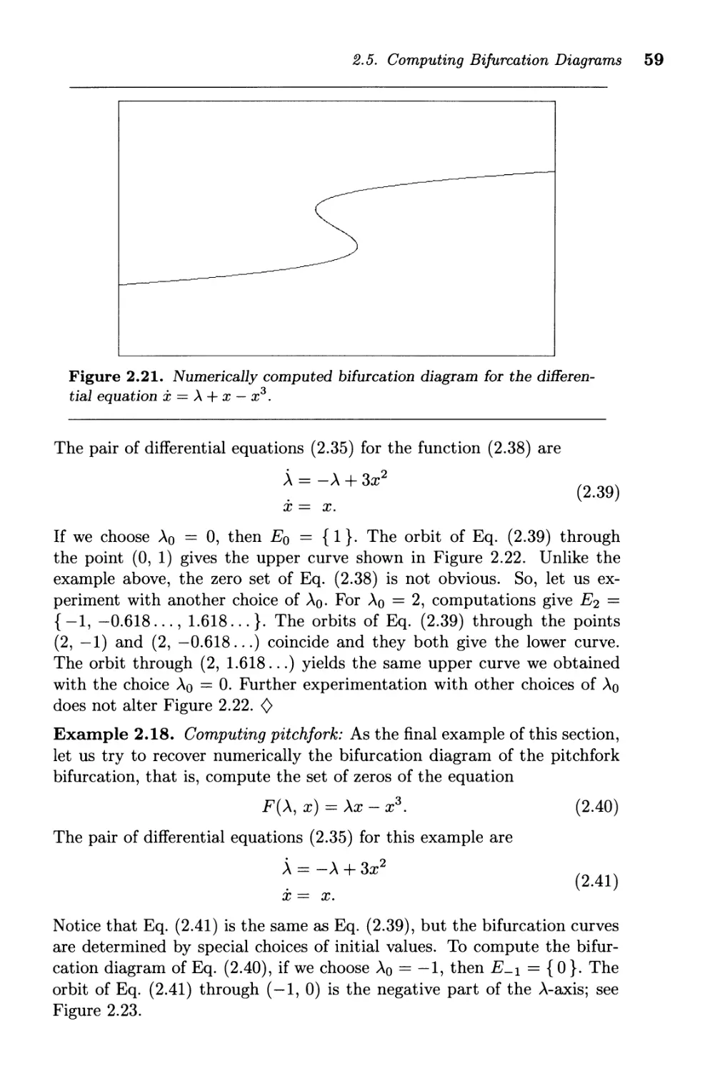
2.5. Computing Bifurcation Diagrams . . . . . . . . . . . . . . . . . . 56
2.6. Equivalence of Flows .... . . . . . . . . . . . . . . . . .. 61
Chapter 3. Scalar Maps
3.1. Euler's Algorithm and Maps . . . . . . . . . . . . . . . . . . . . . 68
3.2. Geometry of Scalar Maps . . . . . . . . . . . . . . . . . . . . . . . 72
3.3. Bifurcations of Monotone Maps . . . . . . . . . . . . . . . . . . . 81
3.4. Period-doubling Bifurcation . . . . . . . . . . . . . . . . . . . .. 87
3.5. An Example: The Logistic Map . . . . . . . . . . . . . . . . . . . 92

xii Contents
PART II: Dimension One and One Half
Chapter 4. Scalar Nonautonomous Equations
4.1. General Properties of Solutions .................. 108
4.2. Geometry of Periodic Equations . . . . . . . . . . . . . . . . . . 113
4.3. Periodic Equations on a Cylinder ................. 118
4.4. Examples of Periodic Equations . . . . . . . . . . . . . . . . .. 122
4.5. Stability of Periodic Solutions ................... 129
Chapter 5. Bifurcation of Periodic Equations
5.1. Bifurcations of Poincare Maps . . . . . . . . . . . . . . . . . .. 134
5.2. Stability of Nonhyperbolic Periodic Solutions . . . . . . . . . . 135
5.3. Perturbations of Vector Fields . . . . . . . . . . . . . . . . . .. 141
Chapter 6. On Tori and Circles
6.1. Differential Equations on a Torus . . . . . . . . . . . . . . . .. 148
6.2. Rotation Number . . . . . . . . . . . . . . . . . . . . . . . . . . . 155
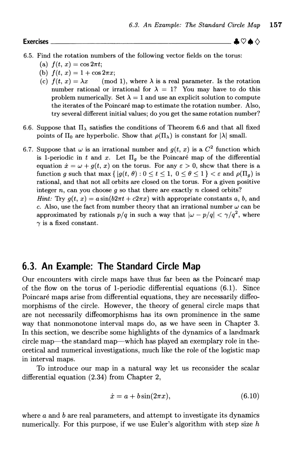
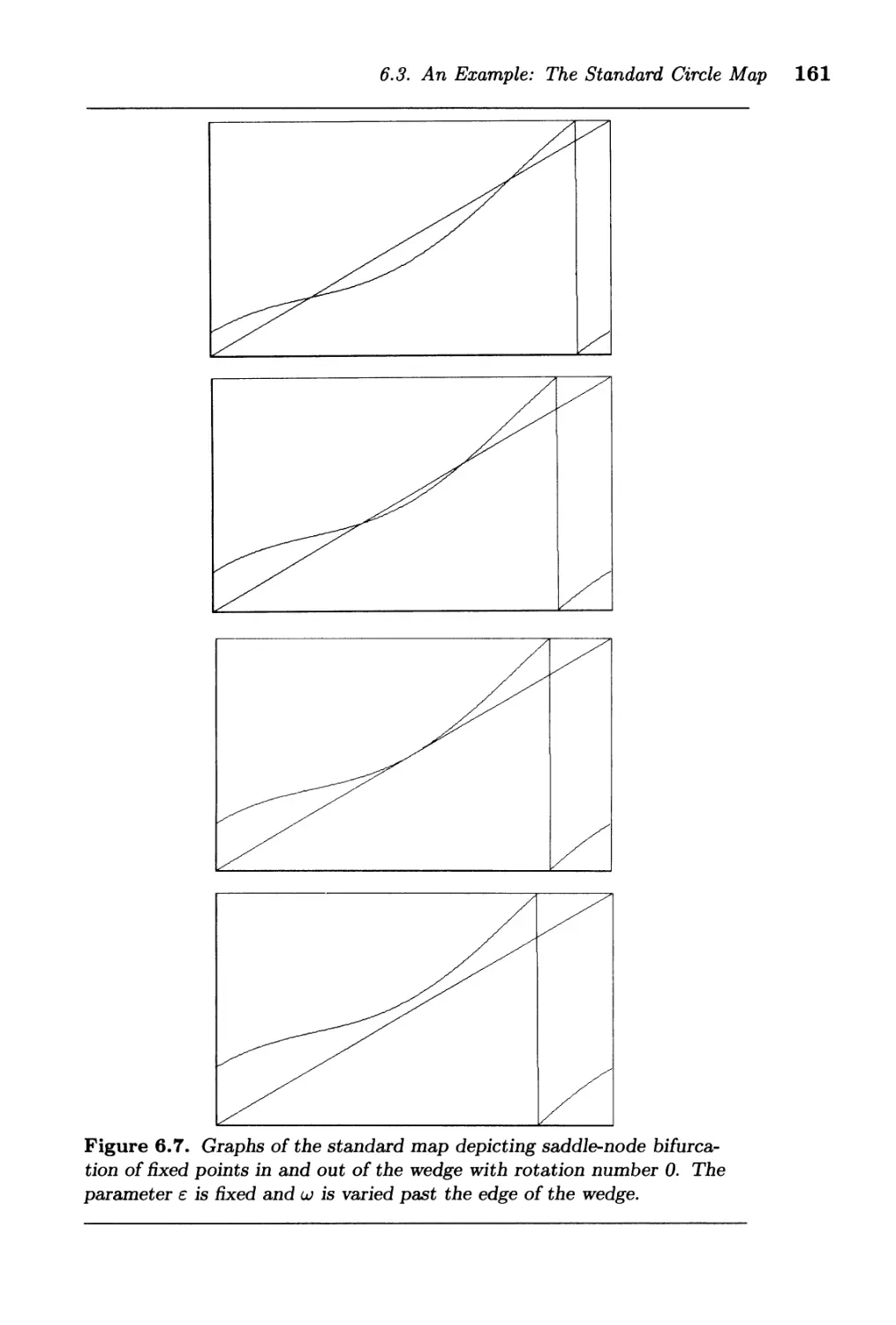
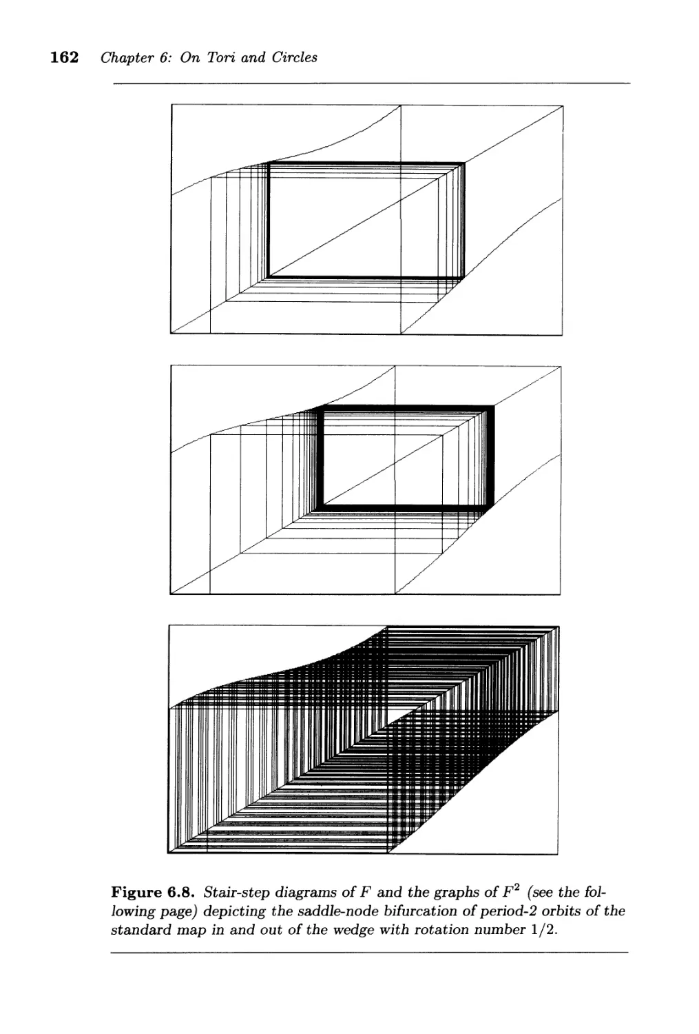
6.3. An Example: The Standard Circle Map ............. 157
PART III: Dimension Two
Chapter 7. Planar A utonomous Systems
7 .1. "Natural" Examples of Planar Systems . . . . . . . . . . . . . . 170
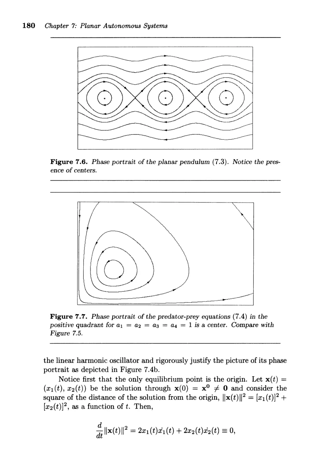
7.2. General Properties and Geometry . . . . . . . . . . . . . . . . . 174
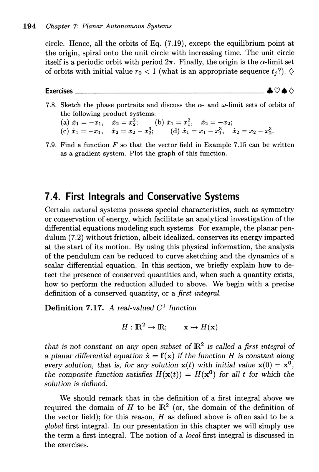
7.3. Product Systems . . . . . . . . . . . . . . . . . . . . . . . . . .. 185
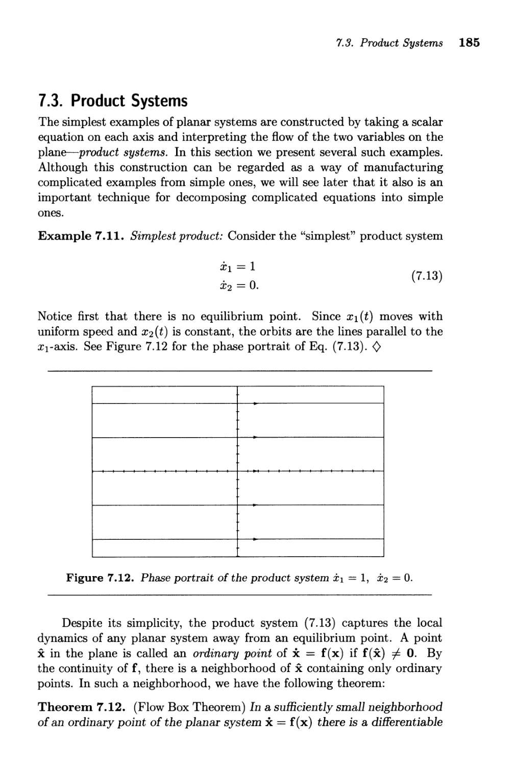
7.4. First Integrals and Conservatjve Systems ............ 194
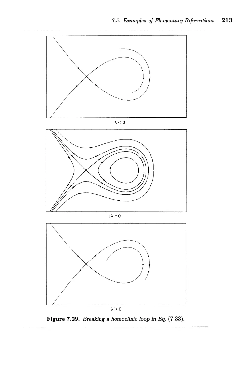
7.5. Examples of Elementary Bifurcations . . . . . . . . . . . . . . . 204
Chapter 8. Linear Systems
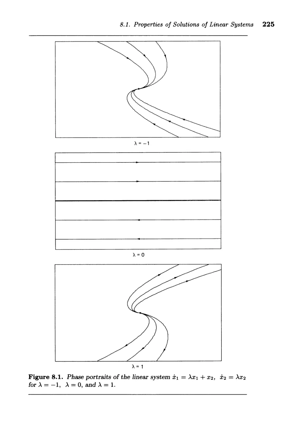
8.1. Properties of Solutions of Linear Systems ............ 218
8.2. Reduction to Canonical Forms . . . . . . . . . . . . . . . . . . . 228
8.3. Qualitative Equivalence in Linear Systems . . . . . . . . . . . . 237
8.4. Bifurcations in Linear Systems . . . . . . . . . . . . . . . . . . . 247
8.5. Nonhomogeneous Linear Systems ... . . . . 253
8.6. Linear Systems with I-periodic Coefficients . . . . . . . . . .. 256
Chapter 9. Near Equilibria
9.1. Asymptotic Stability from Linearization
9.2. Instability from Linearization ......
266
272

Contents xiii
9.3. Liapunov Functions ......................... 277
9.4. An Invariance Principle . . . . . . . . . . . . . . . . . . . . . . . 287
9.5. Preservation of a Saddle . . . . . . . . . . . . . . . . . . . . . . . 292
9.6. Flow Equivalence Near Hyperbolic Equilibria . . . . . . . . . . 301
9.7. Saddle Connections . . . . . . . . . . . . . . . . . . . . . . . . . . 302
Chapter 10. In the Presence of a Zero Eigenvalue
10.1. Stability . . . . . . . . . . . . . . . . . . . . . . . . . . . . . . . . 308
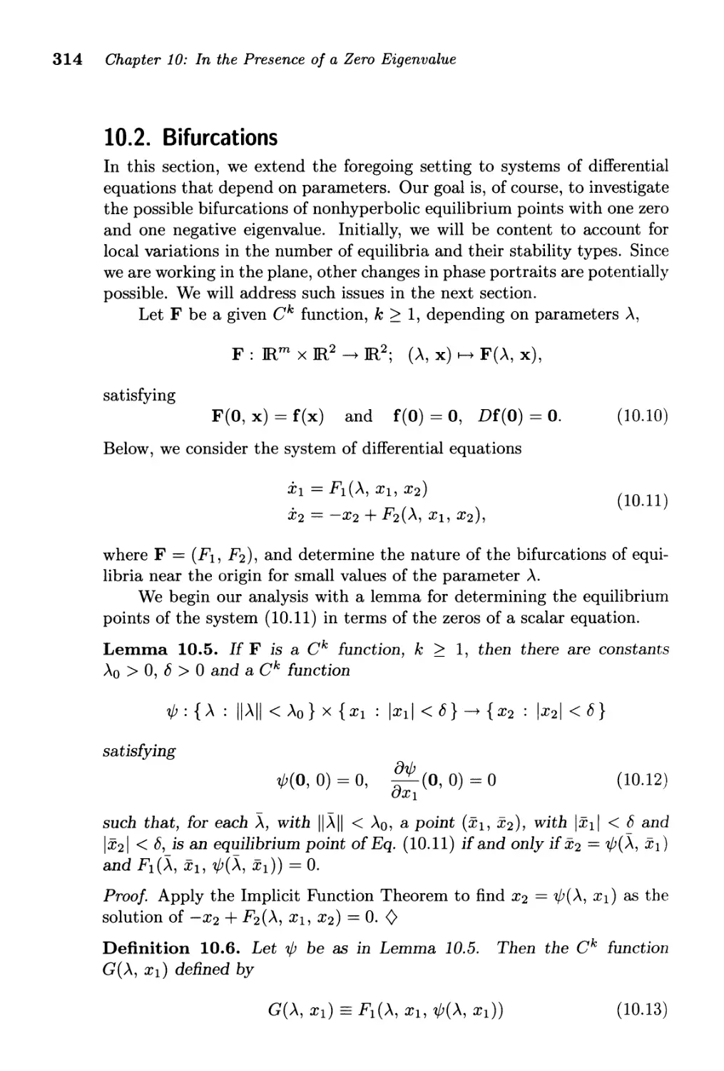
10.2. Bifurcations ............................. 314
10.3. Center Manifolds .......................... 321
Chapter 11. In the Presence of Purely Imaginary Eigenvalues
11.1. Stability . . . . . . . . . . . . . . . . . . . . . . . . . . . . . . . . 334
11.2. Poincare-Andronov-Hopf Bifurcation . . . . . . . . . . . . . . 344
11.3. Computing Bifurcation Curves . . . . . . . . . . . . . . . . . . 357
Chapter 12. Periodic Orbits
12.1. Poincare-Bendixson Theorem . . . . . . . . . . . . . . . . . . . 366
12.2. Stability of Periodic Orbits .................... 375
12.3. Local Bifurcations of Periodic Orbits .............. 382
12.4. A Homoclinic Bifurcation . . . . . . . . . . . . . . . . . . . .. 385
Chapter 13. All Planar Things Considered
13.1. Structurally Stable Vector Fields . . . 390
13.2. Dissipative Systems . . . . . . . . . . . . . . . . . . 394
13.3. One-parameter Generic Bifurcations . . . . . . . . . . . . . 396
13.4. Bifurcations in the Presence of Symmetry ........... 403
13.5. Local Two-parameter Bifurcations . . . . . . . . . . . . . . . . 405
Chapter 14. Conservative and Gradient Systems
14.1. Second-order Conservative Systems ............... 414
14.2. Bifurcations in Conservative Systems ....... . . . . . . . 425
14.3. Gradient Vector Fields . . . . . . . . . . . . . . . . . . . . . . . 432
Chapter 15. Planar Maps
15.1. Linear Maps . . . . . . . . . . . . . . . . . . . . . . . . . . . . . 444
15.2. Near Fixed Points . . . . . . . . . . . . . . . . . . . . . . . . . . 454
15.3. Numerical Algorithms and Maps . . . . . . . . . . . . . . . . . 462
15.4. Saddle Node and Period Doubling . . . . . . . . . . . . . . . . 468
15.5. Poincare-Andronov-Hopf Bifurcation . . . . . . . . . . . . . . 473
15.6. Area-preserving Maps ....................... 484

xiv Contents
PART IV: Higher Dimensions
Chapter 16. Dimension Two and One Half
16.1. Forced Van der Pol . . . . . . . . . . . . . . . . . . . . . . . . . 498
16.2. Forced Duffing . . . . . . . . . . . . . . . . . . . . . . . . . . . . 501
16.3. Near a Transversal Homoclinic Point .............. 504
16.4. Forced and Damped Duffing . . . . . . . . . . . . . . . . . . . . 506
Chapter 17. Dimension Three
17.1. Period Doubling . . . . . . . . . . . . . . . . . . . . . . . . . . . 512
17.2. Bifurcation to Invariant Torus .................. 514
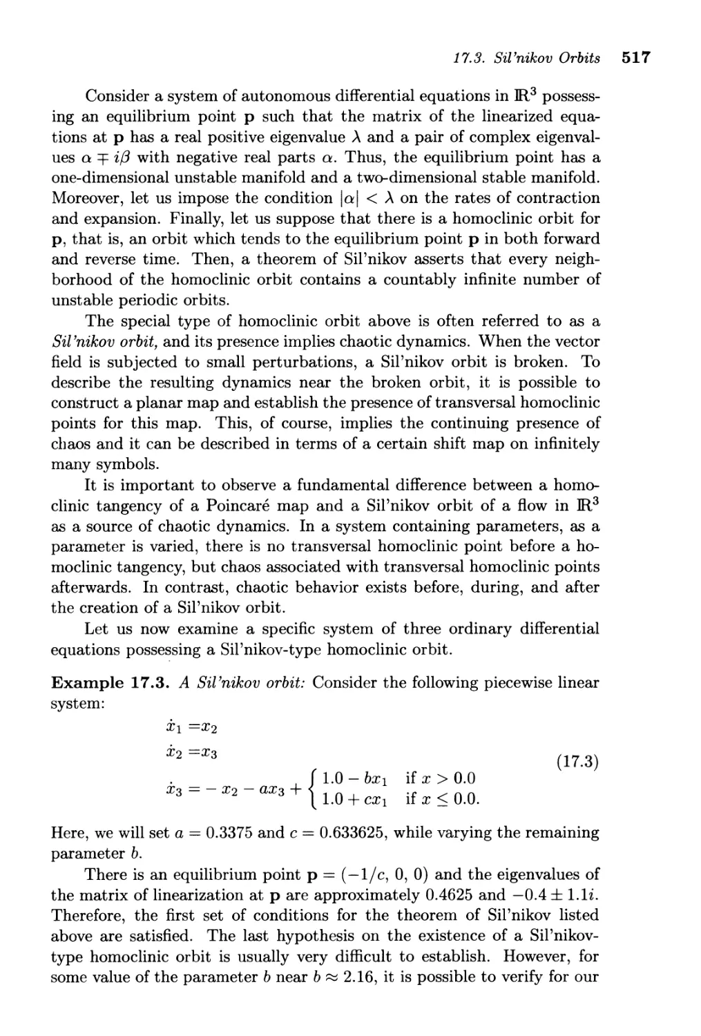
17.3. Silnikov Orbits . . . . . . . . . . . . . . . . . . . . . . . . . . . . 515
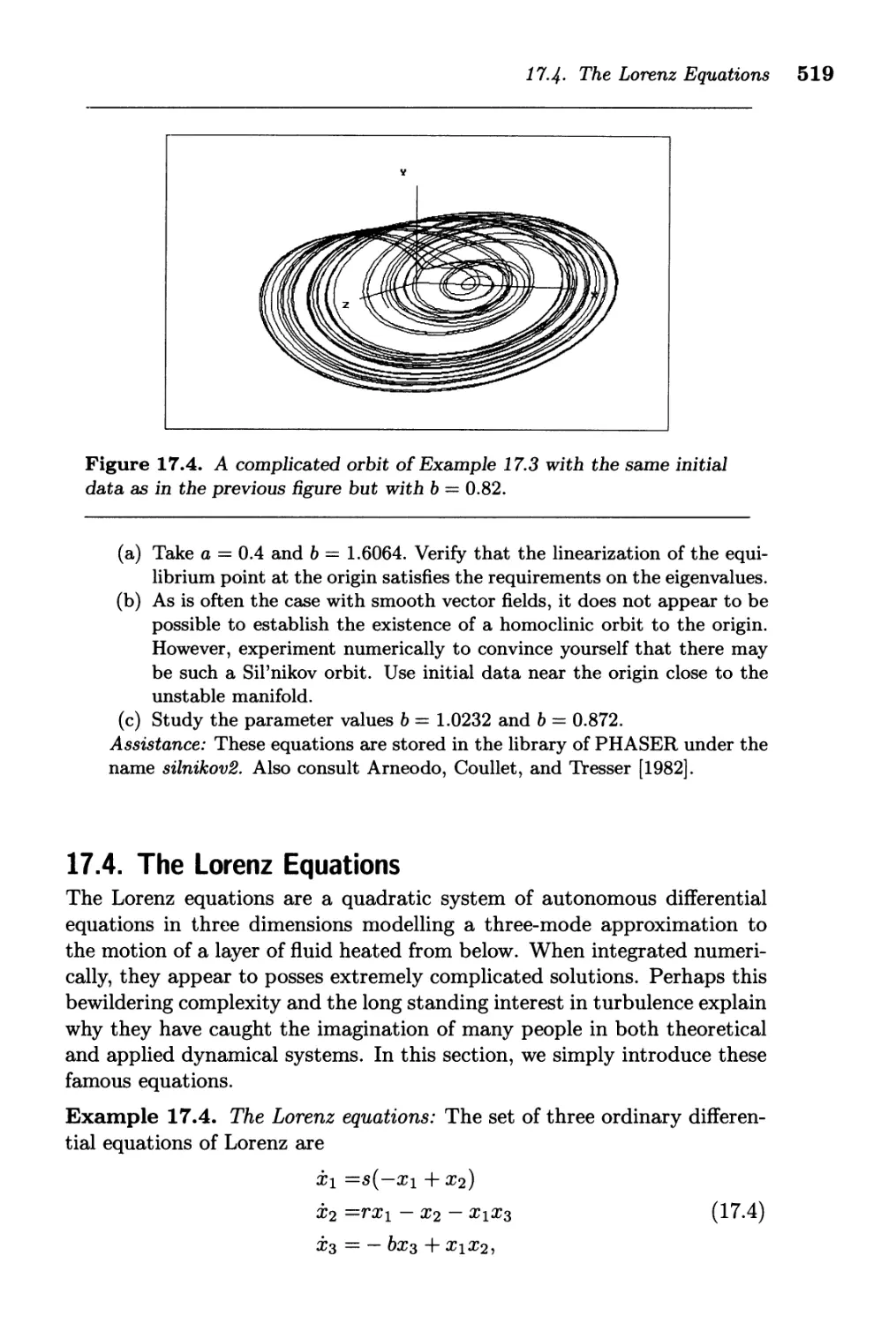
17.4. The Lorenz Equations ....................... 519
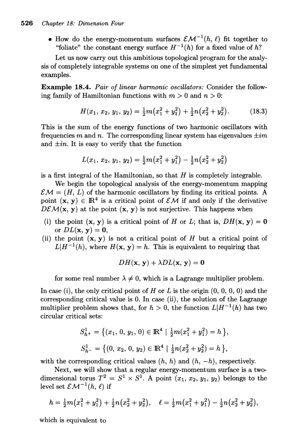
Chapter 18. Dimension Four
18.1. Integrable Hamiltonians
18.2. A Nonintegrable Hamiltonian
524
531
FAREWELL . . . . . . . . . . . . . . . . . . . . . . . . . . . . . . . . . . . 537
ApPENDIX: A Catalogue of Fundamental Theorems .......... 539
REFERENCES ................................. 545
INDEX . . . . . . . . . . . . . . . . . . . . . . . . . . . . . . . . . . . . . . 559

1
Scalar
Autonomous
Equations
In this opening chapter, we present selected basic con-
cepts about the geometry of solutions of ordinary differ-
ential equations. To keep the ideas free from technical
I complications, the setting is one-dimensional-the scalar
i autonomous differential equations. Despite their simplic-
 ity, these concepts are central to our subject and reap-
pear in various incarnations throughout the book. Following a collec-
tion of examples, we first state a theorem on the existence and unique-
ness of solutions. Then we explain what a differential equation is ge-
ometrically. To facilitate qualitative analysis, geometric concepts such
as vector field, orbit, equilibrium point, and limit set are included in
this discussion. The next topic is the notion of stability of an equilib-
rium point and the role of linear approximation in determining stability.
We conclude the chapter with an example of a scalar differential equa-
tion defined on a one-dimensional space other than the realline--a circle.
IIiiIiiiiiiIi
I

4 Chapter 1: Scalar Autonomous Equations
1.1. Existence and Uniqueness
In this introductory section we establish our notation for differential equa-
tions and their solutions. Then, after several motivational examples, we
state a basic existence and uniqueness theorem.
Let I be an open interval of the real line IR and let
x : I ---+ IR; t  x(t)
be a real-valued differentiable function of a real variable t. We will use the
notation x to denote the derivative dx / dt, and refer to t as time or the
independent variable. Also, let
f : IR ---+ IR; x  f(x)
be a given real-valued function. In Chapter 1, we will consider differential
equations of the form
x == f(x),
(1.1)
where x is an unknown function of t and f is a given function of x. Equa-
tion (1.1) is called a scalar autonomous differential equation; scalar because
x is one dimensional (real-valued) and autonomous because the function f
does not depend on t.
We say that a function x is a solution of Eq. (1.1) on the interval I if
x(t) == f(x(t)) for all t E I. We will often be interested in a specific solution
of Eq. (1.1) which at some initial time to E I has the value Xo. Thus we
will study x satisfying
x == f(x),
x(to) == Xo.
(1.2)
Equation (1.2) is referred to as an initial-value problem and any of its
solutions is called a solution through Xo at to. A useful consequence of
the autonomous character of the differential equation in Eq. (1.2) is that
there is no loss of generality in assuming that the initial value-problem is
specified with to == 0, and we will often tacitly do so. To wit, let x(t) be
a solution of Eq. (1.2) through Xo at to and define y(t) = x(t + to). Now,
observe that y(t) is a solution of Eq. (1.2) through Xo at zero since
y(t) == x(t + to) == f(x(t + to)) == f(y(t)) and y(O) == Xo.
As you may recall from your previous studies, a solution of Eq. (1.2)
through Xo at to is given implicitly, using the method of "separation of
variables," by the formula
l x 1
XQ f ( s ) ds = t - to,
(1.3)

1.1. Existence and Uniqueness 5
when the integral is defined. One obtains x(t) by finding the inverse of
the function on the left-hand side of this equation. Occasionally, we will
use this formula to exhibit solutions of special differential equations for the
purposes of illustrations. However, in general, it is impossible to perform
these integrations and one should not expect to obtain explicit formulas for
solutions. It is important to realize this fact from the beginning. In fact,
our objective in this book is to understand as much as possible about the
behavior of solutions of differential equations without the knowledge of an
explicit formula for the solutions.
Let us now give several examples of differential equations and their
solutions in order to realize some of the difficulties that arise in laying the
foundations for the theory, that is, the existence and the uniqueness of
solutions of Eq. (1.2).
Example 1.1. The first example: Consider the differential equation
x == -x.
(1.4 )
It can be seen by simple differentiation that x(t) == e-txo is a solution
through Xo at to == 0, and it is defined for all t E IR. Question: is this the
only solution of Eq. (1.4) satisfying the initial value x(O) == xo? I)
Example 1.2. Finite time: Consider the initial-value problem
x == x 2
,
x(O) == Xo.
(1.5)
It is easy to verify by direct substitution, or using formula (1.3), that the
function
x(t) = 1 xo
- xot
is a solution. Notice that, although the function f(x) == x 2 is remarkably
"nice," the solution x(t) is defined on the interval (-00, 1/xo) for Xo > 0,
on (-00, +00) for Xo == 0, and (1/xo, +00) for Xo < O. The importance
of this example is that the solution is not always defined on all of IR and
the interval of definition of the solution varies with the initial condition.
Furthermore, the solution becomes unbounded as t approaches 1/xo, the
boundary of the interval of definition. I)
Example 1.3. Multiple solutions: Consider the initial-value problem
x == IX,
x(O) == xo,
with x > O.
A solution is given by x(t) == (t + 2VXQ)2 /4. If Xo == 0, then there is also
the solution which is identically zero for all t. Therefore, the initial-value
problem above does not have a unique solution through Xo at zero.

6 Chapter 1: Scalar Autonomous Equations
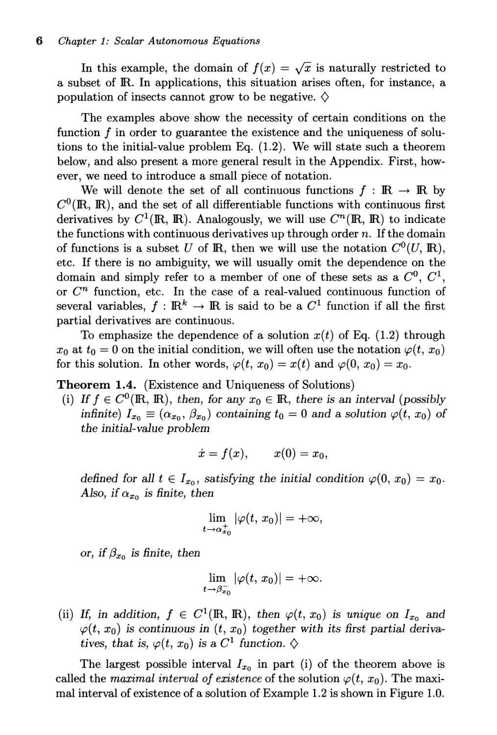
In this example, the domain of f(x) == JX is naturally restricted to
a subset of ffi. In applications, this situation arises often, for instance, a
population of insects cannot grow to be negative. (:;
The examples above show the necessity of certain conditions on the
function f in order to guarantee the existence and the uniqueness of solu-
tions to the initial-value problem Eq. (1.2). We will state such a theorem
below, and also present a more general result in the Appendix. First, how-
ever, we need to introduce a small piece of notation.
We will denote the set of all continuous functions f : ffi ---+ ffi by
CO (ffi, ffi), and the set of all differentiable functions with continuous first
derivatives by e 1 (ffi, ffi). Analogously, we will use en (ffi, ffi) to indicate
the functions with continuous derivatives up through order n. If the domain
of functions is a subset U of ffi, then we will use the notation CO (U, ffi),
etc. If there is no ambiguity, we will usually omit the dependence on the
domain and simply refer to a member of one of these sets as a Co, e 1 ,
or en function, etc. In the case of a real-valued continuous function of
several variables, f : ffi k ---+ ffi is said to be a e 1 function if all the first
partial derivatives are continuous.
To emphasize the dependence of a solution x(t) of Eq. (1.2) through
xo at to == 0 on the initial condition, we will often use the notation '1'( t, xo)
for this solution. In other words, 'P(t, xo) == x(t) and '1'(0, xo) == Xo.
Theorem 1.4. (Existence and Uniqueness of Solutions)
(i) If f E eO(ffi, ffi), then, for any Xo E ffi, there is an interval (possibly
infinite) Ixo (Qxo, !3xo) containing to == 0 and a solution '1'( t, xo) of
the initial-value problem
x == f(x),
x(O) == Xo,
defined for all t E Ixo, satisfying the initial condition '1'(0, xo) == Xo.
Also, if Qxo is finite, then
lim I'P( t, xo) I == +00,
t-+a +
Xo
or, if !3xo is finite, then
lim 1'1' ( t, x 0) I == + 00.
t-+ (3;o
(ii) If, in addition, f E e 1 (ffi, ffi), then 'P(t, xo) is unique on Ixo and
'1'( t, xo) is continuous in (t, xo) together with its first partial deriva-
tives, that is, 'P(t, xo) is a e 1 function. (:;
The largest possible interval Ixo in part (i) of the theorem above is
called the maximal interval of existence of the solution '1'( t, xo). The maxi-
mal interval of existence of a solution of Example 1.2 is shown in Figure 1.0.

1.1. Existence and Uniqueness 7
o
1
t
Figure 1.0. Maximal interval of existence of the solution of x = x 2 with
initial value x(O) = 1 is (-00, 1).
In applications, the function f may not be defined on all of JR. One
common situation is that f E Cn(U, JR), where U is an open and bounded
subset of JR. In this case, the conclusions of Theorem 1.4 are the same
except that all of the limit points of c.p(t, xo) as t  Qt o (or t  (3;o) must
belong to the boundary of U.
Let us now return briefly to the notation c.p(t, xo) for the solution of an
initial-value problem and reexamine it in light of our foregoing discussions.
For a given C 1 function f, Theorem 1.4 implies that the family of all specific
solutions of x = f(x) can be represented by c.p(t, xo) viewed as a function
of two variables, where t E Ixo and Xo E JR. As such, c.p(t, xo) is called the
flow of x = f(x). The domain of this function of two variables could be
somewhat complicated because the domain of t may depend on Xo, as seen
in Example 1.2.
The fine structures of flows will be one of our main concerns in the
following chapters. For the moment, we will be content to introduce a
common name for our subject-dynamical systems. If f is a C 1 function,
then, for each t, the flow c.p( t, xo) gives rise to a map of JR into itself (with
possibly restricted domain) given by Xo  c.p(t, xo). Here are some of the
important properties of this map:
(i) c.p(0, xo) = Xo,
(ii) c.p( t + s, xo) = c.p( t, c.p( s, xo)) for each t and s when the map on either
side is defined,
(iii) c.p( t, xo) is a C 1 map for each t and it has a C 1 inverse given by
c.p( -t, xo).
A map of JR into itself satisfying these three properties is called a C 1
dynamical system on JR. So, we can say in conclusion that the flow of a
scalar autonomous differential equation gives rise to a dynamical system

8 Chapter 1: Scalar Autonomous Equations
on JR. There are also other ways of obtaining dynamical systems and we
will see one such important case in Chapter 3.
Exercises ,. C/ . <;
1.1. Verifying hypotheses: Show that the initial-value problem x == 1 +X2, x(O) ==
o has a unique solution by verifying the hypotheses of Theorem 1.4. Find
the solution. What is the maximal interval of existence of the solution?
1.2. Multiple solutions and numerics: Reexamine Example 1.3, x == yX, with
the initial value x(O) == 0 in light of Theorem 1.4. Which hypothesis of the
theorem is not met by the example to prevent the uniqueness of solutions?
Solve this initial value problem numerically on the computer. If you have not
studied numerical solutions of differential equations before, you may want
to return to this task after reading Chapter 3 or consult the reference below.
Which solution do you obtain? Try several different numerical algorithms.
Do you succeed in obtaining the nonzero solution?
Help: In the sequel, some of the exercises will include numerical experiments
with differential equations. To eliminate the burden of programming, we
suggest the computer program PHASER: An Animator/Simulator for Dy-
namical Systems which accompanies one of our earlier books, Ko<;ak [1989].
1.3. Infinitely many solutions: Show that the differential equation x == x 2 / 3 has
infinitely many solutions satisfying x(O) == 0 on every interval [0, a].
1.4. No solution: Consider the function
f ( x) == { I f x < 0
2 If x > O.
Show that the differential equation x == f (x) has no solution satisfying
x(O) == 0 on any open interval about to == O.
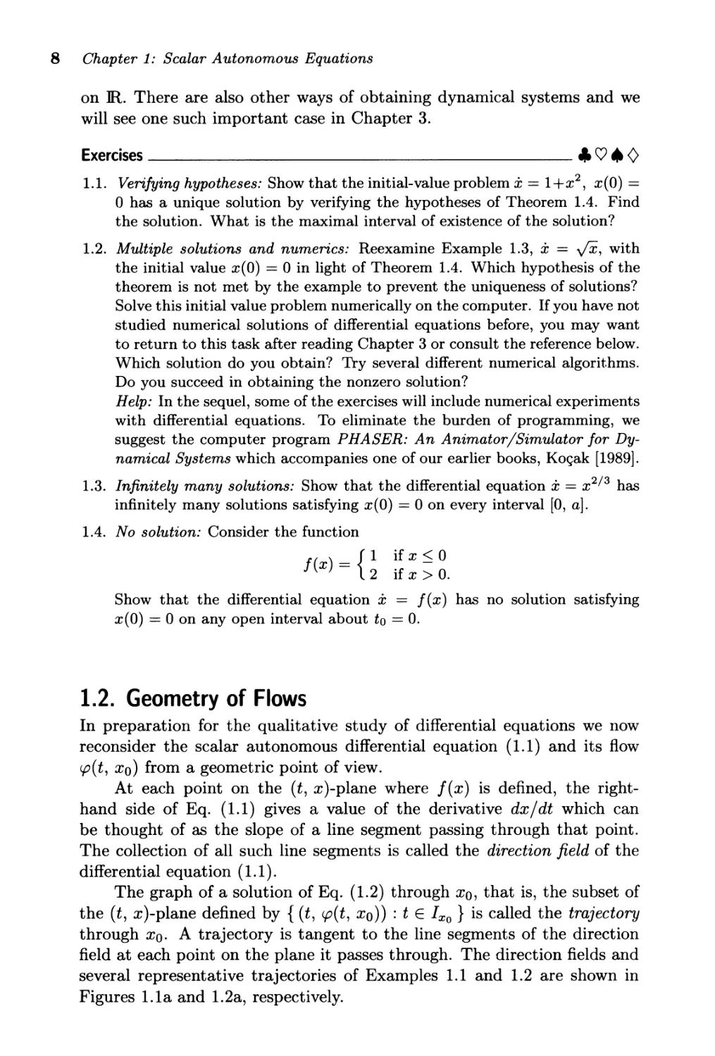
1.2. Geometry of Flows
In preparation for the qualitative study of differential equations we now
reconsider the scalar autonomous differential equation (1.1) and its flow
<p(t, xo) from a geometric point of view.
At each point on the (t, x)-plane where f(x) is defined, the right-
hand side of Eq. (1.1) gives a value of the derivative dx/dt which can
be thought of as the slope of a line segment passing through that point.
The collection of all such line segments is called the direction field of the
differential equation (1.1).
The graph of a solution of Eq. (1.2) through Xo, that is, the subset of
the (t, x)-plane defined by {(t, <p(t, xo)) : t E Ixo } is called the trajectory
through Xo. A trajectory is tangent to the line segments of the direction
field at each point on the plane it passes through. The direction fields and
several representative trajectories of Examples 1.1 and 1.2 are shown in
Figures 1.la and 1.2a, respectively.

1.2. Geometry of Flows 9
x x
\ \ \ \ \ !
\ \ \ \ \ 
"- "- "- "- 
----.. ----.. ----.. ----.. ----..
     t 0
/ / / / t
/ / / / / t
/ I I I I (b) t
(a) Figure 1.1. (a) Direction field along with several trajectories, and (b) vec-
tor field of x = -x.
x x
I I I I I I I t
/ / / / I / /
t
/ / / / / / /
--- --- --- --- --- t
t
0
-- -- -- -- --
/ / / / / / / t
I I t
(a) I I (b) t
Figure 1.2. (a) Direction field along with several trajectories, and (b) vec-
tor field of x = x 2 .
Since f ( x) is independent of t, on any line parallel to the t-axis the
segments of the direction field all have the same slope. Therefore, it is
natural to consider the projection onto the x-axis of the direction field and
the trajectories of Eq. (1.1).
To each point x on the x-axis we can associate the directed line segment
from x to x+ f(x). We can view this directed line segment as a vector based
at x. The collection of all such vectors is called the vector field generated
by Eq. (1.1), or simply the vector field f; see Figures 1.lb and 1.2b.
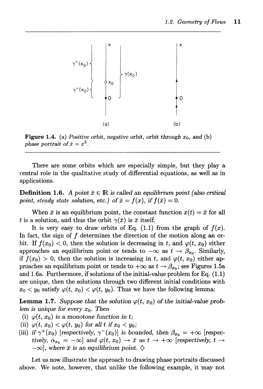
Definition 1.5. The positive orbit,+(xo), negative orbit,-(xo), and orbit

10 Chapter 1: Scalar Autonomous Equations
x x
"y'-(xo)
"y'( xo )
'Y + (xo) { xo
0 0
(a)
(b)
Figure 1.3. ( a) Positive orbit, negative orbit, orbit through Xo, and (b)
phase portrait of x == -x.
,(xo) of Xo are defined, respectively, as the following subsets of the x-axis:
,+(xo) = U '1'(t, xo),
tE [0, !3xQ )
,-(xo) = U c.p(t, xo),
tE(oxQ'O]
,(xo) =
U
c.p(t, xo).
tE (oxQ , !3xQ )
The "velocity" of an orbit at a point x is given by the element of
the vector field at that point; see, for example, Figures 1.lb and 1.2b. As
shown in Figures 1.3 and 1.4, on the orbit ,(xo) we insert arrows to indicate
the direction '1'( t, xo) is changing as t increases. The flow of a differential
equation is then drawn as the collection of all its orbits together with the
direction arrows and the resulting picture is called the phase portrait of the
differential equation; see Figures 1.3b and 1.4b.
It is clear from the definitions above that the orbit ,( xo) is the pro-
jection onto the x-axis of the trajectory through Xo. Consequently, in our
investigation of qualitative properties of solutions of differential equations,
it will be advantageous to focus our attention on orbits (see Lemma 1.7
below). In the process, however, we will lose the information about the
time-parametrization, the speed, of solutions. For instance, while it takes
an infinite amount of time to trace the negative orbit ,- (xo) = [xo, +00),
with Xo > 0, of Example 1.1, it takes only finite time to trace the positive
orbit ,+ (xo) = [xo, +00), with Xo > 0, of Example 1.2; see Figures 1.3a
and 1.4a.

1.2. Geometry of Flows 11
x
x
,+(xo)
,(xo)
'Y-(XQ){ Xo
0 0
(a)
(b)
Figure 1.4. (a) Positive orbit, negative orbit, orbit through Xo, and (b)
phase portrait of x == x 2 .
There are some orbits which are especially simple, but they play a
central role in the qualitative study of differential equations, as well as in
applications.
Definition 1.6. A point x E IR is called an equilibrium point (also critical
point, steady state solution, etc.) of x == f(x), if f(x) == o.
When x is an equilibrium point, the constant function x(t) == x for all
t is a solution, and thus the orbit ,(x) is x itself.
It is very easy to draw orbits of Eq. (1.1) from the graph of f(x).
In fact, the sign of f determines the direction of the motion along an or-
bit. If f(xo) < 0, then the solution is decreasing in t, and cp(t, xo) either
approaches an equilibrium point or tends to -00 as t  (3xo. Similarly,
if f(xo) > 0, then the solution is increasing in t, and cp(t, xo) either ap-
proaches an equilibrium point or tends to +00 as t  (3xo; see Figures 1.5a
and 1.6a. Furthermore, if solutions of the initial-value problem for Eq. (1.1)
are unique, then the solutions through two different initial conditions with
Xo < Yo satisfy cp(t, xo) < cp(t, Yo). Thus we have the following lemma:
Lemma 1.7. Suppose that the solution cp(t, xo) of the initial-value prob-
lem is unique for every Xo. Then
(i) cp(t, xo) is a monotone function in t;
(ii) cp ( t, x 0) < cp ( t, Yo) for all t if x 0 < Yo;
(iii) if ,+(xo) [respectively, ,- (xo)] is bounded, then (3xo == +00 [respec-
tively, Qxo == -00] and cp(t, xo)  x as t  +00 [respectively, t 
-00], where x is an equilibrium point. <>
Let us now illustrate the approach to drawing phase portraits discussed
above. We note, however, that unlike the following example, it may not

12 Chapter 1: Scalar Autonomous Equations
(a)
f(x) = -x
x
x 2
F(x) = 2
x
(b)
Figure 1.5. Determining the phase portrait of X == -x from (a) the
function f (x) == - x, and (b) from the corresponding potential function
F(x) == x2/2. Notice that, unlike in the previous figures, the variable x
is assigned to the horizontal axis. In the subsequent figures we will use
whichever assignment is more convenient.
be so easy to locate the equilibria of a given differential equation. We will
address this difficulty later.
Example 1.8. Consider the differential equation
x = x - x 3 .
(1.6)
The equilibrium points of this equation are -1, 0, and 1, and the function
f(x) = x - x 3 is positive on the interval (-00, -1), negative on (-1,0),

1.2. Geometry of Flows 13
f(x) = X 2
x
(a)
x 3
F(x) = --
3
(b)
x
Figure 1.6. Determining the phase portrait of x == x 2 from (a) the func-
tion f(x) == x 2 , and (b) from the potential function F(x) == -x 3 /3.
positive on (0, 1), and negative on (1, +00). Therefore, its phase portrait
can easily be drawn as in Figure 1.7a. The orbits are the open intervals
(-00, -1), (-1,0), (0, 1), (1, +00), and the points {-I}, {O}, and {I}. <>
Determining the origins and ultimate destinations of orbits will be one
of our primary concerns. Therefore, we introduce the following important
concepts:
Definition 1.9. If,-(xo) is bounded, then the set
a( xo) == lim c.p( t, xo)
t---+a +
XQ

14 Chapter 1: Scalar Autonomous Equations
(a)
f(x) = x - X 3
x
x 2 X 4
F(x)=--+-
2 4
x
(b)
Figure 1.7. Determining the phase portrait of x = x - x 3 from (a) the
function f (x) = x - x 3 , and (b) from the corresponding potential function
F(x) = -x 2 /2 + x 4 /4.
is called the a-limit set of xo. Similarly, if ,+ (xo) is bounded, then the set
W(XO) = Hm <p(t, xo)
t--+ (3;;o
is called the w-limit set of xo.
The last part of Lemma 1.7 can now be restated as follows: the limit
sets a(xo) and w(xo) are equilibrium points, if they exist. In case you are
wondering, the reason for this somewhat strange choice of terminology is

1.2. Geometry of Flows 15
that Q and ware, respectively, the first and the last letters of the Greek
alphabet.
We now present another method that is particularly useful in deter-
mining the flows of certain specific differential equations. Equation (1.1)
can be rewritten in the form
x = f(x) = - d F(x),
(1.7)
where
F(x) = -1'" f(s) ds.
Equation (1.7) in this form is a special case of gradient systems which we
will study later in a more general setting. At this time, it is sufficient to
note that, if x(t) is a solution of Eq. (1.7), then
d d d 2
dt F (x(t)) = dx F (x(t)) . dt x(t) = - [I (x(t))] < o.
Thus F is always decreasing along the solution curves, and hence can be
thought of as a "potential" function of Eq. (1.1). It is evident that the
equilibrium points of the differential equation (1.7) are extreme points of
the potential function F.
Let us now reconsider the previous examples from this new viewpoint.
Example 1.1 revisited. Equation (1.4) can be written as a gradient
system (1.7) with the potential function F(x) = x2/2. The orbits of
x = -x = - d ( 2 )
can be drawn by thinking of the motion of a particle on the graph of the
potential function F(x). As shown in Figure 1.5b, a particle at any point Xo
goes downhill with (ever decreasing) velocity I(x) towards the equilibrium
point O. Therefore, the orbits for this equation are the intervals (-00, 0),
(0, +00), and the equilibrium point O. <>
Example 1.2 revisited. The differential equation (1.5) can be written as
x = x 2 = - d ( _ 3 )
with the potential function F(x) = -x 3 /3. The graph of F(x) and the flow
are shown in Figure 1.6b. Here the orbits are again the same intervals as
in the previous example, however, the two flows are different. <>

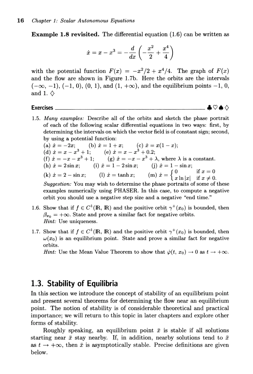
16 Chapter 1: Scalar Autonomous Equations
Example 1.8 revisited. The differential equation (1.6) can be written as
x = x _ X 3 = _ d ( _ 2 + :4 )
with the potential function F(x) = -x 2 /2 + x 4 /4. The graph of F(x)
and the flow are shown in Figure 1.7b. Here the orbits are the intervals
(-00, -1), (-1,0), (0,1), and (1, +00), and the equilibrium points -1, 0,
and 1. 0
Exercises
'-'Q.O
1.5. Many examples: Describe all of the orbits and sketch the phase portrait
of each of the following scalar differential equations in two ways: first, by
determining the intervals on which the vector field is of constant sign; second,
by using a potential function:
(a) x == -2x; (b) x == 1 + x; (c) x == x(1 - x);
(d) x==x-x 3 +1; (e) x==x-x 3 +O.2;
(f) x == -x - x 3 + 1; (g) x == -x - x 3 + ..\, where ..\ is a constant.
(h) x == 2 sin x; (i) x == 1 - 2 sin x; (j) x == 1 - sin x;
{ 0 if x == 0
(k) x == 2 - sin x; (1) x == tanh x; (m) x == x In Ixl if x =I- O.
Suggestion: You may wish to determine the phase portraits of some of these
examples numerically using PHASER. In this case, to compute a negative
orbit you should use a negative step size and a negative "end time."
1.6. Show that if fECI (nt, nt) and the positive orbit, + (xo) is bounded, then
{3xo == +00. State and prove a similar fact for negative orbits.
Hint: Use uniqueness.
1.7. Show that if fECI (nt, nt) and the positive orbit ,+ (xo) is bounded, then
w( xo) is an equilibrium point. State and prove a similar fact for negative
orbits.
Hint: Use the Mean Value Theorem to show that <j;(t, xo)  0 as t  +00.
1.3. Stability of Equilibria
In this section we introduce the concept of stability of an equilibrium point
and present several theorems for determining the flow near an equilibrium
point. The notion of stability is of considerable theoretical and practical
importance; we will return to this topic in later chapters and explore other
forms of stability.
Roughly speaking, an equilibrium point x is stable if all solutions
starting near x stay nearby. If, in addition, nearby solutions tend to x
as t  +00, then x is asymptotically stable. Precise definitions are given
below.

1.3. Stability of Equilibria 1 7
Definition 1.10. An equilibrium point x of Eq. (1.1) is said to be stable
if, for any given E > 0, there is a 8 > 0, depending on E, such that, for every
Xo for which Ixo - xl < 8, the solution c.p(t, xo) of Eq. (1.1) through Xo at
o satisfies the inequality Ic.p(t, xo) - xl < E for all t > o. The equilibrium
point x is said to be unstable if it is not stable.
Definition 1.11. An equilibrium point x is said to be asymptotically stable
if it is stable and, in addition, there is an r > 0 such that Ic.p(t, xo) - xl  0
as t  +00 for all Xo satisfying Ixo - xl < r.
We should point out that we have purposely introduced a redundancy
in this definition of asymptotic stability. In the case of a scalar differential
equation, if every solution with initial value close to x approaches x as
t  +00, then it follows that x is stable. However, this is not so in
higher dimensions and the definition of asymptotic stability as given will
be necessary.
The following lemma, whose proof is left as an exercise, is helpful
in determining the stability of an equilibrium point of Eq. (1.1) from the
function f ( x ) .
Lemma 1.12. An equilibrium point x of x = f(x) is stable if there is a
fJ > 0 such that (x-x)f(x) < 0 for lx-xl < 8. Similarly, x is asymptotically
stable if and only if there is a 8 > 0 such that (x - x)f(x) < 0 for 0 <
lx-xl < 8. An equilibrium point x of x = f(x) is unstable if there is a 8 > 0
such that (x - x)f(x) > 0 for either 0 < x - X < 8 or -8 < x - X < o. 0
Using the lemma above, it is easy to verify that, in Example 1.1,
x = -x, the equilibrium point at 0 is asymptotically stable, while, in
Example 1.2, x = x 2 , the equilibrium point at 0 is unstable; see Figures
1.5a and 1.6a. In Example 1.8, x = x - x 3 , the equilibrium points at -1
and 1 are asymptotically stable, and 0 is unstable; see Figure 1.7 a.
Let us now examine a somewhat intricate example concerning the first
sentence of Lemma 1.12.
Example 1.13. Consider the differential equation
{ 0 if x = o.
j; = f(x) = -x 3 sin  otherwie.
The function f (x) above is continuous together with its first derivative.
The graph of f and the phase portrait of the differential equation above are
depicted in Figure 1.8. The equilibrium points are x = 0, and x = (k7r)-l
where k is any integer. Notice that the equilibrium points [(2k + 1)7r]-1
and - [(2k + 2)7r]-1 are asymptotically stable while - [(2k + 1)7r]-1 and
[(2k + 2)7r]-1 are unstable for k = 0, 1, 2, . . . . The equilibrium point 0 is
stable, but not asymptotically; there is no 8 > 0 such that xf(x) < 0 for
o < Ixl < 8. So, it is not possible to improve Lemma 1.12 by changing the
first statement to say "if and only if." 0

18 Chapter 1: Scalar Autonomous Equations
x
_J
Figure 1.8. Phase portrait of x == _x 3 sin X-I. The origin is stable, but
not asymptotically stable.
It is instructive to contrast stability of an equilibrium point with con-
tinuous dependence of c.p(t, xo) in t, Xo (see Theorem 1.4). For instance,
Example 1.2 has c.p(t, xo) continuous in t, Xo, but the equilibrium point
at 0 is not stable. To understand the difference between these two im-
portant concepts, a certain amount of technical language is unavoidable.
Continuity of c.p(t, xo) in t and Xo near an equilibrium point x implies the
following type of uniformity. Given any interval [0, T], and any E > 0,
there is a 8(E, T) > 0 such that Ixo - xl < 8(E, T) implies Ic.p(t, xo) - xl < E
for 0 < t < T, that is, the function c.p( t, xo) is continuous in Xo uniformly
with respect to t in closed bounded sets. Notice that the number 8(£, T)
in Example 1.2 must approach zero as T ---+ +00. On the other hand, if
x is stable, then 8 depends only on E and not on T; that is, the stability
of an equilibrium point x is equivalent to the statement that c.p(t, xo) is
continuous in Xo at x uniformly with respect to t > o.
It is evident from Definitions 1.10 and 1.11 that the stability of an
equilibrium point x of Eq. (1.1) is a local property of the flow near the equi-
librium. Therefore, it is reasonable to expect that under certain conditions
the stability properties of x can be determined from the linear approxima-
tion, that is, the derivative I'(x) (d/dx) f(x) of the function f near x.
Since the equilibrium point x = 0 of the linear differential equation x = ex
is asymptotically stable if e < 0 and unstable if e > 0, we are naturally led
to the following statement:
Theorem 1.14. Suppose that I is a C 1 function and x is an equilibrium
point of x = I(x), that is, I(x) = O. Suppose also that f'(x) i- O. Then
the equilibrium point x is asymptotically stable if f' (x) < 0, and unstable
if I' (x) > O.

1.3. Stability of Equilibria 19
Proof. We first shift the x-axis by introducing the new variable y x - x,
so that the equilibrium x of x == f(x) corresponds to the equilibrium of
the differential equation iJ == f (x + y) at y == O. If we expand the function
f(x + y) into its Taylor expansion near 0, we obtain
iJ == f'(x)y + g(y),
which can be considered as a perturbation of the linear differential equation
iJ == f'(x)y. In fact, the function g(y) satisfies g(O) == 0 and g'(O) == O.
Since g' (0) == 0, for any E > 0, there is a 8 > 0 such that Ig' (y) I < E if
Iyl < 8. Using the formula g(y) == J g'(8) d8, it follows that Ig(y)1 < Elyl if
Iyl < 8. Now suppose that f'(x) =1= 0 and E < If'(x)l. Then Iyl < 8 implies
that the sign of the function f(x + y) == f'(x)y + g(y) is determined by
the sign of f'(x)y. Therefore, the conclusion of the theorem follows from
Lemma 1.12. <>
The linear differential equation x == f' (x)x is called the linear varia-
tional equation or the linearization of the vector field x == f (x) about its
equilibrium point x. Theorem 1.14 asserts that, when f'(x) =1= 0, the stabil-
ity type of the equilibrium point x of x == f (x) is the same as the stability
type of the equilibrium point at the origin of its linearized vector field.
We introduce the following common terminology for an equilibrium
point satisfying the hypothesis of the theorem above.
Definition 1.15. An equilibrium point x of x == f(x) is called a hyperbolic
equilibrium if f' (x) =1= O.
If f'(x) == 0, then x is called a nonhyperbolic or degenerate equilib-
rium point. Unlike near a hyperbolic equilibrium where the linear term
of the vector field determines the flow locally, the stability properties of a
nonhyperbolic equilibrium x depends on higher-order terms in the Taylor
expansion of the function f(x + y). For instance, while x == 0 is an unsta-
ble equilibrium for x == x 2 , it is asymptotically stable for x == -x 3 . There
are other complications associated with nonhyperbolic equilibria; infinitely
many equilibria are present in any open neighborhood of the nonhyperbolic
equilibrium x == 0 of the differential equation x == -x 3 sin X-I, as we saw
in Example 1.13. These examples point to the realization that a study of
nonhyperbolic equilibria will not be trivial. Despite the difficulties associ-
ated with them, however, nonhyperbolic equilibria playa prominent role
in our subject, as we shall soon see.
Exercises
.t.Q.<>
1.8. Many examples: Determine the equilibrium points of the following scalar
differential equations and compute the linear variational equations about
the equilibria. Identify the hyperbolic equilibria and their stability types.
Finally, sketch phase portraits by hand and also by using PHASER.

20 Chapter 1: Scalar Autonomous Equations
(a) x = 0 ; (b) x = 2.1 x (1 - x) ; (c) X = 1 + x 2 ;
( d) x = 1 - x 2 ; ( e) x = 2x 2 - x 3 ; (f) x = x - x 3 + 0.2;
(g) x = 2 sin x; (h) x = 1 - 2 sin x; (i) x = 1 - sin x;
(j) x = x sin x; (k) x = a - x 3 sin(x- l ) where a > 0 is a constant;
(1) x = x [1 - b(e X - 1)] for values of b = -1.1, -1, -0.1, 0, and 0.1.
1.9. Give an alternative, and perhaps simpler, proof of Theorem 1.14 using the
Mean Value Theorem.
1.10. Minimum: Is an equilibrium point corresponding to a local minimum of a
potential function always asymptotically stable?
1.11. Consider the differential equation x = (1 - X)X- l / 2 for x > O. What is the
a-limit set of a solution? Does a solution reach its a-limit set in finite time?
Compare your answer on PHASER. Any problems?
1.12. Hyperbolic means faster: As we saw, the phase portraits of the differential
equations x = -x and x = _x 3 are qualitatively the same: all orbits even-
tually approach the unique asymptotically stable equilibrium at the origin.
Compare the speeds of approach to the equilibrium. Which one is faster?
Pay particular attention to what happens near the origin, say, for Ix I < 1.
1.13. Quantitative information is important too: As we have remarked earlier,
phase portraits give no information about the values of solutions along
orbits. Such quantitative information, which is of paramount interest in
certain applications, is usually obtained by numerical approximations on
the computer. In fact, good approximations are the most that should be
expected since explicit solutions can be obtained for only very special equa-
tions. On the other hand, it is quite remarkable that some famous applica-
tions involve the use of linear differential equations, hence reducing numeri-
cal tasks to calculating the values of the exponential or logarithm function.
Here are several such examples.
Radioactive Decay: It has been observed experimentally, by Rutherford and
others, that certain radioactive elements decay at a rate proportional to their
mass. By idealizing this complicated natural process, ignoring, for instance,
that atoms are discrete entities, it is reasonable to model the phenomenon
of radioactive decay using a differential equation: if N (t) is the mass of
radioactive substance at time t, then
N = -AN,
where A is a positive constant which is a characteristic of the radioactive
substance.
From the qualitative point of view, all of the matter in such a radioac-
tive substance eventually radiates away. From the quantitative perspective,
however, there are some concerns. First, we need to know the value of A for
a given substance. This is done experimentally. The solution of the linear
differential equation above satisfying N(O) = No is given by N(t) = Noe->'t.
The constant A can be determined by measuring the amount of remaining
mass at some later time, say, T. It is standard to use the half-life of the

1.4. Equations on a Circle 21
substance for 7, that is, the necessary time for the substance to decay to
half of its original size. Show that A == (In 2)/7, where 7 is the half-life.
Once A is determined, N (t) can readily be found for any t by evaluating
the exponential function on a pocket calculator. Have you ever wondered
how your calculator or computer determines the values of the exponential
or logarithm function?
The half-life of the naturally occurring radioactive element l4C, carbon-14,
is known to be 5568 years. Compute the length of time it takes for a mass
of l4C to reduce to 20 percent of its original weight.
Radiocarbon Dating: An effective method of estimating the ages of archeo-
logical finds of organic origin is the method of l4C dating discovered by W.
Libby in 1949. The key idea of the method is remarkably simple: l4C is
in equilibrium in living plants-the amount absorbed from the atmosphere
balances the amount that radiates. Once the plant dies, it ceases to absorb
any more l4C but the radiation continues. One basic cosmological premise
is that the concentration of l4C in the atmosphere has been constant over
millennia. Suppose that at t == 0 a tree dies. Let R( t) be the rate of
disintegration of l4C in the dead wood at time t. Derive the formula
1 R(O)
t == A In R ( t) .
Now, we can measure R(t) at the present time. R(O) is also measurable using
a piece of living plant. So, the age of the dead wood is easy to compute.
Here is an example.
Ag'T"l Dag'lnda: In 1956, a piece of old wood excavated at Mount Ararat gave
a count of 5.96 disintegrations per minute per gram of l4C while living wood
gave 6.68. Did the piece of old wood come from the Ark? Well, l4C dating
is not always reliable over relatively short time spans.
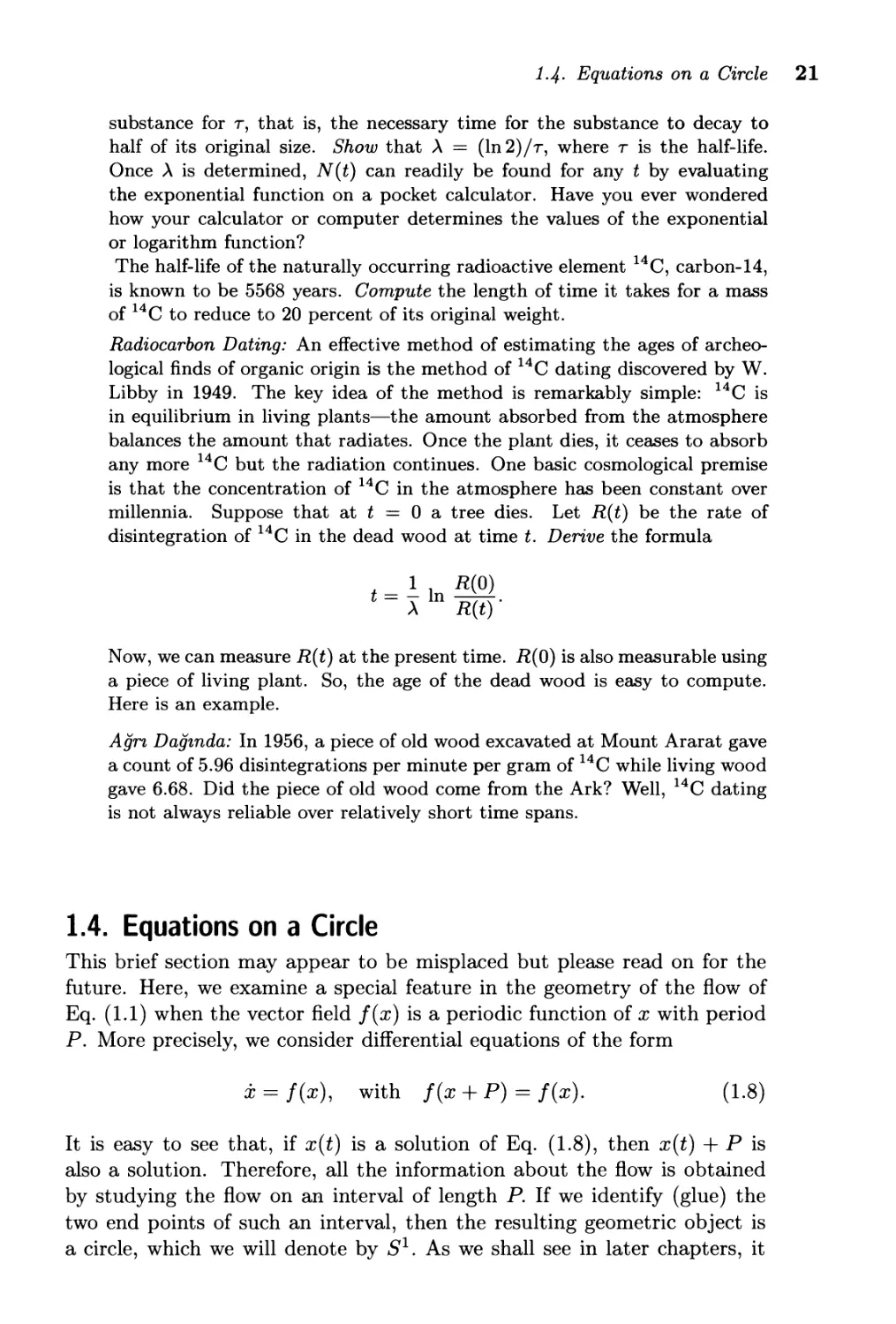
1.4. Equations on a Circle
This brief section may appear to be misplaced but please read on for the
future. Here, we examine a special feature in the geometry of the flow of
Eq. (1.1) when the vector field f(x) is a periodic function of x with period
P. More precisely, we consider differential equations of the form
x == f(x), with f(x + P) == f(x).
(1.8 )
It is easy to see that, if x(t) is a solution of Eq. (1.8), then x(t) + P is
also a solution. Therefore, all the information about the flow is obtained
by studying the flow on an interval of length P. If we identify (glue) the
two end points of such an interval, then the resulting geometric object is
a circle, which we will denote by 8 1 . As we shall see in later chapters, it

22 Chapter 1: Scalar Autonomous Equations
often is advantageous to make such an identification and study the flow of
Eq. (1.8) on 8 1 . For now, we confine our presentation to a simple example.
Example 1.16. Consider the following periodic vector field with period
P = 21r:
x = sinx.
(1.9)
Using the methods of Section 1.2, it is easy to determine the flow ofEq. (1.9)
on JR. The corresponding flow on 8 1 can be obtained by identifying the end
points of any interval of length 21r; see Figure 1.9. 0
I I I
I I I
I I I x
.. . . , . . . 0
I
-21T -1T 0 1T 21T 21T
I
I
I
Figure 1.9. Phase portrait of x = sin x on the line and on the circle.
Here, we conclude our introduction to the dynamics of scalar autono-
mous equations and turn to the meaning of the second word in the title of
our book-bifurcations.
Exercises
.-.<::J.o
1.14. Sketch the phase portraits on the circle and analyze the stability of equilibria
of the following scalar differential equations:
(a) x = 2sinx; (b) x = 1 - 2sinx; (c) x = 1 - sin x;
( d) x = 1 - 2 sin (x + 1); ( e) x = cos( 2x) - cos x + 1.
Bibliographical Notes
If@
There is a vast literature on the fundamental theorem of existence and
uniqueness of solutions of ordinary differential equations. Variations on the
statements and methods of proofs of such theorems abound; see, for exam-
ple, the Appendix, Coddington and Levinson [1955], Hale [1980], Hartman
[1964], and Robbin [1968]. We will have no need to resort to "pathological"
functions as vector fields; the dynamics of polynomial vector fields, with
a few trigonometric functions thrown in, provide us with more complexity
than anyone is able to understand.
It is not our intent in this book to dwell on specialized results that are
manifestations of low dimensionality. Indeed, many of the concepts and

1.4. Equations on a Circle 23
theorems presented in this simple context have counterparts in higher di-
mensions. However, for simplicity and continuity of exposition, we usually
refrain from diversions into higher dimensions until later chapters. For ex-
ample, we have seen that all scalar autonomous differential equations can
be viewed as gradient systems. This is not so in higher dimensions. There
are, however, gradient systems in higher dimensions; in fact, because of
their relatively simple dynamics, as expounded in Chapter 14, they are of
great theoretical interest.
The flow of a differential equation gives rise to a dynamical system.
Should certain systems that exhibit "dynamical behavior" be modeled us-
ing differential equations? How important is the abstract notion of a dy-
namical system in the theory of differential equations? On such questions,
see the essay by Hirsch [1984].
Vector fields on spaces other than the usual Euclidean space arise nat-
urally in applications-Hamiltonian mechanics, for instance-as we shall
see in later chapters. A systematic study of vector fields on compact mani-
folds (closed and bounded smooth subsets of a Euclidean space) goes under
the name of global analysis; see, for example, Nitecki [1971] and Palis and
de Melo [1982].

2
Elementary
Bifurcations
In this chapter, we begin to explore the main theme of our
book: bifurcation theory, the study of possible changes in
the structure of the orbits of a differential equation de-
pending on variable parameters. We first illustrate certain
key ideas by way of specific examples. Then we generalize
these observations and analyze local bifurcations of an ar-
bitrary scalar differential equation. Since the Implicit Function Theorem
is the main ingredient used in these generalizations, we include a precise
statement of this celebrated theorem. We subsequently return to a specific
example and analyze the bifurcations of a differential equation on the circle.
Bifurcation behavior of specific differential equations can be encapsulated
in certain pictures called bifurcation diagrams. Next, we give a numerical
procedure for determining these diagrams, which are very useful in appli-
cations. We conclude the chapter with a discussion of some of the more
subtle aspects of the notion of qualitative equivalence of phase portraits.

26 Chapter 2: Elementary Bifurcations
2.1. Dependence on Parameters - Examples
This section consists of a collection of specific examples designed to illus-
trate some of the key ideas from bifurcation theory. Despite their simplicity,
these examples capture what happens in the general case, as we shall see
in the following sections.
Example 2.1. Hyperbolic equilibrium is insensitive: Consider the linear
differential equation
x == c - x F (c, x),
(2.1)
where c is a real parameter. For c == 0, we have F(O, x) == -x, and thus, in
this case, Eq. (2.1) becomes Eq. (1.4). Therefore, we refer to Eq. (2.1) as
a perturbation of Eq. (1.4). The effect of the introduction of the parameter
c is that the line F(O, x) == -x is vertically translated by a distance c.
However, it is more convenient for our purposes to leave the line fixed and
vertically translate the x-axis by -c. By doing so, we can easily determine
the flows for all values of the parameter c from the graph of F(c, x) by
shifting the x-axis and then using the method in Section 1.2. As shown in
Figure 2.1, for all values of the parameter c, there is a single hyperbolic
equilibrium which is asymptotically stable. <>
c = 0--
x
c<O
c>O
F(O,x)=-x
Figure 2.1. Phase portraits of x == c - x for several values of c.
Example 2.2. Saddle-node bifurcation: Consider the quadratic differential
equation
x == c + x 2 F( c, x),
(2.2)
where c is a real parameter. Notice that Eq. (2.2) is a perturbation of
Eq. (1.5), and that the origin is a nonhyperbolic equilibrium point for
c == O.

2.1. Dependence on Parameters - Examples 27
c<o
F(O, x) = X 2
c = a--
I x
I
I
C>o I
. I
I
I
I
Figure 2.2. Phase portraits of x == c + x 2 for several values of c.
Using the graphical method described in the previous example, we can
easily determine the flow of Eq. (2.2) for all values of the parameter c by
leaving the original parabola F(O, x) == x 2 fixed and vertically translating
the x-axis by -c. The resulting flows are depicted in Figure 2.2. For all
c < 0, the orbits are given by the intervals (-00, - yCC ), (- yCC , yCC ),
and ( yCC , +(0), and the equilibrium points - yCC and yCC . For c == 0,
the orbits are (-00, 0) and (0, +(0), and the equilibrium point O. For all
c > 0, the only orbit is (-00, +(0), and there is no equilibrium point. We
have marked the directions of all these orbits in Figure 2.2.
If the parameter c is varied, as long as c < 0, the number and the
direction of the orbits remain the same; the only change is the shifting
of the location of the equilibrium points :f: yCC . Sirnilarly, for all c > 0,
there is only one orbit and its direction is from left to right. However, if
c == 0, regardless of how small an amount c is varied, the number of orbits
changes: there are two equilibria for any c < 0, and none for c > o. 0
For a scalar differential equation x == f (x), the equilibrium points and
the sign of the function f(x) between the equilibria determine the number
of orbits and the direction of the flow on the orbits. We refer to the number
of orbits and the direction of the flow on the orbits as the orbit structure
of the differential equation or the qualitative structure of the flow.
The study of changes in the qualitative structure of the flow of a dif-
ferential equation as parameters are varied is called bifurcation theory. At
a given parameter value, a differential equation is said to have stable orbit
structure if the qualitative structure of the flow does not change for suf-
ficiently small variations of the parameter. A parameter value for which
the flow does not have stable orbit structure is called a bifurcation value,
and the equation is said to be at a bifurcation point. It is evident from
the analysis above that Eq. (2.1) has stable orbit structure for all values of

28 Chapter 2: Elementary Bifurcations
-
x
"""'-""",-
'"',
""-
,
"
'\
\
c
Figure 2.3. Bifurcation diagram of saddle-node bifurcation. Notice that
the parameter is assigned to the horizontal axis; the stable equilibria are
drawn in solid lines and the unstable equilibria in dashed lines. We will
follow these conventions in bifurcation diagrams.
e, and that Eq. (2.2) has stable orbit structure for any e =1= 0, but is at a
bifurcation point for e = O. The particular bifurcation behavior of Eq. (2.2)
described above is called saddle-node bifurcation. The choice of terminol-
ogy saddle-node will become apparent when we discuss two-dimensional
systems in Part III of our book.
There is another very useful graphical method for depicting some of
the important dynamical features in equations x = F(e, x) depending on
a parameter e. This method consists of drawing curves on the (e, x)-plane,
where the curves depict the equilibrium points for each value of the param-
eter. More specifically, a point (co, xo) lies on one of these curves if and
only if F(eo, xo) = o. Also, to represent the stability types of these equi-
libria, we label stable equilibria with solid curves and unstable equilibria
with dotted curves. The resulting picture is called a bifurcation diagram.
For instance, the bifurcation diagram of the saddle-node bifurcation in Ex-
ample 2.2, x = e + x 2 , is the parabola e = -x 2 labeled as in Figure 2.3.
Example 2.3. Transcritical bifurcation: Consider the differential equation
containing a real parameter e:
x = ex + x 2 ,
(2.3)
which is another perturbation of Eq. (1.5). Unlike the previous example,
this perturbation is not a translation of the unperturbed vector field. N ev-
ertheless, it is still easy to determine the phase portrait of Eq. (2.3) from
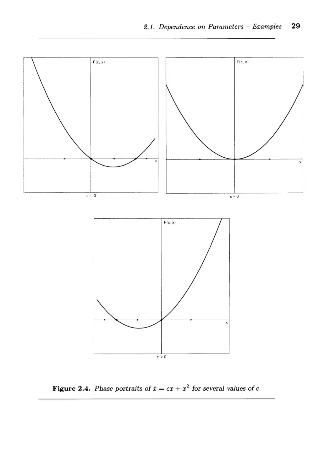
the graph of the function F( e, x) = ex + x 2 as shown in Figure 2.4. Notice
that the origin is an equilibrium point for all values of the parameter e.
For e < 0, the origin is asymptotically stable and there is another equi-
librium point x = -e which is unstable. The parameter value e = 0 is a

2.1. Dependence on Parameters - Examples 29
F(c, x)
x
c <' 0
c=O
x
c>O
Figure 2.4. Phase portraits of x == ex + x 2 for several values of e.

30 Chapter 2: Elementary Bifurcations
-
x
,
,
,
,
,
,
,
,
,
-------
c
Figure 2.5. Bifurcation diagram of trans critical bifurcation.
bifurcation value at which the two equilibria coalesce at the origin, which
is a nonhyperbolic unstable equilibrium point. For C > 0, the origin be-
comes unstable by transferring its stability to another equilibrium point,
x = -c. For this reason, the bifurcation that Eq. (2.3) undergoes is called
trans critical bifurcation; see Figure 2.5. 0
Example 2.4. Hysteresis: Consider the cubic differential equation con-
taining a real parameter c:
x = c + x - x 3 .
(2.4)
Varying c corresponds to a vertical shift of the x-axis in the plot of the
graph of F(c, x) = c + x - x 3 ; see Figure 2.6 for the flows of Eq. (2.4).
For c = 0, Eq. (2.4) is Eq. (1.6) and it has stable orbit structure. The flow
continues to have stable orbit structure for small values of the parameter,
that is, for -Cl < C < Cl, where Cl = 3 is the local maximum value
and -Cl is the local minimum value of F(O, x). For C = -Cl or C = Cl,
the equation is at a bifurcation point. For the parameter values C < -Cl
and C > Cl, the equation again has stable orbit structure. The bifurcation
diagram of Eq. (2.4) is shown in Figure 2.7.
Because of its frequent occurrence in applications, it is worthwhile to
explore the dynamics of Eq. (2.4) in a bit more detail. Let us suppose
that the differential equation is a model of some physical system and the
parameter C is a changeable characteristic of the model. If we start the
system with a very large negative value of c, after a long time, regardless of
the initial condition Xo, the system will be very near a stable equilibrium
state on the left leg of the cubic. Now, let us continuously increase the
value of the parameter c. Since the system was near the stable state when
we began to vary c, it will stay near this stable state for small variations

2.1. Dependence on Parameters - Examples 31
2
C = - 30
C = 0 --
x
2
c=-
3y13
F(O, x) = x - X 3
Figure 2.6. Phase portraits of x == c + x - x 3 for several values of c.
x
\
,
,
,
,
,
\
\
c
Figure 2.7. Bifurcation diagram of x == c + x - x 3 .
in c. In fact, as we increase the parameter c, the system will follow the
stable equilibria on the left until c = Cl. At this point the system will jump
to a different stable equilibrium state on the right leg of the cubic. As
we continue to increase the parameter c, the system will follow the stable
equilibria on the right. The dashed lines in Figure 2.8 show the equilibria
the system will follow as c is increased from a very large negative value to a
very large positive value. Now, if we start decreasing the parameter c from

32 Chapter 2: Elementary Bifurcations
x
\
\
,
,
....-
--
r
1
1
I
I
.
I
I
I
, I
, I
'I
\1
1
I
/
/
/
/'
/'
c
--
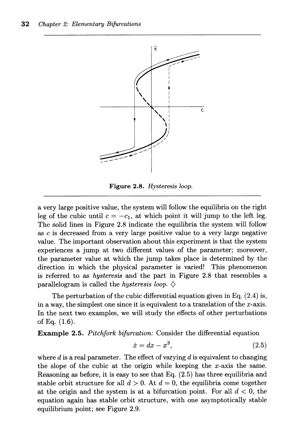
Figure 2.8. Hysteresis loop.
a very large positive value, the system will follow the equilibria on the right
leg of the cubic until C == -Cl, at which point it will jump to the left leg.
The solid lines in Figure 2.8 indicate the equilibria the system will follow
as C is decreased from a. very large positive value to a very large negative
value. The important observation about this experiment is that the system
experiences a jump at two different values of the parameter; moreover,
the parameter value at which the jump takes place is determined by the
direction in which the physical parameter is varied! This phenomenon
is referred to as hysteresis and the part in Figure 2.8 that resembles a
parallelogram is called the hysteresis loop. <>
The perturbation of the cubic differential equation given in Eq. (2.4) is,
in a way, the simplest one since it is equivalent to a translation of the x-axis.
In the next two examples, we will study the effects of other perturbations
of Eq. (1.6).
Example 2.5. Pitchfork bifurcation: Consider the differential equation
x == dx - x 3 , (2.5)
where d is a real parameter. The effect of varying d is equivalent to changing
the slope of the cubic at the origin while keeping the x-axis the same.
Reasoning as before, it is easy to see that Eq. (2.5) has three equilibria and
stable orbit structure for all d > o. At d == 0, the equilibria come together
at the origin and the system is at a bifurcation point. For all d < 0, the
equation again has stable orbit structure, with one asymptotically stable
equilibrium point; see Figure 2.9.

2.1. Dependence on Parameters - Examples 33
d<O
F(d, x) = dx _X 3
x
d=O
d>O
Figure 2.9. Phase portraits of x = dx - x 3 for several values of d.

34 Chapter 2: Elementary Bifurcations
-
x
Figure 2.10. Supercritical pitchfork bifurcation in x == dx - x 3 .
The bifurcation diagram of Eq. (2.5) is shown in Figure 2.10 and,
because of its appearance, that bifurcation is known as the pitchfork bifur-
cation. Notice that x == 0 is always an equilibrium point. However, as the
parameter d passes through the bifurcation value d == 0, the equilibrium
at the origin loses its stability by giving it up to two new stable equilibria
which bifurcate from the origin.
For this particular example, the pitchfork bifurcation is called super-
critical because the additional equilibrium points which appear at the bifur-
cation value occur for the values of the parameter at which the equilibrium
point is unstable. When the additional equilibria occur for the values of
the parameter at which the original equilibrium point is stable, the bifur-
cation is called subcritical. As illustrated in Figure 2.11, an example of a
subcritical pitchfork bifurcation can be seen in the equation x == dx + x 3 . 0
Example 2.6. Fold or cusp: Let us now combine the two different per-
turbations above and consider the cubic differential equation
x == c + dx - x 3 F(c, d, x),
(2.6)
depending on two real parameters c and d. The vector field (2.6) is the
most general perturbation of the function -x 3 with lower order terms be-
cause any term involving x 2 can always be eliminated by an appropriate
translation of the variable. In fact, for a general cubic -x 3 + ex 2 + dx + c,
use the change of variable x  x + e/3 and determine the new coefficients
c and d in terms of e, c, and d.
We begin the analysis of Example 2.6 by first finding the bifurcation
values of the parameters. As we have seen in the previous examples, at
bifurcation points, a differential equation must have a nonhyperbolic equi-

2.1. Dependence on Parameters - Examples 35
-
x
...............
"
"
"
,
\
I
I
/
/
"
.",,-"
"""".
d
Figure 2.11. Subcritical pitchfork bifurcation in x == dx + x 3 .
point, that is,
F(c, d, x) == 0 and
a
ax F(c, d, x) == O.
For this example [Eq. (2.6)], the equations above are equivalent to
c + dx - x 3 == 0 and d - 3x 2 == o.
Our objective is to determine all values of c and d for which these two
equations can have some common solution x. Therefore, we can consider
these equations as defining c and d parametrically in terms of x. Solving
the second equation for d and then substituting the result into the first
equation yields
d == 3x 2 and c == -2x 3 .
(2.7)
If we now eliminate x from these two equations, we obtain the following
equation for a cusp:
4d 3 == 27 c 2 . (2.8)
In Figure 2.12 we have drawn the graph of Eq. (2.8) in the (c, d)-plane;
this graph is a cusp. In each appropriate region of that (c, d)-plane we
have sketched a graph for the function F (c, d, x). In each such sketch we
have indicated the flow determined by Eq. (2.6).
There is a wealth of information packed in Figure 2.12, including the
dynamics of Eqs. (2.4) and (2.5). To extract the dynamics of Eq. (2.4), we
fix d at a positive value, say d == 1, and then obtain the bifurcation diagram
of hysteresis shown in Figure 2.7. To extract the dynamics of Eq. (2.5),
we fix c == 0 and obtain the pitchfork bifurcation diagram in Figure 2.10.
Equation (2.6) also contains a supercritical saddle-node bifurcation in dis-
guise: fix c =1= 0, say c == 1, and vary d, as illustrated in Figure 2.13.

36 Chapter 2: Elementary Bifurcations
d

4d 3 = 27c 2
.

c
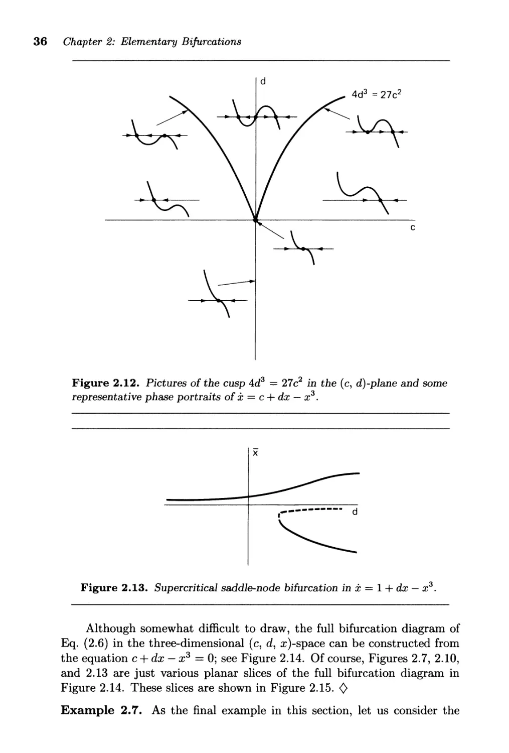
Figure 2.12. Pictures of the cusp 4d 3 = 27 c 2 in the (c, d)-plane and some
representative phase portraits of x = c + dx - x 3 .
x
....--------- d
I
Figure 2.13. Supercritical saddle-node bifurcation in x = 1 + dx - x 3 .
Although somewhat difficult to draw, the full bifurcation diagram of
Eq. (2.6) in the three-dimensional (c, d, x)-space can be constructed from
the equation c + dx - x 3 = 0; see Figure 2.14. Of course, Figures 2.7, 2.10,
and 2.13 are just various planar slices of the full bifurcation diagram in
Figure 2.14. These slices are shown in Figure 2.15. 0
Example 2.7. As the final example in this section, let us consider the

2.1. Dependence on Parameters - Examples 37
c
d
c
d
Figure 2.14. The bifurcation diagram of the cubic differential equation
x == c + dx - x 3 in the (c, d, x )-space. The cusp below is the set of points in
the (c, d)-plane for which the folding surface above has vertical tangency;
over a point inside the cusp, the surface above has multiple values.
following differential equation, depending on a scalar parameter A :
x=A+(mA+1)x-x 3 , (2.9)
where m is a fixed constant. This equation is a special case of Eq. (2.6)
with
C = A and d = mA + 1
for which Eq. (2.8) of the cusp becomes
4(mA + 1)3 = 27A 2 .
(2.10)
(2.11)
For fixed m, the bifurcation values for Eq. (2.9) correspond to the solutions
of the cubic equation (2.11). Geometrically, these bifurcation values are
the points of intersection of the cusp [Eq. (2.8)] with the parametrized line
[Eq. (2.10)]. Each of the three cases, m > 1, m = 1, and m < 1 are
different and are depicted in Figure 2.16, where we have also drawn the
bifurcation diagrams and the orbit structures of Eq. (2.9). You are invited
to visualize these bifurcation diagrams as appropriate planar slices of the
three-dimensional bifurcation diagram given in Figure 2.14.
An important remark for m < 1 lies in the observation that the orbit
structures in the bifurcation diagram are equivalent when the parameter
A lies in the intervals (-00, AO) and (AI, A2)' However, to go from a flow
corresponding to a value of A in the first interval to an equivalent flow for A
in the second interval one must pass through two saddle-node bifurcations.
In other words, the flows of Eq. (2.9) with the same qualitative structure
are not "connected." 0

38 Chapter 2: Elementary Bifurcations
c
d
(a)
\c
d
(b)
l;-c
d
(c)
\c
d
c
d
,\C
d
Figure 2.15. Slices of the bifurcation diagram of x = c + dx - X 3 : (a) hys-
teresis for d = 1, (b) supercritical pitchfork for c = 0, and (c) supercritical
saddle-node for c = 1.

2.1. Dependence on Parameters - Examples 39
-
x
C
"
"
"
""
A.
d
B
C=A
d = mA + 1
d
\
,
C
,
A
8
,
/
/
C
-
x
/
I
I
I
I
I
I
I __--
I ."._---
I"
d
A2 A
I
I
I
I
I I I
.. .. · . .... . tII 1 .. . .... . ·
I I
B
Figure 2.16. Bifurcation diagrams of x = A + (mA + 1) x - x 3 for m > 1,
m = 1, and m < 1.
With these examples at our disposal, we now turn to generalities.
Exercises
.o
2.1. Identify the groups of examples in Exercise 1.5 with the same orbit structure.
2.2. Provide the details of the computation of the bifurcation diagrams in Ex-
ample 2.7.

40 Chapter 2: Elementary Bifurcations
2.3. Constant harvesting: Suppose that a population grows according to the
"logistic model" and is harvested at a constant rate. The dynamics of the
density x(t) of such a population is governed by the differential equation
x == kx - cx 2 - h,
where all the coefficients are positive; k and c reflect the intrinsic growth rate
of the population and h is the rate of harvesting. Notice that the population
grows at a rate proportional to its size when the population density is small.
However, when the population gets large, growth is impaired because of, for
example, overcrowding; the x 2 term reflects this behavior.
Now, the problem is, for fixed k and c, to determine the effect of harvesting
on the population. Since the population density cannot be negative, we are
interested in the solutions of this equation for x > O. For a positive initial
population density, the population is exterminated if there is a finite value of
t such that cp( t, xo) == o. Without finding explicit solutions of the differential
equation, show the following:
( a) If the harvesting rate h satisfies 0 < h < k 2 / (4c), then there is threshold
value of the initial size of the population such that if the initial size
is below the threshold value, then the population is exterminated. On
the other hand, if the initial size is above the threshold value, then the
population approaches an equilibrium point.
(b) If the harvesting rate h satisfies h > k 2 / ( 4c), then the population is
exterminated regardless of its initial size.
2.4. Proportional harvesting: Suppose that a population grows according to the
"logistic model" as in the previous exercise, but is harvested at a rate pro-
portional to the size of the population:
x == kx - cx 2 - hx,
where k, c, and h are positive constants. Show that if k < h, then, regardless
of the initial density Xo > 0, such a population tends toward extermination
as t  +00, but is not exterminated in finite time. Also, analyze the fate of
the population in the cases k == hand k > h.
2.5. Hydroplane: The rectilinear motion of a hydroplane, ignoring pitching and
rolling, is determined by a scalar differential equation of the form
mv == T(v) - W(v),
where v is the velocity of the hydroplane, m is its mass, T is the thrust of the
driving mechanism, and W is the resistance. It is reasonable to assume, for
simplicity, that the thrust is approximately constant. The resistance, on the
other hand, should increase with small and large v, but can be negative for
intermediate values of the velocity due to rising of the hydroplane and the
decrease of the wetted area. Discuss the possible motions of the hydroplane
for various values of the constant thrust.

2.2. The Implicit Function Theorem 41
2.2. The Implicit Function Theorem
In this section, we state a fundamental result from mathematical analysis
known as the Implicit Function Theorem, which turns out to be an indis-
pensable tool in bifurcation theory. The simplified version presented below
is tailored for the study of bifurcations of equilibria of scalar differential
equations. A more general form of this important theorem is given in the
Appendix.
Let A - (AI, . . . , Ak) be a vector in IRk. For now, we take the "norm"
IIAII of A to be
IIAII == (AI + . . . + A%)1/2,
which we may interpret as the length of A. We will say more about norms
of vectors in Chapter 7.
Theorem 2.8. Suppose that F: IRk x IR ---+ IR; (A, x) r--t F(A, x), is a
0 1 function satisfying
F(O, 0) == 0 and
of
ox (0, 0) # o.
Then there are constants 8 > 0 and TJ > 0, and a 0 1 function
'ljJ : {A : II All < 8} ---+ IR
such that
'ljJ ( 0) == 0 and F ( A, 'ljJ ( A )) == 0 for II A II < 8.
Moreover, if there is a (AO, xo) E IRk X IR such that IIAol1 < 8 and Ixol < TJ,
and satisfies the equation F(AO, xo) == 0, then Xo == 'ljJ(AO)' 0
The Implicit Function Theorem can be used to study equilibria in the
following context. Let x == F(A, x) be a differential equation depending
on k parameters A = (AI, ..., Ak)' If x == 0 is a hyperbolic equilibrium
point of the differential equation x == F(A, x) at A == 0, then the conditions
of the Implicit Function Theorem are satisfied. This guarantees that the
equation F(A, x) == 0 may be solved locally for x == 'ljJ(A) as a function of the
parameters (AI,. .. , Ak); see Figure 2.17. Furthermore, of (A, 'ljJ(A))/OX #
o for A sufficiently small. Thus, the qualitative structure of the flow does
not change near x == O. Consequently, there are no bifurcations in the
neighborhood of x == 0 for sufficiently small values of the parameters. In
the next section, we will discuss this situation in detail as well as the
important role that the Implicit Function Theorem plays in bifurcation
theory.

42 Chapter 2: Elementary Bifurcations
x
A
F (A, x) = 0
Figure 2.17. The Implicit Function Theorem.
To apply the Implicit Function Theorem in a specific situation, you
may need to transform variables in such a way that the origin in the ('\, x)-
space becomes a zero of the given function. For example, if G : IRk x IR 
IR; ('\, x) r--t G('\, x), has G('\o, xo) == 0, then we can set F('\, x) ==
G('\o +'\, Xo + x) and F(O, 0) == o.
Exercises
,.Q.O
2.6. For the function F(>", x) == >.. + (1 + >..)x + x 2 , determine the function 'lj;(>..)
whose existence is guaranteed by the Implicit Function Theorem.
Answer: 'lj; ( >..) == - >...
2.7. Apply the Implicit Function Theorem to show that there is a unique solution
of the equation J-L + (1 - J-L)Y + y3 == 0 near (J-L, y) == (1, -1).
2.8. Show that the conditions of the Implicit Function Theorem are satisfied for
the following functions:
(a) >.. + sin x; (b) 1/2 + >.. - cos(7r/6 + x); (c) sin>.. + tanx.
2.3. Local Perturbations Near Equilibria
Earlier in Section 2.1 we considered three specific differential equations,
linear [Eq. (2.1)], quadratic [Eq. (2.2)], cubic [Eq. (2.6)], and investigated
the stability and bifurcation of equilibrium points as a function of the
parameters. In this section we consider a given differential equation x ==
f(x) with an equilibrium point x. We show that, if the first term of the
Taylor expansion of the vector field f at x is linear, quadratic, or cubic,
then under rather general perturbations the bifurcation of equilibria near
x is essentially the same as in the examples mentioned above. It should
be emphasized that in the following analysis we will consider the effects of

2.3. Local Perturbations Near Equilibria 43
quite arbitrary, but small, perturbations. Thus, our results are valid only
in a sufficiently small neighborhood around the equilibrium point. For
simplicity, we shall assume that x == I (x) has an equilibrium point at 0; if
not, we always can translate to a new coordinate system, as in the proof
of Theorem 1.14.
Case I: Hyperbolic equilibria. Suppose that I is a 0 1 function
with j(O) == 0 and j'(O) =1= o. We saw in Theorem 1.14 that the stability
properties of the equilibrium point 0 of the differential equation x == j (x) is
determined by the linear approximation of the vector field near 0, that is,
the higher order perturbations in the Taylor expansion of the vector field
do not effect the qualitative structure of the flow near zero. However, the
question remains: what happens if we make perturbations that influence
the constant and the linear terms? We will show below that the situation
in Example 2.1 also prevails in the general case.
To be precise, consider the perturbed differential equation
x == F(A, x),
(2.12)
where F : IRk x IR  IR; (A, x) r--t F(A, x), is a C 1 function satisfying
aF
F(O, x) == j(x) and ax (0, 0) == j' (0) =1= o.
(2.13)
Let us first investigate the existence of equilibria of the perturbed equa-
tion (2.12). If F(A, 0) =1= 0, then the origin will no longer be an equilibrium
point. However, from Eq. (2.13) and the fact that j(O) == 0, we have
aF
F(O, 0) == 0 and ax (0, 0) == I' (0) =1= o.
Hence, the Implicit Function Theorem implies that there are constants
8 > 0 and TJ > 0, and a 0 1 function 'ljJ(A) defined for II All < 8 with 'ljJ(0) == 0
such that
F(A, 'ljJ(A)) == o.
Moreover, every (A, x) with 'IAII < 8 and Ixl < TJ satisfying F(A, x) == 0 is
given by (A, 'ljJ(A)). Therefore, for each II All < 8, and Ixl < 'fJ, there is a
unique equilibrium x == 'ljJ(A) of Eq. (2.12) satisfying Ix I < TJ.
The stability behavior of the equilibrium 'ljJ( A) can easily be determined
from Theorem 1.14. To do so, we need to compute the sign of the derivative
aF
ax (A, 'ljJ(A)).
From Eq. (2.13) and the fact that 'ljJ(0) == 0, we have ; (0, 'ljJ(0)) == 1'(0) =1=
o. Thus, there is a 8 > 0 such that, for II All < 8, the sign of Eq. (2.14) is
(2.14)

44 Chapter 2: Elementary Bifurcations
the same as that of 1'(0). Therefore, the stability type of the equilibrium
'ljJ(A) of the perturbed equation (2.12) is the same as the stability type of
the equilibrium 0 of the unperturbed equation x = I(x).
We can summarize the discussion above by saying that the flow near
a hyperbolic equilibrium point is insensitive to small perturbations of the
vector field.
Case II: Equilibria with quadratic degeneracy. Suppose that I
is a 0 2 function with 1(0) = 0, I' (0) = 0, but I" (0) =1= o. This is the next
order of complication that occurs when we cannot make a decision about
the stability of an equilibrium point based on the linearization.
Let us consider the perturbed differential equation
x = F(A, x),
(2.15)
where F : IRk x IR ---+ IR; (A, x)  F(A, x), is a 0 2 function satisfying
F(O, x) = I(x),
8F
8x (0, 0) = 0,
8 2 F ( ) " ( )
8x 2 0, 0 = I 0 =1= o.
(2.16)
These conditions together with f(O) = 0 imply that the Taylor expan-
sion of F about the origin has the following form:
x 2
F(A, x) = a(A) + b(A)X + c(A)2 + G(A, x),
with a(O) = 0, b(O) = 0, c(O) = I" (0) =1= 0, and, for any t > 0, there are
8 > 0 and 'TJ > 0 such that the function G satisfies IG(A, x)1 < tlxl 2 for
II All < 8 and Ixl < 'TJ.
As an instance of Case II, let us recall the differential equation x =
I(x) = x 2 and its perturbation (2.2) depending on one parameter (k = 1):
2
X = F('x, x) =,x + f"(O)  .
We saw in Example 2.2 that the flow of this equation changes at A = 0
from two equilibria when Af" (0) < 0 to no equilibrium when Af" (0) > 0;
see Figure 2.2. We will show below that the bifurcation behavior of this
simple example occurs for the general case [Eqs. (2.15) and (2.16)] as well.
To verify the assertion above, it is only necessary to demonstrate that
the function F( A, x) near x = 0 for any small A has a graph which is like a
parabola. This can be accomplished by showing the existence of a unique
extreme point of the function F ( A, x) near x = 0 for small A. The extreme
points of F correspond to the solutions x of the equation
8F
8x (A, x) = O.
(2.1 7)

2.3. Local Perturbations Near Equilibria 45
O:(A) <0 ..
O:(A) = 0
. O:(A) > 0
f"(O) > 0
f" (0) < 0
Figure 2.18. Local bifurcations of a nonhyperbolic equilibrium point with
quadratic degeneracy.
Let H(A, x) 8F(A, x)/8x. Then Eq. (2.16) implies that
H(O, 0) = 0 and  (0, 0) = 1"(0) =I O.
Thus, the Implicit Function Theorem implies that there are constants 8 >
0, r} > 0, and a 0 1 function 'ljJ(A) defined for IIAII < 8 such that 'ljJ(0) = 0
and H(A, 'ljJ(A)) = 0, that is,
: (A, 1jJ(A)) = 0
and, moreover, every solution (A, x) of Eq. (2.17) with IIAII < 8 and Ixl < TJ
is given by x = 'ljJ(A).
For each fixed A, the function F(A, x) has a minimum at x = 'ljJ(A) if
1"(0) > 0, or a maximum if 1"(0) < O. The number of equilibrium points
of Eq. (2.15) depends upon the extreme value a(A) F(A, 'ljJ(A)) of the
function F. In Figure 2.18 we have drawn the flows for these two cases
with several values of a(A) (compare with Figure 2.2). These results can
be summarized analytically by saying that when a(A)/" (0) < 0 there are
two hyperbolic equilibria near the origin, a(A) = 0 implies that there is a
nonhyperbolic equilibrium at the origin, and when a(A)/"(O) > 0 there are
no equilibrium points about the origin.
It is important to observe in the discussion above that the qualitative
structure of the flow of the perturbed equation (2.15) is determined from a
single function of the parameter A, namely, the function a(A) correspond-
ing to the extreme value of F(A, x). Thus, even though there may be k
components of the (vector) parameter A = (AI, A2, . . . , Ak), the bifurcation
behavior of the perturbed equation (2.15) depends on a single number,
a(A). When this situation occurs in a bifurcation problem, we say that the
original vector field 1 is a codimension-one bifurcation.

46 Chapter 2: Elementary Bifurcations
Example 2.9. Two parameters but codimension one: As an example of a
codimension-one bifurcation of a vector field depending on two parameters,
consider the differential equation
x == Al + A2 X + x 2 ,
where A == (AI, A2) are two small parameters. The function a(A) for this
example corresponds to the minimum value of the function F(A, x) == Al +
A2X + x 2 , and it is given by
a(AI' A2) == Al - A.
Thus the bifurcations occur as we cross the curve Al == A/4 in the (AI, A2)-
plane: there are two equilibrium points if Al < A/4, and none if Al >
A/4. 0
Example 2.10. In applications, a single parameter may affect several
terms in the Taylor expansion of a perturbation. For instance, consider the
following perturbation of the vector field f(x) == x 2 given by
x == A 2 + 2aAx + x 2 ,
where A is a scalar parameter, and a is a given constant. As before, the
bifurcation behavior of the perturbed equation depends on the minimum
value of the function F(A, x) == A 2 + 2aAx + x 2 , which is equal to a(A) ==
A 2 (1 - a 2 ). The sign of a(A) is determined by the linear term in the
perturbation if lal > 1, and by the constant term if lal < 1. The bifurcation
takes place at A == 0 in both cases, but the flow is different depending on
whether lal < 1 or lal > 1. You are invited to draw the bifurcation diagram
and representative pictures of the flow. 0
Case III: Equilibria with cubic degeneracy. Suppose that I is a
03-function with f (0) == 0, f' (0) == 0, I" (0) == 0, but f'" (0) =1= O. This is
the level of complication that occurs if the properties of the flow near the
equilibrium point at zero cannot be determined from the linear or second-
order terms of the Taylor expansion of f(x).
We have seen previously (Section 2.1) in the specific example f(x) ==
-x 3 that at least two parameters were needed to capture all of the possible
types of behavior of I under perturbations. In particular, we have studied
the bifurcations in the perturbed equation x == c + dx - x 3 ; see Exam-
ple 2.6 and Figures 2.12 and 2.14. We will show below that this example
is representative of what can happen in the general case near the equilib-
rium point x == 0 of I satisfying the conditions above when I is subjected
to "nice" perturbations that are small together with their derivatives up
through order three.

2.3. Local Perturbations Near Equilibria 47
More specifically, consider the perturbed differential equation
x = F(A, x),
(2.18)
where F : IRk x IR  IR; (A, x) r--t F(A, x), is a C 3 function satisfying
F(O, x) = f(x),
o2F
ox 2 (0, 0) = 0,
of
ox (0, 0) = 0,
;: (0, 0) = fill (0) of:- O.
(2.19)
A complete bifurcation analysis of Eqs. (2.18) and (2.19) is rather com-
plicated and would take us too far afield. Therefore, we confine ourselves
to the two-parameter case. In the presentation below, we first study an
important particular two-parameter perturbation, and then show how to
reduce a general two-parameter perturbation to this special perturbation.
We conclude this somewhat lengthy and technical section by giving a simple
example of a three-parameter perturbation.
We first present the bifurcation analysis for a two-parameter, A =
(AI, A2), perturbation F(A, x) with the following Taylor expansion about
the origin:
x 2 x 3
F(A, x) = Al + A2 X + c(A)2 + d(A)6 + G(A, x),
(2.20 )
with c(O) = 0, d(O) = f"'(O) =1= 0, and, for any € > 0, there are 8 > 0 and
'TJ > 0 such that the function G satisfies IG(A, x)1 < €lxl 3 for IIAII < 8 and
Ixl < 'TJ.
As usual, we begin by finding the bifurcation values of the parameters,
that is, the values of A = (AI, A2) for which the function F(A, x) given
by Eq. (2.20) has multiple zeros. To accomplish this we must solve the
following two equations:
x 2 x 3
o = F(A, x) = Al + A2 X + c(A)2 + d(A)6 + G(A, x),
(2.21 )
of x 2 oG
o = ox (A, x) = A2 + C(A)X + d(A)2 + ox (A, x). (2.22)
We view Eqs. (2.21) and (2.22) as a system of two equations defining Al
and A2 parametrically in terms of x. To obtain the solutions locally, we
can use essentially the method of Gaussian elimination in conjunction with
repeated applications of the Implicit Function Theorem: using Eq. (2.22)
solve locally for A2 as a function of Al and x, then substitute the result
into Eq. (2.21) to determine A I in terms of x.

48 Chapter 2: Elementary Bifurcations
In preparation for the Implicit Function Theorem, let
8F X 2 8G
8x (A, x) H(Al, x, A2) == A2 + C(A)X + d(A)2 + 8x (A, x).
The reordering of the variables is meant to be suggestive because we will
apply the Implicit Function Theorem to H(Al, x, A2) treating (AI, x) as
parameters and A2 as the dependent variable. Observe that H(O, 0, 0) == 0
and 8H(0, 0, 0)/8A2 == 1 =1= o. Thus, by the Implicit Function Theorem,
there is a C 2 function 'l/J2 ( AI, x) defined for A 1 and x small and
H ( AI, x, 'l/J2 ( AI, x)) == O.
Moreover, every small (AI, x, A2) satisfying H(Al, x, A2) == 0 is given by
A2 == 'l/J2(Al, x). From the special form of H, it is not difficult to see, with
a little bit of computing, of course, that
'l/J2(Al, 0) = :2 (0, 0) = 0, 2 (0, 0) = -d(O) = - 1"'(0) -# O.
Thus, the Taylor expansion of the function 'l/J2 (AI, x) with respect to x has
the form
x 2
'l/J2(Al, x) == C(Al)X + D(Al)2 + . .. ,
C(O) == 0, D(O) == - f'" (0) =1= O.
We now substitute A2 == 'l/J2(Al, x) into Eq. (2.21) and solve for Al in
terms of x. Let
( 2.23 )
x 2
o == J(x, AI) - Al + 'l/J2(Al, x)x + C(Al, 'l/J2(Al, x))2
x 3
+ d ( AI, 'l/J2 ( AI, x)) 6 + G ( AI, 'l/J2 ( AI, x), x)
and observe that J(O, 0) == 0 with 8J(0, 0) /8Al == 1 =1= O. Thus, by the
Implicit Function Theorem, there is a 0 3 function 'l/Jl (x) defined for x small
so that
J(x, 'l/Jl(X)) == o.
Moreover, every small (x, AI) satisfying J(x, AI) == 0 is given by Al ==
'l/Jl (x). From the special form of J, it is not difficult to see, again with
some computing, that
'l/Jl(O) == 'l/J(O) == 'l/J(O) == 0, 'l/J'(O) == 2j"'(0).
Thus, the Taylor expansion of the function 'l/Jl (x) has the form
'l/Jl(X) == j"'(0)x3 +... .
(2.24 )

2.3. Local Perturbations Near Equilibria 49
We can now summarize the results of the computations above by saying
that the local solutions Al(X) and A2(X) of Eqs. (2.21) and (2.22) near the
origin are given by
Al(X) = 'l/Jl(X) = If'''(0)x 3 + ...,
A2(X) = 'l/J2('l/Jl(X), x) = -f'''(0)x2 +... .
(2.25)
These equations are the parametric representation of a cusp in the (AI, A2)-
plane which near the origin approximately coincides with the curve
A = -  f'" (O)A.
(2.26 )
If f'" (0) < 0, then the equation above is essentially that of the cusp in
Eq. (2.8). Therefore, the qualitative structure of the flows of the perturbed
equation (2.20), for small values of A, are the same as the ones given in
Figure 2.12. For practice, you should draw the flows for the case when
f'" (0) > O.
Equation (2.20) is an example of a "good" two-parameter perturbation
of a vector field with cubic degeneracy in the sense that the bifurcations
are determined only by the constant and the linear terms of the Taylor
expansion of the vector field. The term C(A)x2/2 did not enter into the
first approximation to the cusp in the (AI, A2)-plane; see Eqs. (2.25) and
(2.26). This is because the function C(A) is differentiable in A and c(O) = O.
Thus, the Taylor expansion for C(A) must be given by
C(A) = ClAl + C2 A 2 + . . . ,
where Cl and C2 are constants; hence, the term C(A)x2 has the form
C(A)X 2 = ClAlX2 + C2A2X2 + . . . .
Observe that, when x is small, the term ClAlX2 is smaller than AI, and the
term C2A2X2 is smaller than A2. Therefore, it is to be expected that the
term C(A)x2 has little influence on the bifurcations of Eq. (2.20).
We now show that an arbitrary two-parameter perturbation of the
cubic degeneracy, under certain reasonable conditions, can be reduced to
the special two-parameter perturbation (2.20). Let J.l = (J.ll, J.l2) be two
parameters and consider the perturbation F(J.l, x) with the following Taylor
expansion about the origin:
X2 __ x3 __
F(J.l, x) = a(J.l) + b(J.l)x + 2(J.l) 2 + d(J.l)e; + G(J.l, x),
(2.27)
with a(O) = b(O) = 2(0) = 0, d(O) = f'" (0) =1= 0, and, for any f > 0, there
are b > 0 and 17 > 0 such that the function G satisfies IG(J.l, x)1 < flxI3 for
11J.l11 < band Ixi < 17.

50 Chapter 2: Elementary Bifurcations
To make certain that (J-L1, J-L2) cover all possible small values of the
constant and the linear terms, that is, the range of the vector-valued func-
tion (a(J-L), b(J-L)) cover a neighborhood of zero for small J-L, we suppose that
the Jacobian of (a(J-L), b(J-L)) with respect to J-L at J-L == 0 is not zero:
det a( a(I£), b(I£))
8(J-L1, J-L2)
# O.
(J-Ll, J-L2)=(0, 0)
(2.28 )
Next, we introduce the transformation of parameters
Al a(J-L1, J-L2),
A2 b(J-L1, J-L2)
(2.29 )
in a neighborhood of A == (AI, A2) and J-L == (J-L1, J-L2) equal to zero. For any
J-L, the constant A is uniquely defined by Eq. (2.29). To know that relation
(2.29) is a good transformation of parameters we need to make certain
that, given A, a constant J-L is uniquely defined by Eq. (2.29). Condition
(2.29) and the Implicit Function Theorem imply that this is the case in a
neighborhood of zero. In fact, if we define the functions
PI (A, J-L) a(J-L) - AI,
then PI (0, 0) == P 2 (0, 0) == 0 and
d 8(P1, P 2 ) 8(a(J-L), b(J-L))
et == det
8(J-L1, J-L2) )..=J-L=O 8(J-L1, J-L2)
P 2 (A, J-L) b(J-L) - A2,
# o.
J-L=O
Thus, J-L is uniquely defined by A and is C 1 in A.
Once the transformation (2.29) of parameters is made, by putting
C(A) 2(J-L(A)), d(A) - d(J-L(A)), and G(A, x) 8(J-L(A), x)), the general
perturbation (2.27) becomes the special perturbation (2.20).
To illustrate the discussion above, we now give examples of a "good"
and a "bad" two-parameter perturbation of the cubic degeneracy.
Example 2.11. Consider the two-parameter perturbation of the vector
field f(x) == -x 3 /6 given by
x 2 x 3
X = 1£1 + 1£2 + (1£2 + I£) x + 1£1 2 - 6'
(2.30)
where J-L1 and J-L2 are two real parameters. For the perturbed vector field
(2.30), the functions in Eq. (2.27) are given by a(J-L) == J-L1 + J-L2, b(J-L) ==
J-L2 + J-Lr, 2(J-L) == J-L1, d(J-L) == -1, and 8(J-L, x) == O. The Jacobian (2.28) of
these functions (a(J-L), b(J-L)) at J-L == 0 is one- "good." Thus, we introduce
the new parameters A == (AI, A2) defined by
Al J-L1 + J-L2,
A2 J-L2 + J-Lr

2.3. Local Perturbations Near Equilibria 51
so that Eq. (2.30) attains the special form of Eq. (2.20) as follows:
x 2 x 3
X == Al + A2 x + C(A)2 - 6'
(2.31 )
where the function c( A) is the unique solution J-L1
equation
C( A) of the cubic
-J.t + J.t1 - Al + A2 == 0
which vanishes for (AI, A2) == (0, 0). The Implicit Function Theorem guar-
antees that such a solution exists and is unique.
The bifurcation curve of Eq. (2.31) in the (A 1, A2)- plane near the origin
is approximately the cusp 8A == 9A, which follows from Eq. (2.26). Thus,
in the original (J-L1, J-L2)-plane this curve becomes
8(J-L2 + J-L)3 == 9(J-L1 + J-L2)2
which, near the origin, is again a cusp with approximately the same shape
as the one in the (AI, A2)-plane. 0
Example 2.12. Consider the two-parameter perturbation of the vector
field f(x) == -x 3 /6 given by
x 2 x 3
. 2
X == J-L1 + J-L2 x + J.t2 2 - 6'
(2.32)
where J-L1 and J.t2 are two real parameters. As a special case of Eq. (2.27),
we have a(J-L) == J-L1, b(J.t) == J-L, c(J.t) == J-L2, and d(J-L) == -1. Notice that the
condition (2.28) is not satisfied. However, we can analyze Eq. (2.32) in the
following way.
From our previous discussion of the cusp, it is natural to eliminate the
x 2 term. If we introduce the new variable y - J.t2 - x, then
. 4332 13
Y == J.t1 + 3J-L2 + 2J-L2Y - "6Y .
Now, if we make the transformation of the parameters
Al J-L1 + 1 J-L ,
, _ 3 2
/\2 == 2J-L2,
(2.33)
then the differential equation above is put into the form of the special
perturbation (2.20):
iJ == Al + A2Y - !y3.
The bifurcation curve of this equation in the (AI, A2 )-plane is given by
Eq. (2.26), which is the cusp 8A == 9Ai.

52 Chapter 2: Elementary Bifurcations
To find the bifurcation curve of Eq. (2.32) in the original (111, 112)-
plane, we substitute the transformation (2.33) into the cusp and obtain
( 3 2 ) 3 ( 4 3 ) 2
8 2 11 2 = 9 111 + "3112 .
A simple computation yields the formula
ILl = ( -t =F v'3) IL.
Thus, the bifurcation values of Eq. (2.32) in the (111, 112)-plane form cubic
curves, not a cusp. Of course, the reason for this deviant behavior is that
the parameters (111, 112) do not enter into the equation in a nice way, that
is, the determinant in Eq. (2.28) is zero-"bad." ()
As we mentioned earlier, a complete analysis of the cubic degeneracy
is beyond the intended scope of our book. Therefore, we end this rather
long section with an example of a three-parameter perturbation.
Example 2.13. Three parameters: Consider the three-parameter pertur-
bation of f(x) = -x 3 /6 given by
x 2 x 3
X = 111 + 112 X + 113 2 - 6'
where 111, 112, and 113 are three parameters. As in the previous example,
the x 2 term can be eliminated by introducing the new variable y - 113 - x.
Then, the differential equation above in the new variable becomes
3
. 1 3 ( 1 2 ) Y
Y = 111 + 112113 + "3113 + 112 + 2113 Y - 6'
Therefore, if we define two new parameters
\- + + 13 ad \- + 12
.1\1 = 111 112113 "3113 n .1\2 = 112 2 11 3'
we obtain the following two-parameter differential equation:
. y3
Y = Al + A2Y - -.
6
The values of Al and A2 which correspond to bifurcation points are given
by the cusp 8A = 9A, as we have computed before. Therefore, the values
of the original parameters (111, 112, 113) corresponding to bifurcation points
must lie on the surface
( 1 2 ) 3 ( 1 3 ) 2
8 112 + 2 11 3 = 9 111 + 112113 + "3113

2.3. Local Perturbations Near Equilibria 53
in the three-dimensional (/-ll, /-l2, /-l3 )-space. As one crosses this surface,
the number of equilibrium points changes from one to three. 0
Exercises
4c:J.o
2.9. On quadratic degeneracy: For each of the vector fields below, draw the
bifurcation diagrams with the corresponding phase portraits:
(a) F(c, e, x) == c + ex + x 2 . This is Example 2.9, but this time use the
transformation x == y - e/2.
(b) F( A, x) == a + (A - a)x + x 2 . Draw x versus A for various values of a.
Notice the difference between a < 0 and a > O.
(c) F( A, x) == A 2 + 2aAx + x 2 . Draw x versus A for various values of a.
Notice the difference between I a I < 1 and I a I > 1.
(d) F(A, x) == A + 2aAx + x 2 , for any fixed value of a.
(e) F( A, x) == A 4 + 2aAx + x 2 , for any fixed value of a.
2.10. On cubic degeneracy: Obtain the bifurcation curves of the following one-
and two-parameter perturbations of the cubic vector field f(x) == _x 3 and
sketch some representative phase portraits:
(a) x == 1 + {Ll + 2{LlX - x 3 ; (b) x == 1 + {L + {LlX - x 3 ;
(c) X == {Ll + {L2 + ({Ll - {L2)X - x 3 ; (d) x == {Ll + {L2 + ({Ll - {L)x - x 3 ;
(e) x == {Ll + {L + {L2X - x 3 ; (f) x == {Ll + {L2 + {LX + {L2 X2 - x 3 .
2.11. On quartic degeneracy: This exercise is on various one- and two-parameter
perturbations of the quartic vector field f (x) == x 4 . A complete discussion
of the most general perturbation of the quartic is very difficult. For each of
the following perturbations, draw the bifurcation diagrams along with the
corresponding vector fields:
(a) F(c, x) == c + x 4 ; (b) F(d, x) == dx + x 4 ;
(c) F(e, x) == ex 2 + x 4 ; (d) F(c, d, x) == c + dx + x 4 ;
(e) F(c, e, x) == c + ex 2 + x 4 ; (f) F(d, e, x) == dx + ex 2 + x 4 .
2.12. Obtain the bifurcation curves of the following one- and two-parameter dif-
ferential equations and sketch some representative phase portraits:
(a) x == {Ll - x 2 /(1 + x 2 ); (b) x == {Ll - x 2 /(1 + X 2 )2;
(c) X == {Ll - x 3 /(1 + x 3 ) for x > -1;
(d) x == {Ll + {L2X - x 3 /(1 + x 3 ) for x > -1.
2.13. Unfolding a pitchfork: As we have seen in Example 2.5, the pitchfork bifur-
cation occurs for the vector field F({L, x) == -x 3 + {LX at {L == 0 where the
number of equilibria changes from one to three or vice versa. An important
practical question is what happens to the bifurcation diagram if this one-
parameter vector field is subjected to small perturbations. Surprising as it
may seem, one can in fact write down a "most general" perturbation of this
vector field near the origin using only two additional parameters:
F({L, AI, A2, x) == _x 3 + {Lx + Al + A2X 2 .
Any other perturbation, however many parameters it may contain, can be
transformed to the particular perturbation above. For this reason, the three-
parameter vector field above is referred to as the unfolding of the pitchfork

54 Chapter 2: Elementary Bifurcations
bifurcation. The purpose of this exercise is to determine the bifurcation
diagrams x versus J1 near zero for fixed values of the unfolding parameters
Al and A2 near zero.
(a) To eliminate the quadratic term, let x = +A2/3 and transform the
vector field to _y3 + vy + 6 1 + A2V/3, where v = J1 + A/3 and 6 1 =
Al - A/27. Notice that this is a special case of Example 2.6.
(b) For Al = 0 and fixed A2 < 0, obtain the bifurcation diagram x versus
J1 and compare your result with Figure 2.16.
(c) For 6 1 = 0, that is, Al < A /27 and A2 < 0, obtain the bifurcation
diagram and, again, refer to Figure 2.16. Do the same analysis for
Al < A/27 and A2 > o.
(d) Discuss some of the remaining cases.
Reference: For more details on this example, and the general theory of
unfoldings of bifurcations, see Golubitsky and Schaeffer [1985].
2.4. An Example on a Circle
In this brief section, we study the bifurcations in a two-parameter perturbation
of the periodic differential equation x = sin x of Section 1.4. By considering the
perturbed periodic equation on a circle, we will obtain a new type of a limit set
different from an equilibrium point, namely, the circle itself.
Example 2.14. Consider the two-parameter perturbation of the periodic vector
field f (x) = sin x given by
x = c + d sin x,
( 2.34 )
where c and d are real parameters. Of course, the perturbed vector field (2.34)
is still periodic with period 211" for all values of the parameters. When d = 0, the
vector field is actually periodic with any period. Furthermore, if c = d = 0, then
the flow consists entirely of equilibrium points. These two cases are not very
interesting. In Figure 2.19 we have drawn the orbits of Eq. (2.34) both on the
real line IR and the circle 8 1 for various parameter values.
Observe that the Q- and the w-limit sets of Eq. (2.34) on 8 1 are either
equilibrium points (case Idl > e) or 8 1 itself (case Idl < lei). Although it
is not apparent from Figure 2.19, in the latter case, each solution is also
periodic in t when considered as a motion on 8 1 . Let us first make this
notion precise.
Definition 2.15. A solution c.p(t, xo), with c.p(O, xo) = Xo, of a scalar
differential equation x = f(x) satisfying f(x+P) = f(x) is called a periodic
solution of period T, if there is aT> 0 such that
c.p(t + T, xo) = c.p(t, xo) + P
for all t > o. If, moreover, c.p( t + T, xo) =1= c.p( t, xo) + P for any 0 < T < T,
then T is called the minimal period.
Returning to our example, for the differential equation (2.34), we have
P = 27r. We now show that if Idl < lei, then every solution of Eq. (2.34) is

2.4. An Example on a Circle 55
I 0
I
I . Idl < - e
I
I
I
I 0
I Idl = - e
. . I . . .
I
I
I
I 0
I
. . I. . . . . . Idl> lei
. . . . . Idl = e 0
. Idl <e 0
Figure 2.19. Phase portraits of x = c + d sin x on IR and 8 1 .
periodic on 8 1 . Since <p( t, xo) is implicitly defined by
l CP(t, xo) dx
t=
XO c + d sin x
and c+d sin x =1= 0 for all x, there is a unique T such that <p(T, xo) = xo+21T',
that is,
l XO + 27r dx 1 27r dx
T- -
- XO e + d sin x - 0 e + d sin x ·
If <p(t, xo) is a solution of Eq. (2.34), then so are <p(t, xo) + 21T' and <p(t +
T, xo). At t = 0 these two solutions are equal; thus, by uniqueness (Theo-
rem 1.4), they are identical for all t > O. This proves the assertion above
and, moreover, shows that the period T is independent of the initial con-
dition.
The time periodicity of the solutions of Eq. (2.34), when Idl < lei,
can easily be observed if we plot trajectories in the (t, x)-plane; see Fig-
ure 2.20. <)
Exercises
,.,<)
2.14. Draw on the circle the phase portraits of the periodic differential equation
x = -A + 2 + cos(2x) - 3cosx
and verify the qualitative features in the indicated ranges of the scalar pa-
rameter A :

56 Chapter 2: Elementary Bifurcations
Xi vs. Time:
12.000000
t
II
I 2rr
I
____________:_1
I
T -I
x1
-12.000000
Figure 2.20. Time periodicity of solutions of x == c + dsinx.
(a) All solutions are periodic if ,\ < -1/8 and ,\ > 6.
(b) There are four equilibria if -1/8 < ,\ < o.
(c) There are two equilibria if 0 < ,\ < 6.
2.15. No equilibria: Suppose that f is a 27r-periodic 0 1 function with the property
that f (x) i= 0 for all x E JR. Show that every solution of the differential
equation x == f (x) is periodic on the circle obtained by identifying the end
points of an interval of length 27r. Derive a formula for the period( s) of the
solutions.
2.5. Computing Bifurcation Diagrams
In exploring the dynamics of a differential equation x == f ( x ), a first key
step is to locate its equilibrium points, equivalently, the zeros of the function
f. For most functions, this is usually a formidable task for the pencil; how-
ever, there are effective approximation procedures that can be performed
on the computer rather easily. We will see one such procedure-Newton's
Method-in Chapter 3. For the moment, we can also use the observation
in Section 1.2 that the equilibrium points of a scalar differential equation
x == f(x) are the Q- and w-limit sets of orbits. Thus, we can obtain approx-
imate values of the zeros of f by following a few selected orbits in forward
or reverse time. Numerical integration of such orbits can be carried out on
the computer using one of the standard numerical methods for initial-value
problems such as Euler's Method (see Section 3.1).
In the case where the vector field depends on a parameter A, one could
apply the same procedure to the equation x == F(A, x) for each fixed value
of A. By performing many numerical experiments for sufficient number of
values of A, one could then arrive at an approximate representation of

2.5. Computing Bifurcation Diagrams 57
the bifurcation diagram of the differential equation. For the simplest of
examples, however, this process is very cumbersome and inefficient. It is
the purpose of this section to describe a practical procedure for determining
the zeros of F( A, x) using differential equations.
Let us suppose that we are given a C 1 function, depending on a scalar
parameter A,
F: IRxIRIR; (A,x)F(A,X)
and wish to determine the set of points (A, x) satisfying the equation
F(A, x) = O.
U sing the observation described earlier, if necessary, let us first determine
a pair of values (AO, xo) with F(AO, xo) = O. Let us assume that in a
neighborhood of (AO, xo) on the (A, x)-plane the zeros of F(A, x) lie on
a smooth curve. We can parametrize this curve by t so that there will
be two C 1 functions A(t) and x(t) satisfying A(O) = AO, x(O) = Xo, and
F(>..(t), x(t)) = 0 for t in a neighborhood of zero.
To represent this parametrized curve as an orbit of a differential equa-
tion, we differentiate the equation F(A(t), x(t)) = 0 with respect to t:
8F . 8F .
8A (A,X)A+ 8X (A,X)X=0.
To satisfy this identity, (, x) must be a constant multiple of the vec-
tor (-  (A, x), f (A, x)) . If we choose the parametrization of the curve
(A(t), x(t)) in such a way that this constant is one, then we arrive at the
pair of differential equations
. 8F
A = - 8x (A, x)
8F
x= 8A (A,X)
(2.35)
satisfying the initial conditions
A(O) = AO, x(O) = Xo.
These differential equations, unfortunately, are not just a pair of in-
dependent scalar equations because their right-hand sides depend on two
variables A and x simultaneously. Consequently, the orbits of such a pair
must be investigated on the (A, x)-plane. We will devote Part III of our
book to a comprehensive study of differential equations of this type. At
this point, we will confine our discussions to a step-by-step description of
a constructive numerical procedure for obtaining the zero set of F(A, x) :

58 Chapter 2: Elementary Bifurcations
. Step 1. Fix A = AO and use the scalar differential
equation x = F(Ao, x) to find the set E Ao of zeros
of F(AO, x).
. Step 2. For each Xo E E Ao ' compute numerically
the solution of the differential equations (2.35) with
initial value A(O) = AO and x(O) = Xo, in both for-
ward and reverse time (using negative step size) di-
rections.
. Step 3. Repeat Step 1 as necessary for other val-
ues of the parameter A because there may be some
components of the curves of zeros of F(A, x) that
never intersect the vertical line A = AO.
Let us now implement these steps on several examples and attempt to
clarify the ambiguity ("as necessary") that is present in Step 3.
Example 2.16. Computing hysteresis: Consider the equation
F(A,X)=A+X-X 3 .
(2.36)
The zero set of this function is, of course, the cubic curve A = -x + x 3 .
However, for the sake of practice, let us try to implement the three steps
above.
In Step 1, let us fix, for example, AO = -5. Then, using the scalar
differential equation x = -5 + x - x 3 , we find that the set of its equilibria
consists of a single point: E-5 = { -1.904. . . }.
In Step 2, differential equations (2.35) for the function (2.36) become
. 2
A = - (1 - 3x )
x = 1
(2.37)
with the initial data A(O) = -5 and x(O) = -1.904. .. . Numerical integra-
tion of this initial-value problem gives the cubic curve shown in Figure 2.21.
Forward integration (using positive time and positive step size) of the pos-
itive orbit gives the piece of the cubic above the line Ao = -5 and the
backward integration (using negative time and negative step size) for the
negative orbit yields the remaining lower part.
Although there is no need for Step 3 in this simple example, let us
see what happens for another value of AO. If we fix AO = 0, for example,
then we have Eo = { -1, 0, I}. Numerical computation of the orbits of
Eq. (2.37) through anyone of the points (0, -1), (0,0), or (0, 1) gives the
same cubic curve. 0
Example 2.17. Consider the equation
F(A, x) = 1 + AX - x 3 .
( 2.38 )

2.5. Computing Bifurcation Diagrams 59
Figure 2.21. Numerically computed bifurcation diagram for the differen-
tial equation x == A + x - x 3 .
The pair of differential equations (2.35) for the function (2.38) are
 = - A + 3x2
(2.39)
x = x.
If we choose Ao = 0, then Eo = {1}. The orbit of Eq. (2.39) through
the point (0, 1) gives the upper curve shown in Figure 2.22. Unlike the
example above, the zero set of Eq. (2.38) is not obvious. So, let us ex-
periment with another choice of Ao. For Ao = 2, computations give E 2 =
{ -1, -0.618.. . , 1.618. . .}. The orbits of Eq. (2.39) through the points
(2, -1) and (2, -0.618.. .) coincide and they both give the lower curve.
The orbit through (2, 1.618. . .) yields the same upper curve we obtained
with the choice Ao = o. Further experimentation with other choices of Ao
does not alter Figure 2.22. 0
Example 2.18. Computing pitchfork: As the final example of this section,
let us try to recover numerically the bifurcation diagram of the pitchfork
bifurcation, that is, compute the set of zeros of the equation
F(A, x) = AX - x3.
The pair of differential equations (2.35) for this example are
 = - A + 3x2
(2.40 )
(2.41 )
X = x.
Notice that Eq. (2.41) is the same as Eq. (2.39), but the bifurcation curves
are determined by special choices of initial values. To compute the bifur-
cation diagram of Eq. (2.40), if we choose Ao = -1, then E-l = {O}. The
orbit of Eq. (2.41) through (-1,0) is the negative part of the A-axis; see
Figure 2.23.

60 Chapter 2: Elementary Bifurcations
Figure 2.22. Numerically computed bifurcation diagram of the differential
equation x = 1 + AX - X3.
Figure 2.23. Numerically computed bifurcation diagram, pitchfork, of the
differential equation x = AX - X3.
For AO = 1, we get El = { -1,0, I}. The orbits of Eq. (2.41) through
the points (1, -1) and (1, 1) give the lower and the upper parts, respec-
tively, of the parabola A = 3x 2 . The orbit through (1, 0) is the positive half
of the A-axis. The point (0, 0) is not obtained as a solution of Eq. (2.41)
unless we choose AO = O. In this case, Eo = {O} and the point (0, 0) is a
(equilibrium) solution of Eq. (2.41). <;
Exercises
4Q.<;
2.16. Use the numerical procedure described in this section, and PHASER, to
draw the bifurcation diagrams in the (A, x)- plane of the following differential

2.6. Equivalence of Flows 61
equations:
(a) x == X2 - A; (b) x == A 2 + X2 - 1;
(c) x == (A + 2)2 + X2 - 1; (d) x == [AX - X 3 ][(A + 2)2 + X2 - 1];
(e) x == 2A 3 + 3A 2 X - X3; (f) x == 2A 3 + 2.9A 2 X - x3;
(g) X == 0.1 + 2A 2 + 3A 2 X - x3; (h) x == (A + X - X3)(A2 + X2 - 1).
2.6. Equivalence of Flows
We agreed in Section 2.1 to consider two flows to be qualitatively equivalent
if they have the same orbit structure, that is, if they have equal number of
orbits and the directions of the flows on the corresponding orbits are the
same. For the case of scalar differential equations this notion of equivalence
of flows has been sufficient for our purposes. In the case of more than one
dimension, which we will consider in later chapters, this somewhat simple-
minded definition of equivalence proves to be inadequate. In this section
we give another definition of flow equivalence which generalizes naturally
to higher dimensions. The old and the new notions of equivalence will, of
course, turn out be the same for scalar differential equations, as we will
show below.
Let cp(t, xo) be the flow of x == f(x), and 'ljJ(t, xo) be the flow of
x == g(x). To compare the orbits of these flows, it is natural to determine
a change of variables
h : IR ---+ IR; x  h(x)
which, for each t, at least takes one flow to the other, that is,
h(cp(t, xo)) == 'ljJ(t, h(xo))
(2.42)
for all t as long as the flows are defined. Furthermore, since we are looking
for an equivalence relation, it is clear that h should be an invertible map
so that h- 1 takes 'ljJ to cp. What additional properties should we require of
h so as to capture the qualitative features of the flows? This is a rather
delicate question because if we do not restrict h sufficiently, we may not be
able to distinguish two qualitatively different flows; at the other extreme,
if we restrict h severely, then two flows with the same orbit structure may
not be equivalent. One "natural" choice would be to require both hand
h -1 to be 0 1 functions.
Definition 2.19. A 0 1 function h : IR ---+ IR with a 0 1 inverse is called a
0 1 diffeomorphism of IR.
To appreciate some of the possible consequences of requiring h to be a
0 1 diffeomorphism, let us study a specific example. Consider the following
linear vector fields
x == -x,
x == -2x.
( 2.43)

62 Chapter 2: Elementary Bifurcations
These two vector fields have the same orbit structure because they each
have one asymptotically stable equilibrium point. For these two vector
fields, Eq. (2.42) becomes
h (e -t xo) = e - 2t h ( Xo ) .
If we differentiate this equation with respect to Xo and evaluate the result
at Xo = 0, then we obtain
e - t h' (0) = e - 2t h' (0) .
Since we require h to be invertible, h' (0) =1= 0 and thus we arrive at the
disturbing implication that -1 = -2. Consequently, we cannot have h to
be a C l function with a C l inverse if we are to consider the flows of x = -x
and x = -2x to be qualitatively equivalent. We settle for the next best
thing.
Definition 2.20. A continuous map h : R ---+ R with a continuous inverse
is called a homeomorphism of R.
Definition 2.21. Two scalar differential equations x = f(x) and x = g(x)
are said to be topologically equivalent if there is a homeomorphism h of R
such that h takes the orbits of one differential equation to the orbits of the
other and preserves the sense of direction in time.
For the purposes of comparing the qualitative features of flows of scalar
differential equations, it is not a loss to require h to be merely a homeo-
morphism.
Theorem 2.22. Two scalar differential equations x = f(x) and x = g(x)
each with a finite number of equilibrium points are topologically equivalent
if and only if they have the same orbit structure.
Proof. Let us first point out that if two vector fields are topologically
equivalent, then the corresponding homeomorphism takes an equilibrium
point of one vector field to an equilibrium point of the other. With this
observation, it is clear that topological equivalence implies that the two
vector fields have the same orbit structure. We will indicate how to prove
the converse implication. Let Xl, . . . , x n be the equilibrium points of the
vector field f with their ordering on the line, and similarly, let Xl, ..., x n
be the equilibrium points of g. Let us choose points 01, ... , 0n+l so that
01 < Xl, X n < 0n+l, and 0i+l lies in between the consecutive equilibria
(Xi, Xi+l). Similarly, choose the points {3l, .. ., {3n+l so that {3l < Xl,
X n < {3n+l, and {3i+l E (Xi, Xi+l); see Figure 2.24.
We will first construct a homeomorphism h : (-00, Xl) ---+ (-00, Xl)
of the two open intervals. For any point Xo in (-00, Xl), there is a unique
value t XQ of time depending on Xo such that cp( t XQ ' xo) = 01. If we let
h(xo) = 1/J( -t XQ ' (3l), then h is a homeomorphism. To extend h, let h(Xl) =
Xl. Since h(xo) r--t Xl as Xo r--t Xl, now the map h : (-00, Xl] ---+ (-00, Xl]
so defined is a homeomorphism.

2.6. Equivalence of Flows 63
a 1
I
.
X 1
a 2
I ·
x 2
a 3
I
.
x 3
a 4
I 
1
---1
.
1\
X 1
2
I
.
1\
x 2
3
I
.
1\
x 3
4
I

Figure 2.24. Constructing homeomorphisms of scalar vector fields.
Similarly, using the flows of f and g, we can construct a homeomor-
phism h : (Xi, Xi+l)  (Xi, Xi+l) of open intervals and then extend h to
the closed intervals by letting h(Xi) = Xi and h(Xi+l) = Xi+l. This con-
struction yields a homeomorphism of JR which establishes the topological
equivalence of the vector fields f and g. <;
Example 2.23. Let us now return to the vector fields (2.43) and, using the
proof of the theorem above, construct a homeomorphism to establish the
topological equivalence of their flows. Since these vector fields have a single
equilibrium point at the origin, let us choose, for example, 01 = {31 = -1
and 02 = (32 = 1. For Xo < 0, we first find t xo such that e-txoxo = -1, that
is, t xo = In(-xo). We then define h(xo) = e 21n (-x o )(_I) = -x6. Similarly,
for Xo > 0, we have t xo = Inxo, and h(xo) = e 21n (xo)1 = x5. Consequently,
the hOlneomorphism
{ X ifx<O
h(x) =  2 if x = 0
x 2 if x > 0
establishes the topological equivalence of the two vector fields x = -x and
x = -2x; see Figure 2.25. Notice that h fails to have a differentiable inverse
only at the equilibrium point zero. <;
For vector fields depending on parameters, we can also capture the
notion of stable orbit structure in terms of the concept of topological equiv-
alence.
Definition 2.24. Let x = F(A, x) be a vector field that depends on k
parameters A = (AI, . . . , Ak). For a fixed value A = , the vector field
x = F(, x) is called structurally stable if there is an c > 0 such that
x = F(A, x) is topologically equivalent to x = F(, x) for all values of A
satisfying IIA - II < c.
In light of Theorem 2.22, the notions of structural stability and stable
orbit structure are evidently the same, as stated below, and thus a parame-
ter value at which the vector field is not structurally stable is a bifurcation
value.

64 Chapter 2: Elementary Bifurcations
h(x)
h- 1 (x)
x
..
x
Figure 2.25. Graphs of homeomorphism h and its inverse for the topolog-
ical equivalence of the flows of x == -x and x == -2x.
Theorem 2.25. A scalar differential equation x = F(, x) with a finite
number of equilibrium points is structurally stable if and only if it has
stable orbit structure. 0
Here we conclude this admittedly lengthy chapter on scalar autono-
mous differential equations. Next, we undertake the study of another sort
of dynamical system on the line--maps.
Exercises
4Q.0
2.17. Identify the functions below as homeomorphisms, diffeomorphisms, or nei-
ther in their domains of definition:
(a) h(x) == 2x + 1; (b) h(x) == 2x 2 ; (c) h(x) == x 3 ;
(d) h(x) == X5/3; (e) h(x) == eX; (f) h(x) == arctanx.
2.18. Construct a homeomorphism of the real line to establish the topological
equivalence of the differential equations x == 2x and x == x + 2.
2.19. Consider the equation x == x 2 - 1 + A depending on a real parameter A.
Show that the flow of this differential equation is topologically equivalent to
that of x == x 2 - 1 if - 00 < A < 1, to x == x 2 if A == 1, and to x == x 2 + 1 if
A > 1.
2.20. Show that if a vector field x == F(A, x) has a finite number of equilibria and
they are hyperbolic, then the vector field is structurally stable.
Bibliographical Notes
@\0
Bifurcations of equilibria of vector fields have close connections with sin-
gularity theory of functions, popularly known as catastrophe theory. A

2.6. Equivalence of Flows 65
light survey of some of these connections is Arnold [1984]; comprehensive
sources are Golubitsky and Schaeffer [1985] and Golubitsky, Stewart, and
Schaeffer [1988]. Sources on catastrophe theory are many; some of the
originals are Whitney [1955], Thorn [1975], and Zeeman [1974]. Golubit-
sky and Guillemin [1973], and Poston and Stewart [1978] contain detailed
expositions. For applications to mechanics, see Thompson and Hunt [1973].
Numerical computation of bifurcation diagrams of one-parameter vec-
tor fields is an important exploratory tool. In dimensions greater than
one, approximation of the bifurcation curves of one-parameter families of
vector fields requires new ideas because they can no longer be obtained as
solutions of appropriate differential equations. Some sample sources are
Allgower and Georg [1979], Doedel [1986], Li and Yorke [1979], Kubicek
and Marek [1986], Peitgen and Priifer [1979], and Smale [1976] and [1987].
Poincare [1881] was the first one to view an ordinary differential equa-
tion as defining a family of orbits, thereby establishing the geometric or
qualitative theory. In spite of the outstanding contributions of Liapunov
[1892] on stability theory and Birkhoff [1927] on dynamical systems, a for-
mal definition of topological equivalence did not appear until Andronov
and Pontrjagin [1937]. As we have seen, this concept led to a natural defi-
nition of bifurcation. We will say more about topological equivalence and
bifurcations of planar vector fields in Chapters 8 and 13.

3
Scalar
Maps
With the current proliferation of computers, numerical
simulations have become common practice, suggesting new
mathematical discoveries and new areas of applications.
Despite the power of numerical approximation schemes as
"experimental" tools and their ease of implementation on
the computer, there is always the difficulty of deciding on
the accuracy of computations. Even in the case of a scalar differential
equation, one can be confronted with rather strange mathematical phe-
nomena. This is largely due to the fact that numerical approximation
of a differential equation leads to a difference equation, and that differ-
ence equations, despite their innocuous appearance, can have amazingly
complicated dynamics. In this chapter, we first illustrate how difference
equations, also called maps, arise in numerical approximations. Because
of their importance in other contexts, we then undertake the study of
dynamics and bifurcations of maps. In particular, we investigate local
bifurcations of a class of maps, monotone maps, which will later play a
prominent role in our study of differential equations. We end the chapter
with a brief exposition of a landmark quadratic map, the logistic map.

68 Chapter 3: Scalar Maps
3.1. Euler's Algorithm and Maps
Most differential equations do not have "closed-form" solutions. To obtain
approximate solutions, especially in applications, one must often resort
to numerical methods. An initial value-problem for a differential equa-
tion is "solved" on the computer as follows. We take a discrete set of
points to, tl, . . . , tn, . .. . For simplicity, we will require that the distance
h - t n + l - t n between two consecutive points, called step size, be con-
stant. Next, we calculate approximate values of the solution x(t) at these
equally spaced points, much like the tabulated values of trigonometric or
logarithmic functions found in older calculus books. Now, given x = f(x)
and x(t o ), our task is to find an algorithm to approximate X(tl). Then,
knowing X(tl), we determine X(t2), and so on with the same algorithm. We
will denote the approximate value of x(t n ) by X n .
The simplest such algorithm, attributed to Euler, is to take t n = nh
and to replace x(t) with the difference quotient (Xn+l - xn)/h. Then the
differential equation x = f (x) becomes the following difference equation:
Xn+l = X n + hf(xn).
(3.1 )
Given Xo, all other approximate values Xl, X2, . . . , X n , . . . can be computed
in succession using this formula. This sequence of numbers is considered
to be the solution of the difference equation with initial value Xo.
Example 3.1. Logistic and Euler: Let us now illustrate the procedure
above on the logistic equation
x=ax(l-x),
(3.2)
where a is a positive parameter. This differential equation represents a
simple model for the density of a population that grows almost exponen-
tially for small initial density and saturates at X = 1. The parameter a
reflects the intrinsic growth rate. In Figure 3.1 we have drawn the flow of
Eq. (3.2) in the region 0 < x < 1, which is the meaningful region in the
model.
Let us approximate the logistic equation (3.2) with the algorithm of
Euler (3.1) and set
b ha
to obtain the following difference equation:
( l+b )
Xn+l = bXn b - X n .
(3.3)

3.1. Euler's Algorithm and Maps 69
f(x)=ax(1-x)
x
Figure 3.1. Scalar logistic differential equation x == ax(l - x).
Given an initial value Xo, it is rather easy to calculate the solution Xo, Xl,
X2, ... of Eq. (3.3) on the computer. So, let us perform several simple
numerical experiments. If b is very small, that is, h is very small relative to
a, then, for any initial value in the interval (0, 1), the solution of Eq. (3.3)
converges monotonically to 1 as n ---+ +00. For example, the solution of
Eq. (3.3) with b == 0.3 and Xo == 0.567 is tabulated in Figure 3.2a. This is
exactly the same qualitative behavior that is exhibited by the orbit of the
differential equation (3.2).
The difficulties begin to occur when b > 1. Since b == ha, this happens,
for example, for a == 1000.0 and h == 0.002. Numerically, h == 0.002 appears
on the surface to be a small step size, but it is overcompensated by the value
of a in the differential equation. For instance, the solution of the difference
equation (3.3) with b == 1.3 and Xo == 0.567 tabulated in Figure 3.2b has
little resemblance to the corresponding orbit of the differential equation
(3.2). Although the solution of the difference equation converges to 1 as
n ---+ +00, it is not monotone and leaves the interval [0, 1]. As the final
numerical experiment, let us consider the solution of Eq. (3.3) with b == 2.8
and Xo == 0.567; see Figures 3.2c and 3.2d. In this case, it is not even clear
that the approximate solution converges to 1 as n ---+ +00. We will reveal
its asymptotic fate at the end of this chapter. <J
The dynamics of the difference equation (3.3) is surprisingly compli-
cated. In fact, a variant of this difference equation, which comes up natu-
rally in biology when modeling a seasonally breeding population, has largely
been responsible for the recent surge of activities in this area. We will try
to convey some of this exciting development in Section 3.5. Let us proceed
with our discussion on the role of difference equations in numerical math-
ematics with a more familiar example-Newton's Method for computing
zeros of functions.
Example 3.2. Roots with Newton: In Section 2.5, we indicated that the
zeros of a function f could be found as the (}- or w-limit sets of the differ-
ential equation x == f(x), and that this process could be implemented on

70
Chapter 3: Scalar Maps
LAST )C1 :
Ie T1_ x V Z
1 1 . IMMNMI8 11.64116:53
1 2 . IMMNMI8 1I.7M718
1 3 . IMMNMI8 11.771:524
1 4. IMMNMI8 11.8244116
1 5."" 11.867834
1 6."" 11.9112244
1 7 . IMMNMI8 11.9287114
1 8."" 11.948:568
1 9."" 11.9632114
1 1 II. IMMNMI8 11.973836
1 11 . IMMNMI8 11.9814811
1 12 . IMMNMI8 11.986933
1 13 . IMMNMI8 11.99118112
1 14. IMMNMI8 11.993:536
1 1:5 . IMMNMI8 11.99:5463
1 16 . IMMNMI8 11.996818
1 17 . IMMNMI8 11.997769
1 18 . IMMNMI8 11.998437 (a)
1 19 . IMMNMI8 11.998911:5
1 211. IMMNMI8 11.999233
LAST Xi:
Ie Ti.... X V Z
1 1 . IMMNMI8 11.886164
1 2 . IMMNMI8 1.1117311:5
1 3 . IMMMMI8 11.994419
1 4. IMMNMI8 1._1634
1 :5 . IMMMMI8 11.999:5116
1 6 . IMMNMI8 1._148
1 7 . IMMNMI8 11.999956
1 8 . IMMNMI8 1.1188813
1 9."" 11.999996
1 111._ 1._1
1 11 . IMMNMI8 1 . IMMNMI8
1 12 . IMMNMI8 1 . IMMMMI8
1 13 . IMMMMI8 1 . IMMNMI8
1 14. IMMNMI8 1 . IMMMMI8
1 1:5 . IMMNMI8 1 . IMMMMI8
1 16 . IMMNMI8 1 . IMMMMI8
1 17 . IMMNMI8 1 . IMMNMI8
1 18."" 1 . IMMNMI8 (b)
1 19 . IMMNMI8 1 . IMMMMI8
1 211. IMMNMI8 1 . IMMMMI8
LAST Xi:
Ie T1_ X V Z
1 1 . IMMNMI8 1.2:54431
1 2 . IMMNMI8 11.3611766
1 3 . IMMNMI8 1. 1MI6486
1 4.11_ 11.988288
1 :5 . IMMMMI8 1.11211836
1 6 . IMMMMI8 11.961279
1 7.__ 1.116:55_
1 8 . IMMNMI8 11.878887
1 9 . IMMNMI8 1.186:587
1 111. IMMNMI8 11.:566663
1 11 . IMMNMI8 1.2:542211
1 12 . IMMMMI8 11.361446
1 13."" 1. _7694
1 14. IMMNMI8 11.98:5986
1 15 . IMMNMI8 1.1124676
1 16 . IMMNMI8 11.953879
1 17 . IMMNMI8 1 .11771162 (C)
1 18 . IMMNMI8 11.8446611
1 19 . IMMNMI8 1.2121147
1 211. IMMNMI8 11.492416
LAST Xi :
Ie Ti_ X V Z
1 781._ 11.253183
1 782._ 11.782611
1 783._ 1.2:58978
1 784._ 11.3461144
1 78:5._ 11.979678
1 786._ 1.1135423
1 787._ 11.93272:5
1 788._ 1.1118423
1 789._ 11.771924
1 7911._ 1.26488:5
1 791._ 11.326749
1 792._ 11.942711:5
1 793._ 1.M39411
1 794._ 11.81162_
1 795._ 1. 243676
1 796._ 11.39:5123
1 797._ 1._4326 (d)
1 798._ 11..7262.
1 799._ 1.1.3.44
1 8_._ fl. :574445
Figure 3.2. Table of solutions of difference equation (3.3) with initial
value Xo = 0.567: (a) Xl - X20 for b = 0.3, (b) Xl - X20 for b = 1.3, (c)
Xl - X20 for b = 2.8, and (d) X78l - X800 for b = 2.8.

3.2. Geometry of Scalar Maps 71
the computer using an approximation procedure such as Euler's algorithm.
Unfortunately, this method is not always "fast," and, more importantly,
does not generalize to vector-valued functions which will be the case when
we study differential equations on the plane.
There are other methods, for example, Newton's Method, designed
specifically for solving f(x) = 0 which overcome the difficulties mentioned
above. You are undoubtedly familiar with this method, but here is another
view of Newton's Method in the spirit of this section. Given a function I,
consider the scalar differential equation
. f(x)
x = - I' (x) .
If we approximate this differential equation using Euler's algorithm with
step size h = 1, then the resulting difference equation
f(x n )
Xn+l = X n - f'(xn)
(3.4)
is the method of Newton. As an example, consider the function f(x) =
x2 - 2 which has two zeros at :f:J2. For this function, the difference equa-
tion (3.4) becomes
X n 1
Xn+l = - +-.
2 X n
If we start with an initial value, for example, Xo = 3, then the solution of
this difference equation converges to J2:
(3.5)
3.00000, 1.83333, 1.46212, 1.41499, 1.41421,
In fact, any solution with initial value Xo > 0 converges to J2, and with
Xo < 0 converges to -J2. For this particular function, an Euler approxi-
mation with a rather large step size gives the expected result. You should
experiment on the computer with various functions and step sizes. <>
In order to explore the exciting dynamics of difference equations a bit
further, we now turn to the task of developing some basic concepts and
theorems.
Exercises
-'CV.<>
3.1. Euler on linear equations: Using Euler's algorithm derive a difference equa-
tion for approximating the solutions of the linear differential equation x =
AX. For a given value of the parameter A, find the largest value of the step
size for which the difference equation has the same qualitative behavior as
that of the differential equation.

72 Chapter 3: Scalar Maps
3.2. Cube root: Determine a difference equation for computing the cube root of
a real number. Put your equation for  into PHASER and iterate until
the first five digits settle down. How many iterations do you need?
3.2. Geometry of Scalar Maps
Given a function f : JR ---+ JR and an initial value Xo, consider the sequence
of iterates of Xo under the function f:
xo, f(xo), f(f(xo)), f(f(f(xo))),
In this section, we will explore the geometry of such sequences.
In the sequel, we will use the notation fn to denote the n-fold compo-
sition of a function f with itself, e.g., f2(xO) == f(f(xo)). Note that fn(xo)
does not mean f(xo) raised to the nth power. Now, let X n == fn(xo). Then
the iterates of Xo under f can be conveniently written as the solution of
the first-order difference equation
Xn+l == f(x n ).
(3.6)
For the sake of brevity, we will sometimes refer to such a difference equation
as a map f.
Definition 3.3. A positive orbit of Xo is the set of points Xo, f (xo), f2 (xo),
. . . , and is denoted by,+(xo).
It is important to realize that a positive orbit of Eq. (3.6) is a set of
discrete points, not an interval. In fact, this is the main reason for the rich
dynamics of difference equations even in one dimension.
Analogous to equilibrium points of differential equations, difference
equations have simple distinguished orbits as well.
Definition 3.4. The point x is called a fixed point for f if f(x) == x.
Notice that the fixed points of f remain fixed under iterations of the
map, as in the case of the equilibrium points of a differential equation being
solutions that are independent of t. However, in computing fixed points, one
must determine the zeros of the function f (x) - x, not f (x). This remark
will be important when we study bifurcations of maps in the next section.
We now turn to a geometric method, called stair-step diagrams, for
following solutions of one-dimensional difference equations. We first plot
the graph of the function f as well as the diagonal, the 45° line. Since
Xn+l == f(x n ), we think of the horizontal axis as X n and the vertical axis
as x n + 1. The vertical line from Xo meets the graph of f at (xo, f (xo)) ==
(xo, Xl). The horizontal line from this point intersects the diagonal at

3.2. Geometry of Scalar Maps 73
(Xl, Xl). The vertical line from this point intersects the horizontal axis at
Xl' By repeating the same steps we can obtain X2, X3, etc. Notice that
this procedure is equivalent to visualizing the phase portrait of Eq. (3.6)
on the diagonal. Also, it is important to observe that the fixed points of
Eq. (3.6) correspond to the points of intersection of the graph of J with the
diagonal. Let us now practice drawing stair-step diagrams on linear maps.
Example 3.5. Linear maps: Consider the linear difference equation
Xn+l == ax n ,
(3.7)
where a is a real parameter. It is easy to see that the positive orbit of
an initial value Xo is the set of points X n == anxo, for n == 0, 1, 2, . . . .
Typical stair-step diagrams for the parameter values a == 2.0, a == 0.5,
a == -0.5, and a == -2.0 are shown in Figure 3.3 (you should consider the
cases a == :1:1). Notice that when a > 0, the positive orbit is monotonically
increasing or decreasing on one side of the fixed point, much like an orbit
of a differential equation. When a < 0, however, a positive orbit jumps al-
ternately to either side of the origin and is no longer monotonic, a behavior
with no counterpart in scalar differential equations. 0
After this graphical diversion, let us return to fixed points and in-
vestigate their stability properties. Analogous to the notions of stability
and asymptotic stability of equilibria of differential equations, we make the
following definitions:
Definition 3.6. A fixed point x of J is said to be stable if, for any E > 0,
there is a 8 > 0 such that, for every Xo for which Ixo - xl < 8, the iterates
of Xo satisfy the inequality IJn(xo) - xl < E for all n > O. The fixed point
x is said to be unstable if it is not stable.
Definition 3.7. A fixed point x of J is said to be asymptotically stable if
it is stable and, in addition, there is an r > 0 such that In(xo)  x as
n  +00 for all Xo satisfying Ixo - xl < T.
In analogy with the linearization about an equilibrium point of a differ-
ential equation given in Theorem 1.14, we expect, under certain conditions,
that the stability type of the fixed point x of a map J(x) to be the same as
the stability type of the fixed point at the origin of the linear map J' (x)x.
It is evident from the stair-step diagrams of the linear map in Figure 3.3
that the fixed point at the origin is asymptotically stable if lal < 1, and
unstable if lal > 1. This suggests the following linearization theorem about
a fixed point.
Theorem 3.8. Let J be a C I map. A fixed point x of J is asymptotically
stable if IJ'(x)1 < 1, and it is unstable if IJ'(x)1 > 1.
Proof. For convenience, we first translate the point (x, x) == (x, J (x)) to
the origin (0, 0). Let u be the new variable defined by u - x-x. Then

74 Chapter 3: Scalar Maps
X n + 1
45° Line___
X 2
X n
a = 2.0
Xo
a = 0.5
X1
Xo
a = -0.5
X 2
a = -2.0
Figure 3.3. Typical stair-step diagrams of linear map Xn+l == aXn.

3.2. Geometry of Scalar Maps 75
the map f in the new coordinates becomes
g(u) f(x + u) - f(x).
Clearly, g(O) = 0 and studying the stability of the fixed point x of f is
equivalent to studying the stability of the fixed point zero of g. Also,
notice that g' ( u) = f' (x + u).
Now, fix E > 0 and define
m min If' (x + s)l, M max If' (x + s)l.
Isl::; Isl::;
Since g(u) = Ju f'(x + s)ds, if lul < E, then
mlul < Ig(u)1 < Mlul.
Consequently, by repeated applications of the chain rule, we have
mlul < Ign(u)1 < M:lul
for n > o.
If If'(x)1 < 1, then there is an E > 0 such that M < 1. Furthermore,
if lul < E, then
Ign(u)1 < M:lul < M:E < E
for n > o.
This shows, by taking 8 = E in Definition 3.6, that the fixed point zero of
9 is stable. Also, since M < 1, M: ---+ 0 as n ---+ +00. Thus, gn(u) ---+ 0 as
n ---+ +00 and so the fixed point is asymptotically stable.
To prove the second part of the theorem observe that, if If'(x)1 > 1,
then there are EO > 0 and 8 0 > 0 such that mo > 1 + 8 0 . Suppose that
u i= 0 and lul < EO. Then, we have
Ign(u)1 > mlul > (1 + 80)nl u l,
as long as Ign (u) I < EO. This inequality shows that there must be a value
of n, say it, such that Igft (u) I > EO. Since u can be taken arbitrarily close
to zero, this implies that the fixed point zero of 9 is unstable. <>
Example 3.9. Computing J2: Let us return to computing J2 with New-
ton in Example 3.2. The solutions of the difference equation (3.5) is equiv-
alent to iterations of the map
x 1
f(x)= 2 + x '
We have drawn in Figure 3.4 the graph of this map and the stair-step
diagram of two of its positive orbits, one with Xo < 0 and the other with
Xo > o. Observe that there are two fixed points at x = :f:J2. Since If'(x)1 =
o < 1, it follows from Theorem 3.8 that both fixed points are asymptotically
stable. It is, of course, this fact which facilitates the computation of J2
with only an approximate initial guess. <>

76 Chapter 3: Scalar Maps
X n + 1
X n
Figure 3.4. Asymptotically stable fixed points of f(x) == x/2 + l/x.
We introduce the following notion for fixed points of differentiable
maps to which Theorem 3.8 is applicable:
Definition 3.10. A fixed point x of f is said to be hyperbolic if If' (x) I =1= 1.
From Theorem 3.8, if a fixed point x of f is hyperbolic, then it must be
either asymptotically stable or unstable and the stability type is determined
from f' (x). However, we should emphasize that the behavior of orbits near
a fixed point x is completely different depending on whether f'(x) > 0 or
f'(x) < O. In fact, as evident in the linear map (3.6), if f'(x) > 0, then in
a neighborhood of x, positive orbits remain on one side of x. If f'(x) < 0,
then positive orbits oscillate about x.
The stability type of a nonhyperbolic fixed point cannot be determined
from the first derivative of the map. To see instances of this, let us iterate
several specific maps on the computer.
Example 3.11. A nonhyperbolic fixed point: Consider the quadratic map
f ( x) = x + x 2 .
(3.8)
The point x = 0 is a nonhyperbolic fixed point of this map with f'(O) = 1.
As seen in Figure 3.5, the fixed point is unstable because it is attracting
from the left, but repelling from the right. If we consider the full map,
not just its linear term, this behavior is evident. The nonlinear term x 2 is
always positive. Consequently, near the origin, the subsequent iterates of
Xo are increasing. <>
Example 3.12. Another nonhyperbolic fixed point: Consider the quadratic
map
f(x) = -x - 3x 2 .
(3.9)

3.2. Geometry of Scalar Maps 77
Figure 3.5. Nonhyperbolic fixed point x == 0 of f (x) == x + x 2 is unstable.
The fixed point at x == 0 is nonhyperbolic with f'(O) == -1. As seen in
Figure 3.6a, the origin is a stable fixed point. Observe that the iterates
move alternately to either side of the fixed point. Thus, to account for the
effect of the nonlinear term in this example, it is more revealing to follow
every other iterate of points by considering the second iterate of the map
f2(x) == x - 18x 3 - 27x 4 ; see Figure 3.6b. Now, it is clear that, for small
Xo, the subsequent iterates converge to the origin. <>
Example 3.13. More nonhyperbolic fixed points: Consider the cubic maps
f ( x) == x - x 3 ,
(3.10)
f ( x) == x + x 3 .
(3.11 )
The point x == 0 is a nonhyperbolic fixed point of these maps with f' (0) == 1.
It is stable in Eq. (3.10), but unstable in Eq. (3.11); see Figure 3.7. Now,
consider two other cubic maps
f(x) == -x - x 3 ,
(3.12)
f(x) == -x + x 3 .
(3.13)
Again, the point x == 0 is a nonhyperbolic fixed point of these maps,
but with f'(O) == -1. The origin is unstable in Eq. (3.12) and stable
in Eq. (3.13); see Figure 3.7. To uncover the effects of the nonlinear terms
in these two maps, you should consider their second iterates f2. <>

78 Chapter 3: Scalar Maps
(a)
(b)
Figure 3.6. Nonhyperbolic fixed point x = 0 of map f(x) = -x - 3x 2 is
stable: ( a) graph of f, and (b) its second iterate f2 (x) = x - 18x 3 - 27 x 4 .
You might suspect from these examples that bifurcation behavior of
nonhyperbolic fixed points could be quite different depending on whether
f' (x) = 1 or f' (x) = -1. This is indeed the situation. Therefore, we will
investigate these two cases separately in the following two sections.
Exercises
,.Q.0
3.3. Existence and uniqueness: Consider the the difference equation
Xn+l = -VX;;.
Are the solutions defined for all n? What is an appropriate existence and
uniqueness theorem for initial value problems of difference equations?
3.4. Do the following for each map below: locate fixed points, find the values
of the parameter at which fixed points are not hyperbolic, determine the

3.2. Geometry of Scalar Maps 79
(b)
(c)
Figure 3.7. Nonhyperbolic fixed point at the origin: (a) stable in f(x) =
x - x 3 , (b) unstable in f (x) = x + x 3 , (c) unstable in f (x) = - x - x 3 , and
( d) stable in f (x) = - x + x 3 .

80 Chapter 3: Scalar Maps
stability types of fixed points, draw typical stair-step diagrams near each
fixed point. To create good pictures, you should use PHASER.
(a) f(>.., x) == >"x(l - x) for>.. > 1;
(b) f(>.., x) == >"x(l - x) + 0.1 for 0 < x < 1;
(c) f(>.., x) == >.. - x 2 ; (d) f(>.., x) == >..2 - x 2 ;
(e) f(>.., x) == eX - >..; (f) f(>.., x) == -(>"/2) arctan x;
(g) f(>.., x) == x - >..x(x - )(x - )(x - 1). In this example, do not forget
to consider the parameter values 1, 4.6, 9.1, 13.6, and 27.1.
3.5. Show that the fixed point of the map obtained from Newton's method for
computing  is asymptotically stable. Accomplish this by estimating an
interval in which  is assured to be.
3.6. Compute the fixed points of the map (3.3),
Xn+l = bXn ( 1 ; b - X n ) .
Determine the values of the parameter b for which a given fixed point is
unstable or asymptotically stable.
3.7. A unique asymptotically stable fixed point: Here is a useful setting for estab-
lishing the existence of such a fixed point. Let f : [a, b]  [a, b] be a map
of an interval into itself. Show the following:
(a) If f is continuous, then it has at least one fixed point in the interval
[a, b].
(b) If, in addition, f is differentiable with I f' (x) I < 1 for all x in [a, b],
then f has a unique fixed point in [a, b]. This fixed point is, of course,
asymptotically stable.
Hint: To show existence, apply the Intermediate Value Theorem to the
function f(x) - x. For uniqueness, suppose that there are two fixed points
and use the Mean Value Theorem to arrive at a contradiction.
3.8. Show that if f : JR  JR is continuous and there is an Xo such that fn (xo) 
x as n  +00, then x is a fixed point of f.
3.9. Comparing rates: Consider the difference equation
Xn+l == X n -  (x - 2).
Determine the appropriate initial values Xo whose iterates converge to y2.
Compare the rate of convergence of this method of computing y2 with that
of Newton's Method.
3.10. A redundancy: If f is continuous, show that the requirement in Definition 3.7
that x be stable is redundant.
3.11. Implicit Function Theorem is constructive: Since we did not present a proof
of the Implicit Function Theorem in Section 2.2, it is not clear how to
obtain the function x == 'ljJ(>..). In this problem, we indicate a constructive
method for obtaining this function as a "fixed point" of a map by converting

3.3. Bifurcations of Monotone Maps 81
the equation F(>", x) = 0 to an equivalent equation x = T(>", x) and then
defining the successive approximations
Xo = 0,
Xn+l = T(>", x n ).
For a given value of >.., the sequence X n converges to 'ljJ(>..) if >.. is sufficiently
small.
To define T(>", x), we use the Taylor expansion of F(>", x):
F(>", x) = a(>..) + b(>")x + G(>", x).
The hypotheses of the theorem imply that b( >..) i= 0 for >.. sufficiently small.
1'herefore, F(>", x) = 0 is equivalent to the equation x = T(>", x) with
T(>", x) = -b(>..)-la(>..) - b(>..)-lC(>", x).
Here is a specific example illustrating the convergence of the iterates. Sup-
pose that
F(>", x) = >.. + (1 + >..)x + x 2 ,
where >.. is a scalar parameter. Then the function 'ljJ(>..) of the Implicit
Function Theorem is 'ljJ(>..) = ->... Recover this function using the method of
successive approximations described above. For this purpose, compute that
T(>", x) = ->"(1 + >..)-1 - (1 + >..)-lX 2 . Then, take>.. = 0.1, >.. = 0.3, >.. = 0.5,
etc., and iterate with initial value Xo = O. Do you observe any difference in
the rate of convergence for different values of >..?
3.3. Bifurcations of Monotone Maps
A restricted class of maps, called monotone maps, play a central role in
certain aspects of differential equations. In this section we undertake the
study of this class. We will apply the results to differential equations in
Chapter 5.
We begin by introducing some terminology. A positive orbit ,+ ==
{XO, Xl, X2, ..., X n , ...} of f, where Xn+l == f(xn) for n > 0, is said to
be monotone nondecreasing if the sequence {xn} is nondecreasing, that
is, Xn+l > X n for every positive integer n. Similarly, ,+ (xo) is said to be
monotone nonincreasing if Xn+l < X n for every positive integer n. Combin-
ing these two notions, we simply say that ,+ (xo) is monotone if it is either
monotone nondecreasing or monotone nonincreasing. Finally, we call f a
monotone map if every positive orbit ,+ (xo) of f is a monotone sequence.

82 Chapter 3: Scalar Maps
Lemma 3.14. If f is a C 1 function with f'(x) > 0 for all x in the domain
of definition of f, then f is a monotone map, that is, the positive orbit
,+ (xo) of any initial condition Xo is a monotone sequence.
Proof. From the Mean Value Theorem, we have
Xn+l - X n = f(x n ) - f(X n -l) = f'(xn)(X n - X n -l)
for some xn. Therefore, Xn+l - X n , for every positive integer n, has the
same sign as that of Xl - Xo. 0
For the purposes of dynamics, we will require f to be at least C 1 with
positive derivative, and refer to such an f simply as a monotone map.
If f is monotone, then f-l, the inverse of f, exists. We will use the
notation f-n to denote the n-fold composition of f-l with itself.
Definition 3.15. If f is monotone, then the negative orbit of Xo is the set
of points Xo, f-l (xo), f-2(xO), . . ., and is denoted by,- (xo). The orbit,
of Xo is defined to be ,(xo) ,+ (xo) U,- (xo).
The geometry of orbits of a monotone map is very similar to that of a
scalar differential equation: the fixed points act like equilibria, and we can
use arrows to indicate the direction of other orbits under forward iteration.
Consequently, to study bifurcations of fixed points of monotone maps we
need only to reinterpret the results in Section 2.3, as we shall do now.
For simplicity of notation, let us assume that the map f has a fixed
point at x = 0; if not, we can change coordinates to make it so. Fur-
thermore, suppose that f'(O) > 0 so that f is monotone in a sufficiently
small neighborhood of the origin. Consider the perturbed map F(A, x)
depending on k parameters A (AI, A2, . . . , Ak):
F : JRk x JR  JR; (A, x)  F(A, x) with F(O, x) = f(x).
If F(A, x) is a C 1 function, then it follows that F(A, x) is also monotone
in x for each small value of A. Now, for each fixed A, the key observation
is that the analysis of fixed points of F( A, x) is equivalent to the analysis
of the zeros of the function
F(A, x) - x.
In Section 2.3 we have analyzed the bifurcations of zeros of a function,
or, equivalently, the bifurcations of equilibria, under various types of hy-
potheses on the linear, quadratic, and cubic terms. We now translate those
results for bifurcations of fixed points of monotone maps.
Case I: Hyperbolic Fixed Points. Suppose that f is a monotone,
C 1 map with f(O) = 0 and f'(O) =11. Consider a C 1 map F(A, x) satisfying
( ) ( ) aF ) , )
F 0, x = f x and ax (0, 0 = f (0 i= 1.

3.3. Bifurcations of Monotone Maps 83
Figure 3.8. Asymptotically stable hyperbolic fixed point of F(A, x)
A + O.5x persists as A is varied.
Then, for IIAII sufficiently small, the perturbed map F has a unique fixed
point near zero whose stability type is the same as the stability of the fixed
point zero of the unperturbed map f.
Example 3.16. One-parameter linear map: Let us consider the linear
map f(x) = O.5x and its one-parameter perturbation given by
F(A, x) = A+O.5x.
For each value of the parameter A, there is a unique hyperbolic fixed point
whose stability type is the same as the fixed point for A = O. See Figure 3.8
for the stair-step diagrams of the perturbed map F for several values of
the parameter A. 0

84 Chapter 3: Scalar Maps
Case II: Fixed Points with Quadratic Degeneracy. Suppose
that f is a monotone, C 2 map with f(O) = 0, f' (0) = 1, but f" (0) =1= O.
Consider a C 2 map F(A, x) satisfying
( ) ( ) 8 F ( ) 82 F ( ) " ( )
F 0, x = f x, 8x 0, 0 = 1, 8x 2 0, 0 = f 0 =1= O.
Then there is a function O:(A), satisfying 0:(0) = 0, which corresponds to
the extreme value of the function F(A, x) - x such that
O:(A)f" (0) < 0 ===> two fixed points of F,
0: ( A) f" (0) = 0 ===> one fixed point of F,
O:(A)f" (0) > 0 ===> no fixed point of F
for sufficiently small values of A.
Example 3.17. One-parameter quadratic map: Consider the map f(x) =
x + x 2 in a sufficiently small neighborhood of zero so that it is monotone.
The local bifurcations of the one-parameter perturbation of f given by
F(A,X)=A+X+X 2
are illustrated in Figure 3.9. In this case, we have O:(A) = A and f"(O) = 2.
Therefore, when A < 0, there are two fixed points; at A = 0, there is one
fixed point; for A > 0, there is no fixed point of F(A, x). 0
Case III: Fixed Points with Cubic Degeneracy. Suppose that f
is a monotone, C 3 map with f(O) = 0, f' (0) = 1, f" (0) = 0, but f'" (0) =1= o.
A complete bifurcation analysis of an arbitrary C 3 perturbation F(A, x)
of f is difficult. Therefore, we confine our discussion to the analysis of
a "typical" example of a two-parameter perturbation. As in Case III of
Section 2.3, under mild hypotheses, study of local bifurcations of fixed
points of any two-parameter map F can be reduced to this example. The
details are identical to the ones given previously.
Example 3.18. Two-parameter cubic map: Consider the map f(x) ==
x - x 3 in a small neighborhood of the origin so that f is monotone. For
the two-parameter, A = (AI, A2), perturbation of f given by
F(A, x) = Al + (1 + A2)X - x 3
there is a cusp in the (AI, A2)-plane such that
. there are three fixed points of F(A, x) for values of (AI, A2) inside the
cusp,
. there is one fixed point of F(A, x) for values of (AI, A2) outside the
cusp,
. there are two fixed points of F( A, x) for values of (AI, A2) on the cusp
if (AI, A2) =1= (0, 0), and one fixed point if (AI, A2) = (0, 0).
The possible local bifurcations of fixed points of F listed above are illus-
trated in Figure 3.10. 0

3.3. Bifurcations of Monotone Maps 85
Figure 3.9. Bifurcations of fixed points of F(A, x) == A + x + x 2 near the
origin: values of A are -0.1, 0, and 0.1.

86 Chapter 3: Scalar Maps
A1
Figure 3.10. Bifurcations of F()", x) = )..1 + (1 + )..2)X - x 3 .
Even if f is not monotone, its hyperbolic fixed points persist under
small perturbation. Nonhyperbolic fixed points of f, however, can undergo
bifurcations with no counterparts in our catalog of bifurcations of equilibria
of scalar differential equations. We now turn to one such bifurcation of
great importance.
Exercises
4CV.O
3.12. A trans critical bifurcation: Show that the map F()", x) = (1 + )..)x + x 2
undergoes a transcritical bifurcation at the parameter value).. = O. Compare
this map with the differential equation in Example 2.3.
3.13. A saddle-node bifurcation: Show that the map F()", x) = eX - ).. undergoes
a saddle-node bifurcation at the parameter value).. = 1.
3.14. Find a value of the parameter).. at which the map F()", x) = ).._x 2 undergoes
a local bifurcation. Identify the bifurcation and draw three representative
stair-step diagrams to illustrate your bifurcation.

3.4. Period-doubling Bifurcation 87
3.4. Period-doubling Bifurcation
In this section, we investigate an important bifurcation that a nonhyper-
bolic fixed point x with f'(x) = -1 is likely to undergo when f is subjected
to perturbations.
As we saw in previous examples, when f'(x) < 0, the map f is not
monotone and it flips a point close to x to the other side of x. If the fixed
point x becomes unstable, an orbit cannot approach to x. However, if the
iterates remain bounded, it is plausible that the odd iterates converge to
a limit point, say, x* and the even iterates converge to f(x*). If this is
the case, then f2(X*) = x* with f(x*) =1= x*, that is x* is a periodic point
of period 2. This bifurcation is called period-doubling or flip bifurcation.
A typical bifurcation diagram of this important bifurcation is shown in
Figure 3.11. Despite its resemblance, this diagram should not be confused
with that of pitchfork bifurcation of equilibrium points.
x*
A
f( x *)
Figure 3.11. Bifurcation diagram of supercritical period-doubling.
Let us begin our exploration of period-doubling bifurcation by defining
the concept of a general periodic point and some related remarks.
Definition 3.19. A point x* is called a periodic point of minimal period
n if jn(x*) = x* and n is the least such positive integer. The set of all
iterates of a periodic point is called a periodic orbit.
A periodic point x* of minimal period n is a fixed point of the map
fn (x). Consequently, the notion of stability of x* follows that of a fixed
point and the linearization result in Theorem 3.8 can be applied to fn to
determine the stability type of x*.

88 Chapter 3: Scalar Maps
Definition 3.20. A periodic point x* of minimal period n is said to sta-
ble, asymptotically stable, or unstable if x* is, respectively, a stable, an
asymptotically stable, or an unstable fixed point of f n .
Let us now establish that our intuitive observation on the possibility
of period-doubling bifurcation in fact occurs for typical perturbations of a
nonhyperbolic fixed point with f'(x) == -1. The statement of the theorem
below is more general than it may appear, as we shall point out shortly.
Theorem 3.21. Let f(x) be a 0 3 function with a fixed point at the origin
satisfying the following conditions:
(i) f(O) == 0, f'(O) == -1;
(ii) [f2 (0)]'" i= O.
Consider a one-parameter perturbation F(A, x) of f(x) with
(iii) F ( 0, x) == f ( x ) , F ( A, 0) == 0,
(iv) aF:, 0) == -(1 + A).
Then there is a neighborhood of (A, x) == (0, 0) in which, for each value of
A with A [f2(0)]'" < 0, there exists a unique periodic orbit {x, F(A, x)}
of minimal period 2 of the perturbed function F(A, x); for values of A with
A [f2 (0)] '" > 0, there is no periodic orbit of minimal period 2. Further-
more, the period-2 orbit is asymptotically stable [respectively, unstable] if
the origin is an unstable [respectively, asymptotically stable] fixed point at
this value of A.
Proof. Periodic points of period 2 of the map F(A, x) correspond to the
fixed points of F 2 (A, x) == F( A, F( A, x)), equivalently, to the zeros of
F 2 (A, x) - x. However, because of condition (iii), the fixed point x == 0 is
a zero of this equation but its minimal period is 1. Therefore, to avoid this
point and locate only the periodic points of minimal period 2, we need to
analyze the zeros of the function
1
- [F 2 (A, x) - x] .
x
To accomplish this, we begin, as usual, by determining the first several
terms of its Taylor expansion. Let us use the notation "prime" to denote
the derivative with respect to x and compute some derivatives:
[F 2 (A, x)]' == F'(A, F(A, x)) F'(A, x),
[F 2 (A, x)]" == F"(A, F(A, x)) [F'(A, x)]2 + F'(A, F(A, x)) F"(A, x).
In particular, at the origin, we have
[ F 2 ( 0, 0)]' == [f 2 ( 0 ) ]' == 1,
[F 2 (0, 0)]" == [f2(0)]" ==0.

3.4. Period-doubling Bifurcation 89
It follows from these formulae that the Taylor expansion of F2(A, x) about
the origin is given by
F 2 (A, x) = (1 + A) 2 X + a A) x 2 + bA) x 3 + . . . ,
where the functions a(A) and b(A) satisfy
a(O) = 0,
b(O) = [f2 (0)]'" .
Therefore, the Taylor expansion we have been seeking is
1 2 a(A) b(A) 2
x [F (A,X)-X] =A(2+A)+T x +6 x +....
(3.14)
Since b( 0) =1= 0, the analysis of the zeros of this function is identical to
the one we have already given in Case II of Section 2.3 for bifurcations
of nonhyperbolic equilibrium points with quadratic degeneracy. In fact,
if A [f2(0)]'" > 0, then there is no zero of Eq. (3.14). If A [f2(0)]'" < 0,
then there are two zeros of Eq. (3.14) which correspond to a single period-2
orbit, {x, F(A, x) }.
In the case A [f2 (0)]'" < 0, to determine the stability type of the
period-2 orbit, we consider the cubic function F 2 (A, x) - x and its three
simple zeros, in a neighborhood of the origin, given by 0, x, and F(A, x).
If the slope (1 + A)2 of F 2 (A, x) at x = 0 is less than one (A < 0 and 0 is
stable), then the slope of F 2 (A, x) - x at x and F(A, x) must be greater
than one and thus the period-2 orbit is unstable. Similarly, if (1 + A)2 > 1,
that is, A > 0 and 0 is unstable, then the period-2 orbit is stable. (;
Example 3.22. Continuation of Example 3.12: Let us now return to the
map in Example 3.12 and consider its one-parameter perturbation given
by
f(x) = -x - 3x 2 , F(A, x) = -(1 + A)X - (3 + A)X 2 .
Since f2(x) = x - 18x 3 - 27x 4 , we have [f2(0)]'" = -108 =1= O. It is
easy to verify that all of the remaining conditions of Theorem 3.21 are
satisfied. Thus, for each small positive value of A, there is a unique periodic
orbit of minimal period 2 which is asymptotically stable; see Figures 3.11
and 3.12. (;
We conclude this section with several remarks regarding Theorem 3.21.
1. For notational simplicity, we assumed x = 0; this can always be
achieved by translation.
2. The nonvanishing assumption on the third derivative cannot be re-
placed by a condition on the second derivative because [/ 2 (0)]" = 0
is always satisfied.

90 Chapter 3: Scalar Maps
(a)
(b)
v /
 /
/ \j
./
(0)
/ \
Figure 3.12. Graphs of the map F()", x) = -(1 + >..)x - (3 + >..)x 2 near the
origin: (a) for>.. < 0, asymptotically stable fixed point at the origin, (b) for
>.. = 0, the origin is not hyperbolic but still attracting, (c) for>.. > 0, there
is a unique asymptotically stable periodic orbit of period 2 (continued).

3.4. Period-doubling Bifurcation 91
(a)
(b)

'c,
\
Figure 3.12 Continued. The same animation sequence as in the previ-
ous page but for p2, the second iterate of the map.

92 Chapter 3: Scalar Maps
3. There is no loss of generality in assuming F(A, 0) = O. In fact, if we let
G(A, x) = F(A, x)-x, then G(O, 0) = 0 and 8G(0, 0)/8x = -2. Thus,
the Implicit Function Theorem implies that there is a unique function
'ljJ(A), with 'ljJ(0) = 0, in a neighborhood of (A, x) = (0, 0) such that
G(A, 'ljJ(A)) = 0, that is, there is a unique fixed point of F(A, x). If we
let x 1---+ 'ljJ(A) + x, then we obtain F(A, 0) = O.
4. Hypothesis (iv) says that 0 is asymptotically stable for A < 0 but
unstable for A > 0 - the stability type changes.
5. The theorem can be used to establish period-doubling bifurcations of
periodic points of any period, not just fixed points, by considering
an appropriate iterate of the map. If the period is large, however,
computing derivatives could get rather cumbersome.
Exercises
,-,Q.o
3.15. Two maps: Find a value of the parameter A at which the map F(A, x) ==
Ax(l - x) is likely to undergo a period-doubling bifurcation. Substanti-
ate your guess numerically using PHASER. Can you prove your observa-
tion? Perform a similar numerical and theoretical investigation on the map
F(A, x) == A - x 2 . Do you observe any essential difference between the dy-
namics of the two maps?
3.16. Show that the map F(A, x) == -(A/2) arctan x undergoes a period-doubling
bifurcation at A == 2. Can you determine the stability type of the resulting
period- two or bi t?
3.17. Doubling period-three: At approximately A == 3.83, the map F(A, x) ==
Ax(l - x) has an asymptotically stable periodic orbit of minimal period
three. Verify this on the computer using PHASER. Increase the parameter
gradually and observe that the period three orbit gives up its stability to
a periodic orbit of minimal period six. Can you prove the result of your
experiment?
3.5. An Example: The Logistic Map
Let us reconsider the difference equation Xn+l = bx n [(1 + b)/b - x n ],
Eq. (3.3) of Section 3.1. If we scale X n and Xn+l by (1 + b)/b, that is, use
the change of variables X n --+ [(1 + b)/b]xn and Xn+l --+ [(1 + b)/bJxn+l'
then the equation becomes Xn+l = (l+b)xn(l-xn). Furthermore, if we let
(1 + b) = A, then the difference equation (3.3) is equivalent to the iteration
of the following one-parameter map:
f(A, x) = Ax(1 - x),
A > 1.
(3.15)
This map is known as the logistic map and has been the subject of recent
intensive studies. Despite its innocuous looks, the logistic map exhibits

3.5. An Example: The Logistic Map 93
many important phenomena encountered in dynamical systems. In this
section, we will touch upon several of its basic properties. Since the results
below will not be used elsewhere in the book, our exposition is descriptive
without full details.
We start our study of the logistic map (3.15) by finding its fixed points:
there are two fixed points, 0 and x). 1- 1/..\. Since we assume A > 1, the
latter fixed point always lies in the interval (0, 1). For future reference, we
note that
f'(..\, 0) == ..\,
f'(..\, x).) == 2 -..\.
(3.16)
When 1 < ..\ < 4, the following lemma shows that the interesting
dynamics of the logistic map occurs for initial conditions in the interval
(0, 1). Of course, f(..\, 1) == f(..\, 0) == O.
Lemma 3.23. Consider the logistic map (3.15):
(i) Suppose that ..\ > 1. If Xo < 0 or Xo > 1, then fn(A, xo)  -00 as
n  +00.
(ii) Suppose that 1 < ..\ < 4. If Xo E (0, 1), then fn(A, xo) E (0, 1) for
any positive integer n.
Proof. (i) If Xo < 0, then f(A, xo) < Xo. Thus fn(A, xo) is a decreasing
sequence. This sequence cannot converge because f has no negative fixed
points. If Xo > 1, then f(..\, xo) < 0; hence the same argument applies. (ii)
The maximum value of f(..\, x) is less than 1. 0
Let us now investigate the dynamics of the logistic map (3.15) for
various ran ges of the parameter ..\.
=> 1 < ..\ < 3 : It follows from Theorem 3.8 and Eq. (3.16) that the fixed point
zero is unstable and the other fixed point x). 1 - 1/..\ is asymptotically
stable.
We can say more about the stability of x).. In fact, if 0 < Xo < 1, then
limn+oo fn (A, xo) == x)., that is, x). is attracting globally. However, the
manner in which solutions approach x). depends on the value of A. To see
this, first suppose that 0 < Xo < 0.5. Then If(..\, xo) - x).1 < Ixo - x).l,
if Xo =I- x). and f'(..\, x) > O. Thus, f n (..\, xo)  x). monotonically as
n  +00. The case 0.5 < Xo < 1 follows from the same argument by noting
that the first iterate f(..\, xo) lies in the interval (0, 0.5). Consequently, it
is evident from Eq. (3.16) when 1 < A < 2, that after at most one iteration,
solutions approach x). monotonically; see Figure 3.13.
If 2 < A < 3, then x). is still attracting globally but the approach to it
is no longer monotonic (this is expected from linearization); see Figure 3.14.
'The proof in this case is somewhat more difficult. You should determine
what h appens in the intermediate case ..\ == 2.
=> ..\ == 3 : The fixed point zero is unstable, but the stability type of x). cannot
be determined from Theorem 3.8 because f'(x A ) == -1 (it can be shown

94 Chapter 3: Scalar Maps
Figure 3.13. Asymptotically stable fixed point of the logistic map for the
parameter value A = 1.8.
that X,\ is still globally attracting). This suggests that A = 3 is a bifurcation
value.
=> 3 < A < 1 + VB : In this case, the fixed points zero and x,\ are both unsta-
ble, therefore, the iterates In(xo) cannot approach to either of the fixed
points. However, they remain in the interval (0, 1). It is plausible that as
A is increased through 3, the fixed point x,\ undergoes a period-doubling
bifurcation giving rise to an asymptotically stable periodic orbit of minimal
period 2; see Figure 3.14.
This is in fact the case. The existence and the asymptotic stability
of such a periodic orbit can be established by analyzing the zeros of the
function J2(A, x) - x. Indeed, using the fact that x = 0 and x = X,\ are
roots of J2(A, x) -x, one shows that the periodic orbit of period 2 is located
at the roots of the equation A 2 x 2 -A(A+1)x+A+1 = O. For 3 < A < l+VB,
this period-2 orbit is asymptotically stable. It can further be shown that it
is globally attracting, except for countably many initial conditions which
land on the fixed point X,x after a finite number of iterations.
We should, of course, be able to conclude the presence of the period-
doubling bifurcation from Theorem 3.21 as well. However, to apply this
theorem to the logistic map, we need to translate the fixed point X,\ to the
origin, and also translate the bifurcation value A = 3 to zero. To this end,
introduce the new variable y and the parameter J.-L, defined by
1
x = 1 - - + y,
A
A = 3 + J.-L.
Then the logistic map becomes
f(J.-L, y) = -(1 + J.-L)Y - (3 + J.-L)y2.

3.5. An Example: The Logistic Map 95
(a)
(b)
(c)
Figure 3.14. The logistic map near the first period-doubling bifurcation:
(a) A = 2.8, (b) A = 3, and (c) A = 3.2 (continued).

96 Chapter 3: Scalar Maps
(a)
(b)
(c)
Figure 3.14 Continued. The second iterates of the logistic map for the
parameter values as in the previous page.

3.5. An Example: The Logistic Map 97
Now, this map is p recisely the one we already studied in Example 3.22.
::::} 3.449 < A < 3.570 : The appearance of the period-two orbit as A is increased
through 3 is only the beginning of a fascinating sequence of bifurcations
that lead to very complicated dynamics. For example, at A = 3.449 (ap-
proximately) the period-two orbit loses its stability and gives rise to an
asymptotically stable period-four orbit, as seen in Figure 3.15. In fact,
there is an increasing sequence of parameter values Al < A2 < A3 < . . . at
which the logistic map repeatedly undergoes a period-doubling bifurcation:
as A is increased through Ak the asymptotically stable periodic orbit of
period 2 k becomes unstable and a stable periodic orbit of tice the period
bifurcates from the orbit of the lower period; see Figure 3.15. The first
several of the bifurcation values approximately are
Al = 3, A2 = 3.449, A3 = 3.544, A4 = 3.564,
This sequence converges to a number Aoo as k  +00 and Aoo is 3.5699456
(approximately). Furthermore, the ratio of the distances of the param-
eter values between successive period-doubling bifurcations approaches a
constant
1 . Ak - Ak -1 4
1m A = .6692... .
k+oo k+1 - Ak
Because of the geometric nature of this sequence, it is not easy by
experimentation on the computer to locate the bifurcation values after the
first several. However, using Eq. (3.17), this is a trivial matter. In fact, it
is a remarkable discovery of Feigenbaum that the number above turns out
to be the same for a large class of maps, not just the logistic map.
( 3.17)
=} A > 3.570: In this range of the parameter the dynamics of the logistic
map becomes quite complicated. For some values of A, iterates move in
very erratic ways, a behavior often called chaos; see Figure 3.16. In fact,
long before the dynamics of the logistic map was unraveled, numerical
analysts were using it as a way to generate random numbers. For other
values of A, there are periodic points which undergo sequences of period-
doubling bifurcations as the parameter is varied. All of this remarkable
dynamics is encapsulated in the numerically computed bifurcation diagram
in Figure 3.17. We refrain from telling the full story, but cannot resist to
point out w hat happens in the large white band.
=} A = 3.839 : There is a unique asymptotically stable periodic orbit of mini-
mal period 3. This orbit is easy to locate on the computer with accuracy
by simply iterating almost any initial value long enough:
x* = 0.149888,
f2(x*) = 0.959299,
f(x*) = 0.489172,
f3(x*) = 0.149888.

98 Chapter 3: Scalar Maps
Figure 3.15. Sequence of period doublings in the logistic map: asymptot-
ically stable periodic orbits of period 2, 4, 8, and 16 at values of A == 3.2,
3.52, 3.55, and 3.567, respectively. First several hundred iterates are not
plotted.

3.5. An Example: The Logistic Map 99
m
/
'" /
/ 
\J
/
1/ \
/ \
V /
1/
\
[/1 \
Figure 3.16. Apparent chaos, or a periodic orbit with a very long period,
in the logistic map for A == 3.891. Iterates between 1000-3000 are plotted.
However, there is more to the dynamics of the logistic map at A == 3.839
than what is readily visible on the computer, as a startling theorem of
Sharkovskii points out.
To state this theorem, let us order the positive integers in the following
way, called the Sharkovskii ordering:
3 r> 5 r> 7 r> . . . r> 2 . 3 r> 2 . 5 r> 2 . 7 r> . . . r> 2 2 . 3 r> 2 2 . 5 r> 2 2 . 7 r> . . .
r> 2 3 . 3 r> 2 3 . 5 r> 2 3 . 7 r> . .. ... r> 2 3 r> 2 2 r> 2 r> 1.
To describe in words, write all the odd numbers except 1, then 2 times the
odd numbers, 2 2 times the odd numbers, 2 3 times, etc. Finally, write the
powers of 2 in decreasing order, with 1 at the end. Despite its strangeness,
this list includes all of the positive integers.
Theorem 3.24. (Sharkovskii) Let f : IR  IR be a continuous map.
Suppose that f has a periodic point of minimal period m. If m r> n in
the Sharkovskii ordering, then f also has a periodic point of minimal pe-
riod n. <)
A noteworthy consequence of this theorem is that if f has a periodic
point of minimal period 3, then it has periodic points of every minimal
period. In particular, the logistic map at A == 3.839, in addition to the
period-3 orbit, has periodic orbits of all minimal periods. However, because
of their ins tability, they are not readily detectable on the computer.
=} A > 3.839 : As the parameter A is increased, the period-3 orbit undergoes
a period-doubling bifurcation and gives up its stability to an asymptoti-
cally stable period-6 orbit; see Figure 3.18. If A is increased further, there

100 Chapter 3: Scalar Maps
"
Figure 3.17. Computer-generated complete bifurcation diagram oE the
logistic map.
is a sequence of period-doubling bifurcations. Remarkably, the ratio of
the distances between these successive period-doubling bifurcations again
approaches the same constant 4.6692 . .. .
Here we end the interlude on maps and turn to the task of putting
some of these results to good use in our study of nonautonomous scalar
differential equations in the next chapter.
Exercises
4(/.0
3.18. Another form for logistic: In the mathematical literature, the logistic map
Xn+l == Ax n (l - x n ) is often transformed to the map Xn+l == J-L - x. Find
the transformation. Identify the values of the parameter J-L at which the
latter map undergoes a saddle-node or a period-doubling bifurcation.

3.5. An Example: The Logistic Map 101
Figure 3.18. Sequence oE period doublings oE a period-3 orbit in the logis-
tic map: asymptotically stable periodic orbits oE period 3, 6, and 12 at the
values oE A == 3.839, 3.845, and 3.849, respectively.

102 Chapter 3: Scalar Maps
3.19. A cubic map: The one-parameter cubic map
Xn+l = (1 - A)X n + AX
is used in genetics involving one locus with two alleles. This map undergoes
a sequence of period-doubling bifurcations which accumulate at the value
of the parameter A = 3.5980... . Experiment on the machine to deter-
mine several successive values of the parameter at which the map undergoes
a period-doubling bifurcation and attempt to find a universal constant of
Feigenbaum type. Be warned that this could be tedious experiment because
of the geometric nature of the sequence of bifurcation values.
Help: This map is stored in the library of PHASER under the name discubic;
just set the parameters. Also, see Rogers and Whitley [1983].
3.20. A map with a period 5 but no period 3 orbit: However unusual it may appear,
the ordering of periods in Sharkovskii's theorem is sharp. Consider, for
example, the map f : [1, 5]  [1, 5] defined by
f(l) = 3, f(3) = 4, f(4) = 2, f(2) = 5, f(5) = 1
with f linear between these integers. Draw the graph of f . Notice that 1 is
a periodic point of minimal period 5. Following the suggestions below, show
that f has no periodic point of minimal period 3. Verify that f3[1, 2] =
[2, 5], f3 [2, 3] = [3, 5], f3 [4, 5] = [1, 4] so that f3 has no fixed points in
these intervals. However, f3[3, 4] = [1, 5] and thus f3 has a fixed point in
[3, 4]. Now, show that this fixed point is unique and thus it is the fixed point
of f, not a periodic point of minimal period 3. To verify the uniqueness of
this fixed point you should observe that f3 is monotonically decreasing on
[3, 4]. To see all this, you may want to draw the graph of f3.
This example is due to Li and Yorke [1975]. The construction above can be
generalized to verify the sharpness of Sharkovskii's ordering for odd periods.
Can you find a map with a period 7 but not a period 5 point? The even
periods require a different idea.
3.21. Topological equivalence of maps: Two maps f and 9 are said to be topolog-
ically equivalent, or topologically conjugate, if there is a homeomorphism h
such that h 0 f 0 h -1 = g.
( a) Show that h takes orbits of f to orbits of g, that is, h 0 fn 0 h -1 = gn.
(b) Here is a famous example of a topological conjugacy. Consider the tent
map defined on the unit interval by the formula
{ ax
g(x) = a(1.0 - x)
if x < 0.5
if x > 0.5,
where a is a parameter. Using the homeomorphism
h( x) = 2 arcsin yX,
7r
verify that the tent map for the parameter value a = 2.0 is topologically
conjugate to the logistic map f(x) = Ax(1.0-x) for the parameter value

3.5. An Example: The Logistic Map 103
A = 4. Notice that the tent map is piecewise linear while the logistic
map is quadratic. It is usually the case that the mathematical analysis
of a piecewise linear map turns out to be somewhat easier than that
of a nonlinear map even if they are topologically conjugate. Indeed,
Ulam and von Neumann [1947] showed the existence of an "invariant
measure" for these maps, at the indicated parameter values, using the
topological conjugacy above. Even if you do not know what an invariant
measure is, you may still want to look up this famous paper.
( c) The tent map is stored in the library of PHASER under the name tent.
Compute some orbits numerically for the two maps at the indicated
parameter values where the two maps are topologically conjugate. Do
you notice a rather strange thing happening in the numerical compu-
tations with the tent map? Try the parameter value a = 1.9999; what
is going on this time? The answer may elude you, but ponder about it
anyway.
3.22. A one-hump map with two attractors: Consider the quartic map
I(a, x) = a(7.86x - 23.31x 2 + 28.75x 3 - 13.30x 4 ),
where a is a scalar parameter. This map has a unique maximum on the unit
interval; visually it looks very much like the logistic map or the tent map,
the so-called "one-hump" maps. Initially, it was hoped that a one-hump
map depending on a parameter could be shown to have at most one stable
periodic orbit for a given value of the parameter. However, the Singer map
has both an asymptotically stable fixed point and an asymptotically stable
periodic orbit of minimal period 2 for the parameter value a = 1.0. Find
them on the computer by trying various initial conditions. Also, explore the
dynamics of this map by changing the parameter a.
Help: This map is stored in the library of PHASER under the name singer.
Also, see Singer [1978] where this map first appeared.
Bibliographical Notes
@)'@
The dynamics cornmunity has been dealing with monotone maps since the
days of Poincare, as we shall see in the next chapter. The study of nonin-
vertible real scalar maps, however, became popular in the early seventies,
and eventually turned into a large industry. The review article by Whitley
[1983], and the books by Collet and Eckmann [1980] and Devaney [1986]
cover some of the basics and more.
It is interesting to note that one of the most remarkable theorems on
scalar maps was already proved in Sharkovskii [1964] before the subject
became vogue; see also Stefan [1977]. A special case was rediscovered in
an article with a provocative title by Li and Yorke [1975].
The surprising geometric nature of the successive period-doubling bi-
furcations in logistic-like maps was observed numerically by Feigenbaum
[1978 and 1980]. This "universal" property was later proved by Lanford

104 Chapter 3: Scalar Maps
[1982 and 1987], using the machine in a novel way. Universality can be
used to make quantitative predictions about bifurcations in a physical sys-
tem where an explicit formula for a map governing the system may not
be available. Such a prediction has been demonstrated by Libchaber and
Mauer [1982] in experiments on Rayleigh-Benard convection.
An elementary exposition of the algorithms of Euler and Newton are
contained in, for example, Conte and deBoor [1972]. Recently, ideas from
dynamical systems have begun to open new avenues in numerical analysis,
as exemplified in Smale [1981 and 1987]; see also Saari and Urenko [1984]
and Ushiki [1986].
Iterating a number on a computer 64 times, let alone 1, 000, 000 times,
can lead to spurious results because of finite floating point arithmetic. It
has long been known that certain well-behaved maps exhibit shadowing
property: near a numerically computed orbit, there exists a true orbit
which, however, may be the orbit of a different initial value than the one
intended; see Anosov [1967] and Bowen [1975]. This important, and com-
forting, property has been established at some parameter values of the
logistic map in Hammel et al. [1987].

1
2

4
Scalar
Nonautonomous
Equations
In this chapter, we begin our study of nonautonomous
scalar differential equations and develop a geometric the-
ory analogous to the one given in Chapter 1 for auton-
omous equations. After a brief general introduction, we
focus our attention on equations with coefficients that are
periodic in time. For such equations, we show that Q- and
w-limit sets, if they exist, are periodic solutions. With the help of this fun-
damental result, we then illustrate in several specific examples how to estab-
lish the existence of periodic solutions. Finally, we investigate the stability
of periodic solutions using the theory of scalar maps developed in Chapter 3.

108 Chapter 4: Scalar Nonautonomous Equations
4.1. General Properties of Solutions
Let f: IR x IR -t IR; (t, x) r-+ f(t, x) be a given continuous function and
C 1 in the variable x. Differential equations of the form
x = f(t, x)
(4.1 )
will be the subject of this and the following chapter. Such an equation
is called nonautonomous because the function f depends explicitly on t as
well as x. In this section, we point out some of the basic similarities and the
important differences between solutions of Eq. (4.1) and the autonomous
case discussed in Sections 1.1, and 1.2.
The notion of a solution of the nonautonomous differential equation
(4.1) and the initial-value problem for Eq. (4.1) are defined in the same way
as in the autonomous case. However, for given initial data (to, xo) E IR x IR,
it will be necessary to denote a solution of Eq. (4.1) through Xo at to by
c.p( t, to, xo) with c.p( to, to, xo) = Xo. The necessary generalization of the
existence and uniqueness theorem for an initial-value problem holds, as
stated in the Appendix, that is, c.p(t, to, xo) is uniquely defined and is
continuous together with its first derivatives with respect to t, to, and Xo
in all variables (t, to, xo).
The direction field of Eq. (4.1) is defined as before, and the trajectory
through (to, xo) is defined to be the set
{(t, c.p(t, to, xo)) : t E Ito,xo} c IR x IR,
where Ito, Xo is the maximal interval of definition of the solution c.p(t, to, x).
It is, of course, also possible to define the orbit of Eq. (4.1) through
Xo at to as the set {(c.p(t, to, xo)) : t E Ito,xo} c IR. However, orbits
of nonautonomous equations do not enjoy the same properties as those of
autonomous ones. More precisely, in the autonomous case, there is a unique
orbit through Xo due to the fact that the solution c.p(t, to, xo) through Xo
at to satisfies c.p(t, to, xo) = c.p(t - to, 0, xo). In the nonautonomous case,
as illustrated by Example 4.2 below, orbits are not uniquely defined by Xo.
The main implication of the discussion above is that, in the qualita-
tive study of nonautonomous differential equations, we cannot effectively
use the orbits in IR, but must consider the trajectories in IR x IR. The
trajectories are, of course, uniquely defined by (to, xo). Although, they are
not monotone in t, solutions of nonautonomous differential equations still
have the useful property of monotonicity with respect to the initial data Xo.
This fact is the content of the lemma below which is a direct consequence
of the uniqueness of solutions (compare with Lemma 1.7).

4.1. General Properties of Solutions 109
x
t
Figure 4.1. Two trajectories of x := sin t.
Lemma 4.1. Let t.p(t, to, xo) and t.p(t, to, Yo) be two solutions of Eq. (4.1)
through Xo at to and Yo at to, respectively. Then
t.p(t, to, xo) < t.p(t, to, Yo) for t > to
if x 0 < yo. I)
Let us now give several examples of nonautonomous differential equa-
tions to illustrate some of their differences from autonomous ones.
Example 4.2. Orbits do not suffice: Consider the simple differential equa-
tion
x == sin t.
Two trajectories of this equation are shown in Figure 4.1 to illustrate the
lnonotonicity with respect to the initial data Xo. Notice that the orbit of
the solution t.p(t, 0, xo) == Xo + 1 - cos t is the interval [xo, Xo + 2] for any
xo. Thus, if Xo is near Yo, then the orbits of the solutions t.p(t, 0, xo) and
r.p(t, 0, Yo) overlap but are not equal. Also, observe that every solution is
periodic with period 27r, the same period as the vector field. I)
Example 4.3. Finite time: Consider the differential equation
x == (cos t) x 2 .
If x(to) == 0, then the solution is x(t) == 0, which is defined on all of IR.
When x(t o ) =1= 0, using the method of separation of variables, it is easy to
see that the solution is given by
1
( /"J ( t t X ) ==
y , 0, 0 ( . t + 1 ) . t .
sIn 0 - - sIn
Xo
If I sin to + 1/ Xo I > 1, then the solution is again defined for all t. Otherwise,
the solution is defined only on a finite interval; see Figure 4.2. For to == 0,
notice that every solution with Ixo I < 1 is periodic with a period of 27r. I)

110 Chapter 4: Scalar Nonautonomous Equations
Figure 4.2. Trajectories of x = (cos t)x 2 .
Figure 4.3. Trajectories of x = -x + cos t.
Example 4.4. Periodic limit: Consider the differential equation
x = -x + cos t.
The flow of this equation is given by
t.p(t, to, xo) = e-(t-to)[xo - (sinto + costo)] + (sint + cost).
Notice that all solutions have the same asymptotic fate for t ---+ +00 : they
approach the periodic solution  (sin t + cos t); see Figure 4.3. I)
Example 4.5. Limit is no solution: Consider the differential equation
. 1 1
x = -x + - - -
t t 2

4.1. General Properties of Solutions 111
Figure 4.4. Trajectories of x = -x + lit - 11t 2 .
for x E III and t > 1. The solution t.p(t, to, xo) is given by
( _ ( t-t ) ( 1 ) 1
r.p t, to, xo) = e 0 Xo - to + t,"
Notice that every solution approaches zero as t ---+ +00, but x(t) == 0 is not
a solution of the differential equation; see Figure 4.4. I)
There is very little that can be said about the general qualitative prop-
erties of solutions of arbitrary nonautonomous scalar differential equations.
However, when the function f(t, x) is periodic in t, we shall see shortly that
the qualitative behavior of solutions is very similar to the autonomous case
if we replace equilibrium points with periodic solutions, as is evident in
Example 4.4. Before delving into the details of this subject, we will derive
a useful explicit formula for solutions of a general linear nonautonomous
differential equation.
Example 4.6. Variation of the constants formula. Consider the linear (in
x) nonautonomous equation
x == a(t)x + b(t),
(4.2)
where a(t) and b(t) are scalar continuous functions. The solution t.p(t, to,xo)
of Eq. (4.2) is given by
ft i t fS
Jj a(u) du - Jj a(u) du
r.p(t, to, xo) = e '0 [xo + e '0 b(s) dS] .
to
( 4.3)
This imposing formula is called the variation of the constants formula
because when b(t) == 0, the homogeneous case, the solution is an exponen-
tial function multiplied by a constant. In the nonhomogeneous case, the
constant is varied with a function of t.

112 Chapter 4: Scalar Nonautonomous Equations
Despite its looks, formula (4.3) is in fact rather easy to derive. To
eliminate the term a(t)x in Eq. (4.2), we introduce the new variable y
defined by
ft a(u)du
X == eJto y.
If x(to) == Xo, then y(to) == Yo and the differential equation (4.2) in the new
variable becomes
. - ft a( u) du b( )
y == e J to t .
To obtain the solution of this differential equation, we simply integrate
with respect to t :
i t fS
- Jj a(u) du
y (t) == Yo + e to b( s ) ds.
to
Now, returning back to the variable x, we recover the solution (4.3). If you
enjoy performing integrations, you may wish to use this formula to obtain
some of the explicit solutions we have used in the examples above. 0
Exercises
,.(/.0
4.1. In Example 4.3, x == (cos t )x 2 , take to == 0 and discuss the maximal interval
of existence of solutions as a function of xo.
4.2. Write the variation of constants formula for the equation x == b(t), where
b( t) is a continuous function.
4.3. Formula for linear equations: Show that the solution of x == a(t)x + f(x)
with x(O) == Xo satisfies
ft I t I t
Jj a(u)du au du
x( t) = e '0 xo + 0 e 8 () f(x( s)) ds.
4.4. Discuss the behavior of the solutions of x == -(sin t)x + 1 as t --t +00.
4.5. A boundary-value problem: Show that there is a nontrivial solution of the
boundary-value problem x == a(t)x, with 0 < t < 1, satisfying x(O) == x(l) if
and only if Jo l a(u) du == O.
4.6. Another boundary-value problem: Consider the boundary-value problem x ==
a(t)x + b(t), with 0 < t < 1, satisfying x(O) == x(l). Prove the following:
(a) If Jo l a( u) du i= 0, then there is a unique solution.
(b) If Jo l a( u) du == 0, then there is a solution if and only if
1 1 eJ.' a(u) du b(s) ds = O.

4.2. Geometry of Periodic Equations 113
How many solutions exist in this case?
4.7. More boundary-value problems: Discuss the solutions of the boundary-value
problem in the previous exercise for the following specific coefficients:
(a) a(t) = 1, b(t) = e t - l ;
(b) a(t) = sin t, b(t) = sin t;
(c) a(t) = sin 27ft, b(t) = sin 27ft;
(d) a(t) = sin 27ft, b(t) = sin t.
4.2. Geometry of Periodic Equations
In this section, we begin our study of an important special class of nonau-
tonomous differential equations where the function f(t, x) has the addi-
tional property that it is periodic in t with a period of 1. More specifically,
we will consider the differential equation
x = f(t, x)
with f(t + 1, x) = f(t, x).
(4.4)
Briefly, we say f(t, x) is l-periodic in t. For simplicity of notation, we
assume the period to be 1; if not, we can always rescale t to make it so.
Let us proceed with certain general observations; specific examples will be
forthcoming in the subsequent sections.
Because of the periodicity of f, the solutions of Eq. (4.4) possess cer-
tain properties which are useful in determining the asymptotic behavior of
the solutions. In order to take advantage of these properties listed below,
we will assume throughout this chapter that the solutions of Eq. (4.4) are
defined for all t E IR. It is easy to see by direct substitution that if x( t) is
a solution of Eq. (4.4), then for any integer k, x(t + k) is also a solution.
Let t.p(t, to, xo) be the solution of Eq. (4.4) through Xo at to. The observa-
tion above, in conjunction with the uniqueness of solutions of initial-value
problems, implies that
t.p(t + 1, to + 1, xo) = t.p(t, to, xo),
(4.5)
t.p(t + 1, to, xo) = cp(t, to, cp(to + 1, to, xo)).
(4.6)
The geometric interpretation of Eq. (4.6) is illustrated in Figure 4.5: when
translated horizontally, the piece of the solution t.p( t, to, xo) on the inter-
val [to + 1, to + 2] coincides with the piece of the solution t.p(t, to, t.p(to +
1, to, xo)) on the interval [to, to + 1].

114 Chapter 4: Scalar Nonautonomous Equations
x
(to ,  (to + 1, to, Xo ))
 ( t, to ,  (to + 1 , to, x 0 ) )
/
C/J 1
/
iP(t, to, xo)
(to, Xo )
to (= 0)
I to + 1
I
I
I
I to + 2
I
I
t
Figure 4.5. Translation invariance of solutions of i-periodic equations.
In the qualitative study of Eq. (4.4) certain special solutions, namely,
the I-periodic ones, are of great significance. As we shall see shortly, 1-
periodic solutions of the nonautonomous equation (4.4) playa role similar
to that of equilibria of the autonomous equation x = f(x). Analogous to
our presentation in Section 2.4, we begin with the following definition:
Definition 4.7. A solution t.p(t, to, xo) of a l-periodic differential equation
x = f(t, x) is called a T-periodic solution if
t.p(t + T, to, xo) = t.p(t, to, xo) for all t.
If, moreover, t.p(t + T, to, xo) =I=- t.p(t, to, xo) for any 0 < T < T, then T is
called the minimal period.
In our subsequent discussion of I-periodic differential equations, we
will be interested chiefly in I-periodic solutions. Let us proceed with a
simple lemma.
Lemma 4.8. A solution t.p(t, to, xo) of a l-periodic differential equation
x = f(t, x) is 1 periodic if and only if t.p(to + 1, to, xo) = Xo.
Proof. If t.p(t + 1, to, xo) = t.p(t, to, xo), then evaluating this equation at
t = to gives t.p(t o + 1, to, xo) = Xo. Conversely, if t.p(to + 1, to, xo) = Xo,
then Eq. (4.6) implies that t.p(t, to, xo) is 1 periodic. <;
The notion of stability of a periodic solution of Eq. (4.4) can be defined
in an analogous way to that of the stability of an equilibrium point of an
autonomous equation given in Section 1.3.
Definition 4.9. A periodic solution t.p(t, to, xo) of Eq. (4.4) is said to
be stable if, for any given E > 0, there is a b > 0 (depending only on

4.2. Geometry of Periodic Equations 115
E and not on to) such that, for every Yo for which Iyo - xol < 8, the
solution r.p(t, to, Yo) of Eq. (4.4) through Yo at to satisfies the inequal-
ity Ir.p(t, to, Yo) - cp(t, to, xo)1 < E for all t > to. The periodic solution
r.p( t, to, xo) is said to be unstable if it is not stable.
Definition 4.10. A periodic solution cp(t, to, xo) of Eq. (4.4) is said to
be asymptotically stable if it is stable and, in addition, there is an r > 0,
independent of to, such that Icp(t, to, yo) - cp(t, to, xo)1 -+ 0 as t -+ +00 for
all Yo satisfying Iyo - xol < r.
As an illustration of an asymptotically stable periodic solution, you
may wish to refer back to the examples in the previous section, in particular,
Example 4.4.
We now begin our investigation of the asymptotic behavior of solutions
of Eq. (4.4). For this purpose, we will suppose that to == o. It is evident
that the asymptotic behavior of the solution cp( t, 0, xo) can be studied by
looking at the following sequence of functions on the interval [0, 1]:
<Pk: [0, 1] -+ nt, k == 0, 1, 2, . . . , defined by
<Po ( t) == r.p ( t, 0, x 0 ) ,
<Pl(t) == cp(t + 1,0, xo),
(4.7)
<Pk(t) == cp(t + k, 0, xo),
o < t < 1,
The uniqueness of solutions and the periodicity in the differential
equation imply that this sequence of functions is monotone, that is, if
<PI (0) > <Po(O) == Xo, then <Pk+1 (t) > <Pk(t) [or, if <PI (0) < <Po(O) == Xo, then
<Pk+l(t) < <Pk(t)]. Consequently, if the sequence is bounded, then there
must be a limit function  ( t) such that <P k ( t ) -+  ( t) monotonically as
k -+ +00. In particular, <Pk(O) -+ (O) monotonically as k -+ +00. Since
<Pk(t) == r.p(t, 0, <Pk(O)) from Eq. (4.6), and r.p(t, 0, xo) is continuous in to, Xo,
it follows that cp(t, 0, (O)) exists for 0 < t < 1 and (t) == cp(t, 0, (O)),
that is, (t) is a solution of the differential equation (4.4) on the interval
o < t < 1. Furthermore, using Eq. (4.6) we obtain
(1) == lim cp(l, 0, <Pk(O)) == lim <Pk+I(O) == (O).
k+ k+
Hence, it follows from Lemma 4.8 that the solution of Eq. (4.4) through
(O) at to == 0 is 1 periodic.
The asymptotic behavior of a solution cp( t, 0, xo) of Eq. (4.4) as t -+
-00 can be studied by considering the sequence of functions defined by
'l/Jk r.p(t - k, 0, xo). If this sequence is bounded, then there must be a
limit function w(t) such that 'l/Jk(t) -+ w(t) as k -+ +00, and W(I) == w(O).
We now record the results of these observations in the theorem below.

116 Chapter 4: Scalar Nonautonomous Equations
Theorem 4.11. If a solution r.p(t, 0, xo) of a i-periodic differential equa-
tion (4.4) is bounded for t > 0, then there is a i-periodic solution <p(t) of
Eq. (4.4) such that
r.p(t + k, 0, xo)  <p(t)
as the integer k ---+ +00
monotonically and uniformly for 0 < t < 1. Similarly, if r.p(t, 0, xo) is
bounded for t < 0, then there is a i-periodic solution w(t) of Eq. (4.4) such
that
r.p(t - k, 0, xo)  w(t)
as the integer k --. +00
monotonically and uniformly for 0 < t < 1. I)
In words, this theorem guarantees that the limit of a solution of a
I-periodic differential equation is always a solution and, in addition, is 1
periodic. However, as seen in Example 4.5, if the differential equation is
not 1 periodic, then it is possible that the limit need not be a solution.
There is an important idea used in the arguments leading to the proof
of Theorem 4.11 and we would like to explore it further. In studying prop-
erties of the functions 1Jk (t), it was only necessary to discuss the behavior
of the sequence of points 1Jk (0). These points can be thought of as an orbit
of a scalar map on the x-axis of the (t, x)- plane.
Definition 4.12. The Poincare map (also called time-one or period map)
of a i-periodic differential equation (4.4) is the scalar mapping
II : IR  IR; Xo I---t r.p(I, 0, xo).
In words, the Poincare map takes the initial value Xo at to = 0 to the
value of the solution r.p( t, 0, xo) at t = 1. Thus, it follows from Eq. (4.6)
that the kth iterate of Xo under II is given by
rrk(XO) = r.p(k, 0, xo).
Of course, the point IIk(xo) is the same as the point 1Jk(O); hence, the
Poincare map is monotone. Also, it is important to notice that, from
differentiable dependence on initial values as stated in the Appendix, the
Poincare map is differentiable with nonnegative derivative.
The chief importance of the Poincare map stems from the following
restatement of Lemma 4.8: a point Xo is the initial value of a I-periodic so-
lution of Eq. (4.4) if and only if Xo is a fixed point of the Poincare map, that
is, II(xo) = Xo. Naturally, the stability properties of a I-periodic solution
of Eq. (4.4) are the same as the stability properties of the corresponding
fixed point of the Poincare map. Thus, we can apply the previous results
on monotone maps (Section 3.3) to the Poincare map of Eq. (4.4) in our
investigation of periodic orbits, as we shall do subsequently.

4.2. Geometry of Periodic Equations 117
In concluding this section, we should remark that during the foregoing
discussion of asymptotic behavior of solutions of Eq. (4.4), particularly in
the definition of Poincare map, we have assumed to to be o. If we take a
value of to other than 0, the resulting Poincare map will not be identical to
the one at to = O. However, the qualitative dynamics of the two Poincare
maps, that is, the number and the stability properties of their fixed points,
will be the same.
Exercises
,.Q.0
4.8. Scaling time: Rescale the time variable so that the 27r-periodic differential
equation x == -x + cos t becomes 1 periodic.
4.9. Suppose that b(t) is a I-periodic continuous function and let b o == Jo l b(s) ds.
Show that all solutions of x == b( t) are 1 periodic if b o == 0; otherwise, they
are all unbounded.
Hint: The Poincare map is II ( xo) == Xo + bo.
4.10. Consider a I-periodic scalar differential equation x == f(t, x) satisfying
f(t, 0) == O. If there is an r > 0 such that for Ixol < r the solutions
cp( t, to, xo)  0 as t  +00, then show that the zero solution x == 0 is
stable.
4.11. Fredholm's Alternative: Suppose that a(t) and b(t) are I-periodic continu-
ous functions and let aD == Jo l a( s) ds. Show the following properties of the
differential equation x == a(t)x + b(t):
1. If aD i= 0, then there is a unique I-periodic orbit which is asymptotically
stable when aD < 0 and unstable when aD > O.
2. Let Co == Jo l exp{ - J8 l a( u) du }b( s) ds. If aD == 0, then every solution is
I-periodic if and only if Co == O.
3. If aD == 0, then every solution is unbounded if Co i= o.
4. Why do you think this problem is called the Fredholm's Alternative?
You may want to look it up in a mathematical encyclopedia or in a
good book on linear algebra.
Hint: From the variations of the constants formula, the Poincare map is
given by
II(xo) = eaoxo + 1 1 ex p {1 1 a(u) du}b(s) ds
and I1(xo) == xo if and only if (e- ao - 1) xo == co.
4.12. Let b(t) be a I-periodic continuous function and consider the differential
equation
j; = - [a o + 2 sin(27rt)] x + e - COS(21Tt) b(t).
Show the following properties of the solutions:
1. If aD i= 0, then there is unique I-periodic solution.
2. If aD == 0 and b o == Jo l b( s) ds == 0, then every solution is 1 periodic.
3. If ao == 0 and b o i= 0, then every solution is unbounded.

118 Chapter 4: Scalar Nonautonomous Equations
4.13. Can you relate the Fredholm Alternative for I-periodic solutions to the
results on the boundary-value problem in the exercises at the end of Sec-
tion 4.1?
Hint: Consider a(t) and b(t) for the boundary-value problem as defined only
on [0, 1], and extend them as I-periodic functions to JR. Even though the
new coefficients are discontinuous in t, the theory remains valid if we allow
discontinuities in the derivatives at the integers.
4.3. Periodic Equations on a Cylinder
In this section, we describe an interesting way of visualizing the trajecto-
ries, functions 1Jk, and the Poincare map of a I-periodic nonautonomous
differential equation.
The solutions of Eq. (4.4) can be represented as orbits of a two-
dimensional autonomous differential equation on a cylinder. To accom-
plish this, let us first convert Eq. (4.4) to the following equivalent pair of
autonomous differential equations:
0=1
x = 1(0, x).
(4.8)
It is clear from the form of the first equation that the orbits of Eq. (4.8)
on the (x, O)-plane correspond to the trajectories of x = f(t, x). We will
undertake a detailed study of a pair autonomous differential equations on
the plane in Part III of our book. However, Eq. (4.8) is rather special, so
let us examine it more closely.
Observe that the first equation is periodic with any period. Let us take
this period to be 1. Thus, from the considerations in Section 1.4, it can
be viewed as a differential equation on the circle 8 1 . Since f is I-periodic,
1(0 + 1, x) = 1(0, x), if we identify the points 0 with points 0 + k, for any
integer k, the second equation remains unchanged. Therefore, the orbits of
Eq. (4.8), hence the trajectories of Eq. (4.4), can be conveniently viewed
on 8 1 x nt, a cylinder.
Since O(t) = to + t is an increasing function of t, an orbit of Eq. (4.8)
continues to wind around the cylinder as time goes on. The function 1Jk (t),
o < t < 1, defined in Eq. (4.7), represents one revolution around the
cylinder. Because 1Jk(l) = 1Jk+1 (0), the sequence of functions {1Jk} fit
together to make a "spiral" on the cylinder. Iterations of an initial point
under the Poincare map is the successive intersection of this spiral with a
vertical line on the cylinder.
Also, Theorem 4.11 can be reinterpreted as follows: if a positive orbit
(t > 0) of Eq. (4.8) is bounded, then it must approach a periodic orbit as
t  +00. Of course, a periodic orbit wraps around the cylinder only once.

4.3. Periodic Equations on a Cylinder 119
n (X o ) = Xo
/
/
/
/
./
.....-
./
\....
--
I
t = 0
Figure 4.6. Poincare map and two solutions of the i-periodic differential
equation x == sin 21rt on the cylinder.
Similarly, if a negative orbit (t < 0) is bounded, then it must do the same
as t  -00. In other words, the (t- and w-limit sets of Eq. (4.8), if they
exist, are periodic orbits. We will explore the geometry of limit sets of
systems of autonomous differential equations in Part III. For the moment,
let us just illustrate these ideas on a couple of simple examples that we
have examined previously.
Example 4.13. In order to make its period 1, let us rescale t in Exam-
ple 4.2 and consider the equation
x = sin 27ft.
This I-periodic differential equation is equivalent to the following pair of
autonomous equations on the plane:
0=1
x = sin 27r0.
We have drawn in Figure 4.6 the flow of this system on the cylinder. Notice
that all orbits are periodic with period 1 which wrap around the cylinder.
Consequently, the Poincare map is the identity map, II(xo) = Xo, and thus
all points are fixed points. 0
Example 4.14. Consider the I-periodic differential equation
x = -x + cos 27ft - 27f sin 27ft,

120 Chapter 4: Scalar Nonautonomous Equations
which is a variation of Example 4.4. Any solution of this linear equation
satisfying x(O) = Xo is given by
cp(t, 0, xo) = e-t(xo - 1) + cos 27ft.
It is evident that there is a unique periodic solution (xo = 1) and it is
asymptotically stable; see Figure 4.7. This observation is, of course, re-
flected in the Poincare map
II(xo) = e-1(xo - 1) + 1.
There is a unique fixed point of this map at Xo = 1,
II(I) = 1,
which corresponds to the periodic solution cp( t, 0, 1) = cos 27ft. Further-
more, since II'(I) = e- 1 < 1, the fixed point, hence the corresponding
periodic solution, is asymptotically stable.
The qualitative properties of the solutions of the I-periodic non au-
tonomous differential equation above can also be seen in the following
equivalent pair of autonomous equations on the cylinder:
0=1
x = -x + cos 27f0 - 27f sin 27f0.
We have drawn in Figure 4.7 a typical orbit of this system on the cylinder as
the orbit spirals towards its w-limit set, the asymptotically stable periodic
orbit. 0
Exercises
,.c:J.o
4.14. To obtain numerical solutions of a I-periodic scalar differential equation,
especially on PHASER, it is often necessary to convert such an equation
to a pair of autonomous equations using Eq. (4.8). Convert the I-periodic
equation in Example 4.3 and reproduce Figure 4.2 using PHASER. To re-
cover the entire figure, you will have to run orbits of the planar differential
equations backward in time.
4.15. Experiment numerically, on PHASER, of course, with the following periodic
differential equations and try to locate as many periodic solutions as you
can; also to sharpen your imagination, when you get an exciting picture,
visualize it as a flow on the cylinder:
(i) x == x 2 + a + b sin t; (ii) x == a sin t + (b + c cos t) x - x 3 ;
(iii) x == a sin t - sin x; (iv) x == a sin t - x 5 ;
(v) X == a sin t + bsin( y'2 t) - sin x.
Suggestions: You should first convert these equations to pairs of autono-
mous differential equations. When entering your equations into PHASER,
do so with parameters. Then systematically fix the values of the parame-
ters and experiment with different initial values. You will easily locate the
asymptotically stable periodic solutions with forward integration. To locate
the unstable periodic solutions, however, integrate backwards in time.

4.4. Examples of Periodic Equations 121
Xo
Il( Xo )
II 2 (X o )
[13 (Xo)
(b)
xo-
(c)
JI(x o )-
11 2 (XO)-
fixed -
pOIn t
-periodic
orbit
n (XO )
Xo
(d)
Figure 4.7. Of the l-periodic equation x == -x + cas 21ft - 21f sin 21ft
( a) several solutions, (b) one solution and its translations to the left by in-
teger amounts, (c) one solution on the cylinder, and (d) the graph of the
Poincare map.

122 Chapter 4: Scalar Nonautonomous Equations
4.4. Examples of Periodic Equations
In this section, we consider several specific examples of I-periodic non au-
tonomous differential equations illustrating the concepts and the results
introduced so far. We also show certain practical ramifications of The-
orem 4.11 in demonstrating the existence of periodic solutions and their
stability.
The minimal period of a I-periodic solution of a I-periodic differential
equation may not always be 1. The minimal period is either l/n, where n
is some positive integer, or the I-periodic solution is in fact an equilibrium
solution. The next two examples illustrate these possibilities.
Example 4.15. Period 1/2: Consider the I-periodic differential equation
x == 47f cos 47ft + (x - sin 47ft) sin 27ft.
It is easy to verify by direct substitution that x(t) == sin 47ft is a solution
whose prime period is 1/2. 0
Example 4.16. Any period: Consider the I-periodic differential equation
x == (cos 2 27ft)x.
It is easy to see that any solution of this equation satisfying x(O) == Xo is
given by
[ t sin 4 7ft ]
'P( t, 0, xo) == Xo exp 2 + 87f '
where exp is the exponential function. If Xo i= 0, then the solution is
unbounded as t ---t +00, but tends to zero as t ---t -00. So the I-periodic
solution whose existence is guaranteed by Theorem 4.11 is periodic with
any period; in fact, it is an (unstable) equilibrium point; see Figure 4.8.
This dynamics is reflected in the Poincare map
II(xo) == cp(l, 0, xo) == xovie;
there is a unique fixed point Xo == 0 which is unstable because II' (xo) ==
vie > 1. 0

4.4. Examples of Periodic Equations 123
Figure 4.8. Solutions of x == (COS 2 21rt)x.
Example 4.17. Qualitative analysis of a linear equation: Consider the
following generalization of the linear (in x) I-periodic equations in Exam-
ples 4.4 and 4.14:
x == -x + e(t),
e(t + 1) == e(t),
(4.9)
where e( t) is an arbitrary continuous function of period 1. Using the Fourier
series it is not difficult to show that the linear equation (4.9) has a unique
periodic solution <1>( t). In fact, if the Fourier series of e( t) is
+ (X)
'""" e ei27rnt
 n ,
n=-(X)
then
+ (X)
<1>(t) == L
e i27rnt
1 + i27rn
en
n=-(X)
is a I-periodic solution (of course, one can obtain a real solution from the
complex one above, if so desired). Since the solution of Eq. (4.9) through
Xo at t == 0 is
<p(t, 0, xo) == e- t [xo - <1>(0)] + <1>(t),
it follows that <1>(t) is the unique I-periodic solution. In addition, this
formula for the solution through Xo shows that the Poincare map is given
by
II(xo) == e- 1 [xo - <1>(0)] - <1>(0),
and its graph is similar to the one given in Figure 4.7d. Thus, the I-periodic
solution <1> (t) is asymptotically stable.

124 Chapter 4: Scalar Nonautonomous Equations
Let us give another proof of the existence and uniqueness of the 1-
periodic solution of this example without using the Fourier series. Since
c(t) is bounded, there is a positive constant M such that Ic(t)1 < M for all
t. Thus, it is clear from the form of Eq. (4.9) that any solution c.p(t, 0, xo)
of Eq. (4.9) satisfies the inequality
-c.p - M < rj; < -c.p + M for all t.
(4.10 )
This implies, as we will show below, that
e-t(xo + M) - M < c.p < e-t(xo - M) + M.
(4.11 )
Therefore, c.p(t, 0, xo) is bounded for t > 0 and, by Theorem 4.11, it ap-
proaches a I-periodic solution <I>(t) as t  +00. To indicate how to estab-
lish, for instance, the left part of this inequality, first multiply the left part
of Eq. (4.10) by e t and obtain
et(rj; + c.p + M) > o.
Then observe that
d
dt (etcp) + etM > O.
Now, integration from 0 to t yields
etc.p - Xo + e t M - M > o.
Finally, multiply through with e- t and rearrange the terms to arrive at the
inequality (4.11).
The uniqueness of <I> (t), and thus its asymptotic stability, is easy to
establish. If x(t) and y(t) are two solutions, then z(t) == x(t) - y(t) satisfies
the linear autonomous differential equation z == -z, whose flow is given by
z(t) == e-tz(O). If x(t) and y(t) are I-periodic, then so is z(t). Consequently,
z(O) == 0 and thus z(t) == 0 for all t. This establishes the uniqueness of <I>(t).
Its asymptotic stability also follows from the form of the flow of z == -z. <>
Since Eq. (4.9) is linear, it may appear that the latter argument above
is unnecessarily convoluted. After all, one could use the explicit formula
given in Example 4.6. Although no such formula exists for nonlinear equa-
tions, qualitative reasoning similar to the one above, however, can be used
successfully to exhibit I-periodic solutions of certain nonlinear I-periodic
differential equations. We now give an instance of such a situation.
Example 4.18. Qualitative analysis of a nonlinear equation: Consider the
nonlinear differential equation
x == -x 3 + c(t),
c( t + 1) == c( t ) ,
(4.12 )

4.4. Examples of Periodic Equations 125
x
) ; rW8t%%08mX3=M
t
x 3 = - M
Figure 4.9. Regions U- and U+ where solutions of x == -x 3 + c(t) are
decreasing and increasing.
where c( t) is an arbitrary continuous function of period 1. Since c( t) is
bounded, there is a positive constant M such that Ic(t)1 < M for all t E JR.
Thus, any solution 'P(t, 0, xo) of Eq. (4.12) satisfies the inequality
-'P 3 - M < cp < -'P 3 + M for all t.
From the form of this inequality, it is natural to determine the sets
where cp > 0 and cp < 0, that is, the subsets of the (t, x )-plane defined by
u+ == { (t, x) : _x 3 - M > O},
u_ == {(t, x) : -x 3 + M < O}.
A solution is increasing in U + and decreasing in U _ as t increases; hence, it
remains bounded for all t > 0; see Figure 4.9. Therefore, by Theorem 4.11,
any solution 'P approaches a periodic solution. Consequently, there exists
at least one I-periodic solution <1>(t) of Eq. (4.12). The same conclusion
can be stated in terms of the Poincare map II(xo). Notice that when
Ixol is large, we have II(xo) > Xo if Xo < 0, and II(xo) < Xo if Xo > O.
Therefore, the graph of II must cross the diagonal, that is, II has a fixed
point corresponding to a I-periodic solution <1>(t).
We now show the uniqueness of <1>. If we let y(t) - x(t) - <1>(t), then
Eq. (4.12) becomes
iI == -(<1> + y)3 + <1>3 == -y{(<1> + y)2 + (<1> + y)<1> + <1>2}.
The expression inside the braces is a positive definite quadratic form in <1>
and <1> + y, that is, it is nonnegative and vanishes only when both variables
are zero. If you have no previous knowledge of quadratic forms, consider

126 Chapter 4: Scalar Nonautonomous Equations
the expression inside the braces as a function of two independent variables
u = 4> + y and v = 4>, and find its zeros. This shows that the expression
inside the braces is positive if y f o. This implies that y( t)  0 as t  +00.
Therefore, the I-periodic solution 4>(t) is asymptotically stable and every
solution of Eq. (4.12) tends to <I>(t) as t  +00. Thus, 4>(t) is the unique
I-periodic solution of Eq. (4.12). This result implies that the Poincare map
of Eq. (4.12) looks qualitatively like that of Example 4.11; see Figure 4.7.0
Example 4.19. In a fluctuating environment: In this example we investi-
gate a generalization of the logistic equation x = ax (1 - x). Let r(t), k(t)
be I-periodic, continuous, positive functions and consider the equation
x = r(t) x [ 1 - kt) ] ·
One can regard this differential equation as a model for the growth of a
population where the intrinsic growth rate r(t) and the carrying capacity
k( t) exhibit periodic (for example, seasonal) fluctuations.
Let us first show that this equation has at least two I-periodic solu-
tions. The trivial solution x(t) - 0 is obviously a I-periodic solution. To
look for a second solution, observe that if x(t) is a solution with x(O) < 0,
then x(t) < 0 for all t > 0 and thus there is no I-periodic solution with
negative initial data. Consequently, we must show that there is a I-periodic
solution with positive initial data. To this end, let Km < k(t) < KM for
some constants Km, K M . Then for any solution x(t) satisfying x(t) > KM,
we have x(t) < o. Also, if x(t) is a solution satisfying 0 < x(t) < Km, then
x(t) > O. Therefore, any solution x(t) with initial data 0 < x(O) < Km
must be bounded for all t E JR, approach zero as t  -00, and approach a
I-periodic solution <I>(t) as t  +00. Furthermore, this I-periodic solution
has the property Km < 4>(t) < KM.
It is possible to show that 4>( t) is the only I-periodic solution with
positive initial data; hence, it is asymptotically stable. It is not entirely
trivial to prove this fact; see the exercises. 0
We end this section with some remarks and problems related to possi-
ble generalizations of the examples above. For instance, the Riccati equa-
tion with periodic coefficients,
 = b(r) + a(r)x - c(r)x 2 ,
where it, b, and c are continuous, I-periodic functions with c(-r) > 0 for all
T, generalizes Example 4.19. The form of this equation can be simplified
somewhat if we change the independent variable T to t through the formula
T = J c- 1 (s)ds. Then the Riccati equation becomes
x = b(t) + a(t)x - x 2 ,
(4.13 )

4.4. Examples 01 Periodic Equations 127
where a = ale and b = ble. If the initial data for Eq. (4.13) is very large
in absolute value, then the solution is decreasing. In the case where the 1-
periodic solutions are hyperbolic [that is, II'(xo) i= 1], there must be a finite
number of them because they are isolated; see the exercises. Furthermore,
the number is even. It is possible to prove that there are no more than two
such solutions; see the exercises.
Consider the following generalization of Example 4.18:
x = _x 3 + d(t)x + c(t),
c(t + 1) = c(t), d(t + 1) = d(t),
(4.14)
where c(t) and d(t) are arbitrary continuous functions of period 1. Using
arguments similar to the ones given in Example 4.17, one can show that
every solution of Eq. (4.14) is bounded for t > o. However, the argument
for uniqueness is no longer valid for this generalization. In fact, we saw in
Section 2.1 that for c and d constants the uniqueness did not hold and there
were sometimes three solutions. If the I-periodic solutions of Eq. (4.14)
are hyperbolic, then there must be an odd number of solutions, but are
there no more than three I-periodic solutions? The answer is yes, but a
complete discussion of Eq. (4.14) is difficult; special cases are contained in
the exercises.
Exercises
,.c::>teo
4.16. Show that the equation x = -x 5 +c(t), where c(t) is a continuous I-periodic
function, has a unique I-periodic solution and is asymptotically stable.
4.17. If c(t), d(t), and e(t) are continuous I-periodic functions, show that the
equation
x = _x 3 + c(t)x 2 + d(t)x + e(t)
has at least one I-periodic solution. Also, if this I-periodic solution is un-
stable, show that there must be another I-periodic solution.
Hint: Show that x < 0 if x is large enough, and x > 0 if -x is large enough.
4.18. Suppose that I is a 0 1 function with I' (x) > 0 for all x and satisfying
I(x)  +00 as x  +00, and f(x)  -00 as x  -00. Show that the
differential equation x = - I(x) + c(t), where c(t) is a continuous I-periodic
function, has a unique I-periodic solution which is asymptotically stable.
Hint: Use the Mean Value Theorem.
4.19. Hyperbolic is isolated: A I-periodic solution c.p(t, 0, xo) is called hyperbolic
if II' (xo) 1= 1. Show that hyperbolic I-periodic solutions are isolated from
other I-periodic solutions, that is, the corresponding hyperbolic fixed points
of the Poincare map are isolated.
4.20. Riccati Equation: If a(t) and b(t) are I-periodic continuous functions, prove
that the Riccati equation
x = b(t) + a(t)x - x 2

128 Chapter 4: Scalar Nonautonomous Equations
has at most two I-periodic solutions.
Hint: Suppose that cp(t) is a I-periodic solution and introduce the transfor-
mation of the variable x == cp + y. Then in the new variable y, the Riccati
equation becomes
iJ == c(t)y - y2,
c(t) == a(t) - 2cp(t).
If we further let w == y-l, then w == -c(t)w + 1. Now, discuss separately the
two cases Jo l c(t) dt i= 0 and Jo l c(t) dt == 0 using the Fredholm Alternative.
4.21. Periodic Logistic Equation: In Example 4.19, we observed that the logistic
equation x == r(t)x[l - x/k(t)] with I-periodic coefficients r(t) > 0 and
k(t) > 0 has as least one positive I-periodic solution. Use the suggestion
below to establish that there is exactly one such solution.
Hint: Suppose that x(t) and x(t) are two positive I-periodic solutions with
x(t) - x(t) > 0 for all t E [0, 1]. Let v(t) == x(t) - x(t). Then show that
v == r(t) x(t) [x(t) - x(t)] x(t)/k(t) + r(t) [1 - x(t)/k(t)]v
< r(t)[l - x(t)/k(t)]v
and
v(l) < v(O) exp {1 1 r(s)(l - x(s)/k(s)) ds } .
Since x(t) is a I-periodic solution of the equation, the exponential term is
equal to 1 and thus v(l) < v(O), which is a contradiction.
4.22. Generalized Logistic: Consider the differential equation x == xf(t, x), where
f satisfies the following ecologically reasonable conditions: 0 1 , I-periodic in
t, decreasing in x for x > 0 and all t, and M > 0 such that f(t, x) < 0 for
x > M and all t. Prove that
(a) If x(O) > 0, then x(t) > 0 for all t.
(b) If Jo l f(t, 0) dt > 0, then there is a unique positive I-periodic solution
to which any other solution with x(O) > 0 approaches.
Hint: Use the suggestions in the previous exercise. For further information,
see de Mottoni and Schiaffino [1981].
4.23. Periodic Harvesting: Consider the logistic equation with harvesting:
x = r(t)x [1 - k(t) ] - h(t)x,
where h(t) is a continuous, nonnegative, I-periodic function. Furthermore,
assume that r( t) - h( t) > 0 so that the harvested population will not eventu-
ally die out. As usual, r(t) and k(t) are continuous, positive, and I-periodic.
Show that there is a I-periodic solution x(t), which is also unique, with the
property
r m - hM k m < x(t) < rM - h m kM,
rM r m

4.5. Stability of Periodic Solutions 129
where the subscripts m and M denote the minima and maxima of the ap-
propriate functions, respectively.
Hint: Note that the equation can be written as
x = [r(t) - h(t)] x [1 - r(t)-ht) ] .
r(t) k(t)
For further information on periodic harvesting, see Sanchez [1982].
4.5. Stability of Periodic Solutions
We have remarked in Section 4.2 that a I-periodic solution cp(t, 0, xo) of
Eq. (4.4) corresponds to a fixed point Xo, II(xo) = Xo, of the Poincare map
11. Furthermore, the stability properties of cp are the same as those of the
fixed point Xo. The Poincare map is differentiable (see the Appendix) and
also monotone nondecreasing; thus, II' (xo) > 0 for all Xo. Consequently,
it follows from Theorem 3.8 that cp is asymptotically stable if II' (:fo) < 1,
and unstable ifII'(xo) > 1. It may appear that to use this result one would
need an explicit formula for the Poincare map which is a difficult object to
compute unless the general solution of Eq. (4.4) is available. To circumvent
this difficulty, in this section we derive a formula for the derivative of the
Poincare map in terms of only the I-periodic solution cp and the vector
field f (t, x). In doing so, we will also discover some other properties of
differential equations which are of independent interest.
Lemma 4.20. If cp(t, 0, xo) is the solution of a i-periodic equation x =
f(t, x) with cp(O, 0, xo) = Xo, then 8cp(t, 0, xo)/8xo is the solution of the
following initial-value problem for a linear differential equation:
i =  (t, cp(t, 0, xo)) z,
z(O) = 1,
(4.15 )
that is,
8cp [ {t 8 f ]
axo (t, 0, xo) = exp 10 ax (s, cp(s, 0, xo))ds .
Proof. The solution cp( t, 0, xo) is given by
( 4.16)
cp(t, 0, xo) = Xo + it I(s, cp(s, 0, xo)) ds.
Differentiating both sides of this equation with respect to Xo, and using the
chain rule, yields
8cp i t 8f 8cp
_ 8 (t, 0, xo) = 1 + _ 8 (s, cp(s, 0, xo)) _ 8 (s, 0, xo) ds.
Xo 0 x Xo

130 Chapter 4: Scalar Nonautonomous Equations
Now, if we let z(t) ocp(t, 0, xo)/oxo, then the equation above becomes
{t of
Z ( t) = 1 + J 0 ax (s, cp ( s, 0, xo)) z( s ) ds.
By differentiating this equation with respect to t, we obtain the linear
differential equation (4.15). Also, since at t == 0 the integral is zero, we
have the initial value z(O) == 1. <;
The differential equation (4.15) is called the linear variational equa-
tion about the solution cp(t, 0, xo). The reason for this terminology is the
following: if we consider the "variation" z(t) about the solution cp(t, 0, xo),
that is, x(t) == cp(t, 0, xo) + z(t), then we obtain
z(t) == f(t, cp(t, 0, xo) + z(t)) - f(t, cp(t, 0, xo)). (4.17)
Retaining only the first term of the Taylor expansion of this vector field
yields the differential equation (4.15).
Lemma 4.21. Let cp(t, 0, xo) be the solution of a l-periodic equation
x == f(t, x) with cp(O, 0, xo) == Xo and II be the Poincare map. Then the
derivative of the Poincare map is given by
, {I of
II (xo) = eXP[Jo ax (t, cp(t, 0, xo)) dt].
Proof. From the definition of the Poincare map, II(xo)
Differentiating both sides with respect to Xo yields
, dII ocp
II (xo) - d (xo) == _ 8 (1, 0, xo).
Xo Xo
Now, the conclusion of the lemma follows from Eq. (4.16). <;
Theorem 4.22. Let cp(t, 0, xo) be a l-periodic solution of the l-periodic
equation (4.4) and define
{I of
ao J 0 ax (t, cp ( t, 0, x 0)) dt.
( 4.18)
cp(l, 0, xo).
Then,
(i) cp(t, 0, xo) is asymptotically stable if ao < 0, and
(ii) cp(t, 0, xo) is unstable if ao > O.
Proof. Since cp(t, 0, xo) is a I-periodic solution, the point Xo is a fixed
point of the Poincare map IT and, from Lemma 4.21, II'(xo) == e ao . Thus,
the conclusion follows from Theorem 3.6 because e ao < 1 if ao < 0, and
e ao > 1 if ao > O. <;
Analogous to Definition 3.10 for the case of autonomous equations, we
introduce the following terminology for I-periodic solutions satisfying the
hypotheses of the theorem above.

4.5. Stability of Periodic Solutions 131
Definition 4.23. A periodic solution cp(t, 0, xo) of (4.4) is called hyper-
bolic if Il'(xo) =11.
We conclude this chapter with examples of hyperbolic and nonhyper-
bolic I-periodic solutions. You also may wish to determine if some of the
I-periodic solutions of earlier examples are hyperbolic.
Example 4.24. A hyperbolic periodic solution: Consider the differential
equation
x == - x 3 + sin 3 27rt + 27r cos 27rt
and its I-periodic solution cp(t, 0, 0) == sin 27rt. Notice that this equation
is a particular instance of Example 4.13. A simple computation yields
1 1 . 2 d 3 0
ao == -3 SIn 27rt t == - - < .
o 2
Therefore, it follows from Theorem 4.21 that the I-periodic solution IS
asymptotically stable. <>
Example 4.25. A nonhyperbolic periodic solution: Consider the differen-
tial equation
x == x 2 - cos 2 27rt - 27r sin 27rt
( 4.19)
and its I-periodic solution cp( t, 0, 1) == cos 27rt. This periodic solution
corresponds to the fixed point of the Poincare map at xo == 1. A simple
computation shows that
II'(l) = e ao = ex p [1 1 2 cos 21ftdt] = 1.
Therefore, the periodic solution is not hyperbolic and thus its stability type
cannot be determined from the linearization of the Poincare map. We will
return to this example in the next chapter. <>
Exercises
.-.C?<>
4.24. Verify that the differential equation
. 2 I 4 2 t . 4 t
x == x -  COS 1f - SIn 1f
41f
has the I-periodic solution c.p(t, 0, 1/(21f)) == [1/(21f)] cos 2 21ft. Show that
this solution is hyperbolic and rr'(I/(21f)) == exp(I/(21f)). There is another
I-periodic solution which is asymptotically stable. Can you find it explicitly?
Are there any more I-periodic solutions?
Hint: See the hint for the Riccati equation.

132 Chapter 4: Scalar Nonautonomous Equations
4.25. Verify that the differential equation
x == _x 3 + 2x + sin 3 27ft - 2 sin 27ft + 27f cos 27ft
has the I-periodic solution <p( t, 0, 0) == sin 27ft. Show that this solution is
unstable with II' (0) == exp(1/2). How many more I-periodic solutions can
you guarantee?
4.26. Suppose that a(t) is I-periodic with 0 < a(t) < 1. Verify that the equation
x == x(l - x)[x - a(t)] has at least three I-periodic solutions.
Hint: Show that x(t) == 0 and x(t) == 1 are asymptotically stable and
therefore there is a I-periodic solution in the interval (0, 1).
Bibliographical Notes
(9@
As we have seen in this chapter, the qualitative behavior of the solutions of
scalar I-periodic differential equations is nearly as simple as the behavior
of scalar autonomous equations once the dynamics is reduced to that of
the Poincare map. If equilibria are replaced by the fixed points of the
Poincare map, the orbit structure is easy to classify because the Poincare
map is monotone. On the other hand, determining the precise number
of I-periodic solutions for a given I-periodic equation is not an easy task
because the differential equation must be integrated to obtain the Poincare
map. For a given polynomial vector field with I-periodic coefficients, the
maximal number of its I-periodic solutions is not known. Pliss [1966] gives
an example of a fourth degree polynomial with at least five I-periodic
solutions. See also Lloyd [1972] for an extensive discussion of these matters.
An important extension of the theory of I-periodic scalar equations
is to take f(t, x) to be quasiperiodic in t; for example, f(t, x) = sin t +
sin J2t. Although there is an extensive theory for such equations (see, for
example, Fink [1974], Sell [1971], and Yoshizawa [1974]), very little is known
about the number of quasiperiodic solutions that can exist. If f(t, x) =
g(x) + c(t) and g'(x) =I 0 for all x, there is a unique quasiperiodic solution,
nicely generalizing the result in Section 4.3. On the Riccati equation with
quasiperiodic coefficients, see Johnson and Sell [1981].

5
Bifurcations of
Periodic
Equations
In this chapter, we investigate the bifurcation behavior
of periodic solutions of I-periodic differential equations.
We first point out that, in terms of Poincare maps, the
study of local bifurcations of periodic solutions is equiva-
lent to the study of bifurcations of fixed points of mono-
tone maps given in Section 3.3. Next, we develop selected
ideas from the "method of averaging" and show how to compute higher-
order derivatives of the Poincare map about a fixed point. For practi-
cal purposes, we accomplish this solely in terms of the vector field and
the I-periodic solution. We then employ these results to determine lo-
cal bifurcations of nonhyperbolic I-periodic solutions of I-periodic differ-
ential equations depending on a scalar parameter. We should warn you
that this chapter, by necessity, is more technical than the previous ones.

134 Chapter 5: Bifurcations of Periodic Equations
5.1. Bifurcations of Poincare Maps
Let us consider a sufficiently differentiable perturbation of a I-periodic
differential equation x = f(t, x) given by
x = F(A, t, x),
(5.1)
where
F : IRk X IR x IR ---+ IR; ( A, t, x) 1---+ F (A, t, x)
satisfying
F (0, t, x) = f ( t, x) and F ( A, t + 1, x) = F ( A, t, x).
Let II(A, x) denote the Poincare map of the perturbed equation (5.1).
It is clear that, regardless of the specific form of Eq. (5.1) , its Poincare
map is a monotone map. Thus, to study the local bifurcations of a 1-
periodic solution cp(t, 0, xo) of x = f(t, x), we need only to recall the
results in Section 3.3 for II( A, x) in the neighborhood of the fixed point Xo
for sufficiently small values of the parameter A.
It may appear that this remark is of no practical use unless an ex-
plicit formula for II( A, x) is available, which is rarely the case. Luckily,
it is possible to circumvent the need for such a formula. For instance, we
have already seen in Section 4.5 how to compute the first derivative of the
Poincare map at a fixed point in terms of the I-periodic solution and the
vector field. Consequently, if the I-periodic solution is hyperbolic, it is easy
to conclude that there will be no local bifurcations. But, what if the 1-
periodic solution is not hyperbolic? We now turn to this difficult question
which will occupy our attention for the remainder of this chapter.
Exercises
,-,Q.O
5.1. Consider the autonomous differential equation x == f(x) with an equilibrium
point X, that is, f(x) == O. When such an autonomous differential equation
is viewed, trivially, as a I-periodic differential equation in t, the equilibrium
point of the autonomous equation becomes a I-periodic solution of the 1-
periodic equation. Show that, as such, the Poincare map II(xo) == cp(l, 0, xo)
of the I-periodic differential equation satisfies II(x) == x and II' (x) == e l ' (x).
5.2. Show that the differential equation x == x 2 - 1 + A cos 27ft has at least
two I-periodic solutions for each A when IAI is sufficiently small. Using the
linear variational equation, discuss the stability properties of these I-periodic
solutions. Finally, show that there are exactly two I-periodic solutions for
each A when IAI is sufficiently small.
5.3. Consider the differential equation x == ao + COX2 + G(A, t, x), where A
is a scalar parameter, ao and Co are constants satisfying ao Co < 0, and

5.2. Stability of Nonhyperbolic Periodic Solutions 135
G is a continuous I-periodic function in t with IG(A, t, x)1 < IAI for all
(t, x) E JR x JR. Show that there is a Ao > 0 such that, for IAI < Ao, there
are exactly two I-perio dic solu tions "pI (A, t) and "p 2(A, x) which have the
properties 1Pl(O, t) = J -ao/eo and 1P2(0, t) = - J -ao/eo. Show also that
these I-periodic solutions are hyperbolic and that "pI is unstable and "p2 is
asymptotically stable if Co > O.
Hint: Use the first exercise above and the properties of the flow when A = O.
5.4. Consider the differential equation
x = _x 3 + (d + Acos27rt)x + (c+ A sin 27rt),
where c and d are constants, and A is a parameter.
(i) Suppose that for some values of c, d, and A = 0 there is a unique
equilibrium point which is hyperbolic. Show that with the same values
of c and d there is a unique I-periodic solution for each IAI small.
(ii) For given values of c, d, and A = 0, suppose that there are three
equilibrium points. Show that for these values of c and d there are
three I-periodic solutions for each IAI small.
(iii) Discuss the stability properties of these I-periodic solutions.
5.5. Consider the differential equation x = f(x) + Ag(t, x), where the function 9
is continuous and I-periodic with Ig(t, x)1 < 1, and the function f satisfies
f(x) = 0 with f' (x) i= 0 for some x. Show that there are constants c > 0 and
Ao such that, for IAI < AO, the differential equation has a I-periodic solution
"p(A, t) with 1P(0, t) = x. Moreover, show that this is the only I-periodic
solution within c of x.
Hint: Consider the Poincare map. Use the first exercise above, and some
results from Chapter 3.
5.2. Stability of Nonhyperbolic Periodic Solutions
As we have seen in Example 4.25, if a I-periodic solution of a I-periodic
differential equation (4.4) is not hyperbolic, then the stability type of the
solution cannot be determined from the linearization of the Poincare map
using Theorem 4.22. In this case, we need to compute the higher-order
derivatives of the Poincare map at the fixed point corresponding to the
periodic solution. The purpose of this section is to show how to do this
in terms of the vector field and the I-periodic solution. We first give the
statement of the main result, and then use it to determine the stability of
the Iperiodic solution in Example 4.25. Finally, we present the details of
the proof. The relief sign <> does not appear for some time; however, the
proof contains important ideas such as transformation of variables.
Let cp(t, 0, xo) be a I-periodic solution of Eq. (4.4) and consider the
variation z(t) about cp(t, 0, xo), that is,
x(t) == cp(t, 0, xo) + z(t).
(5.2)

136 Chapter 5: Bifurcations of Periodic Equations
Then the first several terms of the variational differential equation (4.17)
for z will have the form
z = b(t)z + c(t)z2 + d(t)z3 + O(z4),
(5.3)
where the coefficients are I-periodic functions, and the notation O(z4) de-
notes the terms of order z4 and higher; see the Appendix. Notice that
the study of the neighborhood of the zero solution of Eq. (5.3) is equiva-
lent to the study of the neighborhood of the I-periodic solution cpo Now,
let us assume that cp is nonhyperbolic, that is, II' (0) = 1, or equiva-
lently fo1b(S)ds = O. Then the function y(t) fb(s)ds is I-periodic
in t. To wit, consider y(t + 1) - y(t) = ft t + 1 b(s) ds. Since the inte-
gral over a period of a periodic function is invariant under translation,
ft t + 1 b(s) ds = f01 b(s) ds = o. Thus, y(t) is I-periodic.
In order to eliminate the linear term in the variational equation (5.3),
introduce the I-periodic change of variable u( t) defined by
z(t) = eJo' b(s) ds u(t).
(5.4)
The differential equation (5.3) for the new variable u will have the form
it = c(t)u 2 + d(t)u 3 + O(u 4 ),
(5.5)
where c(t) and d(t) are I-periodic functions given by
c(t) = eJo' b(s)ds c(t) and d(t) = e 2 J' b(s)ds d(t). (5.6)
With this notation, we now state our main theorem.
Theorem 5.1. Suppose that xo is a fixed point of the Poincare map II
with Il'(xo) = 1 of a l-periodic differential equation (4.4). Then
(i) The second derivative of II at the fixed point is given by
II" (xo) = 21 1 c(t) dt 2co,
where the l-periodic function c(t) is as in Eq. (5.6). Thus, the fixed
point at Xo; hence, the corresponding periodic solution cp(t, 0, xo) of
Eq. (4.4), is unstable if Co =1= O.
(ii) If Co = 0, then the third derivative of Il at the fixed point Xo is given
by
II/" (xo) = 61 1 d(t) dt 6d o ,
where d(t) is as in Eq. (5.6). Thus, the fixed point at Xo, hence, the
corresponding periodic solution cp(t, 0, xo) of Eq. (4.4), is unstable if
do > 0 and asymptotically stable if do < O.

5.2. Stability of Nonhyperbolic Periodic Solutions 137
Figure 5.1. The nonhyperbolic i-periodic solution cp(t, 0, 1) = cos 27rt of
the differential equation x = x 2 - cos 2 27rt - 27r sin 27rt is unstable.
Before embarking on the difficult proof of this theorem, let us return to
Example 4.25 and determine whether its nonhyperbolic I-periodic solution
is asymptotically stable or unstable.
Example 5.2. Continuation of Example 4.25. Consider the I-periodic
differential equation x = x 2 - cos 2 21ft - 21f sin 21ft and its nonhyperbolic
I-periodic solution cp(t, 0,1) = cos21ft. If we let x(t) = (cos21ft) + z(t),
then the variational equation is given by
z = 2( cos 21ft)z + z2.
Since J 2( cos 21fs )ds
defined by
( sin 21ft) /1f, we introduce the new variable u ( t )
z (t) = e (sin 27rt) /7r U (t)
and obtain the new differential equation
it = e(sin 27rt)/7r U 2 .
Now, observe that
Co = 1 1 e(sin 27rt)j7r dt > o.
Thus, it follows from the theorem above that the nonhyperbolic I-periodic
solution cp(t, 0, 1) = cos 21ft of Example 4.25 is unstable; see Figure 5.1. <>
Proof of Theorem 5.1. The key idea of the proof is to reduce the variational
equation (5.3) to a differential equation with constant coefficients by using
successive transformation of variables. In the choice of the transformations,

138 Chapter 5: Bifurcations of Periodic Equations
however, care must be taken. The transformations must be I-periodic in
t so as to have the differential equation in the transformed variables be
I-periodic. .
As a consequence of the assumption f01 b( s )ds == 0, the nonhyperbolic-
ity of 'P, we have shown that f; b( s) ds is I-periodic. Therefore, the function
exp{f; b( s) ds} in the transformation (5.4) is I-periodic. Consequently, the
functions c(t) and d(t) in Eq. (5.4) are also I-periodic.
Now, our objective is to determine one final transformation of the
variables to convert Eq. (5.5) to a differential equation with constant co-
efficients in the lower-order terms. The form of Eq. (5.5) suggests that we
consider the transformation
u(t) == w(t) + (3(t)w 2 (t) + ,(t)w 3 (t),
(5.7)
where w(t) is the new variable and (3(t) and ,(t) are I-periodic functions to
be determined. For simplicity of notation, in the formulae below, we will
omit the variable t if there is no danger of confusion. A few calculations
show that the differential equation for w is given by
tV == (1 + 2{3w + 3,W 2 )-1 [( -/3 + c)w 2 + (-1 + d + 2{3c)w 3 + O(w 4 )].
Using the series expansion (1 - x )-1 == 1 + x + x 2 + . .. for Ix I < 1, the
differential equation above for tV can be simplified to the following form:
tV == (-/3 + c)w 2 + (-1 + d + 2{3/3)w 3 + O( w 4 ). (5.8)
Let us now choose {3 and, in a such a way that the differential equa-
tion (5.8) becomes os simple as possible. It is tempting to put /J == c
so that the coefficient of the w 2 term will vanish. Unfortunately, this
choice makes (3(t) a I-periodic function if and only if Co == f01 c(s)ds == O.
In fact, the solutions of /3 == c are given by (3(t) == fJo + f; c(s)ds and
(3(t + 1) == (3(t) if and only if 0 == ft t + 1 c(s)ds == f01 c(s)ds. However, if
we chose fJ(t) == (constant) + f; [c(s) - co] ds, that is, (3(t) satisfies the
differential equation
/3 == c ( t) - co,
(5.9)
then (3(t) is I-periodic. So, we choose {3 satisfying the differential equa-
tion (5.9). We may also require that f01 {3(s)ds == O.
Suppose now that {3 has been chosen as above. To simplify the co-
efficient of the w 3 term in Eq. (5.8), we can determine the function , ( t ) ,
satisfying fo1 ,( s) ds == 0, from the differential equation
1 == m(t) - /1,
(5.10)

5.2. Stability of Nonhyperbolic Periodic Solutions 139
where
m == d + 2{3{3,
/L = 1 1 m(s) ds.
We note that
/L = do 1 1 d(s) ds (5.11)
since /L - do = f; 2/3i3 dt = 2 f\) /3 d/3 and /3(0) = /3(1).
For the choices of (3(t) and l'(t) given by Eqs. (5.9) and (5.10), respec-
tively, the transformation of variables
u == W + (3(t)w 2 + 1'(t)w 3
(5.12)
when applied to Eq. (5.5) yields the following differential equation we have
been seeking:
tV == cow 2 + J-lw 3 + O(w 4 ).
(5.13)
For initial data Wo small, the Poincare map of Eq. (5.13) can be ap-
proximated by computing the Taylor expansion of w(t) in Wo near Wo == O.
We now indicate how to do this for the first two terms. The solution of
Eq. (5.13) satisfying w(O) == Wo is given by
w(t) = Wo + 1 t [cow 2 (s) + O(w 3 )] ds.
Thus, using the chain rule and changing the order of integration and dif-
ferentiation we have
8;2 = 1 + 1 t [2c o w(s) 8;:) + O(w 2 )] ds.
(5.14)
Evaluating Eq. (5.14) at Wo == 0 yields
8w( t) == 1.
8wo
(5.15)
Differentiating Eq. (5.14) once more gives the second derivative
8 2 w(t) == i t [2 ( 8w(S) ) 2 2 ( ) 82w(S) O( 2 )] d
8 2 Co 8 + CoW S 8 2 + w s.
% 0 Wo %
Evaluating this at Wo == 0 and using the fact (5.15) results in
8 2 W ( t )
8 2 == 2cot.
W o

140 Chapter 5: Bifurcations of Periodic Equations
With similar computations, the third-order derivative of w with respect to
Wo evaluated at Wo = 0 can be seen to be
8 3 w(t) 6
8 3 = J-lt.
W o
Thus the Taylor series of w(t) in Wo near Wo = 0 starts as
1 2 1 3 4
w(t) = Wo + 2! 2c o tw o + 3! 6J-ltw o + O(w o ).
Finally, we evaluate this series at t = 1 to obtain the Poincare map of
Eq. ( 5 .13) :
IT(wo) = Wo + cow5 + J-lw + O(wci).
The transformation (5.12) implies that
(5.16)
Uo = Wo + ,8(0)w6 + ,,(O)w.
If we let IT be the Poincare map of Eq. (5.5), then the transformation
(5.12) and the fact that ,8 and" are I-periodic imply that, for initial data
Uo small,
--- 2 3
IT( uo) = II(wo) + ,8(0) [IT(wo)] + ,,(0) [IT(wo)]
= Uo + CoU6 + J-lU + O(u6).
Now, the conclusions of the theorem follow immediately if we differentiate
Eq. (5.17) and use the fact in Eq. (5.11). 0
( 5.17)
Exercises
-'c:J'o
5.6. Consider the I-periodic equation
x == _x 3 + x + sin 3 21rt -  sin 21rt + 21r cos 21rt.
Verify that <p(t, 0, 0) == sin 21rt is a I-periodic solution. Show that II' (0) ==
1, II" (0) == 0, and II'" (0) < O. Establish that this I-periodic solution is
asymptotically stable. You may wish to experiment numerically to see if
there are any additional I-periodic solutions.
5.7. Show that the zero solution of x == [( cos 2 t) (sin 2 t)] x 3 is asymptotically
stable.
5.8. Show that the zero solution of x == [sin t] x 2 is unstable. Notice that Theo-
rem 5.1 is not applicable.

5.3. Perturbations of Vector Fields 141
5.3. Perturbations of Vector Fields
In this section, we extend our foregoing computations of higher-order ap-
proximations of Poincare maps to I-periodic equations depending on a
scalar parameter. This extension, in conjunction with the remarks in Sec-
tion 5.1, will enable us to determine local bifurcations of nonhyperbolic
I-periodic solutions. A specific example will be forthcoming, immediately
following our presentation of the general setting.
Let us reconsider the perturbed equation (5.1),
x == F(A, t, x), F(O, t, x) == f(t, x), (5.18)
with the additional assumptions that A is a scalar parameter and that the
unperturbed I-periodic equation x == f(t, x) has a nonhyperbolic periodic
solution (p(t, 0, xo). In terms of the Poincare map of Eq. (5.18), let us
assume that n(O, xo) == xo, n'(O, xo) == 1, and n"(O, xo) == 2co =1= o. We
now want to study the behavior of solutions of the perturbed equation
(5.18) near the fixed point xo and A == 0 via its Poincare map n(A, xo).
Using the transformation theory given in the proof of Theorem 5.2, we
can assume that the Taylor expansion of Eq. (5.18) is put in the form
w == A(A, t) + B(A, t)w + C(A, t)w 2 + O(w 3 ) (5.19)
with
A(O, t) == B(O, t) == 0, 0(0, t) == Co =1= O.
Notice that Eq. (5.19) is a perturbation of Eq. (5.13). The Poincare map
of Eq. (5.19) is of the form
II(A, wo) == A(A) + [B(A) + l]wo + C(A)w6 + O(wg) (5.20)
with
A(O) == B(O) == 0, 0(0) == Co =1= O.
The number of fixed points of the Poincare map (5.20) depends on the
local behavior of the functions A(A), B(A), and O(A) near A == O. Thus it
becomes important to have a procedure for computing approximate values
of these functions. One possible way of accomplishing this is to determine
the first several terms of their Taylor expansions.
Suppose for the moment that we can compute the partial derivatives
an a 2 n
8>" (0, 0) AD, 8>" 8w o (0, 0) Bo. (5.21)
Then, the first several terms in the Taylor series of the Poincare map is
given by
n(A, wo) == AOA + O(A 2 ) + [1 + BOA + O(A 2 )]WO
+ [co + O(A)]w6 + O(wg).
The following theorem-saddle-node bifurcation for I-periodic differ-
ential equations-is an easy consequence of the remarks in Section 5.1.
(5.22)

142 Chapter 5: Bifurcations of Periodic Equations
Theorem 5.3. Suppose that AoCo =1= O. Then, for A near zero, the differ-
ential equation (5.18) has
(i) no l-periodic solution if AAoco > 0;
(ii) one l-periodic solution if AAoco = 0;
(iii) two l-periodic solutions if AAoCo < O. <)
We now turn to the somewhat difficult task of computing the partial
derivatives of Eq. (5.21). In order to give the idea of the technique for
calculating such things let us start with a general lemma.
Lemma 5.4. If <p(A, t, 0, xo) is the solution of Eq. (5.18) with initial data
<p(A, 0, 0, xo) = xo, then O<p(A, t, 0, Xo)/OA is the solution of the following
initial- value problem for a linear differential equation:
of of
z = ax (A, t, <p(A, t, 0, xo))z + OA (A, t, <p(A, t, 0, xo)),
z(O) = O.
(5.23)
Proof. The proof is similar to that of Lemma 4.20. Observe that
cp( A, t, 0, xo) = Xo + it F(A, s, cp( A, s, 0, xo)) ds.
Now, differentiate both sides of this equation with respect to A and then
imitate the proof of Lemma 4.20. <)
In the case of the perturbed equation (5.19) under study, the lemma
above yields the following initial-value problem:
z = [B(A, t) + 2C(A, t)<p(A, t, 0, wo) + O( <p2)] z
oA oB
+ OA (A, t) + OA (A, t)<p(A, t, 0, wo),
z(O) = o.
(5.24 )
This is a nonhomogeneous linear equation and thus can be solved ex-
actly; see Example 4.6. Since <p(0, t, 0, 0) = 0 and B(O, t) = 0, we obtain
from the solution of Eq. (5.24) that
O<p {toA
8A (0, t, 0, 0) = Jo 8A (0, s )ds.
(5.25 )
Therefore,
an {loA
8A (0, 0) = J o 8A (0, s)ds Ao.
( 5.26)
The computation of the mixed partial derivative of the solution <p can
also be obtained from the solution of an appropriate initial-value prob-
lem. Rather than proving a general lemma, we just give the result for

5.3. Perturbations of Vector Fields 143
Eq. (5.19). Differentiating Eq. (5.24) with respect to Wo and knowing that
z == 8<p(A, t, 0, WO)/8A, we see that 8 2 <p(A, t, 0, wo)/8A8wO is the solu-
tion of the initial-value problem (for simplicity of notation, variables are
omitted)
. 2 8<p 8<p 8B 8<p
u = [B + 2C<p + O(<p )]u + 2C awo a>. + a>. awo '
u(O) == O.
(5.27)
Since, from Lemma 4.20, 8<p/8wo satisfies the differential equation
1; == [B + 2C<p + O(<p2)]v,
v(O) == 1,
(5.28)
and B(O, t) == <p(0, t, 0, 0) == 0, we have
8<p
_ 8 (0, t, 0, 0) == 1.
Wo
( 5.29 )
Therefore, from the solution of the differential equation (5.27) in u, using
the fact C(O, t) == Co and Eqs. (5.25) and (5.29), we obtain
8 2 <p {t {S 8A 8B
a>.awo (0, t, 0, 0) = Jo [2eo Jo a>. (0, r )dr + a>. (0, s)] ds.
(5.30)
Consequently,
8 2 rr {I {S 8A 8B
a>.awo (0, 0) = Jo [2Co Jo a>. (0, r )dr + a>. (0, s)] ds Bo.
(5.31 )
Admittedly, the sequence of ideas and the computational details of
the foregoing bifurcation analysis are rather complicated. So, let us now
illustrate the necessary steps on a specific equation.
Example 5.5. A saddle-node bifurcation: Consider the I-parameter per-
turbation of Example 4.25 given by
x == A (1 + cos 27rt) + x 2 - cos 2 27rt - 27r sin 27rt,
(5.32)
where A is a scalar parameter.
If we let x( t) == (cos 27rt) + z( t), then the variational equation is given
by
i == A(l + cos 27rt) + 2( cos 27rt)z + z2.

144 Chapter 5: Bifurcations of Periodic Equations
Since J 2( cos 27r S )ds
defined by
(sin 27rt)/7r, we introduce the new variable u(t)
z( t) = e(sin 27rt)/7r u( t)
and obtain the new differential equation
(5.33)
it = A(1 + cos 27rt)e-(sin 27rt)/7r + e(sin 27rt)/7r u 2 .
( 5.34 )
To put this equation into the form of Eq. (5.19), that is, to make the
coefficient of the u 2 term constant, we introduce the transformation
z(t) = w(t) + (3(t)w 2 (t),
where
/3 = e(sin 27rt)/7r - Co,
Co = 1 1 e(sin 27rt)/7r dt.
Imitating the calculations in the proof of Theorem 5.1, we obtain the fol-
lowing differential equation for w:
W = A(1 + cos 27rt)e-(sin 27rt)/7r
(5.35 )
- 2A,8(t)(1 + Cos27rt)e-(sin27rt)/7r w + [co + O(A)]W 2 + O(w 3 ).
Now, observe that
Ao 1 1 (1 + Cos27rt)e-(sin27rt)/7rdt > 0,
and, from Example 5.2, Co > O. Thus, it follows from Theorem 5.3 above
that near the periodic solution cos 27rt the perturbed equation (5.32) under-
goes a saddle-node bifurcation: it has two I-periodic solutions if A < 0, and
no I-periodic solution if A > 0; see Figure 5.2. You may wish to compute Bo
and determine the Poincare map (5.22) of the perturbed equation (5.35). <>
We end this section with a remark on the general theory. In Theorem
5.3 we assumed that both Ao and Co were not zero. If Ao = 0 but Co =1= 0,
for example, then we need further computations to determine the nature of
the bifurcation point A = O. In particular, it will be necessary to compute
the partial derivative o2II(0, 0) /OA 2 in order to determine the quadratic
terms in A of the function II(A, 0). This is a relatively routine but tedious
task, thus we refrain from giving the details.
Exercises
'-\).<>
5.9. Augment the statement of Theorem 5.3 by identifying the stability types of
the periodic solutions therein.

5.3. Perturbations of Vector Fields 145
Figure 5.2. Saddle-node bifurcation of periodic solutions of the differen-
tial equation x == A(l + cos 27rt) + X2 - COS 2 27rt - 27r sin 27rt.
5.10. Consider the I-periodic equation depending on a parameter A:
x == Aa(t) + Cox 2 + O(X3),
where the function a(t) is I-periodic continuous. Moreover, suppose that
aoCo =I- 0 where Jo l a(s) ds == aD. Identify the bifurcation of I-periodic solu-
tions at A == o.
5.11. Consider the I-periodic equation
x == _X3 + ( + A)X + sin 3 27rt -  sin 27rt + 27r cos 27rt
depending on a scalar parameter A. Knowing that <p(t, 0, 0) == sin 27rt is a
I-periodic solution at A == 0, obtain the bifurcation diagram of I-periodic
solutions of this differential equation near <p( t, 0, 0).
5.12. Consider the I-periodic equation depending on two parameters Al and A2:
x == Ala(t) + A 2 b(t) + COX3 + O(X4),
where Co =I- 0, and a(t) and b(t) are I-periodic continuous functions satisfying
Jo l a(s) ds == Jo l b(s) ds == 1. Show that there is a cusp in the (AI, A2)-plane
near (AI, A2) == (0, 0) for which there are three I-periodic solutions inside
the cusp and one I-periodic solution outside the cusp. Find approximate
formulas for the cusp and for the solutions.
Suggestions: Integrate the differential equation formally to obtain the fol-
lowing expression for the Poincare map:
II(A1, A2, XO) = Xo + Al + A211 b(s)x(s) ds -1 1 X3(S) ds + O(X4).

146 Chapter 5: Bifurcations of Periodic Equations
Observe that
ll(O, 0, xo) == Xo - x, ll(Al, 0, 0) == AI,
all
aA 2 8 x o (0, 0, 0) == A2.
Then, obtain the expansion for the Poincare map near zero:
ll(Al, A2, xo) == Xo + Al + o(IIAII) + [A2 + o(IIAII)]x + O(IIAll)x 2
- [1 + O(IIAII)]x 3 + O(x 4 )
as A  0, where A == (AI, A2). Now, get the cusp.
Bibliographical Notes

The method of using an appropriate change of variables to transform a non-
linear differential equation into a form which exhibits more clearly the in-
teraction between the linear and nonlinear terms, especially the resonances
that can occur, goes under the name of normal form theory. The origins
of this powerful technique can be traced back to Liapunov and Poincare;
Birkhoff formalized the procedure and made extensive use of it in Hamil-
tonian mechanics. Normal form theory, with its many variations, com-
mands a large literature; see, for example, Arnold [1983], Bibikov [1979],
Birkhoff [1927], Chow and Hale [1982], Guckenheimer and Holmes [1983],
Kirchgraber and Stiefel [1978], Sanders and Verhulst [1985], Rand and
Armbruster [1987], and references therein. In particular, performing time-
varying change of variables with the effect of reducing a nonautonomous
differential equation to an autonomous one is called the method of averag-
ing; a standard exposition is in Hale [1980].

6
On
Tori and Circles
In this chapter, as a generalization of the ideas from Sec-
tion 4.3, we show that if a I-periodic nonautonomous dif-
ferential equation is also periodic in x, then it gives rise to a
differential equation on a torus (the surface of a doughnut).
The dynamics of such equations are explored most conve-
niently in terms of their Poincare maps, which happen to
be maps on a circle. Accordingly, in the spirit of Chapter 3, we include a
brief discussion of such maps and study a landmark example, the standard
circle map. Poincare, in conjunction with his work on classical mechanics,
was the first to study vigorously the subject of differential equations on a
torus, in particular circle maps. Since his days, a deep analytical theory of
circle maps has emerged. The purpose of this chapter is merely to point out
a few rudimentary facts and some highlights. We will return to this subject
in Part IV and explore several seminal examples from the theory of oscil-
lations and Hamiltonian mechanics, where tori are naturally omnipresent.

148 Chapter 6: On Tori and Circles
6.1. Differential Equations on a Torus
In this section, we consider nonautonomol1s scalar differential equations
that are I-periodic in both t and x,
x = f(t, x) with f(t + 1, x) = f(t, x) = f(t, x + 1), (6.1)
and describe how the solutions of Eq. (6.1) can be viewed as orbits of a
pair of autonomous differential equations on a torus, 8 1 x 8 1 . It is not a
restriction to assume the periods to be 1; if not, we can always rescale the
variables t and x to make it so.
We begin our discussion by pointing out two key properties of solu-
tions of Eq. (6.1) which facilitate the viewing of solutions on a torus. Let
<p(t, to, xo) be a solution of Eq. (6.1) with <p(to, to, xo) = Xo. Then, from
the uniqueness of the solution of the initial-value problem and the period-
icity properties of f, we have
<p(t + 1, to, xo) = <p(t, to, <p(to + 1, to, xo)),
(6.2)
<p(t, to, xo) + 1 = <p(t, to, Xo + 1).
(6.3)
To proceed, we convert the scalar nonautonomous equation (6.1) to the
following equivalent pair of autonomous differential equations:
0=1
x = f(O, x).
(6.4)
It is clear from the form of the first equation that the orbits of Eq. (6.4)
correspond to the trajectories of Eq. (6.1). The first equation is periodic
with any period; let us take its period to be 1. As we saw in Section 4.3,
the relation (6.2) implies that if we identify 0 with 0 + k, for any integer
k, then the orbits of Eq. (6.4), hence the trajectories of Eq. (6.1), can be
viewed as smooth curves on the cylinder 8 1 x R. Using the relation (6.3),
if we further identify x with x + k, for any integer k, then the orbits of
Eq. (6.4) become smooth curves on the two-torus 8 1 x 8 1 which we denote
by T 2 . For simplicity, let us take 0 0 = 0 and summarize this construction:
Translate all unit squares whose corners lie at the integers to the unit
square [0, 1] x [0, 1], then glue the top of this square to its bottom, and its
left side to its right, while preserving their orientations; see Figure 6.1.

6.1. Differential Equations on a Torus 149
x
: i{\\;}}..
0:::   :.::.:.::.. 
8
[ IJ"-'----
'. ....
. . .
 L...J'_'
JC
 ...
... '. '. "0 '.
:.; < 5;-?t i":'::
Figure 6.1. Gluing the opposite sides of a square, while preserving their
orientations, gives rise to a torus.
Next, we define the notion of the Poincare map of the flow of Eq. (6.4)
on the torus. If we modify Definition 4.12 to take into account the peri-
odicity in x, then we are led to define the Poincare map II of the flow of
Eq. (6.1) to be
II(xo) == <p(1, 0, xo)
(mod 1),
where (mod 1) means that only the fractional part of the value of the
solution is retained. In terms of the orbits of Eq. (6.4) on the (0, x)-plane
this has the following geometric meaning: After all the unit squares with
integer corners are translated to the first unit square, the image of a point
(0, xo) on the left side of the first unit square under the Poincare map
is the x-coordinate of the first point at which the orbit through (0, xo)
leaves the right side of the first unit square. As such, the Poincare map
is a map of the unit interval into itself, II : [0, 1] ---+ [0, 1]; it usually has
a jump discontinuity, but is convenient to iterate on the computer. If
we now perform the identification described earlier by gluing the opposite
sides of the first unit square, then the unit interval becomes a circle of
circumference 1 (the dark circle on the torus in Figure 6.1). Hence, the
Poincare map becomes a diffeomorphism of the circle into itself, II : Sl ---+
8 1 . The properties of the orbits of Eq. (6.4) on the torus are, of course,
reflected in the properties of the iterates of the Poincare map on the circle.
In fact, the periodic points, not just the fixed points, of the Poincare map
correspond to the orbits of Eq. (6.4) that are closed curves.
For the purposes of visualization, it may sometimes be more convenient
to denote a point on the circle by its usual angle cjJ measured in radians.
In this case, a point is determined up to (mod 27r), that is, by any angle of
the form cjJ + 27r k for any integer k.
Let us now illustrate these ideas on the simplest possible example.
Example 6.1. Parallel flow: Consider the differential equation x == c,
where c is a given real number, which is trivially I-periodic both in x in t.

150 Chapter 6: On Tori and Circles
This equation is equivalent to the system
0==1
(6.5)
x == c.
For reasons which will become self-evident momentarily, the flow of this
system on the torus is called a parallel flow.
The orbit of Eq. (6.5) through the point (0, xo) is the line x == cO + Xo.
By taking 0 == 1, we see that its Poincare map is given by II(xo) == c+xo
(mod 1), which is a rotation by arclength of c around the circle. We will
subsequently analyze the geometry of the orbits of Eq. (6.5) on the torus
and its Poincare map for all possible values of c. For the moment, let us
consider a particular case.
For c == 1/2, the orbit of Eq. (6.5) through the point (0, xo) is the line
x == O + Xo.
As seen in Figure 6.2a, this orbit repeats itself in every other unit square
it passes through. So, when these squares are translated to the first unit
square the entire orbit consists of two line segments. If we now identify
the opposite sides of this square, we obtain a closed curve on the torus
which goes through the hole twice before returning to its initial position;
see Figure 6.2b. All orbits are closed curves of this type.
For c == 1/2, the Poincare map of Eq. (6.5) is given by
II(x) ==  +x
(mod 1).
Every point is a periodic orbit of period 2 because II 2 (x) == x; see Fig-
ures 6.2c and 6.2d. It is easy to determine that these period-2 points of
the Poincare map, hence the closed orbits of the corresponding differential
equation, are nonhyperbolic. 0
Our next example concerns the description of a flow on the torus com-
ing from a nonlinear I-periodic differential equation for which an explicit
formula for the Poincare map is not readily available.
Example 6.2. Let us consider the scalar differential equation
x == sin(27rx) + A sin(27rt),
(6.6)
where A is a real parameter, and try to determine the flow of the equivalent
system
0==1
x == sin(27rx) + A sin(27r0)
(6.7)
on the torus.

6.1. Differential Equations on a Torus 151
x
X 2
X2 = Xo
()
(a)
(b)
n(x)
/'
/'
/'
,/
,/
Xo
X1
x
(c)
(d)
Figure 6.2. For iJ = 1, x = 1/2: (a) a solution on the (9, x)-plane and
its translation to the first unit square, (b) a solution on the torus, (c) its
Poincare map on the unit interval, and (d) its Poincare map on the circle.
Let us first set A = 0 and examine the flow of
0=1
x = sin(27rx)
(6.8)
on the torus. Notice that these two equations are independent of each
other. Therefore, we can determine the flow of each equation on 8 1 and
then put the two together on the torus 8 1 x 8 1 . Recall from Section 1.4
that x = sin(27rx) has two equilibria on 8 1 , an unstable one at x = 0, and
an asymptotically stable one at x = 1/2. Moreover, all orbits approach one
of these equilibria in either forward or reverse time. On the torus, these

152 Chapter 6: On Tori and Circles
equilibria correspond to the fixed points of the Poincare map of Eq. (6.8).
From the linear variational equation in Section 4.4, it is not difficult to
determine that these fixed points are hyperbolic with the same stability
type as the corresponding equilibria. Consequently, Eq. (6.8) has two hy-
perbolic periodic orbits on the torus, one asymptotically stable and the
other unstable, and all the remaining orbits approach one of these periodic
orbits either in forward or reverse time.
For A sufficiently small, the fixed points of the Poincare map of the
unperturbed equation retain their stability types because they are hyper-
bolic. It is possible to show that under small perturbations the entire flow
of the perturbed system (6.7) remains qualitatively the same as the flow of
the unperturbed equation (6.8) on the torus; see Figure 6.3. 0
Let us now return to Example 6.1 and determine its flow and the
Poincare map for all values of the parameter c.
Theorem 6.3. Let rr be the circle map defined by
rr(x)==x+c
(mod 1),
(6.9)
where c is a real parameter. Then
(i) there is a periodic point of minimal period q (and then all points are
q-periodic) if and only if c == p/q where p and q are integers with no
common factors;
(ii) each orbit is dense if and only if c is an irrational number.
Proof. (i) If c == p/q, then rrq(x) == x + p == x and thus all points are
periodic of period q. It is clear that q is the minimal period. Conversely,
if rr q (xo) == Xo for some Xo and integer q, then rr q (xo) == qc + Xo which
implies that qc is an integer, hence c is rational. If q is the minimal period,
then c == p/q with p and q having no common factors.
(ii) Let us begin by recalling the definition of "dense." A subset U of
8 1 is said to be dense in 8 1 if, for any c > 0 and any point x in 8 1 , there is
a point x in U such that Ix - xl < c. To proceed, fix Xo E 8 1 and consider
the set U consisting of the orbit of xo, that is, U == {rr n (xo) } where n
runs over the integers. We will show that if c is irrational, then the set []
is dense in 8 1 .
The points rr n (xo), where n runs over the integers, are certainly dis-
tinct for otherwise there would be a periodic orbit of Eq. (6.9) and we know
this is not the case since c is irrational. This infinite sequence of points has
a limit point because 8 1 is closed and bounded. Thus, for any c > 0, there
are integers k > 0 and m such that Irrk+m(xo) - rrm(xo)1 < c. Since rr
preserves distances on 8 1 , it follows that Irrk(xo) - xol < c. Also, the map
rrk takes the arc connecting the points Xo and rrk(xo) to the arc connecting
rrk (xo) to rr 2k (xo) and this arc is of length less than c. Thus, the points

6.1. Differential Equations on a Torus 153
(a)
(b)
(c)
Figure 6.3. For equation x == sin(21rx) + A sin(21rt): (a) Poincare map and
the flow on the torus for A == 0, (b) flow on the unit square for A == 0, and
(c) flow on the unit square for A == 0.15.

154 Chapter 6: On Tori and Circles
/ -'"
,- ./
/
/ /'
"
/ V
"
(a)
/'" /'
-
-
x- 
(b)
- --- ........ .......
Figure 6.4. For x == 0.51234. .. (irrational!): (a) its Poincare map on the
unit interval, and (b) a dense orbit on the torus.
Xo, rrk(xo), rr2k(xo), . . . divide 51 into arcs of length less than c. Since E
was arbitrary, it follows that the orbit {rr n (xo) } is dense in 8 1 . 0
The implications of this theorem for the geometry of the parallel flow
of Eq. (6.5) are easy to deduce. When c is rational of the form c = p/q,
the orbits are closed curves on the torus which go around the torus p times
while going through the hole of the torus q times. When c is irrational,
the orbits never close up and any single orbit comes arbitrarily close to any
given point on the torus; see Figure 6.4.
Exercises
,.Q.O
6.1. Rational or not?: Draw the solutions of x == 2/3 on the unit square and on
the torus. Now, draw the solutions of x == 0.666666. . . on the unit square
and on the torus.

6.2. Rotation Number 155
6.2. No Sharkovskii on the circle: Show by an example that Theorem 3.24 of
Sharkovskii does not hold on the circle.
6.3. Investigate the flows of the following differential equations on the torus:
(a) x == sin 21rt; (b) x == 1 + sin 21rt;
( c) X == ,\ + sin 21rt , where ,\ is a real parameter.
6.4. A numerical puzzle: Consider the circle map
Xn+ 1 == 2x n
(mod 1).
Iterate the initial point Xo == 0.33 under this map several times by hand;
yes, by hand. Then iterate the same point in the computer. Do you see a
difference in the asymptotic behavior of the orbit?
Aid: Use the one-dimensional map named mod stored in the library of
PHASER.
6.2. Rotation Number
In Lemma 6.3, we saw that, for c irrational, each orbit under the Poincare
map is dense in Sl. Also, in Example 6.2, we observed that the Poincare
map has (two) isolated hyperbolic periodic points to which the remaining
orbits approach either in forward or backward iteration. In this section, we
state several theorems establishing the remarkable fact that, for 0 2 vector
fields on the torus, these are the "typical" orbit structures, and that the
two possibilities can be distinguished in terms of a single number. We begin
with a precise definition of this magic number.
Definition 6.4. Let x == f (t, x) be l-periodic in t and x, and II its
Poincare map. The rotation number of II, denoted by p(II), is defined
as
p(I1) = lim  cp( n, 0, xo),
Inl---++CX) n
where n is an integer.
Geometrically, the number p(II) can be thought of as the "average"
rotation of a point Xo on the circle under the iterates of the Poincare map
II. The rotation number characterizes much of the qualitative features of
a sufficiently differentiable flow on the torus, as the following fundamental
theorem of Denjoy asserts:
Theorem 6.5. The rotation number p(II) is well-defined, that is, the limit
exists, and is independent of the initial point Xo. Furthermore, if II is a 0 2
map, then
(i) p(II) is rational if and only if II has a periodic orbit of some period;

156 Chapter 6: On Tori and Circles
(ii) p(II) is irrational if and only if every orbit of II is dense on Sl. IJ
In applications, one must often consider Poincare maps of flows on
the torus which depend on parameters. Let II A be the Poincare map of
x = F(A, t, x), where A E JRk, and F is a 0 2 function that is I-periodic in
t and x. An important fact about II A is the following:
Theorem 6.6. Rotation number p(II A ) is a continuous function of the
parameter A. IJ
We will refrain from presenting proofs of these theorems. Instead, let
us return to our previous examples and determine their rotation numbers.
It is evident that the rotation number of the differential equation x = c in
Example 6.1 is p(II) = c, and the contents of Theorem 6.3 is just a precursor
of the results in Theorem 6.5. Next, we compute the rotation number of
Example 6.2. To begin, let us set A = O. Since the rotation number is
independent of the initial point, it is convenient to choose the equilibrium
solution cp(t, 0, 0) = O. With this choice, it is obvious that p(IIo) = O. Thus,
on the average, there is no rotation around the circle. This is consistent
with the flow depicted in Figure 6.3 because all points under the iterates
of the Poincare map eventually approach one of the two fixed points. Since
Xo = 0 is a hyperbolic fixed point of IIo, there is a unique fixed point of the
Poincare map II A near zero for IAI small. Thus p(II A ) is a rational nUIuber
for IAI small. Since the rotation number is continuous in A, it follows that
p(II A ) = 0 for IAI small.
In light of these examples and the theorem of Denjoy, let us now turn
our attention to the task of characterizing structurally stable flows on the
torus. The notions of topological equivalence and structural stability for
scalar autonomous differential equations given in Definitions 2.22 and 2.24
can be extended naturally to the case of flows on the torus by using a
homeomorphism h : T 2 -t T 2 . If the rotation number is irrational, then
every orbit of the Poincare map is dense in Sl. Therefore, one should be
able to make a small change in the vector field to create some closed orbits,
possibly with very long periods. But, in the presence of periodic orbits the
rotation number becomes rational. Moreover, if these periodic orbits are
hyperbolic, then they persist under small perturbations and the rotation
number remains constant. Consequently, the following theorem, which we
state without proof, is plausible:
Theorem 6.7. Consider the flow on the torus of a 0 2 differential equation
x = F(A, t, x) that is l-periodic in t and x, where A is a (vector) param-
eter. For a fixed value A = , the differential equation x = F(, t, x) is
structurally stable if and only if it has rational rotation number and all of
its periodic orbits are hyperbolic. IJ
This result seems to suggest that in applications one is most likely to
encounter rational rotation numbers despite the ubiquity of the irrationals.

6.3. An Example: The Standard Circle Map 157
Exercises
,.Q.o
6.5. Find the rotation numbers of the following vector fields on the torus:
(a) f(t, x) == cos 21rt;
(b) f(t, x) == 1 + cos 21rx;
( c) f (t, x) == AX (mod 1), where A is a real parameter. Is the rotation
number rational or irrational for A == 1 ? You may have to do this
problem numerically. Set A == 1 and use an explicit solution to compute
the iterates of the Poincare map to estimate the rotation number. Also,
try several different initial values; do you get the same rotation number?
6.6. Suppose that Ilx satisfies the conditions of Theorem 6.6 and that all fixed
points of IIo are hyperbolic. Show that p(II,X) is constant for IAI small.
6.7. Suppose that w is an irrational number and g( t, x) is a 0 2 function which
is I-periodic in t and x. Let IIg be the Poincare map of the differential
equation x == w + g( t, x) on the torus. For any c > 0, shew that there is a
function 9 such that max { Ig(t, 0) : 0 < t < 1, 0 < 0 < 1 } < c a.nd p(IIg) is
rational, and that not all orbits are closed on the torus. For a given positive
integer n, can you choose 9 so that there are exactly n closed orbits?
Hint: Try g( t, x) == a sin( b21rt + c21rx) with appropriate constants a, b, and
c. Also, use the fact from number theory that an irrational number w can be
approximated by rationals p/q in such a way that Iw - p/ql < ,/q2, where
, is a fixed constant.
6.3. An Example: The Standard Circle Map
Our encounters with circle maps have thus far been as the Poincare map
of the flow on the torus of 1- periodic differential equations (6.1). Since
Poincare maps arise from differential equations, they are necessarily diffeo-
morphisms of the circle. However, the theory of general circle maps that
are not necessarily diffeomorphisms has its own prominence in the same
way that nonmonotone interval maps do, as we have seen in Chapter 3.
In this section, we describe some highlights of the dynamics of a landmark
circle map-the standard map-which has played an exemplary role in the-
oretical and numerical investigations, much like the role of the logistic map
in interval maps.
To introduce our map in a natural way let us reconsider the scalar
differential equation (2.34) from Chapter 2,
x = a + bsin(27rx),
(6.10)
where a and b are real parameters, and attempt to investigate its dynamics
numerically. For this purpose, if we use Euler's algorithm with step size h

158 Chapter 6: On Tori and Circles
to approximate the solutions of Eq. (6.10), then we arrive at the difference
equation
XnH = w + X n + 2: sin(21rx n ),
(6.11 )
where w = ah and € = 27rbh. We have intentionally introduced the factor
27r so that an important change occurs at € = 1. Of course, Eq. (6.11) is
equivalent to the iteration of the two-parameter map
F(w, c:, x) = w + x + 2: sin(21rx).
( 6.12)
To investigate the dynamics of the differential equation (6.10) on the
circle, we need to study Eq. (6.12) as a map on the circle, that is,
F(w, c:, x) = w + x + 2: sin(21rx)
(mod 1)
( 6.13)
with the end points 0 and 1 of the unit interval identified. As such, this
map is referred to in the mathematical literature as the standard or the
canonical circle map. To see the effect of the choice of the step size, you
may wish to compare the dynamics of this circle map described below with
that of the differential equation (6.10) on the circle.
For 0 < € < 1, the map (6.13) is a diffeomorphism of the circle because
F(w, €, x + 1) = F(w, €, x) + 1 and (d/dx)F(w, €, x) > o. At € = 1, it is
a homeomorphism, and for € > 1, it is no longer one-to-one.
The notion of rotation number can be generalized for homeomorphisms
of the circle. Indeed, when 0 < € < 1, the rotation number p(w, €) of the
standard map is defined to be the following limit:
( ) _ I . Fn(w, €, xo)
p w, € = 1m
Inl+oo n
(6.14 )
where n is integer and the values of the iterates of Xo are used without
(mod 1). It can be proved that all the conclusions in Theorem 6.5, which
we stated for Poincare maps only, remain valid with this definition of the
rotation number. When € > 1, rotation number is not defined as the limit
above no longer exists; we will say more about this later.
Let us first focus our attention on the parameter range 0 < € < 1
where the notion of rotation number is well defined and try to describe the
behavior of the rotation number for various values of the parameters w and
€. We begin with two very special cases where only one of the parameters
is present. When € = 0, this map is simply the rotation around the circle
by arclength wand we have already studied its dynamics in Theorem 6.3.
At the other extreme, when w = 0, there are two fixed points at x = 0
and x = 1/2. They are both hyperbolic and the first one is unstable while

6.3. An Example: The Standard Circle Map 159
. .1
.
0.8 - .
. -
-
. -
 0.6 -
-
3 0.24
.. -
- 0.4 -
Q. -
.. . .
- . 0.22 .
-
0.2 .EJ .. -
--
. . .-
. 0.20
00 0.25 0.26 0.27
0.2 0.4 0.6 0.8
w
Figure 6.5. The graph of the rotation number p(w, e) as a function of w
for fixed 0 < e < 1.
the second is asymptotically stable as long as 0 < c < 1; compare with the
Poincare map of Example 6.2.
For each fixed c = t, with 0 < t < 1, one can prove the following
properties of the rotation number p(w, t) :
. p(w, t) is a nondecreasing and continuous function
of w.
,
. for each rational number p/q, there is an interval
I p / q with nonempty interior such that for all w E
I p / q we have p(w, t) = p/q;
. for each irrational number Q, there is a unique w
such that p(w, t) = Q.
A typical graph of p(w, t) for fixed 0 < t < 1 is shown in Figure 6.5,
where the properties listed above are readily visible. This striking graph,
which is an example of a Cantor function, has also been dubbed as the
"devil's staircase."
In Figure 6.6, we have plotted some of the important features of the
bifurcation diagram of the standard map on the (w, c)-plane. From each
rational number on the w-axis, there originates a sharp widening wedge
with nonempty interior in which the rotation number is this constant ra-
tional. Furthermore, none of these wedges with rational rotation numbers
overlap when 0 < c < 1. From each irrational number on the w-axis, how-
ever, there originates a continuous curve with no interior and extends to
€ = 1.
The dynamics of the standard map within each wedge is rather simple.
Let us examine, for instance, the wedge emanating from the origin. Since
the rotation number is zero in this wedge, the map must have a fixed point.
Indeed, for € i= 0, the fixed points of the map are given by

160 Chapter 6: On Tori and Circles
1.50
1.25
0 1 1
-
1 2 1
1.0
€ 0.75
0.50
0.25
0.0
0.0
0.2
0.4
0.6
0.8
1.0
w
Figure 6.6. Bifurcation diagram of the standard map. Inside each wedge,
the so-called "Arnold tongues," the rotation number is rational.
-27rW
sin(27rx) == .
c
If we fix c and increase W from 0, we see that two fixed points, the in-
tersections of the graphs of sin(27rx) and a horizontal line, one stable and
the other unstable, eventually coalesce and disappear. At this moment, we
move out of the wedge with rotation number 0 and the orbits on Sl become
dense. We have illustrated this saddle-node bifurcation of fixed points in
Figure 6.7, which should be compared with Figure 2.19. A similar dynam-
ical phenomenon occurs in the other wedges, but the role of fixed points
is replaced by that of periodic points of appropriate periods. Figure 6.8
shows the saddle-node bifurcation of period-2 points in the large wedge
with rotation number 1/2.
For c > 1, the dynamics of the standard map becomes rather compli-
cated and some of the interesting observations still remain to be numerical.
As we observed before, in this parameter range the standard map is no
longer a homeomorphism and the rotation number is not defined. The
qualitative dynamics of the map cannot be captured by the rationality or
the irrationality of a single number. The limit in Eq. (6.14) is not unique
but takes values on an interval of real numbers. Consequently, if we try
to extend the bifurcation diagram above the line c == 1, we notice that the

6.3. An Example: The Standard Circle Map 161
Figure 6.7. Graphs of the standard map depicting saddle-node bifurca-
tion of fixed points in and out of the wedge with rotation number o. The
parameter e is fixed and w is varied past the edge of the wedge.

162 Chapter 6: On Tori and Circles
./
./
/
Figure 6.8. Stair-step diagrams of F and the graphs of F 2 (see the fol-
lowing page) depicting the saddle-node bifurcation of period-2 orbits of the
standard map in and out of the wedge with rotation number 1/2.

6.3. An Example: The Standard Circle Map 163

./-_/-'/-
-/
/
..... /'
/<.../
/,J"'./'" ./ ./
,./" .-/,-
/'
--
-
/../ //
/- .../
/"
//
Figure 6.8 Continued.

164 Chapter 6: On Tori and Circles
1
I p /q
n n
I Pn + 1/ q n + 1
00
1 w
y5 - 1
2
Figure 6.9. Constructing a universal constant for the standard circle map.
rational wedges overlap and new wedges grow from irrational rotation num-
bers; see Figures 6.6 and 6.9. This signals the presence of very complicated
orbits, a situation often called chaos.
In the mist of this bewildering complexity, however, there are several
"universal constants" which mark the transition to chaos for a large class of
maps, including the standard map. Since these constants are independent
of the precise form of a map, they could be of practical use in applications,
much like the universal constant of Feigenbaum for interval maps. We
now describe one such universal constant. Consider the irrational number
( y'5 - 1) /2, the golden mean, and its continued fraction expansion
y'5-1
2
1
1
1+
1
1+-
By truncating this expansion at each stage we obtain a sequence of rational
numbers Pn/qn converging to the golden mean. The integers Pn and qn
turn out to be the Fibonacci numbers and satisfy the recursion relations
qn+l == qn +qn-l and Pn == qn-l with the initial values Po == 0, qo == 1. Now,
let Woo denote the value of the parameter W such that p(w oo , 1) == (y'5-1)/2
and let W n denote the value of w closest to Woo such that p(w n , 1) == Pn/qn;

6.3. An Example: The Standard Circle Map 165
see Figure 6.9. Then, the numerical experiments point to the fact
I . Wn - W n -1 8
1m == - 2. 34... .
n--++CX) W n + 1 - W n
It has been proved that this number turns out to be the same for a large
class maps of the circle at their points of transition to chaos. However, the
standard map is not yet one of them.
Exercises
'-'Q.o
6.8. On the shape of a tongue: For the standard circle map, in a region of the
(w, c)-plane with a rational rotation number there is an asymptotically sta-
ble periodic orbit. To determine an approximate shape of such a region,
one can follow the fixed point while changing the parameters. Using this
observation, determine numerically the shapes of the two large regions with
rotation numbers 0 and 1/2.
Help: The standard circle map is stored in the library of PHASER under
the name arnold.
Bibliographical Notes

Since its inception by Poincare, the study of toral flows, circle diffeomor-
phism and rotation number in particular, has evolved into a deep theory
due to the efforts of Denjoy, Arnold, Herman, and others. Arnold [1983], a
good source on this topic, contains proofs of the basic properties rotation
numbers, as well the structural stability result in Theorem 6.7; see also
Coddington and Levinson [1955], Devaney [1986], Hale [1980], Hartman
[1964], and Nitecki [1971].
For C 2 vector fields, there are essentially only two types of qualitative
behavior as described in Theorem 6.5. It is a remarkable fact that there
may be other types of behavior if the vector field is only a C 1 function; see
Denjoy [1932].
It is difficult to determine rotation numbers in specific equations and
one must often resort to numerical computations. Such computations re-
quire special algorithms and a great deal of care; see, for example, Van
Veldhuizen [1988]. After all, what is irrational in floating point arithmetic?
Since the seminal paper of Arnold [1965], the two-parameter standard
map has captured the attention of many mathematicians and scientists.
Prompted by the discoveries of Feigenbaum on interval maps, numerical
experiments (Shenker [1982]) eventually led to the universal scaling proper-
ties of the standard map (Rand [1988]). Circle maps similar to the standard
map are encountered in applications; indeed, the phenomenon of "Arnold
tongues" is used as a paradigm to explain frequency locking phenomena in
certain oscillatory systems (Bak [1986]).

166 Chapter 6: On Tori and Circles
If a circle map is not a diffeomorphism, one can still consider the limit
to define a rotation number, but the limit depends on the initial point. For
piecewise monotone circle maps, one can generalize the concept of rotation
number to one of rotation interval; see Newhouse et al. [1976] and Levi
[1981] .
Our investigation of scalar equations that are I-periodic in t and x
led us naturally to flows on the torus which do not have any equilibrium
points. Toral flows with equilibria, however, do occur in other contexts and
they may exhibit quite different dynamics; see Cherry [1938] and Palis and
de Melo [1982].

7
Planar
Autonomous
Systems
With this chapter we commence our investigation of the
geometry of planar autonomous differential equations. Af-
ter pointing out how such equations arise in applications,
we develop some necessary generalizations of certain ge-
ometric ideas which are reminiscent of the ones explored
earlier for scalar equations. Because the simplest examples
of planar systems are constructed by bundling a pair of scalar equations-
product systems-we present a discussion of such systems, including the
Flow Box Theorem. We also analyze the geometry of conservative sys-
tems as another class of vector fields with special properties. Finally, to
give a hint of things to come, we present multiple examples of autono-
mous differential equations illustrating various bifurcations on the plane.

1 70 Chapter 7: Planar Autonomous Systems
7.1. "Natural" Examples of Planar Systems
Before we embark on the mathematical details of planar equations, let us
first point out several instances in which planar systems arise naturally.
Example 7.1. Planar pendulum: The behavior of many mechanical sys-
tems is governed by Newton's Law, "F == ma," which is a second-order
differential equation (acceleration a is the second derivative of displace-
ment). For example, consider the motion of a simple pendulum that moves
on a vertical plane; see Figure 7.1. In the absence of friction, the displace-
ment angle 0 from the vertical rest position of the pendulum satisfies the
following second-order differential equation:
d 2 0 g.
dt 2 + Y sInO == 0,
(7.1)
where 9 is the gravitational constant and I is the length of the pendulum.
-'\
/
, /
 /
""
"
,_ I _/ I
-----!._--- I
I
+
mg
Figure 7.1. Planar pendulum.
For the purposes of geometrical analysis, as well as numerical sim-
ulations, it is desirable to convert a second-order differential equation to
an equivalent planar system of first-order equations. This can be accom-
plished, for example, by introducing the variables
Xl (t) == O(t),
dO
X2(t) == dt '
Then, in the new variables, Eq. (7.1) becomes
Xl == X2
. 9 .
X2 == -y sIn Xl'
(7.2)

7.1. "Natural" Examples of Planar Systems 171
We will analyze Eq. (7.2) of the pendulum further in Section 7.4.
Example 7.2. Linear harmonic oscillator: For a moment, let us consider
only "small" oscillations of the pendulum and approximate sin (J by (J. As
a further simplification, let us also take 9 == 1.0 and l == 1.0. Then, the pair
of equations (7.2) above becomes
Xl == X2
X2 == -Xl.
(7.3)
This approximate system is known as the linear harmonic oscillator. Be-
cause of its simplicity we will use Eq. (7.3) to illustrate certain basic geo-
metric concepts in the next section. <)
The equations of the planar pendulum (7.2) and the linear harmonic
oscillator (7.3) are examples of "conservative" systems. We will explain
the meaning of this label later in this chapter and also, because of their
importance, devote Chapter 14 to this important class of systems.
Example 7.3. Competing species: In certain applications the use of planar
differential equations may in fact be necessary to describe models. For
instance, let us consider two interacting populations: a prey species Xl and
its predator X2.
For the sake of simplicity, it is plausible to assume that in the absence
of any interactions between the two species, the prey could grow without
bounds and the predator would become extinct. In the presence of interac-
tions, however, the growth rate of Xl should be impaired while the growth
rate of X2 improves. The simplest such mathematical model arising from
these assumptions is called the predator-prey system of Volterra and Lotka:
Xl == alxl - a2 x l x 2
X2 == -a3 X 2 + a4 X I X 2,
(7.4)
where a], a2, a3, and a4 are positive constants.
To obtain a somewhat more realistic model of two interacting species
we can modify Eq. (7.4) to include the effects of competition of the prey
among themselves for their limited amount of resources, and the compe-
tition among the predators for the limited amount of prey. The resulting
system
. b 2
Xl == alxl - a2 x l x 2 - IX I
. b 2
X2 == -a3 x 2 + a4 x l x 2 - 2 X 2,
(7.5)
where b l and b 2 are again positive constants, is called the competing species
model.
Naturally, both of these systems for modeling populations are mean-
ingful only in the positive quadrant of the (Xl, x2)-plane. We will shortly

1 72 Chapter 7: Planar Autonomous Systems
L
Figure 7.2. Circuit diagram of Van der Pol's oscillator.
give a pictorial description of typical solutions of Eqs. (7.4) and (7.5). We
remark here that the predator-prey equation (7.4) is another example of a
conservative system whereas the competing species"equation (7.5) contains
a subtle "dissipative" mechanism. <)
Example 7.4. Van der Pol's oscillator: The study of electrical circuits
provides another source of important differential equations. Let us con-
sider, for example, the series RLC circuit depicted in Figure 7.2. The state
of such an electrical circuit is determined by six time-varying quantities:
i R, ic, i L, which are the values of the currents through the resistor R,
capacitor C, and the inductor L with the direction of the current flow in-
dicated by the arrows in Figure 7.2; and VR, Vc, VL, which are the values
of voltage differences across the three electrical components.
The behaviors of these three electrical components can be character-
ized mathematically. The generalized Ohm's law says that the voltage
across a resistor is a function of the current running through it:
VR = j(iR)'
The function j is called the characteristic of the resistor and its exact form
depends on the type of the material the resistor is made from. The voltage
and the current across an inductor satisfy Faraday's law
diL
L dt = v L,
and a capacitor is governed by the relation
C dvc = i
dt c,

7.1. "Natural" Examples of Planar Systems 173
where Land C are positive constants reflecting the physical characteristics
of the inductor and capacitor, respectively.
The voltage and the current variables of an RLC circuit are interdepen-
dent and must obey certain "conservation" rules as asserted by Kirchkoff.
For our RLC circuit, his current law implies that
. . .
'lR == 'lL == -'lc,
and his voltage law yields
VR + VL - Vc == O.
Using the relations above, we can eliminate all but two of the variables,
i L and VL, which satisfy the system of differential equations
diL .
L dt == Vc - f('lL)
dvc .
C& == -'lL.
If we scale the time variable as t  (CL)I/2t, and let 'lL
(LjC)I/2 x2 , then the resulting equivalent system
Xl, Vc
Xl == X2 - (CjL)I/2 f(xI)
X2 == -Xl
is known as Lienard's equation.
A special type of resistor known as a tunnel diode exhibits a cubic
characteristic function, say, f(xI) == xj3 - Xl. In this case, the system
above becomes
Xl == X2 - (CjL)I/2 (X - Xl)
(7.6)
X2 == -Xl,
which is called the Lienard form of the famous Van der Pol's equation.
This system of equations is equivalent, as indicated in the exercises, to the
original second-order differential equation of Van der Pol:
x + (CjL)I/2 (1- x2) X + X == 0,
(7.7)
which played a very important role in the development of the theory of
nonlinear oscillations and the qualitative study of differential equations.
We will draw in the next section a numerically computed phase portrait
of Van der Pol's equation. However, a complete mathematical analysis of
Van der Pol's oscillator is not trivial, as we shall see in Chapter 12. <)

174 Chapter 7: Planar Autonomous Systems
This concludes our collection of "natural" examples of planar differen-
tial equations. In order to facilitate geometric analyses of these equations,
we now turn to some generalities.
Exercises
.t.C/.o
7.1. Where is the mass? Look up in a physics book to learn how the differential
equation for the pendulum is derived. Does it bother you that the differential
equation (7.1) is independent of the mass of the bob at the end of the
pendulum? Consult Galileo.
7.2. Lienard form: Convert the second-order Lienard's equation ii+ f(x)iJ+y == 0
to the first-order system
Xl == X2 - F(Xl)
X2 == -Xl
using the transformation Xl == Y and X2 == iJ-F(y), where F(y) == J; f(s) ds.
As you see, there is more than one way to convert a second-order equation to
an equivalent first-order system. Now, use this result to obtain the Lienard
form of Van der Pol's equation in Example 7.4.
7.2. General Properties and Geometry
Let I be an open interval of the real line JR and
Xi : I  JR; t 1---+ Xi(t)
for i = 1, 2
be two C l functions of a real variable t. Also, let
Ii : JR2  JR; (Xl, X2) 1---+ Ii (Xl, X2)
for i = 1, 2
be two given real-valued functions in two variables. In the following several
chapters we will undertake a geometrical study of a pair of simultaneous
differential equations of the form
Xl = 11 (Xl, X2)
X2 = 12(Xl, X2).
(7.8)
Let us begin our study of the general planar system (7.8) by developing
some basic notations and geometric concepts. In this discussion, it will
be convenient to use boldface letters to denote vector quantities. For
instance, if we let x = (Xl, X2), X = (Xl, X2), and f = (11,12), then
Eq. (7.8) can be written as
x = f(x).
(7.9)

7.2. General Properties and Geometry 1 75
This equation now looks the same as the scalar equation x = f (x) consid-
ered in Part I, but we must keep in mind that x is a two-vector and f is
a vector-valued function. We will follow the convention of using subscripts
to denote the components of a vector and superscripts to label different
vectors, e.g., xl = (xi, x). In particular, an initial-value problem for
Eq. (7.9) will be indicated by
x = f(x), x(to) = xo.
(7.10)
Since Eq. (7.9) is autonomous, there is no loss of generality, as for scalar
equations, in assuming that the initial-value problem (7.10) is specified
with to = O.
In our study of planar differential equations, it is necessary to measure
distances between two vectors on the plane. To define distance, we first
introduce the concept of a norm on ffi 2 , which is a generalization of the
usual notion of length of vectors.
Definition 1.5. A norm on ffi2 is a function
II II : ffi2  ffi; x  Ilxll
that satisfies the following properties for any vectors x, xl, and x 2 in ffi2,
and any scalar a E ffi :
Ilxll > 0 and Ilxll = 0 if and only if x = 0;
Ilxl + x 2 11 < II xl II + IIx 2 11 (triangle inequality);
Ilaxll = lalllxli.
For a given norm II II, we define the distance between two vectors xl
and x 2 to be Ilxl - x 2 11. The Euclidean norm (length) of a vector x defined
by
Ilxll = J x + x (7.11)
will usually be sufficient for most of our purposes. Sometimes, however, it
may be more convenient to use other norms, hence other distances. For
example, it is easy to verify that the sup-norm defined by
Ilxll max = max(lxll, I X 21)
satisfies all the requirements of a norm listed above. The sup-norm and the
Euclidean norm, however, are considered to be equivalent to one another
because for any x E ffi 2 we have
(ljJ2) Ilxll max < Ilxll < J2llxll max .
(7.12)
One geometric implication of their equivalence is that a "circle" about the
origin in one of the norms can be inscribed in between two appropriate
"circles" in the other norm, and vice versa; see Figure 7.3.

1 76 Chapter 7: Planar Autonomous Systems
X 2
x,
Figure 7.3. Equivalence of the Euclidean norm 0 and the sup norm o.
Consequently, all of the qualitative results concerning differential equa-
tions will be independent of the choice of norm. Quantitative results, on
the other hand, will of course depend on the norm. With the Euclidean
norm, certain arguments become simpler. For example, if x(t) is a solution
ofEq. (7.9), then the function r(t) = Ilx(t)11 is a C 1 function. For the equiv-
alent sup norm, the similar function s(t) = Ilx(t)llmax is not differentiable
at any value of t for which Xl (t) or X2(t) is zero.
The existence and uniqueness results from Theorem 1.4 can readily
be generalized for the planar initial-value problem (7.10). Indeed, if f is a
0 1 function, then, for any xO E ffi 2 , there is an interval (possibly infinite)
Ixo (QxO, !3xo) containing to = 0 and a unique solution <p( t, xO) of the
initial-value problem (7.10) defined for all t E Ixo, satisfying the initial
condition <p(0, xO) = xO. Moreover, <p(t, xo) is a C 1 function. For further
information on these matters, you may consult the Appendix.
To begin our qualitative study, we now reconsider the system (7.9)
and its flow <p(t, xO) from a geometric point of view. At each point of the
(t, x)-space where f(x) is defined, the right-hand side of Eq. (7.9) gives a
value of the derivative dx/ dt which can be considered as the slope of a line
segment at that point. The collection of all such line segments is called the
direction field of the differential equation (7.9).
The graph of the solution of Eq. (7.9) through xO, that is, the curve
in the three-dimensional (t, x)-space defined by { (t, <p( t, xO)) : t E Ixo } is
called the trajectory through xO. Of course, at each point through which it
passes, a trajectory is tangent to a line segment of the direction field. The
spiral-like trajectory of the linear oscillator (7.3) through the point (5, 5)
is shown in Figure 7.4.
Since the function f is independent of t, on any line parallel to the t-axis
the segments of the direction field all have the same slope. Therefore, it is
natural to consider the projections of the direction field and the trajectories

7.2. General Properties and Geometry 177
X 2
X ,
(a)
X 2
x,
(b)
L
Xi VS. Time:
14.000000
t
x, (t)
-14.000000
Figure 7.4. For the linear harmonic oscillator (7.3): (a) a trajectory in
the three-dimensional (t, Xl, X2 )-space, (b) circular orbit resulting from
projecting the helical trajectory onto the (Xl, x2)-plane, and (c) graphs of
Xl (t) and X2(t) vs. t.

1 78 Chapter 7: Planar Autonomous Systems
of Eq. (7.9) onto the (Xl, x2)-plane. More precisely, to each point x on the
(Xl, x2)-plane, where f(x) is defined, we can associate the vector f(x) =
(fl(X), f2(X)) which should be thought of as being based at x. In other
words, we can assign to the point x the directed line segment from x to
x + f(x). In the case of the linear harmonic oscillator (7.3), for example,
at the point (5, 5) we picture an arrow pointing from (5, 5) to (5, 5) +
(5, - 5) = (10, 0). The collection of all such vectors is called the vector
field generated by Eq. (7.3), or simply the vector field f. Projections of
trajectories onto the (Xl, x2)-plane are called orbits. More specifically, we
make the following definition:
Definition 7.6. The positive orbit ,+(xO), negative orbit ,-(xO), and
orbit ,(xO) of xO are defined, respectively, as the following subsets of m?
[the (Xl, x2)-plane]:
,+(XO) = U <.p(t, xO),
tE [0, !3 x o)
,- (xO) = U <.p(t, xO),
tE(oxo,O]
,(xo) = U <.p(t, xo).
tE(ox o , !3 x o)
To compensate for the loss of time parametrization in orbits, on the
orbit ,(xO) we insert arrows to indicate the direction in which <.p( t, xO) is
changing as t increases. The flow of a differential equation is then drawn
as the collection of all its orbits together with the direction arrows; the
resulting picture is called the phase portrait of the differential equation.
Numerically computed phase portraits of the examples we have compiled
in Section 7.1 are illustrated in various figures below.
Certain distinguished orbits play a prominent role in the qualitative
theory of planar systems. The simplest of such orbits, an equilibrium point,
is defined as in the case of scalar equations.
Definition 7.7. A point x E JR 2 is called an equilibrium point (also critical
point, steady state solution, etc.) of x = f (x), if f (x) = 0, that is, if
x = (Xl, X2), then
fl(Xl, X2) = 0, 12(Xl, X2) = o.
In planar systems there can be another orbit of special interest, called
a periodic orbit, which has no counterpart among the scalar autonomous
differential equations. Because of their importance we will devote a great
deal of our attention to periodic orbits in later chapters. For the moment,
however, here is its definition.

7.2. General Properties and Geometry 179
(a)
/
/

(b)
Figure 7.5. (a) The vector field, and (b) the phase portrait of the linear
harmonic oscillator (7.3) in the two-dimensional phase plane (Xl, X2). A
family of concentric periodic orbits encircling an equilibrium point is called
a cen ter.
Definition 7.8. A solution cp(t, xO) of*- == f(x) is called a periodic solu-
tion of period p, with p > 0, if cp(t + p, xO) == cp(t, xO) for all t E JR. The
minimal period p is that period with the property that cp(t, xO) i= xO for
o < t < p. The orbit ,(xO) == {cp( t, xO), t E JR} of a periodic solution
cp( t, xO) with period p is said to be a periodic orbit (also closed orbit) of
period p.
It is evident from this definition that a periodic orbit is a closed curve
on the (Xl, x2)-plane. Also, any orbit of *- == f(x) that is a closed curve
must correspond to a periodic solution.
Exanlple 7.9. Linear harmonic oscillator continued: We now return to

180 Chapter 7: Planar Autonomous Systems
----------------
Figure 7.6. Phase portrait of the planar pendulum (7.3). Notice the pres-
ence of centers.
Figure 7.7. Phase portrait of the predator-prey equations (7.4) in the
positive quadrant for al = a2 = a3 = a4 = 1 is a center. Compare with
Figure 7.5.
the linear harmonic oscillator and rigorously justify the picture of its phase
portrait as depicted in Figure 7.4b.
Notice first that the only equilibrium point is the origin. Let x(t) =
(Xl (t), X2(t)) be the solution through x(O) = XO i= 0 and consider the
square of the distance of the solution from the origin, Ilx(t)112 = [Xl (t)]2 +
[X2(t)]2, as a function of t. Then,
 IIx(t)112 = 2Xl(t)Xl(t) + 2X2 (t)X2 (t) = 0,

7.2. General Properties and Geometry 181
"-,
....._...
-,

---._--
-----------------------
-----
Figure 7.8. Phase portrait of the competing species equations (7.5) in the
positive quadrant for al == a2 == a3 == a4 == 1 and b l == 0.4, b 2 == 0.2.
/
--/'
----/./-
Figure 7.9. Phase portrait of the oscillator of Van der Pol [Eq. (7.6)].
The periodic orbit attracting the nearby orbits is called a limit cycle.
and so
Ilx(t) 11 2 = Ilx O 11 2 for all t.
Consequently, the solution x(t) must remain on the circle of radius Ilx o II
with its center at the origin. Since the circle contains no equilibrium points,
the solution must be periodic of some period.
The direction of the arrows on the circular orbits can easily be deter-
mined from the differential equation. For example, on the positive xl-axis
the vector field points down, hence the solutions move in the clockwise
direction. The resulting phase portrait consisting of a family of periodic
orbits encircling an equilibrium point is called a center.

182 Chapter 7: Planar Autonomous Systems
Xi Vti. TiM.:
2.gggggg
t
x.1
-2.gggggg
Figure 7.10. Graphs of Xl (t) vs. t of two different solutions of the linear
harmonic oscillator. Notice that both solutions have the same period.
XI vs. Tit..:
4.gggGGg
t
x.1
-4.8IHJ8gg
Figure 7.11. Graphs of Xl (t) VS. t of two solutions of the predator-prey
equations. Notice that the solutions have different periods.
We intentionally proceeded to analyze Eq. (7.3) without solving the
differential equation in order to demonstrate that qualitative information
can be obtained without the knowledge of explicit solutions. (Also, the
idea above has far-reaching generalizations which we will discuss in Section
9.3.) In fact, the only thing that we do not know at this point is the period
of a solution. This, of course, can be determined to be 27r directly from
explicit solutions given in the next chapter, or indirectly as indicated in
the exercises. 0
One of our main objectives in the following chapters will be the study
of the asymptotic behavior of solutions of Eq. (7.9). The concept, and the

7.2. General Properties and Geometry 183
variety, of the set of limit points of an orbit of a planar system is consid-
erably more complicated than in the case of scalar equations. Therefore,
before giving any examples, we make several precise definitions.
Definition 7.10. A point y is an w-limit point of the orbit ,(xO) if there
is a sequence t j with t j  !3xo as j  +00 such that cp(tj, xO)  y as
j  +00. That is, y is an w-limit point of the orbit ,(xO) if, for anye > 0,
there is a t(e) such that Ily - cp(t(e), xO)11 < e. The set of all w-limit points
of the orbit ,(xO) is called the w-limit set of ,(xO) and is denoted by w(xO).
An equivalent definition of w(xO) which is geometrically easier to un-
derstand is
w(XO) == n ,+(cp(r, xO)).
TO
In narrative form, to find w (xO) keep discarding the "tail end" of the closure
of the positive orbit of xo. The equivalence of these two definitions of the
w-limit set is not immediately obvious; this you may want to ponder.
The concept of the a-limit set a(xO) of an orbit ,(xO) can be defined
similarly by reversing the direction of time. More precisely, a point y E
a(xO) if there is a sequence t j with t j  axo as j  +00 such that
<p(tj, xO)  y as j  +00. The geo metric definit ion is
a(xO) == n ,-(cp(r, xO)).
TO
To illustrate the concepts of limit sets, let us consider several simple,
but common, situations.
Let x be a point in IR 2 such that cp(t, xO)  x as t  +00. In this
case, we can choose the sequence { tj } to be any increasing sequence with
tj  +00 as j  +00 to show that x E w(XO). Also, x is an equilibrium
point (why?) and w(xO) == x.
As the next example of a planar limit set, let us consider the case of
a point on a periodic orbit. More specifically, suppose that cp(t, XO) is a
periodic solution of minimal period p. Then ,(xO) is a closed curve and
w(xO) == ,(xO) == a(xO). In fact, if y E ,(xO), then there is a t y E [0, p)
such that y == cp(t y , xO). If we now take the sequence tj == jp + t y , where
j == 1,2, ..., then y == cp(tj, XO) for all j and y E w(XO). It is evident that
no other points can be in w(xO). A similar argument shows that a(xO) =
,(xO).
We will meet equilibria and periodic orbits as limit sets in many spe-
cific planar systems. Examples of more complicated limit sets and their
complete classification will be given in Chapter 12.
Exercises
,..o
7.3. Numerical dangers: As we saw in Chapter 3, numerical solutions of scalar
differential equations can sometimes be tricky. Similar difficulties may be-
come more pronounced in planar systems. To appreciate some of the possible

184 Chapter 7: Planar Autonomous Systems
dangers, try to compute with PHASER one of the nontrivial periodic or-
bits of the linear harmonic oscillator using Euler's algorithm with step size
h = 0.1. Do you believe what you see? What is the source of the difficulty?
Recompute the same orbit with Euler, but use smaller step sizes, for exam-
ple, 0.05, 0.01, and 0.001. Will you ever get the correct result in a finite
time? Try these experiments with negative step sizes also. Finally, compute
the same orbit using Runge-Kutta's algorithm with step size h = 0.1.
7.4. Equivalent norms: Even though it may not be an exciting exercise, try to
establish the inequalities (7.12) regarding the equivalence of the Euclidean
and sup norms.
7.5. Recreating pictures: The differential equations of the linear harmonic os-
cillator, predator-prey model, and planar pendulum are stored in the 2D
library of PHASER under the names linear2d, predprey, and pendulum, re-
spectively. Recreate the illustrations in this section using PHASER. Also,
perform experiments to estimate the periods of the periodic orbits of these
systems. Do the periods increase monotonically as you move away from an
equilibrium point?
7.6. Limit sets: Suppose that the vector-valued function x(t) given in each case
below is the solution of some differential equation on the plane. Find the Q-
and w-limit sets if they exist:
( a) x ( t) = e - t ( co t t ) ;
-SIn
(b) x ( t) = e t ( co t t ) ;
- sIn
- t ( cos t ) ( 1 )
( c ) x ( t) = e _ sin t + 0 ;
( d) x ( t) = ( co t ) .
- SIn t
7.7. Two interesting solutions: Verify that the function
( 1 t ) 2
p(t) = 1 - 1  :t
is a solution of the second-order differential equation p-p+ p2 = O. Convert
this equation to a first-order planar system and determine the Q- and w-limit
sets of the solution. To see the orbit of this solution on the plane, enter this
equation into PHASER and use an appropriate initial value.
Repeat these steps for the solution q( t) = V2 sech t of the second-order
differential equation ij - q + q3 = O.
The two types of orbits represented by these two solutions are dubbed
homoclinic and heteroclinic, respectively, and they are the source of much
interesting and complicated dynamical behavior, as we shall see later.

7.3. Product Systems 185
7.3. Product Systems
The simplest examples of planar systems are constructed by taking a scalar
equation on each axis and interpreting the flow of the two variables on the
plane--product systems. In this section we present several such examples.
Although this construction can be regarded as a way of manufacturing
complicated examples from simple ones, we will see later that it also is an
important technique for decomposing complicated equations into simple
ones.
Example 7.11. Simplest product: Consider the "simplest" product system
Xl == 1
X2 == o.
(7.13)
Notice first that there is no equilibrium point. Since Xl (t) moves with
uniform speed and X2 (t) is constant, the orbits are the lines parallel to the
xl-axis. See Figure 7.12 for the phase portrait of Eq. (7.13). 0
Figure 7.12. Phase portrait of the product system Xl == 1, X2 == O.
Despite its simplicity, the product system (7.13) captures the local
dynamics of any planar system away from an equilibrium point. A point
x in the plane is called an ordinary point of x == f(x) if f(x) i= o. By
the continuity of f, there is a neighborhood of x containing only ordinary
points. In such a neighborhood, we have the following theorem:
Theorem 7.12. (Flow Box Theorem) In a sufficiently small neighborhood
of an ordinary point of the planar system x == f(x) there is a differentiable

186 Chapter 7: Planar Autonomous Systems
Y2
X 2
(0, Y 2 ) (Y?,Y) h h(O, Y2) = (0, Y2)
- 
I I
I I
I -
- I
I
I -  I
I - I
I I Y1
I - I
I I h- 1
I - I 4
Figure 7.13. Diffeomorphism h for constructing a flow box.
change of coordinates y = y(x) such that in the new coordinates the orig-
inal system becomes the product system YI = 1, Y2 = o.
Proof. We may first change coordinates (translation, rotation, scaling in
time) so that the ordinary point of interest is moved to the origin, and the
vector field at the origin is f (0) = (1, 0), that is, the vector field at the
origin is pointing along the xl-axis. In a sufficiently small neighborhood of
the origin, consider the mapping h: ffi2  ffi2 given by
h(YI, Y2) CP(YI, (0, Y2)),
where cP is the flow of x = f(x). From the fundamental theorem given
in the Appendix, the map h is differentiable. Also, observe that h is the
identity map on the Y2-axis, and on the YI -axis its derivative at the origin
is f(O) = (1, 0). Hence, from the Inverse Function Theorem, h has a
differentiable inverse, that is, h is a diffeomorphism. Consequently, h maps
an open neighborhood of the origin in the (YI, Y2)-plane, which we take to
be the box shown in Figure 7.13, diffeomorphic ally to an open neighborhood
of the origin on the (Xl, X2)- plane.
Now, using the differentiable mapping h- l , let us pull back the flow
cp(t, (x, xg)) to the (YI, Y2)-coordinates. Let (y, Y) be the unique point
satisfying h(y, Y) = (x, xg). Then,
h-Icp(t, (x, xg)) = h-Icp(t, h(y, Y))
= h-Icp(t, cp(y, (0, Y))
= h-Icp(t + Y, (0, Y))
= h-Ih(t + Y, Y)
= (t + Y, y).

7.3. Product Systems 187
Figure 7.14. Flow box for the product system Xl == Xl, X2 == -X2 about
an ordinary point x.
Since the vector-valued function (t + Y, Y) is the flow of the product
system YI == 1, Y2 == 0, the desired coordinate system is (YI, Y2). <)
It is evident in the proof above that the Flow Box Theorem guarantees
the existence of a box-like neighborhood of any ordinary point of any planar
system such that the orbits of the system enter at one end of the box and
flow out through the other-flow box. Moreover, no orbit leaves through
the sides of the box. Let us illustrate these ideas on a simple example.
Example 7.13. A flow box: Consider the product system
Xl == Xl
X2 == -X2.
(7.14)
Using the scalar differential equation dX2/ dXI == -X2/ Xl, it is easy to see
that the orbits of Eq. (7.14) in the neighborhood of an ordinary point x
are the hyperbolas XIX2 == constant. Therefore, if we introduce the new
coordinates YI == In Xl with Xl > 0 and Y2 == Xl X2, then the sides of the
flow box can be taken to be the lines YI == constant and Y2 == constant;
see Figure 7.14. It is easy to verify that in the new coordinates, Eq. (7.14)
becomes the product system (7.13). <)
To continue our discussion of product systems, let us consider a gen-
eralization of this simple example and determine its phase portrait.
Example 7.14. Linear product: Let a and b be two real constants and
consider the pair of linear equations
Xl == aXI
X2 == bX2.
(7.15)

188 Chapter 7: Planar Autonomous Systems
The solutions of this linear system are given by
Xl (t) = eatx, X2(t) = ebtxg.
The phase portraits of (7.15) on the (Xl, x2)-plane can be determined quite
easily; see Figure 7.15. Let us fix a < 0 and consider all possible values
of b. You might like to draw the phase portraits for the cases when a > o.
If b < a < 0, then both Xl (t), X2(t)  0 exponentially as t  +00,
that is, the w-limit set of any orbit is the origin (0, 0) which is the unique
equilibrium point. Furthermore, all the orbits except the x2-axis are asymp-
totically tangent, as t  +00, to the xl-axis because
dX2 = bX2 = x b e(b-a)t -+ 0 as t -+ +00.
dXI aXI xl a
If b = a < 0, then all orbits tend to the origin along straight lines as
t  +00. The phase portrait of the case a < b < 0 is similar to that of
b < a < 0 with the roles of the axes interchanged. In all of these cases the
equilibrium point (0, 0) is called a stable node because the w-limit sets of
all the orbits is the origin. Typical phase portraits of these three cases are
shown in Figures 7. 15a-c. If a < 0 = b, then all the points on the x2-axis
are equilibrium points; see Figure 7.15d.
If a < 0 < b, then the equilibrium point at the origin is called a saddle
and the flow is shown in Figure 7.15e (see also Example 7.13). It has a
completely different structure than a node since there are two orbits whose
w-limit sets are (0, 0) and two orbits whose a-limit sets are again the origin.
All other orbits leave a neighborhood of the origin in the directions of both
increasing and decreasing t.
The linear product system (7.15) has a nice geometric interpretation
as a gradient system. Let us consider the function
F(XI' X2) = -axi - bx
and its gradient
VF(Xl, X2) - ( Ol F(xI, X2), O2 F(Xl' X2)).
It is easy to verify that Eq. (7.15) is equivalent to the system
XI=- a o F(Xl,X2)
Xl
X2 = - a o F(Xl, X2),
X2
(7.16)

7.3. Product Systems 189
(a)
b<a<O
(b)
b=a<O
(c)
a<b<O
Figure 7.15. Typical phase portraits of the product linear system Xl
aXl, X2 == bX2 (continued).

190 Chapter 7: Planar Autonomous Systems
(d)
a<O=b
(e)
a<O<b
Figure 7.15 Continued.
where the vector field is now written as the negative of the gradient of F :
x == - V' F(x).
If (Xl(t), X2(t)) is a solution of Eq. (7.16), then using the chain rule we
have
d [ a ] 2 [ a ] 2
dt F(Xl(t), X2(t)) = - aXl F(Xl(t), X2(t)) - aX2 F(Xl(t), X2(t))
== -11V'F(Xl(t), x2(t))11 2 < o.
Thus, F is always decreasing along the solutions of Eq. (7.16) and can be
thought of as a "potential" function of Eq. (7.16). The graphs of the surface
z == F(Xl, X2) for several choices of a and b are shown in Figure 7.16. A

7.3. Product Systems 191
a>O b>O
Figure 7.16. Graphs of the potential function F(Xl, X2) = -(axI + bx)
for several choices of a and b.

192 Chapter 7: Planar Autonomous Systems
particle starting on these surfaces moves "downhill" under the flow defined
by Eq. (7.16). For example, when a < 0, b < 0, the particle goes to the
minimum of F. However, when a < 0 < b, the surface has the shape of
a saddle and the particle misses the critical point unless it is started at a
special position. 0
It is also easy to construct nonlinear examples on the plane using
products of nonlinear scalar equations. We present one such example below.
You might like to select some other nonlinear scalar equations from Part I
and draw the phase portraits of their products.
Example 7.15. Product logistic: Let us consider the following system
consisting of a copy of the logistic equation (3.2) on each axis:
Xl == Xl (1 - Xl)
X2 == x2(1 - X2).
We have plotted the phase portrait of Eq. (7.17) in Figure 7.17 which you
are invited to decipher. 0
(7.1 7)
Figure 7.1 7. Phase portrait of a pair of logistic equations as a planar
product system.
It is possible to construct product equations in coordinate systems
other than cartesian coordinates. For instance, product systems in polar
coordinates are particularly useful for constructing examples with periodic
orbits. Of course, once constructed, such examples can be transformed into
cartesian coordinates, if so desired. Here is a favorite example of this sort.
Example 7.16. Polar product: Consider the planar system
Xl == X2 + Xl (1 - xi - X)
X2 == -Xl + x2(1 - xi - x).
(7.18)

7.3. Product Systems 193
Figure 7.18. Phase portrait of the system (7.18).
The appearance of the term xI + x in both equations suggests the presence
of circular symmetry. Hence, if we introduce polar coordinates (r, 0) by
letting Xl = r cos 0 and X2 = r sin 0, then Eq. (7.18) becomes equivalent to
the decoupled system
r = r(1 - r 2 )
.
o = -1.
(7.19)
Since this system consists of two independent scalar equations, its analysis
is quite easy: the radial component is the logistic equation and the angular
component moves with unit speed in the clockwise direction. Thus, the
first equilibrium point of the radial equation at r = 0 is an equilibrium of
Eq. (7.18), but the other equilibrium at r = 1 corresponds to a periodic
orbit of the system. Furthermore, it is clear from the flow of the radial
equation that all solutions of Eq. (7.18), except the origin, spiral onto the
unit circle xI + x = 1 as t -+ +00. The phase portrait of Eq. (7.18) is
drawn in Figure 7.18.
In fact, the general solution of Eq. (7.19) can be found explicitly:
ro
r(t) = 1/2
[r5 + (1 - r5)e- 2t ]
O(t) = -t + 0 0 ,
where ro = r(O) and 0 0 = 0(0). Notice that solutions are defined for all
t E (-00, +00).
Let (ro, 0 0 ) be an initial value with ro -=I O. Then it is easy to see
that any point (1, 0) on the unit circle is an w-limit point of (ro, 0 0 ) by
simply taking the sequence tj in Definition 7.10 to be tj = (0 0 - 0) + 21rj.
Consequently, the w-limit set of any initial value with ro -=I 0 is the unit

194 Chapter 7: Planar Autonomous Systems
circle. Hence, all the orbits of Eq. (7.19), except the equilibrium point at
the origin, spiral onto the unit circle with increasing time. The unit circle
itself is a periodic orbit with period 27r. Finally, the origin is the a-limit set
of orbits with initial value ro < 1 (what is an appropriate sequence tj ?). <)
Exercises
.t..<)
7.8. Sketch the phase portraits and discuss the Q- and w-limit sets of orbits of
the following product systems:
(a) Xl == -Xl, X2 == x; (b) Xl == xI, X2 == -X2;
(c) Xl == -Xl, X2 == X2 - x; (d) Xl == Xl - X, X2 == X2 - X.
7.9. Find a function F so that the vector field in Example 7.15 can be written
as a gradient system. Plot the graph of this function.
7.4. First Integrals and Conservative Systems
Certain natural systems possess special characteristics, such as symmetry
or conservation of energy, which facilitate an analytical investigation of the
differential equations modeling such systems. For example, the planar pen-
dulum (7.2) without friction, albeit idealized, conserves its energy imparted
at the start of its motion. By using this physical information, the analysis
of the pendulum can be reduced to curve sketching and the dynamics of a.
scalar differential equation. In this section, we briefly explain how to de-
tect the presence of conserved quantities and, when such a quantity exists,
how to perform the reduction alluded to above. We begin with a precise
definition of a conserved quantity, or a first integral.
Definition 7.17. A real-valued C 1 function
H : IR?  IR,;
x  H(x)
that is not constant on any open subset of IR,2 is called a first integral of
a planar differential equation x == f(x) if the function H is constant along
every solution, that is, for any solution x( t) with initial value x( 0) == xo,
the composite function satisfies H(x(t)) == H(xO) for all t for which the
solution is defined.
We should remark that in the definition of a first integral above we
required the domain of H to be IR, 2 (or, the domain of the definition of
the vector field); for this reason, H as defined above is often said to be a
global first integral. In our presentation in this chapter we will simply use
the term a first integral. The notion of a local first integral is discussed in
the exercises.

7.4. First Integrals and Conservative Systems 195
It is easy to check if a function is a first integral of a differential equa-
tion using just the vector field, without any knowledge about the solutions:
H is a first integral if
. aH aH
H(x) V H(x) . f(x) == _ a (x) fl(X) + _ a (x) f2(X) == o.
Xl X2
(7.20 )
Here are some planar systems which possess first integrals:
Example 7.18. Let us reconsider three examples from Section 7.1.
Linear liarmonic Oscillator: The total energy
H(XI, X2) == (xi + x)
is a first integral of the linear harmonic oscillator (7.3) because
H(x) == XIX2 - X2XI == O.
This is essentially the computation we have performed earlier in Exam-
ple 7.9, except for the factor 1/2.
Planar pendulum: The total energy function
H(XI, X2) == ml2x + mgl(1 - COSXI)
of the planar pendulum is a first integral, as a similar derivative computa-
tion shows.
Predator-prey: Although the vector field of the predator-prey equations
(7.4) is defined on the entire plane, the biologically meaningful region is
the positive first quadrant. In this restricted domain, the function
H(XI' X2) == al lnx 2 - a2 x 2 + a3 lnx I - a4 X I
is a first integral. Three-dimensional plots of the three first integrals above
are in Figure 17.19. <)
We will shortly reveal how we found the first integrals in the example
above. First, however, let us explain why it is beneficial to have a first inte-
gral. The main utility of a first integral stems from the simple observation
that the orbit through any xO of the differential equation lies on the level
set
H-I(H(xO)) {x: H(x) == H(xO)}
of the function H. A function H that takes on a constant value on all
of JR2 trivially satisfies Eq. (7.20) for any differential equation. In this
trivial case, the only level set is the entire plane; this, of course, yields
no information about the orbits. However, if H is not constant on any

196 Chapter 7: Planar A utonomous Systems
Figure 7.19. Graphs of the first integrals of (a) the linear harmonic oscil-
lator, (b) planar pendulum, and (c) predator-prey.
open subset of the entire plane, then a level set of H is, in general, a one-
dimensional subset of the plane and the orbit through xO is a connected
piece of this one-dimensional set. Now, by just sketching the level sets of a
first integral, one can infer a considerable amount of information about the
shapes of the orbits and hence the phase portrait. The exercise of sketching
curves-algebraic geometry-can at times be difficult even for polynomial
equations. For example, while it is clear that the level sets of the first

7.4. First Integrals and Conservative Systems 197
integral of the linear harmonic oscillator are concentric circles about the
origin, we will have to work a little to determine the level sets of the first
integral of the pendulum.
Unlike the impression we may have given in the example above, "most"
differential equations do not possess nontrivial first integrals. Here is one
such example.
Example 7.19. Nonexistence 01 a first integral: Consider the planar sys-
tem
Xl == -Xl
X2 == -X2.
(7.21 )
As we saw in Example 7.14, the orbits of this system are rays terminating
at the origin. Any first integral must take on a constant value on anyone of
these rays. However, the requirement that a first integral be continuous, in
particular, at the origin, implies that the first integral must have the same
constant value on all the orbits. Thus, any first integral of this system
must be the constant function. <)
We now turn to the important question of the existence of first inte-
grals. Since a first integral gives information about the shapes of orbits
and not their time parametrizations, it is convenient to eliminate the time
variable from the system x == f(x). This is easy to do locally as we now
explain. If xO is not an equilibrium point, then at least one of 11 (XO)
or 12(xO) is not zero. Let us suppose that 11 (xO) f= O. Then, there is
an open neighborhood of xO such that 11 (x) =1= 0 in this neighborhood.
Therefore, the first component of the orbit <p(t, xO) is strictly monotone
in t and it makes sense to replace the t-parametrization of the orbit by a
parametrization in the first coordinate, that is, in the neighborhood of xO ,
the orbit through xO can be defined as a solution of the nonautonomous
scalar equation
dX2 12 ( Xl, X2)
dx 1 f 1 ( Xl, X 2) .
Sinlilar remarks apply when 12(xO) f= O. If xO is an equilibrium point,
then the orbit through xO is the point xO itself and no parametrization is
necessary.
Now, suppose that
(7.22 )
H(Xl, X2) == constant
(7.23)
is the (implicit) solution of the scalar equation (7.22). Then it is a simple
computation to show that such a solution is indeed a first integral of x ==
f(x) in a suitable domain. To wit, differentiate Eq. (7.23),
dH _ 0 8H 8H dX2
-== ==-+--,
dXl 8Xl 8X2 dXl

198 Chapter 7: Planar Autonomous Systems
and use Eq. (7.22) to obtain Eq. (7.20).
If we are lucky, the function H as constructed above will be defined on
all of IR 2 to be a first integral of x = f(x). Here are two simple illustrations
of this method.
Example 7.20. Detecting first integrals: Consider the linear harmonic
oscillator (7.3) in a neighborhood of xO -=I o. Then the corresponding
scalar equation (7.22) becomes
dX2 Xl
dXl -X2
Since this differential equation is separable, it is easy to see by direct inte-
gration that its solutions satisfy the implicitly given equation  (xI + x) =
constant, thus recovering the first integral we have given earlier.
It is instructive to see how the method above for detecting first inte-
grals fails for Eq. (7.21). The scalar equation (7.22) for the system (7.21)
away from the origin is
dX2 X2
dXl Xl
Integration of this separable equation yields the function
X2
H(Xl, X2) = -,
Xl
which, unfortunately, is not CIon the plane and thus not a first integral
of the differential equation (7.21). 0
The most notable examples of differential equations possessing first
integrals arise in mechanical systems without friction and the existence of a
first integral is most apparent in their so-called Hamiltonian formulations.
For a given 0 1 function H : IR 2  IR, a planar system of differential
equations of the form
. 8H
Xl=-
8X2
. 8H
X2 = --
8Xl
is called a Hamiltonian system with the Hamiltonian H. The total energy of
a mechanical system, up to a multiplicative or additive constant, can often
be taken as the Hamiltonian of the system. It is clear from the special
form of the equations that the Hamiltonian function is a first integral-
conservation of energy. A special class of Hamiltonian systems known as
conservative systems comes from a second-order differential equation of the
form jj + g(y) = o. Indeed, it is easy to verify that
(Xl
H(Xl, X2) = X + 10 g(u) du

7.4. First Integrals and ConsenJative Systems 199
is the Hamiltonian of the equivalent first-order system
Xl = X2
X2 = -g(XI).
The theory of conservative, more generally, Hamiltonian, systems is
one of the oldest yet most vigorous areas of dynamical systems. We will
devote many pages to this important topic in later chapters. For the mo-
ment, however, we will be content to conclude this section with an analysis
of the phase portrait of the planar pendulum, Figure 7.6, viewed as a
Hamiltonian system.
Example 7.21. Pendulum: Let us begin our analysis of the pendulum
by finding a first integral. The orbits of the pendulum away from the
equilibrium points (n1r, 0), where n is any integer, are given by the solutions
of the scalar equation
dX2 -(gll) sin Xl
dXI X2
The direct integration of this separable equation yields the first integral
H(Xl, X2) = (X2)2 +  (1 - COSX1).
(7.24)
We now indicate how to obtain the level sets
H-I((H(xO)) = {x : H(x) = H(xo)}
of the first integral H. Since the function H is 21r-periodic in Xl, we will
confine our analysis to the vertical strip of the plane with -1r < Xl < 1r.
Moreover, again due to this periodicity, it suffices to take initial data on
the x2-axis. That is, we need to determine the shapes of the curves of the
form
 (X2)2 +  (1 - COS Xl) =  (xg)2. (7.25)
For any xg, the curve defined by Eq. (7.25) is symmetric with respect to
the xl-axis. Therefore, we need to plot only the curves
X2 = V (xg)2 - (29/l)(1 - COSX1)
(7.26 )
and then reflect through the xl-axis. Notice that the range of the values
of Xl needed to define the curve are given by the inequality
(xg) 2 > (2gll)(1 - cos Xl).
With these observations, we can effectively construct the orbits of the pen-
dulum by considering the values of xg. The directions of the orbits can
easily be inferred from the vector field.

200 Chapter 7: Planar Autonomous Systems
X 2
29
Q (1 - co s Xl)
-1f
1f
Xl
Figure 7.20. Constructing the orbits of the planar pendulum from a first
integral.
For xg = 0, Eq. (7.26) gives the equilibrium points (-7r, 0), (0, 0), and
(7r,0).
For 0 < (xg) 2 < 4g / l, the range of Xl is an interval of length less than
27r and symmetric about the origin; see Figure 7.20. The curve defined by
Eq. (7.26) when reflected about the xl-axis yields a closed curve on the
plane. Since there are no equilibrium points on it, this closed curve is a
periodic orbit corresponding to the oscillation of the pendulum about the
equilibrium position (0, 0); see Figure 7.21.
For (xg)2 = 49/l, the curve defined by Eq. (7.26) and its reflection
about the xl-axis is again a closed curve. However, on this closed curve
there are several orbits. In particular, the equilibrium points (-7r, 0) and
(7r, 0) are on this curve. These equilibria correspond to the vertical position
of the pendulum while the pendulum is "sitting on its head." There are
two other special orbits: one whose a-limit set is (-7r, 0) and w-limit set
is (7r, 0), the other, which is the reflection of this orbit, whose a-limit set
is (7r, 0) and w-limit set is (-7r, 0). These special orbits are called hetero-
clinic orbits and they correspond to the motions of the pendulum from one
equilibrium point to the other, in infinite time. Because of its importance
in dynamical systems, we record here the definition of a heteroclinic orbit
for future reference.
Definition 7.22. An orbit whose a-limit set is an equilibrium point and
w-limit set is another equilibrium point is called a heteroclinic orbit.
If (x) 2 > 4g / l, then the range of Xl is unrestricted and the curve
defined by Eq. (7.26) is a 27r-periodic graph over the xl-axis. The level set

7.4. First Integrals and ConsenJative Systems 201
I
I
I
-1f
1f
H(x) = h = 0---.
..-- B
A--.
H(x) = h < 0---'
Figure 7.21. Flow of the pendulum as viewed on the plane and on the
cylinder.
consists, of course, of this graph and its reflection about the xl-axis. There
are no equilibria on these curves and they correspond to the orbits of the
motions of the pendulum with initial velocity so large that the pendulum
revolves around and around without end.
Let us reexamine the qualitative features of the phase portrait of the

202 Chapter 7: Planar Autonomous Systems
pendulum and present a view of the flow on a cylinder. This is quite nat-
ural, and also convenient. Indeed, the physical state of the pendulum is
determined by its angle of deviation from the vertical position and by its
velocity. Two physical states of the pendulum that differ in () by 27r should
be considered the same. This, of course, is reflected in the differential equa-
tion describing the evolution of the states of the pendulum: Equation (7.2)
remains the same under the change of variables (Xl, X2)  (Xl + 27r, X2).
If we now take the first variable Xl mod 27r, the flow of the pendulum takes
place on the cylinder Sl x JR; see Figure 7.21. Notice that the orbits that
go around and around now become periodic orbits encircling the cylinder.
Besides its physical appeal, this observation has an important theoretical
consequence, as we shall see in the next chapter: all orbits are bounded.
Also, a heteroclinic orbit on the plane turns into another type of special
orbit on the cylinder called a homo clinic orbit whose formal definition will
appear in the following section.
The qualitative description of the flow of the equation of pendulum is
now complete. However, there is one important quantitative question that
still remains: what are the periods of the periodic orbits of the pendulum?
Unlike in the case of the linear harmonic oscillator, the concentric periodic
solutions, say, near the origin, of the pendulum have different periods; the
period is a monotone function of the amplitude. Further details on the
periods are contained in the exercises. <:;
Exercises
".0
7.10. On the line: Define the notion of a first integral for a scalar autonomous
differential equation. Does the scalar equation x == -x have a first integral
that is not identically constant? Can you characterize all conservative scalar
autonomous differential equations?
7.11. A first integral for predator-prey equations: Consider the predator-prey
equations (7.4) in the positive quadrant. Its orbits away from the two equi-
libria (0,0) and (a3/a4, al/a2) are the solution curves of the scalar equation
dX2 -a3X2 + a4XIX2
dXI alXI - a2XIX2
Write this equation in the separable form
al - a2X2 dX2
X2 dx I
-a3 + a4XI
Xl
and integrate it to obtain the first integral
H(XI, X2) == alln X2 - a2X2 + a3 ln Xl - a4XI.
Although it is not immediately obvious, show that the level sets of H are con-
centric closed curves encircling the equilibrium (a3/a4, al/a2), as depicted
in the numerically computed phase portrait in Figure 7.7.

7.4. First Integrals and Conservative Systems 203
Hint: Write the level set H(Xl, X2) == k as the product f(Xl) g(X2) == K,
where the functions f and 9 are given by f(Xl) == X3 /e a4xl and g(X2) ==
Xl /e a2x2 , and K is some constant. Now, determine the graphs of these
functions by finding their critical points, etc.
7.12. Local first integrals: Show, using the Flow Box Theorem, that in a suffi-
ciently small open neighborhood of a regular (nonequilibrium) point there
always exists a local first integral. As seen in Example 7.19, however, a
local first integral need not exist in an open neighborhood of an equilibrium
point.
7.13. Dra\\T the orbits and the direction of the flows of the following differential
equations:
(a) Xl == x2(XI - x), X2 == -Xl (XI - x);
(b) Xl == X2(1 - xi - x), X2 == -xl(l - xi - x).
R-' arning: Watch your division when computing dX2 / dXl.
7.14. Sketch the phase portraits of the following equations and discuss the Q- and
w-limit sets of orbits:
(a) O+(}+(}3 == 0; (b) +(}_(}3 == 0;
( c) 0 + (} - (}2 == 0; ( d) 0 + (} (1 - (}) (A - (}) == 0, 0 < A < 1/2;
(e) Xl == sinx2, X2 == -sinxl.
7.15. Period in conservative systems: Consider the second-order equation jj +
g(y) == 0, or the equivalent first-order system
Xl == X2
X2 == -g(Xl).
(a) Verify that this is a conservative system with the Hamiltonian function
H(Xl, X2) == x/2 + G(Xl), where G(Xl) == fo xl g(u) duo
(b) Show that any periodic orbit of this system must intersect the xl-axis
at two points, say, (a, 0) and (b, 0) with a < b.
(c) Using the symmetry of the periodic orbits with respect to the xl-axis,
show that the minimal period T of a periodic orbit passing through
two such points is given by
T = 21 b V2[G(u_ G(u)]
7.16. Period of the pendulum: For the pendulum:
(a) Show that every periodic orbit encircling the origin has a == -b and the
period is given by
T == 4 1 7r / 2 d
ViTi 0 V I - sin 2 (b/2) sin 2 
Hint: Use the symmetry with respect to the x2-axis, the half-angle
formula cos u == 1 - 2 sin 2 (u/2), and the change of variable sin( u/2) ==
sin sin(b/2).

204 Chapter 7: Planar Autonomous Systems
(b) The formidable integral above is known as an elliptic integral. Do
not try to evaluate it. However, for b small, compute the following
development of its Taylor expansion:
211" [ 1 2 ]
T = J91i 1 + 16 b +... .
Observe that the frequency 211" IT decreases with b. This behavior is
referred to as a soft spring.
( c) What happens to the period as b ---+ 11"?
7.17. A hard spring: Consider the system
Xl = X2
. 3
X2 = -Xl - Xl'
(a) If you have not done so already, sketch the phase portrait.
(b) Obtain the integral formula for the period of the periodic orbits.
( c) Compute the first two terms of the Taylor expansion of the period
when b is small and observe that the frequency increases with b. This
behavior is referred to as a hard spring.
( d) Show that, for b large
1 1
T _  dv
- b 0 v I - v 4
[1+0G)].
(e) What happens to the frequency in the limit as b ---+ +oo?
7.5. Examples of Elementary Bifurcations
In this section, we present several common examples of bifurcations in pla-
nar differential equations. The first pair of examples are product systerns,
and the bifurcations they exhibit are essentially the ones that we have
studied in Section 1.3 in the context of autonomous scalar equations. The
remaining examples, however, are specific to planar systems.
Example 7.23. Saddle-node bifurcation: Consider the product system
depending on a scalar parameter ..\:
Xl = ..\ + xi
X2 = -X2.
(7.27)
Observe that the second equation is linear with X2(t)  0 as t  +00.
Thus, all the orbits of Eq. (7.27) eventually approach the xl-axis where
the dynamics of the system are governed by the first equation. We should

7.5. Examples of Elementary Bifurcations 205
point out, however, that the first equation is simply Example 2.2. The
phase portraits of the flow of Eq. (7.27) for various parameter values are
now easy to construct. For A < 0, there are two equilibria. One of these
equilibria is a saddle point because, as in the linear system in Example 7.13,
there are two orbits near the origin such that the w-limit sets of these orbits
are the origin, and there are two orbits whose a-limit sets are again the
origin. We will undertake a detailed study of the geometry of flows near a
saddle point in Chapter 9. The other equilibrium point is a node because
the w-limit sets of all the orbits starting near this equilibrium point is the
origin. At A = 0 the two equilibria coalesce into one, and for A > 0, the
equilibrium point disappears; see Figure 7.22.
In the study of bifurcations of scalar autonomous equations, bifurca-
tion diagrams were a very convenient way to portray much information
about the qualitative dynamics of the flow. We want to continue to em-
ploy similar bifurcation diagrams in higher dimensions. For the present
example, since the dynamics take place in the first equation we can follow
the equilibrium points by drawing the xl-coordinates of the equilibrium
points as functions of the parameter A. The resulting bifurcation diagram
is then the same as Figure 2.3. <>
Saddle-node bifurcations of equilibria occur quite commonly in non-
product systems as well. The example above, despite its simplicity, cap-
tures the essential features of the general case. Unraveling the meaning of
this remark will be the subject of Chapter 10.
Example 7.24. Pitchfork bifurcation: Consider the product system
. \ 3
Xl = -AXI - Xl
(7.28)
X2 = -X2.
As in the previous example, the dynamics of the system are contained in
the first equation, which we have already analyzed as Example 2.5. The
phase portraits of the system (7.28) for several values of the parameter A
are depicted in Figure 7.23. As in the previous example, if we represent the
equilibrium solutions by their xl-coordinates, then the resulting bifurcation
diagram of Eq. (7.28) is the same as the one in Figure 2.10. <>
Example 7.25. Vertical bifurcation: Consider the following one-parameter
perturbation of the harmonic oscillator:
Xl = AXI + X2
X2 = -Xl + AX2.
(7.29)
In polar coordinates (see Example 7.16), Eq. (7.29) is equivalent to the
decoupled system
r = Ar
() = -1.
(7.30)

206 Chapter 7: Planar Autonomous Systems
x<o
x=o
x>o
Figure 7.22. Phase portraits of the saddle-node bifurcation.

7.5. Examples of Elementary Bifurcations 207
x<o
x=o
x>o
Figure 7.23. Phase portraits of the pitchfork bifurcation.

208 Chapter 7: Planar Autonomous Systems
When A < 0, all solutions spiral clockwise into the origin with increasing t.
For A = 0, this is the harmonic oscillator and as we have already seen, all
solutions are periodic so that the origin is a center. Since at this value of
the parameter the number of periodic orbits changes from none to many,
we consider A = 0 a bifurcation value. For A > 0, all solutions spiral out
clockwise without bounds see Figure 7.24. Let us now plot a bifurcation
diagram for the periodic orbits of Eq. (7.29). Since every periodic orbit
encircles the origin, it is convenient to represent a periodic orbit by its
"amplitude," that is, by the a at which point the periodic orbit intersects
the l-axis. With this convention, the equilibrium point at the origin is
viewed as a degenerate periodic orbit of zero amplitude. The resulting bi-
furcation diagram, which is sometimes aptly dubbed as vertical bifurcation,
is shown in Figure 7.25. <>
Example 7.26. Poincare-Andronov-Hopf bifurcation: Consider the fol-
lowing one-parameter system, which is a variant of Example 7.16:
Xl = X2 + Xl(A - xi - x)
X2 = -Xl + x2(A - XI - x).
(7.31 )
In polar coordinates, Eq. (7.31) is equivalent to the product system
r = r(A - r 2 )
() = -1.
(7.32)
From this polar representation, following the reasoning used in Exam-
ple 7.15, it is easy to determine the phase portraits of Eq. (7.31) for various
values of the parameter A. For A < 0, all solutions spiral clockwise to the
origin with increasing time. When A > 0, the origin becomes unstable and
a periodic orbit of radius if = V>.. appears. Furthermore, all the orbits, ex-
cept the origin, spiral onto this periodic orbit, that is, the w-limit set w(XO)
of any orbit is the periodic orbit if xO 1= o. Phase portraits of Eq. (7.31)
for several values of the parameter are shown in Figure 7.26.
Using the same conventions as in the previous example, we obtain
Figure 7.27 for the bifurcation diagram of Eq. (7.31). It is instructive to
compare this diagram with that of the linear system in Figure 7.25. The
line segment (the nonnegative a-axis) representing the periodic orbits of
the linear system has now been deformed to the curve a = V>.. for the
nonlinear problem.
The birth, or the death, of a periodic orbit through a change in the
stability of an equilibrium point is known as the Poincare-Andronov-Hopf
bifurcation. This most celebrated bifurcation will be the subject of Chap-
ter 11. <>

7.5. Examples of Elementary Bifurcations 209
x<o
x=o
------'-..............
x>o
Figure 7.24. Phase portraits of a bifurcation in a linear system.

210 Chapter 7: Planar Autonomous Systems
a
------...
A
Figure 7.25. Bifurcation diagram (amplitude of periodic orbits as a func-
tion of parameter) for periodic solutions of a linear system: vertical bifurca-
tion.
Example 7.27. Homoclinic or saddle-loop bifurcation: Consider the pla-
nar system depending on a real parameter A:
Xl == X2
. \ 2
X2 == Xl + /\X2 - X I .
( 7.33 )
At this point in our book it is sornewhat difficult to construct the phase
portraits of this system except for A == O. Luckily, as you may suspect,
A == 0 will turn out to be a bifurcation value and thus is a good place to
start.
For A == 0, the system (7.33) is conservative with the first integral
H( ) I 2 I 2 I 3
Xl, X2 == -2 X I + 2 X 2 + 3 X I'
( 7.34 )
A three-dimensional plot of this function is shown in Figure 7.28. The
phase portrait of Eq. (7.33) at A == 0 is sometimes referred to as "the
fish" and it is not difficult to determine from the level sets of this first
integral. The equilibrium point at (1, 0) is a center locally surrounded by
concentric periodic orbits. The other equilibrium point at the origin, when
viewed locally, is a saddle; when viewed globally, however, one of the orbits
emanating from the origin terminates again at the origin after going around
the other equilibrium point. Indeed, the level set H(XI, X2) == 0 is rather
special. It contains the equilibrium point at the origin and the orbit whose
Q- and w-limit sets are again the origin. Such orbits, like the heteroclinic
orbits of the pendulum, playa prominent role in dynamics.
Definition 7.28. An orbit whose Q- and w-limit sets are both the same
equilibrium point is called an homoclinic orbit.

7.5. Examples of Elementary Bifurcations 211
x<o
x=o
x>o
Figure 7.26. Phase portraits of Poincare-Andronov-Hopf bifurcation.

212 Chapter 7: Planar Autonomous Systems
a
-------------
A
Figure 7.27. Bifurcation diagram for Poincare-Andronov-Hopf bifurca-
tion (amplitude of periodic orbit as a function of parameter).
Figure 7.28. The graph of H(Xl, X2) = -x + x + lx.
When A =1= 0, the center is destroyed but the saddle remains. The loop
consisting of the homo clinic orbit and the equilibrium point at the origin,
however, is broken. The manner in which the loop breaks depends on the
sign of the parameter A; see Figure 7.29. 0
Unlike in the case of scalar equations, the precise notion of qualitative
change, or bifurcation, in planar systems is not easy to formulate. Some-
times bifurcations are clearly marked with a change either in the number
of equilibrium points or the number of periodic orbits. At other times,
there can be subtler bifurcations that are "global" in character and thus

7.5. Examples of Elementary Bifurcations 213
x<o
Ix = 0
x>o
Figure 7.29. Breaking a homoclinic loop in Eq. (7.33).

214 Chapter 7: Planar Autonomous Systems
difficult to detect. We will explore these important and exciting issues in
later chapters. Next, however, we explore the dynamics of a very special
class of vector fields-linear.
Exercises
"\/.0
7.18. Recreating pictures: The differential equations of saddle-node, pitchfork,
vertical, and Poincare-Andronov-Hopf bifurcations are stored in the 2D li-
brary of PHASER under the names saddlenod, pitchfork, linear2d, and hopf.
Recreate the illustrations in this section using PHASER.
7.19. A product system: Draw some representative phase portraits of the product
system
. \ 2
Xl == A + Xl
. \ 2
X2 == A + X2
for negative, zero, and positive values of the scalar parameter A.
7.20. A product in polar: Consider the following planar system depending on two
real parameters A and J..L:
Xl == -X2 + Xl [A + J..L(x + x) - (x + X)2]
X2 == Xl + X2 [A + J..L(x + x) - (x + X)2] .
Transform these equations into polar coordinates to obtain a product sys-
tem. Then, discuss the bifurcations of periodic orbits as a function of the
parameters. Draw the bifurcation curves in the (A, J..L )-plane. Also, draw
some typical bifurcation diagrams for fixed A, as well as some for fixed J..L.
7.21. Conservative perturbation of a conservative system: Consider the following
Hamiltonian function depending on a real parameter A:
H(Xl, X2) == AXI + x + x.
Write down the corresponding planar Hamiltonian system of differential
equations and analyze its phase portraits for A < 0, A == 0, and A < O.
Describe in words what happens to the homoclinic orbit as the parameter
A is increased through zero.
7.22. Computing homoclinic orbits numerically: Despite their importance, it is
notoriously difficult to locate heteroclinic or homoclinic orbits in numerical
simulations. Put Example 7.20 into PHASER and try to determine an initial
value to compute the homo clinic loop. Can you determine the coordinates of
the point at which the homoclinic orbit crosses the xl-axis? Plan a similar
numerical experiment for computing the heteroclinic orbits of the pendulum.
7.23. Period near a homoclinic loop: Consider Example 7.27 with A == 0:
Xl == X2
. 2
X2 == Xl - Xl'

7.5. Examples of Elementary Bifurcations 215
Obtain the period function and discuss its behavior in the limit near the
homoclinic loop; and also near the origin.
Bibliographical Notes
@)@
We will reconsider many of the topics of this chapter in more detail later ,
where we will also provide a wide choice of references. For the moment,
here are some sources pertaining mostly to applications which you might
find interesting.
Natural examples of differential equations abound. Mechanics is dis-
cussed from a contemporary viewpoint in Arnold [1978]. The two species
problem is analyzed in Hirsch and Smale [1974]. For various ecological
models, consult D'Ancona [1954], May [1973], Maynard Smith [1968 and
1974], and Pielou [1969]. For Van der Pol's equation, the original source is
Van der Pol [1927]; we will return to this famous equation in Chapter 12.
A general mathematical formulation of electrical circuits is given in Hirsch
and Smale [1974] and Smale [1972]; engineering details are available in, for
example, Desoer and Kuh [1969]. For general applications, see Andronov,
Vitt, and Xhaikin [1966].
Various norms on ffin and their equivalence can be found in, for in-
stance, Smith [1983]. Appropriate formulations of the existence, unique-
ness, and dependence on initial data of solutions of systems of ordinary
differential equations are in the Appendix.

8
Linear
Systems
In this chapter, we undertake a detailed investigation of
the rather special class of planar autonomous differential
equations where the vector field is given by a linear map.
By exploiting special properties of solutions of linear sys-
tems, with a small dose of linear algebra, we will be able
to compute the flows of these systems explicitly and de-
termine their phase portraits. After obtaining explicit solutions, we direct
our attention to qualitative questions and classify linear systems up to flow
equivalence. We also investigate certain bifurcation phenomena within the
class of linear systems. We conclude the chapter with several useful facts
about the solutions of nonautonomous linear differential equations. Ad-
mittedly, striving for explicit solutions may seem somewhat of a deviation
from our earlier efforts. However, this is one of the few situations where
such a complete answer, possessing its own mathematical appeal, exists.
Furthermore, this information will be important in the local qualitative
analysis of equilibrium points of nonlinear systems. The success of obtain-
ing explicit solutions of linear systems is not, however, without an ironic
disappointment. The important task of deciding the qualitative equiva-
lence of two linear systems requires considerably more mathematics than
mere formulas for their explicit solutions, as we shall see in this chapter.

218 Chapter 8: Linear Systems
8.1. Properties of Solutions of Linear Systems
In this section, we study the rather special class of planar autonomous
equations x == f(x) in the case where the vector field f : IR 2  IR 2 is given
by a linear map. More specifically, we consider systems of the form
Xl == alixi + al2 x 2
X2 == a21 Xl + a22 x 2,
(8.1)
where each aij is a real number. If we let
x = () ,
A== ( a ll
a21
a 12 ) ,
a22
then the system (8.1) can be written in the equivalent but more convenient
vector notation
x == Ax.
(8.2)
A system of the form (8.2) is called a homogeneous autonomous linear
system, or simply a linear system.
The existence and uniqueness of solution to initial-value problems for
linear systems (8.2) is, of course, contained in the basic general theoren1
in the Appendix. The fact that Eq. (8.2) is linear, however, facilitates the
following stronger conclusion whose proof is indicated in the exercises.
Lemma 8.1. The solutions of a linear system x == Ax are defined for all
t E IR. 0
Another elementary but basic property enjoyed by the solutions of
linear systems is that, if x 1 (t) and x 2 (t) are two solutions of Eq. (8.2), and
CI and C2 are any two real numbers, then the linear combination CIXI(t) +
C2x2(t) is also a solution of Eq. (8.2).
This property, called the superposition principle, enables us to de-
termine the flow of Eq. (8.2) from any two particular solutions that are
sufficiently different. To ensure that two solutions are different we need
to generalize the usual notion of linear independence of (constant) vectors.
Let us recall first that two vectors vI and v 2 are linearly independent if
and only if CI vI + C2 v 2 == 0 implies CI == 0 and C2 == O. This is equiv-
alent to requiring that vI is not a multiple of v 2 , or the determinant of
the 2 x 2 matrix whose columns consist of these two vectors is nonzero:
det (vI I v 2 ) =1= O. Otherwise, the two vectors are said to be linearly depen-
dent.

8.1. Properties of Solutions of Linear Systems 219
Definition 8.2. Two solutions xl(t) and x 2 (t) of Eq. (8.2) are said to be
linearly independent if, for each t E IR, the relation C1 x I (t) + C2X2 (t) == 0
implies that Cl == 0 and C2 == O.
Linear independence of xl (t) and x 2 (t) is equivalent to the fact that
the determinant of the 2 x 2 matrix whose columns consist of these two
vectors is nonzero:
det (x I ( t) I x 2 ( t ))  0
for all t E IR.
(8.3)
In order to manipulate a pair of solutions effectively we introduce a
bit of terminology.
Definition 8.3. Ifxl(t) and x 2 (t) are two solutions of Eq. (8.2), then the
2 x 2 matrix X(t) (Xl(t) I x 2 (t)), whose columns are the two solutions
is called a matrix solution of Eq. (8.2). If, in addition, det X(t) =1= 0 for all
t E JR, then X(t) is said to be a fundamental matrix solution of Eq. (8.2).
A special fundamental matrix solution satisfying the condition X(O) == I,
where I is the 2 x 2 identity matrix, is called a principal matrix solution.
We now state a lemma which provides the useful fact that it suffices
to check det X(t) at only one value of t, and gives an explicit formula for
the flow of Eq. (8.2) in terms of any fundamental matrix solution.
Lemma 8.4. Properties of fundamental solutions:
(i) If X(t) is a matrix solution of Eq. (8.2) with det X(O)  0, then
det X( t)  0 for all t E IR, that is, X( t) is a fundamental solution
of Eq. (8.2).
(ii) IfX(t) is a fundamental matrix solution, then the solution of Eq. (8.2)
satisfying the initial condition x(O) == XO is given by
cp(t, xO) == X( t) [X(O)] -1 xO.
(8.4)
Proof. (i) First observe that the solution of the initial-value problem x(O) ==
o for Eq. (8.2) is identically zero: c.p(t, 0) == o. Now, suppose that there
are constants Cl, C2, and T such that CIXI(T) + C2x2(T) == 0, where xl(t)
and x 2 (t) are the columns of X(t). Then, CIXI(t + T) + C2X2(t + T) is also
a solution for Eq. (8.2), which for t == 0 is zero. Therefore, by uniqueness
of solutions, we have
cp ( t, 0) == Cl X I (t + T) + C2X2 (t + T).
Thus, if we take t == -T, then we obtain
o == cp( -T, 0) == C1XI(0) + C2X2(0).
Now, the linear independence of the vectors xl(O) and x 2 (0) implies that
Cl == C2 == O.

220 Chapter 8: Linear Systems
(ii) The right-hand side of Eq. (8.4) is a solution of Eq. (8.2) be-
cause it is a linear combination of the solutions x 1 (O) and x 2 (O). Since
X(O) X(O)-l = I, it also satisfies the initial condition. Thus, from the
uniqueness theorem, it is the solution. 0
The superposition principle implies that the set of all solutions of
Eq. (8.2) is a vector space. The lemma above shows that the dimension
of this vector space is two. After discovering some general facts about the
flows of linear systems, we will determine explicit bases for the vector space
of solutions of Eq. (8.2) for any given coefficient matrix A.
As we saw in the first example of our book, the flow of the scalar
linear differential equation x = ax is given by the exponential function
c.p(t, xo) = eatxo. To obtain an analogous formula for the flow of linear
planar systems we introduce the notation
eAt - X(t)X(O)-I,
(8.5)
where X(t) is any fundamental matrix solution ofEq. (8.2). Then, Eq. (8.4)
for the flow of Eq. (8.2) can be written as the matrix exponential
c.p(t, Xo) = eAtxO,
(8.6)
hence establishing the desired analogy. Of course,
e AO = I,
and thus eAt is a principal matrix solution of Eq. (8.2).
We now collect several important properties of the principal matrix
solution eAt and provide the reason for this choice of notation.
Lemma 8.5. The principal matrix solution eAt satisfies the following
properties:
(i) eA(t+s) = eAt e As ;
(ii) (eAt) -1 = e- At ;
(iii) :t eAt = Ae At = eAt A;
( iv ) eAt = ",+00 lAnt n = I + At + l.A 2 t 2 + ...
L....in=O n! 2!.
Proof. (i) For any fixed s, the matrices eA(t+s) and eAt e As are matrix
solutions of Eq. (8.2) which coincide at t = o. The uniqueness theorem
implies the desired equality.
(ii) Take s = -t in property (i).
(iii) The first equality follows from the definition of eAt given in
Eq. (8.5). The second one is again a consequence of the uniqueness theo-
rem with the observation that both Ae At and eAt A are matrix soltions
of Eq. (8.2).

8.1. Properties of Solutions of Linear Systems 221
(iv) This property is considerably more difficult to establish than the
previous ones and a complete proof requires a certain amount of mathe-
matical sophistication. Here, we will present the essential steps to make it
convIncIng.
We should remark that it is possible to take property (iv) as the defi-
nition of eAt provided that one establishes the convergence of this matrix
power series. Then, one can demonstrate all the other properties of eAt
including the result that eAt is the principal matrix solution of Eq. (8.2).
Following our presentation in this chapter, however, we will establish the
formula for its power series expansion from the fact that eAt is the principal
matrix solution of Eq. (8.2).
For the sake of brevity of notation, let us set P(t) eAt. Now, observe
that for each vector XO E JR, the matrix P (t) satisfies the integral equation
P(t)xO = Ixo + it AP(s)xO ds.
(8.7)
Since P(t) appears on both sides of this equation, we attempt to find P(t)
iteratively by using successive approximations. If we take as our initial
guess
p(O)(t)XO == Ixo,
and compute the successive iterates with
p(kH)(t)XO = Ixo + it AP(k) (s)X O ds,
(8.8)
then as the kth iterate, for k == 0, 1, 2, . . ., we obtain the polynomial ex-
preSSIon
1 1
p(k)(t)xO == Ixo + AxOt + ,A2xOt 2 +... + k , AkxOt k .
2. .
We now show that the sequence of vectors p(k)(t)xO given by this
formula converges as k ---+ +00. The first observation is that it suffices to
show the convergence of p(k)(t)xO for all XO on the unit circle 8 1 - {x :
II xII == I} only, because any vector in JR2 can be written as a scalar multiple
of some vector on 8 1 . The second observation is the fact that, since IIAxol1
as a function of XO is continuous and 8 1 is a closed bounded set, there
exists a constant Q > 0 such that
IIAxOl1 < Q
for all xO E 8 1 .
With these observations it is now easy to establish the following estimates
on the norms of the iterates p(k) (t)xo:
1 1
IIP(k) (t)xO II < 1 + at + 2! a 2 t 2 + . . . + k! akt k < eat

222 Chapter 8: Linear Systems
and
1
IIP(k+l) (t)x O _ p(k) (t)xOII < ok+lt k + 1 .
- (k + I)!
This implies that the sequence p(k) (t)xO converges as k --+ +00 to a vector
function, say, <p( t, xO), uniformly for all xO E 8 1 , and t in a bounded set.
The remaining step is to show that the limit vector function c.p(t, xO)
satisfies the integral equation (8.7). To this end, we take the limits of both
sides of Eq. (8.8) and interchange the order of limit and integration:
lim p(k+l)(t)XO = Ixo + t lim AP(k) (s)XO ds.
k+ h k+
Because of the uniform convergence of the series this process can be justified
rigorously to obtain the integral equation
<p(t, XO) = XO + I t A<p(s, XO) ds.
Therefore, c.p(t, xO) is the solution of Eq. (8.2) satisfying the initial condi-
tion <p(0, XO) = xo. Since, from Eq. (8.6), c.p(t, xO) = eAtxO, the sequence
pk(t) converges to eAt as k --+ +00. 0
It is evident from the lemma above that the principal matrix solution
eAt enjoys many of the properties of the analogous scalar exponential func-
tion. Despite these similarities, however, there are also major differences
between the scalar and matrix exponential functions, and care must be
exercised in computations. For instance, in general, eAt. e Bt =1= e(A+B)t for
two 2 x 2 matrices A and B. Here are two such matrices.
Example 8.6. Noncommuting matrices: Consider the matrices
A=( ),
B = (1 ).
Since An = Bn = 0 for n > 2, the power series expansions of eAt and e Bt
given by Lemma 8.5 consist of the first two terms only. Thus,
At ( It )
e = I + At = 0 1 '
Bt ( 1 0 )
e = I + Bt = -t 1 '
and
At Bt ( 1 - t 2
e . e =
-t
).

8.1. Properties of Solutions of Linear Systems 223
The power series of e(A+B)t is also easy to sum, if we recall that the
power series expansions of the scalar functions sin t and cos t are given by
+00 t2n+1 t3 t5 t 7
sint= .L:)-1)n (2n+1)! =t- 3! + 5! - 7! +...
n=O
and
+00 t2n t2 t4 t 6
cost = .L:)-1)n (2n)! = 1- 2! + 4! - 6! +....
n=O
Again, using part (iv) of Lemma 8.5 we obtain rather easily that
e(A+B)t = e( 1 )t = ( co t
- SIn t
sin t )
cos t '
which is different from the matrix eAte Bt . 0
The "anomaly" illustrated in the example above can be avoided in
certain special but computationally very useful situations.
Lemma 8.7. If two matrices A and B commute, that is, AB = BA, then
e(A+B)t = eAte Bt . 0
A proof of this lemma is outlined in the exercises. We will shortly put
this fact to good use.
It may appear from the calculations performed in Example 8.6 that
one could compute eAt from its power series expansion given in Lemma 8.5.
Unfortunately, this is not so in general, as it is impractical to sum the
series except for special coefficient matrices. In the following example,
we compute eAt directly from its power series for three such very special
matrices A, and determine the phase portraits of the corresponding linear
systems x = Ax. Despite their specialized forms, these systems, known
as canonical systems or systems in Jordan Normal Form, are of central
importance in the theory of linear systems. In fact, using a bit of linear
algebra, we will show in the next section that the computation of eAt for
any coefficient matrix A can be reduced, by a linear change of coordinates,
to one of these canonical cases.
Example 8.8. Linear Canonical Systems: Consider the following three
classes of linear systems with coefficient matrices:
( i) (1 2)'
(ii) ( ),
(iii) ( Q (3 )
-(3 Q ,
where A, AI, A2, Q, and (3 =1= 0 are real numbers. Let us compute the
exponentials of these matrices.

224 Chapter 8: Linear Systems
Case (i). Diagonal matrix:
If A= (1
2) ,
( eAl t
then eAt = 0
e2t ) .
In this case, it is easy to sum the power series if we observe that
( An
A n = 
:)
and recognize the series
+00 1
e t =  _tn
n!
n=O
of the scalar exponential function. Notice that the diagonal matrix A is
the coefficient matrix of Example 7.14 and various possible phase portraits
were already given in Figure 7.15.
Case (ii). Triangular matrix:
If A = ( ), then eAt = eAt ( ).
To compute eAt we will utilize Lemma 8.7. We can write the matrix A as
the sum of two commuting matrices:
A=( )+( ).
The diagonal part of the matrix can be exponentiated as above and the
exponential of the second matrix was already computed in Example 8.6.
So, the desired formula for eAt follows from Lemma 8.7.
Let us now draw the phase portrait of the corresponding linear sys-
tem. We will suppose that A < 0 and leave the remaining cases A = 0 and
A > 0 to you to practice with. We first observe that the origin is the only
equilibrium point. Next, using the explicit formula c.p(t, x O ) = eAtx O for
solutions we see that all orbits approach the origin as t --+ +00. further-
more, since dX2/dxI --+ 0 as t --+ +00, all orbits eventually become tangent
to the xl-axis at the origin. The resulting phase portrait as depicted in
Figure 8.1 is often called a ( stable) improper node.

8.1. Properties of Solutions of Linear Systems 225
A =-1
A=O
A = 1
Figure 8.1. Phase portraits of the linear system Xl = AXI + X2, X2 = AX2
for A = -1, A = 0, and A = 1.

226 Chapter 8: Linear Systems
Case (iii). "Complex" matrix:
If
A== ( Q (3 )
-{3 Q ,
then
eAt == eot ( co {3t
- SIn {3t
sin (3t )
cos (3t .
Computation of eAt is similar to the previous case. We write A as the sum
of two commuting matrices
A=( )+(fJ )
and use Lemma 8.7 together with Example 8.6.
To determine the phase portraits of the corresponding linear systems
observe that the components of the vector eAtxO are periodic functions
of t which are multiplied by the factor e ot . Thus, since we assume that
{3 =1= 0, when Q < 0, the solutions spiral towards the unique equilibrium
at the origin as t ---+ +00. For Q == 0, all solutions are periodic; and when
Q > 0, the solutions spiral out without bound. We have drawn typical phase
portraits in these three cases when {3 > 0; see Figure 8.2. You should draw
the analogous phase portraits when {3 < o. (Hint: examine the vector field
as well as the solutions.) The phase portraits of this "complex" case can,
of course, be easily determined using polar coordinates. We will explain
the reason for the label "complex" in the next section. 0
Exercises
"C?'0
8.1. An animation sequence: Draw the phase portraits and indicate the direction
of the flows of the following linear systems:
(a) x = (1 ) x; (b) x = ( 1) x;
(c) X = (1 1) x; (d) x = ( ) x; (e) x = ( U x.
What is the difference between ( a) and (b)? Also, try to visualize the
transition from (c) to (d) to (e) as an animated sequence.
8.2. A proof of Lemma 8.1: Once the explicit formula in part (iv) of Lemma 8.5
is established, the conclusion of Lemma 8.1 is immediate. However, the
fact that solutions of a linear system are defined for all time can also be
established directly:
(a) Show that for a given 2 x 2 matrix A, there exists a k > 0 such that
IIAxl1 < k II xii for all x E JR?
(b) Differentiate the norm Ilx(t)112 with respect to t and obtain the estimate
! it Ilx(t)112 < kllx(t)112. Conclude that Ilx(t)11 < exp(kltl) for all t E JR.
8.3. Prove that if AB == BA, then BeAt == eAtB.

8.1. Properties of Solutions of Linear Systems 227
0' < 0,  > 0
0' = 0, {3 > 0
0' > 0, {3 > 0
Figure 8.2. Typical phase portraits of a "complex" linear canonical system.

228 Chapter 8: Linear Systems
Hint: Verify that BeAt and eAtB are matrix solutions of x = A x and use
uniqueness.
8.4. Prove that if AB = BA, then e(A+B)t = eAt e Bt .
Hint: Using the previous exercise, verify that e(A+B)t and eAte Bt are matrix
solutions of the linear system x = (A + B) x.
8.5. A square under the flow: Draw the image of the unit square in the first
quadrant under the flow of the linear system Xl = -Xl, X2 = X2 at t = 1
and also at t = -1. What are the areas of the images?
8.2. Reduction to Canonical Forms
In this section, we will show how to put a matrix A into one of the three
canonical forms given in Example 8.8. To accomplish this, we first need
to consider how a linear system x = Ax is affected by a linear change of
coordinates.
Let P be an invertible 2 x 2 matrix and consider the new variables y
given by x = Py, or equivalently, y = P-1x. Then, in the new coordinates
the linear system x = Ax becomes
y = p- 1 APy.
(8.9)
It is also easy to determine the flow in the new coordinates using Eq. (8.6):
x(t) = Py(t) = PeP-1APtyO = (PeP-1APtp-l) xO,
and thus
eAt = Pe P - 1 APtp-l.
(8.10)
Multiplication by p-l on the left and by P on the right results in the
convenient formula
eP-lAPt = p-1eAtp,
(8.11 )
which should be thought of as an addendum to the list of the properties of
the principal matrix solution given in Lemma 8.6.
The main computational utility of linear coordinate transformations
lies in formula (8.10). The strategy is to find an appropriate P so that the
new coefficient matrix p-l AP becomes one of the canonical matrices given
in Example 8.7. As we saw in that example, it is rather easy to exponentiate
such matrices. So, Eq. (8.10) enables us to reduce the computation of eAt
to a couple of matrix multiplications. Let us illustrate this idea on a simple
example.

8.2. Reduction to Canonical Forms 229
Example 8.9. Changing to canonical: Consider the linear system x = Ax
with
( 5 -4 )
A = 4 -5 '
(8.12)
and the transformation matrix P and its inverse p- 1 given by
p=( ),
p- 1 = ( 2/3
-1/3
-1/3 ) .
2/3
Then, in the new coordinates y = p- 1 x, the linear system becomes the
canonical system
y=P-1APy= ( 3)Y'
As we saw in Example 8.8, the flow of this canonical system is given by
1 ( e3t
c.p(t, yO) = e P - APt yO = a
a ) °
e- 3t y.
Now, using formula (8.10), we can readily determine the flow in the original
coordinates:
r.p(t, xO) = P (et e3t) p- 1 x O
1 ( 4e3t - e- 3t -2e 3t + 2e- 3t )
xO.
= 3 2e 3t - 2e- 3t _e 3t + 4e- 3t
In contrast with the flow of the canonical system, this explicit formula does
not readily reveal much information about the geometry of the flow; see
Figure 8.3. For this reason, in our qualitative study of planar systems, we
will usually prefer to transform linear systems into their canonical forms. 0
Despite the simplicity of these computations, one important question
remains: How did we find the coordinate transformation P that led us to
the canonical form? The answer lies in uncovering certain special numbers
and vectors associated with the coefficient matrix A.
Definition 8.10. A (real or complex) number A is called an eigenvalue of
a matrix A if there is a (real or complex) nonzero vector v such that
Av = AV.
The vector v is called an eigenvector of A corresponding to the eigen-
value A.
For future reference, we should point out that, since A is a real matrix,
a real eigenvalue has a corresponding real eigenvector. A complex eigen-
value, however, has a necessarily complex eigenvector of the form v l + iv 2 ,
where both Vi and v 2 are real and nonzero vectors.

230 Chapter 8: Linear Systems
Figure 8.3. Phase portraits of Eq. (8.12) and its canonical form.
In computations, we first determine the eigenvalues of A. To this
end, notice that in the definition above we are requiring the homogeneous
system of linear equations
(A - AI) v = 0
(8.13)
to have a nonzero solution. This is equivalent to the fact that
det (A - AI) = O.
(8.14)
Therefore, the eigenvalues of A are the roots of this quadratic polynomial in
A. The quadratic polynomial in Eq. (8.14) is called the characteristic poly-
nomial of A. Once the eigenvalues are found, corresponding eigenvectors
can be computed easily by solving the system of linear equations (8.13).

8.2. Reduction to Canonical Forms 231
Example 8.11. Continuation of Example 8.9: With the goal of finding
the transformation matrix P, let us compute the eigenvalues and their cor-
responding eigenvectors of the coefficient matrix A of Example 8.9. From
Eq. (8.14), the characteristic polynomial of A is
( 5 - A -4 )
det(A-AI)=det 4 -5-A
= (5 - A)( -5 - A) + 16 = O.
The roots of this quadratic polynomial in A are Al = 3 and A2 = -3 which
are the eigenvalues of A. To find the eigenvectors corresponding to the
eigenvalue Al = 3, we solve the system of linear equations (8.13):
(A - 3I)v = ( =:) v = () .
It is easy to see that solutions of this system are scalar multiples of the
vector
VI = () .
Similarly, we find that the eigenvalues corresponding to the eigenvalue A2 =
-3 are scalar multiples of the vector
v 2 = () .
Observe now that these two vectors are linearly independent, and the trans-
formation matrix P we chose in Example 8.9 has its columns as these
eigenvectors. 0
Some embellishments of the computations in this example yield a con-
structive proof of the following general result for transforming an arbitrary
2 x 2 matrix to a canonical matrix.
Theorem 8.12. Let A be a 2 x 2 matrix with real entries. Then, there
exists a real invertible 2 x 2 matrix P such that
p- I AP = J,
where J is one of the following three matrices in Jordan Normal Form:
( i) (1 2)'
(ii) ( l),
( . . . ) ( Q (3 )
1/I/l a .
-fJ Q

232 Chapter 8: Linear Systems
Here, A, AI, A2' Q, and (3 =1= 0 are real numbers.
Proof. (i) Real distinct eigenvalues: Let us suppose that A has two real and
distinct eigenvalues Al and A2 with corresponding, necessarily real (why?),
eigenvectors yl and y2, that is,
A yi == Ai yi for i == 1, 2.
(8.15)
As a candidate for a transformation matrix P, consider the matrix whose
columns consist of the two eigenvectors:
P == (ylly2).
We first establish the invertibility of P by exhibiting the linear inde-
pendence of its columns, the eigenvectors. Suppose that there are constants
CI and C2 such that
1 2 0
CI Y + C2 Y == .
(8.16)
Then, multiplying both sides of this equation by A and using relations
(8.15), we obtain
CIAI yl + C2 A 2 y2 == O.
( 8.17)
Now, we multiply Eq. (8.16) by A2 and then subtract the resulting equation
from Eq. (8.17) to obtain
CI (AI - A2) yl == o.
Since we assumed that Al - A2 =1= 0, and yl is not the zero vector, this
implies that CI == 0; and now Eq. (8.16) yields C2 == O. Thus, the eigen-
vectors yl and y2 corresponding to two distinct eigenvalues are linearly
independent.
Now, routine matrix multiplications suffice to exhibit the desired trans-
formation property of P:
AP == (AylIAy2) == (AIyll A2y2) == PJ,
where
J=(l 2)'
Since P is invertible, if we multiply both sides of this matrix equation by
p-I, we obtain the desired similarity
p- 1 AP = J = (l 2)'
(ii) Equal eigenvalues: There are two cases to consider. First, sup-
pose that A is a double eigenvalue but there are two corresponding linearly

8.2. Reduction to Canonical Forms 233
independent eigenvectors y1 and y2. Then, as in the case of the distinct
eigenvalues, the transformation matrix P = (y11 y2) yields the similarity
p- 1 AP = J = ( ).
As the second possibility, let us suppose that A is still a double eigen-
value but with only one independent eigenvector. Let y1 be such an eigen-
vector. We will show momentarily that in this case there is a second vector
y2 which is linearly independent from y1 and satisfies the equation
(A - AI) y2 = y1.
(8.18 )
Given this fact, if we take the transformation matrix P as P = (y11 y2),
then
AP = (Ay1IAy2) = (Ay11 y1 + Ay2) = PJ,
where
J=( ).
Since P is invertible, if we multiply both sides of this matrix equation by
p-l, we obtain the desired similarity
p- 1 AP = J = ( )
  .
Let us now show the existence of y2 satisfying Eq. (8.18). Since
(A - AI) is not the zero matrix (why?), if there is no such vector y2, then
the range of (A - AI) must contain a vector u 1 so that u 1 and y1 are lin-
early independent. Let u 2 be such that (A - AI) u 2 = u 1 . Consequently,
any vector, and in particular u 2 , can be written as a linear combination of
u 1 and y1:
u 2 = Cly1 + C2 u1 .
If we substitute this into the equation (A - AI) u 2 = u 1 and use the fact
that yl is an eigenvector, we obtain
C2 (A - AI) u 1 = u 1 .
Since u 1 is not the zero vector, it follows that C2 i= 0 and thus
[A - (A + :J I] u 1 = o.
This equation implies that A + 1/ C2 is an eigenvalue of A which is contrary
to our assumption that A was the only eigenvalue. Consequently, there must

234 Chapter 8: Linear Systems
exist a vector y2 satisfying Eq. (8.18) from which the linear independence
of yl and y2 is almost immediate.
(iii) Complex eigenvalues: Suppose that A == 0: + i{3, with {3 :/= 0,
is a complex eigenvalue of A with a corresponding complex eigenvector
yl + iy2, that is,
A (yl + iy2) == (0: + i(3) (yl + iy2) ,
(8.19 )
where yl and y2 are two nonzero real vectors. Furthermore, these two real
vectors are linearly independent. Indeed, suppose that they were linearly
dependent. Then there would be two nonzero real constants C1 and C2
such that C1 yI + C2 y2 == 0, or equivalently yl == (c2/c1)y2. Using this
in Eq. (8.19) we obtain Ay2 == (0: + i(3) y2. Since the left-hand side of
this equation is real and the right-hand side is complex, we arrive at a
contradiction. So, the vectors yl and y2 must be linearly independent.
As a transformation matrix P, consider the matrix whose columns
consist of the real and imaginary parts of the complex eigenvector:
P == (yl I y2) .
To exhibit the desired transformation property of P, observe that by equat-
ing its real and imaginary parts, complex equation (8.19) is equivalent to
the following pair of real equations:
Ayl == o:yI - {3y2,
Ay2 == {3yI + o:y2.
Now, routine matrix multiplications yield
AP == (Ayll Ay2) == (o:yI - {3y21 (3yI + o:y2) == PJ,
where
J== ( 0: (3 ) .
-{3 0:
Since P is invertible, if we multiply both sides of this matrix equation by
p-1, we obtain the desired similarity
P -1 AP == J == ( (3 )
_a.(3 a. .
This concludes the proof of the theorem and our somewhat extended ex-
cursion into linear algebra. 0
We remarked in Section 8.1 that the space of solutions of a planar
linear system is a two-dimensional vector space. The efforts in the proof
of the theorem above easily yield a basis for this vector space. If one is

8.2. Reduction to Canonical Forms 235
interested in only finding the explicit solution of an initial-value problem
for a linear system, then one can simply consider a linear combination
of these basis vectors and adjust the coefficients appropriately. Sample
computations along these lines are suggested in the exercises. With these
remarks it may seem that the theory of linear systems is complete. The
next two sections, however, contain interesting surprises.
Exercises
,-Q.O
8.6. Changing coordinates: Consider the linear system Xl == Xl, X2 == -X2.
Transform this system to new coordinates y == P -1 X for various choices of
P below and sketch the phase portraits in these new coordinate systems:
( ), ( ), ( 1)' ( 2)'
8.7. Find the Jordan Normal Form and also compute eAt for each of the following
matrices:
( ),
 (1 ),
(_2  p ) ,
where p and ware constants, and you will have to consider their relative
magnitudes.
8.8. Determining fundamental matrix solutions: In this exercise we outline how
to find two linearly independent solutions of x == A x using eigenvalues and
eigenvectors.
(a) Show that if Al i- A2 are two real eigenvalues of A and v l and v 2
are eigenvectors corresponding to At and A2, respectively, then eAt tvl
and e A2t v 2 are two linearly independent solutions of the linear system
x == A x.
(b) Show that if Al == A2 are the eigenvalues of A and there is only one
independent eigenvector v l corresponding to Al and v 2 is any solution
of (A - AlI)v 2 == v l , then eAt tvl and eAt t (v 2 + tv l ) are two linearly
independent solutions of the linear system x == A x. As a specific
example, find the solution of the initial-value problem
x =  (1 ) x,
x(O) = ( ) .
(c) If A == Q + i{3, with (3 i- 0, is a complex eigenvalue of A and v == v l + iv 2
be a corresponding complex eigenvector, then
xl(t) == eat (v l cos{3t - v 2 sin{3t) ,
x 2 (t) == eat (v l sin (3t + v 2 cos (3t)

236 Chapter 8: Linear Systems
are two linearly independent solutions of the linear system " = Ax.
As a specific example, find the solution of the initial-value problem
. ( 1 -1 )
x = 5 -3 x,
x(O) = ( ) .
8.9. All ellipses: Show that every orbit of the linear system
. ( 0 -2 )
x= 8 0 x
is an ellipse. The origin is, of course, a degenerate ellipse. Draw the phase
portrait of the system.
8.10. A second-order equation: Consider the second-order differential equation
y + PiJ + w 2 y = 0, where p and ware real constants. Convert this differen-
tial equation to an equivalent planar linear system and find a fundamental
matrix solution.
8.11. On characteristic polynomial: Show that the characteristic polynomial of a
2 x 2 matrix A can be written as
det(A - A I) = A 2 - (tr A)A + det A,
where
tr A = all + a22 = Al + A2,
det A = alla22 - a2la12 = AlA2,
and Al and A2 are the roots of the equation det(A - A I) = O.
8.12. A useful estimate: As an application of Theorem 8.12 on normal forms,
establish the following estimate:
If the eigenvalues of a 2 x 2 matrix A have negative real parts, then there
are positive constants k and a such that, for all x E ]R?,
IleAtxl/ < ke- at I/xll
for t > O.
The utility of this result will become apparent in the next section.
8.13. A "stiff" linear system: Since the exact solutions of linear systems can
readily be written down, they often serve as testing grounds for various nu-
merical algorithms for solving initial-value problems for ordinary differential
equations. For example, try to solve the following linear system using Euler,
Improved Euler, Runge-Kutta, and various step sizes:
. _ ( 998.0
x - -999.0
1998.0 )
-1999.0 x.
Any success? Compute the eigenvalues and the eigenvectors of the sys-
tem to obtain explicit solutions; compare your theoretical findings with the

8.3. Qualitative Equivalence in Linear Systems 237
numerical ones. By the way, the term stiff does not really have a precise
mathematical definition; it usually means that the solutions are doing inter-
esting things on a very short, as well as on a long, time scale. To capture
such a behavior numerically, one must use either a "very small" step size,
and wait, or detect the places where the drastic changes are and vary the
step size accordingly. How do the magnitudes of the eigenvalues of the lin-
ear system above compare? For more information on this linear system, see
Forsythe et al. [1977], p. 124.
8.3. Qualitative Equivalence in Linear Systems
The purpose of this section is to investigate the question of qualitative
equivalence of planar linear systems in the spirit of Section 2.6. Let us
begin with a precise definition of the notion of qualitative equivalence.
Definition 8.13. Two planar linear systems i = Ax and i = Bx are said
to be topologically equivalent if there is a homeomorphism h : IR 2  IR 2
of the plane, that is, h is continuous with continuous inverse, that maps
the orbits ofi = Ax onto the orbits ofi = Bx and preserves the sense of
direction of time.
Since we have a formula for the flows of planar linear systems, it is
convenient to recast this definition in a somewhat more quantitative form
by mapping one flow to the other, that is,
h(eAtx) = eBth(x)
(8.20 )
for every t E IR and x E ]R2. A homeomorphism h satisfying Eq. (8.20)
is a bit more special than the one required in Definition 8.13; while it
maps orbits onto orbits, it also preserves the time parametrizations of the
orbits. However, as we shall shortly see, in the case A and B are hyperbolic,
that is, their eigenvalues have nonzero real parts, the homeomorphism h in
Definition 8.13 can indeed be chosen to satisfy Eq. (8.20).
The question of topological equivalence of linear systems is a some-
what difficult one. Therefore, to motivate the introduction of the formal
definition of qualitative equivalence above, let us first reexamine the re-
sults of the previous section. In the course of transforming matrices into
their Jordan Normal Forms we have investigated the question of topological
equivalence in a limited context by considering only invertible linear maps
as our allowable homeomorphisms. In fact, Eqs. (8.9) and (8.11) imply
that if there is an invertible 2 x 2 matrix P such that A = P-1BP, then
the flows of i = A x and i = B x are related by PeAt = eBtp. In other
words, if matrices A and B are similar, also called conjugate, then the flows
of i = A x and i = B x are linearly equivalent. It is easy to verify the

238 Chapter 8: Linear Systems
converse implication by simply differentiating the equation PeAt = eBtp
and then evaluating it at t = o.
Unfortunately, linear equivalence is a bit too restrictive for comparing
the qualitative features of flows of linear systems. For example, the two
linear systems x = - I and x = - 2 I should be considered qualitatively
equivalent yet they are not linearly equivalent; this follows from the fact
that the matrices -land - 21 are not similar because they have different
eigenvalues, as shown in the exercises.
After linear equivalence, one may naturally ponder about the differen-
tiable equivalence of linear systems: For given two matrices A and B, does
there exist a diffeomorphism h : IR 2  IR 2 satisfying h(eAtx) = eBth(x)?
In the case of hyperbolic linear systems, differentiable equivalence offers
nothing new, as the following simple lemma attests:
Lemma 8.14. Two hyperbolic linear systems x = Ax and x = Bx are
differentiably equivalent if and only if they are linearly equivalent.
Proof. Linear equivalence, of course, implies differentiable equivalence;
........
therefore, we need to show the converse implication. Suppose that h :
IR 2  IR 2 is a diffeomorphism satisfying Eq. (8.20). Let h(O) = c. Since
o is an equilibrium point of x = Ax, it follows that c is an equilibrium
point of x = Bx, that is, Bc = o. Now, consider the diffeomorphism of JR?
consisting of the shift g(x)  x-c. The diffeomorphism 9 takes orbits
........
of x == Bx into itself, and the diffeomorphism h = 9 0 h takes orbits of
x = Ax to the orbits x = Bx while leaving the origin fixed, that is, h
satisfies Eq. (8.20) and h(O) = o.
Now, if we differentiate Eq. (8.20) with respect to xO and set xO = 0,
we obtain HeAt = eBt H, where H = Dxh(O) which is a linear map. If we
differentiate with respect to t and set t = 0, then HA = BH. <>
It is evident from the foregoing discussion that we have no choice
but face the difficult task of deciding the qualitative equivalence of linear
systems using homeomorphisms of the plane.
Let us now state two theorems on the topological classification of pla-
nar linear systems and discuss some of their implications. Because of their
lengths, we will defer the proofs to the end of the section. Here is the first
theorem covering the hyperbolic linear systems.
Theorem 8.15. Suppose that the eigenvalues of two matrices A and B
have nonzero real parts. Then the two linear systems x = Ax and x = Bx
are topologically equivalent if and only if A and B have the same number
of eigenvalues with negative (and hence positive) real parts. Consequently,
up to topological equivalence, there are three distinct equivalence classes
of hyperbolic planar linear systems with, for example, the following repre-
sentatives:

8.3. Qualitative Equivalence in Linear Systems 239
(i) (1 1): two negative eigenvalues;
(ii) ( ): two positive eigenvalues;
(iii) ( 1): one positive and one negative eigenvalue.
In elementary books on differential equations, most often only the lin-
ear equivalence of hyperbolic linear systems is considered and a host of
terms, such as node, improper node, spiral, etc., are introduced to label
various phase portraits; see Figure 8.4. From the topological viewpoint,
however, there ar' only three cases and they are determined solely by the
signs of the real parts of the eigenvalues, as asserted in the theorem above.
Notice in particular the striking assertion that a stable spiral and a stable
node are topologically equivalent. Consequently, it is preferable to em-
ploy the following terminology whose appropriateness will become apparent
when we study the qualitative features of nonlinear differential equations
near an equilibrium: A linear system whose eigenvalues have negative real
parts is called a hyperbolic sink; a linear system whose eigenvalues have
positive real parts is called a hyperbolic source; and, when one eigenvalue is
negative and the other is positive the linear system is said to be a hyperbolic
saddle.
We next present the topological classification of nonhyperbolic linear
systems.
Theorem 8.16. If a coefficient matrix A has at least one eigenvalue with
zero real part, then the planar linear system x == A x is topologically
equivalent to precisely one of the following five linear systems with the
indicated coefficient matrices:
( i) (): the zero matrix;
(ii) (1 ): one negative and one zero eigenvalue;
(iii) (): one positive and one zero eigenvalue;
(iv) (g ): two zero eigenvalues but one eigenvector;
(v) (1 ): two purely imaginary eigenvalues.
Phase portraits of the representatives of the three hyperbolic and the
five nonhyperbolic linear systems are depicted in Figure 8.5.
From a visual inspection of phase portraits of linear systems, the con-
clusions of the two theorems above are quite plausible, yet formal proofs
turn out to be somewhat long and intricate. We now begin this arduous
task, which will occupy our attention during the remaining part of this
section, with some auxiliary results on quadratic forms.
A real symmetric matrix C, that is, C T == C where the superscript T
denotes the transpose, is said to be positive definite if the quadratic form

240 Chapter 8: Linear Systems
Figure 8.4. (a) All linear systems whose eigenvalues have negative real
parts-sinks-are topologically equivalent (continued).

8.3. Qualitative Equivalence in Linear Systems 241
Figure 8.4 Continued. (b) Linear saddles are topologically equivalent.
x T Cx > 0 for all x =1= o. An important geometric property of a positive
definite quadratic form on the plane is that the level set { x : x T Cx = k },
for any k > 0, is an ellipse encircling the origin. In the lemma below, we
establish the existence of some quadratic forms with additional properties
which will playa crucial role in the proof of Theorem 8.15.
Lemma 8.17. If the eigenvalues of A have negative real parts, then there
exists a positive definite matrix e such that ATe + CA = -I.
Proof. Without loss of generality, we may assume that the matrix A is in
Jordan Normal Form and consider three cases:
Case (i): A = (-;' -2)' Al > 0, A2 > O. Take C = (l/(A.) l/(A2»)'
Case (ii): A = (:::: !a)' 0: > 0, and (3 f:. O. Take C = 1/(20:) I.

242 Chapter 8: Linear Systems
x 2 X 2 X 2
,J 
x, X, x,
\ (
(-1 0) ( ) ( -)
o -1
x 2
x 2
x 2
-
.. -
- - -
. . . . . . . . .
x, x, - x
. . . . . . . .
- -
( )
(-6 g)
( )
x 2
x 2
. 
-
.. - ..
- x, x,
- - - -
- - -
 .. ..
(g 6)
(- 6)
Figure 8.5. Phase portraits of representatives of topological equivalence
classes of planar linear systems.

8.3. Qualitative Equivalence in Linear Systems 243
Case (iii): A = (O>' \). For any c > 0, we can assume that A =
(-0>' >.) by the transformation of coordinates x I---> (  )x. If we let D =
1/ (2A) I, then
( -1
A TD + DA ==
cj(2A)
c/(2A) ) -E.
-1
Now, choose c so that 1 - [c/(2A)]2 > 0 and introduce the change of co-
ordinates x  E- l / 2 x. Then the matrix C E- l / 2 DE- l / 2 possesses the
desired properties. 0
We now turn the proof of our first main result of the section.
Proof of Theorem 8.15. Let us first observe that the conditions on the
coefficient matrices A and B are necessary for topological equivalence. For
this purpose, it is not difficult to persuade oneself that if a homeomorphism
takes a bounded positive orbit of x == A x to a bounded positive orbit
of x == B x, then the homeomorphism also takes the w-limit set of one
positive orbit to that of the other. A similar remark holds for a-limit sets
of bounded negative orbits also. Consequently, if A has both eigenvalues
with negative real parts and A is topologically equivalent to B, then every
solution of x == B x approaches zero as t ----* +00. Thus, both eigenvalues
of B must have negative real parts. A similar argument holds, as t ----* -00,
if both eigenvalues of A have positive real parts. If A has one positive and
one negative eigenvalue, then there must be one nonequilibrium solution
of x == B x that approaches zero as t ----* +00 and another solution that
approaches zero as t ----* -00. Consequently, B must have one negative and
one positive eigenvalue.
To prove sufficiency, let us begin with Case (iii) as it is the simplest.
From the previous section, we may assume that if A and B have one
negative and one positive eigenvalue, then they can be put, by linear change
of coordinates, into the following Jordan Normal Forms:
( -AI
A==
o
2) ,
( - J-ll
B==
o
:2) ,
where each Ai > 0 and J-li > O. Now, recall from Section 2.6 that the two
linear scalar differential equations
Xl == -AlXl,
Xl == - J-ll Xl
are topologically equivalent with some homeomorphism hI : JR ----* JR. Sim-
ilarly, the scalar equations
X2 == A2 X 2,
X2 == J-l2 X 2

244 Chapter 8: Linear Systems
are topologically equivalent via a homeomorphism h 2 : JR ---+ JR. The flows
of the planar linear systems x = A x and x = B x are then topologically
equivalent with the homeomorphism
h : JR2 ---+ JR2; h(x) = (hI (Xl), h 2 (X2)).
We now turn to Case (i) and construct homeomorphisms to establish
the topological equivalence of planar linear systems whose eigenvalues have
negative real parts. Case (ii) follows from Case (i) by simply replacing t
with -to The construction below may appear a bit technical, but the
geometric idea behind it is quite simple. For each linear system, find an
ellipse encircling the origin such that each orbit, except the equilibrium
point at the origin, crosses the ellipse in the same direction and only at one
point. Now, map homeomorphic ally one ellipse to the other, and map an
orbit through a point on the first ellipse to the orbit passing through the
image point on the second ellipse. Finally, extend such a homeomorphism
to include the origin. This idea is reminiscent of polar coordinates where
the ellipse is the "angular variable" and the orbits are the "radial variable."
To prove the existence of two ellipses with the desired properties men-
tioned above, we use Lemma 8.17 and some ideas from the theory of "Li-
apunov functions." We will delve into the topic of Liapunov functions in
Chapter 9. Here, we will be content to point out that if the derivative of a
positive definite quadratic function along the solutions of a linear system
x = A x is negative, except at the origin, then the orbits cross the elliptical
level sets inward. There exist two positive definite symmetric matrices CA
and C B such that
ATCA + CAA = -I,
BTC B + CBB = -I.
Let x( t) be a solution of x = A x, then
d
dt [xT (t) C A x(t)] = x T (t) [A TCA + CAA] x(t) = _x T (t) x(t).
Therefore, any nonequilibrium solution x( t) of x = A x crosses the level sets
of x T C AX inward. A similar computation shows that any nonequilibrium
solution x( t) of x = B x crosses the level sets of x T CBx inward also; see
Figure 8.6.
It is now easy to define a homeomorphism h : JR2 - 0 ---+ JR2 - 0 that
takes the orbits of x = A x to the orbits of x = B x. Let Ii : {x : XTCAX =
I} ---+ {x : x T CBx = I} be a given homeomorphism of the two ellipses.
For any xO i= 0, there is a unique time txo such that xl e-AtxoxO lies on
the ellipse XTCAx = 1. Now, define h(xO) = eBtxOh(xl); see Figure 8.7.
It is evident, from continuous dependence of solutions on initial data, that
-.
h is a homeomorphism; in fact, it is a diffeomorphism if h is chosen to be
a diffeomorphism.

8.3. Qualitative Equivalence in Linear Systems 245
x 2
x 2
x 1
x 1
x = Ax
x = Bx
Figure 8.6. Orbits of a planar linear system whose eigenvalues have neg-
ative linear parts cross the level curves of an appropriate positive definite
quadratic function, ellipses, inward.
h(x 1 )
Figure 8.7. Constructjng a homeomorphism between the flows of two pla-
nar linear systems whose eigenvalues have negative real parts.
To extend the domain of the homeomorphism h above to all of R 2 ,
we define h(O) == O. It remains to show that h is continuous at o. For this
purpose, suppose that 0 < 8 < 1 is given and consider xO E {x : XTCAx <
8}. Then there is to == to(8) with txo > to, and t o (8) ---+ +00 as 8 ---+ O.
Since the set {x : x T CBx == I} is bounded by a positive constant, say,

246 Chapter 8: Linear Systems
M, and IleBtxll < ke- at for t > 0 and some positive constants k and a, it
follows that
Ilh(xO)11 = IleBtxOh(e-AtxoxO)II < ke- ato (6)M.
Therefore, for any € > 0, there is 8 > 0 such that Ilh(xO)1I < € so long as
(xO)TCAXO < 8. Since XTCAx is norm equivalent to the Euclidean norm,
h is continuous at the origin. As we saw in an example above, however, h
cannot always be made a diffeomorphism at the origin. <:;
We now give an outline of a proof of the classification of nonhyperbolic
planar linear systems.
Proof of Theorem 8.16. It is not difficult to establish that a nonhyperbolic
planar linear system is topologically equivalent to one of the five cases
by putting the coefficient matrix in Jordan Normal Form and using the
ideas from the proof of Theorem 8.15. In the last case it is necessary to
reparametrize the periodic orbits. Therefore, it remains to show that no
two cases in the statement of the theorem are topologically equivalent.
Here are the distinguishing qualitative features of each case that makes it
unIque:
A = (g g): Every orbit is an equilibrium point.
A = (1 g): The w-limit sets of all positive orbits are equilibrium points.
A = ( g): The a-limit sets of all negative orbits are equilibrium points.
A = (g ): All positive and negative nonequilibrium orbits are unbounded.
A = (1 ): Each nonequilibrium orbit is periodic. 0
Exercises
,,.<:;
8.14. Eigenvalues and similarity: Show that similar matrices have the same eigen-
values.
Hint: det (P- l AP - AI) = det (P- l AP - p- l AI P) = det (A - AI).
8.15. On topological and linear equivalence: Show that the following two linear
systems have the same eigenvalues and thus are topologically equivalent;
however, they are not linearly equivalent:
. ( -2 0 )
x = 0 -2 x,
ic = (2 2) x.
Draw the phase portraits of these two linear systems and compare.

8.4. Bifurcations in Linear Systems 247
8.16. Construct a homeomorphism of IR 2 to establish the topological equivalence
of the flows of the following two linear systems:
. ( -1 0 )
x== 0 2 x,
x=(= )X.
8.17. All the same: Consider the following five coefficient matrices A of the linear
systems x == A x:
(1 1)' (1 1)' (1 2)'
(1 !3)' (1 2)'
(a) For each A above, determine a symmetric matrix CA satisfying the
matrix equation AT CA + CAA == -I.
(b) Draw the level set {x : x T CAX == 1 } for each of your CA.
( c ) Construct homeomorphisms of IR 2 so as to establish the topological
equivalence of the flo,vs of all five linear systems.
8.4. Bifurcations in Linear Systems
In this section, we first explore the prominence of hyperbolic linear planar
systems among the set of all planar linear systems. We observe, as ex-
pected, that under small perturbations, hyperbolic linear systems do not
undergo any bifurcations. Moreover, we show that "almost all" linear sys-
tems are hyperbolic. Then, despite the ubiquity of hyperbolic linear sys-
tems, we reason why one must also investigate the possible bifurcations of
nonhyperbolic linear systems and determine such bifurcations.
When dealing with questions regarding all linear systems, it is conve-
nient to view a 2 x 2 matrix as a point in ]R4 by, for example, ordering
the entries of such a matrix into a four-vector. The lemma below shows
that the subset of]R4 consisting of the hyperbolic 2 x 2 matrices is an open
subset of ]R 4 .
Lemma 8.18. Suppose that A is hyperbolic. Then there is an open neigh-
borhood U of A in ]R 4 such that for any B E U the linear system x == B x
is topologically equivalent to x == Ax.
Proof. It follows from the quadratic formula that the real parts of the
eigenvalues of A are continuous functions of the entries of A. Now, use
Theorem 8.15. 0

248 Chapter 8: Linear Systems
Of course, the main implication of this theorem in bifurcation theory
is that the phase portrait of a hyperbolic linear system does not change
topologically if the entries of its coefficient matrix are varied by a small
amount.
The next lemma asserts the ubiquity of hyperbolic linear systems; in
mathematical terms, they are dense in the set of all linear systems. Let us
first recall the definition of dense subset: a subset H c R 4 is dense in R 4
if for any e > 0 and any point x E R 4 , there is a point x E H such that
Ilx - xii < e.
Lemma 8.19. Hyperbolic linear systems are dense in the set of all linear
systems.
Proof. Let A be any nonhyperbolic 2 x 2 matrix in Jordan Normal Form.
Observe that, for any e =1= 0 and lei small, the matrix A+eI is hyperbolic. 0
A subset of H of R 4 that is both dense and open constitutes almost
all of R 4 : the density implies that every point in the complement of 1t
can be well approximated by points of H, and the openness implies that
no point in H can be approximated arbitrarily closely by the points in the
complement of H.
A property concerning 2 x 2 matrices is said to be generic if the set
of matrices possessing this property contains an open and dense subset of
R 4 . In particular, hyperbolicity is a generic property.
One perplexing implication of the genericity of hyperbolic linear sys-
tems in the set of all linear systems is that under arbitrarily small pertur-
bations a nonhyperbolic system can be made hyperbolic. In applications,
a coefficient matrix may be known only approximately and thus it appears
quite likely that one should encounter only hyperbolic linear systems in real
life. Despite this reasoning, however, there are common situations where
one cannot avoid nonhyperbolic systems. For example, the physical sys-
tem under investigation may possess certain symmetries or conserve energy.
Another situation is that we may be given a linear system that contains
parameters and that the parameters enter into the system as continuous
functions. In this case, it is unavoidable to hit one of the nonhyperbolic sys-
tems as we vary the parameters continuously if there are parameter values
at which the linear systems belong to two different hyperbolic equivalence
classes.
In the discussion of bifurcations of linear systems below, our point of
departure will be a bit different than what we have been accustomed to in
earlier chapters. Instead of analyzing the possible bifurcations of a given
linear system containing parameters, we will insert a minimum number
of parameters in any given nonhyperbolic system in such a way that as
the parameters are varied we can reach, up to topological equivalence, any
linear system in a small neighborhood of the nonhyperbolic linear system.

8.4. Bifurcations in Linear Systems 249
The resulting parameter-dependent linear system is called an unfolding of
the nonhyperbolic linear system. Various generalizations of this idea are
fundamental in the modern theory of local bifurcations.
Let us proceed by recalling that all of the relevant information regard-
ing the eigenvalues of a 2 x 2 matrix A is contained in its characteristic
polynomial
det(A - A I) = A 2 - (tr A)A + det A,
where
tr A = all + a22 = Al + A2, det A = alla22 - a2la12 = AlA2, (8.21)
and Al and A2 are the roots of the equation det(A - A I) = O.
It suffices to investigate the bifurcations of nonhyperbolic systems in
Jordan Normal Form. Excluding the zero matrix, there are three such
matrices:
( ),
(_0{1 ),
( ),
where A =1= 0 and (3 =1= O. Furthermore, without loss of generality, we shall
take A = -1 and (3 = 1.
Case (i): UnfoldingAo = (l g). It follows from Theorem 8.16 that there
is a neighborhood of Ao in ffi4 such that in this neighborhood the matrices
that are topologically equivalent to the nonhyperbolic matrix Ao satisfy
the conditions tr A < 0 and det A = o. The set of such matrices is a
three-dimensional surface El in ffi4 containing the matrix Ao = (l g).
To verify that El is indeed a three-dimensional surface, consider the deter-
minant as a function det : ffi4  ffi and compute that a22 det A I A = -1.
Now, the desired geometric conclusion can be deduced as a cor01lary of
the Implicit Function Theorem; see the Submanifold Theorem in the Ap-
pendix. Observe that all the matrices on one side of the surface l are
topologically equivalent.
We would now like to construct a curve of matrices which crosses this
surface "transversally" at the point Ao. In other words, we define a matrix
A(J-l) depending on a scalar parameter J-l such that A(O) = Ao and that
as the parameter J-l is varied from negative to positive values, one crosses
the surface El from the side with tr A(J-l) < 0 and det A(J-l) < 0 to the
side with tr A(J-l) < 0 and det A(J-l) > o. Observe that on the first side, the
matrices have two real negative eigenvalues, and on the other side, they
have one negative and one positive eigenvalue. One such one-parameter
matrix is
A(J1-) = (1 ), (8.22)
where J-l is a small real parameter. For reasons that are self-evident, the
nonhyperbolic matrix Ao is often said to be a codimension-one singular-
ity. An oversimplified three-dimensional depiction of this bifurcation is
illustrated in Figure 8.8.

250 Chapter 8: Linear Systems
tr A < 0
det A < 0
+
tr A < 0
det A > 0
+
( -1 0 )
A(,u) = O,u
Figure 8.8. An unfolding of (l g) depending on one parameter.
Case (ii): Unfolding Ao = (1 ). The construction of an unfolding of
this nonhyper bolic matrix is similar to that of the previous case if the role
of determinant and trace are interchanged. Indeed, the matrices that are
topologically equivalent to the nonhyperbolic matrix Ao = (1 ) above
satisfy the conditions tr A = 0 and det A > O. The set of such matrices in
a neighborhood of Ao is a three-dimensional surface E 2 in R 4 containing
the matrix Ao. To wit, consider trace as a function tr : R 4  R; compute
that a a tr A lA = 1.
au 0
We would now like to construct a matrix A(J.-l) depending on a scalar
parameter J.-l such that A (0) = Ao and that as the parameter J.-l is varied
from negative to positive values, one crosses the surface E 2 from the side
with tr A(J.-l) < 0 and det A(J.-l) > 0 to the side with tr A(J.-l) > 0 and
det A(J.-l) > O. Observe that on the first side, the matrices have eigenvalues
with negative real parts, and on the other side, the eigenvalues have positive
real parts. One such I-parameter matrix is
A(JL) = (1 ),
(8.23)
where J.-l is a real parameter near zero. The geometry of this co dimension-
one bifurcation is depicted in Figure 8.9.
Case (iii): Unfolding Ao = (g ). The construction of an unfolding of
this nonhyperbolic matrix is essentially a combination of the two previous
cases above. The matrices that are topologically equivalent to Ao satisfy
the conditions A =1= 0 with det A = 0 and tr A = O. These conditions

8.4. Bifurcations in Linear Systems 251
det A > 0 det A > 0
tr A > 0 tr A < 0
A(O) A(p)
C) @ 6
A(/-l) = (  :)
Figure 8.9. An unfolding of (l ) depending on one parameter.
define a two-dimensional surface, say, M in a neighborhood of Ao in ffi,4.
 otice that this two-dimensional surface M is the intersection of the three-
dimensional surface l where det A == 0 and the three-dimensional surface
2: 2 where tr A == O. Now, our task is to define a two-dimensional surface
which intersects the two-dimensional surface M transversally at the point
Ao, that is, at the point Ao, the direct sum of the tangent planes of the
two two-dimensional surfaces is IR 4 . In other words, we need to construct
a matrix A(J.-ll, J.-l2) depending on two parameters such that A(O, 0) == Ao
and as we vary the parameters we can reach matrices whose eigenvalues
are either both negative, one negative and the other positive, have negative
real parts, or have positive real parts. Two such two-parameter matrices
are
( J.-ll 1 )
A(J.Ll' J.L2) = - J.L2 J.Ll '
A(J.Ll, J.L2) = (l :2)'
(8.24 )
where J.-ll and J.-l2 are real parameters near zero. For a pictorial summary
of this bifurcation, see Figure 8.10.
The nonhyperbolic matrix ( ) is, in a way, the simplest example
of a codimension-two singularity. Its second unfolding above will be of
paramount importance when we investigate the bifurcations of an equilib-
rium point of a nonlinear system in Chapter 13.
Exercises
4\).0
8.18. Open but not dense: Show that the set of planar linear systems for which
the origin is a sink is an open but not dense subset of IR 4 .

252 Chapter 8: Linear Systems
A(J.L" J.L2)
A(Jl" Jl2) = (, Jl'2)
Figure 8.10. An unfolding of ( ) depending on two parameters.
8.19. Is it generic?: Determine if each of the following properties of the coefficient
matrices A of planar linear systems is generic:
( a) det A i- 0; (b) det A == 1; (c) 0 < det A < 1;
(d) trAi-O; (e) trA==O; (f) trA 2 i-0;
(g) no real eigenvalues; (h) both eigenvalues real.
8.20. Dense open sets are "fat": Prove that if 8 1 , . . . , 8k are open and dense
subsets of IR n , then their intersection 8 1 n . . . n 8k is also open and dense
in IR n .
8.21. For the following matrices, discuss the transition from one topological equiv-
alence class to another as the scalar parameter A is varied:
(a) ( );
( 1 -2A )
(b) A -2A + A 2 .
8.22. Does the matrix
A(/Ll, /L2, /L3) = (l
1 + /12 )
/13
depending on three real parameters /11, /12, and /13 unfold the co dimension-
two singularity
A(O, 0, 0) = ( ) ?
Moral: It is not just the number of parameters that counts, it is also where
they are inserted.

8.5. Nonhomogeneous Linear Systems 253
8.23. Make a choice: We gave two unfoldings [Eq. (8.24)] of ( ) depending on
two parameters. Do you prefer one over the other? Argue for or against.
8.24. Zero matrix: How many parameters are necessary to unfold the zero matrix?
8.25. Any bifurcations? Let A(A) be a 2 x 2 real matrix depending on a real pa-
rameter A, for 0 < A < 1, with A(O) == Ao and A(I) == AI. For the following
choices of Ao and AI, must there be any bifurcations as the parameter is
varied?
(a) ( -I I) , ( -I );
Ao== 0 A l == 0
(b) ( -I ), Al = ( I) ;
A o == 0
( -I 2) , ( -I !I) .
( c ) Ao == 0 A l == 0
8.5. Nonhomogeneous Linear Systems
In this brief section, we will determine an explicit formula for the flow of
the nonautonomous differential equation
x == Ax + g(t),
(8.25)
where g is a given vector-valued 0 1 function. An equation of the form
(8.25), although its vector field is not a linear function in the precise alge-
braic sense, is called a nonhomogeneous linear system.
As in Example 4.6, with the intention of eliminating the term contain-
ing x, we introduce the new variable y(t) given by
y(t) == e-Atx(t).
(8.26)
To obtain the differential equation in the new variable, we differentiate
both sides of Eq. (8.26) with respect to t:
y == -Ae-Atx + e-Ati..
Now, if we substitute Eq. (8.25) into the equation above, we get the desired
differential equation
y == e-Atg(t).
(8.27)
Suppose that we specify the initial condition x( to) == x O for the original
equation (8.25). In the new coordinates, this is the same as specifying the
initial condition y(to) == e-AtoxO for Eq. (8.27). To obtain the solution

254 Chapter 8: Linear Systems
y(t) satisfying the initial condition above, we simply integrate both sides
of Eq. (8.27) from to to t and rearrange the terms:
y(t) = e-AtoxO + t e-Asg(s) ds.
ita
Now, using part (ii) of Lemma 8.5, we can transform this solution back to
the original coordinates and obtain
x(t) = eAt [e-Atox O + 1: e-ASg(s) dS] .
(8.28)
This formula is known as the variation of the constants formula, likely be-
cause, in contrast with the solution of the homogeneous part, the expression
inside the brackets has now become a function of t.
The variation of constants formula (8.28), of course, gives the flow of
the nonautonomous system (8.25) and, when written in the expanded form
cp(t, to, xO) = eA(t-to}xO + eAt t e-ASg(s)ds,
ita
(8.29 )
reveals an important insight. Observe that the first term is the flow of the
linear part x = Ax of Eq. (8.25). It is easy to verify that the second term
is the "particular solution" of the full equation (8.25) satisfying the initial
condition x(to) = O. We should add in conclusion that our interest in this
explicit solution of nonhomogeneous linear systems stems from its utility
in certain technical estimates related to questions of stability of nonlinear
autonomous systems, as we shall see in the next chapter.
Exercises
-'\/.0
8.26. Find the general solution of the affine system
Xl == X2 + 1
X2 == -Xl + 1
and sketch its phase portrait.
8.27. Study the effect of the change of variables x == Py, where P is a 2 x 2 invert-
ible matrix, on the affine system x == Ax + g( t). If A has two real distinct
eigenvalues, can the affine system be transformed to a product system?
8.28. Adjoint Equation: Suppose that A is a constant square matrix. The linear
system y == -yA, where y is a row vector, is called the adjoint equation for
x == Ax.
(a) Show that the flow 'ljJ(t, yO) of the adjoint equation is given by the
formula 'ljJ(t, yO) == yOe- At .

8.6. Linear Systems with l-periodic Coefficients 255
(b) Show that 'ljJ(t, yO)cp(t, XO) = yOxO for all t E IR, where cp(t, XO) is the
flow of x = Ax.
8.29. Fredholm's Alternative: Suppose that f( t) is a continuous 27r-periodic vector
function and consider the differential equation x = A x + f (t).
(a) Show that this equation has a 27r-periodic solution if and only if
(27r
J o y(t) f(t) dt = 0
for all 27r-periodic solutions of the adjoint equation.
(b) If there is a 27r-periodic solution y(t) of the adjoint equation such that
J0 27r y(t) f(t) dt =I- 0, then show that every solution is unbounded.
Hints for (a): Recall from linear algebra that a matrix equation Bx = e
has a solution if and only if be = 0 for all row vectors b such that
bB = O.
Use the variation of constants formula to show that XO is the initial
value of a 27r-periodic solution of x = A x + f(t) if and only if
{27r
(I - e- 21rA ) XO = - J o e-ABf(s) ds.
Show that y(t) with y(O) = yO is a 27r-periodic solution of the adjoint
equation if and only if yO (I - e- 27rA ) = O.
Now use the remarks on linear algebra and the previous exercise on
adjoint equation.
Hint for (b): Ifx(t) is a solution of the equation, compute dy(t)x(t)jdt,
integrate from 0 to t, and show that y(t)x(t) is unbounded in t.
8.30. Resonance: Consider the differential equation Ii + x = cos wt, where w is
a constant. Using Fredholm's alternative show that there is a 27r-periodic
solution if and only if w =I- 1. In the case w = 1, show that every solution is
unbounded.
8.31. If f(t) is a continuous 27r-periodic function, show that the differential equa-
tion x + x = f(t) has a 27r-periodic solution if and only if
(27r
J o f(t) cos t dt = 0,
(27r
J o f(t) sin t dt = O.

256 Chapter 8: Linear Systems
8.6. Linear Systems with I-periodic Coefficients
In this section, we present certain rudimentary facts about the solutions of
a nonautonomous linear system
x = A(t)x,
( 8.30)
where A(t) is a 2 x 2 matrix whose elements are continuous functions of
t E ffi. We then examine geometrically the important special case where the
entries of A(t) are I-periodic functions. Such equations are of considerable
practical importance in determining the stability type of periodic orbits of
nonlinear planar systems when the periodic orbits are known explicitly, as
we shall see in Chapter 12.
As in Section 8.1, the solution of an initial-value problem for Eq. (8.30)
can be obtained from any fundamental matrix solution of Eq. (8.30). The
proof of the lemma below is similar to that of Lemma 8.4.
Lemma 8.20. Properties of fundamental matrix solutions:
(i) If X(t) is a matrix solution of Eq. (8.30) satisfying det X(t o ) =f 0,
then detX(t) =f 0 for all t E ffi, that is, X(t) is a fundamental matrix
solution of Eq. (8.30).
(ii) IfX(t) is a fundamental matrix solution of Eq. (8.30), then the solution
r.p(t, to, xO) satisfying r.p(to, to, xO) = xO is given by
cp(t, to, xO) = X(t) [X(t)]-l xO.
Next, we state and prove a useful formula, known as Liouville's For-
mula, about a matrix solution of Eq. (8.30).
Lemma 8.21. (Liouville) IfX(t) is a matrix solution ofi. = A(t) x, then
det X(t) = det X(to) ex p { l t tr A(s) ds },
to
(8.31 )
where tr A(t) = all (t) + a22(t), the sum of the diagonal entries of A(t).
Proof. We may assume that X(t) is a fundamental matrix solution of
Eq. (8.30), otherwise the formula is trivially true. Now, let B(t) be defined
as the matrix [X(t)]-l A(t) X(t), or, equivalently, A(t) X(t) = X(t) B(t).
Notice that tr B(t) = tr A(t).
For simplicity of notation, let z(t) - det X(t). To establish the formula
of Liouville, it suffices to show that z( t) satisfies the differential equation
i = [tr A(t)] z.

8.6. Linear Systems with l-periodic Coefficients 257
Now, let X(t) = [x1(t) I x2(t)] and compute:
z = det [xl (t) I x 2 (t)] + det [xl (t) I x 2 (t) ]
= det [A(t)x 1 (t) I x2(t)] + det [x1(t) I A(t)x 2 (t)]
= det [b 11 (t)X 1 (t) I x2(t)] + det [x1(t) I b 22 (t)X 2 (t)]
= [b 11 (t) + b 22 (t)] det [x1(t) I x 2 (t)]
= [tr B(t)] z(t)
= [tr A(t)] z(t). !)
In conjunction with Liouville's Formula, it is useful to remember a
geometrical fact about determinants: the determinant of a 2 x 2 matrix is
the area of the parallelogram bounded by the column vectors of the matrix.
Thus, the formula of Liouville expresses how areas of the parallelogram
defined by a matrix solution change in t. We will use this observation
mon1entarily.
For the remaining part of this section, we assume that the coefficient
matrix of Eq. (8.30) is also I-periodic in t, that is, for all t,
x = A(t)x,
A(t + 1) = A(t).
(8.32)
To bring out the geometry in the solutions of Eq. (8.32), it is helpful to
extend the notion of the Poincare map of I-periodic scalar equations from
Section 4.2. For this purpose, we need to sample the solutions of Eq. (8.32)
at integer values of t.
Let X(t) be the principal matrix solution of Eq. (8.32) with X(O) =
I. Then X(t + 1) is also a fundamental matrix solution of Eq. (8.32).
Therefore, there is an invertible 2 x 2 matrix C with constant entries such
that
X(t + 1) = X(t) C.
( 8.33 )
Now, since X(t) is the principal matrix solution of Eq. (8.32), if x(t) is the
solution of Eq. (8.32) with x(O) = xo, then
x(t) = X(t)xo
and
x(t + 1) = X(t + l)xO = X(t)Cxo.
In words, the action of translating the solution x( t) by 1 unit of time is the
same as translating the initial value xO into the new initial value C xo. In
particular,
x(n) = CnxO
( 8.34 )
for any integer n.

258 Chapter 8: Linear Systems
.... .
" ,
.......................
....................
............ ..
0jliillli
....,.......-
/»){)., \y>
!::,i!"!!:::f::!:':!!
."."
". ...................
t
.:.:::.:.:.::::::::::::.:.......
" ,
. . . . . . . . . . . . . . . . . . . . . . .
.......................
.......................
...............
Figure 8.11. Poincare map of a l-periodic linear system.
The behavior of solutions of Eq. (8.32) are reflected in the dynamics
of the iterates of the two-dimensional linear map
C : ill?  ill?;
xO  C xO
,
which should be viewed as the Poincare map of the I-periodic linear system
(8.32), see Figure 8.11.
We will undertake a detailed study of planar maps, including, of course,
the linear ones, in Chapter 15. For the moment, however, we trust that
you will find the few remarks below acceptable. The notions of a fixed
point and its stability that we have developed in Chapter 3 for scalar maps
are easily generalized to planar maps. This essentially entails replacing
scalar quantities with vectors, and absolute values with norms, in several
definitions in Chapter 3. With similar replacements, Definitions 4.9 and
4.10 are also readily generalized to yield definitions of stability, asymptotic
stability, and instability of a solution of the I-periodic system (8.32).
A periodic solution of Eq. (8.32) corresponds to a fixed point of the
linear planar map (8.34), and the stability type of the periodic solution of
Eq. (8.32) is the same as the stability type of the corresponding fixed point
of the map (8.34). Notice in particular that the zero solution of Eq. (8.32)
corresponds to the fixed point of C at the origin. We now summarize the
main implications of these remarks for the zero solution of Eq. (8.32).
Lemma 8.22. Let J.-li and J.-l2 be the eigenvalues of the matrix C as given
in Eq. (8.33). Then
(i) If IJ.-lil < 1, for i = 1, 2, then the zero solution of Eq. (8.32) is asymp-
totically stable.
(ii) If 1J.-l11 = 1J.-l21 = 1 and J.-ll =I J.-l2, then the zero solution of Eq. (8.32) is
stable.
(iii) If one of the eigenvalues has modulus greater than 1, then the zero
solution of Eq. (8.32) is unstable. <>

8.6. Linear Systems with l-periodic Coefficients 259
One situation that is not addressed by this lemma is when lJ.lll ==
1f.l21 == 1 and Ml == M2. Interestingly enough, this difficult case does occur
in applications, as we shall see in an example below.
Due to their importance in the theory of I-periodic linear systems, the
eigenvalues of the matrix C are given their own names which we record
here for reference.
Definition 8.23. The eigenvalues of the matrix C satisfying Eq. (8.33) are
called the characteristic multipliers of the l-periodic linear system (8.32).
It is possible to prove considerably more about the structure of linear
I-periodic systems, but we refrain from doing so here. Be warned, however,
that unlike the case of linear systems with constant coefficients, the theory
of I-periodic linear systems remains difficult without a complete resolution.
To illustrate the richness of this subject, we conclude this section with an
example of great prominence.
Example 8.24. Mathieu's Equation: The following second-order linear
differential equation with I-periodic coefficients
y + (0- 2 + E: cos 27rt)y == 0,
where 0- > 0 and E: are two real parameters, is known as the linear Mathieu
Equation.
For computational purposes, it is convenient to convert the second-
order equation above to the equivalent I-periodic linear system
x == A(t) x,
A ( t ) - ( 0 1 )
- - 0- 2 - E: cos 27rt 0 .
( 8.35 )
Let X(t) be the principal matrix solution of Eq. (8.35) and C - X(I). It is
easy to discern fornl Lemma 8.21 that det C == exp fa 1 tr A(t) dt == 1. Since
the determinant is the product of the eigenvalues, we have the important
relation below between the eigenvalues of C:
MIM2 == 1.
( 8.36)
In light of this fact, Lemma 8.22 yields the following theorem for Mathieu's
Equation.
Theorem 8.25. For Mathieu's linear differential equation (8.35):
(i) If Ml is not real, then IMll == 1M2 I == 1 and the zero solution is stable.
(ii) If Ml is real and IMll < 1, then 1M2 I > 1 and the zero solution is
unstable. <>

260 Chapter 8: Linear Systems
Imaginary
Imaginary
Real
Real
. Stable 0 Unstable
Figure 8.12. Characteristic multipliers of Mathieu's Equation near bifur-
cation values.
Let us now begin the exploration of certain ramifications of this the-
orem with a geometric observation. From an earlier remark concerning
areas and determinants, the relation (8.36) implies that the Poincare map
C of Mathieu's equation is an area-preserving map of the plane, that is,
the area of a region on the plane and the area of its image under the map
C are the same. Consider now a region of the plane in the form of, say, a
square. Part (i) of the theorem above says that in the case of stability a
square is rotated around and bent out of shape while its area remains the
same. In the case of instability, on the other hand, the image of the square
under C is elongated in one direction and contracted in the other, as part
(ii) implies.
The remaining two possibilities that are not covered by Theorem 8.25
are when J-ll = J-l2 = 1 or J-ll = J-l2 = -1. In either case, the zero solution
will change its stability type if the characteristic multipliers move a little
when the parameters are varied-bifurcations. The way they move are
depicted in Figure 8.12.
Now, the main problem is to determine which of the two cases in Theo-
rem 8.25 prevail for given values of the parameters a and c. To accomplish
this, we need to know something about the trace of C as a function of
the parameters. Unfortunately, no one has succeeded in computing tr C
for all values of the parameters. In fact, the only case where the trace is
known is the trivial case for c = 0, that is, when the equation of Mathieu
is autonomous.
For c = 0, the eigenvalues of Care e iu and e- iu , both of which have
mod ul us 1. If a =1= k7r, for k = 0, 1, 2, . . ., then the eigenvalues are not real
and thus the zero solution is stable. It is possible to enlarge the domain
of stability to bigger subsets of the (a, c)-plane than just these pieces of
the a-axis. For example, suppose that ao > 0 is fixed with ao =1= k7r.

8.6. Linear Systems with l-periodic Coefficients 261
€
a
Figure 8.13. Shaded regions are the zones of stability in the (a, e)-plane
oE the linear Mathieu Equation.
Then, for each such ao, there exists an EO > 0 such that, for lEI < Eo,
the eigenvalues of C remain to be nonreal. This observation follows from
the continuous dependence of distinct eigenvalues on the parameters which
is a consequence of the quadratic formula. Using sophisticated analysis
and numerical computations, it is possible to determine fairly accurately
the shapes of the curves on the parameter plane dividing the regions of
stability and instability; see Figure 8.13. As a numerical experiment, we
have tried in Figure 8.14 to find a point on one of these curves dividing
the regions of stability. We fixed a == 0.6540, and plotted a solution and
its Poincare map of Mathieu's Equation with initial data near the origin
for the values of the parameter E == 0.3900, E == 0.3950 and E == 0.4000. It
appears that the point (0.6540, 0.3995) on the (a, E)-plane is almost at the
boundary of stability. <>
We conclude here our study of linear differential equations and next
turn to the role of linear theory in the local analysis of nonlinear vector
fields.
Exercises
,..<>
8.32. Characteristic multipliers of constant coefficients: Consider a constant ma-
trix A as a I-periodic function and find the characteristic multipliers of the
system x == Ax.
8.33. Computing characteristic multipliers: Find the characteristic multipliers of
the following systems:
(a) Xl == (sin 27ft) Xl, X2 == (-1 + COS27ft)X2;
(b) Xl == (sin t) Xl, X2 == (-1 + cos t) X2;
(c) Xl == (cos 27ft) Xl, X2 == (sin 27ft) Xl + (-1 + cos 27ft) X2.
8.34. Characteristic multipliers are invariants: Show that the characteristic mul-
tipliers are independent of the choice of the fundamental matrix.

262
Chapter 8: Linear Systems
PHASE PORT:
x ..in:
x ..X:
-6.99999
.
6.999999
y ..in:
-4.99999
y "AX:
4.999999
z ..in:
-.19.9999
Z "AX:
.19.99999
MAP POIHC:
X ..in:
X "AX:
-6.99999
6.999999
y ..in:
y "AX:
-4.99999
4.999999
PHASE PORT:
X ..in:
X ..X:
-6.99999
6.999999
y ..in:
-4.99999
Y "AX:
4.999999
z ..in:
-.19.9999
Z "AX:
.19.99999
MAP POIHC:
X ..in:
X ..ax:
-6.99999
6.999999
y ..in:
Y ..X:
-4.99999
4.999999
PHASE PORT:
X ..in: X ..X:
-6.99999 6.999999
Y ..in: y ..X:
-4.99999 4.9999_
Z ..in: Z ..X:
-.19.9999 .19.99999
MAP POIHC:
X ..in: X ..X:
-6.99999 6.999999
y ..in: y ..X:
-4.99999 4.999999
Figure 8.14. Searching for a point at the boundary of a region of stabil-
ity of Mathieu's Equation. A solution with initial data (0.2, 0.231) and its
Poincare map for three distinct parameter values (0-, e) = (0.6540, 0.3900),
(0.6540, 0.3950), and (0.6540, 0.4000).

8.6. Linear Systems with l-periodic Coefficients 263
-.
Hint: If X(t) and X(t) are two fundamental matrices, and X(t+ 1) = X(t) C
-. -. -. -.
and X(t + 1) = X(t) C, then C is similar to C.
8.35. Negative real parts are not enough: As we saw earlier in this chapter, all
solutions of a linear system with constant coefficients eventually go to zero
if the eigenvalues of its coefficient matrix have eigenvalues with negative real
parts. Unfortunately, this is not so in general for linear I-periodic systems.
Here is an example of this sort from Markus and Yamabe [1960]. Consider
the I-periodic linear system whose coefficient matrix is
( -1 + (3/2) cos 2 t
A(t) =
-1 - (3/2) sin t cos t
1 - (3/2) cos t sin t
-1 + (3/2) sin 2 t
).
(a) Compute the eigenvalues of A(t) to find AI, 2 = [-1 ::i: iV7] /4. Notice,
in particular, that the real parts of the eigenvalues are negative. On the
other hand, verify that the vector (- cos t, sin t )e t / 2 is a solution of the
I-periodic system above; but this solution is unbounded as t  +00.
(b) One of the characteristic multipliers is e'Tr. What is the other multiplier?
(c) If you are brave, you may wish to tackle the somewhat futile exercise
of finding a second linearly independent solution of this system.
8.36. Floquet representation: If X( t) is a fundamental matrix solution of a linear
system with I-periodic coefficients (8.32), then there exists a I-periodic
matrix P(t) and a constant matrix B, with perhaps complex entries such
that
X(t) = P(t)e Bt .
Show how to reduce Eq. (8.32) to a linear system with constant coefficients.
The catch is that it is very difficult to compute characteristic multipliers.
Hint: Since X(t + 1) = X(t) C and the matrix C is nonsingular, C has a
logarithm B, that is, C = e B . Let P(t) = X(t) e- Bt . If x = P(t) y, then
y = B x. When is the matrix B real?
8.37. Mathieu on PHASER: The equation of Mathieu is stored in the library of
PHASER under the name mathieu in three dimensions. Investigate the
zones of stability numerically; in particular, reproduce Figure 8.14.
Bibliographical Notes
@)@
Jordan Normal Form is one of the central results in Linear Algebra, and
you can look up the details for higher dimensions in any good book on Lin-
ear Algebra. However, most algebraists prefer algebraically closed fields-
complex numbers; for the real case and applications to differential equa-
tions, see, for example, Hirsch and Smale [1974]. For large systems, one
often has to resort to numerics, in which case care is required; see Golub
and Wilkinson [1976]. By the way, we never had to put a matrix larger
than 4 x 4 into normal form.

264 Chapter 8: Linear Systems
In contrast to the linear classification (Jordan Normal Form) of linear
systems, their topological classification is of relatively recent origin; see
Arnold [1973] for an exposition, and Landis [1973] and Kuiper [1975] for
the complete answer in all dimensions. Applications of these results to
control theory of linear systems are contained in Willems [1980].
Genericity is an important consideration in securing general results by
leaving out often difficult exceptional cases. Hirsch and Smale [1974] have
the linear theory in higher dimensions. In Chapter 13, we will explore this
important topic for nonlinear planar systems.
Unfolding, with roots in singularity theory of functions, is one of the
key notions in modern bifurcation theory. Unfolding of linear differential
equations appears in Arnold [1971]; see also Ko<;ak [1984]. More general
settings pertaining to local unfoldings of nonlinear systems are discussed
by Arnold [1972 and 1983] and in Chapter 13.
Mathieu's Equation appears in oscillation theory; consult, for example,
Hale [1963], McLachlan [1947], and Stoker [1950]. The more prominent
Hill's Equation contains Mathieu's Equation as a special case; see Magnus
and Winkler [1979].

9
Near
Equilibria
II In this chapter, we investigate the stability and instabil-
ity properties of equilibrium points of planar differential
equations. It is evident from our foregoing discussions
that the stability type of an equilibrium point of a lin-
ear system is determined by the eigenvalues of its coeffi-
cient matrix. Analogous to the results in Section 1.3, we
prove several theorems to show that, under certain conditions, the stabil-
ity type of an equilibrium point of a nonlinear planar differential equation
is determined by the linear approximation of the vector field in a suffi-
ciently small neighborhood of the equilibrium point. In order to deter-
mine how large these "small" neighborhoods can be, we present another,
somewhat more geometric, technique--the direct method of Liapunov-
for investigating the stability of an equilibrium of a nonlinear system.
We continue our presentation with an analysis of some of the finer ge-
ometric details of the flows of nonlinear systems in a neighborhood of
an equilibrium point of saddle type. Next, we include a discussion of
deciding the local equivalence of flows of nonlinear systems from that
of their linear approximations. We conclude the chapter with an exam-
ple illustrating the global dynamics of saddle points-saddle connections.

266 Chapter 9: Near Equilibria
9.1. Asymptotic Stability from Linearization
In this section, we first give precise definitions of stability, instability, and
asymptotic stability of equilibrium points of planar autonomous systems.
Then we prove a fundamental result on the asymptotic stability of an equi-
librium point from the linearization of a vector field.
Definition 9.1. An equilibrium point x of a planar autonomous system
x == f(x) is said to be stable if, for any given E > 0, there is a 8 > 0
(depending only on E) such that, for every xo for which Ilxo - xii < 8, the
solution c.p(t, x O ) of x == f(x) through xO at t == 0 satisfies the inequality
1Ic.p(t, xO) - xII < E for all t > O. The equilibrium x is said to be unstable if
it is not stable, that is, there is an 'TJ > 0 such that, for any {) > 0, there is
an xO with Ilx o - x'i < {) and txo > 0 such that 1Ic.p(txo, xO) - xii == ry.
From the definitions of stability and instability, it is expected that the
discussion of instability should, in general, be more difficult than that of
stability. As we shall see below, a comparison of the proofs of Theorems 9.5
and 9.7 will attest to this.
Definition 9.2. An equilibrium point x is said to be asymptotically stable
if it is stable and, in addition, there is an r > 0 such that 1Ic.p(t, xO) - xii --+
o as t ---+ +00 for all xO satisfying Ilxo - xii < r.
We remarked in Section 1.3 that an equilibrium point of a scalar dif-
ferential equation is asymptotically stable if any solution starting near the
equilibrium point approaches the equilibrium point in forward time. The
requirement that the equilibrium point be stable is satisfied automatically.
For the asymptotic stability of an equilibrium point of a planar system,
however, this additional requirement is essential. There are vector fields on
the plane for which all solutions approach an equilibrium point as t --+ +00
and yet the equilibrium point is not stable. We refrain from giving an
explicit formula for such a vector field; one possible planar phase portrait
with the desired pathology is depicted in Figure 9.1.
With our previous study of linear systems from Chapter 8, it is not
a difficult matter to verify the following facts on the asymptotic stability
and the instability of equilibria of linear systems:
Theorem 9.3. If all the eigenvalues of the coefficient matrix A in the
linear system x == Ax have negative real parts, then its equilibrium point
x == 0 is asymptotically stable. Moreover, there are positive constants K
and Q such that
IleAtxO II < K e- at IIxo II for all t > 0, xO E IR? (9.1)

9.1. Asymptotic Stability from Linearization 267
Figure 9.1. All solutions approach an equilibrium point as t  +00 but
the equilibrium point is not stable.
If one of the eigenvalues of the coefficient matrix A has positive real part,
then the equilibrium point x == 0 is unstable. <>
It is evident in the definitions above that the stability type of an equi-
librium point is a local property. Consequently, as in the case of the scalar
equations, it is reasonable to expect that under certain conditions the sta-
bility type of x can be determined from the approximation of the vector
field f with its derivative, which is a linear vector field. For this purpose,
let us suppose that f == (11, 12) is a 0 1 function, and let the matrix
all (x)

a II (x)
0X2
Df(x) ==
a12 (x)

a12 (x)
0X2
be the Jacobian matrix of f at the point x.
Definition 9.4. If x is an equilibrium point of x == f(x), then the linear
differential equation
x == Df(x)x
is called the linear variational equation or the linearization of the vector
field f at the equilibrium point x.
We now state and prove a fundamental result on the asymptotic sta-
bility of an equilibrium point from the linearization of the vector field. The
proof may appear a bit technical, but the character of the proof and some
of the estimates have wider utility in the stability aspects of differential
equations.
Theorem 9.5. Let f be a 0 1 function. If all the eigenvalues of the Jaco-
bian matrix Df(x) have negative real parts, then the equilibrium point x
of the differential equation x == f(x) is asymptotically stable.

268 Chapter 9: Near Equilibria
Proof To study the stability properties of x, it is convenient to introduce
the new variable
y(t) = x(t) - X,
so that the equilibrium point x of x = f(x) corresponds to the equilibrium
point y = 0 of the differential equation
y = f(y + x).
Using Taylor's formula in several variables, we can expand the function
f(y + x) about x to obtain
f(y + x) = f(x) + Df(x)y + g(y),
where the remainder function g(y) satisfies
g(O) = 0 and Dg(O) = o.
(9.2)
Therefore, since f(x) = 0, the differential equation y = f(y + x) can be
written in the form
Y =Df(x)y + g(y).
(9.3)
We are going to prove the theorem by showing that the solution y(t) = 0
of Eq. (9.3) is asymptotically stable.
For future reference, we note that the properties (9.2) of g(y) imply
that near the origin g(y) is "small" compared to y. More precisely, it
follows from the Mean Value Theorem that, for any m > 0, there is an
c > 0 such that
Ilg(y) II < mllyll if Ilyll < c.
(9.4)
Returning to the differential equation (9.3), let y(t) be the solution
of Eq. (9.3) satisfying the initial condition y(O) = yO. If we view g(y(t))
as a function of t, then, from the variation of the constants formula in
Section 8.5, we obtain
yet) = eAt yO + l t eA(t-s)g(y(s)) ds.
(9.5)
Although the function y(t) appears on both sides, we will use this integral
equation to estimate Ily( t) II in terms of Ilyo II as a function of t.
Let us suppose that the constants K and Q are given as in Theorem
9.3, m > 0 is such that mK < Q, and c > 0 is chosen so that Eq. (9.4) is
satisfied. Then, from the estimate (9.1) in Theorem 9.3, we have
Ily(t)1I < Ke-atllyOIl + l t Ke-a(t-s)mlly(s)11 ds,

9.1. Asymptotic Stability from Linearization 269
as long as Ily( s) II < c and 0 < s < t. Multiplying both sides of this
inequality with eat yields
e"tlly(t) II < Kily011 + it Kme"81Iy(s) II ds.
If we now apply Gronwall's inequality (see the exercises) to the function
eat IIy( t) II, we obtain
eatlly(t)11 < KllyOlle Kmt .
Finally, by multiplying both sides of the inequality above bye-at, we obtain
the estimate we have been seeking:
Ily(t)11 < KllyOlle-(a-Km)t
for Ily(t)II < c.
(9.6)
To finish the proof, select 8 > 0 so that K 8 < c. If II yO II < 8, then the
inequality (9.6) guarantees that Ily(t)11 < c since Q - Km > o. Therefore,
the solution y(t) exists for all t > 0 and the equilibrium solution y = 0
of Eq. (9.3) is stable. Also from Eq. (9.6), we have y(t)  0 as t  +00
if Ily011 < 8. Consequently, y = 0 is asymptotically stable and the rate of
approach to the equilibrium is exponentially fast. 0
Example 9.6. The damped pendulum: As an application of the asymp-
totic stability theorem above, let us consider the equation for the damped
pendulum given by
(j + 2aO + w 2 sin () = 0,
(9.7)
where a > 0 reflects friction and w 2 _ 9fl. Using the transformation in
Example 7.1, it is easy to see that this second-order equation is equivalent
to the planar system
Xl = X2
. 2 . 2
X2 = -w SlnXI - aX2.
(9.8)
The equilibrium points of this system are (n7r, 0), where n is any integer.
Let us first consider the stability of the equilibrium point at the origin.
The Jacobian of the vector field (9.8) is the matrix
( 0
Df x -
( ) - -w 2 cos Xl
-a) .
Therefore, the linearization of Eq. (9.8) at the point x = (0, 0), the linear
system x = Df(O)x, is the following planar linear differential equation:
. ( 0
x = 2
-w
_ a ) x.
(9.9)

270 Chapter 9: Near Equilibria
The eigenvalues of this linear system can easily be found to be
J-tl,2 = -a X J a 2 - W 2 .
The real parts of both eigenvalues are negative for all a > 0 and w > 0
(why?). Therefore, by Theorem 9.5, the equilibrium point (0, 0) of the non-
linear equation (9.8) is asymptotically stable. For comparison, the phase
portraits of both the nonlinear equation (9.8) and its linearization (9.9)
near the origin have been plotted in Figure 9.2 for several values of the
parameters a and w.
What about the stability of the other equilibrium points? It is easy to
see that, when n is an even integer, the linearized equations at the equilib-
rium points (n7r, 0) are the same as the system (9.9). So the analysis above
applies to these points as well. When n is an odd integer, however, the lin-
earized equations are different. We will consider the stability properties of
such points in the next section. 0
Exercises
'-'Q.o
9.1. Using Jordan Normal Forms, provide a proof of Theorem 9.3.
9.2. Show that the zero solution of the differential equations whose vector fields
are given below is asymptotically stable:
( , f ( ) - ( -Xl - X2 - (xi + X) ) .
a) x - Xl - X2 + (xi + X) ,
(b) f(x) = ( COS X l - sin Xl 2- 1 ) .
Xl - X2 - X2
9.3. Gronwall's Inequality: Let K be a nonnegative constant and let 1 and 9 be
continuous nonnegative functions for a < t < b which satisfy
J(t) < K + it J(8) g(8) d8,
a < t < b,
then
J(t) < K eJ: g(o) do, a < t < b.
Suggestions: Let h(t) = K + J: 1(8) g(8) d8, and notice that h(a) = K.
Using calculus, obtain h(t) = I(t) g(t) < h(t) g(t). Multiply this inequality
by exp{ - J: 1(8) g(8) d8} to arrive at
 [h(t) ex p { -it J(8) g(8) d8 }] < o.
Now integrate from a to t to obtain the desired inequality.

9.2. Instability from Linearization 271
Figure 9.2. Local phase portraits of the damped nonlinear pendulum and
its linearization near the equilibrium point at the origin for the values of
the friction coefficients 0.25 and 1.5.

272 Chapter 9: Near Equilibria
9.4. Asymptotic stability under small perturbations: Suppose that the eigenvalues
of the matrix A have negative real parts and B( t) is a I-periodic matrix with
IIB(t) xii < 811xll for all t and x. Show that if 8 is sufficiently small, then all
solutions of x == [A + B(t)] x approach zero as t ---+ +00.
Hint: Use the variations of the constants formula and Gronwall's inequality.
9.2. Instability from Linearization
In this section, we state and prove a fundamental result on instability of
an equilibrium point from the linearization of a vector field. The proof
is again a bit involved, but the method, especially in the latter half, has
important generalizations which we will explore subsequently.
Theorem 9.7. Let f be a 0 1 function. If at least one of the eigenvalues
of the Jacobian matrix Df(x) has positive real part, then the equilibrium
point x of the differential equation x = f(x) is unstable.
Proof. Using the same notation and transformation as in the proof of
Theorem 9.5, it suffices to show that the solution y( t) == 0 of the differential
equation
Y =Df(x)y + g(y)
(9.10)
is unstable. Depending on the real parts of the eigenvalues of the Jacobian
matrix, there are two cases to consider.
Let us suppose first that both eigenvalues of the Jacobian matrix have
positive real parts. If we replace t by -t in Eq. (9.10), then we obtain the
differential equation
y = - Df(x)y - g(y).
(9.11)
Since the eigenvalues of -Df(x) have negative real parts, by Theorem 9.5,
the solution y = 0 of Eq. (9.11) is asymptotically stable. In particular,
there is an r > 0 such that, if Ily011 = r, then the solution 'P(t, yO) of
Eq. (9.11) approaches 0 as t  +00.
Now, fix c and yO satisfying 0 < c < rand Ily011 = r. Let £ be the time,
depending on c and yO, such that 11'1'(£, yO)11 = c. Notice that '1'( -t, yO) is
a solution of Eq. (9.10) and '1'(-£, '1'(£, yO)) = yO. Therefore, the solution
of Eq. (9.10) with initial data '1'(£, yO), satisfying 11'1'(£, yO)11 = c, reaches
the circle Ilyll = r in a finite amount of time. Since c can be chosen
arbitrarily small, this implies the instability of the equilibrium solution
y = 0 of Eq. (9.10).
Let us suppose now, as the second case, that the eigenvalues of the Ja-
cobian matrix are real with J-t1 < 0 < J-t2. By a linear change of coordinates
(see Section 8.2) the Jacobian matrix can be put into a diagonal canonical

9.2. Instability from Linearization 273
form so that Eq. (9.10) has the form
Y1 = J-t1Y1 + 91 (Y1, Y2)
Y2 = J-t2Y2 + 92 (Y1, Y2),
(9.12)
where the function g = (91,92) still possesses the properties seen in Eq.
(9.2).
To prove the instability of the equilibrium at the origin of Eq. (9.12),
we will determine a function V and a region near the origin in such a
way that the function is increasing along the solutions of Eq. (9.12) in this
region. To accomplish this, consider the function
V(Y1, Y2) = (Y - yi)
and compute its derivative along the solution curves of Eq. (9.12). If
(Y1(t), Y2(t)) is a solution ofEq. (9.12), and Ily(t)1I < € then using Eq. (9.4)
we make the following estimates:
. dV
V(y(t)) = di(Y1(t), Y2(t))
. .
= Y2Y2 - Y1Y1
= J-t2Y + Y2 92(Y1, Y2) - J-t1yi - Y1 91 (Y1, Y2)
> J-t2Y - mllyll (IY11 + IY21) - J-t1Y
> (J-t2 - m)y - 2m1Y111Y21- (J-t1 + m)YI.
Now, consider the set
n = { (Y1, Y2) : Y2 > IY11 }
which is the wedge lying above the lines Y2 = :f:Y1, as shown in Figure 9.3.
Notice that in the region n the level set V- 1 (C2) lies above the level set
V -1 ( C1) if C2 > C1.
Next, let us choose € > 0 and m so that Eq. (9.4) is satisfied and
J-t2 -4m > O. Let U = { (Y1, Y2) : Ilyll < €} be an open neighborhood of the
origin. In the region n n U, we have V (y) > 0 and V (y) > (J.L2 - 4m )y > o.
Suppose that yO E n n U. Then the solution through yO remains in
n as long as y(t) E U. To finish the proof, we observe that the solution
through yO has norm equal to € for some value of t, that is, the solution
must hit the boundary of U. This follows because there is 6 > 0 such that
V(y) > 6 if y E U and V(y) > V(yO). The proof of the instability of the
equilibrium point of Eq. (9.12) at the origin is now complete. 0
Example 9.8. The damped pendulum continued: Let us consider the sta-
bility type of the equilibrium points (n7r, 0) of Eq. (9.8) when n is an odd

274 Chapter 9: Near Equilibria
Y2 = -Y,
Y2
C 2 > C, > 0
Y,
Figure 9.3. The level sets oEV and the region n where V(y) > o.
integer. The linearization of Eq. (9.8) at these equilibrium points is the
linear system
. ( 0 1 )
x = w 2 _ 2a x.
(9.13)
The ejgenvalues of this linear system can easily be found to be
J.11,2 = -a:i: v a 2 +w 2 .
Since one eigenvalue is positive (and the other is negative), it follows frorn
Theorem 9.7 that these equilibrium points are unstable.
For comparison, we have plotted in Figure 9.4 the phase portraits of the
nonlinear system (9.8) and its linearization (9.13) near one of these unstable
equilibrium points. Of course, the linear system is a saddle. Furthermore,
the nonlinear system looks much like a saddle also, and the linearization is
a good reflection of the local phase portrait of the nonlinear system near
the equilibrium. The preservation of a saddle under small perturbations of
a linear system is true in general and we will explore this fact further in
Section 9.5. 0
The stability type of an equilibrium point of a nonlinear system cannot
always be determined from linearization. It is evident from Theorems 9.5
and 9.7 that such a situation can occur only if some eigenvalue of the
linearization has zero real part (and the remaining eigenvalue has negative
real part). In this case, we must examine effects of the specific nonlinear
terms of the vector field to determine the local dynamics. Indeed, \ve
have already encountered an instance of this difficulty in the saddle-node

9.2. Instability from Linearization 275
/
/'
Figure 9.4. Local phase portraits of the damped nonlinear pendulum and
its linearization near one of the unstable equilibria.
bifurcation given in Example 7.23 where one zero eigenvalue was present.
Here is an example with purely imaginary eigenvalues:
Example 9.9. When linearization does not suffice: Consider the system
of nonlinear differential equations
Xl = X2 + AXI (XI + x)
X2 = -Xl + AX2(xI + x),
(9.14)
where A is a scalar parameter. These equations are a nonlinear perturbation
of the harmonic oscillator (7.4) but the perturbation does not affect the
linear terms. For all values of A, the origin is an equilibrium point and the

276 Chapter 9: Near Equilibria
linearized equation at the origin is, of course, the harmonic oscillator
. ( 0 1 )
x = _lOx.
(9.15)
The eigenvalues of this linear system are :f:i, which have zero real parts.
To analyze the behavior of the nonlinear system (9.14), we compute
the derivative of the square of the distance of a solution from the origin:
d 2 2 ) ( 2 2 ) 2
dt (Xl + X2 = 2,\ xl + X 2 .
If ,\ < 0, then Ilx(t)112 approaches zero monotonically as t --+ +00. Thus,
the equilibrium at the origin is asymptotically stable. However, if ,\ > 0,
then all solutions of Eq. (9.14) with initial data xO i= 0 escape to infinity.
Therefore, in this case, the origin is unstable. 0
Exercises
'-'Q.o
9.5. Equilibrium of Van der Pol: Consider the Lienard form of Van der Pol's
oscillator
Xl = X2 - A(xr/3 - Xl)
X2 = -Xl,
where A is a scalar parameter. Show that the only equilibrium point is at
the origin. Determine its stability type as a function of A.
9.6. Show that the zero solution of the differential equations whose vector fields
are given below is unstable:
(a) f(x) = (Xl :22x ) ;
(b) f(x) = ( Xl + 5X2 + XI;2 ) ;
5Xl + X2 - X2
( eXl +X2 - 1 )
(c) f(x) = sin(xl + X2) .
9.7. Find all equilibrium points of the following systems of differential equations
and determine their stability properties:
(a) Xl = 1 - XlX2, X2 = Xl - x;
(b) Xl = 2Xl - xI - XlX2, X2 = -X2 + XlX2;
(c)Y+iJ+y3=O;
(d) Xl = sin(xl + X2), X2 = e Xl - 1;
(e) Xl = Xl - x - XlX, X2 = 2X2 - x - x2xf.
Try to sketch the phase portraits of the first three equations. Make sure
to use the information about the linearized equations at each equilibrium
point.

9.3. Liapunov Functions 277
9.8. If the origin is a stable but not asymptotically stable equilibrium point of
the planar system x == f(x), can the origin be a saddle point of the linearized
equations?
9.9. Feedback control: Consider the equation for the pendulum of length l, mass
m, in a viscous medium with friction proportional to the velocity of the
pendulum. Suppose now that the objective is to stabilize the pendulum in
the vertical position (above its pivot) by a control mechanism which can
move the pivot of the pendulum horizontally. Let us assume that f) is the
angle from the vertical position measured in the clockwise direction and th.e
restoring force v due to the control mechanism is a linear function of f) and f),
that is, v(O, 0) == Clf) + c 2 0. Convince yourself that the differential equation
.. . 9 1 .
0+ mf) - 1: sin 0 - 1: (Clf) + C2f)) cos f) == 0
describes the motion of such a pendulum. Show that the constants Cl and
C2 can be chosen in such a way so as to make the equilibrium point (f), 9) ==
(0, 0) asymptotically stable.
9.10. "Pole" placement: In the problem above, the linearized equations had the
form
x == Ax + by,
b=(),
and the problem was solved by choosing v == e T x == ClXl + C2X2 so that
the eigenvalues of the matrix A + beT have negative real parts. Prove the
following result:
Theorem: If the matrix (b I Ab) is nonsingular, that is, the linear system
above is controllable, then there is a vector e such that the eigenvalues of
A + beT have negative real parts.
Hint: There is a vector e with tr (A + beT) < 0 and det(A + beT) > o.
9.3. Liapunov Functions
For an asymptotically stable equilibrium point x of a planar system x =
f(x), it is of considerable practical importance to obtain good estimates
of the basin of attraction of x, that is, the subset of ]R2 consisting of the
initial data XO with the property <p(t, xO)  x as t  +00. To be sure,
it is possible to extract from the proof of Theorem 9.5 an estimate of the
basin of attraction of an asymptotically stable equilibrium point. However,
this would yield only a crude estimate because in the method of proof
we paid no particular attention to any special features that the nonlinear
terms in a specific differential equation may possess. In this section, we
present a different procedure-the direct method of Liapunov-for studying
stability type of an equilibrium point; a procedure which is more geometric,

278 Chapter 9: Near Equilibria
makes explicit use of nonlinear terms, and usually gives a better estimate
of the basin of attraction of an asymptotically stable equilibrium point.
Variants of this geometric method yield instability results, as well as means
to establish the stability type of an equilibrium point in the presence of
eigenvalues with zero real parts. As we saw in earlier examples, this latter
case cannot be established from linearization. Despite this praise, however,
we should point out that the direct method of Liapunov is not without
certain serious limitations, as we shall see momentarily.
The main idea behind Liapunov's method is to determine how certain
special real-valued functions vary along the solutions of x = f(x). Let us
begin by defining these functions.
Definition 9.10. Let U be an open subset ofIR 2 containing the origin. A
real-valued 0 1 function
V : U  IR; x  V(x)
is said to be positive definite on U if
(i) V(O) = 0;
(ii) V(x) > 0 for all x E U with x =1= o.
A real-valued 0 1 function V is said to be negative definite if - V is positive
definite.
For instance, the function V (Xl, X2) = XI + x is positive definite on
all of IR 2 , while the function V(XI, X2) = xI + x - x is positive definite
on only a sufficiently small strip about the xl-axis. On the other hand, the
functions V(XI, X2) = Xl +X, V(XI, X2) = (Xl +X2)2, and V(XI, X2) = xI
are not positive definite in any open neighborhood of the origin.
To gain insight into Liapunov's method, we need to explore some of the
geometric aspects of positive definite functions. If V is a positive definite
function on U, then V has a minimum at the origin. If this extreme point
of V is isolated, then the surface z = V(x) representing the graph of V
in IR 3 near the origin has the general shape of a parabolic mirror pointing
upward. The intersections of this graph with the horizontal plane z = k,
that is, the level sets of V,
V- I (k) = {XEIR 2 : V(x)=k},
are closed curves for small k > o. The projection of these level sets onto
the (Xl, x2)-plane results in concentric ovals encircling the origin; see Fig-
ure 9.5. These remarks are, of course, obvious in the examples above, and
they can be made precise locally for certain classes of functions known as
"Morse functions"; namely, those functions V (x) for which the eigenval-
ues of the Hessian matrix (8 2 V(x)j 8x i 8xj) evaluated at local minima are
positive. In this case, the Implicit Function Theorem implies that these

9.3. Liapunov Functions 279
v
x 2
V(x 1 ' X 2) = c 2
X 2
V(x 1 ' X 2) = c 2
V(x 1 ' X 2) = c 1
x 1
x,
Figure 9.5. Graph and level curves of a positive definite function V near
the origin.
local minima are isolated. Also, one can show that the level sets of V near
the minima are diffeomorphic to circles; see the Appendix. However, a sat-
isfactory characterization of the level sets of an arbitrary positive definite
function is not available.
In simple situations, the standard choice of positive definite functions
come from homogeneous quadratic polynomials (quadratic forms) in two
variables. Here is an elementary test for positive definiteness of such func-
tions:
Lemma 9.11. A homogeneous quadratic function V(XI, X2) = aXI +
2bxIX2 + cx, where a, b, and c are real numbers, is positive definite if
and only if a > 0 and ac - b 2 > o.
Proof. We will prove the necessity of the conditions on the coefficients;
the sufficiency follows from similar reasoning. Suppose that V is positive
definite. Since V(XI, 0) > 0 if Xl =1= 0, we must have a > o. If X2 =1= 0 is
fixed, then V(XI, X2) > 0 for all Xl and there can be no real zeros Xl of
V(XI, X2). Thus the discriminant 4(b 2 - ac) of this quadratic function must
be negative. 0
Now, we would like to determine how the solutions of x = f(x) cross
the level sets of a positive definite function V. If x( t) is a solution of
x = f(x), then
V(x(t)) = a 8V (x(t)) Xl(t) + a 8V (x(t)) X2(t).
Xl X2
(9.16)

280 Chapter 9: Near Equilibria
V(x) = k
V(x) = k
V(x) = k
xO
V(XO)<O
V(XO)=O
V(XO»O
Figure 9.6. Crossing level curves.
This expression is simply the inner product of the vector f(x) with the
gradient vector \7V(x) of V at the point x:
V(x) = f(x) . \7V(x) = Ilf(x) II . II\7V(x) II cos 0,
(9.17)
where 0 is the angle between f(x) and \7V(x). The gradient vector \7V(x)
is the outward normal vector to the level curve of V at x. Thus, if V(x) < 0,
then the angle between f(x) and \7V(x) is obtuse which implies that the
orbit through x is crossing the level curve from the outside to the inside.
Similarly, if V(x) = 0, then the orbit is tangent to the level curve; if
V(x) > 0, the orbit is crossing the level curve from the inside to the outside.
These three possibilities are shown in Figure 9.6. With these observations,
the following basic theorem of Liapunov is quite plausible:
Theorem 9.12. (Liapunov) Let x = 0 be an equilibrium point ofi. = f(x)
and V be a positive definite C 1 function on a neighborhood U of O.
(i) IfV(x) < 0 for x E U - {O}, then 0 is stable.
(ii) If V (x) < 0 for x E U - {O}, then 0 is asymptotically stable.
(iii) IfV(x) > 0 for x E U - {O}, then 0 is unstable.
Proof. Because of the geometric remarks above, we will give a formal proof
of (i) only. Let € > 0 be sufficiently small so that the neighborhood of the
origin consisting of the points with Ilxll < € is contained in U. Let m be
the minimum value of V on the boundary Ilxll = € of this neighborhood.
Since V is positive definite and the set Ilxll = € is closed and bounded,
we have m > O. Now choose a 8 with 0 < 8 < € such that V(x) < m for
IIxll < 8. Such a 8 always exists because V is continuous with V(O) = O.
If Ilxoll < 8, then the solution x(t) of i. = f(x) with x(O) = xO satisfies
Ilx(t)11 < € for t > 0 since V(x(t)) < 0 implies that V(x(t)) < V(xO) for
t > O. This proves the stability of the equilibrium point at the origin. <)

9.3. Liapunov Functions 281
Appropriately, a function V implying the stability of an equilibrium
point is named after Liapunov:
Definition 9.13. A positive definite function V on an open neighborhood
U of the origin is said to be a Liapunov function for x = f(x) if V(x) < 0
for all x E U - {O}. When V(x) < 0 for all x E U - {O}, the function V is
called a strict Liapunov function.
One of the main difficulties in applying the direct method of Liapunov
to specific systems is that it may not at all be easy to determine an ap-
propriate positive definite function. In certain natural systems, however, a
pertinent choice, such as the energy function, is usually self-evident.
Example 9.14. Pendulum: The linearization of the differential equations
of the pendulum (7.1) at the origin has purely imaginary eigenvalues and
thus the stability type of the equilibrium point at the origin cannot be
deduced from the linear approximation. So, let us try to apply the theorem
of Liapunov above. The tempting choice V(XI, X2) = xI+x as our positive
definite function yields V (Xl, Xl) = 2XI X2 + 2X2 ( - 9 / 1) sin Xl. Since V does
not have a definite sign in any open set containing the origin, Liapunov's
theorem does not seem to be applicable. However, let us consider the total
energy of the pendulum
V(XI, X2) = m12x + mgl(l - COSXI).
Since the mass, length, and the gravitational constants are positive, V is
positive definite in a sufficiently small neighborhood of the origin. More-
over, from Eq. (9.16), we have
V(x) O.
Thus, from part (i) of the theorem of Liapunov, the orIgIn IS a stable
equilibrium point of the planar pendulum (7.2). <)
In our next example, we attempt to determine a basin of attraction of
an asymptotically stable equilibrium point using a Liapunov function.
Example 9.15. Basin of attraction: Consider the second-order differential
equation
z + 2az + z + z3 = 0,
where a is a constant satisfying 0 < a < 1, which is equivalent to the system
Xl = X2
. 2 3
X2 = -Xl - aX2 - Xl.
(9.18)
The origin is the only equilibrium point and the ei genvalues of the lineariza-
tion at the origin are -a:1:. i{3, where {3 = v I - a 2 . Consequently, it follows

282 Chapter 9: Near Equilibria
Y1
Figure 9.7. A level set of the function yi + y is a circle and that of
a y Y2 is a hyperbola.
from Theorem 9.5 that the origin is asymptotically stable. Let us now try
to estimate the basin of attraction of the origin by using a Liapunov func-
tion. With the intent of determining a quadratic Liapunov function, we
first put the linear part of the vector field into Real Jordan Normal Form.
If we use the new variables y defined by
y = Px,
P= ( 1 0 )
-a {3 ,
p- 1 = !.. ( {3 0 )
{3 a 1 '
then the system (9.18) becomes
Yl = -aYl + {3Y2
. {3 1 3
Y2 = - Yl - aY2 - (3 Yl .
(9.19)
We now take our Liapunov function as the quadratic function
1 22
V(Yl, Y2) = 2a (Yl +Y2)'
then a simple computation yields that
. 2 2 1 3
V(Yb Y2) = -(Yl + Y2) - aj3 Y1Y2.
Now, the main ask is to determine the largest subset of IR 2 containing the
origin where - V is positive definite. This is a difficult task, so let us settle
for the largest such disk. Observe that the level sets of the function Yr + Y
are circles about the origin and the level sets of the function a YY2 are
similar to hyperbolas; see Figure 9.7.

9.3. Liapunov Functions 283
From the symmetry of .- V, it is evident that the radius TO of the
largest circle inside which - V is positive definite must satisfy
2 1 4
TO - a{3 To = 0,
that is, TO = yOJJ. Thus, every solution of Eq. (9.19) with initial value yO
satisfying Ily011 < TO approaches the origin as t -+ +00. The circle of radius
ro becomes an ellipse when transformed back to the original variables.
With a little more work, one could obtain a slightly larger s1!bset of
the basin of attraction of the origin. However, it is clear that - V is not
positive definite on all of IR 2 . One could also try other Liapunov functions
to obtain possibly larger subsets of the basin of attraction of the origin.
Since it is not clear what to try, the important question remains: How
la.rge is the basin of attraction of the origin? We will answer this question
after we uncover additional properties of Liapunov functions in the next
section. !)
There is a chapter in the theory of Liapunov functions that is usually
referred to as the converse theorems of Liapunov. The basic premise of
these results is that if an equilibrium point is, for example, asymptotically
stable, then there exists an appropriate Liapunov function with the proper-
ties listed in (ii) of Theorem 9.12. Although it may be of limited practical
use, such a result is of considerable theoretical interest, as we shall see
in Chapter 13. In this spirit, let us reprove Theorem 9.5 on asymptotic
stability of an equilibrium point from linearization.
Example 9.16. A Liapunov function for an asymptotically stable equilib-
riu'fft point: Let us suppose that the initial transformation of the variables
in the proof of Theorem 9.5 have been made and consider the system
x = Ax + g(x),
(9.20)
where A, which is the Jacobian matrix, has eigenvalues with negative real
parts, g(O) =.0 and Dg(O) = O. We now construct a Liapunov function
that implies the asymptotic stability of the origin for Eq. (9.20).
Our Liapunov function will be chosen as a quadratic form V(x) =
xTBx, where the symmetric matrix B satisfies A TB + BA = -I. Lemma
8.17 implies that there is such a V that is positive definite. Then, for
Eq. (9.20), we have
V(x) = _x T x + 2x T Bg(x).
For any m > 0, there is a 8 > 0 such that Ilg(x)1I < mllxll if IIxll < 8. Let
(3 be the largest eigenvalue of B, then
V(x) < -(1 - 2{3m)x T x.

284 Chapter 9: Near Equilibria
u
Figure 9.8. Instability theorem of Cetaev.
If m < 1/(2(3), then -V is positive inside the disk U = {x : II xII < 8}.
Therefore, the quadratic function V as constructed satisfies the hypothe-
ses of Theorem 9.12 (ii) and thus the origin is an asymptotically stable
equilibrium point of Eq. (9.20). <:;
We conclude this section with an embellishment of the theorem of
Liapunov. The instability part of Theorem 9.12 has the deficiency of con-
sidering a full neighborhood of the origin and thus is not applicable to
equilibria of saddle type. The following theorem of Cetaev, which is remi-
niscent of the latter part of the proof of Theorem 9.7, is a way to remedy
this shortcoming:
Theorem 9.17. (Cetaev) Let U be a sufficiently small open neighborhood
of the origin. If there is an open region 0 and a 0 1 function V : 0  IR
with the properties
(i) the origin is a boundary point of 0;
(ii) V(x) = 0 for all x on the boundary points of 0 inside U;
(iii) V(x) > 0 and V(x) > 0 for all x EOn U,
then the origin is an unstable equilibrium point.
Sketch of Proof. We have illustrated in Figure 9.8 a typical situation de-
scribed by the theorem. From the property (i), there are points in 0, hence
in U, that are arbitrarily close to the origin. From (ii) and (iii), no orbit
starting from anyone of these points in 0 can cross the boundary of 0 in U.
Thus, also from (iii), such orbits must leave the neighborhood U through
0. Consequently, the origin is an unstable equilibrium point. <:;
Example 9.18. Instability with Cetaev: As an application of the theorem
of Cetaev, let us consider the system of differential equations
Xl = x + x2xi
X2 = -X2 + xI,

9.3. Liapunov Functions 285
which has an equilibrium point at the origin. Notice that since the eigen-
values of the linearized vector field at the origin are 0 and -1, none of
the theorems in the previous two sections is applicable. Therefore, let us
consider the function V(XI, X2) == xI/2 - x/2 and the open region
o == { (Xl, X2) : Xl > X2 > -Xl }.
Observe that V(x) > 0 for x E 0, and V(x) == 0 on the boundary. Next, we
compute the derivative of V along the solutions of the differential equations
above:
V(XI, X2) == xi - X2(X - X) + x.
It is not immediately obvious that we are in the realm of Cetaev's theorem.
However, in a sufficiently small neighborhood U of the origin, we have the
estimate
. 4 2 2
V(XI, X2) > Xl - (1 + c)IX2I x I + X2,
where c > 0 is small. By viewing the right-hand side of this inequality as
a quadratic form in IX21 and xI, it is easy to see that V(x) > 0 for x in a
neighborhood of x == 0 and, in particular, for x E 0. Now, the conditions
of Theorem 9.17 are satisfied and thus the origin is unstable. 0
Exercises
.-.(/.0
9.11. Graphics: Computer graphics is a very useful tool for plotting graphs of
functions. You should locate a standard package with 3-D graphics capabil-
ities and plot the graphs of a few functions, for example,
V(Xl, X2) == x + 4x; V(Xl, X2) == x + XlX2 + 2x;
V(Xl, X2) == (Xl + X + 2)2; V(Xl, X2) == X + X + X;
V(Xl, X2) == X + X - X; V(Xl, X2) == X + (1 - COSXl).
Find the largest neighborhoods of the origin where these functions are pos-
itive definite.
9.12. Odd polynomials: Show that a homogeneous polynomial of odd degree can-
not be positive definite.
Hint: Take X2 == aXl, and factor out a power of Xl.
9.13. Use Theorem 9.12 to show that, for c > 0, every solution of the system
Xl == X2, X2 == -Xl - CX2 approaches the origin as t  +00.
Suggestion: Use an appropriate quadratic function; consult Section 8.3.
9.14. No linear part: For the three systems below, linearization is of no help in
determining the stability type of the equilibrium point at the origin be-
cause the Jacobian matrix at the origin is the zero matrix. However, using
quadratic functions, determine the stability types of the origin:
(a) Xl == -X + XlX, X2 == -2XX2 - x;
(b) Xl == -X + 2x, X2 == -2XlX;
(c) Xl == X - X, X2 == XlX + 2XX2 + X.

286 Chapter 9: Near Equilibria
9.15. After Lagrange and Dirichlet: Consider the conservative system
Xl = X2, X2 = -g(Xl),
where the function 9 is, say, C l .
(a) Show that each isolated minimum point Xl of the potential function
fo xl g(u) du corresponds to a stable equilibrium point (Xl, 0) of the
system.
Help: See Chapter 14.
(b) Give an example of a function 9 such that Xl is not a minimum of the
potential function and yet (Xl, 0) is a stable equilibrium point.
Hint: Try a nonanalytic function.
9.16. Suppose that you have the function V(Xl, X2) = xe-Xl defined on the
whole (Xl, x2)-plane and that relative to some planar differential equation
V(Xl, X2) = -XV(Xl, X2). Can you conclude anything about the solutions
of the original differential equation? If not, what is the trouble?
9.17. Consider the system of equations
Xl = X2 - Xl!(Xl, X2)
X2 = -Xl - x2f(xl, X2),
where! is a real-valued C l function. Notice that the origin is an equilibrium
point independent of the specific form of !. U sing a quadratic function,
show that if f(xl, X2) > 0 in some open neighborhood of the origin, then
the origin is asymptotically stable. What is the stability type of the origin
if ! (Xl, X2) < 0 in a neighborhood of the origin?
9.18. Show that the origin is an unstable equilibrium point for the system
. 3
Xl = Xl + XlX2
.23
X2 = -X2 + X2 + XlX2 - Xl'
Hint: Consider the function V (Xl, X2) = xt /4 - x /2 and show
. 6 3 2
V(Xl, X2) = Xl + X2 X l (1 + Xl) + x2(1 - Xl - X2)
> x - IX211xl13 + x > 0
in a small neighborhood of the origin, except the origin itself.
9.19. Actual basin of attraction: Using the function V(Xl, X2) = xI/2 + x/4,
determine the largest ellipse contained in the basin of attraction of the origin
of the system
. 2
Xl = -Xl + X2
X2 = -2X2 + 3x.
Answer: xI/2 + x/4 = 1/9.

9.4. An lnvariance Principle 287
Experiment numerically to convince yourself that the actual basin of attrac-
tion of the origin is larger than this ellipse. However, it is not the entire
plane because there are other equilibrium points.
9.20. Indirect control: Suppose that 1/; : IR  IR, a 1---+ 1/;(0'), is a 0 1 function
satisfying 1/;(0) = 0, 0'1/;(0') > 0 if a -# 0, and J: 1/;(s) ds  +00 as 10'1 
+00. For k, c, and p positive constants with kp > 0, show that every solution
of the indirect control problem
x = -kx - ,  = 1/;(0'),
a = ex - p,
approaches zero as t  +00.
The label "indirect control" comes from the fact that in the system above
the control variable  is not given directly as a function of the state variable
X; instead, it is determined indirectly using another differential equation. In
certain situations, indirect control turns out to be very efficient; on related
matters, see, for example, Lefschetz [1965].
9.4. An Invariance Principle
In this section, we continue our study of Liapunov functions with a more
detailed discussion of the basin of attraction of an asymptotically stable
equilibrium point. In preparation for later chapters, we will commence our
exposition in a setting that is applicable for general limit sets and then
specialize to the case of equilibrium points.
Definition 9.19. A subset U of JR2 is said to be positively invariant [re-
spectively, negatively invariant] under the flow <p of x = f(x) if, for any
xO E U, the positive orbit ,+ (XO) [respectively, negative orbit ,- (XO)]
through XO belongs to U.
Below, we will be chiefly interested in subsets of the plane that are
both positively and negatively invariant.
Definition 9.20. A subset M ofJR2 is said to be invariant under the flow
<p of x = f(x) if, for any xO E M, the orbit ,(xO) through xO belongs to
M; or, in consolidated notation, <p( t, M) = M for each t E JR.
Some of the noteworthy examples of invariant sets we have seen are, of
course, equilibrium points and periodic orbits. More generally, the lemma
below provides some of the important topological properties of the limit
set of any positive or negative orbit among which is the fact that the limit
set is invariant.

288 Chapter 9: Near Equilibria
S.
J
u,
U 2
Figure 9.9. If w(XO) were not connected.
Lemma 9.21. Ifapositiveorbit,+(xO) [respectively, ,-(xO)] is bounded,
then the w-limit set w(xO) [respectively, o:(xO)] is a nonempty, compact,
and connected invariant set.
Proof. The fact that w(xO) is nonempty and compact are relatively easy
consequences of the definition of omega-limit set. Let us establish the key
property of invariance of w(XO). If y is in w(XO), then there is a sequence
{tj}, satisfying tj  +00 as j  +00, such that <p(tj, xO)  y as j 
+00. Consequently, for any fixed t in (-00, +00), we have <p( t + tj, xO) =
<p(t, <p(tj, XO))  <p(t, y) as n  +00 from the continuity of <p. This shows
that the orbit through y belongs to w(XO) which establishes the invariance
of w(xO).
We now show that w(xO) is connected. Suppose that w(xO) is not
connected so that there are two nonempty, disjoint, closed sets WI (XO)
and W2(XO) such that w(xO) = WI (xO) U W2(XO). Then there exist two dis-
joint open sets U 1 and U2 with Wl(XO) c U 1 and W2(XO) C U2. Let {t j }
be a sequence with <p(tj, xO) E U 1 , and {Tj} be another sequence with
<p(Tj, xO) E U 2 . We can choose these sequences so that Tj < tj < Tj+l.
Then there must exist a sequence {Sj} satisfying tj < Sj < Tj+l such that
<p(Sj, xO) fj. U 1 U U 2 . But there is a limit point of the sequence {<p(Sj, XO)}
which is not in w(xO) and this is a contradiction; see Figure 9.9. <:;
With the terminology above, we now state the main theorem of this
section.
Theorem 9.22. (Invariance Principle) Let V be a real-valued function
and let U = {x E ]R2 : V(x) < k}, where k is a real number. Suppose
further that V is continuous on the closure U of U and is 0 1 on U with
V(x) < 0 for x E U. Consider the subset S of U defined by
S = {x E U : V(x) = O}

9.4. An lnvariance Principle 289
and let M be the largest invariant set in S. Then every positive orbit that
starts in U and remains bounded has its w-limit set in M.
Proof. For xO E U, let cp(t, xO) be the solution through xO and suppose
that it is bounded for t > o. Then V(cp(t, xO)) < 0 and thus V(cp(t, xO)) <
V(xO) < k for all t > o. Consequently, cp(t, xO) E U for all t > o. Moreover,
V(cp(t, xO))  c, where c is a constant, as t  +00. The continuity of V
implies that V(y) = c for any y E w(xO). Since w(xO) is invariant, we
have V ( cp ( t, y)) = c for all t E JR. Thus V ( cp ( t, y)) = 0 for all t E JR and
w(xO) C S. Now, the invariance of w(xO) implies that w(xO) C M. <>
For practical applications, we state several important consequences of
the Invariance Principle:
Corollary 9.23. If, in addition, every positive orbit is bounded, V is
positive definite, and M consists of the origin, M = {O}, then the origin
is asymptotically stable and all of U belongs to its basin of attraction. <>
Corollary 9.24. If, in addition, every positive orbit is bounded and V is
positive definite for x E U - {O}, then M = {O}, that is, the origin is
asymptotically stable and all of U belongs to its basin of attraction. <>
Theorem 9.25. If V : JR2  JR is a 0 1 function such that V(x)  +00
as Ilxll  +00 and V(x) < 0, for all x E JR2, then every positive orbit is
bounded and has its w-limit set in M, the largest invariant set in {x E
JR2 : V(x) = O}. <>
Example 9.26. Global orbit structures: Here, we complete the analyses
of two previous examples using the Invariance Principle.
Continuation of Example 9.15: Let us now determine the entire basin
of attraction of the asymptotically stable origin. We begin by choosing a
different Liapunov function. When a = 0, notice that this is a conservative
system with the energy function
V(X1, X2) = (xI + x) + xi,
so that the orbits of Eq. (9.18) lie on the level sets of this function; see
Figure 9.10. The parameter a, when a > .0, causes the system to lose
energy. Therefore, it is natural to compute V to see how this happens. A
simple computation yields
. 2
V(X1, X2) = -2ax 2 .
Let us now apply the corollaries of the invariance principle. Since V(x) 
+00 as Ilxll  +00, for any k, each of the sets U in the statement of the
Invariance Principle is bounded. Moreover, it is clear that the set S is
contained in the xl-axis. Now, we determine the largest invariant set M

290 Chapter 9: Near Equilibria
I 
\
\
\

Figure 9.10. Level sets of the Liapunov function V(Xl, X2) ==  (xi + x) +
xt and the phase portrait of Eq. (9.18).
on the xl-axis. Since M is invariant, we need only look for solutions of
Eq. (9.18) which remain on the xl-axis for all t E JR. The first equation
in Eq. (9.18) implies that Xl == 0, or Xl == constant. The second equation
implies that Xl == o. Thus, M consists of the origin in JR 2 . Consequently,
the basin of attraction of the origin is all of JR2; see Figure 9.10.
Continuation of Examples 9.6 and 9.8: Let us consider the damped
pendulum equation (9.8). As our Liapunov function, we will use the Hamil-
tonian
V(XI, X2) == x + (1 - COSXl)
of the undamped pendulum. A short calculation yields
. 2
V(XI X2) == -ax 2 .

9.4. An lnvariance Principle 291
In order to bound the positive orbits of the damped pendulum, we put its
flow on the cylinder 8 1 x JR. As such, the flow of the damped pendulum has
two equilibria (0, 0) and (-IT, 0) on the cylinder. Recall from the discussion
of the flow of the undamped pendulum on the cylinder in Example 7.21
that the level sets of V are closed curves. A positive orbit of the damped
pendulum crosses a level curve of V from above to below if X2 > 0, and
from below to above if X2 < O. Consequently, all positive orbits of the
damped pendulum on the cylinder are bounded. Now, what we need is
an extension of the Invariance Principle to the cylinder; luckily, such an
extension is valid but we refrain from presenting the details. Therefore, we
conclude that the w-limit set of each orbit of the damped pendulum on the
cylinder is one of the two equilibrium points.
Finally, it is important to observe that the local phase portraits of the
undamped and damped penduli are qualitatively the same in a sufficiently
small neighborhood of the equilibrium point (-IT, 0). Globally, however, the
homo clinic loop of the undamped pendulum is now broken for the damped
pendulum. Breaking of homoclinic loops playa significant role in dynamics
and we will investigate it further at a later time. <>
Exercises
4c:J.<>
9.21. On unbounded orbits: The hypothesis of boundedness in the statement of
Lemma 9.21 is essential. Draw a picture of an orbit of a planar system
whose w-limit set is empty. Also, draw a picture of an orbit of a planar
system whose w-limit set is nonempty but disconnected. Can you write
down specific planar systems with these properties?
9.22. Use Theorem 9.22 to show that, for c > 0, every solution of the system
Xl == X2, X2 == -Xl - CX2 approaches the origin as t --+ +00.
9.23. Consult a classic book: Decipher the equivalent statement and the proof of
Lemma 9.21 as given on page 198 of the classic book of Birkhoff [1927].
9.24. Where is Van der Pol's periodic orbit? Consider the Lienard form of Van
der Pol's oscillator:
Xl == X2 - A(X - Xl)
X2 == -Xl,
where A > O. The only equilibrium point is at the origin and it is unsta-
ble. We will show in Chapter 12 that this system has a unique periodic
orbit, encircling the origin, which attracts all other orbits except the origin.
Herein, we determine how far away this periodic orbit must lie from the
origin. Observe that reversing time, t  -t, is equivalent to taking A < O.
Take A < 0 and use the Liapunov function V(Xl, X2) == xi/2+x/2 to show
that the basin of attraction of the origin contains the interior of the disk
xi + x < 3. Conclude that when A > 0, the periodic orbit must lie in the
exterior of this disk.

292 Chapter 9: Near Equilibria
9.25. Breaking a homoclinic loop: Consider the system
Xl = X2
X2 = -2Xl - aX2 - 3x,
where a > 0, and explore its dynamics as follows:
1. Show that (0, 0) is asymptotically stable and (2/3, 0) is a saddle point.
2. Draw typical level sets of the function V (Xl, X2) = x /2 + x + x.
This is the energy function of the conservative case when a = O. Notice
especially that the level set V (x 1, X2) = 0 contains the origin as well
as a loop (a homoclinic loop) which starts and ends at the origin.
3. For every XO E ]R.2 for which ,+(XO) is bounded, show that w(XO) is
one of the equilibrium points.
4. Estimate the basin of attraction of the origin.
5. Let W S (2/3, 0) be the set of oints XO in ]R.2 with w(XO) = (2/3, 0).
Show that Ilcp(t, xO)1I ---+ +00 as t ---+ -00. This can be done by contra-
diction; assume that a(xO) is not empty and conclude that a(xo) is an
equilibrium point.
6. Observe that there are orbits which are unbounded in both directions
in time t.
7. Finally, sketch the qualitative phase portrait of the system on the plane.
9.26. Breaking a heteroclinic loop: For a > 0, discuss the properties of the solu-
tions of the system
Xl = X2
. 2 3
X2 = -Xl - aX2 + Xl
in the same detail as in the previous exercise using the energy function for
the case a = O.
9.27. A difficult problem: Suppose that p(t + 1) = p(t) > 0 for all t. Can you use
some of the ideas in this chapter to show that every solution of x + p( t)x +
X = 0 approaches zero as t ---+ +oo? If not, take some particular p(t) and
experiment numerically using PHASER.
9.5. Preservation of a Saddle
We saw earlier in this chapter that if the linearization of a vector field
at an equilibrium point is a saddle, then the equilibrium point is unstable.
But, what distinguishes a saddle geometrically from other types of unstable
equilibria? A close inspection of phase portraits near a saddle, in Figure 9.4,
for example, points to the presence of four special orbits that approach the
equilibrium point in forward or reverse time. These special orbits, together
with the equilibrium point, play a very important role in the qualitative
analysis of differential equations. So, we begin the study of these sets with
their precise definitions.

9.5. Preservation of a Saddle 293
Definition 9.27. Let U be a neighborhood of an equilibrium point x.
Then the local stable manifold W8(X, U), and the local unstable manifold
W1.t(x, U) of x are defined, respectively, to be the following subsets ofU:
W 8 (x, U) _ {XO E U : <p(t, xo) E U for t > 0,
and <p(t, xo)  x as t  +oo},
WU(x, U) = {xO E U : <p(t, XO) E U for t < 0,
and <p(t, xO)  x as t  -00 }.
Let us examine a simple specific nonlinear system and determine its
local stable and unstable manifolds.
Example 9.28. Stable and unstable manifolds: Consider the nonlinear
planar differential equations
Xl = -Xl
. 2
X2 = X2 + Xl.
(9.21 )
This system has a unique equilibrium point at the origin, and its lineariza-
tion at this point is the canonical linear system
. ( -1
x=
o
) x,
which is a saddle. It is self-evident from our previous study of this linear
system that the local stable and local unstable manifolds of the origin
are, respectively, the Xl - and x2-axis, including the origin. To determine
the corresponding manifolds in the nonlinear system, we compute its flow
explicitly. Of course, we have purposely concocted this example so that
this is easy to do. In fact, by solving the linear differential equation for Xl
and using it in the second equation, we obtain from the variations of the
constants formula
Xl(t) = e-tx
X2(t) = e t [xg + 1(x)2] -le-2t(x)2.
Now, it is clear from these formulas that the local unstable and local stable
manifolds are, respectively, the x2-axis and the parabola X2 = -(1/3)(xr);
more formally, for any disk U containing the origin,
WU(O, U) = {(x, xg) E U : x = O},
W 8 (0, U) = {(x, xg) E U : xg = -1(x)2}.
We have drawn in Figure 9.11 the local stable and local unstable manifolds
of Eq. (9.21) as well as those of its linearization at the origin. <>

294 Chapter 9: Near Equilibria
I
t
I
'........ I .//
--l/ WS(O,U)
x,
x2 l
//'/--  W U (0, U)
II u! '\
I I \
, \
\ I I x,
\ t /
" /
" I / WS (0, U)
....._--,-/../
X21
/----t--........ W U (0, U)
/' I
/ I "-
I \
/ U 4 \
I I \
I \
Figure 9.11. The local stable and local unstable manifolds of Eq. (9.21)
and its linearization near the origin.
With the intent of obtaining a general result, let us isolate several
noteworthy features of the example above. The local stable [respectively,
unstable] manifold of the origin of the nonlinear system is a smooth graph
over the local stable [respectively, unstable] manifold of the linearized sys-
tem. Furthermore, the local stable [respectively, unstable] manifolds of the
nonlinear system and its linearization are tangent at the equilibrium point.
If linearization is to reflect the qualitative features of the phase portrait
of a nonlinear system near an equilibrium point, then, in general, we expect
these observations to be true. The theorem below secures that this is indeed
the case. We should emphasize that since linearization is a local process, we
can expect success only locally near an equilibrium point. In this sense, the
example above is a bit too special; its local stable and unstable manifolds
are graphs globally. Later in this section, we will present other examples
where this is not the case, and explore this issue further. But, first, let us
state our general local theorem.

9.5. Preservation of a Saddle 295
By an appropriate linear change of coordinates, a general planar dif-
ferential equation x = f(x) whose linearization at the origin is a saddle can
always be transformed to the "normal form"
Xl = AlXl + gl (Xl, X2)
X2 = A2 X 2 + g2(Xl, X2),
(9.22)
where Al < 0, A2 > 0, and the function g (gl, g2) satisfies g(O) = 0,
Dg(O) = o. Notice that the local stable and unstable manifolds of the
linearization at the origin are, respectively, the Xl- and x2-axis. Let us
now suppose that our differential equation has been put into the normal
form (9.22). Then we have the following theorem:
Theorem 9.29. For the system (9.22), there is a 8 > 0 such that, in the
neighborhood U - {(Xl, X2) : IXll < 8, IX21 < 8} the local stable and
local unstable manifolds of the equilibrium point at the origin are given by
WS(O, U) = {(Xl, X2) X2 = hs(Xl), IXll < 8},
WU(O, U) = {(Xl, X2) Xl = h u (X2), IX21 < 8},
where the functions hs and hu are as smooth as the function g in Eq. (9.22).
Furthermore, they satisfy
h s (0) = 0, hu (0) = 0,
dhs (0) = 0,
dXl
dhu (0) = O.
dX2
(9.23)
We will not give a proof of this theorem because some of the necessary
technical details are beyond the intended scope of our book. Instead, we
will devise a constructive method for approximating, say, the function hs
to any desired accuracy in specific differential equations. To be of practical
use, such a method, unlike in Example 9.28, should not depend on the
explicit knowledge of the flow. We will accomplish this by deriving a scalar
differential equation whose solution satisfying hs (0) = 0 is the local stable
manifold of the equilibrium point at the origin. If we differentiate with
respect to t the defining equation X2(t) = hs (Xl(t)) given by the theorem
above, then we obtain
. dh s .
X2 = - d Xl'
Xl
If we now substitute the expressions for Xl and X2 given by the differential
equation (9.22), and use hs for the X2 variable, then the solution of the
initial-value problem
d dhs [A1X1 + 91 (Xl, hs)] = A2 h s + 92 (Xl, h s ), hs(O) = 0
Xl
(9.24)

296 Chapter 9: Near Equilibria
is the local stable manifold of the origin. In an analogous way, we obtain
for the local unstable manifold the initial-value problem
d d hu [A2X2 + g2(h u , X2)] = Alhu + gl (hu, X2), hu(O) = o.
X2
(9.25)
Admittedly, these differential equations look rather formidable. One
can, of course, attempt to solve them numerically. Or, better yet, one can
also readily obtain approximate solutions by using Taylor expansions of
the functions hs or hu near the origin and then equating the coefficients,
as illustrated in the example below.
Example 9.30. Computing local stable and unstable manifolds: Let us
reconsider Example 9.28 in light of the scalar differential equations (9.24)
and (9.25). In this case, these equations become
dhs [-Xl] = hs + X,
dXl
hs(O) = 0,
(9.26)
dhu [ 2 ]
- d X2 +hu = -hu,
X2
hu (0) = 0,
(9.27)
respectively. Because of the properties (9.23), the functions hs and hu can
be expanded in power series of the form
1 2 1 3
hs(Xl) = 2a2X1 + 3! a 3 X 1 +'..,
1 2 1 3
h u (X2) = 2 b2x2 + 3! b 3 x 2 + . . .,
where ai and b i are unknown coefficients. We can determine these coeffi-
cients by substituting the power series of hs and hu into Eqs. (9.26) and
(9.27), respectively. Finally, by equating the coefficients we readily see that
hs(Xl) = -lxi and h u (X2) = 0,
thus recovering the same results we obtained earlier from explicit solu-
tions. <:;
Let us now return to the beginning of this section and try to generalize
the concept of local stable and unstable manifolds of an equilibrium point
x. If we do not confine our attention to a local neighborhood U of X, then
we are led to the following definition of two invariant sets:

9.5. Preservation of a Saddle 297
Definition 9.31. The global stable manifold W8(X), and the global unsta-
ble manifold WU(x) of an equilibrium point x are defined, respectively, to
be the following sets:
W 8 (x) {xO E JR? : <p(t, XO)  x as t  +oo},
WU(x) {xO E JR? : <p(t, xo)  x as t  -oo}.
It is clear from this definition that in Example 9.28, we have, in fact,
determined the global stable and unstable manifolds of x = 0, because in
this case W8(X, U) = W 8 (x) n U and WU(x, U) = WU(x) n U. Unfor-
tunately, this is not true in general; global stable and unstable manifolds
can be very complicated and come arbitrarily close to themselves. This
excludes a global analog of Theorem 9.29, as seen in the example below.
Example 9.32. Global stable and unstable manifolds: Let us reexamine
Example 7.27 at A = 0 in light of these remarks. The origin is an equi-
librium point of saddle type; thus, by Theorem 9.29, the local stable and
unstable manifolds are graphs over the local stable and unstable manifolds,
respectively, of the linearized equations. The global stable and global un-
stable manifolds of the origin, on the other hand, are not graphs because the
entire homoclinic orbit is part of both of these manifolds; see Figure 9.12. 0
Overlapping of global stable and unstable manifolds usually leads to
nonlocal bifurcations. In higher dimensions, this is a cause of complicated
dynamical behavior. Despite the difficulties associated with these mani-
folds, unraveling their geometry is essential in the study of complicated
dynamical systems, as we shall see in later chapters.
We conclude this section with several remarks on the definition and
computational aspects of global stable and unstable manifolds. It is rather
difficult to determine these global manifolds using Definition 9.31 since it
appears that one must search through the entire plane for appropriate ini-
tial data. An alternative, but equivalent, way is to obtain the global mani-
folds from the corresponding local ones; to obtain W8(X), let the points in
W8(X, U) flow backward in time, and to obtain WU(x), let the points in
WU(x, U) flow forward in time:
W 8 (x) U <p(t, W 8 (x, U)),
tO
WU(x) - U <p(t, WU(x, U)).
tO
For computational purposes, it is advantageous to observe that, from the
uniqueness of solutions, it suffices to follow only the points on the intersec-
tion of au, the boundary of U, and the local manifolds:
W 8 (x) = U<p(t, aUnW 8 (x, U))UW 8 (x, U),
tO

298 Chapter 9: Near Equilibria
X 2
X 2
w s (0)
' 0
"
,
,
,
x,
,.-,
", \
/ \
, ,
0', I
r--
w u (0)
x,
x,
w u (O/U)
Figure 9.12. Homoclinic orbit is part of both the global stable and global
unstable manifolds of the equilibrium point.
WU(x) = U cp(t, au n WU(x, U)) u WU(x, U).
tO
This method, coupled with the approximation procedure for local stable
and unstable manifolds we have presented earlier, provides a reasonably
practical way to compute the global stable and unstable manifolds.
Exercises
4Q.0
9.28. Consider the planar systems
(a) Xl == -Xl, X2 == X2 +X;
(b) Xl == X2, X2 == X I + x.
Show that the origin is a saddle point. Determine the stable and unstable
manifolds of the origin for the linearized as well as the nonlinear systems.
Sketch and compare the phase portraits of the linearized equations about
the origin and the nonlinear equations.
9.29. Find approximations for the local stable and unstable manifolds of all saddle
points of the f0110wing differential equations:

9.5. Preservation of a Saddle 299
(a) ij + 2AO + sin () == 0, where A > 0;
(b) Xl == 1 - XIX2, X2 == Xl - x.
9.30. Travelling Waves of Fisher's Equation: Let u(x, t) be a real-valued function
of the "spacial" scalar variable X E IR and time, and r > 0 be a constant.
The partial differential equation
au a 2 u
- == - + ru(1 - u)
at ax 2
has served as a model for interaction between local population growth and
global dispersion. A solution u( x, t) of this partial differential equation is
said to be a travelling wave solution with wave speed c > 0 if there is a
function v : IR  IR such that u(x, t) == v(x - ct) for all x E IR and t E IR.
A travelling wave solution must satisfy the second-order ordinary differential
equation
v" + cv ' + rv(1 - v) == 0,
where v' == dv / ds and s == x - ct.
Show that, for every c > 2yr, there is a travelling wave solution satisfying
v(s)  1 as s  -00 and v(s)  0 as s  +00, moreover, v'(s) < O.
Suggestion: Discuss the stability properties of the equilibrium points and
note special properties of the unstable manifold of the equilibrium point
at (1, 0). Then show that there is a triangular region in the (v, v')-plane
bounded by the lines v' == 0, v == 1, and v' == - J-lV (for an appropriate
J-l) which is positively invariant. For further information, see Kolmogorov,
Petrovskii, and Piskunov [1937], and Jones and Sleeman [1983].
9.31. Show that the partial differential equation
au a 2 u
- == - + u(1 - u)(u - a)
at ax 2 '
where 0 < a < 1/2, has a travelling wave solution which approaches zero as
t  -00 and 1 as t  +00. Also, show that it is the unique travelling wave
solution with these properties.
Suggestion: The ordinary differential equation for the travelling wave will
have the equilibrium points (0, 0) and (1, 0) as saddle points. You will
need to use the fact that stable and unstable manifolds depend continuously
on parameters and also observe how level sets of the conservative system
v" + u(1 - u)( u - a) == 0 are crossed.
9.32. Wazewski's Principle and existence of stable manifold: In this exercise, we
outline a proof the existence of the stable manifold for a hyperbolic equi-
librium point with one positive and one negative eigenvalue. The geometric
idea behind this proof is a special case of Wazewski's Principle. Consider
the system
. ( -AI
x==
o
2 ) x + g(x),

300 Chapter 9: Near Equilibria
where '\1, '\2 are positive numbers, and the function g satisfies g(O) == 0
and Dg(O) == O. Let V be the quadratic function
Vex) ==  (-X/'\l + X/'\2) .
1. There are constants € > 0, J-t > 0, and k > 0 such that 1 - J-tk > 0 and,
for Ilxll < €, we have Vex) > (1 - J-tk) Ilx11 2 .
2. Plot the level curves of V, and choose a square with its center at the
origin so that the square lies inside the disk IIxll < €, as shown in
Figure 9.13. Observe that solutions enter the square on the sides e and
e ' , and leave on the other two sides I and f'.
x 2
v=o
v=o
x 2
f
Pe e'
e
x,
P ,
e
f'
Figure 9.13. Proving the existence of the stable manifold of a hyperbolic
saddle using Wazewski's Principle. The diagonal lines and hyperbolas are
the level curves of the quadratic function V.
3. There is a point Pe on the side e such that the solution c.p(t, pe) through
pe remains in the square for all t > O. There is also a point Pe' on e'
with similar properties.
Hint: Consider two pieces of the side e such that solutions through
one piece leave the square via the side I, and the solutions through
the other piece leave the square via the side I'. Use continuity with
respect to initial data.
4. Show that c.p(t, Pe) -+ 0 as t -+ +00.
Hint: Use the fact V(c.p(t, pe)) -+ 0 as t  +00.
5. The point Pe is unique on e. There is also a unique point Pe' on e' with
similar properties.

9.6. Flow Equivalence Near Hyperbolic Equilibria 301
Hint: If qe is any other such point distinct from Pe, then show that
V(Pe - qe) > 0 and V(<p(t, Pe) - <p(t, Pe)) > 0 for all t. Now, since
<p(t, Pe) -+ 0 as t -+ +00, conclude that <p(t, qe) eventually leaves the
square.
6. Show that the curve W == ,+ (Pe) U {O} U ,+ (Pel) is a graph over the
Xl-axIS.
Hint: Take smaller squares.
7. Finally, establish that W above is 0 1 . Therefore, W is the local stable
manifold of the origin, that is, W == Wlc (0).
Hint: Consider the function V 71 (x) ==  ( - x / A 1 + 1JX / A2) depending
on 1J > 0, and compute V 71 and let 1J -+ O.
9.6. Flow Equivalence Near Hyperbolic Equilibria
\Ve saw previously in this chapter that, in the absence of eigenvalues with
zero real part, linearization captures many of the local qualitative features,
such as stability type and local stable and unstable manifolds of nonlinear
systems near equilibria. Therefore, it is natural to ponder if linearization
determines the full orbit structure locally. In this brief section, we state
a remarkable theorem which, under certain conditions, provides a positive
answer to this difficult question. Let us begin with a precise definition of
equivalence of vector fields.
Definition 9.33. Two planar differential equations x = f(x) and x =
g(x) defined on open subsets U and V of JR2, respectively, are said to be
topologically equivalent if there is a homeomorphism h : U -+ V such that
h maps the orbits of the vector field f onto the orbits of g and preserves
the sense of direction of time.
In the next definition, we single out certain equilibria about which
we can expect, in light of Example 9.9, for instance, to capture the local
dynamics of nonlinear systems from linearization.
Definition 9.34. An equilibrium point x ofx = f(x) is said to be hyper-
bolic if all the eigenvalues of the Jacobian matrix Df(x) have nonzero real
parts.
Near hyperbolic equilibria linearization tells it all, as the following
theorem asserts:
Theorem 9.35. (Grobman-Hartman) If x is a hyperbolic equilibrium
point ofx = f(x), then there is a neighborhood ofx in which f is topolog-
ically equivalent to the linear vector field x = Df(x)x. ()
Because of the hyperbolicity of the equilibrium point x, the homeomor-
phism h above can be chosen so as to preserve also the time parametrization

302 Chapter 9: Near Equilibria
of the orbits of the vector fields involved. To paraphrase the theorem of
Grobman-Hartman, let c.p(t, xO) be the flow of x == f(x), and 1jJ(t, xO) be
the flow of x == Df(x)x. Then the homeomorphism h : U  JR2 can be
chosen such that
h (c.p(t, xO)) == 1jJ (t, h(xO))
for all t as long as c.p ( t, xO) remains in U.
We have shown in Section 8.3 that any two linear systems with hy-
perbolic equilibrium points are topologically equivalent if they have an
equal number of eigenvalues with positive real parts and an equal number
with negative real parts. This result, in conjunction with the theorem of
Grobman-Hartman above, provides us a way to determine the topological,
or flow, equivalence of two nonlinear vector fields in a sufficiently small
neighborhood of a hyperbolic equilibrium point.
Another implication of the theorem of Grobman and Hartman is that
the stability type of a hyperbolic equilibrium point is preserved under arbi-
trary but small nonlinear perturbations. In the next two chapters we will
investigate the behavior of nonhyperbolic equilibria under small perturba-
tions and the possible bifurcations.
Exercises
,..o
9.33. Find two specific nonlinear planar differential equations with the following
properties: each has a unique equilibrium point, the linearized vector fields
at these equilibria are topologically equivalent, but the flows of the two
nonlinear vector fields on the whole plane are not topologically equivalent.
9.34. Try to prove the theorem of Grobman-Hartman in the special case where
f(O) == 0 and the eigenvalues of Df(O) have negative real parts.
Hint: Borrow ideas from Example 9.16 and the proof of Theorem 8.15.
9.7. Saddle Connections
In the preceding sections we have established that near a hyperbolic saddle
point all is well-linearization suffices. From a somewhat global viewpoint,
however, there can be complications as we saw in Example 9.32: the unsta-
ble manifold wanders out and returns as the stable manifold of the same
saddle point. It is also possible that the unstable manifold of one sad-
dle point could become the stable manifold of another saddle point; thus,
connecting two saddle points. In this section, we give an example of this
important global dynamical phenomenon.
We begin by defining the characteristic feature of a planar flow that
we will demonstrate.

9. 7. Saddle Connections 303
Definition 9.36. A planar differential equation x = f(x) is said to have a
saddle connection between two saddle points xl and x 2 if the intersection
of WU(xl) and W8(X 2 ) is not empty; equivalently, if there is a point p
such that a(p) = xl and w(p) = x 2 .
In the special case when the two saddle points coincide, a saddle con-
necting orbit is a homo clinic orbit, as in Example 9.32. We now give an
example in which a saddle connection occurs between two distinct saddle
points-a heteroclinic orbit-and the connection is broken when the vector
field is perturbed.
Example 9.37. Breaking a saddle connection: Consider the system
Xl = A + 2XIX2
. 1 22
X2 = + Xl - X2
(9.28)
depending on a parameter A.
Typical phase portraits of this system for three different values of the
parameter are depicted in Figure 9.14. For A = 0, there are two hyperbolic
equilibrium points at (0, 1) and (0, -1), both of which are saddle points.
Also, the x2-axis is invariant, that is, any orbit starting on the axis stays
on the axis. In particular, the orbit of any initial point lying on the x2-axis
and in between the two equilibria has its a-limit set as the saddle point
(0, -1) and its w-limit set as the other saddle point (0, 1). Thus, the system
(9.28) for A = 0 has a heteroclinic saddle connection.
For IAI =1= 0, and small, there are still two saddle points, lying on
opposite sides of the x2-axis, but the saddle connection is no longer present.
Consequently, the bifurcation that occurs as A moves away from zero is
called breaking a saddle connection. 0
We will return to saddle connections in Chapter 13, and further explore
how they effect the global behavior of planar flows at large.
Exercises
-'\;).0
9.35. Breaking saddle connections: For the following systems show that, for k = 0,
there are saddle connections, and for k 1= 0, there are no saddle connections:
(a) Xl = X2, X2 = - sin Xl - kX2;
(b) Xl = ksinxl + sinx2, X2 = - sinxl + ksinx2.
Bibliographical Notes

The thesis of Liapunov in 1892 was seminal in the development of stability
theory. One of his motivations for using positive definite functions was
to investigate the stability of nonhyperbolic equilibria. To implement his
program, he developed transformation theory, which was the basis for our

304
Chapter 9: Near Equilibria
,I I
,i \
I' \
.:: =--::'"".::':--::= ===-------
------
,
I
 ./
'. '-------------------==-=.=--====---=-==:.=.
-----
-------

I
I
-'"
\
\
\

\
\
'"
'-
I
I
I
'.
'.
"
------_.--- -
-----...
",- -------=== ====-==-====.=...--- ---
---------=-=-..::.:::'-='-=::--i?==;;
" ,
\ t
I l
'I I
I, I'
A = -0. 1
---------:::-----
---------
I I
I I
I I
I I
,/ \,
, ',.
---
---- ----
----
-- --
---
------ -- -----
-----------
"4
,;
{
.."
--------
-----
.-*----------- -------
-------- ----,
:=-----
A = 0.0
I' I
I I
I I
" "
,
.
.....
----=-.::....:::.::--::""'::
-
"-
\
I
I
!
/-
/
/
I
J
I
I
I
/
-,,/
"
"

I
\
-- - - ---"I
::...="b=-==..::.-::--
,
, I
I '
I
II ,I
--- -- I
-- -- -- ,
- --
- 
,)J' - --- ---=::-=::.-.::::=_
I

,
A = 0.1
Figure 9.14. Breaking a heteroclinic saddle connection.

9.7. Saddle Connections 305
presentation in Section 5.3, and the converse theorems of stability for spe-
cial types of vector fields. Lyapunov [1947], with a spelling variation, is
the original source; Cetaev's instability theorem is from Cetaev [1934]. La
Salle and Lefschetz [1961] contains an elementary exposition; Yoshizawa
[1966] has general converse theorems and historical references.
The Invariance Principle in Section 9.4 is due to La Salle [1960], al-
though similar ideas were developed independently by others; see, for exam-
ple, Krasovskii [1963]. This principle is used widely in applications and has
special prominence in infinite dimensional dynamical systems as explained
in Hale [1977], Henry [1981], and Sell [1971].
A nice proof of Theorem 9.29 on the existence of stable and unstable
manifolds is in Irwin [1980]; see also Palis and de Melo [1982]. In the
exercises, we outlined a procedure for obtaining the existence of the stable
manifold of a saddle point by exploiting the fact that, if orbits exit on two
opposite sides of a box about the saddle point and enter on the other two
sides, then some solution remains in the box. This is a special case of a
principle formalized by Wazewski in 1947; precise formulations are in Cesari
[1963] and Hartman [1964]. An extension of this idea is the concept of an
'isolating block" of an invariant set, the existence of which is equivalent
to the property that an invariant set is isolated. Further generalizations
yield an index theory which is important in detecting when there are orbits
connecting two different invariant sets; see Conley [1978] and Rybakowski
[1987] .
The linearization theorem near hyperbolic equilibria in Section 9.6 is
due to Grobman [1959] and Hartman [1964]. Another proof, which gener-
alizes to infinite dimensions, can be found in Palis and de Melo [1982].

10
In the Presence
of a
Zero Eigenvalue
In this chapter, we undertake the study of stability and bi-
furcations of nonhyperbolic equilibria of a planar system in
the case where the linearized vector field has one zero and
one negative eigenvalue. Our investigation culminates in
the observation that the local dynamics and bifurcations of
such a planar system are determined from those of an ap-
propriate scalar differential equation. Analysis of the resulting scalar equa-
tion can, of course, be accomplished using the results in Chapters 1 and 2.
To provide a geometric view of this reduction from two dimensions to one,
we include an exposition of a class of important invariant curves-center
Inanifolds-which capture the asymptotic features of these planar systems.

308 Chapter 10: In the Presence of a Zero Eigenvalue
10.1. Stability
In this section, we show how to determine the stability of a nonhyperbolic
equilibrium point of a planar vector field with one zero and one negative
eigenvalue. Since linear approximation is of no help in this pursuit, we will
have to examine how a particular nonlinear term of a vector field affects
the flow near such a nonhyperbolic equilibrium point. Let us begin with a
familiar example which encapsulates the essence of the general situation.
Example 10.1. Let k > 1 be an integer, a =1= 0 be a real number and
consider the product system
. k
Xl == ax I
X2 == -X2.
Regardless of the values of a and k > 1, the eigenvalues of the linearized
equation about the equilibrium point at the origin are always 0 and -1.
Consequently, to determine the stability type of the origin we need to
investigate the effect of the nonlinear term of the vector field. Since X2 (t) --t
o as t --t +00, the stability properties of the equilibrium point x == 0 are
determined by the first scalar equation Xl == ax. It is now evident that
the origin is asymptotically stable if a < 0 and k is odd, and unstable
otherwise; see Figure 10.1. <>
We now turn to the general setting. Let f be a given C k function, with
k > 1,
f : JR? --t JR?; x r--+ f(x),
satisfying
f(O) == 0,
Df(O) == 0
(10.1)
and consider the planar system of differential equations
Xl == !1(XI, X2)
X2 == -X2 + !2(XI, X2).
To bring the linear part of this system to the forefront, let us write it, for
a moment, in vector notation:
(10.2)
x= ( l)X+f(X).
Notice that the linear part of the vector field about the equilibrium point
at the origin is in Jordan Normal Form with eigenvalues 0 and -1. In ap-
plications, the linearization of a vector field with one zero and one negative
eigenvalues may not always come in normal form [Eq. (10.2)]; however,
such a vector field can always be put into this form with a linear change of
coordinates and a rescaling of the independent variable t.

10.1. Stability 309
Figure 10.1. Phase portraits of Xl == ax, X2 == -X2 near the origin for
a == -0.1 and a == 0.1.
We begin our investigation of the stability of the origin of Eq. (10.2)
with an explanation of the key idea which dates back to Liapunov. If x( t) ==
(XI(t), X2(t)) is a solution ofEq. (10.2) with initial values close to zero, then
the variation of Xl (t) occurs more slowly than the variation of X2(t). Thus,
it is reasonable to consider Xl as constant in the second equation, and
consider X2 in the first equation as the zero (XI) of -X2 + !2(XI, X2). As
a result, Eq. (10.2) becomes almost like a product system and its dynamics
in a neighborhood of the origin should then be determined by the scalar
differential equation Xl == !1(XI, (XI)).
Let us now make these ideas more precise. Consider the equation
F(XI, X2) -X2 + !2(XI, X2) == O.
Since F(O, 0) == 0 and 8F(0, 0)j8x2 == -1, the Implicit Function Theorem

310 Chapter 10: In the Presence of a Zero Eigenvalue
implies that there is a constant fJ > 0 and a unique Cl function 'ljJ : {Xl
IXII < fJ}  {X2 : IX21 < fJ} such that
-'l/J(Xl) + f2(Xl, 'l/J(Xl)) = 0,
'ljJ(0) = 0, 'ljJ' (0) = o.
(10.3)
(10.4)
The latter relation in Eq. (10.4) follows from differentiating Eq. (10.3) with
respect to Xl and setting Xl = O.
The following theorem, which generalizes the observations in Exam-
ple 10.1, is not difficult to establish, except perhaps the arithmetic of "big
0" for which you may wish to consult the Appendix:
Theorem 10.2. Suppose that f = (11, 12) is a C k + l function with
11 (Xl, 'ljJ(Xl)) = ax + O(IX+ll) as Xl  0, (10.5)
where a =1= 0 is a real number, k is a positive integer, and 'ljJ( Xl) is as
given in Eq. (10.3). Then the equilibrium point at the origin of the planar
system Eq. (10.2) is asymptotically stable if a < 0 and k is an odd integer;
otherwise, it is unstable.
Prool. It is convenient to introduce the new variables y = (Yl, Y2) defined
by
Xl = Yl, X2 = Y2 + 'ljJ(Yl).
In these variables the original system (10.2) becomes
Yl = 91 (Yl, Y2)
Y2 = -Y2 + 92(Yl, Y2),
(10.6)
where
9l(Yl, Y2) = fl(Yl, 'ljJ(Yl) + Y2)
92(Yl, Y2) = 12(Yl, 'ljJ(Yl) + Y2) - 12(Yl, 'l/J(Yl))
- 'ljJ' (Yl) 11 (Yl, 'ljJ(Yl) + Y2).
The stability properties of the equilibrium point y = 0 of Eq. (10.6) are
the same as those of the equilibrium point x = 0 of Eq. (10.2).
Since the conclusions of the theorem concern a sufficiently small neigh-
borhood of the origin, we proceed, as you might suspect, to determine the
first several terms of the Taylor series of these functions about the origin.
Using Eqs. (10.5) and (10.4), we obtain, as Ilyll  0,
9l(Yl, Y2) = ay [1 + 0 (lIyll)] + Y2 0 (llyll)
92(Yl, Y2) = 0 (Iy+ll) + Y2 0 (1Iyll).
(10.7)

10.1. Stability 311
Let us now consider the function
V ( ) - 1 k+l I 2
YI, Y2 - - a(k+ 1) YI + "2Y2
and compute its derivative along the solutions of Eq. (10.6). Utilizing
Eq. (10.7), we observe that there is a 8 > 0 such that for lIyll < 8:
V(YI, Y2) == _yk [1 + 0 (lIyll)] + YY20 (llyll) - Y [1 + 0 (1Iyll)]
< - [yk - YY2 + yJ .
The function - V (YI, Y2) can easily be seen to be positive definite by treat-
ing it as a quadratic function in Yt and Y2.
Now, the desired conclusions follow rather easily from our earlier re-
sults in Chapter 9. If a < 0 and k is odd, then V (YI, Y2) is positive definite;
thus, from Theorem 9.14 of Liapunov, y == 0 is asymptotically stable. If
a > 0 and k is odd, then we apply Theorem 9.1 7 of Cetaev to the function
- V to conclude the instability of y == o. The remaining case a =1= 0 and k
even follows from the same theorem. <>
Using the Taylor series of the functions involved, it is a routine, but
perhaps tedious, task to apply Theorem 10.2 to specific equations.
Example 10.3. Consider the particular instance of Eq. (10.2) given by
Xl == axf + XlX2
X2 == -X2 + x + XlX2 - xf,
where a is a given real constant. The function (XI) in Eq. (10.3) is a
solution of
-(XI) + [(XI)]2 + Xl (XI) - xr == o.
Substituting a Taylor series for (XI) and equating the coefficients of like
powers of Xl, we obtain (XI) == -xy + O(lxiD and fl(XI, (XI)) == axy-
xi + O(lxfl). Now, Theorem 10.2 implies that the equilibrium x == 0 of
Eq. (10.8) is asymptotically stable if a < 0 and unstable if a > o.
We have plotted in Figure 10.2 several numerically computed phase
portraits of Eq. (10.8). There is an important practical consideration in
dealing with a nonhyperbolic equilibrium point which is visible in these
apparently incomplete pictures. Unlike the hyperbolic case where approach
to an equilibrium point is exponentially fast in t, it can take a very long
time to approach a nonhyperbolic asymptotically stable equilibrium point.
As a result, it sometimes is disheartening to watch orbits come to a crawl on
the computer monitor while investigating bifurcations where many exciting
phenomena revolve around nonhyperbolicity. <>
We conclude our discussion of stability of equilibria in the presence
of a zero eigenvalue with a generalization of Theorem 10.2. A proof of
this extension requires considerably more sophisticated ideas, which should
explain its absence.
(10.8)

312 Chapter 10: In the Presence of a Zero Eigenvalue
---......
l
I
Figure 10.2. Numerically computed partial phase portraits of Eq. (10.8)
for a = -1.0, a = 0.0, and a = 1.0.

10.2. Bifurcations 313
Theorem 10.4. Let (Xl) be defined as in Eq. (10.3). Then the equi-
librium x == 0 of Eq. (10.2) is stable [respectively, asymptotically stable,
unstable] if and only if the equilibrium Xl == 0 of the scalar differential
equation
Xl == fl(Xl, (Xl))
is stable [respectively, asymptotically stable, unstable]. <>
(10.9)
Exercises
,..<>
10.1. From Liapunov's thesis: Consider the following system of differential equa-
tions from Liapunov's thesis:
. 2 b 2
Xl == aXl + XlX2 + CX2
. /J 2 2
X2 == -X2 + {.Xl + mXlX2 + nX2,
where a, b, c, f, m, and n are constants. Show that
1. if a i= 0, then the origin is unstable;
2. if a == 0, bf < 0, then the origin is asymptotically stable;
3. if a == 0, bf > 0, then the origin is unstable;
4. if a == b == 0, cf? i= 0, then the origin is unstable;
5. if a == b == c == 0, then the origin is stable but not asymptotically;
6. if a == f == 0, then the origin is stable but not asymptotically.
10.2. Everything periodic: Show that the origin of the second-order system jj+y3 ==
o is a stable equilibrium point. Use the symmetry of the equation to show
that all orbits are indeed periodic.
10.3. Consider the planar system
Xl == 11 (Xl, X2)
X2 == J-LX2 + 12 (Xl, X2),
where f(O) == 0, Df(O) == 0, and J-L i= 0 is a given constant. Discuss the
stability properties of the equilibrium at the origin.
Hint: Rescale the independent variable t, but be aware of the sign of J-L when
interpreting flows.
10.4. Consider the planar system x == Ax + f(x), where f(O) == 0, Df(O) == 0,
and the matrix A has one zero and one nonzero eigenvalue. Describe how
you would reduce the discussion of the stability of the origin to the case
considered in the previous problem.
10.5. As a specific instance of the problem above, determine the stability type of
the origin of the system
. 2 3
Xl == -Xl + X2 + Xl + XlX2 + aXl
. 2 b 3
X2==Xl-X2+ X l+ XlX2+ X 2'

314 Chapter 10: In the Presence of a Zero Eigenvalue
10.2. Bifurcations
In this section, we extend the foregoing setting to systems of differential
equations that depend on parameters. Our goal is, of course, to investigate
the possible bifurcations of nonhyperbolic equilibrium points with one zero
and one negative eigenvalue. Initially, we will be content to account for
local variations in the number of equilibria and their stability types. Since
we are working in the plane, other changes in phase portraits are potentially
possible. We will address such issues in the next section.
Let F be a given Ok function, k > 1, depending on parameters A,
F . ffi,m X ffi,2  ffi,2. ( A X )  F ( A X )
. ", ,
satisfying
F(O, x) == f(x) and f(O) == 0, Df(O) == o.
(10.10)
Below, we consider the system of differential equations
Xl == FlCX, Xl, X2)
X2 == -X2 + F 2 (A, Xl, X2),
(10.11)
where F == (Fl, F 2 ), and determine the nature of the bifurcations of equi-
libria near the origin for small values of the parameter A.
We begin our analysis with a lemma for determining the equilibrium
points of the system (10.11) in terms of the zeros of a scalar equation.
Lemma 10.5. If F is a Ok function, k > 1, then there are constants
Ao > 0, 8 > 0 and a Ok function
'ljJ: {A : IIAII < AO} X {Xl IXII < 8}  {X2 IX21 < 8}
satisfying
'ljJ(0, 0) == 0,
81j; (0, 0) = 0
aXl
(10.12)
such that, for each , with IIII < Ao, a point (Xl, X2), with IXII < 8 and
IX21 < 8, is an equilibrium point of Eq. (10.11) if and only if X2 == 'ljJ(, Xl)
and Fl ( , Xl, 'ljJ ( , Xl)) == o.
Proof. Apply the Implicit Function Theorem to find X2 == 'ljJ( A, Xl) as the
solution of -X2 + F 2 (A, Xl, X2) == o. <;
Definition 10.6. Let 'ljJ be as in Lemma 10.5. Then the Ok function
G(A, Xl) defined by
G(A, Xl) Fl(A, Xl, 'ljJ(A, Xl))
(10.13)

10.2. Bifurcations 315
is called the bifurcation function and the equation
G(A, Xl) == 0
(10.14)
is referred to as the bifurcation equation of the system Eq. (10.11).
It is now evident that the equilibrium points of the scalar differential
equation
Xl == G(A, Xl)
(10.15)
are in one-to-one correspondence with the equilibrium points of the planar
system (10.11). It turns out that the stability types of the corresponding
equilibria of Eqs. (10.11) and (10.15) agree as well. Before we delve into
the stability question, however, let us reexamine one of our stock examples.
Example 10.7. Consider the product system
Xl == A + xI
X2 == -X2,
where A is a scalar parameter. The equilibrium points of this system are
given by x == (Xl, X2) with X2 == 1/;(A, Xl) == 0 and Xl satisfying the bi-
furcation equation G(A, Xl) == A + xI == O. There are no solutions of the
bifurcation equation if A > 0, and two solutions Xl == :t V A if A < O. The
corresponding equilibria of the scalar differential equation Xl == G (A, Xl)
are hyperbolic, one of which is asymptotically stable and the other of which
is unstable. <>
In the case where the equilibria of the scalar differential equation
(10.15) are hyperbolic, it is not difficult to establish the stability types
of the corresponding equilibria of the planar system (10.11).
Theorem 10.8. Let 1/;(A, Xl) be as in Lemma 10.5 and x == (Xl, 1/;(, Xl))
is an equilibrium point of Eq. (10.11) with "II < Ao, IXll < 8, and
1'lfJ(, xl)1 < 8. Then Ao and 8 can be chosen small enough so that
(i) x is a hyperbolic stable node if 8G(, Xl)/8xl < 0,
(ii) x is a saddle point if 8G(, Xl)/8xl > O.
Proof. It is convenient to begin by making the transformation of variables
Xl == Yl,
X2 == Y2 + 1/;(, Xl).
In the new coordinates Eq. (10.11) becomes
Yl == Fl ( , Yl, 1/; ( , Yl) + Y2)
Y2 == -Y2 + F 2 CX, Yl, 1/;(, Yl) + Y2) - F2(, Yl, 1/;(, Yl))
8 - - -
- _ 8 (A, Yl) Fl (A, Yl, 1/;( A, Yl) + Y2),
Yl

316 Chapter 10: In the Presence of a Zero Eigenvalue
and (YI, Y2) = (Xl, 0) is an equilibrium point. The Jacobian of this vector
field evaluated at (Xl, 0) is given by the matrix (for the sake of brevity,
variables are omitted)
8C
ay;
2fl
aY2
A(, Xl) =
8'l/; 8C
- ay; ay;
-1 + ffi - 8'l/; 2fl
aY2 ay; aY2
To determine the stability type of the equilibrium point (Xl, 0) it suf-
fices to discern the signs of the real parts of the eigenvalues of A(-X, Xl).
As we have shown in the exercises, the eigenvalues of A(, Xl) vary con-
tinuously in  and Xl. Since the eigenvalues of A(O, 0) are 0 and -1, for
sufficiently small -X and Xl, one eigenvalue of A(, Xl) is near 0 and the
other near -1. We now need to determine the sign of the eigenvalue near O.
The determinant of the Jacobian A(.-\, Xl) is
- _ 8C - _ [ 8 F 2 - _ - _ ]
det A(.x, xd = aYl (.x, Xl) -1 + aY2 (.x, Xl, 1jJ(.x, xd) .
We can choose Ao and 8 sufficiently small to assure, for example, that
18F2(' Xl, 'lj;(, xI))/8Y21 < 1/2 for II-XII < Ao and IXII < 8.
Consequently, since det A is the product of the eigenvalues of A and
one of the eigenvalues is negative, the eigenvalue of A near zero has the
same sign as the sign of 8C(-X, xI)/8YI' Now the desired conclusions follow
from the theorems in Sections 9.1 and 9.2. <>
As an application of this theorem, we can now state a result that we
have alluded to on several previous occasions-saddle-node bifurcation:
Theorem 10.9. Consider the system (10.11) in the case where A is a scalar
parameter. If
8FI
8.-\ (0, 0, 0) =1= 0,
8 2 FI
8 2 (0, 0, 0) =1= 0,
Xl
then there is a saddle-node bifurcation at .x = 0, that is, when .x a:;'1 a;;r <
0, there are two hyperbolic equilibria, one saddle and the other an asymp-
totically stable node, and no equilibrium when .x a:;'1 a;:t > o.
Proof: Compute the first several terms of the Taylor series of the bifurcation
function C(.-\, Xl)' then use the results from Section 2.3. <>
To make our exposition of the theory of bifurcation functions complete,
we should state a generalization of Theorem 10.8 when the equilibria of
Eq. (10.15) are not hyperbolic. It is considerably more difficult to prove
this extension, but here is the statement of the general situation.

10.2. Bifurcations 317
Theorem 10.10. Let 'ljJ(>.., Xl) be defined as in Lemma 10.5 and, for a
given small , let x == (Xl, 'ljJ(.x, Xl)) be an equilibrium point of Eq. (10.11).
Then the equilibrium point x is stable [respectively, asymptotically stable,
unstable] if and only if the equilibrium Xl of the scalar differential equation
Xl == G(, Xl)
is stable [respectively, asymptotically stable, unstable]. <>
Let us now demonstrate how to use the method of bifurcation function
to investigate the dynamics of a somewhat more substantial example of
practical interest.
Example 10.11. Damped pendulum with torque: Consider the following
second-order differential equation describing the motion of a planar pen-
dulum in the presence of damping and constant torque M:
(} + (} + sin (} == M.
(10.16)
If the rod of the pendulum is rigid, then one can interpret the application
of the torque as pushing the pendulum with constant force that is perpen-
dicular to the rod. We would like to analyze the possible bifurcations of
the equilibrium positions of such a pendulum as a function of the value M
of the torque. To utilize the general results above, we have to transform
Eq. (10.16) into the normal form (10.11). For this purpose, we begin by
converting Eq. (10.16) into the first-order planar system
Yl == Y2
Y2 == -Y2 - sin Yl + M,
(10.17)
,vhere Yl == (} and Y2 == (}. Since sin Yl is periodic with period 27r, we confine
our discussion to the values of Yl in the interval [-7r, 7r].
The equilibrium points of Eq. (10.17) are given by Y2 == 0 and sin Yl ==
.Al. For M > 1, there are no equilibrium points; when M == 1, there is a
single equilibrium point at (7r /2, 0); for M < 1, there are two equilibrium
points. It appears that the equilibrium point at (7r /2, 0) undergoes a bi-
furcation at the parameter value M == 1. To analyze the behavior of the
orbits ofEq. (10.17) near M == 1 and (Xl, X2) near (7r/2, 0), let us use the
translation of variables
M == 1 + A,
7r
Yl == 2" + Zl, Y2 == Z2,
and transform Eq. (10.17) to the system
Zl == Z2
Z2 == - Z2 - cos Z 1 + 1 + A
(10.18)

318 Chapter 10: In the Presence of a Zero Eigenvalue
so that for A == 0 the origin is an equili bri urn point. The coefficient matrix
of the linearization of Eq. (10.18) at the origin is
( !1).
To put this matrix into Jordan Normal Form, observe that its eigenval-
ues are 0 and -1 with the corresponding eigenvectors (1, 0) and (-1, 1).
Therefore, if we make the transformation of variables
z == Px,
( 1 -1 )
P== 0 1 '
then Eq. (10.18) becomes
x = ( 1) x + p-l ( _ COS(XI _ °X2) + 1 + A) ,
or equivalently
Xl == - COS(XI - X2) + 1 + A
X2 == -X2 - COS(XI - X2) + 1 + A.
The system (10.19) is now in the normal form (10.11) and the hypothe-
ses of Theorem 10.9 are satisfied. Therefore, at A == 0 the system (10.19)
undergoes a saddle-node bifurcation; when A < 0, there are two equilibria,
one an asymptotically stable node and the other a saddle, and there are no
equilibria when A > O.
For future reference, as well as for practice, let us also compute the
bifurcation function for Eq. (10.19). From the second equation, we first
need to determine the function (A, Xl) satisfying
(10.19)
-(A, Xl) - COS(XI - (A, Xl)) + 1 + A == o.
(10.20)
Since we are interested in local bifurcations, it suffices to determine a few
terms of the Taylor series of  about (A, Xl) == (0, 0). Therefore, consider
the power series of  given by
(A, Xl) == CIOA + C20 A2 + CIIAXI + C02 X I + O((IAI + I X II)3),
where the coefficients Cij are to be determined. If we substitute this ex-
pansion into Eq. (10.20) and use the Taylor series of the cosine, then a
somewhat laborious calculation yields
(A, Xl) == A + A2 - AXI + XI + O((IAI + IXII)3).
(10.21 )

10.2. Bifurcations 319
From the form of the vector field (10.19) and Eq. (10.20) it is clear that the
bifurcation function is G(>", Xl) = 1jJ(>.., Xl). Therefore the scalar differential
equation (10.15) becomes
Xl = >.. + >..2 - >"XI + X + 0((1>"1 + IXII)3).
(10.22)
By appealing to Section 2.3, you should analyze the bifurcations of equilib-
ria of Eq. (10.22) near the origin, and confirm the presence of a saddle-node
bifurcation at >.. = o. 0
Using the bifurcation function we have succeeded in accounting for the
bifurcations of equilibria and their stability of the damped pendulum with
torque. The complete flow of Eq. (10.19) near the origin, however, still
remains to be determined. With this purpose in mind, we now turn to the
theory of center manifolds.
Exercises
-'Q'O
10.6. Draw the bifurcation diagrams for the equilibrium solutions of the following
systems:
(a) Xl = -X2, X2 = '\Xl - X2;
(b) Xl = X2, X2 = -X2 + x - A;
(c) Xl = 3AXl - 3AX2 - x - x, X2 = AXI - X2.
10.7. Analyze the equilibrium points and their stability types of the system
Xl = AXI - x + 2XlX2
X2 = (A - 1)x2 + x + XlX2,
near the origin for small values of the scalar parameter A.
10.8. Consider the following system depending on two parameters A and J.L:
. 3 2 +
Xl = J.L - Xl - XlX2 XlX2
. 2 2 + \
X2 = -X2 + X2 X l - Xl A.
Find the approximate bifurcation curves near the origin in the ('\, J.L )-plane
for the equilibria near (0, 0). Also sketch the representative phase portraits
for each region of the parameter space.
10.9. Odd symmetry: Suppose A is a scalar parameter and the functions Fl and
F 2 in Eq. (10.11) satisfy, for i = 1, 2,
Fi(A, -Xl, -X2) = -Fi(A, Xl, X2).
1. Show that x = 0 is always a solution.
2. Show that the bifurcation function G(A, Xl) is odd in Xl.
3. If {)2G(0, O)/{)A{)Xl i= 0 and {)3G(0, O)/{)x i= 0, show that there is a
pitchfork bifurcation at ,\ = O.

320 Chapter 10: In the Presence of a Zero Eigenvalue
4. Suppose that Fl and F 2 are analytic functions in all variables. Then
the bifurcation function G(>", Xl) is also analytic. Using this fact, show
that if 8 2 G(0, 0)/8>..8xl i= 0, then either there is a pitchfork bifurcation
at >.. == 0, or G(>", Xl) - 0 for>.. == O.
10.10. Even symmetry: Suppose that>.. is a scalar parameter and the functions Fl
and F 2 in Eq. (10.11) satisfy, for i == 1, 2,
F i ( >.., - Xl, X2) == F i ( >.., Xl, X2).
1. Show that G(>", Xl) is even in Xl.
2. If 8G(0, 0)/8>.. i= 0 and 8 2 G(0, 0)/8x i= 0, show that there is a saddle-
node bifurcation at >.. == o.
3. If G(>", Xl) is analytic and 8G(0, 0)/8>.. i= 0, show that there is a saddle-
node bifurcation at >.. == o.
10.11. Consider the planar system
Xl == 11 (Xl, X2)
X2 == J.LX2 + lIXl + 12 (Xl, X2),
where f(O) == 0, Df(O) == 0, and J.L i= 0 and 1I i= 0 are given constants. Dis-
cuss the stability properties of the equilibrium at the origin. First, be daring
and compute the bifurcation function without putting the linear part into
normal form. Then normalize the linear part and compute the bifurcation
function again. How do the two cases compare?
10.12. Bifurcation from a simple eigenvalue: In a neighborhood of the origin, obtain
those values Q == Q* (x) such that the following system has an equilibrium
point on the line Xl == X:
Xl == QXl + 11 (Xl, X2)
X2 == -X2 +/2(Xl, X2),
where f(O) == 0 and Df(O) == O. Draw some possible curves Q == Q*(Xl) in
the (Q, Xl )-plane (the bifurcation curve) and label the stable and unstable
equili bria in the usual way.
Hint: Observe that the sign of 8G/8xl is the sign of -(Q*)'(x)x and use
Theorem 10.8.
10.13. Let A(>") be a 2 x 2 matrix whose entries are continuous functions of parame-
ters>.. E :IRk. If the eigenvalues of A(O) are distinct, show that the eigenvalues
of A(>") are continuous functions of >.. in a neighborhood of >.. == O.
Hint I: (For real eigenvalues) If J.Ll (>..) and J.L2(>") are real eigenvalues of
A(>"), then J.Ll (0) i= J.L2(0) implies that the line tr A(O) == J.Ll (0) + J.L2(0) and
the hyperbola det A(O) == J.Ll (0)J.L2 (0) intersect at two points. (Draw their
pictures.) For>.. i= 0 and small, the picture persists.
Hint II: Show that [tr A(>..)]2 - 4 det A(>") i= 0 at >.. == O.
Hint III: Let us suppose that A(>") == Ao + B(>"), where B(O) == 0 and Ao is
a diagonal matrix of the form Ao == diag (J.L, J.Lg). Here is an outline of how

10.3. Center Manifolds 321
to use the method of bifurcation function to find an eigenvalue J.Ll near J.L
for small A =1= o. A number J.L == J.L + v is an eigenvalue of A(A) if and only if
there is a nonzero vector x == (Xl, X2) such that [A(A) - J.LI - vI] x == 0,
which is equivalent to the pair of equations
[-v + b ll (A)]Xl + b 12 (A)X2 == 0
b 2l (A)Xl + [J.Lg - J.L - v + b22(A)]X2 == O.
From the second equation solve for X2 as a linear function of Xl. Substitute
the result into the first equation to obtain the "bifurcation equation." From
the bifurcation equation conclude, with the help of the Implicit Function
Theorem, that v can be determined as a function of A. This method is
applicable to n x n matrices.
10.3. Center Manifolds
In this section, we determine fine structures of flows and bifurcations near
an equilibrium point at which the matrix of the linear approximation has
one zero and one negative eigenvalue. Our presentation resembles, with
certain added complications, that of stable and unstable manifolds near a
saddle. In fact, we will see that there is some invariant curve-local center
manifold-tangent to the line containing the eigenvectors corresponding to
the zero eigenvalue of the linearized vector field. Since the other eigen-
value is negative, all orbits starting near the origin approach this invariant
curve. The qualitative behavior of the local flow on the plane can then
be determined from the flow of an appropriate scalar differential equation
on the center manifold. To fix the main ideas in a simple context, we will
first describe the theory of center manifolds for Eq. (10.2). Eventually, we
will generalize the setting to the parameter dependent equation (10.11) to
study its local bifurcations. Let us begin with a precise definition of local
center manifolds for Eq. (10.2).
Definition 10.12. A C k curve WC(O, U) in a neighborhood U of the origin
is said to be a local center manifold for Eq. (10.2) if
. WC(O, U) is invariant under the flow of Eq. (10.2), that is, if x(t) is
a solution of Eq. (10.2) with the initial value x(O) E WC(O, U), then
x(t) E WC(O, U) as long as x(t) E U;
. WC(O, U) is a graph of a C k function h(XI) == X2 and is tangent to the
Xl -axis a.t the origin, that is,
WC(O, U) == {(Xl, X2) X2 == h(XI), (Xl, X2) E U},
where the function h satisfies
h(O) == 0,
(O) = o.
aXI
(10.23)

322 Chapter 10: In the Presence of a Zero Eigenvalue
If there is no chance of confusion, we will usually omit the word "local"
and the reference to the origin and the neighborhood U. To appreciate
some of the subtleties associated with center manifolds, let us reexamine
Example 10.1, and inspect Figures 10.1 and 10.2 a bit more closely.
Example 10.13. Many center manifolds: Consider the product system
. 3
Xl == ax I
X2 == -X2,
(10.24)
where a is a given real number. The origin is an equilibrium point for all
values of a and the linearization at the origin is
. ( 0 0 )
x == 0 -1 x.
The xl-axis contains the eigenvectors corresponding to the zero eigenvalue
and is the center manifold of the linearized system. Since Eq. (10.24) is a
product system, it is clear that the graph of h( Xl) == 0, which is the xl-axis,
is a center manifold of Eq. (10.24). All orbits approach this center manifold
exponentially fast and the flow of the planar system looks essentially like
the flow of the scalar differential equation Xl == axr on the center Inanifold.
Unlike the stable and unstable manifolds, center manifolds are not
always unique. In fact, it is apparent from Figure 10.1 that when a < 0
the union of an orbit from the left half-plane and an orbit from the right
half-plane, together with the origin, is also a center manifold of Eq. (10.24).
More specifically, it is easy to determine that for any two constants CI and
C2 the graph of the function
{ Cl e l /( 2ax i)
h(Xl) == 0
C2 e l /( 2ax i)
if Xl < 0
if Xl == 0
if Xl > 0
yields a center manifold of Eq. (10.24). It is important to notice, however,
that on all of these center manifolds the flows are equivalent. Consequently,
for the qualitative study of the dynamics it is inconsequential which center
manifold we use. Nevertheless, coexistence of many center manifolds is
a potential cause for concern as it frequently is troublesome to compute
nonunique entities. We will address this issue later in this section. <)
The example above is admittedly a bit too simple. However, the local
phase portrait of the nonproduct system (10.5) plotted in Figure 10.2 also
suggests the existence of an attracting center manifold. This is indeed the
case for the general system (10.2) as the following theorem asserts:

10.3. Center Manifolds 323
Theorem 10.14. Let the vector field (10.2) be Ok and consider a suf-
ficiently small neighborhood U of the origin in IR 2 . Then there exists a
local center manifold we in U consisting of the graph of a Ok function
h(XI) == X2. Moreover, there are positive constants a and (3 such that, for
any solution x(t) with initial value x(O) E U, the estimate
IX2(t) - h(XI(t))1 < ae-{3tl x2 (0) - h(Xl(O))1
(10.25)
holds as long as x(t) E U. <)
In lieu of a proof, which is rather technical, here is an important prac-
tical consequence of this theorem.
Theorem 10.15. An equilibrium point of Eq. (10.2) in U is stable [re-
spectively, asymptotically stable, unstable] if and only if the corresponding
equilibrium point of the scalar differential equation
Xl == fl(XI, h(XI))
(10.26)
on the center manifold defined by h is stable [respectively, asymptotically
stable, unstable]. <)
To utilize the theory of center manifolds in applications, we now show
how to compute them in specific equations. For practical purposes, it
suffices to have a procedure for the computation of several terms of the
Taylor series of a function h(Xl) defining a center manifold. As in the
case of the local stable and unstable manifolds, we will accomplish this
by deriving an appropriate differential equation. If we differentiate with
respect to t the defining equation X2 (t) == h( Xl (t)), then we obtain
. 8h ( ) .
X2 ==  Xl Xl'
UXI
If we now substitute the expressions for Xl and X2 given by the differential
equation (10.2), then a solution of the partial differential equation
8h
-h(XI) + f2(XI, h(XI)) == (XI) fl(XI, h(XI))
UXI
(10.27)
subject to the initial values
h(O) == 0,
h (0) = 0
UXI
yields a center manifold defined by h( Xl)' The partial differential equation
(10.27) cannot, of course, be solved for h in most cases. Therefore, we opt
for a sufficiently accurate approximate solution to facilitate a local analysis

324 Chapter 10: In the Presence of a Zero Eigenvalue
of the flow. To accomplish this, we expand h(Xl) into a power series in the
variable Xl as
h(Xl) = C2X + C3X + O(I X lI4),
(10.28)
where the coefficients Ci are to be determined. We now substitute this series
into the partial differential equation (10.27) and determine Ci by equating
the coefficients of like terms.
Example 10.16. Continuation of Example 10.13: Using the procedure
outlined above, we now compute the Taylor series of the center manifold
of Eq. (10.24). In this case, the differential equation (10.28) becomes
ah 3
-h(Xl) = _ a (Xl) aXle
Xl
(10.29)
If we expand h(Xl) into power series in Xl as in Eq. (10.28) and then
substitute it into Eq. (10.29), we find that all the coefficients are O. Conse-
quently, h(Xl) - 0 is a solution of Eq. (10.29). This, of course, yields the
xl-axis as the center manifold, but what about the other center manifolds
of Eq. (10.24)? The resolution of this dilemma lies in the realization that
a function does not need to be zero in an interval about the origin even if
all its Taylor coefficients vanish. In fact, all the other center manifolds are
so "flat" near the origin that all their Taylor coefficients about the origin
are 0, as a simple computation shows. 0
Although center manifolds are not unique, the power series method
above always yields a unique Taylor series, if it exists. It turns out that all
center manifolds have the same Taylor expansions near the origin; so, our
approximation procedure is a good one. Let us make these remarks a bit
more precise. For any function
9 : IR x IR ---+ IR; Xl r-+ g(Xl)
satisfying
8g (0) = 0
aXl
which is Ok, with k > 1, in a neighborhood of the origin, consider the
function M(g)(Xl) defined by
g(O) = 0,
ag
M(g)(Xl) = _ a (Xl) 11 (Xl, g(Xl)) + g(Xl) - 12(xl, g(Xl)).
Xl
Then one can prove the following approximation result for any center man-
ifold:

10.3. Center Manifolds 325
Theorem 10.17. Let h be a center manifold of Eq. (10.2). Suppose that
M(g)(XI) = O(IXllk) as Xl ---+ 0, where k > 1. Then, as Xl ---+ 0,
Ih(XI) - g(xI)1 = O(IXll k ).
In the comfort of this theorem, let us return to Figure 10.2 and deter-
mine the power series of the apparent center manifold resembling a cubic
curve.
Example 10.18. Continuation of Example 10.3: The power series solution
of the partial differential equation (10.27) in this case is given by
h(XI) = -x + O(IXI14).
Thus the flow on the center manifold is determined by the scalar differential
equation
Xl = ax + xlh(XI) = ax - x1 + O(IXI15).
It is interesting to notice that the vector field of this scalar differential
equation has the same terms up through order four as the ones we have
obtained earlier using the method of bifurcation function. 0
We now generalize the theory of center manifolds to systems of differ-
ential equations (10.11) which depend on parameters, and investigate the
possible bifurcations near the origin for small A. This extension may appear
formally to consist of insertion of a A or two into the previous definitions
and theorems. For the sake of completeness, we will make such insertions.
From a geometric point of view, however, center manifolds become consid-
erably more complicated in the presence of parameters: for each small A
there is a curve, and the collection of these curves form a surface-a center
manifold. Here is the precise definition:
Definition 10.19. A family of Ok curves W{(O, U) in a neighborhood U
of the origin is said to be a local center manifold for Eq. (10.11) if
. W{(O, U) is invariant under the flow of Eq. (10.11), that is, ifx(t) is
a solution of Eq. (10.11) with the initial value x(O) E W{(O, U), then
x(t) E W{(O, U) as long as x(t) E U;
. W{(O, U) is a graph of a Ok-function h(A, Xl) = X2 and, for A = 0, is
tangent to the Xl -axis at the origin, that is,
W{(O, U) = { (Xl, X2) : X2 = h(A, Xl), (Xl, X2) E U},
where the function h satisfies
h(O, 0) = 0,
8h
_ 8 (0, 0) = O.
Xl
(10.30)

326 Chapter 10: In the Presence of a Zero Eigenvalue
X 2
}-X 1
A
Figure 10.3. The inclined plane is a center manifold of Example 10.20.
To appreciate some of the subtleties associated with center manifolds
when a vector field depends on parameters, let us examine several examples.
Example 10.20. Consider the product system
· 3
Xl = -Xl
X2 = -X2 + A,
where A is a scalar parameter. A center manifold is the graph of h( A, Xl) =
A and the flow on the center manifold is given by Xl = -X. On the
(Xl, x2)-plane this center manifold is the family of horizontal lines X2 = A
parametrized by A. It is more revealing to visualize this center manifold in
the (A, Xl, x2)-space: it is the inclined plane in Figure 10.3. The intersec-
tions of the inclined plane with vertical planes are the family of lines X2 = A.
The plane of the center manifold is tangent to the xl-axis at A = o. 0
Example 10.21. Consider the linear system
Xl = 0
X2 = AXI - X2,
where A is a scalar parameter. A center manifold is given by h(A, Xl) = AXI,
which is a family of rotating lines given by X2 = AXI on the (Xl, X2)-
plane. In the (A, Xl, X2 )-space this center manifold is the "hyperbolic ruled
surface" depicted in Figure 10.4. 0

10.3. Center Manifolds 327
X 2
h,
A
Figure 10.4. The ruled surface is a center manifold of Example 10.21.
The existence theorem for an attracting center manifold for Eq. (10.11)
reads as follows:
Theorem 10.22. Let the vector field (10.11) be Ok and consider a suf-
ficiently small neighborhood U of the origin in JR2. Then, for IIAII small,
there exists a local center manifold W{ in U consisting of the graph of a Ok
function h(A, Xl) = X2. Moreover, for any solution x(t) with initial value
x(O) E U there are positive constants a and /3 such that
IX2(t) - h(A, xI(t))1 < ae- 13t lxl(O) - h(A, xl(O))1
(10.31)
as long as x(t) E U. 0
Despite possible nonuniqueness of center manifolds, the attraction es-
timate (10.31) implies the following property of any center manifold:
Corollary 10.23. An equilibrium point of Eq. (10.11) in U must always
be on any center manifold. 0
Because W{ is attracting all solutions starting in U, the omega limit set
w(xO) of xO E U must be in W{. Since w(xO) is invariant and W{ is one
dimensional, we have the following result:

328 Chapter 10: In the Presence of a Zero Eigenvalue
Corollary 10.24. The omega limit set w(xO), if it exists, of any orbit of
Eq. (10.11) with initial value xO E U is an equilibrium point. <)
This corollary enables us to "fill in" the phase portraits of Eq. (10.11) near
the origin rather easily because it rules out the existence of, for example,
periodic orbits. Another practical implication, which is considerably more
than a mere corollary, of Theorem 10.22 is the following:
Theorem 10.25. An equilibrium point of Eq. (10.11) in U is stable [re-
spectively, asymptotically stable, unstable] if and only if the corresponding
equilibrium point of the scalar differential equation
Xl == FI(A, Xl, h(A,XI))
(10.32)
on the center manifold defined by h is stable [respectively, asymptotically
stable, unstable]. <)
As in the case of Eq. (10.2), the computation of a center manifold
for Eq. (10.11) is facilitated through an appropriate partial differential
equation for h( A, Xl). If we differentiate with respect to t the defining
equation X2(t) == h(A, XI(t)), then we obtain
. 8h ( \ ) .
X2 == _ 8 A, Xl Xl.
Xl
If we now substitute the expressions for Xl and X2 given by the differential
equation (10.11), then a solution of the partial differential equation
8h
-h(A, Xl) + F 2 (A, Xl, h(A, Xl)) == _ 8 (A, Xl) FI(A, Xl, h(A, Xl)) (10.33)
Xl
subject to the initial values
h(O, 0) == 0,
8h
_ 8 (0, 0) == 0
Xl
yields a center manifold defined by h(A, Xl). In search of an approximate
solution of Eq. (10.33), we expand h(A, Xl) into a power series in the vari-
ables A and Xl as
h(A, Xl) == CIOA + C20 A2 + CIIAXI + C02 X I + O((IAI + I X lI)3),
(10.34)
where the coefficients Cij are to be determined. We now substitute this
series into the partial differential equation (10.33) and determine Cij by
equating the coefficients of like terms.
Although center manifolds are not unique, the computational effective-
ness of the power series method above can again be demonstrated. Suppose
that
g : IR m x IR ---+ IR; (A, Xl) r-+ g(A, Xl)

10.3. Center Manifolds 329
satisfying
g(O, 0) = 0,
og (0, 0) = 0
aXI
is a Ok function, with k > 1,in a neighborhood of the origin, and consider
the function M(g)(A, Xl) defined by
8g
M(g)(A, Xl) = _ 8 (A, Xl) FI(A, Xl, g(A, Xl)) + g(A, Xl)
Xl
- F 2 (A, Xl, g(A, Xl)).
Then one can prove the following approximation result for any center man-
ifold:
Theorem 10.26. Let h(A, Xl) be a center manifold of Eq. (10.11). Sup-
pose that M(g)(A, Xl) = O((IAI + IXIl)k) as (A, Xl)  0, where k > 1.
Then as (A, Xl)  0,
Ih(A, Xl) - g(A, XI)I = O((IAI + IXIl)k).
In light of these theoretical and computational remarks, we now com-
plete the analysis of a previous example by determining a center manifold
and the flow on it.
Example 10.27. Damped pendulum with torque continued: The partial
differential equation (10.33) for the system (10.19) is
-h(A, Xl) + [- COS{XI + h{A, Xl)) + 1 + A]
8h
= _ 8 (A, Xl) [- COS(XI + h(A, Xl)) + 1 + A].
Xl
(10.35 )
As a result of juggling power series there emerges the expansion
h{A, Xl) = A - A2 + 2AXI - X + 0 ({IAI + IXII)3) .
The scalar differential equation on the center manifold is given by
Xl = - COS(XI - h(A, Xl)) + 1 + A
= A + A2 - AXI + X + 0 ((IAI + IXII)3) .
The terms up through order two are the same as the ones we have obtained
in Example 10.11 with the method of bifurcation functions. Therefore,
using the center manifold theory it is now quite easy to construct the full
flow of the system of equations (10.19) on the (Xl, x2)-plane. To recover
the dynamics of the pendulum in the original coordinates (YI, Y2), all that

330 Chapter 10: In the Presence of a Zero Eigenvalue
remains to be done is to undo the effects of shearing by the matrix P and
the translation. <)
We have presented in this chapter two methods for investigating sta-
bility and bifurcations of equilibria in the presence of a zero eigenvalue-
bifurcation function and center manifolds. Despite their obvious similar-
ities, they differ in subtle ways. We conclude this chapter with a brief
comparison of the two methods.
To understand some of the differences, let us reconsider Eq. (10.2).
From Theorem 10.4, we know that the stability properties of the equilib-
rium point at the origin are the same as the zero solution of
Xl == fl(Xl, 'ljJ(Xl)),
( 10.36)
where the function 'ljJ(Xl) is the solution of
-'ljJ + f2 (Xl, 'ljJ) == O.
From Theorem 10.15, we also know that the same statement is true relative
to the equilibria of the equation
Xl == fl(Xl, h(Xl)),
where the graph of the function h is a center manifold. The proof of
Theorem 10.4 relies heavily on the existence of a center manifold; however,
once the result is established, it is better to use Eq. (10.36). Indeed, the
function 'ljJ is usually much easier to approximate than h; the computation
of 'ljJ involves only f2, while the computation of h uses both fl and f2.
Furthermore, 'ljJ has the theoretical advantage of being uniquely defined
and is as smooth in Xl as fl and f2 (even up to analyticity). Center
manifolds do not enjoy these properties.
The theories of bifurcation functions and center manifolds have gen-
eralizations for systems of differential equations in IR n for which the linear
approximation at an equilibrium point has k zero and n - k negative eigen-
values. Theorem 10.14 on stability being determined by the flow on a
center manifold remains valid in this more general setting. The bifurcation
function, on the other hand, is usually insufficient for determining stability
if k > 1.
Exercises
I-Q.0
10.14. Many center manifolds: Find all center manifolds of the system
. 2
Xl == Xl
X2 == -X2.

10.3. Center Manifolds 331
10.15. Draw some center manifolds of the system
. \ 2
Xl == /\ + Xl
X2 == -X2
in the ('\, Xl, x2)-space. Put ,\ == 0 first.
10 .16 . No analytic center manifold: Consider the system
. 3
Xl == -Xl
. 2
X2 == -X2 + Xl'
This vector field is, of course, analytic. Show that this system has no analytic
center manifold.
Hint: Let h(Xl) == L7=o; ci x l and determine that C2 == 1, Ci == 0 for i odd,
Ci+2 == iCi for i even.
10.17. Show that the equilibrium point at the origin of the system
. 3 b 2
Xl == XlX2 + aXl + XlX2
. 2 d 2
X2 == -X2 + CXl + XlX2
1. is asymptotically stable if either a+c < 0, or a+c == 0 and cd+bc 2 < 0;
2. is unstable if either a + c > 0, or a + c == 0 and cd + bc 2 > O.
Do this problem using bifurcation function and a center manifold. Compare
the efforts of your computations in the two methods.
10.18. For Eq. (10.2), let 'l/J(Xl) be the solution of Eq. (10.3), and h(Xl) be a center
manifold. Suppose that
f 1 ( Xl, 'l/J ( Xl)) == ax  + 0 ( I X 11 k + 1 ) ,
fl (Xl, h(Xl)) == bx + O(IXll i + l ),
with a#-O and b #- O. Show that k == f and a == b.
10.19. Rotated pendulum: Consider a pendulum of mass m and length 1 hinged to
a movable joint and rotated with angular velocity w about its pivot. The
motion of such a pendulum is not planar. However, the projection of the
motion of the pendu]um on a plane is governed by the differential equation
jj = w 2 cos () sin () - t sin () - mil,
where, as usual, () is the displacement of the pendulum from its rest position.
1. Show that there is a pitchfork bifurcation at Wo == vfiil and discuss
the stability properties of the equilibrium points for all values of w.
2. If w < Wo, show that every orbit, except the stable manifold W S (7r, 0),
approaches the origin as t ---t +00.
3. If w > Wo, does every orbit approach an equilibrium point?

332 Chapter 10: In the Presence of a Zero Eigenvalue
10.20. On the machine: Plot on the computer, using PHASER, for example, some
representative phase portraits of the damped pendulum with torque and
rotated pendulum to observe the bifurcations.
Bibliographical Notes
@)@
The stability of nonhyperbolic equilibria with one zero eigenvalue was in-
vestigated by Liapunov in 1892. His method of reducing a two-dimensional
problem to a scalar one has a far-reaching generalization which goes under
the name of Method of Liapunov-Schmidt. A nice exposition of this impor-
tant method is given in Hale [1984]; full details are available in Chow and
Hale [1982] and Golubitsky and Schaeffer [1985]. For historical reasons,
you may also like to see Schmidt [1908].
The center manifold is one of the key ideas in bifurcation theory. Al-
though the idea had been around a long time, the first complete proof of
its smoothness in a neighborhood of a nonhyperbolic equilibrium point of
an ordinary differential equation appeared in Kelley [1967]. By now, there
are many expositions of it; see, for example, Carr [1981]. Center manifolds
are important in the case of partial differential equations as well. In fact,
one of the most active areas of current research is the existence of finite
dimensional manifolds which capture the asymptotic behavior of partial
differential equations. For reaction-diffusion equations, the existence of
global center manifolds-called inertial manifolds-has been proved. This
is important in reducing the dynamics of an infinite dimensional system to
those of a finite dimensional one; see Mallet-Paret and Sell [1989].

11
In the Presence of
Purely Imaginary
Eigenvalues
1 In this chapter, we investigate the stability and bifurca-
I I : tions of a nonhyperbolic equilibrium point of a planar dif-
. 1 ferential equatio in he cas where the liearized vector
: field has purely ImagInary eIgenvalues. USIng polar coor-
: dinates, we capture the dynamics of such a system in the
______ neighborhood of the equilibrium point in terms of the dy-
namics of an appropriate nonautonomous scalar differential equation with
periodic coefficients. For the analysis of this scalar equation, we appeal to
results in Chapters 4 and 5. When the vector field is subjected to small
perturbations, the original equilibrium point persists, and there can be
no new equilibria in the neighborhood. However, if the eigenvalues of the
linearized system move away from the imaginary axis, one expects the equi-
librium point to change its stability type. This change is typically marked
by the appearance of a small periodic orbit encircling the equilibrium point.
We present a proof of this celebrated result-the Poincare-Andronov-Hopf
Theorem-and a discussion of the stability of the periodic orbit. We con-
clude with an exposition of computational procedures for determining bi-
furcation diagrams of periodic orbits bifurcating from an equilibrium point.

334 Chapter 11: In the Presence of Purely Imaginary Eigenvalues
11.1. Stability
As we have seen in Example 9.9, when the eigenvalues of the linearized vec-
tor field at an equilibrium point are purely imaginary, the local dynamics
about the equilibrium point cannot be determined by the linear approxi-
mation. Indeed, depending on the nonlinear terms, the equilibrium can be
unstable, stable, or even asymptotically stable. Consequently, we need to
investigate the effects of the nonlinear terms in each particular situation.
In this section, we show how to carry out such an investigation by reducing
the dynamics in the neighborhood of a nonhyperbolic equilibrium point
with purely imaginary eigenvalues to the dynamics of a 27r-periodic scalar
differential equation.
Let us begin by recalling briefly the dynamics of Example 9.9.
Example 11.1. Consider the planar system
. ( 2 2 )
Xl = X2 + aXI Xl + X2
. ( 2 2 )
X2 = -Xl + aX2 Xl + X 2 ,
(11.1)
where a is a given real number. Regardless of the value of the constant a,
the origin is an equilibrium point and the eigenvalues of the linearization
at the origin are :f:i. If we introduce polar coordinates (r, 0) defined by
X I = r cos 0,
X2 = -r sin 0,
(11.2)
then Eq. (11.1) becomes
r = ar 3
o = 1.
(11.3 )
This is a rather special product system. Since 0 > 0, the orbits spiral
monotonically in 0 around the origin. Therefore, the stability type of the
origin of Eq. (11.1) is the same as that of the equilibrium point r = 0 of
the radial equation r = ar 3 . Of course, r = 0 is asymptotically stable if
a < 0, stable at a = 0, and unstable for a > 0; see Figure 11.1. <)
Unlike the example above, planar systems for which the linearization
near an equilibrium point has purely imaginary eigenvalues do not always
turn out to be product systems when transformed into polar coordinates.
However, with some care, we can still pursue the line of reasoning in this
example and reduce the problem to the analysis of a 27r-periodic, rather
than autonomous, scalar differential equation. To be specific, let f be a
given C k function, k > 2,
f: IR? ---+ IR?; x  f(x),

11.1. Stability 335
Figure 11.1. For Eq. (11.1), origin is always an equilibrium point with
purely imaginary eigenvalues; however, it is asymptotically stable for a =
-0.5, stable for a = 0.0, and unstable for a = 0.5.

336 Chapter 11: In the Presence of Purely Imaginary Eigenvalues
satisfying
f(O) = 0,
IIDf(O) II < 1,
(11.4 )
where the norm of the Jacobian matrix IIDf(O) II is a nonnegative real num-
ber such that IIDf(O)xll < IIDf(O)llllxll for all x E IR 2 . We should remark
that if we were interested in only stability of equilibria it would be suffi-
cient to prepare the differential equation by appropriate transformations
to reduce it to the case f(O) = 0, Df(O) = 0 so that f contains terms of
degree two and higher. We have chosen to impose the lesser restriction on
the norm of the derivative of f for the purpose of bifurcation studies which
we will undertake in the next section. Now, consider the planar system of
differential equations
Xl = X2 + 11 (Xl, X2)
X2 = -Xl + I2(xl, X2).
(11.5)
To bring the linear part of this system to the forefront, let us write it, for
a moment, in vector notation:
x = (1 ) x + f(x).
Notice that the linear part of the vector field about the equilibrium point at
the origin is in Jordan Normal Form with eigenvalues ::!:i. In applications,
the linearization of a vector field with purely imaginary eigenvalues may
not always come in normal form [Eq. (11.5)]; however, such a vector field
can always be put into this form with a linear change of coordinates and a
resealing of the independent variable t.
Since the linear part has rotational symmetry, it is reasonable to in-
troduce polar coordinates (11.2) to investigate the dynamics of the system
(11.5) in a sufficiently small neighborhood of the origin. As a result of a
short calculation, we see that, in polar coordinates, Eq. (11.5) becomes
r = R(r, 0)
o = 1 + 8(r, 0),
(11.6)
where
R( r, 0) =11 (r cos 0, -r sin 0) cos 0 - 12 (r cos 0, -r sin 0) sin 0
1
8(r, 0) = - - [11 (r cos 0, -r sin 0) sin 0 + I2(r cos 0, -r sin 0) cos 0]
r
(11.7)
when r =1= 0, and at r = 0 we define
. ( cos 0 )
8(0, 0) = (sIn 0, cos O)Df(O) . () .
- sIn

11.1. Stability 337
Since f satisfies Eq. (11.4), the function R is C k and 8 is C k - 1 , and they
satisfy
R(O, 0) = 0, 18(0, 0) I < 1.
(11.8)
More importantly, notice that both R(r, 0) and 8(r, 0) are 27r-periodic
functions in the variable O.
Now, we explain how to reduce, when r is sufficiently small, the discus-
sion of the orbits of Eq. (11.5) to the discussion of solutions of a 27r-periodic
scalar differential equation. Since 18(0, 0) I < 1 for all 0, and 8(r, 0) is con-
tinuous, we can choose 8 > 0 such that 1 + 8(r, 0) > 0 f?r all 0 and Irl < 8.
Consequently, in a neighborhood of the origin, we have 0 > o. The pleasant
implication of this is that the orbits of Eq. (11.6) spiral monotonically in 0
around the origin. Therefore, we can eliminate t in Eq. (11.6) and obtain
an equation for r as a function of 0 through the differential equation
dr
dO = R(r, 0),
(11.9)
where
R(r, 0) = (r, 0)
1+8(r,0)
which is a C k - 1 function, 27r-periodic, and satisfies
R(O, 0) = O.
(11.10)
The solutions of Eq. (11.9) give the orbits of Eq. (11.5). We can also
recover the solutions of Eq. (11.5) as a function of time from the solutions
of Eq. (11.9) by following the steps below:
. Fix ro and find the solution r(O, ro) of Eq. (11.9) satisfying the initial
value r(O, ro) = roo The orbit of Eq. (11.5) through the point xO =
(r.o, 0) is then given by
,( xO) = { (x 1, X 2) : Xl = r ( 0, r 0) cos 0,
X2 = -r(O, ro)sinO, 0 < O+oo}.
(11.11)
. Find the solution O(t) of the initial-value problem
iJ = 1 + 8(r(0, ro), 0),
0(0) = O.
(11.12)
. The solution x(t) of Eq. (11.5) through the point XO = (ro, 0) is then
given by
Xl ( t) = r ( 0 ( t ), ro) cos 0 ( t )
X2(t) = -r(O(t), ro) sinO(t).
(11.13)

338 Chapter 11: In the Presence of Purely Imaginary Eigenvalues
Let us now illustrate, by way of an example, the role of the 27r-periodic
scalar differential equation dr/dO in the stability analysis of the equilibrium
point at the origin of the system (11.5).
Example 11.2. A damped oscillator: Consider the second-order differen-
tial equation
jj + y2iJ + y = 0,
or equivalently the system
Xl = X2
. 2
X2 = -Xl - XIX2.
Using the methods presented in Chapter 9, Liapunov functions, and the
Invariance Principle, it can be shown rather easily that the equilibrium
point of Eq. (11.14) at the origin is asymptotically stable. Let us estab-
lish the same result with the methods presented in this section. In polar
coordinates, the scalar equation (11.9) for the system (11.14) is given by
d d O r = -[cos 2 0 sin 2 OJr 3 + 0(r 4 )
(11.15)
= -l [1 - cos( 40)]r 3 + 0(r 4 ).
Let us use the transformation theory from Chapter 5 to make several terms
of the Taylor series of the vector field independent of O. For this purpose,
introduce the variable p defined by
r = p + a(O)p3, (11.16)
where a(O) is a 27r-periodic function to be determined. In the new variable,
Eq. (11.15) becomes
: = -l [1 - cos(4B) + 8a'(B)] p3 + O(p4).
To make the coefficient of the p3 term independent of 0, we choose a'(O) ==
l cos(40). With this choice of transformation (11.16), we obtain
dp
dB = -lp3 + O(p4). (11.17)
Here, we have abused the "big 0" notation a bit, in the sense that the
coefficients of the higher-order terms may depend on 0, but this is of no
concern. Now, it is evident that p = 0 is asymptotically stable; hence, frOID
the form of the transformation (11.16), r = 0 is also asymptotically stable.
With more complicated situations in mind, we should point out that the
same conclusion is obtained from the inspection of the Poincare map IT of
Eq. (11.17), which is given by
II(po) = Po - lpg + 0(P6).
Despite the asymptotic stability, it is of practical consideration to keep
in mind that the approach to the equilibrium is not exponential (slow!)
because of nonhyperbolicity; see Figure 11.2. <>
(11.14)

11.1. Stability 339
Figure 11.2. For Eq. (11.14), the origin is an asymptotically stable equi-
librium point with purely imaginary eigenvalues.
The procedure used in the example above can easily be extended to the
general case of Eq. (11.5). All that is needed is the transformation theory
from Section 5.2 to convert the scalar equation dr j dO to the equation dp j dO
for which the lowest order term in the Taylor expansion of the vector field
has a nonzero constant coefficient. For Eq. (11.9), it is possible to show
that this lowest order term must always be odd (see the exercises). With
these remarks, the following result is immediate.
Lemma 11.3. Suppose that f = (/1, /2) is a C 2k + 2 function in Eq. (11.5)
with the corresponding transformed scalar equation
dp = ap2k+1 + o(lp2k+11) as p -+ 0,
dO
where a =I 0 is a real number, k is a positive integer. Then the equilibrium
point at the origin of the planar system (11.5) is asymptotically stable if
a < 0; otherwise it is unstable. <)
In some situations, it may happen that the coefficients of all powers
of p in the scalar equation dp j dO are zero, that is, the equation dr j dO is
formally transformed to dpjdO = O. In this case, it is quite difficult to decide
the stability type of the origin. However, with a further restriction on the
function f, we have the following Center Theorem of Liapunov which we
state without a proof:
Theorem 11.4. Suppose that f is analytic. Then, for the equilibrium
point at the origin of Eq. (11.5), one of the three alternatives holds:
. the origin is unstable;
. the origin is asymptotically stable;

340 Chapter 11: In the Presence of Purely Imaginary Eigenvalues
. the origin is a center, that is, every solution in a neighborhood of the
origin is periodic. (;
Of course, the first two possibilities are covered by Lemma 11.3 where
the vector field near the equilibrium point behaves radially as the solutions
of p = ap2k+1 with a =1= 0, for some positive integer k. The third possibility
corresponds to the case when dr I dO can formally be transformed to zero.
For the latter case the analyticity assumption is essential; otherwise, there
is another alternative, as the following example demonstrates.
Example 11.5. Stable but not a center: Consider in polar coordinates the
product system
. { 0
r = _e- 1 / r2 sin(l/r)
o = 1.
ifr=O
otherwise
The Taylor series of dr IdO at the origin is identically zero. It is easy to see
that the origin is stable; yet, it is not a center. To wit, notice that there
are infinitely many concentric periodic orbits encircling the origin with
amplitudes, or radii, (k1f) -1, where k is any positive integer. The periodic
orbits with amplitudes [(2k + 1)1f]-1 are asymptotically stable while the
ones with amplitudes [(2k + 2)1f]-1 are unstable. Consequently, the origin
is stable but not asymptotically stable. (;
This concludes the stability analysis of an equilibrium point whose
linearization has purely imaginary eigenvalues. The method of polar co-
ordinates and reduction to the scalar equation dr I dO also provides an ef-
fective tool for studying periodic orbits of Eq. (11.5) about the origin. In
the remaining part of this section, we study such periodic orbits. The
observations below are almost self-evident.
Lemma 11.6. There is a bounded neighborhood U of the origin in IR 2
such that each periodic orbit r of Eq. (11.5) lying in U encircles the origin;
also, ifxo = (ro, 0) E r with ro > 0, then the solution r(O, ro) of Eq. (11.9)
satisfying the initial value r(O, ro) = ro is 21f-periodic in O. Conversely, if
r(O, ro) is a 21f-periodic solution of Eq. (11.9), then the orbit r(xO) with
xO = (ro, 0) of the planar system (11.5) is a periodic orbit. The minimal
period T of such a r is the first value of t for which the solution O(t) of
Eq. (11.12) satisfies
O(T) = 21f.
(11.18)
The reduction of the discussion of the orbits of Eq. (11.5) near the ori-
gin to the discussion of solutions of Eq. (11.9) has important consequences
for limit sets of orbits of Eq. (11.5). The result below is a special case of the
Poincare-Bendixson Theorem, a fundamental result which we will explore
more fully in the next chapter:

11.1. Stability 341
Theorem 11.7. There is a bounded neighborhood U of the origin in 1R 2
such that ifxo E U and the solution cp(t, xO) of Eq. (11.5) remains in U
for t > 0 [respectively, t < 0], then the omega-limit set w(xO) [respectively,
a(xO)] is either a periodic orbit or the equilibrium point at the origin.
Proof. Suppose that U is as in Theorem 4.11. If cp(t, xO) of Eq. (11.5)
remains in U for t > 0 (or t < 0), then the solution r(O, ro), with ro = Ilxoll,
of (11.9) is bounded for 0 > 0 (or 0 < 0). Theorem 4.11 implies that
r(O, ro) approaches a 21T-periodic solution of Eq. (11.9). Now, the desired
conclusions follow from the relations (11.13). (;
We now turn to the problem of relating the stability type of a periodic
orbit of the planar system (11.5) to that of the corresponding 21T-periodic
solution of the scalar equation (11.9). In Chapter 4 we have defined the
notions of stability, asymptotic stability of solutions of Eq. (11.9), but, al-
though alluded to it, have not yet agreed on a precise notion of stability of a
periodic orbit of a planar autonomous system. By analogy with the defini-
tion of stability of an equilibrium point of a planar system, it is tempting to
define a periodic orbit as stable if any orbit starting near the periodic orbit
stays close to the periodic orbit for all positive time. Unfortunately, this
notion turns out to be a bit too restrictive. For example, the equilibrium
point at the origin of the planar pendulum is surrounded by concentric
periodic orbits; therefore, it is natural to consider anyone of these periodic
orbits to be stable. However, any two such periodic orbits have different
periods and thus at a fixed time they could be at diametrically opposite
positions. To overcome this dilemma, we consider a periodic orbit r of
Eq. (11.5) as a closed curve and neglect its time parametrization. In this
context, we define the distance of a point x E H{,2 to a periodic orbit r,
denoted by dist (x, r), to as
dist (x, r) - min{ Ilx - xii, for all x E r}.
Definition 11.8. A periodic orbit r of the planar system (11.5) is said to
be orbitally stable if, for any € > 0, there is a 6 > 0 such that dist (xO, r) < 6
implies that dist (cp(t, XO), r) < € for all t > O. The periodic orbit r is said
to be orbitally unstable if it is not orbitally stable.
Definition 11.9. A periodic orbit r of Eq. (11.5) is said to be orbitally
asymptotically stable if it is orbitally stable and, in addition, there is a b > 0
such that dist(xO, r) < b implies that dist(cp(t, xO), r) -+ 0 as t -+ +00,
that is, w(xO) C r.
Notice that in the definition above we said w(XO) c r. It is a conse-
quence of the Poincare-Bendixson theorem, to be presented in the following
chapter, that w(xO) = r.

342 Chapter 11: In the Presence of Purely Imaginary Eigenvalues
Definition 11.10. A periodic orbit r of Eq. (11.5) is said to be orbitally
asymptotically stable with asymptotic phase if it is orbitally asymptotically
stable and, moreover, for any xO with dist (XO, r) < b and yO E r there
exists a real number lJ such that
Ilcp(t, xO) - cp(t + lJ, yO)11  0 as t  +00.
With these definitions, in conjunction with our earlier observations in
this section, the theorem below is almost immediate:
Theorem 11.11. Let r be a periodic orbit of Eq. (11.5) and let 1/;(0) be
the corresponding 21T-periodic solution of Eq. (11.9). Then
. r is orbitally stable [respectively, orbitally asymptotically stable] if
1/;( 0) is stable [respectively, asymptotically stable] as a solution of
Eq. (11.9),
. r is orbitally asymptotically stable with asymptotic phase if it is or-
bitally asymptotically stable and, for any solution r(O, ro) ofEq. (11.9)
with ro near 1/;(0), there is a real number v such that the solution O(t)
of the initial-value problem
iJ = 1 + 8(r(0, ro), 0),
0(0) = 0
has the property O(t) - t  lJ as t  +00. 0
Exercises
-,<::).0
11.1. Consider the second-order equation jj + y3 + y = 0, or the equivalent system
Xl = X2
. 3
X2 = -Xl -X2.
What is the stability type of the equilibrium point at the origin?
11.2. Discuss the stability properties of the origin for the system
. 2
Xl = X2 + XIX2 + aXIX2
.22
X2 = -Xl - Xl + X2
for various values of a.
11.3. Consider the system
Xl = X2,
. 3
X2 = -Xl + Xl.
Show that an application of the transformation theory formally takes dr/dO
to the equation dp/dO = O. Make sure to exploit the symmetry of the vector

11.1. Stability 343
field in your computations. Also, show that there is a first integral. Find
one and draw the level curves near the origin.
11.4. Discuss the stability and instability of the equilibrium points of the system
. 3
Xl = -X2 + X2
. 3
X2 = -Xl + Xl'
Note especially the equilibrium point at (1, 0).
11.5. Always odd power: Suppose that the transformation theory of Section 5.2 is
applied to Eq. (11.9) to obtain dp/dO = arJ + o(lplj) with a i= O. Show that
j is an odd integer.
Hint: If j is even, then the origin is unstable for Eq. (11.5). Replacing 0 by
-0, one obtains the same result. Show that this is a contradiction.
11.6. Coo vs. analytic: Find a Coo, but not analytic, example of Eq. (11.5) so
that the transformation theory applied to dr/dO leads to dp / dO = 0 yet the
origin is unstable.
11.7. Symmetry and center: Consider the second-order differential equation x +
X2 + X = 0, or the equivalent system
Xl = X2
. 2
X2 = -Xl - X2'
(a) Show that there is a center in the neighborhood of the origin.
Hint: Symmetry makes it easy. Observe that if (Xl(t), X2(t)) is a solu-
tion, so is (Xl (-t), -X2 (-t)).
(b) Show that an application of the transformation theory formally takes
dr / dO to the equation dp/ dO = O.
(c) Draw the phase portrait of the system on the computer; or, see Diener
and Reeb [1986] for the phase portrait of this system as well as many
other exciting planar pictures.
11.8. Show that all orbits of the equation y + y + y5 = 0 are periodic. Use
synlmetry.
11.9. Two centers: Show that the system
Xl = 2XlX2
. 1 2 2
X2 = 4 - Xl + X2
has two centers.
Hint: Use the change of variable Xl t---+  + Xl to find one of the centers.
11.10. Different periods: Show that every solution of the equation
ii +  [y2 + vi y4 + 1P] y = 0

344 Chapter 11: In the Presence of Purely Imaginary Eigenvalues
has the form y(t) = csin(ct + d), where c and d are constants. Notice
the different periods of different periodic solutions. Discuss the stability
properties of each solution as well as the stability properties of the orbits on
the plane.
11.11. Hyperbolicity and asymptotic phase: Let r be an orbitally asymptotically
stable periodic orbit corresponding to a 27r-periodic solution 'lj;(B) of the
scalar equation (11.9). If'lj;(B) is hyperbolic, show that r is orbitally asymp-
totically stable with asymptotic phase as follows:
1. Without loss of generality, take 'lj; (B) = 0, that is, the periodic orbit
corresponds to the zero solution of Eq. (11.9).
2. Prove that, for ro small, there are positive constants a and k such that
Ir(B, ro)1 < ke- a (} for B > O.
3. If (t) = B(t) - t, then (t) = J:<t) R(r(B, ro), B)  dB, where Idt/dBI <
2, if ro is small.
4. There is a constant K such that IR(r(B, ro), B)  I < K e- o (}, for B > O.
5. For any € > 0, there is a To > 0 such that I(t) - (T)I < € if t, T > To.
Thus, there is a v > 0 such that (t) - v  0 as t  +00.
11.2. Poincare-Andronov-Hopf Bifurcation
In this section we study bifurcations in the neighborhood of a nonhyper-
bolic equilibrium point with nonzero purely imaginary eigenvalues. It fol-
lows from the Implicit Function Theorem that under small perturbations
of the vector field, an equilibrium point persists and no new equilibria are
created. However, if the stability type of the equilibrium changes when
subjected to perturbations, then this change is usually accompanied with
either the appearance or disappearance of a small periodic orbit encircling
the equilibrium point. Let us begin with a precise statement of this impor-
tant bifurcation phenomenon:
Theorem 11.12. (Poincare-Andronov-Hopf) Let x = A('\)x + F('\, x)
be a Ok, with k > 3, planar vector field depending on a scalar parameter
,\ such that F{'\, 0) == 0 and DxF('\, 0) == 0 for all sufficiently small
1'\1. Assume that the linear part A('\) at the origin has the eigenvalues
a('\) :f: i{3(,\) with a(O) == 0 and (3(0) i- O. Furthermore, suppose that tIle
eigenvalues cross the imaginary axis with nonzero speed, that is,
da
d,\ (0) i- o.
(11.19)
Then, in any neighborhood U of the origin in IR 2 and any given'\o > 0 there
is a  with II < '\0 such that the differential equation x == A()x+F(, x)
has a nontrivial periodic orbit in U.
It is remarkable that the essential hypotheses of the theorem concern
only the linear part of the vector field. The requirement that the vector

11.2. Poincare-Andronov-Hopf Bifurcation 345
field vanish at the origin is inconsequential since it can always be satisfied
with a change of variables around an arbitrary equilibrium point. To un-
cover some of the finer details of this bifurcation, such as the stability of the
resulting periodic orbit, one must investigate the effects of the nonlinear
terms. This poses nontrivial computational challenges some of which we
will address later in this chapter. Before embarking on a proof of the bifur-
cation theorem above, let us examine several specific examples exhibiting
bifurcations of periodic orbits from an equilibrium.
As our first example, let us reconsider a familiar system from Chapter 7
and illustrate some of the possibilities for bifurcation diagrams of periodic
orbits near an equilibrium point.
Example 11.13. Consider the rather special planar system of the form
Xl == X2 + F( A, r 2 )XI
X2 == -Xl + F(A, r 2 )X2'
(11.20)
where A is a scalar parameter, r 2 == xI + x, and F satisfies F( 0, 0) == 0 so
that the origin is an isolated equilibrium point. In polar coordinates, this
system becomes the product system
r == F(A, r 2 )r
0==1.
(11.21)
The existence and stability properties of periodic solutions of Eq. (11.20)
are the same as the corresponding equilibrium points and their stability
types of the scalar differential equation r == F( A, r 2 )r. Indeed, if either
r == 0 or F(A, a 2 ) == 0, then (acost, -asint) is a 21T-periodic solution of
Eq. (11.20) with "amplitude" a.
The bifurcation diagram for periodic solutions of Eq. (11.20) is simply
a plot of the solutions of F(A, a 2 ) == 0 in the (A, a)-plane together with the
A-axis. As usual, stable periodic orbits are indicated by solid curves and
unstable ones with dashed curves.
Let us now take several specific forms for F and draw the correspond-
ing bifurcation diagrams.
. For F( A, r) == A: we obtain a linear perturbation of the linear har-
monic oscillator. There is no nontrivial periodic orbit except at A == 0,
at which case there is one periodic orbit for each amplitude a. All pe-
riodic orbits are orbitally stable. See Figure 11.3a for the bifurcation
diagram.
. For F( A, r) == A - r 2 : there is a unique nontrivial periodic orbit if
A > 0 for a particular value of a; namely, a == JX. The periodic orbit
is orbitally asymptotically stable. See Figure 11.3b for the bifurcation

346 Chapter 11: In the Presence of Purely Imaginary Eigenvalues
diagram. Because the bifurcation curve emanates from the origin to
the right, the bifurcation is called supercritical.
. For F(>", r) == -(r 2 - c)2 + c 2 + >.. with c > 0 a fixed constant: there
are two nontrivial periodic orbits, one orbitally unstable and the other
orbitally asymptotically stable, for -c 2 < >.. < 0 with amplitudes
[c::t (>.. + c 2 )1/2] 1/2. The two periodic orbits coalesce and disappear as
>.. decreases through -c 2 . There is only one periodic orbit for>.. > 0 and
it is orbitally asymptotically stable. See Figure 11.3c for the complete
bifurcation diagram. Because the bifurcation curve emanates from the
origin to the left, the bifurcation is called subcritical.
In each of these examples the hypotheses of the Poincare-Andronov-
Hopf bifurcation theorem are satisfied. The existence of a periodic orbit
with small amplitude for small >.. as asserted by the theorem is evident;
however, the stability type of the periodic orbit depends on the nonlinear
terms of the vector field. Moreover, as seen in the first and last cases, there
can also be additional periodic orbits, possibly with large amplitudes, for a
given small 1>"1. Indeed, a glance at the bifurcation diagrams in Figure 11.3
suggests that the bifurcation diagram of the general situation should be a
distortion of that of the linear harmonic oscillator but the diagram is still
a graph over the a-axis. (;
Our second example concerns a variant of the oscillator of Van der Pol.
This famous equation exhibits the essential characteristics of the typical
manner in which a periodic orbit appears through a Poincare--Andronov-
Hopf bifurcation. More importantly, however, the method of computations
is realistic and it points the way to a successful analysis of the general case.
Example 11.14. Van der Pol's oscillator: Consider the following second-
order differential equation depending on a small scalar parameter >..:
jj - (2)'' - y2)y + y == 0,
which is equivalent to the planar system
Xl == X2
X2 == -Xl + 2>"X2 - XI X 2.
( 11.22)
The eigenvalues of the lineariz ation of Eq. (11.22) about the equilib-
rium point at the origin are>.. ::t i y' l - >..2. For>.. < 0, the origin is asymp-
totically stable because the real parts of the eigenvalues are negative. At
>.. == 0, the origin is still asymptotically stable as we have shown in Exam-
ple 11.2. For>.. > 0, the real parts of the eigenvalues become positive and
thus the origin is unstable.
It is clear that the planar system (11.22) satisfies the hypotheses of
the Poincare-Andronov-Hopf bifurcation theorem and thus it must have a

11.2. Poincare-Andronov-Hopf Bifurcation 347
a
@)
 \ 0
-------- A
( a)
a
;)
---------A
( b)
a
J
.. .......
... .......
..' ......
... ..,...
..... ......
'(,,
I()
______ ---..:::J7"'" A
(c)
Figure 11.3. Bifurcation diagrams of Eq. (11.20) for three different func-
tions F: (a) for F(A, r 2 ) == A is degenerate; (b) for F(A, r 2 ) == A - r 2 is
supercritical; and (c) for F(A, r 2 ) == _(r 2 - C)2 + c 2 + A is subcritical.
periodic orbit near the origin for some small values of A, as seen in Figure
11.4. To gain insight into the dynamics of Eq. (11.22), let us perform some
detailed computations which are also indicative of the general situation.
Using polar coordinates and the transformation theory presented in the
previous section, we will show below that, as the eigenvalues cross the

348 Chapter 11: In the Presence of Purely Imaginary Eigenvalues
A = -0.1
A = 0.0
A = 0.1
A = 0.3
Figure 11.4. Poincare-Andronov-Hopf bifurcation in Van der Pol.

11.2. Poincare-Andronov-Hopf Bifurcation 349
imaginary axis, the origin gives up its stability to a periodic orbit. More
specifically, we will demonstrate that, for each small A > 0, there is a unique
nontrivial periodic orbit r A near the origin which is orbitally asymptotically
stable. Moreover, r A ---+ 0 as A ---+ O.
Let F1(A, x) = 0 and F 2 (A, x) = 2AX2 - XiX2. Then there is a AO > 0
such that
IIDF(A, 0) II < 1 for IAI < AO
and thus the conditions (11.4) for reduction to a 27r-periodic scalar equation
dr / dO are satisfied as long as I A I < AO' Indeed, for the oscillator of Van der
Pol, Eq. (11.9) is given by
dr 2Ar sin 2 0 - r 3 cos 2 0 sin 2 0
dO 1 + 2A sin 0 cos 0 - r 2 cos 3 0 sin 0 .
The next task is to compute a few terms of the Taylor series of Eq. (11.23)
in r. For this purpose, it suffices to use the expansion (1 - Z)-l = 1 +
z + z2 + z3 + O(z4) for Izi < 1, and some trigonometric identities. As a
result, for IAI and r small we obtain the following as the Taylor series of
Eq. (11.23):
dr
dO = [A - A cos(20) + O(A 2 )] r -l[1-cos(40) + O(A)]r 3 +O(r 4 ). (11.24)
(11.23)
We now apply the transformation theory of periodic scalar equations
to make the coefficients of the powers of r up through r 3 independent of O.
For the linear terms, if we change to the new variable p by putting
r = p e-(A/2) sin(26) ,
then Eq. (11.24) becomes
: = [A + O(A 2 )]p -l[l - cos(40) + O(A)]p3 + O(p4).
As for the cubic terms, we let
da 1 ( )
dO = 8 cos 40 ,
as in Example 11.2, and arrive at the desired equation
p  p + a(O)p3,
 = [A + O(A 2 )]p - [l + O(A)]p3 + O(p4).
(11.25)
Notice that the p2 term is not present. The Poincare map IT of Eq. (11.25)
is the map
IT(po) = Po + [A + O(A 2 )]pO - [l + O(A)]pg + O(p).
(11.26)

350 Chapter 11: In the Presence of Purely Imaginary Eigenvalues
To find the periodic solutions of Eq. (11.25) near the origin, we need to
locate the fixed points of its Poincare map (11.26); equivalently, solve the
equation
[A + 0(A 2 )]po - [k + O(A)]p + O(pt) = O.
The solution Po = 0 of this equation corresponds to the equilibrium
point at the origin. The other solution satisfies the equation
A + 0(A 2 ) - [k + 0(A)]P6 + O(p) = O.
This equation can be considered either for A as a function of Po, or Po as a
function of A. In either case, this represents a curve--bifurcation curve--in
the (A, po)-plane which has the property that there are periodic orbits of
the equation with approximate amplitude Po if and only if (A, Po) lie on
this curve. For small positive A and Po, the approximate bifurcation curve
IS
A = kP6 + O(p)
(11.27)
or
Po = V8 + O(A).
(11.28)
The latter equation (11.28) corresponds to a fixed point of the Poincare map
and the derivative of the Poincare map at this fixed point is 1- 2A +0(A 2 ).
For small positive A, this derivative has absolute value less than one which
implies that the fixed point, hence the corresponding periodic solution, is
asymptotically stable.
The results of these computations on the oscillator of Van der Pol
can be summarized most conveniently in the bifurcation diagram depicted
in Figure 11.5, where the approximate radius Po of the periodic orbit is
plotted as a function of the parameter A. The equilibrium point at the
origin is included as a periodic orbit as well. The solid curve represents
the asymptotically stable periodic orbit and the dashed line the unstable
solution. As A is increased through A = 0, the origin gives up its stability
to the periodic orbit which grows in amplitud proportional to \11. 0
We now turn to a proof of the Poincare-Andronov-Hopf bifurcation
theorem. To make the subsequent computations manageable, it is conve-
nient to put the linear part of the vector field in a simpler form. Using a
linear change of variables, we may transform the matrix of the linearized
vector field at the origin to the matrix
( a(A)
-(3(A)
(3(A) ) .
a(A)
From the assumption (3(0) =1= 0, we can change the time variable so that
(3(A) = 1 for IAI small. Also, the assumption (dajdA)(O) =1= 0, in conjunc-
tion with the Inverse Function Theorem, implies that there is a one-to-one

11.2. Poincare-Andronov-Hopf Bifurcation 351
a
A
Figure 11.5. The bifurcation diagram of Van der Pol's oscillator: approxi-
mate radius of the periodic orbit, which is asymptotically stable, as a func-
tion of the parameter A.
correspondence between a(,x) and ,x. This permits us to use a(,x) as the
parameter rather than ,x. As a result of all these transformations, we may
assume that the linear part of the vector field at the equilibrium point is
of the form
(1 ).
We now assume that the normalization processes above have been
performed and confine our attention to the following setting. Let F be a
given Ok function, k > 3,
F : JR x JR2 ---+ JR2; (,x, x)  F(,x, x),
satisfying
F(,x, 0) = 0,
DxF(,x, 0) = 0,
( 11. 29 )
and consider the system of differential equations
Xl = ,xXI + X2 + FI(,x, Xl, X2)
X2 = -Xl + ,xX2 + F 2 (,x, Xl, X2).
(11.30)
For this normalized system, the Poincare-Andronov-Hopf theorem can
be reformulated in the following way, where the variable a should be viewed
as the approximate amplitude of a periodic solution:
Theorem 11.15. For the system (11.30), there are constants ao > 0,
,xo > 0, 8 0 > 0, and real-valued 0 1 functions ,x*(a), T*(a) of a real variable
a, and a T*(a)-periodic vector-valued function x*(t, a) with the following
properties: for 0 < a < ao,

352 Chapter 11: In the Presence of Purely Imaginary Eigenvalues
. A * ( 0) == 0, T* ( 0) == 211", II x * (0, a) II == a.
. The function x*(t, a) is a solution of the system (11.30) with the pa-
rameter value A == A * (a) and its components are given by
x  ( t, a) == a cos t + o( I a I) ,
x;(t, a) == -asin t + o(lal) as a  O.
. For IAI < AO and IT - 211"1 < 8 0 , every T-periodic solution x(t) of
eq. (11.30) satisfying IIx(O) II == a and Ilx(t) II < ao must be given by
the function x* (t, a), except for a possible translation in phase.
Proof. Using the technique of reduction from the previous section, we
compute that the 211"-periodic scalar equation (11.9) for the system (11.30)
has the form
dr
dO == A r + P ( A, r, 0),
(11.31)
with
P( A, 0, 0) == 0,
Dr P( A, 0, 0) == o.
(11.32)
From Lemma 11.6, we need to investigate the 211"-periodic solutions of
Eq. (11.31). If r(A, 0, a) is a solution of Eq. (11.31) with initial value
r(A, 0, a) == a, then r(A, 0 + 211", a) == r(A, 0, a) for all 0 if and only if
r( A, 211", a) == a. From the variation of the constants formula, the solutions
of Eq. (11.31) satisfying r(A, 0, a) == a are given by
r(A, 9, a) = eAOa+ 1° eA(O-sJp(A, r(A, s, a), s)ds
( 11.33)
and thus r(A, 211", a) == a if and only if A and a satisfy
1 27r
(1 - e - 27r A) a + e - AS P ( J...., r ( J...., s, a), s) ds == O.
o .
( 11.34 )
Using the Implicit Function Theorem, we will show that the values of
a and A satisfying this equation is a curve in the (a, A)-plane and that this
curve is a graph over the a-axis expressed by A as a function of a. From
Eq. (11.32), a == 0 satisfies Eq. (11.34) because the integrand vanishes. This
trivial solution corresponds to an equilibrium solution. To find nontrivial
periodic solutions, let us consider the function h( a, J....) given by
1 1 27r
h(a, A) 1 - e- 27rA + - e- AS P(A, r(J...., s, a), s) ds
a 0
for a =f. 0, and define
h(O, 0) == o.

11.2. Poincare-Andronov-Hopf Bifurcation 353
Now, it follows from Eq. (11.32) that h is a C l function near a = ,\ = 0,
and
oh
0'\ (0, 0) = -211" =I O.
Therefore, from the Implicit Function Theorem, there exists a function
'\*(a) with '\*(0) = 0 such that
h( a, ,\ * (a)) = O.
Now, with this ,\ * ( a ), the function r * ( 0, a) = r ( ,\ * ( a), 0, a) is a 211"-
periodic solution of Eq. (11.30). Consequently, the orbit through the point
xO(a) = (a, 0) given by
,(xO(a)) = {(Xl, X2) : Xl = r*(O, a) cosO,
X2 = -r*(O, a) sinO, 0 < 0 < 211"}
is a periodic orbit of the system (11.30).
To obtain the corresponding solution of Eq. (11.30), let O*(t, a) be the
solution of
iJ = 1 + 8('\*(a), r*(O, a),O)
satisfying 0* (0, a) = o. Then the minimal period of ,( xO (a)) is determined
by the first value T*(a) for which
O*(T*(a), a) = 211".
In particular, we have T*(O) = 211". If we now define
x * ( t, a) ( r * ( 0* ( t, a), a) cos 0* ( t, a), - r * ( 0* ( t, a), a) sin 0* ( t, a)),
then it is not difficult to see that x* satisfies the conditions of the theo-
rem. 0
The stability type of the periodic orbits in the theorem above can be
inferred from the derivative of the function ,\ * (a) when this derivative is
not zero; see Figure 11.6. More specifically, we have the following theorem
with a somewhat technical proof:
Theorem 11.16. Let '\*(a) be the function given in Theorem 11.15 and let
r a be the corresponding periodic orbit of Eq. (11.30). Then, for sufficiently
small a = a, the periodic orbit r ii is orbitally asymptotically stable if
d'\*(u)jda> 0, and unstable if d'\*(o')jda < O.
Proof. In this proof we will continue to use the notation developed in the
proof of the previous theorem. For fixed a, let  = ,\*(0,). Using the solution
r(X, 9, a) = e'oa + 1 0 eX(O-s) P(X, r(X, s, a), s) ds
(11.35)

354 Chapter 11: In the Presence of Purely Imaginary Eigenvalues
a
a
\
\
,
"
A
A
Supercritical
Subcritical
Figure 11.6. Two typical graphs of the function '\*(a). Stability type of a
periodic orbit r a with amplitude a can be inferred from the bifurcation di-
agram: ra is orbitally asymptotically stable if d'\*(a)jda > 0, and unstable
if d'\*(a)jda < O.
of the scalar differential equation (11.31), we will compute the derivative of
the Poincare map IT of Eq. (11.31) at a == a. For computational purposes,
it is convenient to consider the quantity q(a) defined by
q(a) e 27rX [IT' (a) - 1] ,
so that the stability type of the periodic orbit r a can be inferred from
the sign of q(a). We will now determine this sign by differentiating various
expressIons.
First, observe that differentiating Eq. (11.35) with respect to a and
then evaluating it at a == a and () == 27r results in the following expression
for q(a):
q(a) = 1 - e- 27r '>; + 1 27r e-'>;s : (X, r(X, s, a), s) : (X, s, a) ds. (11.36)
Second, using ,X == 'x*(a), from Eq. (11.34) we have
{27r
(1 - e- 27rA * (a)) a + Jo e- A * (a)s P(.x * (a), r(.x * (a), s, a), s) ds = O.
(11.37)
To make the notation manageable in subsequent computations, it is con-
venient to rewrite this equation as
(1 - e- 27rA *(a)) a + ag(.x*(a), a) = 0
(11.38)

11.2. Poincare-Andronov-Hopf Bifurcation 355
or
1 - e - 27r A * (a) + 9 ().. * ( a ), a) == o.
(11.39)
The existence of such a function 9 follows from Eq. (11.32). Now, differen-
tiating Eq. (11.38) with respect to a and then putting a == a yields
( 1 - e- 27rX ) + a ( 1 _ e- 27rA * (a) ) I _
da a=a
d - I d I
+ da (ag().., a)) a=a + da (ag()..*(a), ii)) a=a == o.
Combining the first and the third "terms" in the equation above in con-
junction with Eq. (11.36), and combining the second and the fourth terms
in conjunction with Eq. (11.39), we arrive at
q(ii) - ii  (X, ii) = O.
As a result, we obtain the following formula for the derivative of the
Poincare map:
- 8 g
II' (ii) - 1 = iie- 27f A 8a (X, ii).
(11.40 )
Finally, differentiate Eq. (11.39) with respect to a and put a == a:
-(A *)' (ii) [27re- 27fX + ::..* (X, ii)] =  (X, ii).
Thus, for sufficiently small ii, we have
sign [-(A*)'(ii)] = sign  (X, ii).
(11.41)
Now, from the relations (11.40) and (11.41), the desired conclusion
sign [II' ( a) - 1] == sign [- ( ).. * ) , ( a) ]
is self-evident. 0
As a reward of this somewhat intricate proof, you should reexamine
the earlier bifurcation diagrams in this chapter. In particular, you should
differentiate the bifurcation curve (11.27) of the oscillator of Van der Pol.
Exercises
leC/'O
11.12. Rayleigh's equation: The second-order equation jj + y3 - 2>"y + y = 0, where
>.. is a small scalar parameter, arises in the theory of sound and is known

356 Chapter 11: In the Presence of Purely Imaginary Eigenvalues
as Rayleigh's equation. Convert this into a first-order system and investi-
gate the Poincare-Andronov-Hopf bifurcation about A = O. Determine the
stability type of the periodic orbit.
Answer: The approximate bifurcation curve is A = a 2 /8 + O(a 3 ).
11.13. Discuss the periodic orbits of the system
. \ 2
Xl = AXI + X2 + XlX2 + aXlX2
. \ 2 2
X2 = -Xl + AX2 - Xl + X2
near the origin for IAI small.
11.14. Discuss the Poincare-Andronov-Hopf bifurcation near the origin for A near
zero of the system
Xl = Xl + X2
X2 = (A - 2)Xl + (A - 1)x2 - x - XX2.
In this example, you should first put the linear part for A = 0 in Jordan
Normal Form.
11.15. Center in Hamiltonian systems: Consider a Hamiltonian function of the
form
H(Xl, X2) =  (x + x) + 0 ((Ixli + IX21)2)
as lXII, I X 21  0, and {3 1= O. Then, the Hamiltonian system
. 8H
Xl=-
8X2
. 8H
X2 = --
8Xl
has a center at the origin. This is easy to show using the method of Liapunov
functions. Establish the existence of a center from the Poincare- Andronov-
Hopf bifurcation theorem.
Hint: Consider the one-parameter system
Xl = A 8H + 8H
8Xl 8X2
X2 = A 8H _ 8H
8X2 8Xl
for A in a neighborhood of zero. N ow verify that this system satisfies the
hypotheses of the bifurcation theorem and that there are no periodic orbits
except for A = O. For further information on this approach, see Schmidt
[1978] and his exposition in Marsden and McCracken [1976].

11.3. Computing Bifurcation Curves 357
11.3. Computing Bifurcation Curves
Although the hypotheses of the Poincare- Andronov-Hopf bifurcation theo-
rem concern only the linear part of the vector field, the shape of the bifurca-
tion curve depends very much on the nonlinear terms. To utilize the results
from the previous section, for example, Theorem 11.16, in specific applica-
tions, it is important to have constructive procedures for determining these
bifurcation curves. In this section we first outline such a procedure which,
in effect, is a rephrasing of the transformation theory already presented
in Chapter 5. Then we determine the bifurcation diagrams that are most
likely to occur in applications.
The main idea behind calculating bifurcation curves is to determine an
appropriate transformation of the variable r(A, B) so that the 27r-periodic
differential equation dr/dB is transformed to one with constant coefficients.
Once this is accomplished, the approximate form of the Poincare map, and
thus the corresponding bifurcation curve, can be written down rather easily.
Let us suppose that Eq. (11.9) can be formally written as a power
serIes In r:
d +00
d = L Rk(A, 9) r k , (11.42)
k=l
where the coefficients Rk(A, B) are 27r-periodic functions in B.
Next, we introduce the new variable p defined by
+00
r = p + L bk(A, B) pk, (11.43)
k=l
where b 1 (0, B) = 0 and bk(A, B) are 27r-periodic functions to be determined.
In the new variable the differential equation (11.42) has the form
dp +00 [ 8b k ]
d9 = t; Ck(A, 9) - 89 (A, 9) pk.
Now, choose the functions b k so that
8b k _
7iii ( A, B) = Ck ( A, B) - Ck ( A) , ( 11.44 )
where Ck is the "average" of Ck given by
1 (27r
Ck(A) = 271" Jo Ck(A, s) ds.
With these choices of bk, the differential equation (11.42) formally reduces
to the following differential equation with constant coefficients:
d +00
d: = L Ck(A) pk. (11.45)
k=l
Here is an important practical fact about this differential equation:

358 Chapter 11: In the Presence of Purely Imaginary Eigenvalues
Lemma 11.17. The formal power series (11.44) contains only the odd
powers of p, that is,
+00
dp _ '" _ ( ' ) 2k+ 1
dB - L...." C2k+ 1 /\ P .
k=l
( 11.46) .
Proof. We indicate only an outline. If r('x, B) is a solution of Eq. (11.42),
then so is -r('x, B + 7r). Consequently, the even coefficients R 2k (,x, B) in
Eq. (11.42) have average zero. This implies that the coefficients C2k('x, B)
in Eq. (11.45) have the same property. 0
Actual implementation of the computations outlined above can be
rather cumbersome in almost any realistic example. Fortunately, there are
two reasons for comfort. First, in most applications we need to compute
only the first few b k . Moreover, since we need to know only the approxiInate
shape of bifurcation curves, it is advantageous to make formal expansion in
powers of the parameter ,x as well and retain only a few of the terms. Sec-
ond, these tedious computations can be performed on the computer rather
routinely with the help of one of many existing symbol manipulation pro-
grams, once such a code is developed. With these remarks, you should now
recompute the transformation of the variables in Example 11.14, even if
you have to resort only to paper and pencil.
In the remaining part of this section we will examine a special case
of the Poincare-Andronov-Hopf bifurcation (Theorem 11.12) by imposing
restrictions on the first two terms of the differential equation (11.46). These
restrictions are not very stringent and they are met in typical-generic-
situations.
Consider the following planar differential equation:
. _ ( a('x)
x - -(3(,X)
(3(,X) )
a(.\) x + F(.\, x),
(11.47)
where ,x is a scalar parameter, F is a Ok function, with k > 4, satisfying
F('x, 0) = 0 and DxF('x, 0) = 0 for sufficiently smalll'xi. Moreover, assume
that a(O) = 0 but (3(0) =1= o. Then using the transformation theory outlined
above, one can show that the corresponding scalar differential equation
(11.46) with constant coefficients has the form
dp [ a' (0) ( 2 ] [ C ] 3 4
dO = ,8(0) .\ + 0 .\) p - ,8(0) + 0(.\) p + O(p ),
(11.48)
where a'(O) = (dajd'x)(O) and c is some constant. From the form of the
Poincare map of Eq. (11.48) and Theorem 11.16, the following result on the
bifurcation curve 'x(a), where a is the approximate amplitude, ofEq. (11.47)
should be evident:

11.3. Computing Bifurcation Curves 359
a
a
- .....
"
"
------- A
------- A
(X' (0) > 0
c>O
(x' (0) > 0
c<O
a
a
.,.,.-
,-
"
,I
A
A
(X' (0) < 0
c>O
(x' (0) < 0
c<O
Figure 11.7. Bifurcation diagrams of periodic orbits in generic Poincare-
Andronov-Hopf bifurcations.
Theorem 11.18. (Generic Poincare-Andronov-Hopf Bifurcation) The bi-
furcation curve for periodic orbits of Eq. (11.47) with the additional hy-
potheses a'(O) =1= 0 and c =1= 0 in Eq. (11.48) is approximately
( ) c 2 3 )
A a = a'(O) a + O(a
as a -t O. The nontrivial periodic orbit is orbitally asymptotically stable if
ca'(O) > 0, and unstable if ca'(O) < o. (;
The possible generic bifurcation diagrams resulting from this theorem
are depicted in Figure 11.7. It is now instructive to reexamine two of our

360 Chapter 11: In the Presence of Purely Imaginary Eigenvalues
previous examples in light of these bifurcation diagrams. The bifurcation in
the oscillator of Van der Pol in Example 11.14 is generic because 0.'(0) == 1
and c == 1/8. The bifurcation in the linear harmonic oscillator of Case I in
Example 11.13, however, is not generic since c == O.
We end this section with a remark concerning the coefficient c of the
cubic term in Eq. (11.48). One can, of course, use the transformation theory
above to derive a general explicit formula for c in terms of the coefficients
of the vector field (11.47). Because of its importance in applications, there
exist several variants of such a formula. Here is a popular one:
sign of c == sign of (F1)XIXIXI + (F 1 )XIX2 X 2 + (F 2 )XIXIX2 + (F 2 )X2 X 2 X 2
- f3(O) { (F 1 )XIX2 [(F1)XIXl + (F 1 )x2 x 2]
- (F 2 )XIX2 [(F 2 )XIXI + (F 2 )X2 X 2]
- (F 1 )XIX1(F 2 )XIXl + (F 1 )x2 x 2(F 2 )x2 X 2},
where, for example, (F 1 )XIX2 denotes (8 2 Fl/8x18x2)(0, 0). To practice
your partial differentiation, after putting the oscillator of Van del' Pol into
the form (11.47), you may wish to compute the sign of its cubic term with
this formula.
Exercises
,.Q.0
11.16. FitzHugh Neuron Model: In 1961, Fitzhugh proposed the following system
as a model of nerve impulse transmission:
Xl == -Xl (Xl - a) (Xl - 1) - X2 + qH(t)
X2 == b(Xl - ,X2),
where 0 < a < 1, , > 0, b > 0, and q are constants; H(t) is the Heaviside
function H(t) == 0 for t < 0 and H(t) == 1 for t > O. In this model, q
represents the stimulus, Xl represents the response (instantaneous turning
on of sodium permeability through the nerve membrane), and X2 represents
a recovery variable (turning on of potassium permeability). Suppose that
, < 3(a 2 - a+ 1)-1 and show that there is a critical value qo of q such that
a Poincare-Andronov-Hopf bifurcation occurs at qo. Discuss the stability
of the resulting periodic orbit. For further information on this important
model, see FitzHugh [1961] and Jones and Sleeman [1983].
11.17. Chemical instabilities and sustained oscillations: Consider the chemical re-
action
A-+X
B+X-+Y+D
2X + Y -+ 3X
X -+ E,

11.3. Computing Bifurcation Curves 361
where the initial and the final concentrations of the chemicals A, B, D, and
E are constant, and the concentrations of X and Y satisfy the differential
equations
x = a - (b + I)X + x2y
Y = bX - X2y
for some positive constants a and b. If you have not studied chemistry, just
begin with this system of differential equations and explore their dynamics.
1. Show that (a, b/a) is an equilibrium point which is stable for a 2 + 1 > b
and unstable for a 2 + 1 < b.
2. Fixing a and using b as a parameter, show that the conditions of the
Poincare-Andronov-Hopfbifurcation theorem are satisfied at b = a 2 +1
for the differential equations Xl = X - a and X2 = Y - b/a.
3. For b = a 2 + 1, determine the stability properties of the solution
(Xl, X2) = (0, 0).
4. Find the approximate formula of the bifurcation curve for the periodic
orbits.
For further information on this problem, see Lefever and Nicholis [1971].
11.18. A predator-prey model: Consider the system
. (1 Xl ) !3XlX2
Xl = rXl - - -
k a + Xl
X2 = SX2 ( 1 _ X2 ) ,
VXl
where all the parameters are positive. In this model, the predator X2 be-
comes satiated during periods of abundance and whose carrying capacity is
proportional to the amount of prey, Xl, available. For more information on
these equations, see May [1973].
(i) Show that there is exactly one equilibrium point x at which the preda-
tor and prey coexist, that is, both coordinates of the equilibrium point
are positive.
(ii) Show that there is a value of the parameter s at which the equilibrium
point x undergoes a Poincare-Andronov-Hopf bifurcation.
(iii) If you try to determine the stability properties of the resulting periodic
orbit, be aware. The computations are very lengthy; this may be a
good place to explore symbolic manipulations on the machine.
11.19. A generic bifurcation: Show that in the system below there is a generic
Poincare-Andronov-Hopf bifurcation from the equilibrium point (1, 1) at
A = 0:
Xl = Xl [1 + A2 - (Xl - 1 - A)2 - X2]
X2 = X2( -1 + Xl).
Determine whether the bifurcation is sub critical or supercritical.
11.20. A nongeneric bifurcation: Consider the differential equation, in polar coor-
dinates, given by
r = r( -2A 2 + 3Ar 2 - r 4 )
9 = 1.

362 Chapter 11: In the Presence of Purely Imaginary Eigenvalues
Show that the conditions of the generic Poincare-Andronov-Hopf bifurca-
tion theorem are not satisfied and there are two periodic orbits for each
A > O.
11.21. Damping with one sign change: Notice that the damping coefficient in Van
der Pol's equation changes sign twice. Discuss the Poincare-Andronov-Hopf
bifurcation for the second-order equation
x + (A + x)x + x + x 2 == 0,
where the damping coefficient changes sign only once. For a more general
discussion of such equations, see Obi [1954].
Bibliographical Notes

The stability of an equilibrium point whose linearization has purely imag-
inary eigenvalues was investigated extensively by Liapunov. In fact, he
used polar coordinates and transformation theory as given in the text, and
obtained Theorem 11.4 by showing that the formal series in the transfor-
mation was convergent.
As the label suggests, Theorem 11.12 was independently discovered
by Andronov [1929] and Hopf [1943]. Hopf remarks in his paper that the
theorem must have been known to Poincare [1892] because in his writings
Poincare has discussions on the effect of the change of stability of an equi-
librium point in the creation of a limit cycle (an isolated periodic orbit). It
is not always easy to give due and proper credit to individuals, especially
in naming theorems. Over repeated objections, Theorem 11.12 is often to
referred in the mathematical literature as simply the Hopf bifurcation. In
the interest of fairness, we have deviated from the usual practice and used
all three names, however cumbersome this may be.
The number of mathematical sources on the Poincare-Andronov-Hopf
bifurcation is large. In addition to the two classic papers mentioned above,
there are two books devoted entirely to this bifurcation: Hassard et al.
[1980], which addresses computational issues, and Marsden and McCracken
[1976], which contains an English translation of Hopf's paper.
There are more general methods for investigating the local bifurcations
of periodic orbits than the one we have presented in this chapter. From the
theoretical as well the computational viewpoint, perhaps the most impor-
tant of them is a reduction to the zeros of a bifurcation function, using an
abstract variant of the Method of Liapunov-Schmidt. The setting of this
procedure is necessarily infinite dimensional and requires rather sophisti-
cated analysis beyond the intended scope of our book. If you are familiar
with Banach Spaces and the Implicit Function Theorem in such spaces, we
urge you to consult Chow and Hale [1982], Golubitsky and Schaeffer [1985],

11.3. Computing Bifurcation Curves 363
and the references therein for this important application of the Method of
Liapunov-Schmidt to the study of bifurcations of periodic orbits.
Poincare-Andronov-Hopf bifurcation has appropriate generalizations
for partial differential equations which can be found in, for example, Henry
[1981], Kielhofer [1979], or Marsden and McCracken [1976].

12
Periodic
Orbits
1 I After equilibrium points, the most interesting solutions of
I. planar differential equations are periodic orbits. In fact,
I' we have seen in the previous chapter the birth of periodic
orbits when a nonhyperbolic equilibrium point undergoes
a Poincare-Andronov-Hopf bifurcation. There can also
 be periodic orbits far away from equilibrium points. The
detection of such orbits is very difficult. In 1900, as part of problem six-
teen of his famous list, Hilbert posed the following question: What is the
number of (isolated) periodic orbits of a general polynomial system of dif-
ferential equations on the plane? The problem remains unsolved even for
the case where the components of the planar vector field are quadratic
polynomials. Our inability to solve this basic problem exemplifies, in a
striking way, the limited scope of our knowledge of periodic orbits. De-
spite the somber note, in this chapter we first present several basic the-
orems on the presence or absence of periodic orbits of planar systems.
We then investigate the stability and local bifurcations of periodic or-
bits in terms of Poincare maps. As an important application of these
ideas, we establish the existence of a globally attracting periodic orbit of
the oscillator of Van der Pol. We conclude the chapter with an exam-
ple illustrating how a periodic orbit can bifurcate from a homoclinic loop.

366 Chapter 12: Periodic Orbits
12.1. The Poincare-Bendixson Theorem
We begin this section by stating a fundamental theorem on the possible
Q- and w-limit sets of autonomous planar differential equations. For the
definitions of limit sets, you may refer back to Chapter 7.
Theorem 12.1. Suppose that x == f(x) is a planar system with a finite
number of equilibrium points. If the positive orbit ,+ (XO) ofxo is bounded,
then one of the following is true:
. The w-limit set w(xO) is a single point x which is an equilibrium point
and c.p(t, XO) --+ X as t --+ +00.
. w(XO) is a periodic orbit r and either ,+(XO) == w(XO) == r or else
,+(XO) spirals with increasing time toward r on one side ofr.
. w(XO) consists of equilibrium points and orbits whose (}- and w-limit
sets are the equilibrium points. 0
The three possibilities above hold for Q(xO) when ,- (xO) is bounded.
We will refrain from presenting a proof of this theorem. However, we should
point out that any such proof relies on another fact known as the Jordan
Curve Theorem, a result that is "geometrically obvious" but notoriously
difficult to prove. Since we will use this fact tacitly throughout this chapter,
here is its statement:
Theorem 12.2. (Jordan Curve Theorem) A closed curve in R 2 which
does not intersect itself separates R 2 into two connected components, one
bounded, which is called the interior of the curve, and the other unbounded,
which is called the exterior of the curve. 0
After this short diversion, let us return to Theorem 12.1 on limit sets.
We have already encountered the occurrence of the first two cases in specific
planar differential equations. Because of its common occurrence in theory
and in applications, the latter possibility of the second case is given a special
name:
Definition 12.3. A periodic orbit r is called a limit cycle if there are two
points in R 2 , one in the interior of r and the other in the exterior, such
that the Q- or w-limit sets of the orbits through these points is the periodic
orbit r.
We will devote a great deal of attention to limit cycles in this chapter.
First, however, let us exhibit the occurrence of a limit set described in the
third case of Theorem 12.1 in a specific planar system.
Example 12.4. Homoclinic loop as a limit set: Consider the planar system
Xl == 2X2
X2 == 2XI - 3XI + AX2(X - xI + X),
(12.1 )

12.1. The Poincare-Bendixson Theorem 367
where A is a scalar parameter. There are two equilibrium points; the one
at (0, 0) is a saddle for all values A, and the other at (2/3, 0) is a source
(unstable) if A < 0 and a sink (stable) when A > O. Notice that at A =
0, these equations essentially coincide with the Hamiltonian system-the
fish-whose Hamiltonian is given in Eq. (7.34). Indeed, the perturbation
terms are chosen so that the homo clinic loop of the fish remains intact
under the perturbation. To see this, we compute the derivative of the
function
V(Xl, X2) = x - xi + x
along the solutions of Eq. (12.1) to obtain
V(Xl, X2) = 2AX(X - xi + x).
rrhus, for all values of the parameter A, the curve x-xi+x = 0 is invariant
for the flow; this curve is, of course, the homo clinic loop containing the
orIgIn.
Let us now examine the flow inside the homo clinic loop. Using the
Invariance Principle, it is not difficult to show the following: when A <
0, the w-limit set, and when A > 0, the a-limit set of any point inside
the homo clinic loop, except the equilibrium point (2/3, 0), is part of the
homoclinic loop. With a little more work, using some of the ideas to be
presented in Section 12.3, one can show that these limit sets are, in fact, the
entire homoclinic loop. Typical phase portraits of Eq. (12.1) depicting these
situations are shown in Figure 12.1. If you try to locate the homoclinic loop
as a limit set of an orbit on the computer, for any finite time the "computed
limit set" looks like a periodic orbit. However, if you watch carefully, you
will notice that the orbit moves ever so slowly as it passes closer to the
origin, and it takes a long time to make one round about the loop. 0
Let us now turn our attention to periodic orbits and isolate an impor-
tant special case of Theorem 12.1 which suggests a way to determine the
existence of a nontrivial periodic orbit that is not necessarily close to an
equilibrium point.
Theorem 12.5. (Poincare-Bendixson) If w(XO) is a bounded set which
contains no equilibrium point, then w(XO) is a periodic orbit. 0
In order to use the Poincare-Bendixson theorem to exhibit the exis-
tence of a nontrivial periodic orbit, one could attempt to construct an open
bounded set V in R 2 which contains no equilibrium point and such that
any solution that begins in V remains in V for all t > 0, that is, V is an
open and bounded positively invariant set. Next, for any xO E V, one also
shows that w(XO) contains no points on the boundary of V. Then, since
V contains no equilibrium points, w(XO) must be a periodic orbit. Let us
illustrate these remarks on a concocted example.

368 Chapter 12: Periodic Orbits
x= -5
x =-1
x=o
X=5
Figure 12.1. Phase portraits of Eq. (12.1). Notice that the homoclinic
loop is an w-limit set when A < 0 and an a-limit set when A > O.

12.1. The Poincare-Bendixson Theorem 369
X 1
Figure 12.2. Partial phase portrait of Eq. (12.2) near the boundary of
the annulus  < xi + x < 1.
Example 12.6. A positively invariant set: Consider the system
Xl == X2
X2 == -Xl + x2(1 - xI - 2x).
(12.2)
Observe that the origin is the only equilibrium point of Eq. (12.2). There-
fore, we will attempt to construct an annular region V with the desired
properties mentioned above. To accomplish this, we compute the derivative
of the function V(XI, X2) == (xI + x)/2 along the solutions of Eq. (12.2):
. 2 2 2
V(XI, X2) == x2(1 - Xl - 2X2)'
. 2 2 I. 2 2
Since V(XI, X2) > 0 for Xl + x2 < 2' and V(XI, X2) < 0 for Xl + X2 > 1,
any solution which starts in the annulus  < xI + x < 1 remains in this
annulus for all t > O. Since the origin is not in the closure of this annulus,
from the Poincare- Bendixson theorem, there exists at least one periodic
orbit of Eq. (12.2) in the annulus; see Figure 12.2. <>
In general, there may be several difficulties in utilizing the theorem of
Poincare- Bendixson to locate periodic orbits of specific differential equa-
tions. First, unlike the example above, it is usually a nontrivial task to
construct a region V with the desired properties. Second, to determine the
number of periodic orbits in V one often has to uncover special properties
of the differential equation.
One particularly important case is when we can ascertain that there is
at most one periodic orbit in V, then there will be exactly one, say r, and
w(xO) == r for all xO E V. Since ,+(xO) spirals with increasing time toward
r on one side of rand r belongs to the interior of V, it follows that points
xO on both sides of r have their positive orbits approaching r. Thus, r is

370 Chapter 12: Periodic Orbits
asymptotically stable. Let us now illustrate some of these remarks on the
oscillator of Van der Pol, jj - (A - y2)iJ + y = O. In Section 11.2, we have
shown for A > 0 and small that there is a periodic orbit of approximate
radius 2VX. We now would like to discuss the case for any positive A. To
accomplish this, it is advantageous and justifiable to scale y as VXy to arrive
at the equivalent equation jj - A(l - y2)iJ + y = O. In the analysis below,
it will be more convenient to convert, in the usual way, this second-order
equation to an equivalent first-order planar system.
Theorem 12.7. The equation of Van der Pol
Xl = X2
X2 = -Xl + A(l - XI)X2
(12.3)
has a nontrivial periodic orbit for all values of the scalar parameter A.
Proof. We will consider the case A > O. When A = 0, the equation becomes
the linear harmonic oscillator. The case A < 0 can be reduced to the
first case by reversing time. To show the existence of a periodic orbit
we will invoke the Poincare-Bendixson theorem. For this purpose, we will
construct a positively invariant region bounded by a closed curve encircling
the origin. Since the origin is the only equilibrium point and the eigenvalues
of the linearized equations at the origin have positive real parts, no orbit,
except the origin itself, can have the origin as its w-limit set. This implies
that there must be a periodic orbit inside the positively invariant region.
We now begin the construction of a simple (without self-intersections)
closed curve K which will form the outer boundary of a positively invariant
region. The idea for constructing the curve K is to begin at a point A
on the negative x2-axis and use the special properties of the vector field
to obtain a curve lying in the left half-plane which intersects the positive
x2-axis at a point E and such that the angle between the tangent vector
to this curve and the vector field (12.3) is in the interval (0, 7r). Since
Eq. (12.3) is symmetric with respect to the origin, we can also define the
reflection of this curve through the origin and obtain points A' and E'. If
A' > E', then the curve AE A' E' A will be a suitable curve K.
The precise construction of J( consists of piecing together various curve
segments. First, we draw an auxiliary curve Q,
Q(XI, X2) -Xl + A(l - XI)X2 = 0,
(12.4)
which has three components and their asymptotes given by Xl == :f:l and
X2 = 0; see Figure 12.3. The component of this curve with asymptotes
X2 = 0 and Xl = -1 is crossed from left to right by the vector field (12.3).

12.1. The Poincare-Bendixson Theorem 371
Figure 12.3. Constructing a positively invariant region for the oscillator
of Van der Pol.
To construct the first piece of our curve JC, we take a point A = (0, xg)
on the negative x2-axis sufficiently far away from the origin, and follow the
orbit of the system
Xl = X2
(12.5)
X2 = A(l - XI)X2
passing through the point A. An easy integration shows that this orbit
intersects the line Xl = -1 at the point B = (-1, -2A/3 + xg). Along the
arc AB we have
-Xl + A(l - Xi)X2 _ A(l - Xi) X 2 = _ Xl < o.
,
X2 X2 X2
thus, the orbits of Eq. (12.3) cross AB from right to left.
Next, we follow the orbit of the differential equation
Xl = X2
X2 = -Xl
(12.6)
emanating from B until the orbit, which is a circular arc with its center
at the origin, hits the component of the curve (12.4) in the upper left
quadrant. Let C denote the point of intersection; such a point always
exists if the point A is taken sufficiently far from the origin. Along the
curve BC we have
-Xl + A(l - Xi) X 2 + Xl = A(l _ xD < 0;
X2 X2

372 Chapter 12: Periodic Orbits
thus, the orbits of Eq. (12.3) cross BG from left to right.
For the next piece of our curve K, we first study the points of tangency
of an orbit of the differential equation
Xl = X2
X2 = -Xl + AX2
(12.7)
with the component of the curve (12.4) on the upper left quadrant. By
implicitly differentiating Eq. (12.4), it is not difficult to compute that the
first coordinate xt of such a point D = (xt, x) satisfies the equation
1 + (1 - A2)x2 + 2A2x4 - A 2 X 6 = O.
(12.8)
When X = -1, the left-hand side of Eq. (12.8) is positive, and when Ixl is
sufficiently large the left-hand side is negative; hence, there exists a solution
xl of Eq. (12.8). Among the solutions of Eq. (12.8) we take the one nearest
to -1. When the point A is sufficiently far from the origin, the point D
lies to the right of G. It is clear that the orbits of Eq. (12.3) are crossing
the segment of the curve (12.4) between G and D from left to right.
To continue our curve JC, we follow the orbit of Eq. (12.7) starting
from point D until it hits the x2-axis at a point which we will denote by
E. Since
-Xl + A(l - XI)X2
X2
-Xl + AX2 \ 2 0
= -AX I < ,
X2
the orbits of Eq. (12.3) cross the curve DE from left to right.
The first half of our curve is now constructed and it is ABGDE. To
construct the other half, we observe that Eq. (12.3) is symmetric with
respect to the origin. Let A' B'G' D' E' be the reflection of ABGDE with
respect to the origin. Since D, hence E, is fixed, we may ensure that A'
lies above E by taking A far from the origin. Also, observe that orbits
of Eq. (12.3) cross the curve segment EA' from left to right. From the
symmetry, it is now clear that the region encircled by the closed curve K =
ABGDEA' B'G' D' E' A is positively invariant for the flow of the oscillator
of Van der Pol.
In the proof above, we used a point of tangency D of the curve Q and
the vector field (12.7). The proof could have been completed by choosing
any other point D on the same component of Q. However, the choice in
the proof is optimal in the sense that it allows one to construct the smallest
region containing periodic orbits. More precisely, taking E as fixed by the
construction above, one can vary A so that either the point G also becomes
a point of tangency for Q and the vector field (12.6) or the point E = -A.
This is the optimal K by the method of construction given in the proof. 0
After developing a little more mathematics, we will prove in the next
section that the equation of Van der Pol has in fact a unique nontrivial
periodic orbit which is stable when A > 0, and unstable when A < O.

12.1. The Poincare-Bendixson Theorem 373
As is evident in the proof above, searching for periodic orbits in spe-
cific differential equations can be rather cumbersome. It is best to avoid
undertaking such a task if the equations do not have a periodic orbit in the
first place. Here is a useful result to know for ruling out the existence of
periodic orbits in certain instances.
Theorem 12.8. (Bendixson's Criterion) Let D be a simply connected
open subset of IR 2 (a region with no "holes," the interior of a disk, for
example). If div f - 8fl/8xl + 8f2/8x2 is of constant sign and not iden-
tically zero in D, then i == f(x) has no periodic orbit lying entirely in the
region D.
Proof. Let us suppose that there is a periodic orbit r lying in D. We will
show that this assumption leads to a contradiction. The interior S of r is
simply connected; hence, from Green's theorem we have
J j "! ( 8fl 8f2 )
!r (11 dX2 - h dXl) = J s OXl + OX2 dXl dX2'
On any orbit, in particular, on r, we have 11 dX2 - 12 dXl == o. Therefore,
the integral on the left has value zero. The integral on the right, however,
cannot be zero because the integrand has constant sign and not zero in S. 0
An easy but important generalization of the criterion of Bendixson is
the following theorem:
Theorem 12.9. (Dulac's Criterion) Let D C IR 2 be a simply connected
open set and B(Xl, X2) be a real-valued 0 1 function in D. If the function
div Bf == 8(BIl)j8xl + 8(BI2)j8x2 is of constant sign and not identi-
cally zero in D, then i == f(x) has no periodic orbit lying entirely in the
region D. 0
The function B is called a Dulac function. This theorem reverts to
Bendixson in the special case when B(Xl, X2) 1. There is no general
method for determining an appropriate Dulac function for a given system
of planar differential equations, much like the difficulty of finding an "inte-
grating factor."
Example 12.10. No periodic orbit: Consider the following quadratic sys-
tem on the plane:
. 2
Xl == -X2 + Xl - XlX2
X2 == Xl + XlX2.
Since fl(Xl, X2) == -X2 + xI - XlX2 and 12(Xl, X2) == Xl + XlX2, we have
8fl 8/2
- + - == 3Xl - X2.
8 X l 8X2

374 Chapter 12: Periodic Orbits
Hence, Bendixson's Criterion is insufficient to exclude the existence of a
periodic orbit. However, if we use the mysterious Dulac function given by
B(XI, X2) = (1 + x2)-3(-1- XI)-l,
then we have
BB ! BB }
I + 2 = 2 (1 + ) -3 ( - 1 _ ) -2
B B Xl X2 Xl.
Xl X2
Again, this expression is not of one sign, but do not despair. Notice that
the line X2 = -1 is invariant under the flow, and the vector field crosses
the line Xl = -1 in the same direction. Thus if there is a periodic orbit
it must lie entirely in one of the four regions separated by these two lines.
However, the function div Bf keeps one sign on anyone of these four re-
gions. Consequently, from Dulac's Criterion, our quadratic system has no
periodic orbits. 0
We end this section with the statement of a geometric theorem on the
symbiotic relationship of a periodic orbit with an equilibrium point.
Theorem 12.11. Let r be a periodic orbit enclosing an open set U on
which the vector field is defined. Then U contains an equilibrium point. 0
Exercises
,..0
12.1. Determine the phase portraits of the system
Xl = X2
X2 = Xl - 2x + AX2(xf - x + x),
for all values of the scalar parameter A. What are the possible limit sets?
Hint: Use V(Xl, X2) = xt - xi + x and the invariance principle.
12.2. A nonconvex periodic orbit: Show that, when A is sufficiently large, say,
A > 10, a periodic orbit of Van der Pol's equation is not a convex closed
curve.
Hint: At the points (-1, X2) with X2 > 0 show that dX2 / dXl > 0 and
d2x2/dxI > O.
12.3. No periodic orbit: Show that the system of equations
. 2 3
Xl = Xl + X2 + Xl
. 2
X2 = -Xl + X2 + X2 X l
has no nontrivial periodic orbit.

12.2. Stability of Periodic Orbits 375
12.4. No periodic orbit: Show that the system of equations
.23
Xl = Xl - XlX2 + X2
. 3 2 3
X2 = X2 - X2 X l + Xl
has no nontrivial periodic orbit in the region xi + X < 4.
12.5. Draw the phase portrait of the system of equations
Xl = (2 - Xl - 2X2)Xl
X2 = (2 - 2Xl - X2)X2
on the first quadrant of the (Xl, x2)-plane.
Suggestions: First, find the equilibrium points and determine their stability
types. Then, investigate the stable and unstable manifolds of the equilibria.
Notice that the lines Xl = X2, Xl = 0, and X2 = 0 are invariant. Next,
show that there are no periodic orbits using Theorem 12.11. Finally, apply
Theorem 12.1. What is the vector field doing for large Xl and X2?
12.2. Stability of Periodic Orbits
In this section we show how the behavior of solutions near a periodic orbit
can be investigated in terms of the dynamics of a scalar monotone map-the
Poincare map. We also derive a formula for the derivative of the Poincare
map and use it to complete the analysis of the oscillator of Van der Pol.
The construction of the Poincare map of a planar system near a peri-
odic orbit is similar to the one presented in Chapter 4 for I-periodic scalar
equations. However, some precautions must be taken to insure that the
map is well-defined. To be specific, let cp(t, p) be a periodic solution with
minimal period T of the differential equation i = f(x) and denote the cor-
responding periodic orbit by r. Now, choose a vector v E ffi? so that v
and the tangent vector f(p) to r at p are linearly independent. Let Le be
the line segment defined by
Le={XEffi?: x=p+av, O < lal < e}.
The line segment Le is called a transversal section to the periodic orbit r
at the point p.
Next, we define a map on a subset of Le induced by the flow. Let us
choose e so small that Le intersects the periodic orbit r only at the point p,
and that all orbits crossing Le do so in the same direction; see Figure 12.4.
The latter requirement can be met using the Flow Box Theorem. Since
<p(T, p) = p and solutions depend continuously on initial values, there is
8 > 0 such that, if xO E L8, then there is a first time T(xO) > 0, depending
on xo, at which cp(T(xO), xo) E Le.

376 Chapter 12: Periodic Orbits
Figure 12.4. Local transversal section Le to the periodic orbit r at the
point p, and the Poincare map.
Definition 12.12. The Poincare map or first return map II near a periodic
orbit r is defined to be the map
II : L8  L g ; xO r--+ <p(T(xo), xO).
The points on the transversal section L g have a natural ordering: two
points xO == p + aov and xl == p + al v satisfy xO > xl if and only if
ao > al. Using this ordering, the Poincare map II is said to be monotone
if xO > xl on L8 implies II(xO) > II(x l ).
Some of the most basic properties of the Poincare map are listed in
the theorem below:
Theorem 12.13. The Poincare map possesses the following properties:
(i) The Poincare map II near the periodic orbit r is a monotone C 1 map.
(ii) The orbit ,(xO) of a point xO E L8 is a periodic orbit if and only ifxo
is a fixed point of the Poincare map, that is, II(xO) == xO.
(iii) The periodic orbit r, with pEr, is orbitally asymptotically stable if
II' (p) < 1, and unstable if II' (p) > 1.
Proof. We indicate a graphic reason for the monotonicity of II. The re-
maining assertions are geometrically self-evident from our earlier studies of
scalar maps; therefore, we refrain from giving formal details.
Let xO and xl be on L8 with xO > xl. Consider the simple closed
curve Cxt consisting of the part of the orbit ,(xl) between the points xl
and II(x l ) together with the line segment on L g between xl and II(x l ); see
Figure 12.5. Then, from the Jordan Curve Theorem, Cxt has an interior
and an exterior. Since the orbits cross L g in the same direction, and the
orbits cannot intersect each other, we have II(xO) > II(xl) which implies
the monotonicity of the Poincare map. 0

12.2. Stability of Periodic Orbits 377
Figure 12.5. Monotonicity of the Poincare map.
Definition 12.14. The periodic orbit r through the point p is said to be
hyperbolic if p is a hyperbolic fixed point of the Poincare map II, that is,
II' (Po) =1= 1.
The somewhat formal setup above is not much use for stability analysis
of periodic orbits unless one can compute the derivative of the Poincare
map. We now present a formula for such a computation if the corresponding
periodic solution is explicitly known.
Theorem 12.15. Let cp(t, p) be a T-periodic solution through p of the
planar differential equation x = f(x). Then
II'(p) = ex p {l T ( : + : ) (4?(t, p)) dt}.
(12.9)
Proof. Consider the T-periodic linear variational equation of x = f(x)
about the T -periodic solution cp( t, p):
x = Df(<p(t, p))x.
(12.10)
Recall from Lemma 8.21, the Liouville's formula, that the fundamental
matrix solution X(t) with X(O) = I of the T-periodic linear system (12.10)
satisfies the relation
det X(T) = ex p {l T tr Df( 4?(t, p)) dt }.
We will establish the formula by showing that II' (p) = det X(T).
To this end, we determine the matrix representation of X(T) in the ba-
sis {f(p), p } of IR 2 . Therefore, we need to compute the vectors X(T)f(p)
and X(T)v. Notice that the function cp(t, p) is a solution of Eq. (12.10)

378 Chapter 12: Periodic Orbits
and <j;( t, p) == <j;( t + T, p). Since <j;(0, p) == <j;(T, p) == f(p) and <j;( t, p) ==
X(t)f(p), we have
X(T)f(p) == f(p).
(12.11)
We next compute X(T)v. If we differentiate the Poincare map
II(p + av) == <p(T(p + av), (p + av)),
lal < b,
with respect to a and put a == 0, we obtain
aT
II'(p)v == aa (p) f(p) + X(T)v.
(12.12)
From Eqs. (12.11) and (12.12), it follows that the matrix of X(T) in the
basis {f(p), p } is
( 1 -aT(p)jaa )
X ( T ) ==
o II' (p )
It is now clear that II' (p) == det X(T). 0
Let us now illustrate some of the properties of the Poincare map on
one of our standard examples.
Example 12.16. An explicit Poincare map: Consider the familiar planar
system
Xl == -X2 + xI(l - xi - X)
X2 == Xl + x2(1 - xi - x)
and its periodic solution (Xl (t), X2 (t)) == (cos t, sin t). Let us determine the
Poincare map of Eq. (12.13) about the periodic orbit and determine the
stability type of the periodic orbit by differentiating the Poincare map. We
take as our transversal section
(12.13)
L == {(Xl, X2) E IR?: Xl > 0, X2 == O}.
If we transform everything into polar coordinates Xl == r cos 0 and
X2 == r sin 0, then Eq. (12.13) becomes
r == r(l - r 2 )
0==1
,
(12.14)
the periodic orbit is given by r(t) == 1, and the transversal section L be-
comes
L == {(r, 0) E IR+ x Sl:r > 0,0 == O}.

12.2. Stability of Periodic Orbits 379
Since the system (12.14) is a product system, it is easy to obtain the general
solution:
( ) ( [ ( - 2 ) - 2t ] -1/2 )
'P t, rO, (}O = 1 + rO - 1 e , t + (}o .
The return time for any point on L is 27r. Thus the Poincare map is given
by
II(ro) = [1 + (ro2 - 1) e- 47r ] -1/2 .
This map has a fixed point at ro = 1, which, of course corresponds to the
periodic orbit. The derivative of the Poincare map at this fixed point is
easily seen to be
II' (1) = dII = e- 41r < 1.
dro ro=l
Consequently, the fixed point ro = 1, hence the corresponding periodic
orbit, is hyperbolic and, moreover, orbitally asymptotically stable. The
same conclusion can also be obtained from the formula in Theorem 12.15
without the explicit knowledge of the Poincare map. You may wish to
perform the integration in Eq. (12.9) to confirm the computations above. <)
In certain situations it is possible to put the formula (12.9) in Theo-
rem 12.15 to good use even if the periodic orbit is not explicitly known.
Here is one such successful case:
Theorem 12.17. A nontrivial periodic orbit oEthe oscillator (12.3) oEVan
der Pol with A > 0 is hyperbolic and orbitally asymptotically stable.
Proof. Let r be a nontrivial periodic orbit with period T and let x(t) be
the corresponding solution. From Theorem 12.13 and the formula (12.9),
we need to show that the derivative of the Poincare map satisfies
II'(x(O)) = ex p {l T A (1 - [Xl(t)]2) dt} < 1.
We will accomplish this by proving that the value of the integral is negative.
Consider the function
V(X1, X2) = (xI + x)
and compute V along the solutions of Eq. (12.3):
V(X1, X2) = A(l - xI)x = -2A(1 - xI) [xI - V(X1, X2)] .
(12.15)
The function V assumes a minimum value on the periodic orbit r at some
point, say, x(f). Thus, V(x(f)) = 0 and either X2(f) = X1(f) = 0 or X1(f) =
:f=1.

380 Chapter 12: Periodic Orbits
We now show that the first case is impossible. If X2(l) = 0, then
X2 (l) =1= 0 for otherwise we would have Xl (l) = 0; uniqueness of the solutions
would then imply that x(t) = 0 for all t which is impossible. Therefore,
if Xl (l) = X2(l) = 0, then Xl (l) = X2(l) =1= 0 and thus Xl (t) has either a
maximum or a minimum at t = t. Consequently, the function 1 - [XI(t)]2
has a fixed sign for t near t; hence, V(x(t)) has constant sign for t near t.
Thus, V (x( t)) is strictly monotone for t near t, which contradicts the fact
that it has a minimum at t = t.
From the argument above, the fact that V(x(l)) = 0 implies that
X2(l) =1= 0 and XI(l) = ::i:l. Therefore, V(x(t)) > 1/2 for all t.
Now, a simple rearrangement of Eq. (12.15) yields the formula
V(x(t)) + 2,X (1 _ [Xl(tW) = _ ,X (1 - [Xl(t)]2)2
V(x(t)) -  V(x(t)) - 
Integrating both sides of this equation over the periodic orbit f results in
2 {T ,X (1 _ [Xl(t)]2) dt = -,X {T (1  [t)Ft dt < 0
Jo Jo V x t - 2
because the integral of the first term on the left vanishes, the parameter A
and the integrand on the right are both positive. <)
This seemingly local result has an easy but very important consequence
for the global dynamics of the oscillator of Van der Pol.
Theorem 12.18. (Uniqueness of limit cycle in Van der Pol) For A > 0,
the oscillator (12.3) of Van der Pol has a stable limit cycle to which every
nonequilibrium solution tends with increasing time.
Proof. We have shown in the previous theorem that every periodic orbit of
Van der Pol's oscillator is orbitally asymptotically stable. Let us suppose
that there are two such periodic orbits, say f l and f 2 . Since, from The-
orem 12.11, every periodic orbit must contain an equilibrium point in its
interior and the origin is the only equilibrium point of the differential equa-
tion (12.3), one of the periodic orbits must be in the interior of the other.
Now, let xO be a point in between f l and f 2 such that its omega-limit set
w(xO) = fl. The alpha-limit set a(xO) of xO cannot be f 2 . Therefore, there
must be an unstable periodic orbit between f l and f 2 , which contradicts
the fact that all periodic orbits are orbitally asymptotically stable. <)
We end this section with an example of a planar system possessing a
nonhyperbolic periodic orbit.
Example 12.19. Consider the planar system
Xl = -X2 + xI(1 - xI - x)2
X2 = Xl + x2(1 - xI - x)2.
(12.16)

12.2. Stability of Periodic Orbits 381
Figure 12.6. Phase portrait of Eq. (12.16). The unit circle is an unstable
and nonhyperbolic periodic orbit.
and its periodic solution (XI(t), X2(t)) = (cost, sint). It is easy to see,
using formula (12.9) in Theorem 12.15, that the periodic orbit is nonhyper-
bolic. The global phase portrait of Eq. (12.16) can easily be determined by
transforming the system to polar coordinates Xl = r cos () and X2 = r sin ():
r = r(1 - r 2 )2
() = 1.
The periodic orbit is unstable, as seen in Figure 12.6. <;
Bifurcations of nonhyperbolic periodic orbits will be the subject of the
next section where we will also investigate an interesting perturbation of
the example above.
Exercises
.t.Q'<;
12.6. Linearizing about a periodic orbit: Verify the asymptotic stability of the
periodic orbit of Example 12.16 without using the Poincare map: Linearize
the equations about the periodic orbit and study the resulting 27r-periodic
linear system.
12.7. Rigorous numerics: Demonstrate that the planar system
Xl == X2
X2 == Q (1 - xi - x) X2 - Xl
has an orbitally asymptotically stable periodic orbit for the parameter value
Q == 0.05. This system is used in Franke and Selgrade [1979] as a test case
of a rigorous numerical procedure for locating an orbitally asymptotically
stable periodic orbit of a planar system.

382 Chapter 12: Periodic Orbits
12.8. Oscillators with hyperbolic periodic orbit: Using reasoning similar to the one
in the proof of Theorem 12.18, establish the following more general result:
Consider the second-order equation x + f(x)x + g(x) = 0, where f and g,
are, say, 0 1 . Suppose that
(i) f(x) < 0 for Xl < X < X2, and f(x) > 0 for X < Xl or X > X2, where
Xl < 0 < X2;
(ii) xg(x) > 0 for X i= 0;
(iii) G(Xl) = G(X2), where G(x) = fox g(x) dx.
Show that every periodic orbit is hyperbolic with TI ' (p) < 1. Thus, if there
is a periodic orbit, it is unique. For assistance, see Coppel [1965], p. 86.
Under mild additional assumptions it can be proved that a periodic orbit
actually exists, see Levinson and Smith [1942].
12.9. Hyperbolicity and finiteness: Consider a planar differential equation x ==
f(x) with the property that the vector field f is transversal to the unit disk
D and that D is positively invariant. Suppose further that all equilibrium
points and all periodic orbits are hyperbolic and there is no orbit connecting
saddles. Prove that the number of periodic orbits in D is finite using the
following suggested steps:
1. There are only a finite number of equilibria in D.
2. If there were infinitely many periodic orbits, then there must be a
nested sequence of them: (i) ')'1 :) ')'2 :) ..., or (ii) ')'1 C ')'2 C ... .
3. Let 9j = ')'j U (interior of')'j) and suppose that (i) is satisfied and define
S = nj9j. Show that the boundary of S is invariant.
4. S is either a closed orbit or contains an equilibrium point. Show that
this leads to a contradiction.
5. How do you handle case (ii)?
12.3. Local Bifurcations of Periodic Orbits
Let ro be a periodic orbit of x = f(x). Consider the perturbed differential
equation
x = F(A, x),
(12.17)
where
F : IRk X IR 2 ---+ IR2; (A, x) t---+ F(A, x)
satisfying F(O, x) = f(x). In this section we investigate the behavior of
solutions of Eq. (12.17) in a neighborhood of the periodic orbit fo for small
values of the parameter A near A = O.
On the theoretical level, it is quite easy to study the local bifurcations
of Eq. (12.17) near the periodic orbit fo in terms of its Poincare map. In-
deed, let a local transversal section Lc to the periodic orbit f 0 be defined
as in the previous section. There are Ao > 0 and 8 > 0 such that for
o < IAI < Ao, and xO E L8, there is a first time T(A, xO) > 0 such that the

12.3. Local Bifurcations of Periodic Orbits 383
solution cp(A, t, xO) of Eq. (12.17) satisfies cp(A, T(A, xO), xO) E Le. There-
fore, we define the Poincare map depending on parameters as II(A, xO) =
cp(A, T(A, xO), xO) mapping L8 into Le. The Poincare map II(A, xO) will
be monotone for the same reason that II(O, XO) was in Theorem 12.13. Of
course, periodic orbits near ro correspond to fixed points of II(A, xO).
Now, the general results in Section 3.3 on fixed points of monotone
maps can be applied to the Poincare map II(A, xO). For example, if ro is
hyperbolic, then for each A with IAI small, there is a unique periodic orbit
r A near r 0 and r A is also hyperbolic.
When ro is nonhyperbolic, the bifurcations near the periodic orbit ro
are determined from the bifurcations of the Poincare map II(A, xO). The
example below corresponds to a saddle-node bifurcation of the nonhyper-
bolic fixed point of the Poincare map at, for instance, xO = (1, 0).
Example 12.20. A saddle-node bifurcation of periodic orbits: Consider
the planar system
Xl = -Xl sin A - X2 cos A + (1 - x - x)2(Xl COS A - X2 sin A)
X2 == Xl COS A - X2 sin A + (1 - x - x)2(Xl sin A + X2 COS A),
(12.18)
where A is a real small parameter. This one-parameter system is the rota-
tion of the vector field of Example 12.16 through an angle A.
In polar coordinates Xl == r cos 0 and X2 = r sin 0, the system (12.18)
has the form
r == r [ (1 - r 2 ) 2 cos A - sin A ]
iJ = (1 - r 2 ) 2 sin A + cos A.
Since the first equation is independent of 0, it is easy to see that, in the
radial direction, the system above undergoes a saddle-node bifurcation as
the parameter A passes through zero. Indeed, if A > 0, and is sufficiently
close to zero, then the system (12.19) has two periodic orbits; an unstable
periodic orbit
(12.19)
X + x = 1 + v tanA,
which is a circle of radius greater than 1, and a stable periodic orbit
x + x = 1- v tanA,
which is a circle of radius less than 1. For the parameter value A = 0, this,
of course, is Example 12.9 which has a single nonhyperbolic (unstable)
periodic orbit at x +x = 1. If A < 0, then system (12.19) has no periodic
orbits because r > 0 and all the solutions, except the origin, go to infinity
as t -+ +00; see Figure 12.7.
The system (12.19) undergoes other bifurcations at the parameter val-
ues, for example, A == 7r / 4 or A = 7r /2 which you might like to investigate.
If you need assistance, consult Andronov et al. [1973], pp. 212-217. <>

384 Chapter 12: Periodic Orbits
x = -0. 1
x=o
x = 0.1
Figure 12.7. A saddle-node bifurcation of periodic orbits of Eq. (12.19).

12.4. A H omoclinic Bifurcation 385
Exercises
.t.Y>.o
12.10. A quadmtic system with two limit cycles: Consider the quadratic planar
system depending on a parameter A:
Xl = P(Xl, X2) cos A - Q(Xl, X2) sin A
X2 = P(Xl, X2) sin A + Q(Xl, X2) COS A,
where P( Xl, X2) and Q( Xl, X2) are given by
P(Xl, X2) = 169(Xl - 1)2 - 16(X2 - 1)2 - 153,
Q(Xl, X2) = 144(Xl - 1)2 - 9(X2 - 1)2 - 135.
Notice that the parameter A rotates the vector field. For A = 0.8, there is a
stable limit cycle surrounding the equilibrium point (0, 0), and an unstable
limit cycle around the equilibrium point (2, 2). Locate these limit cycles
using a computer. To find the unstable one, you should run the solutions
backward with a negative step size. This system is contained in the library
of PHASER under the name hilbert2.
12.4. A Homoclinic Bifurcation
In the search for periodic orbits, it is important to understand how periodic
orbits can be created or destroyed through bifurcations. The most famous
instance of this is, of course, the Poincare-Andronov-Hopf bifurcation. In
this brief section, which consists of one example, we will illustrate how a
periodic orbit can bifurcate from or be absorbed by a homo clinic loop.
Example 12.21. Periodic orbit from a homoclinic loop: Consider the
planar system
Xl = 2X2
. 2 3 2 ( 3 2 2 )
X2 = Xl - Xl - X2 Xl - Xl + X2 - C ,
( 12.20)
where c is a scalar parameter. Notice that when c = 0, these equations re-
duce to the special case of Example 12.4 with A = -1: there is a homoclinic
loop through the origin and attracts from within, as seen in Figure 12.8b.
We now analyze the phase portrait of this system for small nonzero
values of the parameter c near zero. For all values of c, there are two
equilibrium points; the one at (0, 0) is always a saddle, and the other at
(2/3, 0) is unstable (source) when c > -4/27.
To analyze the details of the phase portraits of Eq. (12.20) further, we
consider the function
V(Xl, X2) = xr - xI + x

386 Chapter 12: Periodic Orbits
c = -0. 1
c=O
c = 0.1
Figure 12.8. A bomoclinic bifurcation in Example 12.21 near c == O.
Wben c < 0, tbere is a periodic orbit; at c == 0, it becomes tbe bomoclinic
loop; for c > 0, tbe bomoclinic loop is broken and tbere is no periodic orbit
nearby.

12.4. A Homoclinic Bifurcation 387
and compute its derivative along the solutions of Eq. (12.20) to obtain
. 322
V(XI, X2) == - 2X 2(X I - Xl + X2 - c).
For -4/27 < c < 0, using the lnvariance Principle, one can see that there
is an orbitally asymptotically stable periodic orbit lying on the curve x -
xI + x - c == 0, with Xl > o. As c ---+ 0, the periodic orbit approaches
the homoclinic loop through the origin. For c > 0, the homoclinic loop is
broken and also there is no periodic orbit. This sequence of bifurcations is
illustrated in Figure 12.8. <>
When a homoclinic loop is broken, the birth of a (unique) periodic
orbit can be established under fairly general assumptions; however, we
refrain here from such a formulation. Homoclinic loops play a significant
role in bifurcation theory and we will encounter them again in Chapter 13
when we consider planar flows at large.
Exercises
"y>.<>
12.11. Show that in Example 12.21 the equilibrium point at (2/3, 0) undergoes
a Poincare-Andronov-Hopf bifurcation at the parameter value c = -4/27.
Observe that as the parameter c is decreased from 0 towards -4/27, the
periodic orbit springing off the homo clinic loop gradually becomes smaller
and finally disappears into the equilibrium point at (2/3, 0).
12.12. Consider the planar system
Xl = X2
X2 = Xl - x + AX2 + aXlX2.
Observe that the origin is a saddle point. Fix the value of a at a positive
value. Then experiment on PHASER to convince yourself that there is a
negative value of A at which the system has a homo clinic loop. Now, change
A a little to break the homo clinic loop, and search for the unique periodic
orbit in the proximity of the original homoclinic loop.
Bibliographical Notes
@\0
The details of the central result of Poincare and Bendixson can be found
in many sources; see, for example, Hale [1980], Hartman [1964], and Hirsch
and Smale [1974]. A proof of the Jordan Curve Theorem is in New-
man [1953]. A generalization of the Poincare-Bendixson theory for two-
dimensional surfaces other than the plane are given in Schwartz [1963].
A comprehensive reference on the search for limit cycles, Dulac func-
tions, etc., on the plane is Yeh [1986]. The proof of the existence of a
limit cycle of the oscillator of Van der Pol is from Ye [1986] and that of its
hyperbolicity is from Coppel [1965].

388 Chapter 12: Periodic Orbits
The sixteenth problem of Hilbert has a fascinating history and remains
one of the few unanswered questions of his list. Curiously, number sixteen is
absent in the collection by Browder [1976] on the progress of Hilbert's prob-
lems. The first major result on the sixteenth problem was the "theorem"
of Dulac [1923] asserting the finiteness of the total number of limit cycles
of a general polynomial planar vector field. Later, a gap in his "proof"
was discovered; it turned out to be nonrectifiable. Recently, the theorem
of Dulac has been proved by Bamon [1987] for quadratic polynomials, with
major contributions by II'yaschenko. For general polynomials, there are
announcements of Dulac's theorem in Ecalle et al. [1987] and II'yaschenko
[1990]. A bound for the number of limit cycles, however, still appears to
be distant, even for quadratic polynomials, although there have been false
proofs and claims. The general feeling is that there can be at most four
limit cycles in the case of quadratics, and there is such an example by Wang
and also by Shi [1980] stored in the library of PHASER under the name
hilbert4. For easy reading on quadratic vector fields, consult Chicone and
Tian [1982].
One important question regarding the bifurcations of a homoclinic loop
is the number of resulting periodic orbits. Under fairly general assumptions,
most notably the requirement that the trace of the linearization at the
saddle point be different from zero, one can establish the uniqueness of the
bifurcating periodic orbit. If the trace condition is not met, it is possible
to obtain any number of periodic orbits. Bifurcation of periodic orbits of
planar systems is covered in great detail in Andronov et al. [1973], including
results on bifurcations of homoclinic loops. Do not miss especially the last
chapter of this book, where many specific examples are presented. Some
of these topics and the role of planar bifurcations in higher dimensions are
contained in Chow and Hale [1982].

13
All Planar
Things
Considered
In the numerous chapters that have come before, we have
encountered many bifurcations, such as saddle-node for
equilibria and periodic orbits, Poincare-Andronov-Hopf,
and breaking homo clinic loops and saddle connections. It
is natural to ponder when, if ever, we will stop adding
to the list and produce a complete catalog of all possible
bifurcations. In this chapter, we indeed provide such a list for "generic"
bifurcations of planar vector fields depending on one parameter. However,
due to the overwhelming difficulty of the subject matter, our exposition,
while precise, is devoid of verifications. To circumvent certain technical
complications, we confine our attention to a closed and bounded region of
the plane, and in such a region characterize the structurally stable vec-
tor fields. To motivate this confinement, we then make a short digression
to describe a class of vector fields whose dynamics are naturally confined
to a bounded region-dissipative systems. Next, we explore the geome-
try of sets of mildly structurally unstable vector fields-first-order struc-
tural instability. By determining the sets of such vector fields forming
hypersurfaces in the set of all vector fields, we arrive at a list of one-
parameter "generic" bifurcations. You will undoubtedly notice that some
of the familiar bifurcations are absent from the list. We provide an expla-
nation for this as well, in terms of symmetries. We end the chapter with
a glimpse into the intricate bifurcations of two- parameter vector fields.

390 Chapter 13: All Planar Things Considered
13.1. Structurally Stable Vector Fields
On many previous occasions we have considered properties of vector fields
that are preserved under small perturbations of the vector field. Here, we
finally cast, in the spirit of Section 2.6, this important topic of qualita-
tive dynamics in a general setting, and give a complete characterization
of those planar vector fields for which the orbit structure remains quali-
tatively unchanged under small perturbations-structurally stable vector
fields.
Our first-order task is to introduce a suitable distance on the space
of planar vector fields so as to make the notion of "small perturbation"
of a vector field precise. Because of the unboundedness of the plane, this
turns out to be more difficult than it first appears. To circumvent this and
other difficulties, we will restrict our comparison of vector fields to some
compact--closed and bounded-subset of the plane.
Let V be a compact subset of ]R2 with a smooth boundary and let
Xk(V) denote the C k vector fields defined on V and pointing inwards at
the boundary points of V. To specify a neighborhood of a vector field in
Xk(V), one fixes a norm on ]R2 and defines the CO distance of two vector
fields f and g in Xk(V) to be
Ilf - gilD = sup { Ilf(x) - g(x)11 }.
xEV
However, the CO distance yields neighborhoods that are 'too large.' For
instance, two vector fields that are CO close may not have the same number
of hyperbolic equilibria; see Figure 13.1. To avoid this undesirable situa-
tion, we introduce the C 1 distance by requiring the functions as well as
their derivatives to be close at all points of V:
Ilf - gill = sup { Ilf(x) - g(x)ll, IIDf(x) - Dg(x)11 }.
xEV
In this definition, we view the derivatives as linear functions and use any
norm on ]R4. With the C 1 distance, we define the 6 neighborhood of f to be
the set of all vector fields g in Xk(V), with k > 1, satisfying Ilf - gilt < 6.
The resulting topology on X k (V) is called the C 1 topology.
We also will have occasion to employ cr distances by imposing close-
ness conditions on higher-order derivatives,
IIf - gllr = sup { IIDif(x) - Dig(x)11 },
xEV; Oir
and use the C r topology on the set of vector fields Xk(V); we omit further
details.

13.1. Structurally Stable Vector Fields 391
Figure 13.1. Two (scalar) functions that are close in the CO topology but
not in the C l topology may have different number of zeros.
To summarize our notation, in this chapter Xk(V) will denote the
space of C k vector fields, k > 1, defined on a compact subset V of the
plane and pointing inwards at the boundary points of V. The topology on
the infinite dimensional space Xk(V) will be at least the C 1 topology.
These technical conventions attended, we now return to dynamics.
Definition 13.1. Two vector fields f and g are said to be topologically
equivalent if there is a homeomorphism h : V --+ V such that h maps the
orbits of f onto the orbits of g and preserves the sense of direction of time.
Definition 13.2. A vector field f E Xk(V), with k > 1, is structurally
stable if there is a neighborhood N f off in Xk(V) such that any g E N f is
topologically equivalent to f.
This definition is admittedly a bit amalgamated; we consider two vec-
tor fields to be "near" if their values as well as their derivatives are close,
while settling to compare their phase portraits up to only topological equiv-
alence without reference to differentiability. As we pointed out in Section
8.3, topological equivalence and not differentiable equivalence is the natu-
ral concept even when comparing linear systems. It is a remarkable fact
that these perplexing choices of comparisons result in a complete charac-
terization of the structurally stable vector fields in a bounded region of the
plane. Before we state the result, let us recall several definitions from the
past.
Definition 13.3. An equilibrium point x of a vector field f is called hy-
perbolic if the linear vector field Df(x) has eigenvalues with nonzero real
parts. In the case when one eigenvalue is positive and the other negative
the equilibrium point x is called a saddle point.

392 Chapter 13: All Planar Things Considered
Definition 13.4. A periodic orbit ,(xO) is called hyperbolic if the deriva-
tive of the Poincare map satisfies IT' (xO) =1= 1.
Definition 13.5. An orbit is called a saddle connection if its Q- and w-
limit sets are saddle points. A saddle connection is called a heteroclinic
orbit if its Q- and w-limit sets are distinct saddle points, and homoclinic if
the limit sets are the same saddle point.
With these dynamical concepts at our disposal, we can now state the
main theorem on structural stability for planar vector fields pointing into
a compact region V of the plane.
Theorem 13.6. (Structurally stable vector fields) A C k vector field f E
Xk(V), with k > 1, is structurally stable on V if and only if f has the
following properties:
(i) all equilibrium points are hyperbolic;
(ii) all periodic orbits are hyperbolic;
(iii) there are no saddle connections. 0
The necessity of these conditions for structural stability are self-evident
from our previous examples in the study of local bifurcations. The suffi-
ciency, however, is difficult to establish and thus we say no more about
it.
Despite the mathematical elegance of the theorem above, it is not, in
general, easy to determine if a specific planar vector field is structurally
stable. For example, it is difficult to verify if a vector field points into a
compact region, and periodic orbits are nearly impossible to locate. Nev-
ertheless, here is one success story based on our earlier work.
Example 13.7. Van der Pol is structurally stable: In the previous chapter,
while proving the existence of a periodic orbit of the equation of Van der
Pol, we constructed a compact set, say, V, into which all orbits eventually
entered. The boundary of this set had a couple of corners, but it is possible
to modify the set a bit to smooth out the boundary while ensuring that
the flow still points inward at the boundary. Inside this set there is an
equilibrium point and a periodic orbit both of which we showed to be
hyperbolic. Moreover, there is no saddle connection because the w-limit
set of any orbit except the origin is the periodic orbit. Now that we have
verified all the hypotheses of the theorem above, we conclude that the
equation of Van der Pol is structurally stable within the class Xk(V), the
set of C k vector fields pointing inward into V and endowed with the C k
topology. 0
Despite the difficulties posed by specific vector fields, the general situ-
ation is less of a concern as "most" planar vector fields in X k (V) turn out
to be structurally stable.

13.1. Structurally Stable Vector Fields 393
Theorem 13.8. (Genericity of structural stability) The subset of Xk(V)
consisting of the structurally stable vector fields is open and dense in
Xk(V), that is, structural stability is a generic property. (;
In light of this theorem, it appears to be practically convenient to ig-
nore structurally unstable planar vector fields because an arbitrarily small
perturbation will usually turn a structurally unstable vector field into a
structurally stable one. This is a reasonable strategy for a single planar
vector field; if the vector field depends on a parameter, however, the dif-
ficulties abound, as we shall see later in this chapter. Before delving into
the depths of bifurcations, we now make a short diversion and explore the
boundary condition we have elected to impose on our vector fields.
Exercises
,..(;
13.1. A structurally stable system: Show that the planar system
Xl = 2Xl + X2 - Xl (xi + x)
. ( 2 2 )
X2 = -X2 - X2 Xl + X2
is structurally stable by verifying all the hypotheses of Theorem 13.6.
Hints: The vector field is symmetric with respect to the reflection through
origin, and points inward on a large enough disk. There are no periodic
orbits because there is an invariant line through the origin. Further help is
available in Andronov et al. [1973], p. 190. Also, you might like to plot the
phase portrait of this planar system using PHASER.
13.2. Determine the CO norm of the vector field in the previous problem on the
disk you have chosen. Can you compute its C l norm?
13.3. Why compact? If you want to know how to introduce a topology on the set
of vector fields defined on a noncompact set, look up "Whitney topology' in,
for example, Hirsch [1976].
13.4. Sketch a flow on a bounded domain such that all equilibria are hyperbolic,
yet there are an infinite number of hyperbolic periodic orbits.
Suggestion: Make the periodic orbits accumulate on an invariant set which
consists of equilibrium points and orbits connecting them.
13.5. Structural stability and finiteness: If f E X k is structurally stable then f
may have only a finite number of equilibrium points and periodic orbits.
Suggestion: You must exclude, among other things, that the situation in the
previous exercise does not occur.

394 Chapter 13: All Planar Things Considered
13.2. Dissipative Systems
In the setting of the previous section we considered the dynamics of vector
fields only on a compact domain and pointing inwards into the domain.
This is not an innocuous constraint; for example, the grand theorem on
structural stability does not apply even to a linear saddle which of course
is structurally stable. However, there is a class of systems of considerable
practical interest-dissipative systems-that falls naturally into the setting
of the previous section. In this section, we simply point out several facts
on dissipative systems. Let us begin with their definition.
Definition 13.9. A planar differential equation x == f(x) is said to be
dissipative if there is a bounded subset B ofIR 2 such that, for any XO E IR 2 ,
there is a time to, which depends on XO and B, so that the solution cp(t, xO)
through XO satisfies cp(t, xO) E B for t > to.
This definition can be rephrased by saying that a system is dissipative
if infinity is a source; every orbit moves a certain distance from infinity
and remains away. For our purposes in this chapter, one of the important
properties of dissipative systems is the following:
Theorem 13.10. If x == f(x) is dissipative, then there exists a set V
diffeomorphic to a disk with the property that on the boundary of V the
vector field points inside V. <)
We will momentarily say more about this theorem. First, however, we
define the omega-limit set of a set.
Definition 13.11. The omega-limit set w(U) of a subset U of IR 2 under
the flow of x == f(x) is defined to be the set
w(U) == n 1+(cp(T, U)),
TO
where the overline is the closure of the positive orbits of x == f(x) through
all XO E U.
Asymptotic behavior of a dissipative system can be localized to the
study of a flow on a subset of the plane with many desirable properties.
Definition 13.12. A set A is said to be a global attractor of a dissipative
system if A is compact, connected, invariant, and w(U) c A for every
bounded set U.
Theorem 13.13. A dissipative system has a unique global at tractor. <)
U sing the attractor, one can show the existence of an appropriate
global Liapunov function with the following properties: The Liapunov func-
tion vanishes on the attractor, the level curves surround the attractor, and

13.2. Dissipative Systems 395
Figure 13.2. Global attractor of the dissipative equation x + x - x + x 3 = O.
the vector field points inside the level curves except the zero level curve.
This is how a proof of Theorem 13.10 goes; however, the existence of the
Liapunov function is just that and one does not generally expect to be able
to construct it.
These discouraging words aside, let us now consider some specific ex-
amples of dissipative systems. We can, of course, recall Van der Pol again,
in which case the global attractor is the limit cycle together with its interior.
We now offer another example of a dissipative system.
Example 13.14. The global attractor of a damped conservative system:
Consider the second-order equation x + x - x + x3 = 0, or the equivalent
first-order system
Xl = X2
X2 = -X2 + Xl - xr.
We will show that the global attractor of this system, as seen in Figure 13.2,
is the unstable manifold of the origin together with the equilibrium points
( -1, 0) and (1, 0) :
A = W U (0, 0) U { ( -1, 0) } U { (1, 0) }.
We first establish the existence of the global attractor by using the
lnvariance Principle, Theorem 9.25, and the Liapunov function
V( ) I 2 I 4 I 2
X = -iXI + 4 X I + iX2.
Since V(x) = -x < 0 and the level curve V-I (c) for c large is a closed
curve, each orbit is bounded. From the Invariance Principle, for any
XO E JR 2 , the omega-limit set w (XO) is one of the three equilibria (-1, 0),
(0, 0), or (1, 0). The system is therefore dissipative and there exists a global
attractor.
We now determine the structure of the attractor. The equilibrium
points (-1, 0) and (1, 0) are asymptotically stable while (0, 0) is a saddle
point. The set WU(O, 0) u { (-1, 0) } U { (1, 0) } is a compact invariant set
and thus must belong to the global attractor. To establish that this set is
indeed the entire global attractor, we need to show that the alpha-limit set
a(xO) for any point XO E A is an equilibrium point.

396 Chapter 13: All Planar Things Considered
If y E a(xO), then there is a sequence t n  -00 as n  +00, with
tn-l > 1 + tn, so that <p(t n , xO)  y as n  +00. Since V(<p(r, XO)) <
V(<p(t, xO)) for r > t, we have
V(<p(t n - 1 , xo)) < V(<p(t n + t, xO)) < V(<p(t n , xO))
for all nand t E [0,1]. Taking the limit as t  +00, we have V(<p(t, y)) =
V(y) for t E [0, 1] and, consequently, for t E JR. Thus, V(<p(t, y)) = 0 for
t E JR and y is an equilibrium point. 0
This concludes our brief diversion into dissipative systems and we now
return to our main task in this chapter, the generic bifurcations of one-
parameter planar vector fields.
Exercises
et-Q.o
13.6. Changing attractors: Convert each second-order equation below to a first-
order system and determine if it is dissipative. Plot their global attractors
using PHASER as you vary the parameters A or J-l. Make sure to use initial
conditions very near the saddle points:
(a) x + AX - x + X3 = 0;
(b) x + X + AX + X3 = 0;
(c) x + x + J-l + AX + X3 = 0;
(d) x-x(A-x 2 )+x=0.
13.7. On limit set of a set: For any subset U of IR 2 , one can define another limit
set w(U) of U as follows:
w(U) = U w(xo).
xOEU
Using an example from the previous exercise, show that w(U) =1= w(U).
13.3. One-parameter Generic Bifurcations
We saw earlier in this chapter that the structurally stable vector fields in
Xk(V) form an open and dense subset of this infinite dimensional space.
For the purposes of tracking down bifurcations, however, we need to under-
stand how the structurally unstable vector fields sit in the space of vector
fields X k (V). Of course, the variety of structurally unstable vector fields
is endless and thus the possible bifurcations are numerous. However, in
the case of one-parameter vector fields the situation is not hopeless if we
content ourselves with identifying the most likely-generic-bifurcations.
In this section, we finally produce a catalog of such bifurcations of planar
vector fields depending on one parameter.

13.3. One-parameter Generic Bifurcations 397
To motivate our search for generic bifurcations, let us begin our ex-
position with a simple analogy: in three dimensions, for example, a curve
cannot avoid intersecting a surface while going from one side to the other;
a curve) on the other hand, is not likely to intersect another curve or a
point while moving around in three dimensions. A one-parameter fam-
ily of vector fields in X k (V) defines a curve in this infinite dimensional
space of vector fields. Suppose that there is a hypersurface-codimension-
one submanifold-consisting of structurally unstable vector fields and that
structurally stable vector fields on the two sides of the hypersurface are
topologically different. While varying the parameter, if the curve of vector
fields moves from one side of the hypersurface to the other, then the curve
cannot avoid hitting the hypersurface, but in all likelihood it would miss
subsets of smaller dimensions.
Let us proceed by making the notion of a codimension-one submanifold
of the infinite dimensional space X k (V) precise.
Definition 13.15. A subset S of Xk(V) is said to be a C r submanifold of
codimension one if there is an open subset U of Xk(V) and a C r function
H : U ---t IR, for some r > 1, such that S = {f E U : H (f) = O} and that
DH(f) =1= 0 for all fEU.
With the intent of identifying certain co dimension-one submanifolds
consisting of structurally unstable vector fields, we will single out various
subsets of Xk(V). In particular, we would like a vector field on one of these
submanifolds to be structurally stable with respect to the perturbations
along the submanifold, while the vector field is structurally unstable with
respect to perturbations in ;rk(V).
Definition 13.16. A structurally unstable vector field f is said to be first-
order structurally unstable if there is a neighborhood of f in the subset
of structurally unstable vector fields with the induced topology, such that
every structurally unstable vector field in this neighborhood is topologically
equivalent to f.
We will identify codimension-one submanifolds of Xk(V) consisting of
first-order structurally unstable vector fields by violating the conditions for
structural stability as listed in Theorem 13.6 in as mild a way as possible.
In the case of equilibria, we consider two types of nonhyper bolic equilibria.
The first kind is when zero is a simple eigenvalue of the linearization and
the scalar vector field on the center manifold, or the bifurcation function,
starts with a quadratic term. This kind of nonhyperbolic equilibria was the
subject of Chapter 10; see, in particular, Definition 10.6, Theorem 10.10,
and Theorem 10.15.
Definition 13.17. A nonhyperbolic equilibrium point x of f is called an
elementary saddle node if zero is a simple eigenvalue of Df(x) and the

398 Chapter 13: All Planar Things Considered
scalar vector field on a center manifold has the form
Xl = axi + O(x) as Xl  0,
a # O.
The second kind of nonhyperbolic equilibrium point is the one with
purely imaginary eigenvalues. Following the setting of Chapter 11, in polar
coordinates, we will assume that the radial equation dp/dt in normal form
starts with a cubic term; see, in particular, Lemma 11.3. Recall that the
quadratic term is necessarily zero.
Definition 13.18. A nonhyperbolic equilibrium point x of f is called an
elementary composed focus if the eigenvalues of Df(x) are purely imaginary
and in polar coordinates the radial equation in normal form is given by
dp
- = ap3 + O(p4) as p  0,
dt
a # o.
These two kinds of mildly nonhyperbolic equilibrium points are re-
ferred to as quasi-hyperbolic equilibria. Next, we consider mildly nonhy-
perbolic periodic orbits.
Definition 13.19. A periodic orbit ,(xO) is called quasi-hyperbolic if the
derivatives of the Poincare map satisfy IT' (xO) = 1 and IT"(xO) # 1.
Homoclinic loops must also satisfy a nondegeneracy condition.
Definition 13.20. Let x be a saddle point with trace Df(x) # o. An
orbit for which both the a- and w-limit sets are x is called an elementary
homoclinic loop.
We need one final definition for the exclusion of certain global compli-
cations.
Definition 13.21. If in each neighborhood of a point p there is a point q
such that w(p) # w(q), or a(p) # a(q), then the orbit through p is called
a separatrix.
With these definitions, we now produce a complete, albeit long, list of
first-order structurally unstable planar vector fields.
Theorem 13.22. (First-order structurally unstable vector fields) A vector
field in Xk(V), with k > 4, is first-order structurally unstable if and only
if it belongs to one of the sets below:
8 1 : The set of vector fields which have only one elementary saddle node
as nonhyperbolic equilibrium point, have all other equilibrium points
and periodic orbits hyperbolic, and do not have any saddle connec-
tions. Moreover, none of the separatrices of the saddle node may go
to a saddle point, and no two separatrices of the saddle node are con-
tinuations of each other (see Figure 13.3).

13.3. One-parameter Generic Bifurcations 399
(a)
( b)
Figure 13.3. Partial phase portraits of (a) first-order structurally unsta-
ble, and (b) not first-order structurally unstable vector field.
52: The set of vector fields which have only one elementary composed
focus as nonhyperbolic equilibrium point, have all other equilibrium
points and periodic orbits hyperbolic, and do not have any saddle
connections.
53: The set of vector fields which have only one quasi-hyperbolic periodic
orbit, have all other periodic orbits and equilibrium points hyperbolic,
and do not have any saddle connections. Moreover, there may not be
two saddle point separatrices going to the quasi-hyperbolic periodic
orbit, one for t -t -00 and the other for t -t +00 (see Figure 13.4).
54: The set of vector fields which have an elementary homoclinic loop
as the only saddle connection, and have all equilibrium points and
periodic orbits hyperbolic. Moreover, a separatrix of a saddle point
may not go to the elementary homoclinic loop for t -t -00 or t -t +00.
55: The set of vector fields which have only one saddle connection from one
saddle point to another, and have all equilibrium points and periodic
orbits hyperbolic. ()
The collection of the sets of first-order structurally unstable vector
fields described in the theorem above forms a codimension-one submanifold
of Xk(V).
Theorem 13.23. The set U=l 5 i is a codimension-one C k - 1 submanifold
of Xk(V), with k > 4, and it is open in the set of all structurally unstable
vector fields (in the induced topology). ()
To uncover the bifurcations of first-order structurally unstable vector
fields lying on one of these co dimension-one submanifolds, we need to de-
scribe a neighborhood of f E 5 i in the set of vector fields X k (V). Since 5 i is
a codimension-one submanifold of Xk(V), a vector field f E 5 i has a neigh-
borhood Wi C Xk(V) consisting of three disjoint sets, Wi = U i U Si U Vi,

400 Chapter 13: All Planar Things Considered
Figure 13.4. Partial phase portrait of a vector field that is not first-order
structurally unstable. When the nonhyperbolic periodic orbit disappears, a
saddle connection appears.
J,-
/
/
/
/
,//U,
V,
Figure 13.5. Neighborhood of a first-order structurally unstable vector
field.
such that U i and Vi are open subsets of Xk(V) containing structurally sta-
ble vector fields, and Si is an open subset of Si. Moreover, the vector fields
in each component of Wi are topologically equivalent. We will momentarily
describe the dynamics of vector fields in each component of a neighborhood
Wi. First, however, let us explain the consequences of such knowledge for
bifurcations.
A one-parameter vector field is a curve in Xk(V). Let us suppose that
such a curve of vector fields crosses one of the co dimension-one subman-
ifolds Si transversally for some value of the parameter; see Figure 13.5.
Here, transversal crossing means that at the point of contact the curve is
not tangent to the co dimension-one submanifold; this is the typical situa-

13.3. One-parameter Generic Bifurcations 401
tion. Now, the knowledge of the flows of the vector fields in each neighbor-
hood Wi yields a characterization of the typical bifurcations of first-order
structurally unstable vector fields. We should emphasize that while the list
of bifurcations is for local variations of the parameter near a bifurcation
value, the consideration of the flows are global in V.
We now proceed with the enumeration of neighborhoods of first-order
structurally unstable vector fields. In each description, we only indicate
the changes near the nonhyperbolic equilibria or periodic orbits and saddle
connections; see Figure 13.6.
Theorem 13.24. (All codimension-one bifurcations of first-order struc-
turally unstable vector fields) Each first-order structurally unstable vector
field f E 5 i has a neighborhood Wi = U i U Si U Vi such that, in each
component, vector fields have the following dynamics:
. Near 51: There are two cases to consider. (1) Saddle-node bifurcation
of an equilibrium: A vector field f E 51 has an elementary saddle node
at an equilibrium point x and no separatrix of the saddle node forms
a loop; there are no equilibrium points of f near x if f E U l ; there is
a hyperbolic saddle and a hyperbolic node near x if f E VI.
(2) Saddle-node bifurcation on a loop: A vector field f E 51 has an
elementary saddle node at an equilibrium point x and a separatrix of
the saddle-node forms a loop; there are no equilibrium points off near
x if f E U l , no separatrix loop but a hyperbolic periodic orbit near its
neighborhood; there is a hyperbolic saddle and a hyperbolic node near
x and a connecting orbit from the saddle to the node near the original
saddle-node loop if f E VI.
. Near 52: Generic Poincare-Andronov-Hopf bifurcation: A vector field
f E 52 has an elementary composed focus at an equilibrium point x;
there is a hyperbolic equilibrium point but no periodic orbit off near x
iff E U 2 ; there is a hyperbolic equilibrium surrounded by a hyperbolic
periodic orbit near x if f E V 2 .
. Near 53: Saddle-node bifurcation of a periodic orbit: A vector field
f E 53 has a quasi-hyperbolic periodic orbit I which is stable from
one side and unstable from the other; there is no periodic orbit of f
near I iff E U 3 ; there are two hyperbolic periodic orbits, one orbitally
asymptotically stable and the other unstable, near I if f E V 3 .
. Near 54: Elementary homoclinic loop bifurcation: A vector field f E 54
has an elementary homoclinic loop r at an equilibrium point x; there
is no periodic orbit of f near r if f E U 4 ; there is a unique hyperbolic
periodic orbit near r if f E V 4 .
. Near 55: Breaking a saddle connection: A vector field f E 55 has a
saddle connection; there is no saddle connection iff E U 5 or in V 5 . ()
We hope that the list in the theorem above and the illustrations in Fig-
ure 13.6 make our efforts of almost a dozen chapters a bit more meaningful.

402 Chapter 13: All Planar Things Considered
U 1
51
VI
.

r
"-
r--
'--


co
j


G
6
Figure 13.6. Generic bifurcations of first-order structurally unstable pla-
nar vector fields depending on one parameter. Only partial phase portraits
near orbits undergoing changes are shown.

13.4. Bifurcations in the Presence of Symmetry 403
Yet, some of the one-parameter bifurcations that we have elaborated on at
length are not contained in the list. We now turn to a brief explanation of
their absence.
Exercises
13.8. Saddle node on a loop: Consider the system
Xl = Xl (1 - X - X) + x2(1 + A + Xl)
X2 = -xl(l + A + Xl) + x2(1 - X - X).
,..o
In polar coordinates Xl = r cos () and X2 = -r sin (), show that the system
becomes
r = r(l - r 2 )
() = 1 + A + r cos () .
Now, verify the following dynamics as the parameter A is varied: The circle
r = 1 is always invariant under the flow and all solutions except the origin
approach this circle in forward time. On the circle r = 1, there are two
equilibria for A < 0, and I AI small, corresponding to the zeros of 1 + A+COS () =
O. Observe that one of the equilibria is a saddle and the other is a node. For
A > 0, there are no equilibria and the circle r = 1 is a periodic orbit.
13.4. Bifurcations in the Presence of Symmetry
The concept of structural stability depends very much on the class of al-
lowable perturbations. A vector field that is structurally unstable with
respect to arbitrary perturbations chosen from the general set of vector
fields Xk(V) may remain topologically unchanged if the allowable pertur-
bations are confined to a smaller set of vector fields. Even if a vector field
is structurally unstable, when it is subjected to special perturbations, the
vector field may undergo bifurcations other than the ones we have enu-
merated earlier. In this section, we give several simple instances of these
special, yet practically important, considerations.
Example 13.25. Saddle connection preserved: Let us consider the planar
vector field
Xl == 2XI X2
. 1 22
x2 == + Xl - X2
from Example 9.37. As we saw there, this system has two saddle points
(0, 1) and (0, -1). Also, there is a saddle connection between them, part of
the x2-axis, so that the system (13.1) is structurally unstable. For example,
the perturbation
(13.1 )
Xl == A + 2XIX2
. 1 22
x2 == + Xl - x2
(13.2)

404 Chapter 13: All Planar Things Considered
has no saddle connection for any nonzero value of the parameter A.
Now, let us observe that the system (13.1) is symmetric with respect
to the x2-axis. In particular, the x2-axis is invariant. To preserve this
symmetry, let us allow perturbations of which the first component is odd in
Xl, and the second even in X2. With such perturbations, it is impossible to
break the saddle connection. For example, the one-parameter perturbation
Xl = AXI + 2XIX2
. 1 22
X2 = +X I -x2,
for IAI sufficiently small, leaves the topological type ofEq. (13.1) unchanged.
Of course, the perturbation (13.2) does not posses the symmetries of
the original system (13.1) above. ()
Example 13.26. Transcritical bifurcation reconsidered: The vector field
. 2
Xl = Xl
X2 = -X2
has an equilibrium point at the origin which is quasi-hyperbolic of saddle-
node type. As we saw in the previous section, this system belongs to a
co dimension-one submanifold of type 51 of Theorem 13.3.
Now, let us consider the one-parameter perturbations of this vector
field in such a way that for all parameter values the origin remains an equi-
librium point with no restriction on its stability type. The one-parameter
vector field
Xl = AXI + x
X2 = -X2,
(13.3 )
for instance, satisfies this requirement. At A = 0, we have the original
vector field. For nonzero A there are two hyperbolic equilibrium points;
the origin is asymptotically stable and the other unstable when A < 0, the
origin is unstable and the other is asymptotically stable when A > O. This,
of course, is a transcritical bifurcation, not a saddle- node bifurcation.
We infer now that evidently the vector field (13.3) does not cross the
co dimension-one sub manifold 51 transversally as the parameter A is varied,
and thus the resulting bifurcation is not one of the generic co dimension-one
bifurcations; see Figure 13.7. ()
Restricting the set of allowable perturbations is an important practical
consideration in many contexts. For instance, a vector field may possess
certain symmetry properties, such as being conservative or gradient, that
must simply be preserved when perturbed. Before we investigate the dy-
namics and bifurcations of such vector fields in the following chapter, we
take a short diversion and examine a couple of planar vector fields depend-
ing on two parameters.

13.5. Local Two-parameter Bifurcations 405
51
Figure 13.7. A one-parameter vector field undergoing a transcritical bi-
furcation meets the codimension-one su bmanifold 51 nontransversally.
Exercises
.-.c::?o
13.9. Consider the planar vector field
Xl == AXI + 2XlX2 + X
. 1 2 2
X2 == 4 - Xl - X2
depending on a parameter A. For A == 0, locate a saddle connection. Can
you break this saddle connection for any value of A?
13.10. Pitchfork is odd: Verify that the standard example
. \ 3
Xl == AXI - Xl
X2 == -X2
exhibiting a pitchfork bifurcation has odd symmetry, that is, the vector field
satisfies f( -x) == -f(x).
13.5. Local Two-parameter Bifurcations
To classify generic bifurcations of planar vector fields depending on two
parameters, one could attempt to generalize the topological ideas pre-
sented in Section 13.3. One could first identify certain co dimension-two
submanifolds, consisting of structurally unstable vector fields, in the space
of vector fields Xk(V). Then by uncovering the changes in the dynamics of
two-parameter vector fields crossing these sub manifolds transversally, one
could arrive at a catalog of generic two-parameter bifurcations. This is a
difficult program to implement and the results are presently fragmentary.

406 Chapter 13: All Planar Things Considered
Rather than pursuing such a general setting, the goal of this modest section
is to introduce several prominent two-parameter examples of planar vector
fields.
The vector fields in the examples below concern the dynamics in the
neighborhood of an equilibrium point of planar vector fields whose lin-
earization has two zero eigenvalues but one eigenvector, that is, the Jordan
Normal Form of the linearized vector field has the form
A=( ).
As we saw earlier in Section 8.4, this matrix represents a codimension-two
singularity in the space of all planar linear vector fields and an unfolding
of this matrix is
A(>'1' >'2) = (1 ;2)'
where Al and A2 are two parameters near zero. Any linear system in a suf-
ficiently small neighborhood of the matrix A is topologically equivalent to
A(AI, A2) for some values of the parameters. Below, we want to generalize
this idea of unfolding to nonlinear vector fields in the neighborhood of an
equilibrium point whose linear part is the matrix A.
Example 13.27. Unfolding a double zero eigenvalue after Bogdanov and
Takens: Consider a planar vector field depending on two parameters such
that the vector field has an equilibrium point for some fixed values of the
parameters. Also, suppose that this equilibrium point is nonhyperbolic
with two zero eigenvalues but one eigenvector. Moreover, we assume that
our vector field is "in general position" in the set of all planar vector fields
with the above properties. This last condition is a bit too technical to state
here precisely; it is a certain generic transversality condition met by almost
all vector fields, and is obtained from the theory of normal forms.
Now, the remarkable fact is that any vector field possessing the proper-
ties above is locally topologically equivalent to one of the two two-parameter
vector fields
Xl =X2
X2 =AI + A2 X I + xi :f: XIX2,
depending on the :f: sign. More specifically, there are a change of pa-
rameters (with nonzero Jacobian at the fixed values of the parameters)
and a homeomorphism (depending continuously on the parameters) of a
sufficiently small neighborhood of the equilibrium point which maps the
orbits of any planar vector field with the properties above to the orbits of
Eq. (13.4) in the neighborhood of the origin while preserving the sense of
directions of the orbits. In this sense, the vector field (13.4) is said to be
an unfolding of the nonhyperbolic singularity A.
(13.4 )

13.5. Local Two-parameter Bifurcations 407
c
c
A2
2
3
If1fljYf0
A,
3
B
D
B
D
A
1
4
A
Figure 13.8. Bifurcations of the unfolding of a double zero eigenvalue.
It is rather difficult to establish the claims above. Therefore, we con-
tent ourselves with only a pictorial summary of the bifurcation diagram of
the two-parameter family (13.4) for the case of the + sign as shown in Fig-
ure 13.8; the case of the - sign is similar. A careful examination of this bi-
furcation diagram reveals the inclusion of some of the generic one-parameter
bifurcations such as the saddle-node and Poincare-Andronov-Hopf. It is
particularly noteworthy that even though we confined the topological equiv-
alence to a neighborhood of an equilibrium point, we are invariably led to
consider a global bifurcation such as the breaking of a homo clinic loop.

408 Chapter 13: All Planar Things Considered
Consequently, the determination of the phase portraits of Eq. (13.4) is also
nontrivial. In particular, to establish the uniqueness of the resulting limit
cycle, one must resort to such things as Abelian integrals. <>
There are two other important restricted unfoldings of the nonhy-
perbolic singularity A in smaller sets of vector fields possessing special
symmetries.
Example 13.28. Unfolding a double zero eigenvalue with the equilibrium
point fixed: Consider the following two-parameter nonlinear vector fields:
Xl ==X2
:1;2 ==Al Xl + A2 X 2 + xi :f: x,
(13.5)
depending on the :f: sign. Notice that the linear part of the vector field
(13.5) is the unfolding of A in the set of linear vector fields that we have de-
termined in Section 8.4. The distinguishing feature of the vector field (13.5)
is that the origin is an equilibrium point for all values of the parameters.
This two-parameter vector field has a similar bifurcation diagram to that
of the previous example, except that there is no saddle node-bifurcation.
Further information on Eq. (13.5) with the + sign is contained in the ex-
ercises. <>
Example 13.29. Unfolding a double zero eigenvalue with odd symmetry:
Consider the two-parameter vector fields
Xl ==X2
:1;2 ==Al Xl + A2 X 2 :f: xr - xi X2,
(13.6 )
depending on the :f: sign. Again, the linear part of this vector field is the
unfolding of A in the set of linear vector fields. This time, however, the
vector field has the odd symmetry, that is, f(Al, '\2, -x) == -f(Al, A2, x).
Consequently, the nonlinear terms are third degree. We refrain from saying
more about this system except to invite you to ponder about the rather
complicated bifurcation diagram for the - sign depicted in Figure 13.9. <>
Here we conclude Chapter 13. Despite the title of this chapter, we
continue with the prevailing theme of vector fields with special properties
and turn next to the dynamics and bifurcations of conservative and gradient
systems.
Exercises
.-.C::?<>
13.11. On the Bogdanov-Takens example:
(a) Draw the phase portrait of Eq. (13.4) with + sign for the parameter
values (AI, A2) == (0, 0).

13.5. Local Two-parameter Bifurcations 409
............
3
D
@)
A 2
C
D
c
E
@J F
B A 1
2
A

B

x
1
A
6
Figure 13.9. Bifurcations of the unfolding of a double zero eigenvalue
with odd symmetry.
(b) Calculate the bifurcation curves on which the planar system undergoes
saddle-node and Poincare-Andronov-Hopf bifurcations.
(c) This system is stored in the library of PHASER under the name dzero1.
Experiment on the machine and try to detect the bifurcations numeri-
cally.
13.12. Scaled double zero eigenvalue with origin fixed: It not easy to see the dy-
namical features of the system (13.5) in computer simulations. To facilitate
such an exploration, as well as for a theoretical proof, it is convenient to

410 Chapter 13: All Planar Things Considered
scale the equations to obtain
Xl ==X2
X2 ==Xl - X + (b + dXl)X2,
where band d are two parameters. For the choice of the scaling, see Chow
and Hale [1982], p. 445. Use the initial data (1.5, 0), (1.3, 0), (1.1, 0), and
(-0.1, 0.25) and plot the four orbits for the following parameter values:
fix b == -0.1, and vary d through 0.1, 0.103, 0.105, and 0.115;
fix b == 1, and vary d through 1, 1.101, 1.105, 1.1, and 1.15;
fix b == 3, and vary d through 3, 3.05, 3.17, 3.23, 3.255, and 3.26.
Assistance: These equations are stored in the library of PHASER under the
name dzer02.
13.13. Scaled double zero eigenvalue with odd symmetry: For numerical investiga-
tions, it is convenient to scale Eq. (13.6) to obtain
Xl ==X2
X2 ==Xl - X + (b + dX)X2,
where band d are two parameters. Use the initial data (0.1, 0) and (1.5, 0)
forward in time, and (2, 0) backward in time, with the following parameter
values: fix b == -0.1, and vary d through 0.05,0.1,0.105,0.109,0.125,0.126,
0.135, and 0.139.
Assistance: These equations are stored in the library of PHASER under the
name dzero3.
13.14. Poincare-Andronov-Hopf bifurcation: If an equilibrium point has purely
imaginary eigenvalues but is not an elementary composed focus, then the
radial equation in normal form must begin with terms of degree of at least
five. Suppose that
dp 5 6
dt == ap + O(p) as p  0,
a#O
and show that the following properties hold near the origin:
(i) Any Ok perturbation, with k > 6, of the vector field can have at most
two periodic orbits.
(ii) Give a specific perturbation for which there are exactly two periodic
orbits.
Bibliographical Notes

Detailed descriptions of norms, topologies, etc., on function spaces are given
in, for example, Irwin [1980].
The notion of structural stability was developed by Andronov and
Pontrjagin [1937]. Their definition went as follows: f is structurally stable

13.5. Local Two-parameter Bifurcations 411
if, for any c > 0 there is a 8 > 0 such that Ilf - gill < 8 implies that there
exists an c homeomorphism h : V  V which maps the orbits of f to the
orbits of g while preserving the sense of direction of time. By the way,
an c homeomorphism moves no point more than c. Peixoto [1959] showed
that this definition of structural stability is equivalent to the one given in
the text. With this result, the openness of the set of structurally stable
systems became self-evident.
The statement of the theorem on the characterization of structurally
stable vector fields on a disk was first given by Andronov and Pontrjagin
[1937]. The appropriate generalization of this result to orient able compact
two-manifolds and the density of structurally stable systems are due to
Peixoto [1962]; see also Palis and de Melo [1982]. In dimensions greater
than two, structurally stable systems are not dense, as shown by Smale
[1966] .
A general exposition of dissipative systems is given in the recent mono-
graph by Hale [1988]; see also Temam [1988].
The restriction to a disk is a nontrivial assumption. In applications, it
is not easy to establish that a given system is dissipative. In the case of a
nondissipative system, there can be bifurcations that can only be observed
by the global considerations of the vector field on the entire plane. Such
bifurcations are called bifurcations at infinity. For polynomial vector fields
on the plane, bifurcations at infinity are studied by Sotomayor [1985] and
Sotomayor and Paterlini [1987].
The study of dynamics and bifurcations in the presence of symmetry
is currently an exciting area of our subject. A comprehensive exposition is
available in Golubitsky and Schaeffer [1985] and Golubitsky, Stewart, and
Schaeffer [1988].
The general ideas on the unfolding of nonlinear vector fields near an
equilibrium point are discussed by Arnold [1983]. Example 13.27 was inves-
tigated by Bogdanov [1981] and Takens [1974]. The proof of the versality
of the unfolding is quite difficult; full details are in Bogdanov [1981]. Ex-
ample 13.28 is analyzed in Carr [1981] and Chow and Hale [1982]. The
system with odd symmetry in Example 13.29 is studied in Takens [1974],
with further essential computations in Carr [1981].

14
Conservative
and
Gradient Systems
,'9 III In this chapter, we investigate the dynamics of two classes
- \!- II of vector fields with special characteristics-conservative
\i I and gradient. Both types of vector fields have the com-
/. mon property that they are defined in terms of functions;
I however, their flows are completely different. While peri-
J : odic and homo clinic orbits may be omnipresent in con-
servat1ve systems, the limit sets of orbits of gradient systems are nec-
essarily part of the set of equilibria. We first uncover certain basic re-
lations between the phase portraits of these systems and the geometry
of underlying functions. Then we identify subsets of desirable "generic"
functions. The vector fields of generic functions are structurally stable in
the restricted sense that they are insensitive to small perturbations of the
underlying functions. Analysis in the generic situations is made possible
by the fact that the flows of both types of vector fields are essentially
determined by the unstable manifolds of the saddle points. We also il-
lustrate typical one-parameter bifurcations of conservative and gradient
systems in nongeneric cases. Of course, the setting for the bifurcation
theory of these systems has the important restriction that change of pa-
rameters preserve the conservative or gradient character of vector fields.

414 Chapter 14: Conservative and Gradient Systems
14.1. Second-order Conservative Systems
Here, we return to the theme of Section 7.4 and further discuss some of the
basic properties of second-order conservative systems. Such a conservative
system is defined in terms of its potential function, a real-valued function of
a real variable. We first point out how to determine certain features of the
phase portrait of a conservative system from its potential function. Then
we identify a class of potential functions-generic potentials-for which the
phase portraits are determined by the behavior of the unstable manifolds of
the saddle points. Finally, we show that the phase portrait of a conservative
system with a generic potential does not change qualitatively under small
perturbations of its potential function.
For a given 0 1 function v : ffi ---+ ffi, the second-order differential
equation
z+v(z)=o
or the equivalent system
Xl = X2
X2 = -V(Xl)
(14.1 )
is said to be a second-order conservative system. Indeed, the function
E(Xl, X2) = x + V(Xl)'
where
(Xl
V(xd = Jo v(s) ds
is a conserved quantity, or first integral of Eq. (14.1). That is, E is con-
stant on the orbits of Eq. (14.1) because, for each solution (Xl(t), X2(t)) of
Eq. (14.1), we have E(Xl(t), X2(t)) = 0 for all t. The conserved quantity E
is called the total energy of the system (14.1); the term x/2 is called the
kinetic energy and the function V is the potential energy.
As we saw in Section 7.4, the shapes of the orbits of the conservative
system (14.1) can be determined from the knowledge of the level sets of its
energy function. Indeed, the orbit through xO with E(xO) = Eo lies on the
level curve
E- l ( Eo) = { (x 1, X2) : X2 = :l: [2 (Eo - V ( Xl) ] !, V ( Xl) < Eo}
(14.2)
of the energy function. A simple, but practically important, observation
about the level curves of an energy function is that they are symmetric
with respect to the xl-axis.
It is preferable to extract as much information as possible from the
scalar potential function, rather than the energy function. With this intent,
we proceed with an examination of the role of the extreme values of a
potential function.

14.1. Second-order Conservative Systems 415
Definition 14.1. A point Xl is called a critical point of the C l function
V : IR ---+ IR if V' (Xl) = o. The value of V at a critical point is called a
critical value. A critical point Xl is called nondegenerate if V" (Xl) =I O.
It is evident that equilibrium points of the conservative system (14.1)
lie on the xl-axis and that a point (Xl, 0) is an equilibrium point if and only
if Xl is a critical point of the potential function. The equilibria correspond-
ing to nondegenerate critical points are isolated. Moreover, their types can
easily be determined: isolated maxima correspond to saddle points and
isolated minima correspond to centers.
Lemma 14.2. Suppose that Xl is a critical point of a potential function
V so that x = (Xl, 0) is an equilibrium point of the conservative vector
field (14.1). Then
(i) x is a saddle point ifV"(XI) < 0;
(ii) x is a center if V" (Xl) > o.
Proof. It is no loss in generality to assume that Xl = O. If V" (0) < 0, then
the matrix of the linear variational equation about the origin has nonzero
eigenvalues, one being positive and the other negative. Thus, 0 is a saddle
point. To establish the second part, we observe that the Taylor Expansion
of the energy function about the origin is of the form
E(XI, X2) = 1x + 1 x IV"(0) [1 + O(XI)]
as x ---+ O. If V"(O) > 0, then the level curves of E near the origin are
ellipses. Since the origin is an isolated equilibrium point, each orbit near
the origin is a closed curve, that is, the origin is a center. <)
Unstable manifolds of saddle points playa key role in the shapes of
phase portraits of conservative systems. Here are some facts on such un-
stable manifolds.
Lemma 14.3. Suppose x = (Xl, 0) is a saddle point of Eq. (14.1) with
stable and unstable manifolds W8(X) and WU(x), respectively. Then
(i) the reflection of W 8 (x) through the xl-axis is WU(x);
(ii) if ,+(y) for y E WU(x) is bounded and V(z) =I V(XI) for all saddle
points (z, 0) different from x, then ,(y) is a homoclinic orbit with
a(y) = w(y) = x.
Proof. To prove the first part of the lemma, we observe that the value of
the energy on W8(X) and WU(x) is equal to E(x). Also, the direction of
the motion along orbits is reversed as the orbit crosses the xl-axis. This is
sufficient to obtain the conclusion in the first part.
For the second part, we notice that the Poincare-Bendixson Theorem
implies that the w-limit set of y E WU(x) cannot be a periodic orbit and
therefore must contain equilibrium points and orbits connecting them. The

416 Chapter 14: Conservative and Gradient Systems
hypothesis that no two saddle points correspond to the same potential
energy value implies that the w-limit set of y is x. I)
With the intent of identifying a class of well-behaved conservative sys-
tems, we now present several examples and indicate how to determine their
phase portraits from their potential functions.
Example 14.4. The Fish: In Example 7.27, we discussed the system
Xl = X2
. 2
X2 = Xl - Xl'
This system is conservative with the potential function
V( ) I 2 I 3
Xl =-2 X I+3 X I'
The critical point at Xl = 1 of the potential function is a nondegenerate
minimum, and thus the point (1, 0) is a center for the corresponding flow.
The point Xl = 0 is a nondegenerate maximum of the potential function and
thus the corresponding equilibrium point (0, 0) of the flow is a saddle point.
Moreover, using the formula for the level curves of the energy function, we
observe that the right piece of the unstable manifold of the saddle point
at the origin is a homo clinic loop encircling the center. Since there are no
other equilibria inside the loop, all orbits inside the loop are periodic. We
have drawn in Figure 14.1 the graph of the potential function as well as
the phase portrait of the Fish. I)
Example 14.5. Duffing's equation: Consider the potential function
V( ) I 2 I 4
Xl = -2 x I + 4 x I
and the corresponding conservative system
Xl = X2
. 3
X2 = Xl - Xl'
The potential function has nondegenerate minima at -1 and 1; thus the
vector field has centers at (-1, 0) and (1, 0). Also, there is a nondegenerate
maximum at the origin and thus a saddle point at (0, 0). Moreover, using
the formula (14.2) for the level curves of the total energy, we observe that
the unstable manifold of the saddle point is a figure eight. The full flow is
shown in Figure 14.2: inside each loop of the figure eight there is a center,
and outside the figure eight, all orbits are periodic. I)
We now present a pair of examples to illustrate the decisive role of the
unstable manifolds of saddle points in the flows of conservative systems.

14.1. Second-order Conservative Systems 417
Figure 14.1. The potential function V(Xl) = -xi/2 + x/3 and phase
portrait of the fish in Example 14.4.
Example 14.6. Consider the potential function
V( ) I 2 I 3 I 4
Xl = 3 x I + gX I - 4 x I
and the corresponding conservative system
Xl = X2
X2 = -Xl (1 - XI)( + Xl).
The vector field has a center at (0, 0) corresponding to the nondegenerate
minimum of the potential function at o. Also, there are two saddle points,
( - , 0) and (1, 0), corresponding to the nondegenerate critical points at
- and 1. To complete the phase portrait, we need to look at the unstable
manifolds of the saddle points. Since V (1) > V ( -  ), the unstable manifold

418 Chapter 14: Conservative and Gradient Systems
Figure 14.2. The potential function V(Xl) == -xI/2 + xf/4 and phase
portrait of the equation of DufIing in Example 14.5.
of the saddle point (1, 0) is above the unstable manifold of ( - , 0) on the
upper plane. Also, the right piece of the unstable manifold of (- , 0) is a
homo clinic loop encircling the center . Now, the rest of the phase portrait
can readily be filled in, as shown in Figure 14.3. <>
Example 14.7. Consider the potential function
V( ) 2 2 I 3 I 4
Xl == 3 X I - gX I - 4 X I
and the corresponding conservative system
Xl == X2
X2 == -Xl (1 - XI)(  + Xl)'

14.1. Second-order Conservative Systems 419
Figure 14.3. The potential function V(Xl) == xI + x - xt and phase
portrait of Example 14.6.
As in the previous example, the potential function has two nondegenerate
maxirrla, one at -1 and the other at 1, and one nondegenerate minimum
at O. Therefore, local phase portraits of the two conservative systems are
similar. Globally, however, they are quite different. This time, the unsta-
ble manifold of the saddle point (1, 0) sits below that of (-1' 0) because
V(l) < V(-1)' We have drawn in Figure 14.4 the complete phase portrait
of this system and its potential function. We will return to this and the
previous example in the following section on bifurcations of second-order
conservative systems. <>
The behavior of a potential function at infinity can have profound
effects on the flow of the corresponding conservative system, as the following
example illustrates.

420 Chapter 14: Conservative and Gmdient Systems
Figure 14.4. The potential function V(Xl) = xI - ix - xt and phase
portrait of Example 14.7.
Example 14.8. Bounded potential: Consider the potential function
V(XI) = -xle- X1 .
(14.3)
The only critical point of this function is a nondegenerate minimum at
Xl = 1, thus the corresponding conservative system
Xl = X2
X2 = (1 - xl)e- X1
has a center at (1, 0). As long as the value of the potential is negative, the
orbits are periodic. When the potential is positive, however, each orbit is
unbounded, as shown in Figure 14.5.

14.1. Second-order Conservative Systems 421
Figure 14.5. The bounded potential function V(Xl)
phase portrait of Example 14.8.
-Xle- X1 and
The importance of the potential (14.3) becomes self-evident when com-
pared with the potential V(Xl) = !x of the linear harmonic oscillator.
Both potential functions have a single nondegenerate minimum, but the
phase portraits of the corresponding conservative systems are not equiva-
lent. The source of the difficulty is the boundedness of the potential (14.3)
as x  +00. <>
There are certain noteworthy common characteristics of the foregoing
potential functions which facilitate the analysis of the corresponding con-
servative vector fields. The most apparent feature is the nondegeneracy of
critical points for ease of local determination of phase portraits. At the
global level, there are three key elements. First, the number of critical
points is finite. Second, the critical values of anyone of these poten-
tial functions are distinct; the importance of this observation will become

422 Chapter 14: Conservative and Gradient Systems
self-evident in the following section. Last, we need to avoid the difficulty
associated with boundedness in one or both directions, as exhibited by the
potential function (14.3), and prefer that they be unbounded for Xl  +00
and Xl  -00. The flow of a conservative system with a potential function
possessing these properties can be constructed from the knowledge of the
unstable manifolds of the saddle points.
With these remarks, we now identify a class of desirable potential
functions for which the unstable manifolds of the saddles determine the
conservative flow.
Definition 14.9. A potential function V is called generic if it satisfies the
following conditions:
(i) there are finitely many critical points of V;
(ii) each critical point of V is non degen erate, that is, V" (Xl) =1= 0 for all
critical points Xl;
(iii) no two maximum values of V are equal;
(iv) IV(Xl)1  +00 as IXll  +00, that is, V 1S unbounded for both
Xl  +00 and Xl  -00.
Let us now explain what makes generic potentials so desirable and
justify our slight abuse of the word generic in this context. For this pur-
pose, we need to consider the space of all 0 2 potential functions. However,
for the sake of precision and brevity, we shall now consider 0 2 functions
defined on a compact interval. This restriction is necessitated by the diffi-
culty of introducing a reasonable topology on the space of functions defined
on unbounded sets. On a compact interval, the requirement (iv) in Defini-
tion 14.9 becomes irrelevant.
Theorem 14.10. Let C 2 (I) be the set of real-valued 0 2 functions defined
on a compact interval I and having no critical points at the end points of
the interval. Also, endow this function space with the 0 2 topology. Then
a given generic potential in C 2 (I) has a neighborhood in C 2 (I) such that
the conservative vector field of any potential function in this neighborhood
is topologically equivalent to the vector field of the given generic potential
function. Moreover, the subset of generic potentials in C 2 (I) is open and
dense. 0
We refrain from giving a formal proof of this theorem; however, here
are some of the basic ingredients. The first part of this result follows
essentially from the Implicit Function Theorem. A small 0 2 perturbation
leaves the number and the type of nondegenerate critical points of the orig-
inal generic potential function unchanged. Moreover, the inequality of the
maximum values remains unaffected. Finally, you must convince yourselves
that the relative positions of the unstable manifolds of the saddle points
are also preserved under perturbations. For the second part of the theorem

14.1. Second-order Conservative Systems 423
on the density of generic potentials one resorts to "Sard's Theorem;" see
the Appendix
It is important to contrast the theorem above with the structural sta-
bility results in the previous chapter. To be sure, a conservative system
with a generic potential is not always structurally stable because it may
have a saddle connection in the form of a homo clinic loop. However, if
we allow only conservative perturbations of a conservative system whose
potential is generic with finitely many critical points, then such a system
remains qualitatively intact. This is structural stability in a limited way,
only in the confines of conservative systems.
With these remarks, we conclude our study of generic potentials and
consider the possibilities that arise when we encounter a nongeneric poten-
tial.
Exercises
,,.o
14.1. Determine the potential functions of the second-order conservative systems
below. From these functions, construct the phase portraits:
(a)x+x+x3=0; (b)x+x-x 3 =0;
(c) x+x-x 2 =0; (d) x+x(l-x)(O.l-x) =0.
14.2. Prove that nondegenerate critical points of a potential function are isolated.
14.3. A minimum for the potential does not imply a center: Find a potential
function V(Xl) that has a minimum at Xl and yet there is no neighborhood
of (Xl, 0) in which all orbits of Eq. (14.1) are periodic. Can this happen if
we require the function V (x 1) to be analytic?
14.4. A maximum for the potential does not imply instability: Find a potential
function V(Xl) that has a maximum at Xl and yet the equilibrium point
(Xl, 0) is stable. Can this happen if we require the function V(Xl) to be
analytic?
14.5. Unstable manifolds say it all: Formulate and prove a result to the effect
that "the unstable manifolds of the saddle points determine the structure
of the flow of a generic potential function." Even if you are apprehensive
about this difficult and somewhat vague problem, use the fact to draw phase
portraits from generic potentials.
14.6. Hamiltonian flows preserve area: The result of this problem explains the
absence of sinks or sources in the phase portraits of Hamiltonian, hence
conservative, systems. Recall from Section 7.4 that, for a given 0 1 function
H : JR 2 --t JR, the planar system
. 8H(q, p)
q=
8p
. 8H(q, p)
p=-
8q
is called a Hamiltonian system with the Hamiltonian function H.

424 Chapter 14: Conservative and Gradient Systems
(a) Show that the total energy of a second-order conservative system is a
Hamiltonian function.
(b) Let Do be a region, say, with a smooth boundary, in the plane and
consider the image of Do under the flow of a planar differential equation.
That is, consider the set D(t) = { <p(t, XO) : XO E Do }, where <p(t, XO)
is the solution of the equation x = f(x) through xO. If A(t) is the area
of D(t), prove that
A(t) = j div f(x) dx.
D(t)
Suggestion: Use the fact that
A(t) = j det a<p(t, x) dx.
Do ax
( c) Prove now that the flow of a Hamiltonian system preserves area.
14.7. Find a Hamiltonian for the system
. .
Xl = - cos Xl sIn X2,
. .
X2 = SIn Xl cos X2
and draw the flow.
14.8. Kepler motion: In an appropriate coordinate system, the motion of a planet
around the sun (considered as fixed) with the attractive force being propor-
tional to the inverse square of the distance I z I of the planet from the sun
is given by the solution of the second-order conservative system with the
potential function -lzl- l for z i= O. Show that the orbits are closed curves
if the total energy is negative. You can also show that they are ellipses by
considering the second-order differential equation obtained by the change of
variables u = Izl- l .
14.9. Neutral damping: The Hamiltonian character of some differential equations
may not be self-evident. Here is such an equation.
(i) Show that the second-order equation
Z+Z2+ g (Z)=O
may be transformed to Hamiltonian form by letting q = z and p = qe 2Q .
Answer: The Hamiltonian function is
H(q, p) = p2e-2q + l q g(z)e 2z dz.
(ii) Draw the phase portrait for g(z) = z.

14.2. Bifurcations in Conservative Systems 425
14.2. Bifurcations in Conservative Systems
In the previous section, we saw that the qualitative structure of the flow
of a conservative system with a generic potential function does not change
under small perturbations of its potential function. Here, we illustrate with
several examples some of the likely bifurcations when nongeneric potentials
are perturbed. In these examples, we selectively violate the conditions for
genericity as listed in Definition 14.9.
Example 14.11. Potential with a degenerate critical point: Consider the
potential function
V(A, Xl) = -AXI + kxr
depending on a scalar parameter A. For A = 0, the point Xl = 0 is a
degenerate critical point of V(O, Xl) and thus the potential is not generic.
Let us now discuss how the flow of the corresponding conservative system
Xl = X2
. \ 2
X2 = /\ - Xl
changes as the parameter A is varied from negative to positive values.
A < 0: The potential function is generic. There are two critical points
of the potential function both of which are nondegenerate. The minimum
at M corresponds to a center; the maximum at - M corresponds to a
saddle point and it has a homoclinic loop encircling the center. The phase
portrait is shown in Figure 14.6a.
A = 0: As we have observed above, the potential function is not
generic. The critical point at 0 is degenerate and corresponds to an unsta-
ble equilibrium point and its stable and unstable sets form a cusp. These
sets as well as the complete flow are depicted in Figure 14.6b.
A > 0: Again, the potential function is generic. Indeed, there are no
critical points of the potential function and thus no equilibrium points of
the flow. The complete flow is shown in Figure 14.6c.
In summary, as A is varied from negative to positive values, the non-
degenerate maximum and minimum of the potential function merge into a
degenerate critical point and disappear. In the phase portrait, the homo-
clinic loop shrinks to a point and disappears. The bifurcation at A = 0 is
called a saddle-center bifurcation. <>
Example 14.12. Potential with equal maxima: Consider the potential
function
V(A, Xl) = (1 + A)xi - kAXr - xi
depending on a scalar parameter A in the range -1 < A < 1.

426 Chapter 14: Conservative and Gradient Systems
Figure 14.6. A saddle-center bifurcation in the potential V(,x, Xl) ==
-'xXI + x/3 with a degenerate critical point for'x == O. The correspond-
ing phase portraits are on the following page.

14.2. Bifurcations in Conservative Systems 427
Figure 14.6 Continued.

428 Chapter 14: Conservative and Gradient Systems
The critical points 0, 1, and -1 - A of V (A, Xl) are nondegenerate; the
points 1 and -1- A are maxima and the point 0 is a minimum. Moreover,
the potential function tends to infinity as Ixi -+ +00 for each A. However,
for A = 0, the potential function V(O, Xl) is not generic because V(O, 1) ==
V(O, -1). On the other hand, we see that for A 1= 0, the potential function is
generic with V(A, 1) > V(A, -1 - A) for A < 0, and V(A, 1) < V(A, -1 -
A) for A > O. Using this information, we determine that the flow of the
corresponding conservative system
Xl == X2
X2 = -Xl (1 - xI)(l + A + Xl)
changes with A as depicted in Figure 14.7.
There is clearly a bifurcation in the dynamics of the equation at A == o.
As A -+ 0 from negative values, the homo clinic orbit defined by the unstable
manifold of the saddle point at (-1 - A, 0) becomes larger, coinciding
eventually with parts of the stable and unstable manifold of the saddle
point (-1, 0) to form heteroclinic orbits between the two saddle points.
For A -+ 0 from positive values, a phenomenon similar to that for negative
A occurs but with the role of the saddle points interchanged. <>
The bifurcations that we have encountered in the two preceding ex-
amples represent typical situations for one-parameter families of potential
functions. In fact, with only one parameter to vary, one does not expect
more than two maximal values of the potential to coincide, or to have
more than two nondegenerate critical points merge to a degenerate critical
point. In lieu of making this statement precise, we now present a potential
function depending on two parameters.
Example 14.13. A two-parameter potential: Consider the potential func-
tion
V(A, J-l, Xl) = AXI + !J-lxi - ixi
depending on two real parameters A and J-l. We now analyze the bifurcations
of the corresponding conservative vector field
Xl == X2
X2 == -A - J-lXI + x
for small values of the parameters near zero.
Since the critical points of V are the zeros of a cubic polynomial, there
can be at most three critical points. In fact, we showed in Chapter 2 that
the bifurcation curve in the (A, J-l )-space for the critical points of V is the
cusp 4J-l3 = 27 A 2 , as shown in Figure 14.8.

14.2. Bifurcations in Conservative Systems 429
Figure 14.7. Formation of the heteroclinic orbits in the bifurcation of the
potential V(A, Xl) == (1 + A)xi - kAX - xt with equal maxima. The
corresponding phase portraits are on the following page.

430 Chapter 14: Conservative and Gmdient Systems
\
\
\.
Figure 14.7 Continued.

14.2. Bifurcations in Conservative Systems 431
8
p.
A
c
A
3
c
Figure 14.8. Bifurcations of the two-parameter potential V (A, J-t, Xl)
AXI + !J-tXI - xf in Example 14.13.
If ('\, J-L) lies below this cusp, there is only one critical point of V which
is a nondegenerate maximum and the flow is just a hyperbolic saddle. For
('\, J-L) = (0, 0), the only critical point of V is Xl = 0 and it is degenerate;
the flow has only an unstable equilibrium point.
For the parameter values on the cusp, the potential function has two
critical points, one of which is a nondegenerate maximum, and the other
of which is degenerate. As the parameter values cross into the cusp, the
degenerate critical point splits into a nondegenerate maximum and a nonde-
generate minimum, as in Example 14.11. Inside the cusp, the critical points
are always two nondegenerate maxima and a nondegenerate minimum, but
the flows are not equivalent for all parameter values. Indeed, there are pa-
rameter values at which the two maxima have the same maximum values;
such parameter values are exactly the positive J-L-axis. As parameter values
cross the positive J-L-axis, the homoclinic orbit turns into two heteroclinic
orbits and then back to a homo clinic orbit, as in Example 14.12. <>
This concludes our study of dynamics and bifurcations of second-order
conservative systems. We now turn our attention to gradient systems,
another class of vector fields defined in terms of a function yet with different
dynamics.

432 Chapter 14: Conservative and Gradient Systems
Exercises
,..0
14.10. Perturbations of bounded potentials: For A a real parameter, discuss the
bifurcations in the flows for the following potential functions which are
bounded in one or both directions:
(i) V(Xl) = A - xle- X1 ;
(ii) V ( Xl) = 1 - A - cos Xl.
14.11. Small perturbations at infinity may change the flow: Given a potential func-
tion Vo (z ) which approaches 00 as I z I  00 and V ( z) > 0 for I z I large, show.
that there is a perturbation V.x(z) such that V.x(z)  00 as Izi  00 and
also has two critical points which approach 00 as A  O.
14.12. Rotating pendulum: Consider a pendulum of mass m and length l con-
strained to oscillate in a plane rotating with angular velocity w about a
vertical line. If u denotes the angular deviation of the pendulum from the
vertical and I is the moment of inertia, then
I .. 2 l 2. l . 0
u - mw SIn u cos u + mg sIn u = .
By changing the time scale, this is equivalent to
ii - (cos u - A) sin u = 0,
where A = 9 / (w 2 l). Discuss the flows for each A > 0 paying particular
attention to the bifurcations in the flow.
Help: Consult Hale [1980], p. 178.
14.13. Show that the following equations are Hamiltonian and discuss the bifurca-
tions in the flow for nonnegative values of the parameters:
(i) Xl = Xl (a - bX2), X2 = -X2( c - dXl).
Hint: Let Xl = e q and X2 = e P .
(ii) Xl = Xl(l - Xl)(a - bX2), X2 = -x2(1- X2)(C - dXl).
Hint: Let Xl = e q /(1 + e q ) and X2 = e P /(1 + e P ).
14.14. Discuss the bifurcations in the flows of the following equations depending
on two parameters, A and p,:
(i) Xl = X2, X2 = A + P,Xl - x;
(ii) Xl = X2, X2 = -(Xl - p,)(1 - Xl)(l + A + Xl).
14.3. Gradient Vector Fields
In this section, we investigate a class of planar vector fields that are gra-
dients of functions. What makes these gradient vector fields worthy of a
section of their own is the simplicity of their asymptotic dynamics: the (}-
and w-limit sets of bounded orbits belong to the set of equilibria. Following
a short summary of rudimentary facts, we establish this result as a conse-
quence of the observation that the defining function is nonincreasing along

14.3. Gradient Vector Fields 433
the solutions of a gradient system and the Invariance Principle from Chap-
ter 9. We then explore the dynamics and bifurcations of several specific
gradient systems, some of which are old favorites. Using these examples as
a guide, we identify a subclass of structurally stable gradient systems that
are also generic in the space of gradient vector fields.
Definition 14.14. If F : JR2 ---t JR is a C 2 function, the gradient vector
field is
-V'F(x) - - ( F(X), F(X) )
aXl aX2
and the corresponding gradient system of differential equations is
x = -V'F(x).
(14.4)
The points at which the gradient of F vanishes correspond to the
equilibria of the gradient system (14.4). To underline the significance of
such points, we introduce the following definition:
Definition 14.15. A point x is said to be a critical point of F ifV' F(x) =
o. A critical point x is called nondegenerate if the eigenvalues of the Hessian
at x, the matrix of the second partial derivatives
a 2 F _ a 2 F_
8Xl8xl (x) 8Xl8x2 (x)
a 2 F -
8X28xl (x)
a 2 F -
8X28x2 (x)
are nonzero.
In the case of nondegenerate critical points, precise information on the
dynamics of the corresponding equilibria can be obtained from the local
geometry of the graph of the function F.
Lemma 14.16. An equilibrium point of a gradient system (14.4) is hyper-
bolic if and only if the corresponding critical point of F is nondegenerate.
lEx is a hyperbolic equilibrium of (14.4), then
. x is an unstable node if and only if F has an isolated maximum at x;
. x is asymptotically stable if and only if F has an isolated minimum at
x;
. x is a saddle point if and only if F has a saddle at x. <>
The key observation for the verification of this lemma is that the ma-
trix of the linear variational equation about an equilibrium point of the
gradient system (14.4) is the Hessian matrix of F evaluated at that point.
The eigenvalues of the Hessian matrix are real because it is a symmetric
matrix. Consequently, nondegenerate critical points correspond to hyper-
bolic equilibrium points.
The most remarkable aspect of the dynamics of gradient systems is
that equilibrium points are the only possible limit sets.

434 Chapter 14: Conservative and Gradient Systems
Theorem 14.17. If ,+(xO) is a bounded positive orbit of a gradient sys-
tem (14.4), then the w-limit set w(xO) belongs to the set of equilibria of
Eq. (14.4). If the equilibrium points are isolated, then such an w-limit
set is a single equilibrium point. If F(x) ---t +00 as IIxll ---t +00, then
every positive orbit of Eq. (14.4) is bounded. Similarly, if,- (xO) is a
bounded negative orbit of a gradient system (14.4), then the a-limit set
a(xO) belongs to the set of equilibria of Eq. (14.4). If the equilibrium
points are isolated, then such an a-limit set is a single equilibrium point.
If F(x) ---t -00 as Ilxll ---t +00, then every negative orbit of Eq. (14.4) is
bounded.
Proof. We indicate the proof for positive orbits. If x(t) is a bounded
solution of Eq. (14.4) for t > 0, then the derivative of F along such a
solution satisfies
d
dt F(x(t)) = -1V'F(x(t)W < o.
Now, the Invariance Principle of Section 9.4 implies that w(x(O)) belongs
to the set of equilibria. If the equilibria are isolated, then w(x(O)) is a single
point because the limit set is connected. The statement on the boundedness
of positive orbits is a consequence of the fact that F(x(t)) < F(x(O)). 0
This theorem and its proof have several noteworthy implications. The
first corollary is that the solutions of a gradient vector field cross the level
sets of the function F orthogonally and inward, except at critical points.
Thus, from the geometry of the level sets of F, one can infer much about
the phase portrait of a gradient system. The second implication, which is
the important one in the sequel, is that a gradient system cannot have any
periodic or homo clinic orbits.
With these general facts at our disposal, it is now time to investi-
gate the dynamics of specific examples of planar gradient systems. Before
proceeding with the more substantial examples below, you may wish to
reconsider the linear gradient system in Example 7.14.
Example 14.18. Reaction-diffusion: The planar differential equations
Xl = 2(X2 - Xl) + xI(l - XI)
X2 = -2(X2 - Xl) + x2(1 - x)
arise as a model of a reaction-diffusion system. This is a gradient system
for the function
F(XI, X2) = (xi + x + 2xi + 2x - 8XIX2),
whose graph is as shown in Figure 14.9a. The critical points of Fare
(0,0), (1, 1), and (-1, -1), all of which are nondegenerate. Therefore,

14.3. Gradient Vector Fields 435
Figure 14.9. The function F and the corresponding gradient How of the
reaction-diffusion gradient system in Example 14.18.
these points are hyperbolic equilibria of the gradient system. It is easy
to verify that the origin is a saddle point with a one-dimensional unstable
manifold whereas the other equilibria are asymptotically stable. Further-
more, all positive orbits are bounded because F(x) ---+ +00 as IIxll ---+ +00.
Consequently, it follows from Theorem 14.17 that the w-limit set of any
orbit must be one of the three equilibrium points. Using the fact that the
line Xl = X2 is invariant, we see that the complete flow is the one shown in
Figure 14.9b. 0
Example 14.19. Vibrating membranes: In the study of the vibrations of
rectangular membranes, an application of the method of Liapunov-Schmidt
leads to the system of equations
. 3 b 2
Xl = -Xl - XIX2 + Xl
. 3 b 2
X2 = -X 2 - X I X2 + X2,
where b is a real parameter. This is a gradient system for the function
4 b 422
Xl 2 2 X 2 Xl X 2
F(XI' X2) = "4 + 2 XIX2 + "4 - 2 - 2'
whose graph is given in Figure 14.10a.
Let us now outline the construction of the phase portrait of this gra-
dient system for the parameter range 0 < b < 1. To locate the equilibria,
we have drawn in Figure 14.10b the zero set of the first component of the
vector field with dashed curves, and the zero set of the second component
with solid curves. There are nine equilibrium points corresponding to the
intersections of these two cubic curves. All equilibria are nondegenerate
and labeled with SN, S, and UNto designate, respectively, stable node,

436 Chapter 14: Conservative and Gradient Systems
(b)
SN
"
\
--t--
S /
.,
(c)
Figure 14.10. On vibrating membranes in Example 14.19: (a) The graph
of F; (b) locating the equilibria; and (c) the gradient How.
saddle point, and unstable node. Of course, this information is obtained
by computing the eigenvalues of the Hessian of F at the equilibria.
All the positive orbits of this gradient system are bounded because
F(x) ---+ +00 as Ilxll ---+ +00. It thus follows from Theorem 14.17 that every
solution approaches one of the nine equilibria as t ---+ +00. Finally, we
observe from the symmetries of the vector field that the xl-axis, X2-axis as
well as the lines Xl = X2 and Xl = -X2 are invariant under the flow. With
this information and the stability properties of the equilibria, we conclude
that the flow of the gradient system has the qualitative structure as shown
in Figure 14.10c. <>
In order to identify a class of gradient vector fields for which the qual-
itative structure of the flow will not change under small perturbations of
the defining function, we must understand the typical types of bifurcations
that may occur. The first possibility is, of course, the bifurcation of a
nonhyperbolic equilibrium point of a gradient system corresponding to a
degenerate critical point of F. Since the eigenvalues of the linear variational
equation must be real, the saddle-node bifurcation will be typical if only

14.3. Gradient Vector Fields 437
one of the eigenvalues is zero. We now reproduce an example of such a
bifurcation from Chapter 7.
Example 14.20. Saddle-node bifurcation: Let us reconsider the one-
parameter product system
Xl == -A + xi
X2 == -X2
from Example 7.23. As we saw there, the origin undergoes a saddle-node
bifurcation at A == o. All we need to add here is the fact that this system
is a gradient system for the function
F(A, x) == AXI - lxf + x,
and that, for A == 0, the origin is a degenerate critical point of F where the
Hessian has a simple zero eigenvalue. <>
As we have indicated above, a gradient system cannot have periodic
or homo clinic orbits; thus, no need to be concerned with their bifurcations.
However, the possibility of a heteroclinic saddle connection is real, as we
can cite Example 9.17.
Example 14.21. Breaking a heteroclinic saddle connection: Let us recon-
sider the one-parameter system
Xl == A + 2XIX2
. 1 2 2
X2 == + Xl - X 2
from Example 9.17. As we saw there, for all parameter values near zero
there are always two hyperbolic saddle points. However, for A == 0, there
is a heteroclinic saddle connection between these two saddle points, but it
is broken for any nonzero value of the parameter. Now, the relevance of
this example in the context of the present section is the fact that this is a
gradient system with the function
F(A, x) == -AXI - X2 + lx - XI X 2'
Therefore, a heteroclinic saddle connection can be broken with a perturba-
tion that does not change the gradient character of the vector field. <>
We now turn to the task of identifying a subset of gradient systems
whose flows do not change under small perturbations of the defining func-
tions. With the foregoing examples in mind, we proceed as follows:

438 Chapter 14: Conservative and Gradient Systems
Definition 14.22. A gradient vector field - V F is said to be generic if
(i) F has a finite number of critical points;
(ii) each critical point of F is nondegenerate;
(Hi) there are no saddle connections;
(iv) IF(x)1  +00 as IIxll  +00.
This definition invites a comparison with the definition of generic con-
servative systems. Unlike Definition 14.9, the definition of a generic gradi-
ent system is not strictly in terms of the underlying function F but involves
a global property of the vector field itself. This is not an entirely satisfac-
tory situation with no easy resolution.
As in the case of conservative systems, we will now restrict our consid-
erations to compact subsets of the plane to state the role of generic gradient
vector fields in the set of all gradient vector fields.
Theorem 14.23. Let V be a compact subset ofJR2 with a smooth bound-
ary and g2(V) be the real-valued C 2 functions on V with no critical points
on the boundary. Also, endow this function space with the C 2 topology.
Then, a given function in g2(V) with generic gradient vector field has a
neighborhood in g2(V) such that the gradient vector field of any function
in this neighborhood is topologically equivalent to the given generic gradi-
ent vector field. Moreover, the subset of functions in g2(V) with generic
gradient vector fields is open and dense. <>
It may be evident from the considerations in Section 13.1 that generic
gradient vector fields are structurally stable at large, save the boundary
conditions, not just in the set of gradient vector fields. The density, how-
ever, stands only in the set of gradient vector fields.
We conclude here our study of dynamics and bifurcations of planar
vector fields. However, we will remain on the plane for one more chapter
and explore the intriguing world of planar maps.
Exercises
,..<>
14.15. Linear gradient systems: Show that a linear system x == A x is gradient if
A is a symmetric matrix.
14.16. Always gradient: Show that any product system
Xl == !l(Xl),
X2 == f2(X2)
is a gradient system.
14.17. Many degenerate critical points: Consider the function F(xl, X2) == xx.
Find the critical points of F and show that they are all degenerate. Draw
the graph of the function. Finally, construct the phase portrait of the cor-
responding gradient vector field.

14.3. Gradient Vector Fields 439
14.18. Show that each of the systems below is a gradient system, determine the
values of the parameters for which the vector field is generic, and discuss
the bifurcations in the flows:
(i) Xl = Xl + {3X2, X2 = X2 + {3Xl for (3 E JR.
(ii) Xl = J.L(X2 - Xl) + Xl (1 - X), X2 = -J.L(X2 - Xl) + x2(1 - x) for
J.L > o.
14.19. Analyze the flow of the gradient system
. 3 b 2
Xl = -Xl - XlX2 + Xl,
. 3 b 2
X2 = -X2 - XlX2 + X2
coming from vibrating membranes for the parameter values b > 1.
14.20. Global attractors: Identify the global attractors of two examples from the
text, the reaction-diffusion and vibrating membrane.
14.21. No homoclinic orbits: Show that a gradient system on the plane cannot have
a homo clinic orbit.
14.22. A nongradient system: Consider the damped conservative system
Xl = X2,
. 3
X2 = Xl - Xl - X2.
(a) Show that the w-limit set of every solution exists and is an equilibrium
point.
(b) Show that this system cannot be a gradient system.
Hint: Compute the eigenvalues of the linear variational equation at the
equilibrium point (1, 0).
14.23. Unfolding a function and its gradient vector field: There is a theory of un-
folding a function which is one of the cornerstone ideas of catastrophe theory.
For example, the universal unfolding of the function F (Xl, X2) =  (x + x)
is the three-parameter family of functions
F(Al, A2, A3, Xl, X2) = (x + X) - AlXlX2 - A2Xl - A3X2.
Thom calls the catastrophe, the set in the three-dimensional parameter space
for which F changes its number of preimages, associated with this function
the hyperbolic umbilic. Explore the phase portrait of the corresponding
gradient vector field. One could also unfold this gradient vector field in
the set of gradient vector fields. Comparison of the two unfoldings raises
interesting issues, as discussed in the second reference below.
References: General facts about catastrophe theory including the hyperbolic
umbilic can be found in, for example, Poston and Stewart [1978]. The
gradient vector field above is discussed by Guckenheimer in Peixoto [1973].
14.24. Unfolding the elliptic umbilic: Another entry in Thom's famous list of seven
elementary catastrophes is the unfolding of the elliptic umbilic
F(Al, A2, A3, Xl, X2) = X - XX2 + AlXl + A2X2 + A3(X + x).

440 Chapter 14: Conservative and Gradient Systems
Explore the phase portrait of the gradient vector field of this function.
Help: Information about the elliptic umbilic is contained in Poston and
Stewart [1978]. The gradient vector field of the elliptic umbilic is stored in
the library of PHASER under the name gradient.
Bibliographical Notes
@)'@
Critical points of functions played a prominent role throughout this chap-
ter. A deep study of nondegenerate critical points of a real-valued function
is the subject of Morse Theory; see the Appendix and the standard ref-
erence Milnor [1963]. The statement of the Theorem of Sard is given in
the Appendix; consult Milnor [1965] or Smith [1983] for further details. A
relevant application of Sard's Theorem for our purposes is on page 37 of
Milnor [1963].
In the case where the elements of the set of equilibria of a gradient
system are not isolated, it is possible that the w-limit set of a bounded
orbit is a continuum of equilibria; such an example is on page 14 of Palis
and de Melo [1982]. There are several applications where the equilibrium
points are not isolated and yet the w-limit set of a bounded orbit is a
single point; see, for example, Aulbach [1984], Hale and Massatt [1982],
and Henry [1981].
Gradient systems have diverse uses. They play an important role in
catastrophe theory; see, for example, Thorn [1969], Poston and Stewart
[1978], and Zeeman [1977]. In differential topology, especially in Morse
theory, one flows along gradient vector fields to take one manifold to an-
other, as described in Milnor [1963]. Similar ideas are used in Smale [1961
and 1961a] to affirm the Poincare conjecture in higher dimensions. In
numerical analysis, computing methods under the names "conjugate gra-
dient" or "steepest descent" essentially consist of flowing along gradient
vector fields; see, for example, Conte and deBoor [1972]. Because of the
fact that bounded solutions approach an equilibrium, computations yield
convergent results.
The example of a vibrating membrane is studied in Chow, Hale, and
Mallet-Paret [1976]. A good reference for reaction-diffusion equations is
Fife [1979].
It is evident that the dynamics of a gradient system are essentially
determined by the equilibria and the possible connecting orbits between
any pair of equilibria. This observation can be made precise and practical
by resorting to simple combinatorics. One associates the vertices of a graph
with equilibria and the edges with connecting orbits. Such graphs are used
to classify all two-dimensional gradient flows, as explained by Peixoto in
Peixoto [1973] and Hale [1977].
It is not possible to characterize all structurally stable systems in di-
mensions greater than two. However, there is a nice result in Smale [1961]

14.3. Gradient Vector Fields 441
and Palis and Smale [1970] for gradient vector fields on a compact man-
ifold of any dimension: gradient systems with only hyperbolic equilibria
and transversal intersection of stable and unstable manifolds are struc-
turally stable, and structurally stable gradient systems are open and dense
in the set of all gradient systems.

15
Planar
Maps
After about a dozen chapters on differential equations, we
return here to the theme of Chapter 3 and explore, this
time, some of the basic dynamics and bifurcations of pla-
nar maps. Our motives for delving into planar maps are
akin to the ones for studying scalar maps; namely, as nu-
merical approximations of solutions of differential equa-
tions or as Poincare maps. We begin our exposition with an introduction to
the dynamics of linear planar maps. Then, following a section on lineariza-
tion, we turn to numerical analysis and give examples of planar maps aris-
ing from "one-step" approximations of planar differential equations or from
"two-step" approximations of scalar differential equations. Afterwards, we
undertake, as usual, a detailed study of bifurcations of fixed points, includ-
ing the Poincare-Andronov-Hopf bifurcation for maps. The final part of
the chapter is devoted to a synopsis of area-preserving maps, an important
class arising from classical mechanics and possessing a rich history. The
subject of planar maps is a vast one that is also mathematically rather so-
phisticated. Yet, many planar maps with innocuous appearances continue
to defy satisfactory mathematical analysis. Indeed, the purpose of this
modest, albeit long, chapter is to acquaint you with several famous pla-
nar maps and encourage you to explore their dynamics on the computer;
for further mathematical nourishment, we will refer you to other sources.

444 Chapter 15: Planar Maps
15.1. Linear Maps
For a given function f : IR 2  IR 2 , consider the first-order planar difference
equation
xn+1 = f(x n ),
(15.1)
which is an iteration under the map f. To avoid drowning in sub or su-
perscripts, as well as to bring the function f to the forefront, it is often
convenient to write such a difference equation as
x  f(x).
In this section, after several brief general remarks, we explore the geometry
of the orbits of maps in the case f is a linear function.
Most of the necessary notation and many of the concepts from the
theory of scalar maps as expounded in Chapter 3 are easily generalized to
planar maps. Since it is quite likely that you have studied that chapter a
long while ago, let us rapidly record several of these generalizations. For
instance, the positive orbit,+ of a point xo in IR 2 is the sequence of images
of xo under the successive compositions of the map f:
,+ (xo) = {xO, f(xO), ..., fn(xO), . . . }.
If the map f is invertible, we use the notation f-n to denote the n-fold
composition of f-1 with itself, and define the negative orbit,- of xO to be
,-(X O ) = {xO, f-1(x O ), ..., f-n(x O ), ...}.
When both the positive and negative orbits exist, the orbit, of xO is the
union of the two: ,(xO) = ,+(xO) U ,-(xO).
The most notable positive orbit of a map is one consisting of a single
point that is fixed under all iterates of the map.
Definition 15.1. A point x E IR 2 is called a fixed point of f if f(x) = x.
A fixed point x of f is said to be stable if, for any e > 0, there is a 8 > 0
such that, for every xO for which Ilxo - xII < 8, the iterates of xO satisfy
IIfn(xO) - xii < e for all n > o. A fixed point x is said to be unstable if it
is not stable. A fixed point is said to be asymptotically stable if it is stable
and, in addition, there is an r > 0 such that fn(xO)  x as n  +00 for
all xO satisfying Ilxo - xii < r.
Orbits that are fixed points of some iterate of a map playa prominent
role in the dynamics of planar maps.

15.1. Linear Maps 445
Definition 15.2. A point x* E ]R2 is called a periodic point of minimal
period n iffn(x*) == x* and n is the least such positive integer. The set of
all iterates of a periodic point is called a periodic orbit.
The notions of stability, asymptotic stability, and instability for peri-
odic orbits are immediate by considering the corresponding fixed points of
the appropriate power of the map.
Definition 15.3. A point y is called an w-limit point of the positive orbit
,+(xO) ofxo if there is a sequence of positive integers ni such that ni ---+
+00 and fni (xO) ---+ y as i ---+ +00. The w-limit set w(xO) of ,+ (xO) is the
set of all its w-limit points. In the case f is invertible, the a-limit set of
,- (xO) is defined similarly by taking ni to be negative integers.
Definition 15.4. A set M in ]R2 is said to be invariant under the map
f iff(M) == M, that is, for any x in M we have f(x) E M and there is a
point y in M such that f(y) == x.
After these generalities, we now turn to the main topic of this section-
planar linear maps. A linear map on ]R2, in a basis, is given by
xAx
(15.2)
for some 2 x 2 matrix A. The positive orbit of xO E ]R2 is the sequence of
images of xO under the positive powers of the coefficient matrix:
+ ( 0 ) _ { ° A ° A n ° }
, X - x, X,..., x,....
As in the case of planar linear differential equations, we can use the
Jordan Normal Form of a coefficient matrix A to compute the orbits of
the linear map (15.2). To accomplish this, let us determine the effect of a
linear transformation on the orbits of Eq. (15.2): if P is an invertible 2 x 2
matrix, then
(p-l A p)n == p-l A np
(15.3)
for any positive integer n. Consequently, we choose a transformation matrix
p so that p-l A P is in Jordan Normal Form, and compute. As we saw in
Chapter 8, it is easy to compute the powers of a matrix in Normal Form.
Let us now analyze the dynamics of several examples of linear maps and
plot their phase portraits.
Example 15.5. A hyperbolic sink: Consider the following coefficient
matrix in Jordan Normal Form:
( 0.9 0 )
A==
o 0.8 .
We first need to find the fixed points of the linear map x  A x, that is,
determine the solutions of the linear system (A - I)x == O. Since A - I is

446 Chapter 15: Planar Maps
xO
x 1
. X 2
. .
. . .
. . . . . .. ... ...:::::::::;"'.+..u:;:::::::: ,:::" .
Figure 15.1. A single orbit, and the phase portrait of the hyperbolic sink
in Example 15.5.
invertible, the origin x = 0 is the only fixed point of the linear map. The
powers of A are given by
An = ( (0. 0 9)n 0 )
(0.8)n ·
It is evident that An approaches the zero matrix as n  +00. Thus, the
origin is an asymptotically stable fixed point, as seen in Figure 15.1. To
infer how a positive orbit approaches the origin, notice that the eigenvalues
of A are 0.9 and 0.8 with corresponding eigenvectors v l = (1, 0) and
v 2 = (0, 1), respectively. For any initial value xo = (x, xg), we have
A nxO = (0.9)nx v l + (0.8)n x g v 2 .

15.1. Linear Maps 447
Consequently, the positive orbits approach the origin faster in the direction
of y2 than in the direction of y I. <>
When examining static pictures of phase portraits of planar maps you
should keep in mind that an orbit is just a sequence of discrete points and
not a continuous connected curve. As a result, it could at times be difficult
to interpret certain phase portraits. Here is an example of this sort.
Example 15.6. A hyperbolic sink with reflection: Consider the linear map
with the coefficient matrix
( 0.9
A=
°
-.8) .
Following the notations and the computations in the previous example, for
any initial vector xo = (x, x), we have
Anx O = (0.9)nXyl + (-I)n(0.8)n x g y 2.
Again, A nxO  0 as n  +00 for every xO. However, due to the presence
of the negative eigenvalue, the positive orbit through xO jumps back and
forth across the xl-axis; see Figure 15.2. If we try to fit smooth curves
through the points on an orbit, there would usually be a piece above the
xl-axis and another one below, the two forming a cusp at the origin. <>
Example 15.7. A hyperbolic source: Consider the coefficient matrix
A = (10 1 12)'
whose eigenvalues are greater than one. For any initial value x O = (x, x),
we have
A nxO = (1.1 )nx yl + (1.2)n x g y2.
It is evident that the origin is an unstable fixed point; see Figure 15.3.
Furthermore, by considering the iterates of the inverse of this map, A -n ,
it is easy to deduce that the a-limit set of any point is the origin. <>
Example 15.8. A hyperbolic saddle: Consider the coefficient matrix
( 1.1
A=
°
O9) ,
with one eigenvalue greater and the other larger than one in absolute value.
Since for any initial vector xO = (x, x), we have
Anx O = (1.I)nxyl + (0.9)nxgy2,
the origin is unstable. However, unlike a source, w(O, x)
a(x, 0) = (0, 0); see Figure 15.4. <>
(0, 0) and

448 Chapter 15: Planar Maps
x 1
x 3
x 5
-........
x 4
x 2
XO
. ...
. .' . '. I ......
. . . . . . . : ":.. ;.::':ii!j!...I...:.: : : : . . .. ..
Figure 15.2. A single orbit, and the phase portrait of the hyperbolic sink
with reflection in Example 15.6.
Example 15.9. A nonhyperbolic linear map: Consider the linear system
A = ( 0.9 0 )
01'
whose eigenvalues are 0.9 and 1. Observe now that, in addition to the origin,
every point on the x2-axis is a fixed point. Moreover, since the iterates of
an initial vector xo = (x, x) are
A nxO = (0.9)nx v l + xg v 2 ,
we have w(x, x) = (0, x). It is evident that the origin is a stable fixed
point; see Figure 15.5. <>

15.1. Linear Maps 449
Figure 15.3. Phase portrait of the hyperbolic source in Example 15.7.
. . . . . . . . .
. . . . . . .
. .' :' :: ,. :,. ',., .'" . : , ;;; :;;::::<t::.::::';,,, ,; . .: ".'. ":': ., ...
Figure 15.4. Phase portrait of the hyperbolic saddle in Example 15.8.
Example 15.10. A nonhyperbolic linear map with reflection: Consider
the linear system
( 0.9 0 )
A=
o -1 '
whose eigenvalues are 0.9 and -1. The origin is the only fixed point. The
iterates of an initial vector x O = (x, xg) are
A nxO = (0.9)nx VI + (-I)n x g v 2 .
It is clear that the origin is stable. Observe, moreover, that every point
on the x2-axis is a periodic point of minimal period 2, and the w-limit set
of any initial point (x, xg) is the periodic orbit consisting of the points
(0, xg) and (0, -xg); see Figure 15.6. <;

450 Chapter 15: Planar Maps
Figure 15.5. Phase portrait of the nonhyperbolic linear map in Example
15.9.
x 4 X 2 xO
x 5 x 3 x 1
Figure 15.6. A single orbit of the nonhyperbolic linear map with reflec-
tion in Example 15.10.
Example 15.11. Complex eigenvalues: Let us consider the following
coefficient matrix with complex eigenvalues:
A = ({J ),
(3 =I O.
The eigenvalues of A are axi(3. If we write these complex numbers in their
polar representation
a = ACOSW,
(3 = A sinw,

15.1. Linear Maps 451
where A = J a 2 + {32 and -7r < W < 7r, the coefficient matrix becomes
A = A ( co w sin w ) .
- SIn w cos w
(15.4)
Now, it is evident that the action of Anon a vector x is to rotate the
vector by angle nw and then multiply it by An. Consequently, we can
readily infer the asymptotic fates of orbits. Indeed, if A < 1, the origin is
asymptotically stable; when A > 1, the origin is unstable. The case A = 1
is particularly noteworthy: the orbit through xO lies on the circle with
radius Ilxoll centered about the origin. The flow on such a circle, however,
depends on w. As we saw in Chapter 6, each orbit on the circle is periodic
if w /27r is rational, and dense if w /27r is irrational. Typical orbits for each
of the three cases above are plotted in Figure 15.7.
As A passes through 1, the linear map (15.4) undergoes a "vertical"
bifurcation in the following sense: for A =I 1, there are no closed curves
invariant under the map (15.4), except the trivial one consisting of a single
point, and, for A = 1, there is a one-parameter family of closed invariant
curves. In the nonlinear case, the counterpart of this is the Poincare-
Andronov-Hopf bifurcation which we will explore later in this chapter. 0
It is evident by now from the examples above that the stability type of
the fixed point at the origin of a linear map is, in most cases, determined by
the moduli, not the real parts, of the eigenvalues of the coefficient matrix.
Before we state our general result to this end, let us recall that modulus,
also referred to as absolut e value, of a complex number a + i{3 is defined
to be la + i{31 = J a 2 + {32.
Theorem 15.12. The fixed point x = 0 of a linear map x  Ax is
asymptotically stable if and only if the eigenvalues of A have moduli less
than one. If at least one eigenvalue of A has modulus greater than one,
then the fixed point is unstable. 0
The class of linear planar maps covered by this theorem play a signif-
icant role in local analysis. Therefore, we now define the following termi-
nology that we have already been using:
Definition 15.13. A linear planar map x  Ax is called hyperbolic if the
eigenvalues of A have moduli different than one.
The stability type of a nonhyperbolic fixed point of even a linear map
cannot always be determined from only its eigenvalues, as indicated in the
exercises. Nonhyperbolic fixed points will be the subject of bifurcation
theory a bit later in the chapter. For the moment, we turn to a simpler
question and point out the role of hyperbolicity in the stability analysis of
nonlinear maps near fixed points.

452 Chapter 15: Planar Maps
A = 0.996
. . .. . ."
. . .
. . ..: qh::.fM\:::.: :...
. . .' . .
A = 1.000
,
I
". .,' .,. .- ...." .,
/" ,. ., , "
'.
f
!
!
.,
,
\.
1
,
I
J
i
,
.
I
t
,-
,-
,-
".
.... ... .-. .,. "
,
'.
A = 1.001
. . . . .
. . . .
. . . . . .
: : : .0° .' . .
............\\ : i ! "./,-::.::::
'. "0. "0. "0. ° 0
. ."
. . ° 0 .
. ..
..
.... "0
"0 0.
.. .
. . . . . . ...... ......
"0 .... "0. "0.
. . .
.0' .0.0. "0 "0. "0. "0. "0 ",
.... ,0" .0 . . . . .
............:.<:/././ / . \ ..... .... ... ...
. . . .'
. . . . . .
. . . .
. . . .
. . . .
. . . . . .
. . . . . .
Figure 15.7. A single (!) orbit of the linear map (15.4) with complex
eigenvalues for A = 0.996, A = 1.000, and A = 1.001.

15.1. Linear Maps 453
Exercises
.t.Y>.o
15.1. Describe the dynamics of the linear maps with the coefficient matrices below,
and identify each as hyperbolic or not:
a.
(° 0 2 );
(  );
b. ( °0 2
 2 ) j c.
( °0 2 -.3);
d.
e.
( 1/V2
-1/V2
1/V2 ) ;
1/V2
f.
( -1 0 )
01.
Aid: Two-dimensional linear maps are stored in the library of PHASER
under the name dislin2d, if you wish to plot the phase portraits of linear
maps.
15.2. Stability type of a nonhyperbolic linear map: In case you got the impression
in the text that eigenvalue 1 implies stability, consider the linear map
x  ( ;) x.
Notice that for all values of the parameter '\, the eigenvalues of the coefficient
matrix are 1. At ,\ = 0, it is the identity map so that the origin is a stable
fixed point. Try to determine the phase portrait of this linear map for
nonzero, both positive and negative, values of the parameter'\. Is the origin
still stable for nonzero ,\? Do the same problem for the nonhyperbolic linear
map
( -1 ,\ )
x  0 -1 x.
The difficulty with these examples is the fact that 1, or -1, is not a simple
root of the minimal polynomial; for more information, see, for example, La
Salle in Hale [1977].
15.3. Show that the w-limit set of a point is invariant.
15.4. First integrals for maps: The orbits of maps are sets of discrete points.
However, it is often advantageous to know the equations of the curves on
which positive orbits may lie. Such curves are usually the level curves of a
function-first integral-that is constant along orbits (see Section 7.4). The
notion of a first integral for maps is defined as follows:
A function H : IR 2 -+ IR is called a first integral for a map f if
(H 0 f)(x) = H(x)
for all x in the domain of the map.
Show that for the linear map
( cos w
f(x) = _ sinw
sin w ) x
cosw

454 Chapter 15: Planar Maps
the function H(Xl, X2) = X + x is a first integral.
15.5. Topological types of linear maps: Following the ideas in Section 8.3, define
the notion of topological equivalence of planar maps. Then, try to list as
many topologically distinct linear planar maps as you can. Keep in mind
that under homeomorphisms a periodic orbit goes to a periodic orbit with
the same period. Be warned that there are many more topological types of
linear maps than the ones given for linear planar differential equations.
References: The topological classification of linear maps in the plane and
the higher dimensions turns out to be a bit more complicated than that
of linear differential equations. For a nice exposition on this and related
matters, see Robbin [1972] and Kuiper and Robbin [1973].
15.2. Near Fixed Points
In this section we rephrase several selected results from Sections 9.1, 9.2,
and 9.4, and cast them in the setting of maps and their fixed points. In-
cluded in the list are the determination of stability type of a fixed point
from linearization, and the geometry of the stable and unstable manifolds
of a saddle point. To expedite the exposition, we have elected to omit
all verifications. As you read this section you should keep in mind that
everything said holds for periodic orbits as well by simply considering an
appropriate power of a map.
Definition 15.14. If x is a fixed point of a 0 1 map x  f(x), then the
linear map
x  Df(x) x,
where Df(x) is the Jacobian matrix
(15.5)
Df(x) =
() 11 (x)

() 11 (x)
0X2
812 (x)
ax;
812 (x)
ax;
is called the linearization of the map f at the fixed point x.
We single out certain fixed points with well-behaved dynamics.
Definition 15.15. A fixed point x of x  f(x) is said to be hyperbolic if
the linear map (15.5) is hyperbolic, that is, if the Jacobian matrix Df(x)
at x has no eigenvalues with modulus one.
It is easy to determine the stability type of a hyperbolic fixed point
from the linearization of the map at the fixed point:

15.2. Near Fixed Points 455
Theorem 15.16. Let f be a C l function with a fixed point x.
(i) If all the eigenvalues of the Jacobian matrix Df(x) have moduli less
than one, then the fixed point x is asymptotically stable.
(ii) If at least one of the eigenvalues of Df(x) has modulus greater than
one, then x is unstable. 0
We now apply the theorem above to an important specific map, to
which we will return in a later section for a deeper investigation.
Example 15.17. Delayed logistic map: Consider the second-order scalar
difference equation
Yn+l = AYn(1 - Yn-l),
(15.6)
where A is a positive real parameter. This is the discrete logistic model of a
single population, except that the nonlinear term regulating the population
growth contains a time delay of one generation.
To elucidate the geometry of the dynamics of the second-order differ-
ence equation (15.6), it is convenient to convert it to an equivalent first-
order planar map. To this end, if we let
n
Xl = Yn-l,
n
X2 = Yn,
then we obtain the equivalent first-order system
X n+l - X n
1 - 2
x+l = Ax(l - X).
To avoid the overabundant superscripts, we will prefer to write this system
of difference equations as the iteration of the map
()  C\X2(: Xl)) ,
(15.7)
which is called the delayed logistic map.
The map (15.7) has two fixed points, one at (0, 0) and the other at
(1 - 1/ A, 1 - 1/ A). The Jacobian matrix at the origin is
( ),
which has the eigenvalues 0 and A. Consequently, the origin is asymptoti-
cally stable if 0 < A < 1, and unstable if A > 1.
The Jacobian matrix at the other fixed point (1 - 1/ A, 1 - 1/ A) is
(1 ° '\ ),

456 Chapter 15: Planar Maps
which has the eigenvalues
p,( >.) = ! (1 + \1' 5 - 4>' ) ,
p,( >.) = ! (1 - \1' 5 - 4>' ) .
For 1 < A < 2, the eigenvalues have moduli less than one, and thus the
fixed point is asymptotically stable; see Figure 15.8.
At A = 2, the eigenvalues at the fixed point (1 - 1/ A, 1 - 1/ A) =
(1/2, 1/2) have moduli one (on the unit circle in the complex plane) and
thus the fixed point is nonhyperbolic. Consequently, the stability of the
fixed point cannot be determined from linearization and depends on the
nonlinear terms.
Observe that when A = 2 the eigenvalues are sixth roots of unity:
! (1 ::!: i v'3) = e:3:.i1r /3.
(15.8)
We will point out later in this chapter the significance of this seemingly
irrelevant observation on the bifurcations of the nonhyperbolic fixed point
(1 - 1/ A, 1 - 1/ A) as the parameter A is varied near A = 2. 0
.....,..
, ,
..' ........, :./
Figure 15.8. Asymptotically stable fixed point of the delayed logistic map
(15.7) at (1 - 1/ A, 1 - 1/ A) for the parameter value A = 1.98. This is a
single orbit! The shadow of sixth root of unity is visible in the presence of
six strands.
We now turn our attention to the fine structure of the flow of a map
near a hyperbolic fixed point. The counterpart of the results from differ-
ential equations that we presented in Chapter 9 can easily be formulated
for maps when a map is differentiable with a differentiable inverse, that
is, when it is a diffeomorphism. For the remainder of this section, let us
assume that f is a diffeomorphism, thus excluding zero as an eigenvalue.

15.2. Near Fixed Points 457
If a hyperbolic fixed point is asymptotically stable, then there is an
open neighborhood of the fixed point in which all points tend to the fixed
point under forward iterations; such a fixed point is often called a sink.
When a fixed point is unstable, there are two qualitatively distinct cases.
If both eigenvalues are greater than one in modulus, then there is an open
neighborhood of the fixed point in which all points tend to the fixed point
under backward iterations-a source. However, if one eigenvalue is smaller
and the other is larger than one in absolute value, then in any open neigh-
borhood of the fixed point, some points tend to the fixed point under
forward iterations while others under backward iterations-a saddle.
The local fine structure of a saddle point of a diffeomorphism is anal-
ogous to that of a saddle point of a planar differential equation (as we
described in Section 9.5).
Definition 15.18. Let U be a neighborhood of a fixed point x of a diffeo-
morphism f defined in U. Then the local stable manifold W8(X, U), and
the local unstable manifold WU(x, U) of x are defined, respectively, to be
the following subsets of U:
W 8 (x, U) _ {xo E U : fn(xO) E U for all n > 0,
and fn(xO) -+ x as n -+ +oo},
WU(x, U) - {xO E U : f-n(xO) E U for all n > 0,
and f-n(xO) -+ X as n -+ +00 }.
The key geometric properties of these local invariant manifolds are the
content of the theorem below, which we state without a proof.
Theorem 15.19. (Stable and Unstable Manifolds) Let f : R 2 -+ R 2 be
a diffeomorphism with a hyperbolic saddle point X, that is, the linearized
map Df(x) at the fixed point has nonzero eigenvalues IJLll < landlJL21 > 1.
Then W8(X, U) is a curve tangent at x to, and a graph over, the eigenspace
corresponding to JLl, while WU(x, U) is a curve tangent at x to, and a graph
over, the eigenspace corresponding to JL2. These curves are as smooth as
the map f. 0
If we do not confine our attention to a local neighborhood U of x, then
we are led to the global analogs of the two invariant sets:
Definition 15.20. The global stable manifold W8(X), and the global un-
stable manifold WU(x) of an equilibrium point x are defined, respectively,
to be the following sets:
W 8 (x) - {xO E R 2 : fn(xO) -+ x as n -+ +oo},
WU(x) {xO E ill? : f-n(xO) -+ X as n -+ +oo}.

458 Chapter 15: Planar Maps
The global stable manifold W8(X) and the global unstable manifold
WU(x) can be constructed from the corresponding local ones; to obtain
W8(X), let the points in W8(X, U) flow under backward iterates, and to
obtain WU(x), let the points in WU(x, U) flow under forward iterates:
W 8 (x) U r- n (w 8 (x, U)),
n2:0
WU(x) U rn(wu(x, U)).
n2:0
It is important to note that the behavior of global stable and unstable
fixed points differs from the similar invariant manifolds of equilibria of
differential equation. In particular, it is possible for the invariant manifolds
of a fixed point to cross each other at some other point without coinciding
exactly.
Definition 15.21. Let x be a saddle point of a diffeomorphism r. A point
p is called a homoclinic point for r if
rn(p)  x
as n  +00 and as n  -00.
The homoclinic point p is said to be transversal if the tangent vectors to
WU(x) and W8(X) at p do not coincide.
The presence of transversal homo clinic points of planar maps is an
unmistakable sign of dynamical complexity. It is, of course, rare that one
can theoretically establish the existence of homo clinic points in specific
equations; however, numerical evidence can at times be convincing, as in
the case of one of the most famous planar maps.
Example 15.22. The Henon map: Consider the quadratic map
( Xl ) I---+- ( 1 + X2 - aXI )
X2 bXI
(15.9)
depending on two real parameters a and b. As indicated in the exercises,
this map is a diffeomorphism when b =I O.
Following Henon, let us set, for the moment,
a = 1.4,
b = 0.3.
At these parameter values there are two fixed points and their coordinates
are
-(1 - b) :!: J(l - b)2 + 4a
Xl = 2a
X2 = bXI'

15.2. Near Fixed Points 459
- - - - --- -I
--
I
I
I
I
(a)
Figure 15.9. (a) Local stable and unstable manifolds of a saddle point of
the Henon map; and (b) global stable and unstable manifolds of the same
saddle point with many intersections-transversal homoclinic points.
Linearization about the fixed points reveals that the fixed point
Xl == 0.63135448 . . . , X2 == 0.18940534 . . .
is a saddle point with the eigenvalues
/11 == 0.15594632..., /12 == -1.92373886... .
The slope of eigenvector of /11 is 1.92373886. . . and the slope of eigenvector
of /12 is -0.15594632. .. .
For a crude approximation of the unstable manifold of the saddle point,
we can take a sufficient number of initial points lying on the eigenvector
of /12 and iterate forward. For the stable manifold, we iterate points on
the eigenvector of /12 using the inverse of the map. The result of such
an experiment, with further refinements, is depicted in Figure 15.9, where
intersection points of the stable and the unstable manifolds are visible.
The global dynamics of the Henon map are quite complicated and
the mathematical details are still fragmentary for many parameter values,
including the ones chosen by Henon. However, we should note that for
a == 1.4 and b == 0.3, Henon discovered through numerical experiments that
in a region of the plane almost all solutions eventually get attracted to a
set-the Henon attractor-that is neither a fixed point nor a periodic orbit.
For a picture of this strange attractor, see Figure 15.10. It is interesting to
observe that the attractor appears to be the global unstable manifold of the
saddle point. We will provide further information on the Henon map later
in this chapter, including a novel reason why a numerical analyst might
also be interested in this map. -0

460 Chapter 15: Planar Maps
:::;;:::. ;,.:';:' ::<';::.;.; :';::;;;::':::;:: ::;:':;.':.: .::: :.;:::
.........--
.. ...... .-:-:.....
.:- :::.'  ': -:- -,
.. ""'"'::"' ..::.- .....
:-: '.-: ::: -:::-::-:.-:-: '::-::-- "-
I-", """ "''' -
....,.. .............., 
....-...
..........
-"',
..
--.""'"
", to:.-

--"-.. - -----.: -.. .. "'" ,
........._..."'"....
.......,....
Figure 15.10. The "strange attractor" of the Henon map at the param-
eter values a = 1.4 and b = 0.3. The picture is obtained by iterating the
initial value (0.63135448, 0.18940634) and plotting the iterates 1000-5000.
The second picture is an enlargement of a region near the initial point.
Exercises
.-..o
15.6. Linearization and nonhyperbolicity: Find two planar maps with the follow-
ing properties: both have a fixed point and the linearization at the fixed
points are the same linear map but the fixed point of one of the maps is
asymptotically stable while the fixed point of the other map is unstable.
15.7. Nonhyperbolic fixed point of the delayed logistic map: The delayed logistic
map is stored in the library of PHASER as a planar map under the name
dellogis. Using the machine, investigate the following questions:
(a) At the parameter value a = 1, the only fixed point of the delayed logistic
map is the origin. Since one of the eigenvalues is equal to 1, the fixed
point is not hyperbolic and thus linearization yields no information

15.2. Near Fixed Points 461
about its stability type. Is the origin asymptotically stable because of
the form of the nonlinearity?
(b) At the parameter value a == 2, the fixed point (1/2, 1/2) is nonhyper-
bolic. Is it asymptotically stable?
(c) To anticipate what is to come, increase the parameter value very slowly
past a == 2. Does the resulting bifurcation resemble anything familiar?
15.8. Is the delayed logistic map invertible on IR 2 for all parameter values? If not,
determine the parameter values and a region of the plane on which the map
is invertible.
15.9. The inverse of Henon: Verify that, when b i= 0, the quadratic map
( Xl ) ( x2/b )
X2  xl-1+ax/b2
is indeed the inverse of the Henon map.
15.10. The Henon attractor: The Henon map is stored in the library of PHASER
under the name henon; while you are thinking about the problems below,
you may wish to experiment on the machine as well.
(a) As Henon did, set a == 1.4 and b == 0.3. Consider the quadrangle in
the plane whose vertices are given by the four points (-1.33, 0.42),
(1.32, 0.133), (1.245, -0.14), and (-1.06, -0.5). Show that under the
Henon map this quadrangle is mapped into itself; such a region is often
said to be "trapping."
(b) Select an initial point in this quadrangle and plot its iterates 100-2000.
Try this for several other initial vectors in the quadrangle. Do you get
about the same picture?
15.11. Henon and logistic: Show that using the linear change of variables Xl  xl/a
and X2  bX2/a, the Henon map (15.9) transforms to
( : ) r-+ (a + b:: - x ) .
The interesting observation about the new form of the map is that when
b == 0, the first component is the logistic map. Consequently, the Henon
map contains all the complexity of the logistic map, and more. You should
experiment numerically on PHASER using very small nonzero values of b.
15.12. The Lozi map: This map is a piecewise linear version of the Henon map
obtained by replacing the square term with absolute value:
( Xl )  ( 1 + X2 - alXll ) ,
X2 bX2
where a and b are real parameters. The map of Lozi is stored in the library
of PHASER under the name lozi. Take a == 1.7 and b == 0.5; plot the iterates
1000-3000 of the initial vector (0.11, 0.21). The resulting picture is the Lozi

462 Chapter 15: Planar Maps
attractor. Try several other initial points. Can you determine a trapping
region?
Notes: It is often the case that mathematical analysis tends to be easier for
piecewise linear maps than smooth nonlinear ones. In fact, unlike the case
of the Henon map, it has been proved that the Lozi map has a hyperbolic
strange attractor; see Lozi [1978] and Misiurewicz [1980].
15.13. Liapunov functions for maps: The stability type, more importantly, the
basin of attraction, of a fixed point of a planar map can also be determined
using an appropriate modification of Liapunov functions that we explored
in Part II.
A real-valued function V : JR?  JR is called a Liapunov function centered
about a fixed point x of a planar map f if
(i) V(x) > 0 for x i= x;
(ii) V(x) = 0;
(iii) (V 0 f) (x) < V(x).
U sing the quadratic function V (Xl, X2) = X + x, analyze the stability and
the domain of attraction of the fixed point (0, 0) of the planar map
( Xl ) t---+ ( aX2/(1 + X) ) ,
X2 b X l/(l + x)
where a and b are two real parameters. You should consider several cases
depending on the values of the parameters; a 2 = b 2 = 1 requires special
care.
References: For more information on this example, Liapunov functions, and
the Invariance Principle for maps at large, see the expository article by La
Salle in Hale [1977], or his books (La Salle [1976 and 1987]).
15.3. Numerical Algorithms and Maps
We saw in Section 3.1 that the numerical approximation of solutions of an
autonomous scalar differential equation using Euler's algorithm naturally
gave rise to a scalar difference equation. The accuracy of the numerical
approximation of the solutions could then be determined by analyzing the
dynamics of the resulting scalar map depending on one parameter, the step
size. In this section, we pursue this important idea further and explore the
effects of several other numerical methods of approximation of solutions of
differential equations. Even if you are not a great fan of numerical analysis,
read on to see the incarnation of the Henon map from the logistic equation.
As our first example, we will consider the ramifications of approxi-
mating solutions of a planar linear differential equation using Euler's al-
gorithm. Before we embark on numerical analysis, however, let us recall
our notational convention. In the numerical algorithms below, we will use
a constant step size h. The approximate value of a vector solution of a

15.3. Numerical Algorithms and Maps 463
planar differential equation x(t) = (Xl (t), X2(t)) at time t = nh, where n
is an integer, will be denoted by x D = (xl' x2').
Example 15.23. Linear systems and Euler: Consider the linear planar
differential equation x = A x, where A is a 2 x 2 matrix. If we use Euler's
method with step size h to approximate the derivative
xn+l _ x n
x(nh)  h ' (15.10)
then the linear planar differential equation becomes the planar linear map
xn+l = (I + hA)x n . (15.11)
The origin is a fixed point of this linear planar map corresponding to the
equilibrium point of the differential equation. Let us now analyze the dy-
namics of the linear planar map (15.11) as a function of the step size for
various coefficient matrices in Jordan Normal Form.
(i) Asymptotic stability preserved: Consider the linear differential sys-
tem with the coefficient matrix
A=(l 2)'
where both Al and A2 are negative so that the equilibrium point at the
origin is asymptotically stable. The eigenvalues of 1 + hA are 1 + hAl and
l+hA2, both of which have modulus less than 1 if the step size h is assumed
to be sufficiently small and positive. In this case, the fixed point at the
origin of the planar linear map (15.11) is asymptotically stable also.
(ii) Saddle preserved: If Al > 0 and A2 < 0, then one of the eigenvalues
ofI+hA must have modulus greater than 1 and the other less than 1 when h
is small and positive. Consequently, the saddle character of the equilibrium
is reflected in the phase portrait of the approximate linear map about the
corresponding fixed point at the origin.
(iii) Center destroyed: Since nonhyperbolic equilibria are very sensitive
to small perturbations, we have reason to fear that numerical approxima-
tions will destroy a center. To validate that such fears are indeed well-
founded, let us consider the planar linear differential equations with the
coefficient matrix
A = (1 ),
which has eigenvalues :t:i. The eigenvalues of I + hA are 1 :t: ih, both of
which have modulus greater than 1. Consequently, the fixed point 0 of
the linear map (15.11) is unstable (source) for every positive step size h.
However, the equilibrium point at the origin is a center for the differential
equation. The disturbing realization now is that no matter how small a
step size we use, it is impossible to capture even the qualitative features of
a center using Euler's algorithm; see Figure 15.11. <)

464 Chapter 15: Planar Maps
Figure 15.11. A (nonhyperbolic) periodic orbit of a linear center, and its
Euler approximation with step size 0.05.
We now consider the consequences of using a "two-step" numerical
algorithm to approximate the solutions of a scalar differential equation.
Our example is, of course, the logistic equation so that we may compare
new findings with the results in Section 3.1.
Example 15.24. Central difference and the Logistic equation: Let us
consider the scalar logistic differential equation (3.2) at the parameter value
a = 1,
y = y(1 - y).
(15.12)
We saw there that Euler's algorithm yielded a reasonable result to capture
the asymptotic stability of the equilibrium point at f} = 1. Here, we will
study this equilibrium point by approximating the derivative y(t) at t = nh
with the central difference, or the midpoint, algorithm
. ( h)  Yn+l - Yn-l
Y n 2h.
(15.13)
If we use the central difference (15.13) on the logistic equation (15.12),
we obtain the second-order difference equation
Yn+l = Yn-l + 2hYn(1 - Yn).
By setting xl = Yn and x'2 = Yn-l, we can convert this second-order
difference equation to the equivalent planar map
(:)  ( 2hX l(1 X 1Xl)+X2).
(15.14)

15.3. Numerical Algorithms and Maps 465
The equilibrium point f} = 1 of Eq. (15.12) corresponds to the fixed
point of the map (15.14) at x = (1, 1). To determine its stability type, we
compute that the Jacobian matrix at this fixed point is
(-;h ).
The eigenvalues of this matrix are
J.ll = -h - J h 2 + 1,
J.l2 = -h + J h 2 + 1.
When h > 0, one eigenvalue, J.ll, is smaller than -1 and the other is between
o and 1. Consequently, the fixed point (1, 1) is a saddle point of the map
(15.14).
Now, the disappointing conclusion is that no matter how small a pos-
itive step size we use, it is impossible to capture the asymptotic stability
of the equilibrium point f} = 1 with the central difference algorithm. 0
We now come to our final example in this section; we trust you will
find it exciting. The numerical approximation scheme we are about to
introduce may not have a wide practical appeal from the viewpoint of
numerical analysis, but the resulting planar map is certainly a famous
one-the Henon map.
Example 15.25. The Logistic equation, a mixed difference scheme, and
the Henon map: We saw above that while Euler's algorithm was capable
of capturing the asymptotic stability of the fixed point f} = 1 of the logistic
equation (15.12), the central difference algorithm failed hopelessly. To see
how things might degrade from good to bad, let us now use a weighted
"average" of the two methods to approximate iJ at t = nh:
. ( h )  ( 1- A ) Yn+l - Yn-l + A Yn+l - Yn
Y n 2h h'
(15.15)
where 0 < A < 1. At A = 0 this is reduced to the central difference (15.13),
and at A = 1 it becomes Euler's algorithm.
Using the mixed-difference algorithm (15.15) to approximate and then
converting, as usual, the resulting second-order difference equation yields
the following equivalent map:
()  ( lA [(>'+h)ZlZ hz] + + Z2).
(15.16)
The unstable equilibrium point f} = 0 and the asymptotically stable
equilibrium point f} = 1 of the logistic equation (15.12) correspond, respec-
tively, to the fixed points (0, 0) and (1, 1) of this Inap. We will indicate

466 Chapter 15: Planar Maps
the stability types and some of the bifurcations of these fixed points in the
exercises. For now, let us manipulate the form of the map (15.16) a bit
more.
If we make the affine transformation
)., + h [ h - )., ]
Zl = 2h 1 + )., Xl + 1 ,
)., + h [ h - )., ]
Z2 = 2h 1 _ )., X2 + 1
and put
h2 - ).,2
a=
(1 + ).,2)2 '
1-)"
b= 1+),, '
we obtain
( )  (1 + X:x aX i ) .
This, of course, is the map we have been seeking-the Henon map. The
parameter values a = 1.4 and b = 0.3 chosen by Henon correspond approx-
imately to )., = 0.538 and h = 1.9. 0
(15.17)
After this interlude on numerical analysis, we now return to basics and
investigate bifurcations of fixed points of planar maps.
Exercises
,.<:/.0
15.14. Suppose that A has an eigenvalue with positive real part. Show that 1+ hA
must have an eigenvalue with modulus greater than 1 if h is positive.
15.15. Safe step size: Consider the linear system of differential equations
. ( -1.5
x=
o
!1 ) x.
What is the largest safe step size in the numerical integration of the system
using Euler's algorithm?
15.16. Central difference and hyperbolic equilibria: Consider the linear scalar dif-
ferential equation
y = ay,
where a is a nonzero real number so that the origin is a hyperbolic equilib-
rium. Approximate the derivative of y with the central difference
. ( h) "oJ Yn+l - Yn-l
yn "oJ ,
2h
and arrive at the linear planar map:
xn+l = (2 1 a ) x n .

15.3. Numerical Algorithms and Maps 467
Show that the origin is a saddle point of this map. It is evident from this
example that using the central difference one cannot preserve the stability
of a hyperbolic equilibrium point of a scalar differential equation for either
t ---+ +00 or t ---+ -00.
15.17. A center-preserving algorithm: Here, we describe an algorithm that captures
the qualitative feature of a linear center. Consider the second-order scalar
differential equation
y+y=o
whose phase portrait, when written as a first-order system, is a center.
(a) Show that approximating the second derivative of y by the central dif-
ference
OO (t)  y(t + h) - 2y(t) + y(t - h)
y  h 2 '
turns the differential equation into the second-order difference equation
Yn+l - 2Yn + Yn-l + h 2 Yn = O.
(b) Set x = Yn and x = Yn-l, and convert the second-order difference
equation to the equivalent planar linear map
x n +1 = (2 -;. h 2 1) x n .
(c) Compute that the eigenvalues of the coefficient matrix are
Al =  [2 - h 2 + ih J 4 - h2] ,
A2 = AI,
and verify that both are complex and have unit moduli.
(d) Show that each orbit of the planar linear map lies on an ellipse and the
ellipses are concentric. Determine the equations of the ellipses.
(e) We captured the qualitative character of the center, but not the quan-
titative one because the orbits of the differential equation lie on circles
in the (x, x )-plane. Can you choose a better coordinate system for the
corresponding map so as to capture the quantitative character of the
center?
15.18. A hyperbolic limit cycle and Euler: Consider our old-time favorite example
of a planar differential equation:
Xl = -X2 + xl(l - x - x)
X2 = Xl +X2(1- x - x),
possessing a hyperbolic orbitally asymptotically stable limit cycle at xi +
x = 1. Show that the planar map resulting from approximating the so-
lutions of this system using Euler has an invariant circle of radius rh =

468 Chapter 15: Planar Maps
V I + (1 - V I - h 2 )/h, where h is the step size. For 0 < h < 1, we have
rh = 1 + O(h).
15.19. Mixed difference and the fixed points: Consider the planar map (15.16).
Show that, for positive step size h, the fixed point (0, 0) is a saddle if
o < A < 1. The other fixed point (1, 1) is a sink if the Euler component of
the mixed difference scheme (15.15) is sufficiently dominant; more precisely,
if 0 < h < 1 and A > h/2.
15.20. Fast computation of elliptic integrals: This perplexing numerical analysis
problem concerns the computation of the following elliptic integral of the
second kind:
1 7r / 2
I(a, b) = 0
dB
V a 2 cos 2 B + b 2 sin 2 B '
where a and b are some constants. To compute the numerical value of this
integral for given values of a and b, consider the planar map
( Xl ) t---+ ( ! (Xl + X2) ) .
X2 V X lX2
For the initial conditions x = a and xg = b, both components Xl and X2 of
the orbit converge quadratically to the value of the integral I (a, b). Perform
such iterations on the machine.
Reference: This method is called an arithmetic-geometric mean iteration
and was known to Gauss and Legendre. The map above is stored in the
library of PHASER under the name gauss. If you are curious why this
strange iteration scheme works, consult Borwein and Borwein [1984].
15.4. Saddle Node and Period Doubling
If a fixed point of a nonlinear map is nonhyperbolic-that is, if at least one
eigenvalue of the linearization at the fixed point has modulus one-then
the stability type of the fixed point cannot be determined from the linear
approximation. Moreover, if the nonlinear map depends on parameters,
then we expect the fixed point to undergo a bifurcation as the parameters
are varied. In this section we consider several such bifurcations in the
cases where the eigenvalues of the linearization are real. Bifurcations of
nonhyperbolic fixed points with complex eigenvalues will be the subject of
the next section.
If one eigenvalue of the linearization at a fixed point of a planar map
is 1 while the other eigenvalue is different from 1 or -1, then such a fixed
point typically undergoes a saddle-node bifurcation. In special situations,
for example, in the presence of symmetry, other bifurcations such as pitch-
fork are also possible. In the case where one eigenvalue is -1 and the other

15.4. Saddle Node and Period Doubling 469
is again different from :f: 1, the typical bifurcation is period doubling. As
in the case of bifurcations of equilibrium points of planar differential equa-
tions with one zero eigenvalue, which we have considered in great detail
in Chapter 10, there are two possible ways to investigate the bifurcations
of nonhyperbolic fixed points of planar maps with a 1 or -1 eigenvalue.
One way is to use a center manifold for maps and reduce the problem to
one dimension and then apply the results from Chapter 3 on bifurcations
of scalar maps. The second way is to employ a variant of the bifurcation
equation for finding the zeros of functions on IR 2 as developed in Chap-
ter 10; in the case of maps, the appropriate functions are f - I for saddle
node, and f2 - I for period doubling.
For reasons similar to the ones we have explained at the end of Chapter
10, it is often advantageous to use the method of bifurcation function when
analyzing specific maps. Let us now briefly summarize this procedure for
maps depending on a parameter A. We may assume that the origin is a
fixed point for A = 0 and that the linear part of the map at the fixed point
is in Jordan Normal Form. Thus, it suffices to consider the map
x  ( Z ) x + g(A, x),
(15.18)
where
J-L =11, g(O, 0) = 0, Dxg(O, 0) = O.
The fixed points of the map (15.18) are the solutions of the pair of equations
gl(A, Xl, X2) = 0,
(1 - J-L)X2 - g2(A, Xl, X2) = O.
Since J-L =I 1, we can apply the Implicit Function Theorem to obtain a
solution X2 = (A, Xl), with (O, 0) = 0 and 8(0, 0)/8XI = 0, of the
second equation. Therefore, the fixed points of the map (15.18) are given
by (Xl, (A, Xl)), where Xl are the solutions of the bifurcation equation
G(A, Xl) gl(A, Xl, (A, Xl)) = O.
(15.19)
One can prove the following result which is comparable to Theorem
10.8 on the stability types of equilibrium points of a planar differential
equation with a zero eigenvalue.
Theorem 15.26. Suppose that x = (Xl' (,x, Xl)) is a fixed point of
Eq. (15.18) satisfying the bifurcation equation G('x, Xl) = o. Then
(i) when J-L < 1, the fixed point x is hyperbolic and asyrnptotically stable
if8G('x, xI)/8xI < 0, and is a saddle if8G('x, XI)/8xI > 0;
(ii) when J-L > 1, the fixed point x is a saddle if 8G('x, XI)/8xI < 0, and is
an unstable node if 8G('x, XI)/8xI > o. 0

470 Chapter 15: Planar Maps
Using the product of two scalar maps, it is rather easy to construct
examples of planar maps exhibiting certain elementary bifurcations of fixed
points. Here is a nonproduct example to illustrate the utility of the theorem
above.
Example 15.27. A saddle-node bifurcation: Consider the planar map
( Xl ) I----t ( A + Xl + AX2 +  ) ,
X2 0.5X2 + AXI + Xl
where A is a scalar real parameter ranging in a small neighborhood of o.
Simple computations yield X2 = 1/;( A, Xl) = 2x + 2AXI, and the bifurcation
equation (15.19) for the fixed points of the map becomes
A + 2A2xI + (1 + 2A)X = o.
If A < 0, there are two zeros of the bifurcation function. From part
(i) of Theorem 15.26, the fixed point with the smaller Xl coordinate is
asymptotically stable, while the other fixed point is a saddle. When A = 0,
these two fixed points coalesce at the origin which is a nonhyperbolic fixed
point. If A > 0, there are no zeros of the bifurcation function and thus
no fixed points either. This, of course, is a saddle-node bifurcation for the
nonhyperbolic fixed point at the origin as the parameter A passes through
zero. 0
Example 15.28. Saddle node in the Henon map: Let us consider the
Henon map from Section 15.2:
( Xl ) I----t ( 1 + X2 - ax? ) .
X2 bXI
(15.20)
Here, we will fix b = 0.3 and locate a saddle-node bifurcation while we
vary the parameter a. As we indicated before, the fixed points of the Henon
map are given by the solutions of X2 = bXI and ax! + (1 - b)XI - 1 = 0 :
_ -(I-b):i:J(I-b)2+4a
Xl = 2a '
X2 = bXI.
At a = -(1 - b)2/4, there is a unique fixed point. Linearization at this
fixed point shows that the fixed point is nonhyperbolic with 1 as an eigen-
value; the other eigenvalue is less than one in absolute value. Close to this
bifurcation value, there are no fixed points when a < -(1 - b)2/4, and two
hyperbolic fixed points when a > -(1 - b)2/4. One of these fixed points is
unstable and the other stable. 0
We refrain from presenting a detailed statement of period-doubling
bifurcation when one eigenvalue passes through -1. Instead, we will be
content to demonstrate this important bifurcation in the Henon map.

15.4. Saddle Node and Period Doubling 471
Example 15.29. Period doubling in the Henon map: Here, we continue
to work in the setting of the example above. If we proceed to increase
the parameter a, the stable fixed point becomes nonhyperbolic at a =
3(1 - b)2/4 when one of the eigenvalues becomes -1; the other eigenvalue
remains less than one in absolute value.
When a is increased through 3(1 - b)2/4, the negative eigenvalue be-
comes larger than one in absolute value and the fixed point loses its sta-
bility. It is possible to show that the fixed point gives up its stability to
an asymptotically stable periodic orbit of period 2. As the parameter a
is increased further, the Henon map undergoes successive period-doubling
bifurcations; see Figure 15.12.
The successive bifurcation values of the parameter forms a geometric
sequence, much like in the case of the period-doubling bifurcations of the
logistic map as we described in Section 3.5; however, the ratio of the suc-
cessive terms in the geometric sequence of the Henon map turns out to be
a different constant than that of the logistic map. 0
Exercises
tltc,.o
15.21. A period-7 orbit for Henon: For the parameter values a = 1.24 and b = 0.3,
the Henon map (15.20) has an attracting periodic orbit of period 7. Find it
on the computer by using appropriate initial data, for example, XO = (0, 0).
Also, try other initial data. While leaving b fixed, increase a gradually until
this periodic orbit doubles its period. Can you double the period again?
Hint: When plotting orbits, leave out the transients; that is, do not plot,
say, the first 1000 iterates.
15.22. A pitchfork bifurcation: Consider the following planar map depending on a
scalar parameter ,\:
( :)  ( -O.5Xl :2 AX2 - x ) .
(a) Notice that the origin is a fixed point for all values of'\. Show that the
origin undergoes a pitchfork bifurcation near ,\ = 3/2.
(b) There are additional fixed points at (:i V '\ - 3/2, :i V '\ - 3/2). At ,\ =
3, compute that the eigenvalues at these fixed points are -1 and -1/2.
Analyze the bifurcation as ,\ passes through 3. In your computations
you should translate the fixed point to the origin and then put the
linear part into Jordan Canonical Form.
15.23. Bifurcation in mixed-difference algorithm: Consider the map (15.16) from
the previous section. Fix the step size h and, while varying '\, show the
following:
(a) One of the fixed points of the map undergoes a pitchfork bifurcation
at ,\ = h/2;
(b) determine the value of ,\ at which the fixed point (1, 1) loses its stability
to an asymptotically stable periodic orbit of period 2.

472 Chapter 15: Planar Maps
Figure 15.12. Successive period-doubling bifurcations in the Henon map.
The parameter values are b = 0.3, and a is varied through 0.3, 0.7, 1.0, and
1.05. The initial point for all parameter values is (0, 0). Transients (first
several hundred iterates) have been discarded.

15.5. Poincare-Andronov-Hopf Bifurcation 473
15.24. A two-parameter map: Consider the following map depending on two real
parameters, Al and A2:
( Xl ) ......... ( Al + Xl + A2X2 +  ) .
X2 0.5X2 + A2Xl + Xl
Analyze the bifurcation of fixed points near the origin for (AI, A2) small in
norm. What is happening near the curve A - Al = O?
Hint: The bifurcation equation is Al + 2'\Xl + (1 + 2'\2)X = O.
15.5. Poincare-Andronov-Hopf Bifurcation
In this section, we consider bifurcations of a fixed point of a planar map
depending on one parameter in the case where the eigenvalues are complex
conjugates and of unit moduli. As the eigenvalues move off the unit circle,
the generic result is that there appears a closed invariant curve-all the
iterates of any point on the curve remain on the curve--encircling the fixed
point. Below, we give a precise statement of this bifurcation and analyze
several illustrative examples.
We begin with a prototypical specific planar map exhibiting the birth
of an invariant circle surrounding a fixed point.
Example 15.30. The canonical example: Consider the following map
depending on a real scalar parameter A:
( Xl ) ( 2 2 ) ( COSw
 A - Xl - X 2 .
X2 sIn w
- sin W ) ( Xl ) .
cos W X2
(15.21 )
The origin is a fixed point of this map for all values of A. The linear
part of this map is the same as the linear map (15.4) that we examined in
Example 15.11: as the parameter A is increased through 1, the eigenvalues
cross the unit circle from the inside to the outside, and thus the stability
type of the origin changes from one of asymptotic stability to that of in-
stability. To see what else might be happening near the origin, we need
to investigate the effects of the nonlinear terms. For this purpose, it is
convenient to transform the map (15.21) to polar coordinates to obtain
( ; )  ( A; + :3 ) .
(15.22)
It is now e vident that for A > 1, the map (15.22) has an invariant circle
of radius r = V A - 1. Moreover, the omega-limit set of every positive orbit,
except the origin, is contained in this circle. The flow on the invariant circle
is simple rotation with rotation number w. For the bifurcation diagram of
Eq. (15.21), see Figure 15.13. 0

474 Chapter 15: Planar Maps
1
A
Figure 15.13. The bifurcation diagram of the canonical example (15.21).
As ,\ is increased pass 1, the asymptotically stable fixed point yields its
stability to an invariant circle. The vertical variable is the radius of the
invariant circle.
The birth of an invariant circle in the example above is the "typical"
local bifurcation near a fixed point as a pair of complex conjugate eigenval-
ues move off the unit circle. Indeed, a general result can be established by
transforming a reasonably well-behaved nonlinear map locally to a "normal
form" resembling the canonical example above. Here is a statement of the
main theorem of this subject in all its fine details:
Theorem 15.31. (Poincare-Andronov-Hopf Bifurcation for Maps) Let
F : JR x JR2  JR2;
(A, x)  F(A, x)
be a C 4 map depending on a real parameter A satisfying the following
conditions:
(i) F(A, 0) = 0 for A near some fixed AO;
(ii) DF(A, 0) has two non-real eigenvalues J-L(A) and Ji(A) for A near AO
with IJ-L(AO) I = 1;
(iii) dd IJ-L(A) I > 0 at A = AO;
(iv) J-Lk(AO) #1 for k = 1, 2, 3, 4.
Then there is a smooth A-dependent change of coordinates bringing F into
the form
F(A, x) = F(A, x) + 0 (1IxllS)
and there are smooth functions a(A), b(A), and W(A) so that in polar coor-
dinates the function F(A, x) is given by
( r )  ( 1J-L(A)lr - a(A)r 3 ) .
() () + W(A) + b(A)r 2
(15.23)
If a(AO) > 0, then there is a neighborhood U of the origin and a 8 > 0
such that, for I A - AO I < 8 and xO E U, the w-limit set of xO is the origin

15.5. Poincare-Andronov-Hopf Bifurcation 475
if A < AO and belongs to a closed invariant C l curve r(A) encircling the
origin if A > AO. Furthermore, r(Ao) = o.
If a(AO) < 0, then there is a neighborhood U of the origin and a 8 > 0
such that, for IA - AO I < 8 and xO E U, the a-limit set of xO is the origin
if A > AO and belongs to a closed invariant C l curve r(A) encircling the
origin if A < AO. Furthermore, r(AO) = o. 0
A proof of this theorem is beyond the intended scope of our book.
However, let us examine the hypotheses of the theorem carefully so that
we may apply it to specific maps. The first four hypotheses concern only the
linear part of a map and they can easily be checked. The somewhat mys-
terious fourth condition excluding the first four roots of unity is included
to arrive at the desired normal form, as we shall explain momentarily. The
sign of the coefficient a(AO) of the cubic term is what characterizes the bi-
furcation: when a( AO) > 0, the bifurcation is said to be supercritical; when
a(AO) < 0 is subcritical; the case a(AO) = 0 cannot be determined from the
cubic terms alone. The main practical difficulty in applications lies in the
determination of this sign. Luckily, there is an explicit formula for this
tedious task, which we now present.
To simplify the notation, let us begin by observing that we need to
compute the value of the coefficient a(A) at only one fixed value of A;
namely, at the bifurcation value AO. Consequently, we omit AO from our
notation and consider a general map f : JR 2 ---+ JR 2 that has a fixed point at
the origin with complex eigenvalues J-L = a + i(3 and p = a - i{3 satisfying
0: 2 + {32 = 1 and (3 =I O. By putting the linear part of such a map into
Jordan Canonical Form, we may assume f to have the following form near
the origin:
x  f(x) = (;
-(3 ) ( Xl ) + ( 91 (Xl, X2) ) .
a x2 92 ( Xl, X2)
(15.24)
Then the magic coefficient a of the cubic term in Eq. (15.23) in polar
coordinates is equal to
[ (1 - 2J-L)p2 ] 1 2 2
a=Re I-J1- '1160 +"21'111 +1'021 -Re(il61),
(15.25)
where
60 = {(gl)XIXl - (gl)x2x2 + 2(g2)XIX2
+ i [(g2)XIXl - (g2)X2X2 - 2(gl )XIX2] },
61 ={ (gdxlxl + (gdx2x2
+ i [(g2)XIXl + (g2)X2 X 2] },

476 Chapter 15: Planar Maps
02 =l {(gdXlxl - (gl)X2 X 2 - 2(g2)X1X2
+ i [(g2)X1Xl - (g2)X2X2 + 2(gl )X1X2] },
and
61 = 116 {(gdX1X1Xl + (gdxlx2x2 + (g2)X1X1X2 + (g2)X2X2X2
+ i [(g2)X1X1Xl + (g2)X1X2X2 - (gl )X1X1X2 - (gdx2X2XJ }.
"Re" in formula (15.25) represents the real parts of those complex numbers,
and all the partial derivatives are evaluated at the fixed point at the origin.
Admittedly, the formula above appears rather formidable, but rest
assured that we will not attempt to derive it. Instead, let us demonstrate
its utility on one of our earlier maps.
Example 15.32. Delayed logistic map continued: Here, we continue with
the analysis in Example 15.17 near the parameter value Ao = 2 and estab-
lish, as consequence of the theorem above, that the fixed point (1/2, 1/2)
undergoes a supercritical Poincare-Andronov-Hopf bifurcation.
From our earlier computations, it is evident that the hypotheses (i)-
(iv) of Theorem 15.31 are satisfied. The only remaining hypothesis to verify
is the computation of the coefficient a(2) of the cubic term in normal form
[Eq. (15.23)]. To accomplish this, we set A = 2 and put the delayed logistic
map
()  (2X2(;Xd)
(15.26)
into the form (15.24). For this purpose, we first translate the fixed point
(1/2, 1/2) to the origin by applying the transformation
( Xl ) I----t ( Xl +  ) .
X2 X2 + 
Next, we put the linear part of the map into Jordan Normal Form by
making one further change of variables:
( )  p ( ) ,
where
( 0
p-
J3/2
12 ) ,
p-1 = (-1J3 2:).

15.5. Poincare-Andronov-Hopf Bifurcation 477
The resulting map x  f(x) is given by
( Xl ) ( 1/2
f X2 = ../3/2
-../3/2 ) ( Xl )  ( -2XlX2 - 2X ) .
1/2 X2 0
This map is now in the form (15.24) and we can use formula (15.25)
with the nonlinear terms 91 (Xl, X2) = - 2X lX2 - 2x and 92(Xl, X2) = o. A
short computation yields
2o=(I+i),
ll = -1,
02 =  (1 - i),
2l = 0,
and
_ -../3 + 7 0
a- 4 >.
Consequently, the bifurcation is supercritical: for A > 2 and A - 2 suf-
ficiently small, the delayed logistic map (15.26) has an attracting closed
curve encircling the fixed point (1 - 1/ A, 1 - 1/ A); see Figure 15.14.
We should emphasize that the smooth invariant curve is guaranteed
for values of the parameter that are sufficiently near the bifurcation value.
What happens "far away" from the bifurcation value may be rather com-
plicated and perplexing, as shown in Figure 15.15. 0
We now once again return to the general setting of Theorem 15.31 and
indicate how to arrive at the normal form (15.23). During our normal form
computations, the necessity of the hypothesis (iv) will become self-evident.
To simplify the notation, let us suppose that, by a A-dependent transforma-
tion, the linear part of our map is already in normal form [Eq. (15.24)]. Of
course, a, {3, 91, and 92 would depend on A; however, let us leave A out of
our formulas. With these simplifications, our difficult computational task
is made feasible by introducing the complex change of variables
z = Xl + iX2,
- .
Z = Xl - 'lX2.
( 15.27)
This complex coordinate system (z, z) is called the "zee-zeebar" coordi-
nates. It is comforting to notice that the change of variables is invertible
with the inverse
1
Xl = -(z + z),
2
1
X2 = 2i (z - z)
so that we may transform the results of our computations back to reality.
To consolidate our notation, let
p-l = (
i . ) ,
-'l
p= ( i
2i 1
1)

478 Chapter 15: Planar Maps


Figure 15.14. Supercritical Poincare-Andronov-Hopf bifurcation in the
delayed logistic map (15.26) for'\ = 1.990, 2.000, 2.003, and 2.010.

15.5. Poincare-Andronov-Hopf Bifurcation 479
/'-------"
/ \
\
)
I
/
/
/'
///'
,J
---
--- . -...----- --
J 1
I'
3'/
y/
/ /
// ;'
...-y /
/://
/' //
/ /
/'
/ ,", ".,.-" .--
/-- ---.
. ..'" .
Figure 15.15. Far away from the bifurcation value, at A = 2.265, the
invariant "circle" of the delayed logistic map (15.6) folds onto itself and
becomes nonsmooth. For emphasis, a piece of the invariant curve near its
tip is enlarged.
so that the transformation and its inverse can be written as
( ) = p-l () , ( ) = p (  ) .
In the (z, z) coordinates, the map f in Eq. (15.24) transforms to
()  P-lf (p () ) = (  :: :D ·
Now, a short calculation yields that the function 'ljJ has the form
'ljJ(z, z) = J-LZ + 0 (lzI2) ;

480 Chapter 15: Planar Maps
the other function 'ljJ is simply the conjugate of 'ljJ and has the linear term
[lz. Thus it suffices to consider only one of the component functions, say,
'ljJ, which is really a function of a scalar complex variable z. Indeed, this is
the main advantage of working in complex coordinates: a real planar map
becomes a scalar map of a complex variable.
Our next task is to simplify, or to eliminate, as many of the higher-
order terms as possible in the Taylor series of 'ljJ using successive complex
transformations. The following lemma indicates the possible simplifica-
tions:
Lemma 15.33. If J-Lk =1= 1 for k = 1, 2, 3, or 4, then there is smooth change
of variables bringing 'ljJ into the form
'ljJ(z, z) = J-LZ + 21Z2 z + 04z4 + 0 (lzI 5 ) ,
(15.28)
where 21 and 04 are complex numbers.
Proof. Let us begin by observing that all possible quadratic terms are
absent in the normal form above. To show how to eliminate the quadratic
terms, we consider a general Taylor series of the form
'ljJ(z, z) = J-LZ + 20z2 + llZZ + 02z2 + 0 (lzI 3 ) .
N ow we try a change of variables of the form
Q(z, z) = z + 1'20z2 + 1'11ZZ + 1'02z2
and determine appropriate coefficients to achieve our goal. Notice that
near the origin this is an invertible transformation with inverse
Q-l (z, z) = z - 1'20 Z2 - 1'11 ZZ - 1'02 z2 + 0 (l z I 3 ) .
A tedious computation shows that the transformed map Q-1 0 1jJ 0 Q is
given by
Q-1 0 'ljJ 0 Q(z, z) = J-LZ + (20 - J-L1'20 + J-L21'20) z2
+ (11 - J-L1'11 + J-L[l1'11) zz
+ (02 - J-L1'02 + [l21'02) z2 + 0 (lzI3) .
We can remove all the quadratic terms by choosing
20
1'20 = J-L (1 - J-L) ,
11
1'11 = J-L(1 - [l) ,
02
1'02 == -2 .
J-L-J-L
These choices are possible because of our assumption that J-L =1= 1 and J-L3 =1=
1, the latter one being necessary for the third choice.

15.5. Poincare-Andronov-Hopf Bifurcation 481
The simplification of higher-order terms are accomplished in a similar
manner. For the cubic terms, for instance, one considers a transformation
of the form
Q(z, z) = z + L pqZpzq,
p+q=3
which leaves the lower-order terms unchanged, and determines suitable
coefficients where the remaining condition J.l4 i= 1 becomes necessary for
success. We will spare you the tedious details. 0
A routine computation shows that the complex normal form (15.28)
yields the polar normal form (15.23) by letting z = re- i8 and 'ljJ(z, z) =
 e- i8 . N ow that we have indicated how to arrive at the normal form
(15.23), you might get the impression that the rest of the proof of the
Poincare-Andronov-Hopf bifurcation theorem for maps should be easy.
After all, the dynamics of the cubic part of the normal form in polar coor-
dinates is easy to establish. Unfortunately, it is technically quite demanding
to account for the effects of the higher-order terms.
In the paragraphs above we have explained the necessity of the some-
what mysterious requirement that the eigenvalues be different from the
first four roots of unity. The question remains, however: what really hap-
pens if this condition is not met? The dynamics of such maps-strong
resonancean be exceedingly complicated and the answer is not yet com-
pletely known. We end this section with an example exhibiting a rather
innocuous anomaly due to a strong resonance.
Example 15.34. A strong resonance: Consider the planar map depending
on a parameter A:
( )  (A X 2 xi ) .
(15.29)
This map has a fixed point with coordinates
Xl = X2 = ! ( -1 + v' 4A + 1 ) .
When the parameter passes through A = 3/4, it follows from linearization
that this fixed point changes from a sink to a source while the eigenvalues
leave the unit circle through ::i:i. Consequently, the nonresonance condition
in the Poincare-Andronov-Hopf bifurcation theorem is not satisfied. Do
we still get an invariant smooth closed curve encircling this fixed point as
the eigenvalues cross the unit circle?
The answer to this question in the case of our example is delightfully
simple. As A increases through A = 3/4, two orbits of period 4 bifurcate
from the fixed point: a sink
(p+, p+)  (p+, p-)  (p-, p-)  (p-, p+)  (p+, p+)

482 Chapter 15: Planar Maps
..-j..
...- .... . ., ,
: n::(!:i:.::.: ;::.::'!;:::::!
,'J': ...
::,/' \" .....
. . ..... '. . A
;: :: !:;; ;;:..;;; .:
I -'I,
" ,"
.... , /....
','Z
. ...... .
':. .::. .'. : .
, :: :;{;:;;,,::;; ; ,,;::;';::
. . -. .
'>':'::;;:::;;,;; ,.
. .., ...
Figure 15.16. A strong resonance in Eq. (15.29) as eigenvalues leave the
unit circle at :f:i. The bifurcating invariant closed curve, the square, is not
smooth, and the orbits on the invariant square are not simple rotations.
and a saddle
(p+, q)  (q, p-)  (p-, q)  (q, p+)  (p+, q),
where
p:!:=(l:1: v'4 A-3), q=(-1+ v' 4A+l).
The four horizontal and vertical line segments connecting the points of
the periodic sink contain the saddle points, and form an invariant square
which bifurcate from the fixed point. Thus, there is still an invariant closed
curve-a square-encircling the fixed point, but the curve is no longer
smooth; moreover, the dynamics on the square is not simply a rotation.
This invariant square is illustrated in Figure 15.16. Further information on
this system is contained in the exercises. 0

15.5. Poincare-Andronov-Hopf Bifurcation 483
Exercises
tltcv.o
15.25. Verify that the canonical example (15.21) satisfies all the hypotheses of the
Poincare-Andronov-Hopf bifurcation theorem. Using the elaborate formula
(15.25), revalidate the stability type of the invariant circle.
15.26. A subcritical Poincare-Andronov-Hopf bifurcation: Analyze the bifurcations
of the map
( Xl ) ( \ 2 2 ) ( cos w
 .1\ + Xl + X2 .
X2 sIn w
- sin W ) ( Xl ) .
cos W X2
Suggestions: Do this problem two ways. First, transform the map to po-
lar coordinates and analyze its dynamics directly. Second, verify all the
hypotheses of Theorem 15.31 and compute the sign of the cubic term in
cartesian coordinates using formula (15.25).
15.27. No Hopf in Henon: Show that the fixed points of the Henon map (15.20)
do not undergo a Poincare-Andronov-Hopf bifurcation for any values of the
parameters.
15.28. On the invariant square: Consider the map (15.29):
( :)  (A X 2X)
from Example 15.34, where A is a real parameter.
(a) Show that the second iterate of this map is the product system
( Xl )  ( A - XI )
X2 A - x .
Up to a simple change of variables, each coordinate is really the logistic
map. Determine now that each scalar map undergoes a period-doubling
bifurcation at A == 3/4.
(b) After translating the fixed point to the origin, show that at A == 3/4,
the map has the complex form
z  iz - iZ2Z - iiz 3 + O(lzI 5 ).
15.29. A discrete predator-prey model: Consider the following planar map depend-
ing on two parameters a and b:
( Xl )  ( ax 1 (1.0 - Xl) - Xl X2 ) .
X2 (1/b)XlX2
This map describes a discrete model of interactions between two species: a
prey, Xl, and a predator, X2. In the absence of the predator, the population
of the prey is governed by the logistic equation. Furthermore, it is assumed

484 Chapter 15: Planar Maps
that each predator consumes a number of prey proportional to the abun-
dance of that prey. For the growth rate of the predator, the assumption
is that the number of offsprings produced by each predator is proportional
to the number of preys it kills. For further information on this and other
biological models, see Maynard-Smith [1968].
(a) Fix the parameter b = 0.31, and vary a, say from 2.0 to 3.6545, on the
computer. Observe the birth of an attracting invariant closed curve
through Poincare-Andronov-Hopf bifurcation. Can you determine the
precise value of the parameter a at which the bifurcation occurs?
(b) Observe that as the parameter a is increased by and by relatively far
away from the bifurcation value the invariant closed curve becomes
nonsmooth and eventually breaks up.
Help: This model is stored in the library of PHASER under the name disp-
prey. Be warned, however, that what happens to the invariant curve is rather
complicated and the details are not easy to decipher by simple simulations
on the machine.
15.30. Symbolic computations: Consider the delayed logistic map (15.26) and carry
out all the necessary power series computations to arrive at the normal form
(15.23) in polar coordinates.
Help: Computational demands of normal forms in bifurcation theory, es-
pecially in higher dimensions, can be formidable and it is best to resort to
the machine. For such matters, see Hassard et al. [1980], and Rand and
Armbruster [1987].
15.6. Area-preserving Maps
In this section, we consider a rather special class of maps: area-preserving
maps. Despite their specialized nature, such maps playa prominent role in
Hamiltonian mechanics. Indeed, several theorems we state below are some
of the most spectacular results of this time-honored subject.
As the adjective suggests, an area-preserving map is a map that pre-
serves the area of a planar region under the forward iterates of the map.
Following our discussions in Section 8.5, we make the following definition:
Definition 15.35. A map f : ffi,2  ffi,2 is said to be area-preserving if
det Df(x) = 1
(15.30)
at all points x E ffi,2.
As our first example of area-preserving maps, let us reassemble the
dynamics of linear area-preserving maps.
Example 15.36. Linear area-preserving maps: It is rather easy to de-
termine if a planar linear map x  Ax preserves area in terms of the

15.6. Area-preserving Maps 485
Saddle
Parabolic
Elliptic
Figure 15.17. Three possible eigenvalue configurations of a linear area-
preserving map relative to the unit circle on the complex plane.
eigenvalues of A. Indeed, A is area-preserving if the product of its eigen-
values J-LI and J-L2 is 1:
J-L 1 J-L2 = 1.
(15.31 )
This observation follows, of course, from the fact that the derivative of
a linear map is itself and that the determinant of a square matrix is the
product of its eigenvalues.
The constraint (15.31) on the eigenvalues suggests three dynamically
distinct possibilities to consider:
(i) Saddle: J-LI and J-L2 are real, of the same sign, and IJ-LII < 1 < 1J-L21.
(ii) Parabolic: J-LI = J-L2 = 1 or J-LI = J-L2 = -1.
(iii) Elliptic: J-LI and J-L2 are nonreal, J-LI = [l2, and IJ-LII = 1J-L21 = 1.
These three configurations of the eigenvalues with respect to the unit circle
on the complex plane are depicted in Figure 15.17. Corresponding phase
portraits can easily be inferred from Section 15.1. 0
The main utility of the knowledge of linear systems is, of course, in
deciphering the local dynamics of a fixed point of a nonlinear planar map
through linearization. The saddle case (i) is hyperbolic and thus lineariza-
tion suffices to conclude instability. The remaining two cases are nonhyper-
bolic and linearization is inconclusive. Let us choose to ignore the parabolic
case since it is rather specialized. The elliptic case, however, is one of the
most commonly encountered situations in conservative mechanical systems
exhibiting some sort of stability. We now turn to a resolution of this very
difficult case.
The stability of an elliptic fixed point of a nonlinear area-preserving
map cannot be determined solely from linearization and the effects of the
nonlinear terms in local dynamics must be accounted for. As you might
suspect by now, this task is facilitated by simplifying the nonlinear terms

486 Chapter 15: Planar Maps
through appropriate coordinate transformations-normal form. One pos-
sible reduction to a well-suited normal form is the content of the lemma
below.
Lemma 15.37. (Birkhoff Normal Form) Let f : IR?  ]R2 be an area-
preserving en map with a fixed point at the origin whose complex eigen-
values J-L and jl are on the unit circle. If there is some integer q with
4 < q < n+1
and the eigenvalues satisfy
J-Lk =1= 1 for k = 1, 2, . . . , q,
then in a suitable complex coordinate system the map f can be put into
the normal form
z  f(z, z) = J-LZ eia(zz) + g(z, z),
where
a(zz) = allzl 2 + . . . + a s lzl 2s ,
s = [] - 1,
is a real polynomial in Izl 2 and the function 9 vanishes with its derivatives
up to order q - 1 at z = z = O. The square brackets denote the largest
integer in q/2. 0
Equipped with this normal form result, we are now ready to state our
main stability theorem.
Theorem 15.38. (Stability of an Elliptic Fixed Point) Let f be an area-
preserving planar map with an elliptic fixed point at the origin satisfying
the conditions in the lemma above. If the polynomial a (lzI2) does not
vanish identically, then the origin is a stable fixed point. 0
In the stability criterion above, the typical situation is that q = 4,
s = 1, and al =1= 0; it is interesting to notice that this is exactly the same
nonresonance condition as in the Poincare-Andronov-Hopf theorem of the
previous section.
As we will not validate this stability theorem, let us explore its ramifi-
cations on a substantial example. In order not to burden you with extensive
normal form computations, we will be content to explore the dynamics of
the example below through numerical simulations.
Example 15.39. Cremona map: Consider the quadratic planar map
( Xl ) ( Xl COS A - [X2 - xI] sin A )
x2  Xl sin A + [X2 - xI] cos A
(15.32)

15.6. Area-preserving Maps 487
depending on a real parameter A. It is easy to verify that this map is
area-preserving with a fixed point at the origin.
A particularly interesting parameter value is A = 21r /3. At this pa-
rameter value the origin is an elliptic fixed point in strong resonance: the
eigenvalues are third roots of unity. In each frame of Figure 15.18, we
have plotted several positive orbits near the origin for a different param-
eter value. First, the parameter A is set to just a little less than 21r /3;
notice that the origin is a stable elliptic fixed point surrounded by closed
invariant curves. At A = 21r /3, the invariant curves shrink to the origin
and the origin appears to be unstable. Finally, as. A is increased to a value
that is a little larger than 21r /3, the invariant curves are reborn and the
origin is again stable.
Assuming the fact that the higher-order terms of the Birkhoff normal
form are not identically zero, all these macroscopic observations are consis-
tent with the theoretical results above. The microscopic details, however,
are quite a bit subtler than they first appear, as we shall see momentarily. 0
For technical reasons, we now restrict our attention to a special class
of area-preserving maps defined in an annulus. More precisely, in polar
coordinates consider an annulus defined by
a < r < b,
where 0 < a < b, and an area-preserving map given by
(;)  (8 + (r)) ·
(15.33)
A map of the form (15.33) is called a twist map because such a map leaves
each circle of constant radius invariant and the orbits are simple rotations
on these circles. We will impose the further restriction
d"( # 0
dr
in the annulus so that the angle of rotation is not constant and depends on
the radius.
From our investigations in Chapter 6 on circle maps, it is easy to
describe the dynamics of a twist map (15.33): on each circle for which the
rotation number is a rational number the orbits are periodic, otherwise
they are dense on the circle. It is a remarkable fact that under small area-
preserving perturbations some of these invariant circles persist.
Theorem 15.40. (Twist Theorem) Consider in polar coordinates the fol-
lowing area-preserving perturbation of a twist map
(;)  (8+(r)) +eg(e, r, 8)
(15.34)

488 Chapter 15: Planar Maps
.........---...
,::..; f ...
. '.' . .'.. :.....:.:.:._..J ('.::::::::::' .. .. .'
.......:{)
.:.::\:.,:
"':'" ":':":":'::...:::::..l':::'::,:>-...
'.: ...:......;;:............
" ...,.............
. .,--.,..........
" '. ;1. " ,.' ..... .
.  t "'--.... ,'_
};J t
, _...
, " .(.n. '''_.
" ...'
:: .'
'1,,",
r ....-
- -
"-s-:?)
.J(
Figure 15.18. In the vicinity of the origin of the Cremona map (15.32)
as the parameter is increased by and by past A = 27r /3. At A = 27r /3, the
origin is unstable.

15.6. Area-preserving Maps 489
defined in an annulus a < r < b such that d,/dr =1= 0, the function g is C 5 ,
and lei is sufficiently small. Then, given any number w between ,(a) and
,(b) incommensurable with 27r, and satisfying
 _ E > clql-5/2
27r q
(15.35 )
for all integers p and q, there exists a differentiable closed curve
r(T) == G1(e, T)
O(T) == T + G 2 (e, T)
(15.36)
with G 1 and G 2 of period 27r in T, which is invariant under the map (15.34).
The positive orbits on the curve (15.36) are given by the simple rotation
T  T + w. 0
Verification of this theorem, which we will not attempt here, is exceed-
ingly difficult. Some of its consequences, however, are easy to appreciate.
The bizarre number theoretic condition (15.35) requires that w must be
an irrational number and must be badly approximated by the rationals.
The geometric implication of this theorem is that such an invariant circle
of the unperturbed twist map (15.33) survives small area-preserving per-
turbations, possibly deformed a bit. It is evident that there are infinitely
many surviving concentric invariant closed curves, and that an orbit of the
perturbed map remains between two such curves. From these observations,
the stability result of Theorem 15.38 is now plausible by considering a small
annulus about the origin.
What happens to the other invariant circles? Usually they break up,
although the Twist Theorem says nothing about them. A disintegrating
circle may give rise to periodic orbits and some of these periodic orbits can
in turn be elliptic surrounded by invariant and disintegrating curves. This
hierarchy can result in bewildering dynamical complexity, as seen in the
Cremona map.
Example 15.41. Cremona map continued: For the purpose of illustrat-
ing the dynamical hierarchy described above, let us avoid strong reso-
nances and consider the Cremona map (15.32) at the parameter value,
say, cos A == 0.24. It is evident in Figure 15.19 that the origin is an elliptic
fixed point surrounded by closed invariant curves. As we move outwards,
these curves get distorted and finally break up. There appears an elliptic
periodic orbit of period 5, the five small "islands," and an intermediate
hyperbolic periodic orbit. Finally, we reach a "chaotic" region where there
are no more visible surviving invariant curves.

490 Chapter 15: Planar Maps
.. ....-... "'-.-
...........-.. ..
". ".,.," "-
............. '9Ip ...."'.... ....,
" " .""'" ..... -"',
.... ......, .-').." -.............. '"
"'" .... ..: '-... - '. ..................
" .. ,0( '" "" ......
\ '''" ---I.. " ........ .... ....., ___
\ \ "\.. ... .... .......... ....----
\ \ "\. {'" '........... _._---_.
J J ....  .... ._---.--
, .... ... ' ... _.... __ .... ._ .--.--__._u
,  -... -'--'-u.. '.._ _..........._._______... __..._
..,/ J Q "". _
/' ,/ ?i.:::
",_::..,;";;,,,,,,-: ": : /f,!?i'g'" :::_'C' '"::-::
..' . ...--.--- :.:. ( ( '
-...-...---..-..-....----------n____. ...."' ')t. 
_ "H'" _. - - _..u- -"_-""_:___,__.. ,:,::::'."'" .;,::>\.. "
.................., "'''''' "',..., :.. ',- \
""'.. '....... '" .,".... -., 1'10.
Figure 15.19. Disintegration of invariant curves of the Cremona map
away from the origin.
If we examine the finer details, we expect to see a similar structure
about each elliptic periodic point. This is substantiated in Figure 15.19
where we have enlarged a small region encompassing the far-right hyper-
bolic periodic point and parts of the neighboring two islands. About each
new smaller island, the miniature replication of the larger structure con-
tinues.
The dynamical complexity described above is certainly in concert with
the Twist Theorem. However, unlike the pictures, the theorem suggests the
presence of the complex structure arbitrarily near the origin. This is not
easily discernible from numerical simulations because very near the origin
the effects of the nonlinear terms are almost negligible. Sufficiently far away
from the origin the nonlinear terms act as a large enough perturbation to
make their presence pronounced.

15.6. Area-preserving Maps 491
In a couple of pictures and a descriptive paragraph we have tried here
to convey the incredible complexity of the global dynamics of the Cremona
map, but the mathematical details are still fragmented. Nevertheless, you
should feel the excitement on the computer by exploring the finer details
for various parameter values. 0
As we have pointed out in the opening of the chapter, our findings
about planar maps have ramifications for differential equations in the form
of Poincare maps. We now turn to an exploration of some of these in Part
IV of our book.
Exercises
4\/.0
15.31. Fixed points of Cremona: Show that the Cremona map (15.32) has another
fixed point (Xl, X2), where
Xl == 2 tan( '\/2),
X2 == 2 tan 2 ('\/2).
Can you determine the stability type of this fixed point? This map also
has many periodic orbits; up to period 4, they can be found explicitly; see
Henon [1969].
Aid: This map is stored in the library of PHASER under the name cremona.
15.32. Inverse of Cremona: Verify that the planar quadratic map
( Xl ) ( Xl cos,\ + X2 sin ,\ )
X2  -Xl sin'\ + X2 cos,\ + [Xl cos,\ + X2 sin ,\]2
is the inverse of Cremona map (15.32). To follow full, not just positive,
orbits of an invertible map on the computer an explicit expression for the
inverse map is needed. You may wish to use the inverse map above while
investigating the dynamics of the Cremona map.
Aid: This map is stored in the library of PHASER under the name icremona.
15.33. Consider the cubic planar mapping
( Xl ) ( [Xl + (X2)3] COS,\ - X2 sin'\ )
X2  [Xl + (X2)3] sin'\ + X2 COS,\ .
Verify that it is an area-preserving map. Observe on the computer that
when sin 2,\ i- 1 the origin is a stable fixed point.
Reference: A theoretical proof of the stability of the origin using the Twist
Theorem, as well as a reason why this map is of any interest, is contained
in Siegel and Moser [1971], p. 246.
15.34. Area-preserving Henon: Consider once more the Henon map
( Xl )  ( 1+X2-a(Xl)2 ) .
X2 bXl

492 Chapter 15: Planar Maps
Fix b = -1 and observe that the map is area-preserving. Determine the
ranges of the parameter a for which one of the fixed points is elliptic. Now
explore, on the machine, when necessary, the dynamics in the proximity of
the elliptic fixed point, looking for resonances, invariant curves, etc.
15.35. A map on the torus: Consider the map
(:)  ( ) (:) (mod 1).
(a) Observe that the determinant of this map is 1; thus, it is a diffeomor-
phism and "area" - preserving.
(b) Show that (0, 0) is the only fixed point by solving
2Xl + X2 = Xl + m
Xl + X2 = X2 + n,
where m and n are integers.
( c) Determine that the origin is a saddle, and compute its stable and unsta-
ble manifolds. You may want to do this on the plane and then identify
the squares with integer coordinates. Do the stable and unstable man-
ifolds intersect?
(d) Show that the point (1/2, 1/2) is a periodic point of period 3. Find
some other periodic points with different periods. In fact, show that
its periodic points are dense in the unit square.
Notes: This famous map is stored in the library of PHASER under the name
anosov. Also, see Arnold [1968 and 1983], Devaney [1986], and Smale [1966]
for several important occasions in which anosovappears.
15.36. Gingerman-a piecewise linear area-preserving map:
( :)  (1 - x:: IXII) .
As we saw in the text, an elliptic fixed point of a sufficiently smooth area-
preserving twist mapping is usually surrounded by infinitely many invariant
circles; between these circles are annular zones of complexity. The piecewise
linear map above exhibits such dynamics in the proximity of its elliptic fixed
point at (1, 1). Try various initial conditions.
Notes: This map is stored in the library of PHASER under the name gin-
germane For further details, consult Devaney [1984].
15.37. Mathieu's equation: In light of your new knowledge of area-preserving maps,
you may wish to return to Section 8.6 and reexamine the dynamics of the
equation of Mathieu.
Note: Mathieu's equation is stored in the library of PHASER under the
name mathieu in dimension three.

15.6. Area-preserving Maps 493
Bibliographical Notes
@)'@
Some of the specific maps described in the text have been the subject of
many studies. The delayed logistic map is described in Maynard-Smith
[1968] from a biological viewpoint. The finer details are elucidated in
Pounder and Rogers [1980], and particularly in Aronson et al. [1980 and
1982]. The mathematical literature on the Henon map is very extensive
and still growing; while Henon [1976] is, of course, the place to start, you
should consult Benedicks and Carleson [1991] for an exciting new develop-
ment. The Cremona map, suggested by Siegel and Moser [1971], is studied
extensively by Henon [1969].
The details of the local theory of hyperbolic fixed points, including
the Hartman-Grobman theorem for maps (see Section 2.6), as well as sta-
ble and unstable manifolds are given in Hartman [1964], Irwin [1980], and
Nitecki [1971]. The center manifold theorem for maps is described by Carr
[1981] and Lanford [1973]. Poincare [1892] remarked on the dynamical
complexity associated with homoclinic points. Smale [1965 and 1967] and
Sil'nikov [1967] showed the depth of this complexity; see also Newhouse's
exposition in Guckenheimer et al. [1980]. A discussion of structural sta-
bility for diffeomorphisms, in the spirit of Chapter 13, is available in Palis
and de Melo [1982].
In his review article, Ushiki [1986] describes some of the recent trends
in numerical analysis of differential equations from the viewpoint of dynam-
ical systems. Several representative references for "safe" approximations of,
for example, hyperbolic periodic orbits, are Braun and Hershenov [1977],
Beyn [1987], Eirola and Lorenz [1988], and Kloeden and Lorenz [1986].
The effects of floating point arithmetic in the Henon map are addressed in
Curry [1979] and Hammel et al. [1988]. Methods for computing invariant
curves of maps are examined in van Veldhuisen [1988a].
The Poincare--Andronov-Hopf bifurcation theorem for maps is of more
recent origin than the one for differential equations. Indeed, contrary to
the usual practice, it would be more appropriate to call it "invariant cir-
cle," or "Neimark-Sacker" bifurcation; see Neimark [1959], Sacker [1965],
and Ruelle and Takens [1972]. The exposition in Lanford [1973] is par-
ticularly accessible and contains most of the necessary details; a general
reference is looss [1979]. An account of the stability formula is given in
Wan [1978]. Strong resonances were first investigated by Arnold [1983]
and Takens [1974]; an exposition is contained in Whitley [1983]. The case
of fourth roots of unity still remains unresolved.
The study of area-preserving maps was initiated by Poincare and stud-
ied extensively by Birkhoff [1927]. The main reference for a proof of the
Twist Theorem is Moser [1973]; see also Moser [1962 and 1967] and Siegel
and Moser [1971]. More recent developments are described in a review by
Moser [1986]. A comparable theorem was formulated for analytic Hamilto-

494 Chapter 15: Planar Maps
nians by Kolmogorov [1954] and proved by Arnold [1963]; expositions are in
Arnold and Avez [1968] and Arnold [1978]. Consequently, these results are
collectively called the KAM theory for Kolmogorov, Arnold, and Moser.
Long ago, Levi-Civita [1901] was concerned about strong resonances in
mechanics; a newer account is Anosov and Katok [1972]. Even when an
elliptic fixed point of an area-preserving map is stable so that there are
invariant closed curves, the dynamics of the map between two such curves
are usually quite complicated: there are homoclinic points, as shown in
Zehnder [1973].
No exposition of planar maps would be complete without mentioning
fractals; so we mention them. Some of the popular sources are Barnsley
[1988] and Peitgen and Richter [1986].

1 +
2

16
Dimension
Two
and One Half
In the final part of our book, we break the barrier of dimen-
sion two and venture into higher dimensions. Dynamical
diversity in such dimensions is truly bewildering. Con-
sequently, to bring our book to a conclusion in a finite
number of pages, we attempt here to convey the current
excitement of our subject with mere thumbnail sketches
of several prominent examples. This chapter consists of abbreviated geo-
metrical descriptions of two classical examples from the theory of forced
oscillations: Van der Pol and Duffing. These nonautonomous planar sys-
tems contain a term that is a periodic function of time-hence the title
of the chapter. Because of the time periodicity of the nonautonomous
terms, the qualitative dynamics of these equations are studied most con-
veniently in the space IR 2 X 8 1 . Indeed, since in this space both of these
equations possess global Poincare maps, the results from the previous chap-
ter become the natural mathematical backdrop. In the chaotic behavior
of Duffing's equation, the decisive role is played by transversal homoclinic
points of its Poincare map. We expound on this important connection by
including a description of the dynamics of planar maps near such points.

498 Chapter 16: Dimension Two and One Half
16.1. Forced Van der Pol
As we have noted in Chapter 13, the oscillator of Van der Pol is struc-
turally stable under small autonomous perturbations. Here, we sketch a
geometric description of the changes in the structure of the solutions when
the oscillator is subjected to nonautonomous periodic perturbations.
Let us consider the nonautonomous system
Xl = X2
X2 = -Xl + (1 - Xi)X2 + Af(t) ,
(16.1)
where f is a T-periodic function of the independent variable t, and A is a
real parameter. The term Af(t) is called the forcing function. When A = 0,
there is no forcing and the system (16.1) is the oscillator of Van der Pol.
As we pointed out in Chapter 4, it is necessary to examine the tra-
jectories (Xl, X2, t) of the nonautonomous system (16.1) in IR 2 x IR rather
than the orbits in ]R2. Equivalently, we may consider the orbits of the
three-dimensional autonomous system
Xl = X2
X2 = -Xl + (1 - Xi)X2 + Af(X3)
X3 = 1.
(16.2)
In this setting, let us first re-examine the case of A = 0 : the limit cycle, the
isolated periodic orbit, of the unforced oscillator of Van der Pol becomes a
cylinder; that is, topologically it is homeomorphic to 8 1 x IR. This cylinder
is an invariant manifold in the sense that any solution starting on the
cylinder remains on it for all positive time. Moreover, this invariant cylinder
attracts all nearby solutions. For A = 0, the invariant cylinder is filled with
a family of periodic solutions, as seen in Figure 16.1a. Of course, the
cylinder under the projection IR 2 x IR  IR 2 simply becomes the limit
cycle.
Now, let us consider the case of periodic forcing with small amplitude,
that is, IAI small. In this case, there is still a cylinder in ]R2 x ]R close
to the invariant cylinder of the unforced oscillator. This new cylinder is
again an invariant manifold of solutions of the forced equation (16.1) and
attracts all nearby solutions. However, the flow on the invariant cylinder
of the forced equation can be quite different from the one of the unforced
oscillator. We have plotted in Figure 16.1b several solutions of the forced
oscillator (16.1) with the forcing function 0.2 cos 3t.
Next, we would like to view the solutions of Eq. (16.1) in a different
setting which offers several distinct advantages. Since the forcing function

16.1. Forced Van der Pol 499
Figure 16.1. (a) Solutions of the unforced oscillator of Van der Pol are
attracted to an invariant cylinder in JR 2 X JR. (b) The invariant cylinder
persists under periodic forcing with small amplitude. The forcing term is
0.2 cos 3t.
is periodic in time with period T, the solutions are translation invariant in
time by a distance of T, as we have observed in Section 4.2. Consequently,
by identifying the time dimension at t = 0 with t = T, we can view the
solutions of Eq. (16.1) in IR 2 x Sl. Equivalently, we may consider the orbits
of the system
Xl = X2
X2 = -Xl + (1 - Xi)X2 + Af(X3)
X3 = 1 mod T.
(16.3)
With the identification above, the invariant cylinder of the system (16.2)
now becomes diffeomorphic to a torus: Sl x Sl. This torus is an invariant

500 Chapter 16: Dimension Two and One Half
CUT PLANE:
x min: x max:
-4.00000 4. 000000
y min: y max:
-4.00000 4.000000
z min: z max:
-10.0000 10.00000
MAP POINC:
x min: x max:
-4. 00000 4. 000000
y min: ' , y max:
-4.00000 4.000000
CUT PLANE:
x min: x max:
-4.00000 4.000000
y min: y max:
-4.00000 4.000000
z min: z max:
-10.0000 10. 00000
MAP POINC:
x min: x max:
-4.00000 " ,.' 4.000000
y min: : :
,.M ... . y max:
-4.00000 4. 000000
Figure 16.2. An orbit and its Poincare section of the oscillator of Van der
Pol: (a) Unforced and (b) with forcing term 0.3 cos 3t.
manifold of the forced oscillator (16.3) and attracts all nearby solutions.
For A = 0, the flow on this torus is qualitatively a parallel flow which we
studied in Section 6.2. If A =1= 0 with IAI is small, the torus still persists
but the flow on it usually is not a parallel flow and may have orbitally
asymptotically stable and unstable periodic orbits.
The qualitative dynamics of Eq. (16.3) that we have just described can
be recast in terms of a Poincare map; see Figure 16.2. To this end, we take
the plane L consisting of the points (Xl, X2, 0) as our cross section which
solutions pierce transversally in view of the last component of Eq. (16.3).
The Poincare map II is then defined by following the solution through
(Xl, X2) E L for time T when the solution next intersects L, that is,
II : L --.. L;
(Xl, X2, 0)  (CP(T,XI' X2, 0), 0),

16.2. Forced Duffing 501
where <p(T, Xl, X2, 0) is the solution of Eq. (16.3) through (Xl, X2, 0) at t =
O. Now, the global dynamics of Eq. (16.3) have the following interpretation.
For IAI small, the equilibrium point at the origin becomes an unstable fixed
point of the Poincare map II. This fixed point is very near the origin. The
iterates of all other points converge to an invariant closed curve encircling
the fixed point; see Figure 16.2. This invariant curve is, of course, a cross
section of the invariant torus. Consequently, the asymptotic dynamics
of periodically forced oscillations with small amplitude forcing term can
be captured in terms of the dynamics of a circle diffeomorphism that we
have studied in Chapter 6. When A = 0, the circle diffeomorphism is a
simple rotation with no fixed points. For IAI small, however, it can have
asymptotically stable and unstable fixed points.
If the amplitude of periodic forcing is large, then the dynamics of the
periodically forced Van der Pol's oscillator (16.1) gets rather complicated
as the map on the invariant closed curve ceases to be a diffeomorphism.
We refrain from delving further into these intricacies.
Exercises
.-.c::>.o
16.1. Forced Van der Pol on PHASER: The oscillator of Van der Pol with the
forcing term A cos wt is stored in the 3D library of PHASER under the name
forcevdp. Study large amplitude forcing and observe the dynamics on the
invariant curve of the Poincare map. Also, investigate the effect of the
forcing frequency w.
16.2. Forced Duffing
In this section, we outline the dynamics of a periodically forced conservative
system, the equation of Duffing from Example 14.5. More specifically, we
consider the system
Xl = X2
X2 = Xl - xf + Af(t)
for parameter values IAI small, where the forcing function f(t) is a periodic
function with period T. We will examine the dynamics of Eq. (16.4) on
IR 2 x 8 1 , as we have done in the case of the periodically forced Van der
Pol's equation in the preceding section. Equivalently, we will investigate
the orbits of the system
(16.4)
Xl = X2
X2 = Xl - xf + Af(x3)
X3 = 1 mod T.
(16.5)

502 Chapter 16: Dimension Two and One Half
CUT PLANE:
x min:
-1.50000
y min:
-1.50000
z min:
-10.0000
x max:
1.500000
y max:
1.500000
z max:
10.00000
MAP POINC:
x min:
-1.50000
y min:
-1.50000
. . .
. ,. # . - .... 0 0 ." ...
.: {. (::::) )
..........
. ,.0'
. ....... ...,.' .
x max:
1.500000
y max:
1.500000
,0 0 '
, ""......,... .0..
t.. .. . . (' ;.
. ..................; ..
Figure 16.3. Solutions and Poincare map of DufIing's equation without
forcing. The map is area-preserving.
Let us begin (without force) by setting A = O. As depicted earlier in
Figure 14.2, the planar phase portrait of the unforced Duffing consists of
two centers, one at each equilibrium (-1,0) and (1, 0), and a saddle point
at (0, 0) whose stable and unstable manifolds form a figure eight outside
of which all orbits are again periodic. When viewed in IR 2 x 8 1 , each
periodic orbit of the unforced Duffing's equation becomes a torus and each
equilibrium point corresponds to a periodic solution.
It is most convenient to study the dynamics of Eq. (16.4) in IR 2 x 8 1
with the aid of a Poincare map. It is evident that for A = 0, a Poincare map
of the unforced Duffing is area-preserving. In the terminology of Section
15.6, each center at (-1, 0) and (1, 0) corresponds to an elliptic fixed point
of the Poincare map surrounded by closed invariant curves which are the
cross sections of the tori nearby; see Figure 16.3. Evidently, a Poincare map
is not only area-preserving but also a twist map in an annulus surrounding
each elliptic fixed point.
Next, let us consider what may happen in the presence of periodic
forcing with small amplitude. It is true that a Poincare map is still an
area-preserving map for A =1= O. Therefore, when IAI small, the celebrated
Twist Theorem, Theorem 15.40, guarantees the existence of many closed
invariant curves for the Poincare map. Some of these invariant curves are
visible in Figure 16.4. The dynamics between two closed invariant curves
may be rather complicated. Rest assured, however, that all orbits are
bounded for IAI small.
You have surely noticed that so far we have been avoiding the fate of
the homo clinic loops under small perturbations. For A = 0, the Poincare
map has a homo clinic fixed point at the origin, as in Definition 15.21. When
IAI -# 0 but small, there is now a transversal homo clinic point in the vicinity

16.2. Forced Duffing 503
CUT PLANE:
x Min:
-8.58888
Y Min:
-.1. 88888
Z Min:
-.18.8888
MAP POINC:
x Min:
.." 0.
.' .... '.>:;:::::-::: '.' '.
j' ( ( ) 1:
. . '.
....'-.. - ,.1'1:
.....'"'"- -:::- ..:
" .
-8.58888
51 Min:
-.1. 88888
x Max:
.1.588888
Y Max:
.1.888888
Z Max:
.18.88888
x Max:
.1.588888
Y Max:
.1.888888
Figure 16.4. Closed invariant curves surrounding an elliptic fixed point of
a Poincare map of the Duffing's equation with forcing 0.2 cos t.
CUT PLANE:
x Min:
-.1.58888
Y Min:
-.1. :5 8888
Z Min:
-.18.8888
MAP POINC:
x Min:
. .....
-.1. 58888
. . :.. ::.:,:..L:'
Y Min:
. ° 0 eo. . "
."0 .
...... .
-.1. :5 8888
. . I
x Max:
1.588888
Y MAX:
1.:588888
Z Max:
18.88888
x Max:
1.:588888
Y Max:
1.:588888
Figure 16.5. An orbit of a Poincare map of the periodically forced Duff-
ing equation near the homoclinic orbit. The cross section of the orbit does
not appear to lie on a closed invariant curve which indicates that the orbit
is not periodic or quasiperiodic. The initial values are (0, 0) and the forc-
ing term is 0.2 cos t, as in the previous figure.
of the origin and the dynamics near the homo clinic loops of the unforced
equation becomes rather complicated, as illustrated in Figure 16.5. In order
to describe this complexity in a bit more detail, we now turn to a general
exposition of orbits near a transversal homo clinic point of planar maps.
Exercises
.t.v>. 0
16.2. Forced linear oscillator: In the spirit of this section, investigate the dynamics

504 Chapter 16: Dimension Two and One Half
of the periodically forced linear harmonic oscillator jj + y == A cos wt as a
function of the forcing amplitude A and the forcing frequency w.
16.3. Forced Duffing on PHASER: The equation of Duffing with the periodic forc-
ing term A cos wt is stored in the 3D library of PHASER under the name
forceduf. First, try to reproduce the figures in the text. Then, experiment
with various values of the forcing amplitude and frequency. Also, try some
initial data far away from the origin. Can you get any unbounded solutions
even for relatively large forcing amplitudes?
16.3. Near a Transversal Homoclinic Point
Many of the chaotic motions that are observed in dynamical systems are
intimately associated with the presence of transversal homo clinic points of
maps. In this section, we provide specific information about the intricate
dynamics near such points.
We begin by introducing an abstract dynamical system whose ubiquity
near transversal homo clinic points will be the main assertion of this section.
Let A = {O, I} be the set consisting of two elements 0 and 1; the set A is
referred to as the symbol set. Let S be the set of all bi- infinite sequences
of the form
S = { . . . S-n . . . S-2 S-1. So S1 S2 ... Sn . . . }
whose entries are chosen from the symbol set A. The set S can be endowed
with a metric to make it a topological space. Indeed, it can be verified that
+00 l: { o . f -
_ Un 1 Sn = Sn
d(s, s) = L _ I I ' where 8n = 1 . f -J. -
2 n 1 Sn I Sn,
n=-oo
defines a distance between two bi-infinite sequences sand s. In words, two
sequences are "close" if they agree on a sufficiently long central block.
We next define a map a : S ---+ S by
a(s)n = Sn+1.
This map is a homeomorphism of S and it is called, appropriately, the shift
map because it simply shifts the entries of a sequence by one place to the
right.
For the convenience of labeling the orbits of a, let us agree to use
an over line to denote the repeating segment of a b i-infi nite sequence; for
example, { . . .010101.01010101 . . . } is denoted by {01.01 }. With this con-
vention, it is evident that a has two fixed points { O.O } and { I. 1 }. Also,
it is easy to see that a has many periodic orbits; for example, here is a
periodic orbit of perio d 2:
{01.01 }  { 10.10}  {01.01 }.
Indeed, the shift map a has an amazing variety of orbits, as listed in the
following lemma.

16.4. Forced and Damped Duffing 505
Lemma 16.1. The shift map on the space of bi-infinite sequences with
two symbols has
. a countably infinite number of periodic orbits, including periodic orbits
oE arbitrarily high period;
. an uncountably infinite number of nonperiodic orbits, including count-
ably many homoclinic and heteroclinic orbits;
. a dense orbit. <;
Now, we state the main result of this section which asserts that the
dynamics in a neighborhood of a transversal homo clinic point is at least as
complicated as that of the shift map.
Theorem 16.2. Let II : R 2 ---+ R 2 be a planar diffeomorphism with a
transversal homoclinic point q. Then, in any neighborhood of q, the map
II has a hyperbolic invariant set on which the iterate rr n , for some positive
integer n, is topologically equivalent to the shift map on two symbols. <;
Since topological equivalence preserves qualitative features of orbits,
on the invariant set, there are many fixed points, periodic, nonperiodic,
homoclinic, and heteroclinic orbits. An equally important fact is the hy-
perbolicity of the invariant set. Although we have not defined hyperbolicity
of a general invariant set, the implication is that the invariant set persists
under small perturbation of the map.
The actual dynamics near a transversal homo clinic point is in fact
more complicated than that of the shift map on two symbols. Further
generalizations of shift maps on bi-infinite sequences with infinite number
of symbols are needed to account for the full dynamics. Instead of pur-
suing such extensions, we now turn to an investigation of the creation of
transversal homo clinic points in a specific system.
Exercises
-'\/.0
16.4. For the shift map a : Establish the following for the shift map on two sym-
bols.
(a) List all possible period 3 orbits.
(b) When an irrational number in the interval [0, 1] is expressed in base 2,
it yields a non-repeating sequence of a and 1. Using the fact that the
set of irrational numbers in the unit interval is uncountable, prove that
a has an uncountable number of nonperiodic orbits.
(c) What are the stable and unstable sets of the fixed point { O.O }?
(d) Construct a homo clinic orbit to { a. a } .
(e) Construct a heteroclinic orbit to { O.O } and {01.01} .

506 Chapter 16: Dimension Two and One Half
16.4. Forced and Damped Duffing
As we have just seen, the existence of a transversal homoclinic point of
a planar map leads to very complicated behavior of orbits nearby. Such
dynamical complexity is often dubbed as chaos. In this section, we numeri-
cally explore the onset of chaos in the balancing act of forcing and damping
of the equation of Duffing.
In a family of planar maps depending on parameters, the onset of chaos
typically occurs at the parameter values for which the stable and unstable
manifolds of a saddle point come into contact tangentially-homoclinic
tangency. As we have drawn schematically in Figure 16.6, there is no
homo clinic point before such a parameter value, and there are transversal
homo clinic points afterwards. This scenario for the creation of transversal
homo clinic points and the accompanying complicated dynamics can indeed
be established for the forced damped Duffing equation
Xl = X2
X2 = Xl - x - J-tX2 + Af(t) .
(16.6)
p
w s (p)
p
I WS(p)
homocl inic
tangency
p
w u (p)
w u (p)
w u (p)
transversal
homoclinic
points
Figure 16.6. Creation of transversal homoclinic points through a homo-
clinic tangency.
Let us first quickly note that the dynamics of Eq. (16.6) with damping
but no forcing, that is, when J-t > 0 and A = o. In this case, the w-limit set of
each orbit is one of the three equilibria (-1, 0), (0, 0), or (1, 0). Following
our previous convention, let us now view the solutions of Eq. (16.6) as the
orbits of
Xl = X2
X2 = Xl - x - J-tX2 + Af(X3)
X3 = 1 mod T
(16.7)

16.4. Forced and Damped Duffing 507
CUT PLANE:
x min: x max:
-1.70000  1.700000
y min: y max:
-1.70000 1.700000
z min: z max:
-10.0000 10.00000
MAP POINC:
x min: x max:
-1.70000 1.700000
y min: .'
y max:
-1.70000 1.700000
CUT PLANE:
x Min:
..
x Max:
-1. 71i11i11i11i1
1. 7 iii iii iii iii iii
Y Min:
Y Max:
-1.71i11i11i11i1
1. 7 1iI1iI1iI1iI1iI
Z Min:
Z Max:
-11i1.IiIIiICiJIiI
11i1.CiJCiJCiJCiJIiI
MAP POINC:
x Min:
x Max:
-1. 71i11i11i11i1
1.71i11i11i11i11i1
Y Min:
".
. . .. .
Y Max:
-1.71i11i11i11i1
" H
.... . .
1.71i11i11i11i11i1
Figure 16.7. Passage through homoclinic tangency in the damped forced
Dufling equation. Damping is fixed at J-L = 0.2 and forcing is A = 0.2 and
A = 0.25. The initial data for the computed orbit is (0, 0, 0).
in the space R 2 x 8 1 . Then, the equilibrium point (0, 0) corresponds to a
fixed point of saddle type of the Poincare map while the other two equilibria
are represented by asymptotically stable fixed points.
Now, let us fix the damping parameter J.-t at some positive value. If IAI
is sufficiently small, then the dynamics of the Poincare map remains the
same and the w-limit set of each orbit is one of the hyperbolic fixed points.
As we increase the forcing parameter A, however, there is a value of the
parameter A for which the stable and the unstable manifolds of the saddle
point have a homo clinic tangency. When we increase the amplitude of
the forcing term further, transversal homoclinic points are created and the
associated complicated dynamics sets in. As depicted in Figure 16.7, this
mode of transition to chaos in the forced damped Duffing equation (16.7)

508 Chapter 16: Dimension Two and One Half
that we have just outlined is indeed visible in the numerically computed
orbits and their Poincare sections.
It is true that the forced damped Duffing has a hyperbolic invari-
ant set with complicated dynamics as we have described in Theorem 16.2.
However, the invariant set provided by this theorem is not an attracting
set. Consequently, it is not certain that the computed trajectories typi-
cally turn out to be chaotic. Indeed, it is possible to observe complicated
transient behavior which ultimately turns out to be asymptotically peri-
odic motion. Presently, determination of the attracting invariant set of the
damped forced Duffing remains an open problem.
Exercises
-,\/.0
16.5. Damped Duffing is dissipative: Prove that the equation of Duffing is dissipa-
tive if there is positive damping but no forcing. Identify the global attractor.
16.6. Duffing on PHASER: The equation of Duffing with damping and periodic
forcing term A cos wt is stored in the 3D library of PHASER under the name
forceduf. In Figure 16.7, we implied that for J-L == 0.2, there is a homo clinic
tangency for some value of A in the interval [2.0, 2.5]. Try to locate the value
of A for which the orbit through the origin first becomes complicated. Also,
investigate the effect of the forcing frequency on the dynamics.
16.7. Two attractors: For the parameter values J-L == 0.3 and A == 0.15, the forced
damped Duffing has both a large stable periodic orbit and a Inore compli-
cated attractor. Find them on PHASER. Try the initial data (1.8, 0.0, 0.0)
for the periodic orbit.
Bibliographical Notes
cg-@
There is an extensive theory of invariant manifolds of nonautonomous dif-
ferential equations which are perturbations of autonomous equations with
a "normally hyperbolic" set. The existence of invariant tori for the peri-
odically forced Van der Pol was first proved by Krylov and Bogoliubov in
1938, an exposition of which is given in Bogoliubov and Mitropolski [1961]
and Hale [1961]. Perhaps unaware of their work, Levinson [1950] obtained
similar results. More recent work on such invariant manifolds can be found
in, for example, Hale [1980], or Hirsch, Pugh, and Shub [1977].
Beginning with Van der Pol and Van der Mark [1927], several varia-
tions of the oscillator of Van der Pol with possibly large amplitude forcing
have received much attention. It was noted in Cartwright and Littlewood
[1945] that in some parameter ranges there were two periodic solutions with
different periods. More importantly, they discovered a family of solutions
with "random" behavior. Related sources on this subject are Levinson
[1949], Levi [1981], and Guckenheimer and Holmes [1983].

16.4. Forced and Damped Duffing 509
The original reference to Duffing's Equation seems to be Duffing [1918].
The existence of the invariant curves of Duffing's equation with small ampli-
tude forcing was established by Moser [1961] as one of the first illustrations
of the famous KAM theory. The complicated behavior near the homo clinic
orbit was considered by McGehee and Meyer [1974].
Poincare was well aware of the complexity of dynamics associated with
transversal homo clinic orbits. Birkhoff proved that there must be infinitely
many periodic points nearby. Smale [1963 and 1967] gave the result in
the text relating the dynamics to the shift map with a finite number of
symbols. He also introduced the horseshoe map as an abstract prototype
of the dynamics that should be prevalent near a transversal homo clinic
orbit. A variant of this theory for an infinite number of symbols is in
Moser [1973]. Sil'nikov [1967] classified the types of orbits that remain in
a neighborhood of a transverse homoclini orbit. A detailed exposition of
related topics and some applications are given in Wiggins [1988].
Some of the deeper properties of homo clinic tangencies of planar dif-
feomorphisms are investigated from an abstract point of view by Newhouse
[1979]; see also Gavrilov and Silnikov [1972 and 1973], Newhouse in Guck-
enheimer, Newhouse, and Moser [1982], Kan, Koak, and Yorke [1990],
and Robinson [1983]. A specific criterion for the existence of a transver-
sal homoclinic orbit for the forced damped Duffing equation was given by
Melnikov [1963]. A detailed discussion of the creation of a homo clinic tan-
gency for the same equation is provided by Chow, Hale, and Mallet-Paret
[1980]. Further generalizations of these methods are available in, for exam-
ple, Palmer [1984] and the books of Guckenheimer and Holmes [1983] and
Wiggins [1988].

17
Dimension
Three
In this chapter, we introduce four vector fields to illus-
trate selected highlights from three-dimensional dynamics
and bifurcations. In the first example, a periodic orbit of
a vector field in JR3 yields its stability to another periodic
orbit of approximately twice the period. In the second ex-
ample, as a periodic orbit becomes unstable, an invariant
torus appears nearby. Using an appropriate Poincare map, these two local
bifurcations are, respectively, the counterparts of the period-doubling and
Poincare--Andronov-Hopf bifurcations of a fixed point of a planar map from
Chapter 15. The third example illustrates an important source of chaotic
dynamics other than successive period-doubling bifurcations, a special type
of homo clinic orbit-Sil'nikov orbit or saddle-focus. The final example
features the Lorenz equations, the strange attractor most photographed.

512 Chapter 17: Dimension Three
17.1. Period Doubling
Dynamics of a differential equation in IR 3 near one of its periodic orbits can
be reduced to the local dynamics of a planar diffeomorphism near a fixed or
periodic orbit. In this section, we first briefly indicate how such a reduction
is accomplished. Then, we illustrate the consequences for a periodic orbit
of a differential equation in IR 3 when the corresponding fixed point of the
map undergoes a period-doubling bifurcation as described in Section 15.4.
The planar reduction of dynamics near a periodic orbit in IR 3 is anal-
ogous to the construction of a Poincare map as we have described in Sec-
tion 12.2. Let r be a periodic orbit of a vector field in IR 3 passing through a
point p. Also, let L be a planar section through the point p and transverse
to r. Then, the orbit through a point x in L which is sufficiently close to
p will return to L. Therefore, we can define a planar map II : L ----+ L by
letting the image of x be the first point at which the orbit through x pierces
L in the same direction as r. The planar map II is called the Poincare map
and it is a local diffeomorphism on L. The point p is a fixed point of II and
the dynamics of the vector field near r is determined from the properties
of the Poincare map near the fixed point p.
U sing a Poincare map, the bifurcations of a nonhyperbolic fixed point
of a planar map from Section 15.4 can now be interpreted as bifurcations
of periodic orbits of differential equations in IR 3 . Here are two such inter-
pretations.
If one of the eigenvalues of the linearization DII(p) of the Poincare
map II at the fixed point p is 1 and the other eigenvalue has absolute
value different than 1, then under perturbation there can be a saddle-
node bifurcation. The implication for the vector field is the coalescing and
disappearance of two periodic orbits. This is similar to the bifurcation we
have already encountered in Section 12.3 and thus we will not pursue it.
The second situation is more interesting as it cannot occur in planar
vector fields. If one of the eigenvalues of the linearization of the Poincare
map DII(p) is -1 and the other has absolute value different than 1, then
the nonhyperbolic fixed point p of II usually undergoes a period-doubling
bifurcation when the vector field is subjected to perturbations. The cor-
responding bifurcation in the flow of the differential equations in IR 3 is
the appearance of a periodic orbit near r with a period approximately
twice that of r. This important bifurcation is readily observable (see Fig-
ure 171.1) in the numerical simulations of the following three-dimensional
vector field:

17.1. Period Doubling
513
PHAS£ PORT:
x Min:
- HI . 1iI1iI1iI1iI
o
x Max:
11i1.1iI1iI1iI1iI1i1
Y Min:
-11i1.1iI1iI1iI1i1
Y Max:
11i1.1iI1iI1iI1iI1i1
Z Min:
-11i1.1iI1iI1iI1i1
Z Max:
11i1.1iI1iI1iI1iI1i1
MAP POINC:
x Min:
x Max:
-11i1.1iI1iI1iI1i1
11i1.1iI1iI1iI1iI1i1
Y Min:
Y Max:
-11i1.1iI1iI1iI1i1
11i1.1iI1iI1iI1iI1i1
PHASE PORT:
x Min: x Max:
-10.0IilOO 10.IiIOIilIiiO
Y Min: y Max:
-10,OIilIiiO 11i1.IiIIiIIiIIiIO
Z Min: z Max:
-10.1iI1iI1iI1i1 11i1.IiIIiIOIilIii
MAP POINC:
x Min: x Max:
-11i1. IiIIiIO' 11i1.IiIIiIIiIIiIO
Y Min: Y Max:
-10.IiIOIilIii lli1.IiIIiIOOIii
PHAS E PORT:
x Min: x Max:
-11i1.1iI1iI1iI1i1 11i1.1iI1iI1iI1iI1i1
Y Min: Y Max:
-11i1.IiIOIilIii 11i1.1iI1iI1iI1iI1i1
Z Min: Z Max:
-11i1.01il1il1i1 11i1.1iI1iI1iI1iI1i1
MAP POINC:
x Min: x Max:
-11i1.1iI_1i1 11i1._1iI1iI1i1
Y Min: Y Max:
-11i1.1iI_1i1 10.IiIIiIIiIOO
Figure 17.1. Period doubling in three dimensions: Successive doubling
of the period of an asymptotically stable periodic orbit (limit cycle) and
a Poincare map for Example 17.1. The parameter A is varied through 2.2,
3.1, and 3.95. The initial point for all parameter values is (2, 2, 0). To dis-
card the transients, the orbits are plotted for time 50 to 80.

514 Chapter 17: Dimension Three
Example 17.1. Period doubling in IR 3 : Consider the three-dimensional
system of equations
Xl = -(X2 + X3)
X2 = Xl + 0. 2X 2
X3 = 0.2 + X3(X1 - ,X)
depending on the scalar parameter ,X. It is, of course, theoretically not
possible to locate a periodic orbit, let alone a Poincare map, of this system.
Numerically, however, it is a routine matter to see that there is an orbitally
asymptotically stable periodic orbit for ,X = 2.2. For ,X = 3.1, this periodic
orbit becomes unstable and a new stable periodic orbit of twice the period
appears. As the parameter ,X is increased further, a periodic orbit of period
4 appears, and the process continues. In Figure 17.1, we have plotted the
periodic orbit and successive period-doubling bifurcations. <)
(17.1)
Exercises
4Q.<)
17.1. On Example 17.1: This system is from Rossler [1976] and stored in the
library of PHASER under the name rossler. Investigate the fate of the
periodic orbit 8$ you gradually increase the parameter to, say, A == 5.7.
Observe, in particular, how successive period-doubling bifurcations give rise
to a "strange attractor."
17.2. Period doubling in Duffing: Period doubling occurs in forced damped oscil-
lators also. For the damping coefficient J.L == 0.22 and the forcing coefficient
A == 0.3, the equation of Duffing from Section 16.4 has a stable periodic orbit
of period 3. On PHASER, use the initial data (1.4, 0) and discard transient
to find the periodic orbit. Next, take J.L == 0.222 to double the period of the
orbit.
17.2. Bifurcation to Invariant Torus
We saw in Section 15.5 that bifurcation of a nonhyperbolic fixed point
of a planar map with complex eigenvalues of unit modulus is usually ac-
companied with an invariant closed curve surrounding the fixed point-the
Poincare-Andronov-Hopf bifurcation. When we consider a Poincare map
near a periodic orbit of a vector field in IR 3 , the implications of this bi-
furcation is that the nonhyperbolic periodic orbit corresponding to such a
fixed point of the Poincare map is usually accompanied with an invariant
torus. In this section, we exhibit the birth of an attracting invariant torus
in a specific vector field in dimension three.
Example 17.2. Birth of an invariant torus in IR3: Consider the following
three-dimensional vector field:

17.3. Sil'nikov Orbits 515
Xl == (A - b) X 1 - ex 2 + Xl [x 3 + d ( 1.0 - x)]
X 2 ==cx 1 + (A - b) X 2 + x 2 [ X 3 + d ( 1.0 - x)]
X3 ==AX3 - (x + x + x),
where A is a parameter, and b, e, and d are constants which we will fix
below. These equations represent an unfolding of the equilibrium at the
origin with a pair of purely imaginary and a zero eigenvalue. Here, we will
not attempt to elucidate the dynamics of this system in its full generality;
rather, we will be content to numerically illustrate only the birth of an
invariant torus. For this purpose, we set b == 3.0, e == 0.25, and d == 0.2,
while varying the parameter A.
For A > 0 and small, there is an asymptotically stable equilibrium
point, with a positive x3-coordinate near the origin. At approximately A 
1.68, this equilibrium point becomes unstable and undergoes a Poincare-
Andronov-Hopf bifurcation. The resulting periodic orbit is hyperbolic and
orbitally asymptotically stable.
At A == 2.0, the periodic orbit is no longer hyperbolic, but is still
orbitally asymptotically stable due to the nonlinear terms. For A > 2.0, the
periodic orbit becomes unstable and an attracting invariant torus appears
near the periodic orbit. As the parameter is increased past 2.0, the invariant
torus grows quite rapidly. This sequence of bifurcations is illustrated in
Figure 17.2. 0
(17.2)
Exercises
-'<::J'O
17.3. On Example 17.2: This vector field is from Langford [1985].
(a) Identify the bifurcation of the origin at A == O.
(b) Show that one of the equilibria resulting from the bifurcation above
undergoes a Poincare--Andronov-Ropf bifurcation at A  1.68.
(c) Verify numerically that for A == 2.0, the nonhyperbolic periodic orbit is
still attracting.
(d) Increase A further and investigate the fate of the invariant torus.
Help: Exarnple 17.2 is stored in the library of PRASER under the name
zerom.
17.3. Sil'nikov Orbits
We saw in Sections 16.3 and 16.4 that chaotic dynamics occurs for a
Poincare map when the stable and unstable manifolds of a hyperbolic fixed
point intersect transversally. It is also possible for chaotic behavior to be
present in a flow in IR 3 from the mere existence of a homo clinic orbit of
a special type-Sil 'nikov orbit or saddle focus. In this section, we outline
this important source of dynamical complications.

516 Chapter 17: Dimension Three
Figure 17.2. Birth of an invariant torus: Example 17.2 has an asymptoti-
cally stable limit cycle for A == 1.95, which looses its stability to an attract-
ing torus for A == 2.005. The torus grows as the parameter is increased to
A == 2.02. The initial values for all pictures are (0.1, 0.1, 0.1).

17.3. Sil 'nikov Orbits 51 7
Consider a system of autonomous differential equations in IR 3 possess-
ing an equilibrium point p such that the matrix of the linearized equa-
tions at p has a real positive eigenvalue ,X and a pair of complex eigenval-
ues Q: =f i{3 with negative real parts a. Thus, the equilibrium point has a
one-dimensional unstable manifold and a two-dimensional stable manifold.
Moreover, let us impose the condition lal < ,X on the rates of contraction
and expansion. Finally, let us suppose that there is a homo clinic orbit for
p, that is, an orbit which tends to the equilibrium point p in both forward
and reverse time. Then, a theorem of Sil'nikov asserts that every neigh-
borhood of the homo clinic orbit contains a count ably infinite number of
unstable periodic orbits.
The special type of homo clinic orbit above is often referred to as a
Sil'nikov orbit, and its presence implies chaotic dynamics. When the vector
field is subjected to small perturbations, a Sil'nikov orbit is broken. To
describe the resulting dynamics near the broken orbit, it is possible to
construct a planar map and establish the presence of transversal homo clinic
points for this map. This, of course, implies the continuing presence of
chaos and it can be described in terms of a certain shift map on infinitely
many symbols.
It is important to observe a fundamental difference between a homo-
clinic tangency of a Poincare map and a Sil'nikov orbit of a flow in IR 3
as a source of chaotic dynamics. In a system containing parameters, as a
parameter is varied, there is no transversal homo clinic point before a ho-
moclinic tangency, but chaos associated with transversal homo clinic points
afterwards. In contrast, chaotic behavior exists before, during, and after
the creation of a Sil'nikov orbit.
Let us now examine a specific system of three ordinary differential
equations possessing a Sil'nikov-type homoclinic orbit.
Example 17.3. A Sil'nikov orbit: Consider the following piecewise linear
system:
Xl ==X2
X2 ==X3
. { I. 0 - bx I
X3 == - x2 - aX3 + 1 0
. + ex I
if X > 0.0
if x < 0.0.
(17.3)
Here, we will set a == 0.3375 and e == 0.633625, while varying the remaining
parameter b.
There is an equilibrium point p == (-lie, 0, 0) and the eigenvalues of
the matrix of linearization at p are approximately 0.4625 and -0.4:f:: 1.li.
Therefore, the first set of conditions for the theorem of Sil'nikov listed
above are satisfied. The last hypothesis on the existence of a Sil'nikov-
type homoclinic orbit is usually very difficult to establish. However, for
some value of the parameter b near b  2.16, it is possible to verify for our

518 Chapter 17: Dimension Three
y
x
Figure 17.3. A Sil'nikov type homoclinic orbit in Example 17.3. The ini-
tial values are (-1.576, 0.0, 0.0) and b = 2.16.
example the presence of a homo clinic orbit to p because of the piecewise
linear character of the vector field (17.3). We have plotted a reasonably
good numerical approximation to this Sil'nikov orbit in Figure 17.3; the
one-dimensional unstable manifold of the equilibrium point corresponding
to the positive real eigenvalue moves out and later spirals in along the two-
dimensional stable manifold corresponding to the complex eigenvalues with
negative real parts.
Many of the complicated orbits that arise after the breaking of the
homo clinic orbit are unstable and thus not readily visible In numerical
computations. In our example, however, there seems to be a rather intricate
attracting set for parameter values relatively far from the value for which
the homo clinic orbit of Eq. (17.3) is present. We refrain from further
exploration of this system, but simply offer you the orbit in Figure 17.4 for
the parameter value b == 0.82. 0
Exercises
4Q.O
17.4. On Example 17.3: This example is stored in the library of PHASER under
the name silnikov. Use it to recreate the figures in this section and for
further exploration of the dynamics.
17.5. Piecewise linear vs. smooth: The statement of the theorem of Sil'nikov is
really for smooth vector fields. With appropriate modifications, it is also
applicable to the piecewise linear example in the text. Now, consider the
following smooth version of our vector field:
Xl =X2
X2 =X3
X3 = - X2 - aX3 + bXl (1.0 - Xl).

17.4. The Lorenz Equations 519
y
Figure 17.4. A complicated orbit of Example 17.3 with the same initial
data as in the previous figure but with b = 0.82.
(a) Take a = 0.4 and b = 1.6064. Verify that the linearization of the equi-
librium point at the origin satisfies the requirements on the eigenvalues.
(b) As is often the case with smooth vector fields, it does not appear to be
possible to establish the existence of a homo clinic orbit to the origin.
However, experiment numerically to convince yourself that there may
be such a Sil'nikov orbit. Use initial data near the origin close to the
unstable manifold.
(c) Study the parameter values b = 1.0232 and b = 0.872.
Assistance: These equations are stored in the library of PHASER under the
name silnikov2. Also consult Arneodo, Coullet, and Tresser [1982].
17.4. The Lorenz Equations
The Lorenz equations are a quadratic system of autonomous differential
equations in three dimensions modelling a three-mode approximation to
the motion of a layer of fluid heated from below. When integrated numeri-
cally, they appear to posses extremely complicated solutions. Perhaps this
bewildering complexity and the long standing interest in turbulence explain
why they have caught the imagination of many people in both theoretical
and applied dynamical systems. In this section, we simply introduce these
famous equations.
Example 17.4. The Lorenz equations: The set of three ordinary differen-
tial equations of Lorenz are
Xl =s( -Xl + X2)
X2 =rxI - X2 - XIX3
X3 = - bX3 + XIX2,
(17.4)

520 Chapter 17: Dimension Three
Figure 17.5. A numerically computed nonperiodic orbit of the Lorenz
equations projected onto the (Xl, x3)-plane.
where s, r, and b are three real positive parameters. Following Lorenz,
we will set the parameter values to s = 10.0, r = 28.0, and b = 8/3.
Representative dynamics and bifurcations for other parameter values are
indicated in the exercises.
It is relatively easy to establish that the Lorenz equations (17.4) are
dissipative. Therefore, it follows from Theorem 13.13 that they have a
global attractor that is a compact, connected invariant set. The geometry
of the attractor is exceedingly complicated, however, because there are
no asymptotically stable equilibria or periodic orbits. Consequently, the
attractor of Lorenz is dubbed as a strange attractor. All solutions approach
the attractor quite rapidly; once on the attractor, most solutions seem to
exhibit aperiodic and almost random behavior. Moreover, two solutions
with close initial data display radically different dynamical behavior; a
behavior called sensitive dependence on initial data.
We have illustrated these two key features, nonperiodic solutions and
sensitive dependence on initial data, of the Lorenz equations in Figures 17.5
and 17.6. It appears that some of the most profound investigations of
Lorenz were motivated by these two factors. You might like to recreate
these numerical experiments using PHASER. Be forewarned, however, that
many of the numerically observed properties of these innocuous looking
equations still await a proof, despite the concerted efforts of many mathe-
maticians. 0
Exercises
,.c:J.O
17.6. Lorenz is dissipative: Using the quadratic Liapunov function
V(Xl, X2, X3) == rx + ax + a(x3 - 2r)2,

17.4. The Lorenz Equations 521
Xi '"'5. TiMe:
22.999999
t
xJ.
-22.999999
Figure 17.6. Sensitive dependence on initial data in the solutions of the
Lorenz equations. The Xl -coordinates of two solutions against time are
plotted. Although their initial data are close, the two solutions behave
quite differently.
show that the Lorenz equations are dissipative for the parameter values set
in the text.
Reference: Consult Appendix C of Sparrow [1982] for the details of the
necessary computations and other possible Liapunov functions.
17.7. Elementary bifurcations in Lorenz: Fix b = 8/3 and a = 10.0, and establish
the following bifurcations as the parameter r is varied:
(a) For 0 < r < 1, the origin is the global attractor.
(b) At r = 1, the origin undergoes a pitchfork bifurcation. To explain the
presence of pitchfork, rather than saddle-node bifurcation, verify that
the differential equations are invariant under the reflection symmetry
(Xl, X2, X3) r-+ (-Xl, -X2, X3)'
(c) For r > 1, many global things happen, but they are hard to identify
theoretically or numerically. For example, at r = 13.962... one piece
of the unstable manifold of the origin forms a homoclinic loop. Conse-
quently, for values of r larger than this one, the dynamics get noticeably
complicated.
(d) For r = 24.74..., two of the equilibrium points undergo Poincare-
Andronov-Hopf bifurcation. It is subcritical, in case you look for it
numerically.
17.8. Period doubling in Lorenz: Fix, as usual, b = 8/3 and a = 10 for the
following numerical experiments:
(a) For r = 100.5, use the initial data (0.0, 5.0, 75.0) to locate an asymptot-
ically stable periodic orbit. Watch its projection on the (Xl, x3)-plane.
Make sure to discard transients.
(b) Observe period doubling in the parameter range 99.524 < r < 100.795.
Try, for example, the initial data above with r = 99.65.

522 Chapter 17: Dimension Three
( c ) Explore period-doubling bifurcations also in the parameter windows
145.0 < r < 166.0 and for r > 214.364.
Help: The equations of Lorenz are stored in the library of PHASER under
the name Lorenz.
Bibliographical Notes
@)'@
Example 17.1 displaying a sequence of period-doubling bifurcations is taken
from Rossler [1976]. Period-doubling sequences occur frequently in systems
that eventually become chaotic. In case you have missed them, see the
exercises for the forced damped oscillator of Duffing in the previous chapter,
or the Lorenz equations.
Example 17.2 exhibiting an inva.riant torus is from Langford [1985].
The unfolding of a purely imaginary and a zero eigenvalue is a codimension-
two bifurcation. This important bifurcation, "interaction of periodic and
steady state mode," is studied in Langford [1979]; see also Spirig [1983].
The dynamics near a homo clinic orbit in three dimensions as described
in the text is due to Sil'nikov [1965]; generalizations to higher dimensions
are in Sil'nikov [1970]. Example 17.3 is from Arneodo, Coullet, and Tresser
[1982]. Recently, homo clinic orbits of ordinary differential equations have
attracted much attention; several representative sources are Glendinning
and Sparrow [1984], Guckenheimer and Holmes [1983], and especially Wig-
gins [1988]. Sil'nikov-type homoclinic orbits have been found in applica-
tions such as nerve axon equations; see, for example, Evans, Fenichel, and
Feroe [1982], and Hastings [1982].
The Lorenz equations command vast mathematical and experimental
literature. The original paper Lorenz [1963] is must reading. The book by
Sparrow [1982] and the references therein should provide sufficient resources
for further exploration.

18
Dimension
Four
This is the final chapter! At the same time, it is the begin-
ning of a new geometric adventure into dimension four-
the hyperspace. Arguably, the most natural differential
equations residing in dimension four are the Hamiltonian
systems with two degrees of freedom. Hence, we have cho-
sen them as the subject of this chapter. Following a rapid
introduction to the setting of Hamiltonian systems, we outline a topolog-
ical program for the study of a small class of Hamiltonians-completely
integrable systems-that can be analyzed successfully. From this contem-
porary viewpoint, we then study the flow of a pair of linear harmonic
oscillators. Here, the term bifurcation gains yet another meaning in the
context of level sets of the energy-momentum mapping. Our success with
completely integrable systems is somewhat overshadowed by their rarity.
Indeed, a satisfactory analysis of a general Hamiltonian system in four
dimensions-unlike the case of the plane, one degree of freedom-is cur-
rently beyond reach. To hint at this complexity, we conclude the chapter
with an example of a Hamiltonian that, in all likelihood, is nonintegrable.

524 Chapter 18: Dimension Four
18.1. Integrable Hamiltonians
We begin this section with a rapid description of a setting for Hamilto-
nian mechanics in four dimensions. Then, we implement a topological
programme for the global analysis of particularly well-behaved Hamilto-
nians, the completely integrable systems, using a pair of linear harmonic
oscillators.
A classical mechanical conservative system with a four-dimensional
phase space can be characterized by its Hamiltonian function
H : JR4  JR;
(Xl, X2, Y1, Y2)  H(X1, X2, Y1, Y2),
where Xi are the position and Yi are the generalized momentum variables.
We will assume in the sequel that the Hamiltonian is at least a 0 1 function.
The time evolution of the system is then governed by the vector field X H
given by the following system of four first-order differential equations of
Hamilton:
X H
. 8H
Xi=-
8Yi
. 8H
Yi = --
8Xi
for i = 1, 2.
(18.1 )
The next important concept of Hamiltonian mechanics is the notion
of conservation.
Definition 18.1. A real-valued 0 1 function L : JR4  JR is called a
conserved quantity or a first integral of H, or X H , if L is constant on the
orbits of X H. Equivalently, L is a first integral of H if their Poisson bracket
2
{H, L} = '"' ( 8H 8L _ 8H 8L )
 8 y . 8x' 8x.8 y .
i=l 1, 1, 1, 1,
vanishes identically for all (x, y) E JR4.
A trivial but important observation is that H is always a first integral
of X H . Consequently, an orbit of XH cannot wander in JR4. More precisely,
if H(xO, yO) = h, then the orbit through (xO, yO) lies on the level set
H- 1 (h), which is called a constant energy surface. It usually is a three-
dimensional surface (submanifold) in JR4. This is of little comfort for any
general observations, however, because of the immense variety of flows in
three dimensions, as we have previously seen. Therefore, for the remainder
of this section, we confine our attention to a special class of Hamiltonians.

18.1. Integrable Hamiltonians 525
Definition 18.2. A Hamiltonian H is called completely integrable if it has
another first integral L that is functionally independent from H; equiva-
lently, {H, L } == 0 and the differentials of H and L are linearly independent
except on a subset ofIR 4 of measure zero.
If L is a first integral of Hand L(xO, yO) == f, then the orbit of X H
through (xO, yO) lies on the level set L -1 (f), which is called a constant
momentum surface. Consequently, in the case of a completely integrable
Hamiltonian, the orbit through (xO, yO) lies on the intersection of two
three-dimensional submanifolds H- 1 (h) and L -1 (f). As a result, the dy-
namics of a completely integrable Hamiltonian H with an integral L is
essentially determined by the vector-valued function
EM : IR 4 ---4 IR 2 ,
(Xl, X2, YI, Y2)  (H(X1' X2, Y1, Y2), L(X1, X2, Y1, Y2)),
(18.2)
which is called the energy-momentum mapping of XH.
The qualitative study of a completely integrable Hamiltonian system
consists of a thorough analysis of its energy-momentum mapping. We
begin the local analysis by identifying the topological type of the two-
dirnensional energy-momentum surfaces EM -1 (h, f) for all (h, f) E IR 2 ,
and determining the flow of X H on them. For this purpose, we need to
identify two types of values of the energy and momentum. A value (h, f) E
IR 2 is called a regular value of EM if the derivative of EM has maximum
rank on all of EM -1 (h, f); otherwise it is a critical value. In the case of
regular values, we have the following general result:
Theorem 18.3. Let H be a completely integrable Hamiltonian and con-
sider the (h, f) level set EM -1 (h, f) of its energy-momentum mapping
EM. If (h, f) is a regular value of EM, then
(i) EM- 1 (h, f) is a smooth two-dimensional surface that is invariant un-
der the flow of X H .
(ii) Connected pieces of EM- 1 (h, f) are diffeomorphic to either the two-
dimensional torus T 2 == 8 1 X 8 1 if they are compact, or the cylinder
8 1 x IR or IR 2 if they are noncompact.
(iii) The flow of X H on each torus piece T 2 is a conditionally periodic
motion, that is, it has constant velocity field in suitable toral coordi-
nates. 0
To complete the qualitative analysis of the energy-momentum mapping
we need to locate the critical values of EM and address the following global
questions:
. What is the bifurcation set of EM; that is, the set of (h, f) E IR 2 at
which the topological type of the energy-momentum level sets change?

526 Chapter 18: Dimension Four
. How do the energy-momentum surfaces £M- 1 (h, f) fit together to
"foliate" the constant energy surface H- 1 (h) for a fixed value of h?
Let us now carry out this ambitious topological program for the analy-
sis of completely integrable systems on one of the simplest yet fundamental
examples.
Example 18.4. Pair of linear harmonic oscillators: Consider the follow-
ing family of Hamiltonian functions with m > 0 and n > 0:
H(X1, X2, Y1, Y2) = m(xI + yi) + n(x + Y).
(18.3 )
This is the sum of the energy functions of two harmonic oscillators with
frequencies m and n. The corresponding linear system has eigenvalues ::t:im
and ::t:in. It is easy to verify that the function
L(X1, X2, Y1, Y2) = m(xI + yi) - n(x + Y)
is a first integral of the Hamiltonian, so that H is completely integrable.
We begin the topological analysis of the energy-momentum mapping
£ M = (H, L) of the harmonic oscillators by finding its critical points. A
point (x, y) E IR 4 is a critical point of £M if and only if the derivative
D£M(x, y) at the point (x, y) is not surjective. This happens when
(i) the point (x, y) is a critical point of H or L; that is, DH(x, y) = 0
or DL(x, y) = 0,
(ii) the point (x, y) is not a critical point of H but a critical point of
LIH-l(h), where H(x, y) = h. This is equivalent to requiring that
DH(x, y) + ADL(x, y) = 0
for some real number ,\ =1= 0, which is a Lagrange multiplier problem.
In case (i), the only critical point of H or L is the origin (0, 0, 0, 0) and the
corresponding critical value is O. In case (ii), the solution of the Lagrange
multiplier problem shows that, for h > 0, the function LIH-1(h) has two
circular critical sets:
s+ = {(Xl, 0, Y1, 0) E IR 4 I m(xI + yi) = h },
8- = {(O, X2, 0, Y2) E IR 4 I n(x + Y) = h },
with the corresponding critical values (h, h) and (h, - h), respectively.
Next, we will show that a regular energy-momentum surface is a two-
dimensional torus T 2 = 8 1 X 8 1 . A point (Xl, X2, Y1, Y2) belongs to the
level set £M- 1 (h, f) if
h I ( 2 2 ) 1 ( 2 2 )
= 2 m xl + Y1 + 2 n x2 + Y2 ,
n 1 ( 2 2 ) 1 ( 2 2 )
{. = 2 m xl + Y1 - 2 n X2 + Y2 ,
which is equivalent to

18.1. Integrable Hamiltonians 527
t
. t=h
.';.
.::::..
. "0;::
. t=-h
h
Figure 18.1. Bifurcation diagram of harmonic oscillators: The range of
the energy-momentum mapping is the shaded wedge. On the darkened
line segments the preimage of a point, except the origin, is a critical cir-
cle. In the inside of the wedge away from the boundaries the preimage of
a point is a two-dimensional torus. A constant energy surface is diffeomor-
phic to 8 3 , and it is foliated with two critical circles and a family of tori in
between.
2 2 h+f 2 2 h-f
Xl + YI = , X2 + Y2 =
m n
Thus, £M-I(h, f) is the product of two circles if h =1= f and h =1= -f.
With these bits of information, we now draw a bifurcation diagram for
the level sets of the energy momentum mapping of the harmonic oscillators,
as seen in Figure 18.1. The set of critical values of £M are the darkened
half-lines, the range of the map is the shaded wedge, and the inside of the
wedge away from the boundary contains the regular values. Unlike our
earlier bifurcation diagrams, in the bifurcation diagram of £ M we record
not the dynamics of the flow of X H but the changes in the topology of the
level sets of £ M. As such, the bifurcation diagram is independent of the
frequencies m and n.
The flow of X H on the level sets of the energy-momentum mapping are
easy to describe. The level set £M- I (0, 0) consists of the origin, which is
an equilibrium point. For h > 0, the circular critical level sets £M-I(h, h)
and £M- I (h, -h) are always periodic orbits regardless of the frequencies.
The flow on each regular torallevel set depends strongly on m and n. If m
and n are rationally related so that m = (a/b)n for a/b a rational number

528 Chapter 18: Dimension Four
. ... - , .....=.....::.::..
co.
/.
 ),
Figure 18.2. Periodic orbits on a toroidal energy-momentum surface: If
the frequencies m and n of oscillators are rationally related so that m ==
(a/b)n for a/b a rational number in lowest terms, then every orbit, except
the critical circles, is a (a, b) toral knot. In these figures, (1, 1) and (2, 1)
toral knots are shown.
'
.-:' ,
.v o .
...
...... .........................
Figure 18.3. An ergodic orbit on a toroidal energy-momentum surface: If
the frequencies of oscillators are not rationally related, then each orbit is
dense on the torus.
in lowest terms, then the flow consists of parallel (a, b) toral knots, and
every orbit is periodic, as illustrated in Figure 18.2. If m and n are not
rationally related, then every orbit is dense on the torus; see Figure 18.3.
This concludes our answer to the first global question we have posed above.
We now briefly turn to the second global question. A constant energy
surface H-l(h) of the harmonic oscillators is diffeomorphic to the three-

18.1. Integrable Hamiltonians 529
-:.o..: .
':;.. 
'.(,
, ,
, 
roo . "_0"
'S:f;-':::..
; - - \:
.  f'
Figure 18.4. A view of 8 3 : The three-sphere 8 3 is foliated with two crit-
ical circles and a one-parameter family of tori in between. Under the four-
dimensional stereographic projection, 8 3 minus one point is mapped into
all of IR 3 . Here, a sliced view of the foliated 8 3 under stereographic pro-
jection is shown. One critical circle is inside the smallest torus, while the
other is a vertical line through the hole.
sphere 8 3 . As indicated in the bifurcation diagram, Figure 18.1, such a
constant energy surface is the union of the two critical circles 8+ and
S_, and a one-parameter family of tori "in between" parametrized by the
values of the first integral L. This foliation of 8 3 is indeed intricate; the two
critical circles are linked, and concentric tori enveloping the critical circles
fill in the rest of 8 3 . This complicated four-dimensional geometry can be
visualized in three dimensions with the aid of computer graphics, as shown
in Figures 18.4 and 18.5.
It is noteworthy that although the solutions of the Hamilton's equa-
tions for the linear harmonic oscillators can be written down in terms
of trigonometric functions, global considerations lead to deep topological
questions. We refrain from presenting further topological details and sim-
ply invite you to ponder the graphics. 0
Exercises
.-..o
18.1. Lissajous figures: The projection of a solution of a pair of linear harmonic os-
cillators onto the (Xl, x2)-plane consisting of the position variables is called
a Lissajous figure. Draw some Lissajous figures for various values of the

530 Chapter 18: Dimenson Four
(a)
(b)
 "
...
(c)
(d)

'"
(e)
(1)
Figure 18.5. Another animated view of 53 Thf1 two tori are closely en-
veloping the two critical circles. A third torus is shown as it moves from
one torus to the other. The third torus has been cut into bands to reveal
its linkage with the other tori.
frequencies m and n. For your convenience, the differential equations of lin-
ear harmonic oscillators are stored in the 4D library of PHASER under the
name harmoscil.
18.2. Opposite harmonic oscillators: Consider the Hamiltonian function
H(xI, X2, Yl, Y2) == m(x + Y) - n(x + Y),

18.2. A Nonintegrable Hamiltonian 531
with m > 0 and n > O. This is the energy function of two linear oscillators
"running opposite in time."
(a) Verify that H is completely integrable with the first integral
L(xl, X2, Yl, Y2) = !m(x + Y) + !n(x + y).
(b) Carry out the topological program for the energy-momentum mapping
of this system.
(c) Establish that the origin is a stable equilibrium point of the Hamil-
tonian vector field XH even though the Hamiltonian is not positive
definite.
Reference: For this and the following problem, you may wish to consult
Koak et al. [1986].
18.3. At Lagrange libmtion point L4: The quadratic part of the Hamiltonian func-
tion of the planar restricted three-body problem at one of the relative equi-
librium points is the following function:
H(ql, q2, PI, P2) = V; (q1P2 - Q2pI) +  (Q + Q).
(a ) Verify that the quadratic function
J2
L(ql, q2, PI, P2) = 2 (qlP2 - q2Pl)
is a first integral; thus H is completely integrable.
(b) Write down the corresponding four-dimensional Hamiltonian differen-
tial equations; they are constant coefficient.
(c) Compute that the eigenvalues are -:t:.J2/2i.
(d) Show that even though all the eigenvalues are purely imaginary, the
origin is an unstable equilibrium point of the linear system. You may
need the explicit solution.
18.2m A Nonintegrable Hamiltonian
Although we have devoted a lengthy section to integrable Hamiltonians,
they are quite rare, in a precise sense, in the set of all Hamiltonian systems.
This was apparent to Poincare in his work on celestial mechanics. Presently,
striking examples of nonintegrable Hamiltonians are abundant due, in part,
to computer experiments. In this section, we introduce one such influen-
tial example of a nonintegrable Hamiltonian from a model galaxy in an
asymmetrical potential.
Example 18.5. Henon-Heiles Hamiltonian: Consider the following cubic
Hamiltonian function in R 4 :
H( ) I ( 2 2 2 2 ) 2 I 3
Xl, X2, YI, Y2 = 2 xl +X2 +YI +Y2 +X I X2 - 3 X 2.
(18.4 )

532 Chapter 18: Dimension Four
Let us begin with a relatively easy local question. Is the origin a sta-
ble equilibrium point of the Hamiltonian vector field X H ? The matrix of
the linearized vector field at the origin has purely imaginary eigenvalues in
1 : 1 resonance, and thus its stability type cannot be determined from lin-
earization. However, since the quadratic part of the Hamiltonian function
is positive definite, it is not difficult to establish that the origin is stable.
The important question regarding the global dynamics of the Hamilto-
nian (18.4) is the existence or the lack thereof of an additional first integral.
To gather experimental evidence towards a resolution of this question, "\\re
compute an orbit numerically and manipulate it graphically. For a crude
idea, we first project the solution into three dimensions, for example, the
(Xl, X2, x4)-space. This projection can be rather complicated. To gain
further geometric insight, we then plot the points of intersections of the
computed orbit with a two-dimensional plane, say the (X2, x4)-plane.
Since the Hamiltonian itself is conserved, a computed solution, barring
numerical inaccuracies, usually lies on a three-dimensional constant energy
surface in R 4 . If there happens to be another first integral in addition to
the Hamiltonian, then the solution will be confined to a two-dimensional
submanifold such as a torus or a cylinder. If, however, there is no addi-
tional first integral, then the solution will typically wander in this three-
dimensional constant energy surface. These two cases can be distinguished
most easily on the planar section. In the presence of an additional first
integral, the points of intersection on the plane will yield curves; otherwise,
they will be a sprinkling of dots not lying on any discernible curve.
We have plotted in Figure 18.6 a sequence of numerically computed
orbits and their planar sections. In this sequence, we have selected the
initial data with increasing energy values. The results are rather reveal-
ing. For small energy values, there appears to be closed curves on the
planar section. As the value of the Hamiltonian gets larger, the curves
begin to disintegrate, which is a strong indication that the Henon-Heiles
Hamiltonian is not completely integrable.
A cursory explanation of the disintegration of the invariant tori for
increasing energy values is the following. For small energy values, we may
view the Henon-Heiles Hamiltonian (18.4) as a small perturbation of the
completely integrable Hamiltonian (18.3) of a pair of harmonic oscillators
because the quadratic terms dominate the cubic ones. Now the presence of
closed curves on the planar section for small energy values can be inferred
from the Twist Theorem by noting that on the planar section near the ori-
gin we have an area-preserving perturbation of a twist map. Consequently,
for larger energy values the perturbations become stronger leading to dis-
integration of more of the invariant curves.
Despite the strong numerical evidence above, the important question
still remains: Does the Hamiltonian (18.4) of Henon-Heiles have a first in-
tegral that is functionally independent from the Hamiltonian? The answer

18.2. A Nonintegrable Hamiltonian
533
CUT PLANE:
x Min:
-g.5gggg
y Min:
-g.5gggg
Z Min:
-1g.gggg
MAP POINC:
x Min:
-g.5gggg
'y Mi n:
-g.5gggg
CUT PLANE:
x Min:
-g.5gggg
Y Min:
-g.5gggg
Z Min:
-1g.gggg
MAP POINC:
x Min:
-g.5gggg
Y Min:
-g.5gggg
CUT PLANE:
x Min:
-g.5gggg
Y Min:
-g.5gggg
Z Min:
-1g.gggg
MAP POINC:
x Min:
-g.5gggg
Y Min:
-g.5gggg
c_>
x Max:
g.5ggggg
Y Max:
g.5ggggg
Z Max:
19.9gggg
x Max:
g.5ggggg
Y Max:
g.5ggggg
x Max:
9.5ggggg
Y Max:
g.5ggggg
Z Max:
19.9gggg
. '.::.:')
x Max:
g.5ggggg
Y Max:
g.5ggggg
x Max:
g.5ggggg
Y Max:
g.5ggggg
Z Max:
19.9gggg
x Max:
g.5ggggg
Y Max:
g.5ggggg
Figure 18.6. Three numerically computed orbits and their planar sections
of the Henon-Heiles Hamiltonian with increasing energy. The initial data
for the first orbit is Xl == 0.34, X2 == 0.25, YI == 0.1, and Y2 == 0.1. For
the other two orbits, Xl is increased to 0.375 and 0.383. The orbits are pro-
jected into the (X2, Y2, xI)-space and the section plane is Xl == O.

534 Chapter 18: Dimension Four
is not yet entirely satisfactory. It recently has been proved that the Henon-
Heiles Hamiltonian has no analytic first integral; however, the nonexistence
of a differentiable first integral has not yet been established. <:;
Exercises
,,.<:;
18.4. Consult Henon-Heiles: There are some famous pictures in the original ar-
ticle by Henon and Heiles [1964] which you should try to duplicate on the
computer. How did they pick so many initial conditions on a given constant
energy surface? Do not be fooled by pictures so readily. When inspected in
detail, some of those nice looking invariant curves may not be curves at all.
Substantiate this remark on the machine using extreme enlargements.
18.5. Generalized Henon-Heiles: Consider the Hamiltonian
H( ) 1 ( 2 b 2 2 2 ) 2 1 3
Xl, X2, Y1, Y2 == 2 aXl + X2 + Y1 + Y2 + XIX2 + 3CX2,
where a, b, and c are three real parameters. Notice that when a == b == 1
and c == -1, this is the Henon-Heiles Hamiltonian. It is known that the
Hamiltonian above is completely integrable for (only?) the following sets of
values of the parameters:
(i) a == band c == 1;
(ii) a and b arbitrary, c == 6;
(iii) b == 16a and c == 16.
The corresponding Hamiltonian vector field of the Hamiltonian function
above is stored in the library of PHASER under the name henheile. Using
a variety of initial values, substantiate this assertion.
18.6. The last problem: We hope that you have enjoyed the classical designs sprin-
kled throughout the book. Reexamine them with a mathematician's eye.
Bibliographical Notes

A general account of Hamiltonian mechanics, including complete integrabil-
ity and proof of Theorem 18.3, is given by Abraham and Marsden [1978] and
Arnold [1978]. Generic properties of Hamiltonian systems are investigated
by Robinson [1970]; nongenericity of complete integrability is discussed by
Marcus and Meyer [1974].
Topology of the energy-momentum mappings of linear Hamiltonian
systems in four dimensions are studied further using computer graphics
by Koak et al. [1986]; see also Cushman [1974]. Additional illustrations
and mathematical details of the foliation of 8 3 , which is related to the
famous Hop! map, are in Koak and Laidlaw [1987]. Global analysis of
a nonlinear completely integrable example, the spherical pendulum, is in
Cushman [1983].
The original reference to the Henon-Heiles Hamiltonian is Henon and
Heiles [1964]. A survey on this famous Hamiltonian is Churchill, Pecelli,

18.2. A Nonintegrable Hamiltonian 535
and Rod [1979]; its analytic nonintegrability was established by Ito [1985]
and Churchill and Rod [1988]. General results on the nonexistence of an-
alytic first integrals are in Ziglin [1982 and 1983]; see also the survey by
Kozlov [1987]. The question of C k vs. analytic complete integrability of
certain Hamiltonians is investigated by Oliva and Castilla [1989] and Gorni
and Zampieri [1989].
Celestial mechanics occupies a special place among Hamiltonians; the
classic source is Siegel and Moser [1971]. Moser [1973] describes some of
the more recent developments such as random motions, homo clinic points,
and analytic nonintegrability. For lighter reading, try Pollard [1966] and
Milnor [1983].
A delightful survey of some of the influential numerical experiments in
Hamiltonian mechanics, including the planar restricted three-body prob-
lem, is in Henon [1983]. Many of the examples in this article are stored in
the library of PHASER, if you wish to experiment. All-purpose numerical
algorithms can fail miserably for Hamiltonian systems; see, for example,
Hockett [1990] for spurious chaos in the Eulerian numerics of the central
force problem, which is a completely integrable system. The development
of special purpose symplectic numerical integration algorithms appears to
be promising, as exposed by Channell and Scovel [1990].

Farewell
It has indeed been a long and occasionally arduous journey
through dynamics together; thank you for your persever-
ance. We do hope that we have not made the struggle
inherent to learning any more painful than necessary. To
echo the opening paragraph of our book, we trust that you
have found many of the ideas, and especially the examples,
informative and enjoyable. In any case, we would like to hear from you with
your suggestions and criticisms so that we can make our book a better one
in the future.
Despite the innumerable pages we have already filled, we have been
unable to mention many exciting new developments in dynamical systems.
With the presumption of joint enthusiasm, we would like to offer in these
closing sentences an inevitably biased selection from the current directions
of research.
The chaotic behavior that we briefly encountered in PART IV is more
ubiquitous in applications than previously realized. Unfortunately, a de-
tailed understanding of all aspects of a chaotic flow is nearly impossible,
and most current efforts are directed towards identification and computa-
tion of distinguishing characteristics in specific systems. Dimension of an
attractor, Liapunov exponents, and entropy are some of the most signifi-
cant such entities.
One can often construct an invariant measure so as to identify those
parts of the space where the flow of a dynamical system is most likely to
be for a long time. Construction of such measures and the study of the
ensuing benefits are the subject of ergodic theory.
Complicated dynamics arise through bifurcations, and the more degen-
erate the bifurcation, the more complex the resulting dynamics. Ideally,
one attempts to find a bifurcation point-an organizing center-with the

538 Farewell
property that all possible dynamics are encountered in a neighborhood of
this point. A search for these organizing centers is underway through the
exploitation of symmetries and singular perturbations.
In applications, many phenomena are modelled in the framework of in-
finite dimensional dynamical systems: partial differential equations, func-
tional equations, etc. Adaptation of ideas from finite dimensional dynamics
to this setting promises profound insights into fundamental processes such
as turbulence in fluid flow, pattern formation in biological and ecological
systems, and phase transitions in condensed matter.
Perhaps we will have the opportunity to explore some of these exciting
topics together in a future volume. Perhaps. For now, FAREWELL.

Appendix
For your convenience, we collect here a bit of notation as
well as statements of several fundamental theorems from
analysis and differential equations that we had occasion to
use in our book. We have also cited references containing
the proofs of these results. Let us begin with precise defi-
nitions of 0 and 0 notations which we have utilized rather
liberally throughout the text; for further information, see Hardy [1952].
Little Big Oooh. Let f and 9 be two given functions. We say that
f(x) = O(g(x)) as x  0
if there are constants a > 0 and A > 0 such that If(x)1 < Alg(x)1 for
Ixl < a. We say that
f(x) = o(g(x)) as x  0
if, for any c > 0, there is a 8 > 0 such that If(x)1 < clg(x)1 for Ix I < 8.
Here are some examples of these notations:
sin x = O(x), cosx = 0(1), x-I + x- 3 = 0(x- 3 ) as x  0;
sin x = 0(1), 1 - cosx = o(x), e- I / ixi = o(xn) as x  o.
We next state a series of theorems from analysis. Until further notice,
the proofs of these results can be found in, for example, Smith [1983]. We
commence with the Intermediate-value Theorem for real-valued functions
of a. real variable.
Intermediate-value Theorem. If the function f : [a, b]  IR is con-
tinuous and f(a) < 0 < f(b), then there exists a point c E (a, b) so that
f(c) =0.
The next two statements are the Mean-value Theorem of a real-valued
function of a real or vector variable. The gradient is denoted by V'.

540 Appendix
Scalar Mean-value Theorem. Let f : [a, b]  R be continuous, and
differentiable on the open interval (a, b). Then for any two points Xl and
X2 on the interval [a, b], there is a point x between them such that
f(X2) - f(XI) = (X2 - xI)f' (x).
Mean-value Theorem. Suppose that U is an open subset in Rn, and
that xl and x 2 are two points of U such that U contains the line segment
L from xl to x 2 . If f : U  R is a real- valued function defined on the set
U, then
f(x 2 ) - f(x l ) = V' f(x) . (x 2 - xl)
for some point x on the line segment L.
The most useful tool in local analysis is approximation of functions
with polynomials. The next two statements are the scalar and vector ver-
sions of Taylor's Theorem regarding such approximations.
Scalar Taylor's Theorem. Suppose that f : I  R defined on an open
interval I is a C m + l function. If a and X are any two points in the interval
I, then there is a point  between them such that
mIl
f(x) = " - f(k)(a) (x - a)k + f(m+l)() (x - a)m+l
k! (m+1 ) ! '
k=O
where f(k) denotes the kth derivative of the function f.
For the general version of Taylor's Theorem, we introduce a bit of
notation. Let i = (iI, i 2 , . .. , in) be an n-vector with nonnegative integer
components. The norm of i is Iii = i l + i2 + . . . + in. For x E Rn, let xi be
the product xi = xi 1 X2 . . . xn. Finally, if f : Rn  R has Iii derivatives,
let
alii
Dif(x) = . . f(x).
aX1 . . . aXn
Taylor's Theorem. If f : Rn  R is a C m + l function on an open set
containing the line segment from points a to x, then there is a point  on
this line segment such that
,,1 · 1" ·
f(x) =  Iii! Dd(a) (x - a)' + (m + I)!  Dd(t;,) (x - a)',
lilm lil=m+l
The next two statements are about the derivatives of the composition
of two functions, both in the scalar and vector cases.

Appendix 541
Scalar Chain Rule. Let f : IR  IR and 9 : IR  IR be two real-
valued functions of a real variable. If f is differentiable at point a and 9 is
differentiable at f(a), then the composite function (g 0 f) (x) = g(f(x)) is
differentiable at a, and
(g 0 f)'(a) = g'(f(a)) f'(a).
Chain Rule. Let f : IRk  IRm and g : IRm  IRn such that f is
differentiable at x and g is differentiable at f(x). Then the composite
function g 0 f : IRk  IRn is differentiable at x, and
D(g 0 f) (x) = Dg(f(x)) 0 Df(x).
The second most important tool in local analysis is the Inverse and
Implicit Function Theorems.
Inverse Function Theorem. Let U be an open set in IRn and let f :
U  IRn be a C k function with k > 1. IE a point x E U is such that the
n x n matrix Df(x) is invertible, then there is an open neighborhood V of
x in U such that f : V  f(V) is invertible with a C k inverse.
Implicit Function Theorem. Let U be an open set in IRm x IRn and
let f : U  IRn be a C k function with k > 1. Consider a point (x, y) E U,
where x E IRm and y E IR n , with f(x, y) = c. If the n x n matrix Dyf(x, y)
of partial derivatives is invertible, then there are open sets V m C IRm and
V n C IRn with (x, y) E V m x V n C U and a unique C k function 1/J : V m 
V n such that f(x, 1/J(x)) = c for all x E V m . Moreover, f(x, y) =1= c if
(x, y) E V m x V n and y =1= 1/J(x). The derivative of the function 1/J is given
by the formula
D1/J(x) = - [Dyf(x, 1/J(x))]-l Dxf(x, 1/J(x)).
A useful corollary of the Implicit Function Theorem is the following
geometric fact:
Submanifold Theorem. Let U be an open set in IRn and let f : U  IRP
be a differentiable function such that Df(x) has rank p whenever f(x) = O.
Then f-1(0) is an (n - p)-dimensional manifold in IRn.
In case you are wondering what the third most important result of
local analysis might be, some contend that it is the Malgrange Preparation
Theorem; see, for example, Golubitsky and Guillemin [1973]. This theorem
is useful in bifurcation theory, although we did not refer to it; consult Chow
and Hale [1982]. Two results to which we did refer in the text are the
Lemma of Morse and the Theorem of Sard; for proofs, see Milnor [1963
and 1965].

542 Appendix
Morse Lemma. Let f : IRn ---+ IR be a sufficiently differentiable func-
tion. If x is a nondegenerate critical point of J, that is, D J(x) = 0 and
the Hessian matrix (8 2 f(X)/8xi8xj) is nonsingular, then there is a local
coordinate system (Y1, ..., Yn) in a neighborhood U of x, with Yi(X) = 0
for all i, such that
f(y) = f(x) - yr - ... - Y + Y+l +... + Y
for all y E U. The integer k is the number of negative eigenvalues of the
Hessian matrix.
Sard's Theorem. Let U be an open set in IRn and consider a sufficiently
differentiable function f : U ---+ IRP. Let C be the set of critical points of f,
that is, the set of all x E U with rank Df(x) < p. Then f(C) has measure
zero in IRP.
Finally, we come to the generalizations of both the first theorem of
our book and the subject at large: the existence, continuation, uniqueness,
and dependence on initial data and parameters of an initial-value problem.
We proceed with a notational interlude. Let U be an open set in
IR x IRn and
f : U ---+ IR n ; (t, x) t---+ f(t, x).
Now, suppose that (to, xO) E U and consider the initial-value problem
x = f(t, x),
x(to) = xo.
(AI)
A function cp(t, to, xO) is said to be a solution of the initial-value problem
(AI) in an interval I containing to if cp is a C 1 function of t on I and satisfies
the initial data and the differential equation (AI) for each tEl. If cp is a
solution of Eq. (AI) on I, then a function \11 is said to be a continuation
of the solution cp if \11 is a solution of Eq. (AI) on a larger open interval
containing I and \l1(t, to, xO) = cp(t, to, xO) for tEl. An interval I is said
to be a maximal interval of existence if cp has no continuation to a larger
interval.
Existence, Uniqueness, and Smoothness. Let f : U ---+ IRn, where U
is an open set in IR x IRn and consider the initial-value problem
x = f(t, x),
x(to) = xo.
(i) If f E CO (U, IR n ), then there exists a solution cp ( t, to, xO) of the ini tial-
value problem defined for all t on a maximal interval of existence
( ato, x O , /3to, x O ).
(ii) For any closed bounded set W C U, there is 8 > 0, depending on W,
such that (t, cp(t, to, xO))  W for t  (ato,xo + 8, /3to,xo - 8).
(Hi) If f E Ck(U, IRn), with k > 1, then there exists a unique solution
cp(t, to, xO) of the initial-value problem defined on a maximal interval
of existence; moreover, cp is C k in (t, to, xO).

Appendix 543
Dependence on Parameters. Let U be an open set in R x Rn, and A
be a vector parameter in an open subset A ofRm. Iff E Ck(A x U, Rn),
with k > 1, then the solution cp(A, t, to, xO) of the initial-value problem
:X: = f(A, t, x),
x(to) = xO
is a C k function of (A, t, to, xO).
The proofs of these two theorems are, among others, in Coddington
and Levinson [1955], Hale [1980], Hartman [1964], and Robbin [1968].

References
ABRAHAM, R. and MARSDEN, J. [1978]. Foundations of Mechanics, Second
Edition. Benjamin/Cummings: Reading, Massachusetts.
ABRAHAM, R. and SHAW, C. [1982]. Dynamics, the Geometry of Behavior, I-IV.
Aerial Press: P.O. Box 1360, Santa Cruz, California 95061.
ANDRONOV, A. [1929]. "Application of Poincare's theorem on 'bifurcation points'
and 'change in stability' to simple autooscillatory systems," C. R. Acad. Sci.
(Paris), 189, 559-561.
ANDRONOV, A., LEONTOVICH, E.A., GORDON, 1.1., and MAIER, A.G. [1973].
Theory of Bifurcations of Dynamic Systems on a Plane. Wiley: New York, New
York.
ANDRONOV, A. and PONTRJAGIN, L. [1937]. "Systemes grossiers," Dokl. Akad.
Nauk., SSSR, 14, 247-251.
ANDRONOV, A., VITT, A., and XHAIKIN, S.E. [1966]. Theory of Oscillators.
Pergamon Press: New York, New York.
ANOSOV, D.V. [1967]. "Geodesic flows and closed Riemannian manifolds with
negative curvature," Proc. Steclov Inst. Math., 90.
ANOSOV, D.V. and KATOK, A.B. [1972]. "New examples in smooth ergodic the-
ory, Ergodic diffeomorphisms," Trans. Mosc. Math. Soc., Am. Math. Soc., 23,
1-32.
ARNEODO, A., COULLET, P., and TRESSER, C. [1981]. "Possible new strange
attractor with spiral structure," Commun. Math. Phys., 79, 573-579.
[1982]. "Oscillations with chaotic behavior: An illustration of a theorem of Shil-
nikov," J. Stat. Phys., 27, 171-182.
ARNOLD, V.1. [1963]. " Proof of a theorem of A.N. Kolmogorov on the invariance
of quasi-periodic motions under small perturbations of the Hamiltonian," Russian
Math. Surveys, 18, 9-36.
[1965]. "Small denominators, I: Mappings of the circumference onto itself," AMS
Trans. Sere 2, 46, 213-284.
[1971]. "Matrices depending on parameters," Russian Math. Surveys, 26, 29-43.

546 References
[1972]. "Lectures on bifurcations in versal families," Russian Math. Surveys, 27,
54-119.
[1973]. Ordinary Differential Equations. M.I.T. Press: Cambridge, Massachusetts.
[1978]. Mathematical Methods of Classical Mechanics. Springer-Verlag, New York,
New York, Heidelberg, Berlin.
[1983]. Geometrical Methods in the Theory of Ordinary Differential Equations,
Grundlehren der mathematischen Wissenschaften, 250. Springer-Verlag: New
York, New York, Heidelberg, Berlin.
[1984]. Catastrophe Theory. Springer-Verlag: New York, New York, Heidelberg,
Berlin.
ARNOLD, V.1. and AVEZ , A. [1968]. Ergodic Problems of Classical Mechanics.
Benjamin: New York, New York, Amsterdam.
ARONSON, D.G., CHORY, M.A., HALL, G.R., and McGEHEE, R. [1980]. "A
discrete dynamical system with subtly wild behavior," in New Approaches to
Nonlinear Problems in Dynamics, Holmes, P. (Ed.), 339-359. SIAM Publications:
Philadelphia, Pennsylvania.
[1982]. "Bifurcations from an invariant circle for two- parameter families of maps
of the plane: a computer assisted study," Commun. Math. Phys., 83, 303-354.
AULBACH, B. [1984]. Continuous and Discrete Dynamical Systems near Manifolds
of Equilibria. Lect. Notes in Math., Vol. 1094. Springer-Verlag: New York, New
York, Heidelberg, Berlin.
BAK, P. [1986]. "The Devil's staircase," Physics Today, 39 (12), 38-45.
BAMON, R. [1987]. "Quadratic vector fields in the plane have a finite number of
limit cycles," Publications Mathematiques, I.H.E.S., 64, 111-142.
BARNSLEY, M. [1988]. Fractals Everywhere. Academic Press: San Diego.
BENDIXSON, I. [1901]. "Sur les courbes definies par des equations differentielles,"
Acta. Math., 24, 1-88.
BENEDICKS, M. and CARLESON, L. [1991]. "The dynamics of the Henon map,"
Ann. Math., 133, 73-169.
BEYN, W.J. [1987]. "On invariant closed curves for one-step methods," Numerische
Mathematik, 51, 103-122.
BIBIKOV, Y.N. [1979]. Local Theory of Nonlinear Analytic Ordinary Differential
Equations. Lecture Notes in Math., Vol. 702. Springer-Verlag: New York, New
York, Heidelberg.
BIRKHOFF, G. [1927]. Dynamical Systems, Amer. Math. Soc. Colloq. Publ., 9.
American Mathematical Society: Providence, Rhode Island.
BOGDANOV, R.1. [1981]. "Versal deformation of a singularity of a vector field on
the plane in the case of zero eigenvalues," Sel. Math. Sov., 1, 389-421.
BOGOLIUBOV, N. and MITROPOLSKI, Y.A. [1961]. Asymptotic Methods in the
Theory of Nonlinear Oscillations. Gordon and Breach: New York, New York.
BORWEIN, J.M. and BORWEIN, P.B. [1984]. "The arithmetic-geometric mean
and fast computation of elementary functions," SIAM Rev., 26, 351-366.
BOWEN, R. [1975]. "w-limit sets for Axiom A diffeomorphisms," J. Differential
Equations, 18.
BRAUN, M. [1983]. Differential Equations and Their Applications, Third Edition,
Applied Mathematical Sciences, 15. Springer-Verlag: New York, New York, Hei-
delberg, Berlin.

References 547
BRAUN, M. and HERSHENOV, J. [1977]. "Periodic solutions of finite difference
equations," Quart. Appl. Math., 35, 139-147.
BROWDER, F. [1976]. Editor; Mathematical Developments Arising from Hilbert
Problems, Proceedings of Symposia in Pure Mathematics, XXVII. Amer. Math.
Soc.: Providence, Rhode Island.
CARR, J. [1981]. Applications of Center Manifold Theory, Applied Mathematical
Sciences, 45. Springer-Verlag: New York, New York, Heidelberg, Berlin.
CARTWRIGHT, M.L. and LITTLEWOOD, J.E. [1945]. "On nonlinear differential
equations of the second order: I. The equation jj-k(1-y2)iJ+y = bAkcos(At+a),
k large," J. London Math. Soc., 20, 180-189.
CESARI, L. [1963]. Asymptotic Behavior and Stability Problems, Second Edition.
Springer-Verlag: New York, New York, Heidelberg, Berlin.
CETAEV, N.G. [1934]. "Un theoreme sur l'instabilite," Dokl. Akad. Nauk SSSR,
2, 529-534.
CHANNEL, P.J. and SCOVEL, C. [1990]. "Symplectic integration of Hamiltonian
systems," Nonlinearity, 3, 231-259.
CHERRY, T. [1938]. "Analytic quasiperiodic curves of discontinuous type on a
torus," Proc. London Math. Soc., 44.
CHICONE, C. and TIAN, J.H. [1982]. "On general properties of quadratic sys-
tems," Amer. Math. Monthly, 89, 167-179.
CHOW, S.N. and HALE, J.K. [1982]. Methods of Bifurcation Theory. Springer-
Verlag: New York, New York, Heidelberg, Berlin.
CHOW, S.N., HALE, J., and MALLET-PARET, J. [1975]. "Applications of generic
bifurcations, I," Arch. Rat. Mech. Anal., 59, 159-188.
[1976]. "Applications of generic bifurcations, II," Arch. Rat. Mech. Anal., 62,
209-236.
[1980]. "An example of bifurcation to homo clinic orbits," J. Diff. Eqns., 37, 351-
373.
CHOW, S.N. and MALLET-PARET, J. [1977]. "Integral averaging and bifurca-
tion," J. Diff. Eqns., 26, 112-159.
CHURCHILL, R.C. and ROD, D.L. [1988]. "Geometrical aspects of Ziglin's non-
integrability theorem for complex Hamiltonian systems," J. Diff. Eqns., 76, 91-
114.
CODDINGTON, E. and LEVINSON, N. [1955]. Theory of Ordinary Differential
Equations. McGraw-Hill: New York, New York.
COLLET, P. and ECKMANN, J.-P. [1980]. Iterated Maps on the Interval as a
Dynamical System. Birkhauser: Boston, Massachusetts.
CONLEY, C. [1978]. Isolated Invariant Sets and the Morse Index, CBMS 38. Amer.
Math. Soc.: Providence, Rhode Island.
CONTE, S.D. and DeBOOR, C. [1972]. Elementary Numerical Analysis, Second
Edition. McGraw-Hill: New York, New York.
COPPEL, W.A. [1965]. Stability and Asymptotic Behavior of Differential Equa-
tions. Heath Mathematical Monographs.
CURRY, J .H. [1979]. "On the Henon transformation," Commun. Math. Phys., 68,
129-140.
CUSHMAN, R. [1974]. "The momentum mapping of the harmonic oscillator," Sym-
pOSe Math., 14, 323-342.

548 References
[1983]. "Geometry of the energy-momentum mapping of the spherical pendulum,"
CWI Newslett., 1, 4-18.
D'ANCONA, U. [1954]. The Struggle for Existence. Brill: Leiden.
de MOTTONI, P. and SCHIAFFINO, A. [1981]. "Bifurcation results for a class of
periodic quasi linear parabolic equations," Math. Meth. Appl. Sci., 3, 11-20.
DENJOY, A. [1932]. "Sur les courbes definies par les equations differentielles a la
surface du tore," J. Math. Pures Appl., 17, 333-375.
DESOER, C. and KUH, E. [1969]. Basic Circuit Theory. McGraw-Hill: New York,
New York.
DEVANEY, R.L. [1978]. "Transversal homo clinic orbits in an integrable system,"
Am. J. Math., 100, 631-642.
[1984]. "A piecewise linear model for the zones of instability of an area-preserving
map," Physica lOD, 387-393.
[1986]. An Introduction to Chaotic Dynamical Systems. Benjamin/Cummings:
Menlo Park, California, Reading, Massachusetts.
DIENER, M. and REEB, G. [1986]. "Champs polynomiaux: Nouvelles trajectoires
remarquables," Bull. Soc. Math. Belgique, 38, 131-150.
DOEDEL, E. [1986]. AUTO: Software for Continuation and Bifurcation Problems
in Ordinary Differential Equations. CIT Press: Pasadena, California.
DOEDEL, E. and FRIEDMAN, M. [1989]. "Numerical computation of heteroclinic
orbits," J. Compo Appl. Math., 25, 1-16.
DUFFING, G. [1918]. Erzwungene Schwingungen bei Veriinderlicher Eigenfrequenz.
Braunschweig.
DULAC, M.H. [1923]. "Sur les cycles limites," Bull. Soc. Math. France, 51, 45-188.
ECALLE, J., MARTINET, J., MOUSSU, R., and RAMIS, J.-P. [1987]. "Non-
accumulation des cycles-limites," C.R. Acad. Sci. Paris, Tom 304, Series I, 13, p.
375, and 14, p. 431.
ECKMANN, J.-P. and RUELLE, D. [1985]. "Ergodic theory of chaos and strange
attractors," Rev. Modern Phys., 57, 617-656.
EIROLA, T. and NEVANLINNA, O. [1988]. "What do multistep methods approx-
imate?," Numer. Math., 53, 559-569.
EVANS, J.W., FENICHEL, N., and FEROE, J.A. [1982]. "Double impulse solu-
tions in nerve axon equations," SIAM J. Appl. Math., 42, 219-234.
FEIGENBAUM, M.J. [1978]. "Quantitative universality for a class of nonlinear
transformations," J. Stat. Phys., 19, 25-52.
[1980]. "Universal behavior in nonlinear systems," Los Alamos Sci., 1, 4-27.
FIFE, P. [1979]. Mathematical Aspects of Reaction Diffusion Systems, Lecture
Notes in Mathematics, Vol. 28. Springer-Verlag: New York, New York, Heidel-
berg, Berlin.
FINK, A.M. [1974]. Almost Periodic Differential Equations, Lecture Notes in Math-
ematics, Vol. 377. Springer-Verlag: New York, New York, Heidelberg, Berlin.
FITZHUGH, R. [1961]. "Impulses and physiological states in theoretical models of
nerve membrane," Biophys. J., 1, 445-466.
FRANKE, J. and SELGRADE, J. [1979]. "A computer method for verification of
asymptotically stable periodic orbits," SIAM J. Math. Anal., 10, 614-628.

References 549
GAVRILOV, N.K. and SIL'NIKOV, L.P. [1972]. "On three-dimensional dynam-
ical systems close to systems with a structurally unstable homo clinic curve, I,"
Mat. Sbornik, 17, 467-485.
[1973]. Ibid. II, 19, 139-156.
GLENDINNING, P. and SPARROW, C. [1984]. "Local and global behavior near
homo clinic orbits," J. Stat. Phys., 35, 645-696.
GOLUB, G. and WILKINSON, J. [1976]. "Ill-conditioned eigensystems and the
computation of Jordan canonical form," SIAM Rev., 18, 578-619.
GOLUBITSKY, M. and GUILLEMIN, V. [1973]. Stable Mappings and their Sin-
gularities. Springer-Verlag: New York, New York, Heidelberg, Berlin.
GOLUBITSKY, M. and SCHAEFFER, D.G. [1985]. Singularities and Groups in
Bifurcation Theory, Vol. I, Applied Mathematical Sciences, 51. Springer-Verlag:
New York, New York, Heidelberg, Berlin.
GOLUBITSKY, M., STEWART, I., and SCHAEFFER, D.G. [1988]. Singularities
and Groups in Bifurcation Theory, Vol. II, Applied Mathematical Sciences, 51.
Springer- Verlag: New York, New York, Heidelberg, Berlin.
GORNI, G. and ZAMPIERI, G. [1990]. "Complete integrability for Hamiltonian
systems with a cone potential," J. Diff. Eqns., 85, 302-337.
GROBMAN, D. [1959]. "Homeomorphisms of systems of differential equations,"
Dokl. Akad. Nauk SSSR, 129, 880-881.
GUCKENHEIMER, J. and HOLMES, P. [1983]. Nonlinear Oscillations, Dynamical
Systems, and Bifurcations of Vector Fields, Applied Mathematical Sciences, 42.
Springer- Verlag: New York, New York, Heidelberg, Berlin.
GUCKENHEIMER, J., MOSER, J., and NEWHOUSE, S. [1980]. Dynamical Sys-
tems. Progress in Mathematics, No.8. Birkhauser: Boston, Massachusetts.
HALE, J.K. [1961]. "Integral manifolds of perturbed differential systems," Ann.
Math., 73, 496-531.
[1963]. Oscillations in Nonlinear Systems. McGraw-Hill: New York, New York,
Toronto, London.
[1977]. Editor, Studies in Ordinary Differential Equations, MAA Studies in Math-
ematics, 14.
[1977a]. Theory of Functional Differential Equations. Springer-Verlag: New York,
New York, Heidelberg, Berlin.
[1980]. Ordinary Differential Equations, Second Edition. Robert E. Krieger Pub-
lishing Company: Huntington, New York.
[1981]. Topics in Dynamic Bifurcation Theory," NFS-CBMS Lectures, 47, Am.
Math. Soc., Providence, Rhode Island.
[1984]. "Introduction to dynamic bifurcation," in Lecture Notes in Mathematics,
Vol. 1057. Springer-Verlag: New York, New York, Heidelberg, Berlin.
HALE, J.K. and LA SALLE, J. [1963]. " Differential equations: Linearity vs. Non-
linearity," SIAM Rev., 5, 249-272.
HALE, J.K. and MASSATT, P. [1982]. "Asymptotic behavior of gradient-like sys-
tems," in Dynamical Systems II (Eds. Bednarek, A. and Cesari, L.), 85-101.
Academic Press: New York, New York, London.
HAMMEL, S.M., YORKE, J.A., and GREBOGI, C. [1987]. "Do numerical orbits
of chaotic dynamical processes represent true orbits?," J. Complexity, 3, 136-145.

550 References
[1988]. "Numerical orbits of chaotic dynamical processes represent true orbits,"
Bull. Amer. Math. Soc., 19,465-469.
HARDY, G.H. [1952]. A Course in Pure Mathematics. Cambridge University Press:
Cambridge.
HARTMAN, P. [1963]. "On the local linearization of differential equations," Proc.
Am. Math. Soc., 14, 568-573.
[1964]. Ordinary Differential Equations. Wiley: New York, New York.
HASSARD, B.D., KAZARINOFF, N.D., and WAN, Y.-H. [1980]. Theory and Ap-
plications of the Hopf Bifurcation. Cambridge University Press: Cambridge.
HASSARD, B.D. and WAN, Y.-H. [1978]. "Bifurcation formulae derived from cen-
ter manifold theory," J. Math. Anal. Appl., 63(1), 297-312.
HASTINGS, S. [1982]. "Single and multiple pulse waves for the Fitzhugh-Nagumo
equations," SIAM J. Appl. Math., 42, 247-260.
HENON, M. [1969]. "Numerical study of quadratic area-preserving mappings,"
Quart. Appl. Math., 27, 291-312.
[1976]. "A two-dimensional mapping with a strange attractor," Commun. Math.
Phys., 50, 69-77.
[1983]. "Numerical exploration of Hamiltonian systems," in Les Houches, Session
XXXVI, 1981 - Chaotic Behavior of Deterministic Systems (Eds. HeIleman, R.
and Stora, R.). North-Holland: Amsterdam.
HENON, M. and HEILES, C. [1964]. "The applicability of the third integral of
motion: Some numerical experiments," Astron. J., 69, 73-79.
HENRY, D. [1981]. Geometric Theory of Semilinear Pambolic Equations. Lecture
Notes in Mathematics, Vol. 840. Springer-Verlag: New York, New York, Heidel-
berg, Berlin.
HIRSCH, M.W. [1976]. Differential Topology. Springer-Verlag: New York, New
York, Heidelberg, Berlin.
[1984]. "The dynamical systems approach to differential equations," Bull. Am.
Math. Soc., 11, 1-63.
HIRSCH, M.W., PUGH, C., and SHUB, M. [1977]. Invariant Manifolds. Lecture
Notes in Mathematics, Vol. 583. Springer-Verlag: New York, New York, Heidel-
berg, Berlin.
HIRSCH, M.W. and SMALE, S. [1974].Differential Equations, Dynamical Systems,
and Linear Algebra. Academic Press: New York, New York, London.
HOCKETT, K. [1990]. "Chaotic numerics from an integrable Hamiltonian system,"
Proc. Am. Math. Soc., 108, 271-281.
HOLMES, P.J. and RAND, D. [1978]. "Bifurcations of the forced Van der Pol
oscillator," Quart. Appl. Math., 35, 495-509.
HOPF, E. [1943]. "Abzweigung einer periodischen losung von einer stationaren
losung eines differentialsystems," Ber. Verh. Sachs, Acad. Wiss. Leipzig Math.
Phys., 95, 3-22.
IL'YASHENKO, Y. S. [1990]. "Finiteness theorems for limit cycles," Uspekhi Mat.
Nauk, 45, 143-200.
IOOSS, G. [1979]. Bifurcation of Maps and Applications. North-Holland: Amster-
dam.
IRWIN, M.C. [1980]. Smooth Dynamical Systems. Academic Press: New York, New
York.

References 551
ITO, H. [1985]. "Non-integrability of Henon-Heiles system and theorem of Ziglin,"
Kodai Math. J., 8, 120-138.
JOHNSON, R.A. and SELL, G.R. [1981]. "Smoothness of spectral subbundles
and reducibility of quasiperiodic linear differential systems," J. Diff. Eqns., 41,
262-288.
JONES, D.S. and SLEEMAN, B.D. [1983]. Differential Equations of Mathematical
Biology. George Allen and Unwin: London.
KAN, I., KOQAK, H., and YORKE, J. [1990]. "Antimonotonicity: Concurrent
creation and annihilation of periodic orbits," Ann. Math., to appear.
KELLEY, A. [1967]. "The stable, center stable, center, center unstable, and un-
stable manifolds," J. Diff. Eqns., 3, 546-570.
KIELHOFER, H. [1979]. "Hopf bifurcation at multiple eigenvalues," Arch. Rational
Mech. Anal., 69, 53-83.
KIRCHGRABER, U. and STIEFEL, E. [1978]. Methoden der Analytischen Sorung-
rechnung und ihre Anwendungen. Teubner: Stutgart.
KLOEDEN, P.E. and LORENZ, J. [1986]. "Stable attracting sets in dynamical
systems and in their one-step discretizations," SIAM J. Numer. Anal., 23, 986-
995.
KOQAK, H. [1984]. "Normal forms and versal deformations of linear Hamiltonian
systems," J. Diff. Eqns., 51, 359-407.
[1989] . Differential and Difference Equations through Computer Experiments,
Second Edition, with diskettes containing PHASER: An Animator/Simulator for
Dynamical Systems for I.B.M. Personal Computers. Springer-Verlag: New York,
New York, Heidelberg, Berlin.
KOQAK, H., BISSHOPP, F., BANCHOFF, T., and LAIDLAW, D. [1986]. "Topol-
ogy and mechanics with computer graphics: Linear Hamiltonian systems in four
dimensions," Advances in Applied Mathematics, 7, 282-308.
KOQAK, H. and LAIDLAW, D. [1987]. "Computer graphics and the geometry of
8 3 ," The Mathematical Intelligencer, 9, 8-10.
KOLMOGOROY, A.N. [1954]. "La theorie generale des systemes dynamique et
mechanique classique," Proc. Int. Congr. Math., Amsterdam. 315-333. English
translation in Abraham and Marsden [1978].
KOLMOGOROY, A.N., PETROYSKII, I.G., and PUSKINOY, N.S. [1937]. "A
study of the equation of diffusion with increase in the quantity of matter, and its
application to a biological problem," Bjul. Moskovskovo Gos. Univ., 17, 1-72.
KOZLOY, Y.Y. [1987]. "Phenomena of nonintegrability in Hamiltonian systems,"
in Proc. International Congress of Mathematicians, 1161-1170. Am. Math. Soc.:
Providence, Rhode Island.
KRASOYSKII, N.N. [1963]. Stability of Motion. Stanford Univ. Press: Palo Alto,
California.
KUBICEK, M. and MAREK, M. [1986]. Computational Methods in Bifurcation
Theory and Dissipative Structures, Springer Series Compo Physics. Springer-
Verlag: New York, New York, Heidelberg, Berlin.
KUIPER, N.H. [1975]. "The topology of the solutions of a linear differential equa-
tion on IR n ," in Manifolds-Tokyo 1973, 195-203. University of Tokyo Press:
Tokyo.

552 References
KUIPER, N.H. and ROBBIN, J. [1973]. "Topological classification of linear endo-
morphisms," Invent. Math., 19, 83-106.
LADIS, N.N. [1973]. "Topological equivalence of linear flows," Differential Equa-
tions, 9, 938-947.
LANFORD, O. [1973]. "Bifurcations of periodic solutions into invariant tori: The
work of Ruelle and Takens," in Nonlinear Problems in the Physical Sciences and
Biology, Lecture Notes in Mathematics, Vol. 322, 159-192. Springer-Verlag: New
York, New York, Heidelberg, Berlin.
[1982]. "A computer-assisted proof of the Feigenbaum conjectures," Bull. Am.
Math. Soc., 6, 427-434.
[1987]. "Computer-assisted proofs in analysis," in Proc. International Congress
of Mathematicians, 1385-1394. Am. Math. Soc.: Providence, Rhode Island.
LANGFORD, W. [1979]. "Periodic and steady mode interactions lead to tori,"
SIAM J. Appl. Math., 37, 22-48.
[1985]. "Unfolding of degenerate bifurcations," in Chaos, Fractals, and Dynamics
(Eds. Fisher, P. and Smith, W.), 87-103. Marcel Dekker: New York, New York,
Basel.
LA SALLE, J. [1960]. "The extent of asymptotic stability," Prod. Natl. Acad. Sci.
U.S.A., 46, 363-365.
[1976]. The Stability of Dynamical Systems, Regional Conference Series in Applied
Mathematics, 25. SIAM: Philadelphia, Pennsylvania.
[1987]. The Stability and Control of Discrete Processes, Applied Mathematical
Sciences, 62. Springer-Verlag: New York, New York, Heidelberg, Berlin.
LA SALLE, J. and LEFSCHETZ, S. [1961]. Stability by Liapunov's Direct Method,
With Applications. Academic Press: New York, New York.
LEFEVER, F. and NICHOLlS, G. [1971]. "Chemical instabilities and sustained
oscillations," J. Theoretical Biology, 30, 267-284.
LEFSCHETZ, S. [1965]. Stability of Control Systems. Academic Press: New York,
New York.
LEVI, M. [1981]. "Qualitative analysis of the periodically forced relaxation oscil-
lations," Mem. AMS, 214, 1-147.
LEVI-CIVITA, T. [1901]. "Sopra alcuni criteri di instabilita," Ann. Mat. Pura
Appl. 3(5), 221-307.
LEVINSON, N. [1949]. "A second-order differential equation with singular solu-
tions," Ann. Math., 50, 127-153.
[1950]. "Small periodic perturbations of an autonomous system with a stable
orbit," Ann. Math., 52, 727-738.
LEVINSON, N. and SMITH, O.K. [1942]. "A general equation for relaxation os-
cillations," Duke Math. J., 9, 382-403.
LI, T.Y. and YORKE, J. [1975]. "Period three implies chaos," American Math.
Monthly, 82, 985-992.
[1979]. "Path following approaches for solving nonlinear equations: Homotopy,
continuous Newton, and projection," in Lecture Notes in Mathematics, Vol. 370,
257-264. Springer-Verlag: New York, New York, Heidelberg, Berlin.
LIBCHABER, A. and MAUER, J. [1982]. "A Rayleigh-Bernard experiment: He-
lium in a small box," in Nonlinear Phenomena at Phase Transitions and In-

References 553
stabilities (Ed. Riste, T.), 259-286. Plenum Publication Corp.: New York, New
York.
LLOYD, N.G. [1972]. "The number of periodic solutions of the equation z = ZN +
Pl(t)zN-1 +... + PN(t)," Proc. London Math. Soc., 27(3),667-700.
LORENZ, E. [1963]. "Deterministic nonperiodic flow," J. Atmospheric Sci., 20,
130-141.
LOZI, R. [1978]. "Un attracteur etrange(?) du type attracteur de Henon," J. Phys.,
39, 9-10.
LYAPUNOV, A. [1947]. Probleme Geneml de la Stabilite de Mouvement, Annals
of Math. Studies, 17. Princeton University Press: Princeton, New Jersey. (Trans-
lation of the Russian edition originally published in 1892 by the Mathematics
Society of Kharkov.)
MALLET-PARET, J. and SELL, G. [1989]. "Inertial manifolds for reaction-
diffusion equations in higher space dimension," J. Amer. Math. Soc., 1, 805-866.
MAGNUS, W. and WINKLER, S. [1979]. Hill's Equation. Dover: New York, New
York.
MARCUS, L. and MEYER, K. [1974]. "Generic Hamiltonian systems are neither
integrable nor ergodic," Mem. Am. Math. Soc., 144.
MARCUS, L. and Y AMABE, H. [1960]. "Global stability criteria for differential
systems," Osaka Math. J. 12, 305-317.
MARSDEN, J. and McCRACKEN, M. [1976]. Hopf Bifurcation and Its Applica-
tions, Applied Mathematical Sciences, 19. Springer-Verlag, New York, New York,
Heidelberg, Berlin.
MAY, R. [1973]. Stability and Complexity in Model Ecosystems. Princeton Univer-
sity Press: Princeton, New Jersey.
MAYNARD SMITH, J. [1968]. Mathematical Ideas in Biology. Cambridge Univer-
sity Press: London, New York, New York.
[1974]. Models in Ecology. Cambridge University Press: London, New York, New
York.
MEL'NIKOV, V.K. [1963]. "On the stability of the center for time periodic per-
turbations," Trans. Moscow Math., 12, 1-57.
McGEHEE, R. and MEYER, K. [1974]. "Homo clinic points of area-preserving
diffeomorphisms," Amer. J. Math., 96, 409-421.
McLACHLAN, N.W. [1947]. Theory and Application of Mathieu Functions. The
Clarendon Press: Oxford.
MILNOR, J. [1963]. Morse Theory. Princeton University Press: Princeton, New
Jersey.
[1965]. Topology from the Differentiable Viewpoint. The University Press of Vir-
ginia, Charlottesville.
[1983]. "On the geometry of the Kepler problem," Amer. Math. Monthly, 90,
353-364.
MISUREWICZ, M. [1980]. "Strange attractors for the Lozi mapping," in Nonlinear
Dynamics, Annals of the New York Academy of Sciences, 357, 348-358.
MOSER, J. [1962]. "On invariant curves of area-preserving mappings of an annu-
lus," Nachr. Akad. Wiss., Gottingen Math. Phys., Kl, 1-20.
[1968]. "Lectures on Hamiltonian Systems," Memoirs A.M.S., 81.

554 References
[1973]. Stable and Random Motions in Dynamical Systems. Princeton University
Press: Princeton, New Jersey.
[1986]. "Recent developments in the theory of Hamiltonian systems," SIAM Re-
view, 28, 459-486.
N EIMARK, J.1. [1959]. "On some cases of periodic motions depending on param-
eters," Dokl. Acad. Nauk SSSR, 129, 736-739.
NEWHOUSE, S. [1979]. "The abundance of wild hyperbolic sets and non-smooth
stable sets," Publ. I.H.E.S., 50, 101-151.
NEWHOUSE, S., PALlS, J., and TAKENS, F. [1976]. "Stable arcs of diffeomor-
phisms," Bull. Amer. Math. Soc., 82, 491-502.
NEWMAN, M.H.A. [1953]. Topology of Plane Sets. Cambridge University Press:
London, New York, New York.
NITECKI, Z. [1971]. Differentiable Dynamics. M.LT. Press: Cambridge, Massa-
chusetts.
OBI, C. [1954]. "Researches on the equation x + (C1 + c2X)X + x + x3 = 0," Proc.
Cambridge Philos. Soc., 50, 26-32.
OLIVA, W.M. and CASTILLA, M.S. [1989]. "On a class of COO-integrable Hamil-
tonian systems," Proc. Royal Soc. Edinburgh, 113, 293-314.
PALlS, J. and de MELO, W. [1982]. Geometric Theory of Dynamical Systems:
An Introduction. Springer-Verlag: New York, New York, Heidelberg, Berlin.
PALlS, J. and SMALE, S. [1970]. "Structural stability theorems," in Global Anal-
ysis (Eds. Chern, S.S. and Smale, S.), Proceedings of Symposia in Pure Mathe-
matics, Vol. XIV, 223-232. American Mathematical Society: Providence, Rhode
Island.
PALMER, K. [1984]. "Exponential dichotomies and transversal homo clinic points,"
J. Differential Equations, 55, 225-256.
PEITGEN, H.O. and RICHTER, P.H. [1986]. The Beauty of Fractals: Images of
Complex Dynamical Systems. Springer-Verlag: New York, New York, Heidelberg,
Berlin.
PEITGEN, H.O. and PRUFER, M. [1979]. "The Leray-Schauder continuation
method in a constructive element in the numerical study of nonlinear eigenvalue
and bifurcation problems," Lect. Notes in Math., 730, 326-409.
PEIXOTO, M.M. [1959]. "On structural stability," Ann. Math., 69(2), 199-222.
[1962]. "Structural stability on two dimensional manifolds," Topology, 1, 101-120.
[1973]. Editor, Dynamical Systems. Academic Press: New York, New York, Lon-
don.
PIELOU, E.C. [1969]. An Introduction to Mathematical Ecology. McGraw-Hill: New
York, New York.
PLISS, V.A. [1966]. Nonlocal Problems in the Theory of Oscillations. Academic
Press: New York, New York.
POINCARE, H. [1881]. "Memoire sur les curves definies par une equation differen-
tielle," J. Math. Pures Appl., 7(3), 375-422.
[1899]. Les Methodes Nouevelles de la Mechanique Celeste. Gauthier-Villar: Paris.
POLLARD, H. [1966]. Mathematical Introduction to Celestial Mechanics. Prentice-
Hall: Englewood Cliffs, New Jersey.

References 555
POSTON, T. and STEWART, I. [1978]. Catastrophe Theory and its Applications.
Pitman: San Francisco.
POUNDER, J.R. and ROGERS, T.D. [1980]. "The geometry of chaos: Dynamics of
a nonlinear second-order difference equation," Bull. Math. BioI., 42(4), 551-597.
RAND, D. [1988]. "Universality and renormalization in dynamical systems," in
New Directions in Dynamical Systems (Eds. Bedford, T. and Swift, J. W.). Cam-
bridge University Press: Cambridge.
RAND, R.H. and ARMBRUSTER, D. [1987]. Perturbation Methods, Bifurcation
Theory and Computer Algebra. Applied Mathematical Sciences, 65. Springer-
Verlag: New York, New York, Heidelberg, Berlin.
RAYLEIGH, L. [1883]. "On maintained vibrations," Philos. Magazine, 15, 229.
ROBBIN, J. [1968]. "On the existence theorem for differential equations," Proc.
Am. Math. Soc., 19, 1005-1006.
[1972]. "Topological conjugacy and structural stability for discrete dynamical
systems," Bull. Amer. Math. Soc., 78, 923-952.
ROBINSON, C. [1970]. "Generic properties of conservative systems, I, II," Am. J.
Math., 92, 562-603 and 897-906.
[1983]. "Bifurcation to infinitely many sinks," Commun. Math. Phys., 90, 433-
459.
ROGERS, T.D. and WHITLEY, D.C. [1983]. "Chaos in the cubic mapping," Math.
Modelling, 4, 9-25.
ROSSLER, O.E. [1976]. "An equation for continuous chaos," Phys. Lett., A57,
397-398.
RUELLE, D. [1980]. "Strange attractors," Math. In telligencer, 2, 126-132.
RUELLE, D. and TAKENS, F. [1971]. "On the nature of turbulence," Commun.
Math. Phys., 20, 167-192.
[1971a]. "Note concerning our paper 'On the nature of turbulence'," Commun.
Math. Phys., 23, 343-344.
RYBAKOWSKI, K. [1987]. The Homotopy Index and Partial Differential Equa-
tions. Springer-Verlag: New York, New York, Heidelberg, Berlin.
SAARI, D.G. and URENKO, J.B. [1984]. "Newton's method, circle maps, and
chaotic motion," Am. Math. Monthly, 91, 3-18.
SACKER, R.J. [1965]. "A new approach to the perturbation theory of invariant
surfaces," Commun. Pure Appl. Math., 18, 717-732.
SANCHEZ, D.A. [1982]. "Periodic environments, harvesting, and a Riccati equa-
tion," in Nonlinear Phenomena in Mathematical Sciences, 883-886. Academic
Press: New York, New York, London.
SANDERS, J. and VERLHULST, F. [1987]. Averaging Methods in Nonlinear Dy-
namical Systems. Springer-Verlag: New York, New York, Heidelberg, Berlin.
SCHMIDT, D.S. [1978]. "Hopf's bifurcation theorem and the center theorem of
Liapunov with resonant cases," J. Math. Anal. Appl., 63, 354-370.
SCHMIDT, E. [1908]. "Zur Theorie der linearen and nichtlinearen Integralgleichun-
gen," Math. Ann., 65, 370-379.
SCHWARTZ, A.J. [1963]. "A generalization of the Poincare--Bendixson theorem
to closed two-dimensional manifolds," Amer. J. Math., 85, 453-458. Errata, ibid,
85, 753.

556 References
SELL, G. [1971]. Topological Dynamics and Ordinary Differential Equations. Van
Nostrand Reinhold: London.
SHARKOVSKII, A.N. [1964]. "Coexistence of cycles of a continuous map of a line
into itself," Ukr. Math. Z., 16, 61-71.
SHENKER, S.J. [1982]. "Scaling behavior in a map of a circle onto itself: Empirical
results," Physica 5D, 405-411.
SHI, S.-L. [1980]. "A concrete example of the existence of four limit cycles for plane
quadratic systems," Sci. Acta, 23, 153-158.
SIEGEL, C.L. and MOSER, J.K. [1971]. Lectures on Celestial Mechanics. Springer-
Verlag: New York, New York, Heidelberg, Berlin.
SIL'NIKOV, L.P. [1965]. "The case of the existence of a denumerable set of periodic
motions," SOy. Math. Dokl., 6, 163-166.
[1967]. "On a Poincare-Birkhoff problem," Math. USSR-Sbornik, 3, 353-371.
[1970]. "A contribution to the problem of the structure of an extended neighbor-
hood of a rough equilibrium state with saddle-focus type," Math. USSR-Sbornik,
10, 91-102.
SINGER, D. [1978]. "Stable orbits and bifurcations of maps of the interval," SIAM
J. Appl. Math., 35, 260-268.
SMALE, S. [1961]. "On gradient dynamical systems," Ann. Math., 74, 199-206.
[1961a]. "Generalized Poincare's conjecture in dimensions greater than four,"
Ann. Math., 74, 391-406.
[1963]. "Diffeomorphisms with many periodic points," in Differential and Combi-
natorial Topology (Ed. Cairns, S.S.), 63-80. Princeton University Press: Prince-
ton, New Jersey.
[1966]. "Structurally stable systems are not dense," Amer. J. Math., 88, 491-496.
[1967]. "Differentiable dynamical systems," Bull. Amer. Math. Soc., 73, 747-817.
[1972]. "On the mathematical foundations of electrical circuit theory," J. Differ-
ential Geom., 7, 193-210.
[1976]. "A convergent process of price adjustment and global Newton's method,"
J. Math. Econ., 3, 1-14.
[1981]. "The fundamental theorem of algebra and complexity theory," Bull. Amer.
Math. Soc., 4, 1-36.
[1987]. "Algorithms for solving equations," in Proc. International Congress of
Mathematicians, 172-195. Am. Math. Soc.: Providence, Rhode Island.
SMITH, K.T. [1983]. Primer of Modern Analysis. Springer-Verlag: New York, New
York, Heidelberg, Berlin.
SOTOMAYOR, J. [1974]. "Generic one-parameter families of vector fields on two-
dimensional manifolds," Publ. Math. IHES, 43, 5-46.
[1984]. Introduccion al Estudio de las Bifurcationes de los Sistemas Dinamocos.
Universidad Simon Bolivar, Fodo Editorial: Caracas.
[1985]. "Stable planar polynomial vector fields," Rev. Mat. Iberoamericana, 1,
15-23.
SOTOMAYOR, J. and PATERLINI, R. [1987]. "Bifurcations of polynomial vec-
tor fields in the plane," in Oscillations, Bifurcations, and Chaos (Toronto, Ont.,
1986), 665-685, OMS ConE. Proc., 8. Amer. Math. Soc.: Providence, Rhode Is-
land.

References 557
SPARROW, C. [1982]. The Lorenz Equations: Bifurcations, Chaos and Strange
Attractors, Applied Mathematical Sciences, 41. Springer-Verlag: New York, New
York, Heidelberg, Berlin.
SPIRIG, F. [1983]. "Sequence of bifurcations in a three-dimensional system near a
critical point," J. Appl. Math. Phys. (ZAMP) , 34, 259-276.
STEFAN, P. [1977]. "A theorem of Sarkovskii on the existence of periodic orbits of
continuous endomorphisms of the real line," Commun. Math. Phys., 54, 237-248.
STOKER, J.J. [1950]. Nonlinear Vibrations. Interscience: New York, New York.
T AKENS, F. [1971]. "A C 1 counterexample to Moser's twist theorem," Indag.
Math., 33, 379-386.
[1974a]. "Singularities of vector fileds," Publ. Math. IHES, 43, 47-100.
[1974b]. "Forced oscillations and bifurcations," Commun. Math. Inst., Rijksuni-
versiteit Utrecht, 3, 1-59.
[1987]. "Homo clinic bifurcations," in Proc. International Congress of Mathemati-
cians, 1229-1236. Am. Math. Soc.: Providence, Rhode Island.
TEMAM, R. [1988]. Infinite Dimensional Dynamical Systems in Mechanics and
Physics. Springer-Verlag: New York, New York, Heidelberg, Berlin.
THOM, R. [1975]. Structural Stability and Morphogenesis. Addison Wesley: New
York, New York.
THOMPSON, J.M.T. and HUNT, G.W. [1973]. A General Theory of Elastic Sta-
bility. Wiley: New York, New York.
TODA, M. [1981]. Theory of Nonlinear Lattices. Springer-Verlag: New York, New
York, Berlin, Heidelberg.
U LAM, S.M. and von NEUMANN, J. [1947]. "On combinations of stochastic and
deterministic processes," Bull. Amer. Math. Soc., 53, 1120.
USHIKI, S. [1986]. "Chaotic phenomena and fractal objects in numerical analysis,"
in Patterns and Waves, 221-258. North Holland: Amsterdam.
VAN DER POL, B. [1927]. "Forced oscillations in a circuit with nonlinear resis-
tance," London, Edinburg and Dublin Philos. Mag., 3, 65-80.
VAN DER POL, B. and VAN DER MARK, J. [1927]. "Frequency demultiplica-
tion," Nature, 120, 363-364.
VAN VELDHUIZEN, M. [1988]. "On the numerical approximation of the rotation
number," J. Computational and Applied Math., 21, 203-212.
[1988a]. "Convergence results for invariant curve algorithms," Math. Computa-
tion, 51, 677-697.
WAN, Y.H. [1978]. "Computations of the stability condition for the Hopf bifur-
cation of diffeomorphisms on ]R?," SIAM J. Appl. Math., 34, 167-175.
WHITLEY, D.C. [1983]. "Discrete dynamical systems in dimensions one and two,"
Bull. London Math. Soc., 15, 177-217.
WHITNEY, H. [1955]. "On singularities of mappings of Euclidean spaces: I. Map-
pings of the plane into the plane," Ann. Math., 62, 374-410.
WIGGINS, S. [1988]. Global Bifurcations and Chaos. Springer-Verlag: New York,
New York, Berlin, Heidelberg.
WILLEMS, J.C. [1980]. "Topological classification and structural stability of linear
systems," J. Diff. Eqns., 35, 306-318.

558 References
Y E Y AN-QIAN and Others [1986]. Theory of Limit Cycles. Translations of Math-
ematical Monographs, 66. Amer. Math. Soc.: Providence, Rhode Island.
YORKE, J. [1989]. "Dynamics." Software for dynamical systems. University of
Maryland.
YOSHIZAWA, T. [1966]. Stability Theory of Liapunov's Second Method. Math.
Soc. Japan: Tokyo.
[1974]. Stability Theory and the Existence of Periodic and Almost Periodic Solu-
tions. Springer-Verlag: New York, New York, Heidelberg, Berlin.
ZEEMAN, C. [1977]. Catastrophe Theory: Selected Papers, 1972-1977. Addison-
Wesley: Reading, Massachusetts.
ZEHNDER, E. [1973]. "Homo clinic points near elliptic fixed points," Commun.
Pure Appl. Math., 26, 131-182.
ZIGLIN, S.L. [1982]. "Branching of solutions and nonexistence of first integrals in
Hamiltonian mechanics, I," Functional Anal. Appl., 16, 181-189.
[1983]. "Branching of solutions and nonexistence of first integrals in Hamiltonian
mechanics, II," Functional Anal. Appl., 17, 6-17.

Index
To enhance the utility of the index, we have followed certain typesetting
conventions regarding the page numbers. An underlined page number
indicates a main source of information such as a definition or a theo-
rem. The suffix "r" refers to a reference in the mathematical literature.
An italicized page number points to an example. Underlined italicized
page numbers are reserved for the three hundred and fourteen figures.
Abelian integral, 408.
adjoint equation, 254-255.
alpha-limit point, 183 .
of maps, 445 .
alpha-limit set, 14 , 183 , 366, 368 .
of maps, 445 .
analytic vector field, 331, 339.
animation, 530 .
annulus, 369 , 487.
area-preserving flow, 423.
area-preserving map, 260, 484-493,
484 , 487 , 493r, 502 .
Henon, 491.
linear, 484 , J.85 .
piecewise linear, 492.
Arnold tongues, 160 , 165.
asymptotic phase, 342 .
and hyperbolicity, 344.
asymptotically stable equilibrium point,
17 , 18 , 266 , 267 .
asymptotically stable fixed point,
73 , 444 , 455 .
attractor, 394 , 395 , 439.
dimension, 537.
strange, 520 ; see also chaos.
autonomous, 4 .
averaging, 146r.
basin of attraction, 277 , 281, 286.
Bendixson's Criterion, 373 , 374.
bifurcation and symmetry, see symmetry.
bifurcation at infinity, 411r.
bifurcation diagram, 28 .
computation of, 56-61, 57 , 59 , 60 ,
65r, 357-360.
of harmonic oscillators, 210 , 527.
of hysteresis, 31 , 38 .
of integrable Hamiltonians, 527.
of logistic map, 100 .
of Poincare-Andronov-Hopf, 212 , 359 .
of saddle node, 28 , 36 , 38 .
of subcritical pitchfork, 35 .
of supercritical pitchfork, , 38 .
of transcritical, 30 .
of Van der Pol, 351.
of vertical, 210 .
bifurcation equation, 315 .
bifurcation function, 315 , 317 , 330.
and symmetry, 317-318.
versus center manifold, 330.

560 Index
bifurcation of conservative systems,
425-431.
bifurcation of equilibrium, see pitchfork,
Poincare- Andronov-Hopf, saddle
node, and transcritical.
bifurcation of fixed point, see period
doubling, Poincare- Andronov- Hopf,
saddle node, and transcritical.
bifurcation of gradient systems, 436-440.
bifurcation of linear systems, 247-253.
bifurcation of one-periodic equation,
133-146.
bifurcation of periodic orbit, 382-386.
bifurcation point, 27 .
bifurcation set, 525.
bifurcation value, 27 .
Birkhoff Normal Form, 486 .
boundary-value problem, 112.
breaking a saddle connection, 210, 213 ,
303, 304. , 401 , 402 .
CO, C 1 distance, 390 .
C 1 , C r topology, 390 , 410r.
versus CO topology, 391 .
C 2 topology, 422 .
en function, 6 .
canonical form, 223;
see also Jordan Normal Form.
Cantor function, 159.
catastrophe theory, 64r, 439.
center, 179 , 180, 181 , 343, 416.
and numerical solutions, 463, ill, 467.
in Hamiltonian systems, 356.
center manifold, 321-332, 321 , 326 ,
327, 332r.
approximating, 325 , 328.
attraction of, 322.
depending on parameter, 325 .
for maps, 493r.
nonanalytic, 331.
nonuniqueness of, 330, 322.
versus bifurcation function, 330.
Center Theorem of Liapunov, 339 , 340.
central difference algorithm, 464 , 466.
Cetaev's Instability Theorem, 284 ,
284. , 305r.
chain rule, 540 .
chaos, 97, 99 , 103r, 506, 517, 520,
522r, 535r.
in Cremona map, 489.
in delayed logistic map, 479 .
in Duffing, 503 , 507.
in Henon, 460 .
in Henon-Heiles, 533 .
in logistic map, 97, 100 .
in Lorenz, 520 .
onset of, 506.
characteristic multiplers, 259 , 260 ,
261, 263.
invariance of, 261.
characteristic polynomial, 230 .
and trace and determinant, 236.
chemical instability, 360.
circle, phase portrait on, 21, 22 , 54, 55 .
circle map, 149, 150-166, 165r, 487.
of forced oscillations, 501.
periodic orbits of, 155.
standard, 157-165, 158 .
closed orbit, see periodic orbit.
codimension-one bifurcation, 45 , 249-250,
250 , 251 , 252 .
all planar generic, 396-403, 401 ,
402 , 411r.
with two parameters, 46.
codimension-one singularity, 249.
codimension-one submanifold, 249,
397 , 541.
codimension-two bifurcation, 251, 252 ,
405-412, 407, 409 , 431.
codimension- two singularity, 251.
commuting matrices, 223.
competing species, 171, 181 .
complete integrability, 525 , 526, 531.
analytic versus smooth, 535r.
nongenericity of, 534r.
composed focus, elementary, 398 .
computer graphics, 529, 534r.
conjugate gradient method, 440r.
conservation of energy, 198.
conservative system, second-order, 194,
198 , 214, 413-432, 414 .
bifurcations in, 425-432.
generic, 422 .
period of, 203.
structural stability, 423.
conserved quantity, 524 ;
see also first integral.
constant energy surface, 524 .
constant momentum surface, 525 .
continuation of solution, 542.
continued fraction, 164.
controllable, 277.
Cremona map, 486 , 488 , 489, 490 ,
491, 493 .
chaos in, 489, 490 .
inverse of, 491.

critical point, 11, 415 , 433 , 440r.
degenerate, 425, 426 , 438.
nondegenerate, 415 , 433 , 438;
see also Morse.
critical value, 415 , 525.
cross section, see local transversal.
cusp, 35 , 36 , 37, 49, 84, 86, 428.
cylinder, 118 , 119 , 121 .
invariant, 498 , 499 , 525.
degenerate critical point, 425, 426 , 438.
degenerate equilibrium, quadratic, 44 , 53.
cubic, 46 , 53.
quartic, 53.
degenerate fixed point, quadratic, 84 .
cubic, 84 .
delayed logistic map, 455 , 4.56 , 460, 493r.
chaos in, 4.79 .
Poincare- Andronov- Hopf bifurcation
in, 476, 4.78 .
Denjoy's Theorem, 155 , 165 .
dense, 152 , 248, 25l.
dense orbit on torus, 154 .
devil's staircase, 159 , 165r.
diffeomorphism, 61 , 186 .
differentiable equivalence, 61, 238 .
dimension, one, viii, 3-104.
one and one half, viii, 105-166.
two, viii, 169-494.
two and one half, ix, 495-509, 497 .
three, ix, 511-522.
four, ix, 523-536.
direction field, 8 , 9 , 176.
dissipative system, 394 , 394-396,
411r, 508, 521.
distance, 1 75.
double zero eigenvalue, 239 , 24.2 , 246,
406 , 408, 411r.
unfolding, 406, 4.07, 411r.
unfolding linear, 250 , 252 .
unfolding with odd symmetry,
408 , 409 , 411r.
unfolding with origin fixed, 408 .
Duffing's Equation, 416 , JM., 501-509.
forced, 501 , 503 , 509r.
forced and damped, 506 , 507.
homo clinic tangency in, 506.
period-doubling in, 514.
Dulac, function, 373 , 374, 387r.
criterion, 373 .
dynamical system, vii, 7 , 23r, 65r.
ecological models, 215r;
see also competing species, delayed
logistic, logistic, and predator-prey.
Index 561
eigenvalue, 229 , 231.
complex, 234.
equal, 232.
purely imaginary, 333-364.
real distinct, 232.
with negative real part, 263, 266 , 267 .
zero, 307-332.
eigenvector, 229 , 231, 232-237.
electrical circuits, 172 , 172-174, 215r.
elementary composed focus, 398 ,
399, 40l.
elementary homoclinic loop, 398 , 40l.
elementary saddle node, 397 , 398, 40l.
elliptic fixed point, 485 , 502, 503 .
at resonance, 488 , 494r.
stability of, 486 , 493r.
elliptic integral, 204.
numerical computation of, 468.
elliptic umbilic, 439.
energy, 414.
energy-momentum mapping, 525 , 526.
bifurcation diagram of, 527.
level set of, 525, 527.
energy-momentum surface, 525 , 528 .
entropy, 537.
equilibrium point, 11, 178 .
asymptotically stable, 17 , 266 .
hyperbolic, 19 , 301 , 39l.
nonhyperbolic, 308, 334.
quasi-hyperbolic, 398 .
stable, 17 , 266 .
unstable, 17 , 266 .
ergodic orbit on torus, 528 .
ergodic theory, 537.
Euler's algorithm, 68 , 104r, 463 .
and hyperbolic limit cycle, 467.
and linear systems, 184, 463 , JQ1.
and logistic map, 68.
on circle, 157.
Existence and Uniqueness of Solutions,
6 , 22r, 218 , 542 , 543r.
Faraday's Law, 172.
feedback control, 277.
Fibonacci numbers, 164.
figure eight, 416 .
in Duffing, 502.
first integral, 194 , 196 , 202, 524 .
analytic versus smooth, 534.
detecting, 198.
for maps, 453 .
local, 194, 203.
nonexistence of, 197, 535r.

562 Index
first-order structurally unstable vector
field, 397 , 398 , 399 , 400 .
first return map, see Poincare map.
fish, 416 , ill.
Fisher's Equation, 299.
FitzHugh neuron model, 360.
fixed point, 72 , 444 .
asymptotically stable, 73 , 444 , 455 .
hyperbolic, 76 , 82, 83 , 454 .
nonhyperbolic, 76, 77, 78 , 79 , 84.
stable, 73 , 444 .
unstable, 73 , 444 , 455 .
flip bifurcation, see period-doubling.
floating point arithmetic and dynamics,
104r, 493r.
Floquet representation, 263.
flow, 7 .
on torus, 147-154, 153 , 166r.
flow box, 186 , 187.
Flow Box Theorem, 185 , 186 , 203, 375.
fluctuating environment, 126.
fold bifurcation, 34; see also cusp.
foliation, 526.
forced Duffing, 501 ; see also Duffing.
forced linear oscillator, 503.
forced Van der Pol, 498 ;
see also Van der Pol.
forcing function, periodic, 498.
Fourier series, 123.
fractals, 494r.
Fredholm's Alternative, 117, 255.
frequency locking, 165r.
functionally independent, 525 .
fundamental matrix solution, 219 , 235.
of one-periodic linear system, 257.
galaxy model, 53l.
Galileo, 174.
general position, 406.
generic, 248 , 252, 264r.
codimension-one bifurcations, 396,
401 , 402 , 411r.
gradient vector field, 438 .
potential function, 422 , 423.
properties of Hamiltonians, 534r.
structural stability, 393 , 411r.
global analysis, 23r.
global attractor, 394 , 395 .
golden mean, 164.
gradient, 188 , 280.
gradient vector field, 12 -li, 15, 23, 188 ,
432-442, 433 , 435, 4.36 , 440r.
bifurcations of, 436 .
generic, 438 .
linear, 438.
omega-limit set of, 434.
unfolding of, 439.
Grobman-Hartman Theorem, 301 ,
305r, 493r.
Gronwall's Inequality, 269, 270.
Hamilton's equations, 524 .
Hamiltonian system, 198, 423, 494r,
523-536, 524 , 534r.
completely integrable, 525 , 526, 534.
nonintegrable, 531, 533.
hard spring, 204.
harmonic oscillator, see linear harmonic
oscillator.
Hartman-Grobman Theorem,
see Grobman-Hartman.
harvesting, constant, 4 o.
periodic, 128.
proportional, 4 o.
Henon Map, 458 , 4.59 , 460 , 493r.
and logistic map, 461, 465.
and Poincare-Andronov-Hopf
bifurcation, 483.
area-preserving, 49l.
attractor of, 459, 460 , 46l.
inverse of, 461.
period 7 orbit of, 47l.
period doubling in, 471, 472 .
saddle-node bifurcation in, 470.
Henon-Heiles Hamiltonian, 531 ,
533 , 534, 534r.
generalized, 534.
Hessian, 278, 433 , 542.
heteroclinic orbit, 184, 200 , 392, 4.35 ,
4.36 ; see also saddle connection.
breaking, 292, 303, 304. , 428, 4.30 ,
431 , 437.
Hilbert's sixteenth problem, 365 ,
385, 388r.
Hill's Equation, 264r.
homeomorphism, 62 , 63 , , 237.
of linear systems, 24.5 .
homoclinic bifurcation, 210, 385, 386 ,
388r, 401 , 402 , 407, 408 .
homoclinic orbit, 184, 202, 210 , 212 , 213
392 , 416, ill, 425-430, 439, 522r.
as limit set, 366, 368 .
breaking, 210, 213 , 292.
elementary, 398 , 399, 40l.
in three-space, 517, 518 .
period of, 214.
homoclinic point, 458 , 493r.
in forced damped Duffing, 506.

tangency, 506 , 506 , 509r.
transversal, 458 , 459 , 502, 504 , 509r.
Hopf Bifurcation Theorem,
see Poincare-Andronov-Hopf.
Hopf map, 534r.
horseshoe, 509r.
hydroplane, 40.
hyperbolic equilibrium point, 19 , 20,
26 , 43, 301 , 391.
saddle, sink, source, 239.
hyperbolic fixed point, 76 , 82, 83 , 454 .
hyperbolic linear map, 445-449, 451.
hyperbolic linear systems, 237, 238.
genericity of, 248.
hyperbolic periodic orbit, 377 , 392 .
hyperbolic periodic solution, 131.
hyperbolic umbilic, 439.
hyperbolicity and finiteness, 382.
hysteresis, 30 , 31 , 32 , 38 , 58, 59 .
loop, 32 .
Implicit Function Theorem, 41 , ,
43, 47, 80, 344, 541.
independent variable, 4.
index theory, Conley, homotopy, 305r.
indirect control, 287.
inertial manifold, 332r.
infinite dimensional dynamical
system, 538.
initial-value problem, 4 , 175 ;
see also Existence.
instability, from linearization, 272, 274 .
from Cetaev's Theorem, 284 .
integrable Hamiltonian, 523-530,
525 , 527, 534r.
Intermediate-value Theorem, 80, 539 .
Invariance Principle, 287-291, 288 ,
305r, 395, 434.
invariant closed curve, 473, 475 , 478 ,
481, 482 , 493r.
disintegration of, 479 , 489, 490 .
invariant cylinder, 498, 499 .
invariant manifold, see center, stable,
and unstable manifold.
invariant set, 287 , 305r.
for maps, 445 .
negatively, positively, 287.
invariant torus, bifurcation, 514 ,
516 , 522r.
disintegration of, 532.
Hamiltonian, 528 .
Inverse Function Theorem, 541.
irrational flow on torus, 154 .
islands, 489 .
Index 563
isolating block, 305r.
Jacobian matrix, 267 , 454.
Jordan Curve Theorem, 366 , 376, 387r.
Jordan Normal Form, 223 , 228, 231 , 263r.
and linear equivalence, 237.
and maps, 445.
KAM Theorem, 494r;
see also Twist Theorem.
Kepler motion, 424.
kinetic energy, 414.
Kirchkoff's Law, 173.
Lagrange libration point, 531.
Lagrange multiplier, 526.
level set, 195 , 278 , 414, 524-531.
crossing, 280 .
Liapunov exponents, 537.
Liapunov function, 277-280, 281 , 305r.
converse theorems for, 283 , 305r.
for maps, 462.
strict, 281.
Liapunov's thesis, 313.
Liapunov-Schmidt method, 332r, 362r.
Lienard's Equation, 173.
limit cycle, 181 , 193 , 366 , 384 ,385,
386 , 387r, 408, 498.
and Euler, 467.
in three-space, 513 , 516 .
linear combination, 218.
linear gradient system, 438.
linear harmonic oscillator, 171, 177, 179 ,
179 , 182 , 184, 195, 196 .
and numerics, 183, 184, 463, JQ1, 467.
forced, 503.
pair of, 526 , 527, 530, 534r.
linear independence, 219 .
linear map, 73 , li, 445 , 445-453.
hyperbolic, 445-449, 451.
nonhyperbolic, 448, 453.
topological classification of, 454r.
linear periodic equation, 123, 256-263.
linear system, 218 , 218-255.
and Euler's algorithm, 183, 463 .
bifurcations of, 247-253.
canonical, 223, 228-236.
hyperbolic, 237-238, 240 .
nonhomogeneous, 253-254.
nonhyperbolic, 239.
stiff, 236.
topological classification of, 237-247.
with one-periodic coefficients, 256-263.
linear variational equation, 19 , 130 , 267 .

564 Index
linearization, 19 , 265-277, 267 , 301;
see also Grobman-Hartman.
asymptotic stability from, 266-272,
269, 271 .
at a fixed point, 73 , 454 , 460.
instability from, 272-275, 273, 275 .
of pendulum, 271 , 275 .
of a periodic orbit, 381.
when insufficient, 275.
linearly equivalent, 237 , 238 .
Liouville's Formula, 256 .
Lissajous figure, 529 .
local transversal section, 375 , 376 ,
382, 500 , 512, 513 .
logistic differential equation, 68 , 69 .
and Euler, 68.
generalized, 128.
pair of, 192, 192 .
periodic, 128.
logistic map, 92 , 92-104, 100 .
and Henon, 461, 465.
bifurcation diagram of, 100 .
chaos in, 99 .
period-doubling in, 95 , 97, 98 , 99, 101.
strong resonances of, 483.
Lorenz Equations, 519 , 520 , 521 , 522r.
Lozi map, 461.
Lyapunov, see Liapunov.
map, 67-103, 72 , 443-495.
monotone, 81 , 103r.
Mathieu's Equation, 259 , 263, 264r, 492.
characteristic multipliers of, 260 .
zones of stability of, 261 , 262 .
matrix exponential, 220 ;
see also principal matrix solution.
of commuting matrices, 223, 226.
matrix solution, 219.
maximal interval of existence, 6 , 7,
109, 110 , 542 .
Mean-value Theorem, 20, 539 .
measure zero, 525.
mechanics, 215r, 534r.
membrane, 435, 436 , 439.
metric for bi-infinite sequences, 504.
mixed difference algorithm, 468, 471.
mod, 149.
modulus, 451.
momentum variable, 524.
monotone map, 81.
Morse, function, 278, 440r.
Lemma, 542 .
negative definite function, 278 .
negative orbit, 9, 10 , 11 .
of maps, 444 .
nerve axon equation, 522r.
neutral damping, 424.
Newton's Law, 170.
Newton's Method, 71 , 75, 76 , 104r.
node, 188.
nonautonomous, 107-144, 108 , 111,
256-263, 497-510.
nondegenerate critical point, 415 , 433 ,
438; see also Morse.
nonhomogeneous linear system, 253 .
nonhyperbolic equilibrium, 308.
and computing, 311.
nonhyperbolic fixed point, 76, 77,
78 , 79 , 84.
nonhyperbolic linear map, 448, 453.
nonhyperbolic periodic orbit, 381 .
nonhyperbolic periodic solution, 137.
nonintegrable Hamiltonian, 531, 533 .
nonperiodic orbit, 99 , 460 , 479 , 503 , 520 .
nonresonance condition, 474, 480, 486.
norm, 175 , 215r, 390, 410r.
equivalence, 175, 176 .
Euclidean, 175 , 176 .
sup, 175 , 176 .
normal form theory, 146r, 411r.
numerical analysis and dynamics, 493r.
0, big and small, 539 .
odd symmetry, 408.
Ohm's Law, 172.
omega-limit point, 183 .
of map, 445 .
omega-limit set, 14 , 183 , 291, 366, 193.
and center manifold, 327.
connectedness of, 288 .
homoclinic loop as, 368 .
of a set, 394 .
of gradient system, 434 .
of map, 445 .
one-parameter bifurcations,
see codimension-one bifurcations.
one-periodic equation, 113 , 113-146,
132r.
bifurcations of, 133-146.
hyperbolic solution of, 127, 131.
limit sets of, 116 .
linear, 123 , 256-264.
nonhyperbolic solution of, 135-140,
137.
on cylinder, 118-121.
Poincare map of, 116 , 119 , 121 , 134.

saddle-node bifurcation in, 1M.
translation invariance of, 111.
orbit, 9 , 178, 10 , 11, 177, 178.
negative, positive, 9, 10 , 11 , 178.
of maps, 444.
of nonautonomous equation, 108.
structure, 27 , 62 .
orbitally asymptotically stable, stable,
unstable, 34l.
ordinary point, 185 , 187.
organizing center, 537.
parabolic, 485.
parallel flow on torus, 150 , 151 , 500, 528 .
pendulum, planar, 170, 174, 180 , 195,
199 , 201 , 28l.
damped, 269, 271 , 273, 275 .
damped with torque, 317.
first integral for, 195, 196 , 200 , 28l.
on cylinder, 201 , 202.
period of, 203.
rotated, 331, 432.
spherical, 534r.
period, 54 , 56 , 87 , 114 , 179 , 182 .
in conservative system, 203.
near homoclinic loop, 214.
of pendulum, 203.
period-doubling bifurcation, 87-92,
88 , 468 .
bifurcation diagram of, 87.
in Duffing, 514
in Henon, 471, 472 .
in logistic map, 94-97, 95 , 98 ,
100 , 101 , 103r.
in Lorenz, 522.
in three-space, 512 , 513 , 514, 522r.
periodic equation, see one-periodic
equation.
periodic orbit, 179 , 365-388;
see also limit cycle.
bifurcation, 382.
from homoclinic loop, 385, 386 .
hyperbolic, 377, 392 .
linearization of, 381.
nonexistence of, 373.
nonhyperbolic, 381, 381 .
of maps, 87 , 445 .
quasi-hyperbolic, 398 , 399, 40l.
saddle-node bifurcation of, 384 , 40l.
periodic point of maps, 87 , 445.
periodic solution, 54 , 56 , 114 , 116 , 179 .
asymptotically stable, stable,
unstable, 114-115.
derivative of Poincare map, 130 , 136.
Index 565
hyperbolic, 127, 131 , 131.
nonhyperbolic, 131, 137, 141, 143.
periodic vector field, 21.
perturbation, 26.
phase portrait, 10 , 12 , 13 , li, 178 .
of linear systems, 242 .
on circle, 22 , 55 .
PHASER, ix, 8.
equations in the library of:
anosov, 492.
arnold, 165.
cremona, 491.
discubic, 102.
dislin2d, 453.
dispprey, 484.
dzero 1, 409.
dzero2, 410.
dzero3, 410.
forceduf, 504.
forcevdp, 50l.
gauss, 468.
gingerman, 492.
gradient, 440.
harmoscil, 530.
henheile, 534.
henon, 461.
hilbert2, 385.
hilbert4, 388.
hopf, 214.
icremona, 491.
linear2d, 184, 214.
lorenz, 522.
lozi, 46l.
mathieu, 492.
mod, 155.
pendulum, 184.
pitchfork, 214.
predprey, 184.
rossler, 514.
saddlenod, 214.
silnikov, 518.
silnikov2, 519.
singer, 103.
tent, 103.
zeroim, 515.
piecewise linear vector field, 519.
pitchfork bifurcation, 34, , 35 ,
38 , 205, 207.
and symmetry, 319, 405.
in Lorenz, 52l.
in maps, 47l.
numerical computation of, 59, 60 .
unfolding of, 53.

566 Index
Poincare map, 376 , 376 , 378.
derivative of, 130 , 136 , 377.
in four-space, 533 .
in three-space, 512 .
monotonicity of, 376, 377.
of Duffing, 502, 502 , 503 , 507.
of one-periodic equation, 116 , 119 ,
130 , 121 , 134, 136 .
of one-periodic linear system, 258, 258 .
of periodically forced oscillator, 500.
of toral flow, 149, 151 .
Poincare- Andronov-Hopf bifurcation
for vector fields, 211 , 344-356,
344 , 351 , 362r, 410, 515.
generic, 359 , 359 , 361, 40l.
in FitzHugh neuron model, 360.
in Lorenz, 521.
in partial differential equations, 363r.
in predator-prey model, 361.
in Rayleigh, 355.
in Van der Pol, 346, 348 .
nongeneric, 361.
subcritical, supercritical, 346, 354 .
Poincare- Andronov-Hopf bifurcation for
maps, 473-483, 474 , 451, 493r.
in delayed logistic, 476, 478 .
subcritical, supercritical, 475.
Poincare-Bendixson Theorem, 366, 367 ,
368 , 369 , 370, 387r, 415.
on surfaces, 387r.
Poisson bracket, 524 .
pole placement, 277.
position variable, 524.
positive definite, function, 278 , 279 .
Hamiltonian, 531, 532.
quadratic form, 239 , 244, 283, 279 .
positive orbit, 9 , 10 , 11 .
of maps, 444 .
positively invariant set, 287 , 367,
369 , 371.
potential energy, 414 .
potential function, 12 , 13 , li, 15,
190 , 191 , 414 .
bounded, 420, 421 , 432.
generic, 422 .
maximum, minimum of, 423.
two-parameter, 431 .
with degenerate critical point, 425.
with equal maxima, 429 .
predator prey, 171, 180 , 182 , 215r, 361.
discrete, 483.
first integral for, 195, 196 , 202.
principal matrix solution, 219-222.
product system, 185 , 187, 192, 192 ,
214, 309.
as gradient system, 438.
in polar coordinates, 193 .
linear, 187, 189 , 191 .
simplest, 185 .
purely imaginary eigenvalues, 251 ,
334-364, 335 , 339 , 362.
quadratic form, 125, 239, 279 , 283.
positive definite, 239, 244, 283, 279 .
quadratic system, planar, see Hilbert.
qualitative structure of the flow, 27.
qualitative theory, 65r.
quasi-hyperbolic, equilibrium, 398 .
periodic orbit, 398 .
quasiperiodic, 132r.
Rayleigh Equation, 355.
Rayleigh-Bernard convection, 104r.
reaction-diffusion equation, 434,
435 , 439, 440r.
regular value, 525.
resonance, 255.
strong, 481 , 482 , 488 , 493r.
restricted three-body problem, 531, 535r
Riccati Equation, 126 , 127, 132r.
root computing, 71, 75, 76 .
root of unity, 456, 456 , 474, 480, 48l.
rotation interval, 166r.
rotation number, 155 , 165r.
computation of, 165r.
in standard circle map, 159 .
irrational, 157, 164.
rational, 154-156, 160, 162.
8 3 , see three-sphere.
saddle, 188, 191 , 239 , 241 ,272, 275 ,
284 , 292.
of map, 415, Ml, 457.
saddle-center bifurcation, 425 , 426 .
saddle connection, 302 , 304 , 392;
see also heteroclinic, homoclinic.
and symmetry, 403.
breaking, 303, 304 , 401 , 403 .
saddle-focus, see Sil'nikov.
saddle node, elementary, 397 .
saddle-node bifurcation, 26 , 28, 28 , 36 ,
44 , 204, 206 , 316 , 401 , 437.
and even symmetry, 320.
in Henon, 470.
in standard circle map, 161 , 162 .
of fixed point, 86, 468 .
of periodic orbit, 383, 384 , 40l.
of periodic solution, 141, 143, 145 .

on a loop, 401 , 4.02 , 403.
Sard's Theorem, 423, 542 .
scalar, 4.
autonomous equation, 3-66.
maps, 67-104, 155-166
non autonomous equation, 107-155.
second-order differential equation, 170;
see also conservative system.
sensitive dependence on initial data,
520 , 521 .
separation of variables, 4.
separatrix, 398 .
shadowing, 104r.
Sharkovskii's Theorem, 99 , 102, 103r.
on the circle, 155.
shift map, 504 , 509r, 517.
Sil'nikov orbit, 515 , 518 , 519, 522r.
similar matrices, 237 .
eigenvalues of, 238, 246.
singularity theory, 64r, 439, 440r.
sink, 239 , , 445, 447.
soft spring, 204.
source, 239 , 447, 457.
spherical pendulum, 534r.
stability theory, 65r.
of elliptic fixed point, 486 .
versus continuous dependence on
initial data, 18.
with purely imaginary eigenvalues,
334-343.
with zero eigenvalue, 308-313.
stable equilibrium point, 17 , 18 ,
266 , 313, 340.
stable fixed point, 73 , 444 , 486 .
stable manifold, local, 293 , 294 , 295 ,
296, 299 , 300 , 305r.
global, 297 , 298 .
of fixed point, 457 , J59 .
stair-step diagram, 72 , lie
standard circle map, 157-164, 165r.
and universality, 164 .
bifurcation diagram of, 160 .
rotation number of, 1.59 .
saddle-node bifurcation in, 161 .
steady state solution, 11;
see also equilibrium.
steepest descent, 440r.
step size, 68.
stereographic projection, 529.
strange attractor, 459, 460 , 514, 520.
strong resonance, 481, 482 .
structural stability, 63-64, 391 , 392 ,
393, 410r.
Index 567
for diffeomorphisms, 493r.
genericity of, 393 .
in conservative systems, 423.
Peixoto's Theorem, 392 , 393 , 411r.
on torus, 156, 165r.
sub critical bifurcation, 34 , 346, 475.
submanifold, 397 , 54!.
supercritical bifurcation, 34 , 346, 475.
superposition principle, 218.
symbol set, 504 .
symbolic dynamics, 509r.
symmetry and bifurcations, 319, 320,
403 , 408, 411r.
symplectic integration, 535r.
Taylor's Theorem, 540 .
tent map, 102.
three-sphere, 529 , 530 .
foliation of, 529, 534r.
time, 4.
topological equivalence, 62 , , 65r,
301 , 391.
of linear maps, 454r.
of linear systems, 237, , m,
, MQ, 264r.
of maps, 102 .
topology, see C and Whitney.
torus, 148 , MJl..
flow on, 153 , 166r.
Hamiltonian, 525 , 528 , 529 , 530 .
in forced Duffing, 502, 503 .
in forced Van der Pol, 499, 500 .
map on, 492.
trajectory, 8 , 9 , 108, 109 , 176 , 177.
transcritical bifurcation, 30, 30 .
and symmetry, 404 , 405 .
of fixed point, 86.
transversal, 249.
transversal homoclinic point, 458 , J59 ,
503 , 505 , 506 , 509r.
and shift map, 504-505
in Duffing, 502, 503 , 506, 507, 509r.
in Henon, J59 .
transversal section, see local.
travelling wave, 299 , 299.
triangle inequality, 175 .
tunnel diode, 173.
turbulence, 519.
twist map, 487 , 502, 532.
Twist Theorem, 487 , 491, 493 .
two-step methods, 464.
two-parameter local bifurcations,
see codimension-two bifurcations.

568 Index


unfolding, 249 , 264r, 411r, 522r.
a zero eigenvalue, 249, 250 , 252 .
double zero eigenvalue, 250 , 252 ,
253, 406 , 407, 408.
double zero with symmetry, 408 ,
4.09 , 410.
gradient vector field, 439.
pitchfork, 53.
purely imaginary eigenvalues, 250, 251 .
universality, in interval maps, 97 ,
100, 103r.
in circle maps, 164 , 165r.
unstable equilibrium point, 17 , 266 ,
272-277, 272 , 280, 284.
unstable fixed point, 73 , 444 , 455 .
unstable manifold, 293 , 294 , 295 ,
305r, 415.
and g
neric potentials, 423.
approximating, 296.
global, 295 , 297 , 298 .
of fixed point, 457 , 459 .


Van der Pol's oscillator, 181 , 215r,
276, 291, 370 , 387r.
forced, 498, 499 , 508r.


hyperbolicity of its limit cycle, 379 .
in electrical circuits, 172, 172 .
Poincare- Andronov- Hopf bifurcation
in, 346 , 348 , 351 .
positively invariant set for, 371 .
structural stability of, 392.
uniqueness of its limit cycle, 380 .
variation of the constants formula,
111 , 254 .
vector field, 9 , 9 , 23r, 178 , 179 .
on circle, 21, 54, 55 .
on torus, 148-155.
vertical bifurcation, 209 , 210 .
vibrating membrane, 435 , 436 , 440r.
Wazewski's Principle, 299 , 300 , 305r.
Whitney topology, 393.


zee-zeebar coordinates, 477 , 480,
483, 486.
zero eigenvalue, 239, 242 , 246, 249 ,
307-332, 308 , 309 , 312 .
and stability, 310, 311, 313 .
bifurcations from, 314, 316 , 317.
unfolding, 250 , 252 .
see double.