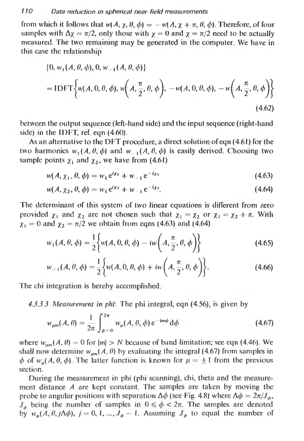
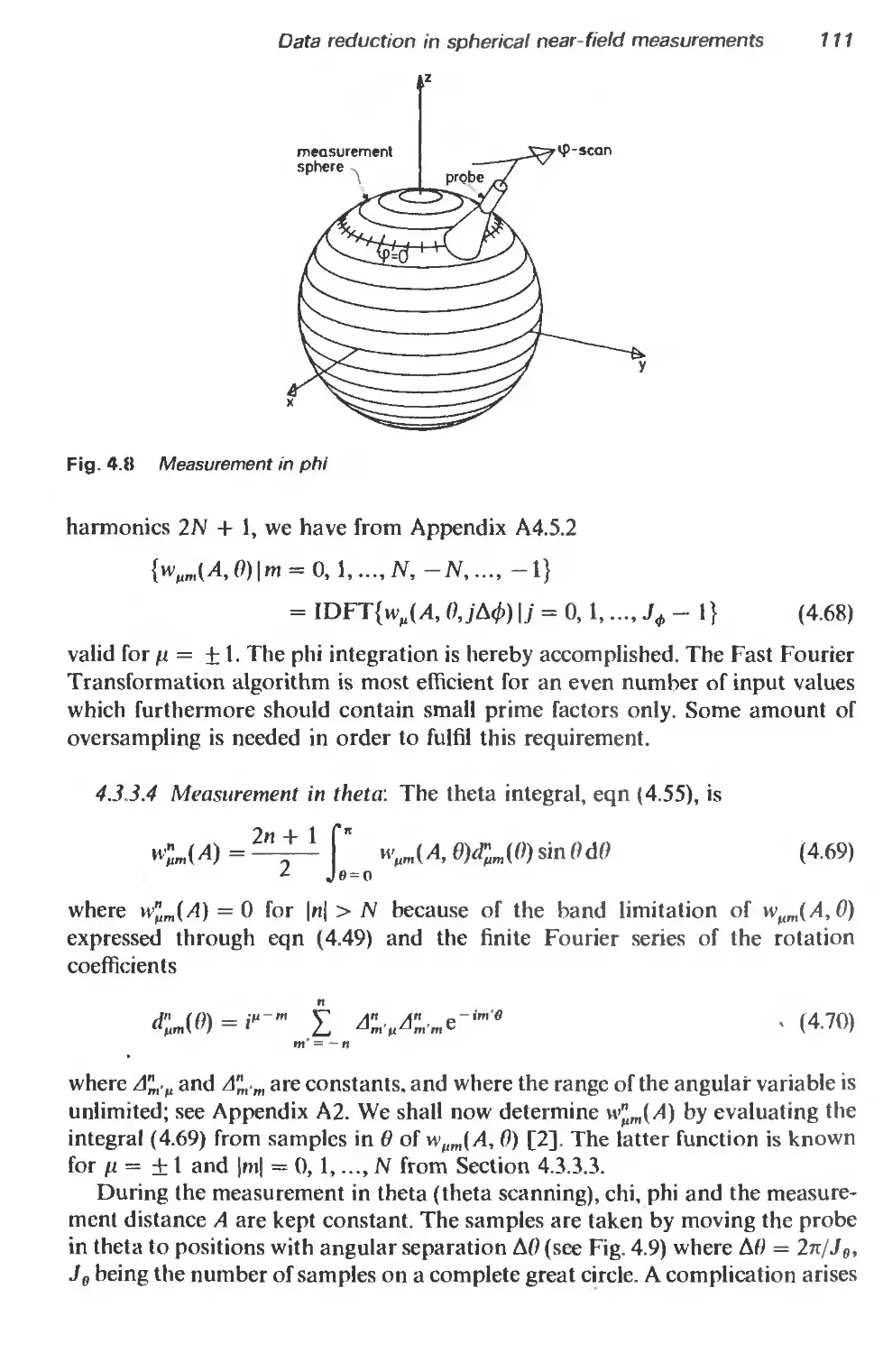
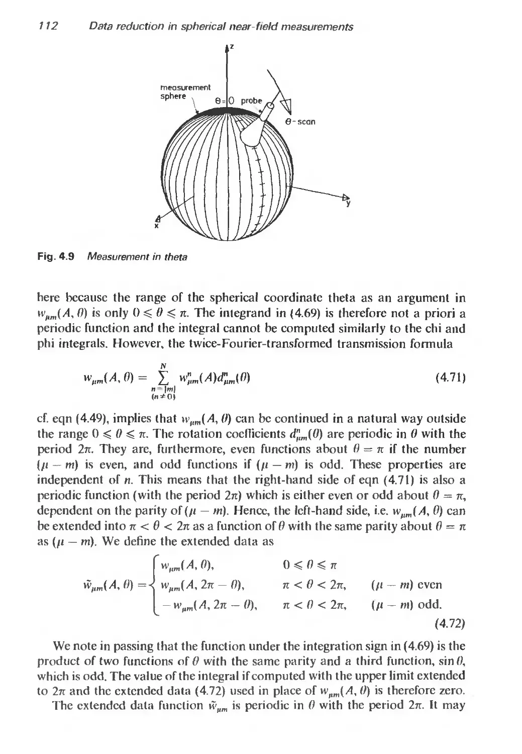
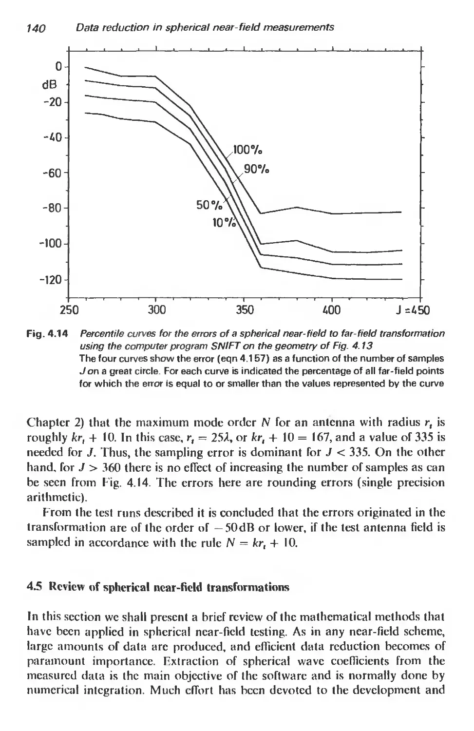
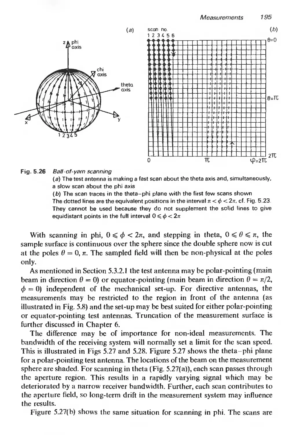
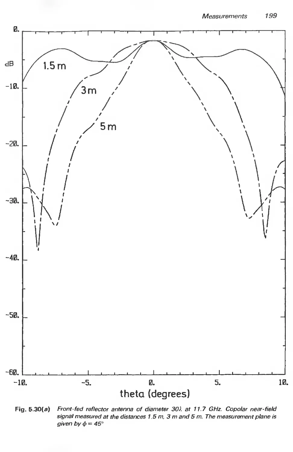
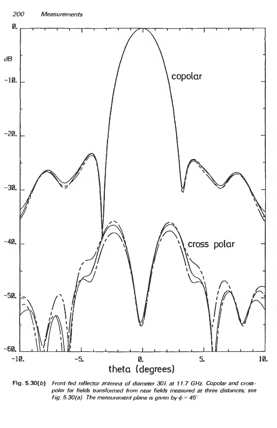
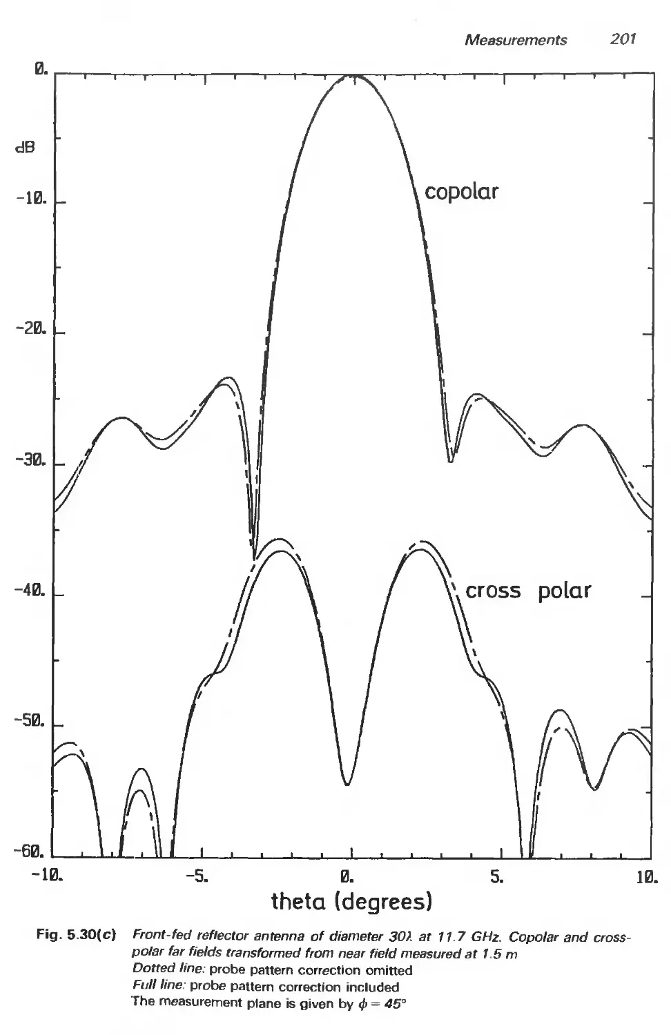
/


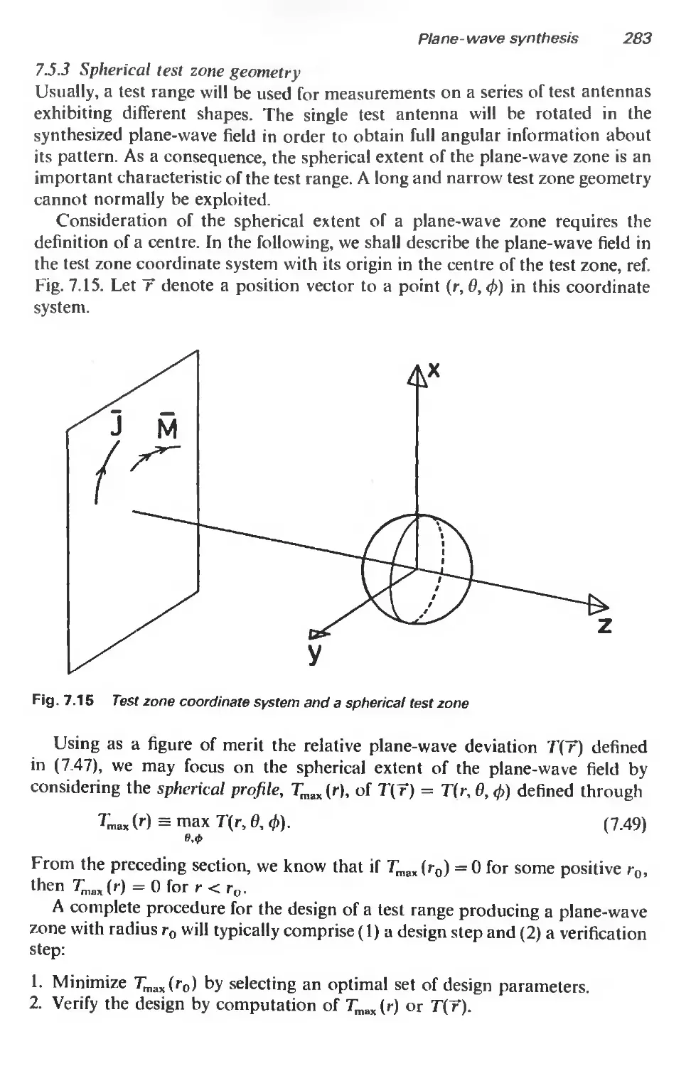


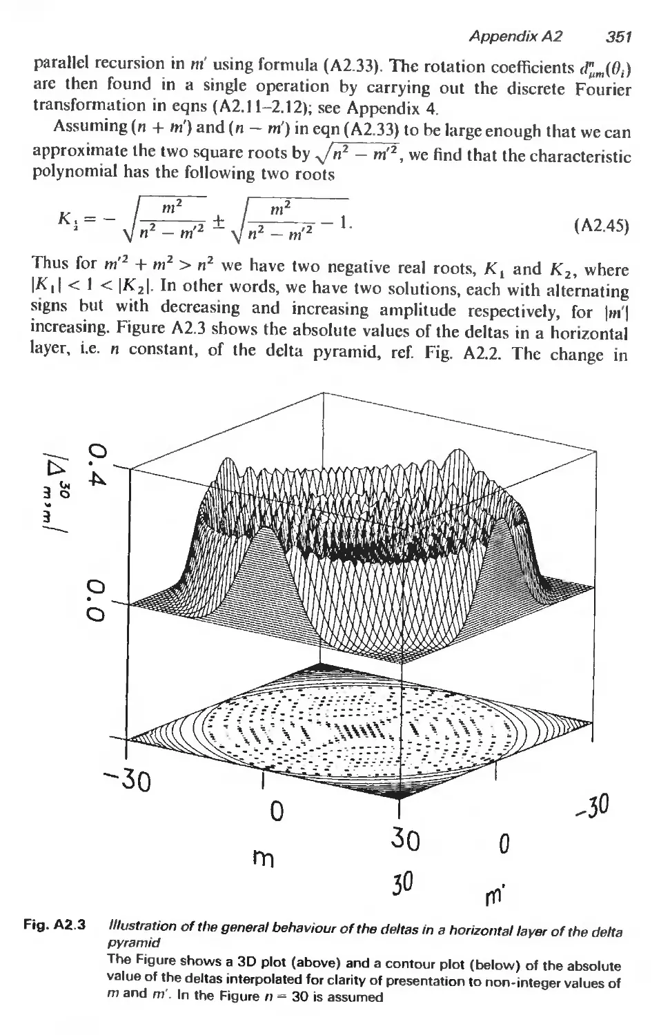


Текст
ELECTROMAGNETIC WAVES SERIES 26
Peter Peregrinus Ltd on behalf of
the Institution of Electrical Engineers
Edited
IEE ELECTROMAGNETIC WAVES SERIES 26
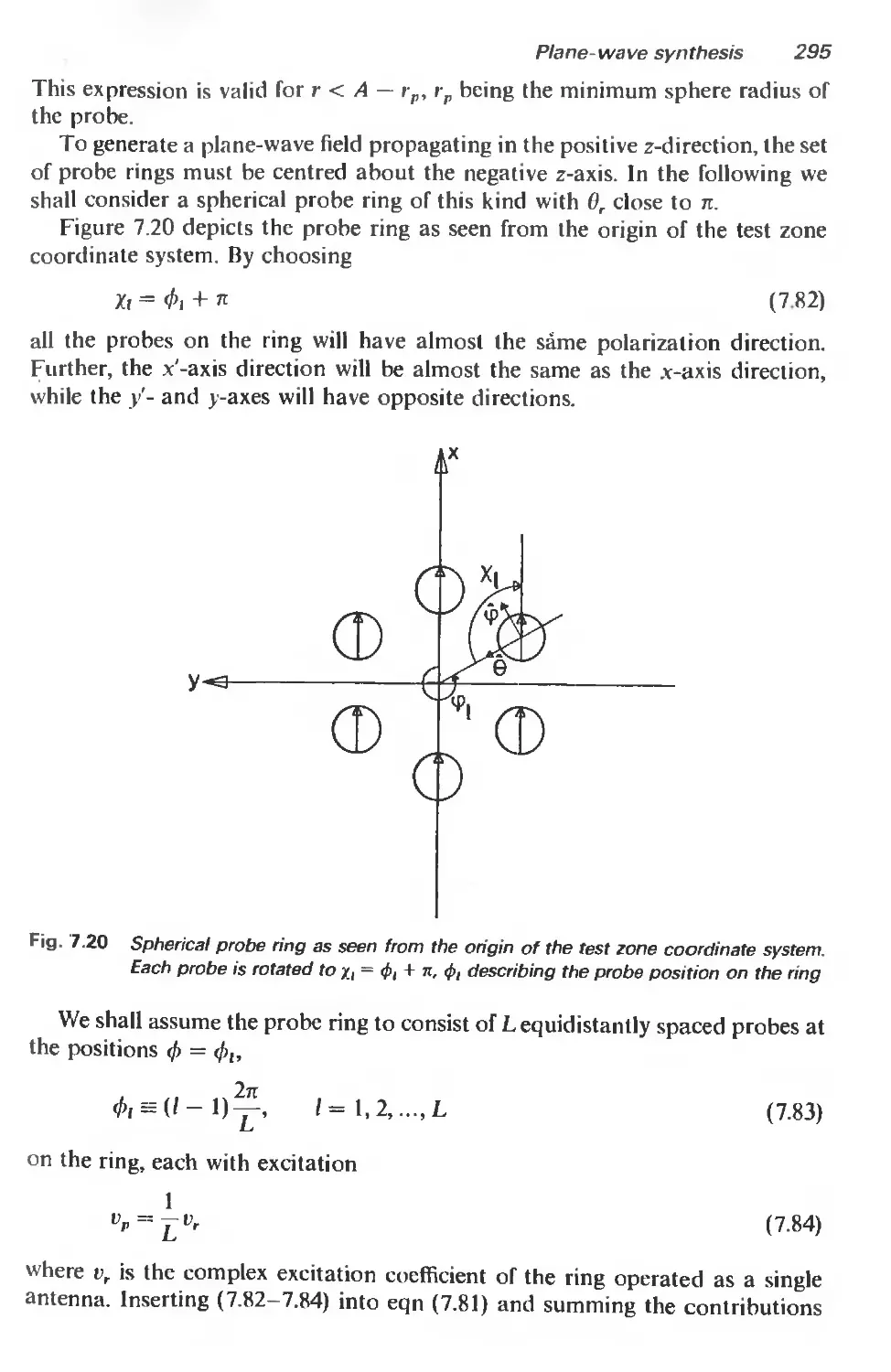
Series Editors: Professors R J. B. Clarricoats and J. R. Wait
SPHERICAL
NEAR-FIELD
ANTENNA
MEASUREMENTS
Other volumes in this series
Volume 1
Volume 2
Volume 3
Volume 4
Volume 5
Volume 6
Volume 7
Volume 8
Volume 9
Volume 10
Volume 11
Volume 12
Volume 13
Volume 14
Volume 15
Volume 16
Volume 17
Volume 18
Volume 19
Volume 20
Volume 21
Volume 22
Volume 23
Volume 24
Volume 25
Geometrical theory of diffraction for electromagnetic waves
Graeme L. James
Electromagnetic waves and curved structures
Leonard Lewin, David C. Chang and Edward F. Kuester
Microwave homodyne systems
Ray J. King
Radio direction-finding
R J. D. Gething
ELF communications antennas
Michael L Burrows
Waveguide tapers, transitions and couplers
F. Sporleder and H. G. Unger
Reflector antenna analysis and design
R J. Wood
Effects of the troposphere on radio communications
Martin R M. Hall
Schumann Resonances in the earth-ionosphere cavity
R V. Bliokh, A. R Nikolaenko and Y F. Filippov
Aperture antennas and diffraction theory
E. V Jull
Adaptive array principles
J. E. Hudson
Microstrip antenna theory and design
J. R, James, R S. Hall and C. Wood
Energy in electromagnetism
H. G. Booker
Leaky feeders and subsurface radio communications
R Delogne
The handbook of antenna design, volume I
Editors: A. W Rudge, K. Milne, A. D. Olver, R Knight
The handbook of antenna design, volume 2
Editors: A. W Rudge, K. Milne, A. D. Olver, R Knight
Surveillance radar performance prediction
R Rohan
Corrugated horns for microwave antennas
R J. B. Clarricoats and A. D. Olver
Microwave antenna theory and design
Editor: S. Silver
Advances in radar techniques
Editor: J. Clarke
Waveguide handbook
N. Marcuvitz
Target adaptive matched illumination radar
Dag T. Gjessing
Ferrites at microwave frequencies
A. J. Baden Fuller
Propagation of short radio waves
Editor: D. E. Kerr
Principles of microwave circuits
Editors: C. G. Montgomery, R. H. Dicke, E. M. Purcell
SPHERICAL
NEAR-FIELD
ANTENNA
MEASUREMENTS
Edited by
J. E. Hansen
Peter Peregrinus Ltd. on behalf of the Institution of Electrical Engineers
Published by: Peter Peregrinus Ltd., London, United Kingdom
© 1988: Peter Peregrinus Ltd.
All rights reserved. No part of this publication may be reproduced, stored
in a retrieval system or transmitted in any form or by any means—
electronic, mechanical, photocopying, recording or otherwise—without
the prior written permission of the publisher.
While the author and the publishers believe that the information and
guidance given in this work are correct, all parties must rely upon their
own skill and judgment when making use of them. Neither the author nor
the publishers assume any liability to anyone for any loss or damage
caused by any error or omission in the work, whether such error or
omission is the result of negligence or any other cause. Any and all such
liability is disclaimed.
British Library Cataloguing In Publication Data.
Spherical near-field antenna measurements theory and practice —
(IEE electromagnetic waves series; 26).
1. Antennas (Electronics)—Measurement
I. Hansen, J.E. II. Hald, J.
III. Institute of Electrical Engineers
IV. Series
621.38'028'3 TK7871.6
ISBN 0 86341 110 X
Contributing authors
J. Hald, Briiel & Kjter, Nterum, Denmark
J. E. Hansen, Technical University of Denmark
E Jensen, T1CRA, Copenhagen, Denmark
E Holm Larsen, Technical University of Denmark
Contents
Contributing authors listed v
Preface xiii
1 Introduction 1
1.1 Background 1
1.1.1 Introduction 1
1.1.2 Brief outline of antenna testing 1
1.1.3 Spherical near-field testing 2
1.2 Organization of (this) book 4
References 6
2 Scattering matrix description of an antenna 8
2.1 Introduction 8
2.2 Spherical waves 9
2.2.1 Introduction 9
2.2.2 Power-normalized spherical waves 12
2.2.3 The spherical waveguide 15
2.2.4 Power flow 23
2.3 The antenna scattering matrix 27
2.3.1 Definitions 27
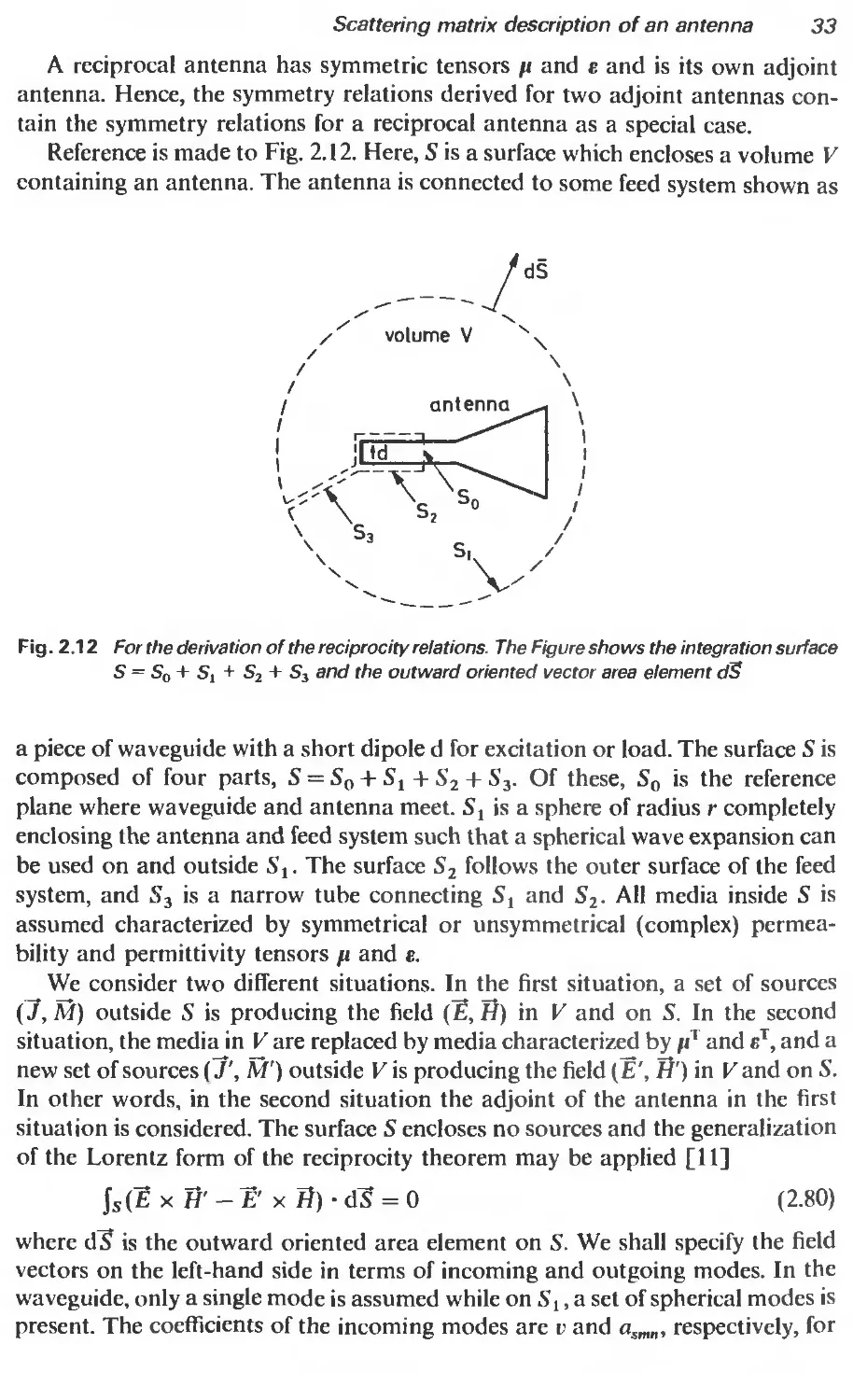
2.3.2 Reciprocity 32
2.3.3 The field from electric and magnetic dipoles 37
2.3.4 Scattering matrices for electric and magnetic dipoles 40
2.3.5 Remarks on the definition of antenna scattering matrices 46
2.4 Antenna parameters expressed by spherical waves 48
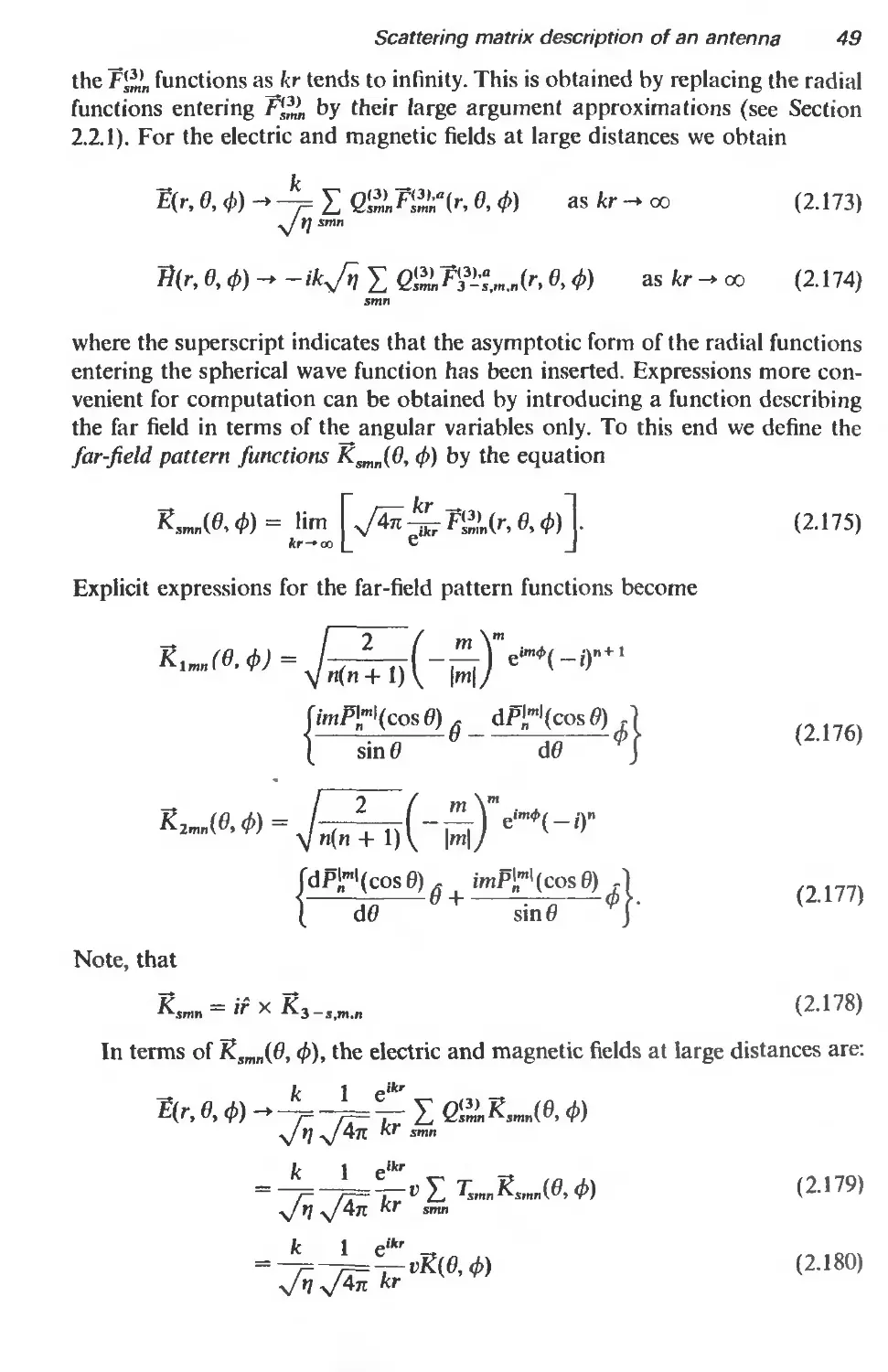
2.4.1 Far-field patterns 48
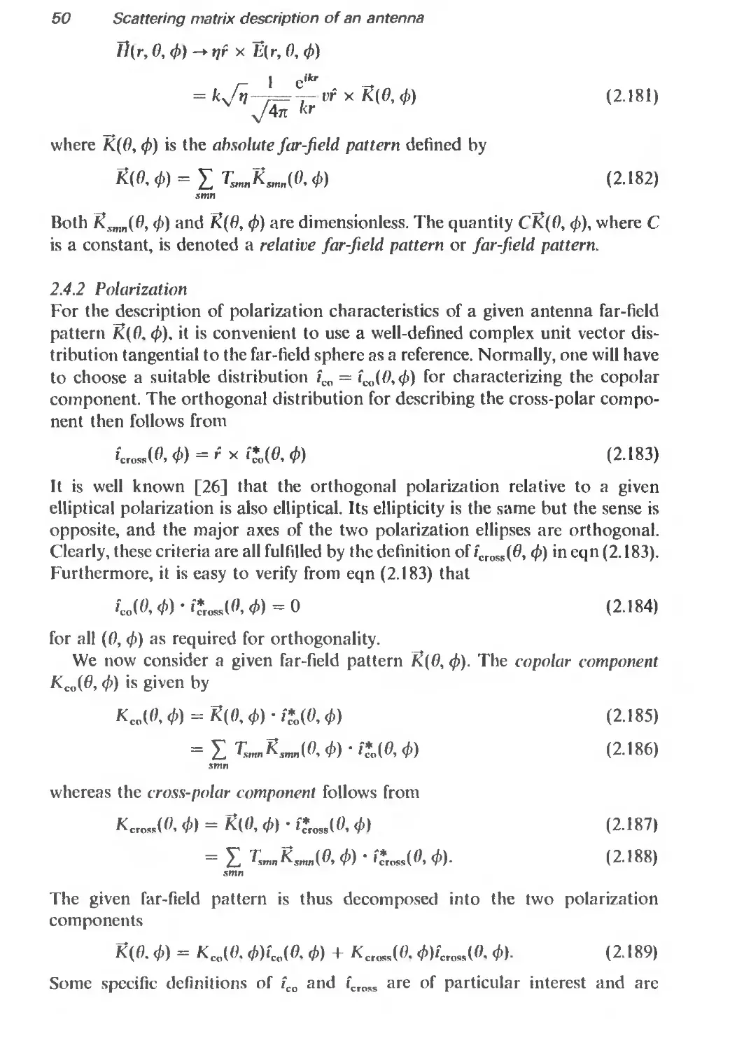
2.4.2 Polarization 50
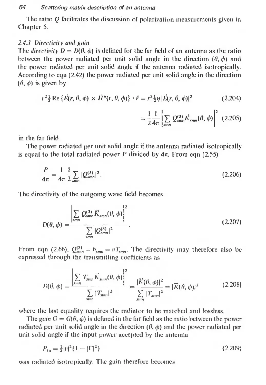
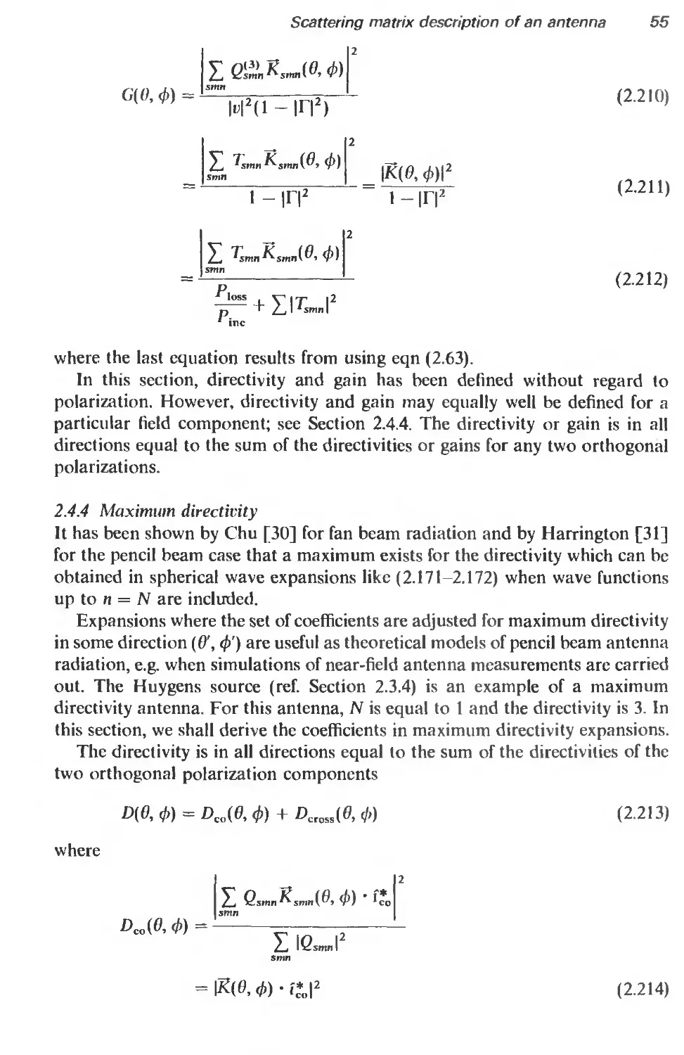
2.4.3 Directivity and gain 54
2.4.4 Maximum directivity 55
References 59
3 Scattering matrix description of antenna coupling 61
3.1 Introduction 61
3.2 The transmission formula 62
3.2.1 Geometry 62
3.2.2 Test antenna transmitting, probe receiving 63
Contents
viii
3.2.3 Test antenna receiving, probe transmitting 67
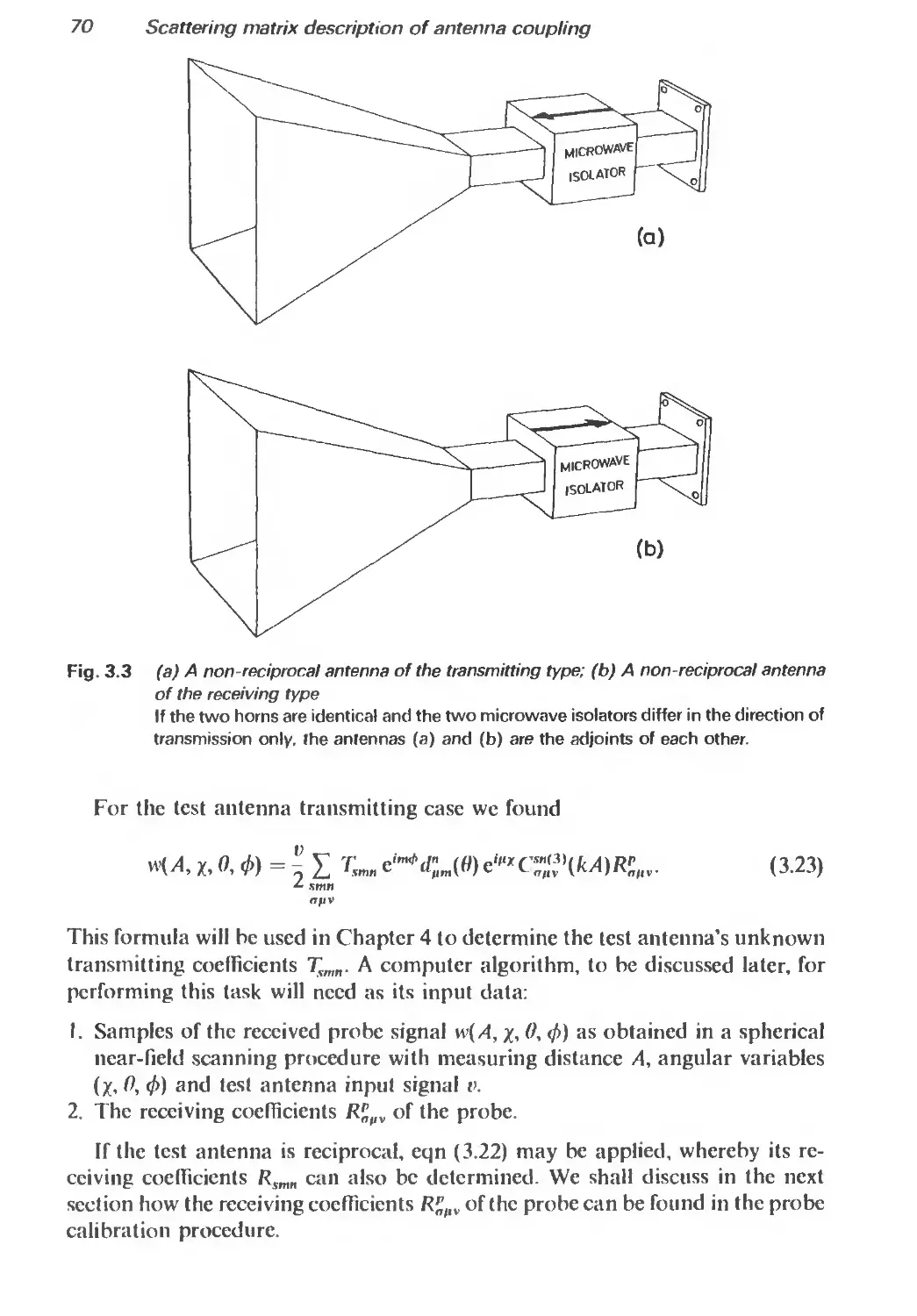
3.2.4 Reciprocal and non-reciprocal test antennas 69
.3.2.5 Iterative scheme for probe calibration 71
3.3 Special cases of the transmission formula 73
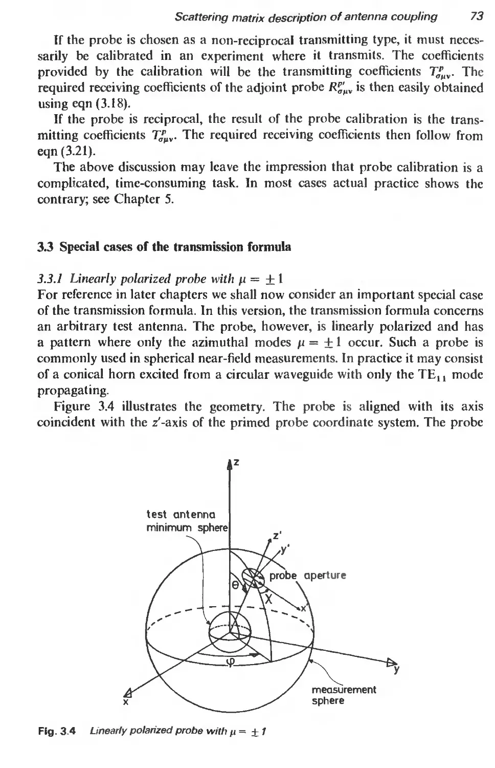
3.3.1 Linearly polarized probe with p = + I 73
3.3.2 The Hertzian dipole as a probe 76
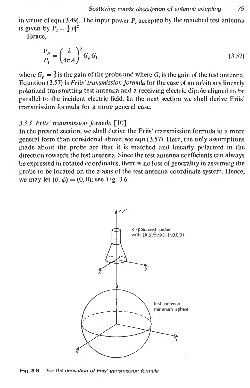
3.3.3 Friis' transmission formula 79
3.4 The transmission formula with multiple reflections included 82
References 87
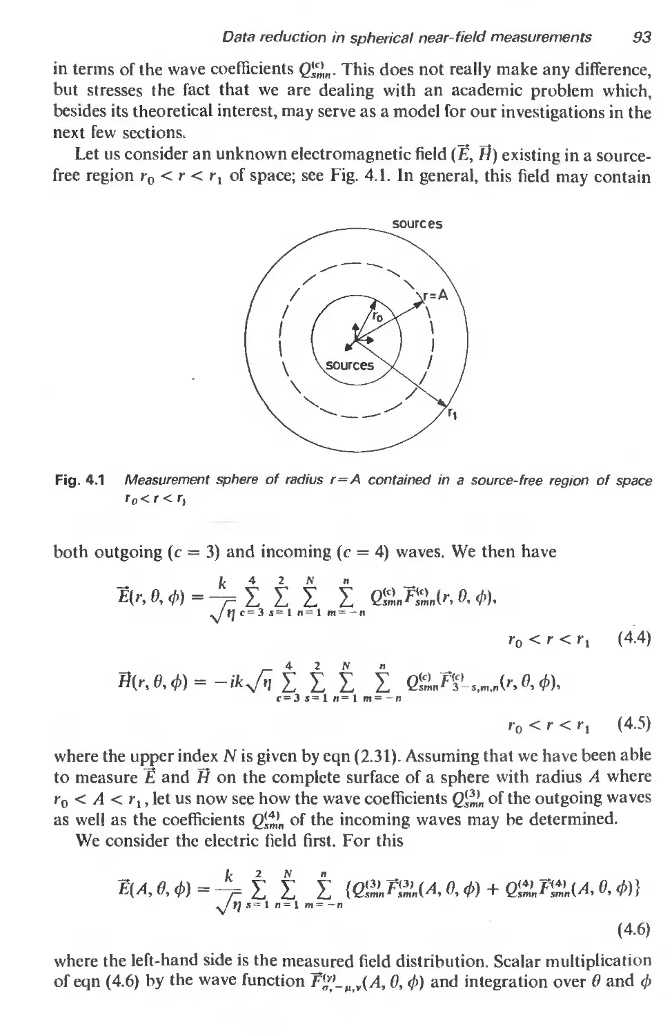
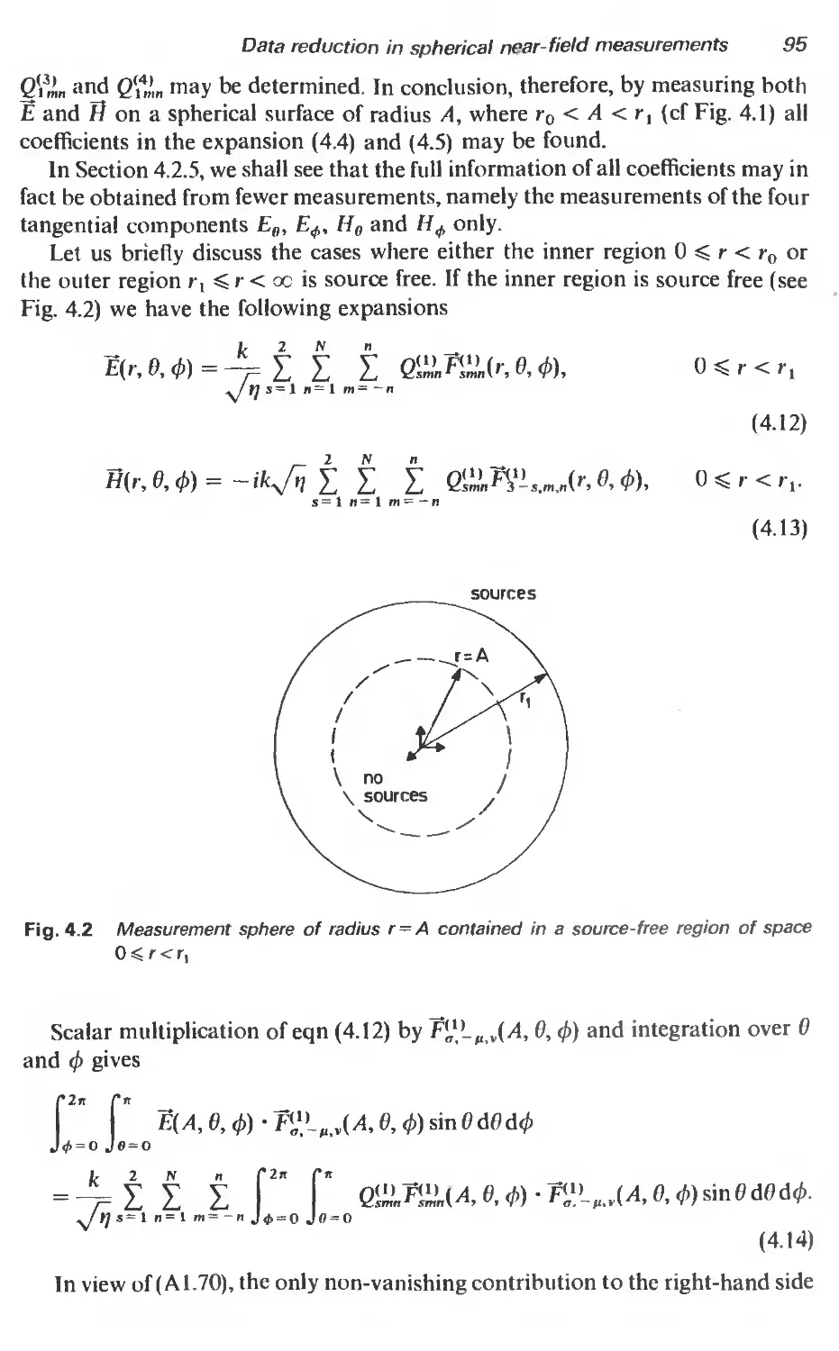
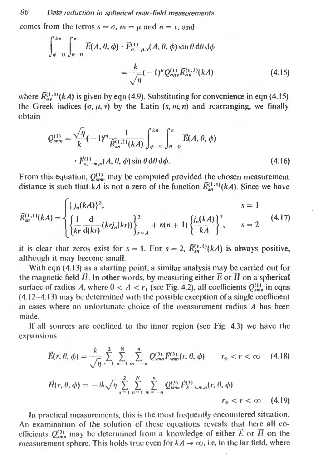
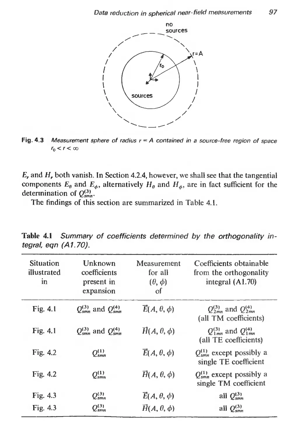
4 Data reduction in spherical near-field mcsaurcmcnts 89
4.1 Introduction 89
4.2 Measurement without probe correction 92
4.2.1 Introduction 92
4.2.2 General case 92
4.2.3 Measurement of the radial field components 98
4.2.4 Measurement of two tangential field components 100
4.2.5 Wood’s method 102
4.3 Measurement with probe correction 104
4.3.1 Introduction 104
4.3.2 Analytical solution of the transmission formula 104
4.3.3 Discrete solution of the transmission formula 107
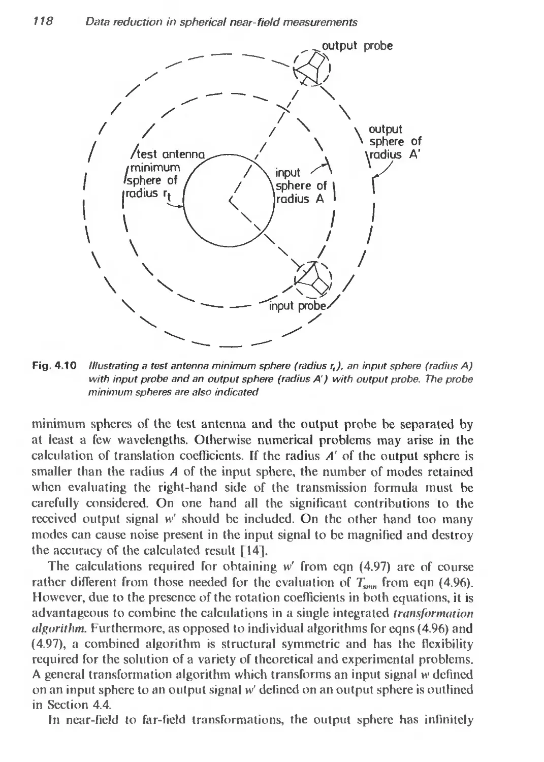
4.3.4 Field transformations and radiated fields 117
4.4 Outline of a spherical near-field transformation algorithm 125
4.4.1 Introduction 125
4.4.2 Summary of the theory underlying a transformation algorithm 125
4.4.3 On the number of sample points 128
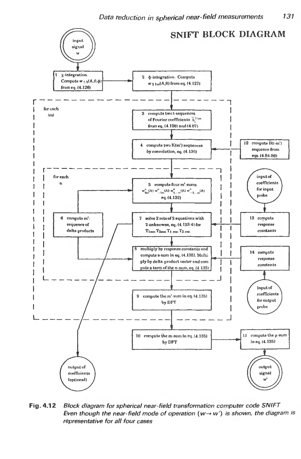
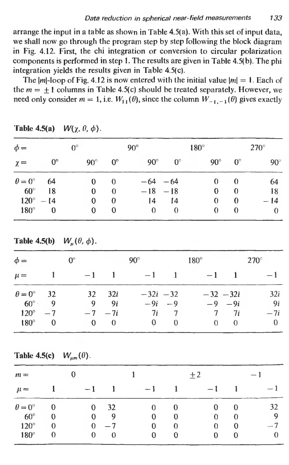
4.4.4 Block diagram of a transformation algorithm 132
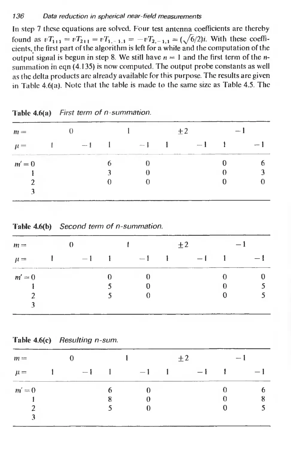
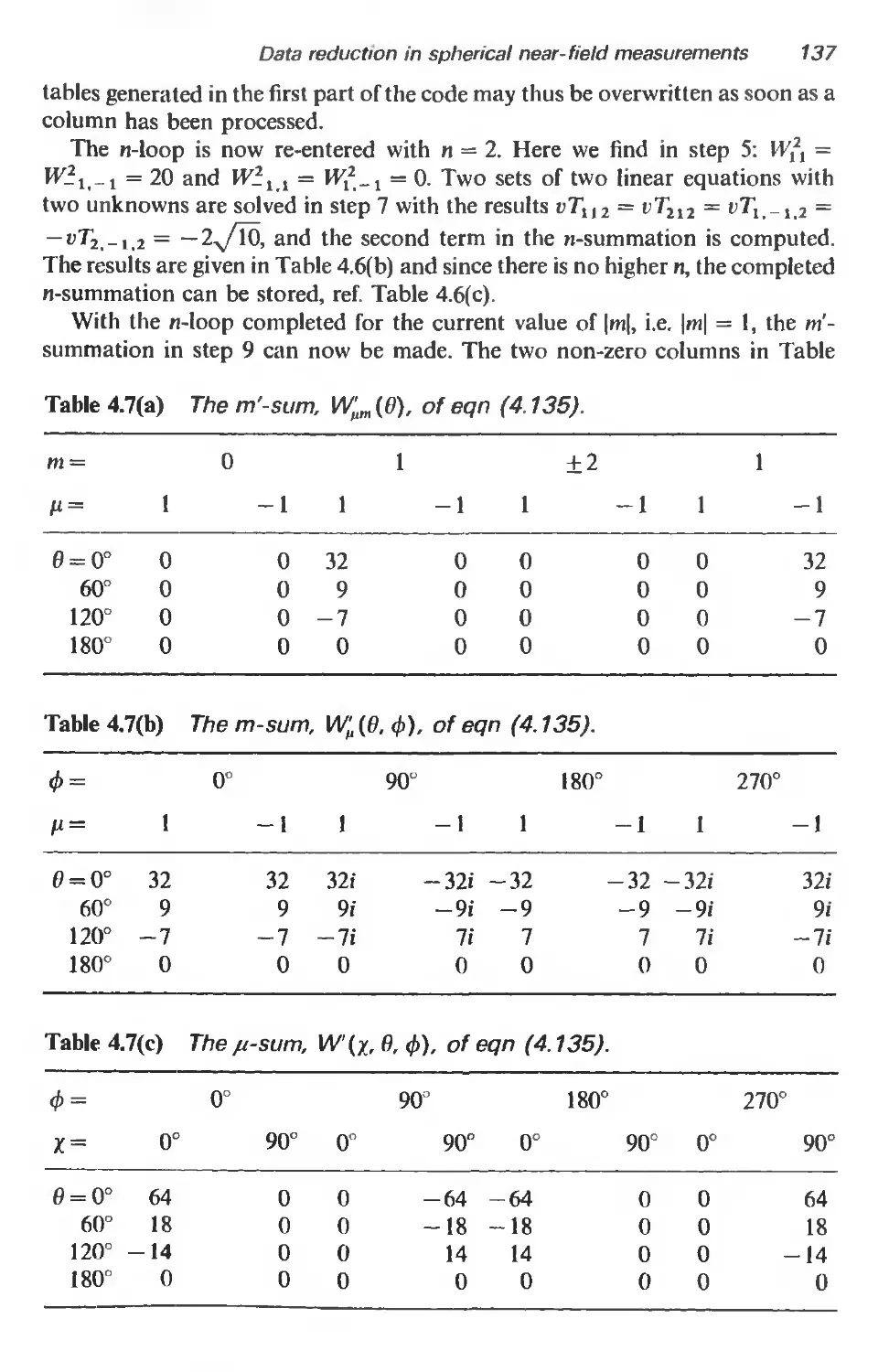
4.4.5 A simple example 132
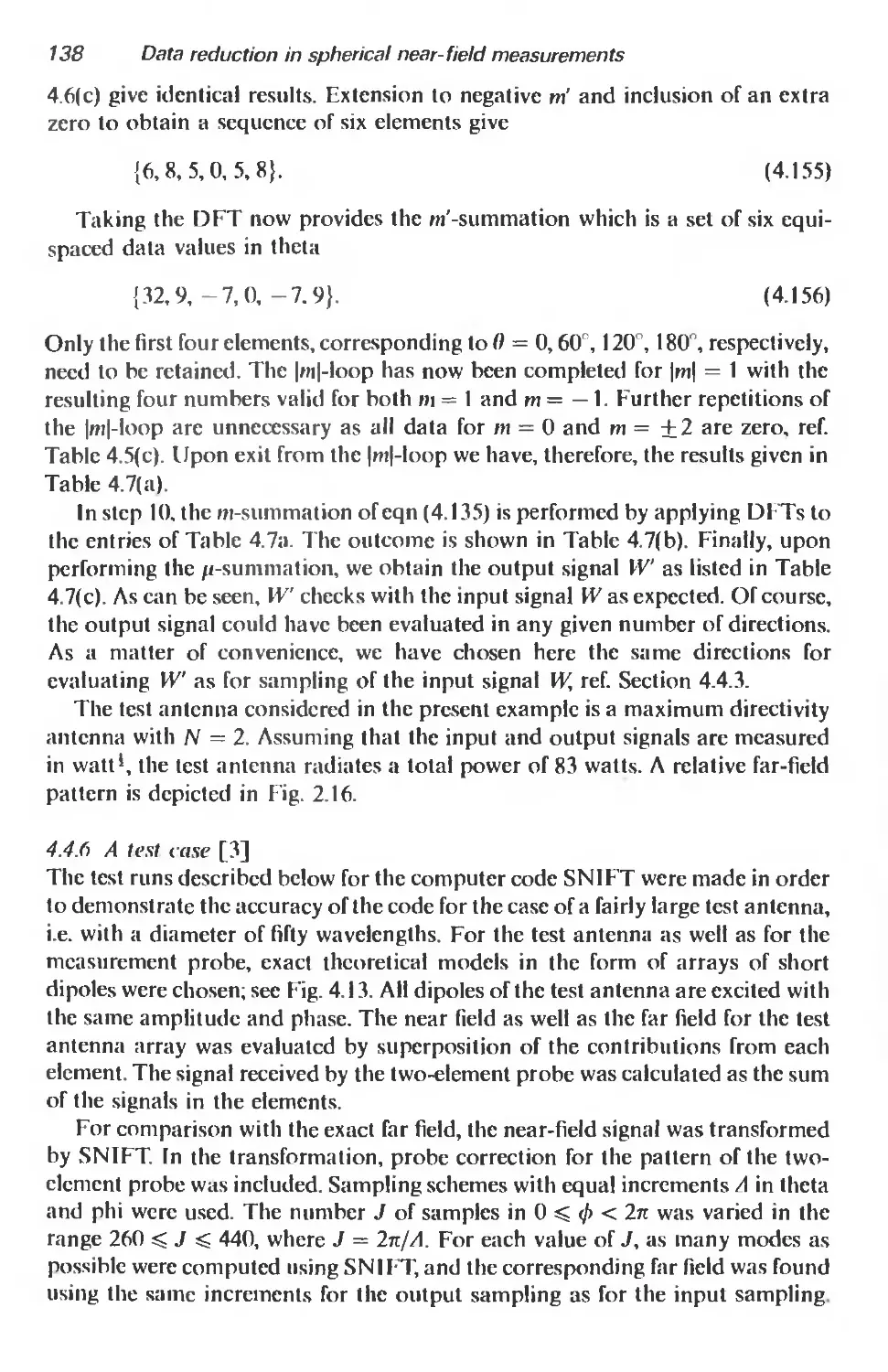
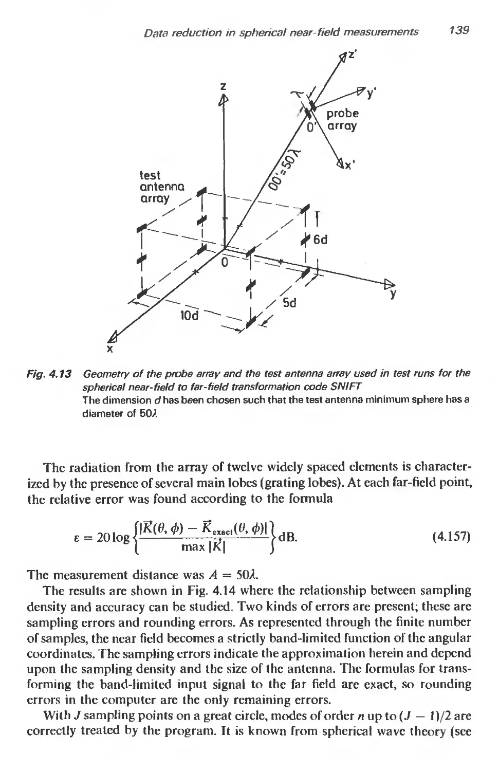
4.4.6 A test case 138
4.5 Review of spherical near-field transformations 140
References 145
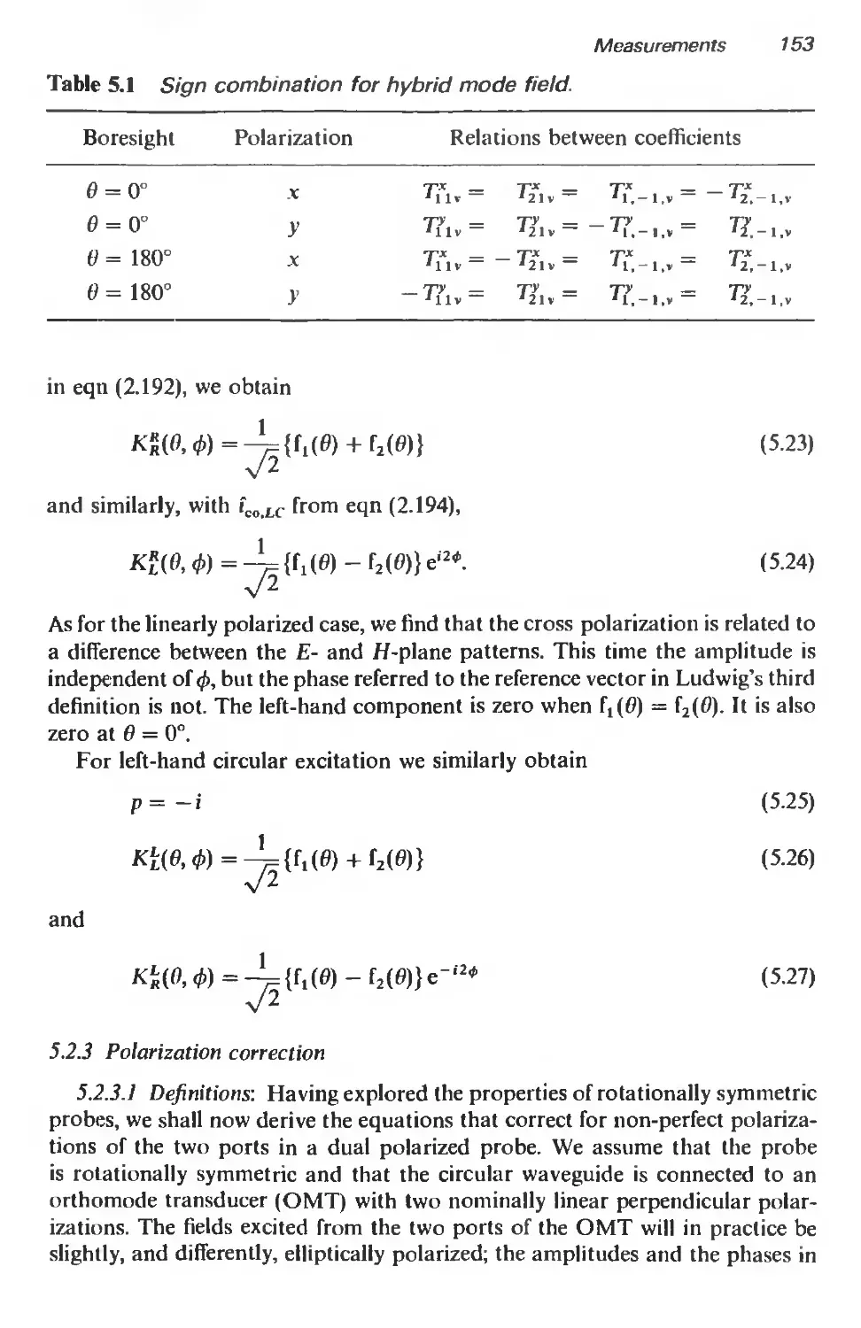
5 Measurements 147
5.1 Introduction 147
5.2 Probes for near-field scanning 147
5.2.1 Introduction 147
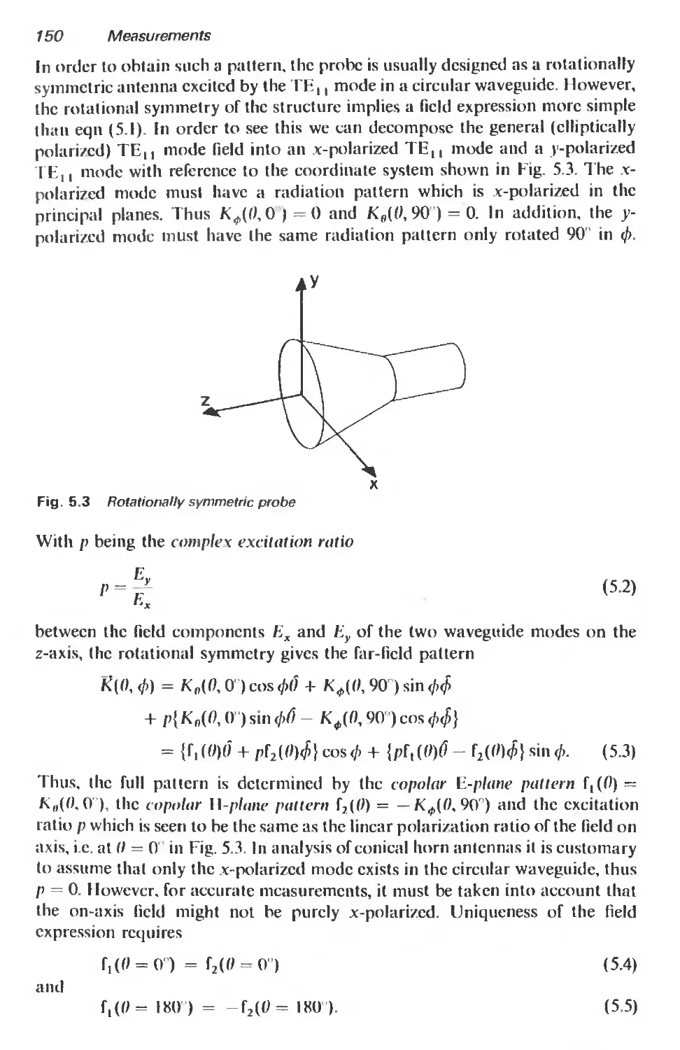
5.2.2 Rotationally symmetric probes 149
5.2.3 Polarization correction 153
5.2.4 Polarization calibration 157
5.2.5 Pattern calibration 163
5.3 Probe-corrected measurements 165
5.3.1 Introduction 165
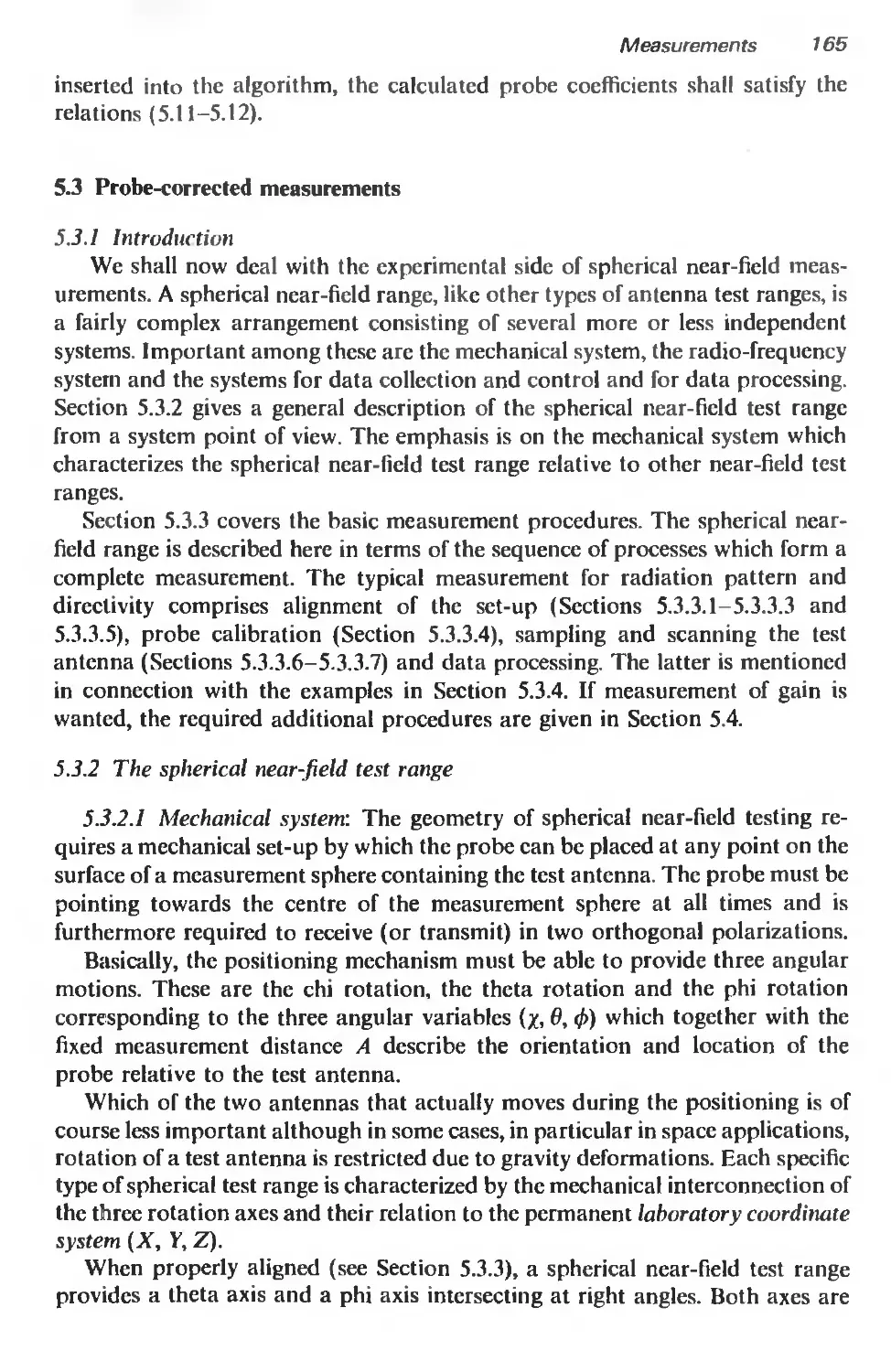
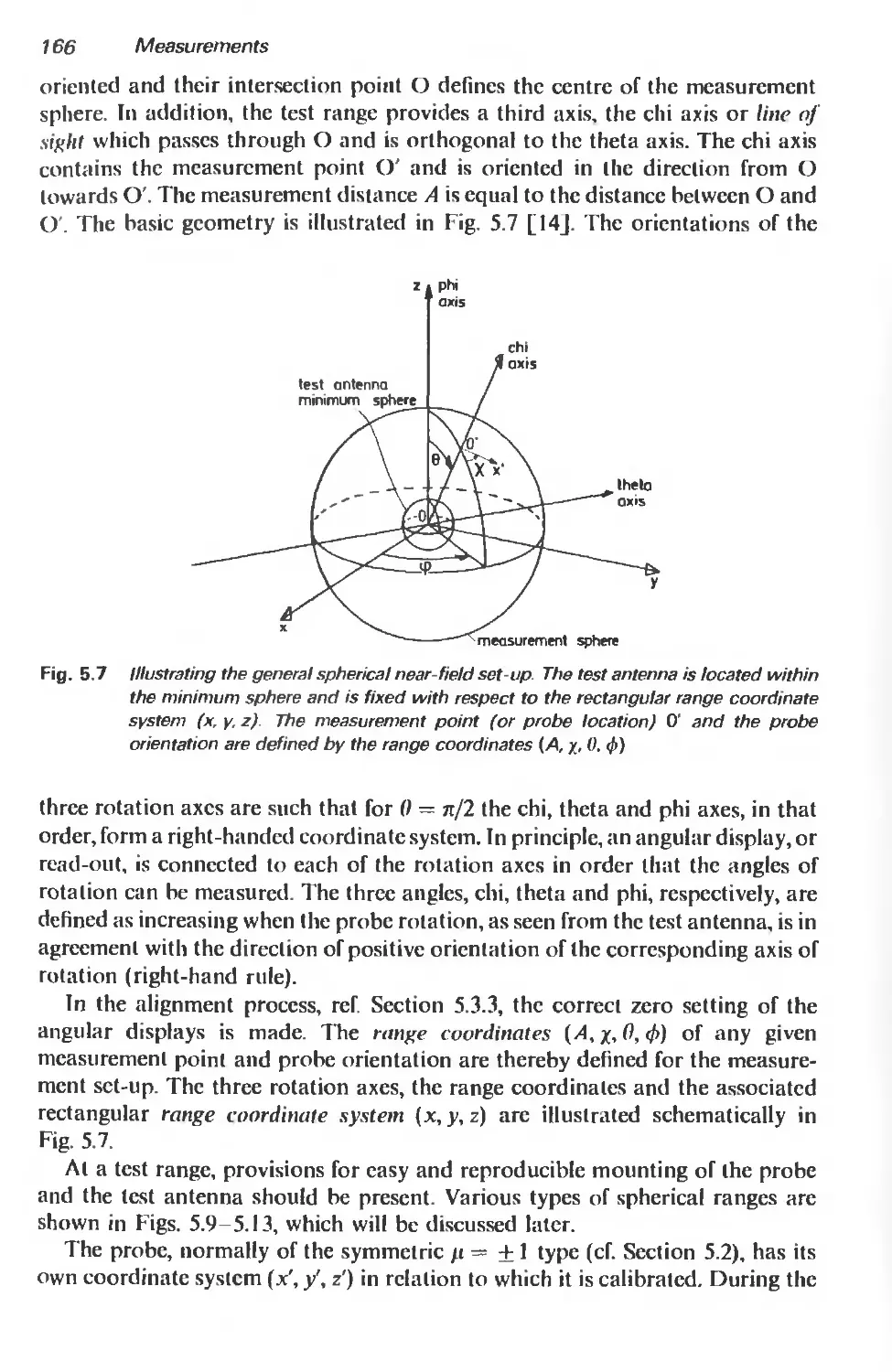
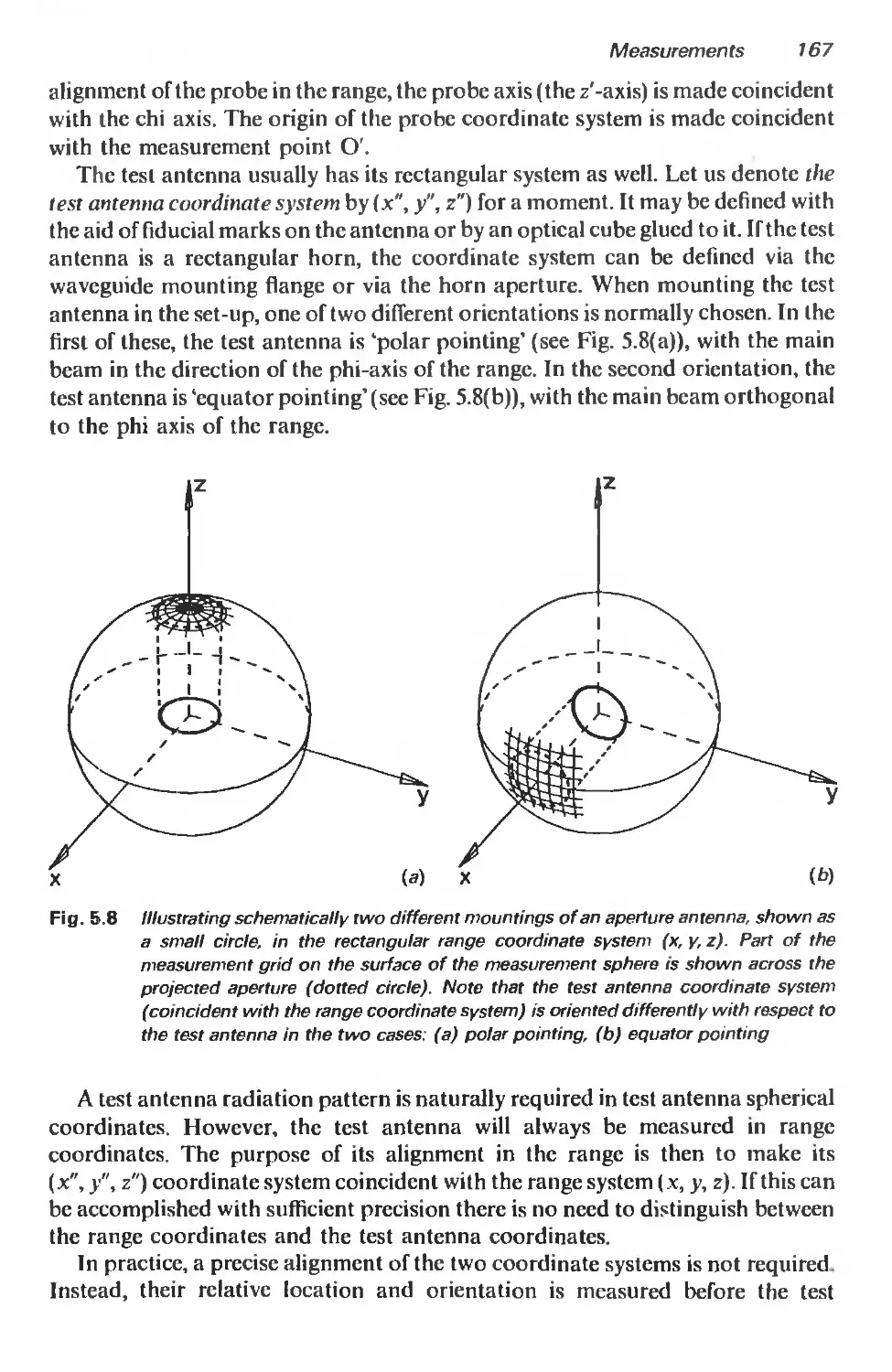
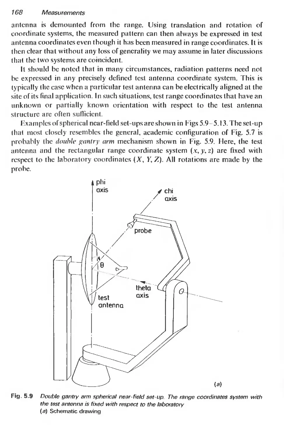
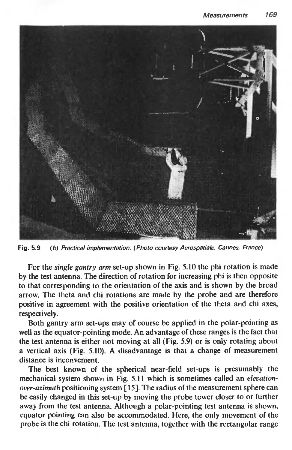
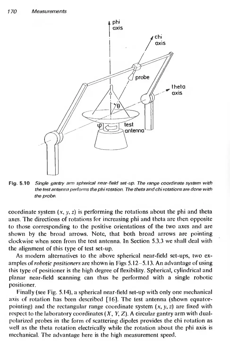
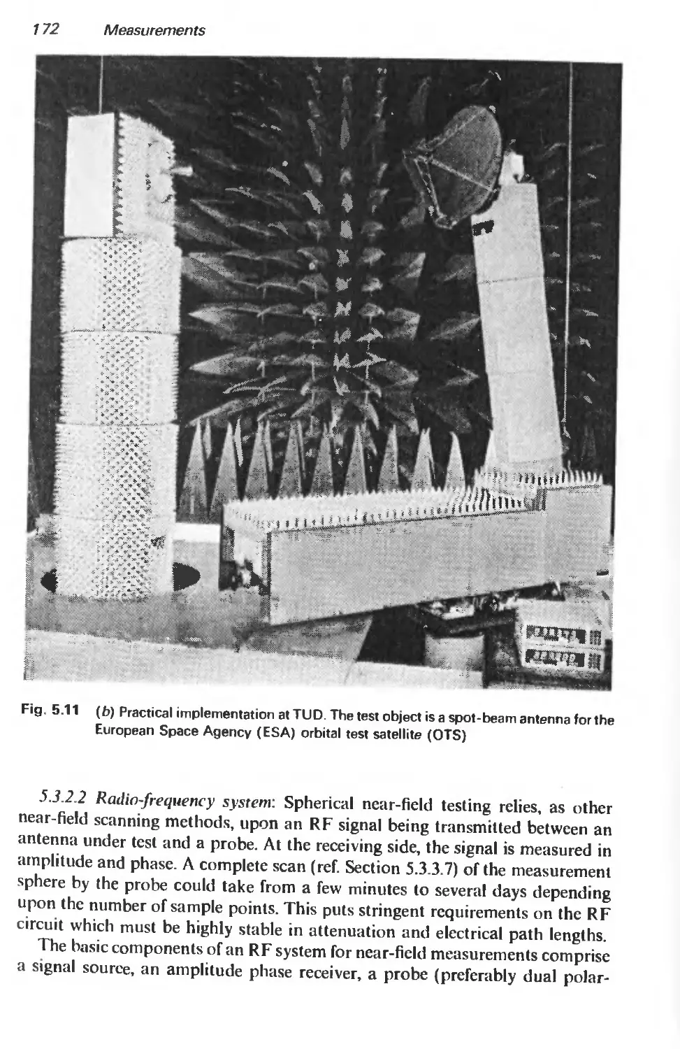
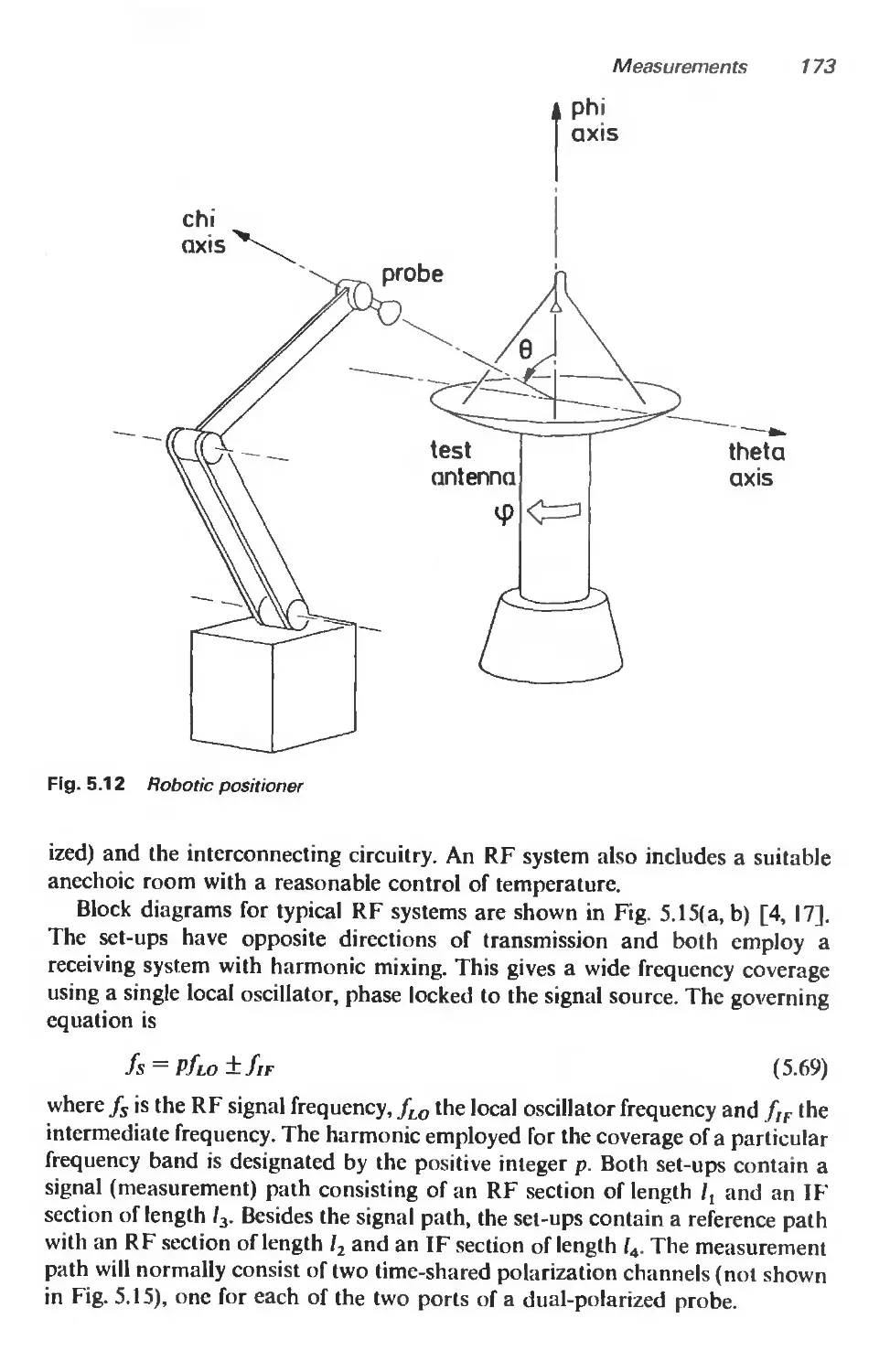
5.3.2 The spherical near-field test range 165
5.3.3 Basic measurement procedures 181
5.3.4 Measurement examples 197
5.4 Determination of gain 206
5.4.1 Introduction 206
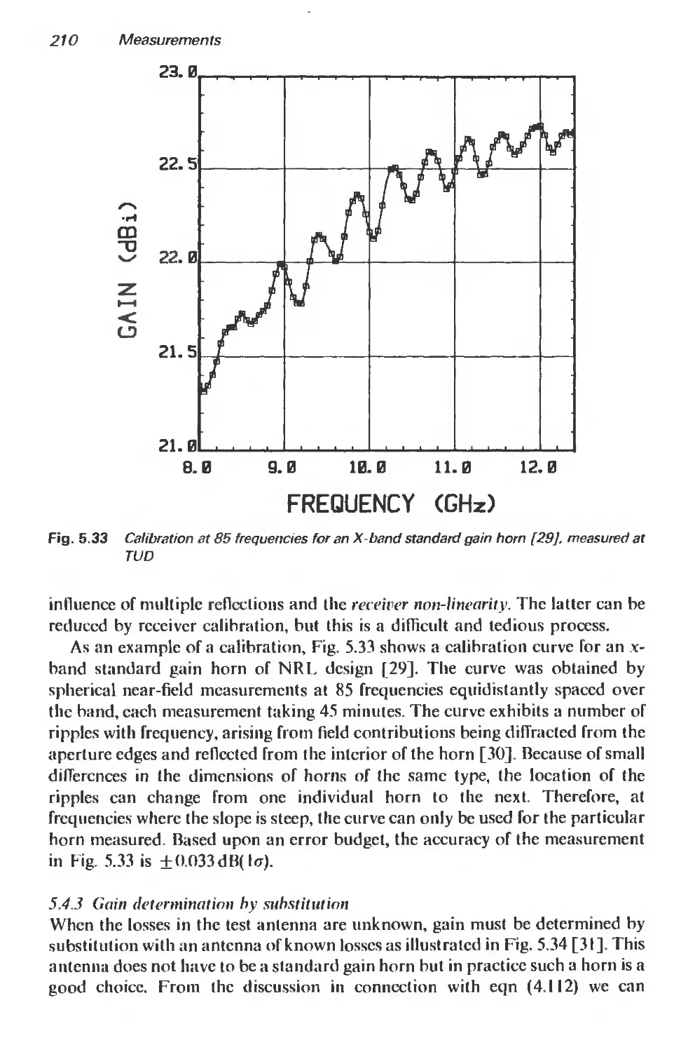
5.4.2 Gain calibration of horns 207
5.4.3 Gain determination by substitution 210
References 214
Contents
ix
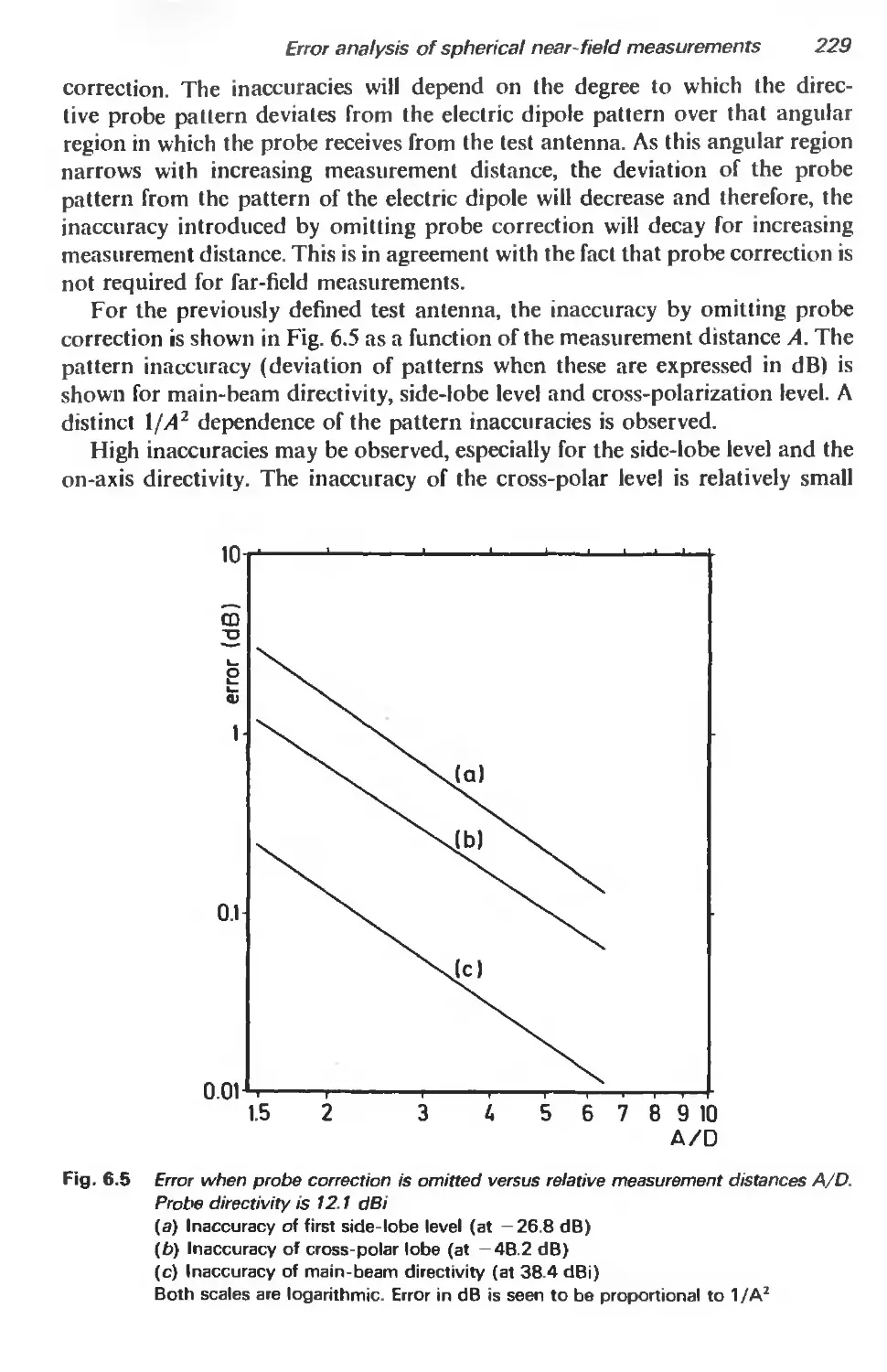
6 Error analysis of spherical near-field measurements 216
6.1 Introduction 216
6.2 Near-field measurements 216
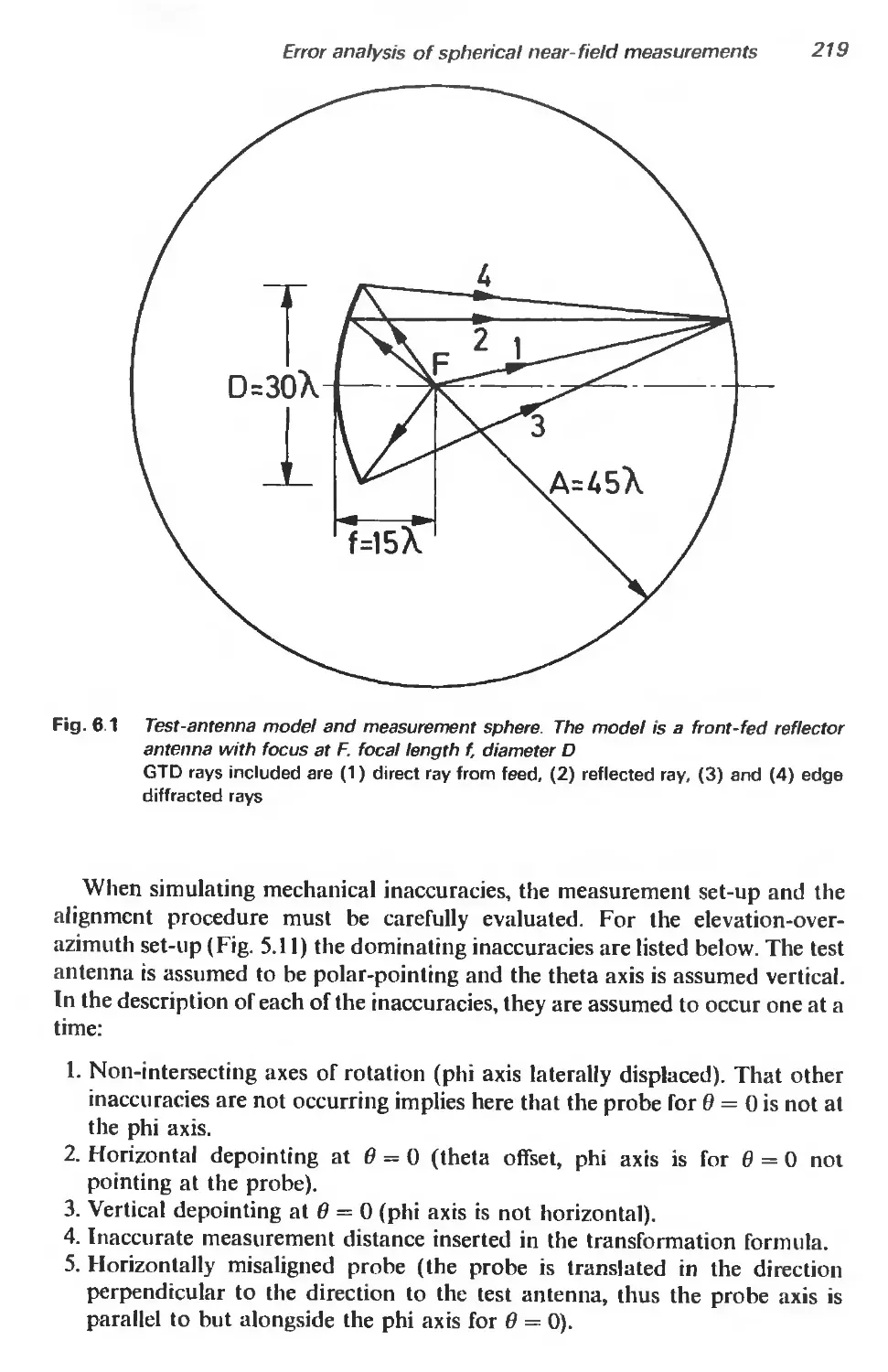
6.3 Mechanical inaccuracies 218
6.4 Receiver inaccuracies 222
6.5 Probe correction 228
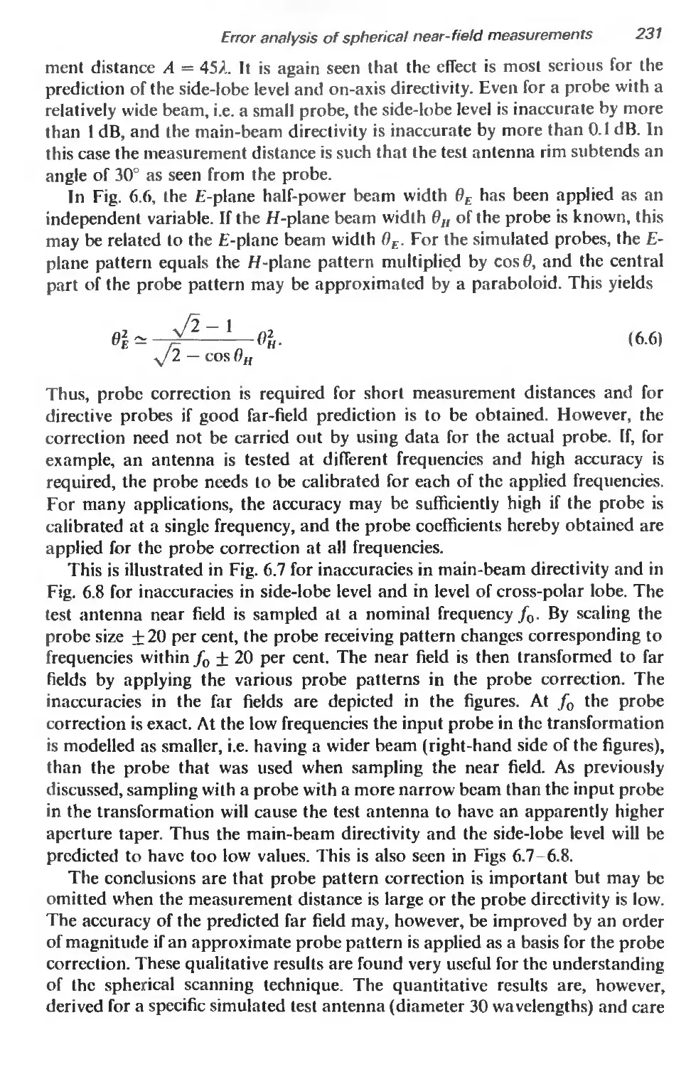
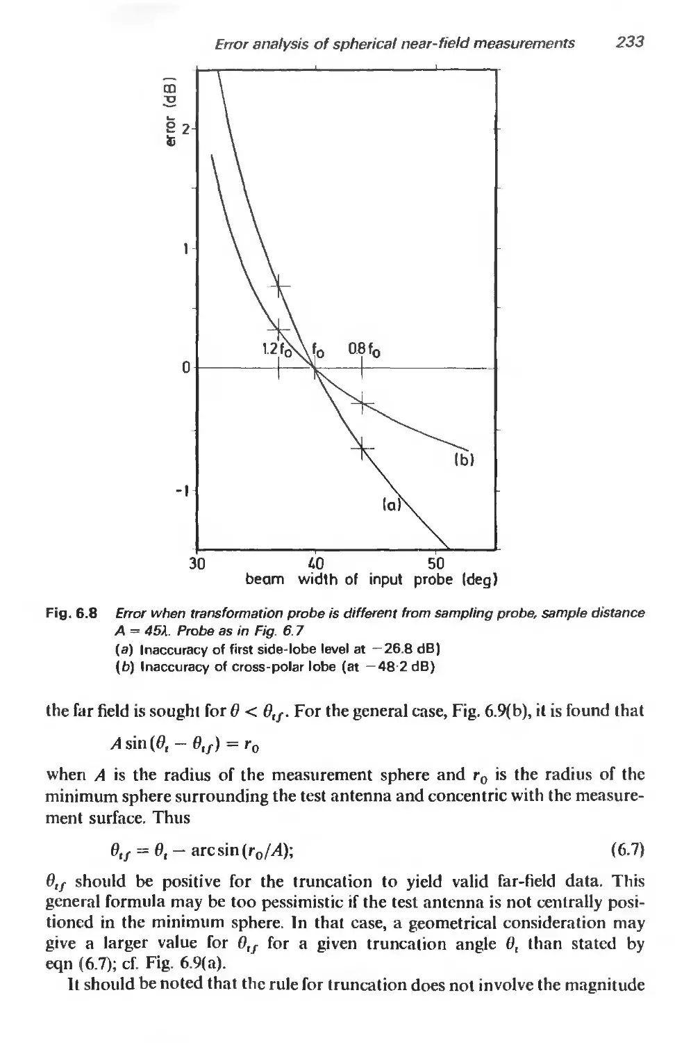
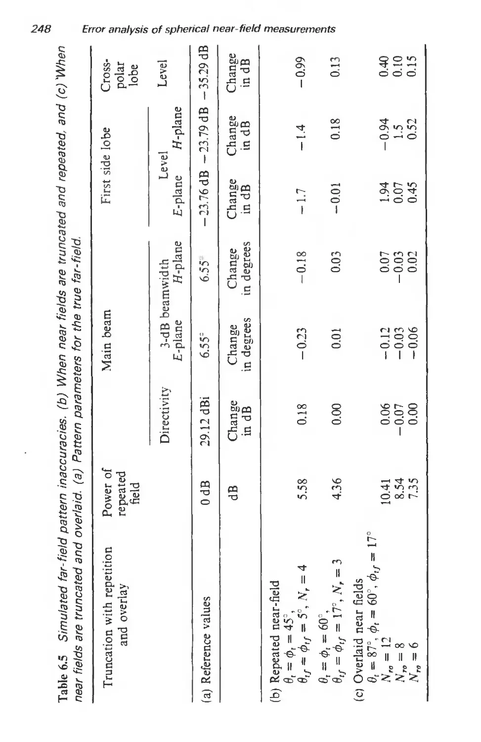
6.6 Truncation 232
6.6.1 Introduction 232
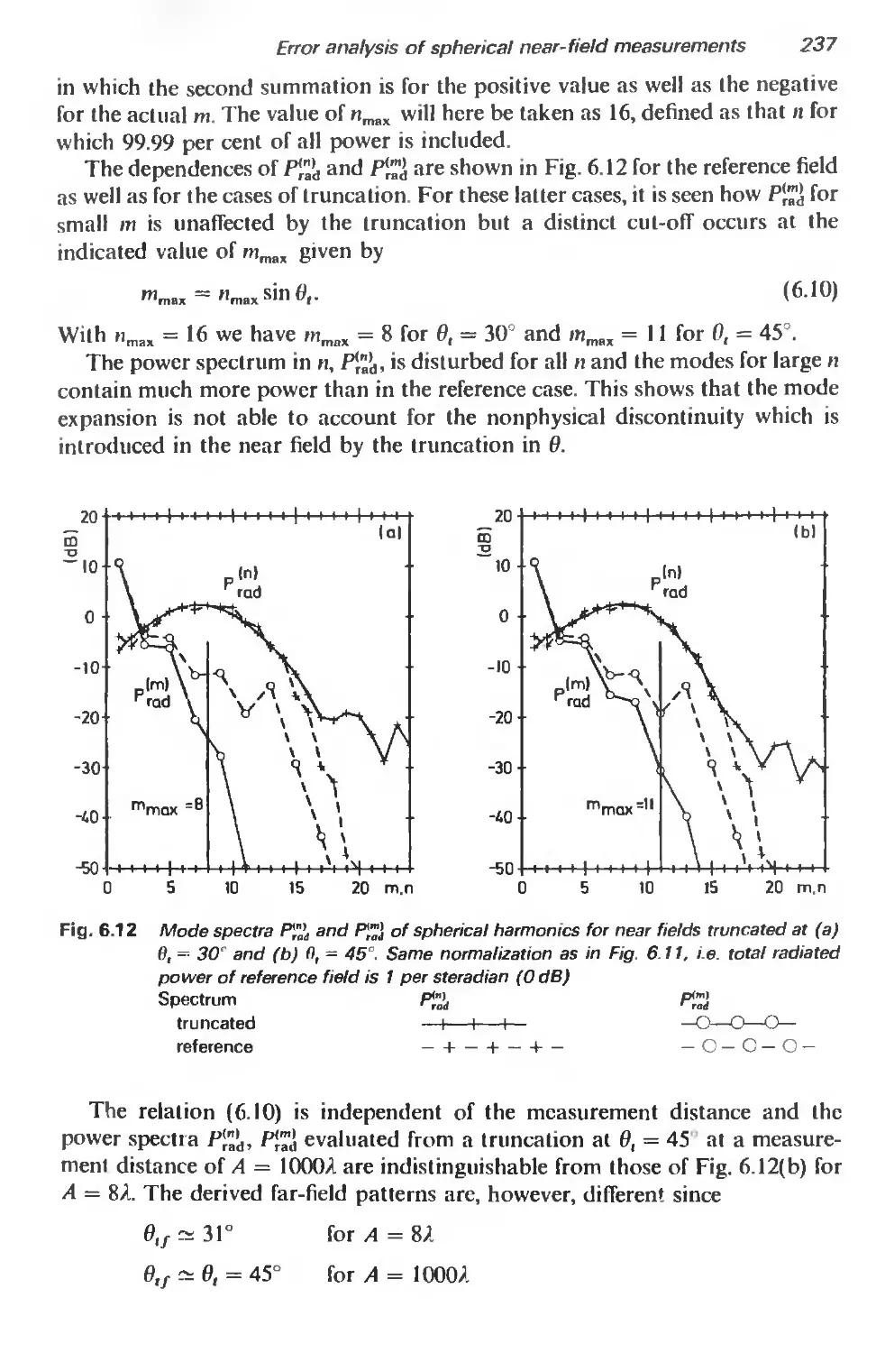
6.6.2 Polar truncation 234
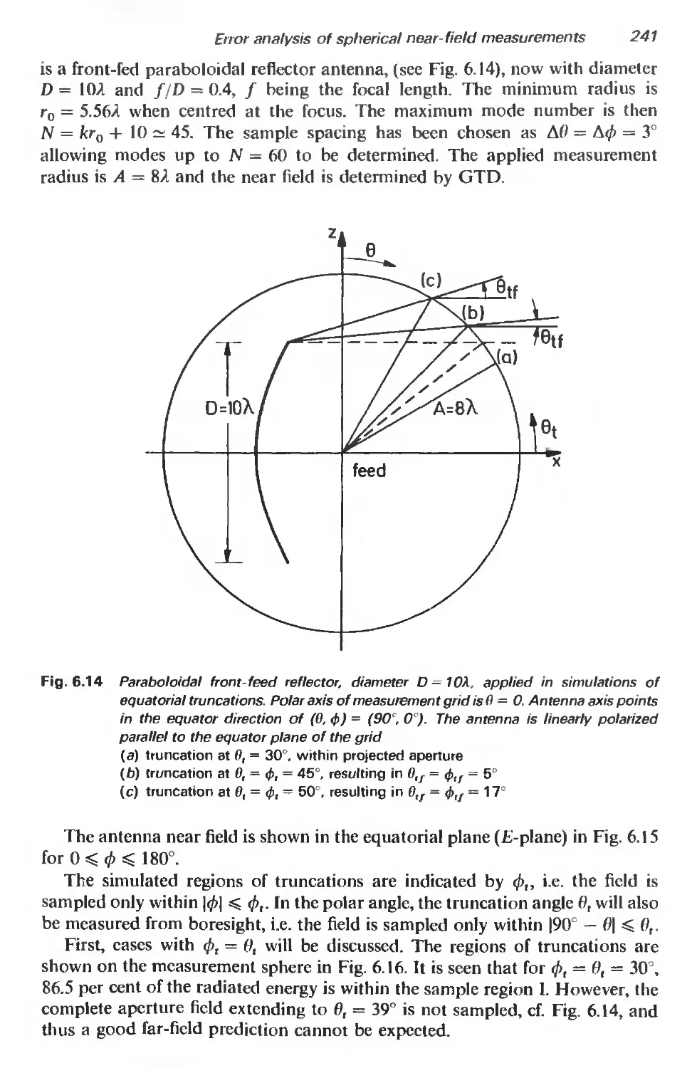
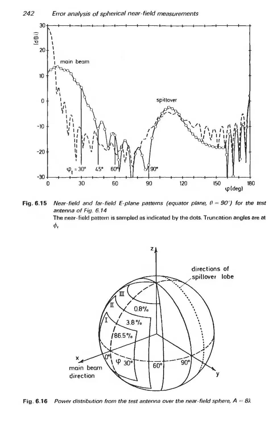
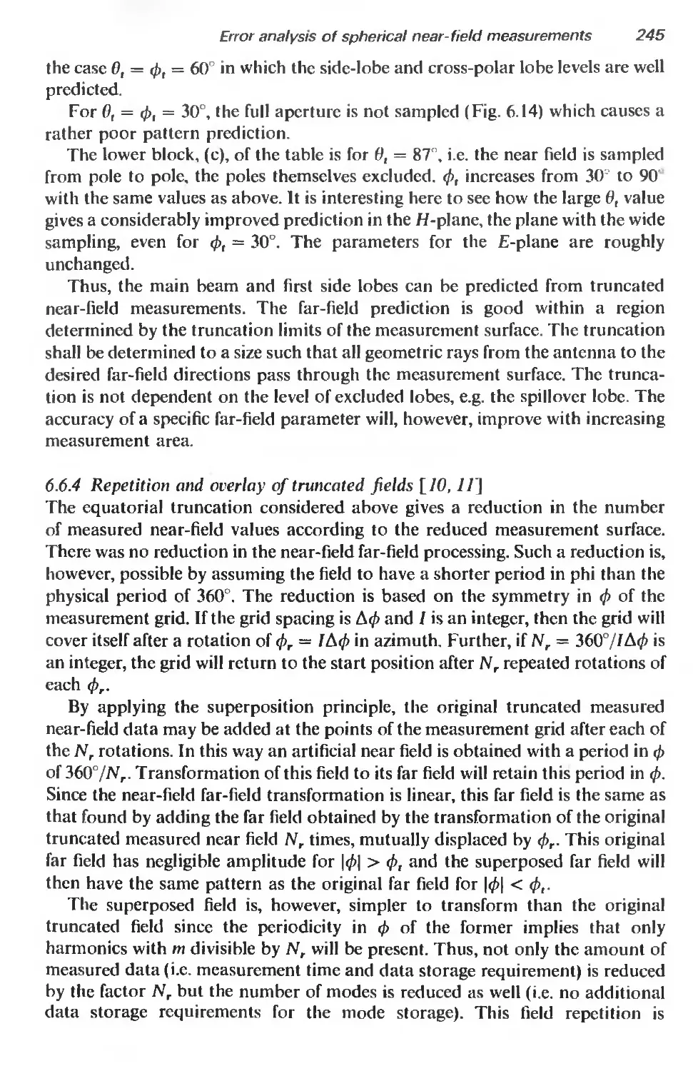
6.6.3 Equatorial truncation 240
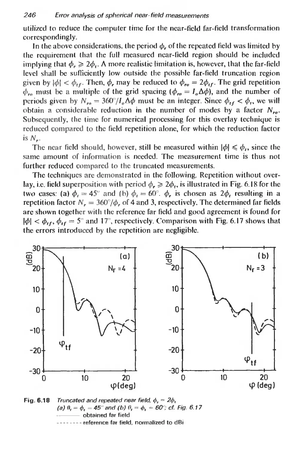
6.6.4 Repetition and overlay of truncated fields 245
6.7 Evaluation of measurements 250
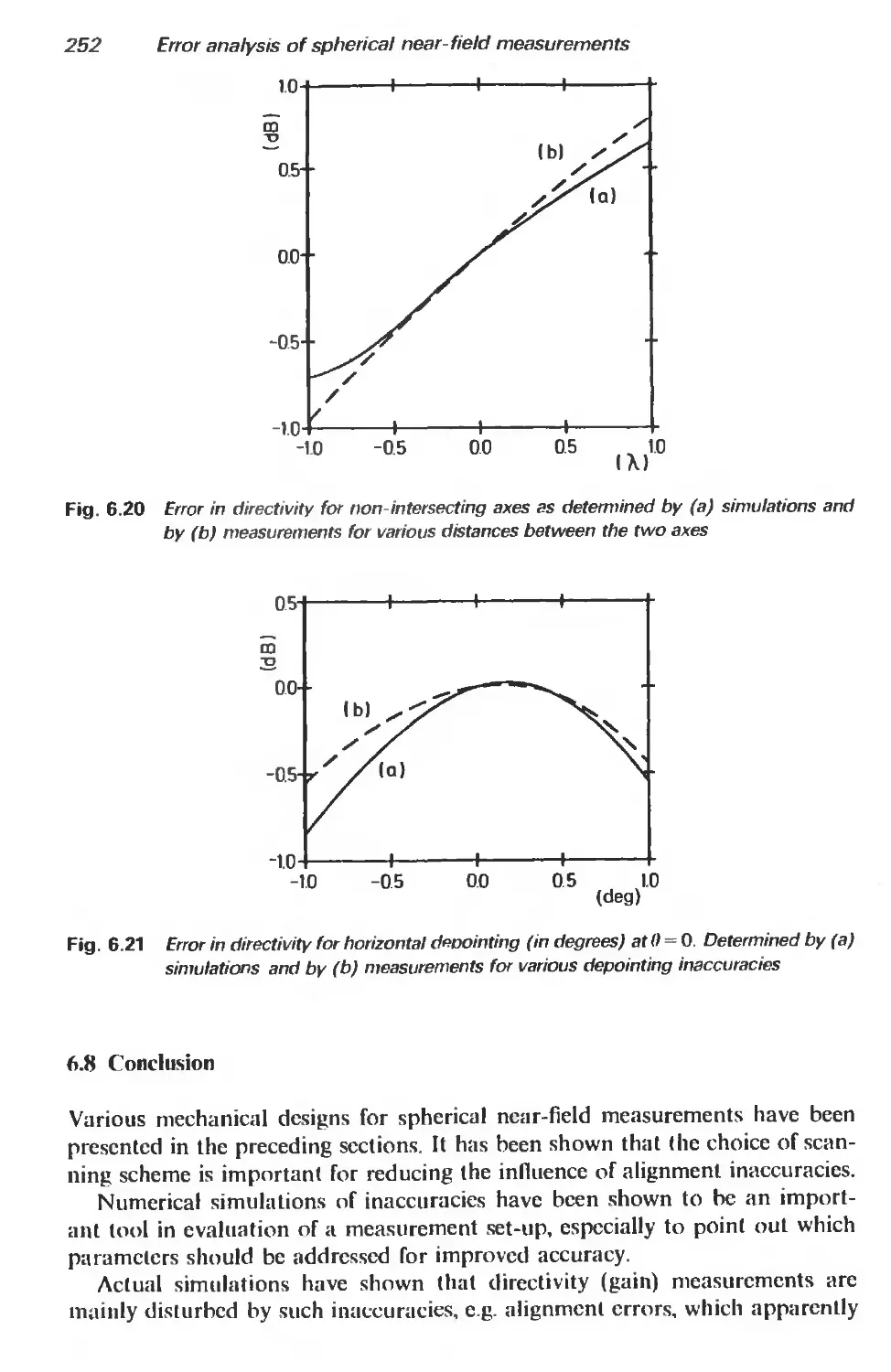
6.8 Conclusion 252
References 253
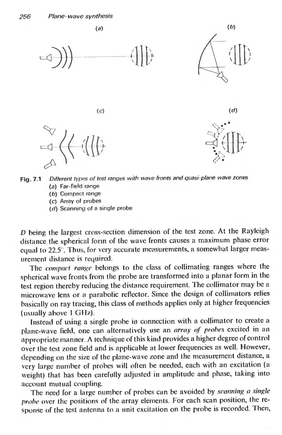
7 Plane-wave synthesis 255
7.1 Introduction 255
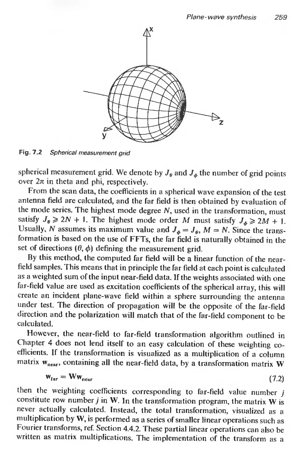
7.2 Spherical near-field far-field transformation as a plane-wave synthesis
method 258
7.3 Basic concepts in generation of plane-wave fields 263
7.3.1 Introduction 263
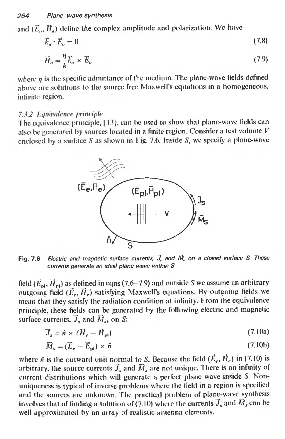
7.3.2 Equivalence principle 264
7.3.3 Relationship to a scattering problem 265
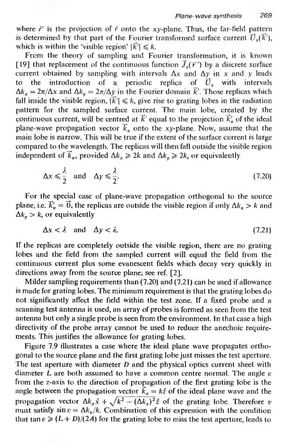
7.3.4 Truncation and sampling of continuous sources of plane waves 267
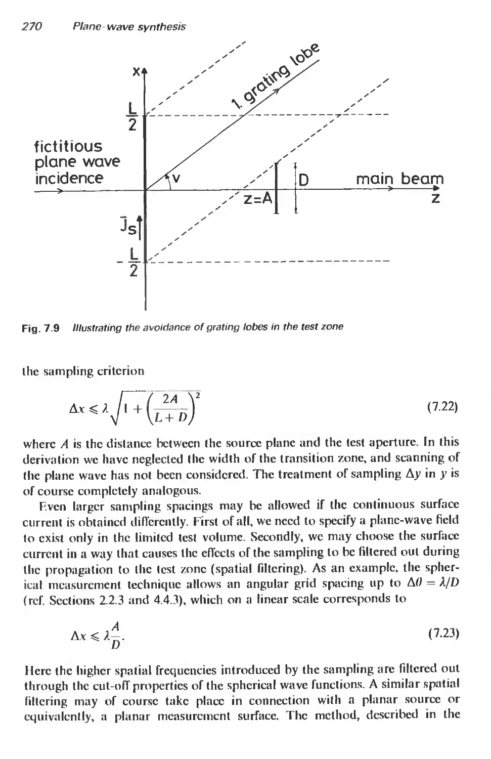
7.4 The Sheffield method 271
7.4.1 Introduction 271
7.4.2 Measurement without probe correction 271
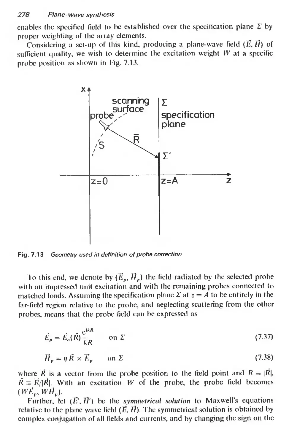
7.4.3 Measurement with probe correction 277
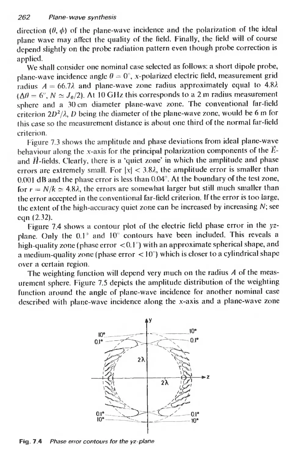
7.5 Figures of merit for plane-wave deviation 280
7.5.1 Introduction 280
7.5.2 General figures of merit for plane-wave deviation 281
7.5.3 Spherical test zone geometry 28-3
7.5.4 Measurement error upper bounds 285
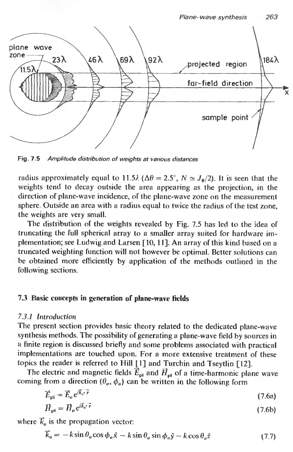
7.6 Numerical optimization methods for plane-wave synthesis 287
7.6.1 Introduction 287
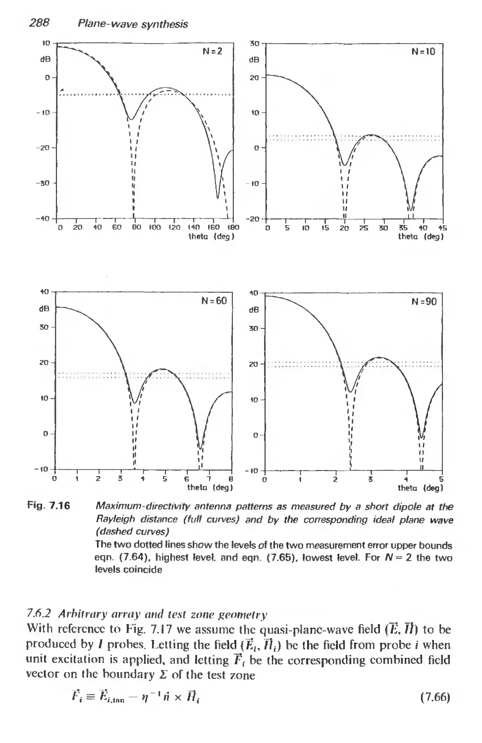
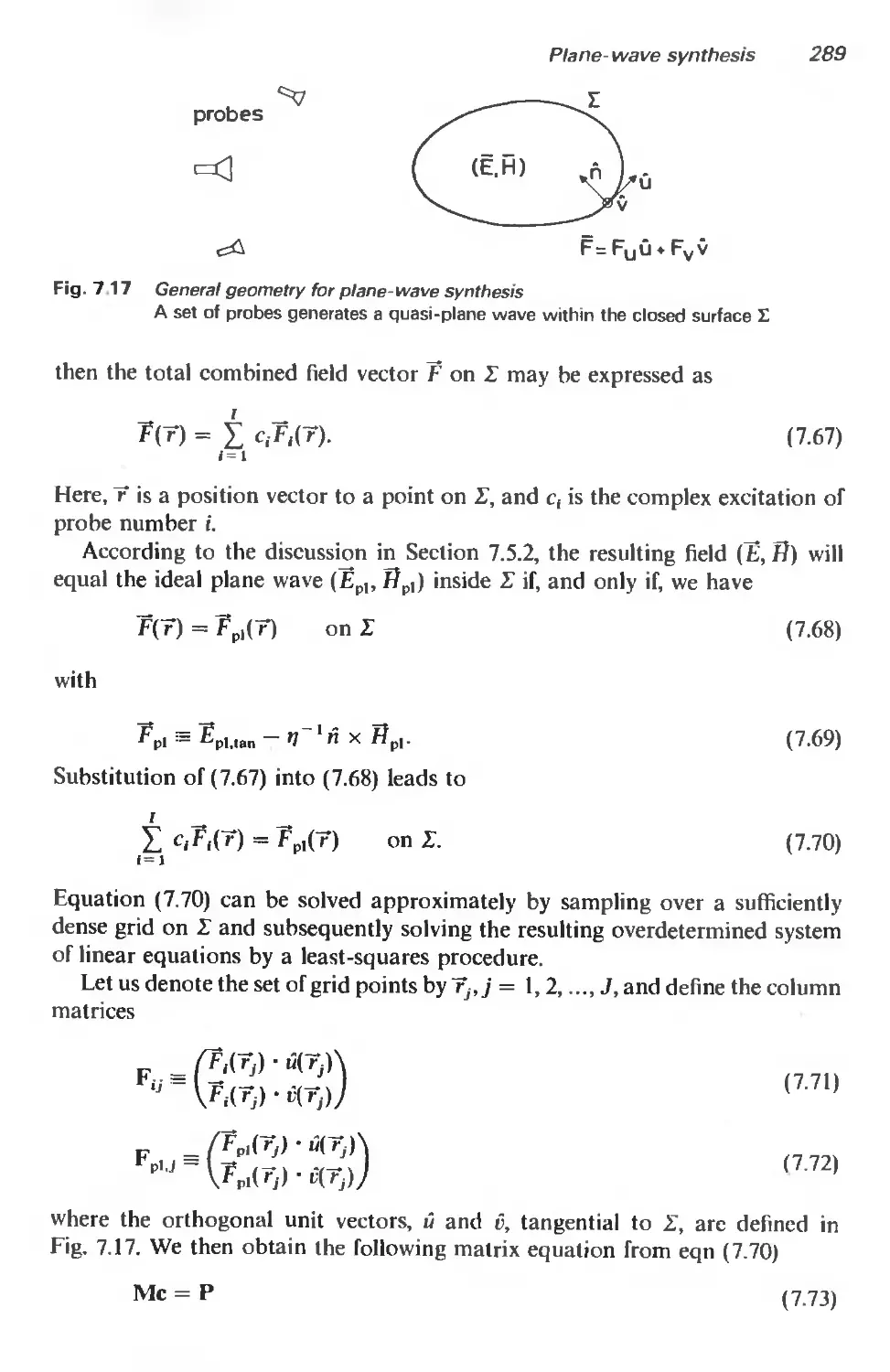
7.6.2 Arbitrary array and test zone geometry 288
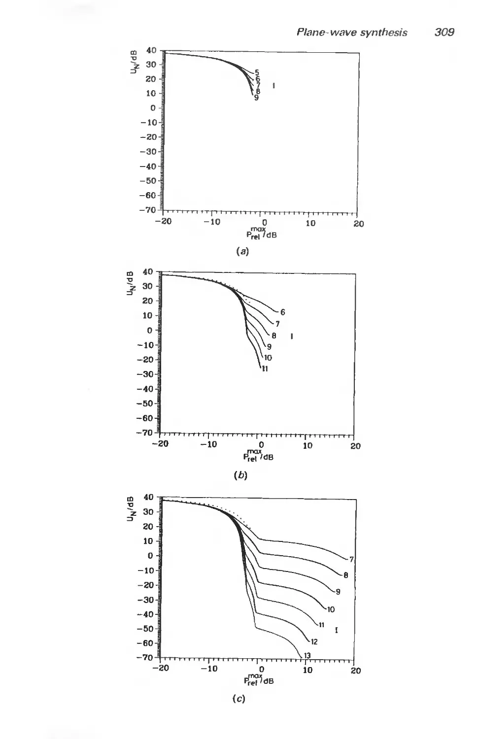
7.6.3 Ring sources and spherical test zones 291
References 310
Appendices
Al Spherical wave functions, notation and properties 312
Al.l Notation 312
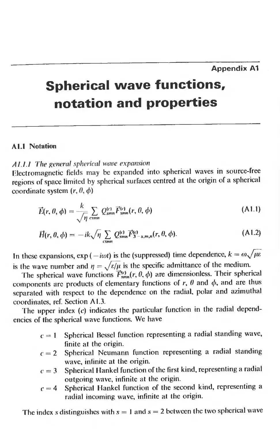
A 1.1.1 The general spherical wave expansion 312
A 1.1.2 Single index convention 313
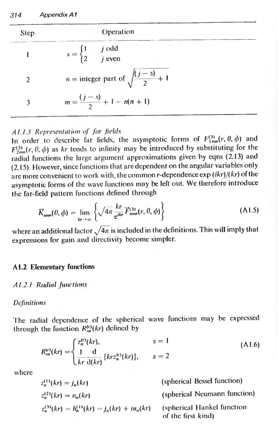
A 1.1.3 Representation of far fields 314
Al.2 Elementary functions 314
Al.2.1 Radial functions 314
A 1.2.2 Angular functions 318
A1.3 Wave functions 325
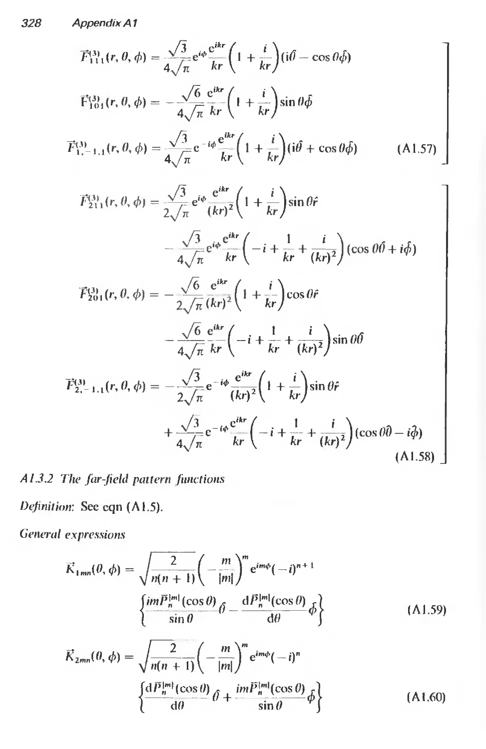
Al.3.1 The spherical wave functions 325
A 1.3.2 The far-field pattern functions 328
X
Contents
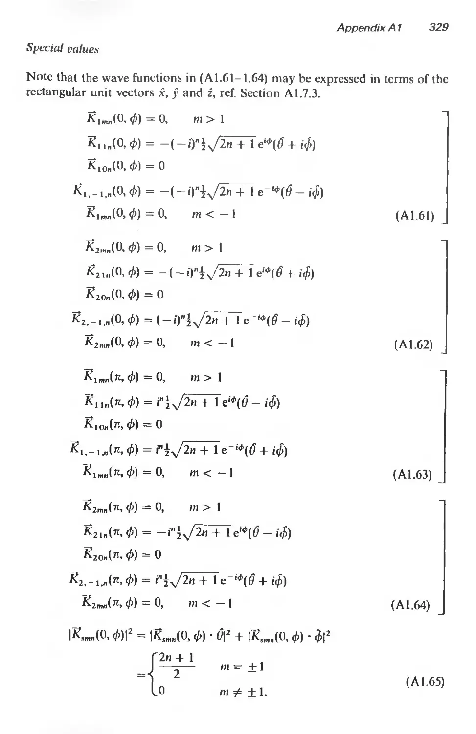
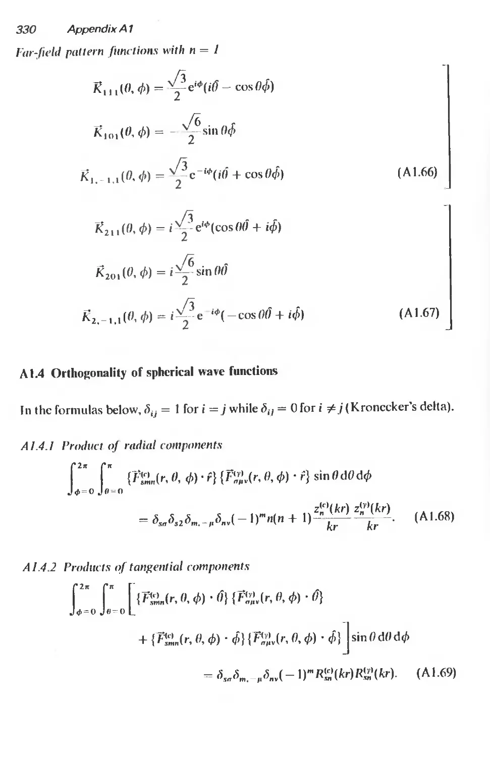
A1.4 Orthogonality of spherical wave function^ 330
A 1.4.1 Product of radial components 330
A 1.4.2 Products of tangential components 330
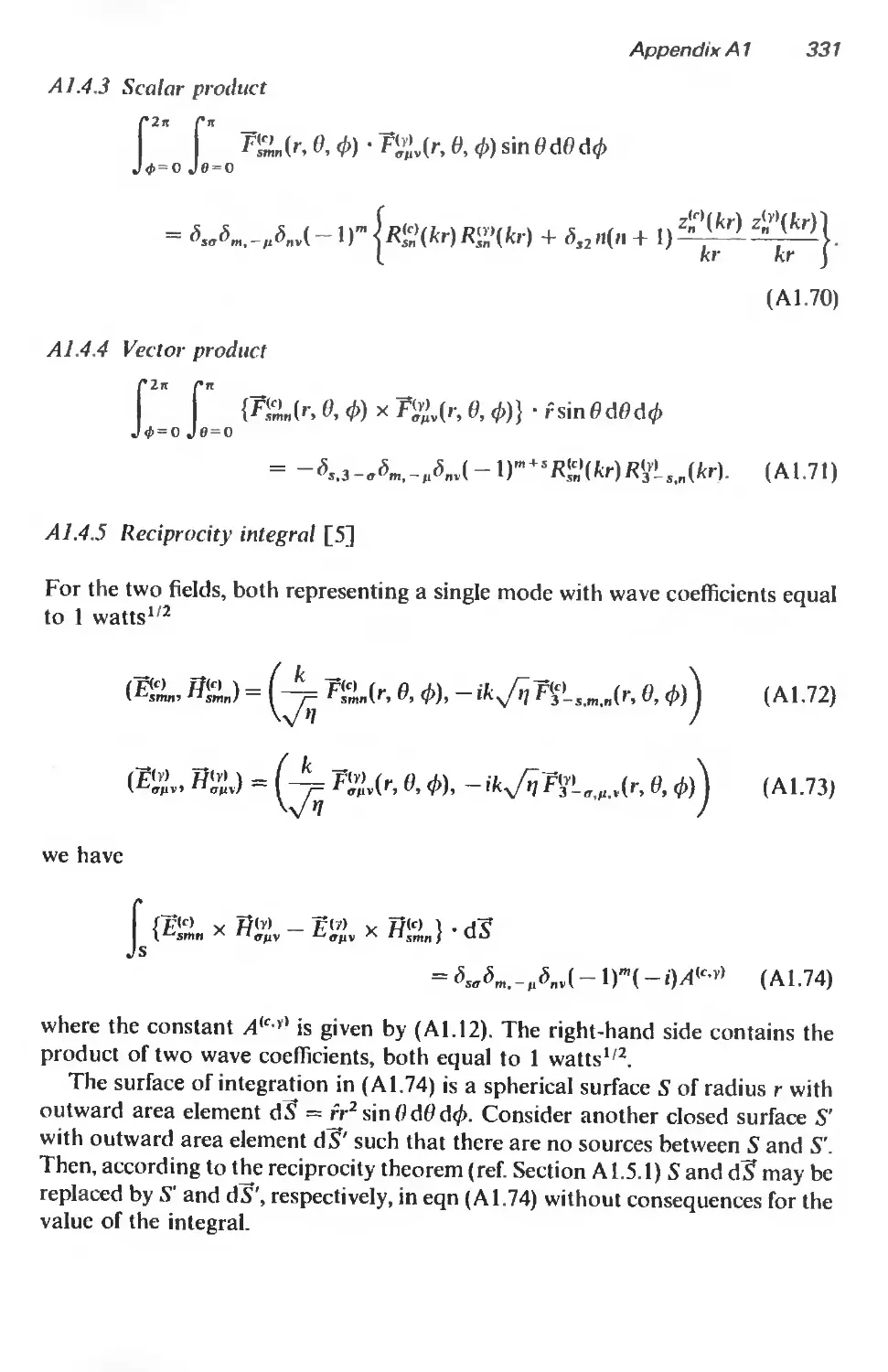
A 1.4.3 Scalar product 331
A 1.4.4 Vector product 331
A 1.4.5 Reciprocity integral 331
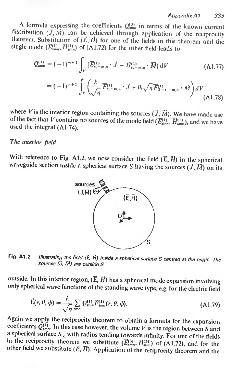
Al.5 Calculation of spherical wave coefficients from current distributions 332
A 1.5.1 General formulation 332
A 1.5.2 Source symmetries 334
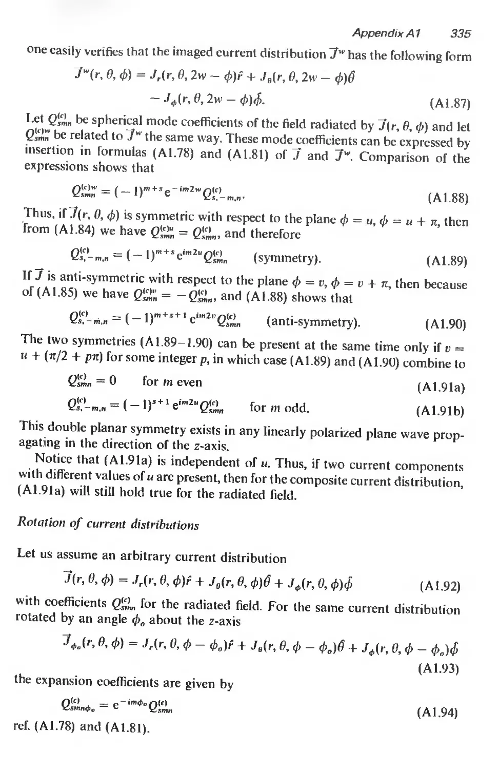
A 1.5.3 The continuous x-polarized current ring 336
A 1.5.4 The sampled x-polarized planar current ring 337
A 1.5.5 Ring of currents tangential to a sphere 339
Al.6 The plane wave 341
Al.7 Relations between spherical and rectangular coordinates 341
A 1.7.1 Coordinate transformations 341
A1.7.2 Scalar products of unit vectors 342
A 1.7.3 Behaviour of certain vector distributions at 6 = 0 and 0 = n 342
References 342
A2 Rotation of spherical waves 343
A2.1 Euler angles 343
A2.2 Notation 343
A2.3 The rotation coefficient 345
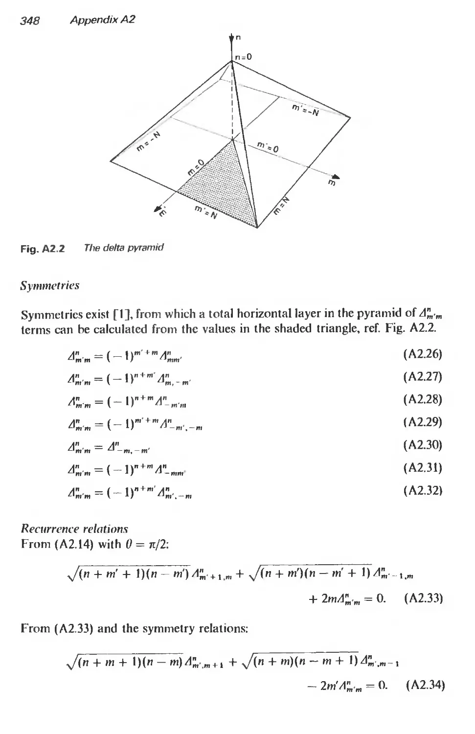
A2.4 The deltas 347
A2.5 On the computation of rotation coefficients 350
A2.5.1 Stability of three-term recurrences 350
A2.5.2 Stability of delta recurrences 350
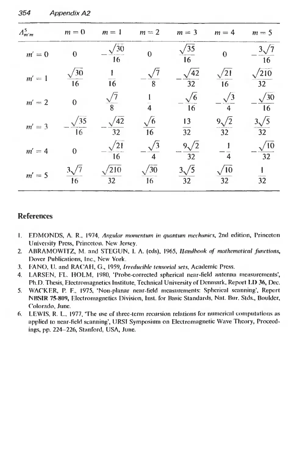
A2.6 Tables of low-order deltas 352
References 354
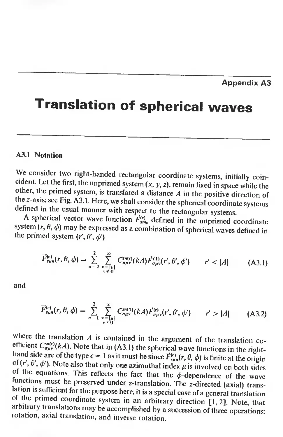
A3 Translation of spherical waves 355
АЗ. 1 Notation 355
A3.2 The translation coefficient 356
References 360
A4 Data processing in antenna measurements 361
A4.1 Introduction 361
A4.2 The discrete Fourier transform 362
A4.2.1 Definitions 362
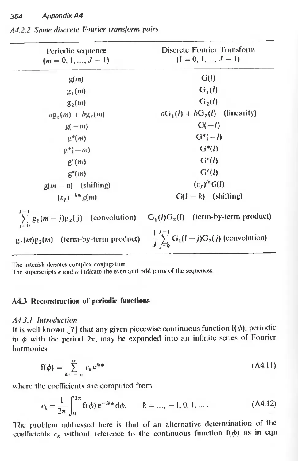
A4.2.2 Some discrete Fourier transform pairs 364
A4.3 Reconstruction of periodic functions 364
A4.3.1 Introduction 364
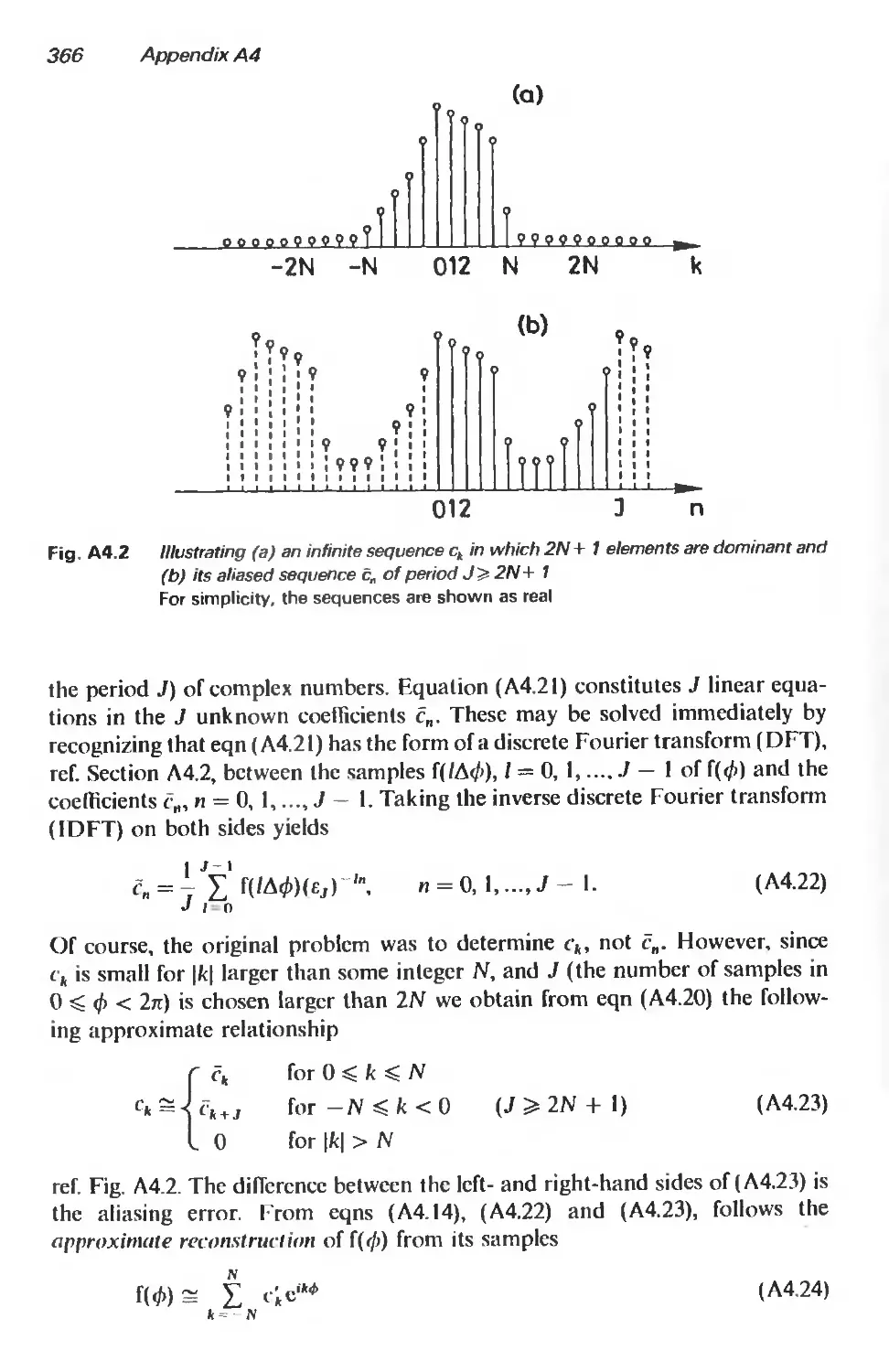
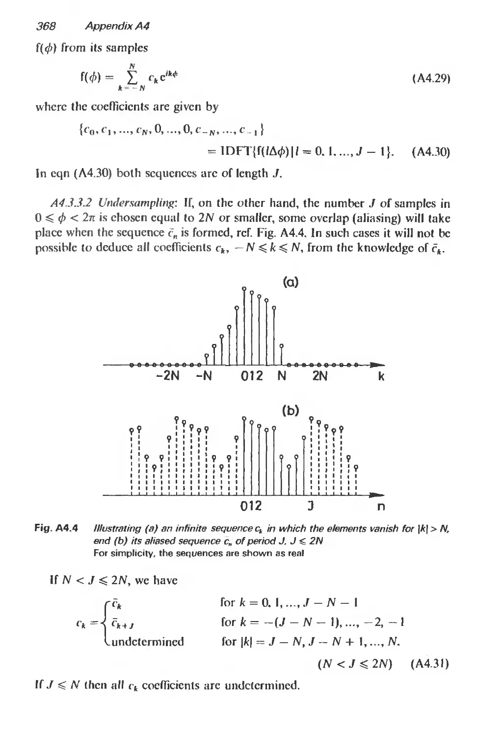
Л4.3.2 Quasi-band-limited case 365
A4.3.3 Band-limited case with 2N + 1 coefficients 367
A4.4 Special case of reconstruction 369
A4.4.1 Introduction 369
Л4.4.2 Shifting of sample points 369
Л4.4.3 Increased resolution 370
A4.4.4 Suppresion of noise 371
A4.4.5 Decreased resolution 371
A4.5 Numerical integration of periodic, band-limited functions 372
Contents xi
А4.5.1 General case A4.5.2 A special case References 372 372 373
AS List of principal symbols and uses 374
Index 377
Preface
Spherical near-field antenna testing is an interesting and powerful method
within the general area of antenna measurements. The present book aims at
presenting theoretical and practical aspects of the spherical test technique in a
comprehensive manner. The book is intended for use primarily by the research
and development engineer engaged in antenna measurements. It is hoped,
however, that it may also be found useful to others by providing reference
material on related topics, notably spherical electromagnetic waves.
While some of the results described in the book have not been published
before, most of its contents is based on research documented in doctoral
dissertations, research reports and papers from the Electromagnetics Institute
at the Technical University of Denmark (TUD) over the last twenty years.
The original inspiration to the work done at TUD in this area is owed to
E. V. Jull of the University of British Columbia, Canada, who did some of the
early work on near-field antenna theory and measurements in the late fifties and
who was a visiting scientist at TUD for two periods in 1963-65. With the
inauguration in 1967 of the large Radio Anechoic Chamber at TUD and the
acquiring, little by little, of automated equipment and computing facilities, the
idea of embarking into a research programme on near-field antenna measure-
ments became obvious. The first result in this connection was achieved by
F. Jensen whose thesis (1970) contains a basic theoretical element of spherical
near-field testing, the transmission formula.
A. C. Ludwig, formerly at the Jet Propulsion Laboratory, Pasadena, USA,
who was a visiting professor at TUD in 1972 and 1979, developed the first useful
algorithm for utilizing Jensen’s transmission formula. While at TUD, he also
presented his now well-known definitions of cross polarization. In 1975, F. Holm
Larsen spent a short period of time at the National Bureau of Standards (NBS)
in Boulder, USA, where he learnt of the new, efficient algorithm published by
P. Wacker for inverting Jensen’s transmission formula and acquainted himself
with a computer code developed by R. L. Lewis for the case without probe
correction. As a part of his thesis work, Larsen presented in 1977 the first
complete spherical near-field measurement with transformation to the far field
based on his own algorithm in which probe correction was included.
xiv Preface
Already in 1976 an agreement between the European Space Agency (ESA)
and TU D for a joint effort regarding further development of spherical near-field
testing was signed. In a scries of theoretical and experimental contracts, in which
TICRA of Copenhagen took part, an experimental spherical near-field
facility at TUD was constructed which enables in-depth studies of the technique.
A number of TUD staff members were involved in the project. Among these
H. Bach, E. Lintz Christensen and F. Conrad were prominent. The TUD ESA
facility is in extensive use for research, measurement of antennas for space
applications and calibration of standard-gain horns. The spherical test tech-
nique has become commercially available and is now implemented at several
large test ranges in Europe and elsewhere.
The authors wish to acknowledge the support received from ESA during
many years of co-operation. Special thanks are due to J. Aasted and
N. E. Jensen, former and present head of the ESTEC antenna section, and
J. Hammer for supervising the major part of our contracts. On many occasions
over the years, the authors have had the opportunity to discuss antenna
measurements with staff members of NBS. This fact has markedly influenced
our work within spherical near-field testing and the presentations in this book.
In this connection, the authors would like to thank A. Newell, P. Wacker,
A. D. Yaghjian, R. L. Lewis, R. Wittmann and C. Stubcnrauch. Thanks are also
due to D. Hess of Scientific-Atlanta Inc., Atlanta, USA for many discussions.
The valuable help and suggestions from colleagues at TUD and TICRA
in the preparation of the manuscript are gratefully acknowledged. J.
Lemanczyk undertook the time-consuming task of reading the manuscript and
making linguistic improvements and corrections. He also did the measurements
presented in Chapter 5. S. K. Lynggaard computed and prepared the figures
illustrating special functions in Chapter 2 and Appendix A2. He also produced a
large number of the other figures in the book. A Frandsen made the computa-
tions for Section 4.4.6 and proofread some of the chapters. S. Boel Pedersen read
Appendix A4 and suggested improvements.
As mentioned above, all chapters and appendices reflect previous work
although generally in a considerably reworked and revised form. F. Holm
Larsen wrote Sections 5.2 and 5.4 as well as Appendices A2 and АЗ. F. Jensen
wrote Chapter 6. J. Hald wrote Chapter 7 and Section A 1.5. The remainder of
the book was written by J. E. Hansen.
November, 1986
J.E.H.
Chapter 1
Introduction
1.1 Background
1.1.1 Introduction
A need for precise measurement of the radiation from microwave antennas has
arisen in connection with the development of advanced antenna design concepts
and improved theoretical approaches for antenna analysis. The need has been
felt in particular within space applications where antennas are being constructed
to tight specifications, i.e. down to the order of one per cent in gain. Antenna
testing has therefore attracted considerable interest in recent years where a large
number of studies have been made and new developments effected.
The oldest type of test range, the outdoor far-field range, has seen a few
modern implementations. However, it is to the indoor test techniques that most
of the efforts have been devoted. The compact range as well as near-field
scanning ranges in planar, cylindrical and spherical geometries have all more or
less reached mature states. They are now being installed at many places and
seem to be the natural choice for contemporary antenna testing.
The present book concerns itself with one of the newer measurement schemes:
spherical near-field scanning.
1.1.2 Brief outline of antenna testing
The angular dependence of the electromagnetic field radiated from a transmit-
ting antenna is not invariant but changes gradually with the distance. At large
distances from the antenna it approaches a definitive shape, the far-field radi-
ation pattern. For most antennas, the far-field pattern is the characteristic of
primary interest. To obtain the far field experimentally for a given antenna is the
objective of antenna testing.
For any fixed direction in space relative to the antenna under test, the
radiated far field is a plane wave propagating in that particular direction. As a
consequence of reciprocity, the amplitude and phase of the far field as a function
of angle may therefore be recorded experimentally as the received signal when
the test antenna is immersed and rotated in a plane wave field.
2
Introduction
The ability to provide plane wave illumination of the antenna under test is a
basic requirement for any test range. This is accomplished with an auxiliary
antenna: the probe. The creation of a uniform plane wave zone of sufficient
quality without parasitic interference fields can be achieved in a number of
different ways.
In far-ficld test ranges, ample separation of the test antenna and the probe is
used as a means of obtaining the plane wave condition. At the Rayleigh distance
R, given by R - 2/J2/>, where Я is the wavelength, the curvature of the spherical
wave radiated from a small probe is small enough for the deviation from a plane
wave over a volume containing a test antenna of diameter D to be less than n/8
in phase. Although the Rayleigh distance is commonly taken as sufficient when
a true far-ficld recording is required, errors in the recorded pattern may not
be negligible at this distance. Far-licld ranges can be impractical due to the
required measurement distance, typically several hundred metres, which in it-
self makes the suppression of reflections from the ground and nearby objects
difficult. Nevertheless, accurate far-licld ranges exist, although they are few in
number, at least in Furope.
In general, solutions to the problem of constructing precision test ranges for
antennas have been found in the protected indoor environment of radio anechoic
chambers. The basic principle of the compact range is to use a probe in the shape
of a large collimating device to generate a plane wave zone without requiring the
large separation of a far-ficld range.
Systems for near-field scanning employ a single, small probe which is scanned
in a regular grid across a measurement surface in the near field of the test
antenna. The measurement surface may be plane (planar scanning) or it may
be cylindrical (cylindrical scanning). It may also have the form of a spherical
surface enclosing the test antenna. In this case the near-field scanning method is
spherical scanning, the subject of this book. (See Fig. 1.1.) In all scanning
methods, the far-ficld characteristics of the test antenna are derived by applying
suitable processing schemes to the near-field data obtained from the scanning
process. This is equivalent to viewing the plane wave zones of the near-field
scanning ranges as being synthesized in a computer.
It is not the intention here to discuss the relative merits and drawbacks of
the various types of test ranges. Such comparisons can probably only lead to
meaningful results when particular applications are in mind. Instead, some of
the features of spherical near-field testing are given below.
1.1.3 Spherical near-field testing
Some of the features of spherical near-field testing (SNFT) of antennas are:
1. SNFT employs the fact that antenna radiation may always be expressed in
terms of a truncated expansion in electromagnetic spherical waves satisfying
Maxwell’s equations. The truncation error is small compared to other errors,
i.e. measurement errors and computational round off errors. Due to a cut-olf
property of spherical waves the number of terms in such truncated spherical
Introduction
3
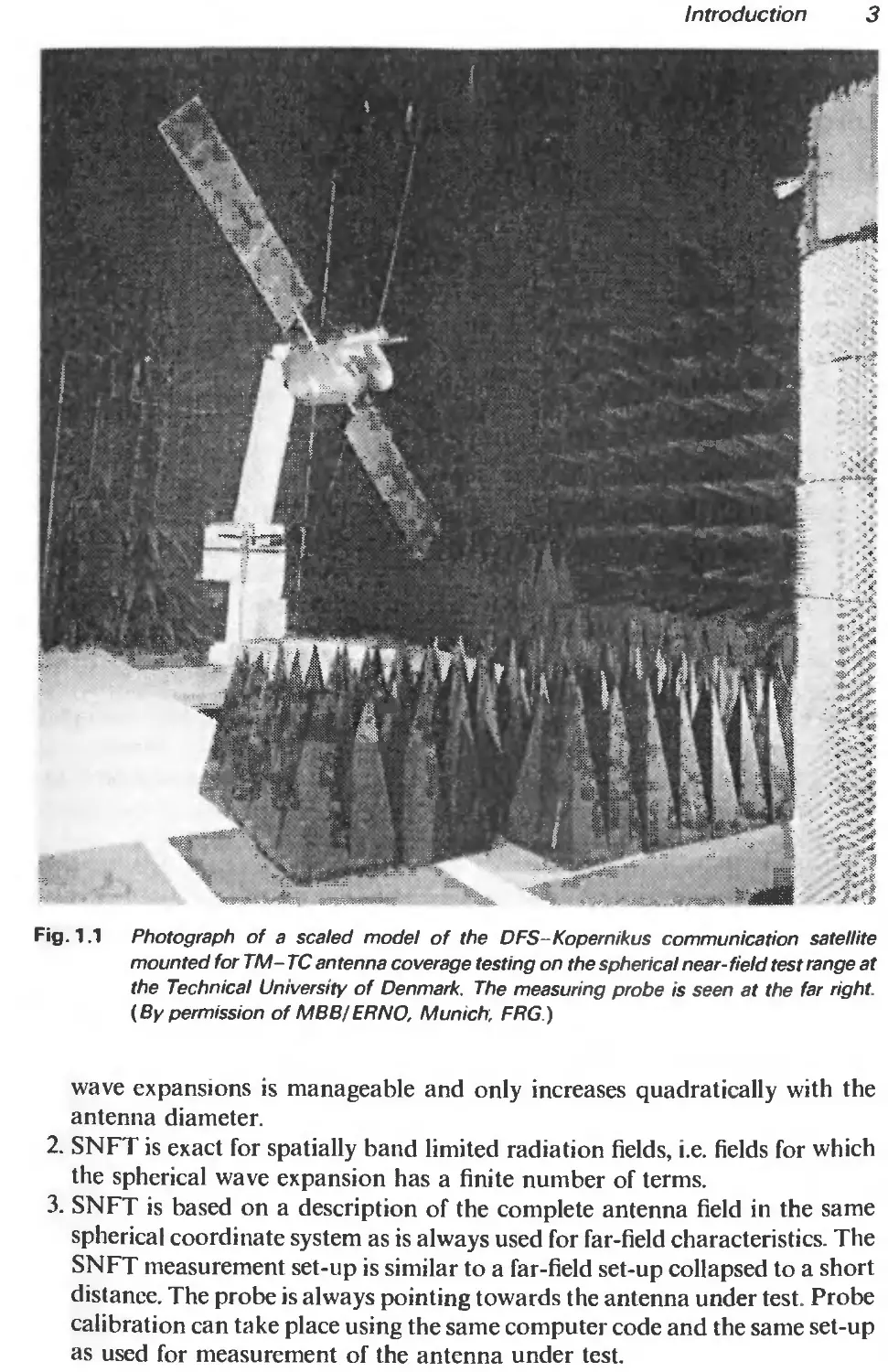
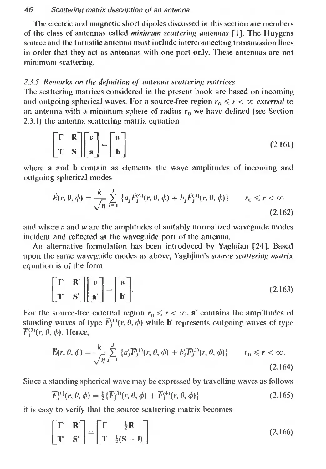
Fig. 1.1 Photograph of a scaled model of the DFS-Kopernikus communication satellite
mounted for TM-TC antenna coverage testing on the spherical near-field test range at
the Technical University of Denmark. The measuring probe is seen at the far right.
(By permission of MBB/ERNO, Munich; FRG.)
wave expansions is manageable and only increases quadratically with the
antenna diameter.
2. SNFT is exact for spatially band limited radiation fields, i.e. fields for which
the spherical wave expansion has a finite number of terms.
3. SNFT is based on a description of the complete antenna field in the same
spherical coordinate system as is always used for far-field characteristics. The
SNFT measurement set-up is similar to a far-field set-up collapsed to a short
distance. The probe is always pointing towards the antenna under test. Probe
calibration can take place using the same computer code and the same set-up
as used for measurement of the antenna under test.
4
Introduction
4. SNFT inherently provides antenna directivity. This makes it ideally suited to
precision gain calibration of (for example) standard gain antennas of known
ohmic losses.
5. In SNFT the measurement surface (a sphere) has a finite area. Truncations,
which might introduce errors, are not required.
6. SNFT is suitable for the measurement of narrow beam antennas as well as
broad beam or omnidirectional antennas.
7. Antenna gain can be determined in SNFT by a substitution method.
8. SNFT provides easy means of non-trivial self checking by change of the
measurement distance or by translation of the antenna under test within the
measurement sphere. The influence of reflections and multiple reflections can
be assessed in this way.
9. Disturbing reflections from the environment may be suppressed in SNFT by
using a directive probe.
10. SNFT can be configured in a number of different mechanical set-ups.
Movement of the antenna under test can be completely avoided, if required.
The physical dimensions of a set-up are only slightly larger than the size of the
largest antenna that can be measured.
1.2 Organization of (this) book
Several review papers on antenna testing including spherical near-field methods
have been published in recent years [1 8]. It is not the intention, therefore, to
provide another comprehensive survey of the literature on test methods in this
book. Instead, brief references to papers relevant to the material presented are
included in the chapters.
Chapter 2 provides the necessary theoretical background for the later
chapters by describing electromagnetic spherical wave expansions, their defini-
tions and properties. Power normalized spherical waves in a new, simple
notation are used throughout. An account of the antenna scattering matrix, a
concept from general antenna theory, is given using the new notation. It is
shown how the scattering matrix elements—i.e. the reflection coefficient, the
receiving and transmitting coefficients as well as scattering coefficients—
describe all of the antenna’s properties in г» concise manner.
In Chapter 3, a spherical near-field transmission formula is derived using the
scattering matrix formulation of Chapter 2. As all other scanning techniques for
antenna near-field testing, spherical scanning utilizes a transmission formula as
its theoretical basis. A transmission formula expresses the complex signal
received by an antenna when another antenna, usually within the near field,
is transmitting. The receiving coefficient of the first antenna as well as the
transmitting coefficients of the second antenna and various geometrical factors
enter the spherical near-field transmission formula. Il is shown that for large
separations between the two antennas the spherical near-field transmission
formula reduces to the well-known Friis’s transmission formula.
Introduction
5
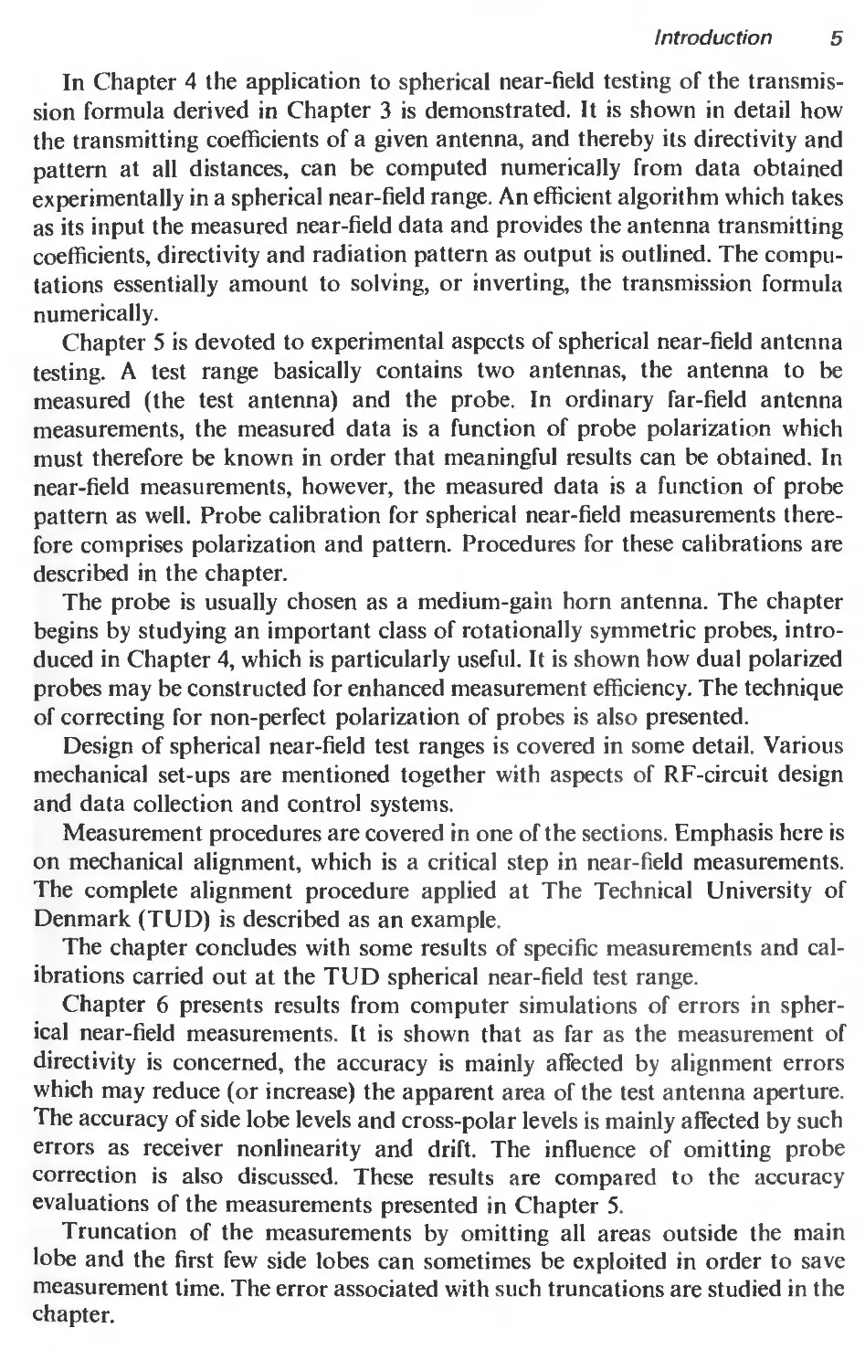
In Chapter 4 the application to spherical near-field testing of the transmis-
sion formula derived in Chapter 3 is demonstrated. It is shown in detail how
the transmitting coefficients of a given antenna, and thereby its directivity and
pattern at all distances, can be computed numerically from data obtained
experimentally in a spherical near-field range. An efficient algorithm which takes
as its input the measured near-field data and provides the antenna transmitting
coefficients, directivity and radiation pattern as output is outlined. The compu-
tations essentially amount to solving, or inverting, the transmission formula
numerically.
Chapter 5 is devoted to experimental aspects of spherical near-field antenna
testing. A test range basically contains two antennas, the antenna to be
measured (the test antenna) and the probe. In ordinary far-field antenna
measurements, the measured data is a function of probe polarization which
must therefore be known in order that meaningful results can be obtained. In
near-field measurements, however, the measured data is a function of probe
pattern as well. Probe calibration for spherical near-field measurements there-
fore comprises polarization and pattern. Procedures for these calibrations are
described in the chapter.
The probe is usually chosen as a medium-gain horn antenna. The chapter
begins by studying an important class of rotationally symmetric probes, intro-
duced in Chapter 4, which is particularly useful. It is shown how dual polarized
probes may be constructed for enhanced measurement efficiency. The technique
of correcting for non-perfect polarization of probes is also presented.
Design of spherical near-field test ranges is covered in some detail. Various
mechanical set-ups are mentioned together with aspects of RF-circuit design
and data collection and control systems.
Measurement procedures are covered in one of the sections. Emphasis here is
on mechanical alignment, which is a critical step in near-field measurements.
The complete alignment procedure applied at The Technical University of
Denmark (TUD) is described as an example.
The chapter concludes with some results of specific measurements and cal-
ibrations carried out at the TUD spherical near-field test range.
Chapter 6 presents results from computer simulations of errors in spher-
ical near-field measurements. It is shown that as far as the measurement of
directivity is concerned, the accuracy is mainly affected by alignment errors
which may reduce (or increase) the apparent area of the test antenna aperture.
The accuracy of side lobe levels and cross-polar levels is mainly affected by such
errors as receiver nonlinearity and drift. The influence of omitting probe
correction is also discussed. These results are compared to the accuracy
evaluations of the measurements presented in Chapter 5.
Truncation of the measurements by omitting all areas outside the main
lobe and the first few side lobes can sometimes be exploited in order to save
measurement time. The error associated with such truncations are studied in the
chapter.
6
Introduction
In Chapter 7 the alternative viewpoint on antenna measurements known as
plane wave synthesis is presented. ЛИ types of antenna test ranges are in fact
based upon the creation of a plane wave. The plane wave may exist physically as
in compact ranges or as in far-field ranges. In these, the test antenna (if receiving)
is rotated in a test zone where a field exists that is close to being a plane wave.
The plane wave may also be synthesized in a computer, as a suitable weighted
sum of the contributions from a transmitting probe which is moved stepwise (or
from several probes present simultaneously) on a surface surrounding the test
zone. The test antenna far field is then simply the sum of its responses to each
transmitting probe, weighted in the same way.
For spherical near-field measurements, the plane-wave synthesis viewpoint
has been introduced at the University of Sheffield in England. The theory is
outlined in the chapter together with alternative approaches. The problem of
numerical optimization of plane wave zones from spherical or planar arrays is
addressed.
The book is concluded by five appendices of which the first three provide a
systematic listing of equations and definitions pertaining to spherical waves. The
fourth appendix summarizes elements of data processing theory pertinent to
antenna measurements. Appendix 5 is a list of principle symbols and their uses.
Although a coherent exposition of spherical near-field measurements is at-
tempted and the presentation therefore contains a number of references from
chapter to chapter, much of the material can be read independently. This is
particularly true as far as Chapter 2 and the appendices Al, A2 and A3 are
concerned. These cover a large part of the classical theory on electromagnetic
spherical waves and include a number of formulas that have not been published
before. Some of the experimental techniques described in Chapter 5 are also of
interest in connections other than spherical near-field measurements. As an
example, the section on dual polarized probes is also applicable to plane
polar near-field techniques. Chapter 7 on plane-wave synthesis can also be
read independently of the previous chapters. Appendix A4 deals with the
discrete Fourier transform (DFT) and applications within general antenna
theory and measurements.
References
I. JOHNSON, R. C., ECKER, H. A. and HOLLIS, J. S„ 1973, ‘Determination of far-field antenna
patterns from near-field measurements', Proc. IEEE, Vol. 61, No. 12, pp. 1668 1694, Dec.
2. WACKER, P. F. and NEWELL, A. C„ 1977. ‘Advantages and disadvantages of planar, circular
cylindrical, and spherical scanning and description of the NBS antenna scanning facilities’, ESA
Workshop on Antenna Testing Techniques, ESTEC. Holland. ESA SP 127. pp. 115-121, June.
3. KUMMER, W. H. and GILLESPIE, F. S„ 1978, ‘Antenna measurements— 1978’, Proc. IEEE,
Vol. 66. No. 4, pp. 483 507. Apr.
4. PARIS, D. T„ LEACH, W. M., Jr. and JOY, E. B„ 1978, ‘Basic theory of probe-compensated
near-field measurements', IEEE Trans., Vol. AP-26, No. 3, pp. 373-379, May.
Introduction 7
5. TURCHIN, V. I. and TSEYTLIN, N. M., 1979, ‘Antenna testing based on near-field
measurements (Review)’, Radio Engineering & Electronic Physics, Vol. 24, pp. 1-26, Dec.
6. APPEL-HANSEN. J. et al., 1982, ‘Antenna Measurements’, Chapter 8 in The Handbook of
Antenna Design, Vol. 1, Peter Peregrinus, London.
7. VOK.URKA, V. J., 1984, ‘Advanced antenna measurements’, 14th European Microwave Con-
ference, pp. 60-70, Liege, Belgium, Sept.
8. YAGHJIAN, A. D., 1986, ‘An overview of near-field antenna measurements’, IEEE Trans.,
Vol. AP-34, pp. 30-45, Jan.
Chapter 2
Scattering matrix description
of an antenna
2.1 Introduction
The presentation in later chapters of spherical near-field testing of antennas
rests upon the characterization of each of the two antennas involved in the
measurement situation, the antenna under test and the probe, in terms of a
scattering matrix.
The scattering matrix description of an antenna was introduced by Dicke [1].
Since then the approach has been used in a number of studies [2, 3,4, 5] of the
radiating, scattering and coupling properties of arbitrary, structurally unspeci-
fied, lossless antennas. The scattering matrix contains the properties of an
antenna system with respect to a set of antenna terminals or local port. It also
describes the behaviour with respect to the electromagnetic field outside a
‘minimum sphere’ enclosing the system. Here, an infinite set (denumerable) of
radiation ports are assumed one for each set of two spherical vector waves,
usually an incoming and an outgoing wave. Similar to the waves in the trans-
mission lines, the spherical waves must be carefully defined and should
preferably be normalized with respect to power. The scattering matrix thus
relates the complex amplitudes of all waves. Since an infinity of spherical waves
is needed for the general field it must contain an infinite number of rows and
columns. However, as we shall touch upon several times, the infinite matrix can
be truncated. This accounts for an important physical principle, band limitation,
which applies to all practical antenna structures. Such ordinary antenna
properties as power gain and directivity arc functionals on the scattering matrix
elements.
Scattering matrix theory plays an important role in connection with spherical
near-field testing. Firstly, the theory is convenient for the derivation of a
‘spherical’ transmission formula. Here, it is not required that the test antenna
and the probe arc both reciprocal antennas. Reciprocity, if present, is expressed
conveniently as a relationship between elements of the scattering matrix.
Secondly, scattering matrix theory provides the link between quantities measur-
able in transmission lines and external fields without reference to particular
Scattering matrix description of an antenna
9
structural types. The theory constitutes a means for absolute measurements of
electromagnetic fields without unknown or unspecified constants.
The present chapter begins (Section 2.2) with a description of spherical wave
theory in sufficient detail for the purpose of a comprehensive treatment in later
chapters of the theoretical sides of spherical near-field antenna measurements
without probe correction (Section 4.2) and with probe correction (Section 4.3
and later chapters). The presentation of spherical waves is traditional, however
with a new and simplified notation for the wave functions.
In Section 2.3 the main elements of power-normalized scattering matrix
theory for antennas are introduced. The chapter concludes (Section 2.4) by
giving formulas for important antenna properties and parameters in terms
of spherical waves and scattering matrix elements. The theory of maximum
directivity (Section 2.4.4) is a classical subject of general interest which is
sometimes useful in computer simulation of near-field measurements.
2.2 Spherical waves
2.2.1 Introduction
Most of the material in this book depends on the particular solutions to
Maxwell’s equations known as spherical wave functions or spherical waves.
These are well-defined and convenient building blocks for general electromag-
netic fields. Their usefulness in antenna theory and spherical near-field measure-
ments rests on many interesting properties of which several will be discussed
here (and in further detail in Appendices Al, A2 and A3).
The applications of spherical waves within electromagnetic theory and
antennas are numerous. A survey of the extensive literature on applications falls
outside the scope of the present book. Spherical wave functions were introduced
by W. W. Hansen [6] who proposed a method of generating solutions to the
vector wave equation in any coordinate system in which the scalar wave
equation is separable. A detailed formulation and derivation is given by Stratton
[7]. Later presentations have been given in several books. Some of these are
Morse and Feshbach [8], Harrington [9], Tai [10], Collin and Zucker [11], to
mention a few. A more recent exposition is given by Ludwig [12].
With an assumed time dependence of exp( — icot), Maxwell’s equations for the
electromagnetic field in a region of a linear, isotropic and homogeneous medium
are
V x U = —icoeE + 7 (2.1)
V x £ = icopU - M (2.2)
where Й and T are the magnetic and electric field vectors, co is the angular
frequency, and e and ц permittivity and permeability, respectively, of the
medium. The assumed sources are 7 (electric current density) and Л7 (magnetic
current density).
10
Scattering matrix description of an antenna
In a source-free region. Maxwell’s equations imply that both E and П satisfy
the vector wave equation
V x (V x C) - k2C = 0 (2.3)
where k, the propagation constant, is given by к = o\/pc = 2n/A, where 2 is the
wavelength. Only the loss-free case is considered. However, lossy media can be
accounted for by making к complex in cqn (2.3). In fact, most of the formulas
presented later can be applied with к and the specific admittance i/ = у/(г./ц) of
the medium assumed complex. Exceptions are the formulas for power flow in
Section 2.2.4 and the expressions for directivity and gain in Section 2.4.3.
The spherical wave functions arc defined in the spherical coordinates (r, 0, ф)
with unit vectors (r, 0, ф) illustrated in Eig. 2.1 together with a rectangular
coordinate system (x, y, z) with unit vectors (x, y, z). With 7 — rf, and f =
f(r, 0, ф) being a generating function obtained by solving the scalar wave
equation
(V2 + k2)f=0 (2.4)
it may be shown that the vector functions m and 7 defined through
Hi = Vf x 7 (2.5)
n = к 1V x lit (2.6)
satisfy eqn (2.3).
Fig. 2.1 Rectangular coordinate system (x, y, z) and spherical coordinate system (r, 0, </>) with
unit vectors f, fi, <f>. The spherical coordinates r, 0 and ф are confined to the intervals
О o< "л 0 $ 0 s; л and О^ф < 2 л, respectively
Scattering matrix description of an antenna
11
From eqns (2.3) and (2.6) we have
m = r2Vx(Vxm) (2.7)
= L'Vxt (2.8)
Hence, in and n are related by curl operations and are ideally suited to represent
an electromagnetic field (E, H) in a homogeneous medium.f
In Stratton [7], a generating function, obtained by separation of variables
COS
f^(r,°’ ® =z"’(M p" (cos sin тф (2.9)
with n = 1,2, 3,... and m = 0, 1, 2,..., n is used to generate m and И. Here, e
and о signify even and odd, respectively, referring to the choice of the trigono-
metric function in the ^-dependence. The function P”(cos0) describing the
0-dependence of f is the associated Legendre function of nth degree and ruth
order. The radial function z(„c,(kr) is specified by an upper index (c) as one
of the functions
z*,1’ = jn(kr) (spherical Bessel function) (2.10a)
z*,2' = n„(kr) (spherical Neumann function) (2.10b)
z*,3’ = h{„iy(kr) = j„(kr) + in„(kr) (spherical Hankel function
of the first kind) (2.10c)
44’ = h<„2y{kr) = j„(kr) — in„(kr) (spherical Hankel function
of the second kind) (2.10d)
where c = 1 and c = 2 indicate standing waves, while c = 3 represents an out-
ward travelling wave, and c = 4 an inward travelling wave.
In passing, it may be noted that the right-hand side of eqn (2.9) has the
surprisingly simple property of being expressible by a finite number of trigono-
metric functions and inverse powers of kr.
With the proper choice of one or two values of c in eqn (2.9), a complete and
orthogonal set of functions is obtained which may be used as a basis for all finite,
continuous and single-valued solutions to (2.4) in any of the regions 1,2 and 3 in
Fig. 2.2.
By employing f£,’„(r, в, ф) in eqns (2.5) and (2.6), we obtain the well-known
solutions to the vector wave equation [7]
sin 0 cos
uni ,dP”(cos0)cos
-4 (M--------. тфф (2.11)
ав sm
t The third (irrotational) W. W. Hansen vector wave function T = Vf is not needed in the present
book. For applications of T, see ref. [33].
12 Scattering matrix description of an antenna
scatterer
Fig. 2.2 Source-free regions 1, 2 and 3 limited by spherical surfaces centred at the origin of
the coordinate system
0. Ф) = -z^rj/^cosfl)<™тфг
1 d , dP”(cosfl)cos -
kr d{kr) du sin
1 d ,, ,, , mP?(cost?) sin , -
+ Г AlTl J krzn(kr)}----— тФФ-
krd(kr) sinO cos
(2.12)
For use in connection with the definitions of far fields, we shall also need the
asymptotic form of the m and n functions with c = 3 and c = 4 as kr tends to
infinity. This is obtained by introducing the large argument approximations
valid for kr » n
„ifcr z(3)(fcr)^(_lr+l КГ kr -> 00 (2.13)
e ifcr z^(kr)-.i"+t-— КГ kr -* 00 (2.14)
^ikr -У-г- kr kr —* 00 (2-15)
e-lkr kr kr —» 00 (2.16)
and replace the radial functions in (2.11) and (2.12) accordingly.
2.2.2 Power-normalized spherical waves
In order to obtain a more compact notation, Jensen [13] introduced one symbol
T*jj„ to designate m and n with the convention that s = 1 denotes the in-function
while s = 2 gives the it-function. At the same time, a slightly different generating
Scattering matrix description of an antenna
13
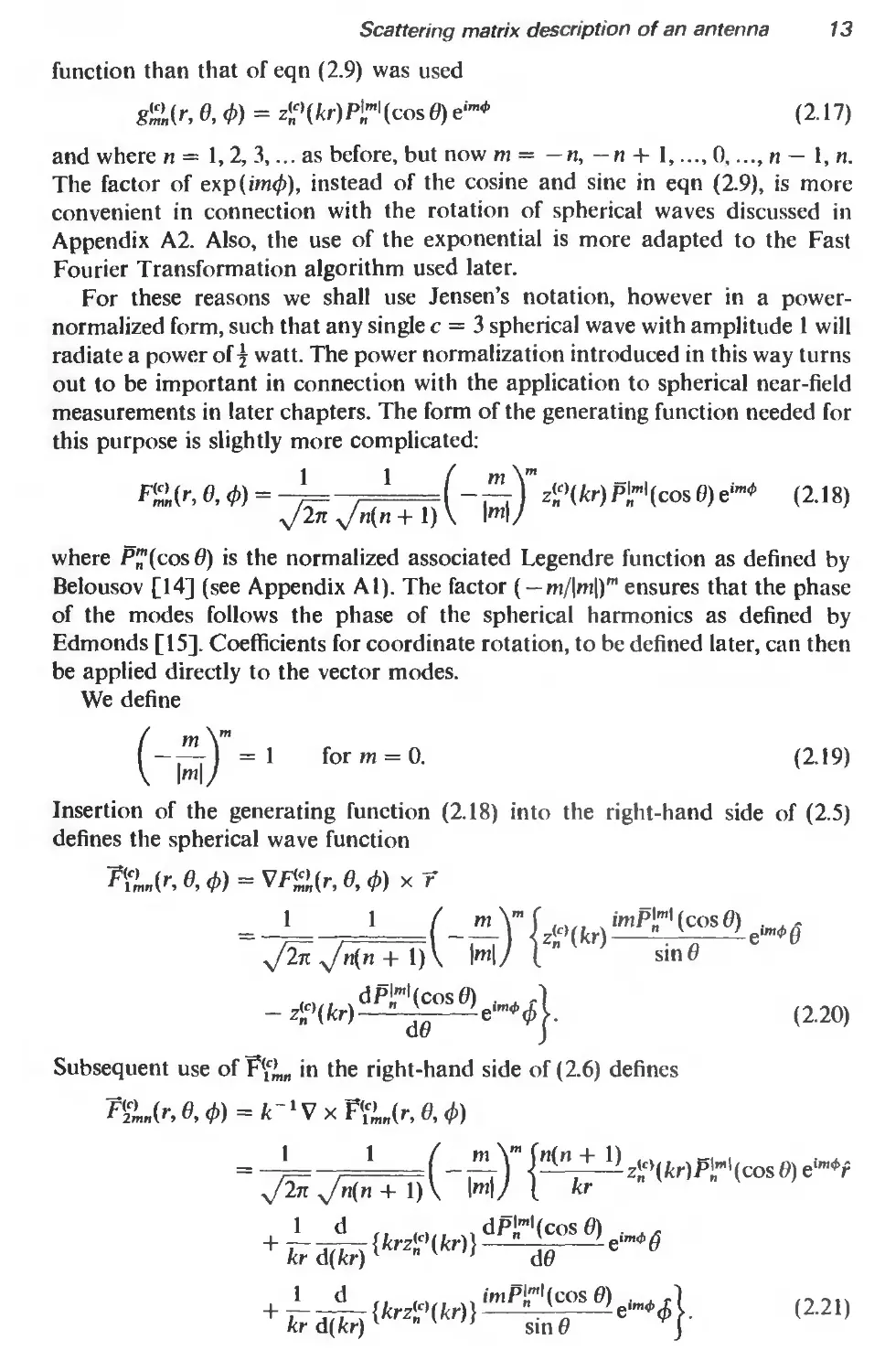
function than that of eqn (2.9) was used
g«(r, в, ф) = zHM/t^cose) eim*
(2.17)
and where n = 1,2, 3,... as before, but now m = — n, — n 4- 1,..., 0,..., n — 1, n.
The factor of ехр(тф), instead of the cosine and sine in eqn (2.9), is more
convenient in connection with the rotation of spherical waves discussed in
Appendix A2. Also, the use of the exponential is more adapted to the Fast
Fourier Transformation algorithm used later.
For these reasons we shall use Jensen’s notation, however in a power-
normalized form, such that any single c = 3 spherical wave with amplitude 1 will
radiate a power of | watt. The power normalization introduced in this way turns
out to be important in connection with the application to spherical near-field
measurements in later chapters. The form of the generating function needed for
this purpose is slightly more complicated:
F*^(r, #,</>) = L_ z<f>(/cr)plm|(cos0)e^ (2.18)
yJ2n y/n(n + 1) \ lml/
where P”(cos 0) is the normalized associated Legendre function as defined by
Belousov [14] (see Appendix Al). The factor ( — m/|m|)m ensures that the phase
of the modes follows the phase of the spherical harmonics as defined by
Edmonds [15]. Coefficients for coordinate rotation, to be defined later, can then
be applied directly to the vector modes.
We define
(2.19)
eim^0
sinO
I — —- 1=1 for m = 0.
\ Н/
Insertion of the generating function (2.18) into the right-hand side of (2.5)
defines the spherical wave function
0, ф) = (r, 0, ф) x r
1 1 ( '
у/2п у/r^n + 1)\ I»
Subsequent use of in the right-hand side of (2.6) defines
F%n(r, 0,ф) = к~'Ух F(1c’,„(r, 0, ф)
1 1
(2.20)
1)z">(fer)P"'"l(cos e) е‘тФр
J Ё_ {krz,c,(kr)} ^cos етф 6
kr d(M{lirZn de e °
Id . imP'nm,(cos 6) . . fl
7~ ТГГТ {^(kr)} —7. 1 е^Фф I.
kr d(fcr) ’ sin 0 J
(2.21)
14 Scattering matrix description of an antenna
Equations (2.20) and (2.21) are the (dimensionless) power-normalized spher-
ical wave functions used throughout this book. Asymptotic forms of the radial
functions (2.13-2.16) may be inserted in a similar manner into F'[U(r, Ф) and
F$2,„(r, О, ф) as was done in connection with the m and li functions.
The electric field in a source-free region of space such as region 2 of Fig. 2.2
may now be written as a weighted sum of the spherical wave functions defined
above
k
E(r, О, ф)=-7=^ Q^L(r, О, Ф). (2.22)
у/ Г] esmn
From eqn (2.2), we have for the associated magnetic field
H(r, 0, ф) = (iw/i)"1V x E(r, 0, ф)
= - Z о, Ф). (2.23)
exmn
The wave functions F’X are dimensionless and the additional factors in front of
the summation signs in (2.22) and (2.23) are needed in order to obtain the
dimension of watts1/2 for the wave coefficients With this convention, the
expression for the power P radiated by outward travelling modes is as simple as
possible:
F = 'Z Ю2 watts (2.24)
£ stnn
as will be shown in Section 2.2.4.
In (2.24), the summation is understood in this way
2 ou и
Z = Z Z Z (2-25)
5ЖИ 5 — 1 И = 1 Ш = П
while for the summation in (2.22) and (2.23)
4 2 no и
Z = Z Z Z Z • (2.26)
esmn c = 3 s= 1 и = I rtf = ri
The choice of c = 3 and 4 in (2.26) indicates that both inward and outward
propagating waves arc present in the particular summation. In the general case,
the proper choice of one or two values of c warrants a complete and orthogonal
representation of all finite, continuous and single-valued solutions to Maxwell’s
equations in any of the regions 1, 2 or 3 in Fig. 2.2. In later chapters, the upper
index c in expansions such as (2.22) and (2.23) is sometimes omitted. This is
done when only one value of c is present in a particular sum and, furthermore, it
is clear from the context which type of wave is needed.
In representations such as (2.22) and (2.23), the employment of the index s in
the spherical wave functions FJ2n serves the purpose of distinguishing between
two different functions. One of the two wave functions, i.e. has no radial
Scattering matrix description of an antenna
15
component. It will therefore always represent that part of a (magnetic or
electric) field which is transverse with respect to the radial coordinate r. The
magnetic field of a transverse magnetic (TM) wave is proportional to
whereas the associated electric field is proportional to f For transverse
electric (ТЕ) waves, the roles of the wave functions are reversed. Here, the
electric field is proportional to F{^m„, while the associated magnetic field is
represented by F^. Note that the sum of the indices s in the wave functions
describing the electric and magnetic field vectors of a given electromagnetic field
is always 3, as evident from (2.22) and (2.23).
When attached to the wave coefficient however, the index s has a
slightly different meaning. Here, s = 1 always indicates a coefficient to a TE-
wave while s = 2 indicates a TM-wave coefficient.
In practice the summations will always be truncated. The maximum value of
n and m retained in the sums will be denoted by N and M, respectively. Since
Pj,m|(cos0) vanishes for |ж| > л, we must have M N. In most cases, M = N
because a full mode set in m is usually needed. For this latter case, we shall define
for later use an index transformation which converts the index triplet (s, m, n) to
the single index j. The transformation is
j = 2{n(n + l) + m—l}+s (2.27)
whereby the triple summation is reduced to a single summation
2 N n J
Z Z Z = Z (2.28)
s=ln=lm=—и j~ 1
with
J = 2N(N + 2). (2.29)
The index transformation implies that we may use substitutions like, for ex-
ample, QS,„ = QP and F’^„ = F'f whenever a condensed notation is convenient.
The summation over s, m and n may be depicted in an (n, m) coordinate
system (the nm plane) where all values of n and m present in the summation can
be indicated. To each of these points correspond two terms of the summation,
i.e. the terms with s = 1 and s = 2. The index transformation (2.27) and the nm
plane is illustrated in Fig. 2.3.
2.2.3 The spherical waveguide
Spherical wave theory can be given a physical interpretation which turns out to
be particularly useful in connection with spherical near-field measurements. As
will be discussed in this section and in later chapters, spherical wave radiation
may be visualized as taking place in a spherical waveguide [9,16, 17]. Many of
the well-known properties of conventional cylindrical guides are found to have
their counterparts in the spherical waveguide. Concepts such as orthogonal
modes, cut-off, propagation and evanescence are common features.
We consider a transmitting antenna which is not necessarily centred in a
16
Scattering matrix description of an antenna
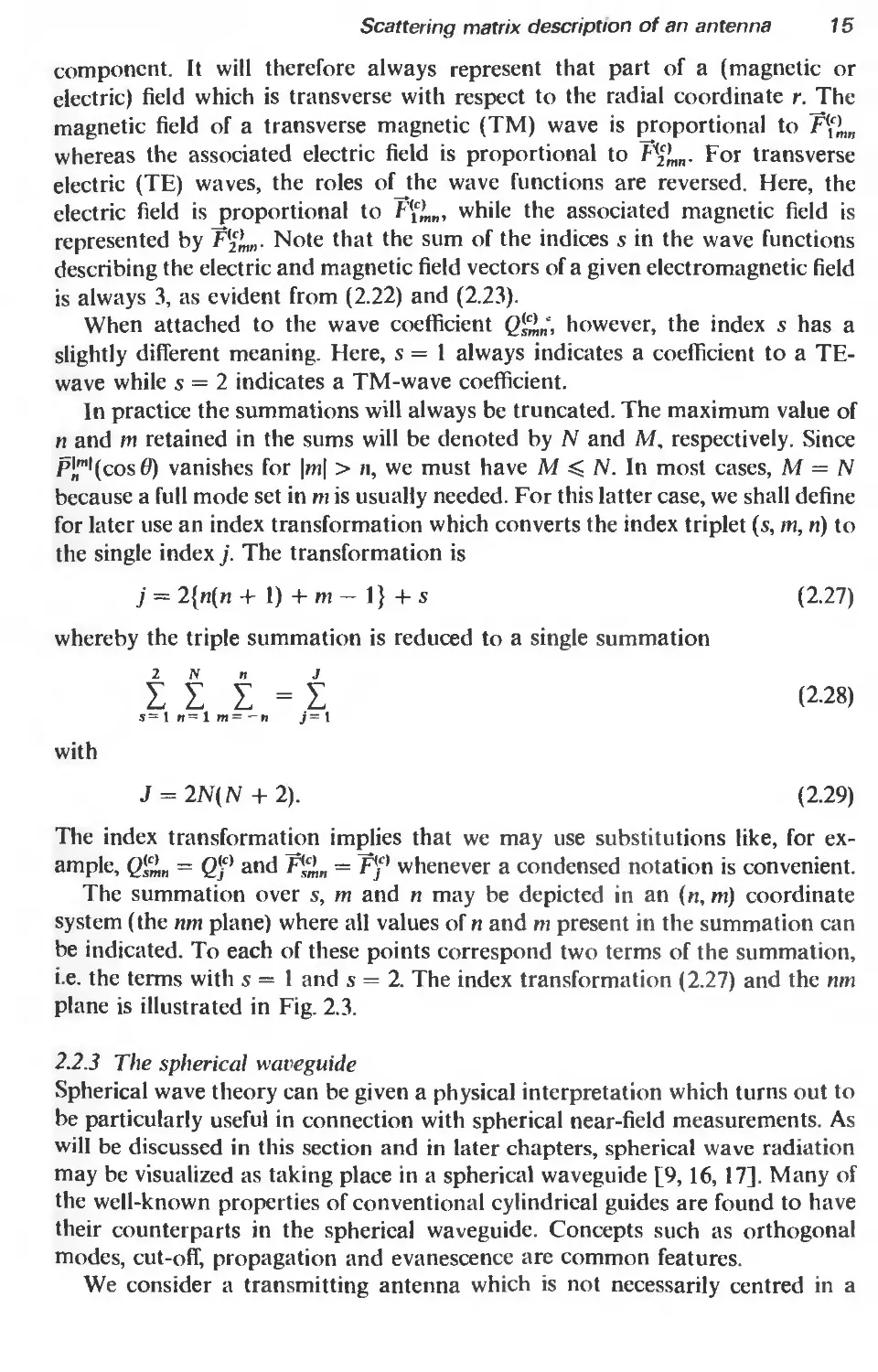
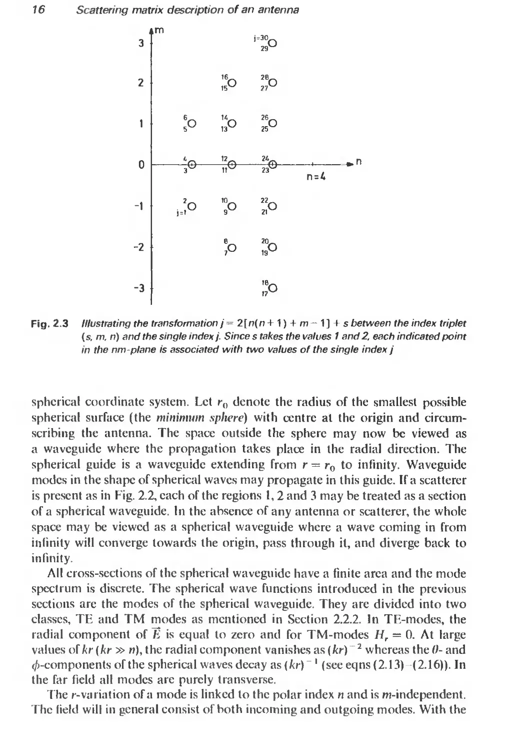
Fig. 2.3 Illustrating the transformation j = 2[n(n + 1) + m - 1 ] + s between the index triplet
(s, m. ri) and the single index j. Since s takes the values 1 and 2. each indicated point
in the nm-plane is associated with two values of the single index j
spherical coordinate system. Let r0 denote the radius of the smallest possible
spherical surface (the minimum sphere) with centre al the origin and circum-
scribing the antenna. The space outside the sphere may now be viewed as
a waveguide where the propagation takes place in the radial direction. The
spherical guide is a waveguide extending from r = r0 to infinity. Waveguide
modes in the shape of spherical waves may propagate in this guide. If a scatterer
is present as in Fig. 2.2, each of the regions 1,2 and 3 may be treated as a section
of a spherical waveguide. In the absence of any antenna or scatterer, the whole
space may be viewed as a spherical waveguide where a wave coming in from
infinity will converge towards the origin, pass through it, and diverge back to
infinity.
All cross-sections of the spherical waveguide have a finite area and the mode
spectrum is discrete. The spherical wave functions introduced in the previous
sections are the modes of the spherical waveguide. They are divided into two
classes, ТЕ and TM modes as mentioned in Section 2.2.2. In TE-modes, the
radial component of E is equal to zero and for TM-modes Hr — 0. At large
values of kr(kr » n), the radial component vanishes as(kr)”2 whereas the 0- and
«/(-components of the spherical waves decay as (kr)~ 1 (see eqns (2.13)-(2.16)). In
the far field all modes are purely transverse.
The r-variation of a mode is linked to the polar index n and is m-independent.
The field will in general consist of both incoming and outgoing modes. With the
Scattering matrix description of an antenna 17
chosen time dependence of exp( — iwt), the type c — 3 radial functions, (/„''(kr)
and (l/kr)(d/d(kr)) {krh{„l}(kr)}, belong to outward propagating modes satisfying
the radiation condition at infinity. The functions of type c = 4, namely hj,2>(kr)
and (1 /kr)(d/d(kr)) {krhl^\kr)}, correspond to inward propagation. If a source-
free region contains the centre of the spherical waveguide (region 1 of Fig. 2.2),
the type c = 1 functions, j„(kr) and (l/kr)(d/d(kr)){krj„(kr)}, must be chosen
since only these functions are finite at the origin. Alternatively, equal amounts of
ingoing and outgoing waves may be used since
j„(kr) = №>(kr) + h<2>(kr)) (2.30)
In a conventional (loss-free) cylindrical waveguide with a constant cross-
section, some modes may be above cut-off and propagate along the guide
without decay while others are below cut-off and are decayed exponentially. In a
spherical waveguide, the cross-section of the guide is increasing with r. This
means that more and more spherical modes may propagate as r grows.
Similarly, when r is diminished, fewer modes may propagate. The transition
between propagation and evanescence for a mode occurs around a radial
distance of rt = n/k. With r « r„ the decay is extremely rapid but diminishes as r
approaches rt. Over the transition region around rt, propagation begins
gradually and for r » rt, a c = 3 mode of index n propagates in the outward
direction with the simple spherical divergence rate of r“* in amplitude.
As mentioned above, the minimum sphere for a given antenna is defined as
the sphere of smallest radius centred at the origin to completely circumscribe the
antenna. For an antenna with a minimum sphere of radius r0, the radiated field
may in principle contain an infinity of modes. However, if it is assumed that the
various modes all have amplitudes of the same order of magnitude at r — r0,
those with n > kr0 will be heavily attenuated outside r0. Only modes with
n < kr0 are of importance in the far field or at some close distance where a near-
field measurement may be taken. This is a consequence of the cut-off property of
the radial functions for the outward propagating modes. The radial functions are
very large (and dominantly imaginary) for r smaller than the cut-off distance n/k.
For r larger than n/k, the amplitude of the radial functions behaves as r~1 to
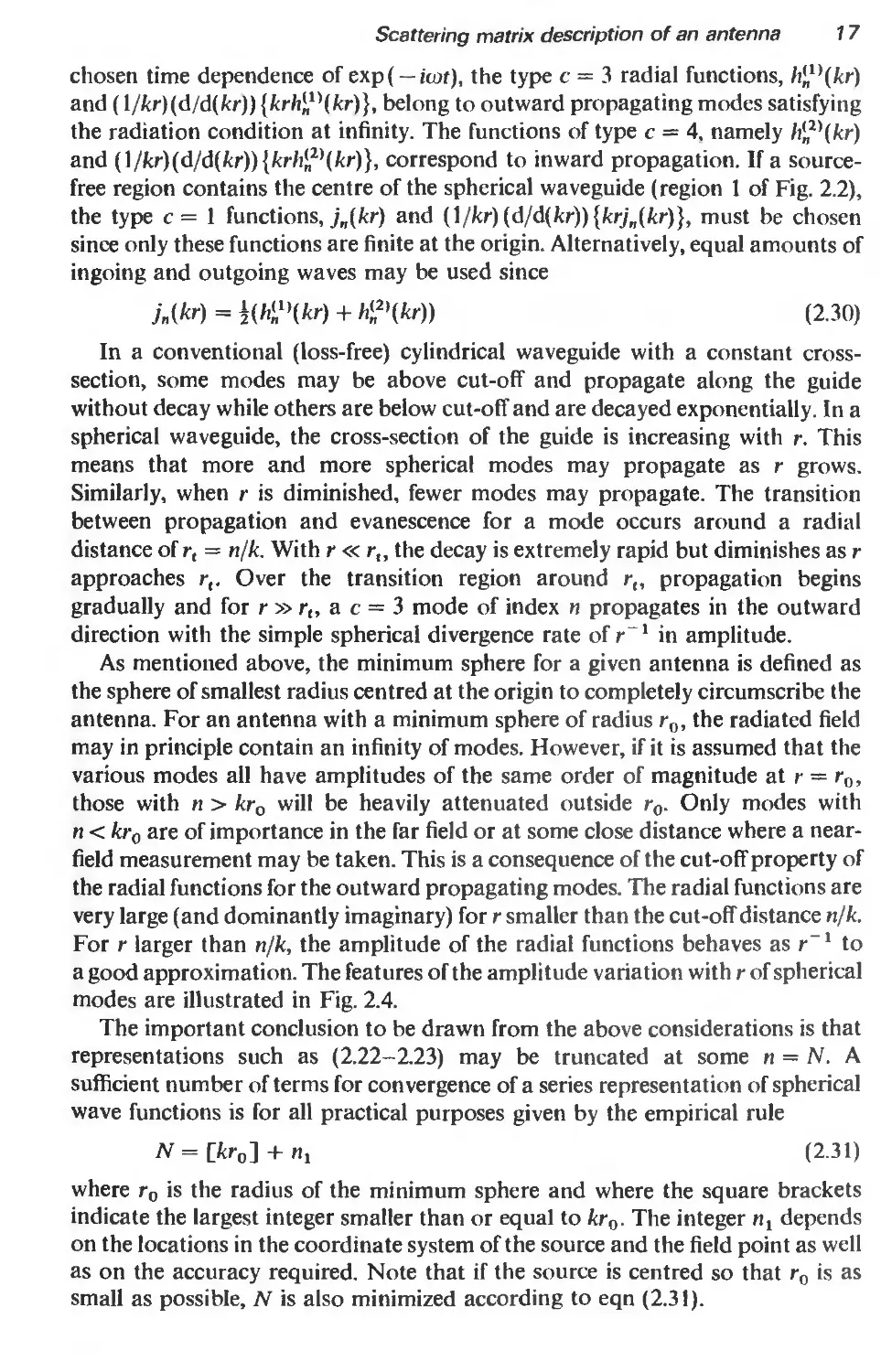
a good approximation. The features of the amplitude variation with r of spherical
modes are illustrated in Fig. 2.4.
The important conclusion to be drawn from the above considerations is that
representations such as (2.22-2.23) may be truncated at some n = N. A
sufficient number of terms for convergence of a series representation of spherical
wave functions is for all practical purposes given by the empirical rule
N = [kr0] + n, (2.31)
where r0 is the radius of the minimum sphere and where the square brackets
indicate the largest integer smaller than or equal to kr0. The integer n, depends
on the locations in the coordinate system of the source and the field point as well
as on the accuracy required. Note that if the source is centred so that r0 is as
small as possible, N is also minimized according to eqn (2.31).
18
Scattering matrix description of an antenna
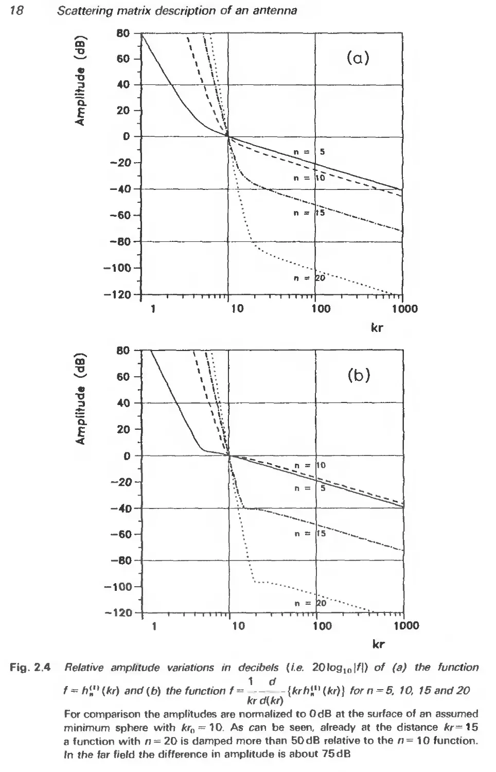
Fig. 2.4 Relative amplitude variations in decibels (i.e. 20logln|/|) of (a) the function
1 d
f—ft’^^r) and(b) the function f = — -{krhi'^kr)} forn = S. 10, 1Sand20
kr d(kr)
For comparison the amplitudes are normalized to OdB at the surface of an assumed
minimum sphere with fcro = 1O. As can be seen, already at the distance fcr=15
a function with n = 20 is damped more than 50 dB relative to the n= 10 function.
In the far field the difference in amplitude is about 75 dB
Scattering matrix description of an antenna 19
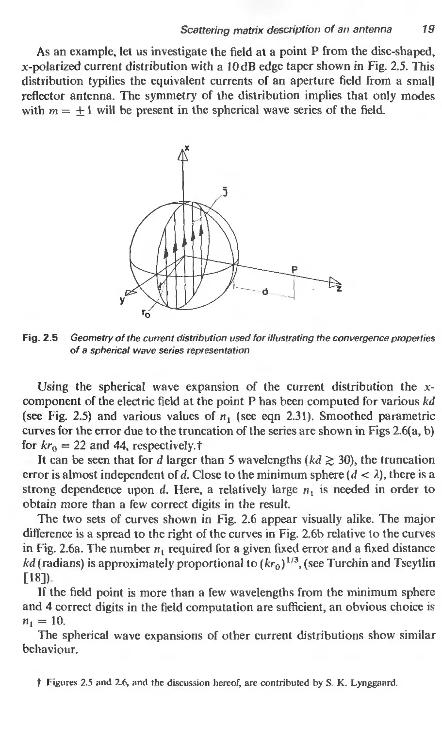
As an example, let us investigate the field at a point P from the disc-shaped,
x-polarized current distribution with a 10 dB edge taper shown in Fig. 2.5. This
distribution typifies the equivalent currents of an aperture field from a small
reflector antenna. The symmetry of the distribution implies that only modes
with m = +1 will be present in the spherical wave series of the field.
Fig. 2.5 Geometry of the current distribution used for illustrating the convergence properties
of a spherical wave series representation
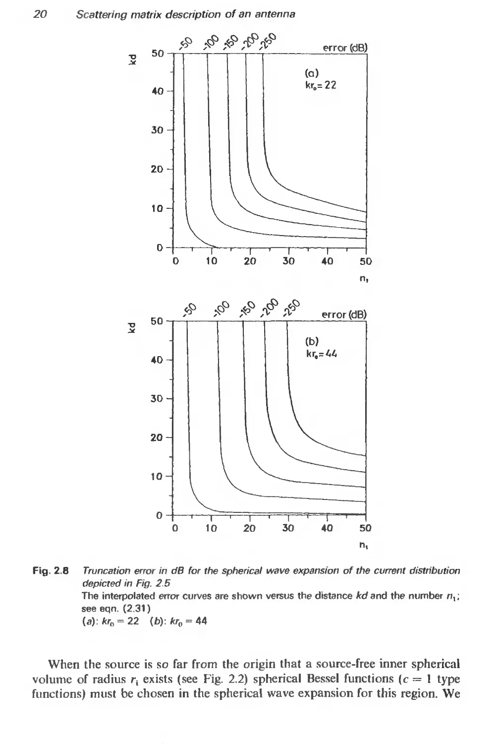
Using the spherical wave expansion of the current distribution the x-
component of the electric field at the point P has been computed for various kd
(see Fig. 2.5) and various values of (see eqn 2.31). Smoothed parametric
curves for the error due to the truncation of the series are shown in Figs 2.6(a, b)
for kr0 = 22 and 44, respectively.!
It can be seen that for d larger than 5 wavelengths (kd > 30), the truncation
error is almost independent of d. Close to the minimum sphere (d < A), there is a
strong dependence upon d. Here, a relatively large is needed in order to
obtain more than a few correct digits in the result.
The two sets of curves shown in Fig. 2.6 appear visually alike. The major
difference is a spread to the right of the curves in Fig. 2.6b relative to the curves
in Fig. 2.6a. The number и, required for a given fixed error and a fixed distance
kd (radians) is approximately proportional to (кг0)1/3, (see Turchin and Tseytlin
[18])
If the field point is more than a few wavelengths from the minimum sphere
and 4 correct digits in the field computation are sufficient, an obvious choice is
nt = 10.
The spherical wave expansions of other current distributions show similar
behaviour.
t Figures 2.5 and 2.6, and the discussion hereof, are contributed by S. K. Lynggaard.
20 Scattering matrix description of an antenna
50
40
30
20
10
0
0 10 20 30 40 50
n.
Fig. 2.8 Truncation error in dB for the spherical wave expansion of the current distribution
depicted in Fig. 2.5
The interpolated error curves are shown versus the distance kd and the number nx;
see eqn. (2.31)
(a): kr„ = 22 (b): kr0 = 44
When the source is so far from the origin that a source-free inner spherical
volume of radius r, exists (see Fig. 2.2) spherical Bessel functions (c = 1 type
functions) must be chosen in the spherical wave expansion for this region. We
Scattering matrix description of an antenna
21
have here
N = [кг] + и.
(2.32)
valid for points of evaluation with r < The upper limit N is thus associ-
ated with the position of the point of evaluation and arises from the decay of
the spherical Bessel function for r < n/k. Typically, и, = 10 may be used as in
eqn (2.31).
The related question of whether field representations (2.22-2.23) can be
truncated at some |m| = M (where M < N) will be touched upon later.
The phase of the radial functions approximates the simple exp(ikr) de-
pendence for kr » n. For smaller values of kr, the phase begins to deviate and at
a certain distance given by r = 4n2/nk, the phase deviation is close to я/8 for all
modes [19]. The phase variation with r of spherical modes is illustrated in
Fig. 2.7.
The amplitude and phase behaviour of the spherical modes divide, for each
mode, the space into the regions
0 < r < n/k evanescent region
n/k <r < 4n2/nk Fresnel region (near field)
4n2/nk < r < oo Fraunhofer region (far field).
The three regions of space are also defined for an antenna radiating several
modes. In this case, the limits are as follows
r0 < r < N/k
N/k <r< 4N2/nk
4N2/itk <r < co
evanescent region
Fresnel region (near field)
Fraunhofer region (far field)
where as before, r0 is the radius of the minimum sphere and N given by
eqn (2.31).
For a source with a minimum sphere of diameter D = 2r0, the Rayleigh
distance R is conventionally defined as
(2.33)
~ 2
21V\2 _ 4 N2
к) лк
(2.34)
which coincides with the above limit between the Fresnel and Fraunhofer
regions.
The phi-variation exp(im</>) of a mode depends on the azimuthal index tn
which indicates the number of oscillations in the interval 0 < ф < 2л. For
m / 0, the field of a mode rotates around the z-axis with time. The rotation is
in the positive sense from the x-axis towards the у-axis with m positive, and in
22
Scattering matrix description of an antenna
kr
Fig. 2.7 Relative phase variations of (a) the function f=h,„,,(kr') and (b) the function
1 d
f= Ikth'11 (kr)} for n = 5. 10, IS and 20. The phases are normalized so that
krd(kf)
all phase angles tend towards kr as kr-* oo
Scattering matrix description of an antenna 23
the negative sense if m is negative. The mode functions F*^„(r, 0, ф) are single-
valued and continuous functions. For this reason, only modes with tn = 0 can
have a radial component on the z-axis, and only modes with m = + 1 will have
в- and ^-components here. Thus
0, </>)], = [F£>„(r, я, </>)]r = 0 for nt * 0 (2.35)
and
[F«„(r, 0, ФЪ = [F£„(r, я, </>)]„ = 0 for m * ± 1. (2.36)
Ф Ф
For m = ± 1, the field of each mode is circularly polarized on the z-axis.
The theta-variation of a mode depends on both n and m. It has the form of a
standing wave with zeros spaced non-equidistantly between 0 and я. The zeros
are more closely spaced in the neighbourhood of 0 = я/2 than around the poles.
In certain regions close to the poles, i.e. for 0 < sin 6 < sin ()c = |m|/n, the
associated Legendre functions are below cut-off. Here, the mode amplitude
tends rapidly towards zero as sin в -> 0. From the formulas of Appendix A2 on
coordinate rotation of spherical waves, one can obtain a Fourier expansion in
theta of the components of a spherical mode. In this expansion the fastest
oscillating terms have a theta-dependence of exp(inO) or exp( — inO). This
property will be used later to derive a sampling criterion.
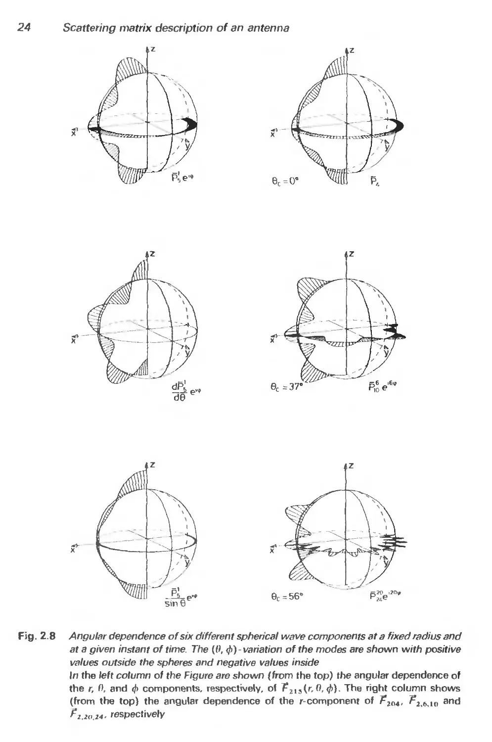
The field configurations showing phi- and theta-variations for individual
components of certain modes are illustrated in Fig. 2.8.
2.2.4 Power flow
In this section we shall consider the power flow associated with an outgoing
spherical wave field in a lossless media.
The power flow in a time-harmonic electromagnetic field is described by the
complex Poynting vector 5 defined by+
S = x Й*. (2.37)
The outward flux of the real part of S through a closed surface expresses the
total power P radiated by the sources inside the surface. For a spherical surface
of radius r
P= | | Re(f-^)r2sinfldfld^. (2.38)
]ф=о Je=o
The outward flux of the imaginary part of S equals 2u> multiplied by the time
average Wc of the electric energy minus the time average Wm of the magnetic
energy stored outside the integration surface [20].
2w(lK- И;,) = | 2" f" Im(r-3)r2sin0d0d</>. (2.39)
J^=o = o
t The superscript * is used to denote complex conjugate.
24
Scattering matrix description of an antenna
Fig. 2.8
♦z
Angular dependence of six different spherical wave components at a fixed radius and
at a given instant of time. The (0, ф)-variation of the modes are shown with positive
values outside the spheres and negative values inside
In the left column of the Figure are shown (from the top) the angular dependence of
the r, 0, and ф components, respectively, of T2l!(r,0, ф). The right column shows
(from the top) the angular dependence of the r-component of ?216ЛО and
F2.20.2t- respectively
Scattering matrix description of an antenna 25
In the far field of any given source, the electric and magnetic field vectors are
related as in a plane wave
Й = qr xE (2.40)
and the complex Poynting vector is real
S = |E x П*
= -}E x (t]f x E*)
— ivlE]2r watts per square meter. (2.41)
The power Pt radiated per unit solid angle in the direction (0, ф) is thus
expressed by
P1(0, ф) = |»/|E|2r2 watts per steradian. (2.42)
Let us now compute the outward flux of the complex Poynting vector through a
sphere of a finite radius r
Г j (Ex H*) • fr2 sin0d0d</> (2.43)
2 J^,==o Je=o
for the case of an outgoing wave field, i.e. a field which can be represented by
spherical wave functions of type c = 3
к
E(r, G, Ф) = Y G, Ф) (2.44a)
yjЦ smn
H(r, е,ф)=-ik'fa E J'. в, Ф). (2.44b)
Ofiv
In order to be able to identify contributions from products of terms with dif-
ferent indices when the product E x Й* is computed, we have introduced the
Greek letters <r, p, v to denote the summation indices in (2.44b). The flux may
readily be determined by using the relation
E^*(r, G, Ф) = (- l)mF'*> „'„(r, G, Ф) (2.45)
and the orthogonality integral for the vector product of two spherical wave
functions (see Appendix Al):
£2”o £” o 6, ф) x F^v(r, 0, ф)} fsin0d0d</>
= 53_„^т._^„,(-1)3^(-1Г^(^)Е(Л3,„(кг)
where we have used the abbreviation
'z%y(kr) for s = 1
Pdiro|lrzi'’,b')! f°”“2
(2.46)
(247)
26 Scattering matrix description of an antenna
and the Kronecker delta
. _ (0 for i
iJ~[l for i =/.
(2.48)
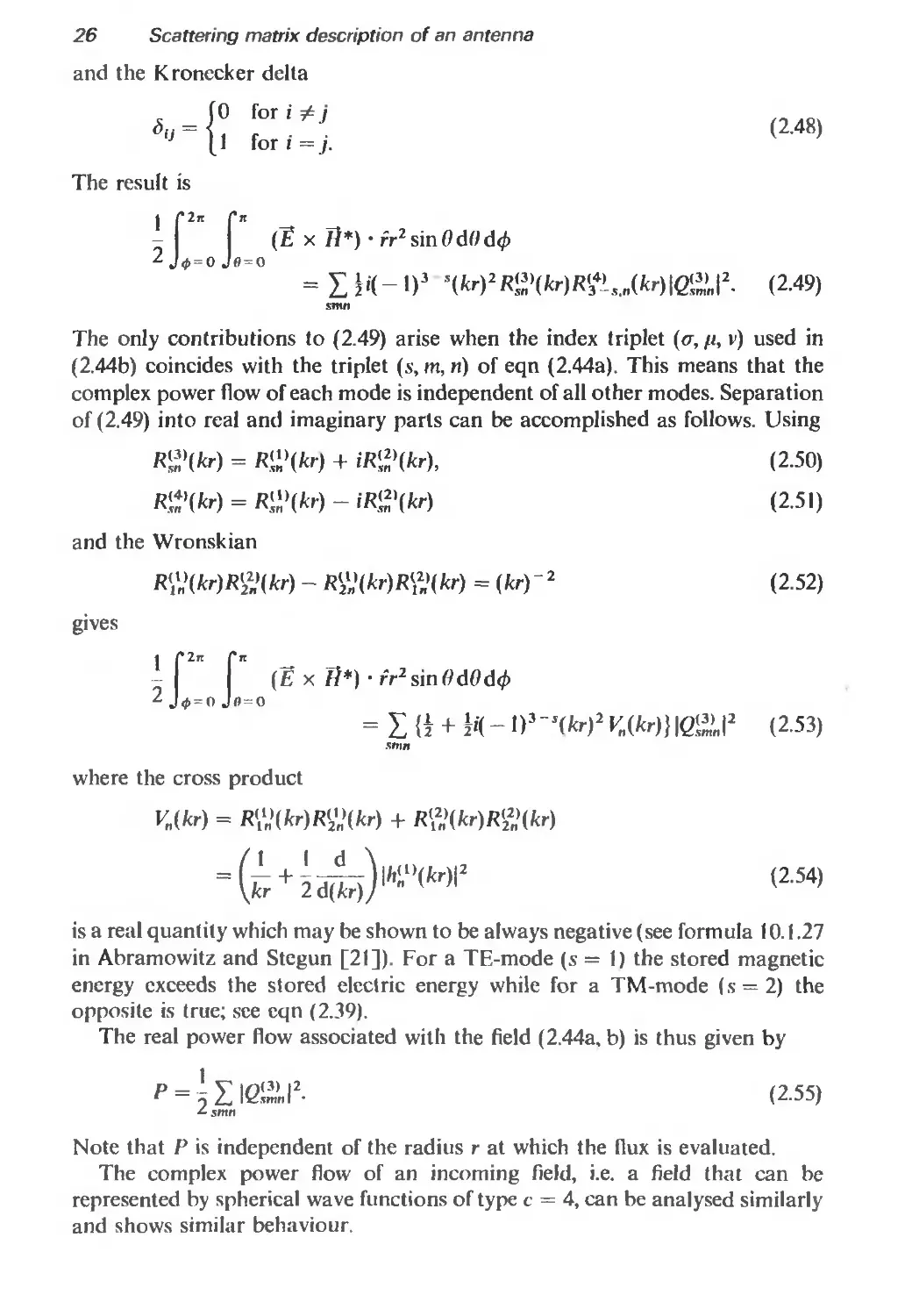
The result is
J (Ё x Й*) • rrI 2sin0dfld</>
= Z -1)3 * W)2 ic<3> I2. (2.49)
smn
The only contributions to (2.49) arise when the index triplet (<r, ft, v) used in
(2.44b) coincides with the triplet (s, tn, n) of eqn (2.44a). This means that the
complex power flow of each mode is independent of all other modes. Separation
of (2.49) into real and imaginary parts can be accomplished as follows. Using
Wr) = R'"(kr) + iR‘2)(kr), (2-50)
R^(kr) = R^(kr) - iR^(kr) (2.51)
and the Wronskian
R\"(kr)R%!(kr) - R^(kr)R^(kr) = (kr)- 2 (2.52)
gives
-J J (Ex f?*) • fr2sin(?d0d</>
= I {1 + И - i)3~s(M2 k,(m}ie.^i2 (2.53)
5ГИЛ
where the cross product
K(M = R^(kr)R^(kr) + R?>(kr)R%>(kr)
(2И|
is a real quantity which may be shown to be always negative (see formula 10.1.27
in Abramowitz and Stegun [21]). For a TE-mode (s = 1) the stored magnetic
energy exceeds the stored electric energy while for a TM-mode (s = 2) the
opposite is true; see eqn (2.39).
The real power flow associated with the field (2.44a, b) is thus given by
I2. (2.55)
smn
Note that P is independent of the radius r at which the flux is evaluated.
The complex power flow of an incoming field, i.e. a field that can be
represented by spherical wave functions of type c = 4, can be analysed similarly
and shows similar behaviour.
Scattering matrix description of an antenna
27
2.3 The antenna scattering matrix
2.3.1 Definitions
The general antenna with an associated spherical coordinate system may be
considered as a waveguide junction with several ports. One port, the ‘local port’,
is connected to a generator or a load. The remaining ports are ‘radiation ports’
connected to equivalent modal transmission lines, one for each spherical mode
in the field outside the antenna’s minimum sphere. The modal transmission lines
together form the spherical waveguide discussed in Section 2.2.3. All of the
properties of the antenna as a transmitting, receiving or scattering device are
then contained in linear relationships between the complex amplitude coef-
ficients of incoming and outgoing modes on a set of transmission lines each
carrying a single mode. A linear relationship of this kind is the antenna
scattering matrix formulation introduced by Dicke [1]. Obviously, such a
formulation must be based upon careful definitions and normalizations of the
modes involved.
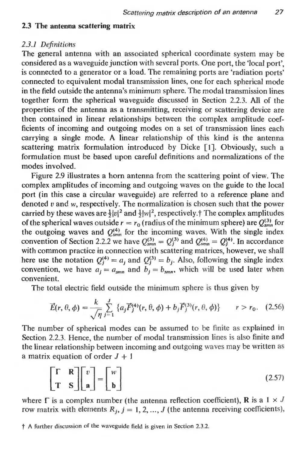
Figure 2.9 illustrates a horn antenna from the scattering point of view. The
complex amplitudes of incoming and outgoing waves on the guide to the local
port (in this case a circular waveguide) are referred to a reference plane and
denoted v and w, respectively. The normalization is chosen such that the power
carried by these waves are||r|2 and ||w|2, respectively.! The complex amplitudes
of the spherical waves outside r = r0 (radius of the minimum sphere) are Q*3,„ for
the outgoing waves and for the incoming waves. With the single index
convention of Section 2.2.2 we have 2*3)„ = Qj-3) and 1° accordance
with common practice in connection with scattering matrices, however, we shall
here use the notation 04) = Oj and Qj3’ = bj. Also, following the single index
convention, we have as = asrrin and bj — bsmn, which will be used later when
convenient.
The total electric field outside the minimum sphere is thus given by
к J
E(r, 0,ф)=—£ Ф) + bjF^tr, в, Ф)} r > r0. (2.56)
хЛ7=1
The number of spherical modes can be assumed to be finite as explained in
Section 2.2.3. Hence, the number of modal transmission lines is also finite and
the linear relationship between incoming and outgoing waves may be written as
a matrix equation of order J + 1
Г «Пр
T Sj|_a
w
b
(2.57)
where Г is a complex number (the antenna reflection coefficient), R is a 1 x J
row matrix with elements RJy j = 1, 2,..., J (the antenna receiving coefficients),
t A further discussion of the waveguide field is given in Section 2.3.2.
28
Scattering matrix description of an antenna
(b)
1
2
radiation
ports
Fig. 2.9 Illustrating a horn antenna from the scattering point of view
(a) Antenna with waveguide modes and spherical modes
(b) Network representation
T is a J x 1 column matrix with elements Th i= 1,2................J (the antenna
transmitting coefficients), and S is J x J square matrix with elements (the
antenna scattering coefficients). The J x 1 column matrices a and b contain as
their elements ...........<0. and bi, b2, ..., bj- The three matrices R, T and S
describe in an absolute and concise manner the antenna’s receiving, transmitting
and scattering properties, respectively. In expanded form, eqn (2.57) becomes
Tt>+ £ Rjtij = w (2.58)
j= ।
7Jv + £ Syttj =/),, i= 1,2, (2.59)
2 = I
In a condensed form, eqn (2.57) may be written
Sa = fi (2.60)
Scattering matrix description of an antenna
29
where S is called the total scattering matrix for the antenna. The elements of the
total scattering matrix are dimensionless.
For a lossless antenna, the total scattering matrix is unitary, i.e. = I, [1]
where I denotes the unit matrix of (J + l)th order]. The unitarity condition
implies that the norm, the sum of the elements absolute squared, of every
column and every row in § equals unity. In particular, for the first column
|Г|2 + |T|2 = 1- (2.61)
For a lossy antenna in the purely transmitting case, the total radiated power is
equal to the power incident in the waveguide minus the sum of the reflected
power and the power dissipated in the antenna
I Z |b,|2 = in2 - (l|w|2 + Ploss). (2.62)
2 i=i
Dividing through by the incident power Pinc = i|u|2, and making use of
eqn (2.57) with a = 0, we arrive at the relationship
|F|2 + |T|2 = 1-^1 (2.63)
* inc
analogous to eqn (2.61). It may be shown that in the lossy case, all other
columns and all rows in § have norms equal to or less than one.
The total scattering matrix for empty space is not defined. However, the
scattering matrix S has a meaning in this case. For empty space, in which a
spherical coordinate system is defined, any incident spherical wave will converge
towards the origin as a focal point, pass through it, and emerge as a diverging
spherical wave. In other words, for empty space, b = a, so we must have S = I,
where I is the unit matrix of infinite order.
The symmetry properties of § will be discussed in Section 2.3.2.
A convenient way to visualize the properties of the scattering matrix formu-
lation outlined above is to utilize scattering flow graphs [22]. The complete
flow graph corresponding to eqn (2.57) contains 2J + 2 nodes and (J + I)2
branches. The incoming waves define nodes v and Oj,j = 1, 2,..., J, while the
outgoing waves determine the nodes w and bt, i= 1,2, Each of the
incoming wave nodes is connected to each of the outgoing wave nodes, and the
wave transformations that take place in the antenna are indicated by desig-
nations on the oriented branches. The complete flow graph becomes very large
even for a relatively small number of waves. However, a representation of
sufficient generality need not contain more than the four nodes shown in
Fig. 2.10.
An incoming wave v at the local port is partly reflected via branch Г and
+ The superscript * is used to denote the Hermitian conjugate of a matrix. For later use we shall
also define the superscripts T and * for the transposed matrix and the complex conjugate matrix,
respectively, so that S+ = (S*)T.
30
Scattering matrix description of an antenna
incoming wave
local port
outgoing wave
local port
outgoing spherical
wave, port i
incoming spherical
wave. port j
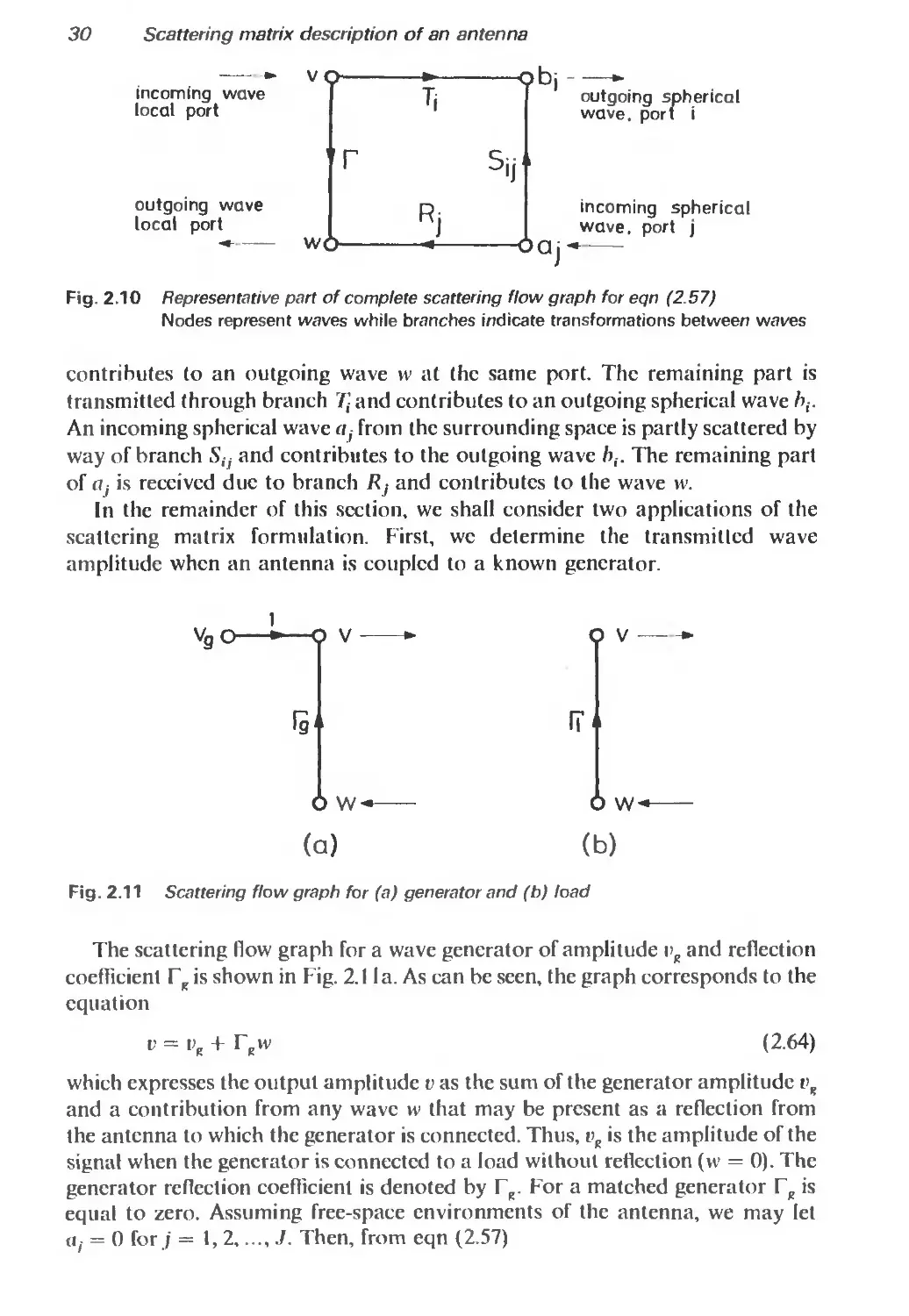
Fig. 2.10 Representative part of complete scattering flow graph for eqn (2.57)
Nodes represent waves while branches indicate transformations between waves
contributes to an outgoing wave w at the same port. The remaining part is
transmitted through branch Ц and contributes to an outgoing spherical wave
An incoming spherical wave af from the surrounding space is partly scattered by
way of branch S;j and contributes to the outgoing wave />,. The remaining part
of cij is received due to branch Rj and contributes to the wave vv.
In the remainder of this section, we shall consider two applications of the
scattering matrix formulation. First, we determine the transmitlcd wave
amplitude when an antenna is coupled to a known generator.
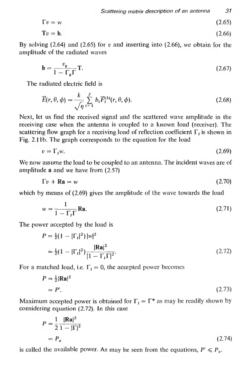
Fig. 2.11 Scattering flow graph for (a) generator and (b) load
The scattering flow graph for a wave generator of amplitude i>K and reflection
coefficient Fg is shown in Fig. 2.11 a. As can be seen, the graph corresponds to the
equation
v = pr + TKw (2.64)
which expresses the output amplitude и as the sum of the generator amplitude t>s
and a contribution from any wave w that may be present as a reflection from
the antenna to which the generator is connected. Thus, vK is the amplitude of the
signal when the generator is connected to a load without reflection (w = 0). The
generator reflection coefficient is denoted by FR. For a matched generator FK is
equal to zero. Assuming free-space environments of the antenna, we may let
а I = 0 for j = 1,2...J. Then, from eqn (2.57)
Scattering matrix description of an antenna
31
Ги = w (2.65)
Tt = b. (2.66)
By solving (2.64) and (2.65) for v and inserting into (2.66), we obtain for the
amplitude of the radiated waves
Ь = ГЛ=7Т (W)
The radiated electric field is
— к J
E(r, 0, ф) = —— £ Ь,Т’3)(г, 0, ф). (2.68)
V9i=i
Next, let us find the received signal and the scattered wave amplitude in the
receiving case when the antenna is coupled to a known load (receiver). The
scattering flow graph for a receiving load of reflection coefficient Г, is shown in
Fig. 2.11b. The graph corresponds to the equation for the load
v = rtvv. (2.69)
We now assume the load to be coupled to an antenna. The incident waves are of
amplitude a and we have from (2.57)
Гг + Ra = w (2.70)
which by means of (2.69) gives the amplitude of the wave towards the load
Ra. (2.71)
1 — 1,1
The power accepted by the load is
^ = 1(1 - |F(|2)|w|2
= i(l-|r,|2)|1-|R^-. (2-72)
|1 — i /11
For a matched load, i.e. Г, = 0, the accepted power becomes
P = j|Ra|2
= P. (2.73)
Maximum accepted power is obtained for Г, = Г* as may be readily shown by
considering equation (2.72). In this case
1 |Ra|2
2 1 - )T|2
= Pa (2.74)
is called the available power. As may be seen from the equations, P' < Pa.
32 Scattering matrix description of an antenna
The amplitude of the waves scattered by the antenna is obtained as follows.
From equation (2.57) we have
Tv + Sa = b. (2.75)
Insertion for v from eqn (2.69) and subsequently for vv from eqn (2.71) gives the
outgoing wave amplitude
b = {ТГ,(1 - IT,) 'R + S}a. (2.76)
This is, however, not the wave amplitude of the field scattered by the antenna
itself. We must remember that in our formulation, the scattering matrix for
empty space is not equal to zero but equal to the unit matrix I. We must
therefore subtract the outgoing wave which, in our formulation, is inherently
present whenever a spherical wave is incident towards the origin in empty space.
The wave amplitude b' for the field scattered by the antenna becomes
b' = {TF,( I - ГГ,)1 R | (S - I)}a. (2.77)
The first term in the parenthesis on the right-hand side describes the part of the
received waves that is reflected by the load and therefore is reradiated with the
directional characteristics of transmitted waves. The second term relates to the
part of the received waves that is scattered directly off from the antenna
structure without entering the antenna waveguide.
When the antenna is terminated in a matched load, Г, is equal to zero, and
b' = (S - I)a. (2.78)
The scattered electric field is
r J
E'(r, 0,ф) =---- £ b'iP^tr, 0, ф) (2.79)
where />,',»= 1, 2,..., J are the elements of the column matrix b'.
2.3.2 Reciprocity
A (linear) non-reci procal antenna or scatterer is characterized by the fact that
part of or all of the material media from which they have been fabricated is
described by the general complex unsymmetrical permeability and permittivity
tensors p and e. In practice, non-reciprocal antennas or scatterers occur
whenever a magnetized ferrite (c.g. in a microwave isolator) is a part of the
structure. By reversing the direction of the static biasing magnetic field, p and e
arc in effect replaced by the transposed tensors pT and £*, and a new device
evolves, called the adjoint antenna or adjoint scatterer [23]. The adjoint of the
adjoint antenna or scatterer is the original device itself.
In this section we shall derive the specific symmetry relations which exist
between the elements of the receiving matrix for a given antenna and the
elements of the transmitting matrix for the adjoint antenna. We shall also,
without proof, state a relationship between the elements of the scattering
matrices of adjoint antennas.
Scattering matrix description of an antenna 33
A reciprocal antenna has symmetric tensors p and £ and is its own adjoint
antenna. Hence, the symmetry relations derived for two adjoint antennas con-
tain the symmetry relations for a reciprocal antenna as a special case.
Reference is made to Fig. 2.12. Here, S is a surface which encloses a volume V
containing an antenna. The antenna is connected to some feed system shown as
Fig. 2.12 For the derivation of the reciprocity relations. The Figure shows the integration surface
S = So+ St + S2 + S3 and the outward oriented vector area element dS
a piece of waveguide with a short dipole d for excitation or load. The surface 5 is
composed of four parts, 5 = So + St + S2 + S3. Of these, So is the reference
plane where waveguide and antenna meet. Sj is a sphere of radius r completely
enclosing the antenna and feed system such that a spherical wave expansion can
be used on and outside Sj. The surface S2 follows the outer surface of the feed
system, and S3 is a narrow tube connecting St and S2. All media inside 5 is
assumed characterized by symmetrical or unsymmetrical (complex) permea-
bility and permittivity tensors p and c.
We consider two different situations. In the first situation, a set of sources
(J, M) outside S is producing the field (£, H) in V and on S. In the second
situation, the media in V are replaced by media characterized by //* and £T, and a
new set of sources (J', M') outside V is producing the field (£', H') in V and on S.
In other words, in the second situation the adjoint of the antenna in the first
situation is considered. The surface 5 encloses no sources and the generalization
of the Lorentz form of the reciprocity theorem may be applied [11]
fs(£ x H' - £' x Й) • dS = 0 (2.80)
where dS is the outward oriented area element on S. We shall specify the field
vectors on the left-hand side in terms of incoming and outgoing modes. In the
waveguide, only a single mode is assumed while on S1, a set of spherical modes is
present. The coefficients of the incoming modes are v and asm„, respectively, for
34 Scattering matrix description of an antenna
the unprimed field, and v' and respectively, for the primed field. Similarly,
the outgoing modes have the coefficients w, bsnm and w',
For the integral over the reference plane in the waveguide, a suitable field
representation is as follows [16]. For the unprimed field we shall use for the
tangential components
E, = -7=(u + w;e (2.81)
V'l
= ky/t](v — w)h (2.82)
with a similar representation for the primed field. The normal components are
not needed for the integration. With the normalization indicated, the vector
modal functions F and h defined over the waveguide cross-section are dimen-
sionless and may be assumed real. The coefficient v for the incident wave and the
coefficient w for the reflected wave both have the dimension watts1/2. We shall
also introduce the normalization integral
Re {k2 JSo7 x /7* dS} = - 1 (2.83)
where the total inward power flow at the reference plane is given by ||u|2 — ||vv|2.
We obtain
JSn(£ x H' — E' x 7?) • dS = k2 JSo(r + w)(u' — w')(F x h) • dS
— k2fSo(c' + w') (v — vv)(e x h) • dS
= 2(rw' — t/w) (2.84)
The integration over S! can be performed using the orthogonality integral
(2.46). For the unprimed field we shall use the representation
i _
£ = -7= E (а-Л + b™^) (2-85)
ж/яш
й = -ikjn Y («™Ж,.т.„ + fismnF(33’,.m.J (2.86)
smn
with a similar representation for the primed field. For the first term in the
generalized reciprocity theorem we have
(ExH’)-dS
x E («'.vmn F(3423-.m-.n- + fe;m-„ F'332s. m,„.)| • dS. (2.87)
Scattering matrix description of an antenna
35
Use of the orthogonality integral (Al.71) gives
(£ x Й') -dS = -i(kr)2 X (-l)3~’(-l)m
Si 5mn
(asmnas.-m.nR™,R34-s.n + bsmn<-
+ asm„b's^mt„R^R^L^„ + bsmnh;
(2.88)
The second term of the integral is calculated in a similar way. After changes in
the summation indices it can be subtracted from (2.88). The following expression
results
[ (£ x Й' — £' x H) • = ~i(kr)2 £ (—l)3-s(~l)m
Si smn
I
( 0 (^smn^st — m,n ^smn^st — m,n)
smn
(2.89)
(2.90)
where we have used the Wronskian
R^R^ s.n - R№-,.n = -(-1)3 (2.91)
In the integral over S2, the integrand vanishes identically since on the con-
ducting surface we have = n xE and = n x £' where t indicates
tangential component and denotes the surface impedance of the material
[11]. The contribution from S3 also vanishes because the integrand is finite and
we may let the radius of the narrow tube S3 tend to zero. Therefore,
k+s3(£ x H' - £' x Й) -dS = 0. (2.92)
As a result of eqns (2.80), (2.84), (2.90) and (2.92) we finally obtain
vw' - v'w = Y (- - asm„bi.-m,„)
smn
(2.93)
which is valid for an arbitrary choice of the coefficients p, v, a and a'. Equation
(2.93) expresses the generalized Lorentz form of the reciprocity theorem for the
fields in two different situations as described above.
In order to arrive at relations between transmitting and receiving properties
of antennas, we now consider a special case of eqn (2.93).
We shall assume that the unprimed quantities refer to a situation where the
antenna of Fig. 2.12 is acting as a transmitting antenna with unity excitation
(1 watt1'2) and no spherical waves are coming in from the surrounding space, i.e.
p = 1 (2.94)
asmn = 0 f°r all s> m and n.
(2.95)
36 Scattering matrix description of an antenna
The primed quantities correspond to a second situation where we shall assume
the (adjoint) antenna to be purely receiving with a single spherical mode (of
indices rr, //, v and unity amplitude) as the only incident field, i.e.
v' = 0
, fl for (s, — tn. n) = (<T, Д, v)
as. т.п otherwise.
With these wave amplitudes, we obtain from equation (2.93)
This equation expresses a relationship between quantities belonging to the two
situations. In each of these situations, we also have the dependencies following
from the general scattering matrix equation (2.57), i.e. in the first situation
(2.96)
(2.97)
(2.98)
Г = w (2.99)
T = b (2.100)
and in the second situation
R'a' = w' (2.101)
S'a' = b'. (2.102)
Use of (2.100) and (2.101) on the right- and left-hand side of eqn (2.98), re-
spectively, yields
r;„ = (-i)"7;._p., (поз)
or, since the indices trftv may be chosen arbitrarily
RU = (-l)mT,_ m.„. (2.104)
Equation (2.104) is the desired relationship between elements of the receiving
and transmitting matrices for two adjoint antennas.
For the scattering properties of adjoint antennas, the following relations may
be shown to hold
SXv = (-l)m + "S™ (2-105)
and
Г' = Г. (2.106)
As important special cases of eqns (2.104) and (2.105) we have for a reciprocal
antenna
R,mn = (-I)",'T™ (2.107)
and
Щ = (-1)т+^Г":! (2-108)
respectively.
Scattering matrix description of an antenna
37
2.3.3 The field from electric and magnetic dipoles
For use in the next section we shall establish the fields of electric and magnetic
dipoles in terms of spherical wave functions. A short z-directed electric dipole
located at the origin produces the electromagnetic field [11]
Ck2
Е*е(г,0,ф) = --^—de
h\l\kr)
kr
cos Of
Гк2 1 d
+ s'mf)e (2.109)
4n kr d(fcr)
ik2
lte(r, 0, ф) = ~7—de hf^(kr) sin 0 ф
(2.110)
where de = ll is the dipole moment (product of current I and dipole length I)
and where h^lkr) is the Hankel function of first kind and first order
W(kr) = _e 1+ '
kr \ kr
(2.111)
and
1 d eikr ( 1 i 1
kra(kr) kr [ kr (kr) j
(2.112)
As may be seen by comparing (2.109) and (2.110) to the expressions given in
Section Al.3.1 for the wave functions with n = 1, the field of the z-directed dipole
can be written
к
Pe(r, 0, ф) = — £ QsmnF™(r, 0, Ф)
y/t] smn
Hze(r, 0, ф) = -ik^ £ CsmnF(33ls.m.„(r, 0, ф).
(2.113)
(2.H4)
With only one term in the summations, i.e. s = 2, m = 0 and n = 1, we have
^Ar,0^)=-^=Q2oiF^(r,0^)
yfh
Hz(r, 0, Ф) = -ik^Qw^Ar, 6, Ф)
with
(2.115)
(2.116)
n ~ 1 k л
V201---------r=~~pae-
y/f>n y/4
(2.117)
Having thus expressed the field of the z-directed dipole in terms of spherical
waves, we shall now turn to the x- and у-directed dipoles. The radial behaviour
of the field components of the z-oriented dipole is independent of the angular
38
Scattering matrix description of an antenna
coordinates 0 and </>. Л reorientation of the dipole will therefore not give rise to
spherical modes with values of n other than n = 1. There are only six spherical
modes altogether with n = 1, and it would not be difficult from inspection and
symmetry considerations to obtain the correct combination needed for expres-
sing the fields of the x-oriented and y-oriented dipoles. However, we shall here
prefer to use a more systematic approach with rotation of the coordinate system.
Let us consider again the z-oriented dipole at the origin of an (x, y, z)
coordinate system. Let us assume another coordinate system (x', y', z’) to be
initially coincident with the (x, y, z) system. We shall now keep the dipole fixed
in space but rotate the primed coordinate system through the Euler angles
(X„, 0„, </>„) =
71
°’ ~2’°
(2.118)
thereby obtaining a new system (x', y', z') which is rotated with respect to the
(x, y, z) system. As may be easily seen using the definitions of Euler angles (see
Section Л2.1), the dipole will then be oriented along the (positive) x'-axis. The
following formula (see Section A2.2) gives the expansion of a spherical mode
F*jjn(r, Ф) defined in the unrotated, unprimed coordinate system in terms of a
finite series of spherical modes F*‘'*n(r', O', ф') defined in the rotated, primed
coordinate system.
Л2„(г, 0,ф) = t (2.119)
M = -И
where с^1т(0о) is a rotation coefficient. Using
= (2.120)
(2.122)
readily obtained from formulas (A2.13), (A2.7) and the tables A2.6 we find that
/2— /2 —
F^Jr. О, Ф) = F<31(г, O', ф') O', ф'). (2.123)
Insertion of (2.123) into eqns (2.115) and (2.116) and omitting the primes gives
the field produced by a short x-directed dipole located at the origin:
Ee(r, 0,ф)=-±= Q2oi V' •* <r’ °’ - F<2и С2 »24)
VO Z
Scattering matrix description of an antenna
39
= ~ik^iQ20l ^{Т^_1Л(г,О,ф)</>)}.
(2.125)
The field from the у-directed dipole may be found from eqn (2.124) and (2.125)
by rotation of the coordinate system through the Euler angles
(XoA,<M = (o,0,-0 (2.126)
or from eqn (2.115) and (2.116) by rotation of the coordinate system through the
Euler angles
(n n \
-p-pOk (2.127)
The result is
к i/2_
ЕУ(г,0,ф) = — Q2ol4-{F,23.’_1,1(r,0,</«) + n3?i(r,e, </>)} (2.128)
yjtl z
Ж(г, 6, ф) = - ik^)Q20l {F?>_ 1U (r, 0, Ф) + F<3', (r, 0, Ф)}
(2.129)
in which the Q201 is given by eqn (2.117).
For a short magnetic dipole located at the origin, a similar analysis may be
carried out. A magnetic dipole may be described either as a short element of
magnetic current or as a small electric current loop. In the latter case, the
orientation of the dipole is defined by using the direction of the current in the
loop and the right-hand rule. The magnetic dipole moment dm is given by
dm = IJ (2.130)
= -impSF (2.131)
where Im is the magnetic current element, and I its length, and where S is the area
of the loop and Г the loop current.
The fields of a magnetic dipole oriented along the z-axis, x-axis and у-axis are
given by, respectively
E^(r,0,</))=-^QlolF'13'1(r,0,</)) (2.132)
^(r, 0, </>) = -lfcx/^Q101f(201(r> 6, ф) (2.133)
E^,(r,e, Ф) =-^=Qlol^{F(13’_1>1(r,0,</))-Т(^1(г,е,ф)} x/n L (2.134)
40 Scattering matrix description of an antenna
1Ц,(г, О, ф) = - iky/tiQtnx {F<2n , ,(r, 0, </>) - Fl23},(r, 0, ф)}
(2.135)
к. i
ЕЦг, О, ф) = 01O1 , ,(r,0, ф) + Ffljr, fl, ф)} (2.136)
0,ф)=- ik^tQini {F£l1,1 (г, о, ф) + Fftjr, fl, Ф)}.
(2.137)
In these expansions Qt01 is given by
Qio! =------7=ky/t]dm (2.138)
У 6zt
If de and dm are chosen such that
(2.139)
the fields of the electric dipole and a magnetic dipole with the same orientation
are interrelated by
Em = Uh (2.140)
Wm = — t]Ee. (2.141)
This may be verified by insertion of eqn (2.139) in the field expansions. The
magnetic dipole is in this case the dual source of the electric dipole and the field
(E„,, llm} is the dual field of(Er, Tle). As may be easily verified from eqns (2.117),
(2.138) and (2.139), the requirement that a z-directed magnetic dipole is the dual
source of a given similarly oriented electric dipole leads to the relation
Qioi = — ^Qzoi (2.142)
between the expansion coefficients in the spherical wave expansion of the two
fields.
2.3.4 Scattering matrices for electric and magnetic dipoles
As examples of scattering matrices, we shall now consider the scattering matrices
of the short electric and magnetic dipoles. The scattering matrix formulation is
essentially a tool for the bookkeeping of modes. We shall therefore in this
section visualize the short electric and magnetic dipoles as connected to a
generator (transmitting case) or to a load (receiving/scattering case) through a
transmission line with only one mode propagating. The minimum sphere for the
Scattering matrix description of an antenna 41
dipoles has vanishing radius, and the field is described in terms of spherical
modes (see Section 2.3.3) using the single index convention of eqn (2.27).
We intend to determine the elements of the total scattering matrix § as given
by eqns (2.57) and (2.60). We assume the dipoles to be lossless and matched to
the transmission line as well so that Г = 0. Then, from eqn (2.63), |T|2 = 1.
Let us first consider the z-directed electric dipole. In the transmitting case, the
outgoing wave amplitudes b are obtained by equating the right-hand sides of
eqns (2.68) and (2.115)
L j k
—j= Ё btFf'lr, e, Ф) = -^e20i f<201 (Г, o, </>)
/ M i = 1 /и
(2.143)
t]i=l у/Ч
which shows that the power is radiated in a single mode. From the single index
convention, this mode has the index i — 2{n(n + 1) + m — 1} + s = 4 and
Since Tv — b, and |c|2 = |Q2oil2 due to power conservation, we can write
by properly choosing the reference plane in the transmission line.
For the receiving/scattering case we have by the reciprocity equation (2.107)
which shows that only one mode of the incoming field will transfer power to the
load.
There now remain the elements Stj of S. The total scattering matrix is unitary
and the sum of the squares of the absolute values of the elements is equal to one
for each row and column in §. Equations (2.145) and (2.146) then yield |Si412 = 0
for all i, and |S4j-|2 = 0 for all j. The remaining elements are determined by
making the observation that the dipole is invisible to all incoming modes with
indices different from 4 and, therefore, will act as empty space in relation to these
modes. This is in accordance with the fact that the mode F^1* is the only spherical
mode which possesses a non-vanishing z-component at the origin (see eqns
(Al.51-1.53)). In other words
1 (i=7)A(i/4)
0 otherwise.
(2.147)
The total scattering matrix for the z-directed short electric dipole has now been
42
Scattering matrix description of an antenna
found, and is given by
"0 0 0 010 0
0 10 0 0 0 0
0 0 1 0 0 0 0
0 0 0 1 0 0 0
Sx =
10 0 0 0 0 0
0 0 0 0 0 10
0 0 0 0 0 0 1
(2.148)
As an example of the use of (2.148), we consider the receiving case with an
arbitrary incident field specified by a set of wave coefficients a.
In the absence of any dipole, the incoming modes undergo scattering by
empty space. The scattering matrix for empty space is the unit matrix as ex-
plained in Section 2.3.1. We therefore have in this case b = a which shows that
equal amounts of incoming and outgoing modes must be present in the total
field. With no dipole present, the total field is
к J
E(r, 0,ф) = ~Х {а^(гу 0, ф) + bjF?\r, 0, ф)}
V^1
к J
= -у 2 £ flfF*"(r, 0, ф). (2.149)
у/П J=l
In the presence of a z-directed dipole, we have the scattering matrix equation
w
b
(2.150)
Assuming the dipole transmission line to be connected to a matched load, i.e.
v = 0, and, since eqn (2.146) holds, we have w = u4. Hence, all the energy of the
incoming F!,4* mode is received by the dipole and absorbed in the load. From
(Al.51-1.53) F(4" = F^, is the only mode to have a z-component at the origin.
Setting r = 0 in eqn (2.149) therefore yields
E(0,0, ф)
(2.151)
whereby
w = fl4 = Ez(0,0, ф).
£ к
(2.152)
Scattering matrix description of an antenna
43
Equation (2.152) expresses the received signal in a dipole in terms of the electric
field component parallel to the dipole.
For the scattered field we have from (2.150)
i = 4
i / 4.
bf =
0
cif
(2.153)
The total scattering matrices for x- and у-directed dipoles are given below
without proof.
ft1* ft > II !! 0 0^000 2 0 1 0 0 0 0 x/2 1 ^—0-000 2 2 0 0 0 1 0 0 0 0 0 0 1 0 0 0 0 0 0 1 0-000 2 2 0 0 0 0 0 0 0 0 0 0 0 2 0 1 0 0 0 0 0 - 0 0 0 2 2 0 0 0 1 0 0 0 0 0 0 10 0 0 0 0 0 1 k/2 1 -V- 0 — 0 0 0 2 2 0 0 0 0 0 0
x/2 л
0 ...
2
0 0
1
0
2
0 0
0 0 (2.154)
0 0
1
0
2
0 1
0 0
_ 1 ~2 0
0 0 0 0 (2.155)
0 0
1 2 0
0 1
44
Scattering matrix description of an antenna
For the dual magnetic dipoles, the scattering matrices are as follows:
£» CZ9 C/S з* а и з" II II II ~0 0 0 — i 0 0 ..." 0 10 0 0 0 0 0 1 0 0 0 — i 0 0 0 0 0 0 0 0 0 10 0 0 0 0 0 1 0 0 0 0 2 1 0 0 0 2 2 0 0 10 0 0 0 0 10 0 0 0 0 1 a/2 1 - 0 0 0 2 2 0 0 0 0 0 0 0 0 0 -- 2 i 0 0 0 - 2 2 0 0 10 0 ( 0 0 0 1 0 f 0 0 0 0 1 ( 4 0 0 0 ’ 2 2 2 0 0 0 0 0 c
(2.156)
-v/2 'T i 2 0 0 0 1 2 0 0 ... 0 0 0 0 0 1 (2.157)
/2 „
0
2
1
- 0
2
0
0 (2.158)
0
0
Scattering matrix description of an antenna 45
For antennas consisting of more than one dipole, receiving and transmitting
elements can be obtained by adding the corresponding elements for the
individual dipoles multiplied by their excitation weights. The scattering ele-
ments, however, must be found by considerations involving the scattering of the
antenna for various incident fields.
A z-directed Huygens source is defined as the combination of an x-directed
electric dipole and a dual but у-directed magnetic dipole. The total scattering
matrix for the Huygens source is
о -H 0 о -j -i 0 ...' 1 1 1 0 0 -i -i 0 i — J 1 0 0 —| | 0 0 0 0 1 0 0 0 0
s;n II 0 0 0 0 1 0 0 0 i —4 1 0 0 | — 4 0 -i 1100 1 10 0 0 0 0 0 0 0 1 (2.159)
As another example, the combination of an x-directed electric dipole and a y-
directed electric dipole excited in phase quadrature forms a z-directed turnstile
with the total scattering matrix
0 0 1 0 0 0 0 0
0 1 0 0 0 0 0 0
0 0 0 0 0 0 1 0
0 0 0 10 0 0 0
0 0 0 0 1 0 0 0
0 0 0 0 0 1 0 0
(2.160)
0 0 0 0 0 0 0
0 0 0 0 0 0 0 1
Note that S? is rather simple with the only non-vanishing elements in the first
column and the first row being T6 and R2, respectively. This reflects the fact that
the given turnstile has an electric field which is represented by the spherical wave
F6 = T{2ii only. The far field is right-hand circularly polarized at 6 = 0 and left-
hand circularly polarized at 0 = n.
46 Scattering matrix description of an antenna
The electric and magnetic short dipoles discussed in this section are members
of the class of antennas called minimum scattering antennas [I]. The Huygens
source and the turnstile antenna must include interconnecting transmission lines
in order that they act as antennas with one port only. These antennas are not
minimum-scattering.
2.3.5 Remarks on the definition of antenna scattering matrices
The scattering matrices considered in the present book are based on incoming
and outgoing spherical waves. For a source-free region rn r < oo external to
an antenna with a minimum sphere of radius r0 we have defined (see Section
2.3.1) the antenna scattering matrix equation
Г R v w
T S a b
(2.161)
where a and
outgoing spherical modes
b contain as elements the wave amplitudes of incoming and
к '
E(r, 0. </>) = -3= X {«/T’(r, 0. </>) + b,Fj3’(r, О, Ф)}
r0 < r < oo
(2.162)
and where и and w are the amplitudes of suitably normalized waveguide modes
incident and reflected at the waveguide port of the antenna.
An alternative formulation has been introduced by Yaghjian [24]. Based
upon the same waveguide modes as above, Yaghjian’s source scattering matrix
equation is of the form
(2.163)
For the source-free external region r0 < r < oo, a' contains the amplitudes of
standing waves of type F\i}(r. О, ф) while b' represents outgoing waves of type
Fj”(r, О, ф). Hence,
l J
E(r, 0, ф) = £ {«fF‘n(r, 0, ф) + h'jF^fr, 0, ф)} r0 < r < oo.
(2.164)
Since a standing spherical wave may be expressed by travelling waves as follows
F<"(r, 0, ф) = |{Fy’'(r, О, ф) + F54'(r, 0, ф)}
it is easy to verify that the source scattering matrix becomes
“Г R,-| ГГ |R
T S' T |(S - I)
(2.165)
(2.166)
Scattering matrix description of an antenna 47
when expressed by the elements of the classical scattering matrix of eqn (2.161).
For empty space, as seen previously, the classical theory has S = I, where I is the
unit matrix. Therefore, in the source scattering formulation we must have S' = 0.
Note that the antenna reflection coefficients and the transmitting coefficients are
the same in the two formulations, i.e. Г' = Г and T = T.
Hitherto we have dealt with external regions only. Although we shall in
general avoid internal regions, let us briefly touch upon the situation illustrated
in Fig. 2.13. Here, for a source-free region 0 < r internal to a given antenna,
horn
antenna
Fig. 2.13 Horn antenna with source free internal region of radius rf and minimum sphere of
radius r0
we may define a scattering matrix equation identical in form to (2.161). How-
ever, since we prefer to retain the symbol a to designate incident modes, and the
symbol b for reflected modes, the electric field is in this case given by
к '
E(r, 0, ф) = £ {«fFj3)(r, 0, ф) + bjF^}(r, в, ф)} 0 < r < rf.
r] i=i
(2.167)
For the internal region, a source scattering matrix equation similar to (2.163)
still applies. However, the wave amplitudes a' and b' are in this case defined
through
к Л
~Ё(г, 0,ф)=—^ {а'}Т?'(г, 0, ф) 4- bj-F/^r, 0, ф)} 0 $ г < г,-
(2.168)
Having thus defined the classical and source scattering partitioning of the
fields for interior regions, we shall consider a simple example. Let us assume that
the antenna in Fig. 2.13 is excited with a waveguide mode of amplitude v and
48 Scattering matrix description of an antenna
that no other sources are present. The source scattering matrix equation then
yields
Г'р + R'O = w (2.169)
as the field, ref. eqn (2.168), must be only represented by b'-modes which are
finite at the origin. As can be seen from this equation, F' represents the antenna
reflection coefficient. In contrast, the classical scattering matrix equation
formally gives
Гр + Ra = w (2.170)
for the amplitude of the reflected waveguide mode. Thus, Г is the reflection
coefficient when a = 0, i.e. when a drain absorbing all modes is placed at the
origin of the coordinate system. This means that Г, if defineable, is dependent
on the location of the coordinate system. Therefore, it does not represent the
antenna reflection coefficient in free space. However, the interpretation of
eqn (2.170) is even more problematic since the elements of a will start growing
large for n > . Even though the elements of R become small from the same
krh it is an open question whether the series Ra is convergent and accordingly
whether Г is rigorously defined by eqn (2.170).
For interior regions, the source scattering matrix formulation therefore is the
only useable formulation. For empty space, the source scattering matrix is equal
to 0 as we have seen above. Despite these advantages of using the source
scattering matrices, we have preferred the classical scattering matrices in this
book. The reason is that the distinction between incoming and outgoing waves
is very clear in this formulation and moreover, the necessary considerations of
power flow and power normalization are simplest in the framework of the
classical theory.
Note, that for the special case of a pure scatterer, i.e. an antenna without
any local port, Yaghjian’s source scattering matrix reduces to the T^matrix
introduced by Waterman [25] in connection with the null-field method in
electromagnetic scattering theory.
2.4 Antenna parameters expressed by spherical waves
2.4.1 Far-field patterns
A general outgoing wave field is
, L
E(r, 0, Q™F™(r, 0, ф) (2.171)
Й(г, 0, ф)=-ikjri £ Q^nF^ s.m.„(r, 0, </>). (2.172)
In order to obtain expressions for the far field we need the asymptotic form of
Scattering matrix description of an antenna
49
the F’j’„,„ functions as kr tends to infinity. This is obtained by replacing the radial
functions entering F*,™ by their large argument approximations (see Section
2.2.1). For the electric and magnetic fields at large distances we obtain
E(r, 0, </>)-> -7= E 0, Ф) as kr -> co
yjt] smn
(2.173)
H(r, iky/q Y Q™„T?±as,m.Ar> 0, Ф) as kr^<x> (2.174)
smn
where the superscript indicates that the asymptotic form of the radial functions
entering the spherical wave function has been inserted. Expressions more con-
venient for computation can be obtained by introducing a function describing
the far field in terms of the angular variables only. To this end we define the
far-field pattern functions Ksmn(0, ф) by the equation
£»ти(0, Ф) =
ftr-*oo
t /с г —
^^^р£!Аг,б,Ф)
(2.175)
Explicit expressions for the far-field pattern functions become
— I 2 ( m\m
К2тп(6,Ф) =
Note, that
(imP'„m'(cos 0) л dPj,m|(cos 0) A
<---------------g-----------------ф \
( sin в d0 J
е‘тф
fdPj,m|(cos 0) д imP^ (cos 0) -)
( d0 + sin0
Ksmn = if x K3_s m„
(2.176)
(2.177)
(2.178)
In terms of Kjm„(0, ф), the electric and magnetic fields at large distances are:
T(r, 0, ф) Ф)
у/^у/4-п. kr smn
= * JL^V £ TsmnRsmA0, Ф) (2-179)
y/q y/4n kr smn
к 1 p,fcr
= -т=-^=5-»К(0,Ф) (2.180)
\/t1y/4n kr
50 Scattering matrix description of an antenna
U(r, 0, ф) —* ijr x E(r, 0, ф)
= k'/ti —vr x R(0, ф) (2.181)
у/4п kr
where К(в, ф) is the absolute far-field pattern defined by
K(M) = E (2.182)
smn
Both J^mn(fl, ф) and K((), ф) are dimensionless. The quantity CK(0, ф), where C
is a constant, is denoted a relative far-field pattern or far-field pattern.
2.4.2 Polarization
For the description of polarization characteristics of a given antenna far-field
pattern K(0, ф), it is convenient to use a well-defined complex unit vector dis-
tribution tangential to the far-field sphere as a reference. Normally, one will have
to choose a suitable distribution ic„ = fco(0, ф) for characterizing the copolar
component. The orthogonal distribution for describing the cross-polar compo-
nent then follows from
LM Ф) = f x «'?„(6, ф) (2.183)
It is well known [26] that the orthogonal polarization relative to a given
elliptical polarization is also elliptical. Its ellipticity is the same but the sense is
opposite, and the major axes of the two polarization ellipses are orthogonal.
Clearly, these criteria are all fulfilled by the definition of fcross(0, ф) in eqn (2.183).
Furthermore, it is easy to verify from eqn (2.183) that
</>)' «XUfl, </>) = 0 (2.184)
for all (0, ф) as required for orthogonality.
We now consider a given far-field pattern K(0, ф). The copolar component
Kco(0, ф) is given by
Kc„(fl, ф) = K(0, ф) • f*(0, ф) (2.185)
= E Tsmn ф) • /* (0, ф) (2.186)
smn
whereas the cross-polar component follows from
Kcro„(0, Ф) = K(0, Ф) • fc*ross(0, Ф) (2.187)
= E T™K^O, ф) ф). (2.188)
smn
The given far-field pattern is thus decomposed into the two polarization
components
K(0. ф) = Kc„(0. ф),№(0. ф) + Kcross(0. </>)fcross(0, Ф). (2.189)
Some specific definitions of ico and fcross are of particular interest and are
Scattering matrix description of an antenna
51
commonly used. For linear polarization, the so-called ‘definition .3’ by Ludwig
[27] is based on the unit vectors
»со,зь(^ </>) = #cos(0 - </>„) - <£sin(</> - ф0) 0 в < n (2.190)
'croSS,3t(0> Ф) = r x »Х.зь(0. Ф)
= 0sin(</> - </>„) + фсо$(ф — ф0) 0^0 < n (2.191)
Before applying eqns (2.190) and (2.191) to any given antenna pattern, the
positive z-axis must be made coincident with the antenna boresight direction,
and the reference angle ф0 shall be chosen to equal the angle from the x-axis to
the major axis of the polarization ellipse at в = 0.
If ф„ is chosen equal to zero, the reference polarization as given by (2.190) is
identical to the polarization of a linearly polarized Huygens source consisting of
an x-di reeled electric dipole combined with a у-directed magnetic dipole, (see
Section 2.3.4). Figure 2.14 illustrates the distribution of reference and cross-
polarization unit vectors on the far-field sphere. Note, that one set of vectors is
derived from the other by a rotation about the z-axis.
Fig. 2.14 Co- and cross-polarization unit vector distributions on the far-field sphere
(a) Ф) with ф„ = 0°
(b) same as (a)
(c) U3t.W Ф) with ф„ = 20°
(d) Ф) with = 0°
52 Scattering matrix description of an antenna
In the case of circular polarization, a generalization of the above definition
(with фо — 0) may be used. If the desired polarization is right-handed, we define
[28]
fcv.Rct0’ Ф) = -7p'co.3I.(0. Ф) + ''cross,3L(0, Ф)]ф„ = о
1
‘Ф(6 + i$)
(2.192)
0 в < n
which, with our time factor exp( — kot), everywhere is right-hand circularly
polarized [29] and identical to the polarization of a circularly polarized
Huygens source, i.e. the superposition of two orthogonal linearly polarized
Huygens sources fed in phase quadrature. The associated cross-polar unit vector
is
'cross.Rc(^ </>) = Г X Z* w.(0, Ф)
= ~^=е‘ф(0 - z^) O^0<zr (2.193)
72
which is left-hand circularly polarized everywhere. If the desired polarization is
left-handed, we similarly define
'co,ufti Ф) — ~^['co,3Z.(^ Ф) ~ "cross.3Z.(^> </’)]фо = 0
= -Ue -‘ф(б -i$) G^0<n (2.194)
,/2
whereby
'cross.Z.e(^ Ф) = r x f* IC(0, ф)
= ~е‘ф(() + 1ф) 0 0 < n. (2.195)
./2
In most cases, the absolute phase difference between two circular polarization
components is not of importance and the factors i or — z in eqns (2.193) and
(2.195) may be left out. Note, however, that the factors exp(z</>) and exp( —z</>) in
the above formulas are necessary in order to provide continuity at в = 0 of the
distribution of the polarization unit vectors on the far-field sphere. At 0 = it, the
unit vector distributions in eqns (2.190-2.195) are all discontinuous.
We shall conclude this section by providing, for a given far-field pattern,
formulas for the axial ratio r and the tilt angle /1 of the polarization ellipse.
Let us assume, in accordance with common practice, that the far field is
specified in terms of circularly polarized components without a factor z in the
cross-polar component. This may be obtained by choosing instead z'co J?c
Scattering matrix description of an antenna 53
and iCB IC as the basis of the decomposition into orthogonal components. The
advantage hereof is that for ф = 0 the two в-components have the phase zero.
(2.196)
K((), ф) = KR(0, ф)!т,кс(0, ф) + KL(6, ф^иМ ф).
Defining
= |KR|exp(^R)
and
= 1*4.1 exp(^L)
and introducing the complex circular polarization ratio
Kr
e = —
K,
(2.197)
(2.198)
(2.199)
л
4
л
4
(2.200)
(2.201)
the axial ratio r = tga of the polarization ellipse may be expressed in two ways
8 l*R| + l*QI
lei -1
IQI + 1
Here, a = 0 corresponds to linear polarization. Positive and negative values of a
correspond to right- and left-handed elliptical polarizations, respectively.
The tilt angle Д of the polarization ellipse is given by
„ - Фк
P 2
= -larg(e) (2.203)
with respect to the linearly polarized vector [fco,3/.(0, Ф)1ф.=о, see Fig. 2.15.
(2.202)
Fig. 2.15 Polarization ellipse
54 Scattering matrix description of an antenna
The ratio Q facilitates the discussion of polarization measurements given in
Chapter 5.
2.4 L? Directivity and gain
The directivity D — D(0, ф) is defined for the far field of an antenna as the ratio
between the power radiated per unit solid angle in the direction (О, ф) and
the power radiated per unit solid angle if the antenna radiated isotropically.
According to eqn (2.42) the power radiated per unit solid angle in the direction
(О, ф) is given by
r2| Re {E(r, 0, ф) x 7)*(r, 0, ф)} • r = r2|E(r, 0, ф)\2 (2.204)
1 1
2 4л
2
(2.205)
in the far field.
The power radiated per unit solid angle if the antenna radiated isotropically
is equal to the total radiated power P divided by 4л. From eqn (2.55)
P 1 1
— = —-У IO'” P
4л 4л 2
The directivity of the outgoing wave field becomes
D(0, ф) =
E Ф)
smn
~Eie£’i2
(2.206)
(2.207)
From eqn (2.66), gj”, = bsmn — vTsmn. The directivity may therefore also be
expressed through the transmitting coefficients as
E КппК'тЛ^Ф)
D(0, ф) = —----------------
E |Tsmn|2
№(o, Ф)\2
E IW
(2.208)
= |K(fl, ф)|2
where the last equality requires the radiator to be matched and lossless.
The gain G = G(0, ф) is defined in the far field as the ratio between the power
radiated per unit solid angle in the direction (0, ф) and the power radiated per
unit solid angle if the input power accepted by the antenna
Pi„ = ll'’l2(» - in2)
(2.209)
was radiated isotropically. The gain therefore becomes
Scattering matrix description of an antenna
55
G(0, ф) =
E йХ-л Ф)
smn
М2(1-|Г|2Г
(2.210)
(2.211)
E TsmnKsmn(M)
smn
^ + ZlTsm„i2
' inc
(2.212)
where the last equation results from using eqn (2.63).
In this section, directivity and gain has been defined without regard to
polarization. However, directivity and gain may equally well be defined for a
particular field component; see Section 2.4.4. The directivity or gain is in all
directions equal to the sum of the directivities or gains for any two orthogonal
polarizations.
2.4.4 Maximum directivity
It has been shown by Chu [30] for fan beam radiation and by Harrington [31]
for the pencil beam case that a maximum exists for the directivity which can be
obtained in spherical wave expansions like (2.171-2.172) when wave functions
up to n = N are included.
Expansions where the set of coefficients are adjusted for maximum directivity
in some direction (O', </>') are useful as theoretical models of pencil beam antenna
radiation, e.g. when simulations of near-field antenna measurements are carried
out. The Huygens source (ref. Section 2.3.4) is an example of a maximum
directivity antenna. For this antenna, N is equal to 1 and the directivity is 3. In
this section, we shall derive the coefficients in maximum directivity expansions.
The directivity is in all directions equal to the sum of the directivities of the
two orthogonal polarization components
D(0, ф) = Dco(0, ф) + Dcross(0, ф)
where
DCB(0, Ф)
E Ф) • >'e*
smn
E ICs-l2
= 1^(0, ф) • f* I2
(2.213)
(2.214)
56
Scattering matrix description of an antenna
and
= |K(0,</>)-f*ow|2.
(2.215)
Applying the Cauchy-Schwartz inequality [32] to equation (2.214) yields
Eie.«J2 «я- »*i2
DCB(()\ Ф') ~--------------------- (2.216)
E l&J2
smn
= E |Ksm„(0'. <//) • <* |2
sinn
= »„(«'.</’') (2.217)
where equality in (2.216) is obtained for
&™„ = ‘(К,ти«Л </>')•»;*)* (2.218)
c being an arbitrary constant.
The maximum value of DCB(0, ф) in any given direction (O’, ф') is thus given
by eqn (2.217). The set of wave coefficients required for actually obtaining the
maximum is given by (2.218).
Let the desired polarization unit vector fco be given by
fco = a J 4-(2.219)
where a and /? are complex constants satisfying the relation
|a|2 + 1Д12 = I- (2.220)
We then have
</>') = E {l(K lmn(0', </>'))fla*|2 + |(Й1ИИ(0', Ф‘))ФР*\2
тп
+ К^2ИИ(0\ </>'))ea*l2 + КЙ2ип(0\ Ф'))фР*\2 }• (2.221)
From Section А 1.3.2 we have
{Klmn(0', </>')}„ = - i{K2mn(0', Ф’)}ф (2-222)
and
{К im„(0\ Ф')}Ф = i{K2m„(0', ф')}0 (2.223)
Scattering matrix description of an antenna
57
so that
nco.mM (0\ Ф') = E {|к1ти(Я', <Я12(Ы2 + l/?l2)}
mn
= E|KiU*M')l2 (2.224)
П1П
independent of the choice of reference polarization.
In order to determine Dco m„ we first consider the case (O’, ф’) = (0,0). For
this choice the calculation becomes particularly simple since all other terms than
those with m = +1 and m = — 1 vanish (see Section A 1.3.2).
f)Co.max(0,0)=E|Klm„(0,0)|2
mn
N
= X {l^lln(0,0)|2 + |K1._1>„(0,0)|2}
n = 1
N
= Z (2n + 1)
n=l
= N2 + 2N. (2.225)
For arbitrary values of (0', ф'), the maximum directivity must equal the maxi-
mum directivity obtainable for (O', </>') = (0,0), as it must be directionally
independent. The reason is that N, the maximum value of n, is independent of
rotation; see Section A2.2. This means that if a certain directivity is obtainable
within N terms in n in one direction, it is also obtainable in any other direction
within the same number of terms simply by rotating the spherical wave
expansion.
The conclusion is therefore that independent of the direction (O', </>') and of
the chosen copolar polarization, we have
f>co.max(0',</>') = N2 + 2N. (2.226)
The set of expansion coefficients required for obtaining the maximum directivity
in the direction (O', </>') =(0,0) follows from (2.218). As an example, let us
consider the case where the polarization is linear and parallel to the x-axis. We
then get from Section Al.3.2:
Qh„ = Qi.-i,, = Q2ib= -G2,-i.n = c(-«W2n+ 1) (2.227)
where c is an arbitrary constant.
All other coefficients are equal to zero. Note, that these coefficients are
proportional to the coefficients for an x-polarized plane wave travelling in the
positive direction of the z-axis (see Section A1.6). The expansion for maximum
directivity, however, is employing the far-field pattern functions Ksm„ whereas
the plane wave expansion utilizes F^*,.
It may be shown that maximum directivity expansions with a prescribed
polarization such as derived above have zero cross-polarization in all directions.
Examples of radiation patterns are shown in Fig. 2.16.
58
Scattering matrix description of an antenna
6 (deg)
Fig. 2.16 Maximum directivity far-field patterns 0)| in decibels (i.e. 20logln|T()) for
prescribed upper limits N= 1, 2, 3, 4, 10 and 20 in the spherical wave expansion.
The peak maximum directivities N1 + 2N are normalized to 0 decibels
e(deg)
Scattering matrix description of an antenna
59
References
1. DICKE, R. H., MONTGOMERY, C. G. and PURCELL, E. M., 1965, Principles of microwave
circuits, Dover Publications, Inc., New York.
2. KAHN, W. K. and KURSS, H., 1965, ‘Minimum-scattering antennas’, IEEE Trans., Vol. AP-13,
No. 5, pp. 671 675, Sep.
3. WASYLK1WSKYJ, W. and KAHN, W. K., 1970, ‘Theory of mutual coupling among
minimum-scattering antennas’, IEEE Trans., Vol. AP-18, No. 2, pp. 204-216, Mar.
4. WASYLKIWSKYJ, W. and KAHN, W. K., 1970, ‘Scattering properties and mutual coupling of
antennas with prescribed radiation pattern’, IEEE Trans., Vol. AP-18, No. 6, pp. 741-752, Nov.
5. GATELY, A. C„ Jr., STOCK, D. J. R. and RU-SHAO CHEO, B„ 1968, ‘A network description
for antenna problems’, Proc. IEEE, Vol. 56, No. 7, pp. 1181-1193, July.
6. HANSEN, W. W., 1935, ‘A new type of expansion in radiation problems’, Phys. Review, Vol. 47,
pp. 139-143, Jan.
7. STRATTON, J. A., 1941, Electromagnetic Theory, Chapter VII, McGraw-Hill, Inc., New York.
8. MORSE, P. M. and FESHBACH, H., 1953, Methods of theoretical physics, Chapter 13, Vol. 2,
McGraw-Hill, Inc., New York.
9. HARRINGTON, R. F., 1961, Time-harmonic electromagnetic fields. Appendix E, McGraw-
Hill, Inc., New York.
10. TAI, С. T, 1971, Dyadic Green’s functions in electromagnetic theory, Intext Educational
Publishers, San Francisco.
11. COLLIN, R. E. and ZUCKER, F. J. (editors), 1969, Antenna Theory, McGraw-Hill, Inc., New
York.
12. LUDWIG, A. C., 1982, ‘Spherical wave theory’, Chapter 2.3 in The Handbook of Antenna
Design, Vol. 1, Peter Peregrinus, London.
13. JENSEN, F., 1970, ‘Electromagnetic near-field-far-field correlations’, Ph.D. Thesis, Laborat-
ory of Electromagnetic Theory, Technical University of Denmark, Report LD 15, July.
14. BELOUSOV, S. L., 1962, Tables of normalized associated Legendre polynomials, Pergamon
Press, Oxford.
15. EDMONDS, A. R., 1974, Angular momentum in quantum mechanics, 2nd edition, Princeton
University Press, Princeton, New Jersey.
16. MARCUV1TZ, N., 1951, Waveguide handbook, Dover Publications, Inc., New York.
17. FELSEN. L. and MARCUVITZ, N., 1973, Radiation and scattering of waves. Prentice-Hall,
Englewood Cliffs, New Jersey.
18. TURCHIN, V. 1. and TSEYTLIN, N. M., 1979, ‘Antenna testing based on near-field
measurements (Review)’, Radio Engineering & Electronic Physics, Vol. 24, pp. 1-26, Dec.
19. POTTER, P. D., 1967, ‘Application of spherical wave theory to Cassegrainian-fed paraboloids’,
IEEE Trans.. Vol. AP-15, No. 6, pp. 727-736, Nov.
20. COLLIN, R. E. and ROTHSCHILD, S., 1964, ‘Evaluation of antenna Q’, IEEE Trans:,
Vol. ЛР-12, No. 1, pp. 23-27, Jan.
21. ABRAMOW1TZ, M. and STEGUN, I. A. (editors), 1965, Handbook of mathematical functions,
Dover Publications, Inc., New York.
22. KERNS, D. M. and BEATTY, R. W., 1966, Basic theory of waveguide junctions and introductory
microwave network analysis, Pergamon Press, Oxford.
23. KERNS, D. M.. 1981, ‘Plane-wave scattering-matrix theory of antennas and antenna-antenna
interactions’, NBS Monograph 162, Nat. Bur. Stds., Boulder Colorado, June.
24. YAGHJIAN, A. D., 1977, ‘Near-field antenna measurements on a cylindrical surface: A source
scattering-matrix formulation’, Nat. Bur. Stds., Tech. Note 696, Boulder, Colorado, July.
25. WATERMAN, P. C., 1971, ‘Symmetry. Unitarity and Geometry in Electromagnetic Scat-
tering’, Phys Renew D, Vol. 3, No. 4, pp. 825-839, Feb.
26. RUMSEY, V. H., DESCHAMPS, G. A., KALES, M. L. and BOHNERT. J. 1., 1951,
Techniques for handling elliptically polarized waves with special reference to antennas’, Proc.
IRE, Vol. 39, pp. 533-552, May.
60 Scattering matrix description of an antenna
27. I UDWIG, Л. C, 1973, ‘The definition of cross polarization’, IEEE Trans.. Vol. ЛР-21, No. 1,
pp. 116 119, Jan.
28. WOOD, I’. J., 1980, Reflector antenna analysis and design, Peter Peregrinus, London.
29. (EF.F, 1969, ‘1F.F.F. Standard definitions of terms for antennas', IEEE Trans., Vol. AP-17. No. 3,
pp. 262 269, May.
30. CIIC, L. J., 1948, ‘Physical limitations of omni-directional antennas’, J. Appl. Phys., Vol. 19,
pp. 1163 1175, Dec.
31. HARRINGTON, R. F„ 1960, ‘Effect of antenna size on gain, bandwidth and efficiency’, J. Res.
NBS, Vol. 64D. No. 1, pp. 1 12, Jan.- Feb.
32. RALL, L. B„ 1969, Computational solution of nonlinear operator equations, John Wiley & Sons,
Inc., New York.
33. COLLIN, R. E, 1986, ‘Dyadic Green’s function expansions in spherical coordinates’,
Electromagnetics, Vol. 6, pp. 183 207.
Chapter 3
Scattering matrix description of
antenna coupling
3.1 Introduction
The scattering matrix theory for antennas, (see Chapter 2), is the obvious tool
for analyzing the interaction between the test antenna and the probe in near-
field test ranges with spherical geometries. In particular, the theory forms a
natural basis for a simple derivation of the transmission formula in spherical
coordinates. This formula is fundamental to spherical near-field testing of
antennas, and its derivation is the main subject of this chapter.
Historically, the first derivation of a transmission formula for spherical
scanning did not utilize scattering matrices. Instead, the Lorentz reciprocity
theorem (see Appendix Al) was used in the derivation [1]. Furthermore, the
first application to пёаг-field testing of scattering matrix theory was related
to planar scanning [2] and employed an extended theory where continuous
spectra of plane waves were used rather than the discrete set of spherical waves.
The scattering matrix formulation of a spherical near-field transmission formula
was first given by Wacker [3] and further developed and clarified by Larsen [4]
who introduced a power-normalized formulation. A scattering matrix formu-
lation for the spherical case was presented by Lewis [5] who extended the source
scattering matrix concept, developed by Yaghjian [6] for the cylindrical case, to
spherical coordinates. (See also Appel-Hansen [7].)
In this chapter, we shall present in Section 3.2.2 the derivation of the spherical
near-field transmission formula [4]. The formula expresses the complex signal
received by a probe of known receiving coefficients as a function of the probe
coordinates and the probe rotation when a test antenna of unknown coeffi-
cients is transmitting. In the original derivation [1] the probe rotation was not
included. A rotation of the probe must be included in the theory before the
orthogonality of the mathematical factors entering the formula can be fully
utilized in the calculations (ref. Chapter 4) leading to the wanted transmitting
coefficients of the test antenna. This fact was recognized independently in [8]
and in [9].
62 Scattering matrix description of antenna coupling
In Section 3.2.3 a different transmission formula, slightly more complicated
and valid for the opposite direction of transmission, is derived. Both trans-
mission formulas arc deduced without assuming reciprocity for either of the two
antennas involved. Of course, in case of reciprocal antennas, the two trans-
mission formulas become identical. In Section 3.2.4 it is shown that one and the
same computer algorithm (detailed in later chapters) may be used in the data
processing of near-field measurements irrespective of whether or not the test
antenna and probe are reciprocal and independent of which antenna transmits
and which receives.
Any near-field measurement requires some kind of probe calibration, i.e.
determination of the set of probe receiving coefficients. This must be done in a
separate spherical near-field scan before the test antenna can be measured. A
special measuring procedure may be required here and is outlined in Section
3.2.5. Probe calibration from a practical point of view, and in much more detail,
is described in Chapter 5.
Some theoretical results of a general interest are reported in Section 3.3. The
transmission formula takes a particularly simple form for the important class of
probes with azimuthal indices +1 only. This form is derived in Section 3.3.1
where also the concept of the prohe response constants is defined for later use. In
Section 3.3.2 a number of results pertaining to electric and magnetic dipole
probes arc derived. The well known Friis' transmission formula [10] is shown in
Section 3.3.3 to be a special case of the transmission formula.
The chapter concludes with the application of scattering matrix theory to
the derivation of a transmission formula with multiple reflections included
(Section 3.4), [II], [12], [13].
3.2 The transmission formula
3.2.1 Geometry
The geometry of the measurement set-up for spherical near-field measurements
differs from the geometry of far-field measurements only in the measurement
distance. While in far-field measurements the distance between the test antenna
and the measurement probe usually is kept larger than the Rayleigh distance,
the measurement distance in spherical near-field measurement is of the order of
a few times the radius of the test antenna minimum sphere.
During the measurement, the test antenna is kept fixed in an unprimed
(x, y, z) coordinate system while the probe, including its own primed coordinate
system (x', /, z'), is moved on a spherical surface of radius A centred at the
origin. The probe coordinates are thus (Л, 0, ф) in the test antenna coordinate
system. The probe is constantly pointing towards the origin of the (x, y, z)
coordinate system while scanning the measurement sphere. The possibility of
rotating the probe by an angle / around its own axis is also required in spherical
near-field measurements, although normally the values / = 0 and / = n/2 will
Scattering matrix description of antenna coupling 63
be sufficient as we shall see later. Figure 3.1 shows the test antenna and probe
minimum spheres (non-intersecting) as well as their coordinate systems.
Fig. 3.1 Test antenna and probe minimum spheres
The probe coordinate system is shown for / = 0.
3.2.2 Test antenna trahsmitting, probe receiving
Let us consider the field radiated by the test antenna expressed in its own
spherical system (r, 6, ф) with associated rectangular system (x, y, z)
k
E,(r, 0,ф)=—=£ Q™F™(r, 6, ф)
yjt] smn
к
= —F E e, Ф), r>r0 (3.1)
ХГИЛ
where r0 is the radius of the test antenna minimum sphere and where t; and Tsm„
is the excitation amplitude and test antenna transmitting coefficients, respect-
ively. In (3.1) use has been made of the relationships Q^„ = bsm„ = rTsmn; see
Section 2.3.1 and eqn (2.66).
We shall first seek for this field an expansion in the primed probe coordinate
system (before the probe is introduced). Such an expansion shall be obtained by
successively describing each of the modes in eqn (3.1) in a sequence of rotated
and translated coordinate systems as shown in Fig. 3.2. In doing so, we shall use
the convention that a wave function expresses a spherical mode belonging to the
same coordinate system as the coordinates in the argument of the function.
64 Scattering matrix description of antenna coupling
Further, we shall use mode indices srnn Гог modes expressed in the unprimed
coordinates, while mode indices rtpv designate modes in the primed coordinate
system.
Before (left) and after (right) first rotation. The rotation is about the z-axis and
defined by the angle ф„
Fig. 3.2(a)
As the first step in the derivation we describe the modes in eqn (3.1) in
coordinates with indices 1. These are obtained from the unprimed coordinates
by a rotation about the z-axis through an angle ф„; see Fig. 3.2(a).
F™„(r, О, ф) = c^F^r,, 0,, Ф1), r, > r0.
(3.2)
Fig. 3.2(b) Before (left) and after (right) second rotation. The rotation is about the уj -axis
and defined by the angle 0„
As the second step we describe the modes in eqn (3.2) in coordinates with
indices 2. These are obtained from the coordinates with index 1 by a rotation
Scattering matrix description of antenna coupling 65
about the yraxis through an angle 6O; see Fig. 3.2(b).
t ^м^(г2,е2,ф2), Г2>Го (3.3)
p= -Л
where d£m(0„) is a rotation coefficient (see Appendix A2).
Fig. 3.2(c) Before (left) and after (right) third rotation. The rotation is about the z2-axis and
defined by the angle
As the third step we describe the modes in eqn (3.3) in coordinates with index 3.
These are obtained from the coordinates with index 2 by a rotation about the
z2-axis through an angle see Fig. 3.2(c).
02. 02) = e"**°F£>(r3, 03, Фз). r3 > r0. (3.4)
Fig. 3.2(d) Before (left) and after (right) translation The translation is in the positive
direction of the z3 -axis
Finally, we describe the modes in eqn (3.4) in the primed probe coordinates.
These are obtained from the coordinates with index 3 by a translation of A > 0
66 Scattering matrix description of antenna coupling
along the z,-axis; see Fig. 3.2(d).
2 ю
О'з, 03, Фз) = Z Z C^(kA)F^\ (Г, Ф’) r'<(A- r„)
ff- 1
v/0
(3.5)
where C^^(kA) is a translation coefficient, ref. Appendix A3. The fact that the
left-hand side of eqn (3.5) is finite for r3 > r0 implies that only standing waves
(c = 1) containing the spherical Bessel functions occur on the right-hand side.
In passing, we note that
П1А(Л O’, Ф1) = O', ф') + O', </>'))
indicating that the standing wave may be replaced by the sum of an incoming
and an outgoing wave, each of amplitude |.
In summary, the above equations yield
Т^,о,ф)
= Z O', ф’) + O', ф’)}.
rr/tv
(3.6)
The expansion sought for the test antenna field on the left-hand side of
eqn (3.1) is now obtained by inserting eqn (3.6) into the right-hand side of
eqn (3.1). The resulting equation is
к _
E, = Z t’Tsmneim*"d;;m(«Jei'1^C^’(M)l(F^ + О (3.7)
у/f] smn
’ ffflV
where the angles (/„, 0„, ф„) describing the orientation of the probe coordinate
system are the Euler angles (ref. Appendix A2).
Having established the above expansion we shall now place the probe an-
tenna at the origin of the primed coordinate system and determine its response
to the test antenna field. The currents induced on the probe will only contribute
to the outgoing probe modes. They cannot by themselves modify the coefficients
of the incoming modes.
Let it first be assumed that reflected signals between the test antenna and the
probe do not contribute significantly to the field incident on the probe. This
assumption implies that the coefficients of the spherical modes T^v(r', O', ф')
incident on the probe will not be changed by the insertion of the probe. In other
words, the field scattered by the probe and subsequently rescattered by the test
antenna is assumed to be negligible at the probe location. The field scattered by
the probe may of course be determined explicitly, if needed. This is done in
Section 3.4 on the influence of multiple reflections.
We shall also assume that the receiver (load) connected to the probe is
perfectly matched to the transmission line. The reflection coefficient Г( is thus
Scattering matrix description of antenna coupling 67
zero. This second assumption is made on the grounds that in most practical
cases the signal received by the probe is not measured in absolute units (i.e.
watts). A factor accounting for mismatch is not of any significance in such cases.
Furthermore, Гр = 0 can always be assumed in theoretical considerations where
abstract sources such as the Hertzian dipole are involved. The restriction on T(
(or Tp) can be relinquished, as described in Section 5.4, on the measurement of
gain.
The signal w received by the probe may now be computed. To this end we
make use of eqn (2.71) without the mismatch factor
w = Rpa (3.8)
where Rp contains the probe receiving coefficients R^v and a has as its com-
ponents the wave amplitudes a„pv of those modes in eqn (3.7) which are incident
on the probe. The incident modes are the F^(r', 6', ф') wave functions, hence
= 5 I Tsm„ eim^^m(6o) е'«»сдаы). (3.9)
Omitting the subscripts о on the probe angles (/„, 0B, ф„) and inserting eqn (3.9)
into eqn (3.8) gives the transmission formula
w(A, z, e, Ф) = X eim*<m(0) e^C^(kA)R^v. (3.10)
smn
(TfTV
The transmission formula (3.10) expresses the complex signal received by the
probe as a function of probe position and orientation relative to the transmitting
test antenna. The formula is central for spherical near-field antenna testing and
will be used later to determine the unknown test antenna coefficients Tsm„ from
samples of the received probe signal MA /, О, ф).
Note, that no assumption about reciprocity of the test antenna or the probe
has been made in the derivation.
3.2.3 Test antenna receiving, probe transmitting
A transmission formula may also be derived for the case where the test antenna
is receiving and the probe is transmitting. For this purpose we may use the same
geometry (Fig. 3.1) and use a similar procedure as in Section 3.2.2. The field
radiated by the matched probe is
к .
Ep(r', O', »PT^n3Mr', O', ф') r> > r'o (3.11)
where vp is the amplitude of the signal applied to the probe, and where r'o is
the radius of the probe minimum sphere. In order to express this field in the
unprimed test antenna coordinate system, we may go through the same series of
coordinate transformations as previously, however in the opposite order of
succession and with the opposite arguments. Instead of using ф„, 0„, y„ and A as
68 Scattering matrix description of antenna coupling
in Section 3.2.2 we shall here need transformations with — A, — 0„ and
— </>„. The formula expressing Ep in the unprimed test antenna coordinate
system then becomes
L
EP = Z - kA) -0O) e-'^|(F<’> + ?£>„)
v smn
(3.12)
by analogy with eqn (3.7).
The following two assumptions will now be made:
1. Reflected signals between the probe and the test antenna shall not contribute
significantly to the field incident on the test antenna.
2. The receiver (load) or the test antenna is perfectly matched to its transmission
line, thus Г, = 0 or Г = 0.
The signal received by the test antenna now becomes
w, = Ra (3.13)
where a contains the incident wave amplitudes asm„ as defined through
eqn (3.12)
«,™= у Z (3.14)
(TfiV
and where R contains the test antenna receiving coefficients Rsm„. Omitting
again the subscripts о on the probe angles (/„, 0о, ф„) and inserting eqn (3.14)
into eqn (3.13) we obtain
>Vy Z (3.15)
5ГЯЛ
which can be further reduced by application of the symmetry relations (A3.13),
(A2.7)
= у Z .ЛкА)e”,Mzdpm(0)e (3.16)
afiv
smn
By using (A2.9) and subsequently replacing nt by — nt and p by — p under the
summation sign, which does not change the value of the sum, we obtain
= y Z (-0'7;^M.^“?’(^)e/''4m(e)e,m*(-I)”,«s.-ffl.n- (3.17)
n/iv
smn
The transmission formula (3.17) expresses the complex signal received by the
test antenna as a function of the position and orientation of a transmitting
probe. No assumption about reciprocity of the test antenna or the probe has
been made in the derivation of (3.17). The formula is slightly more complicated
Scattering matrix description of antenna coupling 69
than the formula (3.10) for the opposite direction of transmission This is not
surprising as the derivation in the two cases is not symmetrical with respect to
the two antennas. Note, however, that by introducing from eqns (2.103) and
(2.104) the relations
^-^ = (-1)"^ (3.18)
= (-i)B,TJ'mB (3.19)
between the coefficients of the original antennas and the coefficients of their
adjoint antennas (indicated by the primes), we obtain the following transmission
formula
= у Z C“?’(M eiwtdjm(0) e‘W T^n- (3.20)
smn
With respect to known and unknown quantities, eqn (3.20) is similar in form
to eqn (3.10). The two equations, however, apply to opposite directions of
transmission.
Provided the excitations are the same, i.e. vp = v, the signal received in a given
spherical near-field set-up is equal to the signal received in the same set-up,
where the receiver and transmitter are interchanged and the adjoint antennas
substituted for the original antennas. In particular, if the test antenna and the
probe are both reciprocal, eqns (3.10) and (3.20) yield identical received signals,
since in this case the primes disappear and
7Z-(1,v = (-l’)',^v (3.21)
Rs.-m.n = (-l)m Ts„„. (3.22)
In the next two sections applications of the derived transmission formulas will
be shown.
3.2.4 Reciprocal and non-reciprocal test antennas
In this section, application of the transmission formulas in connection with
the measurement of the test antenna is considered. Later chapters will cover
practical aspects.
The choice of the direction of transmission in a near-field experiment of
course depends upon the test antenna to be measured. If the test antenna is of a
non-reciprocal transmitting type, obviously it must be transmitting during the
measurements for physical reasons. If it is of a non-reciprocal receiving type it
must be receiving during the measurement. Examples of non-reciprocal trans-
mitting and receiving antennas are shown schematically in Fig. 3.3. Should the
test antenna be reciprocal, the choice of direction of transmission is unimpor-
tant. In the two preceding sections, transmission formulas for both directions of
transmission have been derived.
70
Scattering matrix description of antenna coupling
Fig. 3.3 (a) A non-reciprocal antenna of the transmitting type: (b) A non-reciprocal antenna
of the receiving type
If the two horns are identical and the two microwave isolators differ in the direction of
transmission only, lhe anlennas (a) and (b) are the adjoints of each other.
For the test antenna transmitting case we found
MA x, О, ф) = £ т;тя e-^d"m(«) e^C^\kA)R^v. (3.23)
smn
ttftV
This formula will be used in Chapter 4 to determine the test antenna’s unknown
transmitting coefficients Ts,„„. A computer algorithm, to be discussed later, for
performing this task will need as its input data:
1. Samples of the received probe signal w(A, 7,0, ф) as obtained in a spherical
near-field scanning procedure with measuring distance A, angular variables
(/, (К Ф) and test antenna input signal v.
2. The receiving coefficients R^pv of the probe.
If the test antenna is reciprocal, eqn (3.22) may be applied, whereby its re-
ceiving coefficients Rsm„ can also be determined. We shall discuss in the next
section how the receiving coefficients of the probe can be found in the probe
calibration procedure.
Scattering matrix description of antenna coupling
71
For the test antenna receiving case we found
W,(A x, M) = у E T;m„eim^/;m(0) e**C“<v3’(M)K£,v (3.24)
5И1Л
which is of the same form with respect to known and unknown quantities as
eqn (3.23). The above mentioned algorithm may therefore be used without
change for determining Т*т„, the transmitting coefficients of the adjoint test
antenna. For this application of the computer algorithm, the input data must be
1. Samples of the received test antenna signal w,(/4, x, О, Ф) as obtained in
a spherical near-field scanning procedure with measuring distance A, angular
variables (x, 6, ф), and probe input signal vp.
2. The receiving coefficients of the adjoint probe.
Apart from the reciprocal case where 7^'m„ = T,m„, the coefficients 7^'m„ are not of
direct interest. However, eqn (3.19) may be invoked and the physical relevant
test antenna receiving coefficients Rsm„ thereby found. We shall discuss in the
next section how the receiving coefficients R^'pv of the adjoint probe can be found
in the probe calibration procedure.
If the test antenna and the probe are both reciprocal, the two transmission
formulas become identical. Note, that in this case a knowledge of the probe
receiving coefficients is required by the computer algorithm even when the
probe is transmitting. Also, the algorithm will provide test antenna transmitting
coefficients even when the test antenna is receiving in the experiment.
3.2.5 Iterative scheme for probe calibration
In this section, application of the transmission formulas in connection with the
calibration of the probe is considered.
Calibration of the probe antenna, i.e. determination of its set of receiving
coefficients, must be done in a separate spherical near-field scan before the test
antenna can be measured.
In itself, of course, the probe calibration requires another measuring probe,
the auxiliary probe, which must be known, and the question then arises: How do
we obtain the data for the auxiliary probe? One solution to this problem is to
assume the auxiliary probe to be a Hertzian dipole or a Huygens source for
which the receiving coefficients are known; see Section 2.3.4. This will be
sufficient if the actual auxiliary probe is chosen, e.g. as an open waveguide or a
small horn, and if the measurement distance is so large that the variation over
the probe minimum sphere of the auxiliary probe field is correct (i.e. as the far
field of a Hertzian dipole).
It is also possible to calibrate the auxiliary probe as well as the probe itself in
one single operation. Two near-field scans carried out in the spherical near-field
set-up is needed for this purpose. In the first spherical scan, the probe plays the
role of an unknown test antenna and is measured with the given auxiliary probe.
72 Scattering matrix description of antenna coupling
Let the set of recorded data be denoted by A. In the second scan, the two probes
arc interchanged and the direction of transmission in the set-up reversed. Let the
set of data obtained in this way be denoted by B.
Further, let the known set of theoretical coefficients for a simple source (a
Hertzian dipole or Huygens source with the same polarization on axis as the
auxiliary probe) be denoted by c0. An iterative process can now be established in
a succession of runs with the computer program; see Table 3.1.
Table 3.1 Iteration scheme for determining coefficients for probe and
auxiliary probe.
Computer program run No. Input to program Output from program Set of test antenna coefficients generated
Measured data Set of probe coefficients
1 A <'<> <i
2 В Cl c2
3 A C2 c3
4 В c3 Q
etc. etc. etc. etc.
In the first run the input to the program is the measured data set A and the set
of coefficients c0. The output from the program is another set of coefficients
called C|. In the second run, the measured data set В together with the set of
coefficients Cj is taken as input to the program. The output is a new set of
coefficients called c2. Provided the assumed simple source used in the first
approximation has the correct on-axis polarization, the process will converge
rapidly, e.g. in two steps. As can be seen, both the coefficients of the auxiliary
probe and the coefficients of the probe itself will be determined by the process.
In the above discussion we have deliberately avoided specifying which
coefficients —transmitting or receiving, original or adjoint—are used in the
single steps. This depends on whether the actual probe is of a non-reciprocal
receiving type, a non-reciprocal transmitting type, or perhaps is reciprocal. The
choice of probe is dictated in the last end by the type of test antenna to be
measured.
If the probe is chosen as a non-reciprocal receiving type, it must necessarily
be calibrated in an experiment where it receives. The coefficients provided by
the calibration will be the transmitting coefficients of the adjoint probe.
Application of eqn (3.18) subsequently yields the required probe receiving
coefficients RJ„V.
Scattering matrix description of antenna coupling 73
If the probe is chosen as a non-reciprocal transmitting type, it must neces-
sarily be calibrated in an experiment where it transmits. The coefficients
provided by the calibration will be the transmitting coefficients 7^,v. The
required receiving coefficients of the adjoint probe R^v is then easily obtained
using eqn (3.18).
If the probe is reciprocal, the result of the probe calibration is the trans-
mitting coefficients 7^v. The required receiving coefficients then follow from
eqn (3.21).
The above discussion may leave the impression that probe calibration is a
complicated, time-consuming task. In most cases actual practice shows the
contrary; see Chapter 5.
3.3 Special cases of the transmission formula
3.3.1 Linearly polarized probe with p = + 1
For reference in later chapters we shall now consider an important special case
of the transmission formula. In this version, the transmission formula concerns
an arbitrary test antenna. The probe, however, is linearly polarized and has
a pattern where only the azimuthal modes p = +1 occur. Such a probe is
commonly used in spherical near-field measurements. In practice it may consist
of a conical horn excited from a circular waveguide with only the TElt mode
propagating.
Figure 3.4 illustrates the geometry. The probe is aligned with its axis
coincident with the z'-axis of the primed probe coordinate system. The probe
Fig. 3.4 Linearly polarized probe with p= ±1
74 Scattering matrix description of antenna coupling
aperture distribution is such that its radiation in the principal planes is linearly
polarized. The direction of polarization is parallel to the x'z'-plane. For this class
of probes we have Rf „ = Rflv and R$ v — — R$iv; see eqns (5.8-5.9). All
other probe receiving coefficients RJ/1V are equal to zero. The test antenna is
placed in the unprimed test antenna coordinate system such that its minimum
sphere is centred at the origin.
The test antenna has the transmitting coefficients 7’m„ and the applied signal
v watts1/2. The received probe signal is и(Л, x, 0, ф) where (Л, 0, ф) are
coordinates defining the probe location relative to the test antenna as previ-
ously. From eqn (3.23) we have the transmission formula
MX, X, О, ф) = ~ X Tsm„ eim4m(fl) е^С^кАЖ^. (3.25)
L SHIH
We shall now introduce a new concept: the probe response constants, defined
by
' E <X?’(M)R£1V. (3.26)
(TV
Using eqn (A3.12) for the translation coefficients with negative p, we then have
from (3.26)
Р,.-1Л(М) = (-1Г+1^1П(М. (3-27)
The probe response coefficients vanish for p / +1. Insertion into eqn (3.25)
yields
= v X Tsm„eim*{d"lm(0)efz + (- l)’+1dllm(fl)e-'*}Psln(M. (3-28)
smn
The curly bracket in eqn (3.28) is now considered separately. For s = 1 we
obtain
{d^e'-' + ^Uffie-*}
= {d"lm(6) + <f lm(0)}cosZ + {d"lm(0)-d-Llm(»)}isinZ (3.29)
=-----7==е',тф{К1ти(0, ф) • tfcosx + К lm„(0, ф) • <^sinx}
J2n + 1
(3.30)
by virtue of eqns (A2.2O-2.23). For s = 2 we obtain in a similar way
{^m(0)e'> - d"_lm(ffie '>}
=-----2' е~‘тф{К2т„(в, ф) tfcosx + К2м.(0, Ф) • ^sinx}
Jin + 1
(3.31)
Scattering matrix description of antenna coupling 75
Equations (3.30-3.31) are now inserted into eqn (3.28). The transmission
formula for the type of probe considered here becomes
MA /, 0, ф) = v Y Tsm„Psl„(kA)—=^=Ksmn(e, ф) • x' (3.32)
smn + 1
where the /-dependence on the right-hand side is contained in x. For / = 0 and
X — n/2 we have x' = 6 and x' = ф, respectively. Let us introduce the notations
we = MA0,0, ф) and и'ф = MA n/2, в, ф). Equation (3.32) can then be written
in the vector form
f — 2i" 1 —
We6 + ыфФ = V £ Ttmi<Psl„(kA) ->Ksm„(0, Ф). (3.33)
smn ( yJ7.n + 1 J
From this equation, it is seen that if a probe with response constants satisfying
eqn (3.27) and
Pstn^A) = -|r\/2n + l (3.34)
can be found, the far field from the test antenna is measured directly. It is
observed that the required probe constants are of the same form as plane wave
coefficients (ref. Appendix Al.6). This is related to the fact that the far field of a
test antenna can be measured as its response to a plane wave. A detailed proof,
however, is outside the scope here.
We shall conclude this section by deriving a useful alternative form of
eqns (3.32-3.33).
The far-field pattern functions Ksm„(0, ф) have the same angular dependence
as the component tangential to the measurement sphere of the spherical wave
function
[?£’„( A 0, 0)](ang = R^(kA)Ksmn(6, ф) (3.35)
х/4л
which may be seen by comparing the definitions (Al.45-1.46) and (Al.59-1.60).
The probe response constants Psi„(kA) is shown in the next section to take a
particular simple form for a tangential electric x'-directed Hertzian dipole probe
PIi„(M = + 1C’(M). (3-36)
о
Introducing now the electric Hertzian dipole response constant Ра1я(к/1) and
the tangential component of the spherical wave function, ref. eqn (3.35), into
eqn (3.32), yields the following version of the transmission formula
M А, = (3.37)
smn Г
76 Scattering matrix description of antenna coupling
or, in vector form
Wof) + »фф = Z p/"!^
SMJI
(3.38)
valid for a p = +1 probe, linearly x'-polarized in its principal planes. The probe
signal is seen to have the form of the tangential component of a spherical wave
expansion. Note also that the role of the probe is only to provide weight factors
RsiAkA)/P^in(kA) to the spherical wave functions in eqns (3.37-3.38).
3.3.2 The Hertzian dipole as a probe
The x'-directed tangential electric Hertzian dipole is a special case of the linearly
polarized probe with p = ± 1 considered in the last section. In this section, we
shall state some results pertaining to x'-dirccted electric and magnetic dipole
probes; see Fig. 3.5.
Fig. 3.5 Hertzian dipole as a receiving probe
Let us first consider the probe response constants. For the x'-directed electric
dipole, the only receiving coefficients different from zero are = — RJ.-i.i =
— >/2/2, ref. eqn (2.154). From eqn (3.26) we therefore have
W = —УЛ-'р(Ы)
= 1{<\2R£’(M) +<53 s.2iRW(kA)}
^i \/2^ 1 Л’’’(kA)
О
(3.39)
Scattering matrix description of antenna coupling
77
and
^iV2n +
О
(3.40)
where we have used the formulas (A3.20-3.21) for the translation coefficients.
Similar results may be obtained for the x'-directed magnetic dipole. Here, the only
receiving coefficients different from zero are Kin = — Rt.-i.i = — i(x/2/2),
ref. eqn (2.157). For this probe it may be shown that the response constants are
Ks"n(bl) = -^i\/2u+ IR^fM)
О
(3.41)
and
Р2-!,„(кА) = ^-\/2u + 1 R'33ls.n(M). (3.42)
Note that the x'-directed magnetic dipole is y'-polarized.
Next, let us examine the signal received by dipole probes. For the x'-directed
electric dipole, eqn (3.37) takes the form
we(/4, z, 0, ф) = \-^=v £ Tsm„F’3’„(^, 0, ф)\• x'. (3.43)
For the x'-directed magnetic dipole, the corresponding relation is
wm( Л, x, 0, ф) = I - iky/tjv £ TS„„F$L sm,„( A, 0, ф)\ • x. (3.44)
2k^t! I smn J
The quantities in the curly brackets in the above equations are the electric
and magnetic field vectors Е(А,в,ф) and Н(А,в,ф), respectively, of the test
antenna field. In other words,
ие(Л,О,0,</>) = ^|^Ев(Л,0,</>) (3.45)
и'е(л, |, 0, ф) = ЕФ(А, в, ф) (3.46)
и-т(Л, 0, 0, </>) = ^^=Но(А,0, ф) (3.47)
2^
пт(А^Лф\=^^Нф(А,е,Ф). (3-48)
\ 2 ) 2ky/tj
Непсе, the signal received by an electric (magnetic) dipole is proportional to
the incident electric (magnetic) field parallel to the dipole. The constant of
78
Scattering matrix description of antenna coupling
proportionality for the electric dipole has been derived earlier (eqn (2.152)) and
is well known [14].
In the far field, the signal in an electric dipole probe may be found from
eqn (3.43) by introducing the far-field pattern K(0, ф), ref. eqn (2.182).
./бе№Л -
wr(/l, О, Ф) i’K(fi, ф) • x, kA -r oo. (3.49)
It is convenient to define the normalized far-field probe signal We as
^(Z, Ф) = Um
M Ot>
0, ф)-^
(3.50)
whereby eqn (3.49) may be replaced by
fP-(Z, 0. </’)—- i>K(0, Ф) x'.
4
(3.51)
By letting x take the values 0 and zr/2, respectively, eqn (3.51) is equivalent to
and
IV-(0, о, Ф)= ^vK„(0, Ф)
IVе
^гКф(0, ф).
(3.52)
(3.53)
Т(КФ
The test antenna far-field pattern can thus be expressed in terms of the
normalized far-field probe signal
ШФ)=-/6
Wp(0, О, ф)0 + We
(3.54)
The gain G(fl. ф) of the matched test antenna becomes (cf eqn (2.211))
G(0, ф) = |K(0, ф)\2
8 J
зы7!
2
2
W(0, О, Ф) +
,0,ф
(3.55)
Finally, as an application of some of the formulas derived above, let us invest-
igate the transfer of power between an arbitrary linearly polarized test antenna
and a receiving electric Hertzian dipole in the limit of large separation (far-field
conditions) between the two antennas.
The power Pt, received by the probe when aligned parallel to the electric field
of the test antenna is given by
pp = 2И12
lal2 3 —
->---------г |Z<(6>, ф)|2 for kA -» oo
2 8(Ы)2'
(3.56)
Scattering matrix description of antenna coupling 79
in virtue of eqn (3.49). The input power P, accepted by the matched test antenna
is given by Pt = ||t’|2.
Hence,
where Gp = | is the gain of the probe and where G( is the gain of the test antenna.
Equation (3.57) is Frits’ transmission formula for the case of an arbitrary linearly
polarized transmitting test antenna and a receiving electric dipole aligned to be
parallel to the incident electric field. In the next section we shall derive Friis’
transmission formula for a more general case.
3.3.3 Friis’ transmission formula [10]
In the present section, we shall derive the Friis’ transmission formula in a more
general form than considered above; see eqn (3.57). Here, the only assumptions
made about the probe are that it is matched and linearly polarized in the
direction towards the test antenna. Since the test antenna coefficients can always
be expressed in rotated coordinates, there is no loss of generality in assuming the
probe to be located on the z-axis of the test antenna coordinate system. Hence,
we may let (0, ф) = (0, 0); see Fig. 3.6.
Fig. 3.6 For the derivation of Friis' transmission formula
80 Scattering matrix description of antenna coupling
For convenience, the transmission formula is restated here
Н’(Л, /, 0, </>)= - У Tw,„eim^/;;m(()) e^C^(kA)R^ (3.58)
£ smn
rr/tv
where the symbols have been defined previously.
Let us examine the right-hand side of (3.58) as kA tends to infinity. The
asymptotic behaviour of the translation coefficients C™J3,(k/t) is given by
eqns (A3.22-3.24) and dictates that only terms with p = 1 and p — — 1 in (3.58)
are of importance for large separations. Assuming the probe to be polarized
in the direction of the x'-axis, we have z — 0, as well as Rplv = R^-i.,, and
Rz।„ = - R?. i.v Equation (3.58) yields
" E + J1m(0)C^’(M)R$lv
(ЛЛ -» nt)) smn
+ dn 1.m(0)CTL3’.v(M)R? lv - d'L
(3.59)
The rotation coefficients take the simple form </^m(0) = <5/im for all values of n,
when the argument theta is equal to zero (no rotation). We thus obtain
H’ -5 E {Tu,,<Tg’(/U)Rflv + TslnC?W(kA)R'2lv
+ E, 1.„CT,?1.v(k4)RVlv - Ts_. l.„C^\,(kA)Rp2lv}. (3.60)
Finally, by introducing the asymptotic form of the translation coefficients
V _______________
w -^ТТЕ^" V(2v+ 6(2n+ 1)
(кЛ-сп) 4 KA vn
(RViv + R^vlfT.H.T r21n+ G.-M-Ti.-,.,,). (3.61)
The transmission formula (3.61) is now recast in a form which is suitable for the
derivation of the Friis’ formula. Introduction of the gains of the probe and the
test antenna remains.
The far-field pattern of the probe in the probe coordinate system is in the
direction of the test antenna given by
кр(ц,ф) = E т^к„„^ф)
tyftv
= E '-‘ч/ЕнЛ (R?lv + R§Iv)x (3.62)
V
by using the relations (Al.63-1.64) for the far-field pattern functions K„/1V.
Similarly, for the far-field pattern of the test antenna in the direction of the
Scattering matrix description of antenna coupling
81
probe, we find that
K(0, </>) = £ tUjo, </>)
smn
= -ЕГ"|72п+ l(Tlln + T21n + - Т2._1л)х
Л
-р’_п + 1172и+ ’(T1In+T21n - + T2_ln)y.
(3.63)
It is now clear that eqn (3.61) may be written as !
v e,llX , ,
w ~— {iKp(n, ф) • x} {K(0, ф) • x} for kA -» oo. (3.64)
2 kA
Taking the absolute squared on both sides of eqn (3.64) and introducing the
gain of the probe
G„ = \Kp(7i, ф) • x|2 (3.65)
as well as the gain of the x-polarized part of the test antenna field
G, = |K(0, ф) • x|2
ref. eqn (2.211) with Г = 0, yields
im2 ад
l|r|2 4(L4)2’
By introducing the normalized far-field signal
kA
w= Km w-дд
(fc4-*oo) L e
we obtain
1I1TI2 = G„G,
lid2- 4 •
Equations (3.67, 3.69) are equivalent forms of Friis’ transmission formula for
the far-field transfer of power between two antennas. The Friis’ transmission
formula expresses the power received by the matched probe relative to the input
power accepted by the matched test antenna in terms of the gain product for the
two antennas. The probe is assumed to be linearly polarized. The test antenna is
in general elliptically polarized with G, being the gain of the field component
(linearly polarized) that is parallel to the probe polarization.
(3.66)
(3.67)
(3.68)
(3.69)
t It should be noted that the 90 degrees phase shift implied by the factor of i in (3.64) is also present
in the generalized reciprocity theorem by Brown [15].
82 Scattering matrix description of antenna coupling
If the accepted power j|t>|2 is replaced by the radiated power, we get
11Ч2 = GrD.
' V i т 12 4(M)2
smn
or, equivalently,
Wl2 G,D,
1 4
l^„i2
4- smn
(3.70)
(3.71)
where Dr is the directivity of that test antenna field component which is parallel
to the probe.
Polarization mismatch between the test antenna and the probe may easily be
included in the above formulas, if needed.
3.4 The transmission formula with multiple reflections included
We shall show in this section that multiple reflections between the probe and the
test antenna may be taken into account in the transmission formula. In the
derivations in Section 3.2 as well as in the applications in Section 3.3, we have
assumed that the field radiated by a transmitting test antenna was not changed
by the insertion of the probe into the field. Of course, the currents induced in the
probe create a scattered field which in turn must introduce currents on the test
antenna. These extra test antenna currents will radiate a reflected field which in
most cases can be considered small as compared to the direct radiated field from
the test antenna. This first-order reflected field as well as higher-order multiple
reflected fields, which are even smaller, may be accounted for in the transmission
formula, however at the expense of simplicity. The transmission formula with
multiple reflections included turns out to become nonlinear in the unknown test
antenna coefficients. Furthermore, as the scattering coefficients of both test
antenna and probe will become involved, full correction for multiple reflections
in near-field measurements is extremely complicated. On the other hand, the
transmission formula with multiple reflections included may provide some
insight into the interaction mechanisms which take place in spherical near-field
measurements.
With reference to Fig. 3.7 where the signals at the probe and test antenna
reference planes are defined, we have the individual scattering matrix equations
for the two antennas
(3.72)
Scattering matrix description of antenna coopting
83
and
minimum sphere S
Fig. 3.7 Test antenna and probe with non-intersecting minimum spheres and local ports
defined by reference planes in waveguides. Also shown are the incoming and
outgoing signals at the reference planes
Г R v w,
T S a b
(3.73)
where the indices p and t denote the probe and test antenna, respectively,
and where the other symbols have their usual meaning in the single index
convention; see Section 2.2.2. The column lengths in eqns (3.72) and (3.73) are
Jp + 1 and J + 1, respectively, where Jp = 2Np(Np + 2) and J = 2N(N + 2).
The probe and the test antenna minimum spheres have different radii so the
maximum v and n in their spherical wave expansions, viz. v = Np and n = N,
respectively, are in general different.
Similarly to what was done in connection with the discussion following
eqn (2.76) we subtract the column matrices
and
(3.74)
from both sides of eqns (3.72) and (3.73), respectively. This gives
(3-75)
84
Scattering matrix description of antenna coupling
and
Г R v w,
T S-I a b —a
(3.76)
where lp and I denote unit matrices of appropriate column lengths. Equations
(3.75-3.76) are of a form similar to the source scattering matrix equation; see
Section 2.3.5.
At the test antenna local port we have (cf eqn (2.64))
v = + Erw, (3.77)
where and TR are the generator signal and reflection coefficient, respectively.
At the probe local port the following equation holds (cf eqn (2.69))
i’P = r,w (3.78)
where vp and Г, are the amplitude of the signal reflected back to the probe and
the load reflection coefficient, respectively.
The amplitude ap of the incoming modes in the probe system are purely
associated with currents on the test antenna. The field from these currents is the
total field with outgoing mode coefficients b minus the incident field with
outgoing mode coefficients a. We may therefore write
(3.79)
i
where
e;f = i eim^;;m((?) c™<?(M) (3.80)
cf eqn (3.6). The single index i on the left-hand side is representing the index
triplet (s, m, n) referring to the test antenna and should not be confused with the
imaginary unit i on the right-hand side. The single index fl represents (cr, p, v)
referring to the probe. Equation (3.79) may be written in matrix form
ap = G"(b- a). (3.81)
Similarly, the incoming test antenna modes may be related to the probe modes
through
«; = ЕСг(6р-яр) (3.82)
а
or, in matrix form
a = G(bp~ ap) (3.83)
where
G,a = 1G$3,(-M)e- im*d"m„( -0)e (3.84)
are the matrix elements of the matrix G“, ref. eqn (3.12).
Scattering matrix description of antenna coupling 85
Having established above the equations pertaining to the waves of Fig. 3.7,
we shall now introduce the corresponding scattering flow graphs (see also
Section 2.3.1).
The complete flow graph covering all waves is of course very large. How-
ever, the diagram in Fig. 3.8(a) is of sufficient generality to fully illustrate all
mechanisms involved in the mutual coupling between the test antenna and the
probe. Wave nodes with indices or double indices are representatives for many
waves. Similarly, the branches with indices represent wave transformations of
many waves.
Fig. 3.8 Scattering flow graphs with generator and load included for the two-antenna
system in Fig. 3.7. (a) Full diagram, (b) Reduced diagram.
An overall scattering matrix equation relating the waves at the two antenna
reference planes can be found by eliminating the four column matrices ap,
(bp — ap), a and (b — a) from eqns (3.75-3.76), (3.81) and (3.83). The calcul-
ations are lengthy and shall be omitted here. The result is
Мц M12 v w,
m21 m22Jli>pJ
(3.85)
where
Ми = Г + R{1 — G~(SP — IP)G + (S — I)}-1G“(SP — IP)G+T (3.86)
Ml2 = R{1 - G~(SP - Ip)G+(S - I)}-’G~Tp (3.87)
86 Scattering matrix description of antenna coupling
M2I = Rp{lp- G'(S — I)G”(SP — lp)} ‘G+T (3.88)
M22 = Гр + RP{IP — G f(S- l)G (Sp- Ip)} *G + (S - l)G“Tp
(3.89)
Figure 3.8(b) shows the scattering flow graph (with generator and load in-
cluded) corresponding to eqn (3.85).
In addition to eqn (3.85) it is of interest to avail of a relationship between p
the generator signal amplitude, and the amplitude w of the wave received by the
probe. Such an equation results when i’. w, and vp are eliminated from eqn (3.85)
by introducing the relations (3.77-3.78). We obtain
m21
vv “ (1 - rj( I ~ M22 г,) (3'90)
which is a general form of the transmission formula with multiple reflections
included.
As discussed by Kerns [12, 16] and by Wacker [13], the two different matrix
factors in the parenthesis in eqns (3.86 3.89) are associated with the multiple
scattered fields between the test antenna and the probe. The first term I in the
Neumann series
{I - G(SP - lr)G + (S — l)}~1 = I + {G (Sp - F)G + (S- I)}
+ {G (Sp — IP)G + (S - I)}2 + ...
(3.91)
represents in eqn (3.86) the field scattered back to the test antenna from the
probe without having reached the reference plane in the probe transmission line;
see Fig. 3.7. The second term represents the three times scattered field, and so on.
Equation (3.87) is associated with the field reflected from the load. From this
equation, the first term of the Neumann series describes the transmission
through the probe back into the test antenna. The second term represents a field
which has undergone two additional scatterings, etc. The second and higher-
order terms in eqn (3.91) tend to zero when the separation between the test
antenna and the probe tends to infinity. The series converges at all separations
larger than some finite distance.
If no probe is present, the scattering matrix Sp must be substituted by lp,
which is the scattering matrix of the point at the origin of the empty probe
coordinate system. In eqn (3.86), this yields Mn = Г as expected.
The back-scattering cross-section of a matched horn is often more than lOdB
below the value when the horn is short-circuited [17]. Introduction of matched
conditions, c.g. through insertion of a microwave isolator between the probe and
the load, will therefore reduce the effect of probe scattering and the consequent
change, through multiple reflections, of the probe signal vv; see Fig. 3.9. This is of
particular relevance since the probe is always pointing towards the test antenna.
Scattering matrix description of antenna coupling
87
test
antenna
space
probe
isolator
Fig. 3.9 Scattering flow graph for measurement set-up with a microwave isolator inserted
between the probe and its load
Note, that in Fig. 3.9 no signal arrives at node vp. This node and the two
branches leading from it may therefore be omitted from the flow graph.
References
1. JENSEN, E, 1970, ‘Electromagnetic near-field-far-field correlations’, Ph.D. Thesis, Laborat-
ory of Electromagnetic Theory, Technical University of Denmark, Report LD 15, July.
2. KERNS, D. M., 1970, ‘Correction of near-field antenna measurements made with an arbitrary
but known measuring antenna’, Electronics Letters, Vol. 6, No. 11, pp. 346 347, May.
3. WACKER, P. F., 1975, ‘Non-planar near-field measurements: Spherical scanning’, Report
NBSIR 75-809, Electromagnetics Division, Inst, for Basic Standards, Nat. Bur. Stds., Boulder,
Colorado, June.
4. LARSEN, FL. HOLM, 1980, ‘Probe-corrected spherical near-field antenna measurements’,
Ph.D. Thesis, Electromagnetics Institute, Technical University of Denmark, Report LD 36,
Dec.
5. LEWIS, R. L., 1981, ‘Spherical-wave source-scattering-matrix analysis of the mutual coupling
between two antennas’, IEEE AP-S Symposium Digest, Vol. 1, pp. 261-264, Los Angeles. USA,
June.
6. YAGHJIAN, A. D., 1977, ‘Near-field anlenna measurements on a cylindrical surface: A source
scattering-matrix formulation’, Nat. Bur. Stds., Tech. Note 696, Boulder, Colorado, July.
7. APPEL-HANSEN, J., GILLESPIE, E. S., HICKMAN, T. G. and DYSON, J. D., 1982,
‘Antenna measurements’, Chapter 8 in The Handbook of Antenna Design, Vol. 1, Peter
Peregrinus, London.
8. JENSEN, F., 1975, ‘On the probe compensation for near-field measurements on a sphere’,
Archie fiir Elektronik und Ubertragungstechnik, Vol. 29, No. 7/8, pp. 305-308, July-Aug.
9. WACK ER, P. F., 1974, ‘Near-field antenna measurements using a spherical scan: Efficient data
reduction with probe correction’. Conference on Precision Eleclromagnetic Measurements,
I EE Conference Publication No. 113, London.
10. FRIIS, H. T., 1946, ‘A note on a simple transmission formula’. Proc. IRE. Vol. 34, pp. 254-256,
May.
11. KINBER, B. YE. and ARSAYEV, I. YE.. 1971, ‘Mutual coupling of antennas in the Fresnel
zone’. Radio Engineering & Electronic Physics, Vol. 11, pp. 1844-1851, Nov.
12. KERNS, D. M„ 1976, ‘Plane-wave scattering-matrix theory of antennas and antenna-antenna
interactions: formulation and applications’, J. Res. NBS, Vol. 80B, No. 1, pp. 5-51, Jan.-Mar.
88 Scattering matrix description of antenna coupling
1. 1. WACKER, P. F„ 1972, ‘Theory and numerical techniques for accurate extrapolation of near-
zottc antenna and scattering measurements’, NBS Report 107.1.1, Nat. Bur. Stds., Boulder,
Colorado, Apr.
14. COLLIN, R. F... 1969, ‘The receiving antenna’. Chapter 4 in R. E. Collin and F. J. Zucker
(editors). Antenna I'henry, Vol. 1, McGraw-Hill, Inc., New York.
15. BROWN, J., 1958, ‘A generalized form of the aerial reciprocity theorem’, Proc. /ЕЕ, Vol. 105,
Sect. C, pp. 472 475.
16. KERNS, I). M., 1981, ‘Plane-wave scattering-matrix theory of antennas and antenna antenna
interactions’, NRS Monograph 162. Nat. Bur. Stds., Boulder, Colorado, June.
17. FRANDSEN, A., 1985, ‘A numerical investigation of scattering from small conical horn
antennas’, Ph.D. Thesis, Electromagnetics Institute, Technical University of Denmark, Report
LI) 58, Nov.
Chapter 4
Data reduction in spherical
near-field measurements
4.1 Introduction
As we have seen in Chapter 2, an antenna is characterized by its total scattering
matrix §. The elements of this matrix fall into four categories: the antenna reflec-
tion coefficient (one element), the antenna scattering coefficients (J2 elements),
the antenna receiving coefficients (J elements) and the antenna transmitting
coefficients (J elements). Here, J equals 2N(N + 2), where N is given by the
electrical radius kr0 (in radians) of the minimum sphere plus a small number,
typically about 10; see Section 2.2.3.
The determination of the reflection coefficient is relatively simple and direct,
and it does not present a problem as far as data processing is concerned. The
scattering coefficients on the other hand, are very difficult and cumbersome to
obtain from near-field measurements. However, in comparison with the receiv-
ing and transmitting properties of an antenna, the scattering behaviour is
usually of minor importance and will only be touched briefly upon in this book.
The main problem in spherical near-field testing is to determine receiving and
transmitting coefficients for an antenna from measurements in its near field. As
discussed in Chapter 3, it is usually sufficient to deal with one of these sets of
coefficients.
We shall choose here to consider a measurement set-up in which the test
antenna transmits and the probe receives. The required data processing for ob-
taining the test antenna transmitting coefficients and subsequently the radiated
field is then the subject of this chapter. Two different theoretical approaches
are possible: measurement with and without probe correction.
Measurement with probe correction
In the first approach, which is also the most important, the influence of the
extent of a realistic probe, e.g. a conical horn, is taken into account. Such a probe
will not measure the field at its location but rather some weighted average of the
field over the horn aperture. The measured quantity here is the received signal w.
Since w is expressed in the transmission formula derived in Chapter 3, this
90
Data reduction in spherical near field measurements
formula is the natural theoretical starting point. What is required for evalu-
ating the test antenna coefficients from the probe signal is then an inversion
or solution of the transmission formula. In Section 3.2.4, the existence of a
computer algorithm for this purpose has already been anticipated. This chapter
deals with its theory and construction.
The transmission formula, eqn (3.10), is repeated below.
и’(Л, x, 0, ф) = Tme^C^kA)R^v (4.1)
smn
<TftV
where </",m(0) and C™*v’(M) are well-defined rotation and translation coeffi-
cients, respectively (see Appendices Л2 and A3), and where R£/Iv are the probe
receiving coefficients. These are known from the probe calibration procedure;
see section 3.2.5. The probe signal w is assumed available for all values of (0, </>)
on the measurement sphere (radius Л) and at all orientation angles / of the
measurement probe, or inpul probe; see big. 3.1.
Obviously, eqn (4.1) cannot be solved for Tsm„ on a computer using the
continuous data assumed on the left-hand side. At some step in the solution
process a discretization by selection of specific measurement points must be
made. The number of unknown Tsm„ coefficients is 2N(N + 2) (see eqn (2.29))
so at least this number of discrete data samples must be recorded in the
measurements.
A straightforward but inefficient method of solving the transmission formula
is to form a system of linear equations which can be solved numerically, by
inserting 2N(N + 2) discrete values of (Л,/, 0, </>) in eqn (4.1). The method
leads to ill-conditioned systems of equations and is not practical except possibly
for small N, e.g. N = 2 or N = 3. It is interesting to note, however, that the
method does not depend upon equidistant sampling, or for that matter, upon
the spherical shape of the measurement surface.
An efficient and accurate algorithm adapted to practical measurements and
based upon equidistant sampling on a spherical surface is presented in Sections
4.3 and 4.4. The experimental results in Chapter 5 arc derived from application
of this algorithm to measured data.
After a brief introduction in Section 4.3.1, the transmission formula is solved
analytically for the transmitting coefficients in Section 4.3.2 by exploitation of
the orthogonality exhibited by the functions involved on the right-hand side. As
a result, the coefficients are expressed explicitly in terms of three integrals, one
for each of the angular variables /, ф and 0. In Section 4.3.3 these integrals
arc calculated numerically. It is conveniently left to the numerical integration
schemes to determine in which points the integrand, and thereby the measured
data, is actually needed. In this way a discrete solution of the transmission
formula is obtained and the wanted transmitting coefficients cart be found by
applying the specified discrete operations to discrete data. The chi and phi
integrals (Sections 4.3.3.2 and 4.3.3.3) turn out to be Fourier integrals while the
Data reduction in spherical near-field measurements 91
evaluation of the theta integral is more complex. For spatially band-limited
signals, as assumed here, the numerical evaluation of all three integrals are exact
provided certain sampling criteria are fulfilled.
An efficient reduction of the theta integral based on the Wacker algorithm
[1,2] with improvements by Larsen [3,4] is described in detail in Sections
4.3.3.4 and 4.3.3.5.
When the unknown coefficients 7jm„ have been found as outlined above, the
test antenna far field or the field at other distances may be readily evaluated by
using eqn (4.1) once again, this time by insertion of known quantities on the
right-hand side. If the electric far field is wanted, the receiving coefficients of an
output probe in the shape of an electric dipole in the required orientation is
inserted. If the magnetic field is wanted, the output probe must be a magnetic
dipole. It is clear that as soon as 7OT„ has been determined, the transmission
formula can be used to transform the field back and forth between different
spheres. The concepts of input and output probes and their application in field
transformations are discussed in Section 4.3.4.
Section 4.4 contains some considerations on the practical construction of a
computer code for the procedures formulated in Section 4.3. It also includes a
test case for such a code.
Measurement without probe correction
In the second and much simpler approach, the probe is assumed to be a good
approximation to a short electric or magnetic dipole or a combination thereof.
This approach is relevant for probes of low directivity applied at a not-too-close
distance to the test antenna; see Section 3.2.5.
The received signal in an electric or magnetic dipole is merely proportional to
the component of the electric or magnetic field, respectively, parallel to the
dipole as discussed in Section 3.3.2.
For a given test antenna, the field components are contained in the spherical
wave expansion
к 2 N ”
Т(А,в,ф)=—^ £ £ vTsm„F^n(A,e^), A>r0 (4.2)
t] s = 1 n = 1 m = —n
Л(А,е,ф) = -ikjv f t A>r0
s= 1 n= 1 m= — л
(4.3)
which then must be solved for the unknown coefficients 7Mnn. In eqns (4.2)
and (4.3) r0 and A are the radii of the test antenna minimum sphere and the
measurement sphere, respectively. The upper limit N in the n-summation is
given by eqn (2.31). The components of E(A, в, ф) or Й(Л, в, ф) are assumed
available for all (0, ф).
An obvious, but impractical ‘big matrix’ method of solution consists in
insertion of a sufficient number of discrete measurement points in eqns (4.2) and
92 Data reduction in spherical near-field measurements
(4.3). Thereby, a system of linear equations is formed from which 7,m„ can be
found numerically [5].
More efficient methods can be constructed by first carrying out an analytical
solution by making use of the orthogonalities of the functions involved. Several
different schemes are possible here and are explored in Section 4.2. In Section
4.2.2 we follow Stratton [6] and use the orthogonality, eqn (A1.70), for the
vector function F^„. More fundamental orthogonalities, cf eqns (A1.68~l.69),
are exhibited by the components of These are investigated in Sections
4.2.3-4.2.5.
The eventual discrete solution of the spherical wave expansion can be
obtained by evaluating numerically the integrals of the analytical solution.
The integrals are of the same form as in the probe corrected case. Numerical
integration and sampling, therefore, will not be given a separate treatment in
connection with measurements without probe correction.
Having found the test antenna coefficients, the far field or the field at other
distances may readily be evaluated by insertion of the coefficients into the
spherical wave expansion.
Short electric or magnetic dipoles have well-known receiving coefficients and
are of course only special cases of the general probe assumed in eqn (4.1). The
test antenna coefficients Tsmn found by doing measurements with dipoles and
subsequently solving eqns (4.24.3) are therefore equally well obtainable from
the transmission formula (4.1). It is felt, however, that the approach in which
near-field measurements of the E- and //-vectors themselves form the basis for
prediction of the far field is conceptually the simplest.
We shall therefore derive details of this method first. By doing so, we are also
following the line in the historical development over the last few decades by
which spherical near-field theory has moved from being a rather academic
exercise to become a practical tool in the hands of engineers.
4.2 Measurement without probe correction
4.2.1 Introduction
The problem of deriving the transmitting coefficients for a given source when
some or all of the field components on a spherical surface have been measured is
addressed in the present section. Only analytical expressions in terms of certain
integrals of measured continuous data will be derived. The question of
constructing formulas that apply to discrete sampled data will not be considered
in this connection but is the subject of Section 4.3 for the case of probe-corrected
measurements.
4.2.2 General case
Instead of considering a test antenna with unknown transmitting coefficients
Tsm„ and input signal amplitude v, we shall choose to formulate the general case
Data reduction in spherical near-field measurements
93
in terms of the wave coefficients Q^„. This does not really make any difference,
but stresses the fact that we are dealing with an academic problem which,
besides its theoretical interest, may serve as a model for our investigations in the
next few sections.
Let us consider an unknown electromagnetic field (E, Й) existing in a source-
free region r0 < r < rt of space; see Fig. 4.1. In general, this field may contain
Fig. 4.1 Measurement sphere of radius r=A contained in a source-free region of space
r0<r<r,
both outgoing (c = 3) and incoming (c = 4) waves. We then have
Ь 4 2 N n
E(r, 0, </>)=—= £ Z Z Z Q^L(r, 0, </>),
yjf] c = 3 s = 1 л = i m= — л
r0 < r < rt (4.4)
4 2 N n
Л{г,е,Ф)^ -ik'fa Z Z Z Z о,ф),
c = 3 s= 1 n= 1 m= -n
r0<r<r,
(4.5)
where the upper index N is given by eqn (2.31). Assuming that we have been able
to measure Ё and Й on the complete surface of a sphere with radius A where
r0 < A < rt, let us now see how the wave coefficients Q^„ of the outgoing waves
as well as the coefficients of the incoming waves may be determined.
We consider the electric field first. For this
E(A, = Z {CM^(A 6, Ф) + Q№2n(A, e, Ф)}
yj s = 1 и= 1 m = — n
(4.6)
where the left-hand side is the measured field distribution. Scalar multiplication
of eqn (4.6) by the wave function „(Л, в, ф) and integration over 0 and ф
94
Data reduction in spherical near-field measurements
gives
f f E(A, fl, ф) • Г(Д„.ДЛ, fl, ф) sin fldfld</>
J</> 0 Jo=o
L 2 N n C2n Гя
= ТИ Z {6»(W) + 0%„Е™(А,0,ф)}
yjt] »- 1 n*=l rn = -n JfO J I/ O
• fl, ф) sin Odfld</>. (4.7)
In view of the orthogonality integral (A1.70), the only non-vanishing con-
tribution to the right-hand side comes from the term s = <r, m = /< and n = v so
that
| E( A, fl, ф) • F™ „ Д Л, fl, ф) sin fl dfl 6ф
JO O
= 4(-1)" {ei3;,дзлм + Q^R^A)}
where we have introduced the abbreviation
R™(kr) = [RV(kr)R^(kr) + <Ss2n(n +
(4-8)
(4-9)
Substituting for convenience in eqn (4.8) the Greek indices (ст, /<, v) by the
Latin indices (s, m, n) and rearranging, we finally obtain
Q^nR^v}(kA) + С^’Л^^(кЛ)
= \^(_l)«-f f Ё(А,(),ф) • 7*у1т „(Л, fl, ф) sinfldfld</>. (4.10)
к ]ф=оJo=o
By choosing у — 3 and у = 4 in the above equation, we obtain two linear
equations in the two unknown coefficients and Q(^„.
However, it is not difficult to prove from eqn (A 1.11) that the determinant of
the system of equations is given by
R™(kA) R*-3>(kA)
R%*'(kA) R£4>(kA)
0 s= 1
4«(h +1) _
(Ы)6 5 2
(4.11)
In other words, from a measurement of E on the complete spherical surface
r = Л. only the TM-wa ve coefficients Q^„ and Q{imn таУ be determined. This may
be explained by the fact that for 5 = 1, the electric field has no radial compon-
ent. The remaining tangential components are not sufficient in distinguishing
between inward and outward travelling waves.
A similar analysis may be carried out for the magnetic field W. The outcome
of this is that from a measurement of П alone, only the TE-wave coefficients
Data reduction in spherical near-field measurements 95
QVm„ and QVt’n may be determined. In conclusion, therefore, by measuring both
E and Й on a spherical surface of radius A, where r0 < A < rt (cf Fig. 4.1) all
coefficients in the expansion (4.4) and (4.5) may be found.
In Section 4.2.5, we shall see that the full information of all coefficients may in
fact be obtained from fewer measurements, namely the measurements of the four
tangential components Eo, Еф, Ho and Нф only.
Let us briefly discuss the cases where either the inner region 0 $ r < r0 or
the outer region r, $ r < oc is source free. If the inner region is source free (see
Fig. 4.2) we have the following expansions
Ь 2 N n
E(r, 0,ф)= — £ £ £ QsmnFsmnir, 0, ф),
у/ s = 1 л — 1 m — ~ n
2 N n
Н(г,0,ф) = -iky/t] £ £ £ 0, </0,
s=l n~ 1 m =
0 < r <
(4.12)
0 < r < rv
(4.13)
Fig. 4.2 Measurement sphere of radius r = A contained in a source-free region of space
0^ r<rt
Scalar multiplication of eqn (4.12) by 0, ф) and integration over 0
and ф gives
I* | E( A, 0, ф) • F^JA, 0, ф) sin 0 d0 йф
J«/» = o Je=o
L 2 N n C2n Гп
= Z Q^^n(A,0^)-F^JA,0^)Sin0d0^.
yj t] s- 1 n = 1 m — —n J Ф = 0 J 0 - 0
(4.14)
In view of (A 1.70), the only non-vanishing contribution to the right-hand side
96 Data reduction in spherical near-field measurements
conics from the terms s = a, m = ц and n = v, and
| f 7:(Л, 0, ф) • v(/l, 0, </>)sinfld(ld</>
]ф=оJe=o
= ”7=(- l)''CMVn(bl) (4.15)
y/4
where /^"(кЛ) is given by eqn (4.9). Substituting for convenience in eqn (4.15)
the Greek indices (a, //, v) by the Latin (s, m, n) and rearranging, we finally
obtain
• Л.'-т.пМ- n> </>)sinfldOd</>.
(4.16)
From this equation, Q^„ may be computed provided the chosen measurement
distance is such that kA is not a zero of the function ’(кЛ). Since we have
{./„(k^)}2, s=l
d 1> (,,.(M))! . (4.17)
+ + " [mj • ’ ’2
it is clear that zeros exist for s = 1. For s = 2, /?^”(кЛ) is always positive,
although it may become small.
With eqn (4.13) as a starting point, a similar analysis may be carried out for
the magnetic field H. In other words, by measuring either E or 7? on a spherical
surface of radius A, where 0 < A < r, (see Fig. 4.2), all coefficients Q(s^„ in eqns
(4.12-4.13) may be determined with the possible exception ofa single coefficient
in cases where an unfortunate choice of the measurement radius A has been
made.
If all sources are confined to the inner region (see Fig. 4.3) we have the
expansions
к 2 N ”
Е(Г, 0. ф) = —= £ Ё ф)
./ s = 1 и “ 1 m = n
r0 < r < co (4.18)
2 N n
П(г,(),ф) = —ik^/t] £ Y £ 61™E(337s.m.n(r,^,</>)
5=1 n — 1 m — n
r0 < r < oo (4.19)
In practical measurements, this is the most frequently encountered situation.
An examination of the solution of these equations reveals that here all co-
efficients Q(JHn may be determined from a knowledge of either E or H on the
measurement sphere. This holds true even for kA -» oo, i.e. in the far field, where
Data reduction in spherical near-field measurements
97
Fig. 4.3 Measurement sphere of radius r = A contained in a source-free region of space
r0 < r < co
Er and Hr both vanish. In Section 4.2.4, however, we shall see that the tangential
components Ee and Еф, alternatively Hg and Нф, are in fact sufficient for the
determination of
The findings of this section are summarized in Table 4.1.
Table 4.1 Summary of coefficients determined by the orthogonality in-
tegral, eqn (A1.70).
Situation illustrated in Unknown coefficients present in expansion Measurement for all (0,Ф) of Coefficients obtainable from the orthogonality integral (A1.70)
Fig. 4.1 and Q%„ Е(А,е,ф) and C/L (all TM coefficients)
Fig. 4.1 Q%„ and 7/(Л, в, ф) co, and (all ТЕ coefficients)
Fig. 4.2 е(а, е, Ф) Q*i»n except possibly a single ТЕ coefficient
Fig. 4.2 ou) П(а, е, Ф) Q^„ except possibly a single TM coefficient
Fig. 4.3 O'3» Е(А, в, ф) all e£’B
Fig. 4.3 o,3) xsmn И(А, в, ф) ah C£’„
98
Data reduction in spherical near-field measurements
4.2.3 Measurement of the radial field components
Measurement of the radial components of the field as the basis for determining
the unknown test antenna coefficients l'sm„ has been described theoretically and
experimentally by James and Longdon [5J. In the measurement procedure, the
signal received in a radial electric and a radial magnetic dipole is recorded on the
surface of a measurement sphere of radius A, r„ < A < co (sec Fig. 4.4). It is
assumed that there arc no sources outside the test antenna minimum sphere.
Fig. 4.4 Measurement sphere with radial electric and magnetic dipoles
The signal received by a short electric and magnetic dipole is given by
e Jil
(4.20)
and
krf 2 ”
(4-21)
(see Section 3.3.2).
In eqns (4.20) and (4.21), the subscript p indicates the field components
parallel to the electric and magnetic dipole, respectively. Combining eqns (4.2)
and (4.20), we have for the signal in the radial electric dipole
/ 6л 2 N n
(Л, 0,0, $) = — - t>£ Z Z Тхтп1^п(Л,0,ф)-г.
£ x~ | n-Im=-n
(4.22)
Data reduction in spherical near-field measurements
99
The angle % ((he probe orientation in the tangential plane) is not relevant for a
radial dipole and has been set equal to zero in the argument list on the left-hand
side. In order to solve eqn (4.22) for the unknown coefficients Tsm„, we shall use
the orthogonality integral (A1.68). Multiplying both sides of eqn (4.22) by
Fг’.’-дд-М, 0,ф) • r and integrating over в and ф gives
I I н£(Л, 0,6, ф)Т^-„'Г(А, 0, Ф) f sin вМйф
f2n P ./бл 2 N и _
= i ‘’I Z £ Tsmn{F{^„(A, в, ф)
—0 Jp=O s=l«=lm=-«
{Fa’Lp.„(4, 6, Ф) ’ r} sin0d0d</>
= ^2-i’T2U-l)"v(v +
'W\kA)\2
kA J '
(4.23)
Substituting for convenience in eqn (4.23) the indices (2, p, v) by (2, m, и) and
rearranging, we obtain
vT - 2 ( IF 1 f M Y
2m" х/бГ ’ n(n + l)\h(„l>(kA)J
I w*(x, o, e, ф)Т^т1П(А, о, Ф) • rsin оаеаф (4.24)
J</>=o Je = o
whereby the TM-coefficients T2mi are found and expressed in terms of measured
and known quantities only.
In determining the TE-coefficients, we must repeat the experiment using a
radial magnetic dipole. Combining eqns (4.3) and (4.21) leads to the following
equation for the signal in the radial magnetic dipole
/ 2 Л n
<(4, 0,0, ф) = -iV— v Z Z rsm„F'33l,m.n(А, 0,ф)-г (4.25)
s =1 n = | m=—n
from which a similar procedure as outlined above for the electric dipole leads to
= JL(_ir__L_
Убл 7 nOn-Dv^M
f <(4,0, 0, ф)^п^А, 0, Ф) • f sin оаодф. (4.26)
Ф=^о Je = o
As evident from the above discussion, measurement of one of the radial field
components alone is not sufficient for determining the complete field. Both
components are needed. On the other hand, information about partial fields
(TM or ТЕ) is obtainable from measurements where only one of the two ele-
mentary types of dipoles is employed.
100 Data reduction in spherical near-field measurements
A serious drawback of the method is that, for increasing r, the radial field
components tend to zero at least as fast as r~2 while the tangential field com-
ponents discussed in the next section decay as r-1. The presence of relatively
strong tangential components may put unrealistic requirements on the accuracy
of radial probe alignment. Note, that measurements using radial dipoles alone
are not sufficient in cases where both inward and outward propagating waves
are present.
The results of this section are summarized in Table 4.2.
Table 4.2 Summary of coefficients determined by the orthogonality in-
tegral, eqn (A1.68).
Unknown coefficients present in expansion Measurement for all (0, ф) of Coefficients obtainable from the orthogonality integral (A 1.68)
T лятп Er(A, 0, ф) Tlmn (the TM-coefficients)
T ’.чти Hr(A, 0, ф) Tlm„ (the TE-coefficients)
4.2.4 Measurement of two tangential field components
This scheme, proposed by A. C. Ludwig-[7], is based upon the orthogonality
integral (A1.69). During the measurement, the signals received in theta- and phi-
directed electric dipoles are recorded; see Fig. 4.5. Using eqns (4.2) and (4.20), we
Fig. 4.5 Measurement sphere with theta- and phi-directed electric dipoles
Data reduction in spherical near-field measurements
101
have
/бл 2 N n
H-UO,fl^)=Y t>£ £ X TimnT^smn(A, О, Ф) • 6 (4.27)
s= 1 n= 1 m— ~n
= f £ ТзтпТ£„(А,е,Ф)-ф. (4.28)
\ s=ln=lm=-n
Multiplying these equations by „(Л, 0, ф) • 6 and F^L,,ДЛ, 0, ф) • ф,
respectively, integrating over 0 and ф and adding the resulting equations, yields
| Г ЫП3’-^ ’ + ^F<’»_M.V • ф} sin0d0d0
J</> = o Je-o
= -1)"(R^kA)}1. (4.29)
Substituting for convenience in eqn (4.29) the indices (<r, p, v) by (s, m, n) and
rearranging, we obtain
2
t>Tsmn = —=(-1)тда(М)}-2
^/бл
Г2л l*n
{wee6 + »‘фф} • F^m.n(4,0, Ф) sin вавдф. (4.30)
0 = 0
Ф=о
This equation expresses the test antenna transmitting coefficients Tsm„ in terms
of measured and known quantities only.
If, instead of tangential electric dipoles we had used tangential magnetic
dipoles, this would have lead to the alternative equation
cTsm„ = ™(-l)m{R'33l,„(M)}-2
^/бл
Г «0+ w^}-F<33ls._m>„(A,0,</>)sin0d0d</>. (4.31)
J Ф=о Je=o
As may be seen by comparing eqn (4.31) to eqn (4.30), there is, in principle, no
difference in the information obtained about the test antenna whether one is
Table 4.3 Summary of coefficients determined by the orthogonality in-
tegral, eqn (A1.69).
Unknown coefficients Measurement for present in expansion all (0, ф) of Coefficients obtainable from the orthogonality integral (A 1.69)
Tsmn Ee(A, 0, ф) and Еф(А, 0, ф) Tsmn Н^А,0,ф) and Нф( А, в,ф) 3 3 3 3
102 Data reduction in spherical near-field measurements
using tangential electric or tangential magnetic dipoles. Both types of dipoles
yields the complete lick! provided both orientations (0 and ф) are used. Note,
that measurements using two tangential dipoles alone arc not sufficient in cases
where both inward and outward propagating waves are present.
The results of this section arc summarized in Table 4.3.
4.2.5 Wood's method
Under certain circumstances in practical measurements, it may prove inconveni-
ent or impossible to mount the antenna close to the centre of the measurement
sphere. In such cases, there is a need for an ability to specify the origin of the
spherical wave expansion of the test antenna independently of the measurement
sphere. Wood [8,9] has developed an interesting theory capable of handling the
general situation, illustrated schematically in Fig. 4.6(b). The formulation is
based on the reciprocity integral (A 1.74) and requires, in principle, measurement
of two electric and two magnetic tangential field components.
Let us first consider the concentric measurement set-up shown in Fig. 4.6(a).
From eqns (4.2 4.3) and (4.20-4.21), we have for the four measured signals in
this situation
w^,0,fl,</>)=^-6%E f Ё TsmnF^„(A,0^]-6 (4.32)
s = 1 л — I m = -n
= Ё t - t тт^™(А,о,Ф)'Ф (4.33)
\ S=l И=1 Bl=~ n
<(А0,0,ф)=Ё Ё т'^-^л^фуб
£ Л=1Л=1Л1=—Л
(4.34)
и’ф(а~,м)=-^<’Е E E ТхтпТ^п(А,0,ф)-ф
(4.35)
Equations (4.32-4.35) arc now multiplied by components of an inward
travelling test field; we choose „ • ф, • 0, Т^\11л.-ф and
respectively. By superposition with the proper signs of the resulting
four equations, making use of the reciprocity integral (A 1.74) and substituting
the Greek letter indices (<r, /t, v) by (s, »i, n), we finally obtain
^^smn
+ 7*4lт.„(А,0,ф)} A2 sin 0dlld</> (4.36)
Data reduction in spherical near-field measurements
103
Fig. 4.6 (a) Measurement sphere S and test antenna minimum sphere, (b) Displaced
measurement sphere S' and test antenna minimum sphere
where the integration is carried out over the measurement surface S. In
Fig. 4.6(b), the measurement situation is the same, apart from a displacement
(e.g. along the z-axis, as shown) of the measurement surface S to a new relative
position S' such that the test antenna minimum sphere is contained in both S
and S'. According to Section Al.4.5, the orthogonality integral may then be
104
Data reduction in spherical near-field measurements
equally well evaluated over S' with the result that
ik2 C2n C”
vTsm„ = -T=( - If Ц^.ф' - wJ.O'J • F<34’s. m.„(r, О, ф)
+ Ф' - w£ O'] • F<41 m.„(r, О, Ф)} A 2 sin O' dO' 6ф' (4.37)
which expresses the unknown vTsmn in terms of quantities measured on the
eccentricially placed measurement sphere. Note, that in eqn (4.37) the wave
functions are defined in the unprimed coordinate system of the test antenna.
Their arguments (r, 0, ф) are functions of the integration variables (O', ф').
Wood’s method may be applied to cases where both outward and inward
propagating waves are present and must be distinguished. The inward travelling
modes arc found by using the same measured data in connection with an
outward propagating test field (y = 3) in the orthogonality integral.
The importance of the method lies in the fact that even in eccentric set-ups,
eqn (4.37) provides the usual transmitting coefficients as defined relative to the
centre О of the test antenna minimum sphere. The number of coefficients is
then as small as possible. Direct application of the method of Section 4.2.4 to
the geometry in Fig. 4.6(b) would imply a test antenna minimum sphere of
unnecessarily large radius, hence requiring more modes in the representation of
the field.
In a practical implementation of the method. Wood has introduced certain
approximations whereby the four dipoles required in the measurements can be
substituted by two Huygens sources as probes. For details, the reader is referred
to the original work [8].
4.3 Measurement with probe correction
43.1 Introduction
We shall now turn to a main issue of this book: the determination of trans-
mitting coefficients for a given test antenna when the signal received by a
directive probe has been recorded. An analytical solution in terms of certain
integrals of measured continuous data is derived in Section 4.3.2. The corre-
sponding formulation for discrete sampled data is deduced in Section 4.3.3.
Section 4.3.4 deals with the straightforward processes of computing directivity,
gain and radiated fields when the transmitting coefficients have been found.
43.2 Analytical solution of the transmission formula
The objective of this section is to solve the transmission formula for the un-
knowns, i.e. the test antenna transmitting coefficients Tsmn. The transmission
formula
м-(Л, z, fl, </>) = 5 Z T,™e""4m(0^C^(kA)R^ (4.38)
smn
cr/tv
Data reduction in spherical near-field measurements 105
is a finite series representation of the signal received by an arbitrary probe with
known receiving coefficients R%llv. Introducing the probe response constants (see
Section 3.3.1)
W = | £ C%?(kA)R'apv (4.39)
where C™(^(kA) are translation coefficients (ref. Appendix A3) we obtain the
shorter form
M А, Х,О,Ф) = »£ Tsmn e^d^O) Psp„(kA). (4.40)
smn
In (4.40), w is the signal received in position (0, ф) on the measurement sphere of
radius A, v is the input signal to the test antenna and / is the probe rotation
angle. The products, eim'M^m(0)e"'z, are rotation coefficients of the spherical
wave functions (see Appendix A2). The probe response constants, Pspn(kA),
express the probe’s sensitivity at the location (A, %, 0, ф) = (A, 0,0,0) to a test
antenna mode (s, p, ri) of unity amplitude.
A given probe will in general need many probe coefficients R^pv, where
о = 1,2, p = - vmax,..., 0,..., vmax and v = |/r|, • • •, vmax, (v 0), for its adequate
characterization. The maximum value of p depends on the degree of azimuthal
symmetry of the probe. However, p can never exceed vmax s krp + 10 where rp is
the radius of the probe minimum sphere. Hence, a probe which is small in terms
of the wavelength can only possess a few harmonics in its azimuthal pattern. The
indices (s, m, ri) of the test antenna transmitting coefficients Tsm„ are limited to
s = 1, 2, m = — N,..., 0,..., N and n = |m|,..., N, (n Ф 0), where A = kr, + 10, r,
being the radius of the test antenna minimum sphere.
The solution is modelled after the methods proposed independently by
Wacker [1] and Jensen [10]. It is carried out in three steps. We exploit the
orthogonality of the exponential function
C2n
eitm-m'»d^ = 2it8nm. (4.41)
Jo
in the first two steps and the orthogonality (A2.10) of the rotation coefficient
Фрт(в) in the third step.
Let us first rewrite the transmission formula (4.40) slightly
w( A, x, 6, Ф) = Z %i( A 6, ф) e"*z (4.42)
Д '’max
where
2 N л
Wp(A,G^) = v^ Z Z Tsmne™^;m(0)Ps.„(M). (4.43)
s=1 и = 1 m =—л
As seen from (4.42), vv„( А, в, ф) is a coefficient in the expansion of w into a finite
Fourier series in /. We may solve eqn (4.42) for w„(A, 0, ф) by multiplying both
106 Data reduction in spherical near-field measurements
sides by e z and integrating from 0 to In with respect to %
f2" C2n f Vm"« 1
w(A,x,0, Ф)е il‘lr(lx= < £ w1,(Afl,</>)ci''4c“''‘zdx
Jz = O J X -0 (/1 = -Vmnw J
= 2nW".(A. 0. ф).
(4.44)
Substituting for convenience fi by ft and rearranging gives the transformed
data
I f2”
2л . x -(i
w(A,x,0, ф)е^6Х.
(4-45)
As expressed in this equation, и’„(Л, 0, ф) is the Fourier transform of the
measured data н(Л, /, 0, ф). The transformed data %(Л, 0, ф) equals the
transformed right-hand side of the transmission formula; see eqn (4.43).
In the next step we rewrite the transformed transmission formula (4.43) as
follows
п’„(А.0,ф)= X w^/MOe""*
m- N
where
(4.46)
2 N
w^(A,0) = vt E T^^P^kA).
S=t n ^Twt|
(л*0)
(4.47)
As evident from (4.46), wMm(/1, 0) is a coefficient in the expansion of w(1 into a
finite Fourier scries in ф. We may solve eqn (4.46) (of the same form as
eqn (4.42)) for w,,m with the result
1 C2"
%,m(A0)=- - ^0,ф)е-‘’”фдф.
(4.48)
Equations (4.47) and (4.48) are two-dimensional Fourier transforms of the right-
hand side of the transmission formula and the measured data, respectively.
The last step consists in rewriting the twice-transformed transmission
formula (4.47) in this way
N
w„„,(A0)= E и7™(-4)<™(°)
" W
(n/O)
where
(4.49)
2
»^т(Л) = Г E '^„„/’„„(M).
s- I
(4.50)
Equation (4.49) can be solved by applying the orthogonality (A2.I0). The result
is the following integral over the twice-transformed data
2n + 1 C"
<.M) = w„m(A, 0)^(0) sin 0 do. (4.51)
2 Joo
и'„(Л, 0. ф)
Data reduction in spherical near-field measurements 107
We have now completed the three steps needed to solve the original trans-
mission formula (4.40). Writing eqn (4.50) explicitly we obtain
vTlmnPilin(kA) 4- vT2mnP2ltn(kA) = ^m(A). (4.52)
For each pair of indices (tn, n) where m — —N,..., 0,..., N and и = |m|,..., N,
(n 0), (4.52) constitutes as many equations in the two unknowns t>Tlmn and
t>T2ma as the number of different values of the probe azimuthal index ц one takes
into account.
Following an idea of P. F. Wacker [2], a probe with indices p = ± 1 only may
be chosen. Such a probe can be constructed, e.g. as a conical horn. Also, at large
measuring distances, the p = +1 probe modes will dominate over any other
probe mode that might be present. This is obvious from eqn (4.39) and the
asymptotic form of the translation coefficients; see eqns (A3.22-3.24). Therefore,
a probe which may not be completely rotational symmetric, e.g. a rectangular
horn, will approximate a /z = + 1 probe as long as it is applied not too closely to
the test antenna. When a p = +1 probe is selected, eqn (4.52) reduces to two
equations in the two unknowns vTim„ and rT2mn.
^Т1ииРця(Ы) 4- vT2mnP2i„(kA) = и’п1т(Л) (4.53)
fTlmnPlt-l:„(kA) 4- vT2m„P2 _l n(kA) = w"_lm(A). (4.54)
In rare cases where p = + 1 is insufficient in describing the probe, more than two
equations in the two unknowns vTlmn and vT2mn may be derived from eqn (4.52).
We shall not go into detail here with the question of dealing with this situation.
The analytical closed-form solution developed in this section forms the basis
for the derivation in the next section of a discrete solution of the transmission
formula. Assuming a p = + 1 probe, Section 4.3.3 is devoted to calculating the
right-hand side of eqn (4.52) from the measured signal w(A %, 0, ф).
4.3.3 Discrete solution of the transmission formula
4.3.3.1 Introduction: In Section 4.3.2 we have derived equation (4.52) for the
determination of the test antenna transmitting coefficients Tsm„. As we have
seen, the right-hand side is expressed as a three-fold integral transform of the
measured data и(Л, %, 6, ф); see eqns (4.51), (4.48) and (4.45), respectively,
2n 4- 1 Cn
<imM) = —~— ^^(А, 0)dam(0)sin0d0
Jf? = O
n= 1,2, ...,N;m = -n......0,...,n-p = -vmax,..., 0...., vmax (4.55)
where
1 f2n
™мт(Л, 0)=— w„(A, в, ф)е ,тфАф
Зф=о
m= -N,...,0,...,N;M= - vmax,..., 0,..., vmax (4.56)
108 Data reduction in spherical near-field measurements
with
1 f2"
w„(A, О, Ф) = — МЛ, Z. О, ф) e dz
Jz = o
h= -.Vmax (4-57)
where w(A, z, О, ф) is the received signal (measured data).
In this section we shall consider the questton of calculating these integrals by
numerical methods. In numerical integration schemes, samples of the function
to be integrated are taken at certain points in the interval of integration and
are multiplied by certain weights accompanying these points. The sum of the
products of the sampled values of the function and the weights is then an
approximation to the value of the integral. The choice of sampling intervals and
weights is determined by consideration of the function to be integrated, the
required accuracy, etc.
The three integrals we are dealing with here are, however, particularly
simple. The chi and phi integrals are both Fourier integrals of periodic, band-
limited functions. Such integrals may be evaluated exactly by the Discrete
Fourier Transform (DFT) technique for which an efficient algorithm (the Fast
Fourier Transform, FFT) exists. The theta integral may also be evaluated
exactly by Fourier techniques [11,2].
The chi integral (4.57) is calculated both by the DFT and in a more direct
manner in Section 4.3.3.2. In Section 4.3.3.3, the DFT is used for the evaluation
of the phi integral (4.56) and in Sections 4.3.3.4 and 4.3.3.5 the theta integral
(4.55) is treated. In all cases, the simplicity of assuming a p — +1 probe (see
Section 4.3.2) is exploited. For a brief account of the Discrete Fourier Transform
(DFT) and its inverse transform (IDFT), the reader is referred to Appendix
A4.2. Considerations of reconstruction by sampling and of the evaluation of
Fourier integrals are given in Appendix A4.3.
4.3.3.2 Measurement in chi: The chi integral, eqn (4.57), is repeated below for
convenience
if2*
w (Л, 0, </>) = — w(/l, z, 0, ф)е '"Zdz
2л Jx=o
/< = Vmnx (4.58)
where w„(/l, 0, ф) = 0 for |/i| > vm„x due to the band limitation (see eqn (4.42)).
With а /I = + 1 probe, only the w,(/l, 0, ф) and w.J/l, 0, ф) modes of w are
present.
Nevertheless, in calculating the integral (4.58), let us first make use of the
results of Appendix A4.5.2, where a periodic function, e.g. w, is assumed to
contain the 2N + 1 modes of orders — N,..., 0,..., N and where these are
Data reduction in spherical near-field measurements 109
determined from integrals of the form (4.5g). As shown in A4.5.2 these integrals
are readily calculated in closed form by applying an IDFT of order Jz to a
sequence of Jx samples of the function, where JX^2N + 1. Assuming p = + 1,
we have here N = 1 and Jx 3. Three samples of the measured signal w (equally
spaced in the interval 0 < / < 2л) are therefore sufficient for determining
и'1(Л, 0, </>), w_ ДЛ, 0, ф) and w0(/l, 0, </>).
During the measurement in chi (chi scanning), theta and phi as well as the
measurement distance are kept constant. The samples are taken by rotating the
probe to angular positions with separation А/ (see Fig. 4.7) where А/ = 2n/Jx,
Jx = 3. Denoting the samples by w(A,j&%, 0, ф), j = 0, 1, 2 we then have
{и-Д 0, ф)\р = 0, 1, - 1} = IDFT{w(4,jAz, 0, </>)|j = 0,1, 2}. (4.59)
Fig. 4.7 Measurement in chi
Instead of Jx = 3, one might choose Jx = 4. This choice corresponds to the
perhaps more natural sampling increment л/2 and represents only a slight
oversampling. Denoting the samples by и’(Л,уА/, 0, ф),] = 0,1,2, 3 we have in
this case
{w„(A0, ф)\р = 0, 1, ±2, -1} = IDFT{w(/l,jAz, 0, </>)|j = 0, 1, 2, 3}
(4.60)
where w2( A, 0, ф) and w_ 2( A, 0, ф) share the third position of the output sequence
from the IDFT as indicated in the parameter list on the left-hand side of
eqn (4.60).
With a p = ±1 probe the received signal м(Л, /, 0, ф) contains only two
modes
w(A,x, 0, ф) = Wj(X, 0, ф)сУ + w_t(^,0, ф)е~1х (4.61)
110
Data reduction in spherical near-field measurements
from which it follows that w(/l, /, I), ф) = — w(A,x + n, 0, ф). Therefore, of four
samples with А/ = n/2, only those with / = 0 and / = n/2 need to be actually
measured. The two remaining may be generated in the computer. We have in
this case the relationship
{0, Wjf/l, 0,ф), 0, »v_,(А, П,ф)}
= 1DFT< w(/l, 0, (?, ф), wl A, j, 0, ф J, — w(/l, 0, 0, ф), — w( A, 0, ф
(4-62)
between the output sequence (left-hand side) and the input sequence (right-hand
side) in the IDFT, ref. eqn (4.60).
As an alternative to the DFT procedure, a direct solution of eqn (4.61) for the
two harmonics w,(/l, 0,ф) and w. ДЛ, 0, ф) is easily derived. Choosing two
sample points and /2, we have from (4.61)
w(/1, Xi, 0, ф) = w, e'*1 + w (e ,Z|
w(/l, Xz, Ф) — *vi e‘*2 + w_ ! e 'X1.
(4.63)
(4.64)
The determinant of this system of two linear equations is different from zero
provided and /2 are not chosen such that Xi — Xz or Xi = Хг + With
/j = 0 and x2 — я/2 we obtain from eqns (4.63) and (4.64)
1
Wj (A, 0, ф) = -< w(/l, 0,0, ф) — iw( A, 0, ф
2
w . ДЛ, 0, ф) — jw(/l, 0, 0, ф) 4- iwf A, j, 0, ф
(4.65)
(4.66)
The chi integration is hereby accomplished.
4.3.3.3 Measurement in phi: The phi integral, eqn (4.56), is given by
w/im(^«) = 01 Г" wM(AM)e
(4.67)
where w(im(/l, (?) = 0 for |m| > N because of band limitation; see eqn (4.46). We
shall now determine w(im(/l, (?) by evaluating the integral (4.67) from samples in
ф of и'и(Л, (?, ф). The latter function is known for p = +1 from the previous
section.
During the measurement in phi (phi scanning), chi, theta and the measure-
ment distance A are kept constant. The samples are taken by moving the
probe to angular positions with separation A</> (see Fig. 4.8) where Лф — 2п/Зф,
Зф being the number of samples in 0 ф < 2тг. The samples are denoted
by w„(/l,(?,/A</>), / = 0, 1. Assuming J# to equal the number of
Data reduction in spherical near-field measurements
111
Fig. 4. 8 Measurement in phi
harmonics 2N + 1, we have from Appendix A4.5.2
{wMm(A, 0)|m = O, \,...,N, —N,...,-1}
= IDFT{w„(A, 0,j&4>) |j = 0,1,..., 7^-1} (4.68)
valid for p = ± 1. The phi integration is hereby accomplished. The Fast Fourier
Transformation algorithm is most efficient for an even number of input values
which furthermore should contain small prime factors only. Some amount of
oversampling is needed in order to fulfil this requirement.
4.33.4 Measurement in theta: The theta integral, eqn (4.55), is
2n + 1 f"
<m( A) = —— w„m( А, 6)^т(0) sin OdO (4.69)
£ Je=o
where »v£m(A) = 0 for |n| > N because of the band limitation of wMm(A,0)
expressed through eqn (4.49) and the finite Fourier series of the rotation
coefficients
<m(0) = f A^A^me-fme • (4.70)
m’ = ~n
where and are constants, and where the range of the angular variable is
unlimited; see Appendix A2. We shall now determine vv£m(A) by evaluating the
integral (4.69) from samples in Q of w(,„,(A, 0) [2]. The latter function is known
for p = +1 and |m| = 0,1,..., N from Section 43.3.3.
During the measurement in theta (theta scanning), chi, phi and the measure-
ment distance A are kept constant. The samples are taken by moving the probe
in theta to positions with angular separation AO (see Fig. 4.9) where AO = 2n/Je,
Je being the number of samples on a complete great circle. A complication arises
112
Data reduction in spherical near-field measurements
Fig. 4. 9 Measurement in theta
here because the range of the spherical coordinate theta as an argument in
и'дпХА 0) is only 0 0 n. The integrand in (4.69) is therefore not a priori a
periodic function and the integral cannot be computed similarly to the chi and
phi integrals. However, the twice-Fourier-transformed transmission formula
N
%(A0) = Z и-",т(Л)^т(0)
n-|m|
(n*0)
(4.71)
cf. eqn (4.49), implies that »v„m(/l, 0) can be continued in a natural way outside
the range 0 0 < it. The rotation coefficients d",m(0) are periodic in 0 with the
period 2л. They are, furthermore, even functions about в = it if the number
(/i — tn) is even, and odd functions if (ft — nt) is odd. These properties are
independent of n. This means that the right-hand side of eqn (4.71) is also a
periodic function (with the period 2л) which is either even or odd about 0 = л,
dependent on the parity of (p — tn). Hence, the left-hand side, i.e. w^f/1, 0) can
be extended into it < в < 2л as a function of 0 with the same parity about I) = л
as (/i — tri). We define the extended data as
w„m(/l, 0),
0 < 0 < it
fl) = < 2it - 0),
-w„m(A,2n - 0),
it < 0 < 2л,
n < 0 < 2л,
(/i — tn) even
{p — m) odd.
(4.72)
We note in passing that the function under the integration sign in (4.69) is the
product of two functions of 0 with the same parity and a third function, sin 0,
which is odd. The value of the integral if computed with the upper limit extended
to 2л and the extended data (4.72) used in place of w(im(/l, 0) is therefore zero.
The extended data function w)lm is periodic in 0 with the period 2л. It may
Data reduction in spherical near-field measurements 113
therefore be expanded into the finite Fourier series
Z bfe"* O^0<2n (4.73)
1= — N
with the same number of terms as in (4.71). Insertion of (4.70) and (4.73) into
(4.69) gives
2« 4- 1 f ” N n
<.M)=—£ hre"V-m £ ^.M^.me-im'esin0d0
£ = m'=-n
(4.74)
2n + 1 N п C"
= £ ЪГ e"'~m'>e sin ОАО.
l=-N m'=-n J 0 = 0
(4-75)
The integral in (4.75) is denoted by G(l — m’). We have
G(l — tn') = I e'('~m)esin0d0
Je=o
=S o,
2
(I - m') = ± 1
|/ - m'\ = 3, 5, 7,...
|I — m'| = 0,2,4,....
(4.76)
In (4.75), the only unknowns on the right-hand side are now the Fourier
coefficients />("". These may be found by inverting eqn (4.73) using the DFT
relationship, ref. Appendix A4.3.3, between б}"" and equispaced samples in
0 0 < 2л of the extended data wMm(/f, 0). With Je = 2N + 1 samples we have
{hrU = 0,1,..., A, — A,..., — 1}
= IDFT{wm„(AjA0)|j = 0, 1,..., Je - 1}
(4.77)
where A0 = 2n/Je. Again, the Fast Fourier Transformation algorithm is most
efficient for an even number of input values containing small prime factors only.
Some amount of oversampling is needed to fulfil this requirement. Although the
theta integral has now been reduced to discrete operations on the data available
from the phi integral, further reductions are possible. These will be discussed in
the next section.
43.3.5 Further reduction of the theta integral: In this section we shall show
how the theta integral can be further reduced such that an efficient algorithm for
114 Data reduction in spherical near-field measurements
its evaluation can be constructed. Equation (4.75) reads
2n + 1 /v "
<,(/!) = 5 Z ЬГ Z A”m.„Anm.mG(l - m’)
и = 1,..., N; m = —n,.... 0,..., n; p = +1 (4.78)
where the symbols have been defined earlier.
It is observed that
= (- 1)" ' n'b"ml
(4.79)
which is easily seen from eqns (4.72) and (4.73). Also, we have the relationship
Anm,Anmn = (-\)^mA\„,ltAn m.m (4.80)
which is a consequence of eqn (Л2.28).
From eqns (4.79) and (4.80) it then follows that
br^nm;Am = m m- (4.81)
Since further
G(/ nt') = - G(nt' — I), {I — tn) = ± 1 (4.82)
the terms in eqn (4.78) with (/ — nt') = + 1 cancel and we may write
2n + 1 " N
Sm(/I) = Z Z W(I-m')h{“
£ m'= n l= N
n = 1,..., N; nt = — n,..., 0,..., n; p = +1 (4.83)
where H(l-m') =< o, 2 (I — nt') odd (I — m') even. (4.84)
Note that Il{l — nt') = The /-summations Ll — (/ —m’)2’ = H(m' - I). in eqn (4.83)
= Z -Л II(m' - 1)ЬГ, - N si m < N (4.85)
are independent of n and must be carried out before the m'-summation in order
to avoid unnecessary operations. Evaluation of K(in') for all m' can be done in
a straightforward manner by multiplication of a square matrix by a column
matrix.
As shown by Larsen [3], considerable savings in computer time for evalu-
ation of eqn (4.85) can be obtained by exploiting the special form of the П-
matrix. The right-hand side of eqn (4.85) resembles, for each value of m', a
convolution between two sequences; see Appendix A4.2.2. Neither of the
Data reduction in spherical near-field measurements 115
sequences are periodic and the DFT cannot immediately be used for calculation
of the sum. However, the two sequences can be made periodic in the following
way.
We define a new sequence I7(j) obtained by truncation of the infinite П
sequence
n(j) = n(j), -2N<j^2N (4.86)
and define it to be periodic with a period of 4N so that fl(j) = fl(j + c4N),
c = 0, 4-1, + 2,....
Likewise, let us introduce the sequence £}"" obtained by extending the finite
bfm sequence with zeros
г- (bl"",
ft"" ’ (4.87)
' [0, — 2N<l<—N and N<l^2N ' ’
and define it to be periodic with the period of 4N so that
c = 0, ±1, ±2,....
It is now relatively easy to show that replacement of the original sequences
by the periodic sequences does not change the I-sum for m in the interval
— N m C N
4N- i
K(m’) = X П(т'~1)^п -N^nt’^N (4.88)
1 = 0
and this expression has the form of a discrete convolution which can be
calculated as the IDFT of the term by term product of two DFTs.
K(m') = IDFT{DFT{I7(i) |i = 0, 1,..., 4/V}
DFT{^m|j = 0, 1,..., 4/V}} (4.89)
cf Appendix A4.2.2. The DFT of the I7-sequence needs of course only to be
calculated once. Furthermore, the 17-sequence is even, and
ft""1 == (- l)"+m#L";. (4.90)
Since these properties are retained after taking discrete Fourier transforms,
we conclude that
K(m') = ( —l)’*+mK( —m') (4.91)
a property which is used later.
As pointed out by Lewis [12], the fact that the sequences keep their parity
through the discrete Fourier transform of eqn (4.77) can be used to cut the
number of DFTs in half. A sequence with index m and a sequence with index
(m + 1) will always be of opposite parity. They can therefore be taken through
the operations of eqn (4.77) simultaneously. The sequences are first added, and
then, after the operations have been carried out on their sum, they are separated
again; see Appendix A4, eqns (A4.9-4.I0). Furthermore, as shown by Larsen [4],
116 Data reduction in spherical near-field measurements
since the sequences keep their parity even through the convolution (4.89), it
is possible here as well to cut the number of DFTs in half by the same technique.
An alternative way of obtaining the same reduction in the computations in
the convolution (4.89) is to use the prior knowledge of the sequences being even
(tn odd) and odd (tn even) [ 13]. For even and odd sequences, their lengths in the
convolution can be reduced from 4N to 2N.
Having performed the /-summations of eqn (4.83), we now consider the
remaining sum
2n + 1 "
<.M)=—Z A^.mK(rn')
n = 1,..., N; tn = —n,..., 0,..., n; p = +1. (4.92)
It is observed that
A"-m’l,An.m.mK( — m') = А^Апт.тК(т') (4.93)
which is a consequence of eqns (4.80) and (4.91). The summation range in
eqn (4.92) can therefore be reduced to 0 < m' < n by multiplication by two for
tn' 0.
The calculation of the deltas requires some attention. A useful recurrence
relation is the following
\/(” + ™' + l)(n - tn') Anm.+ lim + У(п + tn’)(n — m'+ I) A”m._ 1-m
+ 2rnAnm.m = 0 (4.94)
in which tn is the only varying parameter. The formula is numerically stable
going backwards from tn' = n to m' = 0. The starting value can be given in
closed form
/2n(2n — 1)... (n — m + 1)
у (и — m)!
(4.95)
ref. Appendix A2.4. The main advantage of (4.94) is that the deltas are calculated
in the same order as they are needed. In this way intermediate storage of the
three-dimensional data structure (the ‘delta pyramid’, Fig. A2.2) of the deltas
is avoided. Notice that the recurrence for and A^-m can be done simul-
taneously, since the square roots are the same. The square roots of each
parenthesis under the square root signs may conveniently be precomputed in a
table giving for p = 1,..., 2/V + 1.
The above computations of wJJm(/l) must be carried out for all n, m and p.
This completes the discussion of the evaluation of the theta integral. The
findings of Section 4.3.3 are summarized later (Section 4.4.2). They form the
basis for the construction of the computer program outlined in Sections
4.44-4.4.6.
Data reduction in spherical near-field measurements 117
4.3.4 Field transformations and radiated fields
4.3.4.1 Input and output probes: In Sections 4.3.3.1-4.3.3.5, the test antenna
transmitting coefficients Tsm„ have been found through a discrete, exact solution
or inversion of the transmission formula
МЛ, X, О, ф) = £ vTsm„e'^d^m(O)ei'iXPSfl„(kA). (4.96)
smn
In this equation, v is the signal applied to the test antenna and w the signal (the
input signal) received by the measurement probe (or input probe). The probe is
located at a point (Л, 0, ф) on the measurement sphere (the input sphere) and
rotated by an angle x as described in Chapter 3. The quantities PSfl„(kA) are the
probe response constants while the remaining factors on the right-hand side
constitute a rotation coefficient for spherical wave functions; see Appendix A2.
The transmitting coefficients are sufficient to characterize the test antenna.
However, the real interest is usually in gain and directivity or in components of
the radiated field either at finite ranges or in the far field. We therefore need, as
a final step in the complete measurement procedure, to derive a suitable
formulation for these purposes.
A straightforward way of obtaining fields from known coefficients is to com-
pute the relevant field expansion. The field at a finite distance can be found from
the common spherical wave expansion. If the far field is wanted, a far-field
expansion can be used.
However, an alternative method exists. As shown in Section 3.3.2, the deter-
mination of a field component by evaluation of a field expansion is equivalent to
computing the signal received by a properly oriented short dipole located at the
field point. Instead of evaluating field expansions, we may therefore equally well
use the transmission formula and compute the signal received by a short dipole.
We need only to insert on the right-hand side the known test antenna
coefficients as well as the response constants for the short dipole.
The described way of computing a field component can be looked upon as a
special case of a more general procedure. With reference to Fig. 4.10, let us
assume that in addition to the input probe another probe (the output probe) is
placed at (0, ф) on an output sphere of radius A'. Let this probe be rotated by an
angle x and let P'slin(kA') denote its response constants. The transfer of signals
(i.e. coupling) between the given test antenna and the output probe is a quantity
of general interest which can easily be found from the transmission formula. We
need only to insert the various factors, which are all known, under the
summation sign in eqn (4.96) and calculate the sum vv' (the output signal).
н>'(А',Х,0,ф) = X vTsm„d^d"m(0)e^P^„(kA') (4.97)
smn
± 1
assuming the output probe to be a p = + 1 probe.
The calculation of the signal received by an output probe requires that the
118
Data reduction in spherical near-field measurements
Fig. 4.10 Illustrating a test antenna minimum sphere (radius r,), an input sphere (radius A)
with input probe and an output sphere (radius A') with output probe. The probe
minimum spheres are also indicated
minimum spheres of the test antenna and the output probe be separated by
at least a few wavelengths. Otherwise numerical problems may arise in the
calculation of translation coefficients. If the radius A' of the output sphere is
smaller than the radius A of the input sphere, the number of modes retained
when evaluating the right-hand side of the transmission formula must be
carefully considered. On one hand all the significant contributions to the
received output signal w' should be included. On the other hand too many
modes can cause noise present in the input signal to be magnified and destroy
the accuracy of the calculated result [14].
The calculations required for obtaining w' from eqn (4.97) are of course
rather different from those needed for the evaluation of Tsm„ from eqn (4.96).
However, due to the presence of the rotation coefficients in both equations, it is
advantageous to combine the calculations in a single integrated transformation
algorithm. Furthermore, as opposed to individual algorithms for eqns (4.96) and
(4.97), a combined algorithm is structural symmetric and has the flexibility
required for the solution of a variety of theoretical and experimental problems.
A general transformation algorithm which transforms an input signal w defined
on an input sphere to an output signal w' defined on an output sphere is outlined
in Section 4.4.
In near-field to far-field transformations, the output sphere has infinitely
Data reduction in spherical near-field measurements 119
large radius. In far-field to near-field transformations, the input sphere has
infinitely large radius. Sometimes, e.g. for filtering purposes, a far-field to far-
field transformation is required in which case both the input and the output
sphere has infinitely large radius. The form taken by eqns (4.96-4.97) in case of
infinitely large radii is discussed in Section 4.3.4.2.
4.3.4.2 Infinitely remote probes: In the special cases where the radius A of the
input sphere or the radius 4' of the output sphere, or both, are infinitely large, it
is convenient to introduce a separate formulation. For an input probe which is
linearly x'-polarized in the principal planes and "where the azimuthal index p is
limited to + 1, we have
Л,±1.П(Ы) =|ZCse-:±1,v(k4)R₽.±1.v (4.98)
where
Л._1,я(М) = (-1)’+1Р,1Я(М) (4.99)
as described in Section 3.3.1. Introducing the large argument approximation (see
eqns (A3.22-3.24)) of the translation coefficients in eqn (4.98) yields
Ps,±lAkA)-*TZP^ kA~*™ <4100)
KA
where the normalized far-field probe response constants are given by
----------------------- vmax .
P^n = W2» + 1 i-"-1 Z V2v+ 1 r{P?lv + R^} (4.101)
V=1
and
ЛТ-1.я = (-1)5+1Рйп- (4.102)
In the important case where the input probe is a short x'-directed electric
dipole, equations (4.101-4.102) reduce to
РЖ = ~^y/2n+l i~" (4.103)
= (~ l)s^V2n+ 1 Г". (4.104)
О
For an x'-directed magnetic dipole, we state without proof
W = F" + * (4.105)
О
= (- l)s^ V2" + 1 r" + l- (4.106)
О
Note that the x'-directed magnetic dipole is y'-polarized.
120 Data reduction in spherical near-field measurements
The purpose of introducing the far-field probe response constants is of course
to provide a means of dividing out the factor е'кЛ/кА on both sides of the
transmission formula. On the right-hand side of the transmission formula,
will replace к/1) while on the left-hand side, the probe signal
w(/l, 0, ф) is substituted by the normalized far-field probe signal
defined as
Iff/, (к Ф1 — lim
kA -• m
H’M, X,0, Ф]сГкл
(4.107)
The far-ficld form of the transmission formula (4.96) becomes
Ы(х.0,ф)= £ ^c^e^.
smn
«=- + 1
(4.108)
The above equations pertaining to infinitely remote input probes apply
equally well to infinitely remote output probes. The far-field form of the trans-
mission formula (4.97) is
w’(X, 0, </>)=£ t’7;mneimM;,n,(0) e-«.
smn
(4.109)
4.3.43 Relative measurements: In experimental antenna work, it is common
practice to take relative pattern measurements only. Two different levels of
relativity may be distinguished in this connection. Patterns can be measured
relative to some unknown but fixed reference given, e.g. by an arbitrary setting of
the measurement receiver amplification. They may also be made relative to the
specific but unknown test antenna input power. Hypothetically, this may be
assumed to be equally distributed in all directions hence defining the isotropic
level or 0 dB level in the radiation pattern.
Absolute measurements are seldom required. If they are needed, e.g. for the
determination of the equivalent isotropic radiated power (EIRP), the above
relative measurements must be supplemented by an additional absolute
measurement to determine the level in dBm of the applied signal source.
The formulations discussed until this point have all been in terms of absolute
quantities. The purpose of the present and the following sections is to show how
antenna parameters can actually be determined from relative measurements.
The general tool employed in spherical near-field measurements is a transform-
ation algorithm based upon formulas (4.96-4.97) and (4.108-4.109). A simple
diagram for such an algorithm is shown in Fig. 4.11(a). More details of a
particular algorithm are contained in Section 4.4.
I'he input to the algorithm consists of samples of the signal w measured by a
calibrated input probe. If the input sphere is specified to have infinitely large
radius, the input must instead be the normalized far-field probe signal W. The
output signal w’ is computed at points on the output sphere and is a prediction
Data reduction in spherical near-field measurements
121
Fig. 4.11(a) Simple diagram for a transformation algorithm. Inputs are the measured finite
range data w or the far-field data W. Outputs are the finite range signal w' or the
far-field signal W. The algorithm needs information as to the response
constants of the input and output probes and supplies the test antenna
coefficients as an additional output
Fig. 4.11(b) Illustrating the algorithm of Figure 4.11(a) when relative input quantities are
applied
122 Data reduction in spherical near-field measurements
оГ the signal that would be measured there using a calibrated (known) output
probe. 1Г the output sphere is specified as being infinitely large, the output is the
normalized far-field probe signal W'. As an intermediate result, the algorithm
computes vTsm„, i.e. the test antenna input signal multiplied by the transmitting
coefficients. In the calculations, the algorithm needs information on the probe
response constants for both probes. If a probe is infinitely remote, the far-field
probe response constants are needed instead.
Let us now assume that relative input signals are given to the algorithm. The
corresponding output follows from the observation that the transmission
formula is linear. If a measured signal iv is known only to within a multiplicative
constant <4, the quantity vTsm„ is determined from eqn (4.96) to within the same
constant. In other words, if ct w is the measured input signal, the part of the
transformation algorithm which solves eqn (4.96) for the transmitting coeffi-
cients produces as an output civT,„m. On the other hand, if the measured signal
has been measured absolutely, i.e. <4 = 1, but the probe receiving coefficients
R’±1 , and thereby the response constants Ps ±,„ have only been determined to
within a factor c2, the algorithm yields vTsmn/c2. If the two input quantities w
and Ps ± i „ of eqn (4.96) arc both known in relative measures only, i.e. to within
the factors c, and c2, respectively, the computations lead to vTsm„cl/c2.
Similar considerations can be made in connection with eqn (4.97) for the
output signal w' (or eqn (4.109) for И7'). Here, the known quantities are vTsmn
and Ps.-t i.„ (or P'^.ln). Of these, vTsmi may have been determined apart from a
factor cx/c2 as discussed above. The output probe response constant Pj±1 „ is of
course well known in such computations where a theoretical antenna like an
electric short dipole is used as the output probe. In other cases, the same probe
may have been chosen for input as well as for output. Here P'x_ ± j „ will be known
to within the same factor c2 as Ps ±1 „. In the general situation, however, the
response constants for the output probe must be assumed unknown to within a
multiplicative constant c3. As the output signal, therefore, eqn (4.97) and the
corresponding part of the transformation algorithm provides the quantity
w(fi/f2)f3- A simple diagram illustrating the influence of unknown constants
on the input and output of the transformation algorithm is shown in Fig.
4.11(b).
4.3.4.4 Determination of antenna parameters- In this section we shall address
the question of obtaining directivity and gain for the test antenna, as well as its
radiated fields, from the data measured in a spherical near-field set-up.
Let us first deal with a situation where relative measurements are made. The
signal received by the probe during the spherical near-field scan is then <4 w as
discussed in the previous section. The response constants of the input probe are
obtained in a probe calibration scheme and are assumed to be c2 Ps,±i,„- For the
output probe let us select an infinitely remote electric dipole. For such a probe,
the far-field response constants can be found from eqns (4.103-4.104) without
unknown constants, c, = 1. With the given inputs, the outputs of the
Data reduction in spherical near-field measurements 123
transformation algorithm are vTsm„Ci/c2 and W'c{/c2. The directivity in the
direction (в, ф) of that polarization component specified by the output probe
orientation angle x can now be found from Friis’ transmission formula (3.71)
GpD,IIIV'I2
4 1
5 E |t’Tsmn|2
£ smn
(4.110)
2
^2
(4.111)
2 ‘
smn
C2
|e vt-
In other words, expressed in measured and computed relative quantities, the test
antenna directivity in the required polarization component is given by
r- 2
W
<2
(4-112)
2
smn
C2
E vtsi
smn
since the probe gain Gp for a short electric dipole is |.
As a second example, we consider a measurement where the signal received
during the near-field scanning is measured relative to the test antenna input
power. First, a direct connection between the signal source and the receiver is
established. Taking into account the various mismatch factors, an unknown
constant Cj times the test antenna input signal v is thereby found. Next, the near-
field scanning is performed with the receiver settings untouched. This yields the
signal received by the input probe to within the same constant c,w. Let us
assume that the response constants of the input probe have been found
absolutely by applying a suitable calibration procedure, i.e. c2 = 1. For the
output probe, we select an infinitely remote electric dipole. The response
constants of a dipole are well known so that c3 = 1. With the inputs mentioned,
the outputs of the transformation algorithm are Cj W and c, We now have
from eqn (3.69)
GpGt_l|fF'|2
(4.113)
4 IM2
_ikiWz,l2
ilciH2 ’
Expressed in measured and computed quantities, the test antenna gain in the
specified polarization component is given by
.. 8 |c, ИП2
' 3 Icjul2
(4.114)
(4.115)
124
Data reduction in spherical near-field measurements
since the gain of a short electric dipole probe is f. Note, that since c, v is known
from a separate measurement, the test antenna coefficients 7’„,„ can also be
determined from the algorithm output. If the equivalent isotropic radiated
power (EIRP) is sought, an additional absolute measurement of ||u|2 is required
and
EIRP(0, ф) = i|t>|2Gt(0, </>). (4.116)
As the third example, we seek the absolute far-field pattern K(0, ф) of the test
antenna. From eqn (3.54), this is given in terms of the normalized far-field signal
as follows
К(0,г/>)=Ь^
3v
(71 \
~,0,ф\ф
(4.H7)
where И"(0, Ф) and kP'fTt/?, 0, ф) are the normalized far-field output probe
signals in a theta- and a phi-oriented short electric dipole, respectively. To
determine K(0, ф), the knowledge of v and W' to within the same constant c, is
obviously sufficient. Hence, the same measurements as in the previous example
can be used. W' is required for both orientations у = 0 and у = n/2 of the output
probe.
Instead of using an output probe in the shape of an electric dipole, a general
directive output probe may be applied. It is clear from the Friis transmission
formula (eqn (3.57)) that any remote linearly polarized probe of gain Gp will
receive a signal proportional to the test antenna far field and
К(О) = ^
№'(0,0,Ф)в+
(4.118)
where GP = j is the gain of a short electric dipole.
The amplitude of the absolute far-field pattern K(fi, ф) equals unity at the
isotropic level, i.e. where Gt(0, ф) is equal to one. If this feature is not required, a
relative far-field pattern may be sufficient. We define
I / 71 \ -
Krc,(0, Ф) = <•{ IV'(0,0, ф)() + ИД0, ф \ф
(4.119)
where c is an arbitrary constant.
Finally, let us consider the tangential components of the electric and mag-
netic fields at a point (A', 0, ф) of the test antenna field. We have
2k f / л \ -1
ElBng« 0, ф) = -== {w'r(A', 0, 0, ф)6 + w'p Л', -, 0,ф]ф\ (4.120)
yjbnt] I \ 2 / J
lilang(A',f), Ф)=^^
^/6n
и-""(Л',0,1),ф)(1+ w""/(4.121)
Data reduction in spherical near-field measurements 125
cf eqns (3.45-3.48). Obviously, a determination of E(ang and f?lang requires that
the output probe signals w' are known absolutely without multiplicative
constants. We shall not go into detail here with the various schemes that can be
devised for this purpose.
4.4 Outline of a spherical near-field transformation algorithm
4.4.1 Introduction
This section presents an outline of a general computer code for spherical near-
field transformations with probe correction [4]. The code has already been
touched upon briefly in Section 4.3.4, where the concepts of the input probe, the
output probe, the input sphere and the output sphere were introduced.
For easy reference, a summary of the theory underlying the code is given
in Section 4.4.2. Some remarks regarding the number of sample points follow in
Section 4.4.3 and a detailed block diagram for the code is then described
in Section 4.4.4. In Section 4.4.5 the numerical processes generated by the code
are illustrated step by step for the simple but non-trivial case where an
artificial input signal is sampled by an infinitely remote Huygens source probe.
Section 4.4 concludes with some results from a test case (Section 4.4.6) that
illustrate the accuracy of the computer code.
4.4.2 Summary of the theory underlying a transformation algorithm
The present section summarizes the equations behind an integrated spherical
near-field algorithm. As discussed in Section 4.3.4.1, the functions of such an
algorithm are twofold. In one part of the algorithm, the unknown test antenna
coefficients 7’mn are determined from the transmission formula (ref. e.g. Section
4.3.4.1)
w(A,x,6,<l>)= Z vT^c^d^Mc^P^kA) (4.122)
smn
д=±1
by a series of discrete linear operations on the signal w( A, x, О, Ф) as received by
the measurement probe (input probe) on the measurement sphere (input
sphere). These operations have been studied in great detail in Sections
4.3.3 1-4.3.3.5. In a second, and much simpler part of the algorithm, the co-
efficients are reinserted into the transmission formula. This permits the evalu-
ation of an output signal w\A',xff$) as it would be measured on the output
sphere by the output probe. The output signal is given by
«ШМ) = £ vT^e^d^eye^p^ikA') (4.123)
smn
H=±l
ref. Section 4.З.4.1. Situations where either the radius A of the measurement
sphere or the radius A' of the output sphere, or both, are infinite, must be treated
as special cases. The governing equations here which replace (4.122) and (4.123)
126
Data reduction in spherical near-field measurements
are
WUM) = E vT,mn^d”pm(H)e^Pfpn (4.124)
smn
H=±l
and
W'(X, 0,ф) = £ (4.125)
smn
I<=±1
respectively, as discussed in Section 4.3.4.2. The two equations (4.124-4.125) are
the limiting forms of (4.122-4.123) when the radii A and A', respectively, tend to
infinity, and the factors cikA/kA and e'kA/kA', respectively, are cancelled on both
sides of the equation signs. The resulting normalized far-field probe response
constants P",„ and as well as the normalized far-field probe signals IV and
IV' have been introduced and discussed in Section 4.3.4.2.
In brief, a transformation algorithm takes as its input either a signal w
measured at a finite range A or a normalized signal IV measured in the far field.
The output is either a signal w' evaluated at a finite range A' or a normalized
signal W evaluated at infinity. Hence, four different modes of operation of the
algorithm are possible. In all four, the transmitting coefficients T,m„ for the test
antenna are computed in the first part of the algorithm.
The calculations required in the four modes are very similar. For brevity,
therefore, only the mode where both radii are finite will be considered in detail
here.
First part of the algorithm (evaluation of transmitting coefficients) : The radius
A of the measurement sphere must satisfy the requirement that kA >
krt + krp + 10 where r, and rp are the radii of the test antenna and the probe
minimum spheres, respectively. The indices (s, m, n) of the test antenna coeffi-
cients Tsm„ are then limited to s = 1,2, m = — N,..., 0,..., N and n = |m|,..., N,
(n # 0), where N = kr, + 10. Even though the measurement radius A is a
constant, we use the notation w(4, 0, ф) for the received signal (the measured
data) as a function of (x, 0, ф) on the measurement sphere. The probe is assumed
to be a symmetric x'-polarized, p — + 1 probe.
In the spherical scanning process, the first step is at an arbitrary measurement
point (0, ф) to rotate the probe in x and take two samples of w; one for / = 0 and
one for x = n/2. From this data, we are able to compute (Section 4.3.3.2) the
transformed data w±1(/f, 0, ф) by
if ( n \)
w± t(/f, 0, ф) = -< w(/f, 0,0, ф) + iwl A, в, ф j >. (4.126)
The next step is to repeat the chi measurement at J# equispaced points
ф = j = 0, 1,..., — 1 in the range 0 < ф < 2n, where Л</> = 2п/Зф is the
sampling interval in ф. Based upon the results obtained (Section 4.3.3.3) we
Data reduction in spherical near-field measurements 127
calculate the twice-transformed data w±lm(4, в), m = —N,0,.... N, by
{w±lm(4, 0)|m = 0, -1}
= IDFT{W±1(A,0,jA<A)|j =0,1,.... Jd- 1}. (4.127)
Finally, the above two-step procedure is repeated at equispaced points in theta.
The data is collected in the natural interval 0 в n. However, an extension of
the data into an extended range 0 0 < 2л must be defined, as described in
Section 4.3.3.4. This is done in the computer for each sample point, according to
eqn (4.72). The extended data samples w± lm(4, jA0), j = 0, 1,..., Jg — 1, where
Л0 = 2n/Je, are used to compute the Fourier coefficients bt±lm
{bl±lm|/ = 0,1,...,/V, —/V,..., — 1}
= IDFT{w±lm(A^)|j = 0,l,...,J„- 1} (4.128)
for all m = — N,..., 0,..., N. With the Fourier coefficients at hand we are able to
compute from equation (4.83)
2n + 1 " N
и'"±1т(Л)= ±——- i1-" £
m' = i~ -N
m= — N,...,0...../V; n = |m|,...,/V, (n / 0). (4.129)
To this end, the /-summation is recast in the shape of a convolution summation
4N- i
K(w')= £ fi(l- т')Б?ип (4.130)
1 = 0
where П(1 — m') and 61±lm are sequences obtained from П(1 — m') and b(±lm,
respectively, by truncations and period extensions as detailed in Section 4.3.3.5.
The convolution summation can be efficiently calculated by the Fast Fourier
Transform
K(w') = IDFT{DFT{/?(i)|i = 0,1, ...,4/V}
DFT{^lm|j = 0, 1,...,41V}}. (4.131)
The remaining m'-summation
M=±l (4.132)
is then computed using a recurrence in m' for the deltas.
The two linear equations (4.53-4.54)
vTlmnPlln(kA) + vT2mnP2ln(kA) = w"m(4) (4.133)
vTinnPlt_l<n(kA) + гТ2тпР2._1.и(Ы) = w"_lm(4). (4.134)
in the two unknowns uTlmn and vT2m„ may now be solved for all values of (m, n)
in the ranges m = — N, ...,0,..., N and n = |ni|,..., N, (n 0). In (4.133-4.134),
128 Data reduction in spherical near-field measurements
v denotes the test antenna input signal amplitude and P,im are the probe
response constants; see eqn (4.39). In order to find Tlm„ and Gmni the signal v
applied -to the test antenna must be measured separately and divided out.
However, a knowledge of the product vTsmn is sufficient in many cases, as
discussed in Section 4.3.4.3.
Second part of the algorithm (evaluation of output signal): Insertion of vTsm„
and evaluation of the right-hand side of eqn (4.123) is straightforward. Let us
rewrite eqn (4.123) by introducing the Fourier series representation of the
rotation coefficients (see eqn (Л2.12))
N N
w’(A', 1,0,ф)= £ e'"* £ е‘тф £ eim *
|i=±l m~~N m'=~N
N 2
У £ vTsm„Psl,„(kA'). (4.135)
n = tnax s= 1
The computations can conveniently be carried out from right to left. It is noted
that the delta products needed for each (tn, n) are the same as those used in the
computation of the coefficients r7’mn in the first part of the algorithm. In a
computer code, it is therefore efficient to make use of the delta product by
computing the relevant term of the n-summation in eqn (4.135) before
proceeding in the first step of the code to the computation of Tsm„ for the next
value of n. The code outlined in Sections 4.4.4-4.4.5 utilizes this principle of
integrating the computations in the two steps. The tn'-, m- and /«-summations
may all be carried out efficiently for the required number of directions (0, ф) and
probe orientations /, respectively, by using DFT techniques; see Appendix A4.
4.4.3 On the number of sample points
Input sampling: The process summarized in Section 4.4.2 completely defines
the input sampling scheme which must be followed during the scanning of the test
antenna near field. The sampling is equidistant in theta and phi, and is done with
two probe orientations (/ = 0 and / — n/2) at each sampling point. Assuming a
full mode set (s, m, n) for the test antenna, where s = 1, 2, n = 1, 2,..., N and
m = — n,..., 0,..., n the total number of modes is given by (cf Appendix Al.1.2)
N0 = 2N(N + 2). (4.136)
The number of samples required for the determination of all mode coefficients
may be estimated as follows. .
The minimum number of theta-samples Je which must be available is
Je — 2N + 1 (see Section 4.3.3.4). Of these, however, only W + 1 samples are
real measurements taken in the natural interval 0 < 0 < it. The remaining /V
samples are generated in the computer. The minimum number of phi-samples
is Зф = 2N + I taken in 0 < ф < 2л. The minimum number of chi-samples is 2.
Data reduction in spherical near-field measurements 129
Hence, the total number of samples on the measurement sphere is
Ni = 2(27V + 1)(N + 1). (4.137)
For N large this is approximately equal to twice the total number of modes /Vo
in the full mode set. This may be surprising, but the reason for the low sampling
efficiency (~ 50 per cent) is that we have assumed = 27V + 1 for all theta. This
leads to an unnecessarily high density of sample points near the poles 6 = 0 and
0 = 7t.
An alternative sampling strategy is to apply some degree of thinning of the
closely spaced samples near the poles. If instead of 2/V + 1 samples we use
(2N + 1) sin 6 samples on each circle of latitude, the interspacing (measured in
wavelengths) between sampling points in phi remains constant for all values of
theta. Since the average value of sin 6 in the interval 0 < 6 < n is 2/n, the average
number of samples on the circles of latititude becomes (2N + l)2/n in this way.
With thinned sampling the total number of samples on the sphere is therefore
given by
N2=-W1=-(2N+1)(N+1). (4.138)
n n
Of course, with (27V + 1) sin 6 samples on a circle of latitude, only harmonics
with |m| < N sin 6 can be determined from the phi integral. On the other hand,
due to the cut-off property of the associated Legendre functions (see Section
2.2.3) the remaining harmonics have low amplitudes and contribute negligibly
to the test antenna’s near and far fields.
The mode limit N corresponds to a minimum sphere of radius rt = N/k for
the test antenna. The above sampling criteria yields a distance of A/2 between
sampling points if these are projected on the minimum sphere.
Further reduction in the number of samples may be obtained in cases where a
priori information of the test antenna is available. Let us first assume an antenna
geometry which is such that it can be enclosed by a minimum cylinder with its
axis coinciding with the z-axis and with a radius rc which is smaller than
the radius of the minimum sphere. The cylindrical mode expansion involves
exponential functions exp (+ йпф) where ф is the cylindrical azimuth coordinate.
This expansion may be truncated at |m| = M, where M = krc + 10. However,
the same limit applies for the spherical modes which also have the exponen-
tial dependence exp( + im</>). Hence, with M = krc + 10 we have for the total
number of samples on the measurement sphere:
N3 = 2(2M + 1)(N + 1). (4.139)
Another case in which the mode content for the test antenna is limited at
|m| = M, where M < N, is the rotational symmetric antenna where the axis
of rotation coincides with the z-axis and where the excitation contains the
harmonics exp(+ im</>), m = 0,1,..., M only. The rotational symmetric antenna
structure will not create components of the spherical wave field other than those
130 Data reduction in spherical near-field measurements
already present in the excitation. The total number of input samples on the
measurement sphere is again given by eqn (4.139).
Output sampling: The output signal may of course be evaluated in any
number of points and no sampling criteria exist in this connection. A natural
procedure, however, is to compute the output for sufficiently many points on the
output sphere to retain all information (i.e. all modes) present in the input signal.
In this way, the output may replace the input signal in the computer memory. If,
at a later stage, a special representation in the shape of, for example, a contour
Table 4.4 Input parameters for the computer code SNIFT performing
spherical wave transformations.
•I в Number of samples in 0 0 < 2ti of the input signal w (or W).
J* A/2 Number of samples in 0 < ф < 2n of the input signal w (or W). Radius of input sphere (measurement distance) in wavelengths. If the input signal is W (far field measurement) this parameter is not used by the code.
v ’ max Maximum value of v for the receiving coefficients of the input probe.
N Maximum value of n in the coefficients Tsm„ of the spherical wave expansion to be fitted to the input data. N must be specified in the interval 1 < N < (Jfl — l)/2.
M Maximum value of m in the coefficients Tsm„ of the spherical wave expansion to be fitted to the input data. M must be specified in the interval 0 < M C min ((J^ — 1 )/2, N).
•1ц Number of samples in 0 0 < 2n of the output signal w' (or W).
J* A'/X Number of samples in 0 < ф < 2n of the output signal w' (or W’). Radius of output sphere (evaluation distance) in wavelengths. If the output signal is IV (far-field evaluation) this parameter is not used by the code.
^max Maximum value of v' for the receiving coefficients of the output probe.
Control parameter for selecting one of the four modes of operation
(I) w->w', (2) w-+W', (3) (4) fV-> ff”
(near field (near field (far field (far field
to near field) to far field) to near field) to far field)
Data reduction in spherical near-field measurements
131
SNIFT BLOCK DIAGRAM
2 ф integration. Compute
wf !m(A,0) from eq. (4 127)
Г----------
I for each
t Iml
output of
coefficients
(optional)
12 compute n(l-m')
sequence from
eqs, (4.84 86)
Fig. 4.12 Block diagram for spherical near-field transformation computer code SNIFT
Even though the near-field mode of operation (w-> w') is shown, the diagram is
representative for all four cases
132
Data reduction in spherical near-field measurements
plot or a single cut in the radiation pattern is needed, this can always be
obtained very simply by the DFT-techniques of Appendix A4.
4.4.4 Block diagram of a transformation algorithm
A computer code SNIFT in which a transformation algorithm is implemented
has been developed [3]. The input parameters required by SNIFT are listed in
Table 4.4. A block diagram is shown in Fig. 4.12. The input signal is either w or
W. The output signal is either w' or W'. Capital letters W and W’ refer to the
far field. The selected mode of operation is only affecting the computations of
response constants in the processes numbered 13 and 14.
4.4.5 A simple example
In this section we shall demonstrate the processes which take place when the
spherical near-field transformation computer program SNIFT is executed with
a selected set of input data. For simplicity, we shall assume that the measure-
ment sphere and the evaluation sphere both have infinite radii. This has the
advantage that evaluation of spherical Hankel functions in connection with the
probe constants is avoided. The mode of operation of SNIFT to be demon-
strated is thus a non-trivial far-field to far-field transformation where a
normalized far-field input signal W(%, 0, ф) is transformed to a normalized
far-field output signal W'(x, Ф)- The input and output probes are chosen to
be identical so that W = W'. This serves as a useful validity check of the
computations. For the input signal as measured by the input probe we shall
choose a trigonometric function continuous on the measurement sphere
W(X, 0, ф) = (20 cos 20 + 32cos0+ 12)cos(/ + ф). (4.140)
The form chosen for W makes it possible to express all data samples and
intermediate results solely in terms of integers and square roots of integers. The
signal W is band limited with N = 2 and M = 1 so relatively few harmonics are
present. The theoretical least number of samples in theta is 2/V + 1 — 5.
However, we shall choose here six samples in theta (0 < 0 < 360°) correspond-
ing to a sampling interval of 60 degrees. Four of these samples fall in the natural
interval for the angle theta 0 < 0 < 180" and form the input to the program. For
the phi dependence, 2M + 1=3 samples in the interval 0 < ф < 360° are
sufficient. A slight oversampling shall also be applied in phi, however, and we
shall choose four samples here. Finally, in chi, we choose the two samples / = 0
and x = 90" which are sufficient when a p = +1 input probe is used.
The sampling intervals, 60" in theta and 90" in phi, yield an even length for all
DFTs and IDFTs. In the previous sections, the number of samples in theta and
phi has always been the theoretical least, i.e. odd. In the example here it is felt,
however, that even length sampling sequences would be appropriate. The reason
is that practical near-field measurements almost exlusively employ even length
sequences. This is due to the fact that the FFT algorithm is most efficient for an
even number of samples. The total number of input samples becomes 32. Let us
Data reduction in spherical near-field measurements 133
arrange the input in a table as shown in Table 4.5(a). With this set of input data,
we shall now go through the program step by step following the block diagram
in Fig. 4.12. First, the chi integration or conversion to circular polarization
components is performed in step 1. The results are given in Table 4.5(b). The phi
integration yields the results given in Table 4.5(c).
The |m|-loop of Fig. 4.12 is now entered with the initial value |/n| = 1. Each of
the m = + 1 columns in Table 4.5(c) should be treated separately. However, we
need only consider tn = 1, i.e. Wu(0), since the column _](0) gives exactly
Table 4.5(a) I4/(Z, 0, ф).
ф = 0‘ 90° 0° 90° 180° 270° 90°
1 = 0° 90° 0° 90° 0°
0 = 0° 64 0 0 -64 -64 0 0 64
60' 18 0 0 -18 -18 0 0 18
120° -14 0 0 14 14 0 0 -14
180° 0 0 0 0 0 0 0 0
Table 4.5(b) l4/„(0,</>).
</> = 0° 90° 180° 270°
1 -1 1 -1 1 -1 1 -1
0 = 0° 32 32 32i — 32i -32 -32 — 32i 32i
60° 9 9 9i — 9i — 9 — 9 — 9i 9i
120° — 7 — 7 — 7i 7i 7 7 7i — 7i
180° 0 0 0 0 0 0 0 0
Table 4.5(c) W„m(0).
tn — 0 1 ±2 -1
11 = 1 -1 1 -1 1 -1 1 -1
0 = 0° 0 0 32 0 0 0 0 32
60° 0 0 9 0 0 0 0 9
120° 0 0 — 7 0 0 0 0 — 7
180° 0 0 0 0 0 0 0 0
134 Data reduction in spherical near-field measurements
the same result. In step 3, the following operations on Wt l(0) are performed. We
have
{Hzi1(./60”)|./ = 0, 1,2,3} = {32,9, -7,0}. (4.141)
Extension into the range 0 $ 0 < 360“ gives
IFH = {32,9, -7,0, -7,9}. (4.142)
The IDFT hereof isf
h}1 = {6, 8, 5,0,5, 8} (4.143)
which is subsequently extended with zeros to obtain the (-sequence
ft1 = {6, 8, 5,0,0,0,0,0.0,0, 5, 8}. (4.144)
In step 12, the following sequence of length 12 is generated
/7 = {2,0, - j, 0, - 0, - j2,, 0, - Л. 0, -1,0}. (4.145)
In step 4, the convolution of (4.144) and (4.145) is performed as follows. The
DFTs of (4.144) and (4.145) are, respectively,
{32, 11 + 8^/3, 9, -4, -7, 11 - 8^/3,0, 11 - 8^3, -7, -4,9, 11 + 8^/3}
(4.146)
and
<J6_ L6Q 288 328 288 160 J6_ 160 288 328 288 1601 (л 1171
1 105' 105» 105» 105» 105» 105» 105» 105» 105, 105, 105» 105 f- \4.14I)
Note, that (4.146) is nothing but an interpolation in theta of the previous data
И7]], ref. eqn (4.141). Multiplying the two DFTs together and taking the IDFT
of the product gives
fl.6 32 16 12 464 32 176 32 464 32 16 321
13'3'3, 5 , 105’ — 21, 105» ~ 21» 105» 5 » 3 ’• 3 F
(4.148)
The first three and the last two numbers form the K(m') sequence with m = 1
{K(m')|m' = 0, 1,2, -2, -1} = {’/,V, ^,V»¥b (4.149)
Due to the symmetry, only the values 0 $ m' $ 2 are needed in the m'-
summation. Multiplication by two for m' > 0 gives the reduced K(m') sequence
obtained with m = 1
{¥»T,¥}- (4.150)
Treatment of HCj -JO) gives an identical sequence for m = — 1.
t Note that the sequences in eqn (4.143) could have been generated from only three samples in theta
(i.e. fl — 0, 90,180") by application of the ‘splitting’ techniques, eqn (A4.32). This is due to the fuel
that (4.14.3) is an even sequence. Had eqn (4.140) contained m = 0 or |m| = 2 contributions, lhe
sequences corresponding Io (4.143) would have been odd, and the splitting techniques would not
have worked. Since the splitting lechniquc is not fully general, it has not been utilized here.
Data reduction in spherical near-field measurements 135
Before entering the n-loop of Fig. 4.12, let us define the input and output
probes and evaluate their normalized far-field response constants. For both
probes, we shall apply an x'-polarized maximum directivity antenna with W = 2;
see Section 2.4.4. The main direction of both probes is towards the test antenna,
i.e. in the direction of the negative z'-axis of the probe coordinate system.
Without proof, we shall state
for the input probe. The same constants apply for the output probe, so
p'cc _ poo
* ЯЦП * s/in*
Let us also state the delta products required for evaluating the reduced
m'-sums in step 5. The reduced summation range in tn' is 0 < m' sj n so we only
need the following products (cf Appendix A2.6)
^01 ^01 —
= |,
^oi ^oi — 0
^>^=4
^21 ^21 = I
(4-152).
The n-loop of Fig. 4.12 is now entered. For n = 1, we easily obtain in step 5:
W/i = 12, ILZ2, ] = Wi‘_i =0, Wl] _] = 12. The two sets of two equations
with two unknowns become, for this value of n,
(4.153)
(4.154)
136 Data reduction in spherical near-field measurements
In step 7 these equations are solved. Four test antenna coefficients are thereby
found as t’Tjn — vT2li = vl\ L1 = —vT2i-iA = (^/6/2)1. With these coeffi-
cients, the first part of the algorithm is left for a while and (he computation of the
output signal is begun in step 8. We still have n = 1 and the first term of the n-
summation in eqn (4.135) is now computed. The output probe constants as well
as (he delta products are already available for this purpose. The results are given
in Table 4.6(a). Note that the table is made to the same size as Table 4.5. The
Table 4.6(a) First term of n-summation.
Ш = 0 1 ±2 -1
F = 1 1 -11 -1 1 -1 1 -1
in' = 0 6 0 0 6
1 3 0 0 3
2 0 0 0 0
3
Table 4.6(b) Second term of n-summation.
in — ( p= 1 ) 1 ±2 -1 -11 -11 -11 -1
tn' = 0 0 0 0 0
1 5 0 0 5
2 5 0 0 5
3
Table 4.6(c) Resulting n-sum.
m = 0 1 ±2 -1
F= 1 -11 -11 -11 -1
ni’ = 0 6 0 0 6
1 8 0 0 8
2 5 0 0 5
3
Data reduction in spherical near-field measurements 137
tables generated in the first part of the code may thus be overwritten as soon as a
column has been processed.
The n-loop is now re-entered with и = 2. Here we find in step 5: =
W-i,~1 = 20 and л = И^2-! = 0. Two sets of two linear equations with
two unknowns are solved in step 7 with the results vTll2 = vT2t2 = vTt -l 2 =
— vT2 _l 2 = —2^/10, and the second term in the n-summation is computed.
The results are given in Table 4.6(b) and since there is no higher n, the completed
и-summation can be stored, ref. Table 4.6(c).
With the n-loop completed for the current value of |m|, i.e. |m| = 1, the m-
summation in step 9 can now be made. The two non-zero columns in Table
Table 4.7(a) The m'-sum, H^m(0), of eqn (4.135).
tn = 0 1 1 -1 ±2 1
1 -1 1 -1 1 -1
0 = 0° 0 0 32 0 0 0 0 32
60° 0 0 9 0 0 0 0 9
120° 0 0 — 7 0 0 0 0 — 7
180° 0 0 0 0 0 0 0 0
Table 4.7(b) The m-sum. l%(0,</>), of eqn (4.135).
</> = 0° 90° 180° 270°
0 = 1 -1 1 -1 1 -1 1 -1
0 = 0° 32 32 32i — 32i -32 -32 — 32i 32i
60° 9 9 9i — 9i — 9 — 9 — 9i 9i
120° -7 — 7 — li li 7 7 li — li
180° 0 0 0 0 0 0 0 0
Table 4.7(c) The /t-sum, W'(X, О, Ф)> of eqn (4.135).
Ф = 0° 90° 180° 270°
7 = 0° 90° 0° 90е 0° 90° 0° 90°
e = o° 64 0 0 -64 -64 0 0 64
60° 18 0 0 -18 -18 0 0 18
120° -14 0 0 14 14 0 0 -14
180° 0 0 0 0 0 0 0 0
138 Data reduction in spherical near-field measurements
4.6(c) give identical results. Extension to negative tri and inclusion of an extra
zero to obtain a sequence of six elements give
{6,8, 5,0, 5, 8}. (4.155)
Taking the DFT now provides the m'-summation which is a set of six equi-
spaced data values in theta
{32,9,-7,0,-7,9}. (4.156)
Only the first four elements, corresponding to 0 — 0,60°, 120°, 180°, respectively,
need to be retained. The |m|-loop has now been completed for |m| = 1 with the
resulting four numbers valid for both ni = 1 and m = — 1. Further repetitions of
the |»j|-loop are unnecessary as all data for tn = 0 and m = ±2 are zero, ref.
Table 4.5(c). Upon exit from the |m|-loop we have, therefore, the results given in
Table 4.7(a).
In step 10, the m-summation of eqn (4.135) is performed by applying DFTs to
the entries of Table 4.7a. The outcome is shown in Table 4.7(b). Finally, upon
performing the д-summation, we obtain the output signal IF' as listed in Table
4.7(c). As can be seen, W checks with the input signal kF as expected. Of course,
the output signal could have been evaluated in any given number of directions.
As a matter of convenience, we have chosen here the same directions for
evaluating И" as for sampling of the input signal IV, ref. Section 4.4.3.
The test antenna considered in the present example is a maximum directivity
antenna with N = 2. Assuming that the input and output signals are measured
in watt*, the test antenna radiates a total power of 83 watts. A relative far-field
pattern is depicted in Fig. 2.16.
4.4.6 A test ease [3]
The test runs described below for the computer code SNIFT were made in order
to demonstrate the accuracy of the code for the case of a fairly large test antenna,
i.e. with a diameter of fifty wavelengths. For the test antenna as well as for the
measurement probe, exact theoretical models in the form of arrays of short
dipoles were chosen; see Fig. 4.13. All dipoles of the test antenna are excited with
the same amplitude and phase. The near field as well as the far field for the test
antenna array was evaluated by superposition of the contributions from each
element. The signal received by the two-element probe was calculated as the sum
of the signals in the elements.
For comparison with the exact far field, the near-field signal was transformed
by SNIFT. In the transformation, probe correction for the pattern of the two-
clcmcnt probe was included. Sampling schemes with equal increments A in theta
and phi were used. The number J of samples in 0 ф < 2л was varied in the
range 260 < J 440, where J = 2n/A. For each value of J, as many modes as
possible were computed using SNIFT, and the corresponding far field was found
using the same increments for the output sampling as for the input sampling
Data reduction in spherical near-field measurements
139
Fig. 4.13 Geometry of the probe array and the test antenna array used in test runs for the
spherical near-field to far-field transformation code SNIFT
The dimension d has been chosen such that the test antenna minimum sphere has a
diameter of 50Л
The radiation from the array of twelve widely spaced elements is character-
ized by the presence of several main lobes (grating lobes). At each far-field point,
the relative error was found according to the formula
e = 20 log
\к(0,ф)-к„вс1{е,Ф)\
max |K|
dB.
(4.157)
The measurement distance was A = 502.
The results are shown in Fig. 4.14 where the relationship between sampling
density and accuracy can be studied. Two kinds of errors are present; these are
sampling errors and rounding errors. As represented through the finite number
of samples, the near field becomes a strictly band-limited function of the angular
coordinates. The sampling errors indicate the approximation herein and depend
upon the sampling density and the size of the antenna. The formulas for trans-
forming the band-limited input signal to the far field are exact, so rounding
errors in the computer are the only remaining errors.
With J sampling points on a great circle, modes of order n up to (J — 1 )/2 are
correctly treated by the program. It is known from spherical wave theory (see
140
Data reduction in spherical near-field measurements
Fig. 4.14 Percentile curves for the errors of a spherical near-field to far-field transformation
using the computer program SNIFT on the geometry of Fig. 4.13
The four curves show the error (eqn 4.157) as a function of the number of samples
Jon a great circle. For each curve is indicated the percentage of all far-field points
for which the error is equal to or smaller than the values represented by the curve
Chapter 2) that the maximum mode order /V for an antenna with radius r, is
roughly kr, + 10. In this case, r, = 25Л, or kr, + 10 = 167, and a value of 335 is
needed for J. Thus, the sampling error is dominant for J < 335. On the other
hand, for J > 360 there is no effect of increasing the number of samples as can
be seen from Fig. 4.14. The errors here are rounding errors (single precision
arithmetic).
From the test runs described it is concluded that the errors originated in the
transformation are of the order of — 50dB or lower, if the test antenna field is
sampled in accordance with the rule N = kr, + 10.
4.5 Review of spherical near-field transformations
In this section wc shall present a brief review of the mathematical methods that
have been applied in spherical near-field testing. As in any near-field scheme,
large amounts of data are produced, and efficient data reduction becomes of
paramount importance. Extraction of spherical wave coefficients from the
measured data is the main objective of the software and is normally done by
numerical integration. Much effort has been devoted to the development and
Data reduction in spherical near-field measurements 141
improvement of numerical methods appropriate for the particular forms of
integrals occurring in spherical near-field testing. The phi and theta integrals
discussed in the preceding sections may serve as prototypes for such integrals.
In the methods used by James and Longdon [5] in connection with the
measurement of radial field components (see Section 4.2.3), the integrals were
solved numerically by Simpson’s rule in both theta and phi. The practical cases
investigated were restricted to spherical mode orders up to N = 3.
For larger values of N, it is imperative to take advantage of the fact that the
theta and phi integrals can be carried out separately. The phi integrals are
independent of the index n and should therefore be carried out first. For the phi
integrals which have periodic, band-limited integrands, an exact algorithm is
avalable—see Appendix A4.5.2. The integration rule in question, the trapez-
oidal rule, is here equivalent to a discrete Fourier transform. This is simpler than
Simpson’s rule and can furthermore be applied to the phi integral for all values
of m simultaneously. The phi integrals are of the form
1 C2n
R = — [(ф)е~‘тфйф, m= — N, ...,0,..., N. (4.158)
2л Jo
The required number of samples in the trapezoidal rule equals the number of
harmonics, 2N + 1.
For the probe-corrected case, the theta integral has the form (ref. Section
4.3.3.4),
le = f\„m(O)d^(0)sin0d0
Jo
p = + 1; m = —n,..., 0,..., и; n = 1,2,..., N. (4.159)
One could hope for the existence of an exact algorithm for this integral as well.
Neither Simpson’s rule nor the trapezoidal rule can be expected to provide exact
results for theta integrals, since the integrand is not periodic. Accurate results
may of course be achieved by these rules if a sufficient number of sample points
are used. Ludwig [15] has used the trapezoidal rule for the integral in Section
4.2.4 and Wood [16] applied Simpson’s rule for the integral in Section 4.2.5.
Ludwig has furthermore developed an iterative improvement scheme [17] to
correct for the imperfections of the quadrature rule. The iterations also correct
for rounding errors in the first steps of the calculations, so the final results can
be more accurate than those obtained by the so-called exact algorithms. An
example of an exact algorithm for the integral in eqn (4.159) is the Gaussian
integration rule. With p sampling points, this type of integration is exact for a
polynomium of degree 2p — 1. Apart from the sind factor, the integrand in
eqn (4.159) will always be a polynomial in cos в. The degree of this polynomial is
less than or equal to 2N assuming a band limit of N for the data function g„m(0).
This can be deduced from eqns (A2.5) and (A2.8). Therefore, a Gaussian
quadrature rule for the integral (4.159) with cos в as the integration variable and
142 Data reduction in spherical near field measurements
N + 1 sampling points over the interval — 1 $ cos 6 1 gives exact values of
the integral and thereby exact values of the spherical wave coefficients. A
disadvantage of the method in experimental work is that the samples have to be
taken at specific non-equidistant values of theta.
In search for an exact method based on equidistant samples, Ricardi and
Burrows [II] and, independently, Wacker [2] discovered the possibility of
applying a Fourier transformation in theta. It is not trivial to see this since the
data is only taken in the interval 0 0 л and is not a periodic function.
However, as explained in Section 4.3.3.4, the data can be artificially extended
with the correct parity into the interval n <0 <2n such that the extended data
function, denoted g(,m(0), is a band-limited function, periodic with the period 2л.
Л finite Fourier series therefore exists
n
= £ b,eiW
I -N
0 < 0 < 2л.
(4.160)
Ricardi and Burrows insert this expansion into the theta integral with the result
In —
N
= - N
(4.161)
I
where the integral can be evaluated analytically with the aid of certain re-
currence relations. In the method of Wacker, the extended data as well as the
product d”m(0) sin 0 is expanded into a finite Fourier series and inserted into the
theta integral. Also in this case the resulting integral can be solved directly in
closed form. The Wacker algorithm is a key to exact and efficient handling of the
theta integral.
Further improvements have been introduced by Larsen [3,4]. Instead of
applying a Fourier series to the product d”m(0)sin0, Larsen used the Fourier
expansion (ref. Appendix A2) of d”m{0) and kept the factor sin П in the remaining
integral so that
N n (Г" )
= I E e'"sinOdoVb,.
I~ - N m' - —n (Jo J
(4.162)
This facilitates the calculation of the far field where the Fourier coefficients of
d”m can be reused. Also, as shown by Larsen, considerable savings can be made
by carrying out the (-summation before the m'-summation. This is due to the fact
that the /-summation is independent of n and, furthermore, can be computed as
a convolution summation. In addition, a recurrence formula for the deltas in
eqn (4.162) was found with the summation index »i' as the only varying
parameter The features mentioned arc all important for an efficient implemen-
tation of Wacker’s idea. The Wacker Larsen approach was described in detail
in Section 4.3.
The three Fourier transform methods for the theta integral are exact for
Data reduction in spherical near-field measurements 143
band-limited functions. They are also numerically well conditioned in cases
where the data function, e.g. due to noise, is not strictly band limited. The
methods of Section 4.3 have been used extensively at TUD since 1978 for far-
field computations from measured or numerically generated near-field data.
This has proven reliable for a number of applications [18, 19]. Examples are
provided in Chapter 5.
Recent developments have shown that the number of additions and multi-
plications in spherical near-field algorithms can be further reduced at the cost of
some complexity in the formulation.
In order to explain how this reduction is obtained, we shall compare the
scheme with probe correction to the non-corrected cases where either the radial
field components or two tangential components are measured, respectively.
In the probe-corrected scheme, there are two scalar integrals (4.159) to
calculate for each (m, n), i.e. one with p — +1 and one with p = — 1. In the
expansion (4.161), the terms are generally non-zero. The same is true for the
delta products in eqn (4.162).
In data reduction for the case where the measured signal is a radial field
component, ref. Section 4.2.3, the data functions w® and w" can be expanded into
scalar spherical harmonics. The resulting two theta integrals have the same form
as (4.161) with p = 0. As it turns out, however, every other term for varying I
is zero [11]. If the theta integrals are further reduced to a form similar to
(4.162) with p = 0, every other delta product for varying m' is zero as well; see
eqn (A2.38).
In data reduction for the case of measurements of two tangential field
components, as described in Section 4.2.4, the data functions are tangential
vectors and must therefore be expanded into tangential wave functions. The
functions Ksmn(0, ф) (see Appendix Al.3.2) can be used for this purpose.
According to eqns (A2.17-2.23) this is equivalent to employing the functions
—and ^d"Om(fi) (4.163)
sin и аи
multiplied by the tangential unit vectors. For each (ni, n) there are two vector
dot products to integrate. This yields four scalar theta integrals of a form similar
to (4.161) with d",m(fl) replaced by the functions (4.163). As it turns out, half of
the terms in the equations corresponding to (4.161) vanish in this case as well. If
the theta integrals are further reduced to forms similar to (4.162), every other
delta product vanishes.
As indicated above, the probe-corrected case and the non-corrected case with
two tangential components yield the same number of terms for the theta
integrals. In the method where the radial field components are measured, half as
many terms are needed for the theta integrals.
As pointed out by Yaghjian and Wittmann [20, 21, 22], the probe-corrected
case can be formulated in terms of the tangential components of the wave
144 Data reduction in spherical near-field measurements
functions. This follows from the relationship
-I
x/«(n + lj
indn-AO) d
sin (I d(/
(4.164)
in connection with eqns(A2.17-2.23). An explicit formula is eqn (3.38). Yaghjian
[20] obtained this result by expressing the output ofa directive probe in terms of
spatial derivatives of the test antenna fields at the origin of the probe coordin-
ate system. He was thereby able to avoid the translation coefficients of the
transmission formula.
Wittmann [21] showed that the four scalar theta integrals arising in the
formulation can be reduced to two integrals still involving </Jm(R) such that every
other term in the resulting two summations corresponding to eqn (4.162) is zero.
Also, the recursion relation (Л2.37) for the product can be used in this
connection.
It is interesting to note that the original paper by Ricardi and Burrows [11]
also devises a way to cut the computations in half. They calculate the integrals
containing (d/dffi d^m(0) from the integrals containing ^„(ffi/sin 0 by recursion.
As an alternative way by which the halving of terms for the theta integral can be
obtained, Lewis and Wittmann [23] have shown that the integrals
li =
(4.165)
can be evaluated recursively from the integrals
g„m((0</om(^sin»d0,
M = + 1
(4.166)
for which every other term vanishes when expanded similarly to eqns
(4.161-4.162).
In conclusion, the two integrals with p = + 1 (eqn (4.162)) in our formulation
may be replaced by two integrals where every other term in the summation is
zero. Thus the number of terms may be suppressed to the same number as is
required for the theta integral in connection with the measurement of radial field
components. On the other hand, the resulting algorithm is complicated by some
extra calculations cither before or after the m'-summation.
Finally, it should be mentioned that the computations can be further reduced
if the input data arc zero on a part of the measurement sphere. Lewis [12, 23]
has described a scheme for the case where the data are zero on a hemisphere
around one of the poles, e.g. for n/2 0 < n. When the test antenna’s main
beam is pointing in the direction of the equator of the measurement sphere, i.e.
0 = n/2, computational savings can be obtained by assuming the field to repeat
itself with a certain period 2it/p, where p is an integer [24, 25]. The latter
approach is demonstrated in Chapter 6.
Data reduction in spherical near-field measurements
145
References
1. WACKER, P. E, 1974, ‘Near-field antenna measurements using a spherical scan: Efficient data
reduction with probe correction’. Conference on Precision Electromagnetic Measurements.
I EE Conference Publication No. 113, pp. 286-288, London, England.
2. WACKER, P. E, 1975, ‘Non-planar near-field measurements: Spherical scanning', Report
NBSIR 75-809, Electromagnetics Division, Inst, for Basic Standards, Nat. Bur. Stds., Boulder,
Colorado, June.
3. LARSEN, FL. HOLM, 1979, ‘Improved algorithm for probe-corrected spherical near-field/far-
field transformation’. Electronics Letters, Vol. 15, No. 19, pp. 588-590, Sep.
4. LARSEN, FL. HOLM, 1980, ‘Probe-corrected spherical near-field antenna measurements’,
Ph.D. Thesis, Electromagnetics Institute, Technical University of Denmark, Report LD 36,
Dec.
5. JAMES, J. R. and LONGDON, L. W., 1969, ‘Prediction of arbitrary electromagnetic fields
from measured data’, Alta Frequenza, Vol. 38, Num. Spec., pp. 286-290, May.
6. STRATTON, J. A., 1941, Electromagnetic Theory, Chapter VII, McGraw-Hill, Inc., New York.
7. LUDWIG, A. C., 1971, ‘Near-field far-field transformations using spherical-wave expansions’,
IEEE Trans., Vol. AP-19, No. 2, pp. 214-220, Mar.
8. WOOD, P. J., 1977, ‘The prediction of antenna characteristics from spherical near field
measurements, Part I, theory’, Marconi Review, Vol. 40, No. 204, pp. 42-68.
9. WOOD, P. J., 1977, ‘The prediction of antenna characteristics from spherical near field
measurements, Part II, experimental validation’, Marconi Review, Vol. 40, No. 205,
pp. 117-155.
10. JENSEN, E, 1975, ‘On the probe compensation for near-field measurements on a sphere’,
Archiv fur Elektronik und (Jbertragungstechnik, Vol. 29, No. 7/8, pp. 305-308, July-Aug.
11. RICARDI, L. J. and BURROWS, M. L, 1972, ‘A recurrence technique for expanding a
function in spherical harmonics’, IEEE Trans., Vol. C-21, No. 6, pp. 583-585, June.
12. LEWIS, R. L., 1981, ‘Spherical scanning data processing; An algorithm for halving the data
processing effort when the radiation into the back hemisphere is negligible’, IEEE AP-S
Symposium Digest, Vol. 1, pp. 246-249, Los Angeles, USA, June.
13. LEWIS, R. L., 1982, ‘The aliasing error in near-field spherical scanning due to the FFT—equal
to zero?’, URSI National Radio Science Meeting, University of Colorado, p. 145, Boulder,
Colorado, USA, Jan.
14. CABAYAN, H. S„ MURPHY, R. C. and PAVLASEK, T. J. E, 1973, ‘Numerical stability and
near-field reconstruction’, IEEE Trans., Vol. AP-21, No. 3, pp. 346-351, May.
15. LUDWIG, A. C., t970, ‘Calculation of scattered patterns from asymmetrical reflectors’, Ph.D.
dissertation. Jet Propulsion Laboratory, Technical Report 32-1430, Pasadena, California, Feb.
16. WOOD, P. J., 1980, Reflector antenna analysis and design, Peter Peregrinus, London.
17. LUDWIG, A. C., 1972, ‘Calculation of orthogonal-function expansions from imperfect data’,
Laboratory of Electromagnetic Theory, Technical University of Denmark, Report R102.
18. LEMANCZYK, J. H., HANSEN, J. E. and LARSEN, FL. HOLM, 1984, ‘Evaluation of the
spherical near field range at the Technical University of Denmark’, IEEE AP-S Symposium
Digest, Vol. 2, pp. 682-685, Boston. June.
19. HANSEN, J. E., 1984, ‘The TUD-ESA spherical near-field antenna test facility, Lyngby,
Denmark’, Publication BR-19, European Space Agency.
20. YAGHJIAN, A. D., 1984, ‘Simplified approach to probe-corrected spherical near-field
scanning’, Electronics Letters, Vol. 20, No. 5, pp. 195-196, Mar.
21. WITTMANN, R. C., 1984, ‘Probe correction in spherical near-field scanning, viewed as an
ideal probe measuring an effective field’, IEEE AP-S Symposium Digest, Vol. 2, pp. 674-677,
Boston, June.
22. YAGHJIAN, A. D. and WITTMANN, R. C., 1985, ‘The receiving antenna as a linear
differential operator: Application to spherical near-field scanning’, IEEE Trans., Vol. AP-33,
No. 11, pp. 1175-1185, Nov.
146 Data reduction in spherical near-field measurements
23. LEWIS. R L and WITTMANN, R. C., ‘Improved spherical and hemispherical scanning
algorithms', IEEE Trans, .inlcnnas Propagai. To be published.
24 SI IAPIRA, J.. I979, ‘Sampling and processing in antenna pattern measurement, Record of the
11 th Convention of IEEE in Israel, Paper No. B2-5. Tel Aviv, Israel, Oct.
25. HESS. P. W. and TAVORMINA, .1. .1., 1982, ‘An algorithm with enhanced efficiency for
computing the far field from near-field data on a partial spherical surface’, URS1 National
Radio Science Meeting, University of Colorado, p. 185, Boulder, Colorado, USA, Jan.
Chapter 5
Measurements
5.1 Introduction
This chapter deals with the practical aspects of spherical near-field antenna
testing. Section 5.2 on measurement probes provides a transition from the
theoretical chapters to the experimental techniques beginning in Section 5.3.
Section 5.3 on probe corrected measurements contains a section (5.3.2) where
the spherical near-field test range is examined from a system point of view. In
another section (5.3.3), the test range is described from the point of view of the
various measurement procedures that can be carried out on the range and that
constitute a complete measurement of a given test antenna. Some measurement
results obtained at the TUD test range are also presented (Section 5.3.4). As was
shown in Chapter 4, the basic spherical near-field measurement not only yields
the radiation patterns of the test antenna but also its directivity. If the test
antenna gain is wanted, some additional measurements must be carried out.
These are dealt with in Section 5.4.
5.2 Probes for near-field scanning
5.2.1 Introduction
A probe for measurements of electromagnetic fields is usually thought of as
a small device designed for the detection, at a single point, of electric field
components, magnetic field components or a combination of these [1, 2]. How-
ever, in near-field scanning of antennas, advantage is taken of the fact that the
sources for the field of interest are located to one side of the probe only. Thus, a
directive probe like a horn antenna can be used to suppress signals from sources
outside the test zone; it will also receive a stronger signal from the test antenna.
This corresponds to what is done to avoid the ground reflection in far-field
measurements. The directivity implies that the receiving pattern in the solid
angle of interest will be rather independent of the structure on which the probe is
mounted. The pattern can therefore be measured in a separate set-up, and the
148
Measurements
results can be used for corrections in the data processing when the probe is
employed in the near-field scanner. Because of the directive probes and the
existence of good absorbers, near-field measurements on microwave antennas
can be orders of magnitude more accurate than field strength measurements at
lower frequencies. Although the directive probe senses a combination of the
/.-field and the H-ficld, each of the individual field components can be found
by data processing after the near-field scanning.
The above considerations could be interpreted as if an optimum probe would
have a constant pattern in the directions of the test antenna and zero outside, as
indicated in l ig. 5.1. However, to shape such a pattern even approximately
would require a large probe which would cause a high level of multiple re-
flections between the probe and the test antenna. Therefore it is better to accept
a certain amplitude taper over the test zone as indicated in Fig. 5.2, and to use
the probe correction to correct for it.
Fig. 5.1 Probe having a constant pattern over the minimum sphere
minimum
Fig. 5.2 Probe having a tapered pattern over the minimum sphere
In Chapter 4 we found that in order to obtain a practical data-processing
scheme for spherical near-field measurements, it was necessary to restrict the
probe pattern to contain spherical modes with /t = + I only. This requirement
Measurements
149
does not put a limit on the directivity of the probe since the latter is related to the
maximum value of the polar index v (ref. Section 2.4.4). The p = + 1 require-
ment in spherical scanning is satisfied by rotationally symmetric horns fed by
the fundamental TEn mode in a circular waveguide. It has been found useful to
confine the choice of probes to rotationally symmetric structures although the
patterns of these are restricted relative to the general p = +1 patterns.
However, this restriction allows a model to be formulated for a dual-polarized
probe where the on-axis polarizations of the two ports are allowed to be dif-
ferent. An important feature of this probe system [3], which is described in the
present chapter, is that critical parts of the calibration are not carried out until
the probe has been mounted in its final position and connected to the receiver.
In this way the calibration does not depend on reproducibility of cable
connections and reflection coefficients. Because the field of the test antenna in
spherical near-field measurements is rotated relative to the polarization vector
of the probe, determination of cross polarization is very sensitive to the phase
and amplitude difference between the measured field components. Accordingly,
the calibration method mentioned above is important for spherical near-field
measurements. In fact the dual polarized probe system can be used for all scan
geometries with the following advantages:
1. The two polarization components are measured simultaneously at the same
scan coordinates.
2. Only one scan rather than two is needed.
3. No mechanical rotation of the probe is needed.
4. Critical parts of the receiver (like the mixer) can be time-shared between the
two channels such that amplitude and phase drift affect the two polarization
components in the same way [4].
5. The pattern calibration only requires measurement of the copolar patterns in
two planes which simplifies the calibration relative to a full pattern measure-
ment [5, 6].
6. The polarization calibration takes care of mismatch between the probe and
the receiver cables as well as coupling between the two ports of the probe and
differences between the two channels of the receiver.
Sections 5.2.2 to 5.2.5 outline the theory behind the calibrations and the
corrections pertaining to the dual-polarized probe.
5.2.2 Rotationally symmetric probes
5.2.2.1 Influence of rotational symmetry on patterns: The general form of the
far-field pattern from a spherical wave expansion that only contains modes with
p = + 1 can be written in terms of cos ф and sin ф as
K(0, ф) = K(0, 0°) cos ф + K(0,90°) sin ф
= {Ke(0,0°)0 + Кф(0, 0°)^} cos<£
+ {Ke(0,9O")0 + Кф(0,90°)</>} sin ф. (5.1)
150 Measurements
In order to obtain such a pattern, the probe is usually designed as a rotationally
symmetric antenna excited by the ТЕ,, mode in a circular waveguide. However,
the rotational symmetry of the structure implies a field expression more simple
than eqn (5.1). In order to see this we can decompose the general (clliptically
polarized) ТЕ,, mode field into an x-polarized ТЕ,, mode and a y-polarized
ТЕ, । mode with reference to the coordinate system shown in Fig. 5.3. The .x-
polarized mode must have a radiation pattern which is x-polarized in the
principal planes. Thus Кф(0,0 ) =0 and Ke(0,90 ) = 0. In addition, the y-
polarizcd mode must have the same radiation pattern only rotated 90" in ф.
Fig. 5.3 Rotationally symmetric probe
With p being the complex excitation ratio
P
P = / (5.2)
Ex
between the field components Ex and Ey of the two waveguide modes on the
z-axis, the rotational symmetry gives the far-ficld pattern
K(0, ф) = K„(0, O' ) cos фб + Кф(0, 90") sin фф
+ p{ Kn(d, 0") sin фб — Кф(0,90") cos фф]
= {Г, (0)6 + р(2(0)ф}соьф + {pft(0)6 - f2((l)<M sin ф. (5.3)
Thus, the full pattern is determined by the copolar E-plane pattern f,(0) =
K„(0, O' ), the copolar ((-plane pattern f2(P) = — Кф(0, 90") and the excitation
ratio p which is seen to be the same as the linear polarization ratio of the field on
axis, i.e. at 0 = 0‘ in Fig. 5.3. In analysis of conical horn antennas it is customary
to assume that only the .x-polarizcd mode exists in the circular waveguide, thus
p = 0. However, for accurate measurements, it must be taken into account that
the on-axis field might not be purely x-polarizcd. Uniqueness of the field
expression requires
f,(0 = 0") = f2(0 = O") (5.4)
and
f,(P= 180) = -f2(0 = 180). (5.5)
Measurements
151
Note that the pattern of the rotationally symmetric probe contains two pat-
tern functions while the general д = ±1 field equation (5.1) allows for four
independent pattern functions.
Relations can be derived for the copolar and the cross-polar field components
for the pattern in eqn (5.3) with the x-polarized mode excitation
Kx(0, ф) = f,(0)cos</># — f2(0) sin ф$. (5.6)
Multiplying by the complex conjugate of the polarization vectors after Ludwig’s
third definition, ref. eqns (2.190-2.191), we obtain
K*Q(0, Ф) = M0) cos2 ф + f2(0) sin2 ф (5.7)
К*™Л6,Ф) = {fi(0) - f2(0)}cos</>sin</>. (5.8)
Thus, it is seen that the cross-polar field has maxima in the ф = 45° and
ф = 135° planes that are related to a difference in amplitude and phase between
the E-plane and the H-plane patterns as pointed out by Ludwig [7, 8].
5.22.2 Influence of rotational symmetry on coefficients: In a similar fashion, the
rotational symmetry imposes certain restrictions upon the transmitting or
receiving coefficients of the probe. For purely x-polarized excitation, the current
distribution is symmetrical about the ф = 0° plane, and eqn (A 1.89) yields
(5.9)
^21v ~ ~ "GX,-1,V (5.10)
Using the reciprocity relation (2.104) we get for the receiving coefficients
= (5.И)
KLv= (5.12)
These relations were imposed on the probe treated in Section 3.3.1.
For purely y-polarized excitations, equation (A 1.89) gives
7?iv= (5.13)
(5.14)
The coefficients for the total pattern (5.3) are proportional to the x-
coefficients plus p times the у-coefficients. For these coefficients, eqns (5.9-5.14)
combine to
Tllv = QTt, _1>v (5.15)
T21,= ~QT2.-t,, (5.16)
where Q is the circular polarization ratio, ref. eqn (2.199), for в = 0°.
152 Measurements
5.2.2.3 Equal E- and H-plane patterns: For a rotationally symmetric x-
polarized antenna where the E-plane pattern and the H-plane pattern are the
same in amplitude and phase
f1(») = G(0) (5-18)
eqns (5.7) and (5.8) show that the copolar field pattern is rotational symmetric
and the cross-polar field is zero. A comparison with eqn (5.5) shows that such a
pattern must have a null on the negative z-axis.
The implication of eqn (5.18) on the coefficients is
77|,= ?2Х|> = 7?.-!.,= (5.19)
Examples of such patterns are the Harrington maximum directivity antennas
discussed in Section 2.4.4. For a given v, equal weighting and proper phasing of
the ТЕ and the TM modes as in eqn (5.19) give a field with equal E- and H-plane
patterns. Such a field can be called a hybrid mode HEtv in the spherical wave-
guide, corresponding to the nomenclature used in corrugated horns [9].
It is also of interest to consider the field, (5.7) and (5.8), assuming opposite
E- and H-plane patterns
f,(0)= -f2(0). (5.20)
Such a field has a null on the positive z-axis and the relationship
7m = (5.21)
among the coefficients. In eqn (5.21), the TM coefficients have changed sign
relative to eqn (5.19). For a given v, the four modes correspond to an EH |„ mode
in the spherical waveguide.
However, the transformation from eqn (5.19) to (5.21) can also be carried out
by reversing the z-axis by rotating it 180° about the у-axis. This can be verified
by inspection of the rotation coefficients for spherical waves (A2.I6). Therefore,
a spherical EH,V mode referred to the positive z-axis is the same as an HE)v
mode referred to the negative z-axis. The sign combination for the four mode
coefficients with a given v is distinctive for the boresight direction and the x- or
y-polarization of a hybrid mode field, as summarized in Table 5.1.
5.2.2.4 Circularly polarized excitation: We shall now consider circularly polar-
ized excitation in the waveguide. For right-hand circular excitation, indicated
below by a superscript R, we have
P = i (5.22)
in eqn (5.3). Multiplying by the complex conjugate of the reference vector
Measurements 153
Table 5.1 Sign combination for hybrid mode field.
Boresight Polarization Relations between coefficients
0 = 0° X тх — Jllv — 7?lv = ^.-1.V =
0 = 0° У ТУ 'llv ” ТУ *21v ~~ — ТУ — 11.- l.v — ТУ *2,-l.v
0 = 180° X -T2\v =
0 = 180° У ту 1 1 1 V “ ТУ — *21 v “ ТУ — М.-l.v — ТУ •2,—l,v
in eqn (2.192), we obtain
Kg(0,^)=-^{f1(0) + f2(0)} (5.23)
and similarly, with i"coXC from eqn (2.194),
ф) = {fx(0) - f2(0)} e‘4 (5.24)
V2
As for the linearly polarized case, we find that the cross polarization is related to
a difference between the E- and H-plane patterns. This time the amplitude is
independent of ф, but the phase referred to the reference vector in Ludwig’s third
definition is not. The left-hand component is zero when fj(0) = f2(0). It is also
zero at в = 0°.
For left-hand circular excitation we similarly obtain
p=-i (5.25)
Kf:(0,^) = -L{fI(0) + f2(0)} (5.26)
and
К^(0,ф) = -^(0) - f2(0)}e-’2* (5.27)
5.2.3 Polarization correction
5.2.3.1 Definitions: Having explored the properties of rotationally symmetric
probes, we shall now derive the equations that correct for non-perfect polariza-
tions of the two ports in a dual polarized probe. We assume that the probe
is rotationally symmetric and that the circular waveguide is connected to an
orthomode transducer (OMT) with two nominally linear perpendicular polar-
izations. The fields excited from the two ports of the OMT will in practice be
slightly, and differently, elliptically polarized; the amplitudes and the phases in
154 Measurements
particular will he different. When the probe is receiving, the signal in one port
will therefore not precisely correspond to the signal in the other port when the
probe is rotated 90", as it is assumed in the usual near-field probe-correction
algorithms.
One basic assumption for the following equations is that the two ports are
separated from the (lared part of the probe by a circular waveguide of sufficient
length such that only two perpendicular TEU modes can pass through. As
indicated in Fig. 5.4, the port with nominal л-polarization will be denoted ‘port Г,
Fig. 5.4 Dual-polarized probe. Excitation of port I yields a field on the z-axis which is
essentially x-polarized. Excitation of port II yields a field on the z-axis which is
essentially y-polarized
while the y-polarizcd port is ‘port II’. In this way, the excited port index is not
later confused with the x- and у-component indices. The polarization properties
of the two ports are described either by the linear polarization ratios p* and p11 or
by the circular polarization ratios Q* and Q11. In addition an amplitude phase
factor Апф between the two ports is introduced. We have
e; - ie‘ _ i - ip'
V E'x + iE\ I + ip1
Г/Н .-i/ll I ;MII
n _ Lx iEy _ _ 1 ip_
V + 1+ip"
(5.28)
(5.29)
(5.30)
(5.31)
(5.32)
Measurements
155
The quantities E\, Ey, E" and E" are field components on the probe axis when
the probe is transmitting from the port given by its upper index. Lower indices x
and у refer to the coordinate system in Fig. 5.5(a). During measurements on
the probe, it is convenient to have the z-axis pointing out of the probe as in
Fig. 5.5(a). However, in the transformation algorithm described in Chapter 4, the
z-axis is directed into the probe as in Fig. 5.5(b). In addition, the polarization
components corresponding to у = 0° and у = 90° are directed as the 6 and
ф unit vectors in Fig. 5.5(b); hence E" = — E“, ref. eqn (5.32) which defines
Адф. The strategy chosen here is to use the unprimed coordinate system for the
correction for the non-perfect polarization of the probe and then, reverse the
coordinate system such that the receiving coefficients used for probe pattern
correction are referred to the primed coordinate system in Fig. 5.5(b).
The parameters in eqns (5.28-5.32) have been chosen such that a perfect
polarized probe has p' — 0, pH = 0, Q* - 1, Q11 = — 1 and Авф - 1.
Fig. 5.5 Probe polarization correction
(a) Probe coordinate system (x, y, z) used during measurement
(b) Probe coordinate system (x', /, Z) used in transformation
The Greek tetter coordinates and unit vectors belong to the test antenna coordinate
system
5.2.3.2 Derivation of the polarization correction equations: The transverse
components of the transmitted E-field on the z-axis can now be written in terms
of the above parameters. If we transmit through port 1, we get
Е'хх + Е'уу = еМ-Р1#)- (5-33)
If we excite port II with the same amplitude and phase, we get
F1
Е?х + Е"у = -^(р"б + $). (5.34)
Адф
When a field is incident on the probe, it will create a theta-directed ТЕ, t mode
field and a phi-directed TElt mode field in the circular waveguide. Each of the
156
Measurements
two modes will couple to each of the two ports. We define we to be the signal
received in port I from the theta-directed mode. Further let ыф be defined as the
signal that would have been received from the phi-directed mode if port I were
rotated 90 clockwise as seen from the test antenna. Hereby the ratio between wfl
and ivф equals the amplitude ratio and phase difference of the two mode fields in
the circular waveguide. Because of the rotational symmetry of the probe, the
relative couplings from the two modes to the two ports will be the same as the
signals that would be received from two small electric dipoles placed on the z-
axis. This allows us to apply reciprocity to eqns (5.33) and (5.34). The signals
received in the two ports become
w‘ = - p'wj, (5.35)
w" = л (p"w” + (536>
А(1ф
These equations arc solved for ivn and иф which are the signals that would be
measured in a perfectly polarized probe.
I + (537)
W* = р"и’' + ^w"). (5.38)
These arc the polarization correction equations. They can also be written in
terms of circular components by substitution of equations (4.65 4.66) and
(5 28 5.29)
%-+, = 2g, + - <2>"} (5.39)
w"=-'= gii{~~(Cjl + ,)eV + (5-40)
5.2.3 J Discussion: Although reciprocity entered the derivation of the above
equations, they can be used for non-reciprocal probes as well, provided the
polarization parameters are determined in the proper transmit/receive mode.
For a receiving probe, in the definitions (5.28) to (5.32) can be taken as the
signal received in the proper port from a dipole with the indicated polarization.
A significant observation [3] about the polarization correction equations
is that they only require a linear relationship between the two pure waveguide
modes and the signals w1 and w". Therefore w1 and w11 can be defined as readings
on the receiver with the entire RF-system assembled as described in Section
5.3.2.2. In that case, the polarization parameters are measured for the integrated
system and with that, eqns (5.37) to (5.40) will also correct for mismatch in
Measurements
157
connectors and cables, bad isolation in the OMT or the switch, and cross talk,
gain and phase differences between the two channels of the receiver. In most
cases, including the measurement examples in the present chapter, only relative
probe correction is needed since the total system sensitivity is determined in a
separate measurement. However, the output of eqns (5.37) and (5.38) is defined
in an absolute sense as the signal that would be measured with a perfect x-
polarized probe having the same gain as the x-component of port I (cf. eqn 5.35).
Equations (5.37) to (5.40) can also be used for a single polarized probe since
a 90° rotation between the two measurements results in p" = p1 and QH = — Q*.
A perfect rotary joint implies Авф = 1.
5.2.4 Polarization calibration
5.2.4.1 Polarization scans: A polarization calibration of the probe comprises
determination of the parameters used in the equations described in the pre-
ceding section. Usually, these measurements are carried out after the probe
pattern measurement described in Section 5.2.5, but they are outlined here in
order to shorten the treatment of on-axis probe polarization. The measurements
are carried out with the probe integrated into the scanning system, and a second
antenna with known on-axis polarization rotating in front of it. The second
antenna can be a small symmetric pyramidal horn which typically will have an
axial ratio better than 60 dB and therefore can be assumed to be linearly
polarized, or its polarization can be determined in a three-antenna polarization
measurement in which one of the antennas may be the probe.
One pair of antennas is mounted in front of each other at a time. By rotating
one of the antennas about the common axis, one can determine the product of
the two circular polarization ratios. This is done for all three pairs of antennas
and the individual polarization ratios of the antennas can then be found by
solving three equations with three unknowns.
Such polarization scans are used for polarization calibration as well as for the
three-antenna measurement. The phi-scan for theta equal to zero in a spherical
near-field measurement is an example of a polarization scan. We shall therefore
consider this in some detail. We require a coordinate system being defined for
each antenna with the z-axis pointing out of the aperture and the x-axis
perpendicular to it. For this purpose, it is convenient to mount the horns on
precision frames where a spirit level can be used to define horizontality of the
x-axis.
Suppose two antennas a and b are mounted as shown in Fig. 5.6 with the
observation point P being in the far field of both antennas. The field radiated by
each antenna can then be decomposed into circular components at the point P.
The letter R denotes right- and L denotes left-hand circular polarization with
respect to the directions of propagation z° and zb. If one antenna is transmitting
to the other, and either antenna is rotated an angle u as defined in the figure,
then the received signal can be written
158
Measurements
Fig. 5.6 Polarization measurement
w(u) = c'(K°RKbReu + KaLKbLc “)
= C(Q“Qbe‘“ + e“'“)
= C\Qahe'u + e~'“) (5.41)
where
Qa = T^ (542)
Q'b S QaQb (5.43)
and where C and C are constants.
Note that u is defined such that the signal is independent of which antenna
is rotated. Tn addition, the symbols R and L are defined such that (5.41) is
independent of which antenna is transmitting and which is receiving. A re-
ciprocal antenna which is right-hand polarized when transmitting will also be
right-hand polarized when receiving. The angle u is zero when x° is parallel to xb.
The phase variation with и can be explained in the following way: assume
that the field from antenna a is purely left-hand polarized, KR = 0. In this case,
increasing и is equivalent to increasing the time t (see Fig. 5.6).
As our time factor is the received signal must depend on и as e-'". It is
seen that the variation of the signal is determined by the product of the circular
polarization ratios for the two antennas. This product can either be determined
by a manual procedure [10] or from an automatic measurement [11].
5.2.4.2 Manual polarization measurements: The manual measurement involves
I. The maximum-to-minimum ratio of the signal in dB.
2. The position umin of one of the minima.
3. The sense of the phase variation with increasing u.
The signal has a minimum when the e'” term and the e~lu term are in opposite
Measurements
159
phase. There is a maximum when they are in phase. This happens 90° from the
minima. There are two maxima and two minima. Let wmin be one of the minima,
then
arg(C0,>) + Mmin = -umin + 180° + «360°
arg(Qo1’) = — 2umin + 180° + n36O°.
Further we define the maximum-to-minimum ratio
(5.44)
wmax
M'min
i + ient,i
1 - ICabl
(5.45)
which can be solved to give
ieobi =
S01’ Til*1
s-1’ - 11
(5.46)
To determine whether the plus or the minus sign shall be applied, the phase
variation of w(u) near umin is examined. The plus sign implies |2of,| > 1 whereby
eqn (5.41) indicates that arg(w(u)) will increase with increasing и near wmin. The
minus sign shall be used when arg (w(u)) is decreasing. However, the above
formulas assume a time factor of e-,<0'. In order to check the time factor of the
measurement equipment, one can note the direction of phase change when the
distance between the two antennas is slightly increased. A decreasing phase
means an e-jkr dependence of the measured signal and a time factor of cJM' such
that the sign of the phase must be shifted before the above formulas can be
applied.
5.2.4.3 Automatic polarization measurement: In the automatic polarization
measurement procedure a full scan is taken for 0 = 0°, 0° < ф < 360° and the
phase and amplitude of the signal are sampled equidistantly. The angle ф is
equivalent to и in Fig. 5.6. These data are then Fourier transformed. With
being the number of samples, the Fourier components are calculated from
wm=4- E wWe '”4 (5.47)
J Ф J=0 J4>
corresponding to the Fourier series
(Л n/2
»<Ф) = I wmeim*. (5.48)
m - -(J* - l)/2
Ideally, the signal should have the form
w(</>) = w + j е‘ф + w_ j е~,ф (5.49)
but in practice, other components will be present due to nonlinearity of the
receiver, small phase changes during the rotation, misaligment and near-field
160 Measurements
effects. The polarization ratio product Qah is found directly as
Q‘,h = IHl (5.50)
The procedure has the advantage that, apart from being automatic, Q"1' is
found by averaging over many samples thereby increasing the accuracy of
the measurement.
An extension of this method has been published, where both antennas are
rotated such that antenna a rotates a full revolution for each position of antenna
/>[12]
52.4.4 Completing the three-antenna measurement: With three antennas, a, h
and c, three sets of measurements are made and Qab, QM and Qhc are determined.
From these quantities Q", Qb and Qc can be calculated.
Qb - Q"bIQa (5.52)
0 = (Г7СГ- (5.53)
The sign ambiguity in eqn (5.51) means that the polarization can be calculated
apart only for a constant of 90" in the tilt angle. The sign must be chosen from
knowledge of one of the antennas. Near x-polarization (within 45") implies that
the real part of Q is positive.
From Q" (the circular polarization ratio), other polarization parameters like
axial ratio and tilt angle can be found. In measurements it is customary to slate
the axial ratio in dB and the sense explicitly. This is slightly different from the
definition in eqn (2.201).
Axial ratio = 20 log 1 + IQnl dB
Tilt angle = - |arg(6")
(5.54)
(5.55)
Sense:
ICnl > I
i<?ni = ।
IQ"I < 1
implies right-hand polarization
implies linear polarization
implies left-hand polarization
(5.56)
If a dual-polarized probe enters, two sets of three-antenna measurements
have actually been made: one for each of the two ports I and II. Therefore two
values of the circular polarization ratio can be calculated for each of the two
other antennas. The inconsistency between the results indicates the accuracy
of the measurement. Further redundancy can be added by including a fourth
antenna [10].
Measurements
161
In case the polarization ratio of the rotating antenna Qa in front of the
probe is known, polarization ratios Q' and Q" for the probe ports can be found
from eqn (5.53). However, it is possible to calculate the ratio Q'/Q11 from a
polarization scan without knowing Qa, since
e1 wv.w1!,
Q" Q"Q° wLpv'',’
Thus each time an antenna is rotated in front of the probe, one gets a value
which can be checked for consistency with the polarization calibration.
5.2А.5 Amplitude phase factor for dual-polarized probes: The polarization
calibration also comprises determination of the amplitude phase factor between
the two ports of the probe. As we shall see later, accuracy in this determination
is highly important in spherical near-field measurements. We shall here derive
a number of estimates that should all theoretically give the same result, but
since no measurement is perfect, they will not. One will have to consider the
experimental circumstances to choose among them since they are sensitive to
different kinds of errors.
The amplitude phase factor Авф is defined in eqn (5.32). Comparison with
Figs 5.5(a) and 5.6 shows that if the second antenna is linearly x-polarized, the
ratio can be found from measurements at two angles u of port I and port II,
respectively.
(ЛД - ^11(2700) •
Similarly
_wH180°)
I 0ф>2 wll(90°) •
(5.58)
(5.59)
Since a rotation of 180° ideally gives a phase change of 180°, various other
combinations or mean values of the above expressions can be used. If a polar-
ization scan has been taken with an x-polarized antenna and has been Fourier
transformed, we find
w’+1 ef0 + wLje '° _.w,+ i+w’_1
(Л*)з = wl'1e-'w2,+w'lje1”'/2» =
(5.60)
If the antenna is not x-polarized, i.e. / 1, the ratio between j and w'_ j is
changed by Q°, since ideally
^ = е'с
W-i
(5.61)
with a similar relation for port II. Therefore, if we multiply the measured w_, by
Qa, we gel the same relationship between w+J and w_j as we would have
162 Measurements
obtained for the perfect polarized antenna such that we can use eqn (5.60)
,и'+1 + wLjQ"
'w'll - •*" 1G"
(5.62)
A particular formula for a y-polarized antenna is obtained with Q" = — 1.
Equation (5.62) is good for near-linear polarization, but it becomes inaccurate if
antenna a is close to circular polarization. Right-hand polarization for example
implies that Q" is large such that the small numbers w1 , and w’l,, corre-
sponding to left-hand circular polarization, are amplified in the expression. We
can eliminate w1 (Q" and w". ( Q" by using the ideal formula (5.61) for port I and
its equivalent for port II, respectively. In this way we obtain an expression which
only involves the right-hand circular components
.. . _.(G,+ 1)G,,»’,+ i = .(1-*pi,)w’,+ i
1 fl*,s '(сГ|-|)«, 'd-ipw:/
(5.63)
We can also get a formula which only involves the left-hand circular
components
= ,(G‘+ О w-Lj .(1 +ip") w*_,
й*'6 '(G" — О w", '(I Tip1) w",’
(5.64)
Finally, it is possible to find the amplitude phase factor from measurement of
w1 and w" with a linearly polarized antenna rotated 45°. If Q" is the polarization
ratio of the antenna before the 45" rotation, i.e. Q" is close to 1, insertion of vv1
and и", after the rotation, into the polarization correction equations (5.39) and
(5.40) ideally yields a ratio w(,= + ,/wM=_1 equal to — iQ". Solving the resulting
equation gives
.. , _ (I ->GllGn)(Gl+ l)H',(u = 45")
7 (i + Q‘G")( 1 - G")h"(m = 45") (5‘65)
It should be made clear that the various estimates are not totally independ-
ent. Nevertheless, in practical measurements the final cross-polar results can
depend on which one is used. Estimates 3, 4, 5 and 6 are averages over many
samples. They require the phase measurement to be stable and the antenna not
to deform during rotation. Estimates 1, 2, 3 and 4 are not very sensitive to small
(unknown) ellipticities of the polarizations of either the ports or the rotating
antenna. These estimates are very suitable in a calibration without a three-
antenna measurement. They require, however, reasonably linear polarization
of the small horn involved. Estimates 5 and 6 should be used for circularly
polarized antennas. If the ratio G’/G" determined from the measured data by
eqn (5.57) is the same as the ratio between Q' and Q" used in 5 and 6, these
estimates will give identical results. If furthermore, Q" used in 4 satisfies (5.61), 4
Measurements
163
will also give this result. Estimate 7 is not affected by changes during rotation
such as deformation of a large antenna. This can be of interest when checking
whether an amplitude phase factor has changed between calibration and near-
field scanning of the test antenna.
Nonlinearity of the receiver will affect the polarization correction and the
amplitude phase factor. In a polarization scan, nonlinearity can be observed as
low-order harmonics different from +1. If they are too high compared to the
+1 harmonics, signal power can be reduced or a linearity correction can be
worked out.
5.2.5 Pattern calibration
After polarization correction, the near-field data for the test antenna can be
interpreted as having been measured by a symmetric probe with linear polar-
ization on the axis, i.e. a probe with a pattern as in eqn (5.6). Correction for this
pattern is done using spherical receiving coefficients for the probe as described in
Chapter 4. Only the copolar E-plane pattern fj(0) and the copolar H-plane
pattern f2(0) are needed for determination of the coefficients. Although the
probe pattern correction in the data processing takes place after the polarization
correction, measurement of the probe pattern is actually done before the
polarization calibration described in the previous section.
The measurements are usually carried out with the probe mounted as the test
antenna on a two-axis positioner; see Fig. 5.11. A small pyramidal horn can
be used as measuring antenna. The probe axis shall be coincident with the
horizontal rotation axis (phi axis). The theta angle is varied by rotation about
the vertical axis. Preferably this axis shall be in the aperture plane of the probe.
This is not strictly necessary but the intersection point for the two axes defines
the centre of the probe coordinate system. It is convenient to have this located at
the probe aperture when the near-field measurement distance is to be deter-
mined later. There is no reason to search for a phase centre in this measurement
since the phase pattern is measured relative to the probe coordinate system and
is included in the probe pattern correction. The E-plane pattern is measured
with the pyramidal horn horizontally polarized while the horn polarization
must be vertical during H-plane measurements. The probe polarization shall
also be horizontal and vertical, respectively, in the two measurements. This can
be accomplished by rotating the probe 90° between the two measurements but
for a dual-polarized probe it is preferable to switch the excitation from port I to
port II. In this way the two patterns are measured in the same physical plane
such that their phase difference is not affected by a small error in the intersection
of the probe axis and the vertical axis. The pyramidal horn has still to be rotated.
The phase difference is important for the determination of cross-polar lobes as
can be seen from eqn (5.8). Lack of intersection will show up as an asymmetrical
phase curve as explained in [13, p. 74]. The probe model, ref. eqn (5.3), assumes
the patterns to be symmetric about в = 0°. Measured data can be slightly
asymmetric. Therefore, if they have been measured all the way from 6 = 0° to
164 Measurements
() = 360", one can calculate a symmetric pattern as
ч,п.(0. Ф) = <A) + *(360" - 0, </>)}. (5.66)
Also, one can rotate the probe 180" in ф, measure the pattern, and subtract it
from the first one to get an average pattern. The pattern shall be subtracted
because the phase has changed 180". Finally, the symmetric E- and H-plane
patterns are normalized to have the same amplitude and phase al 0 = 0°.
An alternative lo the above procedure is to measure the copolar and lhe
cross-polar pattern in lhe ф = 45" plane [9, p. 179]. The functions f, (W) and f2(0)
can then be found by solving eqns (5.7) and (5.8) with ф = 45".
An advantage of the direct measurement of E- and H-plane patterns is that
lhe probe and the measuring antenna need not be perfectly linearly polarized
on boresight. In addition lhe two patterns can be mutually normalized by
comparison at the intersection point such that one does not have to keep the
phase constant during polarization shift of the measuring antenna.
The full pattern of lhe probe with linear excitation can now be found by eqn
(5.6). The pattern is inserted into the algorithm described in Chapter 4 which
calculates spherical wave coefficients Tsm„. Theoretically, one should apply the
receiving coefficients for the measuring antenna in this calculation but in
practice the probe and the measuring antenna are small compared to the
measurement distance. Therefore, dipole coefficients can be used for the
measuring antenna, ref. Section 3.3.2, and the iteration described in Section 3.2.5
is not necessary.
The final step in the calculation of probe coefficients is a reorientation of the
coordinate system in Fig. 5.5(a). During the measuremenl of the probe pattern
and lhe polarization measurements, it is convenient to have the z-axis pointing
out of the probe as in Fig. 5.5(a). This is the normal convention in measurement
set-ups. However, in the transmission formula for spherical near-field measure-
ments with probe correction, the z'-axis points into the probe and away from the
test antenna, as described in Chapter 4 and shown in Fig. 5.5(b). The
reorientation is accomplished by rotating the coordinate system 180" about the
x-axis. It is carried out by the following operation on the coefficients
7^ = (-l)nT.,_m,n (5.67)
which can be derived from the rotation formulas for spherical waves, (A2 2) and
(A2.16). Finally, receiving coefficients are found by the following formula valid
for reciprocal antennas:
Rsmn = 1-1)Т-„. (5.68)
The Rwm terms for m = + 1 are the wanted probe coefficients. When the probe is
moved to the probe tower after pattern calibration, lhe name of the coefficients
is changed to thereby leaving the indices smn for the lest antenna modes.
Because of the symmetry and lhe linear polarization of the probe pattern
Measurements
165
inserted into the algorithm, the calculated probe coefficients shall satisfy the
relations (5.11-5.12).
5.3 Probe-corrected measurements
53.7 Introduction
We shall now deal with the experimental side of spherical near-field meas-
urements. A spherical near-field range, like other types of antenna test ranges, is
a fairly complex arrangement consisting of several more or less independent
systems. Important among these are the mechanical system, the radio-frequency
system and the systems for data collection and control and for data processing.
Section 5.3.2 gives a general description of the spherical near-field test range
from a system point of view. The emphasis is on the mechanical system which
characterizes the spherical near-field test range relative to other near-field test
ranges.
Section 5.3.3 covers the basic measurement procedures. The spherical near-
field range is described here in terms of the sequence of processes which form a
complete measurement. The typical measurement for radiation pattern and
directivity comprises alignment of the set-up (Sections 5.3.3.1-5.3.3.3 and
5.3.3.5), probe calibration (Section 5.3.3.4), sampling and scanning the test
antenna (Sections 5.3.3.6-5.3.3.7) and data processing. The latter is mentioned
in connection with the examples in Section 5.3.4. If measurement of gain is
wanted, the required additional procedures are given in Section 5.4.
53.2 The spherical near-field test range
5.3.2.1 Mechanical system: The geometry of spherical near-field testing re-
quires a mechanical set-up by which the probe can be placed at any point on the
surface of a measurement sphere containing the test antenna. The probe must be
pointing towards the centre of the measurement sphere at all times and is
furthermore required to receive (or transmit) in two orthogonal polarizations.
Basically, the positioning mechanism must be able to provide three angular
motions. These are the chi rotation, the theta rotation and the phi rotation
corresponding to the three angular variables (/, 0, ф) which together with the
fixed measurement distance A describe the orientation and location of the
probe relative to the test antenna.
Which of the two antennas that actually moves during the positioning is of
course less important although in some cases, in particular in space applications,
rotation of a test antenna is restricted due to gravity deformations. Each specific
type of spherical test range is characterized by the mechanical interconnection of
the three rotation axes and their relation to the permanent laboratory coordinate
system (X, Y, Z).
When properly aligned (see Section 5.3.3), a spherical near-field test range
provides a theta axis and a phi axis intersecting at right angles. Both axes are
166 Measurements
oriented and their intersection point О defines the centre of the measurement
sphere. Tn addition, the test range provides a third axis, the chi axis or line of
sight which passes through О and is orthogonal to the theta axis. The chi axis
contains the measurement point O' and is oriented in the direction from О
towards O'. The measurement distance A is equal to the distance between О and
O'. The basic geometry is illustrated in Fig. 5.7 [14]. The orientations of the
Fig. 5.7 Illustrating the general spherical near-field set-up. The test antenna is located within
the minimum sphere and is fixed with respect to the rectangular range coordinate
system (x, y, z). The measurement point (or probe location) 0’ and the probe
orientation are defined by the range coordinates (A 0. ф)
three rotation axes are such that for 0 = л/2 the chi, theta and phi axes, in that
order, form a right-handed coordinate system. Tn principle, an angular display, or
read-out, is connected to each of the rotation axes in order that the angles of
rotation can be measured. The three angles, chi, theta and phi, respectively, are
defined as increasing when the probe rotation, as seen from the test antenna, is in
agreement with the direction of positive orientation of the corresponding axis of
rotation (right-hand rule).
Tn the alignment process, ref. Section 5.3.3, the correct zero setting of the
angular displays is made. The range coordinates (Л, у, 0, ф) of any given
measurement point and probe orientation are thereby defined for the measure-
ment set-up. The three rotation axes, the range coordinates and the associated
rectangular range coordinate system (x, y, z) are illustrated schematically in
Fig. 5.7.
Al a test range, provisions for easy and reproducible mounting of the probe
and the test antenna should be present. Various types of spherical ranges are
shown in Figs. 5.9-5.13, which will be discussed later.
The probe, normally of the symmetric /t — + 1 type (cf. Section 5.2), has its
own coordinate system (x', y', z') in relation to which it is calibrated. During the
Measurements
167
alignment of the probe in the range, the probe axis (the z'-axis) is made coincident
with the chi axis. The origin of the probe coordinate system is made coincident
with the measurement point O'.
The test antenna usually has its rectangular system as well. Let us denote the
test antenna coordinate system by (x", y", z") for a moment. It may be defined with
the aid of fiducial marks on the antenna or by an optical cube glued to it. If the test
antenna is a rectangular horn, the coordinate system can be defined via the
waveguide mounting flange or via the horn aperture. When mounting the test
antenna in the set-up, one of two different orientations is normally chosen. In lhe
first of these, the test antenna is ‘polar pointing’ (see Fig. 5.8(a)), with the main
beam in the direction of the phi-axis of the range. In the second orientation, the
test antenna is ‘equator pointing’ (see Fig. 5.8(b)), with the main beam orthogonal
to the phi axis of the range.
Fig. 5.8 Illustrating schematically two different mountings of an aperture antenna, shown as
a small circle, in the rectangular range coordinate system (x, y, z). Part of the
measurement grid on the surface of the measurement sphere is shown across the
projected aperture (dotted circle). Note that the test antenna coordinate system
(coincident with the range coordinate system) is oriented differently with respect to
the test antenna in the two cases: (a) polar pointing, (b) equator pointing
A test antenna radiation pattern is naturally required in test antenna spherical
coordinates. However, the test antenna will always be measured in range
coordinates. The purpose of its alignment in the range is then to make its
(x", y", z") coordinate system coincident with the range system ( x, y, z). If this can
be accomplished with sufficient precision there is no need to distinguish between
the range coordinates and the test antenna coordinates.
In practice, a precise alignment of the two coordinate systems is not required.
Instead, their relative location and orientation is measured before the test
168 Measurements
antenna is demounted from the range. Using translation and rotation of
coordinate systems, the measured pattern can then always be expressed in test
antenna coordinates even though it has been measured in range coordinates. It is
then clear that without any loss of generality we may assume in later discussions
that the two systems are coincident.
It should be noted that in many circumstances, radiation patterns need not
be expressed in any precisely defined test antenna coordinate system. This is
typically (he case when a particular test antenna can be electrically aligned at the
site of its final application. In such situations, test range coordinates that have an
unknown or partially known orientation with respect to the test antenna
structure are often sufficient.
Examples of spherical near-field set-ups are shown in Figs 5.9- 5.13. The set-up
(hat most closely resembles the general, academic configuration of Fig. 5.7 is
probably (he double gantry arm mechanism shown in Fig. 5.9. Here, the test
antenna and the rectangular range coordinate system (x, y, z) are fixed with
respect to the laboratory coordinates (X, У, Z). All rotations are made by the
probe.
Fig. 5.9 Double gantry arm spherical near-field set-up. The range coordinates system with
the test antenna is fixed with respect to the laboratory
(a) Schematic drawing
Measurements
169
Fig. 5.9 (b) Practical implementation. (Photo courtesy Aerospatiale, Cannes, France)
For the single gantry arm set-up shown in Fig. 5.10 the phi rotation is made
by the test antenna. The direction of rotation for increasing phi is then opposite
to that corresponding to the orientation of the axis and is shown by the broad
arrow. The theta and chi rotations are made by the probe and are therefore
positive in agreement with the positive orientation of the theta and chi axes,
respectively.
Both gantry arm set-ups may of course be applied in the polar-pointing as
well as the equator-pointing mode. An advantage of these ranges is the fact that
the test antenna is either not moving at all (Fig. 5.9) or is only rotating about
a vertical axis (Fig. 5.10). A disadvantage is that a change of measurement
distance is inconvenient.
The best known of the spherical near-field set-ups is presumably the
mechanical system shown in Fig. 5.11 which is sometimes called an elevation-
over-azimuth positioning system [15]. The radius of the measurement sphere can
be easily changed in this set-up by moving the probe tower closer to or further
away from the test antenna. Although a polar-pointing test antenna is shown,
equator pointing can also be accommodated. Here, the only movement of the
probe is the chi rotation. The test antenna, together with the rectangular range
Fig. 5.10 Single gantry arm spherical near-field set-up. The range coordinate system with
the test antenna performs the phi rotation. The theta and chi rotations are done with
the probe.
coordinate system (x, y, z) is performing the rotations about the phi and theta
axes. The directions of rotations for increasing phi and theta are then opposite
to those corresponding to the positive orientations of the two axes and are
shown by the broad arrows. Note, that both broad arrows are pointing
clockwise when seen from the test antenna. In Section 5.3.3 we shall deal with
the alignment of this type of test set-up.
As modern alternatives to the above spherical near-field set-ups, two ex-
amples of robotic positioners are shown in Figs 5.12-5.13. An advantage of using
this type of positioner is the high degree of flexibility. Spherical, cylindrical and
planar near-field scanning can thus be performed with a single robotic
positioner.
Finally (see Fig. 5.14), a spherical near-field set-up with only one mechanical
axis of rotation has been described [16]. The test antenna (shown equator-
pointing) and the rectangular range coordinate system (x, y, z) are fixed with
respect to the laboratory coordinates (X, У, Z). A circular gantry arm with dual-
polarized probes in the form of scattering dipoles provides the chi rotation as
well as the theta rotation electrically while the rotation about the phi axis is
mechanical. The advantage here is the high measurement speed.
Measurements
171
theta
axis
Fig. 5.11 Elevation over azimuth spherical near-field set-up. The range coordinate system
with the test antenna performs both the phi and the theta rotation. The chi rotation
is done with the probe
(a) Schematic drawing
172
Measurements
Fig. 5.11 (b) Practical implementation at TUD. The test object is a spot-beam antenna for the
European Space Agency (ESA) orbital test satellite (OTS)
5.3.2.2 Radio-frequency system: Spherical near-field testing relies, as other
near-field scanning methods, upon an RF signal being transmitted between an
antenna under test and a probe. At the receiving side, the signal is measured in
amplitude and phase. A complete scan (ref. Section 5.3 3.7) of the measurement
sphere by the probe could take from a few minutes to several days depending
upon the number of sample points. This puts stringent requirements on the RF
circuit which must be highly stable in attenuation and electrical path lengths.
The basic components of an RF system for near-field measurements comprise
a signal source, an amplitude phase receiver, a probe (preferably dual polar-
Measurements 173
phi
axis
Fig. 5.12 Robotic positioner
ized) and the interconnecting circuitry. An RF system also includes a suitable
anechoic room with a reasonable control of temperature.
Block diagrams for typical RF systems are shown in Fig. 5.15(a, b) [4, 17].
The set-ups have opposite directions of transmission and both employ a
receiving system with harmonic mixing. This gives a wide frequency coverage
using a single local oscillator, phase locked to the signal source. The governing
equation is
fs — PfboifiF (5.69)
where fs is the RF signal frequency, fLO the local oscillator frequency and flF the
intermediate frequency. The harmonic employed for the coverage of a particular
frequency band is designated by the positive integer p. Both set-ups contain a
signal (measurement) path consisting of an RF section of length I, and an IF
section of length /3. Besides the signal path, the set-ups contain a reference path
with an RF section of length l2 and an IF section of length I4. The measurement
path will normally consist of two time-shared polarization channels (not shown
in Fig. 5.15), one for each of the two ports of a dual-polarized probe.
174
Measurements
theta
axis
(a)
Fig. 5.13 Robotic positioner
(a) Schematic drawing
The stability of an RF system during mechanical rotation of the test antenna
(or the probe) is affected by the electrical properties of the rotary joints em-
ployed. The phase shift through a coaxial rotary joint as a function of rotation
is often rather independent of frequency and could typically amount to + 0.l
degrees at fto as well as at fs. In Fig. 5.15(a) the phase change introduced by
the rotary joints is therefore typically a factor p (the LO harmonic number)
smaller than the corresponding phase change in Fig 5.15(b). Hence, from this
point of view, the set-up in Fig. 5.15(a) is preferable. On the other hand, the
length /| of the RF section in the signal path is considerably shorter in
Fig. 5.15(b) than in Fig. 5.15(a) for the same measurement distance; this is a
clear advantage at the highest frequency where cable attenuation may become a
limiting factor. Cable attenuation should be kept as low as practical in order
Fig. 5.13 (b) Details of probe carriage. (Photo courtesy Ericsson Radio Systems, Gothenburg, Sweden)
Measurements 7 75
176 Measurements
Fig. 5.14 Spherical near-field set-up with circular gantry arm and scattering dipoles
that small leakages at connectors carrying a high signal level should not
interfere with the RF transmission between the test antenna and the probe.
The long-term stability of an RF system is dependent upon, for example,
temperature drift and frequency drift of the various components. For a dis-
cussion of the influence of these factors, reference is made to Chapter 6. In order
to make the phase measurement in Fig. 5.15 least sensitive to small changes
in temperature (cable lengths) and frequency, the signal frequency phase
shifts fli and fl2 (radians) in the sections /, and /2, respectively, and the local
oscillator frequency phase shifts P3 and /J4 (radians) in the sections l3 and l4,
respectively, should be related as follows
/?I - PPi = p2~ PK- (5.70)
This requirement determines the optimum position of the local oscillator unit in
the RF circuit under the condition of frequency drift.
Proper operation of the RF system is very critical for the accuracy of
the measurements. With the test antenna oriented for maximum signal, the
Measurements
177
Fig. 5.15
(a)
(b)
Examples of RF systems for near-field amplitude and phase measurements. Lengths
of sections I2. I3, /4 are measured between dashed lines
(a) Test antenna transmitting, probe receiving
(b) Probe transmitting, test antenna receiving
178 Measurements
amplitude of the signal in the signal path should be adjusted to a value that
ensures an acceptable signal-to-noisc ratio. On the other hand, too high a signal
level may cause nonlinearity in the system, so a compromise will have to be
made. Receiver nonlinearity gives rise to systematic errors in the near field and
the calculated far field. Too high a reference level may create cross-talk, i.e. phase
errors of low-level signals in the signal path.
Fig. 5.16 Schematic of the TUD spherical near-field test range. The measurement distance is
indicated by di
The dash-dot lines indicate axes of rotation
Measurements
179
5.3.23. Data collection and control: The large amount of data required
in spherical near-field antenna testing can only be handled by automated,
computer-controlled measurement systems. The near-field data must be digit-
ally sampled and facilities for data storage must be present. The many
instruments that comprise a near-field test range, and the large number of
parameters that must be defined prior to any measurement series, require
computer control. Complex and lengthy scanning sequences must be performed
automatically. Data processing is essential in all near-field ranges where the test
antenna far field is obtained through computation. For a measurement system
to be efficient it must be able to process previously acquired data while new
measurements are in progress. This puts certain requirements to the overall
system. It is not the intention here to go into detail with antenna range
Table 5.2 Software packages included in the data collection and control
system of the TUD spherical near-field test range.
Monitor program
— supervisory program from which the other programs may be invoked
— restarts the system after power failure or major error conditions
— restarts the system after operator intervention
— chains a sequence of test files and invokes the test file executor
automatically
Keyboard module
— provides manual control (via terminal) of positioning and measuring
equipment
Test file generator
— generates and edits test files
— offers interactive assistance to users
— default values are provided if desired
— the resulting test file is saved on disc
— multiple frequencies in a single test file, including automatic phase-lock
control of receiver
Test file executor
— performs the measurements on the basis of labelled test files
— supervises the measurement equipment and collects data
Scan conversion program
— controls data quality on a full-scan basis; faulty scans are repeated
— performs data reduction on oversampled scans; tests for higher-order
modes
— reference channel data filtering
— optional data normalization
180 Measurements
instrumentation. Instead, as an example, the data system for the spherical
near-field range at TUD [18] is briefly outlined below. This system is probably
typical of many automated test range designs. A schematic of the system is
shown in Fig. 5.16. As can be seen, the signal source, the receiver and the
positioning system are tied to the microcomputer and the minicomputer by a
data bus.
The control of the antenna tower movements, the setting of frequencies and
power levels of the signal source and the receiver settings are done by the
microcomputer. During the near-field scanning, the two angular coordinates
(rotation about the horizontal and vertical axes) of each measurement point are
measured by high-precision, backlash-free angular decoders and transmitted to
the microcomputer which also reads the measured signal, i.e. amplitude and
phase of each of the two polarization channels, as well as the reference signal
amplitude. The microcomputer may hence be described to act as a preprocessor,
relieving the minicomputer of the time-critical parts of the measurements. The
minicomputer has the overall control and guides the measurements according to
a predefined test file It also makes all data reduction, scan-by-scan quality
analysis, plotting of curves and contour maps, as well as the spherical near-field
to far-field transformations, as concurrent tasks. The measurement system is
operated from cither of two parallel-coupled terminal consoles. A small hand-
held control box is very convenient during the alignment process. Some of the
software packages of the system are listed in Table 5.2.
Table 5.3 Software packages included in the TUD spherical near-field test
range.
Transformation program (SNIFT)
- near-field to far-field transformation with probe correction
— efficient use of vector instructions
— efficient data segmentation
— underflow protection
- minimum increments Afl = A0 = 0.18°
Spherical near-field test facility simulation program (FACSIM)
computes the influence of errors in spherical near-field facilities
contains several test antenna models
handles several types of error sources
— several output formats
Utility programs
interpolation, contour plots, polar plots, colour graphics, etc.
- FORTRAN
statistical-analysis programs
Measurements
181
5.3.2.4 Data-processing system: The basic element of the data-processing
system at the TUD spherical near-field range is the transformation algorithm
SNIFT described in detail in Chapter 4. Besides SNIFT, a near-field facility
simulation program FACSIM is very convenient in assessing the influence of
various error sources in spherical near-field testing. FACSIM has been used
extensively in the preparation of the material in Chapter 6. Finally, the TUD
data-processing system contains various utility programs. The software
packages are listed in Table 5.3.
5.3.3 Basic measurement procedures
5.3.3.1 Geometrical adjustments and alignment tools: Prior to any meas-
urement, the mechanical set-up must be precisely aligned to conform with the
geometrical constraints of spherical near-field testing. Adjustment possibilities
for this purpose must be integrated into the system, and suitable alignment tools
such as levellers and mirrors should be available. The various types of set-ups
(see Section 5.3.2.1) may require their own specially designed alignment pro-
cedures [11,14,19,20]. In the present section, however, only the mechan-
ical system shown in Fig. 5.11 will be discussed. The TUD implementation
(cf. Fig. 1.1) of this system is outlined in Fig. 5.17 and may serve as a prototype
[11, 19]. The discussion in the remainder of this section pertains to the TUD
spherical near-field scanner.
Its basic elements are the test antenna tower, or antenna tower, which
provides the theta and phi axes and the movable probe tower which provides
the chi axis. The test antenna can be mounted on a mounting flange on the
horizontal phi axis for which the bearings are contained in the model head on top
of the antenna tower. The vertical theta axis is based on preloaded high-
precision ball bearings located in the tower base.
Intersection of the theta and phi axes can be obtained using a translation
shuttle which moves the swing arm and the antenna tower relative to the tower
base. The swing arm is fitted with a hand wheel by which the distance d3, the
flange offset from the theta axis to the mounting flange can be varied. The dual-
polarized probe (length d2) is mounted on an interchangeable front plate on a
probe frame (see also Fig. 5.20) which ensures its precise and reproducible
fixation on the probe tower. A system of adjustment screws and shuttles allows
the probe frame to be placed as required during the alignment process. Besides
the probe frame, mounted on a vertical translation shuttle, there is a one-second
theodolite which is used extensively when the system is aligned.
In Table 5.4 are listed the adjustments A1-A13, not all of which are shown in
Fig. 5.17. Also, a list of alignment tools (T1-T6) and a list of short designations
(X1-X6) for various axes of the system, are given. The symbols are used in the
next two sections where the alignment of the set-up is described.
182
Measurements
Fig. 5.17 Outline of the TUD spherical near-field scanner
The three distances, di, d2 and d3 are the measurement distance, the probe length
and the flange offset, respectively
5.33.2 Alignment of the antenna tower: The purpose of aligning the antenna
tower is to arrive at a situation where two conditions are fulfilled:
1. The theta axis (XI) is vertical and intersects at right angles with the phi axis
(X2). The intersection point is denoted by O.
Measurements
183
Table 5.4 List of adjustments, axes designations and alignment tools
pertaining to the TUD spherical near-field scanner.
Adjustments
Al Rotation about the theta axis (XI)
A2 Rotation about the phi axis (X2)
A3 Adjustment of tower base
A4 Tilting of the antenna tower
A5 Translation of antenna tower and swing arm (transverse)
A6 Translation of antenna tower and swing arm (longitudinal)
A7 Movement of probe tower
A8 Vertical translation of the theodolite
A9 Tilt of probe turntable and probe
A IO Probe turntable
All Three-dimensional translation of the probe
A12 Offset of theta angle indicator (not shown)
A13 Offset of phi angle indicator (not shown)
Axes designations
XI Theta axis
X2 Phi axis
X3 Optical axis of the theodolite
X4 Chi axis or probe axis
X5 Image of X3 in T4
X6 Polarization axis (x'-axis) of the probe
Alignment tools (see Fig. 5.20)
T1 Leveller for alignment of the theta axis
T2 Leveller for alignment of the phi axis
T3 Theodolite
T4 Adjustable optical mirror, with centre cross, for mounting flange
T5 Optical mirror with centre cross
T6 Leveller for alignment of the probe frame
2. An optical mirror (T4) with centre cross is fixed to the mounting flange with
its reflecting face perpendicular to X2 and its centre coinciding with O.
While the first condition ensures the alignment of the antenna tower per se, the
second condition allows the antenna tower to be used in the process of align-
ing the probe tower; see Section 5.3.3.3. The alignment of the antenna tower
comprises the following three steps:
Alignment of the theta axis (XI): The leveller (Tl) is placed on the swing arm
near the axis and the air bubble is observed at four fixed angular positions (90-
degree intervals) of the swing arm. The four wedge blocks (A3) are adjusted until
184
Measurements
the bubble stands at the same point of the scale in the four positions. И is
possible to align the theta axis to be vertical within 0.0005 degrees. The
alignment has proven to be stable over a long period of time. Control of the
alignment and possible readjustment of the theta axis is done as a routine each
year.
Alignment of the phi axis (X2): 1. The adjustable mirror (T4) is mounted on
the mounting flange and aligned to be perpendicular to the phi axis. This is done
with the aid of the theodolite (T3) as follows (see Fig. 5.18). The internal
reference plane of T3 is first carefully adjusted to be horizontal. Using the
vertical and horizontal adjustments on T3 until the image (in T4) of its cross-
hairs is viewed as coincident with the cross-hairs themselves makes the optical
Fig. 5.18 Aligning the TUD spherical near-field scanner
Measurements
185
axis (X3) of ihe theodolite perpendicular to T4. (This method of making X3
perpendicular to a plane mirror is known as autocollimation.) The horizontal
and vertical scales of T3 are now read. After a rotation of T4 by 180.00' about
the phi axis, a new autocollimation is made resulting in new readings of the
horizontal and vertical scales of T3. The optical axis (X3) of the instrument is
then set to the mean of the readings from the two autocolhmations. A third
autocollimation can now be made during which the adjustment screws on T4 are
used while T3 is untouched. T4 is now perpendicular to the phi axis.
2. In order to locate the point where the phi axis passes the plane of T4, the
theodolite is focused on and aimed at the centre cross of the mirror. The
footprint of the phi axis is then found as the mid-point between two positions of
the centre cross as observed before and after a rotation A2 of the flange with T4
by 180.00° about the phi axis. The optical axis X3 of the theodolite is directed
towards the mid-point and the centre of the mirror T4 is moved to this position
using the translation shuttles on the mirror. The phi axis now passes through
the centre of the mirror. The process may be repeated in order to improve the
accuracy.
3. With T4 aligned, the theodolite optical axis X3 is set horizontal and auto-
collimation in T4 is made by adjusting the antenna tower inclination angle v
using A4 while T3 is untouched. The phi axis is now horizontal and the leveller
T2 on the model head can be adjusted until the air bubble is in the centre
position. Finally, the theodolite is moved by means of the vertical translation
shuttle (A8) until the optical axis (X3) is at the same height as the centre of T4.
The phi axis is hereby aligned.
Intersection of the theta axis (XI) and the phi axis (X2): 1. First, the theta
axis is identified by the theodolite. This is accomplished by selecting a fixed
point on the antenna tower and taking the average of two readings during which
the tower is rotated about XI to +90.00° and —90.00°, respectively.
2. The theodolite axis (X3) is now directed towards the theta axis and set
horizontal. Autocollimation in the mirror (T4) is made by rotation about the
theta axis, leaving the theodolite untouched. With T3 focused on the plane of T4,
the centre of the latter is moved to the optical axis (X3) by use of the translation
shuttle A5 beneath the swing arm.
3. The theta and phi axes now intersect. However, in order to check this and for
the sake of the probe alignment in the next step, the antenna tower is moved in
the direction of the phi axis (using the translation shuttle A6) until the centre of
the mirror coincides with the intersection point. This may be seen by rotating
the tower about 60° about the vertical axis such that the centre of the mirror can
still be seen in the theodolite. If no movement of the centre of the mirror is
observed upon subsequent rotations, the mirror centre is coincident with the
intersection point. The intersection of the theta and phi axes can now be checked
186
Measurements
by observing that the centre of the mirror does not move when rotated about
either axis.
53.3.3 Completing the alignment: The purpose of the procedures in this
section is to achieve the following conditions
1. lhe probe axis X4 (lhe chi axis) is horizontal and passes through the inter-
section point O. The probe polarization reference axis X6 (x'-axis. Fig. 5.7),
defined to be parallel to the probe frame top face, is horizontal.
2. The theta angle zero setting and the measurement distance d I are defined.
The set-up is ready for setting of the wanted flange offset d3 and for mounting of
a test antenna.
The alignment of the set-up is completed in the following three steps:
Alignment of the probe: The theodolite is aimed at the intersection point О
and is, apart from focusing, not touched during the rest of the alignment
procedure. At this point, the image (X5) of the optical axis (X3) in the mirror
(T4) is for all settings of Л1 horizontal and goes through the intersection point.
lhe probe axis (X4) is now aligned by making it coincident with X5. The
probe mirror (T5) is mounted on a front plate on the probe frame and the
antenna tower is rotated about the theta axis until the centre of the probe mirror
can be seen in the theodolite. The probe mirror is now made perpendicular to X5
by indirect (two-mirror) autocollimation (see Fig. 5.19), using the probe frame
turntable (A 10) and the three adjustment screws (A9). At the same time, the
polarization reference axis (X6), defined to be parallel to the probe frame top
face, is made horizontal by using a leveller T6.
probe frame
mirror
I T5
fronl plate
Fig. 5.19 Indirect autocollimation for probe alignment (top view)
theodolite
The theodolite is focused on the plane of the probe mirror (T5) and the centre
of the mirror is moved to the theodolite image axis X5 by using two of the
translation shuttles below the probe frame. After some readjustment of Л9 and
AIO, the axes X4 and X5 coincide and X6 is horizontal.
The probe frame is hereby aligned.
Measurements
187
Zero setting of theta indicator: The angle display for the theta axis is read,
and the antenna tower is rotated (Al) about this axis until autocollimation is
obtained directly in the adjustable mirror (T4). The angle display is read again
and the difference between the two readings gives the angle и in Fig. 5.19. After a
rotation about the theta axis by 2u in the opposite direction the phi axis points
towards the probe centre and the theta angle display can be set to zero using
A12. The mirror with front plate can now be removed and a probe on a front
plate put in its place.
Measurement distance and flange offset: The measurement distance is defined
as the distance between the probe reference point O', usually the centre of the
probe aperture, and the intersection point of the theta and phi axes. It can be
obtained by measuring the distance with a ruler between a reference point on the
edge of the adjustable mirror mount (T4) and the probe frame front plate,
adding the thickness of the mirror mount and subtracting the length d2 of the
probe. It is important that the phi axis is pointing towards the probe centre
during the measurement. As an alternative method of measuring the distance, a
reference distance bar (Fig. 5.20) of length 0.50000m can be mounted on the
Fig. 5.20 Alignment tools etc. for the TUD spherical scanner
Front: 5 m extendible ruler for determination of the measurement distance
Second row: adjustable mirror (T4). mirror (T5) on probe frame front plate,
levellers T1 and T2, 0.5 m reference bar
Third row: Kern DKM-2A theodolite, four probes, extension flange for antenna
tower, ring for mounting probe frame on antenna tower
Fourth row: three standard gain horns, probe frame, probe frame with dual
polarized probe on front plate
188 Measurements
flange of the model head. By reading the subtended angle as seen from the
theodolite, the measurement distance can be determined.
The measurement distance can be varied about 5 cm by using the axial
translation shuttle All. Large variations of the distance must be made by
moving the probe tower on the rails (A7).
If the distance d3 from the flange on the model head to the intersection point
(i.e. the phase reference point) is required to be different from the distance
determined by the adjustable mirror, the handwheel on the swing arm (A6) can
be used. It is important that the displacement is done with the adjustable mirror
(T4) mounted in the antenna tower. In this way, possible deformations can be
observed in the theodolite and corrected for by A4, A5, Al I and A12.
The measurement set-up is now fully aligned. The adjustable mirror (T4) can
be removed and the antenna under test put in its place. Adjustment A4, together
with T2, can be used to correct for possible bending of the antenna tower due to
the weight of the test antenna.
Some of the alignment tools employed are shown in Fig. 5.20.
5.3.3.4 Probe calibration: With the spherical near-field set-up aligned, the
next step in the sequence of measurements is the calibration of the probe. The
purpose of the probe calibration is to generate the probe receiving coefficients
required by the near-field to far-field transformation algorithm (ref. Section
4.4.4).
If the measurement distance is large enough or if the probe directivity is low,
the coefficients of the physical probe may be substituted by the coefficients of a
simple theoretical probe model such as a short dipole or a Huygens source. (The
error involved in this approximation is discussed in Section 6.5.) At closer
distances and at higher probe directivities, the coefficients of a suitable
maximum-directivity antenna, (ref. Section 2.4.4) may serve as convenient
theoretical substitutions for the probe coefficients. This is of course also an
approximation. If full accuracy is required, the probe must be calibrated
experimentally as described in Section 5.2. In general, the calibration comprises
pattern calibration (probe in antenna tower), polarization calibration (probe in
probe tower) and, for dual-polarized probe systems, a measurement of the
complex amplitude phase ratio between the signal in the two polarization
channels
5.3.3.5 Alignment test: With the calibrated probe on the probe tower and
with the given test antenna on the mounting flange of the antenna tower the
so-called flip test is useful for checking the alignment. As seen from the test
antenna, the two directions (ff, </>) and (— 0, ф + л) are identical. Therefore we
have for the received signal
w(0, ф) — — w( — 0, ф + л) (5.71)
so that
|w(fl, </>)| = |w( —О, ф + л)|
(5 72)
Measuremen ts
189
Hence, if two amplitude cuts are taken for example at ф — 0 and ф — n, they will
appear identical if the latter cut is flipped, i.e. plotted against —0 instead of
against в. Figure 5.21(a) shows the result of a correct theta angle display setting.
As can be seen, the curves with ф = 0 and ф = n are identical. In Fig. 5.21(b) the
effect of an error of 0.1 degrees in the setting of the theta angle display is clearly
visible. The displacement between the curves is twice the error in the phi axis
pointing. Once detected, the pointing error may easily be corrected for.
The flip test may also be used to detect possible deformations under rotation
of the test antenna or its mount. If such deformations are present, the two curves
in a flip test cannot be made coinciding by a displacement in theta.
THETA
Fig. 5.21 Flip test for a test antenna of diameter 27.4 wavelengths
(a) Correct theta angle display setting
(b) Theta axis error of 0.1°
THETA
533.6 Sampling and sampling test: Prior to the near field scanning of the test
antenna, the distribution of data points on the measurement sphere, i.e. the
sampling scheme, must be decided upon according to the general sampling
criteria.
The sampling of the test antenna near field follows the general principles
outlined in Section 4.4.3. Usually, the test antenna is mounted so that the radius
r, of its minimum sphere is as small as possible. The highest significant wave
mode present in the test antenna field is given by
N = kr, + 10. (5.73)
190 Measurements
The maximum permissible sampling increment in theta is then
= (N » I). (5.75)
In phi, the maximum sampling increment is the same. If the radius rc of the
smallest cylinder parallel to the z-axis and enclosing the test antenna is smaller
than r( we may choose
A0 3 — (M»l) (5.76)
M
where M = krc + 10.
In practical measurements the size of the minimum sphere that encloses the
currents of significance may not be obvious.
A useful experimental check of the above sampling criteria may be carried out
as described below. A single full scan in theta will produce a received signal w((l),
0 0 < In, amenable to expansion in Fourier harmonics exp(im'O). The cut-off
in amplitude of the higher harmonics in such an expansion rather closely follows
that of the test antenna coefficients, provided the theta scan is taken in a plane
containing the largest antenna dimension. Actually, one of the flip test scans can
be used. In other words, a graph of the harmonics of w(0) may be used to obtain
an independent estimate of the number of significant spherical modes in the test
antenna field. As an example of this test (the N-test), Fig. 5.22 shows a graphic
representation of the amplitude of the harmonics of the theta cut (Fig. 5.21) in
the near field of a reflector antenna. In this case the current distribution has a
well-defined minimum sphere with a diameter of 27.4 wavelengths. As can be
seen, a choice of N = kr, = 86 is almost, but not quite, satisfactory. If, instead,
N = kr, + 10 = 96 is chosen, all significant modes are seen to be included. The
graph was obtained by taking the IDFT of 360 sampled values of w(0). The
theoretical justification for the /V-test can be examined by inserting the finite
Fourier series (Л2.12) for the rotation coefficient into the transmission formula
(3.10).
53.3.7 Schemes for scanning: When the question of interspacing between
measurement points has been settled a scanning scheme must be determined.
This defines the precise order in which the individual points are to be taken. The
measurement of the near-field signal can of course be made in a process where
the probe is moved stepwise from point to point. For several reasons, however,
continuous mechanical movements in the set-up are much more expedient, at
least when a full measurement sphere shall be scanned. Assuming a sampling
as given by equations (5.75 5.76) an obvious requirement is that the angular
Measurements
191
Fig. 5.22 N-test for a reflector antenna of diameter 27.4 wavelengths; see Fig. 5.21
The noise level is approximately - 40 dB
movement during the time required to take a measurement is small compared to
the angular distance between consecutive measurement points.
Of the various ways the measurement sphere may be mechanically scanned
the most common are (1) scans in phi with steps in theta and (2) scans in theta
with steps in phi. Less common is (3) scanning in both phi and theta, e.g.
continuous ball-of-yarn scanning. At first sight, it may seem unimportant which
scheme is chosen. There are differences between them, however, which will be
described in the present section.
7 92 Measurements
A theta scan as well as a phi scan is periodic with the period 2n. However, the
measurement sphere is covered twice for 0 < ф < 2л and 0 < 0 < 2л. Thus, each
point may be sampled in two different ways. To sample a signal w at the point
(0.Ф) is the same as to sample w at the point ( — 0, ф + л). Theoretically,
the' two positions are the same. However, when mechanical inaccuracies are
encountered, the two points need not coincide and different near-field data may
be sampled, cf. Section 5.3.3.5.
The measurement sphere may be depicted in a rectangular theta-phi plane;
see Fig. 5.23. The repetition of the plane with the period 2л in theta and phi is
illustrated by mapping the Earth with the North Pole at theta equal to zero
and phi equivalent to the eastern longitude. In this way the North Pole is at the
lines 0 = ±2рл, p — 0, 1, 2 ... , and the South Pole at the lines 0 = л + 2рл,
p = 0, 1, 2 . . . Note that when 2рл 0 sj л + 2рл the sphere is seen from the
outside while for л + 2рл 0 2л + 2рл it is seen from the inside.
in the remainder of this section reference is made to the measurement set-up
shown in Fig. 5.11. The set-up is assumed to be aligned as described in Sections
5.3.3.2 5.3.3.3
Fig 5.23 Theta phi plane mapping the Earth
Measurements
193
Scan in phi. step in theta: In this case, the test antenna is first rotated about
the theta axis to the first theta value, i.e. 0 = 0. Then, a continuous rotation
about the phi axis will perform a scan in phi during which the near-field signal
may be measured at equidistant points with increments Д</>. A step Д0 is now
made and a new phi scan can be taken; see Fig. 5.24. All scans are assumed to be
in the interval 0< ф < 2л. In order to maintain a continuous rotation in phi, it
may be useful to scan in intervals ф„ < ф < ф„ + 2л, where ф„ is changed from
scan to scan. The data can then be translated to the interval 0 < ф < 2л
afterwards.
(a) The test antenna is rotated continuously about the phi axis and stepped about
the theta axis
(b) The scan traces in the theta-phi plane with the first few scans shown
Scan in theta, step in phi: When the test antenna is scanned in theta (see
Fig. 5.25) the desired starting angle, i.e. ф = 0 is first obtained by rotation about
the phi axis. A continuous rotation about the theta axis will then give a scan in
theta with — л < 0 < л for a full revolution. The near-field signal is sampled at
equispaced increments Д0 with the two poles included. Having completed the
theta scan, a step Д</> is now made about the phi axis, and so on. An advantage
for this scheme is that the points 0 = 0 and 0 = л provide a possibility for
comparison of the near-field signal since these two positions are common to all
theta scans.
Ball-of-yarn scanning: This scanning strategy is illustrated in Fig. 5.26 where
the version with a fast scan in theta simultaneous with a slow scan in phi is
shown. The sampling points are then lying on the straight line ф = (Д</>/2л) 0 in
the theta-phi plane. In the figure, all scanning traces are displaced to the
interval 0 < 0 < 2л. The sampling is for 0 0 < it. The sampling interval in phi
is 0 < ф < 2л. The full rotation of 2л in theta is unavoidable for continuous
mechanical scanning and the full rotation of 2л in phi is required in order to get
194
Measurements
Fig. 5.25 Scan in theta, step in phi
(a) The test antenna is rotated continuously about the theta axis and stepped about
the phi axis.
(b) The scan traces in the theta- phi plane.
equidistant spacing in phi across ф — 0 and ф = n. The samples are located on
the circles of latitude 0 = (пв — l)Afl, ne = 1,2,... , Je/2 + 1 where = 2л/Л0 is
the number of samples for a full revolution 0 si 0 < 2л. This means that the
sample points are displaced in phi by (ne — 1)Аф/30 in the scanned </>-interval.
Since this interval is 0 si ф < 2л then the samples may easily be shifted to
ordinary scan positions ф = пфЛф, пф — 0, 1,2... in the beginning of the near-
field to far-field transformation, see Section A4.4.2.
The ball-of-yarn type of scanning is of relevance in cases where steps that
may cause mechanical vibrations of the test antenna must be avoided. A vari-
ation of this technique has been considered by Mostafavi and Bolomey [16]
who proposed an electronically scanned gantry arm; see Fig. 5.14.
Discussion: From Figs 5.24 and 5.25 it is seen that the scan areas in the
theta phi plane are different. Thus, the field is scanned over different halves of
the double sphere, cf. Fig. 5.23. With mechanical inaccuracies in the scan set-up,
the sample points (0, ф) and ( — 0, ф + л) will not coincide. It may then be of
importance where the cut separating the sampled sphere from the remaining
part of the double sphere is made since a discontinuity in the sampled field may
occur along this cut.
By scanning in theta. — л < 0 < л, phi is stepped for фо sg ф < ф„ + л where
any value of ф„ may be chosen. The cut in the double sphere is in this case the
great circle ф = ф„,ф„ + л. Discontinuities along this cut will give rise to non-
physical harmonics (especially harmonics in m) in the field.
Measurements
195
Fig. 5.26 Ball-of-yarn scanning
(a) The test antenna is making a fast scan about the theta axis and, simultaneously,
a slow scan about the phi axis
(b) The scan traces in the theta-phi plane with the first few scans shown
The dotted lines are the equivalent positions in the interval л < ф < 2n, cf. Fig. 5.23.
They cannot be used because they do not supplement the solid lines to give
equidistant points in the full interval 0 < ф < 2n
scon no. (b)
With scanning in phi, 0 < ф < 2л, and stepping in theta, 0 < в < л, the
sample surface is continuous over the sphere since the double sphere now is cut
at the poles 0 = 0, л. The sampled field will then be non-physical at the poles
only.
As mentioned in Section 5.3.2.1 the test antenna may be polar-pointing (main
beam in direction 0 = 0) or equator-pointing (main beam in direction 0 = л/2,
ф = 0) independent of the mechanical set-up. For directive antennas, the
measurements may be restricted to the region in front of the antenna (as
illustrated in Fig. 5.8) and the set-up may be best suited for either polar-pointing
or equator-pointing test antennas. Truncation of the measurement surface is
further discussed in Chapter 6.
The difference may be of importance for non-ideal measurements. The
bandwidth of the receiving system will normally set a limit for the scan speed.
This is illustrated in Figs 5.27 and 5.28. Figure 5.27 shows the theta-phi plane
for a polar-pointing test antenna. The locations of the beam on the measurement
sphere are shaded. For scanning in theta (Fig. 5.27(a)), each scan passes through
the aperture region. This results in a rapidly varying signal which may be
deteriorated by a narrow receiver bandwidth. Further, each scan contributes to
the aperture field, so long-term drift in the measurement system may influence
the results.
Figure 5.27(b) shows the same situation for scanning in phi. The scans are
196
Measurements
theta
Fig. 5.27 Theta-phi plane for a polar-pointing test antenna. The beam area is shown shaded.
(a) Scanning in theta
(b) Scanning in phi
then either within the aperture or outside. This gives slowly varying signals,
and a narrow bandwidth may be applied within the first few scans. Drift in
the measurement system throughout the measurement period has only little
influence.
For the equator-pointing test antenna, (Fig. 5.28) there is no fundamental
difference between scanning in theta and scanning in phi. Some of the scans will
pass through the aperture region. This results in a rapidly varying signal in the
receiver demanding a wide bandwidth. Further, twice as many scans are
required to cover the aperture as compared with phi scanning for the polar-
pointing antenna (Fig. 5.27(b)). Thus, drift in the measurement system will
influence correspondingly more.
Conclusion: For a given test antenna the choice of scanning strategy can be
based upon the above discussion. Before measurements can be started and data
taken, however, there are usually other considerations to be made. These are
concerned with questions as scan speed, maximum permissible acceleration,
criteria for rejection of single scans (inaccurate sampling positions), on-line
Measurements
197
Fig. 5.28 Theta -phi plane for a equator-pointing test antenna. The beam area is shown shaded.
(a) Scanning in theta
(b) Scanning in phi
processing of phi scans (oversampling and Fourier transformation), mains
power failure actions, etc. However, as these items depend very much on the test
antenna, the required accuracy and on the individual range installations, details
will be omitted here.
Upon completion of a spherical near-field scan the acquired data is proces-
sed by the transformation program. Figure 5.29 illustrates the measuring and
computer time for the TUD facility as a function of the test antenna diameter or
as a function of the step increment. As an example, a test antenna of diameter
110 wavelengths requires, in a normal scan-step procedure, a step increment
of about 0.5 degree. At a fixed measurement speed, the measuring time is pro-
portional to the number of scans. At a speed of 4 degrees per second, the total
measuring time is about 10 hours. The transformation time is about half of the
measurement time for this size of test antenna.
The time estimates of Fig. 5.29 may be lowered by applying the techniques of
Section 6.6. See also Section 4.4.3.
5.3.4 Measurement examples
As an example, the three near-field patterns shown in Fig. 5.30(a) have been
measured at 11.7 GHz for the 30-wavelengths front-fed reflector antenna in
Fig. 5.11 at distances of 1.5m, 3m and 5m, respectively. Figure 5.30(b) shows
the three copolar and three cross-polar patterns after transformation to the far
198
Measurements
Fig. 5.29 Measuring and computer time for the TUD spherical near-field facility
field. The agreement between the curves serves as a consistency check on the
measurement system and indicates the measurement accuracy.
The influence of the probe pattern correction on the copolar field is dem-
onstrated in Fig. 5.30(c) where the correction has been omitted in obtaining the
dashed curve. Probe polarization correction is included. At a distance of 1.5 m,
the probe pattern has a taper of 2 dB over the reflector aperture and if this taper
is not corrected for, one gets a broadening of the main lobe and a lower peak
directivity. The influence on peak directivity and gain can be deduced from
Table 5.6. While the first spherical near-field measurements with probe pattern
correction were carried out on a low-gain antenna [21], the effect on a high-gain
antenna was first demonstrated indirectly by comparison of results from a
spherical measurement without probe correction to a far-field pattern obtained
from planar near-lield measurements [22]. That the probe pattern correction is
actually able to adjust the main lobe correctly was first demonstrated for the
curved coordinate in cylindrical near-field measurements [23] and later for
spherical near-field measurements [11].
The cross-polar field depends on the value chosen for the polarization
reference angle (</>„ in eqns 2.190-2.191). In order to display the actual axial
Measurements
199
theta (degrees)
Fig. 5.30(a) Front-fed reflector antenna of diameter 30>. at 11.7 GHz. Copolar near-field
signal measured at the distances 1.5 m, 3 m and 5 m. The measurement plane is
given Ьуф = 45°
200
Measurements
theta (degrees)
Fig. 5.30(b) Front-fed reflector antenna of diameter 30) at 11.7 GHz. Copolar and cross-
polar far fields transformed from near fields measured at three distances; see
Fig. 5.30(a). The measurement plane is given by ф = 45'
Measurements
201
theta (degrees)
Fig. 5.30(c) Front-fed reflector antenna of diameter 30). at 11.7 GHz Copolar and cross
polar far fields transformed from near field measured at 1.5 m
Dotted line: probe pattern correction omitted
Full line: probe pattern correction included
The measurement plane is given by ф = 45°
202
Measuremen ts
theta (degrees)
Fig. 5.30(d) Front-fed reflector antenna of diameter 30). at 11.7 GHz. Copolar and cross-
polar far fields transformed from near field measured at 1.5 m
Dotted line: wilhout probe polarization correction
Full line' with probe polarization correction
The measurement plane is given by ф - 45"
Measurements
203
Fig. 5.30(e) Front-fed reflector antenna of diameter 30). at 11.7 GHz. Contour plot centred
at (8. <t>) = (0, 0) and of diameter 20 of the cross-polar far field transformed
from the near field measured at 1.5 m. Polarization correction included, see
Fig 5.30(b) and (d). Levels in dB: -38. -40. ... -60
ratio of the far field on boresight, ф0 has been adjusted such that the cross-polar
reference vector is parallel to the minor axis of the polarization ellipse at в — 0°.
This corresponds to rotating the probe polarization in a far-field measurement.
However, the same value of ф„ has been used for the three curves in Fig. 5.30(b).
The fact that фп can be adjusted in the computer after the measurements have
been carried out is an advantage of near-field scanning and transformation. Л
contour plot corresponding to the solid cross-polar pattern in Fig. 5.30(b) is
shown in Fig. 5.30(e). By considering the measured phase, it can be deduced that
the field is left-hand elliptical in the two lobes in the ф = 45° cut, but right-hand
elliptical in the ф = 135° lobes. Consequently, there are borders separating the
lobes where the field is perfectly linearly polarized.
However, as the tilt angle is slightly changing, one will not have exact zero
cross polarization along these borders as we keep ф„ constant for the plot. At
204
Measurements
Fig. 5.30(0 Front-fed reflector antenna of diameter 30). at 11 7 GHz. Contour plot centred
at (t> ф) = (0. 0) and of diameter 20 of the cross-polar far field trans-
formed from near field measured at 1.5 m. No polarization correction, see
Fig. 530(d) Levels in dB -38, - 40, .... —60
(I = O', the field is left-hand elliptical with an axial ratio of 54dB in accordance
with the two left-hand lobes somewhat melting together in Fig. 5.30(e).
The probe polarization correction mainly influences the cross-polar fields at
boresight. This can be seen in Figs 5.30(d) and 5.30(f) where the dashed curve
and the contour plot shows the cross-polar field calculated without polarization
correction. Probe pattern correction is included. The two probe ports had an
average polarization of 43dB right-hand elliptical and this changes the deter-
mined on-axis polarization of the test antenna to be right-hand elliptical if it is
not corrected for. The pattern correction can also affect the cross-polar lobes but
this is not pronounced in the present example because the cross-polar field of the
horn probe is small within the test zone between the 2dB points. The
discrepancy of the cross-polar lobes in Fig. 5.30(b) is mainly related to the
amplitude phase factor between the two probe channels since the lobes are very
sensitive to even small changes in this factor.
Measurements
205
As another example, Figs 5.31 show directivity patterns for a 34 by 19
wavelengths offset reflector. The antenna has a contoured beam formed by four
feed horns [18]. Figure 5.31(a) shows a comparison between far fields transfor-
med from near-field measurements made at 1.4 m, 2.5 m and 4.9 m. Figure
5.31(b) shows a contour plot of the copolar pattern as transformed from the
near-field measurement taken at 2.5 m.
Z7t
Fig. 5.31 Radiation patterns for a 34 x 19 wavelengths offset reflector
(a) Copolar and cross-polar pattern for 0 = 0°
(b) Copolar contour pattern for Oti 10’
206
Measurements
The accuracies of lhe above two spherical near-field measurement examples
are summarized in Table 5.5. The accuracies quoted in Table 5.5 are estimates
based upon repeated measurements of the same patterns, but with measurement
parameters such as distance, speed, scan type etc. varied in a systematic manner
[24].
Table 5.5 Typical measurement results and the corresponding
1o accuracies.
Antenna type Design parameter Measured values Accuracy (la)
Symmetrical Directivity 36.86 d Bi + 0.03 d В
front-fed 31)2 Sidclobe level -18.5 dB ±0.2dB
reflector C’ross-polarmax. — 37dB ±2.0dB
Main beam
polarization
axial ratio 54dB LHE + 2.0dB
tilt angle 89.31 deg + 0.03 deg
Elliptical Directivity 29.70 d Bi + 0.04dB
offset
reflector Sidelobe level -31.51 dB + 0.43dB
(342 x 192) Cross-polar max. - 20.85 dB ±0.16dB
5.4 Determination of gain
5.4.1 Introduction
While directivity for a test antenna can be calculated directly from a spherical
near-field measurement as we have seen previously, determination of gain
requires some extra effort. The reason is that gain involves the power accepted
by the antenna from the transmission line rather than the power radiated by the
antenna. The extra information needed can be obtained in one of the following
ways:
I. Calculation of the relative loss in the antenna, ref. eqn (2.212).
2. Connection of the signal generator to the receiver through a device with
known attenuation.
3. Substitation of the test antenna by an antenna with known loss or known
gain.
Measurements
207
The first method cannot be used in general. The second is not convenient when a
calibrated dual-polarized probe is used since it would imply a disconnecting of
one of the ports of the probe that could disturb the phase and amplitude factor.
It would also require the gain of the probe to be known as discussed in Section
4.3.4.4. The third method therefore, is adopted here and will be described below.
Usually, a standard gain horn is used in the substitution measurement. Three
steps are involved.
1. Near-field scanning of the test antenna.
2. Comparison of the near-field signal from the test antenna with the near-field
signal from the horn.
3. Near-field scanning of the standard gain horn.
In addition, the loss in the standard gain horn must be estimated. Mismatch
correction can be added if necessary.
The measurement of the standard gain horn together with the loss calcula-
tion implies that the gain of the horn does not have to be known in advance. In
fact, the spherical near-field measurement of the standard gain horn constitutes
a gain calibration in itself. With proper care, the accuracy one can obtain in this
calibration is comparable to the best of other methods available.
Therefore, we shall treat the horn gain calibration separately in Section 5.4.2
and the gain determination by substitution in Section 5.4.3.
5.4.2 Gain calibration of horns
The gain calibration of horns by a spherical near-field measurement is based on
the assumption that the loss in the horn is small. For an А-band standard gain
horn, the loss can be calculated to values between 0.01 dB and 0.02 dB, mainly
arising from the waveguide section of the horn. Thus, inaccuracies in the loss
calculation will not contribute significantly to the overall error budget. There-
fore, when the directivity D has been determined, the gain can be found by the
formulas
G(dB) = D(dB) - loss(dB). (5.77)
The calculation of directivity from a spherical measurement is described in
previous chapters. For standard gain horns it is of interest to optimize the
measurement parameters for accurate determination of the copolar far field at
the boresight and the total radiated power. The measurement time should also
be as short as possible since calibration is often wanted at many frequencies. For
example, the determination of probe polarization ratios can in general be
omitted.
The spherical near-field transformation with probe correction takes care of the
near-field correction corresponding to the distance correction calculated by Chu
and Semplak [25]. An advantage of the transformation is that the correction is
based on measured patterns rather than on an idealized model. Correction factors
based on measured patterns have earlier been published by Ludwig and Norman
208
Measurements
[26]. However, many other error sources must be controlled to give an accurate
directivity value. In order of importance, they are
1? Multiple reflections between horn and probe.
2. Non-linearity of the receiver.
3. Noise and drift.
4. Scattering and absorption by the antenna tower.
5. Reflections from the surroundings.
6. Leakage from connectors.
7. Sampling errors.
8. Malfunction of a component or an instrument.
Scattering from the antenna tower is made small by mounting the horn well in
front of the tower head. One cannot place a large absorber behind the horn since
this would reduce the total radiated power.
Reflections from the floor and the walls can be reduced by shortening the
measurement distance for a fixed height of the towers and by increasing the
directivity of the probe [27]. On the other hand, this increases multiple
reflections between the horn and the probe. In principle, therefore, a tradeoff
must be made. However, for measurements in an anechoic chamber with towers
of reasonable height, multiple reflections will dominate. The level of multiple
reflections can be measured by varying the measurement distance over a short
interval. Figure 5.32 shows an example of the signal between two X-band
standard gain horns at 11.7 GHz with variation of the measurement distance
around 2.7 m. Multiple reflection causes a variation of the signal with a period of
Л/2. The peak-to-peak variation is about O.lldB in the example but can be
larger at other frequencies. At longer ranges, ground reflections can also be
identified by varying the separation between the antennas but this requires
measurements over a longer interval than above [8]. One way of reducing the
error from multiple reflections is to take the average of two measurements
differing by Л/4 in distance.
Standard gain horns have been used as probes for gain calibration at TUD
because one then has two similar antennas such that the iteration procedure for
calculation of probe coefficients in Section 3.2.5 could be carried out [28].
However, it has been found that, by using a conical horn probe with a gain of
15dBi rather than a standard gain horn with 22dBi gain and increasing the
measurement distance to 5 m, the influence of multiple reflections in the example
above is reduced to 0.01 dB. Additional advantages of the conical probe is that it
can be dual polarized and that it is in general more symmetrically and accur-
ately made than a conventional standard gain horn. A disadvantage is that two
probes are needed to cover a waveguide band, e.g. the X-band.
For standard gain horns, it is advantageous to scan the radiated field in theta.
First, the horn is radiating in the z-direction implying that a denser sampling in
theta than in phi is needed. Also the fact that only accurate field values close to
0 — 0 are wanted adds to this conclusion. It has been found that A</> = 10" is
Measurements
209
Fig. 5.32 Multiple reflections recorded by changing the distance between two X-band
standard gain horns around 2.7 m
sufficient. Secondly, scanning in theta means that long-term drift in amplitude
will affect the peak far-field value and the total radiated power in the same way.
The reason is that the peak far-field value in the transformation is found by
summing over mainly one point (0 = 0°) from each scan and this value will
follow the power contribution from the scan. With phi scanning, the data for the
peak far-field value would be determined in the beginning of the measurement
and drift would only affect the power. Thus the influence of long-term amplitude
drift on the gain value is small. Thirdly, scanning in theta means that the number
of modes required in the transformation can be determined by the N-test
described in Section 5.3.3.6. Thus, noise reduction can be obtained in the
transformation by oversampling in theta. Optimum location of the rotation
centre will be somewhere inside the horn behind the aperture.
The influence of noise and drift can be investigated by repeated measurements
with other measurement parameters unchanged. Another consistency check is
to measure two spheres as described in Section 5.3.3.7 and compare the results.
Using the above precautions, the major error sources will be the remaining
210
Measurements
FREQUENCY (GHz)
Fig. 5.33 Calibration at 85 frequencies for an X-band standard gain horn [29]. measured at
TUD
influence of multiple reflections and the receiver non-linearity. The latter can be
reduced by receiver calibration, but this is a difficult and tedious process.
As an example of a calibration, Fig. 5.33 shows a calibration curve for an x-
band standard gain horn of NRL design [29]. The curve was obtained by
spherical near-field measurements at 85 frequencies equidistantly spaced over
the band, each measurement taking 45 minutes. The curve exhibits a number of
ripples with frequency, arising from field contributions being diffracted from the
aperture edges and reflected from the interior of the horn [30]. Because of small
differences in the dimensions of horns of the same type, the location of the
ripples can change from one individual horn to the next. Therefore, at
frequencies where the slope is steep, the curve can only be used for the particular
horn measured. Based upon an error budget, the accuracy of the measurement
in Fig. 5.33 is + 0.033 dB( ter).
5.4.3 Gain determination by substitution
When the losses in the test antenna are unknown, gain must be determined by
substitution with an antenna of known losses as illustrated in Fig. 5.34 [31]. This
antenna does not have to be a standard gain horn but in practice such a horn is a
good choice. From the discussion in connection with eqn (4.112) we can
Measurements
211
center of
rotation v ।
probe frame
flange
Fig. 5.34 Gain measurement by near-fieldsubstitution, (a) The signal received from the test
antenna and (b) The signal received from a standard gain horn are compared. The
probe pattern has a 2 dB taper over the test antenna aperture
Note the position of the centre of rotation relative to the standard gain horn
calculate directivity as
Ф) = ,--------p--------
-"rad
(5.78)
where IV, is the far-field output signal from the transformation with a short
dipole as output probe. Prad is calculated as one half times the sum of the squares
of the coefficients in the same transformation. By definition
rin.. Н1адф)|2 8 <£)|2
G'(0’ = I о - , n = а —Б---------
- 1 rad ' * loss 1 acc
(5.79)
where Pat.c is the power accepted by the antenna.
Disregarding the influence of mismatch, one can find Pacc by exchanging the
test antenna by a horn. The horn is then scanned and the data transformed
without any changes in gain settings or data-processing parameters. Assuming
no loss in the horn, P„cc is found in proper scale from the spherical wave
coefficients.
212 Meastiremen ts
In practice, however, it is convenient to insert a comparison measurement
where the signal at one point in the near field of the test antenna is
compared to the signal at one point (02, ф2) °f *he horn near field. Formally we
can extend eqn (5.79) as
,((, ,, 1W(M)I2 ihMfW,)!21Н(02,Ф2)|28Ж(0,0)|2
' 1Н(^^)1Чк/,(»2,<М2 Ж(0,0)|2 з pecc •
(5.80)
In (his way, the gain has been written as a product where the first factor is the
far-field to near-field ratio for the test antenna determined in the transformation.
The second factor is the ratio between the two near-field signals determined in
the comparison measurement and the third factor is the near-field to far-field
ratio for the horn determined in the transformation for the horn. The last factor
can be recognized as the gain of the horn.
The advantage in splitting the measurement into factors in this way is that
receiver gain and cable attenuations can be changed from one factor to another
so long as the ratio between the numerator and the denominator of the in-
dividual factors is not affected. For example, two different semirigid antenna
cables can be used for the test antenna and the horn during scanning of each
antenna and a stable flexible cable can be used in the comparison measurement
where the antennas do not have to be rotated.
It is a prerequisite for the use of eqn (5.80) that a short dipole is used as output
probe in the transformations for both the test antenna and the horn. Also, the
input probe coefficients must be the same in the two transformations. Con-
cerning the near-field values, it must be noted that the polarization correction
eqns (5.37-5.38) shall be applied to either both or none of two corresponding
values. This means that either the polarization correction must be included in
the near-field far-field ratio or it must be applied to the comparison measure-
ment. For linearly polarized antennas where the component selected to enter the
comparison measurement is parallel to one port of the probe, polarization
correction will not be very significant as long as the same port is used for test
antenna and horn. If different ports are used, it is important to compensate for
the amplitude difference.
The last factor in eqn (5.80) can in principle be replaced with a true (pre-
calibrated) gain value for the standard gain horn [32, 33]. However, it is still
necessary to scan (he horn, and (hereforc a gain value can always be calculated.
One can argue that it is advantageous to use the latter gain value even if it has
been measured under less ideal circumstances than described in the previous
section and is therefore less accurate. Using the latter gain value, the two values
of ffj,(0,0) in eqn (5.80) are identical such that one effectively divides by the
accepted power. Using the true gain value, one divides by the peak far field.
Multiple reflections arc a significant error source. They will vary during
scanning such that they affect the total power less than the peak far-field value.
If deemed necessary, mismatch can be corrected for by measuring the an-
Table 5.6 Calculation of gain values for a test antenna, ref. Fig. 5.11 (b), by near-field substitution with standard gain
horn (SGH). The values both with and without probe pattern correction are given for each of the two distances. The
corresponding directivity values are given in the bottom line.
Near-field distance: 1.5 m Near-field distance: 3 m
Without correction With correction Without correction With correction
(+ ) Far field, test antenna 13.27 dB 13.87 dB 8.24 dB 8.40 d В
( —) Near field, test antenna 0 0 0 0
( + ) Signal with test antenna -0.23 -0.23 0.21 0.21
(-) Signal with SGH 0.13 0.13 -4.80 -4.80
(+) Near field SGH 0 0 0 0
(-) Far field SGH -0.68 -0.64 -0.60 -0.58
(+) Gain SGH 22.60 22.54 22.68 22.67
( = ) Gain of test antenna 36.19dB 36.69 dB 36.53 dB 36.66 dB
Directivity of test antenna 36.66 dBi 36.82 dBi 36.83 dBi 36.87 dBi
Measurements 213
214
Measurements
lenna reflection coefficients and the reflection coefficient of the cable used in the
comparison measurement as described for far-field substitution measurements
in [13].
Table 5 6 shows the application of equation (5.80) on measurements on the
reflector antenna described in Section 5.3.4 Scanning and substitution has been
carried out at two distances 1.5 m and 3.0in. Transformations have been carried
out both with and without probe correction, i.e. with the actual probe and a
short electric dipole, respectively, as input probe It is seen that all near-field
values have been normalized to OdB before the transformations The reflector
antenna and the horn have very different gains in the far field. The difference
between (he near-field signals at 1.5 m is quite small because the beam width for
the horn corresponds to the width of the reflector aperture. Note that the gain
values used for the standard gain horn arc different. Probe pattern correction
gives a change of 0.5dB in test antenna gain but only 0.!6dB in directivity.
These values apply to the I 5m measurement where the probe pattern has
a taper of 2dB over the test antenna aperture, as indicated in Fig. 5.34.
Comparison between gain and directivity shows that internal loss in the antenna
is between 0.1 and 0.2dB.
References
1. BASSEN. H. I. and SMITH, G. S., 1983, ‘Electric field probes A review', IEEE Trans.,
VoL AP-.3I, pp. 710 718, Sep
2. KANDA, M, LARSEN, E. B„ BORSERO, M„ GALLIANO, P. G., YOKOSHFMA. I. and
NAUMAN, N. S., 1986, ‘Standards for clcclromagnetic field measurements’, Proc. IEEE,
pp. 120 128, Jan
3. LARSEN. EL. HOLM and HANSEN, J. F, 1979, ‘A dual-polarized probe system for ncar-
lield measurements', IEEE 4P-S Symposium Digest, pp 557 560, Seatlie, USA, June.
4 Scicnlific-Allanla, 1977, ‘Model 1774 llircc-channcl programmable microwave receiver, in-
struction manual'. Aug.
5. NF WELL. A. C., 1985, ‘Planar near-field measurements’. Lecture Notes, National Bureau of
Standards, Boulder, Colorado. June.
6. NEWELL. A. FRANCIS, M. II. and KREMER, D. P„ 1984, ‘The determination of near-
field correction parameters for circularly polarized probes’, Antenna Measurement Techniques
Association Meeting, Paper No ЗЛ.З, pp. I 29, San Diego, Oct.
7. LUDWIG Л. C„ 1967, ‘Gain computations from pattern integration", IEEE Trans., Vol. AP-
IS, pp 309 311, Mar.
8. LUDWIG, A. C„ HARDY J and NORMAN, R 1972, ‘Gain calibration of a horn antenna
using pattern integration'. Technical Report 32-1572 Jcl Propulsion Laboratory, California,
Ocl.
9. CLARRICOATS, P. J. В and OLVF.R, A„ 1984, Corrugated horns for microwave antennas,
Peter Peregrinus Lid., I ondon.
10. NEWELL, A C„ 1975. ‘Improved polarization measurements using a modified three-antenna
technique', IEEE APS Symposium Digest, pp. 337 340, Illinois. June
IL CHRISTENSEN. E. L„ HANSEN, .1 F„ HANSEN, С K„ HANSEN, S. B„ LARSEN, Fl.
HOI M and LEMANCZYK G FL, 1981. ‘Facility descriplion and measurement results'.
I xpcrhneiilal spherical near held anlenna tcsl facility, phase 2. Final rcporl Vol I, FSA
Contract No. 3916/79/NL/DG. Electromagnetics Institute, Technical University of Denmark,
Rcporl R248, Dec.
Measurements
215
12. JONES, J. R. and HESS, D. W., 1985, ‘Automated three-antenna polarization measurements
using digital signal processing’. Antenna Measurement Techniques Association Meeting, Paper
No. 6. pp. i i 1, Florida, Oct.
13. IEEE, 1979, TEEE Standard test procedures Гог antennas’, The Institute of Electrical and
Electronics Engineers. Inc.. IEEE Sid. 149.
14. HESS, D. W.. 1982, ‘Series 2020 spherical near-field range configuration’, Scientific-Atlanta,
Inc. Report 4IA004Z, Apr.
15. HOLLIS, J. S., LYON, T. J. and CLAYTON, Jr., L., (editors), 1970, Microwave antenna
measurements, Scientific-Allanta. Inc., Atlanta, Georgia, USA, July.
16. MOSTAFAVI, M. and BOLOMEY, J. C., 1985, ‘Correction scheme for continuous rotation of
the test antenna using fast near-field measurement techniques’, IEEE Trans., Vol. AP-33, No. 8,
pp. 922 924. Aug.
17. BOYLES, J. W., 1986, ‘Long range antenna measurements with the HP 8510 using harmonic
mixers’, Antenna Measurement Techniques Association Meeting, pp. 19-24, Ottawa. Sep.
18. HANSEN, J. E., 1984, ‘The TUD-ESA spherical near-field antenna test facility, Lyngby,
Denmark’, Publication BR-19, European Space Agency.
19. BACH. H., CHRISTENSEN, E. LINTZ, HANSEN, J. E„ JENSEN, F. and LARSEN, FL.
HOLM, 1979, ‘Facility design and test runs’, Experimental spherical near-field antenna test
facility. Final Report, Vol. I (summary of work). ESA Contract No. 3337/NL/AK. Elec-
tromagnetics Institute, Technical University of Denmark, Report R208, Apr.
20. ZIEG, S. W., 1982, ‘A precision optical range alignment technique’, Antenna Measurement
Techniques Association Meeting, Paper No. 14, pp. 1-20, New Mexico, Oct.
21. LARSEN, FL. HOLM, 1977, ‘Probe correction of spherical near-field measurements’,
Electronics Letters, Vol. 13. No. 14, pp. 393-395. July.
22. NEWELL, A. C. and REPJAR, A. G., 1977, ‘Results of spherical near-field measurements on
narrow-beam antennas’, IEEE AP-S Symposium Digest, pp. 382-385, Stanford, USA, June.
23. STUBENRAUCH, С. E, 1979, ‘Some recent near-field measurements at NBS’, Antenna
Measurement Techniques Association Meeting, Atlanta, Georgia, USA, Oct.
24. LEMANCZYK, J. H.. HANSEN, J. E. and LARSEN, FL. HOLM, 1984, ‘Evaluation of the
spherical near-field range at the Technical University of Denmark’, IEEE AP-S Symposium
Digest, Vol. 2, pp. 682-685, Boston, June.
25. CHU, T. S. and SEMPLAK, R. A., 1965, ‘Gain of electromagnetic horns’. Bell Syst. Tech. J.,
Vol. 44, pp. 527-537, Mar.
26. LUDWIG, A. C. and NORMAN, R. A., 1973, ‘A new method for calculating correction factors
for near-field gain measurements’, IEEE Trans., Vol. AP-21, pp. 623-628, Sep.
27. HANSEN, P. C. and LARSEN, FL. HOLM, 1984, ‘Suppression of reflections by directive
probes in spherical near-field measurements’, IEEE Trans., Vol. AP-32, pp. 119-125, Feb.
28. LEMANCZYK, J. H„ LARSEN, FL. HOLM, HANSEN, J. E. and AASTED, J., 1981,
‘Calibration of standard gain antennas using a spherical near-field technique’, Conference on
Antennas and Propagation, IEE Conference Publication No. 195, Pari 1, pp. 241-245, York,
England, Apr.
29. SLAYTON, W. T., 1954, ‘Design and calibration of microwave antenna gain standards, U.S.
Naval Res. Lab., Report 4433, Nov.
30. JULL, E. V., 1973, ‘Errors in the predicted gain of pyramidal horns’, IEEE Trans., Vol. AP-21,
pp. 25-31, Jan.
31. LARSEN, FL. HOLM, 1983, ‘SNIFTD—a new computer program for spherical near-field
transformation’. Antenna Measurement Techniques Association Meeting, Paper No. 20,
pp. 1-20, Annapolis, Sep.
32. HESS, D. W. and JONES, J. R., 1983, ‘Gain comparison measurements in spherical near-field
scanning’, Antenna Measurement Techniques Association Meeting, Paper No. 22, pp. 1-28,
Annapolis, Sep.
33. HESS, D. W., JONES, J. R., GREEN, С., MELSON, B. and PROCTOR, J., 1985, ‘Spherical
near-field antenna measurements improve through expanded software features’, Microwave
Systems News, Vol. 15, No. 3, pp. 64-83, Mar.
Chapter 6
Error analysis of spherical
near-field measurements
6.1 Introduction
Near-field testing involves a numerical transformation of the measured data to
(he far field of the antenna. Thus, the influence of measurement inaccuracies may
be found difficult to evaluate directly and it may be an advantage to apply
computer simulations of the measurements [1J. The principle and results of
simulations for the spherical technique arc presented in the following sections.
The influence of probe correction is analyzed and the effects of truncation of the
measurement sphere will be considered. Finally, simulated inaccuracies are
compared to inaccuracies of real measurements.
The simulations are all carried out for directive spot beam antennas with
emphasis on prediction of their far fields within the region of the main beam and
the first side lobe. For other types of test antennas, such as contoured beam
antennas or omnidirectional antennas mounted on a scattering body, the nature
of the near field is quite different from the quasi-plane wave in front of the
aperture of the spot-beam antenna. Hence, the results of simulations presented
here should be taken only as guidelines. For evaluation of a particular antenna
measurement, simulations with the actual parameters are desirable.
6.2 Near-field measurements
The principle of near-field simulations is to numerically sample a modelled
antenna near field with a well-known, simulated measurement inaccuracy. The
test antenna model must have a well-defined near field that can be easily gen-
erated at all realistic probe positions. The most simple probe model is a short
electric dipole which, as its output, directly gives a signal proportional to the
electric field component in the direction of the dipole, ref. eqns (3.45 -3.46).
In the spherical measurement set-up, the field is probed at points given by
spherical coordinates (/1, ft, $} where A is the radius of the measurement sphere,
and 0 and ф vary in equidistant steps. Al these points, the theta and phi com-
Error analysis of spherical near-field measurements 217
ponents of the field are measured, and the sampled signals are proportional to
Eg = E(A, 9, ф) • 0 (6.1a)
Еф - Е(Л, 9, ф) • $ (6.1b)
where Е(Л, 0, ф) is the electric field of the test antenna.
When simulating mechanical inaccuracies, the positions of the sampling
probe are slightly modified to (А1, в', ф') according to the inaccuracies simulated.
The probe orientation may be inaccurate as well. Calling the probe orientation
& and ft when the probe is intended to sample the theta and phi components of
the field, respectively, we get for the sampled signals
E'e = E(A', 9’, </>') • 6' (6.2a)
Е'ф = Е(Л', 9', ф') • </?. (6.2b)
The position of the sample point (A', 9', ф') may be different for the two polar-
ization samples if these are not sampled simultaneously.
When electrical inaccuracies are simulated, the sampled signals are disturbed
to
Е? = f,(E', Е'ф) (6.3a)
EJ = f2(Ei,E;) (6.3b)
where f, and f2 are functions describing the receiver non-linearities, time
variation, etc. The two functions will in general be different when a two-channel
receiver system is applied. For the ideal electrical system (mechanical in-
accuracies only), we have
E'l = E'e (6.4a)
Е"ф = E; (6.4b)
and for the ideal mechanical system (receiver inaccuracies only), we have
Ej = f,(Ee, Еф) (6.4c)
E;=f2(Ee,EJ. (6.4d)
When the sampled near field has been generated, the far field can be determined
by the near-field far-field transformation and the inaccuracies of the far-field
pattern may be assessed by comparing to an accurate far-field reference. This
reference field may be obtained by a transformation of the accurate near field.
The model of the test antenna shall be correct in the sense that the set of field
data satisfies Maxwell’s equations. This can be obtained by defining the antenna
through a set of coefficients to a spherical wave expansion. The near field may
then be determined from this expansion. A correct model may also be obtained if
the antenna is an array of short dipoles. The near field is then determined by
superposition of the near fields from each of the individual dipoles.
However, these models have a drawback. The inaccurate near field must be
218
Error analysis of spherical near-field measurements
determined at points that in general are not placed in a regular grid at a fixed
measurement distance. The near-field generation in the computer may therefore
require considerably more time than the transformation to the far field. The
time for the near-field generation increases drastically with the antenna dia-
meter; for practical purposes, this may give an upper limit for the size of the test
antenna to be simulated.
An approximate antenna model with a fast field determination should then
be sought. Such an approximate model may be applied as long as its precision is
better than that of the set-up to be simulated. This can be tested by displacing
the measurement grid with respect to the antenna, e.g. by moving the point of
rotation. The displacement must be comparable in size to the inaccuracies to be
simulated. If the antenna model is correct (satisfying Maxwell’s equations), the
far-field parameters remain unchanged. When the antenna model is approxi-
mate, small changes may occur. These changes in the far-field parameters due to
the approximate antenna model must be small compared to the field changes
determined by the simulations.
A high-gain test antenna model which is fast and still has a high accuracy
may be based on the geometrical theory of diffraction (GTD). The test antenna
can then be modelled as a paraboloidal reflector antenna [2, 3]. The GTD
model only needs to include the reflected ray and two diffracted rays; see Fig. 6.1.
The on-axis caustic from the reflector rim may be ignored if the simulated
mechanical inaccuracies arc sufficiently small. Numerical experiments have
shown that the radial displacement of grid points near 0 = 0 due to inaccuracies
must be small compared to the wavelength, and the transverse displacement
must be small compared to the grid size in theta.
Actual simulations have been carried out; they will be described in the
following sections. The simulations arc carried out by the program package
FACSIM [4, 5]. As test antenna, a front-fed reflector antenna with a diameter
D = 302 and focal length f = 152 has been chosen. As the GTD model is not
sufficiently accurate for the probe evaluations in Section 6.5, the antenna model
is defined through a set of coefficients to the spherical wave expansion. These
coefficients are obtained from a reference near field based on the GTD model of
Fig. 6.1. The antenna parameters are chosen close to those of the reflector
antenna for which measurements were presented in Section 5.3.4. The feed is
linearly polarized and the reflector edge illumination is — 15dB. The near field is
sampled with a theta spacing of 1.25" and a phi spacing of 22.5". The antenna
far-field characteristics are given at the top of Table 6.1 in the next section.
6.3 Mechanical inaccuracies
Simulations of mechanical inaccuracies may be carried out for any one of the
measurement set-ups discussed in Section 5.3.2.1, taking into account the
different mechanical inaccuracies present in the actual set-up. The influence of
deformations due to gravity has been discussed by Frandscn [6].
Error analysis of spherical near-field measurements
219
Fig. 6 1 Test-antenna model and measurement sphere The model is a front-fed reflector
antenna with focus at F. focal length f diameter D
GTD rays included are (1) direct ray from feed, (2) reflected ray, (3) and (4) edge
diffracted rays
When simulating mechanical inaccuracies, the measurement set-up and the
alignment procedure must be carefully evaluated. For the elevation-over-
azimuth set-up (Fig. 5.11) the dominating inaccuracies are listed below. The test
antenna is assumed to be polar-pointing and the theta axis is assumed vertical.
In the description of each of the inaccuracies, they are assumed to occur one at a
time:
1. Non-intersecting axes of rotation (phi axis laterally displaced). That other
inaccuracies are not occurring implies here that the probe for 0 = 0 is not at
the phi axis.
2. Horizontal depointing at 0 = 0 (theta offset, phi axis is for 0=0 not
pointing at the probe).
3. Vertical depointing at 0 = 0 (phi axis is not horizontal).
4. Inaccurate measurement distance inserted in the transformation formula.
5. Horizontally misaligned probe (the probe is translated in the direction
perpendicular to the direction to the test antenna, thus the probe axis is
parallel to but alongside the phi axis for 0 — 0).
220 Error analysis of spherical near-field measurements
6. Vertically misaligned probe (the probe axis is parallel to but above or below
the phi axis for 0 = 0).
7. Probe rotated around the probe axis.
8. Finite angular resolution in positioning system (causes inaccuracies in the
positions of the sample points with respect to the antenna).
For the gantry arm measurement set-ups (ref. Section 5.3.2.1) other inaccuracies
may be more important. Thus, for the set-up of Fig. 5.10, the following
additional inaccuracies, caused by gravity, are of interest.
9. Sag of gantry swing arms (proportional to sin fl).
10. Sag of horizontal gantry arm.
The depointing and rotation of the probe corresponding to these shifts of the
probe position are significant for the far-field prediction (when the probe is not
very directive).
The direct influence of a given inaccuracy can be difficult to assess. It may be
seen, however, that error 2, horizontal depointing at 0 = 0, has the effect that the
measurement starts a little off the centre of the projected aperture. Thus, if the
depointing is in the direction of theta rotation, the field will be sampled at points
with too large a theta value and the sampled aperture will appear smaller than
the true aperture. As a result the determined antenna directivity will be too
small. Also, errors I and 5 have the same effect on the directivity.
Error 7, in which the probe is rotated around the probe axis, causes a part of
the unwanted field component to be sampled unintentionally. Then, for a
linearly polarized test antenna, too high an on-axis cross polarization will be
predicted.
It shall be noted that for several of the mechanical inaccuracies, a correction
is possible if the amount of the inaccuracy can be determined. Thus, for error 7,
the test antenna coordinate system will often be defined by the on-axis linear
polarization direction. Hence the probe rotation will, to some extent, be
compensated for by a corresponding rotation of the test antenna reference
system and the cross polarization caused by the probe rotation will vanish in the
on-axis direction.
For actual simulations, results are given in Table 6.1. Inaccuracies in lengths
are chosen as 0.12 and in angles, as 0.Г apart from the angular resolution errors
which are +0.03° (rectangularly distributed). The results are obtained by
simulating the inaccuracies individually.
The simulations have shown that most of the far-field inaccuracies of Table 6.1
have a linear dependence on the inaccuracies of the set-up but in some cases, the
dependence is quadratic, cf. Section 6.7. It is thus realistic to scale the table
values to smaller mechanical inaccuracies than stated, while an extrapolation to
higher inaccuracies cannot be recommended. Furthermore, the results of
simulations have shown that the contribution to the far-field inaccuracies
arising from several individual mechanical inaccuracies in general may be found
as the root sum square of the individual inaccuracies.
Table 6.1 Influence on far-field pattern performances of typical mechanical inaccuracies (reflector antenna, D = ЗОЯ).
Dashes (—) indicate values below the level of numerical accuracy. The sign of the inaccuracies will in some cases
change when the sign of the simulated error is changed.
Mechanical inaccuracies Main beam First First Cross-
null side lobe polar lobe
Directivity Cross- Beam Position Level Level
polar level width
Reference far-field values 38.4 dBi — co dB 2.25° 2.95° -26.8 dB -48.2 dB
Change Increased Change Change Change Change
in dB to (dB) in degrees in degrees in dB in dB
Elevation-over-azimuth set-up
1. Non-intersecting axes (0.1Я) 0.07 —. 0.02 0.02 0.07 0.05
2. Horizontal depointing (0.Г) at 9 = 0 0.03 — — — 1.2 003
3. Vertical depointing (0.1°) at 0 = 0 — -75 — — — __
4. Wrong measurement distance (0.1л) — — — — 0.14 «
5. Horizontal probe misalignment (0.1 A) 0.04 — — 0.01 1.6 0.03
6. Vertical probe misalignment (0.Ы) — — — — —
7. Probe rotated (0.Г) around probe axis — -55 — — — 0.15
8. Angular resolution (±0.03°) — — — — 0.11 0.09
Especially for single gantry arm set-up:
9. Sag of gantry swing arms 0.01 — 0.01 — 0.24 --
(0.Г maximum)
10. Sag of horizontal gantry arm (0.1Я) — — — — — 0.01
The reference field has a null for the cross polarization in the main beam direction. The table values show, relatively to the peak directivity, the level to which
the cross polarization increases when the inaccuracies are introduced.
Note that horizontal and vertical has different meaning with respect to test antenna orientation for the elevation-over-azimuth set-up than for the gantry
arm set-up, cf. Figs 5.10-5.11.
Error analysis of spherical near-field measurements
222 Error analysis of spherical near-field measurements
The results are found reliable with an error level below — 70d В for the actual
test antenna Minor changes in the test antenna f/D ratio or feed taper can
change the influence on the pattern parameters and for practical evaluations of
an actual measurement set-up, the stated pattern inaccuracies shall be taken as
guidelines only.
From the values in Table 6.1, it can thus be concluded that good directivity
measurement requires small tolerances on the intersection of the axes (error I)
and on the horizontal alignment (2 and 5). As a result of the test antenna being
polar-pointing, the horizontal alignment of the probe (5) is much more critical
than the vertical alignment (6); the former contributes most significantly to the
inaccuracy of the side lobe level. The cross-polar contribution due to slight
rotation of the probe (7) increases the on-axis cross-polar level with an equal
amount, 20 log (sin 0.Г) = — 55 dB. The cross-polar lobe itself is, in spite of the
low level at -48dB, only slightly affected by the mechanical inaccuracies.
For the single gantry arm set-up, the sag of the swing arms (9) results in a
varying phase error over the projected aperture (polar-pointing test antenna,
Fig. 5.10). This effect is also observed at case 4, wrong measurement distance,
and causes an inaccurate prediction of the side-lobe level. The sag of the
horizontal gantry arm (10) is, however, assumed to be vertical and independent
of the swing arm position given by theta. It will, over the projected aperture,
cause a constant phase error with little effect on the far-field pattern.
As a result of the applied geometry, depointing of the main beam does not
occur. This parameter is therefore not shown in the table. Prediction of pattern
inaccuracies for test antennas or mechanical set-ups different from those
investigated here requires separate investigations. If has, however, been found
from simulations of other antennas that the best measurement accuracies are
obtained for antennas with high directivity. The larger the antenna aperture
within which the field has nearly constant amplitude, the less sensitive to
mechanical inaccuracies is the sampling.
6.4 Receiver inaccuracies
When the signal from the test antenna has been sampled by the measuring
probe, it is interpreted by the receiver system and stored for later numerical
processing. This signal interpretation depends partly on the type of mechanical
scanning. The limited band width of the receiver and the drift in the measure-
ment system may result in a preferred scan technique, cf. Section 5.3.3.7. In the
following simulations, a polar-pointing test antenna is assumed scanned in phi
with step in theta, cf. Fig. 5.27(b).
Electrical inaccuracies are considered as arising in the receiver only. Other
electrical inaccuracies, e.g. instabilities in the signal source, can be simulated as
corresponding receiver instabilities and thus need not be separately simulated.
Further examples arc bending of cables (position dependent) and change of
Error analysis of spherical near-field measurements
223
cable length with temperature (time dependent) which may both be simulated as
phase errors. Frequency variations have not been considered since the frequency
stability usually is very high (thus a frequency change of 10-7 over a range
length of 2802, 8 metres at X-band, results in a phase change of 0.01°, a factor 10
below the phase resolution).
The receiver inaccuracies are modelled by disturbing the signals in the two
channels according to evaluated inaccuracies in an actual set-up or according to
the specifications for the receiver. The latter are discussed below for Scientific-
Atlanta Inc. Series 1770 receivers.
Amplitude inaccuracies
The receiver may be applied in two modes, a logarithmic and a linear amplitude
mode.
In the logarithmic mode, the error typically consists of a one-sided level-
dependent term, 0.05dB/10dB, a one-sided level-independent term, 0.1 dB (as-
sumed to be linearly decreasing to zero when the signal increases from — lOdB
to OdB; since the maximum per definition is OdB a systematic error signal
is not possible here). The resolution is +0.1 dB (round-off error). These error
specifications are depicted, against the signal level, in Fig. 6.2.
Fig. 6.2 Specification limits for receiver amplitude inaccuracies in dB (logarithmic mode)
Level-dependent term (a), level independent term (b) and total inaccuracy
specification; the latter includes a resolution error of ±01 dB
In the linear mode, the error consists of the one-sided level-dependent term
0.05dB/i0dB, a one-sided level-independent term, 0.5 per cent, (assumed lin-
early decreasing to zero when the signal decreases from 15 per cent to 0 per cent
and also when the signal increases from 95 per cent to 110 per cent (maximum)),
and a resolution of 0.1 per cent, cf. Fig. 6.3.
The one-sided terms are simulated to act in the same direction in order to
simulate worst-case conditions.
For both modes, the dynamic range is simulated as 60 dB in the way that
signals below — 60dB are set to this level.
224
Error analysis of spherical near-field measurements
Fig. 6.3 Specification limits for receiver amplitude inaccuracies (linear mode)
Level-dependent term (a), level-independent term (b), and total inaccuracies
specification; the latter includes a resolution error of +0.1%
Phase nonlinearities
The phase error may consist of a one-sided level-dependent term, 0.04"Д1В, and
a resolution of 0.Г as illustrated in Fig. 6.4.
Fig. 6.4 Specification limits for receiver phase inaccuracies
Level-dependent term (a), and total inaccuracy specification; the latter includes a
resolution error of ±0.1"
Thermal noise
The thermal noise is Rayleigh-distributed at a noise level 80dB below maximum
signal.
The phase of the thermal noise is uniformly distributed between — 180° and
+ 180”.
Cross-talk
The cross-talk coupling between any of the three channels is — 80dB. the phase
being arbitrary.
Drift
Drift can be caused by several sources. Aging is modelled as a linear drift,
0.ldB/24h in amplitude and 0.8"/24h in phase. Temperature variations are
Error analysis of spherical near-field measurements 225
assumed sinusoidal, causing amplitude inaccuracies, 0.05dB/°C, and phase
inaccuracies, 0.2°/°C. The correlation between the channels are assumed to be
good, i.e. the relative drifts as well as the caused inaccuracies for the three
channels are the same within +20 per cent.
Measurement delay
The field is usually probed during a continuous scan starting at the theoretical
measurement point and lasting 10-15 ms, i.e. the measurement is carried out
over a certain angular region. This is simulated by delaying the amplitude
measurement by 5 ms and the phase measurement by 7.25 ms which corresponds
to the average time delays.
Measurement response time
The limited receiver bandwidth causes a finite response time of the receiver. If
the true signal is w(</>), the received response w'(</>) is
p j
w'(<b)= (6.5)
J-oo vt
when ф is the scan angle. The sampling rate is given by the angular scan velo-
city v and т is the response time, 9 ms for amplitude and 5.8 ms for phase
measurements.
Simulations of the receiver inaccuracies according to the above specifica-
tions yield the results stated in Table 6.2. For the drift, the measurements are
simulated to last 24 h with a sinusoidal temperature change of + 1°C over a
period of 10 h. For the measurement delay and the measurement response time
the test antenna is assumed scanned in phi with an angular velocity of 1 rpm.
At the bottom of Table 6.2, the inaccuracy of the total receiver system is
given as the result of the simulations and as the algebraic sum of the separate
inaccuracies in the table. Good agreement is found here which shows that the
inaccuracies are additive.
Care must be taken, however, in adding the individual contributions. For
example, consider the main-beam directivity for which the amplitude error in
linear mode is 0.005 dB and the phase error is — 0.005 dB. When simulated
together, the error vanishes, i.e. the two inaccuracies seem to cancel each other.
This is not, however, necessarily the case in actual measurements since the
inaccuracies here depend on the side to which the one-sided terms are actually
occurring. In other cases, as for measurement delay and measurement response
for which each of the errors tends to increase the predicted level of cross
polarization, the two errors partly cancel the effect of each other when acting at
the same time. The reason for this cancelling is that while the former error causes
a delay of the measurement, the latter, due to the finite bandwidth in the
receiver, causes a delay of the signal through the receiver. Taking these effects
into consideration, the worst-case sums are given at the bottom of Table 6.2.
Table 6.2 Pattern inaccuracies caused by receiver (Scientific-Atlanta, Inc., Series 1770). Reflector antenna, D = 30/..
Dashes (—) indicate values below the level of numerical accuracy. The sign of the inaccuracies will in some cases
change when the sign of the simulated error is changed. (See also the footnotes to Table 6.1.)
Receiver inaccuracies Directivity Main beam First null Position First side lobe Level Cross- polar lobe Level
Cross- polar level Beam width
Reference far-field values 38.4 dBi — x dB 2.25= 2.95= -26.8 dB - 48.2 dB
Elevation over azimuth set-up Change Increased Change Change Change Change
in dB to (dB) in degrees in degrees in dB in dB
Amplitude, logarithmic mode 0.01 -70 -0.01 -0.02 0.3 0.1 ±0.2
linear mode 0.005 -80 -0.01 -0.02 0.3 0.2+ 0.4
Phase -0.005 — — — -0.04 0.1
Thermal noise — — — — — -0.01+003
Cross-talk — — — — — —
Linear drift -0.005 — — — —
Temperature drift — — — — 0 02 0.5
Scan velocity 6= s'1: measurement delay — -65 — — — + 0.03
measurement response — -60 — — — 0.02 ±0.06
Total logarithmic mode
simulated -0 005 -76 -0.01 -0.02 0.3 0.5 + 02
algebraic sum — -78 -0.01 -0.02 0.3 0.7±0.2
worst-case sum 0.02 -62 -0.01 -0.02 0.3 0.7+ 0.3
Total linear mode
simulated -0.005 -70 -0.01 -0.02 0.3 0.7 + 02
algebraic sum -0.005 -70 -0.01 -0.02 0.3 0.8 ±0.4
worst-case sum 0.015 -65 -0.01 -0.02 0.4 0.8 ±0.5
226 Error analysis of spherical near-field measurements
Error analysis of spherical near-field measurements 227
In a similar way as for the mechanical inaccuracies, the receiver inaccuracies
have been found to be proportional to the receiver errors when these are small.
For the measurement delay and measurement response, the inaccuracies are
proportional to the sampling rate (scan velocity).
Furthermore, as the mechanical errors and the receiver errors are independ-
ent, it is expected that the consequences of mechanical and electrical errors
acting in the same measurement will give inaccuracies of the far-field pattern
which can be predicted as the sum of the inaccuracies caused individually by the
mechanical and the electrical inaccuracies. This has been verified by simulations
of typical mechanical and electrical inaccuracies.
Main-beam depointing has not been observed for any of the simulated cases,
and this parameter has not therefore been discussed.
In the same way as for the mechanical errors, the receiver simulations
themselves are quite accurate but the results can only be taken as guidelines
since the determined accuracies depend on the actual test antenna and on the
test set-up.
From the tabulated inaccuracies, it is concluded that the two different am-
plitude modes are of the same accuracy. While the mechanical simulations
showed the highest inaccuracy on the prediction of the side-lobe level, the
receiver inaccuracies also influences the cross-polarization levels.
It is difficult to relate the various receiver inaccuracies to the inaccuracies on
the far-field pattern. The only exception is the change in cross-polarization level
caused by measurement delay and response time. Since the simulated measure-
ments are scanned in phi. these inaccuracies will have the effect that the sample
points are slightly shifted in phi. This gives an apparent rotation of the test
antenna in the opposite sense and since the field is linearly polarized, this results
only in a polarization shift. This might be avoided by scanning in theta, in which
case the polarization only changes slowly with the scan angle. But in that case,
the amplitude variation with the scan angle is large, and inaccuracies will then
occur on the copolar pattern parameters.
The choice of the scanning scheme with respect to the double sphere, cf.
Section 5.3.3.7, also has influence on the electrical inaccuracies. Thus, a slow
time-varying drift in the system will not be serious when scanning in phi. The
aperture field, which is most important, is then determined during one unbroken
part of the measurements. If the measurements were performed with scans in
theta, the aperture would be measured as part of each scan during the whole
measurement period and long-term drift is influencing. Furthermore, a drift will
cause a field discontinuity when the first scan at ф = ф0 shall be matched to the
last scan at ф = л + фо — Д</>.
Finally, it shall again be stressed that electrical inaccuracies other than those
caused by the receiver will exist and need to be evaluated separately.
228 Error analysis of spherical near-field measurements
6.5 Probe correction
With respect to inaccuracies, the probe correction may conceptually be separ-
ated as polarization correction and pattern correction.
While probe pattern correction is important only for near-field measure-
ments the probe polarization correction is required for all antenna meas-
urements when the probe polarization is not ideal. Thus, it is well known from
far-field measurements that the polarization cannot be measured with better
accuracy than that of the polarization of the probe. This is also the case for
near-field measurements and inaccurate polarization correction will not be
further discussed.
It should, however, be mentioned that if the test antenna is circularly
polarized, the probe can with advantage also be circularly polarized. If the
probe is linearly polarized, the cross polarization of the test antenna shall be
determined as the difference between two large, linearly polarized signals which
nearly cancel each other. This requires high accuracy in the measurements to
obtain a good cross-polarization determination.
In the following, the previously defined linearly polarized test antenna will be
sampled by ideally linearly polarized probes and the effect of probe pattern
correction will be analyzed. In the transformation the input probe is varied,
while the output probe always is a short electric dipole, cf. Section 4.3.4.1.
Probe pattern correction concerns the pattern directivity of the probe. If the
field components are to be sampled directly, a small probe, (e.g. an open-ended
waveguide) shall be applied. A small probe with a wide beam has, however, a
low gain and will collect stray fields from the measurement site; sec Section 5.2.1.
It is thus advantageous to apply a directive probe, and probe pattern correction
may be required in the near-field far-field transformation.
With respect to the influence of measurement errors, simulations have shown
that the far-field inaccuracies are independent of the probe directivity. Thus, the
previous results for the influence of mechanical errors and of receiver errors are
unchanged.
In the simulations of the influence of the probe correction, it is necessary to
have a probe model which is correct (i.e. satisfying Maxwell's equations). An
end-fire array of six short electric dipoles is chosen as probe. This array has
И ~ ± 1 as required by the algorithm. The directivity is 12.1 dBi and the 3dB
beamwidth is 40° and 43е in the E- and H-planes, respectively.
Each dipole element will sample the electrical field component along the
dipole at the dipole position. The response of the six-element dipole probe can
then be determined as the sum of six field components. In the summation, the
field components must be weighted by the excitation coefficients of the probe
array.
Of the actual simulations, we first consider the inaccuracies introduced when
the input probe is directive while the probe correction is carried out as if the
input probe is a short electric dipole. This is referred to as the case of no probe
Error analysis of spherical near-field measurements 229
correction. The inaccuracies will depend on the degree to which the direc-
tive probe pattern deviates from the electric dipole pattern over that angular
region in which the probe receives from the test antenna. As this angular region
narrows with increasing measurement distance, the deviation of the probe
pattern from the pattern of the electric dipole will decrease and therefore, the
inaccuracy introduced by omitting probe correction will decay for increasing
measurement distance. This is in agreement with the fact that probe correction is
not required for far-field measurements.
For the previously defined test antenna, the inaccuracy by omitting probe
correction is shown in Fig. 6.5 as a function of the measurement distance A. The
pattern inaccuracy (deviation of patterns when these are expressed in dB) is
shown for main-beam directivity, side-lobe level and cross-polarization level. A
distinct l/Л2 dependence of the pattern inaccuracies is observed.
High inaccuracies may be observed, especially for the side-lobe level and the
on-axis directivity. The inaccuracy of the cross-polar level is relatively small
A/D
Fig. 6.5 Error when probe correction is omitted versus relative measurement distances A/D.
Probe directivity is 12.1 dBi
(a) Inaccuracy of first side-lobe level (at -26.8 dB)
(b) Inaccuracy of cross-polar lobe (at -4B.2 dB)
(c) Inaccuracy of main-beam directivity (at 38.4 dBi)
Both scales are logarithmic. Error in dB is seen to be proportional to 1/A2
230 Error analysis of spherical near field measurements
when taking into account the low value of this level. That the cross polarization
is almost not affected is due to the fact that the simulated directive probe has
a cross-polarization behaviour which is not far from that of the single electric
dipole. The inaccuracies in on-axis directivity and side-lobe level are, however,
caused directly by the probe directivity. When the probe is directly in front of the
test antenna, a large signal is received. When the probe moves towards the edge
of the test antenna projected aperture, the signal will decrease and will decrease
all the more as the probe directivity increases. This is due to the fact that the
quasi-plane aperture field from the test antenna will then illuminate the probe
from an off-axis direction. This will represent too high an aperture taper of the
test antenna and thus will result in too low values for its directivity and side-lobe
level when not probe corrected.
The inaccuracy resulting from omission of probe correction is seen to be
significant for short measurement distances, i.e. in cases for which the probe
pattern distinctly differs from the pattern of the electric dipole over the region
illuminating the test antenna. With this background, it is also expected that the
higher the directivity of the applied probe is (or, more precisely, the narrower its
beam is), the more important is the probe correction for the obtained accuracy.
Probes of various beam widths have been modelled by varying the number
(from 4 to 10) of electric dipoles in the probe array applied in the simulations.
The test antenna is sampled with the different probes, and the inaccuracies
caused by omitting probe correction are illustrated in Fig. 6.6 for the measure-
Fig. 6.6 Error when probe correction is omitted versus E-plane beam width of sampling probe
Measurement distance is A = 45>
(a) Inaccuracy of first side-lobe level (at —26 8 dB)
(b) Inaccuracy of cross-polar lobe (at 48.2 dB)
(c) Inaccuracy of main-beam directivity (at 38.4 dBi)
Error analysis of spherical near-field measurements 231
ment distance A — 45/. It is again seen that the effect is most serious for the
prediction of the side-lobe level and on-axis directivity. Even for a probe with a
relatively wide beam, i.e. a small probe, the side-lobe level is inaccurate by more
than 1 dB, and the main-beam directivity is inaccurate by more than 0.1 dB. In
this case the measurement distance is such that the test antenna rim subtends an
angle of 30° as seen from the probe.
In Fig. 6.6, the E-plane half-power beam width вЕ has been applied as an
independent variable. If the H-plane beam width вн of the probe is known, this
may be related to the E-plane beam width 0E. For the simulated probes, the E-
plane pattern equals the H-plane pattern multiplied by cos в, and the central
part of the probe pattern may be approximated by a paraboloid. This yields
,/2—1
6E ~ . (6.6)
x/2 — cos 0H
Thus, probe correction is required for short measurement distances and for
directive probes if good far-field prediction is to be obtained. However, the
correction need not be carried out by using data for the actual probe. If, for
example, an antenna is tested at different frequencies and high accuracy is
required, the probe needs to be calibrated for each of the applied frequencies.
For many applications, the accuracy may be sufficiently high if the probe is
calibrated at a single frequency, and the probe coefficients hereby obtained are
applied for the probe correction at all frequencies.
This is illustrated in Fig. 6.7 for inaccuracies in main-beam directivity and in
Fig. 6.8 for inaccuracies in side-lobe level and in level of cross-polar lobe. The
test antenna near field is sampled at a nominal frequency /0. By scaling the
probe size +20 per cent, the probe receiving pattern changes corresponding to
frequencies within f0 + 20 per cent. The near field is then transformed to far
fields by applying the various probe patterns in the probe correction. The
inaccuracies in the far fields are depicted in the figures. At f0 the probe
correction is exact. At the low frequencies the input probe in the transformation
is modelled as smaller, i.e. having a wider beam (right-hand side of the figures),
than the probe that was used when sampling the near field. As previously
discussed, sampling with a probe with a more narrow beam than the input probe
in the transformation will cause the test antenna to have an apparently higher
aperture taper. Thus the main-beam directivity and the side-lobe level will be
predicted to have too low values. This is also seen in Figs 6.7-6.8.
The conclusions are that probe pattern correction is important but may be
omitted when the measurement distance is large or the probe directivity is low.
The accuracy of the predicted far field may, however, be improved by an order
of magnitude if an approximate probe pattern is applied as a basis for the probe
correction. These qualitative results are found very useful for the understanding
of the spherical scanning technique. The quantitative results are, however,
derived for a specific simulated test antenna (diameter 30 wavelengths) and care
232
Error analysis of spherical near-field measurements
Fig. 6.7 Error in main-beam directivity (at 384 dBi) when transformation probe is different
from sampling probe, sample distance A = 45Л
Within the two horizontal lines the simulated probe changes are obtained by a
frequency shift of +20% from the nominal frequency of a probe of 6 hertzian
dipoles. Outside the lines, the probe is changed by the number of elements in the
probe
must be taken in an attempt to draw quantitative conclusions for test antennas
quite different from the one applied here.
6.6 Truncation
6.6.1 Introduction
The measurement time may be reduced considerably if the near field is sampled
over only a part of the measurement surface. The remaining field values are then,
in the transformation to far field, assumed to be zero.
The truncation principle is that the near field must be measured over at least
that part of the surface which includes all rays which may radiate from any part
of the test antenna to any of the desired far-field directions [7, 8]. This is
schematically shown in I'ig. 6.9. The near field shall be sampled up to 0 = 0t if
Error analysis of spherical near-field measurements
233
Fig. 6.8 Error when transformation probe is different from sampling probe, sample distance
A = 45k. Probe as in Fig. 6.7
(a) Inaccuracy of first side-lobe level at —26.8 dB)
(b) Inaccuracy of cross-polar lobe (at -48-2 dB)
the far field is sought for в < 0tJ-. For the general case, Fig. 6.9(b), it is found that
A sin(0, — e,f) = r0
when A is the radius of the measurement sphere and r0 is the radius of the
minimum sphere surrounding the test antenna and concentric with the measure-
ment surface. Thus
etf -= 0, — arc sin (r0M): (6.7)
6tf should be positive for the truncation to yield valid far-field data. This
general formula may be too pessimistic if the test antenna is not centrally posi-
tioned in the minimum sphere. In that case, a geometrical consideration may
give a larger value for 0tf for a given truncation angle 0t than stated by
eqn (6.7); cf. Fig. 6.9(a).
It should be noted that the rule for truncation does not involve the magnitude
234 Error analysis of spherical near-field measurements
Fig. 6.9 Regions of validity for truncation, (a) Front-fed reflector antenna and (b) general
case with sources within the minimum sphere of radius r„. The near field is sampled
over the spherical sector, radius A. for 0 < Ot. Edge diffracted rays are encountered
for 0 < (),r which limits the region in which the far field can be predicted
In the specific case (a), the path of the limiting diffracted ray / is known. In the
general case (b) the path may start anywhere inside the minimum sphere to which I
then must be assumed to be tangential
of the field. This is not required to be negligible over the neglected part of the
measurement surface.
Depending on the direction of the lobes of interest with respect to the spher-
ical measurement grid, the truncation may be carried out in theta (measurements
over a polar segment) or in phi (measurements over an equatorial sector) or
both. This will be discussscd further below.
6.6.2 Polar truncation
The simulations for polar truncations are carried out with a test antenna which,
in order not to have rotational symmetry, is an array of 4 x 4 x 4 y-dirccted
electrical short dipoles (the array is centred in the origin, element spacings are
52/6, 152/16 and 32/8 along x, у and z, respectively, fed with a phase progression
of — I lzr/12 along z). The radius of the minimum sphere is r0 — 1.962. The
spherical wave expansion may be then truncated at N = kr0 + 10 = 22.3. We
will apply N = 24 corresponding to sample spacings Д0 = &ф — 7.5°. The near
field is sampled at A = 82; see Fig. 6.10.
The near field has been truncated at 0, = 30° and 45° for which 0lf — 16° and
31", respectively. The obtained far fields are shown together with the reference
far field in Fig. 6.11. The agreement between the patterns is found to be good for
0 < 0lf. The fields are given as directivity patterns. Thus, the reference far-field
Error analysis of spherical near-field measurements 235
Fig. 6.10 Test antenna applied in simulations of polar truncations, (a) The test antenna is an
array of 64 dipoles, measurement radius is A = 8/.. (b) Near-field and far-field bi-
plane patterns (ф = 0) of the test antenna. The dots indicate the points at which the
near field is sampled. Truncation angles are at в,
pattern is normalized to radiated power relative to isotropic radiation. The
truncated far-field patterns are normalized with the same normalization factor
as the reference pattern since the radiated (but not the sampled) power is in-
dependent of truncation.
Due to the cut-off properties, cf. Section 2.2.3, spherical harmonics with
m > nmM sin 0, will not contribute to the field for 0 < (),. It is thus expected that
these harmonics are not detected when the field is truncated at 6,. To illustrate
236
Error analysis of spherical near-field measurements
Fig. 6.11 Far-field patterns, ф = 0 when the near field is truncated at (a) O, = 30' and
(b) 0, = 45"
---------Far field obtained from the near field truncated at 0,
---------Reference far field, normalized to dBi
this we will consider the power radiated by all modes with the same n
= | Z t ic«j2
я = 1.2 m = - и
and the power radiated by all modes with the same |m|
I птяя
= = Z Z Z
я — 1,2 m’ r= mm n = m
(6.8)
(6.9)
Error analysis of spherical near-field measurements 237
in which the second summation is for the positive value as well as the negative
for the actual m. The value of nmax will here be taken as 16, defined as that n for
which 99.99 per cent of all power is included.
The dependences of P^d and P*raJ are shown in Fig. 6.12 for the reference field
as well as for the cases of truncation. For these latter cases, it is seen how P(raJ for
small m is unaffected by the truncation but a distinct cut-off occurs at the
indicated value of mmax given by
"Imax = «max sin0,. (6.Ю)
With nmax = 16 we have rnmax = 8 for в, = 30° and »Mmax = 11 for 0t = 45°.
The power spectrum in n, Pfy, is disturbed for all n and the modes for large n
contain much more power than in the reference case. This shows that the mode
expansion is not able to account for the nonphysical discontinuity which is
introduced in the near field by the truncation in 6.
Fig. 6.12 Mode spectra and P"] of spherical harmonics for near fields truncated at (a)
в, =- 30° and (b) fl, = 45°. Same normalization as in Fig. 6.11, i.e. total radiated
power of reference field is 1 per steradian (0 dB)
Spectrum P™, P1);)
truncated —I---1----1— —О—О—О—
reference —I- — + — + - —O—O—O —
The relation (6.10) is independent of the measurement distance and the
power spectra Pfa(j evaluated from a truncation at 0, = 45 at a measure-
ment distance of A = 10002 are indistinguishable from those of Fig. 6.12(b) for
A = 82. The derived far-field patterns are, however, different since
0(/^31° for A = 82
6,f ~ 0, = 45° for A = 10002
238
Error analysis of spherical near-field measurements
6 (deg)
Fig. 6.13
Mode truncation at m = = 7 corresponding to 0, = 26"
(a) Far field patterns, ф = 0
--------mode truncated field
--------reference far field, dBi
(b) Mode spectra Р["!л
truncated —I-----1-1—
reference —I-----1-----1—
* rad
- О - О - О -
Table 6.3 Polar truncation, simulated pattern inaccuracies, (a) Pattern parameters for reference far field, (b)
Truncation in polar angle 9 at 9t, far field accurate for 9 < 9t/ (theoretical limit), (c) Truncation in mode order m atmmax
fnmax = 16). Dashes (—) indicate values below the level of numerical accuracy.
Polar truncation Power of truncated field Main beam First side lobe Level
Directivity 3 dB beam width
E-plane H-plane
(a) Reference values OdB 21.15 dBi 13.50° 15.34° —13.16 dB
dB Change in dB Change in degrees Change in degrees Change in dB
(b)0, = 3O°, 0t/=16° -1.26 0.13 -0.43 -o.ro -2.1
9, = 37.5°, 9If = 23.5° -1.18 -0.09 0.28 0.29 -0.9
0, = 45°, 9,f = 31° -1.12 -0.02 0.08 0.02 0.14
(c) = 7, 9t = 26° -0.05 — — — 0.12
Error analysis of spherical near-field measurements 239
240 Error analysis of spherical near-field measurements
according to eqn (6.7). Thus, the mode expansion for the two resultant far fields
are different though the power distribution of the modes is the same.
The cut-olT property expressed by eqn (6.10) will further have the conse-
quence that if the field is desired for fl < fl,, then the mode expansion may be
truncated in m independently of the truncation of the measurement sphere. By
the truncation in m, the azimuthal spacing A</> may be increased to
180°
A0 =-------. (6.11)
As an example, we may consider the case when the far field is desired for
0 < 0, = 26 . The near field is assumed sampled over the full sphere but the ex-
pansion may be truncated at m = minax = 7 (based on nmax = 16) as shown in
Fig. 6.13(b). The resultant far field is shown in Fig. 6.13(a). It is seen that the
agreement with the reference far field is good for fl < fl,. Furthermore, since
»imax = 7, the near-field data may be thinned to A</> = 25.7" (not shown).
Quantitative evaluation of the inaccuracies introduced by truncation is given
in Table 6.3. At the top, (a), the pattern parameters for the reference far field are
given. Part (b) illustrates the inaccuracies caused by near-field truncation at
fl = fl, with fl, values from 30" to 45". The far field will be accurate for
fl < О,,, fl,j ranging from 16” to ЗГ according to eqn (6.7). It is seen that the
inaccuracies decrease with increasing fl,, and reasonable accuracies are only
obtained when the first side lobe (at fl = 25.3") is within fl — (),r which is the case
only for fl, = 45", cf. Fig. 6.11.
The bottom line, (c), of Table 6.3 shows inaccuracies for modal truncation at
mmax = 7 (cf. Fig. 6.13) corresponding to accurate far-field prediction for fl < fl,
= 26" according to eqn (6.10). The inaccuracies in the main beam are below the
numerical inaccuracies of the simulations. For the side lobe, the inaccuracy is
small though the side-lobe position is close to the truncation limit fl,.
The conclusion on polar truncation is that the measurement time as well as
the amount of measured data may be reduced considerably with only a small
increase in the inaccuracy of the predicted far-field parameters. The computer
time for the near-field far-field processing may be reduced by the processing of a
reduced number of modes when njmax is reduced and for truncated measure-
ments, advantage can be taken by transforming measured data obtained with a
sparse sampling in phi. A reduction in the theta transformation of the truncated
data can be accomplished if the radiation into the back hemisphere can be
neglected [9].
6.6.3 Equatorial truncation
When a test antenna is mounted with the main beam pointing at a point on the
equator of the measurement grid (fl — 90"), truncation gets a new aspect. First,
the measurements need to be carried out with the same spacing in phi and theta
since the order m of azimuthal modes will be maximum (ninMX = nmilx). Second, a
truncation, e.g. around the aperture, shall be performed in both phi and theta.
The simulations in this section are again carried out for a test antenna which
Error analysis of spherical near-field measurements 241
is a front-fed paraboloidal reflector antenna, (see Fig. 6.14), now with diameter
D= 10Л and f/D — OA, f being the focal length. The minimum radius is
r0 = 5.56Л when centred at the focus. The maximum mode number is then
/V = kr0 + 10 ~ 45. The sample spacing has been chosen as Л0 = A</> = 3°
allowing modes up to N = 60 to be determined. The applied measurement
radius is A = 8Л and the near field is determined by GTD.
Fig. 6.14 Paraboloidal front-feed reflector, diameter D = WX, applied in simulations of
equatorial truncations. Polar axis of measurement grid is 0 = 0. Antenna axis points
in the equator direction of (0, ф) = (90е, O'). The antenna is linearly polarized
parallel to the equator plane of the grid
(a) truncation at 0, = 30°, within projected aperture
(b) truncation at 0, = ф, = 45°, resulting in 0,f = ф,г — 5°
(c) truncation at 0, = ф, = 50°, resulting in 0,f = фг/= 17°
The antenna near field is shown in the equatorial plane (E-plane) in Fig. 6.15
for 0 ф 180°.
The simulated regions of truncations are indicated by ф„ i.e. the field is
sampled only within |</>| ф,. In the polar angle, the truncation angle в, will also
be measured from boresight, i.e. the field is sampled only within |90° — 0| =$ 0t.
First, cases with ф, = f)t will be discussed. The regions of truncations are
shown on the measurement sphere in Fig. 6.16. It is seen that for ф, = 0, = 30°,
86.5 per cent of the radiated energy is within the sample region 1. However, the
complete aperture field extending to 0, = 39° is not sampled, cf. Fig. 6.14, and
thus a good far-field prediction cannot be expected.
242
Error analysis of spherical near-field measurements
Fig. 6.15 Near-field and far-field E-plane patterns (equator plane, 0 = 90 ) for the test
antenna of Fig. 6.14
The near-field pattern is sampled as indicated by the dots. Truncation angles are at
Ф,
Fig. 6.16 Power distribution from the test antenna over the near-field sphere, A = 8X
Error analysis of spherical near-field measurements 243
When ф, = (I, = 45°, both regions 1 and II which contain 90.3 per cent of
the radiated energy, are sampled. The far field may be well predicted within
the region limited by the ray from the edge of the reflector to the edge of
measurement area. This limit is at <frlf = 6,f = 5°. Application of the general
expression (6.7) will lead to a more pessimistic value (1°) of </>r/ and 0lf. The
resulting far field is shown in an equatorial cut in Fig. 6.17(a) in which </»r/ = 5°
is also indicated. As in Section 6.5.1, the patterns are normalized to the
directivity of the reference field.
Fig. 6.17 Near field truncated at (a) 0,= ф,= 45 and (Ь) 0, — ф,= 60”, corresponding to
ф1{ = 5 and 17°, respectively
------------------far field obtained from truncated near field
------------------reference far field, normalized to dBi
Truncation at = в, = 60° results in a far field as shown in Fig. 6.17(b). The
measurement surface now includes region III, Fig. 6.16, through which only 0.8
per cent of the total energy is radiated. However, = ф,^ is now increased to
17° (Fig. 6.14) and a good agreement with the reference far field is found at this
angle. This confirms that it is the angular measurement area, not the percent-
age of included power, that determines the far-field region with good pattern
prediction.
The pattern inaccuracies for various cases of truncation are shown in Table 6.4
in which the first line (a) shows the pattern parameters for lhe full reference far
field. In the next block, (b), are shown the inaccuracies occurring for equal
truncation in 0 and ф (0, = </>,). In accordance with the increasing measurement
area, the accuracies improve considerably for increasing 0r, ф,. The exception is
Table 6.4 Equatorial truncation, simulated pattern inaccuracies, (a) Pattern parameters for reference far field; (b) and
(c) Truncation at (9,, ф;). The near field is sampled within |90° — 0| < 9„ \ф\ < ф,. accurate within |90= — 0| < 9lf, \ф\ ф,/. Far field will, approximately, be
Equatorial truncation Power of Main beam First side lobe Cross-
truncated polar
field lobe
Directivity 3-dB beamwidth Level Level
E-plane H-plane £-plane H-plane
(a) Reference values OdB 29.12 dBi 6.55= 6.55= - 23.76 dB -23 79 dB - 3529dB
dB Change Change Change Change Change Change
in dB in deg. in deg. in dB in dB in dB
(b) Truncation at 9t = ф,:
9, = Ф, = 30°, 9tf = ф„ = 0° -0.63 -1.2 0.72 0.62 3.7 2.3 -3.2
9, = ф, = 45=, 9t/ = = 5° -0.45 0.13 -0.14 -0.20 -1.6 -1.1 -0.07
9, = ф! = 6Р,9„ = ф,г = 17° -0.41 0.02 -0.04 0.03 -0.05 0.03 0.02
9, = ф, = 90°, 9If = ф„ = 5 1= -0.40 0.02 -0.02 -0.01 -0.14 -0.30 0.10
(c) Truncation at 0t = 87°:
ф, = 30°, ф„ = 0° -0.52 -0.61 0.82 -0.15 3.8 -0.39 -1.1
ф, = 45°, ф„ = 5’ -0.42 0.07 -0.13 -0.06 -2.2 0.56 -0.13
ф, = 60=, фг/ = 17° -0.40 0.02 -0.05 0.03 0.14 0.38 -0.02
Ф, = 90% ф„ = 51= -0.39 0.01 -0.03 0.01 -0.01 -0.08 0.09
Error analysis of spherical near-field measurements
Error analysis of spherical near-field measurements 245
the case в, = ф, = 60° in which the side-lobe and cross-polar lobe levels are well
predicted.
For 0, = ф, = 30°, the full aperture is not sampled (Fig. 6.14) which causes a
rather poor pattern prediction.
The lower block, (c), of the table is for 0, = 87", i.e. the near field is sampled
from pole to pole, the poles themselves excluded, ф, increases from 30 to 90
with the same values as above. It is interesting here to see how the large 0t value
gives a considerably improved prediction in the H-plane, the plane with the wide
sampling, even for ф, = 30°. The parameters for the E-plane are roughly
unchanged.
Thus, the main beam and first side lobes can be predicted from truncated
near-field measurements. The far-field prediction is good within a region
determined by the truncation limits of the measurement surface. The truncation
shall be determined to a size such that all geometric rays from the antenna to the
desired far-field directions pass through the measurement surface. The trunca-
tion is not dependent on the level of excluded lobes, e.g. the spillover lobe. The
accuracy of a specific far-field parameter will, however, improve with increasing
measurement area.
6.6.4 Repetition and overlay of truncated fields [70, 77]
The equatorial truncation considered above gives a reduction in the number
of measured near-field values according to the reduced measurement surface.
There was no reduction in the near-field far-field processing. Such a reduction is,
however, possible by assuming the field to have a shorter period in phi than the
physical period of 360°. The reduction is based on the symmetry in ф of the
measurement grid. If the grid spacing is Д </> and 1 is an integer, then the grid will
cover itself after a rotation of фг = /Д</> in azimuth. Further, if Nr = 360°//Д</> is
an integer, the grid will return to the start position after Nr repeated rotations of
each фг.
By applying the superposition principle, the original truncated measured
near-field data may be added at the points of the measurement grid after each of
the Nr rotations. In this way an artificial near field is obtained with a period in ф
of 360°/Nr. Transformation of this field to its far field will retain this period in ф.
Since the near-field far-field transformation is linear, this far field is the same as
that found by adding the far field obtained by the transformation of the original
truncated measured near field Nr times, mutually displaced by фг. This original
far field has negligible amplitude for |</>| > ф, and the superposed far field will
then have the same pattern as the original far field for |</>| < ф,.
The superposed field is, however, simpler to transform than the original
truncated field since the periodicity in ф of the former implies that only
harmonics with m divisible by Nr will be present. Thus, not only the amount of
measured data (i.e. measurement time and data storage requirement) is reduced
by the factor Nr but the number of modes is reduced as well (i.e. no additional
data storage requirements for the mode storage). This field repetition is
246 Error analysis of spherical near-field measurements
utilized to reduce the computer time for the near-field far-field transformation
correspondingly.
In the above considerations, the period фг of the repeated field was limited by
the requirement that the full measured near-field region should be included
implying that фг 2ф,. A more realistic limitation is, however, that the far-field
level shall be sufficiently low outside the possible far-field truncation region
given by |</>| < ф,р Then, фг may be reduced to фга = 2ф1Г. The grid repetition
фг„ must be a multiple of the grid spacing (фг„ = 1„&ф), and the number of
periods given by Nr„ = 360 /1„кф must be an integer. Since </>r/ < ф„ we will
obtain a considerable reduction in the number of modes by a factor Nr„.
Subsequently, the time for numerical processing for this overlay technique is
reduced compared to the field repetition alone, for which the reduction factor
is Nr.
The near field should, however, still be measured within |</>| < </>,, since the
same amount of information is needed. The measurement time is thus not
further reduced compared to the truncated measurements.
The techniques arc demonstrated in the following. Repetition without over-
lay, i.e. field superposition with period ф, 2ф,, is illustrated in Fig. 6.18 for the
two cases: (а) ф, = 45° and (b) ф1 = 60°. фг is chosen as 2ф, resulting in a
repetition factor Nr = 36О°/фг of 4 and 3, respectively. The determined far fields
are shown together with the reference far field and good agreement is found for
|</>| < ф,г, ф,г — 5" and 17”, respectively. Comparison with Fig. 6.17 shows that
the errors introduced by the repetition are negligible.
Fig. 6.18 Truncated and repeated near field, </>, = 2ф,
(a) 0, = Ф, = 45" and (b) 0, = </>, = 60"; cf. Fig. 6.17
obtained far field
--------reference far field, normalized to dBi
Error analysis of spherical near-field measurements 247
Applying repetition with overlay, i.e. field superposition with period
фг < 2ф„ is illustrated in Fig. 6.19. With ф, = 60°, three cases are considered:
(а) фго = 30°, (b) фго = 45° and (с) фг<1 = 60° for which the repetition factor Nr0
is 12, 8 and 6, respectively. Since the reference field at ф = фг/ (= 17°) is — 28 dВ
relative to the main beam, reasonably good results can be expected near ф = 0.
The level at ф = 0ro/2 will, however, be wrong by a factor 2 (6dB) since the field
here, from the repeated neighbour far field, is overlaid with the same field value
as that of the field itself. This far field periodicity is clearly seen in Fig. 6.19(a).
It is obvious that the field is not necessarily well-predicted in the full range
|0| < as was the case for truncated measurements and for repetitions alone.
.Thus, when the repetition factor is high, as in Fig. 6.19(a), = 12, we have
0ro/2 = 15° which is smaller than 0(/ = 17°. Nevertheless, the prediction of the
main beam is still good.
Fig. 6.19 Far fields obtained from truncated and overlaid near fields Near-field truncation at
(I, = 87", </>, = 60°. Repetition and overlay with (a) Nr„ = 12. (b) Nro = 8 and (c)
N.„=6
------------------obtained far field
------------------reference field, normalized to dBi
A quantification of the inaccuracies in the predicted far-field parameters are
given in Table 6.5. As previously, the first line (a) in the table shows the pattern
parameters for the nontruncated reference far field. The next two lines, (b), are
for truncated repeated near fields (Fig. 6.18). The deviations from the reference
field agree well with the results for the truncated near field, cf. Table 6.4. The
accuracy in the main-beam region tends to have increased somewhat while the
side lobe and especially the cross-polar lobe have decreased in accuracy. Thus,
the repetition technique itself changes the level of the inaccuracies only slightly.
In the bottom section, (c), of Table 6.5, results for truncated overlaid near
fields are given for the same cases as in Fig. 6.19. As discussed above, the
accuracy cannot be good outside the main lobe for Nrn= 12, and also for
Nr„ = 8, some inaccuracies are seen. For Nm = 6, the accuracy agrees with that of
the corresponding case of truncation (Table 6.4, second-to-last line). Again it is
Table 6.5 Simulated far-field pattern inaccuracies, (b) When near fields are truncated and repeated, and (c) 'When
near fields are truncated and overlaid, (a) Pattern parameters for the true far-field.
Truncation with repetition and overlay Power of repeated field Main beam First side lobe Cross- polar lobe
Directivity 3-dB beamwidth £-plane //-plane Level £-plane //-plane Level
(a) Reference values 0 dB 29.12 dBi 6.55= 6.55 - 23.76 dB - 23.79 dB -35.29 dB
dB Change in dB Change in degrees Change in degrees Change in dB Change in dB Change in dB
(b) Repeated near-field e, = Ф, = 45=, et/ = ф,г = 5°, ЛГг = 4 5.58 0.18 -0.23 -0.18 -1.7 -14 -0.99
8, = Ф, = 60=, 8tf = фс/ = IT, Nr = 3 4.36 0.00 0.01 0.03 -0.01 018 0.13
(c) Overlaid near fields et = 87°, Ф, = 60=, ф„ = 17° Л’,. = 12 ^o = 8 ^0 = 6 10.41 8.54 7.35 0.06 -0.07 0.00 -0.12 -0.03 -0.06 0.07 -0.03 0.02 1.94 0.07 0.45 -0.94 1.5 0.52 0.40 0.10 0.15
248 Error analysis of spherical near-field measurements
Error analysis of spherical near-field measurements 249
found that the main-lobe results tend to improve when overlay is used while the
results for the other lobes tend to degrade.
The power of the repeated fields, relative to the reference field, is given in the
first column of Table 6.5. Since the truncated fields are repeated Nr (or Nro)
times, the power is correspondingly increased with respect to the power of the
truncated fields, which explains the high power values. The increase in power by
repetition will not necessarily be the value Nr(Nro) converted to dB. This
depends on the relative phases of the repeated fields when superposed.
Gain values of the test antenna shall be determined in the usual way, e.g. by
the substitution method or by measuring the range insertion loss. The antenna
gain is not influenced by the truncation which is a numerical, not physical, tool.
The antenna loss determined from truncated measurements will include the
power radiated in the truncated region. Directivity cannot be predicted from trun-
cated measurements and will always require measurements over the full sphere.
The investigations show that truncation of the near-field measurements is
possible irrespective of the direction of the test antenna to the measurement grid.
It is important that the measurements are carried out over a sufficiently large
part of the measurement sphere, roughly corresponding to a tube surrounding
the test antenna and pointing in the direction in which the far field is desired.
This tube will include fewer points of the measurement grid the larger the
measurement distance is. It is interesting that the spherical wave theory, as
based on modes radiating in all directions from the antenna under test as
illustrated here, can be used to follow sectoral parts of the energy from the near
field to the far field. Thus, the physical ray interpretation of the field can also be
used in the interpretation of spherical measurements. This is related to the
discussion on weighting functions, cf. Fig. 7.5.
The technique, used in conjunction with a proper probe correction, can
improve the accuracy of conventional far-field ranges significantly for measure-
ments of antennas which otherwise would be too large to be measured at an
existing far-field range.
The repetition and overlay can only be used for antennas with the main-beam
pointing on the equator of the measurement grid. The measurements can,
however, be carried out as polar measurements with a certain number of cuts
through the main-beam. If the measurement points are placed with the same
spacing as would be used for a conventional far-field measurement this will, in
connection with Fourier interpolation in theta and phi, give sufficient informa-
tion for an accurate determination of the field at grid points corresponding to an
equatorial region. Then repetition and overlay can be applied. This technique
requires the field to be sampled only over the full near-field main-beam or, on
intermediate measurement distances, over the main-beam and the first side
lobes. Thus, even for large antennas, the number of measurement points need
not drastically exceed the number of points for far-field measurements. By the
repetition and overlay technique, the time required for numerical processing can
also be kept to a reasonable level (for a minicomputer, the process time will be
less than the required measurement time).
250 Error analysis of spherical near-field measurements
6.7 Evaluation of measurements
As previously mentioned, linearity exists between the various measurement
inaccuracies and the consequential inaccuracies in the predicted far field. This
holds in general for mechanical inaccuracies smaller than 0.12 in linear measure
and 0.Г in angular measure. When mechanical and electrical inaccuracies are
simulated in combinations, the consequences arc found to be additive. Thus, a
summation of the individual far-field inaccuracies will give a worst-case estimate
of the resulting inaccuracies.
This has been practised for the measurement set-up at TUD for a reflector
antenna 302 in diameter (see Fig. 6.1). The individual inaccuracies have been
evaluated and it was found that the performance of the measurements was
predicted very accurately. This is summarized in Table 6.6. Further, the
inaccuracies as determined from full sphere measurements. Section 5.3.4, are
included. The measurements were evaluated by comparing far fields trans-
formed from near fields measured at quite different measurement distances.
The main-beam directivity was predicted accurately to within 0.04dB and the
measurements showed inaccuracies of 0.03 dB. The cross polarization in this
direction is disturbed with a signal 59 dB below main beam. The nominal test
antenna has no cross polarization in this direction. For the measurements,
a cross-polarization level 54dB below peak was disturbed by 2dB which
corresponds to a disturbing signal at —67dB. According to the simulations,
the inaccuracies arc caused by the receiver especially by the amplitude
nonlinearities.
The accuracies of the beam width and of the position of the first null were not
determined for the measurements.
For the level of the first side lobe, the measurements again show better
accuracy than the simulations. For the level of the cross-polar lobe, on the other
hand, the simulations arc a little too optimistic.
Later studies [12, 13] have detailed these investigations and show that
simulations of errors are applicable but approximations in the antenna
modelling may limit the region of application. Well-known inaccuracies were
introduced in the measurements and the far fields were compared to those of
corresponding simulations. Examples are shown in Figs 6.20 6.21 which show
errors in directivity for two types of alignment inaccuracy: non-intersecting axes
and horizontal depointing, respectively (cf. Table 6.1). The investigated
inaccuracies were chosen large compared to realistic alignment inaccuracies in
order to dominate over the influence of other non-controlled inaccuracies of the
measurements. The simulation model shows reasonable good agreement with
the practical measured inaccuracies even though strut scattering and feed
blockage were not included in the simulated test antenna.
Table 6.6 Inaccuracies at the set-up at TUD, simulated (worst case) and measured, (a) The simulations do not include
drift of the receiver nor multiple reflections, (b) Pattern parameters for reference far field of simulations, (c) Measured
inaccuracies, (d) Far-field pattern parameters of measured field.
Main beam First null Position First side lobe Level Cross- polar lobe Level
Directivity Cross- polar level Beam width
Change Increased Change Change Change Change
in dB to (dB) in degrees in degrees in dB in dB
(a) TUD facility, simulated optimum
performance
mechanical inaccuracies 0.02 -60 — 0.01 0.6 0.1
receiver inaccuracies (S/A 1770) 0.02 -78 0.01 0.03 0.4 2
total inaccuracies 0.04 -59 0.01 0.04 1.0 2
(b) Reference values 38.4 dBi — oo dB 2.25° 2.95° -26.8 dB - 48.2 d В
Change Error Change Change
in dB level (dB) in dB in dB
(c) TUD measured inaccuracies
total inaccuracies 0.03 -67 0.2 2
(d) Measured reference values 36.9 dBi - 54 dB -18.5 dB - 37 dB
Error analysis of spherical near-field measurements 251
252
Error analysis of spherical near-field measurements
Fig. 6 20 Error in directivity for non intersecting axes as determined by (a) simulations and
by (b) measurements for various distances between the two axes
Fig. 6.21 Error in directivity for horizontal denointing (in degrees) at 0 = 0. Determined by (a)
simulations and by (b) measurements for various depomtmg inaccuracies
6.8 Conclusion
Various mechanical designs for spherical near-field measurements have been
presented in the preceding sections. It has been shown that (he choice of scan-
ning scheme is important for reducing the influence of alignment inaccuracies.
Numerical simulations of inaccuracies have been shown to be an import-
ant tool in evaluation of a measurement set-up, especially to point out which
parameters should be addressed for improved accuracy.
Actual simulations have shown that directivity (gain) measurements are
mainly disturbed by such inaccuracies, e g. alignment errors, which apparently
Error analysis of spherical near-field measurements
253
reduce (or increase) the aperture area of the test antenna. Side lobes and cross-
polar lobes are disturbed mainly by inaccuracies, e.g. drift in the receiver, which
cause inconsistent near-field values on the axis.
Probe correction in the near-field far-field transformation is required if precise
results are desired. However, the correction may be omitted if the measurement
distance is large compared to the test antenna diameter or if the probe is small
in terms of wavelengths.
The probe should be calibrated at the applied frequency. However, when the
probe pattern is somewhat independent of frequency, the same probe pattern
correction can be used over a reasonable frequency band, and a good accuracy
can still be obtained.
Probe polarization correction, as for conventional far-field measurements, is
required for accurate prediction of the cross polarization, a field parameter for
which the tolerances may be tight.
If measurements are carried out on an outdoor range which is too short
to measure the far field directly, the spherical near-field technique can be used
with advantage to compensate for the finite measurement distance. If ground
reflections disturb the measurements, these can be suppressed by applying a
directive probe; in such cases it may be necessary to apply a probe correction
(see Section 5.2.6).
Truncation of the measurement surface is possible whether the test antenna
points on the pole of the measurement grid or on an equator point of the grid.
This reduces the measurement time considerably. If the test antenna points on
an equator point of the measurement grid, the measured near field can be
repeated over the full sphere. This may reduce the requirements to the computer
storage and to the transformation time with a factor of about 36/BlVwhcrc BW
is the test antenna far-field half-power beam width in degrees. The inaccuracies
introduced by such a repetition will be minimal.
The conclusions drawn here are based on simulations for a 30 wavelengths
diameter reflector antenna (the truncation simulations are for smaller antennas).
The requirements for the measurement set-up will depend on the antenna under
test but it is expected that the results and the conclusions are typical for the type
of antenna investigated.
Simulations are easy to carry out and give a good general knowledge of the
performances of a given measurement set-up. Thus, modifications and improve-
ments in the set-up can be evaluated from examinations of the near field as well
as the far field. In this way, the simulations provide an understanding of the
spherical technique and its applications.
References
1. JENSEN, F., 1978, ‘Computer simulations as a design tool in near-fietd testing’, Conference on
Antennas and Propagation, IEE Conference Publication No. 169. Part 1, pp. 111-114, London,
England, Nov.
254 Error analysis of spherical near-field measurements
2. JENSEN. F. and LARSEN. Fl . HOLM. 1977, ‘Spherical near-field technique’, IEEE AP-S
Symposium Digest. pp. 378 381, Stanford, USA, June.
3. BACH, IL. FRANDSEN, A. and IARSFN, F’L. HOLM, 1981, ‘Pattern prediction for a
focused reflector antenna using GTD and near-field to far-field transformations’. Conference
on Antennas and Propagation, IEE Conference Publication No. 195, Part I, pp. 499 500. York,
England. Apr.
4. JFNSEN, F.. 1981. ‘Computer simulations of inaccuracies in spherical ncar-licld testing’,
Conference on Antennas and Propagation, IEE Conference Publuaiion No. 195. Part I,
pp. 288 292, York, England, Apr.
5. JENSEN. F. 1981, ‘Accuracy requirements evaluated from numerical simulations’, Experi-
mental spherical near-field antenna test facility, phase 2. Final Report Vol. II, FSA Contract
No. 3916/79/NI /DG. 77CR.4 Report S-t 13-03, TICRA, Copenhagen, Denmark
6. FRANDSEN. A., 1983, ’Study of an offset reflector antenna with a sagging feed support’,
Expeiimental spherical ncar-licld antenna test facility, phase 3. Final Report Vol. II, ESA
Contract 4682, TICRA Report S-I79-0I, TICRA, Copenhagen, Denmark.
7. NE WELL, Л. C. and REPJAR, A. G„ 1977, ‘Results of spherical near-field measurements on
narrow-beam antennas'. IEEE AP-S Symposium Digest, pp. 382 385, Stanford, LISA, June.
8. JENSEN, F., 1977, ‘The spherical near-field far-field technique and its application to satellite
antennas’, ESA Workshop on Antenna Testing Techniques, ESA SP 127, pp. 151 158, ESTEC,
Holland, June.
9. LEWIS, R. L, 1981. ‘Spherical scanning data processing; An algorithm for halving lhe dala
processing effort when the radiation into the back hemisphere is negligible’, IEEE AP-S
Symposium Digest. Vol. I, pp. 246 249, Los Angeles, USA, June.
10. SHAPIRA, J.. 1979, ‘Sampling and processing in antenna pattern measurement’, Record of lhe
11 th Convention of IEEE in Israel, Paper No. B2-5, Tel Aviv, Israel, Oct.
II. HESS. D. W. and TAVORMINA. .1. J., 1982. ‘An algorithm wilh enhanced efficiency for
computing the far field from ucar-lield data on a partial spherical surface’, URSI National
Radio Science Meeting, University of Colorado, p. 185, Boulder, Colorado, USA. Jan.
12. FRANDSEN, A., 1984, ‘Comparison between measurements and computer simulations of
errors in spherical near-field measurements'. Experimental spherical near-field antenna lest
facility, phase .3, Final Report Vol. IV, ESA Contract No. 4682, TICRA Report S-149-01,
TICRA. Copenhagen. Denmark.
13. FRANDSEN, A., 1985, ‘Comparison between mcasurcmenls and simulations of inaccuracies
in spherical ncar-licld measurements’, URSI Meeting, Paper No. A-l-4, p. 5, Vancouver. June.
Chapter 7
Plane-wave synthesis
7.1 Introduction
The preceding chapters have detailed a method which allows overall prediction
of the field from an arbitrary test antenna based on measurements over a
spherical surface. The most important application of this method is the
prediction of the far field of the test antenna based on measured near-field data.
In the present chapter, we shall consider the general problem of far-field
measurements from the point of view of plane-wave synthesis. This point of view is
straightforward if we consider the measurement of the receiving characteristics
of a test antenna. The far-field pattern can here be measured with the receiv-
ing test antenna rotated in an incident plane-wave field. Any deviation from
plane-wave behaviour of the incident field in the volume occupied by the test
antenna—caused, for example, by compromises in the design of the range,
reflections from surroundings or multiple interaction—will cause errors in the
measured far-field data. Arguments of this kind show that any far-field
measurement technique must, in some way, realize or synthesize a quasi-plane-
wavc field in the test zone. The creation of a plane-wave zone of sufficient quality
can be achieved in a number of different ways which may be used to classify the
various types of far-field measurement ranges. The quality of the plane-waves
produced allows comparison of the different ranges.
If the far- field pattern in the transmitting mode of operation is needed and
if the test antenna is not reciprocal, then the test range must be operated in
the receiving mode. Even then, however, the plane-wave synthesis property is
inherent in the range.
Figure 7.1 depicts some test ranges and the corresponding quasi-plane-wave
zones.
In a conventional far-field range, the plane-wave zone is generated by a small
probe at some sufficiently large distance. The conventional far-field criterion
prescribes a measurement distance not smaller than the Rayleigh distance
256
Plane- wave synthesis
(a)
(b)
(c)
(d)
Fig. 7.1 Different types of test ranges with wave fronts and quasi-plane wave zones
(a) Far-field range
(b) Compact range
(c) Array of probes
(d) Scanning of a single probe
D being the largest cross-section dimension of the test zone. At the Rayleigh
distance the spherical form of the wave fronts causes a maximum phase error
equal to 22.5". Thus, for very accurate measurements, a somewhat larger meas-
urement distance is required.
The compact range belongs to the class of collimating ranges where the
spherical wave fronts from the probe are transformed into a planar form in the
test region thereby reducing the distance requirement. The collimator may be a
microwave lens or a parabolic reflector. Since the design of collimators relies
basically on ray tracing, this class of methods applies only at higher frequencies
(usually above 1 GHz).
Instead of using a single probe in connection with a collimator to create a
plane-wave field, one can alternatively use an array of probes excited in an
appropriate manner. A technique of this kind provides a higher degree of control
over the test zone field and is applicable at lower frequencies as well. However,
depending on the size of the plane-wave zone and the measurement distance, a
very large number of probes will often be needed, each with an excitation (a
weight) that has been carefully adjusted in amplitude and phase, taking into
account mutual coupling.
The need for a large number of probes can be avoided by scanning a single
probe over the positions of the array elements. For each scan position, the re-
sponse of the test antenna to a unit excitation on the probe is recorded. Then,
Plane-wave synthesis
257
provided the test antenna is electrically linear, the response to the entire array
illumination (the incident quasi-plane wave) can be computed as the weighted
sum of the responses to the single probes. In this procedure, the complex weights
of the array elements exist only in the computer. Therefore, based on a single
scan, different sets of weights synthesizing plane waves propagating in different
directions may be used to obtain far-field information about the test antenna in
different directions. Thus, in scan techniques, the plane-wave field never exists
physically but only as a concept inherent in the technique.
Physically constructing the array has the advantage that the generated
plane wave can be applied for radar cross-section measurements and for
electromagnetic susceptibility tests [1].
The problem of establishing a set of weights that will provide a plane-wave
zone of sufficient size and quality can be, and has been, approached in a number
of different ways. A distinction can be made according to the receiving/trans-
mitting operation of the test antenna assumed in the analysis of the problem.
In the case where the analysis is carried through with the test antenna receiv-
ing, it is the array that establishes the field to be measured. This emphasizes
the plane-wave synthesis nature of the problem. Therefore, considering this
mode of operation, a natural objective in the determination of a set of optimum
weights would be the achievement of a plane-wave zone of sufficient size and
quality. Methods that are derived from this objective are referred to as plane-
wave synthesis methods for far-field estimation. In a plane-wave synthesis
method, typically the weighting function will be computed initially and then
either used in a hardware implementation of the array or stored in the computer
for the processing of subsequent measurements.
Martsafey [2] analyzed the use of a planar array for plane-wave synthesis and
considered the significance of the directional properties of the probe as well.
However, no general method for the determination of a weighting function for
a finite array was proposed. Only homogeneous illumination was investig-
ated, and a smooth tapering of the weights at the boundaries of the array was
suggested.
At the University of Sheffield, Bennett and Schoessow [3-4] presented and
analyzed a plane-wave synthesis method including an iterative numerical
procedure for computation of a weighting function [5-8]. The method of
Bennett and Schoessow, and later rather different methods by Hill [1] and Hald
[9], are treated in some detail later in this chapter.
Next, let us consider the case where the far-field estimation is analyzed with
the test antenna being operated as a transmitter. In this case, the test antenna
creates the field to be measured, and the outputs from the array elements are
naturally interpreted as samples of the test antenna near field, especially if a
scanning probe is used. The problem of determining the far field is therefore
naturally treated as that of estimating the distant field with the near field known
in amplitude and phase over some measurement surface. This formulation of the
problem has led to the development of the near-field to far-field transformation
258
Plane- wave synthesis
methods in which the near field is probed over some elementary surface (planar,
cylindrical or spherical) and the far field is obtained through expansion of the
field in a series of modes.
In the near-field to far-field transformation methods based on characteristic
mode expansions, the weighting function corresponding to the estimation of
a specific far-field component is not explicitly generated. The weights are,
however, implicit since each far-field component is obtained effectively as a
weighted sum of the single probe responses.
Ludwig and Larsen [10, 11] pointed out that, if these implicit weights were
used as excitations for the entire probe array, then, by reciprocity, a quasi-plane
wave field would be established in the test zone. Comparison of different test
ranges through the size and quality of the synthesized plane-wave zones has the
advantage of being independent of a specific test antenna. Ludwig and Larsen
suggested that near-field to far-field transformation algorithms can be validated
through evaluation of the synthesized plane wave and the algorithm described in
Chapter 4 was in fact analyzed that way. Note, that the significance of probe
correction as well as the influence of measurement errors can be easily studied in
a validation procedure based on computation of the synthesized plane-wave
field. The problem of estimating the errors, caused by plane-wave imperfections,
in the measurement of parameters such as gain for a given test antenna is left
unsolved using a validation of this kind.
Section 7.2 contains a presentation of some of the results of Ludwig and
Larsen. In Section 7.3, some basic possibilities and limitations related to gen-
eration of a plane-wave field in a finite region are discussed, and Section 7.4
outlines some basic ideas behind the plane-wave synthesis method of Bennett
and Schoessow. Section 7.5 presents some figures of merit for the deviation from
ideal plane-wave behaviour of a quasi-plane wave. In the numerical synthesis
methods by Hill and by Hald, presented in Section 7.6, these figures of merit are
used to define least-squares fits of the independent probe fields to the ideal
plane-wave
7.2 Spherical near-field far-field transformation as a plane-wave
synthesis method
The first part of this section briefly introduces the algorithm of Ludwig and
Larsen [10] for computation of the probe weights which are effectively used by
the transformation algorithm of Chapter 4 in computing a specific far-field
component. In the second part, a weighting function, as well as a synthesized
quasi-plane wave field, is investigated. The results all originate from the work of
Ludwig and Larsen [10, 11].
The spherical scan, which provides the input data to the transformation
algorithm, consists of measuring equidistantly in theta and phi the test antenna’s
near field with two polarization orientations of the probe. Figure 7.2 depicts the
Plane- wave synthesis
259
Fig 7.2 Spherical measurement grid
spherical measurement grid. We denote by Je and the number of grid points
over 2tc in theta and phi, respectively.
From the scan data, the coefficients in a spherical wave expansion of the test
antenna field are calculated, and the far field is then obtained by evaluation of
the mode series. The highest mode degree /V, used in the transformation, must
satisfy Je 2N + 1. The highest mode order M must satisfy 2M + 1.
Usually, N assumes its maximum value and J,/, = Je, M = N. Since the trans-
formation is based on the use of FFTs, the far field is naturally obtained in the
set of directions (0, </>) defining the measurement grid.
By this method, the computed far field will be a linear function of the near-
field samples. This means that in principle the far field at each point is calculated
as a weighted sum of the input near-field data. If the weights associated with one
far-field value are used as excitation coefficients of the spherical array, this will
create an incident plane-wave field within a sphere surrounding the antenna
under test. The direction of propagation will be the opposite of the far-field
direction and the polarization will match that of the far-field component to be
calculated.
However, the near-field to far-field transformation algorithm outlined in
Chapter 4 does not lend itself to an easy calculation of these weighting co-
efficients. If the transformation is visualized as a multiplication of a column
matrix wnear, containing all the near-field data, by a transformation matrix W
wfar = Wwncir (7.2)
then the weighting coefficients corresponding to far-field value number j
constitute row number j in W. In the transformation program, the matrix W is
never actually calculated Instead, the total transformation, visualized as a
multiplication by W, is performed as a series of smaller linear operations such as
Fourier transforms, ref. Section 4.4.2. These partial linear operations can also be
written as matrix multiplications. The implementation of the transform as a
260 Plane-wave synthesis
series of linear operations can therefore be illustrated by rewritingr(7.2) in the
following form
wfar = WvW,_....W2W)WncBr (7.3)
v being some positive integer. Here, the matrices Wf are not calculated
either; they just represent elementary linear transformations of data. Thus, the
right-hand side in (7.3) is computed by subsequently exposing the data to the
transforms Wf.
From (7.2), it is evident that by using a unit column matrix w„car =
(0,..., 0, 1,0,..., 0)T, as input to the transformation algorithm, a column of W
could be obtained. To obtain the weights corresponding to a single far-field
direction, which constitute a row in W, it would therefore in general be
necessary to execute the transformation program for each of the unit matrices
w
*’near
To circumvent this problem, Ludwig and Larsen [10] modified the trans-
formation algorithm to provide the weights producing far-field value number j
corresponding to the direction (flj, and polarization Details of the
modified algorithm shall not be given, but the basic idea is to rearrange all
the partial matrix multiplications in a way that corresponds to transposing
eqn (7.3), i.e. reverse the sequence of matrix multiplications and transpose all the
matrices.
Following the discussion in connection with (7.2) and (7.3) we have
WT = W[W|... Wj ,Wvr (7.4)
and the weights corresponding to the far-field direction (fly, ф^ and polarization
Xj constitute column j in WT. It is easy to verify that if [WT], denotes column j in
VVT, and [Wj]) column j in WJ, then because of (7.4), we have
[WTX= WlWl.-.W^JWyX. (7.5)
which is an expression for the set of weights needed. The matrix multiplications
by W,1, i < v, correspond to simple linear operations, e.g. Fourier transforms,
just like the multiplications by W,. In (7.3), the matrix W, performs inverse
Fourier transformations in chi, phi and theta, with each row corresponding to a
specific value of (/, 0, ф). The other partial linear transformations W,, i < v, are
independent of theta, phi and chi. Therefore, [\V,r]j contains a set of exponen-
tials which define the far-field direction ((),-, ф-,) and polarization y,, ref. [10],
and the weights corresponding to this direction and polarization are then ob-
tained by exposing [W]]j to the linear operations represented through Wj,
i = v - 1, v - 2, ..,2, 1.
The size of the synthesized plane-wave zone can be estimated through the
following consideration. In the transformation algorithm, all the spherical wave
components of the test antenna field with n < N are transformed exactly into the
far-field region. Conversely, by a reciprocity argument, the quasi-plane wave
field generated by the spherical probe array will have a spherical wave
Plane-wave synthesis
261
expansion which is exactly that of the ideal plane wave for n N. This result, in
connection with the fact that the spherical wave functions TV™ with n > /V
become small for kr < N, implies a vanishing plane-wave deviation for r < N/k.
The radius N/k of the plane-wave zone is seen to be proportional to the highest
mode degree N used in the transformation. Using N kr0, as discussed in
Section 2.2.3, the plane-wave zone just covers the test antenna minimum sphere.
The size of the plane-wave zone is limited by the radius A of the measurement
sphere. If the spacing ЛЛ0 between the measurement points approaches half a
wavelength, and the maximum value of N, N Je/2, is used, then the plane-
wave zone radius N/k approaches its upper limit A.
The quality of the synthesized plane-wave will depend on various parameters.
First of all, the measurement sphere radius A and the radius N/k of the plane-
wave zone have some influence especially when N/k approaches A. But also the
Fig. 7.3 Deviation from the ideal plane wave along the x-axis
(a) Amplitude deviation
(b) Phase deviation
262
Plane- wave synthesis
direction (0,ф) of the plane-wave incidence and the polarization of the ideal
plane wave may affect the quality of the field. Finally, the field will of course
depend slightly on the probe radiation pattern even though probe correction is
applied.
We shall consider one nominal case selected as follows: a short dipole probe,
plane-wave incidence angle 0 = 0". x-polarized electric field, measurement grid
radius A = 66.72 and plane-wave zone radius approximately equal to 4.82
(AO = 6", N ~ Jn/2). At 10 GHz this corresponds to a 2 m radius measurement
sphere and a 30 cm diameter plane-wave zone. The conventional far-ficld
criterion 2l)2/h, D being the diameter of the plane-wave zone, would be 6 in for
this case so the measurement distance is about one third of the normal far-ficld
criterion
Figure 7.3 shows the amplitude and phase deviations from ideal plane-wave
behaviour along the x-axis for (he principal polarization components of the E-
and //-fields. Clearly, there is a ‘quiet zone' in which the amplitude and phase
errors are extremely small. For |x| < 3.82, the amplitude error is smaller than
0.001 dB and the phase error is less than 0.04 ’. At the boundary of the test zone,
for r = N/k ~ 4.82, the errors arc somewhat larger but still much smaller than
the error accepted in the conventional far-field criterion. If the error is too large,
the extent of the high-accuracy quiet zone can be increased by increasing /V; see
eqn (2.32).
Figure 7.4 shows a contour plot of the electric field phase error in the yz-
plane. Only the 0.1’ and 10 contours have been included. This reveals a
high-quality zone (phase error <0 Г) with an approximate spherical shape, and
a medium-quality zone (phase error < 10’) which is closer to a cylindrical shape
over a certain region.
The weighting function will depend very much on the radius A of the meas-
urement sphere. Figure 7.5 depicts the amplitude distribution of the weighting
function around the angle of plane-wave incidence for another nominal case
described with plane-wave incidence along the x-axis and a plane-wave zone
F«g 7.4 Phase error contours for the yz-plane
Plane-wave synthesis
263
Fig. 7.5 Amplitude distribution of weights at various distances
radius approximately equal to 11.5Л (AO = 2.5°, N ~ Je/2). It is seen that the
weights tend to decay outside the area appearing as the projection, in the
direction of plane-wave incidence, of the plane-wave zone on the measurement
sphere. Outside an area with a radius equal to twice the radius of the test zone,
the weights are very small.
The distribution of the weights revealed by Fig. 7.5 has led to the idea of
truncating the full spherical array to a smaller array suited for hardware im-
plementation; see Ludwig and Larsen [10,11]. An array of this kind based on a
truncated weighting function will not however be optimal. Better solutions can
be obtained more efficiently by application of the methods outlined in the
following sections.
7,3 Basic concepts in generation of plane-wave fields
7.3.1 Introduction
The present section provides basic theory related to the dedicated plane-wave
synthesis methods. The possibility of generating a plane-wave field by sources in
a finite region is discussed briefly and some problems associated with practical
implementations are touched upon. For a more extensive treatment of these
topics the reader is referred to Hill [1] and Turchin and Tseytlin [12].
The electric and magnetic fields Epl and Hpi of a time-harmonic plane wave
coming from a direction (0„, </>„) can be written in the following form
F₽i =~Ёое1к°г (7.6a)
#Pi = Ноел-’г (7.6b)
where Tc„ is the propagation vector:
Xo = - fc sin 0„ cos ф„х - к sin в„ sin ф„у - к cos 0„z (7.7)
264 Plane-wave synthesis
and (E„, //„) define the complex amplitude and polarization. We have
' К = 0 (7.8)
7/o = ^„x^o (7.9)
к
where i; is (he specific admittance of the medium. The plane-wave fields defined
above are solutions to the source free Maxwell’s equations in a homogeneous,
infinite region.
7.7.2 Equivalence principle
The equivalence principle, [13], can be used to show that plane-wave fields can
also be generated by sources located in a finite region. Consider a test volume V
enclosed by a surface S as shown in Fig. 7.6 Inside S, we specify a plane-wave
Fig. 7.6 Electric and magnetic surface currents, J, and /V),
currents generate an idea! plane wave within S
on a closed surface S. These
field (Epl, flpl) as defined in eqns (7.6 7.9) and outside S we assume an arbitrary
outgoing field (Er, Hr) satisfying Maxwell’s equations. By outgoing fields we
mean that they satisfy the radiation condition at infinity. From the equivalence
principle, these fields can be generated by the following electric and magnetic
surface currents, Js and Ms, on S:
Л = n x (Jle - /7р1) (7.10a)
MS = (EP-Epl)xn (7.10b)
where it is the outward unit normal to S. Because the field (Ep, tie) in (7.10) is
arbitrary, the source currents Js and Ms are not unique. There is an infinity of
current distributions which will generate a perfect plane wave inside S. Non-
uniqueness is typical of inverse problems where the field in a region is specified
and (he sources arc unknown. The practical problem of plane-wave synthesis
involves that of finding a solution of (7.10) where the currents J, and Ms can be
well approximated by an array of realistic antenna elements.
Plane-wave synthesis
265
The exterior field (£e, J?e) is arbitrary in principle because it does not affect
the response of a test antenna in V In practice, however, it is desirable to keep
the field outside the test volume small thereby avoiding reflections from sur-
rounding objects that would distort the plane-wave field.
Although the source distributions (7.10) are highly idealized, they show that
there is no basic limitation to generating a perfect plane wave by sources close
to the plane-wave zone. The practical limitations arise from the use of realistic
antennas in attempting to approximate the smooth current distributions (7.10).
The signal w received by a test antenna immersed in the plane-wave field
generated by the sources {Js, can be expressed as a reaction integral over
the surface S:
w = C \ (7.11)
Js
where (£r, Ht) is the field of the test antenna as a radiator. C is a constant for the
particular test antenna and dS is a surface area element. Formula (7.11), which
can be derived from the reciprocity theorem (A 1.75) (see, for example, [9] and
[12]), expresses the far field of the test antenna as an integral transform of the
near field. The kernels in the transformation are simply the electric and magnetic
surface currents 7S and Ms producing the incident plane-wave field. This
observation is analogous to the fact that the arrays simulated in spherical near-
field techniques produce a plane-wave field in the test zone. As a consequence,
we need not distinguish between weighting functions and plane-wave source
distributions.
7.3.3 Relationship to a scattering problem
In general, the set of surface current solutions given by (7.10) involve both
electric and magnetic surface currents. Among these solutions, those requiring
electric currents only or magnetic currents only are particularly useful. An
electric current might be approximated by an array of dipole antennas, and a
magnetic current distribution might be approximated by an array of loops
(magnetic dipoles). The desired currents can be found by examining the relevant
scattering problems as shown below.
Consider a field (Ef, Й(), incident on a closed perfect electric conductor as
shown in Fig. 7.7(a). Only an electric surface current Js will be set up on the
surface S and that current distribution will radiate a scattered field (£s, Bs). The
total field everywhere is the sum of the incident and scattered fields. Inside S,
the total field must be zero in accordance with Waterman’s extended boundary
condition [14]:
£ + 7: = (T)
insi<fes- 17121
If we choose the incident field to be the negative of the desired plane wave
266
Plane-wave synthesis
Fig. 7.7 Illustrating the relation between a scattering problem and a plane-wave synthesis
problem
(a) Scattering problem for plane-wave incidence on a perfect conductor
(b) Source problem for plane-wave synthesis
(Е( = — Ep|, lij — — Йр1), then from (7.12), the scattered field inside S is exactly
the desired plane wave
lnsideS- (7’,3)
"s — "pl J
If we now remove the incident field and let the surface currents J, radiate in free
space, the result will be the desired plane wave inside S and the scattered field,
(E„ F?,), outside S as shown in Fig. 7.7(b). Thus, a solution to the problem of
finding an electric surface current distribution which generates a plane wave
inside S can be obtained by solving the problem of plane-wave scattering by the
same shape. Analytical solutions are available for plane-wave scattering by
simple shapes [15] such as spheres and cylinders. Numerical methods are
required for general shapes, and integral equation solutions [16, 17] are typically
utilized.
Solutions (7.10) involving only magnetic surface currents can be achieved
similarly by considering the corresponding scattering problem for a perfect
magnetic conductor, or alternatively, by application of duality to the electric
current solution [1].
Plane-wave synthesis 267
Usually, the scattering problems associated with plane-wave synthesis prob-
lems either have very complicated analytical solutions or must be solved by a
complex numerical method. One case of practical interest is when the surface S
of the perfect electric conductor in Fig. 7.7(a) does not have a large curvature. In
this case, the physical optics approximation [13] yields the following simple
result
2n x (-Йр|),
0,
illuminated area
shadow area.
(7.14)
The errors caused by the physical optics approximation are mainly due to
the coarseness of approximation in the region of the boundary between the
‘illuminated’ and the ‘shadow’ portions of S. The effects on the generated plane-
wave field are therefore very similar to the effects of a truncation of the exact
surface current distribution treated in the following section.
7.3.4 Truncation and sampling of continuous sources of plane waves
In practical implementations of current distributions like the one given in (7.10),
often only a truncated surface will be utilized, and a sampling of the continuous
current distribution is applied. As long as a source surface is large with only a
small curvature and the physical optics current (7.14) is considered, the effects of
truncation and sampling will be similar to the planar case. We shall therefore
assume the source surface S to be the xy-plane.
Figure 7.8 depicts a sheet of physical optics current defined by a fictitious
plane wave incident at an angle 0B relative to the normal of the conducting
source plane. The near field of the planar current sheet will consist of a plane-
wave zone in the shadow region of the sheet, a transition zone along the shadow
Fig. 7.8 Near field of truncated physical optics current
268
Plane-wave synthesis
boundary, and a very small field outside the shadow region. Provided the
dimensions arc large compared to wavelength, diffraction theory [I] applies to
the investigation of the transition zone and of the ripples in the plane-wave field
caused by the edge diffraction. Following the analysis in [I], the width d of the
transition zone will depend on the wavelength 2 and the distance p to the edge of
the current sheet through the relation
d = a J.p
(7.15)
where a is a constant depending primarily on the ripple that can be tolerated in
the plane-wave zone. Thus, if the current sheet has a width L, the test zone has a
diameter D, and lhe distance between the current sheet and the test zone is A,
then for 0„ close to л
D + 2/l|tan0„| + Uy/kA (7.16)
in order that the test zone is within the plane-wave region. The relation (7.16)
limits the range over which the angle of plane-wave incidence can be scanned.
It has been assumed that the test zone and the current sheet have a common
axis, ref. Fig. 7.8.
in the plane-wave region, the interference between the desired plane wave and
the edge-diffracted fields produces ripples. At a distance of 302 from a 302 by 302
square current sheet, the amplitude ripple amounts to about 1.6 dB for the case
of normal plane-wave incidence (0„ = л), [I]. For ()„ 7 n, the error will be larger.
A way of reducing the ripple is to use a smooth taper instead of the sharp cut-off
at the edges of the sheet. A tapering of this kind will, however, reduce the width
of the plane-wave zone [ I J.
The main effect of an equidistant sampling of the continuous planar surface
current can be understood by considering the effect on the far-field pattern. In
the far-field region, the magnetic vector potential 7(7) is related to the surface
current 7,(7') on S, through the relation [18]
7(7) = /' e“r
4лг
7,(7’)e * 'r dS
.V
(7.17)
where r = |7|, and f = 7/r is a unit vector in the far-field direction. The integral
in (7.17) has the form of a two-dimensional Fourier transform of the current
7,(7'). We shall use the prime to indicate two-dimensional vectors. Intro-
duction of the Fourier transform U,(K'} of the surface current 7,(7')
VS(K’)= 7,(7') e '* ?'d,S'
J.S’
allows the far-field vector potential to be expressed as
7(7) = / с‘‘гП,(Аг')
4лг
(7.18)
(7.19)
Plane- wave synthesis
269
where f' is the projection of f onto the xy-plane. Thus, the far-field pattern
is determined by that part of the Fourier transformed surface current Us(k'),
which is within the ‘visible region’ |7cj k.
From the theory of sampling and Fourier transformation, it is known
[19] that replacement of the continuous function by a discrete surface
current obtained by sampling with intervals Дх and Ду in x and у leads
to the introduction of a periodic replica of Us with intervals
Дкх = 2л/Дх and Дку = In/ky in the Fourier domain k'. Those replicas which
fall inside the visible region, |k'| k, give rise to grating lobes in the radiation
pattern for the sampled surface current. The main lobe, created by the
continuous current, will be centred at k' equal to the projection k'„ of the ideal
plane-wave propagation vector k„ onto the xy-plane. Now, assume that the
main lobe is narrow. This will be true if the extent of the surface current is large
compared to the wavelength. The replicas will then fall outside the visible region
independent of k„, provided Дкх 2k and Дку 2k, or equivalently
Z 2
Дх and Ду (7.20)
For the special case of plane-wave propagation orthogonal to the source
plane, i.e. k'o = 0, the replicas are outside the visible region if only Дкх > к and
Дку > к, or equivalently
Дх < 2 and Ду < 2. (7.21)
If the replicas are completely outside the visible region, there are no grating
lobes and the field from the sampled current will equal the field from the
continuous current plus some evanescent fields which decay very quickly in
directions away from the source plane; see ref. [2].
Milder sampling requirements than (7.20) and (7.21) can be used if allowance
is made for grating lobes. The minimum requirement is that the grating lobes do
not significantly affect the field within the test zone. If a fixed probe and a
scanning test antenna is used, an array of probes is formed as seen from the test
antenna but only a single probe is seen from the environment. In that case a high
directivity of the probe array cannot be used to reduce the anechoic require-
ments. This justifies the allowance for grating lobes.
Figure 7.9 illustrates a case where the ideal plane wave propagates ortho-
gonal to the source plane and the first grating lobe just misses the test aperture.
The test aperture with diameter D and the physical optics current sheet with
diameter L are both assumed to have a common centre normal. The angle v
from the z-axis to the direction of propagation of the first grating lobe is the
angle between the propagation vector k„ = kz of the ideal plane wave and the
propagation vector Дкхх + -J к2 — (Akx)2z of the grating lobe. Therefore v
must satisfy sin г = Дкх/к. Combination of this expression with the condition
that tan г > (L + D)/{2A) for the grating lobe to miss the test aperture, leads to
270
Plane wave synthesis
Fig. 7 9 Illustrating the avoidance of grating lobes in the test zone
the sampling criterion
№)'
(7.22)
where A is the distance between the source plane and the test aperture. In this
derivation we have neglected the width of the transition zone, and scanning of
the plane wave has not been considered. The treatment of sampling &y in у is
of course completely analogous.
Even larger sampling spacings may be allowed if the continuous surface
current is obtained differently. First of all, we need to specify a plane-wave field
to exist only in the limited test volume. Secondly, we may choose the surface
current in a way that causes the effects of the sampling to be filtered out during
the propagation to the lest zone (spatial filtering) As an example, the spher-
ical measurement technique allows an angular grid spacing up to AW = 2/D
(ref. Sections 2.2.3 and 4.4.3), which on a linear scale corresponds to
д
л> «
(7.23)
Here the higher spatial frequencies introduced by the sampling are filtered out
through the cut-off properties of the spherical wave functions. A similar spatial
filtering may of course take place in connection with a planar source or
equivalently, a planar measurement surface. The method, described in the
Plane-wave synthesis
271
following section, for generation of a surface source distribution, serves as an
example.
7.4 The Sheffield method
7.4.1 Introduction
A method, for the synthesis of a surface source distribution (weighting function)
specifying a plane wave to exist only in the test zone, has been developed at the
University of Sheffield, [3 8]. This section contains some basic theory related to
the method. For a detailed description of the theory, implementations and
applications, the reader is referred to the original literature.
7.4.2 Measurement without probe correction
7.4.2.! Introduction: The basic theory not including probe correction is based
on the plane-to-planc diffraction theory presented in [20]. With reference to Fig.
7.10, a plane-wave field (E, //) with sources for z < 0 is specified over the plane
X
S
source
surface
z=0
X
specification
plane
X'
z=A
Fig. 7.10 Geometry in plane-to-plane diffraction theory
z = A, A > 0. This specification plane, denoted Z, contains a central cross-section
Z' of the test zone. The plane-to-plane diffraction theory then enables the field
to be computed at another plane, z - const > 0. By computing the field at z = 0,
we may obtain a surface source distribution there, producing the specified field.
272 Plane wave synthesis
The source surface is denoted by S. Initially, the problem of specifying the field at
z = A will be treated.
7.4.2.2 Specification of an electromagnetic field on a plane: Requiring the speci-
fied field to represent a solution to the vector wave equation (2.3) introduces
some restrictions which may be formulated in terms of the plane-wave spectrum
P(kx, ky, A) of the field E(.x, y, A]:
P(kx,ky, d) = 11 E(x,y, 4)e "*'л + куУ)d.vdy.
(724)
The fact that each rectangular component of the field satisfies the scalar Helm-
holtz equation implies that [18]
E{X'y'Z} = (ln?
j P(kx, ky, А)с‘'куХ+куУкк*'г~л)'АкхАку
(7.25)
with
k^^-kl-kl (7.26)
Here, the positive imaginary root must be chosen in the evanescent wave region
к2 T ky > k2 in order to satisfy the radiation condition for z > 0. In order
for the field E(.v, y, z) to satisfy the vector wave equation, it must satisfy the
Helmholtz equation and also be purely solenoidal. The second requirement is
fulfilled if [18]
kxPx + kyPy + kzPx = 0. (7.27)
Hence, only two components can be specified independently. Thus, if Ex and Ey
arc specified, then Px and Py can be determined from (7.24). Equation (7.27) then
prescribes
Рг = - I (kxPx + kyPy) (7.28)
which determines E,(x, y, z). The above specification of the electric field
uniquely determines the magnetic field.
Specification instead of the magnetic field leads to an analogous formulation.
7.4.23 Plane-lo-plane diffraction theory: Once the field has been specified
over the plane z = A. eqns (7.24 7.26) in principle allow prediction of the field in
the entire half space z 2= 0.
For z > A, this prediction procedure is equivalent to the Rayleigh diffraction
formula of the first kind, [20],
Iff- d Гс'*л]
E( x, y, z) = - E(x', y', J) — J— > dx' dy' for z > A (7.29)
2,71 (JA I К I
Plane-wave synthesis
273
where
R = y/(x - x')2 + (y - y')2 + (z - A)2. (7.30)
Formula (7.29) has the Form of a convolution integral.
For z < A, however, the kernel in the corresponding convolution formulation
takes the form of a divergent integral because the transfer function, e'*’12-Л),
in the two-dimensional Fourier domain is unbounded for increasing spatial
frequencies kx and kf. In connection with physical fields with sources for z < 0,
the integral (7.25) will be convergent because |P(kx, kr, A)| will be quickly
decaying when the spatial frequencies tend toward infinity. If A exceeds just a
couple of wavelengths, the evanescent wave components have been attenuated
to a very low level at z = A.
Let us first assume that the field specified at z = A contains no evanescent
components, i.e.
P(kx, ky, Л) = 0 for k2 + k2 > k2. (7.31)
Then, we may choose the opposite sign for the imaginary root in (7.26) and still
obtain the correct solution. After this change, the prediction of the field in the
region 0 < z < A may be expressed through the following convolution [20]:
OO
E(x, y, z) = - — E(x, у', /!) — {——>dx'dy' 0 «S z < A.
2л J J cA ( R J
(7.32)
Now, if the specified field E(x, y, A) contains evanescent components, then
because of the sign change on kz, these components will be attenuated
exponentially by a factor e|tll<2_j4) for decreasing z. Thus, if A is large, such
components have been filtered out at z = 0 when (7.32) is used for the
prediction.
7.4 2.4 Surface source distributions derived from diffraction theory: Formula
(7.32) and the corresponding formula for the magnetic field
co
1 ff d
??(x,y,z)=- — Л(х',у', Л) —<——>dx'dy' 0^z<4
2 л J dA [ R J
— OO
(7.33)
enable the field at z = 0 to be calculated. The problem of finding a set of surface
sources producing a specified field in a closed region was treated in Sections
7.3.2 and 7.3.3 for the special case of the specified field being a perfect plane
wave. To obtain a distribution of electric surface currents at z = 0, producing
the field (7.32—7.33) for z > 0, we apply the method of Section 7.3.3 Let us
imagine the entire half space z > 0 is filled with a perfect conductor, and let us
imagine a field defined as the negative of the field (7.32-7.33) is incident for
274 Plane-wave synthesis
z < 0. The surface current at z — 0
Л(Х, у, 0) = 2( -z) x (- Ihx, y. 0))
= 2z x 71(x, y, 0) (7.34)
produced in this fictitious set-up will generate the desired field for z > 0. Again,
note that evanescent wave components in the field specified at z = A will not be
reproduced because they are heavily attenuated in the backward diffraction
process (7.32 7.33) and will be further attenuated through the physical
propagation of the field generated by the surface current.
So far the source surface S has been the plane z = 0. Since (7.32-7.33) apply
for backward diffraction to the entire region 0 < z < A, we may choose other
source surfaces in this region. As an example, we may choose a surface consisting
of a plane z = B, 0 < В < A, with a central portion around the z-axis replaced
by a sphere with radius A and centred at (x,y, z) — (0,0, A), see Fig. 7.11.
Fig 7 11 Spherical source surface
Provided the current on the planar part is negligible, we obtain a spherical
surface source. If the radius A of the sphere is large compared to wavelength,
we may use the physical optics approximation for the surface current on the
conducting sphere
Js(x, y, z) = — 2n x Я(.х, у, z). (7.35)
Plane-wave synthesis
275
Here h is an outward normal to the sphere, (x, y, z) is a point on the spherical
surface and H(x, у, z) is calculated from (7.33).
7.4.2.5 Specification of a plane-wave field: Having described the method for
generation of surface source distributions, we return to the problem of specifying
a proper field over the plane E, ref. Fig. 7.11. On E' we specify (£, fl) to be a
plane-wave field, while outside E' the field is in principle arbitrary. However,
in order to minimize reflections from surrounding objects, the field outside E'
should preferably have a small amplitude. A choice has to be made since the field
must be specified over the entire plane E. In selecting the field outside E' the
following points should be considered:
I. Evanescent wave components in the field will not be reproduced. With a
bad choice of the field outside E', a significant part of the specified plane-wave
field over E' may become part of the evanescent wave field that will not
be reproduced. The consequence will be ripples in the plane-wave field
produced.
2. The field should preferably be concentrated within a rather small region over
the source surface S in order to minimize the extent of the source distribution.
3. The plane-wave properties of the synthesized field must be retained over
some range in the z-axis direction.
The depth-of-field requirement in point 3 is approached by restricting the source
to cover only a limited area S' on the source surface S. A truncation of the source
area will inevitably introduce ripples in the plane-wave zone. However, if over E
the plane-wave field has been specified in a way to concentrate the backward
diffracted field within the area S', the ripples can be kept below an acceptable
level.
Bennett and Schoessow [3] introduced an iterative technique which allows
an initial specification of a zero-field outside E' in the plane E. With this choice,
serious ripples will be present in the synthesized plane-wave field due to the large
content of evanescent waves as well as the truncation of the source distribution.
The source distribution must be rather wide to produce the fast cut-off of the
plane-wave field at the boundary of E'. These ripples are reduced through the
following iterative procedure. In each step, an error field is diffracted back to the
source surface S. Over E', the error field equals the difference between the plane-
wave field actually synthesized and the ideal plane wave. Outside E' the error
field is specified to be zero. The contribution from this field is then subtracted
from the source distribution within the area S' and a new synthesized field can be
computed. Notice that the field outside E' is not propagated backwards. Thus
the field outside E' is rendered free to grow during the progress of the iteration.
Gradually, this field will approach a form which meets the requirements in
points 1-3 above, [5].
Pereira, Anderson and Bennett [8] suggested a Butterworth type of
amplitude distribution as another initial specification for the field on the
276 Plane-wave synthesis
plane Г, e.g.
|E(v, у, Л)| =
(7.36)
where Po defines the boundary of E’. By careful selection of the small number f.
and the integer N, the requirements formulated in points 1-3 above can be more
or less met by the source distribution function calculated from the initially
specified field. If the field produced by the first source distribution proves to be
unsatisfactory, the iterative procedure described previously can be applied.
7.4.2.6 Sampling of the continuous surface currents: For practical applica-
tions, a discrete set of probes must replace the determined continuous current
distribution. As outlined in Section 7.3.4, the maximum sampling interval
depends very much on the directivity requirements for the probe array.
For the case of a spherical measurement surface, Schoessow [5] derived a
sampling criterion ensuring the first grating lobe to be outside the plane-wave
zone. He showed that the angular spacing criterion Afl < 2/D, known from
the theory of spherical scanning, applies for the Sheffield method. The only
requirement is that the measurement distance, A, exceeds about 2D, D being the
diameter of the plane-wave zone.
If the high directivity obtained by the continuous source distribution is to
be maintained for the probe array the spacing must be chosen so as to avoid
grating lobes. In general, this requires a spacing less than 2/2, ref. (7.20). In the
case where angular scanning of the plane-wave is not applied or is restricted to
a small angle, the spacing may be increased to a value between 2/2 and 2, ref.
eqn (7.21). Pereira, Anderson and Bennett [8] used a spacing equal to 0.752 in a
55 x 55-clemcnt planar array to produce a plane-wave region of size 202 x 202
at a 302 measurement distance. With f. = 0.04, N = 9 (ref. eqn (7.36)) and plane-
wave propagation orthogonal to the array plane, a maximum amplitude ripple
equal to 0.02 dB and a maximum phase ripple equal to 0.1 Г was obtained
without use of the iterative technique for reduction of such ripples. The radiation
pattern did not contain grating lobes.
The directional properties of the array were exploited to reduce the anechoic
requirements to the environment. Note that this is possible only if a scanning
probe or a complete array is applied, ref. Section 7.3.4.
7.4.2.7 Use in connection with spherical scanning: According to the discussion
in connection with formula (7.11), a source distribution for generation of a plane
wave is the same as a weighting function for obtaining a component of the far
field from a test antenna based on measurement of its near field. The surface
source distributions treated in this section may therefore be designated as
weighting functions.
Plane wave synthesis
277
We shall consider briefly the use of a weighting function for a spherical
surface in connection with a spherical scan where the measurements are taken
equidistantly in the two spherical polar coordinates 0 and </> for two orientations
у of a probe (see Fig. 7.12). For a measurement of this kind, a single weighting
Fig. 7.12 Application of a weighting function W(/. 0, <j>) in a set of spherical scan data
(a) On principal elevation axis
(b) Shifted off axis
function W(y, в, ф) defined on the spherical measurement surface can be applied
for prediction of the far field in any direction by proper positioning of the
weighting function relative to the measurement grid. The main difficulty in this
process arises from the fact that for practical reasons the weighting function will
be calculated and stored only for a discrete set of points, e g. for some part of a
spherical grid.
Therefore, to obtain measurement data in the weighting function grid, some
interpolation procedure must be applied to the measured data, ref. Fig. 7 12.
Schoessow [5] investigated a set of interpolation methods and chose a Lagrange
four-point approach. The interpolation of measured data is based on the fact
that the test antenna field will contain spherical harmonics only up to some
upper degree and order, ref. Section 2.2.3.
Both the weighting functions and the necessary set of interpolation parameters
can be precalculated and applied in connection with several measurements [3, 5].
7.4.3 Measurement with probe correction
A weighting function taking into account the directional properties of the probe
can be derived through application of a reciprocity integral in connection with a
symmetrical solution to Maxwell’s equations.
In the derivation we consider a physical realization of the entire infinite probe
array over the source surface S. The array elements must be arranged in a way
that makes mutual interaction between them negligible and at the same time
278 Plane wave synthesis
enables the specified field to be established over the specification plane 2 by
proper weighting of the array elements.
Considering a set-up of this kind, producing a plane-wave field (E, 71) of
sufficient quality, we wish to determine the excitation weight W at a specific
probe position as shown in Fig. 7.13.
Fig. 7.13 Geometry used in definition of probe correction
To this end, we denote by (E H?) the field radiated by the selected probe
with an impressed unit excitation and with the remaining probes connected to
matched loads. Assuming the specification plane X at z = A to be entirely in the
far-ficld region relative to the probe, and neglecting scattering from the other
probes, means that the probe field can be expressed as
gikR
Е"=Еа(1<}^ °" Г (737)
iir = ч R X E„ on 2 (7.38)
where R is a vector from the probe position to the field point and R = |R|,
R s H/|R|. With an excitation W of the probe, the probe field becomes
Further, let (E', /7') be the symmetrical solution to Maxwell’s equations
relative to the plane wave field (E, 71). The symmetrical solution is obtained by
complex conjugation of all fields and currents, and by changing the sign on the
Plane-wave synthesis
279
magnetic field and lhe electric currents,
(Ё',Н') =(E*, — H*). (7.39)
For the probe field the symmetrical solution is (IF*E*, — IV*/?*). This applies
as well in the waveguide used for exciting the probe which shows that the weight
on lhe inward propagating waveguide field (£*, — H*) is W*.
A formula for the complex weight W* on the received waveguide field can
now be obtained by application of the reciprocity theorem (A 1.75) to the fields
(£', H') and (£r, Hp). Two assumptions must be made: First, the part of the field
(E, II) from the probe array which does not pass through the specification
plane E must be negligible. Secondly, the field on Z radiated by the particular
probe must be unaffected by the scattering from the remaining probes. Under
these conditions application of the reciprocity theorem leads to the following
expression
W* = C* j J (E' x Hp - £p x H') • zdx'dy'.
(7.40)
Here, C is a constant for the particular probe, i.e. independent of probe posi-
tion, ref. e.g. [9] where a similar transmission formula is derived for the case of
only one receiving probe. Application of (7.37-7.39) in (7.40) leads to the
expression
Яс-,кВ f
<E* x H + цЕ x (R x £*)
kR (
z dx' dy'.
(7.41)
In (7.41), we may use a vector identity in connection with the last term and
neglect the second-order quantity (z • E*)(R • £). We then obtain
Г Ге
I J kR
z • (£* x H) + t](z • R)(E • £*) zdx'dy'.
(7.42)
Further simplification is obtained if we assume that £ and H are related as in an
ideal plane-wave
H = tjz x £. (7.43)
Inserting (7.43) into (7.42) and neglecting another second-order term (z • E)(z ?*),
leads to
C//
Г Ге ,kR
| J kR
j
(1 + z • R)E* • E'dx'dy'.
(7.44)
280 Plane wave synthesis
The relation (7.43) can be used as an additional restriction in the initial
specification of the field (E, 7?) in the plane X. However, in possible iterative
procedures for suppression of ripples, the relation (7.43) is unlikely to hold for
the error field
Numerical results for a slightly different probe-correction formulation are
given in [4] and [5].
7.5 Figures of merit for plane-wave deviation
7.5.7 Introduction
The idea of using the quasi-plane wave generated or synthesized in a given test
range, for validation of the range and for comparison with other ranges, was
introduced in Section 7.1. Such procedures require the use of some suitable
figures of merit to characterize the deviation between a quasi-plane wave and
the corresponding ideal plane wave in the test zone.
Traditionally, the imperfect plane wave is evaluated in terms of the amplitude
and phase deviation, as described, for example, in [21]. One main reason for this
is that these quantities are obtained relatively easily by measurements in the test
zone when the quasi-plane wave is physically established. Another reason is the
simple interpretation in connection with the conventional far-field ranges. Since
here the test zone is in the far-field region relative to the probe, the quasi-plane
wave has the form of a spherical wave with an amplitude distribution described
through the pattern of the probe. Л third reason is that there exists some
experimental and theoretical knowledge about the influence on the measured
patterns of the amplitude and phase deviations [21].
The amplitude and phase deviations used in the evaluation of test zones
arc, however, not convenient for use as figures of merit for design of test ranges
where some objective function expressing the deviation over the entire test zone
is minimized. In a procedure of this kind, it is not important whether or not a
quantity describing the plane-wave deviation is difficult to measure since it must
be obtained through the application of a mathematical model of the test range.
Instead, a figure of merit to be used in connection with a numerical design
procedure should have the following properties:
1. Amplitude, phase and polarization errors must be taken into account.
2. The compulation of the deviation figure must be simple and efficient.
3. The amount of data necessary to express the plane-wave deviation over the
entire lest zone should be as small as possible.
Section 7 5 2 introduces some general figures of merit for plane-wave de-
viation that can be applied independent of the lest zone geometry. The relative
plane-wave deviation, T, defined on the basis of an error field, (Ec„,
expresses the total relative deviation from the ideal plane-wave at a point,
Planewave synthesis
281
including amplitude, phase and polarization errors. For use tn optimization of
plane-wave zones, the combined field error vector, Terr, is introduced.
In Section 7.5.3, some figures of merit emphasizing the spherical extent of a
plane-wave zone are presented. The spherical profile of the relative plane-wave
deviation is expressed directly in terms of field quantities whereas the error
spectrum, {u„}, and the test zone error norm, UN, are based on spherical wave
expansions.
Evaluation of test ranges based on the figures of merit for plane-wave
deviation presented in Sections 7 5.2 and 7.5.3 has the advantage of being
independent of a specific test antenna. However, these figures do not predict the
measurement errors introduced by the plane-wave deviation. Section 7.5.4
presents two measurement error upper bounds that apply for different classes of
test antennas.
7.5.2 General figures of merit for plane-wave deviation
Denoting a quasi-plane wave field by (E, Й) and the corresponding ideal plane
wave by (Epl, Hpl), the error field (Ёсгг, HetI) is defined as the difference between
these two fields
Errr = E-£pl (7.45)
Uer, = H — 7?pl. (7.46)
Thus, (Eerr, Hen) is a solution to Maxwell’s equations with sources where (E, H)
has sources.
We now define the relative plane-wave deviation, T(7), through the expression
_ |Eerr(r)|z + q 2|Herr(r)|2
|Epl(r)|2 + i/-2|Hpt(r)|2
(7 47)
where 7 is a position vector and ij is the intrinsic admittance of the medium. It is
apparent that Tfir) is the ratio between the time-average energy densities of
the error field and the ideal plane wave. Clearly, this figure of merit takes into
account amplitude, phase and polarization errors.
In relation to point 3 in Section 7.5.1, the function T(7) has the following
important property: if T(~r) = 0 over a closed surface X in a source-free region
(ref. Fig. 7.14) then 7(7) = 0 in the entire volume V bounded by Z. To prove
this, begin first by noting that 7(7) = 0 if and only if the error field (Errr, Пегг)
equals zero. Thus, if 7(7) = 0 on the closed surface Z, then the tangential
components of Eerr and 7Icrr vanish over Z which is sufficient to guarantee that
Ecrr = 0 and ft„r = 0 in К This is due to the fact that (Etrr, 7?„r) is a source-free
solution to Maxwell’s equations in F; see, for example, [22].
On the basis of this property of T, we state the hypothesis that if T is small on
a closed surface Z in the source-free region, then it will be small in the volume V
bounded by Z. Provided this hypothesis holds true, then in order to suppress the
plane-wave deviation in a test zone V, we need only suppress the relative plane-
282
Plane-wave synthesis
Fig. 7.14 Test zone V with boundary X. Arbitrary test zone geometry
wave deviation T on the boundary Z of V. This property of T is very useful in
connection with a numerical design procedure.
Since the property is hypothetical, a plane-wave field obtained by minimiza-
tion of Г over Z should, however, be checked, e.g. by computation of 7(7) over
parts of V. Actual use of T(7) in a numerical design procedure has confirmed the
feasibility of considering T(7) on the boundary of the plane-wave zone only [9].
From the definition (7.47) it is evident that direct minimization of T(7)
involves minimization of the six complex components in Ecrr(7) and ffcrr(7).
However, according to the discussion above it is sufficient to minimize the four
components of Fc„ and Hc„ that are tangential to Z. Hill [I] showed that it is
even sufficient to minimize the two components in the combined field error
vector, F„r:
= b!err.lan - tf1 n x (7.48)
which is tangential to Z, Eetr lan being the component of Ecrr tangential to Z, and
n being the inward unit normal to Z, ref. Fig. 7.14. He proved that if Fm = 0
over Z, then Ecrr = 0 and 7/crr = 0 inside Z. In general, any source-free field
(E, //) in a finite region is uniquely determined by the combined field vector
F = Elan — 1 n x H over the boundary of the region.
The small number of field components involved in Tcrr as compared to
(E„rjBn, ^crr.mn) >s important in lest range design problems where each field
component is a linear function of the design parameters. For such problems,
an optimal parameter set can be obtained by the approximate solution of an
overdetermined set of complex linear equations, the number of equations being
equal to the number of sampling points on Z times the number of field
components, ref. Section 7.6.2.
However, as a figure of merit to be used for mapping of the plane-wave
deviation over regions in space, the relative plane-wave deviation T must be
preferred over the combined field error vector Fcrr or the magnitude of this
vector. The quantity Г simply represents the magnitude of the error field in each
point. A map of T is therefore very simple to interpret. As opposed to this, the
vector Ferr only represents the error field components tangential to a prescribed
surface.
Plane-wave synthesis
283
7.5.3 Spherical test zone geometry
Usually, a test range will be used for measurements on a series of test antennas
exhibiting different shapes. The single test antenna will be rotated in the
synthesized plane-wave field in order to obtain full angular information about
its pattern. As a consequence, the spherical extent of the plane-wave zone is an
important characteristic of the test range. A long and narrow test zone geometry
cannot normally be exploited.
Consideration of the spherical extent of a plane-wave zone requires the
definition of a centre, fn the following, we shall describe the plane-wave field in
the test zone coordinate system with its origin in the centre of the test zone, ref.
Fig. 7.15. Let 7 denote a position vector to a point (г, в, ф) in this coordinate
system.
Fig. 7.15 Test zone coordinate system and a spherical test zone
Using as a figure of merit the relative plane-wave deviation 7(7) defined
in (7.47), we may focus on the spherical extent of the plane-wave field by
considering the spherical profile, Tm!K(r), of T(7) = T(r, в, ф) defined through
Tmax (r) = max T(r, 6, ф). (7.49)
е.Ф
From the preceding section, we know that if Tmax(r0) = 0 for some positive r0,
then Tmax(r) = 0 for r < r„.
A complete procedure for the design of a test range producing a plane-wave
zone with radius r0 will typically comprise (1) a design step and (2) a verification
step:
1. Minimize Tmax(r0) by selecting an optimal set of design parameters.
2. Verify the design by computation of Tmax (r) or T(7).
284 Plane-wave synthesis
Instead of minimizing 7’,„K(r0), we could minimize the combined field error
vector Ferr( 7) defined in (7.48) over the sphere |7| = r0.
Other figures of merit emphasizing the spherical extent of the plane-wave
zone can be achieved by adapting a description of the plane-wave fields in terms
of their spherical wave expansions.
The ideal plane wave (Ep), Hpl) and the quasi-plane wave (E, 77) are ex-
panded in spherical waves of the standing-wave type, e.g. for the electric fields
L
Epl(7) = -= £ F^n(T) (7.50)
у/smn
k
(7.51)
y/t] smn
For the error field (Ecrr, 77cr,) defined in (7.45 7.46), the spherical wave
expansion then takes the following form
к
= 7= I (7-52)
yjtf smn
with
Q!" = Q,™ - (7.53)
Now, the spherical extent of the plane-wave zone is related to the spherical
wave expansions in a very simple manner because of the radial cut-off property
of the spherical wave functions described in Section 2.2.3. Since the func-
tion F’i,’„(r, (), r/>) becomes small for r < n/k, the fields (E, 77), (Epl, 7?pl) and
(Eerr, Hcrr) will be represented almost entirely through wave functions with
n < krf} inside the spherical surface |7| = r0. Thus, if the coefficients are
small for n kr0, the plane-wave deviation will be small for |7| r0.
A possible design procedure with the object of obtaining a plane-wave zone
with radius r0 therefore consists in minimizing |Q"rn| for n N with N ~ kr0. If,
as the objective function in the minimization, we use the test zone error noun,
UN, defined through
the design procedure becomes a least-squares fit in the spherical wave domain of
the field from the test range to a predefined ideal plane wave (Ep), Hpl). The
normalization of UN has been selected such that UN equals an upper bound on
the relative measurement error; this will be discussed later. The normalization
also makes UN dimensionless and independent of the amplitude |Ep)| of the
selected ideal plane-wave field. UN is an integral figure of merit for the relative
plane-wave deviation for |7| < N/k.
Л more elaborate figure of merit for the relative plane-wave deviation,
containing information about the spherical extent of the plane-wave zone, is
Plane-wave synthesis
285
obtained by splitting UN into its contributions u„ from different degrees n of
spherical waves:
" = ~7ГЦ-, ~T j£|e=-|!' |7'55>
x/4n |Epl| ^/tjN sm
From (7.55) and (7.54), it is evident that
= / X u2n. (7.56)
V л= 1
The sequence {n„|n = 1, 2,...} is denoted the error spectrum of the quasi-plane
wave (E, H) with respect to the ideal plane wave (Epl, Hpl) in the selected co-
ordinate system.
It follows from the preceding discussion that the relative plane-wave devi-
ation is small for r r0 if and only if u„ is small for n kr0. Then, just like the
spherical profile of the relative plane-wave deviation 7^,ax(r), the sequence {«,,}
can be used to check the spherical extent and quality of the plane wave zone.
However, {u„} does not directly express the plane-wave deviation. The level of
the relative plane-wave deviation can be estimated by comparing the error
spectrum {«„} with the error spectrum for a simple known quasi-plane-wave, e.g.
the field from a short dipole at the Rayleigh distance 8гр/2.
Using the figures of merit UN and {«„}, we may define a new procedure for
designing a test range producing a plane-wave zone with radius r0:
1. Minimize UN with N ~ kr0 by selecting an optimal set of design parameters.
2. Verify the design by computation of {«„} and/or Tmsx(r).
If a high plane-wave quality is required over the entire test zone, N should be set
to approximately kr0 + 10, ref. eqn (2.32).
The description of plane-wave deviation in terms of spherical wave ex-
pansions takes a very simple form in connection with the spherical near-field to
far-field transformation method of Chapter 4. Following the discussion in
Section 7.2, the synthesized and ideal plane-waves have identical plane-wave
expansions for n < N. In other words,
2"r„ = 0 for n < N (7.57)
in the spherical near-field antenna measurement technique implying that
u„ = 0 for n N. (7.58)
Therefore, the relative plane-wave deviation T is small for |7j < N/k and very
small for | r | < (IV — 10)/k, ref. eqn (2.32).
7.5.4 Measurement error upper bounds
It has already been mentioned that the figure of merit UN defined in (7.54) is
closely related to the problem of estimating an upper bound on the measure-
286 Plane wave synthesis
mcnt error introduced by the plane-wave deviation To treat this problem in
more detail, we introduce a test antenna in the lest zone.
The held (E,, //,) radiated by this antenna is expanded in spherical waves of
the outward propagating type in lhe test zone coordinate system, ref. Fig. 7.15:
E,(r, О, ф) = ”7= E Q\mn(h Ф). (7.59)
Then, according to eqn (2.24), the power Prad radiated by the test antenna can be
expressed as
Frad = ' X l&J2. (7.60)
£ .smn
Since the spherical waves radiate power independently, we may split Pr.,d into
the partial power quantities radiated in spherical waves of different degree n:
и =1,2.3............................. (7.61)
The set of partial power quantities {P*"d|n = 1, 2,...} shall be denoted the test
antenna power spectrum. Il is evident that
= (7-62)
П
An important property of the test antenna power spectrum is that it is invariant
under a rotation of the test antenna about the origin of the coordinate system.
This can be easily verified from the expansion (A2.2) of a spherical wave in a
rotated coordinate system.
To describe the measurement error at a given angular position of lhe test
antenna relative to the plane-wave field, let Aw be the error in the far-field
measurement caused by lhe plane-wave deviation. Further, let wo be the far field
that would be measured by the ideal plane-wave field, if the power Prad from the
test antenna was radiated isotropically and with polarization matching to the
ideal plane-wave field.
Under lhe assumption of strict band limitation
= 0 for n > N' (7.63)
where N' is a given integer, it may be shown [9] that
Aw
— < UN.. (7.64)
w
о
The assumption (7.63) will be reasonable for test antennas that are within the
spherical surface |T| = N'/k.
Plane-wave synthesis
287
As shown in Chapter 4, spherical near-field scanning is an exact method for
test antennas for which the radiated field contains spherical modes of degree
only up to the maximum mode degree N processed in the transformation
algorithm. This result can also be obtained from the error bound (7.63-7.64) by
making use of the fact that the error spectrum {»„} for the synthesized quasi-
plane wave field equals zero for n N. Since u„ equals zero for л N, we have
(Уд,- = 0 for TV' N, and the result follows directly from (7.63-7.64).
If. instead of (7.63), we assume the power spectrum {P„d} of the test antenna
to be known, it can be shown [9] that
Note that the upper bound on the relative measurement error formulated in
(7.65) is invariant under a rotation of the test antenna about the origin of the
coordinate system. This is because the power spectrum {P’"*d} is invariant under
such a rotation.
In both (7.64) and (7.65), the equality may be true so that (7.64) and (7.65) are
the lowest bounds that can be given under the assumptions upon which they are
based. If (7.63) holds true for some N', and the power spectrum {P’"*!} of the test
antenna is known, eqn (7.65) will give the least pessimistic bound since it relies
on the most restrictive assumptions.
Figure 7.16 illustrates the significance of the measurement error upper
bounds (7.64) and (7.65) in connection with measurement by a short dipole
(at the Rayleigh distance) of the far-field radiation pattern from a maximum
directivity antenna (see Section 2.4.4).
7.6 Numerical optimization methods for plane-wave synthesis
7.6.1 Introduction
In the present section we shall treat the following problem: which probe
excitations should be applied to obtain the best plane-wave field for a given test
zone and probe array geometry? The methods to be presented for solution of
this problem apply linear least-squares optimization techniques in connection
with some of the figures of merit for plane-wave deviation defined in Section 7.5.
The method to be presented in Section 7.6.2 was introduced by Hill [1]. It is
based on the application of the combined field vector F, ref. eqn (7.48), and is
applicable with arbitrary test zones and array geometries.
A more specialized method, introduced by Hald [9], is described in Section
7.6.3. The method is based on the test zone error norm UN, ref. eqn (7.54), which
means that the test zone must be spherical. Further, only uniform ring arrays of
probes are used thus excluding the possibility of scanning. These restrictions are
exploited to achieve a method requiring a minimum of computation.
288
Plane-wave synthesis
Fig. 7.16 Maximum-directivity antenna patterns as measured by a short dipole at the
Rayleigh distance (full curves) and by the corresponding ideal plane wave
(dashed curves)
The two dotted lines show the levels of the two measurement error upper bounds
eqn. (7.64), highest level, and eqn. (7.65), lowest level. For N= 2 the two
levels coincide
7.6.2 Arbitrary array and test zone geometry
With reference to Fig. 7.17 we assume the quasi-planc-wave field (/J, fl) to be
produced by / probes. Letting the field (Et, fy) be the field from probe i when
unit excitation is applied, and letting Tt be the corresponding combined field
vector on the boundary E of the test zone
I’—Kmn -n 'ti x /lf (7.66)
Plane-wave synthesis
289
probes
Fig. 717 General geometry for plane-wave synthesis
A set of probes generates a quasi-plane wave within the closed surface £
then the total combined field vector F on Z may be expressed as
?(»•) = E e.Fi(r)-
i= 1
(7.67)
Here, 7 is a position vector to a point on Z, and c, is the complex excitation of
probe number i.
According to the discussion in Section 7.5.2, the resulting field (£, Й) will
equal the ideal plane wave (£p), Йр)) inside Z if, and only if, we have
F(r) = ?pl(7) on Z
(7.68)
with
Fpl s Spl.tan - ч 'Й x Йр1. (7.69)
Substitution of (7.67) into (7.68) leads to
E ci^i(T) = Fpi(T) on Z. (7.70)
(=1
Equation (7.70) can be solved approximately by sampling over a sufficiently
dense grid on Z and subsequently solving the resulting overdetermined system
of linear equations by a least-squares procedure.
Let us denote the set of grid points by j = 1,2,..., J, and define the column
matrices
Г.7
fFJ fj) • й(Fj)\
\F,(7,) • u( r})/
(7.71)
Fpij =
FPi( rj) • u( »j)\
?pi( G-) • c(75)/
(7.72)
where the orthogonal unit vectors, й and v, tangential to Z, are defined in
Fig. 7.17. We then obtain the following matrix equation from eqn (7.70)
Me = P
(7.73)
290 Plane-wave synthesis
where M is the 2J by / matrix
Fl2
22
Г,2
(7 74)
c is the column matrix of complex excitation coefficients
(7.75)
and P contains the combined field components of the ideal plane wave at the
grid points:
(7.76)
Normally, 2J is greater than I and eqn (7.73) can only be solved approx-
imately. The best two-norm solution is obtained by solving the linear least-
squares problem
minimize ||Mc — P||2
c
(7.77)
where ||z||2
, 7. being a complex column matrix with elements zf. The
solution to (7.77) is [23]
с =(M' МГ'М1 P
(7.78)
where M+ designates the Hermitian conjugate of M.
However, the solution (7.78) is often unsatisfactory because it produces for
the probe array a very low directivity towards the test zone. As an example, two
or more probes producing almost the same field in the test zone will cause the
corresponding columns in the matrix M to be almost identical. This means that
M ' M will be ill-conditioned. In general, ill-conditioning of M+ M is very likely
to cause ||c||2 to be large, c being obtained from eqn (7.78). A large value of
||c || 2 means a high value of the power radiated by the probe array to produce the
prescribed amplitude of the plane-wave field and therefore, a low near-field
directivity.
This problem can be circumvented by the introduction of a constraint on
Plane-wave synthesis
291
||c||2 in the least-squares problem (7.77). In other words, c should be obtained as
the solution to the problem
Minimize ||Mc — P||2 subject to ||c||2 < C (7-79)
c
where C is a positive real number. Methods for solving this type of problem will
be discussed in Section 7.6.3.5.
The main advantage of the method outlined above is its generality: array
geometry and test zone geometry can be arbitrarily chosen and different sets of
weights can be computed corresponding to different directions of plane-wave
propagation relative to the array.
The major problems associated with the method are the high dimension of
the constrained least-squares problem (7.79) for large arrays and the problem of
proper sampling of the combined field F over the boundary Z of the test volume.
The general sampling criterion requires a distance between the sampling points
not exceeding half a wavelength.
For large arrays and large test zones, the method will in general be com-
putationally too expensive unless inherent characteristics, such as symmetries,
can be exploited to significantly reduce the number of independent probe
weights and/or the number of samples of the combined field vector. The
problem of identifying and exploiting these inherent characteristics is then an
important task.
7.6.3 Ring sources and spherical test zones
7.6.3. ] Introduction: The computational problem of identifying a set of
optimal probe weights through a least-squares fit of the probe fields to the ideal
plane-wave field can be largely reduced if the test zone and the probe array have
a common axis of rotational symmetry.
In the present section, we shall assume a spherical test zone and a probe array
which exhibits rotational symmetry in a certain sense about the z-axis of the
test-zone coordinate system, ref. Fig. 7.18. More precisely, the probe array is
assumed to consist of a set of uniform ring arrays with all the probes having
parallel or almost parallel polarizations.
With these restrictions on the array structure, the direction of propagation of
the ideal plane wave must be in either the positive or the negative z-direction.
We shall consider plane-wave propagation in the positive z-direction only;
see Fig. 7.18. The array and test zone geometry realized in this way is perfectly
suited for a description of the fields in terms of spherical wave functions. The
ideal plane wave propagating in the z-direction consists of spherical modes
of order m = +1 only, ref. Section A 1.6. If the probe pattern contains only
azimuthal modes p = ± 1, and if the probe spacing on each ring is sufficiently
small, the test zone field from each probe ring can be shown to consist entirely of
spherical modes of order m = + 1 in the test zone coordinate system, ref. Section
7.6.3.3. Thus, within the test zone with radius r0, each one of the independent
292
Plane-wave synthesis
fields will be completely represented by spherical mode coefficients Qs„„ with
m = ±1 and n^N, N ~ kr0, because of the radial cut-off properties of the
spherical wave functions. The presence of planar symmetries can be easily
exploited in the spherical mode representation as described in Section A 1.5.2.
The number of independent excitation coefficients to be determined has
been reduced to equal the number of probe rings by only considering uniform
ring arrays. In reference [9] it was shown for some small ring arrays of short
dipoles that virtually no improvement in the plane-wave quality can be gained
by allowing different excitations of the elements on each ring or by the use of
two orthogonally polarized probes in each probe position.
The main drawback associated with the rotationally symmetric structure is
its inability to scan. However, in connection with a hardware implementation
or when a set of weights for a spherical array geometry is to be applied in con-
nection with a spherical scan, this will usually be of minor importance. In
connection with a spherical scan, a single set of weights applies for prediction in all
directions of the far field, ref. Section 7.4.2.7.
7.63.2 Prohe rings: As described previously, the entire probe array for creation
of the plane-wave field is assumed to consist of a set of uniform ring arrays
having the z-axis as their common axis. Furthermore, we shall assume the entire
composite array to have either a planar or a spherical geometry. In the planar
case (ref. Fig. 7.18) each one of the uniform ring arrays is designated as a planar
prohe ring, while in the spherical case (ref. Fig. 7.19), the term spherical probe ring
is used.
The problem to be treated in Sections 7.6.3.3 and 7.6.3.4 is that of describing
the test zone fields from spherical and planar probe rings in terms of expansions
in spherical wave functions.
Plane-wave synthesis
293
Fig. 7.19
Definition of a discrete and a continuous (x-polarized) spherical probe ring.
Compare also to Fig 7.20
(a) Single probe at 0=0,, ф = 0 on a spherical measurement surface r=A. The
probe is rotated to x = n
(b) Six-element spherical probe ring at в = f)r. The elements are identical, equally
excited and positioned equidistantly along the circle 0 = 0, on the measurement
sphere. Probe No I is rotated to x( = + n. ф1 defining the probe position on the
ring
(c) Illustration of a continuous spherical probe ring at в = 0,: an infinite number of
equally excited probes positioned equidistantly along the circle 0 = 0, on the
measurement sphere, each rotated to %, = ф1 + n
294 Plane- wave synthesis
The spherical wave description turns out to lead to some simple criteria for
the necessary number of elements in a probe ring. In the limit when the number
of elements tends toward infinity, a continuous planar probe ring and respec-
tively, a continuous spherical probe ring is approached, ref. Fig. 7.19 for the
spherical case. The planar and spherical probe rings with a finite number of
elements are treated as being sampled versions of their continuous counterparts
which will be shown to exhibit the desired azimuthal in = +1 rotational
symmetry.
A probe ring is defined partly by the characteristics of one of the probes and
partly by the ring array geometry.
The probe is characterized by the set of transmission coefficients in the
probe coordinate system f.x', y', z'), ref. Fig. 3.1. Denoting by r ' a position vector
to a point (»•', O', ф') in this coordinate system, the field (Ep, Пр) radiated by the
probe has the following spherical mode expansion
к
/ЦТ) = vp-= £ T/;,vF^(r') (7.80)
sjo n,‘v
outside the probe minimum sphere. In eqn (7.80) vp is the complex amplitude of
the signal applied to the probe. The origin of the (x', y', z') coordinate system
defines the exact position of the probe and the z'-axis defines the axis of the
probe with the probe pointing in the negative z7-direction.
The array geometry of a probe ring is defined in the test zone coordinate
system (.x, y, z); see Fig. 7.19 for a spherical probe ring. By 7 we will denote a
position vector to a point (r, 0, </;) in this coordinate system. The position of the
ring is defined by the distance r to the origin and by the angle 0 = 0r from the
positive z-axis to the ring. The position of probe number / on the ring is defined
by ф = </>,. In a spherical probe ring, each probe is pointing toward the origin of
the test zone coordinate system while in a planar probe ring, each probe points
in the positive z-direction. Given the position and the axis direction of the
particular probe, its angle of rotation / = %, about its axis uniquely specifies its
position.
7.63.3 Spherical probe ring: Consider a probe in a spherical probe ring. Its
position and orientation relative to the test zone coordinate system is defined
exactly as the position and orientation of the probe in spherical scanning.
Following the derivations in Sections 3.2.2 and 3.2.3, the probe coordinate
system can be obtained from the test zone coordinate system by rotating it
through the Euler angles Фд followed by a translation A in the positive z'-
direction. Formula (3.12) expresses the probe field (Ep,llp} in the test zone
coordinate system in terms of the transmission coefficients 7Ц
к -
Ep(r) = vp — £ ТаЦС^3»(-М)е-^Ч/:р(-//г)е-^-Г<;»и(г).
afiv
(7.81)
Plane-wave synthesis
295
This expression is valid for r < A — rp, rr being the minimum sphere radius of
the probe.
To generate a plane-wave field propagating in the positive z-direction, the set
of probe rings must be centred about the negative z-axis. In the following we
shall consider a spherical probe ring of this kind with 0r close to n.
Figure 7.20 depicts the probe ring as seen from the origin of the test zone
coordinate system. By choosing
Xt = Ф, + n (7.82)
all the probes on the ring will have almost the same polarization direction.
Further, the x'-axis direction will be almost the same as the x-axis direction,
while the y'- and у-axes will have opposite directions.
Fig. 7.20 Spherical probe ring as seen from the origin of the test zone coordinate system.
Each probe is rotated to Xi~ 4b + n, <f>t describing the probe position on the ring
We shall assume the probe ring to consist of L equidistantly spaced probes at
the positions ф =
ф, = (/-1)^, (=1,2, ...,L (7.83)
L-j
on the ring, each with excitation
"!>=-1vr (7.84)
where v, is the complex excitation coefficient of the ring operated as a single
antenna. Inserting (7.82-7.84) into eqn (7.81) and summing the contributions
296 Plane-wave synthesis
from the single probes, leads to the following expression for the field (E'\ Tl'r )
from the L-element spherical probe ring
E'r(r) = E II E c +
.А/ n/<v <= J J
V ,W1H
C,.( r). (7.85)
Here, the summation in the curly bracket may be reduced by application of the
orthogonality relation (A4.3). The result is
к —
r^(T) = Pr 7= E
v ятя
(7.86)
where
-i! ™=""od 4 (7«t)
(0 nt / m (mod L).
With reference to the definition in Section 2.3.5 of the source scattering matrix
for a region interior to an antenna, let be the interior region (r< A — rp)
transmission coefficients of the /^-element probe ring. Furthermore, let Qrs'^„ be
the coefficients in the spherical mode expansion of the interior field (E'\ if' )
from the ring. Then according to eqns (2.163) and (2.168), we have
(7-88)
which in connection with the mode expansion formula
/c
e;-(7)=e с--. n (7-89)
у/ят
and eqn (7.86) shows that
= E (- • -°r)CZ3\-kA)Tr„ (7.90)
fTflV
= E( - W.-XUfl,) fc (7.91)
м J
Here, (7.91) is obtained by application of eqns (A2.7) and (A3.15).
In eqn (7.91), the content of the curly bracket has the same form as the ex-
pression (3.26) for the probe response constants Р?1П. Assuming a reciprocal
probe, then by virtue of eqns (3.26) and (2.107),
РЦИ = i( - I)" E C^(kA)T^ ,,.v (7.92)
which allows eqn (7.91) to be rewritten in the following form
= 2E -М(1г)Р^р,п(кА). (7.93)
Plane-wave synthesis
297
The coefficients exhibit a characteristic band structure in m in the nm-plane,
the distance between the bands being equal to L due to the form of the expres-
sion (7.87) for For L increasing towards infinity, the side bands disappear
and only the main band constituting the coefficients T^„ of the continuous
spherical probe ring remain:
7X, = 2(r_m>ra(0r)Pfm„(fc4). (7.94)
The field (Ёг, /?,) created by the continuous ring is therefore
t
Er( r) = X ати F<i,U7) (7.95)
yj ЗГПП
where
= (7-96)
For increasing measurement distance A, the coefficients with m # +1
vanish due to the asymptotic behaviour of the translation coefficients C^J;?’(M)
stated in eqns (A3.22-3.24). Thus, as should be expected, the field (£r, lfr)
approaches the azimuthal m = +1 rotational symmetry which is inherent in any
plane wave propagating in the z-direction. Inspection of eqns (7.92) and (7.94)
shows that this m — + 1 rotational symmetry will be present in the field (Er, Hr)
from the continuous probe ring independent of the measurement distance A, if
the probe has the azimuthal д = + 1 symmetry:
7^ = 0 for/i^±L (7.97)
In the following, we shall assume а д = +1 probe. Then according to eqn (7.92),
only the probe response constants Pf(in with д = +1 differ from zero and
eqn (7.94) shows that the transmission coefficients T^„ of the continuous probe
ring differ from zero for m = +1 only.
For the transmission coefficients T^'n of the L-element probe ring, eqn (7.93)
shows the band structure in m which has already been mentioned. Only the
coefficients with in = + 1 + jL, j = 0, ± 1, ±2,differ from zero. This
band structure in the нт-plane is illustrated in Fig. 7.21. If L 3, the main band
at m = +1 (corresponding to j = 0) will be unaffected by the side bands
corresponding to j = +1, +2,.... In this case, the main band coefficients of the
L-element probe ring are the same as the coefficients T^„ of the continuous ring.
Sampling criteria: The band structure of the mode coefficients in the nm-plane
can be exploited to derive a sampling criterion stating how large L should be for
the L-element probe ringto reproduce them = + 1 rotationally symmetric field of
the continuous ring in the test zone.
First, in the mode series representation (7.89) of the field (E^, ty), only the
coefficients Q'^n with n < kr0 contribute significantly to the field within the test
zone because of the radial cut-off property of the spherical wave functions
298 Plane- wave synthesis
Fig. 7.21 Band structure in the nm-plane of the transmission coefficients for an L-element
ring of )i= ±1 probes. The lines X, Y* and Y represent different cut-offs
Ъ Ф)- ref. Section 2.2.3. The implied limitation in the set of significant
coefficients is illustrated by the line X in Fig. 7.21.
Secondly, the cut-ofT of the associated Legendre functions for sin 0 < |m|/n,
ref. Section 2.2.3, implies that only the coefficients with |m|/n < sin 0r will
have a significant amplitude. Л verification of this statement can be achieved by
considering expression (7.93) for the coefficients in connection with
formulas (A2.17-2.19) for the rotation coefficients dn±i m(0). The cut-off in |m|
thus formulated is illustrated by the lines Y+ and Y- in Fig. 7.21, although in a
modified form which will be explained later.
Now, provided the area in the ит-plane bounded by the lines X, Y + , Y~ and
the m-axis contains only the main band at m — +1 of the coefficients T^, the
test zone fields from the /^element array and from the continuous ring will be
virtually identical. Using the cut-off criteria |m| < n sin ()r and n < kr0, this occurs
when
L — 1 > fcrosin0r (7.98)
which corresponds to a maximum angular spacing approximately equal to 2/r0
Plane-wave synthesis 299
between the probe positions on the ring as seen from the origin of the test zone
coordinate system.
The 2/r0 angular spacing equals twice the angular spacing 2/(2r0) allowed in
spherical scanning, the reason being that only plane-wave propagation in the z-
direction is considered. If angular scanning were required, the entire region in
the ши-plane bounded by the lines X, Y+, Y- and the ш-axis would contain
significant coefficients for the continuous ring In that case the angular spacing
2/(2r0) would be required to avoid overlapping of the first side band into the
main band.
To obtain very good agreement between the test zone fields from the
L-element probe ring and from the continuous probe ring, the cut-off criteria
formulated above must be revised. First, the radial cut-ofl' criterion should be
changed to take into account coefficients with n up to N where
N kr0 + 10, ref. Section 2.2.3. Secondly, the cut-off of the associated Legendre
functions in |m| is effective only at |m| ~ |n stn в + 4 (see [9]) as illustrated by the
lines Y+ and Y- in Fig. 7.21. These stronger criteria lead to the following
sampling criterion for the probe ring:
L—1 >|(kro + n1)sin0r + 4. (7.99)
So far the sampling criteria for the choice of L have taken into account only the
field in the test zone with radius r0. If high directivity is of importance for the
ring, then grating lobes introduced by the sampling must be avoided. This
can be ensured if we require the m = + 1 rotational symmetric field of the
continuous ring to be reproduced by the discrete ring in the entire inner region
r < A — rp. Using the weak cut-off criteria, this leads to the sampling criterion
L-l>fc4sin0r (7.100)
which corresponds to a distance about A between the probe positions on the
ring, in agreement with the criterion (7.21) for sampling of a continuous surface
current source.
Finally, it should be mentioned that for the case of identical orientation of the
probes on the ring, the use of an odd number of samples can be shown to be
advantageous over the use of an even number of samples, [24].
Example: Consider an x'-polarized short dipole probe with the following
current distribution function
7(7') = <Й(7')х' (7.101)
when unit excitation, up = 1 watts1'2, is applied. In eqn (7.101), de is a dipole
moment, 8 is the Dirac delta function and x' is a unit vector in the x'-direction.
The spherical mode coefficients = i’p7]f„n of the field from lhe probe can
then be obtained by substituting the current distribution function (7.101) in
300 Plane-wave synthesis
formula (Л 1.78). After division by the excitation coefficient vp, we obtain the
following expression for the probe transmission coefficients
k<L
]P - v 1 —
‘fj/iv 1P r~
y/4
’-„.ДО, O', ф') • x'
(7.102)
which may be reduced by application of eqns (Al.51 1.53).
Formulas (7.92 7 93) now lead to expressions for the interior region trans-
mission coefficients T^'„ of the L-element ring. Thus, the mode coefficients
= iir7’Xn'ofthe field created with excitation rr of the ring are known. With unit
excitation (v, — 1 watts’’2) of the ring, the coefficients arc identical to the
coefficients Q'’n'n of eqns (A 1.103). The coefficients are obtained directly on
the basis of the current distribution function of the probe ring which is known in
this simple case.
7.63.4 Planar probe ring: From the general description of a probe ring
in Section 7.6.3.2, it follows that the only difference between a planar and a
spherical probe ring is the orientation of the probes. In the planar ring, the
probes arc pointing in the z-dircction. Considering an array of rings, another
difference is that a set of planar rings will normally be positioned in a plane,
ref. Fig. 7.18, implying that the rings have different distances to the origin of the
test zone coordinate system. The planar array of rings corresponds to a scanning
technique known as plane polar scanning [25].
Assuming, as for the spherical probe ring, plane-wave propagation in the
positive z-direction, we consider a planar probe ring at z = — A, A > 0, with the
probes pointing in the positive z-dircction. Thus, the z'-axis in the probe
coordinate system is pointing in the negative z-direction of the test zone
coordinate system, ref. Fig. 3.1. The rotation angle of probe number I, at
ф = </>, about its axis is chosen in such a way as to make the x- and the x'-axes
parallel, just like for the spherical probe ring. The ring itself is characterized by
0 — 0r and r — zf/cos(7t — 0r).
It may be verified that starting with the probe coordinate system (r, O', ф') of
the probe at ф = ф,, the test zone coordinate system can be obtained through
the following scries of rotations and translations:
t. Rotate Ф1 in <•/>'.
2. Rotate —0r in 0".
, . 1 . A
3. Translate------------1
cos (л — 0r)
4. Rotate 0r — л in 0'"'.
5. Rotate </>, 4- n 111 ф'"".
Here, an additional prime is added in the coordinate variables after each
operation.
Following a procedure similar to the one outlined in Section 3.2 for obtaining
Plane-wave synthesis
301
the spherical mode expansion of the probe field (®„, JTP) in the test zone co-
ordinate system, we obtain from steps I to 5 above
к / kA \
W = E Tp^d^-9r)C^ —)
smn
d"my.(0r - nJe-^'^'F^fr). (7.103)
The element positions and excitations in the planar ring being defined as in the
spherical probe ring, the following formula for the transmission coefficients 7,'^„
of the continuous planar ring can be derived from eqn (7.103)
(t a \
—Г—йт КЛ-4
cos(n — ur)/
(7.104)
The transmission coefficients of the L-element discrete planar probe ring
exhibit the same band structure in m as the corresponding transmission co-
efficients of the L-element spherical probe ring; see Fig. 7.21.
Clearly, the expression (7.104) for the transmission coefficients of the planar
ring is more complex and requires more computation than the corresponding
set of formulas (7.92). (7.94) for the spherical ring. The planar array geometry is
in general less suited for a description of the fields in terms of spherical wave
functions. However, а p = +1 probe will still cause only the coefficients T^n
with m = + 1 to differ from zero.
For cases where the current distribution function of the probe ring is known
and simple, tt is easier to use this function directly instead of deriving the co-
efficients of the ring from the coefficients Tpmn of the single probe.
Example: As in the previous section we shall consider an x'-polarized short
dipole probe with a current distribution function as defined in eqn (7.101).
For this simple probe, only the transmission coefficients T/n and T2₽ _1 , given
in eqn (7.102) are different from zero. The mode coefficients Q's„n = vrT^n,
v, — 1 watts1'2, of the field from the continuous probe ring, obtained by
application of eqn (7.104), are equal to the mode coefficients Q,’,*,, of
eqns (A 1.97), obtained directly from the current distribution function of the
continuous planar probe ring.
7.6.3.5 Least-squares optimization: Consider a set of I spherical or planar
probe rings centred on the negative z-axis and intended to produce a plane wave
propagating in the positive z-direction within a test zone with radius r0, ref.
Fig. 7.18. The probe rings are uniform ring arrays as described in the preceding
sections. We wish to determine the set of complex excitations vt, i = 1, 2,..., /,
that should be applied to the set of rings to obtain the best plane-wave quality in
the test zone.
302
Plane- wave synthesis
As in Section 7.5.3, wc denote by Q£j,„ the coefficients in a spherical mode
expansion of the ideal plane wave in the test zone coordinate system. Since in
this case the plane wave propagates in the positive z-dircction, we obtain from
eqn (Л 1.106)
= ^'(- Dm/4n «£„,(0) • К = *) (7.105)
where Л'р,(0) is lhe electric field of the ideal plane wave at the origin and
К smt(0 = n) is given by formulas (A 1.63 1.64). From the expressions for
K„„„(0 = n). it follows that
e^n = 0 form/±l. (7.106)
Assuming а ц = ± I probe, then following the derivations in the preceding
sections, only modes with m = + 1 will be present in the test zone field from
any one of the probe rings provided the number of elements L in the ring is
sufficiently large. We shall assume a sufficient number of elements in each of the
probe rings. This means that the test zone field from any one of the probe rings
equals the field from the corresponding continuous ring.
By we shall designate the transmission coefficients T^„ for the continuous
ring number i, ref. eqns (7.94) and (7.104). Then, since ад = +1 probe is applied,
we have
т;Д„ = 0 formal I. (7.107)
The spherical mode coefficients Qtm„ of the total field from the set of / con-
tinuous rings then equal a linear combination of the coefficients T^'„n:
<2™= i ViTZ (7.108)
r= 1
where r, is the complex signal applied to ring number i.
Using the mode coefficients and Qsmn of the ideal and the generated
plane wave, respectively, (he test zone error norm UN defined in eqn (7.54) takes
the following form
where N ~ krn.
To formulate the minimization of UN in the variable excitation coefficients vf
of the rings, we introduce a set of matrices. The matrix Qp| is a column matrix
containing the coefficients of the ideal plane wave in a specific order
QP|s{Glt} и =1,2.........N, m=+l, s=l,2 (7.110)
and i ; is a column matrix containing lhe transmission coefficients of the
Plane - wa ve syn thesis
303
continuous ring i in exactly the same order:
т; = {т;'„} n=l,2,...,N, rn=±l, s=l,2. (7.111)
Thus, both Qp, and T'f are 4N by t matrices.
As a simple extension of the scattering matrix formulation for a one-port
antenna (Section 2.3), we define a column matrix v containing the variable ring
excitations u,
and a matrix T' containing the column matrices T-
T' = (T! T'2 ... TJ). (7.113)
These definitions and eqn (7.108) enable the expression (7.109) for UN to be
rewritten in the following form
1 к
UN= -^_.-- — ||Tv-Qp,||2 (7-H4)
x/4n l£Pil V'l
The two-norm of a complex column matrix was defined in connection with
eqn (7.77).
To minimize the test zone error norm UN as a function of v, we must solve the
4N complex equations in 1 complex variables
Tv = Qpl (7.115)
in the least-squares sense. With reference to eqns (7.77-7.78), the solution to this
problem is
v = (T' + T')-1T'+Qpl. (7.116)
Once an optimal set of excitation coefficients v has been determined, each of the
continuous rings must be sampled according to the guidelines given in Section
7.6.3.3. Then, the excitation of the individual probes can be obtained from
eqn (7.84).
However, for the same reasons as those given in connection with eqn (7.78),
the set of weights v obtained from eqn (7.116) will for some configurations of
rings lead to a low directivity of the array of rings toward the test zone. A
consequence will be a high error sensitivity [9].
To avoid these low-directivity solutions, we introduce a constraint on the
power radiated by the array of rings in the minimization of Hw(v). For this
purpose we need the normalized radiation resistance matrix RrBd for the set
of sampled rings, allowing the total radiated power PrBd to be written in the
304 Plane-wave synthesis
following form
A,rad = v + Rm<iv. (7.117)
The radiation resistance matrix Rrad must be defined for the set of sampled rings
because the sampling has a large influence on the radiated power and on the
directivity The element spacing must be less than 2 on each ring in order for the
directional properties of the discrete ring to approach the directional properties
of the continuous ring, ref. eqn (7.100). Consequently, to obtain a set of optimal
weights taking into account the near-field directivity, the sampling of the rings
must be defined before the weights are computed unless the probe spacings are
less than 2.
As a reference level for the power radiated by the array of rings, we introduce
the power
Ppl iso = 2n/l2r/|Epl|2 (7.118)
needed to establish with an isotropic radiation pattern the required amplitude
|Ep,(U)|. The radiated power Prad normalized with respect to this isotropic
reference level shall be denoted the relative power level and represented by the
symbol Pre|:
(7.119)
pl,iso
Now, provided the created plane-wave field (E, 77) is a good approximation
to the ideal plane wave (Eph within the test zone, it is apparent that 1/Prcl
approximates a near-field directivity of the array of rings toward the test zone.
Therefore, specifying an upper bound P™x on the relative power level Prd in the
minimization of UN
Minimize UN(v) subject to Ptcl(v) < P™’ (7.120)
is equivalent to introduction of a lower bound on the near-field directivity.
Insertion of eqns (7.119) and (7 117) into (7.120) leads to the following for-
mulation of the constrained least-squares problem
Minimize U„(v) subject to v+ Rradv < P'T PplJso (7.121)
to be solved for the desired set of weights v.
To solve (7.121), we perform a transformation of variables. The radiation
resistance matrix Rrad being Hermitian and positive definite means that there
exists an / by / matrix Rr\d satisfying the relation
(RL)'RL-Rrnd (7.122)
The matrix Rl„d can be obtained from Rrad by Cholcski factorization or by
eigen value/eigen vector factorization of Rrad. Different methods will in gen-
eral lead to different matrices RrJad so the same definition has to be applied
throughout
Plane- wave synthesis
305
Defining the column matrix u of transformed excitation variables by
usR^v (7.123)
means that the constrained least-squares problem (7.121) can be rewritten in the
following form
Minimize ||T'u - Qpl ||2 subject to ]|u||f =s£ Fpl.lso (7.124)
where T' is a 4A by / matrix which is the solution to
T = TRL- (7.125)
Once (7.124) has been solved for an optimal column matrix u, the set
of corresponding optimal excitation coefficients v is obtained by solving
eqn (7.123), and the excitation of the single probes can be obtained by the
application of eqn (7.84) for each ring.
A procedure for the solution of problems like (7.124) has been given by
Mautz and Harrington [23]. Their method involves computation of the
eigenvalues and eigenvectors of the matrix T' + T’.
A computationally more stable method, avoiding the computation and use of
the matrix T' + T, is obtained by application of the Singular-Value Decomposition
(SVD) [26, 27] in connection with the matrix T'. Based on a singular-value
decomposition of T', it is possible to obtain the solution to (7.124) for all values
of the maximum relative power level P™x [9, 26].
In an implementation of the SVD method, it is important that explicit calcu-
lation of the large unitary matrix containing the left-hand eigenvectors of T can
be avoided [9]. This unitary matrix is of dimension 4N by AN because T' has AN
rows, ref. eqn (7.125). Examples in which the SVD method has been applied are
given in the following section.
7.63.6 Numerical results'. The results to be presented in this section deal with
the problem of choosing an appropriate geometry for a planar or a spherical
ring array with constant increment between the ring radii: how large should the
array of rings be and which ring radius increment should be chosen. Based on
our knowledge of the distribution of the probe weights applied in spherical
scanning (ref. Section 7.2), it would be reasonable to choose a value for the array
radius between r0 and 2r0, r0 being the test zone radius.
Figure 7.22 depicts a cut along the z-axis of the set-up to be treated. A planar
ring array in the plane z = — A, A = 1002, is used to establish a plane-wave
zone with radius r0 = 152. The selected measurement distance A corresponds to
1/18 of the conventional far-field criterion 8гр/2. Letting p( be the radius of ring
i, we use
р( = ((-1)Ар i=l,2,...,7 (7.126)
where Ap is the increment in the ring radii and I is the number of rings. Thus, the
306 Plane- wave synthesis
inner ring has a radius equal to zero and the radius pr of the entire array of rings
is
z,,= p, = (/- |)Др. (7.127)
The probe is assumed to be an x'-polarized short dipole. This allows lhe interior
region transmission coefficients 7^',jir, of each ring to be computed directly from
the current distribution function of the ring, ref. Sections 7.6.3.4 and A 1.5.3. The
ideal plane wave to be approximated within the test zone is x-polarized and
propagates in the positive z-direction. Its spherical mode expansion coefficients
are obtained from eqn (7.105).
The planar geometry of the ring array has been selected for the purpose of
simplifying the calculation of the normalized radiation resistance matrix Rrad,
ref. eqn (7 117). However, for small ring arrays, i.e. pJA « 1, virtually identical
results can be obtained for spherical and for planar ring arrays. An algorithm for
calculating Rrad was described in reference [9] which considered the spherical
mode expansions of the fields from the rings in a coordinate system with origin
at the centre of the ring array.
In all of the examples to be considered, the rings are sampled according to the
sampling criterion in eqn (7.99). This means that high-directivity solutions
cannot be obtained due to the presence of grating lobes.
For each of the different ring arrays to be considered, the optimal excitation of
the rings is obtained by solving the constrained least-squares problem (7.124)
with spherical modes of degree up to N = 90 (Icr0 = 90). From a singular-value
decomposition of the matrix T the solution for all values of the maximum relative
power level P™“" is obtained. In particular, we obtain the minimum value of the
test zone error norm UN as a function of the specified maximum relative power
level . This function contains important information about the significance
of using (he power (directivity) constraint.
In general, the matrix T” has 4N rows since spherical modes with s = 1, 2
and m = + 1 must be considered for n — I, 2,N. However, for the present
problem, where all sources and electric fields have a common symmetry plane
Plane-wave synthesis
307
containing the z-axis (ф = 0), there is a fixed relation between the mode
coefficients with m = — 1 and those with m = 1, ref. Section Al.5.2. Therefore,
the coefficients with tn = — 1 need not be considered thus reducing the number
of equations in the constrained least-squares problem (7.124) from 4 A to 2N.
All the results to be presented below originate from reference [9].
Example Г. In the first example we choose the increment Др between the rtng
radii approximately equal to the spacing required in spherical scanning. From
the angular spacing requirement Д05сап = 2/(2r0) in spherical scanning we
obtain
Др = ЛД08сап=^Л (7.128)
z r0
Thus, since A = 1002 and r0 = 152, we use
Др = 3.332. (7.129)
With 1 = 6 rings, the radius pr = (/ — 1)Др of the ring array just exceeds the
radius r0 = 152 of the test zone. Using I = 10, pr equals twice the test zone
radius r0.
Figure 7.23 shows the minimum value of the test zone error norm UN as a
function of the specified maximum relative power level P™™ for the cases when
Fig. 7 23 Minimum test zone error norm UK as a function of the specified maximum relative
power level P™’ for the case of 6, 8, 10. 12 and 14 rings with increment
Др = З.ЗЗЯ between the ring radii
6, 8, 10, 12 and 14 rings are used. The dotted curve shows the same relation for
the case of a single x-polarized short dipole at the Rayleigh distance 8гр/2. The
parts of the curves where the power constraint is inactive have been omitted.
These parts are simply horizontal lines starting at the end points of the curves.
308 Plane-wave synthesis
The curves in Fig. 7.23 show that
1. With Ap = /4Aflscan there is little or no need to use the power (directivity)
constraint. There is no low-directivity solution allowing a significant decrease
in Pre| at the expense of a minor increase in UN.
2. Using / = 6 rings, i.e. for pr ~ r0, the minimum plane-wave deviation is of the
same order of magnitude as the deviation present in the field created by a
single short dipole at the Rayleigh distance. The error norm UN is decreased
by about 9 dB each time two rings are added.
Note, that for the parts of the curves where UN approaches its maximum value,
the synthesized test zone field approaches the zero field. For these parts, Prtl
cannot be interpreted as a reciprocal directivity.
Example 2: This example deals with the situation where the increment Ap in
the ring radii is changed. We use Ap = 3.52, Ap = 3.02 and Ap = 2.52. For each
one of these three values of Ap, a series of functions corresponding to
different numbers / of rings have been calculated and plotted, just as for the case
Ap = 3.332 in Fig. 7.23. For each value of Ap, the values of / have been selected
to make the radius pr of the ring array vary from r0 to 2r0.
Figure 7.24 contains the results for the three values of Ap. It appears that
I. For Др < ЛА0ясап = 3.332, it is important to use a power (directivity)
constraint because a low-directivity solution exists and provides the smallest
error norm UN.
2. Using a value of Ap less than A A()scan in connection with a power (directivity)
constraint allows a small value of UN to be achieved with a directivity larger
than OdB. In connection with a scan technique this will, however, require a
grid of scan positions with angular spacing less than A(Iscan.
Conclusion: In conclusion, if we choose Ap /1AWscan, we can omit the
directivity constraint and calculate the set of optimal excitation coefficients from
eqn (7.116). In that case, the fields from the rings are sufficiently different within
the test zone that the matrix T'+ T' is well conditioned and the solution obtained
will be relatively insensitive to small errors [9].
Fig. 7.24 Minimum test zone error norm UN as a function of specified maximum relative
power level P
(а) Ap = 3.52
(b) Ap = 3.0Л
(с) Ap = 2.52
For each of the three values of Ap. the range of values of I has been selected to
make pr vary from r„ to 2r„
Plane-wave synthesis
309
(a)
(b)
(c)
310
Plane-wave synthesis
References
I. HII L, D. A., 1984, ‘Theory of near-field phased arrays for electromagnetic susceptibility
testing'. NHS. Boulder, Colorado, USA, Technical Note 1(172, Feb.
2. MARTSAFFY, V. V„ 1968, ‘Measurement of electrodynamic antenna parameters by the
method of synthesized apertures'. Radio Engineering and Elect. Phvs., Vol. 13, pp. 1869 1873.
3. BENNETT. J. C. and SCHOESSOW. E. P. 1978, 'Antenna ncar-licld/far-licld transformation
using a platic-wavc-synthcsis technique', Proc. I EE, Vol. 125, No. 3, pp. 179 184, Mar.
4. SCHOESSOW, E. P. and BENNETT, J. ( ., 1978, ‘Recent progress in the plane-wave synthesis
technique for antenna ncar-hcld/far-licld transformation'. Conference on Antennas and
Propagation. IEE Conference Publication No. 169, Part I. pp. 123 127, London, Nov.
5. SCHOESSOW, F. I’., 1980, ‘Plane wave synthesis: a new approach to the problem of antenna
near-field, far-ficld transformation'. PhD. Thesis. University of Sheffield, Sep.
6. BENNETT, J. C. and MUNTANGA. N. E„ 1981, ‘Quast-rcal-limc antenna ncar-field/far-lickl
transformation without phase and amplitude recording'. Conference on Antennas and
Propagation. IEE Conference Publication No. 195. Part I, pp. 283 287. York, Apr,
7. BENNETT, .1. C. and GRAZIOTIS. A., 1983, ‘Removal of environmental effects from antenna
radiation patterns by deconvolution processing'. Conference on Anlcnnas and Propagation,
IEE Conference Publication No. 219, Part I, pp. 224 228, Norwich, Apr.
8. PEREIRA, .1. F. R„ ANDERSON, A. P. and BENNETT, .1. C.. 1983, ‘A new procedure for near-
field measurements of microwave antennas without anechoic requirements', Conference on
Antennas and Propagation. IEE Conference Publication No. 2f9. Part I. pp. 219 223.
Norwich, Apr.
9. HALD, 1, 1983, ‘Numerical optimization of plane-wave zones for antenna measurements’,
Ph.D. Thesis, Electromagnetics Institute, Technical University of Denmark, Report LD 51,
Oct.
10. LI IDWIG, A. C. and LARSEN. FL. HOLM. 1979, ‘Spherical near-field measurements from a
“compact-range” viewpoint’. Electromagnetics Institute, Technical University of Denmark,
Report R 213, Apr.
11. LUDWIG. Л. C and LARSEN. FL. HOLM, 1981, ‘Spherical near-field measurements from a
“compact-range" viewpoint'. Conference on Antennas and Propagation, IEE Conference
Publication No. 195, Part I. pp. 274 277. York. England. Apr.
12. TURCHIN. V. I. and TSEYTLIN. N. M„ 1979, ‘Antenna testing based on near-field
measurements (Review)', Radio Engineering rf Electronic Physics, Vol. 24. pp. I 26, Dec.
13. HARRINGTON, R. F„ 1961, Time-harmonic electromagnetic fields. McGraw-Hill, Inc., New
York.
14. WATERMAN. P. C„ 1965, ‘Matrix formulation of electromagnetic scattering’, Proc. IEEE,
Vol. 53. pp. 805 812, Aug.
15. BOWMAN, J. J., SENIOR, T. B. and USLF.NGIII, P. L. E. (eds), 1969, Electromagnetic mid
acoustic scattering hy simple shapes, North-Holland Publishing Co., Amsterdam.
16. MITTRA, R. (cd.), 1973, Computer techniques for electromagnetics, Pcrgamon Press, Oxford.
17. MAUTZ. J. R. and HARRINGTON, R. F„ 1978, ‘H-ficld. E-field and combined field solutions
for conducting bodies of revolution’, Archie fiir Elektronik und tihertragungstcclntik, Vol. 32,
pp. 157 164.
18. COI LIN. R. E. and ZUCKER, F. J. (eds), 1969, Antenna Theory, McGraw-Hill, Inc., New
York
19. PAPOUI.IS. A., 1977, Signal analysis, McGraw-Hill, Inc., New York.
20. SH EWELL, J. R. and WOLF, E., 1968, ‘Inverse diffraction and a new reciprocity theorem'.
Journal of the Optical Society of America, Vol. 58. pp. 1596 1603, Dec.
21. IF.EF, 1979, 'IEEE Standard lest procedures for antennas'. The Institute of Electrical and
Electronics Engineers. Inc.. IEEE Std. 149
22. MUI I.ER. ( ., 1969,1'oundalions of the mathematical theory pl electromagnetic waves. Springer
Verlag, Berlin.
Plane- wave synthesis 311
23. MAUTZ, J. R. and HARRINGTON, R. F., 1975,‘Computational methods for antenna pattern
synthesis’, IEEE Trans., Vol. AP-23, pp. 507-512.
24 KNUDSEN H L., 1951, ‘The necessary number of elements in a directional ring aerial',
Journal of Applied Physics, Vol. 22, No. II, pp 1299 1306, Nov.
25. RAHMAT-SAMII. Y., GALINDO-ISRAEL, V. and M1TTRA, R„ 1980, ‘A plane-polar
approach for far-field construction from near-field measurements’, IEEE Trans., Vol. AP-28.
No. 2, pp. 216-230, Mar.
26. LAWSON, C. L. and HANSON, R. J., 1974, Soiling least squares problems, Prentice Hall, Inc.
27. HANSEN. P. C„ 1984, ’SVD-theory and applications’ Institute for Numerical Analysis,
Technical University of Denmark, Report NI-84-05, Lyngby, Nov.
Appendix А1
Spherical wave functions,
notation and properties
Al.l Notation
A 1.11 The general spherical wave expansion
Electromagnetic fields may be expanded into spherical waves in source-free
regions of space limited by spherical surfaces centred at the origin of a spherical
coordinate system (r, О, ф)
L-
1ЦГ,О,Ф)=--^
у/esmn
Я(г,0,ф)= - ikjv Y 5.т,п(г,О,ф}.
(All)
(A 1.2)
cxtnn
In these expansions, exp(— iwl) is the (suppressed) time dependence, к = (Oy/fie
is the wave number and >; — is the specific admittance of the medium.
The spherical wave functions F^n(r, 0, </>) are dimensionless. Their spherical
components arc products of elementary functions of r, 0 and </>, and are thus
separated with respect to the dependence on the radial, polar and azimuthal
coordinates, ref. Section A 1.3.
The upper index (<) indicates the particular function tn the radial depend-
encies of the spherical wave functions. We have
c = 1 Spherical Bessel function representing a radial standing wave,
finite at the origin.
c = 2 Spherical Neumann function representing a radial standing
wave, infinite at the origin.
< = 3 Spherical Hankel function of the first kind, representing a radial
outgoing wave, infinite at the origin.
c = 4 Spherical Hankel function of the second kind, representing a
radial incoming wave, infinite at the origin.
The index s distinguishes with s = 1 and s = 2 between the two spherical wave
Appendix A1
313
functions F’;’m„ and F^^. The index и indicates the degree of the wave functions
and takes the values n = 1,2, 3,oo. The highest degree retained in compu-
tations is denoted N. The index m indicates the order of Fic„n and F1^,,,,,. The values
taken by m are m = — n, — n + 1, ...,0,.... n — 1, n.
Of the two spherical wave functions only has a radial component and is
analogous to Stratton’s «-function. The other function. F(f’nn, is purely trans-
verse with respect to the radial direction. It is analogous to Stratton’s m-function
[13-
In the above expansion of an electromagnetic field therefore represents
the transverse electric (ТЕ) part while Q^„ is representing the transverse
magnetic (TM) part. The wave coefficients Q^„ are of dimension watts*.
The spherical wave functions are orthogonal (ref. Section A 1.4) and power-
normalized (ref. Section 2.2.4). The power radiated by an outgoing wave field
(c = 3) is given by
F = watts-
smn
(A1.3)
Al.1.2 Single index convention
The summation over the indices (s, m, n) in eqn (Al.l) may be performed in
different orders
У O'c) T(c)
/ < \Lsmn* smn
smn
2 N N 2 N n
= Z Z Z = Z Z Z (Al.4)
s-lm-— А'и —|rn| я=1л=1гм=— и
On the right-hand side of (A 1.4) the inner summation is with respect to in while
on the left-hand side the inner summation is with respect to n. Both triple sums
have the finite number of terms J = 2N(N + 2) where M is the maximum
value of n. The terms in each of the sums may be renumbered to form single
summations.
A suitable index transformation for the right-hand side is
j — 2{n(n + 1) + tn — 1} + s
where j = 1, 2,.... J. Hereby we may write
2 N n J
Z Z Z = Z
3=1 n=l m = -n J= I
Conversely, if the index j is given, the triplet (s, in, n) can be found by the fol-
lowing three-step algorithm:
314
Appendix A1
Step Operation
f I / odd
1 s = b
(2 j even
2 n = integer part of + I
(j' — s)
3 m = —-—- + 1 — n(n + 1)
A 1.1.3 Representation of far fields
In order to describe far fields, the asymptotic forms of lA^„(r, 0, <j>} and
F^Jr, 0, ф) as kr tends to infinity may be introduced by substituting for the
radial functions the large argument approximations given by eqns (2.13) and
(2.15). However, since functions that are dependent on the angular variables only
arc more convenient to work with, the common r-dependence exp (ikr)/(kr) of the
asymptotic forms of the wave functions may be left out. We therefore introduce
the far-field pattern functions defined through
Ктп(<кф)= Нт l\/4n-^Ft3'n(r, (A1.5)
kr->a., Iе J
where an additional factor ч/4я is included in the definitions. This will imply that
expressions for gain and directivity become simpler.
A 1.2 Elementary functions
A 1.2.1 Radial functions
Definitions
The radial dependence of the spherical wave functions may be expressed
through the function R'£{kr) defined by
,, s=l (Л1.6) TH, ’ 5 = 2 Lkr d(kr)
where z*”(kr) = jn(kr) (spherical Bessel function) 42>(M = n„(kr) (spherical Neumann function)
z^'lkr) = li'„”(kr) =j„(kr) + in„{kr)
(spherical Hankel function
of the first kind)
Appendix А1
315
z{*'(kr) — h£}(kr) = j„(kr) — in„(kr) (spherical Hankel function
of the second kind).
Recurrence relations
7(f,( ki t 1 \, = 2„ + «.'M (A 1.7)
Fd?F> = z"’'{kr} + kr a(kr) kr (А1.8)
=(„+1)^_2K1(M (A1.9)
= 2n + 1 + nZ")+ (Al.10)
Wronskian
R£(kr)R$.„,(kr) ~ №>)R^s,n(kr) = -(- 1)^ (Al.l 1)
(M
where the constant Л(с,у) is given by
Л(С1У» у = 1 у = 2 у = 3 у = 4
с = 1 0 1 i с = 2 -1 0 -1 с = 3 — i 1 0 с = 4 i 1 2i — i -1 — 2i 0
Cross product (Al 12)
RW(kr)R£(kr) + R^(kr)R^(kr) = + 1 I|/«V'(MI2- (Al.13)
(кг 2d(Kr)J
Asymptotic behaviour
Large-argument approximations valid for kr » n are
R(i3'(M = 43,(M -♦( —O"+1exp(ikr)/(kr) kr- R^in{br) = z*,4’(kr) -» Г+1 exp ( -ikr)/(kr) kr - Rin(br) = Л^т^{^'43,(М} -> (-i)"exp(ikr)/(kr) kr - KV u( Kr) Rz^kr) - kr d(fc {kr44'(kr)} -> Гехр( ikr)/(kr) kr * co (Al.14) ♦ oo (Al.15) + oo (Al.16) + co (Al.17)
316 Appendix А1
Special values
J„(0) = О, n :> I
lim 1 ( 1 (x/„(x))) = |3’
x >0 x \dx J (0,
h= 1
n> 1
(Al.18)
(Al.19)
(A 1.20)
Low-order functions, s = I
R^fkr) - j„(kr). With kr — x:
y0(x) = x 1 sin x
jt(x) — x ' {—cosx + x”1 sin x}
j2(x) = x 1 {— 3x-1 cosx + ( — I + 3x~2)sinx}
jj(x) — x-1 {(1 — I5x-2)cosx + ( — 6x“' + 15x-3)sinx}
j4(x) = xl {(IOx~1 — IO5x3) cos x + (1-45x 2+ IO5x 4)sinx}
j5(x) = x-,{( —1 + l05x“2 — 945x-4)cosx
+ (I5x 1 — 420x-3 + 945x 5)sinx} (AI.2I)
R’i3,(fcr) = h{ni}(kr). With kr — x:
Л},п(х) = x"1 exp(ix){ i}
liVHx) = x -1 exp(ix) {— 1 — ix 1}
/ij’tx) = x-,exp(ix){ —3x-1 + i(l — 3x-2)}
/?ли(х) = x~' exp(ix){l — I5x 2 + i(6x-1 — 15x 3)}
/i4U(x) = x 1 exp((x){IOx-1 — 105x~3 + i(— I + 45x“2 — IO5x~4)}
/1(5"(х) = x-1 exp(ix){ —1 + IO5x 2 — 945x-4
+ i(- 15x”' + 420x 3 - 945x-5)} (AI.22)
Appendix A1
317
Low-order functions, s = 2
Riltkr) = {krj„(kr)}. With kr = x:
Ki UlKrl
^2o(x) = x-1{cosx}
^21(x) = x-1{x-i cosx + (1 — x2)sinx}
K&V) = *’*{(- 1 + 6x-2)cosx + (3x-1 — 6x-3)sin x}
Ктз(х) = x-1{( —6x-i + 45.x~3)cosx
+ (— 1 + 21x-2 — 45x~4)sinx}
K^x) = x"’{(l - 55x“2 + 420x~4)cosx
+ ( — lOx1 + 195x~3 — 420x-s)sinx}
Я'А’Сх) = x-1{(15x-1 - 630x~3 + 4725x~s)cosx
+ (1 — 120x~2 + 2205x-4 — 4725x-6)sinx} ... эг.
Л23И’(М = у-~~~ {krh{„l'(kr)}. With kr = x:
kr a(kr)
R2o(*) = x-1exp(ix)
KnW = x~1exp(ix){x-1 +i( —1 + x~2)}
R22(x) = x-1 exp(ix){(—1 + 6x“2) + i(-3x~l + 6x-3)}
K&Cx) = x-1exp(ix){( —6x“* + 45x-3) + i( 1 - 21.x~2 + 45.x-4)}
R24(x) = x-1exp(ix){(l - 55x-2 4- 420x-4)
+ /(lOx-1 - 195x-3 + 420x'5)}
r<23s(x) = x_iexp(ix){(15x-1 - 630x~3 + 4725x“5)
+ i( —1 + 120x-2 - 2205x“4 + 4725x“6)}
(A 1.24)
318 Appendix А1
A 1.2.2 Angular Junctions
Definitions
The theta dependence of the spherical components of the spherical wave
functions arc expressed through three functions, all defined in the interval
0 < I) "S n,
P1„",|(cosfl), m—P”\cosO) and Pj;”'(cosfl)
sin fl dfl
where P"'(cosfl) is the normalized associated Legendre function [2]. Note that
only functions of non-negative order |m| are employed, /’"'(cos ()) is defined by
the equation
,-»|cos„l= 7
V 2 (n + mJ!
(A 1.25)
where P™(cos0) is the associated Legendre function, defined for n > 0 and m 0
by
dmP„(cosfl)
P"(cosfl) =(smfl)ra——'
where
1 d"
P„(cosfl) = (cos2 fl-I)"
2 я! d(cosfl)
is the Legendre polynomial. The definition of P™(cos fl) employed in the present
book is the same as that of Stratton [I]. Another definition which includes a
factor ( — 1)"' relative to the present definition is given in [3]. The latter
definition is also in use in electromagnetics [4].
Orthogonality
While the unnormalized associated Legendre functions satisfy
Pncosfl)P'"(cosfl)d(cosfl) =^-Д-, 7^ (AL26)
2n + 1 (n — m)l
we have for (he normalized associated Legendre function
P™( cos fl) P'"( cos fl) dfcos fl) = &nk. (A 1.27)
In these formulas <>nk = I for n = к while <\1Jt = 0 for n к (Kronecker's delta).
Other orthogonality integrals for the unnormalized associated Legendre
Appendix A1
319
functions are
P”(cos0)P*(cos0) sin 20d(cos0)
z \ । ^mk
m(n — m)I
(m,k)/(0,0) (A1.28)
dP™(cos0) dPk'(cos0) m2 1
“410—+^0F-(cose)F‘(cose) d(cos
d0
2 (h + hi)!
--------------—— n(n + 1) <5„k
2n + 1 (n - hi)! ’ "k
(A 1.29)
P?(cos 6) dPf (cos 0) P?(cos 0) dP?(cos 0)
sin0
d0
sin 0
d0
sin0d(cos0) = 0.
(A 1.30)
Recurrence relations
(и - m + l)P:'+1(cosP) - (2a + 1)cosPP^'(cost?)
+ (« + H1)P™ ,(COS0) = 0
(Al.31)
sin 0 P"n'+1 (cos 0) - 2mcos 0 P™(cos 0)
+ (n + m)(n — m 4- l)sin0P”-1(cos0) = 0
(Al.32)
P^(cos 6) — (2n — 1) sin в P^„ {(cos 0) = 0
(A 1.33)
ж P"1 (cos 0)
sin 0
0, m = 0
|cos0{(n - m + l)(n + m)P"-,(cos0) + P? + 1(cos0)}
+ wsin0P”(cos0), m > 0 (Al.34a)
dP™(cos0)
d0
— P,',(cos0), m = 0
|{(n — m + l)(n + ni)P™ '(cost?)
— P™ +1 (cos 0)}, m > 0
(A 1.34b)
Fourier expansion
In the Fourier expansion
P”(cos0)= c„.e,me (A 1.35a)
m' = - n
the coefficients vanish for (m' + n) odd. They satisfy the recurrence relation,
ref. eqn (A2.37)
(n + hi' + 2)(n — m' — l)c„,. + 2 — 2(n2 — hi'2 + n — 2m2)cn,-
+ (ii + nt' — l)(n — nt' + 2)cm._2 = 0 (A1.35b)
320 Appendix A1
with the initial values
/ . nt У' I (2и)!
\ 'jwl/ 22n {n — m)Ia!
and c„_2
ti — 2tn2
2n - 1 Cn'
For nt = 0, eqn (A 1.35b) may be shown to take the form
(n + tn')(n — tn + l)<„, — (n + m' — l)(n — tn' + 2)c,„_2 = 0.
(A 1.35c)
Special values
With the symbol
Gt(n —2)...3- 1,
(л(л — 2)... 4 • 2,
a odd
л even
we have
fl'"1 (cos 0)
|/n| = 0
Ы > о
(A 1.36)
Pj,ra|(cos0)
fl n-2
(- D‘" |,,l|);2—-+ ' (« + |m|) even
(A 1.37)
(n + |w|) odd
10
Pj,m|(cos0)
|m| = 0
M > 0
(A 1.38)
0
Further,
rnPj,m|(cos0) f°
sin (7 fl =0 2
m ± 1
tn = +1
(A 1.39)
ntPjf^cos 0) = 1 m( —!)'" - (n + |m|) even (n - |ni|)!!
sin 6 0 = я/2 0 (n + |m|) odd (A1.40)
fnPlm|(cos(l) J '0 m 7й +1 (A1.41)
sinO s fl ~n m = ± 1
Appendix A1
321
and
dP'm'(cos0) 0 = 0 ro |m| Ф 1 n(n + 1) и =1 (A 1.42)
dO
dpMfcoS 0) '0 (n + |m|) even
d0 = n/2 z _ J Un - |m| + 1 )/2 (Я + lw'l)!! U ’ (n-|w|-l)!> (n + |ni|) odd
(A1.43)
dP'm|(cos0) d0 = “ 0 = it '0 M / 1 (-1)-^ H-I (A 1.44)
Low-order normalized functions
Falcos 0)
n = 1 n = 2 n = 3 n = 4 n = 5
И = 5 3. 154 4 (sin 50 — 5 sin 30 312 + lOsinO)
и =4 35 (cos 40 — 4 cos 20 128_ + 3) 3-2^ 385 (C0S 50 _ 3 cos 30 256 ' + 2cos0)
H = 3 — 2lZ2 (sin 30 — 3 sin 0) 3v'7O 77—(sin 40 — 2 sin 20) 64 v 770 — v (9 sin 50 — 13 sin 30 — 6sin0)
И = 2 ~^p(cos20 - 1) — v ^(cos 30 — cos 0) 3V'5 —7—(7 cos 40 — 4 cos 20 64 -3) x, 1155 - -—(3 cos 50 — cos 30 U8 -2cos0)
|m| = l 2^3 sin 0 sin 20 4 (5 sin 30 + sin0) З4 (7 sin 40 + 2sin20) 64 v 165 (21 s in 50 + 7 sin 30 256 + 2sin0)
|m| = 0 2^cos0 ^^(3 cos 20 + 1) TI -—(5 cos 30 16 +3cos0) —-(35 cos 40 128 + 20 cos 20 + 9) 4/22 2^— (63 cos 50 + 35 cos 30 -56 + 30 cos 0)
322 Appendix A1
Appendix А1
323
sin 6
-ip[,ml(cos 0)
n = I n = 2 n = 3 n = 4 n = 5
|m| = 5 - 3 (cos50 — 3cos30 512 +2cos0)
|m| = 4 — ^-/-(sin 40 — 2 sin 20) 3.'385 —x (5 sin 50 — 9 sin 30 -56 + 2sin0)
И = 3 — (cos 30 — cos 0) — 3< — (cos 40 — cos 20) 16 3^/770 —(15 cos 50 — 13cos30 512 — 2cos0)
|m| = 2 ^^sin 20 4 v (3 sin 30 — sin 0) -“—(7 sin 40 — 2 sin 20) 16 v 1133 (15 sin 50 — 3 sin 30 U8 - 2sin0)
|m|= 1 COS0 715 -5L2~-cos20 '42 15 cos 30 + cos 0) cos 40 + cos 20) v/165 v- (105 cos 50 + 21 cos 30 -56 + 2 cos в)
|m| = 0 — 5^sin0 2 3^/10 . ——sin 20 4 3 14 —(5 sin 30 + sin 0) 15. '2 (7 sin 40 + 2 sin 20) 15 '72 X ~ (21 sin 50 + 7 sin 30 256 + 2sin0)
324 Appendix A1
Appendix A1
325
A 1.3 Wave functions
A 1.3.1 The spherical wave functions
General expressions
i
m
|m|
Sin0
ётфб- г‘с)(МаР'” '(дО5е) e”"^
du
(A1.45)
1
m
IfflI
— ~ ^z*,<?)(fcr)Pj,”'l(cos 0) е‘тфг
Ki
1 d , dPj,m|(cos0) . . -
T5—U{i
1 "
kra(kr) 1 sm0
(A 1.46)
Special values
Note that the wave functions in (Al.47-1.50) may be expressed in terms of the
rectangular unit vectors x, у and z, ref. Section Al.7.3.
F'icL(r,0,</>) = 0, ni>l
= -1 Г + 1 zp(kr)ieP(0 + 1ф)
Ay n
%W)=0
fi!- i.„(r, 0, ф) = — 1 г^(кг)1е~‘ф(б — 1ф)
4 \ n
Filnn(r, 0, ф) =0, m < - 1 (A1.47) _
326 Appendix A1
Я,’.п(г, 0, ф) = О, т > 1
р;мг.о.0)=
у] 4л кг
t.n(r, 0. ф) = 1-d(d— {krz*>(кг)} е~1ф(б - ,ф)
7?£»,„(г, 0. ф) = О, w<-l (А1.48) _
я, ф) = О, т > 1
я, ф) = ( - 1)"^ /2п + 1 г1;>(кг)1ёф(6 - |ф)
Т^0п(Г,п,ф) = о
Л’_1Л(г,л,ф) = (— l)"i Г^^-2^(кг)1е~‘ф(С) + |ф)
Ау] л
Я, ф) - 0, т<-1 (А 1.49)
ВтИ(А я, ф) = 0, т > 1
П6.(Г,М)=(-1Г
У] 4л кг
FV.-i.n(r, я, Ф) = (- О"! /2” + 1 Г дЛД + 1ф)
4 y 71 кг а(кг)
ГгЦГ' я, ф) = 0, ш < - 1 (А 1.50)
Г'1’>1(О,(),ф)=О
?'1,о’1(0./Лф) = 0
Р11.’-1.1(0,0,Ф) = 0
(А1.51)
Appendix A1
327
— /з /з ^211(0, 0, ф) = --7—e'^sinOr + cos 00 + if) = (x + iy) 67П 67 л F201 (0,0, ф) = v~(cos 0 r — sin 0 0) = 6у/П 6^/lt — ^/3 A f2.-i,i(°> 0, </>) = e ,<f,(sin0r + cos00- <ф) (x - ij) 67 л б7л (A1.52) _ ?™п(0,0, ф) = 0, nA 1. (A1.53) ial relation F^(r, е,ф) = (- If 7^1 m,(r, 0, ф). (A 1.54) functions with n = 1 F\ii(r, в, ф) - У/-е'ф | cos (kr) +—7^—H (i0—cos 0</>) 4fn kr[ kr J ' ^101 (л,0, Ф) - ( cos (kr)+—f—И sin 0</> 47л kr{ kr J i.i(r.M) cos(kr) + /r (i0 + cos 0<£) (A1.55) _ Fii 1 (n 0, ф) - e‘* 21 cos (kr) + —~Д sin 0r 27л (kr)2 ( kr J 7^ i,b 1 f - ,, , . cos(kr) sin(kr)) r
4,AC M,n H kr ’ (kr)2 '^) ^201(»'7» Ф) - .2| cos(kr)+ —у—-1 cos 0r 27л (kr)2 ( kr J 7^ if- г. , cos(kr) sin(kr)) . . 47л kr I kr (kr)2 J Т^1л(г,в,ф) =^e-'*-L|-cos(kr) + ^2Lin0r 27л (kr)2 I kr J . v 3 -M 1 f . ,, , , cos(kr) sin(kr)l _ л Ге Hs,n(M +'—г~~-7^\(ы*М-1ф) kr ( kr (kr)2 J
(Al.56) J
328
Appendix Al
/3 c'*r / \
F’Д’i(r, 0, </>) = _^ еф I 1 + — )(itf — cos Оф)
4jn kr \ kr)
/6 e,v / i \
b ioi (k Ф) = —~y= 7 ( । + 7~ )sin ПФ
4^/71 kr \ kr)
_ /3 e'kr I i\ -
F'3.- i.i (г,О,ф) = ^е ‘ф - 1 + , )(i0 + cos Оф)
4y)n kr \ kr)
(Al.57)
-4l >1 hJ'£( II II 4 <k kk I OSl all "s °- % о 5" 1 S: Ml ( 1 + — Isinflr \ kr) r ( 1 i \ [ 1 + / )cosflr \ ^r/ -i + A + TFu)8'11^ kr (kr) ) eikr / i\ —2 1 + — sin0r kr) \ kr) ikr ( 1 i \ (A 1.58)
4,/л kr \ ( + -^=е~‘фС 4y/n
A 1.3.2 The far-field pattern functions
Definition: Sec eqn (Л1.5).
General expressions
F|„„(fl, Ф) =
m
I етф(-1у
iw/’J,™1 (cos 0) л dP'”'(cosO)
— 0-----------------q> >
sin 0 dO J
(Л1.59)
KzmnW </>) =
d/’J)M|(cos 0) - /mPlT'tcos 0) Д
dO + sin 0 J
(A (.60)
Appendix A1
329
Special values
Note that the wave functions in (Al.61-1.64) may be expressed in terms of the
rectangular unit vectors x, у and z, ref. Section Al.7.3.
K)mri(0. ф) = 0, m>l
M<W) = -(-i)"V2n + le^((J + ifo
Kio„(0, </>) = 0
^i.-i.„(o,0) = -(-'УК/гич- le-l*(0—i<^)
Kimn(0, ф) = 0, m < - 1
^2mn(0, Ф) = o, m > 1
K2i„(0, Ф) = -(-i)nix/2n+ 1е‘*(0 + ij)
^2Оп(0> Ф) — 0
*2,-1.„(0, Ф) = (-i)44/2n + 1е-‘ф(ё-1ф)
K2m„(0, ф) = 0, m < - 1
</>) =0, m > 1
Кц„(л, Ф) = + 1 e‘*(0 - i$)
Ф) = 0
Ф) = + 1 е~‘ф(0 + i$)
^imn(rc, ф} = 0, m<—1
К2т„(я, </>) = 0, т>1
^21л(п, Ф) = -1п1У2п + 1 е^(0 - i$)
^2ОП(^ Ф) = 0
^2,-1,„(^ Ф) = i4V2» + 1 е~‘Ф(6 + 1ф)
^2тп(п,Ф)=^, Ш<— 1
(А1.61)
(А 1.62)
(А1.63)
(А1.64)
|Кт„(0, </>)|2 = |^мп(0, ф) 0? + |Ksm„(0, ф) • $|2
'2п + 1
_0
т = +1
т ± 1.
(А 1.65)
330 Appendix A1
Far-field pattern functions with n = 1
11 W Ф) = ''~-ei"V0 - cos Оф)
Kioi(^</>) = - ysinO^
- v/3
Kt. I । (О, ф) = c iO + cos Оф)
R211(0, Ф) = iV--e'*(cosO0 + 1ф)
K2oi (О, ф) = sin 0(1
A
ф) = i~-e ,ф(— cosOO + i</>)
(A 1.66)
(A 1.67)
A 1.4 Orthogonality of spherical wave functions
In the formulas below, = 1 fori = J while <5fy. == Ofori /(Kronecker’s delta).
A 1.4.1 Product of radial components
(*2n
0, Ф) • r} 0, ф) • r} sin ОМАф
Зф=оJp=o
= 5s„«\25m.-,.5„,(- 1Г»(» + 1)-". - (A 1.68)
kr kr
A 1.4.2 Products of tangential components
Г" Г Г0, ф) • 0} {F<;',(r, о, ф) 0}
+ {ЛКп Я, Ф) Ф} {^v(r, О, ф) ф} sin 0d()вф
= ‘W M«5„v(-l)MR^(HRV„’(fcr). (А1.69)
Appendix A1
331
A 1.4 3 Scalar product
f*2n f*n
F^Ar, е,ф)‘ F^v(r,f), Ф) sin ОАбАф
J</> = o Je = o
= С(^)ВДкг) + ^2«(" + t)-. "? ’
( kr kr
(A1.70)
Al.4 4 Vector product
J J {ЯтИ(п в, ф) x F^,(r, О, ф)} rsin вдвдф
= -«I,3-.^-,U-i)-t’R«(HR5'-w(H. (А1.71)
Al.4.5 Reciprocity integral [5]
For the two fields, both representing a single mode with wave coefficients equal
to 1 watts1'2
(k r-
~T F'ZAr, О, Ф),~И^ F(r_,m.n(r, 0, ф)
(A 1.72)
(Е’Д, = (4= F^, в, Ф), - ik^F™^, О, Ф)\ (A1.73)
V>? /
we have
f ®,x^-£g,xC}'d^
Js
= <Mm. (Av(-l)m(-iM'^ (A1.74)
where the constant Л<с,у* is given by (Al.12). The right-hand side contains the
product of two wave coefficients, both equal to 1 watts1'2.
The surface of integration in (A 1.74) is a spherical surface 5 of radius r with
outward area element d£ = fr2sinfidfid</>. Consider another closed surface S'
with outward area element dS' such that there are no sources between S and S’.
Then, according to the reciprocity theorem (ref. Section Al.5.1) S and dS may be
replaced by S' and dS', respectively, in eqn (Al.74) without consequences for the
value of the integral.
332 Appendix A1
A 1.5 Calculation of spherical wave coefficients from current distributions
Al.5.1 General formulation
The reciprocity theorem
Consider a volume V bounded by a surface S and assume two possible sets of
sources (/„MJ and (J2, Л/2) producing the fields and (E2,H2),
respectively, in F and on S. The general form of the reciprocity theorem is then
[61
(E, X fl2 - E2 X H,) - dS
Js
= (F^-Jt-Et- J2-ll2-M2)dV (A1.75)
J v
where dF is the volume element and dS the outward-oriented area clement.
The reciprocity theorem will be applied below for the determination of the
spherical wave coefficients of the field (E, H) radiated by a given distribution of
electric and magnetic currents (J, M) in a linear, isotropic and homogeneous
medium. Two distinct cases will be considered, the exterior field and the interior
field.
The exterior field
With reference to Fig. Л1.1, we consider the field (E, fl) in the spherical
waveguide section outside a spherical surface S enclosing the sources (J, M). In
this region (E, fl) has a spherical mode expansion involving only spherical wave
functions of the outward-travelling type, e.g. for the electric field
b
E(r, 0,ф) = Q%„F™(r, 0, </>).
у/ятпп
(A 1.76)
Fig. Al.1 Illustrating the field (Ё, H) exterior to a spherical surfaces centred at the origin. The
sources (J, fd) are inside S
Appendix А1
333
A formula expressing the coefficients in terms of the known current
distribution (7, M) can be achieved through application of the reciprocity
theorem. Substitution of (E, R) for one of the fields in this theorem and the
single mode (£*„*„, R^J of (A1.72) for the other field leads to
& = (~ l)m+‘ (E<’lm,„ • J - • M)<W (AI.77)
Jr
= (-T+‘ f +
' (A1.78)
where V is the interior region containing the sources (7, M). We have made use
of the fact that V contains no sources of the mode field (Ё’2,, Rlm„), and we have
used the integral (Al.74).
The interior field
With reference to Fig. A 1.2, we now consider the field (E, R) in the spherical
waveguide section inside a spherical surface S having the sources (7, M) on its
Fig. Al .2 Illustrating the field (I, H) inside a spherical surface S centred at the origin. The
sources (J, M) are outside S
outside. In this interior region, (E, R) has a spherical mode expansion involving
only spherical wave functions of the standing wave type, e.g. for the electric field
к
E(r, Q^nF^„(r, 6, Ф).
у/smn
(A 1.79)
Again we apply the reciprocity theorem to obtain a formula for the expansion
coefficients In this case however, the volume V is the region between S and
a spherical surface with radius tending towards infinity. For one of the fields
in the reciprocity theorem we substitute R’’’n) of (Al.72), and for the
Other field we substitute (Is, R). Application of the reciprocity theorem and the
334 Appendix А1
integral (A1.74) then leads to
Q"n = (-1Г+1 f (£” M.„ • J - m.„ • M) d v
(A1.80)
7 (Al 81)
since (£*’*„, has no sources in И The integral over Sa, vanishes because
both (E, 7?) and (E^i, Wj^„) satisfy the radiation condition at infinity.
A 1.5.2 Source symmetries
Planar and rotational source symmetries related to the z-axis have simple
mathematical formulations in spherical coordinates. This fact is easily exploited
to derive corresponding symmetries in the spherical mode expansion coefficients
for the radiated fields. Without loss of generality we shall restrict the treatment
in the remainder of Section Al.5 to comprise electric sources 7 only.
Rotational symmetry
A current distribution J(r, 0. </>) which can be expressed in the following form
7(r,«, </>) = eim*{Jr(r, 0)f + ,/e(r, 0)0 + 4(r, 0)ф} (A1.82)
shall be said to possess rotational symmetry of order m. И this definition is
inserted into formulas (A 1.78) and (A 1.81) for the mode coefficients of the
radiated field, it is evident that
Q^m n — 0 f°r m' / m- (A 1.83)
Planar symmetries
Let 7(r, О, ф) be any current distribution and let 7w(r, О, ф) be the geometrical
image of 7(r. О, ф) in the plane ф = w, ф — w + n. If w = и is a symmetry plane
for J, then
3"(r, 0, ф) — J(r, 0, ф) (symmetry) (A 1.84)
and if iv = с is a plane of anti-symmetry, then
7r(r, О, ф) = — 7(r, О, ф) (anti-symmetry). (Al.85)
The electric field radiated by a current distribution with one or both of the
planar symmetries (A 1.84 85) will possess the same planar symmetries as the
current. Writing
7(r, О, ф) = Jr(r, О, ф)г + J„(r, 0, ф)б + .1ф(г, I), ф)ф (Л 1.86)
Appendix A1
335
one easily verifies that the imaged current distribution J" has the following form
7w(r, 6, ф) — Jr(r, 0, 2w — ф)г + Je(r, 0, 2w — ф)в
~Зф(г,в,2к-ф)ф. (Al.87)
Let be spherical mode coefficients of the field radiated by 7(r, 6, ф) and let
Cl™ be related to 7W the same way. These mode coefficients can be expressed by
insertion in formulas (A1.78) and (A1.81) of J and 7W. Comparison of the
expressions shows that
G1X = (- 1)"+’ e -im2” Q‘?_ m.„. (A 1.88)
Thus, if 7(r, 0, ф) is symmetric with respect to the plane ф = и, ф = и + п, then
from (А 1.84) we have Cl™ = Cl™, and therefore
C£’-m.n = (-l)m+se,m2uC<X (symmetry). (A1.89)
If J is anti-symmetric with respect to the plane ф — v, ф = v + n, then because
of (A 1.85) we have Ql^„ = — 01™, and (Al.88) shows that
01?-™ = (- l)m+s+1 em2vQ^„ (anti-symmetry). (A1.90)
The two symmetries (Al.89-1.90) can be present at the same time only if t> =
и + (л/2 + pn) for some integer p, in which case (A 1.89) and (A 1.90) combine to
Cl™ = 0 for m even (A 1.9la)
01?-™ = (-1)’+1 eim2uClX for m odd. (A1.91b)
This double planar symmetry exists in any linearly polarized plane wave prop-
agating in the direction of the z-axis.
Notice that (A 1.9la) is independent of u. Thus, if two current components
with different values of и arc present, then for the composite current distribution,
(A1.91a) will still hold true for the radiated field.
Rotation of current distributions
Let us assume an arbitrary current distribution
7(r, e, ф) = jr(r, о, ф)г + je(r, e, ф)в + .гф(г, о, ф)ф ( а 1.92)
with coefficients Cl™ for the radiated field. For the same current distribution
rotated by an angle ф„ about the z-axis
ф) = J,(r, в,ф- ф„)г + Je(r, 0,ф — фв)б + .Гф(г, 0,ф — ф„)$
(А1.93)
the expansion coefficients are given by
QlcL^ = e-im*”C12„ (А1.94)
ref. (A1.78) and (A 1.81).
336 Appendix A1
A 1.5.3 The continuous x-polarized planar current ring
This elementary current distribution serves as an illustration of the symmetries
described in Section A 1.5.2, and it is a useful component in plane-wave syn-
thesis. Other polarizations are easily obtained by application of the rotation
formula (A1.94).
Current distribution function
v.'ith
J{r, О, ф) = J„(r, 0)x
- e'* j J0(r, 0) {sin Of + cos 00 + ifi}
+ e Jo(r, 0) {sin Of + cos 00 — i<j>}
Ju(r,0)
5(r-ro)<5(0-0J
2 ‘ />
2 лГо sin u„
(A 1.95a)
(Al.95b)
where d„ is a dipole moment and 6 is the Dirac delta function.
Fig. Al .3 Continuous xpotarized planar current ring, ref. eqn (A1.95)
Normalization
The function ./„(r, 0) has been normalized so as to make the far-field amplitude
on the z-axis independent of r0 and 0B, which follows from the fact that
J(r. 0, ф) d I7 = drx
(A 1.96)
Appendix А1 337
independent of r0 and 6„, as long as И encloses the ring. For 0„ -»0 or 0o -> n the
ring approaches a short dipole on the z-axis.
Symmetries
Comparison with (A 1.82) shows that J contains components with rotational
symmetry of order m = + 1 only. Also, it is evident that there is symmetry in the
plane ф = 0 combined with anti-symmetry in ф = n/2 so (A1.91) will hold true
with и = 0.
Spherical mode expansion
The spherical mode coefficients of the radiated field in the interior region and in
the exterior region are found by inserting (A1.95) in (A1.81) and
respectively. The result is
= 0 for m / ± 1
and
(A1.78),
(A 1.97a)
C’icL = -7=4^— R\rc)(kr0)
y/8tin(n + 1)//
f ^(cosO„) dP^(cos0)
zcos(/o__ + __
e=e,
for m - ± 1
(А1.97Б)
_ Г n(n + 1)
V2mn r--------------
y/8nn(n + 1)»/ _
mkd,
+ R(2n c>o) 5 cos 0,
R\\ c\kr0)Fln(coseo)sine,
ki о
dP*(cosO)
d0
e=e,
P„(cos0a)
sinP,
for m = + 1
(A 1.97c)
where c = 1 for the interior field and c = 3 for the exterior field.
A 1.5.4 The sampled x-polarized planar current ring
This elementary current distribution serves as an illustration of the symmetries
described in Section A 1.5.2, and is a useful component in plane wave synthesis.
Current distribution function
The equidistantly sampled current ring has the following current distribution
function
— 2n L
JL(r, 0,ф)=—^ №> ~ 0, ф) (А 1.98а)
L |=1
338
Appendix А1
Fig. А1.4 Sampled x-polarized planar current ring; ref. eqn (Al.98), shown for L = 6
where L is the number of samples of the continuous distribution J(r, 0, ф),
ref. eqn (A 1.95) and where
2л
0/ = 0e + U-1)r- (A1.98b)
The sampled ring is an x-polarized uniform ring array.
Normalization
It follows from the definition (Al.98) that
I j'(r,0^>)dV=de.i (A1.99)
Jr
as long as V encloses the ring. Thus, each sample is a short dipole with the dipole
moment dc/L.
Symmetries
For ф„ = pn/L, p being an integer, there is symmetry about ф = 0. If, further, L is
even, there is anti-symmetry about ф = я/2.
Spherical mode expansion
Inserting (Al 98) with </>o = 0 in expressions (A1.78) and (Al.81) for the mode
coefficients of the radiated field leads to
Appendix A1
339
er> „ = ) Rft-^o)
,/8лп(п + l)lj X lml /
fWipi’"'(coSej cos6 (5L + SL }
( Sin 0O
, dP^cosf))
+ dtf
(Al.100a)
e=eo
|(f) -kde
y/^nn(n + I)»; \ lml/
^^^i^R'14/t’(^o)PjIm|(cos0o)sin0o((5i11 +
where
+ R(2rc)(fcr0)
dPLm|(cos0)
dfi
cose^^j + ^_t)
e-e„
mpHfcosej
sin0.
(Al.100b)
I
0
<5^ =
m = p (mod L)
m^p (mod L)
(Al.101)
The sampling is seen to introduce sidebands for m — +1 + jL, j = +1,
+ 2,.... These are shown in the nm-planc in Fig. 7.21. If L> 3 these sidebands
will not interfere with the main band at m = ± 1. In this case, the main band
coefficients (m— +1) of the sampled ring are identical with the coefficients of
the continuous ring.
In the case ф„ 0, 5'mit in (Al.100) should be replaced by 1%,/1е'(т~'')фо.
Al.5.5 Ring of currents tangential to a sphere
Current distribution function
The current distribution function of the continuous ring with approximate de-
polarization for 0„ close to n is defined by
7,(r. в, ф) = Jo(r, ())p, (A 1.102a)
where Jo(r,ff) is defined in (A 1.95b) and
p, s —cosфб — sinфф
= + 1ф) + е~'<4(-0- i<£). (Al.102b)
For 0 -» n the ring approaches an x-polarized short dipole on the negative z-
axis.
Appendix А1
340
Fig. А1 5 Sampled ring of currents tangential to a sphere, ref eqns (Al 102) and (A1 98),
shown for L = 6
The current distribution function of the sampled ring is defined, as in the case
of the planar ring, through (Al 98a)
Spherical mode expansion
Only the expansion coefficients of the sampled ring shall be given, since again
the coefficients of the continuous ring are just the main band (ni = ± 1) for a
sampled ring with 3. The result is for ф„ = 0,
n <) = *^g (.
y/8nn(n + l)i? \
f—mP|,m|(cosPo)
1 s|n
tn
|m|
R\\ r,(M
dPj,m|(cosfl)
dP
0 =
(AL 103a)
m
(*) _________
V2mn — /--——
c'(l<r0)
dpl”,|(cos0)
d()
niP!,m|(cos 0„)
sinO„
(A 1.103b)
Appendix А1 341
A 1.6 The plane wave
Consider a plane wave £oexp(ik„ • ~r) coming from a direction (6„, </>„) in free
space. Here, EB describes the amplitude and complex polarization of the wave
while kB is the propagation vector given by
k„ = — ksin0ocost/)ox — к sin 0O sinewy — kcosfl0z. (A 1.104)
The wave has finite amplitude everywhere and may be represented by the
spherical wave expansion
— — к 2 N "
£„cxp(ik0-r) = -= £ X E 6, Ф) (Al.105)
_/ s = 1 n = 1 m = — n
valid for r < R к N/k. The expansion coefficients arc then given by
= (Al. 106)
к
where Ksm„ is the far-field pattern function defined in Section A 1.3.2.
Example
For an x-polarized wave travelling in the direction of the positive z-axis, we have
к 2 N "
xEB exp (ikz) = Z I Z Qsm„ 1*"(г, 0,ф) (A1.107)
y/r} S = 1 П = 1 m~ ~n
where EB is an amplitude constant. The expansion coefficients all vanish except
Qlln = 61,-l.n =(?21n = — Q2.-t.r1
= ^ЕОУ/4пГ+ЧУ/2п+ 1. (Al.108)
к
A1.7 Relations between spherical and rectangular coordinates
Al.7.1 Coordinate transformations
x = rsin0cos</>
у = rsin0sint/>
z = rcos0
r = x/x2 + y2 + z2
0 = ATAN2(Vx2 + y2, z)
ф = ATAN2(y, x)
The ATAN2 function is standard FORTRAN
342 Appendix A1
A 1.7.2 Scalar products of unit vectors
x J- z
f sin fl cost/» sin Osin ф cos fl
a cos 0 cost/» cos fl sin </» — sin 0
— sin </> cost/» 0
A 1.7.3 Behaviour of certain vector distributions at 0 = 0 and 0 = n
Vector distribution on
Value at
Value at
spherical surface
r z — z
0 discontinuous discontinuous
discontinuous discontinuous
fl cost/» — t/» sin </» X discontinuous
fl sin t/» + t/»cost/» У discontinuous
(1 cost/» + t^sin ф discontinuous — X
бятф — </> cos t/> discontinuous -y
exp(it/»)(fl + it/») x 4 iy discontinuous
exp( —tt/»)(fl — i<f>) x — iy discontinuous
exp(it/»)((J — 1ф) discontinuous — x — iy
ехр( — 1'ф)(() 4 i(f>) discontinuous —x + iy
References
I STRATTON, J. A.. 1941, Electromagnetic Theory, Chapter VII, McGraw-Hill, Inc., New York.
2. BELOUSOV, S. L., 1962. Tables of normalized associated l^cgendre polynomials, Pergamon
Press, Oxford.
3. ABRAMOWITZ. M. and STF.GUN. I. A. (eds), 1965. Handbook of mathematical functions,
Dover Publications, Inc., New York.
4. HARRINGTON. R. F, 1961, Time-harmonic electromagnetic fields. Appendix E, McGraw-Hill,
Inc., New York
5. WOOD, P J., 1980, Reflector antenna analysis and design. Peter Percgrinus, London
6. COLLIN, R. E. and ZUCKER, F .1 (eds), 1969, Antenna Theory, McGraw-Hill. Inc, New York.
7. COLLIN, R. E., 1986, ‘Dyadic Green's function expansions in spherical coordinates’, Elec-
tromagnetics, Vol. 6, pp. 183 207.
Appendix A2
Rotation of spherical waves
A2.1 Euler angles
We consider two right-handed rectangular coordinate systems, initially co-
incident. Let the first, the unprimed system (x, y, z), remain fixed in space while
the other, the primed system (x', y, z'), is rotated about the origin from its initial
orientation to some arbitrary orientation in space and kept there.
Any such final orientation of the primed coordinate system may be arrived at
through a succession of three rotations about its own axesf.
We indicate the orientation after the first rotation by a fixed coordinate
system (х^у^г,). The orientation after the second rotation is indicated as
another fixed coordinate system (x2, y2, z2). The three rotations of the primed
coordinate system (x', y', z') arc:
1. A rotation about the z-axis (through an angle фо).
2. A rotation about the y,-axis (through an angle 0„).
3. A rotation about the z2-axis (through an angle /„).
The angles (%„, 0o, фо), in that sequence, are the three Euler angles describing the
rotation from the unprimed to the primed coordinate system, ref. Fig. A2.1. Note
that the order of the Euler angles is specified as reversed with respect to the
sequence of the above three rotations.
In the following sections, we shall consider spherical coordinate systems
defined in the usual manner with respect to the rectangular systems (x, y, z) and
(x', y', z').
A2.2 Notation
A spherical vector wave function F^„(r, 0, ф) defined in the unprimed co-
ordinate system (r, 0, ф) may be expressed as a combination of spherical waves
f The positive direction of rotation about an axis is defined such that a positive rotation of zr/2
about the z-axis carries the x-axis into the initial position of the у-axis (right-hand rule).
344
Appendix А2
Fig. A2.1 Illustrating the Euler angles.
(a) Rotation from unprimed to primed coordinate system
(b) Rectangular plot (theta-phi plane) of a part of the spherical surface in (a)
defined in the primed system (/, O', ф')
7^п(г,0,Ф)= t ^(Хо,0в,фо)Т^п(г',0',ф') (A2.I)
Ц=-П
where the arguments to the function ])”m are the Euler angles defined in Section
Л2.1. Note that the index, s, on the spherical wave function is invariant under
rotation. This is in accordance with the requirement that waves which arc
transverse (electric or magnetic with respect to r) must remain so under rotation.
Appendix A2
345
Also, it is seen that the spherical wave functions on the right-hand side all
contain the same index n as the left-hand side. Independent of the rotation, all
terms in (A2.1) have the same radial dependence. Explicitly introducing the
dependence on the three Euler angles, eqn (A2.1) may be rewritten
0, ф) = f (A2.2)
-n
From (A2.2) it is seen that the first and the last of the three elementary rotations
into which a general rotation may be decomposed give rise to phase shifts only.
The rotation through 0O is more complicated and is described by the rotation
coefficient dealt with in Section A2.3.
A2.3 The rotation coefficient
For brevity, the subscript on Go is omitted below.
General expressions
From Edmonds [1, eqn (4.1.15)]
№ =
(n + p)!(n - д)!]1'2 у
(n + m)!(n - m)!j “
' 2 ст + ц + m
cos- I
2/
(A2.3)
where the symbol
i!
(i-У)!./!
(A2.4)
is the binomial coefficient.
As may be seen, d”m(G) is a real function of 0. The summation over cr involves
all terms in which the binomial coefficients do not lead to negative arguments
for the factorials. From Edmonds [1, eqn (4.1.23)] we have the alternative
formula
<m(P) =
(n + p)!(n — p)l )1/2
(n + ni)!(n — m)!J
COS- I
2/
sin-j PiM_-m',+m)(cos0).
(A2.5)
The function is the Jacobi polynomial [2].
Normalization property
T, (^Zm(O))2 = 1, all (m, n)
li--n
(A2.6)
346 Appendix А2
Symmetries
^m(«) = ^(-«) (A2-7)
<C(«) = (-i)’,+mC„(O) (A2R)
= (A29)
By a geometrical consideration, djjfl) is a periodic function of 0 with a period of
2n. Equation (A2.7) and (Л2.8) show that it has the same parity as (/r 4- m).
Orthogonality
Edmonds [I, eqn (4.6.1)]:
Г" 2
<rnm(0)C(0)sin(,d«= —-Г (A2.10)
Jo ZM + 1
where <5nn. is the Kronccker delta.
Fourier expansion
The finite Fourier series
= Г~т t ^„zl^e-'’"9 (A2.ll)
m‘ ~ ~n
= i“*M t z1"m,I/1"m.me'm'e (A2.12)
tn' = — л
is a key point in the Wacker algorithm discussed in Chapter 4. The Fourier
coefficients have the form of the product of two rotation coefficients of argument
n/2, ref. Edmonds [I, eqn (4.5.2)],
= (A2-13)
Formulas involving are given in Section A2.4.
Recurrence relation [3]
>/(" + ц + l)(n - /i) sinOd^ 1>m(0)
+ \/('i + ft)(n - ц + 1) sin ,.„(«)
+ (2m- 2/i cos ())<i;m(6) = 0 (A2.14)
Special values
^m(0) = (5,im, for all n (A2.15)
^т(я) = (-1)" + т<5,._т. (A2.16)
Appendix A2
347
Special cases [4]
\ |m|/ v2 plm|(cosfi) 'n + 1 (A2.17)
Я" (f)\ + J" , (fit — 2 mdjm(fi) (A? IRA
Vn(n+ 1) sin#
dlM - = - Лтт^°м}- (A2.19)
Insertion of (A2.17) into (A2.18) and (A2.19) and subsequent use of the
definition of the far-field pattern function in eqns (A 1.59 60) yields, respectively
d"m(0) + = -7=X=e-'m*{KlmB(0, ф)}в y/2n + 1 (A2.20)
2f+1 _
= -^==e-""*{K2mB(fi,</>)}^ V 2n + 1 (A2.21)
2i”+l . -
d"lm(0) - ^1т(0) = —=е-’^{К1В1п(0, ф)}ф y/2n + 1 (A2.22)
^~^=е-1тЦ-К2тп(в,ф)}в. ^/2п + 1 (A2.23)
A2.4 The deltas
Since — n < m' < n and — n < m < n the constants Anm m tnay be visualized as
ordered in the so-called delta pyramid [5]. In Fig. A2.2, a delta pyramid for
0 $ n < N is shown.
General expressions
From (A2.3) and (A2.13)
f(n + m')!(n — m')Q1/2 1 v / n + m \(n ~
((n + ni)!(n — m)! j 2” „ \n — tri — <г/\ о /
(A2.24)
From (A2.5) and (A2.13)
л» _ + m')!(n — m’)!]1/2 1
Zj m • —
(n + ni)!(n — m)!
(A2.25)
348
Appendix A2
Fig. A2.2 The delta pyramid
Symmetries
Symmetries exist fl], from which a total horizontal layer in the pyramid of A^„
terms can be calculated from the values in the shaded triangle, ref. Fig. A2.2.
3 3 3 3 3 3 II II 1 1 ^3 .4 ?’ з3 1 з 3 (A2.26) (A2.27)
£ J t £ 1 1 II II £ £ c £ E £ (A2.28) (A2.29)
J”, = An *-*т m —m, - m (Л2.30)
3 3 3 3 3' 3 II II 1 1 k-• I—‘ 3 3 + + 3 3 v Г 1 3 3 (A2.31) (A2.32)
Recurrence relations
From (A2.14) with 0 = n/2:
J(n + tn' + l)(n - tn')A"„ + t „ + уДп 4- tri)(n - tri + 1) zl" _
+ 2tnA”„.m = 0. (A2.33)
From (A2.33) and the symmetry relations:
уДп + m + l)(n - tn)Anm- m + l + 4/(n + tn)(n - tn + 1 t
- 2rn'A"mm = 0. (Л2.34)
Appendix A2
349
Lewis’ recurrence [6]:
у/(п + tri + l)(n — tn') ^/(n + m + l)(n — in)
m + m + 1
y/(n + ni')(n — m + 1) J(n + m)(n - w + 1) Jn
rn' + W-l m-l.m-1
= { {"(« + Л ~ («*' + W)2 + + H4L- (A2.35)
Vertical recurrence relation obtained from recurrences for Jacobi poly-
nomials, ref. Abramowitz and Stegun [2, p. 782]:
y/{n + m' + l)(n — m’ + l)(n + m + l)(n - m + 1) nA",+„;
+ У(п + m')(n- m')(n + m)(n - m)(n +
+ (2n + l)trimA^.„ = 0. (A2.36)
From (A2.33) in general and (A2.33) for m = 0:
(n + m' + 2)(n - tri - i)C- + 2,m4^ + 2t0
4- (n + m' - l)(n - tri + 2)Л^_21й,<-_2 0
- 2(n2 - tn'2 + n - 2tn2)A”m.mA”m.o = 0 (A2.37)
This expansion is a recurrence formula for the coefficients in the Fourier
expansions of d5m(0) as well as for the Legendre functions P”(cos 0) and
P”(cos в), because of eqns (A2.12), (A2.17) and (A1.25), respectively.
Special cases
From (A2.17), the symmetry relations and [2, eqn 8.6.1]
*
0 for (n + m') odd
for (n + m') even
(A2.38)
0 for (n + m) odd
for (n + m) even
(A2.39)
350 Appendix А2
From (A2.24) with m = n
(A2 40)
and by the symmetry relations
(Л2.41)
with the special case
I
F
(A2.42)
Л2.5 On the computation of rotation coefficients
A2.5.I Stability of three-term recurrences
A three-term linear recurrence equation has a double infinity of solutions. In
principle the two starting values determine which solution is found by the
recursion. However, if one seeks to numerically compute a solution that
decreases relative to some other solution, rounding errors will introduce the
second solution which sooner or later will dominate over the wanted solution. In
such cases the recursion should be performed in the opposite direction. The
possibility for such a condition can be tested by means of the theory for linear
difference equations with constant and real coefficients a and b
J’„ + 2 + «.+1 + by„ = 0. (A2.43)
Seeking a solution of the form y„ = K”, where К is a constant, and inserting into
(A2 43) we obtain
Kn(K2 + aK + b) = 0. (A2.44)
Hence, Kn is a solution when К is a root of the characteristic polynomial. If there
are two different real roots Kt and K2 with |Kt| < |K2|, we have a situation
where the absolute value of one solution К" decreases relative to the other
solution K”.
If the polynomial has two complex conjugate roots, the real part and the
imaginary part of K" will constitute two real and independent solutions to the
difference equation (A2.43). These solutions will be oscillating but have the same
envelope Thus, the recurrence will be stable in both directions.
A 2.5.2 Stability of delta recurrences
Rotation coefficients d”m((l) for a single value of 0 can be calculated by the re-
currence formula (A2.14) starting at /< = n with d"m(0} found by setting
/t = n in eqn (Л2 3). However, coefficients for many equidistant values of theta
are often needed. In such cases it is efficient to first compute A”m.m and A^ by
Appendix A2
351
parallel recursion in m' using formula (A2.33). The rotation coefficients
are then found tn a single operation by carrying out the discrete Fourier
transformation in eqns (A2.11-2.12); see Appendix 4
Assuming (n + m') and (n — ni) in eqn (A2.33) to be large enough that we can
approximate the two square roots by x/n2 — m'2, we find that the characteristic
polynomial has the following two roots
(A2.45)
Thus for tn'2 + m2 > n2 we have two negative real roots, Kt and K2, where
|X11 < 1 < |K2|. In other words, we have two solutions, each with alternating
signs but with decreasing and increasing amplitude respectively, for |»i'|
increasing. Figure A2.3 shows the absolute values of the deltas in a horizontal
layer, i.e. n constant, of the delta pyramid, ref. Fig. A2.2. The change in
Fig. A2.3 Illustration of the general behaviour of the deltas in a horizontal layer of the delta
pyramid
The Figure shows a 3D plot (above) and a contour plot (below) of the absolute
value of the deltas interpolated for clarity of presentation to non-integer values of
m and m'. In the Figure n = 30 is assumed
352
Appendix А2
behaviour at the circle nt'2 + tn2 = n2 is clearly seen and it can also be noted that
the deltas form a decreasing solution outside the circle. In order to assure stability
the recursion (A2.33) must therefore be carried out from the face of the pyramid and
inwards. Similarly, it can be shown that eqns (A2.34) and (A2.35) are stable
going inwards, and eqn (A2.36) is stable going from the face of the pyramid and
vertically downwards.
The small values of the deltas outside the circle lead to underflow in a
computer for large tn and n. The corner element given in eqn (A2.42) is the
smallest and can be used to estimate for which и this problem arises. In case of
underflow, the recursion can be started inside the pyramid but outside the circle
with starting values A"m+, „ equal to zero and equal to a small number
larger than zero. Going inwards, the deltas constitute a dominant solution
outside the circle. Here, the recursion converges rapidly provided it is not started
too close to the circle. However, if it is started too close to the face in' — n,
overflow might happen at the other end of the recursion. Due to the arbitrary
starting value, all deltas in one recursion must be normalized by a factor found
by comparison to a known value close to the tn' = 0 plane inside the pyramid.
The numbers A"„m are not suited for the normalization since half of them are zero.
Instead Лnlm can be used because none of these are zero for tn / 0, [4].
A2.6 Tables of low-order deltas
< = 1
tn = 0 tn = 1
tn' = 0 0 2
1 x/2 1
2 2
Appendix A2
353
m - 0 nt = 1 m = 2
1 Уб
tn' = 0 — 0
2 4
1 1
tn' = 1 0
2 2
уё 1 1
m' = 2
4 2 4
m = Q tn = 1 m = 2 m = 3
Уз x/5
tn' =0 0 0
4 4
Уз 1 yio У15
tn — 1 — —— - ' —“ — —
4 8 8 8
m' =2 0 yio _ 1
8 2 8
ч/5 УТ5 ч/б 1
tn — 3 — — —
4 8 8 8
A*.m tn = 0 m = 1 tn = 2 tn = 3 m = 4
nt' = 0 3 0 yio 0 yio
8 8 16
tn' = 1 0 3 J? y? yi4
8 8 8 8
yio y? 1 yi? yi
tn' = 2
8 8 4 8 8
y? yi4 3 yi
m' = 3 0
8 8 8 8
m' = 4 У7О У14 Vz yi 1
16 8 8 8’ 16
354
Appendix A2
m = 0 m = 1 m = 2 m = 3 m = 4 m = 5
tn' = 0 0 _x/30 16 0 У35 16 0 _VZ 16
— 1 Узо 1 s/7 У42 УЛ У210
16 16 8 32 16 32
n 1 Уб / Узо
8 4 16 4 16
m' = 3 У35 y/42 13 9У2 ЗУ5
16 32 16 32 32 32
m — 4 A /21 v/3 9У2 1 /о
16 4 32 4 32
mi* — 5 V? У?!?) Узо ЗУ5 yio 1
16 32 16 32 32 32
References
I. FDMONDS, Л. R„ 1974, /Insular momentum in quantum mechanics, 2nd edition, Princeton
University Press, Princeton. New Jersey.
2. ABRAMOWITZ, M. and STEGUN. I. A. (eds). 1965, Handbook of mathematical functions,
Dover Publications, Inc., New York.
3. FANO, U. and RACAH, G., 1959, Irreducible tensorial sets, Academic Press.
4. LARSEN, FL. HOLM, 1980, ‘Probe-corrected spherical near-field antenna measurements’,
Ph.D. Thesis, Electromagnetics Institute, Technical University of Denmark, Report LD 36, Dec.
5. WACKER, P. F.. 1975, ‘Non-planar near-field measurements: Spherical scanning'. Report
NBSIR 75-809, Electromagnetics Division, Inst, for Basic Standards, Nat. Bur. Stds., Boulder,
Colorado, June.
6. LEWIS, R. L„ 1977, ‘The use of Ihrec-term recursion relations for numerical computations as
applied to near-field scanning', URSI Symposium on Electromagnetic Wave Theory, Proceed-
ings, pp. 224-226, Stanford, USA, June.
Appendix АЗ
Translation of spherical waves
A3.1 Notation
We consider two right-handed rectangular coordinate systems, initially coin-
cident. Let the first, the unprimed system (x, y, z), remain fixed in space while the
other, the primed system, is translated a distance A in the positive direction of
the z-axis; see Fig. A3.1. Here, we shall consider the spherical coordinate systems
defined in the usual manner with respect to the rectangular systems.
A spherical vector wave function defined in the unprimed coordinate
system (r, 0, ф) may be expressed as a combination of spherical waves defined in
the primed system (г', в', ф')
_ 2 co
Е%,№Ф)=£ У С^(кА)Т^,е',ф') г'< |Л| (А3.1)
<r=l v^Tpl
and
_ 2 oc __
^Лг,0,ф)= £ У С^(кА)Е^(г',е',ф') г’>|Л| (А3.2)
а- 1 v=T|i|
v*0
where the translation A is contained in the argument of the translation co-
efficient C^’f/c/l). Note that in (A3.1) the spherical wave functions in the right-
hand side are of the type c = 1 as it must be since 7 ^п(г, 0, ф) is finite at the origin
of (r', 0', ф'). Note also that only one azimuthal index p is involved on both sides
of the equations. This reflects the fact that the «/«-dependence of the wave
functions must be preserved under z-translation. The z-directed (axial) trans-
lation is sufficient for the purpose here; it is a special case of a general translation
of the primed coordinate system in an arbitrary direction [1, 2]. Note, that
arbitrary translations may be accomplished by a succession of three operations:
rotation, axial translation, and inverse rotation.
356
Appendix АЗ
Fig. А3.1 Translation A = |00'| of the primed coordinate system relative to the unprimed
system
A3.2 The translation coefficient
General expression [3, 4]
Translation coefficients with positive arguments (M >0) may be computed
from
\ n(n + l)v(v + 1) \ (v - /i)!(n + /1)!
E • /’ЬМФ‘ + 1) + v(v + 1) - p(p + 1)}
p^T" vi L
+ 53_,„{2iftkA})a(p, n, -p, v, p)z('\kA) (A3.3)
Appendix АЗ
357
where a(p, n, — p, v, p) is a so-called linearization coefficient defined by the ex-
pansion of the product of two unnormalized associated Legendre functions
Р"(х)РЧ(х) = У a(m,n,p,v,p)P; + "(x). (A3.4)
p=Jn'- v|
The specific form of (A3.4) needed in (A3.3) is
P^(x)Pv M(x) = У a(p, n, -p, v, p)Pp(x).
p = h-v|
(A3.5)
The linearization coefficients may be written in terms of the Wigner 3 — j
symbols
a(p, n, -p, v,p) =(2p +
(n + p)!(v - р)!]1/д
(n-p)!(v + p)!j
n V P\(n V
0 0 0/\p — p
(A3.6)
It may be shown from the formulas for 3 — j symbols given by Edmonds
[5, p. 47] that
" v pUo
.° 0 0/
for (n + v + p) odd.
(A3.7)
Hence, the summation index p in (АЗ.З), (A3.4) and (A3.5) only takes the values
p = |n — v|, |n — v| + 2,n + v — 2, n + v.
Recurrence relations for efficient calculation of the linearization coefficients
have been given by Bruning and Lo [6].
Translation coefficients with negative arguments (kA < 0) may be computed
using the symmetry relation (A3.13).
Symmetries
Elementary relations are
C}^'(M) = CftfikA) (A3.8)
C^(kA) = С™?(кА) (A3.9)
Symmetry relations exist for the 3 — j symbols [5] and therefore, in virtue of
(A3.6) and (A3.3), also for the linearization coefficients and the translation
coefficients. Due to the power normalization of our spherical wave functions, the
358 Appendix АЗ
symmetries of the translation coefficients are simple and convenient [4]
C^'(M) = (- + (A3.10)
= (- D’+’( - l)n + vC^„(kA) (A3.11)
= (-l),+’C*’M(M) (A3.12)
Translation coefficients with negative arguments may be obtained from [3]
=(-1)’4я(-1)"^С’У(М) (Л3.13)
-(-1)’4яС;Г’(М) (A3.14)
= СГ,,’.„(М). (АЗ. 15)
Complex conjugation is done as follows
[С™,?’(М)]* = (- 1)I+"C™<V4’(M) (A3.I6)
Special cases [3, 4]
1 д = 0. v > I
p = |n v|.2
{>'(" + 1) + v(v + 1) - p(p + 1)}
n + v + p 4 1
(A3.17)
where in the above summation index p takes the values p = |n — v|, |n — v| + 2,
|n — i’| 4- 4,..., n 4- v — 2, n 4- v.
2. p = Q, v = 1
A) = <5,„
3 r--------------/£’(M)
_/«(«+ i)(2n+ d-^;.-2
Z. K/i
(A3.18)
Appendix АЗ
359
3. p = 1, v Зг 1
x/2>i + 1 j. _ „ >/2у + 1
и(и + 1) v*(v + 1)
P=|n vj.2
(n(n + 1) + v(v + 1) - p(p + I))2
Л + V + p + 1
+ ’) + v(v + 0 - P(P + 1))
2ik A------------------------------------
Qn,'?(M) = R
(A3.19)
where in the above summation index p takes the values p = |n — v|, |n — v| + 2,
|n — v| + 4,n + v — 2, и + v.
4. p = 1, v = 1
CT?’(M) = + 1 {3snR^(kA) + S3 iR'^l kA)} (A3.20)
where R^(kA) is defined in eqn (A 1.6).
5. p = — 1, v > 1
= (- l)s+oCsn"’’’(M). (A3.21)
Asymptotic behaviour [6]
For kA -f oo
C”(M) = o^ forp^±l K/l \ K/т. / (A3.22) (A3.23)
360
Appendix АЗ
(Л3.24)
A note on the computation of translation coefficients
In (A3.17) and (A3.19) the binomial coefficients are of the form
*V) =(/.,) (A325)
yj/zy
where J is an even integer. Direct compulation of B(J) may lead to overflow.
However, if each of the binomial coefficients is replaced by
B'(J) = G/02 ' (A126)
the numerical value of the particular combination of four binomials in (A3.17)
and (A3.19) will not change. The numbers B'(J) are more convenient for
computation since 0.5 > fi'(J) > 0.025 for J = 2,4,..., 1000. B'(J) may be
computed from the recurrence relation
B'(J + 2) = ^B(J) (A3.27)
with the initial value B'(0) = 1.
References
1 STF.IN.S., 1961,‘Addition theorems for spherical wave functions’, J Qunrt. Appl. Muth., Vol. 19,
No I. pp. 15 24
2. CRUZAN, O. R„ 1962, ‘Translation addition theorems for spherical vector wave functions',
J. Quart. .4ppL Math., Vol. 20, No. 1, pp 13 40.
.3 . BRUNING, J H. and LO, Y. T, 1971, ‘Multiple scattering of EM Waves by spheres. Part I —
Multipole expansion and ray-oplical solutions', IEEE Trans., Vol. AP-19, No. 3, pp. 378 .390,
May.
4. LARSEN, EL. HOLM, 1980, ‘Probe-corrected spherical near-field antenna measurements'.
Ph Г). Thesis, Elect romagneties Institute, Technical University of Denmark, Rcporl LU 36, Dec.
5. FDMONDS, A. R., 1974, Annular momentum in quantum mechanics, 2nd edition, Princeton
University Press, Princeton, New Jersey.
6. BRUNING. J H. and LO, Y. T„ 1969, ‘Multiple scattering by spheres', Technical Report
No. 69-5, Anleiina Laboratory, Department of Electrical Engineering, Universily of Illinois.
Urbana, Illinois.
Appendix A4
Data processing in antenna
measurements
A4.1 Introduction
In antenna pattern measurements in general [1, 2, 3] and in spherical near-field
testing in particular [4, 5,6] extensive use is made of various forms of sampling
and reconstruction schemes for band-limited, periodic functions [7]. The pur-
pose of this appendix is to provide an overview of these techniques.
As shown in Chapter 2, the radiation from any antenna can be described by a
finite series of spherical wave functions. The complex signal f(tt) sampled by a
probe on an arbitrary great circle of the measurement sphere is therefore a band-
limited periodic function (with the period 2л). Since the upper limit /V of the
polar index in the spherical wave representation of the antenna field is invariant
with respect to rotation of the antenna coordinate system, the highest harmonics
present in f(i/z) are e±iW’f'. Without loss of generality we may therefore make the
simplifying assumption that the great circle coincides with the equator. We let,
therefore, ф = ф and f(ф) = f(<J>) in the following.
The number of complex samples for the complete reconstruction of f(</>) must
equal (or exceed) the number of harmonics 2/V + 1. This corresponds, perhaps
surprisingly, to a considerably larger sampling interval (of the order of one half-
power beam width) than would normally be required for plotting purposes.
The question of sampling and reconstruction of power patterns is covered by
the general theory and needs no special attention. This is due to the fact that
when the complex function f is band-limited, the real function g(</>) = |f(ф)|2 is
band-limited as well. The highest harmonics contained in g($) are e,2N* and
e~,2N,tl an(j at jeast дм + । rea| sampies are needed.
The reconstruction schemes described are all based on the discrete Fourier
transform and its inverse transform. It is hoped that the notation adopted here
for sequences of complex numbers will facilitate the use of these transforms. As
is well known, an efficient computer algorithm, the Fast Fourier Transform
algorithm (FFT), is available for practical applications. After definitions and
basic theoretical concepts in Sections A4.2-4.3, noise reduction and various
forms of interpolations are dealt with in Section A4.4. For other sampling and
362
Appendix A4
reconstruction schemes, e.g. for such purposes as reduction of range reflections,
error analysis, error reduction or scanning in sections smaller than 2 я, the
reader is referred to the literature [2, 5, 8].
Section Л4.5 deals with numerical integration of periodic band-limited
functions.
A4.2 'l he discrete Fourier transform
A4.2.1 Definitions
Let us denote an ordered sequence of complex numbers g(ni), m = 0, 1,... by
a parenthesis { } enclosing the elements arranged in the given specific order.
We shall use a notation where the elements of the sequence are listed explicitly,
e.g. as in {g(0), g(l), g(2), g(3)} or, alternatively, an indirect notation, e.g.
{g(m)|m = 0, 1,...,./—!}.
The discrete Fourier transform (DFT) of a sequence of J complex numbers is
defined by
j i
DFT{g(m)|m = 0, 1,...,J — 1} = Z g(w)(^)""> I = 0,1,...,J - 1
m = 0
= {G(/)|/ = 0, 1....J — 1} (A4.1)
and is in itself a sequence of J complex numbers. In (A4.1) f.j is defined by
= e2ni/J. (A4.2)
By applying the orthogonality with respect to summation of the exponential
function
Z* =
1 = 0
s = m (mod J)
s/m (modJ)
(A4.3)
J
0
eqn (Л4.1) may be solved for g(m). The inverse discrete Fourier transform
(IDFT) is thereby derived
{g(m)Im = 0, 1,..., J - 1} = Z* G(/)(G) 'm, m - 0, 1,..., J - 1
= IDFT{G(/)|I = 0,1,..., J — 1}. (A4.4)
We have (Kj)'m = (с7)',т + -,) = (£j),, + J,m. Therefore, G(/), as defined by eqn
(A4.1), forms a periodic sequence with the period J
G(/) = G(kJ + I), к = 0, ±1, ±2,.... (A4.5)
Likewise, g(m), if defined by eqn (A4.4), forms a periodic sequence with the
period J
g(m) = g(kJ + ж), к = 0, + 1, ±2,.... (A4.6)
Appendix A4
363
A sequence {g(nt)|m = 0,1,J — 1} is even if
g(m) = g( J — m), m = 1, 2, 1. (A4.7)
It is odd if
g(0) = 0 and g(m) = — g(J — m), m = 1, 2,J — 1. (A4.8)
As a consequence of (A4.8) we have, for odd sequences where the number of
elements J is even, that g(J/2) = 0.
Any given sequence {g(m)|m = 0, 1,..., J — 1} may be written as the sum of
an even part with elements g‘(w) and an odd part with elements g°(m), where
e( x _ Ы°>> W = 0 МЛО1
8 m IKgC"») + g(J - m)), m = 1, 2,..., J - 1
and
, Г0, m = 0
--»)) ,A410’
Two examples of this decomposition is shown in Fig. A4.1.
<f)
Fig. A4.1 (a) A sequence having an odd number of elements with (b) its even part and
(c) its odd part, (d) A sequence having an even number of elements with (e) its
even part and (f) its odd part
For simplicity, the sequences are shown as real
364 Appendix A4
A4.2.2 Some discrete Fourier transform pairs
Periodic sequence (ш = 0, 1 J - 1) Discrete Fourier Transform (1 = 0, 1,. . ., J - 1)
g("0 G(/)
g,(w) G,(/)
gjf»') G2(/)
rtg,(m) + bg2(m) aGJ/) + bG2(l) (linearity)
g(-'n) G(-/)
g*(M) G*(-/)
g*(-m) G*(/)
g‘(w) G^/)
g’fffl) Gn(l)
g(ffl — n) (shifting) (r.j),nG(l)
(e,) *mg(»l) G(l — k) (shifting)
J 1 £ gi('«- 7)g2(/) (convolution) G|(/)G2(/) (term-by-term product)
gl(m)g2(»i) (term-by-term product) 7 E GJ/ _—./)G2(j) (convolution) j J=O
The asterisk denotes complex conjugation.
The superscripts <• and о indicate the even and odd parts of the sequences.
Л4.3 Reconstruction of periodic functions
A4.3.I Introduction
It is well known [7] that any given piecewise continuous function f(</>), periodic
in ф with the period 2л, may be expanded into an infinite series of Fourier
harmonics
Г(ф) = £ c*e“* (A4.ll)
fc = — a
where the coefficients are computed from
1 f2*
q = — f(</>)e ,кф<1ф, к = ...,-1,0,1, .. (Л4.12)
2 л Jo
7 he problem addressed here is that of an alternative determination of the
coefficients ck without reference to the continuous function f(</>) as in eqn
Appendix A4
365
(A4.12). Instead, only samples f(/A$), 1 = 0, 1,..., J — 1, are required where
A</> = 2n/J. J being the number of samples in the interval 0 sg ф < 2л.
In Section A4.3.2 Г(ф) is assumed to be quasi-band-limited, i.e. the terms
in (A4.11) with |/<| sg A are dominant. In Section A4 3.3 the case where f(</>) is
strictly band-limited is considered.
The determination of coefficients on the basis of samples is of importance in
connection with measured data and numerical computations.
From the samples, the complete continuous function may be reconstructed
(interpolated) as will be shown.
A4.3.2 Quasi-band-limited case
We consider first the case where the expansion (A4.ll) contains an infinite
number of terms of which those with |k| < N are dominant. In other words,
f(0) = Z (A4.13)
к — — cd
= Z ске'Ч (A4 14)
k=-N
The samples of ((ф) are given by
f(lA</>; = f ске‘к(1лф> (A4.15)
к — — то
= Z <*(<й)М. 1 = 0,1,..., J- I (A4.16)
ft = - CD
where e7 is given by eqn (A4.2). Let us write the integer к as the sum
k = n + rJ (A4.17)
where и = 0, 1,..., J — 1 and r = ..., — 1,0,1,.... Equation (A4.16) yields
f(/A0)=Z’ Z cn+rJ(EJ)'"+'-'11 (A4.18)
И = 0 Г= — OD
= Z*^)"' Z Cn+rj’ 1 = 0, 1,..., J-1 (A4.19)
n = O r= — co
since (ej)j = 1. Defining now the aliased coefficients c„ by
c„ = Z c»+rj, n = 0, 1..............J - 1 (A4.20)
F — — co
we obtain from eqn (A4.19)
<W) = cn(Ej)nl, I = 0,1,..., J - 1. (A4.21)
и = О
Note, that the aliased coefficients, ref. Fig. A4.2, form a periodic sequence (with
366
Appendix A4
Fig. A4.2 Illustrating (a) an infinite sequence ck in which 2N + 1 elements are dominant and
(b) its aliased sequence c„ of period J > 2N \ 1
For simplicity, the sequences are shown as real
the period J) of complex numbers. Equation (A4.21) constitutes J linear equa-
tions in the J unknown coefficients c„. These may be solved immediately by
recognizing that eqn (A4.21) has the form of a discrete Fourier transform (DFT),
ref. Section Л4.2, between the samples f(/A</>), I = 0, 1,.f — 1 of f(</») and the
coefficients e„, n = 0, 1.J - 1. Taking the inverse discrete Fourier transform
(IDFT) on both sides yields
cn = z' W)^)"1, и = 0, 1,..., J - 1. (A4.22)
J i о
Of course, the original problem was to determine ck, not c„. However, since
t'u is small for |k| larger than some integer N, and J (the number of samples in
0 ^ </> < 2л) is chosen larger than 2N we obtain from eqn (A4.20) the follow-
ing approximate relationship
ch+j
for 0 к N
for — N < к < 0
for |k| > N
(J>2N + 1)
(A4.23)
I 0
ref. Fig. A4 2. The difference between the left- and right-hand sides of (A4.23) is
the aliasing error. From eqns (A4.14), (A4.22) and (A4.23), follows the
approximate reconstruction of f(</>) from its samples
N
f(<A)S У cic1*4’ (A4.24)
k - N
Appendix A4
367
where the coefficients c'k are given by
{q, c'n .... c'N, 0,0, c'_N,.... c'_!} = IDFT{f(/A</>)|/ = 0,1,J - 1}.
(A4.25)
In eqn (A4.25) both sequences are of length J.
A4.3.3 Band-limited case with 2N + / coefficients
An exact reconstruction is possible when [(ф) is band limited, i.e. ck = 0 for
|/c| > N. We have
= Z скекф. (A4 26)
*= -N
Defining the aliased coefficients c„ as before
c„ = f c„+rJ, и = 0, 1,...,J-1 (A4.27)
r — — OO
the analysis proceeds as in A4.3.2. Two distinct cases may be considered:
A4.3.3.1 Sufficient number of samples: Provided the number J of samples in
0 < ф < 2л is chosen larger than 2N, we have the exact relationship
Q
for 0 « к « N
for — N < к < 0
for |k| > N
(J>2N + 1)
(A4.28)
ref. Fig. A4.3. The aliasing error is zero and we have the exact reconstruction of
Fig. A4.3 Illustrating (a) an infinite sequence ck in which the elements vanish for |fc| > N
and (b) its aliased sequence c„ of period J 2N + 1
For simplicity, the sequences are shown as real
368 Appendix A4
[(ф) from its samples
N
f(<A) = Z (A4.29)
k= -N
where the coefficients are given by
{r0, r,,..., cN, 0,0, c_N,,}
= IDFT{f(IA</>)|l = 0. 1}. (A4.30)
In eqn (Л4.30) both sequences arc of length J.
A4.3.3.2 Undersampling: If, on the other hand, the number J of samples in
0 < ф < 2л is chosen equal to 2/V or smaller, some overlap (aliasing) will take
place when the sequence c„ is formed, ref. Fig. A4.4. In such cases it will not be
possible to deduce all coefficients r*, — N к N, from the knowledge of ck.
Fig. A4.4 Illustrating (a) an infinite sequence ct in which the elements vanish for |Ar|> N,
end (b) its aliased sequence c„ of period J. J < 2N
For simplicity, the sequences are shown as real
If N < J < 2N, we have
{Q
Gt-r j
undetermined
for к = 0, 1,..., J - /V - 1
for к = ~(J - N - 1),..., —2, -1
for |k| = J - N, J - N + 1,..., N.
(N<J^2N) (A4.31)
If J N then all ck coefficients are undetermined.
Appendix A4
369
An exception to eqn (A4.31) occurs for J = 2/V (undersampling by one) if for
the function ((ф] it is known that cN = c_N. In this particular case all 2N + 1
coefficients are determined
ck for к = 0, 1,N — 1
for к = N
* |сц+7 fork=—/V
ck+J fork— -(N- 1),...,-2, -1
(J = 2/V and cN = c_w). (A4 32)
A4.4 Special cases of reconstruction
A4.4.1 Introduction
In Section A4 3.3 we have considered a band-limited function Цф), periodic with
the period 2л, and having 2N + 1 Fourier coefficients ck
N
f(0) = I с*е‘Ч (A4.33)
fc = -N
As wc have seen, the values of ck can be determined from a sequence of equi-
spaced samples of f(</>). Firstly, we computed the aliased coefficients ck by taking
the inverse discrete Fourier transform of the sequence of samples
{cJk = 0, 1,...,J- 1} = IDFT{f(/A0)|i = 0, 1.....J- 1} (A4.34)
where Дф = J/2n is the sampling increment. Secondly, we found the original
coefficients ck from ck in a simple manner. If J 2N + 1 all coefficients ck could
be obtained and are given by
{c0, ct,..., cN, 0,..., 0, c_N,..., c_t} = {cjk = 0, 1,..., J - 1} (A4.35)
where both sequences are of the length J.
With the coefficients known, the finite series in eqn (A4.33) can be evaluated.
From its samples, the function Цф) is hereby reconstructed for all values of ф.
In the following sections some variations and modifications of the above
simple case of reconstruction are dealt with.
A4.4.2 Shifting of sample points
Given the sequence of samples {Ц/Аф) 11 = 0,1,..., J — 1} of the function Цф),
ref. Section A4.4.1, we seek the sequence of shifted samples {Ц/Аф + Фо)\1 —
0,1,..., J — 1}. It is assumed that J > 2/V + 1.
We have
N N
[(1Дф + фо) = £ £ ekckeik,&*
*--N kd^-N
(A4.36)
370 Appendix A4
where ek = е'*ф", к = — N, ...,0,..., N. Introducing the aliased coefficients ck,
ref. eqn (A4.34) and ёк, both of period J, where
{eJk-O, 1.....J — 1} = {eo.e,....,^,!),...,!),^.......e_,} (A4 37)
the sequence sought for is given by
{f(/A0 + O' = 0, 1,...,J- 1} = DFT{e*c(k|fc = 0, 1,..., J — 1}
(A4.38)
where the sequence {ё*сд|к = 0, 1..J — 1} on the right-hand side is the term-
by-term product sequence of ek and ck.
If фо is a multiple of A</>, eqn (A4.38) corresponds to the shift theorem in
Section A4.2.2. Note, that if |<Д„| » Ьф it may be numerically advantageous to
reduce |</>„| by cyclic shifts of the samples before using the above scheme.
A4.4.3 Increased resolution
Given the sequence of samples {f(/A0)|I = 0, 1,J — 1} of the function
[(ф), ref. Section A4.4.1, we seek the sequence {Ц1Л'ф)|1 = 0, 1,J' — 1} cor-
responding to an increased sampling density, i.e. J' > J > 2N + 1. Further,
A'</> = In/J'.
Firstly, the sequence of aliased coefficients ck of period J is found, ref. eqn
(Л4 34). This sequence contains the original coefficients ck, possibly interspaced
with zeros, ref. eqn (Л4.35). Next, from the ck sequence a new, longer sequence Бк
is formed by filling in (J' — J) additional zerosf between the elements cN and
f’-w
{Mk = 0, — 1} = {co,cl,...,cJV,0,0......0,0,c_JV,...,c_1}.
(A4.39)
In this equation both sequences arc of the length J'. The sequence sought for
now follows from
{f(/A'</>)|! = 0,.,„.T — 1} = DFT{^|k = 0, — 1} (A4.40)
The above scheme is Whittaker interpolation [9] applied to periodic func-
tions. It is useful in plotting routines for, for example, antenna radiation
patterns. If extended to two dimensions, the scheme can also be used for the
generation of high-resolution contour plots.
t In cases where N is unknown, or a sharp band limitation of f(Ф) cannot be assumed, the elements
shown as zeros in (Л4 39) may not be exact zeros. If, furthermore, J is even the sequence (Л4 39)
contains a middle element rJ/2 and it becomes a question where to fill in the zeros. It may, however,
be argued that a correct procedure is to first split the middle element into two elements (of each
l<2/2) and then fill in (T — 7—1) zeros in the middle of the sequence.
Appendix A4
371
A4.4.4 Suppression of noise
As a primitive scheme of noise suppression when reconstructing f(</>), ref. Section
A4.4.1, from samples with noise, the following method based on oversampling is
useful. For simplicity in notation, the primed quantities below denote the
corresponding unprimed quantities with superimposed noise contributions.
The number J of samples is chosen such that J » 2N + 1. Assuming, for
a moment, noise-free conditions, the aliased coefficients ck are given by eqn
(A4.34). The sequence c* contains {J — (2A + 1)} zeros interspaced between the
elements of significance, ref. eqn (A4.35).
With noise present, J samples of f'(0) are taken and we first compute
{e;|k = 0,1,...,J- 1} =IDFT{f'(IA</>)|/ = 0,1}. (A4.41)
In this sequence all elements are different from zero, and the {J — (2N + 1)}
elements interspaced between the elements of significance now contain noise
only. As the next step, the mentioned {J — (2N + 1)} elements in c'k are all set
equal to zero, and the resulting sequence denoted by ck. A reconstruction with
reduced noise (indicated by the double prime) can now be based on ck
{Г"(1Дф)|/ = 0, 1,...,J- 1} =DFT{c*|k = 0,1}. (A4.42)
If the fine resolution arising from using J » 2N + 1 samples is not needed, the
resolution may be decreased according to the scheme in Section A4.4.5. The
above scheme is well suited to antenna measurements, when the value of A is
given beforehand by the size of a well-defined minimum sphere. The amount of
suppression of noise depends on the noise distribution and the degree of
oversampling.
A4.4.5 Decreased resolution
Given the sequence of samples {f(/A$) 11 = 0,1,..., J — 1} of the function f(0),
ref. Section A4.4.1, we seek the sequence {f(/A'</>)|/ = 0,1,..., J' — 1}, where
Д'ф = 2л/J', corresponding to a decreased sampling density, i.e. J' < J. It is
assumed that J > 2N + 1.
Firstly, the sequence of aliased coefficients ck of period J is found, ref. eqn
(A4.34). This sequence contains the original coefficients ck, possibly interspaced
with zeros, ref. eqn (A4.35). The sequence of original coefficients
{cjk =-A,...,0......A} (A4.43)
can therefore easily be formed. Next, on the basis of the sequence (A4.43) we
generate, ref. eqn (A4.27) a new aliased sequence ck of period J' < J. Of course,
since J' < J, it is likely that some overlap will take place in this process.
The sequence sought for is now given by
{f(/A'</>)|l = 0,1,.... J' - 1} = DFT{q[|fc = 0, 1,...,/' - 1} (A4.44)
valid for all J' in the interval 1 < J' < J. Note, that even the trivial case of just
one sample, J' = 1 is covered by eqn (A4.44).
312 Appendix A4
Л4.5 Numerical integration of periodic, band-limited functions
A4.5J General case
Wc consider the numerical evaluation of the integral
/0 = J Г*" Г(<М<1«А (A4.45)
2 л Jo
where f(</>)is ;1 periodic band-limited function having 2/V + 1 Fourier coeffi-
cients <•*, ref. eqn (A4.33). Insertion of (A4.33) into (A4.45) and term-by-term
integration yields /0 = c0. The coefficient c0 can now be determined from as few
as .1 — IV + 1 samples of f(</>) in the interval 0 ф < 2л, ref. eqns (A4.22) and
(A4.31) and wc obtain
/„=’/£'f(/A<A). (A4.46)
J 1=0
Hence, the integral over the period 2л of a periodic function that is band-limited
to k = + N, can be evaluated exactly by the trapezoidal rule of numerical
integration (equal weights on all samples) with N 4- 1 sample points in the
interval 0 $ ф < 2л. Integration rules of higher order, e g. Simpson’s rule, would
not be exact for this number of sample points.
A4.5.2 A special case
As an application of eqns (A4.45 4.46) wc shall investigate the numerical
evaluation of the often encountered integrals
i C2"
7m = — f(r/>)e тфдф. m = — N, ...,0,..., N (A4.47)
Jo
where ((ф) is as specified in Section A4.5.1. The integrands in eqn (A4 47) are
again band-limited, however with the highest harmonics now being e,2Jv^ and
e",2N*. From (he result in the general case (Section A4.5.I) it therefore follows
that the integral (A4.47) can be evaluated exactly by the trapezoidal rule for ail
values of m, from just J = 2/V + 1 samples of the integrand
1 Jl
/m = - £ f(/A</>)e im'4 m=-N, ...,0............./V (A4.48)
J 1 = 0
where J = 2п/Аф.
But the sums in (A4.48) are nothing but the elements in the I DFT of a
sequence of J samples of f(</>), ref. Section A4.3.3
{/o. /..., 1NJ-N, -J-i} = IDFT{f(/A</>)|/ = 0, 1,..., J - 1}.
(A4.49)
The IDFT can thus be viewed as a powerful tool by which the trapezoidal rule
can be applied to all 2/V -t 1 integrals in eqn (A4.47) simultaneously.
Appendix A4
373
References
I. DRABOWITCH, S. and ANCONA, C., 1978, zlntennes, Tome II (Applications), Masson, Paris.
2. SHAPIRA, J., 1979, ‘Sampling and processing in antenna pattern measurement'. Record of lhe
11th Convention of IEEE in Israel, Paper No. B2-5, Tel Aviv, Israel, Oct.
3. JOY, E. B. and PARIS, D. T, 1972, ‘Spatial sampling and filtering in near-field measurements’,
IEEE Trans., Vol AP-20, No. 3, pp. 253 261, May
4. LEWIS, R. L, 1981, ‘Spherical scanning data processing; An algorithm for halving the data
processing effort when the radiation into the back hemisphere is negligible', IEEE AP-S
Symposium Digest, Vol. 1, pp. 246 249, Los Angeles, USA, June
5. HESS, D. W and TAVORMINA, J. J., 1982, ‘An algorithm with enhanced efficiency for
computing the far field from near-field data on a partial spherical surface’, URSI National Radio
Science Meeting, University of Colorado, Boulder, Colorado, USA, Jan.
6. MOSTAFAV1, M. and BOLOMEY, J. C., 1985, ‘Correction scheme for continuous rotation of
the test antenna using fast near-field measurement techniques’, IEEE Trans., Vol. AP-33, No. 8,
pp 922 924.
7. PAPOULIS, A, 1977, Signal analysis, McGraw-Hill, Inc., New York.
8. HARRIS. F. J., 1978, ‘On the use of windows for harmonic analysis with the discrete Fourier
transform', Proc. IEEE, Vol. 66, No. 1, pp. 51-83, Jan.
9. WHITTAKER, E. T, 1915, ‘On the functions which are represented by the expansions of the
interpolation theory’, Proc. Royal Soc. Edinburgh, Vol. 35, pp, 181-194.
Appendix A5
List of principal symbols and uses
nsm„ = incoming wave coefficient page 27
a, = incoming wave coefficient (single index convention) 27
a = column matrix with elements at, a2,... 28
= outgoing wave coefficient 27
bj — outgoing wave coefficient (single index convention) 27
b = column matrix with elements b2,... 28
= rotation coefficient 38, 65, 345 347
exp( — = time factor (suppressed) 9, 159, 312
h['}(kr) = spherical Hankel function of the first kind 11, 18, 22,
314317
i = imaginary unit 9
i„{0, Ф) = copolar unit vector 50-52
'cross(//> Ф) = cross-polar unit vector 50-52
i,j = indices (single index convention) 15, 313
j„(kr) = spherical Bessel function 11, 314-317
k = free-space propagation constant, 2л/Л 10,312
k„ = plane-wave propagation vector 263
n = surface unit normal vector 35, 264
r0= radius of minimum sphere 12,17
r = radial vector 10
s, m, n = indices 13 16, 64, 312, 313
t = time 9
u„ = element of spherical wave error spectrum 285
v = complex amplitude of a wave, incoming in a waveguide or
applied to a transmitting test antenna 27, 63
vp = complex amplitude of a wave applied to a transmitting
probe 67
vv — complex amplitude of a wave, outgoing in a waveguide or
received by a receiving probe 27, 67, 77
w, ~ complex amplitude of a wave received by a receiving test
antenna 68
Appendix A 5
375
x,y,z = rectangular coordinates 10
x,y,z = rectangular unit vectors 10
г,0,ф = spherical coordinates 10
f, (), ф = spherical unit vectors 10
A = measurement distance 62, 216
Авф = amplitude phase factor 154, 161-163
C’”'3,(M) — translation coefficient 66, 355-360
D, D(0, ф) = directivity 54-58,123
£, H = electric and magnetic field vectors 9
F = combined field vector 282
0, ф) = spherical vector wave function 13, 312, 325-328
G, G(0, ф) = gain 54-55, 123, 207
I = unit matrix 29
J = upper limits on indices i and j 15, 313
7, M = electric and magnetic current densities 9, 332
J„, Ms = electric and magnetic surface current densities 264
Ju, J1' = symmetrical and antisymmetrical current densities 334
Jw = geometrical image current density 334
JL = sampled current density 337
Ф) = far-field pattern function 49, 314, 328-330
K(0, ф) = far-field pattern 50, 124
L= number of probes or samples 295, 338
N, M = upper limits on indices n and m 15, 17, 128, 129
Nr = number of repetitions 245
P"(cos0) = associated Legendre function 11,318-323
P"'(cos0) = normalized associated Legendrefunction 13,318,322-323
P^n = probe response constant 74-77, 119
Лаа — radiated power 286, 303, 304
{P}ad|n =1,2,...}= power spectrum 236, 286
P(fcx, ky, z) = plane-wave spectrum 272
Glmn ~ general spherical wave coefficient 14, 312, 313
= incoming wave coefficient (= 27, 97
= outgoing wave coefficient (= Qsm„ = hsm!) 25,27, 63,97
R^ikr) = radial function 25, 314-317
R,m„ ~ receiving coefficient of an antenna 36
Rj = receiving coefficient (single index convention) 27
R = row matrix with elements Rj, R2,... 27
S = surface 33, 264
S = Poynting’s complex vector 23
= scattering matrix coefficient of an antenna 36
Si} = scattering matrix coefficient (single index convention) 28
S= matrix with elements Su, Sj2,..., S2i, S22,... 28,42-45,
46
T(r) = relative plane-wave deviation 280, 281
376 Appendix A5
7innx(r) = spherical profile of T(r) 283
7’mn = transmitting coefficient of an antenna 36, 63, 101
Tt — transmitting coefficient (single index convention) 28
T = column matrix with elements Tt, T2,... 28
V = volume 33,264
И’(/, О, ф) = normalized far-field input probe signal 78. 120
И"(/, 0, ф) = normalized far-licld output probe signal 120
VV — matrix of transformation weights 259
<’>,,= ( ’ ' (Kronccker’s delta) 26,318
' (0. I//
J I, m = n(modL)
()’ — < , 296, 339
(0, m / и (mod L)
<S(x) = Dirac’s delta 299, 336
A;m= delta ( = r/"im(n/2)) 346 354
Л = wavelength 10
(, tj — specific impedance and admittance 10, 312
r., /< = permittivity and permeability 9
<t, ft, v = indices 25, 64
фг — repetition angle 245
(/„, 0„, фо) = Euler angles 343, 344
ш = angular frequency 9
Г = reflection coefficient 27
V = del; differential vector operator 9
V2 = Laplacian operator 10
* = superscript, denoting complex conjugate 23, 29
7 = superscript, denoting transposed 29
+ = superscript, denoting Hermitian conjugate 29
= denotes unit vector 10
= indicates a vector quantity 9
A, a = boldface letters denote matrices 27
(g(m)|m = 1, 2,...} = sequence 362
Index
absolute far-field pattern 50, 124
absolute measurement 120 124
accepted power 31, 82, 211
accuracies, measurement 206, 210, 213. 251
adjoint antenna 32-36, 70-73
aliased coefficients 365
aliasing 368
aliasing error 366
alignment 181-188
alignment test 188-189
amplitude phase factor 154, 155
determination 161-163
angular functions 318-324
antenna,
adjoint 32-36, 70-73
non-reciprocal 32, 70
reciprocal 33
antenna scattering matrix 27-32, 46-48
antenna tower 182-186
associated Legendre function 11, 318, 357
normalized 13,318
tables 322-324
asymptotic form, spherical wave function 314, 328-330
autocollimation 185
indirect 186
available power 31
axial ratio 53, 160
ball-of-yarn scanning 193-195
Bessel function, spherical 11, 312. 314
binomial coefficients 345, 360
calibration,
probe pattern 163-165, 188
probe polarization 157 163, 188
calibration of gain 207-210
accuracy 210, 213
378
Cauchy-Schwartz inequality 56
chi axis 166. 168. 170, 171, 173, 174, 176, 183
chi integral 108 110
Chu maximum directivity antenna 55
circular polarization 52
circular polarization ratio 53, 151, 154
circularly polarized probe 152, 153
coefficient, reflection 27
coefficients,
aliased 365
binomial 345, 360
for current distributions 332
maximum directivity pattern 55 57
probe receiving 67, 164
receiving 27, 36
rotation 65, 345 347, 350
scattering 28
translation 66, 356 360
transmitting 28, 36, 63, 101
determination with probe correction 104 116
determination without probe correction 92 104
coefficients for plane wave 341
coefficients for rotationally symmetric probe 151
combined field error vector 282
compact range 2, 256
complex conjugate 29
complex excitation ratio 150
continuous probe ring 294, 336, 339
convolution 114 116,127,134,364
coordinate system,
laboratory 165
probe 62 67
range 166
test antenna 62 67, 167
copolar component 50
copolar pattern 150 152
cross polarization 50 53,151 153,198 206
current distribution,
imaged 334, 335
rotated 335
spherical wave coefficients 332 334
current ring,
planar 336 -338
spherical 339
cut-off at polar truncation 237
cut-off property,
Legendre functions 23
radial functions 17, 18
data collection 179 180
decreased resolution 371
delta 347 354
tables 352 354
379
DFT 108, 362
computation rules 364
decreased resolution 371
increased resolution 370
interpolation 370
noise suppression 371
periodic functions 364-372
quasi-band-limited 365-367
shifting of sample points 369, 370
dipole moment,
electric dipole 37
magnetic dipole 39
directivity 54-58
measured and computed 123,213
dual field 40
dual source 40
dual-polarized probe 149, 153-163
E-plane pattern 150-152
EIRP 120, 124
electric dipole,
dipole moment 37
field 37-39
scattering matrix 42, 43
elevation-over-azimuth positioner 169-172
equator-pointing test antenna 167, 196, 197
equatorial truncation 240-249
equivalence principle 264
error analysis 216-254
error field 281
error norm, test zone 284, 302
error spectrum 285
error vector 282-284
Euler angles 343, 344
evaluation of measurements 250-252
evanescent region 21
excitation ratio 150
exterior field 332
far field 21,25
far-field pattern 48-50, 78
absolute 50, 124
relative 50, 124
far-field pattern function 49, 75, 314, 328-330
far-field probe signal 78, 120
far-field range 255
FFT 108
flip test 188, 189
flow graphs 29-31,85-87
Fourier transformation, discrete, see DFT and IDFT
Fraunhofer region 21
Fresnel region 21
380
Friis’ transmission formula 79 82
front plate 181, 186, 187
gain 54. 55, 78, 79
gain calibration 207 210
accuracy 210, 213
multiple reflections 208, 209
gain curve 210
gain determination 123, 206 214
substitution 210 214
gantry arm positioner 168 170,176
generating function 10 13
grating lobes, plane-wave synthesis 269
Hankci function, spherical 11, 18, 22, 312, 314 317
Harrington maximum directivity antenna 55. 152
hemi spherical scanning 144
Hermitian conjugate 29
Hertzian dipole,
probe 71, 76-79
scattering matrix 42 44
I luygens source 45,55,71. 188
polarization 51
scattering matrix 45
hybrid mode 152
ID FT 108, 362
see also DF-T
imaged current distribution 334, 335
inaccuracy simulations,
mechanical 218, 221
receiver 222, 226
increased resolution 370
index transformation 15, 16. 313, 314
input probe 117, 125
input sampling 128
input signal 117
input sphere 117, 125
integration rules 141, 372
interior field 333
interpolation 370
isotropic level 120
Jacobi polynomial 345, 349
Jensen’s notation 12, 13
laboratory coordinate system 165
Legendre function (associated) II, 318, 357
cut-off property 23
normalized 13, 318
tables 322 324
Legendre polynomial 318
381
Lewis’ recurrence 349
Lewis’ technique 115
line of sight 166
linear polarization 51
linear polarization ratio 150, 154
linearly polarized /i = + 1 probe 73-79
local port 8, 27
Lorentz reciprocity theorem 33, 332
Ludwig’s 3rd definition for polarization 51
magnetic dipole,
dipole moment 39
field 39-40
scattering matrix 44
maximum directivity pattern 58, 152
expansion coefficients 55-57
Maxwell’s equations 9
measurement,
absolute 120-124
accuracies 206,210,213,251
error analysis 216-254
evaluation 250-252
examples 197-206
procedures 181-197
radial field component only 98-100
relative pattern 120-124
tangential field components only 100-104
upper bound errors 285-288
with probe correction 104-125
without probe correction 92-104
measurement probe 125, 147-152
measurement sphere 76, 93, 98, 100, 103
minimum cylinder 129
minimum scattering antennas 46
minimum sphere 16
model head 181, 182, 186
mounting flange 181, 182, 186, 188
multiple reflections,
in gain calibrations 208, 209
in transmission formula 82-87
N-test 190, 191
near field 21
near-field simulations 216
Neumann function, spherical 11, 312, 314
noise suppression 371
non-reciprocal antenna 32, 70
norm of matrix 29
normalized associated Legendre function 13, 318
tables 322-324
normalized far-field probe signal 78, 120
normalized far-field response constant 119
382
normalized spherical wave function 14
number of sample points 128 130
OMT 15.3 157
orthogonality, spherical wave function 330 331
orthomode transducer 153 157
output probe 117, 125
output sampling 130
output signal 117, 125
output sphere 117, 125
overlay (of measured field section) 245 248
oversampling 371
pattern,
absolute far-field 50, 124
E- and H-plane 150 152
relative far field 50,124
pattern calibration, probe 163 165, 188
pattern correction, probe 163, 198, 201, 207, 213, 214
pattern function, far-field 49, 75, 314, 328 330
periodic functions 364 372
phi axis 166, 168, 170, 171, 173, 174, 176, 183
phi integral 110. Ill
phi scanning 110, 193, 195 197, 227
planar current ring 336 338
planar probe ring 292, 300, 301
plane-to-plane diffraction theory 272 -273
plane-wave coefficients 341
plane-wave deviation 280 285
spherical profile 281, 283
plane-wave spectrum 272
plane-wave synthesis,
grating lobes 269
ring sources 291
sampled sources 269
spherical test zones 291
truncated sources 267
weighting functions 265,271, 276 280
with probe correction 277
Pointing vector 23 26
polar truncation 234 240
mode cut-off 237
polar-pointing test antenna 167, 195, 196
polarization,
axial ratio 53, 160
circular 52
Huygens source 51
linear 51
Ludwig’s 3rd definition 51
maximum-to-minimum ratio 159
reference angle 51,198 203
tilt angle 53, 160
383
polarization calibration 157-163, 188
polarization correction 153-157, 202-204
equations 156
polarization ellipse 52, 53
polarization measurement,
automatic 159, 160
manual 158, 159
three-antenna 157, 160
polarization ratio,
circular 53, 151, 154
linear 150, 154
polarization scan 157
positioner,
elevation-over-azimuth 169-172
gantry arm 168-170, 176
robotic 170, 173-175
power,
accepted 31,82,211
available 31
radiated 82, 286, 313
power flow 23, 26
power level, relative 304
power normalized spherical wave function 13, 14
power spectrum 237, 286
probe 2, 125, 147-152
circularly polarized 152, 153
coordinate system 62-67
dual-polarized 149, 153-163
Hertzian dipole 71, 76-79
linearly polarized p = + 1 73-79
rotationally symmetric 149-153
coefficients 151
probe calibration 122, 157-165, 188
iterative scheme 71-73
probe correction,
measurements with 104-125
measurements without 92-104
pattern 163, 198, 201, 207, 213, 214
plane-wave synthesis 277
polarization 153-157,202-204
simulations without 228-232
probe frame 181-183, 186, 187
probe model 216, 228
probe pattern calibration 163-165, 188
probe pattern correction 163, 198, 201, 207, 213, 214
probe polarization calibration 157-163, 188
probe polarization correction 153-157, 202-204
probe receiving coefficients 67, 164
probe response constants 74, 105
normalized far-field 119
probe ring 292-301
sampling criteria 297
384
probe ring array, optimized 301, 302
probe signal, normalized far-field 78, 120
probe tower 181 184
radial function 11, 25, 314 317
cut-ofl'property 17, 18
radiated power 82, 286, 313
radiation ports 27
radio-frequency system 172 178
range coordinate system 166
Rayleigh distance 2, 21, 255
receiving coefficients 27, 36
probe 67, 164
reciprocity 8, 32 36
test antenna 69
reciprocity theorem 33, 332
reconstruction,
band-limited case 367 369
decreased resolution 371
increased resolution 370
oversampling 371
periodic functions 364 372
quasi band-limited case 365 367
shifting 369
suppression of noise 371
undersampling 368
recurrence relation, stability 350 352
reference angle, polarization 51, 198 203
reflection coefficient 27
relative far-field pattern 50, 124
relative pattern measurement 120 124
repetition (of measured field section) 245 248
response constant 74, 105
normalized far-field 119
Ricardi and Burrows method 142
ring sources 291, 336, 337, 339
robotic positioner 170, 173 175
rotated current distribution 335
rotation coefficients 65, 345 347
computation 350
rotation of spherical waves 343 354
rotationally symmetric probe 149 153
coefficients 151
sample points, number 128 130
sampled current ring 337, 338, 340
sampled sources, plane-wave synthesis 269
sampling 189 191
sampling criteria,
plane-wave synthesis 269
spherical probe ring 297
sampling test 190,191
385
scanning,
ball-of-yarn 193-195
hemi-spherical 144
phi 193, 195 197, 227
theta 193-197,227
scanning schemes 190 -197
scattering coefficients 28
scattering flow graphs 29-31, 85-87
scattering matrix 27-32, 46 48
electric dipole 42, 43
for empty space 32
Huygens source 45
magnetic dipole 44
reciprocity 36
source 46 48, 296
total 29
turnstile antenna 45
schemes for scanning 190-197
sequence 362
Sheffield method 271 280
shifting of sample points 369, 370
simulations,
correction with approximate probe 231, 232
mechanical inaccuracies 218-222, 221
near-field 216
probe correction omitted 228-232
receiver inaccuracies 222, 226
single index convention 313
single index transformation 15, 16, 313, 314
singular-value decomposition 305
SNFT 2
source scattering matrix 46-48, 296
source symmetry 334
spherical Bessel function 11, 312, 314
spherical coordinate system 10
spherical coordinates, tables 341, 342
spherical current ring 339
spherical Hankel function 11, 18, 22, 312, 314-317
spherical near-field test range 165-181
spherical near-field testing, features 2 4
spherical Neumann function 11, 312, 314
spherical probe ring 292-300
sampling criteria 297
spherical profile 281, 283
spherical scanner systems 165-176
spherical test zones, plane-wave synthesis 291
spherical wave coefficients for current distributions 332
spherical wave error spectrum 285
spherical wave expansion 312
maximum directivity 55-57
of plane wave 341
truncation 15, 17-23
386
spherical wave function 312, 325 328
asymptotic form 314.328 330
degree 313
depiction 24
order 313
orthogonality 330 331
power normalized 13, 14
spherical waveguide 15 23
spherical waves,
rotation 343 354
translation 355 360
stability, recurrence relations 350 352
Stratton’s m- and n-functions 11, 12, 313
SVD 305
swing arm 181 183
system control 179 180
T-matrix 48
tables.
associated Legendre function 322 324
delta 352 354
ТЕ wave 15,16,26,313
test antenna 2
reciprocity 69
coordinate system 62 67, 167
mode) 217 219,235,24)
test file 180
test range, spherical near-field 165 181
theta axis 166, 168, 170, 171. 173, 174, 176, 183
theta integral 111 116
theta scanning 111,193 197,227
three-antenna polarization measurement 157, 160
tilt angle 53, 160
time factor in measurement 159
TM wave 15,16,26,313
total scattering matrix 29
tower base 181, 182
transformation, measurement examples 197 206
transformation algorithm 118, 120 122, 125 128,130 138
accuracy 139, 140
block diagram 131, 132
infinitely remote probes 119, 120
simple example 132 138
test case 138 140
transformation as plane-wave synthesis method 258
translation coefficients 66, 356 360
translation of spherical waves 355 360
transmission formula 67, 68
analytical solution 104 107
discrete solution 107 116
Friis’ 79 82
linearly polarized /< = + 1 probe 75, 76
387
special cases 73 79
with multiple reflections 82 87
transmitting coefficients 28, 36, 63, 101
determination with probe correction 104 116
determination without probe correction 92-104
transposed 29
trapezoidal rule 141, 372
truncated sources, plane-wave synthesis 267
truncation,
measurement surface 232-249
equatorial 240 249
hemi-spherical 144
polar 234 240
polar, mode cut-off 237
wave expansion 15,17-23
turnstile antenna 45
undersampling 368
upper bound measurement errors 285-288
vector wave equation 10
Wacker algorithm 142
Wacker-Larsen approach 142
wave coefficients T1
weighting functions 265, 271, 276-280
Whittaker interpolation 370
Wigner 3-j symbol 357
Wood’s method 102 104
1’iinleil in (he United Kingdom
by l.iehlniii" Souree UK I .hl.
10640411KS00001BC/37-45
SPHERICAL NEAR-FIELD ANTENNA MEASUREMENTS
About the book
The subject of antenna measurements is one which has undergone
revolutionary changes in recent years, in particular within space
applications, where high demands are placed upon antenna design and
construction.
This book presents the specific measurement technique known as
the spherical near-field method. The theoretical treatment of the
method is detailed but of sufficient generality to make the book useful
as a basis for further research on near-field measurements and antenna
coupling problems. Practical aspects of antenna test ranges, data
processing schemes and measurement procedures are described. Other
topics covered are measurement error analysis and generation of plane
wave fields.
The authors draw on the experience from the development,
sponsored by the European Space Agency of one of the first spherical
near-field test ranges. They have contributed to the establishment of
spherical near-field testing as a highly accurate and versatile method,
currently under implementation at test ranges worldwide
About the contributing authors
Jergen Hald received his M.Sc. and Ph D. degrees in electrical
engineering from the Technical University of Denmark |TUD) in 1978
and 1984 respectively, with antenna theory and numerical optimisation
as his mam subje t areas Since 1982 he has been with Brliet & Kjaer
Industry A/S. working with acoustic near-field measurement
techniques, in particular measurement of acoustic intensity and near-
field acoustic holography
Jesper E Hansen received his M.Sc. and Ph.D. degrees in electrical
engineering from TUD in 1957 and 1965 respectively. Since 1966 he has
been an associate professor and head of the antenna group at the
Electromagnetics Institute. TUD He has been project manager for a
number of esearch projects carried out for the European Space Agency
within the areas of spacecraft antennas and spherical near-field
antenna measurements
Frank Jensen received his M Sc and Ph D. degrees in electrical
engineering from TUD in 1968 and 1971 respectively. Since 1982, he has
been with TICRA, Copenhagen, where he works in the field of satellite
antennas He has special experience within near-field measurement
techniques, design and construction of dual polarised high-precision
measurement probes and interaction between satellite antennas and
the structures on which they are mounted.
Femming Holm Larsen received his M.Sc. and Ph D. degrees in
electrical engineering from TUD in 1973 and 1982 respectively. At
present, he is an assistant professor at the TUD Electromagnetics
Institute, where he has been involved in research on antenna
measurements since 1974. In particular, he has developed a number of
computer programs for spherical nea field far-field transformation with
probe correct! n
Peter Peregnnus Ltd.
Southgate House. Stevenage, Herts. SGI IHQ.
United Kingdom
ISBN 086341110 X
Printed in the United Kingdom