/


Автор: Jackson J.D.
Теги: physics mathematical physics classical electrodynamics john wiley & sons inc
ISBN: 0-471-30932-X
Год: 1999


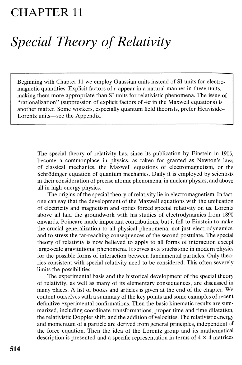
Текст
Vector Formulas
a • (b x c) = b • (c x a) = с • (a x b)
a x (b x c) = (a • c)b - (a • b)c
(a x b) • (c x d) = (a • c)(b . d) - (a . d)(b • c)
V x V^ = 0
V • (V x a) = 0
V x (V x a) = V(V • a) - V2a
V • (i/^а) = a • V^ 4- «/fV • a
V x (i/^a) = \ф x a 4- i/fV x a
V(a • b) = (a • V)b 4- (b • V)a + a x (V x b) 4- b x (V x a)
V • (a x b) = b • (V x a) - a . (V x b)
V x (a x b) = a(V . b) - b(V . a) + (b . V)a - (a . V)b
If x is the coordinate of a point with respect to some origin, with magnitude
r = |x|, n = x/r is a unit radial vector, and f(r) is a well-behaved function of r,
then
V • x = 3 V x x = 0
V-[n/(r)]=^/ + g Vx[n/(r)] = 0
(a - V)n/(r) = №¦ [a - n(a . n)] + n(a . n) ^
Г dr
V(x • a) = a 4- x(V • a) + i(L x a)
where L = - (x x V) is the angular-momentum operator.
Theorems from Vector Calculus
In the following ф, ф, and A are well-behaved scalar or vector functions, У is a
three-dimensional volume with volume element d3x, S is a closed two-
dimensional surface bounding V, with area element da and unit outward normal
n at da.
V • A d3x = A • n da (Divergence theorem)
Jv Js
\ф d3x = фи da
Jv Js
V x A d3x = n x A da
Jv Js
I (фУ2ф + V(/> • Vi/0 d3x = I фп^Vфda (Green's first identity)
I (фУ2ф - фУ2ф) d3x = I (ф\ф - ф\ф) • n da (Green's theorem)
Iif the following S is an open surface and С is the contour bounding it, with line
element d\. The normal n to S is defined by the right-hand-screw rule in relation
to the sense of the line integral around C.
(V x A) • n da = Ф A • d\ (Stokes's theorem)
J S J С
n x \ф da = Ф ф d\
Js Jc
Classical
Electrodynamics
Classical
Electrodynamics
Third Edition
John David Jackson
Professor Emeritus of Physics,
University of California, Berkeley
John Wiley & Sons, Inc.
This book was set in 10 on 12 Times Ten by UG and printed and bound by Hamilton Printing
Company.
This book is printed on acid-free paper. (OO'
The paper in this book was manufactured by a mill whose forest management programs include
sustained yield harvesting of its timberlands. Sustained yield harvesting principles ensure that the
numbers of trees cut each year does not exceed the amount of new growth.
Copyright © 1999 John David Jackson. All rights reserved.
No part of this publication may be reproduced, stored in a retrieval system or transmitted
in any form or by any means, electronic, mechanical, photocopying, recording, scanning
or otherwise, except as permitted under Sections 107 or 108 of the 1976 United States
Copyright Act, without either the prior written permission of the Publisher, or
authorization through payment of the appropriate per-copy fee to the Copyright
Clearance Center, 222 Rosewood Drive, Danvers, MA 01923, (978) 750-8400, fax
(978) 750-4470. Requests to the Publisher for permission should be addressed to the
Permissions Department, John Wiley & Sons, Inc., Ill River Street, Hoboken, NJ 07030,
B01) 748-6011, fax B01) 748-6008, E-Mail: PERMREQ@WILEY.COM.
To order books or for customer service please, call 1 (800)-CALL-WILEY B25-5945).
Library of Congress Cataloging-in-Publication Data
Jackson, John David, 1925-
Classical electrodynamics / John David Jackson.—3rd ed.
p. cm.
Includes index.
ISBN 0-471-30932-X (cloth : alk. paper)
1. Electrodynamics. I. Title.
QC631.J3 1998
537.6—dc21 97-46873
CIP
Printed in the United States of America
10 9
To the memory of my father,
Walter David Jackson
Preface
It has been 36 years since the appearance of the first edition of this book, and 23
years since the second. Such intervals may be appropriate for a subject whose
fundamental basis was completely established theoretically 134 years ago by
Maxwell and experimentally 110 years ago by Hertz. Still, there are changes in
emphasis and applications. This third edition attempts to address both without
any significant increase in size. Inevitably, some topics present in the second
edition had to be eliminated to make room for new material. One major omission
is the chapter on plasma physics, although some pieces appear elsewhere. Read-
Readers who miss particular topics may, I hope, be able to avail themselves of the
second edition.
The most visible change is the use of SI units in the first 10 chapters. Gaussian
units are retained in the later chapters, since such units seem more suited to
relativity and relativistic electrodynamics than SI. As a reminder of the sys-
system of units being employed, the running head on each left-hand page carries
"—SI" or "—G" depending on the chapter.
My tardy adoption of the universally accepted SI system is a recognition that
almost all undergraduate physics texts, as well as engineering books at all levels,
employ SI units throughout. For many years Ed Purcell and I had a pact to
support each other in the use of Gaussian units. Now I have betrayed him! Al-
Although this book is formally dedicated to the memory of my father, I dedicate
this third edition informally to the memory of Edward Mills Purcell A912-1997),
a marvelous physicist with deep understanding, a great teacher, and a wonderful
man.
Because of the increasing use of personal computers to supplement analytical
work or to attack problems not amenable to analytic solution, I have included
some new sections on the principles of some numerical techniques for electro-
electrostatics and magnetostatics, as well as some elementary problems. Instructors may
use their ingenuity to create more challenging ones. The aim is to provide an
understanding of such methods before blindly using canned software or even
Mathematica or Maple.
There has been some rearrangement of topics—Faraday's law and quasi-
static fields are now in Chapter 5 with magnetostatics, permitting a more logical
discussion of energy and inductances. Another major change is the consolidation
of the discussion of radiation by charge-current sources, in both elementary and
exact multipole forms, in Chapter 9. All the applications to scattering and dif-
diffraction are in Chapter 10.
The principles of optical fibers and dielectric waveguides are discussed in two
new sections in Chapter 8. In Chapter 13 the treatment of energy loss has been
shortened and strengthened. Because of the increasing importance of synchro-
synchrotron radiation as a research tool, the discussion in Chapter 14 has been aug-
augmented by a detailed section on the physics of wigglers and undulators for syn-
chroton light sources. There is new material in Chapter 16 on radiation reaction
and models of classical charged particles, as well as changed emphasis.
There is much tweaking by small amounts throughout. I hope the reader will
vii
Viii Preface
not notice, or will notice only greater clarity. To mention but a few minor addi-
additions: estimating self-inductances, Poynting's theorem in lossy materials, polar-
polarization potentials (Hertz vectors), Goos-Hanchen effect, attenuation in optical
fibers, London penetration depth in superconductors. And more problems, of
course! Over 110 new problems, a 40% increase, all aimed at educating, not
discouraging.
In preparing this new edition and making corrections, I have benefited from
questions, suggestions, criticism, and advice from many students, colleagues, and
newfound friends. I am in debt to all. Particular thanks for help in various ways
go to Myron Bander, David F. Bartlett, Robert N. Cahn, John Cooper, John L.
Gammel, David J. Griffiths, Leroy T. Kerth, Kwang J. Kim, Norman M. Kroll,
Michael A. Lee, Harry J. Lipkin, William Mendoza, Gerald A. Miller, William
A. Newcomb, Ivan Otero, Alan M. Portis, Fritz Rohrlich, Wayne M. Saslow,
Chris Schmid, Kevin E. Schmidt, and George H. Trilling.
J. David Jackson
Berkeley, California, 1998, 2001
Preface to the Second Edition
In the thirteen years since the appearance of the first edition, my interest in
classical electromagnetism has waxed and waned, but never fallen to zero. The
subject is ever fresh. There are always important new applications and examples.
The present edition reflects two efforts on my part: the refinement and improve-
improvement of material already in the first edition; the addition of new topics (and the
omission of a few).
The major purposes and emphasis are still the same, but there are extensive
changes and additions. A major augmentation is the "Introduction and Survey"
at the beginning. Topics such as the present experimental limits on the mass of
the photon and the status of linear superposition are treated there. The aim is to
provide a survey of those basics that are often assumed to be well known when
one writes down the Maxwell equations and begins to solve specific examples.
Other major changes in the first half of the book include a new treatment of the
derivation of the equations of macroscopic electromagnetism from the micro-
microscopic description; a discussion of symmetry properties of mechanical and elec-
electromagnetic quantities; sections on magnetic monopoles and the quantization
condition of Dirac; Stokes's polarization parameters; a unified discussion of the
frequency dispersion characteristics of dielectrics, conductors, and plasmas; a dis-
discussion of causality and the Kramers-Kronig dispersion relations; a simplified,
but still extensive, version of the classic Sommerfeld-Brillouin problem of the
arrival of a signal in a dispersive medium (recently verified experimentally); an
unusual example of a resonant cavity; the normal-mode expansion of an arbitrary
field in a wave guide; and related discussions of sources in a guide or cavity and
the transmission and reflection coefficients of flat obstacles in wave guides.
Chapter 9, on simple radiating systems and diffraction, has been enlarged to
include scattering at long wavelengths (the blue sky, for example) and the optical
theorem. The sections on scalar and vectorial diffraction have been improved.
Chapters 11 and 12, on special relativity, have been rewritten almost com-
completely. The old pseudo-Euclidean metric with x4 = ict has been replaced by
g*v (v/ith g00 = +1, gu = -1, i = 1, 2, 3). The change of metric necessitated a
complete revision and thus permitted substitution of modern experiments and
concerns about the experimental basis of the special theory for the time-honored
aberration of starlight and the Michelson-Morley experiment. Other aspects
have been modernized, too. The extensive treatment of relativistic kinematics of
the first edition has been relegated to the problems. In its stead is a discussion
of the Lagrangian for the electromagnetic fields, the canonical and symmetric
stress-energy tensor, and the Proca Lagrangian for massive photons.
Significant alterations in the remaining chapters include a new section on
transition radiation, a completely revised (and much more satisfactory) semi-
classical treatment of radiation emitted in collisions that stresses momentum
transfer instead of impact parameter, and a better derivation of the coupling of
multipole fields to their sources. The collection of formulas and page references
to special functions on the front and back flyleaves is a much requested addition.
Of the 278 problems, 117 (more than 40 per cent) are new.
ix
X Preface to the Second Edition
The one area that remains almost completely unchanged is the chapter on
magnetohydrodynamics and plasma physics. I regret this. But the book obviously
has grown tremendously, and there are available many books devoted exclusively
to the subject of plasmas or magnetohydrodynamics.
Of minor note is the change from Maxwell's equations and a Green's func-
function to the Maxwell equations and a Green function. The latter boggles some
minds, but is in conformity with other usage (Bessel function, for example). It is
still Green's theorem, however, because that's whose theorem it is.
Work on this edition began in earnest during the first half of 1970 on the
occasion of a sabbatical leave spent at Clare Hall and the Cavendish Laboratory
in Cambridge. I am grateful to the University of California for the leave and
indebted to N. F. Mott for welcoming me as a visitor to the Cavendish Laboratory
and to R. J. Eden and A. B. Pippard for my appointment as a Visiting Fellow of
Clare Hall. Tangible and intangible evidence at the Cavendish of Maxwell, Ray-
leigh and Thomson provided inspiration for my task; the stimulation of everyday
activities there provided necessary diversion.
This new edition has benefited from questions, suggestions, comments and
criticism from many students, colleagues, and strangers. Among those to whom
I owe some specific debt of gratitude are A. M. Bincer, L. S. Brown, R. W. Brown,
E. U. Condon, H. H. Denman, S. Deser, A. J. Dragt, V. L. Fitch, M. B. Halpern,
A. Hobson, J. P. Hurley, D. L. Judd, L. T. Kerth, E. Marx, M. Nauenberg, A. B.
Pippard, A. M. Portis, R. K. Sachs, W. M. Saslow, R. Schleif, V. L. Telegdi, T.
Tredon, E. P. Tryon, V. F. Weisskopf, and Dudley Williams. Especially helpful
were D. G. Boulware, R. N. Cahn, Leverett Davis, Jr., K. Gottfried, С. К. Gra-
Graham, E. M. Purcell, and E. H. Wichmann. I send my thanks and fraternal greet-
greetings to all of these people, to the other readers who have written to me, and the
countless students who have struggled with the problems (and sometimes written
asking for solutions to be dispatched before some deadline!). To my mind, the
book is better than ever. May each reader benefit and enjoy!
J. D. Jackson
Berkeley, California, 1974
Preface to the First Edition
Classical electromagnetic theory, together with classical and quantum mechanics,
forms the core of present-day theoretical training for undergraduate and grad-
graduate physicists. A thorough grounding in these subjects is a requirement for more
advanced or specialized training.
Typically the undergraduate program in electricity and magnetism involves
two or perhaps three semesters beyond elementary physics, with the emphasis
on the fundamental laws, laboratory verification and elaboration of their con-
consequences, circuit analysis, simple wave phenomena, and radiation. The mathe-
mathematical tools utilized include vector calculus, ordinary differential equations with
constant coefficients, Fourier series, and perhaps Fourier or Laplace transforms,
partial differential equations, Legendre polynomials, and Bessel functions.
As a general rule, a two-semester course in electromagnetic theory is given
to beginning graduate students. It is for such a course that my book is designed.
My aim in teaching a graduate course in electromagnetism is at least threefold.
The first aim is to present the basic subject matter as a coherent whole, with
emphasis on the unity of electric and magnetic phenomena, both in their physical
basis and in the mode of mathematical description. The second, concurrent aim
is to develop and utilize a number of topics in mathematical physics which are
useful in both electromagnetic theory and wave mechanics. These include
Green's theorems and Green's functions, orthonormal expansions, spherical har-
harmonics, cylindrical and spherical Bessel functions. A third and perhaps most
important purpose is the presentation of new material, especially on the inter-
interaction of relativistic charged particles with electromagnetic fields. In this last area
personal preferences and prejudices enter strongly. My choice of topics is gov-
governed by what I feel is important and useful for students interested in theoretical
physics, experimental nuclear and high-energy physics, and that as yet ill-defined
field of plasma physics.
The book begins in the traditional manner with electrostatics. The first six
chapters are devoted to the development of Maxwell's theory of electromagne-
electromagnetism. Much of the necessary mathematical apparatus is constructed along the way,
especially in Chapter 2 and 3, where boundary-value problems are discussed
thoroughly. The treatment is initially in terms of the electric field E and the
magnetic induction B, with the derived macroscopic quantities, D and H, intro-
introduced by suitable averaging over ensembles of atoms or molecules. In the dis-
discussion of dielectrics, simple classical models for atomic polarizability are de-
described, but for magnetic materials no such attempt to made. Partly this omission
was a question of space, but truly classical models of magnetic susceptibility are
not possible. Furthermore, elucidation of the interesting phenomenon of ferro-
magnetism needs almost a book in itself.
The next three chapters G-9) illustrate various electromagnetic phenomena,
mostly of a macroscopic sort. Plane waves in different media, including plasmas
as well as dispersion and the propagation of pulses, are treated in Chapter 7. The
discussion of wave guides and cavities in Chapter 8 is developed for systems of
arbitrary cross section, and the problems of attenuation in guides and the Q of
xi
ХЙ Preface to the First Edition
a cavity are handled in a very general way which emphasizes the physical pro-
processes involved. The elementary theory of multipole radiation from a localized
source and diffraction occupy Chapter 9. Since the simple scalar theory of dif-
diffraction is covered in many optics textbooks, as well as undergraduate books on
electricity and magnetism, I have presented an improved, although still approx-
approximate, theory of diffraction based on vector rather than scalar Green's theorems.
The subject of magnetohydrodynamics and plasmas receives increasingly
more attention from physicists and astrophysicists. Chapter 10 represents a sur-
survey of this complex field with an introduction to the main physical ideas involved.
The first nine or ten chapters constitute the basic material of classical elec-
electricity and magnetism. A graduate student in physics may be expected to have
been exposed to much of this material, perhaps at a somewhat lower level, as an
undergraduate. But he obtains a more mature view of it, understands it more
deeply, and gains a considerable technical ability in analytic methods of solution
when he studies the subject at the level of this book. He is then prepared to go
on to more advanced topics. The advanced topics presented here are predomi-
predominantly those involving the interaction of charged particles with each other and
with electromagnetic fields, especially when moving relativistically.
The special theory of relativity had its origins in classical electrodynamics.
And even after almost 60 years, classical electrodynamics still impresses and de-
delights as a beautiful example of the covariance of physical laws under Lorentz
transformations. The special theory of relativity is discussed in Chapter 11, where
all the necessary formal apparatus is developed, various kinematic consequences
are explored, and the covariance of electrodynamics is established. The next
chapter is devoted to relativistic particle kinematics and dynamics. Although the
dynamics of charged particles in electromagnetic fields can properly be consid-
considered electrodynamics, the reader may wonder whether such things as kinematic
transformations of collision problems can. My reply is that these examples occur
naturally once one has established the four-vector character of a particle's mo-
momentum and energy, that they serve as useful practice in manipulating Lorentz
transformations, and that the end results are valuable and often hard to find
elsewhere.
Chapter 13 on collisions between charged particles emphasizes energy loss
and scattering and develops concepts of use in later chapters. Here for the first
time in the book I use semiclassical arguments based on the uncertainty principle
to obtain approximate quantum-mechanical expressions for energy loss, etc.,
from the classical results. This approach, so fruitful in the hands of Niels Bohr
and E. J. Williams, allows one to see clearly how and when quantum-mechanical
effects enter to modify classical considerations.
The important subject of emission of radiation by accelerated point charges
is discussed in detail in Chapters 14 and 15. Relativistic effects are stressed, and
expressions for the frequency and angular dependence of the emitted radiation
are developed in sufficient generality for all applications. The examples treated
range from synchrotron radiation to bremsstrahlung and radiative beta processes.
Cherenkov radiation and the Weizsacker-Williams method of virtual quanta are
also discussed. In the atomic and nuclear collision processes semiclassical argu-
arguments are again employed to obtain approximate quantum-mechanical results. I
lay considerable stress on this point because I feel that it is important for the
student to see that radiative effects such as bremsstrahlung are almost entirely
Preface to the First Edition Xlll
classical in nature, even though involving small-scale collisions. A student who
meets bremsstrahlung for the first time as an example of a calculation in quantum
field theory will not understand its physical basis.
Multipole fields form the subject matter of Chapter 16. The expansion of
scalar and vector fields in spherical waves is developed from first principles with
no restrictions as to the relative dimensions of source and wavelength. Then the
properties of electric and magnetic multipole radiation fields are considered.
Once the connection to the multiple moments of the source has been made,
examples of atomic and nuclear multipole radiation are discussed, as well as a
macroscopic source whose dimensions are comparable to a wavelength. The scat-
scattering of a plane electromagnetic wave by a spherical object is treated in some
detail in order to illustrate a boundary-value problem with vector spherical
waves.
In the last chapter the difficult problem of radiative reaction is discussed.
The treatment is physical, rather than mathematical, with the emphasis on delim-
delimiting the areas where approximate radiative corrections are adequate and on
finding where and why existing theories fail. The original Abraham-Lorentz the-
theory of the self-force is presented, as well as more recent classical considerations.
The book ends with an appendix on units and dimensions and a bibliography.
In the appendix I have attempted to show the logical steps involved in setting up
a system of units, without haranguing the reader as to the obvious virtues of my
choice of units. I have provided two tables which I hope will be useful, one for
converting equations and symbols and the other for converting a given quantity
of something from so many Gaussian units to so many mks units, and vice versa.
The bibliography lists books which I think the reader may find pertinent and
useful for reference or additional study. These books are referred to by author's
name in the reading lists at the end of each chapter.
This book is the outgrowth of a graduate course in classical electrodynamics
which I have taught off and on over the past eleven years, at both the University
of Illinois and McGill University. I wish to thank my colleagues and students at
both institutions for countless helpful remarks and discussions. Special mention
must be made of Professor P. R. Wallace of McGill, who gave me the opportunity
and encouragement to teach what was then a rather unorthodox course in elec-
tromagnetism, and Professors H. W. Wyld and G. Ascoli of Illinois, who have
been particularly free with many helpful suggestions on the treatment of various
topics. My thanks are also extended to Dr. A. N. Kaufman for reading and com-
commenting on a preliminary version of the manuscript, and to Mr. G. L. Kane for
his zealous help in preparing the index.
J. D. Jackson
Urbana, Illinois, January, 1962
Contents
Introduction and Survey 1
1.1 Maxwell Equations in Vacuum, Fields, and Sources 2
1.2 Inverse Square Law, or the Mass of the Photon 5
1.3 Linear Superposition 9
1.4 Maxwell Equations in Macroscopic Media 13
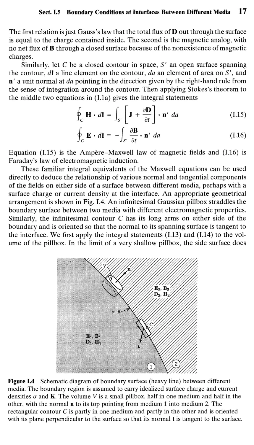
1.5 Boundary Conditions at Interfaces Between Different Media 16
1.6 Some Remarks on Idealizations in Electromagnetism 19
References and Suggested Reading 22
Chapter 1 / Introduction to Electrostatics 24
1.1 Coulomb's Law 24
1.2 Electric Field 24
1.3 Gauss's Law 27
1.4 Differential Form of Gauss's Law 28
1.5 Another Equation of Electrostatics and the Scalar Potential 29
1.6 Surface Distributions of Charges and Dipoles and Discontinuities
in the Electric Field and Potential 31
1.7 Poisson and Laplace Equations 34
1.8 Green's Theorem 35
1.9 Uniqueness of the Solution with Dirichlet or Neumann Boundary
Conditions 37
1.10 Formal Solution of Electrostatic Boundary-Value Problem
with Green Function 38
1.11 Electrostatic Potential Energy and Energy Density; Capacitance 40
1.12 Variational Approach to the Solution of the Laplace and Poisson
Equations 43
1.13 Relaxation Method for Two-Dimensional Electrostatic Problems 47
References and Suggested Reading 50
Problems 50
Chapter 2 / Boundary- Value Problems in Electrostatics: I 57
2.1 Method of Images 57
2.2 Point Charge in the Presence of a Grounded Conducting Sphere 58
2.3 Point Charge in the Presence of a Charged, Insulated, Conducting
Sphere 60
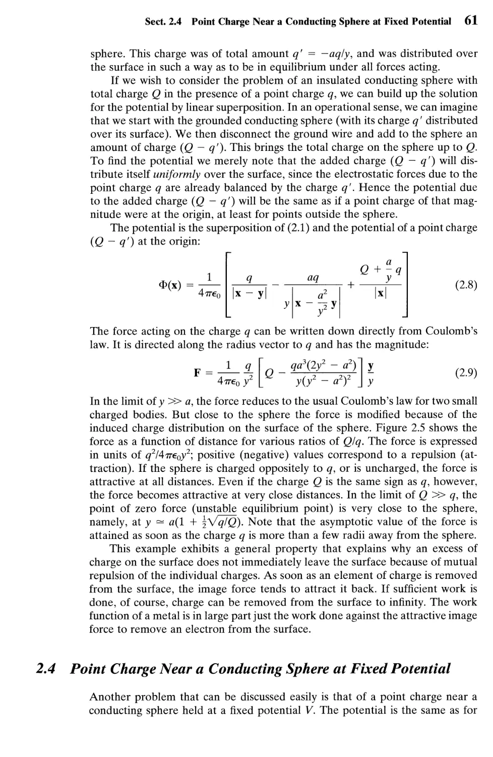
2.4 Point Charge Near a Conducting Sphere at Fixed Potential 61
2.5 Conducting Sphere in a Uniform Electric Field by Method
of Images 62
2.6 Green Function for the Sphere; General Solution
for the Potential 64
2.7 Conducting Sphere with Hemispheres at Different Potentials 65
XV
XVI Contents
2.8 Orthogonal Functions and Expansions 67
2.9 Separation of Variables; Laplace Equation in Rectangular
Coordinates 70
2.10 A Two-Dimensional Potential Problem; Summation
of Fourier Series 72
2.11 Fields and Charge Densities in Two-Dimensional Corners
and Along Edges 75
2.12 Introduction to Finite Element Analysis for Electrostatics 79
References and Suggested Reading 84
Problems 85
Chapter 3 / Boundary- Value Problems in Electrostatics: II 95
3.1 Laplace Equation in Spherical Coordinates 95
3.2 Legendre Equation and Legendre Polynomials 96
3.3 Boundary-Value Problems with Azimuthal Symmetry 101
3.4 Behavior of Fields in a Conical Hole or Near a Sharp Point 104
3.5 Associated Legendre Functions and the Spherical Harmonics
Ylm@, Ф) Ю7
3.6 Addition Theorem for Spherical Harmonics 110
3.7 Laplace Equation in Cylindrical Coordinates; Bessel Functions 111
3.8 Boundary-Value Problems in Cylindrical Coordinates 117
3.9 Expansion of Green Functions in Spherical Coordinates 119
3.10 Solution of Potential Problems with the Spherical Green Function
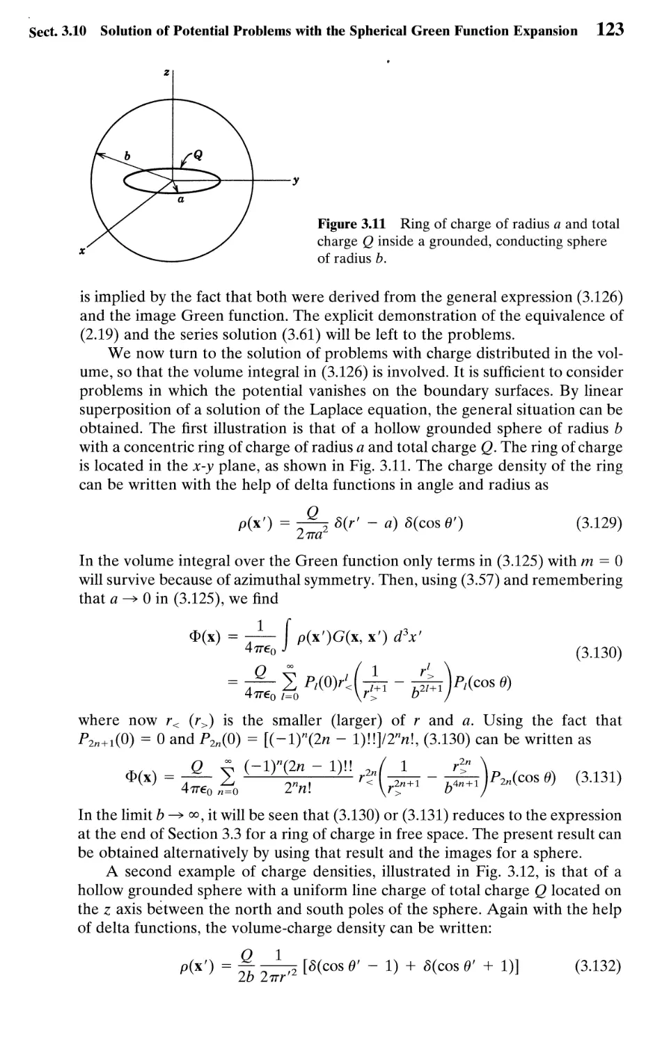
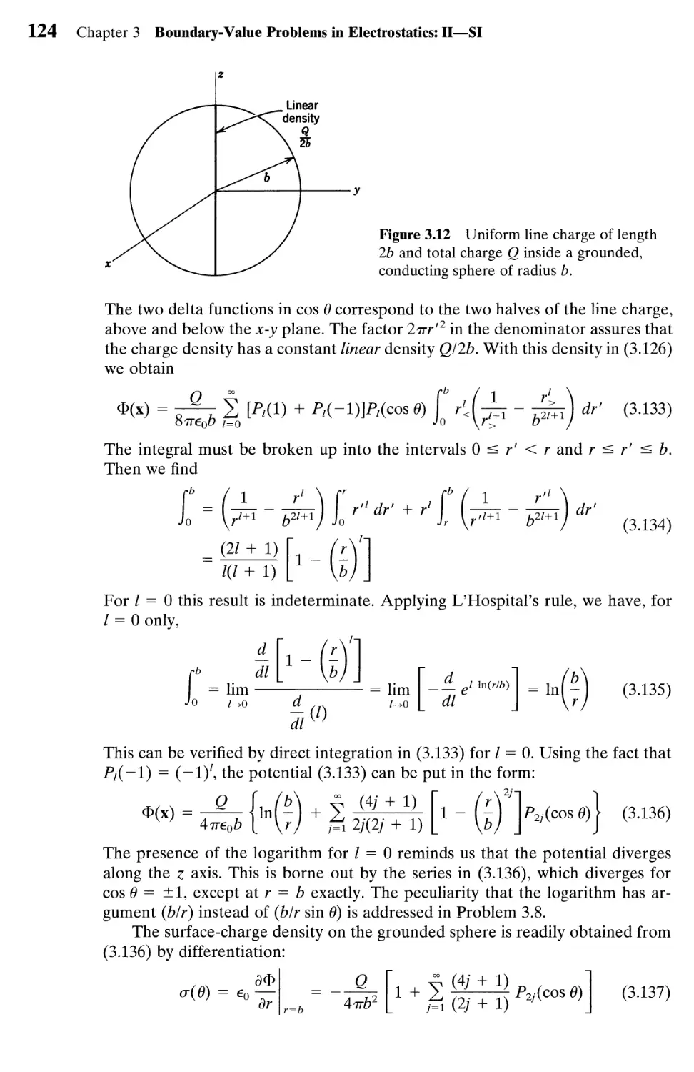
Expansion 112
3.11 Expansion of Green Functions in Cylindrical Coordinates 125
3.12 Eigenfunction Expansions for Green Functions 127
3.13 Mixed Boundary Conditions, Conducting Plane with a Circular
Hole 129
References and Suggested Reading 135
Problems 135
Chapter 4 / Multipoles, Electrostatics of Macroscopic Media,
Dielectrics 145
4.1 Multipole Expansion 145
4.2 Multipole Expansion of the Energy of a Charge Distribution
in an External Field 150
4.3 Elementary Treatment of Electrostatics with Ponderable Media 151
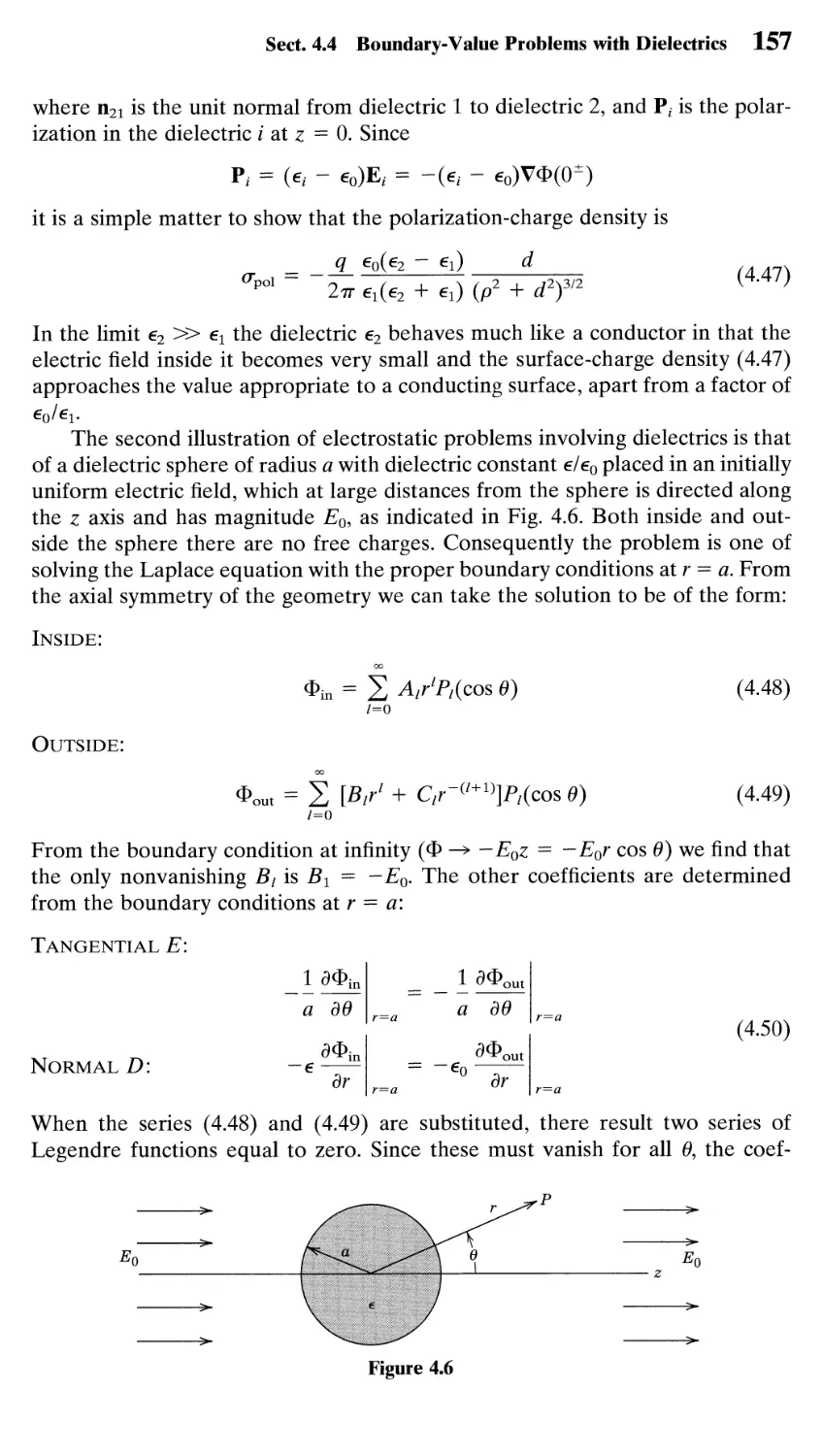
4.4 Boundary-Value Problems with Dielectrics 154
4.5 Molecular Polarizability and Electric Susceptibility 159
4.6 Models for Electric Polarizability 162
4.7 Electrostatic Energy in Dielectric Media 165
References and Suggested Reading 169
Problems 169
Chapter 5 / Magnetostatics, Faraday's Law, Quasi-Static Fields 174
5.1 Introduction and Definitions 174
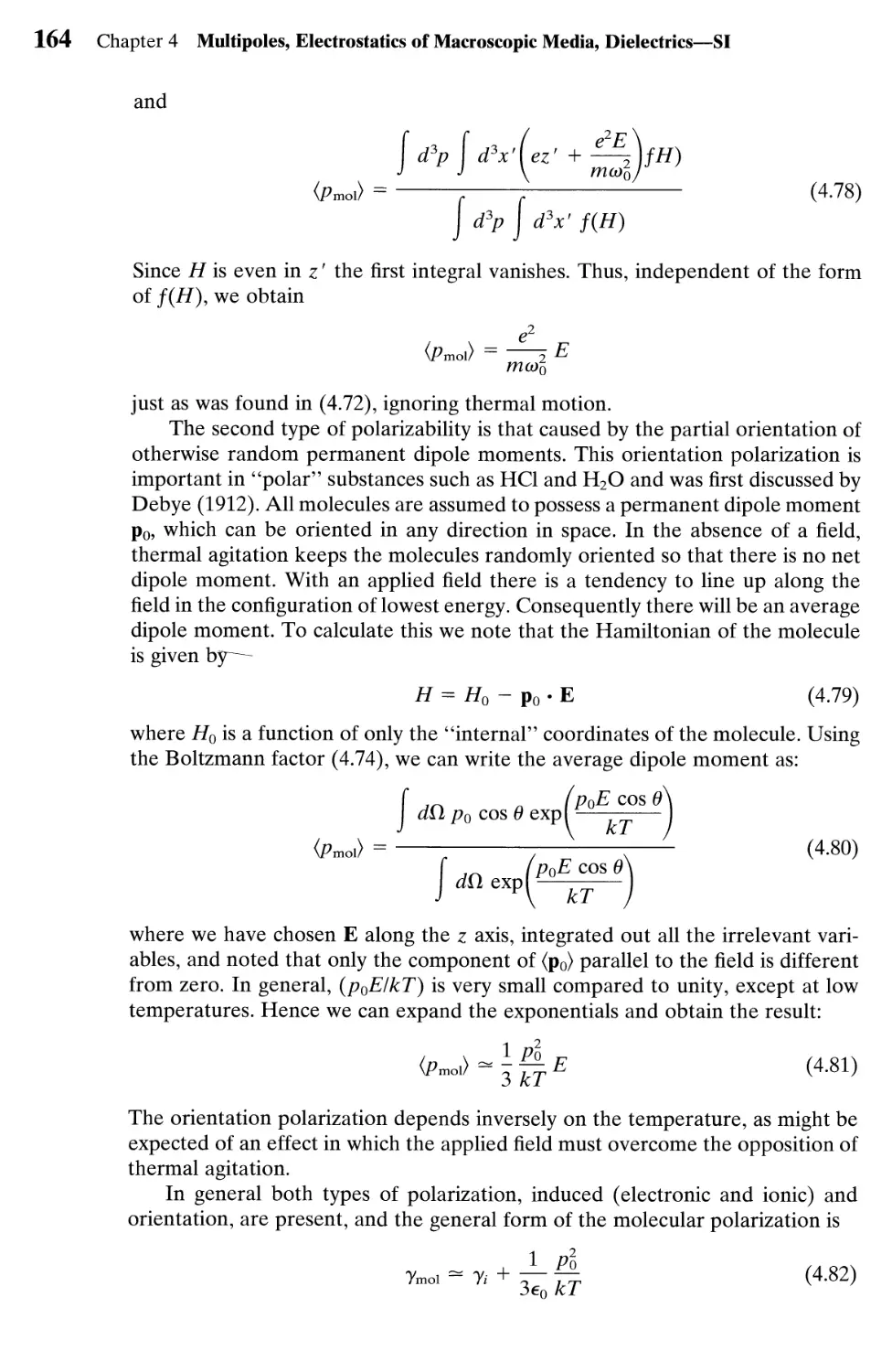
5.2 Biot and Savart Law 175
Contents XV11
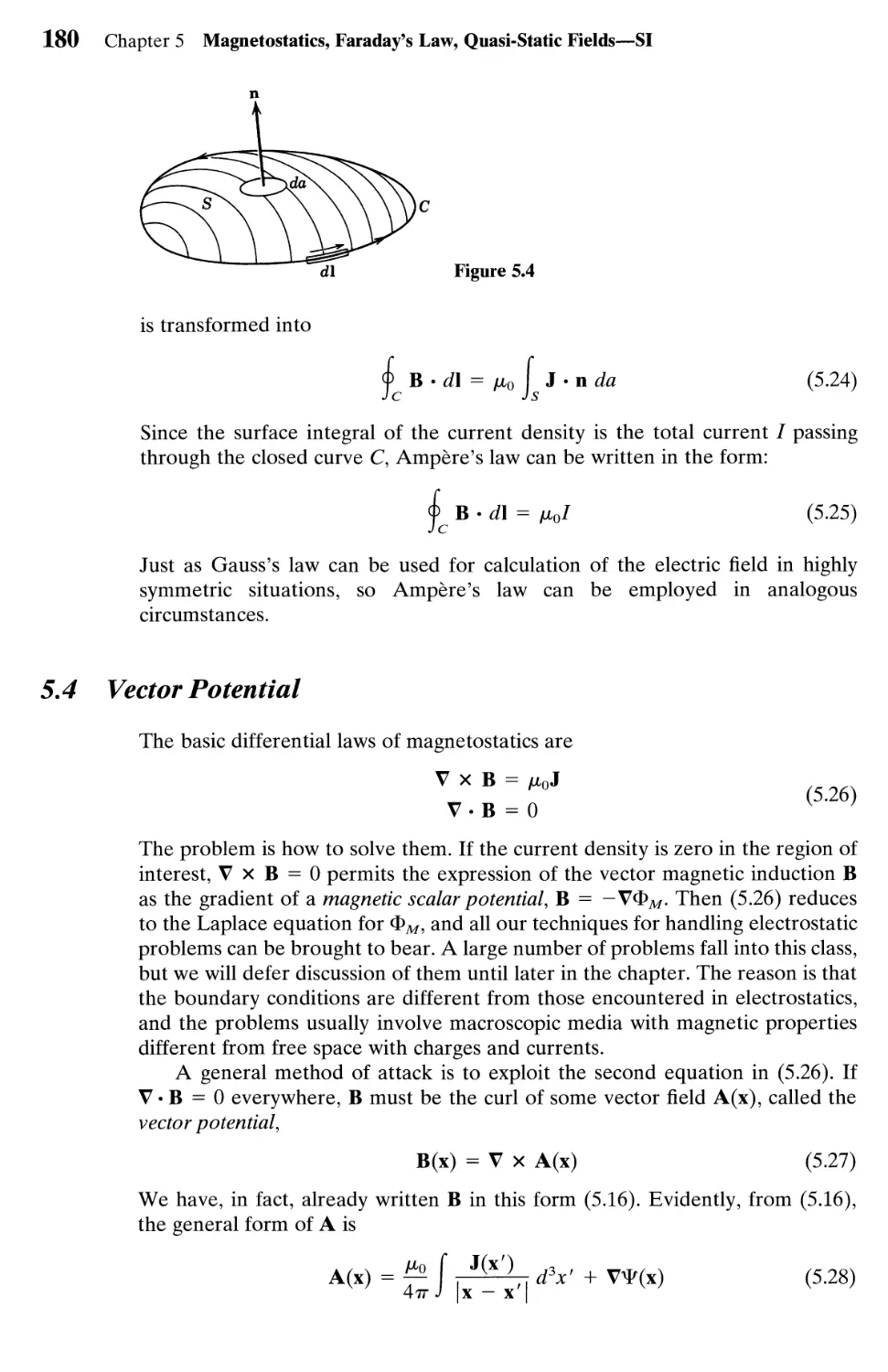
5.3 Differential Equations of Magnetostatics and Ampere's Law 178
5.4 Vector Potential 180
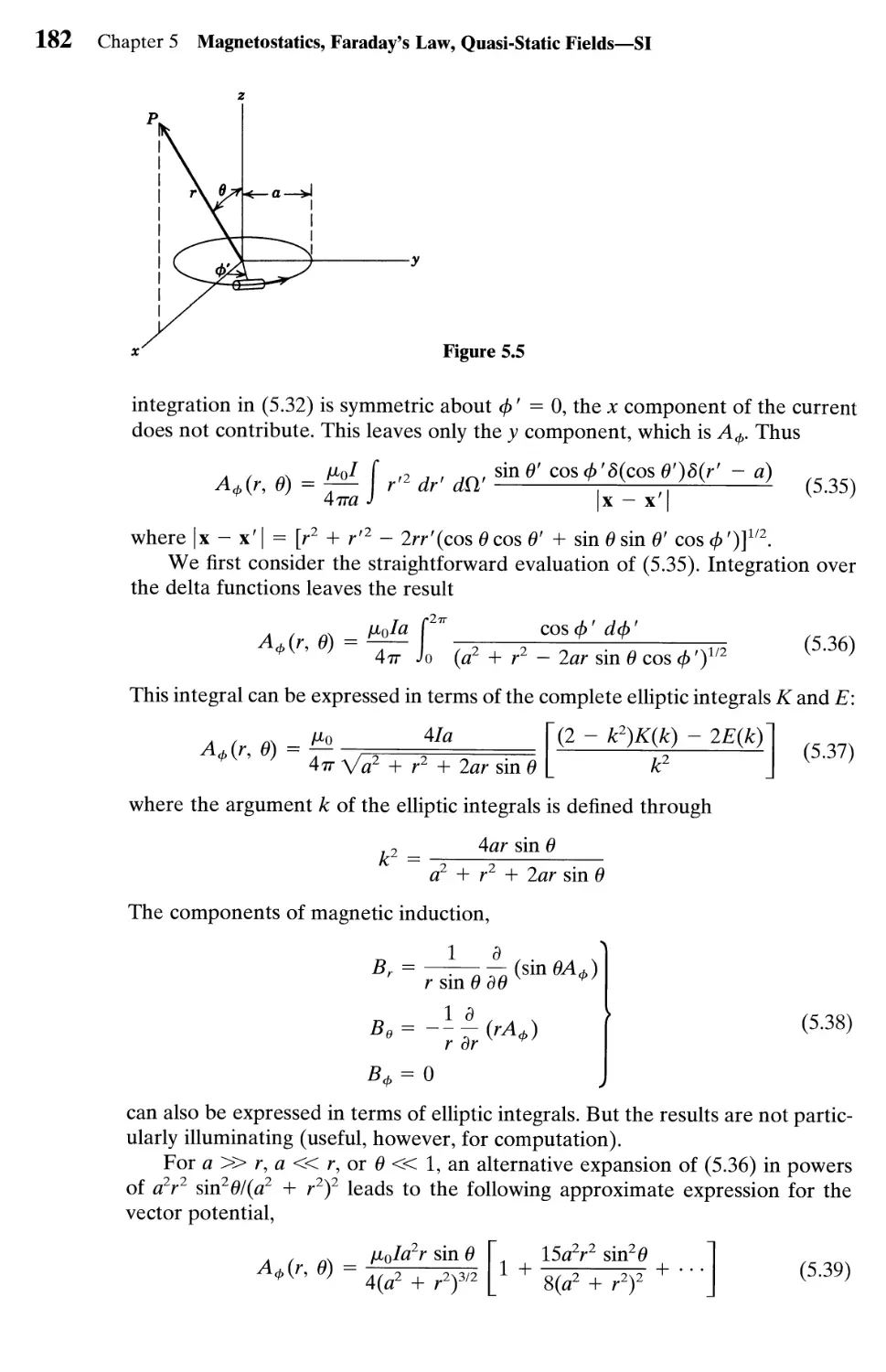
5.5 Vector Potential and Magnetic Induction for a Circular Current
Loop 181
5.6 Magnetic Fields of a Localized Current Distribution, Magnetic
Moment 184
5.7 Force and Torque on and Energy of a Localized Current Distribution
in an External Magnetic Induction 188
5.8 Macroscopic Equations, Boundary Conditions on В and H 191
5.9 Methods of Solving Boundary-Value Problems
in Magnetostatics 194
5.10 Uniformly Magnetized Sphere 198
5.11 Magnetized Sphere in an External Field; Permanent Magnets 199
5.12 Magnetic Shielding, Spherical Shell of Permeable Material
in a Uniform Field 201
5.13 Effect of a Circular Hole in a Perfectly Conducting Plane
with an Asymptotically Uniform Tangential Magnetic Field
on One Side 203
5.14 Numerical Methods for Two-Dimensional Magnetic Fields 206
5.15 Faraday's Law of Induction 208
5.16 Energy in the Magnetic Field 212
5.17 Energy and Self- and Mutual Inductances 215
5.18 Quasi-Static Magnetic Fields in Conductors; Eddy Currents; Magnetic
Diffusion 218
References and Suggested Reading 223
Problems 225
Chapter 6 / Maxwell Equations, Macroscopic Electromagnetism,
Conservation Laws 237
6.1 Maxwell's Displacement Current; Maxwell Equations 237
6.2 Vector and Scalar Potentials 239
6.3 Gauge Transformations, Lorenz Gauge, Coulomb Gauge 240
6.4 Green Functions for the Wave Equation 243
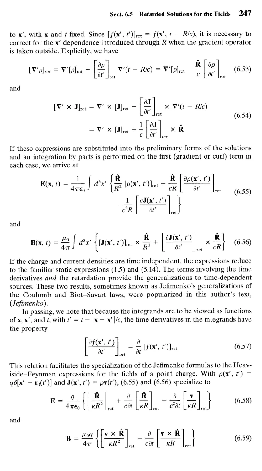
6.5 Retarded Solutions for the Fields: Jefimenko's Generalizations
of the Coulomb and Biot-Savart Laws; Heaviside-Feynman
Expressions for Fields of Point Charge 246
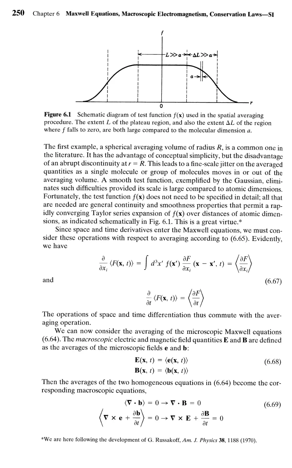
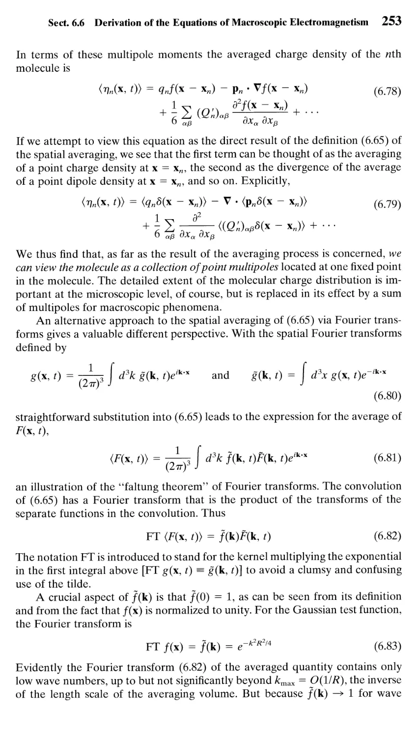
6.6 Derivation of the Equations of Macroscopic Electromagnetism 248
6.7 Poynting's Theorem and Conservation of Energy and Momentum
for a System of Charged Particles and Electromagnetic Fields 258
6.8 Poynting's Theorem in Linear Dissipative Media with Losses 262
6.9 Poynting's Theorem for Harmonic Fields; Field Definitions
of Impedance and Admittance 264
6.10 Transformation Properties of Electromagnetic Fields and Sources
Under Rotations, Spatial Reflections, and Time Reversal 267
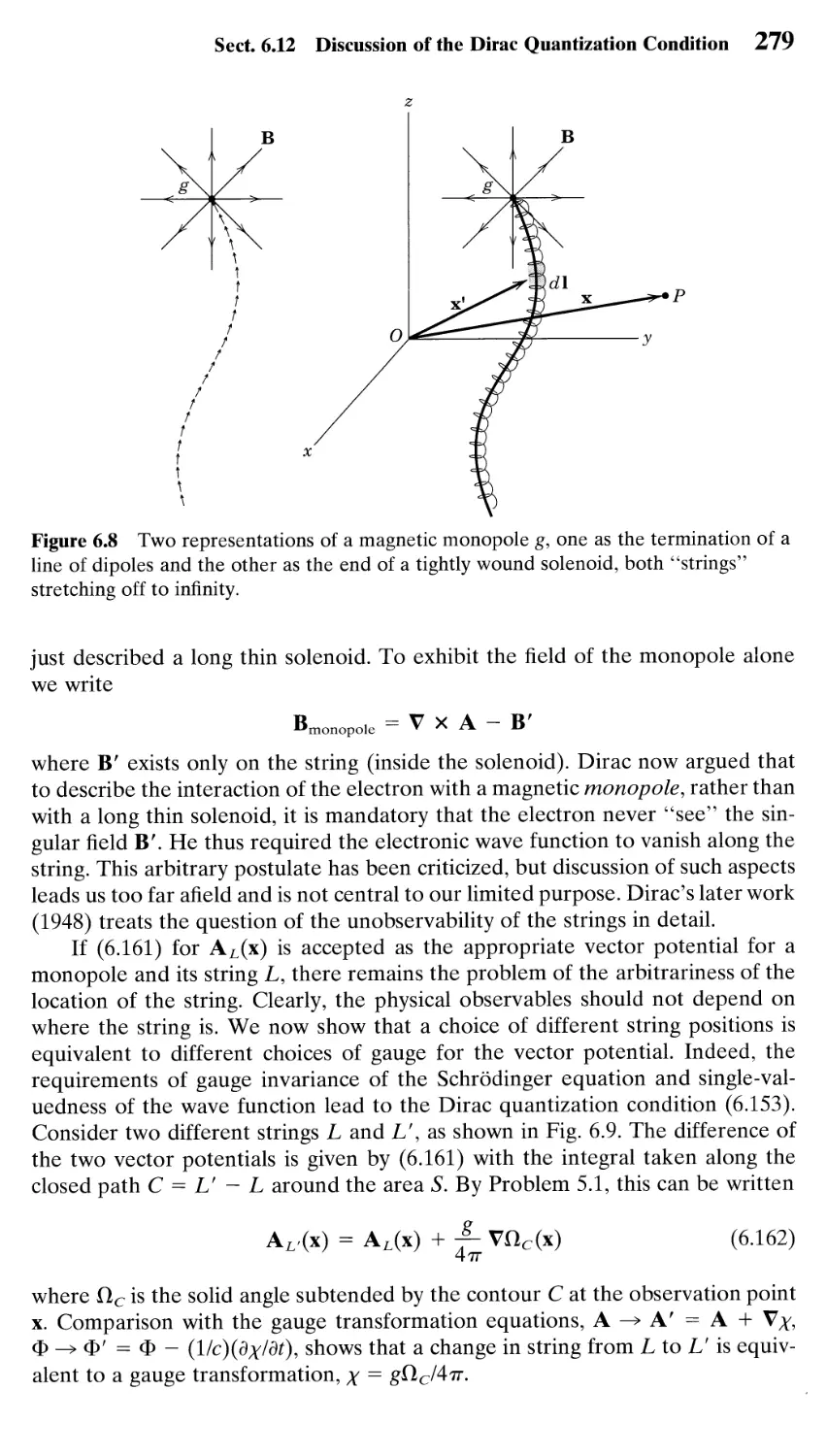
6.11 On the Question of Magnetic Monopoles 273
6.12 Discussion of the Dirac Quantization Condition 275
6.13 Polarization Potentials (Hertz Vectors) 280
References and Suggested Reading 282
Problems 283
XV111 Contents
Chapter 7 / Plane Electromagnetic Waves and Wave Propagation 295
11 Plane Waves in a Nonconducting Medium 295
7.2 Linear and Circular Polarization; Stokes Parameters 299
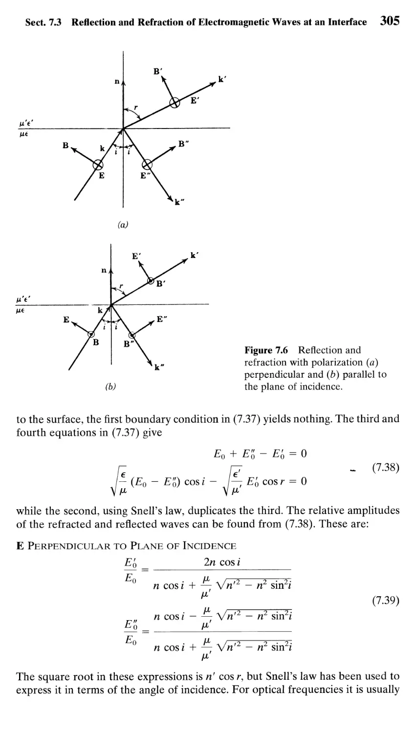
7.3 Reflection and Refraction of Electromagnetic Waves at a Plane
Interface Between Two Dielectrics 302
7.4 Polarization by Reflection, Total Internal Reflection; Goos-Hanchen
Effect 306
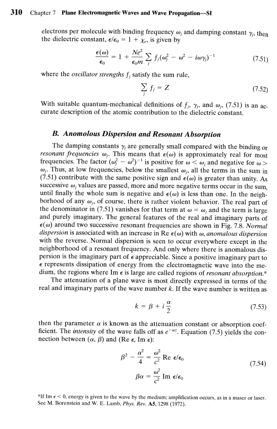
7.5 Frequency Dispersion Characteristics of Dielectrics, Conductors,
and Plasmas 309
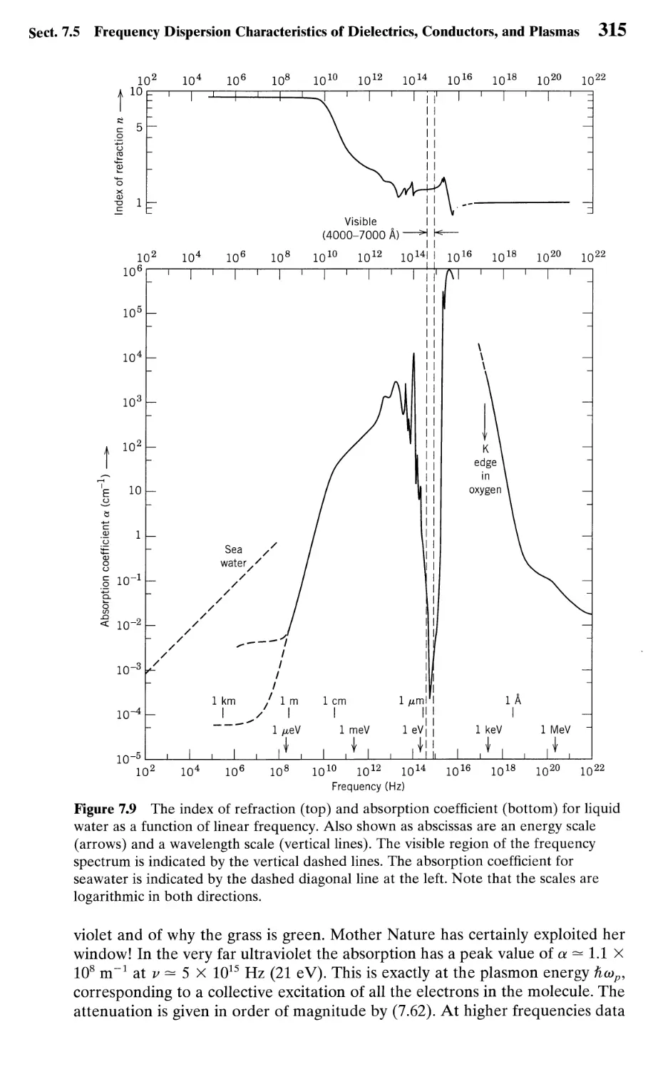
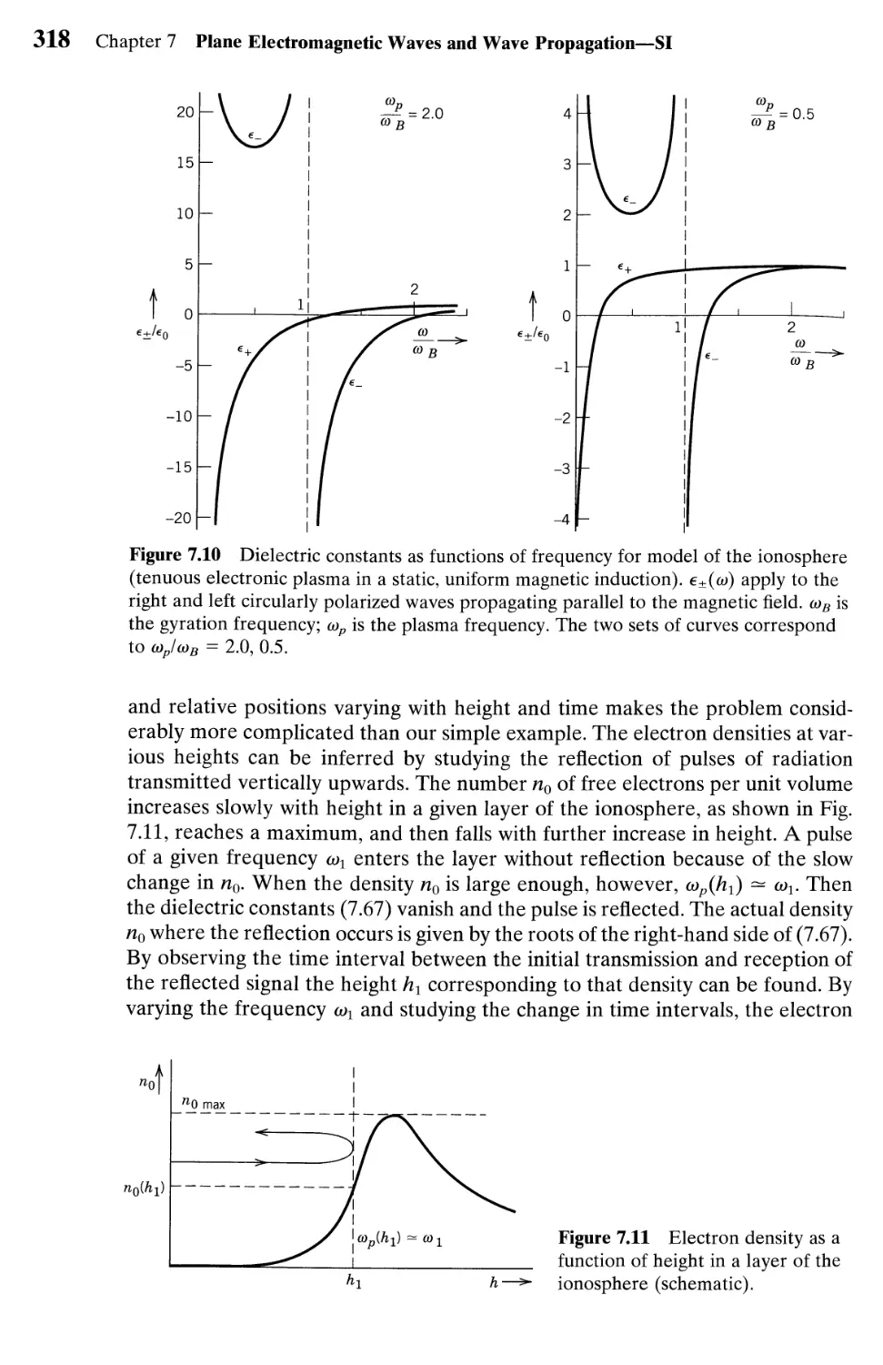
7.6 Simplified Model of Propagation in the Ionosphere
and Magnetosphere 316
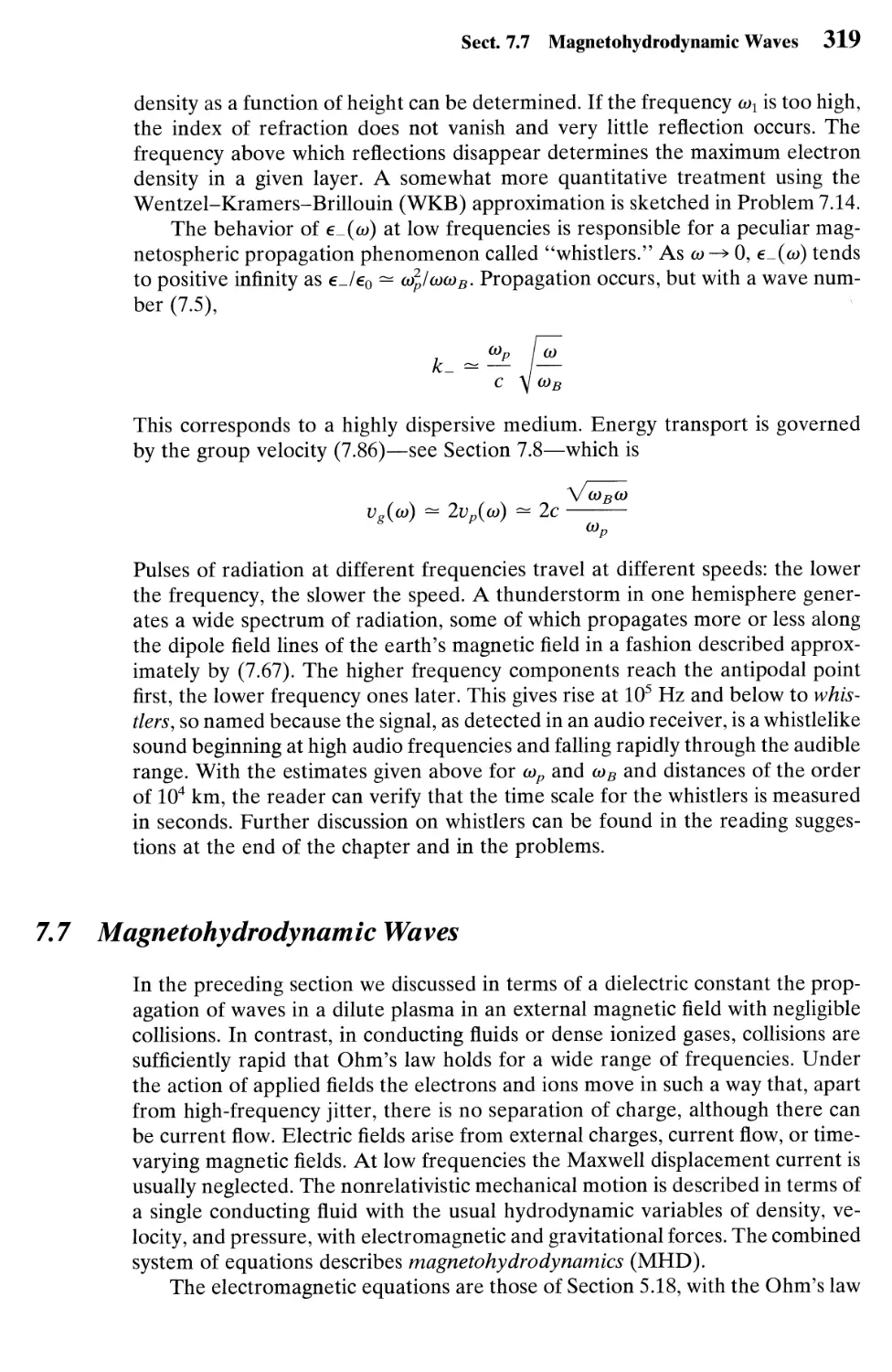
7.7 Magnetohydrodynamic Waves 319
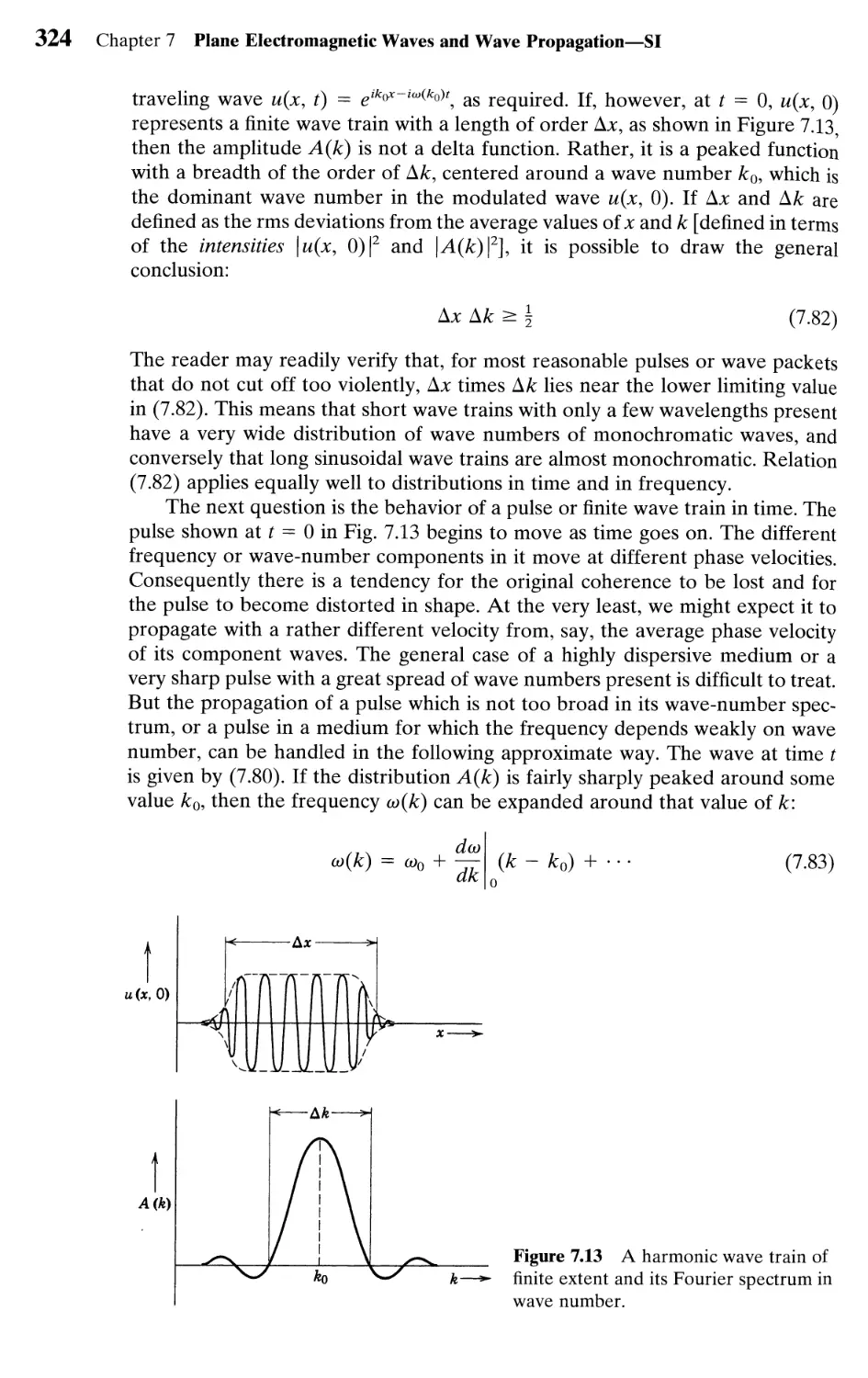
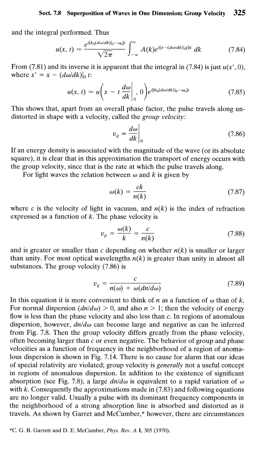
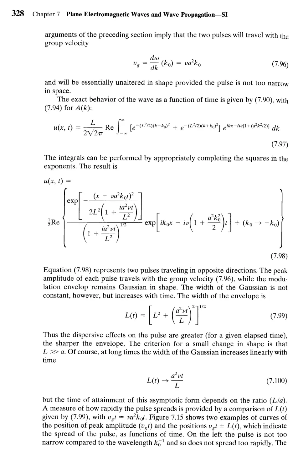
7.8 Superposition of Waves in One Dimension; Group Velocity 322
7.9 Illustration of the Spreading of a Pulse As It Propagates in a Dispersive
Medium 326
7.10 Causality in the Connection Between D and E; Kramers-Kronig
Relations 330
7.11 Arrival of a Signal After Propagation Through a Dispersive
Medium 335
References and Suggested Reading 339
Problems 340
Chapter 8 / Waveguides, Resonant Cavities, and Optical Fibers 352
8.1 Fields at the Surface of and Within a Conductor 352
8.2 Cylindrical Cavities and Waveguides 356
8.3 Waveguides 359
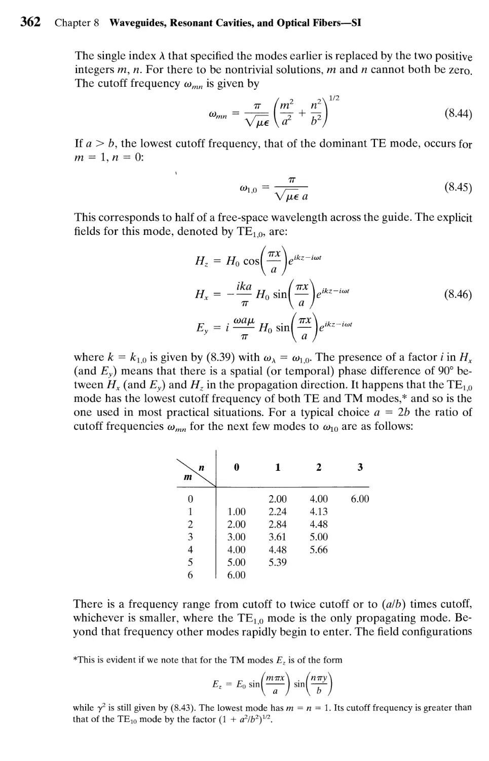
8.4 Modes in a Rectangular Waveguide 361
8.5 Energy Flow and Attenuation in Waveguides 363
8.6 Perturbation of Boundary Conditions 366
8.7 Resonant Cavities 368
8.8 Power Losses in a Cavity; Q of a Cavity 371
8.9 Earth and Ionosphere as a Resonant Cavity:
Schumann Resonances 374
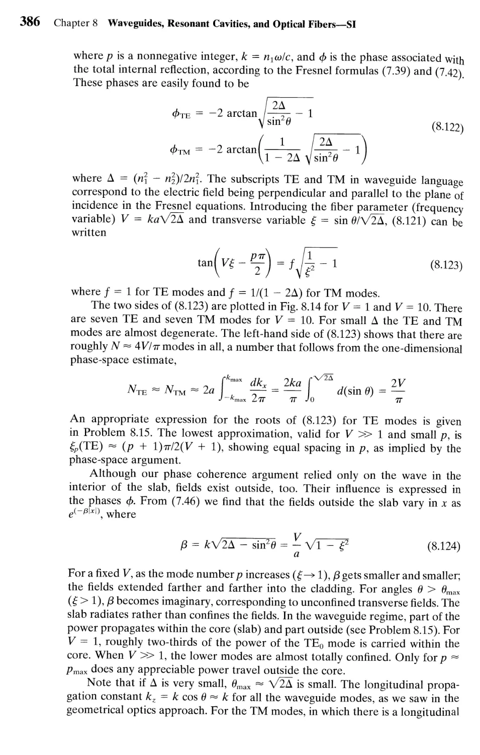
8.10 Multimode Propagation in Optical Fibers 378
8.11 Modes in Dielectric Waveguides 385
8.12 Expansion in Normal Modes; Fields Generated by a Localized
Source in a Hollow Metallic Guide 389
References and Suggested Reading 395
Problems 396
Chapter 9 / Radiating Systems, Multipole Fields and Radiation 407
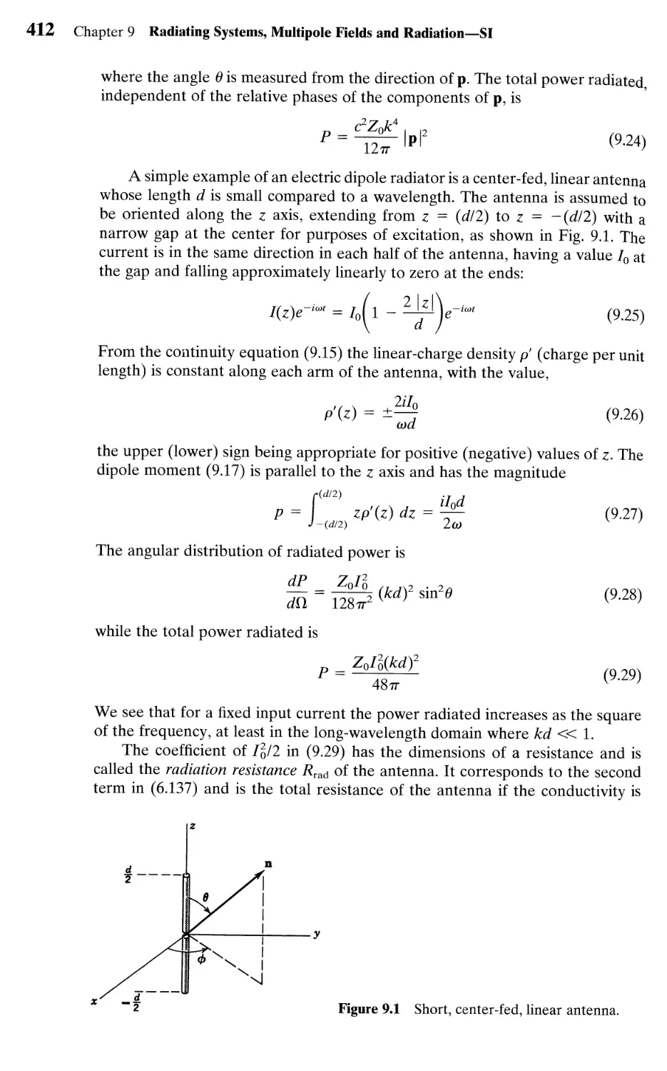
9.1 Fields and Radiation of a Localized Oscillating Source 407
9.2 Electric Dipole Fields and Radiation 410
9.3 Magnetic Dipole and Electric Quadrupole Fields 413
9.4 Center-Fed Linear Antenna 416
9.5 Multipole Expansion for Localized Source or Aperture
in Waveguide 419
Contents XIX
9.6 Spherical Wave Solutions of the Scalar Wave Equation 425
9.7 Multipole Expansion of the Electromagnetic Fields 429
9.8 Properties of Multipole Fields, Energy and Angular Momentum
of Multipole Radiation 432
9.9 Angular Distribution of Multipole Radiation 437
9.10 Sources of Multipole Radiation; Multipole Moments 439
9.11 Multipole Radiation in Atoms and Nuclei 442
9.12 Multipole Radiation from a Linear, Center-Fed Antenna 444
References and Suggested Reading 448
Problems 449
Chapter 10 / Scattering and Diffraction 456
10.1 Scattering at Long Wavelengths 456
10.2 Perturbation Theory of Scattering, Rayleigh's Explanation
of the Blue Sky, Scattering by Gases and Liquids, Attenuation
in Optical Fibers 462
10.3 Spherical Wave Expansion of a Vector Plane Wave 471
10.4 Scattering of Electromagnetic Waves by a Sphere 473
10.5 Scalar Diffraction Theory 478
10.6 Vector Equivalents of the Kirchhoff Integral 482
10.7 Vectorial Diffraction Theory 485
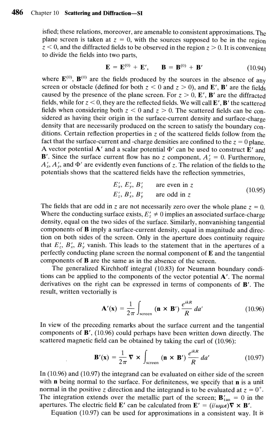
10.8 Babinet's Principle of Complementary Screens 488
10.9 Diffraction by a Circular Aperture; Remarks on Small
Apertures 490
10.10 Scattering in the Short-Wavelength Limit 495
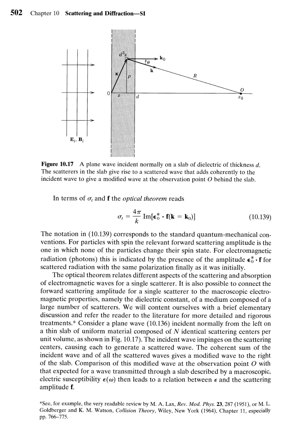
10.11 Optical Theorem and Related Matters 500
References and Suggested Reading 506
Problems 507
Chapter 11 / Special Theory of Relativity 514
11.1 The Situation Before 1900, Einstein's Two Postulates 515
11.2 Some Recent Experiments 518
11.3 Lorentz Transformations and Basic Kinematic Results of Special
Relativity 524
11.4 Addition of Velocities; 4-Velocity 530
11.5 Relativistic Momentum and Energy of a Particle 533
11.6 Mathematical Properties of the Space-Time of Special
Relativity 539
11.7 Matrix Representation of Lorentz Transformations, Infinitesimal
Generators 543
11.8 Thomas Precession 548
11.9 Invariance of Electric Charge; Covariance of Electrodynamics 553
11.10 Transformation of Electromagnetic Fields 558
11.11 Relativistic Equation of Motion for Spin in Uniform or Slowly Varying
External Fields 561
11.12 Note on Notation and Units in Relativistic Kinematics 565
References and Suggested Reading 566
Problems 568
XX Contents
Chapter 12 / Dynamics of Relativistic Particles
and Electromagnetic Fields 579
12.1 Lagrangian and Hamiltonian for a Relativistic Charged Particle
in External Electromagnetic Fields 579
12.2 Motion in a Uniform, Static Magnetic Field 585
12.3 Motion in Combined, Uniform, Static Electric and Magnetic
Fields 586
12.4 Particle Drifts in Nonuniform, Static Magnetic Fields 588
12.5 Adiabatic Invariance of Flux Through Orbit of Particle 592
12.6 Lowest Order Relativistic Corrections to the Lagrangian for Interacting
Charged Particles: The Darwin Lagrangian 596
12.7 Lagrangian for the Electromagnetic Field 598
12.8 Proca Lagrangian; Photon Mass Effects 600
12.9 Effective "Photon" Mass in Superconductivity; London Penetration
Depth 603
12.10 Canonical and Symmetric Stress Tensors; Conservation Laws 605
12.11 Solution of the Wave Equation in Covariant Form; Invariant Green
Functions 612
References and Suggested Reading 615
Problems 617
Chapter 13 / Collisions, Energy Loss, and Scattering of Charged Particles,
Cherenkov and Transition Radiation 624
13.1 Energy Transfer in Coulomb Collision Between Heavy Incident Particle
and Free Electron; Energy Loss in Hard Collisions 625
13.2 Energy Loss from Soft Collisions; Total Energy Loss 627
13.3 Density Effect in Collisional Energy Loss 631
13.4 Cherenkov Radiation 637
13.5 Elastic Scattering of Fast Charged Particles by Atoms 640
13.6 Mean Square Angle of Scattering; Angular Distribution of Multiple
Scattering 643
13.7 Transition Radiation 646
References and Suggested Reading 654
Problems 655
Chapter 14 / Radiation by Moving Charges 661
14.1 Lienard-Wiechert Potentials and Fields for a Point Charge 661
14.2 Total Power Radiated by an Accelerated Charge: Larmor's Formula
and Its Relativistic Generalization 665
14.3 Angular Distribution of Radiation Emitted by an Accelerated
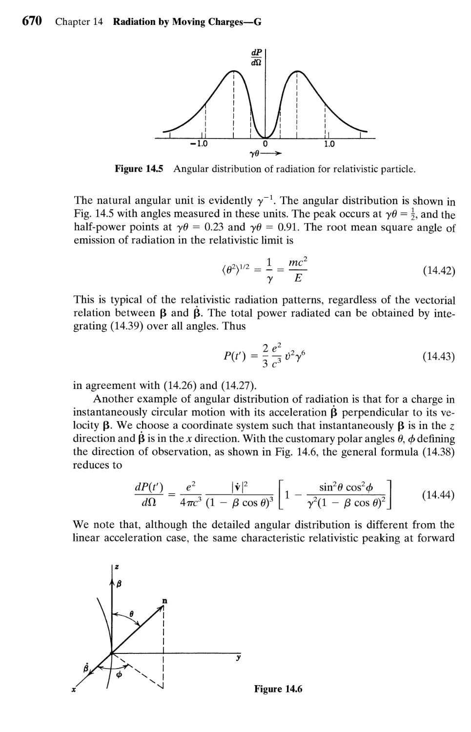
Charge 668
14.4 Radiation Emitted by a Charge in Arbitrary, Extremely Relativistic
Motion 671
14.5 Distribution in Frequency and Angle of Energy Radiated
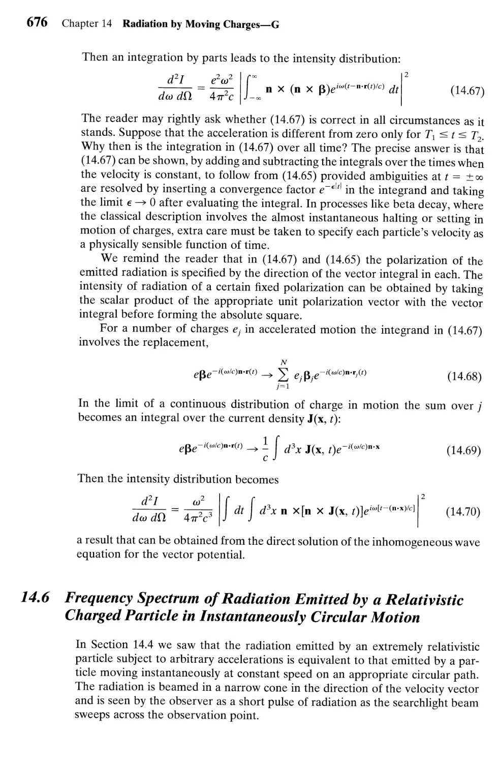
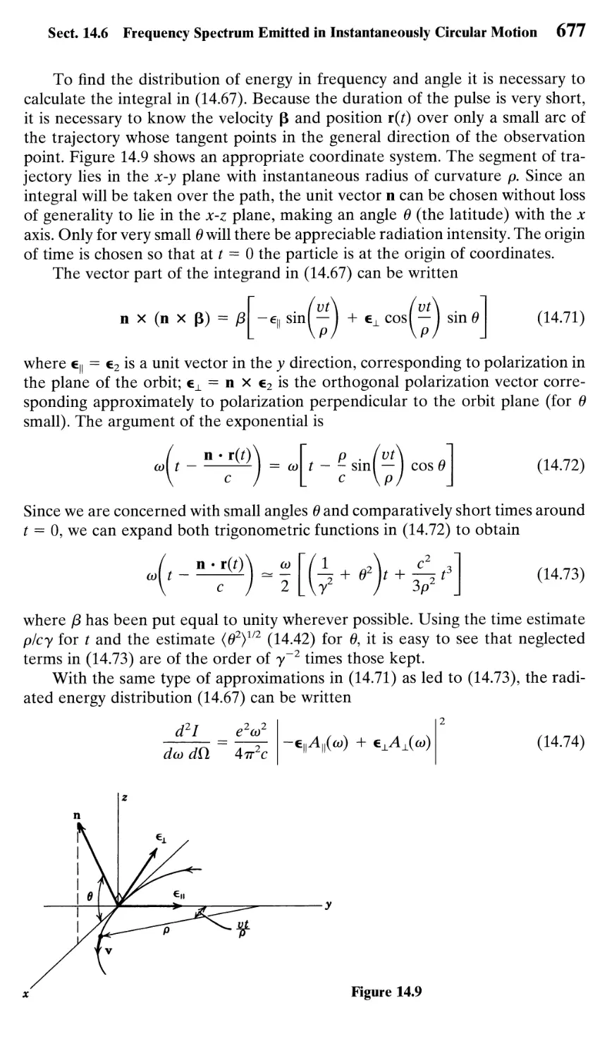
by Accelerated Charges: Basic Results 673
Contents XXI
14.6 Frequency Spectrum of Radiation Emitted by a Relativistic Charged
Particle in Instantaneously Circular Motion 676
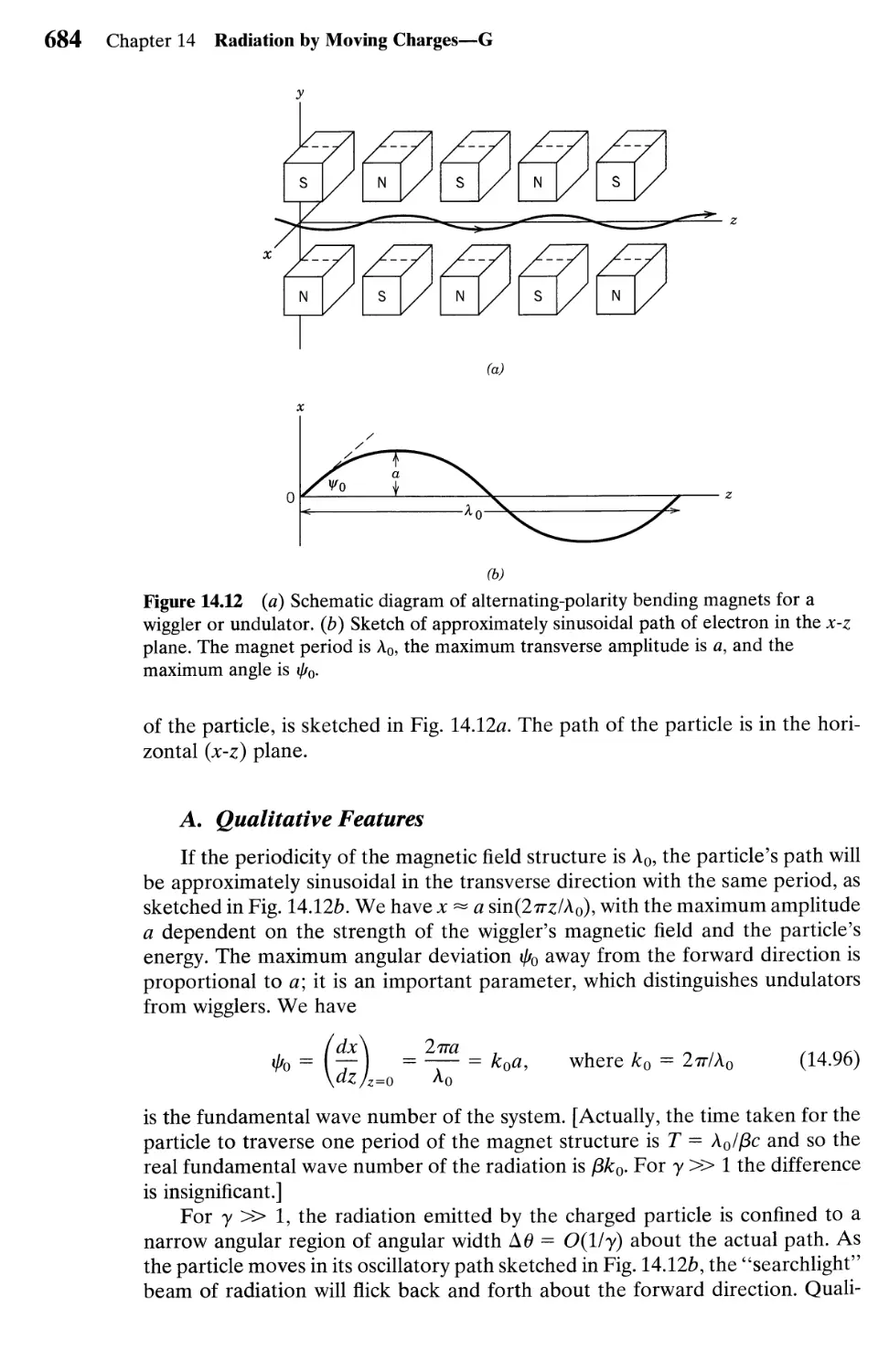
14.7 Undulators and Wigglers for Synchrotron Light Sources 683
14.8 Thomson Scattering of Radiation 694
References and Suggested Reading 697
Problems 698
Chapter 15 / Bremsstrahlung, Method of Virtual Quanta,
Radiative Beta Processes 708
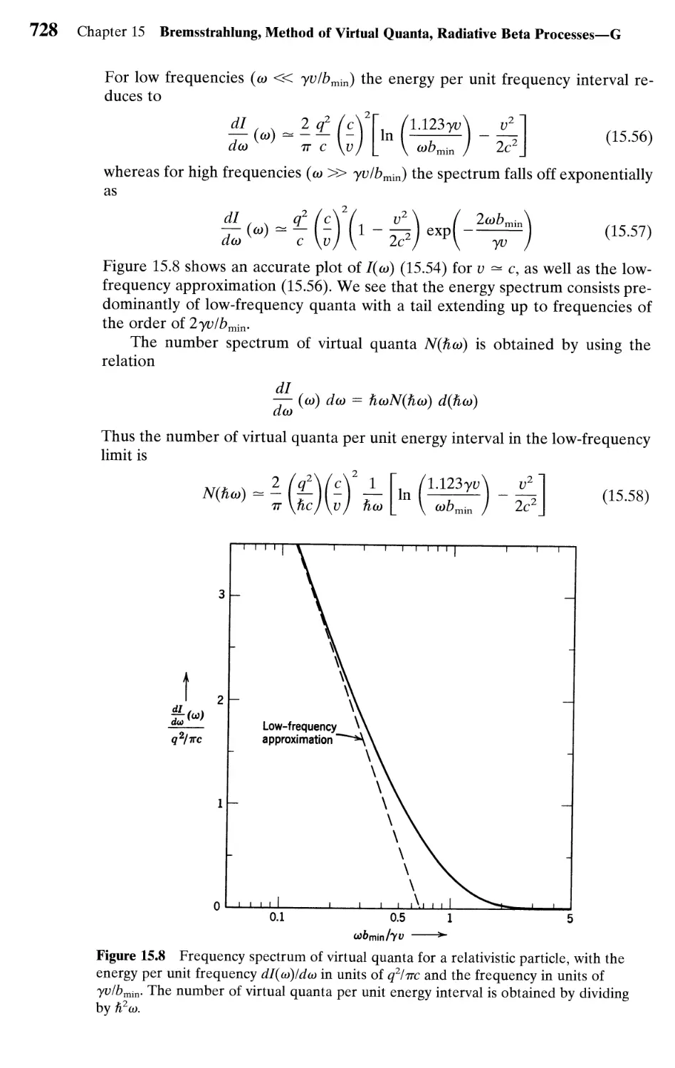
15.1 Radiation Emitted During Collisions 709
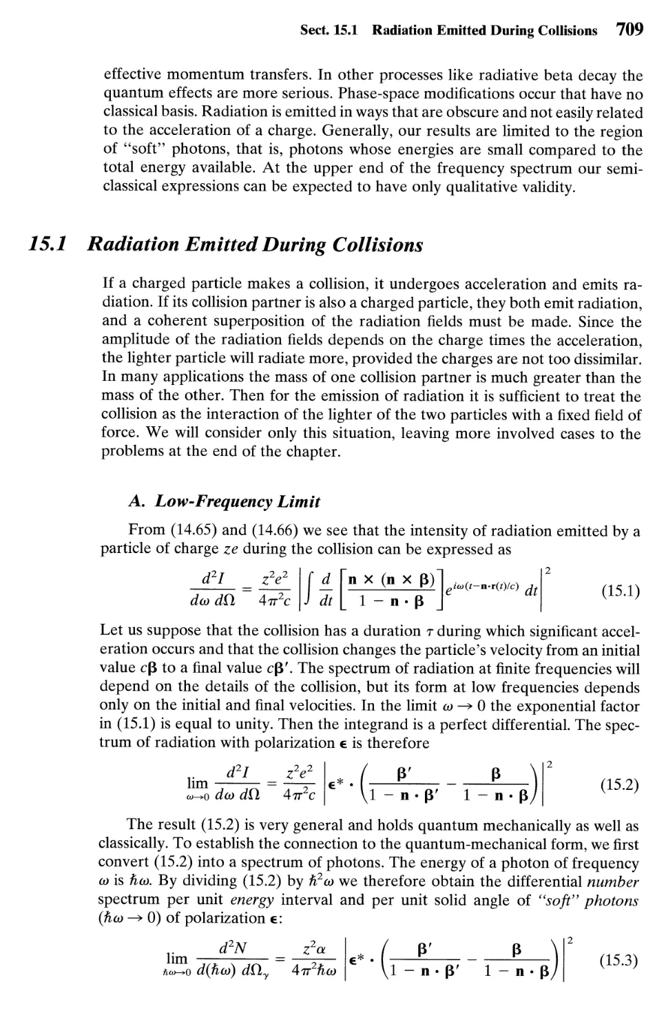
15.2 Bremsstrahlung in Coulomb Collisions 714
15.3 Screening Effects; Relativistic Radiative Energy Loss 721
15.4 Weizsacker-Williams Method of Virtual Quanta 724
15.5 Bremsstrahlung as the Scattering of Virtual Quanta 729
15.6 Radiation Emitted During Beta Decay 730
15.7 Radiation Emitted During Orbital Electron Capture: Disappearance
of Charge and Magnetic Moment 732
References and Suggested Reading 737
Problems 737
Chapter 16 / Radiation Damping, Classical Models
of Charged Particles 745
16.1 Introductory Considerations 745
16.2 Radiative Reaction Force from Conservation of Energy 747
16.3 Abraham-Lorentz Evaluation of the Self-Force 750
16.4 Relativistic Covariance; Stability and Poincare Stresses 755
16.5 Covariant Definitions of Electromagnetic Energy
and Momentum 757
16.6 Covariant Stable Charged Particle 759
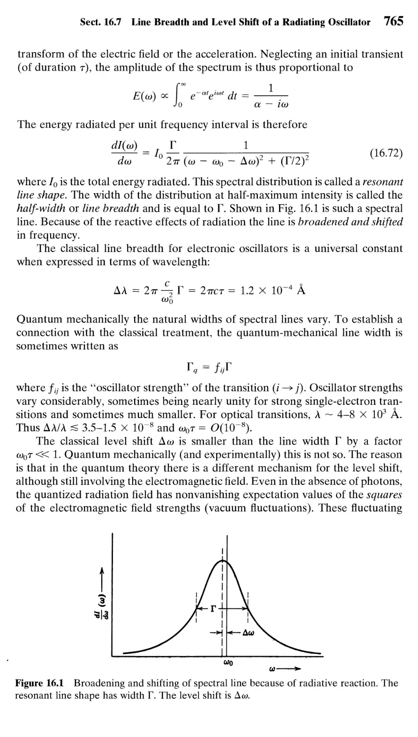
16.7 Level Breadth and Level Shift of a Radiating Oscillator 763
16.8 Scattering and Absorption of Radiation by an Oscillator 766
References and Suggested Reading 768
Problems 769
Appendix on Units and Dimensions 775
1 Units and Dimensions, Basic Units and Derived Units 775
2 Electromagnetic Units and Equations 777
3 Various Systems of Electromagnetic Units 779
4 Conversion of Equations and Amounts Between SI Units
and Gaussian Units 782
Bibliography 785
Index 791
Introduction and Survey
Although amber and lodestone were known to the ancient Greeks, electro-
electrodynamics developed as a quantitative subject in less than a hundred years.
Cavendish's remarkable experiments in electrostatics were done from 1771 to
1773. Coulomb's monumental researches began to be published in 1785. This
marked the beginning of quantitative research in electricity and magnetism on a
worldwide scale. Fifty years later Faraday was studying the effects of time-varying
currents and magnetic fields. By 1864 Maxwell had published his famous paper
on a dynamical theory of the electromagnetic field. Twenty-four years later
A888) Hertz published his discovery of transverse electromagnetic waves, which
propagated at the same speed as light, and placed Maxwell's theory on a firm
experimental footing.
The story of the development of our understanding of electricity and mag-
magnetism and of light is, of course, much longer and richer than the mention of a
few names from one century would indicate. For a detailed account of the fas-
fascinating history, the reader should consult the authoritative volumes by
Whittaker* A briefer account, with emphasis on optical phenomena, appears at
the beginning of Born and Wolf.
Since the 1960s there has been a true revolution in our understanding of the
basic forces and constituents of matter. Now A990s) classical electrodynamics
rests in a sector of the unified description of particles and interactions known as
the standard model. The standard model gives a coherent quantum-mechanical
description of electromagnetic, weak, and strong interactions based on funda-
fundamental constituents—quarks and leptons—interacting via force carriers—pho-
carriers—photons, W and Z bosons, and gluons. The unified theoretical framework is gener-
generated through principles of continuous gauge (really phase) invariance of the
forces and discrete symmetries of particle properties.
From the point of view of the standard model, classical electrodynamics is a
limit of quantum electrodynamics (for small momentum and energy transfers,
and large average numbers of virtual or real photons). Quantum electrodynamics,
in turn, is a consequence of a spontaneously broken symmetry in a theory in
which initially the weak and electromagnetic interactions are unified and the
force carriers of both are massless. The symmetry breaking leaves the electro-
electromagnetic force carrier (photon) massless with a Coulomb's law of infinite range,
while the weak force carriers acquire masses of the order of 80-90 GeV/c2 with
a weak interaction at low energies of extremely short range B X 10~18 meter).
Because of the origins in a unified theory, the range and strength of the weak
interaction are related to the electromagnetic coupling (the fine structure con-
constant a « 1/137).
*Italicized surnames denote books that are cited fully in the Bibliography.
2 Introduction and Survey
Despite the presence of a rather large number of quantities that must be
taken from experiment, the standard model (together with general relativity at
large scales) provides a highly accurate description of nature in all its aspects,
from far inside the nucleus, to microelectronics, to tables and chairs, to the most
remote galaxy. Many of the phenomena are classical or explicable with nonrel-
ativistic quantum mechanics, of course, but the precision of the agreement of the
standard model with experiment in atomic and particle physics where relativistic
quantum mechanics rules is truly astounding. Classical mechanics and classical
electrodynamics served as progenitors of our current understanding, and still play
important roles in practical life and at the research frontier.
This book is self-contained in that, though some mathematical background
(vector calculus, differential equations) is assumed, the subject of electrodynam-
electrodynamics is developed from its beginnings in electrostatics. Most readers are not coming
to the subject for the first time, however. The purpose of this introduction is
therefore not to set the stage for a discussion of Coulomb's law and other basics,
but rather to present a review and a survey of classical electromagnetism. Ques-
Questions such as the current accuracy of the inverse square law of force (mass of the
photon), the limits of validity of the principle of linear superposition, and the
effects of discreteness of charge and of energy differences are discussed. "Bread
and butter" topics such as the boundary conditions for macroscopic fields at
surfaces between different media and at conductors are also treated. The aim is
to set classical electromagnetism in context, to indicate its domain of validity,
and to elucidate some of the idealizations that it contains. Some results from later
in the book and some nonclassical ideas are used in the course of the discussion.
Certainly a reader beginning electromagnetism for the first time will not follow
all the arguments or see their significance. For others, however, this introduction
will serve as a springboard into the later parts of the book, beyond Chapter 5,
and will remind them of how the subject stands as an experimental science.
/./ Maxwell Equations in Vacuum, Fields, and Sources
The equations governing electromagnetic phenomena are the Maxwell
equations,
VD = p
dt (I. la)
VxE + —= 0
dt
V-B = 0
where for external sources in vacuum, D = e0E and В = ^i0H. The first two
equations then become
V • E = ple0
Ж
V x В - -^
Sect. I.I Maxwell Equations in Vacuum, Fields, and Sources 3
Implicit in the Maxwell equations is the continuity equation for charge density
and current density,
^ + V • J = 0 A.2)
dt
This follows from combining the time derivative of the first equation in (I.la)
with the divergence of the second equation. Also essential for consideration of
charged particle motion is the Lorentz force equation,
F^(E + vxB) A.3)
which gives the force acting on a point charge q in the presence of electromag-
electromagnetic fields.
These equations have been written in SI units, the system of electromagnetic
units used in the first 10 chapters of this book. (Units and dimensions are dis-
discussed in the Appendix.) The Maxwell equations are displayed in the commoner
systems of units in Table 2 of the Appendix. Essential to electrodynamics is the
speed of light in vacuum, given in SI units by с = (fjL0e0)~1/2. As discussed in the
Appendix, the meter is now defined in terms of the second (based on a hyperfine
transition in cesium-133) and the speed of light (c = 299 792 458 m/s, exactly).
These definitions assume that the speed of light is a universal constant, consistent
with evidence (see Section 11.2.C) indicating that to a high accuracy the speed
of light in vacuum is independent of frequency from very low frequencies to at
least v — 1024 Hz D GeV photons). For most practical purposes we can approx-
approximate с ^ 3 X 10⁸ m/s or to be considerably more accurate, с = 2.998 X 10⁸ m/s.
The electric and magnetic fields E and В in (LI) were originally introduced
by means of the force equation A.3). In Coulomb's experiments forces acting
between localized distributions of charge were observed. There it is found useful
(see Section 1.2) to introduce the electric field E as the force per unit charge.
Similarly, in Ampere's experiments the mutual forces of current-carrying loops
were studied (see Section 5.2). With the identification of NAq\ as a current in a
conductor of cross-sectional area A with N charge carriers per unit volume mov-
moving at velocity v, we see that В in A.3) is defined in magnitude as a force per unit
current. Although E and В thus first appear just as convenient replacements for
forces produced by distributions of charge and current, they have other important
aspects. First, their introduction decouples conceptually the sources from the test
bodies experiencing electromagnetic forces. If the fields E and В from two source
distributions are the same at a given point in space, the force acting on a test
charge or current at that point will be the same, regardless of how different the
source distributions are. This gives E and В in A.3) meaning in their own right,
independent of the sources. Second, electromagnetic fields can exist in regions
of space where there are no sources. They can carry energy, momentum, and
angular momentum and so have an existence totally independent of charges and
currents. In fact, though there are recurring attempts to eliminate explicit ref-
reference to the fields in favor of action-at-a-distance descriptions of the interaction
of charged particles, the concept of the electromagnetic field is one of the most
fruitful ideas of physics, both classically and quantum mechanically.
The concept of E and В as ordinary fields is a classical notion. It can be
thought of as the classical limit (limit of large quantum numbers) of a quantum-
mechanical description in terms of real or virtual photons. In the domain of
4 Introduction and Survey
macroscopic phenomena and even some atomic phenomena, the discrete photon
aspect of the electromagnetic field can usually be ignored or at least glossed over.
For example, 1 meter from a 100-watt light bulb, the root mean square electric
field is of the order of 50 V/m and there are of the order of 1015 visible photons/
cm2»s. Similarly, an isotropic FM antenna with a power of 100 watts at 108 Hz
produces an rms electric field of only 0.5 mV/m at a distance of 100 kilometers,
but this still corresponds to a flux of 1012 photons/cm2 «s, or about 109 photons in
a volume of 1 wavelength cubed B7 m3) at that distance. Ordinarily an apparatus
will not be sensible to the individual photons; the cumulative effect of many
photons emitted or absorbed will appear as a continuous, macroscopically ob-
observable response. Then a completely classical description in terms of the
Maxwell equations is permitted and is appropriate.
How is one to decide a priori when a classical description of the electromag-
electromagnetic fields is adequate? Some sophistication is occasionally needed, but the fol-
following is usually a sufficient criterion: When the number of photons involved can
be taken as large but the momentum carried by an individual photon is small
compared to the momentum of the material system, then the response of the
material system can be determined adequately from a classical description of the
electromagnetic fields. For example, each 108 Hz photon emitted by our FM
antenna gives it an impulse of only 2.2 X 10~34 N«s. A classical treatment is surely
adequate. Again, the scattering of light by a free electron is governed by the
classical Thomson formula (Section 14.8) at low frequencies, but by the laws of
the Compton effect as the momentum hco/c of the incident photon becomes sig-
significant compared to me. The photoelectric effect is nonclassical for the matter
system, since the quasi-free electrons in the metal change their individual ener-
energies by amounts equal to those of the absorbed photons, but the photoelectric
current can be calculated quantum mechanically for the electrons using a classical
description of the electromagnetic fields.
The quantum nature of the electromagnetic fields must, on the other hand,
be taken into account in spontaneous emission of radiation by atoms, or by any
other system that initially lacks photons and has only a small number of photons
present finally. The average behavior may still be describable in essentially clas-
classical terms, basically because of conservation of energy and momentum. An ex-
example is the classical treatment (Section 16.2) of the cascading of a charged
particle down through the orbits of an attractive potential. At high particle quan-
quantum numbers, a classical description of particle motion is adequate, and the sec-
secular changes in energy and angular momentum can be calculated classically from
the radiation reaction because the energies of the successive photons emitted are
small compared to the kinetic or potential energy of the orbiting particle.
The sources in (LI) are p(x, r), the electric charge density, and J(x, r), the
electric current density. In classical electromagnetism they are assumed to be
continuous distributions in x, although we consider from time to time localized
distributions that can be approximated by points. The magnitudes of these point
charges are assumed to be completely arbitrary, but are known to be restricted
in reality to discrete values. The basic unit of charge is the magnitude of the
charge on the electron,
\qe\ = 4.803 206 8A5) X 10~10 esu
= 1.602 177 33D9) X 10~19 С
Sect 1.2 Inverse Square Law or the Mass of the Photon 5
where the errors in the last two decimal places are shown in parentheses. The
charges on the proton and on all presently known particles or systems of particles
are integral multiples of this basic unit.* The experimental accuracy with which
it is known that the multiples are exactly integers is phenomenal (better than 1
part in 1020). The experiments are discussed in Section 11.9, where the question
of the Lorentz invariance of charge is also treated.
The discreteness of electric charge does not need to be considered in most
macroscopic applications. A 1-microfarad capacitor at a potential of 150 volts,
for example, has a total of 1015 elementary charges on each electrode. A few
thousand electrons more or less would not be noticed. A current of 1 microam-
microampere corresponds to 6.2 X 10¹² elementary charges per second. There are, of
course, some delicate macroscopic or almost macroscopic experiments in which
the discreteness of charge enters. Millikan's famous oil drop experiment is one.
His droplets were typically 1СГ4 cm in radius and had a few or few tens of ele-
elementary charges on them.
There is a lack of symmetry in the appearance of the source terms in the
Maxwell equations (I.la). The first two equations have sources; the second two
do not. This reflects the experimental absence of magnetic charges and currents.
Actually, as is shown in Section 6.11, particles could have magnetic as well as
electric charge. If all particles in nature had the same ratio of magnetic to electric
charge, the fields and sources could be redefined in such a way that the usual
Maxwell equations (I.la) emerge. In this sense it is somewhat a matter of con-
convention to say that no magnetic charges or currents exist. Throughout most of
this book it is assumed that only electric charges and currents act in the Maxwell
equations, but some consequences of the existence of a particle with a different
magnetic to electric charge ratio, for example, a magnetic monopole, are de-
described in Chapter 6.
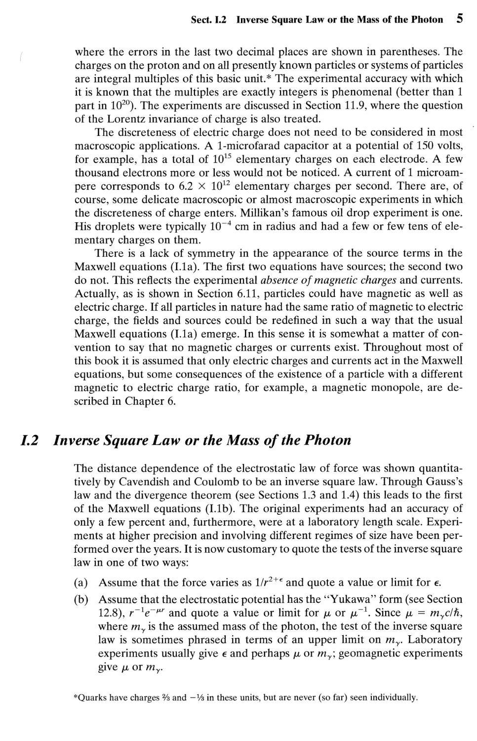
1.2 Inverse Square Law or the Mass of the Photon
The distance dependence of the electrostatic law of force was shown quantita-
quantitatively by Cavendish and Coulomb to be an inverse square law. Through Gauss's
law and the divergence theorem (see Sections 1.3 and 1.4) this leads to the first
of the Maxwell equations (Lib). The original experiments had an accuracy of
only a few percent and, furthermore, were at a laboratory length scale. Experi-
Experiments at higher precision and involving different regimes of size have been per-
performed over the years. It is now customary to quote the tests of the inverse square
law in one of two ways:
(a) Assume that the force varies as l/r2+e and quote a value or limit for e.
(b) Assume that the electrostatic potential has the "Yukawa" form (see Section
12.8), r~xe~^r and quote a value or limit for fi or /л'1. Since /л = myc/h,
where my is the assumed mass of the photon, the test of the inverse square
law is sometimes phrased in terms of an upper limit on my. Laboratory
experiments usually give e and perhaps /л or my\ geomagnetic experiments
give /л or my.
* Quarks have charges % and -Уз in these units, but are never (so far) seen individually.
6 Introduction and Survey
Figure LI Cavendish's apparatus for establishing the inverse square law of
electrostatics. Top, facsimile of Cavendish's own sketch; bottom, line drawing by a
draughtsman. The inner globe is 12.1 inches in diameter, the hollow pasteboard
hemispheres slightly larger. Both globe and hemispheres were covered with tinfoil "to
make them the more perfect conductors of electricity." (Figures reproduced by
permission of the Cambridge University Press.)
Sect. 1.2 Inverse Square Law or the Mass of the Photon 7
The original experiment with concentric spheres by Cavendish* in 1772 gave
an upper limit on e of |e| < 0.02. His apparatus is shown in Fig. I.I.1 About 100
years later Maxwell performed a very similar experiment at Cambridge1 and set
an upper limit of | e| < 5 X 10~5. Two other noteworthy laboratory experiments
based on Gauss's law are those of Plimpton and Lawton,* which gave | e\ < 2 X
10~9, and the recent one of Williams, Faller, and Hill.§ A schematic drawing of
the apparatus of the latter experiment is shown in Fig. 1.2. Though not a static
experiment (v = 4 X 10⁶ Hz), the basic idea is almost the same as Cavendish's.
He looked for a charge on the inner sphere after it had been brought into elec-
electrical contact with the charged outer sphere and then disconnected; he found
none. Williams, Faller, and Hill looked for a voltage difference between two
concentric shells when the outer one was subjected to an alternating voltage of
±10 kV with respect to ground. Their sensitivity was such that a voltage differ-
difference of less than 10~12 V could have been detected. Their null result, when
interpreted by means of the Proca equations (Section 12.8), gives a limit of
6 = B.7 ± 3.1) X 106.
Measurements of the earth's magnetic field, both on the surface and out from
the surface by satellite observation, permit the best direct limits to be set on e or
equivalently the photon mass my. The geophysical and also the laboratory ob-
observations are discussed in the reviews by Kobzarev and Okun' and by Goldhaber
and Nieto, listed at the end of this introduction. The surface measurements of
the earth's magnetic field give slightly the best value (see Problem 12.15), namely,
my < 4 X 10~51 kg
or
fi-1 > 108 m
For comparison, the electron mass is me = 9.1 X 10~31 kg. The laboratory
experiment of Williams, Faller, and Hill can be interpreted as setting a limit
my < 1.6 X 10~50 kg, only a factor of 4 poorer than the geomagnetic limit.
A rough limit on the photon mass can be set quite easily by noting the ex-
existence of very low frequency modes in the earth-ionosphere resonant cavity
(Schumann resonances, discussed in Section 8.9). The double Einstein relation,
hv = myc2, suggests that the photon mass must satisfy an inequality, my <
hvo/c2, where v0 is any electromagnetic resonant frequency. The lowest Schumann
resonance has v0 — 8 Hz. From this we calculate my < 6 X 10~50 kg, a very small
value only one order of magnitude above the best limit. While this argument has
crude validity, more careful consideration (see Section 12.8 and the references
given there) shows that the limit is roughly (R/HI/2 — 10 times larger, R — 6400
km being the radius of the earth, and H — 60 km being the height of the iono-
*H. Cavendish, Electrical Researches, ed. J. С Maxwell, Cambridge University Press, Cambridge
A879), pp. 104-113.
fIbid., see note 19.
*S. J. Plimpton and W. E. Lawton, Phys. Rev. 50, 1066 A936).
§E. R. Williams, J. E. Faller, and H. A. Hill, Phys. Rev. Lett. 26, 721 A971).
8 Introduction and Survey
| Transmitter |
Comparator and
buffer amp
Phase shifter reference
shifts linearly 360°
per % hour
All electronics
inside are battery
powered
Copper
icosahedrons
Aluminum
icosahedrons
Calibration
signal
1
Sealer 50
sec. counting
cycle
Fourier analyze
for signal with
%-hour period
Photo
"=" diode
Figure 1.2 Schematic diagram of the "Cavendish" experiment of Williams, Faller, and
Hill. The concentric icosahedrons are conducting shells. A 4 MHz voltage of 10 kV
peak is applied between shells 5 and 4. Shell 4 and its contiguous shells 2 and 3 are
roughly 1.5 meters in diameter and contain shell 1 inside. The voltage difference
between shells 1 and 2 (if any) appears across the inductor indicated at about 8 o'clock
in shell 1. The amplifier and optics system are necessary to extract the voltage
information to the outside world. They are equivalent to Cavendish's system of strings
that automatically opened the hinged hemispheres and brought up the pith balls to test
for charge on the inner sphere. (Figure reproduced with permission of the authors.)
Sect. 1.3 Linear Superposition 9
sphere.* In spite of this dilution factor, the limit of 1СГ48 kg set by the mere
existence of Schumann resonances is quite respectable.
The laboratory and geophysical tests show that on length scales of order 1СГ2
to 107 m, the inverse square law holds with extreme precision. At smaller dis-
distances we must turn to less direct evidence often involving additional assump-
assumptions. For example, Rutherford's historical analysis of the scattering of alpha
particles by thin foils substantiates the Coulomb law of force down to distances
of the order of 1СГ13 m, provided the alpha particle and the nucleus can be treated
as classical point charges interacting statically and the charge cloud of the elec-
electrons can be ignored. All these assumptions can be, and have been, tested, of
course, but only within the framework of the validity of quantum mechanics,
linear superposition (see below), and other (very reasonable) assumptions. At
still smaller distances, relativistic quantum mechanics is necessary, and strong
interaction effects enter to obscure the questions as well as the answers. Never-
Nevertheless, elastic scattering experiments with positive and negative electrons at cen-
center of mass energies of up to 100 GeV have shown that quantum electrodynamics
(the relativistic theory of point electrons interacting with massless photons) holds
to distances of the order of 10~18 m. We conclude that the photon mass can be
taken to be zero (the inverse square force law holds) over the whole classical
range of distances and deep into the quantum domain as well. The inverse square
law is known to hold over at least 25 orders of magnitude in the length scale!
1.3 Linear Superposition
The Maxwell equations in vacuum are linear in the fields E and B. This linearity
is exploited so often, for example, with hundreds of different telephone conver-
conversations on a single microwave link, that it is taken for granted. There are, of
course, circumstances where nonlinear effects occur—in magnetic materials, in
crystals responding to intense laser beams, even in the devices used to put those
telephone conversations on and off the microwave beam. But here we are con-
concerned with fields in vacuum or the microscopic fields inside atoms and nuclei.
What evidence do we have to support the idea of linear superposition? At
the macroscopic level, all sorts of experiments test linear superposition at the
level of 0.1% accuracy—groups of charges and currents produce electric and
magnetic forces calculable by linear superposition, transformers perform as ex-
expected, standing waves are observed on transmission lines—the reader can make
a list. In optics, slit systems show diffraction patterns; x-ray diffraction tells us
about crystal structure; white light is refracted by a prism into the colors of the
rainbow and recombined into white light again. At the macroscopic and even at
the atomic level, linear superposition is remarkably valid.
It is in the subatomic domain that departures from linear superposition can
be legitimately sought. As charged particles approach each other very closely,
electric field strengths become enormous. If we think of a charged particle as a
*The basic point is that, to the extent that HIR is negligible, the extremely low frequency (ELF)
propagation is the same as in a parallel plate transmission line in the fundamental ТЕМ mode. This
propagation is unaffected by a finite photon mass, except through changes in the static capacitance
and inductance per unit length. Explicit photon mass effects occur in order {HIR) ijl2.
10 Introduction and Survey
localized distribution of charge, we see that its electromagnetic energy grows
larger and larger as the charge is localized more and more. In attempting to avoid
infinite self-energies of point particles, it is natural to speculate that some sort of
saturation occurs, that field strengths have some upper bound. Such classical
nonlinear theories have been studied in the past. One well-known example is
the theory of Born and Infeld.* The vacuum is given electric and magnetic
permeabilities,
— = t° = \l + L ( 2d2 _ ?2ч]
e0 fi I blK >\
-1/2
A.4)
where b is a maximum field strength. Equation A.4) is actually a simplification
proposed earlier by Born alone. It suffices to illustrate the general idea. Fields
are obviously modified at short distances; all electromagnetic energies are finite.
But such theories suffer from arbitrariness in the manner of how the nonlinearity
occurs and also from grave problems with a transition to a quantum theory.
Furthermore, there is no evidence of this kind of classical nonlinearity. The quan-
quantum mechanics of many-electron atoms is described to high precision by normal
quantum theory with the interactions between nucleus and electrons and between
electrons and electrons given by a linear superposition of pairwise potentials (or
retarded relativistic interactions for fine effects). Field strengths of the order of
10n-1017 V/m exist at the orbits of electrons in atoms, while the electric field at
the edge of a heavy nucleus is of the order of 1021 V/m. Energy level differences
in light atoms like helium, calculated on the basis of linear superposition of elec-
electromagnetic interactions, are in agreement with experiment to accuracies that
approach 1 part in 106. And Coulomb energies of heavy nuclei are consistent
with linear superposition of electromagnetic effects. It is possible, of course, that
for field strengths greater than 1021 V/m nonlinear effects could occur. One place
to look for such effects is in superheavy nuclei (Z > 110), both in the atomic
energy levels and in the nuclear Coulomb energy.1 At the present time there
is no evidence for any classical nonlinear behavior of vacuum fields at short
distances.
There is a quantum-mechanical nonlinearity of electromagnetic fields that
arises because the uncertainty principle permits the momentary creation of an
electron-positron pair by two photons and the subsequent disappearance of the
pair with the emission of two different photons, as indicated schematically in Fig.
1.3. This process is called the scattering of light by light^S The two incident plane
waves е1к1-х-1О>1* and е1к2-х-к»2* $о not mereiy acjd coherently, as expected with
linear superposition, but interact and (with small probability) transform into two
different plane waves with wave vectors k3 and k4. This nonlinear feature of
*M. Born and L. Infeld, Proc. R. Soc. London A144, 425 A934). See M. Born, Atomic Physics,
Blackie, London A949), Appendix VI, for an elementary discussion.
+An investigation of the effect of a Born-Infeld type of nonlinearity on the atomic energy levels in
superheavy elements has been made by J. Rafelski, W. Greiner, and L. P. Fulcher, Nuovo Cimento
13B, 135 A973).
*When two of the photons in Fig. 1.3 are virtual photons representing interaction to second order
with a static nuclear Coulomb field, the process is known as Delbrlick scattering. See Section 15.8 of
J. M. Jauch and F. Rohrlich, The Theory of Photons and Electrons, Addison-Wesley, Reading, MA
A955).
Sect. 1.3 Linear Superposition 11
Figure 1.3 The scattering of light by light.
Schematic diagram of the process by which
photon-photon scattering occurs.
quantum electrodynamics can be expressed, at least for slowly varying fields, in
terms of electric and magnetic permeability tensors of the vacuum:
where
T! C A-5)
M* = ^ + 77^ [2(c2S2 - ?2MЛ + 7 ВД + • • •
45 77m с
Here eG and m are the charge (in Gaussian units) and mass of the electron. These
results were first obtained by Euler and Kockel in 1935.* We observe that in the
classical limit (h —» 0), these nonlinear effects go to zero. Comparison with the
classical Born-Infeld expression A.4) shows that for small nonlinearities, the
quantum-mechanical field strength
plays a role analogous to the Born-Infeld parameter b. Here r0 = e^/mc2 —
2.8 X 10~15 m is the classical electron radius and eGlr2Q = 1.8 X 10²⁰ V/m is the
electric field at the surface of such a classical electron. Two comments in passing:
(a) the eik and fiik in A.5) are approximations that fail for field strengths ap-
approaching bq or when the fields vary too rapidly in space or time (h/mc setting
the critical scale of length and h/mc2 of time); (b) the chance numerical coinci-
coincidence of bq and eG/2rl is suggestive but probably not significant, since bq involves
Planck's constant h.
In analogy with the polarization P = D — e0E, we speak of the field-
dependent terms in A.5) as vacuum polarization effects. In addition to the scat-
scattering of light by light or Delbruck scattering, vacuum polarization causes very
small shifts in atomic energy levels. The dominant contribution involves a virtual
electron-positron pair, just as in Fig. 1.3, but with only two photon lines instead
*H. Euler and B. Kockel, Naturwissenschaften 23, 246 A935).
12 Introduction and Survey
of four. If the photons are real, the process contributes to the mass of the photon
and is decreed to vanish. If the photons are virtual, however, as in the electro-
electromagnetic interaction between a nucleus and an orbiting electron, or indeed for
any externally applied field, the creation and annihilation of a virtual electron-
positron pair from time to time causes observable effects.
Vacuum polarization is manifest by a modification of the electrostatic inter-
interaction between two charges at short distances, described as a screening of the
"bare" charges with distance, or in more modern terms as a "running" coupling
constant. Since the charge of a particle is defined as the strength of its electro-
electromagnetic coupling observed at large distances (equivalent to negligible momen-
momentum transfers), the presence of a screening action by electron-positron pairs
closer to the charge implies that the "bare" charge observed at short distances
is larger than the charge defined at large distances. Quantitatively, the lowest
order quantum-electrodynamic result for the Coulomb potential energy between
two charges Zxe and Z2e, corrected for vacuum polarization, is
377 Jim
where a is the fine structure constant (~ 1/137), m is the inverse Compton wave-
wavelength (electron mass, multiplied by c/h). The integral, a superposition of Yukawa
potentials (e~Kr/r) is the one-loop contribution of all the virtual pairs. It increases
the magnitude of the potential energy at distances of separation inside the elec-
electron Compton wavelength (h/mc = aa0 ~ 3.86 X 1СГ13 m).
Because of its short range, the added vacuum polarization energy is unim-
unimportant in light atoms, except for very precise measurements. It is, however,
important in high Z atoms and in muonic atoms, where the heavier mass of the
muon (m^ ~ 207 rae) means that, even in the lightest muonic atoms, the Bohr
radius is well inside the range of the modified potential. X-ray measurements in
medium-mass muonic atoms provide a highly accurate verification of the vacuum
polarization effect in A.6).
The idea of a "running" coupling constant, that is, an effective strength of
interaction that changes with momentum transfer, is illustrated in electromag-
netism by exhibiting the spatial Fourier transform of the interaction energy A.6):
V(Q2) = --~iyv~/ (I 7)
The 1/Q2 dependence is characteristic of the Coulomb potential (familiar in
Rutherford scattering), but now the strength is governed by the so-called running
coupling constant a(Q2), the reciprocal of which is
[a(G2>ri~^-?K^) (L8)
Here a@) = 1/137. 036 ... is the fine structure constant, e is the base of natural
logarithms, and Q2 is the square of the wavenumber (momentum) transfer. The
expression A.8) is an approximation for large Q2/m2. The running coupling a(Q2)
increases slowly with increasing Q2 (shorter distances); the particles are pene-
penetrating inside the cloud of screening electron-positron pairs and experiencing a
larger effective product of charges.
Sect. 1.4 Maxwell Equations in Macroscopic Media 13
Since the lowest order vacuum polarization energy is proportional to a times
the external charges, we describe it as a linear effect, even though it involves (in
a) the square of the internal charge of the electron and positron. Small higher
order effects, such as in Fig. 1.3 with three of the photons corresponding to the
third power of the external field or charge, are truly nonlinear interactions.
The final conclusion about linear superposition of fields in vacuum is that in
the classical domain of sizes and attainable field strengths there is abundant ev-
evidence for the validity of linear superposition and no evidence against it. In the
atomic and subatomic domain there are small quantum-mechanical nonlinear
effects whose origins are in the coupling between charged particles and the elec-
electromagnetic field. They modify the interactions between charged particles and
cause interactions between electromagnetic fields even if physical particles are
absent.
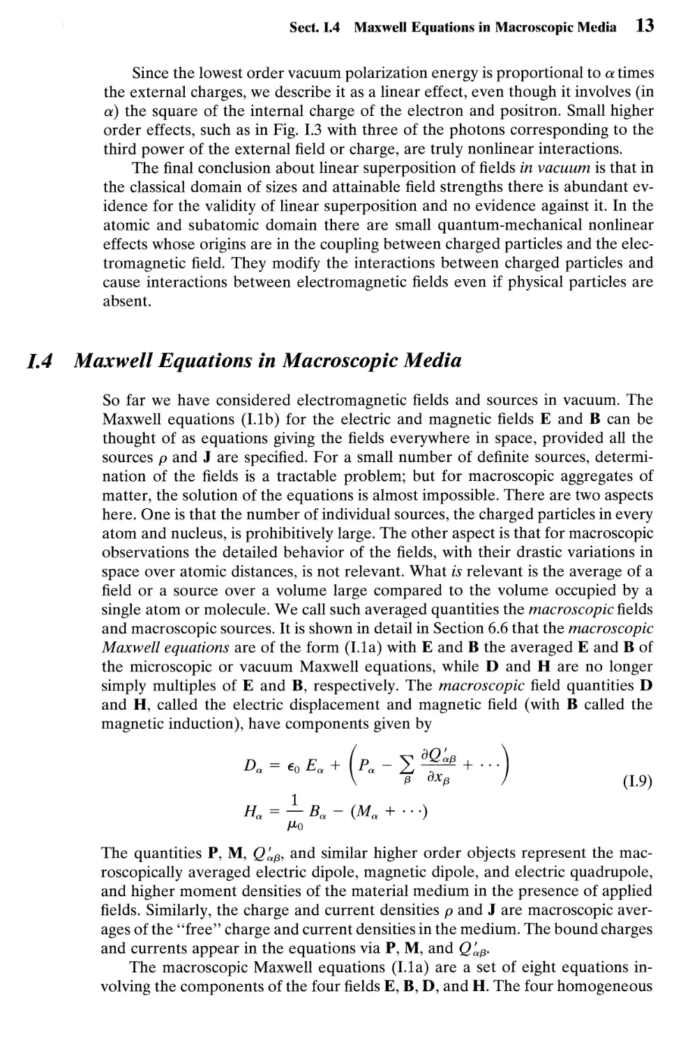
1.4 Maxwell Equations in Macroscopic Media
So far we have considered electromagnetic fields and sources in vacuum. The
Maxwell equations (Lib) for the electric and magnetic fields E and В can be
thought of as equations giving the fields everywhere in space, provided all the
sources p and J are specified. For a small number of definite sources, determi-
determination of the fields is a tractable problem; but for macroscopic aggregates of
matter, the solution of the equations is almost impossible. There are two aspects
here. One is that the number of individual sources, the charged particles in every
atom and nucleus, is prohibitively large. The other aspect is that for macroscopic
observations the detailed behavior of the fields, with their drastic variations in
space over atomic distances, is not relevant. What is relevant is the average of a
field or a source over a volume large compared to the volume occupied by a
single atom or molecule. We call such averaged quantities the macroscopic fields
and macroscopic sources. It is shown in detail in Section 6.6 that the macroscopic
Maxwell equations are of the form (I.la) with E and В the averaged E and В of
the microscopic or vacuum Maxwell equations, while D and H are no longer
simply multiples of E and B, respectively. The macroscopic field quantities D
and H, called the electric displacement and magnetic field (with В called the
magnetic induction), have components given by
A.9)
на = — ва - (ма + • • )
Мо
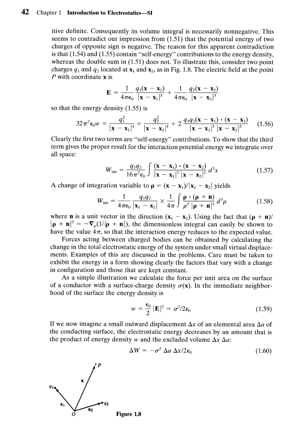
The quantities P, M, Q^ and similar higher order objects represent the mac-
roscopically averaged electric dipole, magnetic dipole, and electric quadrupole,
and higher moment densities of the material medium in the presence of applied
fields. Similarly, the charge and current densities p and J are macroscopic aver-
averages of the "free" charge and current densities in the medium. The bound charges
and currents appear in the equations via P, M, and Q'ap.
The macroscopic Maxwell equations (I.la) are a set of eight equations in-
involving the components of the four fields E, B, D, and H. The four homogeneous
14 Introduction and Survey
equations can be solved formally by expressing E and В in terms of the scalar
potential Ф and the vector potential A, but the inhomogeneous equations cannot
be solved until the derived fields D and H are known in terms of E and B. These
connections, which are implicit in A.9), are known as constitutive relations,
D = D[E, B]
H = H[E, B]
In addition, for conducting media there is the generalized Ohm's law,
J = J[E, B]
The square brackets signify that the connections are not necessarily simple and
may depend on past history (hysteresis), may be nonlinear, etc.
In most materials the electric quadrupole and higher terms in A.9) are com-
completely negligible. Only the electric and magnetic polarizations P and M are sig-
significant. This does not mean, however, that the constitutive relations are then
simple. There is tremendous diversity in the electric and magnetic properties of
matter, especially in crystalline solids, with ferroelectric and ferromagnetic ma-
materials having nonzero P or M in the absence of applied fields, as well as more
ordinary dielectric, diamagnetic, and paramagnetic substances. The study of these
properties is one of the provinces of solid-state physics. In this book we touch
only very briefly and superficially on some more elementary aspects. Solid-state
books such as Kittel should be consulted for a more systematic and extensive
treatment of the electromagnetic properties of bulk matter.
In substances other than ferroelectrics or ferromagnets, for weak enough
fields the presence of an applied electric or magnetic field induces an electric or
magnetic polarization proportional to the magnitude of the applied field. We
then say that the response of the medium is linear and write the Cartesian com-
components of D and H in the form,*
Dn =
The tensors ea/3 and /л'ар are called the electric permittivity or dielectric tensor
and the inverse magnetic permeability tensor. They summarize the linear re-
response of the medium and are dependent on the molecular and perhaps crystal-
crystalline structure of the material, as well as bulk properties like density and temper-
temperature. For simple materials the linear response is often isotropic in space. Then
ea/3 and /Hap are diagonal with all three elements equal, and D = eE, H = ^'B
= B//JL.
To be generally correct Eqs. A.10) should be understood as holding for the Fourier
transforms in space and time of the field quantities. This is because the basic linear con-
connection between D and E (or H and B) can be nonlocal. Thus
Da(x, 0 = 2| d3x' I dt' eaj8(x\ t')Ep(x -x',t- tf)
/3 J J
* Precedent would require writing Ba = 2^ /ларНр, but this reverses the natural roles of В as the basic
magnetic field and H as the derived quantity. In Chapter 5 we revert to the traditional usage.
Sect. 1.4 Maxwell Equations in Macroscopic Media 15
where ea/3(x', t') may be localized around x' = 0, t' = 0, but is nonvanishing for some
range away from the origin. If we introduce the Fourier transforms Da(k, со), Ep(k, со),
and ea/8(k, со) through
;, о) = J d3x J dt f(x, t)e~
Eq. A.10) can be written in terms of the Fourier transforms as
Da(k, со) = 2 eaj8(k, w)E^(k, <u) A.11)
A similar equation can be written Ha(k, со) in terms ofBp(k, со). The permeability tensors
are therefore functions of frequency and wave vector in general. For visible light or elec-
electromagnetic radiation of longer wavelength it is often permissible to neglect the non-
locality in space. Then ea/3 and /x^ are functions only of frequency. This is the situation
discussed in Chapter 7, which gives a simplified treatment of the high frequency properties
of matter and explores the consequences of causality. For conductors and superconductors
long-range effects can be important. For example, when the electronic collisional mean
free path in a conductor becomes large compared to the skin depth, a spatially local form
of Ohm's law is no longer adequate. Then the dependence on wave vector also enters. In
the understanding of a number of properties of solids the concept of a dielectric constant
as a function of wave vector and frequency is fruitful. Some exemplary references are
given in the suggested reading at the end of this introduction.
For orientation we mention that at low frequencies (v ^ 106 Hz) where all
charges, regardless of their inertia, respond to applied fields, solids have dielectric
constants typically in the range of eaa/e0 ~ 2-20 with larger values not uncom-
uncommon. Systems with permanent molecular dipole moments can have much larger
and temperature-sensitive dielectric constants. Distilled water, for example, has
a static dielectric constant of e/e0 = 88 at 0°C and e/e0 = 56 at 100°C. At optical
frequencies only the electrons can respond significantly. The dielectric constants
are in the range, eaa/e0 ~ 1.7-10, with eajeo — 2-3 for most solids. Water has
e/e0 = 1.77-1.80 over the visible range, essentially independent of temperature
from 0 to 100°C.
The type of response of materials to an applied magnetic field depends on
the properties of the individual atoms or molecules and also on their interactions.
Diamagnetic substances consist of atoms or molecules with no net angular mo-
momentum. The response to an applied magnetic field is the creation of circulating
atomic currents that produce a very small bulk magnetization opposing the ap-
applied field. With the definition of fi^p in A.10) and the form of A.9), this means
№о1л'аа > 1. Bismuth, the most diamagnetic substance known, has (/ло/л^ - 1) —
1.8 X 10~4. Thus diamagnetism is a very small effect. If the basic atomic unit of
the material has a net angular momentum from unpaired electrons, the substance
is paramagnetic. The magnetic moment of the odd electron is aligned parallel to
the applied field. Hence /ло/л^а < 1. Typical values are in the range A - 1Лф'аа)
— 10~2-10~5 at room temperature, but decreasing at higher temperatures be-
because of the randomizing effect of thermal excitations.
Ferromagnetic materials are paramagnetic but, because of interactions be-
between atoms, show drastically different behavior. Below the Curie temperature
A040 К for Fe, 630 К for Ni), ferromagnetic substances show spontaneous mag-
magnetization; that is, all the magnetic moments in a microscopically large region
called a domain are aligned. The application of an external field tends to cause
16 Introduction and Survey
the domains to change and the moments in different domains to line up together,
leading to the saturation of the bulk magnetization. Removal of the field leaves
a considerable fraction of the moments still aligned, giving a permanent mag-
magnetization that can be as large as Br = /л0Мг ^ 1 tesla.
For data on the dielectric and magnetic properties of materials, the reader
can consult some of the basic physics handbooks* from which he or she will be
led to more specific and detailed compilations.
Materials that show a linear response to weak fields eventually show nonlin-
nonlinear behavior at high enough field strengths as the electronic or ionic oscillators
are driven to large amplitudes. The linear relations A.10) are modified to, for
example,
A, = 2 ^ + 2 e%EpEy +¦¦¦ A.12)
/3 /3,7
For static fields the consequences are not particularly dramatic, but for time-
varying fields it is another matter. A large amplitude wave of two frequencies щ
and (o2 generates waves in the medium with frequencies 0, 2(оъ 2w2, сог + co2,
а)г - co2, as well as the original а)г and co2. From cubic and higher nonlinear terms
an even richer spectrum of frequencies can be generated. With the development
of lasers, nonlinear behavior of this sort has become a research area of its own,
called nonlinear optics, and also a laboratory tool. At present, lasers are capable
of generating light pulses with peak electric fields approaching 1012 or even 1013
V/m. The static electric field experienced by the electron in its orbit in a hydrogen
atom is eG/al — 5 X 10¹¹ V/m. Such laser fields are thus seen to be capable of
driving atomic oscillators well into their nonlinear regime, capable indeed of
destroying the sample under study! References to some of the literature of this
specialized field are given in the suggested reading at the end of this introduction.
The reader of this book will have to be content with basically linear phenomena.
/.5 Boundary Conditions at Interfaces Between Different Media
The Maxwell equations (I.I) are differential equations applying locally at each
point in space-time (x, t). By means of the divergence theorem and Stokes's
theorem, they can be cast in integral form. Let У be a finite volume in space, S
the closed surface (or surfaces) bounding it, da an element of area on the surface,
and n a unit normal to the surface at da pointing outward from the enclosed
volume. Then the divergence theorem applied to the first and last equations of
(I.la) yields the integral statements
<P D • n da = pd3x A.13)
Js Jv
В • n da = 0 A.14)
*CRC Handbook of Chemistry and Physics, ed. D. R. Lide, 78th ed., CRC Press, Boca Raton, FL
A997-98).
American Institute of Physics Handbook, ed. D. E. Gray, McGraw Hilll, New York, 3rd edition
A972), Sections 5.d and 5.f.
Sect. 1.5 Boundary Conditions at Interfaces Between Different Media 17
The first relation is just Gauss's law that the total flux of D out through the surface
is equal to the charge contained inside. The second is the magnetic analog, with
no net flux of В through a closed surface because of the nonexistence of magnetic
charges.
Similarly, let С be a closed contour in space, S' an open surface spanning
the contour, d\ a line element on the contour, da an element of area on S\ and
n' a unit normal at da pointing in the direction given by the right-hand rule from
the sense of integration around the contour. Then applying Stokes's theorem to
the middle two equations in (I.la) gives the integral statements
d\ =
Jc Js' dt
— • n' da
da
A.15)
A.16)
Equation A.15) is the Ampere-Maxwell law of magnetic fields and A.16) is
Faraday's law of electromagnetic induction.
These familiar integral equivalents of the Maxwell equations can be used
directly to deduce the relationship of various normal and tangential components
of the fields on either side of a surface between different media, perhaps with a
surface charge or current density at the interface. An appropriate geometrical
arrangement is shown in Fig. 1.4. An infinitesimal Gaussian pillbox straddles the
boundary surface between two media with different electromagnetic properties.
Similarly, the infinitesimal contour С has its long arms on either side of the
boundary and is oriented so that the normal to its spanning surface is tangent to
the interface. We first apply the integral statements A.13) and A.14) to the vol-
volume of the pillbox. In the limit of a very shallow pillbox, the side surface does
Figure 1.4 Schematic diagram of boundary surface (heavy line) between different
media. The boundary region is assumed to carry idealized surface charge and current
densities a and K. The volume У is a small pillbox, half in one medium and half in the
other, with the normal n to its top pointing from medium 1 into medium 2. The
rectangular contour С is partly in one medium and partly in the other and is oriented
with its plane perpendicular to the surface so that its normal t is tangent to the surface.
18 Introduction and Survey
not contribute to the integrals on the left in A.13) and A.14). Only the top and
bottom contribute. If the top and the bottom are parallel, tangent to the surface,
and of area Aa, then the left-hand integral in A.13) is
s
D • n da = (D2 - DO • n Aa
and similarly for A.14). If the charge density p is singular at the interface so as
to produce an idealized surface charge density <x, then the integral on the right
in A.13) is
p d3x = <j Aa
Thus the normal components of D and В on either side of the boundary surface
are related according to
(D2 - DO • n = a A.17)
(B2 - BO • n = 0 A.18)
In words, we say that the normal component of В is continuous and the discon-
discontinuity of the normal component of D at any point is equal to the surface charge
density at that point.
In an analogous manner the infinitesimal Stokesian loop can be used to de-
determine the discontinuities of the tangential components of E and H. If the short
arms of the contour С in Fig. 1.4 are of negligible length and each long arm is
parallel to the surface and has length A/, then the left-hand integral of A.16) is
E • d\ = (t x n) • (E2 - EO A/
and similarly for the left-hand side of A.15). The right-hand side of A.16) vanishes
because дВ/dt is finite at the surface and the area of the loop is zero as the length
of the short sides goes to zero. The right-hand side of A.15) does not vanish,
however, if there is an idealized surface current density К flowing exactly on the
boundary surface. In such circumstances the integral on the right of A.15) is
The second term in the integral vanishes by the same argument that was just
given. The tangential components of E and H on either side of the boundary are
therefore related by
n x (E2 - EO = 0 A.19)
n x (H2 - HO = К A.20)
In A.20) it is understood that the surface current К has only components parallel
to the surface at every point. The tangential component of E across an interface
is continuous, while the tangential component of H is discontinuous by an amount
whose magnitude is equal to the magnitude of the surface current density and
whose direction is parallel to К х n.
The discontinuity equations (I.17)-(I.2O) are useful in solving the Maxwell
Sect. 1.6 Some Remarks on Idealizations in Electromagnetism 19
equations in different regions and then connecting the solutions to obtain the
fields throughout all space.
L6 Some Remarks on Idealizations in Electromagnetism
In the preceding section we made use of the idea of surface distributions of charge
and current. These are obviously mathematical idealizations that do not exist in
the physical world. There are other abstractions that occur throughout electro-
electromagnetism. In electrostatics, for example, we speak of holding objects at a fixed
potential with respect to some zero of potential usually called "ground." The
relations of such idealizations to the real world is perhaps worthy of a little dis-
discussion, even though to the experienced hand most will seem obvious.
First we consider the question of maintaining some conducting object at a
fixed electrostatic potential with respect to some reference value. Implicit is the
idea that the means does not significantly disturb the desired configuration of
charges and fields. To maintain an object at fixed potential it is necessary, at least
from time to time, to have a conducting path or its equivalent from the object to
a source of charge far away ("at infinity") so that as other charged or uncharged
objects are brought in the vicinity, charge can flow to or from the object, always
maintaining its potential at the desired value. Although more sophisticated
means are possible, metallic wires are commonly used to make the conducting
path. Intuitively we expect small wires to be less perturbing than large ones. The
reason is as follows:
Since the quantity of electricity on any given portion of a wire at a given
potential diminishes indefinitely when the diameter of the wire is indefi-
indefinitely diminished, the distribution of electricity on bodies of considerable
dimensions will not be sensibly affected by the introduction of very
fine metallic wires into the field, such as are used to form electrical con-
connexions between these bodies and the earth, an electrical machine, or an
electrometer.*
The electric field in the immediate neighborhood of the thin wire is very large,
of course. However, at distances away of the order of the size of the "bodies of
considerable dimensions" the effects can be made small. An important historical
illustration of Maxwell's words is given by the work of Henry Cavendish 200
years ago. By experiments done in a converted stable of his father's house, using
Leyden jars as his sources of charge, thin wires as conductors, and suspending
the objects in the room, Cavendish measured the amounts of charge on cylinders,
discs, etc., held at fixed potential and compared them to the charge on a sphere
(the same sphere shown in Fig. I.I) at the same potential. His values of capaci-
capacitance, so measured, are accurate to a few per cent. For example, he found the
ratio of the capacitance of a sphere to that of a thin circular disc of the same
radius was 1.57. The theoretical value is тг/2.
There is a practical limit to the use of finer and finer wires. The charge per
unit length decreases only logarithmically [as the reciprocal of \n(d/a), where a
*J. C. Maxwell, Л Treatise on Electricity and Magnetism, Dover, New York, 1954 reprint of the 3rd
edition A891), Vol. 1, p. 96.
20 Introduction and Survey
is the mean radius of the wire and d is a typical distance of the wire from some
conducting surface]. To minimize the perturbation of the system below some
level, it is necessary to resort to other means to maintain potentials, comparison
methods using beams of charged particles intermittently, for example.
When a conducting object is said to be grounded, it is assumed to be con-
connected by a very fine conducting filament to a remote reservoir of charge that
serves as the common zero of potential. Objects held at fixed potentials are sim-
similarly connected to one side of a voltage source, such as a battery, the other side
of which is connected to the common "ground." Then, when initially electrified
objects are moved relative to one another in such a way that their distributions
of electricity are altered, but their potentials remain fixed, the appropriate
amounts of charge flow from or to the remote reservoir, assumed to have an
inexhaustible supply. The idea of grounding something is a well-defined concept
in electrostatics, where time is not a factor, but for oscillating fields the finite
speed of propagation blurs the concept. In other words, stray inductive and ca-
pacitive effects can enter significantly. Great care is then necessary to ensure a
"good ground."
Another idealization in macroscopic electromagnetism is the idea of a surface
charge density or a surface current density. The physical reality is that the charge
or current is confined to the immediate neighborhood of the surface. If this region
has thickness small compared to the length scale of interest, we may approximate
the reality by the idealization of a region of infinitesimal thickness and speak of
a surface distribution. Two different limits need to be distinguished. One is the
limit in which the "surface" distribution is confined to a region near the surface
that is macroscopically small, but microscopically large. An example is the pen-
penetration of time-varying fields into a very good, but not perfect, conductor, de-
described in Section 8.1. It is found that the fields are confined to a thickness 8,
called the skin depth, and that for high enough frequencies and good enough
conductivities 8 can be macroscopically very small. It is then appropriate to in-
integrate the current density J over the direction perpendicular to the surface to
obtain an effective surface current density Keff.
The other limit is truly microscopic and is set by quantum-mechanical effects
in the atomic structure of materials. Consider, for instance, the distribution of
excess charge of a conducting body in electrostatics. It is well known that this
charge lies entirely on the surface of a conductor. We then speak of a surface
charge density <x. There is no electric field inside the conductor, but there is, in
accord with A.17), a normal component of electric field just outside the surface.
At the microscopic level the charge is not exactly at the surface and the field
does not change discontinuously. The most elementary considerations would in-
indicate that the transition region is a few atomic diameters in extent. The ions in
a metal can be thought of as relatively immobile and localized to 1 angstrom
or better; the lighter electrons are less constrained. The results of model cal-
calculations* are shown in Fig. 1.5. They come from a solution of the quantum-
mechanical many-electron problem in which the ions of the conductor are
approximated by a continuous constant charge density for x < 0. The electron
density (rs = 5) is roughly appropriate to copper and the heavier alkali metals.
*N. D. Lang and W. Kohn, Phys. Rev. Bl, 4555 A970); B3, 1215 A971); V. E. Kenner, R. E. Allen,
and W. M. Saslow, Phys. Lett. 38A, 255 A972).
Sect. 1.6 Some Remarks on Idealizations in Electromagnetism 21
0.2 -
-0.2 -
Figure 1.5 Distribution of excess charge at the surface of a conductor and of the
normal component of the electric field. The ions of the solid are confined to x < 0 and
are approximated by a constant continuous charge distribution through which the
electrons move. The bulk of the excess charge is confined to within ±2 A of the
"surface."
The excess electronic charge is seen to be confined to a region within ±2 A of
the "surface" of the ionic distribution. The electric field rises smoothly over this
region to its value of <x "outside" the conductor. For macroscopic situations
where 10~9 m is a negligible distance, we can idealize the charge density and
electric field behavior as p(x) = a8(x) and En(x) = <x0(x)/eo, corresponding to a
truly surface density and a step-function jump of the field.
We see that the theoretical treatment of classical electromagnetism involves
several idealizations, some of them technical and some physical. The subject of
electrostatics, discussed in the first chapters of the book, developed as an exper-
experimental science of macroscopic electrical phenomena, as did virtually all other
aspects of electromagnetism. The extension of these macroscopic laws, even for
charges and currents in vacuum, to the microscopic domain was for the most part
an unjustified extrapolation. Earlier in this introduction we discussed some of
the limits to this extrapolation. The point to be made here is the following. With
hindsight we know that many aspects of the laws of classical electromagnetism
apply well into the atomic domain provided the sources are treated quantum
mechanically, that the averaging of electromagnetic quantities over volumes con-
containing large numbers of molecules so smooths the rapid fluctuations that static
applied fields induce static average responses in matter, and that excess charge
is on the surface of a conductor in a macroscopic sense. Thus Coulomb's and
Ampere's macroscopic observations and our mathematical abstractions from
them have a wider applicability than might be supposed by a supercautious phys-
22 Introduction and Survey
icist. The absence for air of significant electric or magnetic susceptibility certainly
simplifies matters!
References and Suggested Reading
The history of electricity and magnetism is in large measure the history of science
itself. We have already cited Whittaker's two volumes, the first covering the period up to
1900, as well as the shorter account emphasizing optics in
Born and Wolf.
Another readable account, with perceptive discussion of the original experiments, is
N. Feather, Electricity and Matter, University Press, Edinburgh A968).
The experimental tests of the inverse square nature of Coulomb's law or, in modern
language, the mass of the photon, are reviewed by
I. Yu. Kobzarev and L. B. Okun', Usp. Fiz. Nauk 95, 131 A968) [transl., Sov.
Phys. Usp. 11, 338 A968).]
and
A. S. Goldhaber and M. M. Nieto, Rev. Mod. Phys. 43, 277 A971).
An accessible treatment of the gauge principle in the construction of field theories,
building on classical electrodynamics and ordinary quantum mechanics, can be found in
I. J. R. Aitchison and A. J. G. Hey, Gauge Theories in Particle Physics, 2nd ed.,
Adam Hilger, Bristol A989).
Suggested reading on the topic of the macroscopic Maxwell equations and their der-
derivation from the microscopic equations can be found at the end of Chapter 6. The basic
physics of dielectrics, ferroelectrics, and magnetic materials can be found in numerous
books on solid-state physics, for example,
Ashcroft and Mermin
Beam
Kittel
Wert and Thomson
Wooten
The second of these is aimed at electrical engineers and stresses practical topics like
semiconductors. The last one is mainly on optical properties. The need for spatial non-
locality in treating the surface impedance of metals (the anomalous skin effect) is discussed
in several places by
A. B. Pippard, Advances in Electronics and Electron Physics, Vol. VI, ed. L.
Marton, Academic Press, New York A954), pp. 1-45; Reports on Progress in
Physics, Vol. XXIII, pp. 176-266 (I960); The Dynamics of Conduction Electrons,
Gordon and Breach, New York A965).
The concept of a wave-vector and frequency-dependent dielectric constant e(k, со) is
developed by
Kittel, Advanced Topic D.
D. Pines, Elementary Excitations in Solids, W. A. Benjamin, New York A963),
Chapters 3 and 4.
F. Stern, Solid State Physics, Vol. 15, eds. F. Seitz and D. Turnbull, Academic
Press, New York, pp. 299-408.
The field of nonlinear optics is now nearly 40 years old. Beginnings and introductions
can be found in
J. A. Giordmaine, Phys. Today 22A), 38 A969).
N. Bloembergen, Am. J. Phys. 35, 989 A967).
References 23
Nonlinear optical phenomena and applications are discussed in
R. L. Sutherland, Handbook of Nonlinear Optics, Marcel Dekker, New York
A966).
Some texts and monographs on the subject are
R. W. Boyd, Nonlinear Optics, Academic Press, New York A990).
M. Schubert and B. Wilhelmi, Nonlinear Optics and Quantum Electronics, Wiley,
New York A986).
Y. R. Shen, The Principles of Nonlinear Optics, Wiley, New York A984).
CHAPTER 1
Introduction to Electrostatics
We begin our discussion of electrodynamics with the subject of electrostatics—
phenomena involving time-independent distributions of charge and fields. For
most readers this material is in the nature of a review. In this chapter especially
we do not elaborate significantly. We introduce concepts and definitions that are
important for later discussion and present some essential mathematical appara-
apparatus. In subsequent chapters the mathematical techniques are developed and
applied.
One point of physics should be mentioned. Historically, electrostatics devel-
developed as a science of macroscopic phenomena. As indicated at the end of the
Introduction, such idealizations as point charges or electric fields at a point must
be viewed as mathematical constructs that permit a description of the phenomena
at the macroscopic level, but that may fail to have meaning microscopically.
1.1 Coulomb's Law
All of electrostatics stems from the quantitative statement of Coulomb's law
concerning the force acting between charged bodies at rest with respect to each
other. Coulomb; in an impressive series of experiments, showed experimentally
that the force between two small charged bodies separated in air a distance large
compared to their dimensions
varies directly as the magnitude of each charge,
varies inversely as the square of the distance between them,
is directed along the line joining the charges, and
is attractive if the bodies are oppositely charged and repulsive if the bodies have
the same type of charge.
Furthermore it was shown experimentally that the total force produced on one
small charged body by a number of the other small charged bodies placed around
it is the vector sum of the individual two-body forces of Coulomb. Strictly speak-
speaking, Coulomb's conclusions apply to charges in vacuum or in media of negligible
susceptibility. We defer consideration of charges in dielectrics to Chapter 4.
1.2 Electric Field
Although the thing that eventually gets measured is a force, it is useful to intro-
introduce a concept one step removed from the forces, the concept of an electric field
due to some array of charged bodies. At the moment, the electric field can be
24
Sect. 1.2 Electric Field 25
defined as the force per unit charge acting at a given point. It is a vector function
of position, denoted by E. One must be careful in its definition, however. It is
not necessarily the force that one would observe by placing one unit of charge
on a pith ball and placing it in position. The reason is that one unit of charge
may be so large that its presence alters appreciably the field configuration of the
array. Consequently one must use a limiting process whereby the ratio of the
force on the small test body to the charge on it is measured for smaller and smaller
amounts of charge.* Experimentally, this ratio and the direction of the force will
become constant as the amount of test charge is made smaller and smaller. These
limiting values of magnitude and direction define the magnitude and direction of
the electric field E at the point in question. In symbols we may write
F = qE A.1)
where F is the force, E the electric field, and q the charge. In this equation it is
assumed that the charge q is located at a point, and the force and the electric
field are evaluated at that point.
Coulomb's law can be written down similarly. If F is the force on a point
charge qu located at xb due to another point charge q2, located at x2, then
Coulomb's law is
X~X A.2)
1 ~" X2
Note that qx and q2 are algebraic quantities, which can be positive or negative.
The constant of proportionality к depends on the system of units used.
The electric field at the point x due to a point charge qx at the point xx can
be obtained directly:
E(x) = kqx ^—^ъ A.3)
| X Xi I
as indicated in Fig. 1.1. The constant к differs in different systems of units.f In
electrostatic units (esu), к — 1 and unit charge is chosen as that charge that exerts
a force of one dyne on an equal point charge located one centimeter away. The
esu unit of charge is called the statcoulomb, and the electric field is measured in
statvolts per centimeter. In the SI system, which we employ here, к = ^тгео) =
1СГ7с2, where e0 ~ 8.854 X 1СГ12 farad per meter (F/m) is called the permittivity
of free space. The SI unit of charge is the coulomb (C), and the electric field is
measured in volts per meter (V/m). One coulomb A C) produces an electric field
Figure 1.1
*The discreteness of electric charge (see Section I.I) means that this mathematical limit is impossible
to realize physically. This is an example of a mathematical idealization in macroscopic electrostatics.
fThe question of units is discussed in detail in the Appendix.
26 Chapter 1 Introduction to Electrostatics—SI
of approximately 8.9874 X 10⁹ V/m (8.9874 GV/m) at a distance of 1 meter. One
electron (q « 1.602 X 1(Г19 С) produces a field of approximately 1.44 X 1(T9
V/m A.44 nV/m) at 1 meter.
The experimentally observed linear superposition of forces due to many
charges means that we may write the electric field at x due to a system of point
charges qt, located at \h i = 1, 2,..., n, as the vector sum:
1 ^ x - x, ^
— 1 | A. Aj |
If the charges are so small and so numerous that they can be described by a
charge density p(x') [if Aq is the charge in a small volume Ax Ay Az at the point
x\ then Aq = p(x') Ax Ay Az], the sum is replaced by an integral:
»'),*"'нз^' A-5)
where d3x' = dx' dy' dz' is & three-dimensional volume element at x'.
At this point it is worthwhile to introduce the Dirac delta function. In one dimension,
the delta function, written 8(x -a), is a mathematically improper function having the
properties:
1. 8(x - a) = 0 for x Ф a, and
2. / 8(x — a) dx = 1 if the region of integration includes x = a, and is zero otherwise.
The delta function can be given an intuitive, but nonrigorous, meaning as the limit of a
peaked curve such as a Gaussian that becomes narrower and narrower, but higher and
higher, in such a way that the area under the curve is always constant. L. Schwartz's theory
of distributions is a comprehensive rigorous mathematical approach to delta functions and
their manipulations.*
From the definitions above it is evident that, for an arbitrary function f(x),
3. f f(x) S(x - a) dx = f(a).
The integral of f(x) times the derivative of a delta function is simply understood if the
delta function is thought of as a well-behaved, but sharply peaked, function. Thus the
definition is
4. Jf(x)8'(x-a)dx= -f(a)
where a prime denotes differentiation with respect to the argument.
If the delta function has as argument a function f(x) of the independent variable x,
it can be transformed according to the rule,
5. 8(f(x)) = yj 8(x-xt)
where f(x) is assumed to have only simple zeros, located at x = xt.
In more than one dimension, we merely take products of delta functions in each
dimension. In three dimensions, for example, with Cartesian coordinates,
6. 8(x - X) - 8(Xl - Хг) 8(x2 - X2) 8(x3 - X3)
*A useful, rigorous account of the Dirac delta function is given by Lighthili See also Dennery and
Krzywicki (Section III.13). (Full references for items cited in the text or footnotes by italicized author
only will be found in the Bibliography.)
Sect. 1.3 Gauss's Law 27
is a function that vanishes everywhere except at x = X, and is such that
f ^ - \W3 - i1 if ^V contains x = X
Jav [O if AV does not contain x = X
Note that a delta function has the dimensions of an inverse volume in whatever number
of dimensions the space has.
A discrete set of point charges can be described with a charge density by means of
delta functions. For example,
n
/ ч X^ s/ _ \ (л (Л
i=l
represents a distribution of n point charges qh located at the points хг. Substitution of this
charge density A.6) into A.5) and integration, using the properties of the delta function,
yields the discrete sum A.4).
1.3 Gauss's Law
The integral A.5) is not always the most suitable form for the evaluation of
electric fields. There is another integral result, called Gauss's law, which is some-
sometimes more useful and furthermore leads to a differential equation for E(x). To
obtain Gauss's law we first consider a point charge q and a closed surface S, as
shown in Fig. 1.2. Let r be the distance from the charge to a point on the surface,
n be the outwardly directed unit normal to the surface at that point, da be an
q outside S
q inside S
Figure 1.2 Gauss's law. The normal component of electric field is integrated over the
closed surface S. If the charge is inside (outside) S, the total solid angle subtended at
the charge by the inner side of the surface is 4тг (zero).
28 Chapter 1 Introduction to Electrostatics—SI
element of surface area. If the electric field E at the point on the surface due to
the charge q makes an angle в with the unit normal, then the normal component
of E times the area element is:
q cos 0
-5- da A.7)
Since E is directed along the line from the surface element to the charge q,
cos в da = r2 dft, where dfl is the element of solid angle subtended by da at
the position of the charge. Therefore
E • n da = ~r— dil A.8)
4Т76
If we now integrate the normal component of E over the whole surface, it is easy
to see that
{qleQ if q lies inside S
4 ч A.9)
0 ftq lies outside S
This result is Gauss's law for a single point charge. For a discrete set of charges,
it is immediately apparent that
E • n da = - E qt A.10)
s 60 i
where the sum is over only those charges inside the surface S. For a continuous
charge density p(x), Gauss's law becomes:
<P E • n da = — I p(x) d3x A.11)
where V is the volume enclosed by 5.
Equation A.11) is one of the basic equations of electrostatics. Note that it
depends upon
the inverse square law for the force between charges,
the central nature of the force, and
the linear superposition of the effects of different charges.
Clearly, then, Gauss's law holds for Newtonian gravitational force fields, with
matter density replacing charge density.
It is interesting to note that, even before the experiments of Cavendish and
Coulomb, Priestley, taking up an observation of Franklin that charge seemed to
reside on the outside, but not the inside, of a metal cup, reasoned by analogy
with Newton's law of universal gravitation that the electrostatic force must obey
an inverse square law with distance. The present status of the inverse square law
is discussed in Section 1.2.
1.4 Differential Form of Gauss's Law
Gauss's law can be thought of as being an integral formulation of the law of
electrostatics. We can obtain a differential form (i.e., a differential equation) by
Sect. 1.5 Another Equation of Electrostatics and the Scalar Potential 29
using the divergence theorem. The divergence theorem states that for any well-
behaved vector field A(x) defined within a volume V surrounded by the closed
surface S the relation
<P A • n da = I
Js Jv
holds between the volume integral of the divergence of A and the surface integral
of the outwardly directed normal component of A. The equation in fact can be
used as the definition of the divergence (see Stratton, p. 4).
To apply the divergence theorem we consider the integral relation expressed
in Gauss's theorem:
ф Е • n da = — р(х)
JS €n Jv
JS €0
Now the divergence theorem allows us to write this as
3x =
(V • Е - pleQ) d3x = О A.12)
for an arbitrary volume V. We can, in the usual way, put the integrand equal to
zero to obtain
V • E = ple0 A.13)
which is the differential form of Gauss's law of electrostatics. This equation can
itself be used to solve problems in electrostatics. However, it is often simpler to
deal with scalar rather then vector functions of position, and then to derive the
vector quantities at the end if necessary (see below).
/.5 Another Equation of Electrostatics and the Scalar Potential
The single equation A.13) is not enough to specify completely the three com-
components of the electric field E(x). Perhaps some readers know that a vector field
can be specified almost* completely if its divergence and curl are given every-
everywhere in space. Thus we look for an equation specifying curl E as a function of
position. Such an equation, namely,
V x E = 0 A.14)
follows directly from our generalized Coulomb's law A.5):
P(x') ^—''
The vector factor in the integrand, viewed as a function of x, is the negative
gradient of the scalar l/|x - x' |:
x - x'|3 \|x - x'
*Up to the gradient of a scalar function that satisfies the Laplace equation. See Section 1.9 on
uniqueness.
30 Chapter 1 Introduction to Electrostatics—SI
Since the gradient operation involves x, but not the integration variable x', it can
be taken outside the integral sign. Then the field can be written
^V*' <Ll5)
Since the curl of the gradient of any well-behaved scalar function of position
vanishes (V x Vi// = 0, for all ф), A.14) follows immediately from A.15).
Note that V x E = 0 depends on the central nature of the force between
charges, and on the fact that the force is a function of relative distances only, but
does not depend on the inverse square nature.
In A.15) the electric field (a vector) is derived from a scalar by the gradient
operation. Since one function of position is easier to deal with than three, it is
worthwhile concentrating on the scalar function and giving it a name. Conse-
Consequently we define the scalar potential Ф(х) by the equation:
E = -VO A.16)
Then A.15) shows that the scalar potential is given in terms of the charge density
by
|X - X
A.17)
where the integration is over all charges in the universe, and Ф is arbitrary only
to the extent that a constant can be added to the right-hand side of A.17).
The scalar potential has a physical interpretation when we consider the work
done on a test charge q in transporting it from one point (A) to another point
(B) in the presence of an electric field E(x), as shown in Fig. 1.3. The force acting
on the charge at any point is
F = qE
so that the work done in moving the charge from A to В is
= - I F • d\ = -q I E • d\ A.18)
J A J A
The minus sign appears because we are calculating the work done on the charge
against the action of the field. With definition A.16) the work can be written
W
= q \ VO • d\ = q I d<$> = q(<$>B - ФА) A.19)
J A J A
E
Figure 1.3
Sect. 1.6 Surface Distributions of Charges and Dipoles 31
which shows that дФ can be interpreted as the potential energy of the test charge
in the electrostatic field.
From A.18) and A.19) it can be seen that the line integral of the electric field
between two points is independent of the path and is the negative of the potential
difference between the points:
Г
JA
= -(Фв - ФА)
A.20)
This follows directly, of course, from definition A.16). If the path is closed, the
line integral is zero,
E • d\ = 0
A.21)
a result that can also be obtained directly from Coulomb's law. Then application
of Stokes's theorem [if A(x) is a well-behaved vector field, S is an arbitrary open
surface, and С is the closed curve bounding S,
С (
Ф A • d\ = (V x A) • n
Jc Js
da
where d\ is a line element of C, n is the normal to S, and the path С is traversed
in a right-hand screw sense relative to n] leads immediately back to V x E = 0.
1.6 Surface Distributions of Charges and Dipoles and
Discontinuities in the Electric Field and Potential
One of the common problems in electrostatics is the determination of electric
field or potential due to a given surface distribution of charges. Gauss's law A.11)
allows us to write down a partial result directly. If a surface S, with a unit normal
n directed from side 1 to side 2 of the surface, has a surface-charge density of
(j(x) (measured in coulombs per square meter) and electric fields Ex and E2 on
either side of the surface, as shown in Fig. 1.4, then Gauss's law tells us imme-
immediately that
(E2 - E0 • n = <r/e0
A.22)
This does not determine Ex and E2 unless there are no other sources of field and
the geometry and form of a are especially simple. All that A.22) says is that there
Side 2
Side 1
Figure 1.4 Discontinuity in the normal
component of electric field across a surface
layer of charge.
32 Chapter 1 Introduction to Electrostatics—SI
is a discontinuity of a/e0 in the normal component of electric field in crossing a
surface with a surface-charge density a, the crossing being made in the direction
of n.
The tangential component of electric field can be shown to be continuous
across a boundary surface by using A.21) for the line integral of E around a
closed path. It is only necessary to take a rectangular path with negligible ends
and one side on either side of the boundary.
An expression for the potential (hence the field, by differentiation) at any
point in space (not just at the surface) can be obtained from A.17) by replacing
p d3x by a da:
[^' A.23)
x - x
For volume or surface distributions of charge, the potential, is everywhere con-
continuous, even within the charge distribution. This can be shown from A.23) or
from the fact that E is bounded, even though discontinuous across a surface
distribution of charge. With point or line charges, or dipole layers, the potential
is no longer continuous, as will be seen immediately.
Another problem of interest is the potential due to a dipole-layer distribution
on a surface 5. A dipole layer can be imagined as being formed by letting the
surface S have a surface-charge density cr(x) on it, and another surface S', lying
close to S, have an equal and opposite surface-charge density on it at neighboring
points, as shown in Fig. 1.5. The dipole-layer distribution of strength D(x) is
formed by letting S' approach infinitesimally close to S while the surface-charge
density (j(x) becomes infinite in such a manner that the product of cr(x) and the
local separation d(x) of S and S' approaches the limit D(x):
lim a(x) d(x) = D(x)
The direction of the dipole moment of the layer is normal to the surface S and
in the direction going from negative to positive charge.
To find the potential due to a dipole layer we can consider a single dipole
and then superpose a surface density of them, or we can obtain the same result
by performing mathematically the limiting process described in words above on
the surface-density expression A.23). The first way is perhaps simpler, but the
second gives useful practice in vector calculus. Consequently we proceed with
Figure 1.5 Limiting process involved in
creating a dipole layer.
Sect. 1.6 Surface Distributions of Charges and Dipoles 33
Figure 1.6 Dipole-layer geometry.
the limiting process. With n, the unit normal to the surface S, directed away from
S\ as shown in Fig. 1.6, the potential due to the two close surfaces is
ф(х) = _L f j?l
4тге0 Js x - x
[
4тге0 Js' |x - x + nd\
For small d we can expand |x - x' + ndl. Consider the general expression
|x + a I, where |a| « |x|. We write a Taylor series expansion in three
dimensions:
1
|x + a| x \xj
In this way we find that as d —> 0 the potential becomes
Ф(х) = -!- f D(x')n • V'( 1—T) da' A.24)
4t760 Js \ x - x' /
In passing we note that the integrand in A.24) is the potential of a point dipole
with dipole moment p = n D da'. The potential at x caused by a dipole p at x' is
Ф(х) =
1 p-(x-x')
¦** 13
Iх " x .
Equation A.24) has a simple geometrical interpretation. We note that
1
A.25)
n-V
x - x
, cosd da'
da - —: -t; - -ail
x — x
where d?l is the element of solid angle subtended at the observation point by the
area element da', as indicated in Fig. 1.7. Note that dCl has a positive sign if в is
Figure 1.7 The potential at P due to the
dipole layer D on the area element da' is just
the negative product of D and the solid angle
element d?l subtended by da' at P.
34 Chapter 1 Introduction to Electrostatics—SI
an acute angle (i.e., when the observation point views the "inner" side of the
dipole layer). The potential can be written:
ф(х) = ~ 4^; L D(x'} m (L26)
For a constant surface-dipole-moment density D, the potential is just the product
of the moment divided by 4т7е0 and the solid angle subtended at the observation
point by the surface, regardless of its shape.
There is a discontinuity in potential in crossing a double layer. This can be
seen by letting the observation point come infinitesimally close to the double
layer. The double layer is now imagined to consist of two parts, one being a small
disc directly under the observation point. The disc is sufficiently small that it is
sensibly flat and has constant surface-dipole-moment density D. Evidently the
total potential can be obtained by linear superposition of the potential of the disc
and that of the remainder. From A.26) it is clear that the potential of the disc
alone has a discontinuity of D/e0 in crossing from the inner to the outer side,
being -D/2e0 on the inner side and +D/2e0 on the outer. The potential of the
remainder alone, with its hole where the disc fits in, is continuous across
the plane of the hole. Consequently the total potential jump in crossing the sur-
surface is:
Ф2 - Ф1 = Dle0 A.27)
This result is analogous to A.22) for the discontinuity of electric field in crossing
a surface-charge density. Equation A.27) can be interpreted "physically" as a
potential drop occurring "inside" the dipole layer; it can be calculated as the
product of the field between the two layers of surface charge times the separation
before the limit is taken.
1.7 Poisson and Laplace Equations
In Sections 1.4 and 1.5 it was shown that the behavior of an electrostatic field
can be described by the two differential equations:
V • E - p/e0 A.13)
and
V x E - 0 A.14)
the latter equation being equivalent to the statement that E is the gradient of a
scalar function, the scalar potential Ф:
E - -УФ A.16)
Equations A.13) and A.16) can be combined into one partial differential
equation for the single function Ф(х):
У2Ф - -p/e0 A.28)
This equation is called the Poisson equation. In regions of space that lack a charge
density, the scalar potential satisfies the Laplace equation:
У2Ф - О A.29)
Sect. 1.8 Green's Theorem 35
We already have a solution for the scalar potential in expression A.17):
/k/v\ I » v / /7^v' (Л ЛП\
Vlrl A.) I I I it л I -L.-L /I
4Т76О •> [X — X |
To verify directly that this does indeed satisfy the Poisson equation A.28), we
operate with the Laplacian on both sides. Because it turns out that the resulting
integrand is singular, we invoke a limiting procedure. Define the "a-potential"
Ф*(х) by
Ф.00 = — f
4t760 J V(x - x'J + a2
The actual potential A.17) is then the limit of the "a-potential" as a —> 0. Taking
the Laplacian of the "a-potential" gives
A.30)
where r — |x — x'|. The square-bracketed expression is the negative Laplacian
of 1/vV2 + a2. It is well-behaved everywhere for nonvanishing a, but as a tends
to zero it becomes infinite at r = 0 and vanishes for г Ф 0. It has a volume integral
equal to 4тг for arbitrary a. For the purposes of integration, divide space into two
regions by a sphere of fixed radius R centered on x. Choose F such that p(x')
changes little over the interior of the sphere, and imagine a much smaller than
R and tending toward zero. If p(x') is such that A.17) exists, the contribution to
the integral A.30) from the exterior of the sphere will vanish like a2 as a —> 0.
We thus need consider only the contribution from inside the sphere. With a
Taylor series expansion of the well-behaved p(x') around x' - x, one finds
r4r + o(a2)
Direct integration yields
V2cDfl(x) = -- p(x) A + O(a2/R2)) + O(a2, a2\og a) V2p + • • •
In the limit a —> 0, we obtain the Poisson equation A.28).
The singular nature of the Laplacian of 1/r can be exhibited formally in terms
of a Dirac delta function. Since V2(l/r) = 0 for г Ф 0 and its volume integral is
-4t7, we can write the formal equation, V2(l/r) - -4т7б(х) or, more generally,
-x>) (L31)
1.8 Green's Theorem
If electrostatic problems always involved localized discrete or continuous distri-
distributions of charge with no boundary surfaces, the general solution A.17) would
36 Chapter 1 Introduction to Electrostatics—SI
be the most convenient and straightforward solution to any problem. There
would be no need of the Poisson or Laplace equation. In actual fact, of course,
many, if not most, of the problems of electrostatics involve finite regions of space,
with or without charge inside, and with prescribed boundary conditions on the
bounding surfaces. These boundary conditions may be simulated by an appro-
appropriate distribution of charges outside the region of interest (perhaps at infinity),
but A.17) becomes inconvenient as a means of calculating the potential, except
in simple cases (e.g., method of images).
To handle the boundary conditions it is necessary to develop some new math-
mathematical tools, namely, the identities or theorems due to George Green A824).
These follow as simple applications of the divergence theorem. The divergence
theorem:
У - A d3x = Ф A • n da
v Js
applies to any well-behaved vector field A defined in the volume V bounded by
the closed surface S. Let A = ф Уф, where ф and ф are arbitrary scalar fields.
Now
V . (ф Уф) = ф У2ф + Уф • Уф A.32)
and
ф Уф • n = ф ^ A.33)
on
where д/дп is the normal derivative at the surface S (directed outward from inside
the volume V). When A.32) and A.33) are substituted into the divergence the-
theorem, there results Green's first identity:
J (ф У2ф + Уф • Уф) d3x = J ф — da A.34)
If we write down A.34) again with ф and ф interchanged, and then subtract it
from A.34), the Уф • Уф terms cancel, and we obtain Green's second identity or
Green's theorem:
- ф V2e?) d3x = js L d? - ф ^j
(ф W - ф V2e?) d3x = js L d? - ф ^j da A.35)
The Poisson differential equation for the potential can be converted into an
integral equation if we choose a particular ф, namely IIR = l/|x - x' |, where x
is the observation point and x' is the integration variable. Further, we put ф = Ф,
the scalar potential, and make use of У2Ф = — p/e0. From A.31) we know that
V2AAR) = -4t7<5(x - x'), so that A.35) becomes
5« H л'=i b ? Ш - з» Ш""'
If the point x lies within the volume V, we obtain:
ф(х) = J_ f Pjf dsx, + 1 i Гi |Ф _ ф _^ / A] da, (L36)
v J 4ire0Jv R 4ttJs [i? dn' dnf \R/]
Sect. 1.9 Uniqueness of the Solution with Dirichlet or Neumann Boundary Conditions 37
If x lies outside the surface S, the left-hand side of A.36) is zero.* [Note that this
is consistent with the interpretation of the surface integral as being the potential
due to a surface-charge density a-eQ дФ/дп' and a dipole layer D = -е0Ф. The
discontinuities in electric field and potential A.22) and A.27) across the surface
then lead to zero field and zero potential outside the volume V.]
Two remarks are in order about result A.36). First, if the surface S goes to
infinity and the electric field on S falls off faster than R'1, then the surface integral
vanishes and A.36) reduces to the familiar result A.17). Second, for a charge-
free volume, the potential anywhere inside the volume (a solution of the Laplace
equation) is expressed in A.36) in terms of the potential and its normal derivative
only on the surface of the volume. This rather surprising result is not a solution
to a boundary-value problem, but only an integral statement, since the arbitrary
specification of both Ф and дФ/дп (Cauchy boundary conditions) is an overspe-
cification of the problem. This is discussed in detail in the next sections, where
techniques yielding solutions for appropriate boundary conditions are developed
using Green's theorem A.35).
1.9 Uniqueness of the Solution with Dirichlet
or Neumann Boundary Conditions
What boundary conditions are appropriate for the Poisson (or Laplace) equation
to ensure that a unique and well-behaved (i.e., physically reasonable) solution
will exist inside the bounded region? Physical experience leads us to believe that
specification of the potential on a closed surface (e.g., a system of conductors
held at different potentials) defines a unique potential problem. This is called a
Dirichlet problem, or Dirichlet boundary conditions. Similarly it is plausible that
specification of the electric field (normal derivative of the potential) everywhere
on the surface (corresponding to a given surface-charge density) also defines a
unique problem. Specification of the normal derivative is known as the Neumann
boundary condition. We now proceed to prove these expectations by means of
Green's first identity A.34).
We want to show the uniqueness of the solution of the Poisson equation,
У2Ф = —р/е0, inside a volume V subject to either Dirichlet or Neumann boundary
conditions on the closed bounding surface S. We suppose, to the contrary, that
there exist two solutions Фг and Ф2 satisfying the same boundary conditions. Let
U = Ф2 - Фг A.37)
Then V2U = 0 inside V, and U = 0 or dU/дп = 0 on S for Dirichlet and Neumann
boundary conditions, respectively. From Green's first identity A.34), with ф= ф
= ?/, we find
I (U V2U + VU • VU) d3x = Ф U—da A.38)
Jv Js dn
*The reader may complain that A.36) has been obtained in an illegal fashion since l/|x — x' | is not
well-behaved inside the volume V. Rigor can be restored by using a limiting process, as in the pre-
preceding section, or by excluding a small sphere around the offending point, x = x'. The result is still
A.36).
38 Chapter 1 Introduction to Electrostatics—SI
With the specified properties of ?/, this reduces (for both types of boundary
condition) to:
\VU\2 d3x = 0
which implies VU - 0. Consequently, inside V, U is constant. For Dirichlet
boundary conditions, U = 0 on S so that, inside V, Фг = Ф2 and the solution is
unique. Similarly, for Neumann boundary conditions, the solution is unique,
apart from an unimportant arbitrary additive constant.
From the right-hand side of A.38) it is evident that there is also a unique
solution to a problem with mixed boundary conditions (i.e., Dirichlet over part
of the surface S, and Neumann over the remaining part).
It should be clear that a solution to the Poisson equation with both Ф and
дФ/дп specified arbitrarily on a closed boundary (Cauchy boundary conditions)
does not exist, since there are unique solutions for Dirichlet and Neumann con-
conditions separately and these will in general not be consistent. This can be verified
with A.36). With arbitrary values of Ф and дФ/дп inserted on the right-hand side,
it can be shown that the values of Ф(х) and УФ(х) as x approaches the surface
are in general inconsistent with the assumed boundary values. The question of
whether Cauchy boundary conditions on an open surface define a unique elec-
electrostatic problem requires more discussion than is warranted here. The reader
may refer to Morse and Feshbach (Section 6.2, pp. 692-706) or to Sommerfeld
{Partial Differential Equations in Physics, Chapter II) for a detailed discussion
of these questions. The conclusion is that electrostatic problems are specified
only by Dirichlet or Neumann boundary conditions on a closed surface (part or
all of which may be at infinity, of course).
1.10 Formal Solution of Electrostatic Boundary- Value
Problem with Green Function
The solution of the Poisson or Laplace equation in a finite volume V with either
Dirichlet or Neumann boundary conditions on the bounding surface S can be
obtained by means of Green's theorem A.35) and so-called Green functions.
In obtaining result A.36)—not a solution—we chose the function ф to be
l/|x - x' |, it being the potential of a unit point source, satisfying the equation:
1 ' = -4tt8(x - x') A.31)
The function l/|x - x'| is only one of a class of functions depending on the
variables x and x', and called Green functions, which satisfy A.31). In general,
V'2G(x, x') = -4тг8(х - x') A.39)
where
G(x, x') = , ]_ ,, + F(x, x') A.40)
I
with the function F satisfying the Laplace equation inside the volume V:
V'2F(x, ж') = О A.41)
Sect. 1.10 Formal Solution of Electrostatic Boundary-Value Problem with Green Function 39
In facing the problem of satisfying the prescribed boundary conditions on Ф
or дФ/дп, we can find the key by considering result A.36). As has been pointed
out already, this is not a solution satisfying the correct type of boundary condi-
conditions because both Ф and дФ/дп appear in the surface integral. It is at best an
integral relation for Ф. With the generalized concept of a Green function and its
additional freedom [via the function F(x, x')], there arises the possibility that we
can use Green's theorem with ф = G(x, x') and choose F(x, x') to eliminate one
or the other of the two surface integrals, obtaining a result that involves only
Dirichlet or Neumann boundary conditions. Of course, if the necessary G(x, x')
depended in detail on the exact form of the boundary conditions, the method
would have little generality. As will be seen immediately, this is not required,
and G(x, x') satisfies rather simple boundary conditions on S.
With Green's theorem A.35), ф = Ф, ф = G(x, ж'), and the specified prop-
properties of G A.39), it is simple to obtain the generalization of A.36):
Ф(х) = —!— ) p(x')G(x, ж') ?
4™ JV A.42)
3x'
The freedom available in the definition of G A.40) means that we can make the
surface integral depend only on the chosen type of boundary conditions. Thus,
for Dirichlet boundary conditions we demand:
GD(x, x') = 0 for x' on S A.43)
Then the first term in the surface integral in A.42) vanishes and the solution is
ф(х) = 4^ I p(x')G°(x>x'> ?x> - h i ф(х'> itda> (L44)
For Neumann boundary conditions we must be more careful. The obvious
choice of boundary condition on G(x, x') seems to be
—7 (x, x') = 0 for x' on S
dn
since that makes the second term in the surface integral in A.42) vanish, as de-
desired. But an application of Gauss's theorem to A.39) shows that
—- da' = - 4t7
S dn
Consequently the simplest allowable boundary condition on GN is
^f(x,x')=-^ for x'on 5 A.45)
оП о
where S is the total area of the boundary surface. Then the solution is
if i с оф
Ф(х) = <ФM + — jv p(x')GN(x, ж') d3x' +^%^СМ da' A.46)
where (ФM is the average value of the potential over the whole surface. The
customary Neumann problem is the so-called exterior problem in which the vol-
40 Chapter 1 Introduction to Electrostatics—SI
ume V is bounded by two surfaces, one closed and finite, the other at infinity.
Then the surface area S is infinite; the boundary condition A.45) becomes ho-
homogeneous; the average value (ФM vanishes.
We note that the Green functions satisfy simple boundary conditions A.43)
or A.45) which do not depend on the detailed form of the Dirichlet (or Neumann)
boundary values. Even so, it is often rather involved (if not impossible) to de-
determine G(x, x') because of its dependence on the shape of the surface S. We
will encounter such problems in Chapters 2 and 3.
The mathematical symmetry property G(x, x') = G(x', x) can be proved for
the Green functions satisfying the Dirichlet boundary condition A.43) by means
of Green's theorem with ф - G(x, y) and ф = G(x\ y), where у is the integration
variable. Since the Green function, as a function of one of its variables, is a
potential due to a unit point source, the symmetry merely represents the physical
interchangeability of the source and the observation points. For Neumann
boundary conditions the symmetry is not automatic, but can be imposed as a
separate requirement.*
As a final, important remark we note the physical meaning of F(x, х')/4т7б0.
It is a solution of the Laplace equation inside V and so represents the potential
of a system of charges external to the volume V. It can be thought of as the
potential due to an external distribution of charges chosen to satisfy the homo-
homogeneous boundary conditions of zero potential (or zero normal derivative) on
the surface S when combined with the potential of a point charge at the source
point x'. Since the potential at a point x on the surface due to the point charge
depends on the position of the source point, the external distribution of charge
F(x, x') must also depend on the "parameter" x'. From this point of view,
we see that the method of images (to be discussed in Chapter 2) is a physical
equivalent of the determination of the appropriate F(x, x') to satisfy the bound-
boundary conditions A.43) or A.45). For the Dirichlet problem with conductors,
F(x, x')/4t760 can also be interpreted as the potential due to the surface-charge
distribution induced on the conductors by the presence of a point charge at the
source point x'.
/. // Electrostatic Potential Energy
and Energy Density; Capacitance
In Section 1.5 it was shown that the product of the scalar potential and the charge
of a point object could be interpreted as potential energy. More precisely, if a
point charge qt is brought from infinity to a point xt in a region of localized electric
fields described by the scalar potential Ф (which vanishes at infinity), the work
done on the charge (and hence its potential energy) is given by
Wt = q&frd A-47)
The potential Ф can be viewed as produced by an array of (n - 1) charges
qj(j = 1, 2,..., и — 1) at positions x7. Then
*See K.-J. Kim and J. D. Jackson, Am. J. Phys. 61, A2) 1144-1146 A993).
Sect. 1.11 Electrostatic Potential Energy and Energy Density; Capacitance 41
so that the potential energy of the charge qt is
Ч
= -Zt Ч ТГ^Г A-49)
О j=i
The total potential energy of all the charges due to all the forces acting between
them is:
4Т7€ i ji
4Т7€О i=\ j<i \xt ~ Xj\
as can be seen most easily by adding each charge in succession. A more symmetric
form can be written by summing over / and; unrestricted, and then dividing by 2:
8Т7€ \x - X\
It is understood that / = / terms (infinite "self-energy" terms) are omitted in the
double sum.
For a continuous charge distribution [or, in general, using the Dirac delta
functions A.6)] the potential energy takes the form:
w=_±_ г г р<щ) d3x ?х,
8Т7€О J J \Х - X'
Another expression, equivalent to A.52), can be obtained by noting that one of
the integrals in A.52) is just the scalar potential A.17). Therefore
W = ^j р(х)Ф(х) d3x A.53)
Equations A.51), A.52), and A.53) express the electrostatic potential energy
in terms of the positions of the charges and so emphasize the interactions between
charges via Coulomb forces. An alternative, and very fruitful, approach is to
emphasize the electric field and to interpret the energy as being stored in the
electric field surrounding the charges. To obtain this latter form, we make use of
the Poisson equation to eliminate the charge density from A.53):
w = ^ \ ф ч2ф d3x
Integration by parts leads to the result:
W = J f |VO|2 d3x = ^ f |E|2 d3x A.54)
where the integration is over all space. In A.54) all explicit reference to charges
has gone, and the energy is expressed as an integral of the square of the electric
field over all space. This leads naturally to the identification of the integrand as
an energy density w:
* = f |EP A-55)
This expression for energy density is intuitively reasonable, since regions of high
fields "must" contain considerable energy.
There is perhaps one puzzling thing about A.55). The energy density is pos-
42 Chapter 1 Introduction to Electrostatics—SI
itive definite. Consequently its volume integral is necessarily nonnegative. This
seems to contradict our impression from A.51) that the potential energy of two
charges of opposite sign is negative. The reason for this apparent contradiction
is that A.54) and A.55) contain "self-energy" contributions to the energy density,
whereas the double sum in A.51) does not. To illustrate this, consider two point
charges qx and q2 located at хг and x2, as in Fig. 1.8. The electric field at the point
P with coordinate x is
1 <?i(x - Xl) 1 q2(x - x2)
- X2|3
so that the energy density A.55) is
^2
(x ~ x2)
x -
I x — x2
I x —
I x — x2
Clearly the first two terms are "self-energy" contributions. To show that the third
term gives the proper result for the interaction potential energy we integrate over
all space:
w _ gl?2 f (X - Xl) - (X - X2)
A change of integration variable to p = (x - Xi)/|xi - x2| yields
4t7 J p3 |
- x2|
|p
A.58)
where n is a unit vector in the direction (xx - x2). Using the fact that (p + n)/
|p + n|3 = -Vp(l/|p + n|), the dimensionless integral can easily be shown to
have the value 4тг, so that the interaction energy reduces to the expected value.
Forces acting between charged bodies can be obtained by calculating the
change in the total electrostatic energy of the system under small virtual displace-
displacements. Examples of this are discussed in the problems. Care must be taken to
exhibit the energy in a form showing clearly the factors that vary with a change
in configuration and those that are kept constant.
As a simple illustration we calculate the force per unit area on the surface
of a conductor with a surface-charge density cr(x). In the immediate neighbor-
neighborhood of the surface the energy density is
w = ^
A.59)
If we now imagine a small outward displacement Ax of an elemental area Aa of
the conducting surface, the electrostatic energy decreases by an amount that is
the product of energy density w and the excluded volume Ax Aa:
AW = -a2 Aa Axl2e0 A.60)
X2
Figure 1.8
Sect. 1.12 Variational Approach to the Solution of the Laplace and Poisson Equations 43
This means that there is an outward force per unit area equal to a2/2e0 = w at
the surface of the conductor. This result is normally derived by taking the product
of the surface-charge density and the electric field, with care taken to eliminate
the electric field due to the element of surface-charge density itself.
For a system of n conductors, each with potential Vt and total charge
Qi (i = 1, 2,..., n) in otherwise empty space, the electrostatic potential energy
can be expressed in terms of the potentials alone and certain geometrical quan-
quantities called coefficients of capacity. For a given configuration of the conductors,
the linear functional dependence of the potential on the charge density implies
that the potential of the zth conductor can be written as
n
Vi = 2 PyQj (i = 1, 2,..., n)
7=1
where the pi} depend on the geometry of the conductors. These n equations can
be inverted to yield the charge on the /th conductor in terms of all the potentials:
Qi = 2 CM (i = 1, 2,. . ., n) A.61)
7=1
The coefficients Cu are called capacities or capacitances while the Q,, / Ф j, are
called coefficients of induction. The capacitance of a conductor is therefore the
total charge on the conductor when it is maintained at unit potential, all other
conductors being held at zero potential. Sometimes the capacitance of a system
of conductors is also defined. For example, the capacitance of two conductors
carrying equal and opposite charges in the presence of other grounded conduc-
conductors is defined as the ratio of the charge on one conductor to the potential dif-
difference between them. The equations A.61) can be used to express this capaci-
capacitance in terms of the coefficients Ctj.
The potential energy A.53) for the system of conductors is
W = \ Е QtVi = \H QiViVj A.62)
The expression of the energy in terms of the potentials Vt and the Ctj, or in terms
of the charges Qt and the coefficients pij9 permits the application of variational
methods to obtain approximate values of capacitances. It can be shown, based
on the technique of the next section (see Problems 1.17 and 1.18), that there are
variational principles giving upper and lower bounds on Cu. The principles permit
estimation with known error of the capacitances of relatively involved configu-
configurations of conductors. High-speed computational techniques permit the use of
elaborate trial functions involving several parameters. It must be remarked, how-
however, that the need for a Green function satisfying Dirichlet boundary conditions
in the lower bound makes the error estimate nontrivial. Further consideration of
this technique for calculating capacitances is left to the problems at the end of
this and subsequent chapters.
1.12 Variational Approach to the Solution of the Laplace
and Poisson Equations
Variational methods play prominent roles in many areas of classical and quantum
physics. They provide formal techniques for the derivation of "equations of mo-
44 Chapter 1 Introduction to Electrostatics—SI
tion" and also practical methods for obtaining approximate, but often accurate,
solutions to problems not amenable to other approaches. Estimates of resonant
frequencies of acoustic resonators and energy eigenvalues of atomic systems
come readily to mind.
The far-reaching concept that physical systems in equilibrium have minimal
energy content is generalized to the consideration of energy-like functional. As
an example, consider the functional
1[Ф\ ^WyV^-V* ?x ~ jv
where the function ф(х) is well-behaved inside the volume V and on its surface
S (which may consist of several separate surfaces), and g(x) is a specified
"source" function without singularities within V. We now examine the first-order
change in the functional when we change t/r —» ф + 8ф, where the modification
8ф(х) is infinitesimal within V. The difference 81 = 1[ф + 8ф] - 1[ф] is
= Jv V^ # V^ d?>X ~ J
81
The neglected term is semipositive definite and is second order in 8ф. Use of
Green's first identity with ф = 8ф and ф = ф yields
81 = I [_v2</, - g] 8ф d3x + Ф 8ф—с1а A.65)
Jv Js dn
Provided 8ф = 0 on the boundary surface S (so that the surface integral vanishes),
the first-order change in 1[ф] vanishes if ф(х) satisfies
VV = ~g A-66)
Recalling that the neglected term in A.64) is semipositive definite, we see that
1[ф] is a stationary minimum if ф satisfies a Poisson-like equation within the
volume V and the departures 8ф vanish on the boundary. With ф —> Ф and g —>
p/e0, the minimization of the functional yields the "equation of motion" of the
electrostatic potential in the presence of a charge density and Dirichlet boundary
conditions (Ф given on S and so 8Ф = 0 there).
The derivation of the Poisson equation from the variational functional is the
formal aspect. Equally important, the stationary nature of the extremum of 1[ф]
permits a practical approach to an approximate solution for ф(х). We choose a
flexible "trial" function ф(х) = АФ(х, а, /3,...) that depends on a normalization
constant A and some number of other parameters, a, /5,..., and is constructed
to satisfy the given boundary conditions on the surface S. The function Ч* may
be a sum of terms with the parameters as coefficients, or a single function of
several parameters; it should be chosen with some eye toward the expected form
of the solution. (Intuition plays a role here!) Calculation of 1[ф] gives the func-
function, I(A, a, /3,...). We now vary the parameters to locate the extremum (actually
a minimum) of I(A, a, /3,...). With the optimum parameters, the trial solution
is the best possible approximation to the true solution with the particular func-
functional form chosen. For the Laplace equation, the normalization constant is de-
determined by the Dirichlet boundary values of ф. For the Poisson equation, it is
determined by the source strength g(x), as well as the boundary values on S.
A different functional is necessary for Neumann boundary conditions. Sup-
Sect. 1.12 Variational Approach to the Solution of the Laplace and Poisson Equations 45
pose that the boundary conditions on ф are specified by дф/дп\5 = /(s), where s
locates a point on the surface S. The appropriate functional is
= - J Чф • \ф d3x - J gфd3x - j> fфda A.67)
J Чф \ф dx J gфdx j
The same steps as before with t/r —» ф + 8ф lead to the first-order difference in
functionals,
= L [~Гф ~ g] 8ф ?х + i (af " /(s)) 8ф da (L68)
81 =
The requirement that 81 vanish independent of 8ф implies
Ч2ф = -g within V and — = /(s) on S A.69)
dn
Again the functional is a stationary minimum for фsatisfying A.69). Approximate
solutions can be found by the use of trial functions that satisfy the Neumann
boundary conditions, just as described above for Dirichlet boundary conditions.
As a simple application to the Poisson equation, consider the two-dimen-
two-dimensional problem of a hollow circular cylinder of unit radius centered on the z-axis,
with an interior source density g(x) = g(p), azimuthally symmetric and inde-
independent of z. The potential vanishes at p = 1. The "equation of motion" for
ф (a function of p alone) in polar coordinates is
A.70)
For trial functions we consider finite polynomials in powers of A - p) and p. A
three-parameter function of the first type is
% = ax(\ - p) + ft(l - pf + Г1A - pK A.71)
This choice might seem natural because it automatically builds in the boundary
condition at p = 1, but it contains a flaw that makes it a less accurate represen-
representation of ф than the power series in p. The reason is that, if the source density g
is well behaved and finite at the origin, Gauss's law shows that i//has a maximum
or minimum there with vanishing slope. The requirements at both the origin and
p = 1 are met by a three-parameter trial function in powers of p:
^2 = ap2 + /3p3 + yp4 - (a + /3 + y) A.72)
We expect this trial function in general to be a better approximation to ф than
¦ф1! for the same number of variational parameters. [We could, of course, impose
the constraint, ax + 2/3x + Ъух = 0 on A.71) to get the proper behavior at the
origin, but that would reduce the number of parameters from three to two.]
The functional integral A.63) for Ф2 is easily shown to be
1 гт , Г1 2 6 4 3 ?
— Д*2] = - a:2 + - a/3 + - ay + - /32
2t7 2 5 3 4
l+n 1 ea+ (L73)
7 У У J e2a e3 e4y
where е„ = Si g(p)(p" ~ 1) P dp.
46 Chapter 1 Introduction to Electrostatics—SI
The integral for Чг^ has the same form as A.73), but different coefficients.
As described above, we seek an extremum of A.73) by setting the partial deriv-
derivatives with respect to the parameters a, /3, and у equal to zero. The three coupled
algebraic linear equations yield the "best" values,
a = 225e2 -
/3 = -420e2
у =
e3
A.74)
441
These values can be inserted into A.73) to give /[ЧУтш as a not very illuminating
function of the en. One would then find that the "kinetic" (first) bracket was
equal to half the "potential" (second) bracket and opposite in sign, a character-
characteristic of the extremum.
To go further we must specify g(p). The results for the best trial functions
¦ф1! and Ф2 are shown in Fig. 1.9 for the source density,
g(p) = -5A -
10V(l - pM
A.75)
The choice of source is arbitrary and is chosen to give a potential that is not quite
featureless. The "best" parameters for ^2 are a = 2.915, /3 = -7.031, and у =
3.642. The variational integral has the value, /[^2]min = -1.5817, compared to
/[<A]exact = -1.6017. The fractional error is 1.3%.
Note that the trial function ty1 fails rather badly for p < 0.3 because it does
0.1 0.2 0.3 0.4 0.5 0.
0.7 0.8 0.9 1.0
Figure 1.9 Comparison of the exact solution ф(р) (solid curve) with two variational
approximations for the potential, ^ (dotted curve) and ^2 (dashed curve). The charge
density A.75) is indicated by the dash-dot curve (arbitrary scale).
Sect. 1.13 Relaxation Method for Two-Dimensional Electrostatic Problems 47
not respect the vanishing slope at p = 0. Nonetheless, it gives /[^i]min = -1.5136,
which is somewhat, but not greatly, worse than 4?2 E.5% error). The insensitivity
of /[^] to errors in the trial function illustrates both a strength and a weakness
of the variational method. If the principle is used to estimate eigenvalues (related
to the value of /[^]), it does well. Used as a method of estimating a solution
ф ~ ^, it can fail badly, at least in parts of the configuration space.
The reader will recognize from A.70) that a polynomial source density leads
to an exact polynomial solution for ф, but the idea here is to illustrate the vari-
variational method, not to demonstrate a class of explicit solutions. Further illustra-
illustration is left to the problems at the end of this and later chapters.
1.13 Relaxation Method for Two-Dimensional
Electrostatic Problems
The relaxation method is an iterative numerical scheme (sometimes called iter-
iterative finite difference method) for the solution of the Laplace or Poisson equation
in two dimensions. Here we present only its basic ideas and its connection with
the variational method. First we consider the Laplace equation with Dirichlet
boundary conditions within a two-dimensional region S with a boundary contour
C. We imagine the region S spanned by a square lattice with lattice spacing h
(and the boundary contour С approximated by a step-like boundary linking lat-
lattice sites along C). The independent variables are the integers (/, /) specifying
the sites; the dependent variables are the trial values of the potential t/r(/,;) at
each site. The potential values on the boundary sites are assumed given.
To establish the variational nature of the method and to specify the iterative
scheme, we imagine the functional integral 1[ф] over S as a sum over small do-
domains of area /г2, as shown in Fig. 1.10a. We consider the neighboring trial values
of the potential as fixed, while the value at the center of the subarea is a varia-
variational quantity to be optimized. The spacing is small enough to permit us to
approximate the derivatives in, say, the northeast quarter of the subarea by
дФ\ _ 1
dy/NE h
and similarly for the other three quarters. The functional integral over the north-
northeast quarter is
~ о [(<Ао - <AnJ + (Фо - ФъJ]
О
The complete integral over the whole (shaded) subarea is evidently
1
\ КФо ~ -AnJ + (Фо ~ ФвУ + (Фо ~ -AsJ + (Фо ~ <AwJ] A-77)
Minimizing this integral with respect to ф0 gives the optimum value,
(<Ao)optimum = 4 @N + Фе + <As + <Aw) A-78)
48 Chapter 1 Introduction to Electrostatics—SI
V given
on С
- -X- - -О - -Ж- - -O - -Ж- - О
-ф--ж---о--ж---а--ж-
- -ж- - -6 - -&- - -О- - -Ж- - -0-
- -*- - - Q - - Х- - -Q- - -Х- - -Q-
-о--ж---о---ж---о---ж-
- -X - -6 - -Ж- - -6- - -Ж- - О
Ы (Ъ)
Figure 1.10 (a) Enlargement of one of the subareas in the functional integral (shaded).
The trial values of the potential at the neighboring sites are labeled if/N, if/s, фв, and i//w,
while the value at the center of the subarea is ф0. (b) One possible iteration is to
replace the trial values at the lattice sites (o) with the average of the values at the
surrounding sites (x).
The integral is minimized if ф0 is equal to the average of the values at the "cross"
points.
Now consider the whole functional integral, that is, the sum of the integrals
over all the subareas. We guess a set of t/r(/, ;) initially and approximate the
functional integral 1[ф] by the sum of terms of the form of A.77). Then we go
over the lattice and replace half the values, indicated by the circles in Fig. 1.106,
by the average of the points (crosses) around them. The new set of trial values
*//(/,;) will evidently minimize 1[ф] more than the original set of values; the new
set will be closer to the correct solution. Actually, there is no need to do the
averaging for only half the points—that was just a replication for half of the
subareas of the process for Fig. 1.10a.
There are many improvements that can be made. One significant one con-
concerns the type of averaging. We could have taken the average of the values at
the corners of the large square in Fig. 1.10a instead of the "cross" values. Or we
could take some linear combination of the two. It can be shown (see Problem
1.22) by Taylor series expansion of any well-behaved function F(x, y) that a
particular weighted average,
, y))) - ^ <F>C + ^ <F>S A.79)
where the "cross" and "square" averages are
(F(x, y))c = ~A [F(x+h, y) + F(x, y+h) + F(x-h, y) + F(x, y-h)] A.80a)
(F(x, y))s = ^ [F(x+h, y+h) + F(x+h, y-h)
F(x-h, y+h) + F(x-h, y-h)]
A.80b)
yields
, y))) = F(x, y) + j^h2 V2F + ^ h4 V2(V2F) + O(h6)
A.81)
Sect. 1.13 Relaxation Method for Two-Dimensional Electrostatic Problems 49
In A.81) the Laplacians of F are evaluated at (x, y). If F(x, y) is a solution of the
Laplace equation, the weighted averaging over the eight adjacent lattice sites in
A.79) gives F at the center with corrections only of order h6. Instead of A.78),
which is the same as A.80a), a better iteration scheme uses t/>new(*\7) = ((*H*\7)))
+ O(h6). With either the "cross" or "square" averaging separately, the error is
O(h4). The increase in accuracy with ((ф)) is at the expense of twice as much
computation for each lattice site, but for the same accuracy, far fewer lattice sites
are needed: ((N)) = O((NJ/3), where ((N)) is the number of sites needed with
((ф)) and (N) is the corresponding number with the "cross" or "square" average.
Equation A.81) has an added advantage in application to the Poisson equa-
equation, ?2ф = —g. The terms of order h2 and h4 can be expressed directly in terms
of the specified charge density and the simplest approximation for its Laplacian.
It is easy to show that the new value of the trial function at (/,;) is generated by
«fcewC, 7) = (Ш 7)» + j g(U 7) + ^ (g(i, 7))c + O(h6) A.82)
where (g)c is the "cross" average of g, according to A.80a).
A basic procedure for the iterative numerical solution of the Laplace or
Poisson equation in two dimensions with Dirichlet boundary conditions is as
follows:
1. A square lattice spacing h is chosen and the lattice sites, including the sites
on the boundary, are labeled in some manner [which we denote here as (/,/)].
2. The values of the potential at the boundary sites are entered in a table of the
potential at all sites.
3. A guess is made for the values, called Фош(^7M at all interior sites. A constant
value everywhere is easiest. These are added to the table or array of "start-
"starting" values.
4. The first iteration cycle begins by systematically going over the lattice sites,
one by one, and computing ((Ф(/,;))) with A.79) or one of the averages in
A.80). This quantity (or A.82) for the Poisson equation) is entered as
Onew(/,;) in a table of "new" values of the potential at each site. Note that
the sites next to the boundary benefit from the known boundary values, and
so their ((Ф)) values are likely initially to be closer to the ultimate values of
the potential than those for sites deep in the interior. With each iteration,
the accuracy works its way from the boundaries into the interior.
5. Once all interior sites have been processed, the set of Фош(*\ 7") is replaced
by the set of Фпе^(г, 7)> and the iteration cycle begins again.
6. Iterations continue until some desired level of accuracy is achieved. For ex-
example, one might continue iterations until the absolute value of the differ-
difference of old and new values is less than some preassigned value at every
interior site.
The scheme just outlined is called Jacobian iteration. It requires two arrays
of values of the potential at the lattice sites during each iteration. A better
scheme, called Gauss-Seidel iteration, employs a trivial change: one replaces
Фоы(^7) with ФПе>*(*\7) as soon as the latter is determined. This means that during
an iteration one benefits immediately from the improved values. Typically, at any
given site, ((Ф)) is made up half of old values and half of new ones, depending
50 Chapter 1 Introduction to Electrostatics—SI
on the path over the lattice. There are many other improvements possible—
consult Press et al., Numerical Recipes, or some of the references cited at the end
of the chapter. The relaxation method is also applicable to magnetic field prob-
problems, as described briefly in Section 5.14.
References and Suggested Reading
On the mathematical side, the subject of delta functions is treated simply but rigor-
rigorously by
Lighthill
Dennery and Kryzwicki
For a discussion of different types of partial differential equations and the appropriate
boundary conditions for each type, see
Morse and Feshbach, Chapter 6
Sommerfeld, Partial Differential Equations in Physics, Chapter II
Courant and Hilbert, Vol. II, Chapters III-VI
The general theory of Green functions is treated in detail by
Friedman, Chapter 3
Morse and Feshbach, Chapter 7
The general theory of electrostatics is discussed extensively in many of the older
books. Notable, in spite of some old-fashioned notation, are
Maxwell, Vol. 1, Chapters II and IV
Jeans, Chapters II, VI, VII
Kellogg
Of more recent books, mention may be made of the treatment of the general theory by
Stratton, Chapter III, and parts of Chapter II.
Readers interested in variational methods applied to electromagnetic problems can
consult
Cairo and Kahan
Collin, Chapter 4
Sadiku, Chapter 4
and
Polya and Szego
for elegant and powerful mathematical techniques.
The classic references to relaxation methods are the two books by R. V. Southwell:
Relaxation Methods in Engineering Science, Oxford University Press, Oxford
A940).
Relaxation Methods in Theoretical Physics, Oxford University Press, Oxford
A946).
Physicists will be more comfortable with the second volume, but much basic material is
in the first. More modern references on relaxation and other numerical methods are
Sadiku
Zhou
Problems
1.1 Use Gauss's theorem [and A.21) if necessary] to prove the following:
(a) Any excess charge placed on a conductor must lie entirely on its surface. (A
conductor by definition contains charges capable of moving freely under the
action of applied electric fields.)
Ch. 1 Problems 51
(b) A closed, hollow conductor shields its interior from fields due to charges out-
outside, but does not shield its exterior from the fields due to charges placed
inside it.
(c) The electric field at the surface of a conductor is normal to the surface and
has a magnitude a/e0, where a is the charge density per unit area on the
surface.
1.2 The Dirac delta function in three dimensions can be taken as the improper limit as
a —> 0 of the Gaussian function
D(a; x, y, z) = (l^a^ exp^-^j (x2 + / + z2)
Consider a general orthogonal coordinate system specified by the surfaces и =
constant, v = constant, w = constant, with length elements dull], dv/V, dw/W in
the three perpendicular directions. Show that
8(x - x') = 8(u - u') 8(v - v') 8{w - w') • UVW
by considering the limit of the Gaussian above. Note that as a —> 0 only the infin-
infinitesimal length element need be used for the distance between the points in the
exponent.
1.3 Using Dirac delta functions in the appropriate coordinates, express the following
charge distributions as three-dimensional charge densities p(x).
(a) In spherical coordinates, a charge Q uniformly distributed over a spherical
shell of radius R.
(b) In cylindrical coordinates, a charge Л per unit length uniformly distributed
over a cylindrical surface of radius b.
(c) In cylindrical coordinates, a charge Q spread uniformly over a flat circular
disc of negligible thickness and radius R.
(d) The same as part (c), but using spherical coordinates.
1.4 Each of three charged spheres of radius a, one conducting, one having a uniform
charge density within its volume, and one having a spherically symmetric charge
density that varies radially as rn (n> -3), has a total charge Q. Use Gauss's theorem
to obtain the electric fields both inside and outside each sphere. Sketch the behavior
of the fields as a function of radius for the first two spheres, and for the third with
n = -2, +2.
1.5 The time-averaged potential of a neutral hydrogen atom is given by
4тгб0 г
where q is the magnitude of the electronic charge, and a^1 = ao/2, a0 being the
Bohr radius. Find the distribution of charge (both continuous and discrete) that will
give this potential and interpret your result physically.
1.6 A simple capacitor is a device formed by two insulated conductors adjacent to each
other. If equal and opposite charges are placed on the conductors, there will be a
certain difference of potential between them. The ratio of the magnitude of the
charge on one conductor to the magnitude of the potential difference is called the
capacitance (in SI units it is measured in farads). Using Gauss's law, calculate the
capacitance of
(a) two large, flat, conducting sheets of area Л, separated by a small distance d;
(b) two concentric conducting spheres with radii a, b (b > a);
(c) two concentric conducting cylinders of length L, large compared to their radii
a,b(b> a).
52 Chapter 1 Introduction to Electrostatics—SI
(d) What is the inner diameter of the outer conductor in an air-filled coaxial cable
whose center conductor is a cylindrical wire of diameter 1 mm and whose
capacitance is 3 X КГ11 F/m? 3 X 10² F/m?
1.7 Two long, cylindrical conductors of radii ax and a2 are parallel and separated by a
distance d, which is large compared with either radius. Show that the capacitance
per unit length is given approximately by
where a is the geometrical mean of the two radii.
Approximately what gauge wire (state diameter in millimeters) would be nec-
necessary to make a two-wire transmission line with a capacitance of 1.2 X 10"и F/m
if the separation of the wires was 0.5 cm? 1.5 cm? 5.0 cm?
1.8 (a) For the three capacitor geometries in Problem 1.6 calculate the total electro-
electrostatic energy and express it alternatively in terms of the equal and opposite
charges Q and —Q placed on the conductors and the potential difference
between them.
(b) Sketch the energy density of the electrostatic field in each case as a function
of the appropriate linear coordinate.
1.9 Calculate the attractive force between conductors in the parallel plate capacitor
(Problem 1.6a) and the parallel cylinder capacitor (Problem 1.7) for
(a) fixed charges on each conductor;
(b) fixed potential difference between conductors.
1.10 Prove the mean value theorem: For charge-free space the value of the electrostatic
potential at any point is equal to the average of the potential over the surface of
any sphere centered on that point.
1.11 Use Gauss's theorem to prove that at the surface of a curved charged conductor,
the normal derivative of the electric field is given by
1_SE _ _/j_ J_
E дп ~ \Rt R
where Rt and R2 are the principal radii of curvature of the surface.
1.12 Prove Green's reciprocation theorem: If Ф is the potential due to a volume-charge
density p within a volume V and a surface-charge density a on the conducting
surface S bounding the volume V, while Ф' is the potential due to another charge
distribution p' and &', then
рФ' d3x + I о-Ф' da = I р'Ф d3x + а'Ф
Jv Js Jv Js
da
1.13 Two infinite grounded parallel conducting planes are separated by a distance d. A
point charge q is placed between the planes. Use the reciprocation theorem of
Green to prove that the total induced charge on one of the planes is equal to (—q)
times the fractional perpendicular distance of the point charge from the other plane.
(Hint: As your comparison electrostatic problem with the same surfaces choose one
whose charge densities and potential are known and simple.)
1.14 Consider the electrostatic Green functions of Section 1.10 for Dirichlet and
Neumann boundary conditions on the surface S bounding the volume V. Apply
Green's theorem A.35) with integration variable у and ф = G(x, у), ф = G(x', y),
with V2y G(z, у) = -4тг6(у - z). Find an expression for the difference [G(x, x') -
G(x', x)] in terms of an integral over the boundary surface S.
(a) For Dirichlet boundary conditions on the potential and the associated bound-
boundary condition on the Green function, show that GD(x, x' must be symmetric
in x and x'.
Ch. 1 Problems 53
(b) For Neumann boundary conditions, use the boundary condition A.45) for
GN(x, x') to show that GN(x, x') is not symmetric in general, but that GN(x,
x') - F(x) is symmetric in x and x', where
= -Ф GN(x, у)
(c) Show that the addition of F(x) to the Green function does not affect the po-
potential Ф(х). See problem 3.26 for an example of the Neumann Green function.
1.15 Prove Thomson's theorem: If a number of surfaces are fixed in position and a given
total charge is placed on each surface, then the electrostatic energy in the region
bounded by the surfaces is an absolute minimum when the charges are placed so
that every surface is an equipotential, as happens when they are conductors.
1.16 Prove the following theorem: If a number of conducting surfaces are fixed in po-
position with a given total charge on each, the introduction of an uncharged, insulated
conductor into the region bounded by the surfaces lowers the electrostatic energy.
1.17 A volume V in vacuum is bounded by a surface S consisting of several separate
conducting surfaces 51,. One conductor is held at unit potential and all the other
conductors at zero potential.
(a) Show that the capacitance of the one conductor is given by
-I
С = €0 J |VOp cPx
where Ф(х) is the solution for the potential.
(b) Show that the true capacitance С is always less than or equal to the quantity
= e0
d3x
where "Ф1 is any trial function satisfying the boundary conditions on the con-
conductors. This is a variational principle for the capacitance that yields an upper
bound.
1.18 Consider the configuration of conductors of Problem 1.17, with all conductors ex-
except 51! held at zero potential.
(a) Show that the potential Ф(х) anywhere in the volume V and on any of the
surfaces St can be written
Ф(х) = Ф Oi(x')Cj(x, x') da'
4тте0 Jsx
where о-г(х') is the surface charge density on St and G(x, x') is the Green
function potential for a point charge in the presence of all the surfaces that
are held at zero potential (but with S± absent). Show also that the electrostatic
energy is
W = -J— <P da<? da' oi(x)G(x, x')oi(x')
8тгб0 js-l js-l
where the integrals are only over the surface Sv
(b) Show that the variational expression
da Ф da'a(x)G(x, x')o-(x')
4тг€0 Ф o-(x) da
with an arbitrary integrable function a(x) defined on Sl9 is stationary for small
variations of a away from av Use Thomson's theorem to prove that the
54 Chapter 1 Introduction to Electrostatics—SI
reciprocal of С^] gives a lower bound to the true capacitance of the con-
conductor St.
1.19 For the cylindrical capacitor of Problem 1.6c, evaluate the variational upper bound
of Problem 1.17b with the naive trial function, "^i(p) = (b - p)l(b - a). Compare
the variational result with the exact result for bla = 1.5, 2, 3. Explain the trend of
your results in terms of the functional form of "Ф^. An improved trial function is
treated by Collin (pp. 275-277).
1.20 In estimating the capacitance of a given configuration of conductors, comparison
with known capacitances is often helpful. Consider two configurations of n conduc-
conductors in which the (n - 1) conductors held at zero potential are the same, but the
one conductor whose capacitance we wish to know is different. In particular, let the
conductor in one configuration have a closed surface S1 and in the other configu-
configuration have surface S[, with S[ totally inside S±.
(a) Use the extremum principle of Section 1.12 and the variational principle of
Problem 1.17 to prove that the capacitance C" of the conductor with surface
S[ is less than or equal to the capacitance С of the conductor with surface 5^
that encloses S[.
(b) Set upper and lower limits for the capacitance of a conducting cube of side a.
Compare your limits and also their average with the numerical value,
С - 0.655Dтг€0а).
(c) By how much do you estimate the capacitance per unit length of the two-wire
system of Problem 1.7 will change (larger? smaller?) if one of the wires is
replaced by a wire of square cross section whose side is equal to its diameter?
1.21 A two-dimensional potential problem consists of a unit square area @ < x < 1,
0 < у < 1) bounded by "surfaces" held at zero potential. Over the entire square
there is a uniform charge density of unit strength (per unit length in z).
(a) Apply the variational principle A.63) for the Poisson equation with the "vari-
"variational" trial function Ф(х,у) = A • x(l - x) - y(l - y) to determine the best
value of the constant A. [I use quotation marks around variational because
there are no parameters to vary except the overall scale.]
(b) The exact (albeit series) solution for this problem is [see Problems 2.15 and
2.16]
16 ^ sin[Bm + 1)ttx] Г cosh[Bm + \)тг(у - Щ
, y)--2 lo Bm + 1K {1 " cosh[Bw + 1Or/2]
For у = 0.25 and у = 0.5, plot and compare the simple variational solution of
part a with the exact solution as functions of x.
1.22 Two-dimensional relaxation calculations commonly use sites on a square lattice with
spacing Ax = Ay = h, and label the sites by (/, j), where /, j are integers and xt =
ih + x0, У] = jh + y0. The value of the potential at (/,;') can be approximated by
the average of the values at neighboring sites. [Recall the relevant theorem about
harmonic functions.] But what average?
(a) If F(x, y) is a well-behaved function in the neighborhood of the origin, but
not necessarily harmonic, by explicit Taylor series expansions, show that the
"cross" sum
Sc = F(h, 0) + F@, h) + F(-h, 0) + F@, -h)
can be expressed as
Sc = 4*1@, 0) + h2V2F + ~ (Fxxxx + Fyyyy) + O(h6)
Ch. 1 Problems 55
(b) Similarly, show that the "square" sum,
Ss = F(h, h) + F(-h, h) + F(-h, -h) + F(h, -h)
can be expressed as
2
, 0) + 2h2V2F - - (Fx>
Fyyyy)
O(h6)
Here Fxxxx is the fourth partial derivative of F with respect to x, evaluated at
x = 0, у = 0, etc. If V2F = 0, the averages SJ4 and SJ4 each give the value of
F@, 0), correct to order h3 inclusive. Note that an improvement can be ob-
obtained by forming the "improved" average,
', 0)» = -
, 0))) = F@, 0) + ^ h2V2F + ^ V2(V2F) + O(h6)
where
If V2F = 0, then S gives F@, 0), correct to order h5 inclusive. For Poisson's
equation, the charge density and its lowest order Laplacian can be inserted
for the same accuracy.
1.23 A transmission line consists of a long straight conductor with a hollow square region
in its interior, with a square conductor of one-quarter the area of the hollow region
centered in the empty space, with edges parallel to the inner sides of outer con-
conductor. If the conductors are raised to different potentials, the potential and electric
field in the space between them exhibit an eightfold symmetry; the basic unit is
sketched in the accompanying figure. The efficacy of the relaxation method in de-
determining the properties of the transmission line can be illustrated by a simple
calculation.
(a) Using only the four interior points indicated in the figure, write down the
relaxation equation for each point for the "cross" and the "improved" aver-
averaging schemes (defined in Problem 1.22) if the inner conductor has Ф = 100
V and the outer has Ф = 0. By performing either the relaxation iteration
process or solving the set of algebraic equations for each scheme, find esti-
estimates for the potential at each of the four points for the two schemes.
(b) From the results of part a make the best estimate (or estimates) you can for
the capacitance per unit length of the transmission line.
(c) (Optional) Using your favorite computational tools, repeat the relaxation cal-
calculation with half the lattice spacing B1 interior points) and compare.
Answer: Ф1 = 48.87 V, Ф2 = 47.18 V, Ф3 = 38.34 V, Ф4 = 19.81 V and С = 10.23
€0 F/m [from an accurate numerical calculation].
I
I
Ф1
I
I
Problem 1.23
56 Chapter 1 Introduction to Electrostatics—SI
1.24 Consider solution of the two-dimensional Poisson equation problem of Problem
1.21, a unit square with zero potential on the boundary and a constant unit charge
density in the interior, by the technique of relaxation. Choose h = 0.25 so that there
are nine interior sites. Use symmetry to reduce the number of needed sites to three,
at @.25, 0.25), @.5, 0.25), and @.5, 0.5). With so few sites, it is easy to do the
iterations with a block of paper and a pocket calculator, but suit yourself.
(a) Use the "improved grid" averaging of Problem 1.22 and the simple (Jacobian)
iteration scheme, starting with 4тг€0Ф = 1.0 at all three interior sites. Do at
least six iterations, preferably eight or ten.
(b) Repeat the iteration procedure with the same starting values, but using Gauss-
Seidel iteration.
(c) Graph the two sets of results of each iteration versus iteration number and
compare with the exact values, 4тг€0Ф@.25, 0.25) = 0.5691, 4тг€0Ф@.5, 0.25)
= 0.7205,4тг€0Ф@.5,0.5) = 0.9258. Comment on rate of convergence and final
accuracy.
CHAPTER 2
Boundary-Value Problems
in Electrostatics: I
Many problems in electrostatics involve boundary surfaces on which either the
potential or the surface-charge density is specified. The formal solution of such
problems was presented in Section 1.10, using the method of Green functions.
In practical situations (or even rather idealized approximations to practical sit-
situations) the discovery of the correct Green function is sometimes easy and some-
sometimes not. Consequently a number of approaches to electrostatic boundary-value
problems have been developed, some of which are only remotely connected to
the Green function method. In this chapter we will examine three of these special
techniques: A) the method of images, which is closely related to the use of Green
functions; B) expansion in orthogonal functions, an approach directly through
the differential equation and rather remote from the direct construction of a
Green function; C) an introduction to finite element analysis (FEA), a broad
class of numerical methods. A major omission is the use of complex-variable
techniques, including conformal mapping, for the treatment of two-dimensional
problems. The topic is important, but lack of space and the existence of self-
contained discussions elsewhere accounts for its absence. The interested reader
may consult the references cited at the end of the chapter.
2.1 Method of Images
The method of images concerns itself with the problem of one or more point
charges in the presence of boundary surfaces, for example, conductors either
grounded or held at fixed potentials. Under favorable conditions it is possible to
infer from the geometry of the situation that a small number of suitably placed
charges of appropriate magnitudes, external to the region of interest, can simu-
simulate the required boundary conditions. These charges are called image charges,
and the replacement of the actual problem with boundaries by an enlarged region
with image charges but not boundaries is called the method of images. The image
charges must be external to the volume of interest, since their potentials must be
solutions of the Laplace equation inside the volume; the "particular integral"
(i.e., solution of the Poisson equation) is provided by the sum of the potentials
of the charges inside the volume.
A simple example is a point charge located in front of an infinite plane con-
conductor at zero potential, as shown in Fig. 2.1. It is clear that this is equivalent to
the problem of the original charge and an equal and opposite charge located at
the mirror-image point behind the plane defined by the position of the conductor.
57
58 Chapter 2 Boundary-Value Problems in Electrostatics: I—SI
V/,
-Ф = 0
-Ф =
Figure 2.1 Solution by method of
images. The original potential problem
is on the left, the equivalent-image
problem on the right.
2.2 Point Charge in the Presence of a Grounded
Conducting Sphere
As an illustration of the method of images we consider the problem illustrated
in Fig. 2.2 of a point charge q located at у relative to the origin, around which is
centered a grounded conducting sphere of radius a. We seek the potential Ф(х)
such that Ф(|х| = a) = 0. By symmetry it is evident that the image charge q'
(assuming that only one image is needed) will lie on the ray from the origin to
the charge q. If we consider the charge q outside the sphere, the image position
y' will lie inside the sphere. The potential due to the charges q and q' is:
Ф(х) =
q/47re0
х-у
д'/4тте0
l*-y'|
B.1)
We now must try to choose q' and |y' | such that this potential vanishes at |x| = a.
If n is a unit vector in the direction x, and n' a unit vector in the direction y, then
Ф(ж) =
д/4тте0
|jcn - yn'
\xn
B.2)
If x is factored out of the first term and у' out of the second, the potential at
x = a becomes:
Ф(х = a) =
q/47re0
.¦--.
B.3)
Figure 2.2 Conducting sphere of radius
a, with charge q and image charge q''.
Sect. 2.2 Point Charge in the Presence of a Grounded Conducting Sphere 59
From the form of B.3) it will be seen that the choices:
q = _q^_ у = a_
а у" а у'
make Ф(х = a) = 0, for all possible values of n • n'. Hence the magnitude and
position of the image charge are
a
B.4)
We note that, as the charge q is brought closer to the sphere, the image charge
grows in magnitude and moves out from the center of the sphere. When q is just
outside the surface of the sphere, the image charge is equal and opposite in
magnitude and lies just beneath the surface.
Now that the image charge has been found, we can return to the original
problem of a charge q outside a grounded conducting sphere and consider various
effects. The actual charge density induced on the surface of the sphere can be
calculated from the normal derivative of Ф at the surface:
a — —e0
дФ
dx
a" a
1 + -^ - 2 - cos у
У У
3/2
B.5)
where у is the angle between x and y. This charge density in units of —qlAira2 is
shown plotted in Fig. 2.3 as a function of у for two values of у I a. The concentra-
-q
Figure 2.3 Surface-charge density a induced on the grounded sphere of radius a as a
result of the presence of a point charge q located a distance у away from the center of
the sphere, a is plotted in units of —qlAira2 as a function of the angular position у away
from the radius to the charge for у = 2a, 4a. Inset shows lines of force for у = 2a.
60 Chapter 2 Boundary-Value Problems in Electrostatics: I—SI
dF = (o2/2e0)da
Figure 2.4
tion of charge in the direction of the point charge q is evident, especially for
у la = 2. It is easy to show by direct integration that the total induced charge on
the sphere is equal to the magnitude of the image charge, as it must be, according
to Gauss's law.
The force acting on the charge q can be calculated in different ways. One
(the easiest) way is to write down immediately the force between the charge q
and the image charge q'. The distance between them is у — у' = уA — a2/y2).
Hence the attractive force, according to Coulomb's law, is:
4«ь a2 \y) V y
For large separations the force is an inverse cube law, but close to the sphere it
is proportional to the inverse square of the distance away from the surface of the
sphere.
The alternative method for obtaining the force is to calculate the total force
acting on the surface of the sphere. The force on each element of area da is
(or2/2e0) da, where or is given by B.5), as indicated in Fig. 2.4. But from symmetry
it is clear that only the component parallel to the radius vector from the center
of the sphere to q contributes to the total force. Hence the total force acting on
the sphere (equal and opposite to the force acting on q) is given by the integral:
'1 <">
1 + -r cos у
У У
Integration immediately yields B.6).
The whole discussion has been based on the understanding that the point
charge q is outside the sphere. Actually, the results apply equally for the charge
q inside the sphere. The only change necessary is in the surface-charge density
B.5), where the normal derivative out of the conductor is now radially inward,
implying a change in sign. The reader may transcribe all the formulas, remem-
remembering that now у < a. The angular distributions of surface charge are similar to
those of Fig. 2.3, but the total induced surface charge is evidently equal to —q,
independent of y.
2.3 Point Charge in the Presence of a Charged, Insulated,
Conducting Sphere
In the preceding section we considered the problem of a point charge q near a
grounded sphere and saw that a surface-charge density was induced on the
Sect. 2.4 Point Charge Near a Conducting Sphere at Fixed Potential 61
sphere. This charge was of total amount q' = -aqly, and was distributed over
the surface in such a way as to be in equilibrium under all forces acting.
If we wish to consider the problem of an insulated conducting sphere with
total charge Q in the presence of a point charge q, we can build up the solution
for the potential by linear superposition. In an operational sense, we can imagine
that we start with the grounded conducting sphere (with its charge q' distributed
over its surface). We then disconnect the ground wire and add to the sphere an
amount of charge (Q - q'). This brings the total charge on the sphere up to Q.
To find the potential we merely note that the added charge (Q - q') will dis-
distribute itself uniformly over the surface, since the electrostatic forces due to the
point charge q are already balanced by the charge q''. Hence the potential due
to the added charge (Q - q') will be the same as if a point charge of that mag-
magnitude were at the origin, at least for points outside the sphere.
The potential is the superposition of B.1) and the potential of a point charge
(Q ~ q') at the origin:
Ф(х) =
4Т76О
aq
Iх ~
B.8)
The force acting on the charge q can be written down directly from Coulomb's
law. It is directed along the radius vector to q and has the magnitude:
F = \
4тг€0у
qa\2y2 -
y(f
'2 ~ а2)] У
~ a2J \ у
B.9)
In the limit of у » a, the force reduces to the usual Coulomb's law for two small
charged bodies. But close to the sphere the force is modified because of the
induced charge distribution on the surface of the sphere. Figure 2.5 shows the
force as a function of distance for various ratios of Q/q. The force is expressed
in units of q2/47T60y2; positive (negative) values correspond to a repulsion (at-
(attraction). If the sphere is charged oppositely to q, or is uncharged, the force is
attractive at all distances. Even if the charge Q is the same sign as q, however,
the force becomes attractive at very close distances. In the limit of Q » q, the
point of zero force (unstable equilibrium point) is very close to the sphere,
namely, at у — a(l + \\^qlQ). Note that the asymptotic value of the force is
attained as soon as the charge q is more than a few radii away from the sphere.
This example exhibits a general property that explains why an excess of
charge on the surface does not immediately leave the surface because of mutual
repulsion of the individual charges. As soon as an element of charge is removed
from the surface, the image force tends to attract it back. If sufficient work is
done, of course, charge can be removed from the surface to infinity. The work
function of a metal is in large part just the work done against the attractive image
force to remove an electron from the surface.
2.4 Point Charge Near a Conducting Sphere at Fixed Potential
Another problem that can be discussed easily is that of a point charge near a
conducting sphere held at a fixed potential V. The potential is the same as for
62 Chapter 2 Boundary-Value Problems in Electrostatics: I—SI
Figure 2.5 The force on a point charge g due to an insulated, conducting sphere of
radius a carrying a total charge Q. Positive values mean a repulsion, negative an
attraction. The asymptotic dependence of the force has been divided out. 4Tre0Fy2/q2 is
plotted versus у la for Q/q = —1,0, 1, 3. Regardless of the value of Q, the force is
always attractive at close distances because of the induced surface charge.
the charged sphere, except that the charge (Q - q') at the center is replaced by
a charge (Va). This can be seen from B.8), since at |x| = a the first two terms
cancel and the last term will be equal to V as required. Thus the potential is
Ф(ж) =
1
4тге0
Iх - yl
aq
У
a2
Va
|x|
B.10)
The force on the charge q due to the sphere at fixed potential is
1
gay3 1 у
- аГ\ ~У
F = 4
For corresponding values of AireoValq and Q/q this force is very similar to that
of the charged sphere, shown in Fig. 2.5, although the approach to the asymptotic
value (Vaq/y2) is more gradual. For Va » q, the unstable equilibrium point has
the equivalent location у — a(l + ^\Zq/47re0Va).
2.5 Conducting Sphere in a Uniform Electric Field
by Method of Images
As a final example of the method of images we consider a conducting sphere of
radius a in a uniform electric field Eo. A uniform field can be thought of as being
Sect. 2.5 Conducting Sphere in a Uniform Electric Field by Method of Images 63
produced by appropriate positive and negative charges at infinity. For example,
if there are two charges ±Q, located at positions z = +Я, as shown in Fig. 2.6a,
then in a region near the origin whose dimensions are very small compared to R
there is an approximately constant electric field Eo — 2Q/4tt€qR2 parallel to the
z axis. In the limit as R, Q —» oo ? with Q/R2 constant, this approximation becomes
exact.
If now a conducting sphere of radius a is placed at the origin, the potential
will be that due to the charges ±Q at +i? and their images TQa/R at z =
Ф =
(г2 + R2 + 2rR cos вI12 (r2 + R2 - 2rR cos df
B.12)
. 2
1
2a2r
i^l r2 + — cos0
XV XV
1/2
where Ф has been expressed in terms of the spherical coordinates of the obser-
observation point. In the first two terms R is much larger than r by assumption. Hence
we can expand the radicals after factoring out R2. Similarly, in the third and
fourth terms, we can factor out r2 and then expand. The result is:
1 [ 2Q 2Q a3 1
Ф = --Ц r cos в + -%¦ -=¦ cos 0
4t760 I R2 R2 r2 J
B.13)
where the omitted terms vanish in the limit R —» oo. In that limit 2Q/4tt€qR2
becomes the applied uniform field, so that the potential is
B.14)
Ф = -ЕЛ r - -г cos
The first term (—Eoz) is, of course, just the potential of a uniform field Eo which
could have been written down directly instead of the first two terms in B.12).
+Q _————'""¦
(a)
(b)
Figure 2.6 Conducting sphere in a uniform electric field by the method of images.
64 Chapter 2 Boundary-Value Problems in Electrostatics: I—SI
The second is the potential due to the induced surface-charge density or, equiv-
alently, the image charges. Note that the image charges form a dipole of strength
D = QaIR X 2a2/R = 4тгб0 Е0а3. The induced surface-charge density is
a = -60
дФ
dr
= 3€0Eq COS в
B.15)
We note that the surface integral of this charge density vanishes, so that there is
no difference between a grounded and an insulated sphere.
2.6 Green Function for the Sphere; General Solution
for the Potential
In preceding sections the problem of a conducting sphere in the presence of a
point charge was discussed by the method of images. As mentioned in Section
1.10, the potential due to a unit source and its image (or images), chosen to satisfy
homogeneous boundary conditions, is just the Green function A.43 or 1.45) ap-
appropriate for Dirichlet or Neumann boundary conditions. In G(x, x') the variable
x' refers to the location P' of the unit source, while the variable x is the point P
at which the potential is being evaluated. These coordinates and the sphere are
shown in Fig. 2.7. For Dirichlet boundary conditions on the sphere of radius a
the Green function defined via A.39) for a unit source and its image is given by
B.1) with q —» 4тгб0 and relations B.4). Transforming variables appropriately,
we obtain the Green function:
G(x, x') =
1
x —
B.16)
Figure 2.7
Sect. 2.7 Conducting Sphere with Hemispheres at Different Potentials 65
In terms of spherical coordinates this can be written:
1
G(x,x') =
(x2 + x'2 - 2xx' cosy)
1/2
x2x'2
+ a2 — 2xx' cos у
1/2
B.17)
where у is the angle between x and x\ The symmetry in the variables x and x'
is obvious in the form B.17), as is the condition that G = 0 if either x or x' is on
the surface of the sphere.
For solution A.44) of the Poisson equation we need not only G, but also
dG/дп'. Remembering that n' is the unit normal outward from the volume of
interest (i.e., inward along x' toward the origin), we have
dG
(x2 - a2)
a(x2 + a2 - lax cos y
12
B.18)
[Note that this is essentially the induced surface-charge density B.5).] Hence the
solution of the Laplace equation outside a sphere with the potential specified on
its surface is, according to A.44),
a(x2 - a2)
(x2 + a2 - lax cos y)
,3/2
du'
B.19)
where d?l' is the element of solid angle at the point (я, 0', ф') and cos у =
cos в cos 0f + sin в sin в' соъ(ф - ф'). For the interior problem, the normal
derivative is radially outward, so that the sign of dG/дп' is opposite to B.18).
This is equivalent to replacing the factor (x2 - a2) by {a2 - x2) in B.19). For a
problem with a charge distribution, we must add to B.19) the appropriate integral
in A.44), with the Green function B.17).
2.7 Conducting Sphere with Hemispheres at Different Potentials
As an example of the solution B.19) for the potential outside a sphere with
prescribed values of potential on its surface, we consider the conducting sphere
of radius a made up of two hemispherical shells separated by a small insulating
ring. The hemispheres are kept at different potentials. It will suffice to consider
the potentials as ± V, since arbitrary potentials can be handled by superposition
of the solution for a sphere at fixed potential over its whole surface. The insu-
insulating ring lies in the z = 0 plane, as shown in Fig. 2.8, with the upper (lower)
hemisphere at potential +V (—V).
+v
Figure 2.8
66 Chapter 2 Boundary-Value Problems in Electrostatics: I—SI
From B.19) the solution for Ф(х, 0, ф) is given by the integral:
Ф(х, 0, ф) = —
f° 1 a(x2-a2) (Z20)
d(cos 0') [ —z ; n ^ )
J-i ) (a + x — 2шс cos y)
3'2
By a suitable change of variables in the second integral @' —» тг — 0', ф' —»
ф' + тг), this can be cast in the form:
d(cos 0')Г(я2 + *2 ~ 2ax cos y)~3/2
B.21)
-(a2 + x2 + 2axcosy)/2]
Because of the complicated dependence of cos у on the angles @', ф') and @, ф),
equation B.21) cannot in general be integrated in closed form.
As a special case we consider the potential on the positive z axis. Then
cos у = cos 0', since 0 = 0. The integration is elementary, and the potential can
be shown to be
Г („2 _ „2\ "|
B.22)
At z = a, this reduces to Ф = V as required, while at large distances it goes
asymptotically as Ф =* 3Fa2/2z2.
In the absence of a closed expression for the integrals in B.21), we can ex-
expand the denominator in power series and integrate term by term. Factoring out
(a2 + x2) from each denominator, we obtain
Г d cos
^° B.23)
+ а2K'2
2acosy)~3/2]
where a = ax/(a2 + x2). We observe that in the expansion of the radicals only
odd powers of a cos у will appear:
[A - 2a cos y)/2 - A + 2a cos y)~3/2] = 6a cos у + 35a3 cos3 у + • • • B.24)
It is now necessary to integrate odd powers of cos у over йф' d(cos 6')\
r2- r1
йф' d(C0S 0') COS у = 77COS 0
1 f°i ^ B.25)
I йф' I d(cos 0') cos3у = ^ cos 0C - cos20)
If B.24) and B.25) are inserted into B.23), the potential becomes
3Va2 (x\x2 - a2)\ \л 35 a2x2 „ 2ч 1
B.26)
Sect. 2.8 Orthogonal Functions and Expansions 67
We note that only odd powers of cos в appear, as required by the symmetry of
the problem. If the expansion parameter is (a2/x2), rather than a2, the series takes
on the form:
Ф(х, 0, ф) = Ц^ cos в - j^ f | cos30 - | cos вJ + • • • B.27)
For large values of xla this expansion converges rapidly and so is a useful rep-
representation for the potential. Even for xla = 5, the second term in the series is
only of the order of 2%. It is easily verified that, for cos 0=1, expression B.27)
agrees with the expansion of B.22) for the potential on the axis. [The particular
choice of angular factors in B.27) is dictated by the definitions of the Legendre
polynomials. The two factors are, in fact, JP^cos 6) and P3(cos 6), and the expan-
expansion of the potential is one in Legendre polynomials of odd order. We establish
this in a systematic fashion in Section 3.3.] Further consideration of both the
exterior and interior problem of the two hemispheres is found in Problem 2.22.
2.8 Orthogonal Functions and Expansions
The representation of solutions of potential problems (or any mathematical phys-
physics problem) by expansions in orthogonal functions forms a powerful technique
that can be used in a large class of problems. The particular orthogonal set chosen
depends on the symmetries or near symmetries involved. To recall the general
properties of orthogonal functions and expansions in terms of them, we consider
an interval (a, b) in a variable ? with a set of real or complex functions ?/„(?),
n = 1, 2,..., square integrable and orthogonal on the interval {a, b). The ortho-
orthogonality condition on the functions ?/„(?) is expressed by
Г
Ja
тФп B.28)
If n = га, the integral is nonzero. We assume that the functions are normalized
so that the integral is unity. Then the functions are said to be orthonormal, and
they satisfy
U$(€)UM) d? = Km B.29)
An arbitrary function /(?), square integrable on the interval (a, b), can be
expanded in a series of the orthonormal functions Un(g). If the number of terms
in the series is finite (say N),
N
№ ~ 2 a«Un(€) B-30)
n = \
then we can ask for the "best" choice of coefficients an so that we get the "best"
representation of the function /(?). If "best" is defined as minimizing the mean
square error MN:
-f
Ja
№ ~ 2 anUn@
B.31)
68 Chapter 2 Boundary-Value Problems in Electrostatics: I—SI
it is easy to show that the coefficients are given by
rb
an = K{
Ja
where the orthonormality condition B.29) has been used. This is the standard
result for the coefficients in an orthonormal function expansion.
If the number of terms N in series B.30) is taken larger and larger, we in-
intuitively expect that our series representation of /(?) is "better" and "better."
Our intuition will be correct provided the set of orthonormal functions is com-
complete, completeness being defined by the requirement that there exist a finite
number No such that for N > No the mean square error MN can be made smaller
than any arbitrarily small positive quantity. Then the series representation
X anUn@ = f(O B.33)
n = \
with an given by B.32) is said to converge in the mean to /(?). Physicists generally
leave the difficult job of proving completeness of a given set of functions to the
mathematicians. All orthonormal sets of functions normally occurring in math-
mathematical physics have been proven to be complete.
Series B.33) can be rewritten with the explicit form B.32) for the coef-
coefficients an:
№ = f I S Ut(nUn(o) /(?') d? B.34)
Since this represents any function /(?) on the interval (a, b), it is clear that the
sum of bilinear terms ?/*(?')?/„(?) must exist only in the neighborhood of
?' = ? In fact, it must be true that
S U*n(nUn@ = 8(f - О B.35)
n = \
This is the so-called completeness or closure relation. It is analogous to the or-
orthonormality condition B.29), except that the roles of the continuous variable ?
and the discrete index n have been interchanged.
The most famous orthogonal functions are the sines and cosines, an expan-
expansion in terms of them being a Fourier series. If the interval in x is (-a/2, a/2), the
orthonormal functions are
/2 . [2тттх\ J2 Bтгтх\
- sin , /- cos
\д \ a ) ya \ a )
where m is a non-negative integer and for m = 0 the cosine function is 1/л/а.
The series equivalent to B.33) is customarily written in the form:
/(*) = \AQ + Д \Am cos^^j + Bm sin^^jj B.36)
where
. 2 f/2 /2тгтх\
Am = - \ f(x) cos djt
й J-a/2JV 7 \ a ) B.37)
^i Гв/2 /^ \
Bm= ~ \ f(x) Sin JX
Sect. 2.8 Orthogonal Functions and Expansions 69
If the interval spanned by the orthonormal set has more than one dimension,
formulas B.28)-B.33) have obvious generalizations. Suppose that the space is
two-dimensional, and the variable ? ranges over the interval (a, b) while the
variable 77 has the interval (c, d). The orthonormal functions in each dimension
are Un(g) and Vm(rj). Then the expansion of an arbitrary function /(?, 77) is
m V) = 21 anmUn(OVm(r,) B.38)
n m
where
anm = \ dA
J a Jc
V) B.39)
If the interval (a, b) becomes infinite, the set of orthogonal functions ?/„(?)
may become a continuum of functions, rather than a denumerable set. Then the
Kronecker delta symbol in B.29) becomes a Dirac delta function. An important
example is the Fourier integral. Start with the orthonormal set of complex
exponentials,
Um{x) = -^= eK27Tmxla) B.40)
Va
m = 0, ±1, ±2,..., on the interval (-all, all), with the expansion:
/(X) = \Ta jL AmeK2imXla) B41)
where
1 Г12
Am = -p e-*2mnx4a)f(x') dx' B.42)
Va J-a/2
Then let the interval become infinite (a —» oo)? at the same time transforming
1тгт
B.43)
= —I dk
a
The resulting expansion, equivalent to B.41), is the Fourier integral,
f(x) = -L f A(k)eikx dk B.44)
where
L= f
VZ77 ^ "~
The orthogonality condition is
^77 J —<x>
A(k) = -L= f e-to/(x) Л B.45)
VZ77 ^ "~°°
70 Chapter 2 Boundary-Value Problems in Electrostatics: I—SI
while the completeness relation is
1 f°°
— e*(*-*') dk = 8(x - x') B.47)
These last integrals serve as convenient representations of a delta function. We
note in B.44)-B.47) the complete equivalence of the two continuous variables
x and k.
2.9 Separation of Variables; Laplace Equation
in Rectangular Coordinates
The partial differential equations of mathematical physics are often solved con-
conveniently by a method called separation of variables. In the process, one often
generates orthogonal sets of functions that are useful in their own right. Equa-
Equations involving the three-dimensional Laplacian operator are known to be sep-
separable in eleven different coordinate systems (see Morse and Feshbach, pp. 509,
655). We discuss only three of these in any detail—rectangular, spherical, and
cylindrical—beginning with the simplest, rectangular coordinates.
The Laplace equation in rectangular coordinates is
д2Ф д2Ф д2Ф , „оч
—z + —г + —г = 0 B.48)
дх2 ду2 dz2
A solution of this partial differential equation can be found in terms of three
ordinary differential equations, all of the same form, by the assumption that the
potential can be represented by a product of three functions, one for each
coordinate:
Ф(х, у, z) = X(x)Y(y)Z(z) B.49)
Substitution into B.48) and division of the result by B.49) yields
1 d2X 1 d2Y 1 d2Z
адлт + УО0^г + ад^г = о B-50)
where total derivatives have replaced partial derivatives, since each term involves
a function of one variable only. If B.50) is to hold for arbitrary values of the
independent coordinates, each of the three terms must be separately constant:
1 d2X
X dx
= -a2
d2Y
Y dy2
1_ fZ,= 2
Z dz2 ~7
B.51)
where
a2 + 01 = y2
If we arbitrarily choose a2 and 01 to be positive, then the solutions of the three
ordinary differential equations B.51) are e±iax, e±if3y, е±л/а2+/32г. The potential
B.49) can thus be built up from the product solutions:
ф = e±iooce±i/3ye±^/o:2+l32z B.52)
Sect. 2.9 Separation of Variables; Laplace Equation in Rectangular Coordinates 71
At this stage a and /3 are completely arbitrary. Consequently B.52), by linear
superposition, represents a very large class of solutions to the Laplace equation.
To determine a and /3 it is necessary to impose specific boundary conditions
on the potential. As an example, consider a rectangular box, located as shown
in Fig. 2.9, with dimensions (a, b, c) in the (x, y, z) directions. All surfaces of the
box are kept at zero potential, except the surface z = c, which is at a potential
V(x, y). It is required to find the potential everywhere inside the box. Starting
with the requirement that Ф = 0 for x = О, у = 0, z = 0, it is easy to see that the
required forms of X, Y, Z are
B.53)
To have Ф = 0 at x = a and у = b, we must have aa = птт and fib = гптт. With
the definitions,
а„ =
птт
а
пгтт
~Ь~
n2 m2
+
in m
B.54)
we can write the partial potential Фпт, satisfying all the boundary conditions
except one,
Фпт - sm(anx) si
sinh(ynmz)
B.55)
The potential can be expanded in terms of these Фпт with initially arbitrary
coefficients (to be chosen to satisfy the final boundary condition):
х, y>z) = 2j Anm sin(an
n,m = \
упфту) sinh(ynmz) B.56)
There remains only the boundary condition Ф = V(x, y) at z = c:
> У) =
B.57)
f = 0-
V(x,y)
7
Figure 2.9 Hollow, rectangular box
with five sides at zero potential, while
the sixth (z = c) has the specified
potential Ф = V(x, y).
72 Chapter 2 Boundary-Value Problems in Electrostatics: I—SI
This is just a double Fourier series for the function V(x, y). Consequently the
coefficients Anm are given by:
rb
I dx\ dy V(x, y) sm(anx) sinGS,^) B.58)
Jo Jo
Anm ah sinh( w:)
If the rectangular box has potentials different from zero on all six sides, the
required solution for the potential inside the box can be obtained by a linear
superposition of six solutions, one for each side, equivalent to B.56) and B.58).
The problem of the solution of the Poisson equation, that is, the potential inside
the box with a charge distribution inside, as well as prescribed boundary condi-
conditions on the surface, requires the construction of the appropriate Green function,
according to A.43) and A.44). Discussion of this topic will be deferred until we
have treated the Laplace equation in spherical and cylindrical coordinates. For
the moment, we merely note that the solution given by B.56) and B.58) is equiv-
equivalent to the surface integral in the Green function solution A.44).
2.10 A Two-Dimensional Potential Problem;
Summation of a Fourier Series
We now consider briefly the solution by separation of variables of the two-
dimensional Laplace equation in Cartesian coordinates. By two-dimensional
problems we mean those in which the potential can be assumed to be indepen-
independent of one of the coordinates, say, z. This is usually only an approximation, but
may hold true to high accuracy, as in a long uniform transmission line. If the
potential is independent of z, the basic solutions of the previous section reduce
to the products
where a is any real or complex constant. The imposition of boundary conditions
on the potential will determine what values of a are permitted and the form of
the linear superposition of different solutions required.
A simple problem that can be used to demonstrate the separation of variables
technique and also to establish connection with the use of complex variables is
indicated in Fig. 2.10. The potential in the region, 0 < x < а, у < 0, is desired,
subject to the boundary conditions that Ф = 0 at x = 0 and x = a, while Ф = V
at у = 0 for 0 < x < a and Ф —» 0 for large y. Inspection of the basic solutions
shows that a is real and that, to have the potential vanish at x = 0 and x = a
for all у and as у —» °°, the proper linear combinations are e~ay sin(ax) with
a = nirla. The linear combination of solutions satisfying the boundary conditions
on three of the four boundary surfaces is thus
Ф(Х У) = 2 An exp(-A27ry/a) sin(n7rx/a) B.59)
The coefficients An are determined by the requirement that Ф = V for у = 0,
0 ^ x < a. As discussed in Section 2.8, the Fourier coefficients are
2 Г
An = -\ Ф(х, 0) sm(n7Tx/a) dx B.60)
a Jo
Sect. 2.10 A Two-Dimensional Potential Problem; Summation of a Fourier Series 73
Ф =0
-Ф = 0
yla = 0.5
Figure 2.10 Two-dimensional potential problem.
With Ф(х, 0) = V, one finds
7ТП
for n odd
for n even
The potential Ф(х, у) is therefore determined to be
4V 1
Ф(х, у) = — 2^ - ехр(-птту/а) sm(rnrx/a)
TT n odd П
B.61)
For small values of у many terms in the series are necessary to give an accurate
approximation, but for у ^ а/тг it is evident that only the first few terms are
appreciable. The potential rapidly approaches its asymptotic form given by the
first term,
4V
Ф(х, у) —» — ехр(-тгу/я) sm(irx/a)
77
B.62)
Parenthetically, we remark that this general behavior is characteristic of all
boundary-value problems of this type, independently of whether Ф(х, 0) is a
constant, provided the first term in the series is nonvanishing. The coefficient Лг
B.60) will be different, but the smooth behavior in x of the asymptotic solution
sets in for у ^ a, regardless of the complexities of Ф(х, 0). This is shown quan-
quantitatively for the present example in Fig. 2.11 where the potential along the two
dashed lines, yla = 0.1, 0.5, of Fig. 2.10 is plotted. The solid curves are the exact
potential, the dotted, the first term B.62). Close to the boundary {yla = 0.1) the
curves differ appreciably, but for yla = 0.5 the asymptotic form is already an
excellent approximation.
74 Chapter 2 Boundary-Value Problems in Electrostatics: I—SI
Figure 2.11 Potentials at yla = 0.1, 0.5 (along the dashed lines of Fig. 2.10) as
functions of xla. The solid curves are the exact solution; the dashed curves are the first
term in the series solution B.61).
There are many Fourier series that can be summed to give an answer in
closed form. The series in B.61) is one of them. We proceed as follows. Observing
that sin в = 1т(ег0), where Im stands for the imaginary part, we see that B.61)
can be written as
ТГ п odd П
With the definition,
this can be put in the suggestive form,
Ф(х, у) = — Im 2 —
Tt n odd П
At this point we can perhaps recall the expansion,*
h Z) = Z - \Z2 + |Z3 - \ZA
B.63)
*Alternatively, we observe that (d/dZ)(^=1Zn/n) = 5?=0Zn = 1/A - Z). Integration then gives
J%=1Znln = -ln(l - Z).
Sect. 2.11 Fields and Charge Densities in Two-Dimensional Corners and Along Edges 75
Evidently,
у Z^ _ 1 /l + Z
n odd M ^ \J-
and
от/ Г /i _l *z\ "I
B.64)
Since the imaginary part of a logarithm is equal to the phase of its argument, we
consider
1 + Z _ A + Z)(l - Z*) _ 1 - \Z\2 + 2/ImZ
i-z~ |i-zp " |i - z\2
The phase of the argument of the logarithm is thus tan-1[2 Im Z/(l - |Z|2)].
With the explicit form B.63) of Z substituted, it is found that the potential
becomes
2V Sm
Ф(х, _y) = — tan 1
77
sinh
тту
B.65)
\ a
The branch of the tangent curve corresponds to the angle lying between 0 and
тг/2. The infinite series B.61) has been transformed into the explicit closed form
B.65). The reader may verify that the boundary conditions are satisfied and that
the asymptotic form B.62) emerges in a simple manner.
The potential B.64) with Z given by B.63) is obviously related to functions
of a complex variable. This connection is a direct consequence of the fact that
the real or the imaginary part of an analytic function satisfies the Laplace equa-
equation in two dimensions as a result of the Cauchy-Riemann equations. As men-
mentioned at the beginning of the chapter, we omit discussion of the complex-variable
technique, not because it is unimportant but for lack of space and because
completely adequate discussions exist elsewhere. Some of these sources are listed
at the end of the chapter. The methods of summation of Fourier series, with
many examples, are described in Collin (Appendix A.6).
2.11 Fields and Charge Densities in Two-Dimensional
Corners and Along Edges
In many practical situations conducting surfaces come together in a way that can
be approximated, on the small scale at least, as the intersection of two planes.
The edges of the box shown in Fig. 2.9 are one example, the corners at x = 0,
у = 0 and x = а, у = 0 in Fig. 2.10 another. It is useful therefore to have an
understanding of how the potential fields, and the surface-charge densities be-
behave in the neighborhood of such sharp "corners" or edges. To be able to look
at them closely enough to have the behavior of the fields determined in functional
form solely by the properties of the "corner" and not by the details of the overall
configuration, we assume that the "corners" are infinitely sharp.
76 Chapter 2 Boundary-Value Problems in Electrostatics: I—SI
The general situation in two dimensions is shown in Fig. 2.12. Two conducting
planes intersect at an angle /3. The planes are assumed to be held at potential V.
Remote from the origin and not shown in the figure are other conductors or
possibly configurations of charges that specify the potential problem uniquely.
Since we are interested in the functional behavior of the fields, etc. near the
origin, but not in the absolute magnitudes, we leave the "far away" behavior
unspecified as much as possible.
The geometry of Fig. 2.12 suggests use of polar rather than Cartesian coor-
coordinates. In terms of the polar coordinates (p, ф), the Laplace equation in two
dimensions is
1 д
дф\ 1 д2ф
dp J р дф
B.66)
Using the separation of variables approach, we substitute
This leads, upon multiplication by р2/Ф, to
р d ( dR\ I d2^ _
Rdp{pTP)+vW
B.67)
Since the two terms are separately functions of p and ф respectively, each one
must be constant:
p_d_l dR\ = 2 1^
R dp \P dp) ' 4r dф2
= 2
The solutions to these equations are
R(p) = apv + bp'v
Щф) = Л cos(i/0) + В sin(i/0)
For the special circumstance of v = 0, the solutions are
R(p) = a0 + b0 ln P
= Ao + Воф
B.68)
B.69)
B.70)
Figure 2.12 Intersection of two conducting planes defining a corner in two dimensions
with opening angle /3.
Sect. 2.11 Fields and Charge Densities in Two-Dimensional Corners and Along Edges 77
These are the building blocks with which we construct the potential by linear
superposition.
Although not central to our present purpose, we note the general solution
of the Laplace equation in two dimensions when the full azimuthal range is per-
permitted as, for example, for the potential between two cylindrical surfaces, p = a
and p = b, on which the potential is given as a function of ф. If there is no
restriction on ф, it is necessary that v be a positive or negative integer or zero to
ensure that the potential is single-valued. Furthermore, for v = 0, the constant
Bo in B.70) must vanish for the same reason. The general solution is therefore
of the form,
Ф(р, ф) = a0 + b0 In p + 2 <*npn sin(w0 + an)
n=1 B.71)
2
If the origin is included in the volume in which there is no charge, all the bn are
zero. Only a constant and positive powers of p appear. If the origin is excluded,
the bn can be different from zero. In particular, the logarithmic term is equivalent
to a line charge on the axis with charge density per unit length Л = -2тте0Ь0, as
is well known.
For the situation of Fig. 2.12 the azimuthal angle is restricted to the range
0 < ф < /3. The boundary conditions are that Ф = V for all p > 0 when ф = 0
and ф = /3. This requires that b0 = Bo = 0 in B.70) and b = 0 and Л = 0 in
B.69). Furthermore, it requires that v be chosen to make sin(^/3) = 0. Hence
v = —, m = 1, 2,. ..
and the general solution becomes
Ф(р, ф) = У + 2 flmpw/3 81п(ттгф//3) B.72)
The still undetermined coefficients am depend on the potential remote from the
corner at p = 0. Since the series involves positive powers of p77^, for small enough
p only the first term in the series will be important.* Thus, near p = 0, the po-
potential is approximately
ф(р? ф) ^ у + a^'P sinG7(/>//3) B.73)
The electric field components are
f
Е„(р,ф) = -—--
B.74)
тгах
*Here we make a necessary assumption about the remote boundary conditions, namely, that they
are such that the coefficient аг is not zero. Ordinarily this is of no concern, but special symmetries
might make аъ or even a2, etc., vanish. These unusual examples must be treated separately.
78 Chapter 2 Boundary-Value Problems in Electrostatics: I—SI
The surface-charge densities at ф = 0 and ф = /3 are equal and are approximately
cr(p) = еоЕф(р, 0) - -^p p^'»-1 B.75)
The components of the field and the surface-charge density near p = 0 all vary
with distance as pG7/^)~1. This dependence on p is shown for some special cases
in Fig. 2.13. For a very deep corner (small /3) the power of p becomes very large.
Essentially no charge accumulates in such a corner. For /3 = тт (a flat surface),
the field quantities become independent of p, as is intuitively obvious. When
/3 > 77, the two-dimensional corner becomes an edge and the field and the surface-
charge density become singular as p —» 0. For /3 = 2тг (the edge of a thin sheet)
the singularity is as p~1/2. This is still integrable so that the charge within a finite
distance from the edge is finite, but it implies that field strengths become very
large at the edges of conducting sheets (or, in fact, for any configuration where
/3>тг).
The preceding two-dimensional electrostatic considerations apply to many
three-dimensional situations, even with time-varying fields. If the edge is a sharp
edge of finite length, as the edge of a cube away from a corner, then sufficiently
close to the edge the variation of the potential along the edge can be ignored.
The two-dimensional considerations apply, although the coefficient аг in B.75)
may vary with distance along the edge. Similarly, the electrostatic arguments are
valid even for time-varying fields. The point here is that with time dependence
another length enters, namely, the wavelength. Provided one is concerned with
distances away from the edge that are small compared to a wavelength, as well
as other relevant distances, the behavior of the fields reduces to electrostatic or
magnetostatic behavior. In the diffraction of microwaves by a hole in a thin
conducting sheet, for example, the fields are singular as p~1/2 as p -» 0, where p
is the distance from the boundary of the hole, and this fact must be taken into
account in any exact solution of the diffraction problem.
The singular behavior of the fields near sharp edges is the reason for the
effectiveness of lightning rods. In the idealized situation discussed here the field
strength increases without limit as p —» 0, but for a thin sheet of thickness d with
a smoothly rounded edge it can be inferred that the field strength at the surface
will be proportional to d~1/2. For small enough d this can be very large. In ab-
absolute vacuum such field strengths are possible; in air, however, electrical break-
breakdown and a discharge will occur if the field strength exceeds a certain value
(depending on the exact shape of the electrode, its proximity to the other elec-
p-l/3 p-l/2
Figure 2.13 Variation of the surface-charge density (and the electric field) with
distance p from the "corner" or edge for opening angles /3 = тг/4, тг/2, тг, Зтг/2, and 2 тт.
Sect. 2.12 Introduction to Finite Element Analysis for Electrostatics 79
trodes, etc., but greater than about 2.5 X 10⁶ V/m for air at normal temperature
and pressure (NTP), sometimes by a factor of 4). In thunderstorms, with large
potential differences between the ground and the thunderclouds, a grounded
sharp conducting edge, or better, a point (see Section 3.4), will have breakdown
occur around it first and will then provide one end of the jagged conducting path
through the air along which the lightning discharge travels.
2.12 Introduction to Finite Element Analysis for Electrostatics
Finite element analysis (FEA) encompasses a variety of numerical approaches
for the solution of boundary-value problems in physics and engineering. Here
we sketch only an introduction to the essential ideas, using Galerkin's method
for two-dimensional electrostatics as an illustration. The generalization to three
dimensions is mentioned briefly at the end. The reader who wishes a deeper
introduction may consult Binns, Lawrenson, and Trowbridge, Ida and Bastos,
Sadiku, Strang, or Zhou.
Consider the Poisson equation, V2*// = —g in a two-dimensional region R,
with Dirichlet boundary conditions on the boundary curve С We construct the
vanishing integral,
г
[ф VV + #Ф] dx dy = 0 B.76)
where ф (х, у) is a test function specified for the moment only as piecewise con-
continuous in R and vanishing on С Use of Green's first identity on the first term
above leads to
dx dy = 0 B.77)
The surface integral vanishes because ф vanishes on C. Galerkin's method con-
consists first of approximating the desired solution ф(х, у) by a finite expansion in
terms of a set of localized, linearly independent functions, ф(]-(х, у), with support
only in a finite neighborhood of x = xh у = у7. For definiteness, we imagine the
region R spanned by a square lattice with lattice spacing h. Then a possible choice
for ф(]-(х, у) is,
фц(х, у) = A - \x - xt\/h)(l - \y - yj\/h) B.78)
for Ijc - xt\ < h, \y - yj\ < h\ otherwise, фц{х, у) = 0. The sum of all the фц over
the square lattice is unity. Other choices of the localized functions are possible,
of course. Whatever the choice, if the number of lattice sites, including the bound-
boundary, is No, the expansion of ф(х, у) takes the form
Ф(х, У) ~ Е ФиФьАх, У) B.79)
Apart from the known values at sites on the boundary, the constant coefficients
4?kt may be thought of as the approximate values of ф(хк, yt). If the lattice spacing
h is small enough, the expansion B.79) will be a reasonable approximate to the
true iff, provided the coefficients are chosen properly.
The second step in Galerkin's method is to choose the test function ф in
B.77) to be the (/, ;)th function on the expansion set, with i and / running sue-
80 Chapter 2 Boundary-Value Problems in Electrostatics: I—SI
cessively over all N internal sites of the lattice. The typical equation derived from
B.77) is
г г
*Фи(х, y) • ЧфЖх, У) dx dy = g(xh yj) ф(;(х, у) dx dy B.80)
JR JR
2
While the integrals are indicated as being over the whole region R, фц has support
only in a small region around the site (xh y}). In B.80) it is assumed that g(x, y)
varies slowly enough on the scale of the cell size to be approximated in the
integral on the right by its value at the lattice site. Once the integrals have been
performed, B.80) becomes one of N coupled inhomogeneous linear algebraic
equations for the N unknowns, tykl. The coupling among the ^kl is confined to a
small number of sites near (xh yj), as indicated in Fig. 2.14 for the localized
function B.78). It is left as a problem to show that the needed integrals for the
functions B.78) are
ф(]-(х, y)dx dy = h2
J JR.
Г 8/3
Pij(x, y) • V(fe(x, y)dx dy = \ \ for
К — I, I J
k = i, 1 = j ±1
B.81)
When the site (/,;) is adjacent to the boundary, there are three or more terms
on the left-hand side of B.80) that are (-1/3) times known boundary values of
(M)
dj)
Figure 2.14 Sketch of the ф^(х, у) in B.78). The sites marked with a dot in the lattice
(bottom) are those coupled by the integrals on the left in B.80) for the localized
function B.78).
Sect. 2.12 Introduction to Finite Element Analysis for Electrostatics 81
ф. These can be moved to the right-hand side as part of the inhomogeneity. If
we write B.80) in matrix form, ЮР = G, with К an N X N square matrix and
*P and G iV-column vectors, the matrix К is a "sparse" matrix, with only a few
nonvanishing elements in any row or column. The solution of the matrix operator
equation by inversion of such a sparse matrix can be accomplished rapidly by
special numerical techniques (see Press et al). Concrete illustration of this ap-
approach is left to the problems at the end of the chapter.
A square lattice is not optimal in many problems because the solution may
change more rapidly in some parts of the domain of interest than in other parts.
In such regions one wishes to have a finer mesh. An FE A method with a standard
generic shape, but permitting different sizes, will be more flexible and therefore
superior. We describe the popular triangle as the basic unit in two dimensions.
The triangular element is assumed to be small enough that the field variable
changes little over the element and may be approximated by a linear form in
each direction. The basic triangular element e(l, 2,3) is shown in Fig. 2.15. Within
this region, we approximate the field variable ф(х, у) ~ фе(х, у) = A + Вх +
Су. The three values (фъ ф2, ф3) at the nodes or vertices determine the coeffi-
coefficients (A, В, С). It is useful, however, to systematize the procedure for numerical
computation by defining three shape functions Nje\x, y), one for each vertex,
such that Nje) = 1 when x = xj9 у = y7 and Nje) = 0 at the other vertices. The
shape functions for the element e vanish outside that triangular domain.
Consider Me) = аг + Ьгх + сгу. Demand that
аг + Ьгхг + c1y1 = 1
ax + Ьгх2 + сгу2 = 0
аг + Ьгх3 + сгу3 = 0
The determinant D of the coefficients on the left is
lx1y1
D = 1 x2y2 = (x2 - хг)(у3 - уг) - (x3 - хг)(у2 - уг)
1хзУз
The determinant D is invariant under rotations of the triangle; in fact, D = 2Se, where Se
is the area of the triangle. The coefficients (аъ Ъъ сг) are
аг = ^ (х2Уэ ~
bi = — (У2 ~ Уз)
_ -1
Figure 2.15 Basic triangular element
e(l, 2, 3) with area Se for FEA in two
dimensions.
82 Chapter 2 Boundary-Value Problems in Electrostatics: I—SI
The other Nje) can be written down by cyclic permutation of indices. The Nj and their
coefficients obey the following relations:
2 Me)(*, У) = 1; X at = 1; X b,- = 0; X c,- = 0;
i=l i=l i=l i=l
dj + bjTe + CjTe = ^ U = 1, 2, 3)
Here xe = (хг + x2 + x3)/3 and ye = (ух + y2 + )>з)/3 are the coordinates of the center of
gravity of the triangular element e.
The shape functions for the triangular elements spanning the region R can
be used in the Galerkin method as the localized linearly independent expansion
set. The field variable ф(х, у) has the expansion,
Ф(х> У) ~ 2 ^f)Ny\x, y) B.82)
fj
where the sum goes over all the triangles / and over the vertices of each triangle.
The constants лР}/) are the desired values of the field at the vertices. (There is
redundant labeling here because adjacent triangles have some vertices in com-
common.) It is worth noting that despite the shift from one set of shape functions to
another as the point (x, y) crosses from one triangle to one adjacent to it, the
function defined by the right-hand side of B.82) is continuous. Because of the
linearity of the shape functions, the value of B.82) along the common side of
the two triangles from either representation is the same weighted average of the
values at each end, with no contributions from the shape functions for the vertices
not in common.
We return to the Poisson equation with Dirichlet boundary conditions and
the vanishing integral B.77). With the expansion B.82) for ф(х, у), we choose
the test function ф(х, у) = N\e\x, у) for some particular element e and vertex i
(only avoiding vertices on the boundary because we require ф = 0 on C). The
choice reduces the integral [and the sum in B.82)] to one over the particular
element chosen, just as did the choice of the localized function in B.80). The
integral, with the inhomogeneity transferred to the right-hand side, is
2 W}e) VN^e) • VNJe) dx dy = gN\e) dx dy B.83)
j=\ Je Je
If g(x, y) changes very little over the element e, it can be approximated by its
value ge = g(xe, ye) at the center of gravity of the triangle and factored out of
the right-hand integral. The remaining integral is
Je
N\e) dx dy = Se(at + b-xe + cy~e) = \Se B.84)
For the left-hand integral in B.83), the linearity of the shape functions means
that the integrand is a constant. We note that dN\e)ldx = bh dN\e)ldy = ch and
define
kf = Se(btbj + ctCj) B.85)
The coefficients k\f form an array of dimensionless coupling coefficients for the
triangle e. It is straightforward to show that they depend on the shape of the
Sect. 2.12 Introduction to Finite Element Analysis for Electrostatics 83
у
1 /45°
2
/
0/
1
2
]
A
//45°
90°
L
>
1
2
-i
1
1
Vs
l
2V3/
/60°
1
Vs
д
/б0°\
l
2V3
1
\2V3
60°\
1
Vs
Figure 2.16 Examples of the triangular coupling coefficients. The "diagonal"
coefficients are at the corners (vertices) and the "off-diagonal" coefficients along the
sides, between vertices.
triangle, but not its orientation or size. Two examples are shown in Fig. 2.16,
where the diagonal elements к\р are located at the corresponding vertices (i) and
the off-diagonal elements k\f along the line connecting vertex / with vertex 7.
With the definition B.85) of the coupling coefficients, B.83) becomes
a = 1,2,3)
B.86)
For each element e there are three algebraic equations, except when the side(s)
of the triangle form part of the boundary. The three coupled equations can be
written in matrix form, k(e)^(e) = G(e\
The result for one element must now be generalized to include all the tri-
triangular elements spanning R. Let the number of interior vertices or nodes be N
and the total number of vertices, including the boundary, be No. Label the inter-
internal nodes with 7 — 1, 2, 3,..., N, and the boundary nodes by 7 = N + 1,
N + 2,..., No. Now enlarge and rearrange the matrix k(e) —» K, where К is an
N X N matrix with rows and columns labeled by the node index. Similarly, define
the Af-column vectors, Ф and G. For each triangular element in turn, add the
elements of k\f and Sege/3 to the appropriate rows and columns of К and G. The
end result is the matrix equation
where
= G
and
1
B.87)
B.88)
3 T j=N+l
The summation over T means over all the triangles connected to the internal
node /; the summation over E means a sum over all the triangles with a side from
internal node / to internal node j. The final sum in Gt contains, for nodes con-
connected directly to the boundary nodes, the known boundary values of ф there
and the corresponding k\f values (not present in the matrix K). The reader may
ponder Fig. 2.17 to be convinced of the correctness of B.88). Just as for the square
lattice, the N X N matrix К is a symmetric sparse matrix, with positive diagonal
elements. As mentioned earlier, there are special efficient methods of inverting
such matrices, even if very large.
84 Chapter 2 Boundary-Value Problems in Electrostatics: I—SI
Figure 2.17 A part of the array of
104 triangular elements spanning the region R,
Boundary ЮЗ assumed to have 100 internal nodes.
The obvious generalization of the triangle to three-dimensional FEA is to
add another vertex out of the plane to make a tetrahedron the basic element of
volume. Now four shape functions, Nje)(x, y, z), are used to give an approxima-
approximation to the field variable within the tetrahedron. The algebra is more involved,
but the concept is the same.
Our discussion is a bare introduction to finite element analysis. Many variants
exist in every branch of physics and engineering. National laboratories and com-
commercial companies have "canned" FEA packages: POISSON is one such pack-
package, developed at the Lawrence Berkeley National Laboratory jointly with
Livermore National Laboratory; TOSCA and CARMEN are two developed at
the Rutherford-Appleton Laboratory in Britain.
References and Suggested Reading
The method of images and the related technique of inversion are treated in many
books; among the better or more extensive discussions are those by
Jeans, Chapter VIII
Maxwell, Vol. 1, Chapter XI
Smythe, Chapters IV and V
The classic use of inversion by Lord Kelvin in 1847 to obtain the charge distribution on
the inside and outside surfaces of a thin, charged, conducting spherical bowl is discussed
in
Kelvin, p. 186
Jeans, pp. 250-251
A truly encyclopedic source of examples of all sorts with numerous diagrams is the book
by Durand, especially Chapters III and IV. Durand discusses inversion on pp. 107-114.
Complex variables and conformal mapping techniques for the solution of two-
dimensional potential problems are discussed by
Durand, Chapter X
Jeans, Chapter VIII, Sections 306-337
Maxwell, Vol. I, Chapter XII
Morse and Feshbach, pp. 443-453,1215-1252
Smythe, Chapter IV, Sections 4.09-4.31
Thomson, Chapter 3
A useful little mathematics book on conformal mapping is
Bieberbach
Ch.2 Problems 85
There are, in addition, many engineering books devoted to the subject, e.g.,
Gibbs
Rothe, Ollendorff, and Polhausen
Elementary, but clear, discussions of the mathematical theory of Fourier series and
integrals, and orthogonal expansions, can be found in
Churchill
Hildebrand, Chapter 5
A somewhat old-fashioned treatment of Fourier series and integrals, but with many ex-
examples and problems, is given by
Byerly
The literature on numerical methods is vast and growing. A good guidepost to per-
pertinent literature is
Paul L. DeVries, Resource Letter CP-1: Computational Physics, Am. J. Phys.
64, 364-368 A996)
In addition to the books cited at the beginning of Section 2.12, two others are
P. Hammond and J. K. Sykulski, Engineering Electromagnetism, Physical Pro-
Processes and Computation, Oxford University Press, New York A994).
C. W. Steele, Numerical Computation of Electric and Magnetic Fields, Van
Nostrand, New York A987).
The first of these has a brief but clear discussion of FEA in Chapter 7; the second treats
FEA and related topics in greater depth.
Problems
2.1 A point charge q is brought to a position a distance d away from an infinite plane
conductor held at zero potential. Using the method of images, find:
(a) the surface-charge density induced on the plane, and plot it;
(b) the force between the plane and the charge by using Coulomb's law for the
force between the charge and its image;
(c) the total force acting on the plane by integrating a^Heo over the whole plane;
(d) the work necessary to remove the charge q from its position to infinity;
(e) the potential energy between the charge q and its image [compare the answer
to part d and discuss].
(f) Find the answer to part d in electron volts for an electron originally one ang-
angstrom from the surface.
2.2 Using the method of images, discuss the problem of a point charge q inside a hollow,
grounded, conducting sphere of inner radius a. Find
(a) the potential inside the sphere;
(b) the induced surface-charge density;
(c) the magnitude and direction of the force acting on q.
(d) Is there any change in the solution if the sphere is kept at a fixed potential VI
If the sphere has a total charge Q on its inner and outer surfaces?
2.3 A straight-line charge with constant linear charge density Л is located perpendicular
to the x-y plane in the first quadrant at (x0, y0). The intersecting planes x = 0,
у > 0 and у = 0, x > 0 are conducting boundary surfaces held at zero potential.
Consider the potential, fields, and surface charges in the first quadrant.
86 Chapter 2 Boundary-Value Problems in Electrostatics: I—SI
(a) The well-known potential for an isolated line charge at (jc0, Уо) is Ф(х, у) =
(Л/4тгбоIп(Д2/г2), where г2 = (x - xof + (у - y0J and R is a constant. De-
Determine the expression for the potential of the line charge in the presence of
the intersecting planes. Verify explicitly that the potential and the tangential
electric field vanish on the boundary surfaces.
(b) Determine the surface charge density a on the plane у = 0, x ^ 0. Plot сг/Л
versus x for Oo = 2, y0 = 1), (x0 = l,yo = 1), and (x0 = l9y0 = 2).
(c) Show that the total charge (per unit length in z) on the plane у = 0, x > 0 is
What is the total charge on the plane x = 0?
(d) Show that far from the origin [p^>p0, where p = V(x2 + y2) and
Po = V(xq + yl)] the leading term in the potential is
ф^ф = 4Л (xoyo)(xy)
asym тге0 p4
Interpret.
2.4 A point charge is placed a distance d > R from the center of an equally charged,
isolated, conducting sphere of radius R.
(a) Inside of what distance from the surface of the sphere is the point charge
attracted rather than repelled by the charged sphere?
(b) What is the limiting value of the force of attraction when the point charge is
located a distance a (= d - R) from the surface of the sphere, if a « Rl
(c) What are the results for parts a and b if the charge on the sphere is twice
(half) as large as the point charge, but still the same sign?
[Answers: (a) dIR - 1 = 0.6178, (b) F = -д2/A6тгбоя2), i.e., image force, (c) for
Q = 2q, dIR - 1 = 0.4276; for Q = q/2, dIR - 1 = 0.8823. The answer for part b
is the same.]
2.5 (a) Show that the work done to remove the charge q from a distance r > a to
infinity against the force, Eq. B.6), of a grounded conducting sphere is
w=
8тгео(г2 - а2)
Relate this result to the electrostatic potential, Eq. B.3), and the energy dis-
discussion of Section 1.11.
(b) Repeat the calculation of the work done to remove the charge q against the
force, Eq. B.9), of an isolated charged conducting sphere. Show that the work
done is
w
47Г60 |_2(r2 " a2) 2r2 r
Relate the work to the electrostatic potential, Eq. B.8), and the energy dis-
discussion of Section 1.11.
2.6 The electrostatic problem of a point charge q outside an isolated, charged con-
conducting sphere is equivalent to that of three charges, the original and two others,
one located at the center of the sphere and another ("the image charge") inside
the now imaginary sphere, on the line joining the center and the original charge.
Ch.2 Problems 87
If the point charge and sphere are replaced by two conducting spheres of radii
ra and rb, carrying total charges Qa and Qb, respectively, with centers separated by
a distance d> ra-\- rb, there is an equivalence with an infinite set of charges within
each sphere, one at the center and a set of images along the line joining the centers.
The charges and their locations can be determined iteratively, starting with a charge
qa{\) at the center of the first sphere and qb(l) correspondingly for the second
sphere. The charge qb(l) has its image qaB) within the first sphere and vice versa.
Then the image charge within the first sphere induces another image within the
second sphere, and so on. The sum of all the charges within each sphere must be
scaled to be equal to Qa or Qb.
The electrostatic potential outside the spheres, the force between the spheres,
etc. can be found by summing the contributions from all the charges.
(a) Show that the charges and their positions are determined iteratively by the
relations,
- 1). xa(j) = r2jdb(j ~ 1), da(j) = d - xa(j)
~ 1), xb(j) = r2blda(j - 1), db{j) = d - xb(j)
for/ = 2, 3, 4,..., with da{\) = db{\) = d, and xa(l) = xb{\) = 0.
(b) Find the image charges and their locations as well as the potentials on the
spheres and force between them by means of a suitable computer program.
[In computing the potential on each sphere, evaluate it in different places: e.g.,
in the equatorial plane and at the pole opposite the other sphere. This permits
a check on the equipotential of the conductor and on the accuracy of
computation.]
(c) As an example, show that for two equally charged spheres of the same radius
R, the force between them when almost in contact is 0.6189 times the value
that would be obtained if all the charge on each sphere were concentrated
at its center. Show numerically and by explicit summation of the series that
the capacitance of two identical conducting spheres in contact is CIAtteqR =
1.3863 • • • [= In 4].
Reference: J. A. Soules, Am. J. Phys. 58, 1195 A990).
2.7 Consider a potential problem in the half-space defined by z ^ 0, with Dirichlet
boundary conditions on the plane z = 0 (and at infinity).
(a) Write down the appropriate Green function G(x, x').
(b) If the potential on the plane z = 0 is specified to be Ф = V inside a circle of
radius a centered at the origin, and Ф = 0 outside that circle, find an integral
expression for the potential at the point P specified in terms of cylindrical
coordinates (p, ф, z).
(c) Show that, along the axis of the circle (p = 0), the potential is given by
(d) Show that at large distances (p2 + z2 » a2) the potential can be expanded in
a power series in (p2 + z2)~\ and that the leading terms are
5CpV + a4) 1
4(p2 + z2) 8(p2 + z2f
Verify that the results of parts с and d are consistent with each other in
their common range of validity.
Chapter 2 Boundary-Value Problems in Electrostatics: I—SI
2.8 A two-dimensional potential problem is defined by two straight parallel line charges
separated by a distance R with equal and opposite linear charge densities Л
and — Л.
(a) Show by direct construction that the surface of constant potential У is a cir-
circular cylinder (circle in the transverse dimensions) and find the coordinates
of the axis of the cylinder and its radius in terms of R, Л, and У.
(b) Use the results of part a to show that the capacitance per unit length С of two
right-circular cylindrical conductors, with radii a and b, separated by a distance
d > a + b, is
С =
cosh
lab
(c) Verify that the result for С agrees with the answer in Problem 1.7 in the
appropriate limit and determine the next nonvanishing order correction in
powers of aid and bid.
(d) Repeat the calculation of the capacitance per unit length for two cylinders
inside each other (d < \b - a\). Check the result for concentric cylinders
{d = 0).
2.9 An insulated, spherical, conducting shell of radius a is in a uniform electric field Eo.
If the sphere is cut into two hemispheres by a plane perpendicular to the field, find
the force required to prevent the hemispheres from separating
(a) if the shell is uncharged;
(b) if the total charge on the shell is Q.
2.10 A large parallel plate capacitor is made up of two plane conducting sheets with
separation D, one of which has a small hemispherical boss of radius a on its inner
surface (D » a). The conductor with the boss is kept at zero potential, and the
other conductor is at a potential such that far from the boss the electric field between
the plates is Eo.
(a) Calculate the surface-charge densities at an arbitrary point on the plane and
on the boss, and sketch their behavior as a function of distance (or angle).
(b) Show that the total charge on the boss has the magnitude Зтге0Е0а2.
(c) If, instead of the other conducting sheet at a different potential, a point charge
q is placed directly above the hemispherical boss at a distance d from its center,
show that the charge induced on the boss is
2.11 A line charge with linear charge density т is placed parallel to, and a distance R
away from, the axis of a conducting cylinder of radius b held at fixed voltage such
that the potential vanishes at infinity. Find
(a) the magnitude and position of the image charge(s);
(b) the potential at any point (expressed in polar coordinates with the origin at
the axis of the cylinder and the direction from the origin to the line charge as
the x axis), including the asymptotic form far from the cylinder;
(c) the induced surface-charge density, and plot it as a function of angle for
Rib = 2, 4 in units of т12тгЬ\
(d) the force per unit length on the line charge.
Ch.2 Problems 89
2.12 Starting with the series solution B.71) for the two-dimensional potential problem
with the potential specified on the surface of a cylinder of radius b, evaluate the
coefficients formally, substitute them into the series, and sum it to obtain the po-
potential inside the cylinder in the form of Poisson's integral:
1 /*2'7r
кн ^ 2тг Jo v ^ }
l2
г?7„, ,,,т<*Ф
b2 + р2 - 2bp соъ(ф' - ф)
What modification is necessary if the potential is desired in the region of space
bounded by the cylinder and infinity?
2.13 (a) Two halves of a long hollow conducting cylinder of inner radius b are sepa-
separated by small lengthwise gaps on each side, and are kept at different poten-
potentials V<l and V2. Show that the potential inside is given by
where ф is measured from a plane perpendicular to the plane through the gap.
(b) Calculate the surface-charge density on each half of the cylinder.
2.14 A variant of the preceding two-dimensional problem is a long hollow conducting
cylinder of radius b that is divided into equal quarters, alternate segments being
held at potential + V and - V.
(a) Solve by means of the series solution B.71) and show that the potential inside
the cylinder is
sin[DK + 2)ф]
2n + 1
(b) Sum the series and show that
(с) Sketch the field lines and equipotentials.
2.15 (a) Show that the Green function G(x, y,x',yr) appropriate for Dirichlet bound-
boundary conditions for a square two-dimensional region, 0<x<l,0<y<l, has
an expansion
G(x, y\ x', y') = 2 2j gn(y, У) sin(wTrx) sin(n7TXf)
where gn(y,yr) satisfies
{?2 ~ «И Sn(y, У') = -477%' - y) and gn(y, 0) = gn(y, 1) = 0
(b) Taking for gn(y, y') appropriate linear combinations of sinh(/27ry') and
cosh(/2 7ry') in the two regions, у' < у and у' > у, in accord with the boundary
conditions and the discontinuity in slope required by the source delta function,
show that the explicit form of G is
G(x, y\ x\ y')
¦X) Sin(W7TJC ) Sinh(/2 7Ty<) Sinh[/2 7r(l — ^>)J
n=i n sinh(/27r)
where y<(y>) is the smaller (larger) of у and y'.
90 Chapter 2 Boundary-Value Problems in Electrostatics: I—SI
2.16 A two-dimensional potential exists on a unit square area @<x<l,0<y<l)
bounded by "surfaces" held at zero potential. Over the entire square there is a
uniform charge density of unit strength (per unit length in z). Using the Green
function of Problem 2.15, show that the solution can be written as
{ 'У) 77*60 ?
sin[Bm + 1)тгх] Г _ cosh[Bm + 1)тг(у - §)]]
Bm + IK 1 cosh[Bm + 1)тг/2] J
2.17 (a) Construct the free-space Green function G(x, у; хг, у') for two-dimensional
electrostatics by integrating \IR with respect to (zf - z) between the limits
±Z, where Z is taken to be very large. Show that apart from an inessential
constant, the Green function can be written alternately as
G(x, y; x\ y') = -ln[(x - x'f + (y - y'f]
= -\n[p2 + p'2 - 2pp' cos(c/> - ф')}
(b) Show explicitly by separation of variables in polar coordinates that the Green
function can be expressed as a Fourier series in the azimuthal coordinate,
where the radial Green functions satisfy
Note that gm(p, p') for fixed p is a different linear combination of the solutions
of the homogeneous radial equation B.68) for p' < p and for p' > p, with a
discontinuity of slope at p' = p determined by the source delta function.
(c) Complete the solution and show that the free-space Green function has the
expansion
00 1 / \m
G(p, ф; р', ф') = -\n(pl) + 2 2 - - ' cos[m(c/> - ф')]
m=1 m \p>/
where p<(p>) is the smaller (larger) of p and p'.
2.18 (a) By finding appropriate solutions of the radial equation in part b of Problem
2.17, find the Green function for the interior Dirichlet problem of a cylinder
of radius b [gm(p, p' = b) = 0. See A.40)]. First find the series expansion akin
to the free-space Green function of Problem 2.17. Then show that it can be
written in closed form as
G = JP2P'2 + b4 - Ipp'b2
? + p'2 - 2pp' cos(c/> -
or
G = In
>\2Л
J
(b) Show that the solution of the Laplace equation with the potential given as
Ф(Ь, ф) on the cylinder can be expressed as Poisson's integral of Problem 2.12.
(c) What changes are necessary for the Green function for the exterior problem
(b < p < oo), for both the Fourier expansion and the closed form? [Note that
the exterior Green function is not rigorously correct because it does not vanish
Ch.2 Problems 91
2.19
2.20
for p or p' —» oo. For situations in which the potential falls off fast enough as
p —» oo 5 no mistake is made in its use.]
Show that the two-dimensional Green function for Dirichlet boundary conditions
for the annular region, b < p < с (concentric cylinders) has the expansion
ln(P2/b2) In(c2/pl) A cos[m(^ - ф')]
° In(c2/b2) + 2 m4
_
+ 2 m4 m[l - (ft/cJ"]
Two-dimensional electric quadrupole focusing fields for particle accelerators can
be modeled by a set of four symmetrically placed line charges, with linear charge
densities ±A, as shown in the left-hand figure (the right-hand figure shows the elec-
electric field lines).
Problem 2.20
2.21
The charge density in two dimensions can be expressed as
Л
a n=o
8(ф - птт/2)
(a) Using the Green function expansion from Problem 2.17c, show that the elec-
electrostatic potential is
4k+2
Ф(р, ф) =
^ cos[D^ + 2) ф]
P>
к=о 2к +
(b) Relate the solution of part a to the real part of the complex function
+ id)]
+ a)\
2Л I (z - ia)(z
w(z) = ~ In ^7-
where z = x + iy = ре1ф. Comment on the connection to Problem 2.3.
(c) Find expressions for the Cartesian components of the electric field near the
origin, expressed in terms of x and y. Keep the к = 0 and к = 1 terms in the
expansion. For у = 0 what is the relative magnitude of the к = 1 B6-pole)
contribution to Ex compared to the к = 0 B2-pole or quadrupole) term?
Use Cauchy's theorem to derive the Poisson integral solution. Cauchy's theorem
states that if F(z) is analytic in a region R bounded by a closed curve C, then
2m jc z' - z
[0
inside
if z is R
outside
Hint: You may wish to add an integral that vanishes (associated with the image
point) to the integral for the point inside the circle.
92 Chapter 2 Boundary-Value Problems in Electrostatics: I—SI
2.22 (a) For the example of oppositely charged conducting hemispherical shells sepa-
separated by a tiny gap, as shown in Figure 2.8, show that the interior potential
(r < a) on the z axis is
z L flVfl2 + z2\
Find the first few terms of the expansion in powers of z and show that they
agree with B.27) with the appropriate substitutions.
(b) From the result of part a and B.22), show that the radial electric field on the
positive z axis is
Va2
(z2 + .2K/2 ^ + z2
for z > a, and
(zlaff
for I z I < a. Show that the second form is well behaved at the origin, with the
value, Er@) = —3V/2a. Show that at z = a (north pole inside) it has the value
— (V5 - l)Vla. Show that the radial field at the north pole outside has the
value V2 Via.
(c) Make a sketch of the electric field lines, both inside and outside the conducting
hemispheres, with directions indicated. Make a plot of the radial electric field
along the z axis from z = -2atoz = +2a.
2.23 A hollow cube has conducting walls defined by six planes x = 0, у = 0, z = 0, and
x = а, у = a, z = a. The walls z = 0 and z = a are held at a constant potential V.
The other four sides are at zero potential.
(a) Find the potential Ф(х, у, z) at any point inside the cube.
(b) Evaluate the potential at the center of the cube numerically, accurate to three
significant figures. How many terms in the series is it necessary to keep in
order to attain this accuracy? Compare your numerical result with the average
value of the potential on the walls. See Problem 2.28.
(c) Find the surface-charge density on the surface z = a.
2.24 In the two-dimensional region shown in Fig. 2.12, the angular functions appropriate
for Dirichlet boundary conditions at ф = 0 and ф = /3 are Ф(ф) = Am sin(ra7r(/>//3).
Show that the completeness relation for these functions is
8(ф - ф') = - 2 sin(m7T(/>/j8) sin(/w?r07j3) for 0 < ф, ф ' < /3
P m = \
2.25 Two conducting planes at zero potential meet along the z axis, making an angle /3
between them, as in Fig. 2.12. A unit line charge parallel to the z axis is located
between the planes at position (p', ф').
(a) Show that Dтгб0) times the potential in the space between the planes, that is,
the Dirichlet Green function G(p, ф\ р', ф'), is given by the infinite series
; р', ф') = 4 5) - p^Pp-™^ ът(т
Ch.2 Problems 93
(b) By means of complex-variable techniques or other means, show that the series
can be summed to give a closed form,
G(p, ф; р', ф') = In
(c) Verify that you obtain the familiar results when /3 = тг and /3 = тг/2.
2.26 The two-dimensional region, p > я, 0 < ф < /3, is bounded by conducting surfaces
at ф = 0, p = я, and ф = /3 held at zero potential, as indicated in the sketch. At
large p the potential is determined by some configuration of charges and/or con-
conductors at fixed potentials.
Ф =0
Problem 2.26
(a) Write down a solution for the potential Ф(р, ф) that satisfies the boundary
conditions for finite p.
(b) Keeping only the lowest nonvanishing terms, calculate the electric field com-
components Ep and Еф and also the surface-charge densities cr(p, 0), cr(p, /3), and
a(a, ф) on the three boundary surfaces.
(c) Consider /3 = тг (a plane conductor with a half-cylinder of radius a on it).
Show that far from the half-cylinder the lowest order terms of part b give a
uniform electric field normal to the plane. Sketch the charge density on and
in the neighborhood of the half-cylinder. For fixed electric field strength far
from the plane, show that the total charge on the half-cylinder (actually charge
per unit length in the z direction) is twice as large as would reside on a strip
of width 2a in its absence. Show that the extra portion is drawn from regions
of the plane nearby, so that the total charge on a strip of width large compared
to a is the same whether the half-cylinder is there or not.
2.27 Consider the two-dimensional wedge-shaped region of Problem 2.26, with /3 = 2ir.
This corresponds to a semi-infinite thin sheet of conductor on the positive x axis
from x = a to infinity with a conducting cylinder of radius a fastened to its edge.
(a) Sketch the surface-charge densities on the cylinder and on the top and bottom
of the sheet, using the lowest order solution.
(b) Calculate the total charge on the cylinder and compare with the total defi-
deficiency of charge on the sheet near the cylinder, that is, the total difference in
charge for a finite compared with a = 0, assuming that the charge density far
from the cylinder is the same.
94 Chapter 2 Boundary-Value Problems in Electrostatics: I—SI
t
2.28 A closed volume is bounded by conducting surfaces that are the n sides of a regular
polyhedron (n = 4, 6, 8, 12, 20). The n surfaces are at different potentials Vh
i = 1, 2,..., n. Prove in the simplest way you can that the potential at the center
of the polyhedron is the average of the potential on the n sides. This problem bears
on Problem 2.23b, and has an interesting similarity to the result of Problem 1.10.
2.29 For the Galerkin method on a two-dimensional square lattice with lattice spacing
/z, verify the relations B.81) for the localized "pyramid" basis functions, фу(х, у)
= A — |jc|//z)A - \y\/h), \x\ < /z, \y | < h, where x and у are measured from the
site (/,;). In particular,
j dxf dy ф,-y(*, y) = h2- j dxf dy V<fc,y • ?фи = |;
J dx J dy V<k+W • Тфи = --; J dx J dy Уфи+1 • Уфи
J dx J
dy V<fc+1,7-+1 • Уфи
фи+1 • Уфи = ;
2.30 Using the results of Problem 2.29, apply the Galerkin method to the integral equiv-
equivalent of the Poisson equation with zero potential on the boundary,
N
dx dy\Уфij • \\p — 4ттрф1}] = 0 with ф(х, у) = 2 *А',;'Фг',;'(Х у)
for the lattice of Problem 1.24, with its three independent lattice sites. Show that
you get three coupled equations for the ф^ values (фъ ф2, фз) and solve to find the
"Galerkin" approximations for the potential at these sites. Compare with the exact
values and the results of the various iterations of Problem 1.24c. Comment.
[ф = 4тгб0Ф].
CHAPTER 3
Boundary-Value Problems
in Electrostatics: II
In this chapter the discussion of boundary-value problems is continued. Spherical
and cylindrical geometries are first considered, and solutions of the Laplace equa-
equation are represented by expansions in series of the appropriate orthonormal func-
functions. Only an outline is given of the solution of the various ordinary differential
equations obtained from the Laplace equation by separation of variables, but the
properties of the different functions are summarized.
The problem of construction of Green functions in terms of orthonormal
functions arises naturally in the attempt to solve the Poisson equation in the
various geometries. Explicit examples of Green functions are obtained and ap-
applied to specific problems, and the equivalence of the various approaches to
potential problems is discussed.
3.1 Laplace Equation in Spherical Coordinates
In spherical coordinates (г, 0, </>), shown in Fig. 3.1, the Laplace equation can be
written in the form:
^ 1 Э / . ЭФ\ 1 дФ л ,„_
~ (гФ) + -=—: sin в — + 9 , 9 ~ = 0 C.1)
2 v ' r2sin0d0\ дв/ г2ьт2вдф2 v '
д ( . дф\ 1 д2ф
7 у. - , . 9 . — Sin в + -;——^
г дг2 v ' г2ътвдв\ дв/ г2 sin2 в дф
If a product form for the potential is assumed, then it can be written:
U(r)
Ф = —^ Р@Ю(ф) C.2)
r
When this is substituted into C.1), there results the equation:
pod2U UQ d (.dP\ UP d2Q
Г\? 9 i Z I I bill U li Z | ^ ~Z — U
If we multiply by r2 sin2 0/UPQ, we obtain:
2 . 2 Г1 d2u l d ( • dpW l d2Q , ч
r2 sin2 0\ 2 + —1~- I sin 0 — I + *§ = 0 C.3)
The ф dependence of the equation has now been isolated in the last term. Con-
Consequently that term must be a constant which we call (-m2):
95
96 Chapter 3 Boundary-Value Problems in Electrostatics: II—SI
Figure 3.1
This has solutions
Q = e±l
C.5)
For Q to be single valued, m must be an integer if the full azimuthal range is
allowed. By similar considerations we find separate equations for P(9) and U(r):
sin в dd
d2U 1A + 1)
dr2 r2
U = 0
C.6)
C.7)
where /(/ + 1) is another real constant.
From the form of the radial equation it is apparent that a single power of r
(rather than a power series) will satisfy it. The solution is found to be:
U = Arl+1 + Br
-i
C.8)
but / is as yet undetermined.
3.2 Legendre Equation and Legendre Polynomials
The в equation for P@) is customarily expressed in terms of x = cos 9, instead
of в itself. Then it takes the form:
This equation is called the generalized Legendre equation, and its solutions are
the associated Legendre functions. Before considering C.9) we outline the
solution by power series of the ordinary Legendre differential equation with
m2 = 0;
C.10)
— + /(/+l)P = O
We assume that the whole range of cos 0, including the north and south poles, is
in the region of interest. The desired solution should then be single valued, finite,
and continuous on the interval -1 < x < 1 in order that it represent a physical
Sect. 3.2 Legendre Equation and Legendre Polynomials 97
potential. The solution will be assumed to be represented by a power series of
the form:
P(x) = xa 2 <*jXJ (З.И)
; = 0
where a is a parameter to be determined. When this is substituted into C.10),
there results the series:
i {(a + j)(a + j - l)ajX^'-2 - [(a + j)(a + j + 1) - /(/ + l)]ajXa+'\ = 0
C.12)
In this expansion the coefficient of each power of x must vanish separately. For
; = 0, 1 we find that
if a0 Ф 0, then a(a - 1) = 0 j
if аг Ф 0, then a(a + 1) = Oj
while for a general j value
[(a + j)(a + / + 1) — /(/ + 1I
7 w '• ^\ V
(a + у + 1)(<2 +7 + 2) J
A moment's thought shows that the two relations C.13) are equivalent and that
it is sufficient to choose either a0 or ax different from zero, but not both. Making
the former choice, we have a = 0 or a = 1. From C.14) we see that the power
series has only even powers of x (a = 0) or only odd powers of x (a = 1).
For either of the series a = 0 or a = 1 it is possible to prove the following
properties:
the series converges for x2 < 1, regardless of the value of /;
the series diverges at x = ±1, unless it terminates.
Since we want a solution that is finite at x = ±1, as well as for x2 < 1, we demand
that the series terminate. Since a and j are positive integers or zero, the recur-
recurrence relation C.14) will terminate only if / is zero or a positive integer. Even
then only one of the two series converges at x = ±1. If / is even (odd), then only
the a = 0 (a = 1) series terminates.* The polynomials in each case have xl as
their highest power of x, the next highest being xl~2, and so on, down to x°(x)
for / even (odd). By convention these polynomials are normalized to have the
value unity at x = +1 and are called the Legendre polynomials of order /, Рг{х).
The first few Legendre polynomials are:
P0(x) = 1
Рг(х) = x
P2(x) = \{Ъх2 - 1)
P3(x) = \{5хъ - Ъх)
P4(x) = |C5jc4 - 30jc2 + 3)^
C.15)
*For example, if / = 0 the a = 1 series has a general coefficient a} = ao/(j + 1) for у = 0, 2,4,.... Thus
the series is ao(x + \x3 + \x5 + • • •). This is just a0 times the power series expansion of a function
Qo(x) = |ln(l + x)/(l - x), which clearly diverges at x = ± 1. For each / value there is a similar function
Qi(x) with logarithms in it as the partner to the well-behaved polynomial solution. See Magnus et al
(pp. 151 ff). Whittaker and Watson (Chapter XV) give a treatment using analytic functions.
98 Chapter 3 Boundary-Value Problems in Electrostatics: II—SI
By manipulation of the power series solutions C.11) and C.14) it is possible
to obtain a compact representation of the Legendre polynomials, known as
Rodrigues' formula:
ВД = ^?и*2-1)' C-16)
[See, for example, Arfken.]
The Legendre polynomials form a complete orthogonal set of functions on
the interval -1 < x < 1. To prove the orthogonality we can appeal directly to
the differential equation C.10). We write down the differential equation for Pi(x),
multiply by Pi(x), and then integrate over the interval:
L \ [ f?]}dx =
L
L M
Integrating the first term by parts, we obtain
/
[ f? ^ J dx = 0 C.18)
If we now write down C.18) with / and /' interchanged and subtract it from C.18),
the result is the orthogonality condition:
[/(/ + 1) - /'(/' + 1)] J Pr(x)Pi{x) dx = 0 C.19)
For / Ф /', the integral must vanish. For / = /', the integral is finite. To determine
its value it is necessary to use an explicit representation of the Legendre poly-
polynomials, e.g., Rodrigues' formula. Then the integral is explicitly:
N, - \l [P,(X)f dx = -J-2 \\ ?: <? - 1)< |j ^ - 1У
Integration by parts / times yields the result:
(_Л\1 Г1
The differentiation 21 times of (x2 - 1)' yields the constant B/)!, so that
The remaining integral can be done by brute force, but also by induction. We
write the integrand as
n - X2\i — n _ x2\(i - x2I'1 = A - х2У~г + — — A - x2I
Thus we have
Sect. 3.2 Legendre Equation and Legendre Polynomials 99
Integration by parts in the last integral yields
or
B1 +
= B1 -
C.20)
This shows that B1 + 1)JV/ is independent of /. For / = 0, with P0(x) = 1, we have
No = 2. Thus Nl = 2/B1 + 1) and the orthogonality condition can be written:
Pr(x)P,(x) dx =
8ri
and the orthonormal functions in the sense of Section 2.8 are
2/ + 1
Ut{x) =
Pt(x)
C.21)
C.22)
Since the Legendre polynomials form a complete set of orthogonal functions,
any function f(x) on the interval -1 < x < 1 can be expanded in terms of them.
The Legendre series representation is:
fix) = 2 A,P,(x)
1=0
where
A,=
21 +
dx
C.23)
C.24)
As an example, consider the function shown in Fig. 3.2:
f(x) = +1 for* > 0
= -1
for x < 0
Then
No
Since -P/(x) is odd (even) about jc = 0 if / is odd (even), only the odd /
coefficients are different from zero. Thus, for / odd,
Аг = B1 + 1)
Г p'«
dx
C.25)
1
1
1
1
-11
1
1
1
1
1
+1
0
x >~
-1
i
I
1
1
1 1
1
1
1
1
1
Figure 3.2
100 Chapter 3 Boundary-Value Problems in Electrostatics: II—SI
By means of Rodrigues' formula the integral can be evaluated, yielding
B1 + 1V7 — 2 V
C.26)
where Bn + 1)!! = Bn + l)Bn - l)Bn - 3) • • • X 5 X 3 X 1. Thus the series
for f(x) is:
f(x) = \Prix) - lP3(x) + ^
C.27)
Certain recurrence relations among Legendre polynomials of different order
are useful in evaluating integrals, generating higher order polynomials from
lower order ones, etc. From Rodrigues' formula it is a straightforward matter to
show that
dPl+1
- ^ - B/ + 1)Л = О
dx dx
C.28)
This result, combined with differential equation C.10), can be made to yield
various recurrence formulas, some of which are:
(/ + l)Pl+1 - B1 + l)xPl + //>,_! = 0
dx dx
(x2 ~ 1) ^ - UP, + lP,.r = 0
C.29)
As an illustration of the use of these recurrence formulas, consider the evaluation
of the integral:
C.30)
h = Jt xP,{x)Pr(x) dx
From the first of the recurrence formulas C.29) we obtain an expression for
xPt(x). Therefore C.30) becomes
h =
dx
The orthogonality integral C.21) can now be employed to show that the integral
vanishes unless Г = I ± 1, and that, for those values,
xP,(x)Pr(x) dx =
2A + 1)
B1 + 1)B/ + 3)'
21
B1 - 1)B/ + 1)'
I' = 1+1
/' = / - 1
C.31)
Sect. 3.3 Boundary-Value Problems with Azimuthal Symmetry 101
These are really the same result with the roles of / and /' interchanged. In a
similar manner it is easy to show that
2A + 1)(/ + 2) Г = Z + 2
x2P(x)P(x)dx-<Bl+1)Bl + 3)Bl^5y
x Рг(х)Рг(х) dx - \ _
L\Ll "Г LI 1) V — 1
B/ - 1)B/ + 1)B/ + 3)'
where it is assumed that /' > /.
3.3 Boundary- Value Problems with Azimuthal Symmetry
From the form of the solution of the Laplace equation in spherical coordinates
C.2), it will be seen that for a problem possessing azimuthal symmetry m = 0 in
C.5). This means that the general solution for such a problem is:
ф0, 0) = 2 [Air1 + Bjr-^lJP^cos 0) C.33)
1=0
The coefficients Л/ and Вг can be determined from the boundary conditions.
Suppose that the potential is specified to be VF) on the surface of a sphere of
radius a, and it is required to find the potential inside the sphere. If there are no
charges at the origin, the potential must be finite there. Consequently Вг = 0 for
all /. The coefficients Аг are found by evaluating C.33) on the surface of the
sphere:
V@) = 2 -V-P/(cos 0) C.34)
/=o
This is just a Legendre series of the form C.23), so that the coefficients Аг are:
2/ + 1 Г
Аг = l J V@)Pl(cos в) sin в d6 C.35)
If, for example, V@) is that of Section 2.7, with two hemispheres at equal and
opposite potentials,
- {
, в) = v\ | J i\(cos в) - 7-(A P3(cos 0) + yJA P5(cos в)---]
(О < в < тг/2)
-V, (тг/2 < в< тг)
then the coefficients are proportional to those in C.27). Thus the potential inside
the sphere is
,3 . . / \ 5 -i
C.36)
To find the potential outside the sphere we merely replace (ridI by (alr)l+l. The
resulting potential can be seen to be the same as B.27), obtained by another
means.
Series C.33), with its coefficients determined by the boundary conditions, is
a unique expansion of the potential. This uniqueness provides a means of ob-
102 Chapter 3 Boundary-Value Problems in Electrostatics: II—SI
taining the solution of potential problems from a knowledge of the potential in
a limited domain, namely on the symmetry axis. On the symmetry axis C.33)
becomes (with z = r)\
1=0
C.37)
valid for positive z. For negative z each term must be multiplied by (-l)z. Sup-
Suppose that, by some means, we can evaluate the potential Ф(г) on the symmetry
axis. If this potential function can be expanded in a power series in z = r of the
form C.37), with known coefficients, then the solution for the potential at
any point in space is obtained by multiplying each power of rl and r~(/+1) by
Pz(cos в).
At the risk of boring the reader, we return to the problem of the hemispheres
at equal and opposite potentials. We have already obtained the series solution
in two different ways, B.27) and C.36). The method just stated gives a third way.
For a point on the axis we have found the closed form B.22):
<$(z = r) =
This can be expanded in powers of a2/r2:
Comparison with expansion C.37) shows that only odd / values (/ = 2; - 1) enter.
The solution, valid for all points outside the sphere, is consequently:
This is the same solution as already obtained, B.27) and C.36).
An important expansion is that of the potential at x due to a unit point charge
atx':
rl
C.38)
where r< (r>) is the smaller (larger) of |x| and |x' |, and у is the angle between x
and x', as shown in Fig. 3.3. This can be proved by rotating axes so that x' lies
-J
Figure 3.3
Sect. 3.3 Boundary-Value Problems with Azimuthal Symmetry 103
along the z axis. Then the potential satisfies the Laplace equation, possesses
azimuthal symmetry, and can be expanded according to C.33), except at the point
x = x':
1
(Air1 +
y)
If the point x is on the z axis, the right-hand side reduces to C.37), while the left-
hand side becomes:
1
1
1
x - x'| (r2 + r'2 - 2rr' cosyI72
Expanding, we find, for x on axis,
\r - Г
x - x'
1=0 V:
For points off the axis it is only necessary, according to C.33) and C.37), to
multiply each term by -P/(cos y). This proves the general result C.38).
Another example is the potential due to a total charge q uniformly distrib-
distributed around a circular ring of radius a, located as shown in Fig. 3.4, with its axis
the z axis and its center at z = b. The potential at a point P on the axis of
symmetry with z = r is just q/4Tre0 divided by the distance AP:
= r) =
1
4тге0 (r2 + c2 - lev cos a)
1/2
where с2 = a2 + b2 and a = tan l {alb). The inverse distance AP can be expanded
using C.38). Thus, for r > c,
a ^ cl
For r < c, the corresponding form is:
00 /
4
Figure 3.4 Ring of charge of radius a and total
charge q located on the z axis with center at z =
104 Chapter 3 Boundary-Value Problems in Electrostatics: II—SI
The potential at any point in space is now obtained by multiplying each member
of these series by -Pz(cos в):
oo I
Ф(г, в) = -1- 2 -fe P/(cos a
4ТТ?О [=0 Г>
where r< (r>) is the smaller (larger) of r and c.
в)
3.4 Behavior of Fields in a Conical Hole or Near a Sharp Point
Before turning to more complicated boundary-value problems, we consider one
with azimuthal symmetry, but with only a limited range of в. This is a three-
dimensional analog of the situation discussed in Section 2.11. Suppose that the
limited angular region, 0 < 0^/3,0 < ф < 2тт, is bounded by a conical conducting
surface, as indicated in Fig. 3.5. For /3 < тг/2, the region can be thought of as a
deep conical hole bored in a conductor. For /3 > тг/2, the region of space is that
surrounding a pointed conical conductor.
The treatment of Section 3.2 for the Legendre differential equation needs
modification. With the assumption of azimuth symmetry, C.10) is still applicable,
but we now seek solutions finite and single-valued on the range of x = cos 9 of
cos/3 < x < 1. Furthermore, since the conducting surface в = /3 is at fixed po-
potential, which we can take to be zero, the solution in cos в must vanish at в = /3
to satisfy the boundary conditions. Since we demand regularity at x = 1 it is
convenient to make a series expansion around x = 1 instead of x = 0, as was
done with C.11). With the introduction of the variable
€ = 2A - x)
the Legendre equation C.10) becomes
C.39)
- U(l - f) -77 + v{y + \)P = 0
Figure 3.5
Sect. 3.4 Behavior of Fields in a Conical Hole or Near a Sharp Point 105
where / has been replaced by v to avoid confusion. The corresponding radial
solutions for U{r)lr in C.2) are rv and r~v~x. With a power series solution,
substituted into C.39), the vanishing of the coefficient of the lowest power of ?
requires a = 0. The recursion relation between successive coefficients in the series
is then
(; + IJ
Choosing a0 = 1 to normalize the solution to unity at ? = 0 (cos 0 = 1), we have
the series representation
^ {+ e +
We first observe that if v is zero or a positive integer the series terminates. The
reader can verify that for v = I = 0, 1, 2,..., the series C.41) is exactly the
Legendre polynomials C.15). For v not equal to an integer, C.41) represents a
generalization and is called a Legendre function of the first kind and order v. The
series C.41) is an example of a hypergeometric function ?F\{a, b\ c; z) whose
series expansion is
v , и ч л ^ ab z ^ a(a + l)b(b + 1) z2 ^
2fi(M;c;^l + 7-+ ф + 1) - + ¦¦¦
Comparison with C.41) shows that the Legendre function can be written
ВД = 2fJ-v9 v + 1; 1; ~4 C.42)
Here we have returned to our customary variable x = cos 0. The properties of
the hypergeometric functions are well known (see Morse and Feshbach, Chapter
5, Dennery and Krzywicki, Sections IV.16-18, Whittaker and Watson, Chapter
XIV). The Legendre function Pv(x) is regular at x = 1 and for |jc| < 1, but is
singular at x = -1 unless v is an integer. Depending on the value of v, it has a
certain number of zeros on the range |jc| < 1. Since the polynomial Piipc) has /
zeros for |jc| < 1, we anticipate that for real v more and more zeros occur as v
gets larger and larger. Furthermore, the zeros are distributed more or less uni-
uniformly on the interval. In particular, the first zero moves closer and closer to
x = 1 as v increases.
The basic solution to the Laplace boundary-value problem of Fig. 3.5 is
ArvPv{zos в)
where v > 0 is required for a finite potential at the origin. Since the potential
must vanish at в = C for all r, it is necessary that
Pv(cosC) = 0 C.43)
This is an eigenvalue condition on v. From what was just stated about the
zeros of Pv it is evident that C.43) has an infinite number of solutions, v — vk
106 Chapter 3 Boundary-Value Problems in Electrostatics: II—SI
(k = 1, 2,...), which we arrange in order of increasing magnitude. For v = ръ
x = cos/3 is the first zero of PVl(x). For v = v2, x = cos/3 is the second zero
of PV2(x), and so on. The complete solution for the azimuthally symmetric poten-
potential in the region 0 < в < /3 is*
k=l
0) C.44)
In the spirit of Section 2.11 we are interested in the general behavior of the
potential and fields in the neighborhood of r = 0 and not in the full solution with
specific boundary conditions imposed at large r. Thus we approximate the be-
behavior of the potential near r = 0 by the first term in C.44) and write
Ф(г, в) - ArvPv(cos в) C.45)
where now v is the smallest root of C.43). The components of electric field and
the surface-charge density on the conical conductor are
дФ
Er= -
dv
1 дФ
Ев= Arv~l sin 0P;(cos в)
T du
cr(r) = -— Ee\e=l3 - -— r" sinpP'v(cos 13)
4^7 4^7
C.46)
Here the prime on Pv denotes differential with respect to its argument. The fields
and charge density all vary as rv~l as r —> 0.
The order v for the first zero of Pv(cos ft) is plotted as a function of C in Fig.
3.6. Obviously, for /3 «1, v » 1. An approximate expression for Ип this domain
can be obtained from the Bessel function approximation,1
P,(cos в) - /ol {2v + 1) sin - 1 C.47)
valid for large v and 9 < 1. The first zero of J0(x) is at x = 2.405. This gives
v - ^^ - - C.48a)
Since |E| and or vary as rv~x there are evidently very small fields and very little
charge deep in a conical hole as ft —> 0. For /3 = тг/2, the conical conductor
becomes a plane. There v = 1 and o- <* 1, as expected. For /3 > тг/2, the geometry
is that of a conical point. Then v < 1 and the field is singular at r = 0. For
/3 —> тг, ^ —> 0, but rather slowly. An approximation for (тт - j8) small is
L
C.48b)
This shows that for (тг - /3) =* 10°, i/ - 0.2 and even for (тг - /3) - 1°, j/ - 0.1.
In any event, for a narrow conical point the fields near the point vary as r~1+e
*The orthogonality of the functions PVk(cos в) on the interval cos /3 < x ^ 1 can be shown in the
same way as for P/(cos в)—see C.17)-C.19). Completeness can also be shown.
tBessel functions are discussed in Section 3.7.
Sect. 3.5 Associated Legendre Functions and the Spherical Harmonics Y,mF, ф) 107
4r-
90
0 (degrees) -
180
Figure 3.6 The order parameter v for the first zero of /\,(cos /3) versus /3. The range
0 < p < 90° corresponds to a conical hole, while 90° < /3 < 180° represents a conical
point. Near r = 0 the fields and surface-charge density are proportional to rv~x. The
dashed curves are the approximate expressions, C.48a) and C.48b).
where e « 1. Very high fields exist around the point. The efficacy of such points
in lightning rods is discussed in Section 2.11.
An extended discussion of potential problems of this general kind by R. N.
Hall [/. Appl Phys. 20, 925 A949)] includes graphs for a number of the roots vk
of C.43) as functions of /3.
3.5 Associated Legendre Functions and the
Spherical Harmonics Ylm(Qy ф)
So far we have dealt with potential problems possessing azimuthal symmetry with
solutions of the form C.33). Unless the range in 9 is restricted, as in Section 3.4,
these involve only ordinary Legendre polynomials. The general potential prob-
problem can, however, have azimuthal variations so that m Ф 0 in C.5) and C.9).
Then we need the generalization of -P/(cos 0), namely, the solution of C.9) with
/ and m both arbitrary. In essentially the same manner as for the ordinary
Legendre functions it can be shown that to have finite solutions on the interval
— 1 < jc < 1, the parameter / must be zero or a positive integer and the integer m
can take on only the values -/, -(/ - 1),.. ., 0,. .., (/ - 1), /. The solution
108 Chapter 3 Boundary-Value Problems in Electrostatics: II—SI
having these properties is called an associated Legendre function PTix). For
positive m it is defined by the formula*:
PTix) = (-1)»A - х2Г12 — Pt(x) C.49)
If Rodrigues' formula is used to represent Pi(x), a definition valid for both pos-
positive and negative m is obtained:
PT(X) = 2!П A " x2)m'2 dx1^ {%2 ~ 1)! C'50)
Pfm{x) and PTix) are proportional, since the differential equation C.9) depends
only on m2 and m is an integer. It can be shown that
PTm(x) = (-1)" ^=-j^ PT(x) C.51)
For fixed m the functions PTix) form an orthogonal set in the index / on the
interval — 1 ^ x < 1. By the same means as for the Legendre functions the
orthogonality relation can be obtained:
г
C.52)
The solution of the Laplace equation was decomposed into a product of
factors for the three variables r, 0, and ф. It is convenient to combine the angular
factors and construct orthonormal functions over the unit sphere. We will call
these functions spherical harmonics, although this terminology is often reserved
for solutions of the generalized Legendre equation C.9). Our spherical harmonics
are sometimes called "tesseral harmonics" in older books. The functions
QmiФ) = е1тф form a complete set of orthogonal functions in the index m on the
interval 0 < ф < 2тт. The functions PTicos 9) form a similar set in the index /
for each m value on the interval — 1 < cos 9 < 1. Therefore their product PTQm
will form a complete orthogonal set on the surface of the unit sphere in the two
indices /, m. From the normalization condition C.52) it is clear that the suitably
normalized functions, denoted by Y/w@, ф), are
From C.51) it can be seen that
Y,,_m@, ф) = (-l)mY*lm@, Ф) C.54)
The normalization and orthogonality conditions are
J-2tt гтт
йф sin в йв Г*Гт,(в, ф)Г1т(в, ф) = S,.,Sm.m C.55)
0 JO
The completeness relation, equivalent to B.35), is
i
2 2 Y*'m(e', ф')У1т{в, ф) = 8(ф - ф'Щсоз в - cos в') C.56)
*The choice of phase for P?(x) is that of Magnus et al. and E. U. Condon and G. H. Shortley in
Theory of Atomic Spectra, Cambridge University Press A953). For explicit expressions and recursion
formulas, see Magnus et ah, Section 4.3.
Sect. 3.5 Associated Legendre Functions and the Spherical Harmonics Y,mF, ф) 109
For a few small / values and m > 0 the list below shows the explicit form of the
Ylm@, ф). For negative m values C.54) can be used.
Spherical Harmonics Y/m@, ф)
1 = 0
j'oo ~~
1
\/4тг
/ = 1
/ = 3
Note that, for m = 0,
1 = 2 \
Y21 = - — sin 0 cos вен
1
^
1AC
ln20 cos ве21ф
F3o = J—(| cos30 - § cos
C.57)
An arbitrary function g@, ф) can be expanded in spherical harmonics:
, Ф) =
C.58)
where the coefficients are
Alm =
A point of interest to us in the next section is the form of the expansion for
0 = 0. With definition C.57), we find:
i=o
C.59)
110 Chapter 3 Boundary-Value Problems in Electrostatics: II—SI
where
- j du Pz(cos 0)g@, ф) C.60)
All terms in the series with m Ф 0 vanish at в = 0.
The general solution for a boundary-value problem in spherical coordinates
can be written in terms of spherical harmonics and powers of r in a generalization
of C.33):
1=0 rn=-l
If the potential is specified on a spherical surface, the coefficients can be deter-
determined by evaluating C.61) on the surface and using C.58).
3.6 Addition Theorem for Spherical Harmonics
A mathematical result of considerable interest and use is called the addition
theorem for spherical harmonics. Two coordinate vectors x and x', with spherical
coordinates (г, 0, ф) and (r\ 0', ф'), respectively, have an angle у between them,
as shown in Fig. 3.7. The addition theorem expresses a Legendre polynomial of
order / in the angle у in terms of products of the spherical harmonics of the angles
0, 0and 0', фг:
4тг l
^/(cosy) = —— 2 Y*lm(e; Ф')?!т(в, Ф) C.62)
Z/ + 1 m = -i
where cos у = cos в cos в' + sin 9 sin в' соъ(ф - ф').То prove this theorem we
consider the vector x' as fixed in space. Then -P/(cos y) is a function of the angles
0, ф, with the angles 0', ф' as parameters. It may be expanded in a series C.58):
Pz(cosy)=2 2 АГт{в~, ф')?Гт(в, ф) C.63)
/'=0 т=-Г
Comparison with C.62) shows that only terms with V — I appear. To see why
this is so, note that if coordinate axes are chosen so that x' is on the z axis, then
у becomes the usual polar angle and -P/(cos y) satisfies the equation:
V'2Pz(cos y) + fc-H jp^cos у) = О C.64)
where V'2 is the Laplacian referred to these new axes. If the axes are now rotated
to the position shown in Fig. 3.7, V'2 = V2 and r is unchanged.* Consequently
Pz(cos y) still satisfies an equation of the form C.64); i.e., it is a spherical harmonic
of order /. This means that it is a linear combination of Y/m's of that order only:
i
Pt(cosy)= 2 Ат(в',ф')?1т(в,Ф) C.65)
m=-l
The coefficients Ат(в', ф') are given by
s у) du C.66)
*The proof that V'2 = V2 under rotations follows most easily from noting that V2^ = V • Vi/> is an
operator scalar product and that all scalar products are invariant under rotations.
Sect. 3.7 Laplace Equation in Cylindrical Coordinates; Bessel Functions 111
Figure 3.7
To evaluate this coefficient we note that it may be viewed, according to C.60),
as the m' = 0 coefficient in an expansion of the function V4tt/B/ + 1) Y*m(d, ф)
in a series of У/т(у, /3) referred to the primed axis of C.64). From C.59) it is
then found that, since only one / value is present, coefficient C.66) is
Ат(в',ф') =
4тг
2/ + 1
), Ф(У,
C.67)
In the limit у —» 0, the angles @, ф), as functions of (y, /3), go over into @', ф').
Thus addition theorem C.62) is proved. Sometimes the theorem is written in
terms of P™(cos 0) rather than Ylm. Then it has the form:
Pz(cos y) = Pz(cos d)Pl(cos 0')
(/ - m)\
C.68)
Pf(cos
в') cos[m(</> - ф')]
^i (/ + m)\
If the angle у goes to zero, there results a "sum rule" for the squares of Y/m's:
^ , 2/ + 1
2 |y/m(^ ФI =-t^t" C-69)
The addition theorem can be used to put expansion C.38) of the potential
at x due to a unit charge at x' into its most explicit form. Substituting C.62) for
Pz(cos y) into C.38), we obtain
— X
C-70)
Equation C.70) gives the potential in a completely factorized form in the coor-
coordinates x and x'. This is useful in any integrations over charge densities, etc.,
where one variable is the variable of integration and the other is the coordinate
of the observation point. The price paid is that there is a double sum rather than
a single term.
3.7 Laplace Equation in Cylindrical Coordinates;
Bessel Functions
In cylindrical coordinates (p, ф, z), as shown in Fig. 3.8, the Laplace equation
takes the form:
д2Ф 1 дФ 1 д2Ф д2Ф л
+ -— + -ч—ч + —т = 0
др2 р др р2 дф2
dzz
C.71)
112 Chapter 3 Boundary-Value Problems in Electrostatics: II—SI
Figure 3.8
The separation of variables is accomplished by the substitution:
Ф(р, ф9 z) = R(p)Q(<l>)Z(z) C.72)
In the usual way this leads to the three ordinary differential equations:
S-W-0 <3.V3)
C.74)
C.75)
C.76)
d2R ldR
dp2 p dp
The solutions of the first two equations are elementary:
Z(z) = e±fc
For the potential to be single-valued when the full azimuth is allowed, v must be
an integer. But barring some boundary-condition requirement in the z direction,
the parameter к is arbitrary. For the present we assume that к is real and positive.
The radial equation can be put in a standard form by the change of variable
x = kp. Then it becomes
d2R ldR
dxl x dx
x2
C.77)
This is the Bessel equation, and the solutions are called Вessel functions of order
v. If a power series solution of the form
R(x) = xa 2 ajxj
is assumed, then it is found that
and
a2j =
a = ±v
1
4j(j + a) 4-
C.78)
C.79)
C.80)
Sect. 3.7 Laplace Equation in Cylindrical Coordinates; Bessel Functions 113
for; = 1,2, 3,.... All odd powers of xj have vanishing coefficients. The recursion
formula can be iterated to obtain
It is conventional to choose the constant a0 = [2аГ(а + I)]. Then the two
solutions are
These solutions are called Bessel functions of the first kind of order ± v. The
series converge for all finite values of x. If v is not an integer, these two solutions
J±v(x) form a pair of linearly independent solutions to the second-order Bessel
equation. However, if v is an integer, it is well known that the solutions are
linearly dependent. In fact, for v = m, an integer, it can be seen from the series
representation that
J-m(x) = (-l)mJm(x) C.84)
Consequently it is necessary to find another linearly independent solution when
v is an integer. It is customary, even if v is not an integer, to replace the pair
J±v(x) by Jv{x) and Nv(x), the Neumann function (or Bessel function of the sec-
second kind):
= Ш cos „r - J_&)
sinvrr
For v not an integer, Nv(x) is clearly linearly independent of Jv{x). In the limit
v —» integer, it can be shown that Nv(x) is still linearly independent of Jv(x). As
expected, it involves log x. Its series representation is given in the reference
books.
The Bessel functions of the third kind, called Hankel functions, are defined
as linear combinations of Jv(x) and Nv(x):
= Jv(x) - iNv{x)\ l ' ^
The Hankel functions form a fundamental set of solutions to the Bessel equation,
just as do Jv{x) and Nv(x).
The functions /„, Nv, H^\ H®) all satisfy the recursion formulas
П„_!(дО + ilv+1(x) = j ilv(x) C.87)
a^ix) - nv+1(x) = 2 ^^ C.88)
where uv(x) is any one of the cylinder functions of order v. These may be verified
directly from the series representation C.82).
114 Chapter 3 Boundary-Value Problems in Electrostatics: II—SI
For reference purposes, the limiting forms of the various kinds of Bessel
function are given for small and large values of their argument. For simplicity,
we show only the leading terms:
x « 1 Jv(x)
1
T(v + 1) \2
2
TT
Y{v) B
+0.5772
Nv(x)
1
TT \X/
In these formulas v is assumed to be real and nonnegative.
\—
_2_
TTX
v = 0
v Ф 0
C.89)
C.90)
x » 1, v
Nv(x)
sin x
ttx \ 2
TT
4
'TT
4
C.91)
The transition from the small x behavior to the large x asymptotic form occurs
in the region of x ~ v.
From the asymptotic forms C.91) it is clear that each Bessel function has an
infinite number of roots. We will be chiefly concerned with the roots of Jv(x):
Uxvn) = 0 (n = 1, 2, 3,...)
C.92)
xvn is the rcth root of Jv(x). For the first few integer values of v, the first three
roots are:
v - 0, xOn = 2.405, 5.520, 8.654,...
v = 1, xln = 3.832, 7.016, 10.173,...
v = 2, x2n = 5.136, 8.417, 11.620,.. .
For higher roots, the asymptotic formula
xvn ^ птт
(v - \) -
gives adequate accuracy (to at least three figures). Tables of roots are given in
Jahnke, Emde, and Losch (p. 194) and Abramowitz and Stegun (p. 409).
Having found the solution of the radial part of the Laplace equation in terms
of Bessel functions, we can now ask in what sense the Bessel functions form an
orthogonal, complete set of functions. We consider only Bessel functions of the
first kind, and we show that Vp Jv{xvnpla), for fixed v > 0, n = 1, 2,... , form
an orthogonal set on the interval 0 < p < a. The demonstration starts with the
differential equation satisfied by Jv(xvnpla)\
\d_
pdp
dJ
2 2 ' 7
a2 r
C.93)
Sect. 3.7 Laplace Equation in Cylindrical Coordinates; Bessel Functions 115
If we multiply the equation by pJv(xvnpld) and integrate from 0 to a, we obtain
p\?
dJv\ хш -
dp
dp +
'*ш Л r( P\J P
о \ a) dp
Г /r2 i?\ I n\ I n\
) = 0
fг )pv[ vn )v\ vn
о \a2 p2j \ a) \ a
Integration by parts, combined with the vanishing of {pJvJ'v) at p = 0 (for v > 0)
and p = fl, leads to the result:
-J.
Ц— 7H1-' «rr-«)"
If we now write down the same expression, with n and nf interchanged, and
subtract, we obtain the orthogonality condition:
pJv(xvn, Чъ
Adroit use of the differential equation, and the recursion formulas C.87) and
C.88) leads to the normalization integral:
pJv(Xvn. ЧШШ 4dp = ^- [Jv+I{xvn)]28n,n C.95)
Assuming that the set of Bessel functions is complete, we can expand an arbitrary
function of p on the interval 0 < p < a in a Fourier-Bessel series:
f(p) = 2,^vnh\xVnz\ C.96)
where
? Г
p/(p)/J '-^ I dp C.97)
Jo l - ' v
a J
l(-^wi)
Our derivation of C.96) involved the restriction v > 0. Actually it can be proved
to hold for all v> -1.
Expansion C.96) and C.97) is the conventional Fourier-Bessel series and is
particularly appropriate to functions that vanish at p — a (e.g., homogeneous
Dirichlet boundary conditions on a cylinder; see the following section). But it
will be noted that an alternative expansion is possible in a series of functions
Vp Jv{yVnPla) where yvn is the nth root of the equation [dJv(x)]/dx = 0. The
reason is that, in proving the orthogonality of the functions, all that is demanded
is that the quantity [pJv(kp)(d/dp)Jv(kfp) - pJv(k'p)(d/dp)Jv(kp)] vanish at
the end points p = 0 and p = a. The requirement is met by Л = xvnla or Л =
yvnla, where Jv(xvn) = 0 and J'v(yvn) = 0, or, more generally, by p(dldp)Jv(kp)
+ XJv{kp) = 0 at the end points, with Л a constant independent of k. The expan-
expansion in terms of the set Vp Jv(yVnPla) is especially useful for functions with van-
vanishing slope at p = a. (See Problem 3.11.)
116 Chapter 3 Boundary-Value Problems in Electrostatics: II—SI
A Fourier-Bessel series is only one type of expansion involving Bessel func-
functions. Some of the other possibilities are:
Neumann series: 2 anJv+n{z)
n=0
Kapteyn series: 2 anh+n{{y + n)z)
Schlomilch series: 2 anJv{nx)
n = \
The reader may refer to Watson (Chapters XVI-XIX) for a detailed discussion
of the properties of these series. Kapteyn series occur in the discussion of the
Kepler motion of planets and of radiation by rapidly moving charges (see Prob-
Problems 14.14 and 14.15).
Before leaving the properties of Bessel functions, we note that if, in the
separation of the Laplace equation, the separation constant k2 in C.73) had been
taken as -k2, then Z(z) would have been sin kz or cos kz and the equation for
R(p) would have been:
d*R ldR
dp2 p dp \'v p
With kp = x, this becomes
cfR ldR Л v2
dx2 x dx
,+тт:-1*2 + з)* = о C-98)
2 ' v jv \ A ¦ V2 }±x - w C.99)
The solutions of this equation are called modified Bessel functions. It is evident
that they are just Bessel functions of pure imaginary argument. The usual choices
of linearly independent solutions are denoted by Iv(x) and ^„(jc). They are de-
defined by
/„(*) = rvJv(ix) C.100)
Kv{x) = - iv+lH^\ix) C.101)
and are real functions for real x and v. Their limiting forms for small and large
x are, assuming real v > 0:
x « 1 Iv(x) -> ц^+ 1} (?) C.102)
0.5772
2x. J C-103)
X
x»l,v Ш - -^= Л 1 + 01 -\ I C.104)
Sect. 3.8 Boundary-Value Problems in Cylindrical Coordinates 117
3.8 Boundary-Value Problems in Cylindrical Coordinates
The solution of the Laplace equation in cylindrical coordinates is Ф =
R(p)Q((j))Z(z), where the separate factors are given in the previous section. Con-
Consider now the specific boundary-value problem shown in Fig. 3.9. The cylinder
has a radius a and a height L, the top and bottom surfaces being at z = L and
z = 0. The potential on the side and the bottom of the cylinder is zero, while the
top has a potential Ф = V(p, ф). We want to find the potential at any point inside
the cylinder. In order that Ф be single valued and vanish at z = 0,
<2(ф) = A sin тф + В cos тф
Z(z) = sinh kz
where v = m is an integer and к is a constant to be determined. The radial factor
is
R(p) = CJJkp) + DNJkp)
If the potential is finite at p = 0, D = 0. The requirement that the potential vanish
at p = a means that к can take on only those special values:
where xmn are the roots of Jm(xmn) = 0.
Combining all these conditions, we find that the general form of the solution
is
Ф(р, ф, z) = 2 2 Jm(kmnp) sinh(kmnz)(Amn sin тф
™=° "=1 C.105a)
+ Bmn cos тф)
At z = L, we are given the potential as V(p, ф). Therefore we have
V(p, Ф) = 2 sinh(ycmwL)/m(ycmwp)(Amw sinrn^ + 5mw совтф)
Figure 3.9
118 Chapter 3 Boundary-Value Problems in Electrostatics: II—SI
This is a Fourier series in ф and a Fourier-Bessel series in p. The coefficients
are, from B.37) and C.97),
_ 2 cosech(^ т ч г27Г
ЦН йф\ dp PV(p, ФУт{ктпР) sin тф
nd) Jo Jo
rrazJm+1(kn
and C.105b)
2 cosech(/cmwL) [2ir Г
Bmn = —J7i—7] г Лф dp pV(p, ФУт(ктпр) cos тф
тга Jm+1(kmna) Jo Jo
with the proviso that, for m = 0, we use \BOn in the series.
The particular form of expansion C.105a) is dictated by the requirement that
the potential vanish at z = 0 for arbitrary p and at p = a for arbitrary z. For
different boundary conditions the expansion would take a different form. An
example where the potential is zero on the end faces and equal to У(ф, z) on the
side surface is left as Problem 3.9 for the reader.
The Fourier-Bessel series C.105) is appropriate for a finite interval in p,
0 < p < я. If д —» °°5 the series goes over into an integral in a manner entirely
analogous to the transition from a trigonometric Fourier series to a Fourier in-
integral. Thus, for example, if the potential in charge-free space is finite for z ^ 0
and vanishes for z —» °°, the general form of the solution for z ^ 0 must be
-if
m=0 JO
dk e~kzJm{kp)[Am(k) smmф + Bm(k) cosrac/>] C.106)
If the potential is specified over the whole plane z = 0 to be V(p, ф) the coeffi-
coefficients are determined by
ra=0 J0
9 Ф)= Z *4(M[AmW sin/иф + ?m(/r) cos т
JO
The variation in ф is just a Fourier series. Consequently the coefficients Am(k)
and Bm(k) are separately specified by the integral relations:
l- f V(p, ф)\™тф] *ф = /^ /^'P){^IH Л' C.107)
^r Jo \zosmф) Jo [Bm(kf))
f)
These radial integral equations of the first kind can be easily solved, since they
are Hankel transforms. For our purposes, the integral relation,
Jo
xJm{kx)Jm{k'x) dx = - 8{k' - k) C.108)
can be exploited to invert equations C.107). Multiplying both sides by pJm(kp)
and integrating over p, we find with the help of C.108) that the coefficients are
determined by integrals over the whole area of the plane z = 0:
cosmф
As usual, for m = 0, we must use jB0(k) in series C.106).
While on the subject of expansions in terms of Bessel functions, we observe
that the functions Jv{kx) for fixed v, Re(z^) > -1, form a complete, orthogonal
Sect. 3.9 Expansion of Green Functions in Spherical Coordinates 119
(in k) set of functions on the interval, 0 < x < oo. For each m value (and fixed
ф and z), the expansion in к in C.106) is a special case of the expansion,
A(x) = A(k)Ukx) dk, where A(k) = к xA(x)Jv(kx) dx C.110)
Jo Jo
An important example of these expansions occurs in spherical coordinates, with
spherical Bessel functions, ji(kr), I = 0,1, 2,.... For present purposes we merely
note the definition,
[Details of spherical Bessel functions may be found in Chapter 9.] The ortho-
orthogonality relation C.108) evidently becomes
/0
= ^2 S(k - k') C.112)
The completeness relation has the same form, with r —» к, к —» r, k' —» r''. The
Fourier-spherical Bessel expansion for a given / is then
f°° 2k2 f°°
A(r) = А{к)и{кг) dk, where A(k) = — г2А{г)]г{кг) dr C.113)
JO 7Г Jo
Such expansions are useful for current decay in conducting media or time-
dependent magnetic diffusion for which angular symmetry reduces consideration
to one or a few / values. See Problems 5.35 and 5.36.
3.9 Expansion of Green Functions in Spherical Coordinates
To handle problems involving distributions of charge as well as boundary values
for the potential (i.e., solutions of the Poisson equation), it is necessary to deter-
determine the Green function G(x, x') that satisfies the appropriate boundary con-
conditions. Often these boundary conditions are specified on surfaces of some sep-
separable coordinate system (e.g., spherical or cylindrical boundaries). Then it is
convenient to express the Green function as a series of products of the functions
appropriate to the coordinates in question. We first illustrate the type of expan-
expansion involved by considering spherical coordinates.
For the case of no boundary surfaces, except at infinity, we already have the
expansion of the Green function, namely C.70):
rH i i ^пт(;ф)и,Ф)
|X — X I /=o m = -l Zl -Г i Г>
Suppose that we wish to obtain a similar expansion for the Green function ap-
appropriate for the "exterior" problem with a spherical boundary at r = a. The
result is readily found from the image form of the Green function B.16). Using
expansion C.70) for both terms in B.16), we obtain:
у* (З.Н4)
120 Chapter 3 Boundary-Value Problems in Electrostatics: II—SI
To see clearly the structure of C.114) and to verify that it satisfies the boundary
conditions, we exhibit the radial factors separately for r < r' and for r > r'\
rr
,
C.115)
Г"-~Ш TPT' r>r>
First of all, we note that for either r or rf equal to a the radial factor vanishes,
as required. Similarly, as r or r' —» °°, the radial factor vanishes. It is symmetric
in r and r'. Viewed as a function of r, for fixed r', the radial factor is just a linear
combination of the solutions rl and r~(/+1) of the radial part C.7) of the Laplace
equation. It is admittedly a different linear combination for r < r' and for
r> r'. The reason for this, which will become apparent below, is connected with
the fact that the Green function is a solution of the Poisson equation with a delta
function inhomogeneity.
Now that we have seen the general structure of the expansion of a Green
function in separable coordinates we turn to the systematic construction of such
expansions from first principles. A Green function for a Dirichlet potential prob-
problem satisfies the equation
V^G(x, x') = -4ttS(x - x') C.116)
subject to the boundary conditions G(x, x') = 0 for either xorx'on the boundary
surface S. For spherical boundary surfaces we desire an expansion of the general
form C.114). Accordingly we exploit the fact that the delta function can be
written*
S(x - x') = - 8(r - г') 8(ф - ф') S(cos в - cos 6')
and that the completeness relation C.56) can be used to represent the angular
delta functions:
8(x-x')=i8(r-r')i 2 ?*т(в',ф')?1т@,Ф) C.117)
Then the Green function, considered as a function of x, can be expanded as
G(x, x') = 2 2 Alm(r\r\ 0', ф')У1т{е, Ф) C.118)
/=0 m = -l
Substitution of C.117) and C.118) into C.116) leads to the results
Alm{r\r\ 0', ф') = gl(r, r')Y*lm@'9 ф') C.119)
*To express 8(x - x') = 8(хг - x[)8(x2 - X2)8(x3 - х'ъ) in terms of the coordinates (&, ?2, is), related
to (хъ х2, x3) via the Jacobian J(xh &), we note that the meaningful quantity is 5(x — x') d3x. Hence
See Problem 1.2.
Sect. 3.9 Expansion of Green Functions in Spherical Coordinates 121
with
1 d2
1A + 1)
4тг
; d?(rg/(r'o)" ^^g/(r' r'] = ~~7 Kr ~n
C.120)
The radial Green function is seen to satisfy the homogeneous radial equation
C.7) for г Ф r'. Thus it can be written as
(Arl + Br~(l+1) for r < r'
The coefficients A,B,A\Bf are functions of r' to be determined by the boundary
conditions, the requirement implied by 8{r - rr) in C.120), and the symmetry of
gz(r, r') in r and r'. Suppose that the boundary surfaces are concentric spheres
at r = a and r = b. The vanishing of G(x, x') for x on the surface implies the
vanishing of g/(r, r') for r = a and r = b. Consequently g/(r, r') becomes
g,(r, /¦') =
A r>-
B'
j+i
r<r'
r> r'
C.121)
The symmetry in r and r' requires that the coefficients A{rr) and B'(r') be such
that g/(r, r') can be written
gl(r, V) =
a2l+l
where r< (r>) is the smaller (larger) of r and r'.To determine the constant С we
must consider the effect of the delta function in C.120). If we multiply both sides
of C.120) by r and integrate over the interval from r = r' - e to r = r' + e,
where e is very small, we obtain
d_
dr
r' + e
[rgi(r, r')]
4тг
C.123)
Thus there is a discontinuity in slope at r = r\ as indicated in Fig. 3.10.
For r = r' + 6, r> = r, r< = r'. Hence
Figure 3.10 Discontinuity in slope of the
radial Green function.
122 Chapter 3 Boundary-Value Problems in Electrostatics: II—SI
Similarly
2H-1
a
Substituting these derivatives into C.123), we find:
С = j= ГТ21ТТЧ C-124)
B1 + 1)
>[¦ - (С ]
Combination of C.124), C.122), C.119), and C.118) yields the expansion of the
Green function for a spherical shell bounded by r = a and r = b:
G(x x') -4,ii П»@^П»«?,») Л _
G{ x} 47Г й ?-i 2i +1 г _ л\2/+1т v< '<+
C.125)
For the special cases a —> 0, b —> o°, and 6 —> o°, we recover the expansions C.70)
and C.114), respectively. For the "interior" problem with a sphere of radius 6,
we merely let a —> 0. Whereas the expansion for a single sphere is most easily
obtained from the image solution, the general result C.125) for a spherical shell
is rather difficult to obtain by the method of images, since it involves an infinite
set of images.
3.10 Solution of Potential Problems with the
Spherical Green Function Expansion
The general solution to the Poisson equation with specified values of the potential
on the boundary surface is (see Section 1.10):
ф(х) = ^ I p^G^ x'>d4< ~ i lф^ дЗda< (ЗЛ26)
For purposes of illustration let us consider the potential inside a sphere of radius
b. First we will establish the equivalence of the surface integral in C.126) to the
method of Section 3.5, equations C.61) and C.58). With a = 0 in C.125), the
normal derivative, evaluated at r' = b, is:
dG _ dG
dn'~^? r,=b
= -S 2 U) Y*lm@', ф')Пп(в, Ф) C.127)
Consequently the solution of the Laplace equation inside r = b with Ф =
V@', ф') on the surface is, according to C.126):
I /
/ ф')?1тF', ф') dw](j) YUO, Ф) C.128)
For the case considered, this is the same form of solution as C.61) with C.58).
There is a third form of solution for the sphere, the so-called Poisson integral
B.19). The equivalence of this solution to the Green function expansion solution
Sect. 3.10 Solution of Potential Problems with the Spherical Green Function Expansion 123
Figure 3.11 Ring of charge of radius a and total
charge Q inside a grounded, conducting sphere
of radius b.
is implied by the fact that both were derived from the general expression C.126)
and the image Green function. The explicit demonstration of the equivalence of
B.19) and the series solution C.61) will be left to the problems.
We now turn to the solution of problems with charge distributed in the vol-
volume, so that the volume integral in C.126) is involved. It is sufficient to consider
problems in which the potential vanishes on the boundary surfaces. By linear
superposition of a solution of the Laplace equation, the general situation can be
obtained. The first illustration is that of a hollow grounded sphere of radius b
with a concentric ring of charge of radius a and total charge Q. The ring of charge
is located in the x-y plane, as shown in Fig. 3.11. The charge density of the ring
can be written with the help of delta functions in angle and radius as
Q
2тга'
8(rr - a) S(cosO')
C.129)
In the volume integral over the Green function only terms in C.125) with m = 0
will survive because of azimuthal symmetry. Then, using C.57) and remembering
that a -> 0 in C.125), we find
Ф« = -~ \ p(x')G(x, x')
О i=o
C.130)
10)
where now r< (r>) is the smaller (larger) of r and a. Using the fact that
^2»+i@) = 0 and P2n@) = [(-1)"Bи - l)!!]/2"w!, C.130) can be written as
1
C.131)
In the limit b —> o°, it will be seen that C.130) or C.131) reduces to the expression
at the end of Section 3.3 for a ring of charge in free space. The present result can
be obtained alternatively by using that result and the images for a sphere.
A second example of charge densities, illustrated in Fig. 3.12, is that of a
hollow grounded sphere with a uniform line charge of total charge Q located on
the z axis between the north and south poles of the sphere. Again with the help
of delta functions, the volume-charge density can be written:
= fb J^r2 [S(cos в' - 1) + S(cos в' + 1)] C.132)
124 Chapter 3 Boundary-Value Problems in Electrostatics: II—SI
Figure 3.12 Uniform line charge of length
2b and total charge Q inside a grounded,
conducting sphere of radius b.
The two delta functions in cos в correspond to the two halves of the line charge,
above and below the x-y plane. The factor 2irr'2 in the denominator assures that
the charge density has a constant linear density QI2b. With this density in C.126)
we obtain
e)
Г ri% -
(злзз)
The integral must be broken up into the intervals 0 < r' < r and r < r' < b.
Then we find
C.134)
B/ + 1)
/(/ +1)
For 1 = 0 this result is indeterminate. Applying L'Hospital's rule, we have, for
/ = 0 only,
гь III1' [b)\ Г d 1 /b\
= lim = lim -- el in(rlb) = In - C.135)
Jo ,_o d_ ,^0 I dl J \r/
This can be verified by direct integration in C.133) for 1 = 0. Using the fact that
Pi(-l) = (-1)', the potential C.133) can be put in the form:
Ф(х) =
Q
4ir€ob
D7
;?! 2/B/ + 1)
1 " Г ^/(cos в) C.136)
The presence of the logarithm for / = 0 reminds us that the potential diverges
along the z axis. This is borne out by the series in C.136), which diverges for
cos в = ±1, except at r = b exactly. The peculiarity that the logarithm has ar-
argument (b/r) instead of (b/r sin в) is addressed in Problem 3.8.
The surface-charge density on the grounded sphere is readily obtained from
C.136) by differentiation:
дФ
Q
Airb2
у|(|тТ)^(со8б)] (ЗЛ37)
Sect. 3.11 Expansion of Green Functions in Cylindrical Coordinates 125
The leading term shows that the total charge induced on the sphere is —Q, the
other terms integrating to zero over the surface of the sphere.
3J1 Expansion of Green Functions in Cylindrical Coordinates
The expansion of the potential of a unit point charge in cylindrical coordinates
affords another useful example of Green function expansions. We present the
initial steps in general enough fashion to permit the procedure to be readily
adapted to finding Green functions for potential problems with cylindrical bound-
boundary surfaces. The starting point is the equation for the Green function:
4тг
V^G(x, x') = S(p - p') 8(ф - ф') 8(z ~ z') C.138)
P
where the delta function has been expressed in cylindrical coordinates. The ф
and z delta functions can be written in terms of orthonormal functions:
C.139)
в<*-*') = 2^-
eiKz~z') j dkcos[k(z - Z')]
1 "
8(ф — ф') = -— 2j ? ^ ^'
?ТГ m= — °o
We expand the Green function in similar fashion:
<3(ж,ж') = А S f dk e™"-*') cos[k(z - z')]gm(k, p, p') C.140)
LIT w=-oc ^0
Then substitution into C.138) leads to an equation for the radial Green function
gm(k, p, p'):
1 d
m
4tt
C.141)
For p Ф p' this is just equation C.98) for the modified Bessel functions, lm(kp)
and Km(kp). Suppose that фг(кр) is some linear combination of Im and Km which
satisfies the correct boundary conditions for p < p', and that ф2(кр) is a linearly
independent combination that satisfies the proper boundary conditions for
p> p'. Then the symmetry of the Green function in p and p' requires that
, p, p') = ф1(кр<)ф2(кр>)
C.142)
The normalization of the product фгф2 is determined by the discontinuity in slope
implied by the delta function in C.141):
C.143)
C.144)
d
gm
dp
where ± means evaluated at p =
L dp
+ dp
]
dgm
+ dp
= p' ± €.}
4тг
_" ~7
-гот C.142) it is evident that
= к{фгф'2 - ф2ф[) = к\?[фъ ф2]
126 Chapter 3 Boundary-Value Problems in Electrostatics: II—SI
where primes mean differentiation with respect to the argument, and }?[фъ ф2]
is the Wronskian of фг and ф2. Equation C.141) is of the Sturm-Liouville type
Jx [P{X) ?] + 8(Х)У = ° C>145)
and it is well known that the Wronskian of two linearly independent solutions of
such an equation is proportional to [1//?(jc)]. Hence the possibility of satisfying
C.143) for all values of p' is assured. Clearly we must demand that the normal-
normalization of the product фгф2 be such that the Wronskian has the value
4тг
W[*h(x), Ы*)] = C-146)
X
If there are no boundary surfaces, gm(k, p, p') must be finite at p = 0 and
vanish at p —> oo. Consequently фг(кр) = Alm(kp) and ф2(кр) = Km(kp). The
constant A is to be determined from the Wronskian condition C.146). Since the
Wronskian is proportional to A/x) for all values of x, it does not matter where
we evaluate it. Using the limiting forms C.102) and C.103) for small x [or C.104)
for large x], we find
W[IJx), Km(x)] = ~ C.147)
so that A = 4тг. The expansion of l/|x - x' | therefore becomes:
= - 2j \ dk е1т(ф~ф } cos[&(z - z')]/w(^p<)^w(^p>) C.148)
|x - x
This can also be written entirely in terms of real functions as:
x — x
= - f dkcos[k(z - z')]
7T JO
77 Jo "" ^"l'vv*- *" /J C.149)
X WoikpJIUkpJ + 2 со5[т(ф - ф')]1т(кР<)КткР>)\
A number of useful mathematical results can be obtained from this expan-
expansion. If we let x' —> 0, only the m = 0 term survives, and we obtain the integral
representation:
} . = - f
+ z ТГ Jo
cosfe K0(kp) dk C.150)
If we replace p2 in C.150) by R2 = p2 + p'2 - 2ppf соь(ф - ф'), then we have
on the left-hand side the inverse distance |x - x' |-1 with zr = 0, i.e., just C.149)
with z' = 0. Then comparison of the right-hand sides of C.149) and C.150)
(which must hold for all values of z) leads to the identification:
K0(kVp2 + p'2 - 2ppr cos(<? - ф')) =
C.151)
I0(kP<)K0(kP>) + 2 2 cos[m(c/> - ф')]/(/)/и/)
Sect. 3.12 Eigenfunction Expansions for Green Functions 127
In this last result we can take the limit к —> 0 and obtain an expansion for the
Green function for (two-dimensional) polar coordinates:
p2 + p'2 - 2pp' cos(</> - ф'),
In
This representation can be verified by a systematic construction of the two-
dimensional Green function for the Poisson equation along the lines leading to
C.148). See Problem 2.17.
3.12 Eigenfunction Expansions for Green Functions
Another technique for obtaining expansions of Green functions is the use of
eigenfunctions for some related problem. This approach is intimately connected
with the methods of Sections 3.9 and 3.11.
To specify what we mean by eigenfunctions, we consider an elliptic differ-
differential equation of the form
VV(x) + [/(ж) + ЛМж) = 0 C.153)
If the solutions ф(х) are required to satisfy homogeneous boundary conditions
on the surface S of the volume of interest V, then C.153) will not in general have
well-behaved (e.g., finite and continuous) solutions, except for certain values of
Л. These values of A, denoted by Aw, are called eigenvalues (or characteristic val-
values) and the solutions фп(х) are called eigenfunctions.* The eigenvalue differ-
differential equation is written:
V2^(x) + [/(ж) + Л„Шж) = 0 C.154)
By methods similar to those used to prove the orthogonality of the Legendre or
Bessel functions, it can be shown that the eigenfunctions are orthogonal:
ф*т{х)фп{х) d3x = 8mn C.155)
where the eigenfunctions are assumed normalized. The spectrum of eigenvalues
\n may be a discrete set, or a continuum, or both. It will be assumed that the
totality of eigenfunctions forms a complete set.
Suppose now that we wish to find the Green function for the equation:
V2G(x, ж') + [/(ж) + A]G(x, ж') = -4tt8(x - ж') C.156)
where A is not equal to one of the eigenvalues \n of C.154). Furthermore, suppose
that the Green function is to have the same boundary conditions as the eigen-
eigenfunctions of C.154). Then the Green function can be expanded in a series of the
eigenfunctions of the form:
G(x, x') = 2 ап(Г)фп(х) C.157)
n
*The reader familiar with wave mechanics will recognize C.153) as equivalent to the Schrodinger
equation for a particle in a potential.
128 Chapter 3 Boundary-Value Problems in Electrostatics: II—SI
Substitution into the differential equation for the Green function leads to the
result:
2 *т(ж')(Л - Хт)фт(х) = -4tt8(x - ж') C.158)
m
If we multiply both sides by ^*(x) and integrate over the volume V, the ortho-
orthogonality condition C.155) reduces the left-hand side to one term, and we find:
ап(х') = 4п^Щ C.159)
л л
Consequently the eigenfunction expansion of the Green function is:
G(x, ж') = 4тг 2j —: :— C.160)
п Лп — Л
For a continuous spectrum the sum is replaced by an integral.
Specializing the foregoing considerations to the Poisson equation, we place
/(ж) = 0 and Л = 0 in C.156). As a first, essentially trivial, illustration we let
C.154) be the wave equation over all space:
(V2 + к2)фк(х) = О C.161)
with the continuum of eigenvalues, k2, and the eigenfunctions:
These eigenfunctions have delta function normalization:
C-162)
d3x = S(k - k') C.163)
Then, according to C.160), the infinite space Green function has the expansion:
^k-(x-x')
А— <3164)
This is just the three-dimensional Fourier integral representation of l/|x - x' |.
As a second example, consider the Green function for a Dirichlet problem
inside a rectangular box defined by the six planes, x = 0, у = 0, z = 0, x = a,
у = 6, z = c. The expansion is to be made in terms of eigenfunctions of the wave
equation:
(V2 + k^MiUx, y,z) = 0 C.165)
where the eigenfunctions which vanish on all the boundary surfaces are
. f ч /~8~ . (Ittx\ . (ттту\ . (mrz\
$imn(x, У, z) = /— sm sm —— sm
y\abc \ a j \ b j \ с /
and C.166)
m2 n2
Sect. 3.13 Mixed Boundary Conditions; Conducting Plane with a Circular Hole 129
The expansion of the Green function is therefore:
G(x, x') = -Ц- C.167)
. (lirx\ . (Ittx'\ . /ттту\ . (miry'\ . (nirz\ . (nirzf
sin sin sm —-— sin —-— sin sin
\ Д / \fl/ \ b I \ b I \ c I \ c
To relate expansion C.167) to the type of expansions obtained in Sections
3.9 and 3.11, namely, C.125) for spherical coordinates and C.148) for cylindrical
coordinates, we write down the analogous expansion for the rectangular box. If
the x and у coordinates are treated in the manner of (в, ф) or (ф, z) in those
cases, while the z coordinate is singled out for special treatment, we obtain the
Green function:
16тг ^ . (Ittx\ . (Ittx'\ . (miry\ .
G(x, x ) = —— У. sin sin sin —-— sir
ab ^ V a) \ a ) \b ) N . ,
sinh(^/wz<) sinh[J^/w(c - z>)J
X ;
/C/w sinh(A./wc)
where Klm = ттA2/а2 + m2lb2I12. If C.167) and C.168) are to be equal, it must
be that the sum over n in C.167) is just the Fourier series representation on the
interval @, c) of the one-dimensional Green function in z in C.168):
. (mrz'
sin
(c - zJ)] 2 A V с
Klmsinh(Klmc)
2 n7r\
\C /
The verification that C.169) is the correct Fourier representation is left as an
exercise for the reader.
Further illustrations of this technique will be found in the problems at the
end of the chapter.
3.13 Mixed Boundary Conditions; Conducting Plane
with a Circular Hole
The potential problems discussed so far in this chapter have been of the orthodox
kind in which the boundary conditions are of one type (usually Dirichlet) over
the whole boundary surface. In the uniqueness proof for solutions of the Laplace
or Poisson equation (Section 1.9) it was pointed out, however, that mixed bound-
boundary conditions, where the potential is specified over part of the boundary and its
normal derivative is specified over the remainder, also lead to well-defined,
unique boundary-value problems. Textbooks tend to mention the possibility of
mixed boundary conditions when making the uniqueness proof and to ignore
such problems in subsequent discussion. The reason, as we shall see, is that mixed
boundary conditions are much more difficult to handle than the normal type.
130 Chapter 3 Boundary-Value Problems in Electrostatics: II—SI
To illustrate the difficulties encountered with mixed boundary conditions, we
consider the problem of an infinitely thin, grounded, conducting plane with a
circular hole of radius a cut in it, and with the electric field far from the hole
being normal to the plane, constant in magnitude, and having different values on
either side of the plane. The geometry is sketched in Fig. 3.13. The plane is at
z = 0; the hole is centered on the origin of coordinates; the nonvanishing as-
asymptotic electric field components are Ez = —Eo for z > 0 and Ez = -Ег for
z < 0. The problem may seem contrived, but with Eo = 0 or Ег = О it has
application for radiation from small holes in the walls of wave guides, where
"small" is defined as small compared to a wavelength so that electrostatic con-
considerations can apply (see Section 9.5).
Since the electric field is specified far from the hole, we write the potential
as
Eoz
ElZ
(z > 0)
(z < 0)
C.170)
If the hole were not there, ФA) would be zero. The top surface of the sheet would
have a uniform surface charge density - €0E0 and the bottom surface a charge
density €0Ег. The potential ФA) can thus be thought of as resulting from a rear-
rearrangement of surface charge in the neighborhood of the hole. Since this charge
density is located on the plane z = 0, the potential ФA) can be represented as
V(x - x'f + {y - y'J + z2
This shows that ФA) is even in z, so that E^ and E^ are even in z, but Е[г) is
odd. We note that E^ and E^ are the x and у components of the total electric
field, but that, because of C.170), Е[г) is not the total z component. Thus, even
though it is odd in z, it does not vanish at z = 0. Rather, it is discontinuous there.
Figure 3.13
Sect. 3.13 Mixed Boundary Conditions; Conducting Plane with a Circular Hole 131
Since the total z component of electric field must be continuous across z = 0 in
the hole, we must have (for p < a)
-Eo + E?\=o+ = ~Ег
Because E^ is odd in z, this relation determines the normal component of the
electric field to be
U+ = -E™\z=0- = \{E0 - Ex)
provided (jc, y) lie inside the opening @ < p < a). For points on the conducting
surface {a < p < o°), the electric field is not known, but the potential is zero by
hypothesis. From C.170) this means that ФA) = О there. Note that in the opening
we do not know the potential. We therefore have an electrostatic boundary-value
problem with the following mixed boundary conditions'.
ЭФA)
= 4(?0 " ?i) for 0 < p < a
dz
and C-171)
ФA)|г=0 = 0 for a < p < oo
Because of the azimuthal symmetry of the geometry, the potential ФA) can
be written in terms of cylindrical coordinates [from C.106)] as
ФA)(р, Z)= I dk A(k)e-kl%(kp) C.172)
Jo
Before proceeding to see how A(k) is determined by the boundary conditions,
we relate A(k) and its derivatives at к = 0 to the asymptotic behavior of the
potential. For large p or | z \ the rapid oscillations of J0(kp) or the rapid decrease
of e~k^ imply that the integral in C.172) receives its important contributions from
the region around к = 0. The asymptotic behavior of ФA) is therefore related to
the behavior of A(k) at small k. We assume that A(k) can be expanded in a
Taylor series around к = 0:
With this series inserted into C.172), the potential ФA) becomes
00 dlA
ФA)(Р, z) = 2 -w @) Д/(р, z) C.173)
/=o «л
where
s/(p> ^) = \ j dfc к1е~к1г%(кр) C.174)
The integral C.174) can evidently be written
Using a result from Problem 3.16c, we find that Bt is
C.175)
132 Chapter 3 Boundary-Value Problems in Electrostatics: II—SI
The reader should not be surprised to find that explicit calculation yields
_Pl(\cos0\)
Bt - ^ C.176)
where cos в = zlr and r = Vp2 + z2. The asymptotic expansion C.173) is thus
an expansion of the spherical harmonic form C.33):
C.177,
As is discussed in the next chapter, this expansion in powers of r~x is called a
multipole expansion. The / = 0 coefficient, A@), is the total charge (divided by
4тге0). The 1=1 coefficient, dA@)/dk, is the dipole moment in the z-direction,
and so on. Once the function A(k) is known these quantities that describe the
asymptotic behavior of the potential can be evaluated without explicit construc-
construction of the potential itself.
We are now ready to discuss the mixed boundary value problem. With the
assumed form C.172) for ФA), the boundary conditions C.171) become a pair of
integral equations of the first kind for A(k):
I dk kA(k)J0(kp) = l(E0 - Ег) for 0 < p < a
Jo
dk A(k)J0(kp) = 0 for a < p < °°
Jo
C.178)
Such pairs of integral equations, with one of the pair holding over one part of
the range of the independent variable and the other over the other part of the
range, are known as dual integral equations. The general theory of such integral
equations is complicated and not highly developed.* Just over a hundred years
ago H. Weber solved the closely related problem of the potential of a charged
circular disc by means of certain discontinuous integrals involving Bessel func-
functions. We appeal to a generalization of Weber's formulas. Consider the dual
integral equations,
dy yg(y)Jn(yx) = xn for 0 < x < 1
Jo
C.179)
dy g(y)Jn(yx) =0 for 1 < x < ~
f
Examination of the formula of Sonine and Schafheitlin for the integral of
J^(at)Jv(bt)t~k (see Watson, pp. 398 ff, or Magnus et al., p. 99) shows that the
solution for g(y) is
T(n + 1) , T{n + 1) Jn+j(y) ,Q1om
hUy) = C'180)
In this relation jn{y) is the spherical Bessel function of order n (see Section 9.6).
*One monograph, I. N. Sneddon, Mixed Boundary Value Problems in Potential Theory, North-
Holland, Amsterdam, and Wiley-Interscience, New York A966), is devoted to our subject. See also
Tranter (Chapter VIII).
Sect. 3.13 Mixed Boundary Conditions; Conducting Plane with a Circular Hole 133
For our pair of equations C.178) we have n = 0, x = pla, у = ka. Therefore
A(k) is
_ (Eo - ЕгУ _ (?0 - Ег) \smka _ a coska\
A(k)- ^ h(ka)- ^ [ e k J C.181)
The expansion of A(k) for small к takes the form,
This means that total charge associated with ФA) is zero and the leading term in
the asymptotic potential C.177) is the / = 1 contribution,
Зтг г3
falling off with distance as r~2 and having an effective electric dipole moment,
p = +^ (Eo - EOfl3 (z S 0) C.183)
The reversal of the effective dipole moment depending on whether the obser-
observation point is above or below the plane is a consequence of the fact that a true
dipole potential is odd in z, whereas C.182) is even. The idea that a small hole
in a plane conducting sheet is equivalent far from the opening to a dipole normal
to the surface is important in discussing the consequences of such openings in
the walls of waveguides and cavities. Figure 9.4 depicts the origin of the dipole-
like field as a consequence of the penetration of the field lines through the hole
to terminate on the side with the smaller constant field. The picture is given
quantitative meaning through C.182) and C.183).
The added potential ФA) in the neighborhood of the opening must be cal-
calculated from the exact expression,
ФA)(р, z) = (E° ~ El) a2 f dk и(ка)е-*%(кр) C.184)
The integral,* after an integration by parts to replace j\ with/0, can be expressed
as a sum of the imaginary parts of the Laplace transforms (for complex p) of
Jv(kp)lk for v — 0, 1. The result, after some simplifications, is
where
A = 1 (z2 + p2 - a2), R = VA2 + 4z2/a2
Some special cases are of interest. The added potential on the axis (p = 0) is
*For integrals of the kind encountered here, see Watson (Chapter 13), Gradshteyn and Ryzhik,
Magnus, Oberhettinger, and Soni, or the Bateman Manuscript Project.
134 Chapter 3 Boundary-Value Problems in Electrostatics: II—SI
For |z| » a thus reduces to C.182) with r = |z|, while for |z| -» 0 it is approx-
approximated by the first term. In the plane of the opening (z = 0) the potential ФA) is
, 0) =
for 0 < p < a (and zero, of course, for p > a). The tangential electric field in the
opening is a radial field,
Etan(p, 0) =
77
C.186)
The normal component of electric field in the opening is, from the first equation
in C.171), just the average of the uniform fields above and below the plane, that
is,
Ez(p, 0) = 4(
C.187)
We note that the magnitude of the electric field has a square root singularity at
the edge of the opening, in agreement with the considerations of Section 2.11.
The surface-charge densities on the upper and lower sides of the conducting plane
in the neighborhood of the hole can be evaluated in a straightforward manner.
The explicit calculation is left to the problems.
Equipotential contours near the circular hole for the full potential C.170)
are shown in Fig. 3.14 for the situation where Ег = 0. At distances more than
2.0
Figure 3.14 Equipotential contours near a circular hole in a conducting plane with a
normal electric field Eo far from the hole on one side and no field asymptotically on the
other (Ег = 0). The numbers are the values of the potential Ф in units of aE0. The
distribution is rotationally symmetric about the vertical dashed line through the center
of the hole.
Ch. 3 Problems 135
two or three times the radius away from the hole, its presence is hardly
discernible.
The classic problem of a charged conducting disc is discussed in detail by
Sneddon (op. cit). The mixed boundary conditions for the disc or hole can be
avoided by separating the Laplace equation in elliptic coordinates. The disc (or
hole) is then taken to be the limiting form of an oblate spheroidal surface. For
this approach, see, for example, Smythe (pp. 124, 171) or Jeans (p. 244).
References and Suggested Reading
The subjects of the special functions of mathematical physics, the solution of ordinary
differential equations, hypergeometric functions, and Sturm-Liouville theory are covered
in many books. For the reader who does not already have his favorite, some of the pos-
possibilities are
Arfken
Dennery and Kryzwicki
Morse and Feshbach
Whittaker and Watson
A more elementary treatment, with well-chosen examples and problems, can be found in
Hildebrand, Chapters 4, 5, and 8
A somewhat old-fashioned source of the theory and practice of Legendre polynomials
and spherical harmonics, with many examples and problems, is
Byerly
For purely mathematical properties of spherical functions one of the most useful one-
volume references is
Magnus, Oberhettinger, and Soni
For more detailed mathematical properties, see
Watson, for Bessel functions
Bateman Manuscript Project books, for all types of special functions
Electrostatic problems in cylindrical, spherical, and other coordinates are discussed
extensively in
Durand, Chapter XI
Jeans, Chapter VIII
Smythe, Chapter V
Stratton, Chapter III
Problems
3.1 Two concentric spheres have radii a, b (b > a) and each is divided into two hemi-
hemispheres by the same horizontal plane. The upper hemisphere of the inner sphere
and the lower hemisphere of the outer sphere are maintained at potential V. The
other hemispheres are at zero potential
Determine the potential in the region a < r < b as a series in Legendre poly-
polynomials. Include terms at least up to / = 4. Check your solution against known
results in the limiting cases b —> °°, and a —> 0.
3.2 A spherical surface of radius R has charge uniformly distributed over its surface
with a density QIAttR2, except for a spherical cap at the north pole, defined by the
cone в = а.
136 Chapter 3 Boundary-Value Problems in Electrostatics: II—SI
(a) Show that the potential inside the spherical surface can be expressed as
ф = 2
T [P/+l(cos a) " P'-i(cos «)] ф~1
where, for / = 0, P/_1(cos a) = — 1. What is the potential outside?
(b) Find the magnitude and the direction of the electric field at the origin.
(c) Discuss the limiting forms of the potential (part a) and electric field (part b)
as the spherical cap becomes A) very small, and B) so large that the area with
charge on it becomes a very small cap at the south pole.
3.3 A thin, flat, conducting, circular disc of radius R is located in the x-y plane with its
center at the origin, and is maintained at a fixed potential V. With the information
that the charge density on a disc at fixed potential is proportional to (R2 - p2)~1/2,
where p is the distance out from the center of the disc,
(a) show that for r > R the potential is
ч 2VR ^ (-1)
(b) find the potential for r < R.
(c) What is the capacitance of the disc?
3.4 The surface of a hollow conducting sphere of inner radius a is divided into an even
number of equal segments by a set of planes; their common line of intersection is
the z axis and they are distributed uniformly in the angle ф. (The segments are like
the skin on wedges of an apple, or the earth's surface between successive meridians
of longitude.) The segments are kept at fixed potentials ±V, alternately.
(a) Set up a series representation for the potential inside the sphere for the gen-
general case of 2n segments, and carry the calculation of the coefficients in the
series far enough to determine exactly which coefficients are different from
zero. For the nonvanishing terms, exhibit the coefficients as an integral over
cos в.
(b) For the special case of n = 1 (two hemispheres) determine explicitly the po-
potential up to and including all terms with / = 3. By a coordinate transformation
verify that this reduces to result C.36) of Section 3.3.
3.5 A hollow sphere of inner radius a has the potential specified on its surface to be
Ф = VF, ф). Prove the equivalence of the two forms of solution for the potential
inside the sphere:
(r + a — 2ar cos y)
where cos у = cos в cos в' + sin в sin в' cos(</> - ф').
i / \i
(b) ф(х) = 22 л1т(-)г1т(о,Ф)
i=o m=-i \a/
where Alm = / du' Y*m@', ф'ЩО', ф').
3.6 Two point charges q and —q are located on the z axis at z = +a and z = —a,
respectively.
(a) Find the electrostatic potential as an expansion in spherical harmonics and
powers of r for both r > a and r < a.
Ch. 3 Problems 137
(b) Keeping the product qa = p/2 constant, take the limit of a -> 0 and find the
potential for г Ф 0. This is by definition a dipole along the z axis and its
potential.
(c) Suppose now that the dipole of part b is surrounded by a grounded spherical
shell of radius b concentric with the origin. By linear superposition find the
potential everywhere inside the shell.
3.7 Three point charges (q, -2q, q) are located in a straight line with separation a and
with the middle charge (~2q) at the origin of a grounded conducting spherical shell
of radius b, as indicated in the sketch.
Problem 3.7
(a) Write down the potential of the three charges in the absence of the grounded
sphere. Find the limiting form of the potential as a —> 0, but the product
qa2 = Q remains finite. Write this latter answer in spherical coordinates.
(b) The presence of the grounded sphere of radius b alters the potential for r < b.
The added potential can be viewed as caused by the surface-charge density
induced on the inner surface at r — b or by image charges located at r > b.
Use linear superposition to satisfy the boundary conditions and find the po-
potential everywhere inside the sphere for r < a and r > a. Show that in the
limit a —> 0,
Ф(г, в, ф)
¦M
2тгеог3 \
- -5 )P2(cos в)
3.8 There is a puzzling aspect of the solution C.136) for the potential inside a grounded
sphere with a uniformly charged wire along a diameter. Very close to the wire (i.e.,
for p = r sin в « b), the potential should be that of a uniformly charged wire,
namely, Ф = (QIATreQb) \n(b/p) + Фо. The solution C.136) does not explicitly have
this behavior.
(a) Show by use of the Legendre differential equation C.10) and some integration
by parts, that ln(cosec в) has the appropriate expansion in spherical harmonics
to permit the solution C.136) to be written in the alternative form,
Ф(х) =
Q
4ireob
2b_
sin в
4/ + 1
2/B/ + 1)
-) F2y(cos в)
138 Chapter 3 Boundary-Value Problems in Electrostatics: II—SI
in which the expected behavior near the wire is manifest. Give an interpre-
interpretation of the constant term Фо = -QIA7reQb. Note that in this form, for any
rib < 1 the Legendre polynomial series is rapidly convergent at all angles.
(b) Show by use of the expansion C.38) that
1
2
and that therefore the charge density on the inner surface of the sphere, Eq.
C.137), can be expressed alternatively as
The (integrable) singular behavior at в = 0 and в = it is now exhibited ex-
explicitly. The series provides corrections in ln(l/0) as в —> 0.
3.9 A hollow right circular cylinder of radius b has its axis coincident with the z axis
and its ends at z = 0 and z = L. The potential on the end faces is zero, while the
potential on the cylindrical surface is given as У(ф, z). Using the appropriate sep-
separation of variables in cylindrical coordinates, find a series solution for the potential
anywhere inside the cylinder.
3.10 For the cylinder in Problem 3.9 the cylindrical surface is made of two equal half-
cylinders, one at potential V and the other at potential - V, so that
V for -7Г/2 < ф < тт/2
(a) Find the potential inside the cylinder.
(b) Assuming L » b, consider the potential at z = L/2 as a function of p and ф
and compare it with two-dimensional Problem 2.13.
3.11 A modified Bessel-Fourier series on the interval 0 < p < a for an arbitrary function
/(p) can be based on the "homogeneous" boundary conditions:
dp
At p = fl, 4- \n[Jv(kp)] = - - (A real)
dp a
The first condition restricts v. The second condition yields eigenvalues к = yvn/a,
where yvn is the rcth positive root of x dJv(x)/dx + A Jv(x) — 0.
(a) Show that the Bessel functions of different eigenvalues are orthogonal in the
usual way.
(b) Find the normalization integral and show that an arbitrary function /(p) can
be expanded on the interval in the modified Bessel-Fourier series
op) = i
with the coefficients An given by
Ch. 3 Problems 139
The dependence on Л is implicit in this form, but the square bracket has al-
alternative forms:
yln-A\djv(yvn)
T
> - ^-i(yXi(y«)l
For Л —> oo we recover the result of C.96) and C.97). The choice Л = 0 is
another simple alternative.
3.12 An infinite, thin, plane sheet of conducting material has a circular hole of radius a
cut in it. A thin, flat disc of the same material and slightly smaller radius lies in the
plane, filling the hole, but separated from the sheet by a very narrow insulating
ring. The disc is maintained at a fixed potential V, while the infinite sheet is kept
at zero potential.
(a) Using appropriate cylindrical coordinates, find an integral expression involv-
involving Bessel functions for the potential at any point above the plane.
(b) Show that the potential a perpendicular distance z above the center of the disc
is
Фо(г) =
Vaz + zzj
(c) Show that the potential a perpendicular distance z above the edge of the disc
where к = 2a/(z2 + 4a2I/2, and K(k) is the complete elliptic integral of the
first kind.
3.13 Solve for the potential in Problem 3.1, using the appropriate Green function ob-
obtained in the text, and verify that the answer obtained in this way agrees with the
direct solution from the differential equation.
3.14 A line charge of length 2d with a total charge Q has a linear charge density varying
as (d2 - z2), where z is the distance from the midpoint. A grounded, conducting,
spherical shell of inner radius b > d is centered at the midpoint of the line charge.
(a) Find the potential everywhere inside the spherical shell as an expansion in
Legendre polynomials.
(b) Calculate the surface-charge density induced on the shell.
(c) Discuss your answers to parts a and b in the limit that d « b.
3.15 Consider the following "spherical cow" model of a battery connected to an external
circuit. A sphere of radius a and conductivity a is embedded in a uniform medium
of conductivity &'. Inside the sphere there is a uniform (chemical) force in the z
direction acting on the charge carriers; its strength as an effective electric field
entering Ohm's law is F. In the steady state, electric fields exist inside and outside
the sphere and surface charge resides on its surface.
(a) Find the electric field (in addition to F) and current density everywhere in
space. Determine the surface-charge density and show that the electric dipole
moment of the sphere is/? = 47T€0aa3F/(a + 2<x').
140 Chapter 3 Boundary-Value Problems in Electrostatics: II—SI
(b) Show that the total current flowing out through the upper hemisphere of the
sphere is
Icrcr' 2
I = , • 7razF
Calculate the total power dissipation outside the sphere. Using the lumped
circuit relations, P = I2 Re = 7Ve, find the effective external resistance Re and
voltage Ve.
(c) Find the power dissipated within the sphere and deduce the effective internal
resistance R{ and voltage V{.
(d) Define the total voltage through the relation, Vt = (Re + Ri)I and show that
Vt = 4aF/3, as well as Ve + V{ = Vt. Show that IVt is the power supplied by
the "chemical" force.
Reference: W. M. Saslow, Am. J. Phys. 62, 495-501 A994).
3.16 (a) Starting from the Bessel differential equation and appropriate limiting pro-
procedures, verify the generalization of C.108),
у 8(k - к') = [ PJv(kp)Jv(k'p) dp
/c J о
or equivalently that
- 8(p - p') = f
p Jo
(p p) f AppAp) dk
p J
where Re(z^) > — 1.
(b) Obtain the following expansion:
I _ ,.= Ё dk e^-«
|x x I m=_0O Jo
(c) By appropriate limiting procedures prove the following expansions:
L== = f e-«%(kp) dk
J0(kVp2 + p'2 - 2pp' cos ф) = 2 eim*JJkp)JJkp')
m = — oo
е1кРсо,Ф = 2 imeim(t>Jm(kp)
m= — oo
(d) From the last result obtain an integral representation of the Bessel function:
2тп Jo
Compare the standard integral representations.
3.17 The Dirichlet Green function for the unbounded space between the planes at
z = 0 and z = L allows discussion of a point charge or a distribution of charge
between parallel conducting planes held at zero potential.
(a) Using cylindrical coordinates show that one form of the Green function is
G(x, x')
S J (ф~ф' {-r)
= i S J е(ф~ф' sm{-r) «u{—)i[t p)K\T
S Jm
Ch. 3 Problems 141
(b) Show that an alternative form of the Green function is
G,x,,,. 2 J_ jr л ,»-.,
3.18 The configuration of Problem 3.12 is modified by placmg a conductmg plane held
at zero potential parallel to and a distance L away from the plane with the disc
insert in it. For definiteness put the grounded plane at z = 0 and the other plane
with the center of the disc on the z axis at z = L.
(a) Show that the potential between the planes can be written in cylindrical co-
coordinates (z, p, Ф) as
(b) Show that in the limit a —> °° with z, p, L fixed the solution of part a reduces
to the expected result. Viewing your result as the lowest order answer in an
expansion in powers of я, consider the question of corrections to the lowest
order expression if a is large compared to p and L, but not infinite. Are there
difficulties? Can you obtain an explicit estimate of the corrections?
(c) Consider the limit of L —> °° with (L - z), a and p fixed and show that the
results of Problem 3.12 are recovered. What about corrections for L ~» a, but
not L -> oo?
3.19 Consider a point charge q between two infinite parallel conducting planes held at
zero potential. Let the planes be located at z = 0 and z = L in a cylindrical coor-
coordinate system, with the charge on the z axis at z = Zo, 0 < z0 < L. Use Green's
reciprocation theorem of Problem 1.12 with problem 3.18 as the comparison
problem.
(a) Show that the amount of induced charge on the plate at z = L inside a circle
of radius a whose center is on the z axis is given by
where Ф(го, 0) is the potential of Problem 3.18 evaluated at z = Zo, p = 0.
Find the total charge induced on the upper plate. Compare with the solution
(in method and answer) of Problem 1.13.
(b) Show that the induced charge density on the upper plate can be written as
This integral can be expressed (see, e.g., Gradshteyn and Ryzhik, p. 728, for-
formula 6.666) as an infinite series involving the modified Bessel functions
К0(птгр/Ь), showing that at large radial distances the induced charge density
falls off as (P)-y2e-irp/L.
(c) Show that the charge density at p = 0 can be written as the series
^ [in - Zo/L)-2 - (n +
г>0, odd
3.20 (a) From the results of Problem 3.17 or from first principles show that the poten-
potential at a point charge q between two infinite parallel conducting planes held
at zero potential can be written as
ы ч q x? . (nirzo\
4z,p) = -^7 X sm -jH
142 Chapter 3 Boundary-Value Problems in Electrostatics: II—SI
where the planes are at z = 0 and z = L and the charge is on the z axis at the
point z = Zq.
(b) Calculate the induced surface-charge densities cro(p) and crL(p) on the lower
and upper plates. The result for crL(p) is
Discuss the connection of this expression with that of Problem 3.19b and 3.19c.
(c) From the answer in part b, calculate the total charge QL on the plate at z = L.
By summing the Fourier series or by other means of comparison, check your
answer against the known expression of Problem 1.13 [C. Y. Fong and С
Kittel, Am. J. Phys. 35, 1091 A967).]
3.21 (a) By using the Green function of Problem 3.17b in the limit L —> °°, show that
the capacitance of a flat, thin, circular, conducting disc of radius R located
parallel to, and a distance d above, a grounded conducting plane is given by
47760 = f
Jo
|j р/0(Лр)о(р) dpj
т
*A - е~2Ы) —ГТп 42
С [f
pa(p) dp
where a(p) is the charge density on the disc.
(b) Use the expression in part a as a variational or stationary principle for C
with the approximation that cr(p) = constant. Show explicitly that you obtain
the correct limiting value for C~x as d « R. Determine an approximate value
of C1 for an isolated disc (d » R) and evaluate the ratio of it to the exact
result, 4тгб0/С = (tt/2)R~\
(c) As a better trial form for a(p) consider a linear combination of a constant and
(R2 - p2y112, the latter being the correct form for an isolated disc.
For part b the following integrals may be of use:
I dt[~r\ ~ Ttt' I
3.22 The geometry of a two-dimensional potential problem is defined in polar coordi-
coordinates by the surfaces ф = 0, ф = /3, and p = a, as indicated in the sketch.
Problem 3.22
Using separation of variables in polar coordinates, show that the Green function
can be written as
m = l ГП
Problem 2.25 may be of use.
Ch. 3 Problems 143
3.23 A point charge q is located at the point (p\ ф', z') inside a grounded cylindrical
box defined by the surfaces z = 0, z = L, p = a. Show that the potential inside the
box can be expressed in the following alternative forms:
Лт(ф-ф')т I XmnP \ j I XmnP
V J m\ ]J m\
Ф(х, x') = 2 2 2
Гх 1 Гх 1
X sinh -^ z< sinh -^ (L - z>)
(пттр<
л L
(птта\
m\ j J
еШ(ф-ф') sj
m=-oo A:=l « = 1
Discuss the relation of the last expansion (with its extra summation) to the other
two.
3.24 The walls of the conducting cylindrical box of Problem 3.23 are all at zero potential,
except for a disc in the upper end, defined by p = b < a, at potential V.
(a) Using the various forms of the Green function obtained in Problem 3.23, find
three expansions for the potential inside the cylinder.
(b) For each series, calculate numerically the ratio of the potential at p = 0,
z = L/2 to the potential of the disc, assuming b = LIA = a/2. Try to obtain at
least two-significant-figure accuracy. Is one series less rapidly convergent than
the others? Why?
(Abramowitz and Stegun have tables; Mathematica has Bessel functions, as
does the software of Press et al.)
3.25 Consider the surface-charge densities for the problem of Section 3.13 of the con-
conducting plane with a circular hole of radius a.
(a) Show that the surface-charge densities on the top and bottom of the plane for
p > a are
Ao-(p)
o\_(p) = to^x + Ao"(p)
where
Ao-(p) = -€b , 2 2 -sin I -
7Г |_Vp2 - a2 \p/J
How does A(j(p) behave for large p? Is A(j(p), defined in terms of ФA), zero
for p < al Explain.
144 Chapter 3 Boundary-Value Problems in Electrostatics: II—SI
(b) Show by direct integration that
lim 2тг dp p(a+ + o-_) + 2тте0 dp p(E0 - Ex) \ = 0
R^oo\_ Ja JO J
Interpret.
3.26 Consider the Green function appropriate for Neumann boundary conditions for the
volume V between the concentric spherical surfaces defined by r = a and r = b,
a < b. To be able to use A.46) for the potential, impose the simple constraint A.45).
Use an expansion in spherical harmonics of the form,
G(x, x') = 2 gfa, r')P/(cos y)
1=0
where gt(r, r') = r'Jr1^1 + ft(r, r').
(a) Show that for / > 0, the radial Green function has the symmetric form
g,(r, r')=j^ +
() + +
(b2l+1 - a2l+1)
(b) Show that for / = 0
where/(r) is arbitrary. Show explicitly in A.46) that answers for the potential
Ф(х) are independent of/(r).
[The arbitrariness in the Neumann Green function can be removed by sym-
symmetrizing go m r and r' with a suitable choice of f(r).]
3.27 Apply the Neumann Green function of Problem 3.26 to the situation in which the
normal electric field is Er = —Eo cos в at the outer surface (r = b) and is Er = 0
on the inner surface (r = a).
(a) Show that the electrostatic potential inside the volume V is
^, ч ,_ r cos в / "ъ
Ф(х) = Eo -^—p
where p = alb. Find the components of the electric field,
^ . . ^ cos и i a \ ^_ , ^ sin и 1 a
J7 (r ff\ ^ — T?n 11— — I P (г й\ = T?n I 1 -I-
1 - p3 \ r) 1 - p5 \ 2r
(b) Calculate the Cartesian or cylindrical components of the field, Ez and Ep, and
make a sketch or computer plot of the lines of electric force for a typical case
of p = 0.5.
CHAPTER 4
Multipoles, Electrostatics of
Macroscopic Media, Dielectrics
This chapter is first concerned with the potential due to localized charge distri-
distributions and its expansion in multipoles. The development is made in terms of
spherical harmonics, but contact is established with the rectangular components
for the first few multipoles. The energy of a multipole in an external field is then
discussed. An elementary derivation of the macroscopic equations of electro-
electrostatics is sketched, but a careful treatment is deferred to Chapter 6. Dielectrics
and the appropriate boundary conditions are then described, and some typical
boundary-value problems with dielectrics are solved. Simple classical models are
used to illustrate the main features of atomic polarizability and susceptibility.
Finally the question of electrostatic energy and forces in the presence of dielec-
dielectrics is discussed.
4.1 Multipole Expansion
A localized distribution of charge is described by the charge density p(x'), which
is nonvanishing only inside a sphere of radius R around some origin.* The po-
potential outside the sphere can be written as an expansion in spherical harmonics:
i=o m=-i It + 1 r
where the particular choice of constant coefficients is made for later convenience.
Equation D.1) is called a multipole expansion; the / = 0 term is called the mon-
opole term, / = 1 are the dipole terms, etc. The reason for these names becomes
clear below. The problem to be solved is the determination of the constants qlm
in terms of the properties of the charge density p(x'). The solution is very easily
obtained from the integral A.17) for the potential:
4тгб0 J |x - х'
with expansion C.70) for l/|x - x' |. Since we are interested at the moment in
the potential outside the charge distribution, r< — r' and r> = r. Then we find:
- 1 ^T7 [[ УТ
60 /,w zi -t i [_J
D-2)
*The sphere of radius R is an arbitrary conceptual device employed merely to divide space into
regions with and without charge. If the charge density falls off with distance faster than any power,
the expansion in multipoles is valid at large enough distances.
145
146 Chapter 4 Multipoles, Electrostatics of Macroscopic Media, Dielectrics—SI
Consequently the coefficients in D.1) are:
qim= \г*1т{е\ф'У1р{*')
D.3)
These coefficients are called multipole moments. To see the physical interpreta-
interpretation of them we exhibit the first few explicitly in terms of Cartesian coordinates:
#00
#11 =
= -7= f
i') d3x' =
1
1
'8тг
/
4тг
') d3x' = -
(Px - iPy)
D.4)
D.5)
- iy'Jp(x') d3x' = -
1 15
I
- 2iQ12 - Q22)
M
D.6)
Only the moments with m > 0 have been given, since C.54) shows that for a real
charge density the moments with m < 0 are related through
u-m = (-l)mqt
D.7)
In equations D.4)-D.6), q is the total charge, or monopole moment, p is the
electric dipole moment:
D.8)
D.9)
p = j x'p(x') d3x'
and Qtj is the traceless quadrupole moment tensor:
= \
Cx5*; - r'2
We see that the /th multipole coefficients [B1 + 1) in number] are linear com-
combinations of the corresponding multipoles expressed in rectangular coordinates.
The expansion of Ф(х) in rectangular coordinates
by direct Taylor series expansion of l/|x — x' | will be left as an exercise for the
reader. It becomqs increasingly cumbersome to continue the expansion in D.10)
beyond the quadrupole terms.
The electric field components for a given multipole can be expressed most
Sect. 4.1 Multipole Expansion 147
easily in terms of spherical coordinates. The negative gradient of a term in D.1)
with definite /, m has spherical components:
+ i) где, ф)
q
B1 + l)e0 q'm rl+2
^h™» DЛ1)
r
F 1 _А__^_у / лл
ф B1 + l)e0 ^ r/+2 sin 0 /wlP' ^
dYlm/d6 and Y/m/sin 0 can be expressed as linear combinations of other Y/W's, but
the expressions are not particularly illuminating and so will be omitted. The
proper way to describe a vector multipole field is by vector spherical harmonics,
discussed in Chapter 9.
For a dipole p along the z axis, the fields in D.11) reduce to the familiar
form:
2p cos в
psind D12)
4тгеог3
?Ф = о
These dipole fields can be written in vector form by recombining D.12) or by
directly operating with the gradient on the dipole term in D.10). The result for
the field at a point x due to a dipole p at the point x0 is:
E(x) = 3"(P,n)P D.13)
4тге|х x|3
where n is a unit vector directed from x0 to x.
There are two important remarks to be made. The first concerns the rela-
relationship of the Cartesian multipole moments like D.8) to the spherical multipole
moments D.3). The former are (/ + 1)(/ + 2)/2 in number and for / > 1 are more
numerous than the B1 + 1) spherical components. There is no contradiction here.
The root of the differences lies in the different rotational transformation prop-
properties of the two types of multipole moments; the Cartesian tensors are reducible,
the spherical, irreducible—see Problem 4.3. Note that for / = 2 we have recog-
recognized the difference by defining a traceless Cartesian quadrupole moment D.9).
The second remark is that in general the multipole moment coefficients in
the expansion D.1) depend on the choice of origin. As a blatant example, con-
consider a point charge e located at x0 = (r0, 60, ф0). Its potential has a multipole
expansion of the form D.1) with multipole moments,
qlm = erl0Y*lmF0, Фо)
These are nonvanishing for all /, m in general. Only the / = 0 multipole
q00 — е/л/4тг is independent of the location of the point charge. For two point
charges + e and -eatx0 and xb respectively, the multipole moments are
qim = e[rloY*lm(°o, Фо) ~ r[Y*lm@i, Фг)]
148 Chapter 4 Multipoles, Electrostatics of Macroscopic Media, Dielectrics—SI
Now the / = 0 multipole moment of the system vanishes, and the / = 1 moments
are
These moments are independent of the location of the origin, depending only on
the relative position of the two charges, but all higher moments depend on the
location of the origin as well. These simple examples are special cases of general
theorem (see Problem 4.4). The values of qim for the lowest nonvanishing mul-
multipole moment of any charge distribution are independent of the choice of origin
of the coordinates, but all higher multipole moments do in general depend on
the location of the origin.
Before leaving the general formulation of multipoles, we consider a result
that is useful in elucidating the basic difference between electric and magnetic
dipoles (see Section 5.6) as well as in other contexts. Consider a localized charge
distribution p(x) that gives rise to an electric field E(x) throughout space. We
wish to calculate the integral of E over the volume of a sphere of radius R. We
begin by examining the problem in general, but then specialize to the two ex-
extremes shown in Fig. 4.1, one in which the sphere contains all of the charge and
the other in which the charge lies external to the sphere. Choosing the origin of
coordinates at the center of the sphere, we have the volume integral of the electric
field,
E(x) d3x = -I УФ d3x D.14)
Jr<R Jr<R
This can be converted to an integral over the surface of the sphere:
E(x) d3x = - I R2 du Ф(х)п D.15)
Jr<R Jr=R
Figure 4.1 Two configurations of charge density and the spheres within which the
volume integral of electric field is to be calculated.
Sect. 4.1 Multipole Expansion 149
where n is the outwardly directed normal (n = x/R). Substitution of A.17) for
the potential leads to
f \ [ П D.16)
E(x) d3x = --f- \ d3x' p(x') [
r<R 4ТГ€О J Jr=
X - X
To perform the angular integration we first observe that n can be written in terms
of the spherical angles @, ф) as
n = i sin в cos ф + j sin в sin ф 4- к cos в
Evidently the different components of n are linear combinations of Y/m for
/ = 1 only. When C.38) or C.70) is inserted into D.16), orthogonality of the Ylm
will eliminate all but the / = 1 term in the series. Thus we have
I da -,—5—г = Ц I da n cos у
D.16')
where cos у = cos 0 cos в' + sin в sin 0' cos((/> - ф'). The angular integral is
equal to 47rn73, where n' = x'lr'. Thus the integral D.16) is
f E(x) d3x = -f- \ d3x' Ц n'p(x') D.17)
Jr<R J60 J Г>
where (r<5 r>) = (r', R) or (/?, r') depending on which of r' and R is larger.
If the sphere of radius R completely encloses the charge density, as indicated
in Fig. 4.1a, then r< = r' and r> = R in D.17). The volume integral of the electric
field over the sphere then becomes
E(x) d3x = -f- D.18)
г 3e0
where p is the electric dipole moment D.8) of the charge distribution with respect
to the center of the sphere. Note that this volume integral is independent of the
size of the spherical region of integration provided all the charge is inside.
If, on the other hand, the situation is as depicted in Fig. 4.1b, with the charge
all exterior to the sphere of interest, r< = R and r> = r' in D.17). Then we have
r<R 3*
From Coulomb's law A.5) the integral can be recognized to be the negative of
4тгб0 times the electric field at the center of the sphere. Thus the volume integral
of Eis
E(x) d3x = — R3E@) D.19)
Jr<R 3
In other words, the average value of the electric field over a spherical volume
containing no charge is the value of the field at the center of the sphere.
The result D.18) implies modification of D.13) for the electric field of a
dipole. To be consistent with D.18), the dipole field must be written as
™.л_ 1 [3n(P-n)-p
у p5(x - x0)
150 Chapter 4 Multipoles, Electrostatics of Macroscopic Media, Dielectrics—SI
The added delta function does not contribute to the field away from the site of
the dipole. Its purpose is to yield the required volume integral D.18), with the
convention that the spherically symmetric (around x0) volume integral of the first
term is zero (from angular integration), the singularity at x = x0 causing an
otherwise ambiguous result. Equation D.20) and its magnetic dipole counterpart
E.64), when handled carefully, can be employed as if the dipoles were idealized
point dipoles, the delta function terms carrying the essential information about
the actually finite distributions of charge and current.
4.2 Multipole Expansion of the Energy of a Charge Distribution
in an External Field
If a localized charge distribution described by p(x) is placed in an external
potential Ф(х), the electrostatic energy of the system is:
W
= j р(х)Ф(х) d3x D.21)
If the potential Ф is slowly varying over the region where p(x) is nonnegligible,
then it can be expanded in a Taylor series around a suitably chosen origin:
Ф(х) = Ф@) + х • УФ@) + \ 2 2 xiXj -^f- @) + • ¦ • D.22)
Z t j dXt dXj
Utilizing the definition of the electric field E = -УФ, the last two terms can be
rewritten. Then D.22) becomes:
Ф(ж) = Ф@) - x • E@) - \ 2 2 xiXj ^ @) + • ¦ •
Z i j oXi
Since V • E = 0 for the external field, we can subtract
PV • E@)
from the last term to obtain finally the expansion:
1 dE-
Ф(х) = Ф@) - x • E@) - 7 2 E C*,*, - гЧ) V2 @) + • • • D.23)
О i j OXt
When this is inserted into D.21) and the definitions of total charge, dipole mo-
moment D.8), and quadrupole moment D.9) are employed, the energy takes the
form:
I dE-
W = дФф) - p • E@) - - 2 2 Qu^r @) + • • • D.24)
This expansion shows the characteristic way in which the various multipoles in-
interact with an external field—the charge with the potential, the dipole with the
electric field, the quadrupole with the field gradient, and so on.
In nuclear physics the quadrupole interaction is of particular interest. Atomic
nuclei can possess electric quadrupole moments, and their magnitudes and signs
reflect the nature of the forces between neutrons and protons, as well as the
Sect. 4.3 Elementary Treatment of Electrostatics with Ponderable Media 151
shapes of the nuclei themselves. The energy levels or states of a nucleus are
described by the quantum numbers of total angular momentum / and its projec-
projection M along the z axis, as well as others, which we will denote by a general index
a. A given nuclear state has associated with it a quantum-mechanical charge
density* Pjm<x(*), which depends on the quantum numbers (/, M, a) but is cylin-
drically symmetric about the z axis. Thus the only nonvanishing quadrupole mo-
moment is q20 in D.6), or Q33 in D.9).T The quadrupole moment of a nuclear state
is defined as the value of (lie) Q33 with the charge density pjMa(x), where e is the
protonic charge:
3z2 - r2)pJMa(x) d3x D.25)
The dimensions of QjMa are consequently (lengthJ. Unless the circumstances
are exceptional (e.g., nuclei in atoms with completely closed electronic shells),
nuclei are subjected to electric fields that possess field gradients in the neighbor-
neighborhood of the nuclei. Consequently, according to D.24), the energy of the nuclei
will have a contribution from the quadrupole interaction. The states of different
M value for the same / will have different quadrupole moments QJM^ and so a
degeneracy in M value that may have existed will be removed by the quadrupole
coupling to the "external" (crystal lattice, or molecular) electric field. Detection
of these small energy differences by radiofrequency techniques allows the deter-
determination of the quadrupole moment of the nucleus.*
The interaction energy between two dipoles px and p2 can be obtained di-
directly from D.24) by using the dipole field D.20). Thus, the mutual potential
energy is
IT - Y I3
Kl X2|
where n is a unit vector in the direction (хг — x2) and it is assumed that хг Ф x2.
The dipole-dipole interaction is attractive or repulsive, depending on the orien-
orientation of the dipoles. For fixed orientation and separation of the dipoles, the
value of the interaction, averaged over the relative positions of the dipoles, is
zero. If the moments are generally parallel, attraction (repulsion) occurs when
the moments are oriented more or less parallel (perpendicular) to the line joining
their centers. For antiparallel moments the reverse is true. The extreme values
of the potential energy are equal in magnitude.
4.3 Elementary Treatment of Electrostatics with Ponderable Media
In Chapters 1, 2, and 3 we considered electrostatic potentials and fields in the
presence of charges and conductors, but no other ponderable media. We there-
*See Blatt and Weisskopf (pp. 23 ff.) for an elementary discussion of the quantum aspects of the
problem.
f Actually <2n and Q22 are different from zero, but are not independent of Q33, being given by
Qn = Q22 = 4<2зз-
*"The quadrupole moment of a nucleus," denoted by Q, is defined as the value of QjMa m the state
M — J. See Blatt and Weisskopf, loc. cit.
152 Chapter 4 Multipoles, Electrostatics of Macroscopic Media, Dielectrics—SI
fore made no distinction between microscopic fields and macroscopic fields, al-
although our treatment of conductors in an idealized fashion with surface charge
densities implied a macroscopic description. Air is sufficiently tenuous that the
neglect of its dielectric properties causes no great error; our results so far are
applicable there. But much of electrostatics concerns itself with charges and fields
in ponderable media whose respective electric responses must be taken into ac-
account. In the Introduction we indicated the need for averaging over macroscop-
ically small, but microscopically large, regions to obtain the Maxwell equations
appropriate for macroscopic phenomena. This is done in a careful fashion in
Chapter 6, after the Maxwell equations with time variation have been discussed.
For the present we merely remind the reader of the outlines of the elementary
discussion of polarization in a fashion that glosses over difficult and sometimes
subtle aspects of the averaging procedure and the introduction of the macroscopic
quantities.
The first observation is that when an averaging is made of the homogeneous
equation, V X Emicro = 0, the same equation, namely,
V x E - 0 D.27)
holds for the averaged, that is, the macroscopic, electric field E. This means that
the electric field is still derivable from a potential Ф(х) in electrostatics.
If an electric field is applied to a medium made up of a large number of
atoms or molecules, the charges bound in each molecule will respond to the
applied field and will execute perturbed motions. The molecular charge density
will be distorted. The multipole moments of each molecule will be different from
what they were in the absence of the field. In simple substances, when there is
no applied field the multipole moments are all zero, at least when averaged over
many molecules. The dominant molecular multipole with the applied fields is the
dipole. There is thus produced in the medium an electric polarization P (dipole
moment per unit volume) given by
P(x) = 2 N^Vi) D.28)
i
where рг is the dipole moment of the /th type of molecule in the medium, the
average is taken over a small volume centered at x and Nt is the average number
per unit volume of the /th type of molecule at the point x. If the molecules have
a net charge et and, in addition, there is macroscopic excess or free charge, the
charge density at the macroscopic level will be
P(X) = 2 Nfa) + Pexcess D.29)
i
Usually the average molecular charge is zero. Then the charge density is the
excess or free charge (suitably averaged).
If we now look at the medium from a macroscopic point of view, we can
build up the potential or field by linear superposition of the contributions from
each macroscopically small volume element AV at the variable point x'. Thus
the charge of AV is p(x') AV and the dipole moment of AV is P(x') AV. If there
are no higher macroscopic multipole moment densities, the potential АФ(х, х')
Sect. 4.3 Elementary Treatment of Electrostatics with Ponderable Media 153
caused by the configuration of moments in AV can be seen from D.10) to be
given without approximation by
1 Г n(x'} P(x'} • (x — x'} 1
АФ(х, x') = -M , P{ \ AV + {/ ( ,*} AV D.30)
4тг€0 \_\x - x' |x — x |3 J
provided x is outside AV. We now treat А У as (macroscopically) infinitesimal,
put it equal to d3x', and integrate over all space to obtain the potential
D.31)
x - x
The second term is analogous to the dipole layer potential A.25), but is for a
volume distribution of dipoles. An integration by parts transforms the potential
into
Ф(х) =
d3x'
1
x - x
[p(x') - V • P(x')]
D.32)
This is just the customary expression for the potential caused by a charge distri-
distribution (p - V • P). With E = -ТФ, the first Maxwell equation therefore reads
V • E = - [p - V • P]
eo
D.33)
The presence of the divergence of P in the effective charge density can be un-
understood qualitatively. If the polarization is nonuniform there can be a net in-
increase or decrease of charge within any small volume, as indicated schematically
in Fig. 4.2.
With the definition of the electric displacement D,
D.34)
D.33) becomes the familiar
D - 60E + P
V • D - p
D.35)
Equations D.27) and D.35) are the macroscopic counterparts of A.13) and A.14)
of Chapter 1.
As discussed in the Introduction, a constitutive relation connecting D and E
is necessary before a solution for the electrostatic potential or fields can be ob-
obtained. In the subsequent sections of this chapter we assume that the response
of the system to an applied field is linear. This excludes ferroelectricity from
discussion, but otherwise is no real restriction provided the field strengths do not
Figure 4.2 Origin of polarization-charge density.
Because of spatial variation of polarization, more
molecular charge may leave a given small volume
than enters it. Only molecules near the boundary are
shown.
154 Chapter 4 Multipoles, Electrostatics of Macroscopic Media, Dielectrics—SI
become extremely large. As a further simplification we suppose that the medium
is isotropic. Then the induced polarization P is parallel to E with a coefficient of
proportionality that is independent of direction:
P = eoXeE D.36)
The constant Xe is called the electric susceptibility of the medium. The displace-
displacement D is therefore proportional to E,
D - бЕ D.37)
where
6 - 60(l + Xe) D.38)
is the electric permittivity; e/e0 = 1 + Xe is called the dielectric constant or relative
electric permittivity.
If the dielectric is not only isotropic, but also uniform, then e is independent
of position. The divergence equations D.35) can then be written
V • E = p/e D.39)
All problems in that medium are reduced to those of preceding chapters, except
that the electric fields produced by given charges are reduced by a factor eo/e.
The reduction can be understood in terms of a polarization of the atoms that
produce fields in opposition to that of the given charge. One immediate conse-
consequence is that the capacitance of a capacitor is increased by a factor of e/e0 if the
empty space between the electrodes is filled with a dielectric with dielectric con-
constant e/e0 (true only to the extent that fringing fields can be neglected).
If the uniform medium does not fill all of the space where there are electric
fields or, more generally, if there are different media juxtaposed, not necessarily
linear in their responses, we must consider the question of boundary conditions
on D and E at the interfaces between media. These boundary conditions are
derived from the full set of Maxwell equations in Section 1.5. The results are that
the normal components of D and the tangential components of E on either side
of an interface satisfy the boundary conditions, valid for time-varying as well as
static fields,
(D2 - DO • n21 = crj
(E2 - EO x n21 = Oj K J
where n21 is a unit normal to the surface, directed from region 1 to region 2, and
a is the macroscopic surface-charge density on the boundary surface (not includ-
including the polarization charge).
4.4 Boundary- Value Problems with Dielectrics
The methods of earlier chapters for the solution of electrostatic boundary-value
problems can readily be extended to handle the presence of dielectrics. In this
section we treat a few examples of the various techniques applied to dielectric
media.
To illustrate the method of images for dielectrics we consider a point charge
q embedded in a semi-infinite dielectric ег a distance d away from a plane inter-
Sect. 4.4 Boundary-Value Problems with Dielectrics 155
Figure 4.3
face that separates the first medium from another semi-infinite dielectric e2. The
surface may be taken as the plane z = 0, as shown in Fig. 4.3. We must find the
appropriate solution to the equations:
and
E = p, z > 0
62V • E - 0, z < 0
V x E = 0, everywhere
D.41)
subject to the boundary conditions at z = 0:
D.42)
Since V x E = 0 everywhere, E is derivable in the usual way from a potential
Ф. In attempting to use the image method it is natural to locate an image charge
q' at the symmetrical position A' shown in Fig. 4.4. Then for z > 0 the potential
at a point P described by cylindrical coordinates (p, ф, z) will be
Ф -
±+v- «>°
D.43)
where Rx = Vp2 + (d - zf, R2 = Vp2 + (d + zf. So far the procedure is
completely analogous to the problem with a conducting material in place of the
dielectric e2 for z < 0. But we now must specify the potential for z < 0. Since
there are no charges in the region z < 0, it must be a solution of the Laplace
equation without singularities in that region. Clearly the simplest assumption is
that for z < 0 the potential is equivalent to that of a charge q" at the position A
of the actual charge q:
4тге2 Ri
D.44)
€2
1
€1
\.
1
Figure 4.4
156 Chapter 4 Multipoles, Electrostatics of Macroscopic Media, Dielectrics—SI
Since
while
the boundary conditions D.42) lead to the requirements:
д (
д
dp
1\
т? 1
I1)
г=0
д
dz
д /
др{
1
^2/
z=0
=0
(р2-
(р2 +
б/
h
Р
d
i2\3/2
2\3/2
These can be solved to yield the image charges q' and q"\
-¦ - -(^
2&
D.45)
For the two cases e2 > ег and e2 < ег the lines of force (actually lines of D) are
shown qualitatively in Fig. 4.5.
The polarization-charge density is given by -V • P. Inside either dielectric,
P = €oXeE, so that -V • P = —€0Xe^ • E = 0, except at the point charge q. At
the surface, however, xe takes a discontinuous jump, Vxe = (ci ~~ ^)/6o as z passes
through z = 0. This implies that there is a polarization-surface-charge density on
the plane z = 0:
- Pi) • П21
D.46)
Figure 4.5 Lines of electric displacement for a point charge embedded in a dielectric
€i near a semi-infinite slab of dielectric e2.
Sect. 4.4 Boundary-Value Problems with Dielectrics 157
where n21 is the unit normal from dielectric 1 to dielectric 2, and Рг is the polar-
polarization in the dielectric / at z = 0. Since
P; = (€i - 60)E, = "F; - 60)УФ@±)
it is a simple matter to show that the polarization-charge density is
2тг
(p2 + d2f
D.47)
In the limit e2 » ex the dielectric e2 behaves much like a conductor in that the
electric field inside it becomes very small and the surface-charge density D.47)
approaches the value appropriate to a conducting surface, apart from a factor of
ео/ег.
The second illustration of electrostatic problems involving dielectrics is that
of a dielectric sphere of radius a with dielectric constant e/e0 placed in an initially
uniform electric field, which at large distances from the sphere is directed along
the z axis and has magnitude Eo, as indicated in Fig. 4.6. Both inside and out-
outside the sphere there are no free charges. Consequently the problem is one of
solving the Laplace equation with the proper boundary conditions at r = a. From
the axial symmetry of the geometry we can take the solution to be of the form:
Inside:
Outside:
Фш = E A/Pticos в)
1=0
оы = 2 [В/ + C;r-('+1>]P;(C0S 0)
1=0
D.48)
D.49)
From the boundary condition at infinity (Ф —> —Eoz = —Eor cos в) we find that
the only nonvanishing Bt is Вг = -Eo. The other coefficients are determined
from the boundary conditions at r = a:
Tangential E:
Normal D:
1
a
— €
дв
дФш
дг
1
а дв
дг
D.50)
When the series D.48) and D.49) are substituted, there result two series of
Legendre functions equal to zero. Since these must vanish for all в, the coef-
Figure 4.6
158 Chapter 4 Multipoles, Electrostatics of Macroscopic Media, Dielectrics—SI
ficient of each Legendre function must vanish separately. For the first boundary
condition this leads (through orthogonality of Рхг = дРг1дв) to the relations:
Аг = -Eo + -|
с ' <"»
while the second gives (through orthogonality of Pi):
(€1€о)Аг = -Eo - 2 ^
п D.52)
(е/еоУАг = -(/ + 1) -^ for / Ф 1
The second equations in D.51) and D.52) can be satisfied simultaneously only
with Аг — Сi — 0 for all / Ф 1. The remaining coefficients are given in terms of
the applied electric field Eo:
Al = \2~TU70)E°
The potential is therefore
COS в
D-54)
cos 0 + — ]E0 -^ cos i
e/e0 + 2/ r2
The potential inside the sphere describes a constant electric field parallel to
the applied field with magnitude
Ein = + 2 Eo < Eo if 6 > 60 D.55)
Outside the sphere the potential is equivalent to the applied field Eo plus the
field of an electric dipole at the origin with dipole moment:
% D.56)
Figure 4.7 Dielectric sphere in a uniform field Eo, showing the polarization on the left
and the polarization charge with its associated, opposing, electric field on the right.
Sect. 4.5 Molecular Polarizability and Electric Susceptibility 159
€ Figure 4.8 Spherical cavity in a dielectric
with a uniform field applied.
oriented in the direction of the applied field. The dipole moment can be inter-
interpreted as the volume integral of the polarization P. The polarization is
It is constant throughout the volume of the sphere and has a volume integral
given by D.56). The polarization-surface-charge density is, according to D.46),
(P)/
D58)
This can be thought of as producing an internal field directed oppositely to the
applied field, so reducing the field inside the sphere to its value D.55), as sketched
in Fig. 4.7. .
The problem of a spherical cavity of radius a in a dielectric medium with
dielectric constant e/e0 and with an applied electric field Eo parallel to the z axis,
as shown in Fig. 4.8, can be handled in exactly the same way as the dielectric
sphere. In fact, inspection of boundary conditions D.50) shows that the results
for the cavity can be obtained from those of the sphere by the replacement
6/€q _^ Fq/6). Thus, for example, the field inside the cavity is uniform, parallel
to Eo, and of magnitude:
Я» = T^~ Eo>Eoife> e0 D.59)
Similarly, the field outside is the applied field plus that of a dipole at the origin
oriented oppositely to the applied field and with dipole moment:
<4'60)
4.5 Molecular Polarizability and Electric Susceptibility
In this section and the next we consider the relation between molecular prop-
properties and the macroscopically defined parameter, the electric susceptibility Xe-
Our discussion is in terms of simple classical models of the molecular properties,
although a proper treatment necessarily would involve quantum-mechanical con-
considerations. Fortunately, the simpler properties of dielectrics are amenable to
classical analysis.
160 Chapter 4 Multipoles, Electrostatics of Macroscopic Media, Dielectrics—SI
Before examining how the detailed properties of the molecules are related
to the susceptibility, we must make a distinction between the fields acting on the
molecules in the medium and the applied field. The susceptibility is defined
through the relation P = 60^eE, where E is the macroscopic electric field. In
rarefied media where molecular separations are large there is little difference
between the macroscopic field and that acting on any molecule or group of mol-
molecules. But in dense media with closely packed molecules the polarization of
neighboring molecules gives rise to an internal field Ег at any given molecule in
addition to the average macroscopic field E, so that the total field at the molecule
is E + E/. The internal field Ег can be written as the difference of two terms,
E,- = Enear - EP D.61)
where Enear is the actual contribution of the molecules close to the given molecule
and EP is the contribution from those molecules treated in an average continuum
approximation described by the polarization P. What we are saying here is that
close to the molecule in question we must take care to recognize the specific
atomic configuration and locations of the nearby molecules. Inside some mac-
macroscopically small, but microscopically large, volume V we therefore subtract out
the smoothed macroscopic equivalent of the nearby molecular contributions (EP)
and replace it with the correctly evaluated contribution (Enear). This difference
is the extra internal field Et.
The result D.18) for the integral of the electric field inside a spherical volume
of radius R containing a charge distribution can be used to calculate EP. If the
volume V is chosen to be a sphere of radius R containing many molecules, the
total dipole moment inside is
4ttR3
p = —p
provided У is so small that P is essentially constant throughout the volume. Then
D.18) shows that the average electric field inside the sphere (just what is desired
for EP) is
The internal field can therefore be written
E; = -!- P + Enear D.63)
The field due to the molecules near by is more difficult to determine. Lorentz
(p. 138) showed that for atoms in a simple cubic lattice Enear vanishes at any
lattice site. The argument depends on the symmetry of the problem, as can be
seen as follows. Suppose that inside the sphere we have a cubic array of dipoles
such as are shown in Fig. 4.9, with all their moments constant in magnitude and
oriented along the same direction (remember that the sphere is macroscopically
small even though it contains very many molecules). The positions of the dipoles
are given by the coordinates \ijk with the components along the coordinate axes
(ia, ja, ka), where a is the lattice spacing, and /, у, к each take on positive and
Sect. 4.5 Molecular Polarizability and Electric Susceptibility 161
Figure 4.9 Calculation of the internal field:
contribution from nearby molecules in a
simple cubic lattice.
negative integer values. The field at the origin due to all the dipoles is, according
to D.13),
xijkV
The x component of the field can be written in the form:
_ v 3(/2p! + ijp2 + ikp3) - (i2 + j2 + к2)рг
2 + k2f2
A2 + j2 + k2
D.64)
D.65)
Since the indices run equally over positive and negative values, the cross terms
involving (ijp2 + ikp3) vanish. By symmetry the sums
у i2 у У2 _^ к2
m (i2 + j2 + k2M12 fk (i2 + j2 + k2f2 fk (i2 + f + k2M12
are all equal. Consequently
ijk
[3/2 - (i2 + f + k2)]Pl
j2 + k2
2f2
D.66)
Similar arguments show that the у and z components vanish also. Hence
Enear = 0 for a simple cubic lattice.
If Enear = 0 for a highly symmetric situation, it seems plausible that Enear = 0
also for completely random situations. Hence we expect amorphous substances
to have no internal field due to nearby molecules. For lattices other than simple
cubic, the components of Enear are related to the components of P through a
traceless tensor saP that has the symmetry properties of the lattice. Nevertheless,
it is a good working assumption that Enear - 0 for most materials.
The polarization vector P was defined in D.28) as
where (pmoi) is the average dipole moment of the molecules. This dipole moment
is approximately proportional to the electric field acting on the molecule. To
exhibit this dependence on electric field we define the molecular polarizability
ymol as the ratio of the average molecular dipole moment to e0 times the applied
field at the molecule. Taking account of the internal field D.63), this gives:
<Pmol) = ^07mol(E + E,-) D.67)
162 Chapter 4 Multipoles, Electrostatics of Macroscopic Media, Dielectrics—SI
ymol is, in principle, a function of the electric field, but for a wide range of field
strengths is a constant that characterizes the response of the molecules to an
applied field. Equation D.67) can be combined with D.28) and D.63) to yield:
P = N7moL0E + | P j D.68)
where we have assumed Enear = 0. Solving for P in terms of E and using the fact
that P = €OxeE defines the electric susceptibility of a substance, we find
Xe = D.69)
as the relation between susceptibility (the macroscopic parameter) and molecular
polarizability (the microscopic parameter). Since the dielectric constant is
e/e0 = 1 + Xe> it can be expressed in terms of ymol, or alternatively the molecular
polarizability can be expressed in terms of the dielectric constant:
D.70)
e0 + 2
This is called the Clausius-Mossotti equation, since Mossotti (in 1850) and
Clausius independently (in 1879) established that for any given substance
(e/e0 - 1)/(е/б0 + 2) should be proportional to the density of the substance.* The
relation holds best for dilute substances such as gases. For liquids and solids,
D.70) is only approximately valid, especially if the dielectric constant is large.
The interested reader can refer to the books by Bottcher, Debye, and Frohlich
for further details.
4.6 Models for the Molecular Polarizability
The polarization of a collection of atoms or molecules can arise in two ways:
the applied field distorts the charge distributions and so produces an induced
dipole moment in each molecule;
the applied field tends to line up the initially randomly oriented permanent dipole
moments of the molecules.
To estimate the induced moments we consider a simple model of harmonically
bound charges (electrons and ions). Each charge e is bound under the action of
a restoring force
F = -mcolx D.71)
where m is the mass of the charge, and coQ the frequency of oscillation about
equilibrium. Under the action of an electric field E the charge is displaced from
its equilibrium by an amount x given by
= eE
*At optical frequencies, ele0 = n2, where n is the index of refraction. With n2 replacing e/e0 in D.70),
the equation is sometimes called the Lorenz-Lorentz equation A880).
Sect. 4.6 Models for the Molecular Polarizability 163
Consequently the induced dipole moment is
pmol = ex = —г Е D.72)
mo)Q
This means that the polarizability is у = e2/mcoleo. If there are a set of charges e;
with masses m; and oscillation frequencies coj in each molecule then the molecular
polarizability is
1 e2
7mol = — 2 ~~4 D-73)
To get a feeling for the order of magnitude of у we can make two different
estimates. Since у has the dimensions of a volume, its magnitude must be of the
order of molecular dimensions or less, namely yel ^ 10~29 m3. Alternatively, we
note that the binding frequencies of electrons in atoms must be of the order
of light frequencies. Taking a typical wavelength of light as 3000 A, we find
со — 6 X 10¹⁵ s. Then the electronic contribution to у is yel ~ (e2/mco2eQ) ~
0.88 X 10~29 m3, consistent with the molecular volume estimate. For gases at
NTP the number of molecules per cubic meter is N = 2.7 X 1025, so that their
susceptibilities should be of the order of Xe ~ 10~3. This means dielectric con-
constants differing from unity by a few parts in 103, or less. Experimentally, typical
values of dielectric constant are 1.00054 for air, 1.0072 for ammonia vapor, 1.0057
for methyl alcohol, 1.000068 for helium. For solid or liquid dielectrics, N ~ 1028
- 1029 molecules/m3. Consequently, the susceptibility can be of the order of unity
(to within a factor 10±x) as is observed.*
The possibility that thermal agitation of the molecules could modify the re-
result D.73) for the induced dipole polarizability needs consideration. In statistical
mechanics the probability distribution of particles in phase space (p, q space) is
some function f(H) of the Hamiltonian. For classical systems,
/(Я) = e~H/kT D.74)
is the Boltzmann factor. For the simple problem of the harmonically bound
charge with an applied field in the z direction, the Hamiltonian is
Я = -^ p2 + ^ colx2 - eEz D.75)
where here p is the momentum of the charged particle. The average value of the
dipole moment in the z direction is
f d3p f d3x (ez)f(H)
(рты) = —. -. D.76)
J d3p\ d3xf(H)
If we introduce a displaced coordinate x' = x - eEz/mool then
H = ±p2 + ^(xr-^L D.77)
2m 2 2тщ
*See, e.g., CRC Handbook of Chemistry and Physics, 78th ed., ed. D. R. Lipe, CRC Press, Boca
Raton, FL A997-98).
164 Chapter 4 Multipoles, Electrostatics of Macroscopic Media, Dielectrics—SI
and
e2E
d3x'[ez' + ъ
ff
J d3p J d3x' f(H)
D.78)
Since H is even in z' the first integral vanishes. Thus, independent of the form
of /(//), we obtain
<Pmol> = E
just as was found in D.72), ignoring thermal motion.
The second type of polarizability is that caused by the partial orientation of
otherwise random permanent dipole moments. This orientation polarization is
important in "polar" substances such as HC1 and H2O and was first discussed by
Debye A912). All molecules are assumed to possess a permanent dipole moment
p0, which can be oriented in any direction in space. In the absence of a field,
thermal agitation keeps the molecules randomly oriented so that there is no net
dipole moment. With an applied field there is a tendency to line up along the
field in the configuration of lowest energy. Consequently there will be an average
dipole moment. To calculate this we note that the Hamiltonian of the molecule
is given Ъу~~~~
H = Ho - po • E D.79)
where Ho is a function of only the "internal" coordinates of the molecule. Using
the Boltzmann factor D.74), we can write the average dipole moment as:
_ (vqE cos в
du p0 cos в expl -j^-
<iVol> = ; T— —— D.80)
П exp(^^)
where we have chosen E along the z axis, integrated out all the irrelevant vari-
variables, and noted that only the component of (p0) parallel to the field is different
from zero. In general, (p0E/kT) is very small compared to unity, except at low
temperatures. Hence we can expand the exponentials and obtain the result:
(Pmoi)~lffE D.81)
The orientation polarization depends inversely on the temperature, as might be
expected of an effect in which the applied field must overcome the opposition of
thermal agitation.
In general both types of polarization, induced (electronic and ionic) and
orientation, are present, and the general form of the molecular polarization is
у . =* y. н E± D 82)
/mol it ^ it \j^*yj^j
Sect. 4.7 Electrostatic Energy in Dielectric Media 165
Nonpolar
1/Г-
Figure 4.10 Variation of molecular
polarizability ymol with temperature
for polar and nonpolar substances:
ymol versus T'\
This shows a temperature dependence of the form (a + ЫТ) so that the two
types of polarization can be separated experimentally, as indicated in Fig. 4.10.
For "polar" molecules, such as HC1 and H2O, the observed permanent dipole
moments are of the order of an electronic charge times 10~8 cm, in accordance
with molecular dimensions.
4.7 Electrostatic Energy in Dielectric Media
In Section 1.11 we discussed the energy of a system of charges in free space. The
result obtained there,
D.83)
W = - р(х)Ф(х) d3x
for the energy due to a charge density p(x) and a potential Ф(х) cannot in general
be taken over as it stands in our macroscopic description of dielectric media. The
reason becomes clear when we recall how D.83) was obtained. We thought of
the final configuration of charge as being created by assembling bit by bit the
elemental charges, bringing each one in from infinitely far away against the action
of the then existing electric field. The total work done was given by D.83). With
dielectric media, work is done not only to bring real (macroscopic) charge into
position, but also to produce a certain state of polarization in the medium. If p
and Ф in D.83) represent macroscopic variables, it is certainly not evident that
D.83) represents the total work, including that done on the dielectric.
To be general in our description of dielectrics, we will not initially make any
assumptions about linearity, uniformity, etc., of the response of a dielectric to an
applied field. Rather, let us consider a small change in the energy 8W due to
some sort of change 8p in the macroscopic charge density p existing in all space.
The work done to accomplish this change is
8W =
= \ <5р(х)Ф(х)
d3x
D.84)
where Ф(х) is the potential due to the charge density p(x) already present. Since
V • D = p, we can relate the change 8p to a change in the displacement of 8D:
8p = V • (SD)
D.85)
166 Chapter 4 Multipoles, Electrostatics of Macroscopic Media, Dielectrics—SI
Then the energy change 8W can be cast into the form:
= J E • SD d3x D.86)
8W
where we have used E = - V<3> and have assumed that p(x) was a localized charge
distribution. The total electrostatic energy can now be written down formally,
at least, by allowing D to be brought from an initial value D = 0 to its final
value D:
W = I d3x I E • SD D.87)
If the medium is linear, then
E • 8T> = §8(E • D) D.88)
and the total electrostatic energy is
W
= - J E • D d3x D.89)
This last result can be transformed into D.83) by using E = -ТФ and V • D =
p, or by going back to D.84) and assuming that p and Ф are connected linearly.
Thus we see that D.83) is valid macroscopically only if the behavior is linear.
Otherwise the energy of a final configuration must be calculated from D.87) and
might conceivably depend on the past history of the system (hysteresis effects).
A problem of considerable interest is the change in energy when a dielectric
object with a linear response is placed in an electric field whose sources are fixed.
Suppose that initially the electric field Eo due to a certain distribution of charges
po(x) exists in a medium of electric susceptibility e0, which may be a function of
position (for the moment 60 is not the susceptibility of the vacuum). The initial
electrostatic energy is
= ^ J Eo • Do d3x
where Do = e0E0. Then with the sources fixed in position a dielectric object of
volume Vi is introduced into the field, changing the field from Eo to E. The
presence of the object can be described by a susceptibility e(x), which has the
value ег inside V\ and e0 outside Vx. To avoid mathematical difficulties we can
imagine e(x) to be a smoothly varying function of position that falls rapidly but
continuously from ex to e0 at the edge of the volume Vx. The energy now has the
value
Wx = ^ J E • D d3x
where D = eE. The difference in the energy can be written:
W = - (E • D - Eo • Do) d3x
2J V OJ D.90)
= ^ J (E • Do - D • Eo) d3x + ^ J (E + Eo) • (D - Do) d3x
Sect. 4.7 Electrostatic Energy in Dielectric Media 167
The second integral can be shown to vanish by the following argument. Since
V x (E + Eo) = 0, we can write
E + Eo = -
Then the second integral becomes:
/ = -\ \ V<& • (D - Do)
Integration by parts transforms this into
= i I фу • (D - Do)
/ = i I фу • (D - Do) d3x = 0
since V • (D - Do) = 0 because the source charge density po(x) is assumed
unaltered by the insertion of the dielectric object. Consequently the energy
change is
W
= ^ J (E • Do - D • Eo) d3x D.91)
The integration appears to be over all space, but is actually only over the volume
Vi of the object, since, outside Vu D = e0E. Therefore we can write
= -\ \
W = — (бх - eo)E • Eo d3x D.92)
2 Jv1
If the medium surrounding the dielectric body is free space, then using the def-
definition of polarization P, D.92) can then be expressed in the form:
W= --J P. EQd3x D.93)
where P is the polarization of the dielectric. This shows that the energy density
of a dielectric placed in a field Eo whose sources are fixed is given by
w = 4P • Eo D.94)
This result is analogous to the dipole term in the energy D.24) of a charge dis-
distribution in an external field. The factor \ is due to the fact that D.94) represents
the energy density of a polarizable dielectric in an external field, rather than a
permanent dipole. It is the same factor \ that appears in D.88).
Equations D.92) and D.93) show that a dielectric body will tend to move
toward regions of increasing field Eo provided ex > e0. To calculate the force
acting we can imagine a small generalized displacement of the body 8g. Then
there will be a change in the energy 8W. Since the charges are held fixed, there
is no external source of energy and the change in field energy can be interpreted
as a change in the potential energy of the body. This means that there is a force
acting on the body:
D.95)
where the subscript Q has been placed on the partial derivative to indicate that
the sources of the field are kept fixed.
168 Chapter 4 Multipoles, Electrostatics of Macroscopic Media, Dielectrics—SI
In practical situations involving the motion of dielectrics the electric fields
are often produced by a configuration of electrodes held at fixed potentials by
connection to an external source such as a battery. To maintain the potentials
constant as the distribution of dielectric varies, charge will flow to or from the
battery to the electrodes. This means that energy is being supplied from the
external source, and it is of interest to compare the energy supplied in that way
with the energy change found above for fixed sources of the field. We will treat
only linear media so that D.83) is valid. It is sufficient to consider small changes
in an existing configuration. From D.83) it is evident that the change in energy
accompanying the changes 8p(x) and 8Ф(х) in charge density and potential is
8W
= - f (p 8Ф + Ф Sp) d3x D.96)
Comparison with D.84) shows that, if the dielectric properties are not changed,
the two terms in D.96) are equal. If, however, the dielectric properties are altered,
e(x) -> e(x) + 8e(x) D.97)
the contributions in D.96) are not necessarily the same. In fact, we have just
calculated the change in energy brought about by introducing a dielectric body
into an electric field whose sources were fixed (8p = 0). Equal contributions in
D.96) would imply 8W = 0, but D.91) or D.92) are not zero in general. The
reason for this difference lies in the existence of the polarization charge. The
change in dielectric properties implied by D.97) can be thought of as a change
in the polarization-charge density. If then D.96) is interpreted as an integral over
both free and polarization-charge densities (i.e., a microscopic equation), the two
contributions are always equal. However, it is often convenient to deal with mac-
macroscopic quantities. Then the equality holds only if the dielectric properties are
unchanged.
The process of altering the dielectric properties in some way (by moving the
dielectric bodies, by changing their susceptibilities, etc.) in the presence of elec-
electrodes at fixed potentials can be viewed as taking place in two steps. In the first
step the electrodes are disconnected from the batteries and the charges on them
held fixed (8p = 0). With the change D.97) in dielectric properties, the energy
change is
8W1=-jp 8Ф1 d3x D.98)
where 8Фг is the change in potential produced. This can be shown to yield
the result D.92). In the second step the batteries are connected again to the
electrodes to restore their potentials to the original values. There will be a flow
of charge 8p2 from the batteries accompanying the change in potential*
8Ф2 = -8Фг. Therefore the energy change in the second step is
8W2 = - J (p 8Ф2 + Ф 8p2) d3x = -28W1 D.99)
*Note that it is necessary merely to know that 8Ф2 = —8Ф1 on the electrodes, since that is the only
place where free charge resides.
Ch. 4 Problems 169
since the two contributions are equal. In the second step we find the external
sources changing the energy in the opposite sense and by twice the amount of
the initial step. Consequently the net change is
§W = ~ j p 8Фг d3x D.100)
Symbolically
8WV = -8WQ D.101)
where the subscript denotes the quantity held fixed. If a dielectric with e/e0 > 1
moves into a region of greater field strength, the energy increases instead of
decreases. For a generalized displacement dg the mechanical force acting is now
^ D.102)
References and Suggested Reading
The derivation of the macroscopic equations of electrostatics by averaging over ag-
aggregates of atoms is presented in Chapter 6 and by
Rosenfeld, Chapter II
Mason and Weaver, Chapter I, Part III
Van Vleck, Chapter 1
Rosenfeld also treats the classical electron theory of dielectrics. Van Vleck's book is
devoted to electric and magnetic susceptibilities. Specific works on electric polarization
phenomena are those of
Bottcher
Debye
Frohlich
Boundary-value problems with dielectrics are discussed in all the references on elec-
electrostatics in Chapters 2 and 3.
Our treatment of forces and energy with dielectric media is brief. More extensive
discussions, including forces on liquid and solid dielectrics, the electric stress tensor, elec-
trostriction, and thermodynamic effects, may be found in
Abraham and Becker, Band 1, Chapter V
Durand, Chapters VI and VII
Landau and Lifshitz, Electrodynamics of Continuous Media
Maxwell, Vol. 1, Chapter V
Panofsky and Phillips, Chapter 6
Stratton, Chapter II
Problems
4.1 Calculate the multipole moments qtm of the charge distributions shown as parts a
and b. Try to obtain results for the nonvanishing moments valid for all /, but in each
case find the first two sets of nonvanishing moments at the very least.
170 Chapter 4 Multipoles, Electrostatics of Macroscopic Media, Dielectrics—SI
-Я а
-тг-у
(a)
(b)
Problem 4.1
4.2
4.3
4.4
(c) For the charge distribution of the second set b write down the multipole ex-
expansion for the potential. Keeping only the lowest-order term in the expan-
expansion, plot the potential in the x-y plane as a function of distance from the
origin for distances greater than a.
(d) Calculate directly from Coulomb's law the exact potential for b in the
x-y plane. Plot it as a function of distance and compare with the result found
in part с
Divide out the asymptotic form in parts с and d to see the behavior at large distances
more clearly.
A point dipole with dipole moment p is located at the point x0. From the properties
of the derivative of a Dirac delta function, show that for calculation of the potential
Ф or the energy of a dipole in an external field, the dipole can be described by an
effective charge density
Peff(x) = -p « V6(X - X0)
The /th term in the multipole expansion D.1) of the potential is specified by the
B/ + 1) multipole moments qtm. On the other hand, the Cartesian multipole
moments,
with a, /3, у nonnegative integers subject to the constraint a + /3 + у = /, are
(/ + 1)(/ + 2)/2 in number. Thus, for / > 1 there are more Cartesian multipole
moments than seem necessary to describe the term in the potential whose radial
dependence is r~l~x.
Show that while the q!m transform under rotations as irreducible spherical ten-
tensors of rank /, the Cartesian multipole moments correspond to reducible spherical
tensors of ranks /, / - 2, / - 4,..., /min, where /min = 0 or 1 for / even or odd,
respectively. Check that the number of different tensorial components adds up to
the total number of Cartesian tensors. Why are only the qlm needed in the expansion
D.1)?
(a) Prove the following theorem: For an arbitrary charge distribution p(x) the
values of the B1 + 1) moments of the first nonvanishing multipole are inde-
independent of the origin of the coordinate axes, but the values of all higher mul-
multipole moments do in general depend on the choice of origin. (The different
moments qlm for fixed / depend, of course, on the orientation of the axes.)
A charge distribution has multipole moments q, p, Qtj,... with respect to one
set of coordinate axes, and moments q', p', <2-7,... with respect to another
(b)
Ch. 4 Problems 171
set whose axes are parallel to the first, but whose origin is located at the point
R = (X, Y, Z) relative to the first. Determine explicitly the connections be-
between the monopole, dipole, and quadrupole moments in the two coordinate
frames.
(c) If q Ф 0, can R be found so that p' = 0? If q Ф 0, p Ф 0, or at least p Ф 0, can
R be found so that Q'tj = 0?
4.5 A localized charge density p(x, y, z) is placed in an external electrostatic field de-
described by a potential Ф@)(х, у, z). The external potential varies slowly in space
over the region where the charge density is different from zero.
(a) From first principles calculate the total force acting on the charge distribution
as an expansion in multipole moments times derivatives of the electric field,
up to and including the quadrupole moments. Show that the force is
F = яЕ<°>@) + {V[p j[j
Compare this to the expansion D.24) of the energy W. Note that D.24) is a
number—it is not a function of x that can be differentiated! What is its con-
connection to F?
(b) Repeat the calculation of part a for the total torque. For simplicity, evaluate
only one Cartesian component of the torque, say Nx. Show that this compo-
component is
j = \n x
4.6 A nucleus with quadrupole moment Q finds itself in a cylindrically symmetric elec-
electric field with a gradient (dEz/dz)o along the z axis at the position of the nucleus.
(a) Show that the energy of quadrupole interaction is
--Hi
(b) If it is known that Q = 2 X 10⁸ m2 and that W/h is 10 MHz, where
h is Planck's constant, calculate (dEz/dzH in units of el4ireQal, where
a0 = 4ire0h2/me2 = 0.529 X 10~10 m is the Bohr radius in hydrogen.
(c) Nuclear charge distributions can be approximated by a constant charge density
throughout a spheroidal volume of semimajor axis a and semiminor axis b.
Calculate the quadrupole moment of such a nucleus, assuming that the total
charge is Ze. Given that Eu153 (Z = 63) has a quadrupole moment Q =
2.5 X 10~28 m2 and a mean radius
R = (a + b)l2 = 7 X 10⁵ m
determine the fractional difference in radius (a - b)IR.
4.7 A localized distribution of charge has a charge density
(a) Make a multipole expansion of the potential due to this charge density and
determine all the nonvanishing multipole moments. Write down the potential
at large distances as a finite expansion in Legendre polynomials.
172 Chapter 4 Multipoles, Electrostatics of Macroscopic Media, Dielectrics—SI
(b) Determine the potential explicitly at any point in space, and show that near
the origin, correct to r2 inclusive,
120
(c) If there exists at the origin a nucleus with a quadrupole moment Q = 10~28 m2,
determine the magnitude of the interaction energy, assuming that the unit of
charge in p(r) above is the electronic charge and the unit of length is the
hydrogen Bohr radius a0 = 4тте0й2/те2 = 0.529 X 10~10 m. Express your an-
answer as a frequency by dividing by Planck's constant h.
The charge density in this problem is that for the m = ± 1 states of the
2p level in hydrogen, while the quadrupole interaction is of the same order as
found in molecules.
4.8 A very long, right circular, cylindrical shell of dielectric constant e/e0 and inner and
outer radii a and b, respectively, is placed in a previously uniform electric field Eo
with its axis perpendicular to the field. The medium inside and outside the cylinder
has a dielectric constant of unity.
(a) Determine the potential and electric field in the three regions, neglecting end
effects.
(b) Sketch the lines of force for a typical case of b — 2a.
(c) Discuss the limiting forms of your solution appropriate for a solid dielectric
cylinder in a uniform field, and a cylindrical cavity in a uniform dielectric.
4.9 A point charge q is located in free space a distance d from the center of a dielectric
sphere of radius a {a < d) and dielectric constant e/e0.
(a) Find the potential at all points in space as an expansion in spherical harmonics.
(b) Calculate the rectangular components of the electric field near the center of
the sphere.
(c) Verify that, in the limit ele0 —> °°, your result is the same as that for the
conducting sphere.
4.10 Two concentric conducting spheres of inner and outer radii a and b, respectively,
carry charges ±Q. The empty space between the spheres is half-filled by a hemi-
hemispherical shell of dielectric (of dielectric constant е/б0), as shown in the figure.
Problem 4.10
(a) Find the electric field everywhere between the spheres.
(b) Calculate the surface-charge distribution on the inner sphere.
(c) Calculate the polarization-charge density induced on the surface of the di-
dielectric at r = a.
Ch. 4 Problems 173
4.11 The following data on the variation of dielectric constant with pressure are taken
from the Smithsonian Physical Tables, 9th ed., p. 424:
Air at 292 К
Pressure (atm)
e/e0
20
40
60
80
100
1.0108
1.0218
1.0333
1.0439
1.0548
Relative density of air as a function of
pressure is given in AIP Handbook,
[3rd ed., McGraw-Hill, New York
A972), p. 4-165].
Pentane (C5H12) at 303 К
Pressure (atm) Density (g/cm3)
e/e0
1
103
4 x 10³
8 x 10³
12 x 103
0.613
0.701
0.796
0.865
0.907
1.82
1.96
2.12
2.24
2.33
Test the Clausius-Mossotti relation between dielectric constants and density
for air and pentane in the ranges tabulated. Does it hold exactly? Approximately?
If approximately, discuss fractional variations in density and (e/e0 — 1). For pentane,
compare the Clausius-Mossotti relation to the cruder relation, (ele0 — 1) oc density.
4.12 Water vapor is a polar gas whose dielectric constant exhibits an appreciable tem-
temperature dependence. The following table gives experimental data on this effect.
Assuming that water vapor obeys the ideal gas law, calculate the molecular polar-
izability as a function of inverse temperature and plot it. From the slope of the
curve, deduce a value for the permanent dipole moment of the H2O molecule (ex-
(express the dipole moment in coulomb-meters).
T(K)
Pressure (cm Hg)
(e/e0 - 1) x 10s
393
423
453
483
56.49
60.93
65.34
69.75
400.2
371.7
348.8
328.7
4.13 Two long, coaxial, cylindrical conducting surfaces of radii a and b are lowered
vertically into a liquid dielectric. If the liquid rises an average height h between the
electrodes when a potential difference V is established between them, show that
the susceptibility of the liquid is
Xe =
(b2 - a2)pgh ]n(b/a)
where p is the density of the liquid, g is the acceleration due to gravity, and the
susceptibility of air is neglected.
CHAPTER 5
Magneto statics, Faraday's Law,
Quasi-Static Fields
5.1 Introduction and Definitions
In the preceding chapters we examined various aspects of electrostatics (i.e., the
fields and interactions of stationary charges and boundaries). We now turn to
steady-state magnetic phenomena, Faraday's law of induction, and quasi-static
fields. From a historical point of view, magnetic phenomena have been known
and studied for at least as long as electric phenomena. Lodestones were known
in ancient times; the mariner's compass is a very old invention; Gilbert's re-
researches on the earth as a giant magnet date from before 1600. In contrast to
electrostatics, the basic laws of magnetic fields did not follow straightforwardly
from man's earliest contact with magnetic materials. The reasons are several, but
they all stem from the radical difference between magnetostatics and electro-
electrostatics: there are no free magnetic charges (even though the idea of a magnetic
charge density may be a useful mathematical construct in some circumstances).
This means that magnetic phenomena are quite different from electric phenom-
phenomena and that for a long time no connection was established between them. The
basic entity in magnetic studies was what we now know as a magnetic dipole. In
the presence of magnetic materials the dipole tends to align itself in a certain
direction. That direction is by definition the direction of the magnetic-flux den-
density, denoted by B, provided the dipole is sufficiently small and weak that it does
not perturb the existing field. The magnitude of the flux density can be defined
by the mechanical torque N exerted on the magnetic dipole:
N = |ul x В E.1)
where |ul is the magnetic moment of the dipole, defined in some suitable set of
units.
Already, in the definition of the magnetic-flux density В (sometimes called
the magnetic induction), we have a more complicated situation than for the elec-
electric field. Further quantitative elucidation of magnetic phenomena did not occur
until the connection between currents and magnetic fields was established. A
current corresponds to charges in motion and is described by a current density
J, measured in units of positive charge crossing unit area per unit time, the di-
direction of motion of the charges defining the direction of J. In SI units it is
measured in coulombs per square meter-second or amperes per square meter. If
the current density is confined to wires of small cross section, we usually integrate
over the cross-sectional area and speak of a current of so many amperes flowing
along the wire.
174
Sect. 5.2 Biot and Savart Law 175
Conservation of charge demands that the charge density at any point in space
be related to the current density in that neighborhood by a continuity equation:
df( + V • J = 0 E.2)
This expresses the physical fact that a decrease in charge inside a small volume
with time must correspond to a flow of charge out through the surface of the
small volume, since the total amount of charge must be conserved. Steady-state
magnetic phenomena are characterized by no change in the net charge density
anywhere in space. Consequently in magnetostatics
V • J - 0 E.3)
We now proceed to discuss the experimental connection between current and
magnetic-flux density and to establish the basic laws of magnetostatics.
5.2 Biot and Savart Law
In 1819 Oersted observed that wires carrying electric currents produced deflec-
deflections of permanent magnetic dipoles placed in their neighborhood. Thus the
currents were sources of magnetic-flux density. Biot and Savart A820), first, and
Ampere A820-1825), in much more elaborate and thorough experiments, estab-
established the basic experimental laws relating the magnetic induction В to the cur-
currents and established the law of force between one current and another. Although
not in the form in which Ampere deduced it, the basic relation is the following.
If d\ is an element of length (pointing in the direction of current flow) of a
filamentary wire that carries a current / and x is the coordinate vector from the
element of length to an observation point P, as shown in Fig. 5.1, then the ele-
elemental flux density JB at the point P is given in magnitude and direction by
dB = kI^- E.4)
It should be noted that E.4) is an inverse square law, just as is Coulomb's law
of electrostatics. However, the vector character is very different.
A word of caution about E.4). There is a temptation to think of E.4) as the
magnetic equivalent of the electric field A.3) of a point charge and to identify
/ d\ as the analog of q. Strictly speaking this is incorrect. Equation E.4) has
meaning only as one element of a sum over a continuous set, the sum representing
the magnetic induction of a current loop or circuit. Obviously the continuity
equation E.3) is not satisfied for the current element / d\ standing alone—the
d\
Figure 5.1 Elemental magnetic induction dB
due to current element / d\.
176 Chapter 5 Magnetostatics, Faraday's Law, Quasi-Static Fields—SI
current comes from nowhere and disappears after traversing the length d\\ One
apparent way out of this difficulty is to realize that current is actually charge in
motion and to replace / d\ by q\ where q is the charge and v its velocity. The
flux density for such a charge in motion would be
В = kq ^f- E.5)
in close correspondence with E.4). But this expression is time dependent and
furthermore is valid only for charges whose velocities are small compared to that
of light and whose accelerations can be neglected. Since we are considering
steady-state magnetic fields in this chapter, we stick with E.4) and integrate over
circuits to obtain physical results.*
In E.4) and E.5) the constant к depends in magnitude and dimension on the
system of units used, as discussed in detail in the Appendix. In Gaussian units,
in which current is measured in esu and magnetic induction in emu, the constant
is empirically found to be к = 1/c, where с is the speed of light in vacuo. The
presence of the speed of light in the equations of magnetostatics is an initial
puzzlement resolved within special relativity where vie has a natural appearance.
In Gaussian units, E and В have the same dimensions: charge divided by length
squared or force per unit charge.
In SI units, к = /ио/4тг = 1СГ7 newton per square ampere (N/A2) or henry
per meter (H/m). Here В has the dimensions of newtons per ampere-meter
(N/A • m) while E has dimensions of N/C. В times a speed has the same dimen-
dimensions as E. Since с is the natural speed in electromagnetism, it is no surprise that
in SI units E and cB form the field-strength tensor F*v in a relativistic description
(see Chapter 11).
We can linearly superpose the basic magnetic-flux elements E.4) by integra-
integration to determine the magnetic-flux density due to various configurations of
current-carrying wires. For example, the magnetic induction В of the long straight
wire shown in Fig. 5.2 carrying a current / can be seen to be directed along the
normal to the plane containing the wire and the observation point, so that the
lines of magnetic induction are concentric circles around the wire. The magnitude
of В is given by
f°° /7/ T
|B| = АтгШ L W^W2 = ^rR E'6)
where R is the distance from the observation point to the wire. This is the ex-
experimental result first found by Biot and Savart and is known as the Biot-Savart
law. Note that the magnitude of the induction В varies with R in the same way
as the electric field due to a long line charge of uniform linear-charge density.
There is an apparent inconsistency here. Currents are, after all, charges in motion. How can E.4),
integrated, yield exact results yet E.5) be only approximate? The answer is that E.5) applies to only
one charge. If a system of many charges moves in such a way that as the unit of charge goes to zero
and the number of charges goes to infinity it produces a steady current flow, then the sum of the
exact relativistic fields, including acceleration effects, gives a magnetostatic field equal to the field
obtained by integrating E.4) over the circuit. This rather subtle result is discussed for some special
situations in Problems 14.23 and 14.24.
Sect. 5.2 Biot and Savart Law 177
Figure 5.2
This analogy shows that in some circumstances there may be a correspondence
between electrostatic and magnetostatic problems, even though the vector char-
character of the fields is different. We see more of that in later sections.
Ampere's experiments did not deal directly with the determination of the
relation between currents and magnetic induction, but were concerned rather
with the force that one current-carrying wire experiences in the presence of an-
another. Since we have already introduced the idea that a current element produces
a magnetic induction, we phrase the force law as the force experienced by a
current element Д d\x in the presence of a magnetic induction B. The elemental
force is
d? =
x В)
E.7)
If the external field В is due to a closed current loop #2 with current /2, then the
total force which a closed current loop #1 with current Д experiences is [from
E.4) and E.7)]:
x (d\2 x x12)
E.8)
The line integrals are taken around the two loops; x12 is the vector distance from
line element d\2 to d\l9 as shown in Fig. 5.3. This is the mathematical statement
of Ampere's observations about forces between current-carrying loops. By ma-
manipulating the integrand it can be put in a form that is symmetric in d\ and d\2
and that explicitly satisfies Newton's third law. Thus
d\x x (d\2 x x12)
IX12|3
d\2)
+
E.9)
Figure 5.3 Two Amperian current loops.
178 Chapter 5 Magnetostatics, Faraday's Law, Quasi-Static Fields—SI
The second term involves a perfect differential in the integral over d\x. Conse-
Consequently it gives no contribution to the integral E.8), provided the paths are closed
or extend to infinity. Then Ampere's law of force between current loops becomes
4tt J J |x12|3
showing symmetry in the integration, apart from the necessary vectorial depen-
dependence on x12.
Each of two long, parallel, straight wires a distance d apart, carrying currents
Д and /2, experiences a force per unit length directed perpendicularly toward the
other wire and of magnitude,
The force is attractive (repulsive) if the currents flow in the same (opposite)
directions. The forces that exist between current-carrying wires can be used to
define magnetic-flux density in a way that is independent of permanent magnetic
dipoles.* We will see later that the torque expression E.1) and the force result
E.7) are intimately related.
If a current density J(x) is in an external magnetic-flux density B(x), the
elementary force law implies that the total force on the current distribution is
F = J J(x) x B(x) d3x E.12)
Similarly the total torque is
N = jxx(JxB)A E.13)
These general results will be applied to localized current distributions in Sec-
Section 5.7.
5.5 Differential Equations of Magnetostatics and Ampere's Law
The basic law E.4) for the magnetic induction can be written down in general
form for a current density J(x):
B(x) = -p | J(x') x X ~ X з d3x' E.14)
This expression for B(x) is the magnetic analog of electric field in terms of the
charge density:
' '(*'),* ~*,'.з<*3*' E-15)
Just as this result for E was not as convenient in some situations as differential
equations, so E.14) is not the most useful form for magnetostatics, even though
it contains in principle a description of all the phenomena.
*In fact, E.11) is the basis of the internationally accepted standard of current. See the Appendix.
Sect. 5.3 Differential Equations of Magnetostatics and Ampere's Law 179
To obtain the differential equations equivalent to E.14), we use the relation
just above A.15) to transform E.14) into the form:
From E.16) it follows immediately that the divergence of В vanishes:
V • В = 0 E.17)
This is the first equation of magnetostatics and corresponds to V x E = 0 in
electrostatics. By analogy with electrostatics we now calculate the curl of B:
VxB = —VxVx I 5(X \ d3xr E.18)
4тг J |x - x
With the identity V x (V x A) = V(V • A) - V2A for an arbitrary vector field
A, expression E.18) can be transformed into
V X В = f V f J(x') • vt-^-Л <*V - ^ \
4тт J \\x - x I/ 4tt J
x - x
E.19)
If we use
\|x - x'l/ \|x - x'
and
1
|x - x
the integrals in E.19) can be written:
= -4тг5(х - x')
V x В = -^ V f J(x') • V'( ]_ t ) dV + MoJ(x) E.20)
Integration by parts yields
^ V f TjJ?l d3x> E.21)
4тг J x - x
V x В =
4tt \ \
But for steady-state magnetic phenomena V • J = 0, so that we obtain
V x В = /jl0J E.22)
This is the second equation of magnetostatics, corresponding to V • E = p/e0 in
electrostatics.
In electrostatics Gauss's law A.11) is the integral form of the equation
V • E = p/e0. The integral equivalent of E.22) is called Ampere's law. It is ob-
obtained by applying Stokes's theorem to the integral of the normal component of
E.22) over an open surface S bounded by a closed curve C, as shown in Fig. 5.4.
Thus
\ V x В -nda = u0 \ J -nda E.23)
Js Js
180 Chapter 5 Magnetostatics, Faraday's Law, Quasi-Static Fields—SI
Figure 5.4
is transformed into
Ф В • d\ = до i -nda E.24)
Jc Js
Since the surface integral of the current density is the total current / passing
through the closed curve C, Ampere's law can be written in the form:
с
В • d\ = ijloI E.25)
Just as Gauss's law can be used for calculation of the electric field in highly
symmetric situations, so Ampere's law can be employed in analogous
circumstances.
5.4 Vector Potential
The basic differential laws of magnetostatics are
V. в ITJ <5-26)
The problem is how to solve them. If the current density is zero in the region of
interest, V X В = 0 permits the expression of the vector magnetic induction В
as the gradient of a magnetic scalar potential, В = —VOM. Then E.26) reduces
to the Laplace equation for Фм, and all our techniques for handling electrostatic
problems can be brought to bear. A large number of problems fall into this class,
but we will defer discussion of them until later in the chapter. The reason is that
the boundary conditions are different from those encountered in electrostatics,
and the problems usually involve macroscopic media with magnetic properties
different from free space with charges and currents.
A general method of attack is to exploit the second equation in E.26). If
V • В = 0 everywhere, В must be the curl of some vector field A(x), called the
vector potential,
B(x) = V x A(x) E.27)
We have, in fact, already written В in this form E.16). Evidently, from E.16),
the general form of A is
A(x) = &f j^r #x' + У?(ж) E.28)
Sect. 5.5 Vector Potential and Magnetic Induction for a Circular Current Loop 181
The added gradient of an arbitrary scalar function 4? shows that for a given
magnetic induction B, the vector potential can be freely transformed accord-
according to
A -> A + V* E.29)
This transformation is called a gauge transformation. Such transformations on A
are possible because E.27) specifies only the curl of A. The freedom of gauge
transformations allows us to make V • A have any convenient functional form we
wish.
If E.27) is substituted into the first equation in E.26), we find
V x (V x A) = /ul0J
or E.30)
V(V . A) - V2A = J
If we now exploit the freedom implied by E.29), we can make the convenient
choice of gauge,* V • A = 0. Then each rectangular component of the vector
potential satisfies the Poisson equation,
V2A - -/ul0J E.31)
From our discussions of electrostatics it is clear that the solution for A in un-
unbounded space is E.28) with 4? = constant:
The condition Ф = constant can be understood as follows. Our choice of gauge,
V • A = 0, reduces to V2^ = 0, since the first term in E.28) has zero divergence
because of V • J = 0. If V2^ = 0 holds in all space, Ф must be at most a constant
provided there are no sources at infinity.
5.5 Vector Potential and Magnetic Induction
for a Circular Current Loop
As an illustration of the calculation of magnetic fields from given current distri-
distributions, we consider the problem of a circular loop of radius a, lying in the x-y
plane, centered at the origin, and carrying a current /, as shown in Fig. 5.5. The
current density J has only a component in the ф direction,
]ф = I sin 0'S(cos в') 8<"Г ~ a' E.33)
The delta functions restrict current flow to a ring of radius a. The vectorial current
density J can be written
J = - ]ф sin ф i + ]ф cos ф j E.34)
Since the geometry is cylindrically symmetric, we may choose the observation
point in the x-z plane (ф = 0) for purposes of calculation. Since the azimuthal
*The choice is called the Coulomb gauge, for a reason that will become apparent only in Section 6.3.
182 Chapter 5 Magnetostatics, Faraday's Law, Quasi-Static Fields—SI
Figure 5.5
integration in E.32) is symmetric about ф' = 0, the x component of the current
does not contribute. This leaves only the у component, which is Аф. Thus
r" dr> du' «**' C°SФ'*(«**'№'- a)
|x — x |
where |x - x'| = [r2 + r'2 - 2rr'(cos 0cos 0' + sin 6 sin 6' cos0')]1/2.
We first consider the straightforward evaluation of E.35). Integration over
the delta functions leaves the result
Аф(г, в) =
rZir
cos<
Jo (a2 + r2 - 2a
E.36)
4tt Jo (a2 + r2 - 2ar sin 6 cos ф ')ш
This integral can be expressed in terms of the complete elliptic integrals К and E:
. , a, _ _мо 4/a ГB ~ k2)K(k) - 2?(fc)l
4tt у a2 + r2 + 2ar sin в |_ k2 J
where the argument к of the elliptic integrals is defined through
2 4ar sin 0
/r = -5 ^ :—
д + r + 2ar sin 0
The components of magnetic induction,
1
E.37)
Br =
r sin в
E.38)
can also be expressed in terms of elliptic integrals. But the results are not partic-
particularly illuminating (useful, however, for computation).
For a » r, a « r, or 6 « 1, an alternative expansion of E.36) in powers
of a2r2 sin2 61 (a2 + r2J leads to the following approximate expression for the
vector potential,
sin 6
1 +
15a2r2 sin20
S(a2 + r2J
E.39)
Sect. 5.5 Vector Potential and Magnetic Induction for a Circular Current Loop 183
To the same accuracy, the corresponding field components are
iuL0Ia2 cos 0 Г 15a2r2 sin20
[
1
J
Br 2(a2 + гГ2 [ 4a2 + r2J + J E.40)
_ /ui0Ia2 sin 0 Г 2 _ 2 15дУ sin20Da2 - 3r2)
Be ~ 4(a2 + r2M/2 L " r + 8(a2 + r2J + '
These can easily be specialized to the three regions, near the axis @ « 1), near
the center of the loop (r « a), and far from the loop (r » a).
Of particular interest are the fields far from the loop:
{lm)
E.41)
Comparison with the electrostatic dipole fields D.12) shows that the magnetic
fields far away from a circular current loop are dipole in character. By analogy
with electrostatics we define the magnetic dipole moment of the loop to be
m = irla2 E.42)
We see in the next section that this is a special case of a general result—localized
current distributions give dipole fields at large distances; the magnetic moment
of a plane current loop is the product of the area of the loop times the current.
Although we have obtained a complete solution to the problem in terms of
elliptic integrals, we now illustrate the use of a spherical harmonic expansion to
point out similarities and differences between the magnetostatic and electrostatic
problems. Thus we return to E.35) and substitute the spherical expansion C.70)
for |x- x'l:
Аф =
^ f r'2 dr> du> 8(cos в>)8{г> - а)е»' 4т ПЛ*', Ф')
E.43)
The presence of е1ф' means that only m = +1 will contribute to the sum. Hence
E.44)
where now r< (r>) is the smaller (larger) of a and r. The square-bracketed quan-
quantity is a number depending on /:
[¦•¦]^«
for / even
2/ + 1 Г(-1Г+1Г(« + 1I „ . „ . E-45)
/ 4irf(/
184 Chapter 5 Magnetostatics, Faraday's Law, Quasi-Static Fields—SI
Then Лф can be written
(-Щ2П - 1)!! гГ1 ,
4 „fо
E.46)
where (In - 1)!! = (In - l)Bw - 3)(- • •) X 5 X 3 X 1, and the л = 0 coefficient
in the sum is unity by definition. To evaluate the radial component of В from
E.38) we need
Then we find
= 1A
E.47)
The 0 component of В is similarly
^ v (-Щ2п + 1)!!
4 4b 2»(/i + l)!
1 /r
+ 1/ a3 U
1 (a
r3\r
Pln+1(cos в) E.49)
The upper line holds for r < a, and the lower line for r > a. For r » a, only the
n = 0 term in the series is important. Then, since P{(cos в) = -sin в, E.48) and
E.49) reduce to E.41). For r « a, the leading term is again n = 0. The fields
are then equivalent to a magnetic induction /то1/2а in the z direction, a result
that can be found by elementary means.
We note a characteristic difference between this problem and a correspond-
corresponding cylindrically symmetric electrostatic problem. Associated Legendre polyno-
polynomials appear, as well as ordinary Legendre polynomials. This can be traced to
the vector character of the current and vector potential, as opposed to the scalar
properties of charge and electrostatic potential.
Another mode of attack on the problem of the planar loop is to employ
an expansion in cylindrical waves. Instead of C.70) as a representation of
x - x' |-1 we may use the cylindrical form C.148) or C.149) or that of Problem
3.16b. The application of this technique to the circular loop will be left to the
problems.
5.6 Magnetic Fields of a Localized Current Distribution,
Magnetic Moment
We now consider the properties of a general current distribution that is localized
in a small region of space, "small" being relative to the scale of length of interest
to the observer. A complete treatment of this problem, in analogy with the elec-
electrostatic multipole expansion, can be made using vector spherical harmonics.*
*This is not the only way. Scalar potentials can be used. See J. B. Bronzan, Am. J. Phys. 39, 1357
A971).
Sect. 5.6 Magnetic Fields of a Localized Current Distribution, Magnetic Moment 185
Figure 5.6 Localized current density
J(x') gives rise to a magnetic induction
at the point P with coordinate x.
These are presented in Chapter 9 in connection with multipole radiation. We
will be content here with only the lowest order of approximation. Assuming
|x| » |x'|, we expand the denominator of E.32) in powers of x' measured
relative to a suitable origin in the localized current distribution, shown schemat-
schematically in Fig. 5.6:
1
x — x
X • X
E.50)
Then a given component of the vector potential will have the expansion,
At(x) = T2 I Л f Л(х') d3x' + —3 • f /,(x')
477 | X| J X J
x' d3x' +
E.51)
The fact that J is a localized, divergenceless current distribution permits simpli-
simplification and transformation of the expansion E.51). Let f(xf) and g(x') be
well-behaved functions of x' to be chosen below. If J(x') is localized but not
necessarily divergenceless, we have the identity
(/J • V'g + gJ • V/ + fgV • J) d3x' = 0
E.52)
This can be established by an integration by parts on the second term, followed
by expansion of /V • (gj). With / = 1 and g = x'h E.52) with V • J = 0 estab-
establishes that
,(x') d3x' = 0
The first term in E.51), corresponding to the monopole term in the electrostatic
expansion, is therefore absent. With / = x\, g = x) and V • J = 0, E.52) yields
J
(x'tJ, + x'jJd ?x' = 0
The integral in the second term of E.51) can therefore be written
• f x7, d3x' = 2 xj I x'jJi d3x
J j J
= ~\^x, \
г j j
3x'
'Jt - х'^) d3x
= -i \x x J (x'
x J)
186 Chapter 5 Magnetostatics, Faraday's Law, Quasi-Static Fields—SI
It is customary to define the magnetic moment density or magnetization as
and its integral as the magnetic moment m:
J(x)]
J(x')
E.53)
E.54)
Then the vector potential from the second term in E.51) is the magnetic dipole
vector potential,
mxx
E.55)
This is the lowest nonvanishing term in the expansion of A for a localized steady-
state current distribution. The magnetic induction В outside the localized source
can be calculated directly by evaluating the curl of E.55):
B(i) . ^ [ML_^]
E.56)
Here n is a unit vector in the direction x. The magnetic induction E.56) has
exactly the form D.13) of the field of a dipole. This is the generalization of the
result found for the circular loop in the last section. Far away from any localized
current distribution the magnetic induction is that of a magnetic dipole of dipole
moment given by E.54).
If the current is confined to a plane, but otherwise arbitrary, loop, the mag-
magnetic moment can be expressed in a simple form. If the current /flows in a closed
circuit whose line element is d\ E.54) becomes
m = - Ф x x d\
For a plane loop such as that in Fig. 5.7, the magnetic moment is perpendicular
to the plane of the loop. Since §|x x d\\ - da, where da is the triangular element
of the area defined by the two ends of d\ and the origin, the loop integral gives
the total area of the loop. Hence the magnetic moment has magnitude,
|m| = / X (Area)
regardless of the shape of the circuit.
E.57)
Figure 5.7
Sect. 5.6 Magnetic Fields of a Localized Current Distribution, Magnetic Moment 187
If the current distribution is provided by a number of charged particles with
charges qt and masses Mt in motion with velocities \h the magnetic moment can
be expressed in terms of the orbital angular momentum of the particles. The
current density is
where xt is the position of the /th particle. Then the magnetic moment E.54)
becomes
1 v /
m = ~ Zj Qi(xi x v/)
^ i
The vector product (хг х \t) is proportional to the /th particle's orbital angular
momentum, Ц- = Mt(xi X yt). Thus the moment becomes
m = ?iL«- E-58)
If all the particles in motion have the same charge-to-mass ratio {qJMi = e/M),
the magnetic moment can be written in terms of the total orbital angular mo-
momentum L:
<5-59>
This is the well-known classical connection between angular momentum and
magnetic moment, which holds for orbital motion even on the atomic scale. But
this classical connection fails for the intrinsic moment of electrons and other
elementary particles. For electrons, the intrinsic moment is slightly more than
twice as large as implied by E.59), with the spin angular momentum S replacing
L. Thus we speak of the electron having a g factor of 2A.00116). The departure
of the magnetic moment from its classical value has its origins in relativistic and
quantum-mechanical effects which we cannot consider here.
Before leaving the topic of the fields of a localized current distribution, we
consider the spherical volume integral of the magnetic induction B. Just as in the
electrostatic case discussed at the end of Section 4.1, there are two limits of
interest, one in which the sphere of radius R contains all of the current and the
other where the current is completely external to the spherical volume. The vol-
volume integral of В is
f B(x) d3x = f V x A d3x E.60)
The volume integral of the curl of A can be integrated to give a surface integral.
Thus
I В d3x = R2 \ du n x A
Jr<R J
where n is the outwardly directed normal. Substitution of E.32) for A and an
interchange of the orders of integration permits this to be written as
f Bd3x= ~^R2 frf3x'J(x') x f
Jr<R 4Т7 J J
da-
x - x
188 Chapter 5 Magnetostatics, Faraday's Law, Quasi-Static Fields—SI
The angular integral is the same one as occurred in the electrostatic situation.
Making use of D.16'), we therefore find for the integral of В over a spherical
volume,
f
J r
where (r<, r>) are the smaller and larger of r' and R. If all the current density is
contained within the sphere, r< = rf and r> = R. Then
Jr<R
Bd3x = ^m E.62)
where m is the total magnetic moment E.54). For the opposite extreme of the
current all external to the sphere, we have, by virtue of E.14),
Jr<R
В@) E.63)
The results E.62) and E.63) can be compared with their electrostatic counter-
counterparts D.18) and D.19). The difference between E.62) and D.18) is attributable
to the difference in the origins of the fields, one from charges and the other from
circulating currents. If we wish to include the information of E.62) in the mag-
magnetic dipole field E.56), we must add a delta function contribution
, ч u0 Г3п(п • m) - m 8тг , Л
BW = A 1 13 + T m5(x)
477 |_ IXI J J
The delta function term enters the expression for the hyperfine structure of
atomic s states (see the next section).
5.7 Force and Torque on and Energy of a Localized Current
Distribution in an External Magnetic Induction
If a localized distribution of current is placed in an external magnetic induction
B(x), it experiences forces and torques according to Ampere's laws. The general
expressions for the total force and torque are given by E.12) and E.13). If the
external magnetic induction varies slowly over the region of current, a Taylor
series expansion can be utilized to find the dominant terms in the force and
torque. A component of В can be expanded around a suitable origin,
Bk(x) = Bk@) + x • VBk@) + • • • E.65)
Then the ith component of the force E.12) becomes
*J
/ Л d3x' + | /;(x>' • VBk@) d3x' + • • • E.66)
Here €ijk is the completely antisymmetric unit tensor {eijk = 1 for / = 1,; = 2,
к = 3, and any cyclic permutation, eijk = -1 for other permutations, and eijk =
0 for two or more indices equal). The volume integral of J vanishes for steady
Sect. 5.7 Force and Torque on and Energy of a Localized Current Distribution 189
currents; the lowest order contribution to the force comes from the second term
in E.66). The result above E.53) can be used [with x -» VBk@)] to yield
Fi = 2 ^(m x V)jBk(x) E.67)
After differentiation of Bk(x), x is to be put to zero. This can be written vecto-
rially as
F = (m x V) x В = V(m • B) - m(V • B) E.68)
Since V • В = 0 generally, the lowest order force on a localized current distri-
distribution in an external magnetic field В is
F = V(m • B) E.69)
This force represents the rate of change of the total mechanical momentum,
including the "hidden mechanical momentum" associated with the presence of
electromagnetic momentum. (See Problems 6.5 and 12.8, and the references cited
at the end of Chapter 12.) The effective force in Newton's equation of motion
of mass times acceleration is E.69), augmented by (l/c2)(d/dt)(E x m), where E
is the external electric field at the position of the dipole. Apart from angular
factors, the relative size of the two contributions is (cB/L) versus {EIX), where L
is the length scale over which В changes significantly and A is the free-space
wavelength of radiation at the typical frequencies present in a Fourier decom-
decomposition of the time-varying electric field.
A localized current distribution in a nonuniform magnetic induction expe-
experiences a force proportional to its magnetic moment m and given by E.69). One
simple application of this result is the time-averaged force on a charged particle
spiraling in a nonuniform magnetic field. As is well known, a charged particle in
a uniform magnetic induction moves in a circle at right angles to the field and
with constant velocity parallel to the field, tracing out a helical path. The circular
motion is, on the time average, equivalent to a circular loop of current that will
have a magnetic moment given by E.57). If the field is not uniform but has a
small gradient (so that in one turn around the helix the particle does not feel
significantly different field strengths), then the motion of the particle can be
discussed in terms of the force on the equivalent magnetic moment. Considera-
Consideration of the signs of the moment and the force shows that charged particles tend
to be repelled by regions of high flux density, independent of the sign of their
charge. This is the basis of the "magnetic mirrors," important in the confinement
of plasmas.
The total torque on the localized current distribution is found in a similar
way by inserting expansion E.65) into E.13). Here the zeroth-order term in the
expansion contributes. Keeping only this leading term, we have
N = J x' x [J x B@)] d3x' E.70)
Writing out the triple vector product, we get
N = |[(x'-B)J- (x'.J)B]dV
190 Chapter 5 Magnetostatics, Faraday's Law, Quasi-Static Fields—SI
The first integral has the same form as the one considered in E.66). Hence we
can write down its value immediately. The second integral vanishes for a localized
steady-state current distribution, as can be seen from E.52) with / = g = rf. The
leading term in the torque is therefore
N - m X B@) E.71)
This is the familiar expression for the torque on a dipole, discussed in Section
5.1 as one of the ways of defining the magnitude and direction of the magnetic
induction.
The potential energy of a permanent magnetic moment (or dipole) in an
external magnetic field can be obtained from either the force E.69) or the torque
E.71). If we interpret the force as the negative gradient of a potential energy U,
we find
U = m • В E.72)
For a magnetic moment in a uniform field, the torque E.71) can be interpreted
as the negative derivative of U with respect to the angle between В and m. This
well-known result for the potential energy of a dipole shows that the dipole tends
to orient itself parallel to the field in the position of lowest potential energy.
We remark in passing that E.72) is not the total energy of the magnetic
moment in the external field. In bringing the dipole m into its final position in
the field, work must be done to keep the current J, which produces m, constant.
Even though the final situation is a steady state, there is a transient period initially
in which the relevant fields are time-dependent. This lies outside our present
considerations. Consequently we leave the discussion of the energy of magnetic
fields to Section 5.16, following Faraday's law of induction.
The energy expression E.72) can be employed in the treatment of magnetic
effects on atomic energy levels, as in the Zeeman effect or for the fine and hy-
hyperfine structure. The fine structure can be viewed as coming from differences
in energy of an electron's intrinsic magnetic moment [xe in the magnetic field seen
in its rest frame. Fine structure, with the subtle complication of Thomas preces-
precession, is discussed briefly in Chapter 11. The hyperfine interaction is that of the
magnetic moment ijln of the nucleus with the magnetic field produced by the
electron. The interaction Hamiltonian is E.72) with m = (xN and В equal to the
magnetic field of the electron, evaluated at the position of the nucleus (x = 0).
This field has two parts; one is the dipole field E.64) and the other is the magnetic
field produced by the orbital motion of the electron's charge. The latter is given
nonrelativistically by E.5) and can be expressed as Borbital@) = /лоеЫ4тгтг3,
where L = x X rav is the orbital angular momentum of the electron about the
nucleus. The hyperfine Hamiltonian is therefore
E.73)
+ "з I H, • Hv - 3
г
The expectation values of this Hamiltonian in the various atomic (and nuclear
spin) states yield the hyperfine energy shifts. For spherically symmetric s states
Sect. 5.8 Macroscopic Equations, Boundary Conditions on В and H 191
the second term in E.73) gives a zero expectation value. The hyperfine energy
comes solely from the first term:
Л?=-^у|<Ш|2<|*е.Ы E.74)
For / Ф 0, the hyperfine energy comes entirely from the second term in E.73)
because the wave functions for / Ф 0 vanish at the origin. These expressions are
due to Fermi, who obtained them from the Dirac equation A930). In applying
E.73) and E.74) it should be remembered that the charge e is negative and that
|xe points in the opposite direction to the electron's spin. The energy difference
E.74) between the singlet and triplet states of the Is state of atomic hydrogen is
the source of the famous 21 cm line in astrophysics.
The difference of the "contact" term in E.73) from the electric dipole form
D.20) allows us to draw a conclusion concerning the nature of intrinsic magnetic
moments. While orbital magnetic moments are obviously caused by circulating
currents, it is a priori possible that the intrinsic magnetic moments of elementary
particles such as the electron, positron, muon, proton, and neutron are caused
by magnetic charges, arranged in magnetically neutral configurations (no net
magnetic charge). If the electron and proton magnetic moments were caused by
groups of magnetic charges, the coefficient 8тг/3 in E.74) would be replaced by
-4 тг/3! The astrophysical hyperfine line of atomic hydrogen would be at 42 cm
wavelength, and the singlet and triplet states would be reversed. The experimen-
experimental results on positronium and muonium, as well as the magnetic scattering of
neutrons, give strong additional support to the conclusion that intrinsic magnetic
moments of particles can be attributed to electric currents, not magnetic charges.*
5.8 Macroscopic Equations, Boundary Conditions on В and H
So far we have dealt with the basic laws E.26) of steady-state magnetic fields as
microscopic equations in the sense of the Introduction and Chapter 4. We have
assumed that the current density J was a completely known function of position.
In macroscopic problems this is often not true. The atoms in matter have elec-
electrons that give rise to effective atomic currents, the current density of which is a
rapidly fluctuating quantity. Only its average over a macroscopic volume is
known or pertinent. Furthermore, the atomic electrons contribute intrinsic mag-
magnetic moments in addition to those from their orbital motion. All these moments
can give rise to dipole fields that vary appreciably on the atomic scale of
dimensions.
The process of averaging the microscopic equations to obtain a macroscopic
description of magnetic fields in ponderable media is discussed in detail in Chap-
Chapter 6. Here, just as in Chapter 4, we give only a sketch of the elementary
*There is a caveat that all particles must have the same origin for their moments. For a pedagogical
discussion of the experiments, see J. D. Jackson, The nature of intrinsic magnetic dipole moments,
CERN Report No. 77-17, CERN, Geneva A977), reprinted in The International Community of Phys-
Physicists: Essays on Physics and Society in Honor of Victor Frederick Weisskopf ed. V. Stefan, AIP Press/
Springer-Verlag, New York A997).
192 Chapter 5 Magnetostatics, Faraday's Law, Quasi-Static Fields—SI
derivation. The first step is to observe that the averaging of the equation,
V • Bmicro = 0, leads to the same equation
V • В = 0 E.75)
for the macroscopic magnetic induction. Thus we can still use the concept of a
vector potential A(x) whose curl gives B. The large number of molecules or atoms
per unit volume, each with its molecular magnetic moment mb gives rise to an
average macroscopic magnetization or magnetic moment density,
M(x) = 2 Nt(mi> E.76)
where Nt is the average number per unit volume of molecules of type / and (щ)
is the average molecular moment in a small volume at the point x. In addition
to the bulk magnetization, we suppose that there is a macroscopic current density
J(x) from the flow of free charge in the medium. Then the vector potential from
a small volume AV at the point x' will be
477
х — х х — х
This is the magnetic analog of D.30). The second term is the dipole vector po-
potential E.55). Letting AFbecome the macroscopically infinitesimal d3x', the total
vector potential at x can be written as the integral over all space,
= Mo Г
4ttJ
J(x') М(х') х (х - х')
4itJ 1\х - х'
The magnetization term can be rewritten as follows:
x - x
Now an integration by parts casts the gradient operator over onto the magneti-
magnetization and also gives a surface integral. If M(x') is well behaved and localized,
the surface integral vanishes. The vector potential E.77) then becomes
The magnetization is seen to contribute an effective current density,
JM = V x M E.79)
The macroscopic equivalent of the microscopic equation, V X Bmicro =
MoJmicro, can be read off from E.78). If the equations E.26) have E.32) as a
solution, then E.78) implies that J + JM plays the role of the current in the
macroscopic equivalent, that is:
V x В = ^0[J + V x M] E.80)
The V x M term can be combined with В to define a new macroscopic field H,
called the magnetic field,
H = — В - M E.81)
Sect. 5.8 Macroscopic Equations, Boundary Conditions on В and H 193
Then the macroscopic equations, replacing E.26), are
V x H = J
VB = 0
E.82)
The introduction of H as a macroscopic field is completely analogous to the
introduction of D for the electrostatic field. The macroscopic equations E.82)
have their electrostatic counterparts,
VD = p
V x E = 0
E.83)
We emphasize that the fundamental fields are E and B. They satisfy the homo-
homogeneous equations in E.82) and E.83). The derived fields, D and H, are intro-
introduced as a matter of convenience, to permit us to take into account in an average
way the contributions to p and J of the atomic charges and currents.
To complete the description of macroscopic magnetostatics, there must be a
constitutive relation between H and B. As discussed in the Introduction, for
isotropic diamagnetic and paramagnetic substances the simple linear relation
В =
E.84)
holds, [л being a parameter characteristic of the medium and called the magnetic
permeability. Typically /л//л0 differs from unity by only a few parts in 105 (/л > /л0
for paramagnetic substances and /л< jul0 for diamagnetic). For the ferromagnetic
substances, E.84) must be replaced by a nonlinear functional relationship,
В = F(H)
E.85)
The phenomenon of hysteresis, shown schematically in Fig. 5.8, implies that В is
not a single-valued function of H. In fact, the function F(H) depends on the
history of preparation of the material. The incremental permeability д(Н) is
defined as the derivative of В with respect to H, assuming that В and H are
parallel. For high-permeability substances, д(Н)/д0 can be as high as 106. Most
untreated ferromagnetic materials have a linear relation E.84) between В and
H for very small fields. Typical values of initial relative permeability range from
10 to 104.
В
H
Figure 5.8 Hysteresis loop giving В in a
ferromagnetic material as a function of H.
194 Chapter 5 Magnetostatics, Faraday's Law, Quasi-Static Fields—SI
Hi
Figure 5.9
The complicated relationship between В and H in ferromagnetic materials
makes analysis of magnetic boundary-value problems inherently more difficult
than that of similar electrostatic problems. But the very large values of rela-
relative permeability sometimes allow simplifying assumptions on the boundary
conditions.
The boundary conditions for В and H at an interface between two media are
derived in Section 1.5. There it is shown that the normal components of В and
the tangential components of H on either side of the boundary are related ac-
according to
(B2 - BO • n = 0 E.86)
n x (H2 - HO = К E.87)
where n is a unit normal pointing from region 1 into region 2 and К is the ide-
idealized surface current density. For media satisfying linear relations of the form
E.84) the boundary conditions can be expressed alternatively as
B2 • n = Bx • n, в2 x n = — Bx x n E.88)
or
Hl ' П = jt Hl П' H2 x n = Hi x n E.89)
If fir » /x2, the normal component of H2 is much larger than the normal com-
component of Hb as shown in Fig. 5.9. In the limit (/x^) -> oo, the magnetic field
H2 is normal to the boundary surface, independent of the direction of Hx (barring
the exceptional case of Hx exactly parallel to the interface). The boundary con-
condition on H at the surface of a material of very high permeability is thus the same
as for the electric field at the surface of a conductor. We may therefore use
electrostatic potential theory for the magnetic field. The surfaces of the high-
permeability material are approximately "equipotentials," and the lines of H are
normal to these equipotentials. This analogy is exploited in many magnet-design
problems. The type of field is decided upon, and the pole faces are shaped to be
equipotential surfaces. See Section 5.14 for further discussion.
5.9 Methods of Solving Boundary- Value Problems
in Magnetostatics
The basic equations of magnetostatics are
V-B = 0, V x H = J E.90)
Sect. 5.9 Methods of Solving Boundary-Value Problems in Magnetostatics 195
with some constitutive relation between В and H. The variety of situations that
can occur in practice is such that a survey of different techniques for solving
boundary-value problems in magnetostatics is worthwhile.
A. Generally Applicable Method of the Vector Potential
Because of the first equation in E.90) we can always introduce a vector
potential A(x) such that
В = V x A
If we have an explicit constitutive relation, H = H[B], then the second equation
in E.90) can be written
V x H[V x A] = J
This is, in general, a very complicated differential equation, even if the current
distribution is simple, unless H and В are simply related. For linear media with
В = ^H, the equation becomes
Vx -VxA =J E.91)
If /л is constant over a finite region of space, then in that region E.91) can be
written
V(V • A) - V2A = fiJ E.92)
With the choice of the Coulomb gauge (V • A = 0), this becomes E.31) with a
modified current density, (^/^0)J. The situation closely parallels the treatment
of uniform isotropic dielectric media where the effective charge density in the
Poisson equation is eop/e. Solutions of E.92) in different linear media must be
matched across the boundary surfaces using the boundary conditions E.88)
or E.89).
B. J = 0; Magnetic Scalar Potential
If the current density vanishes in some finite region of space, the second
equation in E.90) becomes V X H = 0. This implies that we can introduce a
magnetic scalar potential Фм such that
H = -V<DM E.93)
just as E = - \Ф in electrostatics. With an explicit constitutive relation, this time
of В = B[H], the V • В = 0 equation can be written
v • B[-vd>M] = о
Again, this is a very complicated differential equation unless the medium is linear,
in which case the equation becomes
V • ЬЛФМ) = 0 E.94)
If /л is at least piecewise constant, in each region the magnetic scalar potential
satisfies the Laplace equation,
V2<DM = 0
196 Chapter 5 Magnetostatics, Faraday's Law, Quasi-Static Fields—SI
The solutions in the different regions are connected via the boundary conditions
E.89). Note that in this last circumstance of piecewise constancy of fi, we can
also write В = -V^M with V2^M = 0. With this alternative scalar potential the
boundary conditions E.88) are appropriate.
The concept of a magnetic scalar potential can be used fruitfully for closed
loops of current. It can be shown that Фм is proportional to the solid angle
subtended by the boundary of the loop at the observation point. See Problem
5.1. Such a potential is evidently multiple-valued.
С Hard Ferromagnets (M given and J = 0)
A common practical situation concerns "hard" ferromagnets, having a mag-
magnetization that is essentially independent of applied fields for moderate field
strengths. Such materials can be treated as if they had a fixed, specified magne-
magnetization M(x).
(a) Scalar Potential
Since J = 0, the magnetic scalar potential Фм can be employed. The first
equation in E.90) is written as
V • В = fi0V . (H + M) = 0
Then with E.93) it becomes a magnetostatic Poisson equation,
V2OM = -Pm E.95)
with the effective magnetic-charge density,
pM = -V • M E.96)
The solution for the potential Фм if there are no boundary surfaces is
477 J |x - X'l
If M is well behaved and localized, an integration by parts may be performed to
yield
Фм(х)=^/М(х')
4itJ v 7 V|x - x'
Then
1
V
x —
x —
may be used to give
<wx) = _ J_ v . f M(x>) d3x, E 98)
*mW 4тг J |x-x'|
In passing we observe that far from the region of nonvanishing magnetization
the potential may be approximated by
Фм(х) - -? V0) • J M(x VV
in
Sect. 5.9 Methods of Solving Boundary-Value Problems in Magnetostatics 197
where m = /M d3x is the total magnetic moment. This is the scalar potential of
a dipole, as can be seen from the electrostatic D.10). Thus an arbitrary localized
distribution of magnetization asymptotically has a dipole field with strength given
by the total magnetic moment of the distribution.
While physical distributions of magnetization are mathematically well be-
behaved and without discontinuities, it is sometimes convenient to idealize the re-
reality and treat M(x) as if it were discontinuous. Thus, if a "hard" ferromagnet
has a volume V and surface S, we specify M(x) inside V and assume that it falls
suddenly to zero at the surface S. Application of the divergence theorem to pM
E.96) in a Gaussian pillbox straddling the surface shows that there is an effective
magnetic surface-charge density,
aM = n • M E.99)
where n is the outwardly directed normal. Then instead of E.97) the potential is
given by
ад . __L f ИЛИ Л. + _L I ¦'•!¦(»¦) *' EJ00)
4ttJv |x-x'| 4ttJs |x-x'|
An important special case is that of uniform magnetization throughout the vol-
volume V. Then the first term vanishes; only the surface integral over aM contributes.
It is important to note that E.98) is generally applicable, even for the limit
of discontinuous distributions of M, because we can introduce a limiting proce-
procedure after transforming E.97) into E.98) in order to discuss discontinuities in M.
Never combine the surface integral of aM with E.98)!
(b) Vector Potential
If we choose to write В = V x A to satisfy V • В = 0 automatically, then we
write the second equation of E.90) as
V x H = V x (B/fio - M) = 0
This leads to the Poisson equation for A in the Coulomb gauge,
V2A = -fi0JM E.101)
where JM is the effective magnetic current density E.79). The solution for the
vector potential in the absence of boundary surfaces is
as was already shown in E.78). An alternative form is given by the magnetization
term in E.77).
If the distribution of magnetization is discontinuous, it is necessary to add a
surface integral to E.102). Starting from E.77) it can be shown that for M dis-
continuously falling to zero at the surface S bounding the volume V, the gener-
generalization of E.102) is
4тг Jv |x-x'| 4ttJs
The effective surface current (M x n) can also be understood by expressing the
boundary condition E.87) for tangential H in terms of В and M. Again, if M is
constant throughout the volume, only the surface integral survives.
198 Chapter 5 Magnetostatics, Faraday's Law, Quasi-Static Fields—SI
5.10 Uniformly Magnetized Sphere
To illustrate the different methods possible for the solution of a boundary-value
problem in magnetostatics, we consider in Fig. 5.10 the simple problem of a
sphere of radius a, with a uniform permanent magnetization M of magnitude Mo
and parallel to the z axis, embedded in a nonpermeable medium.
The simplest method of solution is that of part C(a) of the preceding section,
via the magnetic scalar potential in spherical coordinates and a surface magnetic-
charge density сгм(в). With M = M0e3 and aM = n • M = Mo cos 0, the solution
E.100) for the potential is
.~. cos0'
|x - x'
With the expansion C.38) or C.70) for the inverse distance, only the 1 = 1 term
survives. The potential is
Фм(г, в) = - M0a2 Ц cos в E.104)
where (r<? r>) are smaller and larger of (r, a). Inside the sphere, r< = r and
r> = a. Then Фм = (l/3)Mor cos в = (l/3)Moz. The magnetic field and magnetic
induction inside the sphere are therefore
We note that Bin is parallel to M, while Hin is antiparallel. Outside the sphere,
r< = a and r> = r. The potential is thus
-r 1 лл з COS0
Фм = - M0a3 —^— E.106)
3 г
This is the potential of a dipole with dipole moment,
m = ^y~ M E.107)
For the sphere with uniform magnetization, the fields are not only dipole in char-
character asymptotically, but also close to the sphere. For this special geometry (and
this only) there are no higher multipoles.
The lines of В and H are shown in Fig. 5.11. The lines of В are continuous
closed paths, but those of H terminate on the surface because there is an effective
surface-charge density aM.
__i_ Figure 5.10
Sect. 5.10 Uniformly Magnetized Sphere 199
В H
Figure 5.11 Lines of В and lines of H for a uniformly magnetized sphere. The lines of
В are closed curves, but the lines of H originate on the surface of the sphere where the
effective surface magnetic "charge," aM, resides.
Brief mention should be made of employing E.98) instead of E.100). With
M = M0e3 inside the sphere, E.98) gives
«Mr, 6) = -I M0 ±
dr>
j
E.108)
Now only the / = 0 term in expansion of the inverse separation survives the
angular integration and the integral is a function only of r. With dr/dz = cos 0,
the potential is
в) = —Мо cos в —
Integration over r' leads directly to the expression E.104) for Фм.
An alternative solution can be accomplished by means of the vector potential
and E.103). Because M is uniform inside the sphere the volume current density
JM vanishes, but there is a surface contribution. With M = M0e3, we have
M x n' = Mo sinfl'e^
= Mo sind'(-sin(j)'e1
cos(/>'e2)
Because of the azimuthal symmetry of the problem we can choose the observa-
observation point in the x-z plane (ф = 0), just as in Section 5.5. Then only the у com-
component of M X n' survives integration over the azimuth, giving an azimuthal
component of the vector potential,
sin в' cos ф'
|x - x'
E.109)
where х' has coordinates (а, в\ ф'). The angular factor can be written
sinfl' cos0' = - /y Re[Yu@\ ф')]
E.110)
200 Chapter 5 Magnetostatics, Faraday's Law, Quasi-Static Fields—SI
Thus with expansion C.70) for |x — x' | only the / = 1, m = 1 term will survive.
Consequently
Лф(х) = ^ M0a2(^J sin в E.1Ц)
where r< (r>) is the smaller (larger) of r and a. With only а ф component of A,
the components of the magnetic induction В are given by E.38). Equation E.111)
evidently gives the uniform В inside and the dipole field outside, as found before.
5.11 Magnetized Sphere in an External Field; Permanent Magnets
In Section 5.10 we discussed the fields of a uniformly magnetized sphere. Because
of the linearity of the field equations we can superpose a uniform magnetic in-
induction Bo = fioHo throughout all space. Then we have the problem of a uni-
uniformly magnetized sphere in an external field. From E.105) we find that the
magnetic induction and field inside the sphere are now
1 1
Hin = - Bo - - M
fi0 3
We now imagine that the sphere is not a permanently magnetized object, but
rather a paramagnetic or diamagnetic substance of permeability fi. Then the
magnetization M is a result of the application of the external field. To find the
magnitude of M we use E.84):
Bin = A*Hin E.113)
Thus
Bo + ^ M = J— Bo - \ M) E.114)
3 \/io 3 /
This gives a magnetization,
M = ± (^^)b0 E.115)
We note that this is completely analogous to the polarization P of a dielectric
sphere in a uniform electric field D.57).
For a ferromagnetic substance, the arguments of the preceding paragraph
fail. Equation E.115) implies that the magnetization vanishes when the external
field vanishes. The existence of permanent magnets contradicts this result. The
nonlinear relation E.85) and the phenomenon of hysteresis allow the creation of
permanent magnets. We can solve equations E.112) for one relation between
Hin and Bin by eliminating M:
Bin + 2^oHin = 3B0 E.116)
The hysteresis curve provides the other relation between Bin and Hin, so that
specific values can be found for any external field. Equation E.116) corresponds
Sect. 5.12 Magnetic Shielding, Spherical Shell of Permeable Material in a Uniform Field 201
Figure 5.12
to a line with slope -2 on the hysteresis diagram with intercept 3B0 on the у axis,
as in Fig. 5.12. Suppose, for example, that the external field is increased until the
ferromagnetic sphere becomes saturated and then decreased to zero. The internal
В and H will then be given by the point marked P in Fig. 5.12. The magnetization
can be found from E.112) with Bo = 0.
The relation E.116) between Bin and Hin is specific to the sphere. For other
geometries other relations pertain. The problem of the ellipsoid can be solved
exactly and shows that the slope of the lines E.116) range from zero for a flat
disc to - oo for a long needle-like object. Thus a larger internal magnetic induction
can be obtained with a rod geometry than with spherical or oblate spheroidal
shapes.
5.12 Magnetic Shielding, Spherical Shell
of Permeable Material in a Uniform Field
Suppose that a certain magnetic induction Bo = /x0H0 exists in a region of empty
space initially. A permeable body is now placed in the region. The lines of mag-
magnetic induction are modified. From our remarks at the end of Section 5.8 con-
concerning media of very high permeability, we would expect the field lines to tend
to be normal to the surface of the body. Carrying the analogy with conductors
further, if the body is hollow, we would expect the field in the cavity to be smaller
than the external field, vanishing in the limit /x —» oo. Such a reduction in field is
said to be due to the magnetic shielding provided by the permeable material. It
is of considerable practical importance, since essentially field-free regions are
often necessary or desirable for experimental purposes or for the reliable working
of electronic devices.
As an example of the phenomenon of magnetic shielding we consider a
spherical shell of inner (outer) radius a (b), made of material of permeability /л,
and placed in a formerly uniform constant magnetic induction Bo, as shown in
Fig. 5.13. We wish to find the fields В and H everywhere in space, but most
particularly in the cavity (r < a), as functions of /л. Since there are no currents
present, the magnetic field H is derivable from a scalar potential, H = -УФМ.
Furthermore, since В = /xH, the divergence equation V • В = 0 becomes
V • H = 0 in the various regions. Thus the potential Фм satisfies the Laplace
202 Chapter 5 Magnetostatics, Faraday's Law, Quasi-Static Fields—SI
Figure 5.13
equation everywhere. The problem reduces to finding the proper solutions in the
different regions to satisfy the boundary conditions E.89) at r = a and r = b.
For r > b, the potential must be of the form,
Фм = -Hor cos в + 2 ik pi(cos e)
1=0
E.117)
to give the uniform field, H = Ho, at large distances. For the inner regions, the
potential must be
a < r <b
г < a
Фм = 2 ( ftr' + yt 4п Wcos в)
1=0 \ Г /
E.118)
1=0
в)
The boundary conditions at r = a and r = b are that He and Br be continuous.
In terms of the potential Фм these conditions become
дФ
м
дв
дг
дФм
дв
дФм
дв
дг
дФм
дв
E.119)
The notation b± means the limit r —> b approached from r ^ b, and similarly for
a±. These four conditions, which hold for all angles в, are sufficient to determine
the unknown constants in E.117) and E.118). All coefficients with l Ф 1 vanish.
The 1=1 coefficients satisfy the four simultaneous equations
«i - Ьърг — 7i = b3H0
2^ + ^-2^ =-b3H0
я Pi + yi —a81 = 0
Here we have used the notation /л' = jjl/jjl0 to simplify the equations. The solu-
solutions for «i and Si are
(b3 - a3)H0
' +
'+2) -2^3 (,*' -IJ
E.121)
B/i' +
' + 2) - 2 -3 fa' - If
Ho
Sect. 5.13 Effect of a Circular Hole in a Perfectly Conducting Plane 203
Figure 5.14 Shielding effect of a shell of highly permeable material.
The potential outside the spherical shell corresponds to a uniform field Ho plus
a dipole field E.41) with dipole moment ax oriented parallel to Ho. Inside the
cavity, there is a uniform magnetic field parallel to Ho and equal in magnitude
to — 8г. For /x » /x0, the dipole moment ax and the inner field — 8г become
b3H0
-Si
9/Xo
#o
E.122)
We see that the inner field is proportional to /x l. Consequently a shield made
of high-permeability material with /x//x0 ~ Ю3 to 106 causes a great reduction in
the field inside it, even with a relatively thin shell. Figure 5.14 shows the behavior
of the lines of B. The lines tend to pass through the permeable medium if possible.
5.13 Effect of a Circular Hole in a Perfectly Conducting Plane
with an Asymptotically Uniform Tangential Magnetic Field
on One Side
Section 3.13 discussed the electrostatic problem of a circular hole in a conducting
plane with an asymptotically uniform normal electric field. Its magnetic counter-
counterpart has a uniform tangential magnetic field asymptotically. The two examples
are useful in the treatment of small holes in wave guides and resonant cavities
(see Section 9.5).
Before sketching the solution of the magnetostatic boundary-value problem,
we must discuss what we mean by a perfect conductor. Static magnetic fields
penetrate conductors, even excellent ones. The conductor modifies the fields only
204 Chapter 5 Magnetostatics, Faraday's Law, Quasi-Static Fields—SI
because of its magnetic properties, not its conductivity, unless of course there is
current flow inside. With time-varying fields it is often otherwise. It is shown in
Section 5.18 that at the interface between conductor and nonconductor, fields
with harmonic time dependence penetrate only a distance of the order of
8 = B1[мостI'2 into the conductor, where со is the frequency and a the conduc-
conductivity. For any nonvanishing со, therefore, the skin depth 8 —» 0 as a —» oo. Os-
Oscillating electric and magnetic fields do not exist inside a perfect conductor. We
define magnetostatic problems with perfect conductors as the limit of harmoni-
harmonically varying fields as со —> 0, provided at the same time that coa —» oo. Then the
magnetic field can exist outside and up to the surface of the conductor, but not
inside. The boundary conditions E.86) and E.87) show that В • n = 0, nxH =
К at the surface. These boundary conditions are the magnetostatic counterparts
of the electrostatic boundary conditions, Etan = 0, D • n = a, at the surface of a
conductor, where in this last relation a is the surface-charge density, not the
conductivity!
We consider a perfectly conducting plane at z = 0 with a hole of radius a
centered at the origin, as shown in Fig. 5.15. For simplicity we assume that the
medium surrounding the plane is uniform, isotropic, and linear and that there is
a uniform tangential magnetic field Ho in the у direction in the region z > 0 far
from the hole, and zero field asymptotically for z < 0. Other possibilities can be
obtained by linear superposition. Because there are no currents present except
on the surface z = 0, we can use H = - УФМ, with the magnetic scalar potential
Фм(х) satisfying the Laplace equation with suitable mixed boundary conditions.
Then we can parallel the solution of Section 3.13.
The potential is written as
+ ФA) for z > 0
forz<0 <
The reversal of sign for the added potential ФA) below the plane is a consequence
of the symmetry properties of the added fields—H^ and H^ are odd in z, while
H{p and ФA) are even in z. This can be inferred from E.14) with the realization
that the effective current is only on the surface z = 0, as is the effective magnetic-
charge density that determines the scalar potential ФA).
From C.106) the added potential can be written in cylindrical coordinates as
ФA)(х) = f
Jo
dk A(k)e-k™h{kp) sin ф E.124)
Ho
Figure 5.15
Sect. 5.13 Effect of a Circular Hole in a Perfectly Conducting Plane 205
Only m = 1 enters because the hole is cylindrically symmetric and the asymptotic
field varies as у = p sin ф. From the boundary conditions on normal В and tan-
tangential H we find that the boundary conditions on the full potential Фм are
Фм continuous across z = 0 for 0 < p < я
дФлл
—- = 0 at z = 0 for a < p< oo
dz
These requirements imply the dual integral equations,
dk A(k)J1(kp) = Hop/2 for 0 < p < a
r E.125)
dk kA(k)h(kp) = 0 for a < p < oo
Jo
These are closely related to, but different from, the electrostatic set C.178) or
C.179). The necessary pair here are
dy g(y)Jn(yx) = *n for 0 < x < 1
E.126)
jo dy yg(y)Jn(yx) = 0 for К x < oo
with solution,
In E.125) we have g = 2A(k)/Hoa2, n = 1, x = pla, and у = ка. Hence
A (k) = —-— j\(ka) E.128)
77
The added potential is therefore
фA)(х) = ^o^ I dkjx(kd)e-k^Jx(kp) sine/) E.129)
77 Jo
By methods similar to those of Section 3.13 it can be shown that far from the
opening the added potential has the asymptotic form
фA)(х) -*lff-?-3 E.130)
This is the potential of a dipole aligned in the у direction, the direction of Ho.
Because of the signs in E.123), the circular hole is equivalent at large distances
to a magnetic dipole with moment
m = ±Ц- Ho for z ё 0 E.131)
where Ho is the tangential magnetic field on the z = 0+ side of the plane in
the absence of the hole. Later (Fig. 9.4) we show qualitatively how the magnetic
206 Chapter 5 Magnetostatics, Faraday's Law, Quasi-Static Fields—SI
field lines distort to give rise to the dipole field. In the opening itself (z = 0,
0 < p < a) the tangential and normal components of the magnetic field are
tfz(p, 0) =
E.132)
Comparison with the corresponding electrostatic problem in Section 3.13
shows similarities and differences. Roughly speaking, the roles of tangential and
normal components of fields have been interchanged. The effective dipoles point
in the directions of the asymptotic fields, but the magnetic moment E.131) is a
factor of 2 larger than the electrostatic moment C.183) for the same field
strengths. For arbitrarily shaped holes the far field in the electrostatic case is still
that of a dipole normal to the plane, while the magnetic case has its effective
dipole in the plane, but now the direction of the magnetic dipole depends on
both the field direction and the orientation of the hole (the hole has an aniso-
tropic magnetic susceptibility).
5.14 Numerical Methods for Two-Dimensional Magnetic Fields
Magnetic fields in the presence of iron or other highly permeable materials can
be evaluated numerically in two dimensions by the relaxation method described
in Section 1.13 or, more generally, by the method of finite element analysis of
Section 2.12. The problems can be classed as "interior" or "exterior," depending
whether the current flow and/or magnetized material and desired field are within
the same region.
First consider the boundary conditions for the field components at the
smooth interface of a highly permeable medium and a nonpermeable one. Lo-
Locally, the interface can be approximated by a plane. The boundary conditions
are that the tangential component of H and the normal component of В are
continuous across the interface, if there are no surface currents. Figure 5.16 is a
Figure 5.16 Illustration of the effect of large permeability on the components of the
magnetic induction and magnetic field on either side of an interface. The sketch has
fi ~ 5juo, not a very high permeability!
Sect. 5.14 Numerical Methods for Two-Dimensional Magnetic Fields 207
sketch of the behavior of the field components, similar to Fig. 5.9 but showing
both В and H components. For a given "external" field B(o) in the nonpermeable
region, the components of В (and H) in the highly permeable medium are more
closely parallel to the interface. The magnitude of the magnetic induction just
inside the highly permeable medium is
1 4!
Mo
while the energy per unit volume (see Section 5.16) there is
|B| B + Bj
These two relations are immediately useful in learning the appropriate boundary
conditions of "exterior" and "interior" problems in the limit jjl/jjl0 —» oo.
The most familiar static magnetic fields are those around a permanent mag-
magnet of high permeability or an iron core excited by remote current-carrying wind-
windings. The region of interest is the nonpermeable region bounded by the highly
permeable pole face or faces—the archetypal "exterior" problem. If we suppose
that the stored energy within the highly permeable medium is finite, the energy
relation shows that, as /x//x0 —» °°, the parallel component of the magnetic field
outside must vanish: the "external" magnetic field at the surface is perpendicular
to the interface. These are just the boundary conditions for the electrostatic field
at the surface of a conducting boundary, as mentioned at the end of Section
5.8. If there are no currents within the nonpermeable region of interest, then
V x H = 0 there and we can write H = -VOM. The magnetic scalar potential
satisfies the Laplace equation, V2OM = 0, with the "pole pieces," surfaces of
constant potential; the analogy with electrostatics is complete.
For simplicity we restrict our discussion of "interior" problems to two di-
dimensions, with steady current flow only in the third direction in a uniform, highly
permeable conducting medium. We are interested in the magnetic induction
within the medium—for example, a long iron third rail of a subway system. The
current flow produces a magnetic induction both inside and outside the medium.
Whatever the magnitudes of the parallel and perpendicular components just out-
outside, the boundary conditions assure that В is parallel to the surface of the me-
medium just inside as /x//x0 —> °°.
If the current density has only a z component, Jz(x, y), the vector potential
A has only a z component, Az(x, y), which satisfies the Poisson equation,
V2AZ = -fiJz. The field components are Bx = dAJdy, By = -dAJdx, Bz = 0.
If the internal field В is tangential to the boundary С of the region R sketched
in Fig. 5.17, we have n • (V± x A) = (n x V±) • A = 0 on C. The gradient operator
in the x-y plane can be resolved into components parallel to and perpendicular
to n. The boundary condition thus becomes
= 0
dl
where dl is an element of arc length along С The vector potential is constant
along the boundary curve С Furthermore, we can infer that in the interior region
R the magnetic field lines are parallel to the contours of constant Az. Because В
= V x A, the density of lines of force is given by the derivative of Az perpen-
208 Chapter 5 Magnetostatics, Faraday's Law, Quasi-Static Fields—SI
Figure 5.17 Cross section of a long, highly permeable
cylindrical conductor with current flow along its length.
dicular to the surfaces of constant value; the spacing of contours of constant Az
with equal increments in Az will show the intensity of the field as well as its
direction.
In implementing numerical methods of solution of the Poisson equation,
V2AZ = ~/x/z, boundary conditions must be specified. That seems to mean the
constant value of Az on the contour С But the vector potential is arbitrary
to within addition of the gradient of a scalar function x- With the choice,
X = -Ao • z, where Ao is the yet undetermined value of Az on C, we define
Az = Az(x, y) — Ao. The Poisson equation problem to be solved then becomes
V2A'Z = /x/z within R with the homogeneous boundary condition A'z = 0 on the
boundary С The value of Az on С is not physically meaningful and is not
needed. With Jz(x, y) specified, the solution by the relaxation technique proceeds
as in Section 1.13.
Powerful numerical codes exist to solve more realistic magnetic field prob-
problems where, for example, the different permeable materials have large, but not
infinite, values of /V/x0. References are given at the end of the chapter.
5.15 Faraday's Law of Induction
The first quantitative observations relating time-dependent electric and magnetic
fields were made by Faraday A831) in experiments on the behavior of currents
in circuits placed in time-varying magnetic fields. Faraday observed that a tran-
transient current is induced in a circuit if (a) the steady current flowing in an adjacent
circuit is turned on or off, (b) the adjacent circuit with a steady current flowing
is moved relative to the first circuit, (c) a permanent magnet is thrust into or out
of the circuit. No current flows unless either the adjacent current changes or there
is relative motion. Faraday attributed the transient current flow to a changing
magnetic flux linked by the circuit. The changing flux induces an electric field
around the circuit, the line integral of which is called the electromotive force, %.
The electromotive force causes a current flow, according to Ohm's law.
We now express Faraday's observations in quantitative mathematical terms.
Let the circuit С be bounded by an open surface S with unit normal n, as in Fig.
5.18. The magnetic induction in the neighborhood of the circuit is B. The mag-
magnetic flux linking the circuit is defined by
= I Вп
Js
da E.133)
Sect. 5.15 Faraday's Law of Induction 209
Figure 5.18
The electromotive force around the circuit is
% = <j> E' -d\ E.134)
where E' is the electric field at the element d\ of the circuit С Faraday's obser-
observations are summed up in the mathematical law,
* = -*f E-135)
The induced electromotive force around the circuit is proportional to the time
rate of change of magnetic flux linking the circuit. The sign is specified by Lenz's
law, which states that the induced current (and accompanying magnetic flux) is
in such a direction as to oppose the change of flux through the circuit.
The constant of proportionality к depends on the choice of units for the
electric and magnetic field quantities. It is not, as might at first be supposed, an
independent empirical constant to be determined from experiment. As we will
see immediately, once the units and dimensions in Ampere's law have been cho-
chosen, the magnitude and dimensions of к follow from the assumption of Galilean
invariance for Faraday's law. For SI units, к = 1; for Gaussian units, к = с1,
where с is the velocity of light.
Before the development of special relativity (and even afterward, when in-
investigators were dealing with relative speeds that were small compared with the
velocity of light), it was understood, although not often explicitly stated, by all
physicists that physical laws should be invariant under Galilean transformations.
That is, physical phenomena are the same when viewed by two observers moving
with a constant velocity v relative to one another, provided the coordinates in
space and time are related by the Galilean transformation, xr = x — \t, tf = t.
In particular, consider Faraday's observations. It is expected and experimentally
verified that the same current is induced in a secondary circuit whether it is moved
while the primary circuit through which current is flowing is stationary or it is
held fixed while the primary circuit is moved in the same relative manner.
Let us now consider Faraday's law for a moving circuit and see the conse-
consequences of Galilean invariance. Expressing E.135) in terms of the integrals over
E' and B, we have
E' . d\ = -k
c
4 I B • n da E.136)
dt Js
210 Chapter 5 Magnet о statics, Faraday's Law, Quasi-Static Fields—SI
' Figure 5.19
The induced electromotive force is proportional to the total time derivative of
the flux—the flux can be changed by changing the magnetic induction or by
changing the shape or orientation or position of the circuit. In form E.136) we
have a far-reaching generalization of Faraday's law. The circuit С can be thought
of as any closed geometrical path in space, not necessarily coincident with an
electric circuit. Then E.136) becomes a relation between the fields themselves.
It is important to note, however, that the electric field, E' is the electric field at
d\ in the coordinate system or medium in which d\ is at rest, since it is that field
that causes current to flow if a circuit is actually present.
If the circuit С is moving with a velocity v in some direction, as shown in Fig.
5.19, the total time derivative in E.136) must take into account this motion. The
flux through the circuit may change because (a) the flux changes with time at a
point, or (b) the translation of the circuit changes the location of the boundary.
It is easy to show that the result for the total time derivative of flux through the
moving circuit is*
4 I В • n da = I — • n da + i (В х v) • d\ E.137)
dt Js Js dt Jcy J v J
Equation E.136) can now be written in the form,
? [E' - k(\ x B)] • d\ = -к jsy • n da E.138)
This is an equivalent statement of Faraday's law applied to the moving circuit С
But we can choose to interpret it differently. We can think of the circuit С and
surface S as instantaneously at a certain position in space in the laboratory. Ap-
Applying Faraday's law E.136) to that fixed circuit, we find
Ф E • d\ = -к \ — • n da E.139)
Jc Js dt y J
*For a general vector field there is an added term, J^(V • B)v • n da, which gives the contribution of
the sources of the vector field swept over by the moving circuit. The general result follows most easily
from the use of the convective derivative,
i = l + T.V
dt dt
Thus
dB дВ дВ
— = — + (v • V)B = — + V X (B X v) + v(V • B)
dt dt dt
where v is treated as a fixed vector in the differentiation. Use of Stokes's theorem on the second term
yields E.137).
Sect. 5.15 Faraday's Law of Induction 211
where E is now the electric field in the laboratory. The assumption of Galilean
invariance implies that the left-hand sides of E.138) and E.139) must be equal.
This means that the electric field E' in the moving coordinate system of the circuit
is
E' - E + k(\ x B) E.140)
To determine the constant к we merely observe the significance of E'. A charged
particle (e.g., one of the conduction electrons) essentially at rest in a moving
circuit will experience a force qE''. When viewed from the laboratory, the charge
represents a current J = qvd(x - x0). From the magnetic force law E.7) or E.12)
it is evident that this current experiences a force in agreement with E.140) pro-
provided the constant к is equal to unity (SI) or lie (Gaussian).
Thus we see that, with our choice of units for charge and current, Galilean
covariance requires that the present constant к be equal to the constant appearing
in the definition of the magnetic field E.4). Faraday's law E.136) therefore reads
E' . d\ = - - \ B-nda E.141)
с dtJs v 7
where E' is the electric field at d\ in its rest frame of coordinates. The time
derivative on the right is a total time derivative E.137). As a by-product we have
found that the electric field E' in a coordinate frame moving with a velocity v
relative to the laboratory is
E' = E + v x В E.142)
Because we considered a Galilean transformation, the result E.142) is an ap-
approximation valid only for speeds small compared to the speed of light. (The
relativistic expressions are derived in Section 11.10.) Faraday's law is no approx-
approximation, however. The Galilean transformation was used merely to evaluate the
constant к in E.135), a task for which it was completely adequate.
Faraday's law E.141) can be put in differential form by use of Stokes's the-
theorem, provided the circuit is held fixed in the chosen reference frame (to have E
and В defined in the same frame). The transformation of the electromotive force
integral into a surface integral leads to
dB\
VxE + — • n da = 0
dtj
Since the circuit С and bounding surface S are arbitrary, the integrand must
vanish at all points in space.
Thus the differential form of Faraday's law is
r)B
V x E + — = 0 E.143)
dt K }
We note that this is the time-dependent generalization of the statement,
V x E = 0, for electrostatic fields.
212 Chapter 5 Magnetostatics, Faraday's Law, Quasi-Static Fields—SI
5.16 Energy in the Magnetic Field
In discussing steady-state magnetic fields in the first 14 sections of this chapter
we avoided the question of field energy and energy density. The reason was that
the creation of a steady-state configuration of currents and associated magnetic
fields involves an initial transient period during which the currents and fields are
brought from zero to the final values. For such time-varying fields there are
induced electromotive forces that cause the sources of current to do work. Since
the energy in the field is by definition the total work done to establish it, we must
consider these contributions.
Suppose for a moment that we have only a single circuit with a constant
current / flowing in it. If the flux through the circuit changes, an electromotive
force % is induced around it. To keep the current constant, the sources of current
must do work. To determine the rate, we note that the time rate of change of
energy of a particle with velocity v acted on by a force F is dEldt = v • F. With
a changing flux, the added field E' on each conduction electron of charge q and
mean velocity v gives rise to a change in energy per unit time of q\ • E' per
electron. Summing over all the electrons in the circuit, we find that the sources
do work to maintain the current at the rate
the negative sign following from Lenz's law. This is in addition to ohmic losses
in the circuit, which are not to be included in the magnetic-energy content. Thus,
if the flux change through a circuit carrying a current / is 8F, the work done by
the sources is
8W = I 8F
Now we consider the problem of the work done in establishing a general
steady-state distribution of currents and fields. We may imagine that the buildup
process occurs at an infinitesimal rate so that V • J = 0 holds to any desired degree
of accuracy. Then the current distribution can be broken up into a network of
elementary current loops, the typical one of which is an elemental tube of current
of cross-sectional area Act following a closed path С and spanned by a surface S
with normal n, as shown in Fig. 5.20.
We can express the increment of work done against the induced emf in terms
of the change in magnetic induction through the loop:
A(8W) = J До- j n • 8B da
Figure 5.20 Distribution of current
density broken up into elemental current
loops.
Sect. 5.16 Energy in the Magnetic Field 213
where the extra A appears because we are considering only one elemental circuit.
If we express В in terms of the vector potential A, then we have
A(8W) = J Ao- J (V x SA) • n da
With application of Stokes's theorem this can be written
A(8W) = J Ao- Ф <5A • d\
Jc
but / Act d\ is equal to J d3x, by definition, since d\ is parallel to J. Evidently the
sum over all such elemental loops will be the volume integral. Hence the total
increment of work done by the external sources due to a change SA(x) in the
vector potential is
= j 8A • J d3x E.144)
8W =
An expression involving the magnetic fields rather than J and 8A can be
obtained by using Ampere's law:
V x H = J
Then
8W = J 8A • (V x H) d3x E.145)
The vector identity,
V . (P x Q) = Q • (V x P) - P . (V x Q)
can be used to transform E.145):
8W
= j [H • (V x SA) + V • (H x SA)] d3x E.146)
If the field distribution is assumed to be localized, the second integral vanishes.
With the definition of В in terms of A, the energy increment can be written:
SW = J H • <5B d3x E.147)
This relation is the magnetic equivalent of the electrostatic equation D.86). In
its present form it is applicable to all magnetic media, including ferromagnetic
substances. If we assume that the medium is para- or diamagnetic, so that a linear
relation exists between H and B, then
H • SB = |S(H • B)
If we now bring the fields up from zero to their final values, the total magnetic
energy will be
W
= - \ H • В d3x E.148)
214 Chapter 5 M agnetostatics, Faraday's Law, Quasi-Static Fields—SI
This is the magnetic analog of D.89).
The magnetic equivalent of D.83) where the electrostatic energy is expressed
in terms of charge density and potential, can be obtained from E.144) by assum-
assuming a linear relation between J and A. Then we find the magnetic energy to be
W
= \ f J • A d3x E.149)
The magnetic problem of the change in energy when an object of perme-
permeability fjLX is placed in a magnetic field whose current sources are fixed can be
treated in close analogy with the electrostatic discussion of Section 4.7. The role
of E is taken by B, that of D by H. The original medium has permeability /x0 and
existing magnetic induction Bo. After the object is in place the fields are В and
H. It is left as an exercise for the reader to verify that for fixed sources of the
field the change in energy is
W = - jv (В . Но - H • Во) d3x
where the integration is over the volume of the object. This can be written in the
alternative forms:
W = \\ (mi " /xo)H • Ho d3x = \\ (—- — |B • Bo d3x
2 Jv1 2 Jv1 \/x0 /xx/
Both /Xi and /x0 can be functions of position, but they are assumed independent
of field strength.
If the object is in otherwise free space, the change in energy can be expressed
in terms of the magnetization as
W
= - \ M • Bo d3x E.150)
2 Jv1
It should be noted that E.150) is equivalent to the electrostatic result D.93),
except for sign. This sign change arises because the energy W consists of the total
energy change occurring when the permeable body is introduced in the field,
including the work done by the sources against the induced electromotive forces.
In this respect the magnetic problem with fixed currents is analogous to the elec-
electrostatic problem with fixed potentials on the surfaces that determine the fields.
By an analysis equivalent to that at the end of Section 4.7 we can show that for
a small displacement the work done against the induced emf 's is twice as large
as, and of the opposite sign to, the potential-energy change of the body. Thus,
to find the force acting on the body, we consider a generalized displacement ?
and calculate the positive derivative of W with respect to the displacement:
The subscript / implies fixed source currents.
The difference between E.150) and the potential energy E.72) for a per-
permanent magnetic moment in an external field (apart from the factor §, which is
traced to the linear relation assumed between M and B) comes from the fact that
E.150) is the total energy required to produce the configuration, whereas E.72)
Sect. 5.17 Energy and Self- and Mutual Inductances 215
includes only the work done in establishing the permanent magnetic moment in
the field, not the work done in creating the magnetic moment and keeping it
permanent.
5.17 Energy and Self- and Mutual Inductances
A. Coefficients of Self- and Mutual Inductance
Just as the concept of coefficients of capacitance for a system of conductors
held at different electrostatic potential is useful (Section 1.11), the concept of
self- and mutual inductances are useful for systems of current-carrying circuits.
Imagine a system of N distinct current-carrying circuits, the ith one with total
current Ih in otherwise empty space. The circuits are not necessarily thin wires
(they can be bus bars, etc.) but are assumed for the present to be nonpermeable.
The total energy E.149) in terms of an integral of J • A/2 can be expressed as
1 N N N
w = 2^ Lfi + g g М,Ц E.152)
where Lt is the self-inductance of the ith circuit and Mtj is the mutual inductance
between the ith andyth circuits. To establish this result, we first use E.32) for the
vector potential to convert E.149) to
w = пи . ^ . л*„, JW ' J(x')
The integrals can now be broken up into sums of separate integrals over each
circuit:
o^ Zj \ a Л1 Zj \
I
\xi ~
In the sums there are terms with / = j and terms with / Ф j. The former define
the first sum in E.152), the latter, the second. Evidently, the coefficients Lt and
Mtj are given by
and
«¦I
Note that the coefficients of mutual inductance Mtj are symmetric in i and y.
These general expressions for self- and mutual inductance are the rigorous
versions of the more elementary definitions in terms of flux linkage. To establish
the connection, consider the expression for mutual inductance (for which the
ambiguities in the definition of flux linkage for self-inductance are absent). The
integral over d3x' times /xo/47ris just the expression E.32) for the vector potential
А(хг) at position x, in the ith circuit caused by the current /7 flowing in the jth
circuit. If the ith circuit is imagined to be negligible in cross section compared to
216 Chapter 5 Magnetostatics, Faraday's Law, Quasi-Static Fields—SI
the overall scale of both circuits, we can write the integrand i(xt) d3x for the
integration over the volume of the /th circuit as J d3x = Jy da d\, where da is a
locally defined element of cross-sectional area and d\ is a directed longitudinal
differential in the sense of current flow. With the vector potential sensibly con-
constant in the cross-sectional integral at a fixed position along the circuit, the mutual
inductance becomes
J f A dl = 7 f (V x A;;) ' n da
= 7 f (V
lj JSl
where A,y is the vector potential caused by the /th circuit at the integration point
on the /th and the factor It comes from the integral over the cross section. Stokes's
theorem has been used to obtain the second form. Since the curl of A is the
magnetic induction B, the area integral is just the magnetic-flux linkage E.133).
Thus the mutual inductance is finally
Mtj = jFtj E.156)
where Ftj is the magnetic flux from circuit / linked within circuit /. For self-induc-
self-inductance, the physical argument is the same, but the ambiguity in the meaning of
the self-flux linkage Fu requires a return to the rigorous expression E.154) based
on the magnetic energy.
For both mutual and self-inductance the energy definitions are fundamental.
If either the conductors carrying the current are permeable or the medium be-
between the conductors is (jjl Ф /x0), E.152) is valid, but E.153) is not. It is then
best to use the expression E.148) for the magnetic energy in terms of the fields
on the left-hand side of E.152) in computation of the coefficients of induction.
The presence of terms such as L dlldt or M12 dI2/dt in the voltage balance in
lumped circuit equations follows immediately from relating the time derivative
of the linked flux (dFldt) to the induced emf % through E.135).
B. Estimation of Self-Inductance for Simple Circuits
The self-inductance of simple current-carrying elements can be estimated by
consideration of the magnetic energy. Suppose a circular wire of cross-sectional
radius a carrying a steady current / forms a loop of circumference С and "area"
A (the quotation marks remind us that, since the loop may not be planar, A may
stand for a projected area). We imagine that the loop, though relatively arbitrary
in shape, does not have kinks in it with radii of curvature as small as the wire
size. An example is sketched in Fig. 5.21. There are three length scales here—
the wire radius, the dimensions of the loop, represented by С/2тт or A1/2, and the
outside region, r » Cllir. From E.152), the relation between the self-inductance
and the magnetic energy, we find that
1 Г R T\
L = -r d3x E.157)
I J \x
Estimation of the magnetic induction will lead to an estimate of the inductance.
On the length scale of the wire radius, we may ignore the curvature and consider
Sect. 5.17 Energy and Self- and Mutual Inductances 217
Diameter = 2a
Figure 5.21 Closed current-carrying
circuit made of a wire of radius a, length
C, and (projected) area A.
the field inside and outside the wire as if it were straight and infinitely long. If
the current density is uniform throughout the interior, from symmetry and
Ampere's law E.25) the magnetic induction is azimuthal and equal to
= /x0/ p<
ф lira p>
where p< (p>) is the smaller (larger) of a and p. We have assumed that the wire
and the medium surrounding it are nonpermeable. The contributions to the in-
inductance per unit length from inside the wire and outside the wire, out to a radius
Pmax, are
^^in _ Mo . ^^outvPmaxj _ Mo , / Pmax
dl 8тг' dl 4тт \ а
The radial integral outside the wire is limited to p < pmax because the expression
for Вф fails to represent the magnetic induction at distances of the order of the
middle length scale. If we look to the interior of the loop, it is clear that for
p = O(C/lir) = О {A112) the isolated straight wire is a very poor representation
of the current pattern. Thus we expect* pmax = O(A112). There is, of course, a
contribution to the inductance from the outside region at distances beyond pmax.
There, at distances large compared to A112, the slow falloff of the magnetic in-
induction as lip is replaced by a dipole field pattern with | В | = (9(/х0т/4тгг3), where
m = О (IA) is the magnetic moment of the loop of wire. Because of the rapid
decrease of the field beyond pmax, the contribution per unit length to the induc-
inductance from large distances (i.e., p ^ A112) can be estimated to be
Г г2ША14шУ dr)
P °{k? Г гША14шУ dr) =
dl \l С J
If we set pmax = (?'AI/2, where ?' is a number of order unity (containing our
ignorance),
/4тгС)
*If the circuit shape is such that A <§c C2, as for an elongated loop, a different estimate of pmax may
be appropriate [e.g., pmax = O(A/C)].
218 Chapter 5 Magnetostatics, Faraday's Law, Quasi-Static Fields—SI
a contribution of order unity compared to the logarithm above. Upon combining
the different contributions, the inductance of the loop is estimated to be
Here we have exhibited the interior contribution explicitly and indicated the
uncertainty in the proper value of pmax and the size of the exterior contribution
through the number ? of order unity.
Four comments: First, if the wire has a magnetic permeability /л, the interior
contribution becomes \ —> /x/2/x0. Second, for a thin wire bent in a circle of radius
large compared to the wire radius, a precise calculation (see Problem 5.32) shows
that ? = 64/тте4 « 0.373. Third, at frequencies high enough to ensure that the
skin depth of the wire is small compared to its radius, the interior contribution
is absent because the current is confined to near the surface of the wire (see next
section). Fourth, if the single turn of wire is replaced by a tight coil of N turns,
with the effective cross-sectional radius of the bundle being a, the self-inductance
is N2 times the expression above.
Exercise
Consider a circuit made up of two long, parallel, nonpermeable, circular wires of
radii a-i and a2, separated by a distance d large compared to the largest radius.
Current flows up one wire and back along the other. Ignore the ends. Use the
method above to show that the self-inductance per unit length is approximately
where ? is of order unity. Can you find a reliable value of ? within the approxi-
approximations stated?
5.18 Quasi-Static Magnetic Fields in Conductors;
Eddy Currents; Magnetic Diffusion
The magnetostatics of the first 14 sections of this chapter are based on Ampere's
law and the absence of magnetic charges. As we saw in Section 5.15, if the mag-
magnetic induction varies in time, an electric field is created, according to Faraday's
law; the situation is no longer purely magnetic in character. Nevertheless, if the
time variation is not too rapid, the magnetic fields dominate and the behavior
can be called quasi-static. "Quasi-static" refers to the regime for which the finite
speed of light can be neglected and fields treated as if they propagated instan-
instantaneously. Said in other, equivalent words, it is the regime where the system is
small compared with the electromagnetic wavelength associated with the domi-
dominant time scale of the problem. As we learn in subsequent chapters, such a regime
permits neglect of the contribution of the Maxwell displacement current to
Ampere's law. We consider such fields in conducting media, where Ohm's law
Sect. 5.18 Quasi-Static Magnetic Fields in Conductors; Eddy Currents; Magnetic Diffusion 219
relates the electric field to the current density and so back to the magnetic field
via the Ampere equation. The relevant equations are
V x H = J, V • В = 0, V x E + — = 0, J = aE E.159)
With В = V x A, Faraday's law shows that the curl of E + дА/dt vanishes. As a
result, we can write E = -дА/dt - V Ф. With the assumption of negligible free
charge and the time-varying В as the sole source of the electric field, we may set
the scalar potential Ф = 0 and have E = -дА/dt. Note that we have the subsidiary
conditions, V • E = 0 and V • A = 0. For media of uniform, frequency-indepen-
frequency-independent permeability /л, Ampere's law can be written V X В = /xJ = /лсгЕ. Elimi-
Elimination of В and E in favor of A and use of the vector identity, V x V x A =
V(V • A) - V2A, yields the diffusion equation for the vector potential,
V2A = fia— E.160)
This equation, which obviously also holds for the electric field E, is valid for
spatially varying, but frequency-independent cr. If the conductivity is constant in
space, it follows that the magnetic induction В and the current density J also
satisfy the same diffusion equation.
The structure of E.160) allows us to estimate the time rfor decay of an initial
configuration of fields with typical spatial variation defined by the length L. We
put V2A = O(AIL2) and дА/dt = O(A/r). Then
т = OifiaL2) E.161)
Alternatively, E.161) can be used to estimate the distance L over which fields
exist in a conductor subjected externally to fields with harmonic variation at
frequency v = 1/r,
L = ol—^=) E.162)
For a copper sphere of radius 1 cm, the decay time of some initial В field inside
is of the order of 5-10 milliseconds; for the molten iron core of the earth it is of
the order of 105 years. This last number is consistent with paleomagnetic
data—the last polarity reversal of the earth's field occurred about 106 years ago;
there is some evidence for a decline to near zero about 5 X 10⁴ years ago and a
rise back to its present value.
A. Skin Depth, Eddy Currents, Induction Heating
A simple quantitative illustration of the fields described by E.160) is afforded
by the situation shown in Fig. 5.22: A semi-infinite conductor of uniform con-
conductivity a and permeability /x occupies the space z > 0, with empty space for
z < 0. The surface at z = 0~ is subjected to a spatially constant, but time-varying,
magnetic field in the x direction, Hx{t) = Ho cos cot. We seek a steady-state so-
solution of E.160) for z > 0, subject to appropriate boundary conditions at z = 0
and finiteness at z —> +°°. Continuity of the tangential component of H and the
220 Chapter 5 Magnetostatics, Faraday's Law, Quasi-Static Fields—SI
x Hx = H0coscot M()
t
.... 1 "
Figure 5.22 At the surface of a semi-infinite conducting permeable medium, a spatially
constant magnetic field, Hx(t) = Ho cos cot, is applied parallel to the surface at z = 0~.
A localized magnetic field and current flow exists within the medium in the region
z < 0(8).
normal component of В across z = 0 requires that at z = 0+, the magnetic field
have only an x component, Hx(t) = Ho cos cot. The linearity of E.160) implies
that there is only an x component throughout the half-space, z > 0 and it is a
function of z and t, Hx(z, t).
Because the diffusion equation is second order in the spatial derivatives and
first order in the time, it is convenient to use complex notation, with the under-
understanding that the physical fields are found by taking the real parts of the solutions.
Thus, the boundary value on Hx is Hx = H0e~io)t, where taking the real part is
understood. The steady-state solution for Hx(z, t) can be written
Hx(z, t) = h(z)e-Uat
where, from E.160), h(z) satisfies
j-^ + ifjLaco)h(z) = 0 \ E.163)
A trial solution of the form, h(z) = eikz leads to the condition
k2 = i/jLcrco or к = ±A + /) / E.164)
The square root has the dimensions of an inverse length characteristic of the
medium and the frequency [see E.162)]. The length is called the skin depth 8:
I 2
8 = / E.165)
у /лстсо
For copper at room temperature (o- = 1.68 X 10"8 П • m), 8 = 6.52 X
10~2/VV(Hz) m, where v = ojI2tt. For seawater, 8 « 240/Vz7(Hz) m (see Fig. 7.9
and accompanying text).
The solution for Hx is the real part of
Hx(z, t) = Ае~г/8еКг/8-ш) + Bez/Se'i(z/S+O)t)
with A and В complex numbers. We must choose В = 0 to avoid exponentially
large fields as z —> °°. Comparison of the solution to the boundary value,
Щ0+, i) = H0e~i(O\ shows that A = Ho and the solution for z > 0 is
Hx(z, t) = Hoe~z/S cos(z!8 - cot) E.166)
The magnetic field falls off exponentially in z, with a spatial oscillation of the
same scale, being confined mainly to a depth less than the skin depth 8.
Sect. 5.18 Quasi-Static Magnetic Fields in Conductors; Eddy Currents; Magnetic Diffusion 221
Since the field varies in time, there is an accompanying small electric field.
From Ampere's and Ohm's laws, together with the existence of only Hx(z, t), we
find that there is only а у component of E, given by
E
a dz (то
Taking the real part and writing l/a8 = /ul8co/2, we have
Ey = ^ Hoe~z/S cos(z/8 - cot + Зтг/4) E.167)
To compare the magnitude of the electric field and the magnetic induction, we
form the dimensionless ratio,
Еу/с/лНх = O(co8/c) « 1
by the quasi-static assumption. The fields are predominantly magnetic, with a
small tangential electric field. The field is associated with a localized current
density (for z > 0),
V2
Jy = стЕу = — Hoe~z/S cos(z/8 - cot + Зтг/4) E.168)
о
whose integral in z is an effective surface current,
Ky(t) = I Jy(z, t) dz = -Ho cos cot
For very small skin depth, the volume current flow in the region within O(8) of
the surface acts as a surface current whose magnitude and direction is such as to
reduce the magnetic field to zero for z » 8. See Section 8.1 for more discussion
relevant to waveguides and cavities.
There is resistive heating in the conductor. The time-averaged power input
per unit volume is PreSistive = (J • E) (recall P = TV = V2/R in a simple lumped
resistor circuit). With E.167) and E.168), we find
1
^resistive = ~Z /Х^Я^ Z E.169)
The heating of the conducting medium to a depth of the order of the skin depth
is the basis of induction furnaces in steel mills and of microwave cookers in
kitchens (where the conductivity of water, or more correctly, the dissipative part
of its dielectric susceptibility, causes the losses—see Fig. 7.9). References to more
elaborate treatments of eddy currents and induction heating are found at the end
of the chapter.
B. Diffusion of Magnetic Fields in Conducting Media
Diffusion of magnetic fields in conducting media can be illustrated with the
simple example of two infinite uniform current sheets, parallel to each other and
located a distance 2a apart, at z = -a and z = +я, within an infinite conducting
medium of permeability /x and conductivity o\ The currents are such that in the
222 Chapter 5 Magnetostatics, Faraday's Law, Quasi-Static Fields—SI
region, 0 < \z\ < a, there is a constant magnetic field Ho in the x direction and
zero field outside. Explicitly, the current density J is in the у direction, and
Jy = H0[8(z + a) - 8(z - a)]
At time t = 0, the current is suddenly turned off. The vector potential and mag-
magnetic field decay according to E.160), with variation only in z and t. We use a
Laplace transform technique: Separate the space and time dependences by
writing
г oo
Hx(z, t) = e-pth{p, z) dp
JO
Substitution into the diffusion equation E.160) for Hx leads to the wave equation,
(d2/dz2 + k2)h(p, z) = 0, where к2 = /лор. Since the situation is symmetric about
z = 0, the appropriate solution is h oc cos(kz). With a change of variable fromp
to к in the transform integral, Hx(z, t) becomes
Hx(z, t) = I e~*tllurh(k) cos(kz) dk E.170)
Jo
The coefficient function h(k) is determined by the initial conditions. At t = 0+,
the magnetic field is \
Hx(z, 0+) = Jo h(k) cos(fo) dk = H0[@(z + a) - &(z - a)] E.171)
where 0(jc) is the unit step function, 0(jc) = 0 for x < 0 and &(x) = I for x > 0.
Exploiting the symmetry in z, we can express the cosine in terms of exponentials
and write
\ \ h(k)eikz dk = Яо[0(г + a) - 0(z - a)] E.172)
where h(—k) = h(k). Inversion of the Fourier integral yields h(k),
h(k) = — e~ikz dz = —r sin(to) E.173)
77" J—a irk
The solution for the magnetic field at all times, t > 0, is therefore
K E.174)
7Г Jo К \\a/
where v = (/иста2)'1 is a characteristic decay rate [see E.161)]. The integral in
E.174) can be expressed as the sum of two terms, each identified with a repre-
representation of the error function,
Г
^ 4= Г с"*2 dx = -\" е-*2"? ^ dx E.175)
VIT JO 7Г JO X
The result is
Ch. 5 References 223
Figure 5.23 Magnetic field distributions given by E.172) for vt < 0, and E.176) for
vt = 0.05, 1, 4 as a function of zla. The outward diffusion with time for t > 0 is
manifest; the rise and fall of the field in time at a fixed position can be noted for
1 < \z\/a<2.
To understand qualitatively the meaning of the solution we note first that
Ф(-# = -Ф(& second that Ф(?) -> 1 - A/V^)[1 - 1Щ2 + • • -]exp(-?2) for
?-^00, and third that Ф(?) - B?Л/тг)A - ?2/3 + • • •) for |f| « 1. For vt -+ 0,
the arguments in E.176) are large in magnitude; the solution obviously reduces
to the right-hand side of E.172), as required. For long times (|?| « 1),
Hx(z, t) -> Н0/\/тп4, independent of \z\la to leading order in an expansion in
\l\Tvt. This result is misleading, however, because the coefficients of the higher
terms in IIvt are z-dependent. A more revealing result is obtained by expanding
the error functions in Taylor series in l/2Vz^ to the third order. The result is
Hx(z, t)
z\2/4vta2\ -I
E.177)
Note that the approximate expression vanishes as vt -> 0, as it should for any
\z\ > a, and goes to Hx « Н01л/тп4 for vt » \z\l2a. For \z\la < 5, it is within
a few percent for any vt > 1. At a given position, the field as a function of time
has a maximum at vt ~ |г|2/2я2 [exact for the approximation E.177)], followed
by the very slow decrease as t~112. Figure 5.23 shows the spatial distributions of
the magnetic field at different fixed times.
References and Suggested Reading
Problems of steady-state current flow in an extended resistive medium are analogous
to electrostatic potential problems, with the current density replacing the displacement
224 Chapter 5 Magnetostatics, Faraday's Law, Quasi-Static Fields—SI
and the conductivity replacing the dielectric constant. But the boundary conditions are
generally different. Steady-state current flow is treated in
Jeans, Chapters IX and X
Smythe, Chapter VI
Magnetic fields due to specified current distributions and boundary-value problems
in magnetostatics are discussed, with numerous examples, by
Durand, Chapters XIV and XV
Smythe, Chapters VII and XII
The atomic theory of magnetic properties rightly falls in the domain of quantum
mechanics. Semiclassical discussions are given by
Abraham and Becker, Band II, Sections 29-34
Durand, pp. 551-573, and Chapter XVII
Landau and Lifshitz, Electrodynamics of Continuous Media
Rosenfeld, Chapter IV
More detailed treatments of the subject, including crystallographic aspects and the topic
of ferromagnetic domains, can be found in
Chakravarty
Craik
Kittel
Ziman, Chapter 10
An encyclopedic reference to the magnetic properties of alloys and other practical infor-
information as well as the theory is
R. M. Bozorth, Ferromagnetlsm, Van Nostrand, New York A978).
Numerical methods in magnetism are discussed in
Ida and Bastos
Zhou
and in the other references cited in the References and Suggested Reading at the end of
Chapter 2.
Faraday's law of induction is somewhat tricky to apply to moving circuits such as
Faraday discs or homopolar generators. There are numerous discussions of these ques-
questions. A sampling from one journal comprises:
D. R. Corson, Am. J. Phys. 24, 126 A956)
D. L. Webster, Am. J. Phys. 31, 590 A963)
E. M. Pugh, Am. J. Phys. 32, 879 A964)
P. J. Scanlon, R. N. Hendriksen, and J. R. Allen, Am. J. Phys. 37, 698 A969)
R. D. Eagleton, Am. J. Phys. 55, 621 A987)
A good treatment of the energy of quasi-stationary currents and forces acting on
current-carrying circuits, different from ours, is given by
Panofsky and Phillips, Chapter 10
Stratton, Chapter II
Inductance calculations and forces are handled lucidly by
Abraham and Becker, Band I, Chapters VIII and IX
and in many engineering texts.
The near-neglected topic of eddy currents and induction heating is discussed with
many examples in
Smythe, Chapter XX
Magnetic fields in conducting fluids or plasmas play a central role in astrophysics,
from the dynamos in the interior of planets to the galaxies. Two references are
E. N. Parker, Cosmlcal Magnetic Fields, Oxford University Press, Oxford A979).
Ya. B. Zel'dovich, A. A. Ruzmaikin, and D. D. Sokoloff, Magnetic Fields In
Astrophysics, Gordon & Breach, New York A983).
Ch. 5 Problems 225
problems
5.1 Starting with the differential expression
4тг |х - :
for the magnetic induction at the point P with coordinate x produced by an incre-
increment of current / dX at x', show explicitly that for a closed loop carrying a current
/ the magnetic induction at P is
B W1
4тг
where П is the solid angle subtended by the loop at the point P. This corresponds
to a magnetic scalar potential, Фм = -1ло1п/4тг. The sign convention for the solid
angle is that П is positive if the point P views the "inner" side of the surface span-
spanning the loop, that is, if a unit normal n to the surface is defined by the direction
of current flow via the right-hand rule, Cl is positive if n points away from the point
P, and negative otherwise. This is the same convention as in Section 1.6 for the
electric dipole layer.
5.2 A long, right cylindrical, ideal solenoid of arbitrary cross section is created by stack-
stacking a large number of identical current-carrying loops one above the other, with TV
coils per unit length and each loop carrying a current /. [In practice such a solenoid
could be wound on a mandrel machined to the arbitrary cross section. After the
coil was made rigid (e.g., with epoxy), the mandrel would be withdrawn.]
(a) In the approximation that the solenoidal coil is an ideal current sheet and
infinitely long, use Problem 5.1 to establish that at any point inside the coil
the magnetic field is axial and equal to
H = N1
and that H = 0 for any point outside the coil.
(b) For a realistic solenoid of circular cross section of radius a (Na » 1), but still
infinite in length, show that the "smoothed" magnetic field just outside the
solenoid (averaged axially over several turns) is not zero, but is the same in
magnitude and direction as that of a single wire on the axis carrying a current
/, even if Na -> °°. Compare fields inside and out.
5.3 A right-circular solenoid of finite length L and radius a has TV turns per unit length
and carries a current /. Show that the magnetic induction on the cylinder axis in
the limit NL -> °° is
Bz = ^^ (cos 0! + cos 02)
where the angles are defined in the figure.
Problem 5.3
5.4 A magnetic induction В in a current-free region in a uniform medium is cylindrically
symmetric with components Bz(p, z) and Bp(p, z) and with a known Bz@, z) on the
axis of symmetry. The magnitude of the axial field varies slowly in z.
226 Chapter 5 Magnetostatics, Faraday's Law, Quasi-Static Fields—SI
(a) Show that near the axis the axial and radial components of magnetic induction
are approximately
(b) What are the magnitudes of the neglected terms, or equivalently what is the
criterion defining "near" the axis?
5.5 (a) Use the results of Problems 5.4 and 5.3 to find the axial and radial components
of magnetic induction in the central region (\z\ « LI2) of^-long uniform
solenoid of radius a and ends at z = ±LI2, including the value of Bz just inside
the coil (p = a').
(b) Use Ampere's law to show that the longitudinal magnetic induction just out-
outside the coil is approximately
B^NIa2\( 12z2 9a2
Bz(p = a , z) « -I——2—II 1 + —7- - 77 + •¦
For L ^>> a, the field outside is negligible compared to inside. How does this
axial component compare in size to the azimuthal component of Problem
5.2b?
(c) Show that at the end of the solenoid the magnetic induction near the axis has
components
/jlqNI jiio]V/ /p
7 ^ 2 ' p ~ 4 \a
5.6 A cylindrical conductor of radius a has a hole of radius b bored parallel to, and
centered a distance d from, the cylinder axis (d + b < a). The current density is
uniform throughout the remaining metal of the cylinder and is parallel to the axis.
Use Ampere's law and principle of linear superposition to find the magnitude and
the direction of the magnetic-flux density in the hole.
5.7 A compact circular coil of radius a, carrying a current / (perhaps TV turns, each with
current UN), lies in the x-y plane with its center at the origin.
(a) By elementary means [Eq. E.4)] find the magnetic induction at any point on
the z axis.
(b) An identical coil with the same magnitude and sense of the current is located
on the same axis, parallel to, and a distance b above, the first coil. With the
coordinate origin relocated at the point midway between the centers of the
two coils, determine the magnetic induction on the axis near the origin as an
expansion in powers of z, up to z4 inclusive:
^„ 3(b2 - a2)z2 , 15(b4 - 6b2a2 + 2a4)z4 , 1
B7 = —rr- 1 + ——^r^~ + — тгт* — + • • •
where d2 = a2 + b2l4.
(c) Show that, off-axis near the origin, the axial and radial components, correct
to second order in the coordinates, take the form
/ , P2\
Bz = cr0 + 0-2 \z - — ; В = -a2zp
\ 2 /
Ch. 5 Problems 227
(d) For the two coils in part b show that the magnetic induction on the z axis for
large | г | is given by the expansion in inverse odd powers of | z | obtained from
the small z expansion of part b by the formal substitution, d —> \z\.
(e) If b = a, the two coils are known as a pair of Helmholtz coils. For this choice
of geometry the second terms in the expansions of parts b and d are absent
@2 = 0 in part c). The field near the origin is then very uniform. What is the
maximum permitted value of \z\la if the axial field is to be uniform to one
part in 104, one part in 102?
5.8 A localized cylindrically symmetric current distribution is such that the current flows
only in the azimuthal direction; the current density is a function only of r and в (or
p and z): J = ф/(г, в). The distribution is "hollow" in the sense that there is a
current-free region near the origin, as well as outside.
(a) Show that the magnetic field can be derived from the azimuthal component
of the vector potential, with a multipole expansion
Аф(г, в) = -^ 2 mLrLPi(cos в)
in the interior and
Аф(г, в) = -^ 2 fibr-^Piicos в)
outside the current distribution.
(b) Show that the internal and external multipole moments are
mL = I d3x r~L~1P1L(cos в) J(r, в)
and
J
LPl(™* в) J(r, в)
5.9 The two circular coils of radius a and separation b of Problem 5.7 can be described
in cylindrical coordinates by the current density
J = ф/5(р - a)[8(z ~ b/2) + 8(z + b/2)]
(a) Using the formalism of Problem 5.8, calculate the internal and external mul-
multipole moments for L = 1,..., 5.
(b) Using the internal multipole expansion of Problem 5.8, write down explicitly
an expression for Bz on the z axis and relate it to the answer of Problem 5.7b.
5.10 A circular current loop of radius a carrying a current / lies in the x-y plane with its
center at the origin.
(a) Show that the only nonvanishing component of the vector potential is
АФ(Р, z)=!:y— dk
7Г JO
where p< (p>) is the smaller (larger) of a and p.
(b) Show that an alternative expression for Аф is
Р, z) = ^ I dk
228 Chapter 5 Magnetostatics, Faraday's Law, Quasi-Static Fields—SI
(c) Write down integral expressions for the components of magnetic induction,
using the expressions of parts a and b. Evaluate explicitly the components of
В on the z axis by performing the necessary integrations.
5.11 A circular loop of wire carrying a current / is located with its center at the origin
of coordinates and the normal to its plane having spherical angles в0, ф0. There is
an applied magnetic field, Bx = B0(l + Py) and By = B0(l + Px).
(a) Calculate the force acting on the loop without making any approximations.
Compare your result with the approximate result E.69). Comment.
(b) Calculate the torque in lowest order. Can you deduce anything about the
higher order contributions? Do they vanish for the circular loop? What about
for other shapes? ^
5.12 Two concentric circular loops of radii a, b and currents /, /', respectively (b < a),
have an angle a between their planes. Show that the torque on one of the loops is
about the line of intersection of the two planes containing the loops and has the
magnitude.
N =
2a
where Pj (cos a) is an associated Legendre polynomial. Determine the sense of the
torque for a an acute angle and the currents in the same (opposite) directions.
5.13 A sphere of radius a carries a uniform surface-charge distribution <x. The sphere is
rotated about a diameter with constant angular velocity o). Find the vector potential
and magnetic-flux density both inside and outside the sphere.
5.14 A long, hollow, right circular cylinder of inner (outer) radius a (b), and of relative
permeability fir, is placed in a region of initially uniform magnetic-flux density Bo
at right angles to the field. Find the flux density at all points in space, and sketch
the logarithm of the ratio of the magnitudes of В on the cylinder axis to Bo as a
function of logio \xr for a2/b2 = 0.5, 0.1. Neglect end effects.
5.15 Consider two long, straight wires, parallel to the z axis, spaced a distance d apart
and carrying currents / in opposite directions. Describe the magnetic field H in
terms of a magnetic scalar potential Фм, with H = — ТФМ.
(a) If the wires are parallel to the z axis with positions, x = ±d/2, у = 0, show
that in the limit of small spacing, the potential is approximately that of a two-
dimensional dipole,
Id sin ф . o 9ч
2тгр
where p and ф are the usual polar coordinates.
(b) The closely spaced wires are now centered in a hollow right circular cylinder
of steel, of inner (outer) radius a (b) and magnetic permeability \x = 1лг1л0.
Determine the magnetic scalar potential in the three regions, 0 < p < a,
a < p < fr, and p > b. Show that the field outside the steel cylinder is a two-
dimensional dipole field, as in part a, but with a strength reduced by the factor
(ixr + lJb2 - (fir - 1)V
Relate your result to Problem 5.14.
(c) Assuming that \xr У> 1, and b = a + t, where the thickness t « b, write down
an approximate expression for F and determine its numerical value for
Ch. 5 Problems 229
\±r = 200 (typical of steel at 20 G), b = 1.25 cm, t = 3 mm. The shielding effect
is relevant for reduction of stray fields in residential and commercial 60 Hz,
110 or 220 V wiring. The figure illustrates the shielding effect for alb = 0.9,
\±r = 100.
Problem 5.15
5.16 A circular loop of wire of radius a and negligible thickness carries a current /. The
loop is centered in a spherical cavity of radius b > a in a large block of soft iron.
Assume that the relative permeability of the iron is effectively infinite and that of
the medium in the cavity, unity.
(a) In the approximation of b » a, show that the magnetic field at the center of
the loop is augmented by a factor A + a312b3) by the presence of the iron.
(b) What is the radius of the "image" current loop (carrying the same current)
that simulates the effect of the iron for r < bl
5.17 A current distribution J(x) exists in a medium of unit relative permeability adjacent
to a semi-infinite slab of material having relative permeability \xr and filling the half-
space, z < 0.
(a) Show that for z > 0 the magnetic induction can be calculated by replacing the
medium of permeability \xr by an image current distribution, J*, with
components,
(b) Show that for z < 0 the magnetic induction appears to be due to a current
distribution \l\irl(\ir + 1)]J in a medium of unit relative permeability.
5.18 A circular loop of wire having a radius a and carrying a current / is located in
vacuum with its center a distance d away from a semi-infinite slab of permeability
ji. Find the force acting on the loop when
(a) the plane of the loop is parallel to the face of the slab,
(b) the plane of the loop is perpendicular to the face of the slab.
(c) Determine the limiting form of your answer to parts a and b when d У> а.
Can you obtain these limiting values in some simple and direct way?
230 Chapter 5 Magnetostatics, Faraday's Law, Quasi-Static Fields—SI
5.19 A magnetically "hard" material is in the shape of a right circular cylinder of length
L and radius a. The cylinder has a permanent magnetization Mo, uniform through-
throughout its volume and parallel to its axis.
(a) Determine the magnetic field H and magnetic induction В at all points on the
axis of the cylinder, both inside and outside.
(b) Plot the ratios B/ijl0M0 and H/Mo on the axis as functions of z for Lla = 5.
5.20 (a) Starting from the force equation E.12) and the fact that a magnetization M
inside a volume V bounded by a surface S is equivalent to a volume current
density JM = (V x M) and a surface current density (M x n), show that in
the absence of macroscopic conduction currents the total magnetic force on
the body can be written
F = - I (V • M)Be d3x + (M • n)Be
Jv Js
da
where Be is the applied magnetic induction (not including that of the body in
question). The force is now expressed in terms of the effective charge densities
pM and crM. If the distribution of magnetization is not discontinuous, the sur-
surface can be at infinity and the force given by just the volume integral.
(b) A sphere of radius R with uniform magnetization has its center at the origin
of coordinates and its direction of magnetization making spherical angles 0O,
ф0. If the external magnetic field is the same as in Problem 5.11, use the
expression of part a to evaluate the components of the force acting on the
sphere.
5.21 A magnetostatic field is due entirely to a localized distribution of permanent
magnetization.
(a) Show that
provided the integral is taken over all space.
(b) From the potential energy E.72) of a dipole in an external field, show that for
a continuous distribution of permanent magnetization the magnetostatic en-
energy can be written
W = f j H • H ?x = -f j M • H
apart from an additive constant, which is independent of the orientation or
position of the various constituent magnetized bodies.
5.22 Show that in general a long, straight bar of uniform cross-sectional area A with
uniform lengthwise magnetization M, when placed with its flat end against an infi-
infinitely permeable flat surface, adheres with a force given approximately by
Relate your discussion to the electrostatic considerations in Section 1.11.
5.23 A right circular cylinder of length L and radius a has a uniform lengthwise mag-
magnetization M.
Ch. 5 Problems 231
(a) Show that, when it is placed with its flat end against an infinitely permeable
plane surface, it adheres with a force
17 9 I If?
F = l^aLM
к к,
where
2а , а
j
(b) Find the limiting form for the force if L » a.
5.24 (a) For the perfectly conducting plane of Section 5.13 with the circular hole in it
and the asymptotically uniform tangential magnetic field Ho on one side, cal-
calculate the added tangential magnetic field HA) on the side of the plane with
Ho. Show that its components for p > a are
7T pWp2 - a2
2H0a3 y2 , Ho [a f a2 ..JaY]
= 4 / 7 о + — - /1 2 - sin l -
7Г pWp2 -а1 7Г [p V p \p/ J
(b) Sketch the lines of surface current flow in the neighborhood of the hole on
both sides of the plane.
5.25 A flat right rectangular loop carrying a constant current Д is placed near a long
straight wire carrying a current /2. The loop is oriented so that its center is a per-
perpendicular distance d from the wire; the sides of length a are parallel to the wire
and the sides of length b make an angle a with the plane containing the wire and
the loop's center. The direction of the current Ix is the same as that of I2 in the side
of the rectangle nearest the wire.
(a) Show that the interaction magnetic energy
W12 = J JT • A2 J3x = IXF2
(where F2 is the magnetic flux from I2 linking the rectangular circuit carrying
hi is
4d2 + b2 + Ad b cos a
4d2 + b2 - Ad b cos a
(b) Calculate the force between the loop and the wire for fixed currents.
(c) Repeat the calculation for a circular loop of radius a, whose plane is parallel
to the wire and makes an angle a with respect to the plane containing the
center of the loop and the wire. Show that the interaction energy is
W12 = fjL0IJ2 d • Re {ela - Ve2la - a2/d2}
Find the force.
(d) For both loops, show that when d » a,b the interaction energy reduces to
W12 ~ m • B, where m is the magnetic moment of the loop. Explain the sign.
5.26 A two-wire transmission line consists of a pair of nonpermeable parallel wires of
radii a and b separated by a distance d > a + b. A current flows down one wire
232 Chapter 5 Magnetostatics, Faraday's Law, Quasi-Static Fields—SI
and back the other. It is uniformly distributed over the cross section of each wire.
Show that the self-inductance per unit length is
5.27 A circuit consists of a long thin conducting shell of radius a and a parallel return
wire of radius b on axis inside. If the current is assumed distributed uniformly
throughout the cross section of the wire, calculate the self-inductance per unit
length. What is the self-inductance if the inner conductor is a thin hollow tube?
5.28 Show that the mutual inductance of two circular coaxial loops in a homogeneous
medium of permeability fi is
M12 = fxVab\ (T~k )K(k) - - E(k)
where
,o 4ab
(a + b2) + d2
and a, b are the radii of the loops, d is the distance between their centers, and К
and E are the complete elliptic integrals.
Find the limiting value when d « a, b and a — b.
5.29 The figure represents a transmission line consisting of two, parallel perfect conduc-
conductors of arbitrary, but constant, cross section. Current flows down one conductor and
returns via the other.
Problem 5.29
Show that the product of the inductance per unit length L and the capacitance
per unit length С is
LC = fie
where \x and e are the permeability and the permittivity of the medium surrounding
the conductors. (See the discussion about magnetic fields near perfect conductors
at the beginning of Section 5.13.)
5.30 (a) Show that a surface current density К(ф) = / cos ф12Я flowing in the axial
direction on a right circular cylindrical surface of radius R produces inside the
cylinder a uniform magnetic induction Bo = ijl0I/4R in a direction perpendic-
perpendicular to the cylinder axis. Show that the field outside is that of a two-dimen-
two-dimensional dipole.
(b) Calculate the total magnetostatic field energy per unit length. How is it divided
inside and outside the cylinder?
(c) What is the inductance per unit length of the system, viewed as a long circuit
with current flowing up one side of the cylinder and back the other?
Answer: L = тг/го/8.
Ch. 5 Problems 233
5.32
5.31 An accelerator bending magnet consists of N turns of superconducting cable whose
current configuration can be described approximately by the axial current density
Л(Р> Ф) = (||jcos05(p-Д)
The right circular current cylinder is centered on the axis of a hollow iron cylinder
of inner radius R' (R' > R). The relative dimensions (R, Rf a few centimeters and
a magnet length of several meters) permit the use of a two-dimensional approxi-
approximation, at least away from the ends of the magnet. Assume that the relative per-
permeability of the iron can be taken as infinite. [Then the outer radius of the iron is
irrelevant.]
(a) Show that the magnetic field inside the current sheath is perpendicular to the
axis of the cylinder in the direction defined by ф = ±тг/2 and has the
magnitude
(b) Show that the magnetic energy inside r = R is augmented (and that outside
diminished) relative to the values in the absence of the iron. (Compare part b
of Problem 5.30.)
(c) Show that the inductance per unit length is
dL __ (тг/jlqN2
dz ~ \ 8
)[•¦?]
A circular loop of mean radius a is made of wire having a circular cross section of
radius fr, with b « a. The sketch shows the relevant dimensions and coordinates
for this problem.
Problem 5.32
(a) Using E.37), the expression for the vector potential of a filamentary circular
loop, and appropriate approximations for the elliptic integrals, show that the
vector potential at the point P near the wire is approximately
Аф = (/io//27r)[ln(8fl/p) - 2]
where p is the transverse coordinate shown in the figure and corrections are
of order (p/a)cos ф and (p/aJ.
(b) Since the vector potential of part a is, apart from a constant, just that outside
a straight circular wire carrying a current /, determine the vector potential
inside the wire (p < b) in the same approximation by requiring continuity of
234 Chapter 5 Magnetostatics, Faraday's Law, Quasi-Static Fields—SI
Лф and its radial derivative at p = b, assuming that the current is uniform in
density inside the wire:
Лф = Оо//4тг)A - P2/b2) + (/io//27r)[ln(8a/b) -2], p <
(c) Use E.149) to find the magnetic energy, hence the self-inductance,
L = jLtofl[ln(8fl/ft) - 7/4] X
Are the corrections of order bla or (blaJ! What is the change in L if the
current is assumed to flow only on the surface of the wire (as occurs at high
frequencies when the skin depth is small compared to b)l
5.33 Consider two current loops (as in Fig. 5.3) whose orientation in space is fixed, but
whose relative separation can be changed. Let Ot and O2 be origins in the two
loops, fixed relative to each loop, and xt and x2 be coordinates of elements d\ and
d\2, respectively, of the loops referred to the respective origins. Let R be the relative
coordinate of the origins, directed from loop 2 to loop 1.
(a) Starting from E.10), the expression for the force between the loops, show that
it can be written
F12 = IJ2VRM12(R)
where Ml2 is the mutual inductance of the loops,
- x2 + R|
and it is assumed that the orientation of the loops does not change with R.
(b) Show that the mutual inductance, viewed as a function of R, is a solution of
the Laplace equation,
V|M12(R) = 0
The importance of this result is that the uniqueness of solutions of the Laplace
equation allows the exploitation of the properties of such solutions, provided
a solution can be found for a particular value of R.
5.34 Two identical circular loops of radius a are initially located a distance R apart on
a common axis perpendicular to their planes.
(a) From the expression W12 = / d3x J: • A2 and the result for Аф from Problem
5.10b, show that the mutual inductance of the loops is
M12 = ц0тга2 | dk e-kRJ\(kd)
Jo
(b) Show that for R > 2a, M12 has the expansion,
(с) Use the techniques of Section 3.3 for solutions of the Laplace equation to
show that the mutual inductance for two coplanar identical circular loops of
radius a whose centers are separated by a distance R > 2a is
9 (a\5 375
+U +
Ch. 5 Problems 235
(d) Calculate the forces between the loops in the common axis and coplanar con-
configurations. Relate the answers to those of Problem 5.18.
5.35 An insulated coil is wound on the surface of a sphere of radius a in such a way as
to produce a uniform magnetic induction Bo in the z direction inside the sphere
and dipole field outside the sphere. The medium inside and outside the sphere has
a uniform conductivity a and permeability /x.
(a) Find the necessary surface current density К and show that the vector poten-
potential describing the magnetic field has only an azimuthal component, given by
аф = -у- -^ sm в
where r< (r>) is the smaller (larger) of r and a.
(b) At t = 0 the current in the coil is cut off. [The coil's presence may be ignored
from now on.] With the neglect of Maxwell's displacement current, the decay
of the magnetic field is described by the diffusion equation, E.160). Using a
Laplace transform and a spherical Bessel function expansion C.113), show
that the vector potential at times t > 0 is given by
where v = 1/fxaa2 is a characteristic decay rate andy^x) is the spherical Bessel
function of order one. Show that the magnetic field at the center of the sphere
can be written explicitly in terms of the error function Ф(х) as
Bz@, t) = Bo\ Ф1 -f= I - -p= exp^
(c) Show that the total magnetic energy at time t > 0 can be written
W =
yY m
Show that at long times (vt » 1) the magnetic energy decays asymptotically
as
m
(d) Find a corresponding expression for the asymptotic form of the vector poten-
potential (at fixed г, в and vt -> °°) and show that it decays as (vt)~3/2 as well. Since
the energy is quadratic in the field strength, there seems to be a puzzle here.
Show by numerical or analytic means that the behavior of the magnetic field
at time t is such that, for distances small compared to R — a(vt)m » a, the
field is uniform with strength (В0/6тгт) (vt)~3/2, and for distances large com-
compared to R, the field is essentially the original dipole field. Explain physically.
5.36 The time-varying magnetic field for t > 0 in Problem 5.35 induces an electric field
and causes current to flow.
(a) What components of electric field exist? Determine integral expressions for
the components of the electric field and find a simple explicit form of the
current density J = &E at t = 0+. Compare your result with the current density
of Problem 5.35a. Find the asymptotic behavior of the electric fields in time.
236 Chapter 5 Magnetostatics, Faraday's Law, Quasi-Static Fields—SI
(b) With Ohm's law and the electric fields found in part a, show that the total
power dissipated in the resistive medium can be written
e-2vt*\kh(k)]2 dk
Note that the power is the negative time derivative of the magnetic energy,
w
(c) Because of Ohm's law, the total electric energy is We - e0P/2a. The total
energy is the sum of We and Wm; its time derivative should be the negative of
the power dissipation. Show that the neglect of the energy in the electric field
is the same order of approximation as neglect of the displacement current in
the equations governing the magnetic field.
CHAPTER 6
Maxwell Equations,
Macroscopic Electromagnetism,
Conservation Laws
In the preceding chapters we dealt mostly with steady-state problems in electric-
electricity and in magnetism. Similar mathematical techniques were employed, but elec-
electric and magnetic phenomena were treated as independent. The only link
between them was that the currents that produce magnetic fields are basically
electrical in character, being charges in motion. The almost independent nature
of electric and magnetic phenomena disappears when we consider time-
dependent problems. Faraday's discovery of induction (Section 5.15) destroyed
the independence. Time-varying magnetic fields give rise to electric fields and
vice versa. We then must speak of electromagnetic fields, rather than electric or
magnetic fields. The full import of the interconnection between electric and mag-
magnetic fields and their essential sameness becomes clear only within the framework
of special relativity (Chapter 11). For the present we content ourselves with ex-
examining the basic phenomena and deducing the set of equations known as the
Maxwell equations, which describe the behavior of electromagnetic fields. Vector
and scalar potentials, gauge transformations, and Green functions for the wave
equation are next discussed, including retarded solutions for the fields, as well as
the potentials. There follows a derivation of the macroscopic equations of elec-
electromagnetism. Conservation laws for energy and momentum and transformation
properties of electromagnetic quantities are treated, as well as the interesting
topic of magnetic monopoles.
6.1 Maxwell's Displacement Current; Maxwell Equations
The basic laws of electricity and magnetism we have discussed so far can be
summarized in differential form by these four (not yet Maxwell) equations:
COULOMB'S LAW V • D = p
AMPERE'S LAW (V • J = 0) V X H = J
dB F.1)
FARADAY'S LAW V X E + = 0
dt
Absence of free magnetic poles V • В = 0
Let us recall that all but Faraday's law were derived from steady-state observa-
observations. Consequently, from a logical point of view there is no a priori reason to
237
238 Chapter 6 Maxwell Equations, Macroscopic Electromagnetism, Conservation Laws—SI
expect that the static equations will hold unchanged for time-dependent fields.
In fact, the equations in set F.1) are inconsistent as they stand.
It required the genius of J. C. Maxwell, spurred on by Faraday's observations,
to see the inconsistency in equations F.1) and to modify them into a consistent
set that implied new physical phenomena, at the time unknown but subsequently
verified in all details by experiment. For this brilliant stroke in 1865, the modified
set of equations is justly known as the Maxwell equations.
The faulty equation is Ampere's law. It was derived for steady-state current
phenomena with V • J = 0. This requirement on the divergence of J is contained
right in Ampere's law, as can be seen by taking the divergence of both sides:
V.J = V-(VxH)^0 F.2)
While V • J = 0 is valid for steady-state problems, the general relation is given
by the continuity equation for charge and current:
V • J + ^ = 0 F.3)
What Maxwell saw was that the continuity equation could be converted into a
vanishing divergence by using Coulomb's law F.1). Thus
Then Maxwell replaced J in Ampere's law by its generalization
dt
for time-dependent fields. Thus Ampere's law became
V x H = J + ^ F.5)
still the same, experimentally verified, law for steady-state phenomena, but now
mathematically consistent with the continuity equation F.3) for time-dependent
fields. Maxwell called the added term in F.5) the displacement current. Its pres-
presence means that a changing electric field causes a magnetic field, even without a
current—the converse of Faraday's law. This necessary addition to Ampere's law
is of crucial importance for rapidly fluctuating fields. Without it there would be
no electromagnetic radiation, and the greatest part of the remainder of this book
would have to be omitted. It was Maxwell's prediction that light was an electro-
electromagnetic wave phenomenon, and that electromagnetic waves of all frequencies
could be produced, that drew the attention of all physicists and stimulated so
much theoretical and experimental research into electromagnetism during the
last part of the nineteenth century.
The set of four equations,
V-D = p V x H = J + —
3t F.6)
V- В = 0 V x E + — = 0
dt
Sect. 6.2 Vector and Scalar Potentials 239
known as the Maxwell equations, forms the basis of all classical electromagnetic
phenomena. When combined with the Lorentz force equation and Newton's sec-
second law of motion, these equations provide a complete description of the classical
dynamics of interacting charged particles and electromagnetic fields (see Section
6.7 and Chapters 12 and 16). The range of validity of the Maxwell equations is
discussed in the Introduction, as are questions of boundary conditions for the
normal and tangential components of fields at interfaces between different me-
media. Constitutive relations connecting E and В with D and H were touched on
in the Introduction and treated for static phenomena in Chapters 4 and 5. More
is said later in this chapter and in Chapter 7.
The units employed in writing the Maxwell equations F.6) are those of the
preceding chapters, namely, SI. For the reader more at home in other units, such
as Gaussian, Table 2 of the Appendix summarizes essential equations in the
commoner systems. Table 3 of the Appendix allows the conversion of any equa-
equation from Gaussian to SI units or vice versa, while Table 4 gives the corresponding
conversions for given amounts of any variable.
6.2 Vector and Scalar Potentials
The Maxwell equations consist of a set of coupled first-order partial differential
equations relating the various components of electric and magnetic fields. They
can be solved as they stand in simple situations. But it is often convenient to
introduce potentials, obtaining a smaller number of second-order equations,
while satisfying some of the Maxwell equations identically. We are already fa-
familiar with this concept in electrostatics and magnetostatics, where we used the
scalar potential Ф and the vector potential A.
Since V • В = 0 still holds, we can define В in terms of a vector potential:
В = V x A F.7)
Then the other homogeneous equation in F.6), Faraday's law, can be written
0 F.8)
This means that the quantity with vanishing curl in F.8) can be written as the
gradient of some scalar function, namely, a scalar potential Ф:
E + дА = _
dt
or F.9)
E = _уф _ дЛ
dt
The definition of В and E in terms of the potentials A and Ф according to F.7)
and F.9) satisfies identically the two homogeneous Maxwell equations. The dy-
dynamic behavior of A and Ф will be determined by the two inhomogeneous equa-
equations in F.6).
At this stage it is convenient to restrict our considerations to the vacuum
240 Chapter 6 Maxwell Equations, Macroscopic Electromagnetism, Conservation Laws—SI
form of the Maxwell equations. Then the inhomogeneous equations in F.6) can
be written in terms of the potentials as
У2Ф + 1 (V . A) = -p/«o F.10)
#A J. . 1 ЭФ\ .
We have now reduced the set of four Maxwell equations to two equations. But
they are still coupled equations. The uncoupling can be accomplished by exploit-
exploiting the arbitrariness involved in the definition of the potentials. Since В is defined
through F.7) in terms of A, the vector potential is arbitrary to the extent that
the gradient of some scalar function Л can be added. Thus В is left unchanged
by the transformation,
A ¦-> A' = A + VA F.12)
For the electric field F.9) to be unchanged as well, the scalar potential must be
simultaneously transformed,
Ф --> Ф' = Ф - — F.13)
The freedom implied by F.12) and F.13) means that we can choose a set of
potentials (А, Ф) to satisfy the Lorenz condition A867),*
V • A + i ^ = 0 F.14)
This will uncouple the pair of equations F.10) and F.11) and leave two inho-
inhomogeneous wave equations, one for Ф and one for A:
1 д2Ф
^2Ф-?^Г=-р/ео F.15)
V2A - ^ ^ = -fio3 F.16)
Equations F.15) and F.16), plus F.14), form a set of equations equivalent in all
respects to the Maxwell equations in vacuum, as observed by Lorenz and others.
6.3 Gauge Transformations, Lorenz Gauge, Coulomb Gauge
The transformation F.12) and F.13) is called a gauge transformation, and the
invariance of the fields under such transformations is called gauge invariance. To
see that potentials can always be found to satisfy the Lorenz condition, suppose
that the potentials А, Ф that satisfy F.10) and F.11) do not satisfy F.14). Then
let us make a gauge transformation to potentials А', Ф' and demand that А', Ф'
satisfy the Lorenz condition:
i** + VA-^ F.17)
c2 dt c2 dt2 v
c2 dt c2 dt c2 dt2
*L. V. Lorenz, Phil. Mag. Ser. 3, 34, 287 A867). See also p. 294.
Sect. 6.3 Gauge Transformations, Lorentz Gauge, Coulomb Gauge 241
Thus, provided a gauge function Л can be found to satisfy
F.18)
the new potentials А', Ф' will satisfy the Lorenz condition and the wave equations
F.15) and F.16).
Even for potentials that satisfy the Lorenz condition F.14) there is arbitrar-
arbitrariness. Evidently the restricted gauge transformation,
A ¦-> A + VA
Ф _ Ф - dA F'19)
~* dt
where
V2A - \ ^4 = 0 F.20)
preserves the Lorenz condition, provided А, Ф satisfy it initially. All potentials
in this restricted class are said to belong to the Lorenz gauge. The Lorenz gauge
is commonly used, first because it leads to the wave equations F.15) and F.16),
which treat Ф and A on equivalent footings, and second because it is a concept
independent of the coordinate system chosen and so fits naturally into the con-
considerations of special relativity (see Section 11.9).
Another useful gauge for the potentials is the so-called Coulomb, radiation,
or transverse gauge. This is the gauge in which
V • A = 0 F.21)
From F.10) we see that the scalar potential satisfies the Poisson equation,
У2Ф = -p/e0 F.22)
with solution,
^ d3x' F.23)
The scalar potential is just the instantaneous Coulomb potential due to the charge
density p(x, t). This is the origin of the name "Coulomb gauge."
The vector potential satisfies the inhomogeneous wave equation,
l a2 A l <эф
V2A г —г- = -/ul0J + -г V — F.24)
с dt с dt
The term involving the scalar potential can, in principle, be calculated from
F.23). Since it involves the gradient operator, it is a term that is irrotational, that
is, has vanishing curl. This suggests that it may cancel a corresponding piece of
the current density. The current density (or any vector field) can be written as
the sum of two terms,
J = Jz + J, F.25)
242 Chapter 6 Maxwell Equations, Macroscopic Electromagnetism, Conservation Laws—SI
where Jt is called the longitudinal or irrotational current antUias V x J, = 0,
while J, is called the transverse or solenoidal current and has V • Jt = 0. Starting
from the vector identity,
V x (V x J) = V(V • J) - V2J F.26)
together with V2(l/|x — x' |) = -4тт8(х - x'), it can be shown that J/ and Jt can
be constructed explicitly from J as follows:
1 f V • T
J, = -— V rd3x' F.27)
4тг J |x - x'| 7
J, = -i- V x V x | :—^—- dV F.28)
4тг J |x - x |
With the help of the continuity equation and F.23) it is seen that
^^ F.29)
Therefore the source for the wave equation for A can be expressed entirely in
terms of the transverse current F.28):
V2A - ^ ^ = -/n,J, F-30)
This, of course, is the origin of the name "transverse gauge." The name "radia-
"radiation gauge" stems from the fact that transverse radiation fields are given by the
vector potential alone, the instantaneous Coulomb potential contributing only to
the near fields. This gauge is particularly useful in quantum electrodynamics. A
quantum-mechanical description of photons necessitates quantization of only the
vector potential.
The Coulomb or transverse gauge is often used when no sources are present.
Then Ф = 0, and A satisfies the homogeneous wave equation. The fields are
given by
dt F.31)
В = V x A
In passing we note a peculiarity of the Coulomb gauge. It is well known that
electromagnetic disturbances propagate with finite speed. Yet F.23) indicates
that the scalar potential "propagates" instantaneously everywhere in space. The
vector potential, on the other hand, satisfies the wave equation F.30), with its
implied finite speed of propagation с At first glance it is puzzling to see how
obviously unphysical behavior is avoided. A preliminary remark is that it is the
fields, not the potentials, that concern us. A further observation is that the trans-
transverse current F.28) extends over all space, even if J is localized.*
*See O. L. Brill and B. Goodman, Am. J. Phys. 35, 832 A967) for a detailed discussion of causality
in the Coulomb gauge. See also Problem 6.20.
Sect. 6.4 Green Functions for the Wave Equation 243
Green Functions for the Wave Equation
The wave equations F.15), F.16), and F.30) all have the basic structure
M) F.32)
where /(x, t) is a known source distribution. The factor с is the velocity of prop-
propagation in the medium, assumed here to be without dispersion.
To solve F.32) it is useful to find a Green function, just as in electrostatics.
We consider the simple situation of no boundary surfaces and proceed to remove
the explicit time dependence by introducing a Fourier transform with respect to
frequency. We suppose that ^F(x, t) and /(x, t) have the Fourier integral
representations,
, t) = ^- *(x, co)e~iwt dco
x, t)=—\ f(x, co)e'ia" dco
/77 J —oo
with the inverse transformations,
/*oo
*(x, со) = J *(x, t)eiwt dt
/(x, со) = J /(x, г)еш dt
F.34)
When the representations F.33) are inserted into F.32) it is found that the
Fourier transform Ч?(х, со) satisfies the inhomogeneous Helmholtz wave equation
(V2 + к2)У(х, со) = -4тг/(х, со) F.35)
for each value of со. Here к = cole is the wave number associated with frequency
со. In this form, the restriction of no dispersion is unnecessary. A priori, any
connection between к and со is allowed, although causality imposes some restric-
restrictions (see Section 7.10).
Equation F.35) is an elliptic partial differential equation similar to the
Poisson equation to which it reduces for к = 0. The Green function G(x, x')
appropriate to F.35) satisfies the inhomogeneous equation
(V2 + k2)Gk(x, x') = -4tt8(x - x') F.36)
If there are no boundary surfaces, the Green function can depend only on R =
x — x\ and must in fact be spherically symmetric, that is, depend only on
R = |R|. From the form of the Laplacian operator in spherical coordinates [see
C.1)], it is evident that Gk(R) satisfies
4 -jL (RG*) + k2°k = -4ttS(R) F.37)
244 Chapter 6 Maxwell Equations, Macroscopic Electromagnetism, Conservation Laws—SI
\
Everywhere except R = 0, RGk(R) satisfies the homogeneous equation
J^ (RGk) + k\RGk) = 0
with solution,
RGk(R) = AeikR + Be~ikR
Furthermore, the delta function in F.37) has influence only at R —> 0. In that
limit the equation reduces to the Poisson equation, since kR « 1. We therefore
know from electrostatics that the correct normalization is
lim Gk(R) = | F.38)
The general solution for the Green function is thus
Gk(R) = AG{+\R) + BGk\R) F.39)
where
±ikR
G<f\R) = —r- F.40)
К
with A + В = 1. With the convention of F.33) for the time dependence, the first
term in F.39) represents a diverging spherical wave propagating from the origin,
while the second represents a converging spherical wave.
The choice of A and В in F.39) depends on the boundary conditions in time
that specify the physical problem. It is intuitively obvious that, if a source is
quiescent until some time t = 0 and then begins to function, the appropriate
Green function is the first term in F.39), corresponding to waves radiated out-
outward from the source after it begins to work. Such a description is certainly
correct and also convenient, but is not unique or necessary. By suitable specifi-
specification of the wave amplitude at boundary times, it is possible to employ the
second term in F.39), not the first, to describe the action of the source.
To understand the different time behaviors associated with Gk+) and G^
we need to construct the corresponding time-dependent Green functions that
satisfy
1 d2\
- — G(±)(x, t\ x\ t') = -4ttS(x - x')8(t - tf) F.41)
С 01 I
Using F.34) we see that the source term for F.35) is
- x')eiwt'
The solutions are therefore Gk±\R)eio)t'. From F.33) the time-dependent Green
functions are
л Г oo ±ikR
G^\R9 r) = — -— • e~™ da> F.42)
Z7T J-oo К
where т = t - tr is the relative time appearing in F.41). The infinite-space Green
function is thus a function of only the relative distance R and the relative time
Sect. 6.4 Green Functions for the Wave Equation 245
т between source and observation point. For a nondispersive medium where
к = со/с, the integral in F.42) is a delta function. The Green functions are
G^(R,t)=-8[t + -) F.43)
or, more explicitly,
( Г |x - x'
Sit' - \t + J—^~
G(±)(x, f; x', t') = : -^ — F.44)
| x — x I
The Green function G(+) is called the retarded Green function because it exhibits
the causal behavior associated with a wave disturbance. The argument of the
delta function shows that an effect observed at the point x at time t is caused by
the action of a source a distance R away at an earlier or retarded time, t' =
t - Rlc. The time difference Rlc is just the time of propagation of the disturbance
from one point to the other. Similarly, G(-) is called the advanced Green function.
Particular integrals of the inhomogeneous wave equation F.32) are
^>(x, 0 = / / G(±)(x, t; x\ t')f(x', f) d3x' dt'
To specify a definite physical problem, solutions of the homogeneous equation
may be added to either of these. We consider a source distribution /(x\ t') that
is localized in time and space. It is different from zero only for a finite interval
of time around t' = 0. Two limiting situations are envisioned. In the first it is
assumed that at time t —> — °° there exists a wave ^in(x, t) that satisfies the
homogeneous wave equation. This wave propagates in time and space; the source
turns on and generates waves of its own. The complete solution for this situation
at all times is evidently
^(x, t) = ^in(x, t) + J J G(+)(x, t; x', О/О', О d3x' dt' F.45)
The presence of G(+) guarantees that at remotely early times, t, before the source
has been activated, there is no contribution from the integral. Only the specified
wave ^in exists. The second situation is that at remotely late times (t —> + °°) the
wave is given as 4fout(x, t), a known solution of the homogeneous wave equation.
Then the complete solution for all times is
^(x, 0 = ^out(x, 0 + / / G(->(x, t\ x\ t')f(x'9 t') d3x' dt' F.46)
Now the advanced Green function assures that no signal from the source shall
exist explicitly after the source shuts off (all such signals are by assumption in-
included in \Pout)-
The commonest physical situation is described by F.45) with ^in = 0. It is
sometimes written with the Green function F.44) inserted explicitly:
*(x, 0 = f [/(xyr)^et d3x' F.47)
J X X
246 Chapter 6 Maxwell Equations, Macroscopic Electromagnetism, Conservation Laws—SI
The square bracket [ ]ret means that the time t' is to be evaluated at the retarded
time, t' = t - |x - x'\lc.
The initial or final value problem at finite times has been extensively studied
in one, two, and three dimensions. The reader may refer to Morse and Feshbach
(pp. 843-847) and also to the more mathematical treatment of Hadamard.
6.5 Retarded Solutions for the Fields: Jefimenko's Generalizations
of the Coulomb and Biot-Savart Laws; Heaviside-Feynman
Expressions for Fields of Point Charge
Use of the retarded solution F.47) for the wave equations F.15) and F.16) yields
Ф(х, t) = -i- f dV \ [p(x\ t%et
4tt-60 J R
where we have defined R = x - x', with R = |x - x'| and (below) R = R/R.
These solutions were first given by Lorenz (op. cit). In principle, from these two
equations the electric and magnetic fields can be computed, but it is often useful
to have retarded integral solutions for the fields in terms of the sources.
Either directly from the Maxwell equations or by use of the wave equations
for Ф and A, F.15) and F.16), and the definitions of the fields in terms of the
potentials, F.7) and F.9), we can arrive at wave equations for the fields in free
space with given charge and current densities,
F.49)
and
V2B - -2 ^ = -MoV x J F.50)
с dt
The wave equation for each of the Cartesian field components is in the form
F.32). The retarded solutions F.47) for the fields can immediately be written in
the preliminary forms
R\ c2 dt' Lt
and
B(x,0 = gJ^v|[V x J]ret F.52)
These preliminary expressions can be cast into forms showing explicitly the static
limits and the corrections to them by extracting the spatial partial derivatives
from the retarded integrands. There is a subtlety here because V'[/]ret Ф [V'/]ret.
The meaning of V under the retarded bracket is a spatial gradient in x\ with t'
fixed; the meaning outside the retarded bracket is a spatial gradient with respect
Sect. 6.5 Retarded Solutions for the Fields 247
to x\ with x and t fixed. Since [/(x\ t')\ret = /(*'» t - Rlc), it is necessary to
correct for the x' dependence introduced through R when the gradient operator
is taken outside. Explicitly, we have
[V'p]ret = V'[p]ret - M V'(t - Rlc) = V'[p]ret - - W F.53)
Ldt Jret C ldt Jret
and
[V X J]ret = V x [J]ret +1^1 x V'(t - Rlc)
F.54)
If these expressions are substituted into the preliminary forms of the solutions
and an integration by parts is performed on the first (gradient or curl) term in
each case, we arrive at
1 pJ(x',Q] 1
C2R I dt' \J
F.55)
and
r>(x, ^j — -— I ax i[j(x,t jjret x —2 + ; x —— л (o.joj
If the charge and current densities are time independent, the expressions reduce
to the familiar static expressions A.5) and E.14). The terms involving the time
derivatives and the retardation provide the generalizations to time-dependent
sources. These two results, sometimes known as Jefimenko's generalizations of
the Coulomb and Biot-Savart laws, were popularized in this author's text,
(Jefimenko).
In passing, we note that because the integrands are to be viewed as functions
of x, x', and t, with f = t - |x - x' |/c, the time derivatives in the integrands have
the property
F.57)
L dt Jret dt
This relation facilitates the specialization of the Jefimenko formulas to the Heav-
iside-Feynman expressions for the fields of a point charge. With p(x\ t') =
q8[x' - r0(O] and J(x\ ?) = pv(f'), F.55) and F.56) specialize to
and
В =
248 Chapter 6 Maxwell Equations, Macroscopic Electromagnetism, Conservation Laws—SI
Here R is the distance from the position of the charge to the observation point;
R is a unit vector from the charge toward the observation point; v is the charge's
velocity; к = 1 - v • R/c is a retardation factor. [See Problem 6.2.] It is important
to note that now there is a difference between d[- • -]Tet/dt and [d • • • /dt]Tet because
x' —> io(tr), where r0 is the position of the charge. The fields are functions of x
and t, with f = t - |x - ro(t')\/c. Feynman's expression for the electric field is
while Heaviside's expression for the magnetic field is
The equivalence of the two sets of expressions for the fields follows from some
careful algebra.
6.6 Derivation of the Equations of Macroscopic Electromagnetism
The discussion of electromagnetism in the preceding chapters has been based on
the macroscopic Maxwell equations,
V • В = О VxE + — = 0
dt
V • D = о VxH = J
dt
where E and В are the macroscopic electric and magnetic field quantities, D and
H are corresponding derived fields, related to E and В through the polarization
P and the magnetization M of the material medium by
D = 60E + P, H = — В - M F.63)
Mo
Similarly, p and J are the macroscopic (free) charge density and current density,
respectively. Although these equations are familiar and totally acceptable, we
have yet to present a serious derivation of them from a microscopic starting point.
This deficiency is remedied in the present section. The derivation remains within
a classical framework even though atoms must be described quantum mechani-
mechanically. The excuse for this apparent inadequacy is that the quantum-mechanical
discussion closely parallels the classical one, with quantum-mechanical expecta-
expectation values replacing the classical quantities in the formulas given below. The
reader can examine the statistical mechanical treatments in the literature cited
at the end of the chapter.
We consider a microscopic world made up of electrons and nuclei. For di-
dimensions large compared to 10~14 m, the nuclei can be treated as point systems,
as can the electrons. We assume that the equations governing electromagnetic
phenomena for these point charges are the microscopic Maxwell equations,
V-b = 0, V x e + — = 0
1 1 F'64)
V • e = 17/eo, V x b - 3 — = ^oj
Sect. 6.6 Derivation of the Equations of Macroscopic Electromagnetism 249
where e and b are the microscopic electric and magnetic fields and r\ and j are
the microscopic charge and current densities. There are no corresponding fields
d and h because all the charges are included in 77 and j. A macroscopic amount
of matter at rest contains of the order of 1023±5 electrons and nuclei, all in in-
incessant motion because of thermal agitation, zero point vibration, or orbital mo-
motion. The microscopic electromagnetic fields produced by these charges vary
extremely rapidly in space and in time. The spatial variations occur over distances
of the order of 10~10 m or less, and the temporal fluctuations occur with periods
ranging from 10~13 s for nuclear vibrations to 10~17 s for electronic orbital motion.
Macroscopic measuring devices generally average over intervals in space and
time much larger than these. All the microscopic fluctuations are therefore av-
averaged out, giving relatively smooth and slowly varying macroscopic quantities,
such as appear in the macroscopic Maxwell equations.
The question of what type of averaging is appropriate must be examined
with some care. At first glance one might think that averages over both space
and time are necessary. But this is not true. Only a spatial averaging is necessary.
(Parenthetically, we note that a time averaging alone would certainly not be
sufficient, as can be seen by considering an ionic crystal whose ions have small
zero point vibrations around well-defined and separated lattice sites.) To delimit
the domain where we expect a macroscopic description of electromagnetic phe-
phenomena to work, we observe that the reflection and refraction of visible light are
adequately described by the Maxwell equations with a continuous dielectric con-
constant, whereas x-ray diffraction clearly exposes the atomistic nature of matter. It
is plausible therefore to take the length Lo = 10~8 m = 102 A as the absolute
lower limit to the macroscopic domain. The period of oscillation associated with
light of this wavelength is L0/c — 3 X 1СГ17 s. In a volume of L\ = 10~24 m3 there
are, in ordinary matter, still of the order of 106 nuclei and electrons. Thus in any
region of macroscopic interest with L » Lo there are so many nuclei and elec-
electrons that the fluctuations will be completely washed out by a spatial averaging.
On the other hand, because the time scale associated with L is actually in the
range of atomic and molecular motions, a time-averaging would not be appro-
appropriate. There is, nevertheless, no evidence after the spatial averaging of the mi-
microscopic time fluctuations of the medium. This is so because, in the absence of
special preparation and the establishment of ordering over macroscopic dis-
distances, the time variations of the microscopic fields are uncorrelated over dis-
distances of order L. All that survive are the frequency components corresponding
to oscillators driven at the external, applied frequencies.
The spatial average of a function F(x, t) with respect to a test function /(x)
is defined as
<F(x, 0) = / d3x' f(x')F(x - x', 0 F.65)
where /(x) is real, nonzero in some neighborhood of x = 0, and normalized to
unity over all space. It is simplest, though not necessary, to imagine /(x) to be
nonnegative. To preserve without bias directional characteristics of averaged
physical properties, we make /(x) isotropic in space. Two examples are
3
/(*) =
4 ttR
>3 -
r < R
10, r>R F.66)
250 Chapter 6 Maxwell Equations, Macroscopic Electromagnetism, Conservation Laws—SI
Figure 6.1 Schematic diagram of test function /(x) used in the spatial averaging
procedure. The extent L of the plateau region, and also the extent AL of the region
where / falls to zero, are both large compared to the molecular dimension a.
The first example, a spherical averaging volume of radius R, is a common one in
the literature. It has the advantage of conceptual simplicity, but the disadvantage
of an abrupt discontinuity at r = R. This leads to a fine-scale jitter on the averaged
quantities as a single molecule or group of molecules moves in or out of the
averaging volume. A smooth test function, exemplified by the Gaussian, elimi-
eliminates such difficulties provided its scale is large compared to atomic dimensions.
Fortunately, the test function /(x) does not need to be specified in detail; all that
are needed are general continuity and smoothness properties that permit a rap-
rapidly converging Taylor series expansion of /(x) over distances of atomic dimen-
dimensions, as indicated schematically in Fig. 6.1. This is a great virtue.*
Since space and time derivatives enter the Maxwell equations, we must con-
consider these operations with respect to averaging according to F.65). Evidently,
we have
/
-/a-««•)?(!-
and
F.67)
The operations of space and time differentiation thus commute with the aver-
averaging operation.
We can now consider the averaging of the microscopic Maxwell equations
F.64). The macroscopic electric and magnetic field quantities E and В are defined
as the averages of the microscopic fields e and b:
E(x, i) = <e(x, 0) F.68)
B(x, 0 = <b(x, 0)
Then the averages of the two homogeneous equations in F.64) become the cor-
corresponding macroscopic equations,
<V.b) = 0->V-B = 0 F.69)
V x e + —) = 0 -> V x E + — = 0
dt/ dt
*We are here following the development of G. Russakoff, Am. J. Physics 38, 1188 A970).
Sect. 6.6 Derivation of the Equations of Macroscopic Electromagnetism 251
The averaged /^homogeneous equations from F.64) become
60V • E = <tj(x, 0) F.70)
1 гЖ1
— VxB-eo— = <j(x, t))
/x0 dt
Comparison with the inhomogeneous pair of macroscopic equations in F.62)
indicates the already known fact that the derived fields D and H are introduced
by the extraction from G7) and (j) of certain contributions that can be identified
with the bulk properties of the medium. The examination of G7) and (j) is there-
therefore the next task.
We consider a medium made up of molecules composed of nuclei and elec-
electrons and, in addition, "free" charges that are not localized around any particular
molecule. The microscopic charge density can be written as
t,(x, 0 = S <&8[ж - хДО] F.71)
j
where Xj(t) is the position of the point charge #,-. To distinguish the bound charges
from the free ones, we decompose 77 as
V = %гее + Abound F.72)
and write
%гее = 2 Qj 8(X ~ Xj)
7(free)
Abound = 2 Уп(х, О
n
(molecules)
where r\n is the charge density of the nth molecule,
Vn(*, 0 = E Qj S(x - x,) F.73)
j(n)
In these and subsequent equations we suppress the explicit time dependence,
since the averaging is done at one instant of time. We proceed by averaging the
charge density of the nth molecule and then summing up the contributions of all
molecules. It is appropriate to express the coordinates of the charges in the nth
molecule with respect to an origin at rest in the molecule. Let the coordinate of
that fixed point in the molecule (usually chosen as the center of mass) be xn(t),
and the coordinate of the yth charge in the molecule be xjn(t) relative to that
origin, as indicated in Fig. 6.2. The average of the charge density of the nth
molecule is
Ых, 0) = / d3x' /(x') тЦх - x', 0
= 2 Qj I d3x' Дх') S(x - x' - xjn - xn) F.74)
j(n) J
= 2 Qj /0 - *n - *jn)
j(n)
Since Xjn is of order atomic dimensions, the terms in the sum have arguments
differing only slightly from (x - xn) on the scale over which f(x) changes appre-
252 Chapter 6 Maxwell Equations, Macroscopic Electromagnetism, Conservation Laws—SI
Figure 6.2 Coordinates for the nth molecule. The origin O' is fixed in the molecule
(usually it is chosen at the center of mass). The /th charge has coordinate xjn relative to
O'', while the molecule is located relative to the fixed (laboratory) axes by the
coordinate х„.
ciably. It is therefore appropriate to make a Taylor series expansion around
(x - xn) for each term. This gives
ЦХ, 0) = 2 ЯЛ
- Xn)
The various sums over the charges in the molecule are just molecular multipole
moments:
Molecular charge
Molecular dipole moment
Molecular quadrupole moment
(Qn)aE = 3
F.75)
F.76)
F.77)
Sect. 6.6 Derivation of the Equations of Macroscopic Electromagnetism 253
In terms of these multipole moments the averaged charge density of the nth
molecule is
(тЦх, t)) = qj(x ~ х„) - р„ • V/(x - xn) FJ8)
+ 1у(О') d2f{x " Xn) i
If we attempt to view this equation as the direct result of the definition F.65) of
the spatial averaging, we see that the first term can be thought of as the averaging
of a point charge density at x = xn, the second as the divergence of the average
of a point dipole density at x = xn, and so on. Explicitly,
(тЦх, t)) = (qn8(x - xn)) - V • <pwS(x - xn)) F 79)
+ \ 1 ^
We thus find that, as far as the result of the averaging process is concerned, we
can view the molecule as a collection of point multipoles located at one fixed point
in the molecule. The detailed extent of the molecular charge distribution is im-
important at the microscopic level, of course, but is replaced in its effect by a sum
of multipoles for macroscopic phenomena.
An alternative approach to the spatial averaging of F.65) via Fourier trans-
transforms gives a valuable different perspective. With the spatial Fourier transforms
defined by
F.80)
g(x, 0 = —^ / d3k g(k, t)e*'* and g(k, t) = j d\ g(x,
straightforward substitution into F.65) leads to the expression for the average of
F(x, t),
(F(x, t)) = —Ц3 f d3k /(k, t)F(k, t)e*'* F.81)
an illustration of the "faltung theorem" of Fourier transforms. The convolution
of F.65) has a Fourier transform that is the product of the transforms of the
separate functions in the convolution. Thus
FT (F(x, 0) = ШПК t) F.82)
The notation FT is introduced to stand for the kernel multiplying the exponential
in the first integral above [FT g(x, t) = g(k, t)] to avoid a clumsy and confusing
use of the tilde.
A crucial aspect of /(k) is that /@) = 1, as can be seen from its definition
and from the fact that /(x) is normalized to unity. For the Gaussian test function,
the Fourier transform is
FT /(x) = /(k) = e~k2R2/4 F.83)
Evidently the Fourier transform F.82) of the averaged quantity contains only
low wave numbers, up to but not significantly beyond kmax = O(l/R), the inverse
of the length scale of the averaging volume. But because /(k) -» 1 for wave
254 Chapter 6 Maxwell Equations, Macroscopic Electromagnetism, Conservation Laws—SI
numbers small compared to the cutoff, the FT (F(x, t)) gives a true representation
of the long-wavelength aspects of F(x, t). Only the small-scale (large wave num-
number) aspects are removed, as expected for the averaging.
Consider the averaging of the charge density of the nth molecule shown in
Fig. 6.2. The Fourier transform of the averaged quantity is
FT (тЦх, 0> = /(к)тЦк, О
F.84)
where
тЦк, 0 =
Here we have taken the spatial Fourier transform relative to xn. The qualitative
behaviors of the two factors in F.84) are sketched in Fig. 6.3. Since the support
for the product is confined to comparatively small wave numbers, it is appropriate
to make a Taylor series expansion of the Fourier transform тЦк, t) for
small |к|,
тЦк, 0 - тЦО, t) + к
Explicitly, we have
тЦк, 0 = /
0, t) +
or
d3x' тЦх', t)[l " * • (x - х„) + • • •]
, t) ~ qn - zk • pn + quadrupole and higher
F.85)
in terms of the molecule's multipole moments. The averaged molecular charge
density can therefore be written as
х, 0) = 7^ f
Bтг) J
d3k
F.86)
= qnf(x - xn) - $n • V/(x - xn)
We have arrived at F.78) by a different and perhaps longer route, but one with
the advantage of giving a complementary view of the averaging as a cutoff in
wave number space, a point of view stressed by Robinson.
The total microscopic charge density F.72) consists of the free and bound
Figure 6.3 Qualitative behavior of the Fourier transforms in F.84) for the transform
of the averaged molecular charge density (rjn(x, t)).
Sect. 6.6 Derivation of the Equations of Macroscopic Electromagnetism 255
charges. Summing up over all the molecules (which may be of different species)
and combining with the free charges, we find the averaged microscopic charge
density to be
<т,(х, г)) = P(x, 0 - V • P(x, 0 + 2 т^т~ G^(x, 0 + • • • F-87)
where p is the macroscopic charge density,
E
, 0 = ( E QA* ~ x;) + 2 qn8(x - xn)) F.88)
ee) n I
(molecules)
P is the macroscopic polarization,
2, PnS(x - xn)) F.89)
(molecules)
and Q'ap is the macroscopic quadrupole density,
E (GAM(x ~ xn)) F.90)
n
(molecules)
When F.87) is inserted in the first equation of F.70), it gives
- 2 i~ Q'aP + ¦ ¦ ¦ = P F-91)
2 —
ex OXa
From F.62) this means that the macroscopic displacement vector D is defined to
have components,
Da = e0Ea + P« - 2 ^ + • • • F.92)
The first two terms are the familiar result F.63). The third and higher terms are
present in principle, but are almost invariably negligible.
To complete the discussion we must consider (j). Because of its vector nature
and the presence of velocities the derivation is considerably more complicated
than the earlier treatment of G7), even though no new principles are involved.
We present only the results, leaving the gory details to a problem for those read-
readers who enjoy such challenges. We begin with the microscopic current density,
j(x, 0 = E qjvA* ~ хД0) F.93)
j
where v7 = dx/dt is the velocity of the yth charge. Again the sum is divided into
one over the free charges and one over the molecules. The current density of the
nth molecule can be averaged just as in F.74) to give
<j*(x, 0) = E Фт + Ў„)/(* - x, - xjn) F.94)
Here we have assumed nonrelativistic motion by writing the velocity of the yth
charge as the sum of an internal relative velocity \jn and the velocity \n = dxjdt
of the origin O' in the molecule. From this point on the development entails
256 Chapter 6 Maxwell Equations, Macroscopic Electromagnetism, Conservation Laws—SI
Taylor series expansions and vector manipulations. A portion of the current in-
involves the molecular magnetic moment,
т„ = Ху (х>. x уm) F.95)
The final result for a component of the averaged microscopic current density is
</«(x, 0> = Л«(х, 0 + ~ [Я«(х, t) - бо?а(х, 0] + 2 б«/зу ^— Му& 0
у, 3 / y1 ^
"^ ^ 7 \ ^ 1ЛР«)а(Уи)/3 ~~ \Рп)р\Уп)а№\Х- ~~ Xrc) ;
/3 OXp \ n
(molecules)
1 -чгл 3
(molecules)
F.96)
The so-far undefined quantities in this rather formidable equation are the mac-
macroscopic current density
J(x, 0 = ( 2 <7,V(x - xj) + 2 ?„Ў„«(* " О ) F-97)
7 n
(free) (molecules)
and the macroscopic magnetization
M(X 0 = ( 2, m^(x - x,)) F.98)
\ n
(molecules)
If the free "charges" also possess intrinsic magnetic moments, these can be in-
included in the definition of M in an obvious way. The last terms in F.96) involve
the electric molecular moments and molecular velocities and cannot be given an
easy interpretation, except in special cases (see below).
When (j) is inserted in the second equation of F.70), there results the mac-
macroscopic Ampere-Maxwell equation of F.62) with the derived magnetic field
quantity H given in terms of В and the properties of the medium as
— В - H) = Ma + ( 2 (Р„ * Ў„)« S(x - x,)
3 /ОС \ П
(molecules)
--Ye —
6 EУ8 а13У dXS
(molecules)
The first term of the right-hand side of F.99) is the familiar result, F.63). The
other terms are generally extremely small; first, because the molecular velocities
\n are small, typically thermal velocities in a gas or lattice vibrational velocities
in a solid and, second, because the velocities fluctuate and tend to average to
zero macroscopically. An exception occurs when the medium undergoes bulk
motion. For simplicity, suppose that the medium as a whole has a translational
Sect. 6.6 Derivation of the Equations of Macroscopic Electromagnetism 257
velocity v. Neglecting any other motion of the molecules, we put yn = v for all
n. Then F.99) becomes, after a little manipulation,
— B-H = M+(D- 60E) x v F.100)
До
where D is given by F.92). This shows that for a medium in motion the electric
polarization P (and quadrupole density Qaf3) enter the effective magnetization.
Equation F.100) is the nonrelativistic limit of one of the equations of
Minkowski's electrodynamics of moving media (see Pauli, p. 105).
The reader may consult the book by de Groot for a discussion of the relativ-
istic corrections, as well as for a statistical-mechanical treatment of the averaging.
From the standpoint of logic and consistency there remains one loose end. In
defining the molecular quadrupole moment (Qn)ap by F.77) we departed from
our convention of Chapter 4, Eq. D.9), and left (Qn)ap with a nonvanishing trace.
Since we made a point in Chapter 4 of relating the five independent components
of the traceless quadrupole moment tensor to the B1 + 1) spherical harmonics
for / = 2, we need to explain why six components enter the macroscopic Maxwell
equations. If we define a traceless molecular quadrupole moment (Qn)ap by
means of D.9), then we have
(QnU = (QnU + E ъ(х*J8ар F.Ю1)
№
Introducing a mean square charge radius ггп of the molecular charge distribution
by
where e is some convenient unit of charge, for example, that of a proton, we can
write F.101) as
The macroscopic quadrupole density F.90) thus becomes
E er2n8aP8(x - xn)
(molecules)
where Qaf5 is defined in terms of (<2„)а/3 just as in F.90). The net result is that in
the averaged microscopic charge density F.87) the traceless quadrupole density
Qaf5 replaces the density Q'aE and the charge density p is augmented by an ad-
additional term,
Pfree + ( E 9п8(х - O) + |V2/ 2 er2n8(x - xn)\ F.102)
(molecules) (molecules)
The trace of the tensor Q'aE is exhibited with the charge density because it is an
/ = 0 contribution in terms of the multipole expansion. The molecular charge
and mean square radius terms together actually represent the first two terms in
an expansion of the / = 0 molecular multipole as we go beyond the static limit.
In the Fourier-transformed wave number space, they correspond to the first two
258 Chapter 6 Maxwell Equations, Macroscopic Electromagnetism, Conservation Laws—SI
terms in the expansion of the charge form factor in powers of k2. This can be
seen from the definition of the form factor F(k2) for a charge density p(x):
F(k2) = | d3x
f з
= j ?X p(x)
e^0 part
sin kr
With the correspondence к <-» -/V, the general equivalence of the form factor
expansion and F.102) is established.
In an interesting monograph alluded to above, Robinson gives a discussion
of the connection between the microscopic equations and the macroscopic equa-
equations similar to ours. However, he makes a distinction between the spatial av-
averaging F.65) with the test function /(x), called "truncation" (of the wave
number spectrum) by him, and the statistical-mechanical averaging over various
sorts of ensembles. Robinson holds that each macroscopic problem has its own
appropriate lower limit of relevant lengths and that this sets the size of the test
function to be used, before any considerations of statistical averaging are made.
6.7 Poynting's Theorem and Conservation of Energy
and Momentum for a System of Charged Particles
and Electromagnetic Fields
The forms of the laws of conservation of energy and momentum are important
results to establish for the electromagnetic field. We begin by considering con-
conservation of energy, often called Poynting's theorem A884). For a single charge
q the rate of doing work by external electromagnetic fields E and В is q\ • E,
where v is the velocity of the charge. The magnetic field does no work, since the
magnetic force is perpendicular to the velocity. If there exists a continuous dis-
distribution of charge and current, the total rate of doing work by the fields in a
finite volume V is
j J • E d3x F.103)
This power represents a conversion of electromagnetic energy into mechanical
or thermal energy. It must be balanced by a corresponding rate of decrease of
energy in the electromagnetic field within the volume V. To exhibit this conser-
conservation law explicitly, we use the Maxwell equations to express F.103) in other
terms. Thus we use the Ampere-Maxwell law to eliminate J:
J J • E d3x = J E • (V x H) - E • — \d3x F.104)
If we now employ the vector identity,
V • (E x H) = H • (V x E) - E • (V x H)
Sect. 6.7 Poynting's Theorem and Conservation of Energy and Momentum 259
and use Faraday's law, the right-hand side of F.104) becomes
I J • E d3x = - I V • (E x H) + E • — + H • — \ d3x F.105)
Jv Jv I y J dt dt j y J
To proceed further we make two assumptions: A) the macroscopic medium is
linear in its electric and magnetic properties, with negligible dispersion or losses,
and B) the sum of D.89) and E.148) represents the total electromagnetic energy
density, even for time-varying fields. With these two assumptions and the total
energy density denoted by
и = - (E • D + В • H) F.106)
F.105) can be written
- J J • E d3x = M — + V • (E x H) d3x F.107)
Since the volume V is arbitrary, this can be cast into the form of a differential
continuity equation or conservation law,
— + V • S = -J • E F.108)
The vector S, representing energy flow, is called the Poynting vector. It is given
by
S = E x H F.109)
and has the dimensions of (energy/area X time). Since only its divergence appears
in the conservation law, the Poynting vector seems arbitrary to the extent that
the curl of any vector field can be added to it. Such an added term can, however,
have no physical consequences. Relativistic considerations (Section 12.10) show
that F.109) is unique.
The physical meaning of the integral or differential form F.107) or F.108)
is that the time rate of change of electromagnetic energy within a certain volume,
plus the energy flowing out through the boundary surfaces of the volume per
unit time, is equal to the negative of the total work done by the fields on the
sources within the volume. This is the statement of conservation of energy. The
assumptions that follow F.105) really restrict the applicability of the simple ver-
version of Poynting's theorem to vacuum macroscopic or microscopic fields. Even
for linear media, there is always dispersion (wMi accompanying losses). Then the
right-hand side of F.105) does not have the simple interpretation exhibited in
F.107). The more realistic situation of linear dispersive media is discussed in the
next section.
The emphasis so far has been on the energy of the electromagnetic fields.
The work done per unit time per unit volume by the fields (J • E) is a conversion
of electromagnetic energy into mechanical or heat energy. Since matter is ulti-
ultimately composed of charged particles (electrons and atomic nuclei), we can think
of this rate of conversion as a rate of increase of energy of the charged particles
per unit volume. Then we can interpret Poynting's theorem for the microscopic
fields (E, B) as a statement of conservation of energy of the combined system of
260 Chapter 6 Maxwell Equations, Macroscopic Electromagnetism, Conservation Laws—SI
particles and fields. If we denote the total energy of the particles within the
volume V as Emech and assume that no particles move out of the volume, we have
^ = J J . E d3x F.110)
dt Jv
Then Poynting's theorem expresses the conservation of energy for the combined
system as
— - — Г
dt dt mech fiel Is
where the total field energy within V is
r
(E2 + c2B2) d3x F.112)
The conservation of linear momentum can be similarly considered. The total
electromagnetic force on a charged particle is
F = q(E + v x B) F.113)
If the sum of all the momenta of all the particles in the volume V is denoted by
Pmech> we can write, from Newton's second law,
* mech
dt
= j (pE + J x B) d3x F.114)
where we have converted the sum over particles to an integral over charge and
current densities for convenience in manipulation. In the same manner as for
Poynting's theorem, we use the Maxwell equations to eliminate p and J from
F.114):
p = e0V • E, J = — V x В - б0 — F.115)
до ^t
With F.115) substituted into F.114) the integrand becomes
E(V • E) + В x c2B x (V x В)
dt
Then writing
and adding c2B(V • В) = О to the square bracket, we obtain
pE + J x В = eo[E(V • E) + c2B(V • B)
- E x (V x E) - c2B x (V x B)] - 60 - (E x B)
dt
The rate of change of mechanical momentum F.114) can now be written
h T бо(Е х B) d x F.116)
dt jv
dt dt jv
= e0 j [E(V • E) - E X (V x E) + c2B(V • B) - c2B x (V X B)] d3x
Sect. 6.7 Poynting's Theorem and Conservation of Energy and Momentum 261
We may tentatively identify the volume integral on the left as the total electro-
electromagnetic momentum Pfieid in the volume V:
field ~6o rLXisax — /хобо rL х и а х @.11/J
The integrand can be interpreted as a density of electromagnetic momentum.
We note that this momentum density is proportional to the energy-flux density
S, with proportionality constant c~2.
To complete the identification of the volume integral of
Г^(ЕХН) F.118)
as electromagnetic momentum, and to establish F.116) as the conservation law
for momentum, we must convert the volume integral on the right into a surface
integral of the normal component of something that can be identified as mo-
momentum flow. Let the Cartesian coordinates be denoted by xa, a = 1,2, 3. The
a = 1 component of the electric part of the integrand in F.116) is given explicitly
by
[E(V . E) - E x (V x E)]x
= E fe + ^2 + 9ЕЛ_ E(*Jk _ ЬЕ\ + EJdEl 3E3
дх2 дх3/ \дхг дх2/ \дх3 дх1
- i <?->+ &<? А) + i(ад) -\ i(Ei + Ei +
This means that we can write the aXh component as
[E(V • E) - E x (V x E)]a = ^r (E«E? ~ ^ E8^
and have the form of a divergence of a second rank tensor on the right-hand
side. With the definition of the Maxwell stress tensor Taf3 as
Tap = eo[EaE, + c2BaB, - |(E • E + c2B . B)8ap] F.120)
we can therefore write F.116) in component form as
J, (Pmech + Pfield)^ = 2 f /" Tap d'x F.121)
at p Jv dXp
Application of the divergence theorem to the volume integral gives
J, (Pmech + Pfield)* = <f S ТарПр dd F.122)
at J s p
where n is the outward normal to the closed surface S. Evidently, if F.122) rep-
represents a statement of conservation of momentum, ^рТарПр is the ath component
of the flow per unit area of momentum across the surface 5 into the volume V.
In other words, it is the force per unit area transmitted across the surface 5 and
acting on the combined system of particles and fields inside V. Equation F.122)
can therefore be used to calculate the forces acting on material objects in elec-
electromagnetic fields by enclosing the objects with a boundary surface S and adding
up the total electromagnetic force according to the right-hand side of F.122).
262 Chapter 6 Maxwell Equations, Macroscopic Electromagnetism, Conservation Laws—SI
The conservation of angular momentum of the combined system of particles
and fields can be treated in the same way as we have handled energy and linear
momentum. This is left as a problem for the student (see Problem 6.10).
The discussion of electromagnetic momentum and the stress tensor in fluids
and solids entails analysis of interplay of mechanical, thermodynamic, and elec-
electromagnetic properties (e.g., де/дТ and de/dp). We refer the reader to Landau
and Lifshitz, Electrodynamics of Continuous Media (Sections 10, 15, 16, 31, 35),
Stratton (Chapter 2), and, for a statistical mechanical approach, to de Groot (Sec-
(Section 13). We note only that, although a treatment using the macroscopic Maxwell
equations leads to an apparent electromagnetic momentum, g = D x В (Min-
kowski, 1908), the generally accepted expression for a medium at rest is
g = ^xH = /x060E x H = -г S F.123)
We note that g is the electromagnetic momentum associated with the fields.
There is an additional co-traveling momentum within the medium from the me-
mechanical momentum of the electrons in the molecular dipoles in response to the
incident traveling wave.* The Minkowski momentum of a plane wave is the
"pseudomomentum" of the wave vector (k = nco/c or hk = n(hco)/c for a photon).
6.8 Poynting's Theorem in Linear Dispersive Media with Losses
In the preceding section Poynting's theorem F.108) was derived with the restric-
restriction to linear media with no dispersion or losses (i.e., D = eE and В = /хН), with
e and /ul real and frequency independent. Actual materials exhibit dispersion and
losses. To discuss dispersion it is necessary to make a Fourier decomposition in
time of both E and D (and В and H). Thus, with
E(x, t) = J dco E(x, co)e~io)t
D(x, t) = J dco D(x, co)e~ioit
the assumption of linearity (and, for simplicity, isotropy) implies that D(x, со) =
e(co)E(\, со), where e(co) is the complex and frequency-dependent susceptibility.
Similarly, B(x, со) = jjl(co)H(x, со). The reality of the fields implies that E(x, - со)
= E*(x, со), D(x, -co) = D*(x, со), and e(—co) = e*(co). The presence of dispersion
carries with it a temporally nonlocal connection between D(x, t) and E(x, t),
discussed in detail in Section 7.10. As a consequence, the term E • (dD/dt) in
F.105) is not simply the time derivative of (E • D/2).
We write out E • (dD/dt) in terms of the Fourier integrals, with the spatial
dependence implicit,
E
*See R. E. Peierls, Proc. R. Soc. London ЪА1, 475 A976) for a very accessible discussion, of which
Problem 6.25 is a simplified version. See also R. Loudon, L. Allen, and D. F. Nelson, Phys. Rev. E
55, 1071 A997).
Sect. 6.8 Poynting's Theorem in Linear Dispersive Media with Losses 263
Split the integrand into two equal parts and in one make the substitutions,
со -> -co', со' —> - со, and use the reality constraints to obtain
dD 1 Г Г
E = - \ dco \ dco'E*(co')[-icoe(co) + ico'e*(co')] • Е(со)е'1(ш~шу F.124)
dt 2 J J
We now suppose that the electric field is dominated by frequency components
in a relatively narrow range compared to the characteristic frequency interval
over which e(co) changes appreciably. We may then expand the factor ico'e*(co')
in the square brackets around со' = со to get
d
[• • •] = 2co Im e{co) - i{co — со') —— (coe*(co)) + • • •
dco
Insertion of this approximation into F.124) leads to
E • ^ = J dco J dco' E*(co') • E(co)co Im е{со)е-^-^
+ i\ld{oldojf E*(a/)'ЕИ ~L и^^
There is a corresponding expression for H • дВ/dt with E —» H and 6^/xon the
right-hand side.
First of all note that if e and /л are real and frequency independent we recover
the simple connection between the time derivative terms in F.105) and du/dt,
with и given by F.106). Second, the first term in F.125) evidently represents the
conversion of electrical energy into heat (or more generally into different forms
of radiation*), while the second term must be an effective energy density. A more
transparent expression, consistent with our assumption of the dominance of E
and H by a relatively narrow range of frequencies can be obtained by supposing
that E = E(t) cos(co0t + a), H = H(t) cos(co0t + /3), where E(t) and H(t)
are slowly varying relative to both l/co0 and the inverse of the frequency range
over which e(co) changes appreciably. If we substitute for the Fourier transforms
E(co) and H(a>) and average both sides of the sum of F.125) and its magnetic
counterpart over a period of the "carrier" frequency co0, we find (after some
straightforward manipulation),
E • - + H • -J = Wo Im вЫ<Е(х, 0 • E(x, ,»
+ щ Im мЫ<Н(х, О • H(x, 0) +
at
where the effective electromagnetic energy density is
\ Ref^ K)l<E(x, t) . E(x, 0)
L doj J F.126b)
, t) • H(x, 0>
*For example, if the dominant frequencies are near an atomic resonance of the medium where ab-
absorption is important (Im e Ф 0), the re-emission of the radiation absorbed at w may be at a/, where
264 Chapter 6 Maxwell Equations, Macroscopic Electromagnetism, Conservation Laws—SI
The presence of the factors d((oe)/dco and d((ojjL)/d(o was first noted by Brillouin
(see Brillouin, pp. 88-93). Our treatment is similar to Landau and Lifshitz, Elec-
Electrodynamics of Continuous Media (Section 80).
Poynting's theorem in these circumstances reads
— + V • S = -J • E - щ Im е(<иь)<Е(х, t) - E(x, t))
Ы F.127)
-a* Im мЫ<Н(х, О • H(x, t))
The first term on the right describes the explicit ohmic losses, if any, while the
next terms represent the absorptive dissipation in the medium, not counting con-
conduction loss. If the conduction current contribution is viewed as part of the di-
dielectric response (see Section 7.5), the - J • E term is absent. Equation F.127)
exhibits the local conservation of electromagnetic energy in realistic situations
where, as well as energy flow out of the locality (V • S Ф 0), there may be losses
from heating of the medium (Im e Ф 0, Im /л Ф 0), leading to a (presumed) slow
decay of the energy in the fields.
6.9 Poynting's Theorem for Harmonic Fields;
Field Definitions of Impedance and Admittance*
Lumped circuit concepts such as the resistance and reactance of a two-terminal
linear network occur in many applications, even in circumstances where the size
of the system is comparable to the free-space wavelength, for example, for a
resonant antenna. It is useful therefore to have a general definition based on field
concepts. This follows from consideration of Poynting's theorem for harmonic
time variation of the fields. We assume that all fields and sources have a time
dependence e~io)\ so that we write
E(x, t) = Re[E(x>-^] = i[E(x)e"lW + E*(x)eiair] F.128)
The field E(x) is in general complex, with a magnitude and phase that change
with position. For product forms, such as J(x, t) • E(x, t), we have
J(x, t) • E(x, i) = \[3(х)е~ш + J*(x)eio}t] • [E(\)e'io)t + E*(x)eio)t] F 129)
= \ Re[J*(x) • E(x) + J(x) • E(x)e~2io)t]
For time averages of products, the convention is therefore to take one-half of
the real part of the product of one complex quantity with the complex conjugate
of the other.
For harmonic fields the Maxwell equations become
V • В = 0, V x E - icoB = 0
V . D = p, V x H + iajD = J l }
*The treatment of this section parallels that of Fano, Chu, and Adler (Sections 8.2 and 8.3). The
reader can find in this book considerable further discussion of the connection between lumped circuit
and field concepts, examples of stray capacitances in inductors, etc. See also the first two chapters of
Adler, Chu, and Fano.
Sect. 6.9 Field Definitions of Impedance and Admittance 265
where all the quantities are complex functions of x, according to the right-hand
side of F.128). Instead of F.103) we consider the volume integral
\\ J* • E d3x
2 Jv
whose real part gives the time-averaged rate of work done by the fields in the
volume V. In a development strictly paralleling the steps from F.103) to F.107),
we have
1 f ^ „ If
2Jv 2Jv F.131)
= - J [-V • (E x H*) - ioj(E • D* - В • H*)] d3x
We now define the complex Poynting vector
S = |(E x H*) F.132)
and the harmonic electric magnetic energy densities,
we = KE • D*), wm = i(B • H*) F.133)
Then F.131) can be written as
- J J* • E d3x + 2ioj j {we - wm) d3x + j> S • n da = 0 F.134)
This is the analog of F.107) for harmonic fields. It is a complex equation whose
real part gives the conservation of energy for the time-averaged quantities and
whose imaginary part relates to the reactive or stored energy and its alternating
flow. If the energy densities we and wm have real volume integrals, as occurs
for systems with lossless dielectrics and perfect conductors, the real part of
F.134) is
j
\ Re(J* • E) d3x + <j> Re(S • n) da = 0
showing that the steady-state, time-averaged rate of doing work on the sources
in V by the fields is equal to the average flow of power into the volume V through
the boundary surface 5, as calculated from the normal component of Re S. This
is just what would be calculated from the earlier form of Poynting's theorem
F.107) if we assume that the energy density и has a steady part and a harmoni-
harmonically fluctuating part. With losses in the components of the system, the second
term in F.134) has a real part that accounts for this dissipation.
The complex Poynting theorem F.134) can be used to define the input im-
impedance of a general, two-terminal, linear, passive electromagnetic system. We
imagine the system in the volume V surrounded by the boundary surface 5, with
only its input terminals protruding, as shown in Fig. 6.4. If the complex harmonic
input current and voltage are It and Vh the complex power input is \V\V^ This
266 Chapter 6 Maxwell Equations, Macroscopic Electromagnetism, Conservation Laws—SI
Л
Л
Figure 6.4 Schematic diagrams of arbitrary, two-terminal, linear, passive
electromagnetic systems. The surface S completely surrounds the system; only the input
terminals protrude. At these terminals, the harmonic input current and voltage are It
and Vh with the input impedance Z defined by Vt = ZIt. The upper diagram applies at
low frequencies where radiation losses are negligible, while the lower one with its
coaxial-line input permits discussion of radiation resistance.
can be written in terms of the Poynting vector by using F.134) applied to all of
space on the outside of S as
F.135)
\l*y. = _<b s • n da
¦Isi
where the unit normal n is outwardly directed, as shown in Fig. 6.4, and we have
assumed that the input power flow is confined to the area St (the cross section of
the coaxial line in the lower diagram of Fig. 6.4). By now considering F.134) for
the volume V surrounded by the closed surface 5, the right-hand side of F.135)
can be written in terms of integrals over the fields inside the volume V:
y*Vt = ^ J J* • E d3x + 2ico j (we - wm) d3x + j> Sn da F.136)
The surface integral here represents power flow out of the volume V through the
surface S, except for the input surface St. If the surface E - St) is taken to infinity,
this integral is real and represents escaping radiation (see Chapter 9). At low
frequencies it is generally negligible. Then no distinction need be made between
St and S; the upper diagram in Fig. 6.4 applies.
The input impedance Z = R - iX (electrical engineers please read as Z =
R + jX\) follows from F.136) with its definition, Vt - ZIt. Its real and imaginary
parts are
R
~\L\2 ReiJ*'
S • n da + 4co Im
- we) d'x'
F.137)
Sect. 6.10 Transformation Properties of Electromagnetic Fields and Sources 267
x = TTli \ 4co Re (wm- we) d3x - Im J* • E d3x \
Ш I Jv Jv J
F.138)
In writing F.137) and F.138) we have assumed that the power flow out through
5 is real. The second term in F.137) is thus the "radiation resistance," important
at high frequencies. At low frequencies, in systems where ohmic losses are the
only appreciable source of dissipation, these expressions simplify to
*\E\2d*x F.139)
X " Щ \v {Wm " We) d"X F140)
Here a is the real conductivity, and the energy densities wm and we F.133) are
also real over essentially the whole volume. The resistance is clearly the value
expected from consideration of ohmic heat loss in the circuit. Similarly, the re-
reactance has a plausible form: if magnetic stored energy dominates, as for a
lumped inductance, the reactance is positive, etc. The different frequency de-
dependences of the low-frequency reactance for inductances (X = coL) and capac-
capacitances (X = -1/coC) can be traced to the definition of L in terms of current and
voltage (V = L dlldt) on the one hand, and of С in terms of charge and voltage
(V = QIC) on the other. The treatment of some simple examples is left to the
problems at the end of the chapter, as is the derivation of results equivalent to
F.139) and F.140) for the conductance and susceptance of the complex
admittance Y.
6.10 Transformation Properties of Electromagnetic Fields
and Sources Under Rotations, Spatial Reflections,
and Time Reversal
The fact that related physical quantities have compatible transformation prop-
properties under certain types of coordinate transformation is so taken for granted
that the significance of such requirements and the limitations that can be thereby
placed on the form of the relations is sometimes overlooked. It is useful therefore
to discuss explicitly the relatively obvious properties of electromagnetic quanti-
quantities under rotations, spatial inversions, and time reversal. The notions have direct
application for limiting phenomenological constitutive relations, and are applied
in the next section where the question of magnetic monopoles is discussed.
It is assumed that the idea of space and time coordinate transformations and
their relation to the general conservation laws is familiar to the reader from
classical mechanics (see, e.g., Goldstein). Only a summary of the main results is
given here.
A. Rotations
A rotation in three dimensions is a linear transformation of the coordinates
of a point such that the sum of the squares of the coordinates remains invariant.
268 Chapter 6 Maxwell Equations, Macroscopic Electromagnetism, Conservation Laws—SI
Such a transformation is called an orthogonal transformation. The transformed
coordinates x'a are given in terms of the original coordinates х$ by
X'a = 2 Я«/3*/3 F.141)
/3
The requirement to have (x'J = (xJ restricts the real transformation coefficients
aap to be orthogonal,
E <*afiaay = 8py F.142)
a
The inverse transformation has {а~г)ар = apa and the square of the determinant
of the matrix (a) is equal to unity. The value det(#) = +1 corresponds to a proper
rotation, obtainable from the original configuration by a sequence of infinitesimal
steps, whereas det(^) = — 1 represents an improper rotation, a reflection plus a
rotation.
Physical quantities are classed as rotational tensors of various ranks depend-
depending on how they transform under rotations. Coordinates xt, velocities vh momenta
рг have components that transform according to the basic transformation law
F.141) and are tensors of rank one, or vectors. Scalar products of vectors, such
as xx • x2 or Vx • p2, are invariant under rotations and so are tensors of rank zero,
or scalars. Groups of quantities that transform according to
B'<# = 2 aayapSByS F.143)
are called second-rank tensors or, commonly, tensors. The Maxwell stress tensor
is one such group of quantities. Higher rank tensor transformations follow
obviously.
In considering electromagnetic fields and other physical quantities, we deal
with one or more functions of coordinates and perhaps other kinematic variables.
There then arises the choice of an "active" or a "passive" view of the rotation.
We adopt the active view—the coordinate axes are considered fixed and the
physical system is imagined to undergo a rotation. Thus, for example, two
charged particles with initial coordinates \г and x2 form a system that under a
rotation is transformed so that the coordinates of the particles are now x{ and
x2, as shown in Fig. 6.5. The components of each coordinate vector transform
according to F.141), but electrostatic potential is unchanged because it is a func-
function only of the distance between the two points, R = \\г - x2|, and R2 is a sum
of scalar products of vectors and so is invariant under the rotation. The electro-
electrostatic potential is one example of a scalar under rotations. In general, if a physical
quantity ф, which is a function of various coordinates denoted collectively by x,
(possibly including coordinates such as velocities and momenta), is such that
when the physical system is rotated with xz- —> xj, the quantity remains unchanged,
</>'(*;) = Ф(хг) F.144)
then ф is a scalar function under rotations. Similarly, if a set of three physical
quantities Va(Xi) (a = 1, 2, 3) transform under rotation of the system according
to
V'M) = 2 OapVfa) F.145)
/3
then the Va form the components of a vector, and so on for higher rank tensors.
Sect. 6.10 Transformation Properties of Electromagnetic Fields and Sources 269
Figure 6.5 Active rotation of a system
О of two charges.
Differential vector operations have definite transformation properties under
rotations. For example, the gradient of a scalar, Vc/>, transforms as a vector, the
divergence of a vector, V • V, is a scalar, and the Laplacian operator V2 is a scalar
operator in the sense that its application to a function or set of functions does
not alter their rotational transformation properties.
Special mention must be made of the cross product of two vectors:
A = В x С F.146)
In component form this vector shorthand reads
/37
where eaCy = +1 for a = 1, /3 = 2, у = 3 and cyclic permutations, eaCy = -1 for
other permutations, and vanishes for two or more indices equal. Because of the
presence of two vectors on the right-hand side, the cross product has some at-
attributes of a traceless antisymmetric second-rank tensor. Since such a tensor has
only three independent components, we treat it as a vector. This practice is jus-
justified, of course, only insofar as it transforms under rotations according to F.141).
In actual fact, the transformation law for the cross product F.146) is
A'a = det(fl) 2 aapAp F.147)
/з
For proper rotations, the only kind we have considered so far, det(a) = +1; thus
F.147) is in agreement with the basic coordinate transformation F.141). Under
proper rotations, the cross product transforms as a vector.
B. Spatial Reflection or Inversion
Spatial reflection in a plane corresponds to changing the signs of the normal
components of the coordinate vectors of all points and to leaving the components
parallel to the plane unchanged. Thus, for reflection in the x-y plane, xt =
270 Chapter 6 Maxwell Equations, Macroscopic Electromagnetism, Conservation Laws—SI
(xh yh Zt) —> xj: = {xh yh — it). Space inversion corresponds to reflection of all
three components of every coordinate vector through the origin, xt —> x ¦ = -~xt.
Spatial inversion or reflection is a discrete transformation that, for more than
two coordinates, cannot in general be accomplished by proper rotations. It cor-
corresponds to det(fl) = — 1, and for the straightforward inversion operation is given
by F.141) with aafi = — 5aj3. It follows that vectors change sign under spatial
inversion, but cross products, which behave according to F.147), do not. We are
thus forced to distinguish two kinds of vectors (under general rotations):
Polar vectors (or just vectors) that transform according to F.145) and for
X; —» x'i = — X/ behave as
V -> V = -V
Axial or pseudovectors that transform according to F.147) and for xt —> x\'¦ = -~xi
behave as
A -> A' = A
Similar distinctions must be made for scalars under rotations. We speak of scalars
or pseudoscalars, depending on whether the quantities do not or do change sign
under spatial inversion. The triple scalar product a • (b x c) is an example of a
pseudoscalar quantity, provided a, b, с are all polar vectors. (We see here in
passing a dangerous aspect of our usual notation. The writing of a vector as a
does not tell us whether it is a polar or an axial vector.) The transformation
properties of higher rank tensors under spatial inversion can be deduced directly
if they are built up by taking products of components of polar or axial vectors.
If a tensor of rank N transforms under spatial inversion with a factor ( — 1)N, we
call it a true tensor or just a tensor, while if the factor is (-1)N+1 we call it a
pseudotensor of rank N.
C. Time Reversal
The basic laws of physics are invariant (at least at the classical level) to the
sense of direction of time. This does not mean that the equations are even in t,
but that, under the time reversal transformation t —> t' = —t, the related physical
quantities transform in a consistent fashion so that the form of the equation is
the same as before. Thus, for a particle of momentum p and position x moving
in an external potential C/(x), Newton's equation of motion,
f -
is invariant under time reversal provided x —> x' = x and p —> p' = -p. The sign
change for the momentum is, of course, intuitively obvious from its relation to
the velocity, v = dx/dt. The consequence of the invariance of Newton's laws under
time reversal is that, if a certain initial configuration of a system of particles
evolves under the action of various forces into some final configuration, a possible
state of motion of the system is that the time-reversed final configuration (all
positions the same, but all velocities reversed) will evolve over the reversed path
to the time-reversed initial configuration.
The transformation properties of various mechanical quantities under rota-
Sect. 6.10 Transformation Properties of Electromagnetic Fields and Sources 271
Table 6.1 Transformation Properties of Various Physical Quantities under Rotations,
Spatial Inversion and Time Reversal3
Physical Quantity
I. Mechanical
Coordinate
Velocity
Momentum
Angular momentum
Force
Torque
Kinetic energy
Potential energy
II. Electromagnetic
Charge density
Current density
Electric field
Polarization
Displacement
Magnetic induction
Magnetization
Magnetic field
Poynting vector
Maxwell stress tensor
X
V
p
L = x x p
F
N = x x F
p2l2m
U(x)
P
J
El
P
dJ
Bl
Ml
hJ
S = E x H
Rotation
(rank of
tensor)
1
1
1
1
1
1
0
0
0
1
1
1
1
2
Space Inversion
(name)
Odd (vector)
Odd (vector)
Odd (vector)
Even (pseudovector)
Odd (vector)
Even (pseudovector)
Even (scalar)
Even (scalar)
Even (scalar)
Odd (vector)
Odd (vector)
Even (pseudovector)
Odd (vector)
Even (tensor)
Time
Reversal
Even
Odd
Odd
Odd
Even
Even
Even
Even
Even
Odd
Even
Odd
Odd
Even
aFor quantities that are functions of x and t, it is necessary to be very clear what is meant by
evenness or oddness under space inversion or time reversal. For example, the magnetic induction is
such that under space inversion, B(x, i) —> B,(x, t) = +B(—x, t), while under time reversal,
B(x, t) -> BT(x, t) = -B(x, -t).
tions, spatial inversion, and time reversal are summarized in the first part of Table
6.1.
D. Electromagnetic Quantities
Just as with the laws of mechanics, it is true (i.e., consistent with all known
experimental facts) that the forms of the equations governing electromagnetic
phenomena are invariant under rotations, space inversion, and time reversal. This
implies that the different electromagnetic quantities have well-defined transfor-
transformation properties under these operations. It is an experimental fact that electric
charge is invariant under Galilean and Lorentz transformations and is a scalar
under rotations. It is natural, convenient, and permissible to assume that charge
is also a scalar under spatial inversion and even under time reversal. The point
here is that physically measurable quantities like force involve the product of
charge and field. The transformation properties attributed to fields like E and В
thus depend on the convention chosen for the charge.
With charge a true scalar under all three transformations, charge density p is
also a true scalar. From the fact that the electric field is force per unit charge, we
see that E is a polar vector, even under time reversal. This also follows from the
272 Chapter 6 Maxwell Equations, Macroscopic Electromagnetism, Conservation Laws—SI
Maxwell equation, V • E = p/e0, since both sides must transform in the same
manner under the transformations.
The first term in the Maxwell equation representing Faraday's law,
VXE + - = O
dt
transforms as a pseudovector under rotations and spatial inversion, and is even
under time reversal. To preserve the invariance of form it is therefore necessary
that the magnetic induction В be a pseudovector, odd under time reversal. The
left-hand side of the Ampere-Maxwell equation,
1 ^ ЭЕ
— V X В -e0— = J
JJL0 dt
can be seen to transform as a polar vector, odd under time reversal. This implies
that the current density J is a polar vector, odd under time reversal, as expected
from its definition in terms of charge times velocity.
We have just seen that the microscopic fields and sources have well-defined
transformation properties under rotations, spatial inversion, and time reversal.
From the derivation of the macroscopic Maxwell equations in Section 6.6 and
the definitions of P, M, etc., it can be seen that E, P, D all transform in the same
way, as do В, М, H. The various transformation properties for electromagnetic
quantities are summarized in the second part of Table 6.1.
To illustrate the usefulness of arguments on the symmetry properties listed
in Table 6.1, we consider the phenomenological structure of a spatially local
constitutive relation specifying the polarization P for an isotropic, linear, non-
dissipative medium in a uniform, constant, external magnetic induction Bo. The
relation is first order in the electric field E, by assumption, but we require an
expansion in powers of Bo up to second order. Since P is a polar vector, and even
under time reversal, the various terms to be multiplied by scalar coefficients must
transform in the same way. To zeroth order in Bo, only E is available. To first
order in Bo, possible terms involving E linearly are
ЭЕ d2E
E x Bo, — x Bo, —-j x Bo, • ¦ •
dt dt
All these are permitted by rotational and spatial inversion grounds, but only
those involving odd time derivatives transform properly under time reversal. For
the second order in Bo, the possibilities are
(Bo-Bo)E, (E-Bo)Bo, (Bo-Bo)^,---
Here only the terms with zero or even time derivatives of E satisfy all the re-
requirements. The most general spatially local expression for the polarization, cor-
correct to second order in the constant magnetic field Bo, is thus
1 np1
- P = *0E + xi — X Bo + *2(B0 • B0)E + *3(E . B0)B0 + • • • F.148)
60 dt
where the \i are real scalar coefficients and higher time derivatives of E can occur,
odd for the terms linear in Bo and even for the zeroth and second powers of Bo.
At low frequencies, the response of essentially all material systems is via electric
Sect. 6.11 On the Question of Magnetic Monopoles 273
forces. This means that at zero frequency there should be no dependence of P
on Bo, and a more realistic form is
I np1 r^K /r^F \
- P = XoE + xi — X Bo + *2(B0 • Bo) —? + Хз[—^ • B0Jb0 F.149)
where we have exhibited only the lowest order time derivatives for each power
of Bo. At optical frequencies this equation permits an understanding of the gy-
gyro tropic behavior of waves in an isotropic medium in a constant magnetic field.*
Another example, the Hall effect, is left to the problems. It, as well as ther-
mogalvanomagnetic effects and the existence of magnetic structure in solids, are
discussed in Landau and Lifshitz {op. cit).
In certain circumstances the constraints of space-time symmetries must be
relaxed in constitutive relations. For example, the optical rotatory power of chiral
molecules is described phenomenologically by the constitutive relations, P =
воД'оЕ + gdB/dt and /x0M = *oB + gdE/dt. The added terms involve pseudoscalar
quantities ? and ?' that reflect the underlying lack of parity symmetry for chiral
substances. (Quantum mechanically, nonvanishing ? or ?' requires both electric
and magnetic dipole operators to have nonvanishing matrix elements between
the same pair of states, something that cannot occur for states of definite parity.)
6.11 On the Question of Magnetic Monopoles
At the present time A998) there is no experimental evidence for the existence
of magnetic charges or monopoles. But chiefly because of an early, brilliant the-
theoretical argument of Dirac/ the search for monopoles is renewed whenever a
new energy region is opened up in high-energy physics or a new source of matter,
such as rocks from the moon, becomes available. Dirac's argument, outlined
below, is that the mere existence of one magnetic monopole in the universe would
offer an explanation of the discrete nature of electric charge. Since the quanti-
quantization of charge is one of the most profound mysteries of the physical world,
Dirac's idea has great appeal. The history of the theoretical ideas and experi-
experimental searches up to 1990 are described in the resource letter of Goldhaber and
Trower.* Some other references appear at the end of the chapter.
There are some necessary preliminaries before examining Dirac's argument.
One question that arises is whether it is possible to tell that particles have mag-
magnetic as well as electric charge. Let us suppose that there exist magnetic charge
and current densities, pm and Jm, in addition to the electric densities, pe and Je.
The Maxwell equations would then be
V • D = Pe, VXH^ + J,
V • В = Pm, -V X E = — + Jm
*See Landau and Lifshitz, Electrodynamics of Continuous Media, p. 334, Problem 3, p. 337.
fP. A. M. Dirac, Proc. R. Soc. London A133, 60 A931); Phys. Rev. 74, 817 A948).
*A. S. Goldhaber and W. P. Trower, Resource Letter MM-1: Magnetic Monopoles, Am. J. Phys. 58,
429-439 A990).
274 Chapter 6 Maxwell Equations, Macroscopic Electromagnetism, Conservation Laws—SI
The magnetic densities are assumed to satisfy the same form of the continuity
equation as the electric densities. It appears from these equations that the exis-
existence of magnetic charge and current would have observable electromagnetic
consequences. Consider, however, the following duality transformation*:
E = E' cos f + Z0H' sin ? Z0D = ZqD' cos f + B' sin f
Z0H = -E' sin f + Z0H' cos ? В = -Z0D' sin f + B' cos f ^ ' 51^
For a real (pseudoscalar) angle ? such a transformation leaves quadratic forms
such as E X H, (E • D + В • H), and the components of the Maxwell stress tensor
Tap invariant. If the sources are transformed in the same way,
Zope = Zop'e cos f + pin sin ? Z0Je = Z0J'e cos f + J^ sin f
Pm = -ZoPe Sin f + p^ COS ? Jm = -ZqJ^ SU1 f + J^ COS f
then it is straightforward algebra to show that the generalized Maxwell equations
F.150) are invariant, that is, the equations for the primed fields (E\ D', В', Н')
are the same as F.150) with the primed sources present.
The invariance of the equations of electrodynamics under duality transfor-
transformations shows that it is a matter of convention to speak of a particle possessing
an electric charge, but not magnetic charge. The only meaningful question is
whether all particles have the same ratio of magnetic to electric charge. If they
do, then we can make a duality transformation, choosing the angle ? so that
pm = 0, Jm = 0. We then have the Maxwell equations as they are usually known.
If, by convention, we choose the electric and magnetic charges of an electron
to be qe = —e, qm = 0, then it is known that for a proton, qe = +e (with the
present limits of error being | ge(electron) + ge(proton)|/e ~ 10~20) and
|<?w(nucleon)| < 2 X 10~24 Zoe.
This extremely small limit on the magnetic charge of a proton or neutron
follows directly from knowing that the average magnetic field at the surface of
the earth is not more than 10~4 T. The conclusion, to a very high degree of
precision, is that the particles of ordinary matter possess only electric charge or,
equivalently, they all have the same ratio of magnetic to electric charge. For
other, unstable, particles the question of magnetic charge is more open, but no
positive evidence exists.
The transformation properties of pm and Jm under rotations, spatial inver-
inversion, and time reversal are important. From the known behavior of E and В in
the usual formulation we deduce from the second line in F.150) that
pm is a pseudoscalar density, odd under time reversal, and
Jm is a pseudovector density, even under time reversal.
Since the symmetries of pm under both spatial inversion and time reversal are
opposite to those of pe, it is a necessary consequence of the existence of a particle
with both electric and magnetic charges that space inversion and time reversal
are no longer valid symmetries of the laws of physics. It is a fact, of course, that
*The presence of the "impedance of free space," Zo = V/xo/€O, in the transformation is a consequence
of the presence of the dimensionful parameters eQ and /ulq in the SI system. Magnetic charge density
differs in dimensions from electric charge density in SI units. For users of Gaussian units, put Zo -> 1.
Sect. 6.12 Discussion of the Dirac Quantization Condition 275
these symmetry principles are not exactly valid in the realm of elementary par-
particle physics, but present evidence is that their violation is extremely small and
associated somehow with the weak interactions. Future developments linking
electromagnetic, weak, and perhaps strong, interactions may utilize particles car-
carrying magnetic charge as the vehicle for violation of space inversion and time
reversal symmetries. With no evidence for monopoles, this remains speculation.
In spite of the negative evidence for the existence of magnetic monopoles,
let us turn to Dirac's ingenious proposal. By considering the quantum mechanics
of an electron in the presence of a magnetic monopole, he showed that consis-
consistency required the quantization condition,
where e is the electronic charge, a = е2/4тге0йс is the fine structure constant
(a ~ 1/137), and g is the magnetic charge of the monopole. The discrete nature
of electric charge thus follows from the existence of a monopole. The magnitude
of e is not determined, except in terms of the magnetic charge g. The argument
can be reversed. With the known value of the fine structure constant, we infer
the existence of magnetic monopoles with charges g whose magnetic "fine struc-
structure" constant is
g2 = rf_ АтгвойЛ ^ 137
47Г/Л0&С 4 \ e2 ) 4
2
Such monopoles are known as Dirac monopoles. Their coupling strength is enor-
enormous, making their extraction from matter with dc magnetic fields and their
subsequent detection very simple in principle. For instance, the energy loss in
matter by a relativistic Dirac monopole is approximately the same as that of a
relativistic heavy nucleus with Z = 137 nil. It can presumably be distinguished
from such a nucleus if it is brought to rest because it will not show an increase
in ionization at the end of its range (see Problem 13.11).
6.12 Discussion of the Dirac Quantization Condition
Semiclassical considerations can illuminate the Dirac quantization condition
F.153). First, we consider the deflection at large impact parameters of a particle
of charge e and mass m by the field of a stationary magnetic monopole of mag-
magnetic charge g. At sufficiently large impact parameter, the change in the state of
motion of the charged particle can be determined by computing the impulse of
the force, assuming the particle is undeflected. The geometry is shown in Fig. 6.6.
The particle is incident parallel to the z axis with an impact parameter b and a
speed v and is acted on by the radially directed magnetic field of the monopole,
В = gr/477T3, according to the Lorentz force F.113). In the approximation that
the particle is undeflected, the only force acting throughout the collision is а у
component,
eg vb
^ (b2 + v2t2f
Fy = evBx = ? F154)
276 Chapter 6 Maxwell Equations, Macroscopic Electromagnetism, Conservation Laws—SI
Figure 6.6 Charged particle
z passing a magnetic monopole at
large impact parameter.
The impulse transmitted by this force is
egvb f°°
4i7 J-= (b2
dt
eg
v2t2K'2 lirb
F.155)
Since the impulse is in the у direction, the particle is deflected out of the plane
of Fig. 6.6, that is, in the azimuthal direction. Evidently the particle's angular
momentum is changed by the collision, a result that is not surprising in the light
of the noncentral nature of the force. The magnitude of the change in angular
momentum is somewhat surprising, however. There is no z component of L ini-
initially, but there is finally. The change in Lz is
ALZ =
F.156)
The change in the z component of angular momentum of the particle is inde-
independent of the impact parameter b and the speed v of the charged particle. It
depends only on the product eg and is a universal value for a charged particle
passing a stationary monopole, no matter how far away. If we assume that any
change of angular momentum must occur in integral multiples of ft, we are led
immediately to the Dirac quantization condition F.153).*
The peculiarly universal character of the change in the angular momentum
F.156) of a charged particle in passing a magnetic monopole can be understood
by considering the angular momentum contained in the fields of a point electric
charge in the presence of a point magnetic monopole. If the monopole g is at
x = R and the charge e is at x = 0, as indicated in Fig. 6.7, the magnetic and
electric fields in all of space are
H = —
4тг/х0
where r' = |x - R
8 n
4тг/х0 г
~тт, E — —
4тге0 г
T2 F.157)
r =
x|, and n' and n are unit vectors in the directions of
(x - R) and x, respectively. The angular momentum Lem is given by the volume
integral of x X g, where g = (E X H)/c2 is the electromagnetic momentum density.
*This argument is essentially due to A. S. Goldhaber, Phys. Rev. 140, B1407 A965).
Sect. 6.12 Discussion of the Dirac Quantization Condition 277
Figure 6.7
The total momentum of the fields Pem (volume integral of g) vanishes. This fol-
follows from the fact that Pem is a vector and the only vector available is R. Thus
Pem = (R/R)P, where P is the volume integral of g • (R/R). But g • R oc
R • (n X n'). Since R lies in the plane defined by the vectors n and n', the triple
scalar product vanishes and so does Pem. This vanishing of the total momentum
means that the angular momentum
F.158)
is independent of choice of origin. To evaluate Lem one can first substitute from
F.157) for the electric field:
— Lem = e f - n X (n X H) d3x = -e \ - [H - n(n . H)] d3
Using a vector identity from the front flyleaf, this can be expressed as
4тгЬет = -e J (B • V)n d3x
where В = /x0H. Integration by parts gives
4тгЬет = e j n(V • B) d3x - e ? n(B • ns)
da
where the second integral is over a surface S at infinity and ns is the outward
normal to that surface. With В from F.157) this surface integral reduces to
(g/47r)/ n dfl = 0, since n is radially directed and has zero angular average. Since
В is caused by a point monopole at x = R, its divergence is V • В = g S(x - R).
The field angular momentum is therefore*
em Air R
F.159)
*This result was first stated by J. J. Thomson, Elements of the Mathematical Theory of Electricity and
Magnetism, Cambridge University Press, Section 284 of the third A904) and subsequent editions.
The argument of Section 284 is exactly the converse of ours. From the conservation of angular
momentum, Thomson deduces the magnetic part e(\ x B) of the Lorentz force.
278 Chapter 6 Maxwell Equations, Macroscopic Electromagnetism, Conservation Laws—Si
It is directed along the line from the electric to the magnetic charge and has
magnitude equal to the product of the charges (in SI units) divided by 4тг. If We
now think of the collision process of Fig. 6.6 and the total angular momentum of
the system, that is, the sum of the angular momenta of the particle and the
electromagnetic field, we see that the total angular momentum is conserved. The
change F.156) in the angular momentum of the particle is just balanced by the
change in the electromagnetic angular momentum F.159) caused by the reversal
of the direction R. A systematic discussion of the classical and quantum-me-
quantum-mechanical scattering problem, including the electromagnetic angular momentum,
is given by Goldhaber (loc. cit).
The Thomson result F.159) was used by Saha* and independently by
Wilsonf to derive the Dirac condition F.153) by semiclassical means. To get nil
instead ofn when only the field angular momentum is considered, it is necessary
to postulate half-integral quantization of Lem, a somewhat undesirable hypothesis
for the electromagnetic field.
Finally, we present a simplified discussion of Dirac's original A931) argument
leading to F.153). In discussing the quantum mechanics of an electron in the
presence of a magnetic monopole it is desirable to change as little as possible of
the formalism of electromagnetic interactions, and to keep, for example, the
interaction Hamiltonian in the standard form,
e e2
#int = еФ p • A + — A • A
m 2m
where Ф and A are the scalar and vector potentials of the external sources. To
do this with a magnetic charge it is necessary to employ an artifice. The magnetic
charge g is imagined to be the end of a line of dipoles or a tightly wound solenoid
that stretches off to infinity, as shown in Fig. 6.8. The monopole and its attached
string, as the line of dipoles or solenoid is called, can then be treated more or
less normally within the framework of conventional electromagnetic interactions
where В = V x A, etc. From E.55) we see that the elemental vector potential
dA for a magnetic dipole element dm at x' is
dA(x) = -— dm x V(:—-—г) F.160)
47r VIх - x I/
Thus for a string of dipoles or solenoid whose location is given by the string L
the vector potential is
For all points except on the string, this vector potential has a curl that is directed
radially outward from the end of the string, varies inversely with distance
squared, with total outward flux g, as expected for the В field of monopole g. On
the string itself the vector potential is singular. This singular behavior is equiv-
equivalent to an intense field B' inside the solenoid and bringing a return contribution
of flux (-g) in along the string to cancel the pole's outward flow. So far we have
*M. N. Saha, Indian J. Phys. 10, 141 A936); Phys. Rev. 75, 1968 A949).
m. A. Wilson, Phys. Rev. 75, 309 A949).
Sect. 6.12 Discussion of the Dirac Quantization Condition 279
В
Figure 6.8 Two representations of a magnetic monopole g, one as the termination of a
line of dipoles and the other as the end of a tightly wound solenoid, both "strings"
stretching off to infinity.
just described a long thin solenoid. To exhibit the field of the monopole alone
we write
-"monopole *
x A - B'
where B' exists only on the string (inside the solenoid). Dirac now argued that
to describe the interaction of the electron with a magnetic monopole, rather than
with a long thin solenoid, it is mandatory that the electron never "see" the sin-
singular field B'. He thus required the electronic wave function to vanish along the
string. This arbitrary postulate has been criticized, but discussion of such aspects
leads us too far afield and is not central to our limited purpose. Dirac's later work
A948) treats the question of the unobservability of the strings in detail.
If F.161) for AL(x) is accepted as the appropriate vector potential for a
monopole and its string L, there remains the problem of the arbitrariness of the
location of the string. Clearly, the physical observables should not depend on
where the string is. We now show that a choice of different string positions is
equivalent to different choices of gauge for the vector potential. Indeed, the
requirements of gauge invariance of the Schrodinger equation and single-val-
uedness of the wave function lead to the Dirac quantization condition F.153).
Consider two different strings L and L', as shown in Fig. 6.9. The difference of
the two vector potentials is given by F.161) with the integral taken along the
closed path С = U — L around the area S. By Problem 5.1, this can be written
= AL(x) +^
F.162)
where flc is the solid angle subtended by the contour С at the observation point
x. Comparison with the gauge transformation equations, A —> A' = A + V^,
Ф -> Ф' = Ф - (l/c)(dx/dt)9 shows that a change in string from L to L' is equiv-
equivalent to a gauge transformation, x = gf
280 Chapter 6 Maxwell Equations, Macroscopic Electromagnetism, Conservation Laws—SI
Figure 6.9 Two different strings L
and L' give monopole vector
potentials differing by a gauge
transformation involving the gradient
of the solid angle Пс(х) subtended at
the observation point P by the
surface S spanning the contour С =
L' - L.
It is well known in quantum mechanics* that a change in the gauge of the
electromagnetic potentials leaves the form of the Schrodinger equation invariant,
provided the wave function is transformed according to
where e is the charge of the particle and x is the gauge function. A change in the
location of the string from L to L1 must therefore be accompanied by a modifi-
modification of the phase of the wave function of the electron,
ф^ ф> = tyjegtlcU'irh F.163)
Since flc changes suddenly by 4тг as the electron crosses the surface S, the wave
function will be multiple-valued unless we require
— = 2ттп
n
(n = 0, ±1, ±2,...)
This is the Dirac quantization condition F.153). It follows from the general re-
requirements of gauge invariance and single-valuedness of the wave function, in-
independent of the location of the monopole's string.
The preceding discussion of magnetic monopoles presents only the most ba-
basic concepts. An extensive literature exists on modifications of the quantization
condition, attempts at a quantum electrodynamics with magnetic monopoles and
electric charges, and other aspects. The interested reader can pursue the subject
through the article by Goldhaber and Trower (op. cit.) and the references at the
end of the chapter.
6.13 Polarization Potentials (Hertz Vectors)
It is sometimes useful to utilize potentials other than the standard scalar and
vector potentials as auxiliary fields from which to determine the fundamental
electromagnetic fields. The most important of these are the polarization potentials
*The demonstration is very easy. See, for example, H. A. Kramers, Quantum Mechanics, North-
Holland, Amsterdam, A957); Dover reprint A964), Section 62.
Sect. 6.13 Polarization Potentials (Hertz Vectors) 281
or Hertz vectors, introduced by Hertz A889) and Righi A901). As the name
suggests, these potentials put the electric and magnetic polarization densities to
the fore. We consider linear, isotropic media with sources of external polarization
densities, Pext and Mext, but no separate macroscopic charge or current. The me-
media are described by electric and magnetic susceptibilities, e and /jl. [The realistic
situation of frequency-dependent quantities can be abstracted by choosing a
unique sinusoidal time dependence and then using Fourier superposition.]
The macroscopic fields are written
D = eE + Pext; В = /Ш + fi0Mext F.164)
Then with the standard definitions F.7) and F.9) of the fields in terms of the
scalar and vector potentials, the macroscopic Maxwell equations yield the wave
equations,
Ч€ —г - V2A = ^ —f + ^0V x Mext F.165a)
ot ot
- V2d> = -i V • Pext F.165b)
with
V • A + /jl6 — = 0
dt
as the Lorenz condition. Two vector polarization potentials, Пе and Пт, are
introduced by writing A and Ф in a form paralleling the structures of the right-
hand sides of the wave equations F.165), namely,
r)TT 1
А = ^+^хПт; Ф = - V • Пе F.166)
When we substitute these definitions into F.165), we find that the Lorenz con-
condition is automatically satisfied. The wave equations become the following equa-
equations for Пе and Пт:
^ + Pext] =
F.16
^» + MextJ = 0
/** ^ + Pext] = 0
F.167a)
x [V2nm - ^
F.167b)
From F.167a) we find that the square-bracketed quantity can at most be equal
to the curl of some vector function, call it (fjL0/fi)Y. When this form is inserted
into F.167b), we have a vanishing curl of a vector quantity that must therefore
be equal at most to the gradient of some scalar field, call it dg/dt. The result is
that the Hertz vectors satisfy the wave equations,
. _ = Pext - ^ V X V F.168a)
Ot /JL
-Г - V2nm = Mext + — + V — F.168b)
282 Chapter 6 Maxwell Equations, Macroscopic Electromagnetism, Conservation Laws—SI
It is left to the problems (Problem 6.23) to show that the arbitrary functions V
and ? may be removed by a gauge transformation on the polarization potentials.
We may thus set V and ? equal to zero with no loss of generality.
The electric and magnetic fields are given in terms of the Hertz vectors by
e = \ v(v • ne) - л ^Ь _ ^v x *Ит F169a)
B^Vx-^ + ^0VxVxnm F.169b)
Outside the source Pext the wave equation F.168a) can be used to express E in
a form analogous to F.169b) for В with the roles of the electric and magnetic
Hertz vectors interchanged.
The wave equations for Пе and Пт have solutions that are particularly simple
if the external polarization densities are simple. For example, a time-dependent
magnetic dipole at the point x0 has a magnetization density,
Mext = m(t)S(x - x0)
From the form of the wave equation F.41) and its solution F.47), we deduce
that the magnetic Hertz vector is
т(г - VueR)
П(f) J
where R = |x - xo|.
Illustrations of the use of polarization potentials can be found in Born and
Wolf, in Stratton, and in Panofsky and Phillips, who discuss elementary multipole
radiation in terms of a Hertz vector. We find it adequate to work with the usual
potentials A and Ф or the fields themselves.
References and Suggested Reading
The conservation laws for the energy and momentum of electromagnetic fields are
discussed in almost all text books. For example,
Panofsky and Phillips, Chapter 10
Stratton, Chapter II
Landau and Lifshitz, Electrodynamics of Continuous Media (Sections 15, 16, 34)
discuss the Maxwell stress tensor in some detail in considering forces in fluids and solids.
The connection of lumped circuit concepts to a description using fields is given by
Adler, Chu, and Fano
Fano, Chu, and Adler
as has already been mentioned. The description of resonant cavities as circuit elements is
treated in a classic paper by
W. W. Hansen, /. Appl Phys. 9, 654 A938).
A thought-provoking discussion of the derivation of the macroscopic equations of
electromagnetism, as well as of the thermodynamics of electric and magnetic systems, is
given by
Robinson
Ch.6 Problems 283
The derivation of the macroscopic Maxwell equations from a statistical-mechanical point
of view has long been the subject of research for a school of Dutch physicists. Their
conclusions are contained in two comprehensive books,
de Groot
de Groot and Suttorp
A treatment of the energy, momentum, and Maxwell stress tensor of electromagnetic
fields somewhat at variance with these authors is given by
Penfield and Haus,
Haus and Melcher
For the reader who wishes to explore the detailed quantum-mechanical treatment of
dielectric constants and macroscopic field equations in matter, the following are suggested:
S. L. Adler, Phys. Rev, 126, 413 A962).
B. D. Josephson, Phys. Rev. 152, 21 A966).
G. D. Mahan, Phys. Rev. 153, 983 A967).
Symmetry properties of electromagnetic fields under reflection and rotation are dis-
discussed by
Argence and Kahan
The subject of magnetic monopoles has an extensive literature. We have already cited
the paper by Goldhaber and his review with Trower, as well as the fundamental papers
of Dirac. The relevance of monopoles to particle physics is discussed by
J. Schwinger, Science 165, 757 A969).
The interest in and status of searches for magnetic monopoles up to the 1980s can be
found in
R. A. Carrigan and W. P. Trower, Magnetic Monopoles, NATO Adv. Sci. Inst.
Series B, Physics, Vol. 102, Plenum Press, New York A983).
The mathematical topics in this chapter center around the wave equation. The initial-
value problem in one, two, three, and more dimensions is discussed by
Morse and Feshbach (pp. 843-847)
and, in more mathematical detail, by
Hadamard
Problems
6.1 In three dimensions the solution to the wave equation F.32) for a point source in
space and time (a light flash at t' = 0, x' = 0) is a spherical shell disturbance of
radius R = ct, namely the Green function G(+) F.44). It may be initially surprising
that in one or two dimensions, the disturbance possesses a "wake," even though
the source is a "point" in space and time. The solutions for fewer dimensions than
three can be found by superposition in the superfluous dimension(s), to eliminate
dependence on such variable(s). For example, a flashing line source of uniform
amplitude is equivalent to a point source in two dimensions.
(a) Starting with the retarded solution to the three-dimensional wave equation
F.47), show that the source f(x\ t') = 8(x')8(y')8(f), equivalent to a t = 0
point source at the origin in two spatial dimensions, produces a two-dimen-
two-dimensional wave,
ч 2cS(ct - p)
*(*> * 0 = Vcy _ 2
where p2 = x2 + / and 0(f) is the unit step function [0(f) = 0 A) if
f<(>H]
284 Chapter 6 Maxwell Equations, Macroscopic Electromagnetism, Conservation Laws—SI
(b) Show that a "sheet" source, equivalent to a point pulsed source at the origin
in one space dimension, produces a one-dimensional wave proportional to
ЧГ(х, t) = 2irc®(ct - \x\)
6.2 The charge and current densities for a single point charge q can be written formally
as
p(x', t') = q8[x' - r(t% J(x', t') = qv(t')8[x' - r(f')]
where r(tr) is the charge's position at time t' and v(f') is its velocity. In evaluating
expressions involving the retarded time, one must put t' = tTet = t — R(t')lc, where
R = x - r(t') (but R = x - x' (f) inside the delta functions).
(a) As a preliminary to deriving the Heaviside-Feynman expressions for the elec-
electric and magnetic fields of a point charge, show that
f rfV 8[x' - r(fret)] = -
J к
where к = 1 - v • R/c. Note that к is evaluated at the retarded time.
(b) Starting with the Jefimenko generalizations of the Coulomb and Biot-Savart
laws, use the expressions for the charge and current densities for a point charge
and the result of part a to obtain the Heaviside-Feynman expressions for the
electric and magnetic fields of a point charge,
and
M ffv x Rl д Гу X R]
4*U xR2 L cdt[ kR \
(c) In our notation Feynman's expression for the electric field is
E = s- f Г41 + ^ - [41 +-Г-2 [*]«.!
while Heaviside's expression for the magnetic field is
TvxR
в =
1 д [v x ft] 1
Utdt[ к \J
Show the equivalence of the two sets of expressions for the fields.
References: O. Heaviside, Electromagnetic Theory, Vol. 3 A912), p. 464, Eq. B14).
R. P. Feynman, The Feynman Lectures in Physics, Vol. 1 A963), Chapter 28, Eq.
B8.3).
6.3 The homogeneous diffusion equation E.160) for the vector potential for quasi-static
fields in unbounded conducting media has a solution to the initial value problem
of the form,
A(x, t) = J d3x' G(x - x', r)A(x', 0)
where A(x', 0) describes the initial field configuration and G is an appropriate
kernel.
Ch. 6 Problems 285
(a) Solve the initial value problem by use of a three-dimensional Fourier trans-
transform in space for A(x, t). With the usual assumptions on interchange of orders
of integration, show that the Green function has the Fourier representation,
G(X " X' l) = B^ / d'k e-^e^->
and it is assumed that t > 0.
(b) By introducing a Fourier decomposition in both space and time, and perform-
performing the frequency integral in the complex &> plane to recover the result of part
a, show that G(x-x', t) is the diffusion Green function that satisfies the in-
homogeneous equation,
dt /ma
and vanishes for t < 0.
(c) Show that if a is uniform throughout all space, the Green function is
/ла\ /-/xcrlx - x'
- I p»vrJ - !
G(x, t; x', 0) = 0(f) f- exp
AirtJ *Д At
(d) Suppose that at time t' = 0, the initial vector potential A(x', 0) is nonvanishing
only in a localized region of linear extent d around the origin. The time de-
dependence of the fields is observed at a point P far from the origin, i.e., |x| =
r » d. Show that there are three regimes of time, 0 < t ^ Tl9 Тг ^ t ^ T2,
and t » T2. Give plausible definitions of 7\ and T2, and describe qualitatively
the time dependence at P. Show that in the last regime, the vector potential
is proportional to the volume integral of A(x', 0) times t~3/2, assuming that
integral exists. Relate your discussion to those of Section 5.18.B and Problems
5.35 and 5.36.
6.4 A uniformly magnetized and conducting sphere of radius R and total magnetic
moment m = AttMR3I3 rotates about its magnetization axis with angular speed w
In the steady state no current flows in the conductor. The motion is nonrelativistic;
the sphere has no excess charge on it.
(a) By considering Ohm's law in the moving conductor, show that the motion
induces an electric field and a uniform volume charge density in the conductor,
p = -moj/rrc2R3.
(b) Because the sphere is electrically neutral, there is no monopole electric field
outside. Use symmetry arguments to show that the lowest possible electric
multipolarity is quadrupole. Show that only a quadrupole field exists outside
and that the quadrupole moment tensor has nonvanishing components,
Q33 = -4mojR2/3c2, Qii = Q22 = -Q33/2.
(c) By considering the radial electric fields inside and outside the sphere, show
that the necessary surface-charge density a@) is
(d) The rotating sphere serves as a unipolar induction device if a stationary circuit
is attached by a slip ring to the pole and a sliding contact to the equator. Show
286 Chapter 6 Maxwell Equations, Macroscopic Electromagnetism, Conservation Laws—SI
that the line integral of the electric field from the equator contact to the pole
contact (by any path) is % = iioma)IAirR.
[See Landau and Lifshitz, Electrodynamics of Continuous Media, p. 221, for an
alternative discussion of this electromotive force.]
6.5 A localized electric charge distribution produces an electrostatic field, E = ~\ф
Into this field is placed a small localized time-independent current density J(x),
which generates a magnetic field H.
(a) Show that the momentum of these electromagnetic fields, F.117), can be trans-
transformed to
_1 f
~ сЧ
Ф5 d3x
provided the product ФН falls off rapidly enough at large distances. How
rapidly is "rapidly enough"?
(b) Assuming that the current distribution is localized to a region small compared
to the scale of variation of the electric field, expand the electrostatic potential
in a Taylor series and show that
Pfieid = ^ E@) x m
where E@) is the electric field at the current distribution and m is the magnetic
moment, E.54), caused by the current.
(c) Suppose the current distribution is placed instead in a uniform electric field
Eo (filling all space). Show that, no matter how complicated is the localized J,
the result in part a is augmented by a surface integral contribution from infinity
equal to minus one-third of the result of part b, yielding
2
Pfieid - ~r~i Eo x m
Compare this result with that obtained by working directly with F.117) and the
considerations at the end of Section 5.6.
6.6 (a) Consider a circular toroidal coil of mean radius a and N turns, with a small
uniform cross section of area A (both height and width small compared to a).
The toroid has a current / flowing in it and there is a point charge Q located
at its center. Calculate all the components of field momentum of the system;
show that the component along the axis of the toroid is
where the sign depends on the sense of the current flow in the coil. Assume
that the electric field of the charge penetrates unimpeded into the region of
nonvanishing magnetic field, as would happen for a toroid that is actually a
set of N small nonconducting tubes inside which ionized gas moves to provide
the current flow.
Check that the answer conforms to the approximation of Problem 6.5b.
(b) If Q = 1(Г6 С (« 6 X 10¹² electronic charges), / = 1.0 A, N = 2000, A =
10~4 m2, a = 0.1 m, find the electric field at the toroid in volts per meter, the
magnetic induction in tesla, and the electromagnetic momentum in newton-
Ch.6 Problems 287
seconds. Compare with the momentum of a 10 /xg insect flying at a speed of
0.1 m/s.
[Note that the system of charge and toroid is at rest. Its total momentum must
vanish. There must therefore be a canceling "hidden" mechanical momentum—see
Problem 12.8.]
6.7 The microscopic current j(x, 0 can be written as
Kv A = ) ОЛ??)(х — X-(tY)
i
where the point charge g7 is located at the point Xj(t) and has velocity v7 = dxj(i)ldt.
Just as for the charge density, this current can be broken up into a "free" (conduc-
(conduction) electron contribution and a bound (molecular) current contribution.
Following the averaging procedures of Section 6.6 and assuming nonrelativistic
addition of velocities, consider the averaged current, (j(x, 0)-
(a) Show that the averaged current can be written in the form of F.96) with the
definitions F.92), F.97), and F.98).
(b) Show that for a medium whose internal molecular velocities can be neglected,
but which is in bulk motion (i.e., \n = v for all n),
1
— B-H = M+(D- e0E) x v
Mo
This shows that a moving polarization (P) produces an effective magnetization
density.
Hints for part a: Consider quantities like (dpjdt), (dQ'Jjpldt) and see what they
look like. Also note that
-± (x - xn@) = -vn • V/(x - xn@)
6.8 A dielectric sphere of dielectric constant e and radius a is located at the origin.
There is a uniform applied electric field Eo in the x direction. The sphere rotates
with an angular velocity ш about the z axis. Show that there is a magnetic field
H = -VOM, where
^J 'xz
where r> is the larger of r and a. The motion is nonrelativistic.
You may use the results of Section 4.4 for the dielectric sphere in an applied
field.
6.9 Discuss the conservation of energy and linear momentum for a macroscopic system
of sources and electromagnetic fields in a uniform, isotropic medium described by
a permittivity e and a permeability /л. Show that in a straightforward calculation
the energy density, Poynting vector, field-momentum density, and Maxwell stress
tensor are given by the Minkowski expressions,
и = \ (eE2 + /xtf2)
S = E x H
g = /xeE x H
Ttj = [eEtEj + цН;Н} - kMeE2 + /xtf2)]
What modifications arise if e and /л are functions of position?
288 Chapter 6 Maxwell Equations, Macroscopic Electromagnetism, Conservation Laws—SI
6.10 With the same assumptions as in Problem 6.9 discuss the conservation of angular
momentum. Show that the differential and integral forms of the conservation law
are
Z (^mech + ^fleld) + V • M = 0
dt
| / (^mech + Afield) <?X + | П • M du = 0
and
i i v шесп ¦ =л-/пеш/ *~ *~ • i
where the field angular-momentum density is
Afield = X X g = fJL€ X X (E X H)
and the flux of angular momentum is described by the tensor
M = T x x
Note: Here we have used the dyadic notation for M4- and Ttj. A double-headed
arrow conveys a fairly obvious meaning. For example, n • M is a vector whose /th
component is 2/ггМ/;. The second-rank M can be written as a third-rank tensor,
Mijk = T4xk - Tikx}. But in the indices / and к it is antisymmetric and so has only
three independent elements. Including the index /, Mijk therefore has nine compo-
components and can be written as a pseudotensor of the second rank, as above.
6.11 A transverse plane wave is incident normally in vacuum on a perfectly absorbing
flat screen.
(a) From the law of conservation of linear momentum, show that the pressure
(called radiation pressure) exerted on the screen is equal to the field energy
per unit volume in the wave.
(b) In the neighborhood of the earth the flux of electromagnetic energy from the
sun is approximately 1.4 kW/m2. If an interplanetary "sailplane" had a sail of
mass 1 g/m2 of area and negligible other weight, what would be its maximum
acceleration in meters per second squared due to the solar radiation pressure?
How does this compare with the acceleration due to the solar "wind" (cor-
(corpuscular radiation)?
6.12 Consider the definition of the admittance Y = G - IB of a two-terminal linear
passive network in terms of field quantities by means of the complex Poynting
theorem of Section 6.9.
(a) By considering the complex conjugate of F.134) obtain general expressions
for the conductance G and susceptance В for the general case including
radiation loss.
(b) Show that at low frequencies the expressions equivalent to F.139) and F.140)
are
В - --ГП5 I (w»> ~ w^ d?>x
6.13 A parallel plate capacitor is formed of two flat rectangular perfectly conducting
sheets of dimensions a and b separated by a distance d small compared to a or b.
Current is fed in and taken out uniformly along the adjacent edges of length b.
Ch. 6 Problems 289
6.14
With the input current and voltage defined at this end of the capacitor, calculate
the input impedance or admittance using the field concepts of Section 6.9.
(a) Calculate the electric and magnetic fields in the capacitor correct to second
order in powers of the frequency, but neglecting fringing fields.
(b) Show that the expansion of the reactance F.140) in powers of the frequency
to an appropriate order is the same as that obtained for a lumped circuit
consisting of a capacitance С = eoab/d in series with an inductance L =
imoad/3b.
An ideal circular parallel plate capacitor of radius a and plate separation d « a is
connected to a current source by axial leads, as shown in the sketch. The current
in the wire is I(t) = /Ocos cot.
Kt)
Problem 6.14
6.15
(a)
(b)
(c)
Calculate the electric and magnetic fields between the plates to second order
in powers of the frequency (or wave number), neglecting the effects of fringing
fields.
Calculate the volume integrals of we and wm that enter the definition of the
reactance X, F.140), to second order in со. Show that in terms of the input
current Ih defined by It = -icoQ, where Q is the total charge on one plate,
these energies are
we d3x —
4тг€0 со2а2
1 +
12c2
Show that the equivalent series circuit has С — тгеоаr/d, L — /jLOd/Srr, and that
an estimate for the resonant frequency of the system is cores — 2\fl da. Com-
Compare with the first root of /0(x).
If a conductor or semiconductor has current flowing in it because of an applied
electric field, and a transverse magnetic field is applied, there develops a component
of electric field in the direction orthogonal to both the applied electric field (direc-
(direction of current flow) and the magnetic field, resulting in a voltage difference be-
between the sides of the conductor. This phenomenon is known as the Hall effect.
(a) Use the known properties of electromagnetic fields under rotations and spatial
reflections and the assumption of Taylor series expansions around zero mag-
magnetic field strength to show that for an isotropic medium the generalization of
Ohm's law, correct to second order in the magnetic field, must have the form
E =
x J) + ргН25 + 02(H • J)H
290 Chapter 6 Maxwell Equations, Macroscopic Electromagnetism, Conservation Laws—SI
where p0 is the resistivity in the absence of the magnetic field and R is called
the Hall coefficient.
(b) What about the requirements of time reversal invariance?
6.16 (a) Calculate the force in newtons acting on a Dirac monopole of the minimum
magnetic charge located a distance 0.5 A from and in the median plane of a
magnetic dipole with dipole moment equal to one nuclear magneton (eh/2m ).
(b) Compare the force in part a with atomic forces such as the direct electrostatic
force between charges (at the same separation), the spin-orbit force, the hy-
perfine interaction. Comment on the question of binding of magnetic mono-
poles to nuclei with magnetic moments. Assume that the monopole mass is at
least that of a proton.
Reference: D. Sivers, Phys. Rev. D2, 2048 A970).
6.17 (a) For a particle possessing both electric and magnetic charges, show that the
generalization of the Lorentz force in vacuum is
F = qeE + qmB/im0 + qev X В - qmv X e0E
(b) Show that this expression for the force is invariant under a duality transfor-
transformation of both fields and charges, F.151) and F.152).
(c) Show that the Dirac quantization condition, F.153), is generalized for two
particles possessing electric and magnetic charges еъ g1 and e2, g2, respectively,
to
g egi
= 2rrn
n
and that the relation is invariant under a duality transformation of the charges.
6.18 Consider the Dirac expression
for the vector potential of a magnetic monopole and its associated string L. Suppose
for definiteness that the monopole is located at the origin and the string along the
negative z axis.
(a) Calculate A explicitly and show that in spherical coordinates it has
components
COS^ / 2 \ @\
— = -— tan -
sin в \4тгг/ \2/
(b) Verify that В = V x A is the Coulomb-like field of a point charge, except
perhaps at в = тт.
(c) With the В determined in part b, evaluate the total magnetic flux passing
through the circular loop of radius R sin в shown in the figure. Consider
0 < тг/2 and в > тг/2 separately, but always calculate the upward flux.
(d) From ф А • d\ around the loop, determine the total magnetic flux through the
loop. Compare the result with that found in part с Show that they are equal
for 0 < в < тг/2, but have a constant difference for тг/2 < 0 < тг. Interpret this
difference.
Ch. 6 Problems 291
Problem 6.18
6.19 (a) Apply space inversion to the monopole vector potential of Problem 6.18 and
show that the vector potential becomes
_ _ A + cos 0) _
ф~ g 4ттг sin в
with the other components vanishing. Show explicitly that its curl gives the
magnetic field of a magnetic monopole, except perhaps at в = 0. [Remember
the space-inversion properties of the magnetic charge!]
(b) Show that the difference, 8A = A' — A, can be expressed as the gradient of
a scalar function, indicating that the original and space-inverted vector poten-
potentials differ by a gauge transformation.
(c) Interpret the gauge function in terms of Fig. 6.9. [Hint: Choose the contour С
to be a rectangle lying in a plane containing the z axis, with three sides at
infinity.]
6.20 An example of the preservation of causality and finite speed of propagation in spite
of the use of the Coulomb gauge is afforded by a dipole source that is flashed on
and off at t = 0. The effective charge and current densities are
p(x, t) = 8(x)8(y)8'(z)8(t)
Jz(x, t) = -8(x)8(y)8(z)8'(t)
where a prime means differentiation with respect to the argument. This dipole is
of unit strength and it points in the negative z direction.
(a) Show that the instantaneous Coulomb potential F.23) is
(b) Show that the transverse current Jt is
where the factor of 2/3 multiplying the delta function comes from treating the
gradient of z/r3 according to D.20).
292 Chapter 6 Maxwell Equations, Macroscopic Electromagnetism, Conservation Laws—SI
(c) Show that the electric and magnetic fields are causal and that the electric field
components are
Ex(x, t) = -&'(r - ct) + - Sf(r - ci) - - 8(r - ct) sin в cos в cos ф
Ey is the same as Ex, with cos ф replaced by sin ф, and
E^ t)=-±-C- \5^в8"(г " ct) + C cos** - 1)
4тгб0 r I J J
Hint: While the answer in part b displays the transverse current explicitly, the less
explicit form
can be used with F.47) to calculate the vector potential and the fields for part c.
An alternative method is to use the Fourier transforms in time of Jt and A, the
Green function F.40) and its spherical wave expansion from Chapter 9.
6.21 An electric dipole of dipole moment p, fixed in direction, is located at a position
ro@ with respect to the origin. Its velocity v = dxjdt is nonrelativistic.
(a) Show that the dipole's charge and current densities can be expressed formally
as
p(x, 0 = -(p • VM(x - ro@); J(x, t) = -v(p • VM(x - ro@)
(b) Show that the off-center moving dipole gives rise to a magnetic dipole field
and an electric quadrupole field in addition to an electric dipole field, with
moments
m = |p x v
and
Qij = 3(xOiPj + xojpi) - 2r0 • pSij
[There are, of course, still higher moments.]
(c) Show that the quasi-static electric quadrupole field is
E(x) = [15n(n • ro)(n • p) - 3ro(n • p) - 3p(n . r0) - 3n(r0 • p)]
47Г6 Т
where n is a unit vector in the radial direction.
6.22 (a) For the off-center, slowly moving, electric dipole of Problem 6.21, show that
the quasi-static vector potential produced by the current flow associated with
the dipole motion is
"l (p x y) x x + 1 [p(x • v) + v(x • p)]"|
Аш2 4тг [_2 r3 ' 2 r3 J
where the first term of the second form (antisymmetric in v and p) is the vector
potential of the magnetic dipole whose moment is given in Problem 6.21. The
added term is symmetric in v and p.
(b) Show that the magnetic field of the symmetric term is
Ch.6 Problems 293
(c) By calculating its curl, show that Bsym is consistent with being the quasi-static
magnetic field associated with the electric quadrupole field of Problem 6.21c.
(d) Show that the total magnetic field (computed from the first form of the vector
potential, i.e., the sum of Bsym and the magnetic dipole field) is
R _ /?o v [3n(n • p) - p]
Comment.
6.23 The wave equations F.168) for the Hertz vectors contain arbitrary source terms
involving the functions V and ? Consider the gauge transformations
Щ = Пе + /x0V x G - Vg; П^ = Пт - /x —
01
where G and g are well-behaved functions of space and time.
(a) Show that, if G and g satisfy the wave equations
then the new polarization potentials Пе and П^ satisfy F.168) with vanishing
V and ?
(b) Show that the gauge transformation on the Hertz vectors is equivalent to a
gauge transformation on A and Ф. What is the gauge function Л of F.19) in
terms of G and g?
6.24 A current distribution J(x, t) localized near the origin varies slowly in time.
(a) Use the Jefimenko expressions F.55) and F.56) for the retarded fields to
evaluate the quasi-static fields far from the current distribution. Assuming that
there are no electric multipole moments and retaining only the magnetic di-
dipole contributions, show that the magnetic and electric fields at the point
(x = rr, t) to first order in an expansion in successive time derivatives are
(m(' ~ric)' ^ -m(t *ric)]
= /xq 1 x dm(t - rlc)
4tt r2 dt
(b) The construction and excitation of an infinite, straight, right circular solenoid
of radius a, with TV turns per unit length, are such that its current I(t) is the
same everywhere along its length and is changed very slowly in time. Show
that the fields far from the solenoid are approximately
/xq Na2 dl(t - р/с) -
2 p dt Ф
where p is the perpendicular distance from the axis, provided max(|dlldtll\)
« dp. A long solenoid with a time-varying current has an electric field outside
it, in contrast to the static situation. Verify that Faraday's law is satisfied.
294 Chapter 6 Maxwell Equations, Macroscopic Electromagnetism, Conservation Laws—SI
6.25 (a) Starting with the Lorentz force expression F.114), show that in the dipole
approximation the force acting on a neutral atom at rest can be expressed as
^^ = (d • V) E + d x В
where d is the atomic dipole moment and E and В are the electric and mag-
magnetic fields at the site of the atom.
(b) For a uniform plane wave of frequency ш in a nonmagnetic tenuous dielectric
medium with index of refraction n(o)), show that the time rate of change of
mechanical momentum per unit volume gmech accompanying the electromag-
electromagnetic momentum gem F.118) of the wave is
/2 1 \ §em
^§mech /2
~1Г - 2{n " ^T
[see Peierls (loc. cit.) for corrections for dense media and non-uniform waves.]
Note of explanation:
The reader may be startled to find (in all but the earliest printings) the association
of Danish physicist Ludvig V. Lorenz's name instead of Dutch physicist Hendrik A. Lo-
rentz's with the relation F.14) between the scalar and vector potentials. Yet it is a fact
that in 1867 Lorenz, in a paper entitled "On the identity of the vibrations of light with
electrical currents," (op. cit.) exploited the retarded solutions for the potentials, derived
F.14) and equations equivalent to wave equations for the electric field, and discussed the
characteristics of light propagation in conductors and transparent media, contemporane-
contemporaneously with Maxwell. H. A. Lorentz has ample recognition in physics terminology without
the mis-attribution of F.14) to him (by others, beginning around 1900). As Van Bladel*
observes, it is up to textbook authors to accord Lorenz his due.1
*J. Van Bladel, IEEE Antennas and Propagation Magazine 33, No. 2, 69 (April 1991).
fAn earlier author who deplored the lack of recognition of Lorenz's contributions is A. O'Rahilly,
Electromagnetic Theory, Dover Publications, New York A965) [originally published as Electromag-
Electromagnetics, Longman Green and Cork University Press A938)], footnote, p. 184.
CHAPTER 7
plane Electromagnetic Waves
and Wave Propagation
This chapter on plane waves in unbounded, or perhaps semi-infinite, media treats
first the basic properties of plane electromagnetic waves in nonconducting me-
media—their transverse nature, linear and circular polarization states. Then the
important Fresnel formulas for reflection and refraction at a plane interface are
derived and applied. This is followed by a survey of the high-frequency dispersion
properties of dielectrics, conductors, and plasmas. The richness of nature is illus-
illustrated with a panoramic view (Fig. 7.9) of the index of refraction and absorption
coefficient of liquid water over 20 decades of frequency. Then comes a simplified
discussion of propagation in the ionosphere, and of magnetohydrodynamic waves
in a conducting fluid. The ideas of phase and group velocities and the spreading
of a pulse or wave packet as it propagates in a dispersive medium come next.
The important subject of causality and its consequences for the dispersive prop-
properties of a medium are discussed in some detail, including the Kramers-Kronig
dispersion relations and various sum rules derived from them. The chapter con-
concludes with a treatment of the classic problem of the arrival of a signal in a
dispersive medium, first discussed by Sommerfeld and Brillouin A914) but only
recently subjected to experimental test.
7.1 Plane Waves in a Nonconducting Medium
A basic feature of the Maxwell equations for the electromagnetic field is the
existence of traveling wave solutions which represent the transport of energy
from one point to another. The simplest and most fundamental electromagnetic
waves are transverse, plane waves. We proceed to see how such solutions can be
obtained in simple nonconducting media described by spatially constant per-
permeability and susceptibility. In the absence of sources, the Maxwell equations in
an infinite medium are
V • В = 0, V x E + — = 0
VD-0, VxH-- = 0
dt
Assuming solutions with harmonic time dependence e~io)\ from which we can
build an arbitrary solution by Fourier superposition, the equations for the am-
amplitudes E(co, x), etc. read
V • В = 0, VxE- icoB = 0
V • D = 0, VxH + icoD = 0
295
296 Chapter 7 Plane Electromagnetic Waves and Wave Propagation—SI
For uniform isotropic linear media we have D = eE, В = julH, where e and д
may in general be complex functions of со. We assume for the present that they
are real and positive (no losses). Then the equations for E and H are
V x E - icoB = 0, V x В + ico/леЕ = 0 G.2)
The zero-divergence equations are not independent, but are obtained by taking
divergences in G.2). By combining the two equations we get the Helmholtz wave
equation
fF.l
= 0 G.3)
Consider as a possible solution a plane wave traveling in the x direction, eikx~i(ot.
From G.3) we find the requirement that the wave number к and the frequency
со are related by
к = VfJie со G.4)
The phase velocity of the wave is
<* 1 с I fi e
v = - = —7= = -, n = / G.5)
к У/не п У/а060
The quantity n is called the index of refraction and is usually a function of fre-
frequency. The primordial solution in one dimension is
u(x, t) = aeikx~ioit + be~ikx~iMt G.6)
Using со = kv from G.5), this can be written
uk(x, t) = aeik(x~vt) + be~ik(x+vt)
If the medium is nondispersive (jne independent of frequency), the Fourier su-
superposition theorem B.44) and B.45) can be used to construct a general solution
of the form
u(x, t) = f{x - vt) + g(x + vt) G.7)
where f(z) and g(z) are arbitrary functions. Equation G.7) represents waves
traveling in the positive and negative x directions with speeds equal to the phase
velocity v.
If the medium is dispersive, the basic solution G.6) still holds, but when we
build up a wave as an arbitrary function of x and t, the dispersion produces
modifications. Equation G.7) no longer holds. The wave changes shape as it
propagates (see Sections 7.8, 7.9, and 7.11).
We now consider an electromagnetic plane wave of frequency со and wave
vector к = кп and require that it satisfy not only the Helmholtz wave equation
G.3) but also all the Maxwell equations. The constraint imposed by G.3) is es-
essentially kinematic; those imposed by the Maxwell equations, dynamic. With the
convention that the physical electric and magnetic fields are obtained by taking
the real parts of complex quantities, we write the plane wave fields as
E(x, t) - %eikn'x-iMt G.8)
B(jc, i) = Шк™~ш
Sect. 7.1 Plane Waves in a Nonconducting Medium 297
where *8, 28, and n are constant vectors. Each component of E and В satisfies
G.3) provided
k2 n • n - /лесо2 G.9)
To recover G.4) it is necessary that n be a unit vector such that n • n = 1. With
the wave equation satisfied, there only remains the fixing of the vectorial prop-
properties so that the Maxwell equations G.1) are valid. The divergence equations in
G.1) demand that
= 0 and n • 28 = 0
G.10)
This means that E and В are both perpendicular to the direction of propagation
n. Such a wave is called a transverse wave. The curl equations provide a further
restriction, namely
28 =
nx%
G.11)
The factor V/xe can be written V/xe — nlc, where n is the index of refraction
defined in G.5). We thus see that cB and E, which have the same dimensions,
have the same magnitude for plane electromagnetic waves in free space and differ
by the index of refraction in ponderable media. In engineering literature the
magnetic field H is often displayed in parallel to E instead of B. The analog of
G.11) for H is
Ж x%/Z
= n
G.11')
where Z = V/x/e is an impedance. In vacuum, Z = Zo = \^/ло1ео ~ 376.7 ohms,
the impedance of free space.
If n is real, G.11) implies that % and 28 have the same phase. It is then useful
to introduce a set of real mutually orthogonal unit vectors (eb e2, n), as shown
in Fig. 7.1. In terms of these unit vectors the field strengths % and 28 are
28 =
Ео
or
G.12)
G.12')
where Eo and E'Q are constants, possibly complex. The wave described by G.8)
and G.12) or G.12') is a transverse wave propagating in the direction n. It rep-
Figure 7.1 Propagation vector к and two
orthogonal polarization vectors €i and e2.
298 Chapter 7 Plane Electromagnetic Waves and Wave Propagation—SI
resents a time-averaged flux of energy given by the real part of the complex
Poynting vector:
The energy flow (energy per unit area per unit time) is
S = ^|?o|2n G.13)
The time-averaged energy density и is correspondingly
This gives
и = - ( бЕ • E* + - В • В*
4 V
u = ~\E0\2 G.14)
The ratio of the magnitude of G.13) to G.14) shows that the speed of energy
flow is v = \l\T\xe, as expected from G.5).
In the discussion that follows G.11) we assumed that n was a real unit vector.
This does not yield the most general possible solution for a plane wave. Suppose
that n is complex, and written as n = nR 4- mz. Then the exponential in G.8)
becomes
„ikn-x—icot __ — An/.x iknR-x—icot
The wave possesses exponential growth or decay in some directions. It is then
called an inhomogeneous plane wave. The surfaces of constant amplitude and
constant phase are still planes, but they are no longer parallel. The relations G.10)
and G.11) still hold. The requirement n • n = 1 has real and imaginary parts,*
n\ - nj = 1 GЛ5)
nR • nz - 0
The second of these conditions shows that nR and n7 are orthogonal. The coor-
coordinate axes can be oriented so that nR is in the x direction and n7 in the у direction.
The first equation in G.15) can be satisfied generally by writing
n = ег cosh в + ie2 sinh в G.16)
where в is a real constant and ег and e2 are real unit vectors in the x and у
directions (not to be confused with ег and e2!). The most general vector % sat-
satisfying n • % = 0 is then
% - (iex sinh в - e2 cosh 6)A + e3A' G.17)
where A and A' are complex constants. For в Ф 0, % in general has components
in the direction(s) of n. It is easily verified that for в = 0, the solutions G.12) and
G.12') are recovered.
We encounter simple examples of inhomogeneous plane waves in the dis-
discussion of total internal reflection and refraction in a conducting medium later
in the chapter, although in the latter case the inhomogeneity arises from a com-
*Note that if n is complex it does not have unit magnitude, that is, n • n = 1 does not imply |n|2 = 1.
Sect. 7.2 Linear and Circular Polarization; Stokes Parameters 299
plex wave number, not a complex unit vector n. Inhomogeneous plane waves
form a general basis for the treatment of boundary-value problems for waves
and are especially useful in the solution of diffraction in two dimensions. The
interested reader can refer to the book by Clemmow for an extensive treatment
with examples.
7.2 Linear and Circular Polarization; Stokes Parameters
The plane wave G.8) and G.12) is a wave with its electric field vector always in
the direction €i. Such a wave is said to be linearly polarized with polarization
vector €i. Evidently the wave described in G.12') is linearly polarized with po-
polarization vector e2 and is linearly independent of the first. Thus the two waves,
l ~ tiiSie
with G-18)
к x E;
« У = 1,2
can be combined to give the most general homogeneous plane wave propagating
in the direction к = An,
E(x, t) = (егЕг + e2E2)eik'x-i(Ot G.19)
The amplitudes Ег and E2 are complex numbers, to allow the possibility of a
phase difference between waves of different linear polarization.
If Ег and E2 have the same phase, G.19) represents a linearly polarized wave,
with its polarization vector making an angle в = tan (Е2/Ег) with €x and a
magnitude E = \JE\ + E\, as shown in Fig. 7.2.
If Ег and E2 have different phases, the wave G.19) is elliptically polarized.
To understand what this means let us consider the simplest case, circular polar-
polarization. Then Ei and E2 have the same magnitude, but differ in phase by 90°.
The wave G.19) becomes:
E(x, 0 - i^ ± ze2yk'x-^ G.20)
with Eo the common real amplitude. We imagine axes chosen so that the wave
is propagating in the positive z direction, while ег and e2 are in the x and у
directions, respectively. Then the components of the actual electric field, obtained
by taking the real part of G.20), are
Ex(x, t) - Eo cos(kz - cot) 1
Ey(x, t) = =h?0 sin(kz - cot)}
Е2Г
€2
Figure 7.2 Electric field of a linearly polarized
wave.
300 Chapter 7 Plane Electromagnetic Waves and Wave Propagation—SI
At a fixed point in space, the fields G.21) are such that the electric vector is
constant in magnitude, but sweeps around in a circle at a frequency со, as shown
in Fig. 7.3. For the upper sign (ег + ie2), the rotation is counterclockwise when
the observer is facing into the oncoming wave. This wave is called left circularly
polarized in optics. In the terminology of modern physics, however, such a wave
is said to have positive helicity. The latter description seems more appropriate
because such a wave has a positive projection of angular momentum on the z
axis (see Problem 7.29). For the lower sign (ei - /e2), the rotation of E is clock-
clockwise when looking into the wave; the wave is right circularly polarized (optics);
it has negative helicity.
The two circularly polarized waves G.20) form an equally acceptable set of
basic fields for description of a general state of polarization. We introduce the
complex orthogonal unit vectors:
with properties
€? • €, = 0
et • €3 - 0
€? • €± = 1
Then a general representation, equivalent to G.19), is
E(x, t) = (E+e+ + ?_€_yk-x-
G.22)
G.23)
G.24)
where E+ and ?_ are complex amplitudes. If E+ and ?_ have different magni-
magnitudes, but the same phase, G.24) represents an elliptically polarized wave with
principal axes of the ellipse in the directions of ег and e2. The ratio of semimajor
to semiminor axis is |A + r)/(l - r)|, where EJE+ = r. If the amplitudes have
a phase difference between them, EJE+ = reia, then it is easy to show that the
ellipse traced out by the E vector has its axes rotated by an angle (a/2). Figure
7.4 shows the general case of elliptical polarization and the ellipses traced out by
both E and В at a given point in space.
For r = ±1 we get back a linearly polarized wave.
The polarization content of a plane electromagnetic wave is known if it can
be written in the form of either G.19) or G.24) with known coefficients (Еъ Е2)
or (E+, EJ). In practice, the converse problem arises. Given that the wave is of
the form G.8), how can we determine from observations on the beam the state
of polarization in all its particulars? A useful vehicle for this are the four Stokes
E(x, t)
tk*x — iwt
Figure 7.3 Electric field of a circularly polarized
wave.
Sect. 7.2 Linear and Circular Polarization; Stokes Parameters 301
Figure 7.4
Electric field and magnetic induction for an elliptically polarized
wave.
parameters, proposed by G. G. Stokes in 1852. These parameters are quadratic
in the field strength and can be determined through intensity measurements only,
in conjunction with a linear polarizer and a quarter-wave plate or equivalents.
Their measurement determines completely the state of polarization of the wave.
The Stokes parameters can be motivated by observing that for a wave prop-
propagating in the z direction, the scalar products,
E,
E,
E,
E
G.25)
are the amplitudes of radiation, respectively, with linear polarization in the x
direction, linear polarization in the у direction, positive helicity, and negative
helicity. Note that for circular polarization the complex conjugate of the appro-
appropriate polarization vector must be used, in accord with G.23). The squares of
these amplitudes give a measure of the intensity of each type of polarization.
Phase information is also needed; this is obtained from cross products. We give
definitions of the Stokes parameters with respect to both the linear polarization
and the circular polarization bases, in terms of the projected amplitudes G.25)
and also explicitly in terms of the magnitudes and relative phases of the com-
components. For the latter purpose we define each of the scalar coefficients in G.19)
and G.24) as a magnitude times a phase factor:
E1 = axeiSl
E+ = a+eiS
E2 =
In terms of the linear polarization basis (eb e2), the Stokes parameters are*
s0 = \ег-Е\2 + |e2.E|2 = aj + a\
sx = \ег-Е\2 - |e2.E|2 = a\ - a\
s2 = 2 Re[(€i • E)*(e2 • E)] = 2ага2 cosC2 - 5^
s3 = 2 Im[(€! • E)*(e2 • E)] = 2ага2 sinC2 - 8г)
If the circular polarization basis (e+, e_) is used instead, the definitions read
G.27)
? • E|2 = a\
al
s0 = \el •
5X = 2 Re[(e* • E)*(e* • E)] = 2a+a_ cos(S_ - 5+)
s2 = 2 Im[(et • E)*(e! • E)] = 2a+a. sin(S_ - 5+)
G.28)
= |€*
E|2
-a2.
*The notation for the Stokes parameters is unfortunately not uniform. Stokes himself used (А, В, С,
D); other labelings are (/, Q, U, V) and (/, M, C, S). Our notation is that of Born and Wolf.
302 Chapter 7 Plane Electromagnetic Waves and Wave Propagation—SI
The expressions G.27) and G.28) show an interesting rearrangement of roles of
the Stokes parameters with respect to the two bases. The parameter s0 measures
the relative intensity of the wave in either case. The parameter sx gives the pre-
preponderance of x-linear polarization over y-linear polarization, while s2 and s3 jn
the linear basis give phase information. We see from G.28) that s3 has the inter-
interpretation of the difference in relative intensity of positive and negative helicity,
while in this basis Sx and s2 concern the phases. The four Stokes parameters are
not independent, since they depend on only three quantities, аъ аъ and 82 - 8b
They satisfy the relation
si = s\ + si + s\ G.29)
Discussion of the operational steps needed to measure the Stokes parameters
and so determine the state of polarization of a plane wave would take us too far
afield. We refer the reader to Section 13.13 of Stone for details. Also neglected,
except for the barest mention, is the important problem of quasi-monochromatic
radiation. Beams of radiation, even if monochromatic enough for the purposes
at hand, actually consist of a superposition of finite wave trains. By Fourier's
theorem they thus contain a range of frequencies and are not completely mono-
monochromatic. One way of viewing this is to say that the magnitudes and phases
(at 8i) in G.26) vary slowly in time, slowly, that is, when compared to the fre-
frequency со. The observable Stokes parameters then become averages over a rel-
relatively long time interval, and are written as
s2 = 2(a1a2 cos(82 - 8г))
for example, where the angle brackets indicate the macroscopic time average.
One consequence of the averaging process is that the Stokes parameters for a
quasi-monochromatic beam satisfy an inequality,
sl>sl + sl + si
rather than the equality, G.29). "Natural light," even if monochromatic to a high
degree, has s± = s2 = s3 = 0. Further discussion of quasi-monochromatic light
and partial coherence can be found in Born and Wolf, Chapter 10.
An astrophysical example of the use of Stokes parameters to describe the
state of polarization is afforded by the study of optical and radiofrequency ra-
radiation from the pulsar in the Crab nebula. The optical light shows some small
amount of linear polarization, while the radio emission at go — 2.5 X 10⁹ s has
a high degree of linear polarization.* At neither frequency is there evidence for
circular polarization. Information of this type obviously helps to elucidate the
mechanism of radiation from these fascinating objects.
7.3 Reflection and Refraction of Electromagnetic Waves
at a Plane Interface Between Dielectrics
The reflection and refraction of light at a plane surface between two media of
different dielectric properties are familiar phenomena. The various aspects of the
phenomena divide themselves into two classes.
*See The Crab Nebula and Related Supernova Remnants, eds. M. C. Kafatos and R. В. С Henry,
Cambridge University Press, New York A985).
Sect. 7.3 Reflection and Refraction of Electromagnetic Waves at an Interface 303
1. Kinematic properties:
(a) Angle of reflection equals angle of incidence.
(b) SnelPs law: (sin /)/(sin r) = n'/n, where i, r are the angles of incidence
and refraction, while n, n! are the corresponding indices of refraction.
2. Dynamic properties:
(a) Intensities of reflected and refracted radiation.
(b) Phase changes and polarization.
The kinematic properties follow immediately from the wave nature of the
phenomena and from the fact that there are boundary conditions to be satisfied.
But they do not depend on the detailed nature of the waves or the boundary
conditions. On the other hand, the dynamic properties depend entirely on the
specific nature of electromagnetic fields and their boundary conditions.
The coordinate system and symbols appropriate to the problem are shown
in Fig. 7.5. The media below and above the plane z = 0 have permeabilities and
permittivities /л, e and /x', б', respectively. The indices of refraction, defined
through G.5), are n = Л//хб//хобо and n' = V/л'e'I/лоео. A plane wave with wave
vector к and frequency go is incident from medium /л, е. The refracted and re-
reflected waves have wave vectors k' and k", respectively, and n is a unit normal
directed from medium /л, е into medium /x', e'.
According to G.18), the three waves are:
Incident
E = Eoe'k-*-'u"
в= kxE
G.30)
Refracted
E' =
k'xE'
G.31)
jU€
Figure 7.5 Incident wave к strikes plane interface between different media, giving rise
to a reflected wave k" and a refracted wave k\
304 Chapter 7 Plane Electromagnetic Waves and Wave Propagation—SI
Reflected
^ <7J2)
The wave numbers have the magnitudes
k| = |k"| = к =
I 1
k' = Ik' 1 „V?? G33)
The existence of boundary conditions at z = 0, which must be satisfied at all
points on the plane at all times, implies that the spatial (and time) variation of
all fields must be the same at z = 0. Consequently, we must have the phase factors
all equal at z = 0,
(k • x)z=0 = (k' • x)z=0 = (k" • x)z=0 G.34)
independent of the nature of the boundary conditions. Equation G.34) contains
the kinematic aspects of reflection and refraction. We see immediately that all
three wave vectors must lie in a plane. Furthermore, in the notation of Fig. 7.5,
к sin i = k' sin r = k" sin r' G.35)
Since k" = k, we find i = r'\ the angle of incidence equals the angle of reflection.
SnelPs law is
^ ^ 1^ П G.36)
sinr к
The dynamic properties are contained in the boundary conditions—normal
components of D and В are continuous; tangential components of E and H are
continuous. In terms of fields G.30)-G.32) these boundary conditions at z = 0
are:
[e(E0 + Eg) - e'E0] • n = 0
[k x Eo + k" x Eg - k' x Eo] • n = 0
(Eo + ES - E?) x n = 0 G37)
- (k x Eo + k" x Eg) - — (kf x Eo) x n = 0
LM & J
In applying these boundary conditions it is convenient to consider two sep-
separate situations, one in which the incident plane wave is linearly polarized with
its polarization vector perpendicular to the plane of incidence (the plane defined
by к and n), and the other in which the polarization vector is parallel to the plane
of incidence. The general case of arbitrary elliptic polarization can be obtained
by appropriate linear combinations of the two results, following the methods of
Section 7.2.
We first consider the electric field perpendicular to the plane of incidence,
as shown in Fig. 7.6a. All the electric fields are shown directed away from the
viewer. The orientations of the В vectors are chosen to give a positive flow of
energy in the direction of the wave vectors. Since the electric fields are all parallel
Sect. 7.3 Reflection and Refraction of Electromagnetic Waves at an Interface 305
(a)
Figure 7.6 Reflection and
refraction with polarization (a)
perpendicular and (b) parallel to
the plane of incidence.
to the surface, the first boundary condition in G.37) yields nothing. The third and
fourth equations in G.37) give
F -\- F" — Ff — П
/— (Eo - Eq) cos/ - /— Eq cosr = 0
- G.38)
while the second, using Snell's law, duplicates the third. The relative amplitudes
of the refracted and reflected waves can be found from G.38). These are:
E Perpendicular to Plane of Incidence
Ео _ 2n cos i
n cos / H \/n'2 - n2 sin2/
G.39)
w n cos / \Jn'2 — n2 sin2/
?_o = /^
?0
n cos i
Vn'2 - n2 sin2/
The square root in these expressions is n' cos r, but Snell's law has been used to
express it in terms of the angle of incidence. For optical frequencies it is usually
306 Chapter 7 Plane Electromagnetic Waves and Wave Propagation—SI
permitted to put /jl//jl' = 1. Equations G.39), and G.41) and G.42) below, are
most often employed in optical contexts with real n and ri, but they are also
valid for complex dielectric constants.
If the electric field is parallel to the plane of incidence, as shown in Fig. 7.6b
the boundary conditions involved are normal D, tangential E, and tangential #
[the first, third, and fourth equations in G.37)]. The tangential E and H contin-
continuous demand that
cos/(?q ~~ ^o) ~~ cos^ Eq = 0
/— (F 4- F"\ — /— F' — 0
Normal D continuous, plus SnelPs law, merely duplicates the second of these
equations. The relative amplitudes of refracted and reflected fields are therefore
E Parallel to Plane of Incidence
E'q 2nnf cos/
Eo
El
Eo
For normal incidence
(*¦ =
E'o
Eo
El
Eo
n'2
n'2
n'2
= 0),
cosz
cos/
cos/
both
2
Le'
+
—
+
nVn'2
nVn~^
nVn'2
- n2 sin2/
- n2 sin2/
- n2 sin2/
G.39) and G.41) reduce to
+
-
+
ri
1
1
ri
1
In 1
+ n
— n
+ n
G.42)
where the results on the right hold for yJ = /л. For the reflected wave the sign
convention is that for polarization parallel to the plane of incidence. This means
that if n' > n there is a phase reversal for the reflected wave.
7.4 Polarization by Reflection and Total Internal Reflection;
Goos-Hanchen Effect
Two aspects of the dynamical relations on reflection and refraction are worthy
of mention. The first is that for polarization parallel to the plane of incidence
there is an angle of incidence, called Brewster's angle, for which there is no re-
reflected wave. With yJ = /m for simplicity, we find that the amplitude of the re-
Sect. 7.4 Polarization by Reflection and Total Internal Reflection; Goos-Hanchen Effect 307
fleeted wave in G.41) vanishes when the angle of incidence is equal to Brewster's
angle,
iB = tan-^J G.43)
For a typical ratio n'ln = 1.5, iB — 56°. If a plane wave of mixed polarization is
incident on a plane interface at the Brewster angle, the reflected radiation is
completely piano-polarized with polarization vector perpendicular to the plane of
incidence. This behavior can be utilized to produce beams of plane-polarized
light but is not as efficient as other means employing anisotropic properties of
some dielectric media. Even if the unpolarized wave is reflected at angles other
than the Brewster angle, there is a tendency for the reflected wave to be pre-
predominantly polarized perpendicular to the plane of incidence. The success of dark
glasses that selectively transmit only one direction of polarization depends on
this fact. In the domain of radiofrequencies, receiving antennas can be oriented
to discriminate against surface-reflected waves (and also waves reflected from
the ionosphere) in favor of the directly transmitted wave.
The second phenomenon is called total internal reflection. The word "inter-
"internal" implies that the incident and reflected waves are in a medium of larger index
of refraction than the refracted wave (n > n'). SnelPs law G.36) shows that, if
n > n\ then r > i. Consequently, r = it 12 when i = i0, where
/0 = sin ^4 G-44)
For waves incident at i = i0, the refracted wave is propagated parallel to the
surface. There can be no energy flow across the surface. Hence at that angle of
incidence there must be total reflection. What happens if / > io7 To answer this
we first note that, for i > z0, sin r > 1. This means that r is a complex angle with
a purely imaginary cosine.
cosr = / /I —) - 1 G.45)
The meaning of these complex quantities becomes clear when we consider the
propagation factor for the refracted wave:
zk''X _ ik'(xsinr+z cos r) _ ^ —&'[(sim/sinz0J—l]1/2z -zfc'(sim/sinzo).x: /n Д6Л
This shows that, for i > i0, the refracted wave is propagated only parallel to the
surface and is attenuated exponentially beyond the interface. The attenuation
occurs within a very few wavelengths of the boundary, except for i — i0.
Even though fields exist on the other side of the surface there is no energy
flow through the surface. Hence total internal reflection occurs for / > i0. The
lack of energy flow can be verified by calculating the time-averaged normal com-
component of the Poynting vector just inside the surface:
S • n = - Re[n • (E' x H'*)] G.47)
308 Chapter 7 Plane Electromagnetic Waves and Wave Propagation—SI
"T"
5
Figure 7.7 Geometrical interpretation of the Goos-
Hanchen effect, the lateral displacement of a totally
internally-reflected beam of radiation because of the
penetration of the evanescent wave into the region
of smaller index refraction.
with H' = (k' x E')/|x'w, we find
Sn =
1
2(O/JL
7Re[(n.k')|Ei|2]
But n • k' = kf cos r is purely imaginary, so that S • n = 0.
The purely imaginary value G.45) of cos r, times n\ is the appropriate quan-
quantity to replace the square root appearing in the Fresnel formula, G.39) and G.41).
Inspection shows that the ratios Eq/E0 are now of modulus unity, as is expected
physically for total internal reflection. The reflected wave does, however, suffer
a phase change that is different for the two kinds of incidence and depends on
the angle of incidence and on {nln'). These phase changes can be utilized to
convert one kind of polarization into another. Fresnel's rhombus is one such
device, whereby linearly polarized light with equal amplitudes in the plane of
incidence and perpendicular to it is converted by two successive internal reflec-
reflections, each involving a relative phase change of 45°, into circularly polarized light
(see Born and Wolf, p. 50).
The evanescent wave penetrating into the region z > 0 has an exponential
decay in the perpendicular direction, e~z/8, where 8~г = fcVsin2/ - sin2/0. The
penetration of the wave into the "forbidden" region is the physical origin of the
Goos-Hanchen effect: If a beam of radiation having a finite transverse extent
undergoes total internal reflection, the reflected beam emerges displaced laterally
with respect to the prediction of a geometrical ray reflected at the boundary.* If
we imagine that the beam is reflected from the plane a distance 8 beyond the
boundary, as indicated in Fig. 7.7, the beam should emerge with a transverse
displacement of D ~ 28 sin /. More careful calculation (see Problem 7.7) shows
that this naive result is modified somewhat, with D dependent on the state of
polarization of the radiation. The first-order expressions for D for the two states
of linear polarization are
Л
ТГ Л
sin/
7Г Vsin2/ - sin2/0'
D» = Dx
[sin2/ - cos2/ • sin2z0]
G.48)
where Л is the wavelength in the medium of higher index of refraction.
The phenomenon of internal reflection is exploited in many applications
where it is desired to transmit light without loss in intensity. In nuclear and
*F. Goos and H. Hanchen, Ann. Phys. (Leipzig) F) 1, 333-346 A947). For an extensive discussion
of the effect, with many references, see the four-part article, H. K. V. Lotsch, Optik, 32, 116-137,
189-204, 299-319, 553-568 A970).
Sect. 7.5 Frequency Dispersion Characteristics of Dielectrics, Conductors, and Plasmas 309
particle physics, plastic "light pipes" are used to carry light from scintillators
(excited by the passage of a charged particle or energetic photon) to photomul-
tipliers, where the light is converted into useful electrical signals. If the light pipe
is large in cross-sectional dimension compared to the wavelength of the light
involved, the considerations presented here for a plane interface have approxi-
approximate validity. In telecommunications, optical fibers exploit total internal reflec-
reflection for transmission of modulated light signals over long distances. The various
transverse dimensions of a multilayered fiber are not always very large compared
to a wavelength. Then the precise geometry must be taken into account; the
language of modes in a waveguide may be more appropriate—see Chapter 8.
7.5 Frequency Dispersion Characteristics of Dielectrics,
Conductors, and Plasmas
In Section 7.1 we saw that in the absence of dispersion an arbitrary wave train
G.7) travels without distortion. In reality all media show some dispersion. Only
over a limited range of frequencies, or in vacuum, can the velocity of propagation
be treated as constant in frequency. Of course, all the results of the preceding
sections that involve a single frequency component are valid in the presence of
dispersion. The values of /a and e need only be interpreted as those appropriate
to the frequency being considered. Where a superposition of a range of frequen-
frequencies occurs, however, new effects arise as a result of the frequency dependence
of 6 and ijl. To examine some of these consequences, we need to develop at least
a simple model of dispersion.
A. Simple Model for e((o)
Almost all of the physics of dispersion is illustrated by an extension to
time-varying fields of the classical model described in Section 4.6. For simplicity
we neglect the difference between the applied electric field and the local field.
The model is therefore appropriate only for substances of relatively low density.
[This deficiency can be removed by use of D.69), if desired.] The relative per-
permeability will be taken equal to unity. The equation of motion for an electron of
charge —e bound by a harmonic force D.71) and acted on by an electric field
E(x, t) is
m[x + yx + (olx\ = -eE(x, t) G.49)
where у measures the phenomenological damping force. Magnetic force effects
are neglected in G.49). We make^ the additional approximation that the ampli-
amplitude of oscillation is small enough to permit evaluation of the electric field at the
average position of the electron. If the field varies harmonically in time with
frequency go as e~lOi\ the dipole moment contributed by one electron is
p = -ex = — (<ц§ - со2 - шу)-гЕ G.50)
If we suppose that there are N molecules per unit volume with Z electrons per
molecule, and that, instead of a single binding frequency for all, there are ff
310 Chapter 7 Plane Electromagnetic Waves and Wave Propagation—SI
electrons per molecule with binding frequency coj and damping constant yy, then
the dielectric constant, e/e0 = 1 + д^е, is given by
*& -1 + %2 M - •* - "«Г
6 em j
where the oscillator strengths fj satisfy the sum rule,
2fj = Z G.52)
j
With suitable quantum-mechanical definitions of /7, y7, and w7, G.51) is an ac-
accurate description of the atomic contribution to the dielectric constant.
B. Anomolous Dispersion and Resonant Absorption
The damping constants y7 are generally small compared with the binding or
resonant frequencies coj. This means that e(co) is approximately real for most
frequencies. The factor (cof - со2)'1 is positive for со < coj and negative for со >
coj. Thus, at low frequencies, below the smallest coj, all the terms in the sum in
G.51) contribute with the same positive sign and e(co) is greater than unity. As
successive coj values are passed, more and more negative terms occur in the sum,
until finally the whole sum is negative and e(co) is less than one. In the neigh-
neighborhood of any coj, of course, there is rather violent behavior. The real part of
the denominator in G.51) vanishes for that term at со = coj and the term is large
and purely imaginary. The general features of the real and imaginary parts of
e(co) around two successive resonant frequencies are shown in Fig. 7.8. Normal
dispersion is associated with an increase in Re e(co) with со, anomalous dispersion
with the reverse. Normal dispersion is seen to occur everywhere except in the
neighborhood of a resonant frequency. And only where there is anomalous dis-
dispersion is the imaginary part of e appreciable. Since a positive imaginary part to
6 represents dissipation of energy from the electromagnetic wave into the me-
medium, the regions where Im e is large are called regions of resonant absorption*
The attenuation of a plane wave is most directly expressed in terms of the
real and imaginary parts of the wave number k. If the wave number is written as
k = /3 + i^ G.53)
then the parameter a is known as the attenuation constant or absorption coef-
coefficient. The intensity of the wave falls off as e~az. Equation G.5) yields the con-
connection between (a, /3) and (Re e, Im e):
2 a2 oj2
В - = —7 Re €/60
4 c2 G.54)
со2
/3a = — Im e/e0
*If Im e < 0, energy is given to the wave by the medium; amplification occurs, as in a maser or laser.
See M. Borenstein and W. E. Lamb, Phys. Rev. A5, 1298 A972).
Sect. 7.5 Frequency Dispersion Characteristics of Dielectrics, Conductors, and Plasmas 311
Im e
Figure 7.8 Real and imaginary parts of the dielectric constant €(co)/€0 in the
neighborhood of two resonances. The region of anomalous dispersion is also the
frequency interval where absorption occurs.
If a « /3, as occurs unless the absorption is very strong or Re e is negative, the
attenuation constant a can be written approximately as
a —
Im e(co)
Re e((o)
G.55)
where /3 = VRe(e/e0) (olc. The fractional decrease in intensity per wavelength
divided by 2тг is thus given by the ratio, Im e/Re 6.
С Low-Frequency Behavior, Electric Conductivity
In the limit со -* О there is a qualitative difference in the response of the
medium depending on whether the lowest resonant frequency is zero or nonzero.
For insulators the lowest resonant frequency is different from zero. Then at со =
0 the molecular polarizability is given by D.73), corresponding to the limit со =
0 in G.51). The elementary aspects of dielectrics in the static limit have been
discussed in Section 4.6.
If some fraction /0 of the electrons per molecule are "free" in the sense of
having coq = 0, the dielectric constant is singular at со = 0. If the contribution of
the free electrons is exhibited separately, G.51) times e0 becomes
e(co) = eb(co)
mco(yo — ico)
G.56)
312 Chapter 7 Plane Electromagnetic Waves and Wave Propagation—SI
where eb(co) is the contribution of all the other dipoles. The singular behavior
can be understood if we examine the Maxwell-Ampere equation
dt
and assume that the medium obeys Ohm's law, J = crE and has a "normal"
dielectric constant eb. With harmonic time dependence the equation becomes
V X H = -ш(еь + i^JE G.57)
If, on the other hand, we did not insert Ohm's law explicitly but attributed instead
all the properties of the medium to the dielectric constant, we would identify the
quantity in brackets on the right-hand side of G.57) with e(co). Comparison with
G.56) yields an expression for the conductivity:
G.58)
This is essentially the model of Drude A900) for the electrical conductivity, with
f0N being the number of free electrons per unit volume in the medium. The
damping constant yo/fo can be determined empirically from experimental data
on the conductivity. For copper, N — 8 X 1028 atoms/m3 and at normal temper-
temperatures the low-frequency conductivity is a — 5.9 X 10⁷ (fl • m). This gives yo//o
— 4 X 10¹³ s. Assuming that /0 ~ 1, this shows that up to frequencies well
beyond the microwave region (со ^ 1011 s) conductivities of metals are essen-
essentially real (i.e., current in phase with the field) and independent of frequency. At
higher frequencies (in the infrared and beyond) the conductivity is complex and
varies with frequency in a way described qualitatively by the simple result G.58).
The problem of electrical conductivity is really a quantum-mechanical one in
which the Pauli principle plays an important role. The free electrons are actually
valence electrons of the isolated atoms that become quasi-free and move rela-
relatively unimpeded through the lattice (provided their energies lie in certain inter-
intervals or bands) when the atoms are brought together to form a solid. The damping
effects come from collisions involving appreciable momentum transfer between
the electrons and lattice vibrations, lattice imperfections, and impurities.*
The foregoing considerations show that the distinction between dielectrics
and conductors is an artificial one, at least away from со = О. If the medium
possesses free electrons it is a conductor at low frequencies; otherwise, an insu-
lator.* But at nonzero frequencies the "conductivity" contribution to e(co) G.51)
merely appears as a resonant amplitude like the rest. The dispersive properties
of the medium can be attributed as well to a complex dielectric constant as to a
frequency-dependent conductivity and a dielectric constant.
*See R. G. Chambers, Electrons in Metals and Semiconductors, Chapman & Hall, New York A990),
or G. Lehmann and P. Ziesche, Electronic Properties of Metals, Elsevier, New York A990).
TIn terms of the quantum-mechanical band structure of the solid, the conductor has some electrons
in a partially filled band, while the insulator has its bands filled to the full extent permitted by the
Pauli principle. A "free" electron must have nearby energy-conserving quantum states to which it
can move. In a partially filled band there are such states, but a filled band has, by definition, no such
states available.
Sect. 7.5 Frequency Dispersion Characteristics of Dielectrics, Conductors, and Plasmas 313
D. High-Frequency Limit, Plasma Frequency
At frequencies far above the highest resonant frequency the dielectric con-
constant G.51) takes on the simple form
(со) п
^ - 1 - -? G.59)
e0 of
where
a? = —
G.60)
The frequency a)p, which depends only on the total number NZ of electrons per
unit volume, is called the plasma frequency of the medium. The wave number is
given in the limit by
ck = VV - (o2p G.61)
Sometimes G.61) is expressed as со2 = co2p + c2k2, and is called a dispersion
relation or equation for со = co(k). In dielectric media, G.59) applies only for
со2 » b?p. The dielectric constant is then close to unity, although slightly less,
and increases with frequency somewhat as the highest frequency part of the curve
shown in Fig. 7.8. The wave number is real and varies with frequency as for a
mode in a waveguide with cutoff frequency cop. (See Fig. 8.4.)
In certain situations, such as in the ionosphere or in a tenuous electronic
plasma in the laboratory, the electrons are free and the damping is negligible.
Then G.59) holds over a wide range of frequencies, including со < cop. For fre-
frequencies lower than the plasma frequency, the wave number G.61) is purely
imaginary. Such waves incident on a plasma are reflected and the fields inside
fall off exponentially with distance from the surface. At со = О the attenuation
constant is
2cop
«plasma ^ ~ G-62)
On the laboratory scale, plasma densities are of the order of 1018 - 1022 electrons/
m3. This means cop ^ 6 X 10¹⁰-6 X 10¹² s~\ so that typically attenuation lengths
(a) are of the order of 0.2 cm to 2 X 10~3 cm for static or low-frequency fields.
The expulsion of fields from within a plasma is a well-known effect in controlled
thermonuclear processes and is exploited in attempts at confinement of hot
plasma.
The reflectivity of metals at optical and higher frequencies is caused by es-
essentially the same behavior as for the tenuous plasma. The dielectric constant of
a metal is given by G.56). At high frequencies (со » y0) this takes the approx-
approximate form,
e((o) - eb(oj) 2 6o
CO
2
CO
where co2p = ne2/m*e0 is the plasma frequency squared of the conduction elec-
electrons, given an effective mass m* to include partially the effects of binding. For
со « cop the behavior of light incident on the metal is approximately the same
314 Chapter 7 Plane Electromagnetic Waves and Wave Propagation—SI
as for the plasma described by G.59). The light penetrates only a very short
distance into the metal and is almost entirely reflected. But when the frequency
is increased into the domain where e((o) > 0, the metal suddenly can transmit
light and its reflectivity changes drastically. This occurs typically in the ultraviolet
and leads to the terminology "ultraviolet transparency of metals." Determination
of the critical frequency gives information on the density or the effective mass
of the conduction electrons.*
E. Index of Refraction and Absorption Coefficient
of Liquid Water as a Function of Frequency
As an example of the overall frequency behavior of the real part of the index
of refraction and the absorption coefficient of a real medium, we take the ubiq-
ubiquitous substance, water. Our intent is to give a broad view and to indicate the
tremendous variations that are possible, rather than to discuss specific details.
Accordingly, we show in Fig. 7.9, on a log-log plot with 20 decades in frequency
and 11 decades in absorption, a compilation of the gross features of n((o) =
Re V/x6//xo6o and a((o) = 2 Im V/хё w for liquid water at NTP. The upper part
of the graph shows the interesting, but not spectacular, behavior of п(со). At very
low frequencies, n(co) — 9, a value arising from the partial orientation of the
permanent dipole moments of the water molecules. Above 1010 Hz the curve falls
relatively smoothly to the structure in the infrared. In the visible region, shown
by the vertical dashed lines, n(co) — 1.34, with little variation. Then in the ultra-
ultraviolet there is more structure. Above 6 X 10¹⁵ Hz (hv — 25 eV) there are no data
on the real part of the index of refraction. The asymptotic approach to unity
shown in the figure assumes G.59).
Much more dramatic is the behavior of the absorption coefficient a. At fre-
frequencies below 108 Hz the absorption coefficient is extremely small. The data
seem unreliable (two different sets are shown), probably because of variations
in sample purity. As the frequency increases toward 1011 Hz, the absorption
coefficient increases rapidly to a — 104 m, corresponding to an attenuation
length of 100 jLtm in liquid water. This is the well-known microwave absorption
by water. It is the phenomenon (in moist air) that terminated the trend during
World War II toward better and better resolution in radar by going to shorter
and shorter wavelengths.
In the infrared region absorption bands associated with vibrational modes of
the molecule and possibly oscillations of a molecule in the field of its neighbors
cause the absorption to reach peak values of a — 106 m. Then the absorption
coefficient falls precipitously over l\ decades to a value of a < 3 X 10 m in
a narrow frequency range between 4 X 10¹⁴ Hz and 8 X 10¹⁴ Hz. It then rises
again by more than 8 decades by 2 X 10¹⁵ Hz. This is a dramatic absorption
window in what we call the visible region. The extreme transparency of water
here has its origins in the basic energy level structure of the atoms and molecules.
The reader may meditate on the fundamental question of biological evolution
on this water-soaked planet, of why animal eyes see the spectrum from red to
*See Chapter 4 of D. Pines, Elementary Excitations in Solids, W. A. Benjamin, New York A963), for
a discussion of these and other dielectric properties of metals in the optical and ultraviolet region.
More generally, see F. Wooten, Optical Properties of Solids, Academic Press, New York A972) and
Handbook of Optical Constants of Solids, ed. E. D. Palik, Academic Press, Boston A991).
Sect. 7.5 Frequency Dispersion Characteristics of Dielectrics, Conductors, and Plasmas 315
1016 1018 1020 1022
10* 10° 10° 1O1U 10" 10
10z
104
10
10
14
10
16
10
18
10
20
1010 1012 101
Frequency (Hz)
Figure 7.9 The index of refraction (top) and absorption coefficient (bottom) for liquid
water as a function of linear frequency. Also shown as abscissas are an energy scale
(arrows) and a wavelength scale (vertical lines). The visible region of the frequency
spectrum is indicated by the vertical dashed lines. The absorption coefficient for
seawater is indicated by the dashed diagonal line at the left. Note that the scales are
logarithmic in both directions.
violet and of why the grass is green. Mother Nature has certainly exploited her
window! In the very far ultraviolet the absorption has a peak value of a — 1.1 X
108 m at v =* 5 X 10¹⁵ Hz B1 eV). This is exactly at the plasmon energy hcop,
corresponding to a collective excitation of all the electrons in the molecule. The
attenuation is given in order of magnitude by G.62). At higher frequencies data
316 Chapter 7 Plane Electromagnetic Waves and Wave Propagation—SI
are absent until the photoelectric effect, and then Compton scattering and other
high-energy processes take over. There the nuclear physicists have studied the
absorption in detail. The behavior is basically governed by the atomic properties
and the density, not by the fact that the substance is water.
At the low-frequency end of the graph in Fig. 7.9 we have indicated the
absorption coefficient of seawater. At low frequencies, seawater has an electrical
conductivity a =* 4.4 ГГ1 m. From G.57) we find that below about 108 Hz a ^
B/jlq(octI/2. The absorption coefficient is thus proportional to Vw and becomes
very small at low frequencies. The line shown is a (m) = 8.4 X 10~3VV(Hz).
At 102 Hz, the attenuation length in seawater is a'1 — 10 meters. This means
that 1% of the intensity at the surface will survive at 50 meters below the surface.
If one had a large fleet of submarines scattered throughout the oceans of the
world and wished to be able to send messages from a land base to the submerged
vessels, one would be led to consider extremely low-frequency (ELF) commu-
communications. The existence of prominent resonances of the earth-ionosphere cavity
in the range from 8 Hz to a few hundred hertz (see Section 8.9) makes that region
of the frequency spectrum specially attractive, as does the reduced attenuation.
With wavelengths of the order of 5 X 10³ km, very large antennas are needed
(still small compared to a wavelength!).*
7.6 Simplified Model of Propagation in the Ionosphere
and Magnetosphere
The propagation of electromagnetic waves in the ionosphere is described in
zeroth approximation by the dielectric constant G.59), but the presence of the
earth's magnetic field modifies the behavior significantly. The influence of a static
external magnetic field is also present for many laboratory plasmas. To illustrate
the influence of an external magnetic field, we consider the simple problem of a
tenuous electronic plasma of uniform density with a strong, static, uniform, mag-
magnetic induction Bo and transverse waves propagating parallel to the direction of
Bo. (The more general problem of an arbitrary direction of propagation is con-
contained in Problem 7.17.) If the amplitude of electronic motion is small and col-
collisions are neglected, the equation of motion is approximately
rax - eB0 x x = -eEe~ia* G.63)
where the influence of the В field of the transverse wave has been neglected
compared to the static induction Bo and the electronic charge has been written
as —e. It is convenient to consider the transverse waves as circularly polarized.
Thus we write
E = (€l ± i€2)E G.64)
and a similar expression for x. Since the direction of Bo is taken orthogonal to ei
and €2, the cross product in G.63) has components only in the direction ex and
*For detailed discussion of ELF communications, see the conference proceedings, ELF/VLF/LFRa-
ELF/VLF/LFRadio Propagation and Systems Aspects, (AGARD-CP-529), Brussels, 28 September-2 October, 1992,
AGARD, Neuilly sur Seine, France A993).
Sect. 7.6 Simplified Model of Propagation in the Ionosphere and Magnetosphere 317
€2 and the transverse components decouple. The steady-state solution of G.63)
is
x = -Л: г Е G.65)
mco{(o -+- (oB)
where coB is the frequency of precession of a charged particle in a magnetic field,
o>b = ^ G.66)
The frequency dependence of G.65) can be understood by the transformation of
G.63) to a coordinate system precessing with frequency ooB about the direction
of Bo. The static magnetic field is eliminated; the rate of change of momentum
there is caused by a rotating electric field of effective frequency (со ± <oB), de-
depending on the sign of the circular polarization.
The amplitude of oscillation G.65) gives a dipole moment for each electron
and yields, for a bulk sample, the dielectric constant
aji
ejeo = 1 - ——^ G.67)
(x)((x) -+- O)B)
The upper sign corresponds to a positive helicity wave (left-handed circular po-
polarization in the optics terminology), while the lower is for negative helicity. For
propagation antiparallel to the magnetic field Bo, the signs are reversed. This is
the extension of G.59) to include a static magnetic induction. It is not completely
general, since it applies only to waves propagating along the static field direction.
But even in this simple example we see the essential characteristic that waves of
right-handed and left-handed circular polarizations propagate differently. The
ionosphere is birefringent. For propagation in directions other than parallel to
the static field Bo it is straightforward to show that, if terms of the order of a>B
are neglected compared to со2 and ш5, the dielectric constant is still given by
G.67). But the precession frequency G.66) is now to be interpreted as that due
to only the component of Bo parallel to the direction of propagation. This means
that (oB in G.67) is a function of angle—the medium is not only birefringent, but
also anisotropic (see Problem 7.17).
For the ionosphere a typical maximum density of free electrons is 1010-1012
electrons/m3, corresponding to a plasma frequency of the order of oop — 6 X 10⁶
-6 X 10⁷ s. If we take a value of 30 /xT as representative of the earth's magnetic
field, the precession frequency is coB — 6 X 10⁶ s.
Figure 7.10 shows e±/e0 as a function of frequency for two values of the ratio
of (o)p/(oB). In both examples there are wide intervals of frequency where one of
6+ or 6_ is positive while the other is negative. At such frequencies one state of
circular polarization cannot propagate in the plasma. Consequently a wave of
that polarization incident on the plasma will be totally reflected. The other state
of polarization will be partially transmitted. Thus, when a linearly polarized wave
is incident on a plasma, the reflected wave will be elliptically polarized, with its
major axis generally rotated away from the direction of the polarization of the
incident wave.
The behavior of radio waves reflected from the ionosphere is explicable in
terms of these ideas, but the presence of several layers of plasma with densities
318 Chapter 7 Plane Electromagnetic Waves and Wave Propagation—SI
= 2.0
-15 -
-20 -
Figure 7.10 Dielectric constants as functions of frequency for model of the ionosphere
(tenuous electronic plasma in a static, uniform magnetic induction). е±(ш) apply to the
right and left circularly polarized waves propagating parallel to the magnetic field. a>B is
the gyration frequency; cop is the plasma frequency. The two sets of curves correspond
to (Dp/coB = 2.0, 0.5.
and relative positions varying with height and time makes the problem consid-
considerably more complicated than our simple example. The electron densities at var-
various heights can be inferred by studying the reflection of pulses of radiation
transmitted vertically upwards. The number n0 of free electrons per unit volume
increases slowly with height in a given layer of the ionosphere, as shown in Fig.
7.11, reaches a maximum, and then falls with further increase in height. A pulse
of a given frequency щ enters the layer without reflection because of the slow
change in n0. When the density n0 is large enough, however, wp(/*i) — щ. Then
the dielectric constants G.67) vanish and the pulse is reflected. The actual density
n0 where the reflection occurs is given by the roots of the right-hand side of G.67).
By observing the time interval between the initial transmission and reception of
the reflected signal the height hx corresponding to that density can be found. By
varying the frequency о)г and studying the change in time intervals, the electron
Figure 7.11 Electron density as a
function of height in a layer of the
ionosphere (schematic).
Sect. 7.7 Magnetohydrodynamic Waves 319
density as a function of height can be determined. If the frequency щ is too high,
the index of refraction does not vanish and very little reflection occurs. The
frequency above which reflections disappear determines the maximum electron
density in a given layer. A somewhat more quantitative treatment using the
Wentzel-Kramers-Brillouin (WKB) approximation is sketched in Problem 7.14.
The behavior of e_(o/) at low frequencies is responsible for a peculiar mag-
netospheric propagation phenomenon called "whistlers." Asw-^0, e_(w) tends
to positive infinity as e_/e0 — oJpIojo)b. Propagation occurs, but with a wave num-
number G.5),
This corresponds to a highly dispersive medium. Energy transport is governed
by the group velocity G.86)—see Section 7.8—which is
vg(co) =* 2vp((o) =* 2c
Pulses of radiation at different frequencies travel at different speeds: the lower
the frequency, the slower the speed. A thunderstorm in one hemisphere gener-
generates a wide spectrum of radiation, some of which propagates more or less along
the dipole field lines of the earth's magnetic field in a fashion described approx-
approximately by G.67). The higher frequency components reach the antipodal point
first, the lower frequency ones later. This gives rise at 105 Hz and below to whis-
whistlers, so named because the signal, as detected in an audio receiver, is a whistlelike
sound beginning at high audio frequencies and falling rapidly through the audible
range. With the estimates given above for cop and o)B and distances of the order
of 104 km, the reader can verify that the time scale for the whistlers is measured
in seconds. Further discussion on whistlers can be found in the reading sugges-
suggestions at the end of the chapter and in the problems.
7.7 Magnetohydrodynamic Waves
In the preceding section we discussed in terms of a dielectric constant the prop-
propagation of waves in a dilute plasma in an external magnetic field with negligible
collisions. In contrast, in conducting fluids or dense ionized gases, collisions are
sufficiently rapid that Ohm's law holds for a wide range of frequencies. Under
the action of applied fields the electrons and ions move in such a way that, apart
from high-frequency jitter, there is no separation of charge, although there can
be current flow. Electric fields arise from external charges, current flow, or time-
varying magnetic fields. At low frequencies the Maxwell displacement current is
usually neglected. The nonrelativistic mechanical motion is described in terms of
a single conducting fluid with the usual hydrodynamic variables of density, ve-
velocity, and pressure, with electromagnetic and gravitational forces. The combined
system of equations describes magnetohydrodynamics (MHD).
The electromagnetic equations are those of Section 5.18, with the Ohm's law
320 Chapter 7 Plane Electromagnetic Waves and Wave Propagation—SI
in E.159) generalized for a fluid in motion to J = cr(E + v x B), in accord with
the discussion of Section 5.15. The generalization of E.160), but for the magnetic
induction, is
— = V x (v x B) + — V2B G.68)
dt /лег '
where for simplicity we have assumed that the conductivity and permeability are
independent of position.
Consider the idealization of a compressible, nonviscous, "perfectly conduct-
conducting" fluid in the absence of gravity, but in an external magnetic field. By perfectly
conducting we mean that the conductivity is so large that the second term on the
right-hand side of G.68) can be neglected—the diffusion time E.161) is very long
compared to the time scale of interest. The hydrodynamic equations are
G.69)
dV 1
p — + p(v • V)v = -Vp - - В x (V x B)
dt jJL
The first equation is conservation of matter; the second is the Newton equation
of motion with the mechanical pressure force density and the magnetic force
density, J x B, in which J has been replaced by V x H. The magnetic force can
be written as
- В x (V x В) = -V( — В2 J + \ (B • V)B
/x \2/x / 2
The first term represents the gradient of a magnetic pressure; the second is an
additional tension. Equation G.69) must be supplemented by an equation of
state.
In the absence of a magnetic field, the mechanical equations can describe
small-amplitude, longitudinal, compressional (sound) waves with a speed s, the
square of which is equal to the derivative of the pressure p with respect to the
density p at constant entropy. With the adiabatic gas law, p = Kpy, where у is
the ratio of specific heats, s2 = ypo/po. By analogy, we anticipate longitudinal
MHD waves in a conducting fluid in an external field Bo, with a speed squared
of the order of the magnetic pressure divided by the equilibrium density,
Vmhd =
To exhibit these waves we consider the combined equations of motion G.68) and
G.69), with the neglect of the V2B//xcr term in G.68), with an unperturbed con-
configuration consisting of a spatially uniform, time-independent magnetic induction
Bo throughout a stationary fluid of constant equilibrium density p0. We then allow
for small-amplitude departures from equilibrium,
В = Bo + Bi(x, t)
p = po + Pl(x, t) G.70)
V = Vi(x, t)
Sect. 7.7 Magnetohydrodynamic Waves 321
If equations G.69) and G.68) are linearized in the small quantities, they become:
Po — + s2Vp! + — x (V x Bx) = 0 G.71)
dt ix
—- - V x (vi x Bo) = О
where s2 is the square of the sound velocity. These equations can be combined
to yield an equation for vi alone:
^Y - s2V(V • vO + \A x V x [V x (Vl x vA)] = 0 G.72)
where we have introduced a vectorial Alfven velocity:
yA = ~^= G.73)
V/хрь
The wave equation G.72) for \г is somewhat involved, but it allows simple
solutions for waves propagating parallel or perpendicular to the magnetic field
direction.* With vi(x, i) a plane wave with wave vector к and frequency go:
Vl(x, t) = vie*"*-1""' G.74)
equation G.72) becomes:
— oo2\1 + (s2 + va)(Il • Vi)k + \A • к[(уд • k)Vi
~ (Ул • Vi)k - (k • vOv^] = 0
If к is perpendicular to \A the last term vanishes. Then the solution for \г is a
longitudinal magnetosonic wave with a phase velocity:
wiong = Vs2 + v2A G.76)
Note that this wave propagates with a velocity that depends on the sum of hy-
hydrostatic and magnetic pressures, apart from factors of the order of unity. If к is
parallel to \A, G.75) reduces to
(k2v2A - оэ2)уг + D " 1 V(V4 ' viK = 0 G-77)
There are two types of wave motion possible in this case. There is an ordinary
longitudinal wave (vx parallel to к and \A) with phase velocity equal to the sound
velocity s. But there is also a transverse wave (vx • \A = 0) with a phase velocity
equal to the Alfven velocity vA. This Alfven wave is a purely magnetohydrody-
magnetohydrodynamic phenomenon, which depends only on the magnetic field (tension) and the
density (inertia).
For mercury at room temperature the Alfven velocity is 7.67 Bo (tesla) m/s,
*The determination of the characteristics of the waves for arbitrary direction of propagation is left
to Problem 7.18.
322 Chapter 7 Plane Electromagnetic Waves and Wave Propagation—SI
1
к
t
{ I
\ iJ
I.)
1
(a) (b)
Figure 7.12 Magnetohydrodynamic waves.
compared with the sound speed of 1.45 X 10³ m/s. At all laboratory field strengths
the Alfven velocity is much less than the speed of sound. In astrophysical prob-
problems, on the other hand, the Alfven velocity can become very large because of
the much smaller densities. In the sun's photosphere, for example, the density is
of the order of 10~4 kg/m3 (-6 X 10²² hydrogen atoms/m3) so that vA ^ 105 B(T)
m/s. Solar magnetic fields appear to be of the order of 1 or 2 X 1(Г4 Т at the
surface, with much larger values around sunspots. For comparison, the velocity
of sound is of the order of 104 m/s in both the photosphere and the chromosphere.
The magnetic fields of these different waves can be found from the third
equation in G.71):
G.78)
The magnetosonic wave moving perpendicular to Bo causes compressions and
rarefactions in the lines of force without changing their direction, as indicated in
Fig. 7.12a. The Alfven wave parallel to Bo causes the lines of force to oscillate
back and forth laterally (Fig. 7.12b). In either case the lines of force are "frozen
in" and move with the fluid.
Inclusion of the effects of fluid viscosity, finite, not infinite, conductivity, and
the displacement current add complexity to the analysis. Some of these elabo-
elaborations are treated in the problems.
к
0)
0
-
tfiBo
(X)
for
for
for
kl
the
the
Bo
longitudinal
transverse к
к
II
II Во
Во
7.8 Superposition of Waves in One Dimension; Group Velocity
In the preceding sections plane wave solutions to the Maxwell equations were
found and their properties discussed. Only monochromatic waves, those with a
definite frequency and wave number, were treated. In actual circumstances such
idealized solutions do not arise. Even in the most monochromatic light source or
the most sharply tuned radio transmitter or receiver, one deals with a finite (al-
(although perhaps small) spread of frequencies or wavelengths. This spread may
originate in the finite duration of a pulse, in inherent broadening in the source,
or in many other ways. Since the basic equations are linear, it is in principle an
Sect. 7.8 Superposition of Waves in One Dimension; Group Velocity 323
elementary matter to make the appropriate linear superposition of solutions with
different frequencies. In general, however, several new features arise.
1. If the medium is dispersive (i.e., the dielectric constant is a function of the
frequency of the fields), the phase velocity is not the same for each frequency
component of the wave. Consequently different components of the wave
travel with different speeds and tend to change phase with respect to one
another.
2. In a dispersive medium the velocity of energy flow may differ greatly from
the phase velocity, or may even lack precise meaning.
3. In a dissipative medium, a pulse of radiation will be attenuated as it travels
with or without distortion, depending on whether the dissipative effects are
or are not sensitive functions of frequency.
The essentials of these dispersive and dissipative effects are implicit in the
ideas of Fourier series and integrals (Section 2.8). For simplicity, we consider
scalar waves in only one dimension. The scalar amplitude u(x, t) can be thought
of as one of the components of the electromagnetic field. The basic solution to
the wave equation has been exhibited in G.6). The relationship between fre-
frequency со and wave number к is given by G.4) for the electromagnetic field.
Either со or к can be viewed as the independent variable when one considers
making a linear superposition. Initially we will find it most convenient to use к
as an independent variable. To allow for the possibility of dispersion we will
consider wasa general function of k:
со = co{k) G.79)
Since the dispersive properties cannot depend on whether the wave travels to
the left or to the right, со must be an even function of k, co(—k) = co(k). For most
wavelengths со is a smoothly varying function of k. But, as we have seen in Section
7.5, at certain frequencies there are regions of "anomalous dispersion" where со
varies rapidly over a narrow interval of wavelengths. With the general form
G.79), our subsequent discussion can apply equally well to electromagnetic
waves, sound waves, de Broglie matter waves, etc. For the present we assume
that к and co(k) are real, and so exclude dissipative effects.
From the basic solutions G.6) we can build up a general solution of the form
u(x, t) = —L= f A{k)eikx-ioi{k)t dk G.80)
V2t7 •>-<*>
The factor I/V277 has been inserted to conform with the Fourier integral notation
of B.44) and B.45). The amplitude A{k) describes the properties of the linear
superposition of the different waves. It is given by the transform of the spatial
amplitude u(x, t), evaluated at t = 0*:
A(k) = -^= f u(x, 0)e~ikx dx G.81)
v 2t7 J-°°
If u(x, 0) represents a harmonic wave elk{yK for all x, the orthogonality relation
B.46) shows that A(k) = л/2тт 8(k — k0), corresponding to a monochromatic
*The following discussion slights somewhat the initial-value problem. For a second-order differential
equation we must specify not only u(x, 0) but also du(x, O)/dt. This omission is of no consequence for
the rest of the material in this section. It is remedied in the following section.
324 Chapter 7 Plane Electromagnetic Waves and Wave Propagation—SI
traveling wave w(x, t) = eik(yX ito^>\ as required. If, however, at t = 0, w(x, 0)
represents a finite wave train with a length of order Ax, as shown in Figure 7.13,
then the amplitude A(k) is not a delta function. Rather, it is a peaked function
with a breadth of the order of AA:, centered around a wave number k0, which is
the dominant wave number in the modulated wave w(x, 0). If Ax and Ak are
defined as the rms deviations from the average values of x and к [defined in terms
of the intensities \u(x, 0)|2 and |Л(А:)|2], it is possible to draw the general
conclusion:
Ax Ak > \
G.82)
The reader may readily verify that, for most reasonable pulses or wave packets
that do not cut off too violently, Ax times Ak lies near the lower limiting value
in G.82). This means that short wave trains with only a few wavelengths present
have a very wide distribution of wave numbers of monochromatic waves, and
conversely that long sinusoidal wave trains are almost monochromatic. Relation
G.82) applies equally well to distributions in time and in frequency.
The next question is the behavior of a pulse or finite wave train in time. The
pulse shown at t = 0 in Fig. 7.13 begins to move as time goes on. The different
frequency or wave-number components in it move at different phase velocities.
Consequently there is a tendency for the original coherence to be lost and for
the pulse to become distorted in shape. At the very least, we might expect it to
propagate with a rather different velocity from, say, the average phase velocity
of its component waves. The general case of a highly dispersive medium or a
very sharp pulse with a great spread of wave numbers present is difficult to treat.
But the propagation of a pulse which is not too broad in its wave-number spec-
spectrum, or a pulse in a medium for which the frequency depends weakly on wave
number, can be handled in the following approximate way. The wave at time t
is given by G.80). If the distribution A(k) is fairly sharply peaked around some
value k0, then the frequency oo(k) can be expanded around that value of k:
doo
oj(k) = oH + —
doo
—
G.83)
u(x,0)
A(k)
-ДЛ-
Figure 7.13 A harmonic wave train of
finite extent and its Fourier spectrum in
wave number.
Sect. 7.8 Superposition of Waves in One Dimension; Group Velocity 325
and the integral performed. Thus
i[k0(doj/dk)\0-oj0]t Г~
u(x, t) -= I A(k)ei[x-(da>/dkMk dk G.84)
277
From G.81) and its inverse it is apparent that the integral in G.84) is just u(xr, 0),
where xr = x — (doo/dk)\0 t:
u(x, t) — u\ x — t ——
о
, 0 ]e^o(^/d/c)io-a,o]r G.85)
This shows that, apart from an overall phase factor, the pulse travels along un-
distorted in shape with a velocity, called the group velocity:
'.-s|.
If an energy density is associated with the magnitude of the wave (or its absolute
square), it is clear that in this approximation the transport of energy occurs with
the group velocity, since that is the rate at which the pulse travels along.
For light waves the relation between oo and к is given by
ck
where с is the velocity of light in vacuum, and n(k) is the index of refraction
expressed as a function of k. The phase velocity is
and is greater or smaller than с depending on whether n(k) is smaller or larger
than unity. For most optical wavelengths n(k) is greater than unity in almost all
substances. The group velocity G.86) is
Vg =
n(a>) + oo{dnldoo)
In this equation it is more convenient to think of n as a function of oo than of k.
For normal dispersion (dnldoo) > 0, and also n > 1; then the velocity of energy
flow is less than the phase velocity and also less than c. In regions of anomalous
dispersion, however, dnldco can become large and negative as can be inferred
from Fig. 7.8. Then the group velocity differs greatly from the phase velocity,
often becoming larger than с or even negative. The behavior of group and phase
velocities as a function of frequency in the neighborhood of a region of anoma-
anomalous dispersion is shown in Fig. 7.14. There is no cause for alarm that our ideas
of special relativity are violated; group velocity is generally not a useful concept
in regions of anomalous dispersion. In addition to the existence of significant
absorption (see Fig. 7.8), a large dnldoo is equivalent to a rapid variation of oo
with k. Consequently the approximations made in G.83) and following equations
are no longer valid. Usually a pulse with its dominant frequency components in
the neighborhood of a strong absorption line is absorbed and distorted as it
travels. As shown by Garret and McCumber,* however, there are circumstances
*C. G. B. Garrett and D. E. McCumber, Phys. Rev. A 1, 305 A970).
326 Chapter 7 Plane Electromagnetic Waves and Wave Propagation—SI
n (со)
Figure 7.14 Index of refraction n(co)
as a function of frequency со at a
region of anomalous dispersion; phase
velocity vp and group velocity vg as
functions Of (x).
in which "group velocity" can still have meaning, even with anomalous disper-
dispersion. Other authors* subsequently verified experimentally what Garrett and
McCumber showed theoretically: namely, if absorbers are not too thick, a
Gaussian pulse with a central frequency near an absorption line and with support
narrow compared to the width of the line (pulse wide in time compared to У у)
propagates with appreciable absorption, but more or less retains its shape, the
peak of which moves at the group velocity G.89), even when that quantity is
negative. Physically, what occurs is pulse reshaping—the leading edge of the
pulse is less attenuated than the trailing edge. Conditions can be such that the
peak of the greatly attenuated pulse emerges from the absorber before the peak
of the incident pulse has entered it! (That is the meaning of negative group
velocity.) Since a Gaussian pulse does not have a sharply defined front edge,
there is no question of violation of causality.
Some experiments are described as showing that photons travel faster than
the speed of light through optical "band-gap" devices that reflect almost all of
the incident flux over a restricted range of frequencies. While it is true that the
centroid of the very small transmitted Gaussian pulse appears slightly in advance
of the vacuum transit time, no signal or information travels faster than c. The
main results are explicable in conventional classical terms. Some aspects are ex-
examined in Problems 7.9-7.11. A review of these and other experiments has been
given by Chiao and Steinberg.1
7.9 Illustration of the Spreading of a Pulse as It Propagates
in a Dispersive Medium
To illustrate the ideas of the preceding section and to show the validity of the
concept of group velocity, we now consider a specific model for the dependence
*S. Chu and S. Wong, Phys. Rev. Letters 48,738 A982); A. Katz and R. R. Alfano, Phys. Rev. Letters,
49,1292 A982); S. Chu, and S. Wong, ibid, 1293. B. Segard and В. Маске, Phys. Lett. 109A, 213 A985).
fR. Y. Chiao and A. M. Steinberg, in Progress in Optics, Vol. 37, ed. E. Wolf, Elsevier, Amsterdam
A997), p. 347-406.
Sect. 7.9 Illustration of the Spreading of a Pulse as It Propagates in a Dispersive Medium 327
of frequency on wave number and calculate without approximations the propa-
propagation of a pulse in this model medium. Before specifying the particular model
it is necessary to state the initial-value problem in more detail than was done in
G.80) and G.81). As noted there, the proper specification of an initial-value
problem for the wave equation demands the initial values of both function u(x, 0)
and time derivative du(x, O)/dt. If we agree to take the real part of G.80) to obtain
u(x,t),
u(x, 0=1 -7= J А(к)егкх~ш(к* dk + c.c. G.90)
then it is easy to show that A(k) is given in terms of the initial values by:
= W= f e-Au{x, 0) + -J- ^ (x, 0I dx G.91)
We take a Gaussian modulated oscillation
u(x, 0) - e~x2/2L2 cos kox G.92)
as the initial shape of the pulse. For simplicity, we will assume that
Jt (x, 0) = 0 G.93)
This means that at times immediately before t = 0 the wave consisted of two
pulses, both moving toward the origin, such that at t = 0 they coalesced into the
shape given by G.92). Clearly at later times we expect each pulse to reemerge
on the other side of the origin. Consequently the initial distribution G.92) may
be expected to split into two identical packets, one moving to the left and one
to the right. The Fourier amplitude A(k) for the pulse described by G.92) and
G.93) is
1 Г -ikx-x2,2i2 , ,
VIttJ— G.94)
= — Te-(L2/2)(k-k0f + e~(L2/2)(k+k0Jl
The symmetry A(-k) = A(k) is a reflection of the presence of two pulses trav-
traveling away from the origin, as is seen below.
To calculate the waveform at later times, we must specify oj = co(k). As a
model allowing exact calculation and showing the essential dispersive effects, we
assume
/ a2k2\
a>(k) = v\l + — j G.95)
where v is a constant frequency, and a is a constant length that is a typical wave-
wavelength where dispersive effects become important. Equation G.95) is an approx-
approximation to the dispersion equation of the tenuous plasma, G.59) or G.61). Since
the pulse G.92) is a modulated wave of wave number к = k0, the approximate
328 Chapter 7 Plane Electromagnetic Waves and Wave Propagation—SI
arguments of the preceding section imply that the two pulses will travel with the
group velocity
Vg =
G.96)
and will be essentially unaltered in shape provided the pulse is not too narrow
in space.
The exact behavior of the wave as a function of time is given by G.90), with
G.94) for A(k):
u(x, i) =
L
Re
I Ve
G.97)
The integrals can be performed by appropriately completing the squares in the
exponents. The result is
u(x, t) =
exp
(x - va2k0t)
2
2L2 1 +
ia2vt
~L2
1 +
ictvt
~L2
exp
- ii/l
(k0 -* -k0)
G.98)
Equation G.98) represents two pulses traveling in opposite directions. The peak
amplitude of each pulse travels with the group velocity G.96), while the modu-
modulation envelop remains Gaussian in shape. The width of the Gaussian is not
constant, however, but increases with time. The width of the envelope is
W =
+
L
G-99)
Thus the dispersive effects on the pulse are greater (for a given elapsed time),
the sharper the envelope. The criterion for a small change in shape is that
L » a. Of course, at long times the width of the Gaussian increases linearly with
time
L(t)
a2vt
G.100)
but the time of attainment of this asymptotic form depends on the ratio (Lid).
A measure of how rapidly the pulse spreads is provided by a comparison of L(t)
given by G.99), with vgt = va2k0t. Figure 7.15 shows two examples of curves of
the position of peak amplitude (vgt) and the positions vgt ± L(t), which indicate
the spread of the pulse, as functions of time. On the left the pulse is not too
narrow compared to the wavelength k^1 and so does not spread too rapidly. The
Sect. 7.9 Illustration of the Spreading of a Pulse as It Propagates in a Dispersive Medium 329
koL<l
Figure 7.15 Change in shape of a wave packet as it travels along. The broad packet,
containing many wavelengths (k0L ^>> 1), is distorted comparatively little, while the
narrow packet (k0L ^ 1) broadens rapidly.
pulse on the right, however, is so narrow initially that it is very rapidly spread
out and scarcely represents a pulse after a short time.
Although the results above have been derived for a special choice G.92) of
initial pulse shape and dispersion relation G.95), their implications are of a more
general nature. We saw in Section 7.8 that the average velocity of a pulse is the
group velocity vg = dcoldk = со'. The spreading of the pulse can be accounted
for by noting that a pulse with an initial spatial width Ax0 must have inherent in
it a spread of wave numbers A/: ~ A/Axo)- This means that the group velocity,
when evaluated for various к values within the pulse, has a spread in it of the
order
AvP
со
Ак
G.101)
At a time t this implies a spread in position of the order of Avgt. If we combine
the uncertainties in position by taking the square root of the sum of squares, we
obtain the width Ax(t) at time t:
G.102)
We note that G.102) agrees exactly with G.99) if we put Ax0 = L. The expression
G.102) for Ax(t) shows the general result that, if со" Ф 0, a narrow pulse spreads
rapidly because of its broad spectrum of wave numbers, and vice versa. All these
ideas carry over immediately into wave mechanics. They form the basis of the
Heisenberg uncertainty principle. In wave mechanics, the frequency is identified
with energy divided by Planck's constant, while wave number is momentum di-
divided by Planck's constant.
The problem of wave packets in a dissipative, as well as dispersive, medium
is rather complicated. Certain aspects can be discussed analytically, but the an-
analytical expressions are not readily interpreted physically. Except in special cir-
circumstances, wave packets are attenuated and distorted appreciably as they prop-
propagate. The reader may refer to Stratton (pp. 301-309) for a discussion of the
problem, including numerical examples.
330 Chapter 7 Plane Electromagnetic Waves and Wave Propagation—SI
7.10 Causality in the Connection Between D and E;
Kramers-Kronig Relations
A. Nonlocality in Time
Another consequence of the frequency dependence of e(со) is a temporally
nonlocal connection between the displacement D(x, t) and the electric field
E(x, t). If the monochromatic components of frequency со are related by
D(x, со) = e(co)E(x, со) G.103)
the dependence on time can be constructed by Fourier superposition. Treating
the spatial coordinate as a parameter, the Fourier integrals in time and frequency
can be written
1 Г
D(x, t) = —= I D(x, со)е~ш dco
and G.104)
D(x, со) = —L= J D(x, t')eioit' dt'
with corresponding equations for E. The substitution of G.103) for D(x, со) gives
D(x, t) = -j= e(co)E(x, co)e~ioit dco
V2t7 •/-«>
We now insert the Fourier representation of E(x, со) into the integral and obtain
D(x, t)=—\ dco e(co)e-io" dt' eio"'E(x, t')
277 J -oo J -oo
With the assumption that the orders of integration can be interchanged, the last
expression can be written as
D(x, t) = €0| E(x, t) + J G(r)E(x, t - t) dr\ G.105)
where G(r) is the Fourier transform of Xe = ^(<^)/^o ~ 1-
G(r) = -J- f [e(co)/e0 - \\e~ioiT dco G.106)
Атт j—oo
Equations G.105) and G.106) give a nonlocal connection between D and E, in
which D at time t depends on the electric field at times other than Г.* If e(co) is
^Equations G.103) and G.105) are recognizable as an example of the faltung theorem of Fourier
integrals: if A(t), B(t), C(t) and a(co), b(co), c(oj) are two sets of functions related in pairs by the
Fourier inversion formulas G.104), and
c(co) = a(a))b(co)
then, under suitable restrictions concerning integrability,
C(t) = -~=\ A{t')B(t - t') dt'
Sect. 7.10 Causality in the Connection Between D and E; Kramers-Kronig Relations 331
independent of со for all со, G.106) yields G(r) oc 3(T) and the instantaneous
connection is obtained, but if e(co) varies with со, G(r) is nonvanishing for some
values of т different from zero.
B. Simple Model for G(t), Limitations
To illustrate the character of the connection implied by G.105) and G.106)
we consider a one-resonance version of the index of refraction G.51):
e(co)/e0 - 1 = co2p(col - со2 - iyco)'1 G.107)
The susceptibility kernel G(r) for this model of e(co) is
col f°° e~ioiT
G(t) = -*• ~2 — dco G.108)
2 77 J-oo O)q — со — lyco
The integral can be evaluated by contour integration. The integrand has poles in
the lower half-w-plane at
coh2 = -— ± v0, where i% = a% - — G.109)
For т < 0 the contour can be closed in the upper half-plane without affecting the
value of the integral. Since the integrand is regular inside the closed contour,
the integral vanishes. For т > 0, the contour is closed in the lower half-plane and
the integral is given by —2m times the residues at the two poles. The kernel
G.108) is therefore
G(T) = co2pe~^12 S-^^ 6{t) G.110)
where 0(т) is the step function [0(т) = 0 for т < 0; 0(т) = 1 for т > 0]. For the
dielectric constant G.51) the kernel G(r) is just a linear superposition of terms
like G.110). The kernel G(r) is oscillatory with the characteristic frequency of
the medium and damped in time with the damping constant of the electronic
oscillators. The nonlocality in time of the connection between D and E is thus
confined to times of the order of y. Since у is the width in frequency of spectral
lines and these are typically 107-109 s, the departure from simultaneity is of
the order of 10~7-10~9 s. For frequencies above the microwave region many
cycles of the electric field oscillations contribute an average weighed by G(r) to
the displacement D at a given instant of time.
Equation G.105) is nonlocal in time, but not in space. This approximation is
valid provided the spatial variation of the applied fields has a scale that is large
compared with the dimensions involved in the creation of the atomic or molecular
polarization. For bound charges the latter scale is of the order of atomic dimen-
dimensions or less, and so the concept of a dielectric constant that is a function only of
со can be expected to hold for frequencies well beyond the visible range. For
conductors, however, the presence of free charges with macroscopic mean free
paths makes the assumption of a simple e(co) or a(co) break down at much lower
frequencies. For a good conductor like copper we have seen that the damping
constant (corresponding to a collision frequency) is of the order of y0 ~ 3 X 10¹³
s at room temperature. At liquid helium temperatures, the damping constant
may be 10~3 times the room temperature value. Taking the Bohr velocity in
332 Chapter 7 Plane Electromagnetic Waves and Wave Propagation—SI
hydrogen (c/137) as typical of electron velocities in metals, we find mean free
paths of the order L ~ c/A37y0) ~ 10~4 m at liquid helium temperatures. On
the other hand, the conventional skin depth 8 E.165) can be much smaller, of
the order of 1(T7 or 10~8 m at microwave frequencies. In such circumstances,
Ohm's law must be replaced by a nonlocal expression. The conductivity becomes
a tensorial quantity depending on wave number к and frequency со. The associ-
associated departures from the standard behavior are known collectively as the anom-
anomalous skin effect. They can be utilized to map out the Fermi surfaces in metals.*
Similar nonlocal effects occur in superconductors where the electromagnetic
properties involve a coherence length of the order of 10~6 m.f With this brief
mention of the limitations of G.105) and the areas where generalizations have
been fruitful we return to the discussion of the physical content of G.105).
C. Causality and Analyticity Domain ofe(cj)
The most obvious and fundamental feature of the kernel G.110) is that it
vanishes for т < 0. This means that at time t only values of the electric field prior
to that time enter in determining the displacement, in accord with our funda-
fundamental ideas of causality in physical phenomena. Equation G.105) can thus be
written
E(x, t) + J G(t)E(x, t - t) dr\ G.111)
This is, in fact, the most general spatially local, linear, and causal relation that
can be written between D and E in a uniform isotropic medium. Its validity
transcends any specific model of e(co). From G.106) the dielectric constant can
be expressed in terms of G(r) as
e(oj)/e0 = 1+1 G(r)eicor dr G.112)
Jo
This relation has several interesting consequences. From the reality of D, E, and
therefore G(r) in G.111) we can deduce from G.112) that for complex со,
€(-a>)/€0 = e*(a>*)/e0 G.113)
Furthermore, if G.112) is viewed as a representation of e(co)/eo in the complex
со plane, it shows that e(co)/eo is an analytic function of coin the upper half-plane,
provided G(r) is finite for all r. On the real axis it is necessary to invoke
the "physically reasonable" requirement that G(r) -> 0 as r^ °° to assure that
е(со)/ео is also analytic there. This is true for dielectrics, but not for conductors,
where G(r) -> cr/e0 as r^ o° and e(co)/eo has a simple pole at со = 0 (б -> ia/co
as со —» 0). Apart, then, from a possible pole at со = 0, the dielectric constant
e(oo)/eo is analytic in со for Im со > 0 as a direct result of the causal relation G.111)
*A. B. Pippard, in Reports on Progress in Physics 23, 176 A960), and the article entitled "The Dy-
Dynamics of Conduction Electrons," by the same author in Low-Temperature Physics, Les Houches
Summer School A961), eds. C. de Witt, B. Dreyfus, and P. G. de Gennes, Gordon and Breach, New
York A962). The latter article has been issued separately by the same publisher.
fSee, for example, the article "Superconductivity" by M. Tinkham in Low Temperature Physics, op.
cit.
Sect. 7.10 Causality in the Connection Between D and ?; Kramers-Kronig Relations 333
between D and E. These properties can be verified, of course, for the models
discussed in Sections 7.5.A and 7.5.C.
The behavior of e(oo)/eo - 1 for large oo can be related to the behavior of
G(r) at small times. Integration by parts in G.112) leads to the asymptotic series,
л iG@) G'@)
CO CO
where the argument of G and its derivatives is т = 0+. It is unphysical to have
G@") = 0, but G@+) Ф 0. Thus the first term in the series is absent, and
e(co)/eo - 1 falls off at high frequencies as o)~2, just as was found in G.59) for the
oscillator model. The asymptotic series shows, in fact, that the real and imaginary
parts of e(co)/eo - 1 behave for large real со as
Re[6(a))/€0 - 1] = ol^X Im €(o>)/€0 = °(^) G-114)
These asymptotic forms depend only upon the existence of the derivatives of
G(t) around т = 0+.
D. Kramers-Kronig Relations
The analyticity of e(oo)/eo in the upper half-w-plane permits the use of Cau-
chy's theorem to relate the real and imaginary part of e(co)/eo on the real axis.
For any point z inside a closed contour С in the upper half-w-plane, Cauchy's
theorem gives
The contour С is now chosen to consist of the real со axis and a great semicircle
at infinity in the upper half-plane. From the asymptotic expansion just discussed
or the specific results of Section 7.5.D, we see that e/e0 — 1 vanishes sufficiently
rapidly at infinity so that there is no contribution to the integral from the great
semicircle. Thus the Cauchy integral can be written
1 Г К»')/* - 1] ia, G.115)
2m J-oo со' — z
where z is now any point in the upper half-plane and the integral is taken along
the real axis. Taking the limit as the complex frequency approaches the real axis
from above, we write z = со + id in G.115):
too' G.116)
Г
-°° со - со -
For real со the presence of the id in the denominator is a mnemonic for the
distortion of the contour along the real axis by giving it an infinitesimal semicir-
semicircular detour below the point oo' = oo. The denominator can be written formally
as
1 PX1) + m8((or - oo) G.117)
oo' — со — id \oo' — oo
334 Chapter 7 Plane Electromagnetic Waves and Wave Propagation—SI
where P means principal part. The delta function serves to pick up the contri-
contribution from the small semicircle going in a positive sense halfway around the
pole at со' = со. Use of G.117) and a simple rearrangement turns G.116) into
e(co)/e0 = 1 + — P \ ^W ; €° dco' G.118)
7П J-oo CO — GO '
The real and imaginary parts of this equation are
Re e(co)/e0 — 1 H— P dco'
77 J-oo CO - CO G.119)
Im e(W)/e0 = -i P Г [Re €(ш')/б° ~ 1] da,'
77 J-oo CO — CO
These relations, or the ones recorded immediately below, are called Kramers-
Kronig relations or dispersion relations. They were first derived by H. A. Kramers
A927) and R. de L. Kronig A926) independently. The symmetry property G.113)
shows that Re e(co) is even in со, while Im e(co) is odd. The integrals in G.119)
can thus be transformed to span only positive frequencies:
2 Г со' Im e(co')/e0 J
Re e(co)/e0 = 1 + - P \ ,2 2 doj
77 JO CO'2 ~ CO2 G.120)
t / v 2%Г [Re e(co')/e0 - 1] ,
Im e(co)/e0 = P \ 7г ~2 dco'
77 Jo CO — GO)
In writing G.119) and G.120) we have tacitly assumed that e(co)/e0 was regular
at со = 0. For conductors the simple pole at со = О can be exhibited separately
with little further complication.
The Kramers-Kronig relations are of very general validity, following from
little more than the assumption of the causal connection G.111) between the
polarization and the electric field. Empirical knowledge of Im e(со) from absorp-
absorption studies allows the calculation of Re e(co) from the first equation in G.120).
The connection between absorption and anomalous dispersion, shown in Fig. 7.8,
is contained in the relations. The presence of a very narrow absorption line or
band at со = со0 can be approximated by taking
Im e(co') — 8(co' — co0) + • • •
2goq
where К is a constant and the dots indicate the other (smoothly varying) contri-
contributions to Im 6. The first equation in G.120) then yields
Re e(co) - ё + ,К 2 G.121)
COq — GO
for the behavior of Re e(co) near, but not exactly at, со = со0. The term ё represents
the slowly varying part of Re e resulting from the more remote contributions to
Im 6. The approximation G.121) exhibits the rapid variation of Re e(co) in the
neighborhood of an absorption line, shown in Fig. 7.8 for lines of finite width. A
more realistic description for Im e would lead to an expression for Re e in com-
complete accord with the behavior shown in Fig. 7.8. The demonstration of this is
left to the problems at the end of the chapter.
Sect. 7.11 Arrival of a Signal After Propagation Through a Dispersive Medium 335
Relations of the general type G.119) or G.120) connecting the dispersive and
absorptive aspects of a process are extremely useful in all areas of physics. Their
widespread application stems from the very small number of physically well-
founded assumptions necessary for their derivation. References to their appli-
application in particle physics, as well as solid-state physics, are given at the end of
the chapter. We end with mention of two sum rules obtainable from G.120). It
was shown in Section 7.5.D, within the context of a specific model, that the di-
dielectric constant is given at high frequencies by G.59). The form of G.59) is, in
fact, quite general, as shown above (Section 7.10.C). The plasma frequency can
therefore be defined by means of G.59) as
oj2p = lim{^2[l - €(a>)/€0]}
CO—>oo
Provided the falloff of Im e(oo) at high frequencies is given by G.114), the first
Kramers-Kronig relation yields a sum rule for oo2:
2 f°°
(o2=-\ wlm e(o))/e0 dco G.122)
77 Jo
This relation is sometimes known as the sum rule for oscillator strengths. It can
be shown to be equivalent to G.52) for the dielectric constant G.51), but is ob-
obviously more general.
The second sum rule concerns the integral over the real part of e(co)
and follows from the second relation G.120). With the assumption that
[Re e(a)')/e0 - 1] = -co2pl gj'2 + O(l/oj'4) for all a' > N, it is straightforward to
show that for со > N
Im бН/?0 = — \-°^ + f [Re €(a/)/6o - 1] dco1} + o(\
TTQ) I N JO J \(O
It was shown in Section 7.10.C that, excluding conductors and barring the un-
physical happening that G@+) Ф 0, Im e((o) behaves at large frequencies as (o~3.
It therefore follows that the expression in curly brackets must vanish. We are
thus led to a second sum rule,
D
- Re e(oj)/e0 dco = 1 + -^ G.123)
N Jo N
which, for N —> oo, states that the average value of Re e(oo)/e0 over all frequencies
is equal to unity. For conductors, the plasma frequency sum rule G.122) still
holds, but the second sum rule (sometimes called a superconvergence relation)
has an added term -iralle^N, on the right hand side (see Problem 7.23). These
optical sum rules and several others are discussed by Altarelli et al.*
7.11 Arrival of a Signal After Propagation Through
a Dispersive Medium
Some of the effects of dispersion have been considered in the preceding sections.
There remains one important aspect, the actual arrival at a remote point of a
*M. Altarelli, D. L. Dexter, H. M. Nussenzveig, and D. Y. Smith, Phys. Rev. B6, 4502 A972).
336 Chapter 7 Plane Electromagnetic Waves and Wave Propagation—SI
wave train that initially has a well-defined beginning. How does the signal build
up? If the phase velocity or group velocity is greater than the velocity of light in
vacuum for important frequency components, does the signal propagate faster
than allowed by causality and relativity? Can the arrival time of the disturbance
be given an unambiguous definition? These questions were examined authori-
authoritatively by Sommerfeld and Brillouin in papers published in Annalen der Physik
in 1914.* The original papers, plus subsequent work by Brillouin, are contained
in English translation in the book, Wave Propagation and Group Velocity, by
Brillouin. A briefer account is given in Sommerfeld's Optics, Chapter III. A com-
complete discussion is lengthy and technically complicated.1 We treat only the qual-
qualitative features. The reader can obtain more detail in the cited literature or the
second edition of this book, from which the present account is abbreviated.
For definiteness we consider a plane wave train normally incident from vac-
vacuum on a semi-infinite uniform medium of index of refraction n(cj) filling the
region x > 0. From the Fresnel equations G.42) and Problem 7.20, the amplitude
of the electric field of the wave for x > 0 is given by
M(*'?) = L [гг^\л((о)еЩш)х~ш dco G-124)
where
A(a>) = ±- \ И/@, t)eiM dt G.125)
Z77 J —oo
is the Fourier transform of the real incident electric field ut{x, t) evaluated just
outside the medium, at x = 0~. The wave number k(co) is
kfa) = - n(a>) G.126)
с
and is generally complex, with positive imaginary part corresponding to absorp-
absorption of energy during propagation. Many media are sufficiently transparent that
the wave number can be treated as real for most purposes, but there is always
some damping present. [Parenthetically we observe that in G.124) frequency, not
wave number, is used as the independent variable. The change from the practice
of Sections 7.8 and 7.9 is dictated by the present emphasis on the time develop-
development of the wave at a fixed point in space.]
We suppose that the incident wave has a well-defined front edge that reaches
x = 0 not before t = 0. Thus и@, t) = 0 for t < 0. With additional physically
reasonable mathematical requirements, this condition on w@, t) assures that А (со)
is analytic in the upper half-w-plane [just as condition G.112) assured the anal-
yticity of e(a)) there]. Generally, A(co) will have singularities in the lower half-w-
plane determined by the exact form of u(x, t). We assume that A(cl>) is bounded
for \o)\ —> oo.
The index of refraction n((o) is crucial in determining the detailed nature of
the propagation of the wave in the medium. Some general features follow, how-
*A Sommerfeld, Ann. Phys (Leipzig) 44,177 A914). L. Brillouin, Ann. Phys. (Leipzig) 44,203 A914).
fAn exhaustive treatment is given in K. E. Oughstun and G. C. Sherman, Electromagnetic Pulse
Propagation in Causal Dielectrics, Springer-Verlag, Berlin A994).
Sect. 7.11 Arrival of a Signal After Propagation Through a Dispersive Medium 337
ever, from the global properties of n(a>). Just as e(a>) is analytic in the upper half-
w-plane, so is n(co). Furthermore, G.59) shows that for \oo\ -> o°, n(oS) ->
1 - oo2pl2co2. A simple one-resonance model of n(a)) based on G.51), with resonant
frequency щ and damping constant y, leads to the singularity structure shown in
Fig. 7.16. The poles of e(o>) become branch cuts in n{co). A multiresonance ex-
expression for 6 leads to a much more complex cut structure, but the upper plane
analyticity and the asymptotic behavior for large | oo\ remain.
The proof that no signal can propagate faster than the speed of light in
vacuum, whatever the detailed properties of the medium, is now straightforward.
We consider evaluating the amplitude G.124) by contour integration in the com-
complex со plane. Since n(a))
G.124) becomes
1 for to
the argument of the exponential in
= i[k(a))x — a>t]
ico(x - ct)
for large \oj\. Evidently, we obtain a vanishing contribution to the integral by
closing the contour with a great semicircle at infinity in the upper half-plane for
x > ct and in the lower half-plane for x < ct. With n(a)) and A(co) both analytic
in the upper half-w-plane, the whole integrand is analytic there. Cauchy's theo-
theorem tells us that if the contour is closed in the upper half-plane {x > ct), the
integral vanishes. We have therefore established that
u(x9 t) = 0 for (jc - ct)>0 G.127)
provided only that A(co) and n(co) are analytic for Imw>0 and n(co) —» 1 for
| o)\ —> oo. Since the specific form of n(co) does not enter, we have a general proof
that no signal propagates with a velocity greater than c, whatever the medium.
For ct > jc, the contour is to be closed in the lower half-plane, enveloping
the singularities. The integral is dominated by different singularities at different
Im ы
Ы2
Figure 7.16 Branch cuts defining the singularities of a simple one-resonance model for
the index of refraction n{co). For transparent media the branch cuts lie much closer to
(but still below) the real axis than shown here. More realistic models for n(co) have
more complicated cut structures, all in the lower half-w-plane. The crosses mark the
possible locations of singularities of A(co).
338 Chapter 7 Plane Electromagnetic Waves and Wave Propagation—SI
times. Brillouin and Sommerfeld used the method of steepest descent* to eval-
evaluate G.124) in various regimes. We sketch the chief aspects using the concepts
of the less rigorous method of stationary phase. The method of stationary phase
is based on the idea that the phase ф(со) in an integral such as G.124) is generally
large and rapidly varying. The rapid oscillations of е1ф over most of the range of
integration mean that the integrand averages almost to zero. Exceptions to the
cancellation occur only when ф(со) is "stationary," that is, when ф(со) has an
extremum. The integral can therefore be estimated by approximating the integral
at each of the points of stationary phase by a Taylor series expansion of ф(о))
and summing these contributions.
We use the idea of stationary phase to discuss the qualitative aspects of
the arrival of the signal without explicit use of the integration formulas. With
ф(со) = k(co)x — cot and k(co) given by G.126), the stationary phase condition
дф/дсо = О becomes
с — = n(co) + со -^ = - for t > to = xlc G.128)
aco dco to
The earliest part of the wave occurs when t/t0 is infinitesimally larger than unity.
From the global properties of n(co) we see that the point of stationary phase is
at | co\ —> oo? where n —> 1. Explicitly, we have
dk °JP t
dco 2co2 to'
showing that the frequency of stationary phase oos ~ oopl\j2(tlto — 1) depends
only on tlto and go2, a global property of the index of refraction. The incident
wave's A(oos) is presumably very small. The earliest part of the signal is therefore
extremely small and of very high frequency, bearing no resemblance to the in-
incident wave. This part of the signal is called the first or Sommerfeld precursor.
At somewhat later times, the frequency cos slowly decreases; the signal grows
very slowly in amplitude, and its structure is complex.
Only when tlto in G.128) reaches n@) is there a qualitative change in the
amplitude. Because со = 0 is now a point of stationary phase, the high frequency
of oscillation is replaced by much lower frequencies. More important is the fact
that d2k(oj)/dco2 = 0 at со = 0. In such circumstances the stationary phase
approximation fails, giving an infinite result. One must improve the approxi-
approximation to include cubic terms in the Taylor series expansion of ф(со) around
oo = cos. The amplitude is expressible in terms of Airy integrals (of rainbow
fame). The wave becomes relatively large in amplitude and of long period for
times t ^ n@)to. This phase of development is called the second or Brillouin
precursor.
At still later times, there are several points of stationary phase. The wave
depends in detail on the exact form of n(co). Eventually, the behavior of A(oj)
begins to dominate the integral. By then the main part of the wave has arrived
at the point x. The amplitude behaves in time as if it were the initial wave prop-
propagating with the appropriate phase velocity and attenuation.
The sequence of arrival of the tiny, high-frequency Sommerfeld precursor,
the larger and slower oscillating Brillouin precursor, and then the main signal,
*See Jeffreys and Jeffreys (Section 17.04) or Born and Wolf (Appendix III) for a discussion of this
method, originally developed by P. Debye.
Ch. 7 References 339
and indeed their detailed appearance, can differ greatly depending upon the
specifics of n(a)), А(оэ), and the position x of observation. A textbook example
can be found in Oughstun and Sherman (op. cit., Fig. 9.10, p. 383).
References and Suggested Reading
The whole subject of optics as an electromagnetic phenomenon is treated authori-
authoritatively by
Born and Wolf.
Their first chapter covers plane waves, polarization, and reflection and refraction, among
other topics. Stokes parameters are covered there and also by
Stone.
A very complete discussion of plane waves incident on boundaries of dielectrics and
conductors is given by
Stratton, Chapter IX.
Another good treatment of electromagnetic waves in both isotropic and anisotropic media
is that of
Landau and Lifshitz, Electrodynamics of Continuous Media, Chapters X and XL
A more elementary, but clear and thorough, approach to plane waves and their properties
appears in
Adler, Chu, and Fano, Chapters 7 and 8.
The unique optical properties of water (Fig. 7.9) and the use of Kramers-Kronig
relations are discussed by
M. W. Williams and E. T. Arakawa, Optical and dielectric properties of materials
relevant for biological research, in Handbook on Synchrotron Radiation, Vol. 4,
eds. S. Ebashi, M. Koch, and E. Rubenstein, North-Holland, New York A991),
pp. 95-145.
See also Vol. 1 A972) of
Franks, Felix, ed., Water: A Comprehensive Treatise in 7 volumes, Plenum Press,
New York A972-82).
Propagation of waves in the ionosphere has, because of its practical importance, an
extensive literature. The physical and mathematical aspects are covered in
Budden
Wait
The special topic of whistlers is discussed in detail in
R. A. Helliwell, Whistlers and Related Ionospheric Phenomena, Stanford Uni-
University Press, Stanford, CA A965).
The topic of magnetohydrodynamic and plasma waves has a very large literature.
The American Journal of Physics Resource Letters,
G. Bekefi and S. C. Brown, Plasma Physics: Waves and radiation processes in
plasma, Am. I. Phys. 34, 1001 A966)
С L. Grabbe, Plasma waves and instabilities, Am. J. Phys. 52, 970 A984)
will lead the reader to appropriate references for further study. For discussion of MHD
in the context of astrophysics, see
Alfven and Falthammar
Cowling
L. F. Burlaga, Interplanetary Magnetohydr о dynamics, Oxford University Press,
New York A995).
A survey of the basic physics involved in the interaction of light with matter can be
found in the semipopular article by
V. F. Weisskopf, Set Am. 219, 3, 60 (September 1968).
340 Chapter 7 Plane Electromagnetic Waves and Wave Propagation—SI
The propagation of waves in dispersive media is discussed in detail in the book by
Brillouin.
The distortion and attenuation of pulses in dissipative materials are covered by
Stratton, pp. 301-309.
The generalization of dispersion to nonlocality in space as well as time via e(co, к) is
an important concept for inelastic electromagnetic interactions. Problem 7.26 introduces
some of the ideas. The uses of e((o, k) are discussed in
Platzman, P. M., and P. A. Wolff, Waves and Interactions in Solid State Plasmas,
Academic Press, New York A972).
Schnatterly, S. E., Inelastic electron scattering spectroscopy, in Solid State Phys-
Physics, Vol. 34, eds. H. Ehrenreich, F. Seitz, and D. Turnbull, Academic Press, New
York A979), pp. 275-358.
Kramers-Kronig dispersion relations and their generalizations find application in
many areas of physics. Examples in high-energy physics can be found in
S. Gasiorowicz, Elementary Particle Physics, Wiley, New York A965).
G. Kallen, Elementary Particle Physics, Addison-Wesley, Reading, MA A964).
G. R. Screaton, ed., Dispersion Relations (Scottish Universities' Summer School
1960), Oliver and Boyd, Edinburgh and London A961).
Some uses in solid-state physics are discussed in the article by
F. Stern, in Solid State Physics, Vol. 15, eds. F. Seitz and D. Turnbull, Academic
Press, New York A963), pp. 299-408.
Problems
7.1 For each set of Stokes parameters given below deduce the amplitude of the electric
field, up to an overall phase, in both linear polarization and circular polarization
bases and make an accurate drawing similar to Fig. 7.4 showing the lengths of the
axes of one of the ellipses and its orientation.
(a) s0 - 3, s± = -1, s2 = 2, s3 = -2;
(b) s0 = 25, s± = 0, s2 = 24, s3 = 7.
7.2 A plane wave is incident on a layered interface as shown in the figure. The indices
of refraction of the three nonpermeable media are пъ n2, n3. The thickness of the
intermediate layer is d. Each of the other media is semi-infinite.
(a) Calculate the transmission and reflection coefficients (ratios of transmitted
and reflected Poynting's flux to the incident flux), and sketch their behavior
as a function of frequency for nx = 1, n2 = 2, n3 = 3; nx = 3, n2 = 2, n3 = 1;
and пг — 2, n2 = 4, n3 = 1.
n2
Problem 7.2
(b) The medium пг is part of an optical system (e.g., a lens); medium n3 is air
(n3 = 1). It is desired to put an optical coating (medium n2) on the surface so
Ch.7 Problems 341
that there is no reflected wave for a frequency co0. What thickness d and index
of refraction n2 are necessary?
7.3 Two plane semi-infinite slabs of the same uniform, isotropic, nonpermeable, lossless
dielectric with index of refraction n are parallel and separated by an air gap (n = 1)
of width d. A plane electromagnetic wave of frequency со is incident on the gap
from one of the slabs with angle of incidence i. For linear polarization both parallel
to and perpendicular to the plane of incidence,
(a) calculate the ratio of power transmitted into the second slab to the incident
power and the ratio of reflected to incident power;
(b) for / greater than the critical angle for total internal reflection, sketch the ratio
of transmitted power to incident power as a function of d measured in units
of wavelength in the gap.
7.4 A plane-polarized electromagnetic wave of frequency со in free space is incident
normally on the flat surface of a nonpermeable medium of conductivity a and di-
dielectric constant €.
(a) Calculate the amplitude and phase of the reflected wave relative to the inci-
incident wave for arbitrary a and e.
(b) Discuss the limiting cases of a very poor and a very good conductor, and show
that for a good conductor the reflection coefficient (ratio of reflected to inci-
incident intensity) is approximately
R — 1 —2 — 8
с
where 8 is the skin depth.
7.5 A plane polarized electromagnetic wave E = E^e'1*'*"' is incident normally on a
flat uniform sheet of an excellent conductor (а У> а>е0) having a thickness D. As-
Assuming that in space and in the conducting sheet /i//^0 = deQ = 1, discuss the
reflection and transmission of the incident wave.
(a) Show that the amplitudes of the reflected and transmitted waves, correct to
the first order in (eoco/aI/2, are:
-A - eA)
where
Et
E,
E,
A
A
Л r
- eA) +
27c
- eA) +
7A +
-A
7A +
0)8
с
e~2X)
e~2X)
[1 1
A = A - i)DI8
and 8 = VI/co/jlo- is the penetration depth.
(b) Verify that for zero thickness and infinite thickness you obtain the proper
limiting results.
(c) Show that, except for sheets of very small thickness, the transmission coeffi-
coefficient is
8(Re yfe-2D/s
T =
cosBD/8) + e~
Sketch log Г as a function of (D/8), assuming Re у = 10 2.
Define "very small thickness."
342 Chapter 7 Plane Electromagnetic Waves and Wave Propagation—SI
7.6 A plane wave of frequency со is incident normally from vacuum on a semi-infinite
slab of material with a complex index of refraction n(co) [n2((o) = e(oji)/e0].
(a) Show that the ratio of reflected power to incident power is
- n((o) 2
R =
1 + n(co)
while the ratio of power transmitted into the medium to the incident power
is
T= 4Ren(<u)
(b) Evaluate Re[/<u(E • D* - В • H*)/2] as a function of (x, y, z). Show that this
rate of change of energy per unit volume accounts for the relative transmitted
power T.
(c) For a conductor, with n2 = 1 + i(a/a)€0), crreal, write out the results of parts
a and b in the limit €0со « a. Express your answer in terms of 8 as much as
possible. Calculate \ Re(J* • E) and compare with the result of part b. Do both
enter the complex form of Poynting's theorem?
7.7 A ribbon beam of plane-polarized radiation of wavelength Л is totally reflected
internally at a plane boundary between two nonpermeable media with indices of
refraction n and n' (n' < n). As discussed in Section 7.4, the ratio of the reflected
to incident amplitudes is a complex number of modulus unity, Eq/E0 = exp [/</>(/, /0)]
for the angle of incidence i > /0, where sin i0 = n'In.
(a) Show that for a "monochromatic" ribbon beam of radiation in the z direction
with an electric field amplitude, E(x)e(ikz~i(Ot\ where E(x) is smooth and finite
in transverse extent (but many wavelengths broad), the lowest order approx-
approximation in terms of plane waves is
E(x,
= e I dK А(к)е1К
where e is a polarization vector, and А (к) is the Fourier transform of E(x),
with support in к around к = 0 small compared to k. The finite beam consists
of plane waves with a small range of angles of incidence, centered around the
geometrical optics value.
(b) Consider the reflected beam and show that for / > /0 the electric field can be
expressed approximately as
E"(x, z, t) = e"E(x" - 8x) exp[/k" • x - icot + /ф(/, /0)]
where e" is a polarization vector, x" is the x coordinate perpendicular to k",
the reflected wave vector, and 8x = -(l//c)[d(/>(/, io)/di].
(c) With the Fresnel expressions of Section 7.3 for the phases <j>(i, i0) for the two
states of plane polarization, show that the lateral displacements of reflected
beams with respect to the geometric optics position are
Л sin/ , shAn
77 (sin i — sin Iq) [sin г — cos z • sin /0J
The displacement is known as the Goos-Hanchen effect (op. cit).
7.8 A monochromatic plane wave of frequency со is incident normally on a stack of
layers of various thicknesses tj and lossless indices of refraction rij. Inside the stack,
the wave has both forward and backward moving components. The change in the
Ch. 7 Problems 343
wave through any interface and also from one side of a layer to the other can be
described by means of 2 X 2 transfer matrices. If the electric field is written as
E — E eikx + E-e~ikx
in each layer, the transfer matrix equation E' = ТЕ is explicitly
<Ef
(a) Show that the transfer matrix for propagation inside, but across, a layer of
index of refraction rij and thickness tj is
= I cos(kjtj) + ia3 sm(kjtj)
where /c7 = rijco/c, I is the unit matrix, and ak are the Pauli spin matrices of
quantum mechanics. Show that the inverse matrix is Г*.
(b) Show that the transfer matrix to cross an interface from nx (x < x0) to
n2 (x > x0) is
(n + 1) (n - 1)
rinterfaCeB, 1) - ^_(n _
where n = njn2.
(c) Show that for a complete stack, the incident, reflected, and transmitted waves
are related by
E =te*<Z).E. Ee = -^E.
^trans ^inc> ^refl ^inc
^22 hi
where Ц are the elements of Г, the product of the forward-going transfer
matrices, including from the material filling space on the incident side into the
first layer and from the last layer into the medium filling the space on the
transmitted side.
7.9 A stack of optical elements consists of N layers with index of refraction n and
thickness tu separated by air gaps (n2 = 1) of thickness t2. A monochromatic plane
wave is incident normally. With appropriate thicknesses, a modest number of layers
can cause almost total reflection of a given range of frequencies, even for normal
n values (e.g., 1.3 < n < 1.8).
(a) Show the transfer matrix for the stack is rstack = TN (I cos a2 — ia3 sin a2),
where a2 = cot2/c, and the single air gap plus foil transfer matrix is
T = (l/4n){[(n + IJ cos(a1 + a2) - (n - IJ cos(a1 - a2)]I
+ ia3[(n + IJ sin^! + a2) + (n — IJ sin^ - a2)]
+ 2ax{n2 - 1) sin аг sin a2
- 2a2(n2 - 1) sin ax cos a2]
with ax = ncotjc.
(b) If all the layers (both air gaps and foils) have optical thicknesses of a quarter-
wavelength of the incident wave, show that
T = -exp(—Лсгх), where Л = ln(n)
is (roughly) the amplitude "decay constant" per layer. Show that the fractional
transmitted intensity is
IF I2 An2N
Lgji- = Sech2[N 1п(и)] = (n2N + 1J - 4 exp[-iV 1п(и2)]
The asymptotic form holds for n2N » 1.
344 Chapter 7 Plane Electromagnetic Waves and Wave Propagation—SI
7.10 An arbitrary optical element of length L is placed in a uniform nonabsorbing ще
dium with index of refraction n((o) with its front face at x = 0 and its back face at
x = L. If a monochromatic plane wave of frequency со with amplitude ф{пс(а) х л
= exp[ik(a))x - iwt] is incident on the front face of the element, the transmitted
wave amplitude is iplraLns(a), x, t) = T(co) QXp[ik(co)(x — L) - mt\ where the relative
transmission amplitude T(a>) = t(oj) ехр[/ф(<у)] is a complex quantity of magnitude
t(co) and phase ф(со).
A plane wave of radiation ф[ПС(х, t), consisting of a coherent superposition of
different frequencies centered around со = щ, with support A(co) narrow on the
scale of variation of r(w), ф(со) and k((o)9 is incident on the optical element. Show
that the transmitted wave for x > L is approximately
*Atrans(X 0 ~ Т(щ)ефф{пс(х', ?)
where /3 is a constant phase and x' = x - L, t' = t - T. The transit or group
delay time (sometimes attributed in another context to E. P. Wigner) is T =
[с1ф(о}Iс[о}\@=@о. If cT < L, some authors speak of superluminal propagation
through the element. Discuss.
7.11 A simple example of the transit time of the preceding problem is afforded by a slab
of lossless dielectric of thickness d and index of refraction n in vacuum.
(a) For a plane wave incident normally, show that the magnitude of the trans-
transmitted amplitude is
K)i 4n
1 v " V[(n + IJ - in - IJ cosBz)]2 + [in - IJ sinBz)]2
while its phase is
- IJ
where z = ncod/c.
(b) Neglecting dispersion, show that for z —» 0 and z = тг, \т\ = 1.0 and cTId =
(n2 + l)/2, while for z = тг/2 (quarter-wave plate), | т\ = 2n/(n2 + 1) and
cTId = 2n2/(n2 + 1). Show also that cTId, averaged over any integer number
of quarter-wavelength optical paths, is (cTId) = n. Does this result tell you
anything about what you might expect for the observed transit time of a long
wave train (Aw/co « 1) through a piece of window glass? Explain.
(c) Calculate numerically and plot the results as functions of z for the magnitude
of the transmission amplitude, its phase, and the transit time in units of die
for n = 1.5 and n = 2.0.
7.12 The time dependence of electrical disturbances in good conductors is governed by
the frequency-dependent conductivity G.58). Consider longitudinal electric fields
in a conductor, using Ohm's law, the continuity equation, and the differential form
of Coulomb's law.
(a) Show that the time-Fourier-transformed charge density satisfies the equation
[a(co) - шео]р(х, <ы) = О
(b) Using the representation a((o) = ao/(l — шт), where a0 = еоа%,т and r is a
damping time, show that in the approximation а>рт » 1 any initial disturbance
will oscillate with the plasma frequency and decay in amplitude with a decay
constant Л = 1/2т. Note that if you use a(oji) — cr@) = ao in part a, you will
Ch.7 Problems 345
find no oscillations and extremely rapid damping with the (wrong) decay con-
constant kw = ao/eo.
Reference: W. M. Saslow and G. Wilkinson, Am. J. Phys. 39, 1244 A971).
7.13 A stylized model of the ionosphere is a medium described by the dielectric constant
G.59). Consider the earth with such a medium beginning suddenly at a height h
and extending to infinity. For waves with polarization both perpendicular to the
plane of incidence (from a horizontal antenna) and in the plane of incidence (from
a vertical antenna),
(a) show from Fresnel's equations for reflection and refraction that for со > cop
there is a range of angles of incidence for which reflection is not total, but for
larger angles there is total reflection back toward the earth.
(b) A radio amateur operating at a wavelength of 21 meters in the early evening
finds that she can receive distant stations located more than 1000 km away,
but none closer. Assuming that the signals are being reflected from the Flayer
of the ionosphere at an effective height of 300 km, calculate the electron
density. Compare with the known maximum and minimum F layer densities
of ~ 2 X 10¹² пГ3 in the daytime and ~ B-4) X 1011 m~3 at night.
7.14 A simple model of propagation of radio waves in the earth's atmosphere or iono-
ionosphere consists of a flat earth at z = 0 and a nonuniform medium with e = e(z) for
z > 0. Consider the Maxwell equations under the assumption that the fields are
independent of у and can be written as functions of z times е<кх~ш\
(a) Show that the wave equation governing the propagation for z > 0 is
% + 12(z)F = 0
where
q2(z) = a>2noe(z) ~ k2
and F = Ey for horizontal polarization, and
1 d2e 3
k2
ч 1 de 3 /de\
^) ^(z) + -~2~-2[T) -k
with F = Ve/ёо Ez for vertical polarization.
(b) Use the WKB approximation to treat the propagation of waves directed ver-
vertically into the ionosphere (k = 0), assuming that the dielectric constant is
given by G.59) with a plasma frequency ojp(z) governed by an electron density
like that shown in Fig. 7.11. Verify that the qualitative arguments in Section
7.6 hold, with departures in detail only for со ~ cop max.
(c) Using the WKB results of part b and the concepts of the propagation of a
pulse from Section 7.8, define an effective height of the ionosphere h'(oj) by
calculating the time T for a pulse of dominant frequency со to travel up and
be reflected back (h' = с772). [The WKB approximation is discussed in most
books on quantum mechanics.]
7.15 The partially ionized interstellar medium (mostly hydrogen) responds to optical
frequencies as an electronic plasma in a weak magnetic field. The broad-spectrum
pulses from a pulsar allow determination of some average properties of the inter-
interstellar medium (e.g., mean electron density and mean magnetic field). The treat-
treatment of an electronic plasma in a magnetic field of Section 7.6 is pertinent.
346 Chapter 7 Plane Electromagnetic Waves and Wave Propagation—SI
(a) Ignoring the weak magnetic field and assuming that тах((ор) « со, show that
с times the transit time of a pulse of mean frequency со from a pulsar a distance
R away is
where ne(z) is the electron density along the path of the light.
(b) The presence of the magnetic field causes a rotation of the plane of linear
polarization (Faraday effect). Show that to lowest order in the magnetic field,
the polarized light from the pulsar has its polarization rotated through an angle
86((o):
where B^z) is the component of В parallel to the path of the light.
(c) Assuming you had an independent measure of the pulsar distance R, what
observations would you make in order to infer (ne) and Eц)? What assump-
assumptions, if any, about the polarization are necessary?
7.16 Plane waves propagate in a homogeneous, nonpermeable, but anisotropic dielectric.
The dielectric is characterized by a tensor eih but if coordinate axes are chosen as
the principle axes, the components of displacement along these axes are related to
the electric-field components by Dt = еьЕ{ (i = 1, 2, 3), where et are the eigenvalues
of the matrix е{]-.
(a) Show that plane waves with frequency a> and wave vector к must satisfy
к x (к х Е) + ц0а>2Т> = 0
(b) Show that for a given wave vector к = kn there are two distinct modes of
propagation with different phase velocities v = co/k that satisfy the Fresnel
equation
where v{ = l/vVo6* is called a principal velocity, and nt is the component of
n along the /th principal axis.
(c) Show that T>a • T>b = 0, where Da, T>b are the displacements associated with
the two modes of propagation.
7.17 Consider the problem of dispersion and waves in an electronic plasma when a
uniform external magnetic induction Bo is present, as in Section 7.6.
(a) Show that in general the susceptibility tensor Xjk(<*>) defined through D} =
2k€jkEk, and ejk = eo(8jk + Xjk), is
k ~ о>вЬ}Ьк - ia)O)Bejklbj\
Ct) yO) — O)B)
where b is a unit vector in the direction of Bo.
(b) By straightforward diagonalization of the dielectric tensor ejk or by an airtight
argument based on the approach and results of Section 7.6, find the eigenval-
eigenvalues €j9j = 1, 2, 3.
Ch. 7 Problems 347
(с) A plane wave (со, к = /en) must satisfy the vector equation of Problem 7.16a.
Show that in terms of Xjk the electric field and wave number must satisfy the
three homogeneous equations,
A - g)Ej + fny-(n • E) + 2 XjkEk = 0, j = 1, 2, 3
к
where f = (cklcof. Keeping only first-order terms in an expansion of Xjk in
powers of coBlco, show that the effective dielectric constant for propagation of
the plane wave is
€±/€0 « 1 f :
CO CO
for positive and negative helicity waves.
7.18 Magnetohydrodynamic waves can occur in a compressible, nonviscous, perfectly
conducting fluid in a uniform static magnetic induction Bo. If the propagation di-
direction is not parallel or perpendicular to Bo, the waves are not separated into
purely longitudinal (magnetosonic) or transverse (Alfven) waves. Let the angle
between the propagation direction к and the field Bo be 6.
(a) Show that there are three different waves with phase velocities given by
u\ = (vA cos вJ
where s is the sound velocity in the fluid, and vA = (ВУ/лроI'2 is the Alfven
velocity.
(b) Find the velocity eigenvectors for the three different waves, and prove that
the first (Alfven) wave is always transverse, while the other two are neither
longitudinal nor transverse.
(c) Evaluate the phase velocities and eigenvectors of the mixed waves in the ap-
approximation that vA » s. Show that for one wave the only appreciable com-
component of velocity is parallel to the magnetic field, while for the other the only
component is perpendicular to the field and in the plane containing к and Bo.
7.19 An approximately monochromatic plane wave packet in one dimension has the
instantaneous form, u(x, 0) = f(x) eik(yX, with f(x) the modulation envelope. For
each of the forms f(x) below, calculate the wave-number spectrum |A(/:)|2 of the
packet, sketch | u(x, 0) |2 and \A(k) |2, evaluate explicitly the rms deviations from the
means Ax and A/c (defined in terms of the intensities \u(x, 0)|2 and |A(/c)|2), and
test inequality G.82).
(a) f(x) = Ne~M/2
(b) f(x) = Ne~a2x2/4
(c) f(x) = |n v
(d) /W = |J
for a
for a
for
for
X
X
X
X
< 1
> 1
< a
> a
7.20 A homogeneous, isotropic, nonpermeable dielectric is characterized by an index of
refraction n(co), which is in general complex in order to describe absorptive
processes.
348 Chapter 7 Plane Electromagnetic Waves and Wave Propagation—SI
(a) Show that the general solution for plane waves in one dimension can be
written
u(x, t) = -j= J dco e-ilot[A(aj)ei
((o/c)n((o)x
where w(x, t) is a component of E or B.
(b) If w(x, t) is real, show that n(—co) = n*(co).
(c) Show that, if u(Q, t) and dw@, ?)/dx are the boundary values of и and its deriv-
derivative at x = 0, the coefficients A(co) and В (со) are
л, \} 1 1 r°° Г • i
A(<y) 111 . , \ . ic du .
) ( \ = - —^= Л егс"г м@, t) T ——- — @, t)
B(co)\ 2V2^J-oo L соп(со)дху }
7.21 Consider the nonlocal (in time) connection between D and E,
D(x, t) = €q\ E(x, t) + J dr G(t)E(x, t - t) \
with the G(t) appropriate for the single-resonance model,
e(co)leo = 1 + co2p(o)l - со2 - iyco)'1
(a) Convert the nonlocal connection between D and E into an instantaneous re-
relation involving derivatives of E with respect to time by expanding the electric
field in the integral in a Taylor series in т. Evaluate the integrals over G(r)
explicitly up to at least d2E/dt2.
(b) Show that the series obtained in part a can be obtained formally by converting
the frequency-representation relation, D(x, со) = e(w)E(x, со) into a space-
time relation,
D(x, t) = c(i |W г)
where the variable со in б((о) is replaced by со —» i(d/dt).
7.22 Use the Kramers-Kronig relation G.120) to calculate the real part of e(oj), given
the imaginary part of e(w) for positive со as
(a) Im e/e0 = \[6(co - сог) - 6(co - c^)], co2 > ooi > 0
Xyco
(b) Im e/e0 =
- a>2J +
In each case sketch the behavior of Im e(co) and the result for Re e(co) as
functions of со. Comment on the reasons for similarities or differences of your
results as compared with the curves in Fig. 7.8. The step function is 0(x) = 0,
x < 0 and 0(jc) = 1, x > 0.
7.23 Discuss the extension of the Kramers-Kronig relations G.120) for a medium with
a static electrical conductivity a. Show that the first equation in G.120) is unchanged,
but that the second is changed into
т / \ a 2(o о Г [Re e(oo') - ер] ,
Im e(co) = P ^——?—- dco'
CO 77 JO CO — CO
[Hint: Consider б(со) — id со as analytic for Imw^ 0.]
7.24 (a) Use the relation G.113) and the analyticity of e(co)leo for Im со > 0 to prove
that on the positive imaginary axis e(co)/eo is real and monotonically decreasing
Ch.7 Problems 349
away from the origin toward unity as со —» /oo, provided Im e > 0 for real
positive frequencies. Assume that G.114) holds for real со.
(b) With the assumption that Im e vanishes for finite real w only at со = О, show
that e(co) has no zeros in the upper half-co-plane.
(c) Write down a Kramers-Kronig relation for eole(co) and deduce a sum rule
similar to G.122), but as an integral over Im[eo/e(<y)].
(d) With the one-resonance model G.107) for e(co) determine Im e(o)) and
1т[1/б(а/)] and verify explicitly that the sum rules G.122) and part с are
satisfied.
7.25 Equation G.67) is an expression for the square of the index of refraction for waves
propagating along field lines through a plasma in a uniform external magnetic field.
Using this as a model for propagation in the magnetosphere, consider the arrival
of a whistler signal (actually the Brillouin precursor and subsequently of Section
7.11).
(a) Make a reasonably careful sketch of с dk/dco, where к = соп(со)/с, for
the positive helicity wave, assuming coplcoB ^ 1. Indicate the interval where
с dk/dco is imaginary, but do not try to sketch it there!
(b) Show that on the interval, 0 < со < coB, the minimum of с dk/dco occurs at
col со в — \, provided cop/coB > 1. Find approximate expressions for с dk/dco for
со near zero and for со near coB.
(c) By means of the method of stationary phase and the general structure of the
solution to Problem 7.20a, show that the arrival of a whistler is signaled by a
rising and falling frequency as a function of time, the falling frequency com-
component being the source of the name.
(d) (Optional) Consider the form of the signal in the Brillouin precursor. Show
that it consists of a modulated waveform of frequency coo = coB/4 whose en-
envelope is the Airy integral. This then evolves into a signal beating with the
two frequencies of part с
7.26 A charged particle (charge Ze) moves at constant velocity v through a medium
described by a dielectric function e(q, co)leo or, equivalently, by a conductivity func-
function cr(q, со) = ico[eo — e(q, со)]. It is desired to calculate the energy loss per unit
time by the moving particle in terms of the dielectric function e(q, со) in the ap-
approximation that the electric field is the negative gradient of the potential and
current flow obeys Ohm's law, J(q, со) = cr(q, a/)E(q, со).
(a) Show that with suitable normalization, the Fourier transform of the particle's
charge density is
Ze
P Ч' ^ BтгK Ч
(b) Show that the Fourier components of the scalar potential are
VV4» WJ — ? / \
q2 e(q, a>)
(c) Starting from dWIdt = /J • E d3x show that the energy loss per unit time can
be written as
dW ZV ( d3q Г Г 1 1 ,
— = ——г —т- dco со Im — \o(co - q • v)
dt 47Г3 J q2 Jo |_€(q, W)J
[This shows that Im[?(q, со)]~г is related to energy loss and provides, by study-
studying characteristic energy losses in thin foils, information on e(q, со) for solids.]
350 Chapter 7 Plane Electromagnetic Waves and Wave Propagation—SI
7.27 The angular momentum of a distribution of electromagnetic fields in vacuum is
given by
L =
Axx(Ex B)
where the integration is over all space.
(a) For fields produced a finite time in the past (and so localized to a finite region
of space) show that, provided the magnetic field is eliminated in favor of the
vector potential A, the angular momentum can be written in the form
Iff 3 1
= -2 d3x\ E x A + 2 Ej(x x V)Aj
HqC J I j=i J
The first term is sometimes identified with the "spin" of the photon and the
second with its "orbital" angular momentum because of the presence of the
angular momentum operator Lop = —i(x x V).
(b) Consider an expansion of the vector potential in the radiation gauge in terms
of plane waves:
Г (Рк
A(x, 0 = 2 —з [eA(kK(kyk— + c.c]
A J B77)
The polarization vectors eA(k) are conveniently chosen as the positive and
negative helicity vectors e± = (l/\/2)(e1 ± ie2) where €i and e2 are real
orthogonal vectors in the plane whose positive normal is in the direction of k.
Show that the time average of the first (spin) term of L can be written as
Can the term "spin" angular momentum be justified from this expression?
Calculate the energy of the field in terms of the plane wave expansion of A
and compare.
7.28 A circularly polarized plane wave moving in the z direction has a finite extent in
the x and у directions. Assuming that the amplitude modulation is slowly varying
(the wave is many wavelengths broad), show that the electric and magnetic fields
are given approximately by
Е(х, у, z, О Н Е0(х, у)(ег ± ie2) + 7 ( ^ ± / -^
L
В ^ +/VU6 Е
where eb e2, e3 are unit vectors in the x, y, z directions.
7.29 For the circularly polarized wave of Problem 7.28 with E0(x, y) a real function of j
and y, calculate the time-averaged component of angular momentum parallel to the
direction of propagation. Show that the ratio of this component of angular mo-
momentum to the energy of the wave in vacuum is
Interpret this result in terms of quanta of radiation (photons). Show that for a
cylindrically symmetric, finite plane wave, the transverse components of angular
momentum vanish.
Ch.7 Problems 351
7.30 Starting with the expression for the total energy of an arbitrary superposition of
plane electromagnetic waves G.8, 7.11) in otherwise empty space, show that the
total number of photons (defined for each plane wave of wave vector к and polar-
polarization e as its energy divided by hck) is given by the double integral
ер f C , ГЕ(х, t) • E(x', t) + c2 B(x, t) • B(x', pi
~ 417^ JJ L |x-x'|2 J
CHAPTER 8
Waveguides, Resonant Cavities,
and Optical Fibers
Electromagnetic fields in the presence of metallic boundaries form a practical
aspect of the subject of considerable importance. At high frequencies where the
wavelengths are of the order of meters or less, the only practical way of gener-
generating and transmitting electromagnetic radiation involves metallic structures with
dimensions comparable to the wavelengths involved. At much higher (infrared)
frequencies, dielectric optical fibers are exploited in the telecommunications in-
industry. In this chapter we consider first the fields in the neighborhood of a con-
conductor and discuss their penetration into the surface and the accompanying re-
resistive losses. Then the problems of waves guided in hollow metal pipes and
of resonant cavities are treated from a fairly general viewpoint, with specific
illustrations included along the way. Attenuation in waveguides and Q
values of cavities are discussed from two different points of view. The earth-
ionosphere system as a novel resonant cavity is treated next. Then we discuss
multimode and single-mode propagation in optical fibers. The normal mode
expansion for an arbitrary field in a waveguide is presented and applied to the
fields generated by a localized source, with brief mention of the use of the nor-
normal mode expansion in the treatment of obstacles in waveguides by variational
methods.
8.1 Fields at the Surface of and Within a Conductor
In Section 5.18 the concept of skin depth and effective surface current was intro-
introduced by a simple example of a planar interface between conductor and vacuum,
with a spatially uniform, time-varying magnetic field at the interface. Here we
generalize the circumstances, at least conceptually, even though the mathematics
is much the same.
First consider a surface with unit normal n directed outward from a perfect
conductor on one side into a nonconducting medium on the other side. Then,
just as in the static case, there is no electric field inside the conductors. The
charges inside a perfect conductor are assumed to be so mobile that they move
instantly in response to changes in the fields, no matter how rapid, and always
produce the correct surface-charge density 2 (capital 2 is used to avoid confusion
with the conductivity cr):
n • D = 2 (8.1)
352
Sect. 8.1 Fields at the Surface of and Within a Conductor 353
to give zero electric field inside the perfect conductor. Similarly, for time-varying
magnetic fields, the surface charges move in response to the tangential magnetic
field to produce always the correct surface current K:
n x H = К
(8.2)
to have zero magnetic field inside the perfect conductor. The other two boundary
conditions are on normal В and tangential E:
n • (B - Bc) = 0
n x (E - Ec) - 0
(8.3)
where the subscript с refers to the conductor. From these boundary conditions
we see that just outside the surface of a perfect conductor only normal E and
tangential H fields can exist, and that the fields drop abruptly to zero inside the
perfect conductor. This behavior is indicated schematically in Fig. 8.1.
The fields in the neighborhood of the surface of a good, but not perfect,
conductor must behave approximately the same as for a perfect conductor. In
Section 5.18 we saw that inside a conductor the fields are attenuated exponen-
exponentially in a characteristic length 8, called the skin depth. For good conductors and
moderate frequencies, 8 is a small fraction of a centimeter. Consequently, bound-
boundary conditions (8.1) and (8.2) are approximately true for a good conductor, aside
from a thin transitional layer at the surface.
If we wish to examine that thin transitional region, however, care must be
taken. First of all, Ohm's law J = crE shows that with a finite conductivity there
cannot actually be a surface layer of current, as implied in (8.2). Instead, the
boundary condition on the magnetic field is
n x (H - Hc) - 0
(8.4)
To explore the changes produced by a finite, rather than an infinite, conductivity,
we employ a successive approximation scheme. First we assume that just outside
the conductor there exists only a normal electric field E± and a tangential mag-
magnetic field Нц, as for a perfect conductor. The values of these fields are assumed
to have been obtained from the solution of an appropriate boundary-value prob-
problem. Then we use the boundary conditions and the Maxwell equations in the
conductor to find the fields within the transition layer and small corrections to
the fields outside. In solving the Maxwell equations within the conductor we
make use of the fact that the spatial variation of the fields normal to the surface
(a) (b)
Figure 8.1 Fields near the surface of a perfect conductor.
354 Chapter 8 Waveguides, Resonant Cavities, and Optical Fibers—SI
is much more rapid than the variations parallel to the surface. This means that
we can safely neglect all derivatives with respect to coordinates parallel to the
surface compared to the normal derivative.
If there exists a tangential Нц outside the surface, boundary condition (8.4)
implies the same Нц inside the surface. With the neglect of the displacement
current in the conductor, the Maxwell curl equations become
Ec - - V x Hc
Hc = — V x Ec
(8.5)
where a harmonic variation e ш has been assumed. If n is the unit normal out-
outward from the conductor and ? is the normal coordinate inward into the con-
conductor, then the gradient operator can be written
V — -n —
neglecting the other derivatives when operating on the fields within the conduc-
conductor. With this approximation the Maxwell curl equations (8.5) become
1 dHc
Ec =* -- n x —-
v H (8.6)
Hc" ~^n x ~di
These can be combined to yield
n • Hc - 0
where 8 is the skin depth defined previously:
8 = ub) (8<8)
The second equation in (8.7) shows that inside the conductor H is parallel to the
surface, consistent with our boundary conditions. The solution for Hc is
H— XJ ^-f/S,,/^ /QQ\
c - ще е {ЬУ)
where Нц is the tangential magnetic field outside the surface. From (8.6) the
electric field in the conductor is approximately
/)(n x Ще~&8е1&8 (8.10)
These solutions for H and E inside the conductor exhibit the properties discussed
in Section 5.18: rapid exponential decay, phase difference, and magnetic field
much larger than the electric field. Furthermore, they show that, for a good con-
Sect. 8.1 Fields at the Surface of and Within a Conductor 355
Figure 8.2 Fields near the surface of a good, but not perfect, conductor. For
dashed curves show the envelope of the damped oscillations of Hc (8.9).
> 0, the
ductor, the fields in the conductor are parallel to the surface* and propagate
normal to it, with magnitudes that depend only on the tangential magnetic field
Ну that exists just outside the surface.
From the boundary condition on tangential E (8.3) we find that just outside
the surface there exists a small tangential electric field given by (8.10), evaluated
at f = 0:
(8.11)
In this approximation there is also a small normal component of В just outside
the surface. This can be obtained from Faraday's law of induction and gives B±
of the same order of magnitude as Ец. The amplitudes of the fields both inside
and outside the conductor are indicated schematically in Fig. 8.2.
The existence of a small tangential component of E outside the surface, in
addition to the normal E and tangential H, means that there is a power flow into
the conductor. The time-averaged power absorbed per unit area is
|н„
(8.12)
*From the continuity of the tangential component of H and the equation connecting E to V x H on
either side of the surface, one can show that there exists in the conductor a small normal component
of electric field, Ec • n — (ia)e/cr)E±, but this is of the next order in small quantities compared with
(8.10). Note that our discussion here presupposes a tangential component of H. In situations in which
the lowest order approximation is essentially electrostatic, the present treatment is inapplicable. Dif-
Different approximations must be employed. See T. H. Boyer, Phys. Rev. A9, 68 A974).
356 Chapter 8 Waveguides, Resonant Cavities, and Optical Fibers—SI
This result can be given a simple interpretation as ohmic losses in the body of
the conductor. According to Ohm's law, there exists a current density J near the
surface of the conductor:
J = aEc = i A - i)(n x H,,)*-*1-*8 (8.13)
The time-averaged rate of dissipation of energy per unit volume in ohmic losses
is \J • E* - (l/2o) | J|2, as written in E.169). The integral of E.169) in z leads
directly to (8.12).
The current density J is confined to such a small thickness just below the
surface of the conductor that it is equivalent to an effective surface current Keff:
Keff = Jo J^-nxH,, (8.14)
Comparison with (8.2) shows that a good conductor behaves effectively like a
perfect conductor, with the idealized surface current replaced by an equivalent
surface current, which is actually distributed throughout a very small, but finite,
thickness at the surface. The power loss can be written in terms of the effective
surface current:
<8Л5>
This shows that Had plays the role of a surface resistance of the conductor.*
Equation (8.15), with Keff given by (8.14), or (8.12) will allow us to calculate
approximately the resistive losses for practical cavities, transmission lines, and
waveguides, provided we have solved for the fields in the idealized problem of
infinite conductivity.
8.2 Cylindrical Cavities and Waveguides
A practical situation of great importance is the propagation or excitation of elec-
electromagnetic waves in hollow metallic cylinders. If the cylinder has end surfaces,
it is called a cavity; otherwise, a waveguide. In our discussion of this problem the
boundary surfaces are assumed to be perfect conductors. The losses occurring in
practice can be accounted for adequately by the methods of Section 8.1. A cylin-
cylindrical surface S of general cross-sectional contour is shown in Fig. 8.3. For sim-
simplicity, the cross-sectional size and shape are assumed constant along the cylinder
axis. With a sinusoidal time dependence e~lOit for the fields inside the cylinder,
the Maxwell equations take the form
VB 0
V x В = -ifiecoE V • E = 0
*The coefficient of proportionality linking Ец and Keff is called the surface impedance Zs. For a good
conductor (8.11) yields Zs = A - i)/a8, but the concept of surface impedance obviously has wider
applicability.
Sect. 8.2 Cylindrical Cavities and Waveguides 357
Figure 8.3 Hollow, cylindrical waveguide of arbitrary cross-sectional shape.
where it is assumed that the cylinder is rilled with a uniform nondissipative me-
medium having permittivity e and permeability /л. It follows that both E and В satisfy
(8.17)
Because of the cylindrical geometry it is useful to single out the spatial vari-
variation of the fields in the z direction and to assume
(8.18)
E(x, y, z, t)\ = Ie(x, y)e±ikz-iaa
B(x, y, z, t)\ [B(x, y)e±ikz-i<ot
Appropriate linear combinations can be formed to give traveling or standing
waves in the z direction. The wave number к is, at present, an unknown param-
parameter that may be real or complex. With this assumed z dependence of the fields
the wave equation reduces to the two-dimensional form
[V? + (песо2 - k2)]\l\ = О
where V2 is the transverse part of the Laplacian operator:
v? = v2 - ~
dz
(8.19)
(8.20)
It is useful to separate the fields into components parallel to and transverse
to the z axis:
where
E - Ez + E,
Ez = zEz
E, = (z x E) x z
(8.21)
(8.22)
and z is a unit vector in the z direction. Similar definitions hold for the magnetic
field B. The Maxwell equations (8.16) can be written out in terms of transverse
and parallel components as
1
~dz
dz
+ icoz x
v,-
B, - V,EZ,
iLt = ,
z •
z •
(V,x
(V, x
V,-
E,)
в,)
Br
= iioBz
~ ~~dZ
(8.23)
(8.24)
(8.25)
It is evident from the first equations in (8.23) and (8.24) that if Ez and Bz are
known the transverse components of E and В are determined, assuming the z
358 Chapter 8 Waveguides, Resonant Cavities, and Optical Fibers—SI
dependence is given by (8.18). Explicitly, assuming propagation in the positive z
direction and the nonvanishing of at least one of Ez and Bz, the transverse fields
are
E, = ^ _ k2 [kVtEz - (oz x VtBz] (8.26a)
and
For waves in the opposite direction, change the sign of k.
Before considering the kinds of field that can exist inside a hollow cylinder,
we take note of a degenerate or special type of solution, called the transverse
electromagnetic (ТЕМ) wave. This solution has only field components transverse
to the direction of propagation. From the second equation in (8.23) and the first
in (8.25) it is seen that Ez = 0 and Bz = 0 imply that E, = ETEM satisfies
V, x ETEM = 0, V, • ETEM = 0
This means that ETEM is a solution of an electrostatic problem in two dimensions.
There are three main consequences. The first is that the axial wave number is
given by the infinite-medium value,
к = k0 = o)VJTe (8.27)
as can be seen from (8.19). The second consequence is that the magnetic field,
deduced from the first equation in (8.24), is
Btem = ± VJTe z X ETEM (8.28)
for waves propagating as e±lkz. The connection between BTEM and ETEM is just
the same as for plane waves in an infinite medium. The final consequence is that
the ТЕМ mode cannot exist inside a single, hollow, cylindrical conductor of in-
infinite conductivity. The surface is an equipotential; the electric field therefore
vanishes inside. It is necessary to have two or more cylindrical surfaces to support
the ТЕМ mode. The familiar coaxial cable and the parallel-wire transmission line
are structures for which this is the dominant mode. (See Problems 8.1 and 8.2.)
An important property of the ТЕМ mode is the absence of a cutoff frequency.
The wave number (8.27) is real for all со. This is not true for the modes occurring
in hollow cylinders (see below).
In hollow cylinders (and on transmission lines at high frequencies) there
occur two types of field configuration. Their existence can be seen from consid-
considering the wave equations (8.19) satisfied by the longitudinal components, Ez and
Bz, and the boundary conditions to be satisfied. Provided the fields are time-
varying, perfect conductivity assures that both E (and D) and В (and H) vanish
within the conductor. (For the latter, the skin depth is vanishingly small.) The
presence of surface charges and currents at the interface allows the existence of
a normal component of D at the boundary, and also a tangential component of
H, but the tangential component of E and the normal component of В must be
Sect. 8.3 Waveguides 359
continuous across the boundary. Thus, for a perfectly conducting cylinder the
boundary conditions are
n x E = 0, n • В = О
where n is a unit normal at the surface S. It is evident that the boundary condition
on Ez is
Ez\s = 0 (8.29)
From the component of the first equation in (8.24) parallel to n it can be inferred
that the corresponding boundary condition on Bz is
dB
дп
= 0 (8.30)
s
where д/дп is the normal derivative at a point on the surface. The two-dimensional
wave equations (8.19) for Ez and Bz, together with the boundary conditions (8.29)
and (8.30), specify eigenvalue problems of the usual sort. For a given frequency
a>, only certain values of wave number к can occur (typical waveguide situation),
or, for a given k, only certain со values are allowed (typical resonant cavity situ-
situation). Since the boundary conditions on Ez and Bz are different, the eigenvalues
will in general be different. The fields thus naturally divide themselves into two
distinct categories:
Transverse Magnetic (TM) Waves
Bz = 0 everywhere; boundary condition, Ez \s = 0
Transverse Electric (ТЕ) Waves
dB7
Ez = 0 everywhere; boundary condition,
dn
= 0
The designations "electric (or E) waves" and "magnetic (or H) waves" are some-
sometimes used instead of TM and ТЕ waves, respectively, corresponding to a spec-
specification of the axial component of the fields. The various TM and ТЕ waves,
plus the ТЕМ wave if it can exist, constitute a complete set of fields to describe
an arbitrary electromagnetic disturbance in a waveguide or cavity.
8.3 Waveguides
For the propagation of waves inside a hollow waveguide of uniform cross section,
it is found from (8.26a, b) that the transverse magnetic and electric fields for both
TM and ТЕ waves are related by
H, = ^- z x E, (8.31)
where Z is called the wave impedance and is given by
к к [Jl
Z =
м«" <тм)
. V (8-32)
360 Chapter 8 Waveguides, Resonant Cavities, and Optical Fibers—SI
where k0 is given by (8.27). The plus (minus) sign in (8.31) goes with z depen-
dependence, elkz (e~lkz). The transverse fields are determined by the longitudinal fields,
according to (8.26):
TM Waves
ik
E, - ±-r V,<A
7
ТЕ Waves
H, = ±% V,<A (8.33)
where фе±1кг is EZ(HZ) for TM (ТЕ) waves* and y2 is defined below. The scalar
function ф satisfies the two-dimensional wave equation (8.19),
(8.34)
(8.35)
where
subject
to the boundary
(V?
y2-
condition,
Ф\б = 0
+ У2)Ф
= /лесо2
or
- 0
-к2
дп
= 0
s
(8.36)
on s
for TM (ТЕ) waves.
Equation (8.34) for ф, together with boundary condition (8.36), specifies an
eigenvalue problem. It is easy to see that the constant y2 must be nonnegative.
Roughly speaking, it is because ф must be oscillatory to satisfy boundary condi-
condition (8.36) on opposite sides of the cylinder. There will be a spectrum of eigen-
eigenvalues y\ and corresponding solutions фх, A = 1, 2, 3,. .., which form an or-
orthogonal set. These different solutions are called the modes of the guide. For a
given frequency со, the wave number к is determined for each value of A:
k2 = fjieco2 - y2 (8.37)
If we define a cutoff frequency а>л,
^ (8.38)
then the wave number can be written:
kA = Vj^eVco2 - col (8.39)
We note that, for со > сох, the wave number kx is real; waves of the A mode can
propagate in the guide. For frequencies less than the cutoff frequency, kA is imag-
imaginary; such modes cannot propagate and are called cutoff modes or evanescent
modes. The behavior of the axial wave number as a function of frequency is
shown qualitatively in Fig. 8.4. We see that at any given frequency only a finite
number of modes can propagate. It is often convenient to choose the dimensions
*We have changed from E and В to E and H as our basic fields to eliminate factors of /л when using
the wave impedances. (Like ordinary impedance, wave impedance involves voltage and current and
so E and H.)
Sect. 8.4 Modes in a Rectangular Waveguide 361
t
ca1
«3
co4 co5
@
Figure 8.4 Wave number kk versus
frequency ш for various modes Л. шк
is the cutoff frequency.
of the guide so that at the operating frequency only the lowest mode can occur.
This is shown by the vertical arrow on the figure.
Since the wave number kk is always less than the free-space value V/x6a>, the
wavelength in the guide is always greater than the free-space wavelength. In turn,
the phase velocity vp is larger than the infinite space value:
CO
1
1
1
CO
(8.40)
The phase velocity becomes infinite exactly at cutoff.
8.4 Modes in a Rectangular Waveguide
As an important illustration of the general features described in Section 8.3 we
consider the propagation of ТЕ waves in a rectangular waveguide with inner
dimensions a, b, as shown in Fig. 8.5. The wave equation for ф = Hz is
—o + —o + 72V= 0
dx2 dy2 Y у
(8.41)
v }
with boundary conditions дф/дп = 0 at x = 0, a and у = 0, b. The solution for ф
is consequently
where
/ \ и (mirx\ (niry\
п{х, У) = Ho cosl —— I cosl —j-- I
Утп = 7Г
m2 n2
(8.42)
(8.43)
Figure 8.5
362 Chapter 8 Waveguides, Resonant Cavities, and Optical Fibers—SI
The single index A that specified the modes earlier is replaced by the two positive
integers m, n. For there to be nontrivial solutions, m and n cannot both be zero.
The cutoff frequency o)mn is given by
/2 2
_ 77 Щ П
(8.44)
If a > b, the lowest cutoff frequency, that of the dominant ТЕ mode, occurs for
m = 1, n = 0:
77
«1,0 =
(8.45)
This corresponds to half of a free-space wavelength across the guide. The explicit
fields for this mode, denoted by TE1>0, are:
77X
Hz = Ho cosl — )elk
77-
(8.46)
77
where к = klfi is given by (8.39) with а>л = о)г>0. The presence of a factor / in Hx
(and Ey) means that there is a spatial (or temporal) phase difference of 90° be-
between Hx (and Ey) and Hz in the propagation direction. It happens that the TE1>0
mode has the lowest cutoff frequency of both ТЕ and TM modes,* and so is the
one used in most practical situations. For a typical choice a = 2b the ratio of
cutoff frequencies o)mn for the next few modes to aI0 are as follows:
0
1
2
3
4
5
6
0
1.00
2.00
3.00
4.00
5.00
6.00
1
2.00
2.24
2.84
3.61
4.48
5.39
2
4.00
4.13
4.48
5.00
5.66
3
6.00
There is a frequency range from cutoff to twice cutoff or to {alb) times cutoff,
whichever is smaller, where the TEX 0 mode is the only propagating mode. Be-
Beyond that frequency other modes rapidly begin to enter. The field configurations
*This is evident if we note that for the TM modes Ez is of the form
„ „ . (mirx\ . (птгу\
Ez = Eo sin sin ——
\ a ) \ b )
while y2 is still given by (8.43). The lowest mode has m = n = 1. Its cutoff frequency is greater than
that of the TE10 mode by the factor A + a2lb2I12.
Sect. 8.5 Energy Flow and Attenuation in Waveguides 363
of the TE1>0 mode and other modes are shown in many books, for example,
American Institute of Physics Handbook [ed. D. E. Gray, 3rd edition, McGraw-
Hill, New York A972), p. 5-54].
8.5 Energy Flow and Attenuation in Waveguides
The general discussion of Section 8.3 for a cylindrical waveguide of arbitrary
cross-sectional shape can be extended to include the flow of energy along the
guide and the attenuation of the waves due to losses in the walls having finite
conductivity. The treatment is restricted to one mode at a time; degenerate modes
are mentioned only briefly. The flow of energy is described by the complex
Poynting vector:
S = |(E x H*) (8.47)
whose real part gives the time-averaged flux of energy. For the two types of field
we find, using (8.31) and (8.33):
a)k
y2
к
2/1 Г Г2 ^ ^^
^fc
,</>
where the upper (lower) line is for TM (ТЕ) modes. Since ф is generally real,*
we see that the transverse component of S represents reactive energy flow and
does not contribute to the time-averaged flux of energy. On the other hand, the
axial component of S gives the time-averaged flow of energy along the guide. To
evaluate the total power flow P we integrate the axial component of S over the
cross-sectional area A:
P = jA S . г da = 0 j * j \а <у,ф)* • (у,ф) da (8.49)
By means of Green's first identity A.34) applied to two dimensions, (8.49) can
be written:
where the first integral is around the curve C, which defines the boundary surface
of the cylinder. This integral vanishes for both types of field because of boundary
conditions (8.36). By means of the wave equation (8.34) the second integral may
be reduced to the normalization integral for ф. Consequently the transmitted
power is
f *** da (8.51)
*It is possible to excite a guide in such a manner that a given mode or linear combination of modes
has a complex ф. Then a time-averaged transverse energy flow can occur. Since it is a circulatory
flow, however, it really represents only stored energy and is not of great practical importance.
364 Chapter 8 Waveguides, Resonant Cavities, and Optical Fibers—SI
where the upper (lower) line is for TM (ТЕ) modes, and we have exhibited all
the frequency dependence explicitly.
It is straightforward to calculate the field energy per unit length of the guide
in the same way as the power flow. The result is
Comparison with the power flow P shows that P and U are proportional. The
constant of proportionality has the dimensions of velocity (velocity of energy
flow) and is just the group velocity:
1 / 7г
(8.53)
as can be verified by a direct calculation of vg = doo/dk from (8.39), assuming
that the dielectric filling the guide is nondispersive. We note that vg is always less
than the velocity of waves in an infinite medium and falls to zero at cutoff. The
product of phase velocity (8.40) and group velocity is constant:
vpVg = j- (8.54)
an immediate consequence of the fact that со Ago °c к Ak.
Our considerations so far have applied to waveguides with perfectly con-
conducting walls. The axial wave number kx was either real or purely imaginary. If
the walls have a finite conductivity, there will be ohmic losses and the power flow
along the guide will be attenuated. For walls with large conductivity the wave
number will have small additional real and imaginary parts:
kx - *f + aA + i/3A (8.55)
where k^ is the value for perfectly conducting walls. The change aA in the real
part of the wave number is generally unimportant except near cutoff when
^i0) —* 0- The attenuation constant /3A can be found either by solving the bound-
boundary-value problem over again with boundary conditions appropriate for finite
conductivity, or by calculating the ohmic losses by the methods of Section 8.1
and using conservation of energy. We will first use the latter technique. The
power flow along the guide will be given by
P(z) = P0e-2^z (8.56)
Thus the attenuation constant is given by
where -dPIdz is the power dissipated in ohmic losses per unit length of the guide.
According to the results of Section 8.1, this power loss is
^A |H|2J/ (8.58)
Sect. 8.5 Energy Flow and Attenuation in Waveguides 365
where the integral is around the boundary of the guide. With fields (8.31) and
(8.33) it is easy to show that for a given mode:
dl (8.59)
where again the upper (lower) line applies to TM (ТЕ) modes.
Since the transverse derivatives of ф are determined entirely by the size and
shape of the waveguide, the frequency dependence of the power loss is explicitly
exhibited in (8.59). In fact, the integrals in (8.59) may be simply estimated from
the fact that for each mode:
dP
dz
1
~ 2cr5
(-UI
\coj Jc
1
/JLCCol
l
«2л\
-2i
n
X \
'ф\21"'
со2
\Ф\2
(V2 +
= О
(8.60)
This means that, in some average sense, and barring exceptional circumstances,
the transverse derivatives of ф must be of the order of magnitude of /]ё
дф
~дп
|nx
(8.61)
Consequently, the line integrals in (8.59) can be related to the normalization
integral of | ф\2 over the area. For example,
с col
A ja
(8.62)
where С is the circumference and A is the area of cross section, while ?л is a
dimensionless number of the order of unity. Without further knowledge of the
shape of the guide we can obtain the order of magnitude of the attenuation
constant /Зл and exhibit completely its frequency dependence. Thus, using (8.59)
with (8.62) and (8.51), plus the frequency dependence of the skin depth (8.8), we
find
со
Г6 г (C\ W Г
yllL<r8x\2A/ / tf\ I
Щ
(8.63)
where a is the conductivity (assumed independent of frequency), 5Л is the skin
depth at the cutoff frequency, and ?A, j]x are dimensionless numbers of the order
of unity. For TM modes, j]x = 0.
For a given cross-sectional geometry it is a straightforward matter to calcu-
calculate the dimensionless parameters ?A and j]x in (8.63). For the ТЕ modes with
n = 0 in a rectangular guide, the values are ?m0 = al(a + b) and r]m0 =
2b/(a + b). For reasonable relative dimensions, these parameters are of order
unity, as expected.
The general behavior of /Зл as a function of frequency is shown in Fig. 8.6.
Minimum attenuation occurs at a frequency well above cutoff. For ТЕ modes
the relative magnitudes of ?л and j)x depend on the shape of the guide and on Л.
366 Chapter 8 Waveguides, Resonant Cavities, and Optical Fibers—SI
TM
2 3
co/u?x—¦
Figure 8.6 Attenuation constant /3A
as a function of frequency for
typical ТЕ and TM modes. For TM
modes the minimum attenuation
occurs at (olшк = л/3, regardless of
cross-sectional shape.
Consequently no general statement can be made about the exact frequency for
minimum attenuation. But for TM modes the minimum always occurs at comin =
л/3а>л- At high frequencies the attenuation increases as a>1/2. In the microwave
region typical attenuation constants for copper guides are of the order
/Зл ~ 1СГ4а>л/с, giving lie distances of 200-400 meters.
The approximations employed in obtaining (8.63) break down close to cutoff.
Evidence for this is the physically impossible, infinite value of (8.63) at со = а>л.
8.6 Perturbation of Boundary Conditions
The use of energy conservation to determine the attenuation constant /3A is direct
and has intuitive appeal, but gives physically meaningless results at cutoff and
fails to yield a value for aA, the change in the real part of the wave number. Both
these defects can be remedied by use of the technique called perturbation of
boundary conditions. This method is capable, at least in principle, of obtaining
answers to any desired degree of accuracy, although we shall apply it only to the
lowest order. It also permits the treatment of attenuation for degenerate modes,
mentioned briefly at the end of this section and in Problem 8.13. The effect of
small distortions of cross section can also be treated. See Problem 8.12.
For definiteness we consider a single TM mode with no other mode (ТЕ or
TM) degenerate or nearly degenerate with it. The argument for an isolated ТЕ
mode is similar. To reduce the number of sub- and superscripts, we denote the
(unperturbed) solution for perfectly conducting walls by a subscript zero and the
(perturbed) solution for walls of finite conductivity by no sub- or superscript.
Thus the unperturbed problem has a longitudinal electric field Ez = ф0, where
(V? + уЪ)фо = 0, фо\5 = 0
(8.64)
and уо is real. For finite, but large, conductivity, Ez = фхъ not zero on the walls,
but is given by (8.11). To lowest order, the right-hand side of (8.11) is approxi-
approximated by the unperturbed fields. By use of the first equation in (8.23) and (8.33),
the perturbed boundary condition on ф can be expressed as
(8.65)
Sect. 8.6 Perturbation of Boundary Conditions 367
where the small complex parameter / is*
(8.66)
Here /jlc and /л are the magnetic permeabilities of the conducting walls and the
medium in the guide, respectively, 8 is the skin depth (8.8), and щ is the cutoff
frequency of the unperturbed mode. The perturbed problem, equivalent to
(8.64), is thus
(V? + у2)ф = 0,
(8.67)
If only the eigenvalue y2 is desired, Green's theorem A.35) in two dimensions
can be employed:
where the right-hand side has an inwardly directed normal [out of the conductor,
in conformity with (8.11) and (8.65)]. With the identifications, ф = ф and ф =
ф%, and use of the wave equations (8.64) and (8.67), and their boundary condi-
conditions, the statement of Green's theorem becomes
24 Г *
— У ) \ Фоф
JA
дфо
дп
dl
(8.68)
Since / is assumed to be a small parameter, it is normally consistent to approx-
approximate ф in the integral on the left by its unperturbed value ф0. This leads to the
final result,
дфо
дп
dl
(8.69)
da
From (8.51) and (8.59) of the preceding section one finds that the ratio of integrals
on the right-hand side of (8.69) enters a previous result, namely,
2
дф0
()
tm
oH
dn
dl
(8.70)
da
where /3@) is defined by (8.57) and (8.63). This means that (8.69) can be written
as
- k@J + 2A
@)
(8.71)
a result that holds for both TM and ТЕ modes, with the appropriate /3@) from
Section 8.5. For k@) » /3@), (8.71) reduces to the former expression (8.55) with
*More generally, / can be expressed in terms of the surface impedance Zs as / = (i(o//ji(ol)Zs.
368 Chapter 8 Waveguides, Resonant Cavities, and Optical Fibers—SI
a = /3. At cutoff and below, however, where the earlier results failed, (8.71) yields
sensible results because the combination fc@)/3@) is finite and well behaved in the
neighborhood of fc@) = 0. The transition from a propagating mode to a cutoff
mode is evidently not a sharp one if the walls are less than perfect conductors,
but the attenuation is sufficiently large immediately above and below the cutoff
frequency that little error is made in assuming a sharp cutoff.
The discussion of attenuation here and in the preceding section is restricted
to one mode at a time. For nondegenerate modes with not too great losses this
approximation is adequate. If, however, it happens that a TM and а ТЕ mode
are degenerate (as occurs in the rectangular waveguide for n Ф 0, m Ф 0), then
any perturbation, no matter how small, can cause sizable mixing of the two
modes. The methods used so far fail in such circumstances. The breakdown of
the present method occurs in the perturbed boundary condition (8.65), where
there is now on the right-hand side a term involving the tangential derivative of
the unperturbed Hz, as well as the normal derivative of Ez. And there is, of
course, a corresponding perturbed boundary condition for Hz involving both
unperturbed longitudinal fields. The problem is one of degenerate-state pertur-
perturbation theory, most familiar in the context of quantum mechanics. The perturbed
modes are orthogonal linear combinations of the unperturbed TM and ТЕ
modes, and the attenuation constants for the two modes have the characteristic
expression,
/3 = i(j8™ + /3TE) ± M/3TM - ?teJ + 4 \K\2 (8.72)
where /3TM and /3TE are the values found above, and К is a coupling parameter.
The effects of attenuation and distortion for degenerate modes using per-
perturbation of boundary conditions are addressed in Problem 8.13. See also Collin.
8.7 Resonant Cavities
Although an electromagnetic cavity resonator can be of any shape whatsoever,
an important class of cavities is produced by placing end faces on a length of
cylindrical waveguide. We assume that the end surfaces are plane and perpen-
perpendicular to the axis of the cylinder. As usual, the walls of the cavity are taken to
have infinite conductivity, while the cavity is filled with a lossless dielectric with
constants /x, €. Because of reflections at the end surfaces, the z dependence of
the fields is that appropriate to standing waves:
A sin kz + В cos kz
If the plane boundary surfaces are at z = 0 and z = d, the boundary conditions
can be satisfied at each surface only if
k = P ~d (P = °' h 2' * *'} (8-73)
For TM fields the vanishing of Et at z = 0 and z = d requires
Ez = ф(х, у) oost^f-) (p = 0, 1, 2,...) (8.74)
Sect. 8.7 Resonant Cavities 369
Similarly for ТЕ fields, the vanishing of Hz at z = 0 and z = d requires
Hz = ф(х, у) sin(^ ) (p = 1, 2, 3,...) (8.75)
Then from (8.31) and (8.33) we find the transverse fields:
TM Fields
(8.76)
„,. =
ТЕ Fields
^ Ш1Х . (P7Tz\ л
Et = 5- sin -— z x Y>
72 \ d ) ^ (8.77)
/77Г
H, = —2 cos
The boundary conditions at the ends of the cavity are now explicitly satisfied.
There remains the eigenvalue problem (8.34)-(8.36), as before. But now the
constant y2 is:
y2 = »eo? - (^j (8.78)
For each value of p the eigenvalue y\ determines an eigenfrequency соЛр:
(8л9)
and the corresponding fields of that resonant mode. The resonance frequencies
form a discrete set that can be determined graphically on the figure of axial wave
number к versus frequency in a waveguide (see Fig. 8.4) by demanding that к =
ртг/d. It is usually expedient to choose the various dimensions of the cavity so
that the resonant frequency of operation lies well separated from other resonant
frequencies. Then the cavity will be relatively stable in operation and insensitive
to perturbing effects associated with frequency drifts, changes in loading, etc.
An important practical resonant cavity is the right circular cylinder, perhaps
with a piston to allow tuning by varying the height. The cylinder is shown in Fig.
8.7, with inner radius R and length d. For a TM mode the transverse wave equa-
equation for ф = Ez, subject to the boundary condition Ez = 0 at p = R, has the
solution:
ф(р, ф) = ?0/ЛУ™Р)^тф (8.80)
where
370 Chapter 8 Waveguides, Resonant Cavities, and Optical Fibers—SI
Figure 8.7
xmn is the nth root of the equation, Jm(x) = 0. These roots were given earlier,
following Eq. C.92). The integers m and n take on the values m = 0, 1, 2,...,
and n = 1, 2, 3,.... The resonance frequencies are given by
fie
Xmn P7T
R2 d2
(8.81)
The lowest TM mode has m = 0, n = 1, p = 0, and so is designated
Its resonance frequency is
2.405
The explicit expressions for the fields are
(8.82)
The resonant frequency for this mode is independent of d. Consequently simple
tuning is impossible.
For ТЕ modes, the basic solution (8.80) still applies, but the boundary con-
condition on Нг[(дф/др)\к = 0] makes
Jmn
R
where х^п is the nth root of Jm(x) = 0. These roots, for a few values of m and
n, are tabulated below (for m Ф 1, x = 0 is a. trivial root):
Roots of J^(x) = 0
m = 0: x'Qn = 3.832, 7.016, 10.173,. ..
m = 1: x[n = 1.841, 5.331, 8.536,...
m = 2: x'2n = 3.054, 6.706, 9.970,. ..
m = 3: x'3n = 4.201, 8.015, 11.336,. ..
Sect. 8.8 Power Losses in a Cavity; Q of a Cavity 371
The resonance frequencies are given by
1
_
mnp~
where m = 0, 1, 2,..., but n, p = 1, 2, 3,.... The lowest ТЕ mode has m =
n = p = 1, and is denoted ТЕ1ДД. Its resonance frequency is
1.841 / иЛ Л"
\
while the fields are derivable from
ф = Hz = Ho//i^pj cos ф sint^jje-^ (8.85)
by means of (8.77). For d large enough (d > 2.03R), the resonance frequency
сущ is smaller than that for the lowest TM mode. Then the ТЕ1ДД mode is the
fundamental oscillation of the cavity. Because the frequency depends on the ratio
dIR it is possible to provide easy tuning by making the separation of the end
faces adjustable.
Variational methods can be exploited to estimate the lowest resonant fre-
frequencies of cavities. A variational principle and some examples are presented in
the problems (Problems 8.9-8.11).
8.8 Power Losses in a Cavity; Q of a Cavity
In the preceding section it was found that resonant cavities have discrete fre-
frequencies of oscillation with a definite field configuration for each resonance fre-
frequency. This implies that, if one were attempting to excite a particular mode of
oscillation in a cavity by some means, no fields of the right sort could be built up
unless the exciting frequency were exactly equal to the chosen resonance fre-
frequency. In actual fact there will not be a delta function singularity, but rather a
narrow band of frequencies around the eigenfrequency over which appreciable
excitation can occur. An important source of this smearing out of the sharp fre-
frequency of oscillation is the dissipation of energy in the cavity walls and perhaps
in the dielectric filling the cavity. A measure of the sharpness of response of the
cavity to external excitation is the Q of the cavity, defined as 2тг times the ratio
of the time-averaged energy stored in the cavity to the energy loss per cycle:
Stored energy
Q = coo — (8.86)
Power loss
Here щ is the resonance frequency, assuming no losses. By conservation of en-
energy the power dissipated in ohmic losses is the negative of the time rate of
change of stored energy U. Thus from (8.86) we can write an equation for the
behavior of U as a function of time:
with solution
dU = _щ
dt Q
U(t) =
(8.87)
372 Chapter 8 Waveguides, Resonant Cavities, and Optical Fibers—SI
If an initial amount of energy Uo is stored in the cavity, it decays away exponen-
exponentially with a decay constant inversely proportional to Q. The time dependence
in (8.87) implies that the oscillations of the fields in the cavity are damped as
follows:
where we have allowed for a shift Aw of the resonant frequency as well as the
damping. A damped oscillation such as this has not a pure frequency, but a
superposition of frequencies around со = щ + Асо. Thus,
doo
where
E(oj) =
(8.89)
The integral in (8.89) is elementary and leads to a frequency distribution for the
energy in the cavity having a resonant line shape:
(a) - щ - AooJ + (co0/2Qf
(8.90)
The resonance shape (8.90), shown in Fig. 8.8, has a full width Г at half-maximum
(confusingly called the half-width) equal to aH/Q. For a constant input voltage,
the energy of oscillation in the cavity as a function of frequency will follow the
resonance curve in the neighborhood of a particular resonant frequency. Thus,
the frequency separation 8co between half-power points determines the width Г
and the Q of cavity is
8oj
Г
(8.91)
Q values of several hundreds or thousands are common for microwave cavities.
To determine the Q of a cavity we can calculate the time-averaged energy
stored in it and then determine the power loss in the walls. The computations
are very similar to those done in Section 8.5 for attenuation in waveguides. We
consider here only the cylindrical cavities of Section 8.7, assuming no degener-
coo
Figure 8.8 Resonance line shape. The
full width Г at half-maximum (of the
power) is equal to the unperturbed
frequency щ divided by the Q of the
cavity.
Sect. 8.8 Power Losses in a Cavity; Q of a Cavity 373
acies. The energy stored in the cavity for the mode Л, р is, according to (8.74)-
(8.77):
where the upper (lower) line applies to TM (ТЕ) modes. For the TM modes with
p = 0 the result must be multiplied by 2.
The power loss can be calculated by a modification of (8.58):
Pioss = ^ ? dl |o dz |n x H|Les + 2 jA da |n x H|Lds (8.93)
For TM modes with p Ф 0 it is easy to show that
where the dimensionless number ?л is the same one that appears in (8.62), С is
the circumference of the cavity, and A is its cross-sectional area. For p = 0, ?A
must be replaced by 2?л. Combining (8.92) and (8.94) according to (8.86), and
using definition (8.8) for the skin depth 5, we find the Q of the cavity:
(8.95)
where \xc is the permeability of the metal walls of the cavity. For /7 = 0 modes,
(8.95) must be multiplied by 2 and ?л replaced by 2?л. This expression for Q has
an intuitive physical interpretation when written in the form:
Q = — (— ) X (Geometrical factor) (8.96)
fic \S8/
where V is the volume of the cavity, and S its total surface area. The Q of a cavity
is evidently, apart from a geometrical factor, the ratio of the volume occupied
by the fields to the volume of the conductor into which the fields penetrate be-
because of the finite conductivity. For the ТЕ1ДД mode in the right circular cylinder
cavity, calculation yields a geometrical factor
1 + 0.209 ^ + 0.244 ~
R R J
that varies from unity for dIR = 0 to a maximum of 2.13 at dIR = 1.91 and then
decreases to 1.42 as d/R —» °°.
Expression (8.96) for Q applies not only to cylindrical cavities but also to
cavities of arbitrary shape, with an appropriate geometrical factor of the order
of unity.
The use of conservation of energy to discuss losses in a cavity has the same
advantages and disadvantages as for waveguides. The Q values can be calculated,
374 Chapter 8 Waveguides, Resonant Cavities, and Optical Fibers—SI
but possible shifts in frequency lie outside the scope of the method. The technique
of perturbation of boundary conditions, described in Section 8.6, again removes
these deficiencies. In fact the analogy is so close to the waveguide situation that
the answers can be deduced without performing the calculation explicitly. The
unperturbed problem of the resonant frequencies of a cavity with perfectly con-
conducting walls is specified by (8.64) or its equivalent for ТЕ modes. Similarly, the
perturbed problem involves solution of (8.67) or equivalent. A result equivalent
to (8.69) evidently emerges. The difference (yl - y2) is proportional to (col ~ со2)
where now co0 is the unperturbed resonant frequency rather than the cutoff fre-
frequency of the waveguide and со is the perturbed resonant frequency. Thus the
analog of (8.69) takes the form,
col - o>2 ^ A + i)I (8.98)
where / is the ratio of appropriate integrals. In the limit of / —> 0, the imaginary
part of со is -il/2co0. From (8.88) this is to be identified with —iaH/2Q, and there-
therefore / = (Oq/Q. Equation (8.98) can thus be written
a/ - <ug И - ^-—^ (8.99)
where Q is the quantity defined by (8.86) and (8.92), (8.93). Damping is seen to
cause equal modifications to the real and imaginary parts of со2. For large Q
values, the change in the resonant frequency, rather than its square, is
COq
Aco - Im со =* - —
The resonant frequency is always lowered by the presence of resistive losses. The
near equality of the real and imaginary parts of the change in со2 is a consequence
of the boundary condition (8.11) appropriate for relatively good conductors. For
very lossy systems or boundaries with different surface impedances, the relative
magnitude of the real and imaginary parts of the change in со2 can be different
from that given by (8.99).
In this section, as in Section 8.6, the discussion has been confined to non-
degenerate modes. Generalization to degenerate modes is treated in Problem
8.13.
8.9 Earth and Ionosphere as a Resonant Cavity:
Schumann Resonances
A somewhat unusual example of a resonant cavity is provided by the earth itself
as one boundary surface and the ionosphere as the other. The lowest resonant
modes of such a system are evidently of very low frequency, since the character-
characteristic wavelength must be of the order of magnitude of the earth's radius. In such
circumstances the ionosphere and the earth both appear as conductors with real
conductivities. Seawater has a conductivity of a ~ 0.1 ft m, while the iono-
ionosphere has a ~ l(T7-10~4 ft m. The walls of the cavity are thus far from
perfectly conducting, especially the outer one. Nevertheless, we idealize the phys-
physical reality and consider as a model two perfectly conducting, concentric spheres
Sect. 8.9 Earth and Ionosphere as a Resonant Cavity: Schumann Resonances 375
with radii a and b = a + h, where a is the radius of the earth {a — 6400 km) and
h is the height of the ionosphere above the earth (h ~ 100 km). Furthermore, if
we are concerned with only the lowest frequencies, we can focus our attention
on the TM modes, with only tangential magnetic fields.* The reason for this is
that the TM modes, with a radially directed electric field, can satisfy the boundary
condition of vanishing tangential electric field at r = a and r = b without appre-
appreciable radial variation of the fields. On the other hand, the ТЕ modes, with only
tangential electric fields, must have a radial variation of approximately half a
wavelength between r = a and r - b. The lowest frequencies for the ТЕ modes,
are therefore of the order of coTB ~ тгс/h, whereas for the lowest TM modes
The general problem of modes in a spherical geometry is involved enough
that we leave it to Chapter 9. Here we consider only TM modes and assume that
the fields are independent of the azimuthal angle ф. The last is no real restriction;
it is known from consideration of spherical harmonics that the relevant quantity
is /, not m. If the radial component of В vanishes and the other components do
not depend on ф, the vanishing of the divergence of В requires that only Вф is
nonvanishing if the fields are finite at 6 = 0. Faraday's law then requires Еф =
0. Thus the homogeneous Maxwell equations specify that TM modes with no ф
dependence involve only Er, Ee, and Вф. The two curl equations of Maxwell can
be combined, after assuming a time-dependence of e~lOit, into
В ^7 w ^7 w г» п /Q 1 f\f\\
— VXVXo — U ^o.lUU)
where the relative permeabilities of the medium between the spheres are taken
as unity. The ф component of (8.100) is
¦— (sin 6 rBs) = 0 (8.101)
The angular part of (8.101) can be transformed into
а Г l a .. ] l д ( . пд(гвф)\ гвф
— — (sin в гВф) = I sin 6 ——— I rir
showing, upon comparison with C.6) or C.9), that the в dependence is given by
the associated Legendre polynomials Pf(cos в) with m = ±1. It is natural there-
therefore to write a product solution,
Вф(г,0) = ^p-P}(cos в) (8.102)
Substitution into (8.101) yields as the differential equation for W/(r),
(r) = 0 (8.103)
with / = 1,2,... defining the angular dependence of the modes.
The characteristic frequencies emerge from (8.103) when the boundary con-
*For a spherical geometry the notation ТЕ (TM) indicates the absence of radial electric (magnetic)
field components.
376 Chapter 8 Waveguides, Resonant Cavities, and Optical Fibers—SI
ditions appropriate for perfectly conducting walls at r = a and r = b are imposed.
The radial and tangential electric fields are
Er = ~^r-Q ^ (sin вВф) = - — 1A + 1) ^ Pz(cos в)
cor smd дв ф cor r
cor dr /V }
The vanishing of Ee at r = a and r = b implies that the boundary condition for
щ(г) is
dr
= 0 for r = a and r = b (8.104)
The solutions of (8.103) are r times the spherical Bessel functions (see Section
9.6). The boundary conditions (8.104) lead to transcendental equations for the
characteristic frequencies. An example is left as a problem; for our present pur-
purposes a limiting case suffices. The height h of the ionosphere is sufficiently small
compared to the radius a that the limit hla « 1 can be assumed. The /(/ + l)/r2
term in (8.103) can be approximated by its value at r - a. The solutions of (8.103)
are then sin(gr) and cos(gr), where q2 is given by the square bracket in (8.103)
evaluated at r = a. With the boundary conditions (8.104), the solution is
щ(г) — A cos [q(r - a)]
where qh = птг, n = 0, 1, 2,.... For n = 1, 2,... the frequencies of the modes
are evidently larger than oo = nirclh and are in the domain of frequencies of the
ТЕ modes. Only for n = 0 are there very-low-frequency modes. The condition
q = 0 is equivalent to щ(г) = constant and
щ - V/(/ + 1) - (8.105)
a
where the equality is exact in the limit hla —> 0. The exact solution shows that to
first order in hla the correct result has a replaced by (a + \h). The fields are
Ee = 0, r2Er oc pz(cos в), гВф ос pi(cos в).
The resonant frequencies (8.105) are called Schumann resonances.* They are
extremely low frequencies: with a = 6400 km, the first five resonant frequencies
are ooiI2tt = 10.6,18.3, 25.8, 33.4, 40.9 Hz. Schumann resonances manifest them-
themselves as peaks in the noise power spectrum of extremely low frequencies prop-
propagating around the earth. Lightning bolts, containing a wide spectrum of fre-
frequencies, act as sources of radial electric fields. The frequency components near
the Schumann resonances are propagated preferentially because they are normal
modes of the earth-ionosphere cavity. The first definitive observations of these
peaks in the noise power spectrum were made in I960/ although there is evidence
that Nikola Tesla may have observed them before 1900.* A typical noise power
*W. O. Schumann, Z. Naturforsch. 72, 149, 250 A952).
ТМ. Balser and C. A. Wagner, Nature 188, 638 A960).
*In U. S. patent 787,412 (April 18,1905), reprinted in Nikola Tesla, Lectures and Patents and Articles,
Nikola Tesla Museum, Beograd, Yugoslavia A956), this remarkable genius clearly outlines the idea
of the earth as a resonating circuit (he did not know of the ionosphere), estimates the lowest resonant
frequency as 6 Hz (close to the 6.6 Hz for a perfectly conducting sphere), and describes generation
and detection of these low-frequency waves. I thank V. L. Fitch for this fascinating piece of history.
Sect. 8.9 Earth and Ionosphere as a Resonant Cavity: Schumann Resonances 377
10
20 30
Frequency (Hz)
40
50
Figure 8.9 Typical noise power spectrum at low frequencies (integrated over 30 s),
observed at Lavangsdalen, Norway on June 19, 1965. The prominent Schumann
resonances at 8, 14, 20, and 26 Hz, plus peaks at 32, 37, and 43 Hz as well as smaller
structure are visible. [After A. Egeland and T. R. Larsen, Phys. Now. 2, 85 A967).]
spectrum is shown in Fig. 8.9. The resonances are clearly visible. They shift
slightly and change shape from day to day, but have average linear frequencies
of 8, 14, 20, 26, 32, 37, and 43 Hz for the first seven peaks. These frequencies
are given quite closely by 5.8V/(/ + 1) Hz, the coefficient being 0.78 times
c/2ira(= 7.46 Hz). The lack of precise agreement is not surprising, since, as al-
already noted, the assumption of perfectly conducting walls is rather far from the
truth. The Q values are estimated to be of the order of 4 to 10 for the first few
resonances, corresponding to rather heavy damping. The effect of the damping
on a resonant frequency is in the right direction to account for the differences
between the observed values and (8.105), but the simple shift implied by (8.99)
is only about half of what is observed. The V/(/ + 1) variation of the resonant
frequencies is, however, quite striking.
The simple picture of a resonant cavity with well-defined, but lossy, walls
accounts for the main features of the Schumann resonances, although failing in
some quantitative aspects. More realistic and detailed models and discussion of
the observations can be found in a review by Galejs,* as well as his monograph,
Galejs. The use of waveguide and resonant cavity concepts in the treatment of
propagation of electromagnetic waves around the earth is discussed in the books
by Budden and Wait listed at the end of this chapter. Two curiosities may be
*J. Galejs, /. Res. Nat. Bur. Stand. (U.S.) 69D, 1043 A965). See also T. Madden and W. Thompson,
Rev. Geophys. 3, 211 A965) and F. W. Chapman, D. L. Jones, J. D. W. Todd, and R. A. Challinor,
Radio Sci. 1, 1273 A966).
378 Chapter 8 Waveguides, Resonant Cavities, and Optical Fibers—SI
permitted here. On July 9, 1962, a nuclear explosion was detonated at high alti-
altitude over Johnston Island in the Pacific. One consequence of this test was to
create observable alterations in the ionosphere and radiation belts on a world-
worldwide scale. Sudden decreases of 3-5% in Schumann resonant frequencies were
observed in France and at other stations immediately after the explosion, the
changes decaying away over a period of several hours. This is documented in
Fig. 17 of the paper by Galejs.
The second curiosity is the proposal* that Schumann resonances can serve
as "a global tropical thermometer." The average magnetic field intensity of the
fundamental Schumann resonance is expected to be strongly dependent on the
frequency of lightning strikes around the world (which are seen from satellite
observations to peak strongly in the tropics, ±23° latitude). The frequency of
lightning strikes at a number of sites in the tropics is known to be dramatically
correlated to the average temperature. This lightning-temperature relation pro-
provides the physical understanding of the remarkably close correlation of
Schumann resonance monthly mean magnetic field strength and monthly mean
surface temperature observed at Kingston, Rhode Island, over a 5.5-year period
and suggests that the Schumann resonances can serve as a global thermometer!
8.10 Multimode Propagation in Optical Fibers
Optical fibers lie at the heart of high-speed, high-capacity telecommunications.
Visible or infrared light, modulated with the signal, is transmitted with little loss
through small silica fibers. The very great frequency of the carrier light means
that very large bandwidths are available for the signals. The technology has ad-
advanced rapidly in the past 25 years; a voluminous technical literature continues
to grow. We can discuss only some of the basic principles. The reader wishing
more can consult the references given at the end of the chapter.
Transmission via optical fibers falls approximately into two classes—multi-
mode or single-mode propagation. "Cores" (the region where most of the energy
flow is located) are typically 50 ^m in diameter for multimode propagation, com-
compared to a wavelength of the order of 1 /mm, while 5 ^m diameters are typical of
single-mode fibers. We first consider multimode transmission for which the se-
migeometrical eikonal or WKB approximation is appropriate. Single-mode prop-
propagation is best described in waveguide terms. These concepts are treated in the
following section.
Optical fiber cables, of the order of 2 cm in diameter, are actually nests of
smaller cables each containing six or eight optical fibers protected by secondary
coatings and buffer layers. The operative fiber consists of a cylindrical core of
radius a [2a = OE0 ^m)] and index of refraction пъ surrounded by a cladding
of outer radius b [2b = 0A50 ^m)] and index of refraction n0 < пъ as shown in
Fig. 8.10<я. Since the wavelength of the light is O(l /mm), the ideas of geometrical
optics apply; the interface between core and cladding can be treated as locally
flat. If the angle of incidence / of a ray originating within the core is greater than
/0, where i0 = sin'^/V^i) is the critical angle for total internal reflection, the ray
will continue to be confined—it will propagate—as shown in Fig. 8.10b and 8.10c.
*E. R. Williams, Science 256, 1184-1187 A992).
Sect. 8.10 Multimode Propagation in Optical Fibers 379
n0
(a)
(b)
(c)
Figure 8.10 Optical fiber core and cladding, with inner cylinder of index of refraction
щ and cladding of index n0 (пг > щ): (a) cross section of fiber; (b) longitudinal
section, showing a total internally reflected ray; (c) longitudinal section of the core,
showing meridional propagating rays with complementary angles of incidence
0 < 0max = cos~1(n0Mi), the critical angle for total internal reflection.
It is convenient to use the complementary angle of incidence 0, measured from
the cylinder axis. Propagation occurs for rays with в < 0max = cos-1(/V^i). It is
also convenient to use the parameter
A =
n\
n0
2n\
(8.106)
Typical operation has A ^ 1%. Then 0max « V2A ^ 0.14 radian (8 degrees).
The system is, of course, a waveguide with discrete modes, as discussed in
Section 8.11. Simple phase-space arguments allow us to estimate the number of
propagating modes. The transverse wave number k± ~ кв is limited because
# < 0max- Two-dimensional phase-space number density dN is
dN = тга2
d2k
B7ГJ
where the first factor is the spatial area, the second the wave-number volume
element, and the factor 2 is for two states of polarization. With d2k = 2i?kL dk± =
2тгк2в dO, we have
N « a2k2
Jo
« \{ка^Щ2 = \V2
(8.107)
Here V = ka\p2A, called the fiber parameter in the literature. Typical numbers
are Л = 0.85 ^m, a = 25 ^m, nx « 1.4 (ka « 260), and A = 0.005, leading to
Af ~ 335. In contrast, single-mode propagation has a = ОB.7 доп) and A =
0@.0025). Then N = 0B), one for each state of polarization. Such a phase-space
estimate is, of course, is only qualitative.
A core with a single coating is the simplest configuration, but multilayer
geometries are possible. Consideration of Snell's law at successive interfaces
380 Chapter 8 Waveguides, Resonant Cavities, and Optical Fibers—SI
shows that if the indices of refraction decrease from layer to layer out from the
center, a ray leaving the axis at some angle is bent successively more toward the
axis until it is totally reflected. In fact, for an arbitrary number of layers outside
the core, the critical angle 6max = cos~1(nouter/«innerM just as for the simple two-
index fiber. The limit of many layers is a "graded" index fiber in which the index
of refraction varies continuously with radius from the axis. Grading addresses
the problem of distortion caused by different optical path lengths for different
angles of launch, as we discuss below.
For multimode propagation, especially in graded fibers, the quasi-geomet-
quasi-geometrical description called the eikonal approximation is appropriate. We assume that
the medium of propagation is a linear, nonconducting, nonmagnetic material with
an index of refraction n(x) = Ve(x)/e0 that varies in space slowly on the scale of
the local wavelength of the wave. With fields varying in time as e~lOit, the Maxwell
equations for E and H can be combined to give Helmholtz wave equations of
the form
V2E + fi0(o2e(x)E + V( - E • Ve) =0
V ) (8.108)
V2H + fi0oJe(x)H - i(o(Ve) x E = 0
The assumption that e(x) changes little over a wavelength allows us to drop the
terms involving the gradient of e as the next order of smallness. Then the com-
components of the electric and magnetic fields satisfy
V2 + ^n2(x) L= 0
(8.109)
Locally, the basic solutions are "plane" waves; that is, there is a local wave num-
number \k(x)\ = (on(x)/c. It is suggestive to write, without approximation to (8.109)
as yet,
ф = eio)S(x)/c (8.110)
where the function S(x) is called the eikonal. Insertion of (8.110) into (8.109)
leads to an equation for S,
^ Их) - VS • VS] + i - V2S = 0
с с
Consistent with the hypothesis of slow variation of n(x) on the scale of a wave-
wavelength (and thus small change in S on the same scale), we neglect the last term
as higher order. We then have the eikonal approximation of quasi-geometrical
optics,
VS • VS = n2(x) (8.111)
To interpret the eikonal S and connect it to geometric ray tracing, we first
consider the expansion of S(x) in a Taylor series around some point x0:
S(x) - S(x0) + (x - x0)
The wave amplitude ф is then
« exp[/co5(xo)]exp| i(x - x0)
Sect. 8.10 Multimode Propagation in Optical Fibers 381
The form of ф is that of a plane wave with wave vector k(x0) = oNS(x0)/c =
n(xo)tok(xq)/c, where k(x0) is a unit vector in the direction of VS(x0). In general
we define k(x) by
VS = n(x)k(x)
(8.112)
The amplitude ф(х) describes a wave front that is locally plane and is propagating
in the direction defined by k(x). If we imagine advancing incrementally in the
direction of k, we trace out a path that is the geometrical ray associated with the
wave. Figure 8.11a sketches such a path. If the distance along the path is labeled
by the variable s, the incremental change Ar has associated with it an incremental
distance As along the path. In the limit of vanishing increments, the ratio Ar/As
becomes dxlds = k. We therefore can write a result equivalent to (8.112) to
describe the optical ray path r(s),
n(x) ^ = VS
as
Consider now the change in the left-hand side with s along the path,
(8.113)
ds
ds
ds
ds
But dlds = к • V, so that, from (8.112), dS/ds = к • kw(r) = w(r). We thus obtain
an equation relating the coordinate r(s) along the ray to the gradient of the index
of refraction, a generalization of SnelVs law,
ds
Rays in a circular fiber fall into two classes:
(8.114)
1. Meridional rays: rays that pass through the cylinder axis; they correspond
to modes with vanishing azimuthal index m and nonvanishing intensity at
p = 0.
2. Skew rays: rays that originate off-axis and whose path is a spiral in space with
inner and outer turning points in radius; they correspond to modes with non-
vanishing azimuthal index m and vanishing intensity at p = 0.
k(r)
k(z, xL
n(x)
(a) (b)
Figure 8.11 (a) Path of wave front defined by ray unit vector k. (b) Propagation in the
z direction with index of refraction graded in the x direction.
382 Chapter 8 Waveguides, Resonant Cavities, and Optical Fibers—SI
For simplicity, we apply (8.114) only to the transmission of meridional rays in an
optical fiber, or equivalently to rays in a "slab" geometry. Let the propagation
of radiation be in the x-z plane, generally in the z direction with an index of
refraction that is "graded" in the x direction, i.e., n = n(x), as indicated in Fig.
8.11b. Suppose that a ray leaves the origin at an angle 0@) with respect to the z
axis, as shown. A distance s along the ray (at the point P) the unit vector к makes
an angle 6(x) with the z axis. Note that we write 6(x), not 6(x, z), because the
coordinate x of the point P on the ray determines the value of z, modulo multiple
values if the ray bends back toward the z axis. In terms of 6(x), the derivatives
in (8.114) are dxlds = sin 6(x) and dzlds = cos 6(x). Then the vector equation
(8.114) has as its two components,
4- [n(x) sin 6{x)} = Щ^- and 4~ 1Ф) cos 0(*I = 0
ds dx ds
The second equation has as its integral, n(x) cos 6(x) = n@) cos 6@). If n(x) is
a monotonically decreasing function of \x |, for any given 0@) there is a maximum
(and a minimum) value of x attained by the ray, namely, when cos 6(xmax) = 1.
The index of refraction at |x| = xmax is
n = n(xmax) = n@) cos[0(O)] (8.115)
The parameter n is a characteristic of a given ray or trajectory [specified by 6@)].
From n(x) we can deduce xmax and so delimit the lateral extent of that trajectory.
To find the actual path x(z) or z(x) of the ray we must return to the equations
for x and z in terms of s. The first integral of the z component of (8.114) is, as
we have just seen, n(dzlds) = n. This means that we can replace dlds in the x
component of (8.114) by dlds = (nln)d/dz. The equation then reads
n d I_ dx\ dn
— n
n(x) dz \ dz) dx
or
Equation (8.116) has the structure of Newton's equation of motion of a particle
of mass m in a potential V(x), with t^z,m^n2, and V(x) —> -n2(x)/2. Just as
in mechanics, use of the "velocity" x' = dxldz allows one to write d2x/dz2 =
d(x'2l2)/dx and find a first integral (conservation of energy in mechanics),
n2x'2 = n2(x) - n2 (8.117)
the constant of integration being determined by the condition that x' = 0 when
n(x) = n. The trajectory z(x) is found from the integral,
z(x) = n f
Jo
dx
Vn2(x) - n2
Here it is assumed that the ray began at the origin with angle 6@). For x < xmax,
the path represents one-quarter of a cycle of oscillation back and forth across
Sect. 8.10 Multimode Propagation in Optical Fibers 383
the x = 0 line, as shown in Fig. 8.12я. The half-period of the ray (from one
crossing of the z axis to the next) is
f*max
Jo Vn
(x) - n2
(8.118)
To discuss the transit time of a wave along an optical fiber, we need to
examine the physical and optical path lengths along the ray. These path lengths
from A to В are
[B iB
Lphy = ds and Lopt = n(x)ds
J A J A
With ds = (nln) dz = (nln)(dzldx) dx = [n(x)/\/n2(x) - n2] dx, we find the
physical and optical path lengths for half a period to be
(8л19)
n
(x) - n Jo Vn (x) - n
The transit time of a ray of a given launch angle 0@) is given by the optical path
divided by c. For a length of fiber z » Z, the transit time T(z) is
T(z) = ^f Z- (8.120)
Different rays, defined by different 8@) orn, have different transit times, a form
of dispersion that is geometrical. (Note that cZ/Lopt is the ray equivalent of the
group velocity within the fiber.) A signal launched with a nonvanishing angular
spread will be distorted unless n(x) is chosen to make the transit time largely
independent of n. With a graded profile that decreases monotonically with |x|,
rays with larger initial angles and so larger xmax will have longer physical paths,
but will have larger speeds (phase velocities) c/n(x) in those longer arcs. There
is thus an inherent tendency toward equalization of transit times. The grading
can in fact be chosen to make all transit times equal (see Problem 8.14). A simple
example is shown in Fig. 8.12b. The fractional increase in optical path length Lopt
[divided by rc@)] relative to Z as a function of в is shown for a simple two-index
fiber and a Gaussian-graded fiber with the same values of nx = n@) and n0
(A = 0.01). For 0 < в < втах » 0.1414, the graded fiber has a fractional change
of less than 10~5; for the simple fiber, the spread is 1%.
The geometrical dispersion resulting from different launch angles 6@) has
its counterpart as intermodal and intramodal dispersion when the propagation is
described by discrete modes, as in the next section (see Problem 8.16). There is
also material dispersion from the optical properties of the dielectrics. The optical
path length Lopt (8.119) is then modified by having one of the factors of n(x) in
the integrand of (8.119) replaced by d[con(co, x)]/dco. For silica, the group velocity
in the infinite medium is stationary at A ~ 1.3 дт; very large bandwidths and
very high information transmission rates are possible there. Absorption is a min-
minimum at A ~ 1.55 )itm; losses are of the order of 0.2 dB/km (see Section 9.7 for
the Rayleigh scattering limit).
384 Chapter 8 Waveguides, Resonant Cavities, and Optical Fibers—SI
0.2
0.1
и—i—i—i—I—г
0.0
-0.1
-0.21 i i i i I i i i i 1 i i i i 1 i i i i I i i i i I i i i
0 12 3 4 5
(a)
10"'
ю-'
ю-1
10"
1СГ
Step-index fiber
Graded fiber
0.02
0.04
0.06
0.08
0.10
0.12
0.14
(b)
Figure 8.12 (a) Rays at critical angles втах and 9max/2 in a simple fiber with A = 0.01
(dashed curves) and a graded fiber of the same radius a, critical angle, and central
index, but with a Gaussian profile, n(x) = nx e~x2/b for 0 < x < a, (b « д/VA) and n(x)
= n0 for x > a. Note the difference in scales. Units are such that a = втах ~ V2/10.
(b) Differences in optical path length (divided by the axial index of refraction) and
actual length along a fiber, [Lopt/n@)Z - 1], for a simple two-index fiber with A = 0.01
and the Gaussian-graded fiber of (a); втах = V2/10. The compensation from faster
phase velocity at larger excursions away from the axis in the graded fiber is striking.
Sect. 8.11 Modes in Dielectric Waveguides 385
gjl Modes in Dielectric Waveguides
While the geometrical ray description of propagation in optical fibers is appro-
appropriate when the wavelength is very short compared to the transverse dimensions
of the guiding structure, the wave nature of the fields must be taken into account
when these two scales are comparable. Just as in a metallic waveguide, propa-
propagation at a given frequency can occur only via certain discrete modes, each with
unique transverse field configurations and axial wave numbers. The bound rays
(в < втах) in the geometric description have their counterparts as bound modes,
with fields outside the core that decrease exponentially in the radial direction.
Unbound rays (в > втах) correspond to the radiating modes, with oscillatory
fields outside the core. Not surprisingly, single-mode propagation is important
in optical communication, just as it is in microwave transmission in metallic
guides. We now discuss modes in a planar guide and then introduce the circular
fiber.
A. Modes in a Planar Slab Dielectric Waveguide
To examine the existence of discrete modes in an optical fiber, we consider
the simple situation of a "step-index" planar fiber consisting of a dielectric slab
of thickness 2a in the x direction and infinite in the other two directions. We look
for waves that are traveling in the z direction and are independent of y. The
indices of refraction are пг and n2 for the slab and its surrounding medium (clad-
(cladding), respectively. The surfaces of the slab are at x = ±a, as shown in Fig. 8.13.
Geometrically, any ray that makes an angle в with respect to the z axis less than
#max is totally internally reflected; the light is confined and propagates in the z
direction, as discussed in the preceding section. The discrete mode structure oc-
occurs when we consider the wave nature of the light. Instead of solving the bound-
boundary-value problem, as for metallic waveguides, we keep to the optical description
(but see Problem 8.15). The path shown in Fig. 8.13 can be thought of as the
normal to the wave front of a plane wave, reflected back and forth or alternatively
as two plane waves, one with positive x component of wave number, kx =
к sin 0, and the other with kx = -k sin 6. To have a stable transverse field con-
configuration and coherent propagation in the z direction, the accumulation of trans-
transverse phase on the path from A to just beyond В (with two internal reflections)
must be an integer multiple of 2тг:
Aha sin в + 2ф = 2ртг (8.121)
Figure 8.13 Slab dielectric waveguide. Ray or normal to wave front at angle в shown.
386 Chapter 8 Waveguides, Resonant Cavities, and Optical Fibers—SI
where p is a nonnegative integer, к = пг(о1с, and ф is the phase associated with
the total internal reflection, according to the Fresnel formulas G.39) and G.42)
These phases are easily found to be
фтв = —2 arctan \——$ 1
4smd (8.122)
/ 1 Гтл \
Фты = -2
where А = (п\ - п\I2п\. The subscripts ТЕ and TM in waveguide language
correspond to the electric field being perpendicular and parallel to the plane of
incidence in the Fresnel equations. Introducing the fiber parameter (frequency
variable) V = ka\/2A and transverse variable ? = sin 0/V2A, (8.121) can be
written
tan IV?-^ =/ ,75-1 (8-123)
where / = 1 for ТЕ modes and / = 1/A - 2A) for TM modes.
The two sides of (8.123) are plotted in Fig. 8.14 for V = 1 and V = 10. There
are seven ТЕ and seven TM modes for V = 10. For small A the ТЕ and TM
modes are almost degenerate. The left-hand side of (8.123) shows that there are
roughly N ~ AVI it modes in all, a number that follows from the one-dimensional
phase-space estimate,
о (kmax dkx 2ka C^ jr . ч 2V
NTB~NTM~2a —^ = d(sm 6) = —
J~kmax 17Г 7Г JO TT
An appropriate expression for the roots of (8.123) for ТЕ modes is given
in Problem 8.15. The lowest approximation, valid for V » 1 and small /?, is
^p(TE) ~ (p + 1)ttI2(V + 1), showing equal spacing in p, as implied by the
phase-space argument.
Although our phase coherence argument relied only on the wave in the
interior of the slab, fields exist outside, too. Their influence is expressed in
the phases ф. From G.46) we find that the fields outside the slab vary in x as
e(-/3WL where
(8.124)
For a fixed V, as the mode number/? increases (?—> 1), C gets smaller and smaller;
the fields extended farther and farther into the cladding. For angles в > 6max
(? > 1), C becomes imaginary, corresponding to unconfined transverse fields. The
slab radiates rather than confines the fields. In the waveguide regime, part of the
power propagates within the core (slab) and part outside (see Problem 8.15). For
V = 1, roughly two-thirds of the power of the TE0 mode is carried within the
core. When V » 1, the lower modes are almost totally confined. Only for/? ~
Pmax does any appreciable power travel outside the core.
Note that if A is very small, 0max ~ V2A is small. The longitudinal propa-
propagation constant kz = к cos в ~ к for all the waveguide modes, as we saw in the
geometrical optics approach. For the TM modes, in which there is a longitudinal
Sect. 8.11 Modes in Dielectric Waveguides 387
J_
_L
_L
J_
0.0 0.1 0.2 0.3 0.4 0.5 0.6 0.7 0.8 0.9 1.0 1.1
(a)
0.0 0.1 0.2 0.3 0.4 0.5 0.6 0.7 0.8 0.9 1.0 1.1
(b)
Figure 8.14 Graphic determination of eigenvalues for planar slab optical fiber:
tan(Vx - ртт/2) = fVl/x2 - 1; x = sin 0/V2A - <9/<9max, V = kaVlK (/ = 1 for
ТЕ modes, / ~ 1 + 2A for TM modes); dashed curves have / = 1.04. (a) V = 1,
x - 0.739 (ТЕ), 0.747 (TM). (b) V = 10, seven roots for ТЕ and for TM (p = 0,. .
.,6).
component of electric field Ez, we have \EZIEX\ = tan в ^ 0max = V2A for small
A. Thus, to zeroth order in A, the TM modes have transverse electric fields and
are degenerate with the ТЕ modes. Appropriate linear superposition of two such
degenerate modes gives a mode with arbitrary direction of polarization in the
x-y plane. Such modes are labeled LP (for linearly polarized, although they can
be circularly or elliptically polarized as well). LP modes are approximate descrip-
descriptions in other geometries, such as circular, provided A « 1, as is mentioned at
the end of this section.
B. Modes in Circular Fibers
Optical fibers come in a wide variety of cross-sectional shapes, many analyz-
able only by numerical methods. The circular fiber with an index of refraction
that is azimuthally symmetric is one of the simplest to discuss, but even it is more
complicated than the one-dimensional slab geometry of the preceding section.
388 Chapter 8 Waveguides, Resonant Cavities, and Optical Fibers—SI
We give only an introduction here. The reader wishing to go into more details
may consult the references cited at the end of the chapter.
We consider a fiber of uniform cross section with unit relative magnetic per-
permeability and an index of refraction that does not vary along the cylinder axis
but may vary in the transverse directions. For the present we do not restrict the
problem to a circular cylinder. The Maxwell equations can be combined, as in
Section 8.2, with assumed propagation as е1кг^~1ш^ to yield the Helmholtz wave
equations for H and E,
2 2
V2H + —=- H = meo(Vn2) X E
K } (8.125)
V2E + ^ E = -V -2 (\n2)
cr [n
where we have written e = n2e0. Just as in Section 8.2, the transverse components
of E and H can be expressed in terms of the longitudinal fields Ez and Hz.
Explicitly, the connections are
E, = —o [kz VtE. — a)fjLOz X VtHz]
У
and (8.126)
x VtEz]
where y2 = n2(o2/c2 — к2 is the radial propagation constant, as for metallic wave-
waveguides. If we take the z component of the equations (8.125) and use (8.126) to
eliminate the transverse field components (and assume that dn2ldz = 0), we find
generalizations of the two-dimensional scalar wave equation (8.34),
V?tfz (?
and (8.127)
V??z + y2Ez - (^j (Vr«2) • V,?z = ^ z • [V,n2 X VtHz]
Our first observation is that, in contrast to (8.34) for ideal metallic guides,
the equations for Ez and Hz are coupled. In general there is no separation into
purely ТЕ or TM modes. We restrict further comments to the simple situation
of a core that is a circular cylinder of radius a with an azimuthally symmetric
index n(p). The cross products on the right-hand sides in (8.127) are proportional
to (дп2/др)(д/рдф)[Ег, Hz]. Only if the fields have no azimuthal variation are these
right-hand sides zero; only in such circumstances are there separate ТЕ and TM
modes. One might think that for a step-index fiber the transverse gradient of n2
would vanish, at least for p < a and for p > a; but there's the rub. The change
from n = щ inside to n = n2 outside implies a transverse gradient,
Vtn2 = -2n2A8(p - я)р
The equations are coupled, unless the fields are independent of azimuth. The
modes with both Ez and Hz nonzero are known as HE or EH hybrid modes. In
Sect. 8.12 Expansion in Normal Modes; Fields Generated by a Localized Source 389
practice, the solution is found by requiring continuity for normal D and В and
tangential E and H across p = a. Separation of variables in cylindrical coordi-
coordinates, assuming variation in azimuth of the form е1тф leads to solutions for Ez
m' p<a
and (8.128)
with the z and t dependences understood. Here y2 = n\aJlc2 — k2z and 01 =
k2 — n\aJlc2. Matching boundary conditions at p = a, with the transverse com-
components computed from (8.126), leads to a determinantal eigenvalue equation
for the various modes (see Problem 8.17). One finds that the ТЕ and TM modes
have nonvanishing "cutoff" frequencies, with the lowest corresponding to V =
nxoxx\f7Alc = 2.405, the first root of J0(x). In contrast, the lowest HE mode
(Я?п) has no "cutoff" frequency. For 0 < V < 2.405, it is the only mode that
propagates in the fiber.
The azimuthally symmetric ТЕ or TM modes correspond to meridional rays;
the HE or EH modes, which have azimuthal variation, say, as ът(тф) or
cos(mc/>), correspond to skew rays. That "skew ray" modes have longitudinal
components of both E and H can be understood physically by considering the
total internal reflection of such a ray at p = a. Since the plane containing such a
ray and the normal to the surface does not contain the z axis, the electric field
vector after reflection will have a different projection on the z axis than before,
as will the magnetic field vector. Successive reflections therefore mix ТЕ and TM
waves; the eigenmodes have both Ez and Hz nonvanishing.
In fibers with very small A, called "weakly guiding waveguides" in the lit-
literature, the fields are found to have very small longitudinal components and are
closely transverse. The language of plane light waves can be employed. For ex-
example, an HEn mode, with azimuthal dependence for Ez of cos ф, has fields that
are approximately linearly polarized and vary as /0(yp) in the radial direction.
In the "weakly guided" approximation, this mode is labeled LPOi.
The discussion so far (and some further aspects addressed in the problems)
provide a brief introduction to the subject of optical waveguides. The literature
is extensive and growing. The interested reader may gain entree by consulting
one of the references at the end of the chapter.
8.12 Expansion in Normal Modes; Fields Generated
by a Localized Source in a Hollow Metallic Guide
For a given waveguide cross section and frequency &>, the electromagnetic fields
in a hollow guide are described by an infinite set of characteristic or normal
modes consisting of ТЕ and TM waves, each with its characteristic cutoff fre-
frequency. For any given finite frequency, only a finite number of the modes can
propagate; the rest are cutoff or evanescent modes. Far away from any source,
390 Chapter 8 Waveguides, Resonant Cavities, and Optical Fibers—SI
obstacle, or aperture in the guide, the fields are relatively simple, with only the
propagating modes (often just one) present with appreciable amplitude. Near a
source or obstacle, however, many modes, both propagating and evanescent,
must be superposed in order to describe the fields correctly. The cutoff modes
have sizable amplitudes only in the neighborhood of the source or obstacle; their
effects decay away over distances measured by the reciprocal of the imaginary
part of their wave number. A typical practical problem concerning a source,
obstacle, or aperture in a waveguide thus involves as accurate a solution as is
possible for the fields in the vicinity of the source, etc., the expansion of those
fields in terms of all normal modes of the guide, and a determination of the
amplitudes for the one or more propagating modes that will describe the fields
far away.
A. Orthonormal Modes
To facilitate the handling of the expansion of fields in the normal modes, it
is useful to standardize the notation for the fields of a given mode, treating ТЕ
and TM modes on an equal footing and introducing a convenient normalization.
Let the subscript Л or /л denote a given mode. One may think of Л = 1, 2, 3,...
as indicating the modes arranged in some arbitrary order, of increasing cutoff
frequency, for example. The subscript Л also conveys whether the mode is а ТЕ
or TM wave. The fields for the Л mode propagating in the positive z direction
are written
EA+)(x, y, z) = [EA(x, y) + EzA(x, y)]eik*z (8.129)
HA+)(x, y, z) = [HA(x, y) + HzA(x, у)]е**
where EA, HA are the transverse fields given by (8.31) and (8.33) and EzA, HzA
are the longitudinal fields. The wave number kx is given by (8.37) and is taken
to be real and positive for propagating modes in lossless guides (and purely imag-
imaginary, kx = iKx, for cutoff modes). A time dependence e~lait is, of course, under-
understood. For a wave propagating in the negative z direction the fields are
EA"> = [EA - EzX]e-ik*z (8el30)
HA-> = [-HA + HzA]e"^z
The pattern of signs in (8.130) compared to (8.129) can be understood from the
need to satisfy V • E = V • H = 0 for each direction of propagation and the
requirement of positive power flow in the direction of propagation. The overall
phase of the fields in (8.130) relative to (8.129) is arbitrary. The choice taken
here makes the transverse electric field at z = 0 the same for both directions of
propagation, just as is done for the voltage waves on transmission lines.
A convenient normalization for the fields in (8.129) and (8.130) is afforded
by taking the transverse electric fields EA(x, y) to be real, and requiring that
SA .E^= 8X^ (8.131)
where the integral is over the cross-sectional area of the guide. [The orthogonality
of the different modes is taken for granted here. The proof is left as a problem
Sect. 8.12 Expansion in Normal Modes; Fields Generated by a Localized Source 391
(Problem 8.18), as is the derivation of the other normalization integrals listed
below.] From the relation (8.31) between electric and magnetic fields it is evident
that (8.131) implies
Нл • Hpda = -^ 5A/t (8.132)
and that the time-averaged power flow in the Ath mode is
(Ел xH^)-zda = ^- 8XtL (8.133)
w
2
It can also be shown that if (8.131) holds, the longitudinal components are nor-
normalized according to
TM Waves
л 9
<szXEztL da = —-j- 8XfJi
ТЕ Waves
rzxHztL da = -^± 8^ (8.134)
As an explicit example of these normalized fields we list the transverse elec-
electric fields and also Hz and Ez of the ТЕ and TM modes in a rectangular guide.
The mode index A is actually two indices (m, n). The normalized fields are
TM Waves
2тгт Iгп7гх\ . Iптгу\
Exmn = 7= cos sin —-
ymnaVab \ a ) \ b )
2irn . lттгх\ Iптту\
Eymn = •== sin cos —- (8.135)
ymnbVab \ a ) \ b )
-2iymn . (mirx\ . (niry\
Ezmn = —Trf sin sin ~T~
kxVab \ a ) \ b )
ТЕ Waves
-2тгп (mirx\ . (niry\
Exmn = Г== COS Sin ——
ymnbVab \ a ) \ b )
2rrm /ттгх\ lrnry\
Eymn -t= sin -— cos —f- (8.136)
ymnaVab \ a ) \ b )
with ymn given by (8.43). The transverse magnetic field components can be ob-
obtained by means of (8.31). For TM modes, the lowest value of m and n is unity,
but for ТЕ modes, m = 0 or n = 0 is allowed. If m = 0 or n = 0, the normalization
must be amended by multiplication of the right-hand sides of (8.136) by 1/V2.
392 Chapter 8 Waveguides, Resonant Cavities, and Optical Fibers—SI
B. Expansion of Arbitrary Fields
An arbitrary electromagnetic field with time dependence e~lOit can be ex-
expanded in terms of the normal mode fields (8.129) and (8.130).* It is useful to
keep track explicitly of the total fields propagating in the two directions. Thus
the arbitrary fields are written in the form
E = E(+) + E(-}, H = H(+) + H(-} (8.137)
where
E<*> = 2 ДтЧ H<±> = 2 Л№±} (8.138)
л л
Specification of the expansion coefficients A[+) and A{-) determines the fields
everywhere in the guide. These may be found from boundary or source condi-
conditions in a variety of ways. Here is a useful theorem:
The fields everywhere in the guide are determined uniquely by specification
of the transverse components of E and H in a plane, z = constant.
Proof: There is no loss in generality in choosing the plane at z = 0. Then from
(8.137), (8.138), and (8.129), (8.130), the transverse fields are
л' (8.139)
Ht = 2j (A{^ - A^Hy
Л'
If the scalar product of both sides of the first equation is formed with Ел and an
integration over the cross section of the guide is performed, the orthogonality
condition (8.131) implies
A{+) + Ai"> = | Ел • Et da
Similarly the second equation, with (8.132), yields
A{+) - Ai"> = Z\ \ HA • Ht da
The coefficients A^ are therefore given by
AP = \ j (EA • Et ± Z2XHX • H,) da (8.140)
This shows that if E, and Ht are given at z = 0, the coefficients in the expansion
(8.137) and (8.138) are determined. The completeness of the normal mode ex-
expansion assures the uniqueness of the representation for all z.
C. Fields Generated by a Localized Source
The fields in a waveguide may be generated by a localized source, as shown
schematically in Fig. 8.15. The current density J(x, t) is assumed to vary in time
as e~lOit. Because of the oscillating current, fields propagate to the left and to the
*We pass over the mathematical problem of the completeness of the set of normal modes, and also
only remark that more general time dependences can be handled by Fourier superposition.
Sect. 8.12 Expansion in Normal Modes; Fields Generated by a Localized Source 393
Figure 8.15 Schematic representation of a
localized source in a waveguide. The walls
of the guide, together with the planes S+
and S-, define the volume containing the
source.
right. Outside the source, at and to the right of the surface S+, say, there will be
only fields varying as eikxZ and the electric field can be expressed as
E - E(+) - 2 ^ltW) (8.141)
A'
with a corresponding expression for H. On and to the left of the surface S_ the
fields all vary as e~~ikxZ and the electric field is
1 = ? ^a"}Ea7) (8.142)
E -
To determine the coefficients AA±} in terms of J, we consider a form of the
energy flow equation of Poynting's theorem. The identity
V • (E x HA±} - EA±} x H) = J • EA±} (8.143)
follows from the source-free Maxwell equations for EA±}, HA±}, and the Maxwell
equations with source satisfied by E and H. Integration of (8.143) over a volume
Abounded by a closed surface S leads, via the divergence theorem, to the result,
(Ex HA±} - EA±} x H) • n da = J • EA±} d3x
Js Jv
(8.144)
where n is an outwardly directly normal. The volume V is now chosen to be the
volume bounded by the inner walls of the guide and two surfaces 5+ and S- of
Fig. 8.15. With the assumption of perfectly conducting walls containing no sources
or apertures, the part of the surface integral over the walls vanishes. Only the
integrals over 5+ and S- contribute. For definiteness, we choose the lower sign
in (8.144) and substitute from (8.141) for the integral over S+:
JS+ x' Js
x Hi") -
X Hit)) da
Js+ x' ->s+
With the fields (8.129) and (8.130) and the normalization (8.133), this becomes
_2_
Zx
The part of the surface integral in (8.144) from S_ is
(8.145)
js =
(E<7> x H<-> - El"> x HID) da
394 Chapter 8 Waveguides, Resonant Cavities, and Optical Fibers—SI
which can easily be shown to vanish. For the choice of the lower sign in (8.144)?
therefore, only the surface S+ gives a contribution to the left-hand side. Similarly,
for the upper sign, only the integral over S_ contributes. It yields (8.145), but
with A{-} instead of A{+\ With (8.145) for the left-hand side of (8.144), the
coefficients A^ are determined to be
j.EPd3x (8.146)
where the field E^} of the normal mode Л is normalized according to (8.131).
Note that the amplitude for propagation in the positive z direction comes from
integration of the scalar product of the current with the mode field describing
propagation in the negative z direction, and vice versa.
It is a simple matter to allow for the presence of apertures (acting as sources
or sinks) in the walls of the guide between the two planes 5+ and 5_. Inspection
of (8.144) shows that in such circumstances (8.146) is modified to read
AP = ^ f (Ex Hf >) • n da - ^ f J • Ejf > d3x (8.147)
Z -/apertures Z JV
where E is the exact tangential electric field in the apertures and n is outwardly
directed.
The application of (8.146) to examples of the excitation of waves in guides
is left to the problems at the end of the chapter. In the next chapter (Section 9.5)
we consider the question of a source that is small compared to a wavelength and
derive an approximation to (8.146): the coupling of the electric and magnetic
dipole moments of the source to the electric and magnetic fields of the Ath mode.
The coupling of waveguides by small apertures is also discussed in Section 9.5.
The subject of sources and excitation of oscillations in waveguides and cavities
is of considerable practical importance in microwave engineering. There is a vo-
voluminous literature on the topic. One of the best references is the book by Collin
(Chapters 5 and 7).
D. Obstacles in Waveguides
Discontinuities in the form of obstacles, dielectric slabs, diaphragms, and
apertures in walls occur in the practical use of waveguides as carriers of electro-
electromagnetic energy and phase information in microwave systems. The expansion of
the fields in normal modes is an essential aspect of the analysis. In the second
A975) edition of this book we analyzed the effects of transverse planar obstacles
with variational methods (Sections 8.12 and 8.13). Lack of space prevents inclu-
inclusion of the material here. The reader interested in pursuing these questions can
refer to the second edition or the references mentioned below and in the Ref-
References and Suggested Reading.
Theoretical and experimental study of obstacles, etc. loomed large in the
immense radar research effort during the Second World War. The contributions
of the United States during 1940-45 are documented in the Massachusetts Insti-
Institute of Technology Radiation Laboratory Series, published by the McGraw-Hill
Book Company, Inc., New York. The general physical principles of microwave
circuits are covered in the book by Montgomery, Dicke, and Purcell, while a
Ch. 8 References 395
compendium of results on discontinuities in waveguides is provided in the volume
by Marcuvitz. Collin, already cited, is a textbook source.
References and Suggested Reading
Waveguides and resonant cavities are discussed in numerous electrical and commu-
communications engineering books, for example,
Ramo, Whinnery, and Van Duzer, Chapters 7, 8, 10, and 11
The two books by Schelkunoff deserve mention for their clarity and physical insight,
Schelkunoff, Electromagnetic Fields
Schelkunoff, Applied Mathematics for Engineers and Scientists
Among the physics textbooks that treat waveguides, transmission lines, and cavities are
Panofsky and Phillips, Chapter 12
Slater
Smythe, Chapter XIII
Sommerfeld, Electrodynamics, Sections 22-25
Stratton, Sections 9.18-9.22
An authoritative discussion appears in
F. E. Borgnis and С. Н. Papas, Electromagnetic Waveguides and Resonators, Vol.
XVI of the Encyclopaedia of Physics, ed. S. Flugge, Springer-Verlag, Berlin
A958).
The books by
Collin
Harrington
Johnson
Waldron
are intended for graduate engineers and physicists and are devoted almost completely to
guided waves and cavities. The standard theory, plus many specialized topics like discon-
discontinuities, are covered in detail. The original work on variational methods for discontinu-
discontinuities is summarized in
J. Schwinger and D. S. Saxon, Discontinuities in Waveguides, Notes on Lectures
by Julian Schwinger, Gordon & Breach, New York A968).
Variational principles for eigenfrequencies, etc., as well as discontinuities, are sur-
surveyed in
Cairo and Kahan
and also discussed by
Harrington, Chapter 7
Van Bladel, Chapter 13
Waldron, Chapter 8
The definitive compendium of formulas and numerical results on discontinuities,
junctions, etc., in waveguides is
Marcuvitz
The mathematical tools for the treatment of these boundary-value problems are pre-
presented by
Morse and Feshbach, especially Chapter 13
Perturbation of boundary conditions is discussed by Morse and Feshbach (pp. 1038 ff).
Information on special functions may be found in the ever-reliable
Magnus, Oberhettinger, and Soni, and in encyclopedic detail in
Bateman Manuscript Project, Higher Transcendental Functions.
396 Chapter 8 Waveguides, Resonant Cavities, and Optical Fibers—SI
Numerical values of special functions, as well as formulas, are given by
Abramowitz and Stegun
Jahnke, Emde, and Losch
Two books dealing with propagation of electromagnetic waves around the earth and
in the ionosphere from the point of view of waveguides and normal modes are
Budden
Wait
See also
Galejs
Schumann resonances are also described in detail in
P. V. Bliokh, A. P. Nicholaenko, and Yu. F. Filtippov, Schumann Resonances in
the Earth-Ionosphere Cavity, transl. S. Chouet, ed. D. L. Jones, IEE Electro-
Electromagnetic Wave Series, Vol. 8, Peter Peregrinus, London A980).
There is a huge literature of the theory and practice of optical fibers for communi-
communications. Our discussion in Sections 8.10 and 8.11 has benefited from the comprehensive
book
A. W. Snyder and J. D. Love, Optical Waveguide Theory, Chapman & Hall, New
York A983).
Books with discussions of the waveguide aspects, as well as much practical detail, are
J. M. Senior, Optical Fibre Communications, 2nd ed., Prentice-Hall, New York
A992).
C. Vassallo, Optical Waveguide Concepts, Elsevier, New York A991).
Numerical methods are often required for optical waveguide geometries. A useful refer-
reference is
F. A. Fernandez and Y. Lu, Microwave and Optical Waveguide Analysis by the
Finite Element Method, Research Studies Press & Wiley, New York A996).
Problems
8.1 Consider the electric and magnetic fields in the surface region of an excellent con-
conductor in the approximation of Section 8.1, where the skin depth is very small
compared to the radii of curvature of the surface or the scale of significant spatial
variation of the fields just outside.
(a) For a single-frequency component, show that the magnetic field H and the
current density J are such that f, the time-averaged force per unit area at the
surface from the conduction current, is given by
where Нц is the peak parallel component of magnetic field at the surface, /лс
is the magnetic permeability of the conductor, and n is the outward normal at
the surface.
(b) If the magnetic permeability /л outside the surface is different from /лс, is there
an additional magnetic force per unit area? What about electric forces?
(c) Assume that the fields are a superposition of different frequencies (all high
enough that the approximations still hold). Show that the time-averaged force
8.2
Ch.8 Problems 397
takes the same form as in part a with |Hj2 replaced by 2(|Hj2), where the
angle brackets (• • •) mean time average.
A transmission line consisting of two concentric circular cylinders of metal with
conductivity a and skin depth 8, as shown, is filled with a uniform lossless dielectric
(/л, е). А ТЕМ mode is propagated along this line. Section 8.1 applies.
(a) Show that the time-averaged power flow along the line is
where HQ is the peak value of the azimuthal magnetic field at the surface of
the inner conductor.
b—^\
Problem 8.2
(b) Show that the transmitted power is attenuated along the line as
P(z) = Poe~2yz
where
7
2*8^ Jb
(c) The characteristic impedance Zo of the line is defined as the ratio of the voltage
between the cylinders to the axial current flowing in one of them at any
position z. Show that for this line
(d) Show that the series resistance and inductance per unit length of the line are
2тг(т8 \а b
where /лс is the permeability of the conductor. The correction to the induc-
inductance comes from the penetration of the flux into the conductors by a distance
of order 8.
398 Chapter 8 Waveguides, Resonant Cavities, and Optical Fibers—SI
8.3 (a) A transmission line consists of two identical thin strips of metal, shown in
cross section in the sketch. Assuming that b » a, discuss the propagation of
а ТЕМ mode on this line, repeating the derivations of Problem 8.2. Show that
y—
аад
= AШ + ц.с8
it
J
11,6
l Ш&Ш
Mo- 6o
Problem 8.3
where the symbols on the left have the same meanings as in Problem 8.2.
(b) The lower half of the figure shows the cross section of a microstrip line with
a strip of width b mounted on a dielectric substrate of thickness h and dielectric
constant e, all on a ground plane. What differences occur here compared to
part a if b » hi If b « hi
8.4 Transverse electric and magnetic waves are propagated along a hollow, right cir-
circular cylinder with inner radius R and conductivity a.
(a) Find the cutoff frequencies of the various ТЕ and TM modes. Determine
numerically the lowest cutoff frequency (the dominant mode) in terms of the
tube radius and the ratio of cutoff frequencies of the next four higher modes
to that of the dominant mode. For this part assume that the conductivity of
the cylinder is infinite.
(b) Calculate the attenuation constants of the waveguide as a function of fre-
frequency for the lowest two distinct modes and plot them as a function of
frequency.
8.5 A waveguide is constructed so that the cross section of the guide forms a right
triangle with sides of length a, a, \fla, as shown. The medium inside has /лг =
Ch.8 Problems 399
(a) Assuming infinite conductivity for the walls, determine the possible modes of
propagation and their cutoff frequencies.
8.6
8.7
8.8
Problem 8.5
(b)
For the lowest modes of each type calculate the attenuation constant, assuming
that the walls have large, but finite, conductivity. Compare the result with that
for a square guide of side a made from the same material.
A resonant cavity of copper consists of a hollow, right circular cylinder of inner
radius R and length L, with flat end faces.
(a) Determine the resonant frequencies of the cavity for all types of waves. With
(\l\fjie R) as a unit of frequency, plot the lowest four resonant frequencies
of each type as a function of RIL for 0 < RIL < 2. Does the same mode have
the lowest frequency for all RIL1
(b) If R = 2 cm, L = 3 cm, and the cavity is made of pure copper, what is the
numerical value of Q for the lowest resonant mode?
A resonant cavity consists of the empty space between two perfectly conducting,
concentric spherical shells, the smaller having an outer radius a and the larger an
inner radius b. As shown in Section 8.9, the azimuthal magnetic field has a radial
dependence given by spherical Bessel functions, ji(kr) and n{(kr), where к = со/с.
(a) Write down the transcendental equation for the characteristic frequencies of
the cavity for arbitrary /.
(b) For / = 1 use the explicit forms of the spherical Bessel functions to show that
the characteristic frequencies are given by
tan kh
kh
?2 + 4-
k2 + ab
_ _ p _ _
where h = b ~ a.
(c)
For hi a « 1, verify that the result of part b yields the frequency found in
Section 8.9, and find the first order correction in hla. [The result of part b
seems to have been derived first by J. J. Thomson and published in his book
Recent Researches in Electricity and Magnetism, Oxford Clarendon Press,
1893, pp. 373 ff.]
For the Schumann resonances of Section 8.9 calculate the Q values on the assump-
assumption that the earth has a conductivity ae and the ionosphere has a conductivity ah
with corresponding skin depths 8e and 8t.
(a) Show that to lowest order in hla the Q value is given by Q = Nh/(8e + 8t) and
determine the numerical factor N for all /.
(b) For the lowest Schumann resonance evaluate the Q value assuming <je = 0.1
(OmL, ov = 1СГ5 (to), h = 102 km.
400 Chapter 8 Waveguides, Resonant Cavities, and Optical Fibers—SI
(c) Discuss the validity of the approximations used in part a for the range of
parameters used in part b.
8.9 A hollow volume V containing a uniform isotropic linear medium (e, /jl) is bounded
by a perfectly conducting closed surface S (which may have more than one discon-
disconnected part). A harmonic electric field inside the cavity satisfies the vector
Helmholtz equation,
V x (V x E) = k2E with к2 = со2/ле
The boundary condition is n x E = 0 (and n • В = 0) on S.
(a) Show that
k2 = V
J E* • [V x (V x E)] d3
I E* •
Jv
Ed3x
is a variational principle for the eigenvalue k2 in the sense that a change of
E —> E + Ж, where both E and Ж satisfy the boundary conditions on S, leads
to only second-order changes in k2.
(b) Apply the variational principle to the ТМОю mode of a right cylindrical cavity
of radius R and length d, using the trial longitudinal electric field Ez =
EQ cosGTp/2R) [no variational parameters]. Show that the estimate of the ei-
eigenvalue is
Compare numerically with the known eigenvalue, the root jc01 of Jq(x).
(c) Repeat the calculation of part b with Ez = E0[l + a(p/RJ - A + a)(p/R)%
where a is a variational parameter. Show that for this trial function the best
estimate is
Г /17-2V34\11/2
kR = 80 • 7=-
L V68 + V34/J
How much better is this truly variational calculation than part b?
8.10 Use the variational principle of Problem 8.9 in terms of the electric field E to find
an estimate of the eigenvalue for к2 for the TEm mode in a right circular cylinder
cavity of radius R and length d with perfectly conducting walls. Use as a trial func-
function Bz = B0(p/R) A - p/2R) cos ф sinGTz/d). [This function satisfies the boundary
conditions of Bz = 0 at z = 0 and z = d, and dBz/dp = 0 at p = R.]
(a) First show that the variational principle can be reexpressed as
I (V x E*) • (V x E) d3x
E* • E d3x
Jv
(b) Show that the (transverse) components of the (trial) electric field are
Ep = E0(l — pl2R) sin ф sinG7z/d); Еф = E0(l ~ pIR) cos ф sm
(c) Calculate the curl of E and show that the approximation for k2 is
/2
A —
18
I
d2
5R2 d
Ch.8 Problems 401
8.11
8.12
Compare with the exact result. For small enough d/R, this mode has a larger
eigenvalue than the TM010 mode. Why should the present variational estimate
be at all reliable?
(d) The original variational expression in Problem 8.9 has an equivalent integrand
in the numerator, E* • [V(V« E) - V2E]. Discuss the relative merits of this
integrand compared with the square of the curl of E in part a for the present
problem.
Apply the variational method of Problem 8.9 to estimate the resonant frequency of
the lowest TM mode in a "breadbox" cavity with perfectly conducting walls, of
length d in the z direction, radius R for the curved quarter-circle "front" of the
breadbox, and the "bottom" and "back" of the box defined by the plane segments
(y = 0, 0 < x < R) and (x = 0, 0 < у < R), respectively. Use the trial function,
Ez = EO(P/R)VA - р1В)ъш2ф
for the only component of electric field present. This function gives vanishing tan-
tangential component of E on the boundary surfaces; the index v is a variational pa-
parameter. Show that
k2R2 =
{v
4)
v(lv + 1)
Minimize with respect to v to find the best estimate of kR from the given trial
function. Compare with the exact answer, kR = 5.13562, the first root of J2(x).
A waveguide with lossless dielectric inside and perfectly conducting walls has a
cross-sectional contour С that departs slightly from a comparison contour Co whose
fields are known. The difference in boundaries is described by 8(x, y), the length
measured from Co to С along the normal to Co at the boundary point (x, y). The
derivative dd/ds along the boundary is higher order in small quantities.
(a) If the eigenvalue parameters and solutions for С and Co are (у2, ф) and (у2,, ф0),
respectively, without degeneracy, show that to first order in 8
2
8(x, y)
dn
дп2
dl
(b)
dx dy
where only the first (second) term in the numerator occurs for TM (ТЕ)
modes. [Hint: Follow the same general approach as used in Section 8.6 for the
effects of finite conductivity.]
Determine the perturbed value of y2 for the lowest ТЕ and TM modes (TE1>0
and TMU) in a rectangular guide if the change in shape is as shown in the
accompanying sketch.
New
boundary
Problem 8.12
402 Chapter 8 Waveguides, Resonant Cavities, and Optical Fibers—SI
8.13 To treat perturbations if there is a degeneracy of modes in guides or cavities under
ideal conditions, one must use degenerate-state perturbation theory. Consider the
two-dimensional (waveguide) situation in which there is an Af-fold degeneracy щ
the ideal circumstances (of perfect conductivity or chosen shape of cross section),
with no other nearby modes. There are N linearly independent solutions ф^\ chosen
to be orthogonal, to the transverse wave equation, (V? + Уо)ф$ = 0, / = 1, 2,... ?
N. In response to the perturbation, the degeneracy is in general lifted. There is a
set of perturbed eigenvalues, yl, with associated eigenmodes, фк, which can be
expanded (in lowest order) in terms of the N unperturbed eigenmodes: фк =
(a) Show that the generalization of (8.68) for finite conductivity (and the corre-
corresponding expression in Problem 8.12 on distortion of the shape of a wave-
waveguide) is the set of algebraic equations,
fy + Дд]*, = o u = i, 2,...,
where
tf, = j>P* and д„ =
for finite conductivity, and
for distortion of the boundary shape.
(b) The lowest mode in a circular guide of radius R is the twofold degenerate TEn
mode, with fields given by
ф{±) = Bz = Boli(y0p) ехр(±/ф) Qxp(ikz - icot)
The eigenvalue parameter is y0 = 1.841/7?, corresponding to the first root of
dJi(x)ldx. Suppose that the circular waveguide is distorted along its length
into an elliptical shape with semimajor and semiminor axes, a = R + AR,
b = R - AR, respectively. To first order in AR/R, the area and circumfer-
circumference of the guide remain unchanged. Show that the degeneracy is lifted by
the distortion and that to first order in ДД/Д, у? = т§A + XAR/R) and yi =
7o(l ~~ kkRIR). Determine the numerical value of Л and find the eigenmodes
as linear combinations of ф(±\ Explain physically why the eigenmodes turn
out as they do.
8.14 Consider an optical fiber with a graded index of refraction for rays confined to the
x-z plane, n(x) = n@) sech(ax). The fiber has large enough transverse dimensions
(x) to contain all rays of interest, which are evidently symmetric about x = 0. The
invariant n = n(xmax) = n@) cos 0@).
(a) Solve the eikonal equations for the transverse coordinate x(z) of the ray and
show that
ooc = sinh~1[sinh(oamax) sin(az)]
where the origin in z is chosen when the ray has x = 0. Sketch rays over one
half-period for "launch angles" 0@) = тг/6, тг/4, and тг/3.
(b) Find the half-period Z of the ray. Does it depend on Til
(c) Show that the optical path length for a half period, Lopt = fn(x) ds is Lopt =
n@)Z. Comment on the effectiveness of this particular grading of the index.
Ch.8 Problems 403
Hint: In the computation of Lopt, a useful change of variables is sinh(cor) =
sinh(axmax) sin t. The resulting integral can be done by contour integration:
/•77/2
г
Jo
dO
1 + a2 sin2<9 2V1 + a2
8.15 Discuss the ТЕ and TM modes in the dielectric slab waveguide of Section 8.11.A
as a boundary-value problem.
(a) Show that (8.123) emerges as the determining relation for both even and odd
modes (in x) and that even or odd p goes with the evenness or oddness of the
mode, defined by the symmetry in x of the transverse fields.
(b) Show that the eigenvalues of f for the ТЕ modes are given approximately by
+ iv \x _ (p + l)V2
b 2(V + 1) L 24(v + 1)
The lowest order result is accurate for V » 1 and small p. Check the accuracy
of the full expression against solution of (8.123) by Newton's method for
V = 1,2,3.
(c) Calculate the power flow in the z direction (per unit length in the у direction)
within the core ( |jc| < a) and in the cladding ( |jc| > a) for the even ТЕ modes
and show that the fractions are
and Fclad - l Г ^(VO
where
Г sini
"[
Г
5=1+
where f is the root of (8.123) for the pth mode. Find corresponding expressions
for the odd ТЕ modes.
8.16 The longitudinal phase velocity in the dielectric slab waveguide of the preceding
problem is vp = co/kz = c/(n1 cos 0p). Intermodal dispersion occurs because the
dielectric media have dispersion and also because the group velocity differs intrin-
intrinsically for different modes.
(a) Making the approximation that the dielectrics' dispersion can be neglected,
show that the group velocity vg = dto/dkz for the TEP mode is
where 0p is the eigenangle of the pth mode (cos 0p = Vl - 2Af2) and fip is
given by (8.124). Interpret the departure from vpvg = c2ln\ (as in metallic
waveguides; f3p —» 00) in terms of the Goos-Hanchen effect and ray-like prop-
propagation at the simple phase speed clnx. [Hint: Write the eigenvalue relation
(8.121) in terms of the independent variable со and the dependent variable kz
and differentiate with respect to 00.]
(b) Write a program to evaluate vg versus V/Vt, where Vt = ртт/2 is the threshold
frequency variable for the pth mode. Make a plot of vg/c for nx = 1.5, n2 = 1.0
fovp = 0, 1, 2,..., 6 as a function of V/Vt(p = 1) on the range @, 10).
(c) Relate the results of part b to the optical path length difference for the step-
index fiber shown in Fig. 8.12&. Can you generate a plot from the results for
vg(p) at fixed V for nx = 1.01, n2 = 1.0 to compare with the "classical" ray
result?
404 Chapter 8 Waveguides, Resonant Cavities, and Optical Fibers—SI
8.17 Consider the propagating modes in a cylindrical optical fiber waveguide of radius
a with a step index of refraction, nx in the core (p < a) and n2 < nx in the cladding
(p > a). Assume that the fields vary as е™Ф+^-1°*ш For bound modes, the fields in
the core (cladding) are proportional to ordinary (modified) Bessel functions JV(KV)
with appropriate values of v and argument, as in (8.128).
(a) Show that for m Ф 0 the eigenvalue relation for the transverse parameter ymn
(and pmn) is
8.19
У Jm f$
a2 W Wlr2 Р
(b)
(c)
8.18 (a)
where у2 = n2oo2/c2 - к\ and р2 = к\ - nloo2/c2, while primes indicate deriv-
derivatives with respect to the argument, and the argument of Jm (Km) is у a (fid).
The first subscript on у is the azimuthal index m; the second designates the
nth root of the eigenvalue equation for fixed m.
Determine the eigenvalue equation for the m = 0 modes (ТЕ and TM) and
show that the lowest "cutoff" frequency corresponds to V = 2.405, the first
root of J0(x), where "cutoff" is the frequency below which the guide radiates
rather than confines.
Show that the lowest HE mode (HEn) has no cutoff frequency and that
for F«l the decay parameter pa ~ Ae~Biy2. Find A and В in terms of щ
and n2.
From the use of Green's theorem in two dimensions show that the TM and
ТЕ modes in a waveguide defined by the boundary-value problems (8.34) and
(8.36) are orthogonal in the sense that
f EzkEZILda = 0 for Л Ф /л
for TM modes, and a corresponding relation for Hz for ТЕ modes.
Prove that the relations (8.131)-(8.134) form a consistent set of normalization
conditions for the fields, including the circumstances when Л is a TM mode
and jx is а ТЕ mode.
The figure shows a cross-sectional view of an infinitely long rectangular waveguide
with the center conductor of a coaxial line extending vertically a distance h into its
interior at z = 0. The current along the probe oscillates sinusoidally in time
with frequency w, and its variation in space can be approximated as I(y) =
Io sm[(co/c)(h — y)]. The thickness of the probe can be neglected. The frequency is
such that only the TE10 mode can propagate in the guide.
(b)
A
Problem 8.19
(a) Calculate the amplitudes for excitation of both ТЕ and TM modes for all
(m, n) and show how the amplitudes depend on m and n for m, n » 1 for a
fixed frequency со.
Ch. 8 Problems 405
8.20
(b) For the propagating mode show that the power radiated in the positive z
direction is
(c)
p =
cokab
sin'
ттХ
a
sin
coh\
2c)
with an equal amount in the opposite direction. Here к is the wave number
for the TE10 mode.
Discuss the modifications that occur if the guide, instead of running off to
infinity in both directions, is terminated with a perfectly conducting surface at
z = L. What values of L will maximize the power flow for a fixed current /0?
What is the radiation resistance of the probe (defined as the ratio of power
flow to one-half the square of the current at the base of the probe) at
maximum?
An infinitely long rectangular waveguide has a coaxial line terminating in the short
side of the guide with the thin central conductor forming a semicircular loop of
radius R whose center is a height h above the floor of the guide, as shown in the
accompanying cross-sectional view. The half-loop is in the plane z = 0 and its radius
R is sufficiently small that the current can be taken as having a constant value /0
everywhere on the loop.
Problem 8.20
(a) Prove that to the extent that the current is constant around the half-loop, the
TM modes are not excited. Give a physical explanation of this lack of
excitation.
(b) Determine the amplitude for the lowest ТЕ mode in the guide and show that
its value is independent of the height h.
(c) Show that the power radiated in either direction in the lowest ТЕ mode is
PZ
16 \
where Z is the wave impedance of the TE10 mode. Here assume R « a, b.
8.21 A hollow metallic waveguide with a distortion in the form of a localized bend or
increase in cross section can support nonpropagating ("bound state") configura-
configurations of fields in the vicinity of the distortion. Consider a rectangular guide that has
its distortion confined to a plane, as shown in the figure, and ТЕ 10 as its lowest
propagating mode, with perpendicular electric field E± = ф. On either side of
the distortion the guide is straight and of width a. Without distortion, ф =
Eo sia(iry/a) exp(±/fe), where к2 = (со/сJ - (тт/аJ. The distortion is described by
a curvature k(s) = 1/R(s) and a width w(s). Locally the element of area in the plane
is dA = h(s, t) ds dt, where s is the length along the guide wall and t the transverse
coordinate, as shown in the figure, and h(s, t) = 1 - k(s)l In terms of s and t the
Laplacian is
hdt
dt h ds\h ds
406 Chapter 8 Waveguides, Resonant Cavities, and Optical Fibers—SI
If the distortions are very small and change slowly in s on the scale of the width
a, an ansatz for the solution is
5, t) =
u{s)
sin
TTt
/h(s, t)
[The factor in the denominator is equivalent to the factor p/2 familiar from Bessel
functions that converts the radial part of the Laplacian in polar coordinates to a
simple second partial derivative (plus an additional term without derivatives).]
(a) Show that substitution of the ansatz into the two-dimensional wave equation,
(V2 + со2/с2)ф — 0, leads to the equation for u(s),
-± + [k2 - v(s)]u = 0 with v(s) = "\-^Щ
if small terms are neglected. Interpret v(s) in analogy with the Schrodinger
equation in one dimension.
(b) If the distortion is in the form of a bend through an angle в with constant
radius of curvature R » a, show that for 6a/R « 1 there is a "bound state"
at frequency co0 where
References: J. Goldstone and R. L. Jaffe, Phys. Rev. В 45, 14100 A992); J. P.
Carini, J. T. Londergan, K. Mullen, and D. P. Murdock, Phys. Rev. В 48,4503
A993).
Problem 8.21
CHAPTER 9
Radiating Systems, Multipole Fields
and Radiation
In Chapters 7 and 8 we discussed the properties of electromagnetic waves and
their propagation in both bounded and unbounded geometries, but very little
was said about the generation of such waves. In the present chapter we turn to
this question and discuss the emission of radiation by localized systems of oscil-
oscillating charge and current densities. The initial treatment is straightforward, with-
without elaborate formalism. It addresses simple systems in which electric dipole,
magnetic dipole, or electric quadrupole radiation dominates, or the sources are
sufficiently simple that direct evaluation of the radiation fields is easy. The simple
multipole expansion of a source in a waveguide is also treated, and the effective
multipole moments of apertures. These "elementary" discussions are followed
by the systematic development of multipole fields of arbitrary order (/, m) and
the derivation of exact formulas for multipole radiation of any order by localized
harmonic systems. Some comparisons of the simple and systematic approaches
are made. Applications to scattering are presented in Chapter 10, along with
diffraction and the optical theorem. Considerations of the relativistic Lienard-
Wiechert fields and radiation by rapidly moving charged particles are deferred
to Chapters 14 and 15.
9.1 Fields and Radiation of a Localized Oscillating Source
For a system of charges and currents varying in time we can make a Fourier
analysis of the time dependence and handle each Fourier component separately.
We therefore lose no generality by considering the potentials, fields, and radia-
radiation from a localized system of charges and currents that vary sinusoidally in
time:
p(x, t) = p(x>—
J(x, t) = Цх)е~ш У ' }
As usual, the real part of such expressions is to be taken to obtain physical
quantities.* The electromagnetic potentials and fields are assumed to have the
same time dependence. The sources are located in otherwise empty space.
*See Problem 9.1 for some of the subtleties that can arise over factors of 2. There are also factors of
2 in the correspondence between classical and quantum-mechanical quantities. For example, in a one-
electron atom our classical dipole moment p is replaced by 2e(f | r | /> for a transition from state / to
state /.
407
408 Chapter 9 Radiating Systems, Multipole Fields and Radiation—SI
It was shown in Chapter 6 that the solution for the vector potential A(x, t)
in the Lorenz gauge is
A(x, 0 = ^ f rfV [ df f^4 fi(V + ^-^1 - t)
4тг j J |x - x'| \ с /
(9.2)
provided no boundary surfaces are present. The Dirac delta function assures the
causal behavior of the fields. With the sinusoidal time dependence (9.1), the
solution for A becomes
where к = со/с is the wave number, and a sinusoidal time dependence is under-
understood. The magnetic field is given by
H = — V x A (9.4)
Mo
while, outside the source, the electric field is
E = ^ V x H (9.5)
where Zo = \rj±j70 is the impedance of free space.
Given a current distribution J(x'), the fields can, in principle at least, be
determined by calculating the integral in (9.3). We will consider one or two ex-
examples of direct integration of the source integral in Section 9.4. But at present
we wish to establish certain simple, but general, properties of the fields in the
limit that the source of current is confined to a small region, very small in fact
compared to a wavelength. If the source dimensions are of order d and the wave-
wavelength is Л = 2тгс/о), and if d « Л, then there are three spatial regions of interest:
The near (static) zone: d « r « Л
The intermediate (induction) zone: d « r ~ \
The far (radiation) zone: d « Л « г
We will see that the fields have very different properties in the different zones.
In the near zone the fields have the character of static fields, with radial com-
components and variation with distance that depend in detail on the properties of
the source. In the far zone, on the other hand, the fields are transverse to the
radius vector and fall off as r, typical of radiation fields.
For the near zone where r « Л (or kr « 1) the exponential in (9.3) can be
replaced by unity. Then the vector potential is of the form already considered in
Chapter 5. The inverse distance can be expanded using C.70), with the result,
lim A(x) = f 2 ^T Щг^ \ WV'YUO', Ф') d3x' (9.6)
kr->0 4ТГ /,m 2/ + 1 Г J
This shows that the near fields are quasi-stationary, oscillating harmonically as
e~l0)t, but otherwise static in character.
In the far zone (kr » 1) the exponential in (9.3) oscillates rapidly and de-
Sect. 9.1 Fields and Radiation of a Localized Oscillating Source 409
termines the behavior of the vector potential. In this region it is sufficient to
approximate*
|x - x'| =* r - n • x' (9.7)
where n is a unit vector in the direction of x. Furthermore, if only the leading
term in kr is desired, the inverse distance in (9.3) can be replaced by r. Then the
vector potential is
kr~
~ 4тг г J
lim A(x) = -p — J(x')e-'*"x d3x'
This demonstrates that in the far zone the vector potential behaves as an outgoing
spherical wave with an angular dependent coefficient. It is easy to show that the
fields calculated from (9.4) and (9.5) are transverse to the radius vector and fall
off as r. They thus correspond to radiation fields. If the source dimensions are
small compared to a wavelength it is appropriate to expand the integral in (9.8)
in powers of A::
= ^ — 2 Ц^ f J(x')(n • x')"
477 Г n П\ J
lim A(x) = ^ — 2 Ц^ f J(x')(n • x')" dV (9.9)
The magnitude of the nth term is given by
-} | J(x')(Jfcn • х')л dV (9.10)
Since the order of magnitude of x' is d and kd is small compared to unity by
assumption, the successive terms in the expansion of A evidently fall off rapidly
with n. Consequently the radiation emitted from the source will come mainly
from the first nonvanishing term in the expansion (9.9). We will examine the first
few of these in the following sections.
In the intermediate or induction zone the two alternative approximations
leading to (9.6) and (9.8) cannot be made; all powers of kr must be retained.
Without marshalling the full apparatus of vector multipole fields, described in
Sections 9.6 and beyond, we can abstract enough for our immediate purpose. The
key result is the exact expansion (9.98) for the Green function appearing in (9.3).
For points outside the source (9.3) then becomes
A(x) = wk 2 hP(kr)YUe, Ф) f J(x%(krf)YU0\ Ф') d3x' (9.11)
l,m J
If the source dimensions are small compared to a wavelength, ji(kr') can be
approximated by (9.88). Then the result for the vector potential is of the form
of (9.6), but with the replacement,
a2{ikrf + • • • + ai{ikrI} (9.12)
^Actually (9.7) is valid for r ^> d, independent of the value of kr. It is therefore an adequate ap-
approximation even in the near zone.
410 Chapter 9 Radiating Systems, Multipole Fields and Radiation—SI
The numerical coefficients at come from the explicit expressions for the spherical
Hankel functions. The right-hand side of (9.12) shows the transition from the
static-zone result (9.6) for kr « 1 to the radiation-zone form (9.9) for кг » 1.
Before discussing electric dipole and other types of radiation, we examine
the question of electric monopole fields when the sources vary in time. The analog
of (9.2) for the scalar potential is
I И3уг I Htr P^ ' ' R\ t' -J- ' ' /I
ax ar | — or i i i
J J x - x' \ с /
Ф(х, 0 =
The electric monopole contribution is obtained by replacing |x - x'| —> |x| = r
under the integral. The result is
^monopolev^? */
q(t' = t - rlc)
4Т7€О
where q(t) is the total charge of the source. Since charge is conserved and a
localized source is by definition one that does not have charge flowing into or
away from it, the total charge q is independent of time. Thus the electric monopole
part of the potential (and fields) of a localized source is of necessity static. The
fields with harmonic time dependence e~lOi\ со Ф 0, have no monopole terms.
We now turn to the lowest order multipole fields for со Ф 0. Because these
fields can be calculated from the vector potential alone via (9.4) and (9.5), we
omit explicit reference to the scalar potential in what follows.
9.2 Electric Dipole Fields and Radiation
If only the first term in (9.9) is kept, the vector potential is
A(x) = ^ — J J(x')dV (9.13)
Examination of (9.11) and (9.12) shows that (9.13) is the / = 0 part of the series
and that it is valid everywhere outside the source, not just in the far zone. The
integral can be put in more familiar terms by an integration by parts:
J J d3x' = -J x'(V • 3)d3xr = -ico J x'p(x')dV (9.14)
since from the continuity equation,
icop = V • J (9.15)
Thus the vector potential is
where
p = J x'p(x')d3x' (9.17)
is the electric dipole moment, as defined in electrostatics by D.8).
Sect. 9.2 Electric Dipole Fields and Radiation 411
The electric dipole fields from (9.4) and (9.5) are
ikrj
(n x p) x n — + [3n(n • p)
We note that the magnetic field is transverse to the radius vector at all distances,
but that the electric field has components parallel and perpendicular to n.
In the radiation zone the fields take on the limiting forms,
rk2 pikr
H = — (n x p) —
4тг г (9.19)
E = Z0H x n
showing the typical behavior of radiation fields.
In the near zone, on the other hand, the fields approach
Ш 1
" 4тг (П Х P) r2 (9.20)
Е = 4^[ЗП(П'Р)-Р]^
The electric field, apart from its oscillations in time, is just the static electric dipole
field D.13). The magnetic field times Zo is a factor (kr) smaller than the electric
field in the region where kr « 1. Thus the fields in the near zone are dominantly
electric in nature. The magnetic field vanishes, of course, in the static limit
к -> 0. Then the near zone extends to infinity.
The time-averaged power radiated per unit solid angle by the oscillating
dipole moment p is
^ = 1 Re[r2n • E x H*] (9.21)
where E and H are given by (9.19). Thus we find
^ = ^4k4\(n xp) x n|2 (9.22)
ail 3z77
The state of polarization of the radiation is given by the vector inside the absolute
value signs.* If the components of p all have the same phase, the angular distri-
distribution is a typical dipole pattern,
*In writing angular distributions of radiation we will always exhibit the polarization explicitly by
writing the absolute square of a vector that is proportional to the electric field. If the angular distri-
distribution for some particular polarization is desired, it can then be obtained by taking the scalar product
of the vector with the appropriate polarization vector before squaring.
412 Chapter 9 Radiating Systems, Multipole Fields and Radiation—SI
where the angle в is measured from the direction of p. The total power radiated,
independent of the relative phases of the components of p, is
(9.24)
A simple example of an electric dipole radiator is a center-fed, linear antenna
whose length d is small compared to a wavelength. The antenna is assumed to
be oriented along the z axis, extending from z = (d/2) to z = —(d/2) with a
narrow gap at the center for purposes of excitation, as shown in Fig. 9.1. The
current is in the same direction in each half of the antenna, having a value /0 at
the gap and falling approximately linearly to zero at the ends:
I(z)e-i0it =
1 -
(9.25)
From the continuity equation (9.15) the linear-charge density p' (charge per unit
length) is constant along each arm of the antenna, with the value,
p'(z) = ±^ (9.26)
the upper (lower) sign being appropriate for positive (negative) values of z. The
dipole moment (9.17) is parallel to the z axis and has the magnitude
P =
>
The angular distribution of radiated power is
dP Z0I20
dVL 128 it2
{kdf sin20
while the total power radiated is
= zQiHkdf
48тг
(9.27)
(9.28)
(9.29)
We see that for a fixed input current the power radiated increases as the square
of the frequency, at least in the long-wavelength domain where kd « 1.
The coefficient of /q/2 in (9.29) has the dimensions of a resistance and is
called the radiation resistance Rrad of the antenna. It corresponds to the second
term in F.137) and is the total resistance of the antenna if the conductivity is
Figure 9.1 Short, center-fed, linear antenna.
Sect. 9.3 Magnetic Dipole and Electric Quadrupole Fields 413
perfect. For this short center-fed antenna Rrad — 5(kdJ ohms. In principle the
input reactance for the antenna can be calculated by applying F.138) or F.140)
of Section 6.9. Unfortunately the calculation depends crucially on the strong
fields near the gap and thus is sensitive to the exact shape and method of exci-
excitation. Since the system is an electric dipole and the electrostatic dipole field
dominates near the antenna, we can nevertheless say with certainty that the re-
reactance is negative (capacitive) for small kd.
9.3 Magnetic Dipole and Electric Quadrupole Fields
The next term in expansion (9.9) leads to a vector potential,
(\
A« = ? "— [~r ~ ik) J J(x')(n • x') d3x' (9.30)
where we have included the correct terms from (9.12) to make (9.30) valid ev-
everywhere outside the source. This vector potential can be written as the sum of
two terms: One gives a transverse magnetic induction and the other gives a trans-
transverse electric field. These physically distinct contributions can be separated by
writing the integrand in (9.30) as the sum of a part symmetric in J and x' and a
part that is antisymmetric. Thus
(n • x')J = |[(n • x')J + (n • J)x'] + |(x' x J) x n (9.31)
The second, antisymmetric part is recognizable as the magnetization due to the
current J:
M = |(x x J) (9.32)
The first, symmetric term will be shown to be related to the electric quadrupole
moment density.
Considering only the magnetization term, we have the vector potential,
A(«) = ^(nxm) —A-—J (9.33)
where m is the magnetic dipole moment,
m = J Md3x = \ J (x x J) d3x (9.34)
The fields can be determined by noting that the vector potential (9.33) is pro-
proportional to the magnetic field (9.18) for an electric dipole. This means that the
magnetic field for the present magnetic dipole source will be equal to 1/ZO times
the electric field for the electric dipole, with the substitution p -> m/c. Thus we
find
1 Г 2/ ч eikr r , ч _/l ik
H = — { k2(n x m) x n Ь [3n(n • m) - ml -т =¦
4тг [ r
Similarly, the electric field for a magnetic dipole source is the negative of Zo
times the magnetic field for an electric dipole (with p -» m/c):
(9.36)
414 Chapter 9 Radiating Systems, Multipole Fields and Radiation—SI
All the arguments concerning the behavior of the fields in the near and far
zones are the same as for the electric dipole source, with the interchange
E -> Z0H, Z0H -» -E, p -> m/c. Similarly the radiation pattern and total power
radiated are the same for the two kinds of dipole. The only difference in the
radiation fields is in the polarization. For an electric dipole the electric vector
lies in the plane defined by n and p, while for a magnetic dipole it is perpendicular
to the plane defined by n and m.
The integral of the symmetric term in (9.31) can be transformed by an in-
integration by parts and some rearrangement:
t' = ~ [ x'(n • x')p(x') rfV (9.37)
The continuity equation (9.15) has been used to replace V • J by icop. Since the
integral involves second moments of the charge density, this symmetric part cor-
corresponds to an electric quadrupole source. The vector potential is
.2 „ikr
e~7 i1 " ?) \ x(n' x')p(x'} rfV (938)
The complete fields are somewhat complicated to write down. We content our-
ourselves with the fields in the radiation zone. Then it is easy to see that
|
E = ikZ0(n x A) x n/fi) J
Consequently the magnetic field is
irk3 eikr f
H = — (n x x')(n • x')p(x') d3x' (9.40)
With definition D.9) for the quadrupole moment tensor,
Зх^ - r28aC)p(x) d3x (9.41)
the integral in (9.40) can be written
n x J x'(n • x')p(x') d3x' = |n x Q(n) (9.42)
The vector Q(n) is defined as having components,
Qa = S QaPnp (9.43)
We note that it depends in magnitude and direction on the direction of obser-
observation as well as on the properties of the source. With these definitions we have
the magnetic induction,
ick3 eikr
H=-- nXQ(n) (9.44)
2477 Г
and the time-averaged power radiated per unit solid angle,
Sect. 9.3 Magnetic Dipole and Electric Quadrupole Fields 415
where again the direction of the radiated electric field is given by the vector inside
the absolute value signs.
The general angular distribution is complicated. But the total power radiated
can be calculated in a straightforward way. With the definition of Q(n) we can
write the angular dependence as
|[nxQ(n)] Xn|2 = Q*
= 2
Q|
pny - 2 Q%Qysnanpnyns
a,/3,y,8
The necessary angular integrals over products of the rectangular components of
n are readily found to be
ripny du = у
a-477
а~ 15
Then we find
4тг
(9.47)
f
[nxQ(n)] xn|2^a = 477^2lQ^
(9.48)
Since <2a/3 is a tensor whose main diagonal sum is zero, the first term in the square
brackets vanishes identically. Thus we obtain the final result for the total power
radiated by a quadrupole source:
The radiated power varies as the sixth power of the frequency for fixed quad-
quadrupole moments, compared to the fourth power for dipole radiation.
A simple example of a radiating quadrupole source is an oscillating sphe-
spheroidal distribution of charge. The off-diagonal elements of Qaf3 vanish. The di-
diagonal elements may be written
Qss = Go, Qn = 222 = -\Qo (9.50)
Then the angular distribution of radiated power is
sinWe (9.51)
This is a four-lobed pattern, as shown in Fig. 9.2, with maxima at в = тг/4 and
Зтг/4. The total power radiated by this quadrupole is
The labor involved in manipulating higher terms in expansion (9.9) of the
vector potential (9.8) becomes increasingly prohibitive as the expansion is ex-
extended beyond the electric quadrupole terms. Another disadvantage of the pres-
present approach is that physically distinct fields such as those of the magnetic dipole
416 Chapter 9 Radiating Systems, Multipole Fields and Radiation—SI
Figure 9.2 A quadrupole radiation pattern.
and the electric quadrupole must be disentangled from the separate terms in
(9.9). Finally, the present technique is useful only in the long-wavelength limit.
A systematic development of multipole radiation begins in Section 9.6. It involves
a fairly elaborate mathematical apparatus, but the price paid is worthwhile. The
treatment allows all multipole orders to be handled in the same way; the results
are valid for all wavelengths; the physically different electric and magnetic mul-
tipoles are clearly separated from the beginning.
9.4 Center-Fed Linear Antenna
A. Approximation of Sinusoidal Current
For certain radiating systems the geometry of current flow is sufficiently sim-
simple that integral (9.3) for the vector potential can be found in relatively simple,
closed form if the form of the current is assumed known. As an example of such
a system we consider a thin, linear antenna of length d which is excited across a
small gap at its midpoint. The antenna is assumed to be oriented along the z axis
with its gap at the origin, as indicated in Fig. 9.3. If damping due to the emission
of radiation is neglected and the antenna is thin enough, the current along the
antenna can be taken as sinusoidal in time and space with wave number к - &>/c,
and is symmetric on the two arms of the antenna. The current vanishes at the
ends of the antenna. Hence the current density can be written
kd
8{x) 8(y)e3
(9.53)
for I z I < (d/2). The delta functions assure that the current flows only along the
z axis. / is the peak value of the current if kd > тт. The current at the gap is
/0 = /sin(ifcd/2).
With the current density (9.53) the vector potential is in the z direction and
in the radiation zone has the form [from (9.8)]:
sin
kd
y- k\z
— ikzcos в
dz
(9.54)
Sect. 9.4 Center-Fed Linear Antenna 417
z
i —
Coaxial
feed
X
2
\
ф \
4N
n
Figure 9.3 Center-fed, linear antenna.
The result of straightforward integration is
kr
(kd \ (kd
cosl — cos в I - cosl —
sin20
(9.55)
Since the magnetic field in the radiation zone is given by H = ikn X A//i0, its
magnitude is |H| = к sin в \A3\/fi0. Thus the time-averaged power radiated per
unit solid angle is
^P Z0/2
Sir2
kd \ kd
cos| -—- cos в I - cosl —
sin в
(9.56)
The electric vector is in the direction of the component of A perpendicular to n.
Consequently the polarization of the radiation lies in the plane containing the
antenna and the radius vector to the observation point.
The angular distribution (9.56) depends on the value of kd. In the long-
wavelength limit (kd « 1) it is easy to show that it reduces to the dipole result
(9.28). For the special values kd = 77B77), corresponding to a half (two halves)
of a wavelength of current oscillation along the antenna, the angular distributions
are
~du ~ Jk2
77
cos" | — cos i
sin20
77
4 cos4! — cos в
sin20
kd = 77
kd = 277
(9.57)
These angular distributions are shown in Fig. 9.7, where they are compared to
multipole expansions. The half-wave antenna distribution is seen to be quite
similar to a simple dipole pattern, but the full-wave antenna has a considerably
sharper distribution.
The full-wave antenna distribution can be thought of as due to the coherent
superposition of the fields of two half-wave antennas, one above the other, ex-
excited in phase. The intensity at в = тг/2, where the waves add algebraically, is
418 Chapter 9 Radiating Systems, Multipole Fields and Radiation—SI
four times that of a half-wave antenna. At angles away from в = тг/2 the ampli-
amplitudes tend to interfere, giving the narrower pattern. By suitable arrangement of
a set of basic antennas, such as the half-wave antenna, with the phasing of the
currents appropriately chosen, arbitrary radiation patterns can be formed by co-
coherent superposition. The interested reader should refer to the electrical engi-
engineering literature for detailed treatments of antenna arrays.
B. The Antenna as a Boundary- Value Problem
Only for infinitely thin conductors are we justified in assuming that the cur-
current along the antenna is sinusoidal, or indeed has any other known form. A
finite-sized antenna with a given type of excitation is actually a complicated
boundary-value problem. Without attempting solution of such problems, we give
some preliminary considerations on setting up the boundary-value problem for
a straight antenna with circular cross section of radius a and length d, of which
the center-fed antenna of Fig. 9.3 is one example. We assume that the conductor
is perfectly conducting and has a small enough radius compared to both a wave-
wavelength Л and the length d that current flow on the surface has only a longitudinal
(z) component, and that the fields have azimuthal symmetry. Then the vector
potential A will have only a z component. With harmonic time dependence of
frequency со and in the Lorentz gauge, the scalar potential and the electric field
are given in terms of A by
Ф(х) = ^ V • A
к (9.58)
E(x) = | [V(V • A) + k2A]
Since A = zAz(x), the z component of the electric field is
zv у к \dz2
But on the surface of the perfectly conducting antenna the tangential component
of E vanishes. We thus establish the important fact that the vector potential Az
{and also the scalar potential) on the surface of the antenna are strictly sinusoidal.
^ + k2 JAZ(P = a,z) = 0 (9.59)
This is an exact statement, in contrast to the much rougher assumption that the
current is sinusoidal.
An integral equation for the current can be found from (9.3). If the total
current flow in the z direction is /(z), then (9.3) gives for Az on the surface of
the antenna,
AZ{P = a, z) = ^ Г I(z')K(z - z') dz'
where
V ttJo V(z - z'f + 4a2 sin20 V
Sect. 9.5 Multipole Expansion for Localized Source or Aperture in Waveguide 419
is the azimuthal average of the Green function elkRIR. The condition (9.59) leads
to the integro-differential equation
° = \J~2 + k) \ ° /(z'№ - z') dz'
\
This can be regarded as a differential equation for the integral, or equivalently
one can integrate (9.59) and equate it to Az(p = a, z). The result is the integral
equation
аг
rZQ+d
cos kz + a2 sin kz = I(z')K(z — z') dz'
Jzq
The constants аг and a2 are determined by the method of excitation and by the
boundary conditions that the current vanishes at the ends of the antenna.
The solution of the integral equation is not easy. From the form of (9.60) it
is clear that when zr — z care must be taken and the finite radius is important.
For a —> 0, the current can be shown to be sinusoidal, but the expansion param-
parameter for corrections turns out to be the reciprocal of \n(d/a). This means that even
for dla = 103 there can be corrections of the order of 10-15%. When there is a
current node near the place of excitation, such corrections can change the an-
antenna's input impedance drastically. Various approximate methods of solution
of (9.61) are described by Jones. A detailed discussion of his version of the theory
and the results of numerical calculations for the current, resistance, and reactance
of a linear center-fed antenna are given by Hallen. Other references are cited in
the suggested reading at the end of the chapter.
9.5 Multipole Expansion for Localized Source
or Aperture in Waveguide
If a source in the form of a probe or loop or aperture in a waveguide is sufficiently
small in dimensions compared to the distances over which the fields vary appre-
appreciably, it can be usefully approximated by its lowest order multipole moments,
usually electric and magnetic dipoles. Different sources possessing the same low-
lowest order multipole moments will produce sensibly the same excitations in the
waveguide. Often the electric dipole or magnetic dipole moments can be calcu-
calculated from static fields, or even estimated geometrically. Even if the source is not
truly small, the multipole expansion gives a qualitative, and often semiquantita-
tive, understanding of its properties.
A. Current Source Inside Guide
In Section 8.12 it was shown that the amplitudes Л^±) for excitation of the
Ath mode are proportional to the integral
j
J • Ef > d3x
where the integral is extended over the region where J is different from zero. If
the mode fields EiT) do not vary appreciably over the source, they can be ex-
420 Chapter 9 Radiating Systems, Multipole Fields and Radiation—SI
panded in Taylor series around some suitably chosen origin. The integral is thus
written, dropping the sub- and superscripts on EiT):
Г 3 Г Г 3 BE 1
J • E d3x = 2 Ux)\ Ea@) + 2 x, -^ @) + • • • \d3x (9.62)
J a=i J |_ /3=1 dX/з J
From (9.14) and (9.17) we see that the first term is
E@) • j J(x) d3x = -icop • E@) (9.63)
where p is the electric dipole moment of the source:
p = - f J(x) d3x
со J
This can be transformed into the more familiar form (9.17) by the means of the
steps in (9.14), provided the surface integral at the walls of the waveguide can
be dropped. This necessitates choosing the origin for the multipole expansion
such that JaXp vanishes at the walls. This remark applies to all the multipole
moments. The use of the forms involving the electric and magnetic charge den-
densities p and pM requires that (xaJp ± x^J^Xy • • • xv vanish at the walls of the
guide. The above-mentioned form for the electric dipole and the usual expression
(9.34) for the magnetic dipole are correct as they stand, without concern about
choice of origin.
The second term in (9.62) is of the same general form as (9.30) and is handled
the same way. The product JaXp is written as the sum of symmetric and antisym-
antisymmetric terms, just as in (9.31):
2 /.*, f= (o) = - 2 (^ - vJf (o) - ff @I
<*з °хр 4 a,p Loxp dxa J (9.64)
+ \ S (Лдэ + V.) ^ (o)
z а5/з оХр
The first (antisymmetric) part has been written so that the magnetic moment
density and the curl of the electric field are clearly visible. With the help of
Faraday's law VxE = /a>B, the antisymmetric contribution to the right side of
(9.62) can be written
f I 2 JaXp ^ @I d3x = mm • B@) (9.65)
J \_a,p OXp Jantisym
where m is the magnetic dipole moment (9.34) of the source. Equations (9.63)
and (9.65) give the leading order multipole moment contributions to the source
integral (9.62).
Other terms in the expansion in (9.62) give rise to higher order multipoles.
The symmetric part of (9.64) can be shown, just as in Section 9.3, to involve the
traceless electric quadrupole moment (9.41). The first step is to note that if the
surface integrals vanish (see above),
I (JaXp + JpXa) d3x = -ш \ xax
d3x
Sect. 9.5 Multipole Expansion for Localized Source or Aperture in Waveguide 421
Then the second double sum in (9.64), integrated over the volume of the current
distribution, takes the form
ш v дЕа Г з
-— 2, — @) p(x) Xaxp d3
Z «fi OXa J
2 а,/з дхр
The value of the double sum is unchanged by the replacement xaxp —>
(xaxp ~ ^28аC) because V • E = 0. Thus the symmetric part of the second term
in (9.62) is
(9.66)
Similarly an antisymmetric part of the next terms in (9.62), involving XpXy, gives
a contribution
\2 ' ft @)l d3x = j 2 ^ it@) (9-67)
antisym "'H p
in(a,0)
where Q^p is the magnetic quadrupole moment of the source, given by (9.41) with
the electric charge density p(x) replaced by the magnetic charge density,
p^(x) = -v . Ж = ~ V • (x x J) (9.68)
If the various contributions are combined, the expression (8.146) for the
amplitude A^ has as its multipole expansion,
2 I r -л v~/ "~ m • Bi+)@)
6 a,p |_ дХр дХр
It should be remembered that here the mode fields E^ are normalized according
to (8.131). The expansion is most useful if the source is such that the series
converges rapidly and is adequately approximated by its first terms. The posi-
positioning and orientation of probes or antennas to excite preferentially certain
modes can be accomplished simply by considering the directions of the electric
and magnetic dipole (or higher) moments of the source and the normal mode
fields. For example, the excitation of ТЕ modes, with their axial magnetic fields,
can be produced by a magnetic dipole antenna whose dipole moment is parallel
to the axis of the guide. TM modes cannot be excited by such an antenna, except
via higher multipole moments.
B. Aperture in Side Walls of Guide
Apertures in the walls of a waveguide can be considered as sources (or sinks)
of energy. In Section 8.12 it was noted that if the guide walls have openings in
the volume considered to contain the sources, the amplitudes Ai±) are given by
422 Chapter 9 Radiating Systems, Multipole Fields and Radiation—SI
(8.147) instead of (8.146). With the assumption that there is only one aperture,
and no actual current density, the amplitude for excitation of the Ath mode is
A[±} = ~- I n • (E x Hf>) da (9.70)
Z J aperture '
where n is an inwardly directed normal and the integral is over the aperture in
the walls of the guide. If the aperture is small compared to a wavelength or other
scale of variation of the fields, the mode field Hjf} can be expanded just as before.
The lowest order term, with H^ treated as constant over the aperture, evidently
leads to a coupling of the magnetic dipole type. The next terms, with linear
variation of the mode field, give rise to electric dipole and magnetic quadrupole
couplings, exactly as for (9.64)-(9.66), but with the roles of electric and magnetic
interactions interchanged. The result is an expansion of (9.70) like (9.69):
/ ч coZx
Л{^ = i —± [peff • Ejf >@) - meff • Bjf >@) + • • •] (9.71)
where the effective electric and magnetic dipole moments are
(9.72)
peff = en J (x • Etan) da
2 С
meff = -— (n X Etan) da
Ifld) J
In these expressions the integration is over the aperture, the electric field Etan is
the exact tangential field in the opening, and in (9.71) the mode fields are eval-
evaluated at (the center of) the aperture. The effective moments (9.72) are the equiv-
equivalent dipoles whose fields (9.18) and (9.35)-(9.36) represent the radiation fields
of a small aperture in a flat, perfectly conducting screen (see Problem 10.10).
Comparison of (9.71) and (9.69) shows that the dipole moments (9.72) are only
half as effective in producing a given amplitude as are the real dipole moments
of a source located inside the guide. The effective dipoles of an aperture are in
some sense half in and half out of the guide.
C. Effective Dipole Moments of Apertures
On first encounter the effective dipole moments (9.72) are somewhat mys-
mysterious. As already mentioned, they have a precise meaning in terms of the elec-
electric and magnetic dipole parts of the multipole expansion of the fields radiated
through an aperture in a flat perfectly conducting screen (considered later: Prob-
Problem 10.10). For small apertures they can also be related to the solutions of ap-
appropriate static or quasi-static boundary-value problems. Such problems have
already been discussed (Sections 3.13 and 5.13), and the results are appropriated
below.
If an aperture is very small compared to the distance over which the fields
change appreciably, the boundary-value problem can be approximated by one in
which the fields "far from the aperture" (measured in units of the aperture di-
dimension) are those that would exist if the aperture were absent. Except for very
elongated apertures, it will be sufficiently accurate to take the surface to be flat
and the "asymptotic" fields to be the same in all directions away from the ap-
Sect. 9.5 Multipole Expansion for Localized Source or Aperture in Waveguide 423
erture. For an opening in a perfectly conducting surface, then, the boundary-
value problem is specified by the normal electric field Eo and the tangential
magnetic field Ho that would exist in the absence of the opening. The fields Eo
and Ho are themselves the result of some boundary-value problem, of propaga-
propagation in a waveguide or reflection of a plane wave from a screen, for example. But
for the purpose at hand, they are treated as given. To lowest order their time
dependence can be ignored, provided the effective electric dipole moment is
related to Eo and the magnetic moment to Ho. (See, however, Problem 9.20.)
The exact form of the fields around the opening depends on its shape, but
some qualitative observations can be made by merely examining the general
behavior of the lines of force. Outside a sphere enclosing the aperture the fields
may be represented by a multipole expansion. The leading terms will be dipole
fields. Figure 9.4 shows the qualitative behavior. The loop of magnetic field pro-
protruding above the plane on the left has the appearance of a line of force from a
magnetic dipole whose moment is directed oppositely to Ho, as indicated by the
direction of the moment m(+) shown below. The magnetic field below the plane
can be viewed as the unperturbed Ho, plus an opposing dipole field (dashed lines
in Fig. 9.4) whose moment is oriented parallel to Ho (denoted by m(") below).
Similarly, the electric field lines above the plane appear to originate from a ver-
vertical dipole moment p(+) directed along Eo, while below the plane the field has
the appearance of the unperturbed normal field Eo, plus the field from a dipole
p(~\ directed oppositely to Eo. The use of effective dipole fields is of course
restricted to regions some distance from the aperture. Right in the aperture the
fields bear no resemblance to dipole fields. Nevertheless, the dipole approxima-
approximation is useful qualitatively everywhere, and the effective moments are all that are
needed to evaluate the couplings of small apertures.
The preceding qualitative discussion has one serious deficiency. While it is
correct to state that the electric dipole moment is always directed parallel or
antiparallel to Eo and so is normal to the aperture, the magnetic dipole moment
is not necessarily parallel or antiparallel to Ho. There are two directions in the
tangent plane, and the relative orientation of the aperture and the direction of
Ho are relevant in determining the direction of meff. Since the effective moments
are obviously proportional to the field strength, it is appropriate to speak of the
electric and magnetic polarizabilities of the aperture. The dipole moments can be
written
Peff = еоУ Ео (9.73)
where yE is the scalar electric polarizability and y^ is the 2x2 magnetic po-
larizability tensor. The magnetic tensor can be diagonalized by choosing principal
axes for the aperture. There are thus three polarizabilities (one electric and two
magnetic) to characterize an arbitrary small aperture. It should be remembered
that the signs of the y's in (9.73) depend on the side of the surface from which
the dipole is viewed, as shown in Fig. 9.4. If there are fields on both sides of the
surface, the expressions in (9.73) must be modified. For example, if there is a
vertically directed electric field Ex above the surface in Fig. 9Ab, as well as Eo
below, then Eo in (9.73) is replaced by (Eo - Ex). Other possibilities can be
worked out from (9.73) by linear superposition.
424 Chapter 9 Radiating Systems, Multipole Fields and Radiation—SI
¦Ho
Ho ^ ]
(а) ' (Ъ)
Figure 9.4 Distortion of (a) the tangential magnetic field and (b) the normal electric
field by a small aperture in a perfectly conducting surface. The effective dipole
moments, as viewed from above and below the surface, are indicated beneath.
The polarizabilities yE and y^ have the dimensions of length cubed. If a
typical dimension of the aperture is d, then it can be expected that the polariz-
polarizabilities will be d3 times numerical coefficients of the order of unity, or smaller.
The expression (9.72) for peff can be seen to be of the form to yield such a result,
since Etan is proportional to Eo, and the two-dimensional integral will give Eo
times the cube of a length that is characteristic of the aperture. Furthermore, the
vectorial properties of peff in (9.72) correspond to (9.73). On the other hand, the
expression in (9.72) for meff is less transparently of the proper form, even though
dimensionally correct. Some integrations by parts and use of the Maxwell equa-
equations puts it into the equivalent and more satisfying form:
meff = 2 I x(n • H) da
(9.74)
where n • H is the exact normal component of H in the aperture and the integra-
integration is over the plane of the aperture. It is now evident that the connection
between Ho and meff is of the general form shown in (9.73). For a circular opening
of radius R the effective dipole moments can be taken from the static solutions
of Sections 3.13 and 5.13. The results are
D
Peff —
SR3
Hn
(9.75)
where the signs are appropriate for the apertures viewed from the side of the
surface where E and H are nonvanishing, as can be checked from Fig. 9.4. The
electric and magnetic polarizabilities are thus
4R3
' 3 '
(9.76)
The use of effective dipole moments to describe the electromagnetic prop-
properties of small holes can be traced back to Lord Rayleigh.* The general theory
was developed by H. A. Bethef and has been applied fruitfully to waveguide and
*Lord Rayleigh, Phil. Mag. XLIV, 28 A897), reprinted in his Scientific Papers, Vol. IV, p. 305.
fH. A. Bethe, Phys. Rev. 66, 163 A944).
Sect. 9.6 Spherical Wave Solutions of the Scalar Wave Equation 425
diffraction problems. It is significant in practical applications that the effective
dipole moments of arbitrary apertures can be determined experimentally by elec-
electrolytic tank measurements.*
Examples of the use of multipoles to describe excitation and scattering in
waveguides and diffraction are left to several problems at the end of the chapter.
Other material can be found in the list of suggested reading.
9.6 Spherical Wave Solutions of the Scalar Wave Equation
In Chapters 3 and 4 spherical harmonic expansions for the solutions of the
Laplace or Poisson equations were used in potential problems with spherical
boundaries or to develop multipole expansions of charge densities and their
fields. Our approach so far for radiating sources has been "brute force," with
creation of the lowest order multipoles more or less by hand. Clearly, treatment
of higher multipoles demands a more systematic approach. We therefore turn to
the development of vector spherical waves and their relation to time-varying
sources.
As a prelude to the vector spherical wave problem, we consider the scalar
wave equation. A scalar field ф(х, t) satisfying the source-free wave equation,
^0 (9.77)
can be Fourier-analyzed in time as
)е~ш dco (9.78)
with each Fourier component satisfying the Helmholtz wave equation
(V2 + &2Жх, fi>) = 0 (9.79)
with k2 = oJ/c2. For problems possessing symmetry properties about some origin,
it is convenient to have fundamental solutions appropriate to spherical coordi-
coordinates. The representation of the Laplacian operator in spherical coordinates is
given in equation C.1). The separation of the angular and radial variables follows
the well-known expansion
<A(x, «0 = 2 fim(r)Ylm@, Ф) (9-80)
l,m
where the spherical harmonics Ylm are defined by C.53). The radial functions
fim(r) satisfy the radial equation, independent of m,
(г) = 0 (9.81)
г г иг г j
With the substitution,
fiir) = ^Г2 Щ(г) (9.82)
*S. В. Cohn, Proc. IRE 39, 1416 A951); 40, 1069 A952).
426 Chapter 9 Radiating Systems, Multipole Fields and Radiation—SI
equation (9.81) is transformed into
dr2 r dr
= 0
(9.83)
This equation is just the Bessel equation C.75) with v = I + \. Thus the solutions
for flm(r) are
^ Nl+in(kr)
(9.84)
It is customary to define spherical Bessel and Hankel functions, denoted by
ji(x), nt(x), AzA'2)(jc), as follows:
7Г
1/2
(9.85)
= l^J [Jl+V2(x) ±
For real x, h^2\x) is the complex conjugate of h^\x). From the series expansions
C.82) and C.83) one can show that
(9.86)
dxj \ x
For the first few values of / the explicit forms are:
• / \ sinx / \ cosx
AW =
3 1
sinx cosx
cosjc sinx
3 cosx
, 3 1 \ „ sinx
= -\-4 COS X - 3 7Г-
\x x x
4 \ /15 M • /15 M
]з(х) = I-4 - -j I sinx - 1-3 - -I cosx
/15 6
П3(Х) = - ~4 2
\х4 х1
15 _ 1
\ХЪ X
6/ _ 15 _ 15/
x x2 x~
(9.87)
Sect. 9.6 Spherical Wave Solutions of the Scalar Wave Equation 427
From the series C.82), C.83), and the definition C.85) it is possible to calculate
the small argument limits (x « 1, /) to be
xl ( x2
}l(x) """ B/ + 1)!! V1 ~
B/ + 1)!! V1 2B/ + 3) + 7 (9.88)
B7-1I1
xl+1 \ 2A - 21)
where B1 + 1)!! = B/ + 1)B/ - 1)BZ - 3) • • ¦ E) • C) ¦ A). Similarly the large
argument limits (x » /) are
jt(x) -* - sin x - —
X \ Z,
щ(х) -* ~ cos( x - у J (9.89)
The spherical Bessel functions satisfy the recursion formulas,
2/ + 1 7M_7 M , 7 M
Z/W = [te/-i(jc) - (/ + 1)z/+i(jc)] (9.90)
— [xzi(x)] = xzt-i(x) - hi(x)
where Zi(x) is any one of the functions ^(jc), nt(x), h\1\x),hf\x). The Wronskians
of the various pairs are
Щ]ь пг) - у W(ji, A/A)) = -W(W/, ^zA)) = ^ (9.91)
The general solution of (9.79) in spherical coordinates can be written
ф(х) = 2 [Af2hf\kr) + Af2hf\kr)\Ylm{e, ф) (9.92)
where the coefficients A$ and A$ will be determined by the boundary
conditions.
For reference purposes we present the spherical wave expansion for the out-
outgoing wave Green function G(x, x'), which is appropriate to the equation,
(V2 + &2)G(x, x') - -8(x - x') (9.93)
in the infinite domain. This Green function, as was shown in Chapter 6, is
ifc|x-x'|
The spherical wave expansion for G(x, x') can be obtained in exactly the same
way as was done in Section 3.9 for the Poisson equation [see especially C.117)
and text following]. An expansion of the form
G(x, x') = 2 gi(r, r')Y*m(e', <t>')YU0, Ф)
428 Chapter 9 Radiating Systems, Multipole Fields and Radiation—SI
substituted into (9.93) leads to an equation for gt(r, r')\
d2 Id l2 /(/+
The solution that satisfies the boundary conditions of finiteness at the origin and
outgoing waves at infinity is
gz(r, r') = Aj^kr^hfXkr^ (9.97)
The correct discontinuity in slope is assured if A = ik. Thus the expansion of the
Green function is
e|'X *' = ikf,jl(kr<)h?\kr>) 2 Y*lm@'9 Ф')?1т& Ф) (9.98)
47Г |X - X | /=o m=-l
Our emphasis so far has been on the radial functions appropriate to the scalar
wave equation. We now reexamine the angular functions in order to introduce
some concepts of use in considering the vector wave equation. The basic angular
functions are the spherical harmonics YlmF, ф) C.53), which are solutions of the
equation
— — (sin в —) + -г^ Лг \Yim = W + !)у/т (9.99)
и в дв \ дв/ sm20 дф2] V y V ;
As is well known in quantum mechanics, this equation can be written in the form:
L2Ylm = 1A + l)Ylm (9.100)
The differential operator L2 = L2X + L2 + L\, where
L = т (r x V) (9.101)
is h'1 times the orbital angular-momentum operator of wave mechanics.
The components of L can be written conveniently in the combinations,
/a a
L+ = Lx + iLy = ei4>\ — + i cot в —
y \дв дф
L_ = Lx - iLy = e-»(-le + i cot в ±J (9.102)
We note that L operates only on angular variables and is independent of r. From
definition (9.101) it is evident that
r • L = 0 (9.103)
holds as an operator equation. From the explicit forms (9.102) it is easy to verify
that L2 is equal to the operator on the left side of (9.99).
From the explicit forms (9.102) and recursion relations for Ylm the following
useful relations can be established:
L+Ylm = V(/ - m)(/ + m
L_Ylm = V(/ + m)(/ - m + 1) YUm_x (9.104)
LzY[m =
Sect. 9.7 Multipole Expansion of the Electromagnetic Fields 429
Finally we note the following operator equations concerning the commutation
properties of L, L2, and V2:
L2L = LL2
L x L = iL \ (9.105)
where
L;-V2 =
V2 = 1 Д М - К
7 Multipole Expansion of the Electromagnetic Fields
With the assumption of a time dependence е~г&я the Maxwell equations in a
source-free region of empty space may be written
V X E = ikZJI, V X H = -ikE/Zo
VE = 0 V-H = 0 ( ' j
where к = со/с. If E is eliminated by combining the two curl equations, we obtain
forH,
(V2 + k2)U = 0, V • H = 0
with E given by (9.108)
E^VXH
к
Alternatively, H can be eliminated to yield
(V2 + k2)E = 0, V • E = 0
with H given by (9.109)
Either (9.108) or (9.109) is a set of three equations that is equivalent to the
Maxwell equations (9.107).
We wish to find multipole solutions for E and H. From (9.108) and (9.109)
it is evident that each Cartesian component of H and E satisfies the Helmholtz
wave equation (9.79). Hence each such component can be written as an expan-
expansion of the general form (9.92). There remains, however, the problem of orches-
orchestrating the different components in order to satisfy V • H = 0 and V • E = 0 and
to give a pure multipole field of order (/, m). We follow a different and somewhat
easier path suggested by Bouwkamp and Casimir.* Consider the scalar quantity
r • A, where A is a well-behaved vector field. It is straightforward to verify that
the Laplacian operator acting on this scalar gives
V2(r • A) = r • (V2A) + 2V • A (9.110)
*C. J. Bouwkamp and H. B. G. Casimir, Physica 20, 539 A954). This paper discusses the relationship
among a number of different, but equivalent, approaches to multipole radiation.
430 Chapter 9 Radiating Systems, Multipole Fields and Radiation—SI
From (9.108) and (9.109) it therefore follows that the scalars, r • E and r • H, both
satisfy the Helmholtz wave equation:
(V2 + k2)(x . E) = 0, (V2 + k2)(r ¦ H) = 0 (9.Щ)
The general solution for r • E is given by (9.92), and similarly for r • H.
We now define a magnetic multipole field of order (/, m) by the conditions,
r . H?O = ^±11 gl(kr)Ylm@, Ф)
k (9.112)
where
gl(kr) = А\Щг\кг) + Af\f\kr) (9.113)
The presence of the factor of /(/ + l)lk is for later convenience. Using the curl
equation in (9.109) we can relate r • H to the electric field:
Zok r • H = - r • (V x E) - - (r x V) • E = L • E (9.114)
where L is given by (9.101). With r • H given by (9.112), the electric field of the
magnetic multipole must satisfy
L • ELM)(r, 0, ф) = 1A + l)Zogl(kr)Ylm(e, ф) (9.115)
and r • E^} = 0. To determine the purely transverse electric field from (9.115),
we first observe that the operator L acts only on the angular variables (в, ф).
This means that the radial dependence of E^ must be given by gi(kr). Second,
the operator L acting on Ylm transforms the m value according to (9.104), but
does not change the / value. Thus the components of E^} can be at most linear
combinations of Y/m's with different m values and a common /, equal to the /
value on the right-hand side of (9.115). A moment's thought shows that for
L • E^f} to yield a single Ylm, the components of Ejjj^ must be prepared before-
beforehand to compensate for whatever raising or lowering of m values is done by L.
Thus, in the term L_?+, for example, it must be that E+ is proportional to L+Ylm.
What this amounts to is that the electric field should be
= Zogl(kr)LYlm@, Ф)
together with (9.116)
H(M) {_ v x F(M)
lm — , V X tj[m
kZ0
Equation (9.116) specifies the electromagnetic fields of a magnetic multipole of
order (/, m). Because the electric field (9.116) is transverse to the radius vector,
these multipole fields are sometimes called transverse electric (ТЕ) rather than
magnetic.
The fields of an electric or transverse magnetic (TM) multipole of order (/, m)
are specified similarly by the conditions,
r . E?> = - Zo ^-^ f,(kr)Ylm(e, Ф)
= 0
Sect. 9.7 Multipole Expansion of the Electromagnetic Fields 431
Then the electric multipole fields are
@, Ф) (9.118)
The radial function ft{kr) is given by an expression like (9.113).
The fields (9.116) and (9.118) are the spherical wave analogs of the ТЕ and
TM cylindrical modes of Chapter 8. Just as in the cylindrical waveguide, the two
sets of multipole fields (9.116) and (9.118) can be shown to form a complete set
of vector solutions to the Maxwell equations in a source-free region. The ter-
terminology electric and magnetic multipole fields will be used, rather than TM and
ТЕ, since the sources of each type of field will be seen to be the electric-charge
density and the magnetic-moment density, respectively. Since the vector spherical
harmonic, LY/m, plays an important role, it is convenient to introduce the nor-
normalized form,*
X/m@, ф) = V-JL- LY/m@, ф) (9.119)
with the orthogonality properties,
X*rm. • Xlm du = 8ir8mm, (9.120)
j
and
Г X*rm. • (r x Xlm) rfft = 0 (9.121)
j
for all /, /', ra, ra'.
By combining the two types of fields we can write the general solution to the
Maxwell equations (9.107):
н = Z \аЕ{1 m)fl(kr)Xlm - - aM(l, ra)V x
^ L k J (9.122)
, ra)V x fl{kr)Xlm + ям(/, m)gl(kr)Xlm
where the coefficients я^(/, га) and ям(/, га) specify the amounts of electric (/, ra)
multipole and magnetic (/, ra) multipole fields. The radial functions fi(kr) and
gi(kr) are of the form (9.113). The coefficients aE(l, ra) and aM(l, ra), as well as
the relative proportions in (9.113), are determined by the sources and boundary
conditions. To make this explicit, we note that the scalars r • H and r • E are
sufficient to determine the unknowns in (9.122) according to
' m^i(kr) = ТТттГТт; f Y'-r ' H du
V/(/ + 1) ¦> (9.123)
ZoaE(l, тШкг) = -7л7=т / Пд •
Edu
*X/m is defined to be identically zero for / = 0. Spherically symmetric solutions to the source-free
Maxwell's equations exist only in the static limit к —> 0. See Section 9.1.
432 Chapter 9 Radiating Systems, Multipole Fields and Radiation—SI
Knowledge of r • H and r • E at two different radii, гг and r2, in a source-free
region will therefore permit a complete specification of the fields, including de-
determination of the relative proportions of /z,A) and hf^ in ft and gh The use of the
scalars r • H and r • E permits the connection between the sources p, J and the
multipole coefficients aE(l, m) and aM(l, rri) to be established with relative ease
(see Section 9.10).
9.8 Properties of Multipole Fields; Energy
and Angular Momentum of Multipole Radiation
Before considering the connection between the general solution (9.122) and a
localized source distribution, we examine the properties of the individual multi-
pole fields (9.116) and (9.118). In the near zone (kr « 1) the radial function
fi(kr) is proportional to nh given by (9.88), unless its coefficient vanishes iden-
identically. Excluding this possibility, the limiting behavior of the magnetic field for
an electric (/, m) multipole is
HS?--yL^ (9.124)
where the proportionality coefficient is chosen for later convenience. To find the
electric field we must take the curl of the right-hand side. A useful operator
identity is
/V x L = rV2 - V( 1 + r -) (9.125)
V dr/
The electric field (9.118) is
у Z0V x l(^) (9.126)
Since (Ylm/rl+1) is a solution of the Laplace equation, the first term in (9.125)
vanishes. Consequently the electric field at close distances for an electric (/, m)
multipole is
fej (9.127)
This is exactly the electrostatic multipole field of Section 4.1. We note that the
magnetic field H^} is smaller in magnitude than E^VZ0 by a factor kr. Hence,
in the near zone, the magnetic field of an electric multipole is always much smaller
than the electric field. For the magnetic multipole fields (9.116) evidently the
roles of E and H are interchanged according to the transformation,
> -Z0H(M), H(?> -> E(M)/Z0 (9.128)
In the far or radiation zone (kr » 1) the multipole fields depend on the
boundary conditions imposed. For definiteness we consider the example of out-
outgoing waves, appropriate to radiation by a localized source. Then the radial func-
function fi(kr) is proportional to the spherical Hankel function h^\kr). From the
Sect. 9.8 Properties of Multipole Fields; Energy and Angular Momentum 433
asymptotic form (9.89) we see that in the radiation zone the magnetic induction
for an electric (/, rri) multipole goes as
(9.129)
Then the electric field can be written
ikr\ eikr
+ ^ V x LYlmJ (9.130)
Since we have already used the asymptotic form of the spherical Hankel function,
we are not justified in keeping powers higher than the first in A/r). With this
restriction and use of the identity (9.125) we find
= -Zo(-/)/+1 ^ Гп x LY/m - -k (rV2 - V)yJ
(9.131)
where n = (г/r) is a unit vector in the radial direction. The second term is evi-
evidently llkr times some dimensionless function of angles and can be omitted in
the limit kr » 1. Then we find that the electric field in the radiation zone is
E$ = ZoH?> x n (9.132)
where H^} is given by (9.129). These fields are typical radiation fields, transverse
to the radius vector and falling off as r~x. For magnetic multipoles the same
relation holds because the Poynting vector is directed radially outward for both
types of multipole.
The multipole fields of a radiating source can be used to calculate the energy
and angular momentum carried off by the radiation. For definiteness we consider
a linear superposition of electric (/, m) multipoles with different m values, but all
having the same /, and, following (9.122), write the fields as
H, = 2 aE(l, т)Х1тк?\кг)е-^
(9.133)
For harmonically varying fields the time-averaged energy density is
и = — (E • E* + Z20U • H*) (9.134)
In the radiation zone the two terms are equal. Consequently the energy in a
spherical shell between r and (r + dr) (for kr » 1) is
dU = ~ 2 <*%{U m')aE(U m) \ X*lm. • Xlm du (9.135)
t-*k mm' ^
m,m
where the asymptotic form (9.89) of the spherical Hankel function has been used.
With the orthogonality integral (9.120) this becomes
434 Chapter 9 Radiating Systems, Multipole Fields and Radiation—SI
independent of the radius. For a general superposition of electric and magnetic
multipoles the sum over m becomes a sum over / and m and \aE\2 becomes
\aE\2 + \aM\2- The total energy in a spherical shell in the radiation zone is thus
an incoherent sum over all multipoles.
The time-averaged angular-momentum density is
m = 2^5 Retr x (E x H*)l (9.137)
The triple cross product can be expanded and the electric field (9.133) substituted
to yield, for a superposition of electric multipoles,
m = g Re[H*(L • H)] (9.138)
Then the angular momentum in a spherical shell between r and (r + dr) in the
radiation zone is
a%(U m')aE(l m) \ (L • Xw)*X/m rfft (9.139)
m,m'
With the explicit form (9.119) for X/m, (9.139) can be written
ReS a*E{h m')aE(l m) f Y*lm,LYlm du (9.140)
m,m' J
From the properties of LY/m listed in (9.104) and the orthogonality of the spher-
spherical harmonics we obtain the following expressions for the Cartesian components
of dMIdr.
Re 2 [V(/ - m)(/ + m + 1) «J(Z, m + 1)
m (9.141)
- m + 1) «I(/, m - l)]aE(l, m)
Т* = ~Fh Im У [V(/ - m)(l + m + 1) a*E{l, m + 1)
- m + 1) fl|(Z, m - l)]aE(l, m)
These equations show that for a general /th-order electric multipole that consists
of a superposition of different m values only the z component of angular mo-
momentum is relatively simple.
For a multipole with a single m value, Mx and My vanish, while a comparison
of (9.143) and (9.136) shows that
M mdU
dr o) dr
independent of r. This has the obvious quantum interpretation that the radiation
from a multipole of order (/, m) carries off mh units of z component of angular
momentum per photon of energy hco. Even with a superposition of different m
values, the same interpretation of (9.143) holds, with each multipole of definite
Sect. 9.8 Properties of Multipole Fields; Energy and Angular Momentum 435
m contributing incoherently its share of the z component of angular momentum.
Now, however, the x and у components are in general nonvanishing, with mul-
multipoles of adjacent m values contributing in a weighted coherent sum. The be-
behavior contained in (9.140) and exhibited explicitly in (9.141)-(9.143) is familiar
in the quantum mechanics of a vector operator and its representation with respect
to basis states of/2 and Jz* The angular momentum of multipole fields affords
a classical example of this behavior, with the z component being diagonal in the
(/, m) multipole basis and the x and у components not.
The characteristics of the angular momentum just presented hold true gen-
generally, even though our example (9.133) was somewhat specialized. For a super-
superposition of both electric and magnetic multipoles of various (/, m) values, the
angular momentum expression (9.139) is generalized to
X \[аЕ(Г, m')aE(l, m) + <(/', m')aM(l m)} f (L • X/w)*X/m du
1
+ i''-l[a%(l\ m')aM{U m) - <&(/', m')aE(l, m)] J (L • ХГт,)*п x Xlm du\
(9.145)
The first term in (9.145) is of the same form as (9.139) and represents the sum
of the electric and magnetic multipoles separately. The second term is an inter-
interference between electric and magnetic multipoles. Examination of the structure
of its angular integral shows that the interference is between electric and mag-
magnetic multipoles whose / values differ by unity. This is a necessary consequence
of the parity properties of the multipole fields (see below). Apart from this com-
complication of interference, the properties of dMIdr are as before.
The quantum-mechanical interpretation of (9.144) concerned the z compo-
component of angular momentum carried off by each photon. In further analogy with
quantum mechanics we would expect the ratio of the square of the angular mo-
momentum to the square of the energy to have value
2 (m2x + м2у + м% _ i(i + i)
2
U2 U2 w
But from (9.136) and (9.141)-(9.143) the classical result for a pure (/, m) multi-
pole is
The reason for this difference lies in the quantum nature of the electromagnetic
fields for a single photon. If the z component of angular momentum of a single
photon is known precisely, the uncertainty principle requires that the other com-
components be uncertain, with mean square values such that (9.146) holds. On the
other hand, for a state of the radiation field containing many photons (the clas-
classical limit), the mean square values of the transverse components of angular
momentum can be made negligible compared to the square of the z component.
*See for example, E. U. Condon and G. H. Shortley, The Theory of Atomic Spectra, Cambridge
University Press, Cambridge A953), p. 63.
436 Chapter 9 Radiating Systems, Multipole Fields and Radiation—SI
Then the classical limit (9.147) applies. For a (/, m) multipole field containing дг
photons it can be shown* that
[M{q\N)f _ N2m2 + N1A + 1) - m2
[U(N)f ~ NW (9'148)
This contains (9.146) and (9.147) as limiting cases.
The quantum-mechanical interpretation of the radiated angular momentum
per photon for multipole fields contains the selection rules for multipole transi-
transitions between quantum states. A multipole transition of order (/, m) will connect
an initial quantum state specified by total angular momentum / and z component
M to a final quantum state with /' in the range |/ - /| </'</ + / and M' =
M — m. Or, alternatively, with two states (/, M) and (/', M'), possible multipole
transitions have (/, m) such that |/ - /' | </</ + /' and m = M - M'.
To complete the quantum-mechanical specification of a multipole transition
it is necessary to state whether the parities of the initial and final states are the
same or different. The parity of the initial state is equal to the product of the
parities of the final state and the multipole field. To determine the parity of a
multipole field we merely examine the behavior of the magnetic field H/m under
the parity transformation of inversion through the origin (r —> -r). One way of
seeing that H/m specifies the parity of a multipole field is to recall that the inter-
interaction of a charged particle and the electromagnetic field is proportional to
(v • A). If H/m has a certain parity (even or odd) for a multipole transition, then
the corresponding Aim will have the opposite parity, since the curl operation
changes parity. Then, because v is a polar vector with odd parity, the states
connected by the interaction operator (v • A) will differ in parity by the parity of
the magnetic field H/m.
For electric multipoles the magnetic field is given by (9.133). The parity trans-
transformation (r —> -r) is equivalent to (r —> г, в —> тг - 0, ф —> ф + тг) in spherical
coordinates. The operator L is invariant under inversion. Consequently the parity
properties of H/w for electric multipoles are specified by the transformation of
YiJd, ф). From C.53) and C.50) it is evident that the parity of Ylm is (-l)z. Thus
we see that the parity of fields of an electric multipole of order (/, m) is (-1I.
Specifically, the magnetic induction H/m has parity ( —l)z, while the electric field
Elm has parity (-1)/+1, since E/m = /Z0V x HJk.
For a magnetic multipole of order (/, m) the parity is (—1)/+1. In this case the
electric field E/m is of the same form as H/m for electric multipoles. Hence the
parities of the fields are just opposite to those of an electric multipole of the same
order.
Correlating the parity changes and angular-momentum changes in quantum
transitions, we see that only certain combinations of multipole transitions can
occur. For example, if the states have / = \ and /' = |, the allowed multipole
orders are / = 1, 2. If the parities of the two states are the same, we see that
parity conservation restricts the possibilities, so that only magnetic dipole and
electric quadruple transitions occur. If the states differ in parity, then electric
dipole and magnetic quadrupole radiation can be emitted or absorbed.
*C Morette De Witt, and J. H. D. Jensen, Z. Naturforsch. 8a, 267 A953). Their treatment parallels
ours closely, with our classical multipole coefficients aE(l, m) and aM(l, m) becoming quantum-me-
quantum-mechanical photon annihilation operators (the complex conjugates, a% and им, become Hermitian con-
conjugate creation operators).
Sect. 9.9 Angular Distribution of Multipole Radiation 437
p.9 Angular Distribution of Multipole Radiation
For a general localized source distribution, the fields in the radiation zone are
given by the superposition
ikr—icot
H -> — 2 (~i)l+1[aE(h w)X/m + aM(l, ra)n x Xlm]
kr Um (9.149)
E -> Z0H x n
The coefficients aE(l, m) and aM(l, m) will be related to the properties of the
source in the next section. The time-averaged power radiated per unit solid angle
is
2
dP_
du
i-i)M[aE(l, m)Xlm X n + aM(l, m)Xlm]
(9.150)
Within the absolute value signs the dimensions are those of magnetic field, but
the polarization of the radiation is specified by the directions of the vectors. We
note that electric and magnetic multipoles of a given (/, m) have the same angular
dependence but have polarizations at right angles to one another. Thus the mul-
multipole order may be determined by measurement of the angular distribution of
radiated power, but the character of the radiation (electric or magnetic) can be
determined only by a polarization measurement.
For a pure multipole of order (/, m) the angular distribution (9.150) reduces
to a single term,
^ = :||,,(/,m)P|X,,,P (9.15!)
From definition (9.119) of X/m and properties (9.104), this can be transformed
into the explicit form:
m) _ Zo |fl(/, m)\2 Г \{l - m){l + m + 1) | Y,,m+
|2
2k2l(l +1) [+ \{l + m)(/ - m + 1) \Уш_г\2 + m2 \Yln
(9.152)
Table 9.1 lists some of the simpler angular distributions.
The dipole distributions are seen to be those of a dipole oscillating parallel
to the z axis (m = 0) and of two dipoles, one along the x axis and one along the
у axis, 90° out of phase (m = ±1). The dipole and quadrupole angular distribu-
distributions are plotted as polar intensity diagrams in Fig. 9.5. These are representative
of / = 1 and / = 2 multipole angular distributions, although a general multipole
Table 9.1 Some Angular Distributions: |X/m@, ф) \2
m
/0 ±1 ±2
tv1 i ^-sin20 -J-A + cos20)
Dipole 8тг 16tt
^ } . — sin20 cos20 -^- A - 3 cos20 + 4 cos40) 77- (I - cos40)
Quadrupole 8тг 16тг } 16тгv }
438 Chapter 9 Radiating Systems, Multipole Fields and Radiation—SI
Figure 9.5 Dipole and quadrupole radiation patterns for pure (/, m) multipoles.
distribution of order / will involve a coherent superposition of the B1 + 1) am-
amplitudes for different m, as shown in (9.150).
It can be shown by means of C.69) that the absolute squares of the vector
spherical harmonics obey the sum rule,
2 \Х1т(в, ф)\2 = ^-^- (9.153)
Hence the radiation distribution will be isotropic from a source that consists of
a set of multipoles of order /, with coefficients a(l, m) independent of m, super-
Sect. 9.10 Sources of Multipole Radiation; Multipole Moments 439
posed incoherently. This situation usually prevails in atomic and nuclear radiative
transitions unless the initial state has been prepared in a special way.
The total power radiated by a pure multipole of order (/, m) is given by the
integral of (9.151) over all angles. Since the Xim are normalized to unity, the
power radiated is
pn m) = —~ \a{l, m)\2 (9.154)
For a general source the angular distribution is given by the coherent sum (9.150).
On integration over angles it is easy to show that the interference terms do not
contribute. Hence the total power radiated is just an incoherent sum of contri-
contributions from the different multipoles:
2k2
= ТГ2 2 [Ы1, m)\2 + WmQ, m)\2} (9.155)
9.10 Sources of Multipole Radiation; Multipole Moments
Having discussed the properties of multipole fields, the radiation patterns, and
the angular momentum and energy carried off, we now turn to the connection
of the fields with the sources that generate them. We assume that there exist
localized well-behaved distributions of charge p(x, r), current J(x, r), and intrinsic
magnetization Л1(х, i). Furthermore, we assume that the time dependence can
be analyzed into its Fourier components, and we consider only harmonically
varying sources,
p(x)e~lW, J(x)<T'w, M(x)e-ioit (9.156)
where it is understood that we take the real part of such complex quantities. A
more general time dependence can be obtained by linear superposition (see also
Problem 9.1).
The Maxwell equations for E and H' = B/^o are
V • H' = 0, V x E - ikZ0H' = 0
V • E = p/e0, V x H' + flfcE/Zo = J + Vxl ^ ' '
with the continuity equation,
= V • J (9.158)
It is convenient to deal with divergenceless fields. Accordingly, we use as field
variables, H' and
E' = E + — J (9.159)
(oe0
In the region outside the sources, E' reduces to E and FT to H. In terms of these
fields the Maxwell equations read
V • H' = 0, VxE'- flfcZoH' =-VxJ
W6
(9.160)
V • E' = 0, V x H' + ifcEVZo = V x M
440 Chapter 9 Radiating Systems, Multipole Fields and Radiation—SI
The curl equations can be combined to give the inhomogeneous Helmholtz wave
equations
(V2 + k2)H' --Vx(JlVxl)
and (9.161)
(V2 + k2)E' = -iZokV x
These wave equations, together with V • H' = 0, V • E' = 0, and the curl equations
giving E' in terms of H' or vice versa, are the counterparts of (9.108) and (9.109)
when sources are present.
Since the multipole coefficients in (9.122) are determined according to
(9.123) from the scalars r • H' and r • E', it is sufficient to consider wave equations
for them, rather than the vector fields E' and H'. From (9.110), (9.161) and the
vector relation, r • (V x A) = (r x V) • A = /L • A for any vector field A, we find
the inhomogeneous wave equations
(V2 + k2)x • H' = /L -(J + Vxl) (9.162)
(V2 + k2)x • E' - ZokL
The solutions of these scalar wave equations follow directly from the develop-
development in Section 6.4. With the boundary condition of outgoing waves at infinity,
we have
• Г ik\x-x'\
r • H'(x) - — V . [J(x') + V x M(x')] d3x'
'-IL-Jl (9.163)
4тг j |x — x
Znk f eik\*~*'\ Г 1 1 .
r • E'(x) — г V • M(x') + 72 V' x J(x') d3x'
4тг j x — x I |_ к J
To evaluate the multipole coefficients by means of (9.123), we first observe that
the requirement of outgoing waves at infinity makes A,B) = 0 in (9.113). Thus we
choose fi(kr) = gi(kr) = h^\kr) in (9.122) as the representation of E and H
outside the sources. Next we consider the spherical wave representation (9.98)
for the Green function in (9.163) and assume that the point x is outside a spherical
surface completely enclosing the sources. Then in the integrations in (9.163),
r< = rf, r> = r. The spherical wave projection needed for (9.123) is
4ttJ
du Y*lm@, ф) ^—±: = ik к?\кгШкг')Г!т(<У, Ф') (9.164)
x - x
By means of this projection we see that aM(l, rri) and aE(l, rri) are given in terms
of the integrands in (9.163) by
m) = vWTT)/jl()L( h) (9.165)
aM(l, m) = ^== / ji{kr)Y*lmL • (J + V x M) d3x
The expressions in (9.165) give the strengths of the various multipole fields
outside the source in terms of integrals over the source densities J and M. They
Sect. 9.10 Sources of Multipole Radiation; Multipole Moments 441
can be transformed into more useful forms by means of the following identities:
Let A(x) be any well-behaved vector field. Then
L • A - /V • (r x A)
(9.166)
L • (V x A) = /V2(r -A) - - - (r2V • A)
These follow from the definition (9.101) of L and simple vector identities. With
A = M in the first equation and A = J in the second, the integral for aE(l, m) in
(9.165) becomes
1 m) = -
= /№)П.[
v • (r x
ic 1 д
where we have used (9.158) to express V • J in terms of p. Use of Green's theorem
on the second term replaces V2 by —k2, while a radial integration by parts on the
third term casts the radial derivative over onto the spherical Bessel function. The
result for the electric multipole coefficient is
aE(l, m) = -
ik(x • JO-,(*r)
- ikV • (r x M)U(kr)
d3x (9.167)
The analogous manipulation with the second equation in (9.165) leads to the
magnetic multipole coefficient,
aM(l, m) = -
J * Irn
V • (r x i)j,(kr) + V • Ж -
- k2(r • M)j,{kr)
d3x
(9.168)
These results are exact expressions, valid for arbitrary frequency and source size.
For many applications in atomic and nuclear physics the source dimensions
are very small compared to a wavelength (krmax « 1). Then the multipole co-
coefficients can be simplified considerably. The small argument limit (9.88) can be
used for the spherical Bessel functions. Keeping only the lowest powers in kr for
terms involving p or J and M, we find the approximate electric multipole
coefficient,
ck
.1+2
) 7B1 + 1)!!
where the multipole moments are
/+ 1
1/2
(Qlm + Q'lm)
(9.169)
Qlm — J Г Y Im
and
Q'rn, =
pd3x
/ r'Y*"
V • (r x it) ?x
(9.170)
The moment Q[m is seen to be the same in form as the electrostatic multipole
moment q[m D.3). The moment Q\m is an induced electric multipole moment due
442 Chapter 9 Radiating Systems, Multipole Fields and Radiation—SI
to the magnetization. It is generally at least a factor kr smaller than the normal
moment Qim. For the magnetic multipole coefficient aM(l, m) the corresponding
long-wavelength approximation is
+ г\1/2
(9.171)
where the magnetic multipole moments are
Mlm = -j±-
and
= -/ rlY*lm V • M d3x
(9.172)
In contrast to the electric multipole moments Qlm and Q\m, for a system with
intrinsic magnetization the magnetic moments Mlm and M\m are generally of the
same order of magnitude.
In the long-wavelength limit we see clearly that electric multipole fields are
related to the electric-charge density p, while the magnetic multipole fields are
determined by the magnetic-moment densities, (r x J)/2 and M.
9.11 Multipole Radiation in Atoms and Nuclei
Although a full discussion of radiative transitions in atoms and nuclei requires a
quantum-mechanical treatment, the qualitative aspects can be gleaned from our
classical formulas by means of semiclassical arguments and simple estimates of
the effective multipole moments. First of all, we note that the transition proba-
probability Г (reciprocal mean life) for emission of a photon of energy hco is given by
the radiated power divided by hco. From (9.154) for the power and (9.169) and
(9.171) for the amplitudes aE and aM in terms of the long-wavelength multipoles,
we find the transition probability for an electric multipole (/, m),
For a magnetic multipole, Qlm + Q'lm -> (Vc)[Mlm + M'lm].
The effective multipole moments can be estimated as to order of magnitude
as follows. Suppose that for the system under consideration the effective charge
is e, the effective mass of the radiating constituents is m, and the effective size is
R. Then the effective magnetization is \M\ = O(eh/mR3), where ehlm is the ef-
effective magnetic moment of the constituents. The most naive estimates of the
multipole coefficients are then
\Qlm\ = O(eRl); \Q'lm\ = o(^
and (9.174)
~\Mlm + M'lm\ = o(—Rl
с \mc
Sect. 9.11 Multipole Radiation in Atoms and Nuclei 443
With these order-of-magnitude estimates some qualitative features of atomic and
nuclear radiative transitions can be abstracted. In atoms and in nuclei the tran-
transition energies hco are invariably small compared to the rest energy me2 of the
constituents. We thus see that \Q'im\ « |Qim\ is a universal expectation. Electric
multipole transitions of order / (denoted by El) are dominated by the transitional
charge density, with negligible contribution from the "magnetization charge."
On the other hand, magnetic multipole transitions (Ml) generally have compa-
comparable contributions from the orbital and intrinsic magnetizations.
In atoms the electrons are the radiating constituents. The size of the system
is R = O(a0/Zeff), where a0 is the Bohr radius and Zeff is of order unity for valence
electron transitions and of order Z for K- or L-shell x-ray transitions. From
(9.174) the relative size of the magnetic multipole moments with respect to the
electric of the same order / is \M\lc\ Q \ = O(hlmcR) = O(Zeff/137). For the same
transition energy, the transition probabilities will be in the ratio
U\f)
TE(l) U\A37f)
Only for x-ray transitions in heavy elements are magnetic multipoles even re-
remotely competitive with electric multipoles of the same order. [Note, however,
that the Ml transitions have the opposite parity properties to the El for the
same /.]
Of interest is the relative size of transition probabilities for multipoles dif-
differing by one unit in order. Ignoring factors of order unity, we see from (9.173)
and (9.174) that
Г?гм(/^1} - O(k2R2) (9.176)
A l)
E,M\
In atoms the transition energies are of order Zlffтс2/A37J, while the size is
R = OA37 h/mcZeff). We thus find kR = O(Zeff/137) and the ratio for successive
El multipoles is of the same order as (9.175). For atomic transitions in which the
angular-momentum selection rules permit several multipoles, the lowest multi-
pole generally dominates. For example, if the initial and final angular momenta
are / = \ and /' = § and the states have the opposite parity, the allowed multipoles
are El and Ml. The El transition will dominate by a factor of order (Zeff/137L.
If the parities are the same, the allowed transitions are Ml and E2. Now the two
transition mechanisms may be comparable, with transition probabilities much
smaller than for opposite parities. In atoms the dominant transitions are El; high
angular momentum states de-excite by a cascade of El transitions, if at all
possible.
In nuclei the situation is somewhat different. Successive multipoles of the
same type still obey the estimate (9.176), but the transition energies vary signif-
significantly. With the nuclear radius R = 1.4 Am X 10~15 m as the effective size,
numerically we have kR ^ [ho)(MeV)] AV3/140. Energies vary from a few keV
to several MeV. In heavy nuclei, this corresponds to a range, kR Ш Ю^-КП1.
Evidently, for energetic nuclear transitions successive multipoles of the same type
are not as suppressed as in atoms. For low energies, however, the suppression of
rate with multipole order is dramatic. MA isomeric transitions with energies of
the order of 100 keV or less can have mean lives of hours. The nuclear estimates
444 Chapter 9 Radiating Systems, Multipole Fields and Radiation—SI
for magnetic relative to electric transition rates of the same order, and for an
electric multipole of one higher order relative to a magnetic transition, are
rE(i)
2
2
rM(/)
= о
(йсо[МеУ]J A43
4000
(9.177)
In these estimates we have taken the effective magnetization to be roughly
3 eh/mNR3, with a g factor of 3 to account for the magnetic moments of nucleons.
Our estimates of the nuclear transition rates are subject to exceptions as-
cribable to special properties of the nuclear states and interactions. In light to
medium mass nuclei, El transitions are strongly suppressed by the isospin sym-
symmetry of nuclear forces, at least at low energies. Ml transitions are far commoner
than El transitions and just as intense. In rare earth and transuranic nuclei, E2
transitions are often 100 times stronger than our estimate because of significant
static and transitional quadrupole moments in these nonspherical nuclei. If al-
allowed by spin-parity, E2 transitions then compete favorably with Ml transitions.
A proper quantum-mechanical treatment of multipole radiation can be found
in Blatt and Weisskopf, Chapter XII. Applications to nuclear transitions are cited
in the References and Suggested Reading at the end of the chapter.
9.12 Multipole Radiation from a Linear, С enter-Fed Antenna
As an illustration of the use of a multipole expansion for a source whose dimen-
dimensions are comparable to a wavelength, we consider the radiation from a thin,
linear, center-fed antenna, as shown in Fig. 9.6. We have already given in Section
9.4 a direct solution for the fields when the current distribution is taken to be
sinusoidal. This will serve as a basis of comparison to test the convergence of
the multipole expansion. We assume the antenna to lie along the z axis from
-(d/2) < z ^ (d/2), and to have a small gap at its center so that it can be suitably
Hz)
Figure 9.6 Linear, center-fed
antenna.
Sect. 9.12 Multipole Radiation from a Linear, Center-Fed Antenna 445
excited. The current along the antenna vanishes at the end points and is an even
function of z. For the moment we will not specify it more than to write
I(z, t) = I(\z\)e^\ /(f) = 0 (9.178)
Since the current flows radially, (r x J) = 0. Furthermore there is no intrinsic
magnetization. Consequently all magnetic multipole coefficients aM(l, rri) vanish.
To calculate the electric multipole coefficient aE(l, rri) (9.167) we need expres-
expressions for the charge and current densities. The current density J is a radial current,
confined to the z axis. In spherical coordinates this can be written for r < (d/2)
J(x) = f ^\ [8(cos в - 1) - 8(cos в + 1)] (9.179)
LTTY
where the delta functions cause the current to flow only upward (or downward)
along the z axis. From the continuity equation (9.158) we find the charge density
= 1_ d_M p(cos,l)g(cos, + l)l
ну ' ш dr 2irr2 v }
These expressions for J and p can be inserted into (9.167) to give
/ 2 rd/2 Г Л AT А Л
aE(l, m) = . dr{ krj,(kr)I(r) -73-3- [rji{kr)} \
J du Y*,m[8(cos в - 1) - S(cos в + 1)]
X
The integral over angles is
du = 27rSmfl[Ylo@) - Y10(tt)]
showing that only m = 0 multipoles occur. This is obvious from the cylindrical
symmetry of the antenna. The Legendre polynomials are even (odd) about в =
ir/2 for / even (odd). Hence, the only nonvanishing multipoles have / odd. The
the angular integral has the value,
= V4ttB/ + 1), / odd, m = 0
With slight manipulation (9.181) can be written
rd/2
(9.182)
To evaluate (9.182) we must specify the current I(z) along the antenna. If
no radiation occurred, the sinusoidal variation in time at frequency со would imply
a sinusoidal variation in space with wave number к = со/с. But as discussed in
Section 9.4.B, the emission of radiation modifies the current distribution unless
446 Chapter 9 Radiating Systems, Multipole Fields and Radiation—SI
the antenna is infinitely thin. The correct current I(z) can be found only by solving
a complicated boundary-value problem. Since our purpose here is to compare a
multipole expansion with a closed form of solution for a known current distri-
distribution, we make the same assumption about I(z) as in Section 9.4.A, namely,
-Ism[j-lc\z\) (9.183)
where / is the peak current, and the phase is chosen to ensure that the current
vanishes at the ends of the antenna. With a sinusoidal current the second part of
the integrand in (9.182) vanishes. The first part is a perfect differential. Conse-
Consequently we immediately obtain, with I(z) from (9.183),
Ue{1 o) = Vd I /(/ + i) lу)h\2)\ lodd (9<184)
Since we wish to test the multipole expansion when the source dimensions
are comparable to a wavelength, we consider the special cases of a half-wave
antenna (kd = tt) and a full-wave antenna (kd = 2тг). Table 9.2 shows the / = 1
coefficient for these two values of kd, along with the relative values for / = 3, 5.
From the table it is evident that (a) the coefficients decrease rapidly in magnitude
as / increases, and (b) higher / coefficients are more important the larger the
source dimensions. But even for the full-wave antenna it is probably adequate
to keep only / = 1 and / = 3 in the angular distribution and certainly adequate
for the total power (which involves the squares of the coefficients).
With only dipole and octupole terms in the angular distribution we find that
the power radiated per unit solid angle (9.150) is
dP
dft 4k2
0)
V6 aE(l, 0)
LY
3,0
(9.185)
The various factors in the absolute square are
= — sin2 6
= -^- sin20E cos20 - IJ (9.186)
3V21 n
№,0)* • (LY3f0) = ^— sin20E cos20 -
О7Г
Table 9.2 Multipole Coefficients for Linear Antenna
kd aE(l9 0) aEC, ti)/aE(l9 О) aEE9 ti)/aE(l9 О)
tt \-1- 4.95 X 10~2 1.02 X 10~3
\ tt d
2tt \fbrrl- 0.3242 2.39 X ПГ2
Sect. 9.12 Multipole Radiation from a Linear, Center-Fed Antenna 447
With these angular factors (9.185) becomes
dp
3Z0/2
77
P aEC, 0)
E cos20 - 1)
(9.187)
V8^(l,0)
where the factor Л is equal to 1 for the half-wave antenna and (тг2/4) for the full
wave. The coefficient of E cos20 - 1) in (9.187) is 0.0463 and 0.3033 for the half-
wave and full-wave antenna, respectively.
A numerical comparison of the exact and approximate angular distributions,
(9.57) and (9.187), is shown in Fig. 9.7. The solid curves are the exact results, the
dashed curves the two-term multipole expansions. For the half-wave case (Fig.
9.7л) the simple dipole result [first term in (9.187)] is also shown as a dotted
curve. The two-term multipole expansion is almost indistinguishable from the
exact result for kd - тт. Even the lowest order approximation is not very far off
in this case. For the full-wave antenna (Fig. 9.7b) the dipole approximation is
evidently quite poor. But the two-term multipole expansion is reasonably good,
differing by less than 5% in the region of appreciable radiation.
The total power radiated is, according to (9.155),
2k2
(9.188)
(a) kd = ir (b) kd -.
Figure 9.7 Comparison of exact radiation patterns (solid curves) for half-wave
(kd = тг) and full-wave (kd = 2тг) center-fed antennas with two-term multipole
expansions (dashed curves). For the half-wave pattern, the dipole approximation
(dotted curve) is also shown. The agreement between the exact and two-term multipole
results is excellent, especially for kd = тт.
448 Chapter 9 Radiating Systems, Multipole Fields and Radiation—SI
AnP
5 -
4 -
3 -
2 -
1 -
Long-wavelength ^^
dipole approx. / \
/ \
/ \
/ \
/ \
/ I
/ I
1 /\ \
L if\ \
1 \ '
L / \\
I / Exact \Vj
/ dipole term \
\ 1 \
j-^^1 i i 1 i i i \q
1
All multipoles
/
/
/
\ I
\ /
V
I \
/ \
/ \
A\
/ ^
\
I i i i
/
f
//
//
//
/ •
Ji
/ /
/ /
\>/ 1 L_
' 1 '
c\
л \
\ \
\ \
\ \
\ \
\\
A\
\v
\\
\ \
\
i
\
r
/ _
/ :
/ i
/ /:
/ /j
i / \
\ • -I
V -
10
15
20
25
Figure 9.8 Total power radiated by center-fed antenna with sinusoidal current
distribution (9.183) versus kd. The ordinate is 4ttP/Z0I2, with / the peak current in
(9.183). The curve labeled "Long-wavelength dipole approx." employs the long-
wavelength dipole moment (9.170) rather than the exact (9.167) used for the curve
labeled "Exact dipole term." The curve labeled "All multipoles" is the sum (9.188)
[actually up to E9].
For the half-wave antenna the coefficients in Table 9.2 show that the power
radiated is a factor 1.00244 times larger than the simple dipole result, CZ0/2/tt3).
For the full-wave antenna, the power is a factor 1.10565 times larger than the
dipole form CZ0/2/4tt).
A comparison of the total power (9.188) for the center-fed linear antenna
with the lowest multipole power, for both the exact lowest multipole and its long-
wavelength approximation, is shown in Fig. 9.8 versus kd. For kd^2ir, the power
is dominated by the El multipole, as we have just seen, but for larger kd the
higher multipoles contribute more and more. It is noteworthy that the long-
wavelength dipole approximation departs significantly from the exact dipole re-
result (and the total power) for kd > тт. The departure, which becomes gross for
larger kd, is a consequence of differences between exact multipole moments and
the long-wavelength approximations to them when the wavelength becomes com-
comparable to or smaller than source size.
References and Suggested Reading
The simple theory of radiation from a localized source distribution is discussed in all
modern textbooks. Treatments analogous to that given here may be found in
Panofsky and Phillips, Chapter 13
Smythe, Chapter 12
Stratton, Chapter 8
Ch.9 Problems 449
More complete discussions of antennas and antenna arrays are given in applied
works, such as
Jordan and Balmain
Kraus
Schelkunoff and Friis
Silver
Treatments of antennas as boundary-value problems from various points of view can
be found in
Hallen
Jones
Schelkunoff, Advanced Antenna Theory
The subject of excitation of waveguides by localized sources and the use of multipole
moments is discussed by
Collin
The original literature on the description of small apertures (Bethe holes) in terms
of effective dipole moments has been cited in Section 9.5. The basic theory and some
applications appear in
Collin
Montgomery, Dicke, and Purcell (pp. 176 ff. and pp. 296 ff.)
Van Bladel
The theory of vector spherical harmonics and multipole vector fields is discussed
thoroughly by
Blatt and Weisskopf, Appendix В
Morse and Feshbach, Section 13.3
Applications to nuclear multipole radiation are given in
Blatt and Weisskopf, Chapter XII
Siegbahn, Chapter XIII by S. A. Moszkowski and Chapter XVI (II) by M.
Goldhaber and A. W. Sunyar
Problems
9.1 A common textbook example of a radiating system (see Problem 9.2) is a config-
configuration of charges fixed relative to each other but in rotation. The charge density
is obviously a function of time, but it is not in the form of (9.1).
(a) Show that for rotating charges one alternative is to calculate real time-depen-
time-dependent multipole moments using p(x, t) directly and then compute the multipole
moments for a given harmonic frequency with the convention of (9.1) by in-
inspection or Fourier decomposition of the time-dependent moments. Note that
care must be taken when calculating qim{t) to form linear combinations that
are real before making the connection.
(b) Consider a charge density p(x, i) that is periodic in time with period T = 2тг/со0.
By making a Fourier series expansion, show that it can be written as
p(x, г) = Po(x) + i
n =
where
1 [
Pn(x) = - Jo p(x, t)ein^ dt
This shows explicitly how to establish connection with (9.1).
450 Chapter 9 Radiating Systems, Multipole Fields and Radiation—SI
(c) For a single charge q rotating about the origin in the x-y plane in a circle of
radius R at constant angular speed co0, calculate the / = 0 and / = 1 multipole
moments by the methods of parts a and b and compare. In method b express
the charge density pn(x) in cylindrical coordinates. Are there higher multi-
poles, for example, quadrupole? At what frequencies?
9.2 A radiating quadrupole consists of a square of side a with charges ±q at alternate
corners. The square rotates with angular velocity со about an axis normal to the
plane of the square and through its center. Calculate the quadrupole moments, the
radiation fields, the angular distribution of radiation, and the total radiated power,
all in the long-wavelength approximation. What is the frequency of the radiation?
9.3 Two halves of a spherical metallic shell of radius R and infinite conductivity are
separated by a very small insulating gap. An alternating potential is applied between
the two halves of the sphere so that the potentials are ± V cos cot. In the long-
wavelength limit, find the radiation fields, the angular distribution of radiated
power, and the total radiated power from the sphere.
9.4 Apply the approach of Problem 9.1b to the current and magnetization densities of
the particle of charge q rotating about the origin in the x-y plane in a circle of radius
R at constant angular speed co0. The motion is such that co0R <зс с
(a) Find (Jx)n, (Jy)n, and {Jz)n in terms of cylindrical coordinates for all n. Also
determine the components of the orbital "magnetization," (x x Jn)/2, and its
divergence [which plays the role of a magnetic charge density for magnetic
multipoles, as in Mlm (9.172)].
(b) What long-wavelength magnetic multipoles (/, m) occur and at what frequen-
frequencies? [Remember that the multipole order / does not necessarily equal the
harmonic number п.]
(c) Use linear superposition to generalize your argument to the four charges ro-
rotating in Problem 9.2 at radius R = я/л/2. What harmonics occur, and what
magnetic multipoles at each harmonic? Is there a magnetic multipole contri-
contribution at the E2 frequency of Problem 9.2? Is it significant relative to the E2
radiation?
9.5 (a) Show that for harmonic time variation at frequency со the electric dipole scalar
and vector potentials in the Lorenz gauge and the long-wavelength limit are
A(x) = -i ^ — p [this is (9.16)]
4тг г
where к = со/с, n is a unit vector in the radial direction, p is the dipole moment
(9.17), and the time dependence e~iwt is understood.
(b) Calculate the electric and magnetic fields from the potentials and show that
they are given by (9.18).
9.6 (a) Starting from the general expression (9.2) for A and the corresponding ex-
expression for Ф, expand both R = |x - x' | and t' = t - Rlc to first order in
| x' \lr to obtain the electric dipole potentials for arbitrary time variation
ф(х> 0 = Tzr з n ¦ P-t + h.n • 4
( )=^L^re
v ' } Am dt
Ch. 9 Problems 451
where pret = p(t' = t - rlc) is the dipole moment evaluated at the retarded
time measured from the origin.
(b) Calculate the dipole electric and magnetic fields directly from these potentials
and show that
dt
4
c2r
(с) Show explicitly how you can go back and forth between these results and the
harmonic fields of (9.18) by the substitutions —ш <-» dldt and peikr~itot <-» pret(O-
9.7 (a) By means of Fourier superposition of different frequencies or equivalent
means, show for a real electric dipole p(t) that the instantaneous radiated
power per unit solid angle at a distance r from the dipole in a direction n is
dCl
x n
where t' = t - rlc is the retarded time. For a magnetic dipole m(r), substitute
(l/c)m x n for (n x p) x n.
(b) Show similarly for a real quadrupole tensor Qap(t) given by (9.41) with a real
charge density p(x, t) that the instantaneous radiated power per unit solid
angle is
dP(t) Zo
du 5767tV
where Q(n, t) is defined by (9.43).
9.8 (a) Show that a classical oscillating electric dipole p with fields given by (9.18)
radiates electromagnetic angular momentum to infinity at the rate
dL k3
lit 12^ МР Х P]
(b) What is the ratio of angular momentum radiated to energy radiated? Interpret.
(c) For a charge e rotating in the x-y plane at radius a and angular speed со, show
that there is only a z component of radiated angular momentum with mag-
magnitude dLJdt = е2к3а2/6тге0. What about a charge oscillating along the z axis?
(d) What are the results corresponding to parts a and b for magnetic dipole
radiation?
Hint: The electromagnetic angular momentum density comes from more than the
transverse (radiation zone) components of the fields.
9.9 (a) From the electric dipole fields with general time dependence of Problem 9.6,
show that the total power and the total rate of radiation of angular momentum
through a sphere at large radius r and time t are
(
6тгб0с3 V dt
/ d2pret
dt 6tt€0c3 \ dt dt2
where the dipole moment p is evaluated at the retarded time f = t - rlc.
452 Chapter 9 Radiating Systems, Multipole Fields and Radiation—SI
(b) The dipole moment is caused by a particle of mass m and charge e moving
nonrelativistically in a fixed central potential V(r). Show that the radiated
power and angular momentum for such a particle can be written as
m\dr j
dLem = _t fdV\
dt m \rdr)
where т = е216тге0тсъ (= 2e2/3mc3 in Gaussian units) is a characteristic time,
L is the particle's angular momentum, and the right-hand sides are evaluated
at the retarded time. Relate these results to those from the Abraham-Lorentz
equation for radiation damping [Section 16.2].
(c) Suppose the charged particle is an electron in a hydrogen atom. Show that the
inverse time defined by the ratio of the rate of angular momentum radiated
to the particle's angular momentum is of the order of a4c/a0, where a =
e2/47re0hc ~ 1/137 is the fine structure constant and a0 is the Bohr radius. How
does this inverse time compare to the observed rate of radiation in hydrogen
atoms?
(d) Relate the expressions in parts a and b to those for harmonic time dependence
in Problem 9.8.
9.10 The transitional charge and current densities for the radiative transition from the
m = 0, 2p state in hydrogen to the Is ground state are, in the notation of (9.1) and
with the neglect of spin,
p(r, 0, ф, t) = -?f- • re-3r/2a°Y00Y10e-1^
where a0 = 4тге0й2/те2 = 0.529 X 1(Г10 m is the Bohr radius, щ = Ъе21Ъ2тге0йа0 is
the frequency difference of the levels, and v0 = e2/47re0h = ас ~ с/137 is the Bohr
orbit speed.
(a) Show that the effective transitional (orbital) "magnetization" is
"M"(r, в, </>, t) = -i ^p tan 0(? sin ф - у cos ф) • p(r, в, ф, t)
Calculate V • "Ж" and evaluate all the nonvanishing radiation multipoles in
the long-wavelength limit.
(b) In the electric dipole approximation calculate the total time-averaged power
radiated. Express your answer in units of (hoH) • (a4c/a0), where a = е2/47ге0йс
is the fine structure constant.
(c) Interpreting the classically calculated power as the photon energy (йщ) times
the transition probability, evaluate numerically the transition probability in
units of reciprocal seconds.
(d) If, instead of the semiclassical charge density used above, the electron in the
2p state was described by a circular Bohr orbit of radius 2a0, rotating with the
transitional frequency щ, what would the radiated power be? Express your
answer in the same units as in part b and evaluate the ratio of the two powers
numerically.
9.11 Three charges are located along the z axis, a charge +2q at the origin, and charges
—q at z = ±a cos cot. Determine the lowest nonvanishing multipole moments,
Ch. 9 Problems 453
the angular distribution of radiation, and the total power radiated. Assume that
ka « 1.
9.12 An almost spherical surface defined by
RF) = Ro[l + /3P2(cos в)]
has inside of it a uniform volume distribution of charge totaling Q. The small pa-
parameter /3 varies harmonically in time at frequency со. This corresponds to surface
waves on a sphere. Keeping only lowest order terms in /3 and making the long-
wavelength approximation, calculate the nonvanishing multipole moments, the an-
angular distribution of radiation, and the total power radiated.
9.13 The uniform charge density of Problem 9.12 is replaced by a uniform density of
intrinsic magnetization parallel to the z axis and having total magnetic moment M.
With the same approximations as above calculate the nonvanishing radiation mul-
multipole moments, the angular distribution of radiation, and the total power radiated.
9.14 An antenna consists of a circular loop of wire of radius a located in the x-y plane
with its center at the origin. The current in the wire is
I = Io cos cot = Re I0e~l(Ot
(a) Find the expressions for E, H in the radiation zone without approximations
as to the magnitude of ka. Determine the power radiated per unit solid angle.
(b) What is the lowest nonvanishing multipole moment (QUm or M/>m)? Evaluate
this moment in the limit ka « 1.
9.15 Two fixed electric dipoles of dipole moment/) are located in the x-y plane a distance
2a apart, their axes parallel and perpendicular to the plane, but their moments
directed oppositely. The dipoles rotate with constant angular speed со about a z axis
located halfway between them. The motion is nonrelativistic (coa/c « 1).
(a) Find the lowest nonvanishing multipole moments.
(b) Show that the magnetic field in the radiation zone is, apart from an overall
phase factor,
ikr
н = сра дз^ + .^ cos6 _ % sin ? е1ф] cos ? ?_
(c) Show that the angular distribution of the radiation is proportional to
(cos20 + cos40) and the total time-averaged power radiated is
P = —— ck6p2a2
15tt€0
Hint: Problem 6.21 is relevant.
9.16 A thin linear antenna of length d is excited in such a way that the sinusoidal current
makes a full wavelength of oscillation as shown in the figure.
Problem 9.16
(a) Calculate exactly the power radiated per unit solid angle and plot the angular
distribution of radiation.
(b) Determine the total power radiated and find a numerical value for the radi-
radiation resistance.
454 Chapter 9 Radiating Systems, Multipole Fields and Radiation—SI
9.17 Treat the linear antenna of Problem 9.16 by the multipole expansion method.
(a) Calculate the multipole moments (electric dipole, magnetic dipole, and elec-
electric quadrupole) exactly and in the long-wavelength approximation.
(b) Compare the shape of the angular distribution of radiated power for the lowest
nonvanishing multipole with the exact distribution of Problem 9.16.
(c) Determine the total power radiated for the lowest multipole and the corre-
corresponding radiation resistance using both multipole moments from part a.
Compare with Problem 9.16b. Is there a paradox here?
9.18 A qualitative understanding of the result for the reactance of a short antenna whose
radiation fields are described by the electric dipole fields of Section 9.2 can be
achieved by considering the idealized dipole fields (9.18).
(a) Show that the integral over all angles at fixed distance r of eo|E|2 - /л0 |Н|2
J lv ' ' ^u ' ' J 2тге0 r6
(b) Using F.140) for the reactance, show that the contribution Xa to the reactance
from fields at distances r > a is
where It is the input current.
(c) For the short center-fed antenna of Section 9.2 show that Xa— — сB/24ттеоа)а3,
corresponding to an effective capacitance 2Аттеоа31d2. With a = d/2, Xa gives
only a small fraction of the total negative reactance of a short antenna. The
fields close to the antenna, obviously not dipole in character, contribute heav-
heavily. For calculations of reactances of short antennas, see the book by
Schelkunoff and Friis.
9.19 Consider the excitation of a waveguide in Problem 8.19 from the point of view of
multipole moments of the source.
(a) For the linear probe antenna calculate the multipole moment components of
P, m, ea/3, Q% that enter (9.69).
(b) Calculate the amplitudes for excitation of the TE10 mode and evaluate the
power flow. Compare the multipole expansion result with the answer given in
Problem 8.19b. Discuss the reasons for agreement or disagreement. What
about the comparison for excitation of other modes?
9.20 (a) Verify by direct calculation that the static tangential electric field C.186) in a
circular opening in a flat conducting plane, when inserted into the defining
equation (9.72) for the electric dipole moment peff, leads to the expression
(9.75).
(b) Determine the value of щшт^ given by (9.72) with the static electric field in
part a.
(c) Use the static normal magnetic field E.132) for the corresponding magnetic
boundary problem with a circular opening to compute via (9.74) the magnetic
dipole moment meff and compare with (9.75).
(d) Comment on the differences between the results of parts b and с and the use
of the definitions (9.72) in a consistent fashion. [See Section 9 of the article,
Diffraction Theory, by C. J. B. Bouwkamp in Reports on Progress in Physics,
Vol. 17, ed. A. C. Strickland, The Physical Society, London A954).]
Ch.9 Problems 455
9.21 The fields representing a transverse magnetic wave propagating in a cylindrical
waveguide of radius R are:
Ez = Jm(yr)eim4>eil3z~ilo\ Hz = 0
к
Ф 2 ' r rr n ^Ф
Ф У2 г Zop
_ lp dtz _ К
Illy ~ , Пф Jllf
where m is the index specifying the angular dependence, /3 is the propagation con-
constant, y2 = k2 - 01 (k = (olc), where у is such that Jm{yR) = 0. Calculate the ratio
of the z component of the electromagnetic angular momentum to the energy in the
field. It may be advantageous to perform some integrations by parts, and to use the
differential equation satisfied by Ez, to simplify your calculations.
9.22 A spherical hole of radius a in a conducting medium can serve as an electromagnetic
resonant cavity.
(a) Assuming infinite conductivity, determine the transcendental equations for
the characteristic frequencies щт of the cavity for ТЕ and TM modes.
(b) Calculate numerical values for the wavelength A/m in units of the radius a for
the four lowest modes for ТЕ and TM waves.
(c) Calculate explicitly the electric and magnetic fields inside the cavity for the
lowest ТЕ and lowest TM mode.
9.23 The spherical resonant cavity of Problem 9.22 has nonpermeable walls of large, but
finite, conductivity. In the approximation that the skin depth 8 is small compared
to the cavity radius a, show that the Q of the cavity, defined by equation (8.86), is
given by
a
Q = - for all ТЕ modes
where xlm = (ale)o)]m for TM modes.
9.24 Discuss the normal modes of oscillation of a perfectly conducting solid sphere of
radius a in free space. (This problem was solved by J. J. Thomson in the 1880s.)
(a) Determine the characteristic equations for the eigenfrequencies for ТЕ and
TM modes of oscillation. Show that the roots for w always have a negative
imaginary part, assuming a time dependence of e~l(Ot.
(b) Calculate the eigenfrequencies for the / = 1 and / = 2 ТЕ and TM modes.
Tabulate the wavelength (defined in terms of the real part of the frequency)
in units of the radius a and the decay time (defined as the time taken for the
energy to fall to e~x of its initial value) in units of the transit time {ale) for
each of the modes.
CHAPTER 10
Scattering and Diffraction
The closely related topics of scattering and diffraction are important in many
branches of physics. Approaches differ depending on the relative length scales
involved—the wavelength of the waves on the one hand, and the size of the
target (scatterer or diffractor) on the other. When the wavelength of the radiation
is large compared to the dimensions of the target, a simple description in terms
of lowest order induced multipoles is appropriate. When the wavelength and size
are comparable, a more systematic treatment with multipole fields is required.
In the limit of very small wavelength compared to the size of the target, semi-
geometric methods can be utilized to obtain the departures from geometrical
optics. We begin with the long-wavelength limit of electromagnetic scattering,
with some simple examples. Then we develop a perturbation approach to scat-
scattering by a medium with small variations in its dielectric properties in order to
discuss Rayleigh scattering, the blue sky, and critical opalescence. To introduce
the more systematic approach with multipole fields, we first present the multipole
expansion of an electromagnetic plane wave and then apply it to the scattering
by a conducting sphere.
Diffraction is treated next, first the scalar Huygens-Kirchhoff theory, then a
vector generalization that leads naturally to a discussion of Babinet's principle
of complementary screens. These tools are applied to diffraction by a circular
aperture, with connection to the low-order effective multipoles of Section 9.5 in
the long-wavelength limit. Scattering at very short wavelengths and the important
optical theorem complete the chapter.
10.1 Scattering at Long Wavelengths
A. Scattering by Dipoles Induced in Small Scatterers
The scattering of electromagnetic waves by systems whose individual dimen-
dimensions are small compared with a wavelength is a common and important occur-
occurrence. In such interactions it is convenient to think of the incident (radiation)
fields as inducing electric and magnetic multipoles that oscillate in definite phase
relationship with the incident wave and radiate energy in directions other than
the direction of incidence. The exact form of the angular distribution of radiated
energy is governed by the coherent superposition of multipoles induced by the
incident fields and in general depends on the state of polarization of the incident
wave. If the wavelength of the radiation is long compared to the size of the
scatterer, only the lowest multipoles, usually electric and magnetic dipoles, are
important. Furthermore, in these circumstances the induced dipoles can be cal-
calculated from static or quasi-static boundary-value problems, just as for the small
apertures of the preceding chapter (Section 9.5).
456
Sect. 10.1 Scattering at Long Wavelengths 457
The customary basic situation is for a plane monochromatic wave to be in-
incident on a scatterer. For simplicity the surrounding medium is taken to have
\xr = er = 1. If the incident direction is defined by the unit vector n0, and the
incident polarization vector is e0, the incident fields are
Emc = €o^o^ ° A0.1)
Hinc = n0 x Einc/Z0
where к = со/с and a time-dependence e~lOit is understood. These fields induce
dipole moments p and m in the small scatterer and these dipoles radiate energy
in all directions, as described earlier (Sections 9.2, 9.3). Far away from the scat-
scatterer, the scattered (radiated) fields are found from (9.19) and (9.36) to be
1 eikr
Esc = k2 — [(n x p) x n - n x m/c]
4тге0 г A02)
Hsc = n x Esc/Z0
where n is a unit vector in the direction of observation and r is the distance away
from scatterer. The power radiated in the direction n with polarization e, per unit
solid angle, per unit incident flux (power per unit area) in the direction n0 with
polarization e0, is a quantity with dimensions of area per unit solid angle. It is
called the differential scattering cross section*:
° X '=*.F I2
— (n, e; n0, €0) = A0.3)
Cl\.L X I si. 11
_ ч* 1? \z
~ry |fc0 * -^incl
LZjQ
The complex conjugation of the polarization vectors in A0.3) is important for
the correct handling of circular polarization, as mentioned in Section 7.2. With
A0.2) and A0.1), the differential cross section can be written
-? (n, e; no, €0) = =гтг k* • p + (n x €*) • m/c|2 A0.4)
ail D'77€0iS0)
The dependence of the cross section on n0 and €0 is implicitly contained in the
dipole moments p and m. The variation of the differential (and total) scattering
cross section with wave number as k4 (or in wavelength as A~4) is an almost
universal characteristic of the scattering of long-wavelength radiation by any fi-
finite system. This dependence on frequency is known as Rayleigh's law. Only if
both static dipole moments vanish does the scattering fail to obey Rayleigh's law;
the scattering is then via quadrupole or higher multipoles (or frequency-
dependent dipole moments) and varies as со6 or higher. Sometimes the dipole
scattering is known as Rayleigh scattering, but this term is usually reserved for
the incoherent scattering by a collection of dipole scatterers.
B. Scattering by a Small Dielectric Sphere
As a first, very simple example of dipole scattering we consider a small di-
dielectric sphere of radius a with \±r = 1 and a uniform isotropic dielectric constant
*In the engineering literature the term bistatic cross section is used for 477 (dcr/dfl).
458 Chapter 10 Scattering and Diffraction—SI
er((o). From Section 4.4, in particular D.56), the electric dipole moment is found
to be
P =
a3Einc
(Ю.5)
There is no magnetic dipole moment. The differential scattering cross section is
ail
er
A0.6)
The polarization dependence is typical of purely electric dipole scattering. The
scattered radiation is linearly polarized in the plane defined by the dipole moment
direction (e0) and the unit vector n.
Typically the incident radiation is unpolarized. It is then of interest to ask
for the angular distribution of scattered radiation of a definite state of linear
polarization. The cross section A0.6) is averaged over initial polarization e0 for
a fixed choice of e. Figure 10.1 shows a possible set of polarization vectors. The
scattering plane is defined by the vectors n0 and n. The polarization vectors e^
and €A) are in this plane, while €q2) = eB) is perpendicular to it. The differential
cross sections for scattering with polarizations eA) and eB), averaged over initial
polarizations, are easily shown to be
du
da±
~du
k4a6
2
k4a6
2
er - 1
er + 2
er- I
er + 2
cos20
A0.7)
where the subscripts || and 1 indicate polarization parallel to and perpendicular
to the scattering plane, respectively. The polarization Щ6) of the scattered ra-
radiation is defined by
da±
du
dcr.
A0.8)
Figure 10.1 Polarization and
propagation vectors for the
incident and scattered radiation.
Sect. 10.1 Scattering at Long Wavelengths 459
I I I
I I I Г
•< COS0
Figure 10.2 Differential scattering cross section A0.10) and the polarization of
scattered radiation A0.9) for a small dielectric sphere (dipole approximation).
" 1 + cos20
The differential cross section, summed over scattered polarization, is
2
er-
cos20)
and the total scattering cross section is
da л
er-
From A0.7) we find for the (electric dipole) scattering by a small dielectric sphere,
(Ю.9)
A0.10)
A0.11)
The differential cross section A0.10) and the polarization of the scattered radi-
radiation A0.9) are shown as functions of cos в in Fig. 10.2. The polarization П@)
has its maximum at в = тг/2. At this angle the scattered radiation is 100% linearly
polarized perpendicular to the scattering plane, and for an appreciable range of
angles on either side of в = тт/2 is quite significantly polarized. The polarization
characteristics of the blue sky are an illustration of this phenomenon, and are, in
fact, the motivation that led Rayleigh first to consider the problem. The reader
can verify the general behavior on a sunny day with a sheet of linear polarizer
or suitable sunglasses.
С Scattering by a Small Perfectly Conducting Sphere
An example with interesting aspects involving coherence between different
multipoles is the scattering by a small perfectly conducting sphere of radius a.
The electric dipole moment of such a sphere was shown in Section 2.5 to be
p = 47Te0a3Einc
A0.12)
460 Chapter 10 Scattering and Diffraction—SI
The sphere also possesses a magnetic dipole moment. For a perfectly conducting
sphere the boundary condition on the magnetic field is that the normal compo-
component of В vanishes at r = a. Either by analogy with the dielectric sphere in a
uniform electric field (Section 4.4) with e = 0, or from the magnetically permeable
sphere (Section 5.11) with \± = 0, or by a simple direct calculation, it is found
that the magnetic moment of the small sphere is
m = -2тга3Н{пс A0.13)
For a linearly polarized incident wave the two dipoles are at right angles to each
other and to the incident direction.
The differential cross section A0.4) is
^ (n, e; no, 60) = k4a6 |c* • e0 - |(n x c*) • (n0 x €0)|2 A0.14)
The polarization properties and the angular distribution of scattered radiation
are more complicated than for the dielectric sphere. The cross sections analogous
to A0.7), for polarization of the scattered radiation parallel to and perpendicular
to the plane of scattering, with unpolarized radiation incident, are
do,, k4a6 , 1|2
du 2 A0.15)
da± _ k4a6
du~ 2
- | cos e\2
The differential cross section summed over both states of scattered polarization
can be written
^ = fcV[f A + cos20) - cos 0] A0.16)
while the polarization A0.8) is
5A + cosy8cos,, <Ш7>
The cross section and polarization are plotted versus cos 0in Fig. 10.3. The cross
section has a strong backward peaking caused by electric dipole-magnetic dipole
interference. The polarization reaches П = +1 at в = 60° and is positive through
the whole angular range. The polarization thus tends to be similar to that for a
small dielectric sphere, as shown in Fig. 10.2, even though the angular distribu-
distributions are quite different. The total scattering cross section is a = 10irk4a673, of
the same order of magnitude as for the dielectric sphere A0.11) if (er — 1) is not
small.
Dipole scattering with its со4 dependence on frequency can be viewed as the
lowest order approximation in an expansion in kd, where d is a length typical of
the dimensions of the scatterer. In the domain kd ~ 1, more than the lowest
order multipoles must be considered. Then the discussion is best accomplished
by use of a systematic expansion in spherical multipole fields. In Section 10.4 the
scattering by a conducting sphere is examined from this point of view. When
kd » 1, approximation methods of a different sort can be employed, as is illus-
illustrated later in this chapter (Section 10.10). Whole books are devoted to the scat-
Sect. 10.1 Scattering at Long Wavelengths 461
I I Г
i I I I I I I I
-< cos0
Figure 10.3 Differential scattering cross section A0.16) and polarization of scattered
radiation A0.17) for a small perfectly conducting sphere (electric and magnetic dipole
approximation).
tering of light by spherical particles possessing arbitrary ^, e, a. Some references
to this literature are given at the end of the chapter.
D. Collection of Scatterers
As a final remark we note that if the scattering system consists of a number
of small scatters with fixed spatial separations, each scatterer generates an am-
amplitude of the form A0.2). The scattering cross section results from a coherent
superposition of the individual amplitudes. Because the induced dipoles are pro-
proportional to the incident fields, evaluated at the position x7 of the yth scatterer,
its moments will possess a phase factor, elkn°'x>. Furthermore, if the observation
point is far from the whole scattering system, (9.7) shows that the fields A0.2)
for the yth scatterer will have a phase factor e~~ikn'xL The generalization of A0.4)
for such a system is
d k4 2
a 2 [€* • P7 + (n x €*) • mj/c]e^
Dтге0Е0J
A0.18)
where q = kn0 - kn is the vectorial change in wave vector during the scattering.
The presence of the phase factors eiqx> in A0.18) means that, apart from the
forward direction where q = 0, the scattering depends sensitively on the exact
distribution of the scatterers in space. The general behavior can be illustrated by
assuming that all the scatterers are identical. Then the cross section is the product
of the cross section for one scatterer times a structure factor,*
A0.19)
*We do not consider here the effects of multiple scattering; that is, we assume that the mean free
path for scattering is large compared to the dimensions of the scattering array.
462 Chapter 10 Scattering and Diffraction—SI
Written out as a factor times its complex conjugate, 2F(q) is
If the scatterers are randomly distributed, the terms with / Ф j' can be shown to
give a negligible contribution. Only the terms with j = j' are significant. Then
2F(q) = N, the total number of scatterers, and the scattering is said to be an
incoherent superposition of individual contributions. If, on the other hand, the
scatterers are very numerous and have a regular distribution in space, the struc-
structure factor effectively vanishes everywhere except in the forward direction. There
is therefore no scattering by a very large regular array of scatterers, of which
single crystals of transparent solids like rock salt or quartz are examples. What
small amount of scattering does occur is caused by thermal vibrations away from
the perfect lattice, or by impurities, etc. An explicit illustration, also providing
evidence for a restriction of the foregoing remarks to the long-wavelength re-
regime, is that of a simple cubic array of scattering centers. The structure factor is
well known to be
= N2
¦2 ^„2
Njsin
A0.20)
where a is the lattice spacing, Ni, N2, N3 are the numbers of lattice sites along
the three axes of the array, N = Л^Л^А^з is the total number of scatterers and
Чъ #2, Чз are the components of q along the axes. At short wavelengths
(ka > тг), A0.20) has peaks when the Bragg scattering condition, qta = 0, 2тг,
4тг,..., is obeyed. This is the situation familiar in x-ray diffraction. But at long
wavelengths only the peak at qta = 0 is relevant because (qta)max = 2ka « 1.
In this limit 2F(q) is the product of three factors of the form [(sin Xi)/xt]2 with
xt = N$0/2. The scattering is thus confined to the region qt ^ 2тг/Л^а, corre-
corresponding to angles smaller than Л/L, where A is the wavelength and L a typical
overall dimension of the scattering array.
10.2 Perturbation Theory of Scattering, Rayleigh's Explanation
of the Blue Sky, * Scattering by Gases and Liquids,
Attenuation in Optical Fibers
A. General Theory
If the medium through which an electromagnetic wave is passing is uniform
in its properties, the wave propagates undisturbed and undeflected. If, however,
*Although Rayleigh's name should undoubtedly be associated with the quantitative explanation of
the blue sky, it is of some historical interest that Leonardo da Vinci understood the basic phenomenon
around 1500. In particular, his experiments with the scattering of sunlight by wood smoke observed
against a dark background (quoted as items 300-302, pp. 237 ff, in Vol. I of Jean Paul Richter, The
Literary Works of Leonardo da Vinci, 3rd edition, Phaidon, London 1970) (also a Dover reprint
entitled The Notebooks of Leonardo da Vinci, Vol. 1, pp. 161 ff.) anticipate by 350 years Tyndall's
remarkably similar observations [J. Tyndall, Philos. Trans. R. Soc. London 160, 333 A870)].
Sect. 10.2 Blue Sky, Scattering by Gases and Liquids, Attenuation in Optical Fibers 463
there are spatial (or temporal) variations in the electromagnetic properties, the
wave is scattered. Some of the energy is deviated from its original course. If the
variations in the properties are small in magnitude, the scattering is slight and
perturbative methods can be employed. We imagine a comparison situation cor-
corresponding to a uniform isotropic medium with electric permittivity e0 and mag-
magnetic permeability /л0. For the present ?0 and /л0 are assumed independent of
frequency, although when harmonic time dependence is assumed this restriction
can be removed in the obvious way. Note that in this section e0 and /jl0 are not
the free-space values! Through the action of some perturbing agent, the medium
is supposed to have small changes in its response to applied fields, so that
D Ф e0E, В Ф ^0H, over certain regions of space. These departures may be
functions of time and space variables. Beginning with the Maxwell equations in
the absence of sources,
V- В = 0, V x E =
A0.21)
V • D = 0, V x H = —
dt
it is a straightforward matter to arrive at a wave equation for D,
V2D - fji0e0 ^ = -V x V x (D - 60E) + e0 f V x (B - ^0H) A0.22)
ot dt
This equation is without approximation as yet, although later the right-hand side
will be treated as small in some sense.*
If the right-hand side of A0.22) is taken as known, the equation is of the
form of F.32) with the retarded solution F.47). In general, of course, the right-
hand side is unknown and F.47) must be regarded as an integral relation, rather
than a solution. Nevertheless, such an integral formulation of the problem forms
a fruitful starting point for approximations. It is convenient to specialize to har-
harmonic time variation with frequency со for the unperturbed fields and to assume
that the departures (D - e0E) and (B - /ioH) also have this time variation. This
puts certain limitations on the kind of perturbed problem that can be described
by the formalism, but prevents the discussion from becoming too involved. With
a time dependence e~i<ot understood, A0.22) becomes
(V2 + k2)T> = -V x V x (D - e0E) - ie0co V x (B - ^0Н) A0.23)
where k2 = доеоаД and /jl0 and e0 can be values specific to the frequency со. The
solution of the unperturbed problem, with the right-hand side of A0.23) set equal
to zero, will be denoted by D@)(x). A formal solution of A0.23) can be obtained
from F.45), if the right-hand side is taken as known. Thus
™ If, e\™'\ Г V x V x (D - e0E)l
D = D(o) + dV \ von
If, eik\™'\ Г V x V x (D - e0E)l
— dV -, \ von ^ .
4тг J |x - x'| [ + i€0a) V X (B - ^0H) J v }
*If prescribed sources p(x, t), J(x, t) are present, A0.22) is modified by the addition to the left-hand
side of
464 Chapter 10 Scattering and Diffraction—SI
If the physical situation is one of scattering, with the integrand in A0.24) confined
to some finite region of space and D(o) describing a wave incident in some direc-
direction, the field far away from the scattering region can be written as
eikr
D -> D<°> + Asc — A0.25)
where the scattering amplitude Asc is
1 Г я .. ,Г V x V x (D - e0E)l
Asc = — d3x' e-lkn'*'\ . ; ° ; A0.26)
4тг J l+ieoa) V x (B - д0Н) J }
The steps from A0.24) to A0.26) are the same as from (9.3) to (9.8) for the
radiation fields. Some integrations by parts in A0.26) allow the scattering ampli-
amplitude to be expressed as
f [n x (D -
The vectorial structure of the integrand can be compared with the scattered
dipole field A0.2). The polarization dependence of the contribution from
(D - e0E) is that of an electric dipole, from (B - д0Н) a magnetic dipole. In
correspondence with A0.4) the differential scattering cross section is
da [e* • Asc[2
where e is the polarization vector of the scattered radiation.
Equations A0.24), A0.27), and A0.28) provide a formal solution to the scat-
scattering problem posed at the beginning of the section. The scattering amplitude
Asc is not known, of course, until the fields are known at least approximately.
But from A0.24) a systematic scheme of successive approximations can be
developed in the same way as the Born approximation series of quantum-
mechanical scattering. If the integrand in A0.24) can be approximated to first
order, then A0.24) provides a first approximation for D, beyond D(o). This ap-
approximation to D can be used to give a second approximation for the integrand,
and an improved D can be determined, and so on. Questions of convergence of
the series, etc. have been much studied in the quantum-mechanical context. The
series is not very useful unless the first few iterations converge rapidly.
B. Born Approximation
We will be content with the lowest order approximation for the scattering
amplitude. This is called the first Born approximation or just the Born approxi-
approximation in quantum theory and was actually developed in the present context by
Lord Rayleigh in 1881. Furthermore, we shall restrict our discussion to the simple
example of spatial variations in the linear response of the medium. Thus we
assume that the connections between D and E and В and H are
D(x) = [€0 + 8c(x)]E(x) A0.29)
B(x) = [д0 + S/i(x)]H(x)
where 8б(\) and 8/л(\) are small in magnitude compared with e0 and /л0. The
differences appearing in A0.24) and A0.27) are proportional to 8e and 8/jl. To
Sect. 10.2 Blue Sky, Scattering by Gases and Liquids, Attenuation in Optical Fibers 465
lowest order then, the fields in these differences can be approximated by the
unperturbed fields:
D - e0E -
D@)(x)
B@)(x)
A0.30)
If the unperturbed fields are those of a plane wave propagating in a direction n0,
so that D(o) and B@) are
D@)(x) = eoDoeikn°-*
= P n0 X D@)(x)
the scalar product of the scattering amplitude A0.27) and €*, divided by Do, is
= . дA) гЛ Г
Do 4тг J
ol4-x <
F* .
e0"
+ (П X €*) • (ПО X €0)
A0.31)
where q = k(n0 - n) is the difference of the incident and scattered wave vectors.
The absolute square of A0.31) gives the differential scattering cross section
A0.28).
If the wavelength is large compared with the spatial extent of 8e and 8fi, the
exponential in A0.31) can be set equal to unity. The amplitude is then a dipole
approximation analogous to the preceding section, with the dipole frequency
dependence and angular distribution. To establish contact with the results already
obtained, suppose that the scattering region is a uniform dielectric sphere of
radius a in vacuum. Then 8e is constant inside a spherical volume of radius a and
vanishes outside. The integral in A0.31) can be performed for arbitrary |q|, with
the result,
€* • Asc 2 8e Jsin qa - qa cos да]
- - к — (€ • €0) —3
uo eo L Я. J
In the limit q —> 0 the square bracket approaches a3/3. Thus, at very low fre-
frequencies or in the forward direction at all frequencies, the Born approximation
to the differential cross section for scattering by a dielectric sphere of radius a is
8e
\ail/BoTn
3e0
A0.32)
Comparison with A0.6) shows that the Born approximation and the exact low
frequency result have the expected relationship.
C. Blue Sky: Elementary Argument
The scattering of light by gases, first treated quantitatively by Lord Rayleigh
in his celebrated work on the sunset and blue sky,* can be discussed in the present
*Lord Rayleigh, Philos. Mag. XLI, 107,274, A871); ibid. XLVII, 375 A899); reprinted in his Scientific
Papers, Vol. I, p. 87, and Vol. 4, p. 397. Rayleigh's papers are well worth reading as examples of a
masterful physicist at work.
466 Chapter 10 Scattering and Diffraction—SI
framework. Since the magnetic moments of most gas molecules are negligible
compared to the electric dipole moments, the scattering is purely electric dipole
in character. In the preceding section we discussed the angular distribution and
polarization of the individual scatterings (see Fig. 10.2). We therefore confine
our attention to the total scattering cross section and the attenuation of the in-
incident beam. The treatment is in two parts. The first, elementary argument is
adequate for a dilute ideal gas, where the molecules are truly randomly distrib-
distributed in space relative to each other. The second, based on density fluctuations
in the gas, is of more general validity. We now identify e0 with the electric per-
permittivity of free space.
If the individual molecules, located at x7, are assumed to possess dipole mo-
moments p7 = 6oymoiE(x7), the effective variation in dielectric constant 8e(x) in
A0.31) can be written as
8e(x) = 60 2 7moi 8(x - x7) A0.33)
j
The differential scattering cross section obtained from A0.31) and A0.28) is
da k4 , l9 , l9_, .
where 2F(q) is given by A0.19). For a random distribution of scattering centers
the structure factor reduces to an incoherent sum, and the cross section is just
that for one molecule, times the number of molecules. For a dilute gas the mo-
molecular polarizability is related to the dielectric constant by er — 1 + Nymoh where
N is the number of molecules per unit volume. The total scattering cross section
per molecule of the gas is thus
-1|2 A0.34)
3ttN2
where the last form is written in terms of the index of refraction n, assuming
\n — 1| « 1. The cross section A0.34) represents the power scattered per mol-
molecule for a unit incident energy flux. In traversing a thickness dx of the gas, the
fractional loss of flux is Na dx. The incident beam thus has an intensity I(x) =
he'000, where a is the absorption or attenuation coefficient (also called the extinc-
extinction coefficient) of G.53) and is given by
2k4
1 1|2 A0.35)
a Na\nl\
Зтг/V
These results, A0.34) and A0.35), describe what is known as Rayleigh scattering,
the incoherent scattering by gas molecules or other randomly distributed dipole
scatterers, each scattering according to Rayleigh's со4 law.
Rayleigh's derivation of A0.35) was in the context of scattering of light by
the atmosphere. Evidently the k4 dependence means that in the visible spectrum
the red is scattered least and the violet most. Light received away from the di-
direction of the incident beam is more heavily weighted in high-frequency (blue)
components than the spectral distribution of the incident beam, while the trans-
transmitted beam becomes increasingly red in its spectral composition, as well as di-
diminishing in overall intensity. The blueness of the sky, the redness of the sunset,
the waneness of the winter sun, and the ease of sunburning at midday in summer
Sect. 10.2 Blue Sky, Scattering by Gases and Liquids, Attenuation in Optical Fibers 467
are all consequences of Rayleigh scattering in the atmosphere. The index of
refraction of air in the visible region D100-6500 A) and at NTP is (n - 1) -
2.78 X 10~4. With N = 2.69 X 10¹⁹ molecules/cm3, typical values of the attenu-
attenuation length Л = a'1 are Л = 30, 77, 188 km for violet D100 A), green E200
A), and red F500 A) light, respectively. With an isothermal model of the at-
atmosphere in which the density varies exponentially with height, the following
intensities at the earth's surface relative to those incident on the top of the at-
atmosphere at each wavelength can be estimated for the sun at zenith and sunrise-
sunset:
Color
Red F500 A)
Green E200 A)
Violet D100 A)
Zenith
0.96
0.90
0.76
Sunrise-Sunset
0.21
0.024
0.000065
These numbers show strikingly the shift to the red of the surviving sunlight at
sunrise and sunset.
The actual situation is illustrated in Fig. 10.4. The curve A shows the power
spectrum of solar radiation incident on the earth from outside as a function of
photon energy. Curve В is a typical spectrum at sea level with the sun directly
102
10
~1 i i ! , ! j j j—
5 3 2.0 1.4 1.2 1.0 0.9 0.8 07
111 1 . i I I i I i 1 i 1 i 1
0.5
1
I
I
Wavelength (microns)
'01234
Photon energy (eV)
Figure 10.4 Power spectrum of solar radiation (in watts per square meter per electron
volt) as a function of photon energy (in electron volts). Curve A is the incident
spectrum above the atmosphere. Curve Б is a typical sea-level spectrum with the sun at
the zenith. The absorption bands below 2 eV are chiefly from water vapor and vary
from site to site and day to day. The dashed curves give the expected sea-level
spectrum at zenith and at sunrise-sunset if the only attenuation is from Rayleigh
scattering by a dry, clean atmosphere.
468 Chapter 10 Scattering and Diffraction—SI
overhead.* The upper dashed curve is the result expected from curve A if the
only attenuation is Rayleigh scattering by a dry, clean, isothermal, exponential
atmosphere. In reality the attenuation is greater, mainly because of the presence
of water vapor, which has strong absorption bands in the infrared, and ozone,
which causes absorption of the ultraviolet, as well as other molecular species and
dust. The lower dashed curve indicates roughly the sunrise-sunset spectrum at
sea level. Astronauts orbiting the earth see even redder sunsets because the at-
atmospheric path length is doubled.
Detailed observations on the polarization of the scattered light from the sky
have been reported.1 Just as with the attenuation, the reality departs somewhat
from the ideal of a dry, clean atmosphere of low density. At 90° the polarization
is a function of wavelength and reaches a maximum of approximately 75% at
5500 A. It is estimated to be less than 100% because of multiple scattering F%),
molecular anisotropy F%), ground reflection E%, and especially important in
the green when green vegetation is present), and aerosols (8%).
The formula A0.35) for the extinction coefficient is remarkable in its pos-
possession of the factor N'1 as well as macroscopic quantities such as the index of
refraction. If there were no atomicity (N —> °°), there would be no attenuation.
Conversely, the observed attenuation can be used to determine N. This point
was urged particularly on Rayleigh by Maxwell in private correspondence. If the
properties of the atmosphere are assumed to be well enough known, the relative
intensity of the light from a definite star as a function of altitude can be used to
determine N. Early estimates were made in this way and agree with the results
of more conventional methods.
D. Density Fluctuations; Critical Opalescence
An alternative and more general approach to the scattering and attenuation
of light in gases and liquids is to consider fluctuations in the density and so the
index of refraction. The volume V of fluid is imagined to be divided into cells
small compared to a wavelength, but each containing very many molecules. Each
cell has volume v with an average number Nv = vN of molecules inside. The
actual number of molecules fluctuates around Nv in a manner that depends on
the properties of the gas or liquid. Let the departure from the mean of the num-
number of molecules in the yth cell be AiV7. The variation in index of refraction 8e
for the yth cell is
л _ де Щ
From the Clausius-Mossotti relation D.70), this can be written
*> - <6'" 3№ + 2> A*' <1036)
*The data in Fig. 10.4 were derived from W. E. Forsythe, Smithsonian Physical Tables 9th revised
edition, Smithsonian Institution, Washington, DC A954), Tables 813 and 815, and from K. Ya.
Kondratyev, Radiation in the Atmosphere, Academic Press, New York A969), Chapter 5.
trT". Gehrels,/. Opt. Soc. Am. 52, 1164 A962).
Sect. 10.2 Blue Sky, Scattering by Gases and Liquids, Attenuation in Optical Fibers 469
With this expression for 8e for the yth cell, the integral A0.31), now a sum over
cells, becomes
A0.37)
In forming the absolute square of A0.37) a structure factor similar to A0.19) will
occur. If it is assumed that the correlation of fluctuations in different cells (caused
indirectly by the intermolecular forces) only extends over a distance small com-
compared to a wavelength, the exponential in A0.37) can be put equal to unity. Then
the extinction coefficient a, given by
du
is
A0.38)
6ttN
(er -
2)
AN2V
NV
where AN2V is the mean square number fluctuation in the volume V, defined by
AN2V =
the sum being over all the cells in the volume V. With the use of statistical
mechanics* the quantity AN2, can be expressed in terms of the isothermal com-
compressibility fiT of the medium:
AN2V
NV
= NkTpT,
Л
v
The attenuation coefficient A0.38) then becomes
(e, - l)(er + 2)
a =
1 со
6ttN [c
dp
NkTp7
A0.39)
A0.40)
This particular expression, first obtained by Einstein in 1910, is called the
Einstein-Smoluchowski formula. For a dilute ideal gas, with | e — 11 « 1 and
NkTfiT = 1, it reduces to the Rayleigh result A0.35). As the critical point is
approached, f}T becomes very large (infinite exactly at the critical point). The
scattering and attenuation thus become large there. This is the phenomenon
known as critical opalescence. The large scattering is directly related to the large
fluctuations in density near the critical point, as stressed originally by
Smoluchowski A904). Very near the critical point our treatment so far fails be-
because the correlation length for the density fluctuations becomes greater than a
wavelength, as first pointed out by Ornstein and Zernicke A914).
For large correlation length Л we must retain the exponential phase factors
in A0.37). The absolute square of the scattering amplitude then involves a double
sum of ANiANje14'^*}, which can be expressed as a Fourier transform of the
density correlation function. Because there is now additional angular dependence
from q, the angular distribution is no longer the simple dipole form. If a corre-
*See F. Reif, Fundamentals of Statistical and Thermal Physics, McGraw-Hill, New York A965),
pp. 300-1, or L. D. Landau and E. M. Lifshitz, Statistical Physics, 3rd edition, Pergamon Press, New
York A980), Chapter XII.
470 Chapter 10 Scattering and Diffraction—SI
lation function of Yukawa form e rlAlr is assumed, it can be shown that the
differential attenuation coefficient for unpolarized incident radiation takes the
form
da@) _ 3
du 16тгl
+ cos20) a
A2q2/NkTpT
i + лу J
A0.41)
where q2 = 2{o)lcJ{l - cos в) and a is given by A0.40). For Aq « 1, integration
over the normalized angular distribution gives back A0.40), but for Л —» oo? t^e
angular integration yields attenuation proportional to (c/AcoJ ln(AoVc) times
A0.40). The frequency dependence as a/ away from the critical point is altered
to roughly со2; the scattered light appears ''whiter" close to the critical point.
We note that, while our expressions diverge exactly at the critical point and
therefore are unphysical, a better treatment yields large but finite attenuation.
One consideration is that the correlation length Л cannot become larger than the
dimensions of the fluid container.
References to the early literature can be found in Fabelinskii, who discusses
the application of light scattering to critical point phenomena and second-order
phase transitions. For treatments of the radial density correlation function, see
Rosenfeld (Chapter V, Section 6), or Landau and Lifshitz {op. cit).
E. Attenuation in Optical Fibers
It is of interest that the ultimate limiting factor setting the maximum distance
between repeater units in optical fiber transmission is the unavoidable attenua-
100 p
0.1
0.01
Ultraviolet
absorption
_L
// Infrared
/ absorption
¦ К--, 1
0.8
0.9
1.0
1.1
1.5
1.6
1.7
1.2 1.3 1.4
Wavelength (jum)
Figure 10.5 Attenuation versus wavelength for a typical low-loss, single-mode silica
optical fiber (schematic). Rayleigh scattering sets the lower limit until infrared
absorption rises above 1.6 /Ш1. The peaks in the observed attenuation are caused by
water (OH ions) dissolved in the glass.
1.8
Sect. 10.3 Spherical Wave Expansion of a Vector Plane Wave 471
tion caused by Rayleigh scattering, and by infrared absorption at longer wave-
wavelengths. The isothermal compressibility of silica glass is /3r ~ 7 X 10~n m2/N,
while the relevant temperature T ~ 1400 К (called the fictive temperature) is
where the fluctuations are frozen in (approximately the annealing temperature).
The effective value of (er - l)(er + 2)/3 « 1.30 in A0.40) is somewhat smaller
than the 1.51 inferred from an index of refraction of n = 1.45 at A = 1.0 /mi. The
net result is that a (km) ~ 0.2/[A (/mi)]4. The conversion to decibels per kilo-
kilometer (a factor of 4.343) gives a (dB/km) ~ 0.85/[A (/mi)]4, shown as the dash-
dotted curve in Fig. 10.5, which displays a schematic representation of typical
data for a low-loss, single-mode optical fiber. For wavelengths less than 1.5 /mi,
the attenuation is dominated by Rayleigh scattering, plus the absorption by im-
impurities such as the hydroxyl ions from very small amounts of water dissolved in
the glass. At wavelengths longer than 1.6 /mi, infrared absorption sets in strongly.
The minimum attenuation of about 0.2 dB/km occurs at A ~ 1.55 jam. The ab-
absorption mean free path at the minimum is 22 km.
10.3 Spherical Wave Expansion of a Vector Plane Wave
In discussing the scattering or absorption of electromagnetic radiation by spher-
spherical objects, or localized systems in general, it is useful to have an expansion of
a plane electromagnetic wave in spherical waves.
For a scalar field ф(х) satisfying the wave equation, the necessary expansion
can be obtained by using the orthogonality properties of the basic spherical so-
solutions ji(kr) YlmF, ф). An alternative derivation makes use of the spherical wave
expansion (9.98) of the Green function (elkRl4irR). We let |x' | —» °° on both sides
of (9.98). Then we can put |x - x' | — r' - n • x on the left-hand side, where n is
a unit vector in the direction of x'. On the right side r> = r' and r< = r. Fur-
Furthermore we can use the asymptotic form (9.89) for h^\kr'). Then we find
pikr' ikr'
~ \l+1ji(kr)Y*lmF', <l>')Ylm(e, ф) A0.42)
« ikX (i)h(kr)YU0, Ф)
477T КГ />w
Canceling the factor eikr'Ir' on either side and taking the complex conjugate, we
have the expansion of a plane wave
eik'x = 4тг 2 i!j,(kr) 2 YU0, Ф)УЛР, Ф') (Ю-43)
/=0 m=-l
where к is the wave vector with spherical coordinates k, 6', ф''. The addition
theorem C.62) can be used to put this in a more compact form
e*-* = 2 i\2l + l);Xfo*)^(cos y) A0.44)
1=0
where у is the angle between к and x. With C.57) for Pt cos(y), this can also be
written as
= 2 /V4ttB/ + 1) МВД,о(у) (Ю.45)
1=0
472 Chapter 10 Scattering and Diffraction—SI
We now wish to make an equivalent expansion for a circularly polarized
plane wave with helicity ± incident along the z axis,
E(x) = (€l ± i€2)e*z
cB(x) = e3 x E = +/E
A0.46)
Since the plane wave is finite everywhere, we can write its multipole expansion
(9.122) involving only the regular radial functions//(/cr):
E(x) =
cB(x) =
a±(l, m)U(kr)Xlm + - b±(l, m)V x j,(kr)X,m
— a±(l, m)V x п(кг)Х1т + b±(l, тO/(^)Х,
lm
A0.47)
To determine the coefficients a±(l, m) and b±(l, m) we utilize the orthogonality
properties of the vector spherical harmonics X,m. For reference purposes we
summarize the basic relation (9.120), as well as some other useful relations:
J [/,(r)Xrm,]* • Ыг)Х1т) du = fig, 8ir8mm,
\ [//№„.]* • [V x gl(r)Xlm] du = 0
, г I" A0-48)
-5 J [V X f,(r)X,.m.]* • [V X gl(r)Xlm] du
In these relations ft(r) and gt(r) are linear combinations of spherical Bessel func-
functions, satisfying (9.81). The second and third relations can be proved using the
operator identity (9.125), the representation
_ r a i
г дг г
for the gradient operator, and the radial differential equation (9.81).
To determine the coefficients a±(l, m) and b±(l, m) we take the scalar product
of both sides of A0.47) with X*m and integrate over angles. Then with the first
and second orthogonality relations in A0.48) we obtain
a±&
J
= J XL • E(x) du
and
b±(U тЫкг) = cjx*lm. B(x)
With A0.46) for the electric field, A0.49) becomes
a±(l, m)U(kr) = \
A0.49)
A0.50)
A0.51)
Sect. 10.4 Scattering of Electromagnetic Waves by a Sphere 473
where the operators L± are defined by (9.102), and the results of their operating
by (9.104). Thus we obtain
a±(l, m)ji(kr) =
n A0.4*
leads to the result,
m
J у W
du
A0.52)
/(/ + 1)
If expansion A0.45) for eikz is inserted, the orthogonality of the Y/m's evidently
a±(U m) = /V4ttB/ + 1) 8Щ±1
From A0.50) and A0.46) it is clear that
b±(l, m) = =Рш±(/, т)
Then the multipole expansion of the plane wave A0.46) is
E(x) = X Л/4тгB/ + 1)
cB(x) = 2 Л/4т7B/ + 1)
h(kr)X,±1 ± - V x h
Ч,±1
-г V X /,!
A0.53)
A0.54)
A0.55)
For such a circularly polarized wave the m values of m = ± 1 have the obvious
interpretation of ± 1 unit of angular momentum per photon parallel to the prop-
propagation direction. This was established in Problems 7.28 and 7.29.
10.4 Scattering of Electromagnetic Waves by a Sphere
If a plane wave of electromagnetic radiation is incident on a spherical obstacle,
as indicated schematically in Fig. 10.6, it is scattered, so that far away from the
scatterer the fields are represented by a plane wave plus outgoing spherical
waves. There may be absorption by the obstacle as well as scattering. Then the
total energy flow away from the obstacle will be less than the total energy flow
towards it, the difference being absorbed. We will ultimately consider the simple
example of scattering by a sphere of radius a and infinite conductivity, but will
for a time keep the problem more general.
The fields outside the sphere can be written as a sum of incident and scattered
waves:
E(x) = Einc + Es,
B(x) = Binc + Bs
A0.56)
ncident
wave
V--' ^^">^ Scattered
Figure 10.6 Scattering of radiation by a localized object.
474 Chapter 10 Scattering and Diffraction—SI
where Einc and Binc are given by A0.55). Since the scattered fields are outgoing
waves at infinity, their expansions must be of the form,
a±(Z)AP>(A:r)X,±1 ± ^ V x
V x
Esc = j 2 /V4t7B/ + 1)
cBsc = - ? /V4irB/ + 1)
2 /=i L ^
A0.57)
The coefficients a±(l) and /3±(/) will be determined by the boundary conditions
on the surface of the scatterer. A priori, it is necessary to keep a full sum over
m as well as / in A0.57), but for the restricted class of spherically symmetric
problems considered here, only m = ±1 occurs.
Formal expressions for the total scattered and absorbed power in terms of
the coefficients of a(l) and /3A) can be derived from the scattered and total fields
on the surface of a sphere of radius a surrounding the scatterer, with the scattered
power being the outward component of the Poynting vector formed from the
scattered fields, integrated over the spherical surface, and the absorbed power
being the corresponding inward component formed from the total fields. With
slight rearrangement of the triple scalar products, these can be written
а2 Г
^sc = -— Re J Esc • (n x Bjc) da A0.58)
a2 f
^abs = Y~ Re J E • (n x B*) rfft A0.59)
Here n is a radially directed outward normal, Esc and Bsc are given by A0.57),
while E and В are the sum of the plane wave fields A0.55) and the scattered
fields A0.57). Only the transverse parts of the fields enter these equations. We
already know that X/m is transverse. The other type of term in A0.55) and A0.57)
is
mV/(/ + 1) 1 a
V x /z(r)X/m = ^ }- fl(r)Ylm + - - [r/z(r)]n x Xlm A0.60)
r r or
where // is any spherical Bessel function of order / satisfying (9.81). When the
multipole expansions of the fields are inserted in A0.58) and A0.59), there results
a double sum over / and /' of various scalar products of the form X*m • X/m',
X*m • (n x Xrm.) and (n x X*m) • (n x X/w). On integration over angles, the
orthogonality relations A0.48) reduce the double sum to a single sum. Each term
in the sum involves products of spherical Bessel functions and derivatives of
spherical Bessel functions. Use of the Wronskians (9.91) permits the elimination
of all the Bessel functions and yields the following expressions for the total scat-
scattering and absorption cross sections (the power scattered or absorbed divided by
the incident flux, 1//jloc):
A0.61)
= ^5 2 B/ + 1)[2 - \a(l) +
Sect. 10.4 Scattering of Electromagnetic Waves by a Sphere 475
The total or extinction cross section is the sum of o-sc and a abs:
"V = -5 2 B/ + 1) Re[«(/) + /3@] A0.62)
К I
Not surprisingly, these expressions for the cross sections resemble closely the
partial wave expansions of quantum-mechanical scattering.*
The differential scattering cross section is obtained by calculating the scat-
scattered power radiated into a given solid angle element du and dividing by the
incident flux. Using the result of Problem 10.6a, we find the scattering cross
section for incident polarization (ex ± /e2) to be
The scattered radiation is in general elliptically polarized. Only if a±(l) = /3±(/)
for all / would it be circularly polarized. This means that if the incident radiation
is linearly polarized, the scattered radiation will be elliptically polarized; if the
incident radiation is unpolarized, the scattered radiation will exhibit partial po-
polarization depending on the angle of observation. Examples of this in the long-
wavelength limit were described in Section 10.1 (see Figs. 10.2 and 10.3).
The coefficients a±(l) and /3±(/) in A0.57) are determined by the boundary
conditions on the fields at r = a. Normally this would involve the solution of the
Maxwell equations inside the sphere and appropriate matching of solutions
across r = a. If, however, the scatterer is a sphere of radius a whose electromag-
electromagnetic properties can be described by a surface impedance Zs independent of po-
position (for this the radial variation of the fields just inside the sphere must be
rapid compared to the radius), then the boundary conditions take the relatively
simple form
Etan = Zsn x B//i0 A0.64)
where E and В are evaluated just outside the sphere. From A0.55), A0.57), and
A0.60) we have
Etan =
and
в = 2 /VM2/ + i){j A ^,- + M) ^ jX;±i
*Our results are not completely general. If the sum over m had been included in A0.57), the scattering
cross section would have a sum over / and m with the absolute squares of a(l, m) and /3(/, m). The
total cross section would stay as it is, with a(l) -> a(l, m = ± 1) and EA) -> /3(/, m = ±1), depending
on the state of polarization of the incident wave A0.46). The absorption cross section can be deduced
from taking the difference of crt and crsc.
476 Chapter 10 Scattering and Diffraction—SI
where x = ka and all the spherical Bessel functions have argument x. The bound-
boundary condition A0.64) requires that, for each / value and for each term X/w and
n x X/w separately, the coefficients of Etan and n x В be proportional, according
to
Zo/ x dx
zjxdx
x\ji
2
A0.65)
By means of the relation 2/, = /j;A) + hf\ the coefficients a±(l) and /3±(/) can be
written
a±(l) + 1 = -
- i
1 d B)
- — (х/г ')
A0.66)
with /3±(/) having the same form, but with ZSIZQ replaced by its reciprocal. We
note that with the surface impedance boundary condition the coefficients are the
same for both states of circular polarization.
For a given Z5, all the multipole coefficients are determined and the scatter-
scattering is known in principle. All that remains is to put in numbers. Before proceeding
to a specific limit, we make some observations. First, if Zs is purely imaginary
(no dissipation) or if Zs = 0 or Zs —» °°, [a±(l) + 1] and [/3±(/) + 1] are numbers
of modulus unity. This means that a±(l) and /3±(/) can be written as
ajl) = (e2i8i - 1), j8±@ = (e2i8>i - 1)
A0.67)
where the phase angles <5Z and 8\ are called scattering phase shifts. Specifically
tan 8i = ji(ka)/rii(ka)
tan 8'i =
(xni(x))
dx
A0.68)
x=ka
if Zs = 0 (perfectly conducting sphere) and <5Z ^ <5J for Zs —» oo.
The second observation is that A0.66) can be simplified in the low- and high-
frequency limits. For ka « /, the spherical Bessel functions can be approximated
according to (9.88). Then we obtain the long-wavelength approximation,
M . \x -
- l)!!f L x
1)Z5/ZO1
\
аЛ1) B1
and the same form for /3±(/), with (ZJZ0) replaced by its inverse. For ka » /,
we use (9.89) and obtain
a±(l) =
ZJZ0
—\ \l+l
1
A0.70)
Sect. 10.4 Scattering of Electromagnetic Waves by a Sphere 477
with /3±(/) = ~a±(l) via the usual substitution. In the long-wavelength limit,
independent of the actual value of Z5, the scattering coefficients a±(l), /3±(/)
become small very rapidly as / increases. Usually, only the lowest term (/ = 1)
need be retained for each multipole series. In the opposite limit of ka » 1,
A0.70) shows that for / « ka, the successive coefficients have comparable mag-
magnitudes, but phases that fluctuate widely. For / ~ /max = ka, there is a transition
region and for / » /max, A0.69) holds. The use of a partial wave or multipole
expansion for such a large number of terms is a delicate matter, necessitating the
careful use of digital computers or approximation schemes of the type discussed
in Section 10.10.
We specialize now to the long-wavelength limit (ka « 1) for a perfectly
conducting sphere (Zs = 0), and leave examples of slightly more complexity to
the problems. Only the / = 1 terms in A0.63) are important. From A0.69) we
find
In this limit the scattering cross section is
% ^a\kdf |Xli±1 + 2m X X,±1|2 A0.71)
ail 3
From Table 9.1 we obtain the absolute squared terms,
n x X1+1|2 = |X1+1|2 = -^- A + cos20)
16тг
The cross terms can be easily worked out:
[±/(n x Xl>±1)* • Xli±1] ="^cos0
Thus the long-wavelength limit of the differential scattering cross section is
4^ ^ a2(kaL[l(l + cos20) - cos 6] A0.72)
ail
Equation A0.72) is the same as A0.16), found by other means and is valid for
either state of circular polarization incident, or for an unpolarized incident beam.
The generalizations to arbitrary incident polarization and to different surface
boundary conditions are left to the problems at the end of the chapter.
The general problem of the scattering of electromagnetic waves by spheres
of arbitrary electric and magnetic properties when ka is not small is complicated.
It was first systematically attacked by Mie and Debye in 1908-1909. By now,
hundreds of papers have been published on the subject. Details of the many
aspects of this important problem can be found in the books by Kerker, King
and Wu, Bowman, Senior, and Uslenghi and other sources cited at the end of the
chapter. The book by Bowman, Senior, and Uslenghi discusses scattering by other
regular shapes besides the sphere.
For scatterers other than spheres, cylinders, etc., there is very little in the
way of formal theory. The perturbation theory of Section 10.2 may be used in
appropriate circumstances.
478 Chapter 10 Scattering and Diffraction—SI
10.5 Scalar Diffraction Theory
Although scattering and diffraction are not logically separate, the treatments tend
to be separated, with diffraction being associated with departures from geomet-
geometrical optics caused by the finite wavelength of the waves. Thus diffraction tradi-
traditionally involves apertures or obstacles whose dimensions are large compared to
a wavelength. To lowest approximation the interaction of electromagnetic waves
is described by ray tracing (geometrical optics). The next approximation involves
the diffraction of the waves around the obstacles or through the apertures with
a consequent spreading of the waves. Simple arguments based on Fourier trans-
transforms show that the angles of deflection of the waves are confined to the region
в :S X/d, where A is the wavelength and d is a linear dimension of the aperture
or obstacle. The various approximations to be discussed below all work best for
XId « 1, and fail badly for A ~ d or A > d.
The earliest work on diffraction is associated with the names of Huygens,
Young, and Fresnel. The first systematic attempt to derive the Fresnel theory
from first principles was made by G. Kirchhoff A882). Kirchhoff 's theory, despite
its mathematical inconsistency and its physical deficiencies, works remarkably
well in the optical domain and has been the basis of most of the work on dif-
diffraction. We first derive the basic Kirchhoff integral and its operative approxi-
approximations, then comment on its mathematical difficulties, and finally describe the
modifications of Rayleigh and Sommerfeld that remove the mathematical
inconsistencies.
The customary geometry in diffraction involves two spatial regions I and II,
separated by a boundary surface Su as shown in Fig. 10.7. The surface S2 is
generally taken to be "at infinity," that is, remote from the region of interest.
Sources in region I generate fields that propagate outward. The surface 5X is
supposed to be made up of "opaque" portions (the boundary conditions are
discussed below) and apertures. The surface Si interacts with the fields generated
in region I, reflecting some of the energy, absorbing some of it, and allowing
some of the fields, modified by their interaction, to pass into region II. The an-
angular distribution of the fields in region II, the diffraction region, is called the
diffraction pattern. It is the diffracted fields in region II that we wish to express
in terms of the fields of the sources and their interaction with the screen and
apertures on 51? or more precisely, in terms of the fields on the surface SV It
Figure 10.7 Possible diffraction geometries. Region I contains the sources of radiation.
Region II is the diffraction region, where the fields satisfy the radiation condition. The
right-hand figure is also indicative of scattering, with a finite scatterer in region I instead
of an active source, and the surface Sx an arbitrary mathematical surface enclosing the
scatterer rather than a material screen with apertures.
Sect. 10.5 Scalar Diffraction Theory 479
should be obvious that the geometry and mode of description is equally appli-
applicable to scattering, with the sources in region I replaced by a scatterer (thought
of as a source being driven by the incident wave).
Kirchhoff's method uses Green's theorem A.35) to express a scalar field (a
component of E or B) inside a closed volume V in terms of the values of the field
and its normal derivative on the boundary surface S. Let the scalar field be
ф(х, t), and let it have harmonic time dependence, e~lOit. The field ф is assumed
to satisfy the scalar Helmholtz wave equation,
(V2 + к2)ф(х) = О A0.73)
inside V. We introduce a Green function for the Helmholtz wave equation
G(x, x'), defined by
(V2 + k2)G(x, x') = -S(x - x') A0.74)
In Green's theorem A.35), we put ф= G, ф= ф, make use of the wave equations
A0.73) and A0.74), and obtain, in analogy to A.36),
ф(х) = j [ф(х')п' . V'G(x, x') - G(x, x>' • V>(x')] da' A0.75)
where n' is an inwardly directed normal to the surface S. Equation A0.75) holds
if x is inside V; if it is not, the left-hand side vanishes.
The Kirchhoff diffraction integral is obtained from A0.75) by taking G to be
the infinite-space Green function describing outgoing waves,
ikR
G(x, x') = — A0.76)
where R = x - x'. With this Green function, A0.75) becomes
1 I eikR Г / / \ R
This is almost the Kirchhoff integral. To adapt the mathematics to the diffraction
context we consider the volume V to be that of region II in Fig. 10.7 and the
surface S to consist of Sx + 52. The integral over 5 is thus divided into two parts,
one over the screen and its apertures (Si), the other over a surface "at infinity"
E2). Since the fields in region II are assumed to be transmitted through 5b they
are outgoing waves in the neighborhood of 52. The fields, hence i/>(x), will satisfy
a radiation condition,
? ??{) A0-78)
With this condition on ф at S2 it is easily seen that the contribution from S2 in
A0.77) vanishes at least as the inverse of the radius of the hemisphere or sphere
as the radius goes to infinity. There remains the integral over 5X. The Kirchhoff
integral formula reads
^(x) = ~hL e-rn' • [v>+ К1 + Шф]da' A0J9)
with the integration only over the surface Sx of the diffracting "screen."
480 Chapter 10 Scattering and Diffraction—SI
To apply A0.79) it is necessary to know the values of ф and дф/дп on the
surface Si. Unless the problem has been solved by other means, these values are
not known. Kirchhoff's approach was to approximate the values of ф and дф/дп
on Si in order to calculate an approximation to the diffracted wave. The
Kirchhoff approximation consists of the assumptions:
1. ф and дф/дп vanish everywhere on Sx except in the openings.
2. The values of ф and дф/дп in the openings are equal to the values of the
incident wave in the absence of any screen or obstacles.
The standard diffraction calculations of classical optics are all based on the
Kirchhoff approximation. It is obvious that the recipe can have only limited va-
validity. There is, in fact, a serious mathematical inconsistency in the assumptions
of Kirchhoff. It can be shown for the Helmholtz wave equation A0.73), as well
as for the Laplace equation, that if ф and дф/дп are both zero on any finite surface,
then ф = 0 everywhere. Thus the only mathematically correct consequence of
the first Kirchhoff assumption is that the diffracted field vanishes everywhere.
This is, of course, inconsistent with the second assumption. Furthermore, A0.79)
does not yield on Sx the assumed values of ф and дф/дп.
The mathematical inconsistencies in the Kirchhoff approximation can be re-
removed by the choice of a proper Green function in A0.75). Just as in Section
1.10, a Green function appropriate to Dirichlet or Neumann boundary conditions
can be constructed. If ф is known or approximated on the surface S1; a Dirichlet
Green function GD(\, x'), satisfying
GZ)(x, x') = 0 for x' on S A0.80)
is required. Then a generalized Kirchhoff integral, equivalent to A0.79), is
ф(х) = [ ф(х') ^f (x, x') da' A0.81)
J Si on
and a consistent approximation is that ф = 0 on Sx except in the openings and ф
is equal to the incident wave in the openings. If the normal derivative of ф is to
be approximated, a Neumann Green function GN(x, x'), satisfying
—f (x, ж') = 0 for x' on S A0.82)
dn
is employed. Then the generalized Kirchhoff integral for Neumann boundary
conditions reads
ф(х) = -J -^7 (x')GW(x, x') da' A0.83)
Again a consistent approximation scheme can be formulated.
For the important special circumstance in which the surface S1 is an infinite
plane screen at z = 0, as shown in Fig. 10.8, the method of images can be used
to give the Dirichlet and Neumann Green functions explicit form:
1 I eikR eikR'\
116 -в Х A0.84)
,
Sect. 10.5 Scalar Diffraction Theory 481
Figure 10.8 Diffraction geometry for a
point source at P', a plane screen with
apertures, and an observation point at
P. The distances from the element of
area da' in the aperture to the points P
and P' are r and rf, respectively. The
angles в and в' are those between r and
n, and r' and -n, respectively.
where R = x - x', and R' = x - x", x" being the mirror image of x\ Explicitly
we have
R = [(x- x'f + (y- y'f + (z - z'J]112
R' = [(x - x'f + (y - y'f + (z + z'f}112
The generalized Kirchhoff integral A0.81) (ф approximated on
the form,
then takes
k С pikR ( i \ r\f . R
An analogous expression can be written for A0.83), both results attributable to
the ubiquitous Rayleigh.*
Comparison of A0.85) with A0.79) shows that A0.85) can be obtained from
A0.79) by omitting the first term in the square brackets and doubling the second
term. The Neumann result A0.83) specialized to a plane screen is equivalent, on
the other hand, to doubling the first term and omitting the second. It might thus
appear that the three approximate formulas for the diffracted field are quite
different and will lead to very different results. In the domain where they have
any reasonable validity they yield, in fact, very similar results. This can be un-
understood by specializing the diffraction problem to a point source at position P'
on one side of a plane screen and an observation point P on the other side, as
shown in Fig. 10.8. The amplitude of the point source is taken to be spherically
symmetric and equal to eikr'lr'. Both P and P' are assumed to be many wave-
wavelengths away from the screen. With the Kirchhoff approximation in A0.79) and
equivalent assumptions in A0.85) and its Neumann boundary condition counter-
counterpart, the diffracted fields for all three approximations can be written in the com-
common form,
A0.86)
= Т~.\ —е^Т Ш в') da'
Z7U /apertures T Y
^Equation A0.85) was also used by Sommerfeld in his early discussions of diffraction. See
Sommerfeld, Optics, pp. 197 ff.
482 Chapter 10 Scattering and Diffraction—SI
where the obliquity factor 0@, в') is the only point of difference. These factors
are
cos в (ф approximated on Si)
cos 6f I — approximated on Si
\dn
|(cos в + cos в') (Kirchhoff approximation)
where the angles are defined in Fig. 10.8. For apertures whose dimensions are
large compared to a wavelength, the diffracted intensity is confined to a narrow
range of angles and is governed almost entirely by the interferences between the
two exponential factors in A0.86). If the source point P' and the observation
point P are far from the screen in terms of the aperture dimensions, the obliquity
factor in A0.86) can be treated as a constant. Then the relative amplitudes of the
different diffracted fields will be the same. For normal incidence all obliquity
factors are approximately unity where there is appreciable diffracted intensity.
In this case even the absolute magnitudes are the same.
The discussion above explains to some extent why the mathematically in-
inconsistent Kirchhoff approximation has any success at all. The use of Dirichlet
or Neumann Green functions gives a better logical structure, but provides little
practical improvement without further elaboration of the physics. An important
deficiency of the discussion so far is its scalar nature. Electromagnetic fields have
vector character. This must be incorporated into any realistic treatment, even if
approximate. In the next section we proceed with the task of obtaining the vector
equivalent of the Kirchhoff or generalized Kirchhoff integral for a plane screen.
10.6 Vector Equivalents of the Kirchhoff Integral
The Kirchhoff integral formula A0.79) is an exact formal relation expressing the
scattered or diffracted scalar field ф(х) in region II of Fig. 10.7 in terms of an
integral of ф and дф/дп over the finite surface S^ Corresponding vectorial rela-
relations, expressing E and В in terms of surface integrals, are useful as a basis for
a vectorial Kirchhoff approximation for diffraction (Section 10.7) and scattering
(Section 10.10), and also for formal developments such as the proof of the optical
theorem (Section 10.11).
To derive a Kirchhoff integral for the electric field, we begin with A0.75) for
each rectangular component of E and write the obvious vectorial equivalent,
E(x) = <J> [E(n' • V'G) - G(n' • V')E] da1 A0.87)
provided the point x is inside the volume V bounded by the surface S. Here, as
in A0.75), the unit normal n' is directed into the volume V. Eventually we will
specify G to be the infinite-space Green function, A0.76), but for the present we
leave it as any solution of A0.74). Because we wish to use certain theorems of
vector calculus that apply to well-behaved functions, while G is singular at
x' = x, we must exercise some care. We imagine that the surface S consists of an
outer surface S' and an infinitesimally smaller inner surface S" surrounding the
Sect. 10.6 Vector Equivalents of the Kirchhoff Integral 483
point x' = x. Then, from Green's theorem, the left-hand side of A0.87) vanishes.
Of course, evaluation of the integral over the inner surface S", in the limit as it
shrinks to zero around x' = x, gives —E(x). Thus A0.87) is restored in practice,
but by excluding the point x' = x from the volume V the necessary good math-
mathematical behavior is assured. With this understanding concerning the surface 5,
we rewrite A0.87) in the form
0 = Ф [2E(n' • V'G) - n' • V'(GE)] da'
j s
The divergence theorem can be used to convert the second term into a volume
integral, thus yielding
0 = j> 2E(n' • V'G) da' + j V'2(GE) d3x'
With the use of V2A = V(V • A) - V x (V x A) for any vector field A, and the
vector calculus theorems,
\ф d3x = <P пф da
Jv ^ Js ^ A0.88)
I V x A d3x = Ф (n x A) da
Jv Js
where ф and A are any well-behaved scalar and vector functions (and n is the
outward normal), we can express the volume integral again as a surface integral.
We thus obtain
0 = Ф [2E(n' • V'G) - n'(V . (GE)) + n' x (V x (GE))] da'
Carrying out the indicated differentiation of the product GE, and making use of
the Maxwell equations, V • E = 0, V x E = icoB, we find
0 = i [ico(n' x B)G + 2E(n' • V'G) - n'(E • V'G) + n' x (V'G x E)] da'
•J S
Expansion of the triple cross product and a rearrangement of terms yields the
final result,
E(x) = Ф [ico(n' x B)G + (n' x E) x V'G + (n' • E)V'G] da' A0.89)
j S
where now the volume V bounded by the surface 5 contains the point x' = x. An
analogous expression for В can be obtained from A0.89) by means of the sub-
substitutions, E —» cB and cB —» —E.
Equation A0.89) is the vectorial equivalent of the scalar formula A0.75). To
obtain the analog of the Kirchhoff integral A0.79), we consider the geometry of
Fig. 10.7 and let the surface 5 be made up of a finite surface Sx surrounding the
sources or scatterer and a surface S2 "at infinity." There is no loss of generality
in taking S2 to be a spherical shell of radius r0 —» °°. The integral in A0.89) can
484 Chapter 10 Scattering and Diffraction—SI
be written as the sum of two integrals, one over Sx and one over S2. On the
surface S2 the Green function A0.76) is given, for large enough r0, by
ikr'
G^^— eikn>'*
4ттг'
and its gradient by
V'G -> -ika'G
Then the contribution from S2 to A0.89) is
<f = ik\ [c(nr x B) - (n' x E) x n' - n'(n' • E)]G da'
or
Ф = iki [c(n' x B) - E]G da'
The fields in region II are diffracted or scattered fields and so satisfy the condition
of outgoing waves in the neighborhood of S2. In particular, the fields E and В
are mutually perpendicular and transverse to the radius vector. Thus, on S2,
E = en' x В + O(llrl). This shows that
-a
and the contribution from the integral over S2 vanishes as r0 —» 00. For the ge-
geometry of Fig. 10.7, then, with S2 at infinity, the electric field in region II satisfies
the vector Kirchhoff integral relation,
E(x) = Ф [ico(n' x B)G + (n' x E) x V'G + (n' • E)V'G] da' A0.90)
where G is given by A0.76) and the integral is only over the finite surface Sx.
It is useful to specialize A0.90) to a scattering situation and to exhibit a
formal expression for the scattering amplitude as an integral of the scattered
fields over 5X. The geometry is shown in Fig. 10.9. On both sides of A0.90) the
Scattered wave
(Es, BJ
Figure 10.9 Scattering geometry. An incident plane wave with wave vector k0 and
fields (Еь Вг) is scattered by an obstacle (the scatterer), giving rise to scattered fields
(Es, Bs) that propagate as spherically diverging waves at large distances. The surface
completely encloses the scatterer.
Sect. 10.7 Vectorial Diffraction Theory 485
fields are taken to be the scattered fields (E5, B5), that is, the total fields (E, B)
minus the incident wave (Ег, Вг). If the observation point P is far from the scat-
terer, then the Green function and the scattered electric field take on their as-
asymptotic forms,
1 eikr
G(x, x') -> — — е~*-*'
E5(x) -> ^ F(k, ко)
where к is the wave vector in the direction of observation, k0 is the incident wave
vector, and F(k, k0) is the (unnormalized) vectorial scattering amplitude. In this
limit, V'G = -ikG. Thus A0.90) can be written as an integral expression for the
scattering amplitude F(k, k0):
F(k, k0) = -f- Ф е~*-х'[(о(п' x B5) + к x (n' x E5) - k(n' • E5)] da' A0.91)
Air Js1
Note carefully how F(k, k0) depends explicitly on the outgoing direction of k.
The dependence on the incident direction specified by k0 is implicit in the scat-
scattered fields E5 and B5. Since we know that к • F = 0, it must be true that in A0.91)
the component parallel to к of the first integral cancels the third integral. It is
therefore convenient to resolve the integrand in A0.91) into components parallel
and perpendicular to k, and to exhibit the transversality of F explicitly:
F(k, ko) = -kx{ e-'-fck X(°' X Bs) -n' x E,l da' A0.92)
4тл Jsl \_ к J
Alternatively, we can ask for the amplitude of scattered radiation with wave
vector к and polarization e. This is given by
e* • F(k, ко) = — Ф 6T*k'xW* • (n' x B5) + е* • (к х (n' x E,))] da'
A0.93)
The terms in square brackets can be interpreted as effective electric and magnetic
surface currents on Sx acting as sources for the scattered fields. The various equiv-
equivalent forms A0.91)-A0.93) are valuable as starting points for the discussion of
the scattering of short-wavelength radiation (Section 10.10) and in the derivation
of the optical theorem (Section 10.11).
10.7 Vectorial Diffraction Theory
The vectorial Kirchhoff integral A0.90) can be used as the basis of an approxi-
approximate theory of diffraction in exactly the same manner as described below A0.79)
for the scalar theory. Unfortunately, the inconsistencies of the scalar Kirchhoff
approximation persist.
For the special case of a thin, perfectly conducting, plane screen with aper-
apertures, however, it is possible to obtain vectorial relations, akin to the generalized
Kirchhoff integral A0.81) or A0.85), in which the boundary conditions are sat-
486 Chapter 10 Scattering and Diffraction—SI
isfied; these relations, moreover, are amenable to consistent approximations. The
plane screen is taken at z = 0, with the sources supposed to be in the region
z < 0, and the diffracted fields to be observed in the region z > 0. It is convenient
to divide the fields into two parts,
E = E(o) + E', В = B(o) + B' A0.94)
where E(o), B(o) are the fields produced by the sources in the absence of any
screen or obstacle (defined for both z < 0 and z > 0), and E', B' are the fields
caused by the presence of the plane screen. For z > 0, E', B' are the diffracted
fields, while for z < 0, they are the reflected fields. We will call E', B' the scattered
fields when considering both z < 0 and z > 0. The scattered fields can be con-
considered as having their origin in the surface-current density and surface-charge
density that are necessarily produced on the screen to satisfy the boundary con-
conditions. Certain reflection properties in z of the scattered fields follow from the
fact that the surface-current and -charge densities are confined to the z — 0 plane.
A vector potential A' and a scalar potential Ф' can be used to construct E' and
B'. Since the surface current flow has no z component, A'z = 0. Furthermore,
Ax, A^ and Ф' are evidently even functions of z. The relation of the fields to the
potentials shows that the scattered fields have the reflection symmetries,
E',Ey,B> are even in z
E'z, B'x, B'y are odd in z ' }
The fields that are odd in z are not necessarily zero over the whole plane z = 0.
Where the conducting surface exists, E'z Ф 0 implies an associated surface-charge
density, equal on the two sides of the surface. Similarly, nonvanishing tangential
components of В imply a surface-current density, equal in magnitude and direc-
direction on both sides of the screen. Only in the aperture does continuity require
that Efz, Bx, By vanish. This leads to the statement that in the apertures of a
perfectly conducting plane screen the normal component of E and the tangential
components of В are the same as in the absence of the screen.
The generalized Kirchhoff integral A0.83) for Neumann boundary condi-
conditions can be applied to the components of the vector potential A'. The normal
derivatives on the right can be expressed in terms of components of B'. The
result, written vectorially is
1 Г eikR
A'(x) = — (n x B') — da' A0.96)
Z7T -/screen J\
In view of the preceding remarks about the surface current and the tangential
components of B', A0.96) could perhaps have been written down directly. The
scattered magnetic field can be obtained by taking the curl of A0.96):
1 Г eikR
B'W = T"V x (nxB') —da' A0.97)
2 77 J screen /v
In A0.96) and A0.97) the integrand can be evaluated on either side of the screen
with n being normal to the surface. For definiteness, we specify that n is a unit
normal in the positive z direction and the integrand is to be evaluated at z = 0+.
The integration extends over the metallic part of the screen; B(an = 0 in the
apertures. The electric field E' can be calculated from E' = (//a>/xe)V x B'.
Equation A0.97) can be used for approximations in a consistent way. It is
Sect. 10.7 Vectorial Diffraction Theory 487
most useful when the diffracting obstacles consist of one or more finite flat seg-
segments at z = 0, for example, a circular disc. Then the surface current on the
obstacles can be approximated in some way—for instance, by using the incident
field B(o) in the integrand. We then have a vectorial version of the generalized
Kirchhoff 's approximation of the preceding section.
It is useful to construct an expression equivalent to A0.97) for the electric
field. From the symmetry of the source-free Maxwell equations with respect to
E and В it is evident that the electric field E' can be expressed by analogy with
A0.97), as
1 Г eikR
E'(x) = ±— V x (n x E') da' A0.98)
Z7T •JS1 R
where it is assumed that E' is known on the whole surface 5X at z = 0+. The
upper (lower) sign applies for z > 0 (z < 0). It can be verified that A0.98) satisfies
the Maxwell equations and yields consistent boundary values at z = 0. The reason
for the difference in sign for z ^ 0, as compared to A0.97) for B', is the opposite
reflection properties of E' compared to B' [see A0.95)].
There is a practical difficulty with A0.98) as it stands. The integration in
A0.98) is over the whole plane at z = 0. We cannot exploit the vanishing of the
tangential components of the electric field on the metallic portions of the screen
because it is the total electric field whose tangential components vanish, not those
of E'. The difficulty can be removed by use of linear superposition. We add E(o)
to the integrand in A0.98) to obtain the full electric field, and subtract the cor-
corresponding integral. We thus have, for the diffracted electric field,
1 Г eikR
E'(x) = ±— V X (n x E) —- da' - EA)(x) A0.99)
LIT JSX R
where
1 Г eikR
EA)(x) = ±— V X I (n x E(o)) da' A0.100)
The integrand in A0.99) now has support only in the apertures of the screen, as
desired. But what is the extra electric field EA)? Just as A0.98) gives the extra
(diffracted) field for z > 0 in terms of a surface integral of itself over the whole
screen, so A0.100) is equal to the "source" field E(o) in the region z > 0. But
because EA) is defined by an integral over the surface at z = 0, it respects the
symmetries of A0.95). A moment's thought will show that this behavior means
that for z < 0 the sum E(o) + EA) describes the fields of the sources in the presence
of a perfectly conducting plane (with no apertures) at z = 0: EA) (and its partner
BA)) are the reflected fields!
If in A0.99) we transfer EA) to the left-hand side, we find for z > 0 the total
electric field, now called the diffracted field, given by
Ediff(x) 4vxf (n x E) ^ da' A0.101)
Z7T ./apertures /v
where the integration is only over the apertures in the screen and E is total
tangential electric field in the apertures. In the illuminated region (z < 0) the
total electric field is
E(x) = E<°>(x) + E<1>(x) - Ediff(x) A0.102)
488 Chapter 10 Scattering and Diffraction—SI
where for both regions Ediff(x) is given by A0.101). This solution for the diffracted
electric field in terms of the tangential electric field in the apertures of a perfectly
conducting plane screen was first obtained by Smythe.* It can serve as the basis
of a consistent scheme of approximation, with the approximate solutions for Ed
satisfying the required boundary conditions at z = 0 and at infinity. Some ex-
examples are discussed in a later section and in the problems.
10.8 Babinet's Principle of Complementary Screens
Before discussing examples of diffraction we wish to establish a useful relation
called Вabinefs principle. Babinet's principle relates the diffraction fields of one
diffracting screen to those of the complementary screen. We first discuss the
principle in the scalar Kirchhoff approximation. The diffracting screen is assumed
to lie in some surface 5, which divides space into regions I and II in the sense of
Section 10.5. The screen occupies all of the surface S except for certain apertures.
The complementary screen is that diffracting screen which is obtained by replac-
replacing the apertures by screen and the screen by apertures. If the surface of the
original screen is Sa and that of the complementary screen is Sb, then Sa + Sb =
S, as shown schematically in Fig. 10.10.
If there are sources inside S (in region I) that give rise to a field ф(х), then
in the absence of either screen the field ф(х) in region II is given by the Kirchhoff
integral A0.79) where the surface integral is over the entire surface S. With the
screen Sa in position, the field фа(\) in region II is given in the Kirchhoff ap-
approximation by A0.79) with the source field ф in the integrand and the surface
integral only over Sb (the apertures). Similarly, for the complementary screen Sfo,
the field фь{х) is given in the same approximation by a surface integral over Sa.
Evidently, then, we have the following relation between the diffraction fields фа
and фь\
Фа + Фь = Ф
A0.103)
This is Babinet's principle as usually formulated in optics. If ф represents an
incident plane wave, for example, Babinet's principle says that the diffraction
Figure 10.10 A diffraction screen Sa and its
complementary diffraction screen Sb.
*W. R. Smythe, Phys. Rev. 72, 1066 A947). See also Smythe, Section 12.18.
Sect. 10.8 Babinet's Principle of Complementary Screens 489
patterns away from the incident direction are the same for the original screen
and its complement.
The result A0.103) also follows from the generalized Kirchhoff integrals
A0.81) or A0.83) if the amplitude or its normal derivative is taken equal to that
of the incident wave in the apertures and zero elsewhere, in the spirit of the
Kirchhoff approximation. All these formulations of Babinet's principle are un-
unsatisfactory in two respects: They are statements about scalar fields, and they are
based on a Kirchhoff approximation.
A rigorous statement of Babinet's principle for electromagnetic fields can be
made for a thin, perfectly conducting plane screen and its complement. The result
follows from the two alternative formulations of this diffraction problem given
in the preceding section. The original diffraction problem and its complementary
problem are defined by the source fields and screens as follows:
Original
E(o), B(o); Sa A0.104)
Complement
The complementary situation has a screen that is the complement of the original
and has source fields with opposite polarization characteristics. For the original
screen Sa the electric field for z > 0 is, according to A0.101),
1 Г eikR
E(x) = — V x (n x E) — da' A0.105)
Z7T JSb К
For the complementary screen Sb we choose to use A0.97) instead of A0.101) to
express the complementary scattered magnetic field B^ for z > 0 as
B'c(x) = ±- V X [ (nxBfc)^-daf A0.106)
LIT JSh К
In both A0.105) and A0.106) the integration is over the screen Sb because of the
boundary conditions on E and B^ in the two cases. Mathematically, A0.105) and
A0.106) are of the same form. From the linearity of the Maxwell equations and
the relation between the original and complementary source fields, it follows that
in the region z > 0 the total electric field for the screen Sa is numerically equal
to с times the scattered magnetic field for the complementary screen Sb:
E(x) = cB'c(x)
The other fields are related by
B(x) = -E'c(x)/c
where the minus sign is a consequence of the requirement of outgoing radiation
flux at infinity, just as for the source fields. If use is made of A0.94) for the
complementary problem to obtain relations between the total fields in the region
z > 0, Babinefs principle for a plane, perfectly conducting thin screen and its
complement states that the original fields (E, B) and the complementary fields
(Ec, Bc) are related according to
E - cBc = E<°> A(Uo7)
В + EJc = B@)
490 Chapter 10 Scattering and Diffraction—SI
Figure 10.11 Equivalent radiators according to Babinet's
principle.
for z > 0, provided the complementary diffraction problems are defined by
A0.104). These relations are the vectorial analogs of A0.103); they are exact, not
approximate, statements for the idealized problem of a perfectly conducting
plane screen. For practical situations (finite, but large, conductivity; curved
screens whose radii of curvature are large compared to aperture dimensions,
etc.), the vectorial Babinet's principle can be expected to hold approximately. It
says that the diffracted intensity in directions other than that of the incident field
is the same for a screen and its complement. The polarization characteristics are
rotated, but this conforms with the altered polarization of the complementary
source fields A0.104).
The rigorous vector formulation of Babinet's principle is very useful in mi-
microwave problems. For example, consider a narrow slot cut in an infinite, plane,
conducting sheet and illuminated with fields that have the magnetic induction
along the slot and the electric field perpendicular to it, as shown in Fig. 10.11.
The radiation pattern from the slot will be the same as that of a thin linear
antenna with its driving electric field along the antenna, as considered in Sections
9.2 and 9.4. The polarization of the radiation will be opposite for the two systems.
Elaboration of these ideas makes it possible to design antenna arrays by cutting
suitable slots in the sides of waveguides.*
10.9 Diffraction by a Circular Aperture;
Remarks on Small Apertures
The subject of diffraction has been extensively studied since Kirchhoff's original
work, both in optics, where the scalar theory based on A0.79) generally suffices,
and in microwave generation and transmission, where more accurate solutions
are needed. Specialized treatises are devoted entirely to the subject of diffraction
and scattering. We will content ourselves with a few examples to illustrate the
use of the scalar and vector theorems A0.79), A0.85) and A0.101) and to com-
compare the accuracy of the approximation schemes.
Historically, diffraction patterns were classed as Fresnel or Fraunhofer dif-
diffraction, depending on the relative geometry involved. There are three length
scales to consider, the size d of the diffracting system, the distance r from the
system to the observation point, and the wavelength Л. A diffraction pattern only
becomes manifest for r » d. Then in expressions like A0.86) or A0.101) slowly
varying factors in the integrands can be treated as constants. Only the phase
*See, for example, Silver, Chapter 9.
Sect. 10.9 Diffraction by a Circular Aperture; Remarks on Small Apertures 491
Figure 10.12
factor kR in elkR needs to be handled with some care. With r » d, it can be
expanded as
kR = кг - к n • x' + j [r'2 - (n • x'J] + • • •
where n = xlr is a unit vector in the direction of observation. The successive
terms are of order (кг), (kd), (kd)(d/r),.... The term Fraunhofer diffraction
applies if the third and higher terms are negligible compared to unity. For small
diffracting systems this always holds, since kd « 1, and we have supposed
dlr « 1. But for systems that are large compared to a wavelength, (kd2lr) may
be of order unity or larger even though dlr « 1. Then the term Fresnel diffraction
applies. In most practical applications the simpler Fraunhofer limit is appropriate.
Far enough from any diffracting system it always holds. We consider only the
Fraunhofer limit here (except for Problem 10.11).
If the observation point is far from the diffracting system, expansion (9.7)
can be used for R = |x - x'|. Keeping only lowest order terms in A/kr), the
scalar Kirchhoff expression A0.79) becomes
ikr Г
ф(х) = --— e~ik'x'[n • V>(x') + & • пф(х')] da' A0.108)
where x' is the coordinate of the element of surface area da\ r is the length of
the vector x from the origin О to the observation point P, and к = k(x/r) is the
wave vector in the direction of observation, as indicated in Fig. 10.12. For a plane
surface we can use the vector expression A0.101), which reduces in this limit to
•ikr f
E(x) = — к x n x Е(х')бГгк'х' da1 A0.109)
2ттг Js±
As an example of diffraction we consider a plane wave incident at an angle
a on a thin, perfectly conducting screen with a circular hole of radius a in it. The
polarization vector of the incident wave lies in the plane of incidence. Figure
10.13 shows an appropriate system of coordinates. The screen lies in the x-y plane
with the opening centered at the origin. The wave is incident from below, so that
the domain z > 0 is the region of diffraction fields. The plane of incidence is
taken to be the x-z plane. The incident wave's electric field, written out explicitly
in rectangular components, is
E, = ?0(€i cos a - e3 sin ay*(*cos«+*sin«) A0.110)
In calculating the diffraction field with A0.108) or A0.109) we will make the
customary approximation that the exact field in the surface integral may be re-
replaced by the incident field. For the vector relation A0.109) we need
(n X Ег)г=0 = E0e2 cos a eiksinax' A0.111)
492 Chapter 10 Scattering and Diffraction—SI
Figure 10.13 Diffraction by a circular
hole of radius a.
Then, introducing plane polar coordinates for the integration over the opening,
we have
ieikrE0 cos a
E(x) = — (k x e2)
fr2
p dp
(ДО.112)
where 0, ф are the spherical angles of k. If we define the angular function,
? = (sin20 + sin2a - 2 sin в sin a cos ф)ш
the angular integral can be transformed into
-^ [
2тг Jo
[
Then the radial integral in A0.112) can be done directly. The resulting electric
field in the vector Smythe-Kirchhoff approximation is
Jkr
E(x) = я2?0 cos a(k X e2) —
The time-averaged diffracted power per unit solid angle is
dP n {kaJ , 2 2 i • 2 ч
-— = Pt cos a -—— (cos2^ + cos20 sin2^)
dil 4tt
where
E2
cos a
A0.113)
A0.114)
A0.115)
is the total power normally incident on the aperture. If the opening is large com-
compared to a wavelength (ka » 1), the factor [IJ^kagykag]2 peaks sharply to a
value of unity at ? = 0 and falls rapidly to zero (with small secondary maxima)
within a region A? ~ {Ilka) away from ? = 0. This means that the main part of
the wave passes through the opening in the manner of geometrical optics; only
slight diffraction effects occur.* For ka ~ 1 the Bessel function varies compara-
*To see this explicitly we expand ? around the geometrical optics direction в = а, ф = 0:
?=- V@ - af cos2a + ф2 sin2a
For ka ^> 1 it is evident that ка% ^> 1 as soon as в departs appreciably from a, or ф from zero, or
both.
Sect. 10.9 Diffraction by a Circular Aperture; Remarks on Small Apertures 493
tively slowly in angle; the transmitted wave is distributed in directions very dif-
different from the incident direction. For ka«l, the angular distribution is entirely
determined by the factor (к х e2) in A0.113). But in this limit the assumption of
an unperturbed field in the aperture breaks down badly.
The total transmitted power can be obtained by integrating A0.114) over all
angles in the forward hemisphere. The ratio of transmitted power to incident
power is called the transmission coefficient T:
г2тг гтг/2
COS а [ ,. [ , 2д , 2jl • 2лЧ
Г = аф (cos у + cos ф sin 0)
77 Jo Jo
A0.116)
In the two extreme limits ka » 1 and ka « 1, the transmission coefficient
approaches the values,
1, ka » 1
\(kdf cos a, ka « 1
The long-wavelength limit (ka « 1) is suspect because of our approximations,
but it shows that the transmission is small for very small holes. For normal inci-
incidence (a = 0) the transmission coefficient A0.116) can be written
Г12 B \
T = Jj(ka sin 0) sin в) dO
Jo u 7\sin0 /
With the help of the integral relations,
Jo nV
sin в Jo t A0.117)
2z
dt
гтг/2 ^ r2z
J2Jz sin 0)sin Ode = — J2n(t)
JO LZ JO
and the recurrence formulas C.87) and C.88), we can put the transmission co-
coefficient in the alternative forms
T =
1 C2ka
2ka Jo
2ka
dt
The transmission coefficient increases more or less monotonically as ka increases,
with small oscillations superposed. For ka» 1, the second form can be used to
obtain an asymptotic expression
T - 1 - ^ 7=^—zjz sm\2ka -?) + ••• A0.118)
2ka 2\^т(ка)ш \ 4/ v J
which exhibits the small oscillations explicitly. These approximate expressions
for Г give the general behavior as a function of ka, but they are not very accurate.
Exact calculations, as well as more accurate approximate ones, have been made
for the circular opening. These are compared with each other in the book by
King and Wu (Fig. 41, p. 126). The correct asymptotic expression does not contain
the l/2ka term in A0.118), and the coefficient of the term in (ka)~312 is twice as
large.
494 Chapter 10 Scattering and Diffraction—SI
We now wish to compare our results of the vector Smythe-Kirchhoff ap-
approximation with the usual scalar theory based on A0.79). For a wave not nor-
normally incident, the question immediately arises as to what to choose for the scalar
function ф(х). Perhaps the most consistent assumption is to take the magnitude
of the electric or magnetic field. Then the diffracted intensity is treated consis-
consistently as proportional to the absolute square of A0.79). If a component of E or
В is chosen for ф, we must then decide whether to keep or throw away radial
components of the diffracted field in calculating the diffracted power. Choosing
the magnitude of E for ф, we have, by straightforward calculation with A0.108),
eikr , /cosa
as the scalar equivalent of A0.113). The power radiated per unit solid angle in
the scalar Kirchhoff approximation is
dP _ (kaJ I cos a + cos ~x
where Pt is given by A0.115). If the alternative scalar formula A0.85) is used,
the obliquity factor (cos a + cos 6I2 in A0.119) is replaced by cos 0.
If we compare the vector Smythe-Kirchhoff result A0.114) with A0.119), we
see similarities and differences. Both formulas contain the same "diffraction"
distribution factor [1г(ка?;)/ка?;]2 and the same dependence on wave number. But
the scalar result has no azimuthal dependence (apart from that contained in ?),
whereas the vector expression does. The azimuthal variation comes from the
polarization properties of the field, and must be absent in a scalar approximation.
For normal incidence (a = 0) and ka » 1 the polarization dependence is un-
unimportant. The diffraction is confined to very small angles in the forward direc-
direction. Then all scalar and vector approximations reduce to the common
expression,
^ p
du
ka sin в
Mka ***-*> A0.120)
The vector and scalar approximations are compared in Fig. 10.14 for the
angle of incidence equal to 45° and for an aperture one wavelength in diameter
{ka = тг). The angular distribution is shown in the plane of incidence (containing
the electric field vector of the incident wave) and a plane perpendicular to it. The
solid (dashed) curve gives the vector (scalar) approximation in each case. We see
that for ka = it there is a considerable disagreement between the two approxi-
approximations. There is reason to believe that the Smythe-Kirchhoff result is close
to the correct one, even though the approximation breaks down seriously for
ka ^ 1. The vector approximation and exact calculations for a rectangular open-
opening yield results in surprisingly good agreement, even down to ka ~ 1.*
*See J. A. Stratton and L. J. Chu, Phys. Rev., 56, 99 A939), for a series of figures comparing the
vector Smythe-Kirchhoff approximation with exact calculations by P. M. Morse and P. J. Rubenstein,
Phys. Rev. 54, 895 A938). The alert reader may be puzzled by the apparent discrepancy in the dates
of Smythe's publication (loc. cit.) and of Stratton and Chu. The two calculations yield the same result,
though quite different in appearance and detail of derivation, the earlier one involving a line integral
around the boundary of the aperture as well as a surface integral over it.
Sect. 10.10 Scattering in the Short-Wavelength Limit 495
4
\r\
V
В
(a)
(b)
Figure 10.14 Fraunhofer diffraction pattern for a circular opening one wavelength in
diameter in a thin, plane, conducting sheet. The plane wave is incident on the screen at
45°. The solid curves are the vector Smythe-Kirchhoff approximation, while the dashed
curves are the scalar approximation, (a) The intensity distribution in the plane of
incidence (E plane), (b) The intensity distribution (enlarged 2.5 times) perpendicular to
the plane of incidence (H plane).
The diffraction by apertures or obstacles whose dimensions are small com-
compared to a wavelength requires methods different from the Kirchhoff or
Kirchhoff-like approximation. The exact formula A0.101) for a plane screen can
be used as a starting point. If the radiation fields of A0.101) are expanded in
multipoles, as in Sections 9.2-9.3, effective multipole moments (9.72) and (9.74)
can be identified in terms of integrals of the exact electric field in the aperture.
The derivation of these effective moments is left as Problem 10.10. Once the
dipole moments of an aperture are known, the diffraction can be calculated
merely by using the dipole fields of Sections 9.2 and 9.3. The example of a circular
aperture with effective moments (9.75) is left to the problems. The whole dis-
discussion of the physical picture parallels that of Section 9.5.С and is not repeated
here.
10.10 Scattering in the Short-Wavelength Limit
Scattering in the long-wavelength limit was discussed in Sections 10.1 and 10.2.
The opposite limit, similar to the Kirchhoff domain of diffraction, is a scattering
by obstacles large compared to a wavelength. Just as for diffraction by a screen,
the zeroth approximation is given by classical ray theory. The wave aspects of
the fields give corrections to this, with the scattering confined to angular regions
only slightly away from the paths of geometrical optics. For a thin, flat obstacle,
the techniques of Section 10.7, perhaps with Babinet's principle, can be used.
But for other obstacles we base the calculation on the integral expression A0.93)
for the scattering amplitude in terms of the scattered fields E5, Bs on a surface
SV just outside the scatterer.
In the absence of knowledge about the correct fields Es and Bs on the surface,
496 Chapter 10 Scattering and Diffraction—SI
we must make some approximations. If the wavelength is short compared to the
dimensions of the obstacle, the surface can be divided approximately into an
illuminated region and a shadow region.* The boundary between these regions
is sharp only in the limit of geometrical optics. The transition region can be shown
to have a width of the order of B/kRI/3R, where R is a typical radius of curvature
of the surface. Since R is of the order of magnitude of the dimensions of the
obstacle, the short-wavelength limit will approximately satisfy the geometrical
condition. In the shadow region the scattered fields on the surface must be very
nearly equal and opposite to the incident fields, regardless of the nature of the
scatterer, provided it is "opaque." In the illuminated region, on the other hand
the scattered fields at the surface will depend on the properties of the obstacle.
If the wavelength is short compared to the minimum radius of curvature, the
Fresnel equations of Section 7.3 can be utilized, treating the surface as locally
flat. Eventually we will specialize to a perfectly conducting obstacle, for which
the tangential Es and the normal Bs must be equal and opposite to the corre-
corresponding incident fields, while the tangential B5 and normal Es will be approxi-
approximately equal to the incident values [see A0.95)].
Because of the generality of the contribution from the shadow region, it is
desirable to consider it separately. We write
e* . F = e* • Fsh + e* • Fin A0.121)
If the incident wave is a plane wave with wave vector k0 and polarization e0,
Ef = Eoeoe1^ A(U22)
В,- = k0 x Ei/kc
the shadow contribution, from A0.93) with Es — — E/5 Bs — -B,, is
E f
e* • Fsh = ~\ e* • [n' x (k0 x €0) + к x (n' x eo)]e'(k°-k)-x' da' A0.123)
where the integration is only over the part of 5X in shadow. A rearrangement of
the vector products allows A0.123) to be written
** • Fsh = ^ [ €* • [(k + k0) X (n' X €0) + (n' • eo)ko]^k°-k)-x' da'
A0.124)
In the short-wavelength limit the magnitudes of k0 • x' and к • x' are large com-
compared to unity. The exponential factor in A0.124) will oscillate rapidly and cause
the integrand to have a very small average value except in the forward direction
where к — k0. In that forward region, 0 ^ 1/kR, the second term in the square
bracket is negligible compared to the first because (e* • ко)/к is of the order of
sin 0 « 1 (remember e* • к = 0 and k0 — k). Thus A0.124) can be approximated
by
• Fsh - ^ €* • e0 [ e'(k°-k>-x'(k0 • n')
LIT ./sh
da'
*For a very similar treatment of the scattering of a scalar wave by a sphere, see Morse and Feshbach
(pp. 1551-1555).
Sect. 10.10 Scattering in the Short-Wavelength Limit 497
The integral over the shadowed side of the obstacle has, in this approximation,
the remarkable property of depending only on the projected area normal to the
incident direction and not at all on the detailed shape of the obstacle. This can
be seen from the fact that (k0 • n') da' = к dxr dyr = к d2x± is just к times the
projected element of area and (k0 — k) • x' = k(l - cos 9)zf — k± • xx — -kx • xx.
Here we have chosen k0 along the z axis, introduced two-dimensional vectors,
xx = х'ег + y'e2, k± = kxe1 + kye2 in the plane perpendicular to k0, and approx-
approximated to small angles. The final form of the shadow contribution to the scattering
when kR » 1 and 9 « 1 is therefore
) f е"*Л d2x± A0.125)
e* • Fsh - ^ ?0(e* • €0
In this limit all scatterers of the same projected area give the same shadow-
scattering contribution. The polarization character of the scattered radiation is
given by the factor e* • e0. Since the scattering is at small angles, the dominant
contribution has the same polarization as the incident wave. In quantum-
mechanical language we say that the shadow scattering involves no spin flip.
For example, consider a scatterer whose projected area is a circular disc of
radius a. Then
L
ka sin 9
and the shadow-scattering amplitude is
aSin6) A0.126)
A0.127)
The scattering from the illuminated side of the obstacle cannot be calculated
without specifying the shape and nature of the surface. We assume, for purposes
of illustration, that the illuminated surface is perfectly conducting. In utilizing
A0.93) we must know the tangential components of Es and Bs on Sv As men-
mentioned in the introductory paragraphs of this section, in the short-wavelength
limit these are approximately opposite and equal, respectively, to the correspond-
corresponding components of the incident fields. Thus the contribution from the illuminated
side is
e* • Fm = -^ f €* • [-n' x (k0 x €0) + к x (n' x eo)]e/(ko-k)'x' da' A0.128)
4ТЛ -/ill
Comparison with the shadow contribution A0.123) at the same stage shows a
sign difference in the first term. This is crucial in giving very different angular
behaviors of the two amplitudes. The counterpart of A0.124) is
e* • Fm = -^ f e* • [k - k0) X (n' X e0) - (n' • eo)ko]^k°-k>-x' da' A0.129)
4ТЛ Jill
For kR » 1, the exponential oscillates rapidly as before, but now, in the forward
direction, where we anticipate the major contribution to the integral, the other
factor in the integrand goes to zero. This can be traced to the presence of (k — k0)
in the first term, rather than the (k + k0) of the shadow amplitude A0.124). The
illuminated side of the scatterer thus gives only a modest contribution to the
498 Chapter 10 Scattering and Diffraction—SI
scattering at small angles. This makes perfect sense if we think of the limit of
geometrical optics. The illuminated side must give the reflected wave, and the
reflection is mainly at angles other than forward.
To proceed further we must specify the shape of the illuminated portion of
the scatter er, as well as its electromagnetic properties. We assume that the surface
is spherical of radius a. Since the contribution is not dominantly forward, we must
consider arbitrary scattering angles. The integrand in A0.129) consists of a rel-
relatively slowly varying vector function of angles times a rapidly varying exponen-
exponential. As discussed in Section 7.11, the dominant contribution to such an integral
comes from the region of integration where the phase of the exponential is sta-
stationary. If @, ф) are the angular coordinates of к and (a, /3) those of n/, relative
to k0, the phase factor is
f(a, /3) = (ко — к) • x' = ka[(l - cos 9) cos a - sin 9 sin a cos(/3 - ф)]
The stationary point is easily shown to be at angles a0, /30, where
77 9
a° = 2 + 2
?o= Ф
These angles are evidently just those appropriate for reflection from the sphere
according to geometrical optics. At this point the unit vector n' points in the
direction of (k - k0). If we expand the phase factor around a = a0, C = /30, we
obtain
/(a, K) = -2ka sin | 1 - \(x2 + cos2 | y2) + • • • A0.130)
where x = a - a0, у = /3 - fi0. Then integral A0.129) can be approximated by
evaluating the square bracket there at a = a0, /3 = /30:
. fi I fa eWasin(e/2)]x2 I j
rJ J
ei[kasin(e/2)cos2(e/2]y
^^ 111 л • ^"^
A0.131)
where er is a unit polarization vector defined by
er = -e0 + 2(nr • eo)nr
nr being a unit vector in the direction of (k - k0). The vector er is just the
polarization expected for reflection, having a component perpendicular to the
surface equal to the corresponding component of e0 and a component parallel to
the surface opposite in sign, as shown in Fig. 10.15. The x and у integrals in
A0.131) can be approximated using eiax dx = vA provided 2ka sin@/2)
» 1, giving
n
_* 17 77 „-2ikas\n(ei2) r* - (Л(\Л1Г)\
For 2ka sin@/2) large, the reflected contribution is constant in magnitude as a
function of angle, but it has a rapidly varying phase; as 9 —> 0, it vanishes as fl2.
Sect. 10.10 Scattering in the Short-Wavelength Limit 499
Figure 10.15 Polarization of the reflected wave relative to the incident polarization: nr
is normal to the surface at the point appropriate for reflection according to geometrical
optics. To avoid complexity in the figure, the wave vectors k0 and к are not shown, but
they are perpendicular to e0 and er, respectively, and so oriented as to make their
difference parallel to nr.
Comparison of the shadow amplitude A0.127) with the reflected amplitude
A0.132) shows that in the very forward direction the shadow contribution dom-
dominates in magnitude over the reflected amplitude by a factor of ka» 1, while at
angles where ka sin в » 1, the ratio of the magnitudes is of the order of
II(ka sin30I/2. Thus, the differential scattering cross section A0.3), summed over
the outgoing and averaged over the initial polarization states, is given in the two
regions by
da_
du
a\kaf
Jx{ka sin в)
ka sin в
в
10
ka
A0.133)
The scattering in the forward direction is a typical diffraction pattern with a
central maximum and smaller secondary maxima, while at larger angles it is iso-
tropic. At intermediate angles there is some interference between the two am-
amplitudes A0.127) and A0.132), causing the cross section to deviate from the sum
of the two terms shown in A0.133). Actually, in the present approximation this
interference is very small for ka » 1. There is more interference in the exact
solution, as shown in Fig. 10.16, where the dips below unity are indicative of
destructive interference.*
The total scattering cross section is obtained by integrating over all angles.
Neglecting the interference terms, we find from A0.133) that the shadow dif-
diffraction peak gives a contribution of тга2, and so does the isotropic part. The total
scattering cross section is thus 2тга2, one factor of the geometrical projected area
coming from direct reflection and the other from the diffraction scattering that
must accompany the formation of a shadow behind the obstacle. The latter part
of the total cross section can be shown to be independent of the detailed shape
of the scatterer in the short-wavelength limit (Problem 10.16). Similarly, for a
general scatterer that is "opaque," the reflected or absorbed part of the total
cross section will also be equal to the projected area, although without specifying
*For a linearly polarized wave incident, the amount of interference depends on the orientation of the
incident polarization vector relative to the plane of observation containing к and k0. For e0 in this
plane the interference is much greater than for e0 perpendicular to it. See King and Wu (Appendix)
or Bowman, Senior, and Uslenghi (pp. 402-405) for numerous graphs with different values of ka.
500 Chapter 10 Scattering and Diffraction—SI
I ¦ I ' I ¦ I ' I '
Figure 10.16 Semilogarithmic plot of the scattering cross section for a perfectly
conducting sphere as a function of scattering angle, with an unpolarized plane wave
incident and ka = 10. The solid curve is the exact result (King and Wu). The dashed
curve is the approximation based on the sum of the amplitudes A0.127) and A0.132).
the properties of the illuminated surface, we cannot say how it is divided between
scattering and absorption.
10.11 Optical Theorem and Related Matters
A fundamental relation, called the optical theorem, connects the total cross sec-
section of a scatterer to the imaginary part of the forward scattering amplitude. The
theorem follows from very general considerations of the conservation of energy
and power flow, and has its counterpart in the quantum-mechanical scattering of
particles through the conservation of probability.
To establish the theorem, we consider the scattering geometry shown in Fig.
10.9. A plane wave with wave vector k0 and fields (E/? Вг) is incident in vacuum
Sect. 10.11 Optical Theorem and Related Matters 501
on a finite scatterer that lies inside the surface Sr. The scattered fields (Es, Bs)
propagate out from the scatterer and are observed far away in the direction of
k. The total fields at all points in space are, by definition,
E = E,- + E5, В = Bi< + B,
The scatterer is, in general, dissipative and absorbs energy from the incident
wave. The absorbed power can be calculated by integrating the inward-going
component of the Poynting vector of the total fields over the surface 5^
Pabs = ——Ф Re(E x B*) • n' da' A0.134)
2/xq Js1
The scattered power is normally calculated by considering the asymptotic
form of the Poynting vector for the scattered fields in the region where these are
simple transverse fields falling off as 1/r. But since there are no sources between
Si and infinity, the scattered power can equally well be evaluated as an integral
over Sx of the outwardly directed component of the scattered Poynting vector:
^scatt = T- <f Re(E, x B*) • n' da' A0.135)
2/x0 JSi
The total power P taken from the incident wave, either by scattering or
absorption, is the sum of A0.134) and A0.135). With some obvious substitutions
and rearrangements, the total power can be written
P = -^— Ф Re[E, x B* + E* x BJ • n' da'
2/x0 Js1
With the incident wave written explicitly as
E. — F «= pikomX
t --kox Ef-
the total power takes the form,
Comparison with A0.93) for the scattering amplitude shows that the total power
is related to the forward (k = k0, e = e0) scattering amplitude according to
P = ^- Im[?* e* • F(k = k0)] A0.137)
This is the basic result of the optical theorem, although it is customary to express
it in a form that is independent of the magnitude of the incident flux. The total
cross section at (sometimes called the extinction cross section in optics) is defined
as the ratio of the total power P to the incident power per unit area, | Eo |2/2Z0.
Similarly, the normalized scattering amplitude f is defined relative to the ampli-
amplitude of the incident wave at the origin as
f(k, k0) = Щ^ A0.138)
502 Chapter 10 Scattering and Diffraction—SI
Figure 10.17 A plane wave incident normally on a slab of dielectric of thickness d.
The scatterers in the slab give rise to a scattered wave that adds coherently to the
incident wave to give a modified wave at the observation point О behind the slab.
In terms of at and f the optical theorem reads
at = у Im[e* • f(k = k0)]
A0.139)
The notation in A0.139) corresponds to the standard quantum-mechanical con-
conventions. For particles with spin the relevant forward scattering amplitude is the
one in which none of the particles change their spin state. For electromagnetic
radiation (photons) this is indicated by the presence of the amplitude et • f for
scattered radiation with the same polarization finally as it was initially.
The optical theorem relates different aspects of the scattering and absorption
of electromagnetic waves for a single scatterer. It is also possible to connect the
forward scattering amplitude for a single scatterer to the macroscopic electro-
electromagnetic properties, namely the dielectric constant, of a medium composed of a
large number of scatterers. We will content ourselves with a brief elementary
discussion and refer the reader to the literature for more detailed and rigorous
treatments.* Consider a plane wave A0.136) incident normally from the left on
a thin slab of uniform material composed of N identical scattering centers per
unit volume, as shown in Fig. 10.17). The incident wave impinges on the scattering
centers, causing each to generate a scattered wave. The coherent sum of the
incident wave and of all the scattered waves gives a modified wave to the right
of the slab. Comparison of this modified wave at the observation point О with
that expected for a wave transmitted through a slab described by a macroscopic,
electric susceptibility e(co) then leads to a relation between e and the scattering
amplitude f.
*See, for example, the very readable review by M. A. Lax, Rev. Mod. Phys. 23, 287 A951), or M. L.
Goldberger and К. М. Watson, Collision Theory, Wiley, New York A964), Chapter 11, especially
pp. 766-775.
Sect. 10.11 Optical Theorem and Related Matters 503
The thickness and the density of the slab are assumed to be so small that
only single scatterings in the slab need be considered and, as a consequence, the
effective exciting field at each scatterer is just the incident field itself. The scat-
scattered field produced at the observation point О with cylindrical coordinates
@, 0, Zq) by the N d3x scatterers in the infinitesimal volume element d3x at the
point x(p, ф, z) in the slab is, in this approximation,
ikR
dEs = — t(k, 0, </>)Eoeik<>'xN d3x
К
where we have written the scattering amplitude in terms of the scattering angles
9 and ф, with sin 9 = p/R, and have assumed that the observation point is many
wavelengths from the slab. The distance from the volume element to О is
R = [p2 + (z0 — zJ]1/2. The presence of the phase factor of the incident wave is
necessary to account for the location of the scatterers at x, rather than at the
origin of coordinates. The total scattered field is obtained by integration over the
volume of the slab:
E
rZir rd p ikR
= NE0 d4>\ dz eikz pdp — f(/c, 9, ф) A0.140)
Jo Jo Jo К
Since p dp = R dR, this expression can be written
r2ir rd roo
Es = NE0 dc)> dz eikz dR eikR t(k, 9, ф) A0.141)
./О Jo J\zQ-z\
where cos 0 = (zo — z)IR. We now treat eikR dR as a differential and integrate
by parts to obtain for the R integration,
dR elkR t(k, 9, ф) = — elkR t(k, 9, ф)
zo-z\ ik
R=\zo-z\
+ Tk L«, dR\^w)eikR dftej{{k> в>ф)
Provided the indicated derivative of f is well behaved, the remaining integral is
of the order of II{k \z0 ~ z\) times the original. Since we have assumed that the
observation point is many wavelengths from the slab, this integral can be ne-
neglected. Neglecting the oscillating contribution at the upper limit R —> o° (this
can be made to vanish somewhat more plausibly by assuming that the number
N of scattering centers per unit volume falls to zero at very large p), we have the
result
I
dR eikR t(k, 0, Ф) = 7 eik\z°~z\ t(k, 0)
zo-z\ k
The scattered field at О is therefore
E
= ^ NEof(k, 0) f dz eik[z+\Zo~z
k Jo
Since Zq > z by assumption, we have finally
2m
Es = ^ NEof(k, 0)eikz° d A0.142)
504 Chapter 10 Scattering and Diffraction—SI
The total electric field at the observation point О is
E = Eoe^o + ?2p KK o) j A0.143)
correct to first order in the slab thickness d. The amplitude at О for a wave with
the same polarization state as the incident wave is
eg • E = Eoeikz°\ 1 + —— eg • t(k, 0) A0.144)
Suppose that we now consider the slab macroscopically, with its electromag-
electromagnetic properties specified by a dielectric constant e(o))/e0 appropriate to describe
the propagation of the wave of frequency со = ck and polarization e0. A simple
calculation using the formulas of Chapter 7 shows that the transmitted wave at
z = Zo is given by
et • E(macroscopic) = Eoeikz°\ 1 + ik(ele0 - 1) - A0.145)
correct to first order in d, but with no approximation concerning the smallness of
| e/e0 — 11. Comparison of A0.144) and A0.145) shows that the dielectric constant
can be written in terms of the forward scattering amplitude as
e(co)/e0 = l+^e*. f(/c, 0) A0.146)
A number of observations are in order. It is obvious that our derivation has been
merely indicative, with a number of simplifying assumptions and the notion of a
macroscopic description assumed rather than derived. More careful consider-
considerations show that the scattering amplitude in A0.146) should be evaluated at the
wave number k' in the medium, not at the free-space wave number k, and that
there is a multiplier to the second term that gives a measure of the effective
exciting field at a scatterer relative to the total coherent field in the medium. The
reader can consult the literature cited above for these and other details. Suffice
it to say that A0.146) is a reasonable approximation for not too dense substances
and provided correlations among neighboring scatterers are not important. It is
worthwhile to illustrate A0.146) with the simple electronic oscillator model used
in Chapter 7 to describe the dielectric constant. The dipole moment of the atom
is given by G.50), summed over the various oscillators:
P =
m j
From A0.2) we infer that the atomic scattering amplitude is
f(k) = -^ ? 2 Ш -co2- iwyir\k x e0) x к
The scalar product of ej with the forward scattering amplitude is then
2 Я*-•>
Sect. 10.11 Optical Theorem and Related Matters 505
Substitution into A0.146) yields the dielectric constant
Ne2
e(a>)/e0 = 1 + 2 Ш ~ ^ ~ itrYj)-1 (Ю-147)
eom j
in agreement with G.51).
Contact can be established between A0.146) and the optical theorem
A0.139) by recalling that the attenuation coefficient a is related to the total cross
section of a single scatterer through a = Nat and to the imaginary part of the
wave number in the medium through a = 2 Im(fc'). From A0.146) and the re-
relations G.54) for the real and imaginary parts of k' in terms of e(o)) we find
$ • f(Re k\ 0)] A0.148)
where I have improved A0.146) by evaluating f at the wave number in the me-
medium, as described above. Equation A0.148) indicates that, if we consider scat-
scattering by a single scatterer embedded in a medium, the optical theorem and other
relations will appear as before, provided we describe the "kinematics" correctly
by using the local wave number k' in the medium. The same situation holds in
the scattering of electrons in a solid, for example, where the effective mass or
other approximation is used to take into account propagation through the lattice.
As a final comment on the optical theorem we note the problem of approx-
approximations for f. The optical theorem is an exact relation. If an approximate ex-
expression for f is employed, a manifestly wrong result for the total cross section
may be obtained. For example, in the long-wavelength limit we find from A0.2)
and A0.5) that the scattering amplitude for a dielectric sphere of radius a is
The forward amplitude is
et • f(k = k0) - k2i
For a lossless dielectric, this amplitude is real; the optical theorem A0.139) then
yields at = 0. On the other hand, we know that the total cross section is in this
case equal to the scattering cross section A0.11):
2
8тг 4 6
= — к4а6
A0.150)
Even with a lossy dielectric (Im e Ф 0), the optical theorem yields a total cross
section,
12тгка3 Im er
while the scattering cross section remains A0.150). These seeming contradictions
are reflections of the necessity of different orders of approximation required to
obtain consistency between the two sides of the optical theorem. In the long-
wavelength limit it is necessary to evaluate the forward scattering amplitude to
506 Chapter 10 Scattering and Diffraction—SI
higher order in powers of со to find the scattering cross section contribution in
the total cross section by means of the optical theorem. For lossless or nearly
lossless scatterers it is therefore simplest to determine the total cross section
directly by integration of the differential scattering cross section over angles. For
dissipative scatterers, on the other hand, the optical theorem yields a nonzero
answer that has a different (usually a lower power) dependence on со and other
parameters from that of the scattering cross section. This contribution is, of
course, the absorption cross section to lowest explicit order in со. It can be cal-
calculated from first principles with A0.134), but the optical theorem provides an
elegant and convenient method. Examples of these considerations are given in
the problems. An analogous situation occurs in quantum-mechanical scattering
by a real potential where the first Born approximation yields a real scattering
amplitude. The second Born approximation has an imaginary part in the forward
direction that gives, via the optical theorem, a total cross section in agreement
with the integrated scattering cross section of the first Born approximation.
References and Suggested Reading
Scattering and diffraction are treated in many optics texts. References concerning
critical opalescence are cited in Section 10.2. The subject of losses in optical fibers and
Rayleigh scattering there can be pursued in
J. M. Senior, Optical Fiber Communications, Prentice Hall, New York A992),
Chapter 3.
H. Murata, Handbook of Optical Fibers and Cables, Marcel Dekker, New York
A988).
The scattering of radiation by a perfectly conducting sphere is treated briefly in
Morse and Feshbach (pp. 1882-1886)
Panofsky and Phillips, Section 13.9
Much more elaborate discussions, with arbitrary dielectric and conductive properties for
the sphere (Mie's problem) are given by
Born and Wolf, Section 13.5
Stratton, Section 9.25
Specialized monographs on the scattering of electromagnetic waves by spheres and
other obstacles are
Bowman, Senior, and Uslenghi
H. C. van de Hulst, Light Scattering by Small Particles, Wiley, New York A957)
Kerker
King and Wu
Kerker has a nice historical introduction, including quotations from Leonardo da Vinci
and Maxwell in a letter to Rayleigh. See also
Van Bladel
The subject of diffraction has a very extensive literature. A comprehensive treatment
of both scalar Kirchhoff and vector theory, with many examples and excellent figures, is
given by
Born and Wolf, Chapters VIII, IX, and XI
The review
C. J. Bouwkamp, Diffraction theory, in Reports on Progress in Physics, ed. A. C.
Stickland, Vol. XVII, pp. 35-100, The Physical Society, London A954)
Ch. 10 Problems 507
has an extensive list of references and treats a number of difficult points. More elementary
discussions of the scalar theory are found in
Slater and Frank, Chapters XIII and XIV
Sommerfeld, Optics
Stone, Chapters 8, 9, and 10
Sommerfeld also discusses his rigorous calculation of diffraction by a straightedge, one of
the few exact solutions in diffraction theory.
The language of diffraction is used increasingly in optical applications, such as Abbe's
theory of the resolution of optical instruments and the phase-contrast microscope. An
introduction to this area from an electrical engineering viewpoint is provided by
J. W. Goodman, Introduction to Fourier Optics, McGraw-Hill, New York A968).
Born and Wolf and also Stone discuss some aspects of these applications.
Mathematical techniques for diffraction problems are discussed by
Baker and Copson
Jones, Chapters 8 and 9
Morse and Feshbach, Chapter 11
A. Rubinowicz, Die Beugungswelle in der Kirchhoffschen Theorie der Beugung,
2nd edition, PWN-Springer, Warsaw-Berlin A966)
L. A. Weinstein (Vaynshteyn), Theory of Diffraction and the Factorization
Method, Golem Press, Boulder, CO A969)
The proof that for short-wavelength scattering or diffraction the transition between
the illuminated and shadow regions is of the order of R/(kRIB can be found in
V. A. Fock, Electromagnetic Diffraction and Propagation Problems, Pergamon
Press, Oxford A965)
Entirely omitted from this chapter is the use of variational principles for diffraction
and scattering. The reader may fill this gap by consulting
Bouwkamp, op. cit.
Cairo and Kahan
Harrington, Chapter 7
H. Levine and J. Schwinger, Commun. Pure Appl. Math. 3, 355 A950)
Morse and Feshbach, Section 11.4
Problems
10.1 (a) Show that for arbitrary initial polarization, the scattering cross section of a
perfectly conducting sphere of radius a, summed over outgoing polarizations,
is given in the long-wavelength limit by
^ (€o, no, n) = k4a6\ - - |e0 • n|2 - - |n • (n0 X eo)|2 - n0 • n
where n0 and n are the directions of the incident and scattered radiations,
respectively, while e0 is the (perhaps complex) unit polarization vector of the
incident radiation (cj • e0 = 1; n0 • €0 = 0).
(b) If the incident radiation is linearly polarized, show that the cross section is
da
o, Ho, n) = k4a6\ - i
(€0, no, n) = k4a6\ - A + cos20) - cos в - - sin20 cos2</>
where n • n0 = cos 0 and the azimuthal angle ф is measured from the direction
of the linear polarization.
508 Chapter 10 Scattering and Diffraction—SI
(c) What is the ratio of scattered intensities at в = тг/2, ф = 0 and в = 77-/2
ф = тг/2? Explain physically in terms of the induced multipoles and their
radiation patterns.
10.2 Electromagnetic radiation with elliptic polarization, described (in the notation of
Section 7.2) by the polarization vector,
reiaeJ)
is scattered by a perfectly conducting sphere of radius a. Generalize the amplitude
in the scattering cross section A0.71), which applies for r = 0 or r = 00 ? an(j
calculate the cross section for scattering in the long-wavelength limit. Show that
[/ \ ~i
- A + cos20) - cos в ~ - („ Г Л sin20 со8Bф - а)
8 4 \1 + r2) yJ
Compare with Problem 10.1.
10.3 A solid uniform sphere of radius R and conductivity or acts as a scatterer of a
plane-wave beam of unpolarized radiation of frequency со, with coR/c « 1. The
conductivity is large enough that the skin depth 8 is small compared to R.
(a) Justify and use a magnetostatic scalar potential to determine the magnetic
field around the sphere, assuming the conductivity is infinite. (Remember
that со Ф 0.)
(b) Use the technique of Section 8.1 to determine the absorption cross section
of the sphere. Show that it varies as (coI/2 provided or is independent of
frequency.
10.4 An unpolarized wave of frequency со = ск is scattered by a slightly lossy uniform
isotropic dielectric sphere of radius R much smaller than a wavelength. The sphere
is characterized by an ordinary real dielectric constant er and a real conductivity
a. The parameters are such that the skin depth 8 is very large compared to the
radius R.
(a) Calculate the differential and total scattering cross sections.
(b) Show that the absorption cross section is
(RZQa)
= 12ttR2
(er + 2J + (Z0o-/kJ
(c) From part a write down the forward scattering amplitude and use the optical
theorem to evaluate the total cross section. Compare your answer with the
sum of the scattering and absorption cross sections from parts a and b.
Comment.
10.5 The scattering by the dielectric sphere of Problem 10.4 was treated as purely elec-
electric dipole scattering. This is adequate unless it happens that the real dielectric
constant e/e0 is very large. In these circumstances a magnetic dipole contribution,
even though higher order in kR, may be important.
(a) Show that the changing magnetic flux of the incident wave induces an azi-
muthal current flow in the sphere and produces a magnetic dipole moment,
IP
30 inc
Ch. 10 Problems 509
(b) Show that application of the optical theorem to the coherent sum of the
electric and magnetic dipole contributions leads to a total cross section,
crt = 12ttR2(RZo(t)\ m0,2\ G /M2 + ^
(Compare Landau and Lifshitz, Electrodynamics of Continuous Media,
p. 323).
10.6 (a) Show that for the scattered wave A0.57) the normalized scattering amplitude
A0.138) is
:/>±1 ± /j8±(Z)n x Xz>±1]
where the polarization vector of the incident wave is (€i ± /е2)Л/2.
(b) Deduce an expression for the total cross section of crt from the optical the-
theorem A0.139) and the above expression for f.
10.7 Discuss the scattering of a plane wave of electromagnetic radiation by a nonper-
meable, dielectric sphere of radius a and dielectric constant er.
(a) By finding the fields inside the sphere and matching to the incident plus
scattered wave outside the sphere, determine without any restriction on ka
the multipole coefficients in the scattered wave. Define suitable phase shifts
for the problem.
(b) Consider the long-wavelength limit (ka « 1) and determine explicitly the
differential and total scattering cross sections. Compare your results with
those of Section 10.1.B.
(c) In the limit er —» °° compare your results to those for the perfectly conducting
sphere.
10.8 Consider the scattering of a plane wave by a nonpermeable sphere of radius a and
very good, but not perfect, conductivity following the spherical multipole field
approach of Section 10.4. Assume that ka « 1 and that the skin depth 8 < a.
(a) Show from the analysis of Section 8.1 that
(b) In the long-wavelength limit, show that for / = 1 the coefficients a±(l) and
j3±(/) in A0.65) are
a±(l)
/Mi)
~ _
"" 3
(kaK
(l - -)
/ g\
_\ + 2a)
8
— i -
a
8
+ lYa
(c) Write out explicitly the differential scattering cross section, correct to first
order in 81a and lowest order in ka.
(d) Using A0.61), evaluate the absorption cross section. Show that to first order
in 8 it is o-abs — Зтг(к8)а2. How different is the value if 8 = al
10.9 In the scattering of light by a gas very near the critical point the scattered light is
observed to be "whiter" (i.e., its spectrum is less predominantly peaked toward
510 Chapter 10 Scattering and Diffraction—SI
the blue) than far from the critical point. Show that this can be understood by the
fact that the volumes of the density fluctuations become large enough that
Rayleigh's law fails to hold. In particular, consider the lowest order approximation
to the scattering by a uniform dielectric sphere of radius a whose dielectric constant
er differs only slightly from unity.
(a) Show that for ka » 1, the differential cross section is sharply peaked in the
forward direction and the total scattering cross section is approximately
with а k2, rather than A:4, dependence on frequency.
(b) Show that for arbitrary ka the total cross section to lowest order in (er - 1)
is the expression given in part a, multiplied by the function
F(z) = 1 + 5z~2 - \z~\\ - cos2z) - z~3 sin2z
, о 4ч {2z 1 ~ cos t ,
where z = 2ka. [This result is due to Lord Rayleigh, 1914.]
10.10 The aperture or apertures in a perfectly conducting plane screen can be viewed
as the location of effective sources that produce radiation (the diffracted fields).
An aperture whose dimensions are small compared with a wavelength acts as a
source of dipole radiation with the contributions of other multipoles being
negligible.
(a) Beginning with A0.101) show that the effective electric and magnetic dipole
moments can be expressed in terms of integrals of the tangential electric field
in the aperture as follows:
da
p = en J (x • Е^)
m = (n x Etan) da
mo/jl J
(9.72)
where Etan is the exact tangential electric field in the aperture, n is the normal
to the plane screen, directed into the region of interest, and the integration
is over the area of the openings.
(b) Show that the expression for the magnetic moment can be transformed into
m
= - I x(n . B) da (9.1 A)
и j
Be careful about possible contributions from the edge of the aperture where
some components of the fields are singular if the screen is infinitesimally
thick.
10.11 A perfectly conducting flat screen occupies half of the x-y plane (i.e., x < 0). A
plane wave of intensity /0 and wave number к is incident along the z axis from the
region z < 0. Discuss the values of the diffracted fields in the plane parallel to the
x-y plane defined by z = Z > 0. Let the coordinates of the observation point be
(X, 0, Z).
(a) Show that, for the usual scalar Kirchhoff approximation and in the limit
Z » X and VkZ » 1, the diffracted field is
where ? = (k/2Z)mX.
Ch. 10 Problems 511
(b) Show that the intensity can be written
where C(f) and S(g) are the so-called Fresnel integrals. Determine the as-
asymptotic behavior of / for f large and positive (illuminated region) and f
large and negative (shadow region). What is the value of / at X = 0? Make
a sketch of / as a function of X for fixed Z.
(c) Use the vector formula A0.101) to obtain a result equivalent to that of part a.
Compare the two expressions.
10.12 A linearly polarized plane wave of amplitude Eo and wave number к is incident
on a circular opening of radius a in an otherwise perfectly conducting flat screen.
The incident wave vector makes an angle a with the normal to the screen. The
polarization vector is perpendicular to the plane of incidence.
(a) Calculate the diffracted fields and the power per unit solid angle transmitted
through the opening, using the vector Smythe-Kirchhoff formula A0.101)
with the assumption that the tangential electric field in the opening is the
unperturbed incident field.
(b) Compare your result in part a with the standard scalar Kirchhoff approxi-
approximation and with the result in Section 10.9 for the polarization vector in the
plane of incidence.
10.13 Discuss the diffraction of a plane wave by a circular hole of radius a, following
Section 10.9, but using a vector Kirchhoff approximation based on A0.90) instead
of the Smythe formula A0.101).
(a) Show that the diffracted electric field in this approximation differs from
A0.112) in two ways, first, that cos a is replaced by (cos в + cos a)/2, and
second, by the addition of a term proportional to (к х e3). Compare with
the obliquity factors 0 of the scalar theory.
(b) Evaluate the ratio of the scattered power for this vector Kirchhoff approxi-
approximation to that of A0.114) for the conditions shown in Fig. 10.14. Sketch the
two angular distributions.
10.14 A rectangular opening with sides of length a and b > a defined by x = ±(a/2),
у = ±(b/2) exists in a flat, perfectly conducting plane sheet filling the x-y plane.
A plane wave is normally incident with its polarization vector making an angle /3
with the long edges of the opening.
(a) Calculate the diffracted fields and power per unit solid angle with the vector
Smythe-Kirchhoff relation A0.109), assuming that the tangential electric
field in the opening is the incident unperturbed field.
(b) Calculate the corresponding result of the scalar Kirchhoff approximation.
(c) For b = a, /S = 45°, ka = 4тг, compute the vector and scalar approximations
to the diffracted power per unit solid angle as a function of the angle в for
ф = 0. Plot a graph showing a comparison between the two results.
10.15 A cylindrical coaxial transmission line of inner radius a and outer radius b has its
axis along the negative z axis. Both inner and outer conductors end at z = 0, and
the outer one is connected to an infinite plane copper flange occupying the whole
x-y plane (except for the annulus of inner radius a and outer radius b around the
origin). The transmission line is excited at frequency со in its dominant ТЕМ mode,
with the peak voltage between the cylinders being V. Use the vector Smythe-
Kirchhoff approximation to discuss the radiated fields, the angular distribution of
radiation, and the total power radiated.
512 Chapter 10 Scattering and Diffraction—SI
10.16 (a) Show from A0.125) that the integral of the shadow scattering differential
cross section, summed over outgoing polarizations, can be written in the
short-wavelength limit as
Г л С
(^-*'^d2k,
= \ d2x± j d2x[ ¦ ~
and therefore is equal to the projected area of the scatterer, independent of
its detailed shape.
(b) Apply the optical theorem to the "shadow" amplitude A0.125) to obtain the
total cross section under the assumption that in the forward direction the
contribution from the illuminated side of the scatterer is negligible in
comparison.
10.17 (a) Using the approximate amplitudes of Section 10.10, show that, for a linearly
polarized plane wave of wave number к incident on a perfectly conducting
sphere of radius a in the limit of large ka, the differential scattering cross
section in the E plane (е0, к0, and к coplanar) is
, 2 Г
-^ (E plane) = - 4 cot20 Jj(ka sin в) + 1
du 4 [
I o\~\
- 4 cot в Jx(ka sin 0) sinf 2 ka sin - j
and in the H plane (e0 perpendicular to k0 and k) is
/7 2 Г
-?- (H plane) = — 4 cosec20 J\(ka sin в) + 1
ail 4
+ 4 cosec в Jx(ka sin в) sin I 2 ka sin - J
(The dashed curve in Fig. 10.16 is the average of these two expressions.)
(b) Look up the exact calculations in King and Wu (Appendix) or Bowman,
Senior and Uslenghi (pp. 402-405). Are the qualitative aspects of the inter-
interference between the diffractive and reflective amplitudes exhibited in part a
in agreement with the exact results? What about quantitative agreement?
10.18 Discuss the diffraction due to a small, circular hole of radius a in a flat, perfectly
conducting sheet, assuming that ka « 1.
(a) If the fields near the screen on the incident side are normal E0e~lOit and
tangential B0e~l(O\ show that the diffracted electric field in the Fraunhofer
zone is
gikr-iuit Г к к
E = — k2a3\ 2c - x Bo + 7 x
Зттг [_ к к
where к is the wave vector in the direction of observation.
(b) Determine the angular distribution of the diffracted radiation and show that
the total power transmitted through the hole is
P = tz^~ k4a6Dc2B20 + El)
10.19 Specialize the discussion of Problem 10.18 to the diffraction of a plane wave by
the small, circular hole. Treat the general case of oblique incidence at an angle a
to the normal, with polarization in and perpendicular to the plane of incidence.
(a) Calculate the angular distributions of the diffracted radiation and compare
them to the vector Smythe-Kirchhoff approximation results of Section 10.9
and Problem 10.12 in the limit ka « 1.
Ch. 10 Problems 513
(b)
(c)
For the conditions of Fig. 10.14 (but for ka « 1) compute the diffraction
intensity in the plane of incidence and compare the relative values with the
solid curve in Fig. 10.14. (Use a protractor and a ruler to read off the values
from Fig. 10.14 at several angles.)
Show that the transmission coefficient [defined above A0.116)] for the two
states of polarization are
64 „
277Г2
64
277Г2
4 cos a
(kaL cos a
Note that these transmission coefficients are a factor (kaJ smaller than those
given by the vector Smythe-Kirchhoff approximation in the same limit.
10.20 A suspension of transparent fibers in a clear liquid is modeled as a collection of
scatterers, each being a right circular cylinder of radius a and length L of uniform
dielectric material whose electric susceptibility differs from the surrounding me-
medium by a small fractional amount dele.
(a) Show that to first order in dele the scattering cross section per scatterer for
unpolarized radiation of wave number к is
2J(q±a) sin(g,|L/2)
do;
8e
k4a4L2
32
COS20)
q±a
(b)
where Jx(z) is the Bessel function of order unity and <?ц (q±) is the component
of the wave number transfer parallel (perpendicular) to the cylinder axis.
In the limit of very slender cylinders (ka «1), show that the scattering cross
section, averaged over the orientation of the cylinder (appropriate for an
ensemble of randomly oriented fibers), is
2 *и л^ г ~ Um(qLI2)^
do_
du
8e
k4a4L2
32
cos
— Si(qL) -
qL/2
(с)
Г
where Si(x) = [(sin x)lx] dx is the sine integral (Abramowitz and Stegun,
Jo
p. 231) and q2 = 2k2(l - cos в).
Plot the square-bracketed quantity in part b as a function of q2L2 on the
range @, 100). Verify that the cross section is the expected one when
kL « 1 and show that when kL » 1 (but ka « 1) the total scattering cross
section is approximately
Итг2
60
Se
e
— k3a4L\ 1 + О
\kL'
kL \]
Comment on the frequency dependence.
CHAPTER 11
Special Theory of Relativity
Beginning with Chapter 11 we employ Gaussian units instead of SI units for electro-
electromagnetic quantities. Explicit factors of с appear in a natural manner in these units,
making them more appropriate than SI units for relativistic phenomena. The issue of
"rationalization" (suppression of explicit factors of Атг in the Maxwell equations) is
another matter. Some workers, especially quantum field theorists, prefer Heaviside-
Lorentz units—see the Appendix.
The special theory of relativity has, since its publication by Einstein in 1905,
become a commonplace in physics, as taken for granted as Newton's laws
of classical mechanics, the Maxwell equations of electromagnetism, or the
Schrodinger equation of quantum mechanics. Daily it is employed by scientists
in their consideration of precise atomic phenomena, in nuclear physics, and above
all in high-energy physics.
The origins of the special theory of relativity lie in electromagnetism. In fact,
one can say that the development of the Maxwell equations with the unification
of electricity and magnetism and optics forced special relativity on us. Lorentz
above all laid the groundwork with his studies of electrodynamics from 1890
onwards. Poincare made important contributions, but it fell to Einstein to make
the crucial generalization to all physical phenomena, not just electrodynamics,
and to stress the far-reaching consequences of the second postulate. The special
theory of relativity is now believed to apply to all forms of interaction except
large-scale gravitational phenomena. It serves as a touchstone in modern physics
for the possible forms of interaction between fundamental particles. Only theo-
theories consistent with special relativity need to be considered. This often severely
limits the possibilities.
The experimental basis and the historical development of the special theory
of relativity, as well as many of its elementary consequences, are discussed in
many places. A list of books and articles is given at the end of the chapter. We
content ourselves with a summary of the key points and some examples of recent
definitive experimental confirmations. Then the basic kinematic results are sum-
summarized, including coordinate transformations, proper time and time dilatation,
the relativistic Doppler shift, and the addition of velocities. The relativistic energy
and momentum of a particle are derived from general principles, independent of
the force equation. Then the idea of the Lorentz group and its mathematical
description is presented and a specific representation in terms of 4 X 4 matrices
514
Sect. 11.1 The Situation Before 1900, Einstein's Two Postulates 515
is given. The important phenomenon of Thomas precession is then discussed.
The experimental basis for the invariance of electric charge, the covariance of
electrodynamics, and the explicit transformation properties of electric and mag-
magnetic fields follow. The chapter concludes with a treatment of the relativistic
equations of motion for spin and a remark on the notation and conventions of
relativistic kinematics.
11.1 The Situation Before 1900, Einstein's Two Postulates
In the 40 years before 1900 electromagnetism and optics were correlated and
explained in triumphal fashion by the wave theory based on the Maxwell equa-
equations. Since previous experience with wave motion had always involved a medium
for the propagation of waves, it was natural for physicists to assume that light
needed a medium through which to propagate. In view of the known facts about
light, it was necessary to assume that this medium, called the ether, permeated
all space, was of negligible density, and had negligible interaction with matter. It
existed solely as a vehicle for the propagation of electromagnetic waves.
The hypothesis of an ether set electromagnetic phenomena apart from the
rest of physics. For a long time it had been known that the laws of mechanics
were the same in different coordinate systems moving uniformly relative to one
another. We say that the laws of mechanics are invariant under Galilean trans-
transformations. To emphasize the distinction between classical mechanics and elec-
electromagnetism let us consider explicitly the question of Galilean relativity for
each. For two reference frames К and K' with coordinates (x, y, z, i) and
(У, у', z', t'), respectively, and moving with relative velocity v, the space and
time coordinates in the two frames are related according to Galilean relativity
by
*;: • -« сил,
provided the origins in space and time are chosen suitably. As an example of a
mechanical system, consider a group of particles interacting via two-body central
potentials. In an obvious notation the equation of motion of the /th particle in
the reference frame K' is
From the connections A1.1) between the coordinates in К and K' it is evident
that y'i = v,- - v, V¦ = V,, child? = d\t/dt, and xj - x) = xt - x7. Thus A1.2) can
be transformed into
namely Newton's equation of motion in the reference frame K.
The preservation of the form of the equations of classical mechanics under
the transformation A1.1) is in contrast to the change in form of the equations
516 Chapter 11 Special Theory of Relativity—G
governing wave phenomena. Suppose that a field ф(х', t') satisfies the wave
equation
in the reference frame K''. By straightforward use of A1.1) it is found that in
terms of the coordinates in the reference frame К the wave equation A1.4)
becomes
The form of the wave equation is not invariant under Galilean transformations.
Furthermore, no kinematic transformation of *Дсап restore to A1.5) the appear-
appearance of A1.4).* For sound waves the lack of invariance under Galilean transfor-
transformations is quite acceptable. The wind throws our voices. Sound waves are com-
compressions and rarefactions in the air or in other materials, and the preferred
reference frame K' in which A1.4) is valid is obviously the frame in which the
transmitting medium is at rest.
So it also appeared for electromagnetism. The vital difference is this. Sound
waves and similar wave phenomena are consequences of Galilean classical me-
mechanics. The existence of preferred reference frames where the phenomena are
simple is well understood in terms of the bulk motions of the media of propa-
propagation. For electromagnetic disturbances, on the other hand, the medium seemed
truly ethereal with no manifestation or purpose other than to support the
propagation.
When Einstein began to think about these matters there existed several
possibilities:
1. The Maxwell equations were incorrect. The proper theory of electromag-
electromagnetism was invariant under Galilean transformations.
2. Galilean relativity applied to classical mechanics, but electromagnetism had
a preferred reference frame, the frame in which the luminiferous ether was
at rest.
3. There existed a relativity principle for both classical mechanics and electro-
electromagnetism, but it was not Galilean relativity. This would imply that the laws
of mechanics were in need of modification.
The first possibility was hardly viable. The amazing successes of the Maxwell
theory at the hands of Hertz, Lorentz, and others made it doubtful that the
*The reader might wish to ponder the differences between the wave equation and the Schrodinger
equation under Galilean transformations. If in K' the Schrodinger equation reads
2m r r dt'
then in К the equation has the same form for the wave function ф provided У is a Galilean invariant
and ф = ф' exp[i(m/h)v • x - i(mv2/2h)t]. The Schrodinger equation is invariant under Galilean
transformations.
Sect. 11.1 The Situation Before 1900, Einstein's Two Postulates 517
equations of electromagnetism were in serious error. The second alternative was
accepted by most physicists of the time. Efforts to observe motion of the earth
and its laboratories relative to the rest frame of the ether, for example, the
Michelson-Morley experiment, had failed. But for this important experiment at
least, the null result could be explained by the FitzGerald-Lorentz contraction
hypothesis A892) whereby objects moving at a velocity v through the ether are
contracted in the direction of motion according to the formula
L(v) = Loll - ^ A1.6)
This rather unusual hypothesis apparently lies outside electromagnetism, since it
applies to bulk matter, but Lorentz later argued that it was rooted in electrody-
electrodynamics. He and Poincare showed that the Maxwell equations are invariant in
form under what are known as Lorentz transformations (see Section 11.9) and
that the contraction A1.6) held for moving charge densities, etc., in electrody-
electrodynamics. With the idea that matter is electromagnetic in nature (the discovery of
the electron encouraged this hypothesis), it is plausible to assume that A1.6)
holds for macroscopic aggregates of electrons and atoms. Lorentz thus saved the
ether hypothesis from contradiction with the Michelson-Morley experiment.
Other experiments caused embarrassment to the ether idea. Fizeau's famous
experiments A851,1853) and later similar experiments by Michelson and Morley
A886) on the velocity of light in moving fluids could be understood only if one
supposed that the ether was dragged along partially by the moving fluid, with
the effectiveness of the medium in dragging the ether related to its index of
refraction!
Apparently it was the implausibility of the explanation of the Fizeau obser-
observations, more than anything else, that convinced Einstein of the unacceptability
of the hypothesis of an ether. He chose the third alternative above and sought
principles of relativity that would encompass classical mechanics, electrodynam-
electrodynamics, and indeed all natural phenomena. Einstein's special theory of relativity is
based on two postulates:
1. POSTULATE OF RELATIVITY
The laws of nature and the results of all experiments performed in a given
frame of reference are independent of the translational motion of the system
as a whole. More precisely, there exists a triply infinite set of equivalent
Euclidean reference frames moving with constant velocities in rectilinear
paths relative to one another in which all physical phenomena occur in an
identical manner.
For brevity these equivalent coordinate systems are called inertial reference
frames. The postulate of relativity, phrased here more or less as by Poincare, is
consistent with all our experience in mechanics where only relative motion be-
between bodies is relevant, and has been an explicit hypothesis in mechanics since
the days of Copernicus, if not before. It is also consistent with the Michelson-
Morely experiment and makes meaningless the question of detecting motion
relative to the ether.
518 Chapter 11 Special Theory of Relativity—G
2. POSTULATE OF THE CONSTANCY OF THE SPEED OF LIGHT
The speed of light is finite and independent of the motion of its source.
This postulate, untested when Einstein proposed it (and verified decisively only
in recent years—see Section 11.2.B), is simplicity itself. Yet it forces on us such
a radical rethinking of our ideas about space and time that it was resisted for
many years.
Because special relativity applies to everything, not just light, it is desirable
to express the second postulate in terms that convey its generality:
2'. POSTULATE OF A UNIVERSAL LIMITING SPEED
In every inertial frame, there is a finite universal limiting speed С for physical
entities.
Experimentally, the limiting speed С is equal to the speed с of light in vacuum.
Postulate 2' (with the first postulate) can be used equally to derive the Lorentz
transformation of coordinates (see Problem 11.1). Our own derivation in Section
11.3 is the traditional one, based on Postulates 1 and 2, but, as Mermin has
emphasized,* the general structure of the Lorentz transformation can be deduced
from the first postulate alone, plus some obvious assumptions, without reference
to the speed of light, except as the empirical parameter that distinguishes the
transformation from the Galilean (see Problem 11.2).
The history of the special theory of relativity and its gradual establishment
through experiments is dealt with in an extensive literature. Some references are
given at the end of the chapter. Of particular note is the "Resource letter on
relativity" published in the American Journal of Physics [30, 462 A962)]. This
article contains references to books and journal articles on the history, experi-
experimental verification, and laboratory demonstrations on all aspects of special
relativity.
In passing we remark that Einstein's postulates require modification of the
laws of mechanics for high-speed motions. There was no evidence at the time
indicating a failure of Galilean relativity for mechanics. This is basically because
relativistic particles and their dynamics were unknown until the discovery of beta
rays around 1900. Poincare had speculated that the speed of light might be a
limiting speed for material particles, but Einstein's special theory of relativity
originated from his desire to treat all physical phenomena in the same way rather
than from any need to "fix up" classical mechanics. The consequences of the
special theory for mechanical concepts like momentum and energy are discussed
in Section 11.5.
11.2 Some Recent Experiments
Although we omit discussion of the standard material, appealing to the reader's
prior knowledge and the existence of many books on the special theory of rela-
relativity, there are two experiments worthy of note. One concerns the first postulate,
namely the search for an "ether drift" (evidence of motion of the laboratory
relative to the ether) and the other the second postulate.
*N. D. Mermin, Relativity without light, Am. J. Phys. 52,119-124 A984).
Sect. 11.2 Some Recent Experiments 519
A. Ether Drift
The null result of the Michelson-Morley experiment A887) established that
the velocity of the earth through the presumed ether was less than one-third of
its orbital speed of approximately 3 X 10⁴ m/s. The experiment was repeated
many times with various modifications, always with no firm evidence of motion
relative to the ether. A summary of all available evidence is given by Shankland
et al. [Rev. Mod. Phys. 27, 167 A955)].
As already noted, these null results can be explained without abandoning
the concept of an ether by the hypothesis of the FitzGerald-Lorentz contraction.
The discovery by Mossbauer A958) of "recoilless" emission or absorption of
gamma rays (called the Mossbauer effect) allows comparison of frequencies to
astounding precision and gives the possibility of very accurate ether drift exper-
experiments based on the Doppler shift. In the Mossbauer effect the recoil momentum
from the emission or absorption of a gamma ray is taken up by the whole solid
rather than by the emitting or absorbing nucleus. This means that the energy of
recoil is totally negligible. A gamma ray is emitted with the full energy Eo of the
nuclear transition, not the reduced energy E ^ Eo - El/2Mc2, where M is the
mass of the recoiling nucleus, resulting from the recoil. Furthermore, with such
recoilless transitions there are no thermal Doppler shifts. The gamma-ray line
thus approaches its natural shape with no broadening or shift in frequency. By
employing an absorber containing the same material as the emitter, one can study
nuclear resonance absorption or use it as an instrument for the study of extremely
small changes of frequency.
To understand the principle of an ether drift experiment based on the
Mossbauer effect, we need to recall the classic results of the Doppler shift. The
phase of a plane wave is an invariant quantity, the same in all coordinate frames.
This is because the elapsed phase of a wave is proportional to the number of
wave crests that have passed the observer. Since this is merely a counting oper-
operation, it must be independent of coordinate frame. If there is a plane electro-
electromagnetic wave in vacuum its phase as observed in the inertial frames К and Kr,
connected by the Galilean coordinate transformation A1.1), is
ф.
If t and x are expressed in terms of f and x' from A1.1), we obtain
Since this equality must hold for all t' and x', it is necessary that the coefficients
of t', x[, x'2, х'ъ on both sides be separately equal. We therefore find
n = n'
(л nv
0) = 0) 1
\ c
c' = с — n • v
A1.8)
These are the standard Doppler shift formulas of Galilean relativity.
The unit wave normal n is seen from A1.8) to be an invariant, the same in
all inertial frames. The direction of energy flow changes, however, from frame
520 Chapter 11 Special Theory of Relativity—G
to frame. To see this, consider the segments of a plane wave sketched in Fig. Ц i
The segments can be thought of as schematic representations of wave packets
At t = t' = 0 the center of the segment is at the point A in both К and K'. If
inertial frame К is the preferred reference frame (ether at rest) the wave packet
moves in the direction n, arriving after one unit of time at the point В in frame
K. The distance AB is equal to c. In frame K' the center of the wave packet
arrives at the point B' after one unit of time. Because of the Galilean transfor-
transformation of coordinates A1.1) the point B' differs from В by a vectorial amount
-v, as indicated in the bottom half of Fig. 11.1. The direction of motion of the
wave packet, assumed to be the direction of energy flow, is thus not parallel to
n in K', but along a unit vector m shown in Fig. 11.1 and specified by
m =
en — v
en — v
(И.9)
Since the experiments involve photon propagation in the laboratory, it is
convenient to have the Doppler formulas A1.8) expressed in terms of the m
appropriate to the laboratory rather than n. It is sufficient to have n in terms of
m correct to first order in vie. From A1.9) we find
A1.10)
С ) С
where v0 is the velocity of the laboratory relative to the ether rest frame.
К'
Figure 11.1
Sect. 11.2 Some Recent Experiments 521
Consider now a plane wave whose frequency is со in the ether rest frame, coo
in the laboratory, and cox in an inertial frame Кг moving with a velocity \± =
щ + v0 relative to the ether rest frame. From A1.8) the observed frequencies
are
(л n
COi = CO 1
V
COq = G)[ 1 -
с
n • v0
If сог is expressed in terms of the laboratory frequency coo and the wave normal
n is eliminated by means of A1.10), the result, correct to order v2/c2, is easily
shown to be
Г „ / „ \ 1
A1.11)
where щ is the velocity of the frame Кг relative to the laboratory, m is the
direction of energy propagation in the laboratory, coo is the frequency of the wave
in the laboratory, and v0 is the velocity of the laboratory with respect to the ether.
Equation A1.11) forms the basis of the analysis of the Mossbauer ether drift
experiments. It is a consequence of the validity of both the wave equation in the
ether rest frame and Galilean relativity to transform to other inertial frames.
Since it involves v0, it obviously predicts an ether drift effect. Consider two
Mossbauer systems, one an emitter and the other an absorber, moving with ve-
velocities щ and u2 in the laboratory. From A1.11) the difference in frequency
between emitter and absorber is
сог - co2 1 , , ( v0
= - (u2 - щ) . m + —
coo с \ с
If the emitter and absorber are located on the opposite ends of a rod of length
2R that is rotated about its center with angular velocity ft, as indicated in Fig.
11.2, then (u2 - щ) • m = 0 and the fractional frequency difference is
A1.12)
^|(o)±|
coo cz
where (vo)± is the component of v0 perpendicular to the axis of rotation.
A resonant absorption experiment of this type was performed in 1963 in
Birmingham.* The Mossbauer line was the 14.4 keV gamma ray in 57Fe, following
the /3+ decay of 57Co. The isotope 57Fe is stable and occurs with a natural abun-
abundance of 2.2%; the absorber was made with iron enriched to 52% in 57Fe. The
cobalt source was emplanted in 56Fe. The emitter and absorber foils were located
as in Fig. 11.2 with R — 4 cm. The observed fractional width of the Mossbauer
line was Aco/co — 2 X 10~12. Counters fixed in the laboratory and located sym-
symmetrically along a diameter of the circle in the plane of the source and absorber
recorded the gamma rays transmitted through the absorber. Two rotational
speeds, ftL = 1257 s and ilH = 7728 s, were alternated during each 4-hour
cycle that data were taken and a diurnal effect connected to the earth's rotation
*D. C. Champeney, G. R. Isaak, and A. M. Khan, Phys. Lett. 7, 241 A963). See also G. R. Isaak,
Phys. Bull. 21, 255 A970).
522 Chapter 11 Special Theory of Relativity—G
Figure 11.2
was sought. From A1.12) it can be seen that with ft ~ 6000 s and R = 4 cm,
an ether drift velocity of 200 m/s would produce a total change of frequency of
the magnitude of the Mossbauer line width. The data showed no diurnal change
in transmission to an accuracy of 1 or 2%. The authors conclude that the mag-
magnitude of the component of v0 past the earth in a plane perpendicular to the
earth's axis of rotation is |(vo)J = 1-6 ± 2.8 m/s, a null result. An improved
experiment along the same lines in 1970 gave a limit of 5 cm/s (see Isaak, op. cit).
A conceptually similar experiment was performed in 1958 using ammonia
masers.* The ammonia molecules have a well-defined direction and nonzero
speeds when they enter the maser cavity. According to A1.11) there is therefore
a shift in the frequency. If the frequencies of two masers whose ammonia mol-
molecules travel in opposite directions are compared, there should be an observable
beat frequency. Furthermore, if the two masers are rotated together through 180°,
the beat frequency should change by Aw/w0 = 4 |umoi • vo|/c2. The null result of
this experiment set the component of ether drift velocity at less than 30 m/s.
These two Doppler shift experiments set observable ether drift speed limits
6000 and 1000 times smaller than the speed of the earth in its orbit and make
the idea that we can ever detect any motion relative to some "absolute" reference
frame quite implausible.
B. Speed of Light from a Moving Source
The second postulate of Einstein, that the speed of light is independent of
the motion of the source, destroys the concept of time as a universal variable
independent of the spatial coordinates. Because this was a revolutionary and
unpalatable idea, many attempts were made to invent theories that would explain
all the observed facts without this assumption. The most notable and resilient
scheme was Ritz's version of electrodynamics A908-1911). Ritz kept the two
homogeneous Maxwell equations intact, but modified the equations involving
the sources in such a way that the speed of light was equal to с only when mea-
measured relative to the source. The Ritz theory is in accord with observation for
the aberration of star positions, the Fizeau experiments, and the original
*C. J. Cedarholm, G. F. Bland, B. L. Havens, and С H. Townes, Phys. Rev. Lett. 1, 342 A958). See
also T. S. Jaseja, A. Javan, J. Murray, and C. H. Townes, Phys. Rev. 133, A1221 A964).
Sect. 11.2 Some Recent Experiments 523
Michelson-Morley experiment. It is customary, however, to cite Michelson-
Morley experiments performed with extraterrestrial light sources (the sun or
other stars) and light from binary stars as establishing the second postulate and
ruling out Ritz's theory. Unfortunately, it seems clear that most of the early
evidence is invalid because of the interaction of the radiation with the matter
through which it passes before detection.*
There are, however, some more recent experiments that do not suffer from
the criticism of Fox. The most definitive is a beautiful experiment performed at
CERN, Geneva, Switzerland, in 1964.t The speed of 6 GeV photons produced
in the decay of very energetic neutral pions was measured by time of flight over
paths up to 80 meters. The pions were produced by bombardment of a beryllium
target by 19.2 GeV protons and had speeds (inferred from measured speeds of
charged pions produced in the same bombardment) of 0.99975c. The timing was
done by utilizing the rf structure of the beam. Within experimental error it was
found that the speed of the photons emitted by the extremely rapidly moving
source was equal to c. If the observed speed is written as с' = с + kv, where v
is the speed of the source, the experiment showed к = @ ± 1.3) X 10~4.
The CERN experiment established conclusively and on a laboratory scale
the validity of the second postulate B) of the special theory of relativity. Other
experiments* on charged particles and neutrinos independently establish the
validity of postulate 2'. See also Section 11.5.
С Frequency Dependence of the Speed of Light in Vacuum
The speed of light is known to an accuracy of a few parts in 109 from mea-
measurements at infrared frequencies and lesser accuracy at higher frequencies (or
equivalently, the meter is defined to this precision). One can ask whether there
is any evidence for a frequency dependence of the speed of electromagnetic
waves in vacuum. One possible source of variation is attributable to a photon
mass. The group velocity in this case is
/ 2\1/2
c(co) = c\l - yj A1.13)
where the photon rest energy is h(o0. As discussed in the Introduction, the
mere existence of normal modes in the earth-ionosphere resonant cavity sets a
limit of щ < Юс/R where R is the radius of the earth. From radiofrequencies
(со ~ 108 s) to со —> oo ? the change in velocity of propagation from a photon
mass is therefore less than Ac/c — 10~10.
Another source of frequency variation in the speed of light is dispersion of
the vacuum, a concept lying outside special relativity but occurring in models
with a discrete space-time. The discovery of pulsars make it possible to test this
*See the papers of criticism by J. G. Fox, Am. J. Phys. 30, 297 A962), 33, 1 A965); /. Opt. Soc. 57,
967 A967). The second paper cited is a detailed discussion of Ritz's emission theory and a critique
of the various arguments against it. See also T. Alvager, A. Nilsson, and J. Kjellman, Ark. Fys. 26,
209 A963).
fT. Alvager, J. M. Bailey, F. J. M. Farley, J. Kjellman, and I. Wallin, Phys. Lett. 12, 260 A964); Ark.
Fys. 31, 145 A965).
*G. R. Kalbfleisch, N. Baggett, E. C. Fowler, and J. Alspector, Phys. Rev. Lett. 43, 1361 A979).
524 Chapter 11 Special Theory of Relativity—G
idea with high precision. Pulsar observations cover at least 13 decades of fre-
frequency, with any one observing apparatus having a certain "window" ir^the
frequency spectrum. The quite small time duration of the pulse from some pulsars
permits a simple estimate for the upper limit of variation on the speed of \[gh^
for two frequencies щ and co2 inside the frequency window of each apparatus*
- c(aJ)
с At
where At is the pulse duration and D is the distance from the source to observer.
For the Crab pulsar Np 0532, A/-3X 10~3 s and D - 6 X 10³ light-years so
that (c At/D) =* 1.7 X 10~14. Various overlapping observations from ~4 X 10⁸ Hz
through the optical region and up to photon energies of 1 MeV indicate constancy
of the speed at the level of Ac/c < 10~14 by this simple estimation.* For higher
energies, an experiment at the Stanford Linear Accelerator1 compared the speed
of 7 GeV photons with that of visible light and found Ac/c < 10~5. Up to very
high energies, then, there is no evidence for dispersion of the vacuum. The speed
of light is a universal constant, independent of frequency.
11.3 Lorentz Transformations and Basic Kinematic
Results of Special Relativity
As is well known, the constancy of the velocity of light, independent of the mo-
motion of the source, gives rise to the relations between space and time coordinates
in different inertial reference frames known as Lorentz transformations. We de-
derive these results in a more formal manner in Section 11.7, but for the present
summarize the elementary derivation and important consequences, omitting the
details that can be found in the many textbooks on relativity. The reader who
wishes more than a reminder can consult the books listed at the end of the
chapter.
A. Simple Lorentz Transformation of Coordinates
Consider two inertial reference frames К and K' with a relative velocity v
between them. The time and space coordinates of a point are (t, x, y, z) and
(f, x', У, z') in the frames К and K', respectively. The coordinate axes in the
two frames are parallel and oriented so that the frame K' is moving in the positive
z direction with speed v, as viewed from K. For simplicity, let the origins of the
coordinates in К and K' be coincident at t = f = 0. If a light source at rest at
the origin in К (and so moving with a speed v in the negative z direction, as seen
from K') is flashed on and off rapidly at t = f = 0, Einstein's second postulate
implies that observers in both К and K' will see a spherical shell of radiation
expanding outward from the respective origins with speed c. The wave front
reaches a point (x, y, z) in the frame К at a time t given by the equation,
c2t2 - (x2 + / + z2) = 0 A1.14)
*J. M. Rawls, Phys. Rev. D5, 487 A972).
ТВ. С. Brown et al., Phys. Rev. Lett 30, 763 A973).
Sect. 11.3 Lorentz Transformations and Basic Kinematic Results of Special Relativity 525
Similarly, in the frame K' the wave front is specified by
cV2 - (x'2 + y'2 + z'2) = 0 A1.14')
With the assumption that space-time is homogeneous and isotropic, as im-
implied by the first postulate, the connection between the two sets of coordinates
is linear. The quadratic forms A1.14) and A1.14') are then related by
c2t'2 - (x'2 + y'2 + z'2) = k\c2t2 - (x2 + / + z2)] A1.15)
where Л = A(v) is a possible change of scale between frames. With the choice of
orientation of axes and considerations of the inverse transformation from K' to
К it is straightforward to show that \{v) = 1 for all v and that the time and space
coordinates in K' are related to those in К by the Lorentz transformation
A1.16)
x[ = y(xt - Cx0)
x2 = x2
x3 = x3
where we have introduced the suggestive notation x0 = ct, хг = z, x2 = x,
x3 = у and also the convenient symbols,
у
P~C P~ P A1.17)
The inverse Lorentz transformation is
Xo = y(*o
xi = y(x[
x2 = x2
x3 = x3
A1.18)
It can be found from A1.16) by direct calculation, but we know from the first
postulate that it must result from A1.16) by interchange of primed and unprimed
variables along with a change in the sign of /3. According to A1.16) or A1.18),
the coordinates perpendicular to the direction of relative motion are unchanged
while the parallel coordinate and the time are transformed. This can be contrasted
with the Galilean transformation A1.1).
Equations A1.16) and A1.17) describe the special circumstance of a Lorentz
transformation from one frame to another moving with velocity v parallel to the
хг axis. If the axes in К and K' remain parallel, but the velocity v of the frame
K' in frame К is in an arbitrary direction, the generalization of A1.16) is
Xo = y(*o - P • x)
G-1)
x' = x + ^-^ (p . X)P
The first equation here follows almost trivially from the first equation in A1.16).
The second appears somewhat complicated, but is really only the sorting out of
components of x and x' parallel and perpendicular to v for separate treatment
in accord with A1.16).
526 Chapter 11 Special Theory of Relativity—G
The connection between /3 and у given in A1.17) and the ranges 0 < ft ^ j
1 < у < oo allow the alternative parametrization,
j3 = tanh Л
and so I
y = cosher (U.20)
y/3 = sinh^J
where ? is known as the boost parameter or rapidity. In terms of ? the first two
equations of A1.16) become
*o = x0 cosh ? - *i sinh ? A1.21)
x[ = —x0 sinh ? + *! cosh ?
The structure of these equations is reminiscent of a rotation of coordinates, but
with hyperbolic functions instead of circular, basically because of the relative
negative sign between the space and time terms in A1.14) [see Section 11.7 and
A1.95)].
B. 4-Vectors
The Lorentz transformation A1.16), or more generally A1.19), describes the
transformation of the coordinates of a point from one inertial frame to another.
Just as for rotations in three dimensions, the basic transformation law is defined
in terms of the coordinates of a point. In three dimensions we call x a vector and
speak of хъ x2, x3 as the components of a vector. We designate by the same name
any three physical quantities that transform under rotations in the same way as
the components of x. It is natural therefore to anticipate that there are numerous
physical quantities that transform under Lorentz transformations in the same
manner as the time and space coordinates of a point. By analogy we speak of
4-vectors. The coordinate 4-vector is (jc0, xu x2, x3); we designate the components
of an arbitrary 4-vector similarly as (Ao, Аъ A2, Аъ)* where Аъ А2, A3 are the
components of a 3-vector A. The Lorentz transformation law equivalent to
A1.16) for an arbitrary 4-vector is
A'v = y(A0 - p • АЛ
A\ = y(A{l - PAO) I A1.22)
J
where the parallel and perpendicular signs indicate components relative to the
velocity v = ф. The invariance from one inertial frame to another embodied
through the second postulate in A1.15) has its counterpart for any 4-vector in
the invariance,
2 =
A1.23)
*Because we are deferring the explicit algebraic treatment of the Lorentz group to Section 11.7, we
do not write a single symbol for this 4-vector. As written, they are the components of the contravariant
4-vector Aa.
Sect. 11.3 Lorentz Transformations and Basic Kinematic Results of Special Relativity 527
where the components (Ao, A') and (Ao, A) refer to any two inertial reference
frames. For two 4-vectors (Ao, Al9 A2, A3) and (Bo, Въ В2, В3) the "scalar prod-
product" is an invariant, that is,
A0S0 - A' • B' = A0B0 - A • В
A1.24)
This result can be verified by explicit construction of the left-hand side, using
A1.22) for the primed components, or using A1.23) for the sum of two 4-vectors.
It is the Lorentz transformation analog of the invariance of A • В under rotations
in three dimensions.
С Light Cone, Proper Time, and Time Dilatation
A fruitful concept in special relativity is the idea of the light cone and "space-
like" and "timelike" separations between two events. Consider Fig. 11.3, in which
the time axis (actually ct) is vertical and the space axes are perpendicular to it.
For simplicity only one space dimension is shown. At t = 0 a physical system, say
a particle, is at the origin. Because the velocity of light is an upper bound on all
velocities, the space-time domain can be divided into three regions by a "cone,"
called the light cone, whose surface is specified by x2 + y2 + z2 = c2t2. Light
signals emitted at t = 0 from the origin would travel out the 45° lines in the figure.
But any material system has a velocity less than с Consequently as time goes on
it would trace out a path, called its world line, inside the upper half-cone: for
example, the curve OB. Since the path of the system lies inside the upper half-
cone for times t > 0, that region is called the future. Similarly the lower half-cone
is called the past. The system may have reached О by a path such as А О lying
inside the lower half-cone. The shaded region outside the light cone is called
elsewhere. A system at О can never reach or come from a point in space-time in
elsewhere.
The division of space-time into the past-future region (inside the light cone)
and elsewhere (outside the light cone) can be emphasized by considering the
invariant separation or interval s12 between two events Pi{h, xx) and P2(t2, x2) in
space-time (we are reverting to t and x temporarily to avoid proliferation of
subscripts). The square of the invariant interval is
~ t2f ~ |Xi - X2|2
A1.25)
For any two events P± and P2 there are three possibilities: A) s\2 > 0, B) s\2 < 0,
C) s\2 = 0. If s\2 > 0, the events are said to have a timelike separation. It is always
ct
Future
Past
Figure 11.3 World line of a system and the light
cone. The unshaded interior of the cone represents
the past and the future, while the shaded region
outside the cone is called "elsewhere." A point
inside (outside) the light cone is said to have a
timelike (spacelike) separation from the origin.
528 Chapter 11 Special Theory of Relativity—G
possible to find a Lorentz transformation* to a new coordinate frame K' such
that x[ = x2. Then
s\2 = c\t[ - tiJ > 0
In the frame K' the two events occur at the same space point, but are separated
in time. Referring to Fig. 11.3, one point can be located at the origin and the
other lies in the past or future. lis\2 < 0, the events are said to have a spacelike
separation. Now it is possible to find an inertial frame K" where t" = t2. Then
s212 = - |xj - x§|2 < 0
In K" the two events occur at different space points at the same instant of time.
In terms of Fig. 11.3, one event is at the origin, while the other lies in the else-
elsewhere region. The final possibility, s\2 = 0, implies a lightlike separation. The
events lie on the light cone with respect to each other and can be connected only
by light signals.
The division of the separation of two events in space-time into two
classes—spacelike separations or timelike separations with the light cone as the
boundary surface between—is a Lorentz invariant one. Two events with a space-
spacelike separation in one coordinate system have a spacelike separation in all co-
coordinate systems. This means that two such events cannot be causally connected.
Since physical interactions propagate from one point to another with velocities
no greater than that of light, only events with timelike separations can be causally
related. An event at the origin in Fig. 11.3 can be influenced causally only by the
events that occur in the past region of the light cone.
Another useful concept is proper time. Consider a system, which for defl-
niteness we will think of as a particle, moving with an instantaneous velocity u(t)
relative to some inertial system K. In a time interval dt its position changes by
dx = u dt. From A1.25) the square of the corresponding infinitesimal invariant
interval ds is
ds2 = c2 dt2 - \dx\2 = c2 dt\\ - p2)
where here /3 = u/c. In the coordinate system K' where the system is instanta-
instantaneously at rest the space-time increments are df = dr, dx' = 0. Thus the invariant
interval is ds = с dr. The increment of time dr in the instantaneous rest frame
of the system is thus a Lorentz invariant quantity that takes the form,
dr = dtVl - P2(t) = -j- A1.26)
The time т is called the proper time of the particle or system. It is the time as seen
in the rest frame of the system. From A1.26) it follows that a certain proper time
interval r2 - тг will be seen in the frame К as a time interval,
VI - p (t)
= Г
y{r)dr A1.27)
Equation A1.27) or A1.26) expresses the phenomenon known as time dila-
dilatation. A moving clock runs more slowly than a stationary clock. For equal time
*By considering equations A1.16), the reader can verify that there exists a Lorentz transformation
with C < 1 provided sj2 > 0. Explicitly, | p | = \хг - x2 \ Iс \ h - t21.
Sect. 11.3 Lorentz Transformations and Basic Kinematic Results of Special Relativity 529
intervals in the clock's rest frame, the time intervals observed in the frame К are
greater by a factor of у > 1. This paradoxical result is verified daily in high-
energy physics laboratories where beams of unstable particles of known lifetimes
т0 are transported before decay over distances many many times the upper limit
on the Galilean decay distance of ст0. For example, at the Fermi National Ac-
Accelerator Laboratory charged pions with energies of 200 GeV are produced and
transported 300 meters with less than 3% loss because of decay. With a lifetime
of r0 = 2.56 X 10~8 s, the Galilean decay distance is crQ = 7.7 meters. Without
time dilatation, only e~3oonj =* 107 of the pions would survive. But at 200 GeV,
у — 1400 and the mean free path for pion decay is actually уст0 — 11 km!
A careful test of time dilatation under controlled laboratory conditions is
afforded by the study of the decay of mu-mesons orbiting at nearly constant speed
in a magnetic field. Such a test, incidental to another experiment, confirms fully
the formula A1.27). [See the paper by Bailey et al. cited at the end of Section
11.11.]
A totally different and entertaining experiment on time dilatation has been
performed with macroscopic clocks of the type used as official time standards.*
The motion of the clocks was relative to the earth in commercial aircraft, the
very high precision of the cesium beam atomic clocks compensating for the rel-
relatively small speeds of the jet aircraft. The four clocks were flown around the
world twice, once in an eastward and once in a westward sense. During the
journeys logs were kept of the aircrafts' location and ground speed so that
the integral in A1.27) could be calculated. Before and after each journey the
clocks were compared with identical clocks at the U.S. Naval Observatory. With
allowance for the earth's rotation and the gravitational "red shift" of general
relativity, the average observed and calculated time differences in nanoseconds
are -59 ± 10 and -40 ± 23 for the eastward trip and 273 ± 7 and 275 ± 21 for
the westward. The kinematic effect of special relativity is comparable to the gen-
general relativistic effect. The agreement between observation and calculation es-
establishes that people who continually fly eastward on jet aircraft age less rapidly
than those of us who stay home, but not by much!
D. Relativistic Doppler Shift
As remarked in Section 11.2.A, the phase of a wave is an invariant quantity
because the phase can be identified with the mere counting of wave crests in a
wave train, an operation that must be the same in all inertial frames. In Section
11.2 the Galilean transformation of coordinates A1.1) was used to obtain the
Galilean (nonrelativistic) Doppler shift formulas A1.8). Here we use the Lorentz
transformation of coordinates A1.16) to obtain the relativistic Doppler shift. Con-
Consider a plane wave of frequency со and wave vector к in the inertial frame K. In
the moving frame K' this wave will have, in general, a different frequency o)' and
wave vector k', but the phase of the wave is an invariant:
ф = cot - к • x = a)'tr - k' • x' A1.28)
[Parenthetically we remark that because the equations of A1.16) are linear the
plane wave in К with phase ф indeed remains a plane wave in frame K'.] Using
*J. C. Hafele and R. E. Keating, Science 111, 166, 168 A972).
530 Chapter 11 Special Theory of Relativity—G
A1.16) and the same arguments as we did in going from A1.7) to A1.8), weiind
that the frequency со' = ck'Q and wave vector k' are given in terms of со = ck
and к by
К = y(k0 ~ P • k)l
k\ = y(k{l - pk0) i A1.29)
kl = k± J
The Lorentz transformation of (k0, k) has exactly the same form as for (x0, x).
The frequency and wave number of any plane wave thus form a 4-vector. The
invariance A1.28) of the phase is the invariance of the "scalar product" of two
4-vectors A1.24). This correspondence is, in fact, an alternate path from A1.28)
to the transformation law A1.29).
For light waves, |k| = k0, |k' | = k'o. Then the results A1.29) can be expressed
in the more familiar form of the Doppler shift formulas
со' = yco(l - /3 cos 0) (ИЗО)
sin 0
tan ff = —
y(cos 0-/3)
where 0 and в' are the angles of к and k' relative to the direction of v. The
inverse equations are obtained by interchanging primed and unprimed quantities
and reversing the sign of /3.
The first equation in A1.30) is the customary Doppler shift, modified by the
factor of y. Its presence shows that there is a transverse Doppler shift, even when
0 = тг/2. This relativistic transverse Doppler shift has been observed spectro-
scopically with atoms in motion (Ives-Stilwell experiment, 1938). It also has been
observed using a precise resonance-absorption Mossbauer experiment, with a
nuclear gamma-ray source on the axis of a rapidly rotating cylinder and the ab-
absorber attached to the circumference of the cylinder.*
11.4 Addition of Velocities, 4-Velocity
The Lorentz transformation A1.16) or A1.18) for coordinates can be used to
obtain the law for addition of velocities. Suppose that there is a moving point P
whose velocity vector u' has spherical coordinates (и', О', ф') in the inertial frame
K'', as shown in Fig. 11.4. The frame K' is moving with velocity v = ф in the
positive хг direction with respect to the inertial frame K. We wish to know the
components of the velocity u of the point P as seen from K. From A1.18)
the differential expressions for dx0, dxx, dx2, dx3 are
dx0 = yv(dxo + /3 dx[)
dxx = yv{dx[ + 0 dx'o)
dx2 = dx2
dx3 = dx'3
*H. J. Hay, J. P. Schiffer, Т. Е. Cranshaw, and P. A. Egelstaff, Phys. Rev. Lett. 4, 165 A960). See
also Т. Е. Cranshaw in Proceedings of the International School of Physics, Varenna, Course XX, 1961,
Academic Press, New York A962), p. 208.
Sect. 11.4 Addition of Velocities, 4-Velocity 531
Figure 11.4 Addition of velocities.
where we have put a subscript on у to distinguish it below from yu =
A - u2lc2y112 and yu> = A — и'21с2)~ш. The velocity components in each frame
are и\ = с dx'Jdx'Q and ut = с dxi/dxo. This means that the components of velocity
transform according to
Mm + V
Ми =
1 +
V • U
A1.31)
u, =
+
V • U
The notation щ\ and u^ refers to components of velocity parallel and perpendic-
perpendicular, respectively, to v. The magnitude of u and its polar angles в, ф in the frame
К are easily found. Since u2lu'2 = иъ1и'ъ, the azimuthal angles in the two frames
are equal. Furthermore,
tan в =
и' sin ff
yv{ur cos в' + v)
and
A1.32)
u'2 + v2 + 2u'v cos ff -
u'v sin ff
и =
1 + ^ cos ff
с
The inverse results for iT in terms of u can be found, as usual, from A1.31) and
A1.32), by interchanging primed and unprimed quantities and changing the sign
of v.
532 Chapter 11 Special Theory of Relativity—G
For speeds u' and v both small compared to c, the velocity addition law
A1.31) reduces to the Galilean result, u = u' + v, but if either speed is cosnpa_
rable to с modifications appear. It is impossible to obtain a speed greater than
that of light by adding two velocities, even if each is very close to c. For the
simple case of parallel velocities the addition law is
u' + v
и = —^ A1.33)
If и' = с, then и = с also. This is an explicit example of Einstein's second pos-
postulate. The reader can check from the second equation in A1.32) that u' = c
implies и = с for nonparallel velocities as well.
The formula for the addition of velocities is in accord with such observational
tests as the Fizeau experiments on the speed of light in moving liquids and the
aberration of star positions from the motion of the earth in orbit.
The structure of A1.31) makes it obvious that the law of transformation of
velocities is not that of 4-vectors, as given by A1.22) and of which A1.16) and
A1.29) are examples. There is however, a 4-vector closely related to ordinary
velocity. To exhibit this 4-vector we rewrite A1.31). From the second equation
in A1.32) it can be shown directly that the factor A + v • u7c2) can be expressed
alternatively through
Ju = yv7uU + —j A1.34)
where yv, yu, yu, are the gammas defined by A1.17) for v, u, and iT, respectively.
When A1.34) is substituted into A1.31) those equations become
Ju "_ ^Mll + ir^ A135)
Comparison of A1.34) and A1.35) with the inverse of A1.22) implies that the
four quantities (ywc, ywii) transform in the same way as (jc0, x) and so form a
4-vector under Lorentz transformations. These four quantities are called the
time and space components of the 4-velocity (C/o, U).
An alternative approach to the 4-velocity is through the concept of proper
time r. Ordinary velocity u is defined as the time derivative of the coordinate
x(t). The addition law A1.31) for velocities is not a 4-vector transformation law
because time is not invariant under Lorentz transformations. But we have seen
that the proper time т is a Lorentz invariant. We can thus construct a 4-vector
"velocity" by differentiation of the 4-vector (jc0, x) with respect to т instead of t.
Using A1.26) we have
TT _ dx0 dx0 dt
A1.36)
dx dx dt
We show in the next section that the components of 4-velocity of a particle are
proportional to its total energy and momentum.
Sect. 11.5 Relativistic Momentum and Energy of a Particle 533
Ц.5 Relativistic Momentum and Energy of a Particle
We next consider the relativistic generalizations of the momentum and kinetic
energy of a particle. These can be obtained for charged particles from the Lorentz
force equation and the transformation properties of electromagnetic fields al-
already established by Lorentz before 1900, but it is useful to give a more general
derivation based only on the laws of conservation of energy and momentum and
on the kinematics of Lorentz transformations. This approach shows clearly the
universality of the relationships, independent of the existence of electromagnetic
interactions for the particle in question.
For a particle with speed small compared to the speed of light its momentum
and energy are known to be
p = mu
A1.37)
E = E@) + \mu2
where m is the mass of the particle, u is its velocity, and E@) is a constant
identified as the rest energy of the particle. In nonrelativistic considerations the
rest energies can be ignored; they contribute the same additive constant to both
sides of an energy balance equation. In special relativity, however, the rest energy
cannot be ignored. We will see below that it is the total energy (the sum of rest
energy plus kinetic energy) of a particle that is significant.
We wish to find expressions for the momentum and energy of a particle
consistent with the Lorentz transformation law A1.31) of velocities and reducing
to A1.37) for nonrelativistic motion. The only possible generalizations consistent
with the first postulate are
p = M(u)u
E = Щи)
where M(u) and Щи) are functions of the magnitude of the velocity u. Compar-
Comparison with A1.37) yields the limiting values,
M@) = m
We make the reasonable assumption that M(u) and Щи) are well-behaved mono-
tonic functions of their arguments.
To determine the forms of M(u) and Щи) we consider the elastic collision
of two identical particles and require that conservation of momentum and energy
hold in all equivalent inertial frames, as implied by the first postulate. In partic-
particular, we consider the collision in two frames К and K' connected by a Lorentz
transformation parallel to the z axis. A certain amount of algebra is unavoidable.
To keep it to a minimum, two approaches are open. One is to set up the velocities
and directions of the particles in such a clever way that the algebra shakes down
quickly into an elegant and transparent result. The other is to pick a straight-
straightforward kinematic situation and proceed judiciously. The first approach lacks
motivation. We adopt the second.
Let the inertial frame K' be the "center of mass" frame with the two identical
534 Chapter 11 Special Theory of Relativity—G
' V = v"
Figure 11.5 Initial and final velocity vectors in the
frame K' for the collision of two identical particles.
particles having initial velocities u'a = v, u'b = — v along the z axis. The particles
collide and scatter, emerging with final velocities, u^ — v', ud = v". The various
velocities are indicated in Fig. 11.5. In K' the conservation equations for
momentum and energy read
E'd
or, with the forms A1.38),
M(v)y
M(v)y = M{v')\'
+ Щи) = %{v') +
M{v")y"
A1.40)
Because the particles are identical it is necessary that %{v') = %{v") and, with
the hypothesis of monotonic behavior of %{v), that v' = v". The second equation
in A1.40) then demands v' = v" = v. The first equation requires v" = — v'. All
four velocities have the same magnitude with the final velocities equal and op-
opposite, just as are the initial velocities. This rather obvious state of affairs is shown
in the right-hand diagram of Fig. 11.6 where the scattering angle in K' is denoted
by 0'.
We now consider the collision in another inertial frame К moving with a
velocity -v in the z direction with respect to K'. From the transformation equa-
Figure 11.6 Initial and final velocity vectors in frames К and K' for the collision of two
identical particles. The lengths and angles of the solid lines representing the velocities
correspond to в' = 30° and C2 = \. The dashed lines in К are the results of a Galilean
transformation from K' to K.
Sect. 11.5 Relativistic Momentum and Energy of a Particle 535
tions A1.31) for velocity it can be seen that particle b is at rest in Awhile particle a
is incident along the z axis with a velocity
1 + C2
where P = v/c. The velocity components of the final velocities uc and ud in К are
similarly
_ ф sin ff _ cjS(l + cos ff)
{Uc)x ~ y(l + p2 cos ff)' (Uc)z " 1 + ?2 cos fl'
- c/3 sin 0' _ cjS(l - cos 0')
(U) (U)
- /32 cos ff)' (Urf)z 1 - /32 cos 0'
A1.42)
with 7 = A - j82)/2.
The equations of conservation of momentum and energy in the inertial frame
Thread
M(ua)ua + M(ub)ub = M(uc)uc + M(ud)ud
%{ua) + «(Mft) = %{uc) + «(M) ( * J
It is apparent from A1.41) and A1.42) or the left-hand diagram of Fig. 11.6 that
while particle b is at rest the other three velocities are all different in general.
Thus the determination of M(u) and %{u) from A1.43) seems obscure. We can,
however, consider the limiting situation of a glancing collision in which ff is very
small. Then in the frame K, ud will be nonrelativistic and uc will differ only slightly
from ua. We can therefore make appropriate Taylor series expansions around
ff = 0 and obtain equations involving M(u), Щи), and perhaps their first deriva-
derivatives. Explicitly, the x component of the momentum conservation equation in
A1.43) is
n ur CP sin °' ur CP sin &
° M(Uc) 7d + ?2 cos ff) MMy(l-f cos ff)
Canceling common factors and rearranging terms, we have
This relation is valid for all ff and in particular for ff = 0+. Inspection of A1.42)
shows that in that limit uc = ua, ud = 0. Thus we obtain
г^)ж@)
From A1.41) it is easy to demonstrate that
1 + /32 _ 1 _ ..
1-/32
A1-45)
536 Chapter 11 Special Theory of Relativity—G
With the value M@) = m from A1.39) we thus have
Щиа) = yam
or equivalently that the momentum of a particle of mass m and velocity u is
nrn
p = ymu = , 2 A1.46)
Determining the functional form of %{u) requires more than the straightfor-
straightforward evaluation of the conservation of energy equation at 0' = 0+. We must
examine the equation for small 0'. From A1.43) we have
%{ua) + «@) = %(uc) + %(ud) A1.47)
where uc and ud are functions of 0'. From A1.42) or A1.32) we find, correct to
order 0'2 inclusive,
ul = ul - 4 + O(V2)
У а
ul = v + o{if)
where ya is given by A1.45) and 77 = c2/320'2/(l - /32) is a convenient expansion
parameter. We now expand both sides of A1.47) in Taylor series and equate
coefficients of different powers of 77:
Щиа) + «@) = %{ua) + 77
The zeroth-order terms give an identity, but the first-order terms yield
Q= 1 d%(ua) /\
ya dua \ dud /Ud=o
With the known nonrelativistic value of the second term from A1.39), we find
m
U a
Integration yields the expression,
„, ч me2
72 + [«@) - me2} A1.48)
for the energy of a particle of mass m and velocity u, up to an arbitrary constant
of integration. Parenthetically we remark that in an elastic scattering process the
conservation of energy condition can be expressed in terms of kinetic energies
Sect. 11.5 Relativistic Momentum and Energy of a Particle 537
alone. Thus the undetermined constant in A1.48) is necessary and is not, as the
reader might have conjectured, the result of our Taylor series expansions. Note
that the kinetic energy T(u) is given unambiguously by
T(u) = «(и) - «@) = m&
1
1/2
" 1
A1.49)
Equations A1.46) and A1.48) are the necessary relativistic generalizations
for the momentum and energy of a particle, consistent with the conservation laws
and the postulates of special relativity. The only remaining question is the value
of the rest energy ^@). We can appeal directly to experiment or we can examine
the theoretical framework. First, experiment. Although ^@) cannot be deter-
determined from elastic scattering, it can be found from inelastic processes in which
one type of particle is transformed into another or others of different masses.
Decay processes are particularly transparent. Consider, for example, the decay
of a neutral K-meson into two photons, K° —» yy. In the rest frame of the
K-meson, conservation of energy requires that the sum of the energies of the two
photons be equal to ^K@). For another decay mode of a neutral K-meson, into
two pions, the kinetic energy of each pion in the K-meson's rest frame must be
Measurement of the pion kinetic energy A1.49) and knowledge of ^K@) allows
determination of %JG). In these examples and every other case it is found that
the rest energy of a particle (or more complicated system) of mass m is given by
the famous Einstein mass-energy relation,
Щ0) = me2 A1.50)
Thus the second, square-bracketed, term in A1.48) is absent. The total energy
of a particle of mass m and velocity u is
trie
E = ymc2 = . A1.51)
A second path to the results A1.50) and A1.51) is theoretical. Although the
expressions A1.46) and A1.48) for the momentum and energy of a particle were
found by applying the principles of special relativity to the conservation of energy
and momentum, the properties of p and E under Lorentz transformations are
not yet explicit. The conservation equations are a set of four equations assumed
to be valid in all equivalent inertial frames. Momentum conservation consists of
three equations relating the spatial components of vectors. Within the framework
of special relativity it is natural to attempt to identify the four equations of con-
conservation as relations among 4-vectors. We observe that the momentum A1.46)
is proportional to the spatial components of the 4-velocity (C/o, U) defined in
A1.36), that is p = raU. The time component of this 4-vector is p0 = mU0 =
myuc. Comparison with A1.48) shows that the energy of a particle differs from
cp0 by an additive constant [Щ0) - me2]. This means that the four equations of
538 Chapter 11 Special Theory of Relativity—G
energy and momentum conservation for an arbitrary collision process can be
written as ,
a b
initial final
у D — V
a b
initial final
where (Ao, A) is a 4-vector with A = 0 and
b a
final initial
From the first postulate, A1.52) must be valid in all equivalent inertial frames.
But if A = 0 in all inertial frames it can be seen from A1.22) that it is necessary
that Ao = 0; the 4-vector (Ao, A) is a null vector. If different types or numbers of
particles can occur in the initial and final states of some process, the condition
Ao = 0 can only be met by requiring that A1.50) hold for each particle separately.
We are thus led to A1.51) as the correct form of the total energy.
The velocity of the particle can evidently be expressed in terms of its
momentum and energy from A1.46) and A1.51) as
u = ^ A1.53)
The invariant "length" of the energy-momentum 4-vector (p0 = E/c, p) is
pl ~ P • P = (meJ A1.54)
We see that the invariant property that characterizes a particle's momentum and
energy is its mass, ra, sometimes called its rest mass.* Equation A1.54), combined
with the conservation equations, forms a powerful and elegant means of treating
relativistic kinematics in collision and decay processes (see the problems at the
end of the chapter). Note that A1.54) permits the energy E to be expressed in
terms of the momentum as
E = Vc2p2 + mV A1.55)
The relations A1.46), A1.51), and A1.53) for momentum, energy, and ve-
velocity of a particle are so universally accepted that it seems superfluous to speak
of experimental tests. It is perhaps worthwhile, nevertheless, to cite some labo-
laboratory demonstrations. One is the connection between the kinetic energy A1.49)
of a particle and its speed.1 The speeds of electrons of known kinetic energies
from 0.5 to 15 MeV (accelerated through a known voltage in a Van de Graaff
generator, verified at the beam catcher by calorimetry) are measured by having
bursts of electrons (At = 3 X 10~9 s) travel a flight path of 8.4 meters. As the
energy increases the transit time falls toward a limiting value of 2.8 X 10~8 s, in
good agreement with A1.49). Verification of с as a limiting speed for material
*Some authors define the mass of a particle to be E/c2, designating it as m or m(u) and reserving the
symbol m0 for the rest mass. We always use the word "mass" for the Lorentz invariant quantity whose
square appears in A1.54).
fW. Bertozzi, Am. J. Phys. 32, 551 A964).
Sect. 11.6 Mathematical Properties of the Space-Time of Special Relativity 539
particles has been carried out for 11 GeV electrons (y — 2 X 10⁷) in the Stanford
experiment cited at the end of Section 11.2, where it was found that the electrons'
speed differed fractionally from с by less than 5 X 1СГ6. An undergraduate ex-
experiment to verify the relation A1.55) between momentum and energy employs
a simple magnet with roughly 10 cm radius of curvature for the momentum mea-
measurement and a Nal crystal for the energy measurement on beta rays.*
The specification of the kinematic properties of a particle (velocity, momen-
momentum, energy) in any inertial frame can be accomplished by giving its mass and
either its velocity u or its momentum p in that frame. A Lorentz transformation
A1.22) of (po> p) gives the results in any other frame. It is sometimes convenient
to use the two components of p perpendicular to the z axis and a rapidity ?
A1.20) as kinematic variables. Suppose that a particle has momentum p in frame
K, with transverse momentum p± and a z component/^. There is a unique Lorentz
transformation in the z direction to a frame K' where the particle has no z com-
component of momentum. In K' the particle has momentum and energy,
p' = p , — = п = Vpl + mV A1.56)
Let the rapidity parameter associated with the Lorentz transformation from К
to K' be ?. Then from the inverse of A1.21) the momentum components and
energy of the particle in the original frame К can be written
p±, P|| = И sinh?, — = И cosh? A1.57)
with И = Vpi + m2c2. The quantity fl/c is sometimes called the transverse mass
(because it depends on p_J or the longitudinal mass (because it is involved in a
longitudinal boost). If the particle is at rest in K\ that is, p± = 0, then the ex-
expressions A1.57) become
p = me sinh?, E = me2 cosh? A1.58)
alternatives to A1.46) and A1.51).
One convenience of p^ and ?^ as kinematic variables is that a Lorentz
transformation in the z direction shifts all rapidities by a constant amount, ^ —»
?(/) - Z, where Z is the rapidity parameter of the transformation. With these
variables, the configuration of particles in a collision process viewed in the lab-
laboratory frame differs only by a trivial shift of the origin of rapidity from the same
process viewed in the center of mass frame.
11.6 Mathematical Properties of the Space-Time
of Special Relativity
The kinematics of special relativity presented in the preceding sections can be
discussed in a more profound and elegant manner that simultaneously simplifies
and illuminates the theory. Three-dimensional rotations in classical and quantum
mechanics can be discussed in terms of the group of transformations of the co-
*S. Parker, Am. J. Phys. 40, 241 A972).
540 Chapter 11 Special Theory of Relativity—G
ordinates that leave the norm of the vector x invariant. In the special theory of
relativity, Lorentz transformations of the four-dimensional coordinates (#05 x\
follow from the invariance of
s2 = xl - xj - x\ - x\ A1.59)
We can therefore rephrase the kinematics of special relativity as the considera-
consideration of the group of all transformations that leave s2 invariant. Technically, this
group is called the homogeneous Lorentz group. It contains ordinary rotations
as well as the Lorentz transformations of Section 11.3. The group of transfor-
transformations that leave invariant
s2(x, y) = (x0 - y0J - (Xl - ytf - (x2 - y2f - (x3 - y3f
is called the inhomogeneous Lorentz group or the Poincare group. It contains
translations and reflections in both space and time, as well as the transformations
of the homogeneous Lorentz group. We shall restrict our discussion to the ho-
homogeneous transformations and subsequently omit "homogeneous" when refer-
referring to the Lorentz group.
From the first postulate it follows that the mathematical equations expressing
the laws of nature must be covariant, that is, invariant in form, under the trans-
transformations of the Lorentz group. They must therefore be relations among
Lorentz scalars, 4-vectors, 4-tensors, etc., defined by their transformation prop-
properties under the Lorentz group in ways analogous to the familiar specification of
tensors of a given rank under three-dimensional rotations. We are thus led to
consider briefly the mathematical structure of a space-time whose norm is defined
by A1.59).
We begin by summarizing the elements of tensor analysis in a non-Euclidean
vector space. The space-time continuum is defined in terms of a four-dimensional
space with coordinates x°, x1, x2, x3. We suppose that there is a well-defined
transformation that yields new coordinates x'°, xrl, x'2, x'3, according to some
rule,
xta = x'a(x°, x\ x2, x3) (a = 0, 1, 2, 3) A1.60)
For the moment the transformation law is not specified.
Tensors of rank к associated with the space-time point x are defined by their
transformation properties under the transformation x —> x'. A scalar (tensor of
rank zero) is a single quantity whose value is not changed by the transformation.
The interval s2 A1.59) is obviously a Lorentz scalar. For tensors of rank one,
called vectors, two kinds must be distinguished. The first is called a contravariant
vector Aa with four components A0, A1, A2, A3 that are transformed according
to the rule
А'" = ^А? A1.61)
In this equation the derivative is computed from A1.60) and the repeated index
j8 implies a summation over /3 = 0, 1, 2, 3. Thus explicitly we have
dx'a n дх'а л дх'а 9 дх'а ,
A ^гA + тт A + tt A + tt A
дх дх дх дх
Sect. 11.6 Mathematical Properties of the Space-Time of Special Relativity 541
We will henceforth employ this summation convention for repeated indices. A
covariant vector or tensor of rank one Ba is defined by the rule
dx
—B, A1.62)
or, explicitly, by
The partial derivative in A1.62) is to be calculated from the inverse of A1.60)
with xp expressed as a function of jc'°, jc'1, x'2, x'3.
Note that contravariant vectors have superscripts and covariant vectors have
subscripts, corresponding to the presence of дх'^/дх13 and its inverse in the rule
of transformation. It can be verified from A1.61) that if the law of transformation
A1.60) is linear then the coordinates jc°, jc1, x2, x3 form the components of a
contravariant vector.
A contravariant tensor of rank two Faf3 consists of 16 quantities that trans-
transform according to
dxfa dxffB
dxy dx8
A covariant tensor of rank two, Gaj3, transforms as
dxy dx8
and the mixed second-rank tensor Hap transforms as
The generalization to contravariant, covariant, or mixed tensors of arbitrary rank
should be obvious from these examples.
The inner or scalar product of two vectors is defined as the product of the
components of a covariant and a contravariant vector,
В • A = BaA™ A1.66)
With this definition the scalar product is an invariant or scalar under the trans-
transformation A1.60). This is established by considering the scalar product B' • A'
and employing A1.61) and A1.62):
Bf • A' = — — B.Ay = — B.Ay = 8pyB*A? = В А
dx'a dxy p dxy p y p
The inner product or contraction with respect to any pair of indices, either on
the same tensor or one on one tensor and the other on another, is defined in
analogy with A1.66). One index is contravariant and the other covariant always.
The results or definitions above are general. The specific geometry of the
space-time of special relativity is defined by the invariant interval s2, A1.59). In
542 Chapter 11 Special Theory of Relativity—G
differential form, the infinitesimal interval ds that defines the norm of our space
is *
(dsJ = (dx0J - (dx1J - (dx2J - (dx3J (U.67)
Here we have used superscripts on the coordinates because of our present con-
conventions. This norm or metric is a special case of the general differential length
element,
{dsJ = gaf3 dxa dx? A1.68)
where ga(B = gpa is called the metric tensor. For the flat space-time of special
relativity (in distinction to the curved space-time of general relativity) the metric
tensor is diagonal, with elements
goO = 1, gll = g22 = g33 = "I A1.69)
The contravariant metric tensor gafB is defined as the normalized cofactor of ga(i.
For flat space-time it is the same:
g* = gap (И.70)
Note that the contraction of the contravariant and covariant metric tensors gives
the Kronecker delta in four dimensions:
where 8/ = 0 for а Ф /3 and 8aa = 1 for a = 0, 1, 2, 3.
Comparison of the invariant length element (dsJ in A1.68) with the similarly
invariant scalar product A1.66) suggests that the covariant coordinate 4-vector
xa can be obtained from the contravariant x13 by contraction with gaf3, that is,
and its inverse,
xa = g"% A1.73)
In fact, contraction with gafB or gaf3 is the procedure for changing an index on any
tensor from being contravariant to covariant, and vice versa. Thus
Fya.. = g<*FWfi
and A1.74)
With the metric tensor A1.69) it follows that if a contravariant 4-vector
has components, A0, A1, A2, A3, its covariant partner has components, Ao =
А0, Аг = —A1, A2 = -A2, A3 = -A3. We write this concisely as
Aa = (A0, A), Aa = (A0, -A) A1.75)
where the 3-vector A has components A1, A2, A3. The scalar product A1.66) of
two 4-vectors is
B-A = BaAa = B°A° - В • A
in agreement with A1.24).
Sect. 11.7 Matrix Representation of Lorentz Transformations, Infinitesimal Generators 543
Consider now the partial derivative operators with respect to i" and xa. The
transformation properties of these operators can be established directly by using
the rules of implicit differentiation. For example, we have
dxfa dxfa дх?
Comparison with A1.62) shows that differentiation with respect to a contravariant
component of the coordinate vector transforms as the component of a covariant
vector operator. From A1.72) it follows that differentiation with respect to a
covariant component gives a contravariant vector operator. We therefore employ
the notation,
dxa \dx0'
д
The 4-divergence of a 4-vector A is the invariant,
dA°
даАа = daAa = —о + V • A A1.77)
an equation familiar in form from continuity of charge and current density, the
Lorentz condition on the scalar and vector potentials, etc. These examples give
a first inkling of how the covariance of a physical law emerges provided suitable
Lorentz transformation properties are attributed to the quantities entering the
equation.
The four-dimensional Laplacian operator is defined to be the invariant
contraction,
? = дада = -^ - V2 A1.78)
This is, of course, just the operator of the wave equation in vacuum.
. 7 Matrix Representation of Lorentz Transformations,
Infinitesimal Generators
We now turn to the consideration of the Lorentz group of transformations. To
make the manipulations explicit and less abstract, it is convenient to use a matrix
representation with the components of a contravariant 4-vector forming the el-
elements of a column vector. The coordinates x°, x1, x2, x3 thus define a coordinate
vector whose representative is
A1.79)
544 Chapter 11 Special Theory of Relativity—G
Matrix scalar products of 4-vectors {a, b) are defined in the usual way by summing
over the products of the elements of a and b, or equivalently by matrix multipli-
multiplication of the transpose of a on b:
(я, b) = db (Ц.80)
The metric tensor ga(B has as its representative the square 4x4 matrix
0 0 0\
0-100
0 0-1 0
0 0 -1
with g2 = /, the 4x4 unit matrix. The covariant coordinate vector is
(П.82)
obtained by matrix multiplication of g A1.81) oni A1.79). Note that in the present
notation the scalar product A1.66) of two 4-vectors reads
a-b = (a, gb) = (ga, b) = dgb A1.83)
On the basis of arguments already presented in Section 11.3 we seek a group
of linear transformations on the coordinates,
x1 = Ax A1.84)
where A is a square 4x4 matrix, such that the norm (x, gx) is left invariant:
x'gx' = xgx A1.85)
Substitution of A1.84) into the left-hand side yields the equality,
xAgAx = xgx
Since this must hold for all coordinate vectors x, A must satisfy the matrix
equation,
AgA = g A1.86)
Certain properties of the transformation matrix A can be deduced immedi-
immediately from A1.86). The first concerns the determinant of A. Taking the deter-
determinant of both sides of A1.86) gives us
det (AgA) = det g (det AJ = det g
Since det g = -1 Ф 0, we obtain
det Л = ±1
There are two classes of transformations: proper Lorentz transformations, con-
continuous with the identity transformation and so necessarily having det A = + 1,
and improper Lorentz transformations. For improper transformations it is suffi-
sufficient, but not necessary, to have det A = — 1. The fact that det A = ±1 does not
unambiguously sort out the two classes is a consequence of the indefinite metric
of space-time. Two examples of improper transformations, A = g (space inver-
inversion) with det A = — 1 and A = —I (space and time inversion) with det A = +1,
illustrate this point.
Sect. 11.7 Matrix Representation of Lorentz Transformations, Infinitesimal Generators 545
The second property of A is the number of parameters needed to specify
completely a transformation of the group. Since A and g are 4X4 matrices,
A1.86) represents 16 equations for the 42 = 16 elements of A. But they are not
all independent because of symmetry under transposition. There are thus
16 — A + 2 + 3) = 10 linearly independent equations for the 16 elements of A.
This means that there are six free parameters—the Lorentz group is a six-param-
six-parameter group. The six parameters can be conveniently thought of as (a) three pa-
parameters (e.g., Euler angles) to specify the relative orientation of the coordinate
axes and (b) three parameters (e.g., components of p) to specify the relative
velocity of the two inertial frames. Parenthetically we remark that for every
six-parameter A giving a proper Lorentz transformation, there is an improper
one represented by —A. From now on we consider only proper Lorentz
transformations.
The explicit construction of A can proceed as follows. We make the ansatz
A = eL A1.87)
where L is a 4 X 4 matrix. The determinant of A is*
det A = det (eL) = eTr L
If L is a real matrix, det A = -1 is excluded. Furthermore, if L is traceless, then
det A = +1. Thus, for proper Lorentz transformations, L is a real, traceless
4x4 matrix. Equation A1.86) can be written
gAg = A-1 A1.88)
From the definition A1.87) and the fact that g2 = I we have
A = eL, gAg = egLg, A'1 = e~L
Therefore A1.88) is equivalent to
gLg = -L
or A1.89)
gL = ~gL
The matrix gL is thus antisymmetric. From the properties of g A1.81) it is evident
that the general form of L is
L =
( 0
\L03
0
-Li2
-L]3
^02
L12
0
~L23
L03\
L13
L23
4
A1.90)
The dashed lines are inserted to set off the 3X3 antisymmetric spatial matrix
corresponding to the familiar rotations in a fixed inertial frame from the sym-
symmetric space-time part of the matrix corresponding to Lorentz transformations
or boosts from one inertial frame to another.
*To prove this, note first that the value of the determinant or the trace of a matrix is unchanged by
a similarity transformation. Then make such a transformation to put L in diagonal form. The matrix
Л will then be diagonal with elements that are the exponentials of the corresponding elements of L.
The result follows immediately.
546 Chapter 11 Special Theory of Relativity—G
The matrix A1.90), with its six parameters is an explicit construction [through
A1.87)] of the transformation matrix A. It is customary, however, to systematize
L and its six parameters by introducing a set of six fundamental matrices defined
by
/о
о
о
о
о
о
о
о
о
о
1
5, =
__о\
о
-1
о/
/о
о
о
/0
0
0
\o
i 0
i о
i о
i -l
0
0
0
0
o\
1
0
o/
Кг =
/oi
о
\о1
1
0
0
0\
/
K, =
.9.....Q..
о -1
1 О
о о
/о!_ о 1 о\
о!"
i| О
\о:
о
о
A1.91)
/0
0
0
V
0 0
0
i\
/
The matrices S, evidently generate rotations in three dimensions, while the ma-
matrices Kt produce boosts. For reference, we note that the squares of these six
matrices are all diagonal and of the form,
о
A1.92)
0
Furthermore, it can be shown that (e • SK = -€ • S and (c' • K) = e' • K, where
€ and e' are any real unit 3-vectors. Thus any power of one of the matrices can
be expressed as a multiple of the matrix or its square.
The general result A1.90) for L can now be written alternatively as
and
L = -to • S -
A =
к
A1.93)
Sect. 11.7 Matrix Representation of Lorentz Transformations, Infinitesimal Generators 547
where ю and ? are constant 3-vectors. The three components each of ы and ?
correspond to the six parameters of the transformation. To establish contact with
earlier results such as A1.16) or A1.21), we consider first a simple situation in
which w = 0 and ? = fa. Then L = -?КХ and with the help of A1.92) and
K\ = Кг we find
A = eL = (I - K\) - Кг sinh? + K\ cosh? A1.94)
Explicitly,
cosh? -sinh? 0 0\
_ I -sinh? cosh? 0 0
A ~ ' 0 0 10
0 0 0 1
This matrix corresponds exactly to the transformation A1.21).* If ? = 0 and
to = ee3, the transformation is similarly found to be
A0 0 0\
0 cose sine 0
0 -sine cose 0 1 v J
0 0 0 1/
corresponding to a rotation of the coordinate axes in a clockwise sense around
the 3-axis.
For a boost (without rotation) in an arbitrary direction,
A = e~i-K
The boost vector ? can be written in terms of the relative velocity Э as
? = Э tanh p
where p is a unit vector in the direction of the relative velocity of the two inertial
frames. The pure boost is then
Aoos,(P) = e-»« tanh^ A1.97)
It is left as an exercise to verify that this transformation gives the explicit matrix:
/ у -rft -У& -rft \
(y - l)/3? (r " l)A
1 +
¦j2 ni rJ
Р Р Р
(У - I)j8ift . , (у - \)Р\ (у -
yft ^2 1+ f J2
\ я (У - l)ftfe (y - l)fefe (y - l)jB§ /
A1.98)
*The reader is reminded that in Sections 11.3,11.4, and 11.5 no distinction is made between subscripts
and superscripts. All components of vectors there are to be interpreted as contravariant components,
in accordance with A1.75).
548 Chapter 11 Special Theory of Relativity—G
The equation x' = Ahoost(fi)x is a matrix statement of the four equations of
A1.19).
The six matrices A1.91) are a representation of the infinitesimal generators
of the Lorentz group. Straightforward calculation shows that they satisfy the
following commutation relations,
IVi> Sj\ — €tjkSk
[Si9 Kj\ = eijkKk A1.99)
[Kh Kj\ = -eijkSk
where the commutator notation is [A, B] = AB - В A. The first relation corre-
corresponds to the commutation relations for angular momentum, the second relation
merely shows that К transforms as a vector under rotations, and the final relation
shows that boosts do not in general commute. The commutation relations A1.99),
with the characteristic minus sign in the last commutator, specify the algebraic
structure of the Lorentz group to be SLB, C) or 0C, 1).
11.8 Thomas Precession
The description of Lorentz transformations in terms of noncommuting matrices
demonstrates that in general the result of successive Lorentz transformations
depends on the order in which they are performed. The commutation relations
A1.99) imply that two successive Lorentz transformations are equivalent to a
single Lorentz transformation plus a three-dimensional rotation. An example of
the kinematic consequences of the noncommutativity of Lorentz transformations
is the phenomenon known as Thomas precession* To motivate the discussion
we first describe the physical context.
In 1926 Uhlenbeck and Goudsmit introduced the idea of electron spin and
showed that, if the electron had a g factor of 2, the anomalous Zeeman effect
could be explained, as well as the existence of multiplet splittings. There was a
difficulty, however, in that the observed fine structure intervals were only half
the theoretically expected values. If a g factor of unity were chosen, the fine
structure intervals were given correctly, but the Zeeman effect was then the
normal one. The complete explanation of spin, including correctly the g factor
and the proper fine structure interaction, came only with the relativistic electron
theory of Dirac. But within the framework of an empirical spin angular momen-
momentum and a g factor of 2, Thomas showed in 1927 that the origin of the discrepancy
was a relativistic kinematic effect which, when included properly, gave both the
anomalous Zeeman effect and the correct fine structure splittings. The Thomas
precession, as it is called, also gives a qualitative explanation for a spin-orbit
interaction in atomic nuclei and shows why the doublets are "inverted" in nuclei.
The Uhlenbeck-Goudsmit hypothesis was that an electron possesses a spin
angular momentum s (which can take on quantized values of ±h/2 along any
axis) and a magnetic moment |ljl related to s by
» = its AU00)
*L. H. Thomas, Phil. Mag. 3, 1 A927).
Sect. 11.8 Thomas Precession 549
where the g factor has the value g = 2. Suppose that an electron moves with a
velocity v in external fields E and B. Then the equation of motion for its angular
momentum in its rest frame is
ds\
1 = |ljl x B' A1.101)
/rest frame
where B' is the magnetic induction in that frame. We will show in Section 11.10
that in a coordinate system moving with the electron the magnetic induction is
is
В'- В--ХЕ A1.102)
Vе/
where we have neglected terms of the order of (v2/c2). Then A1.101) becomes
-j\ =jjlx(b--xE) A1.103)
dt /rest frame \ C /
Equation A1.103) is equivalent to an energy of interaction of the electron spin:
U' = —|ljl • f В - - x E j A1.104)
In an atom the electric force eE can be approximated as the negative gradient
of a spherically symmetric average potential energy V(r). For one-electron atoms
this is, of course, exact. Thus
eE = --^ A1.105)
r dr
Then the spin-interaction energy can be written
U' = —— s • В + -4т (s • L) - ^- A1.106)
°^л 2т с г dr
where L = ra(r x v) is the electron's orbital angular momentum. This interaction
energy gives the anomalous Zeeman effect correctly, but has a spin-orbit inter-
interaction that is twice too large.
The error in A1.106) can be traced to the incorrectness of A1.101) as an
equation of motion for the electron spin. The left-hand side of A1.101) gives the
rate of change of spin in the rest frame of the electron. If, as Thomas first pointed
out, that coordinate system rotates, then the total time rate of change of the spin,
or more generally, any vector G is given by the well-known result,*
f) =(f) +^XG AL107)
Ш /nonrot \ dl /rest frame
where wr is the angular velocity of rotation found by Thomas. When applied to
the electron spin, A1.107) gives an equation of motion:
) = s x
*See, for example, Goldstein (pp. 174-177).
550 Chapter 11 Special Theory of Relativity—G
The corresponding energy of interaction is
U = U* + s • tor
A1.109)
where U' is the electromagnetic spin interaction A1.104) or A1.106).
The origin of the Thomas precessional frequency to r is the acceleration ex-
experienced by the electron as it moves under the action of external forces. Con-
Consider an electron moving with velocity \(t) with respect to a laboratory inertial
frame. The electron's rest frame of coordinates is defined as a co-moving se-
sequence of inertial frames whose successive origins move at each instant with the
velocity of the electron. Let the velocity of the rest frame with respect to the
laboratory at laboratory time t be v(t) = ф, and at laboratory time t + St be
v(t + St) = c(p + Sp). The connection between the coordinates in the electron's
rest frame at time t and the coordinates in the laboratory frame is
= Ahoost(p)x
At time t + St the connection is
= Aboost(P
A1.110)
A1.111)
It is important to note that these transformations of coordinate from the labo-
laboratory to the rest frame are defined here in terms of pure Lorentz boosts without
rotations. We are interested in the behavior of the coordinate axes of the elec-
electron's rest frame as a function of time. Thus we want the connection between
the two sets of rest-frame coordinates, x' at time t and x" at time t + St. This
relation is
x" = ATx'
where
AT = Aboost(p
A1.112)
For purposes of calculating AT a suitable choice of axes in the laboratory frame
is shown in Fig. 11.7. The velocity vector p at time t is parallel to the 1 axis and
the increment of velocity Sfi lies in the 1-2 plane. From A1.98) it follows that
/ у y/1 0 0\
уР у о о
0 0 10
\0 0 0 I,
A1.113)
Figure 11.7
Sect. 11.8 Thomas Precession 551
Similarly we obtain from A1.98), keeping only first-order terms in бр,
/ у + у3/з ад -(у/з + у3 ад) -у ад о\
'•у-1
^boost(P +
-СуР + у3 ад) у
y-1
1
0
0
1/
A1.114)
Straightforward matrix multiplication according to A1.112) yields
/
-У2 8/3,
\ о
0
У- 1
/3
1
0
0
0
l/
A1.115)
This represents an infinitesimal Lorentz transformation that can be written in
terms of the matrices S and К as
AT = I-
S -
A1.116)
where 5Рц and 5p± are the components of Sp parallel and perpendicular to p,
respectively. To first order in Sp, A1.116) is equivalent to
where
Aoost(AP) = / - Ар . К
R(A?l) = / - АН . S
are commuting infinitesimal boosts and rotations, with velocity,
Ap = y
= y2
+ у
and angle of rotation,
AH =
P x
1
P x
Thus the pure Lorentz boost A1.111) to the frame with velocity c(P + Sp) is
equivalent to a boost A1.110) to a frame moving with velocity cp, followed by
an infinitesimal Lorentz transformation consisting of a boost with velocity с Ap
and a rotation АП.
In terms of the interpretation of the moving frames as successive rest frames
of the electron we do not want rotations as well as boosts. Nonrelativistic equa-
equations of motion like A1.101) can be expected to hold provided the evolution of
the rest frame is described by infinitesimal boosts without rotations. We are thus
led to consider the rest-frame coordinates at time t + 8t that are given from those
552 Chapter 11 Special Theory of Relativity—G
at time t by the boost Aboost(Ap) instead of AT. Denoting these coordinates by
x"\ we have
xT = Aboost(W)x'
Using A1.117), A1.112), and A1.110) we can express *"' in terms of the labora-
laboratory coordinates as
xT = #(-Aft)Aboost(P + SP)* A1.118)
The rest system of coordinates defined by x'" is rotated by -Aft relative to the
boosted laboratory axes (x"). If a physical vector G has a (proper) time rate of
change (dGldr) in the rest frame, the precession of the rest-frame axes with
respect to the laboratory makes the vector have a total time rate of change with
respect to the laboratory axes of A1.107), with
,. Aft y2 a x v
o>T = -lim — = —r— —^ A1.119)
&o St у + 1 <r f
where a is the acceleration in the laboratory frame and, to be precise,
(dG/dt)TesifTame = 7(dG/dT)restframe.
The Thomas precession is purely kinematical in origin. If a component of
acceleration exists perpendicular to v, for whatever reason, then there is a
Thomas precession, independent of other effects such as precession of the mag-
magnetic moment in a magnetic field.
For electrons in atoms the acceleration is caused by the screened Coulomb
field A1.105). Thus the Thomas angular velocity is
-ILXJI^ _^LI^ (П.120)
2c m r dr 2m с г dr
It is evident from A1.109) and A1.106) that the extra contribution to the energy
from the Thomas precession reduces the spin-orbit coupling, yielding
ze (z — V\ 1 dV
U = --?— s • В + У6 2 / s • L A1.121)
2mc 2m с г dr
With g — 2 the spin-orbit interaction of A1.106) is reduced by \ (sometimes called
the Thomas factor), as required for the correct spin-orbit interaction energy of
an atomic electron.
In atomic nuclei the nucleons experience strong accelerations because of the
specifically nuclear forces. The electromagnetic forces are comparatively weak.
In an approximate way one can treat the nucleons as moving separately in a
short-range, spherically symmetric, attractive, potential well, VN(r). Then each
nucleon will experience in addition a spin-orbit interaction given by A1.109) with
the negligible electromagnetic contribution U omitted:
UN - s • <or A1.122)
where the acceleration in со T is determined by VN(r). The form of to T is the same
as A1.120) with V replaced by VN. Thus the nuclear spin-orbit interaction is
approximately
2M с г dr
Sect. 11.9 Invariance of Electric Charge; Covariance of Electrodynamics 553
In comparing A1.123) with atomic formula A1.121) we note that both V and VN
are attractive (although VN is much larger), so that the signs of the spin-orbit
energies are opposite. This means that in nuclei the single particle levels form
"inverted" doublets. With a reasonable form for V^, A1.123) is in qualitative
agreement with the observed spin-orbit splittings in nuclei.*
The phenomenon of Thomas precession is presented from a more sophisti-
sophisticated point of view in Section 11.11 where the BMT equation is discussed.
11.9 Invariance of Electric Charge;
Covariance of Electrodynamics
The invariance in form of the equations of electrodynamics under Lorentz trans-
transformations was shown by Lorentz and Poincare before the formulation of the
special theory of relativity. This invariance of form or covariance of the Maxwell
and Lorentz force equations implies that the various quantities p, J, E, В that
enter these equations transform in well-defined ways under Lorentz transfor-
transformations. Then the terms of the equations can have consistent behavior under
Lorentz transformations.
Consider first the Lorentz force equation for a particle of charge q,
^ = q(e + -c X в) A1.124)
We know that p transforms as the space part of the 4-vector of energy and
momentum,
Pa = (Po, P) = m(U0, U)
where p0 = E/c and Ua is the 4-velocity A1.36). If we use the proper time т
A1.26) instead of t for differentiation, A1.124) can be written
^ = - (E/oE + U x В) A1.125)
ат с
The left-hand side is the space part of a 4-vector. The corresponding time com-
component equation is the rate of change of energy of the particle F.110):
^ = 2 U . E A1.126)
ат с
If the force and energy change equations are to be Lorentz covariant, the
right-hand sides must form the components of a 4-vector. They involve products
of three factors, the charge q, the 4-velocity, and the electromagnetic fields. If
the transformation properties of two of the three factors are known and Lorentz
covariance is demanded, then the transformation properties of the third factor
can be established.
Electric charge is absolutely conserved, as far as we know. Furthermore, the
magnitudes of the charges of elementary particles (and therefore of any system
*See, for example, Section. 2.4c of A. Bohr and B. R. Mottelson, Nuclear Structure, Vol. 1, W. A.
Benjamin, New York A969).
554 Chapter 11 Special Theory of Relativity—G
of charges) are integral multiples of the charge of the proton. In the published
literature,* it is experimentally established that the fractional difference between
the magnitude of the electron's charge and the proton's charge is less than 10~19
and unpublished results of King push this limit almost two orders of magnitude
further.1 The results of these experiments can be used to support the invariance
of electric charge under Lorentz transformations or, more concretely, the inde-
independence of the observed charge of a particle on its speed. In his experiments
King searched for a residual charge remaining in a container as hydrogen or
helium gas is allowed to escape. No effect was observed and a limit of less than
10~19e was established for the net charge per molecule for both H2 and He. Since
the electrons in He move at speeds twice as fast as in H2, the charge of the
electron cannot depend significantly on its speed, at least for speeds of the order
of @.01-0.02)c. In the experiment of Fraser, Carlson, and Hughes an atomic
beam apparatus was used in an attempt to observe electrostatic deflection of
beams of "neutral" cesium and potassium atoms. Again, no effect was observed,
and a limit of less than 3.5 X 1(T19 was set on the fractional difference between
the charges of the proton and electron. Cesium and potassium have Z = 55 and
19, respectively. Thus the K-shell electrons in cesium at least move with speeds
of order 0.4c. The observed neutrality of the cesium atom at the level of
10~18-10~19 is strong evidence for the invariance of electric charge.*
The experimental invariance of electric charge and the requirement of
Lorentz covariance of the Lorentz force equation A1.125) and A1.126) deter-
determines the Lorentz transformation properties of the electromagnetic field. For
example, the requirement from A1.126) that U • E be the time component of a
4-vector establishes that the components of E are the time-space parts of a second
rank tensor Fa/3, that is, E • U = F0CUp. Although the explicit form of the field
strength tensor Fafi can be found along these lines, we now proceed to examine
the Maxwell equations themselves.
For simplicity, we consider the microscopic Maxwell equations, without D
and H. We begin with the charge density p(x, t) and current density J(x, t) and
the continuity equation
^ + V • J = 0 A1.127)
dt y }
From the discussion at the end of Section 11.6 and especially A1.77) it is natural
to postulate that p and J together form a 4-vector /":
Г = (cp, J) A1.128)
*J. G. King, Phys. Rev. Lett. 5, 562 A960); V. W. Hughes, L. J. Fraser, and E. R. Carlson, Z. Phys.
D-Atoms, Molecules and Clusters 10, 145 A988). The latter tabulates many of the different methods
and results.
fThe limits on the measured charge per molecule in units of the electronic charge for H2, He, and
SF6 were determined as 1.8 ± 5.4, -0.7 ± 4.7, 0 ± 4.3, respectively, all times 10~21. Private com-
communication from J. G. King A975).
^Mentioning only the electrons is somewhat misleading. The protons and neutrons inside nuclei move
with speeds of the order @.2-0.3)c. Thus the helium results of King already test the invariance of
charge at appreciable speeds. Of course, if one is content with invariance at the level of 10~10 for
vie ~ 10~3 the observed electrical neutrality of bulk matter when heated or cooled will suffice.
Sect. 11.9 Invariance of Electric Charge; Covariance of Electrodynamics 555
Then the continuity equation A1.127) takes the obviously covariant form,
dja = 0 A1.129)
where the covariant differential operator da is given by A1.76). That Ja is a le-
legitimate 4-vector follows from the invariance of electric charge: Consider a large
number of elementary charges totaling 8q at rest* in a small-volume element d3x
in frame K. They are idealized by a charge density p. The total charge 8q =
p d3x within the small-volume element is an experimental invariant; it is thus
true that p' d3xf = p d3x. But the /owr-dimensional volume element d4x = dx° d3x
is a Lorentz invariant:
d(x'° xfl x'2 x'3)
d4Xf = , о 1 2 J d*X = det A d"X = d*X
d(x°, x\ x2, x3)
The equality p' d3x' = p d3x then implies that cp transforms like x°, namely, the
time component of the 4-vector A1.128).
In the Lorenz family of gauges the wave equations for the vector potential
A and the scalar potential Ф are
^VA J
c2 dt2 с
<1U30)
with the Lorenz condition,
-^ —7 - У2Ф = 4тгр
с2 dt2 P
-— + V- A = 0 A1.131)
с dt v
The differential operator form in A1.130) is the invariant four-dimensional
Laplacian A1.78), while the right-hand sides are the components of a 4-vector.
Obviously, Lorentz covariance requires that the potentials Ф and A form a
4-vector potential,
Aa = (Ф, A) A1.132)
Then the wave equations and the Lorenz condition take on the manifestly co-
covariant forms,
UAa = —Г
and ° (
даАа = О
The fields E and В are expressed in terms of the potentials as
с dt A1.134)
В = V x A
*If there is a conduction current J as well as the charge density p in K, the total charge within d3x is
not an invariant. See M0ller, Section 7.5. (His argument assumes the 4-vector character of cp and J,
however.)
556 Chapter 11 Special Theory of Relativity—G
The x components of E and В are explicitly
с dt dx A1.135)
эа, _ ал, = _
By dz
where the second forms follow from A1.132) and да = (д/дх0, -V). These equa-
equations imply that the electric and magnetic fields, six components in all, are the
elements of a second-rank, antisymmetric field-strength tensor,
A1.136)
Explicitly, the field-strength tensor is, in matrix form,
-E7
For reference, we record the field-strength tensor with two covariant indices,
0 Ex Ey Ez
~EZ -By Bx 0
The elements of Fap are obtained from Faf* by putting E —> — E. Another useful
quantity is the dual field-strength tensor SP^. We first define the totally antisym-
antisymmetric fourth-rank tensor eaf3yS:
4l for a = 0, /3 = 1, 7 = 2, 8 = 3, and
any even permutation
for any odd permutation ^ ' '
if any two indices are equal
Note that the nonvanishing elements all have one time and three (different) space
indices and that eaf3yS = — eaPyS. The tensor eaCy8 is a pseudotensor under spatial
inversions. This can be seen by contracting it with four different 4-vectors and
examining the space inversion properties of the resultant rotationally invariant
quantity. The dual field-strength tensor is defined by
A1.140)
The elements of the dual tensor SP^ are obtained from Faf3 by putting E -> В
and В -> -E in A1.137). This is a special case of the duality transformation
F.151).
To complete the demonstration of the covariance of electrodynamics we
0
Bx
У
Bz
-вх
0
-Ez
Ey
-By
Ez
0
-Ex
-B
-E
Ex
0
Sect. 11.9 Invariance of Electric Charge; Covariance of Electrodynamics 557
must write the Maxwell equations themselves in an explicitly covariant form. The
inhomogeneous equations are
V • E = 4тгр
с dt с
In terms of Faf3 and the 4-current /" these take on the covariant form
daFaP = —Jp
с
Similarly, the homogeneous Maxwell equations
A1.141)
1 dB
V • В = 0, VxE + = 0
с dt
can be written in terms of the dual field-strength tensor as
да&аC = О A1.142)
In terms of Fa(*, rather than 2Fa/3, these homogeneous equations are the four
equations
+ dpFya + dyFa(i = 0 A1.143)
where a, /3, у are any three of the integers 0, 1, 2, 3.
With the definitions of Г A1.128), Aa A1.132), and Fa(B A1.136), together
with the wave equations A1.133) or the Maxwell equations A1.141) and A1.142),
the covariance of the equations of electromagnetism is established. To complete
the discussion, we put the Lorentz force and rate of change of energy equations
A1.125) and A1.126) in manifestly covariant form,
^.m^.i^Uf AU44)
dr dr с
The covariant description of the conservation laws of a combined system of elec-
electromagnetic fields and charged particles and a covariant solution for the fields of
a moving charge are deferred to Chapter 12, where a Lagrangian formulation is
presented.
For the macroscopic Maxwell equations it is necessary to distinguish two
field-strength tensors, Faf3 = (E, B) and GaC = (D, H), where FaC is given by
A1.137) and GaC is obtained from A1.137) by substituting E -> D and В -» H.
The covariant form of the Maxwell equations is then
daGa(B = — Jp, да&аC = 0 A1.145)
с
It is clear that with the fields (E, B) and (D, H) transforming as antisymmetric
second-rank tensors the polarization P and the negative magnetization -M form
a similar second-rank tensor. With these quantities given meaning as macroscopic
averages of atomic properties in the rest frame of the medium, the electrodynam-
electrodynamics of macroscopic matter in motion is specified. This is the basis of the electro-
558 Chapter 11 Special Theory of Relativity—G
dynamics of Minkowski and others. For further information on this rather large
and important subject, the reader can consult the literature cited at the end of
the chapter.
11.10 Transformation of Electromagnetic Fields
Since the fields E and В are the elements of a second-rank tensor FaC, their values
in one inertial frame Kr can be expressed in terms of the values in another inertial
frame К according to
In the matrix notation of Section 11.7 this can be written
F = AFA A1.147)
where F and F' are 4X4 matrices A1.137) and A is the Lorentz transformation
matrix of A1.93). For the specific Lorentz transformation A1.95), corresponding
to a boost along the xx axis with speed c/3 from the unprimed frame to the primed
frame, the explicit equations of transformation are
E[ = Ex B[ = Bx
E2 = y(E2 - fiB3) В'2 = y(B2 + pE3) A1.148)
E3 = y(E3 + рв2) B3 = у(В3 - /3E2)
Here and below, the subscripts 1, 2, 3 indicate ordinary Cartesian spatial com-
components and are not covariant indices. The inverse of A1.148) is found, as usual,
by interchanging primed and unprimed quantities and putting /3 -> —/3. For a
general Lorentz transformation from К to a system K' moving with velocity v
relative to K, the transformation of the fields can be written
E' = y(E + p x B) - -^- P(P • E)
7 2 A1.149)
B'-y(B-ME)- ^— P(P • B)
у + 1
These are the analogs for the fields of A1.19) for the coordinates. Transformation
A1.149) shows that E and В have no independent existence. A purely electric or
magnetic field in one coordinate system will appear as a mixture of electric and
magnetic fields in another coordinate frame. Of course certain restrictions apply
(see Problem 11.14) so that, for example, a purely electrostatic field in one co-
coordinate system cannot be transformed into a purely magnetostatic field in an-
another. But the fields are completely interrelated, and one should properly speak
of the electromagnetic field FaC, rather than E or В separately.
If no magnetic field exists in a certain frame K\ as for example with one or
more point charges at rest in K\ the inverse of A1.149) shows that in the frame
К the magnetic field В and electric field E are linked by the simple relation
В = p x E A1.150)
Sect. 11.10 Transformation of Electromagnetic Fields 559
Note that E is not the electrostatic field in K\ but that field transformed from
K' to K.
As an important and illuminating example of the transformation of fields,
we consider the fields seen by an observer in the system К when a point charge
q moves by in a straight-line path with a velocity v. The charge is at rest in the
system K\ and the transformation of the fields is given by the inverse of A1.148)
or A1.149). We suppose that the charge moves in the positive x1 direction and
that its closest distance of approach to the observer is b. Figure 11.8 shows a
suitably chosen set of axes. The observer is at the point P. At t — t' = 0 the
origins of the two coordinate systems coincide and the charge q is at its closest
distance to the observer. In the frame K' the observer's point P, where the fields
are to be evaluated, has coordinatesx[ = —vt',x2 = Ъ,х'ъ — 0, and is a distance
r' = \/b2 + (vtfJ away from q. We will need to express r' in terms of the co-
coordinates in K. The only coordinate needing transformation is the time f =
y[t — ^1с2)хг] = % since x1 = 0 for the point P in the frame K. In the rest frame
K' of the charge the electric and magnetic fields at the observation point are
qvf
B[ = 0,
Bf2 = 0,
Е'ъ = О
В'ъ = 0
In terms of the coordinates of К the nonvanishing field components are
qyvt qb
E[ = -
,2,,2,2\3/2 '
(b2 + y2v2t2)
El =
(b2 + yVr2)
,2,,2*2\3/2
A1.151)
Then, using the inverse of A1.148), we find the transformed fields in the sys-
system K:
E2 = yE2 =
qyvt
(b2 + yWf12
yqb
(b2 + yWK/2
B3 = y[3E2 = [3E2
with the other components vanishing.
A1.152)
Figure 11.8 Particle of charge q moving at constant velocity v passes an observation
point P at impact parameter b.
560 Chapter 11 Special Theory of Relativity—G
Fields A1.152) exhibit interesting behavior when the velocity of the charge
approaches that of light. First of all there is observed a magnetic induction in thp
x3 direction already displayed in A1.150). This magnetic field becomes almost
equal to the transverse electric field E2 as /3 -> 1. Even at nonrelativistic velocities
where у — 1, this magnetic induction is equivalent to
B-2I21I
С Г
which is just the approximate Ampere-Biot-Savart expression for the magnetic
field of a moving charge. At high speeds when у » 1 we see that the peak
transverse electric field E2 (t = 0) becomes equal to у times its nonrelativistic
value. In the same limit, however, the duration of appreciable field strengths at
the point P is decreased. A measure of the time interval over which the fields
are appreciable is evidently
At - — A1.153)
yv }
As у increases, the peak fields increase in proportion, but their duration goes in
inverse proportion. The time integral of the fields times v is independent of ve-
velocity. Figure 11.9a shows this behavior of the transverse electric and magnetic
fields and the longitudinal electric field. For /3 -» 1 the observer at P sees nearly
equal transverse and mutually perpendicular electric and magnetic fields. These
are indistinguishable from the fields of a pulse of plane polarized radiation prop-
propagating in the xx direction. The extra longitudinal electric field varies rapidly from
positive to negative and has zero time integral. If the observer's detecting ap-
apparatus has any significant inertia, it will not respond to this longitudinal field.
Consequently for practical purposes he will see only the transverse fields. This
equivalence of the fields of a relativistic charged particle and those of a pulse of
electromagnetic radiation will be exploited in Chapter 15. In Problem 11.18 the
fields for /3 = 1 are given an explicit realization.
The fields A1.152) and the curves of Fig. 11.9a emphasize the time depen-
dependence of the fields at a fixed observation point. An alternative description can
be given in terms of the spatial variation of the fields relative to the instantaneous
present position of the charge in the laboratory. From A1.152) we see that
EJE2 = -vt/b. Reference to Fig. 11.8 shows that the electric field is thus directed
along n, a unit radial vector from the charge's present position to the observation
point, just as for a static Coulomb field. By expressing the denominator in
A1.152) in terms of r, the radial distance from the present position to the ob-
observer, and the angle ф = cos-1(n • v) shown in Fig. 11.8, we obtain the electric
field in terms of the charge's present position:
E =
The magnetic induction is given by A1.150). The electric field is radial, but the
lines of force are isotropically distributed only for /3 = 0. Along the direction of
motion (ф = 0, тг), the field strength is down by a factor of y~2 relative to isotropy,
while in the transverse directions (ф = тг/2) it is larger by a factor of y. This
whiskbroom pattern of lines of force, shown in Fig. 11.9b, is the spatial "snap-
"snapshot" equivalent of the temporal behavior sketched in Fig. 11.9a. The compres-
Sect. 11.11 Relativistic Equation of Motion for Spin in External Fields 561
yq
Figure 11.9 Fields of a uniformly moving charged particle, (a) Fields at the
observation point P in Fig. 11.8 as a function of time, (b) Lines of electric force for a
particle at rest and in motion (y = 3). The field lines emanate from the present position
of the charge.
sion of the lines of force in the transverse direction can be viewed as a conse-
consequence of the FitzGerald-Lorentz contraction.
//.// Relativistic Equation of Motion for Spin in Uniform
or Slowly Varying External Fields
The effects of a particle's motion on the precession of its spin have already been
discussed in Section 11.8 on Thomas precession. Here we exploit the ideas of
Lorentz covariance to give an alternative, more elegant discussion leading to
what is known as the BMT equation of motion for the spin.* With the magnetic
*Named, not after one of the New York City subway lines, but for V. Bargmann, L. Michel, and
V. L. Telegdi, Phys. Rev. Lett. 2, 435 A959). The equation actually has much earlier origins; Thomas
published an equivalent in 1927 (op. cit.); Frenkel discussed similar equations contemporaneously;
Kramers considered the g = 2 equation in the 1930s.
562 Chapter 11 Special Theory of Relativity—G
moment given by A1.100), the rest frame equation of motion for the spin
A1.101), is
where primes denote quantities defined in the rest frame and s is the spin in that
frame. This equation applies to a particle of mass m, charge e, spin s and a
magnetic dipole moment with Lande g factor of g. It is a classical equation, but
is the same as the quantum-mechanical Heisenberg equation of motion for the
spin operator or, equivalently, the equation of motion for the polarization vector
of the system.
A. Covariant Equation of Motion
To obtain a relativistic generalization of A1.155) it is first necessary to gen-
generalize the spin s from a 3-vector in the particle's rest frame. There are two
avenues open. One is to recall from the end of Section 11.9 that P and -M form
an antisymmetric second-rank tensor. This suggests that |ljl, hence s, may be gen-
generalized to a second-rank tensor SafB. A simpler alternative is to define an axial
4-vector Sa in such a manner that it has only three independent components and
reduces to the spin s in the particle's rest frame.* If Sa denotes the components
of the spin 4-vector in the inertial frame K, the time-component in the rest frame
K' is, according to A1.22),
S'° = y(S° - p . S) = - UaSa
с
where Ua is the particle's 4-velocity. We see that the vanishing of the time-
component in the rest frame is imposed by the covariant constraint,
UaSa = 0 A1.156)
In an inertial frame where the particle's velocity is ф the time component of
spin is therefore not independent, but is
So = p • S A1.157)
It is useful to display the explicit connection between 5" and the rest-frame spin
s. Use of A1.19) or A1.22) and A1.157) yields
s = S - —j^ (P • S)P A1.158)
and the inverse expressions
S - s + -^- (p • s)P
У + Х A1.159)
So = 7P • s
Specification of the rest-frame 3-vector spin s determines the components of the
4-vector spin 5" in any inertial frame.
*The spin 4-vector Sa is the dual of the tensor SaP in the sense that Sa = (l/2c)eal3ySUpSyS, where Ua
is the particle's 4-velocity.
Sect. 11.11 Relativistic Equation of Motion for Spin in External Fields 563
The obvious generalization of the left-hand side of A1.155) is dSaldr, where
ris the particle's proper time. The right-hand side must therefore be expressible
as a 4-vector. We assume that the equation is linear in the spin Sa and the external
fields FaC. It can also involve Ua and dUVdr, the latter being linear in Faf3 itself.
Higher time derivatives are assumed absent. And of course the equation must
reduce to A1.155) in the rest frame. With the building blocks Sa, FaC, Ua, dUVdr
and the requirement of linearity in Sa and FaC, we can construct the 4-vectors,
Other possibilities, such as F^U^S^), (UxF^Ulx)Sa, and (S^UJ dUa/dr,
either vanish, are higher order in Fa/3, or reduce to multiples of the three above.
The equation of motion must therefore be of the form
^ + ^ (SXF^UJU« + ^ (sp ^W A1.160)
where Аъ A2, A3 are constants. The constraint equation A1.156) must hold at
all times. This requires
* (^.)=5-^+ 17.^-0
drv ; dr dr
hence
dU
(Аг - A2)UaFaCSp + A + A3)SP — = 0 A1.161)
If nonelectromagnetic or field gradient forces are allowed, at least in principle,
it is necessary that A\ — A2 and A3 = — 1. Reduction to the rest frame and
comparison with A1.155) gives Аг = ge/2mc. Thus A1.160) becomes
uaWu^] uis f^) AL162)
If the electromagnetic fields are uniform in space, or if gradient force terms like
V(|jl • B), E.69), can be neglected, and there are no other appreciable forces on
the particle, its translational motion is described by A1.144):
dr тс
Then A1.162) becomes the BMT equation
A1.163)
f=± [f r*
В. Connection to the Thomas Precession
The covariant equation A1.162), or its special case A1.164), contain the
Thomas precession of the spin. It occurs in the final term in A1.162), the term
that was specified by the requirement A1.156) that the spin 4-vector be orthog-
564 Chapter 11 Special Theory of Relativity—G
onal to the 4-velocity. To exhibit the Thomas precession explicitly, we consider
the equation of motion for the rest-frame spin s. Using the result
d*L - _ s —
and A1.158) for s in terms of S, we find that the equations,
— = F + y1
dr Y
and
can be combined to give, after some simplification,
In these equations (Fo, F) stand for the time and space components of the terms
with coefficient (gellmc) in A1.162). Since (Fo, F) form a 4-vector, with Fo =
P • F, the first two terms in A1.166) can be recognized as the torque F' evaluated
in the rest frame. Dividing both sides by у and using the definition A1.119) for
the Thomas precession frequency, we find that A1.166) becomes
ds 1
---F4wrxs A1.167)
Since F' is given by the right-hand side of A1.155), this is just A1.107) of Section
11.8.
For motion in electromagnetic fields where A1.163) holds,
^ ^ E)] A1.168)
We also have, from the transformation properties A1.149) of B,
- —^- (P • B)P - p x E1 A1.169)
У
When these expressions are inserted into A1.167), it becomes
ds e
О • в)Э
тт-О» * e]
y +
This form of the equation of motion of the spin vector is Thomas's equation
D.121) of 1927 (op. cit).
С Rate of Change of Longitudinal Polarization
As an example of the use of A1.170) we consider the rate of change of the
component of spin s parallel to the velocity. This is the longitudinal polarization
Sect. 11.12 Note on Notation and Units in Relativistic Kinematics 565
or net helicity of the particle. If p is a unit vector in the direction of P, the
longitudinal polarization is p • s. It changes in time because s changes and also p
changes. Explicitly, we have
Using A1.168) and A1.170), this can be written, after some algebra, as
[(§ - l)p x В + (f - ±)e] A1.171)
d - e
-7 (P -s) = s±
dt v ; me
where s± is the component of s perpendicular to the velocity.
Equation A1.171) demonstrates a remarkable property of a particle with
g — 2. In a purely magnetic field, the spin precesses in such a manner that the
longitudinal polarization remains constant, whatever the motion of the particle.
If the particle is relativistic (/3 —» 1), even the presence of an electric field causes
the longitudinal polarization to change only very slowly, at a rate proportional
to y~2 times the electric field component perpendicular to v.
The electron and the muon have g factors differing from the Dirac value of
2 by radiative corrections of order alir = 0.00232. Because (g - 2) is so small,
the longitudinal polarization of a beam of electrons or muons orbiting in a mag-
magnetic field changes relatively slowly. This phenomenon permits very precise mea-
measurements of the quantity a = (g - 2)/2, called the anomaly or the anomalous
magnetic moment. The values of a provide accurate tests of the validity of quan-
quantum electrodynamics. For muons, 100% longitudinally polarized at birth, the
change in polarization is detected by means of the characteristically asymmetric
angular distribution of the decay electron from the muon relative to the direction
of muon polarization. For electrons from beta decay the initial longitudinal po-
polarization is ±/3. Its change with time is detected by changes in the asymmetry
of Mott scattering (e~) or the angular distribution of the annihilation photons
from positronium formed in an intense magnetic field (e+). The precision attain-
attainable by these techniques is indicated by the recent data:*
a(e~) = 1 159 652 188.4 D.3) X КГ12
a(e+) = 1 159 652 187.9 D.3) X НГ12
a{yr) = 1 165 924 (9) X 10~9
These results are in good agreement with the predictions of quantum electro-
electrodynamics, as discussed in detail in the review by Kinoshita.
Further elaboration of spin precession is left to the problems at the end of
Chapter 12.
11.12 Note on Notation and Units in Relativistic Kinematics
In dealing with Lorentz transformations and relativistic kinematics, it is conve-
convenient to adopt a consistent, simple notation and set of units. We have seen that
*e~, e+: Van Dyck, Schwinberg, and Dehmelt, Phys. Rev. Lett. 59, 26 A987); yr: J. Bailey et al.,
Nucl. Phys. В 150,1 A979). See also the review, T. Kinoshita, ed., Quantum Electrodynamics, World
Scientific, Singapore A990).
566 Chapter 11 Special Theory of Relativity—G
various powers of the velocity of light с appear in the formulas of special relativ-
relativity. These tend to make the formulas cumbersome, although their presence fa-
facilitates extracting nonrelativistic limits (by letting с —> o°). In doing relativistic
kinematics, it is customary to suppress all factors of с by suitable choice of units.
We adopt the convention that all momenta, energies, and masses are measured
in energy units, while velocities are measured in units of the velocity of light. In
particle kinematics the symbols,
p
E
m
V
j
stand for
cp
E
me2
V
—
Thus the connection between momentum and total energy is written as E2 =
p2 + ra2, a particle's velocity is v = pAE, and so on. As energy units, the electron
volt (eV), the megaelectron volt A MeV = 106 eV), and the gigaelectron volt
A GeV = 109 eV) are convenient. One electron volt is the energy gained by a
particle with electronic charge when it falls through a potential difference of one
volt A eV - 1.602 X 10² erg - 1.602 X КГ19 joule).
In addition to eliminating powers of c, it is customary to denote scalar prod-
products of 4-vectors by a centered dot between italicized symbols, with scalar prod-
products of 3-vectors denoted by a dot between boldface symbols, as usual. Thus we
have
a • b = aaba = aobo - a • b
Four-vectors may be written with or without an index. Thus conservation of
energy and momentum may appear as
P=p + q
or
Pa = pa + qa
References and Suggested Reading
The theory of relativity has an extensive literature all its own. Perhaps the most lucid,
though concise, presentation of special and general relativity is the famous 1921 encyclo-
encyclopedia article (brought up to date in 1956) by
Pauli
Another authoritative book is
M0ller
Among the older textbooks on special relativity at the graduate level are
Aharoni
Bergmann, Chapters I-IX
and, more recently,
Anderson, Chapters 6 and 7
Barut, Chapters 1 and 2
Schwartz
Tonnelat, Part II
Ch. 11 References 567
The mathematics (group theory and tensor analysis) of space-time is covered from a
physicist's point of view in
Anderson, Chapters 1-5
Bergmann, Chapter V
Schwartz, Chapter 5
The flavor of the original theoretical developments can be obtained by consulting the
jointly collected papers of
Einstein, Lorentz, Minkowski, and Weyl
and in the collection of reprints of
Kilmister
A very individualistic discussion of special relativity, with extensive references and
perceptive commentary, can be found in the two books by
Arzelies
The main experiments are summarized in
M0ller, Chapters 1 and 12
Condon and Odishaw, Part 6, Chapter 8 by E. L. Hill
The barely mentioned topic of the electrodynamics of moving media is treated by
Cullwick
M0ller, pp. 209 ff.
Pauli, pp. 99 ff.
Penfield and Haus
Cullwick discusses many practical situations. Be forewarned, however, about his Chapter
5 by reading his preface to the second edition.
Relativistic kinematics has been relegated to the problems. Useful references in this
area are
Baldin, Gol'danskii, and Rozenthal
Hagedorn
Sard, Chapter 4
Another neglected subject is the appearance of rapidly moving objects. This fasci-
fascinating topic illustrates how careful one must be with concepts such as the FitzGerald-
Lorentz contraction. Some pertinent papers are
R. Penrose, Proc. Cambridge Philos. Soc. 55, 137 A959).
J. Terrell, Phys. Rev. 116, 1041 A959).
V. F. Weisskopf, Phys. Today 13: 9, 24 A960).
M. L. Boas, Am. J. Phys. 29, 283 A961).
G. D. Scott and H. J. Van Driel, Am. J. Phys. 38, 971 A970).
For the reader who wishes a more elementary or leisurely introduction to special
relativity, there are a host of undergraduate texts, among them
В ohm
Feynman, Vol. 1, Chapters 15-17
French
Mermin
Rindler
Sard
Smith
Taylor and Wheeler
Sard's book is specially recommended. It is at an intermediate level and has a thorough
discussion of Thomas precession and the motion of spin. Hagedorn also discusses the
BMT equation in detail.
Further references on specific topics can be found in the AAPT Resource Letter on
Special Relativity SRT-1, Am. J. Phys. 30, 462 A962).
568 Chapter 11 Special Theory of Relativity—G
Problems
11.1 Two equivalent inertial frames К and K' are such that K' moves in the positive x
direction with speed v as seen from K. The spatial coordinate axes in K' are
parallel to those in К and the two origins are coincident at times t = t' = 0.
(a) Show that the isotropy and homogeneity of space-time and equivalence of
different inertial frames (first postulate of relativity) require that the most
general transformation between the space-time coordinates (x, y, z, t) and
(V, y', z', t') is the linear transformation,
x' = f(v2)x - vf(v2)t; t' = g(v2)t - vh(v2)x; y' = y, zf = z
and the inverse,
x = f(v2)xf + vf(v2)t'; t = g(v2)t' + vh(v2)x'; у = y'\ z = z'
where /, g, and h are functions of v2, the structures of the x' and x equations
are determined by the definition of the inertial frames in relative motion,
and the signs in the inverse equation are a reflection of the reversal of roles
of the two frames.
(b) Show that consistency of the initial transformation and its inverse require
f = g and f - v2fh = 1
(c) If a physical entity has speed u' parallel to the x' axis in K', show that its
speed и parallel to the x axis in К is
u' + v
1 + vu'ihlf)
Using the second postulate 2' (universal limiting speed C), show that h =
f/C2 is required and that the Lorentz transformation of the coordinates re-
results. The universal limiting speed С is to be determined from experiment.
11.2 Consider three inertial frames and coordinates K(x, t), K'(x', t'), and K"(x", t").
Frame K' moves in the x direction with speed иг relative to K\ frame K" moves
with speed v2 relative to K', and speed v3 relative to K. By considering the group
property of the transformations of Problem 11.1 (including the results of parts a
and b), (jc", t") -» (*', t') -» (jc, t) and (*", t") -» (x, i) directly, show that
\h(v2)/f(v2)\ is a universal constant with the dimensions of an inverse speed
squared.
This approach obtains the Lorentz transformation without reference to elec-
tromagnetism or the second postulate, but requires experiment to show that
hlf > 0.
Reference: Y. P. Terletskii, Paradoxes in the Theory of Relativity, Plenum Press,
New York A968), pp. 17-25.
11.3 Show explicitly that two successive Lorentz transformations in the same direction
are equivalent to a single Lorentz transformation with a velocity
v=
This is an alternative way to derive the parallel-velocity addition law.
11.4 A possible clock is shown in the figure. It consists of a flashtube F and a photocell
P shielded so that each views only the mirror M, located a distance d away, and
mounted rigidly with respect to the flashtube-photocell assembly. The electronic
Ch.ll Problems 569
innards of the box are such that when the photocell responds to a light flash from
the mirror, the flashtube is triggered with a negligible delay and emits a short flash
toward the mirror. The clock thus "ticks" once every (Idle) seconds when at rest.
Problem 11.4
(a) Suppose that the clock moves with a uniform velocity v, perpendicular to the
line from PF to M, relative to an observer. Using the second postulate of
relativity, show by explicit geometrical or algebraic construction that the ob-
observer sees the relativistic time dilatation as the clock moves by.
(b) Suppose that the clock moves with a velocity v parallel to the line from PF
to M. Verify that here, too, the clock is observed to tick more slowly, by the
same time dilatation factor.
11.5 A coordinate system K' moves with a velocity v relative to another system K. In
K' a particle has a velocity u' and an acceleration a'. Find the Lorentz transfor-
transformation law for accelerations, and show that in the system К the components of
acceleration parallel and perpendicular to v are
11.6
1 +
c2
a, =
1 +
Assume that a rocket ship leaves the earth in the year 2100. One of a set of twins
born in 2080 remains on earth; the other rides in the rocket. The rocket ship is so
constructed that it has an acceleration g in its own rest frame (this makes the
occupants feel at home). It accelerates in a straight-line path for 5 years (by its
own clocks), decelerates at the same rate for 5 more years, turns around, accel-
accelerates for 5 years, decelerates for 5 years, and lands on earth. The twin in the
rocket is 40 years old.
(a) What year is it on earth?
(b) How far away from the earth did the rocket ship travel?
11.7 In the reference frame К two very evenly matched sprinters are lined up a distance
d apart on the у axis for a race parallel to the x axis. Two starters, one beside each
570 Chapter 11 Special Theory of Relativity—G
man, will fire their starting pistols at slightly different times, giving a handicap to
the better of the two runners. The time difference in К is T.
(a) For what range of time differences will there be a reference frame K' in
which there is no handicap, and for what range of time differences is there
a frame K' in which there is a true (not apparent) handicap?
(b) Determine explicitly the Lorentz transformation to the frame K' appropriate
for each of the two possibilities in part a, finding the velocity of K' relative
to К and the space-time positions of each sprinter in K'.
11.8 (a) Use the relativistic velocity addition law and the invariance of phase to dis-
discuss the Fizeau experiments on the velocity of propagation of light in moving
liquids. Show that for liquid flow at a speed v parallel or antiparallel to the
path of the light the speed of the light, as observed in the laboratory, is given
to first order in v by
Iл 1 со dn(co)
и = —— ± v[l — + -—^
± v[l + ^
nyco) \ n n dco
where со is the frequency of the light in the laboratory (in the liquid and
outside it) and n(co) is the index of refraction of the liquid. Because of the
extinction theorem, it is assumed that the light travels with speed u' =
dn(co') relative to the moving liquid.
(b) Consult the paper of W. M. Macek, J. R. Schneider, and R. M. Salamon
[/. Appl Phys. 35, 2556 A964)] and discuss the status of the Fizeau
experiments.
11.9 An infinitesimal Lorentz transformation and its inverse can be written as
where eaC and e'aC are infinitesimal.
(a) Show from the definition of the inverse that e'aC = -eaC.
(b) Show from the preservation of the norm that eaC = - e^a.
(c) By writing the transformation in terms of contravariant components on both
sides of the equation, show that eaC is equivalent to the matrix L A1.93).
11.10 (a) For the Lorentz boost and rotation matrices К and S show that
(e • SK - -e • S
(c' • KK - e' • К
where e and e' are any real unit 3-vectors.
(b) Use the results of part a to show that
exp(-?E - K) = / - p - К sinh f + (P • KJ[cosh ? - 1]
11.11 Two Lorentz transformations differ by an infinitesimal amount. In the notation of
Section 11.7 they are represented by Ax = eL, A2 = eL+8L. Without using explicit
matrix representations show that to first order in 8L the Lorentz transformation
A = A2AiX can be written as
A = I + 8L + ^ [L, SL] + ^ [L, [L, 8L]] + ^ [L, [L, [L, 8L]]] + •--
Hint: The early terms can be found by brute force, but alternatively consider the
Taylor series expansion in Л of the operator A(X) = ex(L+SL)e~XL anc} then put
A = 1.
Ch. 11 Problems 571
11.12 Apply the result of Problem 11.11 to a purely algebraic deviation of A1.116) on
Thomas precession.
(a) With
_ p • KftanhT1/?)
L
where 0' = V(P + 5р„J + Epj2, show that
(b) Using the commutation relations for К and S, show that
, 2
C2 = [L, CJ = (tanh^jSJ 8L±
C3 = [L, C2] =
C4 - [L, C3] =
where &L± is the term in 8L involving 5p±.
(c) Sum the series of terms for AT = A2A{X to obtain
AT = I- (у2 5р„ + у SP±) • К - -^-x (P X SP±) • S
correct to first order in 5p. [See D. Shelupsky, Am. J. Phys. 35, 650 A967).]
11.13 An infinitely long straight wire of negligible cross-sectional area is at rest and has
a uniform linear charge density q0 in the inertial frame K'. The frame K' (and the
wire) move with a velocity v parallel to the direction of the wire with respect to
the laboratory frame K.
(a) Write down the electric and magnetic fields in cylindrical coordinates in the
rest frame of the wire. Using the Lorentz transformation properties of
the fields, find the components of the electric and magnetic fields in the
laboratory.
(b) What are the charge and current densities associated with the wire in its rest
frame? In the laboratory?
(c) From the laboratory charge and current densities, calculate directly the elec-
electric and magnetic fields in the laboratory. Compare with the results of part a.
11.14 (a) Express the Lorentz scalars Fal3Faf3, &al3Faf3, and &al3(&af3 in terms of E and
B. Are there any other invariants quadratic in the field strengths E and B?
(b) Is it possible to have an electromagnetic field that appears as a purely electric
field in one inertial frame and as a purely magnetic field in some other inertial
frame? What are the criteria imposed on E and В such that there is an inertial
frame in which there is no electric field?
(c) For macroscopic media, E, В form the field tensor Fal3 and D, H the tensor
GaC. What further invariants can be formed? What are their explicit expres-
expressions in terms of the 3-vector fields?
11.15 In a certain reference frame a static, uniform, electric field Eo is parallel to the x
axis, and a static, uniform, magnetic induction Bo = 2E0 lies in the x-y plane,
572 Chapter 11 Special Theory of Relativity—G
making an angle в with the axis. Determine the relative velocity of a reference
frame in which the electric and magnetic fields are parallel. What are the fields in
that frame for в « 1 and в -> (тг/2)?
11.16 In the rest frame of a conducting medium the current density satisfies Ohm's law
J' = crE', where a is the conductivity and primes denote quantities in the rest
frame.
(a) Taking into account the possibility of convection current as well as conduc-
conduction current, show that the covariant generalization of Ohm's law is
Г - \ (U^)Ua = -F^Up
where Ua is the 4-velocity of the medium.
(b) Show that if the medium has a velocity v = ф with respect to some inertial
frame that the 3-vector current in that frame is
J = ya\E + P x В - P(P • E)] + pv
where p is the charge density observed in that frame.
(c) If the medium is uncharged in its rest frame (p' = 0), what is the charge
density and the expression for J in the frame of part b? This is the relativistic
generalization of the equation J = a(E + v X В (see p. 320).
11.17 The electric and magnetic fields A1.152) of a charge in uniform motion can be
obtained from Coulomb's law in the charge's rest frame and the fact that the field
strength Fa(i is an antisymmetric tensor of rank 2 without considering explicitly the
Lorentz transformation. The idea is the following. For a charge in uniform motion
the only relevant variables are the charge's 4-velocity Ua and the relative coordi-
coordinate Xa = Xp - Xg, where xp* and x% are the 4-vector coordinates of the observation
point and the charge, respectively. The only antisymmetric tensor that can be
formed is (Xй№ - X^Ua). Thus the electromagnetic field Fa(B must be this tensor
multiplied by some scalar function of the possible scalar products, XaXa, XJJa,
UaU".
(a) For the geometry of Fig. 11.8 the coordinates of P and q at a common time
in К can be written Xp = (ct, Ъ),Хд = (ct, yf), with b • v = 0. By considering
the general form of Fa(i in the rest frame of the charge, show that
- XaX°
Verify that this yields the expressions A1.152) in the inertial frame K.
(b) Repeat the calculation, using as the starting point the common-time coor-
coordinates in the rest frame, xpa = (ct\ b - yt') and x'qa = (ct', 0). Show that
q
3/2
с (-YaYa)
where Y'a = xpa - x'qa. Verify that the fields are the same as in part a. Note
that to obtain the results of A1.152) it is necessary to use the time t of the
observation point P in К as the time parameter.
(c) Finally, consider the coordinate Xp = (ct, b) and the "retarded-time" coor-
coordinate Xq = [ct - R, P(cr - R)] where R is the distance between P and q at
Ch. 11 Problems 573
the retarded time. Define the difference as Za = [R, b - P(cf - R)]. Show
that in terms of Za and U" the field is
с
11.18 The electric and magnetic fields of a particle of charge q moving in a straight line
with speed v = /3c, given by A1.152), become more and more concentrated as
/3 -* 1, as is indicated in Fig. 11.9. Choose axes so that the charge moves along the
z axis in the positive direction, passing the origin at t = 0. Let the spatial coordi-
coordinates of the observation point be (x, y, z) and define the transverse vector r±, with
components x and y. Consider the fields and the source in the limit of /3 = 1.
(a) Show that the fields can be written as
E = 2q Ц 8(ct - z)\ В = 2q ^-^ 8(ct - z)
r± r±
where v is a unit vector in the direction of the particle's velocity.
(b) Show by substitution into the Maxwell equations that these fields are consis-
consistent with a 4-vector source density,
Г = qcva8B\rj8(ct - z)
where the 4-vector va = A, v).
(c) Show that the fields of part a are derivable from either of the following
4-vector potentials,
A0 = Az = -2q8(ct - z) ln(ArJ; A± = 0
or
A0 = 0 = Az\ A± = -2q®(ct - z) V± ln(Xr±)
where A is an irrelevant parameter setting the scale of the logarithm.
Show that the two potentials differ by a gauge transformation and find
the gauge function, x-
Reference: R. Jackiw, D. Kabat, and M. Ortiz, Phys. Lett. В 277, 148 A992).
11.19 A particle of mass M and 4-momentum P decays into two particles of masses mt
and m2.
(a) Use the conservation of energy and momentum in the form, p2 = P - ръ
and the invariance of scalar products of 4-vectors to show that the total en-
energy of the first particle in the rest frame of the decaying particle is
_ M2 + ml - ml
1 ~ 2M
and that E2 is obtained by interchanging mx and m2.
(b) Show that the kinetic energy Tt of the /th particle in the same frame is
where AM = M — mx — m2 is the mass excess or Q value of the process.
(c) The charged pi-meson (M = 139.6 MeV) decays into a mu-meson (mx —
105.7 MeV) and a neutrino (m2 = 0). Calculate the kinetic energies of the
574 Chapter 11 Special Theory of Relativity—G
mu-meson and the neutrino in the pi-meson's rest frame. The unique kinetic
energy of the muon is the signature of a two-body decay. It entered impor-
importantly in the discovery of the pi-meson in photographic emulsions by Powell
and со workers in 1947.
11.20 The lambda particle (Л) is a neutral baryon of mass M — 1115 MeV that decays
with a lifetime of r = 2.9 X 1СГ10 s into a nucleon of mass m1 — 939 MeV and a
pi-meson of mass m2 — 140 MeV. It was first observed in flight by its charged
decay mode Л -> p + ir~ in cloud chambers. The charged tracks originate from a
single point and have the appearance of an inverted vee or lambda. The particles'
identities and momenta can be inferred from their ranges and curvature in the
magnetic field of the chamber.
(a) Using conservation of momentum and energy and the invariance of scalar
products of 4-vectors show that, if the opening angle 0 between the two tracks
is measured, the mass of the decaying particle can be found from the formula
M2 = m\ + ml + 2ЕгЕ2 - 2ргр2 cos 0
where here рг and p2 are the magnitudes of the 3-momenta.
(b) A lambda particle is created with a total energy of 10 GeV in a collision in
the top plate of a cloud chamber. How far on the average will it travel in the
chamber before decaying? What range of opening angles will occur for a
10 GeV lambda if the decay is more or less isotropic in the lambda's rest
frame?
11.21 If a system of mass M decays or transforms at rest into a number of particles, the
sum of whose masses is less than M by an amount AM,
(a) show that the maximum kinetic energy of the /th particle (mass m) is
(b) determine the maximum kinetic energies in MeV and also the ratios to AM
for each of the particles in the following decays or transformations of particles
at rest:
к+ ->
я:* ->
a:± ->
p + p ~*
p + p -+
e +
77+
e±
V + V
+ 77" 4-
+ 77° +
+ 77° +
277+ + 2t7~
K+
+ K~ H
¦ 77+
V
V
+ 7T°
h37T°
11.22 The presence in the universe of an apparently uniform "sea" of blackbody radi-
radiation at a temperature of roughly 3K gives one mechanism for an upper limit on
the energies of photons that have traveled an appreciable distance since their
creation. Photon-photon collisions can result in the creation of a charged particle
and its antiparticle ("pair creation") if there is sufficient energy in the center of
"mass" of the two photons. The lowest threshold and also the largest cross section
occurs for an electron-positron pair.
(a) Taking the energy of a typical 3K photon to be E = 2.5 X 10~4 eV, calculate
the energy for an incident photon such that there is energy just sufficient to
make an electron-positron pair. For photons with energies larger than this
threshold value, the cross section increases to a maximum of the order of
(e2/mc2J and then decreases slowly at higher energies. This interaction is one
Ch. 11 Problems 575
mechanism for the disappearance of such photons as they travel cosmological
distances.
(b) There is some evidence for a diffuse x-ray background with photons having
energies of several hundred electron volts or more. Beyond 1 keV the spec-
spectrum falls as E~n with n — 1.5. Repeat the calculation of the threshold inci-
incident energy, assuming that the energy of the photon in the "sea" is 500 eV.
11.23 In a collision process a particle of mass m2, at rest in the laboratory, is struck by
a particle of mass тъ momentum рЬлв and total energy EbAB. In the collision the
two initial particles are transformed into two others of mass m3 and m4. The con-
configurations of the momentum vectors in the center of momentum (cm) frame (tra-
(traditionally called the center-of-mass frame) and the laboratory frame are shown in
the figure.
mi. д-si. jyj.— m. *ъ<* ^-7— m
Pub m2\^-^i
P4
Laboratory frame
P3
Problem
11.23
P'
cm frame
>r4
V .
-P'
(a) Use invariant scalar products to show that the total energy W in the cm frame
has its square given by
W2 = ml + m\ + 2т2ЕЪАВ
and that the cms 3-momentum p' is
, = ^2PLAB
P W
(b) Show that the Lorentz transformation parameters pcm and ycm describing the
velocity of the cm frame in the laboratory are
= Plab = ^2 + ?lab
cm m2 + ?LAB' cm W
(c) Show that the results of parts a and b reduce in the nonrelativistic limit to
the familiar expressions,
W^m1 + m2' ( ™2
\m1 + m2/ 2m1
, m2 \ „ PLAB
P =* Plab, ~
т2) гп\ + т2
11.24 The threshold kinetic energy Tth in the laboratory for a given reaction is the kinetic
energy of the incident particle on a stationary target just sufficient to make the
center of mass energy W equal to the sum of the rest energies of the particles in
the final state. Calculate the threshold kinetic energies for the following processes.
Express your answers in MeV or GeV and also in units of the rest energy of the
incident particle (unless it is a massless particle).
(a) Pi-meson photoproduction, yp -> ir°p
(mp = 938.5 MeV, m^ = 135.0 MeV)
576 Chapter 11 Special Theory of Relativity—G
(b)
(c)
Nucleon-antinucleon pair production in nucleon-nucleon collisions, for ex-
example, pp -> pppp.
Nucleon-antinucleon pair production in electron-electron collisions, e~e~ -^
e~e~pp and e+e~ -* pp (me = 0.511 MeV).
11.25 In colliding beam machines such as the Tevatron at Fermilab or the numerous
e+e~ storage rings, counterrotating relativistic beams of particles are stored and
made to collide more or less head-on in one or more interaction regions. Let the
particles in the two beams have masses тг and m2 and momenta рг and /?2, re-
respectively, and let them intersect with an angle в between the two beams.
(a) Show that, to order (mlpf inclusive, the square of the total energy in the cm
frame is
(c)
(d)
W2 = 4Plp2 cos2 - +
m\
(b) Show that the cm inertial frame has a velocity in the laboratory given by
+ p2) sin 0/2
ftm =
(Ег + E2) sin a
where
Pi + P2\ 0
tan a = — — tan -
\Pi - Рг) 2
The angle a is defined in the figure.
Check that the results of part b agree with those of Problem 11.23b.
If the crossing angle is в = 20° and the colliding protons have/?! = p2 = 100
GeV/c, is the laboratory frame a reasonable approximation to the cm frame?
Consider, for example, a proton-proton inelastic collision involving pion pro-
production and examine the collinearity of two pions produced with equal and
opposite momenta of 10 GeV/c in the cm frame.
e/2\
Pi
P2
Problem 11.25
11.26 In an elastic scattering process the incident particle imparts energy to the station-
stationary target. The energy AE lost by the incident particle appears as recoil kinetic
energy of the target. In the notation of Problem 11.23, m3 = тг and m4 = m2,
while AE = T4 = E4 - m4.
(a) Show that AE can be expressed in the following different ways,
m2 9
AE = —^ PlabA ~ cos 0')
cos2
W2 + piAB sin204
AE =
2ra2
Ch. 11 Problems 577
where Q2 = — (pi — /?зJ = (pi - РзJ - (Ег - E3J is the Lorentz invariant
momentum transfer (squared).
(b) Show that for charged particles other than electrons incident on stationary
electrons (m1 » m2) the maximum energy loss is approximately
AEmax - 2y2f}2me
where у and ft are characteristic of the incident particle and у <$с (mxlm^).
Give this result a simple interpretation by considering the relevant collision
in the rest frame of the incident particle and then transforming back to the
laboratory.
(c) For electron-electron collisions, show that the maximum energy transfer is
11.27 (a) A charge density p' of zero total charge, but with a dipole moment p, exists
in reference frame K'. There is no current density in K'. The frame K' moves
with a velocity v = pc in the frame K. Find the charge and current densities
p and J in the frame К and show that there is a magnetic dipole moment,
m = (p x p)/2, correct to first order in /3. What is the electric dipole moment
in К to the same order in /3?
(b) Instead of the charge density, but no current density, in K', consider no
charge density, but a current density J' that has a magnetic dipole moment
m. Find the charge and current densities in К and show that to first order in
j5 there is an electric dipole moment p = p x m in addition to the magnetic
dipole moment.
11.28 Revisit Problems 6.21 and 6.22 from the viewpoint of Lorentz transformations. An
electric dipole instantaneously at rest at the origin in the frame K' has potentials,
Ф' = p • r'/r'3, and A' = 0 (and thus only an electric field). The frame K' moves
with uniform velocity v = Pc in the frame K.
(a) Show that in frame К to first order in /3 the potentials are
where R = x - xo@, with v = dxo/dt at time t.
(b) Show explicitly that the potentials in К satisfy the Lorentz condition.
(c) Show that to first order in /3 the electric field E in К is just the electric dipole
field (centered at x0), or a dipole field plus time-dependent higher multipoles,
if viewed from a fixed origin, and the magnetic field is В = p x E. Where is
the effective magnetic dipole moment of Problem 6.21 or 11.27a?
11.29 Instead of the electric dipole potential of Problem 11.28, consider a point magnetic
moment m in the moving frame K', with its potentials, Ф' = 0, A' = m x r'/r'3
(and so only a magnetic field).
(a) Show that to first order in /3 the potentials in К are
(p X m) ¦ R (m X R)
R3 ' R3
Note that the scalar potential is the same as the static potential of the electric
dipole moment of Problem 11.27b. [But this gives only the irrotational part
of the electric field.l
578 Chapter 11 Special Theory of Relativity—G
(b) Calculate the electric and magnetic fields in К from the potentials and show
that the electric field can be expressed alternatively as
E = Edipole(peff = p x m) - m x —
к
E = Edipole peff = - x m + - n x —
\ I ) l К
E = В x p
where В is the magnetic dipole field. In light of Problem 6.22, comment on
the interpretation of the different forms.
11.30 An isotropic linear material medium, characterized by the constitutive relations
(in its rest frame K'), D' = eE' and ^H' = B', is in uniform translation with
velocity v in the inertial frame K. By exploiting the fact that F^v = (E, B) and
G^v = (D, H) transform as second rank 4-tensors under Lorentz transformations,
show that the macroscopic fields D and H are given in terms of E and В by
D = eE + y2(e - -)[/32E± + P X B]
H = - В + у2 е [-/32B± + P X E]
M V /V
where E± and B± are components perpendicular to v.
11.31 Consider a hollow right-circular cylinder of magnetic insulator (relative perme-
permeabilities 6 and fi and inner and outer radii a and b) set in rotation about its axis
at angular speed со in a uniform axial magnetic field Bo. In 1913 the Wilsons mea-
measured the voltage difference between its inner and outer surfaces caused by a radial
internal electric field. Assuming that locally the relations of Problem 11.30 hold,
that the velocity v = сорф, and that there are only the field components Ep
and Bz, which are independent of z and ф, solve the equations V • D = 0 and
VxH = 0 within the cylinder and show that the internal fields are
p c(l — co2p2/c2) \ lie)' z °|_ 1 — co2p2/c2 J
and that for nonrelativistic motion (cob/с «1) the voltage difference is
This experiment was an early validation of special relativity and Minkowski's elec-
electrodynamics of material media in motion. If you are curious about how the Wilsons
made a magnetic insulator, look up the paper.
Reference: M. Wilson and H. A. Wilson, Proc. Roy. Soc. London A89, 99-106
A913).
CHAPTER 12
Dynamics of Relativistic Particles
and Electromagnetic Fields
The kinematics of the special theory of relativity was developed in Chapter 11.
We now turn to the question of dynamics. In the first part of the chapter we
discuss the dynamics of charged particle motion in external electromagnetic
fields. The Lagrangian approach to the equations of motion is presented mainly
to introduce the concept of a Lorentz invariant action from which covariant dy-
dynamical equations can be derived. The transition to a Hamiltonian, with the
definition of the canonical momentum, is then discussed. Several sections are
devoted to the motion of a charged particle in electric and magnetic fields. Our
treatment of motion in a uniform static magnetic field is followed by considera-
consideration of motion in a combination of electric and magnetic fields. Then the secular
changes (drifts) of a particle's orbit caused by nonuniform magnetic fields and
the adiabatic invariance of the linked flux are discussed. The problem of a rela-
relativistic Lagrangian for a system of interacting charged particles is addressed, and
it is shown that to order v2/c2 it is possible to eliminate retardation effects and
write a Lagrangian (the Darwin Lagrangian) in terms of the instantaneous po-
positions and velocities of the particles.
In the last five sections of the chapter the emphasis is on fields. First, the
Maxwell equations are derived from a suitable Lagrangian. Then, a modified
Lagrangian describing a "photon" with mass is presented and its consequences
in resonant circuits, transmission lines, and cavities described, as well as its man-
manifestation in superconductors. A covariant generalization of the Hamiltonian for
fields is next discussed, along with the conservation laws of energy, momentum,
and angular momentum for fields, both source free and in interaction with
charged particles. The chapter ends with a derivation of the invariant Green
functions that form the basis of the solution of the wave equation with a given
4-vector current density as source.
12.1 Lagrangian and Hamiltonian for a Relativistic Charged
Particle in External Electromagnetic Fields
The equations of motion
— = eu • E A2.2)
dt
579
580 Chapter 12 Dynamics of Relativistic Particles and Electromagnetic Fields—G
for a particle of charge e in external fields E and В can be written in the covariant
form A1.144):
where m is the mass, т is the proper time, and Ua = (yc, yu) = pa/m is the
4-velocity of the particle.
Although the equations of motion A2.1) and A2.2) are sufficient to describe
the general motion of a charged particle in external electromagnetic fields
(neglecting the emission of radiation), it is useful to consider the formulation of
the dynamics from the viewpoint of Lagrangian and Hamiltonian mechanics. The
Lagrangian treatment of mechanics is based on the principle at least action or
Hamilton's principle. In nonrelativistic mechanics the system is described by gen-
generalized coordinates qt(t) and velocities qt(t). The Lagrangian L is a functional
of qt and qt and perhaps the time explicitly and the action A is defined as the
time integral of L along a possible path of the system. The principle of least action
states that the motion of a mechanical system is such that in going from a con-
configuration a at time tx to a configuration b at time t2, the action
А = Г L[qi(t)9 qt(t)9 t] dt A2.4)
is an extremum. By considering small variations of the coordinates and velocities
away from the actual path and requiring 8A = 0, one obtains (see Goldstein,
Chapter 2) the Euler-Lagrange equations of motion,
dt {dqj dqt
We wish to extend the formalism to relativistic particle motion in a manner
consistent with the special theory of relativity and leading for charged particles
in external fields to A2.1) and A2.2) or A2.3). There are several levels of so-
sophistication possible. The least sophisticated and most familiar treatment contin-
continues with ordinary coordinates, velocities, and time and generalizes from the non-
nonrelativistic domain in a straightforward way. More sophisticated is a manifestly
covariant discussion. We first present the elementary approach and then indicate
the manifestly covariant treatment.
A. Elementary Approach to a Relativistic Lagrangian
To obtain a relativistic Lagrangian for a particle in external fields we first
consider the question of the Lorentz transformation properties of the Lagrangian.
From the first postulate of special relativity the action integral must be a Lorentz
scalar because the equations of motion are determined by the extremum condi-
condition, 8A = 0. If we introduce the particle's proper time т into A2.4) through
dt = у dr, the action integral becomes
A = \ yL dr A2.6)
Since proper time is invariant the condition that A also be invariant requires that
yL be Lorentz invariant.
The Lagrangian for a free particle can be a function of the velocity of the
particle and its mass, but cannot depend on its position. The only Lorentz invar-
Sect. 12.1 Lagrangian and Hamiltonian for a Relativistic Charged Particle 581
iant function of the velocity available is UJJa = c2. Thus we conclude that the
Lagrangian for a free particle is proportional to у~г = Vl — /32. It is easily seen
that
I ^
Lfree = —me2 /1 у A2.7)
V c
is the proper multiple of у~г to yield, through A2.5), the free-particle equation
of motion,
| (ymu) = 0 A2.8)
The action A2.6) is proportional to the integral of the proper time over the
path from the initial proper time тг to the final proper time т2. This integral is
Lorentz invariant, but it depends on the path taken. For purposes of calculation,
consider a reference frame in which the particle is initially at rest. From definition
A1.26) of proper time it is clear that, if the particle stays at rest in that frame, the
integral over proper time will be larger than if it moves with a nonzero velocity
along its path. Consequently we see that a straight world line joining the initial
and final points of the path gives the maximum integral over proper time or, with
the negative sign in A2.7), a minimum for the action integral. This motion at
constant velocity is, of course, the solution of the free-particle equation of motion.
The general requirement that yL be Lorentz invariant allows us to determine
the Lagrangian for a relativistic charged particle in external electromagnetic
fields, provided we know something about the Lagrangian (or equations of mo-
motion) for nonrelativistic motion in static fields. A slowly moving charged particle
is influenced predominantly by the electric field that is derivable from the scalar
potential Ф. The potential energy of interaction is V = еФ. Since the nonrelativ-
nonrelativistic Lagrangian is (T - V), the interaction part Lint of the relativistic Lagrangian
must reduce in the nonrelativistic limit to
Lint -> L?n? = -еФ A2.9)
Our problem thus becomes that of finding a Lorentz invariant expression for yLint
that reduces to A2.9) for nonrelativistic velocities. Since Ф is the time component
of the 4-vector potential Aa, we anticipate that yLint will involve the scalar prod-
product ofAa with some 4-vector. The only other 4-vectors available are the momen-
momentum and position vectors of the particle. Since gamma times the Lagrangian must
be translationally invariant as well as Lorentz invariant, it cannot involve the co-
coordinates explicitly. Hence the interaction Lagrangian must be*
Lint = -— UaAa A2.10)
yc
or
Lint = ~еФ + - u • A A2.11)
^Without appealing to the nonrelativistic limit, this form of Lint can be written down by demanding
that yLint be a Lorentz invariant that is A) linear in the charge of the particle, B) linear in
the electromagnetic potentials, C) translationally invariant, and D) a function of no higher than the
first time derivative of the particle coordinates. The reader may consider the possibility of an inter-
interaction Lagrangian satisfying these conditions, but linear in the field strengths FaC, rather than the
potentials Aa.
582 Chapter 12 Dynamics of Relativistic Particles and Electromagnetic Fields—G
The combination of A2.7) and A2.11) yields the complete relativistic Lagrangian
for a charged particle:
L = -me
A2.12)
Verification that A2.12) does indeed lead to the Lorentz force equation will be
left as an exercise for the reader. Use must be made of the convective derivative
[dldt = (д/dt) + u • V] and the standard definitions of the fields in terms of the
potentials.
The canonical momentum P conjugate to the position coordinate x is ob-
obtained by the definition,
P^d± = ymUi + ^Ai (шз)
Thus the conjugate momentum is
P = p + - A A2.14)
where p = ymu is the ordinary kinetic momentum. The Hamiltonian Я is a
function of the coordinate x and its conjugate momentum P and is a constant of
the motion if the Lagrangian is not an explicit function of time. The Hamiltonian
is defined in terms of the Lagrangian as
H = P • u - L A2.15)
The velocity u must be eliminated from A2.15) in favor of P and x. From A2.13)
or A2.14) we find that
» = /, СР~ЛА = A2-!6)
When this is substituted into A2.15) and into L A2.12), the Hamiltonian takes
on the form:
H = V(cP - eAJ + mV + еФ A2.17)
Again the reader may verify that Hamilton's equations of motion can be com-
combined to yield the Lorentz force equation. Equation A2.17) is an expression for
the total energy W of the particle. It differs from the free-particle energy by the
addition of the potential energy еФ and by the replacement p —> [P - (e/c)X\.
These two modifications are actually only one 4-vector change. This can be seen
by transposing еФ in A2.17) and squaring both sides. Then
(W - еФJ - (cP - eAJ = (me2J A2.18)
This is just the 4-vector scalar product,
papa = (meJ A2.19)
where
¦(f'H
Sect. 12.1 Lagrangian and Hamiltonian for a Relativistic Charged Particle 583
We see that the total energy Wlc acts as the time component of a canonically
conjugate 4-momentum Pa of which P given by A2.14) is the space part. A man-
manifestly covariant approach, discussed in the following paragraphs and also in
Problem 12.1 leads naturally to this 4-momentum.
In passing we remark on the question of gauge transformations. Obviously
the equations of motion A2.1) and A2.2) are invariant under a gauge transfor-
transformation of the potentials. Since the Lagrangian A2.10) involves the potentials
explicitly, it is not invariant. In spite of this lack of in variance of L under gauge
transformations it can be shown (Problem 12.2) that the change in the Lagrangian
is of such a form (a total time derivative) that it does not alter the action integral
or the equations of motion.
B. Manifestly Covariant Treatment of the Relativistic Lagrangian
To make a manifestly covariant description, the customary variables x and
u are replaced by the 4-vectors xa and Ua. The free-particle Lagrangian A2.7)
can be written in terms of Ua as
wie
Lfree= VTJJT" A2.21)
Then the action integral A2.6) would be
A = -me VUaUa dr A2.22)
This manifestly invariant form might be thought to provide the starting point for
a variational calculation leading to the equation of motion, dUa/dT = 0. There
is, however, the equation of constraint,
UaUa = c2 A2.23)
or the equivalent constraint,
A2.24)
on the equations of motion. This can be incorporated by the Lagrange multiplier
technique, but we pursue a different, equivalent procedure. The integrand in
A2.22) is
Ja dr = f-f ^- dr = Vg<* dxa dxp
that is, the infinitesimal length element in 4-space. This suggests that the action
integral A2.22) be replaced by
= -me Г g«e ^^
JSl v as ds
A2.25)
where the 4-vector coordinate of the particle is xa(s), with s a parameter that is
a monotonically increasing function of т, but otherwise arbitrary. The action
integral is an integral along the world line of the particle, and the principle of
least action is the statement that the actual path is the longest path, namely the
584 Chapter 12 Dynamics of Relativistic Particles and Electromagnetic Fields—G
goedesic.* The Lagrangian variables are now xa and "the velocity" dxa/ds, but s
is considered as arbitrary. Only after the calculus of variations has been cqrn-
pleted do we identify
B dxa dxp
ft* — г1 ds = с dr
ds ds
A2.26)
and so impose the constraint A2.23). A straightforward variational calculation
with A2.25) yields the Euler-Lagrange equations,
d
me —
ds
dxa/ds
or
m
flT
ds) A
= 0
= 0
A2.27)
A2.28)
as expected for free-particle motion.
For a charged particle in an external field the form of the Lagrangian A2.11)
suggests that the manifestly covariant form of the action integral is
A2.29)
A2.30)
= -Г \mc [^f? + - T2 ^
iSl l у ds ds с ds
Hamilton's principle yields the Euler-Lagrange equations,
- daL = 0
d
ds
dL '
fdxa\
к ds _
where the Lagrangian is
Explicitly, A2.30), upon division by the square root and use of A2.26), becomes
m rfV + e dA^ _e_dj^ ^ = 0
dr с dr с dr
Since dAa/dT = (dxp/dr) dpAa, this equation can be written as
A2.32)
dr2
dr
which is the covariant equation of motion A2.3) in different notation.
The transition to the conjugate momenta and a Hamiltonian is simple
enough, but has problems of interpretation. The conjugate momentum 4-vector
is defined by
= mUa + - Aa
с
A2.33)
*The geodesic is the longest path or longest proper time for timelike separation of events. See
Rohrlich, PP- 277-278.
Sect. 12.2 Motion in a Uniform, Static Magnetic Field 585
The minus sign is introduced so that A2.33) conforms with A2.14); its origin can
be traced to the properties of the Lorentz space-time. A Hamiltonian can be
defined by
H = PaUa + L A2.34)
Elimination of Ua by means of A2.33) leads to the expression,
Hamilton's equations are
dr дРа т
and A2.36)
dr dxa me
(e \ I e \
Pa Aa )\ Pa Aa] = m2c2
с J\ с J
after differentiation. These two equations can be immediately shown to be equiv-
equivalent to the Euler-Langrange equation A2.32).
While the Hamiltonian above is formally satisfactory, it has several problems.
The first is that it is by definition a Lorentz scalar, not an energylike quantity.
Second, use of A2.23) and A2.33) shows that H = 0. Clearly, such a Hamiltonian
formulation differs considerably from the familiar nonrelativistic version. The
reader can refer to Barut (pp. 68 ff.) for a discussion of this and other alternative
Hamiltonians.
12.2 Motion in a Uniform, Static Magnetic Field
As a first important example of the dynamics of charged particles in electromag-
electromagnetic fields we consider the motion in a uniform, static, magnetic induction B.
The equations of motion A2.1) and A2.2) are
^ = %XB5 ^E = o A237)
dt с dt v J
where here the particle's velocity is denoted by v. Since the energy is constant
in time, the magnitude of the velocity is constant and so is y. Then the first
equation can be written
ds
- = vX(oB A2.38)
dt
where
^ Щ
<o* Щ A2.39)
ymc E
is the gyration or precession frequency. The motion described by A2.38) is a
circular motion perpendicular to В and a uniform translation parallel to B. The
solution for the velocity is easily shown to be
v@ = Уц€з + сова(ег - 1е2)е-^ A2.40)
586 Chapter 12 Dynamics of Relativistic Particles and Electromagnetic Fields—G
where e3 is a unit vector parallel to the field, €1 and e2 are the other orthogonal
unit vectors, Уц is the velocity component along the field, and a is the gyration
radius. The convention is that the real part of the equation is to be taken. Then
one can see that A2.40) represents a counterclockwise rotation (for positive
charge e) when viewed in the direction of B. Another integration yields the dis-
displacement of the particle,
x@ = Xo + v{lte3 + ш(€1 - ie2)e'i^t A2.41)
The path is a helix of radius a and pitch angle a = tan (v\\/a)Ba). The magnitude
of the gyration radius a depends on the magnetic induction В and the transverse
momentum p± of the particle. From A2.39) and A2.40) it is evident that
cp± = eBa
This form is convenient for the determination of particle momenta. The radius
of curvature of the path of a charged particle in a known В allows the determi-
determination of its momentum. For particles with charge the same in magnitude as the
electronic charge, the momentum can be written numerically as
p±(MeV/c) - 3.00 X 10~4Ba (gauss-cm) = 300 Ba (tesla-m) A2.42)
12.3 Motion in Combined, Uniform, Static Electric
and Magnetic Fields
We now consider a charged particle moving in a combination of electric and
magnetic fields E and B, both uniform and static, but in general not parallel. As
an important special case, perpendicular fields will be treated first. The energy
equation A2.2) shows that the particle's energy is not constant in time. Conse-
Consequently we cannot obtain a simple equation for the velocity, as was done for a
static magnetic field. But an appropriate Lorentz transformation simplifies the
equations of motion. Consider a Lorentz transformation to a coordinate frame
K' moving with a velocity u with respect to the original frame. Then the Lorentz
force equation for the particle in K' is
where the primed variables are referred to the system K'. The fields E' and B'
are given by relations A1.149) with \ replaced by u. Let us first suppose that
|E| < |B|. If u is now chosen perpendicular to the orthogonal vectors E and B,
u = c E X2B A2.43)
we find the fields in K' to be
E[| - 0, E[= yf E + - x в) = О
V C ' 2 A2.44)
В
Sect. 12.3 Motion in Combined, Uniform, Static Electric and Magnetic Fields 587
where || and _L refer to the direction of u. In the frame K' the only field acting is
a static magnetic field B' which points in the same direction as B, but is weaker
than В by a factor у~г. Thus the motion in K' is the same as that considered in
Section 12.2, namely a spiraling around the lines of force. As viewed from the
original coordinate system, this gyration is accompanied by a uniform "drift" u
perpendicular to E and В given by A2.43). This drift is sometimes called the
E X В drift. The drift can be understood qualitatively by noting that a particle
that starts gyrating around В is accelerated by the electric field, gains energy, and
so moves in a path with a larger radius for roughly half of its cycle. On the other
half, the electric field decelerates it, causing it to lose energy and so move in a
tighter arc. The combination of arcs produces a translation perpendicular to E
and В as shown in Fig. 12.1. The direction of drift is independent of the sign of
the charge of the particle.
The drift velocity u A2.43) has physical meaning only if it is less than the
velocity of light, i.e., only if |E| < |B|. If |E| > |B|, the electric field is so strong
that the particle is continually accelerated in the direction of E and its average
energy continues to increase with time. To see this we consider a Lorentz trans-
transformation from the original frame to a system K" moving with a velocity
u' = с ^ A2.45)
relative to the first. In this frame the electric and magnetic fields are
Ш
E1 - В2
в» = о, bi = у[в - H-^j = о
Thus in the system K" the particle is acted on by a purely electrostatic field which
causes hyperbolic motion with ever-increasing velocity (see Problem 12.3).
The fact that a particle can move through crossed E and В fields with the
uniform velocity и — cEIB provides the possibility of selecting charged particles
according to velocity. If a beam of particles having a spread in velocities is nor-
normally incident on a region containing uniform crossed electric and magnetic
fields, only those particles with velocities equal to cEIB will travel without de-
deflection. Suitable entrance and exit slits will then allow only a very narrow band
of velocities around cEIB to be transmitted, the resolution depending on the
geometry, the velocities desired, and the field strengths. When combined with
momentum selectors, such as a deflecting magnet, these E x В velocity selectors
Figure 12.1 E x В drift of charged
particles in crossed fields.
588 Chapter 12 Dynamics of Relativistic Particles and Electromagnetic Fields—G
can extract a very pure and monoenergetic beam of particles of a definite mass
from a mixed beam of particles with different masses and momenta. Large-seale
devices of this sort are commonly used to provide experimental beams of particles
produced in high-energy accelerators.
If E has a component parallel to B, the behavior of the particle cannot be
understood in such simple terms as above. The scalar produce E • В is a Lorentz
invariant quantity (see Problem 11.14), as is (B2 - E2). When the fields were
perpendicular (E • В = 0), it was possible to find a Lorentz frame where E = 0
if |B| > |E|, or В = 0 if |E| > |B|. In those coordinate frames the motion was
relatively simple. If E • В Ф 0, electric and magnetic fields will exist simulta-
simultaneously in all Lorentz frames, the angle between the fields remaining acute or
obtuse depending on its value in the original coordinate frame. Consequently
motion in combined fields must be considered. When the fields are static and
uniform, it is a straightforward matter to obtain a solution for the motion in
Cartesian components. This will be left for Problem 12.6.
12.4 Particle Drifts in Nonuniform, Static Magnetic Fields
In astrophysical and thermonuclear applications it is of considerable interest to
know how particles behave in magnetic fields that vary in space. Often the vari-
variations are gentle enough that a perturbation solution to the motion, first given
by Alfven, is an adequate approximation. "Gentle enough" generally means that
the distance over which В changes appreciably in magnitude or direction is large
compared to the gyration radius a of the particle. Then the lowest order approx-
approximation to the motion is a spiraling around the lines of force at a frequency given
by the local value of the magnetic induction. In the next approximation, the orbit
undergoes slow changes that can be described as a drifting of the guiding center.
The first type of spatial variation of the field to be considered is a gradient
perpendicular to the direction of B. Let the gradient at the point of interest be
in the direction of the unit vector n, with n • В = 0. Then, to first order, the
gyration frequency can be written
ыв(х) = — B(x) - ajl + -^ (^f) n • xl A2.47)
ymc I Bo \df/0 J
In A2.47) ? is the coordinate in the direction n, and the expansion is about the
origin of coordinates where coB = co0. Since the direction of В is unchanged, the
motion parallel to В remains a uniform translation. Consequently we consider
only modifications in the transverse motion. Writing v± = v0 + vb where v0 is the
uniform-field transverse velocity and \г is a small correction term, we can sub-
substitute A2.47) into the force equation
dt .x - -„w A2-48)
and, keeping only first-order terms, obtain the approximate result
^7= vx + vo(n.xo)^-(^] X (o0 A2.49)
Sect. 12.4 Particle Drifts in Nommiform, Static Magnetic Fields 589
From A2.40) and A2.41) it is easy to see that for a uniform field the trans-
transverse velocity v0 and coordinate x0 are related by
v0 = -w0 x (xo - X) I
1 [ A2-50)
(x0 - X) = — (co0 X v0)
щ
where X is the center of gyration of the unperturbed circular motion (X = 0
here). If (co0 x v0) is eliminated in A2.49) in favor of x0, we obtain
J Vl - — (^- ) co0 x xo(n • x0) x co0 A2.51)
This shows that apart from oscillatory terms, vx has a nonzero average value.
vG - (Уг) = jr №) w0 x <(xo)x(n • x0)) A2.52)
To determine the average value of (xo)±(n • x0), it is necessary only to observe
that the rectangular components of (xo)± oscillate sinusoidally with peak ampli-
amplitude a and a phase difference of 90°. Hence only the component of (xo)± parallel
to n contributes to the average, and
<(xo)> • Xo)) = | n A2.53)
Thus the gradient drift velocity is given by
Wn) A2.54)
A2.55)
An alternative form, independent of coordinates, is
- = ^(Bx V±B)
coBa ZB
From A2.55) it is evident that, if the gradient of the field is such that a \\B/B\
« 1, the drift velocity is small compared to the orbital velocity (coBa). The par-
particle spirals rapidly while its center of rotation moves slowly perpendicular to
both В and VB. The sense of the drift for positive particles is given by A2.55).
For negatively charged particles the sign of the drift velocity is opposite; the sign
change comes from the definition of (oB. The gradient drift can be understood
qualitatively from consideration of the variation of gyration radius as the particle
moves in and out of regions of larger than average and smaller than average field
strength. Figure 12.2 shows this qualitative behavior for both signs of charge.
Another type of field variation that causes a drifting of the particle's guiding
center is curvature of the lines of force. Consider the two-dimensional field shown
in Fig. 12.3. It is locally independent of z. Figure 12.3a shows a constant, uniform
magnetic induction Bo, parallel to the x axis. A particle spirals around the field
lines with a gyration radius a and a velocity coBa, while moving with a uniform
velocity Уц along the lines of force. We wish to treat that motion as a zeroth-order
approximation to the motion of the particle in the field shown in Fig. 123b, where
the lines of force are curved with a local radius of curvature R that is large
compared to a.
590 Chapter 12 Dynamics of Relativistic Particles and Electromagnetic Fields—G
VB
Figure 12.2 Drift of charged particles
due to transverse gradient of magnetic
field.
The first-order motion can be understood as follows. The particle tends to
spiral around a field line, but the field line curves off to the side. As far as the
motion of the guiding center is concerned, this is equivalent to a centrifugal
acceleration of magnitude vj/R. This acceleration can be viewed as arising from
an effective electric field
_ymR
eff " ~e~ ~R* "
A2.56)
in addition to the magnetic induction Bo. From A2.43) we see that the combined
effective electric field and the magnetic induction cause a curvature drift velocity,
ym 2 R X Bo
Vc " C e
With the definition of coB = eB0/ymc, the curvature drift can be written
2 ^R x B<
^o
coBR У ^50
A2.57)
A2.58)
The direction of drift is specified by the vector product, in which R is the radius
vector from the effective center of curvature to the position of the charge. The
sign in A2.58) is appropriate for positive charges and is independent of the sign
of Уц. For negative particles the opposite sign arises from coB.
A more straightforward, although pedestrian, derivation of A2.58) can be
given by solving the Lorentz force equation directly. If we use cylindrical coor-
B0
(a) (b)
Figure 12.3 (a) Particle moving in helical path along lines of uniform, constant
magnetic induction, (b) Curvature of lines of magnetic induction will cause drift
perpendicular to the x-y plane.
Sect. 12.4 Particle Drifts in Nonuniform, Static Magnetic Fields 591
dinates (p, ф, z) appropriate to Fig. 123b with origin at the center of curvature,
the magnetic induction has only а ф component, Вф = B0(R/p). Then the force
equation can be easily shown to give the three equations:
¦? R
p - рф = -o)B — z
P
рф + 2рф = О A2.59)
R
Z = coB — p
9
The second equation has a first integral, р2ф = Rvp a constant. The third equation
has a first integral, z = coB ln(pAR) + v0, where v0 is a constant of integration.
With the zeroth-order trajectory a helix with radius small compared to R, it is
natural to write p = R + x and expand (plR)n and ln(pAR) in powers of xIR. Then
z ~ (oBx + v0, and the radial equation of motion can be approximated by
which describes simple harmonic oscillations in x around a displaced equilibrium
coBR coB
where we have assumed уц « a)BR. The mean value of z is then
(i) ~vo + coB(x) - -^- A2.60)
o)BK
This is just the curvature drift given by A2.58).
For regions of space in which there are no currents the gradient drift vG
A2.55) and the curvature drift vc A2.58) can be combined into one simple form.
This follows from the fact that for a two-dimensional field such as shown in
Fig. 12.3b V x В = 0 implies
VJ? _ _J*
В ~ R2
Evidently then, for a two-dimensional field, the sum of \G and \c is a total drift
velocity,
where v± = coBa is the transverse velocity of gyration. For singly charged non-
relativistic particles in thermal equilibrium, the magnitude of the drift velocity is
172
R(m) ?(gauss)
The particle drifts implied by A2.61) are troublesome in certain types of
thermonuclear machine designed to contain hot plasma. A possible configuration
is a toroidal tube with a strong field supplied by solenoidal windings around the
592 Chapter 12 Dynamics of Relativistic Particles and Electromagnetic Fields—G
torus. With typical parameters of R = 1 meter, В = 103 gauss, particles in a 1 eV
plasma (T — 104 K) will have drift velocities ^ ~ 1.8 X 103 cm/s. This means
that they will drift out to the walls in a small fraction of a second. For hotter
plasmas the drift rate is correspondingly greater. One way to prevent this first-
order drift in toroidal geometries is to twist the torus into a figure eight. Since
the particles generally make many circuits around the closed path before drifting
across the tube, they feel no net curvature or gradient of the field. Consequently
they experience no net drift, at least to first order in 1/R. This method of elimi-
eliminating drifts due to spatial variations of the magnetic field is used in the
Stellarator type of thermonuclear machine, in which containment is attempted
with a strong, externally produced, axial magnetic field.
12.5 Adiabatic Invariance of Flux Through Orbit of Particle
The various motions discussed in the preceding sections have been perpendicular
to the lines of magnetic force. These motions, caused by electric fields or by the
gradient or curvature of the magnetic field, arise because of the peculiarities of
the magnetic-force term in the Lorentz force equation. To complete our general
survey of particle motion in magnetic fields, we must consider motion parallel to
the lines of force. It turns out that for slowly varying fields a powerful tool is the
concept of adiabatic invariants. In celestial mechanics and in the old quantum
theory, adiabatic invariants were useful in discussing perturbations on the one
hand, and in deciding what quantities were to be quantized on the other. Our
discussion will resemble most closely the celestial-mechanical problem, since we
are interested in the behavior of a charged particle in slowly varying fields, which
can be viewed as small departures from the simple, uniform, static field consid-
considered in Section 12.2.
The concept of adiabatic invariance is introduced by considering the action
integrals of a mechanical system. If qt and pt are the generalized canonical co-
coordinates and momenta, then, for each coordinate which is periodic, the action
integral Jt is defined by
Jt = f Pt dqt A2.63)
The integration is over a complete cycle of the coordinate qt. For a given me-
mechanical system with specified initial conditions the action integrals Jt are con-
constants. If now the properties of the system are changed in some way (e.g., a change
in spring constant or mass of some particle), the question arises as to how the
action integrals change. It can be proved* that, if the change in property is slow
compared to the relevant periods of motion and is not related to the periods
(such a change is called an adiabatic change), the action integrals are invariant.
This means that, if we have a certain mechanical system in some state of motion
and we make an adiabatic change in some property so that after a long time we
end up with a different mechanical system, the final motion of that different
system will be such that the action integrals have the same values as in the initial
*See, for example, M. Born, The Mechanics of the Atom, Bell, London A927), or I. Percival and
D. Richards, Introduction to Dynamics, Cambridge University Press, Cambridge A982), Section 9.4.
Sect. 12.5 Adiabatic Invariance of Flux Through Orbit of Particle 593
system. Clearly this provides a powerful tool in examining the effects of slow
changes in properties.
For a charged particle in a uniform, static, magnetic induction B, the trans-
transverse motion is periodic. The action integral for this transverse motion is
/ = <j> P± . d\ A2.64)
where P± is the transverse component of the canonical momentum A2.14) and
d\ is a directed line element along the circular path of a particle. From A2.14)
we find that
J=j> ymv± • d\ + - j> A • d\ A2.65)
Since v± is parallel to dl, we find
Г е Г
j = у утсОва2 dO + - у А • d\ A2.66)
Applying Stokes's theorem to the second integral and integrating over 9 in the
first integral, we obtain
- f В • n
с Js
J = 2тгутсова2 + - В - n da A2.67)
с Js
Since the line element d\ in A2.64) is in a counterclockwise sense relative to B,
the unit vector n is antiparallel to B. Hence the integral over the circular orbit
subtracts from the first term. This gives
/ = утсовтга2 = - (Втга2) A2.68)
с
making use of coB = eB/ymc. The quantity Втга2 is the flux through the particle's
orbit.
If the particle moves through regions where the magnetic field strength varies
slowly in space or time, the adiabatic invariance of / means that the flux linked
by the particle's orbit remains constant. If В increases, the radius a will decrease
so that Втга2 remains unchanged. This constancy of flux linked can be phrased
in several ways involving the particle's orbit radius, its transverse momentum, its
magnetic moment. These different statements take the forms:
are adiabatic invariants A2.69)
where fi = (ecoBa2/2c) is the magnetic moment of the current loop of the particle
in orbit. If there are only static magnetic fields present, the speed of the particle
is constant and its total energy does not change. Then the magnetic moment /jl
is itself an adiabatic invariant. In time-varying fields or with static electric fields,
/jl is an adiabatic invariant only in the nonrelativistic limit.
Let us now consider a simple situation in which a static magnetic field В acts
594 Chapter 12 Dynamics of Relativistic Particles and Electromagnetic Fields—G
Figure 12.4
mainly in the z direction, but has a small positive gradient in that direction. Figure
12.4 shows the general behavior of the lines of force. In addition to the z com-
component of field there is a small radial component due to the curvature of the lines
of force. For simplicity we assume cylindrical symmetry. Suppose that a particle
is spiraling around the z axis in an orbit of small radius with a transverse velocity
\±0 and a component of velocity Уц0 parallel to В at z — 0, where the axial field
strength is Bo. The speed of the particle is constant so that any position along the
z axis
v\
v\ =
A2.70)
where vl = v\0 + vj0 is the square of the speed at z = 0. If we assume that the
flux linked is a constant of motion, then A2.69) allows us to write
в в0
A2.71)
where В is the axial magnetic induction. Then we find the parallel velocity at any
position along the z axis given by
2
= щ
A2.72)
Equation A2.72) for the velocity of the particle in the z direction is equivalent
to the first integral of Newton's equation of motion for a particle in a one-
dimensional potential*
V(z) = \mVf
If B(z) increases enough, eventually the right-hand side of A2.72) will vanish at
some point z = Zo- This means that the particle spirals in an ever-tighter orbit
along the lines of force, converting more and more translational energy into
energy of rotation, until its axial velocity vanishes. Then it turns around, still
spiraling in the same sense, and moves back in the negative z direction. The
particle is reflected by the magnetic field, as is shown schematically in Fig. 12.5.
Equation A2.72) is a consequence of the assumption that p\IB is invariant.
To show that at least to first order this invariance follows directly from the
Lorentz force equation, we consider an explicit solution of the equations of mo-
*Note, however, that our discussion is fully relativistic. The analogy with one-dimensional nonrela-
tivistic mechanics is only a formal one.
Sect. 12.5 Adiabatic Invariance of Flux Through Orbit of Particle 595
Figure 12.5 Reflection of charged
particle out of region of high field
strength.
tion. If the magnetic induction along the axis is B(z), there will be a radial com-
component of the field near the axis given by the divergence equation as
o, z) - ~\f
dz
A2.73)
where p is the radius out from the axis. The z component of the force equation
is
z =
ymc
2ymc
рЧ
dz
A2.74)
where ф is the angular velocity around the z axis. This can be written, correct to
first order in the small variation of B(z), as
z — —
vlo
2B0 dz
A2.75)
where we have used р2ф — -(a2coBH = —(vj_0/coB0). Equation A2.75) has as its
first integral A2.72), showing that to first order in small quantities the constancy
of flux linking the orbit follows directly from the equations of motion.
The adiabatic invariance of the flux linking an orbit is useful in discussing
particle motions in all types of spatially varying magnetic fields. The simple ex-
example described above illustrates the principle of the "magnetic mirror":
Charged particles are reflected by regions of strong magnetic field. This mirror
property formed the basis of a theory of Fermi for the acceleration of cosmic-
ray particles to very high energies in interstellar space by collisions with moving
magnetic clouds. The mirror principle can be applied to the containment of a hot
plasma for thermonuclear energy production. A magnetic bottle can be con-
constructed with an axial field produced by solenoidal windings over some region of
space, and additional coils at each end to provide a much higher field toward the
ends. The lines of force might appear as shown in Fig. 12.6. Particles created or
injected into the field in the central region will spiral along the axis, but will be
reflected by the magnetic mirrors at each end. If the ratio of maximum field Bm
in the mirror to the field В in the central region is very large, only particles with
a very large component of velocity parallel to the axis can penetrate through the
ends. From A2.72) it is evident that the criterion for trapping is
1/2
A2.76)
596 Chapter 12 Dynamics of Relativistic Particles and Electromagnetic Fields—G
Figure 12.6 Schematic diagram of
"mirror" machine for the
containment of a hot plasma.
If the particles are injected into the apparatus, it is easy to satisfy requirement
A2.76). Then the escape of particles is governed by the rate at which they are
scattered by residual gas atoms, etc., in such a way that their velocity components
violate A2.76).
Another area of application of these principles is to terrestrial and stellar
magnetic fields. The motion of charged particles in the magnetic dipole fields of
the sun or earth can be understood in terms of the adiabatic invariant discussed
here and the drift velocities of Section 12.4. Some aspects of this topic are left to
Problems 12.9 and 12.10 on the trapped particles around the earth (the Van Allen
belts).
12.6 Lowest Order Relativistic Corrections to the Lagrangian
for Interacting Charge Particles: The Darwin Lagrangian
In Section 12.1 we discussed the general Lagrangian formalism for a relativistic
particle in external electromagnetic fields described by the vector and scalar po-
potentials, A and Ф. The appropriate interaction Lagrangian was given by A2.11).
If we now consider the problem of a conventional Lagrangian description of the
interaction of two or more charged particles with each other, we see that it is
possible only at nonrelativistic velocities. The Lagrangian is supposed to be a
function of the instantaneous velocities and coordinates of all the particles. When
the finite velocity of propagation of electromagnetic fields is taken into account,
this is no longer possible, since the values of the potentials at one particle due to
the other particles depend on their state of motion at "retarded" times. Only
when the retardation effects can be neglected is a Lagrangian description in terms
of instantaneous positions and velocities possible. In view of this one might think
that a Lagrangian could be formulated only in the static limit, i.e., to zeroth order
in {vie). We will now show, however, that lowest order relativistic corrections can
be included, giving an approximate Lagrangian for interacting particles, correct
to the order of {vieJ inclusive.
It is sufficient to consider two interacting particles with charges qt and q2,
masses тг and m2, and coordinates x1 and x2. The relative separation is r = \г - x2.
The interaction Lagrangian in the static limit is just the negative of the electro-
electrostatic potential energy,
LJNR _ _
int
A2.77)
Sect. 12.6 Darwin Lagrangian 597
If attention is directed to the first particle, this can be viewed as the negative of
the product of qt and the scalar potential Ф12 due to the second particle at the
position of the first. This is of the same form as A2.9). If we wish to generalize
beyond the static limit, we must, according to A2.11), determine both Ф12 and
A12, at least to some degree of approximation. In general there will be relativistic
corrections to both Ф12 and A12. But in the Coulomb gauge, the scalar potential
is given correctly to all orders in vie by the instantaneous Coulomb potential.
Thus, if we calculate in that gauge, the scalar-potential contribution Ф12 is already
known. All that needs to be considered is the vector potential A12.
If only the lowest order relativistic corrections are desired, retardation effects
can be neglected in computing A12. The reason is that the vector potential enters
the Lagrangian A2.11) in the combination qi(\\lc) • A12. Since A12 itself is of the
order of v2lc, greater accuracy in calculating A12 is unnecessary. Consequently,
we have the magnetostatic expression
_1 Г J,(x') rfV
-~cJ |Xl-x'| AZ78)
where Jt is the transverse part of the current due to the second particle, as dis-
discussed in Section 6.3. From equations F.24)-F.28) it can be shown that the
transverse current is
J,(x') = q2y2 8(ж' - x2) - f V К •<'_; - f] A2.79)
t'TT I X X2 I
When this is inserted in A2.78), the first term can be integrated immediately.
Thus
Зг_ Г 1
Аттс J |х' -
сг Аттс J |х' - хг\ I \х' - х2
By changing variables to у = x' - x2 and integrating by parts, the integral can
be put in the form,
cr 4ж J у | у — r |
The integral can now be done in a straightforward manner to yield
^v2 • r^
The differentiation of the second term leads to the final result
a., -1
With expression A2.80) for the vector potential due to the second particle
at the position of the first, the interaction Lagrangian for two charged particles,
including lowest order relativistic effects, is
This interaction form was first obtained by Darwin in 1920. It is of importance
in a quantum-mechanical discussion of relativistic corrections in two-electron
598 Chapter 12 Dynamics of Relativistic Particles and Electromagnetic Fields—G
atoms. In the quantum-mechanical problem the velocity vectors are replaced by
their corresponding quantum-mechanical operators (Dirac a's). Then the inter-
interaction is known as the Breit interaction A930).*
For a system of interacting charged particles the complete Darwin
Lagrangian, correct to order lie2 inclusive, can be written down by expanding
the free-particle Lagrangian A2.7) for each particle and summing up all the in-
interaction terms of the form A2.81). The result is
Darwin = -Z 2j miVi + 7Г-2 Zj miVi ~ о Z
1 8C l r
A2.82)
where rtj = |x, — x;|, f/; is a unit vector in the direction xt — x7, and the prime on
the double summation indicates the omission of the (self-energy) terms, i = j.
Although the Darwin Lagrangian has had its most celebrated application in the
quantum-mechanical context of the Breit interaction, it has uses in the purely
classical domain. Two examples are cited in the suggested reading at the end of
the chapter. See also the problems.
12.7 Lagrangian for the Electromagnetic Field
In Section 12.1 we considered the Lagrangian formulation of the equations of
motion of a charged particle in an external electromagnetic field. We now ex-
examine a Lagrangian description of the electromagnetic field in interaction with
specified external sources of charge and current. The Lagrangian approach to
continuous fields closely parallels the techniques used for discrete point particles^
The finite number of coordinates qt{t) and qt(t),i = 1,2,... ,n, are replaced by
an infinite number of degrees of freedom. Each point in space-time xa corre-
corresponds to a finite number of values of the discrete index /. The generalized co-
coordinate qt is replaced by a continuous field фк{х), with a discrete index (k = 1,
2,... ,n) and a continuous index (xa). The generalized velocity qt is replaced by
the 4-vector gradient, д^фк. The Euler-Lagrange equations follow from the sta-
stationary property of the action integral with respect to variations 8фк and 8(д^фк)
around the physical values. We thus have the following correspondences:
/ -» /, к
qt -> фк(х)
qt -> дафк(х) A2.83)
= E Lt(qi9 qt) -> f
d_ (dL\ _ aL _^ э
, дафк) d3x
dt \dqj dqt д{д^фк) дфк
*See H. A. Bethe and E. E. Salpeter, Quantum Mechanics of One- and Two-Electron Atoms, Springer-
Verlag, Berlin; Academic Press, New York A957), pp. 170 ff.
^For more detail and or background than given in our abbreviated account, see Goldstein (Chapter
12) or other references cited at the end of the chapter.
Sect. 12.7 Lagrangian for the Electromagnetic Field 599
where «SE is a Lagrangian density, corresponding to a definite point in space-time
and equivalent to the individual terms in a discrete particle Lagrangian like
A2.82). For the electromagnetic field the "coordinates" and "velocities" are^4"
and дрАа.
The action integral takes the form,
A = Jj ? d3x dt = J ? d4x A2.84)
The Lorentz-invariant nature of the action is preserved provided the Lagrangian
density «SE is a Lorentz scalar (because the four-dimensional volume element is
invariant). In analogy with the situation with discrete particles, we expect the
free-field Lagrangian at least to be quadratic in the velocities, that is, д^Аа or
Faf3. The only Lorentz-invariant quadratic forms are Faf3Faf3 and Faf33*af3 (see
Problem 11.14). The latter is a scalar under proper Lorentz transformations, but
a pseudoscalar under inversion. If we demand a scalar i? under inversions as well
as proper Lorentz transformations, we must have i?free as some multiple of
Faf3Faf3. The interaction term in i? involves the source densities. These are de-
described by the current density 4-vector, Ja(x). From the form of the electrostatic
and magnetostatic energies, or from the charged-particle interaction Lagrangian
A2.10), we anticipate that i?int is a multiple of JaAa. With this motivation we
postulate the electromagnetic Lagrangian density:
1 1
CP — /7 pap _ _ J Aol /19 OC\
16тг р с
The coefficient and sign of the interaction terms is chosen to agree with A2.10);
the sign and scale of the free Lagrangian is set by the definitions of the field
strengths and the Maxwell equations.
In order to use the Euler-Lagrange equation in the form given in A2.83),
we substitute the definition of the fields and write
? = -77- gkugwi^A* ~ daA»)(dxAv - dvAx) - - JaAa A2.86)
Idtt с
In calculating dSE/d(d^Aa) care must be taken to pick up all the terms. There are
four different terms, as can be seen from the following explicit calculation:
= _ f f V a
д(д?Аа) 167rg^gv(T{+ V ScTF^ - V S/F
Because of the symmetry of gaf3 and the antisymmetry of Faf3, all four terms are
equal and the derivative becomes
The other part of the Euler-Lagrange equation is
—a= --Ja A2.88)
Thus the equations of motion of the electromagnetic field are
1
4^- = c;» A2'89)
600 Chapter 12 Dynamics of Relativistic Particles and Electromagnetic Fields—G
These are recognized as a covariant form of the inhomogeneous Maxwell equa-
equations A1.141).
The Lagrangian A2.85) yields the inhomogeneous Maxwell equations, but
not the homogeneous ones. This is because the definition of the field strength
tensor Faf3 in terms of the 4-vector potential Ax was chosen so that the homo-
homogeneous equations were satisfied automatically (see Section 6.2). To see this in
our present 4-tensor notation, consider the left-hand side of the homogeneous
equations A1.142):
But the differential operator дадх is symmetric in a and A (assuming A^ is well
behaved), while eaf3A^ is antisymmetric in a and A. Thus the contraction on a and
A vanishes. The homogeneous Maxwell equations are satisfied trivially.
The conservation of the source current density can be obtained from A2.89)
by taking the 4-divergence of both sides:
The left-hand side has a differential operator that is symmetric in a and /3, while
Fpa is antisymmetric. Again the contraction vanishes and we have
daJa = 0 A2.90)
12.8 Proca Lagrangian; Photon Mass Effects
The conventional Maxwell equations and the Lagrangian A2.85) are based on
the hypothesis that the photon has zero mass. As discussed in the Introduction,
it can always be asked what evidence there is for the masslessness of the photon
or equivalently for the inverse square law of the Coulomb force and what con-
consequences would result from a nonvanishing mass. A systematic technique for
such considerations is the Lagrangian formulation. We modify the Lagrangian
density A2.85) by adding a "mass" term. The resulting Lagrangian is known as
the Proca Lagrangian, Proca having been the first to consider it A930,1936). The
Proca Lagrangian is
16тг 8тг с
The parameter fx has dimensions of inverse length and is the reciprocal Compton
wavelength of the photon (^ = myclh). Instead of A2.89), the Proca equations
of motion are
4тг
d%a + /j?Aa = —Ja A2.92)
with the same homogeneous equations, даЭ*а(В = О, as in the Maxwell theory. We
observe that in the Proca equations the potentials as well as the fields enter. In
Sect. 12.8 Proca Lagrangian; Photon Mass Effects 601
contrast to the Maxwell equations, the potentials acquire real physical (observ-
(observable) significance through the mass term. In the Lorenz gauge, now required by
current conservation, A2.92) can be written
DAa + ix2Aa = —Ja A2.93)
and in the static limit takes the form
V2A ?A /
If the source is a point charge q at rest at the origin, only the time component
Ao = Ф is nonvanishing. It takes the spherically symmetric Yukawa form
Ф(х) = q — A2.94)
This shows the characteristic feature of the photon mass. There is an exponential
falloff of the static potentials and fields, with the lie distance equal to /a. As
discussed in the Introduction and also in Problem 12.15, the exponential factor
alters the character of the earth's magnetic field sufficiently to permit us to set
quite stringent limits on the photon mass from geomagnetic data. It was at one
time suggested* that relatively simple laboratory experiments using lumped LC
circuits could improve on even these limits, but the idea was conceptually flawed.
There is enough subtlety involved that the subject is worth a brief discussion^
The starting point of the argument is A2.93) in the absence of sources. If we
assume harmonic time and space variation, the constraint equation on the fre-
frequency and wave number is
This is the standard expression for the square of the energy (divided by h) for a
particle of momentum hk and mass /лй/с. Now consider some resonant system
(cavity or lumped circuit). Suppose that when /л = 0 its resonant frequency is co0,
while for /л Ф 0 the resonant frequency is со. From the structure of A2.95) it is
tempting to write the relation,
со2 = col + fiV A2.96)
Evidently, the smaller the frequency, the larger the fractional difference between
со and щ for a given photon mass. This suggests an experiment with lumped LC
circuits. The scheme would be to measure the resonant frequencies of a sequence
of circuits whose col values are in known ratios. If the observed resonant fre-
frequencies are not in the same proportion, evidence for /л Ф 0 in A2.96) would be
found. Franken and Ampulski compared two circuits, one with a certain induc-
inductance L and a capacitance C, hence with col = (ЬС)~г, and another with the same
inductor, but two capacitances С in parallel. The squares of the observed fre-
*P. A. Franken and G. W. Ampulski, Phys. Rev. Lett. 26, 115 A971).
tShortly after the idea was proposed, several analyses based on the Proca equations appeared. Some
of these are A. S. Goldhaber and M. M. Nieto, Phys. Rev. Lett. 26, 1390 A971); D. Park and E. R.
Williams, Phys. Rev. Lett. 26, 1393 A971); N. M. Kroll, Phys. Rev. Lett. 26, 1395 A971); D. G.
Boulware, Phys. Rev. Lett. 27, 55 A971): N. M. Kroll, Phys. Rev. Lett. 27, 340 A971).
602 Chapter 12 Dynamics of Relativistic Particles and Electromagnetic Fields—G
quencies, corrected for resistive effects, were in the ratio 2:1 within errors. They
thus inferred an upper limit on the photon mass, pointing out that in principle
improvement of the accuracy by several orders of magnitude was possible if the
idea was sound.
What is wrong with the idea? The first observation is that lumped circuits
are by definition incapable of setting any limit on the photon mass.* The lumped
circuit concept of a capacitance is a two-terminal box with the property that the
current flow / at one terminal and the voltage V between the terminals are related
by / = С dVldt. Similarly a lumped inductance is a two-terminal box with the
governing equation V = —L dl/dt. When two such boxes are connected, the
currents and voltages are necessarily equal, and the combined system is described
by the equation, V + LC d2V/dt2 = 0. The resonant frequency of a lumped LC
circuit is co0 = (LC)~1/2, period.
It is true, of course, that a given set of conducting surfaces or a given coil of
wire will have different static properties of capacitance or inductance depending
on whether jul = 0. The potentials and fields are all modified by exponential
factors of the general form of A2.94). The question then arises as to whether one
can set a meaningful limit on /л by means of a "tabletop" experiment, that is, an
experiment not with lumped-circuit elements but with ones whose sizes are mod-
modest. The reader can verify, for example, that for a solid conducting sphere of
radius a at the center of a hollow conducting shell of inner radius b held at zero
potential, the capitance is increased by an amount jm2a2b/3, provided jub « 1. It
then turns out that instead of the fractional difference,
- « *S A2.97)
that follows from A2.96) with col = (LC)'1, the actual effect of the finite photon
mass is
— = O(fji2d2) A2.98)
where d is a dimension characteristic of the circuit and щ is the resonant fre-
frequency for /x = 0. This makes a "tabletop" experiment possible in principle, but
very insensitive in practice to a possible photon mass.
Although the estimate A2.98) says it all, it is of interest to consider the effect
of a finite photon mass for transmission lines, waveguides, or resonant cavities.
For transmission lines, the effect of the photon mass is the same as for static
lumped-circuit parameters. We recall from Chapter 8 that for jul = 0 the ТЕМ
modes of a transmission line are degenerate modes, with propagation at a phase
velocity equal to the velocity of light. The situation does not alter if jul Ф 0. The
only difference is that the transverse behavior of the fields is governed by
(у2 - /л2)ф = 0 instead of the Laplace equation. The capacitance and inductance
per unit length of the transmission line are altered by fractional amounts of order
/uL2d2, but nothing else. (The result of Problem 5.29 still holds.)
For ТЕ and TM modes in a waveguide the situation is more complicated.
*I am indebted to E. M. Purcell for emphasizing that this is the point almost universally missed or at
least glossed over in discussions of the Franken-Ampulski proposal.
Sect. 12.9 Effective "Photon" Mass in Superconductivity; London Penetration Depth 603
The boundary conditions on fields and potentials must be considered with care.
Analysis shows (see Kroll, op. cit.) that TM modes have propagation governed
by the naive equation A2.96), but that ТЕ modes generally propagate differently.
In any event, since the cutoff frequency of a guide is determined by its lateral
dimensions, the generally incorrect estimate A2.97) becomes the same as the
proper estimate A2.98).
For resonant cavities a rigorous solution is complicated, but for small mass
some simple results emerge. For example, for a rectangular cavity, A2.96) holds
to a good approximation for modes with /, m, n all different from zero, but fails
if any mode number is zero. This is because the fields behave in the direction
associated with vanishing /, m, or n as static fields and the arguments already
made apply. The low-frequency modes (Schumann resonances) of the earth-
ionosphere cavity, discussed in Section 8.9, are of particular interest. These modes
have a radial electric field and to the zeroth order in h/R, where h is the height
of the ionosphere and R the radius of the earth, are ТЕМ modes in a parallel
plate geometry. Thus their propagation, hence resonant frequencies, are unal-
unaltered from their jul = 0 values. To first order in h/R there is a mass-dependent
change in resonant frequency. The result (see Kroll's second paper cited above)
is that A2.97) is modified on its right-hand side by a multiplicative factor g —
0.44 h/R for the lowest Schumann mode. With h - 70 km, g - 5 X 10. This
means that the resonant frequency of co0 — 50 s is a factor of (l/gI/2 — 14 less
effective in setting a limit on the photon mass than naive considerations imply.
12.9 Effective "Photon" Mass in Superconductivity;
London Penetration Depth
A counterpart of Proca electrodynamics is found in the London theory of the
electromagnetic behavior of superconductors, formulated to explain the Meissner
effect. The Meissner effect A933) is the expulsion of a magnetic field from the
interior of a superconducting material as it makes a transition from the normal
state (T> Tc) to the superconducting state (T < Tc). If the field is applied after
the material is superconducting, it does not penetrate into the sample, or rather,
it penetrates a very small distance called the London penetration depth AL (typ-
(typically a few tens of nanometers). Rather than being a perfect conductor, a
superconductor is perfectly diamagnetic. It is this phenomenon, which is a con-
consequence of an effective "photon" mass for fields within a superconductor, that
we explore briefly.
We begin a simple phenomenological discussion by assuming that the current
flow within a superconductor is caused by the nonrelativistic motion of charge
carriers of charge Q, effective mass mQ, and density nQ. If the average local
velocity of these carriers is v, the current density is
J = QnQ\
In the presence of electromagnetic fields the current can be expressed in terms
of the canonical momentum P through A2.14), P = mQ\ + QAIc:
Q Q2
J = — noV - -^— noA
mQ * mQc
604 Chapter 12 Dynamics of Relativistic Particles and Electromagnetic Fields—G
The superconducting state is a coherent state of the charge carriers with vanishing
canonical momentum. (P = 0 was an assumption by the Londons, but now has
a firm quantum-mechanical foundation—see Kittel, Chapter 12.) The effective
current density within a superconductor is therefore
Q2
J = —^-HqX A2.99)
mQc u }
With this current density inserted in the Lorenz-gauge wave equation for A
[F.16), but in Gaussian units], the wave equation takes the Proca form A2.93),
but with no source term:
V2A - d20A - jul2A = 0
where /л2 = 47rQ2nQ/mQc2. It follows from A2.99) that the boundary condition
on A at an interface between normal and superconducting media across which
no current is flowing is that the normal component of A vanishes. In the static
limit and planar geometry, the solution of the London equation akin to A2.94)
is A oc e±fJJC, showing that the London penetration depth is AL = /a:
A2.100)
The effective "photon" mass is (my)eff = u/ALc. Since the charge carriers are
surely related to electrons in the material, we express the charge Q in units of e,
the protonic charge, the mass mQ in units of me, the electronic mass, and write
the density of carriers in units of the inverse Bohr radius cubed. Then the rest
energy of the "photon" can be written
(mT)eftc2 - ' Q
¦[
The dimensionless quantity in square brackets is presumably of order unity. The
rest energy of the "photon" is thus of the order of the Rydberg energy, that is,
a few electron volts.
Experimentally and theoretically, it is known that the charge carriers in low-
temperature superconductors are pairs of electrons loosely bound by a second-
order interaction through lattice phonons. Thus Q = —2e, mQ = 2me, and
nQ = nefl/2, where neff is the effective number of electrons participating in the
current flow. A useful formula is /л2 = S7rr0nQ, where r0 = 2.818 X 10~15 m is
the classical electron radius. With nQ = OA022 cm) we find
AL = /x = 0D X 10 cm)
The BCS quantum-mechanical theory* shows that at zero temperature, nQ =
«eff/2 = 2EFN@)/3, where EF is the Fermi energy of the valence band and N@)
is the density of states (number of states per unit energy of one electronic spin
state) at the Fermi surface. For a degenerate free Fermi gas, weff is equal to the
total density of electrons, but in a superconductor the density of states is modified
by the interactions and resulting energy gap. Using half the total number of
*J. Bardeen, L. N. Cooper, J. R. Schrieffer, Phys. Rev. 108, 1175 A957).
Sect. 12.10 Canonical and Symmetric Stress Tensors; Conservation Laws 605
valence electrons per unit volume for nQ in A2.100) yields only order-of-
magnitude estimates for AL. In passing we note that in high-temperature (cupric
oxide) superconductors penetration depths are found to be an order of magni-
magnitude smaller than in conventional superconductors.
Measurements of AL, especially its temperature dependence, can be accom-
accomplished by incorporating the superconducting specimen into a resonant circuit
and studying the shift in resonant frequency with change in temperature. In cir-
circumstances in which AL is small compared to both the wavelength Л associated
with the resonant circuit and the sample size, a simple calculation (Problem 12.20)
paralleling Section 8.1 leads to a purely reactive surface impedance,
Zs ~ —i (Gaussian units) or Zs ~ —i Zo (SI units)
с X A
With our convention about time dependence (e~lcot), the impedance is inductive,
corresponding to an inductance per unit area, L = ^i0AL (SI units).
Our sketch of the simple London theory addresses only the Meissner effect,
and not all of it. The magnetic and thermodynamic properties of superconduc-
superconductors, the physical size of the coherent state (coherence length ?), and many other
features are fully addressed only by the microscopic quantum-mechanical theory.
The reader wishing to learn more about superconductivity may consult Ashcroft
and Mermin or Kittel and the numerous references cited there. An alternative,
perhaps more physical, approach (also by F. London) to the London equations
is addressed in Problem 12.21.
12.10 Canonical and Symmetric Stress Tensors;
Conservation Laws
A. Generalization of the Hamiltonian: Canonical Stress Tensor
In particle mechanics the transition to the Hamiltonian formulation and con-
conservation of energy is made by first defining the canonical momentum variables
- dJ±
Pi ~ a*
and then introducing the Hamiltonian
H = 2 PAi - L A2.101)
It can then be shown that dHldt = 0 provided dL/dt = 0. For fields we anticipate
having a Hamiltonian density whose volume integral over three-dimensional
space is the Hamiltonian. The Lorentz transformation properties of Ж can be
guessed as follows. Since the energy of a particle is the time component of a
4-vector, the Hamiltonian should transform in the same way. Since H = f Ж d3x,
and the invariant 4-volume element is d4x = d3x dx0, it is necessary that the
Hamiltonian density Ж transform as the time-time component of a second-rank
tensor. If the Lagrangian density for some fields is a function of the field variables
606 Chapter 12 Dynamics of Relativistic Particles and Electromagnetic Fields—G
фк(х), дафк(х), к = 1, 2,..., n, the Hamiltonian density is defined in analogy
with A2.101) as
^^2 A2.102)
The first factor in the sum is the field momentum canonically conjugate to фк(х)
and дфк1д1 is equivalent to the velocity ф. The inferred Lorentz transformation
properties of Ж suggest that the covariant generalization of the Hamiltonian den-
density is the canonical stress tensor:
r)SP
та" = Е ^-г\ &Ф* - *** A2-103)
к д(дафк)
For the free electromagnetic field Lagrangian
ц> = j? f^v
lOTT
the canonical stress tensor is
where a summation over Л is implied by the repeated index. With the help of
A2.87) (but notice the placing of the indices!) we find
4тг
То elucidate the meaning of the tensor we exhibit some components. With
?? = (E2 - В2)/8тг and A1.138) we find
T00 = — (E2 + B2) + —'
8тг 4tt
Toi = 1(ЕхВ)г- + -У. (А-Е) A2.105)
4тг 4tt
In writing the second terms here we have made use of the free-field equations
V • E = 0 and V x В - дЕ/дх0 = 0. If we suppose that the fields are localized in
some finite region of space (and, because of the finite velocity of propagation,
they always are), the integrals over all 3-space at fixed time in some inertial frame
of the components Г00 and T°l can be interpreted, as in Chapter 6, as the total
energy and с times the total momentum of the electromagnetic fields in that
frame:
(i2io6)
T* d'x - -L | (E X B), d'x -
Sect. 12.10 Canonical and Symmetric Stress Tensors; Conservation Laws 607
These are the usual (Gaussian units) expressions for the total energy and mo-
momentum of the fields, discussed in Section 6.7. We note that the components Г00
and T°l themselves differ from the standard definitions of energy density and
momentum density by added divergences. Upon integration over all space, how-
however, the added terms give no contribution, being transformed into surface in-
integrals at infinity where all the fields and potentials are identically zero.
The connection of the time-time and time-space components of TaC with the
field energy and momentum densities suggests that there is a covariant general-
generalization of the differential conservation law F.108) of Poynting's theorem. This
differential conservation statement is
daTa(i = 0 A2.107)
In proving A2.107) we treat the general situation described by the tensor A2.103)
and the Euler-Lagrange equations A2.83). Consider
к
By means of the equations of motion A2.83) the first term can be transformed
so that
Since !? = !?(фк, дафк), the square bracket, summed, is the expression for an
implicit differentiation (chain rule). Hence
9 дафк) - д?5е = 0
The conservation law or continuity equation A2.107) yields the conservation
of total energy and momentum upon integration over all of 3-space at fixed time.
Explicitly, we have
0 = J дата** ?x = d0 J Го/3 d3x + J dt
d3x
If the fields are localized the second integral (a divergence) gives no contribution.
Then with the identifications A2.106) we find
| ?fle,d = 0, | Pfield = 0 A2.108)
In this derivation of the conservation of energy (Poynting's theorem) and
momentum and in the definitions A2.106) we have not exhibited manifest co-
variance. The results are valid for an observer at rest in the frame in which the
fields are specified. But the question of transforming from one frame to another
has not been addressed. With a covariant differential conservation law, даТаC = 0,
one expects that a covariant integral statement is also possible. The integrals in
A2.106) do not appear to have the transformation properties of the components
of a 4-vector. For source-free fields they do in fact transform properly (see Prob-
Problem 12.18 and Rohrlich, Appendix Al-5), but in general do not. To avoid having
electromagnetic energy and momentum defined separately in each inertial frame,
608 Chapter 12 Dynamics of Relativistic Particles and Electromagnetic Fields—G
without the customary connection between frames, one may construct explicitly
covariant integral expressions for the electromagnetic energy and momentum, of
which the forms A2.106) are special cases, valid in only one reference frame.
This is discussed further in Chapter 16 in the context of the classical electromag-
electromagnetic self-energy problem. (See Rohrlich, Section 4-9, for an explicitly covariant
treatment of the conservation laws in integral form.)
B. Symmetric Stress Tensor
The canonical stress tensor Taf3, while adequate so far, has a certain number
of deficiencies. We have already seen that Г00 and T°l differ from the usual
expressions for energy and momentum densities. Another drawback is its lack
of symmetry—see T°l and Tl° in A2.105). The question of symmetry arises when
we consider the angular momentum of the field,
The angular momentum density has a covariant generalization in terms of the
third-rank tensor,
MafBy = TafBxy _ jccy^ A2.109)
Then, just as A2.107) implies A2.108), so the vanishing of the 4-divergence
daMa^ = 0 A2.110)
implies conservation of the total angular momentum of the field. Direct calcu-
calculation of A2.110) gives
0 = (daTaf3)xy + Tyf3 - {даТау)хР - TPy
With A2.107) eliminating the first and third terms, we see that conservation of
angular momentum requires that TaC be symmetric. Two final criticisms of Га/3,
A2.104), are that it involves the potentials explicitly, and so is not gauge invariant,
and that its trace (Г?) is not zero, as required for zero-mass photons.
There is a general procedure for constructing a symmetric, traceless,
gauge-invariant stress tensor &aC from the canonical stress tensor TaC (see the
references at the end of the chapter). For the electromagnetic TaC of A2.104) we
proceed directly. We substitute d^A* = -F^ + дхА? and obtain
+ \ ГЧ^И - ^ Г^Л dW A2.111)
The first terms in A2.111) are symmetric in a and /3 and gauge invariant. With
the help of the source-free Maxwell equations, the last term can be written
1 л 1
4тг ^a 4tt
т 0F<V^ + ^Ч^Аа) A2.112)
4тг
Sect. 12.10 Canonical and Symmetric Stress Tensors; Conservation Laws 609
The tensor Т*$ has the following easily verified properties:
(i) f daT?? = 0
(ii) T% d3x = 0
Thus the differential conservation law A2.107) will hold for the difference
(TaC - Tff) if it holds for Ta(i. Furthermore, the integral relations A2.106) for
the total energy and momentum of the fields will also be valid in terms of the
difference tensor. We are therefore free to define the symmetric stress tensor &af3:
or
1
Explicit calculation gives the following components,
©00 = _L ,gl + ^24
8тг
1
4тг
1
A2.113)
A2.114)
B2)
The indices / and; refer to Cartesian components in 3-space. The tensor ®a/3 can
be written in schematic matrix form as
_j(M)
A2.115)
In A2.115) the time-time and time-space components are expressed as the energy
and momentum densities F.106) and F.118), now in Gaussian units, while the
space-space components A2.114) are seen to be just the negative of the Maxwell
stress tensor F.120) in Gaussian units, denoted here by 7^;м) to avoid confusion
with the canonical tensor Taf3. The various other, covariant and mixed, forms of
the stress tensor are
-eg
-eg
_T(M)
T(M)
1 ij
®/ =
-eg
T(M)
ij
The differential conservation law
dn®af* = 0
A2.116)
610 Chapter 12 Dynamics of Relativistic Particles and Electromagnetic Fields—G
embodies Poynting's theorem and conservation of momentum for free fields. For
example, with /3 = 0 we have
о = aa©*° = - (— + v • s
С \dt
where S = c2g is the Poynting vector. This is the source-free form of F.108).
Similarly, for /3 — i,
dt px dxj
a result equivalent to F.121) in the absence of sources. The conservation of field
angular momentum, defined through the tensor
MaCy = &aCxy _ &ayxC A2.117)
is assured by A2.116) and the symmetry of @a/3, as already discussed. There are
evidently other conserved quantities in addition to energy, momentum, and an-
angular momentum. The tensor M0Cy has three time-space components in addition
to the space-space components that give the angular momentum density. These
three components are a necessary adjunct of the covariant generalization of an-
angular momentum. Their conservation is a statement on the center of mass motion
(see Problem 12.19).
С Conservation Laws for Electromagnetic Fields Interacting
with Charged Particles
In the presence of external sources the Lagrangian for the Maxwell equations
is A2.85). The symmetric stress tensor for the electromagnetic field retains its
form A2.113), but the coupling to the source current makes its divergence non-
vanishing. The calculation of the divergence is straightforward:
da®aP = 7-
1
+ \
1
2
The first term can be transformed by means of the inhomogeneous Maxwell
equations A2.89). Transferring this term to the left-hand side, we have
da©afi + - F^Jk = — F^
с 8тг
The reason for the peculiar grouping of terms is that the underlined sum can be
replaced, by virtue of the homogeneous Maxwell equation (d^F^ +
dAF^ = 0), by -dxF^ = +dxF^. Thus we obtain
da®af> + - F^A/A = -!- F
С О7Г
Sect. 12.10 Canonical and Symmetric Stress Tensors; Conservation Laws 611
But the right-hand side is now the contraction (in /л and Л) of one symmetric and
one antisymmetric factor. The result is therefore zero. The divergence of the
stress tensor is thus
da&ap = — ^A/A A2.118)
The time and space components of this equation are
-ij.E A2.119)
с v }
\dt
and
A2.120)
These are just the conservation of energy and momentum equations of Chapter 6
for electromagnetic fields interacting with sources described by Ja = (cp, J). The
negative of the 4-vector on the right-hand side of A2.118) is called the Lorentz
force density,
1 /l 1 \
f = - F^JX = - J • E, pE + - J x В A2.121)
с \c с )
If the sources are a number of charged particles, the volume integral of f13 leads
through the Lorentz force equation A2.1) to the time rate of change of the sum
of the energies or the momenta of all particles:
dPP ¦,
C j3y _ particles
dt
With the qualification expressed at the end of Section 12.10.A concerning co-
variance, the integral over 3-space at fixed time of the left-hand side of A2.118)
is the time rate of change of the total energy or momentum of the field. We
therefore have the conservation of 4-momentum for the combined system of
particles and fields:
J d3x(da®aC
| №d + ^aracles) = 0 A2.122)
The discussion above focused on the electromagnetic field, with charged par-
particles only mentioned as the sources of the 4-current density. A more equitable
treatment of a combined system of particles and fields involves a Lagrangian
having three terms, a free-field Lagrangian, a free-particle Lagrangian, and an
interaction Lagrangian that involves both field and particle degrees of freedom.
Variation of the action integral with respect to the particle coordinates leads to
the Lorentz force equation, just as in Section 12.1, while variation of the field
"coordinates" gives the Maxwell equations, as in Section 12.7. However, when
self-energy and radiation reaction effects are included, the treatment is not quite
so straightforward. References to these aspects are given at the end of the
chapter.
Mention should also be made of the action-at-a-distance approach associated
612 Chapter 12 Dynamics of Relativistic Particles and Electromagnetic Fields—G
with the names of Schwarzschild, Tetrode, and Fokker. The emphasis is on the
charged particles and an invariant action principle is postulated with the inter-
interaction term involving integrals over the world lines of all the particles. The idea
of electromagnetic fields and the Maxwell equations is secondary. This approach
is the basis of the Wheeler-Feynman absorber theory of radiation.*
12.11 Solution of the Wave Equation in Covariant Form;
Invariant Green Functions
The electromagnetic fields FaC arising from an external source Ja(x) satisfy the
inhomogeneous Maxwell equations
с
With the definition of the fields in terms of the potentials this becomes
DA? - д\даАа) = —Jp
с
If the potentials satisfy the Lorenz condition, daAa = 0, they are then solutions
of the four-dimensional wave equation,
ПА? = —Jp(x) A2.123)
The solution of A2.123) can be accomplished by finding a Green function D(x,x')
for the equation
UxD(x, x') = 8D\x - xf) A2.124)
where 5D)(x - x') = 8(x0 - Xq) 8(\ - x') is a four-dimensional delta function.
In the absence of boundary surfaces, the Green function can depend only on the
4-vector difference za = xa - xfa. Thus D(x, x') = D(x - x') = D(z) and A2.124)
becomes
We use Fourier integrals to transform from coordinate to wave number space.
The Fourier transform D(k) of the Green function is defined by
D(z) = J^\d4k D(k)e-ik* A2.125)
where k- z = kozo - к • z. With the representation of the delta function being
SD)(z) = —Ц4 f dAke-ik'z A2.126)
one finds that the fc-space Green function is
D(k) = -~ A2-127)
*J. A. Wheeler and R. P. Feynman, Rev. Mod. Phys. 21, 425 A949).
Sect. 12.11 Solution of the Wave Equation in Covariant Form; Invariant Green Functions 613
The Green function D(z) is therefore
(m28)
Because the integrand in A2.128) is singular, the expression as it stands is
ambiguous and is given definite meaning only by the handling of the singularities.
We proceed by performing the integration over dk0 first. Thus
where we have introduced the notation, к = |k|. The k0 integral is given meaning
by considering k0 as a complex variable and treating the integral as a contour
integral in the k0 plane. The integrand has two simple poles, at k0 = ±к as shown
in Fig. 12.7. Green functions that differ in their behavior are obtained by choosing
different contours of integration relative to the poles. Two possible contours are
labeled r and a in Fig. 12.7. These open contours may be closed at infinity with
a semicircle in the upper or lower half-plane, depending on the sign of z0 in the
exponential. For z0 > 0, the exponential, e~ik°z°, increases without limit in the
upper half-plane. To use the residue theorem, we must therefore close the con-
contour in the lower half-plane. The opposite holds for z0 < 0.
Consider now the contour r. For z0 < 0, the resulting integral vanishes be-
because the contour is closed in the upper half-plane and encircles no singularities.
For z0 > 0, the integral over k0 is
= ~2тп Res
k2 - к
k2 -
Kq
2тг
= sin(iczo)
k.z
e
The Green function A2.129) is then
Dr{Z) BтгK J
The integration over the angles of к leads to
Dr(z) = |?^ JQ dK sin(/d?) s
A2.130)
—If
1*0
к
>. a
Figure 12.7
614 Chapter 12 Dynamics of Relativistic Particles and Electromagnetic Fields—G
where R = |z| = |x - x' | is the spatial distance between xa and x'a Using some
simple trigonometry and a change of variable, we can write A2.130) as
f
Dr(z) P^ f dK[e e]
ott R J-oo
The remaining integrals are just Dirac delta functions. Because zo> 0 and R > о
the second integral is always zero. The Green function for contour r is therefore
Dr(x - x') = ^l^ $(*o -xi-R) A2.131)
Here we have reintroduced the original variables x and x'. This Green function
is called the retarded or causal Green function because the source-point time Xq
is always earlier than the observation-point time x0. Equation A2.131), or its
Fourier transform with respect to x0, DttR)~1 ei(oR/c, is the familiar Green function
of outgoing waves of Chapter 6.
With the choice of the contour a in Fig. 12.7, an exactly parallel calculation
yields the advanced Green function,
Da(x _ x>) = e[{x°JR *°)] 8(x0 -xb + R) A2.132)
These Green functions can be put in covariant form by use of the following
identity:
8[(x - x'J] = S[(x0 - x'of - |x-x'|2]
= 8[(x0 - x'o - R)(x0 - x'o + R)]
= ^ [8(*o - x'o - R) + 8(x0 - xb + R)}
Then, since the theta functions select one or the other of the two terms, we have
Dr(x -*') = ? в(х0 - xi) 8[(x - x'f]
Da(x -x')=^- 6{x'o - дс0) S[(x - x'J]
LIT
The theta functions, apparently noninvariant, are actually invariant under proper
Lorentz transformations when constrained by the delta functions. Thus A2.133)
gives the Green functions an explicitly invariant expression. The theta and delta
functions in A2.133) show that the retarded (advanced) Green function is dif-
different from zero only on the forward (backward) light cone of the source point.
The solution of the wave equation A2.123) can now be written down in terms
of the Green functions:
Aa(x) = AUx) + — J d4x' Dr(x - x')Ja(x') A2.134)
or
4тг Г
Aa(x) = A^(x) + — d4x' Da(x - x')Ja(x') A2.135)
с J
Ch. 12 References 615
where A?n and A%ut are solutions of the homogeneous wave equation. In A2.134)
the retarded Green function is used. In the limit x0 —> — °°, the integral over the
sources vanishes, assuming the sources are localized in space and time, because
of the retarded nature of the Green function. We see that the free-field potential
A^Jx) has the interpretation of the "incident" or "incoming" potential, specified
at x0 -> -oo. Similarly, in A2.135) with the advanced Green function, the ho-
homogeneous solution A%ut(x) is the asymptotic "outgoing" potential, specified at
x0 -> +oo. The radiation fields are defined as the difference between the "out-
"outgoing" and the "incoming" fields. Their 4-vector potential is
4тг Г
AU*) = Aaout - A?n = — J dV D(x - x')Ja(x') A2.136)
where
D(z) = Dr(z) - Da(z) A2.137)
is the difference between the retarded and advanced Green functions.
The fields of a charged particle moving in a prescribed path will be of interest
in Chapter 14. If the particle is a point charge e whose position in the inertial
frame К is r(t), its charge density and current density in that frame are
J(X, t) = e v(r) S[x - r(f)] ^
where \(t) = dr(t)/dt is the charge's velocity in K. The charge and current den-
densities can be written as a 4-vector current in manifestly covariant form by intro-
introducing the charge's 4-vector coordinate га(т) as a function of the charge's proper
time т and integrating over the proper time with an appropriate additional delta
function. Thus
J\x) = ec J dr Ua(r) 8D)[x - r(r)] A2.139)
where Ua is the charge's 4-velocity. In the inertial frame K, ra = [ct, r(t)] and
U<* = (yC? yV). The use of A2.139) in A2.134) to yield the potentials and fields
of a moving charge is presented in Section 14.1.
References and Suggested Reading
The Lagrangian and Hamiltonian formalism for relativistic charged particles is
treated in every advanced mechanics textbook, as well as in books on electrodynamics.
Some useful references are
Barut, Chapter II
Corben and Stehle, Chapter 16
Goldstein, Chapter 7
Landau and Lifshitz, Classical Theory of Fields, Chapters 2 and 3
The motion of charged particles in external electromagnetic fields, especially inho-
mogeneous magnetic fields, is an increasingly important topic in geophysics, solar physics,
and thermonuclear research. The classic reference for these problems is
Alfven and Falthammar
616 Chapter 12 Dynamics of Relativistic Particles and Electromagnetic Fields—G
but the basic results are also presented by
Chandrasekhar, Chapters 2 and 3
Clemmow and Dougherty, Chapter 4
Linhart, Chapter 1
Spitzer, Chapter 1
The book by
Rossi and Olbert
covers the motion of charged particles in the fields of the earth and sun. The topic of
adiabatic invariants is treated thoroughly by
Northrop
Another important application of relativistic charged-particle dynamics is to high-
energy accelerators. An introduction to the physics problems of this field will be found in
Corben and Stehle, Chapter 17
Some of the practical aspects as well as the basic physics of accelerators can be found in
Livingston and Blewett
Persico, Ferrari, and Segre
The Darwin Lagrangian A2.82) has been advocated as a useful tool in the description
of low-frequency oscillations in plasmas by
A. N. Kaufman and P. S. Rostler, Phys. Fluids 14, 446 A971).
It has also been used in an interesting paper by
S. Coleman and J. H. Van Vleck, Phys. Rev. 171, 1370 A968)
to resolve a paradox in the conservation of momentum and Newton's third law.
The issue of "hidden momentum" addressed by Coleman and Van Vleck is treated
in a number of pedagogical papers. A valuable early one is
W. H. Furry, Am. J. Phys. 37, 621 A969)
More recent works include:
L. Vaidman, Am. J. Phys. 58, 978 A990).
V. Hnizdo, Am. J. Phys. 65, 55 A997).
V. Hnizdo, Am. J. Phys. 65, 92 A997).
The subject of a Lagrangian description of fields is treated in
Barut, Chapter III
Corben and Stehle, Chapter 15
Goldstein, Chapter 11
Low
Schwartz, Chapter 6
Soper
The general construction of the symmetric, gauge-invariant stress tensor &ф from
TaC is described in
Landau and Lifshitz, Classical Theory of Fields, Sections 32 and 94
The particular questions of the interaction of charged particles and electromagnetic
fields and the associated conservation laws are covered in
Barut, Chapters IV and V
Landau and Lifshitz, Classical Theory of Fields, Chapter 4
Schwartz, Chapter 7
and in an especially thorough fashion by
Rohrlich
who treats the self-energy and radiation reaction aspects in detail. For a careful discussion
of the energy, momentum and mass of electromagnetic fields, consult Rohrlich's book,
just cited, and also
F. Rohrlich, Am. J. Phys. 38, 1310 A970)
Ch. 12 Problems 617
The invariant Green functions for the wave equation are derived in almost any book
on quantum field theory. One such book, with a concise covariant treatment of classical
electrodynamics at its beginning, is
Thirring, Section 1.2 and Appendix II
Two reviews on the subject of the photon mass, already cited in the Introduction, are
A. S. Goldhaber and M. M. Nieto, Rev. Mod. Phys. 43, 277 A971).
I. Yu. Kobzarev and L. B. Okun', Uspek. Fiz. Nauk. 95, 131 A968) [English
transl., Sov. Phys. Uspek. 11, 338 A968)].
Problems
12.1 (a) Show that the Lorentz invariant Lagrangian (in the sense of Section 12.1B)
2
gives the correct relativistic equations of motion for a particle of mass m and
charge q interacting with an external field described by the 4-vector potential
Aa(x).
(b) Define the canonical momenta and write out the effective Hamiltonian in
both covariant and space-time form. The effective Hamiltonian is a Lorentz
invariant. What is its value?
12.2 (a) Show from Hamilton's principle that Lagrangians that differ only by a total
time derivative of some function of the coordinates and time are equivalent
in the sense that they yield the same Euler-Lagrange equations of motion.
(b) Show explicitly that the gauge transformation Aa —»Aa + daA of the poten-
potentials in the charged-particle Lagrangian A2.12) merely generates another
equivalent Lagrangian.
12.3 A particle with mass m and charge e moves in a uniform, static, electric field Eo.
(a) Solve for the velocity and position of the particle as explicit functions of time,
assuming that the initial velocity v0 was perpendicular to the electric field.
(b) Eliminate the time to obtain the trajectory of the particle in space. Discuss
the shape of the path for short and long times (define "short" and "long"
times).
12.4 It is desired to make an E X В velocity selector with uniform, static, crossed,
electric and magnetic fields over a length L. If the entrance and exit slit widths are
Ax, discuss the interval Аи of velocities, around the mean value и = cE/B, that is
transmitted by the device as a function of the mass, the momentum or energy of
the incident particles, the field strengths, the length of the selector, and any other
relevant variables. Neglect fringing effects at the ends. Base your discussion on
the practical facts that L ~ few meters, ?max ~ 3 X 10⁶ V/m, Ax ~ 1(Г3-1(Г4 m,
и ~ 0.5-0.995c. (It is instructive to consider the equation of motion in a frame
moving at the mean speed и along the beam direction, as well as in the laboratory.)
References: С A. Coombes et al, Phys. Rev. 112,1303 A958); P. Eberhard, M. L.
Good, and H. K. Ticho, Rev. Set Instrum. 31, 1054 A960).
12.5 A particle of mass m and charge e moves in the laboratory in crossed, static,
uniform, electric and magnetic fields. E is parallel to the x axis; В is parallel to the
у axis.
(a) For | E | < | В | make the necessary Lorentz transformation described in Sec-
Section 12.3 to obtain explicitly parametric equations for the particle's trajectory.
(b) Repeat the calculation of part a for | E | > | В |.
618 Chapter 12 Dynamics of Relativistic Particles and Electromagnetic Fields—G
12.6 Static, uniform electric and magnetic fields, E and B, make an angle of в with
respect to each other.
(a) By a suitable choice of axes, solve the force equation for the motion of a
particle of charge e and mass m in rectangular coordinates.
(b) For E and В parallel, show that with appropriate constants of integration
etc., the parametric solution can be written
R
x = AR sin ф, у = AR cos ф, z = — Vl + А2 соъ\1(рф)
sinh(p(/>)
P
where R = (mc2leB), p = (E/B), A is an arbitrary constant, and ф is the
parameter [actually cIR times the proper time].
12.7 A constant uniform magnetic induction В in the negative z direction exists in a
region limited by the planes x = 0 and x = a. For x < 0 and x > a, there is no
magnetic induction.
(a) Determine the total electromagnetic momentum G in magnitude and direc-
direction of the combination of a particle with point charge q at (x0, y0, z0) in the
presence of this magnetic induction. Find G for the charge located on either
side of and within the region occupied by the magnetic field. Assume the
particle is at rest or in nonrelativistic motion.
(b) The particle is normally incident on the field region from x < 0 with nonre-
nonrelativistic momentum/?. Assuming that/? > qBa/c, determine the components
of momentum after the particle has emerged into the field-free region, x > a.
Compare the components of the sum of mechanical (particle) and electro-
electromagnetic momenta initially and finally. Why are some components of the
sum conserved and some not?
(c) Assume that p < qBallc and that the initial conditions are such that the
particle's motion is confined within the region of the magnetic induction at
fixed z. Discuss the conservation, or lack of it, of the components of the sum
of mechanical and electromagnetic momentum as the particle moves in its
path. Comment.
12.8 In Problems 6.5 and 6.6 a nonvanishing momentum of the electromagnetic fields
was found for a charge and a current-carrying toroid at rest. This paradox is among
situations involving "hidden momentum." Since the field momentum is propor-
proportional to lie2, you may infer that relativistic effects may enter the considerations.
(a) Consider the charge carriers in the toroid (or other current-carrying systems)
of mass m, charge e, and individual mechanical momentum p = yrav, and
the current density J = ens, where n is the number density of carriers and у
is the relativistic Lorentz factor. Use conservation of energy for each charge
carrier to show that, for the "static" field situation of Problem 6.5, the total
mechanical momentum of the charge carriers,
= I d?x ynm\ = -— I d3x <?>J
just opposite to the field momentum of Problem 6.5a.
(b) Consider the toroid of Problem 6.6 to be of rectangular cross section, with
width w and height h both small compared to a, and hollow tubes of uniform
cross section Aw. Show that the electrostatic potential energy difference be-
Ch. 12 Problems 619
tween the inner and outer vertical segments of each tube yields the change
in ymc2 necessary to generate a net vertical mechanical momentum equal
and opposite to the result of Problem 6.6a, with due regard to differences in
units.
Reference: Vaidman, op. cit.
12.9 The magnetic field of the earth can be represented approximately by a magnetic
dipole of magnetic moment M = 8.1 X 1025 gauss-cm3. Consider the motion of
energetic electrons in the neighborhood of the earth under the action of this dipole
field (Van Allen electron belts). [Note that M points south.]
(a) Show that the equation for a line of magnetic force is r = r0 sin20, where 9
is the usual polar angle (colatitude) measured from the axis of the dipole,
and find an expression for the magnitude of В along any line of force as a
function of 9.
(b) A positively charged particle circles around a line of force in the equatorial
plane with a gyration radius a and a mean radius R (a «. R). Show that the
particle's azimuthal position (east longitude) changes approximately linearly
in time according to
where coB is the frequency of gyration at radius R.
(c) If, in addition to its circular motion of part b, the particle has a small com-
component of velocity parallel to the lines of force, show that it undergoes small
oscillations in в around в = тг/2 with a frequency П = C/\/2)(a/R)(oB. Find
the change in longitude per cycle of oscillation in latitude.
(d) For an electron of 10 MeV kinetic energy at a mean radius R = 3 X 10⁷ m,
find coB and a, and so determine how long it takes to drift once around the
earth and how long it takes to execute one cycle of oscillation in latitude.
Calculate the same quantities for an electron of 10 keV at the same radius.
12.10 A charged particle finds itself instantaneously in the equatorial plane of the earth's
magnetic field (assumed to be a dipole field) at a distance R from the center of
the earth. Its velocity vector at that instant makes an angle a with the equatorial
plane (уц/у± = tan a). Assuming that the particle spirals along the lines of force
with a gyration radius a « R, and that the flux linked by the orbit is a constant
of the motion, find an equation for the maximum magnetic latitude Л reached by
the particle as a function of the angle a. Plot a graph (not a sketch) of Л versus a.
Mark parametrically along the curve the values of a for which a particle at radius
R in the equatorial plane will hit the earth (radius Ro) for R/Ro = 1.2,1.5, 2.0, 2.5,
3, 4, 5.
12.11 Consider the precession of the spin of a muon, initially longitudinally polarized,
as the muon moves in a circular orbit in a plane perpendicular to a uniform mag-
magnetic field B.
(a) Show that the difference П of the spin precession frequency and the orbital
gyration frequency is
independent of the muon's energy, where a = (g — 2I2 is the magnetic
moment anomaly. (Find equations of motion for the components of spin
along the mutually perpendicular directions defined by the particle's velocity,
620 Chapter 12 Dynamics of Relativistic Particles and Electromagnetic Fields—G
the radius vector from the center of the circle to the particle, and the magnetic
field.)
(b) For the CERN Muon Storage Ring, the orbit radius is R = 2.5 meters and
В = 17 X 103 gauss. What is the momentum of the muon? What is the time
dilatation factor y? How many periods of precession T = 2тг/П occur per
observed laboratory mean lifetime of the muons? [mM = 105.66 MeV
t0 = 2.2 X 1(Г6 s, a - a/2ir].
(c) Express the difference frequency П in units of the orbital rotation frequency
and compute how many precessional periods (at the difference frequency)
occur per rotation for a 300 MeV muon, a 300 MeV electron, a 5 GeV elec-
electron (this last typical of the e+e~ storage ring at Cornell).
12.12 In Section 11.11 the BMT equation of motion for the spin of a particle of charge
e and a magnetic moment with an arbitrary g factor was obtained.
(a) Verify that A1.171) is the correct equation for the time derivative of the
longitudinal component of the rest-frame spin vector s.
(b) Let n be a unit 3-vector perpendicular to p and coplanarwith p and s (n is
generally time dependent). Let в be the angle between p and s. Show that
the time rate of change of в can be written as
where E and В are the fields in the laboratory and cp = c/3p is the particle's
instantaneous velocity in the laboratory.
(c) For a particle moving undeflected through an E X В velocity selector and
with (n x p) • В = В, find dO/dt in terms of the gyration frequency eB/ymc.
(d) By defining the two 4-vectors, La = (y/3, y(J) and Na = @, n), show that del
dr can be written in the quasi-covariant form
dr me [2 v
where Ua is the particle's 4-velocity.
12.13 (a) Specalize the Darwin Lagrangian A2.82) to the interaction of two charged
particles (тъ q^) and (ra2, q2)- Introduce reduced particle coordinates, r =
xx - x2, v = Vi - v2 and also center of mass coordinates. Write out the
Lagrangian in the reference frame in which the velocity of the center of mass
vanishes and evaluate the canonical momentum components, px = dL/dvx,
etc.
(b) Calculate the Hamiltonian to first order in lie2 and show that it is
C + + С+) +
\m1 m2/ r 8c2 \m\ m\) 2m1m2c
Compare with the various terms in D2.1) of Bethe and Salpeter [op. cit.
(Section 12.6), p. 193]. Discuss the agreements and disagreements.
12.14 An alternative Lagrangian density for the electromagnetic field is
? = --J- даА»даАР - - JaAa
8тг с
(a) Derive the Euler-Lagrange equations of motion. Are they the Maxwell equa-
equations? Under what assumptions?
Ch. 12 Problems 621
(b) Show explicitly, and with what assumptions, that this Lagrangian density
differs from A2.85) by a 4-divergence. Does this added 4-divergence affect
the action or the equations of motion?
12.15 Consider the Proca equations for a localized steady-state distribution of current
that has only a static magnetic moment. This model can be used to study the
observable effects of a finite photon mass on the earth's magnetic field. Note that
if the magnetization is M(x) the current density can be written as J = c(V xl).
(a) Show that if M = m/(x), where m is a fixed vector and /(x) is a localized
scalar function, the vector potential is
A(x) = -m x V J Дх') p"Z—7] <?х'
(b) If the magnetic dipole is a point dipole at the origin [/(x) = S(x)], show that
the magnetic field away from the origin is
B(x) = [3r(r • m) - m]( 1 + /ir + ^-J — - f/An —
(c) The result of part b shows that at fixed r = R (on the surface of the earth),
the earth's magnetic field will appear as a dipole angular distribution, plus
an added constant magnetic field (an apparently external field) antiparallel
to m. Satellite and surface observations lead to the conclusion that this "ex-
"external" field is less than 4 X 10~3 times the dipole field at the magnetic
equator. Estimate a lower limit on /x in earth radii and an upper limit on
the photon mass in grams from this datum.
This method of estimating /x is due to E. Schrodinger, Proc. R. Irish
Acad. A49, 135 A943). See A. S. Goldhaber and M. M. Nieto, Phys. Rev.
Lett. 21, 567 A968).
12.16 (a) Starting with the Proca Lagrangian density A2.91) and following the same
procedure as for the electromagnetic fields, show that the symmetric stress-
energy-momentum tensor for the Proca fields is
®a/3 = Z~ g
1 + 2(AaAp _ 1
4g kv Д \ 2'
(b) For these fields in interaction with the external source J&, as in A2.91), show
that the differential conservation laws take the same form as for the electro-
electromagnetic fields, namely,
с
(с) Show explicitly that the time-time and space-time components of 0a^ are
Q yE + B + д(ЛЛ + A A)]
8тг
0«> = i[(Ex В), + 1л2Л1Л°]
4тг
12.17 Consider the "Thomson" scattering of Proca waves (photons with mass) by a free
electron.
(a) As a preliminary, show that for an incident plane wave of unit amplitude,
A = €0 cos(kz - cot), where e0 is a polarization vector of unit magnitude
describing either longitudinal (/) or transverse (t) fields, the time-averaged
energy fluxes (measured by ©30) are Ft = а)к/8тт and Ft = (ijl/(oJFt. Show
622 Chapter 12 Dynamics of Relativistic Particles and Electromagnetic Fields—G
also for arbitrary polarization that the ratio of time-averaged energy flux
to energy density is
(в30)
as expected for particles of mass /x.
(b) For polarization e0 initially and polarization € finally, show that the "Thom-
"Thomson" cross section for scattering is
/ \ 2r I j; 12 out
-(е,ео) = ГО?о|€*.ео| ~p-
where r0 is the classical electron radius, Eo is a factor for the efficiency of the
incident Proca field in exciting the electron, and the final factor is a ratio of
the outgoing to incident fluxes. What is the value of Eol
(c) For an unpolarized transverse wave incident, show that the scattering cross
section is
where the first term is the familiar transverse to transverse scattering and the
second is transverse to longitudinal.
(d) For a longitudinally polarized wave incident, show that the cross section,
summed over outgoing polarizations, is
where the first term is the longitudinal to transverse scattering and the second
is longitudinal to longitudinal.
Note that in the limit /л/со —» 0, the longitudinal fields decouple and we
recover the standard Thomson cross section.
12.18 Prove, by means of the divergence theorem in four dimensions or otherwise, that
for source-free electromagnetic fields confined to a finite region of space, the 3-
space integrals of ©00 and SOi transform as the components of a constant 4-vector,
as implied by A2.106).
12.19 Source-free electromagnetic fields exist in a localized region of space. Consider
the various conservation laws that are contained in the integral of daMafiy = 0 over
all space, where МаCу is defined by A2.117).
(a) Show that when /3 and у are both space indices conservation of the total field
angular momentum follows.
(b) Show that when /3 = 0 the conservation law is
dt Eem
where X is the coordinate of the center of mass of the electromagnetic fields,
defined by
d x = xu d x
where и is the electromagnetic energy density and Eem and Pew are the total
energy and momentum of the fields.
Ch. 12 Problems 623
12.20 A uniform superconductor with London penetration depth AL fills the half-space
x > 0. The vector potential is tangential and for x < 0 is given by
Ay = (aeikx + Ье-**)е-ш
Find the vector potential inside the superconductor. Determine expressions for
the electric and magnetic fields at the surface. Evaluate the surface impedance Zs
(in Gaussian units, AttIc times the ratio of tangential electric field to tangential
magnetic field). Show that in the appropriate limit your result for Zs reduces to
that given in Section 12.9.
12.21 A two-fluid model for the electrodynamics of superconductors posits two types of
electron, normal and superconducting, with number densities, charges, masses, and
collisional damping constants, rc7, e7, ra7, and y7, respectively (y = N, S). The elec-
electrical conductivity consists of the sum of two terms of the Drude form G.58) with
f0N —» rij, e —» ej, m —» ra7, y0 —» y7. The normal (superconducting) electrons are
distinguished by yN Ф 0 (ys = 0).
(a) Show that the conductivity of the superconductor at very low frequencies is
largely imaginary (inductive) with a small resistive component from the nor-
normal electrons.
(b) Show that use of Ohm's law with the conductivity of part a in the Maxwell
equations results in the static London equation for the electric field in the
limit o) —» 0, with the penetration depth A2.100), provided the carriers are
identified with the superconducting component of the electric fluid.
CHAPTER 13
Collisions, Energy Loss, and
Scattering of Charged Particles;
Cherenkov and Transition Radiation
In this chapter we consider collisions between swiftly moving, charged particles,
with special emphasis on the exchange of energy between collision partners
and on the accompanying deflections from the incident direction. We also
treat Cherenkov radiation and transition radiation, phenomena associated with
charged particles in uniform motion through material media.
A fast charged particle incident on matter makes collisions with the atomic
electrons and nuclei. If the particle is heavier than an electron (mu or pi meson,
К meson, proton, etc.), the collisions with electrons and with nuclei have different
consequences. The light electrons can take up appreciable amounts of energy
from the incident particle without causing significant deflections, whereas the
massive nuclei absorb very little energy but because of their greater charge cause
scattering of the incident particle. Thus loss of energy by the incident particle
occurs almost entirely in collisions with electrons. The deflection of the particle
from its incident direction results, on the other hand, from essentially elastic
collisions with the atomic nuclei. The scattering is confined to rather small angles,
so that a heavy particle keeps a more or less straight-line path while losing energy
until it nears the end of its range. For incident electrons both energy loss and
scattering occur in collisions with the atomic electrons. Consequently the path is
much less straight. After a short distance, electrons tend to diffuse into the ma-
material, rather than go in a rectilinear path.
The subject of energy loss and scattering is an important one and is discussed
in several books (see references at the end of the chapter) where numerical tables
and graphs are presented. Consequently our discussion emphasizes the physical
ideas involved, rather than the exact numerical formulas. Indeed, a full quantum-
mechanical treatment is needed to obtain exact results, even though all the es-
essential features are classical or semiclassical in origin. All the orders of magnitude
of the quantum effects are easily derivable from the uncertainty principle, as will
be seen.
We begin by considering the simple problem of energy transfer to a free
electron by a fast heavy particle. Then the effects of a binding force on the
electron are explored, and the classical Bohr formula for energy loss is obtained.
A description of quantum modifications and the effect of the polarization of the
medium is followed by a discussion of the closely related phenomenon of
Cherenkov radiation in transparent materials. Then the elastic scattering of in-
incident particles by nuclei and multiple scattering are presented. Finally, we treat
624
Sect. 13.1 Energy Loss in Hard Collisions 625
transition radiation by a particle passing from one medium to another of different
optical properties.
13.1 Energy Transfer in a Coulomb Collision Between Heavy
Incident Particle and Stationary Free Electron;
Energy Loss in Hard Collisions
A swift particle of charge ze and mass M (energy E = yMc2, momentum P =
yfiMc) collides with an atomic electron of charge —e and mass m. For energetic
collisions the binding of the electron in the atom can be neglected; the electron
can be considered free and initially at rest in the laboratory. For all incident
particles except electrons and positrons, M » m. Then the collision is best
viewed as elastic Coulomb scattering in the rest frame of the incident particle.
The well-known Rutherford scattering formula is
? = (fJ cosec< | A3.1)
du \2pvJ 2 v }
where p = уfim с and и = f3c are the momentum and speed of the electron in
the rest frame of the heavy particle (exact in the limit Mlm -^ °°). The cross
section can be given a Lorentz-invariant form by relating the scattering angle to
the 4-momentum transfer squared, Q2 = —(p - p'J. For elastic scattering,
Q2 = 4p2 sin2@/2). The result is
where /3c, the relative speed in each particle's rest frame, is found from /32 =
1 - (Mmc2IP-pf.
The cross section for a given energy loss T by the incident particle, that is,
the kinetic energy imparted to the initially stationary electron, is proportional to
A3.2). If we evaluate the invariant Q2 in the electron's rest frame, we find Q2 =
2mT. With Q2 replaced by 2mT, A3.2) becomes
*r = _2«V. A33)
dT mczCzTz
Equation A3.3) is the cross section per unit energy interval for energy loss Г by
the massive incident particle in a Coulomb collision with a free stationary elec-
electron. Its range of validity for actual collisions in matter is
T < T < T
x mm ^ *- ^ *- max
with Tmin set by our neglect of binding (Tmin ^ h((o) where h(co) is an estimate
of the mean effective atomic binding energy) and Tmax governed by kinematics.
We can find Tmax by recognizing that the most energetic collision in the rest frame
of the incident particle occurs when the electron reverses its direction. After such
a collision, the electron has energy E' = ymc2 and momentum p' = yfimc in the
direction of the incident particle's velocity in the laboratory. The boost to the
laboratory gives
^max = E - me2 = y(Er + pep1) - me2 = 2y2p2mc2 A3.4)
626 Chapter 13 Energy Loss, Scattering; Cherenkov and Transition Radiation—G
We note in passing that A3.4) is not correct if the incident particle has too high
an energy. The exact answer for Tmax has a factor in the denominator, D =
1 + 2mE/M2c2 + m2IM2. For muons (M/m ~ 207), the denominator must be
taken into account if the energy is comparable to 44 GeV or greater. For pro-
protons that energy is roughly 340 GeV. For equal masses, it is easy to see that
Гшх = (y- l)mc2.
When the spin of the electron is taken into account, there is a quantum-
mechanical correction to the energy loss cross section, namely, a factor of
1 - /32 sin2@/2) = A - /32 77Tmax):
da\ _ 27rz2e4
/qm
The energy loss per unit distance in collisions with energy transfer greater
than e for a heavy particle passing through matter with TV atoms per unit volume,
each with Z electrons, is given by the integral,
fT
Je
T—dT
dT A3.6)
mc2fi2
In the result A3.6) we assumed e « Tmax and used A3.5) for the energy-transfer
cross section. The small term, -/32, in the square brackets is the relativistic spin
contribution. Equation A3.6) represents the energy loss in close collisions. It is
only valid provided e » h(co) because binding has been ignored.
An alternative, classical or semiclassical approach throws a different light on the
physics of energy loss. In the rest frame of the heavy particle the incident electron ap-
approaches at impact parameter b. There is a one-to-one correspondence between b and
the scattering angle в (see Problem 13.1). The energy transfer T can be written as
with b$in = ze2lpv. For b » b^in the energy transfer varies as b 2, implying that, if the
energy transfer is greater than e, the impact parameter must be less than the maximum,
When the heavy particle passes through matter it "sees" electrons at all possible impact
parameters, with weighting according to the area of an annulus, lirb db. The classical
energy loss per unit distance for collisions with transfer greater than s is therefore
dE [b™*(e) zV Г/Ь(с) (s)\2~\
-(T>e) = 2«NZJQ T{b)bdb = 2.NZ^[(^)\ A3.7)
Substitution of Z?max and bmin leads directly to A3.6), apart from the relativistic spin cor-
correction. That we obtain the same result (for a spinless particle) quantum mechanically
and classically is a consequence of the validity of the Rutherford cross section in both
regimes.
If we wish to find a classical result for the total energy loss per unit distance, we must
address the influence of atomic binding. Electronic binding can be characterized by the
Sect. 13.2 Energy Loss from Soft Collisions; Total Energy Loss 627
frequency of motion (со) or its reciprocal, the period. The incident heavy particle produces
appreciable time-varying electromagnetic fields at the atom for a time At ~ blyv [see
A1.153)]. If the characteristic time At is long compared to the atomic period, the atom
responds adiabatically—it stretches slowly during the encounter and returns to normal,
without appreciable energy being transferred. On the other hand, if At is very short com-
compared to the characteristic period, the electron can be treated as almost free. The dividing
line is (со)At ~ 1, implying a maximum effective impact parameter
b<?L ~ ^ A3.8)
beyond which no significant energy transfer is possible. Explicit illustration of this cutoff
for a charge bound harmonically is found in Problems 13.2 and 13.3.
If A3.8) is used in A3.7) instead of b^ax(s), the total classical energy loss per unit
distance is approximately
dF\ 72ел
ЗГ =2wNZ±j^]n(Bl) A3.9)
where
Bc = к —j—- = Л —*7~V A3.10)
ze (со) 7]й(со)
In A3.10) we have inserted a numerical constant Л of the order of unity to allow for our
uncertainty in b$ax. The parameter 17 = ze2lhv is a characteristic of quantum-mechanical
Coulomb scattering: 17 «: 1 is the strongly quantum limit; 17 » 1 is the classical limit.
Equation A3.9) with A3.10) contains the essentials of the classical energy loss for-
formula derived by Niels Bohr A915). With many different electronic frequencies, (со) is the
geometric mean of all the frequencies a>;, weighted with the oscillator strength /;:
Z ln(co) = X /у In (Oj A3.11)
Equation A3.10) is valid for 17 > 1 (relatively slow alpha particles, heavy nuclei) but
overestimates the energy loss when 77 < 1 (muons, protons, even fast alpha particles). We
see below that when 17 < 1 the correct result sets 17 = 1 in A3.10).
13.2 Energy Loss from Soft Collisions; Total Energy Loss
The energy loss in collisions with energy transfers less than e, including those
small compared to electronic binding energies, really can be treated properly
only by quantum mechanics, although after the fact we can "explain" the result
in semiclassical language. The result, first obtained by Bethe A930), is
1 jji 2 4
— (T < e) = 2-rrNZ ^5 ЫВШ - /32} A3.12)
where
ууBтеУ
5(e) =
(m3)
The effective excitation energy h(co) is given by A3.11), but now with the proper
quantum-mechanical oscillator strengths and frequency differences for the atom,
including the contribution from the continuum. The upper limit e on the energy
628 Chapter 13 Energy Loss, Scattering; Cherenkov and Transition Radiation—G
transfers is assumed to be beyond the limit of appreciable oscillator strength
Such a limit is consonant with the lower limit e in Section 13.1, chosen to make
the electron essentially free.
The total energy loss per unit length is given by the sum of A3.6) and A3.12);
dx
mc2p2
[Ы(Вд)
where
2y2p2mc2
A3.14)
A3.15)
The general behavior of both the classical and quantum-mechanical energy
loss formulas is illustrated in Fig. 13.1. They are functions only of the speed of
the incident heavy particle, the mass and charge of the electron, and the mean
excitation energy h(co). For low energies (y/3 < 1) the main dependence is as
1//32, while at high energies the slow variation is proportional to ln(y). The min-
minimum value of dE/dx occurs at у/3 ~ 3. The coefficient in A3.12) and A3.14) is
numerically equal to 0.150 z2BZ/A)p MeV/cm, where Z is the atomic number
and A the mass number of the material, while p (g/cm3) is its density. Since
2Z/A ~ 1, the energy loss in MeV(cm2/g) for a singly charged particle in alu-
aluminum is approximately what is shown in Fig. 13.1. For aluminum the minimum
energy loss is roughly 1.7 MeV-(cm2/g); for lead, it is 1.2 MeV-(cm2/g). At high
energies corrections to the behavior in Fig. 13.1 occur. The energy loss becomes
heavy-particle specific, through the mass-dependent denominator D in Гтах, and
ю-2
10
-0
10
\
\
V
-
-
_
_
1
V
\\
\\
\\
\\
\\
\\
\\
0
1 1 1 1 Mil
1 ' 1 ' ' '' М|||
«-•
1 1 1 1 1 111 1 1 1 1 1 1 111
1 1 11 Illlj
Total
1
:
-
-
-
e '
0 keV
I 1 1 1 Mil
-1
10°
101
104
Figure 13.1 Energy loss as a function of y/3 of the incident heavy particle. The solid
curve is the total energy loss A3.14) with h((o) = 160 eV (aluminum). The dashed curve
is the energy loss in soft collisions A3.12) with s = 10 keV. The ordinate scale
corresponds to the curly-bracketed quantities in A3.12) and A3.14), multiplied by 0.15.
Sect. 13.2 Energy Loss from Soft Collisions; Total Energy Loss 629
has a different energy variation and dependence on the material, because of the
density effect discussed in Section 13.3.
The restricted energy loss shown in Fig. 13.1 is applicable to the energy loss
inferred from tracks in photographic emulsions. Electrons with energies greater
than about 10 keV have sufficient range to escape from silver bromide grains.
The density of blackening along a track is therefore related to the restricted
energy loss. Note that it increases more slowly than the total for large 7/З—as
lnG) rather than lnG2). A semiclassical explanation is given below.
Comparison of Bq with the classical Bc A3.10) shows that their ratio is 17 = ze2lhv.
To understand how this factor arises, we turn to semiclassical arguments. Bc is the ratio
of fr^L A3.8) to fr?dn = ze2lymv2. The uncertainty principle dictates a different bmin for
17 < 1. In the rest frame of the heavy particle the electron has momentum/? = ymv. If it
is described by a transversely localized wave packet (to define its impact parameter as
well as possible), the spread in transverse momenta Ap around zero must satisfy A/? «/?;
otherwise, its longitudinal direction would be ill-defined. This limit on A/? translates into
an uncertainty Afr in impact parameter, Afr » hip, or in other words, an effective quan-
quantum-mechanical lower limit,
A3.16)
Evidently, in calculating energy loss as an integral over impact parameters, the larger
of the two minimum impact parameters should be used. The ratio b^in/b^n = 17. When
17 > 1, the classical lower limit applies; for 17 < 1, A3.16) applies and A3.15) is the correct
expression for B.
The value of Bq(s) in A3.12) can also be understood in terms of impact parameters.
The soft collisions contributing to A3.12) come semiclassically from the more distant
collisions. The momentum transfer 8p to the struck electron in such collisions is related
to the energy transfer T according to 8p = BmTI12. On the other hand, the localized
electron wave packet has a spread A/? in transverse momenta. To be certain that the
collision produces an energy transfer less than s, we must have Ap < 8pmax = BmsI12,
hence Afr > hlBmsI12. The effective minimum impact parameter for soft collisions with
energy transfer less than s is therefore
" '-4 " h A3.17)
"minV^ BmsI12
For collisions so limited in impact parameter between A3.17) and bmax = yv/((o), we find
in agreement with Bethe's result.
The semiclassical discussion of the minimum and maximum impact param-
parameters elucidates the reason for the difference in the logarithmic growth between
the restricted and total energy losses. At high energies the dominant energy
dependence is through dEldx oc ln(?) « ln(femax/femin). For the total energy loss,
the maximum impact parameter is proportional to 7, while the quantum-
mechanical minimum impact parameter A3.16) is inversely proportional to 7.
The ratio varies as y2. For energy loss restricted to energy transfers less than e,
the minimum impact parameter A3.17) is independent of 7, leading to Bq(s) oc 7.
630 Chapter 13 Energy Loss, Scattering; Cherenkov and Transition Radiation—G
Despite its attractiveness in making clear the physics, the semiclassical de-
description in terms of impact parameters contains a conceptual difficulty that war-
warrants discussion. Classically, the energy transfer T in each collision is related
directly to the impact parameter b. When b » b(^in, T(b) « 2z2e4/mv2b2 (Problem
13.1). With increasing b the energy transfer decreases rapidly until at b =
bmax ~ yu/((o) it becomes
Here v0 = c/137 is the orbital speed of an electron in the ground state of hydrogen
and /H = 13.6 eV its ionization potential. Since empirically h(co) < Z/H, we see
that for a fast particle (v » y0) the classical energy transfer A3.18) is much
smaller than the ionization potential, indeed, smaller than the minimum possible
atomic excitation.
We know, however, that energy must be transferred to the atom in discrete
quantum jumps. A tiny amount of energy such as A3.18) simply cannot be ab-
absorbed by the atom. We might argue that the classical expression for T(b) should
be employed only if it is large compared to some typical excitation energy of the
atom. This requirement would set quite a different upper limit on the impact
parameters from bmax ~ yv/(co) and lead to wrong results. Could bmax nevertheless
be wrong? After all, it came from consideration of the time dependence of the
electric and magnetic fields A1.152), without consideration of the system being
affected. No, time-dependent perturbations of a quantum system cause significant
excitation only if they possess appreciable Fourier components with frequencies
comparable to 1/h times the lowest energy difference. That was the "adiabatic"
argument that led to bmax in the first place. The solution to this conundrum lies
in another direction. The classical expressions must be interpreted in a statistical
sense.
The classical concept of the transfer of a small amount of energy in every
collision is incorrect quantum-mechanically. Instead, while on the average over
many collisions, a small energy is transferred, the small average results from
appreciable amounts of energy transferred in a very small fraction of those col-
collisions. In most collisions no energy is transferred. It is only in a statistical sense
that the quantum-mechanical mechanism of discrete energy transfers and the
classical process with a continuum of possible energy transfers can be reconciled.
The detailed numerical agreement for the averages (but not for the individual
amounts) stems from the quantum-mechanical definitions of the oscillator
strengths /; and resonant frequencies a>; entering (со). A meaningful semiclassical
description requires (a) the statistical interpretation and (b) the use of the un-
uncertainty principle to set appropriate minimum impact parameters.
The discussion so far has been about energy loss by a heavy particle of mass
M » m. For electrons (M = ra), kinematic modifications occur in the energy
loss in hard collisions. The maximum energy loss is Tmax = (y - l)mc2. The
argument of the logarithm in A3.6) becomes (y - I)mc2/s. The Bethe expression
A3.12) for soft collisions remains the same. The total energy loss for electrons
therefore has Bq A3.15) replaced by
V2 y/3Vy - 1 me2 \/2 y312 me2
^(electrons) = "* \ ~ *~' A3.19)
n((O) П{@)
Sect. 13.3 Density Effect in Collisional Energy Loss 631
the last form applicable for relativistic energies. There are spin and exchange
effects in addition to the kinematic change, but the dominant effect is in the
argument of the logarithm; the other effects only contribute to the added
constant.
The expressions for dEldx represent the average collisional energy loss per
unit distance by a particle traversing matter. Because the number of collisions
per unit distance is finite, even though large, and the spectrum of possible energy
transfers in individual collisions is wide, there are fluctuations around the aver-
average. These fluctuations produce straggling in energy or range for a particle tra-
traversing a certain thickness of matter. If the number of collisions is large enough
and the mean energy loss not too great, the final energies of a beam of initially
monoenergetic particles of energy Eo are distributed in Gaussian fashion about
the mean E. With Poisson statistics for the number of collisions producing a given
energy transfer T, it can be shown (see, e.g., Bohr, Section 2.3, or Rossi, Section
2.7) that the mean square deviation in energy from the mean is
П2 - 2irNZz2e4(y2 + \)t A3.20)
where t is the thickness traversed. This result holds provided Ci « E and fl «
(Eo — E), and also fl » Tmax ~ 2y2C2mc2. For ultrarelativistic particles the last
condition ultimately fails. Then the distribution in energies is not Gaussian, but
is described by the Landau curve. The interested reader may consult the refer-
references at the end of the chapter for further details.
13.3 Density Effect in Collisional Energy Loss
For particles that are not too relativistic, the observed energy loss is given ac-
accurately by A3.14) [or by A3.9) if 77 > 1] for particles of all kinds in media of all
types. For ultrarelativistic particles, however, the observed energy loss is less than
predicted by A3.14), especially for dense substances. In terms of Fig. 13.1 of
{dEldx), the observed energy loss increases beyond the minimum with a slope of
roughly one-half that of the theoretical curve, corresponding to only one power
of у in the argument of the logarithm in A3.14) instead of two. In photographic
emulsions the energy loss, as measured from grain densities, barely increases
above the minimum to a plateau extending to the highest known energies. This
again corresponds to a reduction of one power of y, this time in Bq(e) A3.13).
This reduction in energy loss, known as the density effect, was first treated
theoretically by Fermi A940). In our discussion so far we have tacitly made one
assumption that is not valid in dense substances. We have assumed that it is
legitimate to calculate the effect of the incident particle's fields on one electron
in one atom at a time, and then sum up incoherently the energy transfers to all
the electrons in all the atoms with bmin < b < bmax. Now bmax is very large
compared to atomic dimensions, especially for large y. Consequently in dense
media there are many atoms lying between the incident particle's trajectory and
the typical atom in question if b is comparable to bmax. These atoms, influenced
themselves by the fast particle's fields, will produce perturbing fields at the chosen
atom's position, modifying its response to the fields of the fast particle. Said in
another way, in dense media the dielectric polarization of the material alters the
particle's fields from their free-space values to those characteristic of macroscopic
632 Chapter 13 Energy Loss, Scattering; Cherenkov and Transition Radiation—G
fields in a dielectric. This modification of the fields due to polarization of the
medium must be taken into account in calculating the energy transferred in dis-
distant collisions. For close collisions the incident particle interacts with only one
atom at a time. Then the free-particle calculation without polarization effects will
apply. The dividing impact parameter between close and distant collisions is of
the order of atomic dimensions. Since the joining of two logarithms is involved
in calculating the sum, the dividing value of b need not be specified with great
precision.
We will determine the energy loss in distant collisions (b > a), assuming that
the fields in the medium can be calculated in the continuum approximation of a
macroscopic dielectric constant e((o). If a is of the order of atomic dimensions,
this approximation will not be good for the closest of the distant collisions, but
will be valid for the great bulk of the collisions.
The problem of finding the electric field in the medium due to the incident
fast particle moving with constant velocity can be solved most readily by Fourier
transforms. If the potentials Л^(х) and source density JJjc) are transformed in
space and time according to the general rule,
л = 1 f ,3, Г
} BтгJ J Ч
B77)
then the transformed wave equations become
- -j <o>)
- ^ «(»)
F(k, w)eik-
jk-x—icot
A3.21)
A(k, со) = — J(k, со)
A3.22)
The dielectric constant e((o) appears characteristically in positions dictated by
the presence of D in the Maxwell equations. The Fourier transforms of
and
are readily found to be
p(x, t) = ze 8(x - \t)
J(x, t) = vp(x, t)
A3.23)
p(k, w) = |- S(w - к • v)
J(k, со) = vp(k, w)
From A3.22) we see that the Fourier transforms of the potentials are
2ze 8(co - к • v)
A3.24)
Ф(к, to) =
e((o)
(O
2 w
k2 - -^ e((o)
and
A3.25)
A(k, w) = e(a>) - Ф(к, со)
С
Sect. 13.3 Density Effect in Collisional Energy Loss 633
From the definitions of the electromagnetic fields in terms of the potentials we
obtain their Fourier transforms:
, со) = i\C^^
1 °
B(k, со) = ie(co)k x - Ф(к, со)
A3.26)
In calculating the energy loss to an electron in an atom at impact parameter b,
we evaluate
AE = -el v • E dt = 2e Re icox(co) - E*(co) dco A3.27)
J-oo JO
where x(co) is the Fourier transform in time of the electron's coordinate and E(co)
is the Fourier transform in time of the electromagnetic fields at a perpendicular
distance b from the path of the particle moving along the x axis. Thus the required
electric field is
ЕИ = ^p / d3k E(k, a>)eibk* A3.28)
where the observation point has coordinates @, b, 0). To illustrate the determi-
determination of E(co) we consider the calculation of Ег(со), the component of E parallel
to v. Inserting the explicit forms from A3.25) and A3.26), we obtain
E (@) - 2izef d3ke*k2 \<»<<0)v . 1 S(a - vkx)
ize f d3
BтгУ2 J d
е(о,)Bт7K/2 }"'"- I с2 MJ _ of
К 2 б(<х>)
The integral over J^ can be done immediately. Then
where
The integral over dk3 has the value тг/(Л2 + kfI/2, so that ?i(o>) can be written
The remaining integral is a representation of a modified Bessel function.* The
result is
^ (i)"fe ] <1332>
*See, for example, Abramowitz and Stegun (p. 376, formula 9.6.25); Magnus, Oberhettinger, andSoni
(Chapter XI), or Bateman Manuscript Project, Table of Integral Transforms, Vol. 1 (Chapters I—III).
634 Chapter 13 Energy Loss, Scattering; Cherenkov and Transition Radiation—G
where the square root of A3.30) is chosen so that A lies in the fourth quadrant
A similar calculation yields the other fields:
v W e(co) (
B3(co) = е((о)(ЗЕ2(со)
In the limit e((o) —^ 1 it is easily seen that fields A3.32) and A3.33) reduce to the
results of Problem 13.3.
To find the energy transferred to the atom at impact parameter b we merely
write down the generalization of A3.27):
= 2e 2 /у Re Ц
j Jo
r
AE(b) = 2e 2 /у Re Ц((«) • E*(w) dco
where x7(a>) is the amplitude of the/th type of electron in the atom. Rather than
use G.50) for x;(&>) we express the sum of dipole moments in terms of the mo-
molecular polarizability and so the dielectric constant. Thus
-e 2 fMco) = -~ [б(о,) - l]E(a>)
where N is the number of atoms per unit volume. Then the energy transfer can
be written
AE(b) = -\rr Re f ~ше(о)) |E(w)|2 dco A3.34)
ztt/V jo
The energy loss per unit distance in collisions with impact parameter b > a
is evidently
DЁ.) = 2ttN f AE(b)b db A3.35)
\dX Jb>a Ja
If fields A3.32) and A3.33) are inserted into A3.34) and A3.35), we find, after
some calculation, the expression due to Fermi,
dE
b>a 77 V
Г iwX*aKi(X*a^Ko(XaJ_L _ p2\
JO \e(w) /
where A is given by A3.30). This result can be obtained more elegantly by cal-
calculating the electromagnetic energy flow through a cylinder of radius a around
the path of the incident particle. By conservation of energy this is the energy lost
per unit time by the incident particle. Thus
dE\ ldE с Г
— I = r- = --— 2ттаВ3Е1 dx
dx )b>a v dt 4ttv j-oo
The integral over dx at one instant of time is equivalent to an integral at one
point on the cylinder over all time. Using dx = v dt, we have
(fl
Sect. 13.3 Density Effect in Collisional Energy Loss 635
In the standard way this can be converted into a frequency integral,
тЧ = ~ca Re f Я3ЫД1И do* A3.37)
\ax )b>a Jo
With fields A3.32) and A3.33) this gives the Fermi result A3.36).
The Fermi expression A3.36) bears little resemblance to our earlier results
for energy loss. But under conditions where polarization effects are unimportant
it yields the same results as before. For example, for nonrelativistic particles
(j8 « 1) it is clear from A3.30) that Л — co/v, independent of e(co). Then in
A3.36) the modified Bessel functions are real. Only the imaginary part of l/e((o)
contributes to the integral. If we neglect the polarization correction of Section
4.5 to the internal field at an atom, the dielectric constant can be written
A3-38)
()
m j
where we have used the dipole moment expression G.50). Assuming that the
second term is small, the imaginary part of l/e(co) can be readily calculated and
substituted into A3.36). Then the integral over dco can be performed in the
narrow-resonance approximation. If the small-argument limits of the Bessel
functions are used, the nonrelativistic form of A3.9) emerges, with Bc =
v/a((o). If the departure of Л from co/yv in A3.30) is neglected, A3.9) emerges
with Bc = yv/a((o).
The density effect evidently comes from the presence of complex arguments
in the modified Bessel functions, corresponding to taking into account e(co) in
A3.30). Since e{co) there is multiplied by /32, it is clear that the density effect can
be really important only at high energies. The detailed calculations for all ener-
energies with some explicit expression such as A3.38) for e((o) are quite complicated
and not particularly informative. We content ourselves with the extreme relativ-
istic limit (/3 — 1). Furthermore, since the important frequencies in the integral
over dco are optical frequencies and the radius a is of the order of atomic dimen-
dimensions, I Xa I ~ {code) « 1. Consequently we can approximate the Bessel functions
by their small-argument limits C.103). Then in the relativistic limit the Fermi
expression A3.36) is
\2
dE\ ^2(Ze)Re
Г /а/-Ц - lVlnf^^) - \ ln[l - e(co)]\ dco
Jo \e(co) J{ \ coa J 2 n\
dx)b>a 77 c2 Jo " \e(co) Vl"V <°а J
A3.39)
It is worthwhile right here to point out that the argument of the second logarithm
is actually [1 - f32e(co)]. In the limit 6=1, this log term gives a factor у in the
combined logarithm, corresponding to the old result A3.9). Provided e(co) Ф 1,
we can write this factor as [1 - e(co)], thereby removing one power of у from
the logarithm, in agreement with experiment.
The integral in A3.39) with e(co) given by A3.38) can be performed most
easily by using Cauchy's theorem to change the integral over positive real со to
one over positive imaginary со, minus one over a quarter-circle at infinity. The
integral along the imaginary axis gives no contribution. Provided the Г; in A3.38)
636 Chapter 13 Energy Loss, Scattering; Cherenkov and Transition Radiation—G
are assumed constant, the result of the integration over the quarter-circle can be
written in the simple form:
if)
\dx/b>a
where cop is the electronic plasma frequency
„ ArrNZe2
acop
m
The corresponding relativistic expression without the density effect is
<dE\ (zefco2p
dx
In
Ъ>а
1.123yc\
a(co) I
A3.40)
A3.41)
A3.42)
We see that the density effect produces a simplification in that the asymptotic
energy loss no longer depends on the details of atomic structure through (со)
A3.11), but only on the number of electrons per unit volume through cop. Two
substances having very different atomic structures will produce the same energy
loss for ultrarelativistic particles provided their densities are such that the density
of electrons is the same in each.
Since there are numerous calculated curves of energy loss based on Bethe's
formula A3.14), it is often convenient to tabulate the decrease in energy loss due
to the density effect. This is just the difference between A3.40) and A3.42):
r JdE
lim A —
dx
(ze)W
A3.43)
Without
density
correction
0.1
10 102
G - 1) —
103
104
Figure 13.2 Energy loss, including the density effect. The dashed curve is the total
energy loss without density correction. The solid curves have the density effect
incorporated, the upper one being the total energy loss and the lower one the energy
loss due to individual energy transfers of less than 10 keV.
Sect. 13.4 Cherenkov Radiation 637
For photographic emulsions, the relevant energy loss is given by A3.12) and
A3.13) with e — 10 keV. With the density correction applied, this becomes con-
constant at high energies with the value,
dE(e) (ze)Wp Bmc2s\
—Г^ -* o 2 ln -ТПГ A3.44)
dx 2c \ hza)p j
For silver bromide, hcop — 48 eV. Then for singly charged particles A3.44), di-
divided by the density, has the value of approximately 1.02 MeV • (cm2/g). This
energy loss is in good agreement with experiment, and corresponds to an increase
above the minimum value of less than 10%. Figure 13.2 shows total energy loss
and loss from transfers of less than 10 keV for a typical substance. The dashed
curve is the Bethe curve for total energy loss without correction for density effect.
13.4 Cherenkov Radiation
The density effect in energy loss is intimately connected to the coherent response
of a medium to the passage of a relativistic particle that causes the emission of
Cherenkov radiation. They are, in fact, the same phenomenon in different lim-
limiting circumstances. The expression A3.36), or better, A3.37), represents the en-
energy lost by the particle into regions a distance greater than b = a away from its
path. By varying a we can examine how the energy is deposited throughout the
medium. In A3.39) we have considered a to be atomic dimensions and assumed
|Ля| « 1. Now we take the opposite limit. If \Xa\ » 1, the modified Bessel
functions can be approximated by their asymptotic forms. Then the fields A3.32)
and A3.33) become
-kb
B3(co, b) -
The integrand in A3.37) in this limit is
The real part of this expression, integrated over frequencies, gives the energy
deposited far from the path of the particle. If Л has a positive real part, as is
generally true, the exponential factor in A3.46) will cause the expression to van-
vanish rapidly at large distances. All the energy is deposited near the path. This is
not true only when Л is purely imaginary. Then the exponential is unity; the
expression is independent of a\ some of the energy escapes to infinity as radiation.
From A3.30) it can be seen that Л can be purely imaginary if e((o) is real (no
absorption) and /32e(a>) > 1. Actually, mild absorption can be allowed for, but
638 Chapter 13 Energy Loss, Scattering; Cherenkov and Transition Radiation—G
in the interests of simplicity we will assume that e((o) is essentially real from now
on. The condition /32e((o) > 1 can be written in the more transparent form,
v >
A3.47)
This shows that the speed of the particle must be larger than the phase velocity of
the electromagnetic fields at frequency со in order to have emission of Cherenkov
radiation of that frequency.
Consideration of the phase of Л as /32e changes from less than unity to greater
than unity, assuming that в (со) has an infinitesimal positive imaginary part when
со > 0, shows that
Л - -/
for /32€> 1
This means that (Л*/ЛI/2 = / and A3.46) is real and independent of a. Equation
A3.37) then represents the energy radiated as Cherenkov radiation per unit dis-
distance along the path of the particle:
dE
_
dco
A3.48)
The integrand obviously gives the differential spectrum in frequency. This is the
Frank-Tamm result, first published in 1937 in an explanation of the radiation
observed by Cherenkov in 1934. The radiation is evidently not emitted uniformly
in frequency. It tends to be emitted in bands situated somewhat below regions
of anomalous dispersion, where б(а>) > /3~2, as indicated in Fig. 13.3. Of course,
if /3 — 1 the regions where e(o>) > f3~2 may be quite extensive.
Another characteristic feature of Cherenkov radiation is its angle of emis-
emission. At large distances from the path the fields become transverse radiation
fields. The direction of propagation is given by E x B. As shown in Fig. 13.4, the
angle 6C of emission of Cherenkov radiation relative to the velocity of the particle
is given by
tan0r = -—-
From the far fields A3.45) we find
cos 6C =
A3.49)
A3.50)
Figure 13.3 Cherenkov band.
Radiation is emitted only in shaded
frequency range, where e(co) > p~2.
Sect. 13.4 Cherenkov Radiation 639
Figure 13.4
The criterion /32e > 1 can now be rephrased as the requirement that the emission
angle 6C be a physical angle with cosine less than unity. In passing we note from
Fig. 13.4 that Cherenkov radiation is completely linearly polarized in the plane
containing the direction of observation and the path of the particle.
The emission angle 6C can be interpreted qualitatively in terms of a "shock"
wavefront akin to the familiar shock wave (sonic boom) produced by an aircraft
in supersonic flight. In Figure 13.5 are sketched two sets of successive spherical
wavelets moving out with speed c/Ve from successive instantaneous positions of
a particle moving with constant velocity v. On the left v is assumed to be less
than, and on the right greater than, с/л/е. For v > c/Ve the wavelets interfere
so as to produce a "shock" front or wake behind the particle, the angle of which
is readily seen to be the complement of 6C. An observer at rest sees a wavefront
moving in the direction of 6C.
The qualitative behavior shown in Fig. 13.5 can be given quantitative treat-
V>C/-y/F
V<C/-y/T
Figure 13.5 Cherenkov radiation. Spherical wavelets of fields of a particle traveling
less than and greater than the velocity of light in the medium. For v > c/Ve, an
electromagnetic "shock" wave appears, moving in the direction given by the Cherenkov
angle 6C.
640 Chapter 13 Energy Loss, Scattering; Cherenkov and Transition Radiation—G
ment by examining the potentials Ф(х, t) or A(x, t) constructed from A3.25) with
A3.21). For example, the vector potential takes the form,
k\(\ - C2e) + k\
where e — e{kxv), while p and k± are transverse coordinates. With the unrealistic,
but tractable, approximation that eis a constant the integral can be done in closed
form. In the Cherenkov regime (C2e > 1) the denominator has poles on the path
of integration. Choosing the contour for the kx integration so that the potential
vanishes for points ahead of the particle (x — vt > 0), the result is found to be
2ze
A(x'f) = P
V(x - vtf - № - itf
inside the Cherenkov cone and zero outside. Note that A is singular along the
shock front, as suggested by the wavelets in Fig. 13.5. The expression A3.51) can
be taken as indicative only. The dielectric constant does vary with со = кги. This
functional dependence will remove the mathematical singularity in A3.51).
The properties of Cherenkov radiation can be utilized to measure velocities
of fast particles. If the particles of a given velocity pass through a medium of
known dielectric constant e, the light is emitted at the Cherenkov angle A3.50).
Thus a measurement of the angle allows determination of the velocity. Since the
dielectric constant of a medium in general varies with frequency, light of different
colors is emitted at somewhat different angles. Narrow-band filters may be em-
employed to select a small interval of frequency and so improve the precision of
velocity measurement. For very fast particles (/3 ^ 1) a gas may be used to pro-
provide a dielectric constant differing only slightly from unity and having (e - 1)
variable over wide limits by varying the gas pressure. Counting devices using
Cherenkov radiation are employed extensively in high-energy physics, as instru-
instruments for velocity measurements, as mass analyzers when combined with mo-
momentum analysis, and as discriminators against unwanted slow particles.
13.5 Elastic Scattering of Fast Charged Particles by A toms
In Section 13.1 we considered the scattering of electrons by an incident heavy
particle in that particle's rest frame in order to treat energy transfers to the
electrons. We now turn to the elastic scattering that accompanies passage of swift
particles, whether heavy or light, through matter because of interaction with the
atoms. Charged particles are elastically scattered by the time-averaged potential
created by the atomic nucleus and its associated electrons. The potential is
roughly Coulombic in character but is modified at large distances by the screening
effect of the electrons and at short distances by the finite size of the nucleus.
For a pure Coulomb field, the scattering cross section is given by the
Rutherford formula A3.1), modified at large angles by spin-dependent correc-
corrections [see above A3.5)]. At small angles, all particles, regardless of spin, scatter
according to the small-angle Rutherford expression
da BzZe2\2 1
ш ~ UH • ? A3-52)
Sect. 13.5 Elastic Scattering of Fast Charged Particles by Atoms 641
Even at в = тг/2, the small-angle result is within 30% of the exact Rutherford
formula. Such accuracy is sufficient for present purposes.
The singular nature of A3.52) as в -> 0 is a consequence of the infinite range
of the Coulomb potential. Because of electronic screening, the differential scat-
scattering cross section is finite at в = 0. A simple classical impact parameter cal-
calculation (following Problem 13.1b) with a Coulomb force cutoff sharply at r = a
gives a small-angle cross section
1 -r2 A3.53)
« (
du \ PV ) (в2 +
where 6min is the classical cutoff angle,
«a. -
A better form of screened Coulomb interaction is V(r) = (zZe2lr)e~rla, with
a ~ 1.4 a0Z~1/3 (from a rough fit to the Thomas-Fermi atomic potential). A
classical calculation with such a potential gives a small-angle cross section for
в —> 0 that rises less rapidly than 6~4, but still is singular at в = 0. Quantum
mechanically, either the Born approximation or a WKB eikonal approach yields
a small-angle cross section of the form A3.53) with 6min the quantum-mechanical
cutoff angle
^min pa 192 p
where p is the incident momentum (p = yMv), and m is the electron's mass. In
passing, we note that the ratio of classical to quantum-mechanical angles 0min is
j] = zZe2lhv, in agreement with the corresponding ratio of minimum impact
parameters [see below A3.16)]. For fast particles in all but the highest Z
substances, 77 < 1; the quantum-mechanical expression A3.55) should be used
for 0min.
At comparatively large angles (but still small in actual magnitude) the scat-
scattering cross section departs from A3.53) because of the finite size of the nucleus.
For charged leptons (e, /a, r) the influence of the finite size is a purely electro-
electromagnetic effect, but for hadrons (тг, К, р, a, etc.) specifically strong-interaction
effects also arise. Since the gross overall effect is to lower the cross section below
A3.53) at larger angles for whatever reason, we examine only the electromagnetic
aspect. The charge distribution of the atomic nucleus can be approximated
crudely by a uniform volume distribution inside a sphere of radius R, falling
sharply to zero outside. The electrostatic potential inside the nucleus is parabolic
in shape with a finite value at r = 0:
V(r) =
r < R
r>R
A3.56)
The classical scattering cross section from such a potential exhibits singular be-
behavior at a maximum angle given approximately by the classical formula A3.54),
642 Chapter 13 Energy Loss, Scattering; Cherenkov and Transition Radiation—G
but with a —> R. This phenomenon is a consequence of the scattering angle
6(b) = Ap(b)/p vanishing at b = 0, rising to a maximum at just less than b = R^
and falling again for larger b. The maximum translates into a vanishing derivative
dd/db and so an infinite differential cross section. The bizarre classical behavior
is the vestige of what occurs quantum mechanically. The wave nature of the
incident particle makes the nuclear scattering very much like the scattering of
electromagnetic waves by localized scatterers, discussed in Chapter 10. At short
wavelengths, the scattering is diffractive, confined to an angular range Ав ~ II kR
where к — p/h. Depending on the radial dependence of the localized interaction,
the scattering cross section may exhibit wiggles or secondary maxima and min-
minima, but it will fall rapidly below the point Coulomb result at larger angles. Said
another way, in perturbation theory the scattering amplitude is the product of
the Coulomb amplitude for a point charge and a form factor F(Q2) that is the
spatial Fourier transform of the charge distribution. The form factor is defined
to be unity at Q2 = 0, but becomes rapidly smaller for (QR) > 1. Whatever the
viewpoint, the finite nuclear size sets an effective upper limit of the scattering,
ft
втах pR A
274
ш
me
A3.57)
The final expression is based on the estimate, R = 1.4 A113 X 10 15 m. We note
that 0max » 6min for all physical values of Z and A. If the incident momentum
is so small that 0max > 1, the nuclear size has no appreciable effect on the scat-
scattering. For an aluminum target, 0max = 1 when p ~ 50 MeV/c, corresponding to
50 MeV kinetic energy for electrons and 1.3 MeV for protons. Only at higher
energies are nuclear-sized effects important. Atp ~ 50 MeV/c, 0min ~ 10~4 radian
in aluminum.
The general behavior of the scattering cross section is shown in Fig. 13.6.
The dot-dash curve is the small-angle Rutherford formula A3.52); the solid curve
shows the qualitative behavior of the cross section including screening and finite
nuclear size. The total scattering cross section can be obtained by integrating
A3.53) over the total solid angle,
sin
pv
о (в2 +
03.58)
S
Iog0-
Figure 13.6 Atomic scattering,
J including effects of electronic screening
at small angles and finite nuclear size at
large angles.
Sect. 13.6 Mean Square Angle of Scattering; Angular Distribution of Multiple Scattering 643
The result is
BzZe2\ ~ ~BzZe\
a « J . ejn = тта2[ —— A3.59)
\ pv J \ hv J
The final expression is obtained by use of A3.55) for 6min. It shows that at high
velocities the total scattering cross section can be far smaller than the classical
geometrical area тга2 of the atom.
13.6 Mean Square Angle of Scattering; Angular Distribution
of Multiple Scattering
Rutherford scattering is confined to very small angles even for a point Coulomb
field, and for fast particles 0max is small compared to unity. Thus there is a very
large probability for small-angle scattering. A particle traversing a finite thickness
of matter will undergo very many small-angle deflections and will generally
emerge at a small angle that is the cumulative statistical superposition of a large
number of deflections. Only rarely will the particle be deflected through a large
angle; since these events are infrequent, such a particle will have made only one
such collision. This circumstance allows us to divide the angular range into two
regions—one region at comparatively large angles, which contains only the single
scatterings, and one region at very small angles, which contains the multiple or
compound scatterings. The complete distribution in angle can be approximated
by considering the two regions separately. The intermediate region of so-called
plural scattering must allow a smooth transition from small to large angles.
The important quantity in the multiple-scattering region, where there is a
large succession of small-angle deflections symmetrically distributed about the
incident direction, is the mean square angle for a single scattering. This is defined
by
n A3.60)
With the approximations of Section 13.5 we obtain
(в2) = 262min 1п(^Ц A3.61)
If the quantum value A3.55) of 0min is used along with 0max A3.57), then with
Л — 2Z, A3.61) has the numerical form:
(в2) - 40L, lnB04Z-1/3) A3.62)
If nuclear size is unimportant (generally only of interest for electrons, and per-
perhaps other particles at very low energies), 0max should be put equal to unity in
A3.61). Then instead of B04Z~1/3), the argument of the logarithm in A3.62)
becomes —гц —
V Z1/3 me)
644 Chapter 13 Energy Loss, Scattering; Cherenkov and Transition Radiation—G
Figure 13.7
It is often desirable to use the projected angle of scattering в', the projection
being made on some convenient plane such as the plane of a photographic emul-
emulsion or a bubble chamber, as shown in Fig. 13.7. For small angles it is easy to
show that
@'2) = \
A3.63)
In each collision the angular deflections obey the Rutherford formula A3.52)
suitably cut off at 6min and #max, with average value zero (when viewed relative
to the forward direction, or as a projected angle) and mean square angle (в2)
given by A3.61). Since the successive collisions are independent events, the
central-limit theorem of statistics can be used to show that for a large number n
of such collisions the distribution in angle will be approximately Gaussian around
the forward direction with a mean square angle (®2) = n{62). The number of
collisions occurring as the particle traverses a thickness t of material containing
N atoms per unit volume is
n = Nat — ttN\
2zZe2
This means that the mean square angle of the Gaussian is
Ы ^ I t
Or, using A3.62) for (в2),
{^f) lnB04Z-m)t
A3.64)
A3.65)
A3.66)
The mean square angle increases linearly with the thickness t. But for reasonable
thicknesses such that the particle does not lose appreciable energy, the Gaussian
will still be peaked at very small forward angles. Parenthetically, we remark that
the numerical coefficient in the logarithm can differ from author to author—for
Sect. 13.6 Mean Square Angle of Scattering; Angular Distribution of Multiple Scattering 645
example, Rossi has 175 instead of 204. We also note that in practice the Gaussian
approximation holds only for large n—see the last paragraph of this section for
some elaboration on this point.
The multiple-scattering distribution for the projected angle of scattering is
РмЮ dff = ^j= exp("^) dff A3-67)
where both positive and negative values of в' are considered. The small-angle
Rutherford formula A3.52) can be expressed in terms of the projected angle as
da 77 BzZe2\2 1
1^=г Ьп ^ (i3-68)
This gives a single-scattering distribution for the projected angle:
'% (i3-69)
The single-scattering distribution is valid only for angles large compared to (@2I/2
and contributes a tail to the Gaussian distribution.
If we express angles in terms of the relative projected angle,
A3.70)
<©2>1/2
the multiple- and single-scattering distributions can be written
PM{a) da = 77= e-*2 da
Vtt A3.71)
Ps(a) da = 8 lnB04Z—) IF
where A3.66) has been used for (@2). We note that the relative amounts of mul-
multiple and single scatterings are independent of thickness in these units, and de-
depend only on Z. Even this Z dependence is not marked. The factor 8 lnB04Z~1/3)
has the value 36 for Z = 13 (aluminum) and the value 31 for Z = 82 (lead).
Figure 13.8 shows the general behavior of the scattering distribution as a function
of a. The transition from multiple to single scattering occurs in the neighborhood
of a — 2.5. At this point the Gaussian has a value of 1/600 times its peak value.
Thus the single-scattering distribution gives only a very small tail on the multiple-
scattering curve.
There are two things that cause departures from the simple behavior shown
in Fig. 13.8. The Gaussian shape is the limiting form of the angular distribution
for very large n. If the thickness t is such that n A3.64) is not very large (i.e.,
n ^ 200), the distribution follows the single-scattering curve to smaller angles
than a — 2.5, and is more sharply peaked at zero angle than a Gaussian.* On
the other hand, if the thickness is great enough, the mean square angle @2)
becomes comparable with the angle 0max A3.57) which limits the angular width
of the single-scattering distribution. For greater thicknesses the multiple-scatter-
*For numerical evaluation for very thin samples (e.g., gases), see P. Sigmund and К. В. Winterbon,
Nucl Instrum. Methods 119, 541-557 A974).
646 Chapter 13 Energy Loss, Scattering; Cherenkov and Transition Radiation—G
ю-1-
10-3 -
io-4
- \
" \ !
\ 1
\\ I
\\ 1
v \\ 1
1
I
1
1
1
1
1 1 1
1 1 1 1
_
-
\
Figure 13.8 Multiple- and single-scattering distributions of projected angle. In the
region of plural scattering (a; ~ 2-3) the dashed curve indicates the smooth transition
from the small-angle multiple scattering (approximately Gaussian in shape) to the wide-
angle single scattering (proportional to a~3).
ing curve extends in angle beyond the single-scattering region, so that there is
no single-scattering tail on the distribution (see Problem 13.8).
13.7 Transition Radiation
A charged particle in uniform motion in a straight line in free space does not
radiate. It was shown in Section 13.4, however, that a particle moving at constant
velocity can radiate if it is in a material medium and is moving with a speed
greater than the phase velocity of light in that medium. This radiation, with its
characteristic angle of emission, 6C = sec^172), is Cherenkov radiation. There
is another type of radiation, transition radiation, first noted by Ginsburg and
Frank in 1946, that is emitted whenever a charged particle passes suddenly from
one medium into another. Far from the boundary in the first medium, the particle
has certain fields characteristic of its motion and of that medium. Later, when it
is deep in the second medium, it has fields appropriate to its motion and that
medium. Even if the motion is uniform throughout, the initial and final fields will
be different if the two media have different electromagnetic properties. Evidently
the fields must reorganize themselves as the particle approaches and passes
through the interface. In this process of reorganization some pieces of the fields
are shaken off as transition radiation.
Sect. 13.7 Transition Radiation 647
Figure 13.9 A charged particle of charge ze and velocity v is normally incident along
the z axis on a uniform semi-infinite dielectric medium occupying the half-space z > 0.
The transition radiation is observed at angle в with respect to the direction of motion
of the particle, as specified by the wave vector к and associated polarization vectors
ea and eb.
Important features of transition radiation can be understood without elab-
elaborate calculation.* We consider a relativistic particle with charge ze and speed
v = /3c normally incident along the z axis from vacuum (z < 0) on a uniform
semi-infinite medium (z > 0) with index of refraction п((о), as indicated in Fig.
13.9. The moving fields of the charged particle induce a time-dependent polar-
polarization P(x', i) in the medium. The polarization emits radiation. The radiated
fields from different points in space combine coherently in the neighborhood of
the path and for a certain depth in the medium, giving rise to transition radiation
with a characteristic angular distribution and intensity.
The angular distribution and the formation length D are a direct consequence
of the requirement of coherence for appreciable radiated intensity. The exciting
fields of the incident particle are given by A1.152). The dependence at a point
x' = (V, p', ф') on inverse powers of [p'2 + y2(z' — vtJ] implies that a Fourier
component of frequency со (a) will move in the z direction with velocity v and so
have an amplitude proportional to elOizlv, and (b) will have significant magnitude
radially from the path only out to distances of the order of p^ax — yu/co. On the
*The need for a qualitative discussion has been impressed on me by numerous questions from col-
colleagues near and far and by V. F. Weisskopf on the occasion of a seminar by him where he presented
a similar discussion.
648 Chapter 13 Energy Loss, Scattering; Cherenkov and Transition Radiation—G
other hand, the time-dependent polarization at x' generates a wave whose form
in the radiation zone is
eikr
A = — exp[-ik(z' cos в + p' sin в cos ф')]
where A is proportional to the driving field of the incident particle, к = /?(со)со/с
and it is assumed that the radiation is observed in the x-z plane and in the forward
hemisphere. Appreciable coherent superposition from different points in the me-
medium will occur provided the product of the driving fields of the particle and the
generated wave does not change its phase significantly over the region. The rel-
relevant factor in the amplitude is
expf i — z' ] exp —/ — n(a)) cos в z' exp -/ — n(a))p' sin в cos ф'
\ v J l с JLC J
= exps i — \ — - n((o) cos в \z' \ exp —i — n(a))p' sin в cos ф'
I c L? J J L c J
In the radial direction coherence will be maintained only if the phase involving
p' is unity or less in the region 0 < p' ^ p^ax where the exciting field is appreciable.
Thus radiation will not be appreciable unless
- n((o) — sin в ^ 1
С О)
or
n(o))yO < 1 A3.72)
for у » 1. The angular distribution is therefore confined to the forward cone,
yd ^ 1, as in all relativistic emission processes.
The z'-dependent factor in the amplitude is
expj i' — — - n(o)) cos в \z'
The depth d((o) up to which coherence is maintained is therefore
1Ь
с t tj ч((о) cos в | d(a>) -
We approximate n((o) — 1 — (a)p2aJ) for frequencies above the optical region
where Cherenkov radiation does not occur, /3 — 1 + l/2y2 for a relativistic
particle, and cos в — 1, to obtain
d{v) - -^ф A3.73)
where we have introduced a dimensionless frequency variable,
v = ^^ A3.74)
7^
Sect. 13.7 Transition Radiation 649
We define the formation length D as the largest value of d(v) as a function of v\
D = d{\) = — A3.75)
(Op
For substances with densities of order of unity, the plasma frequency is cop —
3 X 10¹⁶ s, corresponding to an energy h(op — 20 eV. Thus c/(op =* 10~6 cm and
even for у ^ 103 the formation length D is only tens of micrometers. In air at
NTP it is a factor of 30 larger because of the reduced density.
The coherence volume adjacent to the particle's path and the surface from
which transition radiation of frequency со comes is evidently
V((o) ~ TrpLxH d{(o) ~ 2тту[ —
l + v2)
This volume decreases in size rapidly for v > 1. We can therefore expect that in
the absence of compensating factors, the spectrum of transition radiation will
extend up to, but not appreciably beyond, v — 1.
We have obtained some insight into the mechanism of transition radiation
and its main features. It is confined to small angles in the forward direction
(уб ^ 1). It is produced by coherent radiation of the time-varying polarization
in a small volume adjacent to the particle's path and at depths into the medium
up to the formation length D. Its spectrum extends up to frequencies of the order
of со ~ у(op. It is possible to continue these qualitative arguments and obtain an
estimate of the total energy radiated, but the exercise begins to have the ap-
appearance of virtuosity based on hindsight. Instead, we turn to an actual calcula-
calculation of the phenomenon.
An exact calculation of transition radiation is complicated. Some references
are given at the end of the chapter. We content ourselves with an approximate
calculation that is adequate for most applications and is physically transparent.
It is based on the observation that for frequencies above the optical resonance
region, the index of refraction is not far from unity. The incident particle's fields
at such frequencies are not significantly different in the medium and in vacuum.
This means that the Fourier component of the induced polarization P(x', oi) can
be evaluated approximately by
X k
P(x', (o) - y{0)\ X k(x', (o) A3.76)
where Ег is the Fourier transform of the electric field of the incident particle in
vacuum. The propagation of the wave radiated by the polarization must be de-
described properly, however, with the wave number к = (on((o)/c appropriate to
the medium. This is because phase differences are important, as already seen in
the qualitative discussion.
The dipole radiation field from the polarization P(x', (o) d3x' in the volume
element d3x' at x' is, according to (9.18),
ikR
dErad = -(kxP)xk d3x'
К
650 Chapter 13 Energy Loss, Scattering; Cherenkov and Transition Radiation—G
where к is the wave vector in the direction of observation and R — r - к • x'.
With the substitution of A3.76) and an integration over the half-space z' > 0
the total radiated field at frequency oo is
Erad = — -^ \k2 (k x Et) x ke~*'x' d3x'
T \_ 4t7 J Jz'>0
With the approximation,
e(oo) - 1 - ^ A3.77)
oo
the radiated field for oo > oop becomes
eikr /-O02\ Г
Erad =* — -—| (k x Et) x ke'ihx d3x' A3.78)
г \4mr/ Jzf>o }
From equations given later [see A4.52) and A4.60)], this means that the energy
radiated has the differential spectrum in an angle and energy,
с I &
f [k x E,(x, oo)] x
Jz>0
2
A3.79)
Note that the driving fields Ег are defined by the Fourier transform of the fields
of Section 11.10. In our approximation it is not necessary to use the more elab-
elaborate fields of Sections 13.3 and 13.4. In the notation of Fig. 13.9 the incident
fields are (see Problems 13.2 and 13.3)
A3.80)
Ez(x, oo) — —i / ^—г eltoz/vK0[ —
Y 7Г у V \yV
The integral in A3.79) can be evaluated as follows. We first exploit the fact that
the z dependence of Ег is only via the factor eltoz/v, and write
F = \ [k x E,(x, oo)] x ke"*ex d3x
= J dxjdy[k x Et]z=0 x к e-ikxsine Jo dz exp iP - Jk cos e)z
i\ 1 - exp il— - к cos 0 JZ [
oo
к cos i
v
f f .
J JxJ rfy[k x EJZ_O x к е
— ikx sind
The upper limit Z on the z integration is a formal device to show that the con-
contributions from different z values add constructively and cause the amplitude to
grow until Z^D. Beyond the depth D the rapidly rotating phase prevents further
enhancement. For effectively semi-infinite media (slabs of thickness large com-
Sect. 13.7 Transition Radiation 651
pared with D) we drop the oscillating exponential in Z on physical grounds* and
obtain, for a single interface,
F =
i
0)
к cos i
v
JJ dxdy[k x Et]z=0 xke
— ikx sind
The electric field transverse to к can be expressed in terms of the components
Ep, Ez and the polarization vectors ea and eb shown in Fig. 13.9 as
[k x EJ xk = (Ep cos 9 cos ф — Ez sin 9)ea + Ep sin феь
where 9 is the polar angle of к and the prime has been dropped from the azi-
muthal angle of integration. The component parallel to eb integrates to zero
because it is odd in y. Thus, substituting from A3.80), we have
F =
dx e
к cos i
v
со \ утгуи
к cos 9 j
v
ikxsine cos0
Ep — sin 9EZ
z=0
ay
КЛ — Vx2 + y2 + i
\yv )
X COS
The first term can be transformed by an integration by parts in x, using
x
so that
/
77
ze sin 9\ к cos 9 «
l со
v\ к cos 9
v
The remaining integral can be evaluated from the cosine transform,
t2) cos{az)dz =
тг
exp(-|r|Va2 + 01) A3.81)
The result for F is
2V2tt ze sin 0 к cos 9 -
F = en
со
,co \l со2
v\ к cos 9
yv2
k2 si
A3.82)
*A less cavalier treatment of the dependence on thickness is necessary for foils that are not thick
compared to D, or when a stack of foils is employed. See Problems 13.13 and 13.14.
652 Chapter 13 Energy Loss, Scattering; Cherenkov and Transition Radiation—G
In the approximation of relativistic motion (y » 1), small angles (9 « 1), and
high frequencies (со » (op), this becomes
A3.83)
с \о)р/ v2
^+ 7,)A + 7,)
where v is the dimensionless frequency variable A3.74) and 77 = (yffJ is an
appropriate angular variable. With d?l = йф d(cos в) — йф drj/2y2, the energy
distribution in v and 77 is
d2l 77
dv drj у2 р
^ z2e2ya)p
ж
d2l
day dil
A3.84)
V
1 + ^ + 77 ) A + T7J
Angular distributions for fixed rvalues are shown in Fig. 13.10. At low frequen-
frequencies the spectrum peaks at 77 — 1 and then falls relatively slowly as 77"x until the
value 77 = v~2 is reached. Then it falls off as Т7~3. For v ^ 1, the spectrum peaks
at 77 ^ \ and falls at Т7~3 for 77 » 1. At 77 = 0 the denominator in A3.84) is
10"
10"
10"
r
f
f~ "X
г
-
\
\
\
1
1
**
\
\
>
\
|
1
1
\
1 1
чч
1 I
I
-
-
_
-
1 ... 1
1
(yep
Figure 13.10 Angular distributions of transition radiation at v = 0.1, v = 1 and v » 1.
The solid curves are the normalized angular distributions, that is, the ratio of A3.84) to
A3.87). The dashed curve is v4 times that ratio in the limit v -» 00.
Sect. 13.7 Transition Radiation 653
A + v2J, showing that for v » 1 there is negligible intensity at any angle [cf.
coherence volume V((o), above].
The energy spectrum, integrated over the angular variable 77, is
z2e2ycop
dv ж
It has the small and large v limits,
A + 2^2)lnM + -U - 2 A3.85)
dl z2e2ycop 2
— ~ '
dv ж
V « 1
V » 1
A3.86)
The energy spectrum is shown on a log-log plot in Fig. 13.11. The spectrum
diverges logarithmically at low frequencies, where our approximate treatment
fails in any event, but it has a finite integral. The total energy emitted in transition
radiation per interface is
Г di
= T dv =
Jo dv
z2e2ycop z2
3c
3A37)
yh(op
10
1 -
10 -
io-2h-
10'
1-3
10
10
A3.87)
1 1
—
—
-
, 1
V
\\
\\
1 1
\
\ \
\ \
\ \
\ \
\
\
)
1 1
-
\
i\
\\
\\
\\
v
v
v
V
\ _
\ 1
10
Figure 13.11 Normalized frequency distribution (l/l)(dl/dv) of transition radiation as
a function of v — co/ycop. The dashed curves are the two approximate expressions in
A3.86).
654 Chapter 13 Energy Loss, Scattering; Cherenkov and Transition Radiation—G
From Fig. 13.11 we can estimate that about half the energy is emitted in the range
0.1 < v < 1. In quantum language, we say that an appreciable fraction of the
energy appears as comparatively energetic photons. For example, with у = Ю3
and ha)p = 20 eV, these quanta are in the soft x-ray region of 2 to 20 keV.
The presence of the factor of у in A3.87) makes transition radiation attractive
as a mechanism for the identification of particles, and perhaps even measurement
of their energies, at very high energies where other means are unavailable. The
presence of the numerical factor 1/C X 137) means that the probability of en-
energetic photon emission per transit of an interface is very small. It is necessary
to utilize a stack of many foils with gaps between. The foils can be quite thin,
needing to be thick only compared to a formation length D A3.75). Then a
particle traversing each foil will emit twice A3.87) in transition radiation (see
Problem 13.13). A typical set-up might involve 200 Mylar foils of thickness 20
/mi, with spacings 150-300 /mi.* The coherent superposition of the fields from
the different interfaces, two for each foil, causes a modulation of the energy and
angular distributions (see Problem 13.14).
References and Suggested Reading
The problems of the penetration of particles through matter interested Niels Bohr
all his life. A lovely presentation of the whole subject, with characteristic emphasis on the
interplay of classical and quantum-mechanical effects, appears in his comprehensive
review article of 1948:
Bohr
Numerical tables and graphs of energy-loss data, as well as key formulas, are given
by
Rossi, Chapter 2
Segre, article by H. A. Bethe and J. Ashkin
See also
U. Fano, Annu. Rev. Nucl. Sci. 13, 1 A963).
Rossi gives a semiclassical treatment of energy loss and scattering similar to ours. He also
considers the question of fluctuations in energy loss, including the Landau-Symon theory.
The density effect on the energy loss by extremely relativistic particles is discussed,
with numerous results for different substances in graphical form, by
R. M. Sternheimer, in Methods of Experimental Physics, Vol. 5 A, Nuclear Phys-
Physics, Part A, eds. L. C. L. Yuan and C. S. Wu, Academic Press, New York A961),
pp. 4-55.
Cherenkov radiation is discussed in many places. Its application to particle detectors
is described in the book by Yuan and Wu, just mentioned, and also in
D. M. Ritson, ed., Techniques in High Energy Physics, Interscience, New York
A961).
Transition radiation is reviewed with extensive bibliographies by
I. M. Frank, Usp. Fiz. Nauk 87,189 A965) [transl. Sov. Phys. Usp. 8, 729 A966)].
F. G. Bass and V. M. Yakovenko, Usp. Fiz. Nauk 86, 189 A965) [transl. Sov.
Phys. Usp. 8, 420 A965)].
*Some examples of practical devices can be found in H. Pieharz, Nucl. lustrum. Methods A 367, 220
A995), W. Bruckner et al., Nucl lustrum. Methods A 378, 451 A996), and J. Ruzicka, L. Krupa, and
V. A. Fadejev, Nucl lustrum. Methods A 384, 387 A997).
Ch. 13 Problems 655
The calculation of transition radiation from the traversal of interstellar dust grains by
energetic particles, done in the same approximation as in Section 13.7, is given by
L. Durand, Astrophys. J. 182, 417 A973).
A review of both Cherenkov radiation and transition radiation with much history, is
given by
V. L. Ginsburg, Usp. Fiz. Nauk 166, 1033 A996) [transl. Phys. Usp. 39, 973
A996)].
For current applications of both Cherenkov and transition radiation, however, the reader
must turn to specialized journals such as Nuclear Instruments and Methods A. Volume
367 of that journal A995), a conference proceedings, contains descriptions of several par-
particle physics detectors based on these and other principles.
Problems
13.1 If the light particle (electron) in the Coulomb scattering of Section 13.1 is treated
classically, scattering through an angle в is correlated uniquely to an incident tra-
trajectory of impact parameter b according to
и ze2 S
b = — cot-
pi; 2
where p = ymv and the differential scattering cross section is —— = -—
du smO
dO
(a) Express the invariant momentum transfer squared in terms of impact param-
parameter and show that the energy transfer T(b) is
mv2 b2 + b??
where b<& = Ze2/pv and Г@) = Tmax = 2y*pmc2.
(b) Calculate the small transverse impulse Ap given to the (nearly stationary)
light particle by the transverse electric field A1.152) of the heavy particle
q = ze as it passes by at large impact parameter b in a (nearly) straight line
path at speed v. Find the energy transfer T ^ (ApJ/2ra in terms of b. Com-
Compare with the exact classical result of part a. Comment.
13.2 Time-varying electromagnetic fields E(x, t) and B(x, t) of finite duration act on a
charged particle of charge e and mass m bound harmonically to the origin with
natural frequency co0 and small damping constant Г. The fields may be caused by
a passing charged particle or some other external source. The charge's motion in
response to the fields is nonrelativistic and small in amplitude compared to the
scale of spatial variation of the fields (dipole approximation). Show that the energy
transferred to the oscillator in the limit of very small damping is
where E(<w) is the symmetric Fourier transform of E@, t):
E@, t) = --L [ Е(со)е-1Ш dm\ E(co) = -^= [ E@, t)eioit dt
656 Chapter 13 Energy Loss, Scattering; Cherenkov and Transition Radiation—G
13.3 The external fields of Problem 13.2 are caused by a charge ze passing the origin
in a straight-line path at speed v and impact parameter b. The fields are given by
A1.152).
(a) Evaluate the Fourier transforms for the perpendicular and parallel compo-
components of the electric field at the origin and show that
where f = tob/yv, and Kv(g) is the modified Bessel function of the second
kind and order v. [See references to tables of Fourier transforms in Section
13.3.]
(b) Using the result of Problem 13.2, write down the energy transfer A? to a
harmonically bound charged particle. From the limiting forms of the modified
Bessel functions for small and large argument, show that your result agrees
with the appropriate limit of T(b) in Problem 13.1 on the one hand and the
arguments at the end of Section 13.1 on the adiabatic behavior for b » yv/co0
on the other.
13.4 (a) Taking h{a)) = VIZ eV in the quantum-mechanical energy-loss formula, cal-
calculate the rate of energy loss (in MeV/cm) in air at NTP, aluminum, copper,
and lead for a proton and a mu meson, each with kinetic energies of 10,100,
1000 MeV.
(b) Convert your results to energy loss in units of MeV • (cm2/g) and compare
the values obtained in different materials. Explain why all the energy losses
in MeV-(cm2/g) are within a factor of 2 of each other, whereas the values in
MeV/cm differ greatly.
13.5 Consider the energy loss by close collisions of a fast, but nonrelativistic, heavy
particle of charge ze passing through an electronic plasma. Assume that the
screened Coulomb interaction V(r) = ze2 exp(-/cDr)/r, where ku is the Debye
screening parameter, acts between the electrons and the incident particle.
(a) Show that the energy transfer in a collision at impact parameter b is given
approximately by
where m is the electron mass and v is the velocity of the incident particle.
(b) Determine the energy loss per unit distance traveled for collisions with im-
impact parameter greater than bmin. Assuming kubmin « 1, show that
dE\ ^(zefaJl (__J__
where bmin is given by the larger of the classical and quantum minimum
impact parameters [A3.16) and above].
13.6 The energy loss in a plasma from distant collisions can be found with Fermi's
method for the density effect. Consider the nonrelativistic limit of A3.36) with the
relative dielectric constant of a plasma given by G.59) augmented by some
damping,
e(o)) = 1 -
2 .
со + icoT
Ch. 13 Problems 657
Assume that the arguments of the Bessel functions are small (corresponding to a
speed of the incident particle large compared to thermal speeds in the plasma).
(a) Show that the energy loss A3.36) for kub > 1 becomes
Г
s(co)
d@
(b) With the assumption that Г « cop in s(co), show that the formula of part a
yields
(dE\ z2e2 2l
I — I ~ —— cop In
\dx/kr)b>1 v x Wp
Combine with the close-collision result of Problem 13.5 to find the total en-
energy loss of a nonrelativistic particle passing through a plasma,
(dE\ z2e2
CO,
In
Opbmin
where Л is a number of order unity. The presence of cop in the logarithm
suggests that the energy loss may be quantized in units of hcop. In fact, elec-
electrons passing through thin metallic foils do show this discreteness in energy
loss, allowing determination of effective plasma frequencies in metals. [See
H. Raether, Springer Tracts in Modern Physics, Vol. 38, ed. G. Hohler,
Springer-Verlag, Berlin A965), pp. 84-157.]
13.7 With the same approximations as were used to discuss multiple scattering, show
that the projected transverse displacement у (see Fig. 13.7) of an incident particle
is described approximately by a Gaussian distribution,
P(y) dy=A exp^^J dy
where the mean square displacement is (y2) = (x2/6)(@2), x being the thickness of
the material traversed and (@2) the mean square angle of scattering.
13.8 If the finite size of the nucleus is taken into account in the "single-scattering" tail
of the multiple-scattering distribution, there is a critical thickness xc beyond which
the single-scattering tail is absent.
(a) Define xc in a reasonable way and calculate its value (in cm) for aluminum
and lead, assuming that the incident particle is relativistic.
(b) For these thicknesses calculate the number of collisions that occur and de-
determine whether the Gaussian approximation is valid.
13.9 Assuming that Plexiglas or Lucite has an index of retraction of 1.50 in the visible
region, compute the angle of emission of visible Cherenkov radiation for electrons
and protons as a function of their kinetic energies in MeV. Determine how many
quanta with wavelengths between 4000 and 6000 A are emitted per centimeter of
path in Lucite by a 1 MeV electron, a 500 MeV proton, and a 5 GeV proton.
13.10 A particle of charge ze moves along the z axis with constant speed v, passing
z = 0 at t = 0. The medium through which the particle moves is described by a
dielectric constant €(co).
(a) Beginning with the potential Ф(к, со) of A3.25), show that the potential of
frequency со is given as a function of spatial coordinate x by
Ф(со, x) = -y-
ve(co)
658 Chapter 13 Energy Loss, Scattering; Cherenkov and Transition Radiation—G
where z and p = \/x2 + y2 are the cylindrical coordinates of the observation
point.
(b) Assuming that e is independent of frequency and that /32e < 1, take the
Fourier transform with respect to со of the expression in part a and obtain
Ф(х, t). Calculate the electric and magnetic fields and compare them to the
vacuum fields A1.152). Show that, among other things, the vacuum factor у
is replaced by Г - A - /32e)-y2.
(c) Repeat the calculations of parts a and b with f32e > 1. Show that now
Ф(о1,х)^ fc
ve(co) V 2
for со ^ 0. Calculate the remaining Fourier transform to obtain Ф(х, t). Relate
your answer to the result given in Section 13.4 for A(x, t).
13.11 A magnetic monopole with magnetic charge g passes through matter and loses
energy by collisions with electrons, just as does a particle with electric charge ze.
(a) In the same approximation as presented in Section 13.1, show that the energy
loss per unit distance is given approximately by A3.14), but with ze -» /3g,
yielding
(dE\ _ gV (ъ?шЛ
\ dx /magnetic уПС2 \ h(co) I
^ mnnnnnlp '
monopole
(b) With the Dirac quantization condition F.153) determining the magnetic
charge, what z value is necessary for an ordinary charged particle in order
that it lose energy at relativistic speeds at the same rate as a monopole?
Sketch for the magnetic monopole a curve of dEldx equivalent to Fig. 13.1
and comment on the differences.
13.12 A relativistic particle of charge ze moves along the z axis with a constant speed
Cc. The half-space z ^ 0 is filled with a uniform isotropic dielectric medium with
plasma frequency соъ and the space z > 0 with a similar medium whose plasma
frequency is co2. Discuss the emission of transition radiation as the particle tra-
traverses the interface, using the approximation of Section 13.7.
(a) Show that the radiation intensity per unit circular frequency interval and per
unit solid angle is given approximately by
dcodu
1 1
1 Co\ 9 1 0I 9
—~Л ^ ~Г " 2 2 ~*~ "
-)г со Y со
where в is the angle of emission relative to the velocity of the particle and
у = A - p2)-112.
(b) Show that the total energy radiated is
}_z2e2 (щ-со2J
Ъс (щ + oJ)
13.13 Consider the transition radiation emitted by a relativistic particle traversing a di-
dielectric foil of thickness a perpendicular to its path. Assuming that reflections can
be ignored because
|[л(а>)- Щп(со) + 1]|
is very small, show that the differential angular and frequency spectrum is given
by the single-interface result A3.84) times the factor,
^ = 4 sin2©, with ® = *4l + -^+77J —
Ch. 13 Problems 659
Here D = yc/cop is the formation length, v = co/ycop, and r\ — (yOJ. Provided
а У> D, the factor 2F oscillates extremely rapidly in angle or frequency, averaging
to BF) = 2. For such foils the smoothed intensity distribution is just twice that for
a single interface. Frequency distributions for different values of Г = 2Dla are
displayed in Fig. 1 of G. B. Yodh, X. Artru, and R. Ramaty, Astrophys. J. 181, 725
A973).
13.14 Transition radiation is emitted by a relativistic particle traversing normally a uni-
uniform array of N dielectric foils, each of thickness a, separated by air gaps (effec-
(effectively vacuum), each of length b. Assume that multiple reflections can be neglected
for the whole stack. This requires
n(a>) - 1
n(co) + 1
4co2 N
(a) Show that if the dielectric constant of the medium varies in the z direction
as e(co, z) = 1 — (col/(o2)p(z), the differential spectrum of transition radiation
is given approximately by the single-interface result A3.84) times
уь J dz p(z)ei0)zlv expf -/ cos в J k(z') dz' J
where p@) = 1 by convention, \x = co/v - k@) cos 0, and k(z) =
(со/с) \/e(co, z).
(b) Show that for the stack of N foils
^T7
sin2[@ + Щ
where 0 is defined in Problem 13.13 and Ф = v(l + rj)(blAD). Compare
G. M. Garibyan, Zh. Eksp. Teor. Fiz. 60, 39 A970) [transl. Sov. Phys. JETP
33, 23 A971)].
The practical theory of multilayered transition radiation detectors is
treated in great detail by X. Artru, G. B. Yodh, and G. Mennessier, Phys.
Rev. D 12, 1289 A975).
13.15 (a) Find the number Ny of transition radiation quanta with frequencies greater
than ojp emitted per interface, starting from the energy spectrum A3.85).
Show that for у » 1,
where terms of order 1/y2 have been neglected.
(b) Using the result from part a for the number of photons and the value
h(op = 20 eV, find the mean energy of the photons (in keV) for у = 103,
104, 105.
13.16 A highly relativistic neutral particle of mass m possessing a magnetic moment /л
parallel to its direction of motion emits transition radiation as it crosses at right
angles a plane interface from vacuum into a dielectric medium characterized at
high frequencies by a plasma frequency cop. The magnetic moment /л is defined in
the particle's rest frame. [The particle could be a neutron or, of more potential
interest, a neutrino with a small mass.]
(a) Show that the intensity of transition radiation is given by A3.79), provided
the electric field of the incident particle Ег, is given by (Р/л/yze) times the
partial derivative in the z direction of Ep in A3.80). Note that the electric
field actually points azimuthally, but this affects only the polarization of the
radiation, not its intensity.
660 Chapter 13 Energy Loss, Scattering; Cherenkov and Transition Radiation—G
(b) Show that in the combined limit of у » 1 and со » a)p, the intensity distri-
distributions in angle and frequency are given by A3.84) and A3.85), each mul-
multiplied by (jjico/zeycJ.
(c) By expressing /л in units of the Bohr magneton jjlb = eh/2mec and the plasma
frequency in atomic units (hco0 = e2/a0 = 27.2 eV), show that the ratio of
frequency distributions of transition radiation emitted by the magnetic mo-
moment to that emitted by an electron with the same speed is
where a = 1/137 is the fine structure constant and v = co/ycop is the dimen-
sionless frequency variable.
(d) Calculate the total energy of transition radiation, imposing conservation of
energy, that is, v ^ vmax = mc2lhci>p. [This constraint will give only a crude
estimate of the energy in the quantum regime where vmax < 1 because the
derivation is classical throughout.] Show that the ratio of total energies for
the magnetic moment and an electron of the same speed can be written as
20 \fiB/ \hto0/
x)
where G - 1 for pmax » 1 and G - A0 vLJtt) • [ln(l/*w) -2/3] for
^max <5c: 1- F°r fixed particle energy and magnetic moment, how does the
actual amount of radiated energy vary with the particle's mass for very small
mass?
Hint: the integrals of Section 2.7 of Gradshteyn and Ryzhik may be of use, al-
although integration by parts is effective.
CHAPTER 14
Radiation by Moving Charges
It is well known that accelerated charges emit electromagnetic radiation. In
Chapter 9 we discussed examples of radiation by macroscopic time-varying
charge and current densities, which are fundamentally charges in motion. But in
one class of radiation phenomena the source is a moving point charge or a small
number of such charges. In such problems it is useful to develop the formalism
in a way that relates the radiation intensity and polarization directly to properties
of the charge's trajectory and motion. Of particular interest are the total radiation
emitted, the angular distribution of radiation, and its frequency spectrum. For
nonrelativistic motion the radiation is described by the well-known Larmor result
(see Section 14.2). But for relativistic particles a number of unusual and inter-
interesting effects appear. It is these relativistic aspects that we wish to emphasize. In
the present chapter a number of general results are derived and applied to ex-
examples of charges undergoing prescribed motions, especially in external force
fields.
Deflection of ultrarelativistic electrons in magnetic fields found in accelera-
accelerators, but also in plasmas and astrophysical contexts, leads to copious emission of
radiation called "synchrotron radiation." The basic properties of synchrotron
radiation are derived in Sections 14.5 and 14.6. The broad frequency spectrum,
often corresponding to millions of harmonics of the basic frequency of particle
motion, finds uses in solid-state physics and biology wherever intense beams of
x-rays are desirable. These applications have led to the creation of dedicated
"light sources" with special "insertion devices" called wigglers and undulators.
The physics of these magnetic structures, designed to produce spectral "lines"
(actually narrow peaks) of very high brightness and adjustable photon energy, is
discussed in Section 14.7.
14.1 Lienard-Wiechert Potentials and Fields for a Point Charge
In Section 12.11 it was shown that if there are no incoming fields the 4-vector
potential caused by a charged particle in motion is
4тг Г
Aa(x) = — d4x' Dr(x - х')Г(х') A4.1)
с J
where Dr(x - x') is the retarded Green function A2.133) and
Ja(x') = ec | dTVa(r) 8D)[xf - г(т)] A4.2)
661
662 Chapter 14 Radiation by Moving Charges—G
is the charge's 4-vector current, Va(r) its 4-velocity and га(т) its position. Inser-
Insertion of the Green function and the current into A4.1) gives, upon integration
over d4x\
A«(x) = 2ej drVa(r) 6[x0 - ro(r)] 8{[x - r(r)]2} A4.3)
The remaining integral over the charge's proper time gives a contribution only
at т = t0, where т0 is defined by the light-cone condition,
[x ~ r(ro)f = 0 A4.4)
and the retardation requirement x0 > го(то). The significance of these conditions
is shown diagrammatically in Fig. 14.1. The Green function is different from zero
only on the backward light cone of the observation point. The world line of the
particle r(j) intersects the light cone at only two points, one earlier and one later
than x0. The earlier point, га(т0), is the only part of the path that contributes to
the fields at xa. To evaluate A4.3) we use the rule,
S[f(x)] =
' I ,
\dx/x=
where the points x = xt are the zeros of f(x), assumed to be linear. We need
d
[x - г(т)]2 = -2[x - г{т)]рУ%т)
и i
evaluated at the one point, т = т0. The 4-vector potential is therefore
eVa(r)
A%x) =
A4.5)
A4.6)
V-[x- г(т)] т=то
where т0 is defined by A4.4) and the retardation requirement.
The potentials A4.6) are known as the Lienard-Wiechert potentials. They
are often written in noncovariant, but perhaps more familiar, form as follows.
The light-cone constraint A4.4) implies x0 — го(то) = |x - г(то)| = R. Then
V-(x-r) = V0[x0 - r0(T0)] - V • [x - r(T0)]
= ycR - y\ • nR A4.7)
= ycR(l - P • n)
Time
\
- Space
Figure 14.1
Sect. 14.1 Lienard-Wiechert Potentials and Fields for a Point Charge 663
where n is a unit vector in the direction of x - г(т) and P = \(т)/с. The potentials
A4.6) can thus be written
The subscript "ret" means that the quantity in the square brackets is to be eval-
evaluated at the retarded time т0, given by, го(то) = x0 - R. It is evident that for
nonrelativistic motion the potentials reduce to the well-known results.
The electromagnetic fields Fa(B(x) can be calculated directly from A4.6) or
A4.8), but it is simpler to return to the integral over dr, A4.3). In computing Fa(i
the differentiation with respect to the observation point x will act on the theta
and delta functions. Differentiation of the theta function will give 8[x0 — ro(r)]
and so constrain the delta function to be 8(-R2). There will be no contribution
from this differentiation except at R = 0. Excluding R = 0 from consideration,
the derivative 3aAp is
= 2e j dr V\t) 6[x0 - ro(r)] da8{[x - r(r)f) A4.9)
The partial derivative can be written
where / = [x - г(т)]2. The indicated differentiation gives
When this is inserted into A4.9) and an integration by parts performed, the result
is
d"A? = 2ejdr- [y.ix_r)\ 0[*o " ro(T)] 8{[x - r(r)f} A4.10)
In the integration by parts the differentiation of the theta function gives no con-
contribution, as already indicated. The form of A4.10) is the same as A4.3), with
Va(r) replaced by the derivative term. The result can thus be read off by substi-
substitution from A4.6). The field strength tensor is
V • (x - r) dr I V • (x - r)
Here ra and Va are functions of т. After differentiation the whole expression is
to be evaluated at the retarded proper time т0.
The field-strength tensor Fa(B A4.11) is manifestly covariant, but not overly
explicit. It is sometimes useful to have the fields E and В exhibited as explicit
functions of the charge's velocity and acceleration. Some of the ingredients
needed to carry out the differentiation in A4.11) are
(x - г)" = (R, Rn), Va = (ус, уф)
dVa _ 4 • 2*
dr
A\y _ _ _ 2 + / _ ч ^Yl
dr a dr
664 Chapter 14 Radiation by Moving Charges—G
where 3 = d$ldt is the ordinary acceleration, divided by c. When these and A4.7)
are employed the fields A4.11) can be written in the inelegant, but perhaps more
intuitive, forms,
В = [n X E]ret
A4.13)
E(x, 0 = e
72A-
n x {(n - p) x p)
Fields A4.13) and A4.14) divide themselves naturally into "velocity fields," which
are independent of acceleration, and "acceleration fields," which depend linearly
on p. The velocity fields are essentially static fields falling off as R2, whereas
the acceleration fields are typical radiation fields, both E and В being transverse
to the radius vector and varying as R'1.
For the special circumstance of a particle in uniform motion the second term
in A4.14) is absent. The first term, the velocity field, must be the same as that
obtained in Section 11.10 by means of a Lorentz transformation of the static
Coulomb field. One way to establish this is to note from A4.11) for Fa/3 that if
Va is constant, the field is
ec
[V-(x-r)f
[(x -
- (x - rfVa]
A4.15)
in agreement with the third со variant form in Problem 11.17. It may be worth-
worthwhile, nevertheless, to make a transformation of the charge's coordinates from
its present position (used in Section 11.10) to the retarded position used here in
order to demonstrate explicitly how the different appearing expressions, A1.152)
and A4.14), are actually the same. The two positions of the charge are shown
in Fig. 14.2 as the points P and Pr, while О is the observation point. The distance
P'Q is J5R cos в = P • nR. Therefore the distance OQ is A - p • n)R. But from the
triangles OPQ and PP'Qwe have [A - P • n)Rf = r2 - {PQf = r2 - f32R2 sin20.
Then from the triangle OMP' we have R sin в = 6, so that
[A - P . n)R]2 = b2 + v2t2 - /32b2 = —2(b2+ yW) A4.16)
Figure 14.2 Present and retarded positions of a charge in uniform motion.
Sect. 14.2 Larmor's Formula and Its Relativistic Generalization 665
The transverse component E2 from A1.152),
A4.17a)
* (b2 + yWf2
can thus be written in terms of the retarded position as
b
T2(l " 3 • n)
This is just the transverse component of the velocity field in A4.14). The other
components of E and В come out similarly.
14.2 Total Power Radiated by an Accelerated Charge:
Larmor's Formula and Its Relativistic Generalization
If a charge is accelerated but is observed in a reference frame where its velocity
is small compared to that of light, then in that coordinate frame the acceleration
field in A4.14) reduces to
C L xv Jret
The instantaneous energy flux is given by the Poynting vector,
S=fExB =-^|Ej2n A4.19)
4тг 4тг
This means that the power radiated per unit solid angle is*
rIP r p2
A4.20)
If 0 is the angle between the acceleration v and n, as shown in Fig. 14.3, then
the power radiated can be written
This exhibits the characteristic sin20 angular dependence, which is a well-known
result. We note from A4.18) that the radiation is polarized in the plane containing
v and n. The total instantaneous power radiated is obtained by integrating A4.21)
over all solid angle. Thus
p = l$\*\2 A4-22)
This is the familiar Larmor result for a nonrelativistic, accelerated charge.
* As noted in Chapter 9, in writing angular distributions of radiation we always exhibit the polarization
explicitly by writing the absolute square of a vector that is proportional to the electric field. If the
angular distribution for some particular polarization is desired, it can be obtained by taking the scalar
product of the vector with the appropriate polarization vector before squaring.
666 Chapter 14 Radiation by Moving Charges—G
Figure 14.3
Larmor's formula A4.22) can be generalized by arguments about covariance
under Lorentz transformations to yield a result that is valid for arbitrary velocities
of the charge. Radiated electromagnetic energy behaves under Lorentz transfor-
transformation like the zeroth component of a 4-vector (see Problem 12.18). This can be
used (see Rohrlich, p. 109ff.) to show that the power P is a Lorentz invariant. If
we can find a Lorentz invariant that reduces to the Larmor formula A4.22) for
P « 1, then we have the desired generalization. There are, of course, many
Lorentz invariants that reduce to the desired form when /3 —» 0. But from A4.14)
it is evident that the general result must involve only P and p. With this restriction
on the order of derivatives that can appear, the result is unique. To find the
appropriate generalization we write Larmor's formula in the suggestive form:
2 e2 / dp dp
3 m2? \~dt'~dt
A4.23)
where m is the mass of the charged particle, and p its momentum. The Lorentz
invariant generalization is
A4.24)
3 mV V dr dr
where dr = dtly is the proper time element, and pM is the charged particle's
momentum-energy 4-vector.* To check that A4.24) reduces properly to A4.23)
as /3 —» 0 we evaluate the 4-vector scalar product,
= /Jp\ _ 1_ /dE\2 = fdj>\ _
dr dr \dr) c2\dr] \dr)
Jdp
dp\
drj { ]
If A4.24) is expressed in terms of the velocity and acceleration by means of
E = ymc2 and p = yrav, we obtain the Lienard result A898):
P = \~c у6[(^2 - (P * PJ] A4'26)
One area of application of the relativistic expression for radiated power is
that of charged-particle accelerators. Radiation losses are sometimes the limiting
factor in the maximum practical energy attainable. For a given applied force (i.e.,
*That A4.24) is unique can be seen by noting that a Lorentz invariant is formed by taking scalar
products of 4-vectors or tensors of higher rank. The available 4-vectors are/?7* and dp^/dr. Only form
A4.24) reduces to the Larmor formula for )8 —> 0. Contraction of higher rank tensors such as
ptx(dpv/dr) can be shown to vanish, or to give results proportional to A4.24) or m2.
Sect. 14.2 Larmor's Formula and Its Relativistic Generalization 667
a given rate of change of momentum), the radiated power A4.24) depends in-
inversely on the square of the mass of the particle involved. Consequently these
radiative effects are largest for electrons.
In a linear accelerator the motion is one-dimensional. From A4.25) it is ev-
evident that in that case the radiated power is
2
r-\4
3 raV
The rate of change of momentum is equal to the change in energy of the particle
per unit distance. Consequently
P = \4-Af] A4-28)
3 raV \dx) v }
showing that for linear motion the power radiated depends only on the external
forces that determine the rate of change of particle energy with distance, not on
the actual energy or momentum of the particle. The ratio of power radiated to
power supplied by the external sources is
p =lJL\d?^l (e2/mc2) ле
(dEldt) 3 m2c3 v dx 3 me2 dx { ' }
where the last form holds for relativistic particles (/3 —» 1). Equation A4.29) shows
that the radiation loss in an electron linear accelerator will be unimportant unless
the gain in energy is of the order of me2 = 0.511 MeV in a distance of e2/mc2 =
2.82 X 103 cm, or of the order of 2 X 10¹⁴ MeV/m! Typical energy gains are
less than 50 MeV/m. Radiation losses are completely negligible in linear accel-
accelerators, whether for electrons or heavier particles.
Circumstances change drastically in circular accelerators like the synchrotron
or betatron. In such machines the momentum p changes rapidly in direction as
the particle rotates, but the change in energy per revolution is small. This means
that
dp
1 dE
dr '""-1" crfr A430)
Then the radiated power A4.24) can be written approximately
where we have used со = (cf3/p), p being the orbit radius. This result was first
obtained by Lienard in 1898. The radiative-energy loss per revolution is
where lip is actually 1/2тг times the path integral around the ring of [l/p^)]2. For
high-energy electrons (/3 — 1) this has the numerical value,
S?(MeV) = 8.85 X НГ2 ±-f 4" A4-33)
v } p(meters) v '
In the first electron synchrotrons, p — 1 meter, Emax — 0.3 GeV. Hence 8Emax —
1 keV per revolution. This was less than, but not negligible compared to, the
668 Chapter 14 Radiation by Moving Charges—G
energy gain of a few kilovolts per turn. At higher energies the limitation on
available radiofrequency power to overcome the radiation loss becomes a dom-
dominant consideration. In the 10 GeV Cornell electron synchrotron, for example,
the orbit radius is p ~ 100 meters, the maximum magnetic field is —3.3 kG, and
the rf voltage per turn is 10.5 MV at 10 GeV. According to A4.33) the loss per
turn is 8.85 MeV. These same general considerations apply to electron-positron
storage rings, where rf power must be supplied just to maintain the beams at a
constant energy as they circulate. At the LEP ring in Geneva, Switzerland, for
beams at 60 GeV the loss per turn is about 300 MeV per electron.
The power radiated in circular electron accelerators can be expressed nu-
numerically as
P (watts) = 106 8E (MeV) / (amp) A4.34)
where / is the circulating beam current. This equation is valid if the emission of
radiation from the different electrons in the circulating beam is incoherent. In
the largest electron storage rings the radiated power amounts to tens of watts
per microampere of beam. While this power dissipation is a waste to high-energy
physicists, the radiation has unique properties that make it a valuable research
tool. These properties are discussed in Section 14.6, and in greater detail for
dedicated "light sources" in Section 14.7.
14.3 Angular Distribution of Radiation Emitted
by an Accelerated Charge
For an accelerated charge in nonrelativistic motion the angular distribution shows
a simple sin20 behavior, as given by A4.21), where 0 is measured relative to the
direction of acceleration. For relativistic motion the acceleration fields depend
on the velocity as well as the acceleration. Consequently the angular distribution
is more complicated. From A4.14) the radial component of Poynting's vector can
be calculated to be
[S • n]ret = -—
e2 1
Аттс R2
n x [(n - p) x p]
A - P . nK
A4.35)
It is evident that there are two types of relativistic effect present. One is the effect
of the specific spatial relationship between p and P, which will determine the
detailed angular distribution. The other is a general, relativistic effect arising from
the transformation from the rest frame of the particle to the observer's frame
and manifesting itself by the presence of the factors A - P • n) in the denomi-
denominator of A4.35). For ultrarelativistic particles the latter effect dominates the
whole angular distribution.
In A4.35) S • n is the energy per unit area per unit time detected at
an observation point at time t of radiation emitted by the charge at time t' =
t — R(t')lc. If we wanted to calculate the energy radiated during a finite period
of acceleration, say from t' = Тг to t' = T2, we would write
rt=T2 + [R(T2)/c] rt' = T2 ,
E=\ [S • n]ret dt=\ (S • n) — dt' A4.36)
Jt=T1+[R(T1)/c] 1г=тг at
Sect. 14.3 Angular Distribution of Radiation Emitted by an Accelerated Charge 669
Thus we see that the useful and meaningful quantity is (S • n) (dt/df), the power
radiated per unit area in terms of the charge's own time. We therefore define
the power radiated per unit solid angle to be
dP(f)
dU
= i?2(S • n) ^ =
n(l
n)
A4.37)
If we imagine the charge to be accelerated only for a short time during which p
and p are essentially constant in direction and magnitude, and we observe the
radiation far enough away from the charge that n and R change negligibly during
the acceleration interval, then A4.37) is proportional to the angular distribution
of the energy radiated. With A4.35) for the Poynting vector, the angular distri-
distribution is
dP(f) = e2 |n x {(n - p) x p}[2
dil ~ Attc A - n . pM
A4.38)
The simplest example of A4.38) is linear motion in which p and p are par-
parallel. If в is the angle of observation measured from the common direction of P
and p, then A4.38) reduces to
dP(Q
da
e2v2
sin
4тгс3 A - j3 cos вM
A4.39)
For C « 1, this is the Larmor result A4.21). But as J5 -> 1, the angular distri-
distribution is tipped forward more and more and increases in magnitude, as indicated
schematically in Fig. 14.4. The angle 0max for which the intensity is a maximum
is
= cos -(VI + 15^-1) ^-
A4.40)
where the last form is the limiting value for /3 —» 1. In this same limit the peak
intensity is proportional to y8. Even for /3 = 0.5, corresponding to electrons of
—80 keV kinetic energy, 0max = 38.2°. For relativistic particles, 0max is very small,
being of the order of the ratio of the rest energy of the particle to its total energy.
Thus the angular distribution is confined to a very narrow cone in the direction
of motion. For such small angles the angular distribution A4.39) can be written
approximately
da
e2v2
(ydJ
y2e2)
,245
A4.41)
fi Si
Figure 14.4 Radiation pattern for
charge accelerated in its direction of
motion. The two patterns are not to
scale, the relativistic one (appropriate
for у ~ 2) having been reduced by a
factor ~102 for the same acceleration.
670 Chapter 14 Radiation by Moving Charges—G
Figure 14.5 Angular distribution of radiation for relativistic particle.
The natural angular unit is evidently у~г. The angular distribution is shown in
Fig. 14.5 with angles measured in these units. The peak occurs at yd = \, and the
half-power points at yd = 0.23 and yd = 0.91. The root mean square angle of
emission of radiation in the relativistic limit is
(в2I12 = i = ^L A4.42)
у E y
This is typical of the relativistic radiation patterns, regardless of the vectorial
relation between p and p. The total power radiated can be obtained by inte-
integrating A4.39) over all angles. Thus
P(f) = - 6— v2y6 A4.43)
in agreement with A4.26) and A4.27).
Another example of angular distribution of radiation is that for a charge in
instantaneously circular motion with its acceleration P perpendicular to its ve-
velocity p. We choose a coordinate system such that instantaneously p is in the z
direction and P is in the x direction. With the customary polar angles 0, ф defining
the direction of observation, as shown in Fig. 14.6, the general formula A4.38)
reduces to
da
4тгс3 A - j3 cos Of
1 -
sin20
y2(l - 0 cos Of
A4.44)
We note that, although the detailed angular distribution is different from the
linear acceleration case, the same characteristic relativistic peaking at forward
Figure 14.6
Sect. 14.4 Radiation Emitted by a Charge in Arbitrary, Extremely Relativistic Motion 671
angles is present. In the relativistic limit (y » 1), the angular distribution can
be written approximately
dP{?) 2 e2 6 |v|2
du ~ 7Г с3 У A + у262У
The root mean square angle of emission in this approximation is given by A4.42),
just as for one-dimensional motion. The total power radiated can be found by
integrating A4.44) over all angles or from A4.26):
Р(П = | ^-jj? У4 A4.46)
It is instructive to compare the power radiated for acceleration parallel to
the velocity A4.43) or A4.27) with the power radiated for acceleration perpen-
perpendicular to the velocity A4.46) for the same magnitude of applied force. For cir-
circular motion, the magnitude of the rate of change of momentum (which is equal
to the applied force) is ym\. Consequently, A4.46) can be written
A4.47)
When this is compared to the corresponding result A4.27) for rectilinear motion,
we find that for a given magnitude of applied force the radiation emitted with a
transverse acceleration is a factor of y2 larger than with a parallel acceleration.
14.4 Radiation Emitted by a Charge in Arbitrary,
Extremely Relativistic Motion
For a charged particle undergoing arbitrary, extremely relativistic motion the
radiation emitted at any instant can be thought of as a coherent superposition of
contributions coming from the components of acceleration parallel to and per-
perpendicular to the velocity. But we have just seen that for comparable parallel
and perpendicular forces the radiation from the parallel component is negligible
(of order 1/y2) compared to that from the perpendicular component. Conse-
Consequently we may neglect the parallel component of acceleration and approximate
the radiation intensity by that from the perpendicular component alone. In other
words, the radiation emitted by a charged particle in arbitrary, extreme relativ-
relativistic motion is approximately the same as that emitted by a particle moving
instantaneously along the arc of a circular path whose radius of curvature p is
given by
v2 c2
p = — - — A4.48)
v± v±
where v± is the perpendicular component of acceleration. The form of the angular
distribution of radiation is A4.44) or A4.45). It corresponds to a narrow cone or
searchlight beam of radiation directed along the instantaneous velocity vector of
the charge.
For an observer with a frequency-sensitive detector the confinement of the
radiation to a narrow pencil parallel to the velocity has important consequences.
672 Chapter 14 Radiation by Moving Charges—G
The radiation will be visible only when the particle's velocity is directed toward
the observer. For a particle in arbitrary motion the observer will detect a pulse
or burst of radiation of very short time duration (or a succession of such bursts
if the particle is in periodic motion), as sketched in Fig. 14.7. Since the angular
width of the beam is of the order of y, the particle will travel only a distance
of the order of
corresponding to a time,
yv
while illuminating the observer. To make the argument conceptually simple,
neglect the curvature of the path during this time and suppose that a sharp rec-
rectangular pulse of radiation is emitted. In the time At the front edge of the
pulse travels a distance,
1) = сД/ = -
t
P(t)
Figure 14.7 A relativistic particle in periodic motion emits a spiral radiation pattern
that an observer at the point A detects as short bursts of radiation of time duration
T = L/c, occurring at regular intervals To = L0/c. The pulse length is given by A4.49),
while the inierval To = lirplv — 2irp/c. For beautiful diagrams of field lines of radiating
particles, see R. Y. Tsien, Am. J. Phys. 40, 46 A972).
Sect. 14.5 Distribution in Frequency and Angle of Energy: Basic Results 673
Since the particle is moving in the same direction with speed v and moves a
distance d in the time At, the rear edge of the pulse will be only a distance
Р ) у 2у3 v }
behind the front edge as the pulse moves off. The pulse length is thus L in space,
or Lie in time. From general arguments about the Fourier decomposition of finite
wave trains this implies that the spectrum of the radiation will contain appreciable
frequency components up to a critical frequency,
A4.50)
For circular motion dp is the angular frequency of rotation co0 and even for
arbitrary motion it plays the role of a fundamental frequency. Equation A4.50)
shows that a relativistic particle emits a broad spectrum of frequencies, up to y3
times the fundamental frequency. In a 200 MeV synchrotron, ymax — 400, while
coq — 3 X 10⁸ s. The frequency spectrum of emitted radiation extends up to
—2 X 10¹⁶ s, or down to a wavelength of 1000 A, even though the fundamental
frequency is in the 100 MHz range. For the 10 GeV machine at Cornell, ymax —
2 X 10⁴ and wo-3x 10⁶ s. This means that coc ^ 2.4 X 10¹⁹ s, corresponding
to 16 keV x-rays. In Section 14.6 we discuss in detail the angular distribution of
the different frequency components, as well as the total energy radiated as a
function of frequency. In Section 14.7 we show how to modify the spectrum with
magnetic insertion devices.
14.5 Distribution in Frequency and Angle of Energy
Radiated by Accelerated Charges: Basic Results
The qualitative arguments of Section 14.4 show that for relativistic motion the
radiated energy is spread over a wide range of frequencies. The range of the
frequency spectrum was estimated by appealing to properties of Fourier integrals.
The argument can be made precise and quantitative by the use of Parseval's
theorem of Fourier analysis.
The general form of the power radiated per unit solid angle is
^ A4.51)
where
(?) A4.52)
E being the electric field A4.14). In A4.51) the instantaneous power is expressed
in the observer's time (contrary to the definition in Section 14.3), since we wish
to consider a frequency spectrum in terms of the observer's frequencies. For
definiteness we think of the acceleration occurring for some finite interval of time,
or at least falling off for remote past and future times, so that the total energy
radiated is finite. Furthermore, the observation point is considered far enough
674 Chapter 14 Radiation by Moving Charges—G
away from the charge that the spatial region spanned by the charge while accel-
accelerated subtends a small solid-angle element at the observation point.
The total energy radiated per unit solid angle is the time integral of A4.51):
dW f°°
— = J _JA(O|2A A4.53)
This can be expressed alternatively as an integral over a frequency spectrum by
use of Fourier transforms. We introduce the Fourier transform A(co) of A(t),
A(co) = ~^= \ A(t)eiaa dt A4.54)
and its inverse,
f M^e-^dto A4.55)
Then A4.53) can be written
dW 1 f°° f00 f00
—- = — dt I dco dco' A*{to') • A{co)el^'-W)t A4.56)
dil LIT J-oo J-oo J-oo
Interchanging the orders of time and frequency integration, we see that the time
integral is just a Fourier representation of the delta function 8(co' - со). Conse-
Consequently the energy radiated per unit solid angle becomes
A4.57)
^= [_jA(a>)\2 dco
The equality of A4.57) and A4.53), with suitable mathematical restrictions on
the function A(^), is a special case of Parseval's theorem. It is customary to in-
integrate only over positive frequencies, since the sign of the frequency has no
physical meaning. Then the relation,
defines a quantity that is the energy radiated per unit solid angle per unit fre-
frequency interval:
dH cc)|2 A4.59)
dco dfl
If A(t) is real, from A4.55) it is evident that A(-co) = A*(oj). Then
dI =2\A(to)\2 A4.60)
dco dfl
This result relates in a quantitative way the behavior of the power radiated as a
function of time to the frequency spectrum of the energy radiated.
By using A4.14) for the electric field of an accelerated charge we can obtain
a general expression for the energy radiated per unit solid angle per unit fre-
frequency interval in terms of an integral over the trajectory of the particle. We
Sect. 14.5 Distribution in Frequency and Angle of Energy: Basic Results 675
must calculate the Fourier transform A4.54) of AG) given by A4.52). Using
A4.14), we find
where ret means evaluated at f + [R(t')/c] = t. We change the variable of inte-
integration from t to f, thereby obtaining the result:
Since the observation point is assumed to be far away from the region of space
where the acceleration occurs, the unit vector n is sensibly constant in time.
Furthermore the distance R(f) can be approximated as
R(f) - x - n • r(f') A4.63)
where x is the distance from an origin О to the observation point P, and r(t') is
the position of the particle relative to O, as shown in Fig. 14.8. Then, apart from
an overall phase factor, A4.62) becomes
The primes on the time variable have been omitted for brevity. The energy ra-
radiated per unit solid angle per unit frequency interval A4.60) is accordingly
d2l
d(o dCl 4тг2с
г
х [(n - р) х р]
A - Р . пJ
ico(t-n-r(t)/c)
A4.65)
For a specified motion t(t) is known, Р(г) and p(f) can be computed, and the
integral can be evaluated as a function of go and the direction of n. If accelerated
motion of more than one charge is involved, a coherent sum of amplitudes A7(oj),
one for each charge, must replace the single amplitude in A4.65) (see Problems
14.23, 15.1, 15.4-15.8).
Even though A4.65) has the virtue of explicitly showing the time interval of
integration to be confined to times for which the acceleration is different from
zero, a simpler expression for some purposes can be obtained by an integration
by parts in A4.64). It is easy to demonstrate that the integrand in A4.64), ex-
excluding the exponential, is a perfect differential:
(i - p • nJ dt L i - э • n J ^ '
Figure 14.8
676 Chapter 14 Radiation by Moving Charges—G
Then an integration by parts leads to the intensity distribution:
d2l e2co2 Г
do) dil 4тг2с
x (n x ру"('-п-г(о/С) dt
A4.67)
The reader may rightly ask whether A4.67) is correct in all circumstances as it
stands. Suppose that the acceleration is different from zero only for Тг < t < T2.
Why then is the integration in A4.67) over all time? The precise answer is that
A4.67) can be shown, by adding and subtracting the integrals over the times when
the velocity is constant, to follow from A4.65) provided ambiguities at t = ±oo
are resolved by inserting a convergence factor e~elt] in the integrand and taking
the limit 6-^0 after evaluating the integral. In processes like beta decay, where
the classical description involves the almost instantaneous halting or setting in
motion of charges, extra care must be taken to specify each particle's velocity as
a physically sensible function of time.
We remind the reader that in A4.67) and A4.65) the polarization of the
emitted radiation is specified by the direction of the vector integral in each. The
intensity of radiation of a certain fixed polarization can be obtained by taking
the scalar product of the appropriate unit polarization vector with the vector
integral before forming the absolute square.
For a number of charges e7 in accelerated motion the integrand in A4.67)
involves the replacement,
A4.68)
7 = 1
In the limit of a continuous distribution of charge in motion the sum over j
becomes an integral over the current density J(x, t):
:)n.r(O
- I d3x J(x, t)e-*a/c)n'x A4.69)
с J
Then the intensity distribution becomes
d2l со2 * ~ 2
dcodu
I dt I d3x n x [n x J(x,
A4.70)
a result that can be obtained from the direct solution of the inhomogeneous wave
equation for the vector potential.
14.6 Frequency Spectrum of Radiation Emitted by a Relativistic
Charged Particle in Instantaneously Circular Motion
In Section 14.4 we saw that the radiation emitted by an extremely relativistic
particle subject to arbitrary accelerations is equivalent to that emitted by a par-
particle moving instantaneously at constant speed on an appropriate circular path.
The radiation is beamed in a narrow cone in the direction of the velocity vector
and is seen by the observer as a short pulse of radiation as the searchlight beam
sweeps across the observation point.
Sect. 14.6 Frequency Spectrum Emitted in Instantaneously Circular Motion 677
To find the distribution of energy in frequency and angle it is necessary to
calculate the integral in A4.67). Because the duration of the pulse is very short,
it is necessary to know the velocity p and position r(^) over only a small arc of
the trajectory whose tangent points in the general direction of the observation
point. Figure 14.9 shows an appropriate coordinate system. The segment of tra-
trajectory lies in the x-y plane with instantaneous radius of curvature p. Since an
integral will be taken over the path, the unit vector n can be chosen without loss
of generality to lie in the x-z plane, making an angle в (the latitude) with the x
axis. Only for very small в will there be appreciable radiation intensity. The origin
of time is chosen so that at t = 0 the particle is at the origin of coordinates.
The vector part of the integrand in A4.67) can be written
(vt
n x (n x p) = /3 -б,, sin — I + e± cosl —
\P
A4.71)
where ец = e2 is a unit vector in the у direction, corresponding to polarization in
the plane of the orbit; ex = n x e2 is the orthogonal polarization vector corre-
corresponding approximately to polarization perpendicular to the orbit plane (for в
small). The argument of the exponential is
= »[' " f sinQ cos *]
A4.72)
Since we are concerned with small angles в and comparatively short times around
t = 0, we can expand both trigonometric functions in A4.72) to obtain
where /3 has been put equal to unity wherever possible. Using the time estimate
plcy for t and the estimate (в2I12 A4.42) for 0, it is easy to see that neglected
terms in A4.73) are of the order of y~2 times those kept.
With the same type of approximations in A4.71) as led to A4.73), the radi-
radiated energy distribution A4.67) can be written
e2oy2
d2l
dco dil A it2с
A4.74)
Figure 14.9
678 Chapter 14 Radiation by Moving Charges—G
where the amplitudes are*
dt
L
P
Г //l V/21
A change of variable to x = \ ct/pi — + в2 I and introduction of the
A4.76)
parameter ?,
.3/2
3c \y
allows us to transform the integrals in Ап(ш) and А±(ш) into the form:
2 + в2
A47)
-2
г
J exp[/|^(x + |x3)] dx
The integrals in A4.77) are identifiable as Airy integrals, or alternatively as mod-
modified Bessel functions:
Jo
A4.78)
[|f (x
Consequently the energy radiated per unit frequency interval per unit solid angle
is
a I e
The first term in the square bracket corresponds to radiation polarized in the
plane of the orbit, and the second to radiation polarized perpendicular to that
plane.
We now proceed to examine this somewhat complex result. First we integrate
over all frequencies and find that the distribution of energy in angle is
dw = h ~p (l/r21 ey<211 + 1 (i/r2) + в2} (ищ
§i = 1
*The fact that the limits of integration in A4.75) are t = ±°° may seem to contradict the approxi-
approximations made in going from A4.72) to A4.73). The point is that for most frequencies the phase of
the integrands in A4.75) oscillates very rapidly and makes the integrands effectively zero for times
much smaller than those necessary to maintain the validity of A4.73). Hence the upper and lower
limits on the integrals can be taken as infinite without error. Only for frequencies of the order of
со ~ (dp) ~ oH does the approximation fail. But we have seen in Section 14.4 that for relativistic
particles essentially all the frequency spectrum is at much higher frequencies.
Sect. 14.6 Frequency Spectrum Emitted in Instantaneously Circular Motion 679
This shows the characteristic behavior seen in Section 14.3. Equation A4.80) can
be obtained directly, of course, by integrating a slight generalization of the
circular-motion power formula A4.44) over all times. As in A4.79), the first term
in A4.80) corresponds to polarization parallel to the orbital plane, and the second
to perpendicular polarization. Integrating over all angles, we find that seven times
as much energy is radiated with parallel polarization as with perpendicular po-
polarization. The radiation from a relativistically moving charge is very strongly,
but not completely, polarized in the plane of motion.
The properties of the modified Bessel functions summarized in C.103) and
C.104) show that the intensity of radiation is negligible for ? » 1. From A4.76)
we see that this will occur at large angles; the greater the frequency, the smaller
the critical angle beyond which there will be negligible radiation. This shows that
the radiation is largely confined to the plane containing the motion, as shown by
A4.80), being more confined the higher the frequency relative to dp. If со gets
too large, however, we see that ? will be large at all angles. Then there will be
negligible total energy emitted at that frequency. The critical frequency coc be-
beyond which there is negligible radiation at any angle can be defined by ? = 1/2
for 6 = 0. Then we find*
ЛУ A4.81)
mc2) p v }
This critical frequency is seen to agree with our qualitative estimate A4.50) of
Section 14.4. If the motion of the charge is truly circular, then dp is the funda-
fundamental frequency of rotation, co0. Then we can define a critical harmonic fre-
frequency coc — ncco0, with harmonic number,
3 / E \3
n- = 2 Ы A4-82)
Since the radiation is predominantly in the orbital plane for у » 1, it is
instructive to evaluate the angular distribution A4.79) at в = 0. For frequencies
well below the critical frequency (со « coc), we find
d2l
dco dil
«
в=о
1/3 / ч 2/3
тг J \4/ \ с )
For the opposite limit of со » сос, the result is
3 e2
dco dfl
— - Г — e-w/Wc A4.84)
4тг с сос
These limiting forms show that the spectrum at в = 0 increases with frequency
roughly as со213 well below the critical frequency, reaches a maximum in the neigh-
neighborhood of (oc, and then drops exponentially to zero above that frequency.
The spread in angle at a fixed frequency can be estimated by determining
*Our present definition of coc differs from earlier editions. The present one, defined originally by
Schwinger A949), is in general use.
680 Chapter 14 Radiation by Moving Charges—G
the angle вс at which gFc) — ?@) 4- 1. In the low-frequency range (со « coc)?
?@) is very small, so that gFc) — 1. This gives
/ \ 1/3 / \ 1/3
-) =-(—) A4-85)
Kcopj y\ со J
We note that the low-frequency components are emitted at much wider angles
than the average, (в2I12 ~ y. In the high-frequency limit (со > coc), ?@) is large
compared to unity. Then the intensity falls off in angle approximately as
d2l d2l
dco
dco
О-Ъ coy2 02/2 a
0=0
Thus the critical angle, defined by the lie point, is
у\Ъсо)
A4.86)
A4.87)
This shows that the high-frequency components are confined to an angular range
much smaller than average. Figure 14.10 shows qualitatively the angular distri-
distribution for frequencies small compared with, of the order of, and much larger
than coc. The natural unit of angle yd is used.
The frequency distribution of the total energy emitted as the particle passes
by can be found by integrating A4.79) over angles:
Г7Г/2 ,2 т Г°° Л2]
dco J-
d2l
-7772 dco
cos в dO — 2тг
i
d2l
-oo dco
dO
A4.88)
(remember that в is the latitude). We can estimate the integral for the low-
frequency range by using the value of the angular distribution A4.83) at в — 0
and the critical angle вс A4.85). Then we obtain
1/3
d2!
dw c dco dU
0=0
,1/3 4
e2 (cop\
~c
A4.89)
showing that the spectrum increases as со113 for со « сос. This gives a very broad,
flat spectrum at frequencies below coc. For the high-frequency limit where со » coc
we can integrate A4.86) over angles to obtain the reasonably accurate result,
2 / \ 1/2
— - V3^V2 - y( —) e-""* A4.90)
dco с \coJ '
CO «C0c
70-
Figure 14.10 Differential frequency
spectrum as a function of angle. For
frequencies comparable to the critical
frequency coc, the radiation is confined
to angles of the order of y. For
much smaller (larger) frequencies, the
angular spread is larger (smaller).
Sect. 14.6 Frequency Spectrum Emitted in Instantaneously Circular Motion 681
A proper integration of A4.79) over angles yields the expression,*
A T 2 Г00
— = V3 - у — K5/3(x) dx A4.91)
dco с сос J(o/(oc
In the limit со « coc this reduces to the form A4.89) with a numerical coefficient
3.25, while for со » coc it is equal to A4.90). The behavior of dl/dco as a function
of frequency is shown in Fig. 14.11. The peak intensity is of the order of e2ylc,
and the total energy is of the order of e2ycoclc = 3e2y4/p. This is in agreement
with the value of 4тге2у4/3р for the radiative loss per revolution A4.32) in circular
accelerators.
The radiation represented by A4.79) and A4.91) is called synchrotron radi-
radiation because it was first observed in electron synchrotrons A948). The theoret-
theoretical results are much older, however, having been obtained for circular motion
by Schott A912) although their expression in the present amenable form is due
to Schwinger. For periodic circular motion the spectrum is actually discrete, being
composed of frequencies that are integral multiples of the fundamental frequency
co0 = dp. Since the charged particle repeats its motion at a rate of cHirp revo-
revolutions per second, it is convenient to talk about the angular distribution of power
radiated into the nth multiple of co0 instead of the energy radiated per unit fre-
frequency interval per passage of the particle. To obtain the harmonic power ex-
expressions, we merely multiply dlldco A4.91) or d2lldco dd A4.79) by the repetition
rate cllirp to convert energy to power, and by co0 = dp to convert per unit
frequency interval to per harmonic. Thus
2 dH
\
A4.92)
du 277 \p) da> dU ы=пыо
lit \p) dco
These results have been compared with experiment at various energy synchro-
synchrotrons.1 The angular, polarization, and frequency distributions are all in good
agreement with theory. Because of the broad frequency distribution shown in
Fig. 14.11, covering the visible, ultraviolet, and x-ray regions, synchrotron radi-
radiation is a useful tool for studies in condensed matter and biology. We examine
synchrotron light sources and some of the insertion devices used to tailor the
spectrum for special purposes in the next section.
Synchrotron radiation has been observed in the astronomical realm associ-
associated with sunspots, the Crab nebula, and from the particle radiation belts of
Jupiter. For the Crab nebula the radiation spectrum extends over a frequency
range from radiofrequencies into the extreme ultraviolet, and shows very strong
polarization. From detailed observations it can be concluded that electrons with
*This result and the differential distribution A4.79) are derived in a somewhat different way by
J. Schwinger, Phys. Rev. 75, 1912 A949). Schwinger later showed that the first-order quantum-
mechanical corrections to the classical results involve the replacement of w ^ w(l + ho)/E) in
b)~l d2l/do) dCl or (D~l dl/do) [Proc. Natl. Acad. Sci. 40, 132 A954)] and are thus negligible provided
ha)c <$C E, or equivalently, у <зс (pmc/hI/2.
fF. R. Elder, R. V. Langmuir, and H. C. Pollock, Phys. Rev., 74, 52 A948); D. H. Tomboulain and
P. L. Hartman, Phys. Rev., 102, 1423 A956); G. Bathow, E. Freytag, and R. Haensel, /. Appl Phys.,
37, 3449 A966).
682 Chapter 14 Radiation by Moving Charges—G
0.6 I i i i i i i
0.5
У
(b)
Figure 14.11 Normalized synchrotron radiation spectrum (VI)(dI/dy) =
(9\/3/8тг)у K5/3(x) dx, where у = co/(oc and / = 4тге2у4/3р: (a) linear abscissa scale
Jy
and (b) logarithmic abscissa scale.
energies ranging up to 1013 eV are emitting synchrotron radiation while moving
in circular or helical orbits in a magnetic induction of the order of 10~4 gauss
(see Problem 14.26). The radio emission at ~103 MHz from Jupiter comes from
energetic electrons trapped in Van Allen belts at distances from a few to 30-100
radii (Rj) from Jupiter's surface. Data from a space vehicle (Pioneer 10, Decem-
December 4,1973, encounter with Jupiter) passing within 2.8Rj showed a roughly dipole
Sect. 14.7 Undulators and Wigglers for Synchrotron Light Sources 683
magnetic field with a dipole moment of 4Rj gauss. Appreciable fluxes of trapped
electrons with energies greater than 3 MeV and a few percent with energies
greater than 50 MeV were observed. Taking 1 gauss as a typical field and 5 MeV
as a typical energy, Eqs. A2.42) and A4.81) show that the spiraling radius is of
the order of 100-200 meters, co0 ~ 2 X 10⁶ s~\ and that about 103 significant
harmonics are radiated.
The treatment of synchrotron radiation presented here is completely classi-
classical, but the language of photons can be used, if desired. The number of photons
per unit frequency interval is obtained by dividing the intensity distribution
A4.91) [or A4.79)] by hco. Then the photon frequency distribution is
^fKlil(x)dx A4.93)
coc 8тг h
where у = co/o)c and / = 4тте2у4/3р is the total energy radiated per revolution.
Integration over frequency gives the mean number of photons emitted per rev-
revolution per particle,
N = —^ ya A4.94)
where a is the fine structure constant. The mean energy per photon is I/N:
<M = ^Д Ъ<»с A4.95)
As already remarked, because coc is proportional to y3 and у = ОA04) for GeV
energies, fundamental wavelengths Bтгр) of the order of hundreds of meters give
rise to synchrotron photons of wavelengths down to 10~10 meter A angstrom) or
less, corresponding to keV x-rays.
14.7 Undulators and Wigglers for Synchrotron Light Sources
The broad spectrum of radiation emitted by relativistic electrons bent by the
magnetic fields of synchrotron storage rings provides a useful source of energetic
photons for research and was utilized initially in a "parasitic" mode by biologists
and condensed matter physicists. Curved crystals or other devices were used to
select specific frequencies from the continuum. As applications grew, the need
for brighter sources with the radiation more concentrated in frequency led to the
development of magnetic "insertion devices" called wigglers and undulators to
be placed in the synchrotron ring. The magnetic properties of these devices cause
the electrons to undergo special motion that results in the concentration of the
radiation into a much more monochromatic spectrum or series of separated
peaks. The basic formula for the radiation is still A4.67), although here we use
invariance arguments and Lorentz transformations to make the results more
physically understandable.
The essential idea of undulators and wigglers is that a charged particle, usu-
usually an electron and usually moving relativistically, (y » 1), is caused to move
transversely to its general forward motion by magnetic fields that alternate pe-
periodically. The external magnetic fields induce small transverse oscillations in the
motion; the associated accelerations cause radiation to be emitted. A typical
configuration of magnets, with an alternating vertical magnetic field at the path
684 Chapter 14 Radiation by Moving Charges—G
(a)
(b)
Figure 14.12 (a) Schematic diagram of alternating-polarity bending magnets for a
wiggler or undulator. (b) Sketch of approximately sinusoidal path of electron in the x-z
plane. The magnet period is Ao, the maximum transverse amplitude is я, and the
maximum angle is ф0.
of the particle, is sketched in Fig. 14.12я. The path of the particle is in the hori-
horizontal (x-z) plane.
A. Qualitative Features
If the periodicity of the magnetic field structure is Ao, the particle's path will
be approximately sinusoidal in the transverse direction with the same period, as
sketched in Fig. 14.12ft. We have x ~ a sinB7rz/A0), with the maximum amplitude
a dependent on the strength of the wiggler's magnetic field and the particle's
energy. The maximum angular deviation ф0 away from the forward direction is
proportional to a; it is an important parameter, which distinguishes undulators
from wigglers. We have
dx\ lira
<Ao = "Г = — = koa,
\dz/z=o Ao
where k0 = 2тг/А0
A4.96)
is the fundamental wave number of the system. [Actually, the time taken for the
particle to traverse one period of the magnet structure is T = A0//3c and so the
real fundamental wave number of the radiation is /3k0. For у » 1 the difference
is insignificant.]
For 7 » 1, the radiation emitted by the charged particle is confined to a
narrow angular region of angular width A0 = O(l/y) about the actual path. As
the particle moves in its oscillatory path sketched in Fig. 14.12ft, the "searchlight"
beam of radiation will flick back and forth about the forward direction. Quali-
Sect. 14.7 Undulators and Wigglers for Synchrotron Light Sources 685
tatively different radiation spectra will result, depending on whether ф0 is larger
or smaller than Д0.
(a) Wiggler (фо»\в)
For ф0 » Д0, an observer detects a series of flicks of the searchlight beam,
with a repetition rate given by the relation, v0 = со0/2тг = ско/2тг. With Ло of the
order of a few centimeters, v0 = OA0 GHz). The phenomenon is very much as
in an ordinary synchrotron with bunches spaced a few centimeters apart. The
spectrum of radiation extends to frequencies that are y3 times the basic frequency
Ci = c/R, where R is the effective radius of curvature of the path. The minimum
value of R is generally the one of interest. It occurs at the maximum amplitude
of the transverse motion and is
^ ^ A4-97)
2тгф0
The wiggler radiation spectrum is a smooth, featureless spectrum very much like
the synchrotron radiation spectrum of Fig. 14.11, with a fundamental frequency,
fl = 2жфо/\о, and a critical frequency y3 times this value. If the wiggler magnet
structure has N periods, the intensity of radiation will be N times that for a single
pass of a particle in the equivalent circular machine.
It is useful to introduce the parameter K, a scaled angle, by
K= уф0
A wiggler is characterized by К » 1. In terms of K, its critical frequency is
A4.98)
Users of synchrotron light sources tend to speak of wavelength rather than fre-
frequency. The critical wavelength is
Ac = O[-^j A4.99)
(b) Undulators (ф0 « Д0 or К « 1)
If ф0 « Д0, the searchlight beam of radiation moves negligibly compared to
its own angular width. This means that the radiation detected by an observer is
an almost coherent superposition of the contributions from all the oscillations of
the trajectory. For perfect coherence and an infinite number of magnet periods
(and infinitesimal angular resolution of the detector), the radiation would be
monochromatic. For finite N the spread in frequency is Aco/co = OAIN)\ finite
angular acceptance also causes a spread because of the Doppler shift. Neverthe-
Nevertheless, the frequency spectrum from an undulator is sharply peaked (actually a
series of peaks in practice, but with a most intense "fundamental").
The frequency of the "line" from an undulator can be estimated by consid-
considering the particle in its rest frame. The FitzGerald-Lorentz contraction means
that in that frame the magnet structure is rushing by the particle with a spatial
period A0/y. The frequency of simple dipole radiation in that frame is thus
со' ~ уBтгс/Л0). In the laboratory frame the relativistic Doppler shift, со' =
686 Chapter 14 Radiation by Moving Charges—G
yco(l — /3 cos в) ~ o){l + y202)/2y, leads to a spectral line at an angle в with
frequency
Note that at small angles (yd « 1) this frequency has the same y-dependence
as the wiggler's critical frequency, A4.98), for a fixed K.
B. Some Details of the Kinematics and Particle Dynamics
We wish to consider the particle in its average rest frame, in which it executes
oscillations both transversely and longitudinally. If its initial Lorentz parameters
are у and /3, they remain unchanged because the magnetic field does no work on
the particle. But because of the transverse motion, the particle's average speed
in the z direction, /3c, and its associated y, are less than the instantaneous param-
parameters. The average rest frame moves with speed /3c with respect to the laboratory.
One way to find /3 and у is to consider the path shown in Fig. 14.12ft and
compute its length for one cycle:
s = Jo Vl + {dxldzf dz - Jo ° [1 + \{dxldzf + • • •] dz A4.101)
or
s « A0(l + Ы) A4.102)
Here we have assumed that ф0 « 1, and we assume below that у » 1. Since
the particle travels this path as speed /3c, we infer that
Even though /3 ~ 1 and ф0 « 1, so that /3 ~ 1, the difference between /3 and /3
produces a finite (not infinitesimal) difference between у and y:
j2 = i - W - i - /32(i - Ш)
We therefore find
у - . У 1 0 A4.104)
x Vl + |^2
Since /? » 1, is possible even if ф0 « 1, у can differ significantly from y, at least
for wigglers.
The transverse motion has been assumed to be sinusoidal. How is that con-
connected to the structure of the magnet that causes the motion? With /3 and у
constant, the x component of the Lorentz force equation can be written
x = -ef3zBylym, where f3yBz is assumed to be negligible or zero. Approximating
z = ct and /3Z = 1, we have
By{z) = -^ ^ = ^ kla sin koz A4.105)
e dz e
Sect. 14.7 Undulators and Wigglers for Synchrotron Light Sources 687
The requisite magnetic structure is By = Bo sin koz, where Bo = ymc2kla/e. Since
К = ykoa, the important parameter К can be expressed in terms of the known
field of the magnet and its period,
eB eBK
k0mc2 2тттс2
An actual magnet structure will be periodic, but not sinusoidal. We can,
however, make a Fourier decomposition of the actual By in multiples of k0. Each
component will contribute to the motion. The fundamental will dominate. For
simplicity, we keep only that contribution.
The longitudinal oscillations can be found, at least approximately, from the
constancy of /3. We have ySf = >S2 — pi. Since \px\ « /3, we can write
But x = a sin/coz ~ a sin(/cort). Thus px ~ koa cos(k0ct). We then have the
component of p in the z direction as
Pz(t) ~ P ~ \kla2 cos2(k0ct)
= P - \kla\\ + cosB?0c0]
= P ~ cosBA:0c0
4 у
Integrating cpz (t) once with respect to t, we find the longitudinal and transverse
motions to be
z(t) = pet - "u^ 2 sinBfcoc0 and x(t) = -^— sin^ocr) A4.107)
2тгу
С Particle Motion in the Average Rest Frame
It is informative to examine the particle's motion in the frame K', moving
with speed P in the positive z direction. The Lorentz transformations equations
are
x' = x, zf = y(z - 'Pet), cf = y{ct - ~pz)
Substituting z{t) from A4.107) into the last equation, we have
t' = y\
cf = y\ ct(l - P) -
where в = koct. Neglect of the last term gives the first approximation, t = ~yt'.
Then with this result inserted into в, we find a better approximation,
or A4.108)
1 / K2 \
6 = ykoctf - - I + A smBykoctf)
688 Chapter 14 Radiation by Moving Charges—G
Usually the first term is adequate, but in computing time derivatives in the mov-
moving frame, the second term is necessary when differentiating 0@-
The particle's coordinates in the moving frame are
x'(t') = ^-sin
ук2
= л sin
z'@ = -
sin 20@ = -
Ka
8Vl + K2/2
sin26(t')
The motion is a figure-eight pattern of the form
• — /1 т where
G>\ —
\*» /max
Ka
Figure 14.13 shows the shape of the particle's orbit in the moving frame for the
regime К » 1. For К = 1, the z' amplitude is 0.576 times as large as is shown.
For К « 1, the zf oscillations are negligible; the motion is simple harmonic in
the transverse direction.
An important feature of the motion in the moving frame is the maximum
speed of the particle. A straightforward calculation yields the square of the par-
particle's speed in the moving frame to be
~\2
2K2
cos20 +
K4
cos220
][¦
K2
cos 20
2 + K2 ~* " ' 4B + K2J wo *"] [A 2B + K2)
A4.109)
where it is now safe to put 0@ = ~ykoct'. The last factor comes from the form
of dd{t')ldt'. The two limits of К are instructive. For К « 1, the leading term
gives
j3' « К cos 0, К « 1
A4.110a)
corresponding to nonrelativistic simple harmonic motion. This limit is for an un-
dulator. In the opposite limit, К —> oo? the leading behavior is
j8' « 1 - (cos20 - ^J
К
A4.110b)
In this (strong wiggler) limit, the particle's speed varies between 3c/4 and с in
the course of the motion, quite relativistic. From Problems 14.12,14.14, and 14.15,
one can infer that the radiation in the moving frame consists of many harmonics
of the basic frequency, with an angular distribution that is far from a simple dipole
pattern. The laboratory radiation pattern from a strong wiggler is better de-
described by the contributions from the successive segments of the path whose
tangents point in the direction of observation.
Figure 14.13 Orbit of the particle in
the moving (average rest) frame for К
» 1. The arrow indicates the
direction of motion in the laboratory
frame.
Sect. 14.7 Undulators and Wigglers for Synchrotron Light Sources 689
D. Radiation Spectrum from an Undulator
When К « 1, the motion in the average rest frame is very simple. The
particle moves in nonrelativistic simple harmonic motion along the x axis. It emits
monochromatic dipole radiation whose power differential distribution is
—— = — kf4a2 sin2©
dil отг
where k' = y/c0 is the wave number in the moving frame. The coordinates are
shown in Fig. 14.14. Now k'2 sin2© can be written as k'2 sin2© = k'2 - k'2 cos2©
= k'2 + k'y2. With К = ykoa ~ ^укоа for К « 1, the power angular distribution
becomes
du>
A4.111)
To find the laboratory spectrum in angle and frequency (actually, either angle
or frequency), we exploit certain invariances. Since the phase-space density d3k/co
is a Lorentz invariant, it is useful to consider со' d3P'/d3kr, rather than dP'IdCi'.
Inserting a delta function 8(kf - y/c0) to assure the monochromatic nature of the
radiation in the moving frame, we have
d3P' =
„= \e2c2K2
[ 8тг
>'2
K2
)
V - уко)Л d3k'
J «'
A4.112)
where d3kf = k'2 dk' dCi'. Consider now d3P'. If we multiply by the time Д*' it
takes for one period of the magnet structure to pass by the particle in the moving
frame (Atf = Ло/у/3с ~ A0/yc), we obtain the energy radiated per period into the
invariant element of phase space. If we divide by hco' = hck', we obtain the
differential number d3N' of photons emitted into d3k'lco' per passage of a magnet
period. But the number of photons is an invariant quantity. We can therefore
write the connection between the laboratory differential radiation spectrum and
the spectrum in the moving frame as
d3P At' со
d3Pf
(d3k/co) At со' (d3k'/co')
Figure 14.14 Radiation direction and angles
in average rest frame. Particle motion is in the
x-z plane.
690 Chapter 14 Radiation by Moving Charges—G
With At'/At = II у and d3k/co = к dk dU/c, we have
All that remains is to express the primed quantities in terms of the laboratory
variables. The Lorentz transformations are
ky = ky = к sin в sin ф, ф' = ф
k'z = y?(cos 0 - K)
k' = yk(l - ~P cos в)
Using the constraint of the delta function, we have
k= b
1 - p cos в
If we make the appropriate approximations for у » 1 (i.e., в « 1,
/3 « 1 - l/2y2, etc.), A4.113) can be written
а Аа1аа, = еС\Кк°\ 11 4Л Sm Ф к^A + Ч) ~ 2у2^о] A4.114)
ату а/с dф 2тт |_ A + ту) J
where ту = (у#J is the natural angle variable to replace cos в. Note that, be-
because of the delta function, the frequency and angular distributions are not
independent.
(a) Angular Distribution
If we choose to integrate over the frequency spectrum dk, we find the angular
distribution of power to be
d2P _ e2cy2K2k2 f A - туJ . ., _ ^ ,
di) dф 2tt I A + туM
After integration over azimuth, the polar angle spectrum is
A4.116)
where
P = в СУ^ kl A4.117)
is the total power radiated. It is easy to verify that the average value of ту is
(ту) — 1.
(b) Frequency Distribution
To obtain the frequency distribution emitted into an angular range, тух <
ту < ту2, we integrate A4.114) over dф drj. The result is
dP "r " ' + 2V2)} for vmin < v < vmax A4.118)
where v = k/2~y2k0 and vmin = 1/A + ту2), vmax = 1/A + тух). The complete
normalized frequency spectrum is plotted in Fig. 14.15я: the sharply peaked spec-
Sect. 14.7 Undulators and Wigglers for Synchrotron Light Sources 691
0.0 0.2 0.4 0.6 0.8 1.0
(a)
0.01
(b)
Figure 14.15 (a) Normalized frequency spectrum for К <5C 1 and sinusoidal motion.
The dashed lines indicate the frequency interval visible if the angular acceptance is
0 < ув < \. (b) Log-log plot of intensity of fundamental and second harmonic for К =
0.5 with a sinusoidal magnetic field. In real undulators, the spectrum shape depends on
details of the undulator structure.
692 Chapter 14 Radiation by Moving Charges—G
trum between the dashed lines corresponds to an angular acceptance 0 < ту < 1/9
(в < l/Зу). Note that this spectrum is for perfectly sinusoidal motion of the par-
particle at all times. If the number N of magnet periods is finite, the duration of the
oscillatory motion is finite; the radiated wave train will have a fractional spread
in frequency of the order of UN. For large N this spread is generally small com-
compared to the spread from finite acceptance.
For small, but not negligible, K, there are higher harmonics. These can be
thought of as coming from higher multipoles caused by the figure-eight motion
shown in Fig. 14.13. The second harmonic comes from a coherent superposition
of the fields of a dipole in the z direction [zf °c sin 26(t')] and a quadrupole caused
by the x' motion. See Problem 14.27. The resulting frequency spectrum is shown
in Fig. 14.15fo for К = 0.5, with higher harmonics decreasing in intensity, at least
for K<1.
(c) Energy of Photons and Number Emitted per Magnet Period
The radiated power is given by A4.117) and the maximum energy of photons
in the fundamental is hcomax = 2y2кohc (at rj = 0). The amount of energy radiated
per passage of one magnet period is AE = PAt, where A? = A0/c. The number
of photons Ny emitted per magnet period can thus be estimated to be Ny ^
PAtlha)max = O(aK2), where a is the fine structure constant. A calculation based
on A4.118) divided by hco gives
2тг
3
Ny = — aK2 A4.119)
E. Numerical Values and Representative Spectra and Facilities
The parameters К and ha)max are given for electrons in practical (accelerator)
units by
K = eB0 = eBpXp = 934 }
кршс2 lirmc2
and
мл _ 9-496[? (GeV)]
Typical undulators have Bo = 0@.5 T), Ло = ОD cm), E = О A-7 GeV). Hence
K=OB) and ha)max = 0(80 eV-4 keV). Wigglers have Bo = 0A T) and Ao =
OB0 cm). Then K= 0B0).
There are dozens of synchrotron light facilities around the world. Typical of
the modern dedicated facilities (as of 1998) are
Advanced Light Source (ALS), Lawrence Berkeley National Laboratory,
E = 1.5 GeV
National Synchrotron Light Source (NSLS), Brookhaven National Laboratory,
E = 0.75, 2.5 GeV
European Synchrotron Radiation Facility (ESRF), Grenoble, France, E = 6 GeV
Sect. 14.7 Undulators and Wigglers for Synchrotron Light Sources 693
101
10
101
Ю1
18
1.5 GeV undulator \
\
7 GeV undulator \
\
7 GeV wiggler
0.01
10
100
1000
E (keV)
Figure 14.16 Representative photon spectra for actual light sources. The bending
magnet and wiggler spectra are continuous and are closely proportional to A4.79),
evaluated at в = 0. The undulator curves are the envelopes of a series of sharp peaks at
multiples of the fundamental. See text for definition of brightness.
Tristan Light Source, KEK National Laboratory, Tsukuba, Japan, E = 6.5 GeV
Advanced Photon Source (APS), Argonne National Laboratory, E = 1 GeV
The lower energy facilities provide photons in the tens of eV to several keV
range; the high-energy facilities extend to 10-75 keV, and even higher at reduced
flux. Figure 14.16 shows some representative spectra of actual light sources. The
spectral brightnesses indicate the typical capabilities available at relatively low-
energy rings such as the ALS and the higher energy rings such as the APS. For
undulators the smooth curves represent the envelope of the narrow "lines."
Brightness or brilliance is defined as the number of photons per second per mil-
liradian in the vertical and horizontal directions per 0.1% fractional bandwidth
in photon energy, divided by 2тг times the effective source area in square milli-
millimeters. High brilliance rather than high flux is generally desired.
F. Additional Comments
There is a vast amount of detail about synchrotron light sources, the design
of beams, the transport of photons to experiments, and so on. We make only a
few comments here.
1. An undulator's fundamental frequency wmax can be tuned by varying the
undulator parameter К by changing the gap in the magnet structure and so
changing Bo [see A4.106)].
2. The simple undulator with beam oscillations in the horizontal plane provides
linearly polarized light. Circular polarization can be provided by use of a
694 Chapter 14 Radiation by Moving Charges—G
helical undulator designed to make the transverse trajectory an ellipse. Al-
Alternately, two undulators at right angles with an adjustable longitudinal spac-
spacing between them can be used to produce circular polarization or any other
state because of the coherent superposition of the radiation from all the
magnet periods.
3. Free electron lasers are closely related to wigglers and undulators. An un-
undulator can be thought of as radiating in the forward direction at frequency
wmax by spontaneous emission. Addition of a co-traveling electromagnetic
wave of almost the same frequency provides the possibility of interaction and
stimulated emission and growth of the wave.
Further details about the sources and about their uses in research can be
found in the references cited at the end of the chapter.
14.8 Thomson Scattering of Radiation
If a plane wave of monochromatic electromagnetic radiation is incident on a free
particle of charge e and mass m, the particle will be accelerated and so emit
radiation. This radiation will be emitted in directions other than that of the in-
incident plane wave, but for nonrelativistic motion of the particle it will have the
same frequency as the incident radiation. The whole process may be described
as scattering of the incident radiation.
According to A4.20) the instantaneous power radiated into polarization state
€ by a particle of charge e in nonrelativistic motion is
dP e2
— = —^|e*.v|2 A4.120)
du Airc3
The acceleration is provided by the incident plane wave. If its propagation vector
is k0, and its polarization vector e0, the electric field can be written
E(x, t) = еоЕое1к°'*-^
Then, from the force equation for nonrelativistic motion, we have the
acceleration,
v@ = €0 - E0eik°'x-ilot A4.121)
If we assume that the charge moves a negligible part of a wavelength during one
cycle of oscillation, the time average of | v |2 is ^Re(v • v*). Then the average power
per unit solid angle can be expressed as
dP\ с ,
du 8тг'
тс
2
A4-122)
Since the process is most simply viewed as a scattering, it is convenient to intro-
introduce a scattering cross section, as in Chapter 10 defined by
da _ Energy radiated/unit time/unit solid angle
dfl Incident energy flux in energy/unit area/unit time
Sect. 14.8 Thomson Scattering of Radiation 695
Figure 14.17
The incident energy flux is just the time-averaged Poynting vector for the plane
wave, namely, с \Е0\2/8тг. Thus from A4.122) we obtain the differential scattering
cross section,
do;
du
me*
A4.124)
The scattering geometry with a choice of polarization vectors for the outgoing
wave is shown in Fig. 14.17. The polarization vector ег is in the plane containing
n and k0; e2 is perpendicular to it. In terms of unit vectors parallel to the coor-
coordinate axes, €х and e2 are
€i = cos 6(ex cos ф + ey sin ф) — ez sin в
e2 = —ex sin ф + ey cos ф
For an incident linearly polarized wave with polarization parallel to the x axis,
the angular distribution summed over final polarizations is (cos20cos20 + sin2(/>),
while for polarization parallel to the у axis it is (cos20 ът2ф + соъ2ф). For un-
polarized incident radiation the scattering cross section is therefore
me
A4.125)
This is called the Thomson formula for scattering of radiation by a free charge,
and is appropriate for the scattering of x-rays by electrons or gamma rays by
protons. The angular distribution is as shown in Fig. 14.18 by the solid curve. The
total scattering cross section, called the Thomson cross section, is
The Thomson cross section is equal to 0.665 X 10~24 cm2 for electrons. The unit
of length e2lmc2 = 2.82 X 10~13 cm, is called the classical electron radius, since a
classical distribution of charge totaling the electronic charge must have a radius
of this order if its electrostatic self-energy is to equal the electron mass.
The classical Thomson formula is valid only at low frequencies where the
momentum of the incident photon can be ignored. When the photon's momen-
momentum hcolc becomes comparable to or larger than me, modifications occur. These
696 Chapter 14 Radiation by Moving Charges—G
-1
cos 0,
LAB
Figure 14.18 Differential scattering cross section of unpolarized radiation by a point
charged particle initially at rest in the laboratory. The solid curve is the classical
Thomson result. The dashed curves are the quantum-mechanical results for a spinless
particle, with the numbers giving the values of hco/mc2. For ho)lmc2 = 0.25, 1.0 the
dotted curves show the results for spin \ point particles (electrons).
can be called quantum-mechanical effects, since the concept of photons as mass-
less particles with momentum and energy is certainly quantum mechanical (pace,
Newton!), but granting that, most of the modifications are purely kinematical.
The most important change is the one observed experimentally by Compton. The
energy or momentum of the scattered photon is less than the incident energy
because the charged particle recoils during the collision. Applying two-body rel-
ativistic kinematics to the process, we find that the ratio of the outgoing to the
incident wave number is given by the Compton formula,
1 + —^ A - cos 0)
me
where в is the scattering angle in the laboratory (the rest frame of the target). A
quantum-mechanical calculation of the scattering of photons by spinless point
particles of charge e and mass m yields the cross section,
da
2(k'\2 ,
lj |€ '
A4.127)
to be compared with the classical expression A4.124). In the radiation gauge the
quantum-mechanical matrix element is the same as the classical amplitude. The
factor {k'lkJ comes entirely from the phase space. Its presence causes the dif-
differential cross section to decrease relative to the Thomson result at large angles,
as shown by the dashed curves in Fig. 14.18. Also shown in the figure by the
Ch. 14 References 697
dotted curves are the quantum-mechanical results for photon-electron scattering,
that is, the scattering by a point spin \ particle described by the Dirac equation.
The curves are generally similar to those for spinless particles, but are somewhat
larger at large angles because of scattering by the electron's magnetic moment.*
The integral over angles of A4.127) is elementary but slightly involved. We quote
only the limiting forms for hoo « me2 and fioo » me2:
a
hao _ 7
1-2 —-z + • • • , nco « me
, 2ШС A4-128)
3 me2
4 no)
2
no) » me
For scattering by electrons the low-frequency limit is the same, but at high fre-
frequencies there is an additional multiplicative factor, [\ + \ lnBhoj/mc2)].
For protons the departures from the Thomson formula occur at photon en-
energies above about 100 MeV. This is far below the critical energy hco ~ Me2 ~
1 GeV, which would be expected in analogy with the electron Compton effect.
The reason is that a proton is not a point particle like the electron with nothing
but electromagnetic interactions, but is a complex entity having a spread-out
charge distribution with a radius of the order of 0.8 X 10~13 cm caused by the
strong interactions. The departure (a rapid increase in cross section) from Thom-
Thomson scattering occurs at photon energies of the order of the rest energy of the pi
meson A40 MeV).
References and Suggested Reading
The radiation by accelerated charges is at least touched on in all electrodynamics
textbooks, although the emphasis varies considerably. The relativistic aspects are treated
in more or less detail in
Iwanenko and Sokolow, Sections 39-43
Landau and Lifshitz, Classical Theory of Fields, Chapters 8 and 9
Panofsky and Phillips, Chapters 18 and 19
Sommerfeld, Electrodynamics, Sections 29 and 30
Extensive calculations of the radiation emitted by relativistic particles, anticipating
many results rederived in the period 1940-1950, are presented in the interesting mono-
monograph by
Schott
Synchrotron radiation has applications in astrophysics, plasma physics, condensed
matter physics, material science, and biology. Synchrotrons and electron storage rings as
such are discussed in detail in a classic reference,
M. Sands, "The physics of electron storage rings," in Proceedings of the Inter-
International School of Physics Enrico Fermi, Course No. 46, ed., B. Touschek,
Academic Press, New York A971), pp. 257-411.
*For electrons the cross section equivalent to A4.127) has |e* • eo|2 replaced by
|€* * €°|2 + {k4kkf [1 + (€* X ?) ' (€° X €*)]
It is known as the Klein-Nishina formula for Compton scattering.
698 Chapter 14 Radiation by Moving Charges—G
Astrophysical applications are treated in detail in
A. G. Pacholczyk, Radio Astrophysics, Freeman, San Francisco A970); Radio
Galaxies, Pergamon Press, Oxford A977).
Plasma physics applications are discussed by
Bekefi
The classic reference on the subject of wigglers and undulators is
H. Motz, /. AppL Phys. 22, 527 A951).
The production and characteristics of synchrotron radiation from bending magnets, un-
undulators, and wigglers and the many uses are covered exhaustively in the five-volume
work,
Handbook on Synchrotron Radiation, eds., E. E. Koch and others, Vols. 1A, IB,
2, 3, 4, North-Holland, Amsterdam A983-1991).
In Volume 1 A, Chapter 2, S. Krinsky, M. L. Perlman, and R. E. Watson cover all of the
theory and comparison with experiment.
An unpublished 1972 treatment of undulators and wigglers by E. M. Purcell, very like
that of Section 14.7, appears in
Proceedings, Wiggler Workshop, SSRP Report 70/05, eds., H. Winick and T.
Knight, Stanford Linear Accelerator Center A977), p. IV-18.
The scattering of radiation by charged particles is presented clearly by
Landau and Lifshitz, Classical Theory of Fields, Sections 9.11-9.13, and Electro-
Electrodynamics of Continuous Media, Chapters XIV and XV
Problems
14.1 Verify by explicit calculation that the Lienard-Wiechert expressions for all com-
components of E and В for a particle moving with constant velocity agree with the
ones obtained in the text by means of a Lorentz transformation. Follow the general
method at the end of Section 14.1.
14.2 A particle of charge e is moving in nearly uniform nonrelativistic motion. For times
near t = t0, its vectorial position can be expanded in a Taylor series with fixed
vector coefficients multiplying powers of (t - t0).
(a) Show that, in an inertial frame where the particle is instantaneously at rest
at the origin but has a small acceleration a, the Lienard-Wiechert electric
field, correct to order 1/c2 inclusive, at that instant is E = Ev + Ea, where
the velocity and acceleration fields are
i - 3r(r • a)]; Ea = —|- [a — r(r • a)]
and that the total electric field to this order is
E = e-0 - -V [a + r(r • a)]
r2 2c2r L v n
The unit vector f points from the origin to the observation point and r is the
magnitude of the distance. Comment on the r dependences of the velocity
and acceleration fields. Where is the expansion likely to be valid?
(b) What is the result for the instantaneous magnetic induction В to the same
order? Comment.
(c) Show that the lie2 term in the electric field has zero divergence and that the
curl of the electric field is V x E = e(r x a)/c2r2. From Faraday's law, find
the magnetic induction В at times near t = 0. Compare with the familiar
elementary expression.
Ch. 14 Problems 699
14.3 The Heaviside-Feynman expression for the electric field of a particle of charge e
in arbitrary motion, an alternative to the Lienard-Wiechert expression A4.14), is
Е=еЫ +eifl 1Ы +e?r2[n]-
lK Jret LCJret dt LK Jret C dt
where the time derivatives are with respect to the time at the observation point.
The magnetic field is given by A4.13).
Using the fact that the retarded time is r' = r — R{t')lc and that, as a result,
T7 = 1 - P(O ' n(r')
show that the form above yields A4.14) when the time differentiations are
performed.
14.4 Using the Lienard-Wiechert fields, discuss the time-averaged power radiated per
unit solid angle in nonrelativistic motion of a particle with charge e, moving
(a) along the z axis with instantaneous position z(t) = a cos wot,
(b) in a circle of radius R in the x-y plane with constant angular frequency aH.
Sketch the angular distribution of the radiation and determine the total power
radiated in each case.
14.5 A nonrelativistic particle of charge ze, mass m, and kinetic energy E makes a head-
on collision with a fixed central force field of finite range. The interaction is re-
repulsive and described by a potential V(r), which becomes greater than E at close
distances.
(a) Show that the total energy radiated is given by
= 4 z2e2 \т\Г
3 mV V 2 lmm
dV_
dr
2
dr
VV(rmin) - V(r)
where rmin is the closest distance of approach in the collision.
(b) If the interaction is a Coulomb potential V{r) = zZe2lr, show that the total
energy radiated is
where v0 is the velocity of the charge at infinity.
14.6 (a) Generalize the circumstances of the collision of Problem 14.5 to nonzero
angular momentum (impact parameter) and show that the total energy
radiated is given by
A 9 9 / \ 1/2 roo / JT д 2 / 9 ч -1/2
Аш 4z2e2 (m\ Г (dV\ (r TZ/ ч L2 \
3m <r \ 2 / Jrmm \dr) \ 2mr /
where rmin is the closest distance of approach (root of E — V - L2/2mr2),
L = mbv0, where b is the impact parameter, and v0 is the incident speed
(E = mvll2).
(b) Specialize to a repulsive Coulomb potential V(f) = zZe2lr. Show that AW
can be written in terms of impact parameter as
where t = bmvl/zZe2 is the ratio of twice the impact parameter to the distance
of closest approach in a head-on collision.
700 Chapter 14 Radiation by Moving Charges—G
Show that in the limit of t going to zero the result of Problem 14.5b is
recovered, while for t » 1 one obtains the approximate result of Problem
14.7a.
(c) Using the relation between the scattering angle 0 and t (= cot 0/2), show that
AW can be expressed as
(d) What changes occur for an attractive Coulomb potential?
14.7 A nonrelativistic particle of charge ze, mass m, and initial speed v0 is incident on
a fixed charge Ze at an impact parameter b that is large enough to ensure that the
particle's deflection in the course of the collision is very small.
(a) Using the Larmor power formula and Newton's second law, calculate the
total energy radiated, assuming (after you have computed the acceleration)
that the particle's trajectory is a straight line at constant speed:
irz4Z2e6 1
AW =
3mVu0 b3
(b) The expression found in part a is an approximation that fails at small enough
impact parameter. For a repulsive potential the closest distance of approach
at zero impact parameter, rc = 2zZe2lmv%, serves as a length against which
to measure b. The approximation will be valid for b » rc. Compare the
result of replacing b by rc in part a with the answer of Problem 14.5 for a
head-on collision.
(c) A radiation cross section x (with dimensions of energy times area) can be
defined classically by multiplying AW(b) by lirb db and integrating over all
impact parameters. Because of the divergence of the expression at small b,
one must cut off the integration at some b = bmin. If, as in Chapter 13, the
uncertainty principle is used to specify the minimum impact parameter, one
may expect to obtain an approximation to the quantum-mechanical result.
Compute such a cross section with the expression from part a. Compare your
result with the Bethe-Heitler formula [TV times A5.30)].
14.8 A swiftly moving particle of charge ze and mass m passes a fixed point charge Ze
in an approximately straight-line path at impact parameter b and nearly constant
speed v. Show that the total energy radiated in the encounter is
4m2c4C V 3/ b3
This is the relativistic generalization of the result of Problem 14.7.
14.9 A particle of mass m, charge q, moves in a plane perpendicular to a uniform, static,
magnetic induction B.
(a) Calculate the total energy radiated per unit time, expressing it in terms of
the constants already defined and the ratio у of the particles's total energy
to its rest energy.
(b) If at time t = 0 the particle has a total energy Eo = y0mc2, show that it will
have energy E = ymc2 < Eo at a time r, where
3m3c5
1
1 " 2q4B2 [y y0
provided у » 1.
Ch. 14 Problems 701
(c) If the particle is initially nonrelativistic and has a kinetic energy To at t = 0,
what is its kinetic energy at time tl
(d) If the particle is actually trapped in the magnetic dipole field of the earth
and is spiraling back and forth along a line of force, does it radiate more
energy while near the equator, or while near its turning points? Why? Make
quantitative statements if you can.
14.10 A particle of charge e moves at constant velocity pc for t < 0. During the short
time interval, 0 < t < At, its velocity remains in the same direction, but its speed
decreases linearly in time to zero. For t > At, the particle remains at rest.
(a) Show that the radiant energy emitted per unit solid angle is
(Ш _ e2f32 B - p cos 0) [1 + A - P cos вJ] sin20
du ~ 16тгс At A - p cos вL
where в is the polar angle relative to the direction of the initial velocity.
(b) In the limit of у » 1, show that the angular distribution can be expressed
as
dE e2f32y4 ?
d? с At A + ?L
where ? = (ydJ. Show that {в2I12 « Vlly and that the expression for the
total energy radiated is in agreement with the result from A4.43) in the same
limit.
14.11 A particle of charge ze and mass m moves in external electric and magnetic fields
E and B.
(a) Show that the classical relativistic result for the instantaneous energy radiated
per unit time can be written
where E and В are evaluated at the position of the particle and у is the
particle's instantaneous Lorentz factor.
(b) Show that the expression in part a can be put into the manifestly Lorentz-
invariant form,
2z
Ar%
5т с
where r0 = e2lmc2 is the classical charged particle radius.
14.12 As in Problem 14.4a a charge e moves in simple harmonic motion along the z axis,
z(t') = a cos(oHtf).
(a) Show that the instantaneous power radiated per unit solid angle is
dP(t') _ e2cp4 sin2fl cos2Q0r')
dCl Атта2 A + p cos 9 sin aHt'M
where p = асоо/с.
(b) By performing a time averaging, show that the average power per unit solid
angle is
+ C2 cos20
: cos20O
dP_ _ e2cp4 Г 4 +
du ~ 32тга2 [A -
702 Chapter 14 Radiation by Moving Charges—G
(c) Make rough sketches of the angular distribution for nonrelativistic and rel-
ativistic motion.
14.13 Show explicitly by use of the Poisson sum formula or other means that, if the
motion of a radiating particle repeats itself with periodicity T, the continuous
frequency spectrum becomes a discrete spectrum containing frequencies that are
integral multiples of the fundamental. Show that a general expression for the time-
averaged power radiated per unit solid angle in each multiple m of the fundamen-
fundamental frequency a>0 = lir/Tis:
dPm e2a)A0m2
\(t) x n exp imaH\ t — dt
h I \ с /J
14.14 (a) Show that for the simple harmonic motion of a charge discussed in Problem
14.12 the average power radiated per unit solid angle in the rath harmonic is
(b) Show that in the nonrelativistic limit the total power radiated is all in the
fundamental and has the value
2e2 А-г
P~--3a>№
where a2 is the mean square amplitude of oscillation.
14.15 A particle of charge e moves in a circular path of radius R in the x-y plane with a
constant angular velocity со0.
(a) Show that the exact expression for the angular distribution of power radiated
into the rath multiple of coo is
dPm e2oLoR2 J[dJm(mp sin 0)~]2 cot20
—f = „ \ m2{ —-1 + —=-
2ж3
2{
T? / . 1
J2m(mp sin в)
where C = cooR/c, and Jm(x) is the Bessel function of order ra.
(b) Assume nonrelativistic motion and obtain an approximate result for dPJdVL.
Show that the results of Problem 14.4b are obtained in this limit.
(c) Assume extreme relativistic motion and obtain the results found in the text
for a relativistic particle in instantaneously circular motion. [Watson (pp. 79,
249) may be of assistance to you.]
14.16 Exploiting the fact that kod3N/d3k, the number of quanta per invariant phase-space
element d3k/k0, is a Lorentz-invariant quantity, show that the energy radiated per
unit frequency interval per unit solid angle, A4.79), can be written in the invariant
and coordinate-free form
, d3N 4e2
d3k Зтг2га2 I[d2(p • k)/dr2]2 \ dr j 2/3W 2[d2{P'k)ldr
where dr is the proper time interval of the particle of mass m, p^ is the 4-momen-
tum of the particle, k^ is the 4-wave vector of the radiation, and еъ е2 are polar-
polarization vectors parallel to the acceleration and in the direction ex x k, respectively.
The parameter is
2V2 (p • kK12
f 3m ' (\d2(p • k)ldr2\y12
Ch. 14 Problems 703
This expression can be used to obtain the results of Problem 14.17 in an alternative
manner. Hint: In proceeding with a solution, it is useful to expand к • r(r) around
t = 0 in terms of the velocity, acceleration, etc. and compare with A4.72). One
finds, for example, that сос2/р2 = - к • d2\@)/dt2, and, because the energy is
constant,
P " m2c4\d2(p
14.17 A particle of charge e and mass m moves relativistically in a helical path in a
uniform magnetic field B. The pitch angle of the helix is a (a = 0 corresponds to
circular motion).
(a) By arguments similar to those of Section 14.4, show that an observer far from
the helix would detect radiation with a fundamental frequency
O) =
cos о;
and that the spectrum would extend up to frequencies in the order of
3
coc = - j(oB cos a
2
where coB = eBlymc. (Take care in determining the radius of curvature p of
the helical path.)
(b) From part a and the results of Section 14.6, show that the power received by
the observer per unit solid angle and per unit circular frequency interval is
d2P 3e V (oB
da) dCl Stt^c cos2a
where coB and a)c are defined above, f = (&>/2&>c)(l + y2^2K72, and ф is the
angle of observation measured relative to the particle's velocity vector, as in
Fig. 14.9.
14.18 (a) By comparison of A4.91) with A4.79), show that the frequency spectrum of
the received power for the situation in Problem 14.17 is
dP _ /УЗе2уа)Л Лу \
do) \2irc cos a) \(oc/
м = x f
Jx
where G(x) = x K5/3(t) dt and the other symbols are as in Problem 14.17.
Jx
This expression shows that the shape of the power spectrum in units of o)lo)c
is unchanged by the spiraling.
(b) Show that the integral over frequencies yields
P =
3c
Comparison with A4.31) shows that the total received power is independent
of the pitch angle of motion.
[In doing the integration over solid angles in part a, note that ф = 0 corresponds
to 0 = тг/2 - a.]
14.19 Consider the angular and frequency spectrum of radiation produced by a magnetic
moment in nonrelativistic motion, using A4.70) and the fact that a magnetization
density M produces an effective current density Jeff = cV x M.
704 Chapter 14 Radiation by Moving Charges—G
(a) Show that a magnetic moment jjl with magnetization, M = |л(г) 8[x - r(r)],
in nonrelativistic motion gives a radiation intensity (energy radiated per unit
solid angle per unit frequency interval),
dco du 4тг2с3
j
dtnx
(b) The magnetic moment is located at the origin and is caused to precess by an
external torque such that fix = fi0 sin coot and /jlz = /jl0 cos co0t for the time
interval t = -772 to t = 772, where аHТ/2тг » 1. Show that the frequency
distribution of the radiation is very strongly peaked at со = со0, that the an-
angular distribution of radiation is proportional to A + sin20 sin2</>), and that
for Г—> oo? the total time-averaged power radiated is
Compare the result with the power calculated by the method of Section 9.3.
14.20 Apply part a of Problem 14.19 to the radiation emitted by a magnetic moment at
the origin flipping from pointing down to pointing up, with components,
fiz = fi0 tanh(itf), fix = fi0 sech(itf), fiy = 0
where v^1 is characteristic of the time taken to flip.
(a) Find the angular distribution of radiation and show that the intensity per unit
frequency interval is
^ 1 U\ l {16(x/7rL[cosech2x + seen2*]}
where x = ireollv is a dimensionless frequency variable and the quantity in
curly brackets is the normalized frequency distribution in x. Make a plot of
this distribution and find the mean value of ш in units of v.
(b) Apply the method of Problem 9.7 to calculate the instantaneous power and
total energy radiated by the flipping dipole. Compare with the answer in
part a.
14.21 Bohr's correspondence principle states that in the limit of large quantum numbers
the classical power radiated in the fundamental is equal to the product of the
quantum energy (haH) and the reciprocal mean lifetime of the transition from
principal quantum number n to (n - 1).
(a) Using nonrelativistic approximations, show that in a hydrogen-like atom the
transition probability (reciprocal mean lifetime) for a transition from a cir-
circular orbit of principal quantum number n to (n - 1) is given classically by
1 _ 2 (?_ (Ze^\ m^_ \_
т~ 3hc\hc ) h n5
(b) For hydrogen compare the classical value from part a with the correct
quantum-mechanical results for the mean lives of the transitions 2p —> Is
A.6 X 1(Г9 s), 4/ -* 3d G.3 X 1(Г8 s), 6h -> 5g F.1 X 1(Г7 s).
14.22 Periodic motion of charges gives rise to a discrete frequency spectrum in multiples
of the basic frequency of the motion. Appreciable radiation in multiples of the
fundamental can occur because of relativistic effects (Problems 14.14 and 14.15)
even though the components of velocity are truly sinusoidal, or it can occur if the
components of velocity are not sinusoidal, even though periodic. An example of
Ch. 14 Problems 705
this latter motion is an electron undergoing nonrelativistic elliptic motion in a
hydrogen atom.
The orbit can be specified by the parametric equations
x = я (cos и — e)
у = tfVl - e2 sin и
where
a)ot = и — e sin и
a is the semimajor axis, e is the eccentricity, aH is the orbital frequency, and
и is an angle related to the polar angle в of the particle by tan (u/2) =
V(l - e)/(l + e) tan@/2). In terms of the binding energy В and the angular mo-
momentum L, the various constants are
H 2BL2 2 SB3
(a) Show that the power radiated in the kth multiple of щ is
Pk = ^
where Jk(x) is a Bessel function of order к.
(b) Verify that for circular orbits the general result above agrees with part a of
Problem 14.21.
14.23 Instead of a single charge e moving with constant velocity wqR in a circular path
of radius R, as in Problem 14.15, TV charges g7 move with fixed relative positions
6j around the same circle.
(a) Show that the power radiated into the mth multiple of oH is
dPJN) dPJV)
—- = —- F (ЛП
dil dil
where dPm(l)/dCl is the result of part a in Problem 14.15 with e —> 1, and
TV
(b) Show that, if the charges are all equal in magnitude and uniformly spaced
around the circle, energy is radiated only into multiples of NaH, but with an
intensity TV2 times that for a single charge. Give a qualitative explanation of
these facts.
(c) For the situation of part b, without detailed calculations show that for non-
nonrelativistic motion the dependence on TV of the total power radiated is dom-
inantly as f32N, so that in the limit TV —» °° no radiation is emitted.
(d) By arguments like those of part с show that for TV relativistic particles of
equal charge and symmetrically arrayed, the radiated power varies with TV
mainly as e~2NI3y for TV » y3, so that again in the limit TV —» °o no radiation
is emitted.
(e) What relevance have the results of parts с and d to the radiation properties
of a steady current in a loop?
14.24 As an idealization of steady-state currents flowing in a circuit, consider a system
of TV identical charges q moving with constant speed v (but subject to accelerations)
in an arbitrary closed path. Successive charges are separated by a constant small
interval A.
706 Chapter 14 Radiation by Moving Charges—G
Starting with the Lienard-Wiechert potentials for each particle, and making
no assumptions concerning the speed v relative to the velocity of light show that,
in the limit N —> °°, q —> 0, and A —» 0, but Nq = constant and qlL - constant, no
radiation is emitted by the system and the electric and magnetic fields of the system
are the usual static values.
(Note that for a real circuit the stationary positive ions in the conductors
neutralize the bulk charge density of the moving charges.)
14.25 (a) Within the framework of approximations of Section 14.6, show that, for a
relativistic particle moving in a path with instantaneous radius of curvature
p, the frequency-angle spectra of radiations with positive and negative helic-
ity are
=
dco du 6tt2c
(b) From the formulas of Section 14.6 and part a above, discuss the polarization
of the total radiation emitted as a function of frequency and angle. In par-
particular, determine the state of polarization at A) high frequencies (со > coc)
for all angles, B) intermediate and low frequencies (со < coc) for large angles,
C) intermediate and low frequencies at very small angles.
(c) See the paper by P. Joos, Phys. Rev. Letters, 4, 558 A960), for experimental
comparison. See also Handbook on Synchrotron Radiation, (op. cit), Vol.
1A, p. 139.
14.26 Consider the synchrotron radiation from the Crab nebula. Electrons with energies
up to 1013 eV move in a magnetic field of the order of 10 gauss.
(a) For E = 1013 eV, В = 3 X 10 gauss, calculate the orbit radius p, the fun-
fundamental frequency coo = dp, and the critical frequency coc. What is the en-
energy hcoc in keV?
(b) Show that for a relativistic electron of energy E in a constant magnetic field
the power spectrum of synchrotron radiation can be written
P(E, со) = const^
where f(x) is a cutoff function having the value unity at x = 0 and vanishing
rapidly for x » 1 [e.g.,/ =* exp(-co/coc)], and coc = C/2)(eB/mc)(E/mc2Jcos в,
where в is the pitch angle of the helical path. Cf. Problem 14.17a.
(c) If electrons are distributed in energy according to the spectrum N(E) dE
ос Е~п dE, show that the synchrotron radiation has the power spectrum
(P(co)) dco oc to~a dco
where a = (n - l)/2.
(d) Observations on the radiofrequency and optical continuous spectrum from
the Crab nebula show that on the frequency interval from со ~ 108 s to
со - 6 X 10¹⁵ s" the constant a ^ 0.35. At frequencies above 1018 s'1 the
spectrum of radiation falls steeply with a > 1.5. Determine the index n for
the electron-energy spectrum, as well as an upper cutoff for that spectrum.
Is this cutoff consistent with the numbers of part a?
(e) The half-life of a particle emitting synchrotron radiation is defined as the
time taken for it to lose one half of its initial energy. From the result of
Ch. 14 Problems 707
Problem 14.9b, find a formula for the half-life of an electron in years when
В is given in milligauss and E in GeV. What is the half-life using the numbers
from part a? How does this compare with the known lifetime of the Crab
nebula? Must the energetic electrons be continually replenished? From what
source?
14.27 Consider the radiation emitted at twice the fundamental frequency in the average
rest frame of an electron in the sinusoidal undulator of Sections 14.7.C and 14.7.D.
The radiation is a coherent sum of El radiation from the z'(tf) motion and E2
radiation from the x'(t') motion.
(a) Using the techniques and notation of Chapter 9, show that the radiation-zone
magnetic induction is given to sufficient accuracy by
в = zi^it_ nx _ m
8 VI + K2/2 L V n
where k' = 2yk0, n is a unit vector in the direction of k', and a factor of
exp[/A:'(r' - ct')]/r' is understood.
(b) Show that the time-averaged radiated power in the average rest frame,
summed over outgoing polarizations, can be written
dF_ = e^c K2 a^_
dCl' ~ 8тг A + K2/2) 64 '
where
S' = KA + k'y4 + Ш'2к'у2 + llk'2k'2 + k'2k'2 + %k'k'2k'z
(c) Using the invariance arguments in the text in going from A4.111) to A4.118),
show that the laboratory frequency spectrum of the second harmonic is
HP ^ K^-
^ P2A021
where v = A:/2y2A:0 and Рг is the power in the fundamental, A4.117). For the
angular range г]г < r\ < r]2, the minimum and maximum v values are vmin =
2/A + 7]2) and vmax = 2/A + тух). What is the total power radiated in the
second harmonic?
CHAPTER 15
Bremsstrahlung, Method of Virtual
Quanta, Radiative Beta Processes
In Chapter 14 we discussed radiation by accelerated charges in a general way,
deriving formulas for frequency and angular distributions, and presenting ex-
examples of radiation by both nonrelativistic and relativistic charged particles in
external fields. This chapter is devoted to problems of emission of electromag-
electromagnetic radiation by charged particles in atomic and nuclear processes.
Particles passing through matter are scattered and lose energy by collisions,
as described in detail in Chapter 13. In these collisions the particles undergo
acceleration; hence they emit electromagnetic radiation. The radiation emitted
during atomic collisions is customarily called bremsstrahlung (braking radiation)
because it was first observed when high-energy electrons were stopped in a thick
metallic target. For nonrelativistic particles the loss of energy by radiation is
negligible compared with the collisional energy loss, but for ultrarelativistic par-
particles radiation can be the dominant mode of energy loss.
Our discussion begins with consideration of the radiation spectrum at very
low frequencies where a general expression can be derived, valid quantum me-
mechanically as well as classically. The angular distribution, the polarization, and
the integrated intensity of radiation emitted in collisions of a general sort are
treated before turning to the specific phenomenon of bremsstrahlung in Coulomb
collisions. When appropriate, quantum-mechanical modifications are incorpo-
incorporated by treating the kinematics correctly (including the energy and momentum
of the photon). All important quantum effects are included in this way, some-
sometimes leading to the exact quantum-mechanical result. Relativistic effects, which
can cause significant changes in the results, are discussed in detail.
The creation or annihilation of charged particles is another process in which
radiation is emitted. Such processes are purely quantum mechanical in origin.
There can be no attempt at a classical explanation of the basic phenomena. But
given that the process does occur, we may legitimately ask about the spectrum
and intensity of electromagnetic radiation accompanying it. The sudden creation
of a fast electron in nuclear beta decay, for example, can be viewed for our
purposes as the violent acceleration of a charged particle initially at rest to some
final velocity in a very short time interval, or, alternatively, as the sudden switch-
switching on of the charge of the moving particle in the same short interval. We discuss
nuclear beta decay and orbital-electron capture in these terms in Sections 15.6
and 15.7.
In some radiative processes like bremsstrahlung it is possible to account for
the major quantum-mechanical effects merely by treating the conservation of
energy and momentum properly in determining the maximum and minimum
708
Sect. 15.1 Radiation Emitted During Collisions 709
effective momentum transfers. In other processes like radiative beta decay the
quantum effects are more serious. Phase-space modifications occur that have no
classical basis. Radiation is emitted in ways that are obscure and not easily related
to the acceleration of a charge. Generally, our results are limited to the region
of "soft" photons, that is, photons whose energies are small compared to the
total energy available. At the upper end of the frequency spectrum our semi-
classical expressions can be expected to have only qualitative validity.
15.1 Radiation Emitted During Collisions
If a charged particle makes a collision, it undergoes acceleration and emits ra-
radiation. If its collision partner is also a charged particle, they both emit radiation,
and a coherent superposition of the radiation fields must be made. Since the
amplitude of the radiation fields depends on the charge times the acceleration,
the lighter particle will radiate more, provided the charges are not too dissimilar.
In many applications the mass of one collision partner is much greater than the
mass of the other. Then for the emission of radiation it is sufficient to treat the
collision as the interaction of the lighter of the two particles with a fixed field of
force. We will consider only this situation, leaving more involved cases to the
problems at the end of the chapter.
A. Low-Frequency Limit
From A4.65) and A4.66) we see that the intensity of radiation emitted by a
particle of charge ze during the collision can be expressed as
d2l z2e2 <¦•¦¦'--¦ 2
dco du 4тг2с
f d \n x (n x pI w,_n.rr,Vc,
J dt |_ 1 - n . p J
A5.1)
Let us suppose that the collision has a duration т during which significant accel-
acceleration occurs and that the collision changes the particle's velocity from an initial
value ф to a final value ф'. The spectrum of radiation at finite frequencies will
depend on the details of the collision, but its form at low frequencies depends
only on the initial and final velocities. In the limit со —> 0 the exponential factor
in A5.1) is equal to unity. Then the integrand is a perfect differential. The spec-
spectrum of radiation with polarization e is therefore
lim
со—э-0
d
dco
2I
du
z2e2
Att2c
S (
P'
- n- Э
1
P
— n •
\
p/
A5.2)
The result A5.2) is very general and holds quantum mechanically as well as
classically. To establish the connection to the quantum-mechanical form, we first
convert A5.2) into a spectrum of photons. The energy of a photon of frequency
со is hco. By dividing A5.2) by h2a> we therefore obtain the differential number
spectrum per unit energy interval and per unit solid angle of "soft" photons
(hco —> 0) of polarization e:
d2N z2a
o d(fuo) dfly 4тт2йсо
1 - n • Э' 1
A5.3)
710 Chapter 15 Bremsstrahlung, Method of Virtual Quanta, Radiative Beta Processes—G
Figure 15.1 Quantum-mechanical diagrams describing the scattering of a particle
without photon emission (top) and with the emission of a photon (bottom).
where a = e2/hc — 1/137 is the fine structure constant if e is the proton's charge.
The subscript у on the solid-angle element serves to remind us that it is the solid
angle into which the photon goes. The spectrum A5.3) is to be interpreted as
follows. Suppose that the collision is caused by an external potential or other
interaction. Let the cross section for scattering that causes a change in velocity
cfi —> ф' be denoted by da/dup, where p stands for particle. Then the cross
section for scattering and at the same time for producing a soft photon of energy
hco, per unit energy interval and per unit solid angle, is
d3a
dUp d(hco)
= [a, d^dn] ¦ жР (i5-4)
The expression A5.3) can be made to appear more relativistically covariant by
introducing the energy-momentum 4-vectors of the photon, k* = (h/c)(w, wn),
and of the particle, p^ = Mc(y, y0). It is also valuable to make use of the Lorentz-
invariant phase space d3k/k0 to write a manifestly invariant expression,*
d3N
d2N
d2l
(d3k/k0) fuo d(h(o)
a A5.3),
d3N z2
a:
r2
6*
к
h(h<oJ
• pr 6*
• p' fc
•p
' p
2
A5.5)
A5.6)
where the various scalar products are 4-vector scalar products [in the radiation
gauge, 6^ = @, e)]. That A5.6) emerges from a quantum-mechanical calculation
can be made plausible by considering Fig. 15.1. The upper diagram indicates the
scattering process without emission of radiation. The lower three diagrams have
scattering and also photon emission. Their contributions add coherently. The two
diagrams on the left have the photon emitted by the external lines, that is, before
*The fact that ш 2 times d2l/dco du is a Lorentz invariant is not restricted to the limit of
find this result useful in some of our later discussions.
>O.We
Sect. 15.1 Radiation Emitted During Collisions 711
or after the collision; both involve propagators for the particle between the scat-
scattering vertex and the photon vertex of the form
1 1
(p ± kf - M2 ±2p • к
In the limit a> —> 0 these propagators make the contributions from these two
diagrams singular and provide the (hco)'1 in A5.3). On the other hand, the dia-
diagram on the right has the photon emitted from the interior of the scattering
vertex. Its contribution is finite as со —> 0 and so is negligible compared to the
first two. The explicit calculation yields A5.4) with A5.6) in the limit that the
energy and the momentum of the photon can be neglected in the kinematics.
Soft photon emission occurs only from the external lines in any process and is
given by the classical result.
B. Polarization and Spectrum Integrated over Angles
Some limiting forms of A5.2) are of interest. If the particle moves non-
relativistically before and after the collision, then the factors in the denominators
can be put equal to unity. The radiated intensity becomes
(o-^o dco dil
where Др = P' - p is the change in velocity in the collision. This is just a dipole
radiation pattern and gives, when summed over polarizations, and integrated
over angles, the total energy radiated per unit frequency interval per nonrelativ-
istic collision,
A5.8)
For relativistic motion in which the change in velocity Др is small, A5.2) can be
approximated to lowest order in Др as
'ДР + n x (p x Др)^ 2
lim
d2l z2e
2e2
о doj dfl 4tt2c
A - n • PJ
A5.9)
where c$ is the initial (or average) velocity.
We now consider the explicit forms of the angular distribution of radiation
emitted with a definite state of polarization. In collision problems it is usual that
the direction of the incident particle is known and the direction of the radiation
is known, but the deflected particle's direction, and consequently that of Др, are
not known. Consequently the plane containing the incident beam direction and
the direction of the radiation is a natural one with respect to which one specifies
the state of polarization of the radiation.
For simplicity we consider a small angle deflection so that Др is approxi-
approximately perpendicular to the incident direction. Figure 15.2 shows the vectorial
relationships. Without loss of generality n, the observation direction, is chosen
in the x-z plane, making an angle в with the incident beam. The change in velocity
ДР lies in the x-y plane, making an angle ф with the x axis. Since the direction
712 Chapter 15 Bremsstrahlung, Method of Virtual Quanta, Radiative Beta Processes—G
Figure 15.2
of the scattered particle is not observed, we will average over ф. The unit vectors
Су and e± are polarization vectors parallel and perpendicular to the plane con-
containing P and n.
We leave to Problem 15.6 the demonstration that A5.9) gives the expressions
(averaged over ф)
lim
8tt-2c
zV
о do) d?l Sir2 с
|AP|2
|AP|2
(j3 - cos вJ
A-/3 cos вL
1
A — /3 cos вJ
A5.10)
for the low-frequency limits for the two states of linear polarization. These an-
angular distributions are valid for small-angle collisions of all types. The polariza-
polarization PF), defined as (d2l± - d2l^)/(d2l± + ^2/ц), vanishes at в = 0, has a maximum
value of +1 at cos в = /3, and decreases monotonically for larger angles. For
у » 1, it has the form, PF) =* 2y202/(l + yV). This qualitative behavior is
observed experimentally,* but departures from the со —> 0 limit are significant
even for со/сотах = 0.1.
The sum of the two terms in A5.10) gives the angular distribution of soft
radiation emitted in an arbitrary small-angle collision (Др small in magnitude
and perpendicular to the incident direction). For relativistic motion the distri-
distribution is strongly peaked in the forward direction in the by-now familiar fashion,
with a mean angle of emission of the order of y = Mc2/E. Explicitly, in the
limit у » 1 we have
lim
d2l
zVy4|Ap|2
A + yV)
о do) dfi,
y2e2L
A5.11)
The total intensity per unit frequency interval for arbitrary velocity is found by
elementary integration from A5.10) to be
dl
J2_zV
Зтг с
*Some data for electron bremsstrahlung are given by W. Lichtenberg, A. Przybylski, and M. Scheer,
Phys. Rev. A 11, 480 A975).
Sect. 15.1 Radiation Emitted During Collisions 713
For nonrelativistic motion this reduces to A5.8). Since the particle's momentum
is p = уМф, this result can be written as
where Q = |p' — p| is the magnitude of the momentum transfer in the collision.
Equations A5.10) and A5.12) are valid relativistically, as well as nonrelativ-
istically, provided the change in velocity is not too large. For relativistic motion
the criterion is
|ДР|<- or Q<2Mc A5.13)
This can be seen from A5.2). If the two velocities P and P' have an angle
| AP|//3 between them of more than 2/% the two terms in the amplitude will not
interfere. When the direction of emission n is such that one of them is large, the
other is negligible. The angular distribution will be two searchlight beams, one
centered along P and the other along p\ each given by the absolute square of
one term. The radiated intensity integrated over angles is then approximately
lim *L ^ *??- in (Q/Mc) A5.14)
co-^o da) ж
Q>2Mc
For Q > 2Mc the radiated intensity of soft photons is logarithmically dependent
on Q2, in contrast to the linear increase with Q2 shown by A5.12) for smaller
momentum transfers. For nonrelativistic motion the momentum transfers are
always less than the limit of A5.13). The intensity is therefore given by A5.12)
for all momentum transfers.
C. Qualitative Behavior at Finite Frequencies
So far we have concentrated on the very-low-frequency limit of A5.1). It is
time to consider the qualitative behavior of the spectrum at finite frequencies.
The phase factor in A5.1) controls the behavior at finite frequencies. Appreciable
radiation occurs only when the phase changes relatively little during the collision.
If the coordinate r(t) of the particle is written as
r(f) = r@) + I cp(f') df
then, apart from a constant, the phase of the integrand in A5.1) is
Ф@ = Jt - n
If we imagine that the collision occurs during a time т and that P changes rela-
relatively smoothly from its initial to final value, the criterion for appreciable radi-
radiation is
ojtA - n • <p» < 1 A5.15)
714 Chapter 15 Bremsstrahlung, Method of Virtual Quanta, Radiative Beta Processes—G
Г
where (P) = {11т) P(?) dt is the average value of P during the collision. For
nonrelativistic collisions this reduces to
сот < 1
At low frequencies the radiated intensity is given by A5.7), but for ojt > 1 the
oscillating phase factor will cause the integral to be much smaller than when
со = 0. The intensity will thus fall rapidly to zero for со > 11т. For relativistic
motion the situation is more complex. For small | Д P | but with у » 1 the criterion
A5.15) is approximately
^ A + 7202) < 1 A5.16)
Now there is angular dependence. For ojt < 1, there is significant radiation at all
angles that matter. For сот on the range, 1 < сот < у2, there is appreciable radi-
radiation only out to angles of the order of 0max, where в^ах = IIсот. For сот > у2,
A5.16) is not satisfied at any angle. Hence the spectrum of radiation in relativistic
collisions is given approximately by A5.11) and A5.12) provided сот « у2, but
modifications occur in the angular distribution as сот approaches y2, and the in-
intensity at all angles decreases rapidly for со ^ у2/т.
15.2 Bremsstrahlung in Coulomb Collisions
The most common situation in which a continuum of radiation is emitted is in
the collision of a fast particle with an atom. Because of its greater charge, the
nucleus is more effective at producing deflections of the incident particle than
the electrons. Consequently we ignore the effects of the electrons for the present
and consider the radiation emitted in the collision of a particle of charge ze, mass
M, and initial velocity c$ with the Coulomb field of a fixed point charge Ze.
The elastic scattering of a charged particle by a static Coulomb field is given
by the Rutherford formula (see Section 13.1):
IA5 17)
du' \ pv j Bsin072L
where ff is the scattering angle of the particle. This cross section is correct non-
relativistically at all angles, and is true quantum mechanically for the relativistic
small-angle scattering of any particle. It is convenient to express A5.17) as a cross
section for scattering per unit interval in momentum transfer Q. For elastic
scattering,
Q2 = 4p2sin2(ff/2) = 2p2(l - cos ff) A5.18)
With du' = d$' d cos ff = -Q dty dQ/p2, integration over azimuth of A5.17)
gives
dcrs _
^Q~8
Sect. 15.2 Bremsstrahlung in Coulomb Collisions 715
In a Coulomb collision with momentum transfer Q the incident particle is
accelerated and emits radiation. From Section 15.1 we know that the angular
distribution is given by A5.10), at least for small deflections, and the integrated
intensity by A5.12). Since the angular distributions have already been discussed,
we focus on the frequency spectrum, integrated over angles. In analogy with
A5.4) we define the differential radiation cross section,
-^- = ^^•^@ A5.20)
aoj a(J doj dQ
where dl(oj, Q)/doj is the energy radiated per unit frequency interval in a collision
with momentum transfer Q. The differential radiation cross section has dimen-
dimensions of (area X energy/frequency X momentum). The cross section for photon
emission per unit energy interval is obtained by dividing by h2co.
The low-frequency radiation spectrum is given by A5.12), provided Q is not
too large. Inserting both A5.12) and A5.19) into A5.20) we obtain
d2X 16 ZV (z2e2\ 1_ 1_
dcodQ Ъ с \Mc2) p2 Q { }
This result is valid at frequencies and momentum transfers low enough to ensure
that the criteria of Section 15.1 are satisfied. The radiation cross section inte-
integrated over momentum transfers is
dx 16 Z2e2(z2e2\2 1 (Q™*dQ
doj 3 с \Mc2) p2 Jemin Q
or A5.22)
da 3 с \Mc2) f \QmiIi
In summing over momentum transfers we have incorporated the limitations on
the range of validity of A5.21) by means of maximum and minimum values of
Q. At any given frequency A5.21) describes approximately the differential ra-
radiation cross section for only a limited range of Q. Outside that range the cross
section falls below the estimate A5.21) because one or the other of the factors
in A5.20) is much smaller than A5.12) or A5.19) (or zero). This effectively limits
the range of Q and leads to A5.22). Determination of the values of Qmax and
Gmin for different physical circumstances is our next task.
A. Classical Bremsstrahlung
In our discussion of energy loss in Chapter 13 we saw that classical consid-
considerations were applicable provided
zZe2
hv
> 1
For particles of modest charges this means /3 « 1. In this nonrelativistic limit
the maximum effective momentum transfer is not restricted by failure of A5.12).
The only limit is kinematic. From A5.18) we see that
Gmax = 2P= 2MV A5.23)
716 Chapter 15 Bremsstrahlung, Method of Virtual Quanta, Radiative Beta Processes—G
The lower limit on Q is determined classically by the relation between frequency
and collision time that must be satisfied if there is to be significant radiation.
From Section 11.10 and Problem 13.1 we have
1
т
V
Q
2zZe2
bv
so that the condition со < IIr can be written in terms of Q as
2zZe2aj
n >
V
The classical radiation cross section is therefore
. 2
• -z • In
dXe
16ZV
A5.24)
A5'25)
where A is a number of order unity that takes into account our ignorance of
exactly how the intensity falls to zero around сот = 1. This cross section is mean-
meaningful only provided the argument of the logarithm is greater than unity. There
is thus an upper limit oj^Ix on the frequency spectrum. Phrased in terms of a
photon energy it is
A5.26)
Since г] is large compared to unity in this classical situation, we find that the range
of photon energies is limited to very soft quanta whose energies are all very small
compared to the kinetic energy of the incident particle. For rj = 10 the classical
spectrum is shown in Fig. 15.3, with A = 2 (chosen so that for rj = 1 and со = О
the classical and quantum-mechanical cross sections agree).
1.0
Figure 15.3 Radiation cross section (energy X area/unit frequency) for nonrelativistic
Coulomb collisions as a function of frequency in units of the maximum frequency (E/h).
The classical spectrum is confined to very low frequencies. The curve marked "Bethe-
Heitler" is the quantum-mechanical Born approximation result, i.e., A5.29) with A' = 1.
Sect. 15.2 Bremsstrahlung in Coulomb Collisions 717
B. Nonrelativistic Bremsstrahlung
In the classical limit the energy and the momentum of the photon were not
considered. A posteriori such neglect was justified because A5.26) shows that the
spectrum is confined to very low-energy photons. But for fast, though still non-
nonrelativistic, particles with 77 < 1, it is necessary to consider conservation of energy
and momentum including the photon. For scattering by a fixed (or massive) cen-
center of force, the conservation requirements are
E = E' + hco A5.27)
Q2 = (p - p - kJ ^ (p - p'J
where E = p2/2M and E' = p'2/2M are the kinetic energies of the particle before
and after the collision, hco and к = hcon/c are the energy and momentum of the
photon, and Q is the momentum transfered to the scattering center, as before.
The reader can verify that the neglect of the photon's momentum к in the second
expression for Q2 is justified independently of the directions of the momenta
provided the particles are nonrelativistic.
The maximum momentum transfer effective for radiation is again that al-
allowed by the kinematics. Similarly the minimum effective Q is determined by
the kinematics and not by the collision time.* From the second equation in
A5.27) we obtain
P +
Qmin P ~ P ^0)
The second form is obtained by using conservation of energy. The radiation cross
section A5.22) is therefore
A529)
dco 3 с \Mc2) C2 I hco
where again A' is a number expected to be of order unity. Actually, with A' = 1,
A5.29) is exactly the quantum-mechanical result in the Born approximation, first
calculated by Bethe and Heitler A934). The shape of the radiation cross section
as a function of frequency is shown in Fig. 15.3.
The fact that we have obtained the correct quantum-mechanical Born ap-
approximation cross section by semiclassical arguments in which the quantum as-
aspects were included only in the kinematics can be understood from the consid-
considerations of Section 15.1, especially Fig. 15.1. In the Born approximation the
scattering vertex, drawn as a blob there to indicate complicated things going on,
reduces to a point vertex like the photon-particle vertices. The third diagram at
the bottom is absent. Only the external lines radiate; the amplitude is given by
A5.6); the exact kinematics and phase space conspire to yield A5.29).
The radiation cross section dxldco depends on the properties of the particles
involved in the collision as Z2z4/M2, showing that the emission of radiation is
most important for electrons in materials of high atomic number. The total energy
*For soft photons Qmin = p - p' can be approximated by Qmin — 2h<o/v, while the classical expression
A5.24) is QmL = 2r]hco/v. With 17 < 1, the quantum-mechanical Qmin is larger than the classical and
so governs the lower cutoff in Q. For more energetic photons (p — p') is even larger. In relativistic
collisions Qmin is y~3 times its nonrelativistic value and so is much smaller than the quantum minimum
[see A5.33)].
718 Chapter 15 Bremsstrahlung, Method of Virtual Quanta, Radiative Beta Processes—G
lost in radiation by a particle traversing unit thickness of matter containing N
fixed charges Ze (atomic nuclei) per unit volume is
lx~ ~ N Jo
. d@
dx Jo dco
Using A5.29) for dxldo) and converting to the variable of integration x = (hco/E),
we can write the radiative energy loss as
dx 3 \ he
The dimensionless integral has the value unity. For comparison we write the ratio
of radiative energy loss to collision energy loss A3.14):
dETad _ _4_ 2 Z_ m (v\2 1
dEcoll ~3^rZ 137 M \c) lnBq ( ^
For nonrelativistic particles (v « c) the radiative loss is completely negligible
compared to the collision loss. The fine structure constant (e2/hc = 1/137) enters
characteristically whenever there is emission of radiation as an additional step
beyond the basic process (here the deflection of the particle in the nuclear
Coulomb field). The factor m/M appears because the radiative loss involves the
acceleration of the incident particle, while the collision loss involves the accel-
acceleration of an electron.
C. Relativistic Bremsstrahlung
For relativistic particles the limits obtained from conservation of energy must
be modified. The changes are of two sorts. The first is that the maximum effective
Q value is no longer determined by kinematics. It was shown in Section 15.1 that
A5.12) is valid only for Q < 2Mc. For larger Q the radiated intensity is logarith-
logarithmic in Q and given by A5.14). Because of the Q 3 behavior of A5.19) this means
that Qmax in A5.22) is
Qmax - 2Mc A5.32)
The second modification is that the photon's momentum can no longer be ignored
in determining the minimum momentum transfer from A5.27). The minimum
clearly occurs when all three momenta are parallel:
Gmin = P ~ P' ~ к
For relativistic motion of the particle both initially and finally (even though the
photon may carry off appreciable energy), we can approximate cp — E -
M2c4/2E, cp' =* E' - M2cAl2E\ where now E and E' are the total energies. Then
we obtain
Gmin ^ Ц^- A5.33)
With A5.32) and A5.33), the radiation cross section A5.22) becomes
dXR _ 16 ZV /zV\2 / \"EE'
М?) 1П [
Sect. 15.2 Bremsstrahlung in Coulomb Collisions 719
with the customary A" of order unity. This result is the same as is obtained quan-
quantum mechanically in the relativistic limit, provided the photon energy satisfies
hco « E. In the limit of E, Ef » Me2, the quantum formula is
We note in passing that since Qmax — 2Mc, the small change in velocity Др
always lies in the plane perpendicular to the incident direction in a relativistic
collision. The angular distribution of the radiation is thus given by A5.11). The
doubly differential radiation cross section for energy radiated per unit frequency
interval and per unit solid angle for hco « E is then
_ Г 3 ? A +
[Itt У
da> duy [Itt У A + y2e2)A\ da>
where в is the angle of emission of the photon and dxR/dco is given by A5.34).
The smallness of Qmax/p justifies the use of the relativistic Rutherford formula
A5.19) without quantum-mechanical corrections for spin.
D. Relativistic Bremsstrahlung by a Lorentz Transformation
It is instructive to consider the calculation of relativistic bremsstrahlung from
a somewhat different point of view. Suppose that instead of using the laboratory
frame where the force center is at rest we view the process as taking place in the
rest frame К of the initial particle. The emission process as it appears in the two
frames is indicated schematically in Fig. 15.4. A small-angle deflection in the
laboratory corresponds to nonrelativistic motion during the whole collision in the
frame K'. The differential radiated intensity in K' is thus given by the sum of
the two terms in A5.10) with C = 0:
where primes denote quantities evaluated in the frame K'. The change in velocity
can be written for nonrelativistic motion as Др' = Др7Мс, where Др' is the
change of momentum in К. For a small deflection in the laboratory, Др' is per-
perpendicular to the direction of motion and so is the same in the laboratory as in
v
Laboratory Coordinate
frame frame K}
Figure 15.4 Radiation emitted during relativistic collisions viewed from the laboratory
(nucleus at rest) and the frame K' (incident particle essentially at rest).
720 Chapter 15 Bremsstrahlung, Method of Virtual Quanta, Radiative Beta Processes—G
K'. Its magnitude is the momentum transfer Q. The radiated energy spectrum
can therefore be written as
d2!' z2e2/Q
The triply differential radiation cross section for emission of radiation per unit
frequency interval, per unit solid angle, and per unit interval in momentum trans-
transfer is, in analogy to A5.20),
Q
кШ •^•A + с^') A5-37)
dco' du' dQ 8тг2с \Mc) dQ
This is the cross section in frame K'. No primes appear on dcrJdQ or on Q2
because to the extent that Q is transverse, these quantities are obviously invariant
under Lorentz transformations.*
The emission of radiation in the frame Kf appears as simple dipole radiation
in A5.37). To obtain the cross section in the laboratory we must make a Lorentz
transformation. In Section 15.1 we saw that A5.5) is a Lorentz-invariant quantity.
With what has just been said about daJdQ, it is clear that the equation relating
the differential cross sections in the two frames is
oJ dco du dQ o)'2 doj' du' dQ
Thus the triply differential cross section in the laboratory is
dco du dQ Зтгс \Mc) dQ [16тт
A5.38)
A5J9)
The quantities in the square brackets must, of course, be expressed in terms of
(unprimed) laboratory quantities. The relativistic Doppler shift formulas are
со = yco'(l + C cos в')
and
со' = yo>(l - p cos в)
Combining the two equations we obtain
со 1 2y
со' y(l - p cos 8) 1 + у2в2
and A5.40)
cos в - p 1 - у2в2
C°S ff =
1 - p cos в " 1 + у2в2
*Actually, we can use the manifestly invariant 4-momentum transfer whose square is given by
Q2 = - (pi — p2J = (pi - P2J — (^1 - E2J/c2. For elastic scattering by a massive center of force,
Ei = E2, and for small angles and very high energies, the energy difference term can be neglected
even for inelastic collisions.
Sect. 15.3 Screening Effects; Relativistic Radiative Energy Loss 721
The approximations on the right are appropriate for small angles around the
incident direction in the laboratory. With these approximate forms, the square-
bracketed quantity in A5.39) becomes
which is exactly the normalized expression in A5.36). [Use of the exact forms
from A5.40) leads to the sum of the two terms in A5.10).] With the Rutherford
cross section A5.19), or some other collision cross section for dcrJdQ, if appro-
appropriate, we obtain from A5.39) the relativistic bremsstrahlung results as before.
The Doppler shift formulas illustrate an important point. Photons of energies
hojf in K\ emitted at essentially any angle in that frame, appear in the laboratory
within the forward cone and with energies of the order of hco ~ yhco'. Thus
energetic photons in the laboratory energy range Me2 « hco « yMc2 come
from soft quanta with hco' « Me2 in the rest frame of the incident particle.
15.3 Screening Effects; Relativistic Radiative Energy Loss
In the treatment of bremsstrahlung so far we have ignored the effects of the
atomic electrons. As direct contributors to the acceleration of the incident par-
particle they can be safely ignored, since their contribution per atom is of the order
of Z times the nuclear one. But they have an indirect effect through their
screening of the nuclear charge. The potential energy of the incident particle
in the field of the atom can be approximated by the Yukawa form, V(r) =
(zZe2/r) ехр(-г/я), with a — 1.4^0Z~1/3. Instead of A5.17) the scattering cross
section is A3.53) with 6min given by A3.55). In terms of momentum transfer
A5.19) is replaced by
, ">
Я—гГ2 A5-41)
dQ \ Pc J (Q2 + Q2)
where
h Z1/3
mc A5.42)
is the momentum transfer associated with the screening radius a. Note that m is
the electronic mass.
The calculation of bremsstrahlung proceeds as at the beginning of Section
15.2, but with the replacement in A5.22),
Q3dQ
(Q2 + Qi)
,2\2
With the assumption that Qmax is very large compared with both Qmin and Qs,
we find that the logarithm in A5.22) is replaced by
ln led -*ln
722 Chapter 15 Bremsstrahlung, Method of Virtual Quanta, Radiative Beta Processes—G
For Qmin » Qs the effects of screening are unimportant and the results of the
preceding section are unaffected. But for Qmin ^ Qs, important modifications
occur.
From A5.23), A5.28), and A5.32) we see that Qmax can be written in all
circumstances as
Qmax - 2Mv A5.44)
while from A5.28) and A5.33) we find Qmin values,
A5.45)
(NR)
min
= P-P'
hco
2yy'c
2hco
V
hco
' 2y2c
The approximations on the right are applicable for soft photons. (Note that, up
to factors of 2 in the logarithms, a universal formula for Qmin for soft photons is
Gmin — hcoly2v.) Since both values of Qmin are proportional to со for soft photons,
it is clear that there will always be a frequency below which screening effects are
important. With Qs given by A5.42), the ratio of Qmin to Qs for nonrelativistic
bremsstrahlung is
384 hco ШМр hco
Qs Z113 mvc mZ113 (hco)max
where (hco)max = Mv2/2. Except for extremely slow speeds, the frequency at
which Q(run} ~ Qs is a tiny fraction of the maximum. For example, with 100 keV
electrons on a gold target (Z = 79), only for co/comax < 0.04 is screening important.
For particles heavier than electrons the factor Mlm makes screening totally in-
insignificant in nonrelativistic bremsstrahlung.
For relativistic bremsstrahlung, however, screening effects can be important.
The ratio of Qmin to Qs is now
Q<?1 96hco 96M hco
Qs yy'mc2Z113 y'mZ1/3 (hco)max
where (hco)max = yMc2. The presence of the factor y' in the denominator implies
that at sufficiently high energies Q^n can be less than Qs for essentially the whole
range of frequencies [if co/comax = x, then y' = A - x)y\. Then the screening is
said to be complete. The incident energies for complete screening are defined as
E » Es, where the critical energy Es is
For energies large compared to Es, Qmin can be neglected compared to Qs in
A5.43) at all frequencies except the very tip of the spectrum. The radiation cross
section in the complete screening limit is thus the constant value,
dX _ 16 ZV /zV\ ,/233M\
Z T ) ln (J A57)
T T \m
Sect. 15.3 Screening Effects; Relativistic Radiative Energy Loss 723
1.00
Figure 15.5 Radiation cross section in
the complete screening limit. The
constant value is the semiclassical
result. The curve marked "Bethe-
Heitler" is the quantum-mechanical
Born approximation.
The numerical coefficient in the logarithm is subject to some uncertainty, of
course. Bethe and Heitler found a result with 183 instead of 233 in the logarithm
and with the polynomial A - hco/E + 3h2co2/4E2) of A5.35) multiplying it.
For electrons, Es ^ 42 MeV in aluminum (Z = 13) and 23 MeV in lead
(Z = 82). The corresponding values for mu mesons are 2 X 10⁶ MeV and 106
MeV. Because of the factor M/m, screening is important only for electrons. When
E > Es, the radiation cross section is given by the constant value A5.47) for all
frequencies. Figure 15.5 shows the radiation cross section A5.47) in the limit of
complete screening, as well as the corresponding Bethe-Heitler result. Their
proper quantum treatment involves the slowly varying polynomial, which
changes from unity at со = 0 to 0.75 at oj = comax. For cosmic-ray electrons and
for electrons from most high-energy electron accelerators, the bremsstrahlung is
in the complete screening limit. Thus the photon spectrum shows a typical (hco)'1
behavior.
The radiative energy loss was considered in the nonrelativistic limit in Section
15.2.B and was found to be negligible compared to the energy loss by collisions.
For ultrarelativistic particles, especially electrons, this is no longer true. The ra-
radiative energy loss is given approximately in the limit у » 1 by
dEr,
ad
16
ГМС 'П ] I Qmax \
Jo n WGLn + QV
For negligible screening we find approximately
dErad
dx
3
z2e2
Me2
In (\y)yMc2
For higher energies where complete screening occurs this is modified to
dEB
ad
dx
f
3
zV
he \Mc
'°(P?)b2 <i548)
showing that eventually the radiative loss is proportional to the particle's energy.*
The comparison of radiative loss to collision loss now becomes
/233M\
dETad ^ _4_ /Z^\ m \z m/
dErnu З7г\137/М In Вп У
*With the Bethe-Heitler energy dependence shown in Fig. 15.5, the coefficient 16/3 is replaced by 4;
if atomic electrons are counted, the factor of Z2 is replaced by Z(Z +1).
724 Chapter 15 Bremsstrahlung, Method of Virtual Quanta, Radiative Beta Processes—G
The value of у for which this ratio is unity depends on the particle and on Z. For
electrons it is у — 200 for air and у ~ 20 for lead. At higher energies, the radiative
energy loss is larger than the collision loss and for ultrarelativistic particles is the
dominant loss mechanism.
At energies where the radiative energy loss is dominant, the complete screen-
screening result A5.48) holds. Then it is useful to introduce a unit of length Xo, called
the radiation length, which is the distance a particle travels while its energy falls
to е~г of its initial value. By conservation of energy, we may rewrite A5.48) as
dE = _E_
dx ~ Xo
with solution
E(x) = Eoe~x/X°
where the radiation length Xo (including quantum corrections, loc. cit.) is
For electrons, some representative values of Xo are 37 g/cm2 C10 m) in air at
NTP, 24 g/cm2 (8.9 cm) in aluminum, and 5.8 g/cm2 @.51 cm) in lead. In studying
the passage of cosmic-ray or man-made high-energy particles through matter, the
radiation length Xo is a convenient unit to employ, since not only the radiative
energy loss is governed by it, but also the production of electron-positron pairs
by the radiated photons, and so the whole development of the electronic cascade
shower.
15.4 Weizsdcker-Williams Method of Virtual Quanta
The emission of bremsstrahlung and other processes involving the electromag-
electromagnetic interaction of relativistic particles can be viewed in a way that is very helpful
in providing physical insight into the processes. This point of view is called the
method of virtual quanta. It exploits the similarity between the fields of a rapidly
moving charged particle and the fields of a pulse of radiation (see Section 11.10)
and correlates the effects of the collision of the relativistic charged particle with
some system with the corresponding effects produced by the interaction of ra-
radiation (the virtual quanta) with the same system. The method was developed
independently by С F. Weizsacker and E. J. Williams in 1934. Ten years earlier
Enrico Fermi had used essentially the same idea to relate the energy loss by
ionization to the absorption of x-rays by atoms (see Problem 15.12).
In any given collision we define an "incident particle" and a "struck system."
The perturbing fields of the incident particle are replaced by an equivalent pulse
of radiation that is analyzed into a frequency spectrum of virtual quanta. Then
the effects of the quanta (either scattering or absorption) on the struck system
are calculated. In this way the charged-particle interaction is correlated with the
photon interaction. Table 15.1 lists a few typical correspondences and specifies
the incident particle and struck system. From the table we see that the struck
system is not always the target in the laboratory. For bremsstrahlung the struck
Sect. 15.4 Weizsacker-Williams Method of Virtual Quanta 725
Table 15.1 Correspondences Between Charged Particle Interactions
and Photon Interactions
Particle Process
Bremsstrahlung in
electron (light
particle)-nucleus
collision
Collisional ionization
of atoms (in distant
collisions)
Electron disintegration
of nuclei
Production of pions in
electron-nuclear
collisions
Incident
Particle
Nucleus
Incident
particle
Electron
(mass m)
Electron
(mass m)
Struck
System
Electron
(light
particle
mass M)
Atom
Nucleus
Nucleus
Radiative Process
Scattering of virtual
photons of nuclear
Coulomb field by
the electron (light
particle)
Photoejection of
atomic electrons by
virtual quanta
Photodisintegration of
nuclei by virtual
quanta
Photoproduction of
pions by virtual
quanta interactions
with nucleus
hllMv
a
Larger
of
" hlymv
and Я
system is the lighter of the two collision partners, since its radiation scattering
power is greater. For bremsstrahlung in electron-electron collision it is necessary
from symmetry to take the sum of two contributions where each electron in turn
is the struck system at rest initially in some reference frame.
The chief assumption in the method of virtual quanta is that the effects of
the various frequency components of equivalent radiation add incoherently. This
will be true provided the perturbing effect of the fields is small, and is consistent
with our assumption in Section 15.2.D that the motion of the particle in the frame
K' was nonrelativistic throughout the collision.
It is convenient in the discussion of the Weizsacker-Williams method to use
the language of impact parameters rather than momentum transfers in order to
make use of results on the Fourier transforms of fields obtained in previous
chapters. The connection between the two approaches is via the uncertainty-
principle relation,
.
With the expression A5.44) for <2max in bremsstrahlung, we see that the minimum
impact parameter effective in producing radiation is
ft
h
2Mv
A5.50)
as listed in Table 15.1. The maximum impact parameters corresponding to the
Gmin values of A5.45) do not need to be itemized. The spectrum of virtual quanta
automatically incorporates the cutoff equivalent to <2min.
The spectrum of equivalent radiation for an independent particle of charge
726 Chapter 15 Bremsstrahlung, Method of Virtual Quanta, Radiative Beta Processes—G
q, velocity v — c, passing a struck system S at impact parameter ft, can be found
from the fields of Section 11.10:
77 /.4 _ „ УЬ
B3(t) = /ВД
yvt
^1VJ ч (b2 + rWK/2
For /3 — 1 the fields ?2@ and #з@ are completely equivalent to a pulse of plane-
polarized radiation Рг incident on S in the хг direction, as shown in Fig. 15.6.
There is no magnetic field to accompany Et(t) and so form a proper pulse of
radiation P2 incident along the x2 direction, as shown. Nevertheless, if the motion
of the charged particles in S is nonrelativistic in this coordinate frame, we can
add the necessary magnetic field to create the pulse P2 without affecting the
physical problem because the particles in S respond only to electric forces. Even
if the particles in S are influenced by magnetic forces, the additional magnetic
field implied by replacing Ег{г) by the radiation pulse P2 is not important, since
the pulse P2 will be seen to be of minor importance anyway.
From the discussion Section 14.5, especially equations A4.51), A4.52), and
A4.60), it is evident that the equivalent pulse Рг has a frequency spectrum (en-
(energy per unit area per unit frequency interval) dl^co, b)ldco given by
— (со, b) = — \E2(co)\2 A5.51a)
where E2(co) is the Fourier transform A4.54) of E2(t). Similarly the pulse P2 has
the frequency spectrum
-^ (со, b) = ^- \Ex(co)\2 A5.51b)
The Fourier integrals, calculated in Chapter 13, are given by A3.80). The two
frequency spectra are
d(o 1
», b)
dco
c\2l
772 С \V I b2
yv
yv
A5.52)
Figure 15.6 Relativistic charged particle passing the struck system S and the
equivalent pulses of radiation.
Sect. 15.4 Weizsacker-Williams Method of Virtual Quanta 727
We note that the intensity of the pulse P2 involves a factor y~2 and so is of little
importance for ultrarelativistic particles. The shapes of these spectra are shown
in Fig. 15.7. The behavior is easily understood if one recalls that the fields of
pulse Рг are bell-shaped in time with a width At ~ b/yv. Thus the frequency
spectrum will contain all frequencies up to a maximum of order comax ~ IIAt. On
the other hand, the fields of pulse P2 are similar to one cycle of a sine wave of
frequency со ~ yv/b. Consequently its spectrum will contain only a modest range
of frequencies centered around yvlb.
In collision problems we must sum the frequency spectra A5.52) over the
various possible impact parameters. This gives the energy per unit frequency
interval present in the equivalent radiation field. As always in such problems we
must specify a minimum impact parameter Z?min. The method of virtual quanta
will be useful only if bmin can be so chosen that for impact parameters greater
than bmin the effects of the incident particle's fields can be represented accurately
by the effects of equivalent pulses of radiation, while for small impact parameters
the effects of the particle's fields can be neglected or taken into account by other
means. Setting aside for the moment how we choose the proper value of bmin in
general [A5.50) is valid for bremsstrahlung], we can write down the frequency
spectrum integrated over possible impact parameters,
^ (o>, b) + ^ (a), b)\bdb
A5.53)
where we have combined the contributions of pulses Рг and P2. The result is
{ ^21 2} (i5-54)
where
^ - ^гх2[к1(х) ~ к2°(х)]}
х =
yv
A5.55)
0.001
Figure 15.7 Frequency spectra of the two equivalent pulses of radiation.
728 Chapter 15 Bremsstrahlung, Method of Virtual Quanta, Radiative Beta Processes—G
For low frequencies (o> « yv/bmin) the energy per unit frequency interval re-
reduces to
A5.56)
whereas for high frequencies (со » yv/bmin) the spectrum falls off exponentially
as
dJ_
doj
с \v
2c:
2(obmin
yu
A5.57)
Figure 15.8 shows an accurate plot of I(a>) A5.54) for v — c, as well as the low-
frequency approximation A5.56). We see that the energy spectrum consists pre-
predominantly of low-frequency quanta with a tail extending up to frequencies of
the order of 2yv/bmin.
The number spectrum of virtual quanta N(hco) is obtained by using the
relation
dl
—— (oj) doj = h(oN(hoj) d(hoj)
doj
Thus the number of virtual quanta per unit energy interval in the low-frequency
limit is
II /1 17ЧЛ/7? \ ll* I
A5.58)
77 \hc)\v) ha I \ wbmin ) 2
3 -
2 -
q2/7TC
_ \
: \
Low-frequency »\
approximation "~""*\\
\>
\
1 1 1 1 1 1 1
V
¦ , Л, ,
. 1 1 . I
-
-
1 1 ^*4*^-^
1 -
0.1
0.5
1
Figure 15.8 Frequency spectrum of virtual quanta for a relativistic particle, with the
energy per unit frequency dl((o)/dco in units of q2lirc and the frequency in units of
yv/bmin. The number of virtual quanta per unit energy interval is obtained by dividing
by h2co.
Sect. 15.5 Bremsstrahlung as the Scattering of Virtual Quanta 729
The choice of minimum impact parameter bmin must be considered. In brems-
bremsstrahlung, bmin = hllMv, where M is the mass of the lighter particle, as already
discussed. For collisional ionization of atoms, bmin — a, the atomic radius, with
closer impacts treated as collisions between the incident particle and free elec-
electrons. In electron disintegration of nuclei or electron production of mesons from
nuclei, the wave nature of the particle whose fields provide the virtual quanta
sets the effective minimum impact parameter. In these circumstances, bmin =
h/yMv or bmin = R, the nuclear radius, whichever is larger. The values are sum-
summarized in Table 15.1.
The quantum-mechanical version* of the Weizsacker-Williams method of
virtual quanta for ultrarelativistic spin \ electrons (yS —> 1) replaces the square-
bracketed quantity in A5.58)—"the logarithm"—by
т (E + E\ i / 2EE \ (E + E'J 1 (E + E'\ E' . .
L = Htf-J ln \^) " ~^~ln {-ьГ) ~ Ye A59)
where E and E' = E - hco are the initial and final energies of the electron. In
the limit hoo « E, "the logarithm" reduces to
L « A - ucu/E) In (Elmc2) - ^ + -
which is consistent with A5.58) with bmin ~ c/oo = ft, the wavelength (divided by
2тг) of the virtual photon. The quantum-mechanical version finds extensive ap-
application in the so-called two-photon processes in electron-positron collisions.1
15.5 Bremsstrahlung as the Scattering of Virtual Quanta
The emission of bremsstrahlung in a collision between an incident relativistic
particle of charge ze and mass M and an atomic nucleus of charge Ze can be
viewed as the scattering of the virtual quanta in the nuclear Coulomb field by
the incident particle in the coordinate system K\ where the incident particle is
at rest. The spectrum of virtual quanta dF{oo')ldoo' is given by A5.54) with q = Ze.
The minimum impact parameter is hllMv, so that the frequency spectrum ex-
extends up to <of ~ yMc2lh.
The virtual quanta are scattered by the incident particle (the struck system
in K') according to the Thomson cross section A4.125) at low frequencies. Thus,
in the frame K' and for frequencies small compared to Mc2lh, the differential
radiation cross section is approximately
Since the spectrum of virtual quanta extends up to yMc2lh, the approximation
A5.56) can be used for dV (со1)/da>' in the region a/ « Mc2lh. Thus the radiation
cross section in Kf becomes
(^I(^) A5.60,
*R. H. Dalitz and D. R. Yennie, Phys. Rev. 105, 1598 A957).
fH. Terazawa, Rev. Mod. Phys. 45, 615 A973).
730 Chapter 15 Bremsstrahlung, Method of Virtual Quanta, Radiative Beta Processes—G
The cross section in the laboratory can be obtained in the same fashion as in
Section 15.2.D. Using A5.38) and the Doppler formulas A5.40) we find
dcodil 3 с \Mc
/ 2Xy2Mc2 \ ГЗу2A + уУI
\hco(l + y2e2)) \_2тт{1 + у2в2L\
This is essentially the same cross section as A5.36). Upon integration over angles
of emission, it yields an expression equal to the soft-photon limit of A5.34).
Equations A5.60) and A5.61) are based on the Thomson scattering cross
section and so are restricted to a/ < Mc2lh in the rest frame K''. Of course, as
observed in Section 15.2.D, such soft photons transform into energetic photons
in the laboratory. But the spectrum of virtual quanta contains frequencies up to
со' — yMc2/h. For such frequencies the scattering of radiation is not given by the
Thomson cross section, but rather by A4.127) for spinless struck particles or the
Klein-Nishina formula for particles of spin \. The angular distribution of scat-
scattering of such photons is altered from the dipole form of A5.60), as is shown in
Fig. 14.18. More important, the total cross section for scattering decreases rapidly
for frequencies larger than Mc2/h, as can be seen from A4.128). This shows that
in the frame Kr the bremsstrahlung quanta are confined to a frequency range
0 < со' ^ Mc2lh, even though the spectrum of virtual quanta in the nuclear
Coulomb field extends to much higher frequencies. The restricted spectrum in
K' is required physically by conservation of energy, since in the laboratory system
where со =* yo/ the frequency spectrum is limited to 0 < со < (yMc2/h). A detailed
treatment using the angular distribution of scattering from the Klein-Nishina
formula yields a bremsstrahlung cross section in complete agreement with the
Bethe-Heitler formulas (Weizsacker, 1934).
The effects of screening on the bremsstrahlung spectrum can be discussed in
terms of the Weizsacker-Williams method. For a screened Coulomb potential
the spectrum of virtual quanta is modified from A5.56). The argument of the
logarithm is changed to a constant, as discussed in Section 15.3.
Further applications of the method of virtual quanta to such problems as
collisional ionization of atoms and electron disintegration of nuclei are deferred
to the problems at the end of the chapter.
15.6 Radiation Em itted During Beta Decay
In the process of beta decay an unstable nucleus with atomic number Z trans-
transforms spontaneously into another nucleus of atomic number (Z ± 1) while emit-
emitting an electron (+e) and a neutrino. The process is written symbolically as
Z -> (Z ± 1) + e^ + v A5.62)
The energy released in the decay is shared almost entirely by the electron and
the neutrino, with the recoiling nucleus getting a completely negligible share
because of its very large mass. Even without knowledge of why or how beta decay
takes place, we can anticipate that the sudden creation of a rapidly moving
charged particle will be accompanied by the emission of radiation. As mentioned
in the introduction, either we can think of the electron initially at rest and being
accelerated violently during a short time interval to its final velocity, or we can
imagine that its charge is suddenly turned on in the same short time interval. The
Sect. 15.6 Radiation Emitted During Beta Decay 731
heavy nucleus receives a negligible acceleration and so does not contribute to
the radiation.
For purposes of calculation we can assume that at t = 0 an electron is created
at the origin with a constant velocity v = ф. Then from A5.1) or A5.2) the
intensity distribution of radiation is given by
2
A5.63)
dl
dco dfl 4тг2с
1 - n
This is the low-frequency limit of the energy spectrum. The intensity will decrease
from this value at frequencies that violate the condition A5.15). Although it is
difficult to be precise about the value of (P) that appears there, if the formation
process is imagined to involve a velocity-versus-time curve, such as is sketched
in Fig. 15.9, the value of (/3) should not be greater than \. In that case, the criterion
A5.15) is equivalent to сот < 1. The formation time тсап be estimated from the
uncertainty principle to be
T ~ ТЪ ~ I A5-64)
since in the act of beta decay an electron of total energy E is suddenly created.
This estimate of т implies the frequencies for appreciable radiation are limited
to со < E/h. This is just the limit imposed by conservation of energy. The radiation
is seen from A5.63) to be linearly polarized in the plane containing the velocity
vector of the electron and the direction of observation. The differential distri-
distribution in spherical coordinates is
- jzj~P2
dco du 4тг2с h A - /3 cos вJ
while the total intensity per unit frequency interval is
A5.65)
dco
- /3
For /3 « 1, A5.66) reduces to dlldco — 2е2021Ътгс, showing that for low-energy
beta particles the radiated intensity is negligible.
The intensity distribution A5.66) is a typical bremsstrahlung spectrum with
number of photons per unit energy range given by
N{hco) = — -^ -
1 + p
1 - p
- 2
A5.67)
v(t)
Figure 15.9
732 Chapter 15 Bremsstrahlung, Method of Virtual Quanta, Radiative Beta Processes—G
It sometimes bears the name inner bremsstrahlung to distinguish it from brems-
strahlung emitted by the same beta particle in passing through matter.
The total energy radiated is approximately
ы{J\Е A5-68>
For very fast beta particles, the ratio of energy going into radiation to the particle
energy is
E
A5.69)
This shows that the radiated energy is a very small fraction of the total energy
released in beta decay, even for the most energetic beta processes (Emax ~
ЗОгас2). Nevertheless, the radiation can be observed and provides useful infor-
information for nuclear physicists.
In the actual beta process the energy release is shared by the electron and
the neutrino so that the electron has a whole spectrum of energies up to some
maximum. Then the radiation spectrum A5.66) must be averaged over the energy
distribution of the beta particles. Furthermore, a quantum-mechanical treatment
leads to modifications near the upper end of the photon spectrum. These are
important details for quantitative comparison with experiment. But the origins
of the radiation and its semiquantitative description are given adequately by our
classical calculation.
15.7 Radiation Emitted During Orbital-Electron Capture:
Disappearance of Charge and Magnetic Moment
In beta emission the sudden creation of a fast electron gives rise to radiation. In
orbital-electron capture the sudden disappearance of an electron does likewise.
Orbital-electron capture is the process whereby an orbital electron around an
unstable nucleus of atomic number Z is captured by the nucleus, which is trans-
transformed into another nucleus with atomic number (Z - 1), with the simultaneous
emission of a neutrino that carries off the excess energy. The process can be
written symbolically as
Z + e~ -> (Z - 1) + v A5.70)
Since a virtually undetectable neutrino carries away the decay energy if there is
no radiation, the spectrum of photons accompanying orbital-electron capture is
of great importance in yielding information about the energy release.
As a simplified model we consider an electron moving in a circular atomic
orbit of radius a with a constant angular velocity co0. The orbit lies in the x-y
plane, as shown in Fig. 15.10, with the nucleus at the center. The observation
direction n is defined by the polar angle в and lies in the x-z plane. The velocity
of the electron is
sm(co0t + a) + e2co0a cos(co0t + a) A5.71)
Sect. 15.7 Radiation Emitted During Orbital-Electron Capture 733
У
Ze
3^
Figure 15.10
where a is an arbitrary phase angle. If the electron vanishes at t = 0, the frequency
spectrum of emitted radiation A4.67) is approximately*
2
d2l
dw d(
e2a>2
4tt2c3
n X [n X y(t)]eia" dt
A5.72)
where we have assumed that (coalc) « 1 (dipole approximation) and put the
retardation factor equal to unity. The integral in A5.72) can be written
where
dt = -cooa(ej1 + en cos 6I2)
f°
Ix — cos(co0t + a)el(Ot dt
J —00
/2 = J sin(c4/ + а)е1Ш dt
A5.73)
A5.74)
and €±, €|| are unit polarization vectors perpendicular and parallel to the plane
containing n and the z axis. The integrals are elementary and lead to an intensity
distribution,
d2l
dco d
cola2
[(со2 cos2 a + col sin2a)
4ttV (со2 - colJ
+ cos2#(<w2 sin2o; + col cos2a)]
A5.75)
Since the electron can be captured from any position around the orbit, we av-
average over the phase angle a. Then the intensity distribution is
1 cog2
2 v ;
dco dVL 4тг2с \ с J (со2 - colJ 2
The total energy radiated per unit frequency interval is
dl(co)
dco
v ;
= -i- — I —) t~t^ 2ТГ A5.77)
Зтг с \ с J l(co2 - colJ J
*To conform to the admonition following A4.67), we should multiply the velocity A5.71) by a factor
such as A - etlTN(-t) in order to bring the velocity to zero continuously in a short time т near
t = 0. The reader may verify that in the limit щт <$C 1 and cut <$C 1 the results given below emerge.
734 Chapter 15 Bremsstrahlung, Method of Virtual Quanta, Radiative Beta Processes—G
o p unt egy
2 (e2\(co0a\2\co2(co2 + co2)] 1
= — I — 11 -r-2 г\Т" T~ A5.78)
Зтг \hc/\ с / \_ (coz - wq) J hoj ;
while the number of photons per unit energy interval is
co)
For со » co0 the square-bracketed quantity approaches unity. Then the spectrum
is a typical bremsstrahlung spectrum. But for со — co0 the intensity is very large
(infinite in our approximation). The behavior of the photon spectrum is shown
in Fig. 15.11. The singularity at со = co0 may seem alarming, but it is really quite
natural and expected. If the electron were to keep orbiting forever, the radiation
spectrum would be a sharp line at со = co0. The sudden termination of the periodic
motion produces a broadening of the spectrum in the neighborhood of the char-
characteristic frequency.
Quantum mechanically, the radiation arises when an / = 1 electron (mainly
from the 2p orbit) makes a virtual radiative transition to an / = 0 state, from
which it can be absorbed by the nucleus. Thus the frequency co0 must be identified
with the frequency of the characteristic 2p —> Is x-ray, hco0 — CZ2e2/Sa0). Simi-
Similarly the orbit radius is actually a transitional dipole moment. With the estimate
a — ao/Z, where a0 is the Bohr radius, the photon spectrum A5.78) is
co2(co2 + col)
(со2 - со2J
he
hco
A5.79)
The essential characteristics of this spectrum are its strong peaking at the x-ray
energy and its dependence on atomic number as Z2.
So far we have considered the radiation that accompanies the disappearance
of the charge of an orbital electron in the electron-capture process. An electron
possesses a magnetic moment as well as a charge. The disappearance of the
magnetic moment also gives rise to radiation, but with a spectrum of quite dif-
different character. The intensity distribution in angle and frequency for a point
magnetic moment in nonrelativistic motion is given in Problem 14.19a. The elec-
electronic magnetic moment can be treated as a constant vector in space until its
\
1 1 1 1 1
i i i r "i—
Лоз >-
Figure 15.11 Spectrum of photons emitted in orbital-electron capture because of
disappearance of the charge of the electron.
Sect. 15.7 Radiation Emitted During Orbital-Electron Capture 735
disappearance at t = 0. Then, in the dipole approximation, the appropriate in-
intensity distribution is
d2l * "'
dco dft 4ttV
which gives
d2l
J n
еш
dt
A5.80)
dco dft Атг2с3
sin2© A5.81)
where © is the angle between |ul and the observation direction n.
In a semiclassical sense the electronic magnetic moment can be thought of
as having a magnitude \x = \/3(eh/2mc), but being observed only through its
projection fiz = ±(eh/2mc) on an arbitrary axis. The moment can be thought of
as precessing around the axis at an angle a = tan V2, so that on the average
only the component of the moment along the axis survives. It is easy to show
that on averaging over this precession sin2© in A5.81) becomes equal to its av-
average value of |, independent of observation direction. Thus the angular and
frequency spectrum becomes
ZTdu ~ 8Л \mc2)
The total energy radiated per unit frequency interval is
f
О \ 2 A5'83)
dco 2тгс \mcz/
while the corresponding number of photons per unit energy interval is
hco
(me2J
These spectra are very different in their frequency dependence from a brems-
strahlung spectrum. They increase with increasing frequency, apparently without
limit. Of course, we have been forewarned that our classical results are valid only
in the low-frequency limit. We can imagine that some sort of uncertainty-
principle argument such as was used in Section 15.6 for radiative beta decay holds
here and that conservation of energy, at least, is guaranteed. Actually, modifi-
modifications arise because a neutrino is always emitted in the electron-capture process.
The probability of emission of the neutrino can be shown to depend on the square
of its energy Ev. When no photon is emitted, the neutrino has the full decay
energy Ev — Eo. But when a photon of energy hco accompanies it, the neutrino's
energy is reduced to E'v = Eo — hco. Then the probability of neutrino emission is
reduced by a factor,
E'\2 I hcoY
у) = 1-тг A5.85)
This means that our classical spectra A5.83) and A5.84) must be corrected by
multiplication with A5.85) to take into account the kinematics of the neutrino
emission. The modified classical photon spectrum is
736 Chapter 15 Bremsstrahlung, Method of Virtual Quanta, Radiative Beta Processes—G
Figure 15.12 Spectrum of photons emitted in orbital-electron capture because of
disappearance of the magnetic moment of the electron.
This is essentially the correct quantum-mechanical result. A comparison of the
corrected distribution A5.86) and the classical one A5.84) is shown in Fig. 15.12.
Evidently the neutrino-emission probability is crucial in obtaining the proper
behavior of the photon energy spectrum. For the customary bremsstrahlung spec-
spectra such correction factors are less important because the bulk of the radiation
is emitted in photons with energies much smaller than the maximum allowable
value.
The total radiation emitted in orbital-electron capture is the sum of the con-
contributions from the disappearance of the electric charge and of the magnetic
moment. From the different behaviors of A5.79) and A5.86) we see that the
upper end of the spectrum will be dominated by the magnetic-moment contri-
N(Kw)
Figure 15.13 Typical photon spectrum for radiative orbital-electron capture with
energy release Eo, showing the contributions from the disappearance of the electronic
charge and magnetic moment.
Ch. 15 Problems 737
bution unless the energy release is very small, whereas the lower end of the
spectrum will be dominated by the electric-charge term, especially for high Z.
Figure 15.13 shows a typical combined spectrum for Z ~ 20-30. Observations
on a number of nuclei confirm the general features of the spectra and allow
determination of the energy release Eo.
References and Suggested Reading
Classical bremsstrahlung is discussed briefly by
Landau and Lifshitz, Classical Theory of Fields, Section 9.4
Panofsky and Phillips, Section 19.6
A semiclassical discussion analogous to ours, but using impact parameters throughout and
much briefer, appears in
Rossi, Section 2.12
Bremsstrahlung can be described accurately only by a proper quantum-mechanical
treatment. The standard reference is
Heitler
The method of virtual quanta (Weizsacker-Williams method) has only one proper
reference, the classic article by
Williams
Short discussions appear in
Heitler, Appendix 6
Panofsky and Phillips, Section 18.5
The quantum-mechanical form of the method of virtual quanta is described in detail in
Terazawa (op. cit.)
The work of Fermi that predates by 10 years the Weizsacker-Williams treatment is
E. Fermi, Z. Phys. 29, 315 A924).
The limitations of Fermi's approach to energy loss were clarified through the use of quan-
quantum mechanics by
E. J. Williams, Proc. R. Soc. London A139, 163 A933).
Among the quantum-mechanical treatments of radiative beta processes having com-
comparisons with experiment in some cases, are those by
С S. W. Chang and D. L. Falkoff, Phys. Rev., 76, 365 A949).
P. С Martin and R. J. Glauber, Phys. Rev., 109, 1307 A958).
Siegbahn, Chapter XX (III) by С S. Wu.
An important topic not mentioned so far is the production of coherent bremsstrah-
bremsstrahlung beams from high-energy electrons on crystals. Under proper conditions roughly
monochromatic, highly polarized photon beams can be produced. A review of the theory
and experiment is given by
G. Diambrini Palazzi, Rev. Mod. Phys. 40, 611 A968).
Problems
15.1 In radiative collision problems it is useful to have the radiation amplitude ex-
expressed explicitly as an integral involving the accelerations of the particles, as in
A4.65), for example. In the nonrelativistic limit, particles do not move rapidly or
far during the period of acceleration; only the lowest order velocity and retardation
effects need be kept in an approximate description.
738 Chapter 15 Bremsstrahlung, Method of Virtual Quanta, Radiative Beta Processes—G
(a) Show that the integral (times e) in A4.65), which is, apart from an inessential
phase, cR times the Fourier transform of the Lienard-Wiechert electric field
at distance R, can be expanded in inverse powers of с (remembering that
jS = vie and к = cole) as follows:
= ej
j dt,
or
[I'd • \
= e \ dt el0)t\ P± + — (Д|Р±) - гА:гцР± + • •
where /Зц = p • n, Гц = r • n, and p± = (n x p) x n. Neglected terms are of
order lie3 and higher.
(b) Show that the first term in part a corresponds to the electric dipole approx-
approximation, while the next terms are the magnetic dipole and the electric quad-
rupole contributions. [Some integrations by parts are required, with a con-
convergence factor e~eltl to give meaning to the integrals, as discussed following
A4.67).] For a group of charges, show that the generalization of part a can
be written as
-\\
dt2 dt2 6c dt3 v ' '
and the radiated intensity per unit solid angle and per unit frequency as
d2l
dcodu
where
f2 / -\ io / .\ -« ».л. \ 2
dt€ [ dt2 + dt2 ХП + 6е dt3 (П'°
P - X 4jrp m = 2 4j J—r) l , Qa[i = 2
j J Z 7
and the vector Q(n) has components, Qa = ^pQaprip. Relate to the treatment
of multipole radiation in Sections 9.2 and 9.3 and Problem 9.7.
15.2 A nonrelativistic particle of charge e and mass m collides with a fixed, smooth,
hard sphere of radius R. Assuming that the collision is elastic, show that in the
dipole approximation (neglecting retardation effects) the classical differential
cross section for the emission of photons per unit solid angle per unit energy
interval is
d2<T =~(-У^B + 35т^)
du d(hco) 1277 he \c) hco
where в is measured relative to the incident direction. Sketch the angular distri-
distribution. Integrate over angles to get the total bremsstrahlung cross section. Qual-
Qualitatively, what factor (or factors) govern the upper limit to the frequency
spectrum?
15.3 Treat Problem 15.2 without the assumption of nonrelativistic motion, using A5.2)
and assuming the elastic impact is of negligible duration. Show that the cross sec-
section for photon emission is now
d2a R?e2 p2 [ sin20 l_
d{hco) 4t7 he hco [A - /3 cos вJ /33 \1 - /3/ /3
Ch. 15 Problems 739
15.4 A group of charged particles with charges e7 and coordinates ry(f) undergo inter-
interactions and are accelerated only during a time -т/2 < t < т/2, during which their
velocities change from cP7 to c$'}.
(a) Show that for сот « 1 the intensity of radiation emitted with polarization e
per unit solid angle and unit frequency interval is
d2l 1
dco du 4Л '
where
E
/ fV В \
F = V о I 12 l2 L-^n.r/O)/c
rV-n-p; i-n.p7;
(b) An o>° meson of mass 784 MeV decays into 7г+тг" and e+e~ with branching
ratios of 1.3 X 10~2 and 8 X 10~5, respectively. Show that for both decay
modes the frequency spectrum of radiated energy at low frequencies is
/1 + B\ 1 4e2 Г
In E - 2 - — In
dco те|Д P ) \1-PJ J ™ L \m
where Мш is the mass of the oP meson and m is the mass of one of the decay
products. Evaluate approximately the total energy radiated in each decay by
integrating the spectrum up to the maximum frequency allowed kinemati-
cally. What fraction of the rest energy of the co° is it in each decay?
15.5 A situation closely related to that of Problem 15.4b is the emission of radiation
caused by the disappearance of charges and magnetic moments in the annihilation
of electrons and positrons to form hadrons in high-energy storage ring experi-
experiments. If the differential cross section for the process e+e~ —» hadrons is da0,
without the emission of photons, calculate the cross section for the same process
accompanied by a soft photon (hco —» 0) in the energy interval d(hco) around hco.
Compare your results with the quantum-mechanical expressions:
: sin20
d2a = a dao(s') Is'2 - 4m2s' L s' + 2m"
du d(hco) ~ 7Г2 hoj V s2 - 4m2^ ' A — yS2 cos20J
do _ 4a doQ{s') s'2 - 4m2s' 11 1 + /32 /1 + ^
d(hoS) 77 hoj V s2 - 4m2s [2 [ ip П \1 - p)
s' + 2m2
where s = (/?i + p2J, s' = (px + p2 - A:J, P = electron vie in cm. frame. Neglect
the emission of radiation by any of the hadrons, all assumed to be much heavier
than the electrons.
The factors proportional to со2 in the numerators of these expressions can be
attributed to the disappearance of the magnetic moments. If you have not included
such contributions in your semiclassical calculation, you may consider doing so.
15.6 For the soft-photon limit of radiation emitted when there is a small change Ap of
velocity, A5.9) applies, with convenient polarization vectors shown in Fig. 15.2.
(a) Show that
ey • [Ap + n x (p x Ap)] = |Ap|(jS - cos в) cos ф
e± • [Ap + n x (p x Ap)] = |Ap|(l - p cos в) sin ф
leading to A5.10) after averaging over ф.
740 Chapter 15 Bremsstrahlung, Method of Virtual Quanta, Radiative Beta Processes—G
(b) Show that in the limit у » 1 and в « 1
d2l ,zW|AP|2 ГG2^ ~ IJ 1
ZXo dco du 2tt2c [A + 7202L A + y202JJ
where the first (second) term in square brackets corresponds to the parallel
(perpendicular) polarization. This expression leads immediately to A5.11).
(c) Show that the result of part b gives the expression for Р(в) given following
A5.10).
(d) Show that the angular integral of A5.11) or the answer in part b can be
written
I API2 I ч „ _ ... , „2^ _
Um jp. „ -" ' i-n . ^ B - 2y + y2) = -
о dco тгс h у4 3 тгс
15.7 Consider the radiation emitted in nuclear fission by the sudden creation of two
fragments of charge and mass {Zxe, Axm) and (Z2e, A2m) recoiling in opposite
directions with total c.m.s. kinetic energy E. Treat the nuclei as point charges and
their motion after the very short initial period of acceleration is nonrelativistic,
but keep terms up to second order in 1/c, as in Problem 15.1. For simplicity, assume
that the fragments move with constant speeds in opposite directions away from
the origin for t > 0. The relative speed is c/3.
(a) Using the appropriate generalization of Problem 15.1a, show that the inten-
intensity of radiation per unit solid angle and per unit photon energy in the cm.
system is
where в is the angle between the line of recoil and the direction of obser-
observation, and
_
P ~
ZXA2 - Z2AX _ _ ZXA22 + Z2A\
q
a ~ he' P ~ Аг+ A2 ' q " (Аг + A2
Show that the radiated energy per unit photon energy is
0
5
f
d(hco) Зтг
where the first term is the electric dipole and the second the quadrupole
radiation.
(b) As an example of the asymmetric fission of 235U by thermal neutrons, take
Zx = 36, Ax = 95 (krypton), Z2 = 56, A2 = 138 (barium) (three neutrons are
emitted during fission), with E = 170 MeV and me2 = 931.5 MeV. What are
the values of p2 and q2l Determine the total amount of energy (in MeV)
radiated by this "inner bremsstrahlung" process, with the substitution, /32 —>
jS2(l - hco/E), as a crude way to incorporate conservation of energy. What
are the relative amounts of energy radiated in the dipole and quadrupole
modes? In actual fission, roughly 7 MeV of electromagnetic energy is radi-
radiated within 10"8 s. How does your estimate compare? If it is much smaller
or larger, attempt to explain.
15.8 Two identical point particles of charge q and mass m interact by means of a short-
range repulsive interaction that is equivalent to a hard sphere of radius R in their
relative separation. Neglecting the electromagnetic interaction between the two
particles, determine the radiation cross section in the center-of-mass system for a
Ch. 15 Problems 741
collision between these identical particles to the lowest nonvanishing approxima-
approximation. Show that the differential cross section for emission of photons per unit solid
angle per unit energy interval is
d2a
d(hco) d
where в is measured relative to the incident direction and c/3 is the relative speed.
By integration over the angles of emission, show that the total cross section for
radiation per unit photon energy hco is
(q2\ C2R2 1 Г Jl . 2 2 \ [ coR\2 f 3 . 4 \1
= MM " 73— ' T- M32 - + 3 sm26 cos26> + — l-o sm4^
\hc) 4877 hco I \5 / \ с / \ 8 /J
da
d(hco) \hc) 15 hco
Compare these results with that of Problem 15.2 as to frequency dependence,
relative magnitude, etc.
15.9 A particle of charge ze, mass m, and nonrelativistic velocity v is deflected in a
screened Coulomb field, V(f) = Zze2e~OLrlr, and consequently emits radiation. Dis-
Discuss the radiation with the approximation that the particle moves in an almost
straight-line trajectory past the force center.
(a) Show that, if the impact parameter is b, the energy radiated per unit fre-
frequency interval is
/zV\ l с
72„2 /_2Л2
— (o), b) = —j 1-1 cx2K2(ab)
dco З77 с \mczj \v/
for со <c v/b, and negligible for со У> vlb.
(b) Show that the radiation cross section is
dv(co) 16 ZV
?\V \Kl(x) _ Kl(x)
dco Ъ с \mc2) \vj [2
where хг = abmin, x2 = abmax.
(c) With bmin = h/mv, bmax = vlco, and a = l.4a0Z~1/3, determine the radiation
cross section in the two limits, x2 « 1 and x2 » 1. Compare your results
with the "screening" and "no screening" limits of the text.
15.10 A particle of charge ze, mass m, and velocity v is deflected in a hyperbolic path
by a fixed repulsive Coulomb potential, V(r) = Zze2/r. Assume the nonrelativistic
dipole approximation (but no further approximations).
(a) Show that the energy radiated per unit frequency interval by the particle
when initially incident at impact parameter b is
?«, b). ±
(b) Show that the radiation cross section is
dco 3 c3 co0 \Щ/\_ V^o/
(c) Prove that the radiation cross section reduces to that obtained in the text for
classical bremsstrahlung for со « co0. What is the limiting form for со У> co0l
(d) What modifications occur for an attractive Coulomb interaction?
The hyperbolic path may be described by
x = a(e + cosh ?), у = —b sinh ?, co0t = (? + e sinh ?)
where a = Zze2/mv2, e = Vl + (b/aJ, co0 = via.
742 Chapter 15 Bremsstrahlung, Method of Virtual Quanta, Radiative Beta Processes—G
15.11 Using the method of virtual quanta, discuss the relationship between the cross
section for photodisintegration of a nucleus and electrodisintegration of a nucleus.
(a) Show that, for electrons of energy E = ymc2 ^5> me2, the electron disinte-
disintegration cross section is approximately:
пл 2е" С < м fky1mc2\ dco
ael(E) =* - — o-photo(w) In —r —
77 flC JeoT P \ ПСО I CO
where hcoT is the threshold energy for the process and A: is a constant of order
unity.
(b) Assuming that trphoto(co) has the resonance shape:
, \ A e2 r
o-phou,!*»; 277 Mc (o) _ ШоJ + (Г/2J
where the width Г is small compared to (a>o - u>T), sketch the behavior of
<rc\{E) as a function of E and show that for E 5>> hw0,
ael(E) =" - (r) ТГ — ta ( ~"^T~ )
77 \лс/ Me &>0 \mc nco0/
(c) In the limit of a very narrow resonance, the photonuclear cross section can
be written as crphoto(co) = (Ae2IMc) 8(co - co0). Then the result of part b would
represent the electrodisintegration cross section for E > hco0. The corre-
corresponding bremsstrahlung-induced cross section is given in the same approx-
approximation by A5.47), multiplied by (Ае2/Мсйсо0), where Z is the atomic number
of the radiator. Comparisons of the electron- and bremsstrahlung-induced
disintegration cross sections of a number of nuclei are given by E. Wolynec
et al. Phys. Rev. С 11, 1083 A975). Calculate the quantity called Fas a func-
function of E (with a giant dipole resonance energy hco0 ~ 20 MeV) and compare
its magnitude and energy dependence (at the high energy end) with the data
in Figures 1-5 of Wolynec et al. The comparison is only qualitative at E ~
hco0 because of the breadth of the dipole resonance. [F is the ratio of the
bremsstrahlung-induced cross section in units of Z2r\ to the electrodisinte-
electrodisintegration cross section.]
15.12 A fast particle of charge ze, mass M, and velocity v, collides with a hydrogen-like
atom with one electron of charge —e, mass m, bound to a nuclear center of charge
Ze. The collisions can be divided into two kinds: close collisions where the particle
passes through the atom (b < d), and distant collisions where the particle passes
by outside the atom (b > d). The atomic "radius" d can be taken as ao/Z. For the
close collisions the interaction of the incident particle and the electron can be
treated as a two-body collision and the energy transfer calculated from the Ruth-
Rutherford cross section. For the distant collisions the excitation and ionization of the
atom can be considered the result of the photoelectric effect by the virtual quanta
of the incident particle's fields.
For simplicity assume that for photon energies Q greater than the ionization
potential / the photoelectric cross section is
7W 137 \Z
(This obeys the empirical Z4A3 law for x-ray absorption and has a coefficient ad-
adjusted to satisfy the dipole sum rule, J cry(Q) dQ = 2т72е2й/гас.)
Ch. 15 Problems 743
(a) Calculate the differential cross sections dcrldQ for energy transfer Q for close
and distant collisions (write them as functions of QII as far as possible and
in units of 27rz2e4/mv2I2). Plot the two distributions for QII > 1 for non-
relativistic motion of the incident particle and \mv2 = 103/.
(b) Show that the number of distant collisions measured by the integrated cross
section is much larger than the number of close collisions, but that the energy
transfer per collision is much smaller. Show that the energy loss is divided
approximately equally between the two kinds of collisions, and verify that
your total energy loss is in essential agreement with Bethe's result A3.14).
15.13 In the decay of a pi meson at rest a mu meson and a neutrino are created. The
total kinetic energy available is (m^ - m^c2 = 34 MeV. The mu meson has a
kinetic energy of 4.1 MeV. Determine the number of quanta emitted per unit
energy interval because of the sudden creation of the moving mu meson. Assuming
that the photons are emitted perpendicular to the direction of motion of the mu
meson (actually it is a sin20 distribution), show that the maximum photon energy
is 17 MeV. Find how many quanta are emitted with energies greater than one-
tenth of the maximum, and compare your result with the observed ratio of radi-
radiative pi-mu decays. [1.24 ± 0.25 X 1СГ4 for muons with kinetic energy less than
3.4 MeV. See also H. Primakoff, Phys. Rev., 84, 1255 A951).]
15.14 In internal conversion, the nucleus makes a transition from one state to another
and an orbital electron is ejected. The electron has a kinetic energy equal to the
transition energy minus its binding energy. For a conversion line of 1 MeV deter-
determine the number of quanta emitted per unit energy because of the sudden ejection
of the electron. What fraction of the electrons will have energies less than 99% of
the total energy? Will this low-energy tail on the conversion line be experimentally
observable?
15.15 One of the decay modes of a K+ meson is the three-pion decay, K+ —» тг+тг+тг~.
The energy release is 75 MeV, small enough that the pions can be treated non-
relativistically in rough approximation.
(a) Show that the differential spectrum of radiated intensity at low frequencies
in the К meson rest frame is approximately
d2l 2e2 Г_
dco dQ, tA:
where Г_ is the kinetic energy of the negative pion and в is the angle of
emission of the photon relative to the momentum of the negative pion.
(b) Estimate the branching ratio for emission of a photon of energy greater than
A relative to the nonradiative three-pion decay. What is its numerical value
for A = 1 MeV? 10 MeV? Compare with experiment (~2 X 10 for A = 11
MeV).
15.16 One of the decay modes of the charged К meson (MK = 493.7 MeV) is K+ —»
77+77° (M^ = 139.6 MeV, M^o = 135.0 MeV). Inner bremsstrahlung is emitted by
the creation of the positive pion. A study of this radiative decay mode was made
by Edwards et al. [Phys. Rev. D5, 2720 A972)].
(a) Calculate the classical distribution in angle and frequency of soft photons
and compare with the data of Fig. 6 of Edwards et al. Compute the classical
distribution also for /3 = 0.71, corresponding to a charged pion of kinetic
energy 58 MeV, and compare.
744 Chapter 15 Bremsstrahlung, Method of Virtual Quanta, Radiative Beta Processes—G
(b) Estimate the number of radiative decays for charged pion kinetic energies
on the interval, 55 MeV < Т„ < 90 MeV, as a fraction of all K+ decays (the
77+77° decay mode is 21% of all decays). You can treat the kinematics, in-
including the photon, correctly, or you can approximate reality with an ideal-
idealization that has the neutral pion always with the same momentum and the
photon and the charged pion with parallel momenta (see part a for justifi-
justification of this assumption). This idealization permits you to correlate directly
the limits on the charged pion's kinetic energy with that of the photon. Com-
Compare your estimate with the experimental value for the branching ratio for
77+77°7 (with the limited range of ir+ energies) of B.75 ± 0.15) X 10~4.
CHAPTER 16
Radiation Damping, Classical Models
of Charged Particles
16.1 Introductory Considerations
In the preceding chapters the problems of electrodynamics have been divided
into two classes: one in which the sources of charge and current are specified and
the resulting electromagnetic fields are calculated, and the other in which the
external electromagnetic fields are specified and the motions of charged particles
or currents are calculated. Waveguides, cavities, and radiation from prescribed
multipole sources are examples of the first type of problem, while motion of
charges in electric and magnetic fields and energy-loss phenomena are examples
of the second type. Occasionally, as in the discussion of bremsstrahlung, the two
problems are combined. But the treatment is a stepwise one—first the motion of
the charged particle in an external field is determined, neglecting the emission
of radiation; then the radiation is calculated from the trajectory as a given source
distribution.
It is evident that this manner of handling problems in electrodynamics can
be of only approximate validity. The motion of charged particles in external force
fields necessarily involves the emission of radiation whenever the charges are
accelerated. The emitted radiation carries off energy, momentum, and angular
momentum and so must influence the subsequent motion of the charged particles.
Consequently the motion of the sources of radiation is determined, in part, by
the manner of emission of the radiation. A correct treatment must include the
reaction of the radiation on the motion of the sources.
Why is it that we have taken so long in our discussion of electrodynamics to
face this fact? Why is it that many answers calculated in an apparently erroneous
way agree so well with experiment? A partial answer to the first question lies in
the second. There are very many problems in electrodynamics that can be put
with negligible error into one of the two categories described in the first para-
paragraph. Hence it is worthwhile discussing them without the added and unnecessary
complication of including reaction effects. The remaining answer to the first ques-
question is that a completely satisfactory classical treatment of the reactive effects of
radiation does not exist. The difficulties presented by this problem touch one of
the most fundamental aspects of physics, the nature of an elementary particle.
Although partial solutions, workable within limited areas, can be given, the basic
problem remains unsolved.
In quantum mechanics, the situation at first appeared worse, but develop-
development of the renormalization program of quantum field theory in the 1950s led to
a consistent theoretical description of electrodynamics (called quantum electro-
745
746 Chapter 16 Radiation Damping, Classical Models of Charged Particles—G
dynamics or QED, the interaction of electrons and positrons with electromag-
electromagnetic fields) in terms of observed quantities such as mass and static charge. A
weak-coupling theory (a ~ 1/137), QED has proven remarkably successful in
explaining to amazing accuracy the tiny radiative corrections observed in preci-
precision atomic experiments (Lamb shift, anomalous magnetic moments, etc.) by
calculating to higher and higher orders in perturbation theory. More recently,
the success has been extended to weak and strong interactions as well within the
standard model, sketched briefly at the beginning of the Introduction. Unfortu-
Unfortunately, the strong interactions are not really amenable to accurate calculations
via perturbation theory.
In this chapter we address only some of the classical aspects of radiation
reaction.
The question of why many problems can apparently be handled neglecting
reactive effects of the radiation has the obvious answer that such effects must be
of negligible importance. To see qualitatively when this is so, and to obtain
semiquantitative estimates of the ranges of parameters where radiative effects
are or are not important, we need a simple criterion. One such criterion can be
obtained from energy considerations. If an external force field causes a particle
of charge e to have an acceleration of typical magnitude a for a period of time
Г, the energy radiated is of the order of
from the Larmor formula A4.22). If this energy lost in radiation is negligible
compared to the relevant energy Eo of the problem, we can expect that radiative
effects will be unimportant. But If Erad ^ Eo, the effects of radiation reaction will
be appreciable. The criterion for the regime where radiative effects are unim-
unimportant can thus be expressed by
Erad « Eo A6.2)
The specification of the relevant energy Eo demands a little care. We distin-
distinguish two apparently different situations, one in which the particle is initially at
rest and is acted on by the applied force only for the finite interval Г, and one
where the particle undergoes continual acceleration, e.g., in quasiperiodic motion
at some characteristic frequency со0. For the particle at rest initially, a typical
energy is evidently its kinetic energy after the period of acceleration. Thus
Eo ~ m(aTJ
The criterion A6.2) for the unimportance of radiative effects then becomes
2е2а2Т ? 7
- —^— « ma2T2
3 с
or
T»- —
3 me3
It is useful to define the characteristic time in this relation as
r = \—3 A6.3)
3 me
Sect. 16.2 Radiative Reaction Force from Conservation of Energy 747
Then the conclusion is that for time T long compared to т radiative effects are
unimportant. Only when the force is applied so suddenly and for such a short
time that T ~ т will radiative effects modify the motion appreciably. It is useful
to note that the longest characteristic time т for charged particles is for electrons
and that its value is т = 6.26 X 1СГ24 s. This is of the order of the time taken for
light to travel 10~15 m. Only for phenomena involving such distances or times
will we expect radiative effects to play a crucial role.
If the motion of the charged particle is quasiperiodic with a typical amplitude
d and characteristic frequency co0, the mechanical energy of motion can be iden-
identified with Eo and is of the order of
Eo
The accelerations are typically a ~ cold, and the time interval T ~ (Ущ). Con-
Consequently criterion A6.2) is
- з
3c3oj0
or A6.4)
OJqT « 1
where т is given by A6.3). Since щ1 is a time appropriate to the mechanical
motion, again we see that, if the relevant mechanical time interval is long com-
compared to the characteristic time т A6.3), radiative reaction effects on the motion
will be unimportant.
The examples of the last two paragraphs show that the reactive effects of
radiation on the motion of a charged particle can be expected to be important if
the external forces are such that the motion changes appreciably in times of the
order of т or over distances of the order of ст. This is a general criterion within
the framework of classical electrodynamics. For motions less violent, the reactive
effects are small enough to have a negligible effect on the short-term motion.
Their long-term, cumulative effects can be taken into account in an approximate
way, as we see immediately.
16.2 Radiative Reaction Force from Conservation of Energy
The question now arises as to how to include the reactive effects of radiation in
the equations of motion for a charged particle. We begin with a simple plausibility
argument based on conservation of energy for a nonrelativistic charged particle.
A more fundamental derivation and the incorporation of relativistic effects are
deferred to later sections.
If the emission of radiation is neglected, a charged particle of mass m and
charge e acted on by an external force Fext moves according to the Newton equa-
equation of motion:
fflv = Fext A6.5)
Since the particle is accelerated, it emits radiation at a rate given by the Larmor
power formula A4.22),
2e2
3 с
p(t) = ^ 3 (*J A6-6)
748 Chapter 16 Radiation Damping, Classical Models of Charged Particles—G
To account for this radiative energy loss and its effect on the motion of the
particle we modify the Newton equation A6.5) by adding a radiative reaction
force Frad:
my = Fext + Frad A6.7)
While Frad is not determined at this stage, we can see some of the requirements
it "must" satisfy:
Frad "must" A) vanish if v = 0, since then there is no radiation;
B) be proportional to e2, since (a) the radiated power is pro-
proportional to e2, and (b) the sign of the charge cannot enter
in radiative effects;
C) in fact involve the characteristic time r A6.3), since that is
apparently the only parameter of significance available.
We determine the form of Frad by demanding that the work done by this
force on the particle in the time interval tt < t < t2 be equal to the negative of
the energy radiated in that time. Then energy will be conserved, at least over the
interval (tt, t2). With the Larmor result A6.6), this requirement is
f
'2 C2 2 e2
C2 2 e2
Frad .y dt= -\ - — y-ydt
Jh 3 <r
The second integral can be integrated by parts to yield
it
3 c3
If the motion is periodic or such that (v • v) = 0 at t = ti and t = t2, we may write
C2 2 e2 (h 2 e
Frad • v dt = - - v • v dt - - - (v • v)
J ti Э С J ti о С
f(
rad 3 c3
Then it is permissible to identify the radiative reaction force as
2 e2
Frad = - ~3 v = тту A6.8)
The modified equation of motion then reads
m(y - ту) = Fext A6.9)
Equation A6.9) is sometimes called the Abraham-Lorentz equation of mo-
motion. It can be considered as an equation that includes in some approximate and
time-averaged way the reactive effects of the emission of radiation. The equation
can be criticized on the grounds that it is second order in time, rather than first,
and therefore runs counter to the well-known requirements for a dynamical equa-
equation of motion. This difficulty manifests itself immediately in "runaway" solu-
solutions. If the external force is zero, it is obvious that A6.9) has two possible
solutions,
where a is the acceleration at t = 0. Only the first solution is reasonable.
The method of derivation shows that the second solution is unacceptable, since
Sect. 16.2 Radiative Reaction Force from Conservation of Energy 749
(v • v) Ф 0 at tx and t2. It is clear that the equation is useful only in the domain
where the reactive term is a small correction. Then the radiative reaction can be
treated as a perturbation producing slow or small changes in the state of motion
of the particle.
An alternative to A6.9) can be obtained by using the zeroth-order equation
of motion, mv = Fext, to evaluate the radiation reaction term. The resulting
equation,
mv = Fext + r^ = Fext + т ^ + (v • V)Fext
is a valid equation of motion without runaway solutions or acausal behavior. It
is a sensible alternative to the Abraham-Lorentz equation for the classical re-
regime of small radiative effects. It also emerges from a different starting point—
see G. W. Ford and R. F. O'Connell [Phys. Lett A, 157, 217 A991)]. Relativistic
generalizations of A6.9) and A6.10) can be constructed—see Problems 16.7 and
16.9.
To illustrate the use of A6.10) to account for small radiative effects, we
consider a particle moving in an attractive, conservative, central force field. In
the absence of radiation reaction, the particle's energy and angular momentum
are conserved and determine the motion. The emission of radiation causes
changes in these quantities. Provided the accelerations are not too violent, the
energy and angular momentum will change appreciably only in a time interval
that is long compared to the characteristic period of the motion. Thus the motion
will instantaneously be essentially the same as in the absence of radiative reac-
reaction. The long-term changes can be described by averages over the particle's
unperturbed orbit.
If the conservative central force field is described by a potential V(r\ the
acceleration, neglecting reactive effects, is
m
By conservation of energy, the rate of change of the particle's total energy is
given by the negative of the Larmor power:
dE= _2e^ = 2e2
dt ~ 3 c3 W ~ 3m V \dr
With the definition of r A6.3) this can be written
dE т (dV
i , i A6-12)
dt m\dr / v '
Since the change in energy is assumed to be small in one cycle of the orbit, the
right-hand side may be replaced by its time-averaged value in terms of the
Newtonian orbit. Then we obtain
750 Chapter 16 Radiation Damping, Classical Models of Charged Particles—G
The secular change in angular momentum can be found by considering the
vector product of A6.10) with the radius vector r. Since the angular momentum
is L = rar X v, we find
Yt=xX Fext + rt X ^ = rr X (y • V)Fext A6.14)
where the second form results because the force is central and time independent.
With A6.11), the right-hand side of A6.14) is found to be
With the average of this torque over the slowly changing orbit, the secular rate
of change of angular momentum can be written as
dt / m\r dr
Note that this result for the decay of the particle's angular momentum is exactly
the negative of the rate one calculates for the angular momentum radiated in
electric dipole radiation (Problem 9.9).
Equations A6.13) and A6.16) determine how the particle orbit changes as a
function of time because of radiative reaction. Although the detailed behavior
depends on the specific law of force, some qualitative statements can be made.
If the characteristic frequency of motion is щ, the average value in A6.16) can
be written
т /l dV\ т 2
— (--—) mcoo = (о0т
m \r drI m
with some dimensionless numerical coefficient of the order of unity. This shows
that the characteristic time over which the angular momentum changes is of the
order of 1/(oj0t)(o0. This time is very long compared to the orbital period 2тг/(о0,
provided coqT « 1. Similar arguments can be made with the energy equations.
These equations including radiative effects can be used to discuss practical
problems such as the moderation time of a mu or pi meson in cascading from an
orbit of very large quantum number around a nucleus down to the low-lying
orbits. Over most of the time interval the quantum numbers are sufficiently large
that the classical description of continuous motion is an adequate approximation.
Discussion of examples of this kind is left to the problems.
16.3 Abraham-Lorentz Evaluation of the Self-Force
The derivation of the radiation reaction force in Section 16.2, while plausible, is
certainly not rigorous or fundamental. The problem is to give a satisfactory ac-
account of the reaction back on the charged particle of its own radiation fields.
Thus any systematic discussion must consider the charge structure of the particle
and its self-fields. Abraham A903) and Lorentz A904) made the first attempt at
such a treatment by trying to make a purely electromagnetic model of a charged
particle. In the beginning, our discussion is patterned after that given by Lorentz
in his book, Theory of Electrons (note 18, p. 252).
Sect. 16.3 Abraham-Lorentz Evaluation of the Self-Force 751
Let us consider a single charged particle of total charge e with a sharply
localized charge density p(x) in the particle's rest frame. The particle is in external
electromagnetic fields, Eext(x, t), Bext(x, t). We have seen in Sections 6.7 and 12.10
that the rate of change of mechanical momentum plus electromagnetic momen-
momentum in a given volume vanishes, provided there is no flow of momentum out
of or into the volume. Abraham and Lorentz proposed that the apparently
mechanical momentum of a charged particle is totally electromagnetic in
origin. Here we take the more conservative position that the particle's momen-
momentum is partly mechanical, but with an electromagnetic contribution. Then, if G is
the total electromagnetic momentum, the conservation of momentum reads,
/mech dt
or equivalently in terms of the Lorentz force density A2.121),
In this equation the fields are the total fields, and the integration is over the
volume of the particle.
In order that A6.17) take on the form of the Newton equation of motion
dv_(dV\ (dV\
-77 = I -77 ) + "Г I = Fext A6.18)
dt \dt/mech \dtjem
we decompose the total fields into the external fields and the self-fields Es, Bs
due to the particle's own charge and current densities, p and J:
E = Eext + E5
В = Bext + Bs
Then A6.17) can be written as the Newton equations of motion, with the external
force as
Fext = I UEext + -c J x BextJ d3x A6.19)
and the electromagnetic contribution to the rate of change of momentum of the
particle as
Provided the external fields vary only slightly over the extent of the particle, the
external force A6.19) becomes just the ordinary Lorentz force on a particle of
charge e and velocity v.
To calculate the self-force [the integral on the right-hand side of A6.20)] it
is necessary to have a model of the charged particle. We will assume for simplicity
that:
the particle is instantaneously at rest;
the charge distribution is rigid and spherically symmetric.
Our results will then necessarily be restricted to nonrelativistic motions and will
lack some Lorentz transformation properties.
752 Chapter 16 Radiation Damping, Classical Models of Charged Particles—G
For a particle instantaneously at rest A6.20) becomes
The self-field can be expressed in terms of the self-potentials, A and Ф, so that
The potentials are given by Aa = (Ф, A):
A°(x, t)=lj [/"(y)]ret dV A6.23)
with Г = (cp, J) and R = x - x'.
In A6.23) the 4-current must be evaluated at the retarded time f. This differs
from the time t by a time of the order of At ~ {ale), where a is the dimension of
the particle. For a highly localized charge distribution this time interval is ex-
extremely short. During such a short time the motion of the particle can be assumed
to change only slightly. Consequently it is natural to make a Taylor series
expansion in A6.23) around the time f = t. Since [• • -]ret means evaluated at
f = t — (R/c), any retarded quantity has the expansion
With this expansion for the retarded 4-current in A6.23), expression A6.22)
becomes
:
Consider the n = 0 and n = 1 terms in the scalar potential part (the first term in
the square bracket) of the right-hand side. For n = 0 the term is proportional to
dV p(x, t)p(x\ t) VI-
This is just the electrostatic self-force. For spherically symmetric charge distri-
distributions it vanishes. The n = 1 term is identically zero, since it involves VZ?".
Thus the first nonvanishing contribution from the scalar potential part comes
from n = 2. This means that we can change the summation indices so that the
sum now reads
where A6.25)
With the continuity equation for charge and current densities, the curly
bracket in A6.25) can be written
{•••}= J(x\ t) - -^ V • J(x', 0
Sect. 16.3 Abraham-Lorentz Evaluation of the Self-Force 753
In the integral over d3x' we can integrate the second term by parts. We then
have
- I d3x' Rnl —^— V • J = +—^- I d
J n + 2 n + 2 J
This means that the curly bracket in A6.25) is effectively equal to
For a rigid charge distribution the current is
J(x', 0 = p(x', t)y(t)
If the charge distribution is spherically symmetric, the only relevant direction in
the problem is that of v(^). Consequently in the integration over d3x and d3xr
only the component of A6.26) along the direction of \{i) survives. Hence A6.26)
is equivalent to
2-
n + 1 n - 1 /R- v\ 1
—- — (—J J
Furthermore all directions of R are equally probable. This means that the second
term above can be replaced by its average value of f. This leads to the final
simple form of our curly bracket in A6.25):
{¦•¦}= |P(x', 0v@ A6.27)
With A6.27) in A6.25) the self-force becomes, apart from neglected nonlinear
terms in time derivatives of v (which appear for n > 4),
/dp\ = у (Ziyj^d^1 г Зх, г Зх _г
\dt)Gm n=o cn+2 Ъп\ dtn+1 J X J X pX pX
To proceed further it is convenient to introduce Fourier transforms in time
for the external force, the velocity, and the self-force.* The Fourier transform of
the velocity \((o) is defined by
and its inverse, and similarly for the others. If (dp/dt)mech = mo(d\/dt), the Fourier
transform of the force equation A6.18) is
-i(oM(o))y((o) = Fext(w) A6.29)
where the "effective mass" M(co) is
M(co) = m0 + -^ 2 Щ f d3x f d3x' p(x)i?-V(x')
*Here we parallel quantum-mechanical discussions of radiation reaction in the correspondence limit:
Nonrelativistic theory, E. J. Moniz and D. E. Sharp, Phys. Rev. D 10, 1133-1136 A974); fully rela-
tivistic quantum theory (QED) of electrons and positrons, F. E. Low, Ann Phy. (N.Y.). 265, No. 2
A998).
754 Chapter 16 Radiation Damping, Classical Models of Charged Particles—G
The sum over n can be recognized as elO)R/c/R, the outgoing wave Green function.
Hence M((o) can be written
M(co) = mo + ~j d3xj d3x' p(x) ^ p(x') A6.30)
The spherically symmetric average of e IR is
eia>Rlc\
R
For some specific spherically symmetric charge distributions, the spatial integrals
in A6.30) may be performed to give an explicit closed form for M(oo). [See Prob-
Problem 16.4.]
Alternatively, we can introduce the spatial Fourier transform (form factor)
of the charge density to obtain a different expression for M(oo), a "spectral rep-
representation" familiar in quantum mechanics. We define the form factor /(k)
through the three-dimensional transform
p(x) = —^-3 j d3k /(kyk'x A6.31)
where e is the total charge. For a point charge, /(k) = 1. By straightforward
substitution and integration, A6.30) is transformed to
j. A6.32)
where со has a small positive imaginary part.
Equations A6.29) and A6.32) are an almost complete solution for the clas-
classical nonrelativistic motion of an extended charged particle, including radiation
reaction. ["Almost," because we neglected small nonlinear terms in higher pow-
powers of the velocity and we assumed spherical symmetry.] In the limit oo —» 0,
A6.32) is M@) = m, the physical mass of the particle, including the contribution
of the self-fields:
Aбзз)
In terms of m, the effective mass M(oo) can be written
We now comment on the solution we have obtained for the motion of an
extended charged particle, including radiation reaction:
1. The self-field contribution to the mass in A6.33) diverges linearly at large к
without the form factor, reflecting the fact that the self-fields have an elec-
electrostatic energy of the order of e2/a, where a is a scale parameter determining
the size of the charge distribution.
2. The frequency-dependent integral in A6.34) is more convergent by a factor
of k2 than the integral in A6.33) and converges at large k, even if /(k) = 1
(point charge).
Sect. 16.4 Relativistic Covariance; Stability and Poincare Stresses 755
3. For a point charge, the integral in A6.34) can be performed easily by contour
integration to yield
№)]paint = m(l + шт) A6.35)
Insertion of this expression into A6.29), followed by an inverse Fourier trans-
transform, leads back to the Abraham-Lorentz equation, A6.9). The zero in the
upper half -complex- со plane at сот = i in A6.35) signals the runaway solutions
of that equation.
4. For a sufficiently convergent form factor, the integrals in A6.33) and A6.34)
are well behaved, with zeros of M(co), if any, only in the lower half-to-plane.
[See Problem 16.4.] The particle's response to external forces is causal and
without peculiar behavior such as runaway solutions. The particle's extent
must be of the order of cr or greater, corresponding roughly to the classical
charged particle (electron) radius, r0 = e2lmc2.
5. While the nonrelativistic approximation causes conceptual difficulties—the
self-force contribution in A6.33) is actually 4/3c2 times the electrostatic
self-energy, rather than lie2 times it—these are removable by more careful
arguments. [An early relativistic treatment was given by Fermi*; a covariant
description of the electromagnetic parts of the self-energy and momentum is
presented in Section 16.5.]
6. A quantum-mechanical treatment of a nonrelativistic extended charged par-
particle in interaction with electromagnetic fields gives essentially the same re-
results, A6.29) and A6.32), for the expectation value of the appropriate op-
operator (Moniz and Sharp, op. cit). The particle's Compton wavelength,
hlmc ~ 137r0 plays the formal role of the scale parameter a. The self-field
contribution to the mass is then small (or zero, depending on how limits are
taken); the particle's motion is causal; no preacceleration or runaway solu-
solutions occur. Moniz and Sharp endorse A6.10) as the most sensible form of a
classical equation of motion with radiation reaction, to be considered ap-
approximately valid when the reactive effects are small.
16.4 Relativistic Covariance; Stability and Poincare Stresses
So far our discussion of the Abraham-Lorentz model of a classical charged par-
particle has been nonrelativistic, with apologies for the paradox of different electro-
electromagnetic "masses" from electrostatic and Lorentz force (dynamic) consider-
considerations—the infamous 4/3 problem, first noted by J. J. Thomson A881). The root
of the difficulty lies in the nonvanishing of the 4-divergence of the electromag-
electromagnetic stress tensor A2.113). In contrast to source-free fields, the stress tensor ®a(*
of any charged particle model has the divergence A2.118),
da@af* = -F^JJc = -f A6.36)
where fa is the Lorentz force density A2.121). As stated in Problem 12.18, only
if the 4-divergence of a stress tensor vanishes everywhere do the spatial integrals
*E. Fermi, Z. Phy. 24, 340 A922), or Atti. Accad. Nazi Lined Rend. 31, 184, 306 A922).
756 Chapter 16 Radiation Damping, Classical Models of Charged Particles—G
of &a0 transform as a 4-vector. Thus the usual spatial integrals at a fixed time of
the energy and momentum densities,
и = ^ (E2 + B2), g = ^ (E x B) A6.37)
may be used to discuss conservation of electromagnetic energy or momentum in
a given inertial frame, but they do not transform as components of a 4-vector
unless the fields are source-free.
As Poincare observed in 1905-1906,* a deficiency of the purely electromag-
electromagnetic classical models is their lack of stability. Nonelectromagnetic forces are
necessary to hold the electric charge in place. Poincare therefore proposed such
forces, described by a stress tensor PaC to be added to the electromagnetic 0a/3
to give a total stress tensor Saf3,
The particle's total 4-momentum is then defined to be
cPa = j Sao d3x A638)
where the integral is over all 3-space at a fixed time. The right-hand side of A6.38)
transforms as a 4-vector provided
dJSaP = 0 A6.39)
or equivalently, provided
with /, у = 1, 2, 3, and the superscript @) denoting the rest frame (P = 0).
Condition A6.40) is just the statement that the total self-stress (in the three-
dimensional sense) must vanish—the condition for mechanical stability.
Poincare's solution provides stability and also, because of the generality of
the postulates of special relativity, guarantees the proper Lorentz transformation
properties for the now stable charged particle. A criticism might be that Poincare
stresses are not known a priori in the way that &aC is known for the fields. If we
think, however, of macroscopic charged objects, for example a dielectric sphere
with charge on its surface, we know that there are "nonelectromagnetic"
forces—polarization and quantum-mechanical exchange forces (actually electro-
electromagnetic at the fundamental level)—that bind the charge and give the whole
system stability. It is not unreasonable then to include Poincare stresses in our
classical models of charged particles, or at least to remember that care must be
taken in discussion of the purely electromagnetic aspects of such models.
It is of interest to note that for strongly interacting elementary particles one
has a concrete realization of the Poincare stresses through the gluon field. Con-
*H. Poincare, Comptes Rendue 140, 1504 A905); Rendiconti del Circolo Matematico di Palermo 21,
129 A906). The second reference is translated, with modern notation, in H. M. Schwartz, Am. J.
Phys. 39, 1287 A971), 40, 862, 1282 A972).
Sect. 16.5 Covariant Definitions of Electromagnetic Energy and Momentum 757
sider the proton, for example. Its three charged quarks are bound together by
the gluon field in a stable entity with an extended charge distribution. Setting
aside the internal structure and stability of the quarks themselves, the electro-
electromagnetic stress tensor ®af3 must be combined with the "Poincare stress" tensor
Qg13 of the gluon field to give a divergence-free total stress tensor. The main part
of the mass of the proton comes from the strong interactions, not from the elec-
electromagnetic contribution to the self-energy—the neutron and proton have the
same internal strong interactions, but different electromagnetic; their masses dif-
differ by only 0.14% (and in the opposite from expected sense).
In the next section we examine covariant definitions of the total energy and
momentum of electromagnetic fields, even in the presence of sources. These
definitions have some advantages when purely electromagnetic issues are con-
considered, but in general the nonelectromagnetic forces or stresses must not be
forgotten.
16.5 Covariant Definitions of Electromagnetic Energy
and Momentum
As emphasized by Rohrlich, even if the electromagnetic stress tensor 0a/3 is not
divergenceless, it is possible to give covariant definitions of the total electromag-
electromagnetic energy and momentum of a system of fields. The expressions
87rJ(E'2 + B'2)^
f A6.41)
P; = E'xB' d3x'
Attc J
can be considered to define the energy and momentum at a fixed time t' in some
particular inertial frame K', to be specified shortly. The integrands in A6.41) are
elements of the second-rank tensor @a/3. Evidently we must contract one of the
tensor indices with a 4-vector, and the 4-vector must be such as to reduce to d3xr
in the inertial frame K'. We define the timelike 4-vector,
da13 = n13 d3a
where d3a is an invariant element of three-dimensional "area" on a spacelike
hyperplane in four dimensions. The normal to the hyperplane n? has components
A, 0, 0, 0) in K'. The invariant d3a is evidently d3a = rip da13 = d3x'. If the
inertial frame K' moves with velocity c|5 with respect to an inertial frame K, then
in К the 4-vector n& is
n13 = (у, уЭ) A6-42)
A general definition of the electromagnetic 4-momentum in any frame is
therefore
cPae = J @af3 dap = j @af3np d3a A6.43)
758 Chapter 16 Radiation Damping, Classical Models of Charged Particles—G
In K\ rip has only a time component. With d3a = d3x\ this covariant expression
reduces to A6.41). But in the frame K, n@ = (y, - yP) and the covariant definition
has time and space components,
cP°e = у j (u - у . g) d3a
A6.44)
cPt = y\ (ex1 + 7tM)#) d3a
where Г^м) is the 3X3 Maxwell stress tensor F.120). If desired, the invariant
volume element d3a = d3x' can be suppressed in favor of the volume element
d3x in the frame К by means of d3x' = у d3x (integration at fixed time t).
The definitions A6.43) or A6.44) of the electromagnetic 4-momentum afford
a covariant definition starting from the naive expressions A6.41) in any frame
K'. Different choices of the frame Kr lead to different 4-vectors, of course, but
that is no cause for alarm.* There is a natural choice of the frame K' if the
electromagnetic mass of the fields is nonvanishing, namely, the rest frame in
which
— f E(o) x B<0) dV°> = 0
4тгс J
We denote this frame where the total electromagnetic momentum F'e is zero as
K^o) and attach superscripts zero on quantities in that frame to make it clear that
it is a special choice of the frame K'. According to A6.41) the electromagnetic
rest energy is then
= -L f
O77 J
A6.45)
In the frame К the electromagnetic energy and momentum are given by A6.44)
where now v is the velocity of the rest frame K^ in K.
For electromagnetic configurations in which all the charges are at rest in some
frame (the Abraham-Lorentz model of a charged particle is one example), the
general formulas can be reduced to more attractive and transparent forms.
Clearly the frame where all the charges are at rest is K^°\ since there all is
electrostatic and the magnetic field vanishes everywhere in 3-space. For such
electrostatic configurations, the magnetic field is given without approximation in
the framed by A1.150):
В = p x E
The integrand in the first equation of A6.44) is thus
(u _ v. g) = _L (E2 + B2} _ _L p. (E x B)
*One possible choice for K' is the "laboratory" where the observer is at rest. The discussion of the
conservation laws in Chapter 6 may be interpreted in this way.
Sect. 16.6 Covariant Stable Charged Particle 759
a Lorentz invariant. Thus the energy in К is given by
Similarly, the second equation in A6.44) becomes
^^ <fic A6.47)
\
With the invariant integrand (E2 - B2) it is clear that we have a 4-vector
Ре = (ymeC, ymev), where the electromagnetic mass is
(E2 - B2) dV = -Ц[ Е@>2 dV°> A6.48)
O77C J
me 2t (E B) dV Ц
O77C J O77C
in agreement with A6.45).
The equation A6.46) for the energy has been used by Butler* to discuss the
Trouton-Noble experiment, a test of special relativity involving the question of
a torque on a charged suspended capacitor moving with respect to the ether.
Pauli (Section 44) gives a clear discussion of the Trouton-Noble paradox with
emphasis on the early analyses of Lorentz A904) and von Laue A911). In a paper
that includes as a preamble the proof of the assertion of Problem 12.18,
Teukolsky1 has revisited the explanation of the Trouton-Noble experiment. He
stresses that the removal of the paradox requires consideration of the nonelec-
tromagnetic forces for stability, but that it is a matter of choice whether the
balancing of electromagnetic and nonelectromagnetic forces is done in a mani-
manifestly covariant way or not. All that matters is that the total stress tensor Saf3 be
divergenceless.
16.6 Covariant Stable Charged Particle
A. The Model
An illuminating example of the considerations of Sections 16.4 and 16.5 is
provided by a model of Schwinger* for a classical stable spinless charged particle.
With its consideration of the Poincare stresses needed for stability, it may also
be viewed as a prototype for the discussion of macroscopic charged mechanical
systems. The model is, in fact, a modern generalization of Poincare's work 77
years earlier [see the middle paper of Schwartz's translation (op. cit.)]. In the rest
frame K' of the particle, the 4-vector potential is defined as
Ф' = ef(r2), A' = 0
with f(r2) an arbitrary well-behaved function but with the limiting form f(r2) —»
11 r to define the total charge of the particle as e. We now consider a laboratory
frame К in which the particle moves with velocity v and define the 4-velocity
*J. W. Butler, Am. J. Phys. 36, 936 A968).
fS. A. Teukolsky, Am. J. Phys. 64, 1104 A996).
*J. Schwinger, Found. Phys. 13, 373 A983).
760 Chapter 16 Radiation Damping, Classical Models of Charged Particles—G
(divided by c), va = (y, yp) = Ua/c A1.36), with vava = 1. We introduce a
4-vector coordinate ga perpendicular to va,
g* = xa - (vpxp)va, v • ? = v% = 0 A6.49)
Then we define the invariant coordinate variable z by
z = -й2 = -й • й = -x • x + (v • xf A6.50)
In the rest frame K\ ?° = 0, i; = x, and z becomes z = r2.
The covariant generalization of the rest-frame potentials is
Aa = evaf(z) A6.51)
To evaluate the fields we need
Then we have 3aAp = -2egavfif', where /' = df(z)/dz. [Parenthetically, we note
that with a = /3 (and summed) we obtain the Lorenz condition on the potentials
because ? • v = 0.] The field-strength tensor is
F«P = -2e(?avP - ?V)/' A6.52)
The current density is obtained from the Maxwell equations,
С PC
Jp = t~ д«ра/3 = -T- P/' + 2z/"K A6-53)
477 Z77
B. The Electromagnetic and Poincare Stress Tensors; Arbitrariness
The symmetric stress-energy-momentum tensor A2.113) is easily found to
be
] A6.54)
HaP e
77
and its divergence A6.36) is
d@al3_ _lpf
С
2г а р
) [ ? ? zv
e2
77
Z
¦ 2
ч
I J
2zf")] A6.55)
The Lorentz force density [negative of the right-hand side of A6.55)] must
be balanced by Poincare stresses for stability. Schwinger, noting the derivative
relation daG(z) = -2?aG', defines a function t(z) whose derivative is
t'(z) = ^&=-f [3(/'J + 2zf'n A6.56)
UZ Z77
He then defines the Poincare stress tensor to be
with its divergence, dj**? = daga{it(z) = -2^t'. But this is just the negative of
the right-hand side of A6.55)! We thus have
da(®afi + P"f*)= 0
The total stress tensor Saf3 = &аC + РаC is divergenceless; the spatial integrals of
Sa0 transform as a 4-vector. The model is covariant and stable.
Sect. 16.6 Covariant Stable Charged Particle 761
Before proceeding, we note an arbitrariness in the Poincare stresses. Any
nonelectromagnetic stress tensor with a vanishing divergence may be added to
Pa/3. Because v • ? = 0, it follows that da[vavp s(z)] = 0. This means that we may
add ДРа/3 = vavp s(z), with s(z) arbitrary, without changing the stability or co-
variance of the model. We will, of course, change the energy and momentum of
the particle, as is illustrated below for our special choice of the additional term,
pap _^ Ua(l = (gaC + foa^ ^ A6.58)
with h constant. Schwinger discusses the two cases, h = 0 and h = -1. The
components of the total stress tensor Sa0 are explicitly
SiQ = вю + hy2fit
showing that when h = 0, S00 = @00 + t) and Si0 = 0ю in all frames. When
h = —1, S00 = 000 in the particle's rest frame. Schwinger's original choice of
Poincare stresses A6.57) is in some sense the minimal and natural choice, tied
directly to the electromagnegic field configuration. Note that the terms propor-
proportional to vavp contribute to the energy in the rest frame, but not to the stabilizing
forces (from the space parts of Па/3). Poincare had a spherical shell of charge
with an arbitrary "pressure" inside, equivalent to our arbitrary s(z) above.
С The Poincare Function t(z) and Contributions to the Mass
From the first-order differential equation A6.56) and the physical require-
requirement that t{z) vanish at infinity, an integration by parts leads to
2
dz'-^zif'J A6.59)
For specific forms of the potential function f(z) it is a straightforward matter of
integration to find t(z). It is left as an exercise to show for a spherical shell of
charge of radius a and a uniform volume distribution of charge of the same radius
that
= _f_ [ &(a2 - z) 1 Г shell of charge 1
K ' 8тш4 [30(a2 - z)(l - zla2)) [uniform density/
The shell of charge provides the most dramatic illustration of the stabilizing effect
of the Poincare stresses. They exist only inside the sphere. Because there are no
fields inside the sphere, the electromagnetic stress exists only outside the sphere
and gives a destabilizing outward force per unit area at r = a+ equal to е218тта4
in the rest frame. At r = a~, the Pioncare stress provides the stabilizing inward
force—the surface layer of charge feels no net force. Continuity across an inter-
interface of the total stress tensor contracted with the unit normal is the more general
criterion for no net force at the interface.
The electromagnetic contribution to the mass of the particle can be found
from A6.48) directly or from either the rest-frame integral of 000 or J°A°/2c. In
the first way, we need ?@J = 4e2 • z{f'J. Then we find
m&c2 = e2 I 7?I2(J'Y dz A6.60)
Jo
762 Chapter 16 Radiation Damping, Classical Models of Charged Particles—G
The contribution to the rest mass from the Poincare stresses is
mpc2 = A + h) | t(z) d3x'
Integration over angles, then substitution of A6.59) for t(z) and an integration
by parts leads to the result,
mpc2 = |A + h)mec2 A6.61)
The total mass is therefore
M = rae + mp = |D + h)me A6.62)
Note that when h = 0 the mass is 4rae/3, the "dynamic" result, while if h = -1,
M = me, the electrostatic result. On the other hand, if h » 1, most of the mass
is of nonelectromagnetic origin. Neither the 4/3 nor the unity proves anything
about the covariance of the energy and momentum of the particle. This property
is guaranteed by the divergence-free Sa(i, as we now demonstrate.
D. Demonstration of the Covariance of the Particle's Energy
and Momentum
The evaluation of the spatial integrals of 000, 0ю and П00, It0 and their sums
at fixed time x° in the laboratory frame illustrates the conspiracy between the
electromagnetic and Poincare stresses to assure the proper Lorentz transforma-
transformation properties. We begin with 000:
с
77
Since we are to integrate 000 over 3-space at fixed time in K, we need (?0J and
z evaluated explicitly in K. If we take the 3-axis parallel to p, from the definition
A6.49) and и • f = 0, we find ?° - /3?3 and f = y\x3 - px°). With (g1J + (?2J
= (л1J + (л2J ^p2, we have
Z = p2 + y\x3 - fix0J
If we define x'3 = y(x3 - /Зх°), which is just the 3-coordinate in K', the volume
element d3x can be written d3x = d3x'ly. Putting the pieces together, we have
the electromagnetic part of the energy as
Ee = -^j d3xf
Averaging over angles introduces a factor of [(|)y2/32 + \]r'2 instead of the square
bracket. With the definition of me through A6.60), we obtain
A corresponding computation of the integral of 030 gives the electromagnetic
momentum
cPe = J 030 d3x = 1 y/3mec2 A6.64)
Clearly the electromagnetic contributions alone do not transform properly.
Sect. 16.7 Line Breadth and Level Shift of a Radiating Oscillator 763
The nonelectromagnetic contributions to the energy and momentum are
Ep = f П00 d3x = A + hy2) \ t(z) — = :
J J у .
A6.65)
d3x' 1
p = | 11J" d-x = hy^p | t(z) =
cPp = | П30 d3x = hy2p | t{z)
Neither do the Poincare contributions transform properly. The total stress tensor
contributions, the sums of the separate contributions, do, however, yield a proper
relativistic energy and momentum:
E = yMc2, cP = ypMc2 with M = |D + h)me A6.66)
the same rest mass as found above. Schwinger's choices of h = 0 and A = — 1
were made to illustrate that either the electrostatic mass or the "dynamic" mass
can serve as "the mass" when the charge is stabilized by the Poincare stresses.
Other choices of h are possible and, as noted, above, other totally arbitrary con-
contributions to the mass can be introduced without affecting the question of the
covariance of the model.
Although we established the 4-vector nature of energy and momentum using
the conventional definitions of the total energy and momentum by taking 3-space
integrals at fixed time x° in the laboratory frame K, it is of interest to see how
the derivation changes if we use the definitions of Section 16.5, which yield co-
variant expressions for the separate contributions. The appropriate quantities,
according to A6.43), 16.54) and A6.58), are
CPI = J ©«Эу^ d3o- = |^ va J z(fJ d3a A6.67)
cPl = | П°% d3a = A + h)va J t(z) d3a A6.68)
Since the integrands and integration are Lorentz invariants, we may evaluate the
integrals in the rest frame. From A6.60) and below, we see that
cPt = (mec2)va and cP% = |A + h)(mec2)va
are separately 4-vectors by construction, with a sum equal to A6.66). The sim-
simplicity and elegance of the use of the manifestly covariant A6.43) is apparent.
The results are, of course, the same either way.
The Poincare-Schwinger model of a stable charged particle addresses the
issue of the Lorentz transformation properties of the particle's energy and mo-
momentum, but does not attack the question of radiation reaction. For the spherical
shell model, this problem has been treated in detail by Yaghjian* who also treats
the Poincare stresses and stability. See also Rohrlich.1
16.7 Line Breadth and Level Shift of a Radiating Oscillator
The effects of radiative reaction are of great importance in the detailed behavior
of atomic systems. Although a complete discussion involves the rather elaborate
*A. D. Yaghjian, Relativistic Dynamics of a Charged Sphere, Lecture Notes in Physics mil, Springer-
Verlag, Berlin, New York A992).
fF. Rohrlich, Am. J. Phys. 65, 1051-1057 A997).
764 Chapter 16 Radiation Damping, Classical Models of Charged Particles—G
formalism of quantum electrodynamics, the qualitative features are apparent
from a classical treatment. As a typical example we consider a charged particle
bound by a one-dimensional linear restoring force with force constant к = mw§.
In the absence of radiation damping, the particle oscillates with constant ampli-
amplitude at the characteristic frequency щ. When the reactive effects are included,
the amplitude of oscillation gradually decreases, since energy of motion is being
converted into radiant energy. This is the classical analog of spontaneous emis-
emission in which an atom makes a transition from an excited state to a state of lower
energy by emission of a photon.
If the displacement of the charged particle from equilibrium is x(i) and
Fext = -raw2,*, A6.10) becomes
mx — —mco^x — тсо^тх A6.69)
Because of the expected decay of the amplitude, we assume a solution of the
form
x(t) = xoe~at A6.70)
where a should have a positive real part and an imaginary part close to w0 if the
radiative damping effects are small. The ansatz leads to a quadratic equation
for a,
a2 — тсо^а + cl)q — 0
with roots
a = \coIt ± /w0Vl - (ojqt/2J « \coIt ± i(co0 - §WqT2)
In the last form we have expanded to order r2 in the real part. The real part of
a is 172, where Г is known as the decay constant and the change Aw in the
imaginary part from w0 is known as the level shift*:
Г = wgr, Aw - -\colr2 A6.71a)
The alert reader will rightly question the legitimacy of keeping terms of order r2
in the solution of an equation that is an approximation valid only for small т (see
Problem 16.10b). In fact, if the Abraham-Lorentz equation A6.9) is used instead
of A6.10), the resulting cubic equation in a yields, to order r2, the same Г, but
[Aw]A_L - -IojIt2 A6.71b)
The important message here is that the classical level shift Aw is one power higher
order in wor than the decay constant Г.
The energy of the oscillator decays exponentially as e~Tt because of radiation
damping. This means that the emitted radiation appears as a wave train with
effective length of the order of с/Г. Such a finite pulse of radiation is not exactly
monochromatic but has a frequency spectrum covering an interval of order Г.
The exact shape of the frequency spectrum is given by the square of the Fourier
*The reader is invited to pause at this point and consider the decay constant Г from various points
of view. One is to use the Larmor power formula A6.6) and conservation of energy directly to relate
the time-averaged radiated power P(t) to the total energy of the oscillator E(t). Another is to ask for
the initial energy and amplitude x0 of the oscillator such that Г = Р/йщ, corresponding to the emission
of a single photon of energy haH. These can then be compared to the values for a quantum-mechanical
oscillator in its nth quantum state.
Sect. 16.7 Line Breadth and Level Shift of a Radiating Oscillator 765
transform of the electric field or the acceleration. Neglecting an initial transient
(of duration r), the amplitude of the spectrum is thus proportional to
E((o)
/;
1
a — ico
The energy radiated per unit frequency interval is therefore
dl(w) _ Г
1
dco
2tt (w - w0 ~ AwJ + (Г/2J
A6.72)
where /0 is the total energy radiated. This spectral distribution is called a resonant
line shape. The width of the distribution at half-maximum intensity is called the
half-width or line breadth and is equal to Г. Shown in Fig. 16.1 is such a spectral
line. Because of the reactive effects of radiation the line is broadened and shifted
in frequency.
The classical line breadth for electronic oscillators is a universal constant
when expressed in terms of wavelength:
АЛ - 2тт \ Г = Ittct = 1.2 X КГ4 А
W0
Quantum mechanically the natural widths of spectral lines vary. To establish a
connection with the classical treatment, the quantum-mechanical line width is
sometimes written as
Г = f T
where Д is the "oscillator strength" of the transition (i —» ;). Oscillator strengths
vary considerably, sometimes being nearly unity for strong single-electron tran-
transitions and sometimes much smaller. For optical transitions, A ~ 4-8 X 10³ A.
Thus AA/A < 3.5-1.5 X 10"8 and wor = <9A(Г8).
The classical level shift Aw is smaller than the line width Г by a factor
ojqt « 1. Quantum mechanically (and experimentally) this is not so. The reason
is that in the quantum theory there is a different mechanism for the level shift,
although still involving the electromagnetic field. Even in the absence of photons,
the quantized radiation field has nonvanishing expectation values of the squares
of the electromagnetic field strengths (vacuum fluctuations). These fluctuating
Figure 16.1 Broadening and shifting of spectral line because of radiative reaction. The
resonant line shape has width Г. The level shift is Aw.
766 Chapter 16 Radiation Damping, Classical Models of Charged Particles—G
fields (along with vacuum fluctuations in the electron-positron field) act on the
charged particle to cause a shift in its energy. The quantum-mechanical level shift
for an oscillator is of the order of
Aw, (me2
~ oj0t log i
C00 \/
as compared to the classical shift due to emission of radiation,
The quantum-mechanical level shift is seen to be comparable to, or greater than,
the line width. The small radiative shift of energy levels of atoms was first ob-
observed by Lamb in 1947* and is called the Lamb shift in his honor.
16.8 Scattering and Absorption of Radiation by an Oscillator
The scattering of radiation by free charged particles is discussed in Section 14.8.
We now consider the scattering and absorption of radiation by bound charges,
in particular the scattering of radiation of frequency a; by a single nonrelativistic
particle of mass m and charge e bound by a spherically symmetric linear restoring
force mcolx. The total force acting on the particle is (neglecting the magnetic field
term because of the assumption of nonrelativistic motion)
F = -mcolx + eeE0eik'x~i(Ot
where Eo is the magnitude and € the polarization vector of the incident electric
field. We introduce a resistive term mY'y in the equation of motion to allow for
other dissipative processes, corresponding quantum mechanically to other modes
of decay besides photon re-emission. With this addition, substitution into A6.10)
leads in the electric dipole approximation to the equation of motion,
x + (Г + Г)х + co20x = — e(l - шт)е~ш A6.73)
Here we have neglected the (v • V) term for the incident field because it leads to
a vie correction. The steady-state solution is
-йС! A6.74)
m co0 — со — icoi t
where Гг = Г + Г' is the total decay constant or total width at resonance.
The accelerated motion gives rise to radiation fields given by A4.18),
e 1
Erad = ~2 - [n X (n x x]ret
*W. E. Lamb and R. C. Retherford, Phys. Rev. 72, 241 A947).
Sect. 16.8 Scattering and Absorption of Radiation by an Oscillator 767
The scattering amplitude for scattered radiation of polarization e' is
f = .L (e*r-i<*€>)* . Erad
or
/ 2
co2(l - icor)
i
icoTt
me2 col — ы2
A6.75)
The differential scattering cross section is the absolute square of /:
We have omitted the factor of A + со2т2) ~ 1 in the numerator because the cross
section is already proportional to (crJ. The total scattering cross section can be
written
- oo2J + ao2]
Here X = cIcoq is the wavelength divided by 2тг at resonance and Г = coir is the
resonant scattering width or radiative decay constant.
The scattering cross section exhibits a resonance at со = со0 with a peak value
of (T^l*t = 6тгХо(Г/ГгJ. It is proportional to со4 at very low frequencies—Ray-
leigh's law of scattering, discussed in Chapter 10. At very high frequencies
(со » <o0, Гг), it approaches the Thomson scattering cross section for a free
particle. Figure 16.2 shows the scattering cross section over the whole classical
range of frequencies.
The sharply resonant scattering at со = со0 is called resonance fluorescence.
Quantum mechanically it corresponds to the absorption of radiation by an atom,
molecule, or nucleus in a transition from its ground state to an excited state with
the subsequent re-emission of the radiation in other directions in the process of
de-excitation. The factor бтгХ2, in the peak cross section is replaced quantum
mechanically by the statistical factor,
2/« + 1
2B/g
aT
030
Figure 16.2 Total cross section for the scattering of radiation by an oscillator as a
function of frequency. crT is the Thomson free-particle scattering cross section.
768 Chapter 16 Radiation Damping, Classical Models of Charged Particles—G
where Jg and Jex are the angular momenta of the ground and excited states, and
4тгХо is the maximum allowable scattering for any single quantum state. The
remaining factors represent a sum over all final magnetic substates and an av-
average over initial ones, the factor 2 being the statistical weight associated with
the incident radiation's polarizations. The classical result corresponds to Jg = 0
and Jex = 1.
The total cross section, scattering plus absorption, is obtained from the scat-
scattering amplitude A6.75), including the numerator factor A - icor) neglected in
A6.76), by means of the optical theorem A0.139):
a, = у Im[/(e' = €, к' = к)] = б^[(~2 I ^2 + ^1*] A6-78)
The structure of the numerators in the scattering and total cross sections has a
simple interpretation. In A6.78) there is one factor of Г corresponding to the
incident radiation being absorbed. This is multiplied by the sum of widths for all
possibilities in the final state—the elastic scattering and the absorptive pro-
processes—because it is the total cross section. For the elastic scattering cross section
A6.77) there are two factors of Г, one for the initial and one for the final state.
Note that, while the elastic scattering and total cross sections approach the Thom-
Thomson limiting form at high energies, the inelastic or absorptive cross section has
only the resonant shape, vanishing as IIсо2 at high energies provided Г' is energy
independent.
Just as was done in Section 7.5 in the discussion of the atomic contributions
to the polarization and dielectric constant, we can generalize the one-oscillator
model to something closer to reality by assuming that there are a number of
oscillators with resonant frequencies coh radiative decay constants Г, = fjOjfr and
absorptive widths Г). Then the total cross section, for example, becomes
<Ttnt»\ = 6 77 У ]
2 2\2 i 2"r2
Oj - (О ) + (О l;,rJ
With the appropriate definitions of /;, Г;, and w;, this result is almost the correct
quantum-mechanical expression. Lacking are the interference terms from over-
overlapping resonances. The quantum-mechanical scattering amplitude is a coherent
superposition of the contributions of all the intermediate states allowed by the
selection rules. Usually the states are narrow and separated by energy differences
large compared to their widths. Then the interference terms can be ignored. In
special situations they must be included, however.
References and Suggested Reading
The history of the attempts at classical models of charged particles and associated
questions is treated in interesting detail by
Whittaker
The ideas of Abraham, Lorentz, Poincare, and others are presented by
Lorentz, Sections 26-37, 179-184, Note 18
Clear, if brief, treatments of self-energy effects and radiative reaction are given by
Abraham and Becker, Band II, Sections 13, 14, 66
Landau and Lifshitz, Classical Theory of Fields, Section 9.9
Ch. 16 Problems 769
Panofsky and Phillips, Chapters 20 and 21
Sommerfeld, Electrodynamics, Section 36
A relativistic classical point electron theory was first developed by
P. A. M. Dirac, Proc. R. Soc. London, A167, 148 A938).
The Lorentz-Dirac theory is discussed in
Barut
Rohrlich
where other aspects of relativistic classical field theory are treated in detail.
A succinct discussion of "classical electron theory from a modern standpoint" is given
by
S. Coleman, in Electromagnetism: Paths to Research, ed. D. M. Teplitz, Plenum
Press, New York A982), pp. 183-210.
A useful review of all aspects of classical electron models is
P. Pearle, in Electromagnetism: Paths to Research, ed. D. M. Teplitz, Plenum
Press, New York A982), pp. 211-295.
The most detailed and explicit discussion of radiation reaction for a charged spherical
shell is that of
Yaghjian {op. cit.)
Problems
16.1 A nonrelativistic particle of charge e and mass m is bound by a linear, isotropic,
restoring force with force constant ra too-
Using A6.13) and A6.16) of Section 16.2, show that the energy and angular
momentum of the particle both decrease exponentially from their initial values as
e~Tt, where Г = coir. Quantum mechanically, the mean excitation energy of an
oscillator decays in exactly the same way because the total radiative transition
probability for a state with quantum numbers n0, /0 is T(n0, /0) = п0Г. The decay
of the angular momentum approaches the classical law only for /0 » 1.
16.2 A nonrelativistic electron of charge —e and mass m bound in an attractive
Coulomb potential (-Ze2/r) moves in a circular orbit in the absence of radiation
reaction.
(a) Show that both the energy and angular-momentum equations A6.13) and
A6.16) lead to the solution for the slowly changing orbit radius,
r\t) = rl- 9Z(crK -
where r0 is the value of r(t) at t = 0.
(b) For circular orbits in a Bohr atom the orbit radius and the principal quantum
number n are related by r = n2a0/Z. If the transition probability for transi-
transitions from n —» (n - 1) is defined as -dnldt, show that the result of part a
agrees with that found in Problem 14.21.
(c) From part a calculate the numerical value of the times taken for a mu meson
of mass m = 207me to fall from a circular orbit with principal quantum num-
number щ = 10 to one with n2 = 4, and n2 = 1. These are reasonable estimates
of the time taken for a mu meson to cascade down to its lowest orbit after
capture by an isolated atom.
770 Chapter 16 Radiation Damping, Classical Models of Charged Particles—G
16.3 An electron moving in an attractive Coulomb field (-Ze2lr) with binding energy
в and angular momentum L has an elliptic orbit,
2eL2
The eccentricity of the ellipse is given by the square root multiplying the cosine.
(a) By performing the appropriate time averages over the orbit, show that the
secular changes in energy and angular momentum are
de 23/2 Z3e8m1/2 fL
dt 3 c3 L5 V Z2e4m
dL _ 25/2 Ze4 63/2
dt " 3 m1/2c3 L2
(b) If the initial values of e and L are e0 and Lo, show that
Calculate the eccentricity of the ellipse, and show that it decreases from its
initial value as (L/L0K/2, showing that the orbit tends to become circular as
time goes on.
(c) Compare your results here to the special case of a circular orbit of Problem
16.2.
Hint: In performing the time averages make use of Kepler's law of equal areas
(dt = mr2 ddIL) to convert time integrals to angular integrals.
16.4 A classical model of an electron is a spherical shell of charge of radius a and total
charge e.
(a) Using A6.30) for the "mass" M(w) and the angular average of ela)RlcIR, show
that
2
M(co) = m +z
y J 3 ас2
2f_ (e*-l-Jt
3 ас
where ? = 2coa/c, and m = m0 + 2e2/3ac2 is the physical mass of the electron.
(b) Expand in powers of the frequency (?) and show that, to lowest nontrivial
order, M(co) has a zero in the upper half-plane at сот = i, where r = 2e2/3mc3.
What is the physical significance of such a zero?
(c) For the exact result of part a, show that the zeros of coM(co), if any, are defined
by the two simultaneous equations, proportional to the real and imaginary
parts of i(x>M(a)),
e~y cos x - 1 + y(l - uIct) = 0
e~y sinx - x(l - alcr) = 0
where x = Re ? and у = Im ? Find the condition on the radius a such that
coM(o)) has no zeros in the upper half-co-plane. Express the condition also in
terms of the mechanical mass m0 for fixed physical mass. What about zeros
and/or singularities in the lower half-plane?
16.5 The particle of Problem 16.4 is initially at rest in a spatially uniform, but time-
varying electric field E(t) = E0(d(t).
Ch. 16 Problems 771
(a) Show that its speed in the direction of the field is given by the integral
. eEoa Г лу
v(t) = d?
where T = ct/2a.
(b) From the analytic properties of M(?) established in part с of Problem 16.4,
show that v(t) = 0 for t < 0 (no preacceleration).
16.6 A particle of bare mass m0 and charge e has a charge density, p(x) = e e~rlaIAira2r.
(a) Show that the charge form factor is /(k) = A + к2а2)~г.
(b) Show that the mass, A6.33), is
_ mcr
2a
(c) Show that the zeros of M(co), A6.34), in the complex со plane, are given by
сот = -i(cT/a)[l ± A - 2а1ст)-112}
(d) Find the trajectories of the roots in the complex со plane for m0 > 0 and
m0 < 0. Find the limiting form for the roots when акт « 1 and акт » 1.
Discuss.
16.7 The Dirac A938) relativistic theory of classical point electrons has as its equation
of motion,
r i-l __ jjext _|_ Z7rad
dT ** **
where p^ is the particle's 4-momentum, т is the particle's proper time, and F^ad is
the covariant generalization of the radiative reaction force A6.8).
Using the requirement that any force must satisfy F^ = 0, show that
3mc3 I dr
16.8 (a) Show that for relativistic motion in one dimension the equation of motion of
Problem 16.7 can be written in the form,
where p is the momentum in the direction of motion, a dot means differen-
differentiation with respect to proper time, and f(r) is the ordinary Newtonian force
as a function of proper time.
(b) Show that the substitution of p = me sinh у reduces the relativistic equation
to the Abraham-Lorentz form A6.9) in у and т. Write down the general
solution for p(r), with the initial condition that
p(r) = p0 at т = 0
16.9 (a) Show that the radiation reaction force in the Lorentz-Dirac equation of
Problem 16.7 can be expressed alternatively as
m2c2) dr
772 Chapter 16 Radiation Damping, Classical Models of Charged Particles—G
(b) The relativistic generalization of A6.10) can be obtained by replacing
d2pv/dr2 by gvXdFlxt/dr in the expression for F™d. Show that the spatial
part of the generalization of A6.10) becomes
dp Г d? y3 d\ . Л
-Г = F + т у — -^т— x(vxF)
dt r dt c2 dt v ' \
where F is the spatial part of F^xt/y. For a charged particle in external electric
and magnetic fields F is the Lorentz force.
Reference: G. W. Ford and R. F. O'Connell, Phys. Lett. A 174, 182 A993).
16.10 The Abraham-Lorentz equation of motion A6.9) can be replaced by an integro-
differential equation if the external force is considered a function of time.
(a) Show that a first integral of A6.9) that eliminates the possibility of "runaway"
solutions is
m\(t) = e~s?(t + rs) ds
Jo
(b) Show that a Taylor series expansion of the force for small т leads to
•r\ - У п^Ш_
n=o dtn
The approximate equation A6.10) contains the first two terms of the infinite
series.
(c) For a step-function force in one dimension, F(t) - F0®(t), solve the
integro-differential equation of part a for the acceleration and velocity for
t < 0 and t > 0 for a particle at rest at t = -°°. Plot ma/F0 and mvlFQr in
units of tlr. Compare with the solution from A6.10). Comment.
16.11 A nonrelativistic particle of charge e and mass m is accelerated in one-dimensional
motion across a gap of width d by a constant electric field. The mathematical
idealization is that the particle has applied to it an external force ma while its
coordinate lies in the interval @, d). Without radiation damping the particle, hav-
having initial velocity v0, is accelerated uniformly for a time T = (—vo/a) +
л/ivlla2) + ildioi), emerging at x = d with a final velocity v1 = Vi>o + 2ad.
With radiation damping the motion is altered so that the particle takes a time
T' to cross the gap and emerges with a velocity v[.
(a) Solve the integro-differential equation of motion, including damping, assum-
assuming T and T' large compared to т. Sketch a velocity-versus-time diagram for
the motion with and without damping.
(b) Show that to lowest order in r,
Vi = v± T
(c) Verify that the sum of the energy radiated and the change in the particle's
kinetic energy is equal to the work done by the applied field.
16.12 A classical model for the description of collision broadening of spectral lines is
that the oscillator is interrupted by a collision after oscillating for a time T so that
the coherence of the wave train is lost.
(a) Taking the oscillator used in Section 16.7 and assuming that the probability
that a collision will occur between time T and (T + dT) is (ye~vT dT), where
Ch. 16 Problems 773
v is the mean collision frequency, show that the averaged spectral distribution
is
IT/ \ J p , /^
dl(co) Io Г + 2v
da) 2тг
2 + V
so that the breadth of the line is Bv + Г).
(b) For the sodium doublet at 5893 A the oscillator strength is / = 0.975, so that
the natural width is essentially the classical value, АЛ = 1.2 X 1СГ4 A. Esti-
Estimate the Doppler width of the line, assuming the sodium atoms are in ther-
thermal equilibrium at a temperature of 500K, and compare it with the natural
width. Assuming a collision cross section of 10~16 cm2, determine the collision
breadth of the sodium doublet as a function of the pressure of the sodium
vapor. For what pressure is the collision breadth equal to the natural
breadth? The Doppler breadth?
16.13 A single particle oscillator under the action of an applied electric field E0e~i(Ot has
a dipole moment given by
p = а(а))Еое-ш
(a) Show that the total dipole cross section can be written as
2тг
crt((jL>) = — [—ia>a((o) + c.c]
(b) Using only the facts that all the normal modes of oscillation must have some
damping and that the polarizability a(co) must approach the free-particle
value (-e2lmoJ) at high frequencies, show that the cross section satisfies the
dipole sum rule,
г , w 2л2
crt((o) dco =
Jo me
(The discussion of Kramers-Kronig dispersion relations in Chapter 7 is
clearly relevant.)
Appendix on Units and Dimensions
The question of units and dimensions in electricity and magnetism has exercised
a great number of physicists and engineers over the years. This situation is in
marked contrast with the almost universal agreement on the basic units of length
(centimeter or meter), mass (gram or kilogram), and time (mean solar second).
The reason perhaps is that the mechanical units were defined when the idea of
"absolute" standards was a novel concept (just before 1800), and they were urged
on the professional and commercial world by a group of scientific giants (Borda,
Laplace, and others). By the time the problem of electromagnetic units arose
there were (and still are) many experts. The purpose of this appendix is to add
as little heat and as much light as possible without belaboring the issue.
1 Units and Dimensions; Basic Units and Derived Units
The arbitrariness in the number of fundamental units and in the dimensions of
any physical quantity in terms of those units has been emphasized by Abraham,
Planck, Bridgman,* Birge,1 and others. The reader interested in units as such will
do well to become familiar with the excellent series of articles by Birge.
The desirable features of a system of units in any field are convenience and
clarity. For example, theoretical physicists active in relativistic quantum field
theory and the theory of elementary particles find it convenient to choose the
universal constants such as Planck's quantum of action and the velocity of light
in vacuum to be dimensionless and of unit magnitude. The resulting system of
units (called "natural" units) has only one basic unit, customarily chosen to be
mass. All quantities, whether length or time or force or energy, etc., are expressed
in terms of this one unit and have dimensions that are powers of its dimension.
There is nothing contrived or less fundamental about such a system than one
involving the meter, the kilogram, and the second as basic units. It is merely a
matter of convenience.*
A word needs to be said about basic units or standards, considered as inde-
independent quantities, and derived units or standards, which are defined in both
magnitude and dimension through theory and experiment in terms of the basic
units. Tradition requires that mass (m), length (/), and time (t) be treated as
basic. But for electrical quantities there has been no compelling tradition. Con-
Consider, for example, the unit of current. The "international" ampere (for a long
*P. W. Bridgman, Dimensional Analysis, Yale University Press, New Haven, CT A931).
fR. T. Birge, Am. Phys. Teacher (now Am. J. Phys.), 2, 41 A934); 3, 102, 171 A935).
*In quantum field theory, powers of the coupling constant play the role of other basic units in doing
dimensional analysis.
775
776 Appendix
period the accepted practical unit of current) is defined in terms of the mass of
silver deposited per unit time by electrolysis in a standard silver voltameter. Such
a unit of current is properly considered a basic unit, independent of the mass,
length, and time units, since the amount of current serving as the unit is found
from a supposedly reproducible experiment in electrolysis.
On the other hand, the presently accepted standard of current, the "abso-
"absolute" ampere "is that constant current which, if maintained in two straight par-
parallel conductors of infinite length, of negligible circular cross section, and placed
one metre apart in vacuum, would produce between these conductors a force
equal to 2 • 10~7 newton per metre of length." This means that the "absolute"
ampere is a derived unit, since its definition is in terms of the mechanical force
between two wires through equation (A.4) below.* The "absolute" ampere is,
by this definition, exactly one-tenth of the em unit of current, the abampere.
Since 1948 the internationally accepted system of electromagnetic standards
has been based on the meter, the kilogram, the second, and the above definition
of the absolute ampere plus other derived units for resistance, voltage, etc. This
seems to be a desirable state of affairs. It avoids such difficulties as arose when,
in 1894, by act of Congress (based on recommendations of an international com-
commission of engineers and scientists), independent basic units of current, voltage,
and resistance were defined in terms of three independent experiments (silver
voltameter, Clark standard cell, specified column of mercury).1 Soon afterward,
because of systematic errors in the experiments outside the claimed accuracy,
Ohm's law was no longer valid, by act of Congress!
The Systeme International d'Unites (SI) has the unit of mass defined since
1889 by a platinum-iridium kilogram prototype kept in Sevres, France. In 1967
the SI second was defined to be "the duration of 9 192 631 770 periods of the
radiation corresponding to the transition between the two hyperfine levels of the
ground state of the cesium-133 atom." The General Conference on Weights and
Measures in 1983 adopted a definition of the meter based on the speed of light,
namely, the meter is "the length of the distance traveled in vacuum by light during
a time 1/299 792 458 of a second." The speed of light is therefore no longer an
experimental number; it is, by definition of the meter, exactly с = 299 792 458
m/s. For electricity and magnetism, the Systeme International adds the absolute
ampere as an additional unit, as already noted. In practice, metrology laborato-
laboratories around the world define the ampere through the units of electromotive force,
the volt, and resistance, the ohm, as determined experimentally from the
Josephson effect Be/h) and the quantum Hall effect {hie2), respectively.*
*The proportionality constant k2 in (A.4) is thereby given the magnitude k2 = 10 7 in the SI system.
The dimensions of the "absolute" ampere, as distinct from its magnitude, depend on the dimensions
assigned k2. In the conventional SI system of electromagnetic units, electric current (/) is arbitrarily
chosen as a fourth basic dimension. Consequently charge has dimensions It, and k2 has dimensions
of mll~2t~2. If k2 is taken to be dimensionless, then current has the dimensions my2ly2t~x. The ques-
question of whether a fourth basic dimension like current is introduced or whether electromagnetic quan-
quantities have dimensions given by powers (sometimes fractional) of the three basic mechanical dimen-
dimensions is a purely subjective matter and has no fundamental significance.
fSee, for example, F. A. Laws, Electrical Measurements, McGraw-Hill, New York A917), pp. 705-706.
*For a general discussion of SI units in electricity and magnetism and the use of quantum phenomena
to define standards, see B. W. Petley, in Metrology at the Frontiers of Physics and Technology, eds.
L. Corvini and T. J. Quinn, Proceedings of the International School of Physics "Enrico Fermi," Course
CX, 27 June-7 July 1989, North-Holland, Amsterdam A992), pp. 33-61.
Sect. 2 Electromagnetic Units and Equations 777
2 Electromagnetic Units and Equations
In discussing the units and dimensions of electromagnetism we take as our start-
starting point the traditional choice of length (/), mass (ra), and time (t) as indepen-
independent, basic dimensions. Furthermore, we make the commonly accepted definition
of current as the time rate of change of charge (/ = dqldt). This means that the
dimension of the ratio of charge and current is that of time.* The continuity
equation for charge and current densities then takes the form:
V • J + — = 0 (A.I)
To simplify matters we initially consider only electromagnetic phenomena in free
space, apart from the presence of charges and currents.
The basic physical law governing electrostatics is Coulomb's law on the force
between two point charges q and q\ separated by a distance r. In symbols this
law is
Fi = кг ^ (А.2)
The constant кг is a proportionality constant whose magnitude and dimensions
either are determined by the equation (if the magnitude and dimensions of the
unit of charge have been specified independently) or are chosen arbitrarily in
order to define the unit of charge. Within our present framework all that is de-
determined at the moment is that the product (kiqqr) has the dimensions (ml3t~2).
The electric field E is a derived quantity, customarily defined to be the force
per unit charge. A more general definition would be that the electric field be
numerically proportional to the force per unit charge, with a proportionality con-
constant that is a universal constant perhaps having dimensions such that the electric
field is dimensionally different from force per unit charge. There is, however,
nothing to be gained by this extra freedom in the definition of E, since E is the
first derived field quantity to be defined. Only when we define other field quan-
quantities may it be convenient to insert dimensional proportionality constants in the
definitions in order to adjust the dimensions and magnitude of these fields relative
to the electric field. Consequently, with no significant loss of generality the elec-
electric field of a point charge q may be defined from (A.2) as the force per unit
charge,
E = k,f2 (A3)
All systems of units known to the author use this definition of electric field.
For steady-state magnetic phenomena Ampere's observations form a basis
for specifying the interaction and defining the magnetic induction. According to
Ampere, the force per unit length between two infinitely long, parallel wires
separated by a distance d and carrying currents / and /' is
*From the point of view of special relativity it would be more natural to give current the dimensions
of charge divided by length. Then current density / and charge density p would have the same di-
dimensions and would form a "natural" 4-vector. This is the choice made in a modified Gaussian system
(see the footnote to Table 4, below).
778 Appendix
The constant k2 is a proportionality constant akin to кг in (A.2). The dimension-
less number 2 is inserted in (A.4) for later convenience in specifying k2. Because
of our choice of the dimensions of current and charge embodied in (A.I), the
dimensions of k2 relative to кг are determined. From (A.2) and (A.4) it is easily
found that the ratio кг/к2 has the dimension of a velocity squared (l2t~2). Fur-
Furthermore, by comparison of the magnitude of the two mechanical forces (A.2)
and (A.4) for known charges and currents, the magnitude of the ratio кг/к2 in
free space can be found. The numerical value is closely given by the square of
the velocity of light in vacuum. Therefore in symbols we can write
where с stands for the velocity of light in magnitude and dimension.
The magnetic induction В is derived from the force laws of Ampere as being
numerically proportional to the force per unit current with a proportionality
constant a that may have certain dimensions chosen for convenience. Thus for a
long straight wire carrying a current /, the magnetic induction В at a distance d
has the magnitude (and dimensions)
В = 2к2а \ (А.6)
a
The dimensions of the ratio of electric field to magnetic induction can be found
from (A.I), (A.3), (A.5), and (A.6). The result is that (EIB) has the dimensions
(l/ta).
The third and final relation in the specification of electromagnetic units and
dimensions is Faraday's law of induction, which connects electric and magnetic
phenomena. The observed law that the electromotive force induced around a
circuit is proportional to the rate of change of magnetic flux through it takes on
the differential form
VxE + /c3— = 0 (A.7)
dt
where k3 is a constant of proportionality. Since the dimensions of E relative to
В are established, the dimensions of k3 can be expressed in terms of previously
defined quantities merely by demanding that both terms in (A.7) have the same
dimensions. Then it is found that k3 has the dimensions of а~г. Actually, k3 is
equal to a~l. This is established on the basis of Galilean invariance in Section
5.15. But the easiest way to prove the equality is to write all the Maxwell equa-
equations in terms of the fields defined here:
(A.8)
V
V v
V X
3
E = 4тткгр
Ж> /| __]r _ ? _|_
J> — H-TT^ttJ -h
ав _
ar
в = о
к2а
кг
ЭЕ
dt
Sect. 3 Various Systems of Electromagnetic Units 779
Then for source-free regions the two curl equations can be combined into the
wave equation,
V2B - k3 — —^ = О (А.9)
The velocity of propagation of the waves described by (A.9) is related to the
combination of constants appearing there. Since this velocity is known to be that
of light, we may write
= с2 (А.10)
k3k2a
Combining (A.5) with (A.10), we find
1
a
an equality holding for both magnitude and dimensions.
3 Various Systems of Electromagnetic Units
The various systems of electromagnetic units differ in their choices of the mag-
magnitudes and dimensions of the various constants above. Because of relations (A.5)
and (A.ll) there are only two constants (e.g., k2, k3) that can (and must) be
chosen arbitrarily. It is convenient, however, to tabulate all four constants
(къ къ a, k3) for the commoner systems of units. These are given in Table 1. We
note that, apart from dimensions, the em units and SI units are very similar,
differing only in various powers of 10 in their mechanical and electromagnetic
units. The Gaussian and Heaviside-Lorentz systems differ only by factors of 4тг.
Table 1 Magnitudes and Dimensions of the Electromagnetic Constants
for Various Systems of Units
The dimensions are given after the numerical values. The symbol с stands for the
velocity of light in vacuum (c ^ 2.998 X 1010 cm/s « 2.998 X 10⁸ m/s). The first four
systems of units use the centimeter, gram, and second as their fundamental units of
length, mass, and time (/, m, t). The SI system uses the meter, kilogram, and second,
plus current (/) as a fourth dimension, with the ampere as unit.
System kx k2 ol k3
Electrostatic (esu)
Electromagnetic (emu)
Gaussian
Heaviside-Lorentz
SI
1
с\12Г2)
1
1
4тг
1 1Л-7 2
4ТГ€О
(ml3r4r2)
1
c~2(t2r2)
1 ft2j-2\
2 \ /
MO ln-7
(т1Г2Г2)
1
1
сAГг
сAГг
1
)
)
1
1
c-'itr1)
780 Appendix
Only in the Gaussian (and Heaviside-Lorentz) system does k3 have dimensions.
It is evident from (A.7) that, with k3 having dimensions of a reciprocal velocity,
E and В have the same dimensions. Furthermore, with k3 = c~l, (A.7) shows
that for electromagnetic waves in free space E and В are equal in magnitude as
well.
For SI units, (A. 10) reads l/(/xoeo) = c2. With с now defined as a nine-digit
number and k2 = /хо/4тг = 10~7 Him, also by definition, 107 times the constant
ki in Coulomb's law is
107
= c2 = 89 875 517 873 681 764
4ТГ6О
an exact 17-digit number (approximately 8.9876 X 10¹⁶). Use of the speed of light
without error to define the meter in terms of the second removes the anomaly
in SI units of having one of the fundamental proportionality constants 60 with
experimental errors. Note that, although the right-hand side above is the square
of the speed of light, the dimensions of 60 (as distinct from its magnitude) are not
seconds squared per meter squared because the numerical factor on the left has
the dimensions of /ulq1. The dimensions of l/e0 and /л0 are given in Table 1. It is
conventional to express the dimensions of 60 as farads per meter and those of /n0
as henrys per meter. With k3 = 1 and dimensionless, E and cB have the same
dimensions in SI units; for a plane wave in vacuum they are equal in magnitude.
Only electromagnetic fields in free space have been discussed so far. Con-
Consequently only the two fundamental fields E and В have appeared. There remains
the task of defining the macroscopic field variables D and H. If the averaged
electromagnetic properties of a material medium are described by a macroscopic
polarization P and a magnetization M, the general form of the definitions of D
and H are
D = 60E + AP
1 \ (A.12)
H = — В - Л'М
Mo
where e0, /x0, A, A' are proportionality constants. Nothing is gained by making D
and P or H and M have different dimensions. Consequently A and A' are chosen
as pure numbers (A = A' = 1 in rationalized systems, A = A' = 4тг in unration-
alized systems). But there is the choice as to whether D and P will differ in
dimensions from E, and H and M differ from B. This choice is made for conve-
convenience and simplicity, usually to make the macroscopic Maxwell equations have
a relatively simple, neat form. Before tabulating the choices made for different
systems, we note that for linear, isotropic media the constitutive relations are
always written
В =
Thus in (A.12) the constants e0 and /jl0 are the vacuum values of e and /ul. The
relative permittivity of a substance (often called the dielectric constant) is defined
as the dimensionless ratio (е/€0), while the relative permeability (often called the
permeability) is defined as (/x//x0).
Table 2 displays the values of e0 and /x0, the defining equations for D and H,
the macroscopic forms of the Maxwell equations, and the Lorentz force equation
Table 2 Definitions of e0, /jl0, D, H, Macroscopic Maxwell Equations, and Lorentz Force Equation in Various Systems of Units
Where necessary the dimensions of quantities are given in parentheses. The symbol с stands for the velocity of light in vacuum with dimensions
System
Electrostatic
(esu)
Electromagnetic
(emu)
Gaussian
Heaviside-
Lorentz
SI
1
(fr2)
1
1
107
4ttc2
(Л-)
1
1
1
4тг X 1(Г7
(mir2r2)
D,H
D = E + 4тгР
H = c2B - 4тгМ
D - 4 E + 47rP
H = В - 4тгМ
D - E + 4тгР
H - В - 4тгМ
D = E + P
H = В - M
D 60E + P
н=—в-M
Mo
V
V
V
V
•D =4
В =4
•D - p
D p
Macroscopic Maxwell
V x H - 4ttJ + aD
aD
тгр X ^
^ жж 4тг ж 1 aD
с V dr/
V x H + ЭЕ>
dt
V
V
V
V
Equations
XE + f =
dt
l ав
с dt
^ l ав
x E +
с dt
x E + —
dt
0
0
- 0
0
V.B
VB
VB
VB
VB
= 0
- 0
-0
-0
0
Lorentz
Force per
Unit Charge
E + v x В
E + v x В
E + - x В
с
E + - x В
с
E + v x В
©'
2,
и
I
В
1
n
1
782 Appendix
in the five common systems of units of Table 1. For each system of units the
continuity equation for charge and current is given by (A.I), as can be verified
from the first pair of the Maxwell equations in the table in each case.* Similarly,
in all systems the statement of Ohm's law is J = <xE, where <xis the conductivity.
4 Conversion of Equations and Amounts Between SI Units
and Gaussian Units
The two systems of electromagnetic units in most common use today are the SI
and Gaussian systems. The SI system has the virtue of overall convenience in
Table 3 Conversion Table for Symbols and Formulas
The symbols for mass, length, time, force, and other not specifically electromagnetic
quantities are unchanged. To convert any equation in SI variables to the corresponding
equation in Gaussian quantities, on both sides of the equation replace the relevant
symbols listed below under "SI" by the corresponding "Gaussian" symbols listed on
the left. The reverse transformation is also allowed. Residual powers of ^oeo should be
eliminated in favor of the speed of light (c2^oeo = 1)- Since the length and time symbols
are unchanged, quantities that differ dimensionally from one another only by powers of
length and/or time are grouped together where possible.
Quantity
Velocity of light
Electric field (potential, voltage)
Displacement
Charge density (charge, current density,
current, polarization)
Magnetic induction
Magnetic field
Magnetization
Conductivity
Dielectric constant
Magnetic permeability
Resistance (impedance)
Inductance
Capacitance
Gaussian
с
Е(Ф, У)/л/4тгб0
Л/бо/47г D
VA^o p(q, J, /, P)
VW4tt В
H/V4t7>i0
Л/4тг/^с0 М
4ттеосг
еое
R(Z)/4tt€0
L/4ire0
4тте0С
SI
(Мово)-Ш
Е(Ф, V)
D
P(q, J, /, Р)
В
Н
м
сг
е
М-
R(Z)
L
С
с = 2.997 924 58 X 108 m/s
е0 = 8.854 187 8 ... X 102 F/m
fio = 1.256 637 0 ... X 10 Н/ш
/— = 376.730 3 ... П
*Some workers employ a modified Gaussian system of units in which current is defined by / =
(l/c)(dq/dt). Then the current density J in Table 2 must be replaced by cJ, and the continuity equation
is V • J + (l/c)(dp/dt) = 0. See also the footnote to Table 4.
Sect. 4 Conversion of Equations and Amounts Between SI Units and Gaussian Units 783
Table 4 Conversion Table for Given Amounts of a Physical Quantity
The table is arranged so that a given amount of some physical quantity, expressed as so
many SI or Gaussian units of that quantity, can be expressed as an equivalent number
of units in the other system. Thus the entries in each row stand for the same amount,
expressed in different units. All factors of 3 (apart from exponents) should, for accurate
work, be replaced by B.997 924 58), arising from the numerical value of the velocity of
light. For example, in the row for displacement (D), the entry A2тг X 105) is actually
B.997 924 58 X 4тг X 105) and "9" is actually 106 c2 = 8.987 55 .... Where a name
for a unit has been agreed on or is in common usage, that name is given. Otherwise,
one merely reads so many Gaussian units, or SI units.
Physical Quantity
Length
Mass
Time
Frequency
Force
Work
Energy
Power
Charge
Charge density
Current
Current density
Electric field
Potential
Polarization
Displacement
Conductivity
Resistance
Capacitance
Magnetic flux
Magnetic induction
Magnetic field
Magnetization
Inductance*
Symbol
/
m
t
V
F
w\
P
Я
P
I
J
E
Ф, V
P
D
a
R
С
ф, F
В
H
M
L
SI
1 meter (m)
1 kilogram (kg)
1 second (s)
1 hertz (Hz)
1 newton (N)
1 joule (J)
1 watt (W)
1 coulomb (C)
1 Cm
1 ampere (A)
1 Am
1 volt m (Vm)
1 volt (V)
lCm-2
lCm
1 Siemens m
1 ohm (ft)
1 farad (F)
1 weber (Wb)
1 tesla (T)
1 Am
1 Am
1 henry (H)
102
103
1
1
105
107
107
3 x 10⁹
3 x 10³
3 x 10⁹
3 x 10⁵
\ x 10
i
300
3 X 10⁵
12тг X 105
9 X 109
I x 10-11
9 x 10¹¹
108
104
4тг х 10-3
10
I x 10-11
Gaussian
centimeters (cm)
grams (g)
second (s)
hertz (Hz)
dynes
ergs
ergs s
statcoulombs
statcoul cm
statamperes
statamp cm
statvolt cm
statvolt
dipole moment cm
statvolt cm
(statcoul cm)
s
s cm
cm
gauss cm2 or maxwells
gauss (G)
oersted (Oe)
magnetic moment cm
*There is some confusion about the unit of inductance in Gaussian units. This stems from the use
by some authors of a modified system of Gaussian units in which current is measured in
electromagnetic units, so that the connection between charge and current is Im = (l/c)(dq/dt).
Since inductance is defined through the induced voltage V = L(dlldt) or the energy U = jLI2, the
choice of current defined in Section 2 means that our Gaussian unit of inductance is equal in
magnitude and dimensions (^Г1) to the electrostatic unit of inductance. The electromagnetic
current Im is related to our Gaussian current / by the relation Im = A/c)/. From the energy
definition of inductance, we see that the electromagnetic inductance Lm is related to our Gaussian
inductance L through Lm — c2L. Thus Lm has the dimensions of length. The modified Gaussian
system generally uses the electromagnetic unit of inductance, as well as current. Then the voltage
relation reads V = (Lm/c)(dlm/dt). The numerical connection between units of inductance is
1 henry = \ X 101 Gaussian (es) unit = 109 emu
784 Appendix
practical, large-scale phenomena, especially in engineering applications. The
Gaussian system is more suitable for microscopic problems involving the elec-
electrodynamics of individual charged particles, etc. Previous editions have used
Gaussian units throughout, apart from Chapter 8, where factors in square brack-
brackets could be omitted for the reader wishing SI units. In this edition, SI units are
employed exclusively in the first 10 chapters. For the relativistic electrodynamics
of the latter part of the book, we retain Gaussian units as a matter of convenience.
A reminder of the units being used appears at the top of every left-hand page,
with the designation, Chapter Heading—SI or Chapter Heading—G. Some may
feel it awkward to have two systems of units in use, but the reality is that scientists
must be conversant in many languages—SI units are rarely used for electromag-
electromagnetic interactions in quantum mechanics, but atomic or Hartree units are, and
similarly in other fields.
Tables 3 and 4 are designed for general use in conversion from one system
to the other. Table 3 is a conversion scheme for symbols and equations that allows
the reader to convert any equation from the Gaussian system to the SI system
and vice versa. Simpler schemes are available for conversion only from the SI
system to the Gaussian system, and other general schemes are possible. But by
keeping all mechanical quantities unchanged, the recipe in Table 3 allows the
straightforward conversion of quantities that arise from an interplay of electro-
electromagnetic and mechanical forces (e.g., the fine structure constant e2lhc and the
plasma frequency о?р = 4тгпе2/т) without additional considerations. Table 4 is a
conversion table for units to allow the reader to express a given amount of any
physical entity as a certain number of SI units or cgs-Gaussian units.
Bibliography
Abraham, M., and R. Becker, Electricity and Magnetism, Blackie, London A937),
translation from 8th German edition of Theorie der Elektrizitat, Band I.
, Theorie der Elektrizitat, Band II, Elektronentheorie, Teubner, Leipzig A933).
Abramowitz, M., and I. A. Stegun, eds., Handbook of Mathematical Functions, U.S.
National Bureau of Standards A964); Dover, New York A965).
Adler, R. В., L. J. Chu, and R. M. Fano, Electromagnetic Energy, Transmission and
Radiation, Wiley, New York A960).
Aharoni, J., The Special Theory of Relativity, 2nd edition, Oxford University Press, Ox-
Oxford A965).
Alfven, H., and C.-G. FAlthammar, Cosmical Electrodynamics, 2nd edition, Oxford
University Press, Oxford A963).
Anderson, J. L., Principles of Relativity Physics, Academic Press, New York A967).
Arfken, G., and H. J. Weber, Mathematical Methods for Physicists, 4th edition, Aca-
Academic Press, New York A995).
Argence, E., and T. Kahan, Theory of Waveguides and Cavity Resonators, Blackie,
London A967).
Arzelies, H., Relativistic Kinematics, Pergamon Press, Oxford A966).
, Relativistic Point Dynamics, Pergamon Press, Oxford A972).
Ashcroft, N. W., and N. D. Mermin, Solid State Physics, Holt, Rinehart, and Winston,
New York A976).
Baker, В. В., and E. T. Copson, Mathematical Theory of Huygens' Principle, 2nd edi-
edition, Oxford University Press, Oxford A950).
Baldin, A. M., V. I. Gol'danskii, and I. L. Rozenthal, Kinematics of Nuclear Re-
Reactions, Pergamon Press, New York A961).
Barut, A. O., Electrodynamics and Classical Theory of Fields and Particles, Macmillan,
New York A964); Dover reprint A980).
Bateman Manuscript Project, Higher Transcendental Functions, 3 vols., edited by
A. Erdelyi, McGraw-Hill, New York A953).
, Tables of Integral Transforms, 2 vols., edited by A. Erdelyi, McGraw-Hill, New
York A954).
Beam, W. R., Electronics of Solids, McGraw-Hill, New York A965).
Bekefi, G., Radiation Processes in Plasma, Wiley, New York A966).
Bergmann, P. G., Introduction to the Theory of Relativity, Prentice-Hall, Englewood
Cliffs, NJ A942); Dover reprint A976).
Bieberbach, L., Conformal Mapping, Chelsea, New York A964).
Binns, K. J., P. J. Lawrenson, and С W. Trowbridge, The Analytic and Numerical
Solution of Electric and Magnetic Fields, Wiley, New York A992).
Blatt, J. M., and V. F. Weisskopf, Theoretical Nuclear Physics, Wiley, New York
A952).
Вонм, D., The Special Theory of Relativity, Benjamin, New York A965); Addison-
Wesley, Reading, MA A989).
Bohr, N., Penetration of atomic particles through matter, Kgl. Danske Videnskab. Selskab
Mat-fys. Medd., XVIII, No. 8 A948).
785
786 Bibliography
Born, M., and E. Wolf, Principles of Optics, 6 th corr. edition, Pergamon Press, New
York A989).
Bottcher, C. J. F., Theory of Electric Polarization, Elsevier, New York A952).
Bowman, J. J., T. B. A. Senior, and P. L. E. Uslenghi, Electromagnetic and Acoustic
Scattering by Simple Shapes, North-Holland, Amsterdam A969); reprinted A987).
Brillouin, L., Wave Propagation and Group Velocity, Academic Press, New York
A960).
Budden, K. G., The Propagation of Radio Waves, Cambridge University Press, New York
A985); paperback, corrected A988).
Byerly, W. E., Fourier Series and Spherical Harmonics, Ginn, Boston A893); also Dover
reprint.
Cairo, L., and T. Kahan, Variational Techniques in Electromagnetism, Blackie, London
A965).
Chandrasekhar, S., Plasma Physics, University of Chicago Press, Chicago A960).
Chakravarty, A. S., Introduction to the Magnetic Properties of Solids, Wiley, New York
A980).
Churchill, R. V., and J. W. Brown, Fourier Series and Boundary Value Problems, 5th
edition, McGraw-Hill, New York A993).
Clemmow, P. C, The Plane Wave Spectrum Representation of Electromagnetic Fields,
Pergamon Press, Oxford A966); reissued in IEEE/OUP series A996).
Clemmow, P. C, and J. P. Dougherty, Electrodynamics of Particles and Plasmas,
Addison-Wesley, Reading, MA A969); reprinted A990).
Collin, R. E., Field Theory of Guided Waves, 2nd edition, IEEE Press, Piscataway, NJ
A991).
Condon, E. U., and H. Odishaw, eds., Handbook of Physics, 2nd edition, McGraw-
Hill, New York A967).
Corben, H. C, and P. Stehle, Classical Mechanics, 2nd edition, Wiley, New York
A960); reprinted A974).
Courant, R., and D. Hilbert, Methods of Mathematical Physics, 2 vols., Wiley-
Interscience, New York A962).
Cowling, T. G., Magnetohydr о dynamics, 2nd edition, Hilger, London A976).
Craik, D. J., Magnetism: Principles and Applications, Wiley, New York A995).
Cull wick, E. G., Electromagnetism and Relativity, 2nd edition, Longmans, London
A959).
Deb ye, P., Polar Molecules, Dover, New York A945).
Dennery, P., and A. Krzywicki, Mathematics for Physicists, Harper & Row, New York
A967).
Durand, E., Electrostatique et Magnetostatique, Masson, Paris A953).
Einstein, A., H. A. Lorentz, H. Minkowski, and H. Weyl, The Principle of Relativity.
Collected papers, with notes by A. Sommerfeld, Dover, New York A952).
Fabelinskii, I. L., Molecular Scattering of Light, Plenum Press, New York A968).
Fano, R. M., L. J. Chu, and R. B. Adler, Electromagnetic Fields, Energy, and Forces,
Wiley, New York A960).
Feynman, R. P., R. B. Leighton, and M. Sands, The Feynman Lectures on Physics, 3
vols., Addison-Wesley, Reading, MA A963).
French, A. P., Special Relativity, Norton, New York A968).
Friedman, В., Principles and Techniques of Applied Mathematics, Wiley, New York
A956); Dover reprint A990).
Frohlich, H., Theory of Dielectrics, Oxford University Press, Oxford A949).
Galejs, J., Terrestrial Propagation of Long Electromagnetic Waves, Pergamon Press, Ox-
Oxford A972).
Gibbs, W. J., Conformal Transformations in Electrical Engineering, Chapman & Hall,
London A958).
Goldstein, H., Classical Mechanics, 2nd edition, Addison-Wesley, Reading, MA A980).
Bibliography 787
Gradshteyn, I. S., and I. M. Ryzhik, Tables of Integrals, Series, and Products, 4th
edition, prepared by Yu. V. Geronimus and M. Yu. Tseytlin, corr. enlarged edition by
A. Jeffrey, Academic Press, New York A980).
deGroot, S. R., The Maxwell Equations, Studies in Statistical Mechanics, Vol. IV, North-
Holland, Amsterdam A969).
deGroot, S. R., and L. G. Suttorp, Foundations of Electrodynamics, North-Holland,
Amsterdam A972).
Hadamard, J., Lectures on Cauchy's Problem, Yale University Press, New Haven, CT
A923); Dover reprint A952).
Hagedorn, R., Relativistic Kinematics, Benjamin, New York A963, 1973).
Hallen, E., Electromagnetic Theory, Chapman & Hall, London A962).
Harrington, R. F., Time-Harmonic Electromagnetic Fields, McGraw-Hill, New York
A961).
Haus, H. A., and J. R. Melcher, Electromagnetic Fields and Energy, Prentice-Hall,
Englewood Cliffs, NJ A989).
Heitler, W., Quantum Theory of Radiation, 3rd edition, Oxford University Press, Oxford
A954).
Hildebrand, F. В., Advanced Calculus for Applications, 2nd edition, Prentice-Hall, En-
Englewood Cliffs, NJ A976).
Ida, N., and J. P. A. Bastos, Electromagnetics and Calculation of Fields, Springer-
Verlag, New York A992).
Iwanenko, D., and A. Sokolow, Klassische Feldtheorie, Akademie-Verlag, Berlin
A953), translated from the Russian edition A949).
Jahnke-Emde-Losch, Tables of Higher Functions, 6th edition, revised by F. Losch,
Teubner, Stuttgart; McGraw-Hill, New York A960).
Jeans, J. H., Mathematical Theory of Electricity and Magnetism, 5th edition, Cambridge
University Press, Cambridge A925); reprinted A958).
Jeffreys, H., and B. S. Jeffreys, Methods of Mathematical Physics, 3rd edition, Cam-
Cambridge University Press, Cambridge A956); reprinted A972).
Jefimenko, O. D., Electricity and Magnetism, Appleton-Century Crofts, New York
A966); 2nd edition, Electret Scientific, Star City, WV A989).
Johnson, С. C, Field and Wave Electrodynamics, McGraw-Hill, New York A965).
Jones, D. S., The Theory of Electromagnetism, Pergamon Press, Oxford A964).
Jordan, E. C, and K. G. Balmain, Electromagnetic Waves and Radiating Systems, 2nd
edition, Prentice-Hall, Englewood Cliffs, NJ A968).
Kelvin, Lord (Sir W. Thomson), Reprints of Papers on Electrostatics and Magnetism,
2nd edition, Macmillan, London A884).
Kerker, M., The Scattering of Light and Other Electromagnetic Radiation, Academic
Press, New York A969).
Kellogg, O. D., Foundations of Potential Theory, Springer-Verlag, Berlin A929); re-
reprinted by Ungar, New York and by Springer-Verlag A967).
Kilmister, С W., Special Theory of Relativity, Selected Readings in Physics, Pergamon
Press, Oxford A970).
King, R. W. P., and Т. Т. Wu, Scattering and Diffraction of Waves, Harvard University
Press, Cambridge, MA A959).
Kittel, C, Introduction to Solid State Physics, 7th edition, Wiley, New York A996).
Kraus, J. D., Antennas, 2nd edition, McGraw-Hill, New York A988).
Landau, L. D., and E. M. Lifshitz, The Classical Theory of Fields, 4th revised English
edition, translated by M. Hamermesh, Pergamon Press, Oxford, and Addison-Wesley,
Reading, MA A987).
, Electrodynamics of Continuous Media, 2nd edition, Addison-Wesley, Reading,
MA A984).
Lighthill, M. J., Introduction to Fourier Analysis and Generalised Functions, Cambridge
University Press, Cambridge A958).
788 Bibliography
Linhart, J. G., Plasma Physics, 2nd edition, North-Holland, Amsterdam A961).
Livingston, M. S., and J. P. Blewett, Particle Accelerators, McGraw-Hill, New York
A962).
Lorentz, H. A., Theory of Electrons, 2nd edition A915); reprint, Dover, New York
A952).
Low, F. E., Classical Field Theory: Electromagnetism and Gravitation, Wiley, New York
A997).
Magnus, W., F. Oberhettinger, and R. P. Soni, Formulas and Theorems for the
Special Functions of Mathematical Physics, Springer-Verlag, New York A966).
Marcuvitz, N., Waveguide Handbook, M.I.T. Radiation Laboratory Series, Vol. 10,
McGraw-Hill, New York A951).
Mason, M., and W. Weaver, The Electromagnetic Field, University of Chicago Press,
Chicago A929); Dover reprint A952).
Maxwell, J. C, Treatise on Electricity and Magnetism, 3rd edition A891), 2 vols., reprint,
Dover, New York A954).
Mermin, N. D., Space and Time in Special Relativity, McGraw-Hill, New York A968);
Waveland Press, Prospect Heights, IL A989).
M0LLER, C, The Theory of Relativity, 2nd edition, Clarendon Press, Oxford A972).
Montgomery, С G., R. H. Dicke, and E. M. Purcell, Principles of Microwave Cir-
Circuits, M.I.T. Radiation Laboratory Series, Vol. 8, McGraw-Hill, New York A948). Also
available as a Dover reprint.
Morse, P. M., and H. Feshbach, Methods of Theoretical Physics, 2 Pts., McGraw-Hill,
New York A953).
Northrop, T. G., The Adiabatic Motion of Charged Particles, Wiley-Interscience, New
York A963).
Panofsky, W. К. Н., and M. Phillips, Classical Electricity and Magnetism, 2nd edition,
Addison-Wesley, Reading, MA A962).
Pauli, W., Theory of Relativity, Pergamon Press, New York A958), translated from an
article in the Encyklopedie der mathematischen Wissenschaften, Vol. V19, Teubner,
Leipzig A921), with supplementary notes by the author A956).
Penfield, P., and H. A. Haus, Electrodynamics of Moving Media, M.I.T. Press, Cam-
Cambridge, MA A967).
Persico, E., E. Ferrari, and S. E. Segre, Principles of Particle Accelerators, Benjamin,
New York A968).
Polya, G., and G. Szego, Isoperimetric Inequalities in Mathematical Physics, Annals of
Mathematics Series No. 27, Princeton University Press, Princeton, NJ A951).
Press, W. H., B. P. Flannery, S. A. Teukolsky, and W. T. Vetterling, Numerical
Recipes, The Art of Scientific Computing, Cambridge University Press, Cambridge
A986).
Ramo, S., J. R. Whinnery, and T. Van Duzer, Fields and Waves in Communication
Electronics, 3rd edition, Wiley, New York A994).
Rindler, W., Essential Relativity: Special, General, and Cosmological, rev. 2nd edition,
Springer-Verlag, New York A979).
Robinson, F. N. H., Macroscopic Electromagnetism, Pergamon Press, Oxford A973).
Rohrlich, F., Classical Charged Particles, Addison-Wesley, Reading, MA A965, 1990).
Rosenfeld, L., Theory of Electrons, North-Holland, Amsterdam A951).
Rossi, В., High-Energy Particles, Prentice-Hall, Englewood Cliffs, NJ A952).
Rossi, В., and S. Olbert, Introduction to the Physics of Space, McGraw-Hill, New York
A970).
Rothe, R., F. Ollendorff, and K. Polhausen, Theory of Functions as Applied to
Engineering Problems, Technology Press, Cambridge, MA A933), Dover reprint A961).
Sadiku, M. N. O., Numerical Techniques in Electromagnetics, CRC Press, Boca Raton,
FL A992).
Bibliography 789
Sard, R. D., Relativistic Mechanics, Benjamin, New York A970).
Schelkunoff, S. A., Advanced Antenna Theory, Wiley, New York A952).
, Applied Mathematics for Engineers and Scientists, 2nd edition, Van Nostrand,
New York A965).
, Electromagnetic Fields, Blaisdell, New York A963).
Schelkunoff, S. A., and H. T. Friis, Antennas, Theory and Practice, Wiley, New York
A952).
Schott, G. A., Electromagnetic Radiation, Cambridge University Press, Cambridge
A912).
Schwartz, H. M., Introduction to Special Relativity, McGraw-Hill, New York A968).
Segre, E., ed., Experimental Nuclear Physics, Vol. 1, Wiley, New York A953).
Siegbahn, K., ed., Beta- and Gamma-Ray Spectroscopy, North-Holland, Amsterdam;
Interscience, New York A955).
Silver, S., ed., Microwave Antenna Theory and Design, M.I.T. Radiation Laboratory
Series, Vol. 12, McGraw-Hill, New York A949).
Slater, J. C, Microwave Electronics, McGraw-Hill, New York A950).
Slater, J. C, and N. H. Frank, Electromagnetism, McGraw-Hill, New York A947).
Smith, J. H., Introduction to Special Relativity, Benjamin, New York A965).
Smythe, W. R., Static and Dynamic Electricity, 3rd edition, McGraw-Hill, New York
A969); reprinted A989).
Sommerfeld, A., Electrodynamics, Academic Press, New York A952).
, Optics, Academic Press, New York A964).
, Partial Differential Equations in Physics, Academic Press, New York A964).
Soper, D. E., Classical Field Theory, Wiley, New York A976).
Spitzer, L., Physics of Fully Ionized Gases, 2nd edition, Interscience, New York A962).
Stone, J. M., Radiation and Optics, McGraw-Hill, New York A963).
Strang, G., Introduction to Applied Mathematics, Wellesley-Cambridge Press, Wellesley,
MA A986).
Stratton, J. A., Electromagnetic Theory, McGraw-Hill, New York A941).
Taylor, E. F., and J. A. Wheeler, Spacetime Physics, 2nd edition, Freeman, San Fran-
Francisco A992).
Thirring, W. E., Principles of Quantum Electrodynamics, translated by J. Bernstein,
Academic Press, New York A958).
Thomson, J. J., Recent Researches in Electricity and Magnetism, Clarendon Press, Oxford
A893).
Titchmarsh, E. C, Introduction to the Theory of Fourier Integrals, 3rd edition, Oxford
University Press, Oxford A986).
Tonnelat, M.-A., Electromagnetic Theory and Relativity, Reidel, Holland A966).
Tranter, C. J., Integral Transforms in Mathematical Physics, 3rd edition, Methuen, Lon-
London A966).
Van Bladel, J., Electromagnetic Fields, McGraw-Hill, New York A964); reprinted
A985).
Van Vleck, J. H., Theory of Electric and Magnetic Susceptibilities, Oxford University
Press, Oxford A932).
Wait, J. R., Electromagnetic Waves in Stratified Media, Pergamon Press, Oxford A962);
reissued in IEEE/OUP series A996).
Waldron, R. A., Theory of Guided Electromagnetic Waves, Van Nostrand-Reinhold,
London A970).
Watson, G. N., Theory of Bessel Functions, 2nd edition, Cambridge University Press,
Cambridge A952); reprinted A995).
Wert, С A., and R. M. Thomson, Physics of Solids, 2nd edition, McGraw-Hill, New
York A970).
Whittaker, E. Т., A History of the Theories of Aether and Electricity, 2 vols., Nelson,
790 Bibliography
London, Vol. 1, The Classical Theories A910, revised and enlarged 1951), Vol. 2, The
Modern Theories 1900-1926 A953); reprinted by Harper Torchbooks, New York
A960); Dover reprint A989).
Whittaker, E. Т., and G. N. Watson, A Course in Modern Analysis, 4th edition,
Cambridge University Press, Cambridge A950).
Williams, E. J., Correlation of certain collision problems with radiation theory, Kgl
Danske Videnskab. Selskab Mat.-fys. Medd., XIII, No. 4 A935).
Wooten, F., Optical Properties of Solids, Academic Press, New York A972).
Zhou, P.-B., Numerical Analysis of Electromagnetic Fields, Springer-Verlag, New York
A993).
Ziman, J. M., Principles of the Theory of Solids, 2nd edition, Cambridge University Press,
Cambridge A972).
Index
Abraham-Lorentz equation of motion, 748
Dirac's relativistic generalization of, 771
workable approximation to, 749, 772
Abraham-Lorentz model of electron, 750f
difficulties with, 754-5
form factor in, 754
see also Classical charged particle
Absorption, resonant, 310
of radiation, by earth's atmosphere, 467
by oscillator, 655, 768
Absorption coefficient, definition, 310
of ideal gas, 466
of liquid water as a function of frequency,
315
of sea water at low frequencies, 315
Acceleration, relativistic transformation of,
569
Acceleration fields of charge in arbitrary mo-
motion, 664
Action, Lorentz invariance of, 580
Addition of velocities, relativistic, 530f
Addition theorem for spherical harmonics,
110-1
Adiabatic invariance, of flux through particle's
orbit, 592f
of magnetic moment of particle, 593
Admittance, field definition of, 288
Advanced Green function for wave equation,
245
invariant expression for, 613-4
Airy integrals, in terms of Bessel functions,
678
Alfven velocity, 321
Alfven waves, 319f
Ampere's law, 179
Angles of incidence, reflection and refraction,
303
Angular distribution of radiation, from oscillat-
oscillating dipole, 411, 438
from oscillating quadrupole, 415-6, 438
from relativistic accelerated charge, 668f, 678
see also Bremsstrahlung; Multipole radiation;
and Radiation
Angular momentum, electromagnetic, in circu-
circularly polarized plane wave, 350
electromagnetic, expansion of, in plane waves,
350
electromagnetic, of electric charge and mag-
magnetic monopole, 277
of bound particle, slow change caused by radi-
radiation damping, 750
of multipole fields, 432f
rate of radiation of, by oscillating electric di-
dipole, 451-2
Angular momentum density of the electromag-
electromagnetic field, covariant form of the conser-
conservation law for, 608, 610
Angular momentum operator, L, 428
commutation relations for, 429
and other vector differential operators, identi-
identities involving, 428, 432, 441, 472
and vector spherical harmonics, 431
Anomalous dispersion, 310
Anomaly, of magnetic moment of electron and
muon, 565
Antenna, as a boundary-value problem, 418
center-fed, linear, 416f
linear, radiation from in terms of multipoles,
444f
radiation resistance of, 412
short, linear, 412
in wave guide, 392f, 404, 405
Aperture in wave guide or cavity, effective di-
dipole moments of, 421f
Arrival of a signal in a dispersive medium, 335f
Associated Legendre functions, 108
Attenuation, in optical fibers, 470-1
Rayleigh scattering limit for, 470
in resonant cavities, 371f
treatment by perturbation of boundary condi-
conditions, 366f, 374, 401-2
in wave guides, 363f
Attenuation coefficient, see Absorption
coefficient
Attenuation length, for visible light in the atmo-
atmosphere, 467
Averaging procedure, to define macroscopic
fields, 249, 253
Axial vector, definition of, 270
Azimuthal symmetry, potential problems with,
lOlf
Babinet's principle, 488f
Bessel equation, 112
791
792 Index
Bessel functions, 112f
connection with Airy integrals, 678
dual integral equations involving, 132, 205
expansions involving, 115, 118, 119, 126, 138,
140, 141, 702, 705
of first kind, /„, 113
Fourier-Bessel series, 115, 138
Fourier-spherical Bessel series, 119
Fourier transforms of Ko and Къ 656
integral relations involving, 118, 126, 132, 140,
142, 205, 493
integral representation of, 140
Kapteyn series of, 116, 702, 705
leading behavior for large and small argu-
arguments, 114, 116, 427
modified, /„, Kv, 116
Neumann series of, 116
orthogonality, on finite interval, 114-5, 138
on infinite interval, 118, 140
recursion formulas, 113, 427
Schlomilch series of, 116
of second kind, Nv, 113
series for /„, 113
spherical, 426-7
limiting forms, 427
Wronskians, 427
of third kind, H?\ Hf\ 113
zeros of/m(x), 114
zeros of/^(jc), 370
Beta decay, emission of radiation during, 730f
Bethe-Heitler formula for bremsstrahlung, 717,
719
Bibliography, 785f
Biot and Savart law, 175f
Jefimenko generalization of, 247
Birefringence of the ionosphere, 317
Bistatic cross section, definition of, 457
Blue sky, Rayleigh's explanation of, 465f
BMT equation for spin, 561f
Boost parameter, relativistic, 526
Born approximation, in scattering, 464-5
Born-Infeld nonlinear electrodynamics, 10
Bound states in wave guides, 405-6
Boundary conditions, at interface between me-
media, 18, 154, 194
Cauchy, Dirichlet, and Neumann, 37-8
for dielectric wave guide, 388-9
inconsistency in Kirchhoff's approximation for
diffraction, 480
mixed, example of, 129f, 205
perturbation of, 366f, 374, 401-2
at surface of, good conductor, 353
scatterer, in terms of surface impedance, 475
for ТЕ and TM waves in wave guide, 359
Boundary-value problems, Green function
method of solution, 38f
in cylindrical coordinates, 117f
in dielectrics, 154f
image method of solution, 57f
in magnetostatics, methods of solving, 194f
in rectangular coordinates, 70f
in spherical coordinates, 95f
in two dimensions, 72f
see also Diffraction; Resonant cavity; and
Wave guide
Breit interaction, 598
Bremsstrahlung, 714f
angular distribution of, 712
as scattering of virtual quanta, 729-30
Bethe-Heitler formula for, 717, 719
classical, 716
frequency spectrum, 716, 717, 719
at low frequencies, 711
in Coulomb collisions, 714f
inner, 732
maximum effective momentum transfer in,
713, 715, 718
nonrelativistic, 717-8
polarization of, 712
relativistic, 718f
screening effects in, 721f
Brewster's angle, 306-7
Brillouin precursor, 338
Canonical stress tensor, 605-6
for electromagnetic fields, 606
Capacitance, definition of, 43
of a circular disc, Cavendish's value for, 19
variational principles for, 53
Cauchy boundary conditions, 38
Causal connection between D and E, 332
Causal Green function, 614
Causality, 330f
consequences in dispersion, 334
in Coulomb gauge, 242, 291
lack of, with radiation reaction, 748, 772
in special relativity, 528
Cavendish's apparatus for inverse square law,
6-7
Cavity, resonant, see Resonant cavity
Center of mass, of electromagnetic energy, 622
relativistic kinematics of, 575
Characteristic time, in radiation damping, 746
Charge, discreteness of, 4-5
electric, 25
electronic and protonic, equality of magni-
magnitudes, 554
invariance of, 554
quantization of, according to Dirac, 275f
radiation emitted by sudden creation or disap-
disappearance of, in beta processes, 730f, 732f
in uniform motion in vacuum, fields of, 559-
60
Charge conservation, 175, 238, 777
Charge density, and current density as 4-vector,
554
and current density of charged particle, со var-
variant expression for, 615
Index 793
effective magnetic, 196-7
induced by point charge near conducting
sphere, 59
at sharp corners, edges, and points, 78, 106-7
at surface of conductor, quantum-mechanical,
21
Charged particle, dynamics, 579f
Lorentz force on, 3, 260, 579
motion, in nonuniform magnetic fields, 588f
in uniform static magnetic field, 585
classical model of, 759f
Poincare stresses in, 755-7, 760f
stability and covariance of energy and mo-
momentum, 762-3
different contributions to mass, 761-2
See also Abraham-Lorentz model of
electron
Cherenkov angle, 638
Cherenkov radiation, 637f
Circular current loop, fields of, 181f
Classical electron radius, 604, 695, 755
Classical limit, of angular momentum in multi-
pole fields, 435
of electromagnetic fields, 3-4
Clausius-Mossotti relation, 162
Closure, see Completeness
Coherence, of scattering by collection of scatter-
scattering centers, 461-2
Coherence volume in transition radiation, 649
Collisions, Coulomb, energy loss in, 625f
radiation emitted during, 709f
Collision time, for fields of relativistic particle,
560
Commutation relations, for infinitesimal Lorentz
transformation generators, 548
of angular momentum operator, L, 429
Complementary screen, definition of, 488
Completeness, of set of orthogonal functions,
68
Completeness relation, 68
for Bessel functions on infinite interval, 119,
140
for complex exponentials, 70, 125
for spherical harmonics, 108
Compton effect, modification of Thomson scat-
scattering by, 696-7
Conduction in a moving medium, 320, 572
Conductivity, effect of, on quasistatic fields,
218f
relation to complex dielectric constant, 312
Conductor, attenuation in, 313
boundary conditions at, 352f
definition of, 50
diffusion of fields in, 221f
fields at surface of, 352f
fields inside, 220, 354
penetration or skin depth in, 220, 354
surface impedance of, 356
Conical hole or point, fields near, 104f
Conservation, of angular momentum of particles
and fields, 288
of charge and current, 3, 175, 238, 777
of electromagnetic angular momentum, in co-
variant form, 608
of energy of particles and fields, 258f, 611
of field energy and momentum, in covariant
form, 607, 609
of momentum of particles and fields, 260, 611
Constitutive relations, 14
Continuity, at interface, of tangential E and nor-
normal B, 18
Continuity equation, for charge and current, 3,
175, 238, 777
in covariant form, 555, 610
for electromagnetic energy flow, 259
in dissipative media, 264
Contraction of length, see FitzGerald-Lorentz
contraction
Contravariant vector, definition of, 540
Convective derivative, in Faraday's law, 210
in fluid flow, 320
Conversion table, for equations in Gaussian and
SI units, 782
for given amounts in Gaussian and SI units, 783
Correspondence principle of Bohr, 704
Coulomb gauge, definition of, 241
and causality, 242, 291
Coulomb's law, 24
Jefimenko's generalization of, 246f
Coupling constant, running, 12
Covariance, of electrodynamics under Lorentz
transformations, 553f
of physical laws under Lorentz transforma-
transformations, 517, 540
Covariant expressions, for electromagnetic en-
energy and momentum, 757f
for equation of motion for spin, 561f
for Lorentz force equation, 557, 580
for Maxwell equations, 557
for radiative reaction force, 771
Covariant vector, definition of, 541
Critical frequency, as upper limit of frequency
spectrum of radiation emitted by relativ-
relativistic particle, 673, 679
Critical opalescence, 469-70
Cross section, Bethe-Heitler, for bremsstrah-
lung, 717
classical, for bremsstrahlung, 716
classical particle scattering, relation to impact
parameter, 655
definition of, for scattering of electromagnetic
waves, 457, 694
Rutherford, 625, 714
for scattering, and absorption of radiation by
harmonically bound charge, 766f
by large conducting sphere, 499-500
by small conducting sphere, 460, 477
by small dielectric sphere, 458-9
796 Index
Energy (Continued)
electrostatic, in dielectric media, 165f
electrostatic potential, 40f
hyperfine interaction, 190-1
magnetic, 212f
of magnetically permeable body, 214
relativistic, of a particle, 537-8
self-, 42, 754
Energy conservation between particles and
fields, 258f, 610-1
Energy density, electromagnetic, 259
electromagnetic, as @,0) element of symmet-
symmetric stress tensor, 609
effective, in dissipative media, 263
electrostatic, 40f
Energy flow, 259
velocity of, 323, 325
in wave guide, 363f
Energy-level shift due to radiative reaction,
763f
Energy loss, Bethe's quantum-mechanical for-
formula for, 627
Bohr's classical formula for, 627
density effect in, 63If
in electronic plasma, 656-7
fluctuations in, 631
by magnetic monopole, 658
radiative, in collisions, nonrelativistic, 718
in collisions, relativistic, 723-4
per revolution in circular orbit, 667
Energy-momentum 4-vector, 538
Energy radiated, by accelerated charge, angular
and frequency distribution of, 673f
by accelerated magnetic moment, angular and
frequency distribution of, 704
Energy transfer, in Coulomb collision, 625f
to harmonically bound charge, 655
reconciliation of classical and quantum, 630
Equations of motion with radiative reaction,
748-50, 771-2
Ether, 515
Ether drift experiments, 519-22
Evanescent modes in wave guide, 360
Excitation of waves in wave guide, by localized
source, 392f, 419f
Expansion, of arbitrary fields in wave guide in
normal modes, 392
of circularly polarized vector plane wave in
multipole fields, 471f
of Green function, elkR/R, in spherical waves,
428
of |x - x'|~\ in cylindrical coordinates, 126,
140
in plane waves, 128
in spherical coordinates, 102, 111
of scalar plane wave, in spherical harmonics,
471
Expansions, see Orthonormal expansions
Extinction coefficient, see Absorption coefficient
Faltung theorem of Fourier integrals, 330
Faraday effect, astrophysical, 346
Faraday's law of induction, 208f
in differential form, 211
for moving circuit, 209-10
Ferromagnetism, definition of, 15-6
Feynman-Heaviside expressions for fields, see
Heaviside-Feynman expressions for fields
Field, electric, see Electric field
magnetic, see Magnetic field
Fields, of charge in arbitrary motion, 664
of charge moving uniformly, in dielectric,
Fourier transforms of, 633-4
in vacuum, 559
in vacuum, Fourier transforms of, 650, 656
of relativistic charge, equivalence of, to pulse
of radiation, 560, 724f
Field-strength tensors, 556
Finite difference method, 47f
Finite element analysis (FEA), 79f
FitzGerald-Lorentz contraction hypothesis, 517
Fizeau's experiment, 517, 570
Fluctuations, in density of fluid, and scattering,
468-9
in energy loss, 631
Force, between charge and image charge, 60, 61,
62
on charged surface of conductor, 42-3
Coulomb's law of, 24
between current-carrying circuits, 178, 777
on current distribution in magnetic field, 188f
on dielectric body, 167, 169
Lorentz, 3, 260, 579
in covariant form, 557, 580
on magnetically permeable body, 214
on magnetic dipole in nonuniform field, 189
on permanent magnets, 230
between point charge and sphere, 60, 61, 62
radiative reaction, 748-9, 771-2
between two parallel wires, 178, 777
Force density, and divergence of stress tensor,
611
on surface of good conductor, 396
Force equation, Abraham-Lorentz, 748
approximation to, 749
with radiative reaction, Dirac's relativistic, 711
approximation to, 772
integrodifferential, 772
Forward scattering amplitude, relation of, to the
total cross section, 502
relation to dielectric constant, 504
4-current, 554
4-divergence, 543
4-Laplacian, 543
4-tensors of rank k, 540-1
4-vector, contravariant and covariant, definitions
of, 540-1
4-vector potential, 555
4-velocity, of particle, 532
Index 797
Fourier integrals, 69, 243, 253, 330
Fourier series, 68
summation of, example, 74-5
Fourier-Bessel series, 115, 138
Fourier transform, of exponentially damped
wave, 372, 765
of fields of charge in uniform motion, in di-
dielectric, 633-4
in vacuum, 650, 656
of wave packet, 323, 327, 336
Fraunhofer diffraction, definition of, 491. See
also Diffraction
Frequency distribution of radiation, emitted by
electron in classical equivalent of hydro-
hydrogen atom, 704-5
emitted by extremely relativistic charge, quali-
qualitative aspects of, 671-3
emitted by relativistic charge in instanta-
instantaneously circular motion, 681-2
explicit formulas for, 675-6
from the sun, 467
of transition radiation, 653
from undulators and wigglers, 691, 693
Frequency shift, Aw, in resonant cavity, 374
of resonant line of oscillator with radiation
damping, 763f
Frequency spectrum, see Frequency distribution
of radiation
Fresnel diffraction, definition of, 491. See also
Diffraction
Fresnel formula for speed of light in moving
media, 570
Fresnel formulas for reflection and refraction,
305-6
Fresnel's rhombus, 308
Galerkin's method, in FEA, 79f
Galilean invariance, 515
and Faraday's law, 209-10
of phase of wave, 519
Galilean relativity, 515-6
Galilean transformation of time and space coor-
coordinates, 515
Gauge, Coulomb, 241
Coulomb and causality, 242, 291
Lorentz, 241
radiation or transverse, 241
Gauge invariance, 240
Gauge transformation, 181, 240
and Dirac string, 279-80
and particle Lagrangian, 583
and Schrodinger equation, 280
Gaussian pillbox, 17
Gaussian units, basic electrodynamic equations
in, 781. See also Units
Gauss's law, 27-9
differential form of, 29
g-factor, of electron, 548
and muon, numerical values of, 565
Goos-Hanchen effect, 308, 342
Gradient, contravariant and covariant in special
relativity, 543
of electric field, and force on electric dipole,
171
and quadrupole interaction, 150-1
of magnetic induction, and associated particle
drift velocity, 588-9
and force on magnetic dipole, 189
in rectangular, cylindrical, and spherical coor-
coordinates, end papers
in spherical form with L, 472
Green function, definition of, in electrostatics,
38
eikR/R, spherical wave expansion of, 428
for Helmholtz wave equation, 244
invariant, for wave equation, 612f
retarded and advanced, 244, 614
for scalar diffraction by plane screen, 480
symmetry of electrostatic, 40
for time-dependent wave equation, 245
Green function in electrostatics, 38-40
for concentric spheres, 122
for cylindrical box, 143
examples of use of, 64-5, 122f, 141, 142
expansion of, in cylindrical coordinates, 125f
in Legendre polynomials, 102
in eigenfunctions, 127f
in spherical coordinates, 111, 119f
for Neumann boundary conditions, example
of, 144
symmetry of, 40, 52
for rectangular box, 128-9
for sphere, 64, 119f
for two-dimensional problems, 89-93, 127,
142
for two parallel grounded planes, 140-1
Green's first identity, 36, end papers
Green's reciprocation theorem, 52
Green's theorem, 36, end papers
use of, in diffraction, 479
vector equivalent of, 482f
Ground, concept of, 19-20
Group velocity, 325
and phase velocity, 325
in wave guide, 364
Guides, see Wave guide
Gyration frequency, of particle in magnetic
field, 317, 585
Gyration radius, 586
Gyrotropic media, phenomenological expression
for polarization in, 273
Half-width, of resonant line shape, 765
relation to Q value of resonant cavity, 372
Hall effect, phenomenological expression for,
289
Hamiltonian, of charged particle in external
fields, 582, 585
798 Index
Hamiltonian density for fields, as @,0) compo-
component of symmetric stress tensor, 609
Hankel function of order v, 113. See also Bessel
function
Hankel transform, 118
Heaviside-Feynman expressions for fields, 248,
284
Helical path of particle in magnetic field, 586
synchrotron radiation associated with, 703
Helicity, connection to circular polarization, 300
Hemispheres, at different potentials, 65f, 101
Hertz vectors, 280f
Hidden momentum, 189, 618
High-frequency behavior of dielectric constant,
313, 333
Hole, circular, in conducting plane, electric
fields near, 134
effective dipole moments of, 133, 205, 422-4
magnetic fields near, 206
Huygens's principle, 478
Hydrodynamic equations for conducting fluid,
319-20
Hyperfine interaction energy, 190-1
Hysteresis, magnetic, 193
Idealizations in electromagnetism, 19f
Image charges, see Images
Images, method of, 57f
for conducting sphere in uniform field, 62f
for dielectrics, 155-7
for magnetically permeable media, 229
for point charge near conducting sphere, 58f
for two charged spheres, 86-7
Impact parameter, and scattering angle, 655
maximum effective, in Coulomb collisions,
626, 627
minimum effective, in Coulomb collisions,
626, 629
in method of virtual quanta, 725, 729
quantum-mechanical, 629
Impedance, of free space, 297
surface, 355, 475
of two-terminal device, general definition of,
264f
wave, in wave guide, 359
Incoherent scattering from collection of
scatterers, 462
Index of refraction, 296, 303
analytic properties of, 337
and phase and group velocities, 325
relation to forward scattering amplitude, 504
of water, as function of frequency, 314-6
see also Dielectric constant
Inductance, 215f
accurate result for circular loop, 234
coefficients of mutual and self, 215-6
estimation of self, 216
high-frequency compared to low-frequency,
218
and magnetic energy, 215
mutual, of two current loops, 234
self, of transmission lines, 232
units of, 783
Induction, Faraday's law of, 208f
Infinitesimal generators of the Lorentz group,
546, 548
Inhomogeneous plane wave, 298
Inner bremsstrahlung, 732
Integral equations of the first kind, dual, 132
Interaction energy, see Energy
Interface between two media, boundary condi-
conditions at, 16f
Internal field, at position of molecule in dielec-
dielectric, 160
Invariance, see Adiabatic invariance, Relativistic
invariance
Inverse distance between two points, expansion
in Bessel functions, 126, 140
expansion, in Legendre polynomials, 102
in spherical harmonics, 111
Fourier integral representation of, 128
Inverse square law, precise verification of, 5f
Inversion, see Spatial inversion
Ionosphere, propagation of waves in, 316f, 346-7
Irrotational vector, definition of, 242
Jacobian, in Lorentz transformation of 4-dimen-
sional volume element, 555
in transformation of coordinates for delta
function, 120
Jefimenko's expressions for fields, 246f
Kinematics, relativistic, examples of, 573f
notation for, 565-6
Kirchhoff diffraction, see Diffraction
Kirchhoff's integral, in diffraction, 479
vector equivalents of, 482f
Klein-Nishina formula, 697
effects of, in method of virtual quanta, 730
Kramers-Kronig relations, 333f, 348-9
Lagrangian, Darwin, for charged particle inter-
interactions, 597
for electromagnetic fields, 598f
Proca, for massive photons, 600f
for relativistic charged particle in external
fields, 579f
Lagrangian density, for continuous fields, 598-9
Lamb shift, 766
Laplace equation, 34
boundary conditions for, 37
in cylindrical coordinates, lllf
general solution of, in cylindrical coordinates,
117-9
in rectangular coordinates, 71-2
in spherical coordinates, 110
in two-dimensional coordinates, 77, 89
in rectangular coordinates, 70f
Index 799
in spherical coordinates, 95
in two-dimensions, Cartesian coordinates, 72f
in two-dimensions, polar coordinates, 76
uniqueness of solution of, 37-8
Laplace transform, use of, 222
Laplacian operator, and angular momentum op-
operator, 429
in four dimensions, 543
Larmor formula for radiated power, 665
relativistic generalization of, 666
Legendre differential equation, 96
Legendre functions, associated, 108
asymptotic form for large v, in terms of Bessel
function, 106
of order v, 105
Legendre polynomials, 97
expansion of inverse distance in, 102
explicit forms of, 97
integrals of products of, with powers of cos 0,
100-1
orthogonality of, 99
recurrence relations for, 100
Rodrigues's formula for, 98
see also Spherical harmonics
Lenz's law, 209
Level shift, of oscillator frequency, from radia-
radiation damping, 763f
Lienard's generalization of Larmor power for-
formula, 666
Lienard-Wiechert potentials, 661f
Lifetime, of pi mesons in relativistic motion,
529
see Transition probability
Light, speed of, 3, 776
Light cone, 527
Limiting speed, 518
Linear superposition, of electric fields, 26
of plane waves, 296, 322f
of potentials, example of, 61
validity of, 9f
Line breadth, of oscillator with radiation damp-
damping, 763f
Localized source, in wave guide, 392-3
see also Dipole; Multipole; and Multipole
moment
London penetration depth, 604
Longitudinal vector, definition of, 242
Lorenz condition, 240, 294, 555
Lorentz condition. See Lorenz condition.
Lorentz force, 3, 260, 553, 579
in covariant form, 557, 563, 580
density, 611
Lorenz gauge, 241
Lorentz group, 540
infinitesimal generators of, 546, 548
Lorentz invariance, of electric charge, experi-
experimental evidence for, 554
of radiated power, 666
see also Relativistic invariance
Lorentz invariant differential photon spectrum,
710, 720
Lorentz-Lorenz relation, 162
Lorentz transformation, 524f
of electric and magnetic fields, 558
explicit matrix form of, 546-7
of 4-vector, 526
generators of, S and K, 546
matrix representation of, 543f
noncommutativity of, 548
proper and improper, definitions of, 544
of time and space coordinates, 525
see also Relativistic transformation
Loss, see Attenuation, Power loss
Macroscopic averages, 249-50
Macroscopic electromagnetic quantities, 250f
Macroscopic equations, elementary derivation
of, for electrostatics, 151f
for magnetostatics, 191f
Macroscopic fields, 13, 250, 255-6
Macroscopic Maxwell equations, 13, 238
derivation of, 248f
Magnet, permanent, 16, 200
energy of, in external field, 190
method of treating magnetostatic boundary
value problems involving, 196
Magnetic dipole, see Dipole fields; Dipole
moment
Magnetic charge and current densities, 273-4
transformation properties of, 274
Magnetic diffusion, 221-3
Magnetic field, H, boundary conditions on, 18,
194
definition of, 14, 192, 257
see also Magnetic induction
Magnetic flux density, see Magnetic induction
Magnetic induction, B, boundary conditions on,
18, 194
of charge in uniform relativistic motion, 559
of charge, limiting form as v -> c, 573
of circular loop, 182f
of current element, 175
definition of, 174, 178
of long straight wire, 176
of magnetized sphere, 198
of nonrelativistic moving charge, 176, 560
relativistic transformation of, 558
Magnetic moment, adiabatic invariance of,
592f
anomalous, of the electron and muon, 565
density, 186, 256
effective, of hole in conductor, 205
of electron, 548
force on, in nonuniform magnetic field, 189
intrinsic, caused by circulating currents, 191
radiation emitted, in disappearance of, 735-6
when in motion, 704
radiation from time-varying, 413f, 442
800 Index
Magnetic moment (Continued)
scattering by induced, 457, 460
torque on, 174, 189-90
see also Dipole moment
Magnetic monopole, 273f
and quantization of electric charge, 275f
vector potential of, 278, 290-1
Magnetic multipole fields, see Multipoles, Multi-
pole fields
Magnetic permeability, 14-5, 193
Magnetic polarization, 13-4
Magnetic pressure, 320
Magnetic scalar potential, 180, 195
Magnetic shielding, 201f, 228-9
Magnetic tension, 320
"Magnetic" waves, 359, 430
Magnetization, definition of macroscopic, 192, 256
of current density distribution, 186
divergence of, as effective magnetic charge
density, 196
effective current density of, 192
radiation by time-varying, 439f
Magnetized sphere, 198f
in external field, 200-1
Magnetohydrodynamics, equations of, 320
Magnetostatics, basic equations of, 180, 194
methods of solving boundary-value problems
in, 194f
Mass of photon, consideration of, using Proca
Lagrangian, 600f
impossibility of measuring, using lumped cir-
circuits, 601-2
limits on, 7-9
modification of the earth's dipole field by, 621
Maximum and minimum impact parameters, see
Impact parameters
Maximum and minimum scattering angles, in
elastic scattering by atoms, 641-2
Maxwell equations, 2, 238
in covariant form, 557
derived from a Lagrangian, 599-600
in different systems of units, 781
macroscopic, 13f, 238, 248f
plane wave solutions of, 295f
spherical wave solutions of, 429f
Maxwell stress tensor, 261
Mean-square angle of scattering, 643-4
Mean-value theorem, for electric field, 149
for electrostatic potential, 52
for magnetic field, 188
Meissner effect, 603
Metals, actual distribution of charge at surface
of, 21
ultraviolet transparency of, 314
Method of Images, see Images
Metric tensor of special relativity, 542
Michelson-Morley experiment, 517
modern successors to, for detection of ether
drift, 519f
Microwaves, see Diffraction; Resonant cavity;
and Wave guide
Mirror, magnetic, 595-6
Mixed boundary conditions, 38, 129f, 205
MKSA units, see Units
Modes, in cylindrical cavity, 368f
in cylindrical dielectric wave guide, 388-9,
404
normal, in wave guide, 389f
propagating and cutoff or evanescent, 360
ТЕ and TM, in wave guide, 359
in slab dielectric guide, 385f
in spherical geometry, definition of, 375
in wave guide, 360
Molecular multipole moments, 252, 256
Molecular polarizability, 151
models for, 162f
Momentum, canonical, for particle in external
fields, 582
conservation of, between particles and fields,
261, 611
electromagnetic, covariant expression for, 758
hidden mechanical, 189, 618
relativistic, of particle, 536
Momentum density, electromagnetic, 262
and co-moving mechanical momentum in di-
dielectric, 262, 294
as part of covariant symmetric stress tensor,
609
in macroscopic media, 262
Momentum transfer, in Coulomb collision, 625
maximum effective, in bremsstrahlung, 713,
715, 718
minimum effective, in bremsstrahlung, 716,
717, 718, 721-2
Monopole radiation fields, absence of, 410
Mossbauer effect, use in ether drift experiments,
521-2
use to detect transverse Doppler shift, 530
Motion, of charged particle in uniform static
magnetic field, 585-6
see also Particle motion
Moving charge, fields of, 549, 573, 664
Moving circuits and law of induction, 209-10
Multiple scattering of particles by atoms, 643f
Multipole, electrostatic, 146
electrostatic, Cartesian, 146-7
spherical, 146
magnetostatic, 184f
radiating, general aspects of, 407f
time-varying, 407f, 439f
see also Dipole moment; Magnetic moment;
and Multipole moment
Multipole expansion, of electromagnetic fields,
429f
of electrostatic potential, 145f
of Green function for wave equation, 428
of interaction energy, 150
of localized source in wave guide, 419f
Index 801
of radiation by linear antenna, 444f
of scalar plane wave, 471
of vector plane wave, 471f
Multipole fields, 429f
angular momentum of, 433-5
connection to sources, 439f
electric and magnetic, 430-1
energy of, 433
expansion of arbitrary source-free fields in, 431
near-zone properties of, 432
parity properties of, 436
radiation-zone properties, 433
use of, in description of scattering, 473f
Multipole moment, electrostatic, 146-7
estimates of, for radiating atoms and nuclei,
442f
of linear center-fed antenna, 446
magnetostatic, 184f
of oscillating source, exact expressions for,
440
long-wavelength approximations for, 441-2
see also Dipole moment; Magnetic moment;
and Quadrupole moment
Multipole radiation, angular distributions of,
437f
by atoms and nuclei, 442f
by linear center-fed antenna, 444f
lowest order, elementary discussion of, 410f
quantum-mechanical selection rules for, 436
sources of, 439f
total power radiated in, 439
Neumann boundary conditions, definition of, 37
use of, in generalized Kirchhoff diffraction
theory, 480-1
Neumann function, 113. See also Bessel
functions
Nonlinear electrodynamic effects, lOf
Nonlinear optics, 16
Nonlocality, in time, in connection between D
and E, 330
in time and space, 14-5, 331-2
Normalization of fields in wave guide, 391
Normal mode expansion of fields in wave guide,
389f
Nuclear quadrupole moment, 151
interaction energy of, 150, 171
Nuclei, estimates of multipole transition rates in,
442f
Numerical methods, in electrostatics, 47f, 79f
in magnetostatics, 206f
Obliquity factor in diffraction, 482
Obstacles in wave guides, 394
Ohm's law, 14, 219, 312, 356
covariant generalization of, 572
in moving medium, 320
nonlocality of, in conductors at high frequen-
frequencies, 332
Operator relations, see Gradient; Laplacian
Optical fibers, attenuation in, 383, 470-1
circular, 387f
eikonal approximation for, 380f
graded index for, 380, 384, 402
meridional and skew rays in, 381
modal dispersion in, 383, 403
modes in, 385f
propagation in, 378f, 385f
slab, 385f
Optical theorem, proof of, 500f
Orthogonal functions and expansions, 67f
Orthogonality, of Bessel functions on finite in-
interval, 115, 138
of Bessel functions on infinite interval, 118,
119
of complex exponentials on infinite interval,
69
of Legendre polynomials, 99
of sines and cosines, 68
of spherical harmonics, 108
of vector spherical harmonics, 431
Orthogonal transformations, 268
Orthonormal, definition of, 67
Orthonormal expansions, 67f
Fourier, on finite interval, 68
on infinite interval, 69
Fourier-Bessel, 115, 118, 138-9
on infinite interval, 118-9
Legendre, 99
spherical Bessel function, 119
spherical harmonic, 110
vector, for fields in wave guide, 390-1
Oscillations, see Radiation; Waves
Oscillator, absorption of energy by, 655
in model for dielectric constant, 162, 309
with radiation damping, 763f
scattering and absorption of radiation by,
766f
Oscillator strength, 310, 627, 634, 765
Paramagnetism, definition of, 15
Parity, of multipole fields, 436. See also Spatial
Inversion
Parseval's theorem, example of, 674
Particle motion, in crossed E and B, 586f
in dipole field of earth, 619
in external fields, 579f
in inhomogeneous B, 588f, 592f
with radiation reaction, 748-50, 769, 771-2
in uniform static B, 585-6
Penetration depth, see Skin depth
in superconductivity, 604
Perfect conductor, definition of, for magnetic
fields, 204
Permanent magnetization, 16
Permeability, incremental, 193
magnetic, 14, 193
Permittivity, electric, 14
802 Index
Perturbation of boundary conditions, method of,
366f, 374, 401
for degenerate modes, 402
Phase difference, and elliptic polarization, 299
between E and В in conductor, 221, 354
Phase of plane wave, relativistic invariance of,
519, 529
Phase shift for scattering by sphere, 476
Phase velocity, and group velocity, 325-6
of Alfven waves, 321
and group velocity, in wave guide, 364
of whistlers, 319
of plane waves, 296
in wave guide, 361
Photon, angular momentum of multipole, 435-6
Photon mass, effective, in superconductors, 604
limits on, 7-9
treatment of, using Proca Lagrangian, 600f
Photon spectrum, emitted during collisions, 709-
10
Lorentz-invariant expression for, 710
see also Bremsstrahlung; Radiation
Plane wave, electromagnetic, 295f
inhomogeneous, 298
magnetohydrodynamic, 321
reflection and refraction of, 302f
scalar, propagation in dispersive medium,
322f, 326f
expansion of, in spherical harmonics, 471
vector, expansion of, in spherical harmonics,
473
Plasma, confinement of, by magnetic mirrors,
595-6
energy loss in, 656-7
transverse waves in, 313
in external magnetic field, 316f, 347
Plasma frequency, and first precursor, 338
of dielectric medium, 313
sum rule for, 335
Poincare stresses, 755f, 760f
Poisson equation, 34
equivalent integral equation, 36-7
examples of solution of, 123, 124, 137-8
formal solution with Green function, 38f
uniqueness of solution of, 37-8
see also Green function in electrostatics
Polarizability, electronic, 163, 309-10
effective, of aperture in conducting plane,
423-4
models of, 162f
molecular, 162f
orientation, 164
Polarization, charge density, 153, 156
macroscopic, electric, 14, 152, 255
magnetic, 14, 192, 256
magnetic, see Magnetization
surface-charge density, 156, 159
transition radiation from, 647, 649f
of vacuum, 11-13
see also Magnetization
Polarization effects in energy loss, 631f
Polarization of radiation, by reflection, 307
from accelerated charges, 665, 676, 678, 706
in bremsstrahlung, 712
Cherenkov, 639
circular, elliptical, linear, 299f
left- and right-handed, definition of, 300
from multipoles, 411, 414, 437
scattered by atmosphere, 468
scattered by small conducting sphere, 460-1
scattered by small dielectric sphere, 459
Stokes parameters for description of state of,
301-2
from synchrotron, 678-9, 706
in Thomson scattering, 695
x-ray, 712
Polarization potentials, 280f
Polarization vectors, 297, 299f
Polar substances, 164
Polar vector, definition of, 270
Potential, electrostatic, 30
of dipole layer, 33
expansion, in Bessel functions, 118
in Legendre polynomials, lOlf
in spherical harmonics, 110
of line charge in cylindrical coordinates, 127
near small hole in conducting plane, 133
of point charge, between grounded planes,
141-2
in cylindrical box, 143
expansion in cylindrical coordinates, 126
expansion in spherical coordinates, 102,
111, 122
Fourier integral representation of, 128
in rectangular box, 128-9
polarization (Hertz vectors), 280f
in rectangular box, 71-2
scalar and vector, for time-varying fields, 239
in two dimensions, 72f
vector, see Vector potential
Potential energy, see Energy
Power, instantaneous radiated, by accelerated
charge, 665-6, 701
radiated by, charge in arbitrary periodic mo-
motion, 702
charged particles in linear and circular ac-
accelerators, 667
electrons in undulators, 689-91
linear antenna, angular distributions of,
417, 447
(/, m) multipole, 437
oscillating dipole, 411-2, 437
oscillating quadrupole, 414-5, 437
Power flow, see Energy flow
Power loss, because of finite conductivity, 221,
355-6
in resonant cavity, 371f
in wave guide, 363f
per unit area, at surface of conductor, 356
see also Attentuation
Index 803
Poynting's theorem, 258f
covariant generalization of, 607, 610
for dispersive and dissipative media, 262f
for harmonic fields, 264f
Poynting vector, 259
for plane wave, 298
uniqueness, 259
in wave guide, 363
Precession, of spin, Thomas, 548f, 564
Precession frequency, of particle in magnetic
field, 317, 585
Precursor, Brillouin (second), 338
Sommerfeld (first), 338
Pressure, radiation, 288
Proca Lagrangian, 600
Propagation, in anisotropic dielectric, 346
in dispersive medium, 322f, 326f
in ionosphere, 316f, 345
of signal incident on dispersive medium, 335f
see also Signal propagation
Proper time, 528
Pseudoscalar, -tensor, -vector, definitions of, 270
Q, of resonant cavity, definition of,
371
physical interpretation of, 373
of right circular cylindrical cavity, 373
of Schumann resonances, 377, 399
of spherical cavity, 455
Quadrupole moment, electrostatic, 146
interaction of, with field gradient, 150, 171
nuclear, 151
of oscillating source, 414
see also Multipole moment
Quantization of charge, Dirac's argument for,
275f
Quantum-mechanical modifications, in brems-
strahlung, 717
in elastic scattering, 641
in energy loss, 629-30
Quasi-static approximation, 218
Radiated electromagnetic energy, Lorentz trans-
transformation properties of, 617
Radiation, by accelerated charge, angular distri-
distribution of, 668f
Larmor formula for power, 665-6
angular distribution of, for relativistic parti-
particles, 668f
angular and frequency distribution of, for
charge in periodic motion, 702
for charge in arbitrary motion, 675-6
for moving magnetic moment, 704
for relativistic charge, qualitative aspects of,
671-3
in undulators. 689-91
emitted in, beta decay, 730f
collisions, 709f. See also Bremsstrahlung
orbital electron capture, 732f
from electric dipole, 411
from electric quadrupole, 414-5
from linear antenna, 416f, 444f
from localized source, 407f, 439f
from magnetic dipole, 413-4
multipole, see Multipole radiation
by relativistic charge in instantaneously circu-
circular orbit, 676f
invariant and coordinate-free form, 702
from short antenna, 412
synchrotron, 681-3
transition, see Transition radiation
from undulators and wigglers, 683f
Radiation condition for asymptotic fields, 479
Radiation cross section, definition of, 715
for classical bremsstrahlung, 716
in complete screening limit, 722
for nonrelativistic bremsstrahlung, 717
for relativistic bremsstrahlung, 718-9
Radiation damping, see Radiative reaction
Radiation fields, 408-9
of charge in arbitrary motion, 664
of (/, m) multipole, 433
Radiation length, 724
Radiation pressure, 288
Radiation resistance, 267
of short linear antenna, 412-3
Radiation zone, 408
in diffraction, 491
Radiative energy loss, in accelerators, 667-8
in collisions, nonrelativistic, 718
relativistic, 723
Radiative reaction, 745f
characteristic time т of, 746
effective force of, 748, 749
equation of motion including, Dirac's, 771
integrodifferential equation of motion includ-
including, 772
and line breadth, 763f
and shift of oscillator frequency, 763f
simple equation of motion including, 748,
749
slow changes of energy and angular momen-
momentum from, 749-50, 769-70
Radius, classical, of electron, 604, 695, 755
gyration, of particle in magnetic field, 586
Rapidity, definition of, 526
use of, in relativistic kinematics, 539
Ray, in optical fibers, 378f
meridional and skew, 381
Rayleigh's, approximation in diffraction, 481
approximation in scattering, 464
explanation of blue sky, 462f
law of scattering, 457
Rayleigh scattering, 466
Reactance, definition of, in terms of fields, 267
Reciprocation theorem of Green, 52
Reflection, from sphere, in diffraction, 497-9
of charged particle from region of high mag-
magnetic field, 595
of plane wave at interface, 302f
804 Index
Reflection (Continued)
polarization by, 306-7
of radio waves by ionosphere, 317-8
total internal, 307
Refraction, of plane wave at interface, 302f. See
also Index of refraction
Relativistic addition of velocities, 530f
Relativistic effects in angular and frequency dis-
distributions of radiation, 669-70, 672-3,
678f, 686f, 701f, 712
Relativistic covariance, of electrodynamics,
553f
of physical laws under Lorentz transforma-
transformations, 517, 540
Relativistic invariance, of action integral,
580
of electric charge, 554
of 4-dimensional Laplacian, 543
of 4-dimensional volume element, 555
of 4-vector scalar products, 526, 541
use of, in kinematics, 573-4
of phase of plane wave, 529
of photon differential spectrum, 710
of radiated power, 666
of radiation cross section, 720
of speed of light, experiment on, 522-3
Relativistic kinematics, notation and units for,
565-6
Relativistic transformation, of acceleration,
569
of charge and current densities, 554
from cm system to laboratory, 575
of coordinates, 525
of electromagnetic fields, 558, 586-7
of charge in uniform motion, 559, 572
of 4-vectors and tensors, 526, 540f
of 4-velocity, 532
of momentum and energy, 533f
of potentials, 555
of spin vector, 562
and Thomas precession, 548f
of velocities, 530f
of wave vector and frequency, 530
see also Lorentz transformation
Relativity, special theory of, 514f
experiments testing, 518f
mathematical structure of, 539f
postulates of, 517-8
Relaxation method, in electrostatics, 47f
in magnetostatics, 206f
Resistance, definition of, in terms of fields, 266-
7. See also Conductivity; Ohm's law; Ra-
Radiation resistance; Surface resistance
Resonance fluorescence, 767
Resonance, in cavity, 372
Schumann, 376
width Г of, definition of, 372
Resonant absorption, 310, 768
and anomalous dispersion, 310, 334
Resonant cavity, 368f
earth and ionosphere as, 374f
energy stored in, 373
modes of oscillation in circular cylinder, 369-
71
power losses in walls of, 373
Q of, 371f, 455
resonant frequencies of, 369
spherical, 455
spherical concentric shell, 399
Resonant frequency, in cavity, shift of, because
of power loss, 374
of atomic oscillator, 162, 309, 627, 655, 764
shift of, by radiative reaction, 764-6
Resonant line shape, 372, 765
Retarded Green function, 245, 614
Retarded time, 245, 662-3
Rodrigues's formula for Legendre polynomials,
98
Rotations, 267f
as Lorentz transformations, 546-7
transformation properties of physical quanti-
quantities under, 271
Rutherford scattering, connection between an-
angle and impact parameter in, 655
cross section, 625
in terms of momentum transfer, 625, 714
Scalar, under Lorentz transformations, 540
under ordinary rotations, 268
Scalar potential, 30
connection to work done, 30
in magnetostatics, 196
for time-varying fields, 239
see also Potential, electrostatic
Scalar product of two 4-vectors, 527, 541
Scattering amplitude, forward, relation to dielec-
dielectric constant, 504
relation to total cross section, 502
integral expression for, 485
multipole expansion of, 509
Scattering cross section, for particles, classical,
definition of, in terms of impact parame-
parameter, 655
for radiation, definition of, 457, 694
see also Scattering of particles; Scattering of
radiation
Scattering of particles, by atoms, 640f
effects of, electronic screening on, 641
finite nuclear size on, 641-2
mean square angle of, 643
multiple, 643f
Rutherford, 625
single, tail on multiple scattering distribution,
645
total atomic cross section for, 643
Scattering of radiation, at long wavelengths, 456f
coherent and incoherent, 462
Compton, and Klein-Nishina formula, 696-7
Index 805
Delbrtick, 10
by density fluctuations of fluid, 468f
of light by light, 10
multipole description of, 473f
by oscillator with radiative reaction, 766f
perturbation treatment of, 462f
by point charge, 694f
quantum-mechanical modifications of,
696-7
Rayleigh, and the blue sky, 466-7
resonant, 767-8
shadow, 496-7
at short wavelengths, by sphere, 495f
by small conducting sphere, 459f, 477
by small dielectric sphere, 457f
Thomson, 694f
Scattering phase shift, 476
Schumann resonances, 374f
Screening by atomic electrons, effect of, on
bremsstrahlung, 721f
effect of, on small angle elastic scattering, 641
Sea water, attenuation constant of, 316
Selection rules for multipole transitions, 436
Self-energy, classical electrostatic, 754
Self-energy and momentum, 755f
covariant definition of, 757f
Self-force, Abraham-Lorentz evaluation of, 750f
Self-stresses and Poincare stresses, 755-7
Separation of variables, 70
in cylindrical coordinates, 112
in rectangular coordinates, 70
in spherical coordinates, 95-6
Shielding, magnetic, with permeable shell, 201f
of two-wire cable, with iron pipe, 228-9
Signal propagation in a dispersive media, 335f
Brillouin percursor in, 338
Sommerfeld precursor in, 338
steady-state signal in, 338
Signal velocity, upper limit on, 337
Skin depth, 220, 354
and Q of cavity, 373
and surface resistance, 356
in plasma, 313
Smythe-Kirchhoff integral for diffraction of vec-
vector fields, 487
approximation for diffraction by circular
opening, 490f
Snell's law, 303
Soft photon emission, 709-10
equality of classical and quantum-mechanical
expressions for, 710-1
Solenoid, 225-6
Solenoidal vector, definition of, 242
Source, localized, in wave guide, 392f
of multipole radiation, 439f
Space-like separation of two points in space-
time, 528
Space-time, in special relativity, mathematical
description of, 539f
Spatial inversion, 269-70
opposite behavior of electric and magnetic
charge densities under, 274
transformation properties of physical quanti-
quantities under, 271
Special theory of relativity, see Relativity
Speed of light, experimental constancy, indepen-
independent of frequency, 523-4
experimental constancy, independent of mo-
motion of source, 522-3
numerical value of, 3, 776
Sphere, conducting, and point charge, 58, 60, 61
electrostatic Green function for, 64-5
general solution for potential in, 65, 122f
with hemispheres at different potentials, 65f
scattering of radiation by, 457-8, 459-61, 473f,
495f
in uniform electric field, 62f, 157f
uniformly magnetized, 198f
in external field, 200f
Spherical Bessel functions, see Bessel functions
Spherical coordinates, 95
delta function in, 120
Laplace equation in, 95
Spherical harmonics, Y/m, 107f
addition theorem for, 110-1
and angular momentum, 428-9
completeness relation for, 108
explicit forms of, 109
orthogonality of, 108
raising and lowering operators for, 428
sum rule for, 111
vector, see Vector spherical harmonic
Spherical wave, scalar, 425f
vector, 429f
Spherical wave expansion, of, electromagnetic
fields, 431
of Green function, eikR/R, 428
of scalar plane wave, 471
of vector plane wave, 473
Spin, -orbit interaction, 552
relativistic equation of motion for, 561f
Thomas precession of, 548f, 563-4
Thomas's relativistic equation of motion for,
564
Stability, of classical charged particle, and Poin-
Poincare stresses, 755f, 759f
Standards, units and, 775-6
Standing waves in resonant cavity, 368
Stationary phase, method of, 338
Step function, 0(f), definition of, 222, 331
Stokes parameters, 301
Stokes's theorem, 31, end papers
Stress tensor, and conservation laws, 261, 606,
609, 611
canonical, in 4 dimensions, 606
Maxwell, 261
self, of classical electron, 756, 760f
symmetric, in 4 dimensions, 608-9
806 Index
Structure factor, for scattering by collection of
scatterers, 461
Sturm-Liouville equation, 126
Sum rule, dipole, for oscillator strengths, 310
for plasma frequency, 335
Summation convention, for repeated indices,
540-1
Superconvergence relation for dielectric con-
constant, 335
Superposition principle, see Linear
superposition
Surface-charge density, and discontinuity of nor-
normal E and D, 18, 31, 154
on conducting sphere, 59, 64
effective magnetic, 197
and force on surface of conductor, 43
near circular hole in conducting plane, 143
near conical hole or point, 106
near edge or corner in 2 dimensions, 78
polarization, 157, 159
potential of, 32
on sphere with line charge inside, 124
Surface current, and discontinuity of H, 18, 194,
353
effective, 221, 356
effective magnetic, 197
Surface distribution, of charge, 31-2
of electric dipole moment, 32-4
Surface impedance, definition of, 356
use of as boundary condition in scattering,
475
Surface of conductor, charge density at, 21
Surface resistance, of good conductor, 356
Susceptibility, electric, 154, 158f
Synchrotron light source, 661, 683f
examples of, 692-3
typical photon energy spectra from, 693
undulators and wigglers in, 683f
Synchrotron radiation, 676f
angular and frequency distribution of, 678,
680, 682
astrophysical examples of, 681-2
by charge in helical path, 703
polarization of, 678-9, 706
Systeme International (SI), standards of mass,
length and time, 776
electromagnetic units, 776, 779
Tensor, electromagnetic angular momentum,
288, 608, 610
electromagnetic field-strength, 556
dual, 556
Lorentz transformation properties of, 541
Maxwell stress, 261
rotational definition of, 268
stress, in 4 dimensions, see Stress tensor
Test function, in finite element analysis, 79
Theorems from vector calculus, end papers
Thomas factor, 552
Thomas precession, 548f, 563-4
Thomas's relativistic equation for motion of
spin, 564
Thomson cross section, 695
Thomson scattering, 694f
Thomson's theorem, 53
Time dilatation, 527f
experimental verification of, 529
Time-like and space-like separation, 527-8
Time reversal, 270
transformation of physical quantities under,
271
Torque, on current distribution, 178
on magnetic dipole, 174, 190
on spin, 549
on spin, relativistic equation for, 561f
Total cross section and optical theorem, 502
Transformation, see Galilean transformation,
Lorentz transformation, Relativistic
transformation
Transformation properties of physical quantities
under rotations, spatial reflections, and
time reversal, 267f
table of, 271
Transition probability, 442
estimates of, in atoms and nuclei, 442f
in hydrogen-like atoms, 704, 769-70
Transition radiation, 646f
angular and frequency distribution of, 652
effects of foil thickness and multiple foils on,
658-9
formation length for, 649
qualitative considerations of, 646-9
Transmission coefficient, for diffraction by circu-
circular aperture, 493
Transmission line, dominant mode in, 358
examples of, 397-8
relation between L and С for, 232
Transparency, of water in the visible region, 315
ultraviolet, of metals, 314
Transverse Doppler shift, 530
Transverse electric (ТЕ) waves, attenuation of,
in wave guide, 365-6
connection of, with multipole moments, 441
cylindrical, in wave guide, 359
in dielectric wave guide, 388
in rectangular wave guide, 361-2, 391
spherical, 430
in concentric sphere cavity, 375
Transverse electromagnetic (ТЕМ) waves, 358
absence of in hollow wave guides, 358
Transverse magnetic (TM) waves, attenuation
of, in wave guide, 365-6
connection of, with multipole moments, 441
cylindrical, in wave guide, 359
in cylindrical cavity, 369
in dielectric wave guide, 388
Index 807
in rectangular wave guide, 391
spherical, 430-1
in earth-ionosphere cavity, 375
Transverse vector field, definition of, 242
Transverse waves, in magnetohydrodynamics,
321
plane, 295f
inhomogeneous, 298
Traveling wave solutions, 296, 324, 327, 348
for signal propagation in dispersive medium,
335f
in wave guide, 357
Two-dimensional corners and edges, fields and
surface charge densities near, 78
Two-dimensional potentials, 75f
Uncertainty principle, 324, 329
use of, in collision problems to obtain quan-
quantum-mechanical modifications of, 629,
641, 642, 725
Undulators and wigglers, К parameter of, 685
angular and frequency spectra from, 689-93
average rest frame, dynamics and radiated
power in, 687-9
see also Synchtrotron light sources
Uniqueness theorem, for solutions of Poisson or
Laplace equation, 37-8
use of, with Legendre polynomial expansion,
102, 103-4, 234
Units, and relative dimensions of electromag-
electromagnetic quantities, 777f
appendix on, 775f
basic versus derived, 775-6
conversion between Gaussian and SI, 782-3
Maxwell and other equations, in different sys-
systems of, 781
table for conversion of, 782-3
variant of electromagnetic system of, 782-3
Vacuum polarization, 11-2
contribution to atomic potential, 12
Van Allen belts, of Jupiter, synchrotron radia-
radiation from, 682-3
problems illustrating principles of, 619
Variational principle, for capacitance, 53
in electrostatics, 43f
for wave guides and cavities, 400
Vector, under rotations, definition of, 268
Vector field, decomposition of, into longitudinal
and transverse parts, 242
Vector Green's theorem, 482-3
Vector plane wave, spherical wave expansion of,
473
Vector potential, for time-varying fields, 239
of localized oscillating source, 408f
of magnetic dipole, 186
of magnetic monopole, 278, 290-1
in magnetostatics, 180, 195
of oscillating electric dipole, 410
of oscillating electric quadrupole, 414
of oscillating magnetic dipole, 413
on surface of linear antenna, boundary condi-
condition for, 418
Vector spherical harmonics, absolute square of,
table, 437
definition of, 431
orthogonality properties of, 431, 472
sum rule for, 438
Vector theorem, divergence, 29
Green's, 482-3
Stokes's, 31
involving surface and volume integrals, 482-3
involving vector spherical harmonics, 472
see end papers
Velocity, addition of, in special relativity, 530f
E x В drift, 586
4-vector, 532
of light, see Speed of light
relativistic transformation law of, 531
Velocity fields, of charge in arbitrary motion,
663
Velocity selector, 587-8, 617
Virtual quanta, method of, 724f
spectrum of, for point charge, 727-8
quantum-mechanical form of, 729
treatment of relativistic bremsstrahlung, 729f
use of, examples in atomic and nuclear colli-
collisions, 742-3
Visible region, of frequency spectrum, reason
for, 314-5
Water, index of refraction and absorption coeffi-
coefficient of, 315
Wave equation, 240, 243
covariant form of, 555, 612
Green functions for, 243f
Helmholtz, 243
for photons with mass, 601
solutions of, in covariant form, 614-5
spherical wave solutions of, 425f
transverse two-dimensional, in wave guide,
357, 360
Wave guide, 356f
attenuation in, 363f, 367-8
"bound" state in, 405-6
boundary conditions in, 359
cutoff frequency in, 360, 362
dielectric, 385f. See Optical fibers
modes, propagating and evanescent, 360
in rectangular, 361f, 391
obstacles in, 394
orthonormal fields in rectangular, 391
sources in, 392f
ТЕ and TM modes in, 359
variational methods in, 400
Wavelength in wave guide, 361
808 Index
Wave number, and frequency, as 4-vector, 530
connection of, with frequency, as 4-vector,
296, 304, 313, 319, 327
imaginary part of, because of losses, 310, 363,
367
spread of, in wave packets, 324
in wave guide, 360, 364, 367
Wave packets in one dimension, 322f, 348
propagation in dispersive medium, 322f
spreading of, in time, 326f
Waves, Alfven, 321
in ionosphere, 316f
magnetohydrodynamic, 319f
magnetosonic, 322
see also Plane waves; Spherical waves; Trans-
Transverse waves
Weizsacker-Williams method, see Virtual
quanta, method of
Whistler, 319, 349
Wiggler, see Undulators and wigglers
Work, relation to potential energy, 30
Work function of metal and image charges, 61
World line, 527
Wronskian, definition of, 126
of Bessel functions, 126
of spherical Bessel functions, 427
Width, finite, of frequency spectrum of cavity
with losses, 372
finite, of frequency spectrum of oscillator with
damping, 764
x-rays, polarization of, in bremsstrahlung, 712
from synchrotron light sources, 693
Yukawa potential, for scalar potential if photon
has mass, 601
Where to Find Key Material
on Special Functions
SPHERICAL
Legendre polynomials Pi(x) 97-101
Associated Legendre functions Pf(x) 108
Spherical harmonics Ylm@, ф) 108-9
CYLINDRICAL
Bessel functions /Дх), Nv(x) 113-4
Modified Bessel functions /Дх), Kv(x) 116
Spherical.Bessel functions ji(x), nt{x), h^2\x) 426-7
Roots of JJx) = 0 114
Roots of J^(x) = 0 370
Identities involving Bessel functions 126, 132, 140, 205
Airy integrals, connection to Bessel functions 678
ORTHOGONAL FUNCTION EXPANSIONS
Bessel function (finite interval in p) 114-5, 138-9
Bessel function (infinite interval in p) 118
Eigenfunction, of Green function 127-8
Fourier series 68
Fourier integral 69-70
Legendre polynomial 99
Spherical harmonic 109
Spherical Bessel function 119
Explicit Forms of
Vector Operations
Let eb e2, e3 be orthogonal unit vectors associated with the coordinate directions
specified in the headings on the left, and Лъ A2, A3 be the corresponding com-
components of A. Then
а
Cart
•Ы
С
н
II
го
\ф
V-А
VXA
V
V
= ei
Р
--
Р
V* =
. А =
х А =
у2
ТР{р/
(\дА
\р Н
д (
— 1 р
дА
дх.
дх\
1
е2-
Р
!i) ч
L
Р
дА:
dz
+
+ е2 —- + е3
дх2
дА2 дА3
1
дх2 дх3
¦з Л*г\
+ е2
2 ^3/
^х2 ^з2
- + е3 —
2 + 3
" 1 1 А 1
7 е21 *
1 д^ф д2ф
~2 2 "• 2
р ^?ф dz
dф
иХ3
\дх~ъ
эаЛ
др)
dxj
+ е3 - (—
Р \^Р
/Л42
(РЛ2)
^ 1 4^«/г 1 дф
= ех —- + е2 - —- + е3 —: -
дг г дв г sine дф
1 д 1 М3
(sin &42) + —:
г sin 0 о>0 г sin 0 <?ф
Г 1 Mi 1 (9 ,
г —: v"Ai
~yr Sin в дф Г дг
+ е2
= Д^1^-| +
дв
— sin0—-
9
г2ът
9
вдф2