ppm
SPECTROMETRIC
IDENTIFICATION
OF
ORGANIC
COMPOUNDS
SEVENTH EDITION
Robert M. Silverstein
____________________________ Francis X. Webster
David J. Kiemle
SEVENTH EDITION
SPECTROMETRIC
IDENTIFICATION OF
ORGANIC COMPOUNDS
ROBERT M. SILVERSTEIN
FRANCIS X. WEBSTER
DAVID J. KIEMLE
State University of New York
College of Environmental Science & Forestry
JOHN WILEY & SONS, INC.
Acquisitions Editor Debbie Brennan
Project Editor Jennifer Yee
Production Manager
Production Editor
Marketing Manager
Pamela Kennedy
Sarah Wolfman-Robichaud
Amanda Wygal
Senior Designer Madelyn Lesure
Senior Illustration Editor Sandra Rigby
Project Management Services Penny Warner/Progressive Information Technologies
This book was set in 10/12 Times Ten by Progressive Information Technologies and printed
and bound by Courier Westford. The cover was printed by Lehigh Press.
This book is printed on acid free paper. 00
Copyright © 2005 John Wiley & Sons, Inc. All rights reserved.
No part of this publication may be reproduced, stored in a retrieval system or transmitted in
any form or by any means, electronic, mechanical, photocopying, recording, scanning or
otherwise, except as permitted under Sections 107 or 108 of the 1976 United States
Copyright Act, without either the prior written permission of the Publisher, or authorization
through payment of the appropriate per-copy fee to the Copyright Clearance Center, Inc.
222 Rosewood Drive, Danvers, MA 01923, (978)750-8400, fax (978)646-8600.
Requests to the Publisher for permission should be addressed to the Permissions
Department, John Wiley & Sons, Ine., Ill River Street, Hoboken, NJ 07030-5774,
(201 )748-6011, fax (201 )748-6008.
To order books or for customer service please, call 1 -800-CALL WILEY (225-5945).
ISBN 0-471-39362-2
WIE ISBN 0-471-42913-9
Printed in the United States of America
10 9876 5 4321
PREFACE
The first edition of this problem-solving textbook was
published in 1963 to teach organic chemists how to
identify organic compounds from the synergistic infor-
mation afforded by the combination of mass (MS), in-
frared (IR), nuclear magnetic resonance (MNR), and
ultraviolet (UV) spectra. Essentially, the molecule is
perturbed by these energy probes, and the responses
are recorded as spectra. UV has other uses, but is now
rarely used for the identification of organic com-
pounds. Because of its limitations, we discarded UV in
the sixth edition with our explanation.
The remarkable development of NMR now de-
mands four chapters. Identification of difficult com-
pounds now depends heavily on 2-D NMR spectra, as
demonstrated in Chapters 5,6,7, and 8.
Maintaining a balance between theory and practice
is difficult. We have avoided the arcane areas of elec-
trons and quantum mechanics, but the alternative
black-box approach is not acceptable. We avoided
these extremes with a pictorial, non-mathematical ap-
proach presented in some detail. Diagrams abound and
excellent spectra are presented at every opportunity
since interpretations remain the goal.
Even this modest level of expertise will permit so-
lution of a gratifying number of identification prob-
lems. Of course, in practice other information is usually
available: the sample source, details of isolation, a syn-
thesis sequence, or information on analogous material.
Often, complex molecules can be identified because
partial structures are known, and specific questions can
be formulated; the process is more confirmation than
identification. In practice, however, difficulties arise in
physical handling of minute amounts of compound:
trapping, elution from adsorbents, solvent removal,
prevention of contamination, and decomposition of un-
stable compounds. Water, air, stopcock greases, solvent
impurities, and plasticizers have frustrated many inves-
tigations. For pedagogical reasons, we deal only with
pure organic compounds. “Pure” in this context is a rel-
ative term, and all we can say is the purer, the better. In
many cases, identification can be made on a fraction of
a milligram, or even on several micrograms of sample.
Identification on the milligram scale is routine. Of
course, not all molecules yield so easily. Chemical ma-
nipulations may be necessary, but the information ob-
tained from the spectra will permit intelligent selection
of chemical treatments.
To make all this happen, the book presents rele-
vant material. Charts and tables throughout the text
are extensive and are designed for convenient access.
There are numerous sets of Student Exercises at the
ends of the chapters. Chapter 7 consists of six com-
pounds with relevant spectra, which are discussed in
appropriate detail. Chapter 8 consists of Student Exer-
cises that are presented (more or less) in order of in-
creasing difficulty.
The authors welcome this opportunity to include
new material, discard the old, and improve the presen-
tation. Major changes in each chapter are summarized
below.
Mass Spectrometry (Chapter 1)
The strength of this chapter has been its coverage of
fragmentation in El spectra and remains so as a central
theme. The coverage of instrumentation has been
rewritten and greatly expanded, focusing on methods
of ionization and of ion separation. All of the spectra in
the chapter have been redone; there are also spectra of
new compounds. Fragmentation patterns (structures)
have been redone and corrected. Discussion of El frag-
mentation has been partially rewritten. Student Exer-
cises at the end of the chapter are new and greatly ex-
panded.
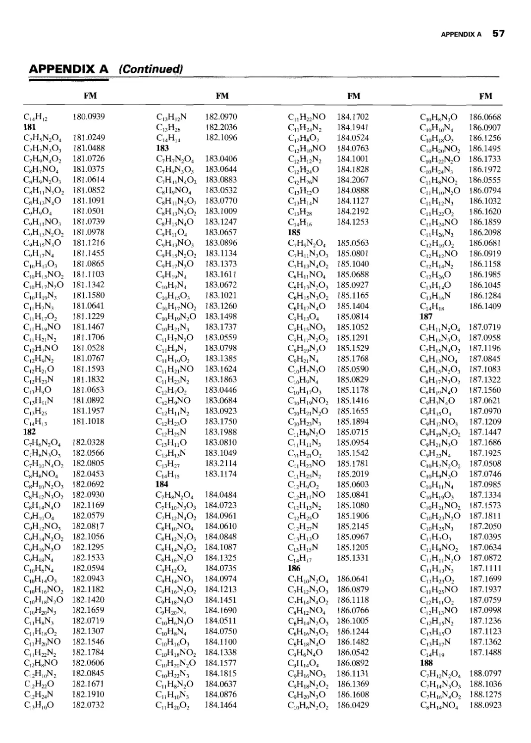
The Table of Formula Masses (four decimal places)
is convenient for selecting tentative, molecular formu-
las, and fragments on the basis of unit-mass peaks. Note
that in the first paragraph of the Introduction to Chap-
ter 7, there is the statement: “Go for the molecular for-
mula. ”
Infrared Spectrometry (Chapter 2)
It is still necessary that an organic chemist understands
a reasonable amount of theory and instrumentation in
IR spectrometry. We believe that our coverage of
“characteristic group absorptions” is useful, together
with group-absorption charts, characteristic spectra,
references, and Student Exercises. This chapter remains
essentially the same except the Student Exercises at
the end of the chapter. Most of the spectra have been
redone.
Proton NMR Spectrometry (Chapter 3)
In this chapter, we lay the background for nuclear mag-
netic resonance in general and proceed to develop pro-
ton NMR. The objective is the interpretation of proton
iii
iv PREFACE
spectra. From the beginning, the basics of NMR spec-
trometry evolved with the proton, which still accounts
for most of the NMR produced.
Rather than describe the 17 Sections in this chap-
ter, we simply state that the chapter has been greatly
expanded and thoroughly revised. More emphasis is
placed on FT NMR, especially some of its theory. Most
of the figures have been updated, and there are many
new figures including many 600 MHz spectra. The num-
ber of Student Exercises has been increased to cover
the material discussed. The frequent expansion of pro-
ton multiplets will be noted as students master the con-
cept of “first-order multiplets.” This important concept
is discussed in detail.
One further observation concerns the separation
of 'H and 13C spectrometry into Chapters 3 and 4. We
are convinced that this approach, as developed in ear-
lier editions, is sound, and we proceed to Chapter 4.
Carbon-13 NMR Spectrometry
(Chapter 4)
This chapter has also been thoroughly revised. All of
the Figures are new and were obtained either at
75.5 MHz (equivalent to 300 MHz for protons) or 150.9
MHz (equivalent to 600 MHz for protons). Many of the
tables of 13C chemical shifts have been expanded.
Much emphasis is placed on the DEPT spectrum.
In fact, it is used in all of the Student Exercises in place
of the obsolete decoupled 13C spectrum. The DEPT
spectrum provides the distribution of carbon atoms
with the number of hydrogen atoms attached to each
carbon.
Correlation NMR Spectrometry;
2-D NMR (Chapter 5)
Chapter 5 still covers 2-D correlation but has been re-
organized, expanded, and updated, which reflects the
ever increasing importance of 2-D NMR. The reorgani-
zation places all of the spectra together for a given
compound and treats each example separately: ipsenol,
caryophyllene oxide, lactose, and a tetrapeptide. Pulse
sequences for most of the experiments are given. The
expanded treatment also includes many new 2-D ex-
periments such as ROESY and hybrid experiments
such as HMQC-TOCSY. There are many new Student
Exercises.
NMR Spectrometry of Other Important
Nuclei Spin 1/2 Nuclei (Chapter 6)
Chapter 6 has been expanded with more examples,
comprehensive tables, and improved presentation of
spectra. The treatment is intended to emphasize chemi-
cal correlations and include several 2-D spectra. The
nuclei presented are:
15N, 19F,29Si, and 31P
Solved Problems (Chapter 7)
Chapter 7 consists of an introduction followed by six
solved “Exercises.” Our suggested approaches have
been expanded and should be helpful to students. We
have refrained from being overly prescriptive. Students
are urged to develop their own approaches, but our
suggestions are offered and caveats posted. The six ex-
ercises are arranged in increasing order of difficulty.
Two Student Exercises have been added to this chap-
ter, structures are provided, and the student is asked to
make assignments and verify the structures. Additional
Student Exercises of this type are added to the end of
Chapter 8.
Assigned Problems (Chapter 8)
Chapter 8 has been completely redone. The spectra are
categorized by structural difficulty, and 2-D spectra
are emphasized. For some of the more difficult exam-
ples, the structure is given and the student is asked to
verify the structure and to make all assignments in the
spectra.
Answers to Student Exercises are available in PDF
format to teachers and other professionals, who can re-
ceive the answers from the publisher by letterhead re-
quest. Additional Student Exercises can be found at
http://www.wiley.com/college/silverstein.
Final Thoughts
Most spectrometric techniques are now routinely ac-
cessible to organic chemists in walk-up laboratories.
The generation of high quality NMR, IR, and MS data
is no longer the rate-limiting step in identifying a
chemical structure. Rather, the analysis of the data has
become the primary hurdle for the chemist as it has
been for the skilled spectroscopist for many years. Soft-
ware tools are now available for the estimation and
prediction of NMR, MS, and IR spectra based on a
structural input and the dream solution of automated
structural elucidation based on spectral input is also
becoming increasingly available. Such tools offer both
the skilled and non-skilled experimentalist much-
needed assistance in interpreting the data. There are a
number of tools available today for predicting spectra,
(see http://www.acdlabs.com for more explicit details),
which differ in both complexity and capability.
In summary, this textbook is designed for upper-di-
vision undergraduates and for graduate students. It will
PREFACE V
also serve practicing organic chemists. As we have reit-
erated throughout the text, the goal is to interpret spec-
tra by utilizing the synergistic information. Thus, we
have made every effort to present the requisite spectra
in the most “legible” form. This is especially true of the
NMR spectra. Students soon realize the value of first-
order multiplets produced by the 300 and 600 MHz
spectrometers, and they will appreciate the numerous
expanded insets. As will the instructors.
ACKNOWLEDGMENTS
We thank Anthony Williams, Vice President and Chief
Science Officer of Advanced Chemistry Development
(ACD), for donating software for IR/MS processing,
which was used in four of the eight chapters; it allowed
us to present the data easily and in high quality. We
also thank Paul Cope from Bruker BioSpin Corpora-
tion for donating NMR processing software. Without
these software packages, the presentation of this book
would not have been possible.
We thank Jennifer Yee, Sarah Wolfman-
Robichaud, and other staff of John Wiley and Sons for
being highly cooperative in transforming the various
parts of a complex manuscript into a handsome Sev-
enth Edition.
The following reviewers offered encouragement
and many useful suggestions. We thank them for the
considerable time expended: John Montgomery, Wayne
State University; Cynthia McGowan, Merrimack Col-
lege; William Feld, Wright State University; James S.
Nowick, University of California, Irvine; and Mary
Chisholm, Penn State Erie, Behrend College.
Finally, we acknowledge Dr. Arthur Stipanovic Di-
rector of Analytical and Technical services for allowing
us the use of the Analytical facilities at SUNY ESF,
Syracuse.
Our wives (Olive, Kathryn, and Sandra) offered
constant patience and support. There is no adequate
way to express our appreciation.
Robert M. Silverstein
Francis X. Webster
David J. Kiemle
From left to right: Robert M. Silverstein, Francis X. Webster, and David J. Kiemle.
PREFACE TO FIRST EDITION
During the past several years, we have been engaged in
isolating small amounts of organic compounds from
complex mixtures and identifying these compounds
spectrometrically.
At the suggestion of Dr. A. J. Castro of San Jose
State College, we developed a one unit course entitled
“Spectrometric Identification of Organic Compounds,”
and presented it to a class of graduate students and in-
dustrial chemists during the 1962 spring semester. This
book has evolved largely from the material gathered
for the course and bears the same title as the course.*
We should first like to acknowledge the financial
support we received from two sources: The Perkin-
Elmer Corporation and Stanford Research Institute.
A large debt of gratitude is owed to our colleagues
at Stanford Research Institute. We have taken advan-
tage of the generosity of too many of them to list them
individually, but we should like to thank Dr. S. A.
Fuqua, in particular, for many helpful discussions of
NMR spectrometry. We wish to acknowledge also the
* A brief description of the methodology had been published: R. M.
Silverstein and G. C. Bassler, J. Chem. Educ. 39, 546 (1962).
cooperation at the management level, Dr. С. M. Himel,
chairman of the Organic Research Department, and
Dr. D. M. Coulson, chairman of the Analytical Re-
search Department.
Varian Associates contributed the time and talents
of its NMR Applications Laboratory. We are indebted
to Mr. N. S. Bhacca, Mr. L. F. Johnson, and Dr. J. N.
Shoolery for the NMR spectra and for their generous
help with points of interpretation.
The invitation to teach at San Jose State College
was extended to Dr. Bert M. Morris, head of the De-
partment of Chemistry, who kindly arranged the ad-
ministrative details.
The bulk of the manuscript was read by Dr. R. H.
Eastman of the Stanford University whose comments
were most helpful and are deeply appreciated.
Finally, we want to thank our wives. As a test of a
wife’s patience, there are few things to compare with an
author in the throes of composition. Our wives not only
endured, they also encouraged, assisted, and inspired.
R. M. Silverstein	Menlo Park, California
G.C. Bassler	April 1963
vi
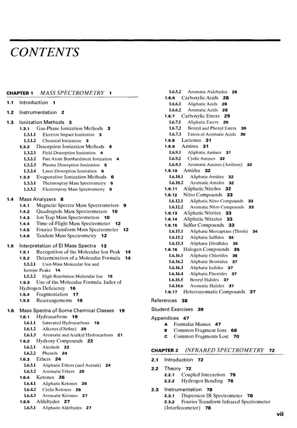
CONTENTS
CHAPTER 1 MASS SPECTROMETRY 1
1.1	Introduction 1
1.2	Instrumentation 2
1.3	Ionization Methods 3
1.3.1 Gas-Phase Ionization Methods 3
1.3.1.1 Electron Impact Ionization 3
1.3.1.2 Chemical Ionization 3
1.3.2 Desorption Ionization Methods 4
1.3.2.1 Field Desorption Ionization 4
1.3.2.2 Fast Atom Bombardment Ionization 4
1.3.2.3 Plasma Desorption Ionization 5
1.3.2.4 Laser Desorption Ionization 6
1.3.3 Evaporative Ionization Methods 6
1.3.3.1	Thermospray Mass Spectrometry 6
1.3.3.2	Electrospray Mass Spectrometry 6
1.4	Mass Analyzers 8
1.4.1	Magnetic Spector Mass Spectrometers	9
1.4.2	Quadrupole Mass Spectrometers 10
1.4.3	Ion Trap Mass Spectrometers 10
1.4.4	Time-of-Flight Mass Spectrometer 12
1.4.5	Fourier Transform Mass Spectrometer	12
1.4.6	Tandem Mass Spectrometry 12
1.5	Interpretation of El Mass Spectra 13
1.5.1 Recognition of the Molecular Ion Peak 14
1.5.2 Determination of a Molecular Formula 14
1.5.2.1 Unit-Mass Molecular Ion and
Isotope Peaks 14
1.5.2.2 High-Resolution Molecular Ion 15
1.5.3 Use of the Molecular Formula. Index of
Hydrogen Deficiency 16
1.5.4 Fragmentation 17
1.5.5 Rearrangements 19
1.6	Mass Spectra of Some Chemical Classes 19
1.6.1 Hydrocarbons 19
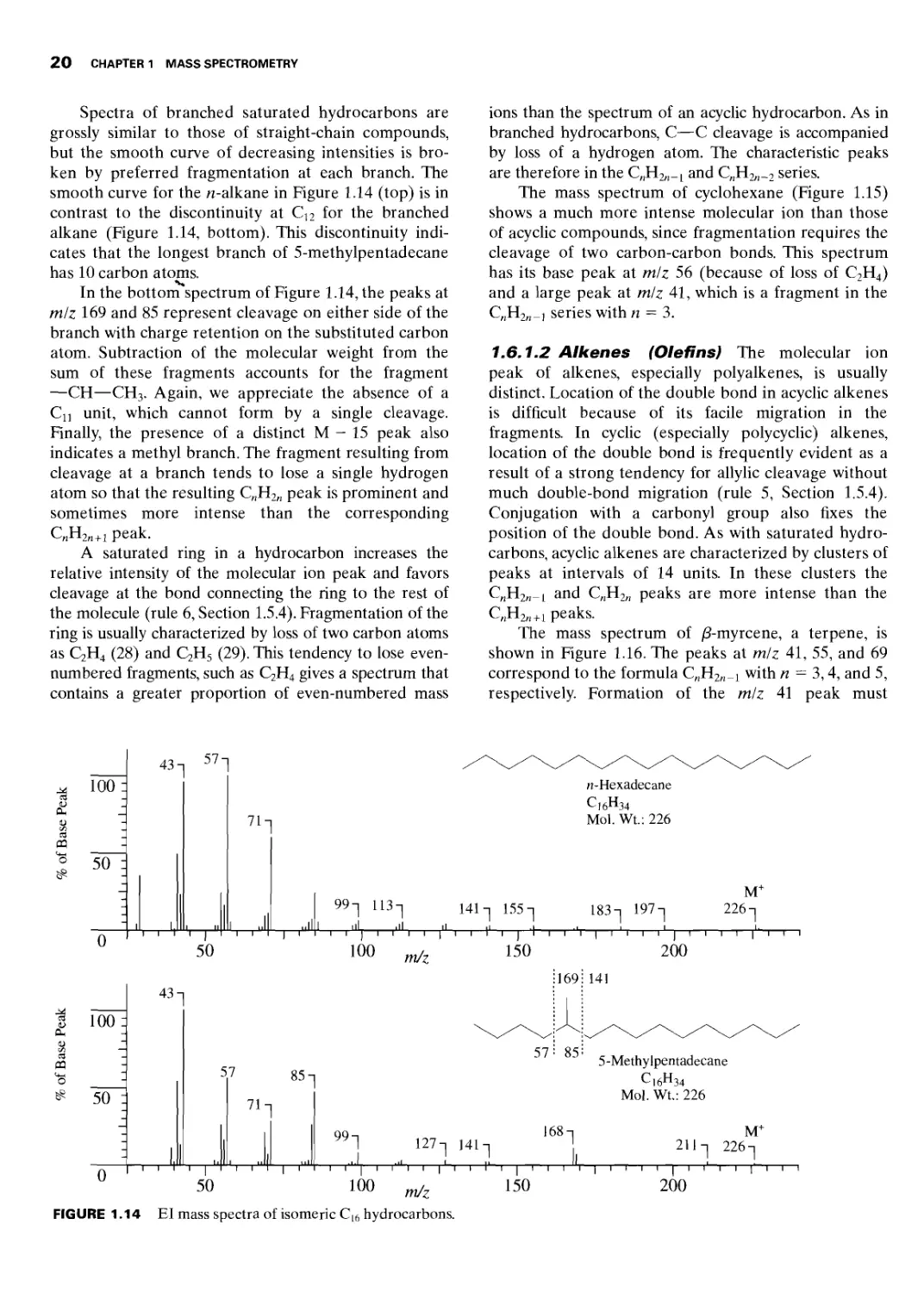
1.6.1.1 Saturated Hydrocarbons 19
1.6.1.2 Alkenes (Olefins) 20
1.6.1.3 Aromatic and Aralkyl Hydrocarbons 21
1.6.2 Hydroxy Compounds 22
1.6.2.1 Alcohols 22
1.6.2.2 Phenols 24
1.6.3 Ethers 24
1.6.3.1	Aliphatic Ethers (and Acetals) 24
1.6.3.2	Aromatic Ethers 25
1.6.4 Ketones 26
1.6.4.1	Aliphatic Ketones 26
1.6.4.2 Cyclic Ketones 26
1.6.4.3	Aromatic Ketones 27
1.6.5 Aldehydes 27
1.6.5.1 Aliphatic Aldehydes 27
1.6.5.2 Aromatic Aldehydes 28
1.6.6 Carboxylic Acids 28
1.6.6.1 Aliphatic Acids 28
1.6.6.2 Aromatic Acids 28
1.6.7 Carboxylic Esters 29
1.6.7.1 Aliphatic Esters 29
1.6.7.2 Benzyl and Phenyl Esters 30
1.6.7.3 Esters of Aromatic Acids 30
1.6.8 Lactones 31
1.6.9 Amines 31
1.6.9.1 Aliphatic Amines 31
1.6.9.2 Cyclic Amines 32
1.6.9.3 Aromatic Amines (Anilines) 32
1.6.10	Amides 32
1.6.10.1	Aliphatic Amides 32
1.6.10.2	Aromatic Amides 32
1.6.11	Aliphatic Nitriles	32
1.6.12	Nitro Compounds	33
1.6.12.1	Aliphatic Nitro Compounds	33
1.6.12.2	Aromatic Nitro Compounds	33
1.6.13	Aliphatic Nitrites	33
1.6.14	Aliphatic Nitrates	33
1.6.15	Sulfur Compounds	33
1.6.15.1 Aliphatic Mercaptans (Thiols) 34
1.6.15.2 Aliphatic Sulfides 34
1.6.15.3 Aliphatic Disulfides 35
1.6.16 Halogen Compounds 35
1.6.16.1	Aliphatic Chlorides	36
1.6.16.2	Aliphatic Bromides	37
1.6.16.3	Aliphatic Iodides 37
1.6.16.4	Aliphatic Fluorides	37
1.6.16.5 Benzyl Halides 37
1.6.16.6 Aromatic Halides 37
1.6.17 Heteroaromatic Compounds 37
References 38
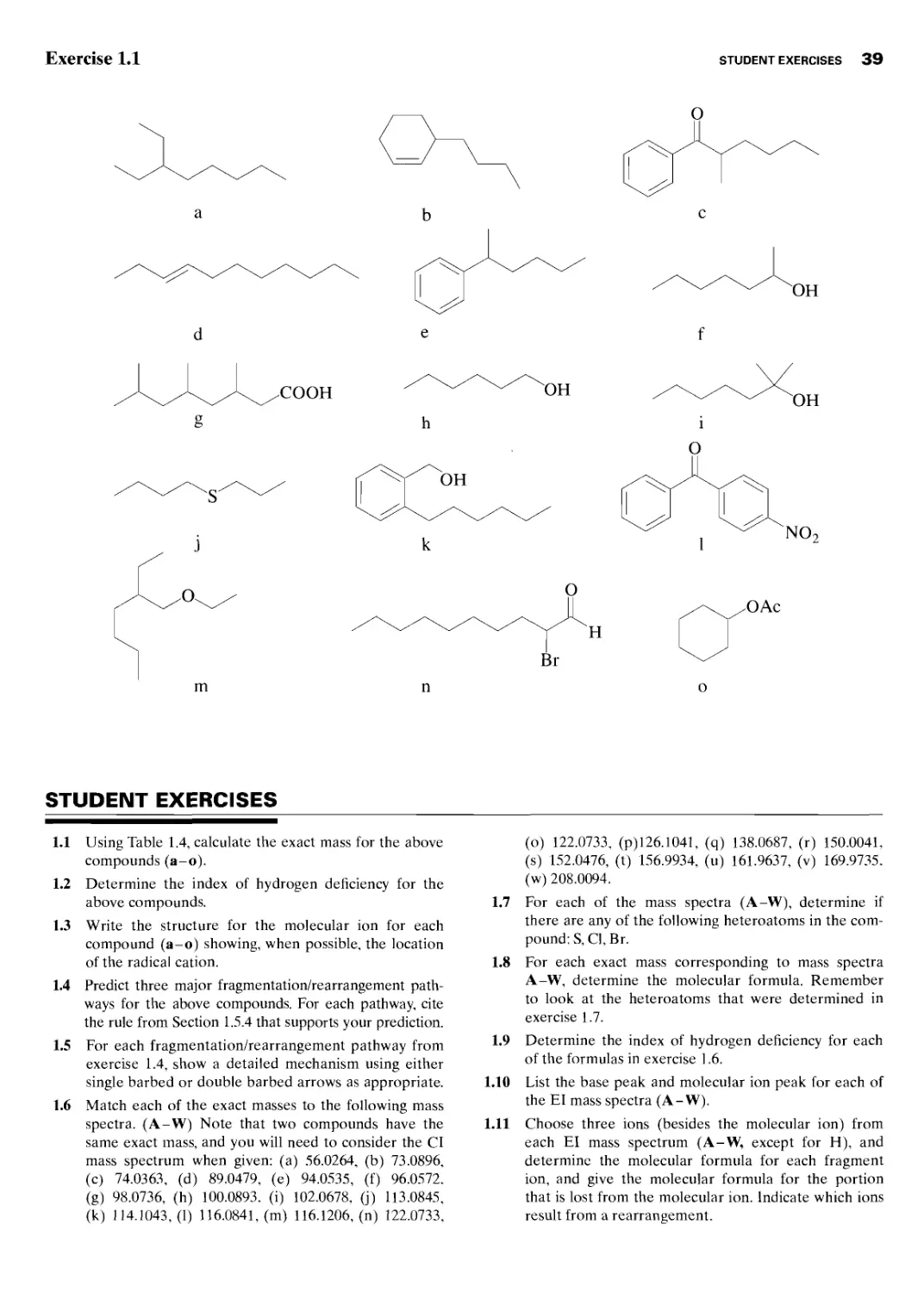
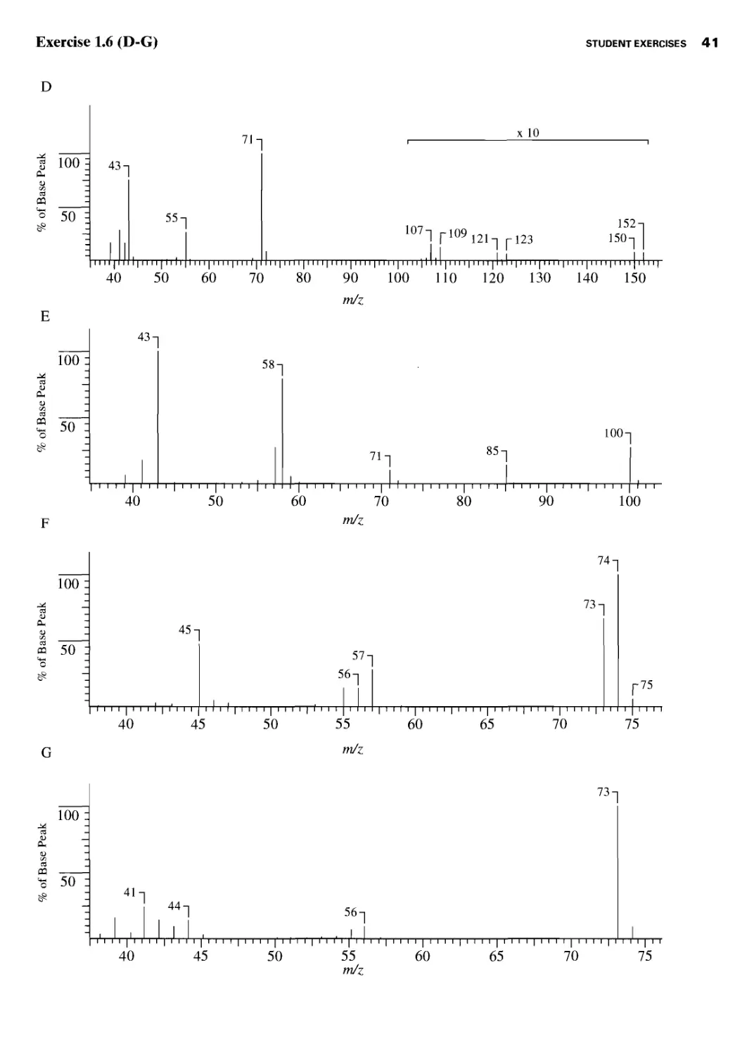
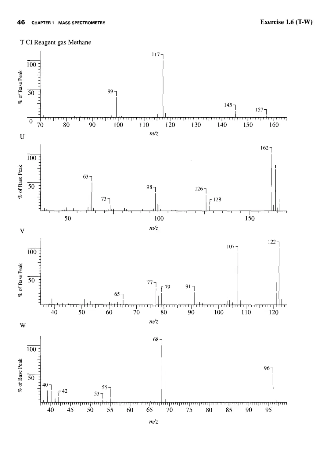
Student Exercises 39
Appendices 47
A Formulas Masses 47
В Common Fragment Ions 68
C Common Fragments Lost 70
CHAPTER 2 INFRARED SPECTROMETRY 72
2.1 Introduction 72
2.2 Theory 72
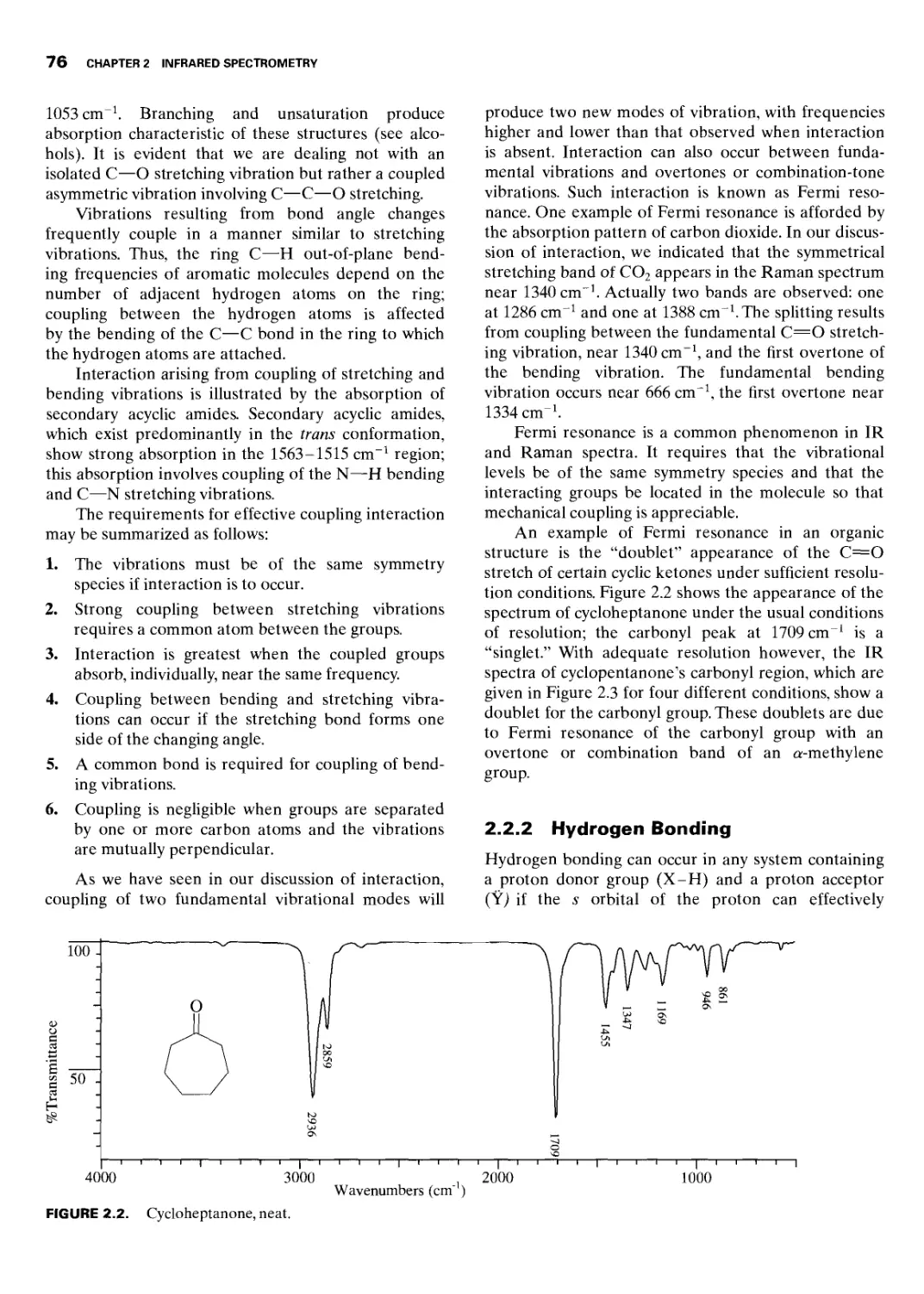
2.2.1 Coupled Interaction 75
2.2.2 Hydrogen Bonding 76
2.3 Instrumentation 78
2.3.1 Dispersion IR Spectrometer 78
2.3.2 Fourier Transform Infrared Spectrometer
(Interferometer) 78
vii
viii CONTENTS
2.4	Sample Handling 79
2.5	Interpretations of Spectra 80
2.6	Characteristic Group Absorption of Organic
Molecules 82
2.6.1 Normal Alkanes (Paraffins) 82
2.6.1.1	C—H Stretching Vibrations 83
2.6.1.2	C—H Bending Vibrations Methyl Groups 83
2.6.2 Branched-Chain Alkanes 84
2.6.2.1	C—H Stretching Vibrations Tertiary C—H
Groups 84
2.6.2.2	C—H Bending Vibrations gem-Dimethyl
Groups 84
2.6.3 Cyclic Alkanes 85
2.6.3.1	C—H Stretching Vibrations 85
2.6.3.2	C—H Bending Vibrations 85
2.6.4 Alkenes 85
2.6.4.1	C—C Stretching Vibrations Unconjugated Linear
Alkenes 85
2.6.4.2 Alkene C—H Stretching Vibrations 86
2.6.4.3 Alkene C—H Bending Vibrations 86
2.6.5 Alkynes 86
2.6.5.1	C—C Stretching Vibrations 86
2.6.5.2	C—H Stretching Vibrations 87
2.6.5.3	C—H Bending Vibrations 87
2.6.6 Mononuclear Aromatic Hydrocarbons 87
2.6.6.1 Out-of-Plane C—H Bending Vibrations 87
2.6.7 Polynuclear Aromatic Hydrocarbons 87
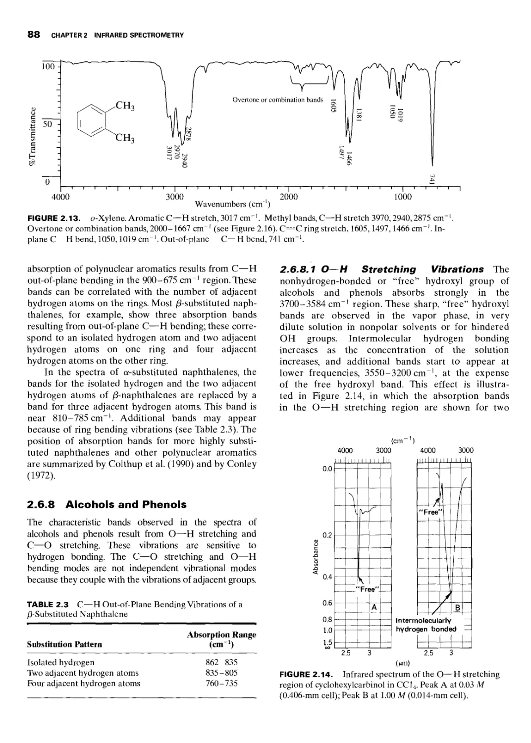
2.6.8 Alcohols and Phenols 88
2.6.8.1 О—H Stretching Vibrations 88
2.6.8.2	C—О Stretching Vibrations 89
2.6.8.3	О—H Bending Vibrations 90
2.6.9 Ethers, Epoxides, and Peroxides 91
2.6.9.1	C—О Stretching Vibrations 91
2.6.10 Ketones 92
2.6.10.1	C—О Stretching Vibrations 92
2.6.10.2	C—C(=O)—C Stretching and Bending
Vibrations 94
2.6.11 Aldehydes 94
2.6.11.1	C=O	Stretching Vibrations	94
2.6.11.2	C—H	Stretching Vibrations	94
2.6.12 Carboxylic Acids 95
2.6.12.1	О—H	Stretching Vibrations	95
2.6.12.2	C=O	Stretching Vibrations	95
2.6.12.3	C—О Stretching and О—H Bending
Vibrations	96
2.6.13 Carboxylate Anion 96
2.6.14 Esters and Lactones 96
2.6.14.1	C=O	Stretching Vibrations	97
2.6.14.2	C—О	Stretching Vibrations	98
2.6.15 Acid Halides 98
2.6.15.1	C=O	Stretching Vibrations	98
2.6.16 Carboxylic Acid Anhydrides	98
2.6.16.1	C=O	Stretching Vibrations	98
2.6.16.2	C—О	Stretching Vibrations	98
2.6.17 Amides and Lactams 99
2.6.17.1	N—H	Stretching Vibrations	99
2.6.17.2	C=O	Stretching Vibrations
(Amide 1 Band) 1OO
2.6.17.3	N—H Bending Vibrations
(Amide II Band) 100
2.6.17.4 Other Vibration Bands 101
2.6.17.5 C=O Stretching Vibrations of Lactams 101
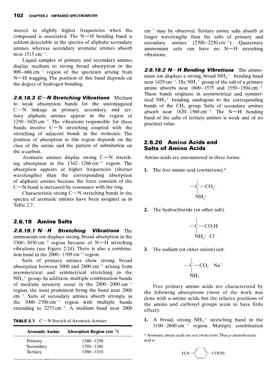
2.6.18 Amines 101
2.6.18.1 N—H Stretching Vibrations 101
2.6.18.2 N—H Bending Vibrations 101
2.6.18.3 C—N Stretching Vibrations 102
2.6.19 Amine Salts 102
2.6.19.1 N—H Stretching Vibrations 102
2.6.19.2 N—H Bending Vibrations 102
2.6.20 Amino Acids and Salts of Amino Acids 102
2.6.21 Nitriles 103
2.6.22 Isonitriles (R—N=C), Cyanates
(R—О—C=N), Isocyanates (R—N=C=O),
Thiocyanates (R—S—C=N), Isothiocyanates
(R—N=C=S) 104
2.6.23 Compounds Containing—N=N 104
2.6.24 Covalent Compounds Containing Nitrogen-
Oxygen Bonds 104
2.6.24.1 N=O Stretching Vibrations Nitro
Compounds 104
2.6.25 Organic Sulfur Compounds 105
2.6.25.1 S=H Stretching Vibrations Mercaptans 105
2.6.25.2	C—S and C=S Stretching Vibrations 106
2.6.26	Compounds Containing Sulfur—Oxygen
Bonds 106
2.6.26.1 S=O Stretching Vibrations Sulfoxides 106
2.6.27 Organic Halogen Compounds 107
2.6.28 Silicon Compounds 107
2.6.28.1 Si—H Vibrations 107
2.6.28.2	SiO—H and Si—О Vibrations 107
2.6.28.3 Silicon—Halogen Stretching Vibrations 107
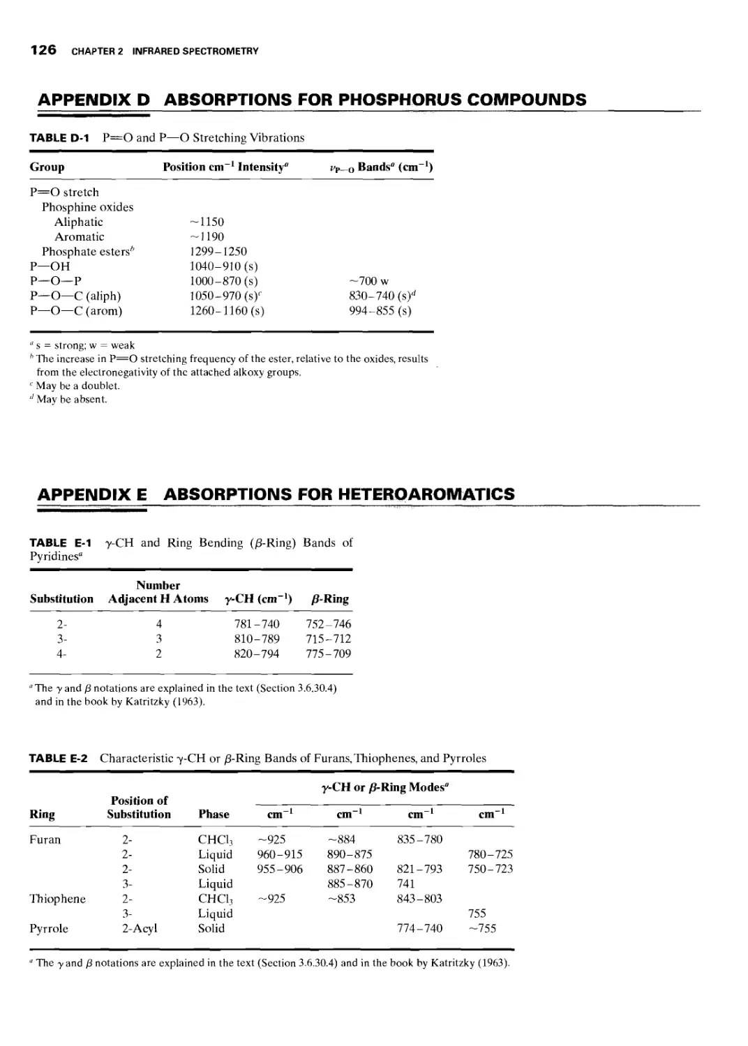
2.6.29 Phosphorus Compounds 107
2.6.29.1	P=O and P—О Stretching Vibrations 107
2.6.30 Heteroaromatic Compounds 107
2.6.30.1	C—H Stretching Vibrations 107
2.6.30.2	N—H Stretching Frequencies 108
2.6.30.3 Ring Stretching Vibrations
(Skeletal Bands) 108
2.6.30.4 C—H Out-of-Plane Bending 108
References 108
Student Exercises 110
Appendices 119
A Transparent Regions of Solvents and Mulling Oils
119
В	Characteristic Group Absorptions	120
C	Absorptions for Alkenes 125
D	Absorptions for Phosphorus Compounds 126
E	Absorptions for Heteroaromatics	126
CHAPTER 3 PROTON MAGNETIC RESONANCE
SPECTROMETRY 127
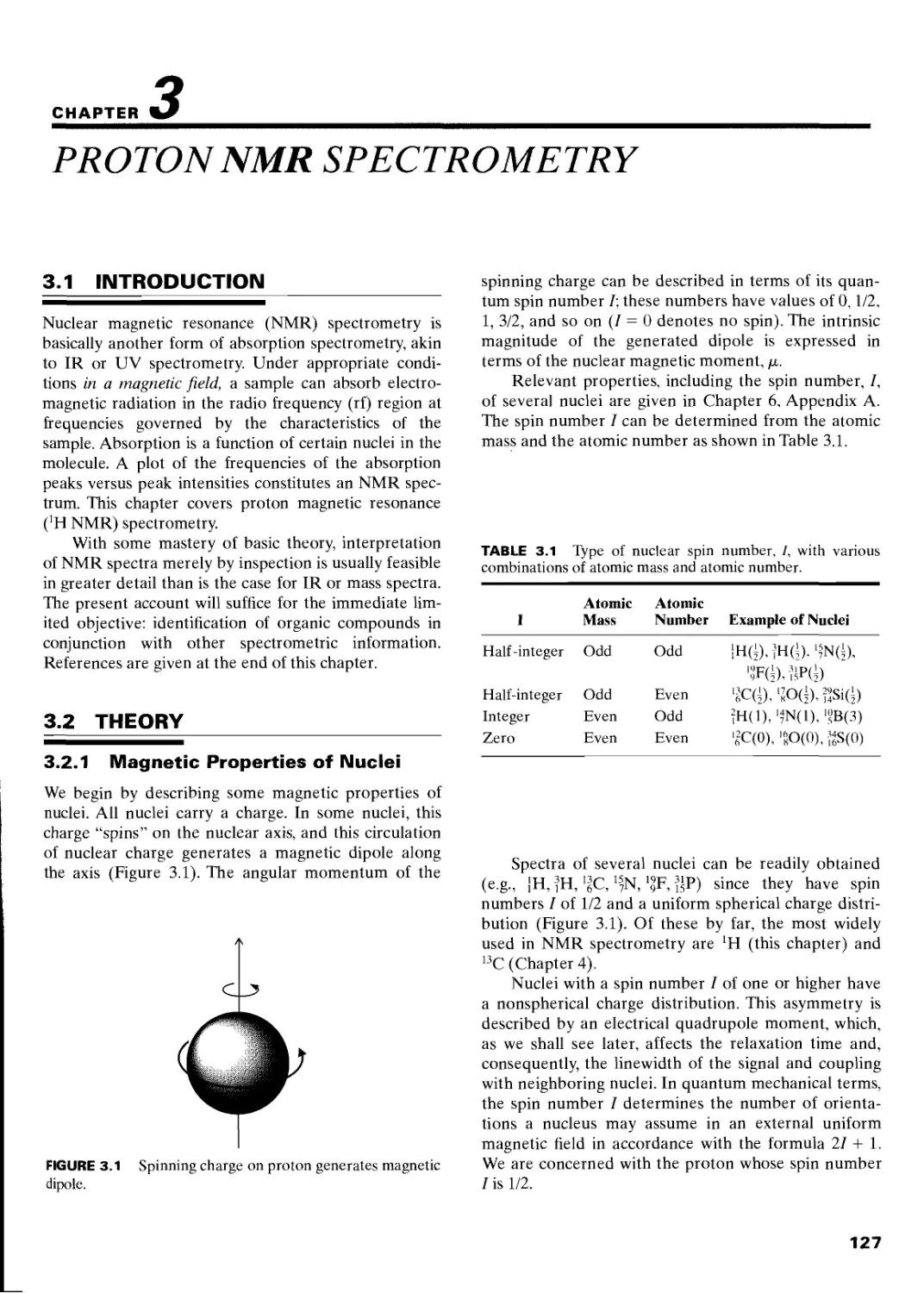
3.1 Introduction 127
3.2 Theory 127
3.2.1 Magnetic Properties of Nuclei 127
3.2.2	Excitation of Spin 1/2 Nuclei 128
3.2.3 Relaxation 130
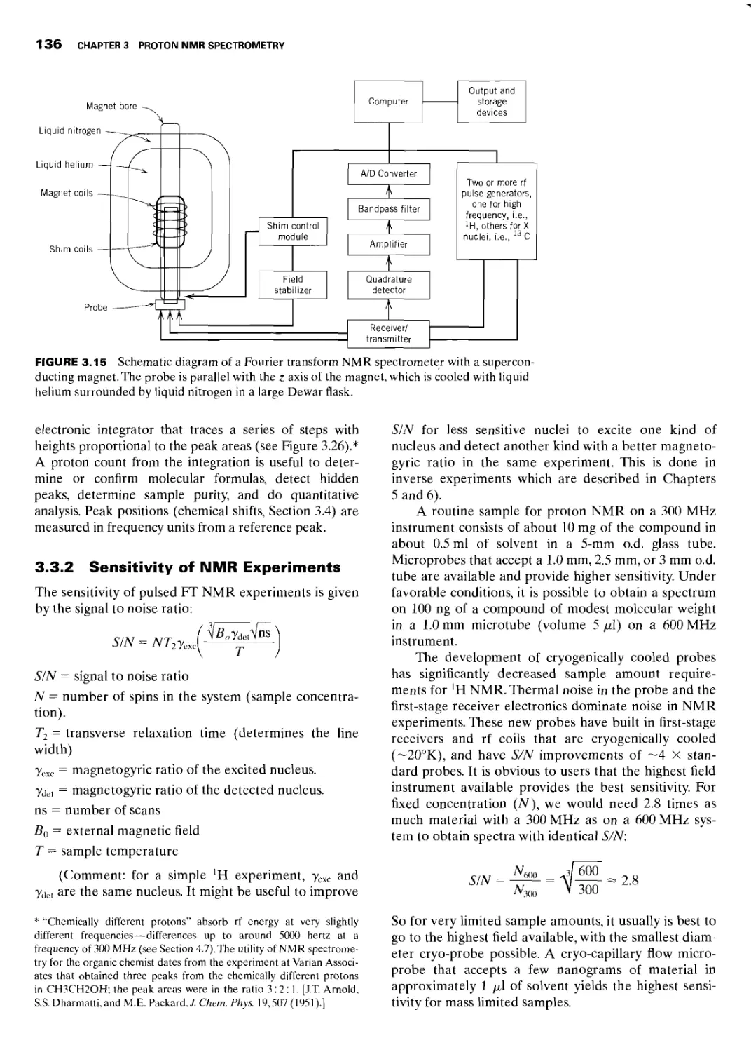
3.3 Instrumentation and Sample Handling 135
3.3.1 Instrumentation 135
3.3.2 Sensitivity of NMR Experiments 136
3.3.3 Solvent Selection 137
CONTENTS iX
3.4	Chemical Shift 137
3.5	Spin Coupling, Multiplets, Spin Systems 143
3.5.1 Simple and Complex First Order
Multiplets 145
3.5.2 First Order Spin Systems 146
3.5.3	Pople Notions 147
3.5.4	Further Examples of Simple, First-Order Spin
Systems 147
3.5.5 Analysis of First-Order Patterns 148
3.6	Protons on Oxygen, Nitrogen, and Sulfur Atoms.
Exchangeable Protons 160
3.6.1 Protons on an Oxygen Atom 150
3.6.1.1 Alcohols 150
3.6.1.2 Water 153
3.6.1.3 Phenols 153
3.6.1.4 Enols 153
3.6.1.5 Carboxylic Acids 153
3.6.2 Protons on Nitrogen 153
3.6.3 Protons on Sulfur 155
3.6.4 Protons on or near Chlorine, Bromine, or
Iodine Nuclei 155
3.7	Coupling of Protons to Other Important Nuclei (19F,
D, 31P, 29Si, and 13C) 155
3.7.1 Coupling of Protons to 19F 155
3.7.2 Coupling of Protons to D 155
3.7.3 Coupling of Protons to 31P 156
3.7.4 Coupling of Protons to 29Si 156
3.7.5 Coupling of Protons to 13C 156
3.8	Chemical Shift Equivalence 157
3.8.1 Determination of Chemical Shift Equivalence
by Interchange Through Symmetry Operations 157
3.8.1.1 Interchange by Rotation Around a Simple Axis of
Symmetry (C„) 157
3.8.1.2 Interchange by Reflection Through a Plane of
Symmetry (<r) 157
3.8.1.3 Interchange by Inversion Through a Center of
Symmetry (i) 158
3.8.1.4 No Interchangeability by a Symmetry
Operations 158
3.8.2 Determination of Chemical Shift Equivalence
by Tagging (or Substitution) 159
3.8.3 Chemical Shift Equivalence by Rapid
Interconversion of Structures 160
3.8.3.1	Keto-Enol Interconversion 160
3.8.3.2	Interconversion Around a “Partial Double Bond”
(Restricted Rotation) 160
3.8.3.3 Interconversion Around the Single Bond
of Rings 160
3.8.3.4 Interconversion Around the Single Bonds
of Chains 161
3.9	Magnetic Equivalence (Spin-Coupling
Equivalence) 162
3.10	AMX, ABX, and ABC Rigid Systems with Three
Coupling Constants 164
3.11	Confirmationally Mobile, Open-Chain Systems.
Virtual Coupling 165
3.11.1 Unsymmetrical Chains 165
3.11.1.1 1-Nitropropane 165
3.11.1.2	1-Hexanol 165
11.2	Symmetrical Chains	167
3.11.2.1	Dimethyl Succinate	167
3.11.2.2	Dimethyl Glutarate	167
3.11.2.3	Dimethyl Adipate	167
3.11.2.4	Dimethyl Pimelate	168
3.11.3 Less Symmetrical Chains 168
3.11.3.1 3-Methylglutaric Acid 168
3.12	Chirality 169
3.12.1 One Chiral Center, Ipsenol 169
3.12.2 Two Chiral Centers 171
3.13	Vicinal and Geminal Coupling 171
3.14	Low-Range Coupling 172
3.15	Selective Spin Decoupling. Double
Resonance 173
3.16	Nuclear Overhauser Effect, Difference
Spectrometry, 1H 1H Proximity Through
Space 173
3.17	Conclusion 175
References 176
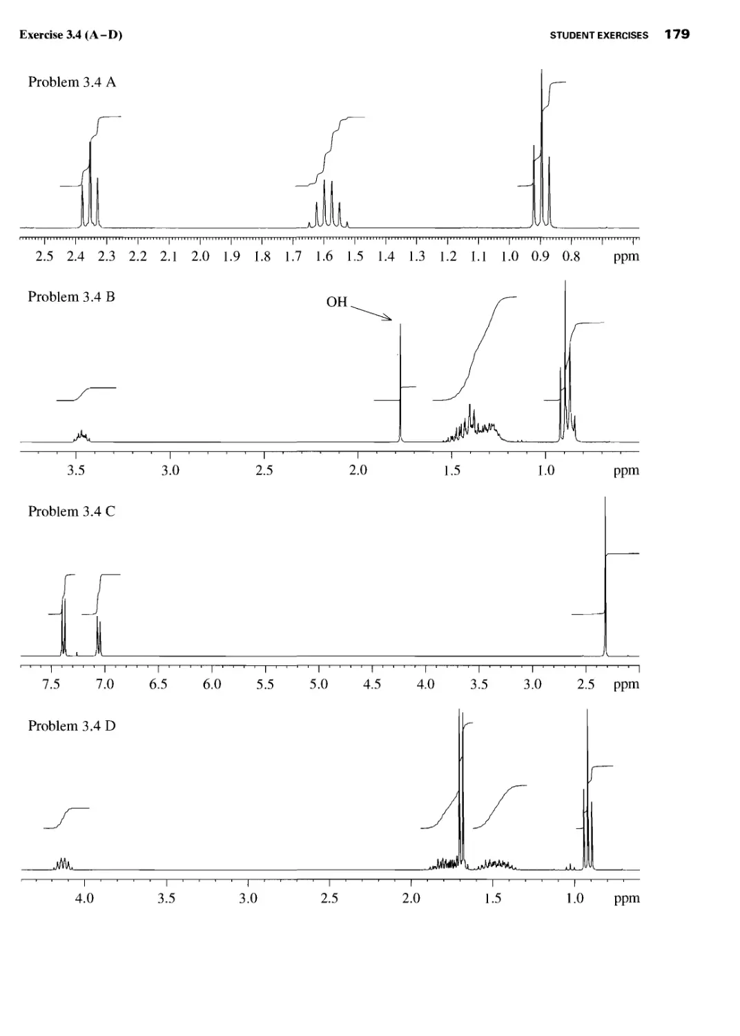
Student Exercises 177
Appendices 188
A Chemicals Shifts of a Proton 188
В Effect on Chemical Shifts by Two or Three
Directly Attached Functional Groups 191
C Chemical Shifts in Alicyclic and Heterocyclic
Rings 193
D Chemical Shifts in Unsaturated and Aromatic
Systems 194
E Protons on Heteroatoms 197
F Proton Spin-Coupling Constants 198
G Chemical Shifts and Multiplicities of Residual
Protons in Commercially Available Deuterated
Solvents 200
H 'H NMR Data 201
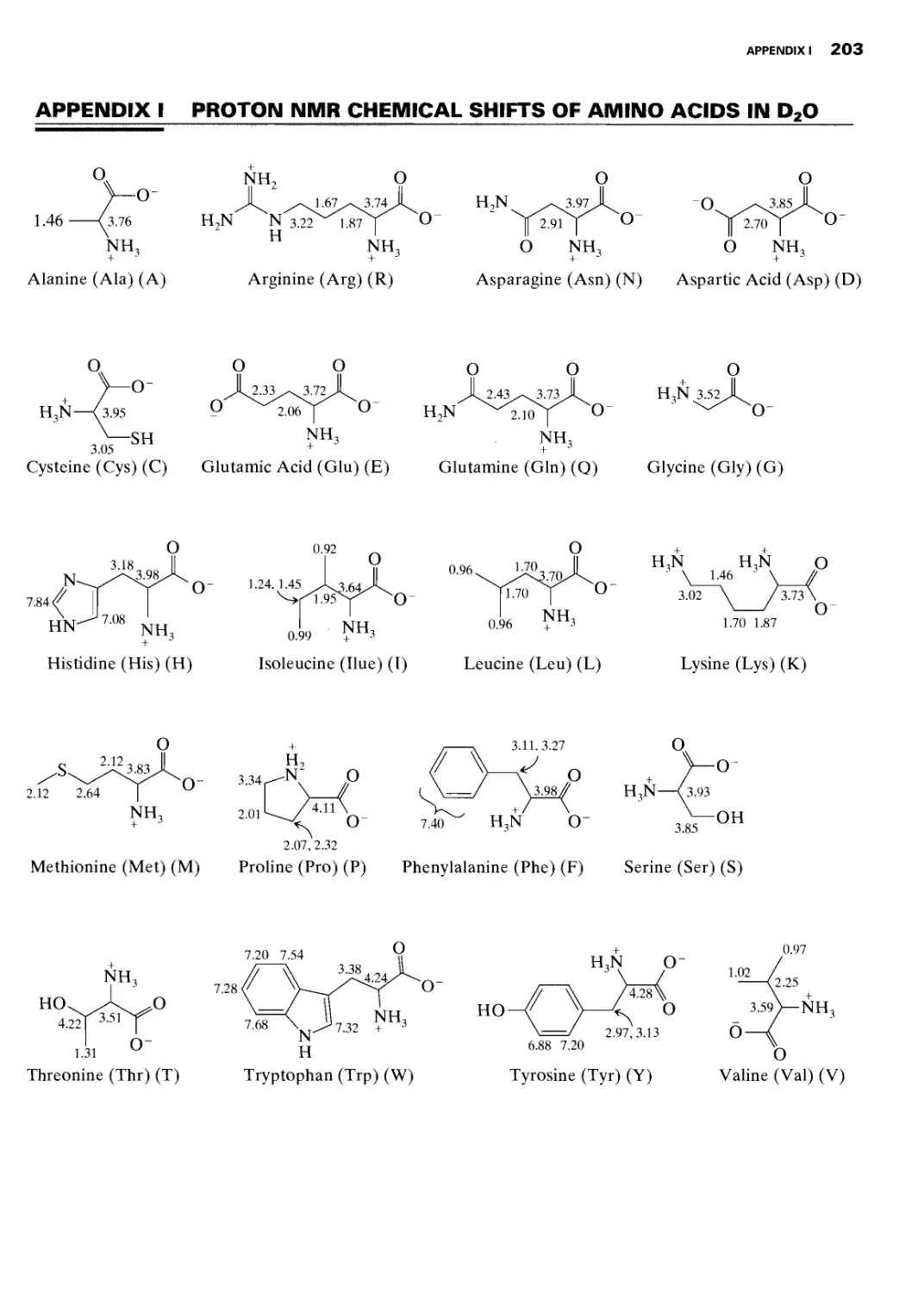
I Proton NMR Chemical Shifts of Amino Acids in
D2O 203
CHAPTER 4 CARBON-13 NMR
SPECTROMETRY 204
4.1 Introduction 204
4.2 Theory 204
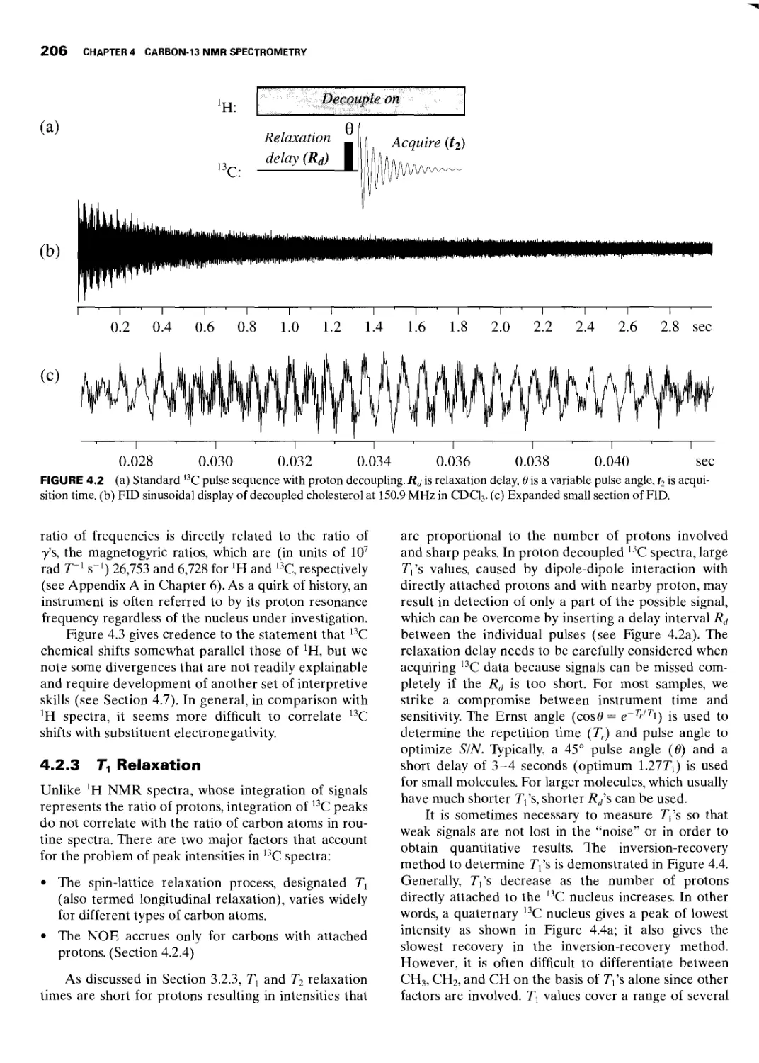
4.2.1 H Decoupling Techniques 204
4.2.2	Chemical Shift Scale and Range 205
4.2.3	Tj Relaxation 206
4.2.4	Nuclear Overhauser Enhancement
(NOE) 207
4.2.5	13C—H Sping Coupling (J Values) 209
4.2.6 Sensitivity 210
4.2.7 Solvents 210
4.3 Interpretation of a Simple 13C Spectrum: Diethyl
Phthalate 211
4.4 Quantitative 13C Analysis 213
4.5 Chemical Shift Equivalence 214
X CONTENTS
4.6	DEPT 215
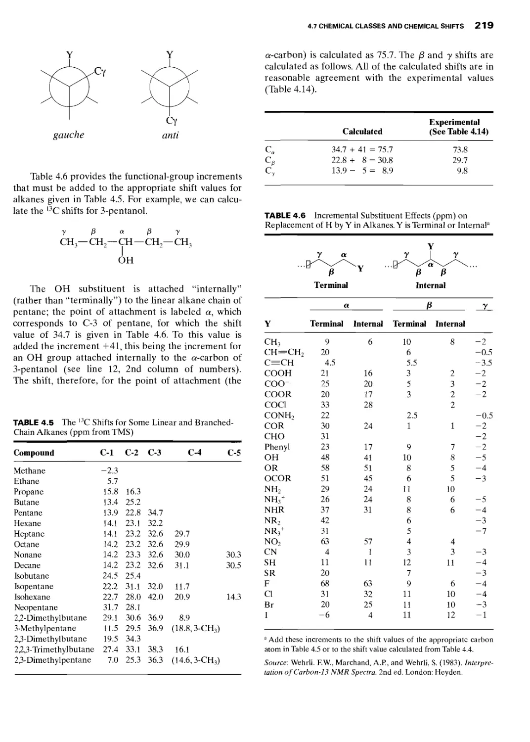
4.7	Chemical Classes and Chemical Shifts 217
4.7.1 Alkanes 218
4.7.1.1 Linear and Branched Alkanes 218
4.7.1.2 Effect of Substituents on Alkenes 218
4.7.1.3 Cycloalkanes and Saturated Heterocyclics 220
4.7.2	Alkenes 220
4.7.3	Alkynes 221
4.7.4	Aromatic Compounds	222
4.7.5	Heteroaromatic Compounds 223
4.7.6	Alcohols 223
4.7.7 Ethers, Acetals, and Epoxides 225
4.7.8	Halides 225
4.7.9	Amines 226
4.7.10 Thiols, Sulfides, and Disulfides 226
4.7.11 Functional Groups Containing Carbon 226
4.7.11.1 Ketones and Aldehydes 227
4.7.11.2 Carboxylic Acids, Esters, Chlorides, Anhydrides,
Amides, and Nitriles 227
4.7.11.3 Oximes 227
References 228
Student Exercises 229
Appendices 240
A The l3C Chemical Shifts, Couplings and
Multiplicities of Common NMR Solvents 240
В 13C Chemical Shift for Common Organic
Compounds in Different Solvents 241
C The 13C Correlation Chart for Chemical
Classes 242
D ,3C NMR Data for Several Natural
Products (S) 244
CHAPTERS CORRELATION NMR
SPECTROMETRY; 2-D NMR 245
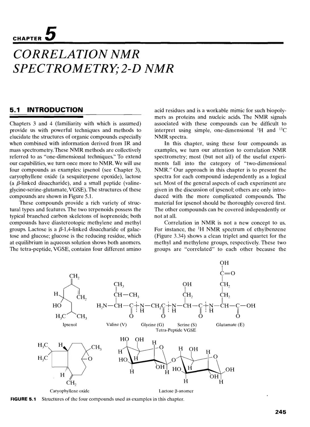
5.1 Introduction 245
5.2 Theory 246
5.3 Correlation Spectrometry 249
5.3.1	'H—*H Correlation: COSY 250
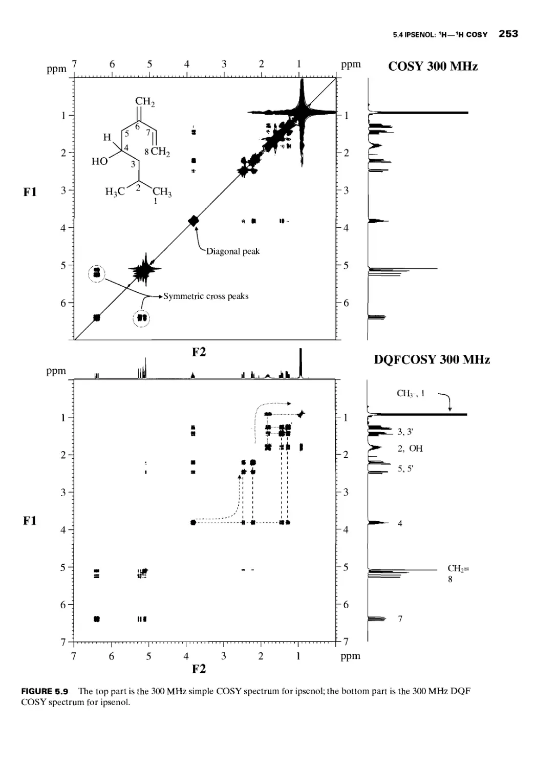
5.4 Ipsenol: 1H—1H COSY 251
5.4.1 Ipsenol: Double Quantum Filtered H—1H
COSY 251
5.4.2 Carbon Detected 13C—1H COSY:
HECTOR 254
5.4.3 Proton Detected H—l3C COSY:
HMQC 254
5.4.4 Ipsenol: HECTOR and HMQC 255
5.4.5 Ipsenol: Proton-Detected, Long Range
'H—13C Heteronuclear Correlation: HMBC 257
5.5 Caryophyllene Oxide 259
5.5.1 Caryophyllene Oxide: DQF-COSY 259
5.5.2 Caryophyllene Oxide: HMQC 259
5.5.3 Caryophyllene Oxide: HMBC 263
5.6 13C—13C Correlations: Inadequate 265
5.6.1 Inadequate: Caryophyllene Oxide 266
5.7	Lactose 267
5.7.1 DQF-COSY: Lactose 267
5.7.2 HMQC: Lactose 270
5.7.3 HMBC: Lactose 270
5.8	Relayed Coherence Transfer: TOCSY 270
5.8.1	2-D TOCSY: Lactose 270
5.8.2	1-D TOCSY: Lactose 273
5.9	HMQC-TOCSY 275
5.9.1 HMQC-TOCSY: Lactose 275
5.10	ROESY 275
5.10.1 ROESY: Lactose 275
5.11	VGSE 278
5.11.1 COSY: VGSE 278
5.11.2 TOCSY: VGSE 278
5.11.3 HMQC: VGSE 278
5.11.4 HMBC: VGSE 281
5.11.5 ROESY: VGSE 282
5.12	Gradient Field NMR 282
References 285
Student Exercises 285
CHAPTER 6	NMR SPECTROMETRY OF OTHER
IMPORTANT SPIN 1/2 NUCLEI 316
6.1	Introduction 316
6.2	15N Nuclear Magnetic Resonance 317
6.3	19F Nuclear Magnetic Resonance 323
6.4	29Si Nuclear Magnetic Resonance 326
6.5	31P Nuclear Magnetic Resonance 327
6.6	Conclusion 330
References 332
Student Exercises 333
Appendices 338
A Properties of Magnetically Active Nuclei 338
CHAPTER 7	SOLVED PROBLEMS 341
7.1 Introduction 341
Problem 7.1 Discussion 345
Problem 7.2 Discussion 349
Problem 7.3 Discussion 353
Problem 7.4 Discussion 360
Problem 7.5 Discussion 367
Problem 7.6 Discussion 373
Student Exercises 374
CHAPTER 8	ASSIGNED PROBLEMS 381
8.1 Introduction 381
Problems 382
CHAPTER Я
MASS SPECTROMETRY
1.1 INTRODUCTION
The concept of mass spectrometry is relatively
simple: A compound is ionized (ionization method),
the ions are separated on the basis of their
mass/charge ratio (ion separation method), and the
number of ions representing each mass/charge “unit”
is recorded as a spectrum. For instance, in the com-
monly used electron-impact (El) mode, the mass
spectrometer bombards molecules in the vapor phase
with a high-energy electron beam and records the
result as a spectrum of positive ions, which have been
separated on the basis of mass/charge (m/z).*
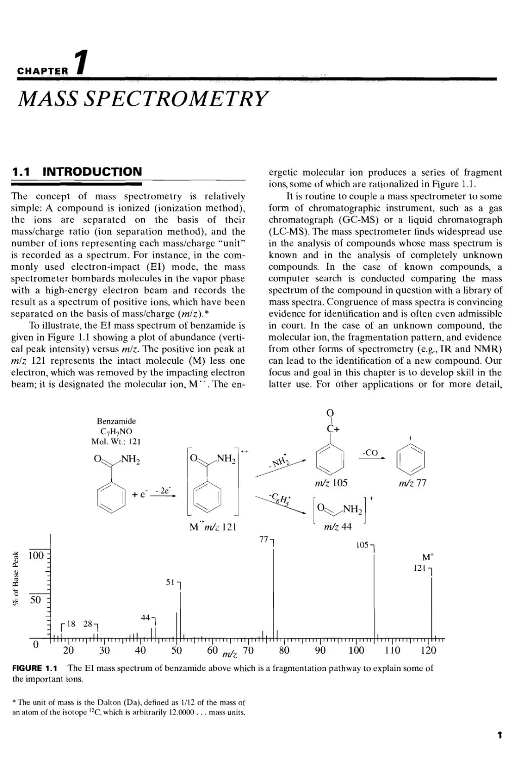
To illustrate, the El mass spectrum of benzamide is
given in Figure 1.1 showing a plot of abundance (verti-
cal peak intensity) versus mlz. The positive ion peak at
mlz 121 represents the intact molecule (M) less one
electron, which was removed by the impacting electron
beam; it is designated the molecular ion, M’+. The en-
ergetic molecular ion produces a series of fragment
ions, some of which are rationalized in Figure 1.1.
It is routine to couple a mass spectrometer to some
form of chromatographic instrument, such as a gas
chromatograph (GC-MS) or a liquid chromatograph
(LC-MS). The mass spectrometer finds widespread use
in the analysis of compounds whose mass spectrum is
known and in the analysis of completely unknown
compounds. In the case of known compounds, a
computer search is conducted comparing the mass
spectrum of the compound in question with a library of
mass spectra. Congruence of mass spectra is convincing
evidence for identification and is often even admissible
in court. In the case of an unknown compound, the
molecular ion, the fragmentation pattern, and evidence
from other forms of spectrometry (e.g., IR and NMR)
can lead to the identification of a new compound. Our
focus and goal in this chapter is to develop skill in the
latter use. For other applications or for more detail,
* The unit of mass is the Dalton (Da), defined as 1/12 of the mass of
an atom of the isotope 12C, which is arbitrarily 12.0000 . . . mass units.
FIGURE 1.1 The El mass spectrum of benzamide above which is a fragmentation pathway to explain some of
the important ions.
1
2 CHAPTER 1 MASS SPECTROMETRY
mass spectrometry texts and spectral compilations are
listed at the end of this chapter.
1.2	INSTRUMENTATION
This past decade has been a time of rapid growth and
change in instrumentation for mass spectrometry.
Instead of discussing individual instruments, the type of
instrument will be broken down into (1) ionization
methods and (2) ion separation methods. In general,
the method of ionization is independent of the method
of ion separation and vice versa, although there are
exceptions. Some of the ionization methods depend on
a specific chromatographic front end (e.g., LC-MS),
while still others are precluded from using chromatog-
raphy for introduction of sample (e.g., FAB and
MALDI). Before delving further into instrumentation,
let us make a distinction between two types of mass
spectrometers based on resolution.
The minimum requirement for the organic chemist
is the ability to record the molecular weight of the
compound under examination to the nearest whole
number. Thus, the spectrum should show a peak at, say,
mass 400, which is distinguishable from a peak at mass
399 or at mass 401. In order to select possible molecu-
lar formulas by measuring isotope peak intensities (see
Section 1.5.2.1), adjacent peaks must be cleanly
separated. Arbitrarily, the valley between two such
peaks should not be more than 10% of the height of
the larger peak. This degree of resolution is termed
“unit” resolution and can be obtained up to a mass of
approximately 3000 Da on readily available “unit reso-
lution” instruments.
To determine the resolution of an instrument, consider
two adjacent peaks of approximately equal intensity. These
peaks should be chosen so that the height of the valley
between the peaks is less than 10% of the intensity
of the peaks. The resolution (R) is R = Mnl(Mn —
where M„ is the higher mass number of the two adjacent
peaks, and Mm is the lower mass number.
There are two important categories of mass
spectrometers: low (unit) resolution and high resolution.
Low-resolution instruments can be defined arbitrarily
as the instruments that separate unit masses up to m!z
3000 [Я = 3000/(3000 - 2999) = 3000]. A high-resolution
instrument (e.g., R = 20,000) can distinguish between
C16H26O2 and C15H24NO2 [Я = 250.1933/(250.1933 -
250.1807) = 19857]. This important class of mass
spectrometers, which can have R as large as 100,000,
can measure the mass of an ion with sufficient accur-
acy to' determine its atomic composition (molecular
formula).
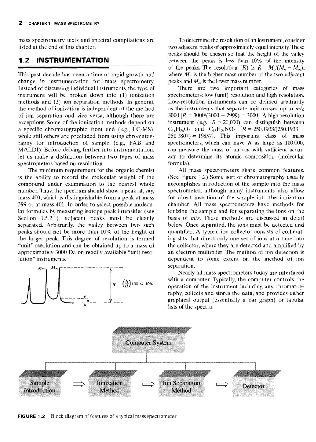
All mass spectrometers share common features.
(See Figure 1.2) Some sort of chromatography usually
accomplishes introduction of the sample into the mass
spectrometer, although many instruments also allow
for direct insertion of the sample into the ionization
chamber. All mass spectrometers have methods for
ionizing the sample and for separating the ions on the
basis of miz. These methods are discussed in detail
below. Once separated, the ions must be detected and
quantified. A typical ion collector consists of collimat-
ing slits that direct only one set of ions at a time into
the collector, where they are detected and amplified by
an electron multiplier. The method of ion detection is
dependent to some extent on the method of ion
separation.
Nearly all mass spectrometers today are interfaced
with a computer. Typically, the computer controls the
operation of the instrument including any chromatog-
raphy, collects and stores the data, and provides either
graphical output (essentially a bar graph) or tabular
lists of the spectra.
Computer System
Sample
introduction
Ionization
Method
Ion Separation
Method
Detector
FIGURE 1.2 Block diagram of features of a typical mass spectrometer.
1.3 IONIZATION METHODS 3
1.3	IONIZATION METHODS
The large number of ionization methods, some of
which are highly specialized, precludes complete cover-
age. The most common ones in the three general areas
of gas-phase, desorption, and evaporative ionization
are described below.
1.3.1 Gas-Phase Ionization Methods
Gas-phase methods for generating ions for mass spec-
trometry are the oldest and most popular methods. They
are applicable to compounds that have a minimum vapor
pressure of ca. H) fi Torr at a temperature at which the
compound is stable; this criterion applies to a large
number of nonionic organic molecules with MW < 1000.
1.3.1.1 Electron Impact Ionization. Electron
impact (El) is the most widely used method for gener-
ating ions for mass spectrometry. Vapor phase sample
molecules are bombarded with high-energy electrons
(generally 70 eV), which eject an electron from a
sample molecule to produce a radical cation, known as
the molecular ion. Because the ionization potential of
typical organic compounds is generally less than 15 eV,
the bombarding electrons impart 50 eV (or more) of
excess energy to the newly created molecular ion,
which is dissipated in part by the breaking of covalent
bonds, which have bond strengths between 3 and 10 eV.
Bond breaking is usually extensive and critically,
highly reproducible, and characteristic of the
compound. Furthermore, this fragmentation process
is also “predictable” and is the source of the powerful
structure elucidation potential of mass spectrometry.
Often, the excess energy imparted to the molecular
ion is too great, which leads to a mass spectrum with
no discernible molecular ion. Reduction of the ion-
ization voltage is a commonly used strategy to obtain
a molecular ion; the strategy is often successful
because there is greatly reduced fragmentation. The
disadvantage of this strategy is that the spectrum
changes and cannot be compared to “standard” liter-
ature spectra.
To many, mass spectrometry is synonymous with
El mass spectrometry. This view is understandable for
two reasons. First, historically, El was universally avail-
able before other ionization methods were developed.
Much of the early work was El mass spectrometry.
Second, the major libraries and databases of mass spec-
tral data, which are relied upon so heavily and cited so
often, are of El mass spectra. Some of the readily
accesible databases contain El mass spectra of over
390,000 compounds and they are easily searched by
efficient computer algorithms. The uniqueness of the
El mass spectrum for a given organic compound, even
for stereoisomers, is an almost certainty. This unique-
ness, coupled with the great sensitivity of the method, is
what makes GC-MS such a powerful and popular
analytical tool.
1.3.1.2 Chemical Ionization. Electron impact
ionization often leads to such extensive fragmentation
that no molecular ion is observed. One way to avoid this
problem is to use “soft ionization” techniques, of which
chemical ionization (CI) is the most important. In CI,
sample molecules (in the vapor phase) are not subjected
to bombardment by high energy electrons. Reagent gas
(usually methane, isobutane, ammonia, but others are
used) is introduced into the source, and ionized. Sample
molecules collide with ionized reagent gas molecules
(CH5+, C4H9+, etc) in the relatively high-pressure CI
source, and undergo secondary ionization by proton
transfer producing an [M + 1]+ ion, by electrophilic
addition producing [M + 15]+, [M + 24]+, [M + 43]+, or
[M T 18]+ (with NH4+) ions, or by charge exchange
(rare) producing a [M]+ ion. Chemical ionization spectra
sometimes have prominent [M — 1]+ ions because of
hydride abstraction. The ions thus produced are even
electron species. The excess energy transfered to the
sample molecules during the ionization phase is small,
generally less than 5 eV, so much less fragmentation
takes place. There are several important consequences,
the most valuable of which are an abundance of molecu-
lar ions and greater sensitity because the total ion
current is concentrated into a few ions. There is
however, less information on structure. The quasimolec-
ular ions are usually quite stable and they are readily
detected. Oftentimes there are only one or two fragment
ions produced and sometimes there are none.
For example, the El mass spectrum of 3, 4-dime-
thoxyacetophenone (Figure 1.3) shows, in addition to
the molecular ion at m/z 180, numerous fragment peaks
in the range of m/z 15-167; these include the base peak
at m/z 165 and prominent peaks at m/z 137 and m/z 77.
The CI mass spectrum (methane, CH4, as reagent gas)
shows the quasimolecular ion ([M + l]\m/z 181) as the
base peak (100%), and virtually the only other peaks,
each of just a few percent intensity, are the molecular
ion peak, m/z 180, m/z. 209 ([M + 29]+ or M + C2H5+),
and m/z 221 ([M + 41]+ or M + C3H5+). These last two
peaks are a result of electrophilic addition of carboca-
tions and are very useful in indentifing the molecular
ion. The excess methane carrier gas is ionized by elec-
tron impact to the primary ions CH4+ and CH3+. These
react with the excess methane to give secondary ions.
CH3+ + CH4-------> C2HS+ and H2
CH4 + C2H5 +-----> C3H5+ and 2H2
The energy content of the various secondary ions
(from, respectively, methane, isobutane, and ammonia)
decrease in the order: CH5+ > t-C4H9+ > NH4+. Thus,
4 CHAPTER 1 MASS SPECTROMETRY
by choice of reagent gas, we can control the tendency
of the CI produced [M + 1]+ ion to fragment. For
example, when methane is the reagent gas, dioctyl
phthalate shows its [M + 1]+ peak (mlz 391) as the
base peak; more importantly, the fragment peaks (e.g.,
mlz 113 and 149) are 30-60% of the intensity of the
base beak. When isobutane is used, the [M + 1]+ peak
is still large, while the fragment peaks are only roughly
5% as intense as the [M + 1]+ peak.
Chemical ionization mass spectrometry is not useful
for peak matching (either manually or by computer) nor
is it particularly useful for structure elucidation; its main
use is for the detection of molecular ions and hence
molecular weights.
1.3.2 Desorption Ionization Methods
Desorption ionization methods are those techniques in
which sample molecules are emitted directly from a con-
densed phase into the vapor phase as ions. The primary
use is for large, nonvolatile, or ionic compounds. There
can be significant disadvantages. Desorption methods
generally do not use available sample efficiently. Often-
times, the information content is limited. For unknown
compounds, the methods are used primarily to provide
molecular weight, and in some cases to obtain an exact
mass. However, even for this purpose, it should be used
with caution because the molecular ion or the quasimo-
lecular ion may not be evident. The resulting spectra are
often complicated by abundant matrix ions.
1.3.2.1 Field Desorption Ionization. In the
field desorption (FD) method, the sample is applied to a
metal emitter on the surface of which is found carbon
microneedles. The microneedles activate the surface,
which is maintained at the accelerating voltage and func-
tions as the anode. Very high voltage gradients at the tips
of the needles remove an electron from the sample, and
the resulting cation is repelled away from the emitter.
The ions generated have little excess energy so there is
minimal fragmentation, i.e., the molecular ion is usually
the only significant ion seen. For example with
cholesten-5-ene-3,16,22,26-tetrol the El and CI do not
see a molecular ion for this steroid. However, the FD
mass spectrum (Figure 1.4) shows predominately the
molecular ion with virtually no fragmentation.
Field desorption was eclipsed by the advent of
FAB (next section). Despite the fact that the method is
often more useful than FAB for nonpolar compounds
and does not suffer from the high level of background
ions that are found in matrix-assisted desorption meth-
ods, it has not become as popular as FAB probably
because the commercial manufacturers have strongly
supported FAB.
1.3.2.2 Fast Atom Bombardment Ionization.
Fast atom bombardment (FAB) uses high-energy
xenon or argon atoms (6-10 keV) to bombard samples
dissolved in a liquid of low vapor pressure (e.g., glyc-
erol). The matrix protects the sample from excessive
radiation damage. A related method, liquid secondary
1.3 IONIZATION METHODS 5
FIGURE 1.4 The electron impact (El), chemical ionization (CI), and field desorption (FD) mass spectra of
cholest-5-ene-3,16,22,26-tetrol.
ionization mass spectrometry, LSIMS, is similar except
that it uses somewhat more energetic cesium ions
(10-30 keV).
In both methods, positive ions (by cation attach-
ment ([M + 1]+ or [M + 23, Na]+) and negative ions
(by deprotonation [M — 1]+) are formed; both types of
ions are usually singly charged and, depending on the
instrument, FAB can be used in high-resolution mode.
FAB is used primarily with large nonvolatile mole-
cules, particularly to determine molecular weight. For
most classes of compounds, the rest of the spectrum is
less useful, partially because the lower mass ranges
may be composed of ions produced by the matrix
itself. However, for certain classes of compounds that
are composed of “building blocks,” such as polysaccha-
rides and peptides, some structural information may
be obtained because fragmentation usually occurs at
the glycosidic and peptide bonds, respectively, thereby
affording a method of sequencing these classes of
compounds.
The upper mass limit for FAB (and LSIMS) ioniza-
tion is between 10 and 20 kDa, and FAB is really most
useful up to about 6 kDa. FAB is seen most often with
double focusing magnetic sector instruments where it
has a resolution of about 0.3 mlz over the entire mass
range; FAB can, however, be used with most types of
mass analyzers. The biggest drawback to using FAB is
that the spectrum always shows a high level of matrix
generated ions, which limit sensitivity and which may
obscure important fragment ions.
1.3.2.3 Plasma Desorption Ionization. Plasma
desorption ionization is a highly specialized technique
used almost exclusively with a time of flight mass
6 CHAPTER 1 MASS SPECTROMETRY
analyzer (Section 1.4.4). The fission products from
Californium 252 (252Cf), with energies in the range of
80-100 MeV, are used to bombard and ionize the sample.
Each time a 252Cf splits, two particles are produced
moving in opposite directions. One of the particles hits
a triggering detector and signals a start time. The other
particle strikes the sample matrix ejecting some
sample ions into a time of flight mass spectrometer
(TOF-MS). The sample ions are most often released as
singly, doubly, or triply protonated moieties. These ions
are of fairly low energy so that structurally useful
fragmentation is rarely observed and, for polysaccharides
and polypeptides, sequencing information is not avail-
able. The mass accuracy of the method is limited by the
time of flight mass spectrometer. The technique is useful
on compounds with molecular weights up to at least
45 kDa.
1.3.2.4 Laser Desorption Ionization. A pulsed
laser beam can be used to ionize samples for mass
spectrometry. Because this method of ionization is
pulsed, it must be used with either a time of flight or a
Fourier transform mass spectrometer (Section 1.4.5). Two
types of lasers have found widespread use: A CO2 laser,
which emits radiation in the far infrared region, and
a frequency-quadrupled neodymium/yttriumaluminum-
garnet (Nd/YAG) laser, which emits radiation in the
UV region at 266 nm. Without matrix assistance, the
method is limited to low molecular weight molecules
(<2 kDa).
The power of the method is greatly enhanced by
using matrix assistance (matrix assisted laser
desorption ionization, or MALDI). Two matrix mate-
rials, nicotinic acid and sinapinic acid, which have
absorption bands coinciding with the laser employed,
have found widespread use and sample molecular
weights of up to two to three hundred thousand Da
have been successfully analyzed. A few picomoles of
sample are mixed with the matrix compound fol-
lowed by pulsed irradiation, which causes sample ions
(usually singly charged monomers but occasionally
multiply charged ions and dimers have been
observed) to be ejected from the matrix into the mass
spectrometer.
The ions have little excess energy and show little
propensity to fragment. For this reason, the method is
fairly useful for mixtures. The mass accuracy is low when
used with a TOF-MS, but very high resolution can be
obtained with a FT-MS. As with other matrix-assisted
methods, MALDI suffers from background interference
from the matrix material, which is further exacerbated by
matrix adduction. Thus, the assignment of a molecular
ion of an unknown compound can be uncertain.
1.3.3 Evaporative Ionization Methods
There are two important methods in which ions or, less
often, neutral compounds in solution (often containing
formic acid) have their solvent molecules stripped by
evaporation, with simultaneous ionization leaving
behind the ions for mass analysis. Coupled with liquid
chromatography instrumentation, these methods have
become immensely popular.
1.3.3.1 Thermospray Mass Spectrometry. In
the thermospray method, a solution of the sample is
introduced into the mass spectrometer by means of
a heated capillary tube. The tube nebulizes and partially
vaporizes the solvent forming a stream of fine droplets,
which enter the ion source. When the solvent completely
evaporates, the sample ions can be mass analyzed. This
method can handle high flow rates and buffers; it was an
early solution to interfacing mass spectrometers with
aqueous liquid chromatography. The method has largely
been supplanted by electrospray.
1.3.3.2 Electrospray Mass Spectrometry.
The electrospray (ES) ion source (Figure 1.5) is oper-
ated at or near atmospheric pressure and, thus is also
called atmospheric pressure ionization or API. The
ESI Spray Droplets with
Excess Charge on Surface
Charged plates
Nebulizer gas (
Nebulizer needle—
Solvent/sample
Nebulizer gas
э © I Mass
e®®® | Spectrometer
тч гл @ @	-
® ftTffi® ®
® ®	I \
•v: \
Capillary Entrance
2-5 kV
Power supply
FIGURE 1.5 A diagram showing the evaporation of solvent leading to individual ions in an electrospray
instrument.
1.3 IONIZATION METHODS 7
sample in solution (usually a polar, volatile solvent)
enters the ion source through a stainless steel capillary,
which is surrounded by a co-axial flow of nitrogen
called the nebulizing gas. The tip of the capillary
is maintained at a high potential with respect to
a counter-electrode. The potential difference produces
a field gradient of up to 5 kV/cm. As the solution exits
the capillary, an aerosol of charged droplets forms. The
flow of nebulizing gas directs the effluent toward the
mass spectrometer.
Droplets in the aerosol shrink as the solvent evap-
orates, thereby concentrating the charged sample ions.
When the electrostatic repulsion among the charged
sample ions reaches a critical point, the droplet under-
goes a so-called “Coulombic explosion,” which releases
the sample ions into the vapor phase. The vapor phase
ions are focused with a number of sampling orifices
into the mass analyzer.
Electrospray MS has undergone an explosion of
activity since about 1990, mainly for compounds that
have multiple charge bearing sites. With proteins, for
example, ions with multiple charges are formed. Since
the mass spectrometer measures mass to charge ratio
(mlz) rather than mass directly, these multiply
charged ions are recorded at apparent mass values of
1/2, 1/3, . . . l/п of their actual masses, where n is the
number of charges (z). Large proteins can have 40 or
more charges so that molecules of up to 100 kDa can
be detected in the range of conventional quadrupole,
ion trap, or magnetic sector mass spectrometers. The
appearance of the spectrum is a series of peaks
increasing in mass, which correspond to pseudo molec-
ular ions possessing sequentially one less proton and
therefore one less charge.
Determination of the actual mass of the ion
requires that the charge of the ion be known. If two
peaks, which differ by a single charge, can be identi-
fied, the calculation is reduced to simple algebra.
Recall that each ion of the sample molecule (Ms) has
the general form (Ms + zH)z+ where H is the mass of a
proton (1.0079 Da). For two ions differing by one
charge, = [Ms + (z + l)H]/(z + 1) and m2 = [(Ms +
zH)/z]. Solving the two simultaneous equations for
the charge z, yields z = (m[ — H)/(m2 - /и,). A simple
computer program automates this calculation for
every peak in the spectrum and calculates the mass
directly.
Many manufacturers have introduced inexpensive
mass spectrometers dedicated to electrospray for two
reasons. First, the method has been very successful
while remaining a fairly simple method to employ. Sec-
ond, the analysis of proteins and smaller peptides has
grown in importance, and they are probably analyzed
best by the electrospray method.
Figure 1.6 compares the El mass spectrum (lower
portion of the figure) of lactose to its ES mass spectrum
(upper portion of figure). Lactose is considered in more
detail in Chapter 5. The El mass spectrum is completely
8 CHAPTER 1 MASS SPECTROMETRY
OH
I
FIGURE 1.7 The electrospray (ES) mass spectrum for the tetra-peptide whose structure is given in the figure. See
text for explanation.
useless because lactose has low vapor pressure, it is ther-
mally labile, and the spectrum shows no characteristic
peaks. The ES mass spectrum shows a weak molecular
ion peak at m/z 342 and a characteristic [M + 23]+, the
molecular ion peak plus sodium. Because sodium ions
are ubiquitous in aqueous solution, these sodium
adducts are very common.
The ES mass spectrum of a tetra-peptide comprised
of valine, glycine, serine, and glutamic acid (VGSE) is
given in Figure 1.7. VGSE is also an example compound
in Chapter 5. The base beak is the [M + 1]+ ion at m/z
391 and the sodium adduct, [M + 23]+, is nearly 90%
of the base peak. In addition, there is some useful
fragmentation information characteristic of each of the
amino acids. For small peptides, it is not uncommon to
find some helpful fragmentation, but for proteins it is
less likely.
Methods of ionization are summarized in Table 1.1.
1.4	MASS ANALYZERS
The mass analyzer, which separates the mixture of ions
that are generated during the ionization step by m/z in
order to obtain a spectrum, is the heart of each mass
spectrometer, and there are several different types with
TABLE 1.1 Summary of Ionization Methods.
Ionization Method	Ions Formed	Sensitivity	Advantage	Disadvantage
Electron impact	M+	ng-Pg	Data base searchable Structural information	M+ occasionally absent
Chemical ionization	M + 1, M + 18, etc	ng-pg	M+ usually present	Little structural information
Field desorption	M+	M-g-ng	Non volatile compounds	Specialized equipment
Fast atom bombardment	M + 1,M + cation M + matrix	Mg-ng	Non volatile compounds Sequencing information	Matrix interference Difficult to interpret
Plasma desorption	M+	P-g-ng	Non volatile compounds	Matrix interference
Laser desorption	M + 1, M + matrix	Mg-ng	Non volatile compounds Burst of ions	Matrix interference
Thermospray	M+	Mg-ng	Non volatile compounds	Outdated
Electrospray	M+,M++,M+ ++, etc.	ng-pg	Non volatile compounds interfaces w/ LC Forms multiply charged ions	Limited classes of compounds Little structural information
1.4 MASS ANALYZERS 9
Sample
introduction
FIGURE 1.8 Schematic diagram of a single focusing, 180" sector mass analyzer. The magnetic
field is perpendicular to the page.The radius of curvature varies from one instrument to an-
other.
different characteristics. Each of the major types of mass
analyzers is described below.This section concludes with
a brief discussion of tandem MS and related processes.
1.4.1 Magnetic Sector Mass
Spectrometers
'Inc magnetic sector mass spectrometer (MS-MS) uses
a magnetic held to deflect moving ions around a curved
path (see Figure 1.8). Magnetic sector mass spectrome-
ters were the first commercially available instruments,
and they remain an important choice. Separation of ions
occurs based on the mass/charge ratio with lighter ions
deflected to a greater extent than are the heavier
ions. Resolution depends on each ion entering the mag-
netic field (from the source) with the same kinetic
energy, accomplished by accelerating the ions (which
have a charge z) with a voltage V. Each ion acquires
kinetic energy E ~ z,V nn>2/2. When an accelerated
ion enters the magnetic field (B), it experiences a
deflecting force (Bzv), which bends the path of the ion
orthogonal to its original direction. The ion is now trav-
eling in a circular path of radius r, given by Bzv niv-lr.
The two equations can be combined to give the familiar
magnetic sector equation: m/z = B;r72E Because the
radius of the instrument is fixed, the magnetic field is
scanned to bring the ions sequentially into focus. As
these equations show, a magnetic sector instrument sep-
arates ions on the basis of momentum, which is the
product of mass and velocity, rather than mass alone:
therefore, ions of the same mass but different energies
will come into focus at different points.
An electrostatic analyzer (ESA) can greatly
reduce the energy distribution of an ion beam by forc-
ing ions of the same charge (z) and kinetic energy
(regardless of mass) to follow the same path. A slit at
the exit of the ESA further focuses the ion beam
before it enters the detector. The combination of an
Sample
introduction
Computer
FIGURE 1.9 Schematic of double-focusing mass spectrometer.
10 CHAPTER 1 MASS SPECTROMETRY
FIGURE 1.10 Schematic representation of a quadrupole “mass filter" or ion separator.
ESA and a magnetic sector is known as double focus-
ing, because the two fields counteract the dispersive
effects each has on direction and velocity.
The resolution of a double focusing magnetic sector
instrument (Figure 1.9) can be as high as 100,000 through
the use of extremely small slit widths. This very high
resolution allows the measurement of “exact masses,”
which unequivocally provide molecular formulas, and is
enormously useful. Such high-resolution instruments
sacrifice a great deal of sensitivity. By comparison, slits
allowing an energy distribution for about 5000 resolution
give at least 0.5 mlz accuracy across the entire mass
range, i.e., the “unit resolution” that is used in a standard
mass spec. The upper mass limit for commercial magnetic
sector instruments is about mlz 15,000. Raising this upper
limit is theoretically possible but impractical.
1.4.2 Quadrupole Mass Spectrometers
The quadrupole mass analyzer is much smaller and
cheaper than a magnetic sector instrument. A quadru-
pole setup (seen schematically in Figure 1.10) consists
of four cylindrical (or of hyperbolic cross-section) rods
(100-200 mm long) mounted parallel to each other, at
the corners of a square. A complete mathematical
analysis of the quadrupole mass analyzer is complex
but we can discuss how it works in a simplified form.
A constant DC voltage modified by a radio frequency
voltage is applied to the rods. Ions are introduced to
the “tunnel” formed by the four rods of the quadrupole
in the center of the square at one end to the rods, and
travel down the axis.
For any given combination of DC voltage and
modified voltage applied at the appropriate frequency,
only ions with a certain mlz value possess a stable tra-
jectory and therefore are able to pass all the way to the
end of the quadrupole to the detector. All ions with dif-
ferent mlz values travel unstable or erratic paths and
collide with one of the rods or pass outside the
quadrupole. An easy way to look at the quadrupole
mass analyzer is as a tunable mass filter. In other
words, as the ions enter at one end, only one mlz ion
will pass through. In practice, the filtering can be car-
ried out at a very fast rate so that the entire mass range
can be scanned in considerably less than 1 second.
With respect to resolution and mass range, the
quadrupole is generally inferior to the magnetic sector.
For instance, the current upper mass range is generally
less than 5000 mlz. On the other hand, sensitivity is gen-
erally high because there is no need for resolving slits,
which would remove a portion of the ions. An important
advantage of quadrupoles is that they operate most effi-
ciently on ions of low velocity, which means that their ion
sources can operate close to ground potential (i.e., low
voltage). Since the entering ions generally have energies
of less than 100 eV, the quadrupole mass spectrometer is
ideal for interfacing to LC systems and for atmospheric
pressure ionization (API) techniques such as electro-
spray (see Section 1.3.3.2). These techniques work best
on ions of low energy so that fewer high-energy collisions
will occur before they enter the quadrupole.
1.4.3 Ion Trap Mass Spectrometer
The ion trap is sometimes considered as a variant of
the quadrupole, since the appearance and operation
of the two are related. However, the ion trap is
potentially much more versatile and clearly has
greater potential for development. At one time the
ion trap had a bad reputation because the earliest ver-
sions gave inferior results compared to quadrupoles.
The results were oftentimes “concentration depen-
dent”; relatively large sample sizes usually gave many
peaks with the mass of the [ion + 1], which renders
the resulting spectra useless in a search with standard
El libraries. These problems have been overcome and
1.4 MASS ANALYZERS 1 1
Ion volume
Source lenses
Einzel lens,
First element
Trap end caps
FIGURE 1.11 Cross sectional view of an ion trap.
the El spectra obtained with an ion trap are now fully
searchable with commercial databases. Furthermore,
the ion trap is more sensitive than the quadrupole
arrangement, and the ion trap is routinely configured
to carry out tandem experiments with no extra hard-
ware needed.
In one sense, an ion trap is aptly named because,
unlike the quadrupole, which merely acts as a mass
filter, it can “trap” ions for relatively long periods of
time, with important consequences. The simplest use of
the trapped ions is to sequentially eject them to a
detector, producing a conventional mass spectrum.
Before other uses of trapped ions are briefly described,
a closer look at the ion trap itself will be helpful.
The ion trap generally consists of three electrodes,
one ring electrode with a hyperbolic inner surface and
two hyperbolic endcap electrodes at either end (a cross
section of an ion trap is found in Figure 1.11). The ring
electrode is operated with a sinusoidal radio frequency
field while the endcap electrodes are operated in one
of three modes. The endcap may be operated at ground
potential, or with either a DC or an AC voltage.
The mathematics that describes the motion of ions
within the ion trap is given by the Mathieu equation.
Details and discussions of three-dimensional ion stabil-
ity diagrams can be found in either March and Hughes
(1989) or Nourse and Cooks (1990). The beauty of the
ion trap is that by controlling the three parameters of
RF voltage, AC voltage, and DC voltage, a wide variety
of experiments can be run quite easily (for details see
March and Hughes 1989).
There are three basic modes in which the ion trap
can be operated. First, when the ion trap is operated
with a fixed RF voltage and no DC bias between the
endcap and ring electrodes, all ions above a certain cut-
off m/z ratio will be trapped. As the RF voltage is
raised, the cutoff miz. is increased in a controlled
manner and the ions are sequentially ejected and
detected. The result is the standard mass spectrum and
this procedure is called the “mass-selective instability”
mode of operation. The maximum RF potential that
can be applied between the electrodes limits the upper
mass range in this mode. Ions of mass contained
beyond the upper limit are removed after the RF
potential is brought back to zero.
The second mode of operation uses a DC poten-
tial across the endcaps; the general result is that there
is now both a low and high-end cutoff (m/z) of ions.
The possibilities of experiments in this mode of
operation are tremendous, and most operations with
the ion trap use this mode. As few as one ion mass can
be selected. Selective ion monitoring is an important
use of this mode of operation. There is no practical
limit on the number of ions masses that can be
selected.
The third mode of operation is similar to the sec-
ond, with the addition of an auxiliary oscillatory field
between the endcap electrodes, which results in adding
kinetic energy selectively to a particular ion. With a
small amplitude auxiliary field, selected ions gain
kinetic energy slowly, during which time they usually
undergo a fragmenting collision; the result can be a
nearly 100% MS-MS efficiency. If the inherent sensitiv-
ity of the ion trap is considered along with the nearly
100% tandem efficiency, the use of the ion trap for
tandem MS experiment greatly outshines the so called
“triple quad” (see below).
Another way to use this kinetic energy addition
mode is to selectively reject unwanted ions from the ion
trap. These could be ions derived from solvent or from
the matrix in FAB or LSIMS experiments. A constant
frequency field at high voltage during the ionization
period will selectively reject a single ion. Multiple ions
can also be selected in this mode.
12 CHAPTER 1 MASS SPECTROMETRY
1.4.4 Time-of-Flight
Mass Spectrometer
The concept of time-of-flight (TOF) mass spectrome-
ters is simple. Ions are accelerated through a potential
(V) and are then allowed to “drift” down a tube to
a detector. If the assumption is made That all of the ions
arriving at the beginning of the drift tube have the
same energy given by zeV = mv2/2, then ions of differ-
ent mass will have different velocities: v = (2zeV/m)1/2.
If a spectrometer possesses a drift tube of length L, the
time of flight for an ion is given by: t = (L2m/2zeV)112,
from which the mass for a given ion can be easily
calculated.
The critical aspect of this otherwise simple instru-
ment is the need to produce the ions at an accurately
known start time and position. These constraints gener-
ally limit TOF spectrometers to use pulsed ionization
techniques, which include plasma and laser desorp-
tion (e.g., MALDI, matrix assisted laser desorption
ionization).
The resolution of TOF instruments is usually less
than 20,000 because some variation in ion energy is
unavoidable. Also, since the difference in arrival times
at the detector can be less than HF7 s, fast electronics
are necessary for adequate resolution. On the positive
side, the mass range of these instruments is unlimited,
and, like quadrupoles, they have excellent sensitivity
due to lack of resolving slits. Thus, the technique is
most useful for large biomolecules.
1.4.5 Fourier Transform
Mass Spectrometer
Fourier transform (FT) mass spectrometers are not
very common now because of their expense; in time,
they may become more widespread as advances are
made in the manufacture of superconducting magnets.
In a Fourier transform mass spectrometer, ions
are held in a cell with an electric trapping potential
within a strong magnetic field. Within the cell, each ion
orbits in a direction perpendicular to the magnetic
field, with a frequency proportional to the ion’s mlz.
A radiofrequency pulse applied to the cell brings all
of the cycloidal frequencies into resonance simultane-
ously to yield an interferogram, conceptually similar
to the free induction decay (FID) signal in NMR or
the interferogram generated in FTIR experiments. The
interferogram, which is a time domain spectrum, is
Fourier transformed into a frequency domain spec-
trum, which then yields the conventional т/z spectrum.
Pulsed Fourier transform spectrometry applied to
nuclear magnetic resonance spectrometry is discussed
in Chapters 3,4, and 5.
Because the instrument is operated at fixed magnetic
field strength, extremely high field superconducting
magnets can be used. Also, because mass range is
directly proportional to magnetic field strength, very high
mass detection is possible. Finally, since all of the ions
from a single ionization event can be trapped and ana-
lyzed, the method is very sensitive and works well
with pulsed ionization methods. The most compelling
aspect of the method is its high resolution, making FT
mass spectrometers an attractive alternative to other
mass analyzers. The FT mass spectrometer can be cou-
pled to chromatographic instrumentation and various
ionization methods, which means that it can be easily
used with small molecules. Further information on FT
mass spectrometers can be found in the book by Gross
(1990).
1.4.6 Tandem Mass Spectrometry
Tandem mass spectrometry or MS-MS (“MS
squared”) is useful in studies with both known and
unknown compounds; with certain ion traps, MS to
the nth (MS(n)) is possible where n = 2 to 9. In
practice, n rarely exceeds 2 or 3. With MS-MS, a “par-
ent” ion from the initial fragmentation (the initial
fragmentation gives rise to the conventional mass
spectrum) is selected and allowed or induced to
fragment further thus giving rise to “daughter” ions.
In complex mixtures, these daughter ions provide
unequivocal evidence for the presence of a known
compound. For unknown or new compounds, these
daughter ions provide potential for further structural
information.
One popular use of MS-MS involves ionizing a
crude sample, selectively “fishing out” an ion character-
istic for the compound under study, and obtaining the
diagnostic spectrum of the daughter ions produced
from that ion. In this way, a compound can be unequiv-
ocally detected in a crude sample, with no prior
chromatographic (or other separation steps) being
required. Thus, MS-MS can be a very powerful screen-
ing tool. This type of analysis alleviates the need for
complex separations of mixtures for many routine
analyses. For instance, the analysis of urine samples
from humans (or from other animals such as race
horses) for the presence of drugs or drug metabolites
can be carried out routinely on whole urine (i.e., no
purification or separation) by MS-MS. For unknown
compounds, these daughter ions can provide structural
information as well.
One way to carry out MS-MS is to link two or
more mass analyzers in series to produce an instrument
capable of selecting a single ion, and examining how
that ion (either a parent or daughter ion) fragments.
For instance, three quadrupoles can be linked (a so
called “triple quad”) to produce a tandem mass spec-
trometer. In this arrangement, the first quadrupole
selects a specific ion for further analysis, the second
1.5 INTERPRETATION OF El MASS SPECTRA 13
TABLE 1.2 Summary of Mass Analyzers.
Mass Analyzer	Mass Range	Resolution	Sensitivity	Advantage	Disadvantage
Magnetic Sector	1-15,000 m/z	0.0001	Low	High res.	Low sensitivity Very expensive High technical expertise
Quadrupole	1-5000 m/z	unit	High	Easy to use Inexpensive High sensitivity	Low res. Low mass range
Ion trap	1-5000 m/z	unit	High	Easy to use Inexpensive High sensitivity Tandem MS (MS")	Low res. Low mass range
Time of flight	Unlimited	0.0001	High	High mass range Simple design	Very high res.
Fourier transform	up to 70 kDa	0.0001	High	Very High res. and mass range	Very expensive High technical expertise
quadrupole functions as a collision cell (collision
induced decomposition, CID) and is operated with
radiofrequency only, and the third quadrupole separates
the product ions, to produce a spectrum of daughter
ions. The field of tandem mass spectrometry is
already rather mature with good books available
(Benninghoven et al. 1987 and Wilson et al. 1989).
In order for an instrument to carry out MS-MS, it
must be able to do the three operations outlined above. As
we have seen however, ion-trap systems capable of
MS-MS and MS(/1) do not use a tandem arrangement
of mass analyzers at all, but rather use a single ion trap
for all three operations simultaneously. As has already
been stated, these ion-trap tandem mass spectrometer
experiments are very sensitive and are now user friendly.
The ion trap brings the capability for carrying out
MS-MS experiments to the benchtop at relatively low cost.
A summary of mass analyzers and ionization
methods is displayed in Table 1.2.
1.5	INTERPRETATION
OF El MASS SPECTRA
Our discussion of interpreting mass spectra is limited to
El mass spectrometry. Fragmentation in El mass spectra
is rich with structural information; mastery of El mass
spectra is especially useful for the organic chemist.
El mass spectra are routinely obtained at an
electron beam energy of 70 eV. The simplest event that
occurs is the removal of a single electron from the
molecule in the gas phase by an electron of the electron
beam to form the molecular ion, which is a radical
cation. For example, methanol forms a molecular ion in
which the single dot represents the remaining odd
electron as seen in Scheme 1.1. When the charge can be
localized on one particular atom, the charge is shown
on that atom:
CH3OH
CH3OH + e ----> CH3OH’>/z 32) + 2e
(Sch 1.1)
Many of these molecular ions disintegrate in
10-10-10~3 s to give, in the simplest case, a positively
charged fragment and a radical. Many fragment ions
are thus formed, and each of these can cleave to yield
smaller fragments; examples of possible cleavages for
methanol are given in Scheme 1.2.
CH3OH +-----> CH2OH+ (m/z 31) + H’
CH3OH +-----> CH3+ (m/z 15) + OH
CH2OH+------> CHO+ (m/z 29) + H2
(Sch 1.2)
If some of the molecular ions remain intact long
enough to reach the detector, we see a molecular ion
peak. It is important to recognize the molecular ion
peak because this gives the molecular weight of the
compound. With unit resolution, this weight is the mo-
lecular weight to the nearest whole number.
A mass spectrum is a presentation of the masses of
the positively charged fragments (including the molecu-
lar ion) versus their relative concentrations. The most
intense peak in the spectrum, called the base peak, is
assigned a value of 100%, and the intensities (height X
sensitivity factor) of the other peaks, including the
molecular ion peak, are reported as percentages of the
base peak. Of course, the molecular ion peak may
sometimes be the base peak. In Figure 1.1, the molecu-
lar ion peak is m/z 121, and the base peak is m/z 77.
14 CHAPTER 1 MASS SPECTROMETRY
A tabular or graphic presentation of a spectrum
may be used. A graph has the advantage of present-
ing patterns that, with experience, can be quickly
recognized. However, a graph must be drawn so that
there is no difficulty in distinguishing mass units.
Mistaking a peak at, say, m/z 79 for m/z 80 can result in
total confusion. The molecular ion peak is usually the
peak of highest mass number except for the isotope
peaks.
1.5.1 Recognition of
the Molecular Ion Peak
Quite often, under electron impact (El), recognition of
the molecular ion peak (M)+ poses a problem. The
peak may be very weak or it may not appear at all; how
can we be sure that it is the molecular ion peak and not
a fragment peak or an impurity? Often the best solu-
tion is to obtain a chemical ionization spectrum (see
Section 1.3.1.2). The usual result is an intense peak at
[M + 1]+ and little fragmentation.
Many peaks can be ruled out as possible molecular
ions simply on grounds of reasonable structure
requirements. The “nitrogen rule” is often helpful. It
states that a molecule of even-numbered molecular
weight must contain either no nitrogen or an even
number of nitrogen atoms; an odd-numbered
molecular weight requires an odd number of nitrogen
atoms.* This rule holds for all compounds containing
carbon, hydrogen, oxygen, nitrogen, sulfur, and the
halogens, as well as many of the less usual atoms such
as phosphorus, boron, silicon, arsenic, and the alkaline
earths.
A useful corollary states that fragmentation at a
single bond gives aji odd-numbered ion fragment
from an even-numbered molecular ion, and an even-
numbered ion fragment from an odd-numbered
molecular ion. For this corollary to hold, the ion
fragment must contain all of the nitrogen (if any) of
the molecular ion.
Consideration of the breakdown pattern coupled
with other information will also assist in identify-
ing molecular ions. It should be kept in mind that
Appendix A contains fragment formulas as well as
molecular formulas. Some of the formulas may be
discarded as trivial in attempts to solve a particular
problem.
The intensity of the molecular ion peak depends on
the stability of the molecular ion. The most stable molec-
ular ions are those of purely aromatic systems. If sub-
stituents that have favorable modes of cleavage are
present, the molecular ion peak will be less intense, and
the fragment peaks relatively more intense. In general,
* For the nitrogen rule to hold, only unit atomic masses (i.e., integers)
are used in calculating the formula masses.
the following group of compounds will, in order of
decreasing ability, give prominent molecular ion peaks:
aromatic compounds > conjugated alkenes > cyclic
compounds > organic sulfides > short, normal alkanes >
mercaptans. Recognizable molecular ions are usually
produced for these compounds in order of decreasing
ability: ketones > amines > esters > ethers > carboxylic
acids ~ aldehydes ~ amides ~ halides. The molecular
ion is frequently not detectable in aliphatic alcohols,
nitrites, nitrates, nitro compounds, nitriles, and in highly
branched compounds.
The presence of an M — 15 peak (loss of CH3), or
an M - 18 peak (loss of H2O), or an M — 31 peak
(loss of OCH3 from methyl esters), and so on, is taken as
confirmation of a molecular ion peak. An M — 1 peak is
common, and occasionally an M - 2 peak (loss of H2 by
either fragmentation or thermolysis), or even a rare
M — 3 peak (from alcohols) is reasonable. Peaks in the
range of M — 3 to M — 14, however, indicate that
contaminants may be present or that the presumed mo-
lecular ion peak is actually a fragment ion peak. Losses
of fragments of masses 19-25 are also unlikely (except
for loss of F = 19 or HF = 20 from fluorinated com-
pounds). Loss of 16 (O), 17 (OH), or 18 (H2O) are likely
only if an oxygen atom is in the molecule.
1.5.2 Determination of
a Molecular Formula
1.5.2.1 Unit-Mass Molecular Ion and Isotope
Peaks. So far, we have discussed the mass spectrum in
terms of unit resolutions: The unit mass of the molecular
ion of C7H7NO (Figure 1.1) is m/z 121—that is, the sum
of the unit masses of the most abundant isotopes: (7 X 12
[for 12C]) + (7X1 [for 'H]) + (1 X 14 [for 14N] + (1 X
16 [for 16O]) = 121.
In addition, molecular species exist that contain the
less abundant isotopes, and these give rise to the “isotope
peaks” at M + 1, M + 2, etc. In Figure 1.1, the M + 1
peak is approximately 8% of the intensity of the molecu-
lar ion peak, which for this purpose, is assigned an inten-
sity of 100%. Contributing to the M + 1 peak are the
isotopes, 13C, 2H, 15N, and 17O. Table 1.3 gives the abun-
dances of these isotopes relative to those of the most
abundant isotopes. The only contributor to the M + 2
peak of C7H7NO is l8O, whose relative abundance is very
low: thus the M + 2 peak is undetected. If only С, H, N,
O, F, P, and I are present, the approximate expected
percentage (M + 1) and percentage (M + 2) intensities
can be calculated by use of the following equations for a
compound of formula CnH^NjO,, (note: F, P, and I are
monoisotopic and do not contribute and can be ignored
for the calculation):
% (M + 1) « (1.1 • n) + (0.36 • x) and % (M + 2) «
(1.1 • n)2/200 + (0.2 -y)
1.5 INTERPRETATION OF El MASS SPECTRA 1 5
TABLE 1.3 Relative Isotope Abundances of Common Elements.
Elements	Isotope	Relative Abundance	Isotope	Relative Abundance	Isotope	Relative Abundance
Carbon	l2C	100	l3C	1.11		
Hydrogen	'H	100	2H	0.016		
Nitrogen	14N	100	15N	0.38		
Oxygen	16O	100	17o	0.04	18O	0.2
Fluorine	I9p	100				
Silicon	28Si	100	29Si	5.1	30Si	3.35
Phosphorus	3lp	100				
Sulfur	32S	100	33s	0.78	34S	4.4
Chlorine	35Cl	100			37C1	32.5
Bromine	79Br	100			81Br	98
Iodine	127I	100				
If these isotope peaks are intense enough to be
measured accurately, the above calculations may be
useful in determining the molecular formula.*
If sulfur or silicon is present, the M + 2 will be more
intense. In the case of a single sulfur atom, 34S contributes
approximately 4.40% to the M + 2 peak; for a single
silicon in the molecule, 30Si contributes about 3.35% to
the M + 2 peak (see Section 1.6.15). The effect of several
bromine and chlorine atoms is described in Section
1.6.16. Note the appearance of additional isotope peaks
in the case of multiple bromine and chlorine atoms.
Obviously the mass spectrum should be routinely
scanned for the relative intensities of the M + 2, M + 4,
and higher isotope peaks, and the relative intensities
should be carefully measured. Since F, P, and I are
monoisotopic, they can be difficult to spot.
For most of the Problems in this text, the unit-
resolution molecular ion, used in conjunction with IR
and NMR, will suffice for determining the molecular for-
mula by browsing in Appendix A. For several more diffi-
cult Problems, the high-resolution formula masses—for
use with Appendix A (see Section 1.5.2.2) — have been
supplied.
Table 1.3 lists the principal stable isotopes of the
common elements and their relative abundance calcu-
lated on the basis of 100 molecules containing the most
common isotope. Note that this presentation differs
from many isotope abundance tables, in which the sum
of all the isotopes of an element adds up to 100%.
1.5.2.2 High-Resolution Molecular Ion. A
unique molecular formula (or fragment formula) can
often be derived from a sufficiently accurate mass
* There are limitations beyond the difficulty of measuring small
peaks: The l3C/2C ratio differs with the source of the compound—
synthetic compared with a natural source. A natural product from
different organisms or regions may show differences. Furthermore,
isotope peaks may be more intense than the calculated value because
of ion-molecule interactions that vary with the sample concentra-
tion or with the class of compound involved.
measurement alone (high-resolution mass spectrometry).
This is possible because the nuclide masses are not
integers (see Table 1.4). For example, we can distin-
guish at a unit mass of 28 among CO, N2, CH2N, and
C2H4. The exact mass of CO is: 12.0000 (for 12C) +
15.9949 (for 16O) = 27.9949; the exact mass of N2 is:
2 X 14.0031 (for 14N) = 28.0062. Similar calculations give
an exact mass of 28.0187 for CH2N and 28.0312 for C2H4.
Thus, the mass observed for the molecular ion of
CO, for example, is the sum of the exact formula
masses of the most abundant isotope of carbon and of
oxygen. This differs from a molecular weight of CO
based on atomic weights that are the average of
TABLE 1.4 Exact Masses of Isotopes.
Element	Atomic Weight	Nuclide	Mass
Hydrogen	1.00794	‘H	1.00783
		D(2H)	2.01410
Carbon	12.01115	12C	12.00000 (std)
		13c	13.00336
Nitrogen	14.0067	l4N	14.0031
		l5N	15.0001
Oxygen	15.9994	16O	15.9949
		17o	16.9991
		18o	17.9992
Fluorine	18.9984	19p	18.9984
Silicon	28.0855	28S1	27.9769
		29S1	28.9765
		3OS1	29.9738
Phosphorus	30.9738	3!p	30.9738
Sulfur	32.0660	32s	31.9721
		33s	32.9715
		34s	33.9679
Chlorine	35.4527	35CI	34.9689
		37CI	36.9659
Bromine	79.9094	79Br	78.9183
		81Br	80.9163
Iodine	126.9045	127I	126.9045
16 CHAPTER 1 MASS SPECTROMETRY
weights of all natural isotopes of an element (e.g., C =
12.01, О = 15.999).
Table 1.4 gives the masses to four or five decimal
places for the common nuclides; it also gives the familiar
atomic weights (average weights for the elements).
Appendix A lists molecular and fragment formulas
in order of the unit masses. Under each unit mass, the
formulas are listed in the standard Chemical Abstract
system. The formula mass (FM) to four decimal places
is given for each formula. Appendix A is designed for
browsing, on the assumption that the student has a unit
molecular mass from a unit-resolution mass spectrome-
ter and clues from other spectra. Note that the table
includes only С, H, N, and O.
1.5.3 Use of the Molecular Formula.
Index of Hydrogen Deficiency
If organic chemists had to choose a single item of infor-
mation above all others that are usually available from
spectra or from chemical manipulations, they would
certainly choose the molecular formula.
In addition to the kinds and numbers of atoms, the
molecular formula gives the'" index of hydrogen defi-
ciency. The index of hydrogen deficiency is the number of
pairs of hydrogen atoms that must be removed from the
corresponding “saturated” formula to produce the mo-
lecular formula of the compound of interest. The index of
hydrogen deficiency is also called the number of “sites
(or degrees) of unsaturation”; this description is incom-
plete since hydrogen deficiency can result from cyclic
structures as well as from multiple bonds. The index is
thus the sum of the number of rings, the number of dou-
ble bonds, and twice the number of triple bonds.
The index of hydrogen deficiency can be calculated
for compounds containing carbon, hydrogen, nitrogen,
halogen, oxygen, and sulfur having the generalized
molecular formula, C„H„,XxNyO?, from the equation
Index = (//) - (m/2) - (x/2) + (y/2) + 1
Thus, the compound C7H7NO has an index of
7 - 3.5 + 0.5 + 1 = 5. Note that divalent atoms (oxy-
gen and sulfur) are not counted in the formula.
For the generalized molecular formula о^пУпДу,
the index = (IV) - (1/2) + (III/2) + 1, where a is H, D,
or halogen (i.e., any monovalent atom), /3 is O, S, or any
other bivalent atom, у is N, P, or any other trivalent
atom, and 3 is C, Si, or any other tetravalent atom. The
numerals I-IV designate the numbers of the mono-,
di-, tri-, and tetravalent atoms, respectively.
For simple molecular formulas, we can arrive at the
index by comparison of the formula of interest with the
molecular formula of the corresponding saturated com-
pound. Compare C6H6 and C6H14; the index is 4 for the
former and 0 for the latter.
O'	О
S+	N+
H3C \h3 H3CZ \>- (C6H5)3P—о
Dimethyl
sulfoxide
nitromethane triphenylphosphine
oxide
FIGURE 1.12 “Polar” Lewis structures of dimethyl
sulfoxide, nitromethane, and triphenylphosphine
oxide that correctly account for the index of hydro-
gen deficiency.
The index for C7H7NO is 5, and a possible structure
is benzamide (see Figure 1.1). Of course, other isomers
(i.e., compounds with the same molecular formula) are
possible, such as
Note that the benzene ring itself accounts for four
“sites of unsaturation”: three for the double bonds and
one for the ring.
Polar structures must be used for compounds con-
taining an atom in a higher valence state, such as sulfur
or phosphorus. Thus, if we treat sulfur in dimethyl
sulfoxide (DMSO) formally as a divalent atom, the
calculated index, 0, is compatible with the structure in
Figure 1.12. We must use only formulas with filled
valence shells; that is, the Lewis octet rule must be
obeyed.
Similarly, if we treat the nitrogen in nitromethane
as a trivalent atom, the index is 1, which is com-
patible with Figure 1.12. If we treat phosphorus in
triphenylphosphine oxide as trivalent, the index is 12,
which fits the Lewis structure in Figure 1.12. As an
example, let us consider the molecular formula
C|3HyN2O4BrS. The index of hydrogen deficiency
would be 13 - 10/2 + 2/2 + 1 = 10 and a consistent
structure would be
(Index of hydrogen deficiency = 4 per benzene ring
and 1 per NO2 group.)
The formula above for the index can be applied to
fragment ions as well as to the molecular ion. When it is
applied to even-electron (all electrons paired) ions, the
result is always an odd multiple of 0.5. As an example,
consider C7H5O+ with an index of 5.5. A reasonable
structure is
1.5 INTERPRETATION OF El MASS SPECTRA 17
since 5 1/2 pairs of hydrogen atoms would be necessary
to obtain the corresponding saturated formula C7H,6O
(С„Н2и+2О). Odd-electron fragment ions will always
give integer values of the index.
Terpenes often present a choice between a
double bond and a ring structure. This question can
readily be resolved on a microgram scale by
catalytically hydrogenating the compound and rerun-
ning the mass spectrum. If no other easily reducible
groups are present, the increase in the mass of the
molecular ion peak is a measure of the number of
double bonds and other “unsaturated sites” must
be rings.
Such simple considerations give the chemist
very ready information about structure. As another
example, a compound containing a single oxygen atom
might quickly be determined to be an ether or a
carbonyl compound simply by counting “unsat-
urated sites.”
1.5.4 Fragmentation
As a first impression, fragmenting a molecule with a
huge excess of energy would seem a brute-force
approach to molecular structure. The rationalizations
used to correlate spectral patterns with structure,
however, can only be described as elegant, though
sometimes arbitrary. The insight of such pioneers as
McLafferty, Beynon, Stenhagen, Ryhage, and Meyer -
son led to a number of rational mechanisms for
fragmentation. These were masterfully summarized
and elaborated by Biemann (1962), Budzikiewicz
(1967), and others.
Generally, the tendency is to represent the molecu-
lar ion with a localized charge. Budzikiewicz et al.
(1967) approach is to localize the positive charge on
either a tt bond (except in conjugated systems), or on a
heteroatom. Whether or not this concept is totally
rigorous, it is, at the least, a pedagogic tour de force. We
shall use such locally charged molecular ions in this
book.
Structures A, B, and C in Figure 1.13, for example,
represent the molecular ion of cyclohexadiene.
Compound A is a delocalized structure with one less
electron than the original uncharged diene; both the
electron and the positive charge are delocalized over
А	В	C
FIGURE 1.13 Different representa-
tions of the radical cation of cyclohexa-
diene.
the tt system. Since the electron removed to form the
molecular ion is a tt electron, other structures, such as
В or C (valence bond structures) can be used. Struc-
tures such as В and C localize the electron and the
positive charge and thus are useful for describing frag-
mentation processes.
Fragmentation is initiated by electron impact. Only
a small part of the driving force for fragmentation is
energy transferred as the result of the impact. The
major driving force is the cation-radical character that
is imposed upon the structure.
Fragmentation of the odd-electron molecular ion
(radical-cation, M‘+) may occur by homolytic or
heterolytic cleavage of a single bond. In homolytic
cleavage (Scheme 1.3,I) each electron “moves” inde-
pendently as shown by a (single-barbed) fishhook: the
fragments are an even-electron cation and a free
radical (odd electron). To prevent clutter, only one of
each pair of fishhooks need be shown (Scheme 1.3,//).
In heterolytic cleavage, a pair of electrons “move”
together toward the charged site as shown by the
conventional curved arrow; the fragments are again
an even-electron cation and a radical, but here the final
charge site is on the alkyl product. (Scheme 1.3, Z/Z)
I CH^CH^O—R------------> CH3 + H2C=6—R
II CH3—/CH?— O—R------->CH3 + H2C=6—R
III CH3—CH2—CH2-^Br-------> CH3—CH2—CH, + Br
IV ch3—ttfKch,---------> CH++ H2C=CH
(Sch 1.3)
In the absence of rings (whose fragmenta-
tion requires cleavage of two or more bonds), most
of the prominent fragments in a mass spectrum are
even-electron cations formed as above by a single
cleavage. Further fragmentation of an even-electron
cation usually results in another even-electron cation
and an-even-electron neutral molecule or fragment
(Scheme 1.3, IV).
Simultaneous or consecutive cleavage of several
bonds may occur when energy benefits accrue from
formation of a highly stabilized cation and/or a stable
radical, or a neutral molecule, often through a well-
defined low-energy pathway. These are treated in
Section 1.5.5 (rearrangements) and in Section 1.6
under individual chemical classes.
The probability of cleavage of a particular bond is
related to the bond strength, to the possibility of low
energy transitions, and to the stability of the fragments,
both charged and uncharged, formed in the fragmenta-
tion process. Our knowledge of pyrolytic cleavages can
be used, to some extent, to predict likely modes of
18 CHAPTER 1 MASS SPECTROMETRY
cleavage of the molecular ion. Because of the
extremely low pressure in the mass spectrometer, there
are very few fragment collisions; we are dealing largely
with unimolecular decompositions. This assumption,
backed by a large collection of reference spectra, is the
basis for the vast amount of information available from
the fragmentation pattern of a molecule. Whereas
conventional organic chemistry deals with reactions
initiated by chemical reagents, by thermal energy, or by
light, mass spectrometry is concerned with the conse-
quences suffered by an organic molecule at a vapor
pressure of about 10-6 mm Hg struck by an ionizing
electron beam.
A number of general rules for predicting promi-
nent peaks in El spectra can be written and rational-
ized by using standard concepts of physical organic
chemistry. \
1.	The relative height of the molecular ion peak is
greatest for the straight-chain compound and
decreases as the degree of branching increases (see
rule 3).
2.	The relative height of the molecular ion peak usu-
ally decreases with increasing molecular weight in
a homologous series. Fatty esters appear to be an
exception.
3.	Cleavage is favored at alkyl-substituted carbon
atoms: the more substituted, the more likely
is cleavage. This is a consequence of the increased
stability of a tertiary carbocation over a secondary,
which in turn is more stable than a primary.
Cation stability order:
CH3+ < R2CH2+ < R3CH+ < R3C+
Generally, the largest substituent at a branch is
eliminated most readily as a radical, presumably
because a long-chain radical can achieve some stability
by delocalization of the lone electron.
4.	Double bonds, cyclic structures, and especially
aromatic (or heteroaromatic) rings stabilize the
molecular ion and thus increase the probability of
its appearance.
5.	Double bonds favor allylic cleavage and give the
resonance-stabilized allylic carbocation. This rule
does not hold for simple alkenes because of the
ready migration of the double bond, but it does
hold for cycloalkenes.
6.	Saturated rings tend to lose alkyl side chains at the
a bond. This is merely a special case of branching
(rule 3). The positive charge tends to stay with the
ring fragment. See Scheme 1.4.
(Sch 1.4)
Unsaturated rings can undergo a retro-Diels-Alder
reaction Scheme 1.5:
(Sch 1.5)
7.	In alkyl-substituted aromatic compounds, cleavage
is very probable at the bond (3 to the ring, giving
the resonance-stabilized benzyl ion or, more likely,
the tropylium ion (see Scheme 1.6).
(Sch 1.6)
8.	The C—C bonds next to a heteroatom are
frequently cleaved, leaving the charge on the frag-
ment containing the heteroatom whose non-
bonding electrons provide resonance stabiliza-
tion.
9.	Cleavage is often associated with elimination
of small, stable, neutral molecules, such as carbon
monoxide, olefins, water, ammonia, hydrogen
sulfide, hydrogen cyanide, mercaptans, ketene, or
alcohols, often with rearrangement (Section
1.5.5).
It should be kept in mind that the fragmentation
rules above apply to El mass spectrometry. Since
other ionizing (CI, etc.) techniques often produce
molecular ions with much lower energy or quasimo-
lecular ions with very different fragmentation patterns,
different rules govern the fragmentation of these
molecular ions.
1.6 MASS SPECTRA OF SOME CHEMICAL CLASSES 19
1.5.5 Rearrangements
Rearrangement ions are fragments whose origin can-
not be described by simple cleavage of bonds in the
molecular ion but are a result of intramolecular atomic
rearrangement during fragmentation. Rearrangements
involving migration of hydrogen atoms in molecules
that contain a heteroatom are especially common. One
important example is the so-called McLafferty
rearrangement; it is illustrated in Scheme 1.7 for the
general case.
where Y =
H, R, OH,
OR, NH2
(Sch 1.7)
To undergo a McLafferty rearrangement, a mole-
cule must possess an appropriately located heteroatom
(e.g., O), a 77 system (usually a double bond), and an
abstractable hydrogen atom у to the C=O system.
Such rearrangements often account for prominent
characteristic peaks and are consequently very useful
for our purpose. They can frequently be rationalized on
the basis of low-energy transitions and increased stabil-
ity of the products. Rearrangements resulting in
elimination of a stable neutral molecule are common
(e.g., the alkene product in the McLafferty rearrange-
ment) and will be encountered in the discussion of
mass spectra of chemical classes.
Rearrangement peaks can be recognized by consid-
ering the mass (m/z) number for fragment ions and for
their corresponding molecular ions. A simple (no
rearrangement) cleavage of an even-numbered molecu-
lar ion gives an odd-numbered fragment ion and simple
cleavage of an odd-numbered molecular ion gives an
even-numbered fragment. Observation of a fragment ion
mass different by 1 unit from that expected for a frag-
ment resulting from simple cleavage (e.g., an even-num-
bered fragment mass from an even-numbered molecular
ion mass) indicates rearrangement of hydrogen has
accompanied fragmentation. Rearrangement peaks may
be recognized by considering the corollary to the “nitro-
gen rule” (Section 1.5.1). Thus, an even-numbered peak
derived from an even-numbered molecular ion is a result
of two cleavages, which may involve a rearrangement.
“Random” rearrangements of hydrocarbons were
noted by the early mass spectrometrists in the petro-
leum industry. For example, the rearrangement of the
neo-pentyl radical-cation to the ethyl cation, shown in
Scheme 1.8, defies a straightforward explanation.
CH,
I
H,C—C—CH,
I
CH3

(Sch 1.8)
1.6 MASS SPECTRA OF
SOME CHEMICAL CLASSES
Mass spectra of a number of chemical classes are
briefly described in this section in terms of the most
useful generalizations for identification. For more
details, the references cited should be consulted (in
particular, the thorough treatment by Budzikiewicz,
Djerassi, and Williams, 1967). Databases are available
both from publishers and as part of instrument capabil-
ities. The references are selective rather than compre-
hensive. A table of frequently encountered fragment
ions is given in Appendix B. A table of fragments
(uncharged) that are commonly eliminated and some
structural inferences are presented in Appendix C.
More exhaustive listings of common fragment ions
have been compiled (see References).
1.6.1 Hydrocarbons
1.6.1.1 Saturated Hydrocarbons. Most of the
early work in mass spectrometry was done on
hydrocarbons of interest to the petroleum industry.
Rules 1-3, (Section 1.5.4) apply quite generally;
rearrangement peaks, though common, are not usually
intense (random rearrangements), and numerous
reference spectra are available.
The molecular ion peak of a straight-chain, satu-
rated hydrocarbon is always present, though of low
intensity for long-chain compounds. The fragmentation
pattern is characterized by clusters of peaks, and the
corresponding peaks of each cluster are 14 mass units
(CH2) apart. The largest peak in each cluster represents
a C„H2n+1 fragment and thus occurs at m/z = 14n + 1;
this is accompanied by C„H2n and C„H2„_] fragments.
The most abundant fragments are at C3 and C4, and the
fragment abundances decrease in a smooth curve down
to [M — C2H5]+; the [M — CH3] + peak is characteristi-
cally very weak or missing. Compounds containing
more than eight carbon atoms show fairly similar spec-
tra; identification then depends on the molecular ion
peak.
20 CHAPTER 1 MASS SPECTROMETRY
Spectra of branched saturated hydrocarbons are
grossly similar to those of straight-chain compounds,
but the smooth curve of decreasing intensities is bro-
ken by preferred fragmentation at each branch. The
smooth curve for the //-alkane in Figure 1.14 (top) is in
contrast to the discontinuity at C12 for the branched
alkane (Figure 1.14, bottom). This discontinuity indi-
cates that the longest branch of 5-methylpentadecane
has 10 carbon atoms.
In the bottom spectrum of Figure 1.14, the peaks at
mlz 169 and 85 represent cleavage on either side of the
branch with charge retention on the substituted carbon
atom. Subtraction of the molecular weight from the
sum of these fragments accounts for the fragment
—CH—CH3. Again, we appreciate the absence of a
Cn unit, which cannot form by a single cleavage.
Finally, the presence of a distinct M - 15 peak also
indicates a methyl branch. The fragment resulting from
cleavage at a branch tends to lose a single hydrogen
atom so that the resulting CnH2n peak is prominent and
sometimes more intense than the corresponding
C„H2n+1 peak.
A saturated ring in a hydrocarbon increases the
relative intensity of the molecular ion peak and favors
cleavage at the bond connecting the ring to the rest of
the molecule (rule 6, Section 1.5.4). Fragmentation of the
ring is usually characterized by loss of two carbon atoms
as C2H4 (28) and СгН5 (29). This tendency to lose even-
numbered fragments, such as C2H4 gives a spectrum that
contains a greater proportion of even-numbered mass
ions than the spectrum of an acyclic hydrocarbon. As in
branched hydrocarbons, C—C cleavage is accompanied
by loss of a hydrogen atom. The characteristic peaks
are therefore in the CnH2n_t and CnH2n_2 series.
The mass spectrum of cyclohexane (Figure 1.15)
shows a much more intense molecular ion than those
of acyclic compounds, since fragmentation requires the
cleavage of two carbon-carbon bonds. This spectrum
has its base peak at mlz 56 (because of loss of C2H4)
and a large peak at mlz 41, which is a fragment in the
C„H2„; series with n = 3.
1.6.1.2 Alkenes (Olefins} The molecular ion
peak of alkenes, especially polyalkenes, is usually
distinct. Location of the double bond in acyclic alkenes
is difficult because of its facile migration in the
fragments. In cyclic (especially polycyclic) alkenes,
location of the double bond is frequently evident as a
result of a strong tendency for allylic cleavage without
much double-bond migration (rule 5, Section 1.5.4).
Conjugation with a carbonyl group also fixes the
position of the double bond. As with saturated hydro-
carbons, acyclic alkenes are characterized by clusters of
peaks at intervals of 14 units. In these clusters the
C„H2n_1 and C„H2„ peaks are more intense than the
C„H2n+1 peaks.
The mass spectrum of /З-myrcene, a terpene, is
shown in Figure 1.16. The peaks at mlz 41, 55, and 69
correspond to the formula C„H2„ , with n = 3,4, and 5,
respectively. Formation of the mlz 41 peak must
1.6 MASS SPECTRA OF SOME CHEMICAL CLASSES 21
involve isomerization. The peaks at mlz 67 and 69 are
the fragments from cleavage of a bi-allylic bond, which
is shown in Scheme 1.9.
(Sch 1.9)
The peak at mlz 93 is rationalized in Scheme 1.10
as a structure of formula C7H9+ formed by double
bond isomerization (resulting in increased conjuga-
tion), followed by allylic cleavage. The ion at mlz 93 has
at least two important resonance forms that contribute
to its stability. As an exercise, the student is encouraged
to draw them.
Cyclic alkenes usually show a distinct molecular
ion peak. A unique mode of cleavage is the
retro-Diels-Alder reaction. This reaction is illustrated
with limonene in Scheme 1.11. A retro-Diels-Alder
reaction in this example gives two isoprene molecules.
Since the reaction is an example of a rearrangement,
one of the isoprene moieties is a neutral molecule.
(Sch 1.11)
1.6.1.3 Aromatic and Aralkyl Hydrocarbons.
An aromatic ring in a molecule stabilizes the molecu-
lar ion peak (rule 4, Section 1.5.4), which is usually
sufficiently large that accurate intensity measurements
can be made on the M + 1 and M + 2 peaks.
Figure 1.17 is the mass spectrum of naphthalene.
The molecular ion peak is also the base peak, and the
largest fragment peak, m/z 51, is only 12.5% as intense
as the molecular ion peak.
An alkyl-substituted benzene ring frequently gives
a prominent peak (often the base peak) at mlz 91
(Sch 1.10)
FIGURE 1.16 El mass spectrum of /3-myrcene.
22 CHAPTER 1 MASS SPECTROMETRY
FIGURE 1.17 El mass spectrum of naphthalene.
(C6H5CH2+). Branching at the a-carbon leads to
masses higher than 91, by increments of 14, the largest
substituent being eliminated most readily (rule 3,
Section 1.5.4). The mere presence of a peak at mass 91,
however, does not preclude branching at the a-carbon
because this highly stabilized fragment may result from
rearrangements. A distinct and sometimes prominent
M — 1 peak results from similar benzylic cleavage of a
С—H bond.
It has been proposed that, in most cases, the
ion of mass 91 is a tropylium rather than a benzylic
cation. This explains the ready loss of a methyl group
from xylenes (Scheme 1.12), although toluene does
not easily lose a methyl group. The incipient molecu-
lar radical ion of xylene rearranges to the
methylcyloheptatriene radical ion, which then cleaves
to the tropylium ion (C7H7+). The frequently
observed peak at m/z 65 results from elimination
of a neutral acetylene molecule from the tropy-
lium ion.
Hydrogen migration with elimination of a neutral
alkene molecule accounts for the peak at m/z 92
observed when the alkyl group is longer than C2.
Scheme 1.13 illustrates with a general example. Note
again that this is an example of a rearrangement.
m/z 92
(Sch 1.13)
A characteristic cluster of ions resulting from an a
cleavage and hydrogen migration in monoalkylbenzenes
appears at m/z 77 (C6H5+), 78 (C6H6+), and 79 (C6H7+).
Alkylated polyphenyls and alkylated polycyclic
aromatic hydrocarbons exhibit the same /3 cleavage as
alkylbenzene compounds.
1.6.2 Hydroxy Compounds
1.6.2.1 Alcohols The molecular ion peak of a pri-
mary or secondary alcohol is usually quite small and for a
tertiary alcohol is often undetectable. The molecular ion
of 1-pentanol is extremely weak compared with its near
homologs. Expedients such as CI, or derivatization, may
be used to obtain the molecular weight.
Cleavage of the C—C bond next to the oxygen atom
is of general occurrence (rule 8, Section 1.5.4). Thus, pri-
mary alcohols show a prominent peak resulting from
+CH2—OH (m/z 31). Secondary and tertiary alcohols
cleave analogously to give a prominent peak resulting
from +CHR—OH (m/z 45,59,73, etc.), and +CRR — OH
(m/z 59,73,87, etc.), respectively. The largest substituent is
expelled most readily (rule 3). Occasionally, the C—H
bond next to the oxygen atom is cleaved; this less
(or least) favored pathway gives rise to an M — 1 peak.
Primary alcohols, in addition to the principal C—C
cleavage next to the oxygen atom, show a homologous
series of peaks of progressively decreasing intensity
resulting from cleavage at C—C bonds successively
removed from the oxygen atom. In long-chain (>C6)
alcohols, the fragmentation becomes dominated by the
hydrocarbon pattern; in fact, the spectrum resembles
that of the corresponding alkene. The spectrum in the
vicinity of a very weak or missing molecular ion peak
of a primary alcohol is sometimes complicated by weak
M - 2 and M - 3 peaks.
A distinct and sometimes prominent peak can
usually be found at M - 18 from loss of water. This
peak is most noticeable in spectra of primary alcohols.
This elimination by electron impact has been rational-
1.6 MASS SPECTRA OF SOME CHEMICAL CLASSES 23
ized and a mechanism in which a S-hydrogen is lost as
shown in Scheme 1.14 I. A similar mechanism can be
drawn in which a y-hydrogen is lost. The M — 18 peak
is frequently exaggerated by thermal decomposition of
higher alcohols on hot inlet surfaces. Elimination of
water, together with elimination of an alkene from
primary alcohols (see Scheme 1.14 //), accounts for the
presence of a peak at M — (alkene + H2O), that is, a
peak at M - 46, M - 74, M - 102,. . .
Alcohols containing branched methyl groups
(e.g., terpene alcohols) frequently show a fairly
strong peak at M — 33 resulting from loss of CH3
and H2O.
Cyclic alcohols undergo fragmentation by compli-
cated pathways; for example, cyclohexanol (M = mlz
100) forms C6HnO+ by simple loss of the a-hydrogen,
loses H2O to form CftH10+ (which appears to have
more than one possible bridged bicyclic structure), and
forms C3H5O + (mlz 57) by a complex ring cleavage
pathway.
A peak at mlz 31 (see above) is quite diagnostic
for a primary alcohol provided it is more intense than
peaks at mlz 45, 59, 73 ... . However, the first-formed
ion of a secondary alcohol can decompose further to
give a moderately intense mlz 31 ion.
Figure 1.18 gives the characteristic spectra of
isomeric primary, secondary, and tertiary C5 alcohols.
FIGURE 1.18 El mass spectra of isomeric pentanols.
24 CHAPTER 1 MASS SPECTROMETRY
Benzyl alcohols and their substituted homologs and
analogs constitute a distinct class. Generally, the parent
peak is strong. A moderate benzylic [leak (M — OH) may
be present as expected from cleavage )3 to the ring. A
complicated sequence leads to prominent M - 1, M - 2,
and M - 3 peaks. Benzyl alcohol itself fragments to give
sequentially the M - 1 ion, the C6H7+ ion by loss of CO,
and the C6H5+ ion by loss of H2 (see Scheme 1.15).
Loss of H2O to give a distinct M — 38 peak is a
common feature, especially pronounced and mechanis-
tically straightforward in some огг/го-substituted benzyl
alcohols. The loss of water shown in Scheme 1.16 works
equally well with an oxygen atom at the ort/io-position
(a phenol). The aromatic cluster at mlz 77, 78, and 79
resulting from complex degradation is prominent here
also.
(Sch 1.16)
1.6.2.2 Phenols. A conspicuous molecular ion
peak facilitates identification of phenols. In phenol
itself, the molecular ion peak is the base peak, and the
M — 1 peak is small. In cresols, the M — 1 peak is
larger than the molecular ion as a result of a facile
benzylic C—H cleavage. A rearrangement peak at m/z
77 and peaks resulting from loss of CO (M — 28) and
CHO (M - 29) are usually found in phenols.
The mass spectrum of ethyl phenol, a typical
phenol, is shown in Figure 1.19. This spectrum shows
that a methyl group is lost much more readily than an
a-hydrogen.
1.6.3 Ethers
1.6.3.1 Aliphatic Ethers (and Acetals). The
molecular ion peak (two mass units larger than that of an
analogous hydrocarbon) is small, but larger sample size
usually will make the molecular ion peak or the M + 1
peak obvious (H’ transfer during ion-molecule collision).
The presence of an oxygen atom can be deduced
from strong peaks at m/z 31, 45, 59, 73, ... . These
peaks represent the RO+ and ROCH2+ fragments.
Fragmentation occurs in two principal ways
1. Cleavage of the C—C bond next to the oxygen
atom (a, /3 bond, rule 8, Section 1.5.4). One or the
other of these oxygen-containing ions may account
for the base peak. In the case shown in Figure 1.20,
the first cleavage (i.e., at the branch position to lose
the larger fragment) is preferred. However, the
first-formed fragment decomposes further by loss
of ethylene to give the base peak; this decomposi-
tion is important when the a-carbon is substituted
(see McLafferty rearrangement, Section 1.5.5)
2. C—О bond cleavage with the charge remaining on
the alkyl fragment. The spectrum of long-chain ethers
becomes dominated by the hydrocarbon pattern.
Acetals are a special class of ethers. Their mass
spectra are characterized by an extremely weak molecu-
lar ion peak, by the prominent peaks at M R and M -
OR (and/or M - OR'), and a weak peak at M - H.
Each of these cleavages is mediated by an oxygen atom
and thus facile. As usual, elimination of the largest group
is preferred. As with aliphatic ethers, the first-formed
oxygen-containing fragments can decompose further
with hydrogen migration and alkene elimination. Ketals
behave similarly.
FIGURE 1.19 El mass spectrum of o-ethylphenol.
1.6 MASS SPECTRA OF SOME CHEMICAL CLASSES 2 5
H
r+c+or
OR'
alkylbenzenes. Clearly, cleavage is mediated by the ring
rather than by the oxygen atom; C—C cleavage next to
the oxygen atom is insignificant.
1.6.3.2 Aromatic Ethers. The molecular ion
peak of aromatic ethers is prominent. Primary cleavage
occurs at the bond to the ring, and the first-formed
ion can decompose further. Thus, anisole (Figure 1.21,
MW fO8) gives ions of m/z 93 and 65. The characteristic
aromatic peaks at m/z 18 and 77 may arise from anisole.
When the alkyl portion of an aromatic alkyl ether
is C2 or larger, cleavage to the ring is accompanied by
hydrogen migration (Scheme 1.17) as noted above for
(Sch 1.17)
FIGURE 1.21 El mass spectrum of anisole.
26 CHAPTER 1 MASS SPECTROMETRY
Diphenyl ethers show peaks at M - H, M - CO,
and M — CHO by complex rearrangements/
1.6.4 Ketones
1.6.4.1 Aliphatic Ketones. The molecular ion
peak of ketones is usually quite pronounced. Major
fragmentation peaks of aliphatic ketones result from
cleavage at one of the C—C bonds adjacent to the oxy-
gen atom, the charge remaining with the resonance-
stabilized acylium ion (Scheme 1.18). Thus, as with
alcohols and ethers, cleavage is mediated by the oxygen
atom. This cleavage gives rise to a peak at mlz 43 or 57
or 71 ... . The base peak very often results from loss of
the larger alkyl group.
R
+ -R-	r*+	+
C=O----->R—C=o <—>R—C=O
R
(Sch 1.18)
When one of the alkyl chains attached to
the C=O group is C3 or longer, cleavage of the
C—C bond once removed (a, /З-bond) from the
C=O group occurs with hydrogen migration to give a
major peak (McLafferty rearrangement, Scheme
1.19). Simple cleavage of the a, /З-bond, which does
not occur to any extent, would give an ion of low sta-
bility because it would have two adjacent positive
centers.
. (Sch 1.19)
Note that in long-chain ketones the hydrocarbon
peaks are indistinguishable (without the aid of high-
resolution techniques) from the acyl peaks, since the
mass of the C=O unit (28) is the same as two methyl-
ene units. The multiple cleavage modes in ketones
sometimes make difficult the determination of the car-
bon chain configuration. Reduction of the carbonyl
group to a methylene group yields the corresponding
hydrocarbon whose fragmentation pattern leads to the
carbon skeleton.
1.6.4.2 Cyclic Ketones. The molecular ion
peak in cyclic ketones is prominent. As with acyclic
ketones, the primary cleavage of cyclic ketones is
adjacent to the C=O group, but the ion thus formed
must undergo further cleavage in order to produce
a fragment. The base peak in the spectrum of
cyclopentanone and of cyclohexanone (Figure 1.22)
is mlz 55. The mechanisms are similar in both
FIGURE 1.22 El mass spectrum of cyclohexanone.
1.6 MASS SPECTRA OF SOME CHEMICAL CLASSES 2 7
cases: hydrogen shift to convert a primary radical to
a conjugated secondary radical followed by forma-
tion of the resonance-stabilized ion, mlz 55. The other
distinctive peaks at mlz 83 and 42 in the spectrum of
cyclohexanone have been rationalized as depicted in
Figure 1.22.
1.6.4.3 Aromatic Ketones. The molecular ion
peak of an aromatic ketone is prominent. Cleavage of
aryl alkyl ketones occurs at the bond /3 to the ring, leav-
ing a characteristic ArC^O fragment (m/z 105 when
Ar = phenyl), which usually accounts for the base peak.
Loss of CO from this fragment gives the “aryl” ion (m/z
77 in the case of acetophenone). Cleavage of the bond
adjacent to the ring to form a RC=O+ fragment
(R = alkyl) is less important though somewhat enhanced
by electron-withdrawing groups (and diminished by
electron-donating groups) in the para-position of the
Ar group.
When the alkyl chain is C3 or longer, cleavage
of the C—C bond once removed from the C=O
group occurs with hydrogen migration. This is
the same cleavage noted for aliphatic ketones that
proceeds through a cyclic transition state and results
in elimination of an alkene and formation of a
stable ion.
The mass spectrum of an unsymmetrical diaryl
ketone, p-chlorobenzophenone, is displayed in
Figure 1.23. The molecular ion peak (m/z 216) is
prominent and the intensity of the M + 2 peak
(33.99%, relative to the molecular ion peak)
demonstrates that chlorine is in the structure (see the
discussion of Table 1.5 and Figure 1.29 in Section
1.6.16).
Since the intensity of the m/z 141 peak is about 1/3
the intensity of the m/z 139 peak, these peaks, which
contain chlorine, correspond to the same fragment. The
same can be said about the fragments producing the
m/z 111 and 113 peaks.
The fragmentation leading to the major peaks is
sketched in Figure 1.23. The Cl—ArC=O peak
is larger than the Cl—Ar+ peak, and the ArC=O+
peak is larger than the Ar+ peak ((3 cleavage favored).
If the [fragment + 2] peaks for the Cl-substituted
moieties are taken into account however, there is little
difference in abundance between Cl—ArCO+ and
ArCO+, or between Cl—Ar+ and Ar+; the inductive
(electron withdrawing) and resonance (electron releas-
ing) affects of the para-substituted Cl are roughly
balanced out as they are in electrophilic aromatic
substitution reactions.
1.6.5 Aldehydes
1.6.5.1 Aliphatic Aldehydes. The molecular
ion peak of aliphatic aldehydes is usually discernible.
Cleavage of the C—H and C—C bonds next to
the oxygen atom results in an M - 1 peak and in
an M — R peak (m/z 29, CHO + ). The M — 1 peak is
a good diagnostic peak even for long-chain alde-
hydes, but the m/z 29 peak present in C4 and
higher aldehydes results from the hydrocarbon
C2H5+ion.
28 CHAPTER 1 MASS SPECTROMETRY
In the C4 and higher aldehydes, McLafferty cleavage
of the a, (3 C—C bond occurs to give a major peak at
m/z 44, 58, or 72,, depending on the a substituents.
This is the resonance-stabilized (Scheme 1.20) ion
formed through the cyclic transition state as shown in
Scheme 1.7, where Y = H.
(Sch 1.20)
(Sch 1.21)
In straight-chain aldehydes, the other unique, diag-
nostic peaks are at M — 18 (loss of water), M — 28 (loss
of ethylene), M — 43 (loss of CH2=CH—O’), and
M - 44 (loss of CH2=CH—OH). The rearrangements
leading to these peaks have been rationalized (see
Budzikiewicz et al., 1967). As the chain lengthens, the
hydrocarbon pattern (m/z 29, 43, 57, 71, . . .) becomes
dominant. These features are evident in the spectrum
of nonanal (Figure 1.24).
1.6.5.2 Aromatic Aldehydes. Aromatic alde-
hydes are characterized by a large molecular ion peak
and by an M — 1 peak (Ar—C=O+) that is always
large and may be larger than the molecular ion peak.
The M — 1 ion, C6H5—CO+ when Ar = phenyl, elimi-
nates CO to give the phenyl ion (m/z 77), which
in turn eliminates acetylene to give the C4H3+ ion
(m/z 51).
1.6.6 Carboxylic Acids
1.6.6.1 Aliphatic Acids. The molecular ion
peak of a straight-chain monocarboxylic acid is weak
but usually discernible. The most characteristic
(sometimes the base) peak is m/z 60 resulting from the
McLafferty rearrangement (Scheme 1.21). Branching
at the a-carbon enhances this cleavage.
In short-chain acids, peaks at M - OH and
M — CO2H are prominent: these represent cleavage
of bonds next to C=O. In long-chain acids, the spec-
trum consists of two series of peaks resulting from
cleavage at each C—C bond with retention of charge
either on the oxygen-containing fragment (m/z 45, 59,
73, 87, . . .) or on the alkyl fragment (m/z 29, 43, 57,
71, 85, . . .). As previously discussed, the hydrocarbon
pattern also shows peaks at m/z 27, 28; 41, 42; 55, 56;
69, 70; ... . In summary, besides the McLafferty
rearrangement peak, the spectrum of a long-chain
acid resembles the series of “hydrocarbon” clusters at
intervals of 14 mass units. In each cluster, however,
is a prominent peak at C„H2„_iO2. Decanoic acid,
Figure 1.25, nicely illustrates many of the points
discussed above.
Dibasic acids usually have low volatility and hence
are converted to esters to increase vapor pressure.
Trimethylsilyl esters are often successful.
1.6.6.2 Aromatic Acids. The molecular ion
peak of aromatic acids is large. The other prominent
peaks are formed by loss of OH (M — 17) and of
CO2H (M — 45). Loss of H2O (M — 18) is prominent if
a hydrogen-bearing ortho group is available as outlined
in Scheme 1.22. This is one example of the general
“ortho effect” noted when the substituents can be in a
six-membered transition state to facilitate loss of a neu-
tral molecule of H2O, ROH, or NH3.
FIGURE 1.24 El mass spectrum of nonanal.
1.6 MASS SPECTRA OF SOME CHEMICAL CLASSES 29
(Sch 1.22)
1.6.7 Carboxylic Esters
1.6.7.1 Aliphatic Esters. The molecular ion peak
of a methyl ester of a straight-chain aliphatic acid is usu-
ally distinct. Even waxes usually show a discernible molec-
ular ion peak. The molecular ion peak is weak in the range
mlz 130 to —200, but becomes somewhat more intense
beyond this range. The most characteristic peak results
from the familiar McLafferty rearrangement (Scheme
1.23 gives the rearrangement for an ester) and cleavage
one bond removed from the C=O group. Thus, a methyl
ester of an aliphatic acid unbranched at the a-carbon gives
a strong peak at mlz 74, which in fact, is the base peak in
straight-chain methyl esters from C6 to C^. The alcohol
moiety and/or the a substituent can often be deduced by
the location of the peak resulting from this cleavage.
(Sch 1.23)
For the general ester, four ions can result from
bond cleavage next to C=O.
R—C—OR'
The ion R+ is prominent in the short-chain esters but
diminishes rapidly with increasing chain length and
is barely perceptible in methyl hexanoate. The ion
R—C=O+ gives an easily recognizable peak for esters.
In methyl esters, it occurs at M — 31. ft is the base peak
in methyl acetate and is still 4% of the base peak in the
C26 methyl ester. The ions [OR']+ and [C(=O)OR'] +
are usually of little importance. The latter is discernible
when R' = CH3 (see mlz 59 peak of Figure 1.26).
First, consider esters in which the acid portion is
the predominant portion of the molecule. The fragmen-
tation pattern for methyl esters of straight-chain acids
can be described in the same terms used for the pattern
of the free acid. Cleavage at each C—C bond gives an
alkyl ion (mlz 29,43, 57,. . .) and an oxygen-containing
ion, C„H2n-iO2+ (mlz 59, 73, 87, . . .). Thus, there are
hydrocarbon clusters at intervals of 14 mass units; in
each cluster is a prominent peak at C„H2/I_|O2+. The
peak (mlz 87) formally represented by the ion
[CH2CH2COOCH3] + is always more intense than its
homologs, but the reason is not immediately obvious.
However, it seems clear that the C„H2„_|O2+ ions do
not at all arise from simple cleavage.
The spectrum of methyl octanoate is presented as
Figure 1.26. This spectrum illustrates one difficulty in
using the M + 1 peak to arrive at a molecular formula
(previously mentioned, Section 1.5.2.1). The measured
value for the M + 1 peak is 12%. The calculated value
is 10.0%. The measured value is high because of an ion-
molecule reaction induced by the relatively large sam-
ple that was used to see the weak molecular ion peak.
30 CHAPTER 1 MASS SPECTROMETRY
FIGURE 1.26 El mass spectrum of methyl octanoate.
Now let us consider esters in which the alcohol
portion is the predominant portion of the molecule.
Esters of fatty alcohols (except methyl esters)
eliminate a molecule of acid in the same manner that
alcohols eliminate water. A scheme similar to that
described earlier for alcohols, involving a single hydro-
gen transfer to the alcohol oxygen of the ester, can
be written. An alternative mechanism involves a
hydride transfer to the carbonyl oxygen (McLafferty
rearrangement).
The loss of acetic acid by the mechanism
described above is so facile in steroidal acetates
that they frequently show no detectable molecular
ion peak. Steroidal systems also seem unusual in
that they often display significant molecular ions
as alcohols, even when the corresponding acetates
do not.
Esters of long-chain alcohols show a diagnostic
peak at mlz 61, 75, or 89 ... . from elimination of the
alkyl moiety as an alkene and transfer of two hydro-
gen atoms to the fragment containing the oxygen
atoms, which in essence is the protonated carboxylic
acid.
Esters of dibasic acids ROOC(CH2)„COOR, in
general, give recognizable molecular ion peaks. Intense
peaks are found at [ROOC(CH2)„C=O] + and at
[ROOC(CH2)J+.
7.6.7.2 Benzyl and Phenyl Esters. Benzyl
acetate (also furfuryl acetate and other similar
acetates) and phenyl acetate eliminate the neutral mol-
ecule ketene (Scheme 1.24); frequently this gives rise to
the base peak.
m/z 108
(Sch 1.24)
Of course, the m/z 43 peak (CH3C=O)+ and
m/z 91 (C7H7)+ peaks are prominent for benzyl acetate.
7.6.7.3 Esters of Aromatic Acids. The molec-
ular ion peak of methyl esters of aromatic acids is
prominent (ArCOOR, R = CH3). As the size of the
alcohol moiety increases, the intensity of the molecular
ion peak decreases rapidly to practically zero at C5. The
base peak results from elimination of • OR, and elimi-
nation of COOR accounts for another prominent
peak. In methyl esters, these peaks are at M — 31 and
M - 59, respectively.
As the alkyl moiety increases in length, three
modes of cleavage become important: (1) McLafferty
rearrangement, (2) rearrangement of two hydrogen
atoms with elimination of an allylic radical, and (3)
retention of the positive charge by the alkyl group.
The familiar McLafferty rearrangement pathway
gives rise to a peak for the aromatic acid, (ArCOOH)+.
The second, similar pathway gives the protonated
aromatic acid, (ArCOOH2)+. The third mode of cleav-
age gives the alkyl cation, R+.
Appropriately, ortfio-substituted benzoates elimi-
nate ROH through the genera] “ortho" effect
described above under aromatic acids. Thus, the base
peak in the spectrum of methyl salicylate is m/z 120;
this ion eliminates carbon monoxide to give a strong
peak at m/z 92.
A strong characteristic peak at mass 149 is found in
the spectra of all esters of phthalic acid, starting with
the diethyl ester. This peak is not significant in the
dimethyl or methyl ethyl ester of phthalic acid, nor in
esters of isophthalic or terephthalic acids, all of which
give the expected peaks at M — R, M — 2R, M —
CO2R, and M - 2CO2R. Since long-chain phthalate
esters are widely used as plasticizers, a strong peak at
m/z 149 may indicate contamination. The m/z 149 frag-
ment (essentially a protonated phthalic anhydride) is
probably formed by two ester cleavages involving the
shift of two hydrogen atoms and then another hydro-
gen atom, followed by elimination of H2O.
1.6 MASS SPECTRA OF SOME CHEMICAL CLASSES 31
1.6.8 Lactones
The molecular ion peak of five-membered ring lactones
is distinct but is weaker when an alkyl substituent is pres-
ent at C4. Facile cleavage of the side chain at C4 (rules 3
and 8, Section 1.5.4) gives a strong peak at M — alkyl.
The base peak (m/z 56) of y-valerolactone (Fig-
ure 1.27) and the same strong peak of butyrolactone are
rationalized, which shows the elimination of acetaldehyde.
Labeling experiments indicate that some of the
m/z 56 peak in y-valerolactone arises from the C4H8+
ion. The other intense peaks in y-valerolactone are at
m/z 27 (C2H3+), 28 (C2H4+), 29 (C2H5+), 41 (C3H5+),
and 43 (C3H7+), and 85 (C4H5O2+, loss of the methyl
group). In butyrolactone, there are strong peaks at m/z
27,28,29,41, and 42 (C3Hfi+).
1.6.9 Amines
1.6.9.1 Aliphatic Amines. The molecular ion
peak of an aliphatic monoamine is an odd number, but
it is usually quite weak and, in long-chain or highly
branched amines, undetectable. The base peak fre-
quently results from C—C cleavage next to the nitro-
gen atom (a, (3 rule 8, Section 1.5.4); for primary
amines unbranched at the a-carbon, this is m/z 30
(CH2NH2+) shown in Scheme 1.25. This cleavage
accounts for the base peak in all primary amines and
secondary and tertiary amines that are not branched at
the a-carbon. Loss of the largest branch (-R" in
Scheme 1.25) from the а-C atom is preferred.
R	R	R
^N^C-R' —H2N=C\ <—> H2N—C\
R"	R'	R'
(Sch 1.25)
When branching at the a-carbon is absent, an
M — 1 peak is usually visible. This is the same type of
cleavage noted above for alcohols. The effect is more
pronounced in amines because of the better resonance
stabilization of the ion fragment by the less electroneg-
ative N atom compared with the О atom.
Primary straight-chain amines show a homologous
series of peaks of progressively decreasing intensity (the
cleavage at the e-bond is slightly more important than at
the neighboring bonds) at m/z 30, 44, 58, . .. resulting
from cleavage at C—C bonds successively removed from
the nitrogen atom with retention of the charge on the
^containing fragment. These peaks are accompanied by
the hydrocarbon pattern of C„H2„+,, C„H2,„ and C„H2„_|
ions. Thus, we note characteristic clusters at intervals of
14 mass units, each cluster containing a peak resulting
from a C„H2„+2N ion. Because of the very facile cleavage
to form the base peak, the fragmentation pattern in the
high mass region becomes extremely weak.
Cyclic fragments apparently occur during the frag-
mentation of longer chain amines. The fragment shown
in Scheme 1.26 gives a six-membered ring; five-
membered rings are also commonly formed.
R
|^NH2 ir	H,
m/z 86
(Sch 1.26)
A peak at m/z 30 is good though not conclusive
evidence for a straight-chain primary amine. Further
decomposition of the first-formed ion from a sec-
ondary or tertiary amine leads to a peak at m/z 30, 44,
58, 72, ... . This is a process similar to that described
for aliphatic alcohols and ethers above and, similarly,
is enhanced by branching at one of the a-carbon
atoms.
Cleavage of amino acid esters occurs at both C—C
bonds (dashed lines below) next to the nitrogen
FIGURE 1.27 El mass spectrum of -y-valerolactone.
32 CHAPTER 1 MASS SPECTROMETRY
atom; loss of the carbalkoxy group (—COOR) is
preferred. The aliphatic amine fragment (+NH2 =
CHCH2CH2R) decomposes further to give a peak
at mlz 30.
NFL
I
R' OOC -r C -r ch2ch2r
H
1.6.9.2 Cyclic Amines. In contrast to acyclic
amines, the molecular ion peaks of cyclic amines are
usually intense unless there is substitution at the a
position; for example, the molecular ion peak of
pyrrolidine is strong. Primary cleavage at the bonds
next to the N atom leads either to loss of an «-hydro-
gen atom to give a strong M — 1 peak or to opening
of the ring; the latter event is followed by elimination
of ethylene to give CH2—+NH=CH2 (m/z 43, base
peak), hence by loss of a hydrogen atom to give
CH2=N+=CH2 (m/z 42). A-methyl pyrrolidine also
gives a C2H4N+ (m/z 42) peak, apparently by more
than one pathway.
Piperidine likewise shows a strong molecular ion
and M — 1 (base) peak. Ring opening followed by
several available sequences leads to characteristic
peaks at m/z 70, 57, 56, 44, 43, 42, 30, 29, and 28. Sub-
stituents are cleaved from the ring (rule 6, Section
1.5.4).
7.6.9.3 Aromatic Amines (Anilines). The mol-
ecular ion peak (odd number) of an aromatic
monoamine is intense. Loss of one of the amino H
atoms of aniline gives a moderately intense M — 1
peak; loss of a neutral molecule of HCN followed by
loss of a hydrogen atom gives prominent peaks at m/z
66 and 65, respectively.
It was noted above that cleavage of alkyl
aryl ethers occurs with rearrangement involving cleav-
age of the ArO—R bond: that is, cleavage was
controlled by the ring rather than by the oxygen atom.
In the case of alkyl aryl amines, cleavage of the
C—C bond next to the nitrogen atom is dominant
(Scheme 1.27): that is, the heteroatom controls
cleavage.
(Sch 1.27)
1.6.10 Amides
1.6.10.1 Aliphatic Amides. The molecular ion
peak of straight-chain monoamides is usually dis-
cernible. The dominant modes of cleavage depend on
the length of the acyl moiety and on the lengths and
number of the alkyl groups attached to the nitrogen
atom.
The base peak (m/z 59, H2NC(=OH+)CH2‘) in
all straight-chain primary amides higher than propi-
onamide results from the familiar McLafferty
rearrangement. Branching at the «-carbon (CH3, etc.)
gives a homologous peak at m/z 73 or 87,... .
Primary amides give a strong peak at m/z 44 from
cleavage of the R—CONH2 bond: (O=C=+NH2);
this is the base peak in Q—C3 primary amides and in
isobutyramide. A moderate peak at m/z 86 results from
y,8 C—C cleavage, possibly accompanied by cycliza-
tion (Scheme 1.28).
Secondary and tertiary amides with an available
hydrogen on the -y-carbon of the acyl moiety and
methyl groups on the N atom show the dominant peak
resulting from the McLafferty rearrangement. When
the A-alkyl groups are C2 or longer and the acyl moiety
is shorter than C3, another mode of cleavage predomi-
nates. This is cleavage of the A-alkyl group (3 to the
nitrogen atom, and cleavage of the carbonyl C—N
bond with migration of an a-hydrogen atom of the acyl
moiety (expelling a neutral ketene molecule) and leav-
ing +NH2=CH2 (m/z 30).
7.6.10.2 Aromatic Amides. Benzamide (Fig-
ures 1.1) is a typical example. Loss of NH2 from the
molecular ion yields a resonance-stabilized benzoyl
cation that in turn undergoes cleavage to a phenyl
cation. A separate fragmentation pathway gives rise to
a modest m/z 44 peak.
1.6.11 Aliphatic Nitriles
The molecular ion peaks of aliphatic nitriles (except
for acetonitrile and propionitrile) are weak or absent,
but the M + 1 peak can usually be located by its behav-
ior on increasing the sample size (Section 1.5.2.1).
A weak but diagnostically useful M — 1 peak is formed
by loss of an a-hydrogen to form the stable ion:
RCH=C=N+.
1.6 MASS SPECTRA OF SOME CHEMICAL CLASSES 33
The base peak of straight-chain nitriles between C4
and C9 is mlz. 41. This peak is the ion resulting from
hydrogen rearrangement in a six-membered transition
state, similar to a McLafferty rearrangement giving a peak
at mlz 41 CH2=C=N+—H. However, this peak lacks
diagnostic value because of the presence of the C3H5
(mlz 41) for all molecules containing a hydrocarbon chain.
A peak at mlz 97 is characteristic and intense
(sometimes the base peak) in straight-chain nitriles C8
and higher. The mechanism depicted in Scheme 1.29
has been proposed to account for this ion.
Simple cleavage at each C—C bond (except the one
next to the N atom) gives a characteristic series of
homologous peaks of even mass number down the entire
length of the chain (mlz 40,54,68,82,. . .) resulting from
the (CH,)„C^N‘ ions. Accompanying these peaks are
the usual peaks of the hydrocarbon pattern.
1.6.12 Nitro Compounds
1.6.12.1 Aliphatic Nitro Compounds. The
molecular ion peak (odd number) of an aliphatic
mononitro compound is weak or absent (except in the
lower homologs). The main peaks are attributable to
the hydrocarbon fragments up to M - NO2. Presence
of a nitro group is indicated by an appreciable peak at
m/z 30 (NO+) and a smaller peak at mass 46 (NO2+).
1.6.12.2 Aromatic Nitro Compounds. The
molecular ion peak of aromatic nitro compounds (odd
number for one N atom) is strong. Prominent peaks
result from elimination of an NO2 radical (M - 46, the
base peak in nitrobenzene), and of a neutral NO mole-
cule with rearrangement to form the phenoxy cation
(M — 30); both are good diagnostic peaks. Loss of
acetylene from the M — 46 ion accounts for a strong
peak at M — 72; loss of CO from the M — 30 ion gives
a peak at M - 58. A diagnostic peak at m/z 30 results
from the NO+ ion.
The isomeric o-, m-, and p-nitroanilines each give a
strong molecular ion (even number). They all give
prominent peaks resulting from two sequences. The
first pathway entails a loss of an NO2 group (M - 46)
to give an mlz 92; this ion loses HCN to give an m/z 65.
The second sequence records a loss of NO (M — 30) to
give m/z 108, which loses CO to give m/z 80.
Aside from differences in intensities, the three
isomers give very similar spectra. The meta and para
compounds give a small peak at m/z 122 from loss of
an О atom, whereas the ortho compound eliminates
OH as depicted in Scheme 1.30 to give a small peak at
m/z 121.
1.6.13 Aliphatic Nitrites
The molecular ion peak (odd number) of aliphatic
nitrites (one N present) is weak or absent. The peak at
m/z 30 (NO+) is always large and is often the base
peak. There is a large peak at m/z 60 (CH2=+ONO) in
all nitrites unbranched at the a-carbon; this repre-
sents cleavage of the C—C bond next to the ONO
group. An a branch can be identified by a peak at mlz
74, 88, or 102 .... Absence of a large peak at m/z 46
permits differentiation from nitro compounds. Hydro-
carbon peaks are prominent, and their distribution and
intensities describe the arrangement of the carbon
chain.
1.6.14 Aliphatic Nitrates
The molecular ion peak (odd number) of aliphatic
nitrates (one nitrogen present) is weak or absent. A
prominent (frequently the base) peak is formed by
cleavage of the C—C bond next to the ONO2 group
with loss of the heaviest alkyl group attached to the
a-carbon. The NO2+ peak at m/z 46 is also prominent.
As in the case of aliphatic nitrites, the hydrocarbon
fragment ions are distinct.
1.6.15 Sulfur Compounds
The contribution (4.4%, see Table 1.3 and Figure 1.28)
of the 34S isotope to the M + 2 peak, and often to a
(fragment + 2) peak, affords ready recognition of
sulfur-containing compounds. A homologous series of
sulfur containing fragments is four mass units higher
than the hydrocarbon fragment series. The number of
sulfur atoms can be determined from the size of the
contribution of the 34S isotope to the M + 2 peak.
The mass of the sulfur atom(s) present is subtracted
from the molecular weight. In diisopentyl disulfide,
for example, the molecular weight is 206, and the
molecule contains two sulfur atoms. The formula
34 CHAPTER 1 MASS SPECTROMETRY
for the rest of the molecule is therefore found under
mass 142, that is, 206 - (2 X 32).
1.6.15.1 Aliphatic Mercaptans (Thiols). The
molecular ion peak of aliphatic mercaptans, except for
higher tertiary mercaptans, is usually strong enough so
that the M + 2 peak can be accurately measured. In
general, the cleavage modes resemble those of alco-
hols. Cleavage of the C—C bond (a,/3-bond) next to
the SH group gives the characteristic ion CH2=SH+
(m/z 47). Sulfur is poorer than nitrogen, but better than
oxygen, at stabilizing such a fragment. Cleavage at the
/З.у bond gives a peak at m/z. 61 of about one-half the
intensity of the m/z 47 peak. Cleavage at the %6-bond
gives a small peak at m/z 75, and cleavage at the 3,e-
bond gives a peak at m/z 89 that is more intense than
the peak at m/z 73; presumably the m/z 89 ion is stabi-
lized by cyclization:
Qs-h
Again analogous to alcohols, primary mercaptans
split out H2S to give a strong M - 34 peak, the result-
ing ion then eliminating ethylene: thus the homologous
series M - H2S - (CH2=CH2)„ arises.
Secondary and tertiary mercaptans cleave at the
a-carbon atom with loss of the largest group to give a
prominent peak M — CH3, M — C2H5, M — C3H7,....
However, a peak at m/z 47 may also appear as a
rearrangement peak of secondary and tertiary mercap-
tans. A peak at M — 33 (loss of HS) is usually present
for secondary mercaptans.
In long-chain mercaptans, the hydrocarbon pattern
is superimposed on the mercaptan pattern. As for alco-
hols, the alkenyl peaks (i.e., m/z 41, 55, 69, . . .) are as
large or larger than the alkyl peaks (m/z 43,57 71,. . .).
1.6.15.2 Aliphatic Sulfides. The molecular ion
peak of aliphatic sulfides is usually intense enough so
that the M + 2 peak can be accurately measured. The
cleavage modes generally resemble those of ethers.
Cleavage of one or the other of the a, ft C—C bonds
occurs, with loss of the largest group being favored.
These first-formed ions decompose further with hydro-
gen transfer and elimination of an alkene. The steps for
aliphatic ethers also occur for sulfides (Scheme 1.31);
the end result is the ion RCH=SH+ (see Figure 1.28
for an example.)
(Sch 1.31)
For a sulfide unbranched at either й-carbon
atom, this ion is CH2=SH+ (m/z 47), and its intensity
may lead to confusion with the same ion derived
from a mercaptan. However, the absence of M - H2S
or M — SH peaks in sulfide spectra makes the
distinction.
A moderate to strong peak at m/z 61 is present
(see alkyl sulfide cleavage, Figure 1.28) in the spectrum
of all except tertiary sulfides. When an a-methyl sub-
stituent is present, m/z 61 is the ion, CH3CH=SH+,
resulting from the double cleavage. Methyl primary
sulfides cleave at the a, /З-bond to give the m/z 61 ion,
CH3—S+=CH2
However, a strong m/z 61 peak in the spectrum of
a straight-chain sulfide calls for a different explanation.
Scheme 1.32 offers a plausible explanation.
(Sch 1.32)
1.6 MASS SPECTRA OF SOME CHEMICAL CLASSES 35
Sulfides give a characteristic ion by cleavage of the
C—S bond with retention of charge on sulfur. The
resulting RS+ ion gives a peak at mlz 32 + CH3, 32 +
C2H5, 32 + C3H7, .... The ion of m/z 103 seems espe-
cially favored possibly because of formation of a
rearranged cyclic ion (Scheme 1.33). These features are
illustrated by the spectrum of di-n-pentyl sulfide
(Figure 1.28).
m/z 103
(Sch 1.33)
As with long-chain ethers, the hydrocarbon pat-
tern may dominate the spectrum of long-chain sul-
fides; the C„H2„ peaks seem especially prominent. In
branched chain sulfides, cleavage at the branch may
reduce the relative intensity of the characteristic
sulfide peaks.
1.6.15.3 Aliphatic Disulfides. The molecular
ion peak at least up to Cl0 disulfides, is strong. A
major peak found in these spectra results from cleav-
age of one of the C—S bonds with retention of the
charge on the alkyl fragment. Another major peak
results from the same cleavage along with a shift of
a hydrogen atom to form the RSSH fragment, which
retains the charge. Other peaks apparently result
from cleavage between the sulfur atoms without
rearrangement, and with migration of one or two
hydrogen atoms to give, respectively, RS+, RS+ — 1,
and RS+ - 2.
1.6.16 Halogen Compounds
A compound that contains one chlorine atom will
have an M + 2 peak approximately one-third the
intensity of the molecular ion peak because of the
presence of a molecular ion containing the 37C1 iso-
tope (see Table 1.4). A compound that contains one
bromine atom will have an M + 2 peak almost equal
in intensity to the molecular ion because of the pres-
ence of a molecular ion containing the 81Br isotope. A
compound that contains two chlorines, or two
bromines, or one chlorine and one bromine will show
a distinct M + 4 peak, in addition to the M + 2 peak,
because of the presence of a molecular ion contain-
ing two atoms of the heavy isotope. In general, the
number of chlorine and/or bromine atoms in a mole-
cule can be ascertained by the number of alternate
peaks beyond the molecular ion peak. Thus, three
chlorine atoms in a molecule will give peaks at
M + 2, M + 4, and M + 6; in polychloro compounds,
the peak of highest mass may be so weak as to escape
notice.
The relative abundances of the peaks (molecular
ion, M + 2, M + 4, and so on) have been calcu-
lated by Beynon et al. (1968) for compounds contain-
ing chlorine and bromine (atoms other than chlorine
and bromine were ignored). A portion of these
results is presented here, somewhat modified, as
Table 1.5. We can now tell what combination of chlo-
rine and bromine atoms is present. It should be
noted that Table 1.4 presents the isotope con-
tributions in terms of percent of the molecular ion
peak. Figure 1.29 provides the corresponding bar
graphs.
As required by Table 1.5, the M + 2 peak
in the spectrum of p-chlorobenzophenone (Fig-
ure. 1.23) is about one-third the intensity of the
molecular ion peak (m/z 218). As mentioned
earlier, the chlorine containing fragments (m/z 141
and 113) show [fragment + 2] peaks of the proper
intensity.
Unfortunately, the application of isotope con-
tributions, though generally useful for aromatic halo-
gen compounds, is limited by the weak molecular ion
peak of many aliphatic halogen compounds of more
than about six carbon atoms for a straight chain, or
fewer for a branched chain. However, the halogen-
containing fragments are recognizable by the ratio of
the (fragment + 2) peaks to fragment peaks in
monochlorides or monobromides. In polychloro
or polybromo compounds, these (fragment + iso-
tope) peaks form a distinctive series of multiplets
(Figure 1.30). Coincidence of a fragment ion with one
of the isotope fragments, with another disruption
of the characteristic ratios, must always be kept in
mind.
Neither fluorine nor iodine has a heavier isotope.
TABLE 1.5 Intensities of Isotope Peaks (Relative to the
Molecular Ion) for Combination of Chlorine and Bromine.
Halogen Present	% M+2	% M+4	% M+6	% M+8	% M+10	% M+12
Cl	32.6					
Cl2	65.3	10.6				
Ci3	97.8	31.9	3.5			
Cl4	131.0	63.9	14.0	1.2		
Cl,	163.0	106.0	34.7	5.7	0.4	
C16	196.0	161.0	69.4	17.0	2.2	0.1
Br	97.9					
Br2	195.0	95.5				
Br3	293.0	286.0	93.4			
BrCl	130.0	31.9				
BrCl2	163.0	74.4	10.4			
Br2Cl	228.0	159.0	31.2			
36 CHAPTER 1 MASS SPECTROMETRY
FIGURE 1.29 Predicted patterns of M, M + 2, M + 4,. . . for compounds with various combinations of chlorine and bromine.
1.6.16.1 Aliphatic Chlorides. The molecular
ion peak is detectable only in the lower monochlo-
rides. Fragmentation of the molecular ion is mediated
by the chlorine atom but to a much lesser degree
than is the case in oxygen-, nitrogen-, or sulfur-
containing compounds. Thus, cleavage of a straight-
chain monochloride at the C—C bond adjacent to
the chlorine atom accounts for a small peak at
m/z 49, CH2=Cl+ (and, of course, the isotope peak at
m/z 51).
Cleavage of the C—Cl bond leads to a small Cl+
peak and to a R+ peak, which is prominent in the lower
chlorides but quite small when the chain is longer than
about C5.
Straight-chain chlorides longer than Cft give
C3H6C1+, C4H8C1+, and C5H1OC1+ ions. Of these,
the C4H8C1+ ion forms the most intense (sometimes
the base) peak; a five-membered cyclic structure
(Scheme 1.34) may explain its stability.
(Sch 1.34)
Loss of HC1 occurs, possibly by 1,3 elimination, to
give a peak (weak or moderate) at M - 36.
117-1
СС13
г 119
100 :
50 :
С1
Г 35 СС1
47-1
СС12
82-|
г 121
Г37
г49 59-1
г 84
|-86
]-123
0
40	50	60	70	80	90	100 НО 120	130	140	150 160
m/z
FIGURE 1.30 EI mass spectrum of carbon tetrachloride (CC14).
1.6 MASS SPECTRA OF SOME CHEMICAL CLASSES 37
In general, the spectrum of an aliphatic monochlo-
ride is dominated by the hydrocarbon pattern to a
greater extent than that of a corresponding alcohol,
amine, or mercaptan.
1.6.16.2 Aliphatic Bromides. The remarks under
aliphatic chlorides apply quite generally to the corre-
sponding bromides.
1.6.16.3 Aliphatic Iodides. Aliphatic iodides
give the strongest molecular ion peak of the aliphatic
halides. Since iodine is monoisotopic, there is no
distinctive isotope peak. The presence of an iodine
atom can sometimes be deduced from isotope peaks
that are suspiciously low in relation to the molecular
ion peaks, and from several distinctive peaks; in
polyiodo compounds, the large interval between major
peaks is characteristic.
Iodides cleave much as do chlorides and bromides,
but the C4H8I+ ion is not as evident as the correspond-
ing chloride and bromide ions.
1.6.16.4 Aliphatic Fluorides. Aliphatic fluo-
rides give the weakest molecular ion peak of the
aliphatic halides. Fluorine is monoisotopic, and its
detection in polyfluoro compounds depends on suspi-
ciously small isotopic peaks relative to the molecular
ion, on the intervals between peaks, and on characteris-
tic peaks. Of these, the most characteristic is m/z 69
resulting from the ion CF3+, which is the base peak in
all perfluorocarbons. Prominent peaks are noted at m/z
119,169,219 . . . ; these are increments of CF2. The sta-
ble ions C3F5 + and C4F7+ give large peaks at m/z 131
and 181. The M - F peak is frequently visible in perflu-
orinated compounds. In monofluorides, cleavage of the
a, (3 C—C bond is less important than in the other
monohalides, but cleavage of a C—H bond on the
a-carbon atom is more important. This reversal is a
consequence of the high electronegativity of the
F atom and is rationalized by placing the positive
charge on the a-carbon atom. The secondary
carbonium ion thus depicted in Scheme 1.35 by a
loss of a hydrogen atom is more stable than the
primary carbonium ion resulting from loss of an alkyl
radical.
’R-ch-fJ- r-^h-f
I---------------> CH2—F
(Sch 1.35)
1.6.16.5 Benzyl Halides. The molecular ion
peak of benzyl halides is usually detectable. The benzyl
(or tropylium) ion from loss of the halide (rule 8, Sec-
tion 1.5.4) is favored even over /З-bond cleavage of an
alkyl substituent. A substituted phenyl ion (a-bond
cleavage) is prominent when the ring is polysubstituted.
1.6.16.6 Aromatic Halides. The molecular ion
peak of an aryl halide is readily apparent. The M — X
peak is large for all compounds in which X is attached
directly to the ring.
1.6.17 Heteroaromatic Compounds
The molecular ion peak of heteroaromatics and alky-
lated heteroaromatics is intense. Cleavage of the
bond (3 to the ring, as in alkylbenzenes, is the general
rule; in pyridine, the position of substitution deter-
mines the ease of cleavage of the /З-bond (see
below).
Localizing the charge of the molecular ion on the
heteroatom, rather than in the ring тг structure, pro-
vides a satisfactory rationale for the observed mode of
cleavage. The present treatment follows that used by
Djerassi (Budzikiewicz et aL, 1967).
The five-membered ring heteroaromatics (furan,
thiophene, and pyrrole) show very similar ring cleavage
patterns. The first step in each case is cleavage of the
carbon-heteroatom bond, followed by loss of either a
neutral acetylene molecule or by loss of radical
fragments. Thus, furan exhibits two principal peaks:
C3H3+ (m/z 39) and HC=O (m/z 29). For thiophene,
there are three peaks, C3H3+ (m/z 39), HC=S+
(m/z 45), and C2H2S+ (m/z 58). And for pyrrole, there
are three peaks: C3H3+ (m/z 39), HC=NH+ (m/z 28)
and C2H2NH+ (m/z 41). Pyrrole also eliminates a
neutral molecule of HCN to give an intense peak at
m/z 40. The base peak of 2,5-dimethylfuran is m/z 43
(CH3C=O+).
Cleavage of the (3 C—C bond in alkylpyridines
(Scheme 1.36) depends on the position of the ring
substitution, being more pronounced when the alkyl
group is in the 3 position. An alkyl group of more
than three carbon atoms in the 2 position can undergo
migration of a hydrogen atom to the ring nitrogen.
(Sch 1.36)
A similar cleavage is found in pyrazines since all
ring substituents are necessarily ortho to one of the
nitrogen atoms.
38 CHAPTER 1 MASS SPECTROMETRY
REFERENCES
General
Beynon, J. H. (1960). Mass Spectrometry and Its Application
to Organic Chemistry. Amsterdam: Elsevier.
Beynon, J. H., and Brenton, A. G. (1982). Introduction to
Mass Spectrometry. Cardiff: University of Wales Publica-
tions.
Beynon, J. H., Saunders, R. A., and Williams A. E. (1968).
The Mass Spectra of Organic Molecules. New York:
Elsevier.
Biemann. K. (1962). Mass Spectrometry, Applications to
Organic Chemistry. New York: McGraw-Hill.
Budzikiewicz, H., Djerassi. C., and Williams. D. H. (1967).
Mass Spectrometry of Organic Compounds. San Francisco:
Holden-Day.
Budzikiewicz, H., Djerassi, C., and Williams, D. H. (1964).
Structure Elucidation of Natural Products by Mass
Spectrometry, Vols. I and 11. San Francisco: Holden-Day.
Chapman. J. R. (1993). Practical Organic Mass Spectrometry,
2nd ed. New York: Wiley.
Constatin, E., Schnell, A., and Thompson, M. (1990). Mass
Spectrometry. Englewood Cliffs, NJ: Prentice-Hall.
Davis, R., and Frierson, M. (1987). Mass Spectrometry. New
York: Wiley. Self-study guide.
Hamming, M., and Foster. N. (1972). Interpretation of Mass
Spectra of Organic Compounds. New York: Academic Press.
Hoffmann, E.D., and Stroobant, V. (2002). Mass Spectrome-
try: Principles and Applications. John Wiley and Sons, Ltd.
Howe. I., Williams, D. H., and Bowen. R. D. (1981). Mass
Spectrometry—Principles and Application. New York:
McGraw-Hill.
McLafferty, F. W., and Turecek. A. (1993). Interpretation of
Mass Spectra, 4th ed. Mill Valley, CA: University Scientific
Books.
McLafferty, F. W, and Venkataraghavan. R. (1982). Mass
Spectral Correlations. Washington, DC: American Chemical
Society.
McNeal, C. J, Ed. (1986). Mass Spectrometry in the Analysis
of Large Molecules. New York: Wiley.
Middleditch, B. S.. Ed. (1979). Practical Mass Spectrometry.
New York: Plenum Press.
Milne, G. W. A. (1971). Mass Spectrometry: Techniques and
Applications. New York: Wiley-Interscience.
Rose, M., and Johnston, R. A. W. (1982). Mass Spectrometry
for Chemists and Biochemists. New York: Cambridge Uni-
versity Press.
Shrader, S. R. (1971). Introduction to Mass Spectrometry.
Boston: Allyn and Bacon.
Smith, R. M. (1998). Understanding Mass Spectra: A Basic
Approach. Wiley-Interscience.
Watson, J. T. (1985). Introduction to Mass Spectrometry. 2nd ed.
New York: Raven Press.
Williams, D. H. (June 1968-June 1979). Mass Spectrometry. A
Specialist Periodical Report, Vols. I-V. London: Chemical
Society.
(1980). Advances in Mass Spectrometry; Applications in Organic
and Analytical Chemistry. New York: Pergamon Press.
Mass Spectrometry Reviews. New York: Wiley, 1982 to date.
Mass Spectrometry Bulletin. Aldermaston, England, 1966
to date.
Data and Spectral Compilations
American Petroleum Institute Research Project 44 and Ther-
modynamics Research Center (formerly MCA Research
Project). (1947 to date). Catalog of Selected Mass Spectral
Data. College Station, TX; Texas A & M University,
Dr. Bruno Zwohnski, Director.
Beynon, J. H., and Williams. A. E. (1963). Mass and Abun-
dance Tables for Use in Mass Spectrometry. Amsterdam:
Elsevier.
(1992). Eight Peak Index of Mass Spectra, 4th ed. Boca
Raton, FL: CRC Press.
Heller, S. R., and Milne, G. W. EPA/N1H Mass Spectral
Search System (MSSS). A Division of CIS. Washington,
DC: U.S. Government Printing Office. An interactive
computer searching system containing the spectra of over
32,000 compounds. These can be searched on the basis of
peak intensities as well as by Biemann and probability
matching techniques.
McLafferty, F. W. (1982). Mass Spectral Correlations, 2nd ed.
Washington, DC: American Chemical Society.
McLafferty, F. W, and Stauffer, D. B. (1988). The Wiley/NBS
Registry of Mass Spectral Data (7 volumes). New York:
Wiley-Interscience.
McLafferty, F. W., and Stauffer, D. B. (1992). Registry of Mass
Spectral Data, 5th ed. New York: Wiley. 220,000 spectra.
McLafferty, F. W., and Stauffer, D. B. (1991). The Important
Peak Index of the Registry of Mass Spectral Data, 3 Vols.
New York: Wiley.
Special Monographs
Ardrey, R. E. (2003). Liquid Chromatography—Mass Spec-
trometry: An Introduction. New York: John Wiley & Sons.
Ashcroft, A. E. (1997). Ionization Methods in Organic Mass
Spectrometry. London: Royal Society of Chemistry.
Cech, N. B., and Enke, C. G. (2002). Practical implications
of some recent studies in electrospray ionization
fundamentals. Mass Spectrometry Reviews, 20, 362-387.
Cole, R. B. Ed. (1997). Electrospray Ionization Mass Spec-
trometry. New York: Wiley-Interscience.
Harrison, G. (1992). Chemical Ionization Mass Spectrometry,
2nd ed. Boca Raton. FL: CRC Press.
Kinter, M., and Sherman, N. E. (2000). Protein Sequencing
and Identification Using Tandem Mass Spectrometry. New
York: Wiley-Interscience.
Linskens, H. F., and Berlin, J. Eds. (1986). Gas Chromatography-
Mass Spectrometry. New York: Springer-Verlag.
March, R. E., and Hughes. R. J. (1989). Quadrupole Storage
Mass Spectrometry. New York: Wiley-Interscience.
McLafferty, F. W. (1983). Tandem Mass Spectrometry, 2nd ed.
New York: Wiley-Interscience.
Message, G. M. (1984). Practical Aspects of Gas Chromatogra-
phy-Mass Spectrometry. New York: Wiley.
Siuzdak, G. (1996). Mass Spectrometry for Biotechnology.
New York: Academic Press.
Waller: G. R.. Ed. (1972). Biochemical Applications of Mass
Spectrometry. New York: Wiley-Interscience.
Waller, G. R., and Dermer. О. C., Eds. (1980). Biochemical
Applications of Mass Spectrometry, First Suppl. Vol. New
York: Wiley-Interscience.
Exercise 1.1
STUDENT EXERCISES 39
STUDENT EXERCISES
1.1	Using Table 1.4, calculate the exact mass for the above
compounds (a-o).
1.2	Determine the index of hydrogen deficiency for the
above compounds.
1.3	Write the structure for the molecular ion for each
compound (a-о) showing, when possible, the location
of the radical cation.
1.4	Predict three major fragmentation/rearrangement path-
ways for the above compounds. For each pathway, cite
the rule from Section 1.5.4 that supports your prediction.
1.5	For each fragmentation/rearrangement pathway from
exercise 1.4, show a detailed mechanism using either
single barbed or double barbed arrows as appropriate.
1.6	Match each of the exact masses to the following mass
spectra. (A-W) Note that two compounds have the
same exact mass, and you will need to consider the CI
mass spectrum when given: (a) 56.0264, (b) 73.0896,
(c) 74.0363, (d) 89.0479, (e) 94.0535, (f) 96.0572.
(g) 98.0736, (h) 100.0893. (i) 102.0678, (j) 113.0845,
(k) 114.1043, (1) 116.0841, (m) 116.1206, (n) 122.0733,
(o) 122.0733, (p)126.1041, (q) 138.0687, (r) 150.0041,
(s) 152.0476, (t) 156.9934, (u) 161.9637, (v) 169.9735.
(w) 208.0094.
1.7	For each of the mass spectra (A-W), determine if
there are any of the following heteroatoms in the com-
pound: S, Cl, Br.
1.8	For each exact mass corresponding to mass spectra
A-W, determine the molecular formula. Remember
to look at the heteroatoms that were determined in
exercise 1.7.
1.9	Determine the index of hydrogen deficiency for each
of the formulas in exercise 1.6.
1.10	List the base peak and molecular ion peak for each of
the El mass spectra (A-W).
1.11	Choose three ions (besides the molecular ion) from
each El mass spectrum (A-W, except for H), and
determine the molecular formula for each fragment
ion, and give the molecular formula for the portion
that is lost from the molecular ion. Indicate which ions
result from a rearrangement.
40 CHAPTER 1 MASS SPECTROMETRY
Exercise 1.6 (A-C)
m/z
m/z
В CI Reagent gas Methane
m/z
C
172-i
170-1
Г-
100
m/z
"T“
150
Exercise 1.6 (D-G)
STUDENT EXERCISES 41
D
711
x 10
о
C-
o
И
—
о
100 =
43-|
50 =
55-|
107-1 г-109
Г 121 q p 123
152-i
150-,
40
50	60	70	80
90	100	110	120	130
140	150
m/z
E
G	m/z
m/z
42 CHAPTER 1 MASS SPECTROMETRY
Exercise 1-6 (H-I)
H CI Reagent gas Methane
57-|
:	85"|	97q
n 11 i'i ।' 11111111' 111111111111111111111111111111111....I.......... ri I | I I I I | I I I I | I 11. | I 11 f | I I I ....
55	60	65	70	75	, 80	85	90	95	100	105
m/z
I
m/z.
I CI Reagent gas Methane
Exercise 1.6 (J-M)
STUDENT EXERCISES 43
J
L	m/z
m/z
m/z
44 CHAPTER 1 MASS SPECTROMETRY
Exercise 1.6 (N-Q)
N
40	45	50	55	60	65	70	75	80	85	90	95
m/z
40	50	60	70	80	90	100	110	120	130	140	150
m/z
P
m/z
m/z
Exercise 1.6 (Q-T)
STUDENT EXERCISES 45
Q CI Reagent gas Methane
m/z.
R
m/z.
T
m/z.
46 CHAPTER 1 MASS SPECTROMETRY
Exercise 1.6 (T-W)
T CI Reagent gas Methane
% of Base Peak	% of Base Peak	% of Base Peak	% of Base Peak
m/z.
m/z
m/z
m/z
APPENDIX A 47
FORMULA MASSES (FM) FOR VARIOUS COMBINATIONS
APPENDIX A OF CARBON, HYDROGEN, NITROGEN, AND OXYGEN"
	FM	FM		FM		FM	
12		H4N2	32.0375	C2H6O	46.0419	CH3N,O	59.0246
C	12.0000	CH4O	32.0262	47		CH,N3	59.0484
13		33		hno2	47.0007	c2H3o2	59.0133
CH	13.0078	HO2	32.9976	CH3O2	47.0133	C2H5NO	59.0371
14		H3NO	33.0215	CH5NO	47.0371	c2h7n2	59.0610
N	14.0031	34		48		C3H7O	59.0497
CH2	14.0157	H2O2	34.0054	o3	47.9847	c3h9n	59.0736
15		38		H2NO2	48.0085	60	
HN	15.0109	C,H2	38.0157	h4n2o	48.0324	ch2no2	60.0085
CH3	15.0235	39		CH4O2	48.0211	ch4n2o	60.0324
16		C2HN	39.0109	49		CH6N3	60.0563
О	15.9949	c3H3	39.0235	h3no2	49.0164	c2H4o2	60.0211
h2n	16.0187	40		52		C2H6NO	60.0450
CH4	16.0313	c2h2n	40.0187	C4H4	52.0313	c2h8n2	60.0688
17		c3H4	40.0313	53		C3H8O	60.0575
HO	17.0027	41		C3H3N	53.0266	c5	60.0000
H3N	17.0266	chn2	41.0140	C4H5	53.0391	61	
18		c2h3n	41.0266	54		CH3NO2	61.0164
H2O	18.0106	c3H5	41.0391	c2h2n2	54.0218	ch5n2o	61.0402
24		42		C3H2O	54.0106	ch7n3	61.0641
c2	24.0000	N3	42.0093	c3h4n	54.0344	C2H5O2	61.0289
26		CNO	41.9980	C4H6	54.0470	C2H7NO	61.0528
CN	26.0031	CH2N2	42.0218	55		62	
C2H2	26.0157	C2H2O	42.0106	c2h3n2	55.0297	CH2O3	62.0003
27		C2H4N	42.0344	C3H3O	55.0184	CH4NO2	62.0242
CHN	27.0109	c3H6	42.0470	c3h5n	55.0422	ch6n2o	62.0480
QH3	27.0235	43		c4H7	55.0548	C2H6O2	62.0368
28		HN3	43.0170	56		63	
n2	28.0062	CHNO	43.0058	C2O2	55.9898	HNO3	62.9956
CO	27.9949	CH3N2	43.0297	C2H2NO	56.0136	ch.-no2	63.0320
ch2n	28.0187	C2H3O	43.0184	c2h4n2	56.0375	64	
c2H4	28.0313	c2h,n	43.0422	C3H4O	56.0262	c5H4	64.0313
29		c3H7	43.0548	C3H6N	56.0501	65	
hn2	29.0140	44		C4H8	56.0626	c4h3n	65.0266
CHO	29.0027	n2o	44.0011	57		c,h,	65.0391
CH3N	29.0266	co2	43.9898	C2H3NO	57.0215	66	
C>H,	29.0391	ch2no	44.0136	c2h5n2	57.0453	c4h4n	66.0344
30		ch4n2	44.0375	C3H5O	57.0340	c5H6	66.0470
NO	29.9980	C2H4O	44.0262	c3h7n	57.0579	67	
h2n2	30.0218	c2h6n	44.0501	C4H9	57.0705	c3h3n2	67.0297
ch2o	30.0106	C3H8	44.0626	58		C4H3O	67.0184
ch4n	30.0344	45		CH2N2O	58.0167	c4h,n	67.0422
QHf,	30.0470	CH3NO	45.0215	ch4n3	58.0406	C5H7	67.0548
31		CH5N2	45.0453	c2H2o2	58.0054	68	
HNO	31.0058	C2H5O	45.0340	C2H4NO	58.0293	c3h4n2	68.0375
h3n2	31.0297	c2h7n	45.0579	c2h6n2	58.0532	C4H4O	68.0262
ch3o	31.0184	46		c3H6o	58.0419	c4h6n	68.0501
ch5n	31.0422	no2	45.9929	c3h8n	58.0657	C5H8	68.0626
32		CH2O2	46.0054	C4H10	58.0783	69	
O2	31.9898	ch4no	46.0293	59		C3H3NO	69.0215
h2no	32.0136	ch6n2	46.0532	chno2	59.0007	c3h5n2	69.0453
“With permission from J.H. Beynon, Mass Spectrometry and its Application to Organic Chemistry, Amsterdam, 1960. The columns headed FM
contain the formula masses based on the exact mass of the most abundant isotope of each element; these masses are based on the most abundanl
isotope of carbon having a mass of 12.0000. Note that the table includes only С, H, N, and O.
48 CHAPTER 1 MASS SPECTROMETRY
APPENDIX A (Continued)
	FM		FM		FM		FM
C4H5O	69.0340	c2h6no2	76.0399	c4h9n2	85.0767	C,H8NO2	90.0555
c4h7n	69.0579	c2h8n2o	76.0637	CSH9O	85.0653	c3H„,N2d	90.0794
CSH9	69.0705	c3h«o2	76.0524	C,H„N	85.0892	c4H,„o2	90.0681
70		C5H2N	76.0187	c6h13	85.1018	c7H(,	90.0470
c2h4n3	70.0406	c6H4	76.0313	86		91	
c,h2o2	70.0054	77		C2H2N2O2	86.0116	C,H3O4	91.0031
c3h4no	70.0293	CH3NO3	77.0113	c2h4n3o	86.0355	C2H5NO3	91.0269
c3h6n2	70.0532	C2HSO3	77.0238	c2h6n4	86.0594	c2h7n2o2	91.0508
c4H6o	70.0419	C2H7NO2	77.0477	c3h4no2	86.0242	c2h9n3o	91.0746
C4HkN	70.0657	c6H5	77.0391	c3h6n2o	86.0480	C3H7O3	91.0395
c5H,„	70.0783	78		C3HKN3	86.0719	C3H9NO2	91.0634
71		C2H6O3	78.0317	c4H6o2	86.0368	c6h,n	91.0422
C2H3N2O	71.0246	CsH4N	78.0344	C4HkNO	86.0606	c7H7	91.0548
c2h5n3	71.0484	c6H6	78.0470	c4h1(1n2	86.0845	92	
C<H,O,	71.0133	79		c5H10o	86.0732	C2H4O4	92.0109
C3H5NO	71.0371	c5h5n	79.0422	c5h12n	86.0970	c2h6no3	92.0348
c3h7n2	71.0610	cfiH7	79.0548	c6H,4	86.1096	C2HxN2O,	92.0586
C4H7O	71.0497	80		87		c3h«o3	92.0473
c4h9n	71.0736	c3h2n3	80.0249	c2h7n4	87.0672	c6H4o	92.0262
C5H|[	71.0861	c4h4n2	80.0375	C3H3O3	87.0082	C6H6N	92.0501
72		CSH4O	80.0262	C3H,NO2	87.0320	c7H8	92.0626
C2H2NO2	72.0085	C,H6N	80.0501	c,h7n2o	87.0559	93	
c2h4n2o	72.0324	c6H«	80.0626	c3h9n3	87.0798	C2H5O4	93.0187
c2h6n3	72.0563	81		C4H7O2	87.0446	C2H7NO3	92.0426
CjH4O2	72.0211	C3H3N3	81.0328	C4H9NO	87.0684	c5h5n2	93.0453
C3H6NO	72.0449	C4HsN2	81.0453	c4h„n2	87.0923	C6HSO	93.0340
c3HKN2	72.0688	C5H5O	81.0340	C5H„O	87.0810	c(,h7n	93.0579
C4H8O	72.0575	c5h7n	81.0579	c5h,3n	87.1049	c7H9	93.0705
c4h1()n	72.0814	c6H9	81.0705	88		94	
C5HI2	72.0939	82		c2H4N2o2	88.0273	c2H6o4	94.0266
73		c3h4n3	82.0406	c2h6n3o	88.0511	c4h4n3	94.0406
C2H3NO2	73.0164	c4h4no	82.0293	c2hkn4	88.0750	c5h4no	94.0293
C2HsN2O	73.0402	c4h6n2	82.0532	C3H4O3	88.0160	CsH6N2	94.0532
c2h7n3	73.0641	c5H6o	82.0419	C3H6NO2	88.0399	c(1H6o	94.0419
C3H3O2	73.0289	c5h«n	82.0657	c3h8n2o	88.0637	C6HKN	94.0657
C3H7NO	73.0528	C6H,0	82.0783	C3H1ON3	88.0876	c7H,„	94.0783
c3h9n2	73.0767	83		C4HKO2	88.0524	95	
C4H9O	73.0653	c3h5n3	83.0484	c4hI(Ino	88.0763	c4h5n3	95.0484
C4HhN	73.0892	C4H3O2	83.0133	c4h12n2	88.1001	c5h5no	95.0371
74		C4H5NO	83.0371	C3HI2O	88.0888	c5h7n,	95.0610
C2H2O3	74.0003	c4h7n2	83.0610	89		C6H7O	95.0497
C2H4NO2	74.0242	C3H7O	83.0497	c2h5n2o2	89.0351	c6h9n	95.0736
СЖО	74.0480	c,h9n	83.0736	c2h7n3o	89.0590	c7Hn	95.0861
c2HKN3	74.0719	c6Hn	83.0861	c2h9n4	89.0829	96	
c3H6o2	74.0368	84		C3HSO3	89.0238	c4h6n3	96.0563
C3HKNO	74.0606	C3H(,N3	84.0563	C3H7NO2	89.0477	CSH4O2	96.0211
c3h10n2	74.0845	C4H4O2	84.0211	c3h9n2o	89.0715	CSH6NO	96.0449
C4HWO	74.0732	c4h„no	84.0449	C3H1(N3	89.0954	CsH8N2	96.0688
75		c4hsn2	84.0688	C4H9O2	89.0603	c6H«o	96.0575
C2H3O3	75.0082	C5HXO	84.0575	c4h„no	89.0841		96.0814
c2h5no2	75.0320	c5H1(1N	84.0814	c7h3	89.0391	C7H12	96.0939
c2h7n2o	75.0559	C6H,2	84.0939	90		97	
c2h9n3	75.0798	85		C2H4NO3	90.0191	c3h5n4	97.0515
C3H7O2	75.0446	C3HsN2O	85.0402	C2H6N2O2	90.0429	c4h5n2o	97.0402
C3H9NO	75.0684	c3h7n3	85.0641	c2h8n,o	90.0668	C5H5O2	97.0289
76		C4H5O2	85.0289	c2hI(1n4	90.0907	CsH7NO	97.0528
C2H4O3	76.0160	C4H7NO	85.0528	C3H6O3	90.0317	c5h9n,	97.0767
APPENDIX A 49
APPENDIX A (Continued)
	FM	FM		FM		FM	
C6H9O	97.0653	102		C4HnNO2	105.0790	C4H6N4	110.0594
C6HjjN	97.0892	QW	102.0542	c6h5n2	105.0453	c5h6n2o	110.0480
c7H,3	97.1018	C3H4NO3	102.0191	ело	105.0340	c5h8n3	110.0719
98		c3h6n2o2	102.0429	c7h7n	105.0579	сдо2	110.0368
C3H4N3O	98.0355	c3h8n3o	102.0668	С8Н9	105.0705	C6H8NO	110.0606
c3h6n4	98.0594	C3H1oN4	102.0907	106		c6h10n2	110.0845
c4h4no2	98.0242	СДО,	102.0317	C2H4NO4	106.0140	e^HjoO	110.0732
с4да2о	98.0480	C4H8NO2	102.0555	СгН6М2О3	106.0379	c7h12n	110.0970
c4h8n3	98.0719	c4h10n2o	102.0794	C2H8N3O2	106.0617	c8h14	110.1096
C5H6O2	98.0368	c4h12n3	102.1032	СЛЛ	106.0856	111	
C5H8NO	98.0606	C5H1002	102.0681	С3нл	106.0266	C4H5N3O	111.0433
C5H1oN2	98.0845	csh12no	102.0919	c3h8no,	106.0504	c4h7n4	111.0672
C6H1()O	98.0732	c5h,4n2	102.1158	C3Hk)N2O2	106.0743	c5h5no2	111.0320
c6H12N	98.0970	C6H14O	102.1045	С4н,л	106.0630	c5h7n2o	111.0559
СЛ4	98.1096	C8H6	102.0470	C6H4NO	106.0293	CsH9N3	111.0789
99		103		сда2	106.0532	e6H7o2	111.0446
QH5n3o	99.0433	C2H5N3O2	103.0382	ОДО	106.0419	C6H9NO	111.0684
c3h7n4	99.0672	c2h7n4o	103.0621	c7h8n	106.0657	c6h„n2	111.0923
C4H3O3	99.0082	c3H3o4	103.0031	c8H10	106.0783	СЛ1О	111.0810
c4h5no2	99.0320	C3H5NO3	103.0269	107		C7H13N	111.1049
c4h7n2o	99.0559	c3h7n2o2	103.0508	Сздао,	107.0218	e8H,5	111.1174
c4h9n3	99.0798	c3h9n3o	103.0746	елмл	107.0457	112	
C5H7O2	99.0446	c3hi1n4	103.0985	CqHijN^Oq	107.0695	C3H4N4O	112.0386
C5H9NO	99.0685	C4H7O3	103.0395	СЛО4	107.0344	c4h4n2o2	112.0273
c5h„n2	99.0923	C4H9NO2	103.0634	C3H9NO3	107.0583	c4h6n3o	112.0511
C6H„O	99.0810	C4HuN2O	103.0872	c5h5n3	107.0484	c4h8n4	112.0750
C6H13N	99.1049	c4h13n3	103.1111	c6h5no	107.0371	C5H4O,	112.0160
C7H15	99.1174	C5HnO2	103.0759	c6h7n2	107.0610	с5дао2	112.0399
100		CSH|,NO	103.0998	ело	107.0497	C,H8N2O	112.0637
C2H4N4O	100.0386	c7h5n	103.0422	c7h9n	107.0736	c5h10n3	112.0876
c,h4n2o2	100.0273	C8H7	103.0548	ОДи	107.0861	C6H8O2	112.0524
C3H6N3O	100.0511	104		108		C6H1()NO	112.0763
c3h8n4	100.0750	СгН4М2О3	104.0222	e2H6NO4	108.0297	ОДЛ	112.1001
C4H4O3	100.0160	С2НДО2	104.0460	C2H8N2O3	108.0535	C7H12O	112.0888
с4дао2	100.0399	c2h8n4o	104.0699	C3H8O4	108.0422	C7H14N	112.1127
c4h8n2o	100.0637	C3H4O4	104.0109	C4H4N4	108.0437	e8H16	112.1253
C4H1oN3	100.0876	сдао3	104.0348	c5h4n2o	108.0324	113	
C5H8O2	100.0524	C3H8N2O2	104.0586	еда	108.0563	C,HSN4O	113.0464
c5h10no	100.0763	C3H10N3O	104.0825	сло2	108.0211	c4h5n2o2	113.0351
c5h12n2	100.1001	c,h12n4	104.1063	СДО	108.0449	e4H7N3O	113.0590
C6H,2O	100.0888	C4H8O3	104.0473	C6H8N2	108.0688	c4h9n4	113.0829
c6h14n	100.1127	c4h10no2	104.0712	ело	108.0575	ОДА	113.0238
QH16	100.1253	c4h12n2o	104.0950	CAN	108.0814	C5H7NO2	113.0477
101		C5H12O2	104.0837	С8н12	108.0939	c5h9n2o	113.0715
C,H3NO3	101.0113	сда2	104.0375	109		C5HuN3	113.0954
C(HsN0O,	101.0351	C7H4O	104.0262	C2H7NO4	109.0375	C6H9O2	113.0603
C3H7N3O	101.0590	еда	104.0501	c4h5n4	109.0515	e6HnNO	113.0841
c3h9n4	101.0829	ел	104.0626	c,h5n2o	109.0402	C6H13N2	113.1080
C4H5O3	101.0238	105		c5h7n3	109.0641	e7H,3o	113.0967
C4H7NO2	101.0477	сда2о3	105.0300	ОДЛ	109.0289	C7H15N	113.1205
c4h9n2o	101.0715	C2H7N3O2	105.0539	C6H7NO	109.0528	c8h17	113.1331
C4HuN3	101.0954	c2h9n4o	105.0777	c6h9n2	109.0767	114	
C5H9O2	101.0603	c3h5o4	105.0187	C7H9O	109.0653	C3H6N4O	114.0542
C5HnNO	101.0841	C3H7NO3	105.0426	c7hun	109.0892	c4h4no3	114.0191
CsH13N2	101.1080	c3h9n2o2	105.0664	C8H13	109.1018	С4дал	114.0429
G,h13o	101.0967	C3HUN3O	105.0903	110		C4H8N3O	114.0668
c6h15n	101.1205	C4H9O3	105.0552	C4H4N3O	110.0355	c4h10n4	114.0907
50 CHAPTER 1 MASS SPECTROMETRY
APPENDIX A (Continued)
	FM		FM		FM		FM
C;H6O3	114.0317	c4h9n2o2	117.0664	C4H8O4	120.0422	C7H9NO	123.0684
c5h8no2	114.0555	c4h„n3o	117.0903	c4h10no3	120.0661	C7Hj 3N2	123.0923
c5h10n2o	114.0794	c4h13n4	117.1142	c4h12n2o2	120.0899	c8Hno	123.0810
c5h12n3	114.1032	C5H9O3	117.0552	c5h4n4	120.0437	СОДЛ	123.1049
C6H10O2	114.0681	C5HnNO2	117.0790	C5H12O3	120.0786	<од5	123.1174
c6h12no	114.0919	c5h13n2o	117.1029	C6H4N2O	120.0324	124	
c6h14n2	114.1158	c5h15n3	117.1267	C6H6N3	120.0563	C2H8N2O4	124.0484
C7H14O	114.1045	c6H13o2	117.0916	C7H6NO	120.0449	c4h4n4o	124.0386
ОД16Н	114.1284	c6h15no	117.1154	C7H8N2	120.0688	c5h4n2o2	124.0273
c8h18	114.1409	c8h7n	117.0579	C8H8O	120.0575	c5h6n3o	124.0511
<ОД	114.0470	C9H9	117.0705	QHjoN	120.0814	c5h8n4	124.0750
115		118		СОД2	120.0939	c6H4o3	124.0160
C3H5N3O2	115.0382	СОДЬОД	118.0253	121		c6h6no2	124.0399
c3h7n4o	115.0621	QH6N4O2	118.0491	СОДОД	121.0249	c6h8n2o	124.0637
c4h5no3	115.0269	c3h4no4	118.0140	QH7N3O3	121.0488	C6H10N3	124.0876
c4h7n2o2	115.0508	ОДОД	118.0379	СОДН4О2	121.0726	ОД8О2	124.0524
c4h9n3o	115.0746	c3H8N3o2	118.0617	C3H7NO4	121.0375	од10мо	124.0763
c4h„n4	115.0985	c3h10n4o	118.0856	c3h9n2o3	121.0614	одод	124.1001
c5h7o3	115.0395	C4H6O4	118.0266	СЛОДО,	121.0852	QN2	124.0062
C5H9NO2	115.0634	c4h8no3	118.0504	C4H9O4	121.0501	C8H,2O	124.0888
c5h„n2o	115.0872	c4h10n2o2	118.0743	C4HnNO3	121.0739	c8h14n	124.1127
c5h13n3	115.1111	c4h12n3o	118.0981	c5h5n4	121.0515	c9H16	124.1253
C6HnO2	115.0759	c4h14n4	118.1220	c6h5n2o	121.0402	125	
C6H13NO	115.0998	CsHi0O3	118.0630	c6h7n3	121.0641	C4H3N3O2	125.0226
c6H15N2	115.1236	c5h12no2	118.0868	<ОДО2	121.0289	c4h5n4o	125.0464
C7H]5O	115.1123	c5h14n2o	118.1107	содью	121.0528	C5H5N2O2	125.0351
C7H17N	115.1362	C6H14O2	118.0994	ОД9М2	121.0767	c5H7N3o	125.0590
ОД	115.0548	(ОД^	118.0532	(ОДО	121.0653	c5h9n4	125.0829
116		ОДО	118.0419	c8HnN	121.0892	<одо3	125.0238
СЛЛО,	116.0335	c8h8n	118.0657	од13	121.1018	C6H7NO2	125.0477
C3H4N2O3	116.0222	СдНю	118.0783	122		c6h9n2o	125.0715
c3h6n3o2	116.0460	119		c,H6N2o4	122.0328	C6H11N3	125.0954
C3H8N4O	116.0699	c2H5N3o3	119.0331	c2h8n3o3	122.0566	ОД9О2	125.0603
C4H4O4	116.0109	C2H7N4O2	119.0570	C2H10N4O2	122.0805	ОДцЬЮ	125.0841
c4h6no3	116.0348	c3h5no4	119.0218	c3h8no4	122.0453	C?H13N2	125.1080
C4H8N2O2	116.0586	c3h7n2o3	119.0457	C3H10N2O3	122.0692	C8H13O	125.0967
ОДОДО	116.0825	c3h9n3o2	119.0695	c4h10o4	122.0579	c8h15n	125.1205
c4h12n4	116.1063	C3HuN4O	119.0934	c5h6n4	122.0594	ОД17	125.1331
c5h8o3	116.0473	C4H7O4	119.0344	QH4no2	122.0242	126	
c5h10no2	116.0712	C4H9NO3	119.0583	c6h6n2o	122.0480	c3H2N4o2	126.0178
c5h12n2o	116.0950	c4h„n2o2	119.0821	c6h8n3	122.0719	c4h4n3o2	126.0304
c5h14n3	116.1189	c4h13n3o	119.1060	(ОДО2	122.0368	c4h6n4o	126.0542
c6h12o2	116.0837	C5H„O3	119.0708	C7H8NO	122.0606	c5h4no3	126.0191
c6h14no	116.1076	ОД13МО2	119.0947	ОДОД	122.0845	c5h6n2o2	126.0429
ОДОД	116.1315	c6h5n3	119.0484	C8H10O	122.0732	c5h8n3o	126.0668
C7H4N2	116.0375	C7H5NO	119.0371	c8H12N	122.0970	c5h10n4	126.0907
QH^O	116.1202	c7h7n2	119.0610	од14	122.1096	c6H6o3	126.0317
QH6N	116.0501	c8H7o	119.0497	123		C6H8NO2	126.0555
C9H8	116.0626	CeH9N	119.0736	СОДОД	123.0406	ОДОДО	126.0794
117		c9Hn	119.0861	СОДМ3О3	123.0644	c6H12N3	126.1032
QH5N4O2	117.0413	120		C3H9NO4	123.0532	c7h10o2	126.0681
C3H3NO4	117.0062	СгН6М3О3	120.0410	c5h5n3o	123.0433	c7hI2no	126.0919
c3h5n2o3	117.0300	c2h8n4o2	120.0648	c5h7n4	123.0672	c7h14n2	126.1158
C,H7N3O2	117.0539	c3h6no4	120.0297	QHjNO,	123.0320	c8H14o	126.1045
C3H9N4O	117.0777	c3h8n2o3	120.0535	c6h7n2o	123.0559	c8h16n	126.1284
C4H5O4	117.0187	C3H10N3O2	120.0774	c6h9n3	123.0798	C9H18	126.1409
C4H7NO3	117.0426	c3h12n4o	120.1012	ОД7О2	123.0446	127	
APPENDIX A 51
APPENDIX A (Continued}
	FM		FM		FM		FM
c3h3n4o2	127.0257	C8H,9N	129.1519	C4H10N3O2	132.0774	C8H8NO	134.0606
c4h5n3o2	127.0382	c9h7n	129.0579	c4h12n4o	132.1012	c8h,(1n2	134.0845
c4h7n4o	127.0621	C]0H9	129.0705	c5h8o4	132.0422	C9H|0O	134.0732
C5H5NO3	127.0269	130		c5h10no3	132.0661	c9h12n	134.0970
c5h7n2o2	127.0508	c3h4n3o3	130.0253	c5h12n2o2	132.0899	CioH]4	134.1096
c5h9n3o	127.0746	c3h6n4o2	130.0491	c5h14n3o	132.1138	135	
C5HuN4	127.0985	c4h4no4	130.0140	C5H16N4	132.1377	C3H7N2O4	135.0406
QH7O,	127.0395	c4h6n2o3	130.0379	c6h4n4	132.0437	c3h9n3o3	135.0644
C6H9NO2	127.0634	c4h8n3o2	130.0617	C6H12O3	132.0786	C3HhN4O2	135.0883
CeHnNjO	127.0872	C4H10N4O	130.0856	c6h14no2	132.1025	c4h9no4	135.0532
CeHi3N3	127.1111	c5H6o4	130.0266	c6h16n2o	132.1264	C4HhN2O3	135.0770
С^НцО,	127.0759	C5H8NO3	130.0504	CjHpNj	132.0563	c4h13n3o2	135.1009
C7H13NO	127.0998	C5H10N2O2	130.0743	c7H16o2	132.1151	CsH3N4O	135.0308
	127.1236	c5h12n3o	130.0981	C8H6NO	132.0449	c,Hno4	135.0657
c8H15o	127.1123	c5h14n4	130.1220	C8H8N2	132.0688	c5HnNO3	135.0896
Q<h17n	127.1362	C6H10O3	130.0630	C,H8O	132.0575	c6h5n3o	135.0433
G)H19	127.1488	c6h12no2	130.0868	C9H10N	132.0814	c6h7n4	135.0672
128		c6h14n2o	130.1107	C1„H12	132.0939	QHjNO,	135.0320
C3H4N4O2	128.0335	C6H16N3	130.1346	133		C7H7N2O	135.0559
C4H4N2O3	128.0222	c7h4n3	130.0406	c3H5N2o4	133.0249	QHyN,	135.0798
C4H6N3O2	128.0460	C7H14O2	130.0994	c3h7n3o3	133.0488	C8H7O2	135.0446
c4h8n4o	128.0699	QH^NO	130.1233	c3h9n4o2	133.0726	C8H9NO	135.0684
C5H4O4	128.0109	C?H18N2	130.1471	c4h7no4	133.0375	C8HnN2	135.0923
QH6NO3	128.0348	c8h6n2	130.0532	c4h9n2o3	133.0614	ОД,О	135.0810
QH8n2o2	128.0586	c8H18o	130.1358	C4H, ,N3O2	133.0852	C,H13N	135.1049
c5h10n3o	128.0825	c9h8n	130.0657	c4h13n4o	133.1091	Ck)H15	135.1174
c5h12n4	128.1063	C,0H10	130.0783	C5H9O4	133.0501	136	
Qh8o3	128.0473	131		C5HnNO3	133.0739	c3h8n2o4	136.0484
QH10no2	128.0712	c3h3n2o4	131.0093	c5h]3n2o2	133.0978	C3HWN3O3	136.0723
c6h12n2o	128.0950	C3H5N3O3	131.0331	c5h15n3o	133.1216	C3H12N4O2	136.0961
c6h14n3	128.1189	c3h7n4o2	131.0570	c6h5n4	133.0515	c4h10no4	136.0610
C7HI2O2	128.0837	c4h5no4	131.0218	C6H13O3	133.0865	c4h12n2o3	136.0848
С,Н14МО	128.1076	c4h7n2o3	131.0457	C6H15NO2	133.1103	CsH2N3O2	136.0147
с,н16м2	128.1315	c4h9n3o2	131.0695	c7h,n2o	133.0402	c5h4n4o	136.0386
C8H16O	128.1202	C4H(iN4O	131.0934	c,h7n3	133.0641	C5H,2O4	136.0735
CsH18N	128.1440	C5H7O4	131.0344	c8h7no	133.0528	c6h4n2o2	136.0273
	128.1566	QH4NO3	131.0583	c8h9n2	133.0767	C6H6N3O	136.0511
C10H8	128.0626		131.0821	C9H9O	133.0653	c6h8n4	136.0750
129		CSH13N3O	131.1060	CjHuN	133.0892	C7H4O3	136.0160
C3H3N3O3	129.0175	C5H15N4	131.1298	c10H13	133.1018	c7h6no2	136.0399
c3H5N4o2	129.0413	С6НИО3	131.0708	134		CjHsN^O	136.0637
c4h5n2o3	129.0300	c6h13no2	131.0947	C3H6N2O4	134.0328	c7h10n3	136.0876
C4H7N3O2	129.0539	c6h15n2o	131.1185	C,HrN3O3	134.0566	C8H8O2	136.0524
C4H9N4O	129.0777	c6h17n3	131.1424	C3HwN4O2	134.0805	c8hI0no	136.0763
C5H5O4	129.0187	c7h3n3	131.0484	c4h8no4	134.0453	c8h12n2	136.1001
C5H7NO3	129.0426	C7H15o2	131.1072	C4H10N2O3	134.0692	C9H12O	136.0888
C5H9N2O2	129.0664	c7h17no	131.1311	C4H12N3O2	134.0930	c9h14n	136.1127
C5HnN3O	129.0903	c8h7n2	131.0610	c4h14n4o	134.1169	c,0H16	136.1253
QH13N4	129.1142	C,H7O	131.0497	C5H10O4	134.0579	137	
C6H9O3	129.0552	c9h9n	131.0736	C5H12NO3	134.0817	C3H9N2O4	137.0563
СбНпМО2	129.0790	CioHji	131.0861	c5h14n2o2	134.1056	C3HuN3O3	137.0801
C6H13N2O	129.1029	132		c6h4n3o	134.0355	C4HnNO4	137.0688
C6H1SN3	129.1267	C3H4N2O4	132.0171	c6h6n4	134.0594	c5h3n3o2	137.0226
C?H13O2	129.0916	C3H6N3O3	132.0410	C6H14O3	134.0943	c5h5n4o	137.0464
CAjNO	129.1154	C3H8N4O2	132.0648	СДОгО	134.0480	QH5n2o2	137.0351
C7H17N2	129.1393	c4h6no4	132.0297	C7H8N3	134.0719	c6h7n3o	137.0590
C8H17O	129.1280	C4H8N2O3	132.0535	c8H6o2	134.0368	c6h9n4	137.0829
52 CHAPTER 1 MASS SPECTROMETRY
APPENDIX A (Continued)
	FM		FM		FM		FM
C7H5O3	137.0238	C6H8N2O2	140.0586	C8H16NO	142.1233	c9h8n,	144.0688
C7H7NO,	137.0477	C6HI(,N3O	140.0825	c8h18n,	142.1471	Q>H2()O	144.1515
	137.0715	c6hI2n4	140.1063	c9h6n.	142.0532	C1(,H8O	144.0575
c7h„n3	137.0954	C7HSO3	140.0473	c9Hl8o	142.1358	CI(1HI(1N	144.0814
C8H9O2	137.0603	C7H1(1NO2	140.0712	c9h2(1n	142.1597	cnHl2	144.0939
CSH,,NO	137.0841	C7Hi2N2O	140.0950	C„,H8N	142.0657	145	
C8H,3N2	137.1080	c7hI4n,	140.1189	C,„H22	142.1722	C4HsN2O4	145.0249
C9H13O	137.0967	C8HI2O2	140.0837	C| |HUI	142.0783	c4h7n,o,	145.0488
c9h,5n	137.1205	C8H,4NO	140.1076	143		c4h9n4o,	145.0726
C,()H ,7	137.1331	c8hi6n2	140.1315	C4H3N2O4	143.0093	CsH7NO4	145.0375
138		C9HI6O	140.1202	c4h3n,o3	143.0331	CsH9N,O3	145.0614
C3H1()N2O4	138.0641	c9hI8n	140.1440	c4h7n4o2	143.0570	CSH,,N,O,	145.0852
c5h4n3o2	138.0304	C,„H6N	140.0501	c,h,no4	143.0218	CsHnN4O	145.1091
CsH6N4O	138.0542	CI(|H7(I	140.1566	c,h7n2o3	143.0457	С6Н9О4	145.0501
c6h4no3	138.0191	c„H8	140.0626	CsH9N3O2	143.0695	C6HUNO3	145.0739
c6h6n2o2	138.0429	141		C,HhN4O	143.0934	C6H|3N2O2	145.0978
C6HSN3O	138.0668	C4H,N3O,	141.0175	c6H7o4	143.0344	C6H|SN3O	145.1216
c6hI0n4	138.0907	c4hsn4o.	141.0413	C6H9NO3	143.0583	c6h,7n4	145.1455
СДО,	138.0317	c,h,no4	141.0062	QH, ,N2O2	143.0821	c7h5n4	145.0515
C7H8NO2	138.0555	C,H,N,O,	141.0300	C6HI3N3O	143.1060	С7н 13O3	145.0865
c7hI0n2o	138.0794	CsH7N3O,	141.0539	C6H„N4	143.1298	C7H„NO7	145.1103
c7h12n3	138.1032	CsH9N4O	141.0777	C7HUO3	143.0708	c7h,7n2o	145.1342
c8hwo2	138.0681	C6H5O4	141.0187	C7HI3NO2	143.0947	c7hI9n,	145.1580
csh12no	138.0919	C6H7NO3	141.0426	c7h„n2o	143.1185	C8HsN7O	145.0402
c8h14n2	138.1158	c6h9n7o,	141.0664	C7H,7N3	143.1424	c8h7n3	145.0641
C9H,4O	138.1045	CftHuN3O	141.0903	C8HI5O7	143.1072	C8H|7O2	145.1229
c9h,6n	138.1284	C6H,3N4	141.1142	c8hi7no	143.1311	C8HI9NO	145.1467
C10H,8	138.1409	C7H9O3	141.0552	C8H19N2	143.1549	c9h7no	145.0528
139		QHhNO,	141.0790	c9h7n2	143.0610	c9h9n7	145.0767
C4H3N4O2	139.0257	c7hI3n7o	141.1029	C9H,9O	143.1436	cl(1H9o	145.0653
c,h3n2o,	139.0144	C7H1sN,	141.1267	C9H7|N	143.1675	Ch.HhN	145.0892
C5HsN3O2	139.0382	C8HI3O2	141.0916	c,(1h7o	143.0497	cuH„	145.1018
CsH7N4O	139.0621	c8h„no	141.1154	CU1H9N	143.0736	146	
C6H5NO3	139.0269	c8hI7n2	141.1393	c,,H,,	143.0861	C4H6N2O4	146.0328
c6h7n2o2	139.0508	C9HI7O	141.1280	144		c4h8n3o3	146.0566
c6h9n3o	139.0747	c9h,9n	141.1519	C4H4N2O4	144.0171	c4h,„n4o3	146.0805
C6HuN4	139.0985	C,oH7N	141.0579	c4h6n3o,	144.0410	c3h8no4	146.0453
C7H7O3	139.0395	c„,H2l	141.1644	c4h8n4o2	144.0648	CsH,(1N2O3	146.0692
C7H9NO2	139.0634	c„H9	141.0705	C,H6NO4	144.0297	C5HpN3O2	146.0930
C7HhN2O	139.0872	142		c,h8n7o3	144.0535	CsHI4N4O	146.1169
Qh.jN,	139.1111	C4H4N3O3	142.0253		144.0774	C6H,()O4	146.0579
c8h 1102	139.0759	c4h6n4o2	142.0491	CsHI2N4O	144.1012	C6H,2NO3	146.0817
CSHI3NO	139.0998	c,h4no4	142.0140	c6H8o4	144.0422	C6Hi4N2O2	146.1056
C8H15N2	139.1236	c5h6n2o.	142.0379	C(1H„,NO3	144.0661	QsH16N3O	146.1295
c9h3n2	139.0297	c5h8n3o2	142.0617	C(,Hi2N2O2	144.0899	c7h6n4	146.0594
C9HI5O	139.1123	C,h„,n4o	142.0856	c„hI4n3o	144.1138	C7HI4O3	146.0943
c9hI7n	139.1362	c(,H6o4	142.0266	c6hi6n4	144.1377	c7Hl6NO2	146.1182
C|(IH|9	139.1488	C6H8NO3	142.0504	C7H12O7	144.0786	C7Hi8N2O	146.1420
СцН7	139.0548	C6HI(1N2O2	142.0743	C7Hi4NO2	144.1025	C8H2O3	146.0003
140		c6hI2n3o	142.0981	c7h,6n2o	144.1264	c8h„n,o	146.0480
C4H4N4O2	140.0335	c6hI4n4	142.1220	c7hI8n3	144.1502	c8h8n3	146.0719
CsH4N2O3	140.0222	c7Hl()o3	142.0630	c8h(,n3	144.0563	c8Hl8o2	146.1307
c5h6n3o2	140.0460	c7h,2no2	142.0868	c8Hl(,o2	144.1151	g,h(,o2	146.0368
C5H8N4O	140.0699	c7h14n2o	142.1107	c8hi8no	144.1389	c9h8no	146.0606
c6H4o4	140.0109	c7hI6n3	142.1346	c8h,„n2	144.1628	C9H h)N2	146.0845
C6H6NO3	140.0348	CSHI4O2	142.0994	c9h6no	144.0449	cl(,Hl(,o	146.0732
APPENDIX A 53
APPENDIX A (Continued)
	FM		FM		FM		FM
C1oH12N	146.0970	c5h,5n3o2	149.1165	C9H13NO	151.0998	C6Hi(1N4O	154.0856
c„H14	146.1096	c6h5n4o	149.0464	C,H15N2	151.1236	C7H6O4	154.0266
147		c6H13o4	149.0814	Cl0Hl5O	151.1123	C7H8NO3	154.0504
C4H7N2O4	147.0406	C6Hi5NO3	149.1052	c1()h17n	151.1362	c7hI(1n2o2	154.0743
c4h9n3o3	147.0644	c7h5n2o2	149.0351	ChH19	151.1488	c7h„n3o	154.0981
C4HhN4O2	147.0883	c7h7n3o	149.0590	152		C7Hi4N4	154.1220
c5h9no4	147.0532	c7h9n4	149.0829	C4H12N2O4	152.0797	C8H|(IO3	154.0630
C5HnN2O3	147.0770	c8H5o3	149.0238	CsH4N4O2	152.0335	c8hI2no2	154.0868
C5H13N3O2	147.1009	C8H7NO2	149.0477	c6h4n2o3	152.0222	c8h]4n2o	154.1107
c5h,5n4o	147.1247	c8h9n2o	149.0715	C6H6N3O2	152.0460	,Л	154.1346
c6H,,o4	147.0657	C8HuN3	149.0954	c6h8n4o	152.0699	C9H]4O2	154.0994
C6H13NO3	147.0896	C9H9O2	149.0603	c7h6no3	152.0348	C.,H]6NO	154.1233
c6h15n2o2	147.1134	C9HhNO	149.0841	c7h8n2o2	152.0586	C9H |8N2	154.1471
c6h17n3o	147.1373	C<>Hi3N2	149.1080	c7h10n3o	152.0825	C,„HI8O	154.1358
	147.0433	cl()Hl3o	149.0967	C7H]2N4	152.1063	C|()H2oN	154.1597
c7h7n4	147.0672	Ck)H15N	149.1205	c8H8o3	152.0473	c,,h8n	154.0657
c7H15o3	147.1021	C„H17	149.1331	c8h10no2	152.0712	С, |H22	154.1722
C7H17NO2	147.1260	150		CkH|2N2O	152.0950	cl2HI()	154.0783
c8h5no2	147.0320	C4H[0N2O4	150.0641	c8hi4n3	152.1189	155	
c8h7n2o	147.0559	c4h12n3o3	150.0879	C9H ,2O2	152.0837	C5H3N2O4	155.0093
c8h9n3	147.0798	c4h14n4o2	150.1118	C9H14NO	152.1076	CsH5N3O3	155.0331
C9H7O2	147.0446	c5h12no4	150.0766	c9h16n2	152.1315	c,h7n4o2	155.0570
C)H9NO	147.0684	c,h14n2o3	150.1005	c10H16o	152.1202	C6HsNO4	155.0218
C9Hj,N2	147.0923	c6h4n3o2	150.0304	c10hI8n	152.1440	c9h7n2o3	155.0457
СщНцО	147.0810	c6h6n4o	150.0542	C„H6N	152.0501	c6h9n3o2	155.0695
CI()HI3N	147.1049	C6HI4O4	150.0892	Син2(1	152.1566	Qhun4o	155.0934
cuH15	147.1174	c7H6N2o2	150.0429	cl2H8	152.0626	C7H7O4	155.0344
148		сдао	150.0668	153		C7H9NO3	155.0583
C4H8N2O4	148.0484	C7H1oN4	150.0907	C5H3N3O3	153.0175	C7H[|N2O2	155.0821
c4h10n3o3	148.0723	c8H6o3	150.0317	C5H5N4O2	153.0413	c7hi3n3o	155.1060
c4h12n4o2	148.0961	c8h8no2	150.0555	C6H5N2O3	153.0300	c8H 1103	155.0708
c5h1(1no4	148.0610	c8h,0n2o	150.0794	C6H7N3O2	153.0539	C8Hi3NO2	155.0947
c,h12n2o3	148.0849	c8h12n3	150.1032	c6h9n4o	153.0777	c8hI5n2o	155.1185
c5h16n4o	148.1325	C9H10O2	150.0681	C7H5O4	153.0187	c8h,7n3	155.1424
c6h4n4o	148.0386	C9H12NO	150.0919	C7H7NO3	153.0426	С9Н15О2	155.1072
c6H12o4	148.0735	c9h14n2	150.1158	c7h9n2o2	153.0664	C9Hi7NO	155.1311
C6H14NO3	148.0974	C1(IH14O	150.1045	c7h„n3o	153.0903	C9H19N2	155.1549
c6h16n2o2	148.1213	C10H16N	150.1284	c7hI3n4	153.1142	C|()H7N2	155.0610
c7h6n3o	148.0511	CuHl8	150.1409	c8H9o3	153.0552	Ck)H |9O	155.1436
c7h8n4	148.0750	151		c8huno2	153.0790	C|(|H2|N	155.1675
C7H16O3	148.1100	C4H(1N2O4	151.0719	c8h13n2o	153.1029	ChH7O	155.0497
C8H6NO2	148.0399	c4h13n3o3	151.0958	c8h15n3	153.1267	c,,h9n	155.0736
c8h8n2o	148.0637	c5h3n4o2	151.0257	C9H13O2	153.0916	cnH23	155.1801
C«H10N3	148.0876	c5h13no4	151.0845	C9H15NO	153.1154	C12H,,	155.0861
c9H8o2	148.0524	c6h3n2o3	151.0144	c9hJ7n2	153.1393	156	
G>H1()NO	148.0763	c6h5n3o2	151.0382	C10H17O	153.1280	C5H4N2O4	156.0171
c,h12n2	148.1001	c6h7n4o	151.0621	C|0H19N	153.1519	c5h6n3o3	156.0410
cl0H12o	148.0888	C7HsNO3	151.0269	c„h7n	153.0579	CsH8N4O7	156.0648
c10h,4n	148.1127	c7h7n2o2	151.0508	C„H2,	153.1644	c6h6no4	156.0297
cuH16	148.1253	C7H9N3O	151.0746	C,2H9	153.0705	c6h8n2o3	156.0535
149		C7HhN4	151.0985	154		C(,H|(iN3O2	156.0774
C4HgN2O4	149.0563	C8H7O3	151.0395	C5H4N3O3	154.0253	c6hI2n4o	156.1012
C4HhN3O3	149.0801	C8H9NO2	151.0634	c5h6n4o2	154.0491	C7H8O4	156.0422
c4h13n4o2	149.1040	c8hun2o	151.0872	c6h4no4	154.0140	C7Hi(1NO3	156.0661
C5HnNO4	149.0688	c8h13n3	151.1111	c6h6n2o3	154.0379	c7hI2n2o2	156.0899
QHI3N2O3	149.0927	C9HUO2	151.0759	C6H8N3O2	154.0617	c7h14n3o	156.1138
54 CHAPTER 1 MASS SPECTROMETRY
APPENDIX A (Continued)
	FM		FM		FM		FM
c7h16n4	156.1377	C7H14N2O2	158.1056	C7H14NO3	160.0974	C8H|0N4	162.0907
c8h12o3	156.0786	c7h16n3o	158.1295	c7h16n2o2	160.1213	c8H18o3	162.1256
c8h14no2	156.1025		158.1533	c7h18n3o	160.1451	c9H6o3	162.0317
c8h16n2o	156.1264	c8h6n4	158.0594	c7h2()n4	160.1690	C9H8NO2	162.0555
c8h18n3	156.1502	c8h14o3	158.0943	c8h6n3o	160.0511	C9H10N2O	162.0794
c9h6n3	156.0563	c8h16no2	158.1182	c8h8n4	160.0750	c9h12n3	162.1032
c9h16o2	156.1151	c8h18n2o	158.1420	c8H16o3	160.1100	CI(,H10O2	162.0681
c9h18no	156.1389	C8H20N3	158.1659	c8h18no2	160.1338	CinH12NO	162.0919
C9H20N2	156.1628	C9H6N2O	158.0480	c8h20n2o	160.1577	C1()H]4N2	162.1158
C10H6NO	156.0449	c9h8n3	158.0719	c9h6no2	160.0399	c„H14o	162.1045
CioH8N2	156.0688	C9H18O2	158.1307	C)H8N2O	160.0637	C„H16N	162.1284
c10H20o	156.1515	c9h20no	158.1546	c9h10n3	160.0876	c12H18	162.1409
C1()H22N	156.1753	C|()H6O2	158.0368	c9H20o2	160.1464	163	
c„h8o	156.0575	c1I(h8no	158.0606	СюН8О2	160.0524	C,HnN2O4	163.0719
CnH10N	156.0814	C10H10N2	158.0845	CioHjqNO	160.0763	C5Hi3N3O3	163.0958
C„H24	156.1879	CwH22O	158.1672	C10H12N2	160.1001	c5hI5n4o2	163.1196
Ci2H12	156.0939	СцН]0О	158.0732	СцН12О	160.0888	c6h,3no4	163.0845
157		CnH,2N	158.0970	CnH14N	160.1127	c6h15n2o3	163.1083
C5H5N2O4	157.0249	c12hi4	158.1096	cl2H16	160.1253	c6h17n3o2	163.1322
c5h7n3o3	157.0488	159		161		c7h5n3o2	163.0382
C5H9N4O2	157.0726	C5H7N2O4	159.0406	c5h9n2o4	161.0563	c7h7n4o	163.0621
c6h7no4	157.0375	c5h9n3o3	159.0644	C5H]1N3O3	161.0801		163.0970
C6H9N2O3	157.0614	c5hhn4o2	159.0883	c5h13n4o2	161.1040	c7HJ7NO3	163.1209
c6h„n3o2	157.0852	c6h9no4	159.0532	C6HuNO4	161.0688	c8h5no3	163.0269
c6h13n4o	157.1091	C6HnN2O3	159.0770	c6h13n2o3	161.0927	C8H7N2O2	163.0508
C^HoO,	157.0501	C6Hi3N3O2	159.1009	c6hi5n3o2	161.1165	c8h9n3o	163.0746
c7h„no3	157.0739	c6h15n4o	159.1247	c6h17n4o	161.1404	c8h„n4	163.0985
C7H13N2O2	157.0978	C7HjjO4	159.0657	C^N.O	161.0464	C9H7O3	163.0395
C7H15N3O	157.1216	c7h13no3	159.0896	c8h5n2o2	161.0351	C9H9NO2	163.0634
c7H17N4	157.1455	C7H15N2O2	159.1134	c8h7n3o	161.0590	C9HuN2O	163.0872
c8h5n4	157.0515	c7h17n3o	159.1373	c8h9n4	161.0829	CyH^N-}	163.1111
C8H13O3	157.0865	c8h5n3o	159.0433	C8HI7O3	161.1178	Cl0HuO2	163.0759
c8h15no2	157.1103	c8h7n4	159.0672	C8H19NO2	161.1416	CI()H13NO	163.0998
c8h17n2o	157.1342	c8h15o3	159.1021	C9H5O3	161.0238	Ci0H15N2	163.1236
c8hi9n3	157.1580	c8h17no2	159.1260	C9H7NO2	161.0477	CnH,5O	163.1123
c9h5n2o	157.0402	c8h19n2o	159.1498	c9h9n,o	161.0715	c„h17n	163.1362
c9h7n3	157.0641	C8H21N3	159.1737		161.0954	cl2Hl9	163.1488
C9H17O2	157.1229	c9h5no2	159.0320	C10H9O2	161.0603	164	
C9Hi9NO	157.1467	c9h7n2o	159.0559	C10HnNO	161.0841	C5H|2N2O4	164.0797
c9h21n2	157.1706	c9h9n3	159.0798	CjoHi3N2	161.1080	C3Hi4N,O3	164.1036
c10h7no	157.0528	c9H19o2	159.1385	C„H13O	161.0967	C5Hi6N4O2	164.1275
c10h9n2	157.0767	C9H21NO	159.1624	CnH15N	161.1205	c6h4n4o7	164.0335
C10H21O	157.1593	C1()H7O2	159.0446	c12H17	161.1331	c6h14no4	164.0923
c10h23n	157.1832	c1(Ih9no	159.0684	162		СбН1бМ2Оз	164.1162
C„H9O	157.0653	C10HuN2	159.0923	C5H10N2O4	162.0641	c7h6n3o2	164.0460
CnHnN	157.0892	ChH.,0	159.0810	c5h12n3o3	162.0879	c7h8n4o	164.0699
c12H13	157.1018	C„H13N	159.1049	c5h14n4o2	162.1118	c7Hl6o4	164.1049
158		c,2H15	159.1174	c6h12no4	162.0766	c8h6no3	164.0348
c5H6N2o4	158.0328	160		C6Hi4N2O3	162.1005	c8h8n2o2	164.0586
c5h8n3o3	158.0566	c5h8n2o4	160.0484	c6h16n3o2	162.1244	c8h10n3o	164.0825
c5h10n4o2	158.0805	c5h10n3o3	160.0723	c6h18n4o	162.1482	c8hI2n4	164.1063
c6h8no4	158.0453	c5h12n4o2	160.0961	c7h6n4o	162.0542	C9H8O3	164.0473
c6h10n2o3	158.0692	c6h10no4	160.0610	C?H14O4	162.0892	c9h10no2	164.0712
c6h12n3o2	158.0930	c6h12n2o3	160.0848	c7h16no3	162.1131	CyH^^O	164.0950
c6h14n4o	158.1169	c6h14n3o2	160.1087	C7H18N2O2	162.1369	c9h14n3	164.1189
C7H)(JO4	158.0579	c6h16n4o	160.1325	c8h6n2o2	162.0429	Ci()H12O2	164.0837
C7H12NO3	158.0817	C7H12O4	160.0735	c8h8n3o	162.0668	c10h14no	164.1076
APPENDIX A 55
APPENDIX A (Continued)
	FM		FM		FM		FM
C|()H|6N2	164.1315	C7H7N2O3	167.0457	C«H„NO3	169.0739	C7Hi3N,O,	171.1009
C„HI6O	164.1202	c7h9n3o2	167.0695	c8h13n2o2	169.0978	c7hisn4o	171.1247
CnH^N	164.1440	C7HuN4O	167.0934	c8h15n3o	169.1216	c8h,|O4	171.0657
C12H2o	164.1566	C8H7O4	167.0344	c8h17n4	169.1455	c8h„no3	171.0896
165		C8H9NO3	167.0583	C9H13O,	169.0865	c8H ,5n2o2	171.1134
C5H13N2O4	165.0876		167.0821	c9h,5no2	169.1103	c8hI7n3o	171.1373
C5HI5N3O3	165.1114	c8hI3n3o	167.1060	c9h17n2o	169.1342	c8hI9n4	171.1611
c6h5n4o2	165.0413	c8h,5n4	167.1298	C9H19N3	169.1580	C9HsN,O	171.0433
C6H1sNO4	165.1001	C9HnO,	167.0708	C1oH7N3	169.0641	c9h7n4	171.0672
c7h5n2o3	165.0300	C9H13NO2	167.0947	C|(IH17O2	169.1229	c9H,so3	171.1021
C7H7N3O2	165.0539	C9H1sN7O	167.1185	C10HI9NO	169.1467	C9HI7NO2	171.1260
c7h9n4o	165.0777	c9hI7n3	167.1424	C1()H2|N2	169.1706	c9hI9n2o	171.1498
C«H5O4	165.0187	C|()H15O2	167.1072	CnH7NO	169.0528	c9h2In3	171.1737
C8H7NO3	165.0426	C|(1H|7NO	167.1311	С, |H9N2	169.0767	cI0h7n2o	171.0559
CbH9N2O2	165.0664	C1(1H19N2	167.1549	C,,H21O	169.1593	c1(1h9n3	171.0798
c8hhn3o	165.0903	CnH7N2	167.0610	c„h23n	169.1832	C|(IH|9O2	171.1385
c8h,3n4	165.1142	C] ,H,9O	167.1436	CI2H9O	169.0653	c1(1h2Ino	171.1624
C9H9O3	165.0552	C,1H21N	167.1675	cI2hun	169.0892	ci((h23n2	171.1863
C9HnNO2	165.0790	c12h9n	167.0736	C,2H25	169.1957	CUH7O2	171.0446
c9h13n2o	165.1029	c\2h23	167.1801	c13H,3	169.1018	c,,h9no	171.0684
CyH^N}	165.1267	с13ни	167.0861	170		c„hun2	171.0923
Ci0H13O2	165.0916	168		c6H6N2o4	170.0328	C. ,H23o	171.1750
Ci0H15NO	165.1154	c6h4n2o4	168.0171	c6h8n3o3	170.0566	CuH2SN	171.1988
Ci0H|7N2	165.1393	C6H6N3O3	168.0410	c6h10n4o2	170.0805	C|7HUO	171.0810
ChH17O	165.1280	c6H8N4o2	168.0648	C7HbNO4	170.0453	CPH|3N	171.1049
CuH19N	165.1519	c7h6no4	168.0297	C7H,(,N2O3	170.0692	CI3H|S	171.1174
cI2h7n	165.0579	c7h8n2o3	168.0535	C7H|2N3O2	170.0930	172	
C12H2|	165.1644	c7H|()n3o2	168.0774	c7h14n4o	170.1169	C6H8N2O4	172.0484
C13H9	165.0705	c7h12n4o	168.1012	c8h10o4	170.0579	CflHulN3O,	172.0723
166		c8H8o4	168.0422	c8hi2no3	170.0817	C(>H i2N4O2	172.0961
CsH14N2O4	166.0954	c8h,(Ino3	168.0661	C8H14N2O2	170.1056	C7H1gNO4	172.0610
c6h4n3o3	166.0253	c8h,2n2o2	168.0899	c8h16n3o	170.1295	C7Hi2N,O,	172.0848
G,h6n4o2	166.0491	c8h14n3o	168.1138	csh18n4	170.1533	c7h14n3o2	172.1087
c7h6n2o3	166.0379	c8h16n4	168.1377	c9h6n4	170.0594	C7Hi(,N4O	172.1325
C7H8N3O2	166.0617	C9H12O3	168.0786	CyH14O3	170.0943	c8H ,2O4	172.0735
QH.xo	166.0856	C9H14NO2	168.1025	C9H16NO2	170.1182	C8Hi4NO3	172.0974
C8H6O4	166.0266	c9h16n,o	168.1264	c9h18n2o	170.1420	C8H |6N2O2	172.1213
c8h8no3	166.0504	C9H18N,	168.1502	c9h2Un3	170.1659	C8Hi8N3O	172.1451
C8Hl0N2O2	166.0743	C|()H16O2	168.1151	cwh6n2o	170.0480	c8h2(1n4	172.1690
c8h,2n3o	166.0981	c1()h18no	168.1389	c10h8n3	170.0719	c9h„n3o	172.0511
CbH|4N4	166.1220	C10H20N2	168.1628	C„,H18O2	170.1307	CyHBN4	172.0750
C9H|()O3	166.0630	c„H8N2	168.0688	c,(1h2(1no	170.1546	CyH |6O3	172.1100
C9H12NO2	166.0868	CnH20O	168.1515	Cu)H22N2	170.1784	c9hi8no2	172.1338
c9h14n2o	166.1107	C, ,H22N	168.1753	c,,h8no	170.0606	C9H2(iN2O	172.1577
c9h16n3	166.1346	CI2H8O	168.0575	CnH1(1N2	170.0845	c9h,2n,	172.1815
C|0H|4O2	166.0994	CI2H1()N	168.0814	CUH22O	170.1671	c,„h6no2	172.0399
Ck)H16NO	166.1233	C|2H24	168.1879	cuh24n	170.1910	c,0h8n2o	172.0637
cl0H 18n2	166.1471	Ci3H12	168.0939	Ci2H10O	170.0732	C|()H|()N3	172.0876
СцН18О	166.1358	169		C12HI2N	170.0970	CUIH2(IO2	172.1464
Ci|H20N	166.1597	cftH5N2o4	169.0249	c12h26	170.2036	CioH77NO	172.1702
Ci2H8N	166.0657	c6h7n3o3	169.0488	C|3H,4	170.1096	CI()H24N2	172.1941
c,2h22	166.1722	c6h9n4o2	169.0726	171		CnH8O2	172.0524
C,3H„,	166.0783	c7h7no4	169.0375	c6h7n2o4	171.0406	CuH^NO	172.0763
167		c7h9n2o3	169.0614	c6h9n3o3	171.0644	CUHI2N2	172.1001
C6HSN3O3	167.0331	C7HnN3O2	169.0852	C6H, |N4O2	171.0883	CUH24O	172.1828
c6h7n4o2	167.0570	C7H13N4O	169.1091	c7h9no4	171.0532	C|2H |2O	172.0888
QH3NO4	167.0218	C8H9O4	169.0501	CyHj	171.0770	cl2Hl4N	172.1127
56 CHAPTER 1 MASS SPECTROMETRY
APPENDIX A (Continued)
	FM		FM		FM		FM
Cl3Hl6	172.1253	CnH12NO	174.0919	C| ,H12O2	176.0837	Ci2H20N	178.1597
173		C„H,4N2	174.1158	c1(h14no	176.1076	c13h8n	178.0657
c6h9n2o4	173.0563	ci2h14o	174.1045	CuHi6N2	176.1315	C|3H22	178.1722
C6HnN3O3	173.0801	ci2h16n	174.1284	Ci2H16O	176.1202	c14Hl(,	178.0783
c6H13N4o2	173.1040	C13H18	174.1409	C12H18N	176.1440	179	
c7h,,no4	173.0688	175		C,3H20	176.1566	C6HI5N2O4	179.1032
c7hI3n2o3	173.0927	C6H, |N2O4	175.0719	177		C6H17N3O3	179.1271
c7h15n3o2	173.1165	C6H13N3O3	175.0958	C6H13N2O4	177.0876	C7H5N3O3	179.0331
C7H,7N4O	173.1404	C6H15N4O2	175.1196	CftH15N3O3	177.1114	c7h7n4o2	179.0570
c8h]3o4	173.0814	c7h13no4	175.0845	C6H17N4O2	177.1353	c7hI7no4	179.1158
C8HI5NO3	173.1052	c7H|5n2o3	175.1083	C7HsN4O2	177.0413	c8h,no4	179.0218
c8hi7n2o2	173.1291	c7h17n3o2	175.1322	c7h,5no4	177.1001	c8h7n2o3	179.0457
C8Hi9N3O	173.1529		175.1560	C7H17N2O3	177.1240	c8h9n3o2	179.0695
C8H2|N4	173.1768	C8H7N4O	175.0621	c7hI9n3o2	177.1478	C8HuN4O	179.0934
c9h7n3o	173.0590	c8H15o4	175.0970	c8h,n2o3	177.0300	C9H7O4	179.0344
c9h9n4	173.0829	C8H17NO3	175.1209	C8H7N3O2	177.0539	C9H9NO3	179.0583
C9HI7O3	173.1178	C8H|9N2O2	175.1447	c8h9n4o	177.0777	С9НцМ2О2	179.0821
C9Hi9NO2	173.1416	c8h2In3o	175.1686	c8h17o4	177.1127	C9H,3N3O	179.1060
c9h21n2o	173.1655	c9h,no3	175.0269	c8h19no3	177.1365	c,h,,n4	179.1298
C„,H5O3	173.0238	c9h7n2o2	175.0508	c9h7no3	177.0426	СДД	179.0708
C10H7NO2	173.0477	c9h9n3o	175.0746	c9h9n2o2	177.0664	c10h13no2	179.0947
Ci()H9N2O	173.0715	C9HuN4	175.0985	C9HuN3O	177.0903	C1()Hi5N2O	179.1185
С|оНцЫ3	173.0954	C9HI9O3	175.1334	C9H13N4	177.1142	ci(1h17n3	179.1424
C10H21O2	173.1542	C9H21NO2	175.1573	CI0H9O,	177.0552	c„H,5o2	179.1072
c10h23no	173.1781	CI(,H7O3	175.0395	C10H„NO2	177.0790	CnHl7NO	179.1311
CnH9O2	173.0603	C|0H9NO2	175.0634	Cl0H13N2O	177.1029	C| |HI9n2	179.1549
CnHnNO	173.0841	CioHnN20	175.0872	C,oH15N3	177.1267	ci2h19o	179.1436
CnH13N2	173.1080	CI0H13N3	175.1111	С„Н13О2	177.0916	Ci2H21N	179.1675
c12hL3o	173.0967	СцНпО2	175.0759	c„h15no	177.1154	cI3h9n	179.0736
ci2hI5no2	173.1205	CltH13NO	175.0998	CuHI7N2	177.1393	cl3H23	179.1801
c13Hl7	173.1331	CnHl5N2	175.1236	c12h17o	177.1280	Ci4H, ।	179.0861
174		C,2H15O	175.1123	CnH19N	177.1519	180	
c6hi(1n2o4	174.0641	cl2H17N	175.1362	CI3H2I	177.1644	c6hI6n2o4	180.1111
c6h12n3o3	174.0879	C13H3O	175.0184	178		c7h6n3o3	180.0410
c6hI4n4o2	174.1118	CI3H|9	175.1488	C6H14N2O4	178.0954	c7h8n4o2	180.0648
c7h,2no4	174.0766	176		C(,H16N3O3	178.1193	c8h6no4	180.0297
C7HmN2O3	174.1005	c6Hl2N2o4	176.0797	C6H18N4O2	178.1431	c8h8n2o3	180.0535
c7h16n3o2	174.1244	c6h14n3o3	176.1036	c7h6n4o2	178.0491	c8H|()n3o2	180.0774
c7h,8n4o	174.1482	c6h16n4o2	176.1275	c7h16no4	178.1080	C8H12N4O	180.1012
c7h16n4o	174.1244	c7hI4no4	176.0923	c7h18n2o3	178.1318	c9h8o4	180.0422
c8h6n4o	174.0542	c7h16n2o3	176.1162	c8h6n2o3	178.0379	c9hI0no3	180.0661
c8h14o4	174.0892	c7h18n3o2	176.1400	c8h8n3o2	178.0617	c9hI2n2o2	180.0899
c8h16no3	174.1131	c7h20n4o	176.1639	C8H)0N4O	178.0856	C9H14N3O	180.1138
c8h18n2o2	174.1369	c8h6n3o2	176.0460	C8H18O4	178.1205	c9h16n4	180.1377
c8h2()n3o	174.1608	c8h8n4o	176.0699	c9H6o4	178.0266	C1()HI2O3	180.0786
c8h22n4	174.1846	c8h16o4	176.1049	C9H8NO3	178.0504	Ci()H14NO2	180.1025
C9H6N2O2	174.0429	c8h18no3	176.1287	c9h10n2o2	178.0743	Ci0H16N2O	180.1264
C9H1oN4	174.0907	C8H20N2O2	176.1526	c9h12n3o	178.0981	C|oH|8N3	180.1502
C9H18O3	174.1256	c9h6no3	176.0348	C9H14N4	178.1220	СцН|6О2	180.1151
c9h20no2	174.1495	c9h8n2o2	176.0586	C,0H10O3	178.0630	ChH18NO	180.1389
c9h27n2o	174.1733	C9H|0N3O	176.0825	C10H12NO2	178.0868	C|iH2()N2	180.1628
CiuH6O3	174.0317	C9H12N4	176.1063	c10h14n2o	178.1107	Ci2H8N2	180.0688
C10H8NO2	174.0555	C9H2()O3	176.1413	C|0H16N3	178.1346	C|2H20O	180.1515
c10h1()n2o	174.0794	C10H8O3	176.0473	c,,H14o2	178.0994	C,2H22N	180.1753
C|0H12N3	174.1032	СюН10ЬЮ2	176.0712	C„HI6NO	178.1233	c13H8o	180.0575
C1()H22O2	174.1620	C|(iH12N2O	176.0950	c„h18n2	178.1471	C|3H10N	180.0814
СцНнА	174.0681	CwH14N3	176.1189	c12h18o	178.1358	C13H24	180.1879
APPENDIX A 57
APPENDIX A {Continued)
	FM		FM		FM		FM
C|4H|2	180.0939	C|3H|2N	182.0970	ChH22NO	184.1702	c,(.h8n3o	186.0668
181		c13H26	182.2036	CuH24N2	184.1941	CioH1()N4	186.0907
C7H5N2O4	181.0249	c14H14	182.1096	c,2H8o2	184.0524	CiqH18O3	186.1256
C7H7N3O3	181.0488	183		c,2hi0no	184.0763	Ci0H20NO2	186.1495
c7h9n4o2	181.0726	C7H7N2O4	183.0406	c12h12n2	184.1001	Ci()H22N2O	186.1733
c8h7no4	181.0375	с,вдо,	183.0644	c12H24o	184.1828	C,oH24N3	186.1972
c8h9n2o3	181.0614	C,H„N4d2	183.0883	C12H26N	184.2067	C„H8NO2	186.0555
C8HnN3O2	181.0852	c8h9no4	183.0532	C13Hl2O	184.0888	CnH.oN.O	186.0794
C8Hi3N4O	181.1091	C8H11N2O3	183.0770	c13h14n	184.1127	CnH12N3	186.1032
G)HqO4	181.0501	c8hi3n3o2	183.1009	c13H28	184.2192	СцН22О2	186.1620
C9HnNO3	181.0739	c8h15n4o	183.1247	c14H16	184.1253	CuH24NO	186.1859
C9HI3N2O2	181.0978	С9Н13О4	183.0657	185		c„h26n2	186.2098
c9h15n3o	181.1216	C9HI3NO3	183.0896	C7H9N2O4	185.0563	Ci2H10O2	186.0681
c9h,7n4	181.1455	c9h,5n7o2	183.1134	C7HuN3O3	185.0801	c12h12no	186.0919
C|()H|3O3	181.0865	c9h17n3o	183.1373	c7h13n4o2	185.1040	CI2Hi4N2	186.1158
C1(1Hi5NO2	181.1103	G7H|9N4	183.1611	С8Н„МО4	185.0688	c12H26o	186.1985
C,()Hi7N2O	181.1342	c1()h7n4	183.0672	Q<HI3N2O3	185.0927	С13Н14О	186.1045
Ci()H19N3	181.1580	C1(1H,5O3	183.1021	C8H15N3O2	185.1165	C13H16N	186.1284
c„h7n3	181.0641	c1(1h17no2	183.1260	c8h17n4o	185.1404	C34H18	186.1409
СцН17О2	181.1229	C1()H19N2O	183.1498	G)H13O4	185.0814	187	
ChH19NO	181.1467	C1oH2,N3	183.1737	C9H15NO3	185.1052	C7HnN2O4	187.0719
C, ,H21N2	181.1706	CnH7N2O	183.0559	C9HI7N7O7	185.1291	C7H13N3O3	187.0958
c12h7no	181.0528	c31h9n3	183.0798	c9h19n3o	185.1529	c7h15n4o2	187.1196
ci2h9n2	181.0767	СцН19О2	183.1385	C9H21N4	185.1768	c8hI3no4	187.0845
Cj2H2|O	181.1593	CnH21NO	183.1624	Ci0H7N3O	185.0590	c8h15n2o3	187.1083
c12h23n	181.1832	СцН23Ы2	183.1863	C10H9N4	185.0829	С8Н17МзО2	187.1322
C)3H9O	181.0653	C12H7O2	183.0446	C1„H17O3	185.1178	c8Hl9N4o	187.1560
CI3HUN	181.0892	C,2H9NO	183.0684	Ci0H19NO2	185.1416	c9h7n4o	187.0621
C,3H25	181.1957	C12HnN2	183.0923	C10H21N2O	185.1655	C9H|5O4	187.0970
cl4Hl3	181.1018	Ci2H23O	183.1750	C1oH23N3	185.1894	СЛпЬЮз	187.1209
182		C12H25N	183.1988	c„h9n2o	185.0715	C9H,9N2O7	187.1447
C7H6N2O4	182.0328	С13Н13О	183.0810	C|iH31N3	185.0954	c9h21n3o	187.1686
С7Н^3О3	182.0566	C13H13N	183.1049	CnH21O2	185.1542	c9h23n4	187.1925
C7H1()N4O2	182.0805	C]3H27	183.2114	c„h23no	185.1781	Ci„H7N2O2	187.0508
c8h8no4	182.0453	C14H15	183.1174	cuh25n2	185.2019	C]oH9N30	187.0746
C8Hi<)N2O3	182.0692	184		C12H9O2	185.0603	Ci()H,|N4	187.0985
	182.0930	c7H8N2o4	184.0484	c12huno	185.0841	C10H19O3	187.1334
c8hi4n4o	182.1169		184.0723	C12H13N2	185.1080	c10h21no2	187.1573
СуНщОд	182.0579	C7H12N4O2	184.0961	C12H25O	185.1906	Ci0H23N2O	187.1811
C9Hi2NO3	182.0817	c8h,(1no4	184.0610	c12h27n	185.2145	CioH25N3	187.2050
GH14n2o2	182.1056	C8H12N2O3	184.0848	c13H13o	185.0967	СцН7О3	187.0395
CqH^NjO	182.1295	c8h14n3o2	184.1087	C13H15N	185.1205	CnH9NO2	187.0634
G)H18N4	182.1533	c8h16n4o	184.1325	c,4H17	185.1331	CnHnN.O	187.0872
c)0h6n4	182.0594	C9H12O4	184.0735	186		CnHl3N3	187.1111
C10H14O3	182.0943	C9H14NO3	184.0974	C7H10N2O4	186.0641	CnH23O2	187.1699
CioHisNOj	182.1182	c9h16n2o2	184.1213	C7H12N3O3	186.0879	c„h25no	187.1937
Ci0H1sN2O	182.1420	c,h18n3o	184.1451	C7H14N4O2	186.1118	Ci2HnO2	187.0759
C|()H20N3	182.1659	C9H20N4	184.1690	C8Hi2NO4	186.0766	c12h13no	187.0998
cuh8n3	182.0719	C10H6N3O	184.0511	C8H14N2O3	186.1005	C12H|5N2	187.1236
cnH18o2	182.1307	CioH8N4	184.0750	c8h16n3o2	186.1244	c13H15o	187.1123
CnH2()NO	182.1546	Ci0H16O3	184.1100	c8h18n4o	186.1482	c13h17n	187.1362
C, |H22N2	182.1784	C1«H18NO2	184.1338	GjH6N4O	186.0542	C34H19	187.1488
c12h8no	182.0606	ci0h20n2o	184.1577	G;Hi4O4	186.0892	188	
C12H1oN2	182.0845	CioH22N3	184.1815	c9h16no3	186.1131	C7H12N2O4	188.0797
C,2H22O	182.1671	c„h8n2o	184.0637		186.1369	c7h14n3o3	188.1036
C)2H24N	182.1910	C„H,()N3	184.0876	C9H20N3O	186.1608	c7h16n4o2	188.1275
C,3HI()O	182.0732	Ci 1 H2()O2	184.1464	C10H6N2O2	186.0429	c8h14no4	188.0923
58 CHAPTER 1 MASS SPECTROMETRY
APPENDIX A (Continued)
	FM		FM		FM		FM
C8HI6N2O3	188.1162	190		Ci4H9N	191.0736	CI3H2IO	193.1593
C8H,8N3O2	188.1400	C7H14N2O4	190.0954	C14H23	191.1801	c13h23n	193.1832
C8H2()N4O	188.1639	c7h16n3o3	190.1193	c15H„	191.0861	CI4H9O	193.0653
c9h6n3o2	188.0460	C7H|RN4O2	190.1431	192		CmH^N	193.0892
c9h8n4o	188.0699	c8h6n4o2	190.0491	c7h16n2o4	192.1111	CI4H25	193.1957
c9hI6o4	188.1049	c8hI6no4	190.1080	c7h18n3o3	192.1349	CI5H13	193.1018
c9hi8no3	188.1287	c8hI8n2o3	190.1318	C7H2i)N4O2	192.1588	194	
C9H20N2O2	188.1526	C8H2(iN3O2	190.1557	c8h6n3o3	192.0410	C7H i8N2O4	194.1267
c9h22n3o	188.1764	c8h22n4o	190.1795	c8h8n4o2	192.0648	c8h6n2o4	194.0328
G)H24N4	188.2003	c9h«n3o2	190.0617	C«H1xNO4	192.1236	c8h8n3o3	194.0566
C1()H8N2O2	188.0586	C9H10N4O	190.0856	C8H2(iN2O3	192.1475	c8H|0n4o2	194.0805
Ck)H10N3O	188.0825	C9HI8O4	190.1205	c9h6no4	192.0297	c,h8no4	194.0453
C|()H|2N4	188.1063	C9H2()NO3	190.1444	c9h8n2o3	192.0535	C9H](iN2O3	194.0692
Ci(>H2()O3	188.1413	c9h„n2o2	190.1682	C9H|0N3O2	192.0774	C9Hi2N3O2	194.0930
C|0H22NO2	188.1651	cI(1h8no3	190.0504	c9h12n4o	192.1012	C9Hi4N4O	194.1169
C|(1H24N2O	188.1890	C|()H|(iN2O2	190.0743	C9H2(IO4	192.1362	C mH |0O4	194.0579
C, ,H8O3	188.0473	Ci(1H,2N3O	190.0981	C1„H8O4	192.0422	CI0Hi2NO3	194.0817
C|iH10NO2	188.0712	C|(|HI4N4	190.1220	Cl0H10NO3	192.0661	C|(|H|4N2O2	194.1056
C„Hi2N2O	188.0950	C](IH22O3	190.1569	c,()h12n2o2	192.0899	CI(,HI6N3O	194.1295
c,,hi4n3	188.1189	C||H|0O3	190.0630	C|0H|4N3O	192.1138	Ck)H|8N4	194.1533
C„H24O2	188.1777	C„H)2NO2	190.0868	CjoH]6N4	192.1377	C, ,H ,4O3	194.0943
C|2H|2O2	188.0837	C,iH,4N2O	190.1107	CnH12O3	192.0786	c,,hI6no2	194.1182
c12hI4no	188.1076	C||H|6N3	190.1346	CnHl4NO2	192.1025	ChH]8N2O	194.1420
c12h16n2	188.1315	C|2H|4O2	190.0994	c,,h16n2o	192.1264	c,,h2(1n3	194.1659
c13h16o	188.1202	ci2h,(.no	190.1233	ChH,8N3	192.1502	ci2h8n3	194.0719
cl3Hl8N	188.1440	c12h18n2	190.1471	c,2Hl6o2	192.1151	CI2H,8O2	194.1307
C14H20	188.1566	C|3H18O	190.1358	c12h18no	192.1389	CI2H2()NO	194.1546
189		c13h2(,n	190.1597	C12H2oN2	192.1628	c17h22n2	194.1784
C7H|3N2O4	189.0876	c,4h22	190.1722	C)3H«N2	192.0688	Ci3H8NO	194.0606
c7h,5n3o3	189.1114		190.0783	Cl3H20O	192.1515	C|3h |On2	194.0845
c7hi7n4o2	189.1353	191		c13h22n	192.1753	C, 3 h22o	194.1671
CxH15NO4	189.1001	c7hi5n2o4	191.1032	ci4h10n	192.0814	cI3h,4n	194.1910
CkHi7N2O3	189.1240	C7H|7N3O3	191.1271	C]4H24	192.1879	Cl4Hl0O	194.0732
C8H|9N3O2	189.1478	C7H19N4O2	191.1509	C15HI2	192.0939	Ci4H,2N	194.0970
c8h2In4o	189.1717	c8h7n4o2	191.0570	193		c,4H26	194.2036
c9h7n3o2	189.0539	c8hi7no4	191.1158	C7H17N2O4	193.1189	CI5HI4	194.1096
c9h9n4o	189.0777	c«hI9n2o3	191.1396	c7h,9n3o3	193.1427	195	
C9H[7O4	189.1127	C8H2|N3O2	191.1635	c8h7n3o3	193.0488	c8h7n2o4	195.0406
C9HI9NO3	189.1365	c9h7n2o3	191.0457	c8h9n4o2	193.0726	c8h9n3o3	195.0644
c9h21n2o2	189.1604	C9H9N3O2	191.0695	c8h19no4	193.1315	CsH||N4O2	195.0883
c9h23n3o	189.1842	C9HhN4O	191.0934	c9h7no4	193.0375	c9h9no4	195.0532
ci0h7no3	189.0426	C9H,9O4	191.1284	c9h9n2o3	193.0614	c9h„n2o3	195.0770
C|()H9N2O2	189.0664	C9H2iNO3	191.1522	C9HhN3O2	193.0852	C9HI3N3O,	195.1009
CkjHjjNjO	189.0903	Сц)Н7О4	191.0344	c9h13n4o	193.1091	C9H1sN4O	195.1247
Ci0H|3N4	189.1142	CI0H9NO3	191.0583	C)0HyO4	193.0501	C|()H]jO4	195.0657
C|(1H2|O3	189.1491	СщН] |N2O2	191.0821	CidHuNO-)	193.0739	CI(,H,3NO3	195.0896
c1()h23no2	189.1730	C1()H13N3O	191.1060	C1(iH13N2O2	193.0978	Ci()H|4N7O2	195.1134
C||H9O3	189.0552	Cj()H|5N4	191.1298	C,0Hi5N3O	193.1216	C,0Hi7N3O	195.1373
C,|H,|NO2	189.0790	СцНцО3	191.0708	Ck)H|7N4	193.1455	cI(1h19n4	195.1611
CnH|3N2O	189.1029	cnH,3NO2	191.0947	C[ |HI3O3	193.0865	c„h7n4	195.0672
C„Hi5N3	189.1267	C, |H|SN2O	191.1185	ChH15NO2	193.1103	c„Hl5o3	195.1021
C|2H|3O2	189.0916	c„H|7n3	191.1424	C,iHI7N2O	193.1342	c,,hI7no2	195.1260
c12h15no	189.1154	cI2h,5o2	191.1072	c„h19n3	193.1580	ChH,9N2O	195.1498
C]2H ,7n2	189.1393	Ci2H,7NO	191.1311	C|2H|7O2	193.1229	ChH2|N3	195.1737
C13HI7O	189.1280	c,,hI9n2	191.1549	cI2h19no	193.1467	Ci2H7N2O	195.0559
c,3H19N	189.1519	C,3H,9O	191.1436	c12h21n2	193.1706	ci2h9n3	195.0798
c14H21	189.1644	c13h2in	191.1675	c13h9n2	193.0767	C|2H |9O2	195.1385
APPENDIX A 59
APPENDIX A (Continued)
	FM		FM		FM		FM
c12h21no	195.1624	СцН|7О3	197.1178	C9H15N2O3	199.1083	c12h28n2	200.2254
C12H23N2	195.1863	c„h19no2	197.1416	c9h17n3o2	199.1322	C13H12O2	200.0837
c13h9no	195.0684	C„H21N2O	197.1655	c9h19n4o	199.1560	C13Hi4NO	200.1076
C13HuN2	195.0923	c„h23n3	197.1894	c10h7n4o	199.0621	C13H16N2	200.1315
c13H23o	195.1750	c12h9n2o	197.0715	СюН15О4	199.0970	Ci3H28O	200.2141
c13h25n	195.1988	CI2H| |N3	197.0954	ci0h17no3	199.1209	CI4H16O	200.1202
c14Hno	195.0810	C12H21O2	197.1542	C10H19N2O2	199.1447	C,4H18N	200.1440
Ci4H|3N	195.1049	C12H23NO	197.1781	C10H21N3O	199.1686	C15H20	200.1566
C14H27	195.2114	c12h25n2	197.2019	QoH23N4	199.1925	201	
c,5Hl5	195.1174	C13H9O2	197.0603	C]]H7N2O2	199.0508	C8H13N2O4	201.0876
196		C13H,,NO	197.0841	CnH9N3O	199.0746	c8h15n3o3	201.1114
c8h8n2o4	196.0484	C13H13N2	197.1080	СцНцЧ	199.0985	c8h17n4o2	201.1353
CsH10N3O3	196.0723	СцН^О	197.1906	C11H19O3	199.1334	c9h15no4	201.1001
C8H12N4O2	196.0961	Ci3H27N	197.2145	C„H21NO2	199.1573	c9h17n2o3	201.1240
c9hI0no4	196.0610	c14H13o	197.0967	CiiH23N2O	199.1811	c9h19n3o2	201.1478
C9H,,N,O3	196.0848	ci4h15n	197.1205	CuH25N3	199.2050	c9h21n4o	201.1717
C9H14N3O2	196.1087	C|4H29	197.2270	CnHjNO,	199.0634	c10h7n3o2	201.0539
СЛЛО	196.1325	CI5H17	197.1331	C12H„N2O	199.0872	CioHcNtO	201.0777
Cl0H12O4	196.0735	198		C,2H13N3	199.1111	СюН17О4	201.1127
C10H|4NO3	196.0974	C8H10N2O4	198.0641	Ci2H23O2	199.1699	C10H19NO3	201.1365
CioHisNjOj	196.1213	C8H12N3O3	198.0879	c12h25no	199.1937	CioH21N202	201.1604
C10H1KN3O	196.1451	C8Hi4N4O2	198.1118	C12H27N2	199.2176	c10h23n3o	201.1842
c10h20n4	196.1690	c9hI2no4	198.0766	С13НцО2	199.0759	Ck)H25N4	201.2081
ChH8N4	196.0750	c9h,4n2o3	198.1005	C13H13NO	199.0998	CuH7NO3	201.0426
C1,H16O3	196.1100	c9h16n3o2	198.1244	CI3H15N2	199.1236	ChH9N2O2	201.0664
CnH18NO2	196.1338	c9h18n4o	198.1482	c13h27o	199.2063	СцНпКзО	201.0903
ChH20N2O	196.1577	C10H14O4	198.0892	c13h29n	199.2301	c„h13n4	201.1142
cnH22N3	196.1815	CioH16N03	198.1131	C14H15O	199.1123	СцН2]О3	201.1491
c12h8n2o	196.0637	C10H18N2O2	198.1369	CmH17N	199.1362	c„h23no2	201.1730
C12HioN3	196.0876	c1()h20n3o	198.1608	CI5H19	199.1488	Ci,H25N2O	201.1968
c12H2()o2	196.1464	CwH22N4	198.1846	200		cuh27n3	201.2207
c12h22no	196.1702	c„h8n3o	198.0668	C8H12N2O4	200.0797	C,2H9O3	201.0552
cI2h24n2	196.1941	ChH10N4	198.0907	c8h14n3o3	200.1036	c12h„no2	201.0790
c13H8o2	196.0524	СцНщО3	198.1256	c8h16n4o2	200.1275	c12h13n2o	201.1029
C13H10NO	196.0763	ChH20NO2	198.1495	c9h14no4	200.0923	c12h15n3	201.1267
C)3H12N2	196.1001	CuH22N2O	198.1733	c9h16n2o3	200.1162	Ci2H25O2	201.1855
C13H24O	196.1828	C] ]H24N3	198.1972	C9H18N3O2	200.1400	CI2H27NO	201.2094
c13H26N	196.2067	C12H8NO2	198.0555	CgH20N4O	200.1639	С13Н)3О2	201.0916
c14H12o	196.0888	Ci2HioN20	198.0794	c10H8N4o	200.0699	C13H,5NO	201.1154
c14H14N	196.1127	C12H12N3	198.1032	C10H16O4	200.1049	c13h17n2	201.1393
C14H28	196.2192	C|2H22O2	198.1620	Ci0H18NO3	200.1287	Ci4H17O	201.1280
C,5H16	196.1253	c12h24no	198.1859	Ci0H20N2O2	200.1526	C14H19N	201.1519
197		C12H26N2	198.2098	c,0h22n3o	200.1764	c15H21	201.1644
C8H9N2O4	197.0563	С1зНюО2	198.0681	C|0H24N4	200.2003	202	
С8НцМ3О3	197.0801	c13h12no	198.0919	C„H8N2O2	200.0586	c8H14N2o4	202.0954
ChH13N4O2	197.1040	C13H14N2	198.1158	С„Н10М3О	200.0825	c8h16n3o3	202.1193
C9H||NO4	197.0688	c13H26o	198.1985	CijH12N4	200.1063	c8h18n4o2	202.1431
C«Hi3N2O3	197.0927	C13H28N	198.2223	СцН20О3	200.1413	C9H6N4O2	202.0491
	197.1165	C14H]4O	198.1045	CnH22NO2	200.1651	c9h16no4	202.1080
C)H,7N4O	197.1404	c14h16n	198.1284	C„H24N2O	200.1890	C9H18N2O3	202.1318
СЮН13О4	197.0814	c14H30	198.2349	CiiN26N3	200.2129	C9H20N3O2	202.1557
CI(1H,5NO3	197.1052	c15H18	198.1409	c12H8o3	200.0473	c9h22n4o	202.1795
Ci0H17N2O2	197.1291	199		C]2H10NO2	200.0712	C]0H8N3O2	202.0617
C|0H19N3O	197.1529	C8H|jN2O4	199.0719	Ci2H12N2O	200.0950	Ci0H10N4O	202.0856
C1i(H2,N4	197.1768	C8H13N3O3	199.0958	C12H14N3	200.1189	Ck)H18O4	202.1205
GiH7n3o	197.0590	c8H|5n4o2	199.1196	C-12H24O2	200.1777	CioH20N03	202.1444
ci7h9n4	197.0829	c9h13no4	199.0845	C12H26NO	200.2015	СюНг2^2О2	202.1682
60 CHAPTER 1 MASS SPECTROMETRY
APPENDIX A (Continued)
	FM		FM		FM		FM
c,„h24n3o	202.1921	C8H2nN4O2	204.1588	C[3H21N2	205.1706	C[|H|9N4	207.1611
ctoH26N4	202.2160	C9H6N3O3	204.0410	c,4h9n2	205.0767	C12HI5O3	207.1021
c„h8no3	202.0504	c9h8n4o2	204.0648	c14H21o	205.1593	CrHl7NO2	207.1260
ChH10N2O2	202.0743	C9H|8NO4	204.1236	c14h23n	205.1832	C|2H|.jN2O	207.1498
c„h12n3o	202.0981	C9H20N2O3	204.1475	C15H9O	205.0653	ci2h21n3	207.1737
c1(h14n4	202.1220	C9H22N3O2	204.1713	C15H,[N	205.0892	c,3h9n3	207.0798
CltH22O3	202.1569	C9H24N4O	204.1952	cl5H25	205.1957	CI3H,9O2	207.1385
c„h24no2	202.1808	Ci.)H8N2O3	204.0535	c16H13	205.1018	CI3H2,NO	207.1624
Ci.W	202.2046	c10h,0n3o2	204.0774	206		C|3H23N2	207.1863
c12Hl0o3	202.0630	c,0h12n4o	204.1012	c8H18N2o4	206.1267	cI4h9no	207.0684
	202.0868	Ci„H2nO4	204.1362	C8H2(,N3O3	206.1506	C|4H| ,n2	207.0923
C12H|4N2O	202.1107	c10h22no3	204.1600	C8H22N4O2	206.1744	c14H23o	207.1750
c12h16n3	202.1346	C1()H24N2O2	204.1839	C9H6N2O4	206.0328	cI4h25n	207.1988
C|2H26O2	202.1934	C,[HSO4	204.0422	c9h8n3o3	206.0566	clsH11o	207.0810
C,3H14O2	202.0994	C,[H1(1NO3	204.0661	c9h10n4o2	206.0805	C,sH13N	207.1049
C13HI6NO	202.1233	C[[H|2N2O2	204.0899	c9h20no4	206.1393	C[7H27	207.2114
c13h18n2	202.1471	C[[HI4N3O	204.1138	C9H22N2O3	206.1631	c16Hl5	207.1174
C14H18O	202.1358	C[[H16n4	204.1377	c10hsno4	206.0453	208	
C14H2(,N	202.1597	c„H24o3	204.1726	ClnH1(1N2O3	206.0692	C8H20N2O4	208.1424
c15H22	202.1722	CI2HI2O3	204.0786	ClnH12N3O2	206.0930	c9h8n2o4	208.0484
203		C12H14NO2	204.1025	c10h14n4o	206.1169	C9H|(iN3O3	208.0723
5N2O.4	203.1032	c,2h16n2o	204.1264	C,„H22O4	206.1518	C9Hi2N4O2	208.0961
C8H|7N3O3	203.1271	c12h,8n3	204.1502	СцН|(,О4	206.0579	C|()H10NO4	208.0610
c8h,9n4o2	203.1509	C,3H16O2	204.1151	C[[H,2NO3	206.0817	C[oH|2N203	208.0848
c9h7n4o2	203.0570	c13h18no	204.1389	C[,h14n2o2	206.1056	cI()hI4n3o2	208.1087
c9h17no4	203.1158	c]3h20n2	204.1628	C[,H16N3O	206.1295	CioH16N40	208.1325
C9H|9N2O3	203.1396	C14H20O	204.1515	CitH18N4	206.1533	c, ,H12O4	208.0735
c9h21n3o2	203.1635	Ci4H22N	204.1753	Ci2H[4O3	206.0943	С, |H14NO3	208.0974
c9h23n4o	203.1873	C15H1oN	204.0814	C[2h16no2	206.1182	ciih,6n2o2	208.1213
Ci0H7N2O3	203.0457	c15H24	204.1879	C12H18N2O	206.1420	c„hi8n3o	208.1451
c10h9n3o2	203.0695	C16H,2	204.0939	CI7H20N3	206.1659	Ci |H2oN4	208.1690
C|()H|jN4O	203.0934	205		C[3H8N3	206.0719	c12h8n4	208.0750
СщН^Од	203.1284	c8hI7n2o4	205.1189	C13H|8O2	206.1307	c,2H16o3	208.1100
c,()h21no3	203.1522	C8Hi9N3O3	205.1427	c13h2(1no	206.1546	c12h18no2	208.1338
c1()h23n2o2	203.1761	C8H21N4O2	205.1666	C13H22N2	206.1784	CI2H20N2O	208.1577
c10h25n3o	203.1999	c9h7n3o3	205.0488	C14H1oN2	206.0845	CI2H22N3	208.1815
CnH7O4	203.0344	c9h9n4o2	205.0726	c14h22o	206.1671	C13HsN2O	208.0637
CUH9NO3	203.0583	c9h19no4	205.1315	c14h24n	206.1910	C13H|0N3	208.0876
СнНп^О,	203.0821	c9h2,n2o3	205.1553	CisHjoO	206.0732	C|3H2I)O2	208.1464
C„HI3N3O	203.1060	C9H23N3O2	205.1791	c,5H12N	206.0970	C,3H22NO	208.1702
cnH15N4	203.1298	C10H7NO4	205.0375	c15H26	206.2036	c,.,h24n2	208.1941
C„H23O3	203.1648	CJ(,H9N2O3	205.0614	c16H14	206.1096	CI4H1()NO	208.0763
CnH25NO2	203.1886	C10HnN3O2	205.0852	207		c,4h,2n2	208.1001
C12H, [Оз	203.0708	c,oHI3n4o	205.1091	C8H19N2O4	207.1345	C|4H24O	208.1828
C[2H,3NO2	203.0947	C|0H21O4	205.1440	c8h21n3o3	207.1584	c,4H26N	208.2067
c12h,5n2o	203.1185	C10H23NO3	205.1679	c9h7n2o4	207.0406	c15Hl2o	208.0888
C12H|7N3	203.1424	c„H9o4	205.0501	c9h9n3o3	207.0644	c,shi4n	208.1127
cI3H|5o2	203.1072	C11H„NO3	205.0739	c9h„n4o2	207.0883	C|5H28	208.2192
c,3h17no	203.1311	C|[H13N2O2	205.0978	c9h21no4	207.1471	cl6Hl6	208.1253
C13H|9N2	203.1549	C[,h15n3o	205.1216	c,0h9no4	207.0532	209	
C)4HJ9O	203.1436	CnHl7N4	205.1455	CioH[[N203	207.0770	C9H9N2O4	209.0563
C|4H21N	203.1675	CI2H13O3	205.0865	c„)H13n3o2	207.1009	C9H,iN3O3	209.0801
c„h9n	203.0736	Ci2H15NO2	205.1103	Ci0H15N4O	207.1247	C9H13N4O2	209.1040
C[5H23	203.1801	c12h17n2o	205.1342	CUH[,O4	207.0657	C1()H, ,no4	209.0688
204		C12HI9N3	205.1580	C,[H13NO3	207.0896	C[0H|3N2O3	209.0927
C8Hi6N2O4	204.1111	c,3H17o2	205.1229	cuh15n2o2	207.1134	CI0H15N3O2	209.1165
CsH18N3O3	204.1349	c13h19no	205.1467	ChHI7N3O	207.1373	c1()h17n4o	209.1404
APPENDIX A 61
APPENDIX A (Continued)
	FM		FM		FM		FM
CUH13O4	209.0814	C16HI8	210.1409	cl3H8o3	212.0473	C1„H18N2O3	214.1318
CnH^NO,	209.1052	211		C|3Hn)NO2	212.0712	C|(1h20n3o2	214.1557
CuHI7N2O2	209.1291	C9HuN2O4	211.0719	c13h12n2o	212.0950	Ck)H22N4O	214.1795
ChH19N3O	209.1529	C9H13N3O3	211.0958	Ci3H14N3	212.1189	CuH8N3O2	214.0617
C] ,h2|N4	209.1768	C9H|5N4O2	211.1196	C,3H24O2	212.1777	C||H|(iN4O	214.0856
c,2h9n4	209.0829	cI0h13no4	211.0845	c13h26no	212.2015	C||H|KO4	214.1205
C12H|7O3	209.1178	Ck)H|5N2O3	211.1083	C13H28N2	212.2254	CnH2(1NO3	214.1444
Ci2HI9NO2	209.1416	C10HI7N3O2	211.1322	C]4H|2O2	212.0837	cuh22n2o,	214.1682
CI2H2iN2O	209.1655	C|()H19N4O	211.1560	c14h14no	212.1076	CuH24N3O	214.1921
C12H23N3	209.1894	c„h7n4o	211.0621	Ci4H16N2	212.1315	cuh26n4	214.2160
c13h9n2o	209.0715	СцН15О4	211.0970	C14H28O	212.2141	cI2h8no3	214.0504
С1зНцК3	209.0954	cuh17no3	211.1209	Ci4H30N	212.2380	C|2H10N2O2	214.0743
С|зН2|О2	209.1542	Ci [HlyN2O2	211.1447	CL,HI6O	212.1202	ci2hi2n3o	214.0981
c13h23no	209.1781	CnH21N3O	211.1686	c15h18n	212.1440	Ci2HI4N4	214.1220
Ci3H25N2	209.2019	CnH23N4	211.1925	C]5H32	212.2505	C|2H22O3	214.1569
c14h9o2	209.0603	c12h9n3o	211.0746	Clf,H2(l	212.1566	c12h24no2	214.1808
c14huno	209.0841	C12HnN4	211.0985	213		c12h2(1n2o	214.2046
C|4H|3N2	209.1080	C12H19O3	211.1334	C9H13N2O4	213.0876	C|2H28N3	214.2285
C,4H23O	209.1906	C17H7|NO7	211.1573	c9hi5n3o3	213.1114	C|3H|0O3	214.0630
Ci4H27N 	209.2145	C12H23N2O	211.1811	c9hI7n4o2	213.1353	cI3hI2no2	214.0869
CI5H13O	209.0967	C12H25N3	211.2050	ci0h15no4	213.1001	c13h]4n2o	214.1107
CI5HI5N	209.1205	cI3h9no2	211.0634	c1(1hI7n2o3	213.1240	CI3HI6N3	214.1346
c,5h29	209.2270	C13HuN2O	211.0872	C10H19N3O2	213.1478	C13H26O2	214.1934
cl6Hl7	209.1331	C13H13N3	211.1111	C10H2|N4O	213.1717	C|3H28NO	214.2172
210		С1зН23О2	211.1699	C||H7N3O2	213.0539	C|3H3oN2	214.2411
C9H1IIN2O4	210.0641	Ci3H25NO	211.1937	CuH9N4O	213.0777	C|4H]4O2	214.0994
c9h12n3o3	210.0879	(-'I3H27N2	211,2176	CnH|7O4	213.1127	c14h,6no	214.1233
c9hI4n4o2	210.1118	C14H(1O2	211.0759	c,,h,9no3	213.1365	C|4H|8N2	214.1471
C1()H|2NO4	210.0766	c14h13no	211.0998	c„h21n2o2	213.1604	C|5HIXO	214.1358
c,„h,4n2o3	210.1005	c,4h,5n2	211.1236	ChH23N3O	213.1842	Q.5H20N	214.1597
C1()HI6N3O2	210.1244	C14H27O	211.2063	c„h25n4	213.2081	c16H22	214.1722
C10Hi8N4O	210.1482	C14H29N	211.2301	C12H9N2O2	213.0664	215	
C| |H|4O4	210.0892	CI5H15O	211.1123	C12HnN3O	213.0903	c9hi3n2o4	215.1032
СцН|6МО3	210.1131	ci5hI7n	211.1362	C12H13N4	213.1142	C9H|7N3O3	215.1271
CnH18N2O2	210.1369	C|3H3|	211.2427	C12H2IO3	213.1491	C9Hi9N4O2	215.1509
cuh2()n3o	210.1608	C16H|9	211.1488	c12h23no2	213.1730	C|()h7n4o2	215.0570
c„h22n4	210.1846	212		c12h2Sn2o	213.1968	C|oH|7N04	215.1158
cI2h8n3o	210.0668	C9H|2N2O4	212.0797	c12h27n3	213.2207	C|()Hi9N2O3	215.1396
cI2h,()n4	210.0907	C9H14N3O3	212.1036	C13H9O3	213.0552	c,„h2In3o2	215.1635
C|2H18O3	210.1256	c9h16n4o2	212.1275	C13HhNO2	213.0790	C|(IH23N4O	215.1873
C|2H2(iNO2	210.1495	C10H,4NO4	212.0923	Ci3H,3N2O	213.1029	CuH7N2O3	215.0457
C|2h22n2o	210.1733	Ctl(Hl6N2O3	212.1162	c13h15n3	213.1267	CuH9N3O2	215.0695
C[2H24N3	210.1972	cI0h18n3o2	212.1400	C13H25O2	213.1855	С, |H, |N4O	215.0934
C13H8NO2	210.0555	C|0H2nN4O	212.1639	C13H27NO	213.2094	СцН19О4	215.1284
Ci3H10N2O	210.0794	C„H8N4O	212.0699	C13H29N2	213.2332	СцН21МО3	215.1522
c13h,2n3	210.1032	C,,H16O4	212.1049	C14H13O2	213.0916	C1|H23N2O2	215.1761
C|3H22O2	210.1620	ChH18NO3	212.1287	C14Hi5NO	213.1154	ChH23N3O	215.1999
Ci3H24NO	210.1859	С, |H2()N2O2	212.1526	c14hI7n2	213.1393	C|,H27N4	215.2238
c,3h26n2	210.2098	c„h22n,o	212.1764	C14H29O	213.2219	cI2h9no3	215.0583
C|4H|0O2	210.0681	C|tH24N4	212.2003	C|5H|7O	213.1280	C,2H| ,n202	215.0821
Ci4H12NO	210.0919	C|2H8N2O2	212.0586	Ci5H|9N	213.1519	c,2h13n3o	215.1060
cI4h,4n2	210.1158	c12h10n3o	212.0825	c,6H21	213.1644	C12H|3N4	215.1298
Ci4H26O	210.1985	Ci2HI2N4	212.1063	214		C|2H23O3	215.1648
Ci4H28N	210.2223	C,2H20O3	212.1413	C9H14N2O4	214.0954	C|7H7SNO7	215.1886
C,,HI4O	210.1045	c12h22no2	212.1651	c9h16n3o3	214.1193	C|2H27N2O	215.2125
cl5HIGN	210.1284	C|2H24N2O	212.1890	C9H18N4O2	214.1431	C12H29N3	215.2363
CI5H3(1	210.2349	c,2h26n3	212.2129	Cj()H|6NO4	214.1080	Ct3H|]O3	215.0708
62 CHAPTER 1 MASS SPECTROMETRY
APPENDIX A (Continued)
	FM		FM		FM		FM
c,3h13no2	215.0947	CnH7NO4	217.0375	c14h22n2	218.1784	Ci,H16N4O	220.1325
c,3h15n2o	215.1185	CnH9N2O3	217.0614	c15h10n2	218.0845	c12h12o4	220.0735
c13h17n3	215.1424	СИН,,М3О2	217.0852	C15H22O	218.1671	c12h14no3	220.0974
C14H)5O2	215.1072	CnH13N4O	217.1091	C,5H24N	218.1910	c12h16n2o2	220.1213
c14h17no	215.1311	ChH21O4	217.1440	c16H10o	218.0732	C12H18N3O	220.1451
C14H19N2	215.1549	CnH23NO3	217.1679	c16h12n	218.0970	Ci2H20N4	220.1690
c,5h19o	215.1436	cuh25n2o2	217.1917	C16H26	218.2036	C13HsN4	220.0750
c15h21n	215.1675	c„h27n3o	217.2156	C17H)4	218.1096	CI3H16O3	220.1100
C16H23	215.1801	C12H9O4	217.0501	219		Ci3H18NO2	220.1338
216		c,2h„no3	217.0739	C9H]9N2O4	219.1345	c13h2(1n2o	220.1577
c9H16N2o4	216.1111	C12H13N2O2	217.0978	C9H21N3O3	219.1584	C|3H22N3	220.1815
c9h18n3o3	216.1349	c12h15n3o	217.1216	C9H23N4O2	219.1822	C14H10N3	220.0876
c9h30n4o2	216.1588	c12h17n4	217.1455	C10H7N2O4	219.0406	Ci4H20O2	220.1464
Ci0H8N4O2	216.0648	C12H2SO3	217.1804	C10H9N3O3	219.0644	c14h22no	220.1702
c10h18no4	216.1236	c12h27no2	217.2043	C10H11N4O2	219.0883	c14h24n2	220.1941
C10H20N2O3	216.1475	CI3H13O3	217.0865	C10H21NO4	219.1471	C,sHl()NO	220.0763
C1«H22N3O2	216.1713	c13hi5no2	217.1103	C10H23N2O3	219.1710	С13Н|2К2	220.1001
c1(,h24n4o	216.1952	c13h17n2o	217.1342	C|oH25N302	219.1948	С|3Н24О	220.1828
c[1h8n2o3	216.0535	c13h19n3	217.1580	c„h9no4	219.0532	cl5H26N	220.2067
c„h10n3o2	216.0774	C14H17O2	217.1229	СпНц^Оз	219.0770	C16H12O	220.0888
c„h,2n4o	216.1012	c14h19no	217.1467	c„h13n3o2	219.1009	c16h14n	220.1127
СцН20О4	216.1362	c14h21n2	217.1706	c„h15n4o	219.1247	c16H28	220.2192
CUH22NO3	216.1600	c15h9n2	217.0767	cuH23o4	219.1597	c17H16	220.1253
ChH24N2O2	216.1839	C15H2IO	217.1593	c„h25no3	219.1835	221	
c„h26n3o	216.2077	c15h23n	217.1832	c,2h„o4	219.0657	C9H21N2O4	221.1502
c»h28n4	216.2316	C16HnN	217.0892	c12h13no3	219.0896	c9h23n3o3	221.1741
C12H8O4	216.0422	C16H25	217.1957	c12h15n2o2	219.1134	c,„h9n2o4	221.0563
C12H10NO3	216.0661	C17H13	217.1018	c12h17n3o	219.1373	C,<,H| ,N3O3	221.0801
C[2H12N2O2	216.0899	218		c17h19n4	219.1611	Ci0H13N4O2	221.1040
c12h14n3o	216.1138	C,H18N2O4	218.1267	C13H15O3	219.1021	CioH23N04	221.1628
c12h16n4	216.1377	C9H20N3O3	218.1506	c13h17no2	219.1260	CnHnNO,	221.0688
C12H24O3	216.1726	c9h22n4o2	218.1744	c13h19n2o	219.1498	Ci,H13N2O3	221.0927
C12H26NO2	216.1965	c10h8n3o3	218.0566	c13h21n3	219.1737	c„hi5n3o2	221.1165
C12H28N2O	216.2203	C|oH1()N402	218.0805	cI4h9n3	219.0798	c„h17n4o	221.1404
C13H|2O3	216.0786	C10H20NO4	218.1393	C14H19O2	219.1385	Ci2H13O4	221.0814
c13h14no2	216.1025	Ci0H22N2O3	218.1631	CI4H21NO	219.1624	c12hI5no3	221.1052
Ci3H16N2O	216.1264	C10H24N3O2	218.1870	c14h23n2	219.1863	C12H17N2O2	221.1291
c13h,8n3	216.1502	c10h26n4o	218.2108	c15h,no	219.0684	C|2H|9N3O	221.1529
C13H28O2	216.2090	c„h8no4	218.0453	Ci5HnN2	219.0923	C|2H2|N4	221.1768
C;4H|6O2	216.1151	CuH10N2O3	218.0692	C15H23O	219.1750	c13h9n4	221.0829
c14h18no	216.1389	C11H12N3O2	218.0930	c15h25n	219.1988	C|3H17O3	221.1178
C14H20N2	216.1628	CuH14N4O	218.1169	C16H„O	219.0810	C(3HjgNO2	221.1416
C15H20O	216.1515	CnH22O4	218.1518	C16H13N	219.1049	c13h2In2o	221.1655
c15h22n	216.1753	CnH24NO3	218.1757	C,6H27	219.2114	cI3h23n3	221.1894
C16Hl0N	216.0814	C„H26N2O2	218.1996	C|7H|5	219.1174	c14h9n2o	221.0715
C16H24	216.1879	C12H10O4	218.0579	220		C|4HhN3	221.0954
c17H12	216.0939	C12H12NO3	218.0817	C,H20N2O4	220.1424	C,4H2IO2	221.1542
217		c12hI4n2o2	218.1056	c9h22n3o3	220.1662	c14h23no	221.1781
C9H17N2O4	217.1189	c12h16n3o	218.1295	c9h24n4o2	220.1901	cI4h25n2	221.2019
c9h19n3o3	217.1427	c12h18n4	218.1533	c10h8n2o4	220.0484	c15h9o2	221.0603
c9h21n4o2	217.1666	c12H26o3	218.1883	CioH10N303	220.0723	c15hhno	221.0841
C10H7N3O3	217.0488	C13H14O3	218.0943	C10H12N4O2	220.0961	Ci5H,3N2	221.1080
C10H9N4O2	217.0726	C13H16NO2	218.1182	c,(,h22no4	220.1549	C15H25O	221.1906
c10h19no4	217.1315	c13h18n2o	218.1420	C10H24N2O3	220.1788	C15H27N	221.2145
C10H21N2O3	217.1553	c13h20n3	218.1659	c„h10no4	220.0610	cl6H13o	221.0967
Ci0H23N3O2	217.1791	c14H18o2	218.1307	CuH12N2O3	220.0848	C16HI5N	221.1205
c10h25n4o	217.2030	c14h20no	218.1546	C|iH14N3O2	220.1087	C16H29	221.2270
APPENDIX A 63
APPENDIX A (Continued)
	FM		FM		FM		FM
c17Hl7	221.1331	C,4H9NO2	223.0634	c„h21n4o	225.1717	c14h28no	226.2172
222		C14HhN2O	223.0872	c12h9n4o	225.0777	cI4h3(1n2	226.2411
C9H22N2O4	222.1580	CI4Hi3N3	223.1111	ci2h17o4	225.1127	C[5Hl4O2	226.0994
CI0HI0N2O4	222.0641	C14H23O2	223.1699	C|2H19NO3	225.1365	ci5h,6no	226.1233
c1()h12n3o3	222.0879	c,4h25no	223.1937	C12H21N2O2	225.1604	C|5H|8N2	226.1471
cI0hI4n4o2	222.1118	C|4H27N2	223.2176	CI2H23N3O	225.1842	CisH3(1o	226.2298
C„Hi2NO4	222.0766	Cl5HnO2	223.0759	c,2h25n4	225.2081	CISH3,N	226.2536
C] ,h]4n2o3	222.1005	C1SHI3NO	223.0998	c13HyN2o2	225.0664	cl6Hl8o	226.1358
ChH16N3O2	222.1244	C15H27O	223.2063	CI3H„N3O	225.0903	c16h2(1n	226.1597
ChHi8N4O	222.1482	c,,h29n	223.2301	c13h13n4	225.1142	C|6H34	226.2662
CUN3O3	221.9940	CI6HI5O	223.1123	C13H2,O3	225.1491	cl7H22	226.1722
cl2Hl4o4	222.0892	cI6hI7n	223.1362	CI3H23NO2	225.1730	227	
C|2H,6NO3	222.1131	C19H3I	223.2427	CI3H25N2O	225.1968	Ck)H|5N2O4	227.1032
C]2H|KN2O2	222.1369	Ci7H|9	223.1488	c13h27n3	225.2207	c„,h17n3o3	227.1271
C|7H7I)N3O	222.1608	224		CI4H9O3	225.0552	Ci0H]9N4O2	227.1509
cI2h22n4	222.1846	C|0H|2N2O4	224.0797	Ci4H,,NO2	225.0790	C,iH,7NO4	227.1158
	222.0668	CI0H|4N3O3	224.1036	Ci4H13N2O	225.1029	С!,н2^3о2	227.1635
c13hion4	222.0907	CInHl6N4O2	224.1275	cI4h15n3	225.1267	c„h23n4o	227.1873
cI3h18o3	222.1256	CtIH14NO4	224.0923	C]4H25O2	225.1855	c12h7n2o3	227.0457
C|3H20NO2	222.1495	C„H16N2O3	224.1162	Ci4H27NO	225.2094	c12h9n3o2	227.0695
c13h22n2o	222.1733	c„h18n3o2	224.1400	Ci4H29N2	225.2332	C|2H| |N4O	227.0934
C13H24N3	222.1972	CnH2()N4O	224.1639	C|5H|3O2	225.0916	CI2H|9O4	227.1284
Cl4H|0N2O	222.0794	C12H8N4O	224.0699	C1SH1SNO	225.1154	Ci2H2iNO3	227.1522
C|4H|2N3	222.1032	c12H16o4	224.1049	ci5hI7n2	225.1393	c12h23n2o,	227.1761
C|4H22O2	222.1620	C12Hi8NO3	224.1287	C,,H29O	225.2219	c12h2Sn3o	227.1999
Ci4H24NO	222.1859	C|2H2()N2O2	224.1526	CISH31N	225.2458	ci2h27n4	227.2238
Ci4H26N2	222.2098	c12h22n3o	224.1764	CI6HI7O	225.1280	c13h9no,	227.0583
С,,Н,0О2	222.0681	c,2h24n4	224.2003	cl6Hl9N	225.1519	ci3hun2o2	227.0821
c15h,2no	222.0919	С|зН8М2О2	224.0586	C|9H33	225.2584	C,,HI3N3O	227.1060
Cl,H14N2	222.1158	Cl3H10N3O	224.0825	C17H2I	225.1644	Ci3H|,N4	227.1298
c15H26o	222.1985	C|3H|2N4	224.1063	226		Ci3H2SNO2	227.1886
C|5H28N	222.2223	C13H2(1O3	224.1413	C1,>HI4N2O4	226.0954	ci3h27n2o	227.2125
cl6Hl4o	222.1045	c13h22no2	224.1651	Cl0H16N3O3	226.1193	ci3h29n3	227.2363
C|6H|6N	222.1284	C,3H24N2O	224.1890	C1()H18N4O2	226.1431	C|4HUO3	227.0708
С1бНз<>	222.2349	c13h26n3	224.2129	c,,h16no4	226.1080	c14hi3no2	227.0947
C,6NO	221.9980	Ci4H10NO2	224.0712	Ci iHiSN2O3	226.1318	c14h15n2o	227.1185
C,7H|8	222.1409	ci4hI2n2o	224.0950	C„H2(1N3O2	226.1557	CI4H|7N3	227.1424
223		Ci4Hi4N3	224.1189	Ci,H22N4O	226.1795	cI4h27o2	227.2012
C10H ] 1N2O4	223.0719	C14H24O2	224.1777	C12HsN3O2	226.0617	c14h29no	227.2250
C1(1HI3N3O3	223.0958	c14h26no	224.2015	C12H1()N4O	226.0856	C|SH]SO2	227.1072
ci(1h15n4o2	223.1196	c14h28n2	224.2254	C,2H|8O4	226.1205	C1sH17NO	227.1311
Ci । H13NO4	223.0845	CI5H,2O2	224.0837	C|2H20NO3	226.1444	CiSH|9N2	227.1549
CUH15N2O3	223.1083	C,5Hi4NO	224.1076	C12H22N2O2	226.1682	cl5H3lo	227.2376
c„hI7n3o2	223.1322	c15h]6n2	224.1315	Ci2H24N3O	226.1929	cI5h33n	227.2615
CuH19N4O	223.1560	C|SH28O	224.2141	c12h26n4	226.2160	c,6H]9o	227.1436
c12h7n4o	223.0621	ci5h3()n	224.2380	c13h10n2o2	226.0743	c16h21n	227.1675
C12H15O4	223.0970	cl6Hl6o	224.1202	c,3hI2n3o	226.0981	cl7H23	227.1801
c12hI7no3	223.1209	c16hi8n	224.1440	C,3Hi4N4	226.1220	228	
C,2H19N2O2	223.1447	c16H32	224.2505	C13H22O3	226.1569	CU1HI6N2O2	228.1111
c,2h21n3o	223.1686	c17H2((	224.1566	c13h24no2	226.1808	C|()H|8N3O3	228.1349
Ci2H23N4	223.1925	225		C|3H26N2O	226.2046	Ck,H2(1N4O2	228.1588
c13h9n3o	223.0746	c10h13n2o4	225.0876	C13H28N3	226.2285	ChH8N4O2	228.0648
C13HnN4	223.0985	CI0H1sN3O3	225.1114	C14H|0O3	226.0630	ChH|8NO4	228.1236
C|3H|9O3	223.1334	C|()H17N4O2	225.1353	cI4h12no2	226.0868	C||H20N2O3	228.1475
C13H7,NO2	223.1573	CnHl5NO4	225.1001	c14hI4n2o	226.1107	ChH22N3O2	228.1713
С|зН2з№2О	223.1811	CUHI7N2O3	225.1240	Ci4H16N3	226.1346	ChH24N4O	228.1952
C,3H25N3	223.2050	CuHI9N3O2	225.1478	c14h26o2	226.1934	c12h8n2o3	228.0535
64 CHAPTER 1 MASS SPECTROMETRY
APPENDIX A (Continued)
	FM		FM		FM		FM
C12H12N4O	228.1012	c14h15no2	229.1103	C10H23N4O2	231.1822	C|3H2))N4	232.1690
C12H20O4	228.1362	c14h17n2o	229.1342	ChH7N2O4	231.0406	C13H28O3	232.2039
c12h22no3	228.1600	c14hi9n3	229.1580	СиН^О,	231.0644	C,4H16O3	232.1100
CI2H24N2O2	228.1839	C14H29O2	229.2168		231.0883	c,4h18no2	232.1338
c12h26n,o	228.2077	c14h„no	229.2407	c„h21no4	231.1471	c,4h2()n2o	232.1577
C12H28N4	228.2316	Ci5H17O2	229.1229	СцН23Ы2О3	231.1710	C|4H22N3	232.1815
c13h8o4	228.0422	Ci5H19NO	229.1467	ChH25N3O2	231.1948	c15h1(,n3	232.0876
C13H1()NO3	228.0661	c15h21n2	229.1706	ChH27N4O	231.2187	C|5H2I)O2	232.1464
C13H12N2O2	228.0899	C16H2,O	229.1593	C12H9NO4	231.0532	C1sH22NO	232.1702
c13h14n3o	228.1138	c16h23n	229.1832	C12H11N2O3	231.0770	cI5h24n2	232.1941
c13h24o3	228.1726	C17H9O	229.0653	Ci2H13N3O2	231.1009	CI6H1(,NO	232.0768
c13h26no2	228.1965	c17h„n	229.0892	c,2h15n4o	231.1247	c16hi2n2	232.1001
C|3H28N2O	228.2203	c,8h13	229.1018	c12h23o4	231.1597	cl(,H24o	232.1828
Ci3H3()N3	228.2442	230		c12h25no3	231.1835	CI6H26N	232.2067
C14H12O3	228.0786	C10H18N2O4	230.1267	C]2H27N2O2	231.2074	C,7H12O	232.0888
C14H14NO2	228.1025	c10h2(,n3o3	230.1506	Ci2H29N,O	231.2312	C,7Hi4N	232.1127
c14h16n2o	228.1264	CioH22N402	230.1744	Cl3HnO4	231.0657	C,7H28	232.2192
CI4H18N3	228.1502	c„h8n3o3	230.0566	C13H13NO3	231.0896	C,8HI6	232.1253
C14H28O2	228.2090	cuhi0n4o2	230.0805	C13H15N2O2	231.1134	233	
c14H30NO	228.2329	C,iH20NO4	230.1393	C|3H]7N3O	231.1373	C1()H23N3O3	233.1741
c14h32n2	228.2567	CuH22N2O3	230.1631	C]3H19N4	231.1611	c1(1h25n4o2	233.1979
C15H16O2	228.1151	СцН^О,	230.1870	C14H15O3	231.1021	C(iH9N2O4	233.0563
c15h18no	228.1389	c„h26n4o	230.2108	c14h17no2	231.1260	C^HuNjO,	233.0801
c15h20n2	228.1628	C12H8NO4	230.0453	cI4h19n2o	231.1498	c„h23no4	233.1628
clsH32o	228.2454	C12H](iN2O3	230.0692	C14H21N3	231.1737	CnH2sN2O3	233.1866
c16H2()o	228.1515	C|2H12N3O2	230.0930	C]5H9N3	231.0798	C, ,h27n3o2	233.2105
c16h22n	228.1753	c12h14n4o	230.1169	C]5H|9O2	231.1385	C12HuNO4	233.0688
c17h10n	228.0814	Ci2H22O4	230.1518	c15h21no	231.1624	C|2H|3N2O3	233.0927
Cl7H24	228.1879	c12h24no3	230.1757	c15h23n2	231.1863	c12h,5n3o2	233.1165
c18H12	228.0939	cI2h26n2o2	230.1996	c16h9no	231.0684	c,2h17n4o	233.1404
229		c12h28n3o	230.2234	c,6h„n2	231.0923	C12H2sO4	233.1753
c,0hI7n2o4	229.1189	c,2H3()N4	230.2473	C16H23O	231.1750	c12h27no3	233.1992
C,„H19N3O3	229.1427	C13H10O4	230.0579	c17Hno	231.0810	c,3Hl3o4	233.0814
CwH2iN4O2	229.1666	c,3h12no3	230.0817	c17h13n	231.1049	C,3H15NO3	233.1052
СцН7М3О3	229.0488	C13H14N2O2	230.1056	C]7H27	231.2114	c13h,7n2o2	233.1291
CnH9N4O2	229.0726	C13H16N3O	230.1295	c18H15	231.1174	Ci3H19N3O	233.1529
ChH,9NO4	229.1315	C]3HlgN4	230.1533	232		Ci3H2IN4	233.1768
СцН21Н,О3	229.1553	C13H26O3	230.1883	C]0H20N2O4	232.1424	C|4H9N4	233.0829
ChH23N3O2	229.1791	C13H28NO2	230.2121	C1gH22N3O3	232.1662	C14HI7O3	233.1178
ChH25N4O	229.2030	C13H30N2O	230.2360	c10h24n4o2	232.1901	C|4H,9NO2	233.1416
c12h9n2o3	229.0614	C,4H14O3	230.0943	CnH8N2O4	232.0484	cI4h21n2o	233.1655
C12HnN3O2	229.0852	c14h16no2	230.1182	C| jH10N3O3	232.0723	c15h9n2o	233.0715
CI2H13N4O	229.1091	c14h18n2o	230.1420	CnH12N4O2	232.0961	c15h,,n3	233.0954
c12h21o4	229.1440	c,4h20n3	230.1659	ChH22NO4	232.1549	c15H21o2	233.1542
c(7h7,no,	229.1679	c14h30o2	230.2247	ChH24N2O3	232.1788	c15h23no	233.1781
C12H25N2O2	229.1917	c15h18o2	230.1307	ChH26N3O2	232.2026	C|5H25N2	233.2019
c12h27n3o	229.2156	c15h20no	230.1546	c„h28n4o	232.2265	C1„H9O2	233.0603
C12H29N4	229.2394	ci5h22n2	230.1784	C12H10NO4	232.0610	C16H,,NO	233.0841
C13H9O4	229.0501	Ci6H10N2	230.0845	C12H12N2O3	232.0848	Ci6Hi3N2	233.1080
C13H„NO3	229.0739	C16H22O	230.1671	C12H14N3O2	232.1087	cl6H25o	233.1906
C]3H13N2O2	229.0978	c16h24n	230.1910	ci2h16n4o	232.1325	Cif,H27N	233.2145
Ci3H„N3O	229.1216	C17H10O	230.0732	c12h24o4	232.1675	C,7H13O	233.0967
c13hI7n4	229.1455	c17hI2n	230.0970	ci2h26no3	232.1914	c17hI5n	233.1205
С|3Н25О3	229.1804	C17H26	230.2036	C|2h28n2o2	232.2152	CI7H29	233.2270
CnH27NO2	229.2043	C18H14	230.1096	C13H12O4	232.0735	СщН|7	233.1331
C13H29N2O	229.2281	231		Ci3HI4NO,	232.0974	234	
Ci3H31N3	229.2520	C„,H19N2O4	231.1345	C13H16N2O2	232.1213	Cl()H22N2O4	234.1580
C14HI3O3	229.0865	C1(1H2,N3O3	231.1584	Ci3H18N3O	232.1451	C]0H24N3O3	234.1819
APPENDIX A 65
APPENDIX A (Continued)
	FM		FM		FM		FM
C]()H26N4O2	234.2057	c15h13n3	235.1111	c12h21n4o	237.1717	C.5H30N2	238.2411
CnH10N2O4	234.0641	Ci5H23O2	235.1699	c13h9n4o	237.0777	CI6H14O2	238.0994
c„h12n3o3	234.0879	c,,h25no	235.1937	C13H17O4	237.1127	CI6HI6NO	238.1233
CnH14N4O2	234.1118	ci5h27n2	235.2176	C13H19NO3	237.1365	cl6Hl8N2	238.1471
ChH24NO4	234.1706	Ci6H]]O2	235.0759	c,3h21n2o2	237.1604	CI6H3(,O	238.2298
CuH26N2O3	234.1945	C16HI3NO	235.0998	c13h23n3o	237.1842	ci6h32n	238.2536
c12h12no4	234.0766	Ci6H]5N2	235.1236	Ci3H25N	237.2081	C17H,8O	238.1358
c12h,4n2o3	234.1005	C16H27O	235.2063	c14h9n2o2	237.0664	CI7H2()N	238.1597
Ci2H16N3O2	234.1244	C16H29N	235.2301	c14hun3o	237.0903	C17H34	238.2662
c12h18n4o	234.1482	C17HI5O	235.1123	cl4H13N4	237.1142	C]8H22	238.1722
c12h26o4	234.1832	c17h17n	235.1362	C14H21O3	237.1491	239	
C13H14O4	234.0892	C17H31	235.2427	Ci4H23NO2	237.1730	СцН15М2О4	239.1032
C13H16NO3	234.1131	C,8H19	235.1488	cI4h25n2o	237.1968	CnH17N3O3	239.1271
cI3h18n2o2	234.1369	236		c14h27n3	237.2207	c„Hl9N4o2	239.1509
c13h2()n3o	234.1608	C|0H24N2O4	236.1737	C15H9O3	237.0552	ci2hi7no4	239.1158
c13h22n4	234.1846	CnH12N2O4	236.0797	C15HhNO2	237.0790	Ci2H19N2O3	239.1396
c14hion4	234.0907	CnH14N3O3	236.1036	Ci5Hi3N2O	237.1029	C|2H21N3O2	239.1635
C14H18O3	234.1256	C, ,h16n4o2	236.1275	c15h15n3	237.1267	c12h23n4o	239.1873
c14h20no2	234.1495	c12h2n3o3	236.0096	c15h25o2	237.1855	CI3H9N3O2	239.0695
C14H22N2O	234.1733	c12h4n4o2	236.0335	c15h27no	237.2094	Ck.HuN.O	239.0934
c14h24n3	234.1972	c12h14no4	236.0923	C|5H29N2	237.2332	C13H19O4	239.1284
C15Hi0N2O	234.0794	Ci2H16N2O3	236.1162	C16H13O2	237.0916	CI3H7|NO7	239.1522
c15h12n3	234.1032	C12H18N3O2	236.1400	c16h15no	237.1154	C13H23N2O2	239.1761
C15H22O2	234.1620	C12H20N4O	236.1639	C16H17N2	237.1393	Ci3H25N3O	239.1999
c15h24no	234.1859	c,3h8n4o	236.0699	Ci6H29O	237.2219	ci3h27n4	239.2238
c15h26n2	234.2098	c13H16o4	236.1049	CI6H31N	237.2458	c14h9no3	239.0583
c16H10o2	234.0681	C13H18NO3	236.1287	C17HI7O	237.1280	С|4НцМ2О2	239.0821
c16h12no	234.0919	C13H20N2O2	236.1526	c17h19n	237.1519	c14h13n3o	239.1060
c,6h14n2	234.1158	C13H22N3O	236.1764	C17H33	237.2584	Ci4H15N4	239.1298
c,6H26o	234.1985	cI3h24n4	236.2003	C|8H21	237.1644	c14H23o3	239.1648
c16h28n	234.2223	c14h1(1n3o	236.0825	238		c14h25no2	239.1886
C|7H16N	234.1284	C14H,2N4	236.1063	c„h14n2o4	238.0954	c14h27n2o	239.2125
C|7H3(I	234.2349	C14H2(IO3	236.1413	CnHl6N3O3	238.1193	c14h29n3	239.2363
C|8H18	234.1409	Ci4H22NO2	236.1651	Ci,Hi8N4O2	238.1431	С15НцО3	239.0708
235		Ci4H24N2O	236.1890	c12h16no4	238.1080	c15hI3no2	239.0947
Ci<)H23N2O4	235.1659	cI4h26n3	236.2129	C|2H1sN2O3	238.1318	c15h15n2o	239.1185
Ci<)H25N3O3	235.1897	Ci5H1()NO2	236.0712	c]2h2()n3o2	238.1557	cI5hI7n3	239.1424
ChHj1N2O4	235.0719	c,,h12n2o	236.0950	c,2h22n4o	238.1795	Ci5H27O2	239.2012
CnH13N3O3	235.0958	Ci5H14N3	236.1189	C|3HsN3O2	238.0617	c15h29no	239.2250
ChH|5N4O2	235.1196	C15H24O2	236.1777	C13Hl0N4O	238.0856	Ci;H3|N2	239.2489
Ci । H25N O4	235.1784	c15h26no	236.2015	C|3H,8O4	238.1205	CI6H|5O2	239.1072
c,2h13no4	235.0845	Ci5H28N2	236.2254	С1зН2о^03	238.1444	c16h17no	239.1311
Ci2H15N2O3	235.1083	CI6HI2O2	236.0837	C13H22N2O2	238.1682	c16h19n2	239.1549
C12H17N3O2	235.1322	c16h14no	236.1076	c13h24n3o	238.1921	C16H31O	239.2376
C12H]9N4O	235.1560	c16h16n2	236.1315	cI3h26n4	238.2160	C16H33N	239.2615
C13H15O4	235.0970	C16H28O	236.2141	c,4h10n2o2	238.0743	Cj7H|9O	239.1436
C^HpNOj	235.1209	C16H30N	236.2380	cI4h,2n3o	238.0981	cl7H2lN	239.1675
C13H19N2O2	235.1447	C17H,6O	236.1202	Ci4H14N4	238.1220	CI7H35	239.2740
Ci3H2]N3O	235.1686	c17h18n	236.1440	Ci4H22O3	238.1569	CjsH23	239.1801
C13H23N4	235.1925	C17H32	236.2505	c14h24no2	238.1808	240	
C14H9N3O	235.0746	C18H20	236.1566	c14h26n2o	238.2046	CnH16N2O4	240.1111
С14НцЫ4	235.0985	237		Ci4H28N3	238.2285	CnH18N3O3	240.1349
C14H19O3	235.1334	CnHl3N2O4	237.0876	C15H10O3	238.0630	C, |H2l)N4O2	240.1588
C14H21NO2	235.1573	CnH,5N,O3	237.1114	c15h12no2	238.0868	C|2H8N4O2	240.0648
Ci4H23N2O	235.1811	CnH17N4O2	237.1353	c15h14n2o	238.1107	Ci2H18NO4	240.1236
CmH25N3	235.2050	c12h15no4	237.1001	c15h16n3	238.1346	c12h2(1n2o3	240.1475
c15h9no2	235.0634	C|2HI7N2O3	237.1240	C15H26O2	238.1934	Ci2H22N3O2	240.1713
Ci5HnN2O	235.0872	C12H19N3O2	237.1478	c15h28no	238.2172	c12h24n4o	240.1952
66 CHAPTER 1 MASS SPECTROMETRY
APPENDIX A (Continued)
	FM		FM		FM		FM
Cl3H8N2O3	240.0535	c15h17n2o	241.1342	c17h24n	242.1910	C12H24N2O3	244.1788
C|3H10N3O2	240.0774	C,5Hi9N3	241.1580	C18H10O	242.0732	Ci2H26N3O2	244.2026
c13h12n4o	240.1012	C15H29O2	241.2168	C18H12N	242.0970	C|2H28N4O	244.2265
C|3H20O4	240.1362	C1SH3,NO	241.2407	c18H26	242.2036	C,3HI(,NO4	244.0610
c13h22no3	240.1600	Cl5H33N2	241.2646	c19Hl4	242.1096	c13hI2n2o3	244.0848
c13h24n2o2	240.1839	C16H17O2	241.1229	243		cI3h14n3o2	244.1087
c,3h28n4	240.2316	CI6HI9NO	241.1467	C11H19N2O4	243.1345	cI3h16n4o	244.1325
c14h8o4	240.0422	C|6H2iN2	241.1706	C11H21N3O3	243.1584	C13H24O4	244.1675
C14Hi(,NO3	240.0661	C16H33O	241.2533	CnH23N4O2	243.1822	c13h26no3	244.1914
C[4H|2N2O2	240.0899	c16h35n	241.2771	c12h7n2o4	243.0406	C|3H28N2O2	244.2152
C14Hi4N3O	240.1138	C,7H2IO	241.1593	c12h9n3o3	243.0644	CI3H3()N3O	244.2391
C|4H16N4	240.1377	c17h23n	241.1832	Ci2H11N4O2	243.0883	c13h32n4	244.2629
C14H24O3	240.1726	C|«H25	241.1957	C12H2INO4	243.1471	CI4H12O4	244.0735
C|4H26NO2	240.1965	242		C12H23N2O3	243.1710	C14H,4NO3	244.0974
C|4H28N2O	240.2203	C,1H18N2O4	242.1267	C|2H25N3O2	243.1948	C|4H]6N2O2	244.1213
C|4Hj0N3	240.2442	СцН2|)М3О3	242.1506	c12h27n4o	243.2187	Ci4H,8N3O	244.1451
c15Hl2o3	240.0786	CnH22N4O2	242.1744	c13h9no4	243.0532	C]4H2()N4	244.1690
CisH14NO2	240.1025	C,2H8N3O3	242.0566	C,3H„N2O3	243.0770	C|4H28O3	244.2039
cI5h16n2o	240.1264	Ci2H1(1N4O2	242.0805	CBH13N3O2	243.1009	С14Нл()МО2	244.2278
Cl5H18N3	240.1502	c,2h2()no4	242.1393	C|3H15N4O	243.1247	C,4H32N2O	244.2516
c,5h28o2	240.2090	c12h22n2o3	242.1631	C13H23O4	243.1597	c15H,6o3	244.1100
clsH30NO	240.2329	C12H24N3O2	242.1870	Ci3H25NO3	243.1835	c15h18no2	244.1338
c15h32n2	240.2567	ci2h26n4o	242.2108	Ci3H27N2O2	243.2074	cI5h2„n2o	244.1577
C16H|6O2	240.1151	c13h8no4	242.0453	C13H29N3O	243.2312	Ci5H22N3	244.1815
С1бН20Ы2	240.1628	C13H10N2O3	242.0692	C13H31N4	243.2551	c,,H32o2	244.2403
c16h18no	240.1389	C|3H|2N3O2	242.0930	С^НцО,;	243.0657	C|6H|()N3	244.0876
C16H32O	240.2454	c13h14n4o	242.1169	c14H13NO3	243.0896	C16H2I,O2	244.1464
c16h34n	240.2693	C13H22O4	242.1518	Ci4H15N2O2	243.1134	CI6H22NO	244.1702
C|7H2()O	240.1515	c,3h24no3	242.1757	C14HI7N3O	243.1373	c16h24n2	244.1941
C17H22N	240.1753	Cl3H26N2O2	242.1996	C14H19N4	243.1611	c17h,„no	244.0763
CI7H36	240.2819	c13h28n,o	242.2234	C14H27O3	243.1961	c17h12n2	244.1001
c,8h24	240.1879	C13H30N4	242.2473	c14h29no2	243.2199	C|7H24O	244.1828
241		C14H10O4	242.0579	C14H31N2O	243.2438	c17h26n	244.2067
CuHi7N2O4	241.1189	C|4H12N O3	242.0817	ci4h33n3	243.2677	C18HI2O	244.0888
C, ,H,9N3O3	241.1427	CI4H14N2O2	242.1056	c15h15o3	243.1021	c18Hl4N	244.1127
C||H21N4O2	241.1666	c14h16n3o	242.1295	c,5h,7no2	243.1260	CI8H28	244.2192
c12h19no4	241.1315	cI4h,8n4	242.1533		243.1498	c19Hl6	244.1253
C12H21N2O3	241.1553	c14H26o3	242.1883	c15h21n3	243.1737	245	
C12H23N3O2	241.1791	Ci4H28NO2	242.2121	CisH3|O2	243.2325	C(|H21N2O4	245.1502
c12h25n4o	241.2030	c,4h30n2o	242.2360	c,5h33no	243.2564	С„Н23М3О3	245.1741
Ci3h, ,n3o2	241.0852	c,4h32n3	242.2598	c16H19o2	243.1385	CnH25N4O2	245.1979
c,3h13n4o	241.1091	CI5H14O3	242.0943	c16h21no	243.1624	CI2H9N2O4	245.0563
c13H2lo4	241.1440	c15h16no2	242.1182	c16h23n2	243.1863	С12НцЫ3О3	245.0801
C[3H25N2O2	241.1679	c,5h18n2o	242.1420	C17H23O	243.1750	CI2H,3N4O2	245.1040
cI3h25n2o2	241.1917	Ci5H20N3	242.1659	c17h25n	243.1988	c12h23no4	245.1628
Ci3H27N3O	241.2156	C|SH30O2	242.2247	C18HUO	243.0810	C12H25N2O3	245.1866
C|3H29N4	241.2394	c15h32no	242.2485	c18H13N	243.1049	c,2h27n3o2	245.2105
Ci4H| |NO3	241.0739	c,5h34n2	242.2724	c18h27	243.2114	c12h29n4o	245.2343
c14Hl3N2o2	241.0978	cl6H18o2	242.1307	c19h15	243.1174	c,3H| ,no4	245.0688
c14h,5n3o	241.1216	c16h20no	242.1546	244		C13Hi3N2O3	245.0927
c14h17n4	241.1445	c16h22n2	242.1784	CnH20N2O4	244.1424	Ci3H15N3O2	245.1165
C|4H25O3	241.1804	c16H34o	242.2611	ChH22N3O3	244.1662	C|3H|7N4O	245.1404
C|4H27NO2	241.2043	C,6H18O2	242.1307	C11H24N4O2	244.1901	Ci3H25O4	245.1753
cI4h29n2o	241.2281	c16h20no	242.1546	C12H8N2O4	244.0484	c13h27no3	245.1992
C14H31N,	241.2520	c16h22n2	242.1784	C12H10N3O3	244.0723	c,3h79n7o7	245.2230
c,5Hl3o3	241.0865	cl6H34o	242.2611	C,2H12N4O2	244.0961	C,3H31N3O	245.2469
c15h,5no2	241.1103	c17H22o	242.1871	c12h22no4	244.1549	C14H13O4	245.0814
APPENDIX A 67
APPENDIX A (Continued)
	FM		FM		FM		FM
cI4h15no3	245.1052	C16H26N2	246.2098	c12hi4n3o3	248.1036	c15h25n2o	249.1968
c14h17n2o2	245.1291	Ci7H10O2	246.0681	Ci2H16N4O2	248.1275	CisH27N3	249.2207
c14h19n3o	245.1529	CI7HI2NO	246.0919	c12h26no4	248.1863	Ci6HnNO2	249.0790
c,4h21n4	245.1768	C17H14N2	246.1158	c12h28n2o3	248.2101	c16h13n2o	249.1029
C14H29O3	245.2117	C17H26O	246.1985	c,3hI4no4	248.0923	c16h15n3	249.1267
c14h31no2	245.2356	C-17H28N	246.2223	Ci3H16N2O3	248.1162	c16H25o2	249.1855
C,5H17O3	245.1178	C18H14O	246.1045	c13h18n3o2	248.1400	C|6h27no	249.2094
c13h19no2	245.1416	c,8h16n	246.1284	Ci3H2()N4O	248.1639	c16h29n2	249.2332
c13h21n2o	245.1655	C|8H30	246.2349	C13H28O4	248.1988	Ci7H13O2	249.0916
C,5H23N3	245.1894	C19H|8	246.1409	C14H16O4	248.1049	c17h15no	249.1154
c16h9n2o	245.0715	247		Ci4H20N2O2	248.1526	c17h17n2	249.1393
Ci6HnN3	245.0954	CnH23N2O4	247.1659	c14h22n3o	248.1764	c17H29o	249.2219
C16H21O2	245.1542	c„h25n3q3	247.1897	c14h24n4	248.2003	ci7h3,n	249.2458
c16h23no	245.1781	ChH27N4O2	247.2136	c13h10n3o	248.0825	C,8H17O	249.1280
CieH25N2	245.2019		247.0719	c,5hI2n4	248.1063	c18h19n	249.1519
c17h„no	245.0841	C12Hi3N3O3	247.0958	cl5H20o3	248.1413	c,8H33	249.2584
C17H13N2	245.1080	c,2h,5n4o2	247.1196	C15H22NO2	248.1651	c19H2,	249.1644
c17h25o	245.1906	c12h25no4	247.1784	C13H24N2O	248.1890	250	
Ci7H27N	245.2145	C|2H27N2O3	247.2023	c15h26n3	248.2129	CnH26N2O4	250.1894
C18H13O	245.0967	C12H29N3O2	247.2261	c16hI0no2	248.0712	Ci2H,4N2O4	250.0954
C18H15N	245.1205	C13H13NO4	247.0845	c16hi2n2o	248.0950	c]2H|6n3o3	250.1193
c18h29	245.2270	C13H15N2O3	247.1083	c16h14n3	248.1189	C|2H18N4O2	250.1431
Ci9H17	245.1331	c13h17n3o2	247.1322	Ci6H24O2	248.1777	c13h16no4	250.1080
246		C13H19N4O	247.1560	c16h26no	248.2015	c13h18n2o3	250.1318
CnH22N2O4	246.1580	c13h27o4	247.1910	CieH28N2	248.2254	C13H2(|N3O2	250.1557
CnH24N3O3	246.1819	c13h29no3	247.2148	C17H12O2	248.0837	C|3H22N4O	250.1795
C, 1H26N4O2	246.2057	C14H15O4	247.0970	c17h14no	248.1076	C14H10N4O	250.0856
C12H10N2O4	246.0641	C14H17NO3	247.1209	Ci7H16N2	248.1315	c14h20no3	250.1444
C12H12N3O3	246.0879	C14H19N2O2	247.1448	Ci7H28O	248.2141	c14h22n2o2	250.1682
C12H14N4O2	246.1118	c14h21n3o	247.1686	C|7H30N	248.2380	c14h24n3o	250.1921
c12h24no4	246.1706	c,4h23n4	247.1925	C,8H,6O	248.1202	c14h26n4	250.2160
C12H26N2O3	246.1945	c15h9n3o	247.0746	Ci8H18N	248.1440	Ci5HI0N2O2	250.0743
C12H28N3O2	246.2183	C15HuN4	247.0985	СщН32	248.2505	c15h12n3o	250.0981
C12H30N4O	246.2422	C15H19O3	247.1334	Ci9H20	248.1566	C15H14N4	250.1220
Ci3H12NO4	246.0766	c15h21no2	247.1573	249		c13H22o3	250.1569
C13H14N2O3	246.1005	c15h23n2o	247.1811	CnH25N2O4	249.1815	c15h24no2	250.1808
c„h16n3o2	246.1244	c15h23n3	247.2050	CuH27N3O3	249.2054	c,5h26n2o	250.2046
C13H18N4O	246.1482	c16h„n2o	247.0872	C12H13N2O4	249.0876	c13h28n3	250.2285
C1,H26O4	246.1832	CteHi3N3	247.1111	c12h15n3o3	249.1114	C]6H|0O3	250.0630
C13H28NO3	246.2070	C16H23O2	247.1699	C12H17N4O2	249.1353	C16HI2NO2	250.0868
Ci3H30N2O2	246.2309	c16h25no	247.1937	C12H27NO4	249.1941	Ci6H,4N2O	250.1107
C)4H14O4	246.0892	Ci6H27N2	247.2176	c13h15no4	249.1001	C16H16N3	250.1346
C14H16NO3	246.1131	C17HnO2	247.0759	Ci3H17N2O3	249.1240	C16H26O2	250.1934
C14H18N2O2	246.1369	c17h13no	247.0998	C13H19N3O2	249.1478	C16H28NO	250.2172
C14H20N3O	246.1608	c17h15n2	247.1236	c13h21n4o	249.1717	Ci6H30N2	250.2411
C14H22N4	246.1846	C17H27O	247.2063	C14H9N4O	249.0777	C]7H|4O2	250.0994
C14H30O3	246.2196	c17h29n	247.2301	C14Hl7O4	249.1127	c17h16no	250.1233
CtsH|(lN4	246.0907	C18H15O	247.1123	c14h19no3	249.1365	c17h18n2	250.1471
C15HI8O3	246.1256	Ci8H17N	247.1362	C14H21N2O2	249.1604	C17H3()O	250.2298
Ci5H20NO2	246.1495	C18H31	247.2427	c14h23n3o	249.1842	c17h32n	250.2536
C1sH22N2O	246.1733	C19H19	247.1488	C14H25N4	249.2081	С)8Н|8О	250.1358
C15H24N3	246.1972	248		c,5h9n2o2	249.0664	c18h20n	250.1597
Ci6H10N2O	246.0794	CnH24N2O4	248.1737	C15HhN3O	249.0903	C18H34	250.2662
Ci6H12N3	246.1032	cuh26n3o3	248.1976	c15h13n4	249.1142	c19H22	250.1722
C16H22O2	246.1620	CuH28N4O2	248.2214	C15H2|O3	249.1491		
Ci6H24NO	246.1859	C12H[2N2O4	248.0797	C15H23NO2	249.1730		
68 CHAPTER 1 MASS SPECTROMETRY
APPENDIX В COMMON FRAGMENT IONS
All fragments listed bear +1 charges. To be used in conjunction with Appendix C. Not all members of homologous and isomeric series are given. The list is meant to be suggestive rather than exhaustive.	Appendix 11 of Hamming and Foster (1972). Table A-7 of McLafferty’s (1993) interpretative book, and the high-resolution ion data of McLafferty (1982) are rec- ommended as supplements.
mlz Ions3
14 CH2 15 CH3 16 О 17 OH 18 H2O,NH4 19 F, H3O 26 (=N,C2H2 27 C2H3 28 QH4, CO, N2 (air), CH=NH 29 C2H5,CHO 30 CH2NH2,NO 31 CH2OH,OCH3 32 O2 (air) 33 SH,CH2F 34 H2S 35 35Clb 36 H35Clb 39 C3H3 40 CH2C=N, Ar (air) 41 C3H5, CH2C=N + H, c2h2nh 42 C3H6,C2H2O 43 C3H7, CH3C=O, C2H5N 44 CH2C(=O)H + H, CH3CHNH2, CO2 (air), NH2C=O, (CH3)2N 45 CH3CH(OH), CH2CH2OH, CH2OCH3, C(=O)OH 46 NO2 47 CH2SH,CH3S 48 CH3S + H 49 CH235Clb 51 CH2F2,C4H3 53 C4H5 54 CH2CH2(:=n 55 C4H7, CH2=CHC=O 56 C4H8 57 C4H9,C2H5C=O 58 CH3C(=O)CH2 + H, C2H5CHNH2, (CH3)2NCH2, c2h5nhch2, c2h5s 59 (CH3)2COH, CH2OC2H5, CO2CH3, NH2C(=O)CH2 + H, CH3OCHCH3,	70 C5H10 71 C5Hn,C3H7C=O 72 C2H5C(=O)CH2 + H, C3H7CHNH2, (CH3)2N=C=O, c2h5nhchch3 and isomers 73 Homologs of 59, (CH3)3Si 74 CH2CO2CH3 + H 75 CO2C2H5 + 2H, C2H5CO2 + 2H, CH2SC2H5, (CH3)2CSH, (CH3O)2CH, (CH3)2SiOH 76 C6H4(C6H4XY) 77 C6H5 (C6H5X) 78 C6H, + H 79 C6H5 + 2H,79Brb 80 CH3SS + H, H79 Brb, OCH2O TST	, XN 1	1 H	CH2 81 \/^CH2, C6H9 82 (CH2);(=\. C6H10, C35Cl2b 83 C6Hn,CH35Cl2b / 5 s 85	’ CbH‘3’ C^C=O’ Cl35ClF2b 86 C3H7C(=O)CH2 + H, c4h9chnh2 and isomers 87 C3H7CO2, Homologs of 73, CH2CH2CO2CH3 88 CH2CO2C2H5 + H 89 CO2C3H7 + 2H, l| |
CH3CHCH2OH, C2H5CHOH 60 CH2CO2H + H, ch2ono 61 CH3CO2 + 2H, CH2CH2SH, CH2SCH3 65 C5H5	90 ||	|	,CH3CHONO2
66 h2s2£^)=c5h6	91 (C6H5)CH2, (C6H5)CH + H, (C6H5)C + 2H, (CH2)435Clb, (C6H5)N
67 C5H7 68 CH,CH2CH2C = N 69 C5H9, CF3, CH3CH=CHC=O, CHj=C(CHpC=O	92 I| -j-CH2, (C6H5)CH2 + H
APPENDIX В 69
APPENDIX В (Continued)
m/z Ionsa
(C6H5)O + H,
96 (CH2)5C=N
99 C7H15,C(H„O,
111
c=o
119 CF3CF2, (C6H5)C(CH3)2,
CH3CH(C6H4)CH3, CO(C6H4)CH3
122 C6H5CO2 + H
123 F(C6H4)C=O, C6H5CO2 + 2H
125 C6H5SO
127 I
128 HI
100 C4H9C(=O)CH2 + H, C5HUCHNH2
101 CO2C4H9
102 CH2CO2C2H7 + H
103 CO2C4H9 + 2H, CsHnS, CH(OCH2CH3)2
104 C2H5CHONO2
105 C6H5C=O, C6H5CH2CH2, C6H5CHCH3
106 c6h5nhch2
107 C6H5CH2O, HO(C6H4)CH2, C2H479Brb
108 C6H5CH2O + hJ V °
N
I
CH3
131 C3F5, C6H5CH=CHC=O
135 (CH2)479Brb
138 CO2(C6H4)OH + H
139 35Cl(C6H4)C=Ob
141 CH2I
147 (CH3)2Si=O—Si(CH3)3
154 (C6H5)2
109
a Ions indicated as a fragment +ztH (zt + 1,2,3.   ) are ions that arise via rearrangement involving hydrogen transfer.
b Only the more abundant isotope is indicated.
70 CHAPTER 1 MASS SPECTROMETRY
APPENDIX C COMMON FRAGMENTS LOST
This list is suggestive rather than comprehensive. It should be recommended as supplements. All of these fragments are lost
used in conjunction with Appendix B. Table 5-19 of Hamming as neutral species.
and Foster (1972) and Table A-5 of McLafferty (1993) are
Molecular Ion Minus	Fragment Lost (Inference Structure)
1 2 15 16 17 18 19 20 26 27 28 29 30 31 32 33 34 35 36 37 38 39 40 41	H- 2H- CH3- О (ArNO2, amine oxides, sulfoxides); -NH2 (carboxamides, sulfonamides) HO- H2O (alcohols, aldehydes, ketones) F- HF CH=CH. -CH=N CH2=CH-, HC=N (aromatic nitrites, nitrogen heterocycles) CH2=CH2, CO, (quinones) (HCN + H) CH3CH2-, (ethyl ketones, ArCH2CH2CH3), -CHO NH2CH2-, CH2O (ArOCH3), NO (ArNO2), C2H6 •OCH3(methyl esters), -CH2OH, CH3NH2 CH3OH, S HS- (thiols), (-CH3 and H2O) H2S (thiols) Cl- HC1, 2H2O H2C1 (or HC1 + H) C3H2, c2n, f2 C3H3, hc2n CH3C=CH CH2=CHCH2- c2
42	CH2=CHCH3, CH2=C=O, H2C^^CH2, NCO, ncnh2 о	о II	II
43	C3H7-(propyl ketones, ArCH2—C3H7), CH3C-(methyl ketones, CH3CG, where G = various functional groups), CH2=CH—O-, (CH3- and CH2=CH2), HCNO
44 45 46 47 48 49 51 52 53 54 55	CH2=CHOH, CO2 (esters, anhydrides), N2O, CONH2, NHCH2CH3 CH3CHOH, CH3CH2O-(ethyl esters), CO2H, CH3CH2NH2 (H2O and CH2=CH2), CH3CH2OH, -NO2 (ArNO2) CH3S- CH3SH, SO (sulfoxides), O3 •CH2CI •chf2 C4H4, c2n2 C4H5 CH2=CH—CH=CH2 CH2=CHCHCH3
APPENDIX С 71
APPENDIX C	(Continued)
Molecular Ion Minus	Fragment Lost (Inference Structure)
56	CH2=CHCH2CH3, CH3CH=CHCH3, 2CO
57 58	C4H9- (butyl ketones), C2H5CO (ethyl ketones, EtC=OG, G = various structural units) •NCS, (NO + CO), CH3COCH3, C4Hl0 H О	О	1 Il	II	/s;
59	CH3OC-, CHjCNH,, Z_\
60	C3H7OH, CH2=C(OH)2 (acetate esters)“ H 1 S’
61	ch3ch2s- , ZA
62 63 64	(H2S and CH2=CH2) •CH2CH2C1 C,H4, s2, so2 CH3
68 69 71	CH2=C—CH=CH2 CF3-, C5H9- C5H„- о II
73 74	сн3сн2ос- C4H9OH
75 76	c6H3 c6H4, cs2
77 78	C6H„ CS2H C6H6, CS2H2, c5h4n
79 80 85 100 119 122 127 128	Br-, C,H5N HBr •ccif2 cf2=cf2 cf3-cf2- C6H5COOH I- HI
McLafferty rearrangement.
CHAPTER
INFRARED SPECTROMETRY
2.1 INTRODUCTION	2.2 THEORY
Infrared (IR) radiation refers broadly to that part of
the electromagnetic spectrum between the visible and
microwave regions. Of greatest practical use to the
organic chemist is the limited portion between 4000
and 400 cm There has been some interest in the
near-IR (14,290-4000 cm1) and the far-IR regions,
700-200 cm-1.
From the brief theoretical discussion that follows, it
is clear that even a very simple molecule can give an
extremely complex spectrum. The organic chemist
takes advantage of this complexity when matching the
spectrum of an unknown compound against that of an
authentic sample. A peak-by-peak correlation is excel-
lent evidence for identity. Any two compounds, except
enantiomers, are unlikely to give exactly the same IR
spectrum.
Although the IR spectrum is characteristic of the
entire molecule, it is true that certain groups of atoms
give rise to bands at or near the same frequency
regardless of the structure of the rest of the molecule.
It is the persistence of these characteristic bands that
permits the chemist to obtain useful structural infor-
mation by simple inspection and reference to gener-
alized charts of characteristic group frequencies. We
shall rely heavily on these characteristic group
frequencies.
Since we are not solely dependent on IR spectra
for identification, a detailed analysis of the spectrum
will not be required. Following our general plan, we
shall present only sufficient theory to accomplish our
purpose: utilization of IR spectra in conjunction with
other spectral data in order to determine molecular
structure.
The importance of IR spectrometry as a tool
of the practicing organic chemist is readily apparent
from the number of books devoted wholly or in
part to discussions of applications of IR spectrome-
try (see the references at the end of this chapter).
There are many compilations of spectra as well as
indeces to spectral collections and to the literature.
Among the more commonly used compilations are
those published by Sadtler (1994) and by Aldrich
(1989).
Infrared radiation of frequencies less than about 100 cm’1
is absorbed and converted by an organic molecule
into energy of molecular rotation. This absorption is
quantized; thus a molecular rotation spectrum consists
of discrete lines.
Infrared radiation in the range from about
10,000-100 cm1 is absorbed and converted by an
organic molecule into energy of molecular vibration.
This absorption is also quantized, but vibrational
spectra appear as bands rather than as lines because a
single vibrational energy change is accompanied by a
number of rotational energy changes. It is with these
vibrational-rotational bands, particularly those occur-
ring between 4000 and 400 cm'1, that we shall be
concerned. The frequency or wavelength of absorp-
tion depends on the relative masses of the atoms, the
force constants of the bonds, and the geometry of the
atoms.
Band positions in IR spectra are presented here as
wavenumbers (F) whose unit is the reciprocal centime-
ter (cm1); this unit is proportional to the energy of
vibration and modern instruments are linear in recipro-
cal centimeters. Wavelength (A) was used in the older
literature in units of micrometers (/rm = 10 m;
earlier called microns). Wavenumbers are reciprocally
related to wavelength.
cm = 104//rm
Note that wavenumbers are sometimes called
“frequencies.” However, this is incorrect since wavenum-
bers (F in units of cm-1) are equal to 1 X 104/A in units
of /tm, whereas frequencies (pin Hz) are equal to с/A in
centimeters, c being the speed of light (3 X 101G cm/s).
The symbol v is called “nu bar.” The IR spectra in this
text are generally given as a linear function of cm
unless otherwise indicated. Note that spectra that are
recorded as a function of /tm are quite different in
appearance from those plotted in cm-1 (see Figure 2.6).
Band intensities can be expressed either as trans-
mittance (T) or absorbance (A). Transmittance is the
ratio of the radiant power transmitted by a sample to
the radiant power incident on the sample. Absorbance
is the logarithm, to the base 10, of the reciprocal of
72
2.2 THEORY 73
the transmittance; A = log10 (1/T). Organic chemists
usually report intensity in semiquantitative terms
(s = strong, m = medium, w = weak).
There are two types of molecular vibrations:
stretching and bending. A stretching vibration is a
rhythmical movement along the bond axis such that the
interatomic distance is increasing or decreasing.
A bending vibration may consist of a change in bond
angle between bonds with a common atom or the
movement of a group of atoms with respect to the
remainder of the molecule without movement of
the atoms in the group with respect to one another.
For example, twisting, rocking, and torsional vibrations
involve a change in bond angles with reference to
a set of coordinates arbitrarily set up within the
molecule.
Only those vibrations that result in a rhythmical
change in the dipole moment of the molecule are
observed in the IR. The alternating electric field,
produced by the changing charge distribution accom-
panying a vibration, couples the molecule vibration with
the oscillating electric field of the electromagnetic
radiation.
A molecule has as many degrees of freedom as the
total degrees of freedom of its individual atoms. Each
atom has three degrees of freedom corresponding to
the Cartesian coordinates (_t, y, z) necessary to describe
its position relative to other atoms in the molecule.
A molecule of n atoms therefore has 3n degrees of free-
dom. For nonlinear molecules, three degrees of freedom
describe rotation and three describe translation; the
remaining 3n — 6 degrees of freedom are vibrational
degrees of freedom or fundamental vibrations. Linear
molecules have 3n — 5 vibrational degrees of freedom,
for only two degrees of freedom are required to
describe rotation.
Fundamental vibrations involve no change in the
center of gravity of the molecule. The three fundamen-
tal vibrations of the nonlinear, triatomic water mole-
cule are depicted in the top portion of Figure 2.1. Note
the very close spacing of the interacting or coupled
asymmetric and symmetric stretching compared with
the far-removed scissoring mode.
The CO2 molecule is linear and contains three
atoms; therefore it has four fundamental vibra-
tions [(3 X 3) — 5] as shown in the middle section of
Figure 2.1. The symmetrical stretching vibration in (1) is
inactive in the IR since it produces no change in the
dipole moment of the molecule. The bending vibrations
in (3) and (4) above are equivalent and are the resolved
components of bending motion oriented at any angle to
the internuclear axis; they have the same frequency and
are said to be doubly degenerate.
The various stretching and bending modes for an
AX2 group appearing as a portion of a molecule, for
example, the CH2 group in a hydrocarbon molecule,
are shown in Figure 2.1. The 3n — 6 rule does not apply
since the CH2 group represents only a portion of a
molecule.
The theoretical number of fundamental vibrations
(absorption frequencies) will seldom be observed
because overtones (multiples of a given frequency) and
combination tones (sum of two other vibrations)
increase the number of bands, whereas other phenom-
ena reduce the number of bands. The following will
reduce the theoretical number of bands.
1.	Fundamental frequencies that fall outside of the
4000-400 cm 1 region.
2.	Fundamental bands that are too weak to be
observed.
3.	Fundamental vibrations that are so close that they
coalesce.
4.	The occurrence of a degenerate band from several
absorptions of the same frequency in highly sym-
metrical molecules.
5.	The failure of certain fundamental vibrations to
appear in the IR because of the lack of change in
molecular dipole.
Assignments for stretching frequencies can be
approximated by the application of Hooke’s law. In the
application of the law, two atoms and their connecting
bond are treated as a simple harmonic oscillator
composed of two masses joined by a spring. The follow-
ing equation, derived from Hooke’s law, states the
relationship between frequency of oscillation, atomic
masses, and the force constant of the bond.
f
(MxMy)/(Mx + My)
where v = the vibrational frequency (cm-1)
c = velocity of light (cm/s)
f = force constant of bond (dyne/cm)
Mx and My = mass (g) of atom and atom y,
respectively.
The value of / is approximately 5 X 105 dyne/cm
for single bonds and approximately two and three
times this value for double and triple bonds, respec-
tively (see Table 2.1). The force constant, /, can be
thought of as a measure of bond “stiffness.” This
force constant can be correlated with such properties
as bond order and bond strength. Because the fre-
quency is directly related to the square root of the
force constant, we know that the frequency of bond
vibrations should decrease as bonds decrease in
strength.
Application of the formula to C—H stretching
using 2.10 X 10-23 and 1.67 X 10-24 g as mass values for
74 CHAPTER 2 INFRARED SPECTROMETRY
FIGURE 2.1. (Top) Vibrational modes for H2O. (Middle) Vibrational modes for linear CO2. (Bottom) Vibrational
modes for a CH2 group (+ and - indicate movement perpendicular to the plane of the page).
2.2 THEORY 75
TABLE 2.1	IR Absorption Regions Using Hooke’s Law		
Bond Type	Force Constant /in dyne/cm	Absorption Region (cm ')	
		Calculated	Observed
С—О	5.0 x 105	1113	1300-800
c—c	4.5 x 105	1128	1300-800
C—N	4.9 x 105	1135	1250-1000
c=c	9.7 x 105	1657	1900-1500
c=o	12.1 x 105	1731	1850-1600
c=c	15.6 x 105	2101	2150-2100
C—D	5.0 x 105	2225	2250-2080
C—H	5.0 x 105	3032	3000-2850
о—H	7.0 x 105	3553	3800-2700
C and H, respectively, places the frequency of the
C—H bond vibration at 3032 cm [. Actually, C—H
stretching vibrations, associated with methyl and meth-
ylene groups, are generally observed in the region
between 2960 and 2850cm '. The calculation is not
highly accurate because effects arising from the envi-
ronment of the C—H within a molecule have been
ignored. The frequency of IR absorption is commonly
used to calculate the force constants of bonds.
The shift in absorption frequency following deuter-
ation is often employed in the assignment of C—H
stretching frequencies. The above equation can be used
to estimate the change in stretching frequency as the
result of deuteration. The term MxMy!(Mx + My) will be
equal to MCMH!(MC + AfH) for the C—H compound.
Since Mc » MH, this term is approximately equal to
MCMHIMC or to AfH. Thus, for the C—D compound, the
term is equal to /WD; the frequency by Hooke’s law appli-
cation is inversely proportional to the square root of the
mass of the isotope of hydrogen. The ratio of the C—H to
C—D stretching frequencies should therefore, equal V2.
If the ratio of the frequencies, following deuteration, is
much less than V2, we can assume that the vibration is not
simply a C—H stretching vibration but instead a mixed
vibration involving interaction (coupling) with another
vibration.
Crude approximations based on Hooke’s law can
be made by calculating the stretching frequencies for
certain bond types as indicated in Table 2.1
To approximate the vibrational frequencies of bond
stretching by Hooke’s law, the relative contributions of
bond strengths and atomic masses must be considered. For
example, a superficial comparison of the C—H group with
the F—H group, on the basis of atomic masses, might lead
to the conclusion that the stretching frequency of the
F—H bond should occur at a lower frequency than that
for the C—H bond. However, the increase in the force
constant from left to right across the first two rows of the
periodic table has a greater effect than the mass increase.
Thus, the F—H group absorbs at a higher frequency (4138
cm-1) than the C—H group (3040 cm-1).
In general, functional groups that have a strong
dipole give rise to strong absorptions in the IR.
2.2.1 Coupled Interactions
When two bond oscillators share a common atom, they
seldom behave as individual oscillators unless the indi-
vidual oscillation frequencies are widely different. This is
because there is mechanical coupling interaction
between the oscillators. For example, the carbon dioxide
molecule (see Figure 2.1), which consists of two C=O
bonds with a common carbon atom, has two fundamen-
tal stretching vibrations: an asymmetrical and a symmet-
rical stretching mode. The symmetrical stretching mode
consists of an in-phase stretching or contracting of the
C=O bonds, and absorption occurs at a wavelength
longer than that observed for the carbonyl group in an
aliphatic ketone. The symmetrical stretching mode pro-
duces no change in the dipole moment (p.) of the mole-
cule and is therefore “inactive” in the IR, but it is easily
observed in the Raman spectrum* near 1340 cm-1. In
the asymmetrical stretching mode, the two C=O bonds
stretch out of phase; one C=O bond stretches as the
other contracts. The asymmetrical stretching mode, since
it produces a change in the dipole moment, is IR active;
the absorption (2350 cm-1) is at a higher frequency
(shorter wavelength) than observed for a carbonyl
group in aliphatic ketones.
<---O=C=O-----------> <-----O=C=O«----------
Symmetrical	Asymmetrical
g = 0	g + 0
This difference in carbonyl absorption frequencies
displayed by the carbon dioxide molecule results from
strong mechanical coupling or interaction. In contrast,
two ketonic carbonyl groups separated by one or more
carbon atoms show normal carbonyl absorption near
1715 cm-1 because appreciable coupling is prevented
by the intervening carbon atom(s).
Coupling accounts for the two N—H stretching
bands in the 3497-3077 cm-1 region in primary amine
and primary amide spectra; for the two C=O stretch-
ing bands in the 1818-1720 cm-1 region in carboxylic
anhydride and imide spectra, and for the two C—H
stretching bands in the 3000-2760 cm-1 region for both
methylene and methyl groups.
Useful characteristic group frequency bands often
involve coupled vibrations. The spectra of alcohols have
a strong band in the region between 1260 and
1000 cm-1, which is usually designated as the “C—О
stretching band.” In the spectrum of methanol this band
is at 1034 cm-1; in the spectrum of ethanol it occurs at
* Band intensity in Raman spectra depends on bond polarizability
rather than molecular dipole changes.
76 CHAPTER 2 INFRARED SPECTROMETRY
1053 cm Branching and unsaturation produce
absorption characteristic of these structures (see alco-
hols). It is evident that we are dealing not with an
isolated C—О stretching vibration but rather a coupled
asymmetric vibration involving C—C—О stretching.
Vibrations resulting from bond angle changes
frequently couple in a manner similar to stretching
vibrations. Thus, the ring C—H out-of-plane bend-
ing frequencies of aromatic molecules depend on the
number of adjacent hydrogen atoms on the ring;
coupling between the hydrogen atoms is affected
by the bending of the C—C bond in the ring to which
the hydrogen atoms are attached.
Interaction arising from coupling of stretching and
bending vibrations is illustrated by the absorption of
secondary acyclic amides. Secondary acyclic amides,
which exist predominantly in the trans conformation,
show strong absorption in the 1563-1515 cm-1 region;
this absorption involves coupling of the N—H bending
and C—N stretching vibrations.
The requirements for effective coupling interaction
may be summarized as follows:
1.	The vibrations must be of the same symmetry
species if interaction is to occur.
2.	Strong coupling between stretching vibrations
requires a common atom between the groups.
3.	Interaction is greatest when the coupled groups
absorb, individually, near the same frequency.
4.	Coupling between bending and stretching vibra-
tions can occur if the stretching bond forms one
side of the changing angle.
5.	A common bond is required for coupling of bend-
ing vibrations.
6.	Coupling is negligible when groups are separated
by one or more carbon atoms and the vibrations
are mutually perpendicular.
As we have seen in our discussion of interaction,
coupling of two fundamental vibrational modes will
produce two new modes of vibration, with frequencies
higher and lower than that observed when interaction
is absent. Interaction can also occur between funda-
mental vibrations and overtones or combination-tone
vibrations. Such interaction is known as Fermi reso-
nance. One example of Fermi resonance is afforded by
the absorption pattern of carbon dioxide. In our discus-
sion of interaction, we indicated that the symmetrical
stretching band of CO2 appears in the Raman spectrum
near 1340 cm1. Actually two bands are observed: one
at 1286 cm1 and one at 1388 cm '.Thc splitting results
from coupling between the fundamental C=O stretch-
ing vibration, near 1340 cm-1, and the first overtone of
the bending vibration. The fundamental bending
vibration occurs near 666 cm’1, the first overtone near
1334 cm ‘
Fermi resonance is a common phenomenon in IR
and Raman spectra. It requires that the vibrational
levels be of the same symmetry species and that the
interacting groups be located in the molecule so that
mechanical coupling is appreciable.
An example of Fermi resonance in an organic
structure is the “doublet” appearance of the C=O
stretch of certain cyclic ketones under sufficient resolu-
tion conditions. Figure 2.2 shows the appearance of the
spectrum of cycloheptanone under the usual conditions
of resolution; the carbonyl peak at 1709 cm is a
“singlet.” With adequate resolution however, the IR
spectra of cyclopentanone’s carbonyl region, which are
given in Figure 2.3 for four different conditions, show a
doublet for the carbonyl group. These doublets are due
to Fermi resonance of the carbonyl group with an
overtone or combination band of an a-methylene
group.
2.2.2 Hydrogen Bonding
Hydrogen bonding can occur in any system containing
a proton donor group (X-H) and a proton acceptor
(Y) if the s orbital of the proton can effectively
FIGURE 2.2. Cycloheptanone, neat.
2.2 THEORY 77
WAVENUMBER (cm q)
FIGURE 2.3. Infrared spectrum of cyclopentanone in
various media. A. Carbon tetrachloride solution (0.15 M).
B. Carbon disulfide solution (0.023 M). C. Chloroform
solution (0.025 M). D. Liquid state (thin film). (Computed
spectral slit width 2 cm '.)
overlap the p or tt orbital of the acceptor group. Atoms
X and Y are electronegative, with Y possessing lone
pair electrons. The common proton donor groups in
organic molecules are carboxyl, hydroxyl, amine, or
amide groups. Common proton acceptor atoms are
oxygen, nitrogen, and the halogens. Unsaturated
groups, such as the C=C linkage, can also act as
proton acceptors.
The strength of the hydrogen bond is at a
maximum when the proton donor group and the axis of
the lone pair orbital are collinear. The strength of the
bond decreases as the distance between X and Y
increases.
Hydrogen bonding alters the force constant of
both groups; thus, the frequencies of both stretching
and bending vibrations are altered. The X—H stretch-
ing bands move to lower frequencies (longer wave-
lengths) usually with increased intensity and band
widening. The stretching frequency of the acceptor
group, for example, C=O, is also reduced but to a
lesser degree than the proton donor group. The H—X
bending vibration usually shifts to a shorter wavelength
when bonding occurs; this shift is less pronounced than
that of the stretching frequency.
Intermolecular hydrogen bonding involves associa-
tion of two or more molecules of the same or different
compounds. Intermolecular bonding may result in
dimer molecules (as observed for carboxylic acids) or
in polymeric molecular chains, which exist in neat sam-
ples or concentrated solutions of monohydroxy alco-
hols. Intramolecular hydrogen bonds are formed when
the proton donor and acceptor are present in a single
molecule under spatial conditions that allow the
required overlap of orbitals, for example, the formation
of a five- or six-membered ring. The extent of both
inter- and intra-molecular bonding is temperature
dependent. The effect of concentration on intermolecu-
lar and intra-molecular hydrogen bonding is markedly
different. The bands that result from intermolecular
bonding generally disappear at low concentrations
(less than about 0.01 M in nonpolar solvents).
Intramolecular hydrogen bonding is an internal effect
and persists at very low concentrations.
The change in frequency between “free” OH
absorption and bonded OH absorption is a measure
of the strength of the hydrogen bond. Ring strain,
molecular geometry, and the relative acidity and basic-
ity of the proton donor and acceptor groups affect
the strength of bonding. Intramolecular bonding
involving the same bonding groups is stronger when
a six-membered ring is formed than when a smaller
ring results from bonding. Hydrogen bonding is
strongest when the bonded structure is stabilized by
resonance.
The effects of hydrogen bonding on the stretching
frequencies of hydroxyl and carbonyl groups are sum-
marized in Table 2.2. Figure 2.14 (spectrum of cyclo-
hexylcarbinol in the О—H stretch region) clearly
illustrates this effect.
TABLE 2.2 Stretching Frequencies in Hydrogen Bonding
x—H	Y Strength	Intermolecular Bonding			Intramolecular Bonding	
	Frequency Reduction		Compound Class	Frequency Reduction "oh	"с—о	Compound Class
	"on	"c=o			
Weak Medium	300a	15b	Alcohols, phenols, and intermolecular hydroxyl to carbonyl bonding	<100a	10 100-300a	50	1,2-Diols, a- and most /З-hydroxy ketones; o-chloro and o-alkoxy phenols 1,3-Diols; some /З-hydroxy ketones; /З-hydroxy amino compounds; nitro compounds
Strong	>500a	50b	RCO2H dimers	>300a	100	o-Hydroxy aryl ketones; «-hydroxy aryl acids; /З-diketones; tropolones
a Frequency shift relative to ‘’free’" stretching frequencies.
b Carbonyl stretching only where applicable.
78 CHAPTER 2 INFRARED SPECTROMETRY
An important aspect of hydrogen bonding
involves interaction between functional groups of
solvent and solute. If the solute is polar, then it is
important to note the solvent used and the solute
concentration.
2.3	INSTRUMENTATION
2.3.1 Dispersion IR Spectrometer
For many years, an infrared spectrum was obtained by
passing an infrared beam though the sample and scan-
ning the spectrum with a dispersion device (the famil-
iar diffraction grating). The spectrum was scanned by
rotating the diffraction grating; the absorption areas
(peaks) were detected and plotted as frequencies
versus intensities.
Figure 2.4 demonstrates a sophisticated double-
beam dispersion instrument, operation of which
involves splitting the beam and passing one portion
through the sample cell and the other portion through
the reference cell. The individual beams are then
recombined into a single beam of alternating segments
by means of the rotating sector mirror, Ml, and the
absorption intensities of the segments are balanced by
the attenuator in the reference beam. Thus, the solvent
in the reference cell and in the sample cell are balanced
out, and the spectrum contains only the absorption
peaks of the sample itself.
2.3.2 Fourier Transform Infrared
Spectrometer (Interferometer)
Fourier transform infrared (FT IR) spectrometry has
been extensively developed over the past decade and
provides a number of advantages. Radiation containing
all IR wavelengths (e.g., 4000-400 cm-1) is split into two
beams (Figure 2.5). One beam is of fixed length, the
other of variable length (movable mirror).
The varying distances between two pathlengths
result in a sequence of constructive and destructive
Piston
Mirror drive

Mirror В (movable)
FIGURE 2.5. Schematic of an FT IR spectrometer.
interferences and hence variations in intensities:
an interferogram. Fourier transformation converts
this interferogram from the time domain into one
spectral point on the more familiar form of the fre-
quency domain. Smooth and continuous variation of
the length of the piston adjusts the position of mirror
В and varies the length of beam B; Fourier transfor-
mation at successive points throughout this variation
gives rise to the complete IR spectrum. Passage of
this radiation through a sample subjects the com-
pound to a broad band of energies. In principle, the
analysis of one broadbanded pass of radiation
through the sample will give rise to a complete IR
spectrum.
PHOTOMETER
FIGURE 2.4. Optical system of double-beam IR spectrophotometer.
2.4 SAMPLE HANDLING 79
There are a number of advantages to FT IR
methods. Since a monochromator is not used, the entire
radiation range is passed through the sample
simultaneously and much time is saved (Felgett’s
advantage). FT IR instruments can have very high reso-
lution (< 0.001 cm-1). Moreover, since the data undergo
analog-to-digital conversion, IR results are easily
manipulated; results of several scans are combined to
average out random absorption artifacts, and excellent
spectra from very small samples can be obtained. An FT
IR unit can therefore be used in conjunction with
HPLC or GC. As with any computer-aided spectrome-
ter, spectra of pure samples or solvents (stored in the
computer) can be subtracted from mixtures. Flexibility
in spectral printout is also available; for example, spec-
tra linear in either wavenumber or wavelength can be
obtained from the same data set.
Several manufacturers offer GC-FT IR instru-
ments with which a vapor-phase spectrum can be
obtained on nanogram amounts of a compound eluting
from a capillary GC column. Vapor-phase spectra
resemble those obtained at high dilution in a nonpolar
solvent: Concentration-dependent peaks are shifted to
higher frequency compared with those obtained from
concentrated solutions, thin films, or the solid state (see
Aldrich, 1989).
2.4	SAMPLE HANDLING
Infrared spectra may be obtained for gases, liquids, or
solids. The spectra of gases or low-boiling liquids may
be obtained by expansion of the sample into an evacu-
ated cell. Gas cells are available in lengths of a few
centimeters to 40 m. The sampling area of a standard
IR spectrophotometer will not accommodate cells
much longer than 10 cm; long paths are achieved by
multiple reflection optics.
Liquids may be examined neat or in solution. Neat
liquids are examined between salt plates, usually without
a spacer. Pressing a liquid sample between flat plates pro-
duces a film 0.01 mm or less in thickness, the plates being
held together by capillary action. Samples of 1-10 nig
are required. Thick samples of neat liquids usually absorb
too strongly to produce a satisfactory spectrum. Volatile
liquids are examined in sealed cells with very thin spac-
ers. Silver chloride plates may be used for samples that
dissolve sodium chloride plates.
Solutions are handled in cells of 0.1-1 mm thick-
ness. Volumes of 0.1-1 ml of 0.05-10% solutions are
required for readily available cells. A compensating
cell, containing pure solvent, is placed in the reference
beam. The spectrum thus obtained is that of the solute
except in those regions in which the solvent absorbs
strongly. For example, thick samples of carbon tetra-
chloride absorb strongly near 800 cm1; compensation
for this band is ineffective since strong absorption
prevents any radiation from reaching the detector.
The solvent selected must be dry and transparent in
the region of interest. When the entire spectrum is of
interest, several solvents must be used. A common pair
of solvents is carbon tetrachloride (CC14) and carbon
disulfide (CS2). Carbon tetrachloride is relatively free of
absorption at frequencies above 1333 cm-1, whereas
CS2 shows little absorption below 1333 cm-1. Solvent
and solute combinations that react must be avoided. For
example, CS2 cannot be used as a solvent for primary or
secondary amines. Amino alcohols react slowly with
CS2 and CC14. The absorption patterns of selected
solvents and mulling oils are presented in Appendix A.
Solids are usually examined as a mull, as a pressed
disk, or as a deposited glassy film. Mulls are prepared
by thoroughly grinding 2-5 mg of a solid in a smooth
agate mortar. Grinding is continued after the addition
of 1 or 2 drops of the mulling oil. The suspended
particles must be less than 2 p.m to avoid excessive
scattering of radiation. The mull is examined as a thin
film between flat salt plates. Nujol® (a high-boiling
petroleum oil) is commonly used as a mulling agent.
When hydrocarbon bands interfere with the spectrum,
Fluorolube® (a completely halogenated polymer con-
taining F and Cl) or hexachlorobutadiene may be used.
The use of both Nujol and Fluorolube mulls makes
possible a scan, essentially free of interfering bands,
over the 4000-250 cm-1 region.
The pellet (pressed-disk) technique depends on
the fact that dry, powdered potassium bromide (or
other alkali metal halides) can be compacted under
pressure to form transparent disks. The sample
(0.5-1.0 mg) is intimately mixed with approximately
100 mg of dry, powdered KBr. Mixing can be effected
by thorough grinding in a smooth agate mortar or,
more efficiently, with a small vibrating ball mill, or by
lyophilization. The mixture is pressed with special dies
under a pressure of 10,000-15,000 psi into a transpar-
ent disk. The quality of the spectrum depends on the
intimacy of mixing and the reduction of the suspended
particles to 2 gm or less. Microdisks, 0.5-1.5 mm in
diameter, can be used with a beam condenser. The
microdisk technique permits examination of samples
as small as 1 gig. Bands near 3448 and 1639 cm-1,
resulting from moisture, frequently appear in spectra
obtained by the pressed-disk technique.
The use of KBr disks or pellets has often been
avoided because of the demanding task of making
good pellets. Such KBr techniques can be less formida-
ble through the Mini-Press, which affords a simple
procedure; the KBr-sample mixture is placed in the nut
portion of the assembly with one bolt in place. The sec-
ond bolt is introduced, and pressure is applied by tight-
ening the bolts. Removal of the bolts leaves a pellet in
the nut that now serves as a cell.
80 CHAPTER 2 INFRARED SPECTROMETRY
Deposited films are useful only when the material
can be deposited from solution or cooled from a melt as
microcrystals or as a glassy film. Crystalline films gener-
ally lead to excessive light scattering. Specific crystal
orientation may lead to spectra differing from those
observed for randomly oriented particles such as exist
in a mull or halide disk. The deposited film technique is
particularly useful for obtaining spectra of resins and
plastics. Care must be taken to free the sample of
solvent by vacuum treatment or gentle heating.
A technique known as attenuated total reflection or
internal reflection spectroscopy is now available for
obtaining qualitative spectra of solids regardless of
thickness. The technique depends on the fact that a
beam of light that is internally reflected from the
surface of a transmitting medium passes a short distance
beyond the reflecting boundary and returns to the trans-
mitting medium as a part of the process of reflection.
If a material (i.e., the sample) of lower refractive index
than the transmitting medium is brought in contact with
the reflecting surface, the light passes through the mate-
rial to the depth of a few micrometers, producing an
absorption spectrum. An extension of the technique
provides for multiple internal reflections along the
surface of the sample. The multiple internal reflection
technique results in spectra with intensities comparable
to transmission spectra.
In general, a dilute solution in a nonpolar solvent
furnishes the best (i.e., least distorted) spectrum.
Nonpolar compounds give essentially the same spectra in
the condensed phase (i.e., neat liquid, a mull, a KBr disk,
or a thin film) as they give in nonpolar solvents. Polar
compounds, however, often show hydrogen-bonding
effects in the condensed phase. Unfortunately, polar
compounds are frequently insoluble in nonpolar solvents,
and the spectrum must be obtained either in a condensed
phase or in a polar solvent; the latter introduces the
possibility of solute-solvent hydrogen bonding.
Reasonable care must be taken in handling salt
cells and plates. Moisture-free samples should be used.
Fingers should not come in contact with the optical sur-
faces. Care should be taken to prevent contamination
with silicones, which are hard to remove and have
strong absorption patterns.
2.5	INTERPRETATION OF SPECTRA
There are no rigid rules for interpreting an IR spec-
trum. Certain requirements, however, must be met
before an attempt is made to interpret a spectrum.
1. The spectrum must be adequately resolved and of
adequate intensity.
2. The spectrum should be that of a reasonably pure
compound.
3. The spectrophotometer should be calibrated so
that the bands are observed at their proper
frequencies or wavelengths. Proper calibration can
be made with reliable standards, such as poly-
styrene film.
4. The method of sample handling must be specified.
If a solvent is employed, the solvent, concentration,
and the cell thickness should be indicated.
A precise treatment of the vibrations of a complex
molecule is not feasible; thus, the IR spectrum must be
interpreted from empirical comparison of spectra and
extrapolation of studies of simpler molecules. Many
questions arising in the interpretation of an IR spec-
trum can be answered by data obtained from the mass
(Chapter 2) and NMR spectra (Chapter 3-6).
Infrared absorption of organic molecules is sum-
marized in the chart of characteristic group absorptions
in Appendix B. Many of the group absorptions vary
over a wide range because the bands arise from
complex interacting vibrations within the molecule.
Absorption bands may, however, represent predom-
inantly a single vibrational mode. Certain absorption
bands, for example, those arising from the C—H,
О—H, and C=O stretching modes, remain within
fairly narrow regions of the spectrum. Important
details of structure may be revealed by the exact
position of an absorption band within these narrow
regions. Shifts in absorption position and changes in
band contours, accompanying changes in molecular
environment, may also suggest important structural
details.
The two important areas for a preliminary exami-
nation of a spectrum are the regions 4000-1300 and
900-650 cm’ '.The high-frequency portion of the spec-
trum is called the functional group region. The charac-
teristic stretching frequencies for important functional
groups such as OH, NH, and C=O occur in this
portion of the spectrum. The absence of absorption in
the assigned ranges for the various functional groups
can usually be used as evidence for the absence of such
groups in the molecule. Care must be exercised, how-
ever, in such interpretations since certain structural
characteristics may cause a band to become extremely
broad so that it may go unnoticed. For example, intra-
molecular hydrogen bonding in the enolic form of
acetylacetone results in a broad OH band, which may
be overlooked. The absence of absorption in the
1850-1540 cm * 1 2 region excludes a structure containing
a carbonyl group.
Weak bands in the high-frequency region, resulting
from the fundamental absorption of functional groups,
such as S—H and C=C, are extremely valuable in the
determination of structure. Such weak bands would be
of little value in the more complicated regions of the
spectrum. Overtones and combination tones of lower
2.5 INTERPRETATION OF SPECTRA 81
frequency bands frequently appear in the high-
frequency region of the spectrum. Overtone and
combination-tone bands are characteristically weak
except when Fermi resonance occurs. Strong skeletal
bands for aromatics and heteroaromatics fall in the
1600-1300 cm-1 region of the spectrum.
The lack of strong absorption bands in the
900-650 cm-1 region generally indicates a nonaromatic
structure. Aromatic and heteroaromatic compounds
display strong out-of-plane C—H bending and ring
bending absorption bands in this region that can
frequently be correlated with the substitution pattern.
Broad, moderately intense absorption in the low-
frequency region suggests the presence of carboxylic
acid dimers, amines, or amides, all of which show
out-of-plane bending in this region. If the region is
extended to 1000 cm-1, absorption bands characteristic
of alkene structures are included.
The intermediate portion of the spectrum,
1300-900 cm”1, is usually referred to as the “finger-
print” region. The absorption pattern in this region
is frequently complex, with the bands originating in
interacting vibrational modes. This portion of the
spectrum is extremely valuable when examined in
reference to the other regions. For example, if
alcoholic or phenolic О—H stretching absorption
appears in the high-frequency region of the spectrum,
the position of the C—C—О absorption band in the
1260-1000 cm”1 region frequently makes it possible to
assign the О—H absorption to alcohols and phenols
with highly specific structures. Absorption in this
intermediate region is probably unique for every
molecular species.
Any conclusions reached after examination of a
particular band should be confirmed where possible by
examination of other portions of the spectrum. For
example, the assignment of a carbonyl band to an alde-
hyde should be confirmed by the appearance of a band
or a pair of bands in the 2900-2695 cm*1 region of the
spectrum, arising from C—H stretching vibrations of
the aldehyde group. Similarly, the assignment of a
carbonyl band to an ester should be confirmed by
observation of a strong band in the C—О stretching
region, 1300-1100 cm”1.
Similar compounds may give virtually identical
spectra under normal conditions, but fingerprint differ-
ences can be detected with an expanded vertical scale
or with a very large sample (major bands off scale). For
FIGURE 2.6. Polystyrene, same sample for both (a) and (b). Spectrum (a) linear in wavenumber (cm J); spectrum
(b) linear in wavelength (/im).
82 CHAPTER 2 INFRARED SPECTROMETRY
cm-1 4000	3600	3200	2800	2400	2000	1800	1600	1400	1200	1000	800	600
Alkenes Alkynes Aromatics OH* C—0 NH2 NH C==N no2 SH S=0 0=S=0	1 3800 r	1 3400 з/sh s/br	1 3000 m yy	1 2600	1 2200 W	—	m/w m s	r m	w	s	s w	
											—	s s
	—	m w			m w		—					
								s	s/m			
				W								
										s		
					—				s	s		
												
3800	3400	3000	2600	2200
I____I I I___________I____I____I____I____I_____I____I_________I__________1_________I_________I__________I_________I__________I
cm-1 4000	3600	3200	2800	2400	2000	1800	1600	1400	1200	1000	800	600
*Free OH, medium and sharp; bonded OH, strong and broad
FIGURE 2.7. Simplified chart of several common functional groups with very characteristic absorptions,
s = strong, m = medium, w = weak, sh = sharp, br = broad.
example, pentane and hexane are essentially indistin-
guishable under normal conditions and can be differen-
tiated only at very high recorder sensitivity.
Finally, in a “fingerprint” comparison of spectra, or
any other situation in which the shapes of peaks are
important, we should be aware of the substantial differ-
ences in the appearance of the spectrum in changing
from a spectrum that is linear in wavenumber to one
that is linear in wavelength (Figure 2.6).
Admittedly, the full chart of characteristic absorption
groups (Appendix B) is intimidating. The following
statements and a simplified chart may help (Figure 2.7).
The first bit of advice is negative: Do not attempt a
frontal, systematic assault on an infrared spectrum.
Rather, look for evidence of the presence or absence of
a few common functional groups with very characteris-
tic absorptions. Start with OH, C=O, and NH groups
in Figure 2.7 since a “yes/no” answer is usually avail-
able. A “yes” answer for any of these groups sharpens
the focus considerably. Certainly the answer will
contribute to development of a molecular formula
from the mass spectrum (Chapter 1) and to an entry
point for the NMR spectra (Chapters 3-6). These
other spectra, in turn, will suggest further leads in the
IR spectrum.
Figure 2.7 lists the common groups that provide
distinctive, characteristic absorptions. Section 2.6 fur-
nishes more detailed information-including a number
of caveats.
2.6 CHARACTERISTIC
GROUP ABSORPTIONS
OF ORGANIC MOLECULES
A table of characteristic group absorptions is presented
as Appendix B. The ranges presented for group absorp-
tions have been assigned following the examination of
many compounds in which the groups occur. Although
the ranges are quite well defined, the precise frequency
or wavelength at which a specific group absorbs is
dependent on its environment within the molecule and
on its physical state.
This section is concerned with a comprehensive
look at these characteristic group absorptions and their
relationship to molecular structure. As a major type or
class of molecule or functional group is introduced in
the succeeding sections, an example of an IR spectrum
with the important peak assignments will be given for
most.
2.6.1 Normal Alkanes (Paraffins)
The spectra of normal alkanes (paraffins) can be inter-
preted in terms of four vibrations, namely, the stretching
and bending of C—H and C—C bonds. Detailed analy-
sis of the spectra of the lower members of the alkane
series has made detailed assignments of the spectral
positions of specific vibrational modes possible.
2.6 CHARACTERISTIC GROUP ABSORPTIONS OF ORGANIC MOLECULES 83
Not all of the possible absorption frequencies of
the paraffin molecule are of equal value in the assign-
ment of structure. The C—C bending vibrations occur
at very low frequencies (below 500 cm-1) and therefore
do not appear in our spectra. The bands assigned to
C—C stretching vibrations are weak and appear in the
broad region of 1200-800 cm they are generally of
little value for identification.
The most characteristic vibrations are those arising
from C—H stretching and bending. Of these vibra-
tions, those arising from methylene twisting and wag-
ging are usually of limited diagnostic value because of
their weakness and instability. This instability is a result
of strong coupling to the remainder of the molecule.
The vibrational modes of alkanes are common to
many organic molecules. Although the positions of
C—H stretching and bending frequencies of methyl
and methylene groups remain nearly constant in
hydrocarbons, the attachment of CH3 or CH2 to atoms
other than carbon, or to a carbonyl group or aromatic
ring, may result in appreciable shifts of the C—H
stretching and bending frequencies.
The spectrum of dodecane, Figure 2.8, is that of a
typical straight-chain hydrocarbon.
2.6.1.1 C—H Stretching Vibrations Absorption
arising from C—H stretching in the alkanes occurs in the
general region of 3000-2840 cm '. The positions of the
C—H stretching vibrations are among the most stable in
the spectrum.
Methyl Groups An examination of a large number
of saturated hydrocarbons containing methyl groups
showed, in all cases, two distinct bands occurring at
approximately 2962 and 2872 cm-1. The first of these
results from the asymmetrical (as) stretching mode in
which two C—H bonds of the methyl group are
extending while the third one is contracting (pasCH3).
The second arises from symmetrical (s) stretching
(rsCH3) in which all three of the C—H bonds extend
and contract in phase. The presence of several methyl
groups in a molecule results in strong absorption at
these positions.
Methylene Groups The asymmetrical stretching
(±,CH2) and symmetrical stretching (psCH2) occur,
respectively, near 2926 and 2853 cm-1. The positions of
these bands do not vary more than ±10 cm ’* in the
aliphatic and nonstrained cyclic hydrocarbons. The fre-
quency of methylene stretching is increased when the
methylene group is part of a strained ring.
2.6.1.2 C—H Bending Vibrations Methyl
Groups Two bending vibrations can occur within a
methyl group. The first of these, the symmetrical bend-
ing vibration, involves the in-phase bending of the
C—H bonds (I). The second, the asymmetrical bending
vibration, involves out-of-phase bending of the C—H
bonds (II).
In I, the C—H bonds are moving like the closing
petals of a flower; in II, one petal opens as two petals
close.
The symmetrical bending vibration (8SCH3) occurs
near 1375 cm '. the asymmetrical bending vibration
(8asCH3) near 1450 cm '.
The asymmetrical vibration generally overlaps the
scissoring vibration of the methylene groups (see
below). Two distinct bands are observed, however, in
compounds such as diethyl ketone, in which the meth-
ylene scissoring band has been shifted to a lower fre-
quency, 1439-1399 cm'1, and increased in intensity
because of its proximity to the carbonyl group.
FIGURE 2.8. Dodecane. C—H stretch: 2953 cm 1 i<;lsCH3,2870 cm 1 цСН-„ 2922 cm 1 i<;lsCH2,2853 cm 1 i’sCH2.
C—H bend: 1464 cnT1 SsCH2,1450 cm-1 SasCH3,1379 cm-1 <5S CH3. CH2 rock: 724 cm1 p CH2.
84 CHAPTER 2 INFRARED SPECTROMETRY
The absorption band near 1375 cm4, arising from
the symmetrical bending of the methyl C—H bonds, is
very stable in position when the methyl group is
attached to another carbon atom. The intensity of this
band is greater for each methyl group in the compound
than that for the asymmetrical methyl bending vibra-
tion or the methylene scissoring vibration.
Methylene Groups The bending vibrations of the
C—H bonds in the methylene group have been shown
schematically in Figure 2.1. The four bending vibrations
are referred to as scissoring, rocking, wagging, and
twisting.
The scissoring band (SsCH2) in the spectra of
hydrocarbons occurs at a nearly constant position near
1465 cm-1 (see Figure 2.8).
The band resulting from the methylene rocking
vibration (p CH2), in which all of the methylene groups
rock in phase, appears near 720 cm 1 for straight-chain
alkanes of seven or more carbon atoms. This band may
appear as a doublet in the spectra of solid samples. In
the lower members of the n-alkane series, the band
appears at somewhat higher frequencies.
Absorption of hydrocarbons, because of methylene
twisting and wagging vibrations, is observed in the
1350-1150 cm"1 region. These bands are generally
appreciably weaker than those resulting from methyl-
ene scissoring. A series of bands in this region, arising
from the methylene group, is characteristic of the
spectra of solid samples of long-chain acids, amides,
and esters.
2.6.2 Branched-Chain Alkanes
In general, the changes brought about in the spec-
trum of a hydrocarbon by branching result from
changes in skeletal stretching vibrations and methyl
bending vibrations; these occur below 1500 cm-1. The
spectrum of isooctane in Figure 2.9 is that of a typical
branched alkane.
2.6.2.1 C—H Stretching Vibrations Tertiary
C—H Groups Absorption resulting from this vibra-
tional mode is very weak and is usually lost in other
aliphatic C—H absorption. Absorption in hydrocar-
bons occurs near 2890 cm”'.
2.6.2.2 C—H Bending Vibrations gem-
Dimethyl Groups Configurations in which two
methyl groups are attached to the same carbon atom
exhibit distinctive absorption in the C—H bending
region. The isopropyl group shows a strong doublet,
with peaks of almost equal intensity at 1385-1380
and 1370-1365 cm1. The tertiary butyl group gives
rise to two C—H bending bands, one in the
1395-1385 cm-1 region and one near 1370 cm1. In
the t-butyl doublet, the long wavelength band is more
intense. When the gem-dimethyl group occurs at an
internal position, a doublet is observed in essentially
the same region where absorption occurs for the iso-
propyl and t-butyl groups. Doublets are observed for
gem-dimethyl groups because of interaction between
the in-phase and out-of-phase CH3 bending of the
two methyl groups attached to a common carbon
atom.
Weak bands result from methyl rocking vibrations
in isopropyl and t-butyl groups. These vibrations are
sensitive to mass and interaction with skeletal stretch-
ing modes and are generally less reliable than the
C—H bending vibrations. The following assignments
have been made: isopropyl group, 922-919 cm ', and
t-butyl group, 932-926 cm"1.
FIGURE 2.9. 2,2,4-Trimethylpentane.* C—H stretch (see Figure 2.8). C—H bend (see Figure 2.8).There are over-
lapping doublets for the t-butyl and the isopropyl groups at 1400-1340 cm"1. Compare the absence of a methylene
rocking band(s) 1000-800 cm"1 to Figure 2.8.
* Isooctane is the trivial name for 2,2,4-trimethylpentane.
2.6 CHARACTERISTIC GROUP ABSORPTIONS OF ORGANIC MOLECULES 85
2.6.3 Cyclic Alkanes
2.6.3.1 C—H Stretching Vibrations The meth-
ylene stretching vibrations of unstrained cyclic
poly (methylene) structures are much the same as those
observed for acyclic paraffins. Increasing ring strain
moves the C—H stretching bands progressively to high
frequencies. The ring CH2 and CH groups in a
monoalkylcyclopropane ring absorb in the region of
3100-2990 cm-1.
2.6.3.2 C—H Bending Vibrations Cyclization
decreases the frequency of the CH2 scissoring vibration.
Cyclohexane absorbs at 1452 cm1, whereas n-hcxane
absorbs at 1468 cm-1. Cyclopentane absorbs at 1455
cm1, cyclopropane absorbs at 1442 cm-1. This shift fre-
quently makes it possible to observe distinct bands for
methylene and methyl absorption in this region.
2.6.4 Alkenes
Alkene (olefinic) structures introduce several new
modes of vibration into a hydrocarbon molecule: a
C=C stretching vibration, C—H stretching vibrations
in which the carbon atom is present in the alkene link-
age, and in-plane and out-of-plane bending of the
alkene C—H bond. The spectrum of Figure 2.10 is that
of a typical terminal alkene.
2.6.4.1 C C Stretching Vibrations Unconju-
gated Linear Alkenes The C=C stretching mode
of unconjugated alkenes usually shows moderate to
weak absorption at 1667-1640 cm-1. Monosubstituted
alkenes, that is, vinyl groups, absorb near 1640 cm1,
with moderate intensity. Disubstituted Ггаш-alkenes,
tri- and tetraalkyl-substituted alkenes absorb at or near
1670 cm1; disubstituted cA-alkenes and vinylidene
alkenes absorb near 1650 cm-1.
The absorption of symmetrical disubstituted trans-
alkenes or tetrasubstituted alkenes may be extremely
weak or absent. The cA-alkenes, which lack the symme-
try of the trans structure, absorb more strongly than
tram-alkenes. Internal double bonds generally absorb
more weakly than terminal double bonds because of
pseudosymmetry.
Abnormally high absorption frequency is
observed for —CH=CF2 and —CF=CF2 groups.
The former absorbs near 1754 cm1, the latter near
1786 cm1. In contrast, the absorption frequency is
reduced by the attachment of chlorine, bromine, or
iodine.
Cycloalkenes Absorption of the internal double
bond in the unstrained cyclohexene system is essen-
tially the same as that of a cA-isomer in an acyclic
system. The C=C stretch vibration is coupled with
the C—C stretching of the adjacent bonds. As the angle
a C becomes smaller, the interaction becomes
/Л
a
less until it is at a minimum at 90° in cyclobutene (1566
cm-1). In the cyclopropene structure, interaction again
becomes appreciable, and the absorption frequency
increases (1641 cm ’).
The substitution of alkyl groups for a hydrogen
atom in strained ring systems serves to increase the fre-
quency of C=C absorption. Cyclobutene absorbs at
1566 cm1,1-methylcyclobutene at 1641 cm -1.
The absorption frequency of external exocyclic
bonds increases with decreasing ring size. Methylenecy-
clohexane absorbs at 1650 cm1, methylenecyclo-
propane at 1781 cm1.
Conjugated Systems The alkene bond stretching
vibrations in conjugated dienes without a center of
symmetry interact to produce two C=C stretching
bands. The spectrum of an unsymmetrical conjugated
diene, such as 1,3-pentadiene, shows absorption near
FIGURE 2.10. 1-Dodecene. C—H stretch (see Figure 2.8). Note alkene C—H stretch at 3082 cm '. C=C
stretch, 1648 cm. see Appendix Table C-l. Out-of-plane C—Hbend: 1000 cm'1, (alkene) 915 cm-1. Methylene
rock: 730 cm 1
86 CHAPTER 2 INFRARED SPECTROMETRY
FIGURE 2.11. Isoprene. C—H stretch: =C—H 3090 cm Coupled C=C—C=C stretch: symmetric 1640 cm 1
(weak), asymmetric 1601 cm' (strong). C—H bend (saturated, alkene in-plane). C—H out-of-plane bend: 992 cm '.
899 cm-1 (see vinyl, Appendix Table C-l.)
1650 and 1600 cm"1. The symmetrical molecule 1, 3-
butadiene shows only one band near 1600 cm"1, result-
ing from asymmetric stretching; the symmetrical
stretching band is inactive in the IR. The IR spectrum
of isoprene (Figure 2.11) illustrates many of these
features.
Conjugation of an alkene double bond with an aro-
matic ring produces enhanced alkene absorption near
1625 cm"1.
The absorption frequency of the alkene bond in
conjugation with a carbonyl group is lowered by about
30 cm"1; the intensity of absorption is increased. In s-cis
structures, the alkene absorption may be as intense as
that of the carbonyl group. s-Trans structures absorb
more weakly than s-cis structures.
Cumulated Alkenes A cumulated double-bond
system, as occurs in the allenes /C=C—CH?| absorbs
near 2000-1900 cm"1. The absorption results from
asymmetric C=C=C stretching. The absorption may
be considered an extreme case of exocyclic C=C
absorption.
2.6.4.2 Alkene C—H Stretching Vibrations
In general, any C—H stretching bands above 3000 cm"1
result from aromatic, heteroaromatic, alkyne, or alkene
C—H stretching. Also found in the same region are the
C—H stretching in small rings, such as cyclopropane,
and the C—H in halogenated alkyl groups. The
frequency and intensity of alkene C—H stretching
absorption are influenced by the pattern of substitution.
With proper resolution, multiple bands are observed for
structures in which stretching interaction may occur. For
example, the vinyl group produces three closely spaced
C—H stretching bands. Two of these result from sym-
metrical and asymmetrical stretching of the terminal
C—H groups, and the third from the stretching of the
remaining single C—H.
2.6.4.3 Alkene C—H Bending Vibrations
Alkene C—H bonds can undergo bending either in the
same plane as the C=C bond or perpendicular to it;
the bending vibrations can be either in phase or out of
phase with respect to each other.
Assignments have been made for a few of the
more prominent and reliable in-plane bending vibra-
tions. The vinyl group absorbs near 1416 cm"1
because of a scissoring vibration of the termi-
nal methylene. The C—H rocking vibration of a
си-disubstituted alkene occurs in the same general
region.
The most characteristic vibrational modes of
alkenes are the out-of-plane C—H bending vibrations
between 1000 and 650 cm"1. These bands are usually
the strongest in the spectra of alkenes. The most
reliable bands are those of the vinyl group, the vinyli-
dene group, and the tranx-disubstituted alkene. Alkene
absorption is summarized in Appendix Tables C-l and
C-2.
In allene structures, strong absorption is observed
near 850 cm"1, arising from =CH2 wagging. The first
overtone of this band may also be seen.
2.6.5 Alkynes
The two stretching vibrations in alkynes (acetylenes)
involve C=C and C—H stretching. Absorption due to
C—H bending is characteristic of acetylene and mono-
substituted alkynes. The spectrum of Figure 2.12 is that
of a typical terminal alkyne.
2.6.5.1 C C Stretching Vibrations The weak
C=C stretching band of alkyne molecules occurs in
the region of 2260-2100 cm"1. Because of symmetry,
no C=C band is observed in the IR for symmetrically
substituted alkynes. In the IR spectra of monosubsti-
tuted alkynes, the band appears at 2140-2100 cm"1.
2.6 CHARACTERISTIC GROUP ABSORPTIONS OF ORGANIC MOLECULES 87
FIGURE 2.12. 1-Heptyne. =C—H stretch,3314 cm '. Alkyl C—H stretch 1450-1360 cm-1 (see Figure 2.8),
2960-2860 cm	C=C stretch, 2126 cm'1. C—H bend: 1463 cm'1 SsCH2,1450 cm'1 SasCH3. =C—H bend overtone.
1247 cm'1. sC—H bend fundamental, 637 cm'1.
Disubstituted alkynes, in which the substituents are
different, absorb near 2260-2190 cm'1. When the sub-
stituents are similar in mass, or produce similar induc-
tive and resonance effects, the band may be so weak as
to be unobserved in the IR spectrum. For reasons of
symmetry, a terminal C=C produces a stronger band
than an internal C=C (pseudosymmetry). The intensity
of the C=C stretching band is increased by conjugation
with a carbonyl group.
2.6.5.2 C—H Stretching Vibrations The
C—H stretching band of monosubstituted alkynes
occurs in the general region of 3333-3267 cm'1. This is
a strong band and is narrower than the hydrogen-
bonded OH and NH bands occurring in the same
region.
2.6.5.3 C—H Bending Vibrations The C—H
bending vibration of alkynes or monosubstituted
alkynes leads to strong, broad absorption in the
700-610 cm-1 region. The first overtone of the C—H
bending vibration appears as a weak, broad band in the
1370-1220 cm'1 region.
2.6.6 Mononuclear
Aromatic Hydrocarbons
The most prominent and most informative bands in the
spectra of aromatic compounds occur in the low-
frequency range between 900 and 675 cm'1. These
strong absorption bands result from the out-of-plane
(“oop”) bending of the ring C—H bonds. In-plane
bending bands appear in the 1300-1000 cm'1 region.
Skeletal vibrations, involving carbon—carbon stretch-
ing within the ring, absorb in the 1600-1585 and
1500-1400 cm'1 regions. The skeletal bands frequently
appear as doublets, depending on the nature of the ring
substituents.
Aromatic C—H stretching bands occur between
3100 and 3000 cm'1. Weak combination and overtone
bands appear in the 2000-1650 cm'1 region. The pat-
tern of the overtone bands is not a reliable guide to the
substitution pattern of the ring. Because they are weak,
the overtone and combination bands are most readily
observed in spectra obtained from thick samples. The
spectrum of Figure 2.13 is that of a typical aromatic
(benzenoid) compound.
2.6.6.1 Out-of-Plane C—H Bending Vibrations
The in-phase, out-of-plane bending of a ring hydrogen
atom is strongly coupled to adjacent hydrogen atoms.
The position of absorption of the out-of-plane bending
bands is therefore characteristic of the number of
adjacent hydrogen atoms on the ring. The bands are
frequently intense and appear at 900-675 cm'1.
Assignments for C—H out-of-plane bending bands
in the spectra of substituted benzenes appear in the chart
of characteristic group absorptions (Appendix B). These
assignments are usually reliable for alkyl-substituted
benzenes, but caution must be observed in the
interpretation of spectra when polar groups are attached
directly to the ring, for example, in nitrobenzenes,
aromatic acids, and esters or amides of aromatic acids.
The absorption band that frequently appears in the
spectra of substituted benzenes near 600-420 cm'1 is
attributed to out-of-plane ring bending.
2.6.7 Polynuclear
Aromatic Hydrocarbons
Polynuclear aromatic compounds, like the mononu-
clear aromatics, show characteristic absorption in three
regions of the spectrum.
The aromatic C—H stretching and the skeletal
vibrations absorb in the same regions as observed for
the mononuclear aromatics. The most characteristic
88 CHAPTER 2 INFRARED SPECTROMETRY
4000	3000	2000	1000
Wavenumbers (cm )
FIGURE 2.13. o-Xylene. Aromatic C—H stretch, 3017 crrT '. Methyl bands, C—H stretch 3970,2940,2875 cm-1.
Overtone or combination bands, 2000-1667 cm (see Figure 2.16). С—C ring stretch, 1605,1497,1466 cm-1. In-
plane C—H bend, 1050,1019 cm '. Out-of-plane —C—H bend, 741 cm-1.
absorption of polynuclear aromatics results from C—H
out-of-plane bending in the 900-675 cm 1 region. These
bands can be correlated with the number of adjacent
hydrogen atoms on the rings. Most /З-substituted naph-
thalenes, for example, show three absorption bands
resulting from out-of-plane C—H bending; these corre-
spond to an isolated hydrogen atom and two adjacent
hydrogen atoms on one ring and four adjacent
hydrogen atoms on the other ring.
In the spectra of а-substituted naphthalenes, the
bands for the isolated hydrogen and the two adjacent
hydrogen atoms of /З-naphthalenes are replaced by a
band for three adjacent hydrogen atoms. This band is
near 810-785 cm-1. Additional bands may appear
because of ring bending vibrations (see Table 2.3). The
position of absorption bands for more highly substi-
tuted naphthalenes and other polynuclear aromatics
are summarized by Colthup et al. (1990) and by Conley
(1972).
2.6.8 Alcohols and Phenols
The characteristic bands observed in the spectra of
alcohols and phenols result from О—H stretching and
C—О stretching. These vibrations are sensitive to
hydrogen bonding. The C—О stretching and О—H
bending modes are not independent vibrational modes
because they couple with the vibrations of adjacent groups.
TABLE 2.3 C—H Out-of-Plane Bending Vibrations of a
/З-Substituted Naphthalene
Substitution Pattern	Absorption Range (cm1)
Isolated hydrogen	862-835
Two adjacent hydrogen atoms	835-805
Four adjacent hydrogen atoms	760-735
2.6.8.1 О—H Stretching Vibrations The
nonhydrogen-bonded or “free” hydroxyl group of
alcohols and phenols absorbs strongly in the
3700-3584 cm"' region. These sharp, “free” hydroxyl
bands are observed in the vapor phase, in very
dilute solution in nonpolar solvents or for hindered
OH groups. Intermolecular hydrogen bonding
increases as the concentration of the solution
increases, and additional bands start to appear at
lower frequencies, 3550-3200 cm at the expense
of the free hydroxyl band. This effect is illustra-
ted in Figure 2.14, in which the absorption bands
in the О—H stretching region are shown for two
FIGURE 2.14. Infrared spectrum of the О—H stretching
region of cyclohexylcarbinol in CC14. Peak A at 0.03 M
(0.406-mm cell); Peak В at 1.00 M (0.0l4-mm cell).
2.6 CHARACTERISTIC GROUP ABSORPTIONS OF ORGANIC MOLECULES 89
different concentrations of cyclohexylcarbinol in
carbon tetrachloride. For comparisons of this type, the
path length of the cell must be altered with changing
concentration, so that the same number of absorbing
molecules will be present in the IR beam at each
concentration. The band at 3623 cm 1 results from
the monomer, whereas the broad absorption near
3333 cm 1 arises from “polymeric” structures.
H R R
/О ZO4
R H H etc.
Strong intramolecular hydrogen bonding occurs in
o-hydroxyacetophenone. The resulting absorption at
3077 cm 1 is broad, shallow, and independent of concen-
In contrast, p-hydroxyacetophenone
(cm 1)
FIGURE 2.15. A portion of the IR spectra of
o-hydroxyacetophenone. Peak A at 0.03 M, cell thickness:
0.41 mm. Peak В at 1.0 M, cell thickness: 0.015 mm.
shows a sharp free hydroxy peak at 3600 cm-1 in dilute
CC14 solution as well as a broad, strong intermolecular
peak at 3100 cm in the spectrum of a neat sample. In
structures such as 2,6-di-t-butylphenol, in which steric
hindrance prevents hydrogen bonding, no bonded
hydroxyl band is observed, not even in spectra of neat
samples.
2.6.8.2 C—О Stretching Vibrations The
C—О stretching vibrations in alcohols (Figure 2.16
and 2.18) and phenols (Figure 2.17) produce a
strong band in the 1260-1000 cm 1 region of the
spectrum.
The C—О stretching mode is coupled with the adja-
cent C—C stretching vibration; thus in primary
alcohols the vibration might better be described as an
asymmetric C—C—О stretching vibration. The vibra-
tional mode is further complicated by branching and
, -к 2000
Wavenumbers (cm )
FIGURE 2.16. Benzyl alcohol. О—H stretch: intermolecular hydrogen bonded, 3329 cm-1. C—H stretch: aromatic
3100-3000 cm C—H stretch: methylene, 2940-2860 cm '. Overtone or combination bands, 2000-1667 cm1. C=C
ring stretch, 1501,1455 cm overlapped by CH2 scissoring, about 1471 cm О—H bend, possibly augmented by
C—H in-plane bend, 1209 cm . C—О stretch, primary alcohol (see Table 2.5) 1023 cm . Out-of-plane aromatic
C—H bend, 745 cm-1. Ring С—C bend, 707 cm .
90 CHAPTER 2 INFRARED SPECTROMETRY
FIGURE 2.17. Phenol (Melt). Broad intermolecular hydrogen bonded, О—H stretch, 3244 cm-1. Aromatic C—H
stretch, 3052 cm-1. Overtone or combination bands, 2000-1667 cm . С—C ring stretch, 1601,1501,1478 cm In-
plane О—H bend, 1378 cm”1. C—О stretch, 1231 cm”1. Out-of-plane C—H bend, 815,753 cm”1. Out-of-plane ring
C==C bend, 699 cm”1. (Broad) hydrogen-bonded, out-of-plane О—H bend, about 650 cm”1.
a,/Sunsaturation. These effects are summarized in Table
2.4 for a series of secondary alcohols (neat samples).
TABLE 2.4 C—C—О Stretching Vibrations of Secondary
Alcohols
Secondary Alcohol	Absorption (cm ')
2-Butanol	1105
3-Methyl-2-butanol	1091
1-Phenylethanol	1073
3-Buten-2-ol	1058
Diphenylmethanol	1014
The absorption ranges of the various types of alco-
hols appear in Table 2.5. These values are for neat
samples of the alcohols.
Mulls, pellets, or melts of phenols absorb at
1390-1330 and 1260-1180 cm '. These bands appar-
ently result from interaction between О—H bending
and C—О stretching. The long-wavelength band is the
stronger and both bands appear at longer wavelengths
in spectra observed in solution. The spectrum of phe-
nol in Figure 2.17 was determined on a melt, to show a
high degree of association.
2.6.8.3 О—H Bending Vibrations The О—H
in-plane bending vibration occurs in the general region
of 1420-1330 cm”1. In primary and secondary alcohols,
the О—H in-plane bending couples with the C—H
wagging vibrations to produce two bands: the first near
1420 cm”1, the second near 1330 cm”1. These bands are
of little diagnostic value. Tertiary alcohols, in which no
coupling can occur, show a single band in this region,
the position depending on the degree of hydrogen
bonding.
The spectra of alcohols and phenols determined in
the liquid state, show a broad absorption band in the
769-650 cm”1 region because of out-of-plane bending
of the bonded О—H group.
4000	3000	2000	1000
Wavenumbers (cm )
FIGURE 2.18. 2-Methyl-l-butanol. О—H stretch, intermolecular hydrogen bonding 3337 cm *. C—H stretch (see
Figure 2.8, 3000-2800 cm”1). C—H bend (see Figure 2.8). C—О stretch 1054 cm”1.
2.6 CHARACTERISTIC GROUP ABSORPTIONS OF ORGANIC MOLECULES 91
TABLE 2.5 Alcoholic C—О Stretch Absorptions
Absorption Range
Alcohol Type	(cm-1)
(1) Saturated tertiary
(2) Secondary, highly symmetrical
(1) Saturated secondary	Ц24-Ю87
(2) ct-Unsaturated or cyclic tertiary
(1)	Secondary, a-unsaturated
(2)	Secondary, alicyclic five- or	1085-1050
six-membered ring
(3)	Saturated primary
(1)	Tertiary, highly a-unsaturated
(2)	Secondary, di-a-unsaturated
(3)	Secondary, a-unsaturated and
a-branched
... „	, r ..	<1050
(4)	Secondary, alicyclic seven- or
eight-membered ring
(5)	Primary, a-unsaturated and/or
a-branched
2.6.9 Ethers, Epoxides, and Peroxides
2.6.9.1 C—О Stretching Vibrations The char-
acteristic response of ethers in the IR is associated with
the stretching vibration of the C—О—C system. Since
the vibrational characteristics of this system would not
be expected to differ greatly from the C—C—C
system, it is not surprising to find the response to
C—О—C stretching in the same general region. How-
ever, since vibrations involving oxygen atoms result in
greater dipole moment changes than those involving
carbon atoms, more intense IR bands are observed for
ethers. The C—О—C stretching bands of ethers, as is
the case with the C—О stretching bands of alcohols,
involve coupling with other vibrations within the mole-
cule. The spectrum of anisole in Figure 2.19 is that of a
typical aryl alkyl ether.
In the spectra of aliphatic ethers, the most char-
acteristic absorption is a strong band in the
1150-1085 cm-l region because of asymmetrical
C—О—C stretching; this band usually occurs near
1125 cm-1. The symmetrical stretching band is usually
weak and is more readily observed in the Raman
spectrum.
The C—О—C group in a six-membered ring
absorbs at the same frequency as in an acyclic
ether. As the ring becomes smaller, the asym-
metrical C—О—C stretching vibration moves
progressively to lower wavenumbers (longer wave-
lengths), whereas the symmetrical C—О—C stretch-
ing vibration (ring breathing frequency) moves to
higher wavenumbers.
Branching on the carbon atoms adjacent to the
oxygen usually leads to splitting of the C—О—C
band. Isopropyl ether shows a triplet structure in the
1170-1114 cm-1 region, the principal band occurring at
1114 cm-1.
Spectra of aryl alky] ethers display an asymmetri-
cal C—О—C stretching band at 1275-1200 cm-1
with symmetrical stretching near 1075-1020 cm [.
Strong absorption caused by asymmetrical C—О—C
stretching in vinyl ethers occurs in the 1225-1200 cm-1
region with a strong symmetrical band at 1075-
1020 cm-1. Resonance, which results in strengthening
of the C—О bond, is responsible for the shift in the
asymmetric absorption band of arylalkyl and vinyl
ethers.
The C=C stretching band of vinyl ethers occurs in
the 1660-1610 cm-1 region. This alkene band is charac-
terized by its higher intensity compared with the C=C
stretching band in alkenes. This band frequently
appears as a doublet resulting from absorption of rota-
tional isomers.
H H
^(2—(2 -x	trans ~ 1620 cm'
Hz	^4
и c
H H
xc—U
cis ~ 1640 cm-1
c7
Coplanarity in the trans-isomer allows maxi-
mum resonance, thus more effectively reducing
the double-bond character of the alkene link-
age. Steric hindrance reduces resonance in the
cA-isomer.
The two bands arising from =C—H wagging
in terminal alkenes occur near 1000 and 909 cm '.
In the spectra of vinyl ethers, these bands are shifted
to longer wavelengths because of resonance.
R—O —C = C\
H
terminal CH2wag, 813 cm-1
trans CH wag, 960 cm-1
Alkyl and aryl peroxides display C—C—О
absorption in the 1198-1176 cm-1 region. Acyl
and aroyl peroxides display two carbonyl absorption
bands in the 1818-1754 cm 1 region. Two bands are
observed because of mechanical interaction between
the stretching modes of the two carbonyl groups.
The symmetrical stretching, or ring breathing fre-
quency, of the epoxy ring, all ring bonds stretching and
92 CHAPTER 2 INFRARED SPECTROMETRY
FIGURE 2.19. Anisole. Aromatic C—H stretch, 3067,3030,3005 cm ; Methyl C—H stretch, 2950,2843 cm
Overtone-combination region, 2000-1650 cm1. С—C ring stretch, 1601,1501 cm1. Asymmetric C—О—C stretch,
1254 cm-1. Symmetric C—О—C stretch, 1046 cm Out-of-plane C—H bend, 784,761 cm	Out-of-plane ring С—C
bend, 699 cm 1
contracting in phase, occurs near 1250 cm-1. Another
band appears in the 950-810 cm-1 region attributed to
asymmetrical ring stretching in which the C—C bond
is stretching during contraction of the C—О bond.
A third band, referred to as the “12 micron band,”
appears in the 840-750 cm-1 region. The C—H
stretching vibrations of epoxy rings occur in the
3050-2990 cm-1 region of the spectrum.
2.6.10 Ketones
2.6.10.1 C= О Stretching Vibrations Ketones,
aldehydes, carboxylic acids, carboxylic esters, lactones,
acid halides, anhydrides, amides, and lactams show a
strong C=O stretching absorption band in the region of
1870-1540 cm-1. Its relatively constant position, high
intensity, and relative freedom from interfering bands
make this one of the easiest bands to recognize in IR
spectra.
Within its given range, the position of the C=O
stretching band is determined by the following factors:
(1)	the physical state, (2) electronic and mass effects of
neighboring substituents, (3) conjugation, (4) hydrogen
bonding (intermolecular and intramolecular), and
(5) ring strain. Consideration of these factors leads to
a considerable amount of information about the envi-
ronment of the C=O group.
In a discussion of these effects, it is customary to
refer to the absorption frequency of a neat sample of a
saturated aliphatic ketone, 1715 cm"1, as “normal.” For
example, acetone and cyclohexanone absorb at
1715 cm1. Changes in the environment of the carbonyl
can either lower or raise the absorption frequency from
this “normal” value. A typical ketone spectrum is
displayed in Figure 2.20.
The absorption frequency observed for a neat sam-
ple is increased when absorption is observed in nonpo-
lar solvents. Polar solvents reduce the frequency of
absorption. The overall range of solvent effects does
not exceed 25 cm ;
Replacement of an alkyl group of a saturated
aliphatic ketone by a hetero atom (G) shifts the
3000	, -1. 2000
Wavenumbers (cm )
FIGURE 2.20. Acetone. vas, Methyl, 2995 cm f vas, Methylene, 2964 cm f vs, Methyl, 2918 cm f Normal C=O
stretch, 1715 cm 3as, CH31422 cm <5S, CH3 1360 cm	C—CO—C stretch and bend, 1213 cm
2.6 CHARACTERISTIC GROUP ABSORPTIONS OF ORGANIC MOLECULES 93
carbonyl absorption. The direction of the shift depends
on whether the inductive effect (a) or resonance effect
(b) predominates.
4 -
/С—О
R
(b)
The inductive effect reduces the length of the
C=O bond and thus increases its force constant and
the frequency of absorption. The resonance effect
increases the C=O bond length and reduces the
frequency of absorption.
The absorptions of several carbonyl compound
classes are summarized in Table 2.6.
Conjugation with a C=C bond results in delo-
calization of the 77 electrons of both unsaturated
groups. Delocalization of the tt electrons of the
C=O group reduces the double-bond character of
the C—О bond, causing absorption at lower
wavenumbers (longer wavelengths). Conjugation
with an alkene or phenyl group causes absorption
in the 1685-1666 cm 1 region. Additional conjuga-
tion may cause a slight further reduction in fre-
quency. This effect of conjugation is illustrated in
Figure 2.21.
Steric effects that reduce the coplanarity of the con-
jugated system reduce the effect of conjugation. In
the absence of steric hindrance, a conjugated system
will tend toward a planar conformation. Thus, a,[3-
unsaturated ketones may exist in s-cis and s-trans con-
formations. When both forms are present, absorption
for each of the forms is observed. The absorption of
benzalacetone in CS2 serves as an example; both the
s-cis and s-trans forms are present at room temperature.
TABLE 2.6 The Carbonyl Absorption of Various
RC(=O)G Compounds
G Effect Predominantly Inductive
G	v C—O (cm ')
Cl	1815-1785
F	-1869
Br	1812
OH (monomer)	1760
OR	1750-1735
G Effect Predominantly Resonance
G	v C=O (cm1)
nh2	1695-1650
SR	1720-1690
The absorption of the alkene bond in conjugation
with the carbonyl group occurs at a lower frequency
than that of an isolated C=C bond; the intensity of
the conjugated double-bond absorption, when in
an s-cis system, is greater than that of an isolated
double bond.
Intermolecular hydrogen bonding between a
ketone and a hydroxylic solvent such as methanol
causes a slight decrease in the absorption frequency
of the carbonyl group. For example, a neat sample
of ethyl methyl ketone absorbs at 1715 cm-1,
FIGURE 2.21. Acetophenone. Overtone of C=O stretch 3352 cm -1; frequency about twice that of C=O
stretch. C=O stretch, 1686 cm lower frequency than observed in Figure 2.20 because of the conjugation with
the phenyl group.
94 CHAPTER 2 INFRARED SPECTROMETRY
whereas a 10% solution of the ketone in methanol
absorbs at 1706 cm1.
/З-Diketones usually exist as mixtures of tau-
tomeric keto and enol forms. The enolic form does
not show the normal absorption of conjugated
ketones. Instead, a broad band appears in the
1640-1580 cm-1 region, many times more intense
than normal carbonyl absorption. The intense
and displaced absorption results from intramolec-
ular hydrogen bonding, the bonded structure being
stabilized by resonance.
Acetylacetone as a liquid at 40°C exists to the
extent of 64% in the enolic form that absorbs at
1613 an-1. The keto form and a small amount of
unbonded enolic form may be responsible for two
bands centering near 1725 cm-1. Interaction between
the two carbonyl groups in the keto form was sug-
gested as a cause for this doublet. The enolic О—H
stretching absorption is seen as a broad shallow band
at 3000-2700 cm-1.
a-Diketones, in which carbonyl groups exist in
formal conjugation, show a single absorption band near
the frequency observed for the corresponding monoke-
tone. Biacetyl absorbs at 1718 cm benzil at 1681 cm
Conjugation is ineffective for a-diketones and the
C=O groups of these diketones do not couple as do,
for example, the corresponding groups in acid anhy-
drides (see Section 2.6.16).
Quinones, which have both carbonyl groups in the
same ring, absorb in the 1690-1655 cm"1 region. With
extended conjugation, in which the carbonyl groups
appear in different rings, the absorption shifts to the
1655-1635 cm 1 region.
Acyclic a-chloro ketones absorb at two frequen-
cies because of rotational isomerism. When the
chlorine atom is near the oxygen, its negative field
repels the nonbonding electrons of the oxygen atom,
thus increasing the force constant of the C=O bond.
This conformation absorbs at a higher frequency
(1745 cm ' ) than that in which the carbonyl oxygen
and chlorine atom are widely separated (1725 cm-1).
In rigid molecules such as the monoketo steroids,
a-halogenation results in equatorial or axial substitu-
tion. In the equatorial orientation, the halogen atom
is near the carbonyl group and the “field effect”
causes an increase in the C=O stretching frequency.
In the isomer in which the halogen atom is axial to
the ring, and distant from the C=O, no shift is
observed.
In cyclic ketones, the bond angle of the CC=O
C
group influences the absorption frequency of the car-
bonyl group. The C=O stretching undoubtedly is
affected by adjacent C—C stretching. In acyclic ketones
and in ketones with a six-membered ring, the angle is
near 120°. In strained rings in which the angle is less
than 120°, interaction with C—C bond stretching
increases the energy required to produce C=O stretch-
ing and thus increases the stretching frequency. Cyclo-
heptanone absorbs at 1709 cm"cyclohexanone absorbs
at 1715 cm-1, cyclopentanone absorbs at 1751 cm"1, and
cyclobutanone absorbs at 1775 cm"1.
2.6.10.2 C—C( O)—C Stretching and Bend-
ing Vibrations Ketones show moderate absorption
in the 1300-1100 cm-1 region as a result of C—C—C
stretching and C—C(=O)—C bending in the
C—C—C group. The absorption may consist of multiple
bands. Aliphatic ketones absorb in the 1230-1100 cm-1
region; aromatic ketones absorb at the higher frequency
end of the general absorption region.
2.6.11 Aldehydes
The spectrum of octanal, illustrating typical aldehydic
absorption characteristics, is shown in Figure 2.22.
2.6.11.1 C=O Stretching Vibrations The
carbonyl groups of aldehydes absorb at slightly
higher frequencies than that of the corresponding
methyl ketones. Aliphatic aldehydes absorb near
1740-1720 cm-1. Aldehydic carbonyl absorption
responds to structural changes in the same manner as
ketones. Electronegative substitution on the a-carbon
increases the frequency of carbonyl absorption.
Acetaldehyde absorbs at 1730 cm-1, trichloroacetalde-
hyde absorbs at 1768 cm"1. Conjugate unsaturation, as in
a,/3-unsaturated aldehydes and benzaldehydes, reduces
the frequency of carbonyl absorption. a,/3-Unsaturated
aldehydes and benzaldehydes absorb in the region
of 1710-1685 cm-1. Internal hydrogen bonding, such
as occurs in salicylaldehyde, shifts the absorption
(1666 cm-1 for salicylaldehyde) to lower wavenumbers.
Glyoxal, like the a-diketones, shows only one carbonyl
absorption peak with no shift from the normal absorp-
tion position of monoaldehydic absorption.
2.6.11.2 C—H Stretching Vibrations The
majority of aldehydes show aldehydic C—H stretch-
ing absorption in 2830-2695 cm-1 region. Two
2.6 CHARACTERISTIC GROUP ABSORPTIONS OF ORGANIC MOLECULES 95
FIGURE 2.22. Octanal. Aliphatic, 2980-2860 cm 1 (see Figures 2.8). Aldehydic, C—H stretch, 2715 cm '. Normal
aldehydic C=O stretch, 1728 cm '.Aldehydic C—H bend, 1381 cm
moderately intense bands are frequently observed
in this region. The appearance of two bands is
attributed to Fermi resonance between the funda-
mental aldehydic C—H stretch and the first
overtone of the aldehydic C—H bending vibration
that usually appears near 1390 cm '. Only one C—H
stretching band is observed for aldehydes, whose
C—H bending band has been shifted appreciably
from 1390 cm ’.
Some aromatic aldehydes with strongly electroneg-
ative groups in the ortho position may absorb as high
as 2900 cm 1.
An absorption of medium intensity near
2720 cm '. accompanied by a carbonyl absorption band
is good evidence for the presence of an aldehyde
group.
2.6.12 Carboxylic Acids
2.6.12.1 О—H Stretching Vibrations In the
liquid or solid state, and in CCl4 solution at concentra-
tions much over 0.01 M, carboxylic acids exist as
dimers due to strong hydrogen bonding.
o—h-^o	p—h—6
R—C	—»R—C
о-H—о	о—н—о
+
The exceptional strength of the hydrogen bond-
ing is explained on the basis of the large contri-
bution of the ionic resonance structure. Because
of the strong bonding, a free hydroxyl stretching
vibration (near 3520 cm ') is observed only in very
dilute solution in nonpolar solvents or in the vapor
phase.
Carboxylic acid dimers display very broad, intense
О—H stretching absorption in the region of
3300-2500 cm '. The band usually centers near
3000 cm ’. The weaker C—H stretching bands are
generally seen superimposed upon the broad О—H
band. Fine structure observed on the long-wavelength
side of the broad О—H band represents overtones and
combination tones of fundamental bands occurring at
longer wavelengths. The spectrum of a typical aliphatic
carboxylic acid is displayed in Figure 2.23.
Other structures with strong hydrogen bonding,
such as /З-diketones, also absorb in the 3300-2500 cm4
region, but the absorption is usually less intense. Also,
the C=O stretching vibrations of structures such as
/З-diketones are shifted to lower frequencies than those
observed for carboxylic acids.
Carboxylic acids can bond intermolecularly with
ethers, such as dioxane and tetrahydrofuran, or with
other solvents that can act as proton acceptors. Spectra
determined in such solvents show bonded О—H
absorption near 3100 cm '.
2.6.12.2 C O Stretching Vibrations The
C=O stretching bands of acids are considerably more
intense than ketonic C=O stretching bands. The
monomers of saturated aliphatic acids absorb near
1760 cm
The carboxylic dimer has a center of symmetry;
only the asymmetrical C=O stretching mode absorbs
in the IR. Hydrogen bonding and resonance weaken
the C=O bond, resulting in absorption at a lower
frequency than the monomer. The C=O group in
dimerized saturated aliphatic acids absorbs in the
region of 1720-1706 cm .
Internal hydrogen bonding reduces the frequency
of the carbonyl stretching absorption to a greater
degree than does intermolecular hydrogen bonding.
For example, salicylic acid absorbs at 1665 cm '.
whereas p-hydroxybenzoic acid absorbs at 1680 cm-'.
96 CHAPTER 2 INFRARED SPECTROMETRY
FIGURE 2.23. Hexanoic acid. Broad О—H stretch, 3300-2500 cm1. C—H stretch (see Figure 2.8), 2967,2874,
2855 cm-1. Superimposed upon О—H stretch. Normal, dimeric carboxylic C=O stretch, 1717 cm . C—О—H
in-plane bend, 1424 cm . C—О stretch, dimer, 1301 cm . F. О—H out-of-plane bend, 946 cm 1
Unsaturation in conjugation with the carboxylic
carbonyl group decreases the frequency (increases
the wavelength) of absorption of both the monomer and
dimer forms only slightly. In genera], a,/3-unsaturated
and aryl conjugated acids show absorption for the dimer
in the 1710-1680 cm-1 region. Extension of conjugation
beyond the a,/3-position results in very little additional
shifting of the C=O absorption.
Substitution in the «-position with electronegative
groups, such as the halogens, brings about a slight
increase in the C=O absorption frequency (10-
20 cm ). The spectra of acids with halogens in the
«-position, determined in the liquid state or in solution,
show dual carbonyl bands resulting from rotational
isomerism (field effect). The higher frequency band
corresponds to the conformation in which the halogen
is in proximity to the carbonyl group.
2.6.12.3 C—О Stretching and О—H Bending
Vibrations Two bands arising from C—О stretch-
ing and О—H bending appear in the spectra of
carboxylic acids near 1320-1210 and 1440-1395 cm-1,
respectively. Both of these bands involve some interac-
tion between C—О stretching and in-plane C—О—H
bending. The more intense band, near 1315-1280 cm-1
for dimers, is generally referred to as the C—О
stretching band and usually appears as a doublet in the
spectra of long-chain fatty acids. The C—О—H bend-
ing band near 1440-1395 cm 1 is of moderate
intensity and occurs in the same region as the CH2
scissoring vibration of the CH2 group adjacent to the
carbonyl.
One of the characteristic bands in the spectra of
dimeric carboxylic acids results from the out-of-plane
bending of the bonded О—H. The band appears near
920 cm-1 and is characteristically broad with medium
intensity.
2.6.13 Carboxylate Anion
The carboxylate anion has two strongly coupled С—О
bonds with bond strengths intermediate between
C=O and C—O.
О
—c'-
xo
The carboxylate ion gives rise to two bands: a strong
asymmetrical stretching band near 1650-1550 cm-1 and
a weaker, symmetrical stretching band near 1400 cm-1.
The conversion of a carboxylic acid to a salt can
serve as confirmation of the acid structure. This is
conveniently done by the addition of a tertiary
aliphatic amine, such as triethyl amine, to a solution of
the carboxylic acid in chloroform (no reaction occurs in
CC14). The carboxylate ion thus formed shows the two
characteristic carbonyl absorption bands in addition to
an “ammonium” band in the 2700-2200 cm-1 region.
The О—H stretching band, of course, disappears. The
spectrum of ammonium benzoate, Figure 2.24, demon-
strates most of these features.
2.6.14 Esters and Lactones
Esters and lactones have two characteristically strong
absorption bands arising from C=O and C—О
stretching. The intense C=O stretching vibration
occurs at higher frequencies (shorter wavelength) than
that of normal ketones. The force constant of the car-
bonyl bond is increased by the electron-attracting
nature of the adjacent oxygen atom (inductive effect).
Overlapping occurs between esters in which the car-
bonyl frequency is lowered, and ketones in which the
normal ketone frequency is raised. A distinguishing
feature of esters and lactones, however, is the strong
2.6 CHARACTERISTIC GROUP ABSORPTIONS OF ORGANIC MOLECULES 97
FIGURE 2.24. Benzoic acid, ammonium salt. A. N—H and C—H stretch, 3600-2500 cm *. B. Ring С—О stretch, 1600 cm l.
C. Asymmetric carboxylate anion C(—O)2~ stretch, 1550 cm'. D. Symmetric carboxylate C(—O), stretch, 1385 cm
C—О stretching band in the region where a weaker
band occurs for ketones. There is overlapping in the
C=O frequency of esters or lactones and acids, but the
OH stretching and bending vibrations and the possibil-
ity of salt formation distinguish the acids.
The frequency of the ester carbonyl responds to
environmental changes in the vicinity of the carbonyl
group in much the same manner as ketones. The spec-
trum of phenyl acetate, Figure 2.25, illustrates most of
the important absorption characteristics for esters.
2.6.14.1 C=O Stretching Vibrations The
C=O absorption band of saturated aliphatic esters
(except formates) is in the 1750-1735 cm 1 region.
The C=O absorption bands of formates, a,/3-
unsaturated, and benzoate esters are in the region of
1730-1715 cm-1. Further conjugation has little or no
additional effect upon the frequency of the carbonyl
absorption.
In the spectra of vinyl or phenyl esters, with
unsaturation adjacent to the C—О— group, a marked
rise in the carbonyl frequency is observed along with
a lowering of the C—О frequency. Vinyl acetate has
a carbonyl band at 1776 cm phenyl acetate absorbs
at 1771 cm
a-Halogen substitution results in a rise in the
C=O stretching frequency. Ethyl trichloroacetate
absorbs at 1770 cm :.
FIGURE 2.25. Phenyl acetate. Aromatic C—H stretch, 3075, 3052 cm”1. C=O stretch, 1771 cm”1: this is higher
frequency than that from a normal ester C=O stretch (1740 cm”1: see Table 2.6) because of phenyl conjugation
with alcohol oxygen; conjugation of an aryl group or other unsaturation with the carbonyl group causes this C=O
stretch to be at lower than normal frequency (e.g., benzoates absorb at about 1724 cm”1). Ring C—C stretch,
1601 cm”1. SasCH3,1493 cm”1, <5SCH3,1378 cm”1. Acetate C(=O)—О stretch, 1223 cm”1. О—C=C asymmetrical
stretch, 1200 cm”1.
98 CHAPTER 2 INFRARED SPECTROMETRY
In oxalates and a-keto esters, as in a-diketones,
there appears to be little or no interaction between the
two carbonyl groups so that normal absorption occurs
in the region of 1755-1740cm '. In the spectra of
/З-keto esters, however, where enolization can occur, a
band is observed near 1650 cm 1 that results from
hydrogen bonding between the ester C=O and the
enolic hydroxyl group.
The carbonyl absorption of saturated 6-lactones (six-
membered ring) occurs in the same region as straight-
chain, unconjugated esters. Unsaturation a to the C=O
° \
1720 cm"1	1760 cm"1
reduces the C=O absorption frequency. Unsaturation
a to the —О— group increases it.
a-Pyrones frequently display two carbonyl absorp-
tion bands in the 1775-1715 cm 1 region, probably
because of Fermi resonance.
Saturated y-lactones (five-membered ring) absorb
at shorter wavelengths than esters or S-lactones:
1795-1760 cm S-valerolactone absorbs at 1770 cm1.
Unsaturation in the y-lactone molecule affects the car-
bonyl absorption in the same manner as unsaturation
in 8-lactones.
<О\	<°\
[[ Vo Г Vo
1800 cm"1	1750 cm"1
In unsaturated lactones, when the double bond is
adjacent to the —О—, a strong C=C absorption is
observed in the 1685-1660 cm-1 region.
2.6.14.2 C—О Stretching Vibrations The
“C—О stretching vibrations” of esters actually
consist of two asymmetrical coupled vibrations:
C—C(=O)—О and О—C—C, the former being
more important. These bands occur in the region of
1300-1000 cm-The corresponding symmetric
vibrations are of little importance. The C—О stretch
correlations are less reliable than the C=O stretch
correlations.
The C—C(=O)—О band of saturated esters,
except for acetates, shows strongly in the
1210-1163 cm region. It is often broader and
stronger than the C=O stretch absorption. Acetates of
saturated alcohols display this band at 1240 cm '. Vinyl
and phenyl acetates absorb at a somewhat lower
frequency, 1190-1140 cm for example, see Fig-
ure 2.25. The C—C(=O)—О stretch of esters of
a,/3-unsaturated acids results in multiple bands in the
1300-1160 cm-1 region. Esters of aromatic acids
absorb strongly in the 1310-1250 cm 1 region.
The analogous type of stretch in lactones is observed
in the 1250-1111 cm 1 region.
The О—C—C band of esters (“alcohol”
carbon—oxygen stretch) of primary alcohols occurs
at about 1164-1031 cm 1 and that of esters of sec-
ondary alcohols occurs at about 1100 cm'1. Aromatic
esters of primary alcohols show this absorption near
1111 cm
Methyl esters of long-chain fatty acids present a
three-band pattern with bands near 1250, 1205,
and 1175 cm '. The band near 1175 cm 1 is the
strongest.
2.6.15 Acid Halides
2.6.15.1 C=O Stretching Vibrations Acid
halides show strong absorption in the C=O stretching
region.. Unconjugated acid chlorides absorb in the
1815-1785 cm-1 region. Acetyl fluoride in the gas
phase absorbs near 1869 cm-1. Conjugated acid halides
absorb at a slightly lower frequency because resonance
reduces the force constant of the C=O bond; aromatic
acid chlorides absorb strongly at 1800-1770 cm-1.
A weak band near 1750-1735 cm'1 appearing in the
spectra of aroyl chlorides probably results from Fermi
resonance between the C=O band and the overtone
of a lower wavenumber band near 875 cm'1. The spec-
trum of a typical aromatic acid chloride is given in
Figure 2.26.
2.6.16 Carboxylic Acid Anhydrides
2.6.16.1 C=O Stretching Vibrations Anhy-
drides display two stretching bands in the carbonyl
region. The two bands result from asymmetrical and
symmetrical C=O stretching modes. Saturated acyclic
anhydrides absorb near 1818 and 1750cm'1. Conju-
gated acyclic anhydrides show absorption near 1775
and 1720 cm'1; the decrease in the frequency of
absorption is caused by resonance. The higher fre-
quency band is the more intense.
Cyclic anhydrides with five-membered rings show
absorption at higher frequencies (lower wavelengths)
than acyclic anhydrides because of ring strain; succinic
anhydride absorbs at 1865 and 1782 cm-1. The lower
frequency (longer wavelength) C=O band is the
stronger of the two carbonyl bands in five-membered
ring cyclic anhydrides.
2.6.16.2 C—О Stretching Vibrations Other
strong bands appear in the spectra of anhydrides as a
result of О О stretching vibrations.
II II
c—c—o—c—c
Unconjugated straight-chain anhydrides absorb near
1047 cm'1. Cyclic anhydrides display bands near
2.6 CHARACTERISTIC GROUP ABSORPTIONS OF ORGANIC MOLECULES 99
FIGURE 2.26. 4-Hexylbenzoyl chloride. Aromatic C—H stretch, 3036 cm-1. C—H stretch 2936,2866 cm ' C=O
stretch, 1779 cm-1 (see Table 2.6). (Acid chloride C=O stretch position shows very small dependence on conjuga-
tion; aroyl chlorides identified by band such as at 1748 cm Fermi resonance band (of C=O stretch and overtone of
884 cm band), 1748 cm .
952-909 and 1299-1176 cm '. The C—О stretching
band for acetic anhydride is at 1125 cm-1.
The spectrum of benzoic anhydride in Figure 2.27
is that of a typical aromatic anhydride.
2.6.17 Amides and Lactams
All amides show a carbonyl absorption band known as
the amide I band. Its position depends on the degree of
hydrogen bonding and, thus, on the physical state of
the compound.
Primary amides show two N—H stretching bands
resulting from symmetrical and asymmetrical N—H
stretching. Secondary amides and lactams show only
one N—H stretching band. As in the case of О—H
stretching, the frequency of the N—H stretching is
reduced by hydrogen bonding, though to a lesser
degree. Overlapping occurs in the observed position of
N—H and О—H stretching frequencies so that an
unequivocal differentiation in structure is sometimes
impossible.
Primary amides and secondary amides, and a
few lactams, display a band or bands in the region
of 1650-1515 cm 1 caused primarily by NH2 or
NH bending, the amide II band. This absorption involves
coupling between N—H bending and other fundamen-
tal vibrations and requires a trans geometry.
Out-of-plane N—H wagging is responsible for a
broad band of medium intensity in the 800-666 cm-1
region.
The spectrum of acrylamide in Figure 2.28 is that
of a typical primary amide of an unsaturated acid.
2.6.17.1 N—H Stretching Vibrations In
dilute solution in nonpolar solvents, primary amides
show two moderately intense N—H stretching
FIGURE 2.27. Benzoic anhydride. Aromatic C—H stretch, 3067, 3013 cm	Asymmetric and symmetric C=O
coupled stretching, respectively: 1779,1717 cm . See Table 2.6. C—CO—О—CO—C stretch, 1046 cm-1.
100 CHAPTER 2 INFRARED SPECTROMETRY
FIGURE 2.28. Acrylamide. N—H stretch, coupled, primary amide, hydrogen bonded; asymmetric, 3352 cm1:
symmetric, 3198 cm . Overlap C=O stretch, amide I band, 1679 cm ; see Table 2.6. N—H bend, amide II band,
1617 cm . C—N stretch, 1432 cm '. Broad N—H out-of-plane bend 700-600 cm i
frequencies corresponding to the asymmetrical and
symmetrical N—H stretching vibrations. These bands
occur near 3520 and 3400 cm ', respectively. In the
spectra of solid samples, these bands are observed
near 3350 and 3180 cm-1 because of hydrogen
bonding.
In IR spectra of secondary amides, which exist
mainly in the trans conformation, the free N—H
stretching vibration observed in dilute solutions occurs
near 3500-3400 cm In more concentrated solutions
and in solid samples, the free N—H band is replaced
by multiple bands in the 3330-3060 cm 1 region. Mul-
tiple bands are observed since the amide group can
bond to produce dimers with an s-cis conformation
and polymers with an s-trans conformation.
R\ /°”H\ /R R' R
C C	o=c/
/c\ zc\	o—c\	/N H
R'	H—О	R	R	R'
s-cis	s-trans
2.6.17.2 C=O Stretching Vibrations (Amide
I Band) The C=O absorption of amides occurs at
lower frequencies than “normal” carbonyl absorption
due to the resonance effect (see Section 2.6.10.1). The
position of absorption depends on the same environ-
mental factors as the carbonyl absorption of other
compounds.
Primary amides (except acetamide, whose C=O
bond absorbs at 1694 cm-1) have a strong amide I
band in the region of 1650 cm-1 when examined in
the solid phase. When the amide is examined in dilute
solution, the absorption is observed at a higher
frequency, near 1690 cm-1. In more concentrated
solutions, the C=O frequency is observed at some
intermediate value, depending on the degree of
hydrogen bonding.
Simple, open-chain, secondary amides absorb
near 1640 cm-1 when examined in the solid state. In
dilute solution, the frequency of the amide I band
may be raised to 1680 cm-1 and even to 1700 cm-1 in
the case of the anilides. In the anilide structure there
is competition between the ring and the C=O for the
nonbonded electron pair of the nitrogen.
The carbonyl frequency of tertiary amides is
independent of the physical state since hydrogen
bonding with another tertiary amide group is impossi-
ble. The C=O absorption occurs in the range of
1680-1630 cm-1. The absorption range of tertiary
amides in solution is influenced by hydrogen bond-
ing with the solvent: 7V,7V-Diethylacetamide absorbs
at 1647 cm-1 in dioxane and at 1615 cm-1 in
methanol.
Electron-attracting groups attached to the nitrogen
increase the frequency of absorption since they effec-
tively compete with the carbonyl oxygen for the elec-
trons of the nitrogen, thus increasing the force constant
of the C=O bond.
2.6.17.3 N—H Bending Vibrations (Amide II
Band) All primary amides show a sharp absorption
band in dilute solution (amide II band) resulting from
N—H, bending at a somewhat lower frequency than
the C=O band. This band has an intensity of one-half
to one-third of the C=O absorption band. In mulls
and pellets the band occurs near 1655-1620 cm-1 and
is usually under the envelope of the amide I band. In
dilute solutions, the band appears at lower frequency,
2.6 CHARACTERISTIC GROUP ABSORPTIONS OF ORGANIC MOLECULES 101
1620-1590 cm-1, and normally is separated from
the amide I band. Multiple bands may appear in the
spectra of concentrated solutions, arising from the free
and associated states. The nature of the R group
R—C(=O)—NH2 has little effect upon the amide
II band.
Secondary acyclic amides in the solid state display an
amide II band in the region of 1570-1515 cm In dilute
solution, the band occurs in the 1550-1510 cm 1 region.
This band results from interaction between the N—H
bending and the C—N stretching of the C—N—H
group. A second, weaker band near 1250 cm-1 also
results from interaction between the N—H bending and
C—N stretching.
2.6.17.4 Other Vibration Bands The C—N
stretching band of primary amides occurs near 1400 cm-1.
A broad, medium band in the 800-666 cm-1 region in the
spectra of primary and secondary amides results from
out-of-plane N—H wagging.
In lactams of medium ring size, the amide group is
forced into the s-cis conformation. Solid lactams absorb
strongly near 3200 cm-1 because of the N—H stretch-
ing vibration. This band does not shift appreciably with
dilution since the s-cis form remains associated at
relatively low concentrations.
2.6.17.5 C=O Stretching Vibrations of
Lactams The C=O absorption of lactams with
six-membered rings or larger is near 1650 cm-1.
Five-membered ring (y) lactams absorb in the
1750-1700 cm-1 region. Four-membered ring (/3)
lactams, unfused, absorb at 1760-1730 cm-1. Fusion of
the lactam ring to another ring generally increases the
frequency by 20-50 cm-1.
Most lactams do not show a band near 1550 cm-1
that is characteristic of s-trans noncyclic sec-
ondary amides. The N—H out-of-plane wagging in
lactams causes broad absorption in the 800-700 cm-1
region.
2.6.18 Amines
The spectrum of a typical primary, aliphatic diamine
appears in Figure 2.29.
2.6.18.1 N—H Stretching Vibrations Primary
amines, examined in dilute solution, display two weak
absorption bands: one near 3500 cm-' and the other
near 3400 cm-'. These bands represent, respectively,
the “free” asymmetrical and symmetrical N—H
stretching modes. Secondary amines show a single
weak band in the 3350-3310 cm-1 region. These bands
are shifted to longer wavelengths by hydrogen bond-
ing. The associated N—H bands are weaker and
frequently sharper than the corresponding О—H
bands. Aliphatic primary amines (neat) absorb at
3400-3300 and 3330-3250 cm-1. Aromatic primary
amines absorb at slightly higher frequencies (shorter
wavelengths). In the spectra of liquid primary and
secondary amines, a shoulder usually appears on the
low-frequency side of the N—H stretching band,
arising from the overtone of the NH bending band
intensified by Fermi resonance. Tertiary amines do not
absorb in this region.
2.6.18.2 N—H Bending Vibrations The N—H
bending (scissoring) vibration of primary amines is
observed in the 1650-1580 cm-1 region of the spec-
trum. The band is medium to strong in intensity and is
4000	3000	2000	1000
Wavenumbers (cm )
FIGURE 2.29. 2-Methyl-l,5-pentanediamine. N—H stretch, hydrogen-bonded, primary amine coupled doublet:
asymmetric, 3368 cm-1. Symmetric, 3291 cm-1. (Shoulder at about 3200 cm-1, Fermi resonance band with overtone of
band at 1601 cm-1. Aliphatic C—H stretch, 2928,2859 cm-'. N—H bend (scissoring) 1601 cm-1. SsCH2 (scissoring),
1470 cm-1. C—N stretch, 1069 cm-1. N—H wag (neat sample), —900-700 cm-1.
102 CHAPTER 2 INFRARED SPECTROMETRY
moved to slightly higher frequencies when the
compound is associated. The N—H bending band is
seldom detectable in the spectra of aliphatic secondary
amines, whereas secondary aromatic amines absorb
near 1515 cm .
Liquid samples of primary and secondary amines
display medium to strong broad absorption in the
909-666 cm-1 region of the spectrum arising from
N—H wagging. The position of this band depends on
the degree of hydrogen bonding.
2.6.18.3 C—N Stretching Vibrations Medium
to weak absorption bands for the unconjugated
C—N linkage in primary, secondary, and ter-
tiary aliphatic amines appear in the region of
1250-1020 cm '. The vibrations responsible for these
bands involve C—N stretching coupled with the
stretching of adjacent bonds in the molecule. The
position of absorption in this region depends on the
class of the amine and the pattern of substitution on
the a-carbon.
Aromatic amines display strong C—N stretch-
ing absorption in the 1342-1266 cm-1 region. The
absorption appears at higher frequencies (shorter
wavelengths) than the corresponding absorption
of aliphatic amines because the force constant of the
C—N bond is increased by resonance with the ring.
Characteristic strong C—N stretching bands in the
spectra of aromatic amines have been assigned as in
Table 2.7.
2.6.19 Amine Salts
2.6.19.1 N—H Stretching Vibrations The
ammonium ion displays strong, broad absorption in the
3300-3030 cm 1 region because of N—H stretching
vibrations (see Figure 2.24). There is also a combina-
tion band in the 2000-1709 cm-1 region.
Salts of primary amines show strong, broad
absorption between 3000 and 2800 cm-1 arising from
asymmetrical and symmetrical stretching in the
NH3 + group. In addition, multiple combination bands
of medium intensity occur in the 2800-2000 cm 1
region, the most prominent being the band near 2000
cm Salts of secondary amines absorb strongly in
the 3000-2700 cm1 region with multiple bands
extending to 2273 cm A medium band near 2000
TABLE 2.7 C—N Stretch of Aromatic Amines
Aromatic Amine Absorption Region (cm-1)
Primary	1340-1250
Secondary	1350-1280
Tertiary	1360-1310
cm-1 may be observed. Tertiary amine salts absorb at
longer wavelengths than the salts of primary and
secondary amines (2700-2250 cm-1). Quaternary
ammonium salts can have no N—H stretching
vibrations.
2.6.19.2 N—H Bending Vibrations The ammo-
nium ion displays a strong, broad NH4 + bending band
near 1429 cm-1. The NH3 + group of the salt of a primary
amine absorbs near 1600-1575 and 1550-1504 cm-1.
These bands originate in asymmetrical and symmet-
rical NH3+ bending, analogous to the corresponding
bands of the CH3 group. Salts of secondary amines
absorb near 1620-1560 cm-1. The N—H bending
band of the salts of tertiary amines is weak and of no
practical value.
2.6.20 Amino Acids and
Salts of Amino Acids
Amino acids are encountered in three forms:
1.	The free amino acid (zwitterion).*
—c—co2
I
NH3+
2.	The hydrochloride (or other salt).
—C—CO,H
I
NH3+ Cl
3.	The sodium (or other cation) salt.
— C—CO, Na+
I
NH,
Free primary amino acids are characterized by
the following absorptions (most of the work was
done with a-amino acids, but the relative positions of
the amino and carboxyl groups seem to have little
effect):
1.	A broad, strong NH3+ stretching band in the
3100-2600 cm-1 region. Multiple combination
* Aromatic amino acids are not zwitterions.Thusp-aminobenzoic
acid is
2.6 CHARACTERISTIC GROUP ABSORPTIONS OF ORGANIC MOLECULES 103
and overtone bands extend the absorption to
about 2000 cm"1. This overtone region usually
contains a prominent band near 2222-2000 cm"1
assigned to a combination of the asymmetrical
NH3+ bending vibration and the torsional oscilla-
tion of the NH3+ group. The torsional oscillation
occurs near 500 cm"1. The 2000 cm"1 band is
absent if the nitrogen atom of the amino acid is
substituted.
2.	A weak asymmetrical NH3+ bending band near
1660-1610 cm"1, a fairly strong symmetrical bend-
ing band near 1550-1485 cm"1.
О
3.	The carboxylate ion group —C~ absorbs
4b
strongly near 1600-1590 cm"1 and more weakly
near 1400 cm"1. These bands result, respectively,
from asymmetrical and symmetrical C(—O)2
stretching.
The spectrum of the amino acid leucine, including
assignments corresponding to the preceding three cate-
gories, is shown in Figure 2.30.
Hydrochlorides of amino acids present the follow-
ing patterns:
1.	Broad, strong absorption in the 3333-2380 cm"1
region resulting from superimposed О—H and
NH3+ stretching bands. Absorption in this region
is characterized by multiple fine structure on the
low-wavenumber side of the band.
2.	A weak, asymmetrical NH3+ bending band near
1610-1590 cm"1; a relatively strong, symmetrical
NH3+ bending band at 1550-1481 cm"1.
3.	A strong band at 1220-1190 cm"1 arising from
C—C(=O)—О stretching.
4.	Strong carbonyl absorption at 1755-1730 cm"1 for
a-amino acid hydrochlorides, and at 1730-1700 cm"1
for other amino acid hydrochlorides.
Sodium salts of amino acids show the normal
N—H stretching vibrations at 3400-3200 cm"1 com-
mon to other amines. The characteristic carboxylate
ion bands appear near 1600-1590 cm 1 and near
1400 cm"1.
2.6.21 Nitriles
The spectra of nitriles (R—C=N) are characterized
by weak to medium absorption in the triple-bond
stretching region of the spectrum. Aliphatic nitriles
absorb near 2260-2240 cm"1. Electron-attracting
atoms, such as oxygen or chlorine, attached to the
carbon atom a to the C=N group reduce the intensity
of absorption. Conjugation, such as occurs in aromatic
nitriles, reduces the frequency of absorption to
2240-2222 cm"1 and enhances the intensity. The spec-
trum of a typical nitrile is shown in Figure 2.31.
© SADTLER RESEARCH LABORATORIES.
PHILADELPHIA, PA. 19104 U.S.A.
SCANNED ON PERKIN-ELMER 521 12-67
FIGURE 2.30. (±)-Leucine. A. Broad (—NH3+) N—H stretch, 3100-2000 cm"1, extended by combination band at
2140 cm"1, and other combination-overtone bands. B. Aliphatic C—H stretch (superimposed on N—H stretch), 2967 cm"1.
C. Asymmetric (—NH3+) N—H bend, 1610 cm"1. D. Asymmetric carboxylate (C=O)2 stretch, 1580 cm"1. E. Symmetric
(—NH3+) N—H bend, 1505 cm"1. F. Symmetric carboxylate (C=O)2 stretch, 1405 cm ‘. G. Torsional (—NH3+) N—H
oscillation, 525 cm"1.
104 CHAPTER 2 INFRARED SPECTROMETRY
FIGURE 2.31. a-Methylbenzyl cyanide. Aromatic C—H stretch, 3067, 3030 cm Aliphatic C—H stretch, 2990,
2944 cm-1. C=N stretch, 2249 cm-1. Out-of-plane C—H bend (aromatic ring), 761 cm
2.6.22 Isonitriles (R—N = C ),
Cyanates (R—О—C=N),
Isocyanates (R—N=C=O),
Thiocyanates (R—S—C—N), and
Isothiocyanates (R—N=C=S)
These groups show the triple bond or cumulative bond
stretch in the 2280-2000 cm-1 region.
2.6.23 Compounds Containing
—N =N Group
The N=N stretching vibration of a symmetrical trans-
azo compound is forbidden in the IR but absorbs in the
1576 cm 1 region of the Raman spectrum. Unsymmetri-
cal pnra-substituted azobenzenes in which the substituent
is an electron-donating group absorb near 1429 cm-1.
The bands are weak because of the nonpolar nature of
the bond.
2.6.24 Covalent Compounds
Containing Nitrogen-Oxygen Bonds
Nitro compounds, nitrates, and nitramines contain
an NO2 group. Each of these classes shows absorption
caused by asymmetrical and symmetrical stretching
of the NO2 group. Asymmetrical absorption results in
a strong band in the 1661-1499 cm-1 region; sym-
metrical absorption occurs in the region between
1389-1259 cm-1. The exact position of the bands is
dependent on substitution and unsaturation in the
vicinity of the NO2 group.
2.6.24.1 N=O Stretching Vibrations Nitro
Compounds In the nitroalkanes, the bands occur
near 1550 and 1372 cm-1. Conjugation lowers the
frequency of both bands, resulting in absorp-
tion near 1550-1500 and 1360-1290 cm-1. Attach-
ment of electronegative groups to the a-carbon
of a nitrocompound causes an increase in the
frequency of the asymmetrical NO2 band and a
reduction in the frequency of the symmetrical
band; chloropicrin, C13CNO2, absorbs at 1610 and
1307 cm-1.
Aromatic nitro groups absorb near the same fre-
quencies as observed for conjugated aliphatic nitro
compounds. Interaction between the NO2 out-of-plane
bending and ring C—H out-of-plane bending frequen-
cies destroys the reliability of the substitution pattern
observed for nitroaromatics in the long-wavelength
region of the spectrum. Nitroaromatic compounds
show a C—N stretching vibration near 870 cm-1. The
spectrum of nitrobenzene, with assignments corre-
sponding to the preceding discussion, is shown in
Figure 2.32.
Because of strong resonance in aromatic
systems containing NO2 groups and electron-donating
groups such as the amino group, ortho or para to
one another, the symmetrical NO2 vibration is
shifted to lower frequencies and increases in
intensity. p-Nitroaniline absorbs at 1475 and
1310 cm-1.
The positions of asymmetric and symmetric NO2
stretching bands of nitramines N—NO2 and the NO
stretch of nitrosoamines are given in Appendix B.
Nitrates Organic nitrates show absorption for
N—О stretching vibrations of the NO2 group and
for the О—N linkage. Asymmetrical stretching in the
NO2 group results in strong absorption in the
1660-1625 cm-1 region; the symmetrical vibration
absorbs strongly near 1300-1255 cm-1. Stretching of
the tt bonds of the N—О linkage produces absorption
near 870-833 cm-1. Absorption observed at longer
wavelengths, near 763-690 cm-1, likely results from
NO2 bending vibrations.
2.6 CHARACTERISTIC GROUP ABSORPTIONS OF ORGANIC MOLECULES 105
FIGURE 2.32. Nitrobenzene. Aromatic C—H stretch, 3113, 3082 cm-1. Asymmetric (ArNO2) (N=O)2 stretch,
1532 cm Symmetric (ArNO2) (N=O)2 stretch 1355 cm 1 C—N stretch for ArNO2, 853 cm’ . Low-frequency
bands are of little use in determining the nature of ring substitution since these absorption patterns result from
interaction of NO2 and C—H out-of-plane bending frequencies. The inability of the “oop” region to reveal
structural information is typical of aromatic compounds with highly polar substituents.
Nitrites Nitrites display two strong N=O stretch-
ing bands. The band near 1680-1650 cm 1 is attributed
to the trans isomer; the cis isomer absorbs in the
1625-1610 cm 1 region. The N—О stretching band
appears in the region between 850 and 750 cm The
nitrite absorption bands are among the strongest
observed in IR spectra.
Nitroso Compounds Primary and secondary
aliphatic C-nitroso compounds are usually unstable
and rearrange to oximes or dimerize. Tertiary and
aromatic nitroso compounds are reasonably stable,
existing as monomers in the gaseous phase or in dilute
solution and as dimers in neat samples. Monomeric,
tertiary, aliphatic nitroso compounds show N=O
absorption in the 1585-1539 cmregion; aromatic
monomers absorb between 1511 and 1495 cm-1.
The N —»О stretching absorption of dimeric
nitroso compounds are categorized in Appendix В as
to cis versus trans and aliphatic versus aromatic.
Nitrosoamine absorptions are given in Appendix B.
2.6.25 Organic Sulfur Compounds
2.6.25.1 S—H Stretching Vibrations Mercap-
tans Aliphatic mercaptans and thiophenols, as liq-
uids or in solution, show S—H stretching absorption in
the range of 2600-2550 cm l. The S—H stretching
band is characteristically weak and may go undetected
in the spectra of dilute solutions or thin films. However,
since few other groups show absorption in this region,
it is useful in detecting S—H groups. The spectrum of
1,6-hexanedithiol in Figure 2.33 is that of a mercaptan
with a detectable S—H stretch band. The band may be
obscured by strong carboxyl absorption in the same
region. Hydrogen bonding is much weaker for S—H
groups than for О—H and N—H groups.
FIGURE 2.33. 1,6-Hexanedithiol Aliphatic C—H stretch, 2936,259 cm к Moderately weak S—H stretch, 2558 cm '.
C—S stretch 730 cm
106 CHAPTER 2 INFRARED SPECTROMETRY
The S—H group of thiol acids absorbs in the same
region as mercaptans and thiophenols.
3.6.25.2 C—S and C=S Stretching Vibra-
tions Sulfides The stretching vibrations assigned to
the C—S linkage occur in the region of 700-600 cm-1.
The weakness of absorption and variability of position
make this band of little value in structural deter-
mination.
Disulfides The S—S stretching vibration is very
weak and falls between 500 and 400 cm-1.
Thiocarbonyl Compounds Aliphatic thials or
thiones exist as trimeric, cyclic sulfides. Aralkyl thiones
may exist either as monomers or trimers, whereas
diaryl thiones, such as thiobenzophenone, exist only as
monomers. The C=S group is less polar than the
C=O group and has a considerably weaker bond. In
consequence, the band is not intense, and it falls at
lower frequencies, where it is much more susceptible to
coupling effects. Identification is therefore difficult and
uncertain.
Compounds that contain a thiocarbonyl group show
absorption in the 1250-1020 cm-1 region. Thiobenzo-
phenone and its derivatives absorb moderately in the
1224-1207 cm 1 region. Since the absorption occurs in
the same general region as C—О and C—N stretching,
considerable interaction can occur between these vibra-
tions within a single molecule.
Spectra of compounds in which the C=S group is
attached to a nitrogen atom show an absorption band
in the general C=S stretching region. In addition, sev-
eral other bands in the broad region of 1563-700 cm~
can be attributed to vibrations involving interaction
between C=S stretching and C—N stretching.
Thioketo compounds that can undergo enolization
exist as thioketo-thioenol tautomeric systems; such sys-
tems show S—H stretching absorption. The thioenol
tautomer of ethyl thiobenzoylacetate,
This absorption occurs at 1050 cm-1 for dimethyl sulfox-
ide (DMSO, methyl sulfoxide). Conjugation brings
about a small change in the observed frequency, in con-
trast to the marked reduction in frequency of the C=O
bond accompanying conjugation. Diallyl sulfoxide
absorbs at 1047 cm-1. Phenyl methyl sulfoxide and
cyclohexyl methyl sulfoxide absorb at 1055 cm-1 in
dilute solution in carbon tetrachloride. The sulfoxide
group is susceptible to hydrogen bonding, the absorption
shifting to slightly lower frequencies from dilute solution
to the liquid phase. The frequency of S=O absorption is
increased by electronegative substitution.
Sulfones Spectra of sulfones show strong absorp-
tion bands at 1350-1300 and 1160-1120 cm-1. These
bands arise from asymmetric and symmetric SO2 stretch-
ing, respectively. Hydrogen bonding results in absorption
near 1300 and 1125 cm-1. Splitting of the high-frequency
band offen occurs in CC14 solution or in the solid state.
Sulfonyl Chlorides Sulfonyl chlorides absorb
strongly in the regions of 1410-1380 and 1204-
1177 cm-1. This increase in frequency, compared with
the sulfones, results from the electronegativity of the
chlorine atom.
Sulfonamides Solutions of sulfonamides absorb
strongly at 1370-1335 and 1170-1155 cm In the solid
phase, these frequencies are lowered by 10-20 cm-1. In
solid samples, the high-frequency band is broadened
and several submaxima usually appear.
Primary sulfonamides show strong N—H stretch-
ing bands at 3390-3330 and 3300-3247 cm-1 in the
solid state; secondary sulfonamides absorb near
3265 cm"1.
Sulfonates, Sulfates, and Sulfonic Acids The
asymmetric (higher frequency, shorter wavelength) and
symmetric S=O stretching frequency ranges for these
compounds are as follows:
TABLE 2.8 Stretching Frequency of Sulfonates, Sulfates,
Sulfonic acids, and Sulfonate salts
Class	Stretching Frequency (cm *)
Sulfonates (covalent)	1372-1335,1195-1168
Sulfates (organic)	1415-1380,1200-1185
Sulfonic acids	1350-1342,1165-1150
Sulfonate salts	-1175,-1055
absorbs broadly at 2415 cm 1 because of hydrogen
bonded S—H stretching absorption.
2.6.26 Compounds Containing
Sulfur—Oxygen Bonds
2.6.26.1 S O Stretching Vibrations Sulfox-
ides Alkyl and aryl sulfoxides as liquids or in solution
show strong absorption in the 1070-1030 cm”1 region.
The spectrum of a typical alkyl arenesulfonate is
given in Figure 2.34. In virtually all sulfonates, the asym-
metric stretch occurs as a doublet. Alkyl and aryl sul-
fonates show negligible differences; electron-donating
groups in the para position of arenesulfonates cause
higher frequency absorption.
Sulfonic acids are listed in narrow ranges above;
these apply only to anhydrous forms. Such acids
hydrate readily to give bands that are probably a
2.6 CHARACTERISTIC GROUP ABSORPTIONS OF ORGANIC MOLECULES 107
FW 200.26
mp 32-34 °C
bp 162°C/10mm
10425-6 CAS [80-40-0I
Ethyl p-toluenesulfonate
d 1.174
Fp316°F
ng 1.5110
IR III, 1166C
NMR II, 2,831 D
Merck 10,3805
1355.5	1005.4	778.3
1177.4	918.4	662.5
1095.2	817.1	555.3
WAVENUMBERS (cm-1)
NICOLET 20SX FT-IR
FIGURE 2.34. Ethyl p-toluenesulfonate. A. Asymmetric S(=O)2 stretch, 1355 cm '. B. Symmetric S(=O)2 stretch, 1177 cm *.
C. Various strong S—О—C stretching, 1000-769 cm '.
result of the formation of hydronium sulfonate salts,
in the 1230-1120 cm4 range.
2.6.27 Organic Halogen Compounds
The strong absorption of halogenated hydrocarbons
arises from the stretching vibrations of the carbon-
halogen bond.
Aliphatic C—Cl absorption is observed in the
broad region between 850 and 550 cm '. When several
chlorine atoms are attached to one carbon atom, the
band is usually more intense and at the high-frequency
end of the assigned limits. Carbon tetrachloride shows
an intense band at 797 cm '. The first overtones of the
intense fundamental bands are frequently observed.
Brominated compounds absorb in the 690-515 cm'1
region, iodo compounds in the 600-500 cm 1 region.
A strong CH2 wagging band is observed for the CH2X
(X = Cl, Br, and I) group in the 1300-1150 cm1
region.
Fluorine-containing compounds absorb strongly
over a wide range between 1400 and 1000 cm'1
because of C—F stretching modes. A monofluo-
roalkane shows a strong band in the 1100-1000 cm'
region. As the number of fluorine atoms in an
aliphatic molecule increases, the band pattern
becomes more complex, with multiple strong bands
appearing over the broad region of C—F absorption.
The CF3 and CF2 groups absorb strongly in the
1350-1120 cm 1 region.
Chlorobenzenes absorb in the 1096-1089 cm'1
region. The position within this region depends on the
substitution pattern. Aryl fluorides absorb in the
1250-1100 cm'1 region of the spectrum. A monofluori-
nated benzene ring displays a strong, narrow absorp-
tion band near 1230 cm .
2.6.28 Silicon Compounds
2.6.28.1 Si—H Vibrations Vibrations for the
Si—H bond include the Si—H stretch (—2200 cm ')
and the Si—H bend (800-950 cm '). The Si—H
stretching frequencies are increased by the attachment
of an electronegative group to the silicon.
2.6.28.2 SiO—H and Si—О Vibrations The OH
stretching vibrations of the SiOH group absorb in the
same region as the alcohols, 3700-3200 cm'1, and strong
Si—О bands are at 830-1110 cm1. As in alcohols, the
absorption characteristics depend on the degree of
hydrogen bonding.
2.6.28.3 Silicon—Halogen Stretching Vibra-
tions Absorption caused by Si—F stretch is in the
800-1000 cm 1 region.
Bands resulting from Si—Cl stretching occur at
frequencies below 666 cm '*.
2.6.29 Phosphorus Compounds
2.6.29.1 P=O and P—О Stretching Vibrations
Such absorptions are listed in Appendix D, Table D-l.
2.6.30 Heteroaromatic Compounds
The spectra of heteroaromatic compounds result pri-
marily from the same vibrational modes as observed
for the aromatics.
2.6.30.1 C—H Stretching Vibrations Hetero-
aromatics, such as pyridines, pyrazines, pyrroles, furans,
and thiophenes, show C—H stretching bands in the
3077-3003 cm-1 region.
108 CHAPTER 2 INFRARED SPECTROMETRY
FIGURE 2.35. Pyridine. Aromatic C—H stretch, 3090-3000 cm-1. C=C, C—N ring stretching (skeletal bands),
1600-1430 cm '. C—H out-of-plane bending, 753,707 cm-1. See Appendix E,Table E-l for patterns in region C for
substituted pyridines.
2.6.30.2 /V—H Stretching Frequencies Het-
eroaromatics containing an N—H group show N—H
stretching absorption in the region of 3500-3220 cm-1.
The position of absorption within this general region
depends on the degree of hydrogen bonding, and hence
upon the physical state of the sample or the polarity of the
solvent. Pyrrole and indole in dilute solution in nonpolar
solvents show a sharp band near 3495 cm-1; concen-
trated solutions show a widened band near 3400 cm1.
Both bands may be seen at intermediate concentrations.
2.6.30.3 Ring Stretching Vibrations (Skeletal
Bands) Ring stretching vibrations occur in the
general region between 1600 and 1300 cm-1. The
absorption involves stretching and contraction of all of
the bonds in the ring and interaction between these
stretching modes. The band pattern and the relative
intensities depend on the substitution pattern and the
nature of the substituents.
Pyridine (Figure 2.35) shows four bands in this
region and, in this respect, closely resembles a mono-
substituted benzene. Furans, pyrroles, and thiophenes
display two to four bands in this region.
2.6.30.4 C—H Out-of-Plane Bending The
C—H out-of-plane bending (y-CH) absorption pattern
of the heteroaromatics is determined by the number of
adjacent hydrogen atoms bending in phase. The C—H
out-of-plane and ring bending (/3 ring) absorption of
the alkylpyridines are summarized in Appendix E,
Table E-l.
Absorption data for the out-of-phase C—H bend-
ing (y-CH) and ring bending (/3 ring) modes of three
common five-membered heteroaromatic rings are
presented in Appendix E, Table E-2. The ranges in
Table E-2 include polar as well as nonpolar sub-
stituents on the ring.
REFERENCES
Introductory and Theoretical
Bellamy, L.J. (1975). The Infrared Spectra of Complex Mole-
cules, 3rd ed. London: Chapman and Hall: New York:
Halsted-Wiley.
Bellamy, L.J. (1968). Advances in Infrared Group Frequencies.
London: Methuen.
Coleman, P.A. (1991). Practical Sampling Techniques for
Infrared Analysis. Boca Raton, FL: CRC Press.
Colthup, N.B., Daly, L.H., and Wiberley, S.E. (1990). Introduc-
tion to Infrared and Raman Spectroscopy, 3rd ed. New
York and London: Academic Press.
Conley, R.T. (1972). Infrared Spectroscopy, 2nd ed. Boston:
Allyn and Bacon.
Durig, J.R. (1985). Chemical, Biological, and Industrial Appli-
cations of Infrared Spectra. New York: Wiley.
Ferraro, J.R., and Basile, L.J., Eds. (1985). Fourier Transform
Infrared Spectroscopy, 4 vols. New York: Academic Press.
Applications.
George, W.O., and McIntire, P (1986). Infrared Spectroscopy.
New York: Wiley.
Griffiths, P.R., and DeHaseth, J.A. (1986). FTIR, New York:
Wiley, 1986.
Herres, W. (1987). HRGC-FTIR, Capillary GC and FTIR
Spectroscopy: Theory and Applications. New York: Huthig.
Mattson, J.S., Ed. (1977). Infrared, Correlation and Fourier
Transform Spectroscopy. New York: Marcel Dekker.
Nakanishi, K., and Solomon, P.H. (1977). Infrared Absorption
Spectroscopy-Practical, 2nd ed. San Francisco: Holden-Day.
Roeges, N.P.G. (1984). Guide to Interpretation of Infrared
Spectra of Organic Structures. New York: Wiley.
REFERENCES 109
Smith, B.C. (1995). Fundamentals of Fourier Transform
Infrared Spectroscopy. Boca Raton, FL: CRC Press.
Szymanski, H.A. Ed. (1969,1970). Raman Spectroscopy: The-
ory and Practice, Vols. 1,2. New York: Plenum Press.
Szymanski, H.A. (1989). Correlation of Infrared and Raman
Spectra of Organic Compounds. Hertillon Press.
Szymanski, H.A. (1964). IR Theory and Practice of Infrared
Spectroscopy. New York: Plenum Press.
Szymanski, H.A. (1964-1967). Interpreted Infrared Spectra,
Vols. I—III. New York: Plenum Press.
Szymanski, H.A. (1963). Infrared Band Handbook. New
York: Plenum Press.
Compilations of Spectra or Data; Workbooks, Special
Topics
Aldrich Library of FTIR Spectra (1989). 3 Vols. Milwaukee,
WI: Includes vapor-phase spectrum Vol. 3
ASTM-Wyandotte Index, Molecular Formula List of Com-
pounds, Names and References to Published Infrared
Spectra. Philadelphia, PA: ASTM Special Technical Publi-
cations 131 (1962) and 131-A (1963). Lists about 57,000
compounds. Covers IR, near-IR, and far-IR spectra.
Bentley, F.F., Smithson, L.D., and Rozek, A.L. (1988). Infrared
Spectra and Characteristic Frequencies—700 to 300 cm~',
A Collection of Spectra, Interpretation and Bibliography.
New York: Wiley-Interscience.
Brown, C.R., Ayton, M.W., Goodwin, T.C., and Derby, T.J.
(1954). Infrared-A Bibliography. Washington, DC: Library
of Congress,Technical Information Division.
Catalog of Infrared Spectrograms, American Petroleum Insti-
tute Research Project 44. Pittsburgh, PA: Carnegie Insti-
tute of Technology.
Catalog of Infrared Spectrograms. Philadelphia: Sadder
Research Laboratories, PA. 19104. Spectra are indexed by
name and by the Spec-Finder. The latter is an index that
tabulates major bands by wavelength intervals. This allows
quick identification of unknown compounds.
Catalog of Infrared Spectral Data, Manufacturing Chemists
Association Research Project, Chemical and Petroleum
Research Laboratories. Pittsburgh, PA: Carnegie Insti-
tute of Technology, to June 30, 1960; College Station,
TX: Chemical Thermodynamics Properties Center. Agri-
culture and Mechanical College of Texas, from July 1,
1960.
Craver, C., Ed. (1982). Desk Book of Infrared Spectra,
2nd ed. Kirkwood MO: Coblenz Society. 900 dispersive
spectra.
Dobriner, K., Katzenellenbogen, E.R., and Jones, R.N. (1953).
Infrared Absorption Spectra of Steriods-An Atlas, Vol. 1.
New York: Wiley-Interscience.
Documentation of Molecular Spectroscopy (DMS), Lon-
don: Butterworths Scientific Publications, and Weinheim/
Bergstrasse. West Germany: Verlag Chemie GMBH, in
cooperation with the Infrared Absorption Data Joint Com-
mittee, London, and the Institut fiir Spectrochemie and
Angewandte Spectroskopie, Dortmund. Spectra are
presented on coded cards. Coded cards containing
abstracts of articles relating to IR spectrometry are also
issued.
Dolphin, D., and Wick, A.E. (1977). Tabulation of Infrared
Spectral Data. New York: Wiley.
Finch, A., Gates, P.N., Radcliffe, K., Dickson, F.N., and Bentley,
F.F. (1970). Chemical Applications of Far Infrared Spec-
troscopy. New York: Academic Press.
Flett, M. St. C. (1969). Characteristic Frequencies of Chemical
Groups in the Infrared. New York: American Elsevier.
Hershenson, H.H (1959, 1964). Infrared Absorption Spectra
Index. New York and London: Academic Press. Two vol-
umes cover 1945-1962.
Infrared Band Handbook. Supplements 1 and 2. (1964). New
York: Plenum Press, 259 pp.
Infrared Band Handbook. Supplements 3 and 4. (1965). New
York: Plenum Press.
Infrared Band Handbook. 2nd rev. ed. (1970). New York: IFI/
Plenum Press. Two volumes.
IRDC Cards: Infrared Data Committee of Japan (S. Mizushima).
Haruki-cho,Tokyo: Handled by Nankodo Co.
Katritzky, A.R., Ed. (1963). Physical Methods in Heterocyclic
Chemistry, Vol. II. New York and London: Academic
Press.
Lin-Vien, D., Colthup, N.B. Fately, W.G., and Grasselli, J.G.
(1991). Handbook of Infrared and Raman Characteristic
Frequencies of Organic Molecules. New York: Academic
Press.
Loader, E.J. (1970). Basic Laser Raman Spectroscopy.
London, New York: Heyden-Sadtler.
Maslowsky, E. (1977). Vibrational Spectra of Organometallic
Compounds. New York: Wiley-Interscience.
Ministry of Aviation Technical Information and Library
Services, Ed. (1960). An Index of Published Infra-Red
Spectra, Vols. 1 and 2. London: Her Majesty’s Stationery
Office.
NRC-NBS (Creitz) File of Spectrograms. Issued by National
Research Council-National Bureau of Standards Commit-
tee on Spectral Absorption Data, National Bureau of Stan-
dards, Washington 25, DC. Spectra presented on edge
punched cards.
Nyquist, R.A. (1984). Interpretation of Vapor-Phase Infrared
Spectra. Philadelphia: Sadtler-Heyden.
Porro, T.J., and Pattacini, S.C. (1993). Spectroscopy 8(7),
40-47. Sample handling.
Sadtler Standard Infrared Grating Spectra. (1972). Philadelphia:
Sadtler Research Laboratories, Inc. 26,000 spectra in 26
volumes.
Sadtler Standard Infrared Prism Spectra. (1972). Philadelphia:
Sadtler Research Laboratories, Inc. 43,000 spectra in 43
volumes.
Sadtler Reference Spectra-Commonly Abused Drugs IR &
UV Spectra. (1972). Philadelphia: Sadtler Research Labo-
ratories, Inc. 600 IR Spectra, 300 UV.
Sadtler Reference Spectra—Gases & Vapors High Resolu-
tion Infrared. (1972). Philadelphia: Sadtler Research Labo-
ratories, Inc. 150 Spectra.
Sadtler Reference Spectra- Inorganics IR Grating. (1967).
Philadelphia: Sadtler Research Laboratories, Inc. 1300
spectra.
Sadtler Reference Spectra—Organometallics IR Grating.
(1966). Philadelphia: Sadtler Research Laboratories, Inc.
400 spectra.
Sadtler Digital FTIR Libraries. (1994). Philadelphia: Sadtler
Research Labs. 100,000 digitized spectra.
110 CHAPTER 2 INFRARED SPECTROMETRY
Socrates, G. (1994). IR Characteristic Group Frequencies.
New York: Wiley.
Stewart, J.E. (1965). Far infrared spectroscopy. In S.K. Free-
man (Ed.), Interpretive Spectroscopy. New York: Reinhold,
p. 131.
Tichy, M. (1964). The determination of intramolecular hydro-
gen bonding by infrared spectroscopy and its applications
in stereochemistry. In R.R. Raphael (Ed.), Advances in
Organic Chemistry: Methods and Results, Vol. 5. New York:
Wiley-Interscience.
STUDENT EXERCISES
2.1	Either benzonitrile or phenylacetonitrile shows a
band of medium intensity at 2940 cm the other com-
pound shows nothing in the range 3000-2500 cm
Explain.
2.2	Select a compound that best fits each of the follow-
ing sets of IR bands (in cm'1). Each set corre-
sponds to a list of just a few important bands for each
compound.
Benzamide
Benzoic acid
Benzonitrile
Biphenyl
Diphenyl sulfone
Formic acid
Isobutylamine
1-Nitropropane dioxane
a.	3080 (w), nothing 3000-2800,2230 (s), 1450 (s), 760
(s), 688 (s)
b.	3380 (m), 3300 (m), nothing 3200-3000,2980 (s),
2870 (m), 1610 (m), -900-700 (b)
c.	3080 (w), nothing 3000-2800,1315 (s), 1300 (s),
1155 (s)
d.	2955 (s),2850 (5), 1120 (s)
e.	2946 (s), 2930 (m), 1550 (s), 1386 (m)
f.	2900 (b, s), 1720 (b, s)
g.	3030 (m), 730 (s), 690 (s)
h.	3200-2400 (5), 1685 (b, s), 705 (s)
i.	3350 (s), 3060 (m), 1635 (s)
s = strong, m = medium, w = weak, b = broad
For Exercises 2.3-2.6, match the name from each list to
the proper IR spectrum. Identify the diagnostic bands in each
spectrum.
Spectra for Exercises 2.3 to 2.8 can be found on the Wi-
ley website at http://www.wiley.com/college/silverstein in PDF
format.
2.3	SPECTRA A-D	2.4	SPECTRA E-1
2.5	1,3?Cyclo hexadiene Diphenylacetylene 1-Octene 2-Pentene SPECTRA J-M	2.6	Butyl acetate Butyramide Isobutylamine Lauric acid Sodium propionate SPECTRA N-R
	Allyl phenyl ether Benzaldehyde o-Cresol m-Toluic acid		Aniline Azobenzene Benzophenone oxime Benzylamine Dimethylamine hydrochloride
2.7	Deduce the structure of compound (S) whose formula is
C2H3NS from the spectrum below.
2.8	Point out evidence for enol formation of 2,4-pentane-
dione (Compound T). Include explanations of the two
bands in the 1700-1750 cm'1 range, the 1650 band, and
the very broad band with multiple maxima running
from 3400-2600cm'1 (only the peaks at 3000-2900
result from C—H stretching).
2.9	For each of the following IR spectra (A-W) list func-
tional groups that a) are present, and b) are absent. The
mass spectra of these compounds are in Chapter 1,
(Exercise 1.6.)
Exercise 2.9
STUDENT EXERCISES 111
Problem 2.9 Spectrum A
100 j
95~]
901
D	z
О ___=
| 85 j
S ---=
c 80 =
CO 1
u
H ---=
75 =
1 1 1 1 1 1 1 1 1 1 1 1 1 !— 1 1 1 1 1 1 1 1 1 1 1 1
3000	2000	1000
Wavenumbers (cm )
70
4000
Problem 2.9 Spectrum В
4000	3000	.	2000	1000
Wavenumbers (cm )
112 CHAPTER 2 INFRARED SPECTROMETRY
Exercise 2.9
Problem 2.9 Spectrum F
4000	3000	.	2000	1000
Wavenumbers (cm )
Exercise 2.9
STUDENT EXERCISES 113
Problem 2.9 Spectrum G
Problem 2.9 Spectrum I
4000	3000	,	,	2000	1000
Wavenumbers (cm )
114 CHAPTER 2 INFRARED SPECTROMETRY
Exercise 2.9
Problem 2.9 Spectrum J
100 .

4000
T--1--1-1--1-1--1-1--1--1-1--]-г
3000	2000
Wavenumbers (cm )
Exercise 2.9
STUDENT EXERCISES 115
116 CHAPTER 2 INFRARED SPECTROMETRY
Exercise 2.9
Problem 2.9 Spectrum R
4000	3000	,	,	2000	1000
Wavenumbers (cm )
Exercise 2.9
STUDENT EXERCISES 117
Problem 2.9 Spectrum T
4000	3000	2000	1000
Wavenumbers (cm1)
118 CHAPTER 2 INFRARED SPECTROMETRY
Exercise 2.9
Problem 2.9 Spectrum V
---1-1--1-1--]-1--1--1-1--1-1--1-1--1-]--1-1--1-1--1--1-1--1-1--1-1--1-1--1-]--1--r~l--1-1
4000	3000	2000	1000
Wavenumbers (cm )

Problem 2.9 Spectrum W
4000	3000	2000	1000
Wavenumbers (cm4)
APPENDIX A 119
CHART AND SPECTRAL PRESENTATIONS OF ORGANIC SOLVENTS, MULLING
OILS, AND OTHER COMMON LABORATORY SUBSTANCES
APPENDIX A TRANSPARENT REGIONS OF SOLVENTS AND MULLING OILS
Wavelength (CM b
The open regions are those in which the solvent transmits more than 25% of the incident light at 1 mm thickness.
The open regions for mulling oils indicate transparency of thin films.
120 CHAPTER 2 INFRARED SPECTROMETRY
APPENDIX В CHARACTERISTIC GROUP ABSORPTIONS*
cm-1 3600	3200	2800	2400	2000	1800	1600	1400	1200	1000	800	600
ALKANES
ALKENES
VINYL	л/
TRANS	/=/
CIS /С/
VINYLIDENE /5
TRISUBSTITUTED /У
TETRASUBSTITUTED //
CONJUGATED	CJ-CJ
CUMULATED ^C = C=CH2
CYCLIC
ALKYNES
MONOSUBSTITUTED
DISUBSTITUTED
MONONUCLEAR AROMATICS
BENZENE
MONOSUBSTITUTED
1,2-DJSUTST1TUTED
1,3-DISUBSTITUTED
1,4-DISUBSTITUTED
1,2,4-TRISUBSTITUTED
1,2,3-TRISUBSTITUTED
1,3,5-TRISUBSTITUTED
ALCOHOLS AND PHENOLS
FREE OH
INTRAMOLECULAR BONDED (WEAK)
INTRAMOLECULAR BONDED (STRONG)
INTERMOLECULAR BONDED
SATURATED TERT.	1
HIGHLY SYMMETRICAL SEC.	J
SATURATED SEC.	1
a-UNSATURATED OR CYCLIC TERT. J
a-UNSATURATED SEC.
ALICYCLIC SEC. (5 OR 6-
MEMBERED RING)
SATURATED PRIMARY	J
a-UNSATURATED TERT.
a-UNSATURATED AND
a-BRANCHED SEC.
Di-a-UNSATURATES SEC.
ALICYCLIC SEC. (7 OR 8-
MEMBERED RING)
a-BRANCHED AND/OR
a-UNSATURATED PRIM.	J
3400	3000	2600	2200
I____ I ______________\___I I _____________\_________I__________I_________I__________I_________I_________I__________I
cm-1 3600	3200	2800	2400	2000	1800	1600	1400	1200	1000	800	600
“ Absorptions are shown by heavy bars, s = strong, m = medium, w = weak, sh = sharp, br = broad. Two intensity designations over a single bar
indicate that two peaks may be present.
h May be absent.
‘ Frequently a doublet.
d Ring bending bands.
APPENDIX В 121
cm-1 3600	3200	2800	2400	2000	1800	1600	1400	1200	1000	800	600
ACETALS “KETALS” ETHERS ALIPHATIC AROMATIC (ARYL—0—CH2) VINYL OXIRANE RING PEROXIDES (ALKYL AND ARYL) PEROXIDES (ACYL AND AROYL) CARBONYL COMPOUNDS KETONES* 6 DIALKYL (—CH2COCH2—) AROMATIC (CONJ) ENOLOF 1,3-DIKETONE a-HYDROXY ARYL KETONE ALDEHYDES6 ALKL AROMATIC (CONJ) CARBOXYLIC ACIDSC DIMERC CARBOXYLATE ION ESTERS FORMATES ACETATES OTHER UNCONJ ESTERS CONJUGATED ESTERS AROMATIC ESTERS	1 3400	1 3000	1 2600	1 2200					s		
									s		
									s		
								s	ГП|		
						S		s	m		
								m					
									m		
									m		
						s			m		
						s		m			
		m	br			s					
		m br				s					
		m (dot	blet)			s	r	n			
				—	—		m rr	m m			
			s							m	
											
		.	—	—	—	—	s	—	s			—
						s		s			
	—	—	—	—	—	s	—	_s s	s	 m	—	
											
3400	3000	2600	2200
I_____I____I____I____I____I_____I____I____I_________I__________I_________I__________I_________I_________I__________I
cm-1 3600	3200	2800	2400	2000	1800	1600	1400	1200	1000	800	600
" Three bands, sometimes a fourth for ketals, and a fifth band for acetals.
6 Conjugated aliphatic examples show C=O stretch at virtually the same position as aromatic structures.
c Conjugated examples show C=O stretch at lower wavenumbers (1710-1680 cm-1). The О—H stretch (3300-2600 cm-1) is very broad.
122 CHAPTER 2 INFRARED SPECTROMETRY
APPENDIX В (Continued)
cm-1 3600	3200	2800	2400	2000	1800	1600	1400	1200	1000	800	600
LACTONES BETA GAMMA DELTA ACID CHLORIDES ALIPHATIC AROMATIC ANHYDRIDES NON-CYCLIC (UNCONJ) NON-CYCLIC (CONJ) CYCLIC (UNCONJ) CYCLIC (CONJ) AMIDES PRIMARY SOLUTION SOLID SECONDARY SOLUTION SOLID TERTIARY LACTAMS SOLUTION SOLID 5-MEMBERED RING 6 OR 7-MEMBERED RING AMINES PRIMARY ALIPHATIC AROMATIC SECONDARY ALIPHATIC AROMATIC TERTIARY ALKPHATIC AROMATIC AMINE SALTS PRIMARY SECONDARY TERTIARY AMMONIUM ION	1 3400	1 3000	1 2600	1 2200	S		s		s		
						s					
						s		s			
										m	
	—	—	—	—	s	1	f®	1 1	1	1 1		 1	1	—	—	s	m	—
						s		s			
					s	s		s		s	
					s	s		s		s	
	m m					s m					m br
	m m m					s					m br
						s					
	m m	m				s					
		—	—	—	—	s				—	— ___
		г W									
						s					
											
	m w m w					r n	n n		_	m	s	or m br
	w								m	n	о
	w							s			
								П	n		
								s			
	s		m				m m				
		s				rr					
	3400 	1		s	m		m						
		3000 1	2600 	1		2200 1										
cm-1 3600	3200	2800	2400	2000	1800	1600	1400	1200	1000	800	600
APPENDIX В 123
cm-1 3600	3200	2800	2400	2000	1800	1600	1400	1200	1000	800	600
NITRILES (RCN) ALIPHATIC AROMATIC CARBODIIMIDES ISONITRILES (RCN) ALIPHATIC AROMATIC ISOCYANATES (RNCO) THIOCYANATES(RSCN) ISOTHIOCYANATES (RNCS) ALKYL	1 3400	1 3000	1 2600	1 2200 m							
				m							
				s			s				
				s							
				s							
	—			s br		—	—	w		—	
				s							
				s							m
				s						m	
NITRO COMPONDS ALIPHATIC		_ 						—	s s	m m			
AROMATIC							s	m			
NITRAMINE								s			
NITROSOAMINES							s				
							s				
NITRATFQ fPONOn’l						s		s		s	
NITRITES (RONO)						s				c	
NITROSO COMPOUNDS (RNO) Al IPHATIC DIMFR (TF?AN^\								s			
ALIPHATIC DIMER (CIS) AROMATIC DIMER (TRANS) AROMATIC DIMER (CIS) ALIPHATIC MONOMER AROMATIC MONOMER SULFUR COMPOUNDS MERCAPTANS,THIOPHENOLS &THIO ACIDS THIOCARBONYL GROUP C=S (NOT LINKED TO N) C=S (LINKED TO N) SULFOXIDES SULFONES SULFONYL CHLORIDES PRIM. SULFONAMIDE (SOLID) SEC. SULFORNAMIDE (SOLID) SULFONATES								s			
							T _s.				
							s s				
						c					
							s				
			w								
											
	—	—	—	—	—	—	m		m		
									m		
									s		
	s s					—	s	rrr' r 1	1	1	1	1 1	1	1	1	1 —	 1	1	1	1	1	s s s s s		
	3400 1	3000 1	2600 1	2200 1									
cm-1 3600	3200	2800	2400	2000	1800	1600	1400	1200	1000	800	600
124 CHAPTER 2 INFRARED SPECTROMETRY
APPENDIX В (Continued)
cm'1 3600	3200	2800	2400	2000	1800	1600	1400	1200	1000	800	600
HALOGEN COMPOUNDS —CH2CI —CH2Br —CH2I —CF2— -CF3 —c=cf2 —cf=cf2 Aryl Fluorides Aryl Chlorides SILICON COMPOUNDS SiH SiH2 SiH3 SiCH3 SiCH2 SiC6H5 SiO Aliphatic SiOCH3 SiOCH2CH3 SiOC6H5 SiOSi SiOH SiF SiF2 SiF3 PHOSPHORUS COMPOUNDS PH PH2 PCH3 PCH2— PC6H5 (Aliphatic)3P—0 (Aromatic)3P~0 (RO)3P=O P—O—CH3 P—O—CH2CH3 P-OC6H5 P—O—P P—O—H О	г—> 11	1 P—OH (SINGLE OH)	1	1 3400	1 3000	1 2600	1 2200				s			s s	s
								s				
									s			
									s			
								s			s	
						s			s			
						s		s				
									s			
									s			
										s		
												
												
								N s			—		
								r	n			
							m		m		s	
									s			
	—	_____	—	—	—	—	—	m m	s s			—		
												
												
									m	s s	—	
												
										s m		
										s m		
			n	0								
				m					m	s		
								m		s		
							m					
							m		m	V		
									s			
								s				
								s				
							m	m	 s	m			
							m m rr		71	s	s			
												s s	w		
												
		s	s	s								
				s _	—	br				s		
												
s = strong m = medium w = weak v = variable
3400	3000	2600	2200
I_____I____I____I____I____I_____I____I____I_________I__________I_________I__________I_________I__________I_________I
cm-1 3600	3200	2800	2400	2000	1800	1600	1400	1200	1000	800	600
appendix с 125
APPENDIX C ABSORPTIONS FOR ALKENES
TABLE C-1 Alkene Absorptions0
H	H	H	H	R	H
XC=C\	c=c		\=C
R	H	R	R	H	R
Vinyl 1648-1638 cm"1 995-985 cm-' (s)ft 915-905 ст-1 (s)	cis 1662-1626cm-' (v) 730-665 cm-1 (s)		trans 1678-1668 cm-1 (v) 980-960 cm 1 (s)c
R	H	R	R	R	R
\=C	C=C		C=C
R	H	H	R	R	R
Vinylidine 1658-1648 cm-1 (m) 895-885 cm-1 (s)	Trisubstituted 1675-1665 ст-1 (w) 840-790 cm"1 (m)		Tetrasubstituted 1675-1665 ст-1 very weak or absent.
“ s = strong, m = medium, w = weak, v = variable.
'’This band also shows a strong overtone band.
‘ This band occurs near 1000 cm’ in conjugated trans-trans systems such as the esters of sorbic acid.
TABLE C-2 C=C Stretching Frequencies in Cyclic and Acyclic Systems (cm 1)
Ring0 or Chain	H		H c	H c	xc=c'	CH, 4c	CH, c	zC=C^	CH, xc	c	
	C	zc=d								c	C=CH2
Chain cis		i66i			1681			1672			1661
Chain trans		1676									
Three-membered ring		1641						1890			1780
Four-membered ring		1566						1685			1678
Five-membered ring		1611			1658			1686			1657
Six-membered ring		1649			1678			1685			1651
Seven-membered ring		1651			1673						
Eight-membered ring		1653									
All rings have cis double bonds.
126 CHAPTER 2 INFRARED SPECTROMETRY
APPENDIX D ABSORPTIONS FOR PHOSPHORUS COMPOUNDS
TABLE D-1 P=O and P—О Stretching Vibrations
Group	Position cm 1 Intensity"	i'p_. о Bands" (cm x)
P=O stretch Phosphine oxides Aliphatic Aromatic Phosphate esters* P—OH P—O—P	-1150 -1190 1299-1250 1040- 910 (s) 1000-870 (s)	-700 w
P—О—C (aliph)	1050 -970 (s)r	830-740 (s)rf
P—О—C (arom)	1260-1160 (s)	994-855 (s)
" s = strong; w = weak
* The increase in P=O stretching frequency of the ester, relative to the oxides, results
from the electronegativity of the attached alkoxy groups.
c May be a doublet.
'' May be absent.
APPENDIX E ABSORPTIONS FOR HETEROAROMATICS
TABLE E-1 y-CH and Ring Bending (Д-Ring) Bands of
Pyridines"
Substitution	Number Adjacent H Atoms	y-CH (cm ')	Д-Ring
2-	4	781-740	752-746
3-	3	810-789	715-712
4-	2	820-794	775-709
"The у and /3 notations are explained in the text (Section 3.6.30.4)
and in the book by Katritzky (1963).
TABLE E-2 Characteristic y-CH or Д-Ring Bands of Furans,Thiophenes, and Pyrroles
Ring	Position of Substitution	Phase	y-CH or Д-Ring Modes"			
			cm 1	cm 1	cm 1	cm 1
Furan	2-	CHC13	-925	-884	835-780	
	2-	Liquid	960-915	890-875		780-725
	2-	Solid	955-906	887-860	821-793	750-723
	3-	Liquid		885-870	741	
Thiophene	2-	CHC13	-925	-853	843-803	
	3-	Liquid				755
Pyrrole	2-Acyl	Solid			774-740	-755
The у and /3 notations are explained in the text (Section 3.6.30.4) and in the book by Katritzky (1963).
Problem 2.3 Spectrum A
Wavelength, (gm)
2.5	3	4	5	6	7	8	9	10	12	15	20	30 40
Q QQ | I I I I I I 1 I | [ 1 i I I I I I 1 I i 1 I 1 I I I I I I I I I I I I I I I I I I I I I I 1 I I I I I I 1 I I I 1 I 1 I I I I 1 I 1 I 1 I I I I I I I I 1 1 I I I 1 1 I il 1 lllllll 1 I I I I 1 I I I I I 1 1 I I I 1 I ll 1 I I 1 I I
0.05
0.10
у—-
Ц 0.20
z
<
g 0.30
о
ел
oo 0.40
4 0.50
0.60
I	:
? nl—l l I I I I I I I I I I I I I I I I I I I I I I I I I I I I I I I I I—I—I—I—I—I---------------------------------1----1----1----1------1----1----1  
“ 4000	3500	3000	2500	2000	1800	1600	1400	1200	1000	800	600	400	200
FREQUENCY (cm-1)	scanned on perkin-elmer 521
©SAOTLER RESEARCH LABORATORIES. INC.
1966 PHILADELPHIA. PA 19104 U.S.A.
Problem 2.3 Spectrum В
Wavelength, (gm)
2.5	3	4	5	6	7	8	9	10	12	15	20	30 40
0.00
0.05
0.10
S 0.20
z
<
“ 0.30
m 0.40
<
0,50
0.60
0,80
1.0
2.0
”4000	3500	3000	2500	2000	1800	1600	1400	1200	1000	800	600	400	200
FREQUENCY (Cm-1)	SCANNED ON PERKIN—ELMER 521
© SADTLER RESEARCH LABORATORIES, INC.
1970 PHILADELPHIA, PA. 19104 U.S.A.
Problem 2.3 Spectrum C
2966.4	1404.1	965.0
1657.8	1306.1	933.2
1455.5	1069.7	697.1
Wavelength, (gm)
2.4 2.5 2.6 2.7 2.8 2.9 3
9
2.2 2.3 2.4 2.5 2.6 2.7 2.8 2.9 3 3.5 4 4.5 5 5.5 6 7 8 9 10 11 12 13 14 15 16 17 16 19 21 23 25
.. ।	. । । l । । • ) i. । । । <i ..
Г~'ГГ..
100 г
.. — 25
1111 1-0.0
.05
0.1
0.2
0.3
40
0.4
30
“ NEAT
10
-0.5
-0.6
-0.7
-0.8
0	.	1	J	I I I	I 1 I
4600 4400 4200 4000 3800 3800 3400 3200 3000 2800 2800 2400 2200	2000	1800	1800	1400	1200	1000	800
WAVENUMBERS (cm-1)
-2.0
600	400
NICOLET 20SX FT-lR
Problem 2.3 Spectrum D
Wavelength, (дпл)
2927.1	1467.1	909.8
1822.5	1378.9	724.5
1641.7	993.3	634.5
5.5
5
2000
1800
10
12	13
15 16
17 18 19
21 23 25
! I i J i сол

.05
0.2
-0.3
7*0.4
-0.5
0.6
-0.7
<-0.8
-0.9
-1.0
Problem 2.4 Spectrum E
1600	1400
WAVENUMBERS (cm-1)
1200
1000
800
..	. -2.0
600	400
NICOLET 20SX FT-IR
2962.1 1366.3 1031.3
1743.1 1303.6 950.8
1466.5 1243.2 606.6
Wavelength, (gm)
0 .	. .	4	-	1	J	- J 1 1 1 I
4600 4400 4200 4000 3800 3600 3400 3200 3000 2800 2600 2400 2200	2000	1800	1800	1400	1200
WAVENUMBERS (cm-1)
10	11	12	13	14	15 16 17 18 19	21 23 25
I _l	।	,	1 I	| I I I I I I I 1 |_0.0
(I	1.	-2.0
1000	800	600	400
NICOLET 20SX FT-IR
Problem 2.4 Spectrum F
3148.2 1712.1 1285.0
2925.9 1466.3 1218.9
2670.8 1412.3 935.3
Wavelength, (дт)
Problem 2.4 Spectrum G
2.5
3
4
5
100
80
60
40
20
0 l_ L
4000
3500
3000
2500
2000
Wavelength, (gm)
6
7
8
9	10
12
15
20
30 40
1800
1600
1400
1200
1000
800
600
400
200
© SADTLER RESEARCH LABORATORIES, INC.
PHILADELPHIA. PA. 19104 U.S.A.
FREQUENCY (cm-1)
SCANNED ON PERKIN-ELMER Б21
Problem 2.4 Spectrum H
Wavelength, (дт)
2.5	3	4	5	6	7	8	9	10	12	15	20	30 40
0.00
0.05
0.10
Ц 0.20
г
<
“ 0.30
о
Й 0.40
<
0.50
0.60
0.80
1.0
2.0
” 4000	3500	3000	2500	2000	1800	1600	1400	1200	1000	800	600	400	200
FREQUENCY (cm-1)	scanned on perkin-elmer 521
© SADTLER RESEARCH LABORATORIES, INC.
PHILADELPHIA, PA. 19104 U.S.A.
Problem 2.4 Spectrum I
3375.8	1366.4	903.6
2955.6	1065.7	839.0
1470.0	939.6	778.0
Wavelength, (дт)
»	II	...	.	11.	I	I L I 1	-2.0
4600 4400 4200 4600 3600 3600 3400 3200 3800 2800 2800 2400 2200	2800	1800	1800	1400	1200	1000	800	800	400
WAVENUMBERS (cm-1)
NICOLET 20SX FT-lR
Problem 2.5 Spectrum J
Wavelength, (gm)
3	4	5	6	7	8	9	10	12	15	20	30 40
ш
о
z
<
tn
CQ
<
2.ol— I I I I I I I I I I I I I 1 I I I . I I I I I I I I V I I I I—I I I I I I I I I I--------------------------1----1-----1----1----1----1-----1---
” 4000	3500	3000	2500	2000	1800	1600	1400	1200	1000	800	600	400	200
©SADTLER RESEARCH LABORATORIES. INC.
FREQUENCY (cm-1)
SCANNED DN PERKIN-ELMER 521
PHILADELPHIA. PA. 19104 U.S.A.
Problem 2.5 Spectrum К
3447.7 1327.7 1106.2
1592.6 1239.7 843.1
1464.2 1170.0 751.3
Problem 2.5 Spectrum L
1599.2	1173.0	926.6
1495.8	1033.3	753.8
1242.5	991.7	691.3
Wavelength, (urn)
10	11	12	13	14	15 10 17 15 19	21 23 25
'	।	'	' J. ! I 1	1	.	.	. , , .. Lqo
°	..	..	.	I 1	.	1 I I I I
4600 4400 4200 4000 3000 3000 3400 3200 3000 2000 2000 2400 2200	2000	1800	1600	1400	1200	1000	800
WAVENUMBERS (cm-1)
-2.0
600	400
NICOLET 20SX FT-IR
Problem 2.5 Spectrum M
1702.5 1310.7 745.4
1596.9 1203.7 688.3
1455.7 827.9 650.0
2.2 2.3 2.4 2.5 2.6 2.7 2.8 2.9 3	3.5
100 . J ._   i...,. i..f i i i i i	।
Wavelength, (/*m)
4.5	5	5.5	6	7
NEAT
0
4600 4400 4200 4000 3800 3600 3400 3200 3000 2800 2600 2400 2200
I t - 1	!	|
2000	1800	1600	1400	1200
WAVENUMBERS (cm-1)
1000
I
800
10	11	12	13
Problem 2.6 Spectrum N
Merck 10,1131
3370.1	1452.3	779.2
3025.9	895.8	735.9
1604.5	858.9	698.3
Wavelength, (/<m)
o	, I I	I I	I I I I I	- 2.0
4800 4400 4200 4000 3800 3800 3400 3200 3000 2800 2800 2400 2200	2000	1800	1600	1400	1200	1000	800	800	400
WAVENUMBERS (cm'1)
Problem 2.6 Spectrum О	Wavelength, (дгп)
2.5	3	4	5	6	7	8	9	10	12	15	20	30 40
0.30
ABSORBANCE
0.40 -
0.50 -
0.60 -
0.80 -	~
1.0 -
9 nL I I I I I I I l l I____________|_I---1-1---1-1-L_J____I_I--1--1__I___I_I--1-1---1-1--1--1-1--1---1-1--1--1-1---1-1---1-------1----1-----1-----1-----1---1-------
00 4000	3500	3000	2500	2000	1800	1600	1400	1200	1000	800	600	400	200
FREQUENCY (cm~1)	scanned on perkin-elmer 521
© SADTLER RESEARCH LABORATORIES. INC.
1966 PHILADELPHIA, PA. 19104 U.S.A.
Problem 2.6 Spectrum P
Problem 2.6 Spectrum Q
3355.3	1498.7	752.6
3037.2	1276.8	692.6
1601.2	1174.8	503.8
Wavelength, (gm)
2.4 2.5 2.8 2.7 2.8 2.9 3
4800 4400 4200 4600 3800 3800 3400 3200 3600
2800 2800 2400 2200
2800
1800
NEAT
10
1800
10
12	13	14	15 16 17 18 19
21 23 25
i I 1 1 1 Lqjj
-.05
I'' 	.
,-0.2
-0.3
-0.5
-0.6
-0.7
-0Л
=?:8
1400
1200
1000
800
WAVENUMBERS (cm-1)
I -	-2.0
800	400
NICOLET 20SX FT-IR
Problem 2.6 Spectrum R
2.5
Wavelength, (gm)
6	7
8	9	10	12	15	20	30 40
0 00 _______I____I___I---1—I—I______I__I___I I I I I 1 I I I I I I I I I I I I I I I I I I I I I 1 I  I I I 1 I I I I I 111111111111111III I I I 11 11 11111111111111111 II nil I 111111111 I I 11111111 I 1111 I
0.05 -
“4000	3500	3000	2500	2000	1800	1600	1400	1200	1000	800	600	400	200
© SADTLER RESEARCH LABORATORIES, INC.
1970 PHILADELPHIA. PA. 19104 U.S.A.
FREQUENCY (cm-1)
SCANNED ON PERKIN-ELMER 521
Problem 2.7 Spectrum S
2934.5	1413.4	563.1
2113.1	1089.7	531.1
1517.4	647.6	458.2
Wavelength, (дт)
2.2 2.3 2.4 2.5 2.8 2.7 2.8 2.9 3	3.5	4	4.5	5	5.5	8	7	8	9	10	11	12	13	14	15 16 17 18 19	21 23 25
168 « J ,i ........................... .	।	. 1 . . 1	।	J i ,	। . i	J	'	' J l -	1 -..............Ji	1-0.0
0	I	II	I	I ‘ I J ' I -2.0
4900 4400 4200 4000 3900 3900 3400 3200 3000 2800 2600 2400 2200	2000	1600	1600	1400	1200	1000	800	600	400
WAVENUMBERS (cm-1)
Problem 2.8 Spectrum T
P7754 CAS [123-54-в]	0	0
2,4-Pentanedione, 99 + %	и	n
CHjCCHjCCH,
FW 100.12	d 0.975
mp-23°C	Fp94°F
bo 140.4 °C	nB 1-4510
Wavelength, (pm)
IR Ш, 252C
NMRII, 1,388В
Merck 10,76
1710.0 1418.8 1249.4
1622.3 1360.9 914.7
1516.8 1304.5 780.7
4600 4400 4200 4000 3000 3000 3400 3200 3000 2000 2000 2400 2200	2000
II I I J I I
1300	1000	1400	1200	1000
2 0
000	400
WAVENUMBERS (cm-1)
CHAPTER
PROTON NMR SPECTROMETRY
3.1 INTRODUCTION
Nuclear magnetic resonance (NMR) spectrometry is
basically another form of absorption spectrometry, akin
to IR or UV spectrometry. Under appropriate condi-
tions in a magnetic field, a sample can absorb electro-
magnetic radiation in the radio frequency (rf) region at
frequencies governed by the characteristics of the
sample. Absorption is a function of certain nuclei in the
molecule. A plot of the frequencies of the absorption
peaks versus peak intensities constitutes an NMR spec-
trum. This chapter covers proton magnetic resonance
(1H NMR) spectrometry.
With some mastery of basic theory, interpretation
of NMR spectra merely by inspection is usually feasible
in greater detail than is the case for IR or mass spectra.
The present account will suffice for the immediate lim-
ited objective: identification of organic compounds in
conjunction with other spectrometric information.
References are given at the end of this chapter.
3.2 THEORY
3.2.1 Magnetic Properties of Nuclei
We begin by describing some magnetic properties of
nuclei. All nuclei carry a charge. In some nuclei, this
charge “spins” on the nuclear axis, and this circulation
of nuclear charge generates a magnetic dipole along
the axis (Figure 3.1). The angular momentum of the
FIGURE 3.1 Spinning charge on proton generates magnetic
dipole.
spinning charge can be described in terms of its quan-
tum spin number /; these numbers have values of 0,1/2,
1, 3/2, and so on (/ = 0 denotes no spin). The intrinsic
magnitude of the generated dipole is expressed in
terms of the nuclear magnetic moment, p..
Relevant properties, including the spin number, I,
of several nuclei are given in Chapter 6, Appendix A.
The spin number I can be determined from the atomic
mass and the atomic number as shown in Table 3.1.
TABLE 3.1 Type of nuclear spin number, /, with various
combinations of atomic mass and atomic number.
I	Atomic Mass	Atomic Number	Example of Nuclei
Half-integer	Odd	Odd	TO-M)- '?<),
			'ШМ)
Half-integer	Odd	Even	TO, l£O(|), j’si())
Integer	Even	Odd	(H(l), ^N(l), >«B(3)
Zero	Even	Even	бС(0), 'sO(O), *S(0)
Spectra of several nuclei can be readily obtained
(e.g., (H, jH, ’|C, ^N, ^F, 15P) since they have spin
numbers I of 1/2 and a uniform spherical charge distri-
bution (Figure 3.1). Of these by far, the most widely
used in NMR spectrometry are *H (this chapter) and
13C (Chapter 4).
Nuclei with a spin number I of one or higher have
a nonspherical charge distribution. This asymmetry is
described by an electrical quadrupole moment, which,
as we shall see later, affects the relaxation time and,
consequently, the linewidth of the signal and coupling
with neighboring nuclei. In quantum mechanical terms,
the spin number I determines the number of orienta-
tions a nucleus may assume in an external uniform
magnetic field in accordance with the formula 21 + 1.
We are concerned with the proton whose spin number
I is 1/2.
127
128 CHAPTER 3 PROTON NMR SPECTROMETRY
3.2.2 Excitation of Spin 1/2 Nuclei
For spin 1/2 nuclei in an external magnetic field (Fig-
ure 3.2), there are two energy levels and a slight excess of
proton population in the lower energy state (Na > Np) in
accordance with the Boltzmann distribution. The states
are labeled a and (3 or 1/2 and -1/2; A£ is given by
A£ = (hy/2-n-)B0
where h is Planck’s constant, which simply states that
A£ is proportional to S() since h, y, and tt are constants.
S(l represents the magnetic field strength.*
FIGURE 3.2 Two proton energy levels in a magnetic field of
magnitude Bo. N is population of spins in the upper (Nf) and
lower (Na) energy states. The direction of the magnetic field
(Bo) is up, parallel to the ordinate, and field strength (Bo)
increases to the right. Larger (Bo) fields increase A£.
Once two energy levels for the proton have been
established, it is possible to introduce energy in the
form of radiofrequency radiation (i/j) to effect a transi-
tion between these energy levels in a stationary mag-
netic field of given strength Bo. The fundamental NMR
equation correlating the applied radiofrequency v, with
the magnetic field strength is
= (у/2тт) S()
since
A£ = hv
The introduced radiofrequency n, is given in mega-
hertz (MHz). A frequency of 100 MHz is needed at a
magnetic field strength Bo of 2.35 tesla (T) for the pro-
ton (or any other desired combination of v and Bo at
the same ratio. See Chapter 6, Appendix A.). At this ra-
tio, the system is in resonance; energy is absorbed by
the proton, raising it to the higher energy state, and a
spectrum can be recorded. Hence, the name nuclear
magnetic resonance spectrometry is applied. The con-
stant у is called the magnetogyric ratio, a fundamental
* The designation В (magnetic induction or flux density) supercedes H
(magnetic intensity). The SI term tesla (T), the unit of measurement for
B, supercedes the term gauss (G);T = 104 G. The frequency term hertz
(Hz) supercedes cycles per second (cps). MHz is megahertz (106 Hz).
nuclear constant; it is the proportionality constant be-
tween the magnetic moment, p, and the spin number, I.
у = Inpihl
The radiofrequency energy v{ can be introduced
either by continuous-wave (CW) scanning of the
frequency range or by pulsing the entire range of fre-
quencies with a single burst of radiofrequency energy.
The two methods result in two distinct “classes” of
NMR spectrometers.
In the CW spectrometer, the sample is placed in
a magnetic field and irradiated by slowly sweeping
the required frequency range. The resulting spectrum is
obtained by recording the absorption of energy as a
function of frequency. In the pulsed spectrometer, the
sample is placed in the magnetic field and irradiated
with a pulse of high power radiofrequency energy with
a frequency range sufficiently large to cover the entire
range. This pulse simultaneously excites all of the nu-
clei in the sample. Immediately following the pulse, the
excited nuclei begin to return to the ground state and
radiate the absorbed energy. A detector collects this
energy producing a free induction decay (FID), which
is the sum of all the nuclei radiating over time. The in-
formation in the FID, which is a function of time, is
converted (Fourier transform, FT) to a readable spec-
trum, which is a function of frequency.
The problem is how to apply radiofrequency (rf)
electromagnetic energy to protons aligned in a sta-
tionary magnetic field and how to measure the
energy thus absorbed as the protons are raised to the
higher spin state. This can be explained in classical
mechanical terms, wherein we visualize the proton as
spinning in an external magnetic field. The magnetic
axis of the proton precesses about the z axis of the
stationary magnetic field B{} in the same manner
in which an off-perpendicular spinning top (or a
gyroscope) precesses under the influence of gravity
(Figure 3.3).
FIGURE 3.3 Classical representation of a proton precess-
ing in a magnetic field of magnitude BQ in analogy with a
precessing spinning top.
3.2 THEORY 129
An assemblage of equivalent protons precessing in
random phase around the z axis (i.e., in the direction of
the stationary magnetic field So) has a net macroscopic
magnetization MQ along the z axis, but none in the xy
plane (Figure 3.4).
When an applied rf (i^) is equal to the precessional
frequency of the equivalent protons (Larmor frequ-
ency pl in MHz), the state of nuclear magnetic
resonance is attained, and the basic NMR relationship
can be written:
'A = ,?i = (у/2тг)Я0
This equation applies to an isolated proton assemblage
(see Sections 3.5).
The aim is to tip the net magnetization Mo toward
the xy horizontal plane of the stationary Cartesian
frame of reference and measure the resulting compo-
nent of magnetization in that plane. Rf electromagnetic
energy pj is applied so that its magnetic component By
is at right angles to the main magnetic field So and is
rotating with the precessing proton assemblage. This is
accomplished by an rf oscillator with its axis (conven-
tionally along the x coordinate) perpendicular to the
axis of the main magnetic field So. Such an oscillator
will generate a CW, oscillating, magnetic field B, along
the direction of the x axis. An oscillating magnetic field
can be resolved into two components rotating in oppo-
site directions (Figure 3.5). One of these components is
rotating in the same direction as the precessional orbit
of the protons; the oppositely rotating component is
ineffective.
When the oscillator frequency p, is varied (fre-
quency “scan”), the frequency of the rotating
magnetic field will come into resonance with the
precessing Larmor frequencies pL of the protons,
induce phase coherence, and tip the net magnetiza-
FIGURE 3.5 An osciflating magnetic field can be resolved into two counterrotating components. Blc and Blcc stand
for By clockwise and By counter clockwise, respectively.
130 CHAPTER 3 PROTON NMR SPECTROMETRY
FIGURE 3.6 (a and b) Oscillator generates rotating component of applied magnetic field BpThe net magnetization Af0 is
tipped to M, which precesses about the z axis generating a component of magnetization in the horizontal plane, (c) Longitudi-
nal relaxation of M to Mo follows a decreasing spiral. Transverse relaxation T2 (dephasing of M) is omitted. The Cartesian
frame is stationary.
tion Mo toward the horizontal plane (Figure 3.6. a
and b). The magnetic component generated in the xy
plane can be detected by the receiver coil mounted in
the xy plane. Thus, the maximum signal intensity is
obtained at the oscillator frequency matching the
precession frequency
Small “spinning side bands” (Figure 3.7) are some-
times seen in a CW spectrum symmetrically disposed
on both sides of a strong absorption peak; these result
from inhomogeneities in the magnetic field and in the
spinning tube. They are readily recognized because of
their symmetrical appearance and because their sepa-
ration from the absorption peak is equal to the rate of
spinning, typically 10-20 Hz.
FIGURE 3.7 Signal of neat chloroform with spinning side
bands produced by spinning rate of 6 Hz, (a), and 14 Hz (b).
(From Bovey, F. A. (1969). NMR Spectroscopy. New York:
Academic Press. With permission.)
The oscillations, also seen only in scanned (CW)
spectra, at the low-frequency end of a strong sharp
peak are called “ringing” (Figure 3.8). These are “beat”
frequencies resulting from passage through the absorp-
tion peak and are common in the older literature.
FIGURE 3.8 Ringing (or wiggles) seen after passage through
resonance in a scanned spectrum. Direction of scan is from left
to right.
The biggest drawback of the CW instrument is that
it takes several minutes to scan the entire spectrum
(0-14 ppm) and is inherently of low sensitivity with
limited sample or with less sensitive nuclei. Repeated
scanning does little to improve the signal/noise ratio.
Typically this type of instrument is used with neat or
very concentrated samples. Other nuclei, such as 13C
(approximately 6000 times less sensitive than 'H), are
not usually analyzed by CW.
So far, we have described the interaction between
the net magnetization MQ of an assemblage of identi-
cal protons in a static, homogeneous magnetic field BQ
and an oscillating rf field — actually one of two
circular components of the rf-generated magnetic
field B} (Figure 3.5). To obtain a spectrum, the oscilla-
tor frequency v\ is scanned over the proton frequency
range; alternatively, the oscillator frequency may be
held constant and the field Bo scanned. Each different
kind of proton must be brought into resonance one
by one. This mode is called CW spectrometry and
was employed in the early instruments. CW is still
used in some of the lower resolution instruments, but
CW has been almost completely superceded by
pulsed FT. However, since the CW mode is grasped
3.2 THEORY 131
more readily, we have discussed it first, using the
familiar, stationary xyz Cartesian frame of reference.
We now present an introduction to pulsed FT
spectrometry and the rotating Cartesian frame of
reference.
The pulsed technique was developed largely in
response to the need for much higher sensitivity in
13C spectrometry (Chapter 4). This higher sensitivity
is achieved by exciting all of the nuclei of interest
simultaneously (in this chapter, protons), then col-
lecting all of the signals simultaneously (Figure 3.9a).
In a sense, a pulse may be described as an instanta-
neous “scan.” A short (microseconds, p.s), powerful
rf pulse of center frequency applied along the
x axis generates the entire, desired frequency range
and has essentially the same effect as the scanning
oscillator: It tips the net magnetization Mo toward
the xy plane (usually a 90° tip) but does so for all of
the protons simultaneously (Figure 3.9b). The magne-
tization signals are almost immediately detected after
the pulse in the xy plane and collected by a computer
(following analog to digital conversion) over a period
of time, which is called the acquisition period (r2)
(Figure 3.9c). During this period, the signals (Af),
which are precessing about the z axis, are detected as
projections on the у axis. For example, instanta-
neously after the pulse, M is located on the у axis and
the signal is at a maximum; after a period of time
the signals rotate to the x axis. The projection on the
у axis is now 0, continuing to rotate the signals go the
—у axis (minimum). This rotation about the z axis
continues until the magnetization (Af) relaxes back to
equilibrium (Section 3.2.3).
The result is a so-called FID, which may be
described as a decaying interferogram (see Section
3.2.3 for examples). The signals collected represent the
difference between the applied frequency vh and the
Larmor frequency cL of each proton. The FIDs are
then Fourier transformed by a computer algorithm into
a conventional NMR spectrum. Since relaxation times
for protons are usually on the order of a few seconds or
fractions of a second, rapid repetitive pulsing with sig-
nal accumulation is possible. Some 13C nuclei — those
that have no attached protons to provide 7) relax-
ation—require much longer intervals between pulses
to allow for relaxation; lack of adequate intervals
results in weak signals and inaccurate peak areas (see
Section 4.3.1).
3.2.3 Relaxation
Having in classical mechanical terms tipped the net
magnetization (Af0) toward the xy plane, we need to
discuss how Af0 returns to the z axis.
There are two “relaxation” processes. The spin-
lattice or longitudinal relaxation process, designated by
the time T}, involves transfer of energy from the
“excited” protons to the surrounding protons that are
tumbling at the appropriate frequencies. Figure 3.6c
shows the loss of the xy component by the 7) process
as the net magnetization returns to the z axis in a
decreasing spiral.
The spin-spin or transverse relaxation, character-
ized by the time T2, involves transfer of energy
among the precessing protons, which results in
dephasing (fanning out), line broadening, and signal
loss (Figure 3.10). The designation Tf is used to
denote the time for all the contributory factors to the
transverse signal loss. This term includes both T2 (the
time of the actual spin dynamics) and the effect
of magnetic field inhomogeneities, which usually
dominates.
Typically, with small molecules, 7) and T2 are simi-
lar in magnitude; the relationship between 7) and T2 is
illustrated below:
As T2 relaxation occurs, it decreases the M in the
xy plane transferring the energy to the z axis. With
larger molecules (and other nuclei), 7) relaxation times
are typically much longer than T2.
For protons in the usual nonviscous solutions, the
T2 relaxation times are sufficiently long that sharp
peaks are obtained, and 7\ relaxation times are short
enough that the intensities of the peaks are propor-
tional to the number of protons involved. Thus, the
relative number of different kinds of protons in a
spectrum can be determined by measuring the areas
under the peaks.
However, for 13C and 15N nuclei, the 7) relaxation
times must be considered since they are longer than
those of protons and vary widely. Several preliminary,
general statements follow, and further relevant details
are found in Chapters 4 and 6.
13C and 15N nuclei undergo T, dipole-dipole inter-
actions with attached protons and, to a lesser extent,
with other nearby protons. There are further complica-
tions with 15N nuclei. In routine spectra of 13C and 15N,
large 7) values result in only partial recovery of the
signal so that a delay interval must be inserted between
the individual pulses (see Figure 4.2a). Thus, we see that
7\ relaxation is intimately involved with peak intensity.
132 CHAPTER 3 PROTON NMR SPECTROMETRY
(a)
0 = 90° RF pulse
„, . e
Relaxation
delay (Rd) I
Acquire fa)
V
0 = 180° RF pulse	0 = 270° RF pulse
No signal
Negative signal
Positive signal
(b)
No signal Negative signal
Positive signal
'\cqtii4lh») nine l/;l
(c)
FIGURE 3.9 (A) Pulse sequence for a standard *H experiment (0) is a variable radio frequency pulse. (B) shows the effect
of various pulse angles (0) and expected signal. (C) shows the rotation of the signal in the xy plane after the 90° pulse.
3.2 THEORY 133
FIGURE 3.10 One spin, rotating at the same frequency as the rotating frame of reference with T2 relaxation in the xy
plane. T2 relaxation will dephase or spread the magnetization in the xy plane, which causes line broadening and decay
of the signals. T2 effects are partially due to inhomogeneous magnetic fields.
In contrast, T2 is involved with peak width in
accordance with the Heisenberg uncertainty principle,
which states that the product of the uncertainty of the
frequency range and the uncertainty of the time inter-
val is a constant:
Др-Дг > 1
If Дг (i.e., T2*) is small, then Др is large, and the
peak is therefore broad. T2*, whose major component is
field inhomogeneity, is the principal determining factor
for peak width since T2 is always less than Zj, or T2. T2
can be measured by looking at the width of a peak at
1/2 height (Figure 3.11).
In Figure 3.16, the effect of T2 line broadening is
illustrated by adding a small amount of iron to the sam-
ple. It is quite apparent what this addition does to the
linewidth of peaks in the frequency domain spectrum,
what is less appreciated is what this addition does to
the time domain data (FID). As mentioned above, T2
determines the amount of time that M remains in the
xy plane; therefore, if T2 relaxation is short (broad
signal), the FID decays to zero much faster than if T2 is
long (sharp signal).
FIGURE 3.11 Peak width at half height.
Assume that the total net magnetization Mo (a broad
vector in Figure 3.12) aligned with the z axis consists of
three individual net magnetizations representing three
different kinds of protons in a chemical compound. With
a 90° pulse, each net magnetization is in resonance with a
different frequency in the pulse, and all are rotated
simultaneously onto the у axis. Each of the component
net magnetizations (narrow vectors) now begins to pre-
cess, each at its own Larmor frequency, while relaxing by
the 7) and T2 mechanisms. There are two practical prob-
lems: First, it is difficult to measure accurately absolute
frequencies that differ over the range of, say, 5000 Hz
around a pulsed central frequency of, say, 300,000,000 Hz
(pi), also called a carrier frequency. For example, our
three different kinds of protons comprising the net
magnetization have Larmor frequencies (pL) of
300,002,000 Hz, 300,000,800 Hz, and 299,999,000 Hz. This
problem is solved by measuring the difference between
each Larmor frequency and the carrier frequency, which
is applied in the middle of the spectral window. The
frequency differences are 2000 Hz, 800 Hz, and
— 1000 Hz; that is, two frequencies are higher than the
carrier frequency and one frequency is lower.
To simplify visualization of the problem, the
static Cartesian frame is replaced by a frame rotating
around the z axis at the carrier frequency (P[). The
situation is similar to that of an observer who is
rotating with the frame as though riding a carousel.
As mentioned above, these frequency differences
comprise the FID as the signal intensities from the pre-
cessing, relaxing vectors decrease.
FID and pulsed FT spectra were described in Sec-
tion 3.2.2. At this point, it will be instructive to look at
both “spectra” even though vital topics such “chemical
shifts” and “spin coupling” have not yet been discussed.
Both the FID and FT are indeed spectra although the
134 CHAPTER 3 PROTON NMR SPECTROMETRY
z
FIGURE 3.12 A rotating frame of reference. The net magnetization M (following a 90° pulse) has three
components with Larmor frequencies vLt, vl 2, and vl3 (i.e., three different protons).The frame is rotating at
П, (the applied pulse). Immediately following the pulse, the components are precessing relative to vLl,
and rL2 have higher frequencies than the frequency of the applied pulse but the frequency of 3 is lower
than that of v,.
FID, a time-domain spectrum, must be made accessible
through the mathematical process of Fourier transform
to a frequency-domain spectrum.
The protons in acetone, CH3—(C=O)—CH3, are
chemically equivalent. As they relax following the pulse,
the signal detected is a single, exponentially decaying
sine wave (time-domain FID) with a frequency equal to
the difference between the applied frequency (p,) and
the Larmor frequency (i^) for the protons. The comput-
erized Fourier transform to a frequency domain spec-
trum results in a single peak (Figure 3.13a) at a chemical
shift of 8 2.05 relative to the arbitrary reference at 8 0.00
О
(b)
(a)
0.2	0.4	0.6
0.8 sec
н3с—c—CH3

0.2
0.4	0.6	0.8 sec
4.0	3.5	3.0	2.5	2.0	1.5 ppm
FIGURE 3.13 (A) FID and FT proton spectra of acetone. (B) FID and FT proton spectra of ethyl acetate. Both in CDC13
at 300 MHz.
3.3 INSTRUMENTATION AND SAMPLE HANDLING 135
(see Section 3.4). The single peak represents the con-
ventional spectrum for the acetone protons.
In contrast with the equivalent methyl groups
of acetone, the CH3 groups and the CH2 group of
ethyl acetate (CH3—(C=O)—OCH2CH3) are all
chemically different from one another. Thus, the FID
(Figure 3.13b) consists of three different super-
posed sine waves and a “beat” (interference) pattern.
The FT spectrum consists of three separate clusters of
peaks. From left to right (Figure 3.13b), we see a quar-
tet, a singlet, and a triplet resulting from “chemical
shifts” and “coupling” (see Sections 3.4 and 3.5).
3.3	INSTRUMENTATION AND
SAMPLE HANDLING
3.3.1 Instrumentation
Beginning in 1953 with the first commercial NMR
spectrometer, the early instruments used permanent
magnets or electromagnets with fields of 1.41, 1.87,
2.20, or 2.35 T corresponding to 60, 80, 90, or 100 MHz,
respectively, for proton resonance (the usual way of
describing an instrument).
The “horsepower race,” driven by the need for
higher resolution and sensitivity, has resulted in wide
use of 300-600 MHz instruments. All of the instru-
ments above 100 MHz are based on helium-cooled
superconducting magnets (solenoids) and operate in
the pulsed FT mode. The other basic requirements
besides high field are frequency-field stability, field
homogeneity, and a computer interface.
The sample (routinely a solution in a deuterated
solvent in a 5-mm o.d. glass tube) is placed in the
probe, which contains the transmitter and receiver coils
and a spinner to spin the tube about its vertical axis in
order to average out field inhomogeneities.
A CW NMR spectrometer (Figure 3.14) consists of
a control console, magnet (typically electromagnets or
permanent magnets are used), and two orthogonal coils
(transmitter and sweep coils) of wire that serve as
antennas for rf radiation. One coil is attached to an
rf transmitter and the other coil is the rf amplifier (pick-
up) coil and is attached to the detection electronics.
Figure 3.15 shows the arrangement for a supercon-
ducting magnet. Note that, in the electromagnet, the tube
spins at right angles to the z axis, which is horizontal,
whereas in the superconducting magnet, the tube fits in
the bore of the solenoid and spins about the z axis, which
is vertical. The transmitter and receiver are coupled
through the sample nuclei (protons in this chapter).
The proton spectrum obtained either by CW scan or
pulse FT at constant magnetic field is shown as a series of
peaks whose areas are proportional to the number of
protons they represent. Peak areas are measured by an
FIGURE 3.14 Schematic diagram of a CW NMR spectrometer. The tube is perpendicular to the z axis
of the magnet: A, sample tube; B, transmitter coil; C, sweep coils; D, receiver coil; E, magnet
136 CHAPTER 3 PROTON NMR SPECTROMETRY
FIGURE 3.15 Schematic diagram of a Fourier transform NMR spectrometer with a supercon-
ducting magnet. The probe is parallel with the z axis of the magnet, which is cooled with liquid
helium surrounded by liquid nitrogen in a large Dewar flask.
electronic integrator that traces a series of steps with
heights proportional to the peak areas (see Figure 3.26).*
A proton count from the integration is useful to deter-
mine or confirm molecular formulas, detect hidden
peaks, determine sample purity, and do quantitative
analysis. Peak positions (chemical shifts, Section 3.4) are
measured in frequency units from a reference peak.
3.3.2 Sensitivity of NMR Experiments
The sensitivity of pulsed FT NMR experiments is given
by the signal to noise ratio:
S/N = AT2ycxcl------------I
S/N = signal to noise ratio
N = number of spins in the system (sample concentra-
tion).
T2 = transverse relaxation time (determines the line
width)
ycxc = magnetogyric ratio of the excited nucleus.
ydel = magnetogyric ratio of the detected nucleus.
ns = number of scans
Bo = external magnetic field
T = sample temperature
(Comment: for a simple 'H experiment, -ycxc and
ydct are the same nucleus. It might be useful to improve
* “Chemically different protons” absorb rf energy at very slightly
different frequencies—differences up to around 5(KX) hertz at a
frequency of 300 MHz (see Section 4.7), The utility of NMR spectrome-
try for the organic chemist dates from the experiment at Varian Associ-
ates that obtained three peaks from the chemically different protons
in CH3CH2OH; the peak areas were in the ratio 3:2: I. [J.T. Arnold,
S.S. Dharmatti, and M.E. Packard./. Chem. Phys. 19,507 (1951).]
S/N for less sensitive nuclei to excite one kind of
nucleus and detect another kind with a better magneto-
gyric ratio in the same experiment. This is done in
inverse experiments which are described in Chapters
5 and 6).
A routine sample for proton NMR on a 300 MHz
instrument consists of about 10 mg of the compound in
about 0.5 ml of solvent in a 5-mm o.d. glass tube.
Microprobes that accept a 1.0 mm, 2.5 mm, or 3 mm o.d.
tube are available and provide higher sensitivity. Under
favorable conditions, it is possible to obtain a spectrum
on 100 ng of a compound of modest molecular weight
in a 1.0 mm microtube (volume 5 /d) on a 600 MHz
instrument.
The development of cryogenically cooled probes
has significantly decreased sample amount require-
ments for 'H NMR. Thermal noise in the probe and the
first-stage receiver electronics dominate noise in NMR
experiments. These new probes have built in first-stage
receivers and rf coils that are cryogenically cooled
(~20°K), and have S/N improvements of ~4 X stan-
dard probes. It is obvious to users that the highest field
instrument available provides the best sensitivity. For
fixed concentration (A), we would need 2.8 times as
much material with a 300 MHz as on a 600 MHz sys-
tem to obtain spectra with identical S/N:
SIN = А» =	.28
Азон	V 300
So for very limited sample amounts, it usually is best to
go to the highest field available, with the smallest diam-
eter cryo-probe possible. A cryo-capillary flow micro-
probe that accepts a few nanograms of material in
approximately 1 p.1 of solvent yields the highest sensi-
tivity for mass limited samples.
3.4 CHEMICAL SHIFT 137
FIGURE 3.16 The effect of a tiny ferromagnetic particle on the proton resonance spectrum of cellobiose octaacetate.
The top spectra are run with the particles present; the bottom curves are the spectra with the particle removed.
3.3.3 Solvent Selection
The ideal solvent should contain no protons and be inert,
low boiling, and inexpensive. Deuterated solvents are
necessary for modern instruments because they depend
on a deuterium signal to lock or stabilize the Bo field of
the magnet. Instruments have a deuterium “channel”
that constantly monitors and adjusts (locks) the Bo field
to the frequency of the deuterated solvent. Typically, 'H
NMR signals are in the order of 0.1 to several Hz wide
out of 300,000,000 Hz (for a 300 MHz system), so the Bo
field needs to be very stable and homogeneous.
The deuterium signal is also used to “shim” the Bo
field. Instruments use small electromagnets (called
shims) to bend the main magnetic field (So) so that
the homogeneity of the field is precise at the center of
the sample. Most modern instruments have approxi-
mately 20-30 electromagnetic shims; they are com-
puter controlled, and can be adjusted in an automated
manner.
Deuterated chloroform (CDC13) is used whenever
circumstances permit—in fact most of the time. The
small sharp proton peak at S 7.26 from the CHC13
impurity present rarely interferes seriously. For very
dilute samples, CDC13 can be obtained in “100% iso-
tope purity.” A list of common, commercially available
solvents with the positions of proton “impurities” (i.e.
CHC13 in CDC13) is given in Appendix G.
Traces of ferromagnetic impurities cause severe
broadening of absorption peaks because of reduction
of T2 relaxation times. Common sources are rust parti-
cles from tapwater, steel wool, Raney nickel, and parti-
cles from metal spatulas or fittings (Figure 3.16). These
impurities can be removed by filtration.
Traces of common laboratory solvents can be
annoying. See Appendix H for an extensive list of
common solvent impurities. Other offenders are
greases and plasticizers (phthalates in particular).
NMR solvents should be kept in a desiccator.
3.4	CHEMICAL SHIFT
Only a single proton peak should be expected from the
interaction of rf energy and a strong magnetic field on
all of the protons in accordance with the basic NMR
equation (Section 3.2.2):
p, = (у/2тт) Bo
where i/j is the applied frequency, BQ is the flux density
of the stationary magnetic field, and у/2тт is a constant.
138 CHAPTER 3 PROTON NMR SPECTROMETRY
Fortunately, the situation is not so simple. A proton in
a molecule is shielded to a very small extent by its elec-
tron cloud, the density of which varies with the chemi-
cal environment. This variation gives rise to differences
in chemical shift positions; this ability to discriminate
among the individual absorptions describes high-
resolution NMR spectrometry.
The basic NMR equation for all protons is now
modified for an assemblage of equivalent protons in
the molecule:
Arc = (у/2тг) S() (1 - o-)
The symbol tris the “shielding constant” whose value
is proportional to the degree of shielding by its electron
cloud. At a given value of S(), the effective frequency at
resonance is less than the applied frequency p,. Electrons
under the influence of a magnetic field circulate and, in
circulating, generate their own magnetic field opposing
the applied field; hence, the “shielding” effect (Figure
3.17). This effect accounts for the diamagnetism exhib-
ited by all organic materials. In the case of materials with
an unpaired electron, the paramagnetism associated with
the net electron spin far overrides the diamagnetism of
the circulating, paired electrons.
The degree of shielding depends on the density of
the circulating electrons, and, as a first, very rough
approximation, the degree of shielding of a proton on a
carbon atom will depend on the inductive effect of
other groups attached to the carbon atom. The differ-
ence in the absorption position of a particular proton
from the absorption position of a reference proton is
called the chemical shift of the particular proton.
We now have the concept that protons in “different”
chemical environments have different chemical shifts.
Conversely, protons in the “same” chemical environment
have the same chemical shift. But what do we mean by
“different” and “same”? It is intuitively obvious that the
chemically different methylene groups of C1CH2CH2OH
have different chemical shifts and that the protons in
either one of the methylene groups have the same
chemical shift. But it may not be so obvious, for example,
that the individual protons of the methylene group of
CftH5CH2CHBrCl do not have the same chemical shift.
For the present, we shall deal with obvious cases and
postpone a more rigorous treatment of chemical shift
equivalence to Section 3.8.
The most generally useful reference compound is
tetramethylsilane (TMS).
CH,
I '
H,c—Si—CH,
‘ I
CH3
This material has several advantages: it is chemically inert,
symmetrical, volatile (bp 27°C), and soluble in most or-
ganic solvents; it gives a single, intense, sharp, absorption
peak, and its protons are more “shielded” than almost all
organic protons. When water or deuterium oxide is the
solvent, TMS can be used as an “external reference” in a
concentric capillary or the methyl protons of the water-
soluble sodium 2, 2-dimethyl-2-silapentane-5-sulfonate
(DSS), (CH3)3SiCH2CH2CH2SO3Na, are used as an inter-
nal reference (0.015 ppm).
Historically and now by convention, the TMS ref-
erence peak is placed at the right-hand edge of the
spectrum and designated zero on the either Hz or S
scale (defined below). Positive Hz or S numbers
increase to the left of TMS, negative numbers increase
to the right.* The term “shielded” means toward the
right; “deshielded” means toward the left. It follows
that the strongly deshielded protons of dimethyl
ether, for example, are more exposed than those of
TMS to the applied field; hence, resonance occurs at
higher frequency—i.e., to the left — relative to the
TMS proton peak. Thus, both the Hz and the S scales
reflect the increase in applied frequency, at constant
field, toward the left of the TMS resonance frequency,
and the decrease in applied frequency toward the
right.
FIGURE 3.17 Diamagnetic shielding of nucleus by circulat-
ing electrons. The arrows, T T T, represent the direction of the
stationary magnetic field of magnitude B,. The circulating
electrons comprise the electrical current, but the current
direction is shown conventionally as flow of positive charge.
* This convention, however, posed a conflict with the practice, in the
earlier days of NMR, of increasing the magnetic field strength (field
scan) from left to right at constant frequency and reporting the
magnetic field strength in terms of the resonance frequency units. This
“upfield scan" meant that the resonance frequency units increased
from left to right, at odds with the conventional <5 scale.
To resolve this conflict, the r scale was introduced (r = IO - <5)
and found its way into the literature from the late I95()’s through the
1970’s—the British literature in particular. Chemical shifts published
during this period should be carefully checked for the convention
used. For example, see Bovey (1967).
The t scale disappeared with the developmenl of frequency-
scan instruments and of the pulsed FT mode, which is essentially an
instantaneous frequency “scan." The terms “upfield” and “downfield"
are now obsolete and have been replaced, respectively, by shielded
(lower 8, or to the right) and deshielded (higher <5, or to the left).
3.4 CHEMICAL SHIFT 139
300 MHz
3000 2700 2400 2100 1800 1500 1200 900 600 300	0 v (Hz)
10	9876543210 6 (ppm)
Higher frequency
less shielding
deshielded
Lower frequency
more shielding
shielded
600 MHz
6000	5400	4800	4200	3600	3000	2400	1800	1200	600	0 v(Hz)
10	9876543210 6 (ppm)
FIGURE 3.18 NMR scale at 300 MHz and 600 MHz. Relatively few organic compounds show absorption peaks to the right
of the TMS peak. These lower frequency signals are designated by negative numbers to the right (not shown in the Figure).
Let us look at the NMR scales in Figure 3.18
and conventionally set the TMS peak at zero at the
right-hand edge. The chemical shifts may be reported
in dimensionless units (labeled S or ppm), starting from
the zero chemical shift of TMS, and are independent of
the designated frequency of the spectrometer in use.
This is done by dividing the chemical shift of a peak in
Hz by the designated frequency of the spectrometer in
MHz. In Figure 3.18, for example, we may place a pro-
ton peak at, say, 1200 Hz on the 300 MHz scale:
1200 Hz
300 MHz
= S 4 or 4 ppm
Or we may change to a 600 MHz spectrometer. The
same proton peak will now be at 2400 Hz on the
600 MHz scale, but the S (or ppm) unit would remain
the same.
2400 Hz
600 MHz
= S 4 or 4 ppm
The strongest magnetic field necessary and available
should be used to spread out the chemical shifts. This is
made clear in Figure 3.18 and in Figure 3.19 in which
increased applied magnetic field in the NMR spectrum
of acrylonitrile means increased separation of signals.
60 MHz
simulated
HB Hx
B\ / X
C=C
н/ 'cN
100 MHz
simulated
300 MHz
simulated
6.4	6.3	6.2	6.1	6.0	5.9	5.8	5.7	5.6	5.5	5.4	5.3 ppm
FIGURE 3.19 Simulated 60,100, and 300 MHz spectra of acrylonitrile; 300 MHz experimental spectrum
(in CDC13) for comparison.
140 CHAPTERS PROTON NMR SPECTROMETRY
The concept of electronegativity (sec Table 3.2) of
substituents near the proton in question is a depend-
able guide, up to a point, to chemical shifts. It tells us
TABLE 3.2 Electronegativity of selected elements
according to Pauling.
H(2.1)
Li (1.0)	Be (1.5)	В (2.0)	C (2.5)	N (3.0)	0(3.5)	F (4.0)
Na (0.9)	Mg (1.2)	Al (1.5)	Si (1.8)	P(2.1)	S (2.5)	Cl (3.0)
Br (2.8)
1 (2.5)
that the electron density around the protons of TMS is
high (silicon is electropositive relative to carbon), and
these protons will therefore be highly shielded (see
Table 3.3). Since C is more electronegative than H, the
sequence of proton absorptions in the alkyl series CH4,
RCH3, R2CH2, and R3CH is from right to left in the
spectrum (Appendix A, Chart A.l).
TABLE 3.3 Chemical shift trends guided
by electronegativity.
Compound	8	Compound	8
(CH3)4Si	0.00	CH3F	4.30
(CH3)2O	3.27	RCO2H	-10.80
We could make a number of good estimates as to
chemical shifts, using concepts of electronegativity and
proton acidity. For example, the values found in Table 3.3
are reasonable solely on the basis of electronegativity.
However, finding the protons of acetylene at 8 1.80,
that is, more shielded than ethylene protons (5 5.25), is
unsettling, and finding the aldehydic proton of acetalde-
hyde at S 9.97 definitely calls for some augmentation of
the electronegativity concept. We shall use diamagnetic
anisotropy to explain these and other apparent anom-
alies, such as the unexpectedly large deshielding effect
of the benzene ring (benzene protons 87.27).
Let us begin with acetylene. The molecule is linear,
and the triple bond is symmetrical about the axis. If this
axis is aligned with the applied magnetic field, the tt
electrons of the bond can circulate at right angles to the
applied field, thus inducing their own magnetic field
opposing the applied field. Since the protons lie along
the magnetic axis, the magnetic lines of force induced
by the circulating electrons act to shield the protons
(Figure 3.20), and the NMR peak is found further to the
FIGURE 3.20 Shielding of alkyne protons.
right than electronegativity would predict. Of course,
only a small number of the rapidly tumbling molecules
are aligned with the magnetic field, but the overall aver-
age shift is affected by the aligned molecules.
This effect depends on diamagnetic anisotropy,
which means that shielding and deshielding depend on
the orientation of the molecule with respect to the
applied magnetic field. Similar arguments can be
adduced to rationalize the unexpected deshielded
position of the aldehydic proton. In this case, the effect
of the applied magnetic field is greatest along the
transverse axis of the C=O bond (i.e., in the plane of
the page in Figure 3.21). The geometry is such that the
aldehydic proton, which lies in front of the page, is in
the deshielding portion of the induced magnetic field.
The same argument can be used to account for at least
part of the rather large deshielding of alkene protons.
Circulating electrons
Induced magnetic
lines of force
FIGURE 3.21 Deshielding of aldehydic protons.
The so-called “ring-current effect” is another exam-
ple of diamagnetic anisotropy and accounts for the
large deshielding of benzene ring protons. Figure 3.22
shows this effect. It also indicates that a proton held
directly above or below the aromatic ring should be
shielded. This has been found to be the case for some of
the methylene protons in 1,4-polymethylenebenzenes.
FIGURE 3.22 Ring current effects in benzene.
3.4 CHEMICAL SHIFT 141
All the ring protons of acetophenone are deshielded
because of the ring current effect. Moreover, the ortho
protons are further deshielded (meta, para 8 —7.40;
ortho 8 —7.85) because of the additional deshielding
effect of the carbonyl group. In Figure 3.23, the carbonyl
bond and the benzene ring are coplanar. If the molecule
is oriented so that the applied magnetic field Bo is per-
pendicular to the plane of the molecule, the circulating tt
electrons of the C=O bond shield the conical zones
above and below them and deshield the lateral zones in
which the ortho protons are located. Both ortho protons
are equally deshielded since another, equally populated,
conformation can be written in which the “left-hand”
ortho proton is deshielded by the anisotropy cone.
Nitrobenzene shows a stronger effect.
FIGURE 3.23 Shielding ( + ) and deshielding (—) zones of
acetophenone.
A spectacular example of shielding and deshield-
ing by ring currents is furnished by some of the annu-
lenes. At about — 60°C, the protons outside the ring of
[18]-annulene are strongly deshielded (8 9.3) and those
inside are strongly shielded (8 — 3.0, i.e., more shielded
than TMS).
Demonstration of such a ring current is good
evidence for planarity and aromaticity, at least at low
temperature. As the temperature is raised, the signals
broaden because of slow interchanges in ring confor-
mations. At about 110°C, a single averaged peak
appears at approximately 8 5.3 because of rapid inter-
changes in ring conformations to give an averaged
chemical shift.
In contrast with the striking anisotropic effects of
circulating tt electrons, the a electrons of a C—C
bond produce a small effect. For example, the axis of
the C—C bond in cyclohexane is the axis of the
deshielding cone (Figure 3.24). The observation that
an equatorial proton is consistently found further to
the left by 0.1-0.7 ppm than the axial proton on the
same carbon atom in a rigid six-membered ring can
thus be rationalized. The axial and equatorial
protons on Cj are oriented similarly with respect to
C—C2 and C,—C6, but the equatorial proton is
within the deshielding cone of the C2—C3 bond (and
C5-C6).
FIGURE 3.24 Deshielding of equatorial proton of a rigid
six-membered ring.
Extensive tables and charts of chemical shifts in
the Appendices give the useful impression that chemi-
cal shifts of protons in organic compounds fall roughly
into eight regions as shown in Figure 3.25.
To demonstrate the use of some of the material in
the Appendices, we predict the chemical shifts of the
protons in benzyl acetate. In Appendix A, Chart A.l,
we see that the chemical shift of the CH3 group is
— 8 2.0. From Table B.l, we find that the CH2 group is
at —8 5.07. In Appendix D, Chart D.l, the aromatic
protons are at —8 7.2. In the spectrum of benzyl
acetate (Figure 3.26), we see three sharp peaks from
right to left at 8 1.96, 8 5.00, and 8 7.22; the “integra-
tion steps” are in the ratios 3:2:5, corresponding to
CH3, CH2, and five ring-protons.* The peaks are all
singlets. This means that the CH3 and CH2 groups are
insulated, that is, there are no protons on the adjacent
carbon atoms for coupling (see Section 3.5). However,
there is a problem with the apparent singlet represent-
ing the ring protons, which are not chemical shift
equivalent (Section 3.8.1) and do couple with one
another. At higher resolution, we would see a multi-
plet rather than an apparent singlet. The expanded
inset shows partially resolved peaks.
* The “integration step”—i.e., the vertical distance between the hor-
izontal lines of the integration trace — is proportional to the number
of protons represented by the particular absorption peak or multiplet
of peaks. These steps give ratios, not absolute numbers of protons.
The ratios actually represent areas under the peaks.
142 CHAPTERS PROTON NMR SPECTROMETRY
Aliphatic alicyclic
|3-Substituted aliphatic
Alkyne
a-Monosubstituted aliphatic
a-Disubstituted aliphatic
Alkene
Aromatic and heteroaromatic
Aldehydic
10	98765432	1	06
PPM
FIGURE 3.25 General regions of chemical shifts. Several aldehydes, several enols, and most carboxylic acids absorb at higher
frequencies than 3 10.
We point out again that an appreciation of the con-
cepts of electronegativity (inductive effects) and of
electron delocalization—combined with an under-
standing of diamagnetic anisotropy—permits both
rationalization and prediction of approximate chemical
shift. Several examples make the point:
1.	In an a,/3-unsaturated ketone, resonance deshields
the /3-proton:
«-proton <5 ~ 6.2
/3-proton 8 ~ 6.8
___________Jkl________________________________________
I 1 1 1 '' I 1 1 1 ' I 1 ' 1 1 1 I 1 1 I 1 1 1 ' I 1 1 1 1 I 1 1 11 I 1 ' 1 1 I 1 1 1 ' I 1 1 1 1 I 1 ''' I 1 1 11 I 1 1 1
7.5	7.0	6.5	6.0	5.5	5.0	4.5	4.0	3.5	3.0	2.5 ppm
FIGURE 3.26 Benzyl acetate in CDC13, 300 MHz.
3.5 SPIN COUPLING, MULTIPLETS, SPIN SYSTEMS 143
2.	In a substituted vinyl ether, the oxygen atom
deshields the a-proton by an inductive effect and
shields the /З-proton by resonance.
H
I a
H.c—C=C—O—CH,
P |
H
H	H
Д /	/
H3C—С	H3C-tC
3 3 0 \ ©
СЛО	«—>	c=o
/“ "\ / "\
H CH,	H CH3
a-proton 6 ~ 6.2
/3-proton 6 ~ 4.6
The above approximate values were calculated
from Appendix D. In comparison the olefinic protons
of trans-3-hexene are at 8 5.40.
3.	The shifts of protons ortho, meta, or para to a sub-
stituent on an aromatic ring are correlated with elec-
tron densities and with the effects of electrophilic
reagents (Appendix Chart D.l). For example, the or-
tho and para protons of phenol are shielded because
of the higher electron density that also accounts for
the predominance of ortho and para substitution by
electrophilic reagents. Conversely, the ortho and para
protons of nitrobenzene are deshielded, the ortho
protons more so (see Figure 3.23).
Since chemical shift increments are approxi-
mately additive, it is possible to calculate the ring pro-
ton shifts in polysubstituted benzene rings from the
monosubstituted values in Appendix Chart D.l. The
chemical shift increments for the ring protons of
m-diacetylbenzene:
for example, are calculated as follows.
Chemical shift increments are the shifts from that
of the protons of benzene (8 7.27). Thus for a
CH3C=O substituent (line 26, Appendix Chart D.l),
the ortho increment is +0.63, and the meta and para
increments are both +0.28 ( + being at higher
frequency than 8 7.27). The C-2 proton has two ortho
substituents; the C-4 and C-6 protons are equivalent
and have ortho and para substituents; the C-5 proton
has two meta substituents. Thus, the calculated incre-
ment for C-2 is +1.26, for C-4 and C-6 is +0.91,
and for C-5 is +0.56. The spectrum shows incre-
ments of +1.13, +0.81, and +0.20, respectively. This
agreement is adequate.*
Obviously, proton NMR spectrometry is a power-
ful tool for elucidating aromatic substitution
patterns—as is 13C NMR (see Chapter 4). Two-
dimensional NMR spectrometry offers another power-
ful tool (see Chapter 5).
3.5 SPIN COUPLING, MULTIPLETS,
SPIN SYSTEMS
3.5.1 Simple and Complex First
Order Multiplets
We have obtained a series of absorption peaks repre-
senting protons in different chemical environments,
each absorption area (from integration) being propor-
tional to the number of protons it represents. We now
consider one further phenomenon, spin coupling. This
can be described as the coupling of proton spins
through the intervening bonding electrons. According
to the Pauli principle, the bonding electrons between
two nuclei are paired so that the spins are
antiparallel. In a magnetic field, there is some ten-
dency for each nucleus to pair its spin with one of the
bonding electrons so that most are antiparallel, this
being the stable state. Coupling is ordinarily not
important beyond three bonds unless there is ring
strain as in small rings or bridged systems, delocaliza-
tion as in aromatic or unsaturated systems, or four
connecting bonds in a “W” configuration (Section
3.14). Two-bond coupling is termed geminal; three-
bond coupling, vicinal:
H —c—H	H —с—с—H
Geminal coupling Vicinal coupling
2 bonds (* 2J)	3 bonds (3J)
Suppose that two vicinal protons are in very different
chemical environments from one another. Each proton
will give rise to an absorption, and the absorptions will
be quite widely separated, but the spin of each proton is
affected slightly by the two orientations of the other
proton through the intervening electrons, so that each
* Calculations for ort/io-disubstituted compounds are less satisfac-
tory because of steric or other interactions between the ortho
substituents.
144 CHAPTER 3 PROTON NMR SPECTROMETRY
absorption appears as a doublet (Figure 3.27). The
frequency difference in Hz between the component
peaks of a doublet is proportional to the effectiveness
of the coupling and is denoted by a coupling constant,
J, which is independent of the applied magnetic field
Bo* Whereas chemical shifts usually range over about
3600 Hz at 300 MHz, coupling constants between
protons rarely exceed 20 Hz (see Appendix F).
FIGURE 3.27 Spin coupling between two protons with
very different chemical shifts.
So long as the chemical shift difference in hertz
(AF) is much larger than the coupling constant (arbi-
trarily AFT is greater than about 8), the simple pattern
of two doublets appear. As AFT becomes smaller, the
doublets approach one another, the inner two peaks
increase in intensity, and the outer two peaks decrease
(Figure 3.28). The shift position of each proton is no
longer midway between its two peaks as in Figure 3.27
but is at the “center of gravity” (Figure 3.29); it can be
estimated with fair accuracy by inspection.
The (d) spectrum in Figure 3.28 (and reproduced
in Figure 3.29), which consists of two distorted dou-
blets, can readily be mistaken for a quartet (see Figure
3.34). Increasing the applied frequency would not pull
the true quartet apart into two doublets. As the intensi-
ties of the outer peaks of spectrum (e) continue to
decrease, failure to notice the small outer peaks may
lead to mistaking the inner peaks for a doublet. Even-
tually the outer peaks disappear and the inner peaks
merge, producing a two-proton, apparent singlet.
At this stage, we can predict the spectrum, given
the structure of a simple compound. Consider the
methylene and methine groups in the compound:
OR
RO —C—CH2—Ph
H
* The number of bonds between coupled nuclei (protons in this chap-
ter) is designated by J and a left superscript. For example, H—C—H
is 2J, H— С—С—H is V, H—C=C—С—H is 47. Double or triple
bonds are counted as single bonds.
(e)
1.0
20	0	-20 Hz
FIGURE 3.28 A two-proton system, spin coupling with a
decreasing difference in chemical shifts and a large J value
(10 Hz); the difference between AB and AX notation is
explained in the text.
FIGURE 3.29 “Center of gravity,” instead of linear mid-
points, for shift location (in the case of “low” AFT ratio).
3.5 SPIN COUPLING, MULTIPLETS, SPIN SYSTEMS 145
FIGURE 3.30 Spin coupling between CH and CH2 with dif-
ferent chemical shifts.
in which the single methine proton is in a very
different chemical environment from the two methyl-
ene protons. Both CH2 protons couple equally with
the methine proton. In Figure 3.30, we see a triplet
and a doublet widely separated with an integration
ratio of 1:2 respectively. The doublet is a result of
splitting of the CH2 absorption by the CH proton. The
triplet can be shown as a result of consecutive split-
ting of the CH absorption by the CH2 protons; the
peaks overlap since the coupling constants are identi-
cal (see Figure 3.31).
In a “simple, first-order multiplet,” the number of
peaks is determined by the number of coupled,
neighboring protons with the same (or very slightly
different) coupling constants. Neighboring protons
are geminal or vicinal i.e., involving two or three
jJu.
a b
a b	||	a b
a b
FIGURE 3.3	1 Triplet by consecutive splitting.
bonds; long-range coupling constants are usually
much smaller (see Section 3.14). As we have seen,
one neighboring proton induces a doublet, and two
equally coupled neighboring protons induce a triplet.
The mulplicity then is n + 1, n being the number of
neighboring, equally coupled protons. The general
formula that covers all nuclei is 2nl + 1,1 being the
quantum spin number (see Section 3.2.1). The
relative intensities of the peaks of a simple, first-
order multiplet also depend on n. We have seen that
doublet peaks (n = 1) are in the ratio 1:1; triplets
(n = 2) are 1:2:1; quartets (n = 3) are 1:3:3:1; and
so forth.
The requirements for a simple, first-order multiplet
can be summarized:
•	The ratio Ар/J must be larger than about 8;
Др is the distance in Hz between the mid-
points of the coupled multiplets. J is the coupling
constant.
•	The number of peaks in the multiplet is n + I,
where n is the number of neighboring protons with
the same coupling constant.
•	The distance in Hz between the individual peaks of
a simple, first-order multiplet represents the cou-
pling constant.
•	The simple, first-order multiplet is centrosymmetric,
with the most intense peak(s) central (see the Pas-
cal triangle, Figure 3.32).
A complex, first-order multiplet differs from a
simple, first-order multiplet in that several different
coupling constants are involved in the complex multi-
plet. The requirement that Ар/J be greater than about
8 still holds, but Pascal’s triangle does not hold for the
complex multiplet. An example is presented later in
Figure 3.37 where it can be seen in the expanded split-
ting pattern that the multiplet consists of a quartet of
doublets; the “stick” pattern is shown in the text and
consists of a sequence of two simple multiplets. Some
dexterity with stick diagrams will be required
throughout. Section 3.5.5 provides a more sophisti-
cated treatment.
It should become obvious, with some experience,
that the ratio Др/J = 8 is not rigorous, but as the ratio
decreases the interpretation gets rougher. The “horse-
power race,” mentioned in Section 3.3 was (and is)
immensely successful in increasing this ratio. The result
has been to simplify spectra and thereby permit identi-
fication of more difficult molecules. It will be useful to
get some feeling for this effect at 60 MHz, 300MHz,
and 600 MHz in Figure 3.33. The compound is
Cl—CH2—CH2—O—CH2—CH2—Cl
At 600 MHz, the spectrum consists of two simple
first-order triplets. At 300 MHz, the spectrum is
146 CHAPTER 3 PROTON NMR SPECTROMETRY
n Multiplicity Relative Intensity Spins Coupling Pattern
0 Singlet (s)
1	Doublet (d)
2	Triplet (t)
3	Quartet (q)
4	Quintet
5	Sextet
1, /2,^1
к ,4, ,6. ,4, /1
10, /5, A
6	Septet
7 Octet A^ ,21, 35, 35, 21, A-
1, /6^ 15 20. .15, .6, A
8 Nonet 1	8	28 56 70 56 28	8	1
A A
FIGURE 3.3	2 Pascal’s triangle. Relative intensities of first-order multiplets; n = number of equivalent coupling
nuclei of spin 1/2 (e.g., protons).
slightly distorted, and there are a few, smaller, extra-
neous peaks. At 60 MHz, there is obvious overlap and
extraneous peaks. (The expanded multiplets are the
result of using the same 8 scale for all the spectra).
The Др/J ratios are 12 at 600 MHz (certainly first-
order), and 6 at 300 MHz (still easily recognized if the
additional splitting is ignored). The 60 MHz overlap-
ping multiplets with extraneous peaks are described
as “higher order.” A glance at Appendix A shows that
substituents Cl and OR are almost equally deshield-
ing and suggests that a 60 MHz spectrum would be
risky. Return to Figure 3.19 for a more sophisticated
example.
3.5.2 First Order Spin Systems
A spin system consists of multiplets that couple to one
another but do not couple outside the spin system. It is
not necessary for every multiplet within the spin system
to be coupled to every other multiplet. A spin system is
“insulated” from other spin systems by heteroatoms and
by quaternary carbon (atoms without attached hydrogen
atoms). The multiplets are coupled as simple first-order,
complex first-order, or higher order. In a spin system
there maybe long-range coupling through the insulating
atom, but this usually involves small coupling constants,
resulting in the appearance of peak broadening.
3.95	3.90	3.85	3.80	3.75	3.70	3.65	3.60	3.55	3.50	3.45 ppm
FIGURE 3.33 Chloroethyl ether (A) 60 MHz, (B) 300 MHz, (C) 600 MHz, all in CDC13.
3.5 SPIN COUPLING, MULTIPLETS, SPIN SYSTEMS 147
The 600 MHz spectrum in Figure 3.33 consists of a
simple first-order spin system, as does the 300 MHz spec-
trum but with minor distortions. The 60 MHz spectrum
consists of a higher order spin system. A spin system may
consist of one or more higher-order multiplets, in which
case it is difficult to determine all of the S value, coupling
constants, and multiplicities by inspection. Figure 3.50
offers an example even at 600 MHz.*
It is notable that chemical shifts are usually
reported to two decimal places. But are these numbers
always valid? Certainly they are for the almost perfect,
first-order triplets at 600 MHz in Figure 3.33. At
60 MHz, however, chemical shifts of the overlapping
multiplets cannot be measured accurately by inspec-
tion. Somewhere between 300 MHz and 60 MHz,
attempts to measure the chemical shifts of similar
compounds would only yield approximations, but not
values accurate to two decimal places.
3.5.3 Pople Notation
The Pople notation provides a means for describing
multiplets, spin and speetra.f Multiplets are now
termed “sets” and each is designated by a capital letter.
If the Др/J ratio is larger than about 8, the coupled sets
are considered to be well separated (i.e., weakly cou-
pled), and the resulting spin systems are designated by
well separated letters of the alphabet such AX. If the
ratio is less than 8, such letters as AB are used. If there
are three weakly coupled sets, they are designated
AMX. If the first two sets are strongly coupled and the
last two weakly, ABX is used. The number of protons in
a set is designated by a subscript number; if there is
only one proton in a set, no subscript is used.
Any such collection of sets insulated from all other
sets, is a spin system. The following are examples of
first-order spin system: AX (two doublets), A2X (dou-
blet, triplet), A2X2 (two triplets), A3X2 (triplet, quartet).
The reasoning is obvious: In A2X for example, the A2
set is split into a doublet by the n + 1 neighboring pro-
tons; in this case there is one proton in the X set; the
two protons in the A2 set account for the triplet.
With two or more sets, there is the complication of
several coupling constants. Thus nitropropane can be
described as follows since the NO2 group spreads out
the three sets:
CH3—CH2—CH2—no2
A3 M2 X2
* Coupling constants have plus and minus signs. However, these have
no effect in a first-order system, in which we can measure J values by
inspection but cannot determine the sign by inspection. Thus, we
disregard the sign.
t Pople, J.A., Schneider, W.G., and Bernstein, H.J.(I959). High
Resolution NMR, New York; McGraw-Hall.
The A and X groups couple with the M group but
the A group does not couple with the X group. The
analysis is presented in Section 3.8.1.1 after discussion
of some relevant material. At this point, we note
only that the spectrum consists of two triplets with
slightly different coupling constants, and a sextet with
slightly broadened peaks.
In the styrene molecule,
all of the vinyl protons are weakly coupled with each
other at 600 MHz (see Section 3.10). As mentioned
above, the letters close together in the alphabet are
used to describe spin systems that are not first order:
AB, A2B, ABC, A3B2C2, etc. These spin systems are
termed “higher order” and cannot be interpreted by
inspection.
Beyond these spin systems are those containing
“magnetically nonequivalent” protons, which are
quite common and have an unpleasant aspect: They
cannot become first-order systems by increasing the
magnetic field. These spin systems are discussed in
Section 3.12.
There are collections of calculated spectra that can
be used to match complex, first-order, splitting patterns
(see references to Wiberg 1962 and Bovey 1988). Alter-
natively, these spin systems can be simulated on the
computer of a modern NMR spectrometer. For exam-
ple see the NMRSIM computer program available
from Bruker BioSpin.
3.5.4 Further Examples of Simple,
First-Order Spin Systems
With an understanding of simple first-order spin sys-
tems and of the Pople notations, we can consider the
following example.
The spectrum in Figure 3.34 consists of two spin sys-
tems insulated from each other by a carbon atom that
has no attached proton. The CH3—CH2 spin system
consists of a well separated triplet and quartet—that is,
an A3X2 system as suggested by the peak multiplicities
and by the 5:2:3 (left to right) ratios of integration. The
favorable Ap/J ratio is a result of deshielding by the
benzene ring.
The ring system, which has an axis of symmetry,
consists of two interchangeable ortho, two inter-
changeable meta protons, and one para proton, all in
the characteristic region for ring protons. The alert stu-
dent, having absorbed the concept of chemical-shift
equivalence, (Section 3.8.3) and the description of the
148 CHAPTER 3 PROTON NMR SPECTROMETRY
FIGURE 3.34 Ethylbenzene in CDC13 at 600 MHz. The ethyl moiety is recognized by the CH3 triplet and the CH2
quartet.
TMS
I.....
0 ppm
Pople notations (Section 3.5.3), would probably write
A2B2C . The student might go even further and predict
that a larger magnet might give a first-order ring sys-
tem, A2M2X. However a larger magnet would separate
the chemical shifts of the ring system, but Section 3.9
will explain that a first-order system would not be
achieved. Briefly, the problem is that neither of the
ortho protons nor the meta protons are “magnetically
equivalent”.
One minor but common feature may be pointed
out. Note the slight broadening of the CH2 quartet.
This is merely the result of a slight “leakage” through
the “insulating” carbon atom; a very small, long-range
coupling exists and can be detected by a high resolu-
tion instrument.
The spectrum of isopropylbenzene in Figure 3.35
presents a simple, first-order spin system. The methine
proton shows a septet because of coupling with six
neighboring identical protons of the two CH3 groups,
all with the same coupling constant. The two chemical-
equivalent CH3 groups (because of free rotation) show
a six-proton doublet because of coupling with the
methine proton. The ring protons present the same dif-
ficulties as those of the ring protons of ethylbenzene
(Figure 3.34).
3.5.5 Analysis of First-Order Patterns
The usual “stick diagram” conveniently explains the
pattern after the fact. However, a first-order pattern
resulting, for example, from coupling of a single
proton with a CH3 group (J = 7 Hz) and two differ-
ent protons (7 = 4 Hz, J = 12 Hz) (Figure 3.36)
would be difficult to reduce to a stick diagram with-
out prior coupling information. B.E. Mann has
proposed a routine procedure for constructing such a
stick diagram.* The following is a brief, slightly modi-
fied description of his procedure for analyzing the
pattern resulting from the above couplings of neigh-
boring protons with a single proton. The horizontal
scale is 10 mm = 5 Hz.
1.	Assign an integer intensity number centered
directly under each peak in the pattern, starting
with intensity 1 for the outermost peaks. A first-
order pattern must have a centrosymmetric distrib-
ution of intensities (level a). If it does not, the
pattern is higher order.
2.	The sum of the assigned peak intensities in level a
must be 2", n being the number of coupling pro-
tons. In this example, n = 5, which corresponds to
coupling of three equivalent neighboring protons
and two nonequivalent protons as specified
above.
3.	Draw a vertical line (stick) centered directly under
each peak of the pattern, i.e., beneath each inten-
sity number. All lines are drawn to equal height
(level b).
* Mann, B.E. (1995). J. Chem. Educ., 72, 614.
3.5 SPIN COUPLING, MULTIPLETS, SPIN SYSTEMS 1 49
' I ' ' ' ' I ' ' ' ' I ' ' ' ' I ' ’ 1 1 I 1 1 1 1 I 1 1 1 1 I 1 1 1 ’ I 1 ' ' 1 I ’ 1 1 ' I 1 1 ' 1 I 1 1 ' 1 I 1 ' ' 1 I ' 1 1 1 I
7.5	7.0	6.5	6.0	5.5	5.0	4.5	4.0	3.5	3.0	2.5	2.0	1.5 ppm
FIGURE 3.35 Cumene (isopropylbenzene) in CDC13 at 300 MHz. The isopropyl moiety is recognized by the
characteristic six-proton doublet and the one-proton septet.
4.	The intensity numbers of the two outer lines at
either end determine the multiplicity at level b.
Thus, in this example, an intensity of 1:1 ordains a
series of doublets. An intensity of 1:2 would ordain
a series of 1:2:1 triplets. An intensity of 1:3 would
ordain a series of 1:3:3:1 quartets, and so forth
through the Pascal triangle (Figure 3.32). Note that
some of the doublets have intensities of 3:3, but
the ratio is still 1:1.
5.	The distance on the Hz scale between the first two
lines in level b gives the coupling constant for the
doublets in level b. All doublets, of course, have the
same coupling constant as that of the end pairs.
Although there is overlapping of the doublets,
there is no difficulty in sorting out the doublets on
the basis of equal coupling and the 1:1 ratio of
paired lines. The Hz scale shows that these are the
4-Hz doublets.
6.	At level c, the “stem” of each pair of lines at level
b is assigned an intensity number, which is the
intensity number of the first line of each pair at
level b. These “stems” now become the lines of
the multiplets at level c—in this example, two
overlapping quartets (7 = 7 Hz) in accordance
with the 1:3 ratio of the first two lines. In turn,
the stems of these quartets are assigned the
intensity number of the first line of each quartet.
The stems now become the lines of the multi-
plet of level d—in this example a doublet
with J = 12 Hz. Note that at each level the lines
should be checked for centrosymmetry of inten-
sity and coupling.
7.	In summary, we confirm, starting at level d, that
there is coupling to a CH proton to give a doublet
(7 = 12 Hz). Each line of this doublet is split into
a quartet (7 = 7 Hz) by vicinal CH3 protons at
level c. Each line of the quartets is split by another
CH proton to give a series of doublets (7=4 Hz)
at level b. The entire scheme rests on the intensity
numbers of the first two lines and the distance in
Hz between these lines. These intensity numbers
ordain the type of multiplet at each level of lines;
the separation in Hz gives the coupling constant at
each level.
It should be noted that accidental degeneracy of
peaks-total or partial coincidence-can cause prob-
lems in assigning intensity numbers. Several examples
are given in the footnote reference. *Note the distinc-
tion between overlapping and coincident peaks. In
Figure 3.36, the doublets overlap but cause no diffi-
culty. In Figure 3.37, the end peaks of three triplets
are coincident. Thus the apparent intensities of level
a are incorrect and are corrected in level b. The erro-
neous assignment is detectable because the outer two
peaks on either side are in the ratio 1:2 and must be
part of a 1:2:1 triplet. The middle triplet now has the
intensities 2:4:2.
* Mann, B.E. (1995). J. Chem. Educ., 72, 614.
150 CHAPTER 3 PROTON NMR SPECTROMETRY
FIGURE 3.36 The coupling constants for this first-order multiplet are doublets of 4 and 12 Hz, and 2 quartets
of 7 Hz. The horizontal scale is 10 mm = 5 Hz.
d
FIGURE 3.37 Peak coincidence arising from a triplet of triplets with coupling constants of 5 Hz and 10 Hz.
3.6 PROTONS ON OXYGEN,
NITROGEN, AND SULFUR
ATOMS. EXCHANGEABLE
PROTONS
Protons directly bonded to an oxygen, nitrogen, or
sulfur atom differ from protons on a carbon atom in
that:
1.	They are exchangeable.
2.	They are subject to hydrogen bonding.
3.	Those on a nitrogen (l4N) atom are subject to par-
tial or complete decoupling by the electrical
quadrupole moment of the 14N nucleus, whose spin
number is one.
Shift ranges for such protons are given in Appen-
dix E. These variations in shift depend on concentra-
tion, temperature, and solvent effects.
3.6.1 Protons on an Oxygen Atom
3.6.1.1 Alcohols Depending on concentration, the
hydroxylic peak in alcohols is found between ~S 0.5
and ~S 4.0. A change in temperature or solvent will
also shift the peak position.
Intermolecular hydrogen bonding explains why
the shift depends on concentration, temperature, and
polarity of solvent. Hydrogen bonding decreases the
electron density around the hydroxylic proton, thus
moving the proton peak to higher frequency.
3.6 PROTONS ON OXYGEN, NITROGEN, AND SULFUR ATOMS. EXCHANGEABLE PROTONS 151
. JJ'it
""I.I.I.I.
4.5	4.0	3.5	3.0	2.5	2.0	1.5	ppm
FIGURE 3.38 CH3CH2OH in CDC13 at 300 MHz, allowed to stand at room temperature, overnight exposed to air. The CH2
peaks are broadened by residual coupling to OH, which also shows slight broadening. Absorbed moisture has increased the
intensity of the OH signal.
Decrease in concentration in a nonpolar solvent dis-
rupts such hydrogen bonding, and the peak appears at
lower frequency — i.e., the alcohol molecules become
less “polymeric.” Increased temperature has a similar
effect.
--O—H- -o—H—о—H-
R R R
Intramolecular hydrogen bonds are less affected
by their environment than are intermolecular hydro-
gen bonds. In fact, the enolic hydroxylic absorption of
/З-diketones, for example, is hardly affected by change
of concentration or solvent, though it can be shifted
to a lower frequency by warming. Nuclear magnetic
resonance spectrometry is a powerful tool for studying
hydrogen bonding.
,H.
O'' О
Rapid exchangeability explains why the hydrox-
ylic peak of ethanol is usually seen as a singlet (Figure
3.38). Under ordinary conditions—exposure to air,
light, and water vapor — acidic impurities develop
in CDC13 solution and catalyze rapid exchange of
the hydroxylic proton.* The proton is not on the
oxygen atom of an individual molecule long enough
for it to be affected by the methylene protons;
therefore there is no coupling. The OH proton
shows a singlet, the CH2 a quartet, and the CH3 a
triplet.
The rate of exchange can be decreased by lower-
ing the temperature, by using a dilute solution, or
by treating the solvent with anhydrous sodium
carbonate or anhydrous alumina, then filtering
through a pad of dry glass wool in a Pasteur
pipette immediately before obtaining the spectrum.
Under these conditions, the OH proton is coupled
with the CH2 protons, and useful information is avail-
able: An OH singlet indicates a tertiary alcohol, a
doublet a secondary alcohol, and a triplet a primary
alcohol.
The use of dry, deuterated dimethyl sulfoxide
(DMSO-d6) or deuterated acetone has the same effect
as the above treatments. In addition, the OH proton
peak is moved to higher frequency by hydrogen bond-
ing between the solute and the solvent, thus providing
*	CDC13 in small vials from Aldrich is pure enough so that a
spectrum of CH3CH2OH taken within several hours showed the
OH peak as a triplet. On standing for about 24 hours exposed to
air, the sample gave a spectrum with the OH peak as a singlet
(Figure. 3.38). The high dilution used with modern instruments also
accounts for the persistence of the vicinal coupling of the OH
proton.
152 CHAPTERS PROTON NMR SPECTROMETRY
H3C CH2~OH
—1—’—1 ’ 1—I 1 ' 1 ' I ' 1 1 1—I ' 1 1 ' I 1 1 ’ 1—I 1 ' 1 ' I '—1 1 ' I ’ 1
4.5	4.0	3.5	3.0	2.5	2.0	1.5	ppm
FIGURE 3.39 CH3CH2OH run in dry deuterated DMSO at 300 MHz. From left to right, the peaks represent OH, CH2
CH3.The small absorption at 3 2.5 represents the 1H impurity in DMSO-d6 (see appendix G).
a useful separation from overlapping peaks of other
protons (see Figure 3.39).
In Figure 3.39 and in the following “stick” diagram,
the CH2 protons of ethanol are coupled to both the
hydroxyl proton and the CH3 protons. The diagram
shows a somewhat overlapping quartet of doublets. The
OH coupling is 5 Hz, whereas the CH3 coupling is
7 Hz. It is usually better to start a coupling diagram
with the largest coupling constant.
At intermediate rates of exchange, the hydrox-
ylic multiplet merges into a broad band, which
progresses to a singlet at higher exchange rates
(Figure 3.38).*
A diol may show separate absorption peaks for
each hydroxylic proton; in this case, the rate of
exchange in hertz is much less than the difference in
hertz between the separate absorptions. As the rate
increases (trace of acid catalyst), the two absorption
peaks broaden and then merge to form a single broad
peak; at this point, the exchange rate (k) in hertz is
approximately equal to twice the original signal separa-
tion in hertz. As the rate increases, the single peak
becomes sharper. The relative position of each peak
depends on the extent of hydrogen bonding of each
hydroxylic proton; steric hindrance to hydrogen bond-
ing moves the peak to the right.
The spectrum of a compound containing rapidly
exchangeable protons can be simplified, and the
exchangeable proton absorption removed, simply by
shaking the solution with excess deuterium oxide or by
obtaining a spectrum in deuterium oxide solution if the
compound is soluble. A peak resulting from HOD will
appear, generally between 8 5.0 and 8 4.5 in nonpolar
solvents and near 8 3.3 in DMSO (see Appendix E).
A CDC13 or CC14 solution in a stoppered NMR tube
may be shaken vigorously for several seconds with 1 or
2 drops of D2O, and the mixture allowed to stand
*	H2O as an impurity may exchange protons with other exchangeable
protons to form a single peak at an averaged position between the
proton peaks involved.
3.6 PROTONS ON OXYGEN, NITROGEN, AND SULFUR ATOMS. EXCHANGEABLE PROTONS 1 53
(or centrifuged) until the layers are clearly separated.
The top aqueous layer does not interfere.
Acetylation or benzoylation of a hydroxyl group
moves the absorption of the CH2OH protons of a pri-
mary alcohol to the left about 0.5 ppm, and the CHOH
proton of a secondary alcohol about 1.0-1.2 ppm.
Such shifts provide a confirmation of the presence of a
primary or secondary alcohol.
3.6.1.2 Water Aside from the problems of
exchangeability, as just discussed, water is an ubiqui-
tous impurity that faithfully obeys Murphy’s law by
interfering with critically important peaks. “Bulk”
water as suspended droplets or wall films gives a peak
at — S 4.7 in CDCl3 (HOD occurs in the DZO exchange
experiment mentioned in Section 3.6.1.1).
Dissolved (monomeric) water absorbs at — S 1.55
in CDC13 and can be a serious interference in a critical
region of the spectrum in dilute solutions.* Use of
C6D6 (dissolved H2O at S 0.4) avoids this interference.
A table of water peaks in the common deuterated
solvents appears in Appendix H.
3.6.1.3 Phenols The behavior of a phenolic proton
resembles that of an alcoholic proton. The phenolic pro-
ton peak is usually a sharp singlet (rapid exchange, no
coupling), and its range, depending on concentration,
solvent, and temperature, is generally to the left (S -7.5
to S —4.0) compared with the alcoholic proton. A car-
bonyl group in the ortho position shifts the phenolic
proton absorption to the range of about S 12.0-S 10.0
because of intramolecular hydrogen bonding. Thus,
o-hydroxyacetophenone shows a peak at about S 12.05
almost completely invariant with concentration. The
much weaker intramolecular hydrogen bonding in
o-chlorophenol explains its shift range (S —6.3 at 1 M
concentration to S —5.6 at infinite dilution), which is
broad compared with that of o-hydroxyacetophenone
but narrow compared with that of phenol.
3.6.1.4 Enols The familiar tautomeric equilibrium
of keto and enol forms of acetylacetone is described in
Section 3.8.3.1 (see Figure 3.45). The enol form pre-
dominates over the keto form under the conditions
described.
Ordinarily we do not write the enol form of ace-
tone or the keto form of phenol, although minuscule
amounts do exist at equilibrium. But both forms of
acetylacetone are seen in the NMR spectrum because
equilibration is slow enough on the NMR scale and the
enol form is stabilized by intramolecular hydrogen
bonding. The enol form of acetone and the keto form
of phenol are not thus stabilized; furthermore, the aro-
* Webster, F.X., and Silverstein, R.M. (1985). Aldrichimica Acta 18
(No. 3),58.
matic resonance stabilization of phenol strongly favors
the enol form. Note the deshielded chemical shift of
the enol proton in Figure 3.45. (See also Appendix
Chart E.l).
Ordinarily, only the keto form of a-diketones such
as 2,3-butanedione is seen in NMR spectra. However,
if the enol form of an a-diketone is stabilized by hydro-
gen bonding-as in the following cyclic a-diketones—
only the stabilized enol form appears in the NMR
spectra.
<5 7.43	S 6.53
,H.	,HX
О	'О	о' о
H3C	A /
(J	V—/
н3с* снз
3.6.1.5 Carboxylic	Acids	Carboxylic acids exist
as stable hydrogen-bonded dimers in nonpolar solvents
even at high dilution. The carboxylic proton therefore
absorbs in a characteristic range S —13.2-S —10.0
and is affected only slightly by concentration. Polar
solvents partially disrupt the dimer and shift the peak
accordingly.
O—H—Ox
M Fr
o—H—о
The peak width at room temperature ranges from
sharp to broad, depending on the exchange rate of
the particular acid. The carboxylic proton exchanges
quite rapidly with protons of water and alcohols (or
hydroxyl groups of hydroxy acids) to give a single
peak whose averaged position depends on concentra-
tion. Sulfhydryl or enolic protons do not exchange
rapidly with carboxylic protons, and individual peaks
are observed.
3.6.2 Protons on Nitrogen
The common 14N nucleus* has a spin number I of 1
and, in accordance with the formula 21 + 1, should
cause a proton attached to it and a proton on an adja-
cent carbon atom to show three equally intense peaks.
There are two factors, however, that complicate the pic-
ture: the rate of exchange of the proton on the nitrogen
atom and the electrical quadrupole moment of the 14N
nucleus (see Section 3.2.1).
Protons on nitrogen may undergo rapid, interme-
diate, or slow exchange. If the exchange is rapid, the
* '’N spectra are discussed in Chapter 6.
154 CHAPTER 3 PROTON NMR SPECTROMETRY
NH proton(s) is decoupled from the nitrogen atom and
from protons on adjacent carbon atoms. The NH pro-
ton peak is therefore a sharp singlet, and the adjacent
CH protons are not split by NH. Such is the case for
most aliphatic amines.*
At an intermediate rate of exchange, the NH pro-
ton is partially decoupled, and a broad NH peak results.
The adjacent CH protons are not split by the NH
proton. Such is the case for .'V-methyl-p-nitroaniline.
If the NH exchange rate is low, the NH peak is still
broad because the electrical quadrupole moment of the
nitrogen nucleus induces a moderately efficient spin
relaxation and, thus, an intermediate lifetime for the
spin states of the nitrogen nucleus. The proton thus
sees three spin states of the nitrogen nucleus (spin
number = 1), which are changing at a moderate rate,
and the proton responds by giving a broad peak that
may disappear in the baseline. In this case, coupling of
the NH proton to the adjacent protons is observed.
Such is the case for pyrroles, indoles, secondary and
primary amides, and carbamates (Figure 3.40).
Note that H—N—C—H coupling takes place
through the C—H, C—N, and N—H bonds, but cou-
pling between nitrogen and protons on adjacent carbon
atoms is negligible. The proton-proton coupling is
observed in the signal caused by hydrogen on carbon;
the N—H proton signal is severely broadened by the
quadrupolar interaction.
* H—C—N—H coupling in several amines was observed follow-
ing rigorous removal (with Na-К alloy) of traces of water. This
effectively stops proton exchange on the NMR time scale. [K.L.
Henold, Chem. Commun., 1340 (1970).]
In the spectrum of ethyl (V-methylcarbamate
(Figure 3.40), the NH proton shows a broad absorption
centered about 3 4.70, and the N—CH3 absorption at
8 2.78 is split into a doublet (J —5 Hz) by the NH pro-
ton. The ethoxy protons are represented by the triplet
at 8 1.23 and the quartet at 8 4.14.
Aliphatic and cyclic amine NH protons absorb
from — 8 3.0 to 0.5; aromatic amines absorb from — 8 5.0
to 3.0 in CDC13 (see Appendix E) because amines are
subject to hydrogen bonding, the shift depends on
concentration, solvent, and temperature. Amide, pyr-
role, and indole NH groups absorb from — 8 8.5 to 5.0;
the effect on the absorption position of concentration,
solvent, and temperature is generally smaller than in
the case of amines. The nonequivalence of the protons
on the nitrogen atom of a primary amide and of the
methyl groups of N, (V-dimethylamides is caused by
C—N
slow rotation around the О bond because of the
C=N+
contribution of the resonance form О (Section
3.8.3.2 and Table 3.4).
Protons on the nitrogen atom of an amine salt
exchange at a moderate rate; they are seen as a broad
peak, (3 —8.5 to 3 -6.0), and they are coupled to pro-
tons on adjacent carbon atoms (J —7 Hz).
The use of trifluoroacetic acid as both a protonat-
ing agent and a solvent frequently allows classification
of amines as primary, secondary, or tertiary. This is illus-
trated in Table 3.4 in which the number of protons on
nitrogen determines the multiplicity of the methylene
3.7 COUPLING OF PROTONS TO OTHER IMPORTANT NUCLEI l”F, D, 31P, 29SI, AND 13CI 155
TABLE 3.4 Classification of Amines by NMR of their
Ammonium Salts in Trifluoroacetic Acid.
Amine Precursor Class	Ammonium Salt Structure	Multiplicity of Methylene unit
Primary	c6h5ch2nh3+	Quartet (Fig. 3.41)
Secondary	c6h5ch2nh2r+	Triplet
Tertiary	c6h5ch2nhr2+	Doublet
Source: Anderson, W.R. Jr., and Silverstein R.M. Anal. Chem., 37,
1417 (1965).
unit in the salt (Figure 3.41). Sometimes the broad
+NH, +NH2 or +NH3 absorption can be seen to consist
of three broad humps. These humps represent splitting
by the nitrogen nucleus (J —50 Hz). With good resolu-
tion, it is sometimes possible to observe splitting of
each of the humps by the protons on adjacent carbons
(J ~7 Hz), but it is easier to observe the splitting on the
sharper a-CH signals. The behavior of the protons in
the H—C—N—H sequence may be summarized as
follows in Table 3.5.*
Chemical Shifts of several classes of protons
attached to 14N are available in Appendix E.
3.6.3 Protons on Sulfur
Sulfhydryl protons usually exchange at a low rate so
that at room temperature they are coupled to protons
on adjacent carbon atoms (J —8 Hz). They do not
exchange rapidly with hydroxyl, carboxylic, or enolic
protons on the same or on other molecules; thus, sepa-
rate peaks are seen. However, exchange is rapid
20 Hz
FIGURE 3.41 NMR spectrum of a-methylene unit of a
primary amine at 100 MHz in CF3CO2H; corresponds to
Table 3.4, first line.
* Courtesy of Dr. Donald C. Dittmer (Syracuse University).
TABLE 3.5 Effect of NH exchange rate on coupling.
Rate of NH Exchange
Fast Intermediate Slow
Effect on	Singlet, sharp	Singlet, broad	Singlet, broad
N—H
Effect on	No coupling	No coupling	Coupling
C-H
enough that shaking the solution for a few minutes
with deuterium oxide replaces sulfhydryl protons
with deuterium. The absorption range for aliphatic
sulfhydryl protons is S 2.5 to S 0.9; for aromatic
sulfhydryl protons, S 3.6 to S 2.8. Concentration, sol-
vent, and temperature affect the position within these
ranges.
3.6.4 Protons on or near Chlorine,
Bromine, or Iodine Nuclei
Protons are not coupled to chlorine, bromine, or iodine
nuclei because of the strong electrical quadrupole
moments of these halogen nuclei. For example, pro-
ton-proton coupling in CH3CH2C1 is unaffected by the
presence of a chlorine nucleus; the triplet and quartet
are sharp.
3.7	COUPLING OF PROTONS
TO OTHER IMPORTANT NUCLEI
(19F, D, 31P, 29SI, AND 13C)
3.7.1 Coupling of Protons to 19F
Since 19F has a spin number of 1/2, H—F coupling and
H—H coupling obey the same multiplicity rules; in gen-
eral, the coupling constants for H—F cover a somewhat
larger range than those for H—H (Appendix F), and
there is more long-range coupling for H—F.
The spectrum of fluoroacetone CH3—
(C=O)—CH2F, in CDC13 at 300 MHz (Figure 3.42)
shows the CH3 group as a doublet at S 2.2 (J = 4.3 Hz)
resulting from long-range coupling by the F nucleus.
The doublet at S 4.75 (7 = 48 Hz) represents the pro-
tons of the CH2 group coupled to the geminal F
nucleus. The 19F nucleus is about 80% as sensitive as
the proton and can be readily observed at the appro-
priate frequency and magnetic field (see Section 6.3)
3.7.2 Coupling of Protons to D
Deuterium (D or 2H) usually is introduced into a mole-
cule to detect a particular group or to simplify a
spectrum. Deuterium has a spin number of 1, a small
156 CHAPTERS PROTON NMR SPECTROMETRY
coupling constant with protons and a small electrical
quadrupole moment. The ratio of the J values for H—H
to those of H—D is about 6.5.
Suppose the protons on the a-carbon atom of a
ketone (X and Y contain no protons)
О
у P a ||
X — сн2— CH2— CH2— C—Y
were replaced by deuterium to give
О
у P a ||
X — CH2—CH2— cd2— c—y
The spectrum of the undeuterated compound con-
sists of a triplet for the a protons, a quintet for the (3 pro-
tons— assuming equal coupling for all protons—and a
triplet for the у protons. For the deuterated compound,
the a-proton absorption would be absent, the /3-proton
absorption would appear, at modest resolution, as a
slightly broadened triplet, and the y-proton absorption
would be unaffected. Actually, at very high resolution,
each peak of the /З-proton triplet would appear as a
very closely spaced quintet (7H_c_c .D ~1 Hz) since
Ini + 1= 2X2X1 + 1=5, where n is the number of
D nuclei coupled to the /3 protons.
Most deuterated solvents have residual proton
impurities in an otherwise completely deuterated mole-
cule; thus, deuterated dimethyl sulfoxide, (CD3)2S=O,
contains a few molecules of CD2H—(S=O)—CD3,
which show a closely spaced quintet (J ~2 Hz, intensities
1:2:3:2:1) in accordance with 2nl + 1 (see Appendix G).
Because of the electrical quadrupole moment of D,
only broad absorption peaks can be obtained from a
spectrum of deuterium nuclei.
3.7.3 Coupling of Protons to 31P
The 31P nucleus has a natural abundance of 100% and
a spin number of 1/2 (therefore no electrical quadru-
pole moment). The multiplicity rules for proton-
phosphorus splitting are the same as those for
proton-proton splitting. The coupling constants are
large (7H_p ~200-700Hz, and 7HC_P is 0.5-20 Hz)
(Appendix F) and are observable through at least four
bonds. The 31P nucleus can be observed at the appro-
priate frequency and magnetic field (Chapter 6).
3.7.4 Coupling of Protons to 29Si
The NMR active 29Si isotope has a natural abundance
of 4.70% (28Si = 92.28%) and a spin number of 1/2.
The value of J 29Si—CH is about 6 Hz. The low-
intensity doublet caused by the 29Si—CH3 coupling can
often be seen straddling (±3 Hz) an amplified peak of
TMS; the low-intensity 13C—H3 “satellite” doublet can
also be seen at ±59 Hz (Section 3.7.5). 29Si spectra can
be obtained at the appropriate frequency and magnetic
field (Chapter 6).
3.7.5 Coupling of Protons to 13C
The isotope 13C has a natural abundance relative to 12C
of 1.1% and a spin number of 1/2. Protons directly
attached to 13C are split into a doublet with a large
3.8 CHEMICAL SHIFT EQUIVALENCE 157
coupling constant, about 115-270 Hz for 13C—H. The
CH3—CH2 group, for example, is predominantly
12CH3—12CH2 but contains a small amount of
l3CH3—12CH2 and of l2CH3—13CH2. Thus, the 13CH3
protons are split into a doublet by 13C (J —120 Hz), and
each peak of the doublet is split into a triplet by the
12CH2 protons (J —7 Hz) as shown below. These “l3C
satellite” peaks are small because of the small number
of molecules containing the 13CH3 group and can usu-
ally be seen disposed on both sides of a large l2CH3
peak (e.g., the large 12CH3 triplet shown below).
3.8	CHEMICAL SHIFT
EQUIVALENCE
The concept of chemical shift equivalence is central to
NMR spectrometry. Chemical-shift equivalent (isochro-
nous) nuclei comprise a set within a spin system (Pople
notation, Section 3.5).
The immediate question is: are selected nuclei in a
molecule chemical shift equivalent, or are they not? If
they are, they are placed in the same set. The answer
can be framed as succinctly as the question: Nuclei are
chemical shift equivalent if they are interchangeable
through any symmetry operation or by a rapid process.
This broad definition assumes an achiral environment
(solvent or reagent) in the NMR experiment; the com-
mon solvents are achiral (Section 3.17).
We deal first with symmetry operations and later
with rapid processes (Section 3.8.3).
3.8.1 Determination of Chemical Shift
Equivalence by Interchange Through
Symmetry Operations
There are three symmetry operations each involving a
symmetry element: rotation about a simple axis of sym-
metry (C„), reflection through a plane of symmetry (<r),
and inversion through a center of symmetry (if* More
rigorously, symmetry operations may be described
under two headings: C„ and Sn. The latter is rotation
* The symmetry operation must relate to the entire molecule.
around an alternating axis of symmetry. It turns out that
is the same as cr, S2 is the same as i, and higher
subscripts for S„ are rare. We shall use C,„ cr, and i. The
subscripts denote the number of such rotations required
to make a 360° rotation. Thus, Ct is a 360° rotation, C2 is
a 180° rotation, etc. The designation requires a 360°
rotation followed by a reflection through the plane at a
right angle to the axis. S2 requires a 180° rotation fol-
lowed by a reflection, and so forth.
Before we describe the three common symmetry
operations to effect interchange of nuclei within a mol-
ecule, we raise another question: How do we know
whether or not a symmetry operation has indeed
resulted in interchange? Simply enough: Build two
models of the molecule-one before the operation, one
after the operation. If they are indistinguishable, inter-
change of the nuclei in question has occurred; or to use
another term, they are superposable. Then graduate to
‘‘three-dimensional” drawings, or even better, three-
dimensional mental images.
Of course, an “identity” operation — a 360° rotation
around a symmetry axis—is not valid. The symmetry
elements are the axis, plane, and center.
3.8.1.1 Interchange by Rotation Around a
Simple Axis of Symmetry (Cn) The protons in
dichloromethane (Figure 3.43, structure a) interchange
by a 180° rotation around a simple axis of symmetry in
the plane of the paper. This C2 interchange shows that
the protons are homotopic; they can also interchange
by a cr operation (next section) through a vertical plane
at right angles to the page, but the C2 operation takes
precedence. The homotopic protons are chemical-shift
equivalent in both achiral and chiral environments, that
is, in solvents and in contact with reagents. Drawings
and models of the molecule are indistinguishable by
inspection before and after the operation. During the
C„ operation, the molecule is treated as a rigid object;
no change in bond angles is permitted. One half of the
molecule interchanges with the other.
3.8.1.2 Interchange by Reflection Through a
Plane of Symmetry (rr) A plane of symmetry
exists if one half of the molecule is the mirror image of
the other half. The protons in chlorofluoromethane
(Figure 3.43, structure b) are interchanged only by
reflection at a right angle through a vertical plane of
symmetry at a right angle to the page; there is no other
symmetry element. The protons are mirror images
(enantiotopes) of each other and are chemical-shift
equivalent only in an achiral solvent or in contact with
an achiral reagent. Chiral solvents or chiral reagents
can distinguish between a pair of enantiotopic protons
in an NMR experiment (Sections 3.17).
The methylene protons of propanoic acid (Figure
3.43, structure c) are exchangeable by reflection
158 CHAPTER 3 PROTON NMR SPECTROMETRY
(g)	(h)	(i)	(j)
FIGURE 3.43 Examples of proton interchange by symmetry operations:
a. Homotopic protons by C2
b, c. Enantiotopic protons by cr
d. Enantiotopic protons by i
e. Diastereotopic protons in a chiral molecule (* denotes chiral center)
(see Section 3.12.1)
f, g, h , i, j Diastereotopic protons in achiral molecules (f is 3-hydroxyglutaric acid; g is glycerol; h is citric acid;
i is diethyl acetal; j is a cyclic acetal of benzaldehyde, 2-phenyl-l,3-dioxolane).
The '‘prime” marks are explained in Section 3.9.
through the plane of symmetry in the plane of the
paper. There are no other symmetry elements. The pro-
tons are enantiotopes of each other and have the same
chemical shift only in an achiral environment. Draw-
ings and models of the molecule are indistinguishable
by inspection before and after the operation.
3.8.1.3 Interchange by Inversion Through a
Center of Symmetry (i) A center of symmetry
exists if a line drawn from each nucleus through the
selected center encounters the same nucleus or group
at the same distance on the other side of the center
(Figure 3.43, structure d).
The inversion is equivalent to an S2 operation, which
consists of a 180° rotation around an alternating axis of
symmetry followed by reflection through a symmetry
plane at a right angle to the axis. Therefore, the inversion
interchange involves a reflection, so that, strictly speak-
ing, the interchangeable nuclei or groups must be mirror
images of one other. This distinction is not necessary for
nuclei or for achiral groups, but it is necessary for inter-
change of chiral groups. Thus, an R group and an
5 group are interchangeable, but two R groups (or two
5 groups) are not. Of course, the same restrictions hold
for interchange through a plane of symmetry (Section
3.8.1.2). In both operations, the interchanged nuclei or
groups are enantiotopic to each other and are chemical
shift equivalent only in an achiral environment.
3.8.1.4 No Interchangeability by a Symme-
try Operation If geminal protons (CH2) in a mol-
ecule cannot be interchanged through a symmetry
element, those protons are diastereotopic to one
another; each has a different chemical shift-except for
coincidental overlap. The diastereotopic geminal pro-
tons couple with each other (through two bonds). In
principle, each geminal proton should show different
coupling constants with other neighboring nuclei,
although the difference may not always be detectable.
A CH2 group consisting of a pair of diastereotopic
protons is shown in Figure 3.43, structure e; the chiral
center is shown by an asterisk, but a chiral center is
not necessary for the occurrence of diastereotopic
protons (see Figure 3.43, structures f-j). The achiral
molecule, 3-hydroxyglutaric acid, has a plane of
symmetry, perpendicular to the page through the mid-
dle carbon atom, through which the two Ha protons
interchange and the two Hb protons interchange, as
enantiotopes. Since there is no plane of symmetry
passing between the protons of each CH2 group, pro-
tons a and b of each CH2 group are diastereotopic. An
idealized first-order spectrum for the diastereotopic
protons of 3-hydroxyglutaric acid is diagrammed as
follows, but in practice most of these types of
compounds even at high resolution, would show par-
tially resolved peaks, because An/J ratios are usually
small.
3.8 CHEMICAL SHIFT EQUIVALENCE 159
The following similar achiral molecules contain
diastereotopic methylene protons: 3-hydroxyglutaric
acid, glycerol, citric acid, diethyl acetal, and a cyclic
acetal (respectively, Figure 3.43, structures f, g, h, i, and j);
structure j involves the additional concept of magnetic
equivalence (Section 3.9).
From the above discussion, diastereotopic protons
cannot be placed in the same set since they are not
chemical-shift equivalent. However it is not uncommon
for diastereotopic protons to appear to be chemical-
shift equivalent in a given magnetic field in a particular
solvent. Such accidental chemical shift equivalence
can usually be detected by using an instrument with
a higher magnetic field or by changing solvents.
For an example of diastereotopic methyl groups, see
Figure 3.55.
Diastereotopic protons (or other ligands) must be
in constitutionally equivalent locations; that is, they can-
not differ in connectivity. For example in structure e of
Figure 3.43, the geminal protons have the same connec-
tivity but differ in the sense that they are not inter-
changeable; thus they are diastereotopic. On the other
hand, the proton on C-3 has a different connectivity
from those on C-2, and the term, “diastereotopic” does
not apply.
Students are familiar with the terms applied to
relationships between stereoisomeric molecules: homo-
meric molecules (superposable molecules), enantiomeric
molecules (nonsuperposable mirror images), and
diastereomeric molecules (stereoisomers that are not
mirror images of one another). These familiar terms are
parallel to the terms that we have introduced above:
homotopic, enantiotopic, and diastereotopic, which are
applied to nuclei or groups within the molecule.
3.8.2 Determination of Chemical
Shift Equivalence by Tagging (or
Substitution)
As noted in Section 3.8.1, a clear understanding of the
concepts of chemical shift equivalence and its relation-
ship to symmetry elements and symmetry operations is
essential to interpretation of NMR spectra. The ques-
tion of the chemical shift equivalence of specific nuclei
can also be approached by a “tagging” or substitution
operation* in which two identical drawings of the same
compound are made; one hydrogen atom in one of the
drawings is tagged (or substituted by a different atom),
and the other hydrogen atom in the second drawing is
also tagged (or substituted) in the same manner. The
resulting drawings (or models) are related to each
other as homomers, enantiomers, or diastereomers. The
H atoms are, respectively, homotopic, enantiotopic, or
diastereotopic. The examples in Figure 3.44 illustrate
the process.
In the first example, the models are superposable
(i.e., homomers); in the second, nonsuperposable
mirror images (i.e., enantiomers); in the third, not mir-
ror images (i.e., diastereomers). Note that the tags are
permanent; i.e., H and (H)are different kinds of atoms.
Alternatively, one proton in each structure may be
replaced by Z, representing any nucleus not present in
the molecule.
* Ault, A. (1974). 7. Chem. Educ., 51, 729.
Homomeric model s
Homotopic atoms
Enantiomeric models
Enantiotopic atoms
Diastereomeric models
Diastereotopic atoms
FIGURE 3.44 Tagged molecules: (A) equivalent molecules, (B) enantiomers, (C) diastereomers.
160 CHAPTERS PROTON NMR SPECTROMETRY
3.8.3 Chemical Shift Equivalence by
Rapid Interconversion of Structures
If chemical structures can interconvert, the result
depends on temperature, catalyst, solvent, and concen-
tration. We assume a given concentration and absence
of catalyst, and we treat four systems.
3.8.3.1 Keto-Enol Interconversion The tau-
tomeric interconversion of acetylacetone (Figure 3.45)
at room temperature is slow enough that the absorp-
tion peaks of both forms can be observed—i.e., there
are two spectra. The equilibrium keto/enol ratio can be
determined from the relative areas of the keto and
enol CH3 peaks, as shown. At higher temperatures the
interconversion rate will be increased so that a single
“averaged” spectrum will be obtained. Chemical shift
equivalence for all of the interconverting protons has
now been achieved. Note that the NMR time scale is of
the same order of magnitude as the chemical shift sep-
aration of interchanging signals expressed in hertz, i.e.,
about 101 — 103 Hz. Processes occurring faster than this
will lead to averaged signals. Note also that the enolic
OH proton peak is deshielded relative to the OH
proton of alcohols because the enolic form is strongly
stabilized by intramolecular hydrogen bonding.
3.8.3.2 Interconversion Around a "Partial
Double Bond" (Restricted Rotation} At room
temperature, a neat sample of dimethylformamide
shows two CH3 peaks because the rate of rotation
around the hindered “partial double bond” is slow. At
~123°C, the rate of exchange of the two CH3 groups is
rapid enough so that the two peaks merge.
S 2.85
H CH3 H CH3
8 2.94
3.8.3.3 Interconversion Around the Single
Bonds of Rings Cyclohexane at room temperature
exists as rapidly interconverting, superposable chair
forms.
An axial proton becomes an equatorial proton and
vice versa in the interconverting structures, and the
spectrum consists of a single “averaged” peak. As the
temperature is lowered, the peak broadens and at a
sufficiently low temperature two peaks appear-one for
the axial protons, one for the equatorial protons. In
other words, at room temperature, the axial and equa-
torial protons are chemical-shift equivalent by rapid in-
terchange. At very low temperatures, they are not
chemical-shift equivalent; in fact, in each “frozen” chair
form, the protons of each CH2 group are diastereotopic
FIGURE 3.45 Acetylacetone in CDC13 at 300 MHz and 32°C. The enol-keto ratio was measured by integration
of the CH3 peaks.
3.8 CHEMICAL SHIFT EQUIVALENCE 161
pairs, but at room temperature, the rate of chair inter-
conversion is sufficiently high to average the chemical
shifts of these geminal protons.
Methylcyclohexane exists at room temperature as a
rapidly interconverting mixture of axial and equatorial
conformers. These conformers are not superposable, and
at low temperatures a spectrum of each conformer exists.
In a fused cyclohexane ring, such as those of
steroids, the rings are “frozen” at room temperature
and the axial and equatorial protons of each CH2
group are not chemical-shift equivalent.
3.8.3.4 Interconversion Around the Single
Bonds of Chains Chemical shift equivalence of pro-
tons on a CH3 group results from rapid rotation around a
carbon-carbon single bond even in the absence of a sym-
metry element. Figure 3.46a shows Newman projections
of the three staggered rotamers of a molecule containing
a methyl group attached to another sp3 carbon atom hav-
ing four different substituents, that is, a chiral center. In
any single rotamer, none of the CH3 protons can be inter-
changed by a symmetry operation. However, the protons
are rapidly changing position. The time spent in any one
rotamer is short (~10‘6 s), because the energy barrier for
rotation around a C—C single bond is small. The chemi-
cal shift of the methyl group is an average of the shifts of
the three protons. In other words, each proton can be
interchanged with the others by a rapid rotational opera-
tion. Thus, without the labels on the protons, the rotamers
are indistinguishable.
In the same way the three rotating methyl groups
of a t-butyl group are chemical shift equivalent except
for rare steric hindrance. Both the methyl group and
the t-butyl group are described as “symmetry tops.”
The staggered rotamers of l-bromo-2-
chloroethane (Figure 3.46b) are distinguishable. How-
ever, in the anti rotamer, Ha and Hb are chemical-shift
equivalent (enantiotopic) by interchange through a
plane of symmetry, as are Hc and Hd; thus, there are
two sets of enantiotopic protons. In neither of the
gauche rotamers is there a symmetry element, but Ha
and Hb, and Hc and Hd, are chemical-shift equivalent
by rapid rotational interchange between two
enantiomeric rotamers. Now we have one chemical
shift for Ha and Hb in the anti rotamer, and a different
chemical shift for Ha and Hb in the gauche rotamers. By
rapid averaging of these two chemical shifts, we obtain
a single chemical shift (i.e., chemical shift equivalence)
FIGURE 3.46 (A) Newman projection of the staggered rotamers of a molecule with a methyl group attached
to a chiral sp3 carbon atom. (B) l-Bromo-l,2-dichloroethane. (C) l-bromo-2-chloroethane.
162 CHAPTER 3 PROTON NMR SPECTROMETRY
for Ha and Hb, and of course for Hc and Hd. Strictly,
the system is AA'XX' but, as explained in Section 3.9,
it is treated as A2X2. In general, if protons can be inter-
changed by a symmetry operation (through a plane of
symmetry) in one of the rotamers, they are also chemi-
cal-shift equivalent (enantiotopic) by rapid rotational
interchange.* *
Consider a methylene group next to a chiral cen-
ter, as in l-bromo-l,2-dichloroethane (Figure 3.46c).
Protons Ha and Hb are not chemical-shift equivalent
since they cannot be interchanged by a symmetry oper-
ation in any conformation; the molecule has no simple
axis, plane, center, or alternating axis of symmetry.
Although there is a rapid rotation around the
carbon-carbon single bond, the CH2 protons are not
interchangeable by a rotational operation; the aver-
aged chemical shifts of Ha and Hb are not identical. An
observer can detect the difference before and after
rotating the methylene group: the protons in each
rotamer are diastereotopic. The system is ABX.
3.9	MAGNETIC EQUIVALENCE
(SPIN-COUPLING EQUIVALENCE)?
In addition to the above requirements for a first-order
spin system, we now consider the concept of “mag-
netic equivalence” (or spin-coupling equivalence)
by comparison with the concept of chemical-shift
equivalence.
* The discussion of rotamers is taken in part from Silverstein, R.M.,
and LaLonde, R.T. (1980). J. Chem. Educ., 57,343
t For excellent introductions to stereoisomeric relationships of
groups in molecules, see Mislow, K., and Raban, M. (1967). In Topics
in Stereochemistry, Vol. 1. page 1; Jennings, W.B. (1975) Chem. Rev.,
75, 307. These authors prefer the term “spin-coupling equivalence.”
If two protons in the same set (i.e., chemical-shift-
equivalent protons in the same multiplet) couple equally
to every other proton in the spin system, they are also
“magnetically equivalent,” and the usual Pople notations
apply: A2, B2, X2 etc. However, if two protons in a set are
not magnetically equivalent, the following notations
apply: AA', BB', XX', etc. To rephrase: Two chemical-
shift-equivalent protons are magnetically equivalent if
they are symmetrically disposed with respect to each
proton in the spin system. Obviously magnetic equiva-
lence presupposes chemical-shift equivalence. In other
words, do not test for magnetic equivalence unless the
two protons in question are chemical-shift equivalent.
The common occurrence of magnetic nonequiva-
lence in aromatic rings depends on the number, kind,
and distribution of the substituents.
Consider the protons in p-chloronitrobenzene (see
Figure 3.47). There is an axis of symmetry (through the
substituents) that provides two sets of chemical-shift-
equivalent protons presumably A2 and X2. However,
neither the two A protons nor the two X protons A are
magnetically equivalent, and the correct labeling is AA'
and XX'.This is not a first-order spin system and is writ-
ten in the Pople notation as AA'XX'. These multiplet
patterns do not conform to first-order intensity patterns
in the Pascal triangle (Figure 3.32) nor do the distances
(in Hz) between the peaks correspond to coupling con-
stants. Spectra such as these do not become first-order
spectra regardless of the strength of the magnetic field.
The choice of designating the spectrum as AA'XX' or
AA'BB' depends quite arbitrarily on the effect of the
substituents on the chemical shifts. At lower magnetic
field these spectra become “deceptively simple.” In the
60 MHz era, students learned to recognize two tight
clusters in aromatic region as indicative of para disubsti-
tution. The pattern of o-dichlorobenzene shows a pat-
tern somewhat resembling that of p-chloronitrobenzene
and for the same reasons (see Figure 3.48). Heteroaro-
matic rings behave similarly.
8.20	8.18	8.16	8.14	8.12 ppm 7.56	7.54	7.52	7.50	7.48 ppm
FIGURE 3.47 p-Chloronitrobenzene in CDC13 at 300 MHz.
3.9 MAGNETIC EQUIVALENCE (SPIN-COUPLING EQUIVALENCE) 163
FIGURE 3.48 o-Dichlorobenzene in CDC13 at 300 MHz.
Three isomeric difluoroethylenes furnish addi-
tional examples of chemical-shift-equivalent nuclei that
are not magnetically equivalent. The systems are
AA'XX'.
Д F* /Hx, Rx /HA,
c=c c=c c=c
F	HF	HF	H
rx’	"л 1 а	пл 1 x	nx
In each system, the protons comprise a set and
the fluorine nuclei comprise a set (of chemical-shift-
equivalent nuclei), but since the nuclei in each set are
not magnetically equivalent, the spectra are not first
order. Both proton and fluorine spectra are readily
available (see Chapter 6).
With some mastery of chemical-shift equivalence
and magnetic equivalence, we return to structure j in Fig-
ure 3.43 whose spectrum is given in Figure 3.49. Structure
7.5	7.0	6.5	6.0	5.5	5.0	4.5	4.0
PPm
FIGURE 3.49 2-Phenyl-l,3-dioxolane in CDC13 at 300 MHz.
164 CHAPTER 3 PROTON NMR SPECTROMETRY
j resembles structures f-i in that the protons in each CH2
group are diastereotopic since there is no plane in the
plane of the paper. Structure j differs, however, in that
(1) the CH2 groups are in a ring with limited flexibility
and (2) the CH2 groups couple with one another. The
question of magnetic equivalence arises: Do the protons
of the “a” set which are obviously chemical-shift equiva-
lent, couple equally with one of the protons of the “b”
set:. The answer is given by the “prime” placed on one of
the “a” and “b” protons. The spin system is therefore
AA'BB', and the spectrum is quite similar in complexity
to the spectrum of o-dichlorobenzene (see Figure 3.48).
The open-chain, conformationally mobile com-
pounds of the type:
consist of two different sets of proton coupled to each
other. The groups Z and Y contain no chiral element
and no protons that couple to the two sets shown; Z and
Y polarities determine the difference between shifts of
the sets (i.e., Ap). If this molecule were rigid, it would be
regarded as an AA'XX' or AA'BB' system depending
on the magnitude of Ар/J, and at a low enough tempera-
ture, this description would be accurate. However, for
such a molecule at room temperature—barring large
conformational preferences—the J values are quite
similar, and, in practice, spectra resembling A2X2 or
A2B2 spectra result. The “weakly coupled” A2X2 system
would show two triplets, and a “strongly coupled” A2B2
system would show a complex, higher order spectrum.
We shall treat these conformationally mobile systems as
A2X2 or A2B2 rather than AA'XX' or AA'BB'.
3.10	AMX, ABX, AND ABC
RIGID SYSTEMS WITH THREE
COUPLING CONSTANTS
In Section 3.5 we discussed the simple, first-order sys-
tem AX. As the ratio Av!J decreases, the two doublets
approach each other with a characteristic distortion of
peak heights to give an AB system, but no additional
peaks appear. However, as an A2X system—a triplet
and a doublet—develops into an A2B system, addi-
tional peaks do appear, and the system presents a
higher order spectrum; the J values no longer coincide
with the measured differences between peaks [see sim-
ulated spectra in Bovey (1988) and in Wiberg and Nist
(1962)].
Having considered these systems, we can now
examine the systems AMX, ABX, and ABC, starting
with a rigid system. Styrene, whose rigid vinylic group
furnishes an AMX first-order spectrum at 600 MHz, is
a good starting point (see Figure 3.50).
Correlation of the structure of a compound with its
spectrum is indeed a gentle approach compared with
interpreting the spectrum of an unknown compound,
but it is instructive.
Since in styrene there is free rotation around the
substituent bond, there are two symmetry planes through
the molecule. In one conformation the vinyl group and
the ring are coplanar in the plane of the page with all
of the protons in the symmetry plane, hence not inter-
changeable. In the other conformation the vinyl group
and the benzene ring are perpendicular to one another,
and the symmetry plane is perpendicular to the plane of
the page. Again the vinyl protons are in the symmetry
plane. The following data in the vinyl group are relevant;
There are three sets in the vinyl system, AMX,
each set consisting of one proton.
Chemical shifts are: X = S 6.73, M = S 5.75,
A = S5.25.
А Асм = 588 Hz, Apxa = 888 Hz, Apam = 300 Hz.
,/XM = 17 Hz,7xa = 11 Hz,7am = 1.0 Hz.
The AvUratios are: XM = 35, XA = 88, MA = 300.
Each set is a doublet of doublets (note the stick
diagrams in Figure 3.50). The X proton is the most
strongly deshielded by the aromatic ring, and the
A proton least so. The X proton is coupled trans across
the double bond to the M proton with the largest cou-
pling constant, and cis across the double bond to the
A proton with a slightly smaller coupling constant. The
result is the doublet of doublets centered at S 6.73 with
two large coupling constants.
The M proton is, of course, coupled to the X pro-
ton and is coupled geminally to the A proton with a
very small coupling constant. The result is a doublet of
doublets centered at S 5.75 with one large and one very
small coupling constant.
The A proton is coupled cis across the double bond
to the X proton with the slightly smaller coupling con-
stant (as compared with the trans coupling). The A pro-
ton is coupled geminally to the M proton with the very
small coupling constant mentioned above. The result is
a doublet of doublets centered at S 5.25 with the large
coupling constant (slightly smaller than the trans cou-
pling) and the very small geminal coupling constant.
In the conformation of the molecule with the per-
pendicular plane of symmetry, the ortho protons of the
ring system are interchangeable with each other as are
the meta protons. However, since the protons in neither
set are magnetically equivalent, the spin system is
AA'BB'C. It is a higher-order system. At 600 MHz, it is
possible to assign the chemical shifts (from left to
right): S 7.42, S 7.33, and S 7.26.
The ratio of the integrals (2:2:1:1:1:1 from left to
right) identifies the S 7.26 proton as para. The ortho pro-
tons are the most deshielded because of the diamagnetic
3.11 CONFORMATIONALLY MOBILE, OPEN-CHAIN SYSTEMS. VIRTUAL COUPLING	165
4460 4450 4440 4430 4420 4410 4400 4390 4380 4370 4360 4350 Hz
7.4	7.2	7.0	6.8	6.6	6.4	6.2	6.0	5.8	5.6	5.4	5.2 ppm
FIGURE 3.50 Styrene in CDC13 at 600 MHz.
effect of the vinyl double bond (see Figure 3.21 for the
similar but stronger effect of the C=O bond).
3.11	CONFORMATIONALLY
MOBILE, OPEN-CHAIN SYSTEMS.
VIRTUAL COUPLING
This Section is limited to some of the more common
spin systems and provides examples of pitfalls that
bedevil students.
3.11.1. Unsymmetrical chains
3.11.1.1 1-Nitropropane As mentioned in Section
3.9, most open-chain compounds—barring severe steric
hindrance—are conformationally mobile at room tem-
perature; coupling constants in each set average out and
become essentially chemically shift equivalent. Thus a
300 MHz, room-temperature spectrum of 1-nitropropane
is described as A3M2X2 rather than A3MM'XX', and
first-order rules apply (see Figure 3.51).
The X2 protons are strongly deshielded by the NO2
group, the M2 protons less so, and the A3 protons very
slightly. There are two coupling constants, ,/AM and JMX
that are very similar but not exactly equal. In fact, at
300 MHz, the M2 absorption is a deceptively simple,
slightly broadened sextet (nA + nx + 1 = 6). At sufficient
resolution, 12 peaks are possible: (nA + 1) (nx + 1) = 12.
The A3 and X2 absorptions are triplets with slightly
different coupling constants. The system is described as
weakly coupled, and we can justify mentally cleaving
the system for analysis.
3.11.1.2 1-Hexanol In contrast, consider the 300
and 600 MHz spectra of 1-hexanol (Figure 3.52). At
first glance at the 300 MHz spectrum, the three-proton
triplet at 8 0.87 seems odd for the CH3 group since the
peak intensities deviate from the first-order ratios of
1:2:1. Furthermore, the “filled-in” appearance of the
expanded set is obvious despite a reasonable A o'./ value
of 13 for the CH2—CH3 groups.
The problem is that the B2, C2, and D2 methylene
groups are strongly coupled to one another; they
166 CHAPTER 3 PROTON NMR SPECTROMETRY
-A_jac
-!-.-j	.	|	.|.i"..i-.।.।.i"	.।.।.।.।.।.|n..
1320	1300	1280 Hz 630 620 610 600 590 Hz 330 320 310 300 290 Hz
4.0	3.5	3.0	2.5	2.0	1.5	1.0 ppm
FIGURE 3.51 1-Nitropropane in CDC13 at 300 MHz.
FIGURE 3.52 1-Hexanol in CDC13 (A) 600 MHz, (B) 300 MHz. Inserts have same ppm scales, hence, the 600 MHz data
has twice the number of Hz per ppm verses the 300 MHz.
3.11 CONFORMATIONALLY MOBILE, OPEN-CHAIN SYSTEMS. VIRTUAL COUPLING 167
appear in the spectrum as a partially resolved band and
act as a “conglomerate” of spins in coupling to the
methyl group, which is formally coupled only to the
adjoining CH2 group. This phenomenon is termed “vir-
tual coupling.”
At 600 MHz the CH2—CH3 Ac/./ value is 26, and the
CH3 multiplet is now a first-order triplet. The В, C, and D
multiplets remain as a tight conglomerate at 300 MHz
but the M multiplet is deshielded enough by the OH
group at 300 MHz so that a somewhat distorted quintet
(splitting by the D and X protons) is apparent, as are
incipient extra peaks; at 600 MHz, we clearly see a first-
order quintet. In both spectra, the strongly deshielded
triplet represents the X methylene protons split by
M methylene protons. The one-proton singlet represents
the OH proton. In order to prevent hydrogen bonding of
the OH proton to the X proton, a trace of p-toluenesul-
fonic acid was added to the CDC13 solution. This was
necessary because of the high purity of the CDC13 (see
Section 3.6.1.1) and because of the low solute concentra-
tion used when working at high magnetic fields.
3.11.2 Symmetrical Chains
3.11.2.1 Dimethyl Succinate The symmetrical,
conformationally mobile, open-chain diesters are worth
examining. Dimethyl succinate:
MeOOC—CH2—CH2—COOMe
A, A2
obviously gives a four-proton singlet.
3.11.2.2 Dimethyl Glutarate Dimethyl glutarate
at 300 MHz is an X2A2X2 system, which can be written
as A2X4 and gives a quintet and a triplet. Less
electronegative substituents in place of the COOMe
groups result in a complex A2B4 spectrum.
MeOOC—CH2—CH2—CH2—COOMe
x2 a2 X,
3.11.2.3 Dimethyl Adipate We move to dimethyl
adipate and confidently cleave the molecule in the
middle to produce two identical A2X2 systems; thus,
we predict a deshielded triplet and a less deshielded
triplet.
The 600 MHz spectrum comes as a shock (see
Figure 3.53). Obviously, this is by no means a first-
order spectrum even though Аг/J for the A2X2 cou-
pling is approximately 21, assuming a J value of
about 7 Hz. If we redraw the structure (Figure 3.53)
we see that the difficulty lies in the two central CH2
groups (labeled 3 and 4) whose protons are all chemi-
cal-shift equivalent and are strongly coupled with
each other; Ar is zero, and the J value is approxi-
mately 7 Hz (Ar/J= 0/7 = 0, certainly not a first-
order situation). To make matters worse, the protons
in group 3 are not magnetically equivalent with the
protons in group 4. The protons in group 3 are
therefore both labeled HA and those in group 4 are
both labeled H A .
To test for magnetic equivalence between HA in
group 3 and HA, in group 4, we ask whether these pro-
tons couple equally with a “probe” proton Hx in group 2.
I--'---Г
3.8	3.6	3.4	3.2	3.0	2.8	2.6	2.4	2.2
FIGURE 3.53 Dimethyl adipate in CDC13 at 600 MHz.
Л_________
—1 1 I 1 I ' Г~
2.0	1.8	1.6	1.4
ppm
168 CHAPTER 3 PROTON NMR SPECTROMETRY
The answer is “no” since the HAHX coupling, involves
three bonds, and the HAHX coupling involves four
bonds; the difference in couplings is large. In the same
sense, HA and HA do not couple equally with the
“probe” proton Hx in group 5. The Pople notation for
this spin system is XXAAA'A'X'X', or more compactly,
X2A2A2'X2'. This is a higher-order system and will
remain so regardless of the strength of the applied mag-
netic field.
One possible point of confusion should be
cleared up: It is often stated that chemical-shift-
equivalent protons do couple with one another,
but peak splitting is not observed in the spectrum.
This statement is insufficient and holds only for first-
order systems. But if magnetic nonequivalence is
involved, the system is not first order and splitting is
observed.
3.11.2.4 Dimethyl Pimelate The next higher
homologue, dimethyl pimelate, returns us to an odd
number of methylene groups, hence to a first-order
spectrum. (See dimethyl glutarate with three methyl-
ene groups in Section 3.11.2.2).
3.11.3 Less Symmetrical Chains
3.11.3.1 3-Methylglutaric Acid A somewhat less
symmetrical series of open-chain compounds can be
obtained by placing a substituent on the center carbon
atom of the chain (see Figure 3.43, structures I) g, h, and i).
For example, consider 3-methylglutaric acid. Because of
the 3-substituent, there is no plane of symmetry through
the chain in the plane of the paper, and, as discussed in
Section 3.8.1, the protons in each methylene group are
not interchangeable and are thus diastereotopes.
This molecule furnishes another example of virtual
coupling (see Section 3.11.1.2). Again we can be lead
astray by a structure that might be expected to give a first-
order spectrum-at least at 300 MHz (see Figure 3.54a).
In other words, the An/J ratios for
CH2
I
H,C—CH
I
CH2
seems adequate, and our expectations of a clean dou-
blet for the CH3 group seem reasonable.
(a)
FIGURE 3.54 3-Methylglutaric acid in D2O. (A) at 300 MHz. (B) at 600 MHz. The COOH peak exchanges with the
D2O therefore is not shown.
3.12 CHIRALITY 169
The difficulty is that the COOH groups deshield
the CH2 groups, thereby decreasing the Ap/J ratio for
CH2—CH; the virtual coupling results in a broadened,
distorted “doublet” for the CH3 at 300 MHz. A simi-
larly distorted “triplet” was shown in Figure 3.52. With
some experience, such distortions are tolerable. But the
overlapping peaks of the CH2—CH—CH2 moiety is
still beyond interpretation by inspection at 300 MHz.
At 600 MHz (see Figure 3.54b), the CH3 group is a
clean doublet resulting from coupling with the CH pro-
ton, which is no longer superposed by the CH2 multiplets.
The CH proton is coupled, quite equally, to seven neigh-
boring protons; this means that the CH multiplet should
consist of eight peaks. And in fact it does, but the eighth
peak is buried under the edge of one of the CH2 multi-
plets, each of which is a doublet of doublets, somewhat
distorted. As mentioned above, the protons of each CH2
group are diastereotopes—meaning two different chem-
ical shifts. The protons of each CH2 group couple with
each other (geminal coupling) and with the CH proton
(vicinal coupling); the geminal coupling is larger—hence
the two multiplets of doublets of doublets.
In summary: At 300 MHz, the spectrum is not first
order since the two CH2 groups and the CH group are
severely overlapped and cannot be analyzed by inspec-
tion. At 600 MHz, they are fairly well separated and
can be analyzed by inspection despite a minor overlap
and some distortion. At 300 MHz, the Pople notation is
A2B2CX3, which becomes A2G2MX3 at 600 Hz. Note
that there is flexibility in choosing letters that are close
together and those that are more widely separated.
3.12	CHIRALITY
The organic chemist—in particular, the natural products
chemist—must always be conscious of chirality when
interpreting NMR spectra. The topic was mentioned in
Section 3.6. A formal definition and a brief explanation
will suffice here: Chirality expresses the necessary and
sufficient condition for the existence of enantiomers. *
Impeccably rigorous but possibly a bit cryptic. The
following comments may help. Enantiomers are non-
superposable mirror images. The ultimate test for a chi-
ral molecule is thus nonsuperposability of its mirror
image. If the mirror image is superposable, the mole-
cule is achiral. The most common feature in chiral mol-
ecules is a chiral center also called a stereogenic center.
A chiral molecule possesses no element of symmetry
other than possibly a simple axis or axes. For examples,
see Figure 3.43, structure e, and the solved Problem 7.6
(see Chapter 7). For reassurance, consider the human
hand, which has no symmetry element. The left and
* Cahn, R.S., Ingold, C., and Prelog, V. (1966). Angew: Chem., Ini. Ed.
EngL., 5,385.
right hands are nonsuperposable mirror images (i.e.,
enantiomers). The term “chirality” translates from
Greek as “handedness.”
3.12.1 One Chiral Center, Ipsenol
The familiar carbon chiral center has four different
substituents as shown in 3-hydroxybutanoic acid (com-
pound e in Figure 3.43). This chiral center is designated
R in accordance with the well-known priority-sequence
rules; in the enantiomeric compound, the chiral center
is designated S. Both enantiomers give the same NMR
spectrum in an achiral solvent, as does the racemate.
Because of the chiral center, there is no symmetry ele-
ment, and the methylene protons are diastereotopes.
Chemical shift nonequivalence of the methyl
groups of an isopropyl moiety near a chiral center is
frequently observed; the effect has been measured
through as many as seven bonds between the chiral
center and the methyl protons. The methyl groups in
the terpene alcohol, 2-methyl-6-methylen-7-octen-4-ol
(ipsenol) are not chemical shift equivalent (Figure
3.55). They are diastereotopic, so a strong magnetic
field is usually necessary to avoid superposition.
Since the nonequivalent methyl groups are each
split by the vicinal CH proton, we expect to see two sep-
arate doublets. At 300 MHz, unfortunately, the pattern
appears to be a classical triplet, usually an indication of a
CH3—CH2 moiety—impossible to reconcile with the
structural formula and the integration. Higher resolution
would pull apart the middle peak to show two doublets.
To remove the coincidence of the inner peaks that
caused the apparent triplet, we used the very effective
technique of “titration” with deuterated benzene,*
which gave convincing evidence of two doublets at
20% C6D6/80% CDC13 and optimal results at about a
50:50 mixture (Figure 3.55). At 600 MHz, two individ-
ual doublets are seen.
* Sanders, J.K.M., and Hunter, B.K.. (1993). Modern NMR Spec-
troscopy, 2nd ed. Oxford: Oxford University Press, p. 289.
170 CHAPTERS PROTON NMR SPECTROMETRY
1 [  1 ' 1 | 1	1 | 1	1 1  | 	1  1 | 1	 1 ' | 1	1  1 | 1	> 1  | 1	1 1  | ' 1  | 1	1  1 | 1  1  | 	1 1 1 | 1 1
7.0 6.5	6.0 5.5 5.0 4.5 4.0 3.5 3.0 2.5 2.0 1.5 ppm
100% CDC13
FIGURE 3.55 2-Methyl-6-methylen-7-octen-4-ol (ipsenol) in CDCT3 at 300 MHz. “Titration” with C6D6. The sample
was a gift from PheroTech, Inc., Vancouver, BC, Canada.
Note that the chiral center accounts for the fact
that the protons of each of the two aliphatic methylene
groups are also diastereotopic. As a result, the rather
simple structure presents a challenge in assigning the
spectrum to the given structure.
The proton integration ratios from left to right are:
1:4:1:1:1:2:1:1:6 which accounts for 18 protons in
accord with the molecular formula C10H18O, but there
are puzzling discrepancies. The six-proton step at 8 0.92
in the integration represents the diastereotopic methyl
protons described above, and the one-proton integration
step at 8 3.82 with several different coupling constants is
a good choice for the CHOH proton (see Appendix A,
Chart A.l). So far, so good. But there are four CH2
groups in the structure and apparently only one in the
integration ratios and even this one is misleading.
It will help at this point to realize that the molecule
consists of three spin systems with the “insulation”
point at C-6 (see Section 3.5.2). The alkyl system
consists of H-l, H-2, H-3, H-4, H-5, and H-9; an alkene
system consists of H-7 and H-8; and another alkene sys-
tem consists of H-10. The alkyl system accounts for the
multiplets at the right of the spectrum, and the alkenes
account for the multiplets at the left side. It will also
help to reiterate that the protons of an alkyl CH2 group
will be diastereotopic in the presence of a chiral center.
As will be the protons of an alkene=CH2 group.
It should now be apparent that the diastereotopic
protons of each alkyl group CH2 group occur as a pair.
One pair (H-3) is at 8 1.28 and 8 1.42; the other pair
(H-5) is at 8 2.21 and 8 2.48. The two-proton multiplet
at 8 1.80 will be discussed later.
Furthermore, the H-5 protons are at higher fre-
quency because they are deshielded by both the OH
group and the C=CH2 group whereas the H-3 protons
are deshielded only by the OH group. The H-5 protons
couple geminally and each proton couples once vici-
nally; thus there is a doublet of doublets (first order) for
each C-5 proton. The H-3 protons couple geminally and
vicinally to two protons; the result for the H-3 protons
(at 300 MHz) is two complex multiplets. Also in favor of
the first-order status for the H-5 protons is a larger An
value (in Hz) between the two H-5 multiplets.
The mysterious multiplet at 8 1.80 may now be
identified by default as the highly coupled H-2 proton
superposed on the OH peak, which could be confirmed
by heating, by a solvent change, or by shaking the solu-
tion with D2O to remove it (see Section 3.6.1.1). Dilu-
tion moves it to a lower frequency. The very small peak
at about 8 2.05 is an impurity.
Predictably the H-7 alkene proton is at the high fre-
quency end of the spectrum. It couples trans (J = 18 Hz)
and cis (J — 10.5 Hz) across the double bond to the H-8
protons to give a doublet of doublets (see Appendix F).
3.13 VICINAL AND GEMINAL COUPLING 171
The absorptions between about 1585 Hz and
1525 Hz contain the peaks from both the H-8 and H-10
protons. At the left side, there is an 18 Hz doublet rep-
resenting one of the H-8 protons coupled trans across
the double bond to H-7. These doublet peaks are at
1585 Hz and 1567 Hz.
At 1546 Hz and 1525 Hz are the two individual
peaks (not a doublet) of the H-10 protons. The very
small geminal coupling results in slight broadening; the
jagged edges are evidence of some long-range coupling.
Note that the height of the right-hand peak is suspicious.
Having determined the trans coupling of one of the
H-8 protons, we search for the corresponding doublet
of the cis coupling. Unfortunately, we seem to be left
with only a singlet at about 1538 Hz but quickly assume
that the missing peak is buried under the suspiciously
large peak at the right edge. Examination at 600 MHz
of these diene spin systems clearly shows the (H-8)
10.5 Hz doublet, appropriate for the cis coupling, and
justifies the above conclusions. Note the problems
engendered by a chiral center.
3.12.2 Two Chiral Centers
l,3-Dibromo-l,3-diphenylethane has a methylene
group between two identical chiral centers (Figure
3.56). In the 17?,3R compound (one of a racemic pair),
Ha and Hb are equivalent and so are Hc and Hd,
because of a C2 axis. In the 15, 37? compound (a meso
compound), attempted C2 rotation gives a distinguish-
able structure. But Ha and Hb are enantiotopes by
interchange through the plane of symmetry shown
perpendicular to the plane of the page. Hc and Hd,
however, cannot be interchanged since they are in the
plane of symmetry; they are diastereotopes.
In the (17?, 37?) compound, Ha and Hb are not mag-
netic equivalent since they do not identically couple to
Hcor to Hd; Hc and Hd also are not magnetic equivalent
since they do not identically couple to Ha or Hb. But
since the J values approximately average out by free
rotation, the spin system is treated as A2X2 and the
spectrum would show two triplets. In the (15, 37?)
(1R, 3 R)-1,3 -Dibromo-1,3 -diphenylpropane
(1 S,3R)-1,3-Dibromo-1,3-diphenylpropane
FIGURE 3.56 TXvo isomers of l,3-dibromo-l,3-diphenyl-
propane. In the (17?,37?)-isomer, Ha and Hb are chemical-shift
equivalent, as are Hc and Hd. In the (15,37?)-isomer, Ha and
Hb are chemical-shift equivalent, but Hc and Hd are not.
compound 7ad = 7bd and 7ac = 7bc; thus in this molecule,
Ha and Hb are magnetic equivalent. The question of
magnetic equivalence of Hc and Hd is not relevant
since they are not chemical-shift equivalent. The spin
system is ABX2.
In the above compound, both chiral centers have the
same substituents. In a compound with two chiral centers
in which such is not the case, there is no symmetry ele-
ment; none of the protons would be interchangeable.
3.13	VICINAL AND GEMINAL
COUPLING
Coupling between protons on vicinal carbon atoms
depends primarily on the dihedral angle ф between
the H—С—C' and the С—С'—H' planes. This angle
can be visualized by an end-on view (Newman projec-
tion) of the bond between the vicinal carbon atoms
172 CHAPTERS PROTON NMR SPECTROMETRY
FIGURE 3.57 The vicinal Karplus correlation. Relationship
between dihedral angle (ф) and coupling constant for vicinal
protons.
and by the perspective in Figure 3.57 in which the
relationship between dihedral angle and vicinal cou-
pling constant is graphed.
Karplus* emphasized that his calculations are
approximations and do not take into account such fac-
tors as electronegative substituents, the bond angles в
(<H—С— C and the <C—С'—H'), and bond lengths.
Deductions of dihedral angles from measured coupling
constants are safely made only by comparison with
closely related compounds. The correlation has been
very useful in cyclopentanes, cyclohexanes, carbo-
hydrates, and polycyclic systems. In cyclopentanes, the
observed values of about 8 Hz for vicinal cis protons and
about 0 Hz for vicinal trans protons are in accord with
the corresponding angles of about 0° and about 90°,
respectively. In substituted cyclohexane or pyranose
rings, the chair is the preferred conformation; the follow-
ing relations in Table 3.6 hold and dihedral angles of
substituents follow from these 37 proton couplings.
Note the near-zero coupling at the 90° dihedral
angle. This has been a source of frustration in attempts
at fitting proposed structures to the NMR spectra.
A modified Karplus correlation can be applied to
vicinal coupling in alkenes. The prediction of a larger
trans coupling (ф — 180°) than cis coupling (ф — 0°) is
TABLE 3.6. Calculated and observed coupling constants,
J, in cyclohexanes based on bond angle.
	Dihedral Angle	Calculated J(Hz)	Observed J(Hz)
Axial-axial	180°	9	8-14 (usually 8-10)
Axial-	60°	1.8	1-7 (usually 2-3)
equatorial			
Equatorial-	60°	1.8	1-7 (usually 2-3)
equatorial			
* Karplus, M. (1959). J. Chem. Phys., 30,11.
Degrees
e
FIGURE 3.58 The geminal Karplus correlation. ,/HH for CH2
groups as a function of >H—C—H. Note the zero coupling
at about 125°.
borne out. The cis coupling in unsaturated rings
decreases with decreasing ring size (increasing
bond angle) as follows: cylohexenes 3J = 8.8—10.5,
cyclopentenes 3J = 5.1-7.0, cyclobutenes 3J = 2.5-4.0,
and cyclopropenes 3/ = 0.5-2.0.
Two-bond geminal CH2 coupling depends on the
H—С—H bond angle в as shown in Figure 3.58. This
relationship is quite susceptible to other influences and
should be used with due caution. However, it is useful
for characterizing methylene groups in a fused cyclo-
hexane ring (approximately tetrahedral, 2/ —12-18),
methylene groups of a cyclopropane ring (2/ —5), or a
terminal methylene group, i.e., - CH2, (2/ —0-3). Elec-
tronegative substituents reduce the geminal coupling
constant, whereas sp2 or sp hybridized carbon atoms
increase it.
Geminal coupling constants are usually negative
numbers, but this can be ignored except for calculations.
Note that geminal couplings are seen in routine spectra
only when the methylene protons are diastereotopic.
In view of the many factors other than angle
dependence that influence coupling constants, it is not
surprising that there have been abuses of the Karplus
correlation. Direct “reading off” of the angle from the
magnitude of the 2 J value is risky.
3.14	LONG-RANGE COUPLING
Proton-proton coupling beyond three bonds (3/) is
usually less than 1 Hz, but appreciable long-range
coupling may occur in such rigid structures as alkenes,
alkynes, aromatics, and heteroaromatics, and in
strained ring systems (small or bridged). Allylic
(H—С—C=C—H) couplings are typically about
3.16 NUCLEAR OVERHAUSER EFFECT, DIFFERENCE SPECTROMETRY, ’H ’H PROXIMITY THROUGH SPACE 1 73
1.6 Hz. The coupling through five bonds in the conju-
gated system of butadiene is 1.3 Hz. Coupling through
conjugated polyalkyne chains may occur through as
many as nine bonds. Meta coupling in a benzene ring
is 1-3 Hz, and para, 0-1 Hz. In five-membered
heteroaromatic rings, coupling between the 2 and 4
protons is 0-2 Hz. 4Jab in the bicyclo[2.1.1]hexane
system is about 7 Hz.
This unusually high long-range coupling constant is
attributed to the “W conformation” of the four cr bonds
between HA and HB.
Нд /С Л
С С
Long-range W coupling
As resolution increases, small couplings beyond
three bonds often become noticeable as line broaden-
ing of the benzylic CH2 and CH3 peaks in Figure 3.34
and Problem 7.2, respectively (see Appendix F for
coupling constants).
3.15 SELECTIVE SPIN DECOUPLING.
DOUBLE RESONANCE
Intense irradiation of a proton (or equivalent protons)
at its resonance frequency in a spin-coupled system
removes the proton’s coupling effect on the neighbor-
ing protons to which it has been coupled. Thus succes-
sive irradiation of the protons of 1-propanol, for
example, yields the following results:
irradiate
H3C—CH2— CH2OH---------> H3C—CH2— CH2OH
Triplet Sextet Triplet Triplet Quartet
irradiate
H3C—CH2— CH2OH----------> H3C—CH2— CH2OH
Singlet	Singlet
irradiate
H3C—CH2— CH2OH----------> H3C—CH2— CH2OH
Triplet Triplet
Thus, we have a powerful tool for determining the
connectivity of protons through bonds and assigning
proton peaks. Furthermore, overlapping peaks can be
simplified by removing one of the couplings.
Figure 3.59 displays the effect of selective spin
decoupling on the neighboring protons of 3-butyne-l-ol
In spectrum 3.59a from left to right, the H-l multi-
plet is a triplet (J = 6 Hz); the H-2 multiplet is a triplet
of doublets (J = 6 Hz and 3 Hz); and the H-4 multiplet
is a triplet (J = 3 Hz). The OH singlet is at S 2.03.
Again from left to right, the integration ratios of the
multiplets are 2:2:1:1 (not shown).
In spectrum (b), the H-l protons are irradiated,
and the H-2 triplet of doublets is collapsed to a doublet
(J = 3). This doublet results from long-range coupling
with H-4. In spectrum (c) the H-2 triplet of doublets is
irradiated, and the H-l triplet is collapsed to a singlet,
and the H-4 is collapsed to a singlet.
In spectrum (d), the H-4 triplet is irradiated, and the
H-2 triplet of doublets is collapsed to a triplet (J = 6).
The overall information obtained from selective
spin decoupling is “connectivity” — that is, progressing
through the protons of the carbon chain.
It is also possible to simplify two overlapping
multiplets by selectively irradiating a neighboring
proton, thus disclosing multiplicity and coupling con-
stants in the residual multiplet.
Other methods for establishing 'H 'H relationships
are described in Chapter 5 and have certain advantages
although selective spin coupling remains useful.
3.16 NUCLEAR OVERHAUSER
EFFECT, DIFFERENCE
SPECTROMETRY, 1H 1H PROXIMITY
THROUGH SPACE
As described under spin decoupling (Section 3.15), it is
possible to irradiate strongly a particular nucleus at its
resonance frequency (p2) and detect loss of coupling
(decoupling) in all the nuclei that were coupled to the
irradiated nucleus. Detection of the decoupled nuclei
is carried out with the usual probe; the added decou-
pler delivers strong, selective pulsed radiation at the
resonance frequency of irradiated nucleus.
Section 3.15 describes *H 'H spin decoupling
through the bonds. Broad-band 'H—l3C spin decoupling
is briefly mentioned in Section 4.2.1 as is the nuclear
Overhauser effect (NOE) (Section 4.2.4), which causes
enhancement of the 13C signal as a beneficent by-product
of the intense decoupling irradiation. The NOE also
occurs in 'H 'H spin decoupling, but the effect is small
and rarely noticed.
Both spin decoupling and the NOE are examples of
double resonance involving use of an additional “chan-
nel” to irradiate one nucleus at v2 and detect the effect
on a different nucleus with a vx pulse. At this point, we
174 CHAPTER 3 PROTON NMR SPECTROMETRY
(d)
HO-CH2-CH2-C=CH
12	3 4
Irradiated
(c)
Irradiated
(b)
3.7 3.6 3.5 3.4 3.3 3.2 3.1 3.0 2.9 2.8 2.7 2.6 2.5 2.4 2.3 2.2 2.1
ppm
FIGURE 3.59 (a) 300 MHz spectrum of 3-butyn-l-ol in CDC13. (b) Irradiated protons on C-l. (c) Irradiated protons
on C-2. (d) Irradiated protons on C-4. Irradiation may cause a detectable change in chemical shift of nearby peaks.
are interested in determining H proximity within a
molecule by means of the through-space NOE, which
can be brought about by using a much weaker irradia-
tion by n2 than that used for decoupling. A proton that is
close in space to the irradiated proton is affected by the
NOE whether or not it is coupled to the irradiated pro-
ton; if it is coupled, it remains at least partially coupled
because the irradiation is weak in comparison with that
used for a decoupling experiment. Polarization—that is,
a change in population of the energy levels—by the
weak v2 irradiation results, through space, in an increase
in the population of the higher energy level in the
nearby non-irradiated proton. This excess population
undergoes T, relaxation to a lower energy level, thereby
increasing the signal intensity of the nearby proton(s). In
very large molecules, other factors intervene, and the
results may be a decrease in signal intensity.
The through-space distances involved in
proximity determinations are quite small, and the effect
decreases as the inverse of the sixth power of the dis-
tance, through space, between the protons. Tire usual
observable enhancement is less than 20%. To increase
the sensitivity, we use the NOE difference experiment,
in which a conventional 'H spectrum* is computer sub-
* Irradiation is applied to a blank region of the spectrum.
tracted from a specific proton—irradiated spectrum;
this subtraction leaves only the enhanced absorptions.
Under these conditions, a measurable effect can be
expected between 44 nuclei over a distance of up to
about 4 A (0.4 nm)t; for example, the distance between
1,3-diaxial protons in the cyclohexane chair form is
-2.6 A. This procedure is a powerful tool in distinguish-
ing among isomers, all of which should be available, if
feasible, for NOE difference spectra (Figure 3.60).
A number of precautions must be taken in carrying
out these ’H proximity experiments [see Derome
(1987); Sanders and Hunter (1993), or Claridge (1999).]
Thus, the irradiating transmitter is “gated” off (turned
off) during signal acquisition to avoid possible interfer-
ence from decoupling effects. This precaution is effec-
tive since the NOE builds up slowly during irradiation
and persists during acquisition, whereas decoupling
effects are instantaneous. Furthermore, since relaxation
rates are very sensitive to the presence of paramagnetic
substances, dissolved oxygen (a diradical) should be
removed by several cycles of freeze, pump, thaw, or by
bubbling nitrogen or argon through the solution. The
tube should then be sealed.
t In the familiar Dreiding models, 1 cm = 0.4 A (0.04 nm).
3.16 NUCLEAR OVERHAUSER EFFECT, DIFFERENCE SPECTROMETRY, 1H 1H PROXIMITY THROUGH SPACE 175
3-СНз	5-СНз
6.6	6.2	1.8	1.4 ppm
FIGURE 3.60 NOE difference spectrometry for compound III. a shows the 1H NMR spectrum, b shows enhancement
of the H-4 proton on irradiation of the 3-methyl group, c shows enhancement of both protons on irradiation of the
5-methyl group. 300 MHz in CDC13.
NOE difference spectrometry determined the sub-
stitution pattern of a natural product, whose structure
was either I or II. The readily available dimethyl
homologue III was submitted to NOE difference spec-
trometry (Figure 3.60).
Irradiation of the 5-methyl group resulted in
enhancement of both H-4 and H-6, whereas irradiation of
the 3-methyl group enhanced only H-4, since the chemi-
cal shift of the methyl absorption peak of the natural
product was almost identical with that of the 3-methyl
group of structure III, the natural product is structure I.
In Figure 3.60, the conventional proton spectrum
is labeled a. Spectrum b shows the result of irradiation
of the 3-methyl group: only H-4 is enhanced. Spec-
trum c shows the result of irradiation of the 5-methyl
group: both H-4 and H-6 are enhanced-all pre-
dictable since enhancement is proximity driven.
Some of the details may seem puzzling, but
remember that this is a “difference” experiment: The
conventional spectrum is subtracted from the irradi-
ated spectrum; during the subtraction and enhance-
ment steps, the irradiated peak returns to the “up”
position; and the un-irradiated peak is not detectable
because it has not been enhanced. The sensitivity
numbers—X4, X128, and X128—refer to the
vertically displayed sensitivity of the left side of each
split spectrum relative to the right side, which remains
Xl. These sensitivity ratios (left side: right side) are
4:1 for spectrum a, and 128: for spectra b and c. The
purpose is merely to keep all peaks at convenient
heights. See footnote for previous study.*
Irradiation of an OH group results in nuclear Over-
hauser enhancement of nearby protons. However, the
usual rapid exchange rate of hydroxylic protons must
be retarded either by using dry deuterated acetone or
deuterated dimethyl sulfoxide as a solvent, or by simply
cooling a CDCI3 solution. Either process also moves the
OH peak to the left; this movement can be controlled to
prevent overlap of absorptions, and, of course, it serves
to identify the OH peak (Section 3.6.1.1).
Distinguishing between a trisubstituted (£)- and a
(Z)-double bond is not a trivial assignment. The use of
NOE difference spectrometry for this purpose is illus-
trated in Problem 7.4.
3.17 CONCLUSION
'H NMR spectrometry is the foundation upon which we
will build an understanding of the magnetic resonance
of other nuclei, especially 13C, which leads to the impor-
tant advanced correlation experiments. We began by
describing the magnetic properties of nuclei, noting the
special importance of spin 1/2 nuclei. For practical
* R.E. Charlton, F.X.. Webster, A. Zhang, C. Schal, D. Liang. 1. Sreng,
W.L. Roelofs (1993). Proc. Natl. Acad. Sci., 90,10202.
176 CHAPTER 3 PROTON NMR SPECTROMETRY
reasons, the historical investigations into the 'H nucleus
led to “high resolution” NMR and the manufacture of
commercial instruments. The initial CW instruments
have been largely supplanted (although not entirely) by
the more powerful and versatile FT spectrometers.
Interpretation of ’H NMR spectra is based on con-
sideration of three interrelated types of information:
integration of signal peaks, chemical shift, and spin-spin
coupling. Integration of the signal peaks provides the
ratio of hydrogen atoms in the compound. The concept
of chemical shift relates the position of the signal in the
spectrum with “chemical environment.” A crucial
concept derived from chemical shift is chemical shift
equivalence. Spin-spin coupling explains the interac-
tion of magnetic nuclei in a set of nuclei. Among other
things, spin-spin coupling provides information about
neighboring nuclei, giving crucial structural insights.
The remaining chapters all deal with NMR either
entirely (Chapters 4, 5, and 6) or in major part (Chap-
ters 7 and 8).
REFERENCES
General
Abraham, R.J., Fisher, J., and Loftus, P. (1989). Introduction to
NMR Spectroscopy, 2nd ed. London-New York: Wiley.
Akitt, J.W. (1992). NMR and Chemistry: An Introduction to
Modern NMR Spectroscopy, 3rd ed. London: Chapman and
Hall.
Asahi. (1997). Handbook of Proton-NMR Spectra and Data.
New York: Academic Press.
Atta-ur-Rahman. (1986). Nuclear Magnetic Resonance. New
York: Springer-Verlag.
Atta-ur Rahman, and Choudhary, M. (1995) Solving Prob-
lems with NMR Spectroscopy. New York: Academic Press.
Ault, A., and Dudek, G.O. (1976). NMR, An Introduction to
Proton Nuclear Magnetic Resonance Spectrometry. San
Francisco: Holden-Day.
Becker, E.D. (1999). High Resolution NMR: Theory and
Chemical Applications, 3rd ed. New York: Academic Press.
Berger, S., and Braun, S. (2004). 200 and More NMR Experi-
ments: A Practical Course. New York: Wiley; (July 9, 2004)
Bovey, F.A. (1988). Nuclear Magnetic Resonance Spec-
troscopy. 2nd ed. New York: Academic Press.
Braun, S., Kalinowski, H., and Berger, S. (1999). 150 and More
Basic NMR Experiments: A Practical Course. 2nd ed., New
York: Wiley.
Breitmaier, E. (2002). Structure Elucidation by NMR in Orga-
nic Chemistry: A Practical Guide. 3rd Revision ed., New
York: Wiley.
Cavanagh, J., Fairbrother, W., Palmer III, A., and Skelton, N.
(1995). Protein NMR Spectroscopy: Principles and Practice
New York: Academic Press.
Claridge, T.D.W. (1999). High-Resolution NMR Techniques in
Organic Chemistry. Elsevier Science. Oxford, UK.
Croasmun, W.R., and Carlson, R.M.K. (1994). Two-
Dimensional NMR Spectroscopy: Applications for Chemists
and Biochemists, 2nd Ed., Fully Updated and Expanded to
Include Multidimensional Work. New York: Wiley.
Derome, A.E. (1987). Modern NMR Techniques for Chem-
istry Research. Oxford: Pergamon.
Farrar, T., and Becker, E. (1971). Pulse and Fourier Transform
NMR: Introduction to Theory and Methods. New York:
Academic Press.
Farrar, T.C. (1987). An Introduction to Pulse NMR Spec-
troscopy. Chicago: Farragut Press.
Freeman, R. (1998). Spin Choreography: Basic Steps in High
Resolution NMR. Oxford University Press on Demand.
Friebolin, H. (1993). Basic One- and Two-Dimensional Spec-
troscopy, 2nd ed. New York: VCH.
Friebolin, H. (1998). Basic One- and Two-Dimensional NMR
Spectroscpoy, 3rd Revised Ed., New York: Wiley.
Fukushima, E., and Roeder, S.B.W. (1986). Experimental Pulse
NMR a Nuts and Bolts Approach. Perseus Publishing.
Boulder, CO.
Grant, D.M., and Harris, R.K. (2002). Encyclopedia of
Nuclear Magnetic Resonance, Advances in NMR. New
York: Wiley.
Gunther, H. (1995). NMR Spectroscopy: Basic Principles,
Concepts, and Applications in Chemistry, 2nd Ed. New
York: Wiley.
Gunther, li. (1995). NMR Spectroscopy, 2nd ed. New York:
Wiley.
Homans, S. W. (1992). A Dictionary of Concepts in NMR.
Clarendon Press.
Ноге, P.J., Wimperis, S., and Jones, J. (2000). NMR: The
Toolkit. Oxford University Press.
Jackman, L.M., and Sternhell. S. (1969). Applications of NMR
Spectroscopy in Organic Chemistry, 2nd ed. New York:
Pergamon Press.
Macomber, R.S. (1988). NMR Spectroscopy—Essential The-
ory and Practice. New York: Harcourt.
Macomber, R.S. (1995). A Complete Introduction to Modern
NMR Spectroscopy New York: Wiley-In terscience.
Martin, G.E., and Zektzer, A.S. (1988). Two-Dimensional
NMR Methods for Establishing Molecular Connectivity: A
Chemist’s Guide to Experiment Selection, Performance, and
Interpretation. New York: Wiley.
Munowitz, M. (1988). Coherence and NMR. New York:
Wiley-Interscience.
Nakanishi, K. (1990). One-Dimensional, and Two-Dimen-
sional NMR Spectra by Modem Pulse Techniques. Univer-
sity Science Books. Herndon, VA.
Neuhaus, D.N., and Williamson, M.P. (1992). The Nuclear
Ovcrhauser Effect in Structural and Conformational Analy-
sis. New York: VCH.
Paudler, WW (1987). Nuclear Magnetic Resonance. New
York: Wiley.
Pihlaja, K., and Kleinpeter, E. (1994). Carbon-13 NMR
Chemical Shifts in Structural and Stereochemical Analysis.
VCH Publishing.
Roberts, ID. (2000). ABCs of FT-NMR. University Science
Books. Herndon, VA.
STUDENT EXERCISES 177
Sanders, J.K., and Hunter, B.K. (1993). Modern NMR Spec-
troscopy, 2nd ed. Oxford: Oxford University Press.
Schwartz, L.J. (1988). A Step-by-Step Picture of Pulsed (Time-
Domain) NMR. J. Chem. Ed. 65,752-756.
Shaw, D. (1987). Fourier Transform NMR Spectroscopy.
Amsterdam: Elsevier.
Shoolery, J .N. (1972). A Basic Guide to NMR. Palo Alto, CA:
Varian Associates.
Williams, K.R., and King, R.W. (1990). J. Chem. Educ., 67,
A125. Sec References therein for previous papers. The
Fourier Transform in Chemistry—NMR.
Yoder, С-H., and Schaeffer, C.D., Jr. (1987). Introduction to
Multinuclear NMR. Menlo Park, CA: Benjamin Cum-
mings.
Van de Ven, F. J. M. (1995). Multidimensional NMR in Liq-
uids: Basic Principles and Experimental Methods. Wiley:
New York.
Weber, U., and Thiele, H. (1998). NMR-Spectroscopy: Modern
Spectral Analysis Wiley: New York; Book and Cassette edi-
tion.
Spectra, Data, and Special Topics
Bovey, F.A. (1967). NMR Data Tables for Organic Com-
pounds, Vol. 1. New York: Wiley Interscience.
Brugel, W. (1979). Handbook of NMR Spectral Parameters,
Vols. 1-3. Philadelphia: Hoyden.
Chamberlain, N.E. (1974). The Practice of NMR Spectroscopy
with Spectra—Structure Correlation for 'H. New York:
Plenum Press.
Kiemle, D.J., and Winter, WT. (1995) Magnetic Spin Reso-
nance. In Kirk-Othmer Encyclopedia of Chemical Technol-
ogy, 4th ed. Vol. 15., New York, Wiley.
Morrill, T.C., Ed. (1988) Lanthanide Shift Reagents in Stereo-
chemical Analysis. New York: VCH.
Pouchert, C.J., and Behnke, J. (1993). Aldrich Library of 13C
and 1H FT-NMR Spectra, 300 MHz. Milwaukee, WI:
Aldrich Chemical Co.
Pretsch, E.. Clerc, T, Seihl, J., and Simon, W. (1989). Spectra
Data for Structure Determination of Organic Compounds,
2nd ed. Berlin: Springer Verlag.
Sadder Collection of High Resolution Spectra. Philadelphia:
Sadder Research Laboratories.
Sasaki, S. (1985). Handbook of Proton-NMR Spectra and
Data, Vols. 15. New York: Academic Press. (4000 spectra)
Varian Associates. (1962,1963). High Resolution NMR Spec-
tra Catalogue, Vol. 1, Vol. 2. Palo Alto, CA: Varian.
Wiberg, K.B, and Nist, B.J. (1962). The Interpretation of NMR
Spectra. New York: Benjamin.
STUDENT EXERCISES
3.1 For each compound given below (a-о), describe all spin
systems (using Pople notation where appropriate), chemi-
cally shift equivalent protons, magnetic equivalent
protons, enantiotopic protons, and diastereotopic protons.
3.2 For each compound above, predict the chemical shifts
for each proton set. Give the source (Table or Appen-
dix) that you use for your prediction.
3.3 Sketch the 'H NMR spectrum for each of the com-
pounds in question 3.1. Assume first order multiplets
where possible.
3.4 Determine the structural formula for the compounds
whose 'H NMR spectra are given (A-W). They were all
run at 300 MHz in CDCI3. The mass spectra were given
in Chapter 1 (Question 1.6) and the IR spectra were
given in Chapter 2 (Question 2.9).
3.5 After determining the structures in exercise 3.4, calcu-
late SM for appropriately coupled multiplets in the
following spectra: A, E, F, G, H, I, K, L, Q, and U.
3.6 For each structure determined in exercise 3.4, describe
all spin systems (using Pople notation where
appropriate), chemically shift equivalent protons, mag-
netic equivalent protons, enantiotopic protons, and
diastereotopic protons.
3.7	Sketch the following spin systems (stick diagrams are
sufficient): AX, A2X, A3X, A2X2, A3X2.
3.8	Sketch the following spin systems (stick diagrams are
sufficient): AMX, A2MX, A3MX, A2MX2, A2MX3,
A3MX3. Assume that A does not couple to X, and that
Лм = Jmx-
3.9	Sketch the following spin systems (stick diagrams are
sufficient): AMX, A2MX, A3MX, A2MX2, A2MX3,
A3MX3. Assume that A does not couple to X, and that
Jma = 10 Hz and JMX = 5 Hz.
3.10	For the three simulated spin systems (pages 185-187),
draw a stick diagram for each first order multiplet in
each spin system. After determining one multiplet in
each spin system, the other two multiplets will be use-
ful checks.
178 CHAPTER 3 PROTON NMR SPECTROMETRY
Exercise 3.1
Exercise 3.4 (А-D)
STUDENT EXERCISES 179
Problem 3.4 C
180 CHAPTER 3 PROTON NMR SPECTROMETRY
Exercise 3.4 (E-H)
Problem 3.4 E
I.......I.......I.......I.......I.......I.......I.......I.......I.......I'......I.......I........I...""!.......Tl......T........
Exercise 3.4 (I-L)
STUDENT EXERCISES 181
Problem 3.4 J
jl/l AjWL
’—I—'—’—'—'—I—'—’—'—'—I—'—'—
2200	2150	2100 Hz
1250
iLI
i
1200
1 I ' 1 1 1 I ' ' ' ' I ' ’ ' ' I ' ' 1 1 I ' ' 1 1 I ' 1 1 ' I 1 1 ' ' I 1 1 ' 1 I 1  1 ' I ' ' 1 ' I ' ' 1 ' I ' 1 ' 1 I
7.5	7.0	6.5	6.0	5.5	5.0	4.5	4.0	3.5	3.0	2.5	2.0 ppm
Problem 3.4 К
Problem 3.4 L
182 CHAPTER 3 PROTON NMR SPECTROMETRY
Exercise 3.4 (M-P)
Problem 3.4 N a pyrazine
Problem 3.4 О
1 proton (x32)
13	12 ppm
i
 i  '   i     i     i     i     i  '   i    1 i     i   ' 1 i   1  i  '   i 1 1   i  1 '
8.5	8.0	7.5	7.0	6.5	6.0	5.5	5.0	4.5	4.0	3.5	3.0 ppm
—।,,,, ।,,, . ।,,>, ।.,,, । ,,,, ।,.,. ।,,,, ।.,,,
7.5	7.0	6.5	6.0	5.5	5.0	4.5	4.0 ppm
Exercise 3.4 (Q-T)
STUDENT EXERCISES 183
Problem 3.4 S Unsaturated ketone
5.0	4.5	4.0	3.5	3.0	2.5	2.0	1.5 ppm
184 CHAPTER 3 PROTON NMR SPECTROMETRY
Exercise 3.4 (U-W)
7.0	6.5	6.0	5.5	5.0	4.5	4.0	3.5	3.0	2.5 ppm
Exercise 3.10A
STUDENT EXERCISES 185
I 1 '
Hz
Л	Л
 I 			 I 			 I 			 I 			 I 			 I 			 I 			 I 			 I 			 I
1120	1115	1110	1105	1100	1095	1090	1085	1080 Hz
-JJUUUIL
1605	1600	1595	1590	1585	1580	1575	1570	1565 Hz
a	b	c
5.5	5.0	4.5	4.0	3.5	3.0	2.5	2.0	1.5	1.0	0.5 ppm
186 CHAPTER 3 PROTON NMR SPECTROMETRY
Exercise 3.10B

»iJUAMj
1120	1115	1110	1105	1100	1095	1090	1085	1080 Hz
jOUoLIi
1605	1600	1595	1590	1585	1580	1575	1570	1565 Hz
5.5	5.0	4.5	4.0	3.5	3.0	2.5	2.0	1.5	1.0	0.5 ppm
Exercise 3.10C
STUDENT EXERCISES 187
м kJUU UtJLa
385	380	375	370	365	360	355	350	345	340	335
Hz
uJujUla
I '	'	'	' I 1	'	'	1 I '	1	'	' I '	1	'	1 I 1	1	'	1 I 1	'	1	1 I 1	1	'	1 I 1	'	1	' I '	1	'	1 I '	1	'	1 I
1120	1115	1110	1105	1100	1095	1090	1085	1080 Hz
<> A	J и UU UU UI	A
1605	1600	1595	1590	1585	1580	1575	1570	1565 Hz
a	b	c
5.5	5.0	4.5	4.0	3.5	3.0	2.5	2.0	1.5	1.0	0.5 ppm
1 88 CHAPTER 3 PROTON NMR SPECTROMETRY
CHART A.1 CHEMICAL SHIFTS OF PROTONS ON A CARBON
ATOM ADJACENT (a POSITION) TO A FUNCTIONAL GROUP
APPENDIX A IN ALIPHATIC COMPOUNDS (M—Y)
i
8
M = methyl M = methylene M = methine	.4	8 .2 5 .8 .6 .4 .2 4 .8 .6 .4 .2 3 .8 .6 .4 .2 2 .8 .6 .4 .2 1 .8 .6 .4 .2 0																										
	M-CH2B																				• •			1				
	M-C = C																	о о										
	M-C=C																			1								
	M-Ph													•			1											
	M-F					0 о	I																					
	M-CI							• •			о о		1															
	M-Br							• •							1													
	M-l						• •						о о					1										
	M-OH																											
	M-OR																											
	M-OPh					• •		о о	1																			
	M-OC( = O)R			• •				о о		1																		
	M — OC( = O)Ph		• •						1																			
	M-OC(=O)CF3						о о		1																			
	M-OTs*				• •				о о	1																		
	M-C(=O)H																											
	M-C( = O)R														• •		о о	1										
	M-C( = O)Ph														О О													
	M-C( = O)OH															• •	о о	1										
	M-C( = O)OR															• •	о о											
	M-C( = O)NRj																1 о » о											
	M-C=N													• •		о о		1										
	m-nh2												• •		о о	1												
	m-nr2													• •			1											
	M-NPhR												о о															
	M~N+R3												о о	1														
	M-NHC(= O)R											о о		1														
	M~NO2							°| О 1																				
.4 .2 5 .8 .6 .4 .2 4 .8 .6 .4 .2 3 .8 .6 .4 .2 2 .8 .6 .4 .2 1 .8 .6 .4 .2 0
APPENDIX A 189
APPENDIX A (Continued)
*OTS is
CH3
190 CHAPTER 3 PROTON NMR SPECTROMETRY
CHART A.2 CHEMICAL SHIFTS OF PROTONS ON A CARBON
ATOM ONCE REMOVED (0 POSITION) FROM A FUNCTIONAL
APPENDIX A GROUP IN ALIPHATIC COMPOUNDS (M—C—Y)
I	M	=	methyl
8	M	=	methylene
S	M	=	methine	8
APPENDIX В 191
EFFECT ON CHEMICAL SHIFTS BY TWO OR THREE DIRECTLY
APPENDIX В ATTACHED FUNCTIONAL GROUPS
Y—CH2—Z and Y—CH —Z
W
groups. Note that chemical shifts of methyl protons can be
calculated by using the constant for H (0.34). For example
H—CH2—Br is equivalent to CH3Br.
The chemical shift of a methylene group attached to two
functional groups can be calculated by means of the
substituent constants (a values) in Table B.l. Shoolery’s rule*
states that the sum of the constants for the attached functional
groups is added to 8 0.23, the chemical shift for CH4:
5(Y—CH 2—Z) = 0.23 +o-Y + trz
Tables B.2a, B.2b, and B.2c: Chemical
Shift Correlations for Methine Protons
Table B.2a gives the substituent constants* to be used with
the formulation
5 CHXYZ — 2.50 + T crY + crz
The chemical shift for the methylene protons, of
C6H5CH2Br, for example, is calculated from the a values in
Table B.l.
0.23
o-ph = 1.85
crBr = 2.33
5 = 4.41 Found, 5 4.43
which is satisfactory if at least two of the substituents are
electron-withdrawing groups. In other words, only a single
substituent may be an alkyl group (R). Within these limits,
the standard error of estimate is 0.20 ppm. For example, the
chemical shift of the methine proton in
OEt
I
CH3—CH—OEt
Shoolery’s original constants have been revised and
extended in Table B.l. The observed and calculated chemical
shifts for 62% of the samples tested were within ±0.2 ppm,
92% within ±0.3 ppm. 96% within 0.4 ppm, and 99%
within ±0.5 ppm.f Table B.l contains substituent constants
(Friedrich and Runkle, 1984) for the more common functional
* Shoolery, J.N. (1959). Varian Technical Information Bulletin, Vol 2,
No. 3. Palo Alto, CA: Varian Associates.
t Data from Friedrich, E.C., and Runkle, K.G. (1984). J. Chem. Educ.
61, 830; (1986)63, 127.
is calculated from Table B.2a as follows:
5 = 2.50 + 1.14 + 1.14 + 0.00 = 4.78
The found value is 4.72.
Tables B.2b and B.2c are used jointly for methine pro-
tons that are substituted by at least two alkyl groups
* Bell, H.M., Bowles, D.B. and Senese, F. (1981). Org. Magn. Reson.,
16, 285. With permission.
TABLE B.1 Substituent Constants for Alkyl Methylene
(and Methyl) Protons.
YorZ	Substituent Constants (<^)	YorZ	Substituent Constants (o’)
—H	0.34	—OC(=O)R	3.01
—CH3	0.68	—OC(=O)Ph	3.27
—c—c	1.32	—C(=O)R	1.50
—c=c	1.44	—C(=O)Ph	1.90
—Ph	1.83	—C(=O)OR	1.46
-cf2	1.12	-C(=O)NR2(H2)	1.47
- CF3	1.14	—C=N	1.59
—F	3.30	-NR2(H2)	1.57
—Cl	2.53	—NHPh	2.04
—Br	2.33	—NHC(=O)R	2.27
—I	2.19	—N3	1.97
—OH	2.56	—NO,	3.36
—OR	2.36	—SR(H)	1.64
—OPh	2.94	—OSO2R	3.13
TABLE B.2a Substituent Constants for Methine Protons.
Group	
—F	1.59
—Cl	1.56
—Br	1.53
—no2	1.84
—nh2	0.64
—NH3+	1.34
—NHCOR	1.80
—OH, —OR	1.14
—OAr	1.79
—OCOR	2.07
—Ar	0.99
—C=C	0.46
-c=c	0.79
—C=N	0.66
—COR, —COOR, —COOH	0.47
—conh2	0.60
—COAr	1.22
—SH, —SR	0.61
—SO2R	0.94
—R	0
192 CHAPTER 3 PROTON NMR SPECTROMETRY
TABLE B.2c Correction Factors for Methine
Substituents of Low Polarity.
TABLE B.2b Observed Methine Proton Chemical Shifts
of Isopropyl Derivatives.
(CH3)2CHZ		(CH3)2CHZ	
z	8 (ppm) obs	z	8 (ppm) obs
H	1.33	HO	3.94
H3C	1.56	RO	3.55
R	1.50	c6H,o	4.51
XCH2	1.85	R(H)C(=O)O	4.94
R(H)C(=O)	2.54	C6H5C(=O)O	5.22
C6H5C(=O)	3.58	F3CC(=O)O	5.20
R(H)OC(=O)	2.52	ArSO2O	4.70
R2(H2)NC(=O)	2.44		
c6h5	2.89	R(H)S	3.16
R2(H2)C=CR(H)	2.62	RSS	2.63
R(H)CsC	2.59		
N=C	2.67	F	4.50
		Cl	4.14
R2(H2)N	3.07	Br	4.21
R(H)C(=O)NH	4.01	1	4.24
O2N	4.67		
	Cyclic
Open-Chain	Methine
Methine Proton	Proton
Systems	Axy	Systems	Axy
СН,—CH —CH3
z
I
CH3—CH —R
z
I
R—CH —R
СН,— СЦ — CH2X
CH3—CH—CH=CH2
z
I
CH3—CH—C6H5
0.00
-0.20
-0.40
-1.0
+ 0.40
+ 0.20
(or other groups of low polarity). Friedrich and Runkle pro-
posed the relationship
Schxyz = S(CH3)2CHZ = &ХУ
in which the X and Y substituents are alkyl groups or other
groups of low polarity. The Z susbstituent covers a range of
polarities. Дху is a correction factor. The relationship states
that the chemical shift of a methine proton with at least two
low-polarity groups is equivalent to the chemical shift of an
isopropyl methine proton plus correction factor.
The substituent constants for a Z substituent on an
isopropyl methine proton are given in Table B.2b. The Ary
correction factors are given in Table B.2c.
The following example illustrates the joint use of Tables
B.2b and B.2c, with CH3, CH=CH2, and C6H5 as sub-
stituents. The most polar substituent is always designated Z.
R—CH—C6H5
+ 0.20
+ 0.40
+ 1.15
+ 0.90
monosub. —0.20
axial H -0.45
equat. H +0.25
0.00
0.00
c6h5
From Table B.2b, 3 = 2.89 for CH3—CH—CH3.
From Table B.2c, Ary = 0.00 for CH3. Ary = 0.40 for
CH=CH2.
C6H5
Therefore, 3 CH3—CH—CH=CH2 = 2.89 + 0.00 +
0.40 = 3.29 (Found: 8 = 3.44).
Z	Z	CfiH5
I	I	I
8 X—CH—Y = 8 CH3—CH—CH=CH2 = 8 CH3—CH—CH3 + Ary
APPENDIX С 193
APPENDIX C CHEMICAL SHIFTS IN ALICYCLIC AND HETEROCYCLIC RINGS
TABLE C.1 Chemicals Shifts in Alicyclic Rings.
TABLE C.2 Chemical Shifts in Heterocyclic Rings.
1.62
^7
H 0.03
194 CHAPTER 3 PROTON NMR SPECTROMETRY
CHEMICAL SHIFTS IN UNSATURATED
APPENDIX D AND AROMATIC SYSTEMS
(See Table D.l)
R«	H
zc=c\
R	R
*\rans	gem
SH - 5.25 +	+ Z,,, + Zlrans
For example, the chemical shifts of the alkene
protons in
are calculated:
Ha	ORfrti/js	1.35 -1.28 0.07	5.25 0.07 3 5.32
H6	OR	1.18	5.25
	СбНз trans	-0.10	1.08
		1.08	3 6.33
C6Hs	OC2H5
zc=c\
TABLE D.1 Substituent Constants (Z) for Chemical Shifts of Substituted Ethylenes.
Substituent R	Z			Substituent R	Z		
	gem	cis	trans		gem	cis	trans
—H	0	0	0	H			
—Alkyl —Alkyl-ring"	0.44 0.71	-0.26 -0.33	-0.29 -0.30	—c=o	1.03	0.97	1.21
—CH2O, —CH2I	0.67	-0.02	-0.07	N			
—CH2S	0.53	-0.15	-0.15	—c=o	1.37	0.93	0.35
—CH2C1, —CH2Br	0.72	0.12	0.07				
—ch2n	0.66	-0.05	-0.23	Cl	1.10	1.41	0.99
—c=c	0.50	0.35	0.10	—c=o			
—C=N	0.23	0.78	0.58	—OR, R: aliph	1.18	-1.06	-1.28
—c=c	0.98	-0.04	-0.21	—OR, R: conj6	1.14	-0.65	-1.05
—C=C conj*	1.26	0.08	-0.01	—OCOR	2.09	-0.40	-0.67
—c=o	1.10	1.13	0.81	—Aromatic	1.35	0.37	-0.10
—C=O conj6	1.06	1.01	0.95	—Cl	1.00	0.19	0.03
—COOH	1.00	1.35	0.74	—Br	1.04	0.40	0.55
				R			
—COOH conj'*	0.69	0.97	0.39	—N R:aliph	0.69	-1.19	-1.31
				R			
				R			
—COOR	0.84	1.15	0.56	—N R:conj6	2.30	-0.73	-0.81
				R			
—COOR conj6	0.68	1.02	0.33	—SR	1.00	-0.24	-0.04
				—SO2	1.58	1.15	0.95
“ Alkyl ring indicates that the double bond is part of the ring R || .
*The Z factor for the conjugated substituent is used when either the substituent or the double bond is further conjugated
with other groups.
Source: Pascual C., Meier, J., and Simon, W. (1966) Helv. Chim. Acta, 49,164.
APPENDIX D 195
TABLE D.2 Chemical Shifts of Miscellaneous Alkenes
R = C(=O)OCH3
R = C(=O)CH3
R = OC(=O)CH3
1.73
1.95
CH2 3.92
Н,Ск.2«Д\
106 CH2 OSiMe
1.97
H CH3
5.98	1.93
H4.90 OSi(CH3)3
H3C	H
1.84	5.62
2.06
H3C	H
1.86	5.97
H3C H
4.35 H
OSi(CH3)
H 5.97
1.65	6.67
5.95	2.28
piperitone linalool a-terpinene
TABLE D.3 Chemical Shifts of Alkyne Protons
HC=CR	1.73-1.88
HG=G-C=CR	1.95
HC=C—Ph	2.71-3.37
HC=C—COH
HG=CH
HG=C—CH=CR2
2.23
1.80
2.60-3.10
TABLE D.4 Chemical Shifts of Protons on Fused Aromatic Rings
196 CHAPTER 3 PROTON NMR SPECTROMETRY
CHEMICAL SHIFTS OF PROTONS ON MONOSUBSTITUTED
CHART D.l BENZENE RINGS
9 .8 .6 .4 .2 8 .8 .6 .4 .2 7 .8 .6 .4 .2 6	6
Benzene a									•											
CH3 (omp)																				
CHjCHj (omp)																				
(CH3)2CH (omp)																				
(CH3)3C o,m,p										• •										
C=CH3 (omp)																				
C=CH o, (mp)								•												
Phenyl o, m, p								•		•										
CF3 (omp)								a												
CHjCI (omp)									•											
CHClj (omp)									•											
CC13 o, (mp)					e			•												
CHjOH (omp)										•										
CHjOR (omp)									•											
CH2OC(=O)CH3 (omp)									•											
CHjNHj (omp)									•											
F m,p.o										•	•									
Cl (omp)																				
Br o, (pm)								•												
I o.pjn							•			•										
OH m,p,o										•	•	•								
OR m, (op)									•											
OC(-O)CH3 m,p,o								•	•	•										
0Tsb(mp), о									•	«										
CH(=O)o,pjn						•	•	•												
C(=O)CH3 o, (mp)						•		•												
C(=O)OH o, p, m									a											
C(=O)OR o, p, m					•															
C(=O)C1 o, p, m					•															
C=N (omp)																				
NHj m,p,o											•		«							
N(CH3)j m(op)												•								
NHC(=O)R o,m,p									*											
NH3 о (mp)						•	•													
N03 о.рдп				•			•	•												
SR (omp)									•											
N=C=O (omp)										•										
9 Я .6 .4 .2 8 .8 .6 .4 .2 7 Я .6 .4 .2 6	б
° The benzene ring proton is at 6 7.27, from which the shift increments are calculated as shown at the end of Section 3.4.
b OTS = p-toluenesulfonyloxy group.
APPENDIX E 197
TABLE D.5 Chemical Shifts of Protons on Heteroaromatic Rings
TABLE D.6 Chemical Shifts of HC=O, HC=N, and HC(O)3 Protons
RCH=O	9.70	HC(=O)OR	8.05
PhCH=O	9.98	HC(=O)NR2	8.05
RCH=CHCH=O	9.78	HC(OR),	5.00
RCH=NOH cis	7.25
RCH=NOH trans	6.65
6.05
PROTONS SUBJECT TO HYDROGEN-BONDING EFFECTS
APPENDIX E (PROTONS ON HETEROATOMS)"
3 17 16 15 14 13 12 11 10 9 8 7 6 5 4 3 2 1 0
Proton	Class																			
OH	Carboxylic acids						H-		—											
Sulfonic acids																			
																			
Phenols												1-		—					
Phenols (intramolecular H bond)							1—				—			—1 in DN'					
Alcohols													p		SO ।	1				4
Enols (cyclic a-diketones)													1—						
Enols (/3-diketones)			1-	—	-1														
Enols (/3-ketoesters)														in	DMS		c'	acetc	ne
Water b															—1	H		•	
Oximes									—										
NH? and NHR Alkyl and cyclic amines																		—	—1
Aryl amines																—			
Amides											1—		—						
Urethanes												1-^	—		4				
Amines in trifluoroacetic acid											H-	—							
SH	Aliphatic mercaptans																		|	1	
Thiophenols																1—	1		
																			
8 17 16 15 14 13 12 11 10 9 8 7 6 5 4 3 2 1 0
“ Solvent CDCI3. Chemical shifts within a range are a function of concentration.
b See Section 3.6.1.2.
198 CHAPTER 3 PROTON NMR SPECTROMETRY
APPENDIX F PROTON SPIN-COUPLING CONSTANTS
Jab (Hz)	Jab Typical Type
Jab (Hz) Jab Typical
\ A /c\ CH0—CH, (free rotation)	0-30 6-8	12-15 7	H A' /C=C\ CH	CH„ /c=c\	6-12 0-3	10 1-2
1 CH0-C-CH„	0-1	0	\ /CH‘		
			/c==c\	4-10	7
					
			\ /CH"		
			X	0-3	1.5
H,,			H„		
ax-ax	6-14	8-10	ня.	ch„	0-3	2
			/c==c\		
ax-eq	0-5	2-3			
eq-eq	0-5	2-3	C=CHa-CH,=	C	9 13	10
			FT	H	3 member	0.5-2.0
			/b	4 member	2.5-4.0
\ /	cis 5 -10		,c=c	5 member	5.1-7.0
	trans 5-10		((ring))	6 member	8.8-11.0
(си or trans)				7 member	9-13
				8 member	10-13
			CH-C=CH„	2-3	
	cis 4-12		-ch-c=c-	СН,—	n ,	
	trans 2-10			b	2-3	
					
(cu or trans)			H		
			h^Zd^		6
Z	cis 7-13				
	trans 4-9				4
H6			/xo/x		
(си or trans)					
				 ,h„		
CHd—OH,, (no exchange)	4-10	5			2.5
				J (ortho) 6-10	9
\ II				J (meta)	1-3	3
/СН-СН,	1-3	2-3	i^A	J (para)	0-1	~0
о					
с==сн ,-сн,,	5-8	6		7(2-3)	5-6	5
				7(3-4)	7-9	8
н				7(2-4)	1-2	1.5
“\ /			T 1	7(3-5)	1-2	1.5
/с=с\	12-18	17	6 A J2	7(2-5)	0-1	1
			N	7(2-6)	0-1	~0
0-3	0-2
	7(2-3)	1.3-2.0	1.8
V-	7(3-4) 7(2-4)	3.1-3.8 0-1	3.6 ~0
	7(2-5)	1-2	1.5
APPENDIX F 199
APPENDIX F (Continued)
Type	Jab (HZ)		Jab Typical	Type	Jab (HZ)	Jab Typical
	J (2-3)	4.9-6.2	5.4	Proton - Carbon-13		
V	J (3-4) J (2-4)	3.4-5.0 1.2-1.7	4.0 1.5	(See Tables 5.17, 5.18) Proton - Fluorine		
	J (2-5)	3.2-3.7	3.4	H	44-81	
и	J (1-3) J (2-3) J (3-4)	2-3 2-3 3-4		ч у a zc\		
1	J (2-4)	1-2				
H	J (2-5)	1.5-2.5		1 ;CH-CF„		
•M-	J (4-5) J (2-5) J (2-4)	4-6 1-2 0-1		z	1 \	1 1 >H-C-CF„	3-25 0-4	
N	J (4-6)	2-3				
4n	N =LSJ’-	J (4-5) J (2-4)	3-4 ~0		zc==c\ h;	f„	1-8	
	J (2-5)	1-2		H		
						
				zc=c\		
					12-40	
Proton - Phosphorus
О	630-707
(CH3)3P	2.7
(СНз)3Р=0	13.4
(СНзСН2)3Р	0.5 (HCCP) 13.7 (HCP)
(СНзСН2)3Р=0	11.9 (HCCP) 16.3 (HCP)
о II	
СН3Р (OR)2	10-13
о 1II	
СН,С Р (OR),	15-20
СН3ОР (OR)2	10.5-12
P[N(CH3)2]3	8.8
O=P[N(CH3)2]3	9.5
Source: Complied by Varian Associates. Absolute values. Reproduced with permission.
200 CHAPTER 3 PROTON NMR SPECTROMETRY
CHEMICAL SHIFTS AND MULTIPLICITIES OF RESIDUAL
PROTONS IN COMMERCIALLY AVAILABLE DEUTERATED
APPENDIX G SOLVENTS (MERCK & CO., INC.)
Compound0 Molecular Weight	(multiplet)	Compound0 Molecular Weight	(multiplet)
Acetic acid-<74	11.53(1)	Nitromethane-d3	4.33 (5)
64.078	2.03 (5)	64.059	
Acetone-d6	2.04 (5)	Isopropyl alcohol-d8	5.12(1)
64.117		68.146	3.89 (br)
Acetonitrile-d3	1.93 (5)		1.10 (br)
44.071			8.71 (br)
Benzerte-dfi	7.15 (br)	Pyridine-d5	7.55 (br)
84.152		84.133	7.19 (br)
Chloroform-d	7.26(1)	Tetrahydrofuran-d8	3.58 (br)
120.384		80.157	1.73 (br)
Cyclohexane-d12	1.38 (br)	Toluene-d8	7.09 (m)
96.236		100.191	7.00 (br)
Deuterium oxide	4.63 (ref. DSS)‘		6.98 (m)
20.028	4.67 (ref.TSPy		2.09 (5)
1,2-Dichloroethane-d4	3.72 (br)	Trifluoroacetic acid-d	11.50(1)
102.985		115.030	
Diethyl-rf]0 ether	3.34 (m)	2,2,2-Trifluoroethyl alcohol-d3	5.02(1)
84.185	1.07 (m)	103.059	3.88 (4 X 3)
Diglyme-d14	3.49 (br)		
148.263	3.40 (br) 3.22 (5)		
N, N-Dimethylformamide-d-/	8.01 (br)		
80.138	2.91 (5) 2.74 (5)		
Dimethyl-d6 sulphoxide	2.49 (5)		
84.170 p-Dioxane-d8	3.53 (m)		
96.156 Ethyl alcohol-rf6 (anh)	5.19(1)		
52.106	3.55 (br) 1.11 (m)		
Glyme-dl()	3.40 (m)		
100.184	3.22 (5)		
Hexafluroacetone deuterate	5.26(1)		
198.067 HMPT-dl8	2.53 (2 X 5)		
197.314 Methyl alcohol-d4	4.78 (1)		
36.067	3.30 (5)		
Methylene chloride-d2	5.32 (3)		
86.945 Nitrobenzene-dj	8.11 (br)		
128.143	7.67 (br) 7.50 (br)		
" Purily (Atom % D) up to 99.96 % ('‘100 %”) for several solvents.
b The residual proton consists of one proton of each kind in an otherwise completely deuterated molecule. For example, deuterated acetic acid has two
different kinds of residual protons: CD2H—COOD and CD3—COOH.The CD2H proton, coupled to two D nuclei is at <5 2.03 with a multiplicity of 5
(i.e.,2nl + 1= 2X2X1 + 1= 5). The carboxylic proton is a singlet at <511.53.
‘ DSS is 3-trimethylsilyl)-l-propane sulfonic acid, sodium salt. TSP is sodium-3-trimethylpropionate-2,2,3,3-d4. Both are reference standards used
in aqueous solutions.
APPENDIX H 201
CHEMICAL SHIFTS OF COMMON LABORATORY SOLVENTS
APPENDIX H as TRACE IMPURITIES
	proton	mult	CDC13	(CD3)2CO	(CD3)2SO	C6D6	CD3CN	CD3OD	d2o
solvent residual peak			7.26	2.05	2.50	7.16	1.94	3.31	4.79
H2O		s	1.56	2.84a	3.33a	0.40	2.13	4.87	
acetic acid	CH3	s	2.10	1.96	1.91	1.55	1.96	1.99	2.08
acetone	CH3	s	2.17	2.09	2.09	1.55	2.08	2.15	2.22
acetonitrile	CH3	s	2.10	2.05	2.07	1.55	1.96	2.03	2.06
benzene	CH	s	7.36	7.36	7.37	7.15	7.37	7.33	
tert-butyl alcohol	CH3	s	1.28	1.18	1.11	1.05	1.16	1.40	1.24
	Off	s			4.19	1.55	2.18		
tert-butyl methyl ether	CCH3	s	1.19	1.13	1.11	1.07	1.14	1.15	1.21
	OCH3	s	3.22	3.13	3.08	3.04	3.13	3.20	3.22
BHT6	ArH	s	6.98	6.96	6.87	7.05	6.97	6.92	
	Off	s	5.01		6.65	4.79	5.20		
	ArCH3	s	2.27	2.22	2.18	2.24	2.22	2.21	
	ArC(CH3)3	s	1.43	1.41	1.36	1.38	1.39	1.40	
chloroform	CH	s	7.26	8.02	8.32	6.15	7.58	7.90	
cyclohexane	CH2	s	1.43	1.43	1.40	1.40	1.44	1.45	
1,2-dichloroethane	CH2	s	3.73	3.87	3.90	2.90	3.81	3.78	
dichloromethane	CH2	s	5.30	5.63	5.76	4.27	5.44	5.49	
diethyl ether	CH3	t,7	1.21	1.11	1.09	1.11	1.12	1.18	1.17
	CH2	q,7	3.48	3.41	3.38	3.26	3.42	3.49	3.56
diglyme	CH2	m	3.65	3.56	3.51	3.46	3.53	3.61	3.67
	CH2	m	3.57	3.47	3.38	3.34	3.45	3.58	3.61
	OCH3	s	3.39	3.28	3.24	3.11	3.29	3.35	3.37
1,2-dimethoxyethane	CH3	s	3.40	3.28	3.24	3.12	3.28	3.35	3.37
	CH2	s	3.55	3.46	3.43	3.33	3.45	3.52	3.60
dimethylacetamide	CH3CO	s	2.09	1.97	1.96	1.60	1.97	2.07	2.08
	NCH3	s	3.02	3.00	2.94	2.57	2.96	3.31	3.06
	NCH3	s	2.94	2.83	2.78	2.05	2.83	2.92	2.90
dimethylformamide	CH	s	8.02	7.96	7.95	7.63	7.92	7.97	7.92
	CH3	s	2.96	2.94	2.89	2.36	2.89	2.99	3.01
	CH3	s	2.88	2.78	2.73	1.86	2.77	2.86	2.85
dimethyl sulfoxide	CH3	s	2.62	2.52	2.54	1.68	2.50	2.65	2.71
dioxane	CH2	s	3.71	3.59	3.57	3.35	3.60	3.66	3.75
ethanol	CH3	t, 7	1.25	1.12	1.06	0.96	1.12	1.19	1.17
	CH2	q, 7rf	3.72	3.57	3.44	3.34	3.54	3.60	3.65
	OH	scd	1.32	3.39	4.63		2.47		
ethyl acetate	CH3CO	s	2.05	1.97	1.99	1.65	1.97	2.01	2.07
	CffCff	q-7	4.12	4.05	4.03	3.89	4.06	4.09	4.14
	CffCff	t,7	1.26	1.20	1.17	0.92	1.20	1.24	1.24
ethyl methyl ketone	CH3CO	s	2.14	2.07	2.07	1.58	2.06	2.12	2.19
	CH2CH3	q,7	2.46	2.45	2.43	1.81	2.43	2.50	3.18
	CH2CH3	t,7	1.06	0.96	0.91	0.85	0.96	1.01	1.26
ethylene glycol	CH	s'1	3.76	3.28	3.34	3.41	3.51	3.59	3.65
“grease”1	CH3	m	0.86	0.87		0.92	0.86	0.88	
	CH2	br s	1.26	1.29		1.36	1.27	1.29	
и-hexane	CH3	t	0.88	0.88	0.86	0.89	0.89	0.90	
	CH2	m	1.26	1.28	1.25	1.24	1.28	1.29	
HMPAs	CH3	d, 9.5	2.85	2.59	2.53	2.40	2.57	2.64	2.61
methanol	CH3	sh	3.49	3.31	3.16	3.07	3.28	3.34	3.34
	OH	S«'‘	1.09	3.12	4.01		2.16		
nitromethane	CH3	s	4.33	4.43	4.42	2.94	4.31	4.34	4.40
n-pentane	CH3	t, 7	0.88	0.88	0.86	0.87	0.89	0.90	
	CH2	m	1.27	1.27	1.27	1.23	1.29	1.29	
2-propanol	CH3	d, 6	1.22	1.10	1.04	0.95	1.09	1.50	1.17
	CH	sep, 6	4.04	3.90	3.78	3.67	3.87	3.92	4.02
202 CHAPTERS PROTON NMR SPECTROMETRY
APPENDIX H (Continued}
	proton	mult	CDC13	(CD3)2CO	(CD3)2SO	C6D6	CD3CN	CD3OD	D2O
pyridine	CH(2)	m	8.62	8.58	8.58	8.53	8.57	8.53	8.52
	CH(3)	m	7.29	7.35	7.39	6.66	7.33	7.44	7.45
	CH(4)	m	7.68	7.76	7.79	6.98	7.73	7.85	7.87
silicone grease'	CH3	s	0.07	0.13		0.29	0.08	0.10	
tetrahydrofuran	CH2	m	1.85	1.79	1.76	1.40	1.80	1.87	1.88
	CH2O	m	3.76	3.63	3.60	3.57	3.64	3.71	3.74
toluene	CH3	s	2.36	2.32	2.30	2.11	2.33	2.32	
	CH(o/p)	m	7.17	7.1-7.2	7.18	7.02	7.1-7,3	7.16	
	CH(m)	m	7.25	7.1-7.2	7.25	7.13	7.1-7.3	7.16	
triethylamine	CH3	t, 7	1.03	0.96	0.93	0.96	0.96	1.05	0.99
	CH2	q,7	2.53	2.45	2.43	2.40	2.45	2.58	2.57
“ In these solvents the intermolecular rate of exchange is slow enough that a peak due to HDO is usually also observed; it appears at 2.81
and 3.30 ppm in acetone and DMSO, respectively. In the former solvent, it is often seen as a 1:1.1 triplet, with 2./,, D = 1 Hz.
h 2,6-Dimethyl-4-tert-butylphenol.
1 The signals from exchangeable protons were not always identified.
'' In some cases (see note a), the coupling interaction between the CH2 and the OH protons may be observed (J — 5 Hz).
c In CD3CN, the OH proton was seen as a multiplet at S 2.69, and extra coupling was also apparent on the methylene peak.
f Long-chain, linear aliphatic hydrocarbons.Their solubility in DMSO was too low to give visible peaks.
8 Hexamethylphosphoramide.
h In some cases (see notes a, d), the coupling interaction between the CH3 and the OH protons may be observed (J = 5.5 Hz).
1 Poly(dimethylsiloxane). Its solubility in DMSO was too low to give visible peaks.
APPENDIX I 203
APPENDIX I PROTON NMR CHEMICAL SHIFTS OF AMINO ACIDS IN P2O
О
О
О
Alanine (Ala) (A)
Arginine (Arg) (R)
Asparagine (Asn) (N)
Aspartic Acid (Asp) (D)
О
NH3
H3N 3.52
O-
Cysteine (Cys) (C)
Glutamic Acid (Glu) (E)
Glutamine (Gin) (Q)
Glycine (Gly) (G)
О
Histidine (His) (H)
Isoleucine (Hue) (I)
Leucine (Leu) (L)
H3N H3N О
' \______1.46	3 \____/
3.02 \	/ 3.73 \
\' О
1.70 1.87
Lysine (Lys) (K)
О
NH3
2.07, 2.32
О
Methionine (Met) (M)
Proline (Pro) (P)
Phenylalanine (Phe) (F)
Serine (Ser) (S)
Threonine (Thr) (T)
Tryptophan (Trp) (W)
6.88 7.20
Tyrosine (Tyr) (Y)
0.97
О
Valine (Vai) (V)
О
CHAPTER
CARBON-13 NMR SPECTROMETRY* *
4.1 INTRODUCTION
Faced with a choice during the early development of
nuclear magnetic resonance spectrometry, most organic
chemists would certainly have selected the carbon
nucleus over the hydrogen nucleus for immediate
investigation. After all, the carbon skeletons of rings
and chains are central to organic chemistry. The prob-
lem, of course, is that the carbon skeleton consists
almost completely of the 12C nucleus, which is not
accessible to NMR spectrometry. The spectrometrist
is left to cope with the very small amount of the 13C
nucleus.
There are enough differences between 13C and 'H
NMR spectrometry to justify separate chapters on ped-
agogical grounds. With an understanding of the basic
concepts of NMR spectrometry in Chapter 3, mastery
of 13C spectrometry will be rapid.
The 12C nucleus is not magnetically “active” (spin
number, I, is zero), but the 13C nucleus, like the 'H
nucleus, has a spin number of 1/2. However, since the
natural abundance of 13C is only 1.1% that of 12C and
its sensitivity is only about 1.6% that of 3H, the overall
sensitivity of 13C compared with !H is about 1/5700Л
The earlier, continuous-wave, slow-scan procedure
requires a large sample and a prohibitively long time
to obtain a 13C spectrum, but the availability of pulsed
FT instrumentation, which permits simultaneous irra-
diation of all l3C nuclei, has resulted in an increased
activity in 13C spectrometry, beginning in the early
1970’s, comparable to the burst of activity in 'H spec-
trometry that began in the late 1950’s.
4.2 THEORY
The theoretical background for NMR has already been
presented in Chapter 3. Some of the principal aspects
of 13C NMR to consider that differ from 'H NMR are
as follows:
• In the commonly used CPD or broadband proton-
decoupled 13C spectrum (see Section 4.2.1), the peaks
* Familiarity with Chapter 3 is assumed.
t Because of the low natural abundance of 13C, the occurrence of
adjacent 13C atoms has a low probability; thus, we are free of the
complication of 13C—13C coupling.
204
are singlets unless the molecule contains other mag-
netically active nuclei such as 2H, 3IP, or 19F.
• The 13C peaks are distributed over a larger chemical-
shift range in comparison with the proton range.
• 13C peak intensities do not correlate with the number
of carbon atoms in a given peak in routine spectra,
due to longer 7) values and NOE.
• The 13C nuclei are much less abundant and much less
sensitive than protons. Larger samples and longer
times are needed.
• For a given deuterated solvent, the l3C and 'H
solvent peaks differ in multiplicities
At first glance, some of the above summary would
seem to discourage the use of 13C spectra. However, the
ingenious remedies for these difficulties have made 13C
NMR spectrometry a powerful tool, as this chapter will
confirm. In fact, side-by-side interpretation of 13C and
'H spectra provide complementary information.
4.2.1 1H Decoupling Techniques
As mentioned in Section 3.7.5, the 13C nucleus does not
show coupling in 'H NMR spectra (except for 13C satel-
lites) due to the low natural abundance of 13C (1.1%);
however, the same cannot be said about the reverse. The
'H nucleus is >99% in natural abundance and effectively
couples to the 13C nuclei. Because of the large ]7СН values
for 13C—'H (—110-320 Hz) and appreciable 2/(ц, 37cu
values for 13C—С—'H and 13C—С—С—'H (-0-60 Hz)
couplings, proton-coupled 13C spectra usually show
complex overlapping multiplets that are difficult to inter-
pret (Figure 4.1a); the proton-coupled spectrum of choles-
terol is hopelessly overlapped and difficult to decipher.
To alleviate this problem, an important development
was the simultaneous use of proton broadband
decoupling—irradiation and saturation of the attached
protons—and detection of 13C signals. Irradiation of the
protons over a broad frequency range by means of a
broadband generator or with Composite Pulse
Decoupling^ (CPD) removes these couplings. In Figure
4.1b, the proton decoupled 13C spectrum of cholesterol
shows 27 single peaks, each representing one of the
carbon atoms. Before we get too far ahead of ourselves,
t Composite pulse decoupling is described as a “continuous sequence
of composite pulses.” See Claridge in references for details.
4.2 THEORY 205
140	130	120 ПО 100	90	80	70	60	50	40	30	20	10 ppm
FIGURE 4.1 (a) Proton coupled l3C spectrum of cholesterol, (b) Proton decoupled l3C spectrum of cholesterol.
Both in CDCl3 at 150.9 MHz.
we defer our discussions of actual interpretation of l3C
spectra until Section 4.3 and 4.7.
The standardized pulse program for a proton de-
coupled 13C spectrum is shown in Figure 4.2a. The
sequence is relaxation delay (Rd) (see Section 4.2.3), rf
pulse (ff), and signal acquisition (t2)- The proton “chan-
nel” has the decoupler on to remove the 44—13C cou-
pling, while a short, powerful rf pulse (of the order of a
few microseconds) excites all the 13C nuclei simultane-
ously. Since the carrier frequency is slightly off reso-
nance FID (free induction decay), for all the 13C fre-
quencies, each 13C nucleus shows a FID, which is an
exponentially decaying sine wave.
Figure 4.2b is a presentation of the FID of the
decoupled 13C NMR spectrum of cholesterol. Figure 4.2c
is an expanded, small section of the FID from Fig-
ure 4.2b. The complex FID is the result of a number of
overlapping sine-waves and interfering (beat) patterns.
A series of repetitive pulses, signal acquisitions, and
relaxation delays builds the signal. Fourier transform by
the computer converts the accumulated FID (a time
domain spectrum) to the decoupled, frequency-domain
spectrum of cholesterol (at 150.9 MHz in CDC13). See
Figure 4.1b.
The result, in the absence of other nuclei such as 2H,
31P, 19F, is a sharp peak for each chemically nonequivalent
carbon in the compound, except for the infrequent coin-
cidence of 13C chemical shifts. See Figure 4.1b for the
41 decoupled 13C spectrum of cholesterol and compare
its simplicity with the ’H coupled spectrum in a. Note
that, when l3C is decoupled from 'H, useful information
on the “multiplicity” of the carbon is lost (n + 1 rule).
For example, in Figure 4.1a, a methyl group is a quartet
(3 + 1) and a methine group is a doublet (1 + 1). A more
complete discussion of multiplets can be found in
Sections 4.2.5 and 4.3. There are techniques, however,
such as the DEPT sequence (Section 4.6) that supplies
this information in a much simpler way.
4.2.2 Chemical Shift Scale and Range
As with 'H NMR, the 13C NMR frequency axis is con-
verted to a unitless scale; this scale is in S units (ppm).
The chemical shifts in routine 13C spectra range over
about 220 ppm from TMS — about 20 times that of
routine H spectra (—10 ppm). As a result of the large
range and the sharpness of the decoupled peaks, coin-
cidences of 13C chemical shifts are uncommon, and
impurities are readily detected. Often, even mixtures
provide useful information. (See Appendix В for an
extensive list of common impurities.) For example,
stereoisomers that are difficult to analyze by means of
'H spectrometry usually show discrete 13C peaks.
The fundamental NMR equation [v = (-у/2тт)Во] is
used to calculate the resonance frequency for the l3C
nucleus at a given magnetic field strength. For example,
a 600 MHz instrument (for 'H) is used at 150.9 MHz to
produce a l3C spectrum—i.e., the ratio is about 4:1. The
206 CHAPTER 4 CARBON-13 NMR SPECTROMETRY
(a)
(b)
Decouple on
*H:
Acquire (t-г)
Relaxation
delay (Rd)
2.2	2.4	2.6	2.8 sec
0.028	0.030	0.032	0.034	0.036	0.038	0.040	sec
FIGURE 4.2 (a) Standard l3C pulse sequence with proton decoupling. Rd is relaxation delay, в is a variable pulse angle, l> is acqui-
sition time, (b) FID sinusoidal display of decoupled cholesterol at 150.9 MHz in CDC13. (c) Expanded small section of FID.
ratio of frequencies is directly related to the ratio of
y’s, the magnetogyric ratios, which are (in units of 107
rad T~l s-1) 26,753 and 6,728 for 'H and 13C, respectively
(see Appendix A in Chapter 6). As a quirk of history, an
instrument is often referred to by its proton resonance
frequency regardless of the nucleus under investigation.
Figure 4.3 gives credence to the statement that 13C
chemical shifts somewhat parallel those of 'H. but we
note some divergences that are not readily explainable
and require development of another set of interpretive
skills (see Section 4.7). In general, in comparison with
’H spectra, it seems more difficult to correlate 13C
shifts with substituent electronegativity.
4.2.3 Тл Relaxation
Unlike rH NMR spectra, whose integration of signals
represents the ratio of protons, integration of 13C peaks
do not correlate with the ratio of carbon atoms in rou-
tine spectra. There are two major factors that account
for the problem of peak intensities in 13C spectra:
•	The spin-lattice relaxation process, designated 7)
(also termed longitudinal relaxation), varies widely
for different types of carbon atoms.
•	The NOE accrues only for carbons with attached
protons. (Section 4.2.4)
As discussed in Section 3.2.3, 7) and 7) relaxation
times are short for protons resulting in intensities that
are proportional to the number of protons involved
and sharp peaks. In proton decoupled l3C spectra, large
7)’s values, caused by dipole-dipole interaction with
directly attached protons and with nearby proton, may
result in detection of only a part of the possible signal,
which can be overcome by inserting a delay interval Rd
between the individual pulses (see Figure 4.2a). The
relaxation delay needs to be carefully considered when
acquiring 13C data because signals can be missed com-
pletely if the Rd is too short. For most samples, we
strike a compromise between instrument time and
sensitivity. The Ernst angle (cos# = e~1r,T\') is used to
determine the repetition time (Tr) and pulse angle to
optimize S/N. Typically, a 45° pulse angle (#) and a
short delay of 3-4 seconds (optimum 1.277)) is used
for small molecules. For larger molecules, which usually
have much shorter 7)’s, shorter Rd’s can be used.
It is sometimes necessary to measure 7)’s so that
weak signals are not lost in the “noise” or in order to
obtain quantitative results. The inversion-recovery
method to determine 7)’s is demonstrated in Figure 4.4.
Generally, 7)’s decrease as the number of protons
directly attached to the I3C nucleus increases. In other
words, a quaternary 13C nucleus gives a peak of lowest
intensity as shown in Figure 4.4a; it also gives the
slowest recovery in the inversion-recovery method.
However, it is often difficult to differentiate between
CH3, CH2, and CH on the basis of 7)’s alone since other
factors are involved. 7) values cover a range of several
4.2 THEORY 207
I-----1-----1------1-----1-----1------1-----1-----1------1-----1-----1------1-----1-----1------1-----1-----1------1-----r-
200 /до нл ню no юо so to 40 го
^EZZZ^B Aldehydes
izzzi
Aromatic
Conjugated Alkene	////Л
]| ZZ////Z/Z_____I Terminal Methylene
Alkene
— )CH-0
M ”C Shift Range
□ 'H Shift Range
ZZ Overlap Region
zzzzz-cHa-o
'Hand ,3C Chemical
Shifts
-O-CHj
^ch-n<-ch2-n(,cHj-n< rvzzzzzzz;^^^»
,	4.0	,p	.0
)сн-с; .-CHyC^CHj-Ct
’CM3-OC'
игл
FIGURE 4.3 Comparison of 1H and 13C Chemical Shifts.


о с
seconds for a CH3 group to well over a minute for some
quaternary 13C nuclei. A delay between pulses of
approximately 5 T, ’s is recommended for a 13C nucleus
without an attached proton, and this appreciable delay
must be tolerated (for quantitative purposes).
The overall pulse sequence in Figure 4.4a follows:
Relaxation—180° pulse—variable time interval—90°
pulse—acquire while decoupling.
In Figure 4.4b, the net magnetic moment Mo is
represented by the upright, boldface vector. The first
pulse inverts the vector clockwise 180° to the ~z axis.
After a short time (Дт), during which the arrow shows
a slight recovery toward its original, upright position,
a 90° pulse rotates the vector clockwise and places it
along the -y axis, which is toward the left at 270°. At
this point, the receiver along the у axis reads the signal
as slightly diminished and negative—that is, pointed
down in the spectrum. We recall that the receiver
accepts the usual 90° signal as positive, hence pointing
up in the phased spectrum.
In Figure 4.4c, Дт has been increased so that the
inverted vector was allowed to proceed further toward
recovery—in fact past the null point; it is again slightly
diminished and pointing up. The 90° pulse rotates it
clockwise and it is recorded as a positive signal.
In Figure 4.4d, the inversion-recovery sequence is
repeated eight times on diethyl phthalate (see Section 4.4
for a complete assignment of diethyl phthalate) of with
increasingly longer Дт time increments. It is apparent
that most signals have different null point’s indicating
that they have different 7) values. As implied above, the
C=O signal at ~8 167 has the slowest recovery in the
inversion-recovery experiment. Its signal inverts between
the seventh and the eighth spectra, whereas the methyl
signal at ~8 13 inverts between the fourth and fifth spec-
tra. Tj’s can be calculated with the following formula:
7) =	which yields approximate values that
suffices for most purposes.
4.2.4 Nuclear Overhauser
Enhancement (NOE)
We described the nuclear Overhauser effect (NOE)
among protons in Section 3.16; we now discuss the het-
eronuclear NOE, which results from broadband proton
decoupling in 13C NMR spectra (see Figure 4.1b). The
net effect of NOE on 13C spectra is the enhancement of
peaks whose carbon atoms have attached protons. This
enhancement is due to the reversal of spin populations
from the predicted Boltzmann distribution. The
total amount of enhancement depends on the theo-
retical maximum and the mode of relaxation. The maxi-
mum possible enhancement is equal to one-half the
ratio of the nuclei’s magnetogyric ratios (y’s) while the
208 CHAPTER 4 CARBON-13 NMR SPECTROMETRY
(a)
180°
Relaxation
\ delay (R^ \
90°
Decoupler on
) Acquire (tf)
Relaxation ------------180°x
delay (Rd)
FIGURE 4.4 (a) Inversion recovery pulse sequence with inverse gated proton decoupling for 1\ measurement.
(b) Short Artime, (c) long Artime, (d) Example of a 13C 1\ data set of diethyl phthalate at 75.5 MHz. See Section 4.3
for complete assignment of diethyl phthalate.
actual enhancement is proportional to the extent of
13C—'H dipolar relaxation. For a proton-decoupled
13C experiment, the maximum NOE enhancement is
7н/(2)ус or 26,753/(2)6,728 which equals 1.98. The total
sensitivity increase is therefore nearly threefold because
the NOE enhancement is added to the original intensity.
The actual enhancement for the 13C—’H system can
be anywhere from 0 to 1.98 depending on the mechanism
of relaxation for each individual nucleus. In practice, for
carbons with no attached protons, the enhancement is
essentially zero since there is practically no l3C—'H
dipolar relaxation. For small to medium-sized organic
4.2 THEORY 209
molecules, 13C—’H dipolar relaxation for carbons with
attached protons is very efficient yielding close to the full
200% increase in signal.
The net effect is a large reduction in the time
needed to obtain a decoupled spectrum as compared
with a coupled spectrum. Furthermore, this contribu-
tion to intensity increase is a nonlinear function of the
number of protons directly attached to the particular
13C nucleus. 13C nuclei without an attached proton are
characterized by peaks of distinctly low intensities (see
Figure 4Tb). These erratic contributions make peak
intensities unrelated to the number of 13C nuclei that
they should represent.
4.2.5 13C—1H Spin Coupling (J values)
Spin-coupling J values — at least as an initial considera-
tion— are less important in l3C NMR than in 'H NMR.
Since routine 13C spectra are usually decoupled,
13C—'H coupling values are discarded in the interest
of obtaining a spectrum in a short time or on small
samples — a spectrum, furthermore, free of complex,
overlapping absorptions.
For the spectrum of cholesterol in Figure 4.1a the
J couplings were retained. We saved considerable time
by using the “gated proton decoupling” technique
rather than the usual, continuous, broadband decou-
pling. The gated proton decoupling technique is
explained as follows. To retain at least part of the NOE
(Section 4.2.3) and still maintain C—H coupling,
the “gated decoupling” technique may be employed
(Figure 4.5). Briefly, the broadband proton decoupler is
gated (switched) “on” during the relaxation delay
period, then gated off during the brief acquisition
period. Thus, the NOE (a slow process), which has built
up during the lengthy delay period, decays only par-
tially during the brief acquisition period. Coupling,
a fast process, is established immediately and remains
throughout the acquisition period. The result is a cou-
pled spectrum, in which at least part of the NOE has
been retained; thus time has been saved.
We did demonstrate the utility of spin coupling in
Figure 4.1a in which the 'Теи coupling values are of
interest. Table 4.1 gives some representative VCH values.
!H:
Decoupling on	Decoupling off
(Rd)
]3C: -----------
FIGURE 4.5 Gated proton decoupling pulse sequence. Rd is
relaxation delay, в is a variable pulse angle, t2 is the acquisition
time.
TABLE 4.1 Some’JCH Values
Compound
J(Hz)
CH4	125.0
CH3CH3	124.9
CH3CH2CH3	119.2
(CH3)3CH	114.2
*\ У~н	123.0
O"H	128.0
PhCH3	129.0
CH3NH2	133.0
	134.0
xh	
ROCH3	140.0
CH,OH	141.0
CH3C1	150.0
CH3Br	151.0
	161.0
(CH3O)2CH2	162.0
CH2C12	178.0
ci	
	180.0
H	
	205.0
CHCl3	209.0
CH3CH=C(CH3)2	148.4
CH2=CH2	156.2
c6H6	159.0
O"H	160.0
C=C=C—H	168.0
	170.0
xh	
CH3CH=O	172.4
	
\ /^H	178.0
NH2CH=O	188.3
=COH(OR)	195.0
CH3CHX, X=halogen	198.0
|^>~H	238.0
CH^CH	249.0
C6H5C=CH	251.0
HC=N	269.0
210 CHAPTER 4 CARBON-13 NMR SPECTROMETRY
TABLE 4.2 Some 2/cn Values
Compound
7(Hz)
sp3
CH3CH3	-4.5
ch3cci3	5.9
RC(=O)CH3	6.0
CH3CH=O >	26.7
*C6H6	1.0
CH2=CH2	2.4
C=C(CH3)H	5.0
(CH3)2C=O	5.5
CH2=CHCH=O	26.9
CH=CH	49.3
Cf,HsOC=CH	61.0
* 3.7 = 7.6 Hz (>2 J).
One-bond 13C—'H coupling ('./ch) ranges from
about 110 to 320 Hz, increasing with increased x char-
acter of the l3C—'H bond, with substitution on the
carbon atom of electron-withdrawing groups, and with
angular distortion. Appreciable 13C—'H coupling also
extends over two or more (n) bonds ("Ли). Table 4.2
gives some representative 2JCH values, which range
from about 5 to 60 Hz.
The 3./CH values are roughly comparable to 2./CH
values for sp3 carbon atoms. In aromatic rings, however,
the 3./CH values are characteristically larger than 2./(H
values. In benzene itself, 3./CH = 7.6 Hz and 2/CH = 1.0
(see Table 4.2).
Coupling of 13C to several other nuclei, the most
important of which are 3IP, l9F, and 2D, may be observed
in proton-decoupled spectra. Representative coupling
constants are given in Table 4.3.
TABLE 4.3 Coupling Constants for 19F, 31P, D Coupled to 13C
Compound	7(Hz)	27(Hz)	V(Hz)	V(Hz)
CH3CF3	271			
CF2H2	235			
CF,CO,H	284	43.7		
c6h5f	245	21.0	7.7	3.3
(CH9)3P	10.9	11.7	12.5	
(СНзСН2)„Р+ Br-	49.0	4.3		
(C6H5)3P3 CH3I-	88.0	10.9		
	'J(Hz) of CH3 = 52			
C2H,(P=O)(OC2H5)2	143	7.1 (Л’ор)	6.9 (Jccop)	
(C6H5)3P	12.4	19.6	6.7	
CDCI3	31.5			
CD3(C=O)CD3	19.5			
(CD3)2SO	22.0			
C6D„	25.5			
4.2.6 Sensitivity
13C nuclei are much less abundant and much less sensi-
tive than protons. Larger samples and longer times are
needed to acquire sufficient signal strength. Let us
turn once again to the sensitivity of pulsed FT NMR
experiments in which the signal to noise ratio (S/N) is
given by the equation (Section 3.3.2):
S/N = NT27 Д—)
We notice that the S/N grows proportionately to
where ns is the number of scans or repetitions of
the pulse program. This relationship is not typically
a problem with 'H experiments where only a few pg to
a mg of material is enough to get good S/N in a few
scans. As mention previously, l3C is —6000 times less
sensitive than 'H, and therefore requires either more
sample (N), higher field strengths Bo (or better probe
technology, i.e., a cryo-probe), or an increase in
the number of scans (ns).
In most labs, the only alternative is to increase ns,
but to double the S/N you need to take four times the
number of scans, which rapidly escalates into long
experiment times due to 1, 4, 16, 64, 256, 1024(lk), 2k,
4k, 16k, 64k,. .. scans. Another solution is presented in
Section 5.4.2, in which is described an experiment that
takes advantage of the higher sensitivity of one nucleus
('H) and transfers the energy to another less sensitive
nucleus (13C).
A routine 13C spectrum at 75.5 MHz normally
requires about 10 mg of sample in 0.5 ml of deuter-
ated solvent in a 5-mm o.d. tube. Samples on the order
of 100 pg can be handled in a probe that accepts
a 2.5-mm o.d. tube, which gives higher sensitivity (see
Section 3.3).
4.2.7 Solvents
Samples for 13C NMR spectrometry are usually dis-
solved in CDC13, and the 13C peak of tetramethylsilane
(TMS) is used as the internal reference.* A list of the
common deuterated solvents is given in Appendix A.
For a given deuterated solvent, the 13C and 'H
solvent peaks differ in multiplicities. It is worth noting
the difference in appearance between the solvent
peaks in a proton spectrum and a 13C spectrum. For
example, the familiar singlet at S 7.26 in a proton spec-
trum is the result of a small amount of CHC13 in the
solvent CDC13. The ’H peak is not split since 12C is
magnetically inactive, and the Cl nucleus has a strong
electrical quadrupole moment. (See Section 3.7); the
* With modern instrumentation, TMS is usually not added; instead,
the 13C peak of the deuterated solvent is used as a reference. The
spectrum, however, is presented with the 13C peak of TMS at 8 0.00 at
the right-hand edge of the scale.
4.3 INTERPRETATION OF A SIMPLE 13C SPECTRUM: DIETHYL PHTHALATE 211
small amount of l3C present is insufficient to produce a
visible doublet. In the case of another useful solvent,
dimethyl-d6 sulfoxide, the quintet at 8 2.49 in a proton
spectrum is a result of the proton in the impurity split
by D2: HCD2—S(=O)—CD3.
The proton peak is split by two deuterium nuclei
with a spin number (/) of one. The multiplicity can be
calculated by the familiar formula Ini + 1; thus 2 X
2x1 + 1= 5. The —CD3 group does not interfere.
In a typical 13C spectrum, the solvent CDC13 leaves a
triplet centered at 8 77.0. But now the presence of small
amount of CHC13 is irrelevant since all protons are
decoupled by the usual broadband decoupling. The triplet
results from splitting of the 13C peak by the D nucleus.
The formula In I + 1 gives 2X1X1 + 1=3. The inten-
sity ratios are 1:1:1. In the case of CD3S(=O)CD3, the
formula gives 2 X 3 X 1 + 1 = 7. The multiplet at 8 39.7 is
a septet with a coupling constant of 21 Hz; the intensity
ratios are 1:3:6:7:6:3:1 (see Appendix A). The follow-
ing diagram is the deuterium analogue of Pascal’s triangle
for protons (see Figure 3.32 for ’H equivalent).
Example
CDC13
CD2C12
(CD3)2SO
Substitution of D for H on a carbon results in a dra-
matic diminution of the height of the 13C signal in a
broadband-decoupled spectrum for the following reasons.
Since deuterium has a spin number of 1 and a magnetic
moment 30% that of 'H, it will split the 13C absorption
into three lines (ratio 1:1:1) with a J value equal to
0.30 X JCH. Furthermore, 7) for 13C—D is longer than
that for 13C—'H because of decreased dipole-dipole
relaxation. Finally, the NOE is lost, since there is no irradi-
ation of deuterium.* A separate peak may also be
seen for any residual 13C—’H since the isotope effect usu-
ally results in a slight shift to lower frequency of the
l3C—D absorption (—0.2 ppm per D atom). The isotope
* The same explanation also accounts for the relatively weak signal
shown by deuterated solvents. In addition, small solvent molecules
tumble rapidly; this rapid movement makes for a longer Tt, hence for
smaller peaks. Deuterated chloroform, CDC13, shows a 1:1 :1 triplet,
deuterated p-dioxane a 1:2:3:2:1 quintet, and deuterated DMSO
(CD3)2SO, a 1:3:6:7:6:3:1 septet in accordance with the 2nl + 1
rule (Chapter 3). The chemical shifts, coupling constants, and multi-
plicities of the l3C atoms of common NMR solvents are given in
Appendix A.
effect may also slightly shift the absorption of the carbon
atoms once removed from the deuterated carbon. As an
example, pure deuterated benzene, a common NMR sol-
vent, gives a 1:1:1 triplet centered at 8 128.0 in a decou-
pled spectrum; J is 25 Hz. Under the same conditions,
pure benzene (C6H6) gives a singlet at 8 128.5 (see Table
4.12 and Appendix A).
4.3 INTERPRETATION OF
A SIMPLE 13C SPECTRUM:
DIETHYL PHTHALATE
Even though we have not discussed the chemical shift
classes (Section 4.7) it is possible to discuss the peak
assignments of diethyl phthalate from what we do
know; that is peak intensities, 13C—'H coupling, and an
expectation of chemical shifts relative to what we know
from the proton chapter. The Tt and NOE affect the
peak intensities and therefore are not representative to
the number of carbons: this, however, results in an
advantage. It is usually possible by inspection of the 13C
spectrum to recognize the nuclei that do not bear pro-
tons by their low intensity (Figure 4.6a C=O, and the
peak labeled 1). The common spin-lattice relaxation
mechanism for 13C results from dipole-dipole interac-
tion with directly attached protons. Thus, nonproto-
nated carbon atoms have longer /) relaxation times,
which together with little or no NOE, results in small
peaks. It is therefore often possible to recognize
carbonyl groups (except formyl), nitriles, nonproto-
nated alkene and alkyne carbon atoms, and other
quaternary carbon atoms readily.
Since diethyl phthalate (CJ2HI4O4) has an axis of
symmetry (and a plane of symmetry), the decoupled l3C
spectrum in Figure 4.6a consists of six peaks. Since there
is no coupling, the peaks are singlets, and there is no
overlap. We examine the chemical shifts and observe
similarities in distribution with 'H chemical shifts (see
Figure 4.3 and Appendix C). For example, we can place
the alkyl groups on the right-hand side of the 13C
spectrum with the deshielded CH2 group to the left of
the CH3 group. It seems safe to designate the strongly
deshielded cluster of three peaks as aromatic. The
C=O group is on the far left. We also note that the 13C
aromatic nucleus (labeled 1) without an attached
proton gives a peak that is distinctly decreased in
height. The same applies to the C=O group.
The V coupling in Figure 4.6b provides the multi-
plicities; that is the number of protons that are directly
attached. These couplings confirm our chemical shifts
assignments. Thus, from right to left, we see the quartet
of the CH3 group (the n + 1 rule) and triplet of the CH2
group. Then there is a cluster of the two doublets of the
two aromatic CH groups and the singlet of the carbon
212 CHAPTER 4 CARBON-13 NMR SPECTROMETRY
I..................................I.....................................I....................................I.....................................I.....................................I.....................................I....................................I.....................................I.....................................I....................................I.....................................I.....................................I.....................................I
170 160 150 140 130 120 110 100 90	80	70	60	50	40	30	20 ppm
FIGURE 4.6 (a) Diethyl phthalate, decoupled 13C spectrum at 150.9 MHz in CDC13, (b) coupled 13C spectrum (c-f)
expansions of coupled 13 C spectrum.
4.4 QUANTITATIVE 13C ANALYSIS 213
atom to which no proton is attached (labeled 1). Finally
there is the C=O singlet at higher frequency.
Starting at Figure 4.6c, we see the expansion of the
quartet shown in Figure 4.6b, each peak of which is now a
triplet resulting from 27 coupling of the methyl * 13C
nucleus with the protons of the adjacent CH2 group.
These 27 couplings are much smaller than the 'J couplings
In d, we see the expansion of the CH2 triplet shown
in Figure 4.6b, each peak of which is now a quartet
resulting from 2J coupling with the CH3 protons. In e,
we see the expansion of the right-hand doublet of the
aromatic cluster labeled 2 in Figure 4.6b. Each peak of
this doublet is split by 2J and 3J coupling of the neigh-
boring protons.
The expansion shown in f is the other aromatic
doublet shown in Figure 4.6b labeled 3. Each peak of
the doublet is split by either 2J or 37 coupling. Also in
the same panel is the expansion of the singlet remaining
in the aromatic cluster of Figure 4.6b. The singlet is not
split by a large coupling since there is no attached pro-
ton. It is split only by the small2J and V couplings and is
readily assigned to the carbon nucleus labeled 1.
Carbon atom 2 is ortho plus meta to the substituents,
and carbon atom 3 is meta plus para. Use of Table 4.12
(Section 4.7.4) gives S 129.6 for peak 2 and S 133.2 for
peak 3. Measurements of peaks in Figure 4.6 give S 128.5
for peak 2 and S 131.2 for peak 3. Reasonable, but per-
haps unexpected to some who recall from Chapter 3 that
a carbonyl substituent deshields the ortho position of
protons more so than the para position. Chart D.l in
Chapter 3 confirms this impression, at least for a single
carbonyl substituent. And the result of comparing ortho
plus with meta plus para gives the expected results: S 8.0
for peak 2, and S 7.60 for peak 3.
4.4 QUANTITATIVE 13C ANALYSIS
Quantitative 13C NMR is desirable in two situations.
First in structure determinations, it is clearly useful to
know whether a signal results from more than one
shift-equivalent carbon. Second, quantitative analysis
of a mixture of two or more components requires that
the area of the peaks be proportional to the number of
carbons atoms causing that signal.
There are two reasons that broadband-decoupled
l3C spectra are usually not susceptible to quantitative
analysis:
• l3C nuclei with long 1\ relaxation times may not
return to the equilibrium Bultzmann distribution
between pulses. Thus, the signals do not achieve full
amplitude (see Section 4.2.3).
• The nuclear Overhauser enhancement (NOE, see
Section 4.2.4) varies among 13C nuclei, and the signal
intensities vary accordingly.
In Section 4.2.5, we discussed the gated proton-
decoupling technique. The purpose was to develop
a high level of the nuclear Overhauser effect so that a
coupled spectrum could be achieved in the least time.
In the present Section, we deal with the inverse-gated
proton decoupling technique. The proton decoupler is
gated off at the beginning of the relaxation delay and
gated on at the beginning of the acquisition period (see
Figure 4.7). The purpose is to maintain a low, constant
level of NOE. This is feasible because the NOE builds
up slowly during the relatively brief time of the signal-
acquisition period. The overall result is a spectrum
consisting of singlets whose intensities correspond to
the number of l3C nuclei they represent. Lest we for-
get, we must still allow for the T{ relaxation delay (Rd).
Figure 4.8 demonstrates the effects of 7) and NOE
on the peak intensities. Figure 4.8a is a standard proton
decoupled 13C spectrum with Rd set to <Ty\ notice that
the methyl is set to one and the rest of the integrals are
labeled above the peaks. The spectrum is not quantita-
tive due to NOE and T, effects. In Figure 4.4d (Section
4.2.3), the protonated aromatic carbons showed the
shortest Tfs, which explains the larger integrals of
those peaks. The spectrum in Figure 4.8b was obtained
using the inverse-gated proton-decoupling technique.
Notice that by removing the NOE effect, the intensities
of the carbons with attached hydrogens are more quan-
titative than the ones that are quaternary. Rd is still less
than Ту. Figure 4.8c illustrates that, by using long relax-
ation delays (Rd > STfs) and by minimizing the effect
of NOE by using the inverse-gated proton-decoupling
technique, 13C data can be quantitative. The drawback
is that it takes a long time to acquire the data because
the Rd has to be set to at least five times the expected
Ту and the loss of part of the NOE means many more
repetitions are needed to build up the signal intensity.
The time required can be reduced by addition of a
paramagnetic relaxation reagent. A common proce-
dure is to add a “catalytic” amount of chromium (III)
acetylacetonate (Cr(acac)3), a paramagnetic substance,
whose unpaired electrons efficiently stimulate transfer
of spin, which effectively reduces the T, and T2
(broader lines) relaxations.
Decoupling off Decoupling on
’H:
FIGURE 4.7 Inverse gated proton decoupling pulse
sequence. Rd is relaxation delay, в is a variable pulse angle,
t2 is the acquisition time.
214 CHAPTER 4 CARBON-13 NMR SPECTROMETRY
1.01 0.98	0.99	1.00
0.35	0.41
(b) I___________________________I_______________________________I_________________________________________
1.37 1.31	0.92	1.00
0.12	0.17
(a) i
.....i.....i.....i......i....i.....i.....i.....i.....i......i....i....i......i.....i.....i.....i.....i.....i
170 160 150 140 130 120 110 100 90 80 70 60 50 40 30 20	ppm
FIGURE 4.8 (a) Standard ‘H decoupled 13C spectrum of diethyl phthalate with relaxation delay (Rd) <7),
(b) inverse-gated proton-decoupling technique with Rd < T^Rd> 5Tj’s and inverse gated decoupling to compen-
sate for NOE. The number above each peak represents its integrated value. Spectra recorded at 150.9 MHz in CDCI,.
4.5 CHEMICAL SHIFT
EQUIVALENCE
The definition of chemical shift equivalence given for
protons also applies to carbon atoms: interchangeabil-
ity by a symmetry operation or by a rapid mechanism.
The presence of equivalent carbon atoms (or coinci-
dence of shift) in a molecule results in a discrepancy
between the apparent number of peaks and the actual
number of carbon atoms in the molecule.
Thus 13C nuclei of the methyl groups in /-butyl
alcohol (Figure 4.9) are equivalent by rapid rotation in
the same sense in which the protons of a methyl group
are equivalent. The l3C spectrum of /-butyl alcohol
shows two peaks, one much larger than the other; the
carbinyl carbon peak (quaternary) is much less than the
(СНз)зС-ОН
______________
180	160	140	120	100	80	60	40	20 ppm
FIGURE 4.9 'H Decoupled ,3C spectrum of /-butanol at 75.5 MHz, in CDC13.
4.6 DEPT 215
т
FIGURE 4.10 (a) 'H Decoupled l3C spectrum of 2,2,4-trimethyl-l-3-pentanediol, solvent is CDCl3 at 75.5 MHz. (b) same
at 150.9 MHz.
intensity of the peak representing the carbon atoms of
the methyl groups.
In the chiral molecule 2,2,4-trimethyl-l ,3-pentanediol
(Figure 4.10) at 75.5 MHz, we note that CH3(a) and
CH3(b) are not equivalent, and two peaks are seen.
Even though the two methyl groups labeled c and c'
are not equivalent, they coincidently show only one
peak. Two peaks are seen at higher field strength
(150.9 MHz).
In Section 3.8.3.2, we noted that the CH3 protons of
(CH3)2NCH=O gave separate peaks at room tempera-
ture, but became chemical shift equivalent at about
123°. Of course, the 13C peaks show similar behavior.
4.6 DEPT
The decision made early in the history of 13C NMR
spectrometry to completely eliminate 'H—l3C cou-
pling by irradiating the entire proton chemical shift
range was always viewed as a mixed blessing. On the
one hand, the simplicity of a spectrum with a single
peak for each unique carbon atom in the molecule
was and is extremely attractive. On the other hand,
'H—13C coupling information is valuable and clearly
useful in determining structure. There have been many
experiments developed over the years attempting to
usefully tap this information and still maintain the
simplicity of the completely decoupled spectrum. Two
are worth mentioning because both were popular at
one time and both are common in older literature.
Also, some of the terminology that we use today grew
from one of these experiments.
The first of these now obsolete experiments is
called the off-resonance 'H decoupled spectrum. In this
experiment, the 'H—l3C coupling is restricted to one
bond (i.e., each carbon only shows coupling to its
attached protons) by moving the broadband decoupler
“off-resonance” or away from the middle of the proton
chemical shift range. Thus, each carbon resonance gives
a singlet (no attached protons), a doublet (one
attached proton), a triplet (two attached protons), or a
quartet (three attached protons). Note that these pat-
terns are an application of first order coupling rules
and the n + 1 rule. This experiment also gave rise to
the common practice (still used today) of referring to a
carbon resonance by its “multiplicity” (“s,” “d,” “t,” or
“q”). We use these descriptions of multiplicity whether
or not we use this experiment.
The other experiment worth mentioning, which, by
the way, is also obsolete, is the attached proton test or
APT. This experiment is based on the different magni-
tudes of 'H—13C coupling for methine, methylene,
and methyl groups. By adjusting certain delays in the
pulse sequence (not given), quaternary and methylene
carbons could be phased up, and methine and methyl
carbons could be phased down. Since phase is arbitrary,
this order could be reversed. This ability of distinguishing
216 CHAPTER 4 CARBON-13 NMR SPECTROMETRY
carbon types by the magnitude of their respective
coupling constants led to the now popular DEPT.
The DEPT sequence (distortion enhancement by
polarization transfer) has developed into the pre-
ferred procedure for determining the number of pro-
tons directly attached to the individual l3C nucleus.
The DEPT experiment can be done in a reasonable
time and on small samples; in fact it is several times
more sensitive than the usual 13C procedure. DEPT
is now routine in many laboratories and is widely
used in the Student Exercises in this textbook. The
novel feature in the DEPT sequence is a variable
proton pulse angle 0 (see Figure 4.11) that is set at
90° for one subspectrum, and 135° for the other
separate experiment.
The DEPT spectrum of ipsenol is shown in Figure
4.12. It consists of the “main spectrum” (a), which is a
standard 'H-decouplcd 13C spectrum; the middle
spectrum (b) is a DEPT 135 where the CH3’s and
CH’s are phased up, whereas the CH2’s are phased
down. The top spectrum (c) is a DEPT 90, where only
CH carbons are detected. Quaternary 13C are not
detected in the DEPT subspectra. We can now inter-
pret the 13C peaks in the main spectrum as CH3, CH2,
CH, or C by examining the two subspectra peaks
along with the main spectrum. The easiest way to
approach the interpretation of the 13C/DEPT spectra
180'
Decouple on
*H:
Acquire fo)
13
FIGURE4.11 DEPT pulse sequence. The 1 /2 J is for CH
coupling constants typically 145 Hz. в is a variable pulse an-
gle. Rd is a relaxation delay, в is a variable pulse angle, t2 is
the acquisition time.
180'
is to first look for peaks that are in the 'H-decoupled
l3C spectrum and not in either of the other two DEPT
spectra..These are identified as being quaternary (no
protons attached), next look at the DEPT 135 and
label all the CH2; they are easily identified because
they are phased down. Finally identifying CH3 versus
CH is accomplished by inspection of the DEPT
135 versus the DEPT 90. The DEPT 90 has only CH
carbons, so by difference the rest that are phased up
in the DEPT 135 are CH3’s.
To illustrate the simplicity of interpreting l3C/DEPT
spectra, we return to ipsenol in Figure 4.12, starting at
140	130	120	110	100	90	80	70	60	50	40	30	20	10 ppm
FIGURE 4.12 (a) Standard l3C decoupled spectrum of ipsenol in CDCl3 at 75.5 MHz. (b) DEPT subspectra: DEPT
135° CH and CH3 up, CH2 down, (c) DEPT 90° CH only.
4.7 CHEMICAL CLASSES AND CHEMICAL SHIFTS 217
the high-frequency peak at the left end of the main
spectrum, we note that there are no peaks directly
aligned above in the subspectra; therefore this peak in
the main spectrum is a C peak—i.e., no attached
proton atoms. The next peak to the right in the main
spectrum is a CH peak, since the peak aligned in the
lower subspectrum is pointed up, as is the aligned peak in
the upper subspectrum. The next two peaks in the main
spectrum are CH2 peaks, since the aligned peaks in the
lower subspectrum are pointed down. The next peak to
the right of the solvent, triplet peak (CDC13) is now
obviously another CH peak. The next two peaks are
CH2 peaks. The next peak is again CH. The next two are
CH3 since the aligned peaks in the lower subspectrum
are pointed up, and there are no aligned peaks in the
upper subspectrum. Summing up, we have (in order of
frequency):
678	10	453219
C, CH, CH2, CH2, solvent, CH, CH2, CH2, CH, CH3, CH3
Yes, interpretation of a DEPT spectrum takes a bit
of practice, but the results are most instructive. Not only
do we have the number of carbon and hydrogen atoms,
but now we have the frequency distribution of carbon
atoms with the number of hydrogen atoms attached to
each carbon. However, there is a discrepancy between
the proton count (see Figure 3.55 for 'H spectrum for
confirmation) in the proton spectrum and in the DEPT
spectrum, since the OH is not recorded in the DEPT
spectrum; nor are protons that are attached to such
atoms as l5N, 33S, 29Si, and 31P It is not difficult to corre-
late the DEPT spectrum with the *H spectrum. In fact, it
is striking to observe how the olefinic and alkyl systems
are widely separated in both spectra.
4.7 CHEMICAL CLASSES
AND CHEMICAL SHIFTS
In this section, chemical shifts will be discussed under
the headings of the common chemical classes of organic
compounds. As noted earlier, the range of shifts gener-
ally encountered in routine 13C studies is about 220 ppm.
As a first reassuring statement, we can say that
trends in chemical shifts of 13C are somewhat parallel
to those of 'H, so that some of the “feeling” for 'H
spectra may carry over to l3C spectra. Furthermore, the
concept of additivity of substituent effects (see
Sections 4.7.1 and 4.7.6) is useful for both spectra. The
13C shifts are related mainly to hybridization, sub-
stituent electronegativity, and diamagnetic anisotropy
(to a lesser extent); solvent effects are important in
both spectra. Chemical shifts for 13C are affected by
substitutions as far removed as the S position; in the
benzene ring, pronounced shifts for * l3C are caused by
substituents at the point of attachment and at the
ortho, meta, and para positions. The l3C chemical
shifts are also moved significantly to the right by the
y-gauche effect (see Section 4.7.1). Shifts to the right as
much as several parts per million may occur on dilu-
tion. Hydrogen-bonding effects with polar solvents
may cause shifts to the left.
As in other types of spectrometry, peak assign-
ments are made on the basis of reference compounds.
Reference material for many classes of compounds has
accumulated in the literature. The starting point is a
general correlation chart for chemical shift regions of
13C atoms in the major chemical classes (see Figure 4.3
and Appendix C): then, minor changes within these
regions are correlated with structure variations in the
particular chemical class. The chemical shift values in
the following tables must not be taken too literally
because of the use of various solvents and concentra-
tion. For example, the C=O absorption of acetophe-
none in CDC13 appears at 2.4 ppm further to the left
than in CC14; the effect on the other carbon atoms of
acetophenone ranges from 0.0 to 1.1 ppm. Further-
more, much of the early work used various reference
compounds, and the values were corrected to give parts
per million from TMS.
A 13C spectrum will often distinguish substitution
patterns on an aromatic ring. If, for example, there are
two identical (achiral) substituents, the symmetry
elements alone will distinguish among the para, ortho,
and meta isomers if the chemical shifts of the ring
carbon atoms are sufficiently different. The para isomer
has two simple axes and two planes. The ortho and
meta isomers have one simple axis and one plane, but
in the meta isomer the elements pass through two
atoms. There is also a symmetry plane in the plane of
the ring in each compound, which does not affect the
ring carbon atoms.
OCH3
The aromatic region of the l3C spectrum for the
para isomer shows two peaks: for the ortho isomer,
three peaks: and for the meta isomer, four peaks. The
quaternary carbon peaks are much less intense than
the unsubstituted carbon peaks.
The additivity of shift increments is demonstrated
in Section 4.7.6.
218 CHAPTER 4 CARBON-13 NMR SPECTROMETRY
4.7.1 Alkanes
4.7.1.1 Linear and Branched Alkanes We
know from the general correlation chart (Appendix C)
that alkane groups unsubstituted by heteroatoms absorb
to about 60 ppm. (Methane absorbs at -2.5 ppm).
Within this range, we can predict the chemical shifts of
individual 13C atoms in a straight-chain or branched-
chain hydrocarbon from the data in Table 4.4 and the
formula given below.
This table shows the additive shift parameters (A)
in hydrocarbons: the a effect of +9.1, the (3 effect of
+ 9.4 ppm, the у effect of —2.5, the S effect of +0.3, the
e effect of +0.1, and the corrections for branching
effects. The calculated (and observed) shifts for the
carbon atoms of 3-methylpentane are:
+ 19.3 (18.6)
б!
CH3
1	2 з| ' 4	5
CH3—CH2—CH—CH2—CH3
+ 11.3 + 29.5 + 36.2
(+ 11.3) (+ 29.3) (+ 36.7)
Calculations of shift are made from the formula: S =
—2.5 + Xr;/1, where S is the predicted shift for a carbon
atom; A is the additive shift parameter; and n is the
number of carbon atoms for each shift parameter (-2.5
is the shift of the 13C of methane). Thus, for carbon atom
1, we have 1 а-, 1 /3-. 2 y-, and 1 S-carbon atoms.
TABLE 4.4 The I3C Shift Parameters in Some Linear and
Branched Hydrocarbons
13C Atoms	Shift (ppm) (A)
a	9.1
V	9.4
У	-2.5
8	0.3
6	0.1
1°(3°)а	-1.1
l°(4°)a	-3.4
2°(3°)a	-2.5
2°(4°)	-7.2
3°(2°)	-3.7
3°(3°)	-9.5
4°(1°)	-1.5
4°(2°)	-8.4
a The notations 1° (3°) and 1° (4°) denote a CH3 group bound to a
R2CH group and to a R3C group, respectively. The notation 2° (3°)
denotes a RCH2 group bound to a R2CH group, and so on.
§!= -2.5 + (9.1 X 1) + (9.4 X 1)
+ (-2.5 X 2) + (0.3 X 1) = 11.3
Carbon atom 2 has 2 a-, 2 /3-, and 1 y-carbon
atoms. Carbon atom 2 is a 2° carbon with a 3° carbon
attached [2°(3°) = -2.5].
S2 = -2.5 + (9.1 X 2) + (9.4 X 2)
+ (-2.5 X 1) + (-2.5 X 1) = 29.5
Carbon atom 3 has 3 a- and 2 /З-carbon atoms,
and it is a 3° atom with two 2° atoms attached
[3°(2°) = - 3.7].Thus,
<53 = -2.5 + (9.1 X 3) + (9.4 X 2)
+ (-3.7 X 2) = 36.2.
Carbon atom 6 has 1 a-, 2 /3-, and 2 y-carbon
atoms, and it is a 1° atom with a 3° atom attached
[1°(3°) =-1.1]. Thus,
<56 =-2.5 + (9.1 X 1) + (9.4 X 2)
+ (-2.5 X 2) + (-1.1 X 1) = 19.3
The agreement with the determined values for
such calculations is very good. Another useful calcu-
lation has been given.* The l3C у shift to lower
frequency resulting from the у carbon has been attrib-
uted to the steric compression of a у gauche interac-
tion but has no counterpart in 'H spectra. It accounts,
for example, for the shift to the right of an axial
methyl substituent on a conformationally rigid cyclo-
hexane ring, relative to an equatorial methyl, and for
the shift to the right of the у carbon atoms of the ring.
Table 4.5 lists the shifts in some linear and branched
alkanes.
4.7.1.2 Effect of Substituents on Alkanes
Table 4.6 shows the effects of a substituent on linear
and branched alkanes. The effect on the a-carbon
parallels the electronegativity of the substituent
except for bromine and iodine.t The effect at the
/З-carbon seems fairly constant for all the sub-
stituents except for the carbonyl, cyano, and nitro
groups. The shift to the right at the у carbon results
(as above) from steric compression of a gauche inter-
action. For Y = N, O, and F, there is also a shift to
the right with Y in the anti conformation, attributed
to hyperconjugation.
* Lindeman. L.P. and Adams. J.Q. (1971). Anal. Chem., 43,1245.
t See Section 3.4,Table 3.2 (Pauling table of electronegativity).
4.7 CHEMICAL CLASSES AND CHEMICAL SHIFTS 219
Y	Y
a-carbon) is calculated as 75.7. The (3 and у shifts are
calculated as follows. All of the calculated shifts are in
reasonable agreement with the experimental values
(Table 4.14).
Cy
gauche	anti
Table 4.6 provides the functional-group increments
that must be added to the appropriate shift values for
alkanes given in Table 4.5. For example, we can calcu-
late the 13C shifts for 3-pentanol.
У P a P У
CH3—CH2—CH—CH2—CH3
OH
The OH substituent is attached “internally”
(rather than “terminally”) to the linear alkane chain of
pentane; the point of attachment is labeled a, which
corresponds to C-3 of pentane, for which the shift
value of 34.7 is given in Table 4.6. To this value is
added the increment +41, this being the increment for
an OH group attached internally to the a-carbon of
3-pentanol (see line 12, 2nd column of numbers).
The shift, therefore, for the point of attachment (the
TABLE 4.5 The 13C Shifts for Some Linear and Branched-
Chain Alkanes (ppm from TMS)
Compound	C-l	C-2	C-3	C-4	C-5
Methane	-2.3				
Ethane	5.7				
Propane	15.8	16.3			
Butane	13.4	25.2			
Pentane	13.9	22.8	34.7		
Hexane	14.1	23.1	32.2		
Heptane	14.1	23.2	32.6	29.7	
Octane	14.2	23.2	32.6	29.9	
Nonane	14.2	23.3	32.6	30.0	30.3
Decane	14.2	23.2	32.6	31.1	30.5
Isobutane	24.5	25.4			
Isopentane	22.2	31.1	32.0	11.7	
Isohexane	22.7	28.0	42.0	20.9	14.3
Neopentane	31.7	28.1			
2,2-Dimethylbutane	29.1	30.6	36.9	8.9	
3-Methylpentane	11.5	29.5	36.9	(18.8,3-CH3)	
2,3-Dimethylbutane	19.5	34.3			
2,2,3-Trimethylbutane	27.4	33.1	38.3	16.1	
2,3-Dimethylpentane	7.0	25.3	36.3	(14.6,3-СНз)	
	Calculated	Experimental (See Table 4.14)
Ca	34.7 + 41 = 75.7	73.8
Cp	22.8 + 8 = 30.8	29.7
Cy	13.9 - 5 = 8.9	9.8
TABLE 4.6 Incremental Substituent Effects (ppm) on
Replacement of H by Y in Alkanes. Y is Terminal or Internal3
			Y	
	У	a		У J. У	
	P	Y	. ,14х	\ p p	
	Terminal		Internal	
	a		P	У
Y	Terminal	Internal	Terminal Internal	
CH3	9	6	10	8	-2
CH=CH2	20		6	-0.5
C=CH	4.5		5.5	-3.5
COOH	21	16	3	2	—2
coo	25	20	5	3	-2
COOR	20	17	3	2	-2
COCI	33	28	2	
conh2	22		2.5	-0.5
COR	30	24	1 1	-2
CHO	31			-2
Phenyl	23	17	9	7	—2
OH	48	41	10	8	-5
OR	58	51	8	5	—4
OCOR	51	45	6	5	-3
nh2	29	24	11	10	
NH3+	26	24	8	6	-5
NHR	37	31	8	6	-4
nr2	42		6	-3
NR3+	31		5	-7
no2	63	57	4	4	
CN	4	1	3	3	-3
SH	11	11	12	11	-4
SR	20		7	-3
F	68	63	9	6	-4
Cl	31	32	11	10	-4
Br	20	25	11	10	-3
I	-6	4	11	12	-1
a Add these increments to the shift values of the appropriate carbon
atom in Table 4.5 or to the shift value calculated from Table 4.4.
Source: Wehrli. F.W., Marchand, A.P., and Wehrli, S. (1983). Interpre-
tation of Carbon-13 NMR Spectra. 2nd ed. London: Heyden.
220 CHAPTER 4 CARBON-13 NMR SPECTROMETRY
1-Pentanol would be treated similarly but as a “ter-
minal” alcohol, and the carbon atom to which the OH
group is attached would again be labeled a.
4.7.1.3 Cycloalkanes and Saturated Hetero-
cyclics The chemical shifts of the CH2 groups
in monocyclic alkanes are given in Table 4.7. The
striking feature here is the strong shift to the right of
cyclopropane, analogous to the shift of its proton
absorptions.
Each ring skeleton has its own set of shift parame-
ters, but a detailed listing of these is beyond the scope
of this text. Rough estimates for substituted rings can
be made with the substitution increments in Table 4.6.
One of the striking effects in rigid cyclohexane rings is
the shift to the right caused by the y-gauche steric
compression. Thus an axial methyl group at C-l causes
a shift to the right of several parts per million at C-3
and C-5.
Table 4.8 presents chemical shifts for several satu-
rated heterocyclics.
TABLE 4.8 Chemical Shifts for Saturated Heterocyclics
(ppm from TMS, neat)
Unsubstituted
Substituted
4.7.2 Alkenes
The sp2 carbon atoms of alkenes substituted only by
alkyl groups absorb in the range of about 110-150
ppm. The double bond has a rather small effect on the
shifts of the sp3 carbons in the molecule as the follow-
ing comparisons demonstrate.
25.4
CH, CH,
I I
H3C—C—CH2—C=CH2
30.4 I 52.2	143.7 114.4
CH,
31.6
24.7
CH, CH,
I I
H3C—c—CH2—CH—CH3
29.9 I 53.5	25.3
CH3
30.4
(£)-2-butene, because of the у effect. (For comparison,
the methyl signals of butane are at 13.4 ppm). Note the
у effect on one of the geminal methyl groups in
2-methyl-2-butene (Table 4.9).
In general, the terminal =CH2 group absorbs to
the right relative to an internal =CH— group, and
(Z)—CH=CH— signals are to the right from those
of corresponding E groups. Calculations of approxi-
mate shifts can be made from the following parame-
ters where a, (3, and у represent substitutents on the
same end of the double bond as the alkene carbon of
interest, and a', /3', and y' represent substitutents on
the far side.
The methyl signal of propene is at 18.7 ppm, and
of propane at 15.8 ppm. In (Z)-2-butene, the methyl
signals are at 12.1 ppm, compared with 17.6 ppm in
TABLE 4.7 Chemical Shifts of Cycloalkanes (ppm from
TMS)
c3H6	-2.9	C7H14	28.4
c4H8	22.4	c8H,6	26.9
C5H,o	25.6	C9H18	26.1
c6H12	26.9	C10H20	25.3
a	10.6
/3	7.2
у	—1.5
a'	-7.9
/3'	-1.8
y'	—1.5
Z(cis) correction	—1.1
These parameters are added to 123.3 ppm, the shift
for ethylene. We can calculate the values of C-3 and C-2
for (Z)-3-methyl-2-pentene as follows:
4.7 CHEMICAL CLASSES AND CHEMICAL SHIFTS 221
TABLE 4.9 Alkene and Cycloalkene Chemical Shift (ppm from TMS)
H2C=CH2
187____136.2
115.9
123.2
13.4	140.2
27.4	113.3
126.0
17.6
13.7
13.7	36.1	114.3
22.3	138.5
132.7 123.2
14.0	133.3	17.9
25.8	123.7
14.0	31.4	138.7
22.4	33.7	1 14.5
137.2 124.0
13.7	35.3	125.1
14.0 20.5	12.3
23.2	131.7	17.7
14.4	131.3
20.5
CH2=C=CH2
74.8 213.5
18.0
109.3	16.9	12.4	109.8	2Г.2	19.6	19.7
107.1
22.1	22.!	26.9	1287
CH3H	CH3H
J3	a	I	|	a'	13'	a'	Ila
H,c—CH2—C=C — CH,	H3c—CH2— c = c—CH,
5	4	3	2	1	5	4	3	2	1
H2C>^C—O — CH3<—>H2C—C=O—CH3
H "	H ••
84.2 153.2
83 = 123.3 + (2 X 10.6) + (1 X 7.2)
+ (1 X -7.9) - 1.1 = 142.7 ppm
32 = 123.3 + (1 X 10.6) + (2 X -7.9)
+ (1 X 1.8) -1.1 = 115.2 ppm
The measured values are C-3 = 137.2 and C-2 =
116.8. The agreement is fair.
Carbon atoms directly attached to a (Z) C=C
group are more shielded than those attached to the
stereoisomeric (£) group by 4-6 ppm (Table 4.9).
Alkene carbon atoms in polyenes are treated as
though they were alkane carbon substituents on one
of the double bonds. Thus, in calculating the shift of
C-2 in 1,4-pentadiene, C-4 is treated like a [3-sp3 car-
bon atom.
Representative alkenes are presented in Table 4.9.
There are no simple rules to handle polar substituents
on an alkene carbon. The shifts for vinyl ethers can be
rationalized on the basis of electron density of the con-
tributor structures
as can the shifts for a-, /З-unsaturated ketones.
The same rationalization applies to the proton
shifts in these compounds. Shifts for several substituted
alkenes are presented in Table 4.10.
The central carbon atom (=C=) of alkyl-substi-
tuted allenes absorbs in the range of about 200-215 ppm,
whereas the terminal atoms (C=C=C) absorb in the
range of about 75-97 ppm.
4.7.3 Alkynes
The sp carbon atoms of alkynes substituted only by alkyl
groups absorb in the range of approximately 65-90 ppm
222 CHAPTER 4 CARBON-13 NMR SPECTROMETRY
TABLE 4.10 Chemical Shift of Substituted Alkenes (ppm from TMS)
22.8
(Table 4.11). The triple bond shifts the sp3 carbon atoms,
directly attached, about 5-15 ppm to the right relative
to the corresponding alkane. The terminal =CH
absorbs further to the right than the internal ^CR.
Alkyne carbon atoms with a polar group directly
attached absorb from about 20-95 ppm.
TABLE 4.11 Alkyne Chemical Shifts (ppm)
Compound	C-l	C-2	C-3	C-4	C-5	C-6
1-Butyne	67.0	84.7				
2-Butyne		73.6				
1-Hexyne	68.1	84.5	18.1	30.7	21.9	13.5
2-Hexyne	2.7	73.7	76.9	19.6	21.6	12.1
3-Hexyne	15.4	13.0	80.9			
Phenanthrene: C-l, 128.3; C-2, 126.3: C-3. 126.3; C-4,
122.2; C-4a, 131.9*; C-9,126.6; C-lOa, 130.1.*
Shifts of the aromatic carbon atom directly
attached to the substituent have been correlated with
substituent electronegativity after correcting for mag-
netic anisotropy effects; shifts at the para aromatic
carbon have been correlated with the Hammett a con-
stant. Ortho shifts are not readily predictable and range
over about 15 ppm. Meta shifts are generally small-up
to several parts per million for a single substituent.
The substituted aromatic carbon atoms can be dis-
tinguished from the unsubstituted aromatic carbon atom
by its decreased peak height; that is, it lacks a proton and
thus suffers from a longer 7) and a diminished NOE.
Incremental shifts from the carbon atoms of ben-
zene for the aromatic carbon atoms of representative
monosubstituted benzene rings (and shifts from TMS
Polar resonance structures explain these shifts for
alkynyl ethers, which are analogous to the shifts for
vinyl ethers (Section 3.34).
23.2	89.4	28.0 88.4
нс=с-о	H3C—c=c—о
HCC—CH3	XCH3
4.7.4 Aromatic Compounds
Benzene carbon atoms absorb at 128.5 ppm, neat or as
a solution in CDC13. Substituents shift the attached
aromatic carbon atom as much as ±35 ppm. Fused-ring
absorptions are as follows:
Naphthalene: C-l, 128.1; C-2,125.9; C-4a, 133.7.
Anthracene: C-l, 130.1; C-2,125.4; C-4a, 132.2; C-9,132.6.
* Assignment uncertain.
4.7 CHEMICAL CLASSES AND CHEMICAL SHIFTS 223
of carbon-containing substituents) are given in Table
4.12. Shifts from benzene for polysubstituted benzene
ring carbon atoms can be approximated by applying
the principle of increment additivity. For example,
the shift from benzene for C-2 of the disubstituted
compound 4-chlorobenzonitrile is calculated by adding
the effect for an ortho CN group ( + 3.6) to that for a
meta Cl group ( + 1.0): 128.5 + 3.6 + 1 = 133.1 ppm.
4.7.5 Heteroaromatic Compounds
Complex rationalizations have been offered for the
shifts of carbon atoms in heteroaromatic compounds.
As a general rule, C-2 of oxygen- and nitrogen-
containing rings is further to the left than C-3. Large
solvent and pH effects have been recorded. Table 4.13
gives values for neat samples of several five- and six-
membered heterocyclic compounds.
4.7.6 Alcohols
Substitution of H in an alkane by an OH group moves
the signal to the left by 35-52 ppm for C-l, 5-12 ppm
for C-2, and to the right by about 0-6 ppm for C-3.
Shifts for several acyclic and alicyclic alcohols are given
TABLE 4.12 Incremental Shifts of the Aromatic Carbon Atoms of Monosubstituted Benzenes (ppm from Benzene
at 128.5 ppm). Carbon Atom of Substituents in parts per million from TMSa
Substituent	C-l (Attachment)	C-2	C-3	C-4	C of Substituent (ppm from TMS)
H	0.0	0.0	0.0	0.0	
CH3	9.3	0.7	-0.1	-2.9	21.3
CH2CH3	15.6	-0.5	0.0	-2.6	29.2 (CH2), 15.8 (CH3)
CH(CH3)2	20.1	-2.0	0.0	-2.5	34.4 (CH), 24.1 (CH3)
C(CH3)3	22.2	-3.4	-0.4	-3.1	34.5(C), 31.4 (CH3)
CH=CH2	9.1	-2.4	0.2	-0.5	137.1 (CH), 113.3 (CH2)
C=CH	-5.8	6.9	0.1	0.4	84.0 (C),77.8 (CH)
C6H5	12.1	-1.8	-0.1	-1.6	
CH2OH	13.3	-0.8	-0.6	-0.4	64.5
CH2O(C=O)CH3	7.7	~0.0	~0.0	~0.0	20.7 (CH3),66.1 (CH2), 170.5 (C=O)
OH	26.6	-12.7	1.6	-7.3	
OCH3	31.4	-14.4	1.0	-7.7	54.1
OC6H5	29.0	-9.4	1.6	-5.3	
O(C=O)CH3	22.4	-7.1	-0.4	-3.2	23.9 (CH3), 169.7 (C=O)
(C=O)H	8.2	1.2	0.6	5.8	192
(C=O)CH3	7.8	-0.4	-0.4	2.8	24.6 (CH3), 195.7 (C=O)
(C=O)C6H5	9.1	1.5	-0.2	3.8	196.4 (C=O)
(C=O)F3	-5.6	1.8	0.7	6.7	
(C=O)OH	2.9	1.3	0.4	4.3	168
(C=O)OCH3	2.0	1.2	-0.1	4.8	51.0 (CH3), 166.8 (C=O)
(C=O)C1	4.6	2.9	0.6	7.0	168.5
(C=O)NH2	5.0	-1.2	0.0	3.4	
C=N	-16	3.6	0.6	4.3	119.5
nh2	19.2	-12.4	1.3	-9.5	
N(CH3)2	22.4	-15.7	0.8	-11.8	40.3
NH(C=O)CH3	11.1	-9.9	0.2	-5.6	
no2	19.6	-5.3	0.9	6.0	
N=C=O	5.7	-3.6	1.2	-2.8	129.5
F	35.1	-14.3	0.9	-4.5	
Cl	6.4	0.2	1.0	-2.0	
Br	-5.4	3.4	2.2	-1.0	
I	-32.2	9.9	2.6	-7.3	
CF3	2.6	-3.1	0.4	3.4	
SH	2.3	0.6	0.2	-3.3	
SCH3	10.2	-1.8	0.4	-3.6	15.9
SO2NH2	15.3	-2.9	0.4	3.3	
Si(CH3)3	13.4	4.4	-1.1	-1.1	
See Ewing, D.E., (1979). Org. Magn. Reson., 12, 499, for 709 chemical shifts of monosubstituted benzenes.
224 CHAPTER 4 CARBON-13 NMR SPECTROMETRY
TABLE 4.13 Shifts for Carbon Atoms of Heteroaromatics (ppm from neat TMS)
Compound	C-2	C-3	C-4	C-5	C-6	Substituent
Furan	142.7	109.6				
2-Methylfuran	152.2	106.2	110.9	141.2		13.4
Furan-2-carboxaldehyde	153.3	121.7	112.9	148.5		178.2
Methyl 2-furoate	144.8	117.9	111.9	146.4		159.1 (C=O), 51.8 (CH3)
Pyrrole	118.4	108.0				
2-Methylpyrrole	127.2	105.9	108.1	116.7		12.4
Pyrrole-2-carboxaldehyde	134.0	123.0	112.0	129.0		178.9
Thiophrene	124.4	126.2				
2-Methylthiophene	139.0	124.7	126.4	122.6		14.8
Thiophene-2-carboxaldehyde	143.3	136.4	128.1	134.6		182.8
Thiazole	152.2		142.4	118.5		
Imidazole	136.2		122.3	122.3		
Pyridine	150.2	123.9	135.9			
Pyrimidine	159.5		157.4	122.1	157.4	
Pyrazine	145.6					
2-Methylpyrazine	154.0	141.8a	143.8a	144.7a		21.6
° Assignment not certain
in Table 4.14. Acetylation provides a useful diagnostic
test for an alcohol: The C-l absorption moves to the
left by about 2.5-4.5 ppm, and the C-2 absorption
moves to the right by a similar amount; a 1,3-diaxial
interaction may cause a slight (~1 ppm) shift to the left
of C-3. Table 4.14 may be used to calculate shifts for
alcohols as described earlier.
TABLE 4.14 Chemical Shift of Alcohols (ppm from TMS)
4.7 CHEMICAL CLASSES AND CHEMICAL SHIFTS 225
4.7.7 Ethers, Acetals, and Epoxides
An alkoxy substituent causes a somewhat larger shift to
the left at C-l (—11 ppm larger) than that of a hydroxy
substituent. This is attributed to the C-l' of the alkoxy
group having the same effect as а /3-С relative to C-l.
The О atom is regarded here as an “a-C” to C-l.
2	1	1'
CH3—CH2—OH	CH3—CH2—O—CH3
17.6 57.0	14.7	67.9	57.б‘
Note also that the “y effect” (shift to the right) on
C-2 is explainable by similar reasoning. Conversely,
the ethoxy group affects the OCH3 group (compare
CH3OH). Table 4.15 gives shifts of several ethers.
The dioxygenated carbon of acetals absorbs in the
range of about 88-112 ppm. Oxirane (an epoxide)
absorbs at 40.6 ppm.
The alkyl carbon atoms of arylalkyl ethers have
shifts similar to those of dialkyl ethers. Note the large
shift to the right of the ring ortho carbon resulting from
electron delocalization as in the vinyl ethers.
4.7.8 Halides
The effect of halide substitution is complex. A single flu-
orine atom (in CH3F) causes a large shift to the left from
CH4 as electronegativity considerations would suggest.
Successive geminal substitution by Cl (CH3C1, CH2C12,
CHC13, CC14) results in increasing shifts to the left-again
expected on the basis of electronegativity. But with Br
and I the “heavy atom effect” supervenes. The carbon
shifts of CH3Br and CH2Br2 move progressively to the
right. A strong progression to the right for I commences
with CH3I, which is to the right of CH4. There is a pro-
gressive shift to the left at C-2 in the order I > Br > F.
Cl and Br show y-gauche shielding at C-3, but I does
not, presumably because of the low population of the
hindered gauche rotamer. Table 4.16 shows these trends.
gauche	anti
TABLE 4.16 Shift Position of Alkyl Halides (neat, ppm
from TMS)
Compound	C-l	C-2	C-3
CH4	-2.3		
CH3F	75.4		
CH3Cl	24.9		
CH2Cl2	54.0		
CHC13	77.5		
CC14	96.5		
CH3Br	10.0		
CH2Br2	21.4		
CHBr3	12.1		
CBr4	-28.5		
CH3I	-20.7		
CH2I2	-54.0		
CHI3	-139.9		
CI4	-292.5		
ch3ch2f	79.3	14.6	
CH3CH2Cl	39.9	18.7	
CH3CH2Br	28.3	20.3	
CH3CH2I	-0.2	21.6	
CH3CH2CH2Cl	46.7	26.5	11.5
CH3CH2CH2Br	35.7	26.8	13.2
CH3CH2CH2I	10.0	27.6	16.2
226 CHAPTER 4 CARBON-13 NMR SPECTROMETRY
Halides may show large solvent effects; for exam-
ple, C-l for iodoethane is at —6.6 in cyclohexane, and
at -0.4 in DMF.
4.7.9 Amines
A terminal NH2 group attached to an alkyl chain causes
a shift to the left of about 30 ppm at C-l, a shift to the
left of about 11 ppm at C-2, and a shift to the right of
about 4.0 ppm at C-3. The NH3+ group shows a some-
what smaller effect. A-alkylation increases the shift to
the left of the NH2 group at C-l. Shift positions for
selected acyclic and alicyclic amines are given in Table
4.17 (see Table 4.8 for heterocyclic amines).
4.7.10 Thiols, Sulfides, and Disulfides
Since the electronegativity of sulfur is considerably less
than that of oxygen, sulfur causes a correspondingly
smaller chemical shift. Examples of thiols, sulfides, and
disulfides are given in Table 4.18.
4.7.11 Functional Groups
Containing Carbon
Carbon-13 NMR spectrometry permits direct observa-
tion of carbon-containing functional groups; the shift
ranges for these are given in Appendix C. With the
exception of CH=O, the presence of these groups
could not be directly ascertained by 'H NMR.
TABLE 4.17 Chemical Shift of Acyclic and Alicyclic Amines (in CDCl3, ppm from TMS)
4.7 CHEMICAL CLASSES AND CHEMICAL SHIFTS 227
TABLE 4.18 Shift Position of Thiols, Sulfides, and Disulfides
(ppm from TMS)
Compound	C-l	C-2	C-3
CH3SH	6.5		
CH3CH2SH	19.8	17.3	
CH3CH2CH2SH	26.4	27.6	12.6
CH3CH2CH2CH2SH	23.7	35.7	21.0
(CH3)2S	19.3		
(CH3CH2)2S	25.5	14.8	
(CH3CH2CH2)2S	34.3	23.2	13.7
(CH3CH2CH2CH2)2S	34.1	31.4	22.0
CH3SSCH3	22.0		
CH3CH2SSCH2CH3	32.8	14.5	
4.7.11.1 Ketones and Aldehydes The R2C=O
and the RCH=O carbon atoms absorb in a characteristic
region. Acetone absorbs at 203.3 ppm, and acetaldehyde
at 199.3 ppm. Alkyl substitution on the a-carbon causes a
shift to the left of the C=O absorption of 2-3 ppm
until steric effects supervene. Replacement of the
CH3 of acetone or acetaldehyde by a phenyl group causes
a shift to the right of the C=O absorption
(acetophenone, 195.7 ppm; benzaldehyde. 190.7 ppm);
similarly, a,j3-unsaturation causes shifts to the right
(acrolein, 192.1 ppm, compared with propionaldehyde,
201.5 ppm). Presumably, charge delocalization by the ben-
zene ring or the double bond makes the carbonyl carbon
less electron deficient.
Of the cycloalkanones, cyclopentanone has a pro-
nounced shift to the left. Table 4.19 presents chemical
shifts of the C=O group of some ketones and alde-
hydes. Because of rather large solvent effects, there
are differences of several parts per million from
different literature sources. Replacement of CH2 of
alkanes by C=O causes a shift to the left at the
a-carbon (—10-14 ppm) and a shift to the right at
the /З-carbon (several ppm in acyclic compounds).
In a coupled spectrum, the aldehyde CH=O is a
doublet.
4.7.11.2 Carboxylic Acids, Esters, Chlorides,
Anhydrides, Amides, and Nitriles The C=O
groups of carboxylic acids and derivatives are in the
range of 150-185 ppm. Dilution and solvent effects
are marked for carboxylic acids; anions appear further
to the left. The effects of substituents and electron
delocalization are generally similar to those for ketones.
Nitriles absorb in the range of 115-125 ppm. Alkyl sub-
stituents on the nitrogen of amides cause a small (up to
several ppm) shift to the right of the C=O group (see
Table 4.20).
4.7.11.3 Oximes The quaternary carbon atom of
simple oximes absorb in the range of 145-165 ppm. It
is possible to distinguish between E and Z isomers
since the C=O shift is to the right in the sterically
more compressed form, and the shift of the more hin-
dered substituent (syn to the OH) is farther to the right
than the less hindered.
OH
N
TABLE 4.1	9 Shift Position of the C=O Group and Other Carbon Atoms of Ketones and Aldehydes (ppm from TMS)
О
228 CHAPTER 4 CARBON-13 NMR SPECTROMETRY
TABLE 4.2	0 Shift Position of the C=O Group and other Carbon Atoms of Carboxylic Acids. Esters, Lactones, Chlorides
Anhydrides, Carbamates, and Nitriles (ppm from TMS)
О
178.1
H,C—COOH
20.6
168.0
Cl,C—COOH
89.1
163.0
RC—COOH
О
JI 60.0
20.0 170 3 О
181.5
H,c—COONa+
in D2O
33.8
13.8
128.7
.11,169.5
Cl
34.1)—COOH
/ 184.8
18.8
27.2
9.2
14.3
142.4
20.8
97.4
131.9
128.0
COOH
173.2
о
23.4	25.5 JI 51.1
'''''ro.i O"^
33.9
32.2
61.0
167.2 COOCH3
I 132.8 52'3
F3C 158.1 O'
14.1
135.0
39.5
132.8 133.0
166.0 COOCH3
1 130.2 51'5
129.9
128.7
169.4 COOH
134.0
129.9
[j 52.0
О
8,4 A
"~-П7О.З О
27.1
133.1
27
166.3
О
О о
О
II
—c—nh2
25.5 174.3
311 О
\
N — О 62.4
36.2	Н
128.6
—C=N
1.3 117.7
10.8
iz.u.8
!8.8	н
149.з\=/101.2
Н	CN
117.6
Н
150.2*
Н
*100.9
CN
173	116.0
118.7
129.1
REFERENCES
General
Abraham, R.J., Fisher, J., and Loftus, P. (1992). Introduction to
NMR Spectroscopy. New York: Wiley.
Beckmann, N. (1995). Carbon-13 NMR Spectroscopy of
Biological Systems. Academic Press, New York.
Breitmaier, E. (2002). Structure Elucidation by NMR in
Organic Chemistry: A Practical Guide. John Wiley & Sons;
3rd Revision edition. New York: Wiley.
Breitmaier, E., and Voelter, W. (1987). Carbon-13 NMR
Spectroscopy. 3rd ed, New York: VCH Publishers.
Claridge, T.D.W. (1999). High-Resolution NMR Techniques in
Organic Chemistry. Elsevier Science.
Farrar, T.C. (1987). An Introduction to Pulse NMR
Spectroscopy. Chicago: Farragut Press.
Kalinowski, H.O., Berger, S., and Braun, S. (1988). Carbon-13
NMR Spectroscopy. New York: Wiley.
Levy, G.C., Lichter, R.L., and Nelson, G.L. (1980). Carbon-13
Nuclear Magnetic Resonance for Organic Chemists, 2nd ed.
New York: Wiley.
Muller. K., and Pregosin, P.S. (1976). Fourier Transform
NM/EA Practical Approach. New York: Academic
Press.
Paudler, WW (1987). Nuclear Magnetic Resonance. New
York, Wiley.
STUDENT EXERCISES 229
Pihlaja, K., and Kleinpeter, E. (1994). Carbon-13 NMR
Chemical Shifts in Structural and Stereochemical
Analysis.
Sanders, J.K. and Hunter, B.K. 1993. Modern NMR
Spectroscopy, 2nd ed. Oxford: Wiley.
Shaw, D. (1984). Fourier Transform NMR Spectroscopy, 2nd ed.
Amsterdam: Elsevier.
Wehrli, F.W., Marchand, A.P., and Wehrli, S. (1988). Inter-
pretation of Carbon-13 NMR Spectra, 2nd ed. New York:
Wiley.
Spectra, Data, and Workbooks
Bates, R.B., and Beavers, W.A. (1981). C-13 NMR Problems.
Clifton, NJ: Humana Press.
Breitmaier, E., Haas, G., and Voelter, W. (1979). Atlas of
C-13 NMR Data, Vols. 1-3. Philadelphia: Heyden (3017
compounds).
Bremser, W, Ernst, L., Franke, B., Gerhards, R., and Hardt, A.
(1987). Carbon-13 NMR Spectral Data (microfiche), 4th ed.
New York: VCH Publishers (58,108 spectra of 48.357
compounds, tabular).
Fuchs, P.L., and Bunnell, C.A. (1979). Carbon-13 NMR-Based
Organic Spectral Problems. New York: Wiley.
Johnson, L. E, and Jankowski, W. C. (1972). Carbon-13 NMR
Spectra, a Collection of Assigned, Coded, and Indexed
Spectra. New York: Wiley.
Pouched, C.J., and Behnke, J. (1993). Aldrich Library of,3C and
’H FT-NMR Spectra, 300 MHz. Milwaukee, Wl: Aldrich
Chemical Co.
Pretsch, E., Clem, T, Seihl, J, and Simon, W. (1981). Spectra
Data for Structure Determination of Organic Compounds.
Berlin: Springer-Verlag.
Sadtler Research Lab. 13C NMR Spectra. Philadelphia:
Sadtler Research Laboratories.
STUDENT EXERCISES
4.1	For each compound given below (a-о), identify all
chemically shift equivalent carbons.
4.2	For each compound below, predict the chemical shifts
for each carbon. Give the source (Table or Appendix)
that you use for your prediction.
4.3	Sketch the proton decoupled 13C NMR spectrum and
DEPT spectra for each of the compounds in question 4.1.
4.4	Confirm the structure and assign all the 13C resonances
in spectra A-W for the compounds whose structures
were determined in Problem 3.4 H NMR. They were all
run at 75.5 MHz in CDC13. The mass spectra were given
in Chapter 1 (Question 1.6) and the IR spectra were
given in Chapter 2 (Question 2.9).
4.5	Predict the number of lines in l3C spectra for the follow-
ing compounds:
Cl	Cl	Cl
13 I	13 I	13 I
D—C—Cl D—C—Cl D—C—D
I I I
Cl	D	D
4.6	Interpret the following 13C/DEPT spectra (4.6A to
4.6F). Confirm the structure and assign all the l3C reso-
nances. Give the source (Table or Appendix) that you
use for your prediction.
4.7	What are the symmetry elements in ortho, meta, para-
diethyl phthalates? How many nonequivalent carbon
atoms and hydrogen atoms are there for each com-
pound? Draw the proton decoupled 13C spectrum and
DEPT spectra for each compound.
230 CHAPTER 4 CARBON-13 NMR SPECTROMETRY
Exercise 4.4 (A-C)
Problem 4.4 A
__I________________________________________________________________________U______
—1----i---1 i-----1--i 1 i r---------i---1 i 1 i--------1 i 1 i 1 i ' i
200	180	160	140	120	100	80	60	40	20 ppm
Problem 4.4 В
85	80 75	70 65	60 55	50 45 40 35	30 25	20	15	10 ppm
Problem 4.4 C
131 ppm
140	130	120	110	100	90	80	70	60	50	40	30	20	10 ppm
Exercise 4.4 (D - F)
STUDENT EXERCISES 231
Problem 4.4 D
1 ' i11 11111'i111' i111 г 111111 1 ' i11'11 '11111'1 г 111111 11 11111111111'i1111111111'1111111' 111111
95 90 85 80 75 70 65 60 55 50 45 40 35 30 25 20 15 10 ppm
Problem 4.4 E

200	180	160	140	120	100	80	60	40	20 ppm
Problem 4.4 F
—i----1 I ' I---------------1-----I----1 I 1 I--------------'----i-----1----I 1--------1----'----1
180	160	140	120	100	80	60	40	20 ppm
232 CHAPTER 4 CARBON-13 NMR SPECTROMETRY
Exercise (G-I)
Problem 4.4 G
95 90 85 80 75 70 65 60 55 50 45 40 35 30 25 20 15 10 ppm
Problem 4.4 H
I____________________[
_________________I 111_____________________________________________________________________________________________________________________________________________________________________
1 1 1 | 1 1 1  | 1   ' |  1 1  | 1 1 1  | 1 1  1 |  1 1 | 1 1 1  I 1   1 | - 1 1  | 1  1 1 | 1 1  ' | '    [     I     I     !     I     I     |	 I
95 90 85 80 75 70 65 60 55 50 45 40 35 30 25 20 15 10 ppm
Problem 4.4 I
I
77.5	77.0 ppm
95 90 85 80 75 70 65 60 55 50 45 40 35 30 25 20 15 10 ppm
Exercise 4.4 (J-L)
STUDENT EXERCISES 233
Problem 4.4 J
Problem 4.4 К
I I I | Г I I I I I I I I | I l I I I I I t I | Г I I I I I I I I | I Г I I I I I I I | I I I I I I I I I | Г I I I I I I I I | I I I I I I I I I | I I I I I I I I I | I I I I I I I I I | j I 1 I I I I I I | I I I I I I I I I | I I I I I I I I I | I I I I I I I I I | ! I I Г I I I I I | I I I I I 1 ! I l | I I I ! I I I I I |
160 150 140 130 120 110 100 90	80	70	60	50	40	30	20 ppm
Problem 4.4 L
I......i......i.......i.......i.......i.......I.......I.......I......I.......I.......I.......I.......I.......I......I.......I.......I
170 160 150 140 130 120 110 100 90	80 70 60	50 40	30	20 ppm
234 CHAPTER 4 CARBON-13 NMR SPECTROMETRY
Exercise 4.4 (M-O)
Problem 4.4 M
180	160	140	120	100	80	60	40	20 ppm
Problem 4.4 N
150 140 130 120 110 100 90	80	70	60	50	40	30	20 ppm
Problem 4.4 О
170	160	150	140	130	120	110	100	90	80	70	60 ppm
Exercise 4.4 (P-R)
STUDENT EXERCISES 235
Problem 4.4 P
155 150 145 140 135 130 125 120 115 110 105 100 95	90	85	80 ppm
Problem 4.4 Q
160
120
60
20
180
80
140
100
40
ppm
Problem 4.4 R
ppm
85	80 75	70 65	60 55	50 45 40 35	30 25 20	15	10
236 CHAPTER 4 CARBON-13 NMR SPECTROMETRY
Exercise 4.4 (S-U)
Problem 4.4 S
200	180	160	140	120	100	80	60	40	20 ppm
Problem 4.4 T
180	160	140	120	100	80	60	40	20 ppm
Problem 4.4 U
__________________________________I______I_______________________________________________________
I
121.2	ppm
___________I___
1 г 11  i'1 '11
155 150 145 140 135 130 125 120 115 110 105 100 95 90	85	80 ppm
Exercise 4.4 (V-W)
STUDENT EXERCISES 237
Problem 4.4 V
___________Ы
______________I
150 140 130 120 110 100	90	80	70	60	50	40	30	20 ppm
Problem 4.4 W
200	180	160	140	120	100	80	60	40	20 ppm
238 CHAPTER 4 CARBON-13 NMR SPECTROMETRY
Exercise 4.6 (A-C)
Problem 4.6 A
С5Н10ВГ2
____________________________________________LJ________________________________
1 ' I 1 1 ' ' I '  ' ' I ' ' ' ' I 1   ' I ' ' ' ' I ' ' ' ' I ' ' ' ' I  ' '  I ' ' ' ' 1 '  ' ' I ' ' '  I ' ' ' ' I ' ' ' ' I ' ' ' ' I ' ' ' ' I
75	70	65	60	55	50	45	40	35	30	25	20	15	10	5 ppm
Problem 4.6B
CgHgOi	।
132
130	128
PPm
170 160 150 140 130 120 110 100 90 80 70 60 50 40 30 20
PPm
Problem 4.6C
c12h27n
 1 •    1 1	   1 •	   1 	   1     1     1     1     1  •   1     1     1 	   1 	•   1 	 •  1    • 1
75	70	65	60	55	50	45	40	35	30	25	20	15	10	5 ppm
Exercise 4.6 (D-F)
STUDENT EXERCISES 239
Problem 4.6D
C16H22O4	
170 160 150 140 130 120 110 100 90	80 70 60 50 40	30 20 ppm
Problem 4.6E
C7H12O
____1__________________________I__________________________L______________I II _____________
' I 1 I ’ I 1 I ’ I 1 I---------------------------'---I---' I ' I 1-----------I----'---1
200	180	160	140	120	100	80	60	40	20 ppm
Problem 4.6F
C8H14O
240 CHAPTER 4 CARBON-13 NMR SPECTROMETRY
THE 13C CHEMICAL SHIFTS, COUPLINGS, AND MULTIPLICITIES
APPENDIX A OF COMMON NMR SOLVENTS
Structure	Name	S(ppm)	Jc—d(Hz)	Multiplicity'
CDC13	Chloroform-^!	77.0	32	Triplet
CD3OD	Methanol-d4	49.0	21.5	Septet
CD3SOCD3	DMSO-d6	39.7	21	Septet
О II				
DCN(CD3)2	DMF-rf7	30.1	21	Septet
		35.2	21	Septet
		167.7	30	Triplet
C6D6	Benzene-d6	128.0	24	Triplet
D,C—CD, 7 \ d2c cd2	THF-dg	25.2	20.5	Quintet
0		67.4	22	Quintet
°				
d2c cd2	Dioxane-dg	66.5	22	Quintet
d2c. ,cd2				
0				
D				
D /L D	Pyridine-dj	123.5 (C-3,5)	25	Triplet
		135.5 (C-4)	24.5	Triplet
		149.2 (C-2,6)	27.5	Triplet
				
0				
II		29.8 (methyl)	20	Septet
CDjCCDj	Acetone-d6	206.5 (carbonyl)	<1	Septet*
CD3CN	Acetonitrile-cF,	1.3 (methyl)	32	Septet
		118.2 (CN)	<1	Septet*
CD3NO2	Nitromethane-d3	60.5	23.5	Septet
cd3cd2od	Ethanol-d6	15.8 (C-2)	19.5	Septet
		55.4 (C-l)	22	Quintet
(CD3CD2)2O	Ether-dl0	13.4 (C-2)	19	Septet
		64.3 (C-l)	21	Quintet
[(CD3)2N]3P=O	HMPA-d18	35.8	21	Septet
cd3co2d	Acetic acid-d4	20.2 (C-2)	20	Septet
		178.4 (C-l)	<1	Septet*
cd2ci2	Dichloromethane-d2	53.1	29	Quintet
(Methylene chloride-d2)
“ Triplet intensities = 1:1:1, quintet = 1:2:3:2:1, septet = 1:3:6:7:6:3:1.
b Unresolved, long-range coupling.
Source: Breitmaier, E., and Voelter, W. (1987). Carbon-13 NMR Spectroscopy, 3rd ed. New York: VCH, p. 109; with permission. Also Merck & Co., Inc.
APPENDIX В 241
13C CHEMICAL SHIFTS of COMMON LABORATORY SOLVENTS
APPENDIX В as TRACE IMPURITIES
		CDCI3	(CD,)2CO	(CD,)2SO	C6D6	CD3CN	CD,OD	d2o
solvent signals		77.16 ± 0.06	29.84 ± 0.01	39.52 ± 0.06	128.06 ± 0.02	1.32 ± 0.02	49.00 ± 0.01	
			206.26 ± 0.13			118.26 ± 0.02		
acetic acid	CO	175.99	172.31	171.93	175.82	173.21	175.11	177.21
	CH3	20.81	20.51	20.95	20.37	20.73	20.56	21.03
acetone	co	207.07	205.87	206.31	204.43	207.43	209.67	215.94
	CH3	30.92	30.60	30.56	30.14	30.91	30.67	30.89
acetonitrile	CN	116.43	117.60	117.91	116.02	118.26	118.06	119.68
	CH3	1.89	1.12	1.03	0.20	1.79	0.85	1.47
benzene	CH	128.37	129.15	128.30	128.62	129.32	129.34	
tert-butyl alcohol	c	69.15	68.13	66.88	68.19	68.74	69.40	70.36
	CH3	31.25	30.72	30.38	30.47	30.68	30.91	30.29
tert-butyl methyl	OCH3	49.45	49.35	48.70	49.19	49.52	49.66	49.37
ether	c	72.87	72.81	72.04	72.40	73.17	74.32	75.62
	CCH3	26.99	27.24	26.79	27.09	27.28	27.22	26.60
BHT	C(l)	151.55	152.51	151.47	152.05	152.42	152.85	
	C(2)	135.87	138.19	139.12	136.08	138.13	139.09	
	CH(3)	125.55	129.05	127.97	128.52	129.61	129.49	
	C(4)	128.27	126.03	124.85	125.83	126.38	126.11	
	CH3Ar	21.20	21.31	20.97	21.40	21.23	21.38	
	CH3C	30.33	31.61	31.25	31.34	31.50	31.15	
	C	34.25	35.00	34.33	34.35	35.05	35.36	
chloroform	CH	77.36	79.19	79.16	77.79	79.17	79.44	
cyclohexane	CH2	26.94	27.51	26.33	27.23	27.63	27.96	
1,2-dichloroethane	CH2	43.50	45.25	45.02	43.59	45.54	45.11	
dichloromethane	CH2	53.52	54.95	54.84	53.46	55.32	54.78	
diethyl ether	CH3	15.20	15.78	15.12	15.46	15.63	15.46	14.77
	CH2	65.91	66.12	62.05	65.94	66.32	66.88	66.42
diglyme	CH3	59.01	58.77	57.98	58.66	58.90	59.06	58.67
	CH2	70.51	71.03	69.54	70.87	70.99	71.33	70.05
	CH2	71.90	72.63	71.25	72.35	72.63	72.92	71.63
1,2-dimethoxyethane	CH3	59.08	58.45	58.01	58.68	58.89	59.06	58.67
	CH2	71.84	72.47	17.07	72.21	72.47	72.72	71.49
dimethylacetamide	CH3	21.53	21.51	21.29	21.16	21.76	21.32	21.09
	co	171.07	170.61	169.54	169.95	171.31	173.32	174.57
	NCH3	35.28	34.89	37.38	34.67	35.17	35.50	35.03
	NCH3	38.13	37.92	34.42	37.03	38.26	38.43	38.76
dimethylformamide	CH	162.62	162.79	162.29	162.13	163.31	164.73	165.53
	CH,	36.50	36.15	35.73	35.25	36.57	36.89	37.54
	CH,	31.45	31.03	30.73	30.72	31.32	31.61	32.03
dimethyl sulfoxide	CH3	40.76	41.23	40.45	40.03	41.31	40.45	39.39
dioxane	CH2	67.14	67.60	66.36	67.16	67.72	68.11	67.19
ethanol	CH3	18.41	18.89	18.51	18.72	18.80	18.40	17.47
	CH2	58.28	57.72	56.07	57.86	57.96	58.26	58.05
ethyl acetate	CH3CO	21.04	20.83	20.68	20.56	21.16	20.88	21.15
	co	171.36	170.96	170.31	170.44	171.68	172.89	175.26
	CH2	60.49	60.56	59.74	60.21	60.98	61.50	62.32
	CH3	14.19	14.50	14.40	14.19	14.54	14.49	13.92
ethyl methyl ketone	CH3CO	29.49	29.30	29.26	28.56	29.60	29.39	29.49
	co	209.56	208.30	208.72	206.55	209.88	212.16	218.43
	CH2CH3	36.89	36.75	35.83	36.36	37.09	37.34	37.27
	CH2CH3	7.86	8.03	7.61	7.91	8.14	8.09	7.87
ethylene glycol	CH2	63.79	64.26	62.76	64.34	64.22	64.30	63.17
“grease”	CH2	29.76	30.73	29.20	30.21	30.86	31.29	
242 CHAPTER 4 CARBON-13 NMR SPECTROMETRY
APPENDIX В	(Continued)
n-hexane HMPA methanol	CH3 CH2(2) CH2(3) CH3 CH3	14.14 22.70 31.64 36.87 50.41	14.34 23.28 32.30 37.04 49.77	13.88 22.05 30.95 36.42 48.59	14.32 23.04 31.96 36.88 49.97	14.43 23.40 32.36 37.10 49.90	14.45 23.68 32.73	
							37.00 49.86	36.46 49.50
nitromethane	CH3	62.50	63.21	63.28	61.16	63.66	63.08	63.22
n-pentane	CH3	14.08	14.29	13.28	14.25	14.37	14.39	
	CH2(2)	22.38	22.98	21.70	22.72	23.08	23.38	
	CH2(3)	34.16	34.83	33.48	34.45	34.89	35.30	
2-propanol	CH3	25.14	25.67	25.43	25.18	25.55	25.27	24.38
	CH	64.50	63.85	64.92	64.23	64.30	64.71	64.88
pyridine	CH(2)	149.90	150.67	149.58	150.27	150.76	150.07	149.18
	CH(3)	123.75	124.57	123.84	123.58	127.76	125.53	125.12
	CH(4)	135.96	136.56	136.05	135.28	136.89	138.35	138.27
silicone grease	CH3	1.04	1.40		1.38		2.10	
tetrahydrofuran	CH2	25.62	26.15	25.14	25.72	26.27	26.48	25.67
	CH2O	67.97	68.07	67.03	67.80	68.33	68.83	68.68
toluene	CH3	21.46	21.46	20.99	21.10	21.50	21.50	
	C(O	137.89	138.48	137.35	137.91	138.90	138.85	
	CH(o)	129.07	129.76	128.88	129.33	129.94	129.91	
	CH(m)	128.26	129.03	128.18	128.56	129.23	129.20	
	CH(p)	125.33	126.12	125.29	125.68	126.28	126.29	
triethylamine	CH3	11.61	12.49	11.74	12.35	12.38	11.09	9.07
	CH2	46.25	47.07	45.74	46.77	47.10	46.96	47.19
APPENDIX C	THE 13C CORRELATION CHART FOR CHEMICAL CLASSES
R = H or alkyl subsituents
Y = polar substituents
Acyclic hydrocarbons
-CH3
I
-CH2
I
-CH
I
I
-c-
I
Alicyclic hydrocarbons
C3H6
C4 H8 to C10H20
Alkenes
H2C= C ~ R
H2C= C -Y
C = C —C = C —R
Allenes
c=c=c
Alkynes
C=C —R
C?C-Y
Aromatics
Ar-R
Ar —Y
Heteroaromatics
Alcohols C-OH
Ethers C-O-C
220	200	180	160	140	120	100	80	60	40	20	0	-20
= c =	—			= C —R	H2C =	—					
									—	—	
					—— -	= c					
	—		—			= c-	HC = R 					
											
							—		—	—	
											
			—								
APPENDIX С 243
APPENDIX C (Continued)
220	200	180	160	140	120	100	80	60	40	20	0	-20
Acetals, Ketals
0- C - 0
Halides
C — F,-3
C -Cl,_4
C - 8r,_„
C - l,_4
Amines C—NR2
Nitro C-NOj
Mercaptans, Sulfides
C-S-R
Sulfoxides, Sulfones
C-SO-R,
C-SOj-R
Aldehydes, sat.
RCHO
Aldehydes, a, 0-unsat.
R-C-C-CH=0
Ketones, sat.
RjC=O
Ketones, a, 0—unsat.
R—C=C—C=0
Carboxylic acids, sat.
RCOOH
Salts RCOO-
Carboxylic acids,
a, unsat.
R—C=C—COOH
Esters, sat.
R-COOR'
Esters, a, 3—unsat.
R-C-C-COOR'
			—	—						—		-28.5
												
												
												„ -292.5
											—	
								—				
220	200	180	160	140	120	100	80	60	40	20	0	-20
Anhydrides (RCO2)O Amides RCONH2 Nitriles R—ON Oximes R2C=NOH Carbarmates R2NCOOR' Isocyanates R—N=C=O Cyanates R—0—ON Isothiocyanates R-N=C=S Thiocyanates R-S—ON												
												
												
												
												
												
	—	—	—	—								
					—							
												
244 CHAPTER 4 CARBON-13 NMR SPECTROMETRY
APPENDIX D	13C NMR DATA FOR SEVERAL NATURAL PRODUCTS (g)
112.9	16.0	27.2	24.4
Myrcene	Geraniol	Linalool	cis-Citral
(Neral, Citral b)
23.8	22.2	23.1	21.7	22.1
Limonene	n-Terpinene	a-Terpineol	Pulegone	Menthol
20.0	19.5
Norbornane	Camphor	a-Pinene	[i -Pinene
19.7
/3-Ionone
18.8
42.4	121.3
Cholesterol
171.6	51.5
CO2CH3
 50.8
Nicotine	Cocaine	/3-D-Glucose
H
Uracil
5
CHAPTER
CORRELATION NMR
SPECTROMETRY; 2-D NMR
5.1 INTRODUCTION
Chapters 3 and 4 (familiarity with which is assumed)
provide us with powerful techniques and methods to
elucidate the structures of organic compounds especially
when combined with information derived from IR and
mass spectrometry. These NMR methods are collectively
referred to as “one-dimensional techniques.” To extend
our capabilities, we turn once more to NMR. We will use
four compounds as examples: ipsenol (see Chapter 3),
caryophyllene oxide (a sesquiterpene epoxide), lactose
(a (Mink cd disaccharide), and a small peptide (valine-
glycine-serine-glutamate, VGSE). The structures of these
compounds are shown in Figure 5.1.
These compounds provide a rich variety of struc-
tural types and features. The two terpenoids possess the
typical branched carbon skeletons of isoprenoids; both
compounds have diastereotopic methylene and methyl
groups. Lactose is a /3-1,4-linked disaccharide of galac-
tose and glucose; glucose is the reducing residue, which
at equilibrium in aqueous solution shows both anomers.
The tetra-peptide, VGSE, contains four different amino
acid residues and is a workable mimic for such biopoly-
mers as proteins and nucleic acids. The NMR signals
associated with these compounds can be difficult to
interpret using simple, one-dimensional JH and 13C
NMR spectra.
In this chapter, using these four compounds as
examples, we turn our attention to correlation NMR
spectrometry; most (but not all) of the useful experi-
ments fall into the category of “two-dimensional
NMR.” Our approach in this chapter is to present the
spectra for each compound independently as a logical
set. Most of the general aspects of each experiment are
given in the discussion of ipsenol; others are only intro-
duced with the more complicated compounds. The
material for ipsenol should be thoroughly covered first.
The other compounds can be covered independently or
not at all.
Correlation in NMR is not a new concept to us.
For instance, the NMR spectrum of ethylbenzene
(Figure 3.34) shows a clean triplet and quartet for the
methyl and methylene groups, respectively. These two
groups are “correlated” to each other because the
OH
CH,	OH	CH,
I	I	I
CH—CH3	CH2	CH2
Valine (V) Glycine (G) Serine (S)	Glutamate (E)
Tetra-Peptide VGSE
FIGURE 5.1 Structures of the four compounds used as examples in this chapter.
245
246 CHAPTER 5 CORRELATION NMR SPECTROMETRY; 2-D NMR
individual spins within each group are coupled (scalar
coupling). First-order rules helped us to interpret
these interactions among neighboring nuclei. Coupling
among protons is only one type of correlation that we
will be considering.
We did a credible job of interpretation of ipsenol
using ’H NMR in Chapter 3, but we can do a better job
using correlation methods, quicker and with less
ambiguity. Caryophyllene oxide, lactose, and VGSE are,
however, too complex to fully analyze using one-
dimensional ’H and 13C NMR alone. Before turning our
attention to the description of specific experiments and
their interpretation, we will first take a closer look at
pulse sequences and Fourier transformation.
5.2 THEORY
We recall that in order to obtain a routine 'H or 13C
NMR spectrum in a pulsed experiment, the “pulse
sequence’’ (Figure 5.2) involves an equilibration in the
magnetic field, an rf pulse, and signal acquisition. This
sequence is repeated until a satisfactory signal/noise
ratio is obtained; Fourier transformation of the FID
results in the familiar frequency-domain spectrum.
Figure 5.2 reveals a number of interesting features.
We note that there is a separate line for the 'H “chan-
nel” and one for the 13C “channel.” These “channels”
represent the hardware associated with the irradiation
and signal acquisition of each relevant nucleus in our
experiments. Following equilibration, the pulse sequence
(a)
(b)
Decoupler on
FIGURE 5.2 (a) Pulse sequence for standard 1-D !H
spectrum, (b) Pulse sequence for a standard (decoupled) ,3C
spectrum, в is normally а (тг/2)х or a 90° pulse along the x
axis. Rd is an equilibration period in the magnetic field
before the pulse.
used to obtain a one-dimensional (1-D) proton spectrum
consists of a tt/2x pulse (0), delay, and signal acquisition
of the order of seconds (Figure 5.2a). We also notice that
the 13C channel (not shown) is inactive during a simple
proton experiment. Normally, we will not show a given
channel unless there is some activity in that channel.
Figure 5.2b is the pulse sequence for a 13C
experiment. The sequence in the 13C channel is exactly
the same as the sequence in the 'H channel in Fig-
ure 5.2a. The protons are decoupled from the 13C nuclei
by irradiating the protons during the experiment; that
is, the proton decoupler is turned on during the entire
experiment. In other experiments, the decoupler for a
given nucleus can be turned on and off to coincide with
pulses and delays in another channel (i.e., for another
nucleus). This process is termed gated decoupling. (See
Sections 4.2.5 and 4.4)
It is worthwhile to review here (see Chapters 3
and 4) what is happening to the net magnetization
vector, Mo, for a single spin during this pulse sequence
when viewed in a rotating frame of reference. In a
frame of reference rotating at the Larmor frequency,
Mo is stationary on the z-axis (equilibration period in
Figure 5.2). A tt/2 (0, 90°) pulse brings Mo onto the
у-axis; when viewed in the rotating frame, the magneti-
zation vector appears to remain stationary although
the magnitude of the vector is decreasing with time
(7\ and T2 relaxation). Returning for a moment to the
static laboratory frame, we see that the net magnetiza-
tion vector is actually not static; it is rotating in the
xy-plane about the z-axis at the Larmor frequency.
This rotating vector generates an rf signal that is
detected as an FID in an NMR experiment. The net
magnetization vector soon returns to the z-axis, relax-
ation is complete, and the sequence can be repeated.
In a simple one-pulse experiment, a tt/2 pulse is used
because it produces the strongest signal. A pulse (0)
less than (or greater than) tt/2 leaves some of the
possible signal on the z (or ~z) -axis; only the compo-
nent of the vector on the у-axis generates a signal.
We now consider multiple-pulse experiments and
two-dimensional (2-D) NMR. Exactly what does the
term “dimension” in NMR mean? The familiar proton
spectrum is a plot of frequency (in 8 units) versus
intensity (arbitrary units)—obviously “2-D” but called
a “1-D” NMR experiment, the one-dimension referring
to the frequency axis. It is important to remember that
the frequency axis, with which we are comfortable, is
derived from the time axis (the acquisition time) of the
FID through the mathematical process of Fourier
transformation. Thus, experimentally, the variable of
the abscissa of a 1-D experiment is in time units.
The so-called 2-D NMR spectrum is actually a 3-D
plot; the omitted dimension in all NMR experiments
(1-D, 2-D, 3-D, etc.) is always the intensity in arbitrary
units. The two dimensions referred to in a 2-D NMR
5.2 THEORY 247
Rd
(л/2)а.	(л/2).г
 А Л 
Acquire (ti)
FIGURE 5.3 Prototype pulse sequence for a 2-D NMR.
The incremental delay, Aq, and the acquisition time, t2, are
Fourier transformed into frequencies, r2 and respec-
tively. (rr/2)r represents a 90° pulse along the x axis.The in-
terval q is of the order of microseconds: t2 is of the order
of seconds.
experiment are both frequency axes. It requires two
Fourier transformations at right angles to each other
on two independent time axes to arrive at two orthog-
onal frequency axes.
When the simple one-pulse experiment is again
considered, there is only one time factor (or variable)
that affects the spectrum, namely the acquisition
time, t2. We now consider a multiple-pulse sequence
in which the equilibration period is followed by two
pulses with an intervening time interval, the final
pulse being the тг/2 acquisition pulse. Thus, we have
inserted an “evolution” period between the pulses. If
we now vary this evolution time interval (q) over
many different “experiments” and collect the result-
ing FIDs into one overall experiment, we have the
basis of a 2-D experiment. Sequential Fourier trans-
formation of these FIDs yields a set of “spectra”
whose peak intensities vary sinusoidally. This first
series of Fourier transformations result in the
“second” frequency axis, v2, derived from the acquisi-
tion time, q, of each FID. The data are now turned by
90°, and a second Fourier transformation is carried
out at right angles to the first series of transforma-
tions. This second series of Fourier transformations
result in the “first” frequency axis, vh a function of
the evolution time, q, which you recall was changed
(i.e., incremented) in the pulse sequence for each
successive FID.
A simple prototype of a 2-D experiment should clar-
ify some of these ideas while serving as a “template” for
other more useful 2-D experiments. In this simple case,
the pulse sequence (Figure 5.3) consists of a relaxation
delay (Rd), a tt/2 pulse, a variable time interval (Aq, the
evolution period), a second tt/2 acquisition pulse, and
acquisition (t2). This pulse sequence (individual experi-
ment) is repeated a number of times (each time resulting
in a separate FID) with an increased q interval.
We choose for this experiment a simple compound,
acetone (CH3—(С = O) — CH3), to avoid the compli-
cation (for now) of spin-spin coupling. In Figure 5.4, we
see that, after the first tt/2 pulse along the x-axis (tt/2)x,
the magnetization Mo has rotated onto the у-axis to M.
The evolution during q for the spin of the equivalent
protons of acetone is shown in a rotating frame. In this
treatment, we ignore spin-lattice relaxation but include
transverse relaxation with time constant T2. If the Lar-
mor frequency (v2) is at higher frequency than that of
the rotating frame, M precesses clockwise in the xy
plane during the time interval q through the angle
2irvq. From trigonometry, the у component of M is M
cos(2irvq), and the x component is M sin(2Trrq).
After time q, the acquisition pulse (tt/2)x rotates
the у component downward onto the — z-axis; this
component therefore contributes no signal to the FID.
The x component, on the other hand, remains
unchanged (in the xy-plane) and its “signal” is
recorded as the FID. When this FID is Fourier trans-
formed, it gives a peak with frequency v2 and ampli-
tude M sin(2-nrq). If we repeat this “experiment” many
times (e.g., 1024 or 2I()), each time increasing q in a
regular way, we obtain 21() FIDs. Successive Fourier
transformation of each of these FIDs gives a series of
“spectra” each with a single peak of frequency v2 and
amplitude M sin(27riL). In Figure 5.5A, 22 of the 1024
spectra are plotted in a stacked plot; we see that the
amplitude of the acetone peak varies sinusoidally as a
function of q. We have now established one of the
frequency axes (r2) for our prototype 2-D spectrum.
FIGURE 5.4 Evolution in a rotating frame of the acetone protons is shown during time interval q following the first
pulse. The second pulse and acquisition give a signal resulting only from the x component of M; this signal amplitude
varies sinusoidally with q. Interval q is in the range of microseconds to milliseconds; t2 is of the order of seconds. The
precessional frequency of the proton is higher than that of the rotating frame.
248 CHAPTER 5 CORRELATION NMR SPECTROMETRY; 2-D NMR
FIGURE 5.5 (a) Stacked plot of 22 “spectra” from acetone in which is varied incrementally, (b) “Projection” of (a) showing
the sinusoidal behavior of the maxima and minima along q for a single column, (c) Resulting interferogram representing a
slice parallel with tt through the tops of peaks in (a) for one column.
Before we establish our second axis, let us do a
little bookkeeping. Remember that each of these spec-
tra that we now have is actually a digitized collection of
points. Let us assume that each of these 1024 spectra is
composed of 1024 data points. Thus, we have a square
matrix of data. If we mentally rotate this collection of
spectra, we can perform a second series of Fourier
transformations on the data orthogonal to the first.
Before we perform these transformations though, let us
take a closer look at the data in Figure 5.5a.
By physically rotating the spectra of Figure 5.5a
so that we are looking along the v2 axis, the data
appear as “projections” shown in Figure 5.5b. Small
circles are drawn at the maxima of the first seven
rows of data of Figure 5.5a. These circles of the
seven maxima are again drawn in Figure 5.5b (and
Figure 5.5c) so that you can follow the rotation and
projection. If we replot one column of data from Fig-
ure 5.5a (let us choose the column that corresponds
to the maximum (and minimum) for the acetone
peak), the data we obtain (Figure 5.5c) look like an
FID or a time-domain spectrum. In fact, it is a time
domain spectrum, now a function of the interval q
from our pulse sequence. To distinguish, we refer to
data obtained in real time (a function of r2) as an FID
and data constructed point by point as a function of q
as an interferogram.
We now perform our second series of Fourier trans-
formations on each of the 1024 interferograms to pro-
duce literally a transform of a transform. This result is
the end product: a 2-D spectrum; we are now faced,
however, with the challenge of visualizing our results.
One way to plot the data is as a “stacked plot” similar to
the plot that we have already seen in Figure 5.5a. This
type of plot, shown in the left part of Figure 5.6, gives
a sense of three-dimensions. Note that the two axes are
now labeled F2 and Fl, which is consistent with the rest
of the text and is commonly used. For this spectrum, this
5.3 CORRELATION SPECTROMETRY 249
FIGURE 5.6 Fourier transformation of a series of FIDs like the ones in Figure 5.5 (C) to give the frequency-domain spec-
trum as both a peak and as contours. The contour plot also shows a projection parallel to F2.
type of plot is satisfactory because there are no peaks
being blocked. Thus, one perspective is sufficient.
For more complex spectra, the data are usually
presented as a series of contours just as hills and
valleys are represented on a topological map. We see
this representation of the data in the right part of
Figure 5.6. Projections of the data are often included in
2-D spectra, which is equivalent to “shining a light” on
the peak to reveal its “shadow,” which is obviously 1-D.
Often these projections are replaced with actual 1-D
spectra that have been acquired separately. So long as
there are no negative peaks (e.g., phase sensitive
COSY, not covered in this book), we use this method
without comment.
5.3 CORRELATION SPECTROMETRY
The observant reader will have realized by now that the
above experiment, which is a type of frequency modula-
tion, provides no additional information beyond the
simple 'H spectrum of acetone. Actually, that is the
beauty of that experiment; it has all of the elements of
a 2-D correlation experiment and we can completely
follow the activity of the net magnetization vector for
acetone using simple vectorial models. Let us turn this
prototype pulse sequence into a general format for all
2-D experiments. If we replace the first tt/2 pulse with
a generalized “pulse” that contains one or more pulses
and concomitant delays and replace the second acquisi-
tion tt/2 pulse with a generalized “acquisition pulse”
that also contains one or more pulses and their
concomitant delays, we arrive at the general pulse
sequence for 2-D correlation experiments, shown in
Figure 5.7. We can usually describe, using simple vector
models and trigonometry, the result of what is happen-
ing inside the boxes and oftentimes we will. For the
time being, let us ignore “the goings on” inside the
boxes and concentrate on what is happening during
q and t2.
In all 2-D experiments, we detect a signal (during
acquisition) as a function of t2; this signal, however, has
been modulated as a function of q. The acetone experi-
ment above is simple because the magnetization
experiences identical modulation during q and t2. In an
experiment in which the magnetization is identically
modulated during q and t2, the resulting peaks will be
such that iq equals p2; in the parlance of 2-D NMR, the
experiment gives rise to diagonal peaks. For useful 2-D
information, we are interested in experiments in which
the magnetization evolves with one frequency during q
and a different frequency during t2. In this case, our
experiment will give rise to peaks in which and p2
are different; this time we call the peaks off diagonal
or cross peaks. In order to interpret a 2-D NMR
spectrum, there are two things that we need to know.
First, what frequencies do the axes represent? One axis
(p2) always represents the nucleus detected during
250 CHAPTER 5 CORRELATION NMR SPECTROMETRY; 2-D NMR
Acquire < ?2 >
lSt
increment
Relaxation
Delay
(Wj)
Д/i
Generalized
Pulse (s)
Generalized
Acquisition
Pulse (s)
Repeat n times
FIGURE 5.7 Generalized pulse sequence for 2-D NMR. The signal detected during acquisition, ?2, is modulated
during the incremental time, th thus giving rise to cross peaks in the 2-D spectrum.
acquisition (t2). The other axis (pH which obviously
depends on ?,) can represent the same nucleus (e.g.,
'H—'H COSY), a different nucleus (e.g., 'H—13C
COSY also called HMQC or HETCOR), or a coupling
constant (e.g., J-resolved spectroscopy, not covered in
this chapter). Second, we need to know how the mag-
netizations are related during and ?2; in this way we
can account for and interpret the cross peaks.
If we return to our prototype 2-D experiment and
apply this pulse sequence to an AX system, we will be
in a better position to appreciate the incremental time,
?p While we can describe mathematically precisely how
the spins evolve during this time, we cannot show this
evolution pictorially with vector diagrams. (The mathe-
matical description for this system requires quantum
mechanics and solution of the density matrix, well
beyond the scope of this text.) After the first tt/2 pulse,
the system can be described as a sum of two terms; each
term contains the spin of only one of the two protons.
During the time ?,, the spins precess (evolve) under the
influences of both chemical shifts and their mutual spin-
spin coupling. The mutual coupling has the effect of
changing some of the individual spin terms into prod-
ucts containing magnetization components of both
nuclei. Next, the second tt/2 pulse causes the spins that
were precessing under both chemical shift and cou-
pling influences to redistribute magnetization among all
spins (there is only one other spin in this case) with
which it is associated (coupled). This redistribution of
magnetization is detected in ?2; thus, a frequency de-
tected in ?2 has its amplitude modulated as a function of
other spins (again, only one here), with which it is cou-
pled during г,, leading to cross peaks connecting the
coupled nuclei. Because the magnetization is redistrib-
uted equally in both directions (i.e., from A to X and
from X to A), the cross peaks (at least for this experi-
ment) will be symmetrically disposed about the diago-
nal. This description of spins precessing and mixing dur-
ing ?, and their redistribution during the acquisition
pulse (and detection during ?2) is admittedly difficult to
follow without pictures. The pulse sequences are not
given detailed explanations because of this difficulty.
5.3.1 1H-1H Correlation: COSY
Our simple 2-D experiment is actually a very impor-
tant experiment sometimes simply called COSY
(Correlation SpectroscopY), and which we will call
'H— гН COSY for the time being in order to clearly
indicate what is being correlated.* The pulse sequence
for 'H — ’H COSY is none other than the one we have
already described above in Figure 5.3: two tt/2 proton
pulses separated by the required evolution period, th
which is systematically incremented, and the acquisi-
tion period, ?2.
The actual pulse sequences used by all modem
spectrometers are more complicated than the idealized
ones given in this text. Many spectrometers employ a
technique known as “phase cycling” in which the phase
of the rf pulse is changed in a regular manner (through
a “cycle”) for each increment. These phase cycles are
extremely important experimental factors that help
remove artifacts and other peculiarities of quadrature
detection. We will ignore phase cycling in our pulse
sequences and discussions because they do not affect
* Many readers will already be aware that acronyms for 2-D NMR
experiments have proliferated along with available experiments.
This chapter attempts neither an encyclopedic approach to
describing these acronyms nor their experimental counterparts.
This chapter does, however, cover enough important experiments
to enable the reader to interpret nearly any 2-D experiment that
one is likely to encounter. Acronyms are listed in the index.
5.4 IPSENOL ’H —’H COSY 251
our understanding and interpretation of these experi-
ments. The interested reader is referred to Claridge
(see References) for these and other experimental
parameters important for 2-D experiments. Another
factor that is ignored in our discussion is the use of
“gradients.” A short description of them and their pur-
pose is given at the end of this chapter.
In the description of the 2-D experiment above
for an AX spin system, we found that during q, spins,
which are mutually coupled, precess under the influence
of both nuclei’s chemical shifts and thus give rise to
peaks in which does not equal r2. In the general case,
'H—'H COSY spectra are interpreted as giving rise to
off diagonal or cross peaks for all protons that have
spin-spin coupling; put simply, the cross peaks correlate
coupled protons. In a sense, the experiment can be
thought of as simultaneously doing all pertinent decou-
pling experiments to see which protons are coupled to
which other protons. Of course, no protons are being
decoupled in an 'H—’H COSY and this experiment
should not be thought of as replacing homonuclear
decoupling experiments (see Section 3.15).
5.4 IPSENOL: 1H —1H COSY
Let us begin our discussion of 2-D NMR by consider-
ing the ’H—’H COSY spectrum of ipsenol, the
monoterpene alcohol considered in some detail in
Sections 3.12.1 and 4.6. For reference and as a re-
minder, the typical 1-D NMR data at 300 MHz for
ipsenol and its structure are provided in Figure 5.8.
The contour display of the simple COSY spectrum
for ipsenol is shown in the top part of Figure 5.9. The
presentation shown here is typical; F2 is found on the
bottom (or top) with the proton scale as usual (from
right to left). Fl is displayed on the right (or left) with
the proton scale running from top to bottom. A proton
spectrum is displayed opposite the Fl scale as a
convenience instead of the poorly resolved projection;
this 1-D spectrum is not part of the —*H COSY
spectrum but added later. From the upper right to the
lower left runs the “diagonal,” a series of absorptions
in which г, equals r2; these diagonal peaks provide
nothing in the way of useful information beyond the
simple 1-D ’H spectrum. On either side of the diago-
nal and symmetrically disposed (at least theoretically)
are the cross peaks. The symmetry in this type of spec-
trum is oftentimes imperfect.
Before undertaking detailed discussions of ’H—
COSY and the structure of ipsenol, there is one further
experimental refinement that decreases the “clutter”
along the diagonal. Although we can interpret this
spectrum without this refinement, there are instances
(i.e., caryophyllene oxide) when this improvement
makes a great deal of difference.
5.4.1 Ipsenol: Double Quantum
Filtered 1H—1H COSY
By simply adding a third tt/2 pulse immediately following
the second tt/2 pulse in our simple COSY pulse sequence
and changing nothing else, we have the pulse sequence
for the very popular Double Quantum Filtered 'H—'H
COSY (DQF-COSY) experiment (Figure 5.10). The
purpose of the third tt/2 pulse is to remove or “filter”
single quantum transitions so that only double quantum
or higher transitions remain. In practical terms, the
double quantum filter will select only those systems with
at least two spins (minimum AB or AX); thus, methyl
singlets (noncoupled) will be greatly reduced. Higher
quantum filtering is possible but is generally not used.
For instance, in a triple quantum filtered COSY, only
systems with three spins or more are selected so that AB
and AX spin systems as well as noncoupled systems will
be eliminated.
FIGURE 5.10 Pulse sequence for Double Quantum Filtered
'H— 'H COSY (DQF -COSY). 0’s are 90° pulses and 3 is
a fixed delay of the order of a few microseconds.
The DQF 'H—'H COSY spectrum of ipsenol can
be found at the bottom of Figure 5.9. Note that the
spectrum seems “cleaner,” especially along the diago-
nal, making the task of interpretation significantly
easier. Because of the greatly improved appearance of
DQF-COSY, all COSYs in this book are double
quantum filtered.
As we begin our interpretation of the DQF-COSY
spectrum in Figure 5.9, let us recall that this spectrum
shows correlation between coupled protons. A point of
entry (i.e., a distinctive absorption) into a COSY spec-
trum (and other types of correlation spectra as well) is
one of the keys to successfully gleaning information from
it. The structure of ipsenol allows for more than one use-
ful entry point, so let us select the carbinol methine at 3.83
ppm. If we begin at the diagonal and trace either directly
to the right or directly up (we obtain the same result
because the spectrum is symmetric), we intersect four off-
diagonal or cross peaks. By drawing lines through these
cross peaks at right angles to the one we just traced, we
find the chemical shifts of the four coupled resonances.
A quick check of the structure of ipsenol finds the
carbinol methine adjacent to two pairs of diastereotopic
methylene groups;* in other words, the proton at
* We will reserve further discussion of diastereotopic methylene
groups until the next section on 'H — 13C COSY or HMQC
252 CHAPTERS CORRELATION NMR SPECTROMETRY; 2-D NMR
1H NMR 300 MHz
13C/DEPT NMR 75.5 MHz
I____________________
I
.......I........I........I.........I.......I.........I........I........I........I........I........I.........I........I........I
140	130	120	110	100	90	80	70	60	50	40	30	20 ppm
FIGURE 5.8 300 MHz ' H, l3C, and DEPT spectra for ipsenol in CDC13. The structure of ipsenol is given with the numbering
used in the text.
5.4 IPSENOL: 1H —1H COSY 253
F2
FIGURE 5.9 The top part is the 300 MHz simple COSY spectrum for ipsenol; the bottom part is the 300 MHz DQF
COSY spectrum for ipsenol.
254 CHAPTERS CORRELATION NMR SPECTROMETRY; 2-D NMR
3.83 ppm is coupled to four protons, and the four protons
correspond to two adjacent methylene groups.
We could continue to trace correlation paths from
these four protons and the reader is invited to do so at
the end of this section. Let us instead select another
equally useful entry point: the isopropyl methine at
1.81 ppm. We again begin at the diagonal and this time
we find that the isopropyl methine is correlated with
three distinct resonances. Two of the correlations
correspond to the two protons of one of the
diastereotopic methylenes that also correlated with the
carbinol methine above. In addition, we find a correla-
tion to the two overlapping methyl doublets at
0.93 ppm. These correlations of course make perfect
sense with the structure; in fact, by only considering
these two protons (i.e., at 3.83 and 1.82 ppm) we have
established correlations (also called “connectivities”)
through three-fifths of the molecule.
Next we consider the two protons on the C-5 meth-
ylene at 2.48 and 2.22 ppm. We have already seen that
they are coupled to the carbinol methine (you can and
should verify this from the methylene protons’
perspective) and we see that they are also coupled to
each other.* In addition, we see weaker cross peaks
from both methylene protons correlating to an olefinic
proton at 5.08 ppm. This correlation is due to long
range coupling (4/HH or four-bond coupling) of the
methylene protons to the cA-proton of the adjacent
double bond. This is a nice correlation to find because
it provides H—H connectivity to the otherwise
isolated diene spin system. In the absence of these
long-range correlations, such isolated spin systems can
be “connected” by either HMBC or INADEQUATE
sequences, which are described below. At this point, the
reader is invited to complete the correlations for
ipsenol in this DQF-COSY spectrum. Correlations can
be found for all protons except the hydroxylic proton,
which is rapidly exchanging.
5.4.2 Carbon Detected
13C—1H COSY: HETCOR
The l3C—'H COSY (HETCOR) experiment correlates
l3C nuclei with directly attached (i.e., coupled) protons;
these are one-bond ('/ch) couplings. The frequency
domains of Fl (i/j) and F2 (p2) are of different nuclei,
and so there is no apparent diagonal or symmetry.
The pulse sequence for this experiment, commonly
called HETCOR (HETeronuclear CORrelation), is
recorded in Figure 5.11a. During the evolution time (q),
the large one-bond heteronuclear /-coupling (/CH) is
used for polarization transfer, and thus only 13C’s bonded
* Geminal methylene protons (sp3 hybridized) are always coupled to
each other and their coupling constant (27HH) is always rather large
(see Appendices, Chapter 3)
directly to 'H’s are detected. To realize maximum polar-
ization transfer, a fixed delay A! = l/(2/CH) is added after
q. The short delay (A2) between the final l3C pulse and
the start of acquisition is a refocusing period so that the
l3C lines do not have opposite phase and thus do not can-
cel one another when 'H-decoupling is applied. The opti-
mal refocusing time (A2) depends on whether the 13C
belongs to a CH, CH2, or CH3 group. Typically, a compro-
mise value of A2 = l/(3/CH) is chosen.
(a)	9o°
(/?</) I
II:	।--------—
180°
(b)
90°
(Rrf)| -1
'H: I 2J
180°
1 1
Decoupler on
Acquire (t2)
Acquire (72)
Decoupler on

FIGURE 5.11 (a) The pulse sequence for a HETCOR. (b)
The pulse sequence for a HMQC.The value for /HC is typi-
cally 145 Hz.
The Fl axis (rq), which is derived from the incre-
mental delay, q, is the proton axis. The F2 axis (p2),
obtained during r2, is the carbon axis. Thus, our tt/2 read
pulse is in the l3C channel, and the FID acquired
during r2 represents the 13C nucleus. Lastly, in an ideal
experiment, the carbons resonances should be singlets
rather than multiplets,! composite pulse (broadband)
decoupling (CPD) is applied in the proton channel
during acquisition so that the carbon signals obtained
from each FID are singlets. Remember, in a 2-D
experiment, correlation occurs during t, and, hence, the
proton decoupler is not turned on during this period.
5.4.3 Proton Detected
1H —13C COSY: HMQC
Historically, the HMQC (Heteronuclear Multiple
Quantum Correlation) experiment was preceded by
t In the presence of one-bond couplings, a methyl carbon will appear
as a quartet, a methylene as a triplet, etc.
5.4 IPSENOL: 1H —’H COSY 255
the HETCOR experiment. Although experimentally
there are many differences, the essential difference is
that, while the HETCOR experiment is carbon
detected, the HMQC experiment is proton detected.
Since there are great discrepancies between proton and
carbon in their relative abundances and sensitivities,
the HMQC is greatly preferred today. The advantage
of inverse experiments over direct detection experi-
ments is that with inverse experiments the nucleus with
the highest у (usually 'H) is detected yielding the
highest sensitivity.
As mentioned in Chapter 3, the absolute sensitivity
of an NMR experiment is given by the following
formula: S/N = (AGycXJyclBJ3/W/2)/7; where ycxc
and 7det are both 13C for the directly detected experi-
ment whereas they are both 'H for the inverse detected
experiment. Replacement of the magnetogyric ratios
gives a sensitivity increase of (у1н/'У13с)5/2, which is
about 30-fold for *H — l3C HMQC compared to the
directly detected method, HETCOR. The challenge of
an inverse-detected chemical shift correlation experi-
ment, however, is that the large signals from *H not
coupled directly to a 13C nucleus must be suppressed,
which poses a dynamic range problem, and usually
requires additional phase cycling. The introduction of
pulsed field gradients in high-resolution NMR greatly
improved the problem of suppressing signals from
'H bonded to 12C: The suppression is almost perfect
without additional phase cycling, which significantly
improves the quality of the spectrum and requires
much less time.
The pulse sequence for the HMQC experiment is
recorded in Figure 5.11b. Three details in this pulse
sequence are worth discussing. The Fl axis (i^),
which is derived from the incremental delay, tb is the
carbon axis. The F2 axis (n2), obtained during t2, is the
proton axis. Thus, our tt/2 read pulse is in the ’H
channel, and the FID acquired during t2 represents
the *H nucleus. Lastly, GARP decoupling—which is
a low power, CPD routine — is used to decouple
nuclei with large chemical shift ranges. This GARP
(Globally optimized, Alternating phase, Rectangular
Pulses) CPD technique is applied on the carbon
channel during acquisition so that the proton signals
obtained are not split into doublets by the 13C nuclei.
Remember that the HMQC is looking at the attached
'H — 13C coupling, which appears as 13C satellite
signals in the 'H spectrum (1.1% natural abundance,
see Section 3.7.5).
5.4.4 Ipsenol: HETCOR and HMQC
The upper portion in Figure 5.12 is the HETCOR
spectrum of ipsenol, and the lower portion is a
HMQC spectrum of ipsenol. The presentation of the
two spectra is the same except that the axes have
been switched. Thus, in the HETCOR spectrum, the
F2 axis on the bottom has the carbon scale and the
Fl axis on the side has the proton scale, whereas in
the HMQC spectrum these axes are reversed. In the-
ory, the information content of the two spectra is
identical; in fact, we find exactly the same correla-
tions for ipsenol. The only real practical considera-
tion when comparing the data of the two experiments
is the difference in the digital resolution of the
carbon axis.
Let us familiarize ourselves with HMQC spectra
by considering the HMQC spectrum of ipsenol (Fig-
ure 5.12. bottom part). Immediately obvious is the
fact that there is no diagonal and no symmetry, this
will be true whenever Fl and F2 represent different
nuclei. In this presentation, the Fl axis (carbon) is
along the left side and the F2 axis (proton) is along
the. bottom. Opposite these axes we find the
corresponding 1-D spectra, which are given as a
convenience and are not part of the actual 2-D spec-
trum. Interpretation of this spectrum is straightfor-
ward. We begin with any carbon atom and mentally
draw a line horizontally until a cross peak is encoun-
tered.* Another line is mentally drawn perpendicular
to the first to find the proton or protons with which it
correlates.
There are only three cases possible for each carbon
atom. If a line drawn encounters no cross peaks, then
the carbon has no attached hydrogens. If the drawn
line encounters only one cross peak, then the carbon
may have either 1,2, or 3 protons attached; if 2 protons
are attached, then they are either chemical shift equiv-
alent or they fortuitously overlap. If the horizontal line
encounters two cross peaks, then we have the special
case of diastereotopic protons attached to a methylene
group. Much of this information will already be avail-
able to us from DEPT spectra (see Section 4.6); indeed,
the HMQC spectrum should, whenever possible, be
considered along with the DEPT.
In ipsenol, there are four methylene groups all of
which possess diastereotopic pairs of protons. Reso-
nances for two of these methylene groups occur in the
carbon spectrum at 41 and 47 ppm. Note with which
protons these carbon atoms are correlated and com-
pare these results with what we found with COSY. As
we expect, the results here confirm our assignments
from COSY and help build an ever-strengthening
basis for our assignments. The other two methylene
carbon atoms are found at higher frequency in the
olefinic region, and the HMQC cross peaks for these
carbon resonances help clarify the overlapping proton
resonances that we find in the proton spectrum.
* We could just as well start on the proton axis and in this case we
would obtain exactly the same result. In cases of overlap in the pro-
ton spectrum, we will not always be able to find all of the proper
starting points. Overlap is usually not a problem on the carbon axis.
256 CHAPTER 5 CORRELATION NMR SPECTROMETRY; 2-D NMR
HETCOR 75.5 MHz
FIGURE 5.12 The bottom part of the figure is the HMQC spectrum for ipsenol while the top part of the figure is the HETCOR
spectrum of ipsenol.
5.4 IPSENOL:1H —1H COSY 257
Ipsenol has two methyl groups that appear as a
“triplet” at 0.93 ppm in the proton spectrum. A closer
look, however, at the inset reveals that it is a pair of
coincidental doublets. Before moving on to the next
section, consider the following question: can the
olefinic methylene carbon resonances be assigned on
the basis of combined information from COSY and
HMQC?
5.4.5 Ipsenol: Proton-Detected, Long
Range 1H—13C Heteronuclear
Correlation: HMBC
For the HMQC described above, we wanted an experi-
ment that eliminated long-range (i.e., two and three
bond) proton-carbon couplings while preserving the
directly attached (i.e., one-bond) couplings, which we
correlated in a 2-D experiment. The HMBC (Het-
eronuclear Multiple Bond Coherence) experiment, on
the other hand, which is also proton detected,* capital-
izes on these two- and-three-bond couplings providing
us with an extremely powerful (although sometimes
cluttered) spectrum. In essence, we indirectly obtain
carbon-carbon (although not 13C—13C) correlations,
and, in addition, we are able to “see” or correlate qua-
ternary carbons with nearby protons. Since both 2./CH
and 3./CH couplings are present, interpretation can be
tedious; we must be methodical in our approach and
keep in mind the HMQC correlations.
Interpretation of HMBC’s requires a degree of
flexibility because we do not always find what we
expect to find. In particular, depending on the
hybridization of carbon and other factors, some of the
two-bond correlations (2JCH) or three-bond (3JCH)
correlations are occasionally absent. To add to the
confusion, infrequently we find four-bond (4/CH) corre-
lations! The variations in correlations that we find are
due to the variations in the magnitude of 2JCH, 3^ch, and
4./CH coupling constants.
The pulse sequence for the HMBC is given in
Figure 5.13 for interested readers. The time delay, 1/(2J),
can be optimized for different coupling constants.
A typical value for J assumes an average long-range
coupling constant of 8 Hz.
The HMBC for ipsenol (Figure 5.14) looks like the
HMQC for ipsenol with two obvious differences: there
are considerably more correlations and the one bond
correlations (HMQC) are gone. (The spectrum is
broken into five sections so that there is sufficient reso-
lution to see all of the correlations.) Interpretation for
ipsenol is straightforward. But first, let us note a com-
mon artifact: 13C satellites of intense proton peaks,
* There is a carbon detected analogue of the HMBC experiment
called COLOC (Correlated spectroscopy for Long range Couplings)
that predated the experiment treated here. The COLOC is not used
much any more and we will not give any examples.
90
180
i90°	90°
13C:___________I I
Acquire (ti)
FIGURE 5.13 Pulse sequence for HMBC. J is chosen for the
long-range CH coupling (2./HC and typically 8 Hz.
especially methyl groups. If we trace parallel to the
proton axis (F2) at about 23 ppm on the carbon axis
(Fl), we find a cross peak at about 0.93 ppm (proton),
which is real. On either side, we find two “cross peaks”
that do not line up (correlate) with any protons in F2.
These are 13C satellites and should be ignored. The
other methyl carbon resonance shows the same
phenomenon; the satellite peaks are marked with
arrows in the figure.
We can begin with either a carbon or a proton
resonance and obtain equivalent results. We will use
the carbon axis as our starting point because we usually
have less overlap there. For example, a line drawn par-
allel to the proton axis at about 68 ppm on the carbon
axis (the carbinol carbon) intersects five cross peaks;
none of the five correlations corresponds to the
attached proton (VCH) at 3.8 ppm. Four of the cross
peaks correspond to the two pairs of diastereotopic
methylene groups (2.48, 2.22, 1.45, and 1.28 ppm) and
these represent, 2JCH, or two-bond couplings. The fifth
interaction (3JCH) correlates this carbon atom (68 ppm)
to the isopropyl methine proton (1.82 ppm), which is
bonded to a carbon atom in the /З-position. The other
carbon atom in a /З-position has no attached protons so
we do not have a correlation to it from the carbinol
carbon atom. Thus, we have indirect carbon connectivi-
ties to two a-carbons and to one of two /3-carbons.
Another useful example can be found by drawing a
line from the carbon resonance at 41 ppm. This carbon
is the C-5 methylene and we first note that correlations
to the attached protons at 2.48 and 2.22 ppm are
absent. There is only one a-carbon that has one or
more attached protons; its corresponding correlation is
found to the C-4 carbinol methine proton at 3.83 ppm.*
There are three /З-carbons and they all have attached
protons. The C-3 methylene carbon shows indirect cor-
relation through both of its diastereotopic protons at
1.45 and 1.28 ppm. The C-7 olefinic methine proton
gives a cross peak at 6.39 ppm as do the protons of the
olefinic methylene group attached to C-6 at 5.16 and
* The other a-carbon at C-6, which was a /З-carbon in our first
example, also shows no correlation in the HMQC. The reader should
show that there are useful correlations to this carbon atom in the
current (Figure 5.14) figure.
258 CHAPTER 5 CORRELATION NMR SPECTROMETRY; 2-D NMR
HMBC 300 MHz
7.0 6.5 6.0 5.5 5.0 4.5 4.0 3.5 3.0 2.5 2.0 1.5 1.0 0.5
rr7	I I I I I I I I I I I I I
20-
PPm
F1
25-
CH3-or 1
2
F2
FIGURE 5.14 The HMBC spectrum for ipsenol. The spectrum is split into five sections for clarity. The arrows in the
top section point to l3C satellites. Lines are drawn to show correlations.
5.5 CARYOPHYLLENE OXIDE 259
5.09 ppm. Since C-6 is a quaternary carbon, the HMBC
experiment enables us to “see through” these normally
insulating points in a molecule. Other assignments are
left to the reader as an exercise; the quaternary carbon
at about 143 ppm (C-6) is a good place to start.
5.5 CARYOPHYLLENE OXIDE
The structure of caryophyllene oxide is significantly
more complicated, and is a worthy challenge for the
methods that we introduced with ipsenol. For use here
and for future reference, the 'H, 13C, and DEPT spectra
are given in Figure 5.15. As an aid in discussing the
DQF-COSY spectrum of caryophyllene oxide, note the
following description of the proton spectrum: there are
three methyl singlets, 0.98, 1.01, 1.19 ppm, two olefinic
“doublets” (small geminal olefinic coupling), 4.86 and
4.97 ppm, and resonances from 13 other protons giving
multiplets between 0.9 and 3.0 ppm. Even though we
know the structure, it is impossible to assign any of
these protons unless we make one or more unreason-
able assumptions.*
5.5.1 Caryophyllene Oxide: DQF-COSY
The DQF-COSY spectrum of caryophyllene oxide can
be found in Figure 5.16. The problem here is that there
is no good entry point. The previous statement is not
trivial. Without an entry point, it is impossible to relate
the many obvious correlations (drawn in for conve-
nience) that we see to a structural formula. Our
approach therefore will be to record some of the corre-
lations that we do see and wait until we have other
information (i.e., HMQC) before we try to translate
these correlations into a structure.
The exocyclic olefinic methylene protons show
obvious COSY correlations to one another. In addition,
we note weak cross peaks between the olefinic protons
at 4.86 and 4.97 ppm and an apparent diastereotopic
methylene group (2.11 and 2.37 ppm) and a quartet at
2.60 ppm, respectively. These interactions are reminis-
cent of the long-range allylic coupling that we saw in
ipsenol; we could assign these correlations to the
diastereotopic methylene C-7 and the methine at C-9.
For now, we will be cautious and conservative, and
return to this point later in the chapter.
A look at the extreme low-frequency portion of this
COSY spectrum reveals an unexpected interaction.
It seems that either one or both of the methyl singlets
shows coupling to resonances at 1.65 and at 2.09 ppm.
* If pressed, we might assume that the allylic bridgehead methine
would be the furthest downfield and assign the doublet of doublets at
2.86 ppm to this proton (wrong). The methods in this chapter will
allow us to make these assignments without making unsubstantiated
assumptions.
This apparent conflict can be resolved by a close exami-
nation of the methyl singlets at about 0.98 ppm. There is
an unusually low-frequency multiplet, partially buried
by the methyl singlets, which we had initially
overlooked. This type of unexpected dividend is
common in correlation spectra; both partially and
completely obscured resonances usually reveal them-
selves in 2-D spectra (see HMQC below). Before
continuing our discussion of caryophyllene oxide, let us
consider ’H — 13C correlations and how 'H—'H corre-
lations interplay with 'H—l3C correlations.
5.5.2 Caryophyllene Oxide: HMQC
The COSY spectrum for caryophyllene oxide can be
understood more clearly when interpreted in
conjunction with the information from an HMQC
spectrum (Figure 5.17). From the DEPT spectrum (see
Figure 5.15), we already know that caryophyllene oxide
has three methyl carbon resonances (16.4, 22.6, and
29.3 ppm), six methylene carbon resonances (26.6,29.2,
29.5, 38.4, 39.1, and 112.0 ppm), three methine carbon
resonances (48.1, 50.1, and 63.0 ppm) and three quater-
nary carbon resonances (33.3,59.1, and 151.0 ppm)
The olefinic methylene group (protons and carbon)
and the three methyl groups (protons and carbons)
are trivial assignments, and they correspond with
our previous discussion. Of more interest and of
greater utility, we assign the three methine protons: the
doublet of doublets at 2.86 ppm (correlates with the
carbon resonance at 63.0 ppm), the apparent quartet at
2.60 ppm (correlates with the carbon resonance
at 48.0 ppm), and an apparent triplet at 1.76 ppm
(correlates with the carbon resonance at 50.1 ppm).
From the COSY and from the known structure, we
now are now able to assign all three methine reso-
nances and “feed” this information back into the
COSY to establish other correlations.
From the long-range, allylic correlation that we
found in the COSY, we now confirm our cautious
assignments that we made earlier. The doublet of dou-
blets at 2.86 ppm is assigned to the methine proton of
the epoxide ring, and its chemical shift is rationalized
on the basis of the deshielding effect of the epoxide
oxygen. The other bridgehead methine (adjacent to the
gem-dimethyl group) is assigned to the multiplet at
1.76 ppm. With these assignments in hand, we could
“jump right back” into the COSY spectrum, but in-
stead we will restrain our enthusiasm for now and as-
sign the methylene protons first. Knowing these assign-
ments first will help speed our way through the COSY.
Beginning from the low-frequency end of the L3C
spectrum, the following assignments can be made: the
methylene carbon at 26.6 ppm correlates with proton
resonances at 1.45 and 1.63 ppm, the methylene carbon
at 29.2 ppm correlates with proton resonances at 2.11
260 CHAPTER 5 CORRELATION NMR SPECTROMETRY; 2-D NMR
XH NMR 600 MHz
i 1 1  1 i 1 1 1 i 1 n_| 1 i 1 1   i 1 1 1 ’ i r 1 1 1 i 1 1   i 1 1 1  i 1 '
5.0	4.5	4.0	3.5	3.0	2.5	2.0	1.5 ppm
13C/DEPT 150.9 MHz
......।......।........।.......।......।.......।.......i.......।.......।......।.......।.......।.......।.......।......।
150	140	130	120	110	100	90	80	70	60	50	40	30	20 ppm
FIGURE 5.15 The 1H. nC, and DEPT spectra for caryophyllene oxide. The numbering for this structure is used in the text.
5.5 CARYOPHYLLENE OXIDE 261
COSY 600 MHz
FIGURE 5.16 The DQF COSY spectrum for caryophyllene oxide. The lower portion is an expanded view with correla-
tion lines drawn in and assignments are given as an aid.
262 CHAPTER 5 CORRELATION NMR SPECTROMETRY; 2-D NMR
HMQC 600 MHz
1 10,2,10' 2' 6' 12
5.0 ppm 2.8 2.6 2.4 2.2 2.0 1.8 1.6	1.4 1.2 1.0 ppm
F2
FIGURE 5.17 The HMQC spectrum for caryophyllene oxide. In place of the usual BC spectrum, the inset uses the DEPT
135 for better clarity.
5.5 CARYOPHYLLENE OXIDE 263
and 2.37 ppm, the methylene carbon at 29.5 ppm
correlates with proton resonances at 1.33 and 2.23
ppm, the methylene carbon at 38.4 ppm correlates with
proton resonances at 0.96 and 2.09 ppm, the methylene
carbon at 39.1 ppm correlates with proton resonances
at 1.62 and 1.68 ppm, and we have already assigned the
olefinic methylene group above. Thus, with little effort
we have assigned a chemical shift for all of the protons
in caryophyllene oxide and correlated them with a
resonance from the 13C spectrum; we have grouped the
diastereotopic protons together for each of the methyl-
ene groups; and we have obtained three separate entry
points for the COSY spectrum when before we had
none. We are now ready to return to the analysis of the
COSY spectrum of caryophyllene oxide and assign the
correlations in light of the structure.
An expanded section from 0.8 to 3.0 ppm of the
DQF-COSY of caryophyllene oxide can be found in
the bottom part of Figure 5.16. Included in this portion of
the figure are lines connecting proton-proton corre-
lations to aid our discussion. The COSY “connectivities”
allow us to construct structure fragments, or in this case,
confirm structural segments. To correlate C-5, C-6, and
C-7, we start with FI-5 at 2.87 ppm. This proton shows
cross peaks with two resonances at 1.32 and 2.24 ppm.
From the HMQC, we know that these are diastereotopic
and assign them as H-6 and H-6'. The protons attached
to C-6 give correlations with protons at 2.11 and
2.37 ppm; we assign these protons, which also are
diastereotopic, to C-7 at 29.2 ppm. The C-7 protons are
coupled to each other, as certainly are the C-6 protons.
Other correlations are also straightforward. The
C-5, C-6, C-7 spin system is isolated so we must select
another entry point. We can start again with the allylic
bridgehead methine (H-9) at 2.60 ppm. We have noted
already the long-range allylic interaction. In addition,
we find three other interactions that the HMQC helps
us to assign. One of the correlations is to a methine
proton at 1.76 ppm, which we assign to H-l. The other
two correlations find two diastereotopic protons
(again, from HMQC) at 1.62 and 1.68 ppm; we assign
them as H-10 and H-10'. The C-10 protons are a dead
end, and we find no other correlations to them.
H-l shows coupling to both C-2 protons at 1.45
and 1.63 ppm. The interaction is weak between H-l and
H-2' at 1.63 ppm. Both C-2 protons are coupled to both
C-3 protons at 0.95 and 2.06 ppm and the appropriate
cross peaks can be found. Thus, we have shown indirect
connectivities from C-10 through C-9, C-l, and C-2 all
the way to C-3. The HMQC has been invaluable in our
interpretation. However, many questions still remain.
We neither have correlations to the three quaternary
carbons nor to the three methyl groups. The HMQC
and the COSY together support the structure for
caryophyllene oxide, but they do not preclude other
possible structures.
5.5.3 Caryophyllene Oxide: HMBC
The HMBC for caryophyllene oxide (Figure 5.18)
allows us to completely confirm the structure of
caryophyllene oxide by giving us the required indirect
carbon-carbon connectivities. An analysis of the
structure of caryophyllene oxide reveals that there
should be 87 cross peaks; this number is derived from
considering each of the 15 carbon atoms and counting
the number of chemical-shift-distinct protons at the
а-positions and the number of chemical-shift-distinct
protons at the /З-positions. In order to keep track of all
of those interactions, one must be methodical indeed.
One way to keep track of these data is to construct
a table listing the carbon resonances in one direction
and the proton resonances in the other. In Table 5.1,
the carbons are given across the top and protons along
the side. The numbering for caryophyllene oxide is the
same in Table 5.1 as in all the figures.
Our approach for this spectrum is no different
from any other spectrum. In this case, it is easier to
start on the proton axis and look for the required cross
peaks to the carbons as listed in Table 5.1. If we wished
to start on the carbon axis, we would, of course, obtain
the same results. If we begin at the top left of the table
with H-l at 1.76 ppm, we see first that H-l is bonded to
C-l at 50.1, a result that we have already determined
with HMQC. Going across the row, we find a total of
eight interactions are expected. In the table, each
interaction is labeled either a or /3 depending upon
whether it is due to a two-bond coupling (2/( H) or a
three-bond coupling (3./CH). Of course, in the spectrum
itself, there is no differentiation of the two types of in-
teractions; we label them that way for our own book-
keeping efforts. Each of the interactions for H-l desig-
nated in the table is found in the spectrum.
There are two protons on C-2, which are labeled H-2
and H-2'; these protons have different chemical shifts, yet
we expect them to act much the same way in the HMBC.
Thus, we have a useful independent check of our HMBC
assignments for each pair of diastereotopic protons in
caryophyllene oxide. For H-2 at 1.45 ppm, we have the
same five correlations that we have for H-2' at 1.63 ppm.
As we study the spectrum and the table more closely, we
find that we have exquisitely detailed structural informa-
tion that can be deciphered with a methodical approach.
An important point about quaternary carbons
requires comment. Until now, we have had no direct
correlations for carbons without protons, nor have we
been able “to see through” heteroatoms such as oxy-
gen, nitrogen, sulfur, etc. Both the two- and three-bond
coupling correlations of HMBC provide us with both
types of critical information. For example, C-4 of caryo-
phyllene oxide at 59.1 ppm has no attached protons,
and so far it has only appeared in the l3C spectrum
of the compound, and we know that it is quaternary
264 CHAPTER 5 CORRELATION NMR SPECTROMETRY; 2-D NMR
HMBC 600 MHz
1 10,2,10' 2' 6' 12
3'
I 13	5	9	7 6 3,7'
1 10,2,10' 2' 6' 12	3'	15,14
5.1 5.0 ppm 2.8 2.6 2.4 2.2 2.0 1.8 1.6	1.4 1.2 1.0 ppm
F2
FIGURE 5.18 The HMBC spectrum for caryophyllene oxide.
5.6 13С—13С CORRELATIONS: INADEQUATE 265
TABLE 5.1 HMBC Correlations for Caryophyllene Oxide
	Carbon	C-l	C-2	C-3	C-4	C-12	C-5	C-6	C-7	C-8	C-13	C-9	C-10	C-ll	C-15	C-14
Proton	PPM	50.1	26.6	38.4	59.1	16.4	63.0	29.5	29.2	151	112	48.0	39.1	33.3	22.6	29.3
H-l	1.76	DB*	a	P						P		a	P	a	P	P
H-2	1.45	a	DB	a	P	P						p		p		
H-2'	1.63	a	DB	a	P	P						p		p		
H-3	0.95	p	a	DB	a	P	p									
H-3'	2.06	p	a	DB	a	P	p									
H-12	1.19			P	a	DB	p									
H-5	2.86			P	a	P	DB	a	P							
H-6	1.28				p		a	DB	a	P						
H-6'	2.23				p		a	DB	a	P						
H-7	2.11						p	a	DB	a	P	p				
H-7'	2.37						p	a	DB	a	P	p				
H-13	4.86								P	a	DB	p				
H-13'	4.97								P	a	DB	p				
H-9	2.6	a	p						P	a	P	DB	a	p		
H-10	1.43	p								p		a	DB	a	P	P
H-10'	1.47	p								p		a	DB	a	P	P
H-15	0.98	p											P	a	DB	P
H-14	1.01	p											P	a	P	DB
*Directly Bonded proton-carbon, which are not seen in the HMBC
from DEPT. If we look in Table 5.1 at the C-4 column,
we find four two-bond correlations and four three-
bond correlations. The HMBC spectrum bears out
these expectations fairly well and gives us direct
evidence of the C-4 position in the molecule.
5.6 13C—13C CORRELATIONS:
INADEQUATE
The HMBC experiment allows us to trace the skeleton
of organic compounds by way of indirect carbon-
carbon connectivities, but the process is tedious
because we do not know whether the correlations are
due to two- or to three-bond couplings. The 2-D
experiment, INADEQUATE (Incredible Natural
Abundance DoublE QUAntum Transfer Experiment),
completes our set of “basic” through-bond correlations;
we have COSY for proton-proton coupling, HMQC
(HETCOR) for one-bond and HMBC for two- and
three-bond proton-carbon coupling, and now INADE-
QUATE for directly attached (one-bond) carbon-car-
bon couplings. For elucidation of the structure of or-
ganic compounds, this experiment is, without question
and without exception, the most powerful and the least
ambiguous available, and, to top it off, the experiment
is easy to interpret. After reading that last statement,
the naturally pessimistic among us inevitably will ask:
what’s the “catch?” Indeed, the “catch” is plain and
simple: sensitivity. Recall from Chapter 4 that the prob-
ability of any one carbon atom being a l3C atom is
about 0.01. Thus, the probability that any two adjacent
carbon atoms will both be l3C atoms (independent
events) is 0.01 X 0.01 or 0.0001; in rounded whole num-
bers, that is about 1 molecule in 10,000!
This seemingly impossible task is accomplished with
the aid of double quantum filtering. We recall from our
DQF-COSY experiment that double quantum filtering
removes all single spin transitions, which in this case cor-
responds to isolated 13C atoms; only those transitions
from systems with two spins (AB and AX systems) and
higher* are detected during acquisition. The main prob-
lem facing us experimentally is sample size, assuming
that the compound has the required solubility in an
appropriate lock solvent. For low molecular weight
compounds (atomic weight <500) run on a modern high
field spectrometer, about 50-100 mg dissolved in 0.5 ml
of a deuterated solvent is appropriate.
One way to imagine this experiment is as a carbon
analogue of DQF-COSY in which both Fl and F2
would be carbon axes, and theoretically this experi-
ment is possible. For practical considerations related to
obtaining complete double quantum filtration, the
INADEQUATE experiment is run slightly differently.
In the display of the INADEQUATE spectrum of
caryophyllene oxide (Figure 5.19), we find that the F2
axis is the familiar carbon axis, which we can, of course,
relate to t2 acquisition. The Fl axis looks unfamiliar
and requires further explanation.
During tb the frequencies that evolve are not the
chemical shifts of the coupled nuclei as they are in a typi-
cal DQF-COSY. Instead, it is the sum of their offsets
* Following the same reasoning as above, the probability of a three-
spin system in an unenriched sample is 1 in 1,000,000.
266 CHAPTER 5 CORRELATION NMR SPECTROMETRY; 2-D NMR
INADEQUATE 150.9 MHz
FIGURE 5.19 The INADEQUATE spectrum of caryophyllene oxide. Correlation lines are drawn as an aid.
from the transmitter frequency of the coupled nuclei that
evolve during q, and, because they are double quantum
filtered, it is only the two-spin AB and AX systems that
contribute significantly to the intensity of cross peaks in
the INADEQUATE spectrum. Proper selection of
experimental parameters in the pulse sequence allows us
to select the larger one-bond couplings ('./cc) thus ensur-
ing that we are only looking at directly bonded carbon-
carbon correlations. The Fl axis is usually given in Hz
and it is two times the range in F2, whose units are ppm.
5.6.1 INADEQUATE;
Caryophyllene Oxide
The 2-D INADEQUATE spectrum of caryophyllene
oxide is presented in Figure 5.19. Cross peaks or corre-
5.7 LACTOSE 267
lations are found at (nA + vx, and at (nA + z<x. vx)
in the (Fl, F2) coordinate system for a given AX sys-
tem. The actual cross peaks themselves are doublets
(see the expanded portion of the spectrum, bottom of
Figure 5.19) with a spacing equal to the (Vcc) coupling
constant. The midpoint of the line connecting the two
sets of doublets is (nA + vx)/2,	+ r\); thus, the
collection of midpoints for all of the pairs of doublets
lie on a line running along the diagonal. This is an
important observation because it can be used to distin-
guish genuine cross peaks from spurious peaks and
other artifacts.
With a better understanding of the Fl axis and the
“diagonal,” we can proceed with interpretation of the
spectrum. Table 5.1 lists carbon chemical shifts and
carbon numbers based on the structure given earlier;
we refer to these numbers in the present discussion.
From Figure 5.19, we can make the high-frequency
connections quite easily. The carbon at highest
frequency is C-8 at 151.0 ppm; by tracing vertically
down from this peak on the F2 axis, we intersect three
cross peak doublets. These cross peaks “connect”
horizontally with C-7 at 29.2 ppm, C-9 at 48.0 ppm,
and C-13 at 112.0 ppm. Toward lower frequencies,
C-13 at 112.0 ppm comes next, and it has only one
cross peak, namely the reciprocal connection to C-8 at
151.0 ppm.
In order to present the low-frequency section
more clearly, the lower portion of Figure 5.19 shows an
expanded view of that area. The higher resolution of
this figure enables us to see the doublet fine structure
more readily. Let us trace one carbon’s connectivities
from this expanded view. C-ll, at 33.3 ppm, is a qua-
ternary carbon, and it accordingly shows four cross
peaks. We have connectivities from C-ll to C-15, at
22.6 ppm, C-14 at 29.3 ppm, C-10 at 39.1 ppm, and
C-l at 50.1 ppm.
Before we conclude our discussion, we note that
the INADEQUATE spectrum of caryophyllene oxide
contains an uncommon phenomenon worth exploring.
Carbons 6 and 7 of caryophyllene oxide nearly over-
lap in the 13C spectrum with each other and with the
C-15 methyl; we list their chemical shifts from Table
5.1 as 29.5 and 29.2 ppm. Because they are bonded to
one another in caryophyllene oxide, they should show
correlation in the INADEQUATE spectrum, but,
instead of an AX system, we have an AB system with
An/J being much less than ten. For this special case,
we no longer expect two doublets whose midpoint lies
on the diagonal; instead, we predict that an AB multi-
plet (see Chapter 3) should fall on the diagonal line
itself. This prediction is borne out in Figure 5.19
where we find a cross peak directly below C-6 and
C-7, and this cross peak intersects the diagonal line.
The other connectivities found in the expanded
spectrum are left to the reader as an exercise. We
summarize this section with two points:
•	2-D INADEQUATE provides direct carbon con-
nectivities enabling us to sketch the carbon skeleton
unambiguously.
•	2-D INADEQUATE has very limited applicability
due to its extremely low sensitivity.
5.7 LACTOSE
The structure for the j3-anomer of lactose is given in
Figure 5.1. The challenges that lactose presents in the
interpretation of its 'H and 13C NMR spectra (Fig-
ure 5.20) are obvious, but the opportunities for
correlation NMR are irresistible. In solution, lactose is
an equilibrium mixture of a- and /З-anomers. The two
diastereomers are epimeric at only one stereocenter
out of ten. In addition, the protons of the two sugar
residues in each diastereomer are “insulated” from
each other by the glycosidic oxygen atom forming
isolated spin systems. This situation is common to all
oligo- and polysaccharides.
We are not going to spend too much time
discussing the 1-D spectra except to note some of the
obvious features. The anomeric proton resonances can
be found at 4.45, 4.67, and 5.23 ppm and the anomeric
carbon resonances at 91.7, 95.6, and 102.8 ppm. The
reason for three anomeric protons and carbons is that
the a- and /З-anomers of glucose give two sets of reso-
nances while the galactose residue, which exists only in
the /З-form, gives a single set of resonances in both the
proton and carbon spectra. The other portions of both
spectra, especially the proton, are quite complicated
and show considerable overlap.
5.7.1 DQF-COSY: Lactose
The DQF-COSY spectrum for lactose (Figure 5.21) is
rich with correlations, and entry points are easy to find.
This figure and others of lactose use a simplified nota-
tion in which galactose resonances are labeled Gn,
where n is the proton or carbon position, and either an
or /3n for positions in the a-glucose residue and the
/З-glucose residue, respectively. Each of the anomeric
protons, which are the protons attached to C-l for each
sugar residue, show one and only one correlation to
their respective C-2 protons. For instance, the anomeric
proton at 4.67 ppm shows a correlation to a proton
(obviously attached to C-2) at 3.29 ppm. This C-2 pro-
ton at 3.29 ppm shows a correlation to a C-3 proton at
3.64 ppm.
Continuation of this process quickly becomes dread-
fully complicated because of the severe overlap of signals.
Many of the correlations have been drawn in with differ-
ent types of lines for each of the different residues in the
expanded view. The reader is invited to trace some of
these correlations but cautioned to be wary of frustration.
268 CHAPTER 5 CORRELATION NMR SPECTROMETRY; 2-D NMR
1H NMR 600 MHz
"I.....i......i.....i......i......i.....i......i.....i......i......i.....i......i.....i......i......i.....i......i.....i......i......i.....i
5.3 5.2 5.1 5.0 4.9 4.8 4.7 4.6 4.5 4.4 4.3 4.2 4.1 4.0 3.9 3.8 3.7 3.6 3.5 3.4 ppm
13C/DEPT 150.9 MHz
J__IULuiLlI
FIGURE 5.20 The ’H, 13C, and DEPT spectra of lactose. In solution, lactose is an equilibrium mixture of anomers.
5.7 LACTOSE 269
COSY 600 MHz
FIGURE 5.21 The DQF COSY spectrum for lactose. See the text for an explanation of the shorthand notation for pro-
ton resonances. Correlation lines are drawn in and assignments are given as an aid.
270 CHAPTER 5 CORRELATION NMR SPECTROMETRY; 2-D NMR
Below, lactose will again be analyzed in light of other
experiments that will literally remove the overlap.
5.7.2 HMQC: Lactose
The HMQC spectrum of lactose is shown in Figure 5.23 in
three sections to minimize overlap and to show good res-
olution on the carbon axis. As with the COSY spectrum,
this figure is labeled with assignments. These assignments
were made with information beyond what we have seen
so far. (By the end of our discussion of lactose, it will be
clear that these assignments are correct, and it should be
obvious how these assignments were made.) Overlap is
less severe so that some of the assignments can be made
quite easily. This spectrum is useful in that it allows us to
find the chemical shift of most of the protons, many of
which are overlapping in the 1-D spectrum.
5.7.3 HMBC: Lactose
Considering the complexity of lactose, a complex and
overlapping HMBC spectrum for lactose is expected.
The spectrum found in Figure 5.24 measures up to this
expectation. Students are encouraged to analyze this
spectrum, which is facilitated with the labeling.
An important correlation in this spectrum is
highlighted in the expanded inset that shows the
correlation between C-4 of glucose (from both a- and
/З-anomers) and the C-l proton of galactose. This
three-bond coupling is extremely important because it
shows that the glycosidic linkage is indeed from galactose
C-l to glucose C-4. Because there is no overlap in this
part of the spectrum, our conclusion is unambiguous.
The “reciprocal” correlation between the C-l carbon of
galactose and the C-4 protons of glucose (both anomers)
is most likely there, but, because there is overlap among
G3 (which also has a correlation to C-l of galactose), a4,
and /34 protons, our conclusion is ambiguous.
5.8 RELAYED COHERENCE
TRANSFER: TOCSY
The common theme so far in our correlation experi-
ments has been to allow spins to evolve during q under
the influence of directly coupled nuclear spins. We have
seen the power of COSY, HMQC, HMBC, and
INADEQUATE to provide us with detailed structural
information for ipsenol, caryophyllene oxide, and lac-
tose. In this section, we will develop another method
for showing correlations and apply it to molecules with
distinct, isolated proton spin systems such as carbohy-
drates, peptides, and nucleic acids.
Our goal is to “relay” or to transfer magnetization
beyond directly coupled spins thus enabling us to see
correlations among nuclei that are not directly coupled
but within the same spin system. The experiment is
called TOCSY (TOtally Correlated SpectroscopY) and
we will consider both the 2-D and 1-D versions. The
pulse sequence for a 2-D TOCSY resembles our proto-
type 2-D experiment, but, instead of a second tt/2 pulse,
we insert a “mixing period” during which the magneti-
zation is “spin locked” on the у-axis (Figure 5.22). To
understand the outcome of the experiment, we can ig-
nore the particulars of spin locking and concentrate on
the consequences of the mixing period. During this mix-
ing period, magnetization is relayed from one spin to its
neighbor and then to its next neighbor and so on. The
longer the mixing period, the further the transfer of
magnetization can propagate traveling, in theory,
throughout an entire spin system.
180,	180y	180,	180,
180,
; з___<5:
- -An)
Acquire (t£)
FIGURE 5.22 The pulse sequence for 2-D TOCSY.
The appearance of a 2-D TOCSY experiment
resembles in all aspects a COSY. The Fl and F2 axes are
for proton; the diagonal contains 1-D information; and
even the cross peaks have the same appearance. The
difference here is that the cross peaks in a COSY are
due to coupled spins while the cross peaks in the
TOCSY spectrum arise from relayed coherence transfer.
For long mixing times in a TOCSY spectrum, all spins
within a spin system appear to be coupled. To appreciate
the advantages of TOCSY, we continue with the disac-
charide lactose, which has three distinct (i.e., separate)
spin systems.
5.8.1 2-D TOCSY: Lactose
The 2-D TOCSY spectrum of lactose is given in
Figure 5.25. The mixing time for this 2-D spectrum was
sufficiently long that magnetic coherence has been
transferred more or less throughout each sugar
residue’s spin system. Compare this figure to the
COSY spectrum for lactose in Figure 5.21 and note the
similarities and differences.
As an example, we can find all of the proton
resonances (and determine their chemical shifts) for the
a-anomer of glucose by starting at its anomeric proton
resonance at 5.23 ppm. These correlations have been
5.8 RELAYED COHERENCE TRANSFER: TOCSY 271
F2
FIGURE 5.23 The HMQC spectrum for lactose. See text for an explanation of the notation. Assignments are given as
an aid.
272 CHAPTER 5 CORRELATION NMR SPECTROMETRY; 2-D NMR
FIGURE 5.24 The HMBC spectrum for lactose. See text for an explanation of the inset.
5.8 RELAYED COHERENCE TRANSFER: TOCSY 273
5.2 5.0 4.8 4.6 4.4 4.2 4.0 3.8 3.6 3.4 ppm
Fl
FIGURE 5.25 The 2-D TOCSY spectrum of /З-lactose. Correlation lines are drawn in and some assign-
ments are given as an aid.
marked in the figure. Assignment of the proton reso-
nances (which are shown in the figure) cannot be made
on the basis of this spectrum alone, but could be made in
conjunction with the COSY spectrum, lire same exer-
cise can be carried out for the other two anomeric
resonances, but these are left for the student.
5.8.2 1-D TOCSY: Lactose
Every 2-D experiment has a 1-D analogue and we
tend to think that these 1-D experiments are less
efficient, which they usually are. If we think again
about our COSY experiment, we have said that
homonuclear decoupling would give us the same type
of information. We select a proton resonance,
irradiate it, and compare the result with the original
1-D proton spectrum. In similar fashion for our
1-D TOCSY, often called НОНАНА (Homonuclear
Hartmann-Hann), we select a proton resonance
and irradiate it; we allow for an appropriate mixing
time for the magnetization to be relayed dur-
ing which we apply spin locking, and we acquire
the 1-D spectrum. The only signals that will be
recorded in this spectrum are those to which
magnetization has been transferred. Put another
way, all other signals that are outside the spin
system do not appear.
An even better scenario is to run a series of 1-D
TOCSY experiments in which the mixing time is sys-
tematically increased while the proton being irradi-
ated is kept constant. To illustrate these experiments,
we irradiated the anomeric proton from the
/З-anomer of the glucose ring in lactose at 4.67 ppm
and run a series of experiments with mixing times
ranging from 20 ms to 400 ms. The results of these
experiments are shown in a series of stacked plots in
Figure 5.26.
At a mixing time of 20 ms, we find only the /32
resonance, which is seen clearly as an apparent triplet
at 3.29 ppm. After 40 ms of mixing time, transfer to
/33 is readily discernable (another apparent triplet)
and the /34 proton is just barely visible. A plot of the
experiment with a mixing time of 80 ms reveals the
/34 resonance a little better, while, after 120 ms,
the signal from /35 has sprouted from the baseline.
After 400 ms, transfer throughout the entire spin
system is evident; the H-5 signal is robust as is the
diastereotopic /36 methylene group. This part of the
figure shows the /36 and /36' resonances with clearly
different coupling constants to /35. One negative
274 CHAPTERS CORRELATION NMR SPECTROMETRY; 2-D NMR
Mixing time 400 ms a 1 irradiated
a4
Mixing time 400 ms 0 1 irradiated
Mixing time 120 ms
A
Mixing time 80 ms
__________________________
Mixing time 40 ms
Mixing time 20 ms
’ll NMR 600 MHz	ft
I.............I..............I..............I..............I..............I	'
3.9	3.8	3.7	3.6	3.5
3.4	3.3 ppm
FIGURE 5.26 Stacked plots of a series of 1-D TOCSY experiments on /З-lactose with increasing “mixing times.”
See text for an explanation. A portion of the 'H NMR spectrum is reproduced for reference in the bottom plot.
5.10 ROESY 275
aspect of long mixing times is that both resolution
and signal are lost. We can usually offset signal loss
by acquiring and summing more FIDs. Also shown in
this figure are the 400 ms (longest mixing time)
experiments for the galactose anomeric proton and
the a-anomeric proton for glucose.
Both the 1-D and 2-D versions of TOCSY find
wide application in deciphering overlapping signals
that originate from different spin systems. The 1-D ver-
sion is particularly exciting as it enables us to “walk”
through a spin system as we systematically increase the
mixing time.
5.9	HMQC-TOCSY
There are various “hybrid” 2-D correlation ex-
periments that combine features of two simpler 2-D ex-
periments. A popular and useful example is the
HMQC-TOCSY spectrum that correlates one-bond
'H—13C couplings (HMQC) but shows these correla-
tions throughout an entire spin system (TOCSY).
This experiment simplifies complex carbohydrate and
peptide systems and allows ready assignments of sys-
tems of protons and carbons.
5.9.1 HMQC-TOCSY: Lactose
The HMQC-TOCSY spectrum for lactose is given in
Figure 5.28 with all of the proton and carbon reso-
nances labeled. The overall appearance of this spec-
trum is reminiscent of an HMBC but the correlations
are quite different. It is equally interesting and useful
to start on the proton axis (F2) or the carbon axis (Fl).
If we start on the proton axis at 5.23 ppm, the anomeric
proton for the a-anomer of glucose (al), and proceed
downward vertically, we find six correlations to the six
carbons of this glucose residue. If we refer back to the
“simple” HMQC spectrum for lactose, we find only one
correlation for this proton. Likewise, the anomeric pro-
ton of the /З-anomer of glucose at 4.67 ppm also shows
six correlations to the carbons of its respective glucose
residue.
Correlations to the anomeric proton of galactose
(4.46 ppm), however, only show four interactions
along the carbon axis. This result is consistent with
the 1-D TOCSY of the galactose anomeric proton
shown in Figure 5.26, where we find that coherence
transfer does not travel beyond H-4 (G4). All six
correlations are found if we start at H-4 (G4, 3.93
ppm) instead. As an exercise, try a similar process
by starting on the carbon axis and tracing horizon-
tally to the left to find HMQC-TOCSY correlations
to protons. The anomeric carbon resonances are
the easiest to try, but it is worthwhile to try others
as well.
5.10	ROESY
In Chapter 3 (Section 3.16), there is a description of
the nuclear Overhauser effect difference experi-
ment, an experiment that provides information about
'H — 'H through-space proximity. Review of this
section is helpful before proceeding here. The
ROESY experiment, rotating-frame Overhauser
effect spectroscopy, is a useful 2-D analogue of the
nuclear Overhauser effect difference experiment.
This experiment is useful for molecules of all sizes
whereas the related experiment, NOESY (nuclear
Overhauser effect spectroscopy), is not very use-
ful with small molecules. NOESY is used primar-
ily with biological macromolecules. Both NOESY
and ROESY experiments correlate protons that
are close to each other in space, typically 4.5
A or less.
Because ROESY correlates proton-proton
(through space) interactions, its appearance and pres-
entation resembles COSY. In fact, COSY peaks
(spin-spin coupling) are present in ROESY spectra;
these COSY peaks are superfluous and should be ig-
nored. Occasionally, another complication arises from
TOCSY-like transfer of magnetic coherence among
7-coupled spins. The pulse sequence for a 2-D
NOESY and a 2-D ROESY is given in Figure 5.27.
The only difference between the two experiments
is that the ROESY uses a spin lock during the
mixing time тш.
(a)
90,	90.,	90., Acquire (G)
(b)
90,	Tm Acquire (^2)
FIGURE 5.27 Pulse sequence for (a) 2-D NOESY and
(b) 2-D ROESY.
5.10.1 ROESY: Lactose
The ROESY spectrum for lactose is given in Figure
5.29. Note the overall appearance in the upper part
of the figure. In the lower part, the anomeric region
is shown as expanded insets. The two glucose
276 CHAPTER 5 CORRELATION NMR SPECTROMETRY; 2-D NMR
FIGURE 5.28 The HMQC-TOCSY spectrum for lactose. Assignments are given as an aid.
5.10 ROESY 277
FIGURE 5.29 Top: the 2-D ROESY spectrum for lactose. Bottom: expansions of the three anomeric correlations.
278 CHAPTER 5 CORRELATION NMR SPECTROMETRY; 2-D NMR
residues are straightforward to interpret. The
a-anomeric proton shows only one correlation and this
is the expected COSY interaction. Recall that by defi-
nition, the a-anomer has its C-l hydroxyl in the axial
position and its C-l proton (al) in the equatorial posi-
tion. In the equatorial position, there are no through
space interactions likely and none are seen.
The other anomer of glucose, in contrast, has its
anomeric proton (/31) in the axial position. In the pre-
ferred chair conformation of glucose, protons occupy
all of the other axial positions leading to presumed
diaxial interactions between H-l (/31) and H-3 (/33) and
between H-l (/31) and H-5 (/35). The ROESY spectrum
reveals three interactions with the anomeric proton,
/31, at 4.67 ppm. The H-2 COSY interaction is, of
course, present, and the two-diaxial NOE interactions
to H-3 (/33) and H-5 (/35) are quite evident.
5.11 VGSE
Proteins or polypeptides are polymers or oligomers
made from a limited number (although a rather large
limited number >20) of (mostly) a-amino acids linked
by amide or peptide bonds. A polypeptide example
would be too difficult an undertaking at this point, but
a tetra-peptide, on the other hand, is quite manageable
while still illustrating most of the important features of
a true polypeptide. Although many small, oligopeptides
are found in nature, a plethora of small peptides are
now manmade utilizing automated synthesis equip-
ment.
The structure of the small peptide being used as an
example in this chapter is given in Figure 5.1. Starting
with the N-terminus, the peptide contains the amino
acids valine, glycine, serine, and glutamic acid (VGSE)
linked in the usual way. The 1-D NMR spectra for this
compound (see Figure 5.30) reveal that the amino acids
making up this compound are relatively simple allow-
ing their individual components to be readily found.
The positions in each amino acid have been labeled
and assignments of the protons and carbons have been
made. The assignments have been given in this figure to
facilitate discussion; they cannot be made from these
data alone.
One aspect of the experimental conditions under
which these spectra were obtained is important to
understand so that the spectra can be rationally inter-
preted. For solubility and stability purposes, peptides
are generally dissolved in buffered water. Recall from
Chapter 3 that compounds prepared for NMR experi-
ments are almost always dissolved in deuterated
solvents. The need for deuterated solvents is so that the
spectrometer can remain “stable” for the duration of
the experiment by way of the field/frequency lock. The
“lock signal” comes from the deuterium NMR signal of
the solvent. However, if the peptide sample were
dissolved in buffered D2O, all of the exchangeable pro-
tons, including the amide protons, would be replaced
with deuterons and not seen. A compromise is neces-
sary; the sample was dissolved in 95% buffered H2O
containing 5% D2O. Note the presence of the three
amide protons between 8.0 and 9.0 ppm. These amide
resonances, as we shall see, are extremely important
and they would be absent if the sample were dissolved
in pure D2O.
5.11.1 COSY: VGSE
The DQF-COSY spectrum of VGSE can be found in
Figure 5.31. As with lactose, there are several good
entry points, especially the three amide protons. Three
of the four amino acid residues can be traced using
these as starting points. The fourth amino acid can be
traced starting with the methyl groups (the only ones in
the molecule) at 1.0 ppm. Verify the correlations that
have been drawn in Figure 5.31. Watch out for confu-
sion between valine and serine.
5.11.2 TOCSY: VGSE
The 2-D TOCSY spectrum for VGSE is given in
Figure 5.32. Like lactose, VGSE is composed of several
isolated spin systems of protons; in this case there are
four moieties. As an example of “total correlation,” the
correlations among the glutamic acid protons
are drawn in the figure. As with the COSY spectrum,
the amide protons are expedient points to initiate the
process. Can you find an appropriate entry point for
the valine, which has no amide proton?
In some ways, the information from the COSY
spectrum of VGSE is complementary to its TOCSY
spectrum, and in other ways the information is redun-
dant. Both spectra allow us to individually assign all of
the proton signals of VGSE in different ways. In this
case, which spectrum furnishes the information more
easily or more clearly?
5.11.3 HMQC: VGSE
Compared to caryophyllene oxide and lactose, the
HMQC spectrum for the tetra-peptide appears rela-
tively simple (Figure 5.33). Indeed, VGSE has only
10 carbon atoms with attached protons and the spec-
trum shows correlations to nine carbons. Actually, there
are 10 correlations as can be seen in the inset of the
shielded methyl portion of the spectrum. Let us sum-
marize the complementary information up to and in-
cluding the HMQC spectrum.
Let us start our analysis with the carbon resonance
at 43 ppm in the HMQC spectrum, which is a —CH2—
5.11 VGSE 279
’H NMR 600 MHz
S NH	E NH
S3 V2
5200	5100	5000	4900 Hz
2700	2600	2500	2400 Hz
E4
V4,5
1400	1300	1200 Hz
4CH,	OH
I 5	I
3 CH-CH,	3 CH2
I .21; I 1
H2N— CH-C-:-N—CH2C-:-N—CH-C
2 II1: H II I H 2 ||
ООО
OH
I
5 C=O
I
"l.....
600 Hz
Valine (V)
3CH2
: I
;-N—CH-C—OH
IH 2	|| I
О
Glycine (G) Serine (S) Glutamate (E)
1--1-1-r—I-1-1-1-1-1-1-1-1-1-1-1—|-1-1-1-1—|—|-1-1-1—|—|-1-1-1—|—|—I-1-1—|—|—|—|—|—|—|—I—|—|—|—|—I-1—|—|—|—I—|-1-1-(—I—|—|-1-1-1—|—1—|-1-1—|—|—|-1-1-1—|—|—|—|-1—|—|
8.5	8.0 7.5 7.0 6.5 6.0 5.5	5.0 4.5 4.0 3.5 3.0 2.5 2.0	1.5 ppm
13C/DEPT 150.9 MHz


VI
178	176	174	172 ppm
S3	V4,5
V2 S2	G2	E3
E4
60	55	50	45	40	35	30	25 ppm
FIGURE 5.30 The ’H, 13C, and DEPT spectra for the tetra-peptide, VGSE, in 95% H2O and 5% D2O.
280 CHAPTER 5 CORRELATION NMR SPECTROMETRY; 2-D NMR
FIGURE 5.31
an aid.
The DQF COSY spectrum of VGSE. Correlation lines are drawn in and some assignments are given as
group from the DEPT spectra, and note that it corre-
lates with a diastereotopic methylene group centered
at 4.04 ppm. From the DQF-COSY spectrum (see Fig-
ure 5.31), the multiplet at 4.04 ppm shows only one cor-
relation to an amide proton at 8.75 ppm. Thus, the
methylene group must belong to the glycine residue,
and furthermore, the glycine residue cannot be the
N-terminus, since the N-terminal amino acid must have
a free amino group.
The serine residue can be accounted for by start-
ing with the carbon resonance at 62 ppm. DEPT indi-
cates another methylene group, and the HMQC
shows that it correlates with coincident protons
resonating at 3.85 ppm. These protons overlap with
another proton. Careful line drawing in the DQF-
COSY (or more easily in the TOCSY spectrum)
suggests correlation with a proton at 4.48 ppm.
This proton shows a correlation to a carbon atom
at 56 ppm in the HMQC spectrum. That proton
also shows a correlation to an amide proton at
8.40 ppm in the COSY Like glycine, the serine
residue cannot be the N-terminus.
Since valine is the only amino acid in the tetra-
peptide that has methyl groups, and since the DEPT
spectra show two methyl groups at about 17 and 18
ppm, we can safely start with those in the HMQC.
Both methyl carbons correlate with the same doublet
at 1.01 ppm clearly indicating that they show appar-
ent “chemical shift equivalence” even though they
are obviously diastereotopic. (Note that the integra-
tion of this doublet in the proton spectrum [Figure
5.30] corresponds to six protons.) The methyl groups
are coupled to a methine proton at 2.20 ppm
(COSY). In turn, the HMQC reveals a correlation
from the methine proton to a carbon resonance at
31.5 ppm. The isopropyl methine (2.20 ppm) shows a
further correlation in the COSY to a methine in the
overlapping multiplet at 3.85 ppm. This proton shows
a correlation in the HMQC to the carbon at 59 ppm.
Although it is difficult to see, this methine does
5.11 VGSE 281
TOCSY 600 MHz
FIGURE 5.32 The 2-D TOCSY spectrum of VGSE. Some correlation lines are drawn in and assignments are given as
an aid.
not correlate any further (i.e., it does not couple
with any of the amide protons) making valine the
N-terminus.
Assignments for the final amino acid (glutamic
acid) logically can begin with the unassigned
carbon at 54 ppm. The HMQC provides us with
its proton partner, a multiplet at 4.21 ppm. Correla-
tions in the COSY spectrum are found for proton
resonances at 1.93 and 2.11 ppm. These two protons
are readily seen as being diastereotopic because
they correlate to the same carbon atom (27
ppm) in the HMQC spectrum. Both of the diaster-
eotopic protons correlate (COSY) with a triplet
at 2.37 ppm, which represents the protons of the
second methylene group of glutamic acid. The
carbon resonance for this methylene group is
revealed in the HMQC at 31 ppm. ft is worth
noting from the COSY spectrum that the methine
proton at 4.21 ppm is coupled to the amide proton at
8.10 ppm.
For VGSE, the HMQC is the perfect accompani-
ment to the DQF-COSY and TOCSY for assigning all
of the protons and nearly all of the carbons (except
the carbonyls). This collection of spectra, however,
does not allow us to assign or confirm the order of
amino acids in the peptide, an immensely important
task.
5.11.4 HMBC: VGSE
The HMBC for VGSE is given in Figure 5.34; to
improve the resolution of the cross peaks, the spec-
trum has been split into four parts. In order to assign
the carbonyl carbon resonances and to completely
sequence the amino acids, we can start at either end
of the molecule. We have previously stated that va-
line is the N-terminal amino acid because its a-amino
group is not part of a peptide bond. A logical place to
start within the valine residue is to assign its car-
bonyl. This assignment can be made to the peak at
282 CHAPTERS CORRELATION NMR SPECTROMETRY; 2-D NMR
HMQC 600 MHz
FIGURE 5.33 The HMQC spectrum for VGSE. Assignments are given as an aid.
170.1 ppm, as there are obvious correlations to the
valine C-2 proton (V2) and the valine C-3 proton
(V3). In addition, there are correlations to the glycine
methylene group (G2) and to the glycine amide pro-
ton (G NH).
These two correlations (and generally, ones like
them) are extremely important in the process of se-
quencing the amino acids. Until now, all of the correla-
tions have been intra-residue, but the HMBC allows
generally for inter-residue correlations. Develop a line
of reasoning to sequence the remaining two amino
acids (serine and glutamic acid). Note that the carbonyl
carbons for glycine and serine overlap in the carbon
spectrum.
5.11.5 ROESY: VGSE
We end our discussion of VGSE by comparing the
ROESY correlations of the amide protons with the
corresponding interactions in COSY and TOCSY.
Figure 5.35 shows comparable sections of each spec-
trum. We have the seen the COSY and TOCSY
portions earlier and showed how these spectra, along
with the HMQC, can be used for intra-residue assign-
ments. The ROESY correlations, on the other hand,
reinforce the HMBC information and help to confirm
the sequence of amino acids with inter-residue
correlations.
The boxed cross peaks illustrate the through
space interaction of the amide proton of one amino
acid with the adjacent amino acid’s C-2 proton. Thus,
the amide proton of glycine (G NH) correlates with
the C-2 proton of valine (V2), the amide proton of
serine (S NH) correlates with the C-2 protons of
glycine (G2), the amide proton of glutamic acid (E
NH) correlates with the C-2 proton (and C-3 protons
as well) of serine (S2 and S3). The manner in which
the data are presented in Figure 5.35 greatly simplifies
our interpretation and makes comparisons more
meaningful.
5.12 GRADIENT FIELD NMR
A well-established area in the field of NMR is the use
of “Pulsed Field Gradients,” or PFG NMR. It is ironic
to consider that so much effort has been expended over
so many years to provide a homogenous or stable mag-
netic field. Today, most modern high field NMR spec-
trometers are routinely equipped with hardware (coils)
5.12 GRADIENT FIELD NMR 283
2.5
F2
HMBC 600 MHz
ppm
V4,5
-E3
---V3
E4
G2
E2
---S2
---V3
---S3
FIGURE 5.34 The HMBC spectrum for VGSE. Important correlation lines are drawn in and assignments are given
as an aid.
284 CHAPTER 5 CORRELATION NMR SPECTROMETRY; 2-D NMR
COSY 600 MHz TOCSY 600 MHz ROESY 600 MHz
FIGURE 5.35 A comparison of the DQF COSY, 2-D TOCSY, and ROESY spectra showing the interactions of the amide
protons.
that rapidly ramps the magnetic field along one of three
mutually orthogonal axes. These magnetic field gradi-
ents are incorporated into the pulse sequence in a large
range of applications. The 600 MHz spectrometer used
to obtain spectra for this edition is equipped triple-axis
gradients.
We include a brief discussion of gradients here
because there are many applications to correlation
experiments. We treat gradients in a general man-
ner; for a more technical treatment and for a
myriad of other applications, consult the review by
Price (1996).
In Section 5.3.1, we mention phase cycling as an
important part of any pulse sequence. The details of
phase cycling are still beyond our treatment (see
Claridge, 1999) but we can easily appreciate one of
their negative aspects: time. In correlation experiments,
anywhere from 4 to 64 phase cycles must be summed in
order to produce one FID. If signal-to-noise is poor,
then the identical cycle is repeated until sufficient
signal is acquired. These phase cycles are wasteful of
spectrometer time and account for at least one reason
why 2-D experiments take so long.
In a PFG experiment, the pulse sequence can be
rewritten so that phase cycling can be greatly reduced
or eliminated altogether. Thus, if signal to noise is
sufficient, each pulse can be saved as one FID in a
2-D experiment. The saving in instrument time is
enormous; experiments that previously took several
hours to an entire day can now be run in a matter
of minutes. One reassuring point for us to realize is
that, even though the experiment is run differ-
ently, the results, and hence, the interpretation remain
the same.
While our initial interest in gradient NMR stems
from the fact that familiar experiments can be
run more quickly and more efficiently, the most
exciting uses of gradients are the experiments that
cannot be run without them. We find that gradients
allow for improved magnetic resonance imaging
(MRI), improved magnetic resonance microscopy,
better solvent suppression (especially water), and
entirely new areas of inquiry such as diffusion
measurements.
STUDENT EXERCISES 285
REFERENCES
Atta-ur, Rahman, and Choudhary, M. (1995). Solving Prob-
lems with NMR Spectroscopy. New York: Academic Press.
Becker, E. (1999). High Resolution NMR: Theory and Chemi-
cal Applications, 3rd ed. New York: Academic Press.
Berger, S., and Braun, S. (2004). 200 and More NMR Experi-
ments: A Practical Course. Weinheim, Germany: VCH Ver-
lagsgesellschaft MBH.
Braun, S., Kalinowski, H., and Berger, S. (1999). 150 and More
Basic NMR Experiments: A Practical Course. 2nd ed.
New York: Wiley.
Brey, W, (Ed.). (1988). Pulse Methods in ID and 2D Liquid-
Phase NMR. New York: Academic Press.
Cavanagh, J., Fairbrother, W., Palmer III, A., and Skelton, N.
(1995). Protein NMR Spectroscopy: Principles and Practice.
New York: Academic Press.
Chandrakumar, N., and Subramanian S. (1987). Modern
Techniques in High Resolution FT NMR. New York:
Springer-Verlag.
Claridge, T.D.W. (1999). High-Resolution NMR Techniques in
Organic Chemistry. New York: Elsevier Science.
Croasmum, W. R., and Carlson, R. M. K. (1987). Two-
Dimesional NMR Spectroscopy. 2nd ed. New York: VCH.
Croasmun, W.R., and Carlson, R.M.K. (1994). TwoDimesional
NMR Spectroscopy: Applications for Chemists and Bio-
chemists, Fully Updated and Expanded to Include Multidi-
mensional Work. 2nd ed. New York: Wiley.
Derome, A. (1987). Modern NMR Techniques for Chemistry
Research. Oxford: Pergamon Press.
Ernst. R. R., Bodenhausen, G., and Wokaum A. (1987). Prin-
ciples of Nuclear Magnetic Resonance in One and Two
Dimensions. Oxford: Clarendon Press.
Farrar, T.C. (1987). An Introduction to NMR Spectroscopy.
Chicago: Farragut.
Farrar, T., and Becker, E. (1971). Pulse and Fourier Transform
NMR: Introduction to Theory and Methods. New York:
Academic Press.
Freeman, R. (1998). Spin Choreography: Basic Steps in High
Resolution NMR. Oxford: University Press on Demand.
Friebolin, H. (1998). Basic One- and Two-Dimensional NMR
Spectroscpoy. 3rd revised ed. New York: Wiley.
Fukushima, E., and Roeder, S.B.W. (1986). Experimental
Pulse NMR a Nuts and Bolts Approach. New York: Perseus
Publishing.
Gunther, H. (1995). NMR Spectroscopy: Basic Principles,
Concepts, and Applications in Chemistry. 2nd ed. New
York: Wiley.
Hoch, J.C., and Stern, A. (1996). NMR Data Processing. New
York: Wiley.
Ноге, P.J. (1995). Nuclear Magnetic Resonance (Oxford
Chemistry Primers, 32). Oxford: Oxford University Press.
Ноге, P.J., Wimperis, S., and Jones, J. (2000). NMR: The
Toolkit. Oxford: Oxford University Press.
Kessler, H.. Gehrke, M., and Griesinger, C. (1988). Two-
Dimensional NMR Spectroscopy. Angew. Chem, Int Ed.
Engl. 27,490-536.
Macomber, R.S. (1995). A Complete Introduction to
Modern NMR Spectroscopy. New York: Wiley-
Interscience.
Martin, G.E., and Zektzer, A.S. (1988). Two-Dimensional
NMR Methods for Establishing Molecular Connectivity: A
Chemist’s Guide to Experiment Selection, Performance, and
Interpretation. New York: Wiley.
Mitchell, T.N., and Costisella, B. (2004). NMR-From Spectra
to Structures: An Experimental Approach. New York:
Springer Verlag.
Munowitz, M. (1988). Coherence and NMR. New York:
Wiley-Interscience.
Nakanishi, K. (1990). One-Dimensional and Two-
Dimensional NMR Spectra by Modern Pulse Techniques.
New York: University Science Books.
Pihlaja, K., and Kleinpeter, E. (1994). Carbon-13 NMR
Chemical Shifts in Structural and Stereochemical Analysis.
Weinheim, Germany: VCH Publishing.
Price, WS. (1996). Gradient NMR. In G.A. Webb (Ed.). Annual
Reports on NMR Spectroscopy. Vol. 32. London: Academic
Press.
Sanders, J.K.M., and Hunter, B.K. (1993). Modem NMR Spec-
troscopy. 2nd ed. Oxford: Oxford University Press.
Schraml, I, and Bellama, J.M. (1988). Two-Dimensional NMR
Spectrometry. New York: Wiley.
Van de Ven, F.J.M. (1995). Multidimensional NMR in
Liquids: Basic Principles and Experimental Methods.
Weinheim, Germany: Wiley-VCH.
Williams, K.R., and King, R.W (1990). The Fourier trans-form
in chemistry—NMR, J. Chem. Ed., 67,125-138.
STUDENT EXERCISES
5.1 For the compounds of Problem 3.3 a-о, draw the
following spectra: COSY, HMQC, HMBC, and
INADEQUATE. Be sure to label the Fl and F2 axes.
Assume experimental conditions are the same as in
Problem 3.3.
5.2 Assign all of the correlations for ipsenol in the DQF
COSY found in Figure 5.9. Indicate each type of cou-
pling as geminal, vicinal, or long range.
5.3 Complete the assignments for ipsenol for the HMBC
found in Figure 5.14. To aid in bookkeeping, you may
want to construct a table similar to Table 5.1.
5.4	Identify the compound C6H10O from its 'H, l3C/DEPT,
COSY, and HMQC spectra and show all correlations.
5.5	Identify the compound C|0H10O from its *H,
,3C/DEPT, COSY, and HMQC spectra and show all
correlations.
5.6	Identify the compound C8H9NO2 from its 'H,
13C/DEPT, COSY, HMQC, and INADEQUATE spec-
tra and show all correlations.
5.7	Assign all of the carbon connectivities for caryophyl-
lene oxide using the INADEQUATE spectrum found
in Figure 5.19.
286 CHAPTER 5 CORRELATION NMR SPECTROMETRY; 2-D NMR
5.8	Identify compound C|0H18O from its *H, 13C/DEPT,
HMQC, HMBC, and INADEQUATE spectra.
5.9	Make as many correlations as possible for lactose us-
ing the 2-D TOCSY found in Figure 5.25. Compare
your results for the glucose residue to the results that
were found in the 1-D НОНАНА in Figure 5.26.
5.10	Given are the structure and 'H, 13C/DEPT, COSY, 1-D
TOCSY, 2-D TOCSY, HMQC, HMQC-TOCSY,
HMBC, and ROESY spectra for raffinose. Confirm the
structure, assign all protons and carbons, and show as
many correlations as possible.
5.11	Given are the structure and H. l3C/DEPT, COSY,
HMQC, and HMBC, spectra for stigmasterol. Confirm
the structure, assign all protons and carbons, and show
as many correlations as possible.
5.12	The ’H, l3C/DEPT, COSY, 2-D TOCSY, HMQC,
HMBC, and ROESY for a tri-peptide containing the
amino acids lysine, serine, and threonine. Sequence the
peptide and assign all protons and carbons. Show as
many correlations as possible.
Exercise 5.4
STUDENT EXERCISES 287
1H NMR 600 MHz
13C/DEPT 150.9 MHz
1
220	200	180	160	140	120	100	80	60	40	20 ppm
288 CHAPTER 5 CORRELATION NMR SPECTROMETRY; 2-D NMR
Exercise 5.4
HMQC 600 MHz
Exercise 5.5
STUDENT EXERCISES 289
1H NMR 600 MHz
4800	4750 Hz 4450	4400 Hz 4350	4300 Hz
1750	1700 Hz 1550	1500 Hz 1250	1200 Hz
J . л
' I 1 ' ' ' l ' 1 ' ' I ' ’ ' 1 l 1 ' 1 ' I ' ' ' 1 l 1 1 1 1 I ' 1  1 I ' 1 ' 1 l 1 1  1 I  1 1 ' I 1 ' ' 1 I ' 1 1 ' I 1 ' ' ' I
8.0	7.5	7.0	6.5	6.0	5.5	5.0	4.5	4.0	3.5	3.0	2.5	2.0 ppm
13C/DEPT 150.9 MHz
290 CHAPTER 5 CORRELATION NMR SPECTROMETRY; 2-D NMR
Exercise 5.5
98765432 ppm
F2
Exercise 5.6
STUDENT EXERCISES 291
1H NMR 600 MHz
I I I I I I | I I I I I I I I I | I I I I I ТП I I I I I | I I . 1	I | I I I I Г I I I I | I I | I I I I I I I I I | I I I I I I I I I | I I I
5480 5470
Hz
5200 5190 Hz
4910 4900 Hz
| I I I I I I I I I | I I n I I I I I | I I I I I I I I I |
4370 4360 Hz
I I I I I I I I I I I I I I I I I I I I I I I I I I I I I I I I I I I I I I I I I I I I I I I I I I I I I I I I I I I I
2590 2580 Hz 790	780 Hz
|—I—I—I—I—|—1—I—I—I—|—I—I—I—I—|—I—I—I—I—|—I—I—I—I—|—1—I—I—I—|—I—I—I—I—|—I—I—I—I—|—I—r-l—I—|—I—I—I—I—|—I—I—I—I—|—I—I—I—I—|—I—I—I—I—|—I—I—I—I—|—I—I—I—I—|—I—I—I—I—|—I—I—I—I—|
9.0 8.5 8.0 7.5 7.0 6.5 6.0 5.5 5.0 4.5 4.0 3.5 3.0 2.5 2.0 ppm
13C/DEPT 150.9 MHz
160 150 140 130 120 110 100	90	80	70	60	50	40	30 ppm
292 CHAPTER 5 CORRELATION NMR SPECTROMETRY; 2-D NMR
Exercise 5.6
F2
Exercise 5.6
STUDENT EXERCISES 293
INADEQUATE 150.9 MHz
-25000 -		- -25000
-20000-		- -20000
-15000^	1	•	- -15000
-10000-		- -10000
-5000-		- -5000
Fl 0-		7	0
5000-		- 5000
10000-		- 10000
	1	I •	
15000-	la	II	- 15000
•	« 	
20000-		- 20000
25000 -		- 25000
	1	1	•	1		1		1		1		1		1	’	1	 160	140	120	100	80	60	40	20	ppm
F2
F2
294 CHAPTER 5 CORRELATION NMR SPECTROMETRY; 2-D NMR
Exercise 5.8
' H NMR 600 MHz
i     i 1    ।     ।	 i    - ।     ।  —'  ।	 1 1 । 1 1 1  ।
5.5	5.0	4.5	4.0	3.5	3.0	2.5	2.0	1.5 ppm
13C/DEPT 150.9 MHz
I I | I I I I I I I I I | 1 I I I I I I I I | I I I I I I > I I | I I I I I I I I I | I I I I I I I I I | I I I I 1 I I I I | I I I I I I I I I | I I I I I I I I T' | I 1 I I I I I I I | 1 I I I I I I I I | I I I I II I I I | I 1ТГ1Т1 1 I | I I I I I I I I I | I I I I 1 I I I I |
150 140	130 120 110 100	90	80	70	60	50	40	30	20 ppm
Exercise 5.8
STUDENT EXERCISES 295
F2
296 CHAPTER 5 CORRELATION NMR SPECTROMETRY; 2-D NMR
Exercise 5.8
HMBC 600 MHz
PPm —11 ILd______________________________________________11___
PPm
F2
Exercise 5.8
STUDENT EXERCISES 297
INADEQUATE 150.9 MHz
1
F2
298 CHAPTER 5 CORRELATION NMR SPECTROMETRY; 2-D NMR
Exercise 5.10
1H NMR 600 MHz
4.1	4.0	3.9	3.8	3.7	3.6	3.5 ppm
5.4 5.3 5.2 5.1 5.0 4.9 4.8 4.7 4.6 4.5 4.4 4.3 4.2 4.1 4.0 3.9 3.8 3.7 3.6 ppm
13C/DEPT 150.9 MHz
74.0	73.5	73.0	72.5	72.0	71.5	71.0	70.5	70.0	69.5	69.0 ppm
Exercise 5.10
STUDENT EXERCISES 299
Mixing time 300 ms 5.40 ppm irradiated	1-d TOCSY 600 MHz
A 4a M мал
Mixing time 80 ms	I ।
Ш ... КС
Mixing time 40 ms	।
Mixing time 20 ms
, ...........................id .
i 111i''' 1 i 1 1 1 1 i 1 1 ' i 1 1 1 1 i 111i111 i  1 1 1 i ’ 1 'Y1 1 1 1 i 1 1 1  i1111i11 1 1 i 1 ' 1 1 i
4.05 4.00 3.95 3.90 3.85 3.80 3.75 3.70 3.65 3.60 3.55 3.50 ppm
Mixing time 300 ms 4.97 ppm irradiated
1-d TOCSY 600 MHz
	
Mixing time 80 ms
Mixing time 40 ms
Mixing time 20 ms
	
1H NMR 600 MHz
4.05 4.00 3.95 3.90 3.85 3.80 3.75 3.70 3.65 3.60 3.55 3.50 ppm
300 CHAPTER 5 CORRELATION NMR SPECTROMETRY; 2-D NMR
Exercise 5.10
Mixing time 80 ms
1-d TOCSY 600 MHz
Mixing time 40 ms
Mixing time 20 ms
jh
’ll NMR 600 MHz
4.05 4.00 3.95 3.90 3.85 3.80 3.75 3.70 3.65 3.60 3.55 3.50 ppm
Exercise 5.10
STUDENT EXERCISES 301
302 CHAPTER 5 CORRELATION NMR SPECTROMETRY; 2-D NMR
Exercise 5.10
Exercise 5.10
STUDENT EXERCISES 303

HMQC 600 MHz
МЖЛл
ppm 4.1	4.0	3.9	3.8	3.7	3.6	3.5 ppm
F2
304 CHAPTER 5 CORRELATION NMR SPECTROMETRY; 2-D NMR
Exercise 5.10
HMQC-TOCSY 600 MHz
5.5 ppm 4.1	4.0	3.9	3.8	3.7	3.6	3.5 ppm
F2
Exercise 5.10
STUDENT EXERCISES 305

HMBC 600 MHz
МаЛл
ppm
60
Fl
65
PPm
69 H
70 H
7П
72 7
73-
74 J
Fl
75 -=
76 н
T1-,
78 H
79 d
80-
817
ppm
95
Fl
100
105
306 CHAPTER 5 CORRELATION NMR SPECTROMETRY; 2-D NMR
Exercise 5.10
ROESY 600 MHz
HDO
ppm ктмм лАл /Ж Ж ЛмЖ Аг А МЖЛл
F2
Exercise 5.11
STUDENT EXERCISES 307
'll NMR 600 MHz
,/Ал
3200	3100 Hz 2200	2100 Hz
1300 Hz 1100	1000 Hz
I-1-1-1-1-1-1-1-1-1-p I-1-1-1-1-1-1-1-1-1 I-1-1-1-1-1-1-1 I-1-1-1-1-1-1-1-1-1-1-1-1-1 I-1-1-1-1-1-1 I
5.0	4.5	4.0	3.5	3.0	2.5	2.0	1.5	1.0 ppm
13C/DEPT 600 MHz
308 CHAPTER 5 CORRELATION NMR SPECTROMETRY; 2-D NMR
Exercise 5.11
2.4 2.2 2.0 1.8 1.6 1.4 1.2 1.0 0.8 0.6 ppm
F2
Exercise 5.11
STUDENT EXERCISES 309
HMQC 600 MHz
I____I _ll________
ii.
ppm5.5 ppm 3.6 ppm 2.2 2.0 1.8 1.6 1.4 1.2 1.0 0.8 0.6 ppm
15-
20-
25-
30-
35 -
Fl
40-
45 -
50-
55-
60-
65-
70-
ppm 3.6 ppm
2.2 2.0 1.8 1.6 1.4 1.2 1.0 0.8 0.6 ppm
F2
310 CHAPTER 5 CORRELATION NMR SPECTROMETRY; 2-D NMR
Exercise 5.11
PPm
ppm
15-
20-
I
25-
30-
35-
F1
40-
45-
50-
55-
60-
65-
70-
i
ppm-
130-
140-
HMBC 600 MHz
3.6 ppm 2.2 2.0 1.8 1.6 1.4 1.2 1.0 0.8 0.6 ppm
5.5 ppm
Exercise 5.12
STUDENT EXERCISES 311
1H NMR 600 MHz
0° C in 5%/95% D2O/H2O
9.0 8.5 8.0 7.5 7.0 6.5 6.0 5.5 5.0 4.5 4.0 3.5 3.0 2.5 2.0 ppm
13C/DEPT 150.9 MHz
III lnwtk HwjHJwwMwL'
312 CHAPTER 5 CORRELATION NMR SPECTROMETRY; 2-D NMR
Exercise 5.12
Exercise 5.12
STUDENT EXERCISES 313
314 CHAPTER 5 CORRELATION NMR SPECTROMETRY; 2-D NMR
Exercise 5.12
COSY 600 MHz
TOCSY 600 MHz ROESY 600 MHz
HMQC 600 MHz
PPm ,
F2
Exercise 5.12
STUDENT EXERCISES 315
HMBC 600 MHz
CHAPTER
NMR SPECTROMETRY OF OTHER
IMPORTANT SPIN 1/2 NUCLEI
6.1 INTRODUCTION
The previous three chapters have shown that nuclear
magnetic resonance experiments with 3H and 13C
nuclei are enormously useful to the chemist working
with organic compounds. There is no need, however, to
limit ourselves to these two important nuclei. Indeed,
there are 120 different nuclei whose spin number, I, is
greater than zero and, therefore, theoretically observ-
able in an NMR experiment. Of these 120 nuclei, 31 of
them are dipolar, which means that their spin number
is one-half (/ = |).
Appendix A lists all magnetically active nuclei
along with some associated useful data. It is worth-
while to spend some time exploring Appendix A and
to compare some of the nuclei listed there with !H
and 13C (also listed). First, we find that many elements
have more than one magnetically active isotope.
A small portion of Appendix A is reproduced in
Table 6.1 (reference to 300 MHz 3H), with the addi-
tion of useful chemical shift ranges. Table 6.1 lists the
nuclei referred to in this chapter. Let us consider the
element hydrogen and its possibilities as an example.
Hydrogen has three isotopes: 3H (protium), 2H (deu-
terium), and 3H (tritium); each isotope has been used
in NMR studies, and each has different advantages to
offer. ’H and 3H both have a spin number of one-half
and they both have high relative sensitivities, but 3H
has essentially zero natural abundance and it is
radioactive. Tritium can therefore only be observed if
we intentionally put it into a molecule synthetically,
while protium is ubiquitous and we are already famil-
iar with its uses.
Deuterium has a spin of one* and a very low nat-
ural abundance; it is not radioactive. It is a useful iso-
tope for mechanistic studies in organic chemistry and
biochemistry. Its low natural abundance allows us to
ignore it when we observe other nuclei (such as 'H and
13C), yet with modern instruments we are still able to
observe natural abundance 2H NMR spectra.
* Nuclei with spin greater than one-half are not covered in this
treatment. We note that, with proper consideration of experimental
details, we can record a spectrum from a deuterium sample.
Table 6.1 also lists the resonance frequency for
each nucleus at 7.0463 T, which corresponds to a reso-
nance frequency of 300 MHz for 3H. Also listed in the
table are useful reference compounds and useful
ranges of detection in parts per million. Chemical shift
data are only useful if properly referenced. In fact,
excluding 'H and 13 *C data, we must exercise extreme
caution when comparing chemical shifts from different
sources because most other nuclei have seen more than
one compound used as a reference.
We start by acknowledging that our goals are mod-
est as we confront such a vast field as multinuclear
NMR. In Section 3.7, we have seen the impact of other
nuclei that possess a magnetic moment (especially
those with spin one-half) on proton spectra. We will
briefly examine the NMR spectrometry of four spin
one-half nuclei, which were selected for their historic
importance in organic chemistry (and related natural
products and pharmaceutical fields), biochemistry, and
polymer chemistry. These four nuclei, 15 * * *N, 19F, 29Si, and
31P, are presented with a few simple examples and a
brief consideration of important experimental factors
and limitations.
The theoretical background for these four nuclei
has already been presented in Chapters 3 and 4. Our
treatment of spin, coupling, NOE, Fourier transforma-
tion, etc. can be applied to these nuclei without modifi-
cation. The concept of chemical shift we also use
without modification, but we must avoid exercising the
predictive skills that we have developed for 'H and 13C
chemical shifts to these nuclei (with some exceptions as
noted).
The use of NMR spectrometry of nuclei other
than 'H and 13C to characterize and identify organic
compounds is now commonplace. The use of other
nuclei in NMR experiments ranges from such diverse
areas as simply determining whether an unknown
compound contains nitrogen to more complex ques-
tions of stereochemistry and reaction mechanisms.
Although our discussions will be limited to four
“other” nuclei, we should not limit our outlook with
respect to the possibilities of other nuclei or other
experiments. In fact, our intention here is to broaden
our outlooks to the nearly limitless possibilities with
NMR and the periodic table.
316
6.2 15N NUCLEAR MAGNETIC RESONANCE 317
TABLE 6.1 Useful Magnetic Resonance Data for Nuclei Discussed in this Chapter
Isotope	Spin	Natural Abundundance %	Sensitivity		MHz at T of 7.0463	Reference Compound	Detection Range ppm
			Relative"	Absolute6			
'H	1/2	99.98	1.00	1.00	300.000	Si(CH3)4	lOtoO
2H	1	1.5 x 1()-2	9.65 X IO-3	1.45 x IO"6	46.051	Si(CD3)4	lOtoO
3H	1/2	0	1.21	0	319.990	Si(CT3)4	lOtoO
l3C	1/2	1.108	1.59 x IO’2	1.76 x 10“4	75.432	Si(CH3)4	220 to 0
14N	1	99.63	1.01 x 10"3	1.01 x IO-3	21.671	14NH3(1)C	900 to 0
15N	1/2	0.37	1.04 x 10’3	3.85 x IO-6	30.398	15NH3 (l)c	900 to 0
17O	5/2	3.7 x 10"2	2.91 x IO"2	1.08 x 10-5	40.670	H2O	1700 to —50
19p	1/2	100	0.83	0.83	282.231	CFC13	276 to -280
29Si	1/2	4.7	7.84 x 10 3	3.69 x 10-4	59.595	Si(CH3)4	80 to -380
lip	1/2	100	6.63 x IO"2	6.63 x IO"2	121.442	85% H3PO4	270 to -480
“At constant field for equal number of nuclei
b Product of relative sensitivity and natural abundance
cAt25°C
6.2 15N NUCLEAR
MAGNETIC RESONANCE
After carbon and hydrogen, oxygen and nitrogen are
the next two most important elements in organic com-
pounds. In the mind of the organic chemist, the pres-
ence of either of these elements represents the pres-
ence of one or more “functional groups” and the use of
IR spectrometry is invoked. Without detracting in any
way from IR, this line of reasoning is nonetheless too
restrictive, especially with respect to nitrogen. Inspec-
tion of Table 6.1 reveals that in the case of oxygen we
have but a single choice of a nucleus on which NMR is
possible; 17O has a spin of 5/2 and it is not used much in
NMR studies while 16O has a spin of 0 (not listed in
Table 6.1).
Nitrogen, on the other hand, has two magnetically
active isotopes, 14N and 15N. Because nitrogen com-
pounds are so important* in organic chemistry and its
applied fields of natural products, pharmacology, and
biochemistry, both of these isotopes have been the sub-
ject of intensive NMR investigation.
If we again refer to Table 6.1, we find that neither
of the two isotopes of nitrogen is ideal for NMR. The
most abundant isotope of nitrogen, 14N, which repre-
sents greater than 99% of nitrogen’s natural abun-
* Aside from the various classes of nitrogen containing functional
groups with which we are familiar, entire fields of study have devel-
oped based on nitrogen-containing compounds. These fields include:
alkaloids, peptides and/or proteins, and nucleic acids. For purposes of
study by NMR, the nucleic acids are a favorite subject because not
only is nitrogen ubiquitous in these compounds but so is phosphorus
(see Section 6.5).
л-dance, possesses a spin of 1 and hence an electric
quadrupole moment. This nucleus has an inherent
low sensitivity and a very broad line due to
quadrupolar relaxation. We shall not consider it any
further.
The other isotope of nitrogen, l5N, also has an inher-
ent low sensitivity, which, when multiplied by a very low
natural abundance, leads to an extremely low absolute
sensitivity. Modern instrumentation has largely over-
come the problem of sensitivity (for labeled samples or
by indirect detection) and we focus our attention on
15N largely because its spin number is one-half and its
line-widths are quite narrow.
There are two important experimental factors that
must be accounted for if we are to be successful in run-
ning 15N experiments. The 15N nucleus tends to relax
very slowly; Tfs of greater than 80 seconds have been
measured. Thus, either long pulse delays must be incor-
porated into our pulse sequence or, alternatively, we
could provide another route for spin relaxation.
A common procedure is to add a “catalytic” amount of
chromium (III) acetylacetonate, a paramagnetic sub-
stance, whose unpaired electrons efficiently stimulate
transfer of spin. In cases where Tfs are not known (and
not intended to be measured), pulse delays and pulse
angles must be considered carefully because the signal
from one (or more) 15N resonance can accrue too
slowly or be missed altogether.
The other experimental factor, the NOE, which
has already been discussed in both Chapters 3 and 4,
we consider now in more detail. Recall that we rou-
tinely run l3C experiments with irradiation of the
protons (i.e., proton decoupled) which, aside from
producing the desired effect of singlets for all carbon
318 CHAPTER 6 NMR SPECTROMETRY OF OTHER IMPORTANT SPIN 1/2 NUCLEI
signals, also enhances the signal for carbons with
attached protons. This enhancement is due to NOE;
the changes in signal intensity arise from polarization
of spin populations away from the predicted Boltz-
mann distribution. The amount of enhancement
depends on two factors: One-half the ratio of the
nuclei’s magnetogyric ratios (y) is the maximum pos-
sible enhancement while the actual enhancement is
proportional to the extent of l3C—'H dipolar relax-
ation. For a proton-decoupled 13C experiment,
the maximum NOE enhancement is -yH/(2)7c or
26,753/(2)6728, which equals 1.98. The total sen-
sitivity increase is therefore nearly threefold be-
cause the NOE enhancement is added to the original
intensity.
The actual enhancement for the l3C—'H system
can be anywhere from 0 to 1.98 depending on the mech-
anism of relaxation for each individual nucleus. In prac-
tice, for carbons with no attached protons, the
enhancement is essentially zero since there is practically
no l3C—'H dipolar relaxation. For small to medium-
sized organic molecules, 13C—'H dipolar relaxation for
carbons with attached protons is very efficient yielding
close to the full 200% increase in signal.
If we apply the same reasoning to the 15N nucleus
we arrive at a very different situation. The magneto-
gyric ratio for l5N is small and negative (y = —2,712).
A quick calculation shows that the maximum NOE
enhancement for l5N is yH/(2)yN (26,753/(2)*
(-2712)) which is equal to -4.93. For the general
case, a spin-one-half nucleus with a positive magneto-
gyric ratio gives positive NOE enhancement with pro-
ton decoupling, while a spin-one-half nucleus with
a negative magnetogyric ratio gives negative NOE
enhancement.
For the 15N nucleus, the maximum enhancement is
-4.93 + 1 or -3.93. In the case where 15N—dipolar
spin-lattice relaxation overwhelms, the signal is
inverted (negative) and its intensity is nearly four times
what it would be in the absence of irradiation. How-
ever, since 15N dipolar relaxation is only one of many
relaxation mechanisms for 15N, proton decoupling can
lead to NOE’s ranging from 0 to -4.93 or a signal
ranging from +1 to -3.93. The experimental downside
to this situation is that any NOE between 0 and -2.0
lowers the absolute intensity of the observed signal. In
fact, an NOE of exactly —1.0 produces no signal at all!
In general, as we saw for carbon and now for nitrogen,
proton decoupling is commonly practiced for routine
heteronuclear NMR experiments. In so doing, we must
always bear in mind the practical outcome of NOE
enhancement.
Let us turn our attention to 15N spectra. As we have
already mentioned, natural-abundance l5N spectra can
routinely be obtained on modern instruments even
though 15N is about an order of magnitude less sensitive
than 13C. Today, there is general agreement that liquid
ammonia* is the standard reference compound for 15N
(used externally) although in the past, many
compounds such as ammonium nitrate, nitric acid,
nitromethane, and others have been used. When con-
sulting the literature, reliable chemical shifts can usually
be obtained after correcting for their reported standard.
We are by now familiar with the construction of a
ppm scale and need not consider the details here.
Nitrogen, like carbon, is a second-row element and in
many ways experiences similar electronic influences. To
a first approximation, the chemical shifts of nitrogen-
containing organic compounds closely parallel carbon
chemical shifts. The chemical-shift range for nitrogen in
common organic compounds is about 500 ppm, which is
about twice that for carbon chemical shifts, t Figure 6.1
shows the chemical shift ranges for many types of nitro-
gen containing compounds. The relatively large chemical
shift range taken together with the very narrow lines for
15N resonances means that the chances of fortuitous
overlap in an l5N spectrum is even smaller than in a l3C
spectrum. Our analogy with carbon can be furthered by
pointing out that, within a given class of compounds, we
can usually derive highly predictive substituent parame-
ters as we did for carbon and that the magnitude of
these parameters are similar to carbon.
Lest we take this analogy with carbon too far, we
must remember that nitrogen is unique and has chemi-
cal shift features peculiar only to nitrogen. The two
most important ones are both due largely to the un-
shared pair of electrons found on nitrogen.
Just as this electron pair has a large impact on the
chemistry of these compounds, it also has a great influ-
ence on the chemical shifts of the nitrogen in certain envi-
ronments. We find quite often that chemical shift positions
are more sensitive to the solvent than are structurally sim-
ilar carbon resonances. The other way that the lone pair
on nitrogen influences chemical shift is through protona-
tion. Surprisingly, we cannot say in which direction the
signal will shift upon protonation; we can say, however,
that both the direction and the magnitude of the shift are
characteristic of the specific type of nitrogen.
The proton-decoupled l5N spectrum of formamide
is shown at the top of Figure 6.2. This spectrum looks
remarkably like a 13C spectrum with a single resonance.
This 13C-like appearance as opposed to an 'H-like
* Nitromethane was used occasionally as an internal reference and
set to zero ppm, but the resulting l5N chemical shifts for nitrogen-
containing organic compounds are generally negative. The use of
liquid ammonia as an external reference precludes the need for neg-
ative numbers because virtually all bN atoms are deshielded by com-
parison, but handling liquid ammonia is awkward. The usual proce-
dure is to add 380 ppm to the shift obtained by reference to
nitromethane in order to report the shift relative to liquid ammonia,
t Both carbon and nitrogen chemical-shift ranges are larger than we
are considering here. Chemical shifts outside of these ranges are
unusual and not of interest in our discussion (See Figure 6.1).
6.2 15N NUCLEAR MAGNETIC RESONANCE 319
900	800	700	600	500	400	300	200	100	0
1	1	1	1	1	1	1	1	1						
Secondary Tertiary ALIPHATIC AMMONIUM IONS primary Secondary Tertiary DIMETHYL ENAMINES ANILINIUM IONS ANILINES PIPERIDINES, DECAHYDROQUINOLINES CYCLIC ENAMINES AMINOPHOSPHINES GUANIDINES UREAS, CARBAMATES, LACTAMS AMIDES	Primary Secondary Tertiary THIOUREAS THIOAMIDES NITRAMINES INDOLES, PYRROLES HYDRAZONES, TRIAZENES IMIDES NITRILES, ISONITRILES PYRROLE-LIKE NITROGENS DIAZO DlAZONIUM PYRIDINES PYRIDINE-LIKE NITROGENS IMINES OXIMES AZOXY NITRO AZO NITROSO	Ar-NO		S-NO	-H=N- Benzofurazan i N-N=O	Imino	Ammo NO 2	~N< -N	-N=N-N Imino	Amino ——	Iso Terminal	Internal Terminal—	—Internal Pyridine	 Furazan Pyrazine Pyrimidine Imidazole ii	i*	i	
		1		1	1			1	1			1	1	1		1
900	800	700	600	500	400	300	200	100	0
FIGURE 6.1 Chemical shift ranges for various nitrogen-containing compounds. Adapted from Levy and Lichter (1979).
appearance will be the norm throughout this chapter as
long as we have proton decoupling. The other feature
worth noting is the direction of the peak. With proton
decoupling, formamide experiences negative NOE en-
hancement and should therefore be negative. In an FT
experiment however, the initial phase of the FID is
random and we could have phased the peak either up
or down; the direction of peaks in a spectrum is arbi-
trary and only has meaning if both types are found in
the same spectrum (see for instance DEPT). The nitro-
gen in formamide has partial double bond character
and is shifted accordingly (deshielding effect).
The proton-coupled and proton-decoupled l5N
spectra of ethylenediamine are shown next in Figure 6.2.
First, we note the relatively shielded position of the
nitrogen here compared to formamide. The other note-
worthy feature of these spectra is the inset showing pro-
ton coupling. Before we discuss this part of the figure,
a few general comments are in order. One, two, and
three bond 15N—’H couplings are common while long-
range couplings usually require intervening pi bonds.
The magnitude and sign of the coupling constants have
been compiled but detailed consideration here is beyond
our goal. We note that 'JNH varies from about 75 to
135 Hz, 2Jnh between 0 and 20 Hz, and VNH between 0
and 10 Hz. If we again consider the inset in Figure 6.2,
we note an apparent quintet with a relatively small cou-
pling constant of about 2-3 Hz. Our interpretation is
that we see no './чн coupling because of rapid exchange
and that the two- and three-bond coupling constants are
about the same. If we have equal coupling constants
(careful, not always a good assumption) in a heteronu-
clear system (e-g- "Лхн), first order rules always apply be-
cause An is of the order of millions of Hz.
The proton decoupled l5N spectrum of pyridine,
which has an aromatic nitrogen, is recorded third in
Figure 6.2. A comfortable pattern is now emerging and,
in fact, we can safely say that there is nothing extraor-
dinary about this or any of the spectra that we have
seen thus far. Since our goal in this chapter is not to
320 CHAPTER 6 NMR SPECTROMETRY OF OTHER IMPORTANT SPIN 1/2 NUCLEI
13.0	12.8	12.6	12.4	12.2 ppm
T
—i—1—i—1—i—' i—1—i—1—i—1—i—1—i—1—i—1—i—1—i—1—i—1—i—1—i—'—i—1—i
320 300 280 260 240 220 200 180 160 140 120 100	80	60 ppm
FIGURE 6.2 Top, the proton-decoupled 15N (30.4 MHz) NMR spectrum of formamide in CDC13 referenced to exter-
nal NH3. Second, the proton-decoupled ,5N NMR spectrum (30,4 MHz) of ethylenediamine in CDC13. The proton-
coupled spectrum is shown in the inset. Third, the proton-decoupled 15N spectrum (30.4 MHz) of pyridine in CDC13.
Fourth, the proton-decoupled 15N (30.4 MHz) spectrum of quinine in CDC13.
6.2 1SN NUCLEAR MAGNETIC RESONANCE 321
OH
5C=O
4 CH3	OH 4 CH2
1'5	|	|
3 СН-СНз	з сн2	3 CH2
|	,	2	1, I 1 , I
H2N—CH-C-J-N—CH2C-:-N—CH-C-:-N—CH-C—OH
2 II1; н II ; н 2 || ; н 2 II1
0	0	0	0
Valine (V) Glycine (G) Serine (S) Glutamate (E)
'll- 15N HSQC 600 MHz
15N Projection from 'H-i?N HSQC 600 MHz (1 Hr)
170	160	150	140	130	120	110	100	90 ppm
15N NMR 60.8 MHz (15 Hrs)
170	160	150	140	130	120	110	100	90 ppm
FIGURE 6.3 The 'H—l5N HSQC spectrum and its projection of a tetra-peptide (structure shown in Figure) in dilute
solution. The 2-D spectrum required 1 hour of instrument time. The bottom spectrum shows an attempt to obtain a
1-D 15N spectrum for 15 hours.
322 CHAPTER 6 NMR SPECTROMETRY OF OTHER IMPORTANT SPIN 1/2 NUCLEI
FIGURE 6.4 The *H—l5N HSQC spectrum of ,5N labeled myoglobin.
catalog the literally thousands of chemical shifts that
have been reported but to “open the door” to the
NMR of other nuclei besides carbon and hydrogen, let
us finish the l5N section of simple or one-dimensional
(1-D) spectra by briefly considering the proton decou-
pled 15N spectrum of quinine (bottom part of Figure
6.2), a well studied, naturally occurring alkaloid.
Both nitrogen atoms of quinine are evident and,
without hesitation, we can make assignments. If, in-
stead, we had isolated quinine as a new unknown, nat-
ural compound we could envision a procedure in which
we extend the concept of identifying compounds from
a combination of spectra to include heteronuclear
NMR; i5N NMR would assume a natural place along-
side mass, infrared, and other NMR spectrometries.
Furthermore, as we made the transition from simple *H
and l3C spectra to correlation spectroscopy in Chapter
5, we ask: Is there more to bN NMR than proton de-
coupled (and proton coupled) spectra? The question is
rhetorical; it is obvious that correlation experiments
are possible and indeed many are commonplace. A
good example is the 'H — 13N HSQC, which is illus-
trated in Figure 6.3 using the tetra-peptide example
(valine-glycine-serine-glutamate) used in Chapter 5.
(HSQC yields the same type of spectrum as the
HMQC; the HSQC has less line broadening in the Fl
dimension and therefore provides better resolution in
Fl.) The experiment was conducted on a dilute solu-
tion (5 mg in 0.5 ml of 95% H2O/5% D2O) of the com-
pound. This spectrum gives us the chemical shifts of all
three amide nitrogens indirectly. At the bottom of this
figure is a comparison of the projection from the 2-D
spectrum onto the 15N axis, which took 1 hour of instru-
ment time to obtain, with an attempt to obtain the
bN spectrum directly, which showed no signal even
after 15 hours. As discussed in Chapter 5, inverse
detected experiments give a sensitivity increase of
(y'H/y15N)5/2, which is about 310-fold for 'H — l5N
HSQC compared to directly detected methods.
In the biochemical field, proteins are prepared for
NMR analysis by synthesizing them with 1;,N labeled
amino acid residues. Since 15N has a natural abundance
of 0.368%, labeling increases the sensitivity of the
experiment by a factor of about 270, which, when com-
bined with the HSQC type experiment, yields about an
84,000-fold sensitivity increase over natural abundance
directly detected methods. Thus, it is possible to obtain
quality spectra on proteins up to 50 kDa.
As an illustration of the power of this technique,
the 600-MHz 'H—15N HSQC of myoglobin is given in
Figure 6.4; a complete analysis of this spectrum is
beyond the scope of this text. Note however, that myo-
globin, which has 153 amino acid residues, is hopelessly
overlapped in the amide portion of the simple 'H NMR
spectrum. However, by separating these resonances in
the bN dimension (Fl), most of the 'H—'’N correla-
tions can be found. The amide 15N region for peptides is
approximately a 40-ppm window from 110-150 ppm.
6.3 19F NUCLEAR MAGNETIC RESONANCE 323
6.3 19F NUCLEAR
MAGNETIC RESONANCE
The NMR of 19F has great historic importance. Fluorine
has only one naturally occurring isotope, 19F, and Table
6.1 reveals that it is an ideal nucleus for study by NMR.
The sensitivity of l9F is about 0.83 that of 'H; this fact is
the main reason why 19F NMR developed contempora-
neously with 'H. The literature on chemical shifts and
coupling constants is now old, and, again, some caution
is needed when comparing older chemical shifts with
newer literature because much of it is referenced to ex-
ternal CF3COOH. Today, trichlorofluoromethane,
CFC13, is the standard 19F reference compound (0 ppm
verses CF3COOH at —78.5 ppm), which is generally in-
ert, volatile, and gives rise to a single |9F resonance.
Our approach to l9F NMR is quite different than
was our approach to 15N NMR and this section is brief.
Fluorine is monovalent and can be thought of as a sub-
stitute for hydrogen in organic compounds. Fluorine is
virtually unknown in naturally occurring organic com-
pounds; our interest in fluorine NMR involves synthetic
compounds. Proton decoupling of 19F NMR experi-
ments does not involve NOE enhancement in a critical
way, and there are no other experimental factors out of
the ordinary. In fact, 19F NMR spectra were routinely
recorded using CW instruments in exactly the same way
as were 'H spectra. Much of the chemical shift and cou-
pling constant data for l9F were published contempora-
neously with those of 'H. Figure 6.5 gives chemical shift
ranges for various fluorine-containing compounds.
The 'H NMR spectrum of fluoroacetone was given
in Chapter 3 to show the effect of fluorine on 'H spec-
tra. Recall that both the methylene group and the
methyl group were split by the l9F atom, each into dou-
blets with different coupling constants. In Figure 6.6,
we have an opportunity to see the reciprocal effect of
the protons on the fluorine atom in fluoroacetone. This
figure shows a complete set 19F, 'H, and l3C spectra. In
the proton-decoupled spectrum, of course, we see only
a singlet for the fluorine atom, reminding us again of a
13C spectrum. In the proton-coupled spectrum, how-
ever, we see that the fluorine is coupled to two sets of
hydrogens producing a triplet with a large coupling
constant; the triplet is further split into three quartets
by a four-bond coupling with the methyl group. The
coupling constants are listed on each spectrum for con-
venience. We emphasize again that the combination of
*Н, 13C, and l9F spectra is more convincing and more
informative than any one spectrum is by itself.
An example of an aromatic fluorine-containing
compound can be found in Figure 6.7, where we have
recorded the l9F spectra (both proton-coupled and
decoupled) of fluorobenzene along with the 'H and l3C
spectra. Once again we find a singlet for the fluorine
atom in the ptoton-decoupled spectrum and a complex
multiplet for the fluorine atom in the proton-coupled
spectrum. The fluorine atom couples differently to
the ortho-, meta-, and pnrn-protons in this mono-
substituted compound. Coupling constants for proton-
fluorine can be found in Appendix F of Chapter 3.
It is tempting to treat the proton spectrum in
a similar fashion to our treatment of fluoroacetone.
What we have, however, is a higher-order system,
AA'GG'MX, where X is a fluorine atom. The fluorine
absorption is deceptively simple in being symmetrical;
the halves are mirror images. The A and A' protons are
not magnetic equivalent since they do not couple
equally with the M proton or the M' proton. Nor are
the M and M' protons magnetic equivalent since they
do not couple equally with the A proton or the A'
proton.
324 CHAPTER 6 NMR SPECTROMETRY OF OTHER IMPORTANT SPIN 1/2 NUCLEI
-224.4	-224.6	-224.8 ppm	-224.4	-224.6	-224.8 ppm
4.3 Hz
'll NMR 300 MHz
48 Hz
__________________________________________________________________JL____
।——।	' ।	 ।—'—।	 ।	 ।	—।——।——।——।——।——।——।—'—।——।
4.8	4.6	4.4	4.2	4.0	3.8	3.6	3.4	3.2	3.0	2.8	2.6	2.4	2.2 ppm
200	180	160	140	120	100	80	60	40	ppm
FIGURE 6.6 The proton-decoupled and proton-coupled I9F NMR spectrum (282.4 MHz) of fluoroacetone in CDC13. The
'H and 13C spectra show reciprocal 19F coupling.
6.3 19F NUCLEAR MAGNETIC RESONANCE 325
19F NMR 282.4 MHz
19F NMR 282.4 MHz
'H Decoupled
l
PPm
13C NMR 75.5 MHz
7.9 Hz
245 Hz
21 Hz
11
1 i 1
-112.1
1 1 1 1 I 1 1 1 1 I ' ' 1 1 I 1 ' ' ' I 1 ' ' ' I ' ' ' 1 I 1 1 ' ' I ' ' ' 1 I 1 1 1 ' I ' 1 1 1 I 1 1 1 ' I ' ' ' ' I
165	160	155	150	145	140	135	130	125	120	115 ppm
FIGURE 6.7 The proton-decoupled and proton-coupled 19F NMR spectrum (282.4 MHz) of fluorobenzene in CDC13.
There is long range coupling in the Щ and 13C spectra (see text for explanation).
326 CHAPTER 6 NMR SPECTROMETRY OF OTHER IMPORTANT SPIN 1/2 NUCLEI
Note the resemblance of the fluorine atom absorp-
tion to the symmetry of the absorptions of the magnetic
nonequivalent aromatic protons described in Section 3.9.
The complexity in all of these spectra is not a result of an
inadequate magnetic field. In fact, a more powerful mag-
netic field would result in greater complexity. This is quite
different from the response of a first-order system, which
may not be resolved in a weak magnetic field, but would
show a first-order spectrum at a sufficiently high field.
Chemical shifts for l9F are difficult to predict and
we will make no attempt to offer a predictive model.
Table 6.2 presents an empirical compilation of
l9F chemical shifts for various fluorine-containing
compounds. One reason that the chemical shifts for
l9F are difficult to predict and rationalize is that less
than 1% of the shielding of the 19F nucleus in organic
compounds is due to diamagnetic shielding. Rather,
TABLE 6.2 Chemical Shifts for Various Fluorine-containing
Compounds
Compound	Chemical Shift (ppm)“
CFO , Reference	0.0
CF2C12	-8.0
CF,C1	-28.6
CFBr,	7.4
CF2Br2	7.0
CFBr,	7.0
CFH3	-271.9
CF2H2	-1436.0
CF3H	-78.6
cf4	-62.3
C4Fk	-135.15
C5FIO	-132.9
(CF3)2CO	-84.6
CF3C(O)OH	-76.5
CF,C(O)OCH3	-74.2
CF3COOEt	-78.7
(CF,),N	-56.0
CH2FCN	-251.0
fch=ch2	-114.0
f2c=ch2	-81.3
f2c=cf2	-135.0
C6F6	-164.9
c6h5f	-113.5
p-c6h4f2	-106.0
c6h5cfh2	-207
C6H5C(O)OCF3	-73.9
C6H5 C(CF,)2OH	-74.7
C6H5CF3	-63.7
F2 (elemental)	422.9
SF6	57.4
SiF4	-163.3
HF (aqueous)	-204.0
KF (aqueous F“)	-125.3
“ Most literature references historically reversed the sign convention
(i.e., negative shifts are reported as positive).
paramagnetic shielding is the predominant factor
and poorly understood.
6.4 29SI NUCLEAR
MAGNETIC RESONANCE
Silicon, like fluorine, does not occur naturally in organic
compounds. Silicon-containing organic compounds,
however, are increasingly used by synthetic organic
chemists and by polymer chemists. The 29Si nucleus is
the only isotope of silicon with a magnetic moment and
has a natural abundance of 4.7%. We have already
come across the 29Si nucleus in the proton NMR spec-
trum of TMS; a small doublet, with a coupling constant
(27s,n) of about 6 Hz, with an intensity of 2-3% strad-
dles the sharp, intense TMS singlet (Section 3.7.4). This
small doublet represents the 4.7% of spin-one-half 29Si,
which naturally occurs in all silicon compounds.
Table 6.1 reveals that the sensitivity of the 29Si
nucleus is about two times that of the 13C nucleus when
both are recorded at natural abundance. The magneto-
gyric ratio for 29Si (ySj) is negative (-5,319) so that for
routine proton decoupled spectra we again have the
possibility of negative 29Si NOE enhancement depend-
ing, of course, on the relative importance of dipolar
spin relaxation. In this case, the maximum NOE is
-2.51. This situation is much worse than with l:,N
NOEs because only NOEs between -2.01 and the
maximum, -2.51, actually result in an “enhancement.”
All other values result in a net decrease in signal inten-
sity compared to no proton decoupling. Thus, experi-
mental conditions must be carefully controlled if we
are to realize the maximum signal, especially because
the 29Si nucleus can have long relaxations.
The chemical shifts for 29Si in common organic
compounds are much smaller than for l3C shifts in
common compounds. This smaller shift range is proba-
bly due to the lack of multiple bonds to silicon because
we find the most deshielding for l3C in sp2 hybridized
atoms. Figure 6.8 gives chemical shift ranges for various
silicon-containing compounds.
The proton decoupled 29Si spectrum of tetram-
ethylsilane (TMS) is shown at the top of Figure 6.9
with the proton coupled spectrum for comparison as an
inset. TMS is the obvious choice for a 29Si reference
compound and we set it at zero ppm. The proton-
coupled spectrum is quite interesting because the 29Si
nucleus is coupled to 12 equivalent protons in TMS.
First order rules predict a multiplet with 13 peaks.
There are 9 peaks clearly visible and 11 with a little
imagination; we do not see the full 13 peaks because
the outer ones are too weak and are lost in the noise.
The 29Si NMR spectrum of triethylsilane in both
proton decoupled and proton coupled modes is pre-
sented next in Figure 6.9. The proton decoupled spec-
6.5 31P NUCLEAR MAGNETIC RESONANCE 327
““ RnSiH4-n
4	3	2	1
McnSif Si=)4-n
4	3	2	1
“	—	— MenSi(OSi=)4_n
4 <	>0
-------------------- (HO)nSi(OSi=)4.n
4<------->0
-------- Si(OSi=)n(OAl=)4_n
SiL6
SiX4 —Cl________________I Br I F______________________________________I
Down to -346
--------------------------------------------------------- MSi
Transition metal silyl compounds
50	0	-50	-100	-150	-200
PPM
FIGURE 6.8 Chemical shift ranges for various silicon-containing compounds. Adapted from Bruker Almanac 1995.
trum gives a singlet that is only slightly shifted from
TMS. In triethylsilane, there is a proton directly attached
to silicon resulting in a large one-bond coupling ('-/so i)
of about 175 Hz. There are smaller two- and three-bond
couplings that lead to identical complex multiplets.
Our last example of 29Si NMR is found at the bottom
of Figure 6.9 where we find the proton decoupled and
proton coupled 29Si spectra of 1,1,3,3-tetraethyldisiloxane.
This compound is commercially available and is widely
used to make various silicon containing polymers. Before
using the sample, a conscientious chemist might analyze it
using various methods, which we now imagine might
include 29Si NMR. In this case, one would find that there
are two types of silicon in the sample because we find a
peak of about 5-10% on the shoulder of the main peak
in the proton-decoupled spectrum. The chemical shift is
negative, a common feature of silicon bonded to oxygen.
The proton coupled spectrum reveals a larger one-
bond coupling constant ('JsiH) of about 215 Hz. The
coupling pattern derived from the two- and three-bond
coupling is complex but the pattern might serve as
a starting point in the interpretation of 29Si spectra of
reaction products.
6.5 31P NUCLEAR
MAGNETIC RESONANCE
The last of the four nuclei that we treat briefly in
this chapter is 31P, the only naturally occurring
isotope of phosphorus. Phosphorus is of great interest
to the organic chemist because reagents containing
phosphorus, which range from various inorganic
forms of phosphorus to the organic phosphines, phos-
phites, phosphonium salts, phosphorus ylides, etc.,
have long been used by organic chemists; the nucleus
is of great interest to the biochemists primarily
because of the nucleic acids that contain phosphate
esters, and also smaller molecules such as ADP,
ATP, etc.
NMR experiments with 3IP are rather straightfor-
ward; 3IP is a spin-one-half nucleus with a positive
magnetogyric ratio (10,840). 3IP NOE enhancement
from proton decoupling is positive with a maximum
of 1.23. There has been a long history and therefore a
rich literature of 31P NMR.31P chemical shift data are
reliable because 85% H3PO4 is virtually the only 3IP
reference compound reported (external) and it
remains the preferred reference today (the top spec-
trum in Figure 6.10). The chemical shift range for 3IP
is rather large and generalizations are dangerous. In
fact, even the different valence states of phosphorus
do not fall into predictable patterns. All is not lost
however, since there are many reliable published
studies of 3IP chemical shifts. Representative proton-
phosphorus coupling constants can be found in
Appendix F of Chapter 3. More complete lists of 31P
coupling constants of phosphorus to protons and
other nuclei are available.
The second spectrum from the top in Figure 6.10
displays the proton-decoupled 31P spectrum of
triphenylphosphine, a common reagent in organic
328 CHAPTER 6 NMR SPECTROMETRY OF OTHER IMPORTANT SPIN 1/2 NUCLEI
29Si NMR 59.6 MHz
CH3
CH2
I
H3C-CH2-Si-CH2-CH3
H
140 120 100 80 Hz
-50	-100 Hz
FIGURE 6.9 Top, the proton-decoupled and proton-coupled 29Si NMR spectra (59.6 MHz) of tetramethylsilane (TMS)
in CDCl3.The outer peaks of the multiplet are not discernible because of insufficient signal/noise. Second, the proton-
decoupled and proton-coupled 29Si NMR spectrum (59.6 MHz) of triethylsilane in CDC13. Bottom, the proton-decoupled
and proton-coupled 29Si NMR spectrum (59.6 MHz) of 1,1,3,3-tetraethyldisiloxane in CDC13.
6.5 31P NUCLEAR MAGNETIC RESONANCE 329
31P NMR 121.5 MHz, 'H Decoupled
H3PO4
140 130 120 110 100	90	80	70	60	50	40	30	20	10	0 ppm
(C6H5)3P
140 130 120 110 100	90	80	70	60	50	40	30	20	10	0 ppm
(C6H5O)3P
140 130 120 110 100	90	80	70	60	50	40	30	20	10	0 ppm
(C2H5O)3P
140 130 120 110 100	90	80	70	60	50	40	30	20	10	0 ppm
FIGURE 6.10 From top to bottom, the proton-decoupled 31P NMR spectrum (121.5 MHz) of 85% phosphoric acid with a
small amount of D2O, of triphenylphosphine in CDC13, of triphenylphosphite in CDC13, and of triethylphosphite in CDC13.
330 CHAPTER 6 NMR SPECTROMETRY OF OTHER IMPORTANT SPIN 1 /2 NUCLEI
TABLE 6.3 Chemical Shifts for Various Phosphorus-
containing Compounds. Adapted from Bruker Almanac 1995.
Phosphorous (III) Compounds	(ppm)a	Phosphorous (V) Compounds	(ppm)a
PMe3	-62	Me3PO	36.2
PEt3	-20	Et3PO	48.3
PPr(n),	-33	[Me4P] + l	24.4
РРг(0з	19.4	[PO4]-3	6
PBu(n)3	-32.5	pf5	-80.3
PBu(z)3	-45.3	PC15	-80
PBu(s)3	7.9	MePF4	-29.9
PBu(r)3	63	Me3PF2	-158
PMeF2	245	Me3PS	59.1
PMeH2	-163.5	Eb,PS	54.5
PMeCl2	192	[Et4p]+1	40.1
PMeBr2	184	[PS4r	87
PMe2F	186	[PFe]-'	-145
PMe2H	-99	[PC14]+I	86
PMe2Cl	-96.5	[PC16]-’	-295
PMe2Br	-90.5	Me2PF3	8
“ Reference to 85% H3PO4 at 0 ppm
synthesis. The spectrum itself is unremarkable in that
we see a single resonance for the single phosphorus
atom in triphenylphosphine. What is remarkable is
the fact that there is a chemical shift range of less
than 10 ppm for the three compounds (the first two
in Figure 6.10 and in Figure 6.11) and yet the phos-
phorus atoms differ widely with respect to valence
state, attached groups, and so on. We would have a
very difficult job trying to rationalize these figures
and it would have been foolish to have tried to pre-
dict these 31P chemical shifts. Table 6.3 provides 31P
chemical shifts for various phosphorus-containing
compounds.
The bottom two spectra in Figures 6.10 are the
proton decoupled 31P NMR spectra of two phos-
phites; they are triphenylphosphite and triethylphos-
phite, respectively. Both compounds give a sharp
single peak as expected. The point here is to illustrate
that even without a set of predictive rules for
chemical shift, we can nonetheless expect useful
information with little chance of overlap. By them-
selves, these spectra might not provide much infor-
mation but when combined with other spectra, they
give one more perspective on composition, structure,
and stereochemistry.
The proton-decoupled 31P NMR spectrum of
diethyl chlorophosphate is found in Figure 6.11 along
with the proton-coupled spectrum. Also included
with this figure are the 'H and 13C NMR spectra for a
complete set. The proton-coupled 3IP spectrum shows
an apparent quintet, suggesting that there is no
appreciable coupling of the phosphorus atom to the
methyl protons of the methyl groups. Inspection of
the corresponding proton spectrum reveals however,
that the methyl groups are actually a triplet of
doublets with the four-bond 31P—'H coupling
constant of ca. 1 Hz. Thus, we conclude that the 1 Hz
coupling is not resolved in the 3IP spectrum but
reveals itself by broadening the lines. The four
protons of the two methylene groups couple equally
(approximately) to the phosphorus atom to give the
observed quintet.
The methylene protons in the 'H spectrum may
at first seem too complex. The matter is resolved by
noting that the methylene protons in diethyl chloro-
phosphate are diastereotopic (see Figure 3.42), and
therefore they are not chemically shift equivalent
and show strong coupling. First order analysis is
impossible.
6.6 CONCLUSIONS
We have attempted in this brief chapter to introduce a
few other useful nuclei and some examples of their
spectra. The emphasis in this chapter is to utilize these
spectra in combination with other spectra, especially
other forms of NMR. We must concede that it is
neither possible nor desirable to become “experts” on
chemical shifts of these (or other) nuclei and their cou-
pling constants. In making this concession, we can be
“comfortable” with these four nuclei, and furthermore,
we can easily broaden our outlook to other elements
throughout the periodic table.
6.6 CONCLUSIONS 331
31P NMR 242.9 MHz 'H decoupled
31P NMR 242.9 MHz 'H coupled
5.8	5.7	5.6	5.5 ppm
'H NMR 600 MHz 3IP decoupled
I | I I I I I I I I I | I I I I I I I I I | I I I I I Г I r I | I I I I I I I I I |
5.8	5.7	5.6	5.5 ppm
1—I ' I—1 I '—I 1—I 1 I—1 I 
4.32 4.30 4.28 4.26 4.24 4.22 ppm
'H NMR 600 MHz coupled 31P
1.44 1.42	1.40	1.38	1.36	1.34 ppm
—i——i—1—i——i—1—i—1—i—1—i—1
4.32 4.30 4.28 4.26 4.24 4.22 ppm
13C NMR 150.9 MHz
65	60	55	50	45	40	35	30	25	20	15 ppm
FIGURE 6.11 From top to bottom, the proton-decoupled and proton-coupled 31P NMR spectra (242.9 MHz), the
3lP-decoupled 'H NMR spectrum, the 3lP-coupled 'H NMR spectrum, and the 3lP-coupled 13C NMR spectrum of diethyl
chlorophosphate in CDClj.
332 CHAPTER 6 NMR SPECTROMETRY OF OTHER IMPORTANT SPIN 1/2 NUCLEI
REFERENCES
Andreis, M., and Koenig, J. L. (1995). Application of nitrogen-15
NMR to polymers. Adv. Polym. Sci., 124,191-237.
Argyropoulos, D. S. (1995). Phosphorus-31 NMR in wood
chemistry: a review of recent progress. Res. Chem. Interme-
diates, 21,373-395.
Berger, S., Braun, S., and Kalinowski, H. O. (1992). NMR-
Spektroskopie von Nichtmetallen. Stuttgart: Georg Thieme
Verlag.
Band 1: Grundlagen, I7O-, 33S- and iaXe-NMR Spek-
troskopie.
Band 2:15N-NMR Spcktroskopie.
Band 3:31P-NMR Spektroskopie.
Band 4:19F-NMR Spektroskopie.
Brey, W., (Ed.,) (1988). Pulse Methods in ID and 2D Liquid-
Phase NMR. New York: Academic Press.
Buchanan, G. W. (1989). Applications of nitrogen-15 NMR
spectroscopy to the study of molecular structure, stereo-
chemistry and binding phenomena. Tetrahedron, 45(3),
581-604.
Chandrakumar, N., and Subramanian, S. (1987). Modern
Techniques in High Resolution FT NMR. New York:
Springer-Verlag.
Chesnut, D. B., and Quin, L. D. (1999). The theoretical deter-
mination of phosphorus NMR chemical shielding. Adv.
Mol. Struct. Res., 5, 189-222.
Coleman, B. (1983). Applications of silicon-29 NMR spec-
troscopy. In P. Laszlo, Ed. NMR Newly Accessible Nuclear,
2 197-228. New York: Academic.
Dungan, C. Fl., and Van Wazer, J. R. (1970). Compilation of
Reported F-19 NMR Chemical Shifts. New York: Wiley-
Interscience.
Emsley, J. W., and Phillips, L. (1971). Fluorine chemical shifts.
In J. W. Emsley, J. Feeney, and L. H. Sutcliffe, Eds., Progress
in Nuclear Magnetic Resonance Spectroscopy, Vol. 7.
Oxford: Pergamon Press.
Everett, T. S. (1988). The correlation of multinuclear spectral
data for selectively fluorinated organic compounds.
J. Chem. Edu., 65,422-425.
Fluck, E., and Heckmann, G. (1987). Empirical methods for
interpreting chemical shifts of phosphorus compounds.
Meth. Stereochemical Anal., 8(Phosphorus-31 NMR Spec-
trosc. Stereochem. Anal.), 61-113.
Fushman, D. (2003). Determination of protein dynamics
using 15N relaxation measurements. Meth. Principles Med.
Chem., 16,283-308.
Gorenstein, D. G. (1983). Nonbiological aspects of phospho-
rus-31 NMR spectroscopy. Prog. Nucl. Magn. Resonance
Spectrosc., 16(1), 1-98.
Gorenstein, D. G. (1984.) Phosphorus-31 NMR. London:
Academic.
Gorenstein, D. G. (1992). Advances in phosphorus-31 NMR.
In R. Engel, Ed. Handbook of Organophosphorus Chem-
istry. New York: Dekker.
Harris, R. K. (1983). Solution-state NMR studies of Group IV
elements (other than carbon). NATO ASI Series, Series C:
Mathematical and Physical Sciences, 103 (Multinucl.
Approach NMR Spectrosc.), 343-359.
Holmes, R. R., and Prakasha, T. K. (1993). Cyclic oxyphos-
phoranes. Phosphorus-31 chemical shift correlations. Phos-
phorus, Sulfur and Silicon and the Related Elements, 80,
1-22.
Horn, H. G. (1973). NMR spectra and characteristic frequen-
cies of compounds containing nitrogen-sulfur-fluorine
bonds. Fluorine Chem. Rev., 6,135-192.
Hulst, R., Kellogg, R. M., and Feringa, B. L. (1995). New
methodologies for enantiomeric excess (ее) determination
based on phosphorus NMR. Recueil des Travaux Chim-
iques des Pays-Bas, 114,115-138.
Hutton, W. C. (1984). Two-dimensional phosphorus-31 NMR.
In D. G. Gorenstein, Ed. Phosphorus-31 [Thirty-One]
NMR. Orlando: Academic.
Karaghiosoff, K., and Schmidpeter, A. (1988). The chemical
shift of two-coordinate phosphorus. II. Heterocycles.
Phosphorus and Sulfur and the Related Elements, 36,
217-259.
Laszlo, R, Ed. (1983). NMR of Newly Accessible Nuclei,
Vol. 1: New York: Academic Press.
Levy, G. C., and Lichter, R. L. (1979). Nitrogen-15 Nuclear
Magnetic Resonance Spectroscopy. New York: John Wiley
& Sons.
Lichter, R. L. (1983). Nitrogen nuclear magnetic resonance
spectroscopy. NATO ASI Series, Series C: Mathematical and
Physical Sciences, 103 (Multinucl. Approach NMR Spec-
trosc.), 207 -244.
Majoral, J. -R, Caminade, A. -M., and Igau, A. (1994). Eluci-
dation of small ring and macrocycle structures using
31P NMR. In L. D. Quin and J. G. Verkade, Eds., Phospho-
rus-31 NMR Spectral Properties in Compound Characteri-
zation and Structural Analysis. New York: VCH pp. 57-68.
Marek, R., and Lycka, A. (2002). 15N NMR spectroscopy in
structural analysis. Curr. Org. Chem., 6(1), 35-66.
Martin, G. J., Martin, M. L., and Gouesnard, J. P. (1981).
!5N-NMR Spectroscopy, Vol. 18. Berlin: Springer-Verlag.
Mason, J. (Ed.). (1987). Multinuclear NMR. New York:
Plenum Press.
Mason, J. (1983). Patterns and prospects in nitrogen NMR.
Chemistry in Britain, 19(8), 654-658.
McFarlane, W. (1987). Special experimental techniques in
phosphorus NMR spectroscopy. Methods in Stereochemical
Anal., 8 (Phosphorus-31 NMR Spectrosc. Stereochem.
Anal.), 115-150.
Mooney, E. F. (1970). An Introduction to ,9F NMR Spec-
troscopy. London: Hoyden.
Quin, L. D., and Verkade, J. G., (Eds.), (1994). Phosphorus-31
NMR Spectral Properties in Compound Characterization
and Structural Analysis. New York: VCH Publishers.
Randall, E. W., and Gillies, D. G. (1971). Nitrogen nuclear
magnetic resonance. In J. W. Emsley, J. Feeney, and
L. H. Sutcliffe, Eds., Progress in Nuclear Magnetic
Resonance Spectroscopy, Vol. 6. Oxford: Pergamon Press,
pp. 119-174.
Rao, B. D. N. (1983). Phosphorus-31 nuclear magnetic
resonance investigations of enzyme systems. Biol. Magn.
Resonance, 5 75-128.
STUDENT EXERCISES 333
Roberts, J. D. (1979). Use of nitrogen-15 nuclear magnetic
resonance spectroscopy in natural-product chemistry. Jap.
J. Antibiotics, 32(SuppL), S112-S121.
Schilf, W, and Stefaniak, L. (2000). Application of 14N and 1SN
NMR for determination of protonation site and hydrogen
bond strength in nitrogen organic compounds. In Atta-
ur-Rahman Ed., New Adv. Anal. Chem., Amsterdam: Har-
wood Academic Publishers.
Schiller, J., and Arnold, K. (2002). Application of high resolu-
tion 31P NMR spectroscopy to the characterization of the
phospholipid composition of tissues and body fluids—a
methodological review. Med. Sei. Monitor, 8(11), 205-222.
Schraml, J., and Bellama, J. M. (1976). Silicon-29 nuclear mag-
netic resonance. In F. C. Nachod, J. J. Zuckerman, and
E. W. Randall, Eds. Determination Org. Struct. Phys.
Methods, 6, 203-269. New York: Academic.
Tebby, J. C. (1987). General experimental techniques and
compilation of chemical shift data. Methods in Stereochem-
ical Anal., 8 (Phosphorus-31 NMR Spectrosc. Stereochem.
Anal.), 1 -60.
Webb, G. A. (Ed.). (1981). Annual Reports on NMR Spec-
troscopy, Vol. 11B: Nitrogen NMR Spectroscopy. London:
Academic Press.
Webb, G. A., and Witanowski, M. (1985). Nitrogen NMR and
molecular interactions. Proc. - Indian Acad. Sci. Chem. Sci.,
94(2), 241-290.
Witanowski, M., Stefaniak, L., and Webb, G. A. (1986). Nitrogen
NMR spectroscopy. Annu. Rep. NMR Spectrosc., 18, 1 -761.
Witanowski, M., and Webb, G. A. (1973). Nitrogen NMR. New
York: Plenum.
Yeagle, P. L. (1990). Phosphorus NMR of membranes. Biol.
Magn. Resonance, 9,1-54.
STUDENT EXERCISES
6.1 Deduce the structure of the compound whose molecular
formula is C5H12N2 from the combined information
from the *H, 13C, DEPT, and 15N NMR spectra. There is
no proton coupled ISN spectrum provided because it
provides no useful information.
6.2 The compound for this problem is a reagent commonly
used in organic synthesis; its molecular formula is
C6HI5SiCl. Provided is the 'H, 13C, DEPT, and 29Si
(proton-decoupled) spectra.
6.3 Determine the structure of the phosphorus-containing
compound whose molecular formula is C|9H18PBr from
the ’H, 13C, DEPT, and 31P (both proton-coupled and
proton-decoupled).
6.4 Determine the structure of the fluorine-containing com-
pound for which the mass, IR, 'H NMR, 13C/DEPT
NMR, and 19F NMR spectra are given.
334 CHAPTER 6 NMR SPECTROMETRY OF OTHER IMPORTANT SPIN 1/2 NUCLEI
Exercise 6.1
13C/DEPT NMR 75.5 MHz
130	120	110	100	90	80	70	60	50	40	30	20 ppm
15N NMR 30.4 MHz
I—1—I—1—I——i—'—I—1—I—1—i—1—и—1—I	1—I—1—i—1—I—1—I—1	I
240	220	200	180	160	140	120	100	80	60	40	20 ppm
Exercise 6.2
STUDENT EXERCISES 335
'll NMR 300 MHz
13C/DEPT NMR 75.5 MHz
35	30	25	20	15	10	5	0	-5 ppm
29Si NMR 59.6 MHz
' 1   I 1   1 I 1 1 '  I  1 1 ' I     I 1 1 1 1 I 1 1 1 1 I     1  1 1  I     I  1   I     I
55	50	45	40	35	30	25	20	15	10	5 ppm
336 CHAPTER 6 NMR SPECTROMETRY OF OTHER IMPORTANT SPIN 1/2 NUCLEI
Exercise 6.3
13C/DEPT NMR 75.5 MHz
130	120	110	100	90	80	70	60	50	40	30	20	10 ppm
31P NMR 121.5 MHz, 'll Decoupled
.	।		|	,	| r- !	.	!	,	|	,	।		,	.	।	,	।	.	।	,	।	,	!	.	,
28	26	24	22	20	18	16	14	12	10	8	6	4	2 ppm
Exercise 6.4
STUDENT EXERCISES 337
MASS
105-,
100 E
175-1
244 -|
50 E
77 -I
127-1
"I I1' । । । I1
100
150	200
m/z
50

T--1-1-1--1-г
2000
1000
'll NMR 300 MHz
Wavenumber (cm-1)
19F NMR 282.4 MHz
-74.6
-74.7
PPm
338
APPENDIX A PROPERTIES OF MAGNETICALLY ACTIVE NUCLEI
Isotope	Spin	Natural Abundance	Magnetic Moment	Magnetogyric Ratio -y/107rads 4T 1	Quadrupole Moment Q/fm2	Frequency Ratio @2.35T	Reference Compound	Relative Receptivity	
								j^Prolon	j^Carbon
3H	1/2	99.9885	4.837353570	26.7522128	—	100.000000	Me4Si	1	5.87 x 103
2H	1	0.0115	1.21260077	4.106 62791	0.286	15.350609	(CD3)3Si	1.11 x 10 й	6.52 x 10"3
3H	1/2	-	5.159714367	28.5349779	-	106.663974	Me4Si-t1	-	—
3He	1/2	1.37 X IO'4	-3.685154336	-20.3801587	-	76.179437	He(gas)	6.06 x 10-7	3.56 X IQ-3
6Li	1	7.59	1.1625637	3.9371709	-0.0808	14.716086	LiCl	6.45 X IQ-4	3.79
7Li	3/2	92.41	4.20407505	10.3977013	-4.01	38.863797	LiCl	0.271	1.59 X 103
9Be	3/2	100	-1.520136	-3.759666	5.288	14.051813	BeSO4	1.39 X IQ-2	81.5
10B	3	19.9	2.0792055	2.8746786	8.459	10.743658	BF3.Et2O	3.95 X IO-3	23.2
“B	3/2	80.1	3.4710308	8.5847044	4.059	32.083974	BF3.Et2O	0.132	7.77 X 102
13c	1/2	1.07	1.216613	6.728284	-	25.145020	Me4Si	1.70 x 10 ’	1
14N	1	99.632	0.57100428	1.9337792	2.044	7.226317	CH3NO2	1.00 x IQ-3	5.9
15N	1/2	0.368	-0.49049746	-2.71261804	-	10.136767	MeNO2	3.84 x IQ-6	2.25 X 10-2
,7O	5/2	0.038	-2.24077	-3.62808	-2.56	13.556457	d2o	1.11 x 10-5	6.50 x 10-2
19p	1/2	100	4.553333	25.18148	-	94.094011	CC13F	0.834	4.90 x 103
21Ne	3/2	0.27	-0.854376	-2.11308	10.155	7.894296	Ne (gas)	6.65 x 10‘6	3.91 x IQ-2
23Na	3/2	100	2.8629811	7.0808493	10.40	26.451900	NaCl	9.27 X IQ-2	5.45 x 102
25Mg	5/2	10.00	-1.01220	-1.63887	19.94	6.121635	MgCl2	2.68 X IQ-4	1.58
27A1	5/2	100	4.3086865	6.9762715	14.66	26.056859	A1(NO3)3	0.207	1.22 x 103
29Si	1/2	4.6832	-0.96179	-5.3190	-	19.867187	Me4Si	3.68 X IQ-4	2.16
31P	1/2	100	1.95999	10.8394	-	40.480742	H3PO4	6.65 X IQ-2	3.91 x 102
33s	3/2	0.76	0.8311696	2.055685	-6.78	7.676000	(NH4)2SO4	1.72 X 10“5	0.101
35C1	3/2	75.78	1.061035	2.624198	-8.165	9.797909	NaCl	3.58 X IQ-3	21
37C1	3/2	24.22	0.8831998	2.184368	-6.435	8.155725	NaCl	6.59 X IQ-4	3.87
39K	3/2	93.2581	0.50543376	1.2500608	5.85	4.666373	KC1	4.76 X IQ-4	2.79
(40K)	4	0.0117	-1.4513203	-1.5542854	-7.30	5.802018	KC1	6.12 X IQ-7	3.59 X IQ-3
(41K)	3/2	6.7302	0.2773961	0.68606808	7.11	2.561305	KC1	5.68 X IQ-6	3.33 x 10-2
43Ca	7/2	0.135	-1.494067	-1.803069	-4.08	6.730029	CaCl2	8.68 X IQ-6	5.10 x IO 2
45Sc	7/2	100	5.3933489	6.5087973	-22.0	24.291747	Sc(NO3)3	0.302	1.78 x 103
47Ti	5/2	7.44	-0.93294	-1.5105	30.2	5.637534	TiCl4	1.56 X IQ-4	0.918
49Ti	7/2	5.41	-1.25201	-1.51095	24.7	5.639037	TiCl4	2.05 X IQ-4	1.2
(5°V)	6	0.25	3.6137570	2.6706490	21.0	9.970309	VOC13	1.39 X 10 4	0.818
51v	7/2	99.75	5.8380835	7.0455117	-5.2	26.302948	VOC13	0.383	2.25 x 103
53Cr	3/2	9.501	-0.61263	-1.5152	-15.0	5.652496	K2CrO4	8.63 X IO'5	0.507
sMn	5/2	100	4.1042437	6.645 2546	33.0	24.789218	KMnO4	0.179	1.05 x 103
57Fe	1/2	2.119	0.1569636	0.8680624	-	3.237778	Fe(CO)3	7.24 x IO'7	4.25 x IQ-3
59Co	7/2	100	5.247	6.332	42.0	23.727074	K3[Co(CN)6]	0.278	1.64 x 103
61Ni	3/2	1.1399	-0.96827	-2.3948	16.2	8.936051	Ni(CO)4	4.09 x IO'5	0.24
63Cu	3/2	69.17	2.8754908	7.1117890	-22.0	26.515473	[Cu(CH3CN)4][C1O4]	6.50 X IQ-2	3.82 x 102
65Cu	3/2	30.83	3.07465	7.60435	-20.4	28.403693	[Cu(CH3CN)4][C1O4]	3.54 x 10~2	2.08 x Ю2
67Zn	5/2	4.10	1.035556	1.676688	15.0	6.256803	Zn(NO3)2	1.18 x IO4	0.692
(69Ga)	3/2	60.108	2.603405	6.438855	17.1	24.001354	Ga(NO3)3	4.19 x 10 2	2.46 x 102
71Ga	3/2	39.892	3.307871	8.181171	10.7	30.496704	Ga(NO3)3	5.71 x 10 2	3.35 x 102
73Ge	9/2	7.73	-0.9722881	-0.9360303	-19.6	3.488315	(CH3)4Ge	1.09 x IO 4	0.642
75 As	3/2	100	1.858354	4.596163	31.4	17.122614	NaAsF6	2.54 x 10 2	1.49 x 102
77Se	1/2	7.63	0.92677577	5.1253857	-	19.071513	Me2Se	5.37 x 10 ’	3.15
(79Br)	3/2	50.69	2.719351	6.725616	31.3	25.053980	NaBr	4.03 x 10 2	2.37 x 102
81Br	3/2	49.31	2.931283	7.249776	26.2	27.006518	NaBr	4.91 x 10 2	2.88 x IO2
83Kr	9/2	11.49	-1.07311	-1.03310	25.9	3.847600	Kr(gas)	2.18 x IQ-4	1.28
(85Rb)	5/2	72.17	1.6013071	2.5927050	27.6	9.654943	RbCl	7.67 x 10’	45
87Rb	3/2	27.83	3.552582	8.786400	13.35	32.720454	RbCl	4.93 x 10 2	2.90 x 102
87Sr	9/2	7.00	-1.2090236	-1.1639376	33.5	4.333822	SrCl2	1.90 x 10~4	1.12
89y	1/2	100	-0.23801049	-1.3162791	-	4.900198	Y(NO3)3	1.19 x IO 4	0.7
91Zr	5/2	11.22	-1.54246	-2.49743	-17.6	9.296298	Zr(C5H,)2Cl2	1.07 x 10 3	6.26
93Nb	9/2	100	6.8217	6.5674 '	-32.0	24.476170	K[NbCl6]	0.488	2.87 x 103
9SMo	5/2	15.92	-1.0820	-1.7510	-2.2	6.516926	Na2MoO4	5.21 x 10~4	3.06
(97Mo)	5/2	9.55	-1.1050	-1.7880	25.5	6.653695	Na2MoO4	3.33 x 10 4	1.95
"Tc	9/2	-	6.2810	6.0460	-12.9	22.508326	NH4TcO4	—	—
"Ru	5/2	12.76	-0.7588	-1.2290	7.9	4.605151	K4[Ru(CN)6]	1.44 x 10 4	0.848
l01Ru	5/2	17.06	-0.8505	-1.3770	45.7	5.161369	K4[Ru(CN)6]	2.71 x 104	1.59
103Rh	1/2	100	-0.1531	-0.8468	-	3.186447	Rh(acac)3	3.17 x 10’	0.186
105Pd	5/2	22.33	-0.7600	-1.2300	66.0	4.576100	K2PdCl6	2.53 x 10‘4	1.49
(,07Ag)	1/2	51.839	-0.19689893	-1.0889181	-	4.047819	AgNO3	3.50 x 10’	0.205
i°9Ag	1/2	48.161	-0.22636279	-1.2518634	-	4.653533	AgNO3	4.94 x 10 ’	0.290
(luCd)	1/2	12.80	-1.0303729	-5.6983131	-	21.215480	Me2Cd	1.24 x IO3	7.27
U3Cd	1/2	12.22	-1.0778568	-5.9609155	—	22.193175	Me2Cd	1.35 x 10 3	7.94
(U3In)	9/2	4.29	6.1124	5.8845	79.9	21.865755	In(NO3)3	1.51 x IO 2	88.50
"’In	9/2	95.71	6.1256	5.8972	81.0	21.912629	ln(NO3)3	0.338	1.98 x 103
(115Sn)	1/2	0.34	-1.5915	-8.8013	-	32.718749	Me4Sn	1.21 x 10 ’	0.711
(117Sn)	1/2	7.68	-1.73385	-9.58879	-	35.632259	Me4Sn	3.54 x IQ-3	20.8
119Sn	1/2	8.59	-1.81394	-10.0317	-	37.290632	Me4Sn	4.53 x IQ-3	26.6
121Sb	5/2	57.21	3.9796	6.4435	-36.0	23.930577	KSbCl6	9.33 X IQ-2	5.48 x 102
(123Sb)	7/2	42.79	2.8912	3.4892	-49.0	12.959217	KSbCl6	1.99 X IQ-2	1.17 x 102
(123Te)	1/2	0.89	-1.276431	-7.059098	-	26.169742	Me2Te	1.64 X 10"	0.961
125Te	1/2	7.07	-1.5389360	-8.5108404	-	31.549769	Me2Te	2.28 x IO 3	13.40
127I	5/2	100	3.328710	5.389573	-71.0	20.007486	KI	9.54 x 10 2	5.60 x 102
129Xe	1/2	26.44	-1.347494	-7.452103	-	27.810186	XeOF4	5.72 x 10 5	33.60
13lXe	3/2	21.18	0.8931899	2.209076	-11.4	8.243921	XeOF4	5.96 x 10 ’	3.50
,33Cs	7/2	100	2.9277407	3.5332539	-0.343	13.116142	CsNO3	4.84 x 10 2	2.84 x 102
(135Ba)	3/2	6.592	1.08178	2.67550	16.0	9.934457	BaCl2	3.30 x IQ-4	1.93
137Ba	3/2	11.232	1.21013	2.99295	24.5	11.112928	BaCl2	7.87 x 10 4	4.62
138La	5	0.09	4.068095	3.557239	45.0	13.19430	LaCl,	8.46 x 10 ’	0.497
139La	7/2	99.91	3.155677	3.8083318	20.0	14.125641	LaCl3	6.05 x IO-2	3.56 x 102
l41Pr	5/2	100	5.0587	8.1907	-5.89	30.62	—	—	—
143Nd	7/2	12.2	-1.208	-1.4570	-63.0	5.45	—	—	—
(Continued)
APPENDIX A PROPERTIES OF MAGNETICALLY ACTIVE NUCLEI 339
340
APPENDIX A PROPERTIES OF MAGNETICALLY ACTIVE NUCLEI (continued)
Isotope	Spin	Natural Abundance	Magnetic Moment	Magnetogyric Ratio y/107 rad s 'T 1	Quadrupole Moment 0/fm2	Frequency Ratio @2.35T	Reference Compound	Relative Receptivity	
								Proton	p Carbon
145Nd	7/2	8.3	-0.7440	-0.8980	-33.0	3.36	—	—	—
147Sm	7/2	14.99	-0.9239	-1.1150	-25.9	4.17	—	—	—
149Sm	7/2	13.82	-0.7616	-0.9192	7.4	3.44	—	—	—
151Eu	5/2	47.81	4.1078	6.6510	90.3	24.86	—	—	—
153Eu	5/2	52.19	1.8139	2.9369	241.2	10.98	—	—	—
155Gd	3/2	14.80	-0.33208	-0.82132	127.0	3.07	—	—	—
157Gd	3/2	15.65	-0.4354	-1.0769	135.0	4.03	—	—	—
159Tb	3/2	100	2.6000	6.4310	143.2	24.04	—	—	—
161Dy	5/2	18.91	-0.5683	-0.9201	250.7	3.44	—	-	—
163Dy	5/2	24.90	0.7958	1.2890	264.8	4.82	—	-	—
165Ho	7/2	100	4.7320	5.7100	358.0	21.34	-	-	-
167Er	7/2	22.93	-0.63935	-0.77157	356.5	2.88	—	—	—
169Tm	1/2	100	-0.4011	-2.2180	—	8.29	—	—	—
171Yb	1/2	14.28	0.85506	4.7288	-	17.499306	—	—	—
l73Yb	5/2	16.13	-0.80446	-1.3025	280.0	4.821	—	—	—
175Lu	7/2	97.41	2.5316	3.0552	349.0	11.404	—	-	—
176Lu	7	2.59	3.3880	2.16844	497.0	8.131	—	—	-
177Hf	7/2	18.60	0.8997	1.0860	336.5	4.007	—	2.61 x 10~4	1.54
179Hf	9/2	13.62	-0.7085	-0.6821	379.3	2.517	—	7.45 x 10 5	0.438
181Ta	7/2	99.988	2.6879	3.2438	317.0	11.989600	KTaCl6	3.74 x 10 2	2.20 x Ю2
183yy	1/2	14.31	0.20400919	1.1282403	-	4.166387	Na2WO4	1.07 x IO*5	6.31 x 10 2
(185Re)	5/2	37.4	3.7710	6.1057	218.0	22.524600	KReO4	5.19 x IO*2	3.05 x 102
187Re	5/2	62.6	3.8096	6.1682	207.0	22.751600	KReO4	8.95 x IO’2	5.26 x 102
187Os	1/2	1.96	0.1119804	0.6192895	-	2.282331	OsO4	2.43 x IO’7	1.43 x IO3
189Os	3/2	16.15	0.851970	2.10713	85.6	7.765400	OsO4	3.95 x IO 4	2.32
(791Ir)	3/2	37.3	0.1946	0.4812	81.6	-1.718	-	1.09 x IO’5	6.38 x 10~2
193Ir	3/2	62.7	0.2113	0.5227	75.1	-1.871	-	2.34 x 10’5	0.137
195Pt	1/2	33.832	1.0557	5.8385	-	21.496784	Na2PtCl6	3.51 x 10’3	20.7
199Hg	1/2	16.87	0.87621937	4.8457916	-	17.910822	Me2Hg	1.00 x 10 ’ 3	5.89
197 Au	3/2	100	0.191271	0.473060	54.7	-1.729	-	2.77 x 10-5	0.162
201Hg	3/2	13.18	-0.7232483	-1.788769	38.6	6.611583	(CH3)2Hg	1.97 x 10~4	1.16
(2°3T1)	1/2	29.524	2.80983305	15.5393338	-	57.123200	T1(NO3)3	5.79 x IO2	3.40 x 102
205^1	1/2	70.476	2.8374709	15.6921808	-	57.683838	T1(NO3)3	0.142	8.36 x Ю2
207pb	1/2	22.1	1.00906	5.58046	—	20.920599	Me4Pb	2.01 x 10~3	11.8
209Bi	9/2	100	4.5444	4.3750	-51.6	16.069288	Bi(NO3)2	0.144	8.48 x 102
235u	7/2	0.72	-0.4300	-0.5200	493.6	1.8414	—	—	—
Nuclei in parentheses are consider to be not the most favorable of the element concerned for NMR
Adapted from Harris. R.K. Becker. E.D.. Cabral de Menezes. S.M. Croodfellnw R and C ГЯП0РГ P f7OO1 \ NJNAR nnm^npl	NTn/duar Crtin ГЧ-,
340 CHAPTER 6 NMR SPECTROMETRY OF OTHER IMPORTANT SPIN 1/2 NUCLEI
CHAPTER #
SOLVED PROBLEMS
7.1 INTRODUCTION
The perennial student question: Where do we start?
The instructor will be sympathetic but not rigidly
prescriptive. There are, however, guidelines that do
start with the prescriptive statement: Go for the molec-
ular formula. Why? Simply because it is the single
most useful bit of information available to the chemist
and is worth the effort sometimes necessary. It pro-
vides an overall impression of the molecule (i.e., the
number and kinds of atoms), and it provides the index
of hydrogen deficiency—in other words, the sum of
the number of rings and of double and triple bonds
(Section 1.5.3).
Development of the molecular formula starts
with recognition of the molecular ion peak (Section
1.5). We assume the usual situation: high-resolution
MS instrumentation is not readily available. Let us
also assume for now that the peak of highest m/z
(except for its isotope peaks) is the molecular ion
peak and is intense enough so that the isotope peak
intensities can be determined accurately and the
presence and number of S, Br, and Cl atoms can be
ascertained. Look also at the fragmentation pattern
of the mass spectrum for recognizable fragments. If
the molecular ion peak is an odd number, an odd
number of N atoms is present.
Difficulty often starts with uncertainty in the choice
of a molecular ion peak. Many laboratories use chemical
ionization as a routine supplement to electron impact,
and of course, access to a high-resolution instrument is
desirable for more difficult problems.
A search of the infrared spectrum for the familiar
characteristic groups is now in order. Note in particu-
lar C—H stretching, О—H and/or N—H, and the
presence (or absence) of unsaturated functional
groups.
With this information in hand, search the proton
NMR spectrum for confirmation and further leads. If the
spectrum allows, determine the total proton count and
ratios of groups of chemical shift-equivalent protons
from the integration. Look for first order coupling
patterns and for characteristic chemical shifts. Look at
the 13C/DEPT spectra; determine the carbon and proton
counts and the numbers of CH3, CH2, CH, and C groups.
A discrepancy between the proton integration and the
number of protons represented in the ,3C/DEPT spectra
represents protons on heteroatoms.
Overlap of proton absorptions is common, but
absolute coincidence of nonequivalent 13C peaks is
quite rare with a high-resolution instrument. Now,
select the most likely molecular formula(s) from
Appendix A of Chapter 1 for comparison and deter-
mine the index of hydrogen deficiency for each. In
addition to difficulties caused by unresolved or over-
lapping peaks, discrepancies may appear between
the selected molecular formula(s) and the 'H and
13C counts because of the presence of elements of
symmetry. But this information also contributes to an
understanding of the molecular structure.
Students are urged to develop their own
approaches. To provide practice in the use of the newer
techniques, we have sometimes presented more infor-
mation than needed, but other Problems should pro-
vide compensatory frustration to simulate the real
world. Remember the overall strategy: Play the spectra
against one another, focusing on the more obvious
features. Develop a hypothesis from one spectrum:
look to the other spectra for confirmation or contradic-
tions; modify the hypothesis if necessary. The effect is
synergistic, the total information being greater than the
sum of the individual parts.
With the high resolution now available, many NMR
spectra are first order, or nearly so, and can be inter-
preted by inspection with the leads furnished by the
mass and infrared spectra. Nevertheless, a rereading of
Sections 3.8 through 3.12 may engender caution.
As an example, consider two similar compounds:
Both rings exist as rapidly flexing ring conforma-
tions, but only in compound A do the protons of each
CH2 group interchange to become chemical-shift
equivalent (enantiotopes). Only compound A has a
plane of symmetry in the plane of the page through
which the protons interchange.
341
342 CHAPTER 7 SOLVED PROBLEMS
From left to right in the spectrum, we predict for
compound A: H-5, a two-proton triplet; H-3, a two pro-
ton triplet; H-4, a two-proton quintet (assuming nearly
equal coupling constants). Given modest resolution,
the spectrum is first order.
Compound В has no symmetry element in the
planar conformation. C-5 is a chiral center, and the
protons of each CH2 group are diastereotopic pairs.
Each proton of the pair has its own chemical shift. The
H-4 proton adjacent to the chiral center is distinctly
separated, but the H-3 protons are not, at 300 MHz.
Each proton of a diastereotopic pair couples geminally
with the other and independently (different coupling
constants) with the vicinal protons to give complex
multiplets.
The possibility of a chiral center should always be
kept in mind; toujours la stereochimie.
The power of 2-D spectra will become more
evident as we work through the problems in Chapters
7 and 8. It is often not necessary to examine all of the
spectra in detail before proposing — tentatively—
possible structures or fragments. Spectral features
predicted for the postulated structures or fragments
are compared with the observed spectra, and struc-
tural modifications are made to accommodate
discrepancies.
These suggestions are illustrated by the following
solved problems presented in increasing order of
difficulty. The assigned problems of Chapter 8, again in
increasing order of difficulty, will provide the essential
practice.
Most students enjoy problem solving and rise to
the challenge. They also begin to appreciate the ele-
gance of chemical structure as they interpret spectra.
Good sleuthing! Be wary of chirality, diastereotopes,
virtual coupling, dihedral angles of about 90°, and mag-
netic nonequivalence.
Finally, what are the requirements for proof of
structure? Ultimately, it is congruence of all available
spectra with those of a pure, authentic sample obtained
under the same conditions and on the same instru-
ments. Obviously, some compromises are acceptable.
Congruence with published spectra or spectral data
is considered acceptable for publication, but this
cannot apply to a new compound, which must then be
synthesized.
Computer programs for simulation of proton
NMR spectra are available.* If accurate measurements
of chemical shifts and coupling constants for all of the
protons can be obtained, the simulated spectrum will
be congruent with the actual spectrum. In many cases,
at least some of the spin systems will be first order. If
not, reasonable estimates of shifts and coupling con-
stants may be made, and the iterative computer
program will adjust the values until the simulation
matches the actual spectrum—assuming, of course,
that the identification is valid.
Checklist for logical and pedagogical complete-
ness, not necessarily in order:
1.	Show how the molecular formula was derived.
2.	Calculate the index of hydrogen deficiency.
3.	Assign diagnostic bands in the IR spectrum.
4.	Assign all protons in the 'H NMR spectrum.
5.	Assign all carbons in the l3C/DEPT NMR spectra.
6.	Calculate or estimate Av/J where appropriate.
7.	Explain multiplicity where appropriate.
8.	Assign all correlations in 2-D spectra.
9.	Show how the El mass spectrum supports the
structure.
10.	Consider possible isomers.
Each problem in this chapter is organized so that
the molecular structure and the spectra appears first
and are followed by the discussion. The molecular
structure is displayed on most of the individual spec-
tra to minimize back-and-forth page turning. The pur-
pose of this arrangement is to encourage students to
make their own tentative connections between the
molecule and familiar features in the spectra. With
this preparation, the subsequent discussions will be
more helpful.
* Spectra can be simulated on the computer of a modern NMR
spectrometer or on a PC. For example, see the NMR-S1M program,
available from Bruker BIOSPIN, Billerica, MA. See also Chapter 3
(Section 3.5.3)
Problem 7.1A
PROBLEM 7.1 DISCUSSION 343
MASS CI reagent gas methane
IR
Wavenumber (cm-1)
344 CHAPTER 7 SOLVED PROBLEMS
Problem 7.1B
’ll NMR 600 MHz
3.7 3.6 3.5 3.4 3.3 3.2 3.1 3.0 2.9 2.8 2.7 2.6 2.5 2.4 2.3 2.2 2.1 2.0 ppm
13C/DEPT NMR 150.9 MHz
 ।     । •	   ।   	• ।     । • • •  ।   •  ।	 i     ।     ।	 i •    ।  •   । 	   । •	 •  ।    • ।
85	80	75	70	65	60	55	50	45	40	35	30	25	20 ppm
PROBLEM 7.1 DISCUSSION 345
PROBLEM 7.1 DISCUSSION
Everything points to a small molecule. There appear
to be no further peaks in the mass spectrum beyond
m/z 69, but it is rejected as the molecular ion because
the next peak is found at m/z 55, a putative loss of
14 mass units. The CI mass spectrum possesses a base
peak of m/z 71, which represents an M + 1 pseudo-
molecular ion. The molecular weight of this com-
pound is thus taken as 70 amu. The IR spectrum
suggests an alcohol with a broad О — H stretching
band at about 3350 cm 1 and a strong C—О stretch-
ing at 1049 cm-1.
The proton spectrum consists of classical first-
order multiplets. From left to right, the multiplicities
and integrations are: triplet (2), singlet (1), doublets
of triplet (2), triplet (1), which yields six hydrogen
atoms. The 13C/DEPT spectra provide four carbon
atoms that read from left to right: C, CH, CH2, CH2.
This discrepancy implies that one of the protons is
bonded to a heteroatom. The OH proton at 2.68 ppm
in the 'H spectrum accounts for the difference in
proton count between the *H spectrum and the
13C/DEPT spectrum.
The assumption of m/z 70 as the molecular ion is
now quite valid. The molecular formula is now assumed
to be C4H6O with an index of hydrogen deficiency of
two. The options are: two double bonds, one double
bond and a ring, two rings, or a triple bond. We can
consider these options seriatim.
Consider two double bonds. Do any of the proton
or carbon peaks fall in the usual ranges for alkenes?
Perusal of Chapters 3 and 4 eliminates the possibility.
This leaves us with rings or a triple bond.
Rings are often difficult to rule out on the basis
of chemical shifts alone, but the spin couplings would be
difficult to explain. Let us consider a triple bond.
Yes, a triple bound would qualify on the basis of
chemical shifts for both protons and carbons. The first
question is whether the triple bond is terminal or inter-
nal; in other words, is there an alkyne proton?
H —C=C —R	or	R — C = C—R'
The 13C spectrum is unequivocal. It shows two
peaks in the range for alkyne carbons. The peak at
70 ppm is about the same height as the two CH2 peaks,
but the peak at about 81.2 ppm is distinctly less intense,
indicating that it has no attached proton. Furthermore,
the 13C/DEPT subspectra show that the peak at about
70 ppm represents a CH group. We can now write two
fragments or substructures:
H—C=C— and —CH2—OH
Insertion of the missing CH2 group gives a complete
molecule:
H—C=C—CH2—CH2— OH
This structure is completely in accord with the 'H and
the l3C/DEPT spectra. The TH spectrum provides a nice
demonstration of long-range coupling through the
triple bond (from H-4 to H-2) splitting the triplet fur-
ther into doublets.
Returning with hindsight to the infrared spectrum,
we may note the strong H—stretching band at
3294 cm 1 superposed on the О—H band. There is also
a strong =C—H band at 640 cm '. Furthermore,
there is a weak but distinctive C=C stretching band
at 2117 cm .
Several of the major peaks in the mass spectrum
are difficult to assign since there are two closely spaced
functional groups. Although trivial, verification of the
assignments of the protons and their multiplicities are
left as an exercise for the student. Likewise, verification
of the assignments of the resonances in the 13C/DEPT
spectra are left for the student.
346 CHAPTER 7 SOLVED PROBLEMS
Problem 7.2A
Wavenumber (cm-1)
NMR 600 MHz
3	4,5	2	7	6	8
i  1 1 1 i 1  1 1 i 1  1  i 1 1 1  i 1 1 1 1 i 1 1 1 1 i 1 1 1 1 i 1 1 1  i 1  1 1 i 1 1 1 1 i 1 1 ' i 1 1  1 i 1 1 1  i
7.0	6.5	6.0	5.5	5.0	4.5	4.0	3.5	3.0	2.5	2.0	1.5 ppm
Problem 7.2В
PROBLEM 7.2 DISCUSSION 347
*H Homodecoupled 600 MHz
lH NMR 600 MHz
---1--1---1--1---1--1---1--1---1--1--1--
6.15	6.10	6.05
—I
PPm
13C/DEPT NMR 150.9 MHz
H н
6/C^4
H3C 5 C 3 c
о
CH2 8
O' 7 'CH3
H H
Ethyl sorbate
CDC13
______________________
1	3 5	4	2
"I.....I.......I....I.......I.....I.......I......I......I"
170	160	150	140	130	120	110	100	90
7
"i....i......i"
80	70	60
"I....I......I"
50	40	30
6 8
i....i
PPm
348 CHAPTER? SOLVED PROBLEMS
Problem 7.2C
F2
6
8
4,5 2
л II
3
ppm ,
HMQC 600 MHz
20-
20
— 8
6
40-
40
60-
60
80-
80
---------- 7
CDC13
F1
100-
120-
140-
160-
4
5
ppm лЛЛаНлъ
- 120
-140
- 100
-160
2
- 4
7	6	5	4	3	2	1 ppm
F2
PROBLEM 7.2 DISCUSSION 349
PROBLEM 7.2 DISCUSSION
The relatively strong peak at m/z. 140 in the mass spec-
trum is a reasonable choice for the molecular ion peak,
since there are no further peaks, and the fragment at
m/z 125 represents loss of CH3. Since 140 is an even
number, there are 0, 2, 4 ... N atoms, and we assume
0 as a starting point. The very small M + 1 and M + 2
peaks preclude S, Cl, and Br.
The strong IR band at 1716 cm 1 indicates a car-
bonyl (C=O) group. The two sharp bands at 1647 cm1
and 1620 cm 1 indicate one or more carbon—carbon
double bonds (C=C) that may be conjugated (see
Section 2.6.4.1).
There are six different kinds of protons in the 'H
spectrum in the ratios, from left to right, 1:2:1:2:3:3
with the total of 12 protons. We now count eight peaks
in the 13C spectrum (assuming one carbon atom per
peak), and from the 13C/DEPT subspectra we read
(from left): (C=O) (from IR), CH, CH, CH, CH, CH2,
CH3, CH3. With the present information, we write
C8H12O with unit mass 124, which is 16 units less than
then a molecular ion peak at mlz 140. Is there another
oxygen atom in the molecular ion?
Indeed so. The chemical shift of the CH2 group at 60
ppm suggests a—(C=O)OCH2— sequence (see Table
4.20). Also, the chemical shift of the carbonyl carbon in
the 13C (168 ppm) suggests a carboxylic acid derivative
such as an ester. The partial molecular formula can now
be revised to CXH12O2 with a hydrogen deficiency of three.
The proton NMR spectrum immediately points
out that the CH3 triplet at the extreme right is
directly attached to the deshielded CH2 group (quar-
tet). The COSY spectrum confirms this correlation.
The sequence, above, is now one end of the molecule:
— (C=O)OCH2CH3.
In the 13C/DEPT spectra, there are four CH alkene
peaks between —119 ppm and —145 ppm. There is also
the remaining CH3 group at —18.5 ppm, which appears
in the proton spectrum at —1.8 ppm as a doublet—
obviously attached to one of the four CH groups.
It may seem presumptuous to formulate a molecu-
lar structure at this early stage, but we do have one end
of the structure, four CH groups with an attached CH3
group, no possibility for branching, and do not forget
the two remaining sites of unsaturation. With some
trepidation, we offer the following structure:
О
CH3—CH=CH—CH=CH—С—О—CH2—CH3
6	5	4	3	2	1	7	8
The synergism between the 13C/DEPT spectra and
the proton spectrum should be explored. There are two
aspects to a proton spectrum: The first-order multiplets
can usually be resolved, whereas the higher-order multi-
plets are frustrating. In the present proton spectrum,
there are five first-order multiplets and two overlapping
multiplets that are not first-order.
The ethyl protons are represented by the triplet
at —1.2 ppm coupled to the deshielded quartet
at —4.1 ppm. The other CH3 group is represented by
the doublet at —1.8 ppm, coupled to one of four alkene
CH protons. Rather than attempting to interpret the
higher-order multiplets, we turn to the 2-D spectra.
In the COSY spectrum, one of the two overlapping
CH groups, which are centered at —6.1 ppm (labeled H-5
and H-4), couples to the CH3 doublet at —1.8 ppm; this
coupling confirms the earlier assumption that the CH3
group is terminal. The proton labeled H-5 also couples
with the other overlapping CH group (labeled H-4),
which in turn couples with the neighboring CH group at
—7.2 ppm (labeled H-3). The slightly broadened doublet
at —5.7 ppm (labeled H-2) is a result of coupling to H-3
and long-range coupling. We can summarize as follows:
О
сн3—сн=сн—сн=сн—с—о—CH2—CH3
1.8	6.1	7.2	5.7	4.1	1.2 ppm
6	5	4	3	2	1	7	8
With the complete proton assignments and the direct
correlations between carbons and attached protons from
the HMQC, we are able to assign all of the carbon reso-
nances, except for the quaternary carbon, which is a triv-
ial assignment in this case. An interesting example is
found in the inset of the HMQC spectrum, which shows
the correlations of the two overlapped protons, H-4 and
H-5. Even though they are overlapped in the proton
spectrum, they are well resolved in the HMQC spectrum
because the carbon resonances are not overlapped.
One important question still remains: Are the double
bonds E (trans) or Z (cis)? This question can be answered
if the olefinic proton J values can be determined. One
obvious starting point is the H-2 doublet, which is the
result of coupling to H-3. The J value is about 16 Hz;
this coupling constant falls within the range given for
E-double bonds given in Appendix F, Chapter 3.
The complex, overlapping multiplets of H-4 and
H-5 are not inviting. However, H-3 shows a pair of
doublets as a result of the 16 Hz (trans) coupling to
H-2 and a 10 Hz single bond coupling to H-4. Unfortu-
nately, the coupling constant for the 4,5-double bond is
not readily accessible. But spin decoupling (homode-
coupling) is worth investigating (see Section 3.15).
Irradiation of H-6 simplifies the overlapping H-5, H-4
complex considerably; in fact, there is a 16 Hz doublet
(somewhat distorted) at the lower-frequency edge.
Irradiation of H-3, individually, simplifies the complex
multiplet and shows a 16 Hz doublet at the high-
frequency edge. Simultaneous irradiation of H-6 and
H-3 results in a pair of 16 Hz doublets. The doublet
intensities are not ideal because of the small ДС./ ratio.
There is now no doubt that both double bonds are E.
350 CHAPTER 7 SOLVED PROBLEMS
Problem 7.3 A
—i—।—i—i—।—i—i—i—।—।—i—।—।—i—।—।—i—i—i—।—i—i—।—।—।—i—i—i—i—।—i—i—i—i—।—i
4000	3000	2000	1000
W avenumber (cm-1)
’ll NMR 600 MHz
7.0	6.5	6.0	5.5	5.0	4.5	4.0	3.5	3.0	2.5	2.0	1.5 ppm
Problem 7.3В
PROBLEM 7.3 DISCUSSION 351
13C/DEPT NMR 150.9 MHz
CDC13
1	5 2 3 4 6	7 8,9
"11.....1.......1.....1......1 .......1......1.....1.......1......1......1.......1......1......1........1
150	140	130	120	110	100	90	80	70	60	50	40	30	20	ppm
352 CHAPTER? SOLVED PROBLEMS
Problem 7.3C
HMQC 600 MHz
F2
7.5	7.0	6.5	6.0	5.5	5.0	4.5	4.0	3.5	3.0	2.5	2.0	1.5 ppm
PROBLEM 7.3 DISCUSSION 353
PROBLEM 7.3 DISCUSSION
The molecular ion is certainly the medium-intensity peak
in the mass spectrum at m/z 150; there is a rational loss of
a CH3 group to give the base peak at m/z 135. The isotope
peaks for the molecular ion do not permit the presence
of S, Cl, or Br. Let us assume, tentatively, that the even-
numbered molecular ion peak indicates the absence of N.
If so, with the help of Appendix A (Chapter 1), the
molecular formula can be limited to these possibilities:
C6H14O4, C8H6O3, C9H10O2, or C|oH14O.The IR spectrum
is notable for the intense OH peak at 3464 cm L The
immediate question is the presence or absence of aro-
maticity. If an aromatic ring is present, is it attached
directly to the OH group to give a phenol? The 1H and
13C spectra provide answers with peaks in the aromatic
regions. The strong IR peaks between 1600-600
wavenumbers suggest aromaticity and ions at 77 and
91 m/z serve to confirm our conclusion.
There are seven different kinds of protons in the
'H spectrum in the ratios, from left to right,
1:1:1:1:1:3:6. Hence a total of 14 protons. The
six-proton doublet at S 1.25 probably represents two
equivalent CH3 groups of an isopropyl moiety; the one-
proton septet at 8 3.2 is the corresponding methine
group of the isopropyl group.
The 13C spectrum shows nine peaks, but one of
them (at 23 ppm) is suspiciously intense and since it
correlates with the six-proton doublet in the HMQC,
we conclude that there are two superposed CH3 groups,
which makes a total of 10 carbon atoms. The 13C/DEPT
spectra specify, from left to right, С, С, C, CH, CH, CH,
CH, CH3(X2), CH3, to which we add the OH group.
Under unit mass 150, the most reasonable molecular
formula is C10H14O, which has an index of hydrogen
deficiency of four. This degree of unsaturation fully
accounts for a benzene ring: i.e., three double bonds and
one ring. Furthermore, the 13C NMR spectrum consists
of an aromatic region and an aliphatic region.
In the aromatic region, the three weak peaks rep-
resent three quaternary carbon atoms, and the three
more intense peaks represent the carbon atoms with
attached hydrogen atoms. The most deshielded, weak
peak at 153 ppm represents the carbon atom to which
the OH group is attached (see Table 4.12).
The substituents in the aliphatic region must be
a methyl group and an isopropyl group. For confirmation,
the aliphatic region in the proton spectrum shows (from
left to right) a one-proton septet (i.e., CH), a three-proton
singlet (i.e., CH3), and a six-proton doublet. It is a doublet
because it consists of two identical CH3 groups coupled to
the CH group—hence an isopropyl substituent.
At this point, we distribute the two alkyl sub-
stituents with reference to the OH group and do so
somewhat indirectly by considering the chemical shifts
and coupling constants of the three ring protons. We
can assume that the proton peak at S 6.6 is ortho to the
OH group (see Chart D.l, Chapter 3). Since this peak
is a broadened singlet, there is no adjacent hydrogen
atom, but there is a hydrogen atom meta to it with a
coupling constant too small to delineate. Furthermore,
since the spectrum shows only one proton ortho to
the OH substituent, the other ortho position must be
attached to either the methyl or the isopropyl group.
The sharp doublet at S 7.1 with a J value of about
8 Hz represents an aromatic hydrogen atom with one
ortho coupling. Since the peaks are sharp, there is no
meta coupling. Its chemical shift places it meta to the OH
group, the alkyl groups having little effect on the chemi-
cal shift (see Chart D.l, Chapter 3).The broad doublet at
S 6.75 para to the OH group, the coupling being ortho
and weakly meta. The choice is between 7 and II.
Thymol
I
The COSY spectrum confirms the previous findings
and shows that the protons of the methyl substituent are
long-range coupled (47) to H-4 and H-6. Interestingly, the
isopropyl CH proton does not show long-range coupling
to H-3 possibly due to the high multiplicity of the CH
absorption, which would produce a very diffuse (not visi-
ble) cross peak. As expected, the aromatic protons show
meta coupling (47) between H-6 and H-4, and ortho (37)
coupling between H-4 and H-3. Structure I (thymol) is
now heavily favored. Note that the definitive long-range
coupling between the CH3 substituent and H-4 and H-6
was not resolved in the 'H spectrum.
The HMQC shows './(ц coupling. Table 4.12 in
Chapter 4 allows us to arrange the aromatic unsubsti-
tuted carbon atoms as C-6, C-4, C-3 from top to bot-
tom. The HMQC spectrum confirms the same sequence
for H-6, H-4, H-3. The aromatic, unsubstituted carbon
atoms can now be correlated with the firmly assigned
aliphatic protons. The substituted aromatic carbon
atoms cannot yet be assigned.
The HMBC spectrum permits correlation between
isolated proton spin systems—i.e., bridging such “insu-
lating” atoms as O, S, N, and quaternary carbon atoms.
R
c—o—c	c—c—c
H	R H
3J	3J
354 CHAPTER 7 SOLVED PROBLEMS
Even in a molecule of modest size, the number of -.1(ц
and 7C// couplings can be daunting. Where to start?
Well, simply pose an important question: How do we
fully confirm the positions of alkyl substituents? The
COSY spectrum did detect the long-range coupling for
the methyl substituent but not for the isopropyl sub-
stituent. Confirmation can be found by looking down
from the CH isopropyl septet in the HMBC spectrum
and observe four cross peaks that correlate this CH pro-
ton with C-8,9 (7), C-2 (7), C-3 (7) and C-l (7) in the
thymol structure. Certainly convincing. As overkill, note
that in the HMBC spectrum, the protons of the methyl
substituent correlate with C-6 (7), C-4 (7) and C-5 (7).
Further, note that the six methyl protons of the isopropyl
group correlate with C-7 (7) and with C-2 (7). Interest-
ing to note that the correlations of H-8 to C-9 (7) and
H-9 to C-8 (7) exist.
The utility of HMBC in correlating quaternary
carbon atoms with assigned protons can be shown by
working out the correlations of C-l, C-5, and C-2. The
assignment earlier of C-l on the basis of its chemical
shift is sound, but the assignment of C-5 and C-2 on the
basis of chemical shift alone should be affirmed by
correlations. This exercise is left to the student.
Bridging across quaternary carbon atoms has been
demonstrated in the course of the above correlations.
Two final points: (1) There are four contours, designated
by arrows, that represent 7CH couplings (large) that have
not been completely suppressed. These CH doublets are
obvious since they straddle the proton peaks. They can
be ignored. (2) The correlations of the OH proton with
C-6, C-2, and C-l should be noted. Correlations to OH
protons can be very useful, but are rarely seen in an
HMBC because they are typically too broad to detect.
Problem 7.4A
PROBLEM 7.4 DISCUSSION 355
10
50	60	70	80	90	100 ,110	120	130	140	150
m/z
Wavenumber (cm-1)
'll NMR 600 MHz
J\J[
I I I I I | I I I I I I I I I | I I I I I I' I I I | 1 I I I I I | I I I I I I I I Г |"l r r I I I I I I | I I I I I I I I I I I I I j I I I I I r T I r | I I I I I I I I I | I I I I I TTTI 1'1 | I I I I I I I I I | I I I I I I I I I | I I I
3260	3250 Hz 3060	3050 Hz 2500 2490 Hz 1270	1260 Hz
5.5	5.0	4.5	4.0	3.5	3.0	2.5	2.0	1.5 ppm
356 CHAPTER 7 SOLVED PROBLEMS
Problem 7.4B
F2
13C/DEPT NMR 150.9 MHz
CDCI3
I I______________________________J—_______________________ Il__________L
3	7	6 2	1	4	5,9 8,10
"I.....П...-r . . . I ..-rj , , ,	, . , !	.1 , . , ,-r, , , , j.. |.!.  1|im.!..|
140	130	120	110	100	90	80	70	60	50	40	30	20 ppm
Problem 7.4C
PROBLEM 7.4 DISCUSSION 357
HMQC 600 MHz
2 6
_____*_
1
9,10,8
5,4
jJL
5
4
1
PPm
2
6
358 CHAPTER 7 SOLVED PROBLEMS
Problem 7.4D
INADEQUATE 600 MHz
3762	1	4598 10
140 130 120 110 100 90	80	70	60	50	40	30	20 ppm
F2
Problem 7.4E
PROBLEM 7.4 DISCUSSION 359
NOE Difference Spectra, 600 MHz
8 irradiated
8 irradiated
1 irradiated
360 CHAPTER 7 SOLVED PROBLEMS
PROBLEM 7.4 DISCUSSION
It is quite likely that the m/z 154 peak, though small
(the gray area is multiplied by ten), is the molecular ion
peak. The m/z 139 peak, also small, results from rational
loss of a methyl group. The alert interpreter also notes
the M-18 peak at m/z 136 and promptly finds the
intense, broad OH peak in the “neat” IR spectrum
at 3321 cm 1 for confirmation; the intense band at
1003 cm 1 is probably C—О stretching. Again, as in
Problem 7.3 we ask: alcohol or phenol; aromatic or not?
The very weak molecular ion peak in the present
problem, together with loss of H2O, suggests, but
does not prove, an alcohol rather than a phenol. It
may be worthwhile at this point to entertain the pos-
sibility that the base peak {m/z 69) represents the
fragment C5H9+ and results directly from the molecu-
lar ion peak by a strongly favored mechanism. If so,
the intact molecule probably contains at least one
double bond.
The l3C/DEPT spectra provide ten distinct carbons
and seventeen hydrogen atoms arranged thus from left
to right: С, C, CH, CH, CH2, CH2, CH2, CH3, CH3, CH3.
The first four are very likely olefinic. If the hydroxylic
hydrogen atom is added, the tentative molecular for-
mula is C10Hl8O, in accord with the molecular ion,
m/z 154. The index of hydrogen deficiency is two, which
would allow two double bonds, supported by the four
olefinic carbon atoms.
At this point, it is possible to solve the overall
structure by using the wealth of information in the
1 -D NMR spectra. This (traditional) approach will be
explored first, followed by modern use of 2-D NMR
spectra. Let us note at this time that the stereochem-
istry of this molecule cannot be proved using simple
'H and J3C NMR spectra.
Beginning with the ’H NMR spectrum, the inte-
gration from left to right reads: 1:1:2:2:2:6:3:1, in
conformity with the 18 hydrogen atoms in the molec-
ular formula. It can also be read: (CH, CH olefinic),
(CH2, deshielded by OH), CH2, CH2, CH3, CH3,
(almost superposed), CH3, OH. Recall from the
13C/DEPT spectra that there are two carbon atoms
that have no attached hydrogen atoms. Recall also
that the 13C/DEPT spectra showed three distinct
CH3 groups, whereas the ’H NMR spectrum showed
H-9 and H-10 peaks apparently superposed even at
600 MHz. However, they are not completely super-
posed when expanded; they are partially overlapped
with some long-range coupling.
The carbinyl carbon is a methylene group (from the
13C/DEPT) and it is a doublet (with some long-range
coupling from H-10) at 8 4.15 in the ’H NMR spectrum.
Since the only methine groups in the structure are
olefinic (also from the 13C/DEPT), the compound must
be an allylic alcohol. The three methyl groups are
relatively deshielded and show no vicinal coupling
forcing us to place them on olefinic carbon atoms.
We consider two possible resulting allylic alcohol
structures:
н с н	H3C H
|	J |	|
C=C— CH2—OH or —C=C—CH2—OH
H3CZ
The structure on the left is in fact a complete mole-
cule with no open valences; hence, it is rejected as the
alcohol “fragment.” The fragment on the right however
seems plausible.
H3C H	H3C H
II	II
H.c—C=C—	and —C=C—CH2—OH
Another “fragment” can be constructed by consid-
ering that we have another double bond with two
methyl groups that have no vicinal coupling (i.e., they
are geminal) and an olefinic methine, shown at left
above. If we consider the two fragments that we now
have and realize that the two remaining pieces that
have not been used are methylene groups, it is a simple
matter of inserting them between the two fragments to
arrive at the structure below:
H3C H	H3C H
II	II
H3C—C=C—CH2—CH2—C=C— CH2—OH
This is a doubly unsaturated terpene alcohol. The
stereochemistry is more accessible (and more obvious)
with the structure of a conventional terpene:
The structure has no chiral center. There is a
plane of symmetry in the plane of the page; thus, the
protons of each methylene group are interchangeable
(enantiotopic). The H-4 protons show a distorted
triplet by coupling to the H-5 protons, which show
a distorted quartet by coupling to the H-4 protons
and to the H-6 proton with a slightly different
coupling constant. The small Av!J ratio for H-4, H-5
also contributes to the distortion. The methyl groups,
H-8 and H-9, are in the symmetry plane, thus not
interchangeable.
PROBLEM 7.4 DISCUSSION 361
Certainly the story is convincing, but the evidence
is based only on the chemical shifts and on coupling
patterns. It is unwarranted to base an analysis on chem-
ical shifts and coupling patterns when a detailed analy-
sis can be done unambiguously with 2-D experiments.
A better approach for solving structures relies less
on the 1-D spectra and taps the wealth of information in
the 2-D spectra. We obtain the molecular formula as we
did above, noting also the presence of the alcohol func-
tion from the IR with confirmation in the l3C/DEPT and
’H NMR spectra. Next, we turn to the 2-D data. Evi-
dence of diastereotopic protons is quickly ascertained in
the HMQC by noting if there are two protons with dif-
ferent chemical shifts that are correlate to the same 13C
peak. No such diastereotopic correlations are seen.
The connectivity data of the COSY spectrum are
most reassuring and a good place to start. The peaks
along the diagonal are numbered for convenience.
A good entry point for the COSY data is the carbinyl
methylene at <5 4.15 (H-l). (If you need convincing that
this peak is the carbinyl methylene, confirmation can be
found in the HMQC and 13C/DEPT.) Correlation by
way of vicinal coupling is found to the olefinic methine
(H-2) at 8 5.41 and correlation to a methyl group at
8 1.68 (H-10) by way of long range coupling is also evi-
dent. How do we know that the proton multiplet at
8 5.41 is a methine? By using the natural interplay of
spectra, the proton multiplet at 8 5.41 correlates with
a carbon resonance at 123 ppm in the HMQC; this
information is fed back into the 13C/DEPT spectra and
we find that the carbon resonance at 123 ppm is a
methine. Likewise, the proton absorption at 8 1.68 is
correlated to a methyl carbon atom in the HMQC.
We can continue the connectivity pattern with the
COSY to H-4 because there is a weak long range cou-
pling from methyl H-10 to methylene H-4 at 8 2.11.
(The student is encouraged to confirm that the multi-
plet at 8 2.11 is a methylene group by switching from
the COSY to the HMQC to the 13C/DEPT.) The only
other correlation to H-4 is to H-5; this correlation is
difficult to discern because the cross peaks are nearly
on the diagonal. The H-5 methylene group shows a cor-
relation to H-6 (the other olefinic methine) at 8 2.03.
H-6 shows two other correlations, both long range, to
the methyl groups H-8 and H-9. There are no other
correlations in this COSY spectrum. The OH proton, of
course, shows no cross peak because of rapid exchange.
At this point, we have assigned all of the protons
but still cannot differentiate between the methyl
groups at H-8 and H-9. Since we know all the 'H
assignments, it is a trivial task to transfer assignments
to the 13C signals through the HMQC spectrum. The
quaternary carbons C-3 and C-7 have no attached
protons and cannot be correlated in the HMQC
spectrum. An HMBC spectrum could be used to corre-
late the quaternary carbon atoms, but for this problem
we use carbon connectivities instead.
The INADEQUATE spectrum delineates the
connectivities between adjacent 13C atoms. It is a
most powerful tool; after all, organic chemistry con-
sists mainly of chains and rings of carbon atoms.
Lines showing connectivities between and among
correlated carbons have been added. As a starting
point, consider the three methyl group carbons C-8,
C-9, and C-10. We note that C-10 is connected to C-3
whereas C-8 and C-9 are both connected to an
olefinic carbon (C-7). These connectivities confirm
our assignment of C-10; however, we are unable to
distinguish between C-8 and C-9. These assignments
are made in the next section. If we continue from
C-3, we see two more connectivities, one to an
olefinic carbon (C-2) (see inset) and the other to an
aliphatic carbon (C-4). The rest of the connectivities
are left as an exercise for the student to transform
the correlations into a carbon skeleton.
There are still two remaining tasks: assignment of
stereochemistry of the C-2, С-3-double bond and
assignment of the C-8 and C-9 methyl groups. NOE dif-
ference spectrometry is described in Section 3.16. It is a
1-D experiment that reveals 'H—]H proximity through
space because of enhancement by the nuclear Over-
hauser effect. The “difference” spectrum is obtained
by subtracting a standard ’H spectrum from the NOE
spectrum; this leaves only the enhanced peak(s).
The task we face with the present molecule —
distinguishing between a trisubstituted (£) double
bond and the corresponding (Z) double bond — is not
a trivial assignment. Nor is the task of distinguishing
H-8 and H-9 methyl groups, as has been mentioned
earlier. For conclusive results, we examine both the
(£) isomer (geraniol) and the (Z) isomer (nerol) at
the C-2 double bond.
In the top half of the NOE Difference Spectra, the
'H NMR spectrum of geraniol, along with the NOE
difference subspectra resulting from irradiation of key
proton groups, and, in the bottom half of the page, the
'H NMR spectrum of nerol (the geometric isomer of
geraniol) along with the corresponding NOE differ-
ence subspectra are given. In geraniol, irradiation of
olefinic methine H-2 shows no NOE enhancement of
the H-10 methyl group; the reciprocal irradiation of the
H-10 methyl group shows no NOE enhancement of the
H-2 methine group. We conclude that these two groups
are on opposite sides of the double bond and assign
geraniol an E-double bond. This assignment is con-
firmed by irradiation of the H-l allylic methylene
group and the concomitant NOE enhancement of the
H-10 methyl group thereby proving their disposition
on the same side of the double bond. Since methyl
groups H-9 and H-10 overlap in the proton spectrum,
362 CHAPTER 7 SOLVED PROBLEMS
they are irradiated together and we see an NOE
enhancement of olefinic methine H-6. Check the result
of irradiation of methine H-6.
Quite often in “real life” problems, especially those
involving natural products, the geometric isomer is not
available (although, in principle, it could be synthe-
sized). For pedagogical purposes, the results from nerol
are presented. In this case, irradiation of olefinic H-2
does result in NOE enhancement of methyl group
H-10 and we conclude that nerol has a Z-double bond.
The assignments of methyl groups H-8 and H-9 are left
to the student.
With hindsight, we can now recognize the fragment
peak at m/z 69 (the base peak) as the result of the
allylic cleavage of an olefin. Ordinarily, reliance on this
cleavage for location of a double bond is dubious, but
in geraniol, cleavage of the bis-allylic bond between
C-4 and C-5 results in the stabilized fragment, m/z 69.
See Section 1.6.1.2 for the analogous allylic cleavage of
/З-myrcene into fragments m/z 69 and 67.
Problem 7.5A
PROBLEM 7.5 DISCUSSION 363
100 :
50
e
Y\err
4000
3000	2000
Wavenumber (cm-1)
1000
H NMR 600 MHz
 i   1  ।     i 	    ।     ।	 1	. . . । . . . . ।	.
3200	3150
Hz
1750	1700 Hz
1450	1400 Hz
AjI A.....
1 I 1 1 1 1 I 1 1 1 1 I 1	1 ' I 1 ' 1 1 I 1 ' 1 ' I
—I 1 ' 1 ' I 1 ' I ' 1 1 1 I ' 1 ' ' I ' ' ' ' I ' ' ' ' I 1 ' ' ' I 1 1 1 ' I ' ' ' ' I ' '   I
5.5	5.0	4.5	4.0	3.5	3.0	2.5	2.0	1.5	1.0 ppm
364 CHAPTER 7 SOLVED PROBLEMS
Problem 7.5B
13C/DEPT NMR 150.9 MHz
____________________________. .1 I___________________________________________ ___ I.J...
।Ш С1)Я II II 11
200	180	160	140	120	100	80	60	40	ppm
Problem 7.5C
PROBLEM 7.5 DISCUSSION 365
HMQC 600 MHz
PPm
210-
PPm :
205-
215
6.0
5.0	4.5	4.0
3.0	2.5	2.0
1.0 ppm
F2
366 CHAPTER 7 SOLVED PROBLEMS
Problem 7.5D
HMBC 600 MHz
PROBLEM 7.5 DISCUSSION 367
PROBLEM 7.5 DISCUSSION
In the mass spectrum, the peak at m/z 149 represents a
rational loss of a CH3 group (M-15) and indicates that
the m/z 164 peak is the molecular ion peak. The absent
M + 2 indicates the absence of Cl, Br, and S. The IR
spectrum shows an intense peak at 1697 cm1, sugges-
tive of a C=O group, which is confirmed by the peak
in the 13C NMR spectrum at 208 ppm (in the range of
ketones). In the ’H NMR spectrum, the integration
steps are: 1:1:2:2:2:2:3:3 (16 protons).The 13C NMR
spectrum indicates 11 carbon atoms. Thus, the tentative
molecular formula is CnH16O, which agrees with the
molecular ion peak of m/z 164. The index of hydrogen
deficiency is four. From left to right in the l3C/DEPT
spectra, the number of protons attached to each carbon
are: С, С, C, CH, CH, CH2, CH2, CH2, CH2, CH3, CH3.
Three of the four degrees of unsaturation can be
dealt with directly in the l3C NMR spectrum. We have
already noted the carbonyl peak and because of its
chemical shift we associate it with a ketone. There are
four olefinic carbon resonances, which account for two
more degrees of unsaturation. By inference, the fourth
degree of unsaturation is attributed to a ring.
The 13C/DEPT spectra have provided the molecu-
lar contents, which is a large step toward deciphering
the structure. We turn to the 2-D spectra to assemble
the pieces. As needed, we will jump from one spectrum
to another. The more shielded of the two methyl groups
at 3 0.93, which correlates with the methyl carbon reso-
nance at 15 ppm in the HMQC, is a good place to start.
This methyl group is coupled to a methylene group
at 3 2.12 as evidenced by the strong cross peak in the
COSY spectrum. The carbon resonance associated with
this group is found at 21 ppm in the HMQC spectrum.
This methylene group also correlates with one of the
olefinic methines in the COSY at 3 5.33. The methylene
group at 3 2.12 shows a nearly first order quintet.
The other olefinic methine at 3 5.18 shows a correla-
tion in the COSY to the first methine (3 5.33) strongly
suggesting a disubstituted double bond. In addition, the
methine at 3 5.18 is coupled to a rather deshielded meth-
ylene group at 3 2.88. This methylene is a broadened
doublet and shows no other vicinal coupling. According
to the COSY, this methylene group shows long-range
coupling to two other groups not yet used (one of the
two unused methylene groups and the other methyl
group.) So far we have a 2-pentenyl group, which must
be attached to one of the quaternary olefinic carbon
atoms. The broadened methyl singlet at 3 2.01 must be
attached to the other quaternary olefinic methine.
If we take stock of the remaining pieces from the
13C/DEPT spectra (a ketone carbonyl, two methylene
groups, and two quaternary olefinic carbons) and the
fact that there is still the unused degree of unsatura-
tion for a ring, we realize that we must draw an
unsaturated five member-ring ketone with these
pieces. Further evidence allows us to order these
pieces. First, the COSY tells us that the two methyl-
ene groups (3 2.30 and 2.45) are vicinally coupled and
therefore adjacent. Second, the l3C chemical shift of
one of the quaternary olefinic carbons is 170 ppm;
such deshielding can only be explained by conjuga-
tion with the ketone carbonyl. One obvious structure
is shown below. The HMBC (see the correlations to
the carbonyl carbon) confirms the ring structure and
the lack of an asymmetric carbon atom (there is a
plane symmetry in the plane of the page) explains the
absence of diastereomeric methylene groups.
Before we finish, we ask ourselves if there are any
constitutional isomers that we need to consider. Yes,
if we switch the two substituents (i.e., the 2-pentenyl
group and the methyl group), the resulting structure
also fits the data so far. Again, the complex HMBC
spectrum resolves the issue. For instance, the ring
substituted methyl resonance at 17 ppm shows only
one correlation to the methylene group at 3 2.45. This
methylene group is in the /З-position to the carbonyl,
thereby confirming the structure given above. Are
there other correlations in the HMBC that can confirm
the structure? The student can finish the assignments.
368 CHAPTER 7 SOLVED PROBLEMS
Problem 7.6A
LCMS ES
% of Base Peak
100 J
90j
801
70j
6o1
50j
40]
30]
201
lol
Arginine (R)
C6H13N4O'
Mass: 157
О
2 II :
Glycine (G)
C2H3NO”
Mass: 57
О ,
Aspartic acid (D)
C4H6NO4'
Mass: 132
О
...	2 II
H2N—CH-C-:-N—CH-C-t-N—ch-c—oh
'	' H I 1 1 H
H
3471 M+l
Gly2
3CH2
4CH2
5CH2
6NH
1
7 C=NH
nh2
Fl
I 1
3CH2
Ci2H22N6O6
Mass: 346
4C=O
OH
M-16
330-1
M-(G,D)
,i
T“l | I I I i
150
Asp 2
PPm ____a_
M-(D) 232q
214q	288 q
I I I I 'I I I I I IT | I I Tl I I I Ll I | T
200	250	300
m/z
I M+23
369 q
т । *~i i T| i i гА г
350
HMQC 600 MHz
4.5	4.0	3.5	3.0	2.5	2.0	1.5 ppm
F2
Problem 7.6В
PROBLEM 7.6 DISCUSSION 369
'll NMR 600 MHz
Asp NH
1	' I ’ I ’ I ' I	I
Arg 5
5200	5000	4800	4600 Hz
2600	2400	2200	2000 Hz
i     i     i     i  1   i 1    i    1 i 1 1 1  i     i     i   1  i     i     i
9.0 8.5 8.0 7.5 7.0 6.5 6.0 5.5 5.0 4.5 4.0 3.5 3.0 2.5 ppm
13C/DEPT NMR 150.9 MHz


370 CHAPTER 7 SOLVED PROBLEMS
Problem 7.6C
COSY 600 MHz
C
Arg 4
Arg 3
2	,ArH.4 ►		 		—•		<	 •		—• •	2
	; Arg 3				
	1	 •			
3	i				3
	• Arji5 							• •	
4					4
	’	.	Г Arg 2	•	••		
5					5
Fl					
6					6
	* •				
7	• •				7
	* Arg NH (6)	•	•	 «	
8					8
	•	•	••		
9	•	• •			9
	9	8	7	6	5	4	3	2	PPm
Asp 3,3'
Arg 5
— Arg 2, Gly2
Asp 2
Arg NH (6)
--- Asp NH
----------- GlyNH
TOCSY 600 MHz
F2
Problem 7.6D
PROBLEM 7.6 DISCUSSION 371
>•	___Asp 3,3'
Gly 2'
---Arg 2, Gly2
=~ Asp 2
------------- AspNH
==--------- Gly NH
ROESY 600 MHz
Arg3
Arg 5
Arg NH (6)
F2
COSY 600 MHz	TOCSY 600 MHz
ROESY 600 MHz
*
Arg 2
1: Gly 2'
< i Gly 2
*
9.5 9.0 8.5 8.0 7.5 ppm 9.0 8.5 8.0 7.5 ppm
9.0 8.5 8.0 7.5 7.0 ppm
F2
F2
F2
372 CHAPTER? SOLVED PROBLEMS
Problem 7.6E
Gly NH
F2
HMBC 600 MHz
4.5 4.0 3.5 3.0 2.5 2.0 ppm
|---- Asp 3
Arg 5
[	Gly 2
. Asp 2
Arg3
Arg 3
Arg 4
Arg 3
Arg 5
Asp 3 3'
Arg 4
Gly 2
Arg 2
. I Gly 2'
Asp 2 i ,
AspNH
Arg NH (6)
Arg 7
Gly 1
Arg 1
Asp 1
Asp 4
PPm
Fl
9.5 9.0 8.5 8.0 7.5 7.0 ppm
4.5 4.0 3.5 3.0 2.5 2.0 ppm
F2
PROBLEM 7.6 DISCUSSION 373
PROBLEM 7.6 DISCUSSION
The last of the solved problems in this chapter is quite dif-
ferent from the other problems presented above, and our
approach takes a different tack as well. The compound is
a tripeptide, and structure elucidation of peptides requires
two distinct “solutions.” First, the individual amino acids
(and their number) are determined and second, the
amino acid units are put in order (sequenced). Neither of
these exercises is trivial since there are more than
20 common amino acids, and the nature of the peptide
bond means that they can be arranged in any order.
Before discussing the actual data, some discussion of
sample handling is worthwhile. The mass spectrum of the
tripeptide was obtained using an electrospray LCMS (see
Chapter 1). Electrospray (ES) is a “soft” method of ion-
ization (a type of chemical ionization), which suppresses
or limits fragmentation and enhances pseudomolecular
ions (depends on the number of charges on the ion, z).
The NMR experiments were obtained in 95% H2O and
5% D2O at 0°C. The reasoning for using these solvents
and the details are given in Section 5.11.
The LCMS ES gives an M + 1 of mlz 347, which
corresponds to a molecular formula of C12H22N6O6.
Derivation of this formula is not considered in detail
since Appendix A in Chapter 1 only goes up to
250 amu. The small peak at mlz 369 (M + 23) is due to
the presence of sodium ions, which are ubiquitous in
aqueous solutions. Although there is only limited frag-
mentation, the fragments that do appear can be quite
useful to an experienced interpreter, and some of the
cleavages are shown in the Problem 7.6A.
To ascertain the three amino acids, we use informa-
tion from the 'H NMR spectrum, the 13C/DEPT spectra,
the COSY spectrum, the TOCSY spectrum, and the
HMQC spectrum. Chemical shifts for protons of amino
acids are given in Appendix I of Chapter 3. Peptides
are chiral molecules, and all methylene groups are
diastereotopic, even those of glycine. (The methylene
group of free glycine is enantiotopic.) A starting point for
peptides (and other compounds made of distinct units
such as oligo- and polysaccharides) is the TOCSY. The
2-D TOCSY shows correlation among all spins in a spin
system, but no correlations to spins outside the system.
For a tripeptide, there are three distinct spin systems, and
they are easy to find in the TOCSY spectrum (Problem
7.6C). The N—H resonance at 8.95 ppm reveals one
spin system showing correlations to two resonances at
3.96 and 4.13 ppm. If we feed this information into
the HMQC spectrum, we find that these two proton-
resonances correlate to the same carbon atom at
41.9 ppm (i.e., a diastereotopic methylene group). This
amino acid is identified as a glycine residue, and since
there is correlation to an amide N—H group, we con-
clude that the glycine is not the N-terminus. (This point
will be confirmed using other methods.)
Another spin system is evident with a convenient
starting point with the N—H resonance at 8.26 ppm.
There are three correlations to this resonance for a
total of four moieties in this spin system. If we again
take this information directly to the HMQC spectrum,
we can find the corresponding carbon resonances. Of
course, there is no correlation to the N—H resonance.
The proton resonance at 4.41 ppm correlates to a car-
bon resonance at 52.4 ppm, and the 13C/DEPT spectra
confirm that this is a methine group. The remaining
spins in the system are proton resonances at 2.58 and
2.72 ppm, which correlate to a single carbon resonance
at 38.6 ppm. The 13C/DEPT confirms that this is a meth-
ylene group. This residue is identified as aspartic acid,
and again we conclude that it is not the N-terminus.
A starting point for the final spin system is the N—H
resonance at 7.35 ppm. There are four other proton reso-
nances in this spin system; the HMQC spectrum and the
13C/DEPT spectra indicate that these resonances repre-
sent one methine group and three methylene groups.
Thus, this amino acid residue is arginine.
The COSY spectrum could be used to confirm our
analysis thus far but it has not been necessary. How-
ever, the COSY and TOCSY are not redundant, and, in
fact, they are complementary in at least one important
aspect. While the TOCSY shows all of the spins in a
spin system, it does not reveal which spins are actually
coupled to one another. For instance, the N—H proton
at 8.26 ppm (from aspartic acid) shows only a correla-
tion to a methine group in the COSY; we can safely
conclude that this N—H group is involved in a peptide
linkage and that the methine group is the a- or asym-
metric carbon of the amino acid. (Glycine is a trivial
case and not considered here.) The N—H proton at
7.35 ppm, which we assigned to an aspartic acid
residue, correlates with all of the spins in the TOCSY,
but only shows coupling to a methylene group at
2.24 ppm in the COSY. This information allows us to
draw two conclusions that were not available from the
TOCSY. First, the N—H resonance is not coupled to
the a-carbon of arginine and therefore must represent
the N—H from the guanadino group and the not
a-amino group. Second, the arginine residue must be
the N-terminal residue because there is no correlation
from the methine proton at 4.13 ppm and an N—H
proton in either the COSY or the TOCSY. In the
discussion of the sequence of the amino acids, we will
confirm this second point.
The combined information from the l3C/DEPT,
COSY, TOCSY, and HMQC enables us to assign all
protons in the 'H spectrum except those that are
exchanging rapidly (i.e., the carboxyl and free amino pro-
tons) and all of the non-quaternary carbon resonances in
the 13C spectrum. There is no need to assign the rapidly
exchanging protons, and the non-quaternary carbons will
be assigned during the sequencing discussion.
374 CHAPTER 7 SOLVED PROBLEMS
The second main objective is to “sequence” the
peptide or place the amino acids in their proper order.
Two powerful tools from our NMR experimental
repertoire are HMBC and ROESY (or NOESY).
Recall that the HMBC shows long range 'H—13C
coupling (generally 2-bond, 27CH, and 3-bond, 3./CH cou-
plings). For sequencing purposes, this experiment
shows correlation between adjacent amino acids, as it
were, “seeing through” the amide (peptide) carbonyl to
the amide N—H. This exercise will also enable us to
assign the carbonyls.
The ROESY experiment facilitates sequencing
utilizing the inevitable through space correlations
between adjoining amino acids. We expect to find
through space connectivities from one amino acid’s N-H
to the adjoining amino acid’s a- or C-2 proton(s). The
data from either experiment should be sufficient;
together they provide strong confirmatory evidence.
The full ROESY spectrum is shown in Problem 7.6D
(top part). ROESY cross peaks show both COSY corre-
lations and NOE correlations. For easy comparison,
therefore, the area of interest for sequencing (the boxed
area) is shown along with the corresponding COSY
and TOCSY (bottom part of Problem 7.6D). The glycine
N—H, which correlates with the adjacent methylene
group in both the COSY and TOCSY spectra, gives an
additional correlation in the ROESY spectrum to H-2 of
arginine. This correlation shows a linkage between
glycine and arginine. Some might consider this correla-
tion inconclusive because of the overlap between H-2
of arginine and one of the H-2’s of glycine. In this case,
confirmation is desirable (see below).
The other connectivity can be established by way
of the NOE interaction between the aspartic acid
N—H and the two glycine H-2’s. There is no ambi-
guity or overlap in this correlation thus proving the
sequence given in Problem 7.6A. An interesting aside
worth noting is the NOE correlation between the
aspartic acid N—H and only one of the two
diastereotopic methylene protons of aspartic acid
(H-3). This selective interaction suggests restricted
rotation and allows steric differentiation and assign-
ment between the diastereotopic protons.
Confirmation of this sequence and assignment of the
quaternary carbons is accomplished with the HMBC,
which is shown in Problem 7.6E. The bottom part of this
page is pertinent. Before confirming the sequence, a sim-
ple assignment of a quaternary carbon is made. The
assignment of the C-7 carbon of arginine can be made by
noting the correlation between the arginine N—H (H-6)
and the quaternary carbon at 156.5 ppm.
The analysis of the HMBC in the region of the car-
bonyl carbons is hampered by the lack of digital resolu-
tion along the Fl axis. Recall that the HMBC experi-
ment is proton detected giving good resolution in the
proton or F2 dimension. The only way to improve reso-
lution along the Fl axis is to increase the number of
FIDs in the experiment, which has serious practical
limitations. The lines drawn in the insets help clarify
the correlations.
The glycine N—H correlates with the arginine
carbonyl (C-l) confirming the arginine-glycine link-
age. The assignment of the arginine carbonyl is
accomplished by noting the correlation of the carbonyl
resonance at about 170 ppm with the arginine methine
H-2. The other linkage is established by the correlation
of the aspartic acid N—H and the glycine carbonyl
(C-l); the glycine carbonyl is pinpointed from its cor-
relations with the glycine diastereotopic methylene
protons. The sequence of the tripeptide is confirmed
by two independent methods.
STUDENT EXERCISES
The following exercises are given for the student to
“solve.” The structures and spectra for two compounds
as shown on the next page. The student should “prove”
the structure from the spectra and assign all protons
and carbons.
Exercise 7.7A
STUDENT EXERCISES 375
MASS
13C/DEPT NMR 150.9 MHz
3-methyl-3-oxetanemethanol
CH2OH
------CH3
о—
80	75	70	65	60	55	50	45	40	35	30	25	20 ppm
376 CHAPTER? SOLVED PROBLEMS
Exercise 7.7B
PPm	4.5	4.0	3.5	3.0	2.5	2.0	1.5 .. 1 .... 1 .... 1 .... 1 .... 1 .... 1 .... 1 ... .		ppm COSY 600 MHz	
1.5- 2.0- 2.5- F1 3.0- 3.5^ 4.0- 4-57			-1.5 -2.0 -2.5 -3.0 -3.5 -4.0 -4.5	
	3-methyl-3-ox ( 1 0— • • • • • •	etanemethanol :h2oh ch3 •		—
PPm	1 I/2		HMQC 600 MHz	
20- 304 40- F1 501 60- 70- 80-	♦ • • »		-20 -30 -40 -50 -60 -70 -80	—
				
	' ' 1 ' '  ' 1 ' '  ' 1 ' '  ' 1     1	   	  4.5	4.0	3.5	3.0	2.5	2.0	1.5 F2		PPm	
Exercise 7.8A
STUDENT EXERCISES 377
MASS
'll NMR 600 MHz
Wavenumber (cm-1)
2350
1200	1150 Hz
1050	1000 Hz 900	850 Hz
uAvJ , Lt
800	Hz 750	700 Hz	600 Hz 550	500 Hz
378 CHAPTER 7 SOLVED PROBLEMS
Exercise 7.8B
13C/DEPT NMR 150.9 MHz
HMQC 600 MHz
20-
30-
F1 40-
50 7
60-
• 
П—'—I—
4.0 ppm
Exercise 7.8C
STUDENT EXERCISES 379
HMBC 600 MHz
мЛА» цАм	1<j
F2
380 CHAPTER 7 SOLVED PROBLEMS
Exercise 7.8D
F2
CHAPTER
ASSIGNED PROBLEMS
8.1 INTRODUCTION
Chapter 7 has been propounded as though unknown
problems were being resolved by the authors. Not so. It
was inevitable that the authors knew the structures.
The students inevitably consulted the structures as they
worked through the explications. The experience,
therefore, has been more rationalization of the given
structures than analysis of spectra. Nonetheless, the
experience was worthwhile.
Chapter 8 will be an experience in foresight rather
than hindsight (except for the final group of problems),
but the first few modest problems should provide
encouragement, as did the problems at the end of each
chapter. Admittedly, difficulties will be encountered
further along, but satisfactions also.
The NMR spectra were obtained at either 300 or
600 MHz for protons and 75.5 or 150.9 MHz for
carbon; CDC13 was the solvent unless otherwise
labeled. At 600 MHz, all 2-D spectra were obtained
with gradients except INADEQUATE. The IR spectra
were obtained neat (i.e. no solvent) unless otherwise
labeled. The mass spectra were obtained by El GC-MS
unless otherwise noted. Methane was used to obtain
the chemical ionization mass spectra.
The problems that follow cover a wide array of
compound types and range from “easy” to “moderate”
to “difficult.” Clearly, these terms are relative; for a
beginning student, none of these problems are truly
easy. With experience, many of the moderately difficult
problems will seem easier especially with 2-D spectra.
The first group of problems has a mass spectrum, an IR
spectrum, and XH and 13C/DEPT spectra. The second
group of problems has, in addition to these spectra,
some 2-D spectra. Many of these problems can be com-
pleted without the 2-D spectra. The third group of
problems is presented with the compound’s structure
and generally has more 2-D spectra.
The problems in the third group are intended as an
exercise so that the student can work with more com-
plicated structures. These problems can be assigned
with the objective of verifying the structure and mak-
ing assignments.
For most of the problems, there is more than
enough information to fully solve the problem, includ-
ing stereochemistry, except, of course, absolute stereo-
chemistry. There are, however, a few problems that lack
enough information to determine stereochemistry. In
these cases, the student should indicate the possible
stereoisomers and suggest ways to distinguish among
them. Additional Student Exercises can be found at
http://www.wiley.com/college/silverstein.
At this point, we may all enjoy a more literary
statement: “It is easy to be wise in retrospect, uncom-
monly difficult in the event.”*
* Stegner, W. (1954). Beyond the Hundredth Meridian. Boston:
Houghton Mifflin. Reprint, Penguin Books, 1992, Chapter 3.
381
382 CHAPTER 8 ASSIGNED PROBLEMS
Problem 8.1
4000	3000	2000	1000
Wavenumber (cm-1)
'll NMR 300 MHz
2.7	2.6	2.5	2.4	2.3	2.2	2.1	2.0	1.9	1.8	1.7	1.6	1.5 ppm
13C/DEPT NMR 75.5 MHz
-1	1 i 1 i 1 i  I 1 T“
200	180	160	140	120	100
ii____________
“I ' T“
80	60
“T~
40
PPm
Problem 8.2
ASSIGNED PROBLEMS 383
MASS
\ /^
I
I I I I I I I I I I 1 I I I I I I
3000	2000
1000
’H NMR 300 MHz
jUU
Wavenumber (cm-1)
2150 2140 Hz 1960	1950 Hz 1930	1920 Hz
—। , . , , । , , , , । , > , , । . . , , । , , . . । . . > > । . . . , [—. .  . । > > > > ।
7.5	7.0	6.5	6.0	5.5	5.0	4.5	4.0	3.5 ppm
13C/DEPT NMR 75.5 MHz
190 180 170 160 150 140 130 120 110 100 90 80 70 60 50 40 ppm
384 CHAPTER 8 ASSIGNED PROBLEMS
Problem 8.3
MASS
m/z
13C/DEPT NMR 75.5 MHz
95 90 85 80 75 70 65 60 55 50 45 40 35 30 25 20 ppm
Problem 8.4
ASSIGNED PROBLEMS 385
MASS
CI Reagent gas methane
50	,	100	150	100	,	150
m/z.	m/z
13C/DEPT NMR 75.5 MHz
_____LU____________________________________________________________________1__________
, , , , । , , , , । , , , . । , , , , । , , , , । , , . . । , , , , । , . , , ।
75	70	65	60	55	50	45 ppm
386 CHAPTER 8 ASSIGNED PROBLEMS
Problem 8.5
MASS
111-1
m/z %M
126 (M)	100.0
127 (M+l)	8.2
128 (M+2)	4.9
126-1
40	50	60	70	80	90	100	110	120	130
m/z
T--1-1-1--1-1-1—П--г-1--1-1-1--1-1--1-1
2000	1000
Wavenumber (cm-1)
'll NMR 300 MHz
A. Il jA 
2300	2280 Hz 2140	2120 Hz
7.5	7.0	6.5	6.0	5.5	5.0	4.5	4.0	3.5	3.0	2.5 ppm
13C/DEPT NMR 75.5 MHz
190 180 170 160 150 140 130 120 110 100 90 80 70 60 50 40 ppm
Problem 8.6
ASSIGNED PROBLEMS 387
lOOi
90J
<u ___=
I 80 |
tt  =
1 70 J
H
11
594
4000
I I I I I I I I I I I
2000	1000
.	Wavenumber (cm-1)
II NMR 300 MHz
АЛ лЛаАлЛ.^
    I I I I I I I I 
2260	2250	2240	2230	2220	2210	2200 Hz
'"I..I.....I.....
1590 1580 1570 Hz
.11 
  I.I...I.....I
640	630	620	Hz
 I 	   I     I  	  (	• I     I     ।	 I     I     I   	1 I     I • 
7.5	7.0	6.5	6.0	5.5	5.0	4.5	4.0	3.5	3.0	2.5 ppm
13C/DEPT NMR 75.5 MHz
____________IUL____________._______________________________ш_____________________________________________l___
r~l | I I I I I'T'II I | I I I I I I I	I I | I I 1 I I I I I I | I I I I I I I I I | I I I I I I I I I | I I I I I I I I I | I I I I I r r I I | I I I I I	I I I I [ I I I I I I	I I I | I I I I I I I I I | I I I I I I I I I | I I I I I I I I I |
140	130	120	110	100	90	80	70	60	50	40	30 ppm
388 CHAPTER 8 ASSIGNED PROBLEMS
Problem 8.7
MASS
--1-1-1-1-1-1-1-1-1-1-1-1-1-1-1-1-1-1-1-1--1-1-1-1-1-1-1-1-г
4000	3000	2000	1000
Wavenumber (cm-1)
1H NMR 300 MHz
_____i_______4*_________________________________________________.___A
i  1   i 1	 1  i	 1 1  i	 1 1  i 1	1 1 1 i '	1 1 1 i 1	1 1  i 	1 1  i	1  1  i
7.0	6.5	6.0	5.5	5.0	4.5	4.0	3.5 ppm
13C/DEPT NMR 75.5 MHz
______________________________________________U___________________________________________________III______________________________________________
..........i..............i.............i............i............i.............i.............i...........i............i.............i
150	140	130	120	110	100	90	80	70	60	50 ppm
Problem 8.8
ASSIGNED PROBLEMS 389
MASS
—।—।—।—।—।—।—।—।—।—।—।—।—।—।—।—।—।—।—।—।—।—।—।—।—j—।—।—।—।—[—।—।—।—।—।
4000	3000	2000	1000
13C/DEPT NMR 75.5 MHz
J L
155	150	145	140	135	130	125	120	115 ppm
390 CHAPTER 8 ASSIGNED PROBLEMS
Problem 8.9
MASS
55-|
x 20
100 =
87 -I
115-1
73 -I
50 Ё
196 q
194-|
50
135 q [-137
163 q [-165
IR
100
m/z
150
<u
100:
4000
'll NMR 300 MHz
3000	2000
Wavenumber (cm-1)
1000
ce
02
'o
0
S
50 :
I
13C/DEPT NMR 75.5 MHz
33.0	32.5	32.0 ppm
]________________________________________________________________________________________ii_______________________________________u_____________________
"'I........I.......।. .т-n-,,,,! !...............!........,гттт....!........!........! !................!........!........!...........r......। ।
170 160 150 140 130 120 110 100 90	80	70	60	50	40	30 ppm
Problem 8.10
ASSIGNED PROBLEMS 391
4000
1000
3000	2000
Wavenumber (cm-1)
'll NMR 300 MHz
3.5
3.0
2.5
2.0
1.0
PPm
13C/DEPT NMR 75.5 MHz
84
82	80	78 ppm
85	80	75	70	65	60	55	50	45	40	35	30	25	20
PPm
392 CHAPTERS ASSIGNED PROBLEMS
Problem 8.11
MASS
4000	3000	2000	1000
13C/DEPT NMR 75.5 MHz
Problem 8.12
ASSIGNED PROBLEMS 393
IR	m/z
S 50 :
i £
H
567
4000
3000	2000	1000
’ll NMR 300 MHz
Wavenumber (cm-1)
19F NMR 282.4 MHz
'll Coupled
'll Decoupled
2400 2390 2380 Hz 2140 2130 Hz
8.0 7.5 7.0 6.5 6.0 5.5 5.0 4.5 4.0 3.5 3.0 ppm
-104.4	-104.5 ppm
13C/DEPT NMR 75.5 MHz
।—1—।—1—।—1—।—'—।—1—।—1—।—1—।——।—1—।
130 128 126 124 122 120 118 ppm
T
190 180 170 160 150 140 130 120 110 100 90	80 70 60 50 40 ppm
394 CHAPTER 8 ASSIGNED PROBLEMS
Problem 8.13
Wavenumber (cm-1)
'll NMR 300 MHz
T
19F NMR 282.4 MHz
*H Coupled
'i.............i..............i	1
7.4	7.3	7.2
7.1 ppm -80.1	-80.2	-80.3 ppm
13C/DEPT NMR 75.5 MHz
130	128	126	124	122	120	118	116 ppm
165	160	155	150	145	140	135	130	125	120	115 ppm
Problem 8.14
ASSIGNED PROBLEMS 395
MASS
s 100 E
D
ел
T
50	60	70	80
138-1
90	100	110	120	130	140
IR
m/z
XH NMR 300 MHz
Wavenumber (cm-1)

290 Hz
1750	1740 Hz
640
Hz
570
560 Hz 300
1
I ' ' ' ' I ' ' ' ' I ' ' ' ' I ' ' ' ' I ' '   I ' ' ' ' I ' 1 ' T I 1 ’ 1 1 I ' 1 ' ' I 1 ' ' 1 I 1 '
6.0	5.5	5.0	4.5	4.0	3.5	3.0	2.5	2.0	1.5 ppm
13C/DEPT NMR 75.5 MHz
_j__________________I______________________________________«1______________ I_____L ...
—]	> । . । > , > । . । , ! , ! , । , !
200	180	160	140	120	100	80	60	40 ppm
396 CHAPTER 8 ASSIGNED PROBLEMS
Problem 8.15
MASS
54-i
50
60	70	80	90	, 100	110	120	130	140	150
nvz.
13C/DEPT NMR 75.5 MHz
i„|J„
"i..i...i...i..।..i..।..।..i..i..i.i
120	110	100	90	80	70	60	50	40	30	20	ppm
Problem 8.16
ASSIGNED PROBLEMS 397
MASS
106-1
50	60	70	80	90	100	110	120	130	140
m/z
1 100:
Oh _Z
III	I I S I I
L>J	L>J	Ю	—	h—	—	и-	00
L>J	—	40	CN	Vi	4^	ON>
4sl	40	L>J	NJ	—	4^	4^	'Vi
00	4^	i—	О	NJ	NJ	40
--1-1--1-1-1-1--1-1-1-1-1--1-1-1-1--1-1-1-1--1-1-1--1-1-1-1-1-1--1-1-1-1-1--1-1
4000	3000	2000	1000
'll NMR 300 MHz
Wavenumber (cm-1)
7.5	7.0	6.5	6.0	5.5	5.0	4.5	4.0	3.5	3.0	2.5	2.0	1.5 ppm
13C/DEPT NMR 75.5 MHz
J_________________Li__________________________________________________________________111	_______________________________L__
.....।............।............।...........i............।............।............।...........।............।............।...........।............i
140	130	120	110	100	90	80	70	60	50	40 ppm
398 CHAPTER 8 ASSIGNED PROBLEMS
Problem 8.17
MASS
j \ ПУК'Т
| 80 j	\ /	।	1,1	।
I ™i V
--1-1--г
4000
1-1--1--1-1--1-1--1--T^-|-1-1--1--1-1--1--1--1-1-1--1--1-1--1--г
3000	2000	1000
13C/DEPT NMR 75.5 MHz
 ।     ।     ।     ।	 j     ।     ।     ।	 i     ।     ।   •  ।     ।     ।
165	160	155	150	145	140	135	130	125	120	115	110 ppm
Problem 8.18
ASSIGNED PROBLEMS 399
MASS
163-1
1 iool
Oh -Z
i	77 q	91n	135q
J—* 1—।	j'	।—।-----1-1—-j---1--J—।----1—1—।—'—।--I  L- J—।—L*-|—•—|-1-1—1—।-1	।	---1---p— -*t
50	100	150
m/z
13C/DEPT NMR 75.5 MHz
1
_j_____________I______LJ_________________________________ш______________________________________L J__________
I I | I I I I I I I I I [ I I I Г1 I I I I | I Г I I I I I I I| I I I I Г Г1 I I | I I Г I I I I I I I I I I I I Г I I I I I I I I I I I I I I I I I Г1 I I I I I I I I I I I I I I I I I I I I I I I I I I I I | I I I I I I I I I I I I I I I < I I | r I I I I I I I I
150	140 130 120 110 100	90	80	70	60	50	40	30	20 ppm
400 CHAPTER 8 ASSIGNED PROBLEMS
Problem 8.19
MASS
4000	3000	2000	1000
Wavenumber (cm-1)
’ll NMR 300 MHz
2440
№...
2420 Hz
I ' ' ' П 1 1 1 ' I ' ' 1 1 I 1 ' ' ' I 1 1 ' 1 I r' 1 1 I 1 ' ' ' I ' 1 ' 1 I ' 1 1 1 I ' ' ' ' I 1 1 ' ' I ' ' 1 1 I ' ' ' 1 I ' ' 1 1 I ' ' '
9.0	8.5	8.0	7.5	7.0	6.5	6.0	5.5	5.0	4.5	4.0	3.5	3.0 ppm
13C/DEPT NMR 75.5 MHz
190 180 170 160 150 140 130 120 110 100 90 80 70 60 50 40 ppm
Problem 8.20
ASSIGNED PROBLEMS 401
MASS
100 E
^1 i I I । I 1 1 1 1 | H I I I 1 1 1 1 I " i 1 । i i । । । । । । । । । । I । | i । । । । । । । । । । ।
40	50	60	70	80 ,	90
m/z
1ЛЙ-.
100	110	120
.	vv avciiuinuci l
1H NMR 300 MHz
А А j/i
MW
I
1—Г—г
2000
1000
  I..... ......I........I	'  I......I    
2060 Hz 2020 Hz 1820	Hz
I 1 ‘ ' 1 I ’ ' ' 1 I ' ' ' 1 I ‘	' I ' ' ’ ' I 1 ' I ' 1 I
7.0	6.5	6.0	5.5	5.0	4.5	4.0	3.5
"I 1 1 ' 1 l ' ' ' ' I
3.0	2.5 ppm
13C/DEPT NMR 75.5 MHz
402 CHAPTERS ASSIGNED PROBLEMS
Problem 8.21
MASS

13C/DEPT NMR 75.5 MHz
200	180	160	140	120	100	80	60	40	ppm
Problem 8.22
ASSIGNED PROBLEMS 403
MASS
13C/DEPT NMR 75.5 MHz

404 CHAPTER 8 ASSIGNED PROBLEMS
Problem 8.23
MASS
100 =
50
IR
ioo?
75-|
1TJr
100
155 -| r 157
'' I .....
150
m/z
183 -| г 185
200 -|
198-1
i x 20 i
264-i
2621
224 "||- 226	260 q
-i—jI1 1111—j—।—
250
1--Г^- г
200
i—।—।—।—।—।—।—।—।—।—।—।—।—।—।—।—।
2000	1000
’ll NMR 300 MHz
Wavenumber (cm-1)
13C/DEPT NMR 75.5 MHz
190 180 170 160 150 140 130 120 110 100 90 80 70 60 50 40 ppm
Problem 8.24
ASSIGNED PROBLEMS 405
IR
'll NMR 300 MHz
Wavenumber (cm-1)
13C/DEPT NMR 75.5 MHz
1,1,--.	......................------------------------------............................—. ................................ L--	.1	, 1.......
I I I | I I 1 I I I I I I | I I I I I I I I I | I I I I I I I I I | I I I I I I I I I | I I I I I I I I I | I I I I I I I I I | I I I I I I I I I | I I I I I I I I I |'l I 111 I I I I | I I I I I I I I I | I I I I I I I I I | I I I Г11 1TI | I I I I I I I I I | I I I I I I I I I | I I I Г1 1 I I I | I I I I I I I I I | I I I I I I I I I |
180 170 160 150 140 130 120 110 100 90 80 70 60 50 40 30 ppm
406 CHAPTER 8 ASSIGNED PROBLEMS
Problem 8.25
Wavenumber (cm-1)
Д.......
11'11. '111 I.I..
'H NMR 300 MHz
2050
2040 Hz
1090	1080 Hz
д
11111  I''   I' 1111
615 610 605 Hz
7.0	6.5	6.0	5.5	5.0	4.5	4.0	3.5	3.0	2.5	2.0 ppm
13C/DEPT NMR 75.5 MHz
I
_________________________________________mJ L____ * 140
.....।.....।......।.....।.....।......।.....।.....।.....।......
140	130	120	110	100	90	80	70	60	50 ppm
Problem 8.26
ASSIGNED PROBLEMS 407
MASS
M
156-1
1 100 E
CL	Я
50	60	70	80	90	100	110	120	130	140	150	160
Wavenumber (cm-1)
'll NMR 600 MHz
6.00 5.95
PPm
13C/DEPT NMR 150.9 MHz
155	150	145	140	135	130	125	120	115	110	105 ppm
408 CHAPTER 8 ASSIGNED PROBLEMS
Problem 8.27A
MASS
100:
cl
40	50	60	70	80	90	100	110
m/z
I pF
I	I	I	I	I I	I	I
Uh	to	—	— ос 'Vi
tc,	40	-J	-U	—* О	Oi	-J
W	NJ	4^	CN СП	CN	—
—	00	to	cn -J
--1--1-1-1-1-1-1-1-1	1-1--1-1-1-1-1-1-1-1	1-1--1-T-1-1-1-1-1-1	1-1-1-1-1-1
4000--------------------------------------3000-2000-1000
Wavenumber (cm-1)
’ll NMR 300 MHz
13C/DEPT NMR 75.5 MHz
170 160 150 140 130 120 110 100	90	80	70	60	50	40 ppm
Problem 8.27В
ASSIGNED PROBLEMS 409
410 CHAPTER 8 ASSIGNED PROBLEMS
Problem 8.28A
e
100:
5(П
4000

3000	2000	1000
13C/DEPT NMR 150.9 MHz
60	55	50	45	40	35	30	25 ppm
Problem 8.28В
ASSIGNED PROBLEMS 411
3.0
2.5
2.0
1.5 ppm
HMQC 600 MHz
F2
412 CHAPTERS ASSIGNED PROBLEMS
Problem 8.29A
MASS
95-|
1 100 E
CL
100:

QO
--1--1-1--1--]-1--1-1--1--1-Г--1--1-1--1-1--1--1-1--1--1-1--1-1--1--1-1--1--1-1--Г
4000	3000	2000	1000
XH NMR 300 MHz
Wavenumber (cm-1)

1540 Hz 1140 Hz 500	480 Hz 440 Hz
—। ' 1 । ’ 1 । ' 1   । 1  ' 1 ।  1 '  । 1 1 ' ।
5.0	4.5	4.0	3.5	3.0	2.5	2.0
13C/DEPT NMR 75.5 MHz
jCr
I 1 1 1 ’ l
1.5 ppm
130	120	110	100	90	80	70	60	50	40	30	20 ppm
Problem 8.29В
ASSIGNED PROBLEMS 413
414 CHAPTER 8 ASSIGNED PROBLEMS
Problem 8.30A
13C/DEPT NMR 75.5 MHz
П
"I.....I......I......I.....I......I.....I......I......I.....I......I.....I......I......I.....I......I......I
170 160 150 140 130 120 110 100 90	80	70	60	50	40	30 ppm
Problem 8.30В
ASSIGNED PROBLEMS 415
416 CHAPTERS ASSIGNED PROBLEMS
Problem 8.31A
MASS
13C/DEPT NMR 150.9 MHz
1
I__________________U
160	150	140	130	120	110	100	90	80	70 ppm
Problem 8.31В
ASSIGNED PROBLEMS 417
F2
418 CHAPTER 8 ASSIGNED PROBLEMS
Problem 8.32A
MASS
'll NMR 600 MHz
Wavenumber (cm-1)

' I 1 1 R ' I 1  I 1 1 1 • I 1 1 1—n ' •—I 1 ' “—I ' '	' ’ 1—I—1—•
2400 Hz 1350 Hz 1150 Hz 1050 Hz 950 Hz 750 Hz 550 Hz
In the above insets each tick mark is 10 Hz
—1	1—1  i— • •—1 i—1—1	1—1—i 1—1—1	—i——1—1—1—i——1—1—1—i—1—
4.0	3.5	3.0	2.5	2.0	1.5	ppm
13C/DEPT NMR 150.9 MHz
J_____________I Illi II
I     I     I •    J 1 1 '-H- I  1   T 1 1 1 ' I 1  ' 1 I 1  1 1 I ' ' 1 1 I 1 1 ' ' I 1 1 ' 1 I 1 ‘ 1 1 ’ | ' 1 1 1 I 1 1 1  I
75	70	65	60	55	50	45	40	35	30	25	20	15 ppm
Problem 8.32В
ASSIGNED PROBLEMS 419
420 CHAPTER 8 ASSIGNED PROBLEMS
Problem 8.33A
--1--1-1--1--1-1--1--1-1--1--1-1--1-1--1--1-1--1--1-1--1-r^-1--1-1--1--1-1--1-1--1--1-1--1--1
4000	3000	2000	1000
13C/DEPT NMR 150.9 MHz
__________________JL—_
" " I....i........i....
29	28 ppm
—।	, । , । , । , । , । , । , ।  । ,
180	160	140	120	100	80	60	40	20 ppm
Problem 8.33В
ASSIGNED PROBLEMS 421
F2
422 CHAPTER 8 ASSIGNED PROBLEMS
Problem 8.34A
I I I I I I I I I | П I I I I I I I I |	1	I--1 I I I I I I | I I I I I
4000	3000	2000	1000
Wavenumber (cm-1)
1H NMR 600 MHz
13C/DEPT NMR 150.9 MHz
.........U........
1' i_____i.....
26	25 ppm
"I.....I.......I........I......I.......4......I.......I........I......I........I......"I.......I
130	120	110	100	90	80	70	60	50	40	30	20	ppm
Problem 8.34В
ASSIGNED PROBLEMS 423
HMQC 600 MHz
F2
424 CHAPTER 8 ASSIGNED PROBLEMS
Problem 8.35A
MASS
.	Wavenumber (cm-1)
’ll NMR 600 MHz
2.4 2.3 2.2 2.1 2.0 1.9 1.8 1.7 1.6 1.5 1.4 1.3 1.2 1.1 1.0 0.9 ppm
13C/DEPT NMR 150.9 MHz
220 ppm 55	50	45	40	35	30	25	20	15 ppm
Problem 8.35В
ASSIGNED PROBLEMS 425
F2
426 CHAPTER 8 ASSIGNED PROBLEMS
Problem 8.35C
Hz
INADEQUATE 150.9 MHz
Problem 8.36A
ASSIGNED PROBLEMS 427
MASS
Wavenumber (cm-1)
'll NMR 600 MHz
jL lb A. A JL
2350 Hz 2300 Hz 1000 Hz 850 Hz	700 Hz 550 Hz
In the above insets each tick mark is 10 Hz
। . , , , । > . , , । > . , > । . , , , ।  , , > । . , , > । ,
3.5	3.0	2.5	2.0	1.5	ppm
13C/DEPT NMR 150.9 MHz
170 160 150 140 130 120 110 100 90	80	70	60	50 40	30	20 ppm
428 CHAPTER 8 ASSIGNED PROBLEMS
Problem 8.36B
HMQC 600 MHz
Problem 8.37A
ASSIGNED PROBLEMS 429
MASS
100 E
50 E
m/z %M
151 (M-l)	37.5
152 (M)	100.0
153 (M+l)	12.7
154 (M+2)	5.2
152-i
70
80
50
60
90	100	110	120	130	140	150
NMR 600 MHz
Wavenumber (cm-1)
Л M III А Я A
4680 Hz 4560 Hz
I ' I 1 I 1 I 1 I '	' I 1 I
4260 Hz 1520 Hz 740	720 Hz 600 Hz
 ।     I  
1.5 ppm
7.5	7.0	6.5	6.0	5.5
1 I 1 1 1  I  1  1 I 1  1--1 1   ' I   •  I     I 
5.0	4.5	4.0	3.5	3.0	2.5	2.0
13C/DEPT NMR 150.9 MHz
—।----.-----1----,-----।----,----1----.----1-----.----।----,----1----.	।----,----1	.
180	160	140	120	100	80	60	40	20 ppm
430 CHAPTER 8 ASSIGNED PROBLEMS
Problem 8.37B
87654321 ppm
F2
Problem 8.38A
ASSIGNED PROBLEMS 431
Wavenumber (cm-1)
*H NMR 600 MHz
КЛ JlA
320	300 Hz
3940 3920
Hz 3880
3860 Hz 3720 Hz 1280 Hz
I.I.I.I.I.I.I.' I.I.I.П
987654321 ppm
13C/DEPT NMR 150.9 MHz

J_____Lil.
170 160 150 140 130 120 110 100 90	80	70	60	50	40	30 ppm
432 CHAPTER 8 ASSIGNED PROBLEMS
Problem 8.38B
F2
Problem 8.38C
ASSIGNED PROBLEMS 433
Hz
-20000-
-15000-
-10000-
-5000-
F1 o-
5000-
100007
15000-
20000-
INADEQUATE 150.9 MHz
-20000
-15000
-10000
-5000
0
5000
10000
15000
20000
F2
434 CHAPTER 8 ASSIGNED PROBLEMS
Problem 8.39A
IR
4000	3000	2000	1000
Wavenumber (cm-1)
'H NMR 600 MHz
2800 Hz 1350 1300 1250 1200 1150 1100 1050 1000	950	900	850 Hz
। , .  , ।	, , , , ।	, . , , ।	.  1 , ।	, , , , ।	, . , , ।	, . , . |—
4.5	4.0	3.5	3.0	2.5	2.0	1.5
t—'—'
Ppm
13C/DEPT NMR 150.9 MHz
20.0	19.9	19.8 ppm
200	180	160	140	120	100	80	60	40	20 ppm
Problem 8.39В
ASSIGNED PROBLEMS 435
436 CHAPTER 8 ASSIGNED PROBLEMS
Problem 8.39C
Hz
-20000-
-15000-
-100007
Fl
-5000-
0-
5000-
INADEQUATE 150.9 MHz
- -20000
- -15000
- -10000
-5000
0
5000
Problem 8.40A
ASSIGNED PROBLEMS 437
MASS
2.1	2.0	1.9	1.8	1.7	1.6	1.5	1.4	1.3	1.2	1.1	1.0 ppm
13C/DEPT NMR 150.9 MHz
75
70
65
60
55
50
45
40
35
30
25 ppm
438 CHAPTER 8 ASSIGNED PROBLEMS
Problem 8.40B
F2
Problem 8.41A
ASSIGNED PROBLEMS 439
MASS
50	100	160	170	180	190
Wavenumber (cm-1)
XH NMR 600 MHz
3.3 3.2 3.1 3.0 2.9 2.8 2.7 2.6 2.5 2.4 2.3 2.2 2.1 2.0 1.9 1.8 1.7 1.6 1.5 1.4 ppm
13C/DEPT NMR 150.9 MHz
170 160 150 140 130 120 110 100 90	80	70	60	50	40	30 ppm
440 CHAPTER 8 ASSIGNED PROBLEMS
Problem 8.41B
F2
Problem 8.42A
ASSIGNED PROBLEMS 441
MASS
И .	7
c	u	v , , I
§
4000
'll NMR 600 MHz
1	| I I I I | I I I I | I I t I | I I I I J T““ I г
3000	2000	1000
Wavenumber (cm-1)
13C/DEPT NMR 150.9 MHz
140	130	120	110	100	90	80	70	60	50	40 ppm
442 CHAPTER 8 ASSIGNED PROBLEMS
Problem 8.42B
F2
Problem 8.42C
ASSIGNED PROBLEMS 443
7.5	7.4	7.3	7.2	7.1 ppm 4.5	4.0	3.5	3.0 ppm
444 CHAPTER 8 ASSIGNED PROBLEMS
Problem 8.43A
о oo
Ю	L/l	~-J	00	-J
00	00	UO	OO	4^
T--1--1--1----1-1-1--1---1---1-Г"------1-----1 1 1-1
2000	1000
OO	00
--1--1-J--1--]-J--I--1-J--1--1-r
4000	3000
II NMR 600 MHz
Wavenumber (cm-1)
~I—1—’—1—'—I—1—'—1—1—I—1—'—1—' I—'—1—'—1—I—1—1—1—1 I—1—1 '—1 I '—’ ’—' I
4.5	4.0	3.5	3.0	2.5	2.0	1.5 ppm
13C/DEPT NMR 150.9 MHz
170 160 150 140 130 120 110 100 90	80	70	60	50	40	30 ppm
Problem 8.43В
ASSIGNED PROBLEMS 445
F2
446 CHAPTER 8 ASSIGNED PROBLEMS
Problem 8.43C
HMBC 600 MHz
F2
Problem 8.44A
ASSIGNED PROBLEMS 447
MASS
8.0 7.8 7.6 7.4 7.2 7.0 6.8 ppm 3.0	2.5	2.0	1.5	ppm
13C/DEPT NMR 150.9 MHz
J*
I '	|	' I ' I ' I '	1	1 I ' I ' I ' I '
200	180	160	140	120	100	80	60	40 ppm
448 CHAPTER 8 ASSIGNED PROBLEMS
Problem 8.44B
HMQC 600 MHz
F2
PPm	1	1 1 .	1		Li		
20-				• *		- 20
40-			•			- 40
60-						- 60
F1 80-						- 80
100-						-100
120-	♦	*				-120
87654321 ppm
F2
Problem 8.44C
assigned problems 449
HMBC 600 MHz
F2
450 CHAPTER 8 ASSIGNED PROBLEMS
Problem 8.45A
MASS
1 100 E
cu -
68-|
IR
153 -i
151 |	168-|
1---1-------1---1-L
150
XH NMR 600 MHz
Wavenumber (cm-1)
13C/DEPT NMR 150.9 MHz
180 170 160 150 140 130 120 110 100 90 80 70 60 50 40 30 ppm
Problem 8.45В
ASSIGNED PROBLEMS 451
5.0	4.5	4.0	3.5	3.0	2.5	2.0	1.5 ppm
F2
452 CHAPTER 8 ASSIGNED PROBLEMS
Problem 8.45C
HMBC 600 MHz
F2
Problem 8.46A
ASSIGNED PROBLEMS 453
105-1
91-|
50	60	70	80	90	100	110	120	130	140	150	160
m/z
IR
100 :
8
i
СЛ
§

50
I 1 1 ~r
4000
I 2
6J 40
40
1 | I I I I I I I I I | I I I I I I I I I---------1-г
3000 2000 1000
1H NMR 600 MHz	Wavenumber (cm-1)
лМл /xAjV, /\ Ay
13C/DEPT NMR 150.9 MHz
140	130	120	110	100	90	80	70	60	50	40	30 ppm
454 CHAPTER 8 ASSIGNED PROBLEMS
Problem 8.46B
ppm ___[
HMQC 600 MHz
F2
Problem 8.46C
ASSIGNED PROBLEMS 455
INADEQUATE 150.9 MHz
456 CHAPTERS ASSIGNED PROBLEMS
Problem 8.47A
CI Reagent gas methane
277-i
100 J FM (found) = 277.1083 by CI
50 |	ЗО5П 317-]
—i----r-W'i-1 1-----1 1 —i r1—r
300
m/z
Wavenumber (cm-1)
'll NMR 600 MHz
8.0	7.5	7.0	6.5	6.0	5.5	5.0	4.5	4.0	3.5	3.0	2.5 ppm
Problem 8.47В
ASSIGNED PROBLEMS 457
458 CHAPTER 8 ASSIGNED PROBLEMS
Problem 8.47C
13C/DEPT NMR 150.9 MHz
180 170	160	150	140	130 120	110 100	90	80	70	60	50	40 ppm
PPm
HMQC 600 MHz
40-
50-
60-
70-
F1
80-
90-
100-
110-
120
130-
8.0	7.5	7.0	6.5	6.0
5.0	4.5	4.0	3.5	3.0	2.5 ppm
F2
Problem 8.47D
ASSIGNED PROBLEMS 459
HMBC 600 MHz
L J Li
8.2	8.0	7.8	7.6	7.4 ppm 5.0	4.5	4.0	3.5	3.0	2.5 ppm
ppm ।-----,--1---,---I---,--1---,---1--,---, l , . . . I , , , , l , , , , l , , ... 1 .... I .... 1 .... I
F2
460 CHAPTER 8 ASSIGNED PROBLEMS
Problem 8.48A
3460	3440 Hz 2800	2780 Hz	2720	Hz 2280	2260 Hz
2220	2200 Hz 2160	2140 Hz 1920	1900 Hz 1440	1420 Hz
1260	1240 Hz 1080	1060 Hz 920	900	880	860 Hz 560 550 540 530 Hz
HDO	r—
5.5	5.0	4.5	4.0	3.5	3.0	2.5	2.0	1.5	1.0 ppm
Problem 8.48В
ASSIGNED PROBLEMS 461
462 CHAPTER 8 ASSIGNED PROBLEMS
Problem 8.48C
Problem 8.48D
ASSIGNED PROBLEMS 463
HMBC 600 MHz
ppm
4
6.0	5.5	5.0	4.5	4.0	3.5	3.0	2.5	2.0	1.5	1.0 ppm
F2

464 CHAPTER 8 ASSIGNED PROBLEMS
Problem 8.49A
MASS
1 wol
382-i
50
50
1151 [-121154-]
'r'l 'I'11"1! |IIL/I,|'4 i-'r I 'I11'1! r"l'
100	150
266-i
IR 100:
200	250	300
m/z
'l I I * I I II
350
T--1-1--1-1--1-1--1-1--1-1--1-1--1-1--1-1--1-1--1-1--1-1--1-1--1-1
3000	2000	1000
Wavenumber (cm-1)
13C/DEPT NMR 150.9 MHz
150	140	130	120	110	100	90	80	70	60	50	40	30	20 ppm
Problem 8.49В
ASSIGNED PROBLEMS 465
466 CHAPTER 8 ASSIGNED PROBLEMS
Problem 8.49C
HMQC 600 MHz
8.5	8.0	7.5 ppm 4.0	3.5	3.0	2.5	2.0	1.5 ppm
F2
Problem 8.49D
ASSIGNED PROBLEMS 467
468 CHAPTER 8 ASSIGNED PROBLEMS
Problem 8.50A
ES MASS
488-!
100:	M+l
M+23
50 :	510-!
'll NMR 600 MHz
O°C in 5%/95% D2O/H2O
HN— CH-C—N— CH-C---N-CH-C—N
I Hl Hl
CH2	CH2	CH2
I	I	I 2
OH	C=O	CH2
I	I
OH	CH2
H2c—nh2
  I  
2700
T
Hz
j
2	1	1
1  I.....'П......' ' * 1 ' I I....I.........I........."Г
2300	2200 Hz	1800	1700 Hz
1	3 2 1	112	2
...i.....i.....i....	  ' i.i.....i.....
1400	1300	1200 Hz 1100	1000	900 Hz
1 1 1
I 1 ' 1 ' I ’	' ' 1 I 1	1 1 ' Г	1 1 1 I 1	1 ' ' I 1	1 1 1 I 1	1 ' ' Г '	1 1 ' T1	' 1 ' Г1	1 ' ' Г	' ' ,_n	' ' ' I 1	1 1 1 I '	1 1  I 1	’ 1 ' I 1 ' 1 ' I
8.5	8.0	7.5	7.0	6.5	6.0	5.5	5.0 4.5	4.0	3.5	3.0	2.5	2.0 ppm
Problem 8.50В
ASSIGNED PROBLEMS 469
C
COSY 600 MHZ

470 CHAPTER 8 ASSIGNED PROBLEMS
Problem 8.50C
TOCSY 600 MHZ
TOCSY 600 MHZ
Problem 8.50D
ASSIGNED PROBLEMS 471
COSY 600 MHz TOCSY 600 MHz ROESY 600 MHz
F2	F2	F2
М2 CHAPTER 8 ASSIGNED PROBLEMS
Problem 8.50E
13C/DEPT NMR 150.9 MHz
CH3
0
HN—CH-C—N— CH-C N-CH-C—N
I H
CH2
OH
CH2
c=o
OH
CH2
CH2
CH2
H2c—NH,
178	176	174
PPm
о
о
о
H
5.0	4.5	4.0	3.5	3.0	2.5	2.0	1.5	ppm
F2
Problem 8.51A
ASSIGNED PROBLEMS 473
MASS
13C/DEPT NMR 150.9 MHz
190	180	170	160	150	140	130	120	110 ppm
474 CHAPTERS ASSIGNED PROBLEMS
Problem 8.51B
Problem 8.51C
ASSIGNED PROBLEMS 475
F2
XH- 15N HSQC 600 MHz
F2
476 CHAPTER 8 ASSIGNED PROBLEMS
Problem 8.52A
MASS
10.0	9.5	9.0	8.5	8.0	7.5	7.0	6.5	6.0	5.5	5.0	4.5	4.0 ppm
13C/DEPT NMR 150.9 MHz
Problem 8.52В
ASSIGNED PROBLEMS 477
F2
478 CHAPTER 8 ASSIGNED PROBLEMS
Problem 8.52C
HMBC 600 MHz
F2
Problem 8.53A
ASSIGNED PROBLEMS 479
—I—I—I—I—I—I—I—I—I—I—I—I—I—I—I—I—I—I—I—I—I—I—I—I—I—I—I—I—I—I—I—I—I—I—I
4000	3000	2000	1000
13C/DEPT NMR 150.9 MHz
1 I 1 1 1 1 Г 1  ' I '    I  ' 1 1 I ’ 1 1 1 Г 1 ' 1 I 1 ’ 1 1 I ' ' ' 1 I 1 1 ' ' I 1 ' ' 1 I ' 1 1 ' I ' ' ' 1 I 1 ' 1 1 Г 1 1 1 I 1 1 ' ' I 1 ' 1 ' I 1 ' ' 1 I
185 180 175 170 165 160 155 150 145 140 135 130 125 120 115 110 ppm
480 CHAPTER 8 ASSIGNED PROBLEMS
Problem 8.53B
F2
Problem 8.53C
ASSIGNED PROBLEMS 481
HMBC 600 MHz
F2
482 CHAPTER 8 ASSIGNED PROBLEMS
Problem 8.54A
MASS
173-1
100 E
246-1
d
03
%
91-i
135-,
50 E
55-|
69 -I
77 -I
231-1
50
100
150
IR
203 -i
218-|
200
250
'll NMR 600 MHz
Wavenumber (cm-1)
CH3
' I ' ' ' ' 1^ ' 1 ' T-1 1 1 1 I ' ' ' 1 I ' 1 1 1 I ' ' 1 1 I 1 1 1 ' I 1 1 1 ' I 1 1 1 1 I 1 1 ' 1 I ' 1 1 ' I
6.5	6.0	5.5	5.0	4.5	4.0	3.5	3.0	2.5	2.0	1.5 ppm
Problem 8.54В
ASSIGNED PROBLEMS 483
PPm
COSY 600 MHZ
1.2-
F1
1.4-
1.6-
1.8-
2.0-
2.2-
2.4-

i ewe
! <rl
-1.2
-1.4
-1.6
-1.8
-2.0
-2.2
-2.4
2.6 H——r-
2.6	2.4
2.2
2.0	1.8	1.6	1.4	1.2
F2
-2.6
PPm
484 CHAPTER 8 ASSIGNED PROBLEMS
Problem 8.54C
13C/DEPT NMR 150.9 MHz
180 170 160 150 140 130 120 110 100 90	80 70 60 50 40 30	20 ppm
Problem 8.54D
ASSIGNED PROBLEMS 485
HMBC 600 MHz
7.0	6.5	6.0	5.5	5.0 ppm 2.4	2.2	2.0	1.8	1.6	1.4	1.2 ppm
ppm I , i .... 1 . ... i , I  ... Il—,—I—,—i—,—I—.—l—.—I—,—I—,—l—
F2
486 CHAPTER 8 ASSIGNED PROBLEMS
Problem 8.55A
100 :
§
50 :
§
4000
1000
3000	2000
Wavenumber (cm-1)
13C/DEPT NMR 150.9 MHz
20
PPm
Problem 8.55В
ASSIGNED PROBLEMS 487
F2
488 CHAPTER 8 ASSIGNED PROBLEMS
Problem 8.55C
F2
Problem 8.56A
ASSIGNED PROBLEMS 489
124-1
140 q
-i—i—I—i—|—i—i—г
150
m/z
T~Tr
200
289-i
272 q
I | I I i г | I I ? I
250
’ll NMR in D2O 600 MHz
Wavenumber (cm-1)
4450	4400 Hz	3000 Hz 2500	Hz	2350	Hz
л......л aAM_ л^М _..A
2250	Hz 1400	1350 Hz	1150 Hz 940 920 900 Hz
7.5	7.0	6.5	6.0	5.5	5.0	4.5	4.0	3.5	3.0	2.5	2.0 ppm
490 chapters assigned problems
Problem 8.56B
Problem 8.56C
ASSIGNED PROBLEMS 491
13C/DEPT NMR 150.9 MHz
170 160 150 140 130 120 110 100	90	80	70	60	50	40 ppm
4.2	4.0	3.8	3.6 ppm
2.4	2.2	2.0	1.8 ppm
492 CHAPTER 8 ASSIGNED PROBLEMS
Problem 8.56D
HMBC 600 MHz
F2
Problem 8.57A
ASSIGNED PROBLEMS 493
100 :
90 E
i
CZ)
80 ’
4000
’ll NMR 600 MHz
3000	2000
Wavenumber (cm-1)
—LjJLi. j
4150 4100 4050 4000 3950 3900 3850 3800 3750 Hz
ppl/^
I I
1000
OCH3
-r
6.5
6.0	5.5	5.0	4.5	4.0	3.5
3.0
PPm
494 CHAPTERS ASSIGNED PROBLEMS
Problem 8.57B
nnm7.0 6.5	6.0	5.5	5.0	4.5	4.0	3.5	3.0	2.5 ppm COSY 600 MHZ
F2
Problem 8.57C
ASSIGNED PROBLEMS 495
170 160 150 140 130 120 110 100	90	80	70	60	50	40 ppm
7.0	6.5	6.0	5.5	5.0	4.5	4.0	3.5	3.0	2.5 ppm
F2
496 CHAPTER 8 ASSIGNED PROBLEMS
Problem 8.57D
Problem 8.58A
ASSIGNED PROBLEMS 497
MASS
312-1
200	250	300	350
m/z
399-1
400
г\ i ill
00
-J O' Ln	NJ	o	£»
-J Ln	Ln	<O	<O
NJ 4^ 00___О Ln____________
2000	1000
13C/DEPT NMR 150.9 MHz
180 170 160 150 140 130 120 110 100 90	80	70	60	50	40	30 ppm
498 CHAPTER 8 ASSIGNED PROBLEMS
Problem 8.58B
HMQC 600 MHz
F2
Problem 8.58C
ASSIGNED PROBLEMS 499
HMBC 600 MHz
8.5	8.0	7.5	7.0 ppm 4.5	4.0	3.5	3.0	2.5	2.0 ppm
IR
4000	3000

1000
T--1-1-1--г
2000
1H NMR 300 MHz
Wavenumber (cm-1)
13C/DEPT NMR 75.5 MHz
Chapter 8 Additional Problems 2
2
Wavenumber (cm-1)
'll NMR 300 MHz
J\j\Jl jJ-vW
"I.I.I.I.I..I "I.I.I.I.I.I.I.I.I.I.
1880	1870	Hz 1800	1790	Hz 680	670	Hz	440	430	420	410	400	390 Hz


—I----'----1-----'---1-----'---1-----'---1-----'----1-----'---1-----'---1-----'----1----'—
180	160	140	120	100	80	60	40	20 ppm
Chapter 8 Additional Problems ЗА
3
—I—I—I—I—I—I—I—I—I—p-1—I—I—I—I—I—I—I—I—I—I—I—f—I—I—I—I—I—I—I—I—I—I—I—I
4000	3000	2000	1000
'll NMR 600 MHz
4700	4680 Hz
Wavenumber (cm-1)
j’Jk JiL jIl
“I—I—I—I—I—I—I—I—I—I—I—I—I—I—I—I—I—I—I—I—I—I—I—I—I—I—I—I—I—I—I—I—I—I—I—I—I—I—I—I—I—I—I—I—I—I—I—I—I—I—I—I—I—I—I—I—I—I—I—I—I—I—I—I—I—I—I—I—I
10.5 10.0	9.5	9.0	8.5	8.0	7.5	7.0	6.5	6.0	5.5	5.0	4.5 ppm
13C/DEPT NMR 600 MHz
170	160	150	140	130	120	110	100	90	80	70	60	50 ppm
Chapter 8 Additional Problems 3B
4
ppm1	1	10	9	8	7	6	5	4	ppm	COSY 600 MHz
4-	♦	- 4	
5-		? 5	
6-		- 6	
	• 8 •*		
Fl ’1~.		- 7	
	• OB		
	fl	•		
8-		- 8	
9-		- 9	
10-		-10	
			
			
11	10	9	8	7	6	5	4 ppm
F2
MASS
Chapter 8 Additional Problems 4A
100 E
65 q
iiniillil
77-1
91-1 ЮЗ -i
121-1
131-1
5
164-1
149-1
50	60	70	80	90	100	110	120	130	140	150	160
m/z
tttt
4000	3000	2000	1000
Wavenumber (cm-1)
H NMR 600 MHz
 iL JUL JUL
—I---'---1--'—
1140	1120 Hz
--1--1-1-1--1-1-1--1-1--1-1-1--1-1-1--1-1--1-1-1--1-1-1--1-1--1-1-1--1-1-1--1-1--1-1-1--1-1--1-1-1--1-1-1--1-1-1--1-1--1-1-1--1-1-1--1-
7.0	6.5	6.0	5.5	5.0	4.5	4.0	3.5	3.0	2.5	2.0 ppm
13C/DEPT NMR 150.9 MHz
I I I I I I I I I I I I I I I I I I I I I I I I I I I I I I I I I I I I I I I I I I I I I I I I I I I I I I I I I I I I I I I I I I I I I I I I I I I I I I I I I I I I I I I I I I I I I I I I I I I I I I I I I I I I I I I I I I I I I I I I I I I I I I I I I I I I I
140	130	120	110	100	90	80	70	60	50	40	30	20 ppm
Chapter 8 Additional Problems 4B
6
HMQC 600 MHz
p₽m _Jl	.11 I	F2			
20-			•		- 20
40-					- 40
					
60-					- 60
Fl 80-					- 80
100-					-100
•					
					
120- »					-120
	•				
	•				
140- гтттт	1 1 1 1 1 1 1 1 1	1 1 1 1 1 1 1 1 1 1 1 1 1 1 1 1 1 1	1 1 1 1 1 1 1 1 1 1 1 1 1 1 1 1 1 1 1 1 1		-140
7.0 6.5 6.0 5.5 5.0 4.5 4.0 3.5 3.0 2.5 2.0 ppm
F2
Chapter 8 Additional Problems 4C
7
F2
Chapter 8 Additional Problems 5 A
8
Wavenumber (cm-1)
1H NMR 300 MHz
jjJuUk JiJMv
I-1-1-1-1-1-1-1-1-1-1-1-1-1-1-1-1-1-1-1-1-1-1-1-1-1-1-1-1-1-1-1-1-1-1-1-1-1-1-1-1-1-1-1-1-1-1-1-1-1-1-1-1-1-1
6.0	5.5	5.0	4.5	4.0	3.5	3.0	2.5	2.0	1.5 ppm
13C/DEPT NMR 75.5 MHz
Chapter 8 Additional Problems 5B
9
Chapter 8 Additional Problems 6A
10
—I—I—I—I—I—I—I—I—I—I—I—I—I—I—I—I—I—I—I—I—I—I—I—I—I—I—I—I—I—I—I—I—I—I—I
4000	3000	2000	1000
Wavenumber (cm-1)
5.5	5.0	4.5	4.0	3.5	3.0	2.5	2.0 ppm
13C/DEPT NMR 150.9 MHz
150 140 130 120 110 100	90	80	70	60	50	40	30	20 ppm
Chapter 8 Additional Problems 6B
11
Chapter 8 Additional Problems 6C
12
5.4
1.8
2.0
5.0 4.8 ppm
HMBC 600 MHz
ЛлЛЛЛЛ**.
1.6 1.5 1.4 ppm
PPm
MASS
Chapter 8 Additional Problems 7A
13
1H NMR 600 MHz
13C/DEPT NMR 150.9 MHz
—i--------1-------1--------1-------1-------1-------1--------1-------1-------1—
200	180	160	140	120	100	80	60	40 ppm
Chapter 8 Additional Problems 7B
14
HMQC 600 MHz
F2
Chapter 8 Additional Problems 7C
15
HMBC 600 MHz
Chapter 8 Additional Problems 8A
16
MASS
109-1
100 E
124-|
TT
40
I I I I I I I I I I I I I
0	120
r43	53-|
81-|
11111 r 11111 ] I I I I | I I I I | I I I I | I I I I | I I I 1111 I I | I I I I | I I I I | I I I I | I I I I 1111 
50	60	70	80	90	100	1
m/z
T-1-1--1-1-1-1-1-1-1-1-1-1--1-1-1-1-Г-1-1-1-1--1-1-1-1-1-1-1-1
3000	2000	1000
Wave number (cm-1)
4000
XH NMR 600 MHz
13C/DEPT NMR 150.9 MHz
i
1
180 170 160 150 140 130 120 110 100 90 80 70 60 50 40 30 ppm
Chapter 8 Additional Problems 8B
17
F2
Chapter 8 Additional Problems 8C
18
Chapter 8 Additional Problems 9A
19
MASS
--1-1-1-1-1-1-1-1-1-1-1-1-1-1-1-1-1-1-1-1-1-1-1-Г—I-1-1-1-1-1-1-1-1-1-1
4000	3000	2000	1000
Wave number (cm-1)
XH NMR 600 MHz
13C/DEPT NMR 150.9 MHz
195 190 185 180 175 170 165 160 155 150 145 140 135 130 125 120 ppm
Chapter 8 Additional Problems 9B
20
F2
Chapter 8 Additional Problems 9C
21
F2
Chapter 8 Additional Problems ЮА
22
MASS
--1-1-1-1-1-1-1-1-1-1-T"“I-1-1-1-1-1-1-1-1-1-1-1-1-1-1-1-1-1-1-1-1-1-1-1
4000	3000	2000	1000
Wave number (cm-1)
XH NMR 600 MHz
JV JL
—I-'-1-'— —I------'-1-'—
2700	2680 Hz 2540	2520 Hz
—,--1--,--1-,-1-,-1-,--1-,--1-,-1--,-1-,--1-,--1-,--1-,-1-,--1-,--1-,--1-
4.4	4.2	4.0	3.8	3.6	3.4	3.2	3.0	2.8	2.6	2.4	2.2	2.0	1.8 ppm
13C/DEPT NMR 150.9 MHz
200	180	160	140	120	100	80	60	40 ppm
Chapter 8 Additional Problems ЮВ
23
HMQC 600 MHz
F2
Chapter 8 Additional Problems ЮС
24
F2
Chapters Additional Problems цд
25
Wavenumber (cm-1)
184
XH NMR 600 MHz
2.9 2.8 2.7 2.6 2.5 2.4 2.3 2.2 2.1 2.0 1.9 1.8 1.7 1.6 1.5 1.4 1.3 1.2 1.1 1.0 ppm
13C/DEPT NMR 150.9 MHz
200	180	160	140	120	100	80	60	40	20 ppm
Chapters Additional Problems ЦВ
26
COSY 600 MHz
L
3.0 2.8 2.6 2.4 2.2 2.0 1.8 1.6 1.4 1.2 1.0 ppm
HMQC 600 MHz
F2
Chapters Additional Problems HC
27
HMBC 600 MHz
Chapters Additional Problems 12A
28
1.9 1.8 1.7 1.6 1.5 1.4 1.3 1.2 1.1
0.9
-1-1-1-1-1-1-1-1-1-1-1-1-1-1-1-1-1-1-1-1-1-1-1-1-1-1-1-1-1-1-1-1-1-1-1-1-1-1-1-1-1-1-1-1-1-1-1-1-1-1-1-1-1
5.5	5.0	4.5	4.0	3.5	3.0	2.5	2.0	1.5 ppm
13C/DEPT NMR 150.9 MHz
1
130	120	110	100	90	80	70	60	50	40	30	20 ppm
Chapters Additional Problems 12B
29
HMQC 600 MHz
F2
Chapters Additional Problems 12C
30
HMBC 600 MHz
5.7 5.6 ppm 2.0	1.8	1.6	1.4	1.2	1.0	0.8 ppm
PPm
F2
INDEX
Absorbance (A): 72
Alternating axis of symmetry (Sn):
157-158
Angular momentum: 127
Annulenes: 141
Atmospheric pressure ionization (API):
6,10
Axis of symmetry (Cn): 147, 157, 162,211
Bo: 9,128,132,137,139,144,205,210
Base peak: 1,3
Bending (bonds): Chapter 2
Boltzmann distribution: 128,207, 318
Broad-band decoupling of protons: 204
13C satellites: 157,204,255,257
Carbon-carbon couplings: 265
Carbon, coupling to ’H: 204
13C-13C correlations (INADEQUATE):
265-267
13C/12C ratio: 15
Center of symmetry (z): 85,157-158
13C-'H coupling constants: 209-210
Characteristic group absorptions: 82-107
Chemical ionization (Cl): 3,4
Chemical shift (S): 137-143
Chemical shift equivalence: 157-162,
214,215
Chemical shift, effect of solvent on: 137,
150,226
Chemical shifts for 19F: 326
Chemical shifts for 15N: 317-322
Chemical shifts for 29Si: 326,327
Chemical shifts for 31P: 327,328
Chirality; 169
CI (chemical ionization) 3, 4
Cn (axis of symmetry): 147,157,162,211
Collision-induced dissociation (CID): 13
COLOC (Correlated spectroscopy for
LOng range Couplings): 257
Contours: 249
Correlation spectrometry: 249
Correlations: 249
COSY (Correlation SpectroscopY):
250-254,259,267
Coulombic explosion: 7
Coupled interactions: 75
Coupling of protons to 13C: 156,209,
210,240
Coupling of protons to D: 155,156
Coupling of protons to 19F: 155
Coupling of protons to 29Si: 156
Coupling of protons to 3IP: 156
Coupling, geminal: 143,171,172
Coupling, vicinal: 143,171,172
Coupling, long-range: 146,172,173
Coupling, strong, weak: 144-150
Coupling, virtual: 165-169
CPD (composite pulse decoupling):
204,254
Cross peaks: 249-252
CW (continuous wave): 28- 130,135
Cycloidal frequency: 12
<5 Scale (chemical shift): 137-143
2-D NMR: 245-285
1-D TOCSY: 273,274
2-D TOCSY: 270-273,278,373
Dalton (Da): 1
Daughter ions: 12,13
Decoupling of protons: 204
Decoupling, gated: 209,246
Decoupling, inverse gated: 208,213
Decoupling, off resonance: 215
Degrees of freedom: 73
Delta scale (3): 137-143
Dephasing: 131
DEPT: 215-217
Deshielding: 140,141,146, 249
Deuterated solvents: 137,156,200,210
Deuterium: 155
Deuterium, exchanged: 153-154, 319
Diamagnetic anisotropy: 140-143,217
Diamagnetism: 138
Diastereomeric molecules: 159
Diastereotopic protons and methyl
groups: 157-172
Dihedral angle (<(>): 171-172
Dimension: 245
Dispersion IR spectrometer: 78
Distortionless enhancement by polar-
ization transfer (DEPT): 215-217
Double focusing: 6, 9,10
Double quantum filtered 'H-'H COSY
(DQF-COSY): 251,266
Double resonance: 173,174
Downfield and upfield 138
Effective frequency (reff): 138
El (electron impact): 1,3
Electrical quadrupole moment: 127,
150-156,210
Electron-impact (El) mode: 1,3
Electronegativity: 106,140,142,206,
217-218,225
Electrospray ionization (ESI): 6-8
Electrostatic repulsion: 7
Elimination of water: 22-24
Enantiomers: 72,159,169
Enantiotopes: 157,158,171,341
Ernst angle: 206
Equivalence, chemical-shift: 157-162,
214-215
Equivalence, magnetic: 162-171
Evolution period: 247
Exchangeability of OH proton: 151,
153
Fl axis (I',): 254,255
F2 axis (r^): 254,255
19F chemical shifts and coupling con-
stants: 199,225,323-326
19F nuclear magnetic resonance:
323-326
FAB (fast atom bombardment): 2,4-5,
11
FD (field desorption): 2,4, 5
Fermi resonance: 76
Ferromagnetic impurities: 137
FID (free induction decay): 128,131,
205
Field desorption (FD): 4
Fingerprint region: 81
First-order spin systems: 147-150
FM (formula mass): 16,47-67
Fourier transform: 128,134,205,246
Fourier transform infrared spectrome-
ter: 78
Fourier transform MS: 6,12
Fragment ions: 1,3,68
Fragmentation: 1, 3,13,17,18
Free induction decay (FID): 128,131,
205
Frequency axis, pp 246-247
Frequency axis, p2: 246-247
Frequency domain spectrum: 12,133,
134,205
Frequency, applied (iq): 131,134,137,
138
Frequency, Larmor (iy): 129,131,133,
246
FT IR (Fourier transform infrared): 78
FT-MS (Fourier transform mass spec-
trometry): 6,12
500
INDEX 501
FT-NMR (Fourier transform NMR)
128-137
Functional group region: 80-108
Fundamental vibrations: 73,76
у (Magnetogyric ratio): 128, 136,318,
326,327,338-340
у Effect: 218
Gated decoupling: 209, 246
Gauche rotamers: 161
GC-FTIR: 108
Geminal coupling: 143,171,172
Gradient field NMR: 282-284
2H (deuterium): 316
3H (tritium): 316
Halides, effect of on protons: 225
'H-13C correlation: 254-257
HETCOR: 254-257
Heavy atom effect: 225
Heisenberg uncertainty principle: 133
HETCOR (HETeronuclear Chemical
Shift CORrelation) 250,254-256,
265,409,413,415
Heteronuclear NMR: 318,322
’H-'H COSY: 250-254, 259, 267
1H-1 H COSY diagonal: 249,250
High-resolution molecular ion: 15
HMBC (Heteronuclear Multiple Bond
Coherence): 257-259,263-265,270
HMQC (heteronuclear Multiple Quan-
tum Coherence): 254-257,
259-263, 270-275,278-282
HMQC-TOCSY: 275
HOD peak: 152,153
НОНАНА (Homonuclear Hartmann-
Hahn): 273
Homomeric molecules: 159
Homotopic: 157-159
Hooke’s law: 73-75
Hydrogen bonding: 76-78,88-110,
150-154,160,167,190,217
Hydroxy substituent: 225
Hydroxylic peak: 150,151
i (Center of symmetry): 85,157-158
I (spin number): 127,128,145,153-156,
204,211,316,338-340
Impurities, ferromagnetic: 137
Impurities: 137,151,156,201,202,205,
241,242
INADEQUATE (Incredible Natural
Abundance DoublE QUAntum
Transfer Experiment): 265-267,361
Index of hydrogen deficiency: 16,341
Integration: 136,141,143, 206,341
Intensity of peaks: 131
Interchange by inversion through a cen-
ter of symmetry (z): 158
Interchange by reflection through a
plane of symmetry (a): 157
Interchange by rotation around a sim-
ple axis of symmetry (Cn): 157
Interchange of chiral groups: 158
Interchange through symmetry opera-
tions: 157
Interchangeable nuclei: 158
Interconversion around a “partial dou-
ble bond”: 160,319
Interconversion around the single
bonds of chains: 161,162
Interconversion around the single
bonds of rings: 160,161
Interconversion, keto-enol: 160
Interferogram: 12,78,131,248
Interferometer: 78
Inverse detected: 255,322
Inverse gated decoupling: 209,246
Ion-molecule interactions: 15
Ion collector: 2
Ion separation: 1,2
Ion trap: 10-13
Ionization chamber: 2
Ionization techniques: 3-8
Irradiation, selective: 173-175,349, 361
Isochronous nuclei: 157
Isotope peaks: 14,15,35-37
Isotopes: *H (protium): 316
2J and H-|3C couplings: 209-213
Л (Lambda, wavelength): 72, 81
Larmor frequency O',): 129,131,133,
246
Long-range coupling: 146,172,173
Longitudinal relaxation (TJ: 130,131,
174,206,214,317
/z (magnetic moment): 127,128,211,
316,338-340
Magnetic dipole: 127,128
Magnetic equivalence: 162-164,167
Magnetic field strength (Bo): 9-12,128,
205,206
Magnetic moment (/z): 127,128,211,
316,338-340
Magnetization, net CV/0): 129-134, 246
Magnetization, spin locked: 270
Magnetogyric ratio (y): 128,136,318,
326,338-340
MALDI: 6,12
Mass/charge (zn/z): 1, 9
Matrix assisted laser desorption/
ionization (MALDI): 6,12
McLafferty rearrangement: 19,28-33
Micrometers (/rm): 72
Microns (/z, obsolete): 72
Mirror image: 157-159,169
Mixing period: 270
Mixing time: 270,273-275
Modulation as a function oft,: 249
Molecular and fragment formulas:
Chapter 1, Appendix A
Molecular formula: 2,10 -16
Molecular ion, M +: 1,3,4
Molecular rotation: 72
Molecular vibration: 72, 73
Molecular weight: 2,4,5
MS/MS (Tandem Mass Spectrometry):
12,13
Mulls: 79,90,100
Multiple internal reflections: 80
Multiple pulse experiments: 246
Multiplicity and relative intensities of
peaks: 143-150
Multiplicity, ,3C peaks: 205, 211,215,240
T(nu bar, wavenumber in cm '): 72,79,
81
v (nu, frequency in Hz) : 72,79,81
i'i (frequency, applied): 131,134,137.
138,144
14N and 15N isotopes: 317-322
1?N coupling constants: 153,319
,5N isotope: 317-322
15N nuclear magnetic resonance:
317-322
Nebulization: 6,7
Net magnetization MQ: 129-134, 246
Newman projections: 161
Nitrogen rule: 14,19
vL. (Larmor frequency): 129,131,133,
246
NOE (nuclear Overhauser effect):
173-175,205-209,211-214
NOE difference spectrometry:
173-175,361
NOE enhancement: 207,208,318,323,
326,327
NOESY: 275,374
Nuclear magnetic moment (/z): 127,128,
211,316,338-340
Nuclear Overhauser Effect: 173-175,
205-209,211-214
Off-diagonal: 249, 251
Off-resonance decoupling: 215
31P coupling constants: 199,327
31P nuclear magnetic resonance:
327-330
Paramagnetic substance: 174, 213,317
Paramagnetism: 138
Parent ion: 12
Partial double bond: 160. 319
502 INDEX
Pascal’s triangle: 145,146,149,162,211
Peak intensity: 136,141,143,206, 341
Pellet (KBr): 79, 90,100
Phase cycling: 250,255,284
Plane of symmetry (<z): 157,158,
161-171,211,341
Point of entry: 251
Pople notation: 147,148,157.162,
168-169
ppm (parts per million on 3 scale):
137-143
Precessional frequency: 129,247
Proton-detected HETCOR: 254-257
Proton-detected, long range 1H-,3C:
257-259,263-265,270
heteronuclear correlation: 254-257
Proton-proton decoupling: 173,349
Proximity through space: 173,175.275,
361
Pulse delay: 317
Pulse sequence: 132,206,208.213,216,
246-257,275
Pulsed field gradient (PFG): 282-284
Pulsed Fourier transform spectrometry:
6,12,78.128,134,205,246
Pulsed MS: 6,12
Quadrature detection: 250
Quadrupole mass spectrometry: 10
Quantitative 13C NMR: 213
Quasimolecular ions: 3,4,18. 343. 368
Quaternary carbons: 257,263
Radiofrequency pt: 128
Raman: 75,76,91,104
Rapid interchange: 141,160
Reagent gas: 3,4
Rearrangements: 19,28-33
Reciprocal centimeter (cm'1): 72
Reference compounds: 217, 316,
338-340
Relaxation processes: 131
Relayed coherence transfer: 270,271,
273
Resolution: unit: 2,10,13,14,16
Resonance frequency: 138,173, 205,
206,316
Restricted rotation: 160, 369
Ring-current effect: 140
Ringing: 130
ROESY: 275,277-278,282,284,286
Rotamers (conformation): 161-162
Rotating frame of reference: 133,134,
246
Satellite peaks, °C: 157,204,255,257
Scissoring: Chapter 2
Selective ion monitoring: 11
Shielding: 138
Shielding constant (<z): 138
29Si NOE enhancement: 326
29Si nuclear magnetic resonance: 326
29Si reference compound: 326
Simple axis of symmetry (Cn): 157
Simulated spectra: 164
S„ (alternating axis of symmetry):
157-158,162
Solvent effects: 92,150,217,226-227
Spin-coupling equivalence: 162,163
Spin-lattice relaxation (Tj): 206,211,
247,318
Spin-spin coupling: 176,247,251
Spin decoupling: 173, 346
Spin lock: 270,273,275
Spin numbers (/): 127
Spin relaxation: 154, 317, 326
Spinning side bands: 130
Stacked plots: 273,274
Stretching (bonds): Chapter 2
Strongly coupled: 87.96,147,164
Superconducting magnet: 12,135
Superposable: 157,159,169
Symmetry operations and elements:
157,217,229
Systems, spin: 145-147,149,165,170,
177
Tj, process. Relaxation: 131,174, 204,
206,247
T2 process, relaxation: 130.131,205,206.
216,246
T (transmittance): 72,73
Tandem MS: 9,11,13
Tautomeric interconversion; 160
Time-domain spectrum: 134,248
Time of flight (TOF): 5, 6,12
TOCSY (TOtally Correlated Spec-
troscopY): 270
Transfer of coherence: 270
Transmittance (T): 72, 73
Transverse relaxation (T2): 130,131,
136,247
Unsaturation, degree of: 16
Upfield and downfield: 138
Vapor-phase spectra: 79,109
Vibrational spectra: 72
Vicinal coupling: 143,151.169,172
Virtual coupling: 165,167-169,342
W conformation (coupling): 173
Wavelength (Л, /z): 72
Wavenumbers (p, cm''): 72, 91
Weakly coupled: 147,164, 165