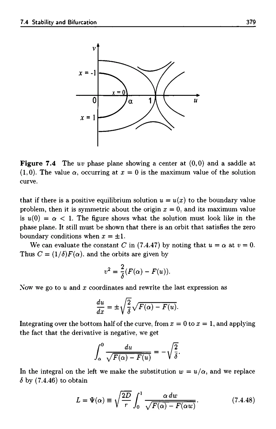
/


Текст
-* WILEY
AN INTRODUCTION TO NONLINEAR
PARTIAL DIFFERENTIAL EQUATIONS
SECOND EDITION
J. David Logan
U
к
A- —
щ (χ)
Piire and Αν, w: Mamemaws; a WtteHwersoence· Series of tews, Monographs» and Tracts
An Introduction to Nonlinear
Partial Differential Equations
Second Edition
J. David Logan
Willa Cather Professor of Mathematics
University of Nebraska, Lincoln
Department of Mathematics
Lincoln, NE
WILEY-
INTERSCIENCE
A JOHN WILEY & SONS, INC., PUBLICATION
Copyright © 2008 by John Wiley & Sons, Inc. All rights reserved.
Published by John Wiley & Sons, Inc., Hoboken, New Jersey.
Published simultaneously in Canada.
No part of this publication may be reproduced, stored in a retrieval system, or transmitted in any form or
by any means, electronic, mechanical, photocopying, recording, scanning, or otherwise, except as
permitted under Section 107 or 108 of the 1976 United States Copyright Act. without either the prior
written permission of the Publisher, or authorization through payment of the appropriate per-copy fee to
the Copyright Clearance Center, Inc., 222 Rosewood Drive, Danvers, MA 01923, (978) 750-8400, fax
(978) 750-4470, or on the web at www.copyright.com. Requests to the Publisher for permission should
be addressed to the Permissions Department, John Wiley & Sons, Inc., 111 River Street, Hoboken, NJ
07030, (201) 748-6011, fax (201) 748-6008, or online at http://www.wiley.com/go/permission.
Limit of Liability/Disclaimer of Warranty: While the publisher and author have used their best efforts in
preparing this book, they make no representations or warranties with respect to the accuracy or
completeness of the contents of this book and specifically disclaim any implied warranties of
merchantability or fitness for a particular purpose. No warranty may be created or extended by sales
representatives or written sales materials. The advice and strategies contained herein may not be suitable
for your situation. You should consult with a professional where appropriate. Neither the publisher nor
author shall be liable for any loss of profit or any other commercial damages, including but not limited
to special, incidental, consequential, or other damages.
For general information on our other products and services or for technical support, please contact our
Customer Care Department within the United States at (800) 762-2974, outside the United States at
(317) 572-3993 or fax (317) 572-4002.
Wiley also publishes its books in a variety of electronic formats. Some content that appears in print may
not be available in electronic format. For information about Wiley products, visit our web site at
www.wiley.com.
Library of Congress Cataloging-in-Publication Data:
Logan, J. David (John David)
An introduction to nonlinear partial differential equations / J. David Logan. — 2nd ed.
p. cm.
Includes bibliographical references and index.
ISBN 978-0-470-22595-0 (cloth : acid-free paper)
1. Differential equations, Nonlinear. 2. Differential equations, Partial. I. Title.
QA377.L58 2008
515.353—dc22 2007047514
Printed in the United States of America.
10 987654321
To Tess, for all her affection and support
Contents
Preface xi
1. Introduction to Partial Differential Equations 1
1.1 Partial Differential Equations 2
1.1.1 Equations and Solutions 2
1.1.2 Classification 5
1.1.3 Linear versus Nonlinear 8
1.1.4 Linear Equations 11
1.2 Conservation Laws 20
1.2.1 One Dimension 20
1.2.2 Higher Dimensions 23
1.3 Constitutive Relations 25
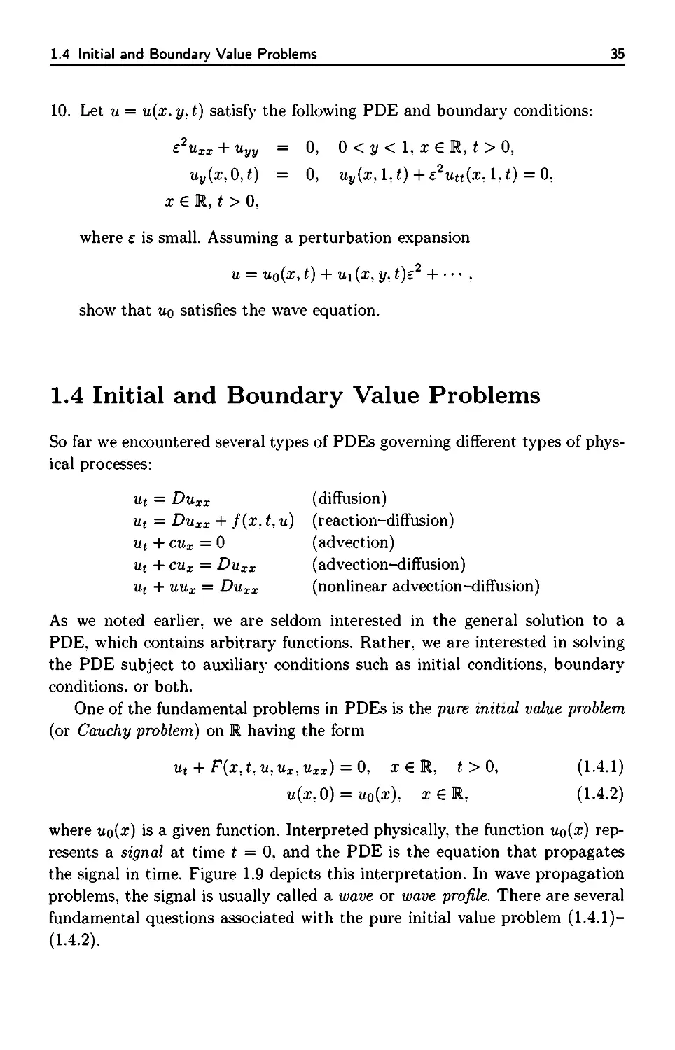
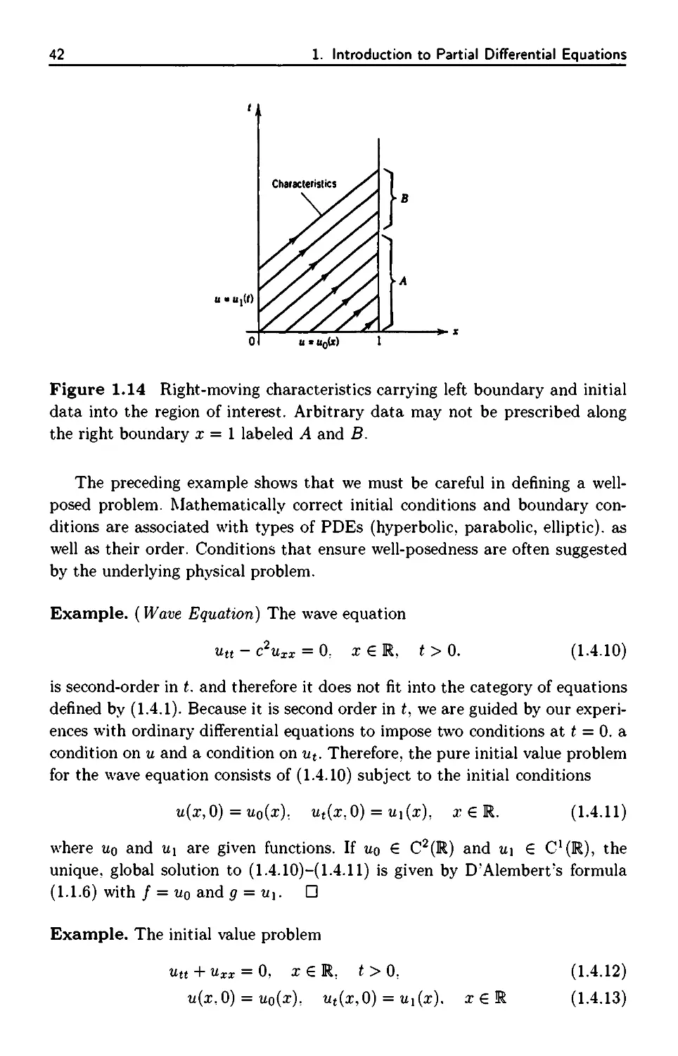
1.4 Initial and Boundary Value Problems 35
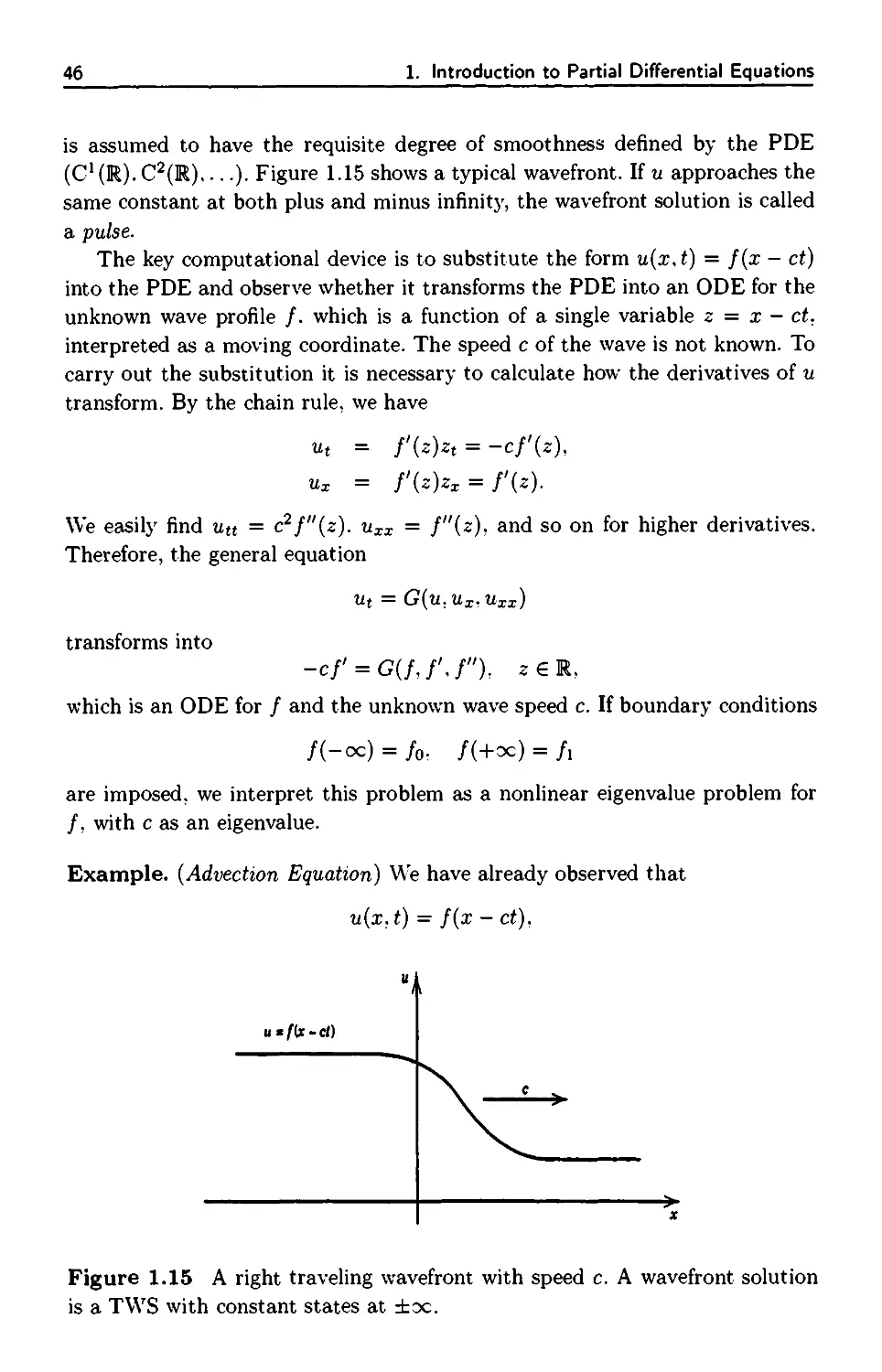
1.5 Waves 45
1.5.1 Traveling Waves 45
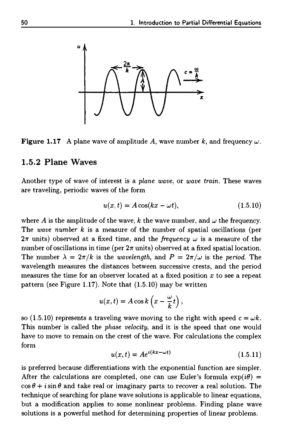
1.5.2 Plane Waves 50
1.5.3 Plane Waves and Transforms 52
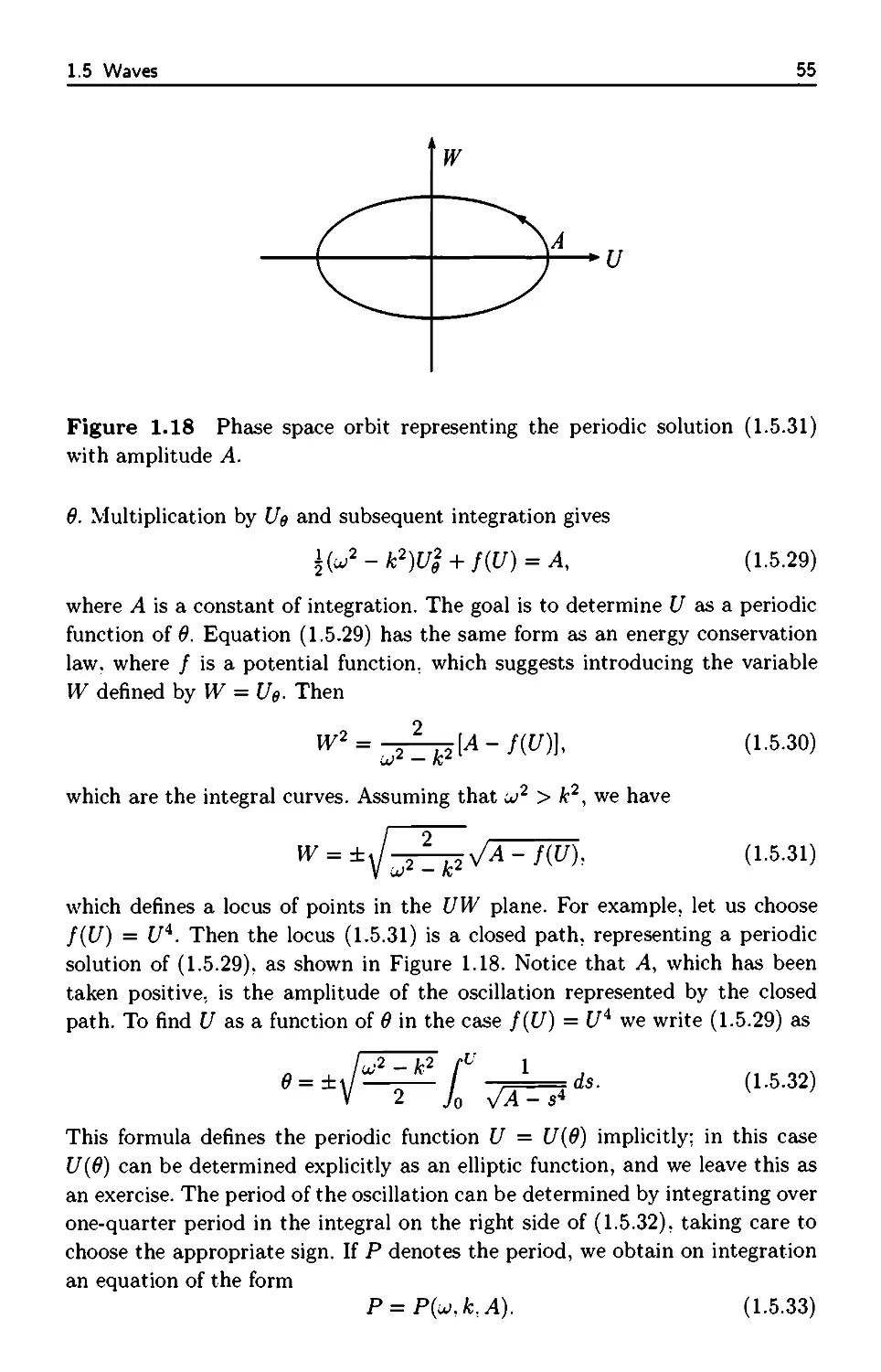
1.5.4 Nonlinear Dispersion 54
2. First-Order Equations and Characteristics 61
2.1 Linear First-Order Equations 62
2.1.1 Advection Equation 62
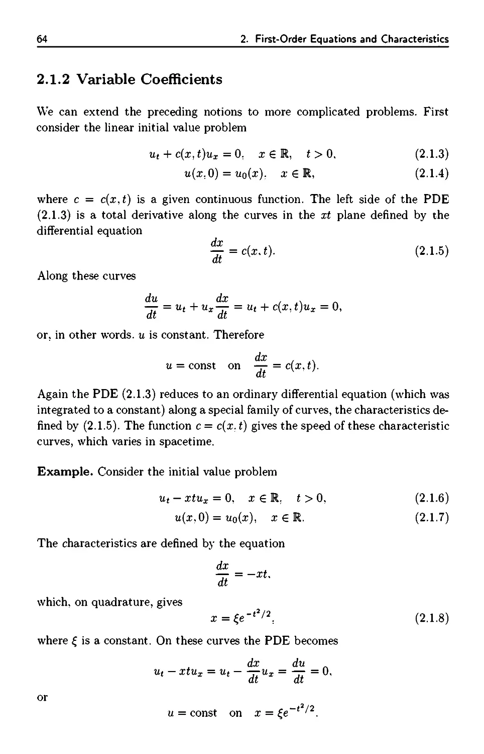
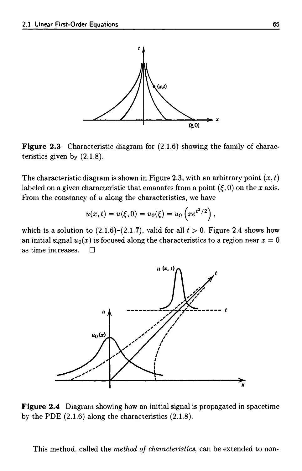
2.1.2 Variable Coefficients 64
2.2 Nonlinear Equations 68
2.3 Quasilinear Equations 72
2.3.1 The General Solution 76
viii Contents
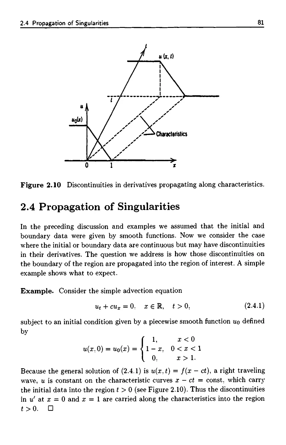
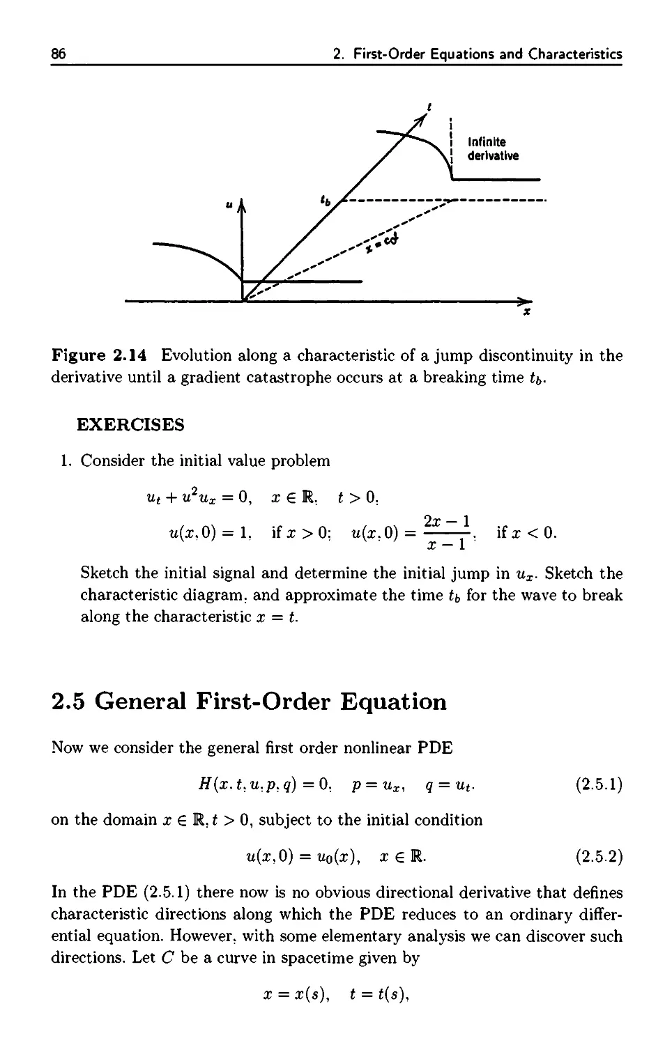
2.4 Propagation of Singularities 81
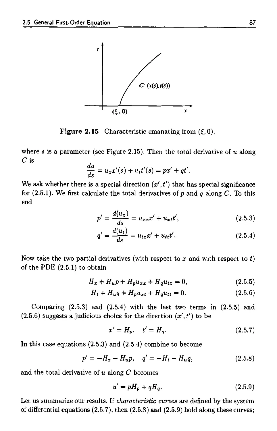
2.5 General First-Order Equation 86
2.5.1 Complete Integral 91
2.6 A Uniqueness Result 94
2.7 Models in Biology 96
2.7.1 Age Structure 96
2.7.2 Structured Predator-Prey Model 101
2.7.3 Chemotherapy 103
2.7.4 Mass Structure 105
2.7.5 Size-Dependent Predation 106
3. Weak Solutions to Hyperbolic Equations 113
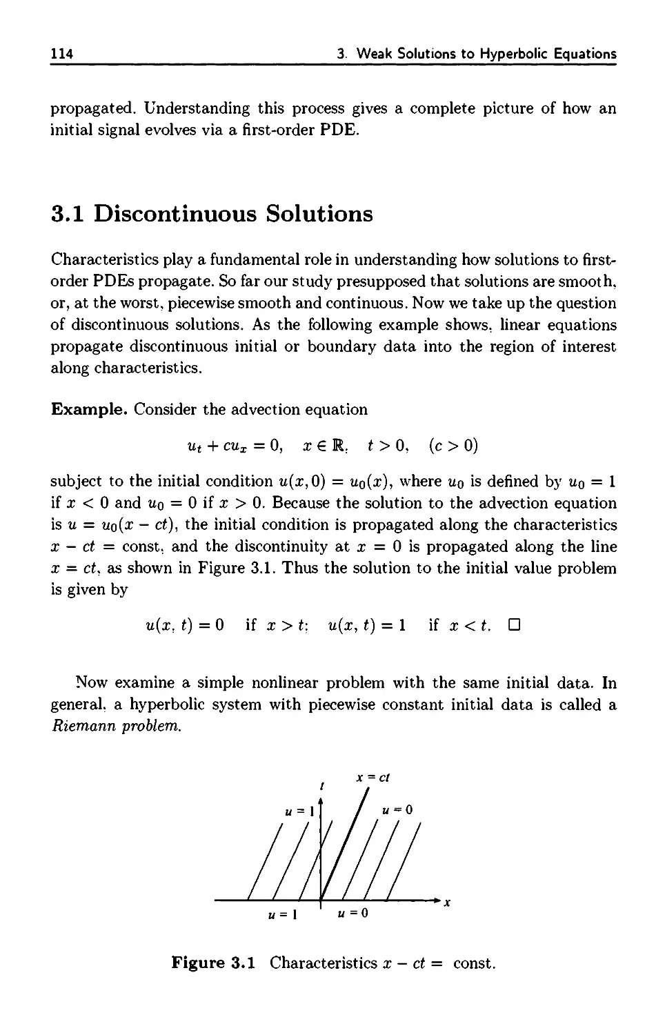
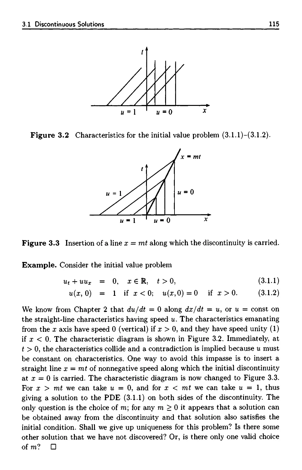
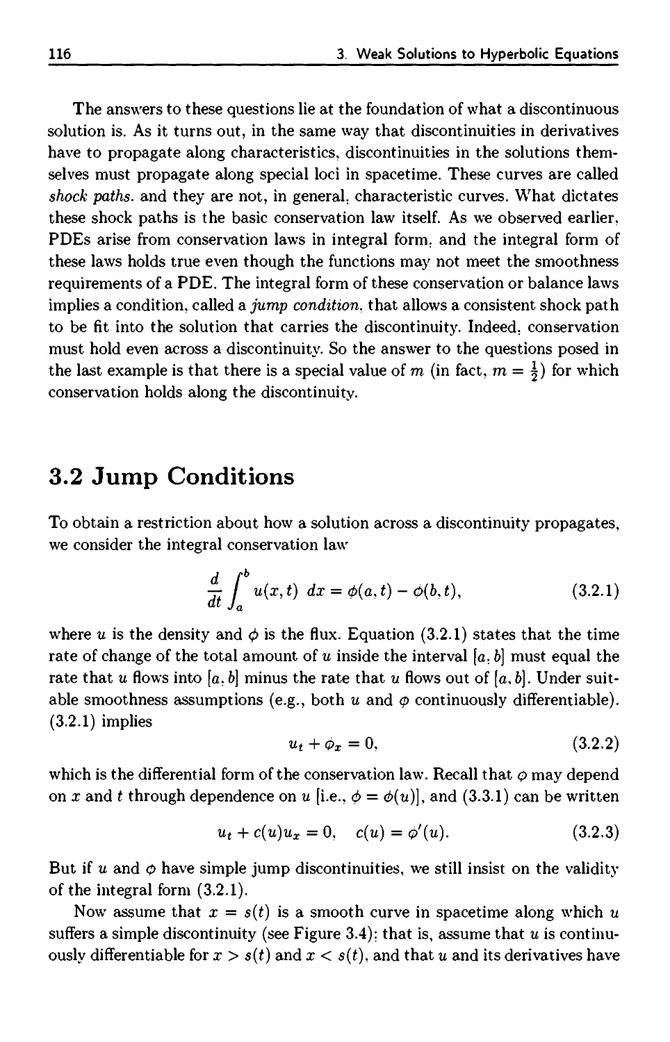
3.1 Discontinuous Solutions 114
3.2 Jump Conditions 116
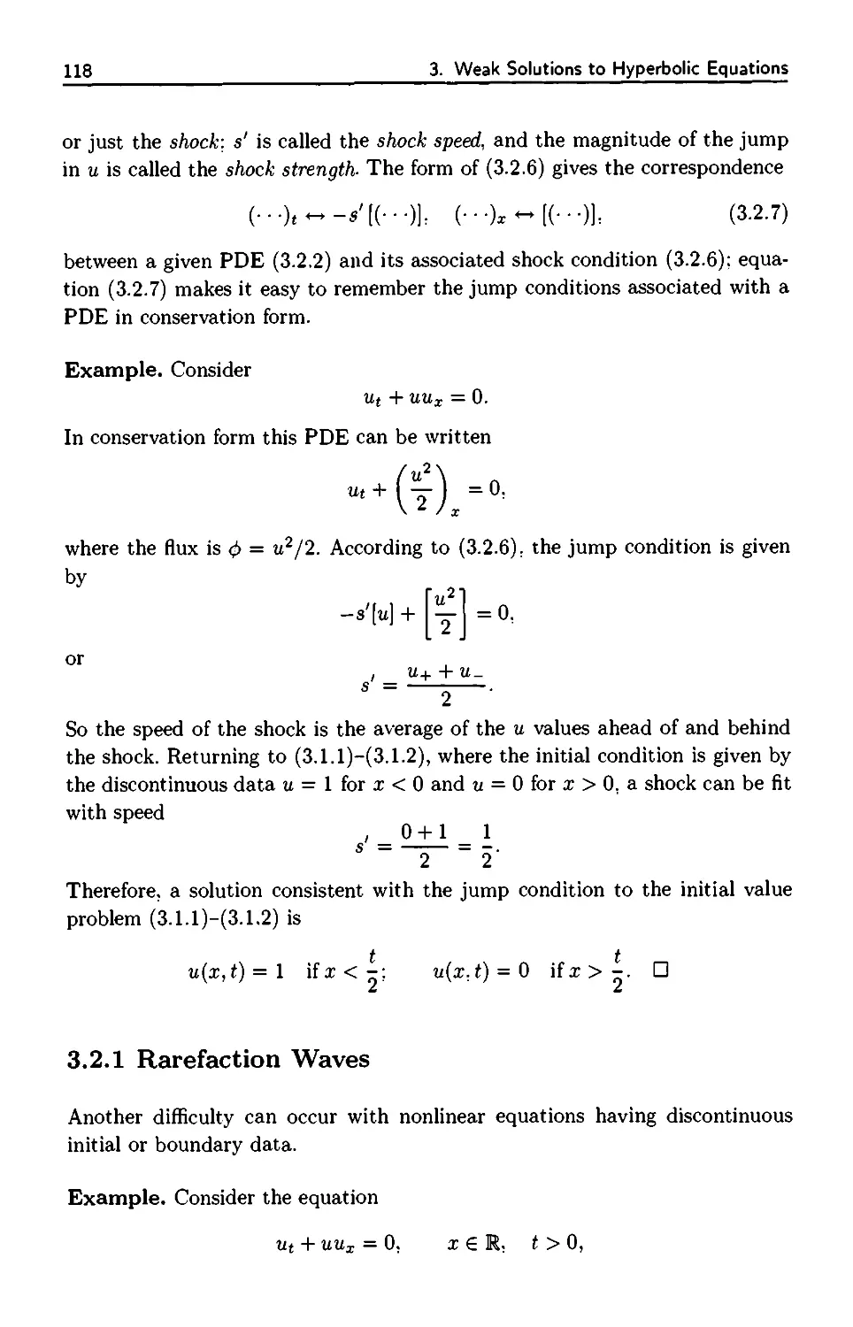
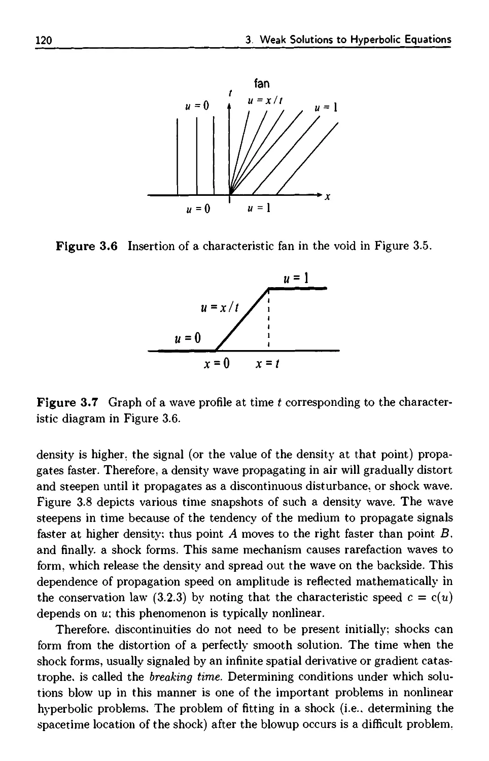
3.2.1 Rarefaction Waves 118
3.2.2 Shock Propagation 119
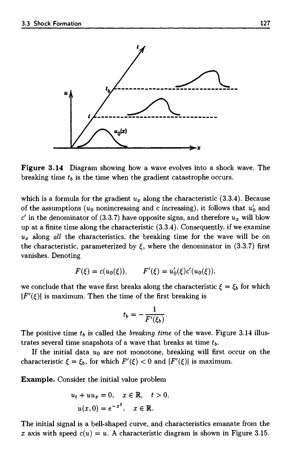
3.3 Shock Formation 125
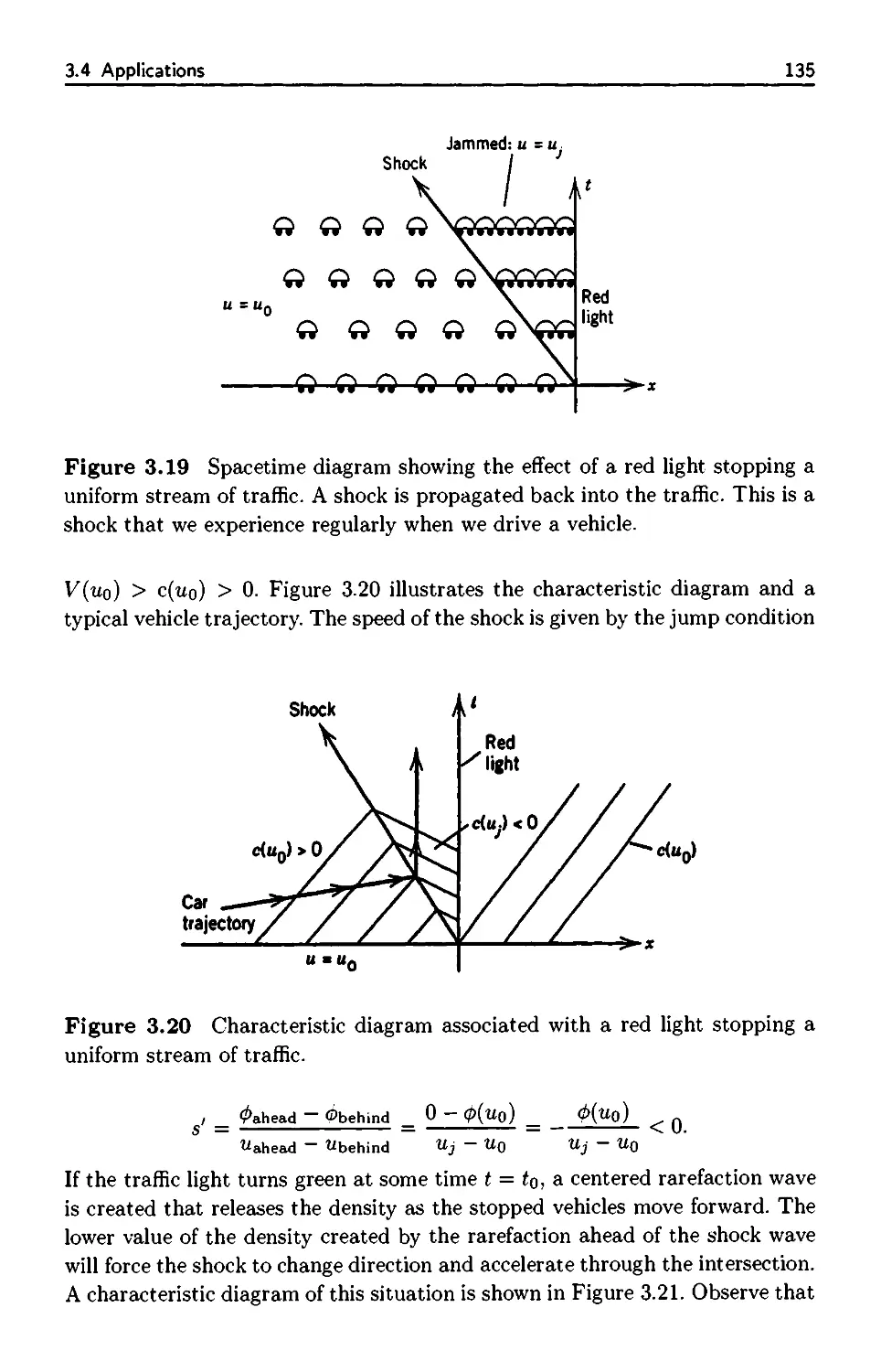
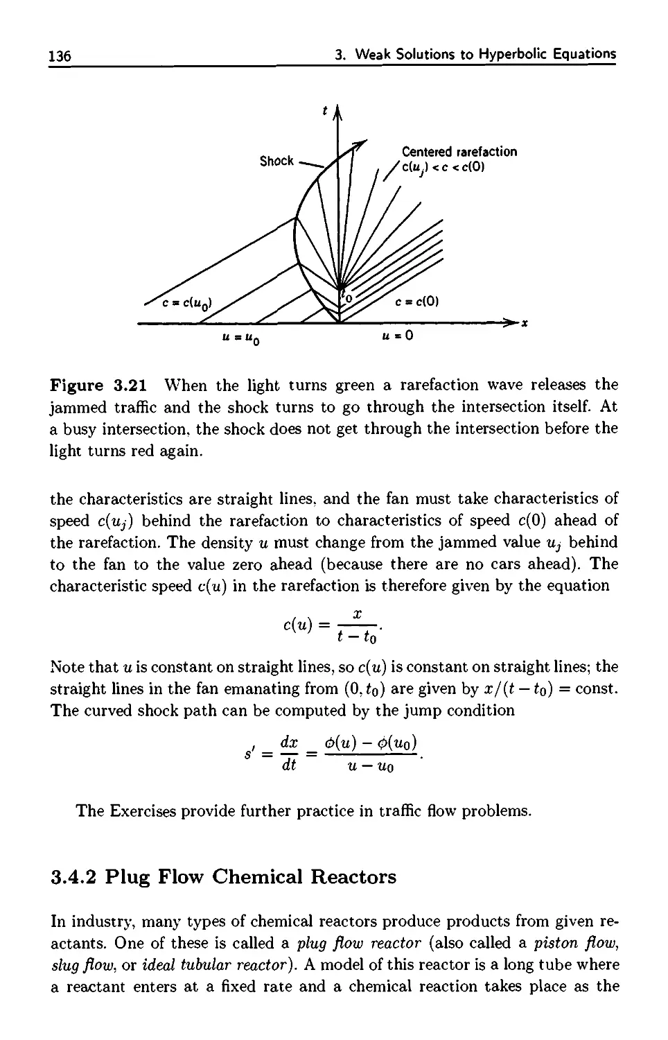
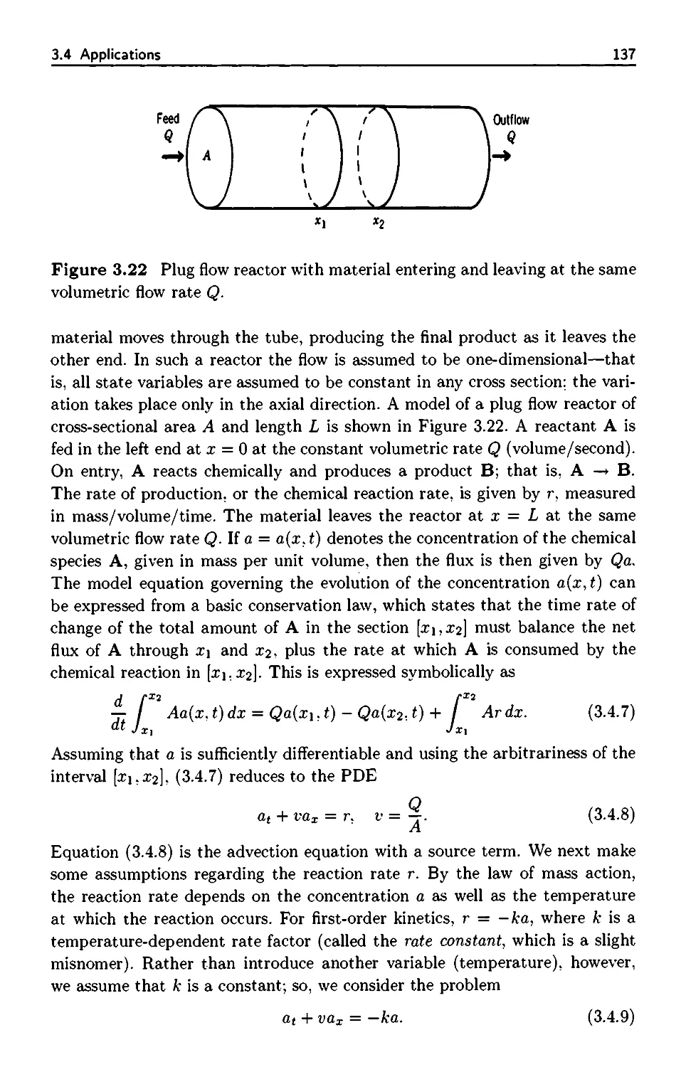
3.4 Applications 131
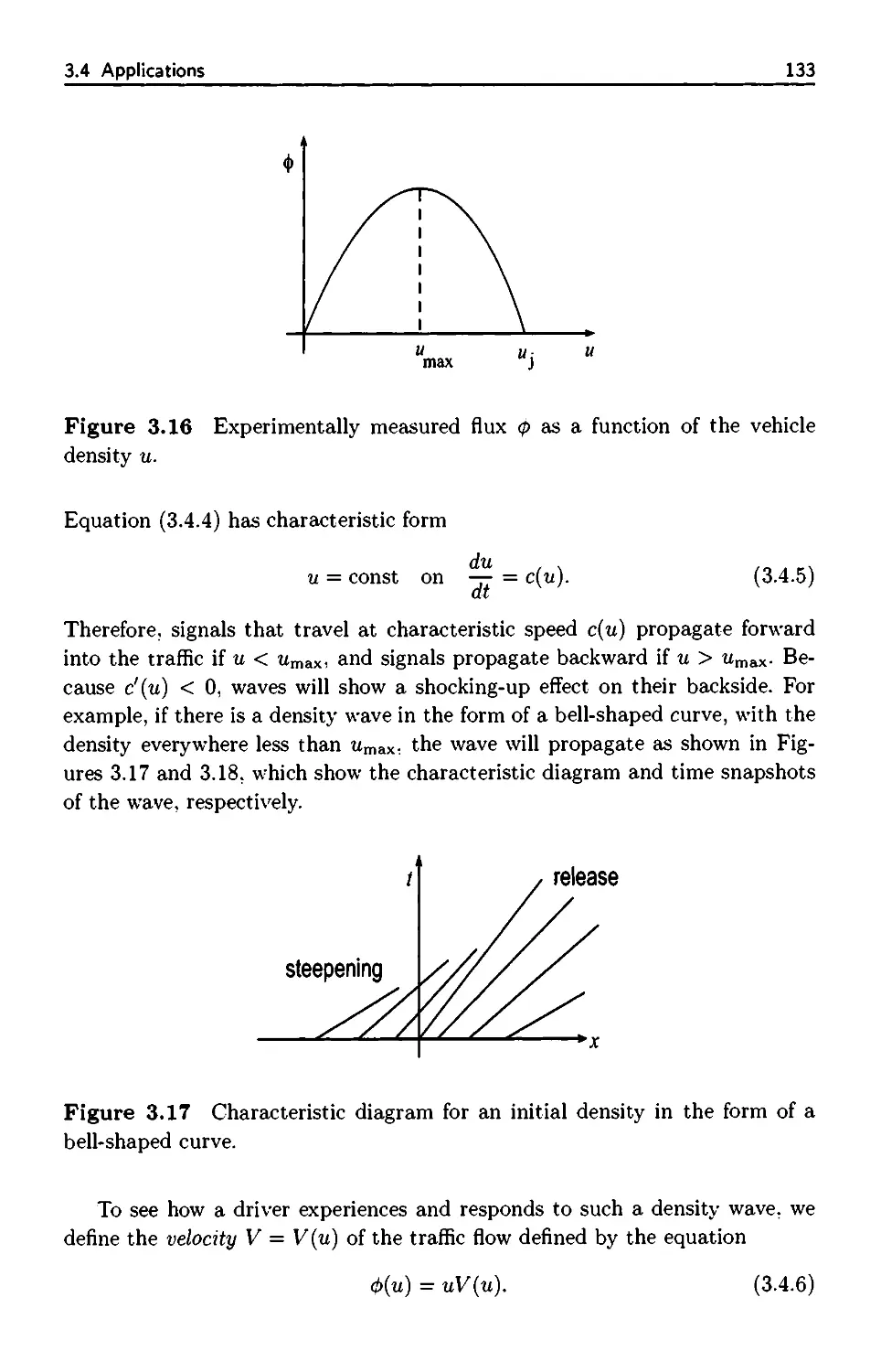
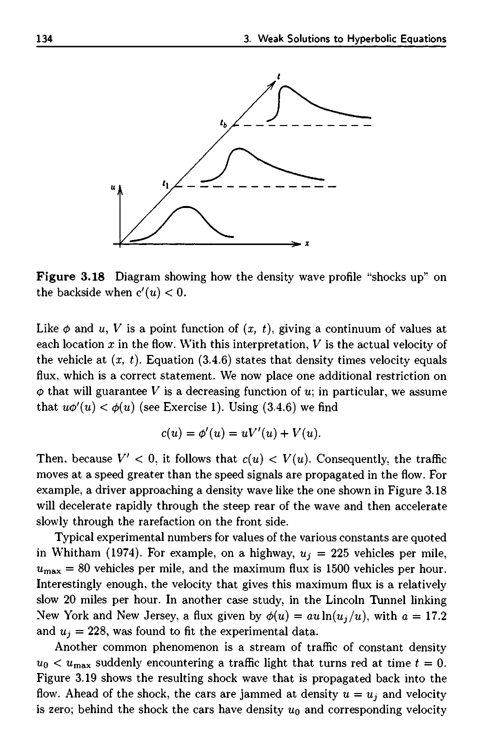
3.4.1 Traffic Flow 132
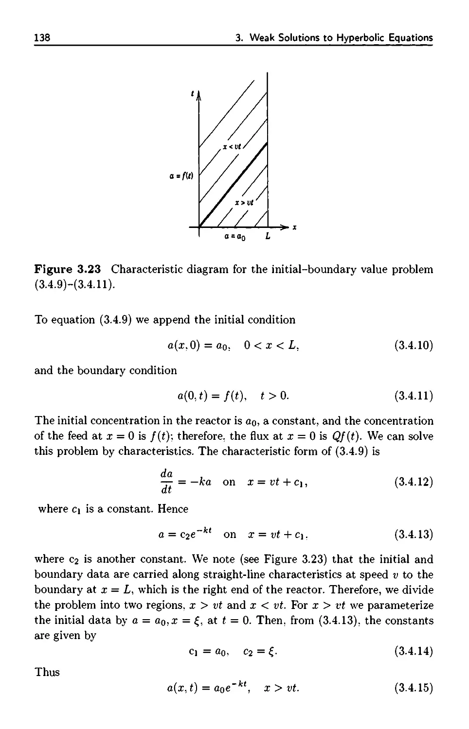
3.4.2 Plug Flow Chemical Reactors 136
3.5 Weak Solutions: A Formal Approach 140
3.6 Asymptotic Behavior of Shocks 148
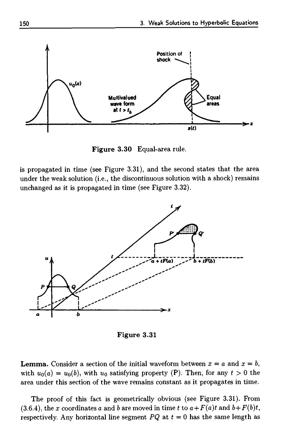
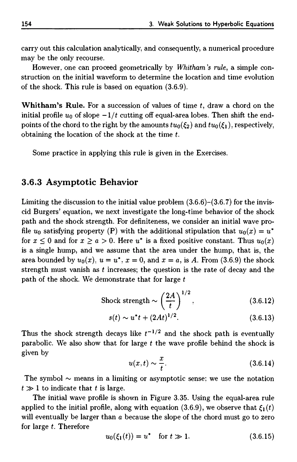
3.6.1 Equal-Area Principle 148
3.6.2 Shock Fitting 152
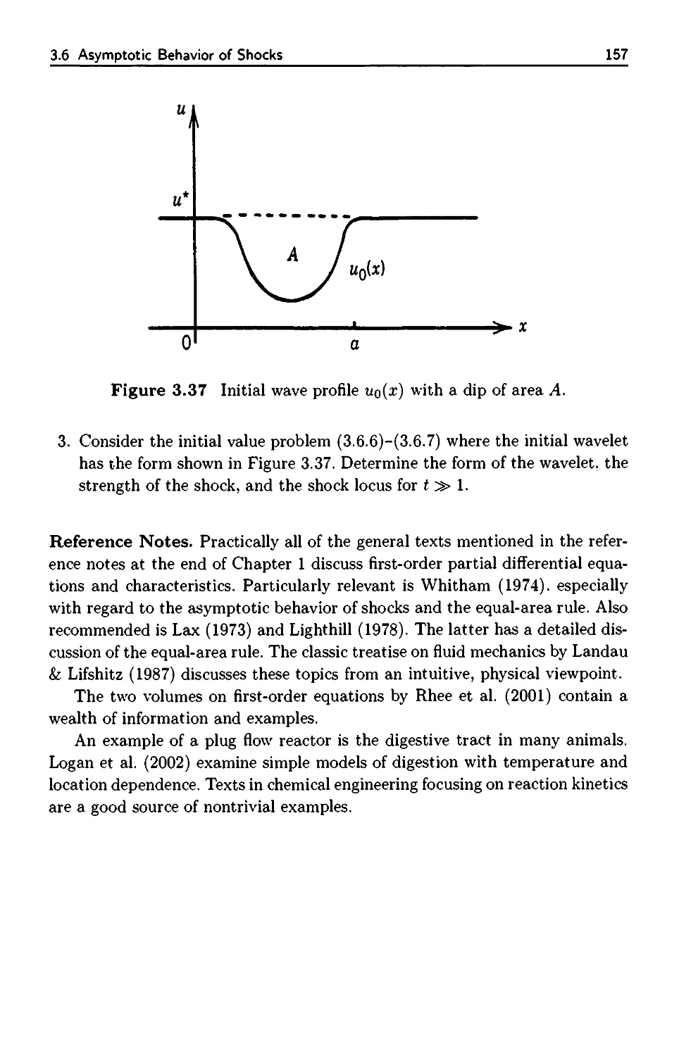
3.6.3 Asymptotic Behavior 154
4. Hyperbolic Systems 159
4.1 Shallow-Water Waves; Gas Dynamics 160
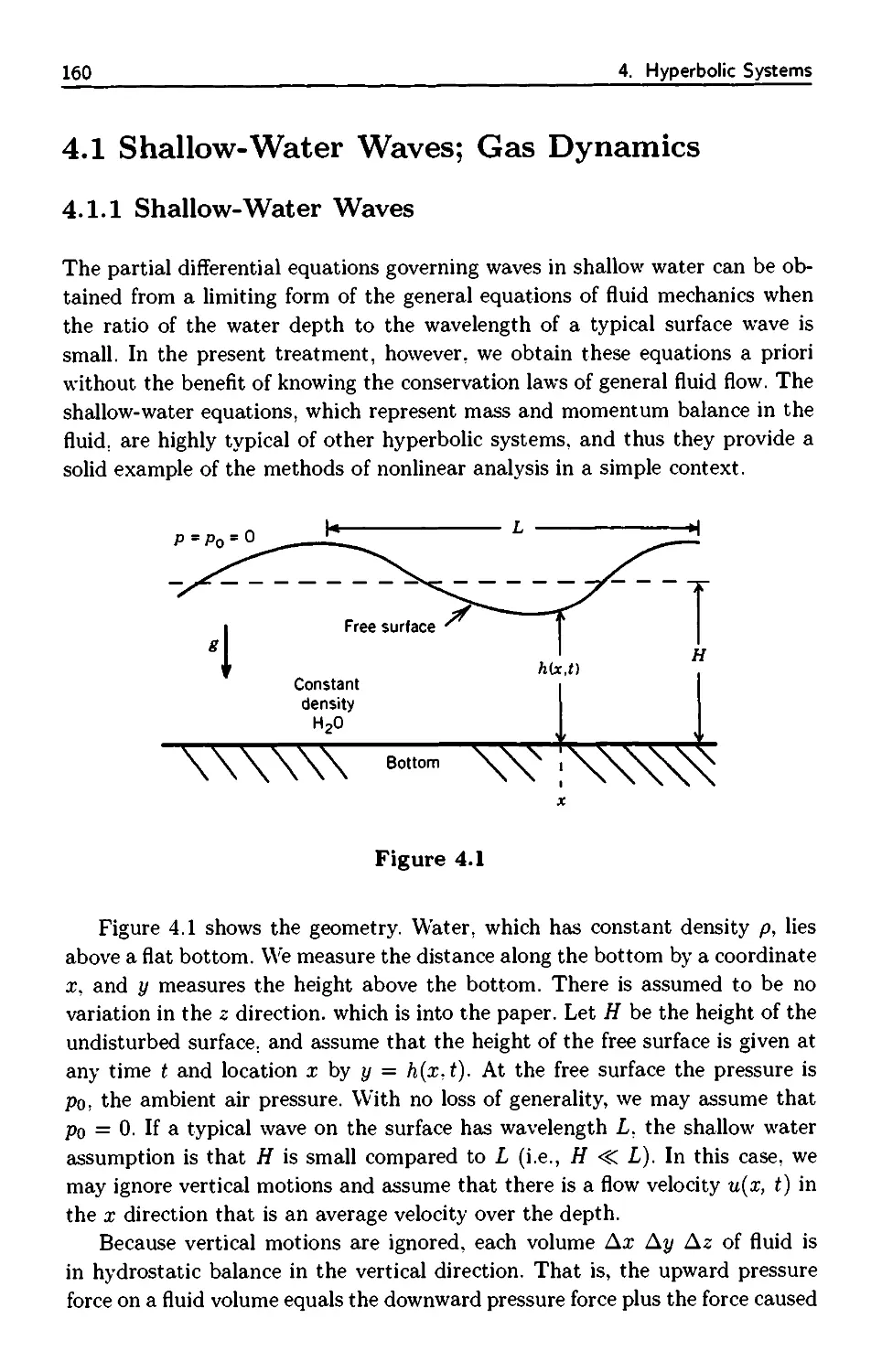
4.1.1 Shallow-Water Waves 160
4.1.2 Small-Amplitude Approximation 163
4.1.3 Gas Dynamics 164
4.2 Hyperbolic Systems and Characteristics 169
4.2.1 Classification 170
4.3 The Riemann Method 179
4.3.1 Jump Conditions for Systems 179
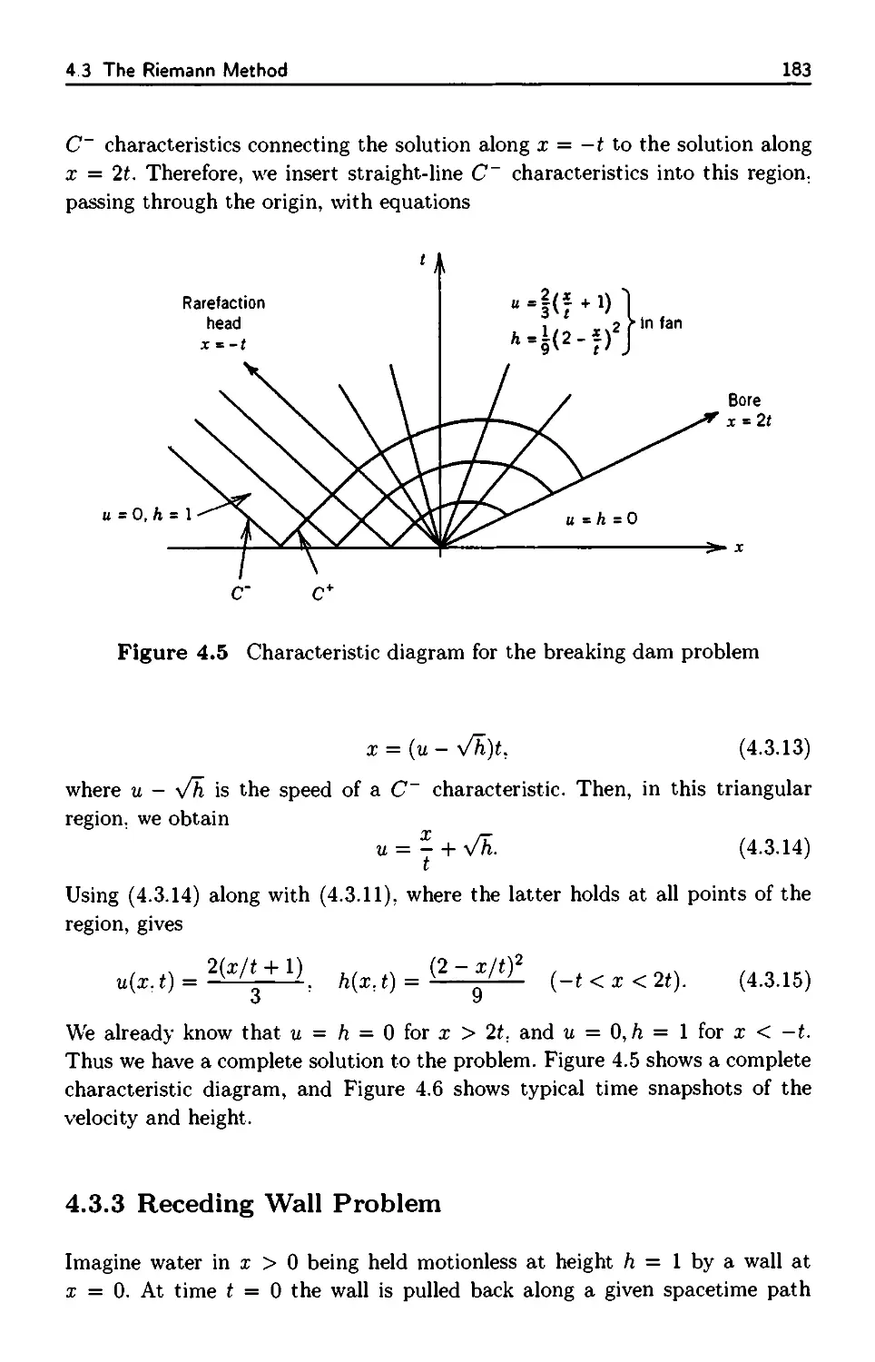
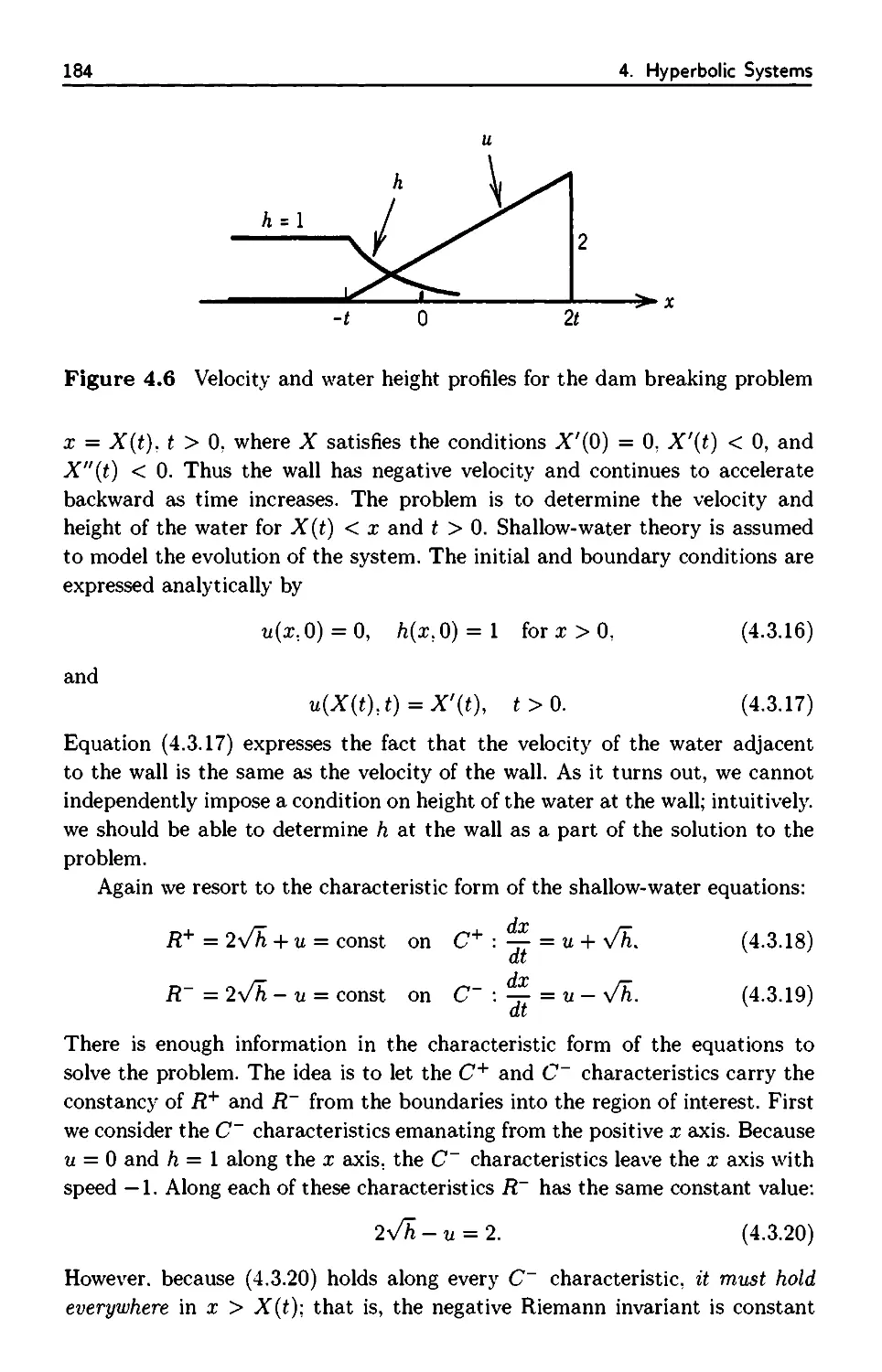
4.3.2 Breaking Dam Problem 181
4.3.3 Receding Wall Problem 183
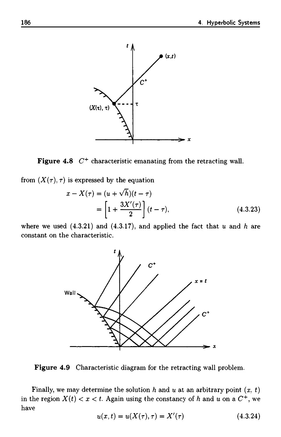
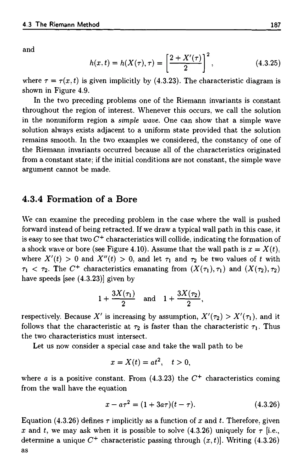
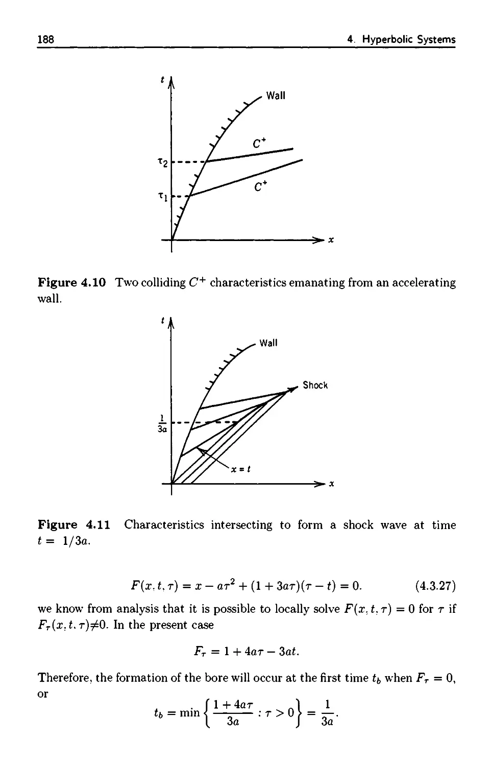
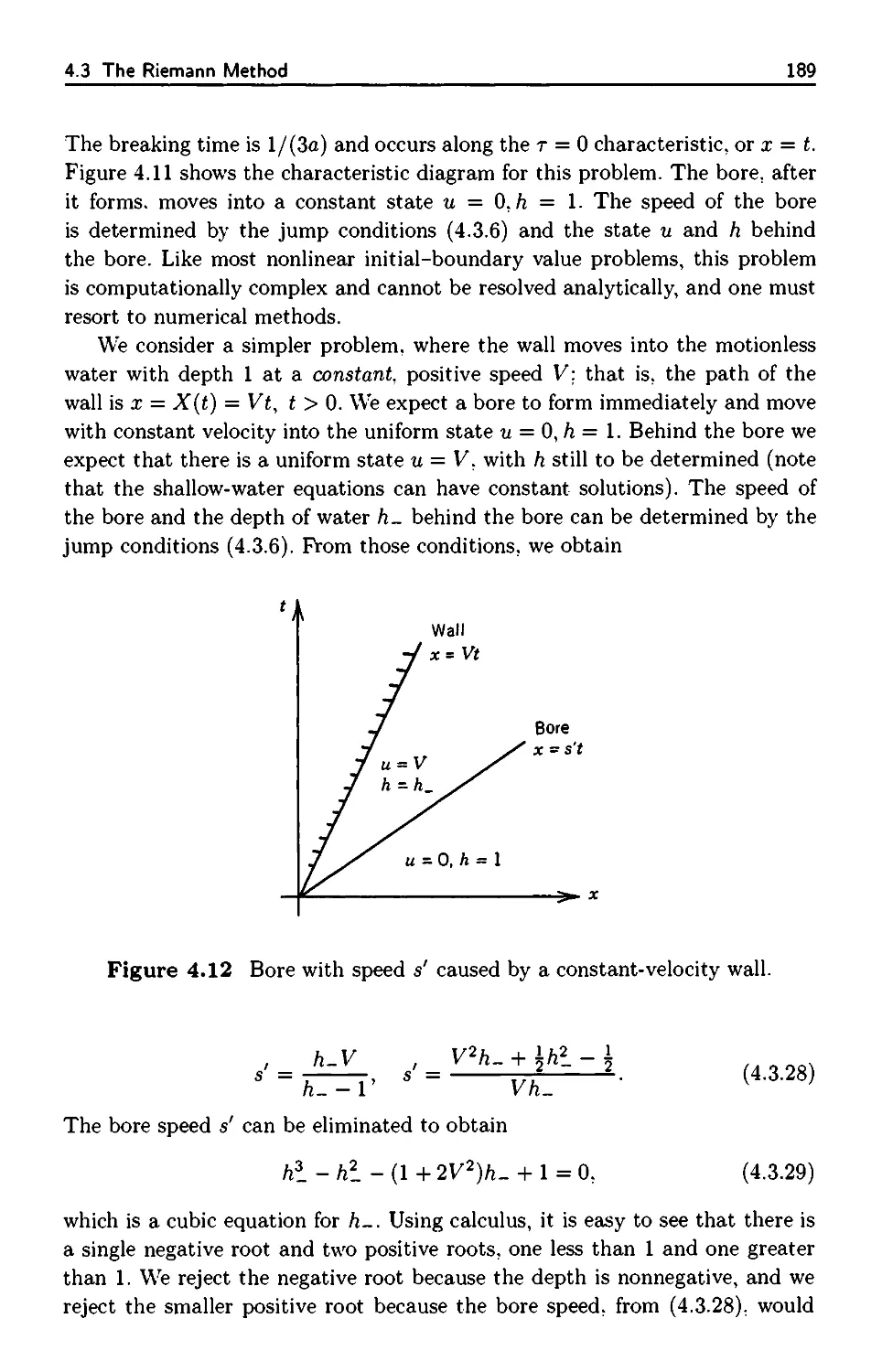
4.3.4 Formation of a Bore 187
4.3.5 Gas Dynamics 190
4.4 Hodographs and Wavefronts 192
4.4.1 Hodograph Transformation 192
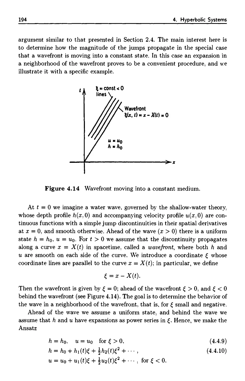
4.4.2 Wavefront Expansions 193
Contents ix
4.5 Weakly Nonlinear Approximations 201
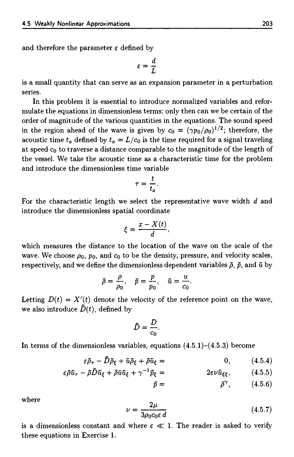
4.5.1 Derivation of Burgers' Equation 202
5. Diffusion Processes 209
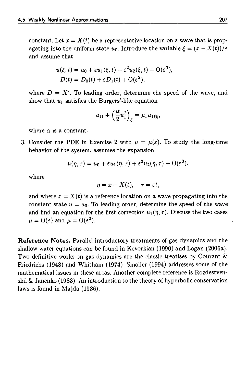
5.1 Diffusion and Random Motion 210
5.2 Similarity Methods 217
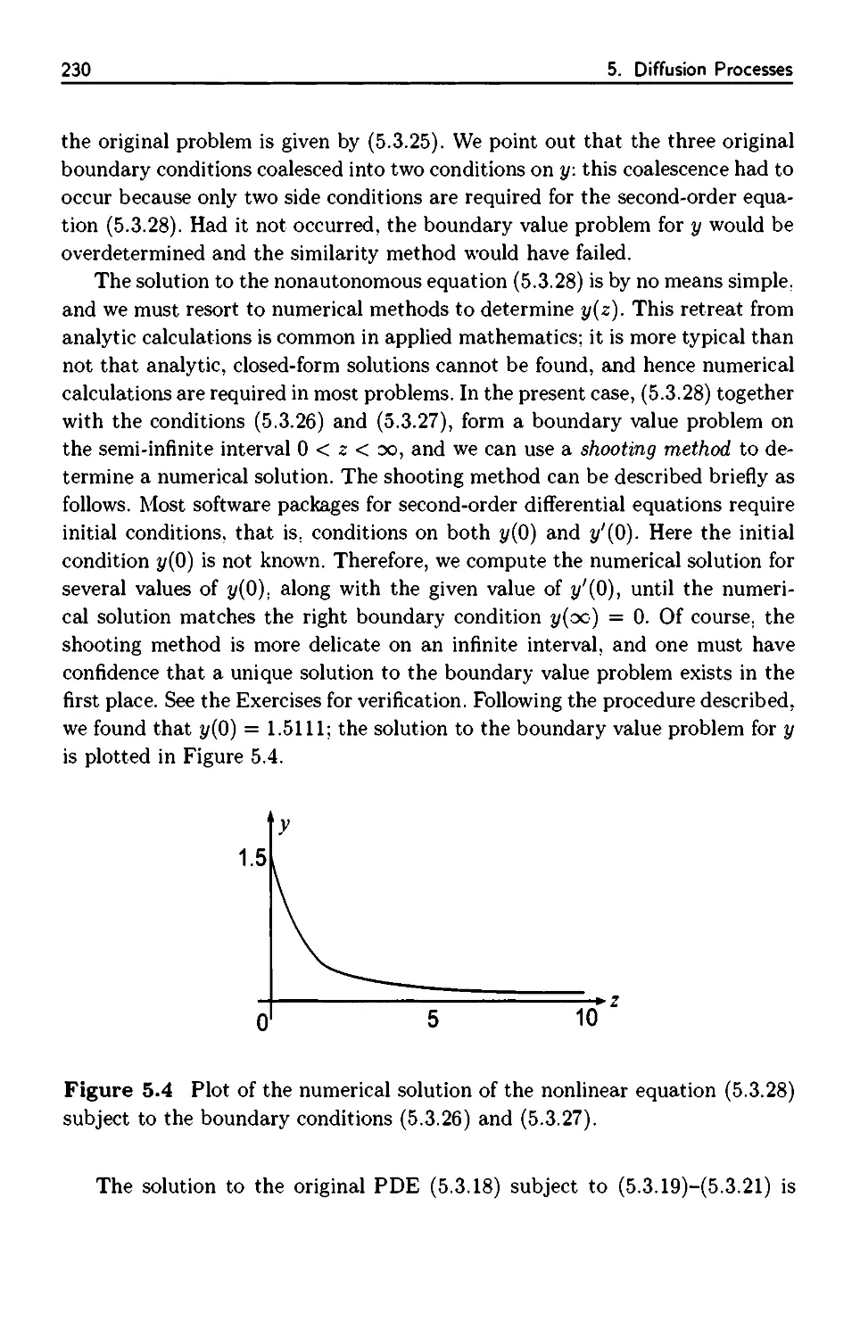
5.3 Nonlinear Diffusion Models 224
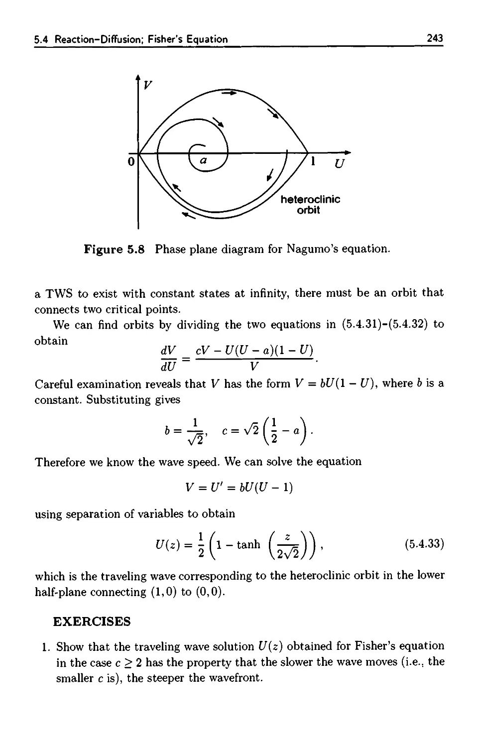
5.4 Reaction-Diffusion: Fisher's Equation 234
5.4.1 Traveling Wave Solutions 235
5.4.2 Perturbation Solution 238
5.4.3 Stability of Traveling Waves 240
5.4.4 Nagumo's Equation 242
5.5 Advection-Diffusion: Burgers' Equation 245
5.5.1 Traveling Wave Solution 246
5.5.2 Initial Value Problem 247
5.6 Asymptotic Solution to Burgers' Equation 250
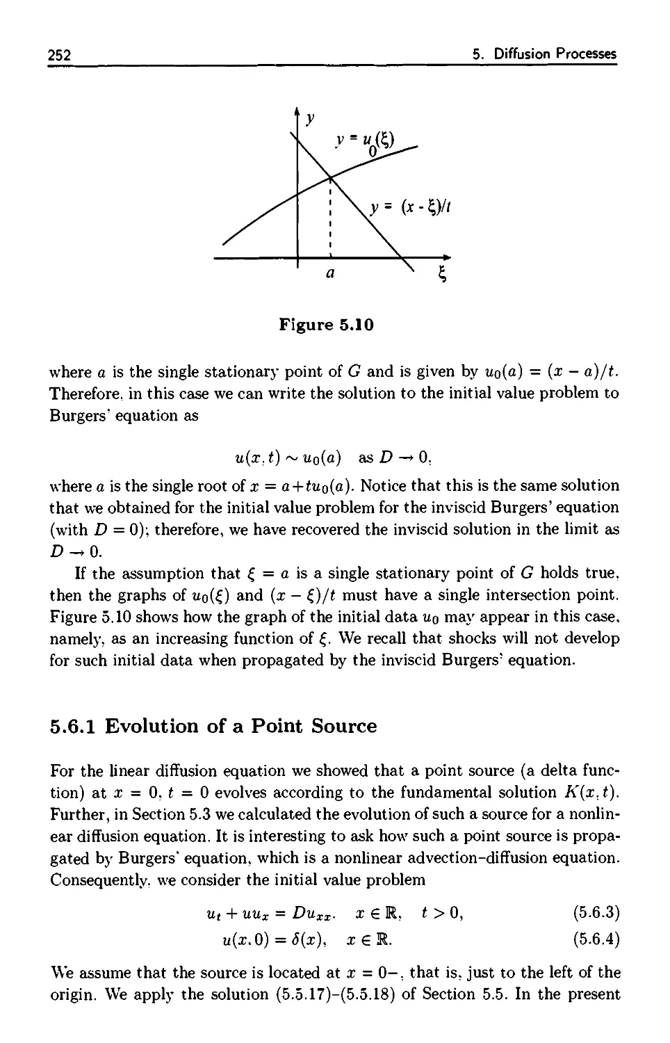
5.6.1 Evolution of a Point Source 252
Appendix: Dynamical Systems 257
6. Reaction-Diffusion Systems 267
6.1 Reaction-Diffusion Models 268
6.1.1 Predator-Prey Model 270
6.1.2 Combustion 271
6.1.3 Chemotaxis 274
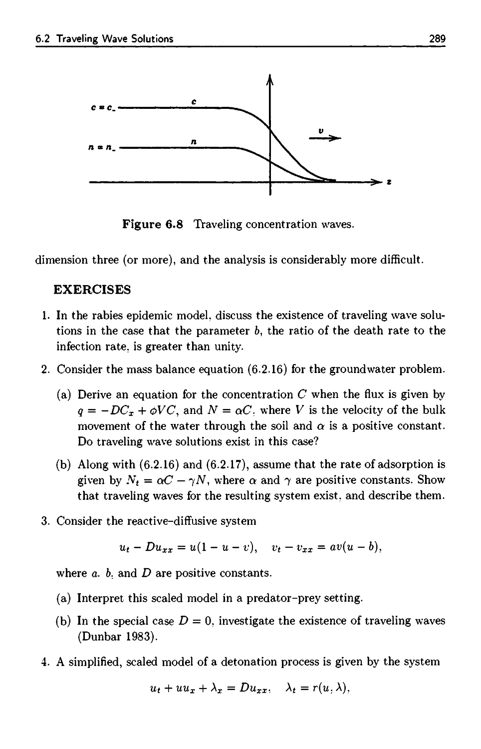
6.2 Traveling Wave Solutions 277
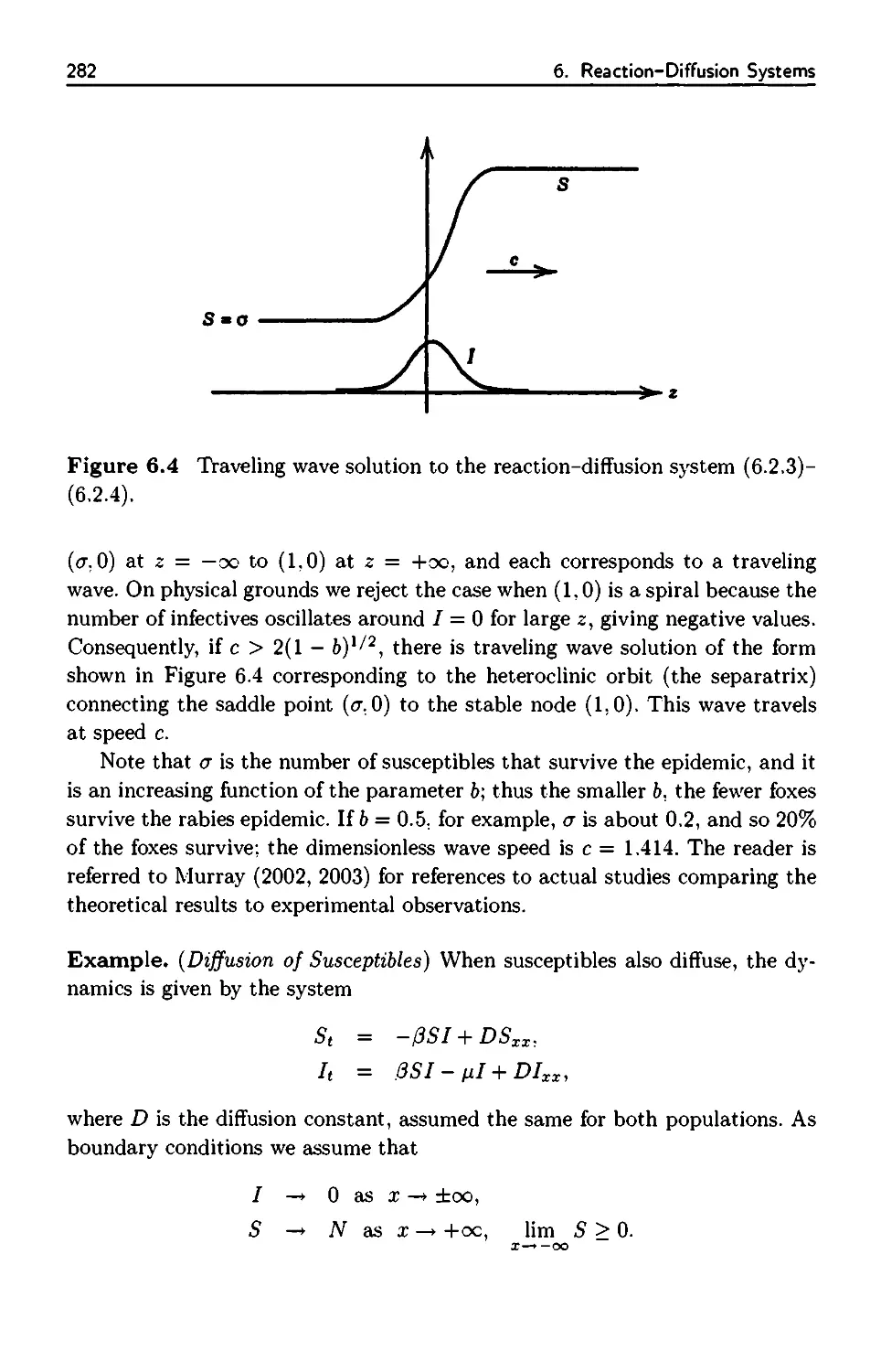
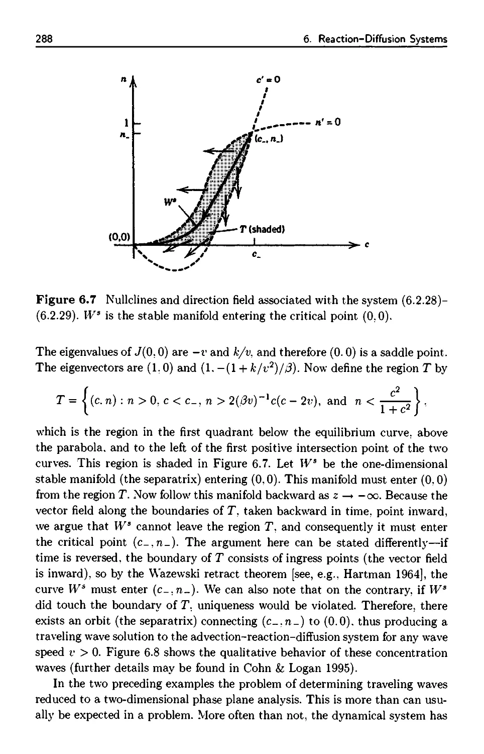
6.2.1 Model for the Spread of a Disease 278
6.2.2 Contaminant Transport in Groundwater 284
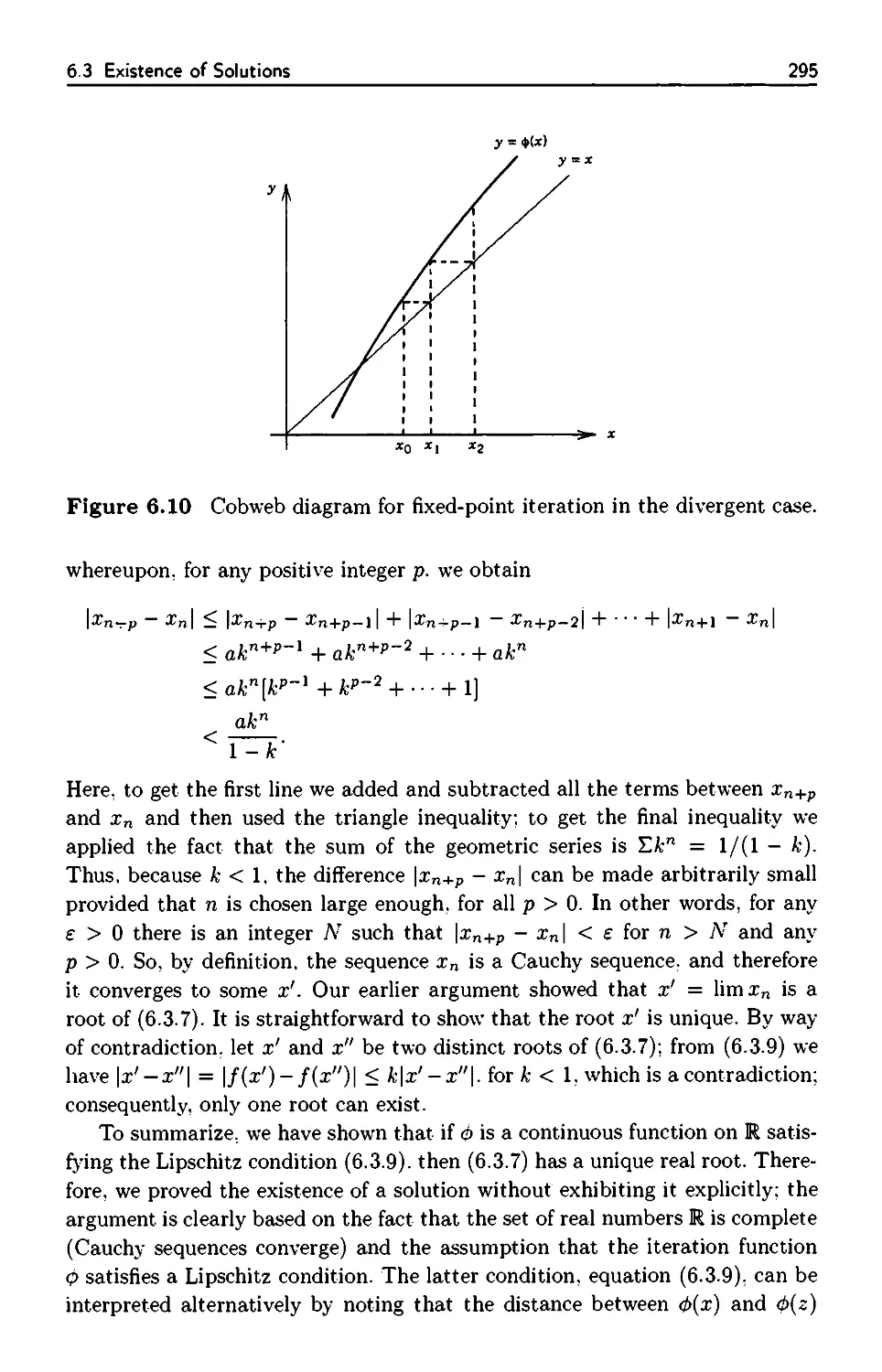
6.3 Existence of Solutions 292
6.3.1 Fixed-Point Iteration 293
6.3.2 Semilinear Equations 297
6.3.3 Normed Linear Spaces 300
6.3.4 General Existence Theorem 303
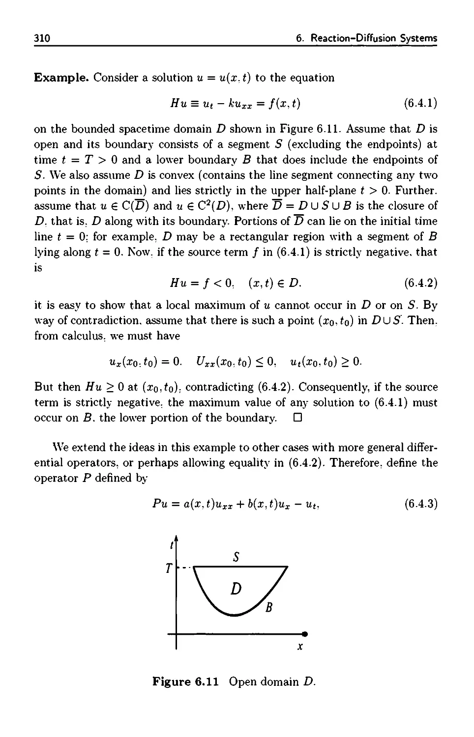
6.4 Maximum Principles and Comparison Theorems 309
6.4.1 Maximum Principles 309
6.4.2 Comparison Theorems 314
6.5 Energy Estimates and Asymptotic Behavior 317
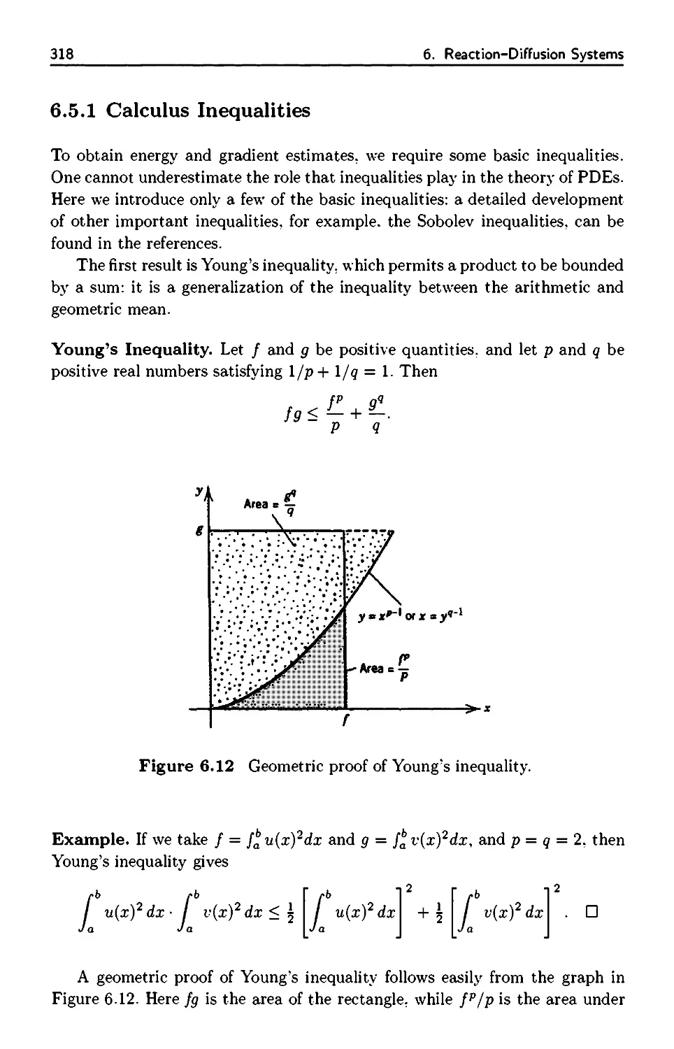
6.5.1 Calculus Inequalities 318
6.5.2 Energy Estimates 320
6.5.3 Invariant Sets 326
6.6 Pattern Formation 333
x Contents
7. Equilibrium Models 345
7.1 Elliptic Models 346
7.2 Theoretical Results 352
7.2.1 Maximum Principle 353
7.2.2 Existence Theorem 355
7.3 Eigenvalue Problems 358
7.3.1 Linear Eigenvalue Problems 358
7.3.2 Nonlinear Eigenvalue Problems 361
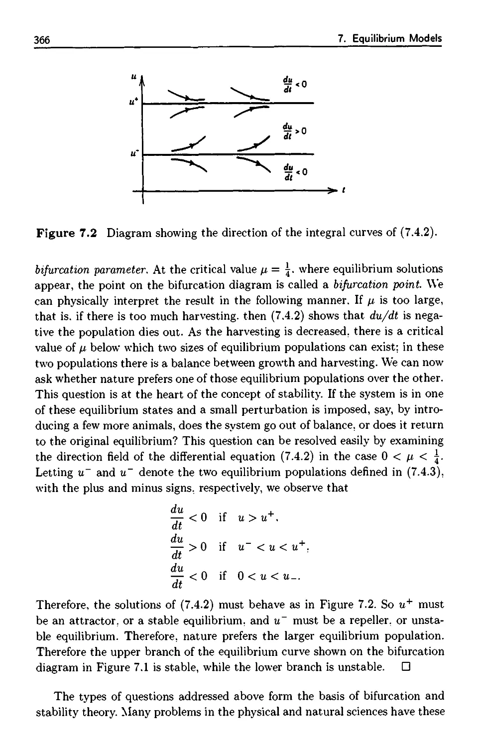
7.4 Stability and Bifurcation 364
7.4.1 Ordinary Differential Equations 364
7.4.2 Partial Differential Equations 368
References 387
Index 395
Preface
Nonlinear partial differential equations (PDEs) is a vast area, and
practitioners include applied mathematicians, analysts, and others in the pure and
applied sciences. This introductory text on nonlinear partial differential equations
evolved from a graduate course I have taught for many years at the University
of Nebraska at Lincoln. It emerged as a pedagogical effort to introduce, at a
fairly elementary level, nonlinear PDEs in a format and style that is accessible
to students with diverse backgrounds and interests. The audience has been a
mixture of graduate students from mathematics, physics, and engineering. The
prerequisites include an elementary course in PDEs emphasizing Fourier series
and separation of variables, and an elementary course in ordinary differential
equations.
There is enough independence among the chapters to allow the instructor
considerable flexibility in choosing topics for a course. The text may be used
for a second course in partial differential equations, a first course in nonlinear
PDEs, a course in PDEs in the biological sciences, or an advanced course in
applied mathematics or mathematical modeling. The range of applications
include biology, chemistry, gas dynamics, porous media, combustion, traffic flow,
water waves, plug flow reactors, heat transfer, and other topics of interest in
applied mathematics.
There are three major changes from the first edition, which appeared in
1994. Because the original chapter on chemically reacting fluids was highly
specialized for an introductory text, it has been removed from the new
edition. Additionally, because of the surge of interest in mathematical biology,
considerable material on that topic has been added; this includes linear and
nonlinear age structure, spatial effects, and pattern formation. Finally, the text
has been reorganized with the chapters on hyperbolic equations separated from
Xll
Preface
the chapters on diffusion processes, rather than intermixing them.
The references have been updated and, as in the previous edition, are
selected to suit the needs of an introductory text, pointing the reader to parallel
treatments and resources for further study. Finally, many new exercises have
been added. The exercises are intermediate-level and are designed to build the
students' problem solving techniques beyond what is experienced in a beginning
course.
Chapter 1 develops a perspective on how to understand problems involving
PDEs and how the subject interrelates with physical phenomena. The subject
is developed from the basic conservation law. which, when appended to
constitutive relations, gives rise to the fundamental models of diffusion, advection.
and reaction. There is emphasis on understanding that nonlinear hyperbolic
and parabolic PDEs describe evolutionary processes; a solution is a signal that
is propagated into a spacetime domain from the boundaries of that domain.
Also, there is focus on the structure of the various equations and what the terms
describe physically. Chapters 2-4 deal with wave propagation and hyperbolic
problems. In Chapter 2 we assume that the equations have smooth solutions
and we develop algorithms to solve the equations analytically. In Chapter 3 we
study discontinuous solutions and shock formation, and we introduce the
concept of a weak solution. In keeping with our strategy of thinking about initial
waveforms evolving in time, we focus on the initial value problem rather than
the general Cauchy problem. The idea of characteristics is central and forms
the thread that weaves through these two chapters. Next. Chapter 4 introduces
the shallow-water equations as the prototype of a hyperbolic system, and those
equations are taken to illustrate basic concepts associated with hyperbolic
systems: characteristics. Riemann's method, the hodograph transformation, and
asymptotic behavior. Also, the general classification of systems of first-order
PDEs is developed, and weakly nonlinear methods of analysis are described;
the latter are illustrated by a derivation of Burgers' equation.
Chapters 1-4 can form the basis of a one-semester course focusing on wave
propagation, characteristics, and hyperbolic equations.
Chapter 5 introduces diffusion processes. After establishing a probabilistic
basis for diffusion, we examine methods that are useful in studying the solution
structure of diffusion problems, including phase plane analysis, similarity
methods, and asymptotic expansions. The prototype equations for reaction-diffusion
and advection-diffusion. Fisher's equation and Burgers' equation, respectively,
are studied in detail with emphasis on traveling wave solutions, the stability
of those solutions, and the asymptotic behavior of solutions. The Appendix
to Chapter 5 reviews phase plane analysis. In Chapter 6 we discuss systems
of reaction-diffusion equations, emphasizing applications and model building,
especially in the biological sciences. We expend some effort addressing theoret-
Preface
Xlll
ical concepts such as existence, uniqueness, comparison and maximum
principles, energy estimates, blowup, and invariant sets; a key application includes
pattern formation. Finally, elliptic equations are introduced in Chapter 7 as a
asymptotic limit of reaction-diffusion equations; nonlinear eigenvalue problems,
stability, and bifurcation phenomena form the core of this chapter.
Chapter 1, along with Chapters 5-8. can form the basis of a one-semester
course in diffusion and reaction-diffusion processes, with emphasis on PDEs in
mathematical biology.
I want to acknowledge many users of the first edition who suggested
improvements, corrections, and new topics. Their excitement for a second edition,
along with the unwavering encouragement of my editor Susanne Steitz-Filler at
Wiley, provided the stimulus to actually complete it. My own interest in
nonlinear PDEs was spawned over many years by collaboration with those with whom
I have had the privilege of working: Kane Yee at Kansas State. John Bdzil at
Los Alamos. Ash Kapila at Rensselaer Polytechnic Institute, and several of my
colleagues at Nebraska (Professors Steve Cohn, Steve Dunbar, Tony Joern in
biology. Glenn Ledder, Tom Shores, Vitaly Zlotnik in geology, and my former
student Bill Wolesensky, now at the College of Saint Mary). Readers of this
text will see the influence of the classic books of G. B. Whitham (Linear and
Nonlinear Waves) and J. Smoller (Shock Waves and Reaction-Diffusion
Equations). R. Courant and K. 0. Friedrichs (Supersonic Flow and Shock Waves),
and the text on mathematical biology by J. D. Murray (Mathematical Biology).
Finally, I express my gratitude to the National Science Foundation and to the
Department of Energy for supporting my research efforts over the last several
vears.
J. David Logan
Lincoln, Nebraska
1
Introduction to Partial Differential
Equations
Partial differential equations (PDEs) is one of the basic areas of applied
analysis, and it is difficult to imagine any area of applications where its impact is not
felt. In recent decades there has been tremendous emphasis on understanding
and modeling nonlinear processes; such processes are often governed by
nonlinear PDEs. and the subject has become one of the most active areas in applied
mathematics and central in modern-day mathematical research. Part of the
impetus for this surge has been the advent of high-speed, powerful computers,
where computational advances have been a major driving force.
This initial chapter focuses on developing a perspective on understanding
problems involving PDEs and how the subject interrelates with physical
phenomena. It also provides a transition from an elementary course, emphasizing
eigenfunction expansions and linear problems, to a more sophisticated way of
thinking about problems that is suggestive of and consistent with the methods
in nonlinear analysis.
Section 1.1 summarizes some of the basic terminology of elementary PDEs,
including ideas of classification. In Section 1.2 we begin the study of the
origins of PDEs in physical problems. This interdependence is developed from the
basic, one-dimensional conservation law. In Section 1.3 we show how
constitutive relations can be appended to the conservation law to obtain equations
that model the fundamental processes of diffusion, advection or transport, and
reaction. Some of the common equations, such as the diffusion equation.
Burgers' equation. Fisher's equation, and the porous media equation, are obtained
An Introduction to Nonlinear Partial Differential Equations, Second Edition.
By J. David Logan
Copyright © 2008 John Wiley к Sons, Inc.
2
1. Introduction to Partial Differential Equations
as models of these processes. In Section 1.4 we introduce initial and boundary
value problems to see how auxiliary data specialize the problems. Finally, in
Section 1.5 we discuss wave propagation in order to fix the notion of how
evolution equations carry boundary and initial signals into the domain of interest.
We also introduce some common techniques for determining solutions of a
certain form (e.g., traveling wave solutions). The ideas presented in this chapter
are intended to build an understanding of evolutionary processes so that the
fundamental concepts of hyperbolic problems and characteristics, as well as
diffusion problems, can be examined in later chapters with a firmer base.
1.1 Partial Differential Equations
1.1.1 Equations and Solutions
A partial differential equation is an equation involving an unknown function of
several variables and its partial derivatives. To fix the notion, a second-order
PDE in two independent variables is an equation of the form
G(x,t,u,ux. iit, uxx. Utt, tixt) = 0, (x.t) £ D, (1.1.1)
where, as indicated, the independent variables χ and t lie in some given domain
D in R2. By a solution to (1.1.1) we mean a twice continuously differentiable
function и = u(x.t) defined on D that, when substituted into (1.1.1), reduces
it to an identity on D. The function u(x, t) is assumed to be twice continuously
differentiable. so that it makes sense to calculate its first and second derivatives
and substitute them into the equation; a smooth solution like this is called a
classical solution or genuine solution. Later we extend the notion of solution
to include functions that may have discontinuities, or discontinuities in their
derivatives: such functions are called weak solutions. The xt domain D where
the problem is defined is referred to as a spacetime domain, and PDEs that
include time t as one of the independent variables are called evolution
equations. When the two independent variables are both spatial variables, say, χ
and у rather than χ and t. the PDE is an equilibrium or steady-state equation.
Evolution equations govern time-dependent processes, and equilibrium
equations often govern physical processes after the transients caused by initial or
boundary conditions die away.
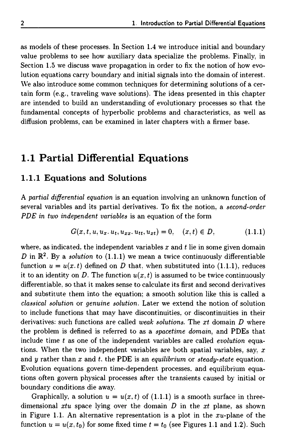
Graphically, a solution и = u(x,t) of (1.1.1) is a smooth surface in three-
dimensional xtu space lying over the domain D in the xt plane, as shown
in Figure 1.1. An alternative representation is a plot in the zu-plane of the
function u = u(x, ίο) for some fixed time t = to (see Figures 1.1 and 1.2). Such
1.1 Partial Differential Equations
3
solution surface
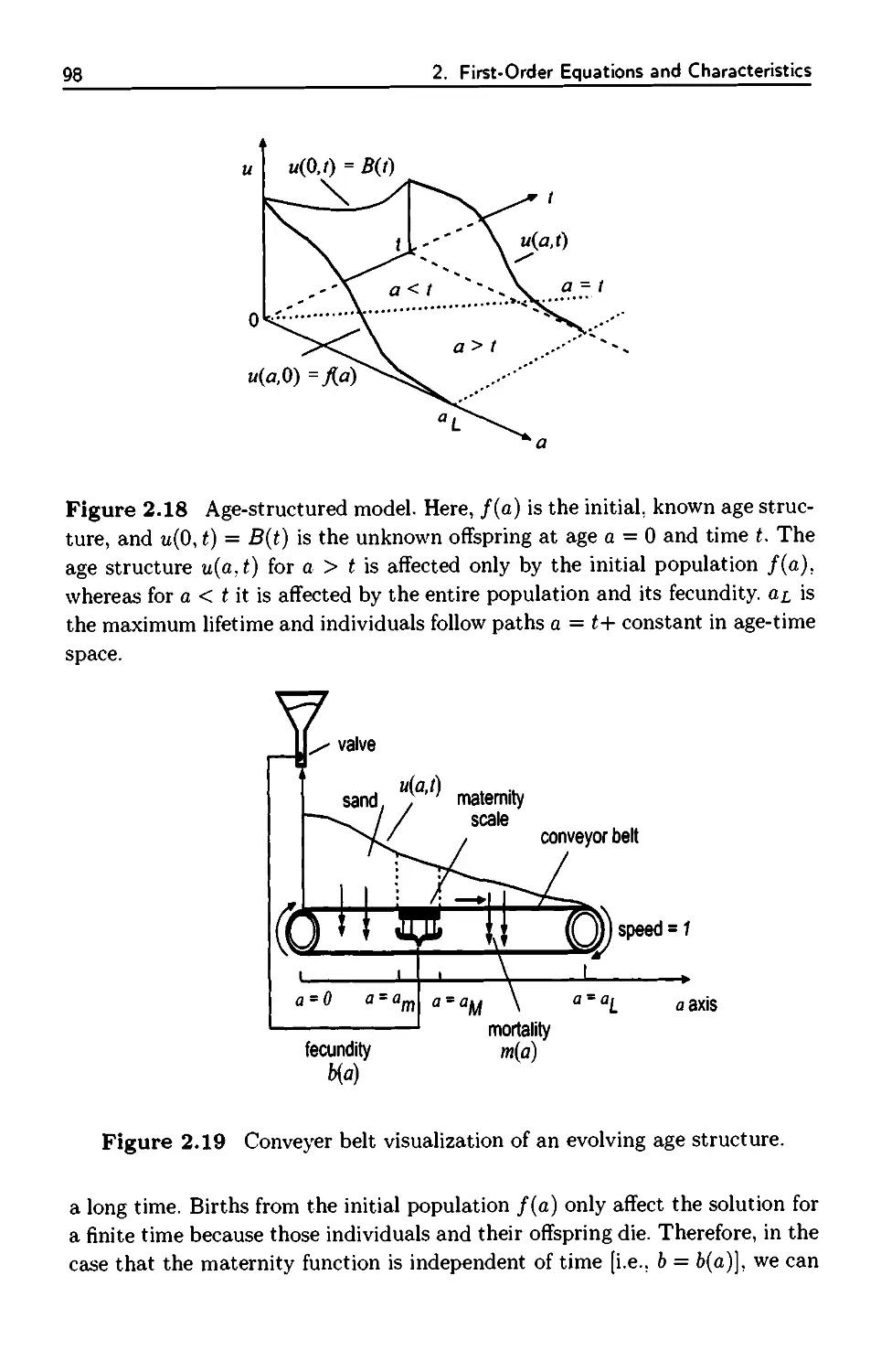
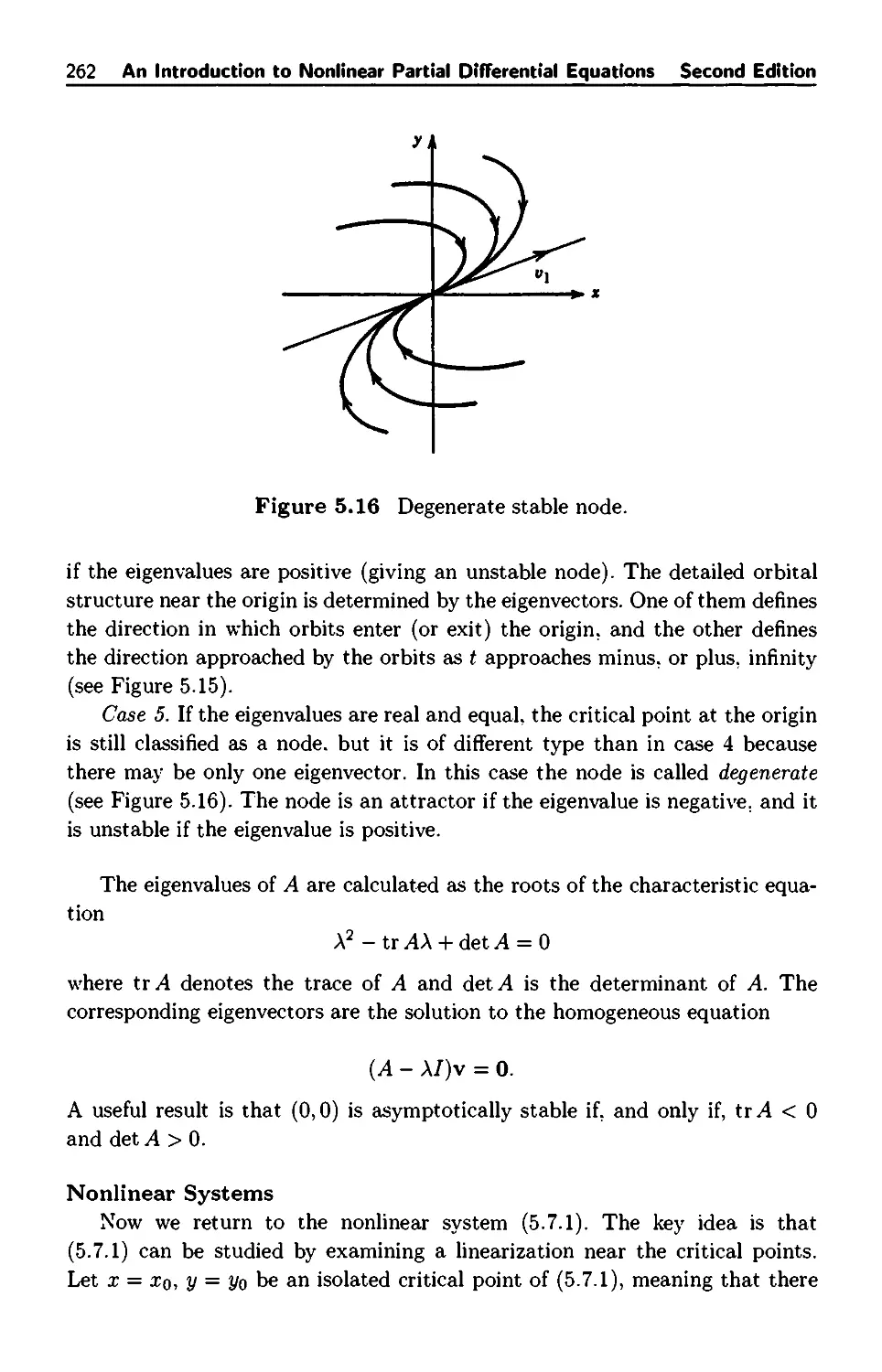
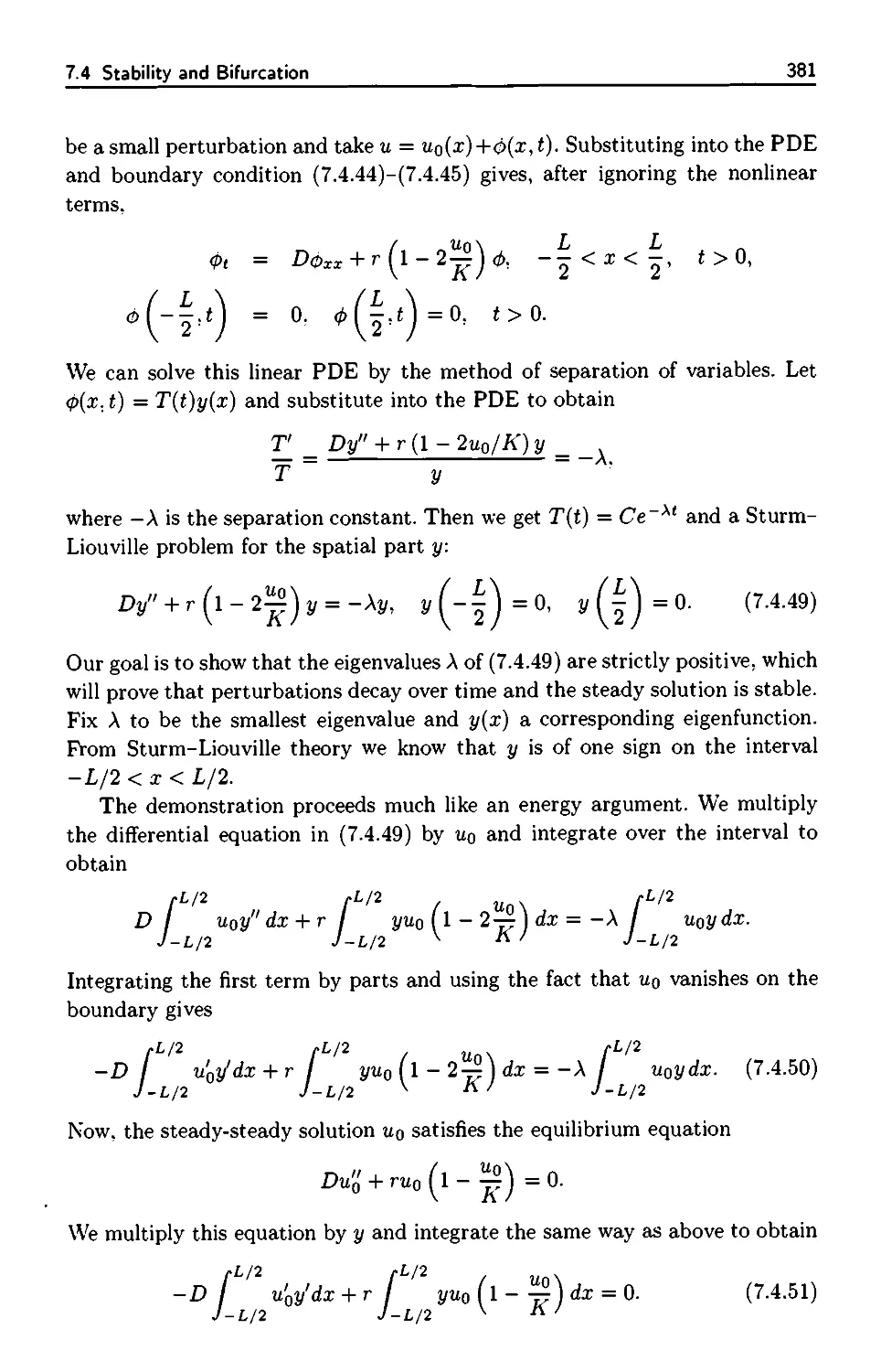
Figure 1.1 Solution surface и = u(x.t) in xtu space, also showing a time
snapshot or wave profile u(x, to) at time to- The functions /, g, and h represent
values of и on the boundary of the domain, which are often prescribed as initial
and boundarv conditions.
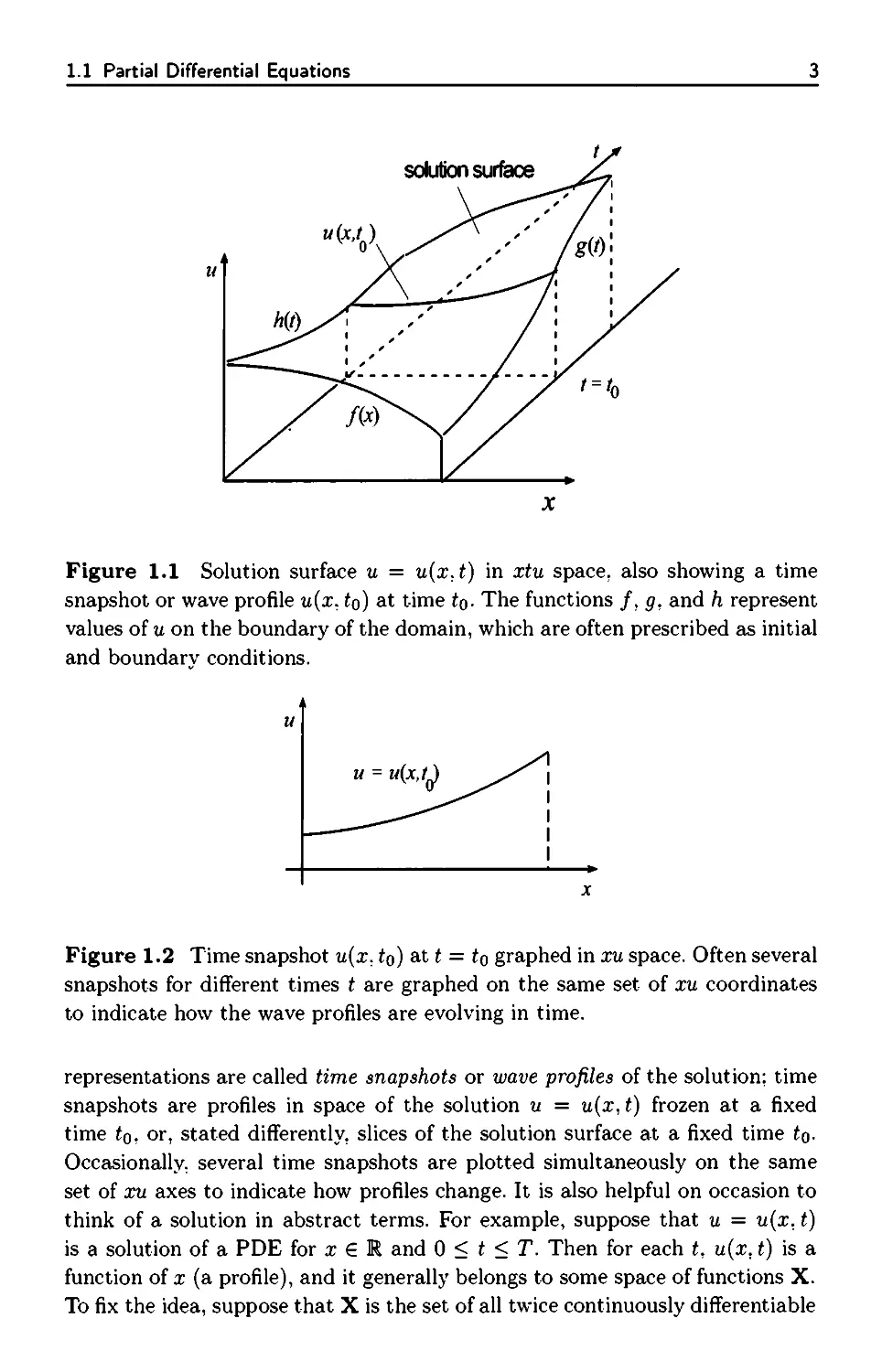
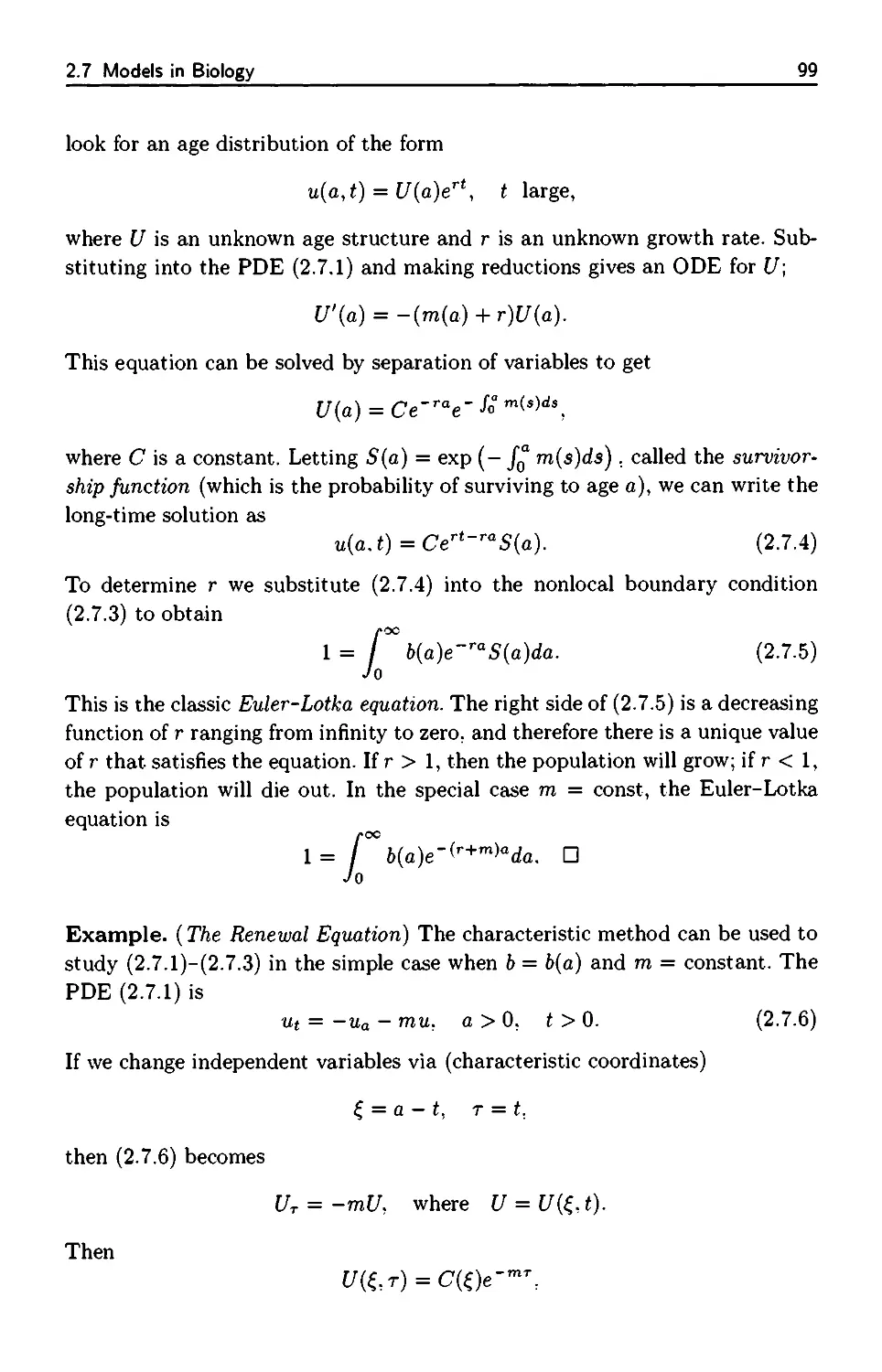
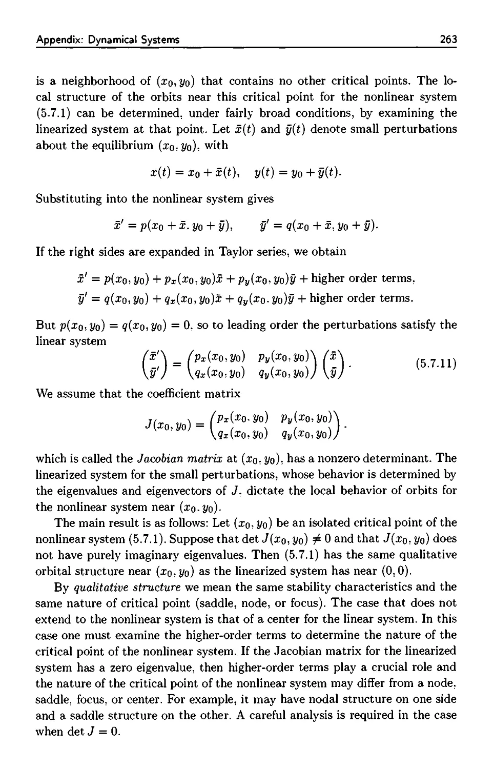
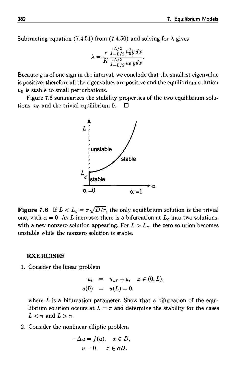
Figure 1.2 Time snapshot u(x. to) at t = to graphed in xu space. Often several
snapshots for different times t are graphed on the same set of xu coordinates
to indicate how the wave profiles are evolving in time.
representations are called time snapshots or wave profiles of the solution; time
snapshots are profiles in space of the solution и = и(х, t) frozen at a fixed
time ίο. or, stated differently, slices of the solution surface at a fixed time to-
Occasionally, several time snapshots are plotted simultaneously on the same
set of xu axes to indicate how profiles change. It is also helpful on occasion to
think of a solution in abstract terms. For example, suppose that и = и(х. t)
is a solution of a PDE for χ € R and 0 < t < T. Then for each t, u(x. t) is a
function of χ (a profile), and it generally belongs to some space of functions X.
To fix the idea, suppose that X is the set of all twice continuously differentiable
4
1. Introduction to Partial Differential Equations
functions on R that approach zero at infinity. Then the solution can be regarded
as a mapping from the time interval [0. T] into the function space X; that is.
to each t in [0, T] we associate a function u(-,t), which is the wave profile at
time t.
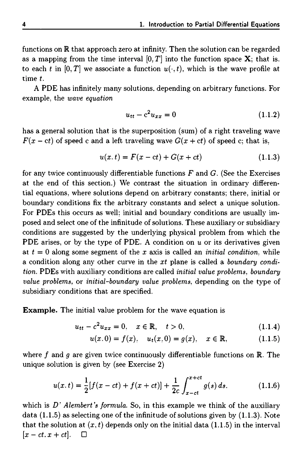
A PDE has infinitely many solutions, depending on arbitrary functions. For
example, the wave equation
utt-c2uxx = 0 (1.1.2)
has a general solution that is the superposition (sum) of a right traveling wave
F(x - ct) of speed с and a left traveling wave G(x + c£) of speed c; that is.
u(x.t) = F(x-ct) + G(x + ct) (1.1.3)
for any twice continuously differentiable functions F and G. (See the Exercises
at the end of this section.) We contrast the situation in ordinary
differential equations, where solutions depend on arbitrary constants; there, initial or
boundary conditions fix the arbitrary constants and select a unique solution.
For PDEs this occurs as well; initial and boundary conditions are usually
imposed and select one of the infinitude of solutions. These auxiliary or subsidiary
conditions are suggested by the underlying physical problem from which the
PDE arises, or by the type of PDE. A condition on и or its derivatives given
at t = 0 along some segment of the χ axis is called an initial condition, while
a condition along any other curve in the xt plane is called a boundary
condition. PDEs with auxiliary conditions are called initial value problems, boundary
value problems, or initial-boundary value problems, depending on the type of
subsidiary conditions that are specified.
Example. The initial value problem for the wave equation is
им - c2Uxx = 0T x£R, t>0: (1-1-4)
u(x.0) = f(x): ut(x;0)=g(x), x€R, (1.1.5)
where / and g are given twice continuously differentiable functions on R. The
unique solution is given by (see Exercise 2)
1 1 fx+ct
Φ-1) = r [f(x - ct) + f(x + ct)} + - / g(s) ds. (1.1.6)
2 2c Jx_ct
which is D' Alembert's formula. So, in this example we think of the auxiliary
data (1.1.5) as selecting one of the infinitude of solutions given by (1.1.3). Note
that the solution at (x, t) depends only on the initial data (1.1.5) in the interval
[x - ct.x + ct]. D
1.1 Partial Differential Equations
5
Statements regarding the single second-order PDE (1.1.1) can be
generalized in various directions. Higher-order equations (as well as first-order
equations), several independent variables, and several unknown functions (governed
by systems of PDEs) are all possibilities.
1.1.2 Classification
PDEs are classified into different types, depending on either the type of
physical phenomena from which they arise or a mathematical basis. As the reader
has learned from previous experience, there are three fundamental types of
equations: those that govern diffusion processes, those that govern wave
propagation, and those that govern equilibrium phenomena. Equations of mixed type
also occur. We consider a single, second order PDE of the for
a(x,t)uxx + 2b(x,t)uxt + c(x,t)uu = d(x,t,u,ux,ut), (хЛ) £ D, (1.1.7)
where a, b. and с are continuous functions on D, and not all of a, b, and с
vanish simultaneously at some point of D. The function d on the right side is
assumed to be continuous as well. Classification is based on the combination
of the second-order derivatives in the equation. If we define the discriminant
Δ by Δ = b2 — ac, then (1.1.7) is hyperbolic if Δ > 0, parabolic if Δ = 0, and
elliptic if Δ < 0.
Hyperbolic and parabolic equations are evolution equations that govern
wave propagation and diffusion processes, respectively, and elliptic equations
are associated with equilibrium or steady-state processes. In the latter case, we
use χ and у as independent variables rather than χ and t. There is also a close
relationship between the classification and the kinds of initial and boundary
conditions that may be imposed on a PDE to obtain a well-posed mathematical
problem, or one that is physically relevant. Because classification is based on
the highest-order derivatives in (1.1.7), or the principal part of the equation,
and because Δ depends on χ and t, equations may change type as χ and t vary
throughout the domain.
Now we demonstrate that equation (1.1.7) can be transformed to certain
simpler, or canonical, forms, depending on the classification, by a change of
independent variables
ξ = ξ(χ,ί), η = η(χΛ). (1.1.8)
We now perform this calculation, with the view of actually trying to determine
(1.1.8) such that (1.1.7) reduces to a simpler form in the ξη coordinate system.
The transformation (1.1.8) is assumed to be invertible. which requires that the
Jacobian J = £,хщ - ξίηχ be nonzero in any region where the transformation
is applied. A straightforward application of the chain rule, which the reader
6
1. Introduction to Partial Differential Equations
can verify, shows that the left side of (1.1.7) becomes, under the change of
independent variables (1.1.8)
auxx + 2buxt + cuu + ■■■ = Αυ,ξξ + 2Bu^n + Cum Λ , (1.1.9)
where the three dots denote terms with lower-order derivatives, and where
Β = αξχηχ + 6(ξχί7ί + ξί%) + c£tr7t,
С = αηΙ + 26r7xf?t + οη2.
Notice that the expressions for A and С have the same form, namely
афх + 2Ьфхфг + сф2,
and are independent.
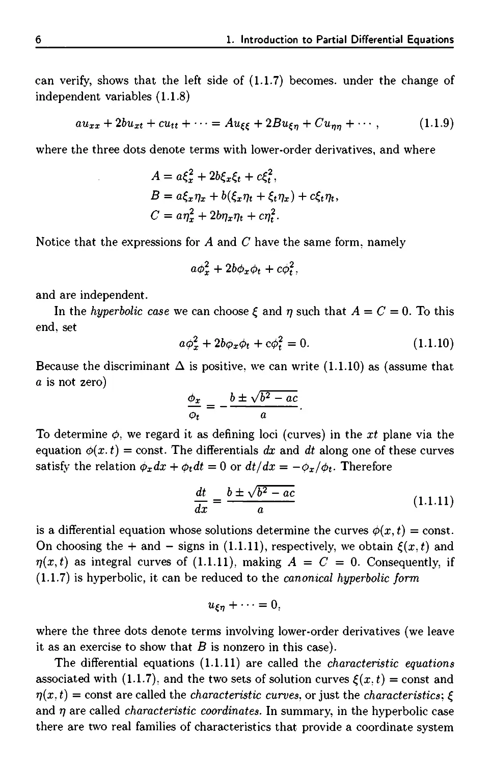
In the hyperbolic case we can choose ξ and η such that A = С = 0. To this
end, set
аф\ + 2bq>x0t + сф2 = О. (1.1.10)
Because the discriminant Δ is positive, we can write (1.1.10) as (assume that
a is not zero)
0i _ b ± y/b2 - ac
Φι a
To determine φ, we regard it as defining loci (curves) in the xt plane via the
equation o(x. t) = const. The differentials dx and dt along one of these curves
satisfy the relation φχάχ + <z>tdi = 0 or dt/dx = —Фх/фг- Therefore
* = ь±Уь^Гс
dx a
is a differential equation whose solutions determine the curves ф(х, i) = const.
On choosing the + and - signs in (1.1.11), respectively, we obtain ξ(χ,ί) and
η(χ,ί) as integral curves of (1.1.11). making A = С = 0. Consequently, if
(1.1.7) is hyperbolic, it can be reduced to the canonical hyperbolic form
ιιξη + ■ ■ ■ = 0,
where the three dots denote terms involving lower-order derivatives (we leave
it as an exercise to show that В is nonzero in this case).
The differential equations (1.1.11) are called the characteristic equations
associated with (1.1.7). and the two sets of solution curves ξ(χ, t) = const and
η(χ. t) = const are called the characteristic curves, or just the characteristics: ξ
and η are called characteristic coordinates. In summary, in the hyperbolic case
there are two real families of characteristics that provide a coordinate system
1.1 Partial Differential Equations
7
where the equation reduces to a simpler form. Characteristics are the
fundamental concept in the analysis of hyperbolic problems because characteristic
coordinates form a natural curvilinear coordinate system in which to examine
these problems. In some cases. PDEs simplify to ODEs along the characteristic
curves.
In the parabolic case (b2 - ac = 0) there is just one family of characteristic
curves, defined bv
Ε.-Ϊ
dx a
Thus we may choose ξ = ξ(χ. t) as an integral curve of this equation to make
A = 0. Then, if η = η(χ, t) is chosen as any smooth function independent of
ξ (i.e.. so that the Jacobian is nonzero), one can easily determine that В = 0
automatically, giving the parabolic canonical form
ΙΙςς + ■ ■ ■ = 0.
Characteristics rarely play a role in parabolic problems.
In the elliptic case (b2 — ac < 0) there are no real characteristics and, as in
the parabolic case, characteristics play no role in elliptic problems. However, it
is still possible to eliminate the mixed derivative term in (1.1.7) to obtain an
elliptic canonical form. The procedure is to determine complex characteristics
by solving (1.1.11), and then take real and imaginary parts to determine a
transformation (1.1.8) that makes A = С and В = 0 in (1.1.9). We leave it as
an exercise to show that the transformation is given by
2 2.1
Then the elliptic canonical form is
Uaa + идз + · · · = 0,
where the Laplacian operator becomes the principal part.
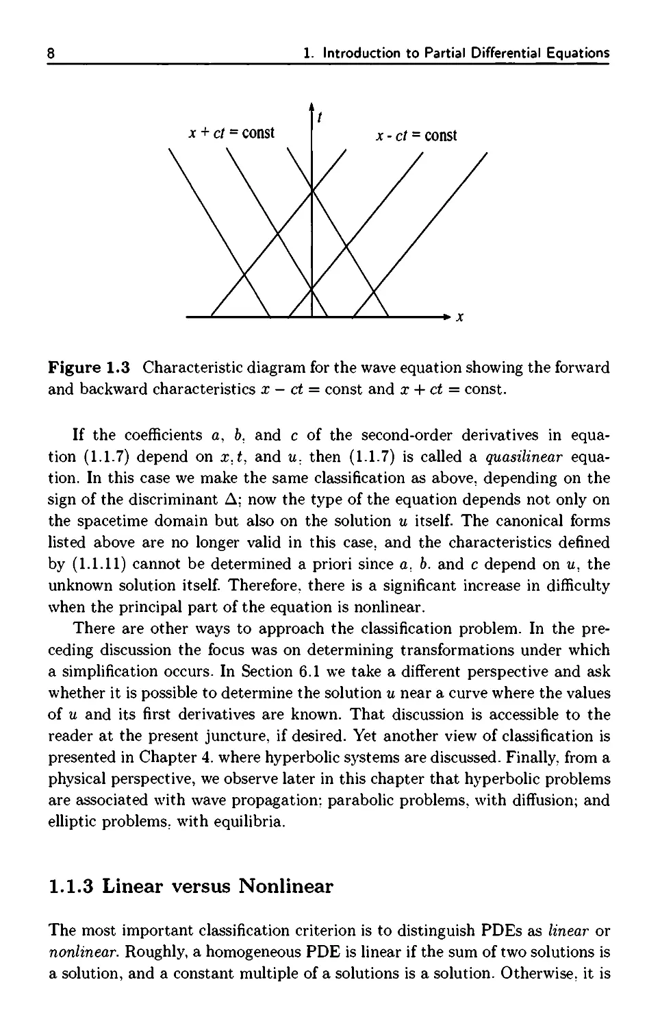
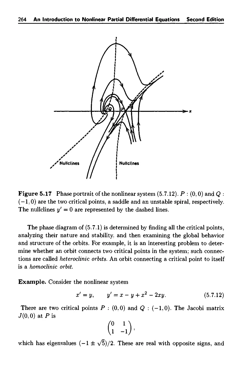
Example. It is easy to see that the characteristic curves for the wave
equation (1.1.2), which is hyperbolic, are the straight lines χ — ct = const and
χ + ct = const. These are shown in Figure 1.3. In this case the characteristic
coordinates are given by ξ = x-ct and η = x+ct. In these coordinates the wave
equation transforms to u^ = 0. We regard characteristics as curves in space-
time moving with speeds с and -c. and from the general solution (1.1.3) we
observe that signals are propagated along these curves. In hyperbolic problems,
in general, the characteristics are curves in spacetime along which signals are
transmitted. D
8
1. Introduction to Partial Differential Equations
*· χ
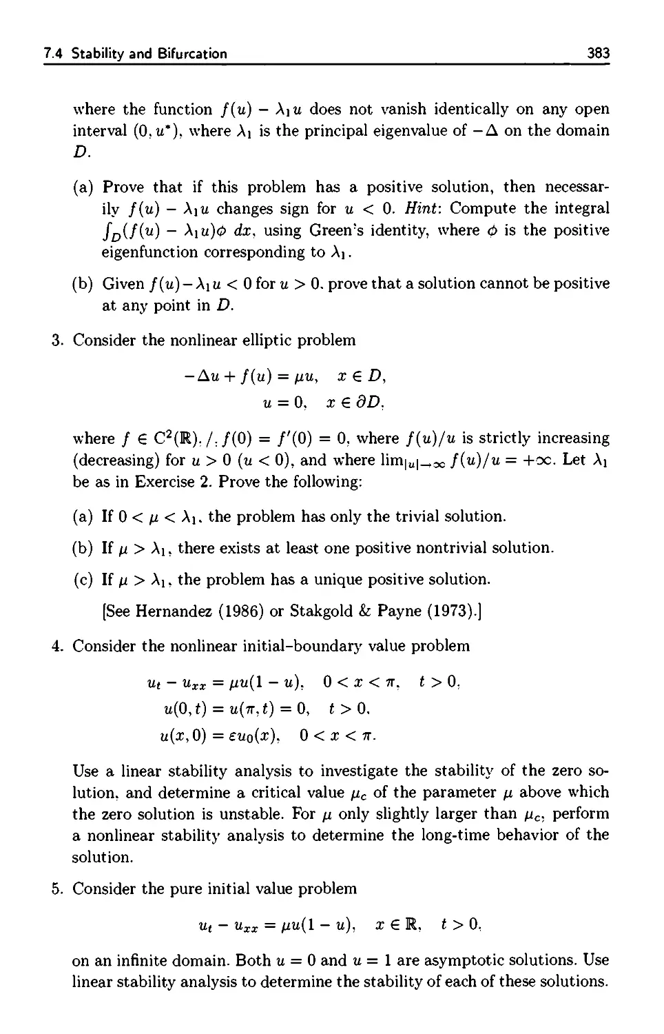
Figure 1.3 Characteristic diagram for the wave equation showing the forward
and backward characteristics χ — ct = const and χ + ct = const.
If the coefficients a, b. and с of the second-order derivatives in
equation (1.1.7) depend on x. t, and u. then (1-1-7) is called a quasilinear
equation. In this case we make the same classification as above, depending on the
sign of the discriminant Δ; now the type of the equation depends not only on
the spacetime domain but also on the solution и itself. The canonical forms
listed above are no longer valid in this case, and the characteristics defined
by (1.1.11) cannot be determined a priori since a. b. and с depend on u, the
unknown solution itself. Therefore, there is a significant increase in difficulty
when the principal part of the equation is nonlinear.
There are other ways to approach the classification problem. In the
preceding discussion the focus was on determining transformations under which
a simplification occurs. In Section 6.1 we take a different perspective and ask
whether it is possible to determine the solution и near a curve where the values
of и and its first derivatives are known. That discussion is accessible to the
reader at the present juncture, if desired. Yet another view of classification is
presented in Chapter 4. where hyperbolic systems are discussed. Finally, from a
physical perspective, we observe later in this chapter that hyperbolic problems
are associated with wave propagation; parabolic problems, with diffusion; and
elliptic problems, with equilibria.
1.1.3 Linear versus Nonlinear
The most important classification criterion is to distinguish PDEs as linear or
nonlinear. Roughly, a homogeneous PDE is linear if the sum of two solutions is
a solution, and a constant multiple of a solutions is a solution. Otherwise, it is
1.1 Partial Differential Equations
9
nonlinear. The division of PDEs into these two categories is a significant one.
The mathematical methods devised to deal with these two classes of equations
are often entirely different, and the behavior of solutions differs substantially.
One underlying cause is the fact that the solution space to a linear,
homogeneous PDE is a vector space, and the linear structure of that space can be
used with advantage in constructing solutions with desired properties that can
meet diverse boundary and initial conditions. Such is not the case for nonlinear
equations.
It is easy to find examples where nonlinear PDEs exhibit behavior with
no linear counterpart. One is the breakdown of solutions and the formation of
singularities; such as shock waves. A second is the existence of solitions, which
are solutions to nonlinear dispersion equations. These solitary wave solutions
maintain their shapes through collisions, in much the same was as linear
equations do, even though the interactions are not linear. Nonlinear equations have
come to the forefront because, basically, the world is nonlinear!
More formally, linearity and nonlinearity are usually defined in terms of the
properties of the operator that defines the PDE itself. Let us assume that the
PDE (1.1.1) can be written in the form
Lu = F, (1.1.12)
where F = F(x. t) and L is an operator that contains all the operations
(differentiation, multiplication, composition, etc.) that act on и = u(x, t) . For
example, the wave equation utt - uxx = 0 can be written Lu = 0, where L is
the partial differential operator dt2 - d2.. In (1.1.12) we reiterate that all terms
involving the unknown function и are on the left side of the equation and are
contained in the expression Lu\ the right side of (1.1.12) contains in F only
expressions involving the independent variables χ and t. If F = 0. then (1.1.12)
is said to be homogeneous: otherwise, it is nonhomogeneous. We say that an
operator L is linear if it is additive and if constants factor out of the operator,
that is, (1) L(u + v) = Lu + Lv, and (2) L(cu) = cLu, where и and υ are
functions (in the domain of the operator) and с is any constant. The PDE (1.1.12)
is linear if I, is a linear operator; otherwise, the PDE is nonlinear.
Example. The equation Lu = ut + uux = 0 is nonlinear because, for example;
L(cu) = сщ + c2uux. which does not equal cLu = c(ut + uux). D
Conditions (1) and (2) stated above imply that a linear homogeneous
equation Lu = 0 has the property that if ui, иг . un are η solutions, the linear
combination
U = C\U\ + C2U2 + ■ ■ ■ + CnUn
10
1. Introduction to Partial Differential Equations
is also a solution for any choice of the constants c\, сг, ■ ■ ■, cn- This fact is called
the superposition principle for linear equations. For nonlinear equations we
cannot superimpose solutions in this manner. The superposition principle can often
be extended to infinite sums for linear problems, provided that convergence
requirements are met. Superposition for linear equations allows one to construct,
from a given set of solutions, another solution that meets initial or boundary
requirements by choosing the constants c\.C2,. ■. judiciously. This observation
is the basis for the Fourier method, or eigenfunction expansion method, for
linear, homogeneous boundary value problems, and we review this procedure
at the end of the section. Moreover, superposition can often be extended to a
family of solutions depending on a continuum of values of a parameter. More
precisely, if и = u{x, t: k) is a family of solutions of a linear homogeneous PDE
for all values of к in some interval of real numbers /. one can superimpose these
solutions formally using integration by defining
u(x. t) = / c(k)u(x, t: k) dk,
where с = c(k) is a function of the parameter k. Under certain conditions that
must be established, the superposition u(x, t) may again be a solution. As in
the finite case, there is flexibility in selecting c(k) to meet boundary or initial
conditions. In fact, this procedure is the vehicle for transform methods for
solving linear PDEs (Laplace transforms, Fourier transforms, etc.). We review
this technique below. Finally, for a homogeneous, linear PDE the real and
imaginary parts of a complex solution are both solutions. This is easily seen
from the calculation
L{v + iw) = Lv + iLw = 0 + 0 = 0,
where the real-valued functions ν and w satisfy Lv = 0 and Lw = 0. None
of these methods based on superposition are applicable to nonlinear problems,
and other methods must be sought. In summary, there is a profound difference
between properties and solution methods for linear and nonlinear problems.
If most solution methods for linear problems are inapplicable to nonlinear
equations, what methods can be developed? We mention a few.
1. Perturbation Methods. Perturbation methods are applicable to problems
where a small or large parameter can be identified. In this case an
approximate solution is sought as a series expansion in the parameter.
2. Similarity Methods. The similarity method is based on the PDE and its
auxiliary conditions being invariant under a family of transformations
depending on a small parameter. The invariance transformation allows one
to identify a canonical change of variables that reduces the PDE to an
ordinary differential equation (ODE), or reduces the order of the PDE.
1.1 Partial Differential Equations
11
3. Characteristic Methods. Nonlinear hyperbolic equations, which are
associated with wave propagation, can be analyzed with success in characteristic
coordinates (i.e.. coordinates in spacetime along which the waves or signals
propagate).
4. Transformations. Sometimes it is possible to identify transformations that
change a given nonlinear equation into a simpler equation that can be
solved.
5. Numerical Methods. Fast, large-scale computers have given tremendous
impetus to the development and analysis of numerical algorithms to solve
nonlinear problems and. in fact, have been a stimulus to to the analysis of
nonlinear equations.
6. Traveling Wave Solutions. Seeking solutions with special properties is a key
technique. For example: traveling waves are solutions to evolution
problems that represent fixed waveforms moving in time. The assumption of
a traveling wave profile to a PDE sometimes reduces it to an ODE, often
facilitating the analysis and solution. Traveling wave solutions form one
type of similarity solution.
7. Steady State Solutions and Their Stability. Many PDEs have steady-state,
or time-independent, solutions. Studying these equilibrium solutions and
their stability is an important activity in many areas of application.
8. Ad Hoc Methods. The mathematical and applied science literature is replete
with articles illustrating special methods that analyze a certain type of
nonlinear PDE. or restricted classes of nonlinear PDEs.
These methods are primarily solution methods, which represent one aspect
of the subject of nonlinear PDEs. Other basic issues are questions of existence
and uniqueness of solutions, the regularity (smoothness) of solutions, and the
investigation of stability properties of solutions. These and other theoretical
questions have spawned investigations based on modern topological and
algebraic concepts, and the subject of nonlinear PDEs has evolved into one of the
most diverse, active areas of applied analysis.
1.1.4 Linear Equations
In this subsection we review, through examples, two techniques from elementary
PDEs that illustrate the use of the superposition principles mentioned above.
These calculations arise later in analyzing the local stability of equilibrium
solutions to nonlinear problems.
12
1. Introduction to Partial Differential Equations
Example. (Separation of Variables) Consider the following problem for и =
u(x, t) on the bounded interval / : 0 < χ < 1 with t > 0, that is
ut = Au. 0 < χ < 1. t > 0.
u(0,i) = u(l.t) = 0, i>0,
u(x:0) = f(x). 0<x<l,
where Л is a linear, spatial differential operator of the form
Au = -{pux)x + qu.
The functions ρ = p(x) and q = q(x) are given, with ρ of one sign on /. and
p, p1. and q continuous on /. Problems of this type are solved by Fourier's
method, or the method of eigenfunction expansions. The idea is to construct
infinitely many solutions that satisfy the PDE and the boundary conditions;
equations (1.1.13) and (1.1.14), and then superimpose them, rigging up the
constants so that the initial condition (1.1.15) is satisfied. This technique is
called separation of variables, based on an assumption that the solution has
the form u(x. t) = g(t)y(x), where g and у are to be determined. When we
substitute this form into the PDE and rearrange terms we obtain
ί. = 0!
9 У '
where the left side depends only on t and the right side depends only on x. A
function of t can equal a function of χ for all χ and t only if both are equal to
a constant, say, -λ, called the separation constant. Therefore
9 У
and we obtain two ODEs, one for g and one for y.
g' = -\g, -Ay = \y.
We say that the equation separates. If we substitute the assumed form of и
into the boundary conditions (1.1.14), then we obtain
»(0) = y(l) = 0.
The temporal equation is easily solved to get g(t) = ce~xt, where с is an
arbitrary constant. The spatial equation along with its homogeneous (zero)
boundary conditions give a boundary value problem (BVP) for y.
-Ay = Xy, 0<x<l, (1.1.16)
y(0) = y(l) = 0. (1.1.17)
(1.1.13)
(1.1.14)
(1.1.15)
1.1 Partial Differential Equations
13
This BVP for y, which is differential eigenvalue problem called a Sturm-
Liouville problem, has the property there are infinitely many real, discrete
values of the separation constant λ. say. λ = λη, η = 1.2....; for which there
are corresponding solutions у = yn(x), η = 1,2..... The λη are called the
eigenvalues for the problem and the corresponding solutions у = yn(x) are called the
eigenfunctions. The eigenvalues have the property that they are ordered and
|λη| —► ос as η —> ос. Therefore we have obtained a countably infinite number
of solutions to the PDE that satisfy the boundary conditions:
un(x,t) = cne~Xntyn(x), n = l,2.....
Now, here is where superposition is used. We add up these solutions and pick
the constants cn so that the initial condition (1.1.15) is satisfied, thus obtaining
the solution to the problem; that is, we form
u(x,t) = ^c„e Xntyn{x)-
n = l
Formally applying the initial condition gives
ОС
i{x.O) = f{x) = Y^cnyn{x). (1.1.18)
u(
n = l
The right side is an expansion of the initial condition / in terms of the
eigenfunctions yn, and we can use it to determine the coefficients cn. This calculation
is enabled by a very important property of the eigenfunctions, namely,
orthogonality. If we define the inner product of two functions φ and ψ by
(φ, ψ) = / φ(χ)ψ(χ)άχ..
Jo
then we say φ and ψ are orthogonal if (φ. φ) = 0. The set of eigenfunctions yn
of the Sturm-Liouville problem (1.1.16)—(1-1.17) are mutually orthogonal, or
(уп,Ут)= yn(x)ym(x)dx = 0, пфт.
Jo
Therefore, if we multiply (1.1.18) by a fixed but arbitrary ym and formally
integrate over the interval /, we then obtain
oo
(f-.Ут) = ^2cn(yn,ym).
n = l
Because of orthogonality, the infinite series on the right side collapses to the
single term cm(ym,ym). Therefore the coefficient cm is given by
„ _ (/.3/m)
Cm —
(Ут,Ут)'
14
1. Introduction to Partial Differential Equations
This relation is true for any m. and so the coefficients cn are
Сп = М-^1 n = L2,.... (1.1.19)
(Уп,Уп)
Therefore, we have obtained the solution of (1.1.13)—(1.1.15) in the form of a
series representation, or eigenfunction expansion.
■<*■·>-Σ &*^··*<χ).
The preceding calculation took a lot for granted, but it can be shown rigorously
that the steps are valid. D
An expansion of a function f(x) in terms of the eigenfunctions yn(x)-, as in
(1.1.18), is called the generalized Fourier series for /. and the coefficients cn,
given by (1.1.19), are the Fourier coefficients. It can be shown that that the
series converges in the mean-square sense:
/ I f(x) ~ 2J спУп{х) J dx -* 0 as N —> oc.
Jo \ n=i /
Pointwise and uniform convergence theorems require suitable smoothness
conditions on the function /.
The method of separation of variables is successful under general boundary
conditions of the form
au(0.t) + l3ux(0,t) = 0, -yti(l.i) + <5ux(l:t) =0,
where α, β, у, and <5 are given constants. Of course, the interval over which
the problem is defined may be any founded interval a < χ < b: we chose
α = 0 and b = 1 for simplicity of illustration. The method may be extended
to problems over higher-dimensional, bounded, spatial domains, as well as to
nonhomogeneous problems. For example, if the PDE in (1.1.13)—(1.1-15) is
replaced by the nonhomogeneous equation
щ = Au + F(x,t), 0 <x<l: t>0.
we can expand the nonhomogeneous term F as a Fourier series of the
eigenfunctions for the homogenous problem, or
oo
F(x:t) = J2-rn(t)yn(x).
n=l
1.1 Partial Differential Equations
15
where the -)n{t) are the known Fourier coefficients (t is a parameter in the
expansion) that can be computed from orthogonality property of the eigen-
functions. Then we assume the solution takes the form
u(x,t) = ^c„(i)3/„(x).
n = l
Substituting these forms into the PDE and the initial condition determines the
cn(t) and therefore the solution to the nonhomogeneous problem.
Problems that are defined over infinite spatial domains require different
techniques based on transform methods.
Example. (Transform Method) Consider the following problem on an infinite
spatial domain:
Щ = uxx, χ > 0, t > 0,
u(0, t) = 0, t > 0,
u(x:0) = f(x), x>0.
Because there are two derivatives with respect to x, we expect to impose
another boundary condition at infinity. Therefore, we demand that и be bounded
as χ —► oo. Further, we assume that / is piecewise continuous and absolutely
integrable over χ > 0. We can proceed as in the preceding example and try a
solution of the form и(хЛ) = g(t)y(x). where g and у are to be determined.
Substituting into the differential equation leads to
9' = -As. -y" = Ay,
where λ is the separation constant. As before, g(t) = ce~xt, where с is an
arbitrary constant. The boundary conditions imply that у is bounded and y(0) = 0.
Thus we have the boundary value problem
-y" = Xy, x> 0,
y(0) = 0. у bounded.
This is a boundary value problem on the semi-infinite domain χ > 0. If λ < 0
there are no nontrivial, bounded solutions (check this), and therefore A > 0.
Let us write λ = к2; then the general solution to the boundary value problem
is
y(x) = a sin kx,
where a is an arbitrary constant and к > 0. Consequently we have found a
family of solutions depending upon a parameter k:
u(x, t, k) = ae~k ' sin kx.
16
1. Introduction to Partial Differential Equations
In contrast to the last example, on a bounded interval, where the
eigenvalues were discrete, the eigenvalues in the present case form a continuum. We
superimpose these solutions over all к and write
roc a
u(x, t) = / a(k)e~k г sin kxdk,
Jo
where a(k) is a function of k. We can determine a(k) from the initial condition.
Putting t = 0 in the last equation gives
/(χ) = / a(k) sin kxdk. (1.1.20)
Jo
This is an integral equation from which we can recover a(k) using a special
case of the Fourier integral theorem: If / is piecewise continuous and absolutely
intcgrable on χ > 0, and if
f(x)= / a(k) sin kxdk.
Jo
then
2 ί°°
a(k) = - f(ξ)sinkξdξ.
π Jo
The function a is the Fourier sine transform of /, and / is the inverse sine
transform of a. Putting everything together gives an integral representation of
the solution to the problem. namely
и(хЛ) = -ί (ί f(ξ)sinkξdξ\e-k2t sin kxdk
- -f ^)(/ e~k2t sin kξ sin kxdk\dξ.
where we have changed the order of integration in the last step. Actually, the
interior integral can be calculated analytically, or looked up in a table, which
we leave as an exercise. D
The reader should notice the great similarity of the solution forms in these
two examples—finite domain versus infinite domain, discrete eigenvalues versus
a continuum of eigenvalues, and expansions in terms of sums versus integrals.
The role of superposition is critical in linear problems, but it does not carry
over to nonlinear problems.
Terminology. We introduce some notation and terminology for some function
spaces that commonly occur in analysis. Let D be an open domain (a set that
does not contain any of its boundary) in either one or several dimensions.
Because D is an open domain we do not have to deal with the question of
1.1 Partial Differential Equations
17
existence of derivatives at boundary points. Using an overbar. D: we denote the
closure of D. which consists of D and its boundary dD; that is, D = D U dD.
By Cn(D) we denote the set of all continuous functions on D that have η
continuous derivatives in D (partial derivatives if D is of dimension greater
than 1). The space of continuous functions on D is denoted by C(D), and
Coc(D) denotes the space of continuous functions on D that have derivatives
of all orders. When a function и belongs to one of these sets, e.g., Cn(D), we
sometimes say that и is of class Cn on D.
EXERCISES
1. Show that the wave equation utt — <?uxx = 0 reduces to the canonical form
υ,ξη = 0 under the change of variables ξ = χ - ct, η = χ + ci, and use
this information to show that the general solution of the wave equation is
u(x, t) = F(x-ct)+G(x+ct), where F and G are arbitrary C2(R) functions.
2. Derive D!Alembert:s formula for the initial value problem for the wave
equation using Exercise 1 and determining F and G from the initial
conditions.
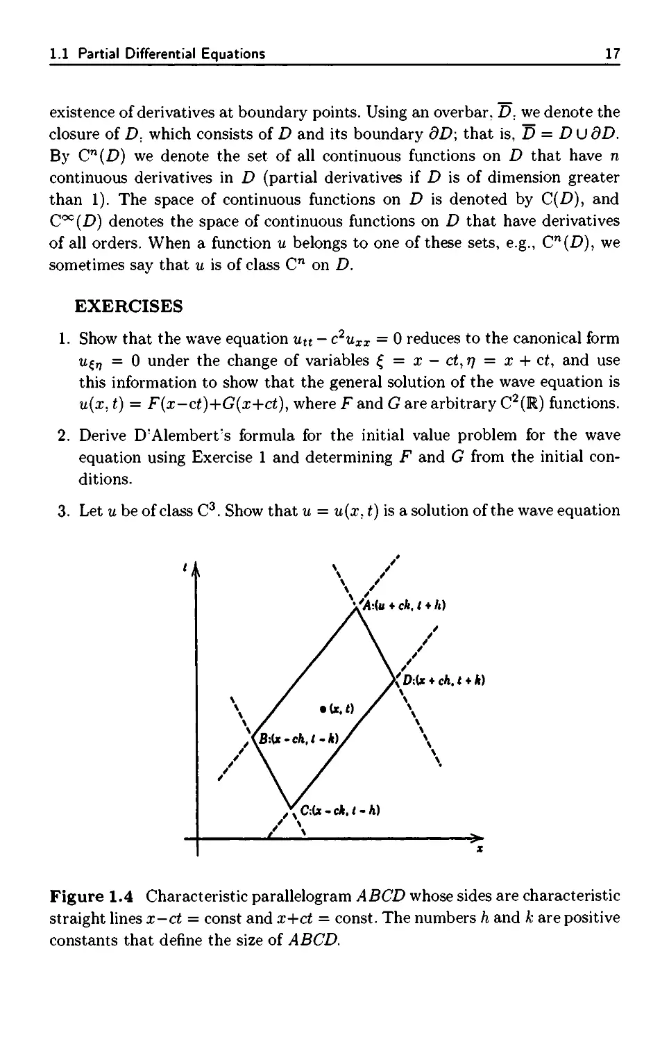
3. Let и be of class C3. Show that и = u(x, t) is a solution of the wave equation
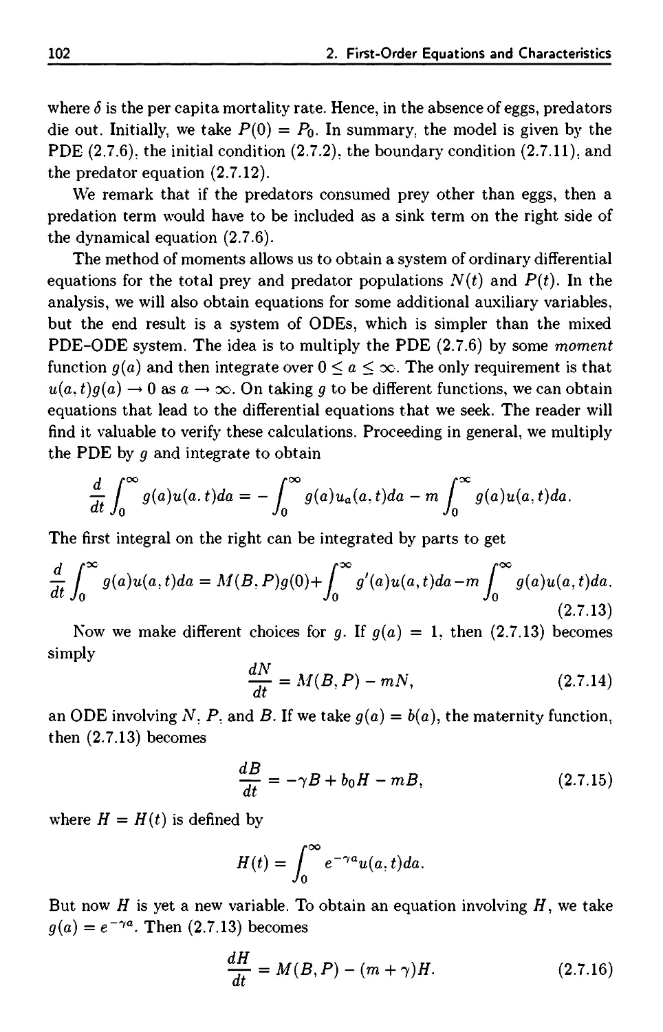
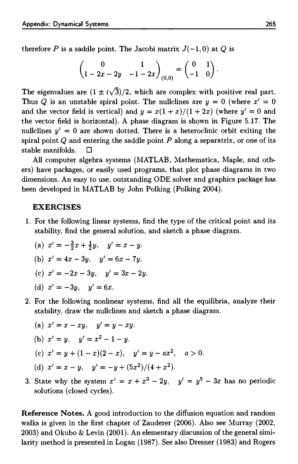
ДС:<*-С*./-А)
<D:U + cA.i + A)
Figure 1.4 Characteristic parallelogram ABCD whose sides are characteristic
straight lines x-ct = const and x+ct = const. The numbers h and к are positive
constants that define the size of ABCD.
18
1. Introduction to Partial Differential Equations
Utt — c2uxx = 0 if, and only if. и satisfies the difference equation
u(x - ck.t - h) + u(x + ck.t + h)
= u(x - ch.t - k) + u(x + ch. t + k)
for all constants h, к > 0. Interpret this result geometrically in the ziplane
by observing that the difference equation relates the value of и at the
vertices of a characteristic parallelogram whose sides are the characteristic
straight lines χ + ct = const and χ - ct = const (see Figure 1.4).
4. Assuming that the initial data / and g for the initial value problem for the
wave equation in Exercise 3 have compact support (i.e., / and g vanish for
\x\ sufficiently large), prove that the solution u(x. i) has compact support
in χ for each fixed time t.
5. Find the general solution of the PDE
x2uxx + 2xtuxt + t2utt = 0
by transforming the equation to canonical form using characteristic
coordinates ξ = t/x, η = t.
6. Let и = и(х, t) be a solution of the nonlinear equation
a(ux, ut)uxx + 2b(ux, ut)uxt + c(ux. ut)utt = 0.
Introduce new independent variables via ξ = ξ(χ. t) and η = η(χ, t), and
a new function φ = φ(ξ, η) defined by φ = xux + tut - u. Prove that
φξ = χ. φη = t. and φ satisfies the linear PDE
α(& Φτ,π - 2&(ξ: η)φξη + ο(ξ, η)φξξ = 0.
(This transformation, known as a hodograph, or a Legendre, transformation,
transforms a nonlinear equation of the given form to a linear equation by
reversing the roles of the dependent and independent variables.)
7. Find a formula for the solution of the initial-boundary value problem
utt = c2uxx, χ > 0, t > 0,
u(x, 0) = /(ζ), ut(x, 0) = g(x), x>0,
u(0:t) = h(t), t>0.
Hint: Use D'Alembert's formula for χ > ct and the difference equation in
Exercise 3 for 0 < χ < ct. Assume sufficient differentiability.
1.1 Partial Differential Equations
19
8. Solve the outgoing signaling problem
Utt = c2uxx. χ > 0, t € R,
u(0,t) = s(t), i€R.
9. Consider the PDE
4uxx + buxt + utt = 2 - ut- ux.
Find the characteristic coordinates and graph the characteristic curves in
the xt plane. Reduce the equation to canonical form and find the general
solution.
10. Classify the PDE
xuxx - Autt = 0.
In the case χ > 0 find the characteristic coordinates and sketch the
characteristics in an appropriate region in the xt plane.
11. Use the separation of variables method to find a series representation of
the solution to the following problems:
(a)
щ = Duxx. 0 < χ < π, t > 0.
u(0:i) = 0: ω(π,ί) = 0, t > 0,
u(x,0) = f(t), 0<χ<π.
(b)
(c)
uu = c2uxx, 0 < χ < 1. t > 0,
u(0,i) = 0, u(l:i) = 0, i>0,
u(z,0) = 0, ut(x,0) = g(t), 0<χ<π.
uxx + uyy = 0, 0 < χ < 1. 0 < у <π,
u(a:,0)=0, иу(х,п) = 0, 0<х<1,
u(0,j/) = 0. u(l,y) = g(y), 0<y<n.
12. Find the general solution of the Euler-Darboux equation
m .
Ux,v = (ux - Uy)
x-y
in the case m = 1. Hint: Look at ((x - y)u)
Xj/.
20 1. Introduction to Partial Differential Equations
1.2 Conservation Laws
Many of the fundamental equations in the natural and physical sciences are
obtained from conservation laws, which are balance laws, equations expressing
the fact that some quantity is balanced throughout a process. In
thermodynamics, for example, the first law states that the change in internal energy in
a system is equal to, or is balanced by, the total heat added to the system plus
the work done on the system. Thus the first law of thermodynamics is really an
energy balance law. or conservation law. As another example, consider a fluid
flowing in some region of space that consists of chemical species undergoing
chemical reaction. For a given chemical species, the time rate of change of the
total amount of that species in the region must equal the rate at which the
species flows into the region, minus the rate at which the species flows out,
plus the rate at which the species is created, or consumed, by the chemical
reactions. This is a verbal statement of a conservation law for the amount of
the given chemical species. Similar balance or conservation laws occur in all
branches of science. In the biosciences, for example, the rate of change of an
animal population in a fixed region must equal the birth rate, minus the death
rate, plus the migration rate (emigration or immigration) into or out of the
region.
1.2.1 One Dimension
Mathematically, conservation laws translate into integral or differential
equations, which are then regarded as the governing equations or equations of
motion of the process. These equations dictate how the process evolves in time.
Here we are interested in processes governed by partial differential equations.
We now formulate the basic one-dimensional conservation law, out of which
will evolve some of the basic models and concepts in nonlinear PDEs.
Let us consider a quantity и = u(x. t) that depends on a single spatial vari-
DIP
χ = α χ χ = b
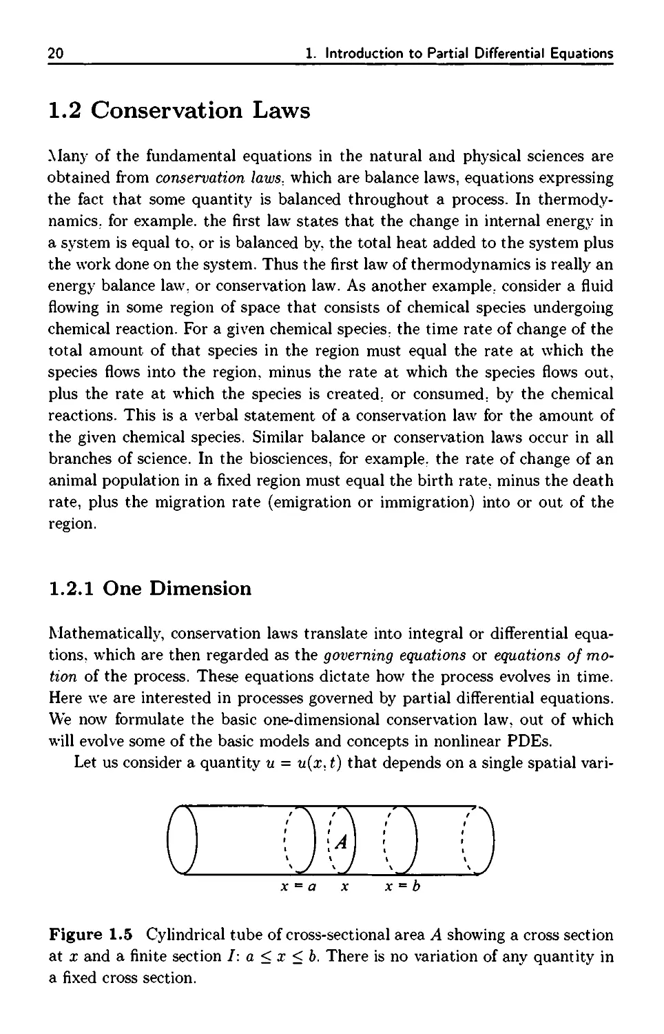
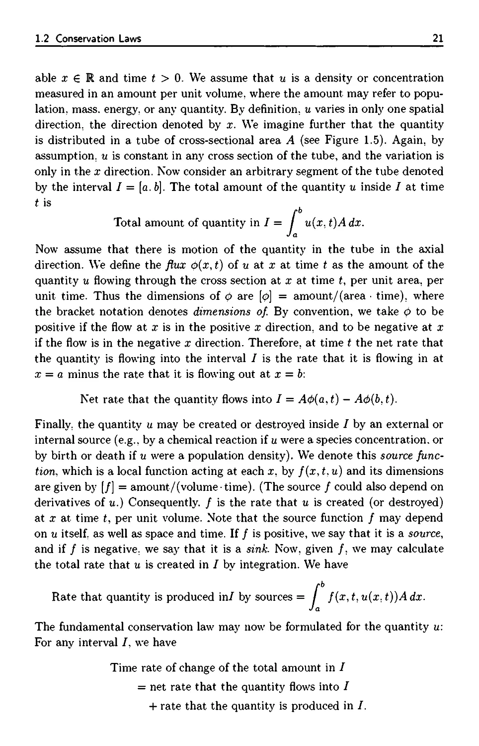
Figure 1.5 Cylindrical tube of cross-sectional area A showing a cross section
at χ and a finite section I: a < χ < b. There is no variation of any quantity in
a fixed cross section.
1.2 Conservation Laws
21
able χ € R and time t > 0. We assume that и is a density or concentration
measured in an amount per unit volume, where the amount may refer to
population, mass, energy, or any quantity. By definition, и varies in only one spatial
direction, the direction denoted by x. We imagine further that the quantity
is distributed in a tube of cross-sectional area A (see Figure 1.5). Again, by
assumption, и is constant in any cross section of the tube, and the variation is
only in the χ direction. Now consider an arbitrary segment of the tube denoted
by the interval / = [a. b]. The total amount of the quantity и inside / at time
t is
,6
Total amount of quantity in / = / u(x. t)A dx.
J a
Now assume that there is motion of the quantity in the tube in the axial
direction. We define the flux ф(х, t) of и at χ at time t as the amount of the
quantity и flowing through the cross section at χ at time t, per unit area, per
unit time. Thus the dimensions of Φ are [ψ] = amount/(area · time), where
the bracket notation denotes dimensions of. By convention, we take Φ to be
positive if the flow at χ is in the positive χ direction, and to be negative at χ
if the flow is in the negative χ direction. Therefore, at time t the net rate that
the quantity is flowing into the interval / is the rate that it is flowing in at
χ = a minus the rate that it is flowing out at χ = b:
Net rate that the quantity flows into / = Αφ(α. t) - Аф(Ъ, t).
Finally, the quantity и may be created or destroyed inside / by an external or
internal source (e.g., by a chemical reaction if и were a species concentration, or
by birth or death if и were a population density). We denote this source
function, which is a local function acting at each x, by f(x, t, u) and its dimensions
are given by [/] = amount/(volumetime). (The source / could also depend on
derivatives of u.) Consequently. / is the rate that и is created (or destroyed)
at χ at time t, per unit volume. Note that the source function / may depend
on и itself, as well as space and time. If / is positive, we say that it is a source,
and if / is negative, we say that it is a sink. Now, given /. we may calculate
the total rate that и is created in / by integration. We have
,6
Rate that quantity is produced in/ by sources = / f(x, t, u(x, t))Adx.
J a
The fundamental conservation law may now be formulated for the quantity u:
For any interval /, we have
Time rate of change of the total amount in /
= net rate that the quantity flows into /
+ rate that the quantity is produced in /.
22 1. Introduction to Partial Differential Equations
In terms of the mathematical symbols and expressions that we introduced
above, after canceling the constant cross-sectional area A, we have
ι pb pb
— и{хЛ)ах = Ф{аЛ)-Ф(ЪЛ)+ I f(x.t.u)dx. (1.2.1)
dt Ja Ja
In summary. (1.2.1) states that the rate that и changes in the interval / must
equal the net rate at which и flows into / plus the rate that и is produced in /
by sources. Equation (1.2.1) is called a conservation law in integral form, and
it holds even if u, o. or / is not a smooth (continuously differentiable) function.
The latter remark is important when we consider physical processes giving rise
to shock waves, or discontinuous solutions, in subsequent chapters.
If conditions are placed on the triad u. φ. and /. then (1.2.1) may be
transformed into a single PDE. Two results from elementary integration theory are
required to make this transformation: (1) the fundamental theorem of calculus,
and (2) the result on differentiating an integral with respect to a parameter in
the integrand. Precisely:
1. jba<px{x.t)dx = o{b.t)-4>{a,t).
2. d/dtja u(x.t)dx = Ja ut(x,t)dx.
These results are valid if φ and и are continuously differentiable functions on R2.
Of course, (1) and (2) remain correct under less stringent conditions, but the
assumption of smoothness is all that is required in the subsequent discussion.
Therefore, assuming smoothness of и and φ. as well as continuity of/, equations
(1) and (2) imply that the conservation law (1.2.1) may be written
6
[ut(x, t) + 0x(x, t) - }{x.t.u)\ dx = 0 for all intervals /= [a, b]. (1-2.2)
Because the integrand is a continuous function of x, and because (1.2.2) holds
for all intervals of integration /, it follows that the integrand must vanish
identically:
ut + όχ = f(x,tu), xGR: t>0. (1.2.3)
Equation (1.2.3) is a PDE relating the density и = u(x.t) and the flux φ =
φ(χ, t). Both are regarded as unknowns, whereas the form of the source function
/ is assumed to be given. Equation (1.2.3) is called a local conservation law, in
contrast to the integral form (1.2.1). The φχ term is called the flux term because
it arises from the movement, or transport, of и through the cross section at x.
The source term / is called a reaction term (especially in chemical contexts) or
a growth or interaction term (in biological contexts). Finally, we have defined
the flux φ as a function of a; and t: this dependence on space and time may occur
through dependence on и or its derivatives. For example, a physical assumption
1.2 Conservation Laws
23
may require us to posit φ(χ, t) = φ(χ, t, u(x, t)). where the flux is dependent on
и itself.
It is important to observe that (1.2.3) was derived under assumptions of
smoothness. If smoothness of the density or flux is not guaranteed, as occurs in
the study of discontinuous solutions, then (1.2.3) must be abandoned in favor
of the integral form (1.2.1) of the conservation law, which is always valid. This
issue becomes the focus of study in Chapter 3.
Finally, we make a general observation about deriving conservation laws.
In the preceding discussion the balance law was applied to an entire interval
/. Assuming smoothness, we can derive the conservation law directly using a
small interval [χ, χ + Ax] and then take the limit as Ax —> 0. Applying the
balance law to the small box [χ, χ + Ax], we obtain
д- (η(ξ, i)A Ax) = Αφ(χ. t) - Αφ(χ + Ax. i) + f(t, η, η(η, t))A Ax:
where ξ and η are points in [χ. χ + Ax], guaranteed by the mean value theorem.
Now, dividing by A Ax gives
9 ic a 0(*: t) - Ф(х + Ax, t)
0j«(£. t) = д^ + f(t, η, ufo, *))■
Taking the limit as Ax —> 0 gives the conservation law (1.2.3). These two
methods for obtaining the conservation law are called, appropriately, the large-
box method and the small-box method.
1.2.2 Higher Dimensions
It is straightforward to formulate conservation laws in higher dimensions. In
this section we limit the discussion to three-dimensional Euclidean space R3.
Let χ = (x\, Χ2: xz) denote a point in R3, and assume that и = и(х, t) is a scalar
density function representing the amount per unit volume of some quantity of
interest distributed throughout a domain D С R3. In this domain let V be
an arbitrary region with a smooth boundary denoted by dV. By an argument
similar to the one-dimensional case, the total amount of the quantity in V is
given by the volume integral
Total amount in V = / u(x. t) dx,
Jv
where dx = dx\dx2dxz represents a volume element in R3. We prefer to write
the volume integral over V with a single integral sign rather than the usual
triple integral. Now. we know that the time rate of change of the total amount
in V must be balanced by the rate that the quantity is produced in V by
24
1. Introduction to Partial Differential Equations
¥*.t)
*~*2
Figure 1.6 Volume V with boundary dV showing a surface element dS with
outward normal η and flux vector φ. The outward normal determines the
orientation of the surface element.
sources, plus the net rate that the quantity flows through the boundary of V.
We let f(x,t,u) denote the source term, so that the rate that the quantity is
produced in V is given by
Rate that и is produced by sources = / f(x.t,u) dx.
In three dimensions the flow can be in any direction, and therefore the flux
is given by a vector ф{хЛ). If n(x) denotes the outward unit normal vector
to the region V (see Figure 1.6), then the net outward flux of the quantity и
through the boundary dV is given by the surface integral
Net outward flux through dV = / ф(х. t) ■ n(x) dS.
JdV
where dS denotes a surface element on dV. Hence, the balance law for и is
given by
(1.2.4)
— udx = - 0-ndS+ / f dx.
dt Jv Jay Jv
The minus sign on the flux term occurs because outward flux decreases the rate
that и changes in V.
The integral form of the conservation law (1.2.4) can be reformulated as a
local condition, that is, a PDE. provided that и and φ are sufficiently smooth
functions. In this case the surface integral can be written as a volume integral
1.3 Constitutive Relations
25
over V" using the divergence theorem (the divergence theorem is the fundamental
theorem of calculus in three dimensions)
/ div φάχ = I φ-ndS. (1.2.5)
JV JdV
where div is the divergence operator. Using (1.2.5) and bringing the derivative
under the integral on the left side of (1.2.4) yields
/ ut dx = - / ά\νφάχ + / f dx.
Jv Jv Jv
The arbitrariness of V then implies the differential form of the balance law:
ut+d\v<f> = f(x.t,u), x£D.. t>0. (1.2.6)
Equation (1.2.6) is the three-dimensional version of equation (1.2.3).
EXERCISES
1. The derivation of the fundamental conservation law (1.2.3) assumed the
cross-sectional area A of the tube to be constant. Derive integral and
differential forms of the conservation law assuming that the area is a slowly
varying function of x. that is. A = A(x) and A'(x) is small. [Note that
A(x) cannot change significantly over small changes in x: otherwise, the
one-dimensional assumption of the state functions и and φ being constant
in any cross section would be violated.]
2. Assuming that there are no sources and φ = ф(и). show that the
conservation law (1.2.1) is equivalent to
rb pb
I u(x,t2)dx = I u(x,t\)dx +
J a J a
I ф{и{аЛ)) dt - I o(u(b,t))dt
Λ] Λι
for all t\ and ti-
1.3 Constitutive Relations
Because equation (1.2.3). or (1.2.6). is a single PDE for two unknown quantities
(the density и and the flux φ), intuition indicates that another equation is
required to have a well-determined system. This additional equation is a relation
that is usually based on an assumption about the physical properties of the
26
1. Introduction to Partial Differential Equations
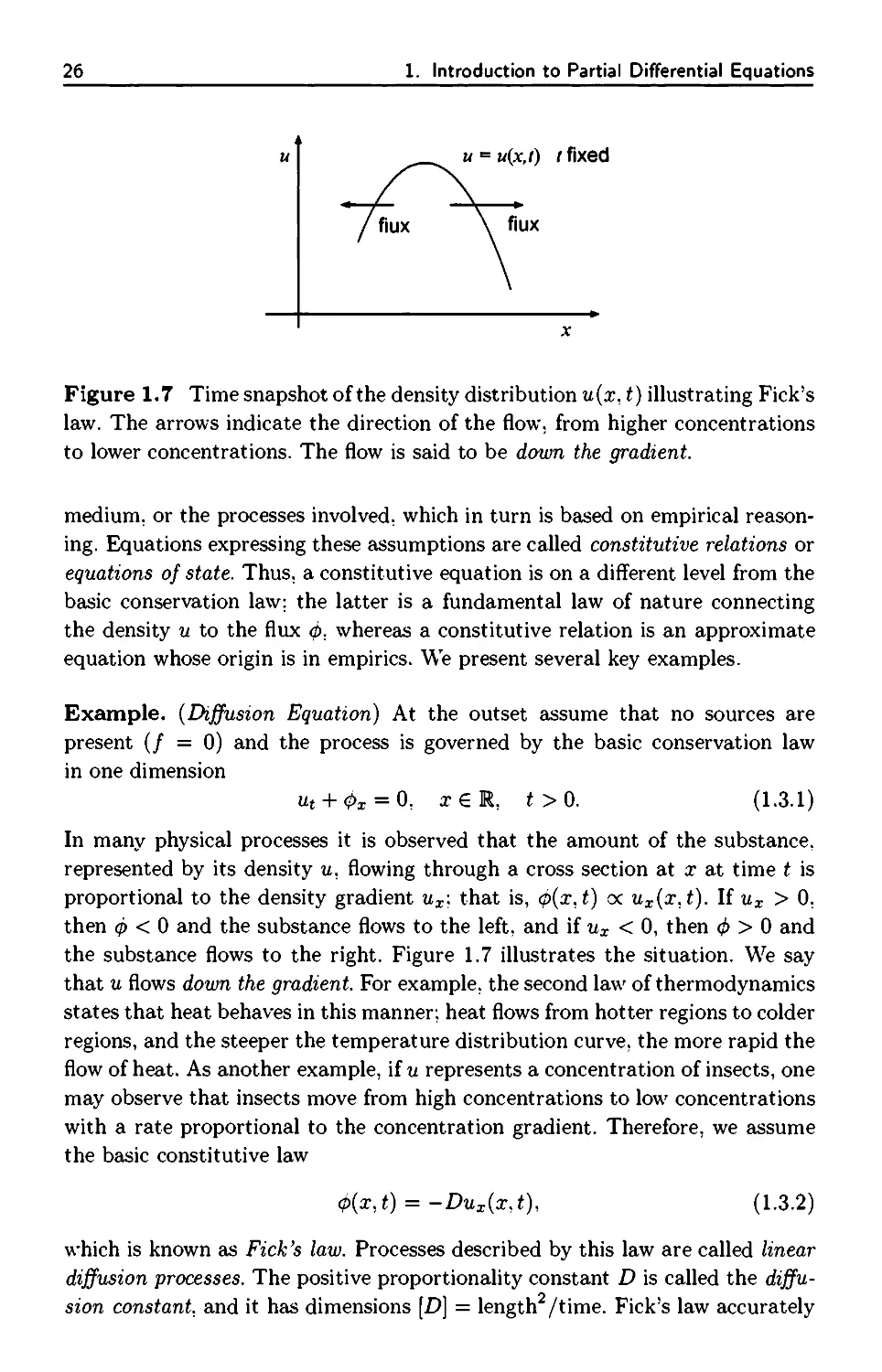
Figure 1.7 Time snapshot of the density distribution u(x, t) illustrating Fick's
law. The arrows indicate the direction of the flow, from higher concentrations
to lower concentrations. The flow is said to be down the gradient.
medium, or the processes involved, which in turn is based on empirical
reasoning. Equations expressing these assumptions are called constitutive relations or
equations of state. Thus, a constitutive equation is on a different level from the
basic conservation law; the latter is a fundamental law of nature connecting
the density и to the flux φ. whereas a constitutive relation is an approximate
equation whose origin is in empirics. We present several key examples.
Example. {Diffusion Equation) At the outset assume that no sources are
present (/ = 0) and the process is governed by the basic conservation law
in one dimension
щ + фх = 0, x£R, t>0. (1.3.1)
In many physical processes it is observed that the amount of the substance,
represented by its density u, flowing through a cross section at χ at time t is
proportional to the density gradient ux: that is, φ(χ, t) oc ux(x,t). If ux > 0.
then φ < 0 and the substance flows to the left, and if ux < 0, then φ > 0 and
the substance flows to the right. Figure 1.7 illustrates the situation. We say
that и flows down the gradient. For example, the second law of thermodynamics
states that heat behaves in this manner; heat flows from hotter regions to colder
regions, and the steeper the temperature distribution curve, the more rapid the
flow of heat. As another example, if и represents a concentration of insects, one
may observe that insects move from high concentrations to low concentrations
with a rate proportional to the concentration gradient. Therefore, we assume
the basic constitutive law
φ(χ,ή = -Dux(x,t), (1.3.2)
which is known as Fick's law. Processes described by this law are called linear
diffusion processes. The positive proportionality constant D is called the
diffusion constant, and it has dimensions [D] = length /time. Fick's law accurately
1.3 Constitutive Relations
27
describes the behavior of many physical and biological systems, and in Chapter
δ we give a supporting argument for it on the basis of a probability model and
random walk.
Equations (1.3.1) and (1.3.2) give a pair of PDEs for the two unknowns и
and φ. They combine easily to form a single second-order linear PDE for the
unknown density и = u(x. t) given by
ut-Duxx = 0. (1.3.3)
Equation (1.3.3), called the diffusion equation, governs conservative processes
when the flux is specified by Fick's law. It may not be clear at this time why
(1.3.3) should be termed the diffusion equation; suffice it to note for the moment
that Fick"s law implies that a substance moves into adjacent regions because of
concentration gradients. We refer to the Duxx term in (1.3.3) as the diffusion
term. D
The diffusion constant D defines a crude characteristic time (or time scale)
Τ for the process. If I, is a length scale (e.g.. the length of the container), the
quantity
T=£ (1.3.4)
is the only constant in the process with dimensions of time, and Τ gives a
measure of the time required for discernible changes in concentration to occur
over the length L.
Example. (Heat Equation) If и = u(x, t) is the thermal energy density (energy
per volume) in a heat-conducting medium, then и = pCT, where ρ is the mass
density (mass per unit volume), С is the specific heat (energy per unit mass
per degree), and Τ = T(x. t) is the temperature (degrees). In the absence of
sources the conservation law is
(pCT)t + φχ = 0..
where φ is the energy flux. The constitutive law, which is a heat analog of
Fick's law. is
φ= -KTx(x.t),
where К is the thermal conductivity of the region. In heat transfer this is
called Fourier's law of heat conduction. Thus, heat energy moves down the
temperature gradient. The conservation law becomes
J-t ~ klxx = 0,
where к = K/pC is the diffusivity. This is the heat equation, which is just the
diffusion equation in the context of heat flow. D
28
1. Introduction to Partial Differential Equations
Example. (Reaction-Diffusion Equation) If sources are present (/^0), the
conservation law
ut + όχ = f(x.t.u) (1.3.5)
and Fick's law (1.3.2) combine to give
ut-Duxx = f(x.t.u). (1.3.6)
which is called a reaction-diffusion equation. Reaction-diffusion equations are
nonlinear if the reaction term / is nonlinear in u. These equations are of great
interest in nonlinear analysis and applications, particularly in combustion
processes and in biological systematics. D
Example. (Fisher's Equation) In studies of elementary population dynamics,
one proposal is that populations are governed by the logistic law, which states
that the rate of change of the total population и = u(t) in a fixed spatial
domain is given bv
where r > 0 is the growth rate and К > 0 is the carrying capacity. Initially, if и
is small, the linear growth term ru in (1.3.7) dominates and rapid population
growth results; as и becomes large, the quadratic competition term -ru2/K
kicks in to inhibit the growth. For large times t, the population equilibrates
toward the asymptotically stable state и = К, the carrying capacity. Now we
add spatial effects. Suppose that the population и is a population density and
depends on a spatial variable χ as well as time t·. that is, и = и(х. t). Then, as
in the preceding discussion, a conservation law may be formulated as
ut + фх = ru (l - £) , (1.3.8)
where / = f(u) = ru(l - u/K) is the assumed local source term given by the
logistics growth law, and φ is the population flux. Assuming Fickrs law for the
flux, we have
ut - Duxx = ru[\-j^j. (1.3.9)
The reaction-diffusion equation (1.3.9) is Fisher's equation, after R. A. Fisher,
who studied the equation in the context of investigating the distribution of an
advantageous gene as it diffuses through a given population. Discussion of this
equation, which is one of the fundamental equations in mathematical biology,
is given in subsequent chapters. D
Example. (Burgers' Equation) To the basic conservation law with no sources
we now append the constitutive relation
o= -Dux + Q(u). (1.3.10)
1.3 Constitutive Relations
29
The density и then satisfies
ut - Duxx + Q(u)x = 0. (1.3.11)
Now there are two terms contributing to the flux, a Fick"s law type of term
-Dux, which introduces a diffusion effect, and a flux term Q(u), depending
only on и itself, that leads to what is interpreted later as advection. In the
special case that Q(u) = u2/2, equation (1.3.11) can be written
ut + uux = Duxx, (1.3.12)
which is Burgers' equation. This is one of the fundamental model equations
in fluid mechanics and illustrates the coupling between advection and
diffusion. Later we derive (1.3.12) using a weakly nonlinear approximation of the
equations of gas dynamics. When D = 0 (no diffusion), then
щ + uux = 0. (1.3.13)
which is called the inviscid Burgers' equation (also, Riemann's equation). It
is the prototype equation for nonlinear advection and arises in gas dynamics,
traffic flow, chromatography, and flood waves in rivers. Equation (1.3.13) is
hyperbolic and describes wave propagation, whereas (1.3.12) is parabolic and
models diffusion. D
Example. (Advection Equation) The simplest flux term occurs when the
material forming the density is carried along by the medium having a fixed velocity,
as in the case of particulants carried by. for example, wind or water. In these
cases the flux is given by the simple linear relationship
o = cu. (1.3.14)
where с is a positive constant having the dimensions of speed. The basic
conservation law is
Ut + cux = 0, (1.3.15)
which is the advection equation. The term advection refers to the horizontal
movement of a physical property (e.g.. a density wave): other equivalent terms
are convection and transport, which have the same meaning. For example,
biologists use the term advection while many engineers use the term convection.
We use these terms interchangeably. This linear first-order PDE (1.3.15) is
the simplest wave equation. Figure 1.8 compares how a signal at time t = 0
propagates under advection. diffusion, and advection-diffusion processes. D
Example. (Diffusion in R3) In Section 1.2 we obtained the basic conservation
law
Ut + ά\νφ = f(x,t.u).
30
1. Introduction to Partial Differential Equations
advection
/-0 t=T
/-0
diffusion
t = T
Figure 1.8 Comparison of advection, diffusion, and advection-diffusion
processes.
In R3 Fick's law takes the form φ = -D grad u\ that is, the flux is in the
direction of the negative gradient of u. Recall the direction of maximum increase
is in the direction of the gradient. Using the vector identity div(grad u) = Δω.
where „
A = — — —
дх\ дх\ dx\
is the Laplacian operator, and assuming that the diffusion coefficient D is
constant, the conservation law becomes
tit - DAu = }(x,t,u),
which is a reaction-diffusion equation in R3. If there are no sources (/ = 0).
we obtain the three-dimensional diffusion equation щ - DAu = 0. D
In summary, we introduced a few of the fundamental PDEs that have been
examined extensively by practitioners of the subject. An understanding of these
equations and a development of intuition regarding the fundamental processes
that they, and other equations, describe is one of the goals of this treatment. We
end this section with the problem of modeling flow through a porous medium.
Example. (Porous Media) Consider a fluid (e.g.. water) seeping downward
through the soil, and let ρ = p(x, t) be the density of the fluid, with positive
1.3 Constitutive Relations
31
χ measured downward. In a given volume of soil only a fraction of the space
is available to the fluid; the remaining space is reserved for the soil itself. In
this sense, the soil is a porous medium through which the fluid flows. If the
fraction of the volume that is available to the fluid is denoted by к. called the
porosity, the fluid mass balance law in a given section of unit cross-sectional
area between χ = a and χ = b is given by
А /*^
— / кр{хЛ)ах = ф{аЛ)-ф{ЬЛ). (1.3.16)
at Ja
where φ is the mass flux. We assume that the mass flux is φ = рг\ where ν is
the volumetric flow rate. Assuming requisite smoothness, the integral balance
law (1.3.16) can be written
«pt+ (/»·)« = 0. (1.3.17)
Here we assumed that the porosity is constant, but in general it could depend
on χ or even p. The conservation law (1.3.17) contains two unknowns, the
density and the flow rate, and therefore we need a constitutive equation that
relates the two. For reasonably slow flows it is observed experimentally that
the volumetric flow rate is given by
v = -^(px + gp): (1.3.18)
where ρ = p(x. t) is the pressure, and the positive constants g, μ, and и are
the acceleration due to gravity, the permeability, and the viscosity of the fluid,
respectively. Equation (1.3.18) is Darcy's law, and it is a basic assumption in
many groundwater problems. It is physically plausible because it confirms our
intuition that the flow rate should depend on the pressure gradient as well as
gravity. Darcy's law is a statement replacing a momentum balance law. When
(1.3.18) is substituted into (1.3.17), we obtain the groundwater equation:
KPt-^(ppx + gp2)x=0. (1.3.19)
Equation (1.3.19) contains two unknowns, ρ and p. because the constitutive
relation (1.3.18) introduced yet another unknown, the pressure. Consequently,
we require another equation to obtain a determined system.
If the fluid is a gas, it is common to neglect gravity and assume an equation
of state for the gas of the form ρ = p(p). In particular, we assume a •y-law gas
having equation of state
^ = {£)\ (1-3.20)
32
1. Introduction to Partial Differential Equations
where po and po are positive constants and 7 > 1. Substituting (1.3.20) into
(1.3.19) and setting g = 0 yields a single PDE for the density ρ having the form
Pt--(p,Px)x=0, (1.3.21)
К
where α = -,μρο/^Ρο· Equation (1.3.21) is a nonlinear diffusion equation called
the porous medium equation, and it governs flows subject to three laws: mass
conservation, Darcy's law, and the gas equation of state. See Aronson (1986)
for a survey on the porous medium equation. D
Finally, we point out that it is often crucial to nondimensionalize a
problem. Differential equations, when formulated, involve dimensioned dependent
and independent variables such as time, length, and temperature. The
Buckingham Pi theorem guarantees that a dimensionally consistent physical law can
always be transformed to one where the variables, as well as the parameters,
are dimensionless. A valid comparison of the relative magnitudes of the terms
in an equation can be made only when a problem is nondimensionalized.
Further, the dimensionless problem often offers an economy over the dimensioned
version in that there is a reduction in the number of parameters. The process
of nondimensionalization is sometimes called scaling. Lin & Segel (1974) and
Logan (2006a) thoroughly discuss scaling and dimensional analysis.
Example. (Scaling) In Fisher's equation,
ut = Duxx + ru (l - — j .
the variables t. x. and и have dimensions is time, length, and animals per area,
respectively. The parameters are the growth rate r with units of 1/time, the
carrying capacity К with units of animals per area, and the diffusion constant
D with dimensions length-squared per time. Using the parameters we can build
dimensionless variables by defining
_ t _ χ _ и
Note that each has the form of a dimensioned variable divided by a constant
with the same dimension. We refer to these constants in the denominator as
scales. For example, the population density is scaled by K. which means that
the population is being measured relative to the carrying capacity; r-1 is the
time scale, meaning that time is being measured relative to the (inverse) growth
rate, and so on. There are usually several ways to determine the scales. By the
chain rule we can transform the PDE into the dimensionless variables. Observe
that derivatives in the PDE transform via
du _ <9v d2u _ К d2v
Έ~ d? Ъх> ~ ~Щ~г~д?'
13 Constitutive Relations
33
and therefore the PDE becomes
T.dv ,., К d2v .. . .
rKd-T = DDTrde + rKv{l-v)'
or
vT = υξξ + v(l - υ).
Therefore, in dimensionless variables Fisher's equation reduces to a model
equation without any constants at all. This simpler equation may be analyzed, and,
if required, a return to interpretations in terms of the original dimensioned
quantities can be made. D
EXERCISES
1. Write the PDE
щ + uux + Uxxx = 0
in the form of a conservation law. identifying the flux φ. Given и as a
solution for which u. ux, and uxx approach zero as \x\ —> зс. show that
/ОС /-ЭС
u(x, t)dx = const. / u2(x.t)dx = const.
•ОС J — ЭО
for all t > 0.
2. In three dimensions assume show that advection should be modeled by the
equation
Uf + divcu = 0.
where с = c(x) is the velocity of the medium. Given с as a constant vector,
show that и = /(χ - ci) is a solution for any real-valued differentiable
function /.
3. Show that Burgers' equation (1.3.12) can be transformed into the linear
diffusion equation (1.3.3) by the Cole-Hopf transformation
2Dvx
и = .
V
4. Show that the PDE
щ + kuux + q{t)u = 0
can be reduced to the inviscid Burgers' equation
vs + vvx = 0
using the transformation
ν = и exp / q(t) dt. s = к exp I - / q(y) dy 1 dt.
34
1. Introduction to Partial Differential Equations
Show that the same transformation transforms
ut + kuux + q(t)u - Duxx = 0
into
v, +vvx -3-1(s)wXi =0,
where g = (k/D) exp (- / q(t) dt).
5. By rescaling, show that the porous media equation can be written in the
form
ит = (ит)к (m>2)
for appropriately chosen dimensionless variables τ. ξ, and и.
6. Show that the nonlinear growth-diffusion equation
St = k(S3)xx + aS
can be reduced to the porous medium equation by the transformations
S = p(xJ)eat, r=±e2at.
7. Consider a porous medium where the fluid is water, and assume that the
density ρ is constant. What equation must the pressure ρ satisfy? Describe
the pressure distribution.
8. Nondimensionalize the growth-advection-diffusion equation
щ = Duxx — cux + ru.
9. The population density u(x. t) of zooplankton in a deep lake varies as a
function of depth χ > 0 and time t (x = 0 is the surface). Zooplankton
diffuse with diffusion constant D. and buoyancy effects cause them to
migrate toward the surface with an advection speed of ag, where g is the
acceleration due to gravity. Ignore birth and death rates.
(a) Find a PDE model for the population density of zooplankton in the
lake, along with the the appropriate boundary conditions at χ = 0 and
χ = +oc.
(b) Find the steady-state population density и = U(x) for zooplankton as
a function of depth, and sketch its graph.
1.4 Initial and Boundary Value Problems
35
10. Let и = u(x. y. t) satisfy the following PDE and boundary conditions:
s2uxx + uyy = 0, 0 < у < 1, χ € R, t > 0,
uy(x,0,t) = 0, uy(x, \,t) + e2utt(x· 1.i) = 0.
χ € R, t > 0,
where ε is small. Assuming a perturbation expansion
и = uo(x, t) + u\ (x, y, t)e2 Η .
show that uq satisfies the wave equation.
1.4 Initial and Boundary Value Problems
So far we encountered several types of PDEs governing different types of
physical processes:
ut = Duxx (diffusion)
ut = Duxx + f(x, t, u) (reaction-diffusion)
iit + cux = 0 (advection)
ut + cux = Dun (advection-diffusion)
щ + uux = Duxx (nonlinear advection-diffusion)
As we noted earlier, we are seldom interested in the general solution to a
PDE, which contains arbitrary functions. Rather, we are interested in solving
the PDE subject to auxiliary conditions such as initial conditions, boundary
conditions, or both.
One of the fundamental problems in PDEs is the pure initial value problem
(or Cauchy problem) on R having the form
ut + F(xA. u,ux,Uxx) = 0, z€R, t > 0, (1-4.1)
и(а\0) = u0(s), z€R, (1-4-2)
where uo(x) is a given function. Interpreted physically, the function uo(x)
represents a signal at time t = 0, and the PDE is the equation that propagates
the signal in time. Figure 1.9 depicts this interpretation. In wave propagation
problems, the signal is usually called a wave or wave profile. There are several
fundamental questions associated with the pure initial value problem (1.4.1)-
(1.4.2).
36
1. Introduction to Partial Differential Equations
1. Existence of Solutions. Given an initial signal Uo(x) satisfying specified
regularity conditions (e.g., continuous, bounded, integrable, or whatever),
does a solution и = u(x, t) exist for all χ € R and t > 0? If a solution
exists for all t > 0, it is called a global solution. Sometimes solutions are
only local: thai, is, they exist for only up to finite times. For nonlinear
hyperbolic problems, for example, a signal can propagate up to a finite time
and blowup occurs; that is, the signal experiences a gradient catastrophe
where ux becomes infinite and the solution ceases to be smooth. In other
problems, for example in some reaction- diffusion equations, the solution u
itself may blow up.
2. Uniqueness. If a solution of (1.4.1)—(1.4.2) exists, is the solution unique?
For a properly posed physical problem we expect an affirmative answer, and
therefore we expect the governing initial value problem, which is regarded
as a mathematical model for the physical system, to mirror the properties
of the system when considering uniqueness and existence questions.
3. Continuous Dependence on Data. Another requirement of a physical
problem is that of stability; that is, if the initial condition is changed by only
a small amount, the system should behave in nearly the same way.
Mathematically, this is translated into the statement that the solution should
depend continuously on the initial data. In PDEs, if the initial value problem
has a unique solution that depends continuously on the initial conditions,
we say that tin: problem is well-posed. A similar statement can be made
for boundary value problems. A basic question in PDEs is the problem of
wcll-posedness.
4. Regularity of Solutions. If a solution exists, how regular is it? In other
words, is it continuous, continuously differentiable, or piecewise smooth?
Figure 1.9 Schematic indicating the time evolution, or propagation, of an
initial signal or waveform щ(х).
1.4 Initial and Boundary Value Problems
37
5. Asymptotic Behavior. If an initial signal can be propagated for all times
t > 0, we may inquire about its asymptotic behavior, or the form of the
signal for long times. If the signal decays, for example, what is the decay
rate? Does the signal disperse, or does it remain coherent for long times?
Does it keep the same shape?
These are a few of the issues in the study of PDEs. The primary issue,
however, from the point of view of the applied scientist, may be methods of
solution. If a physical problem leads to an initial value problem as a
mathematical model, what methods are available or can be developed to obtain a
solution, either exact or approximate? Or, if no solution can be obtained (say.
other than numerical), what properties can be inferred from the governing
PDEs themselves? For example, what is the speed of propagation? Are
solutions wave-like, diffusion-like, or dispersive? These questions are addressed in
subsequent chapters.
Several examples illustrate the diversity of solutions.
Example. (Diffusion Equation) The solution to initial value problem for the
diffusion equation
ut = Duxx, χ € R, t > 0,
u(x,0) = u0(x). х£Ш..
is. as one may verify (e.g., using Fourier transforms), as follows:
и(х.*) = -™.Гио(Ое(х-«'/41>·*.
\/4π£>ί У_ос
The solution is valid for all ί > 0 and χ € R under rather mild restrictions on
the initial signal uo(x), and the solution has a high degree of smoothness even
if the initial data uo are discontinuous. Succinctly stated, diffusion smooths out
signals. D
Example. (Advection Equation) Consider the linear initial value problem for
the advection equation
ut + cux = 0, χ € R, t > 0,
u(a\0) = uo(s); z€R,
where с is a positive constant. It is easy to check that u(x. t) = f(x — ct) is a
solution of the PDE for any differentiable function /. We can apply the initial
condition to determine / by writing u(x,0) = f(x) = uo(x)- Therefore the
global solution to the initial value problem is
u(x,t) = uo(x-ct) x€R, t > 0.
38
1. Introduction to Partial Differential Equations
Graphically, the solution is the initial signal uo(x) shifted to the right by the
amount ct. as shown in Figures 1.10 and 1.11. Therefore, the initial signal moves
forward undistorted in spacetime at speed с Regarding regularity, even if uo is
discontinuous, it appears that the solution holds, provided we can make sense
of derivatives of discontinuous functions. D
Example. (Inviscid Burgers' Equation) A more complicated example is the
nonlinear Cauchy problem
щ + uux = 0. χ £
1
t >0,
u(x.O) =
1 +x
2'
x€
In contrast to the two preceding examples, the solution does not exist for all
t > 0. The initial waveform, in the form of a bell-shaped curve, distorts during
propagation and a gradient catastrophe occurs in finite time. The argument we
present to show this nonexistence of a global solution is typical of the types
of general arguments that are developed later to study nonlinear hyperbolic
problems. Assume that this problem has a solution и = u(x,t), and consider
the family of curves in xt space defined by the differential equation
dx ι a
Tt=u{xA).
Denote a curve С in this family by χ = x(t). Along this curve we have du/dt =
ut(x(t), t) + ux{x(t). t)dx/dt = 0. and therefore и = constant on C. The curve
С must be a straight line because d2x/dt2 = du/dt = 0. The curve C. which is
called a characteristic curve, is shown in Figure 1.12 emanating from a point
!
ι
«oW
ιψ-ct)
■+■*
Position
Figure 1.10 Right traveling wave, which represents the solution to the ad-
vection equation, shown in xu space.
1.4 Initial and Boundary Value Problems
39
(ξ. 0) on the initial timeline (x axis) to an arbitrary point (x,t) in spacetime.
The equation of С is given by
χ-ξ = ω(ξ.0)ί.
where its speed (the reciprocal of its slope). u(£. 0) = (1 + ξ2)-1. is determined
by the initial condition and the fact that и is constant on C. Now let us
determine how the gradient ux of и evolves along curve C. For simplicity denote
g(t) = ux(x(t).t). Then
g'(t) = ъхх— + uxt = (ut + uux)x - u2x = -u2x = -g(t)2.
' — _n2
The general solution of g' = -g is
9(t) =
t + c
с const.
But g(0) = 1/c = -2ξ/(1 + ξ2)2 is the initial gradient, and therefore g is given
bv
1
5(ί)~ί-(1 + ξ2)2/2ξ·
Note that ξ may be chosen positive. Therefore, along the straight line С the
gradient ux becomes infinite at the finite time t = (1 + ξ2)2/2ξ. Therefore a
smooth solution cannot exist for all t > 0. D
The nonexistence of a global solution to the initial value problem is a
typically nonlinear phenomenon. Because physical processes are often governed by
nonlinear equations, we may well ask what happens after the gradient
catastrophe. Actually, the distortion of the wave profile and development of an infinite
gradient is the witnessing of the formation of a shock wave (i.e.. a
discontinuous solution that propagates thereafter). However, the idea of a nonsmooth
u0(x - ct)
Figure 1.11 Right traveling wave shown in Figure 1.10 represented in xtu-
space.
40
1. Introduction to Partial Differential Equations
t
.
(ξ,Ο)
(x,t)/
Figure 1.12 Characteristic С emanating from the χ axis.
solution to a PDE is a concept that must be formulated carefully, and we carry
out this program in Chapter 3.
Another type of problem associated with PDEs is the signaling problem.
In this case the domain of the problem is the first quadrant χ > 0, t > 0 in
spacetime, and initial data are given along the positive χ axis; data are also
prescribed along the positive t axis as boundary conditions, or signaling data
(see Figure 1.13). The form of a signaling problem is
iit + F(x,t.u,ux.uxx) = 0, χ > 0. t > 0,
u(x.0) = uo(x), x > 0.
u(0.t) = ui(t): t>0.
(1.4.3)
(1.4.4)
(1.4.5)
where uo(x) is the given initial state and u\(t) is a specified signal imposed
Signaling condition
u,(()
»■ χ
Figure 1.13 Schematic representing a signaling problem where signaling data
are prescribed at χ = 0 along the time axis and initial data are prescribed at
t = 0 along the spatial axis.
1.4 Initial and Boundary Value Problems
41
at χ = 0 for all times t > 0. As in the case of the initial value problem, the
signaling problem may or may not have a solution that exists for all times t.
In lieu of the condition (1.4.5) given at χ = 0, one may impose a condition
on the derivative и of the form
ux(0,t) = u2(t), t>0.. (1.4.6)
or some combination of и and ux.
u(0.t) + aux(0.t) = u2(t): t>0.
If the PDE is a conservation law and Fick's law ф(х, t) = -Dux{x,t) holds,
condition (1.4.6) translates into a condition on the flux φ. The condition that
the flux be zero at χ = 0 is the physical condition that the amount of и that
passes through χ = 0 is zero; in heat flow problems this condition is called
the insulated boundary condition. A boundary condition of the type (1.4.5) is
called a Dirichlet condition, and one of the type (1.4.6) is called a Neumann
condition. Mixed conditions are called Robin conditions.
If the spatial domain is finite, that is. a < χ < b, one may expect to impose
boundary data along both χ = a and χ = b. and therefore we consider the
initial-boundary value problem
щ + F(x. t.u, ux.uxx) = 0, a < χ < b, t > 0, (1-4.7)
u(x,0) = u0(x). a<x<b. (1.4.8)
u(a,t) = ui(t), u(b.O) = u2(t). t>0. (1.4.9)
where uo: u\, and u2 are given functions. If (1.4.7) is the diffusion equation,
this problem has a solution under mild restrictions on the data. However, if
we consider the advection equation, the problem seldom has a solution for
arbitrary boundary data, as the following example shows.
Example. Consider the initial-boundary value problem
ut + ctix = 0, 0<х<1. t > 0,
with initial and boundary conditions given by (1.4.8) and (1.4.9) with a = 0
and b = 1. We have noted already that the general solution of the advection
equation is u(x.t) = f(x - ct), for an arbitrary function /. Consequently, и
must be constant on the straight lines χ - ct = constant (see Figure 1.14).
Clearly, therefore, data cannot be independently specified along the boundary
χ = b. In this case, the initial data along 0 < χ < 1 are carried along the
straight lines to the segment A on χ = 1: the boundary data along χ = 0 is
carried to the segment В on χ = 1. Thus u(l, t) cannot be specified arbitrarily.
D
42
1. Introduction to Partial Differential Equations
U a|l|(f)
U · Uq(x) 1
Figure 1.14 Right-moving characteristics carrying left boundary and initial
data into the region of interest. Arbitrary data may not be prescribed along
the right boundary χ = 1 labeled A and B.
The preceding example shows that we must be careful in defining a well-
posed problem. Mathematically correct initial conditions and boundary
conditions are associated with types of PDEs (hyperbolic, parabolic, elliptic), as
well as their order. Conditions that ensure well-posedness are often suggested
by the underlying physical problem.
Example. (Wave Equation) The wave equation
u« - c2uxx = 0, χ € R, t > 0.
(1.4.10)
is second-order in t. and therefore it does not fit into the category of equations
defined by (1.4.1). Because it is second order in t. we are guided by our
experiences with ordinary differential equations to impose two conditions at t = 0. a
condition on и and a condition on ut. Therefore, the pure initial value problem
for the wave equation consists of (1.4.10) subject to the initial conditions
u(x, 0) = uo(x): щ(х.О) = ui(x), x£
(1.4.11)
where uq and U\ are given functions. If щ € C2(R) and u\ € C'(R), the
unique, global solution to (1.4.10)—(1.4.11) is given by D'Alembert:s formula
(1.1.6) with f = uq and g = u\. D
Example. The initial value problem
u« + uIX = 0, χ € R, t > 0,
u(x,0) = uo(x), ut(x,0) = u\(x). x£
(1.4.12)
(1.4.13)
1.4 Initial and Boundary Value Problems
43
is not well-posed because small changes, or perturbations, in the initial data
can lead to arbitrarily large changes in the solution (see Exercise 5).
Equation (1.4.12) is Laplace's equation (with variables χ and t. rather than the
usual χ and y), which is elliptic. In general, initial conditions are not correct
for elliptic equations, which are naturally associated with equilibrium
phenomena and boundary data. D
To summarize, the auxiliary conditions imposed on a PDE must be
considered carefully. In the sequel, as the subject is developed, the reader should
become aware of which conditions go with which equations in order to ensure,
in the end, a well-formulated problem.
EXERCISES
1. Solve the signaling problem
iit + cux = 0, χ > 0. t > 0,
u(x.O) = 1, χ > 0,
using the fact that и must be constant on the curves χ = ct + ξ, where ξ is
constant. Hint: Treat the regions χ > ct and χ < ct separately.
2. Obtain the solution to the initial value problem
ut = Uxx, x € R, t > 0,
u(a\0) = uo if \x\ < L and u(x,0) = 0 if |x| > I.
where uo is a constant, in the form
"о
«0M) = --2
-(#)-(#)
where erf is the error function
2 Iх _ 2
erf(x) = —= / e s ds.
V71" Jo
Show that for χ fixed and for large t, we obtain
u{x,t)~ -=.
44
1. Introduction to Partial Differential Equations
3. Find a formula for the solution to the initial-boundary value problem
ut - ux = 0, 0 < χ < 1; t > 0.
u(ar,0) = 2, 0<χ<1;
<1^ = т^·- ί>0·
4. Let и € С1 be a solution to the Cauchy problem
Щ + Q{u)x = 0, χ € R, ί > 0.
u(x.O) = uo(a;), a; € R,
where Q(0) = 0. <5"(u) > 0, and uo is integrable on R with uo(x) = 0 for
χ < xo (for some xo), and uo(a;) > 0 otherwise. Define
U(x,t)= / u(s,t)ds
J —ОС
(a) Show that U satisfies the equation Ut + Q{UX) = 0.
(b) Prove that Q(u) > Q(v) + c(v)(u - v), where c(u) = Q'(u).
(c) Prove that Ut + c(v)Ux < c(v)v - Q(v).
(d) Show that £/(x. t) < Ufc,0)+t[c(v)v-Q(v)]. whereξ is the point where
the line defined by dx/dt = c(v) through the point (x. t) intersects the
χ axis.
(e) In the inequalities above, show that equality holds if υ = и.
(f) Give a geometric-physical interpretation of the results above.
5. By considering solutions un(x. t) = n-1 cos nx coshnt. show that the initial
value problem (1.4.12)—(1.4.13) for Laplace's equation is not well-posed.
6. Consider the initial value problem for the backward diffusion equation:
Щ + ихх = 0, x£R. t>0,
u(xr0) = l, x€R.
Show that the solution does not depend continuously on the initial
condition by considering the functions
un(x. t) = 1 -I— exp(n2i) sin nx.
1.5 Waves
45
1.5 Waves
One of the cornerstones of PDEs is wave propagation. A wave is a recognizable
signal that is transferred from one part of the medium to another part with
a recognizable speed of propagation. Energy is often transferred as a wave
propagates, but matter may not be. There is hardly any area of science or
engineering where wave phenomena are not a critical part of the subject. We
mention a few areas where wave propagation is of fundamental importance.
Fluid mechanics (water waves, aerodynamics, meteorology, traffic flow)
Acoustics (sound waves in air and liquids)
Elasticity (stress waves, earthquakes)
Physics (optics, electromagnetic waves, quantum mechanics)
Biology (spread of diseases, population dispersal, nerve signal transmission)
Porous media (groundwater dynamics, contaminant migration)
Chemistry (combustion and detonation waves)
1.5.1 Traveling Waves
The simplest form of a mathematical wave is a function of the form
u(x.t) = f(x-ct). (1.5.1)
We interpret the density и as the strength of the signal. At t = 0 the wave
has the form f(x). which is the initial wave profile. Then f(x - ct) represents
the profile at time i, which is just the initial profile translated to the right
ct spatial units. The constant с represents the speed of the wave. Evidently,
(1.5.1) represents a right traveling wave of speed с Similarly, u(x. t) = f(x + ct)
represents a left traveling wave of speed с These types of waves propagate
undistorted along the straight lines χ - ct = const, (or χ + ct = const.) in
spacetime.
A key question is whether a given PDE can propagate such a traveling
wave or, in different words, whether a traveling wave solution (TWS) exists
for a given PDE. This question is generally posed without regard to initial
conditions (time is usually regarded as varying from -oc to +эс). so that the
wave is assumed to have existed for all times. However, boundary conditions of
the form
u(-oci) = const., u(+oc.t) = const. (1.5.2)
may be imposed. A wavefront solution is a TWS of the form u(x. t) = f(x -
ct) (or f(x + ct)) subject to the conditions (1.5.2) of constancy at plus and
minus infinity (not necessarily the same constant); at present, the function /
46
1. Introduction to Partial Differential Equations
is assumed to have the requisite degree of smoothness defined by the PDE
(C1 (R). C2(R) ). Figure 1.15 shows a typical wavefront. If и approaches the
same constant at both plus and minus infinity, the wavefront solution is called
a pulse.
The key computational device is to substitute the form u(x,t) = f(x - ct)
into the PDE and observe whether it transforms the PDE into an ODE for the
unknown wave profile /. which is a function of a single variable ζ = χ - ct.
interpreted as a moving coordinate. The speed с of the wave is not known. To
carry out the substitution it is necessary to calculate how the derivatives of и
transform. By the chain rule, we have
u, = f'(z)zt = -cf'(z),
Ux = f'(z)zx = f'(z).
We easily find utt = c2f"(z). uxx = f"(z), and so on for higher derivatives.
Therefore, the general equation
tit = G(u.ux,uxx)
transforms into
-c/' = C(/,/',/"). z£%
which is an ODE for / and the unknown wave speed с If boundary conditions
/(-oc) = /0. /(+»:) = /,
are imposed, we interpret this problem as a nonlinear eigenvalue problem for
/, with с as an eigenvalue.
Example. (Advection Equation) We have already observed that
u(x.t) = f(x - ct),
ιι«/Ίχ-<:/)
I
\ c >
X
Figure 1.15 A right traveling wavefront with speed с A wavefront solution
is a TWS with constant states at ±эс.
1.5 Waves
47
where / is a differentiable function, is a solution to the PDE
щ + cux = 0. (1.5.3)
Therefore, the advection equation (1.5.3) admits wavefront solutions, and it is
the simplest example of a wave equation. D
Example. (Wave Equation) The wave equation
utt = c2uxx
has solutions that are the superposition of right and left traveling waves (see
Section 1.1). D
Example. (Diffusion Equation) The diffusion equation cannot propagate non-
constant wavefronts. To verify this fact, we substitute u = f(z), where
ζ = χ - ct, into the diffusion equation ut = Duxx to obtain the following
ordinary differential equation for the wave profile /:
-cf'(z) = Df"(z), z€R
This linear differential equation has the general solution
f{z) = a + be-"'D,
where a and b are arbitrary constants. The only possibility for / to be constant
at both plus and minus infinity is to require b = 0. Thus, there are
traveling wave solutions, but no nonconstant wavefront solutions to the diffusion
equation. D
Example. (Korteweg-deVries Equation) The KdV equation is
ut + uux + uxxx = 0. (1.5.4)
This nonlinear equation admits traveling wave solutions of different types. One
particular type is the soliton, or solitary wave, which is now derived. Assume
that и = }(z), where ζ = χ - ct. Substituting into (1.5.4) gives
-cf + //' + /'" = 0, (1.5.5)
where the prime denotes d/dz. Integrating (1.5.5) 2 times yields, after
rearrangement
^- = -5=(-/3 + 3c/2 + 6a/ + 6b)1/2, (1.5.6)
dz y/3
where a and b are constants of integration. Here we took the plus sign on the
square root; later we observe that this can be done without loss of generality.
48
1. Introduction to Partial Differential Equations
1
.75
1
-5
ιϊ\
}
L
'
/:
/ ■
0.5
1
-2.5
-\
I
2.5
1
5
I
7.5
Figure 1.16 Plot of the soliton (1.5.8) at t = 0 with 7 = 0.5 and a - 7 = 3.0.
A soliton is an example of a pulse.
The first-order differential equation (1.5.6) for the form of the wave / is
separable. However, the expression under the radical on the right side is a cubic in
/. and therefore different cases must be considered depending on the number
of real roots, double roots, and so on. We examine only one case, namely, when
the cubic has three real roots, where one is a double root. So let us assume that
-/3 + 3c/2 + 6a/ + 66 = (/ - 7)2(a - /), 0 < 7 < a.
Then the differential equation (1.5.6) becomes
(/-7)-1(a-/)-1/2a/=i=dz.
The substitution / = 7 + (a - 7)sech2u· easily reduces (1.5.7) to
-2(a--r)-l/2dw = -^=dz.
v3
(1.5.7)
which integrates to w = y/(a - η)/\2ζ. Consequently, traveling waves in the
case we are considering have the form
/Q_„,\ 1/2
u(x. t) = 7 + (a- 7)sech2[K(z- ct)}. к = ( ' ) (1.5.8)
A graph of the waveform, which is a pulse, is shown in Figure 1.16. It is
instructive to write the roots a and 7 in terms of the original parameters. To
this end we have
-/3 + 3c/2 + 6a/ + 66 = (/ - Ί)2{α - /)
= -/3 + (a + 27)/2 - (270 + 72)/ + Ί2α.
1.5 Waves
49
Therefore, the wave speed с is given by
a + 27 q - 7 . „ .
c=-T- = -3-+7, (1-5.9)
The speed of the wave relative to the state 7 ahead of the wave is proportional
to the amplitude A = a - 7. Both the amplitude and the width of the wave
depend on the wave speed с Thus, the taller and wider the wave, the faster it
moves. For linear waves, say, governed by the wave equation, the speed of
propagation is independent of the amplitude of the wave. Such a waveform (1.5.8) is
known as a soliton, or solitary wave, and many of the important equations
of mathematical physics exhibit soliton-type solutions (e.g., the Boussinesq
equation, the Sine-Gordon equation, the Born-Infeld equation, and nonlinear
Schrodinger equations). In applications, the value of such solutions is that if a
pulse or signal travels as a soliton. the information contained in the pulse can
be carried over long distances with no distortion or loss of intensity. Solitons
occur in fluid mechanics, nonlinear optics, and other nonlinear phenomena. D
There is an interesting history of solitary waves. In 1836 John Scott Russell,
a Scottish engineer, observed such a wave moving along a canal. He followed
it on horseback, noting that it propagated a long distance without changing
form. Many at the time doubted his observation and thought that such waves
could not exist. However, Boussinesq, in 1872, showed that in a special limit of
the equations of fluid flow such water waves can exist; Korteweg and deVries
obtained (1.5.4) in the 1890. It wasn't until the 1960s that physicists Kruskal
and Zabusky obtained the equation as a continuum limit of a model of nonlinear
spring mass chains, and they coined the term soliton.
The interaction between two solitons is both interesting and unexpected. If
two solitons are moving to the right and the one behind represents a stronger
signal (therefore moving faster) than the one ahead, the large one overtakes
the slower, smaller wave and a complicated nonlinear interaction occurs, after
which both waves return to their original shape. The only change is a phase
shift in the two waves. The initial value problem for the KdV equation, with
u(x,0) = uo{x). χ € R, also has interesting behavior. If the initial profile uo
approaches zero fast enough at χ = ±эо. then, over time, the solution divides
into a finite number of solitons moving to the right at their respective speeds
(smaller to larger), plus a small dispersive disturbance moving to -oc. D
The problem of determining whether a given PDE admits wavefront
solutions is fundamental, and it occupies much attention in subsequent chapters.
The search for these types of solutions is one of the basic methods in the
analysis of nonlinear problems.
50
1. Introduction to Partial Differential Equations
Figure 1.17 A plane wave of amplitude A, wave number k, and frequency ω.
1.5.2 Plane Waves
Another type of wave of interest is a plane wave, or wave train. These waves
are traveling, periodic waves of the form
u(x. t) = ,4cos(fcr - ωΐ),
(1.5.10)
where A is the amplitude of the wave, к the wave number, and ω the frequency.
The wave number A; is a measure of the number of spatial oscillations (per
2π units) observed at a fixed time, and the frequency ω is a measure of the
number of oscillations in time (per 2π units) observed at a fixed spatial location.
The number λ = 2n/k is the wavelength, and Ρ = 2π/ω is the period. The
wavelength measures the distances between successive crests, and the period
measures the time for an observer located at a fixed position χ to see a repeat
pattern (see Figure 1.17). Note that (1.5.10) may be written
u(x,t) = Л cos A; (x-—t\,
so (1.5.10) represents a traveling wave moving to the right with speed с = ω-k.
This number is called the phase velocity, and it is the speed that one would
have to move to remain on the crest of the wave. For calculations the complex
form
u(x, t) = Aei{-kx~^ (1.5.11)
is preferred because differentiations with the exponential function are simpler.
After the calculations are completed, one can use Euler's formula exp(i#) =
cos θ + i sin θ and take real or imaginary parts to recover a real solution. The
technique of searching for plane wave solutions is applicable to linear equations,
but a modification applies to some nonlinear problems. Finding plane wave
solutions is a powerful method for determining properties of linear problems.
1.5 Waves
51
Example. {Diffusion Equation) We seek solutions of the form of equation (1.5.11)
to the diffusion equation
ut = Duxx. (1.5.12)
Substituting (1.5.11) into (1.5.12) gives
uj = -iDk2. (1.5.13)
Equation (1.5.13) is a condition, called a dispersion relation, between the
frequency ω and the wave number к that must be satisfied for (1.5.12) to admit
plane wave solutions. Thus we have determined a class of solutions
u(x, t; k) = Ae-Dk2teikx, k£R (1.5.14)
for the diffusion equation that depends on an arbitrary parameter k, the wave
number. The factor exp(ikx) represents a spatial oscillation, and the factor
Aexp(-Dk2t) represents a decaying amplitude. Note that the rate of decay
depends on the wave number k; waves of shorter wavelength decay more rapidly
than do waves of longer wavelength. D
Example. (Wave Equation) Substituting (1.5.11) into the wave equation
utt = c2uxx (1.5.15)
forces
ω = ±ck. (1.5.16)
Therefore, the wave equation admits solutions of the form
u(x,t) = Aeik^x±ct\
which are right and left sinusoidal traveling waves of speed c. D
The technique of looking for solutions of the form (1.5.11) for linear,
homogeneous PDEs of the form
Lu = 0, (1.5.17)
where I, is a linear constant-coefficient operator, always leads to a relation
connecting the frequency ω and the wave number к of the form
G{k,u) = 0. (1.5.18)
This condition is called the dispersion relation corresponding to the PDE
(1.5.17). and it characterizes plane wave solutions entirely. Generally, linear
PDEs (1.5.17) can be classified according to their dispersion relation in the
following way. Assume that (1.5.18) may be solved for ω in the form
ш=ш(к). (1.5.19)
52
1. Introduction to Partial Differential Equations
We say that the PDE is dispersive if u>(k) is real and if u>"(k)^0. When ui(k)
is complex, the PDE is diffusive. The diffusion equation, from the example
above, has dispersion relation ω = -ik2D, which is complex; thus the diffusion
equation is classified as diffusive. The classical wave equation (1.5.15) is neither
diffusive nor dispersive under the foregoing classification. Even though its
solutions are wave-like, it is not classified as dispersive since its dispersion relation
(see 1.5.16) satisfies ω" = 0. For the wave equation, the speed of propagation
is с and is independent of the wave number k. For dispersive equations, the
speed of propagation, or the phase velocity ω/k, depends on the wave number
(or equivalently. the wavelength). The wave equation is generally regarded as
the prototype of a hyperbolic equation, and the term dispersive is reserved for
equations where the phase velocity depends on k. We caution the reader that
the term dispersion is often used in a diffusion context (e.g.. a group of animals
dispersing), and it is important to be aware of this.
Example. (Schrodinger Equation) In quantum mechanics, the Schrodinger
equation for a free particle, under appropriate scalings, is
ut = iuxx.
It is easy to see that the dispersion relation is ω = к2, so that the Schrodinger
equation is dispersive. The Schrodinger equation is neither parabolic nor
hyperbolic. D
1.5.3 Plane Waves and Transforms
Using a plane wave assumption, we already constructed the class of solutions
u(x,tk) = Ae~Dk letkx, к € R. to the diffusion equation
и< = Duxx, χ € R, t > 0.
Formally, superimposing these solutions, we obtain
u(x.t)= IA{k)e-k2Dteikxdk, (1.5.20)
which can be verified to be a solution to the diffusion equation, provided that
A(k) is a well-behaved function (e.g.. continuous, bounded, and integrable on
R). Having (1.5.20) as a solution opens up the possibility of selecting the
function A(k) so that other conditions (e.g., an initial condition) can be met.
Therefore, let us impose the initial condition
u(z,0) = uo(z). x € R,
1.5 Waves
53
to the diffusion equation. From (1.5.20) it follows that
tio(a:)= f A(k)eikxdk. (1.5.21)
J ft
We recognize uo(x) as the Fourier transform of A(k), and therefore A(k) must
be the inverse Fourier transform of the function uo(x). We remind the reader of
these facts by recalling the Fourier integral theorem [see. e.g., Stakgold 1998].
Theorem. Let / be a continuous, bounded, integrable function on Ш. and let
f(k) = ( f(x)eikx dx
be the Fourier transform of /. Then, for all χ € Ε. we have
w-s£
/(*) = — / f(k)e~tlexdk.
/r
Applying this theorem (the variables к and χ have been interchanged) to 1.5.21)
leads us to conclude that
ikx
= hLu°{x
A{k) = — / u0(x)e-llex dx.
Consequently; we have obtained the solution to the Cauchy problem for the
diffusion equation
Ut-Duxx = 0, х£Ш, ί>0, (1.5.22)
u(x,0) = u0(x); х€Ш, (1.5.23)
in the form
u(x,*) = i I ([ u0{Oe~m άξ\ e-k2Dteikx dk. (1.5.24)
Interchanging the order of integration allows us to formally write the solution
as
u(x.. t) = -^ J ίχ0(ξ) ( f e^x-«)-*2D< dk\ άξ. (1.5.25)
The inner integral may be calculated outright by noting
[ e*(x-«)-*2D< dk = 2 Γ e-k2Dt cos(k(x - ξ)) dk
Jr Jo
54
1. Introduction to Partial Differential Equations
Therefore, the solution to the initial value problem (1.5.22)-(1.5.23) for the
diffusion equation is given by
u(x, t) = -jL= j u0{£)e-(x-^'iDt άξ. (1.5.26)
We derived this solution formally, but we have not proved that it is indeed a
solution. A proof would consist of a rigorous argument that (1.5.25) satisfies
the diffusion equation (1.5.22) and the initial condition (1.5.23). To show well
posedness, a uniqueness argument would have to be supplied as well as a proof
that the solution is stable to small perturbations of the initial data. We shall not
carry out these arguments here, but rather, refer the reader to the references
for the details.
This method (finding plane wave solutions followed by superposition and
use of the Fourier integral theorem) is equivalent to the classical Fourier
transform method learned in elementary courses where one takes a Fourier transform
of the PDE and initial condition to reduce the problem to an ordinary
differential equation in the transform domain, which is then solved. Then the inverse
Fourier transform is applied to return the solution in the original domain. This
method is generally applicable to the pure initial value problems on the real
line for linear equations with constant coefficients.
Fourier integral expressions of the type obtained above can be approximated
for large times by the method of stationary phase [e.g., see Bhatnagar 1979].
1.5.4 Nonlinear Dispersion
For nonlinear equations we do not expect plane wave solutions of the form
(1.5.16), and therefore a dispersion relation will not exist as it does for linear
equations. Moreover, superposition for nonlinear equations is invalid. However,
in some nonlinear problems, there may exist traveling periodic wave trains of
the form
u(x.t) = U(e), e = kx-ujt, (1.5.27)
where U is a periodic function. For example, consider the nonlinear PDE
utt - uxx + /'(u) = 0, (1.5.28)
where f(u) is some function of u. yet to be specified. If (1.5.27) is substituted
into (1.5.28), we obtain the ordinary differential equation
(ω2 - k2)Uee + f'(U) = 0.
Here we are using subscripts θ to denote ordinary derivatives of U with respect
1.5 Waves
55
r~
^_
w
_J
Figure 1.18 Phase space orbit representing the periodic solution (1.5.31)
with amplitude A.
Θ. Multiplication by Ue and subsequent integration gives
\{ω2 - k2)Ul + f(U) = A, (1.5.29)
where Л is a constant of integration. The goal is to determine U as a periodic
function of Θ. Equation (1.5.29) has the same form as an energy conservation
law. where / is a potential function, which suggests introducing the variable
W defined by W = Ue. Then
W2 = ^Tk2{A-m]> (1·5·30)
which are the integral curves. Assuming that ω2 > к2, we have
w = ±\luthc2^A~fm (1·5·31)
which defines a locus of points in the UW plane. For example, let us choose
/({/) = {/4. Then the locus (1.5.31) is a closed path, representing a periodic
solution of (1.5.29), as shown in Figure 1.18. Notice that A, which has been
taken positive, is the amplitude of the oscillation represented by the closed
path. To find U as a function of θ in the case /({/) = U4 we write (1.5.29) as
'^ι/^/ττ**- <1·5·32)
This formula defines the periodic function U = U{6) implicitly; in this case
U(6) can be determined explicitly as an elliptic function, and we leave this as
an exercise. The period of the oscillation can be determined by integrating over
one-quarter period in the integral on the right side of (1.5.32), taking care to
choose the appropriate sign. If Ρ denotes the period, we obtain on integration
an equation of the form
Ρ = Ρ{ωΛ.Α). (1.5.33)
56
1. Introduction to Partial Differential Equations
In other words, the frequency ω will depend on the amplitude A as well as the
wave number k. Consequently, the wave speed с = и,·/к will be amplitude-
dependent. This amplitude dependence in the nonlinear dispersion relation
(1.5.33) is one important distinguishing aspect of nonlinear phenomena.
These calculations can be carried out for nonlinear equations of the form
(1.5.28) for various potential functions f(u). Periodic solutions are obtained
when U oscillates between two simple zeros of A — f(U). A thorough discussion
of nonlinear dispersion can be found in Whitham (1974).
EXERCISES
1. Find the dispersion relation for the advection-diffusion equation
ut + aux = Duxx. (a.D>0),
and show that it is diffusive. Use superposition and the Fourier integral
theorem to find an integral representation of the solution of the initial
value problem for this equation. Hint: You will need the Fourier transform
ofeiai/(x).
2. Consider the KdV equation in the form щ - 6uux + uxxx = 0, χ € R,
t > 0. Let и = u(x.t) be a solution that decays, along with its derivatives,
very rapidly to zero as \x\ —> oo. Show that JRudx and /Ru2 dx are both
constant in time.
3. Examine the form of traveling wave solutions of the KdV equation (1.5.4) in
the case that the cubic expression on the right side of (1.5.6) has a triple
real root.
4. Determine and sketch traveling wave solutions of the equation
Utt — uxx = — sinu
in the form
{(" χ — ct 1Ί
exp ± . > , 0 < с < 1.
5. For the following PDEs find the dispersion relation and classify the
equations as diffusive, dispersive, or neither:
(a) utt + a2uxxxx = 0 (beam equation)
(b) щ + uxxx = 0 (dispersive wave equation)
(c) ut + aux + buxxx = 0 (linearized KdV equation)
(d) Uu - c2uxx + bu = 0 (Klein—Gordon equation)
1.5 Waves
57
6. Consider the heat equation in an infinite domain χ > 0 where the boundary
condition at χ = 0 is a periodic function over all time:
щ = kuxx. χ > 0, t € R,
u(0,i) = T0 + Aeiut, teR,
where To. A, and ω of constants, and where и = и(х. t) is the temperature.
This problem models temperatures in the ground subject to surface
periodic temperatures. Find u(x, t) and determine the amplitude and phase
shift, relative to the values at the surface, at a depth x. Answer the same
questions if instead the flux is imposed at the boundary:
-Kux(0,t) = Aei"t, teR.
7. By superimposing plane wave solutions to the dispersive wave equation
Щ + uxxx = 0, find an integral representation of the solution to the Cauchy
problem and write your answer in terms of the Airy function
M{x)=:tL· c°s{j+xz)dz-
8. Find solutions of the outgoing signaling problem for the wave equation:
utt - <?uxx = 0, χ > 0, t € R.
ux(0,t) = s(t), ieR.
9. In equation (1.5.28) take f(u) = u2/2 and determine periodic solutions of
the form и = U(6), where θ = kx - *>t. What is the period of oscillation?
Does ω depend on the amplitude of oscillation in this case?
10. In equation (1.5.28) assume that the potential function f(u) has the
expansion
u2
/(«) = γ+σω4 + ··· ,
where σ is a small known parameter. Assuming that the amplitude is small,
show that periodic wave trains are given by
U(6) = acos6+ ^aa3cos36-\ .
where the frequency and amplitude are
J1 = 1 + к2 + Ъаа2 + ■■■ .
а О2 9 4
A = — + -σα4 + · · ·
2 8
58
1. Introduction to Partial Differential Equations
11. The nonlinear Schrodinger equation occurs in the description of water
waves, nonlinear optics, and plasma physics. It is given by
iut + uxx + -)\u2\u = 0, (1.5.34)
where 7 > 0 and и = и(х, t) is complex-valued.
(a) If и = и(г)е^кг~ш1К where ζ = χ - ct, show that
^ + t(2* - c)~ + (kx-us + k2)U + 7C/3 = 0.
dz* dz
(b) If с = 2k, show that
;g)2=^-2,*+c
for some appropriately chosen constant a, where С is an arbitrary
constant.
(c) Taking С = 0 and α > 0, show that
U(z) = J^sech(v/a(2 - ct))..
and comment on the properties of this solution.
12. Let F = F(u) be a smooth function and suppose
Utt - uxx = F'(u).
Assuming that и and its partial derivative ux both go to zero as \x\ —» oc.
show that
(%u2 + \u\ + F(u)) = const.
/
13. Show that solutions of the nonlinear Schrodinger equation (1.5.34) with
7=1 have the properties
/ \u\2dx = const, / (u2. - h\u\4) dx = const.
Ук Ук
provided и and its derivatives approach zero sufficiently fast as \x\ —► 0.
Reference Notes. Partial differential equations have a long history and a
correspondingly vast literature. The early developments in PDEs were in the
post calculus years of the early 1700s and involved the geometry of surfaces.
However, it soon became clear that PDEs were models of physical phenomena
like fluid flow, vibrating strings, heat conduction, and so on. Euler, Bernoulli
1.5 Waves
59
D'Alembert, Laplace. Lagrange, Fourier, Cauchy, and others developed many
of the basic ideas in the linear theory and its applications. It wasn't until the
last half of the twentieth century, as part of the general interest in nonlinear
science and advancement of computation, that nonlinear PDEs came to the
forefront, particularly in their role in wave propagation and diffusion.
It is impractical to cite more than just a few key references. There are books
at all levels and several research journals, in both mathematics and the pure
and applied sciences, that can be consulted for an entry point to the literature.
Here we reference only a few of the texts and cite only articles that are relevant
to the particular topic under discussion.
Elementary, entry-level texts focus almost exclusively on linear problems,
emphasizing Fourier series, integral transforms, and boundary value problems.
The long-time standard has been Churchill (1969), which remains an excellent
introduction to Fourier series and boundary value problems. There are many
more recent introductory texts, too many to cite. We mention Strauss (1992),
an outstanding treatment, and the author's text (Logan 2004), which is a brief
introduction. More advanced texts include the classic by John (1982), as well
as Evans (1998), McOwen (2003), Guenther к Lee (1996). Renardy к Rogers
(2004), and Stakgold (1998). Strichartz (1994) gives an outstanding perspective
on Fourier transforms and distributions.
More specialized, theoretical books include Friedman (1964) for parabolic
equations, Gilbarg к Trudinger (1983) for elliptic equations, Protter к
Weinberger (1967) for maximum principles, and Pao (1992) for both nonlinear
parabolic and elliptic equations. The treatises by Courant к Hubert (1953,
1962) provide a wealth of information on elliptic and hyperbolic equations,
and Courant к Friedrichs (1948) is still a standard in shock waves and gas
dynamics. Kevorkian к Cole (1981) and Zauderer (2006) discuss perturbation
methods. For nonlinear equations one can consult Lax (1973), Smoller (1994)
and Whitham (1974), all of which are key books. Another text on nonlinear
PDEs that is very similar to the first edition of the present text (Logan 1994)
is Debnath (1997). Bhatnagar (1979) is an excellent introduction to nonlinear
dispersive waves, and solitons are discussed in Drazin к Johnson (1989).
Two excellent volumes that introduce several common and ad hoc methods
for nonlinear PDEs are Ames (1965, 1972)
2
First-Order Equations and Characteristics
A single first-order PDE is a hyperbolic equation that is wave-like, that is,
associated with the propagation of signals at finite speeds. The fundamental
idea associated with hyperbolic equations is the notion of a characteristic, a
curve in spacetime (a hypersurface in higher dimensions) along which signals
propagate. There are several ways of looking at the concept of a characteristic;
one definition, and this forms the basis of our definition of a characteristic, is
that it is a curve along which the PDE can be reduced to a simpler form, for
example, an ordinary differential equation. But ultimately, the characteristics
are the curves along which information is carried.
The aim in this chapter is to build a solid base of understanding of
characteristics by examining a first-order PDE in one spatial variable and time. We
focus on the initial value problem and the signaling problem, and carry out
the analysis under the assumption that a continuous smooth solution exists.
In Chapter 3 the concept of a weak solution is discussed, and the smoothness
assumptions are relaxed. In Sections 2.1 and 2.2 we study linear and nonlinear
equations, respectively, and in Section 2.3 we examine the general quasilinear
equation. Then in Section 2.4 we address the subject of wavefront expansions
and show that discontinuities in the derivatives also propagate along the
characteristics. In Section 2.5 we discuss the general nonlinear equation of first
order.
An Introduction to Nonlinear Partial Differential Equations, Second Edition.
By J. David Logan
Copyright © 2008 John Wiley & Sons, Inc.
62
2. First-Order Equations and Characteristics
2.1 Linear First-Order Equations
2.1.1 Advection Equation
We already showed that the initial value problem for the advection
equation, namely
щ + cux = 0. χ € R, t>0. (2.1.1)
u{x. 0) = u0(x). z€R, (2.1.2)
has a unique solution given by u(x, t) = uo(x - ct), which is a right traveling
wave of speed c. We now present an alternative derivation of this solution that is
in the spirit of the analysis of hyperbolic PDEs. In this entire section we assume
that the initial signal щ is a smooth (continuously differentiable) function.
First we recall a basic fact from elementary calculus. If и = u(x. t) is a
function of two variables and χ = x(t) defines a smooth curve С in the xt
plane, the total derivative of и along the curve С is given, according to the
chain rule, by
d dx
—u(z(i), t) = ut(x(t), t) + ux(x(t): t) — .
This expression defines how и changes along C. By observation, the left side
of equation (2.1.1) is a total derivative of и along the curves defined by the
equation dx/dt = с We may therefore recast (2.1.1) into the statement
dv. dx
— = 0 along the curves defined by —- = c,
dt dt
or. equivalently
и = constant on χ - ct = ξ.
where ξ is a constant. In these expressions we have suppressed the arguments of
и for concise notation; all expressions involving и are assumed to be evaluated
along the curve, namely, at (x(t). t). Consequently, the PDE (2.1.1) reduced to
an ordinary differential equation, which was subsequently integrated, along the
family of curves χ - ct = ξ. which are solutions to dx/dt = с If we draw one
of these curves in the xt plane that passes through an arbitrary point (x, t), it
intersects the χ axis at (ξ,Ο); its speed is с and its slope is 1/c because we are
graphing t versus χ rather than χ versus t. It is common to refer to the speed
of a curve in spacetime, rather than its slope (see Figure 2.1). Now, because и
is constant on this curve, we have
u(x. i) = ΐί(ξ, 0) = ωο(ξ) = uo(x - ct).
which is the solution to the initial value problem (2.1.1)—(2.1.2). The totality of
all the curves χ - ct = ξ. where ξ is constant, is called the set of characteristic
2.1 Linear First-Order Equations
63
/
I
(ξ,Ο)
' X - Ct - ξ
Figure 2.1
point (ζ. t).
Characteristic curve with speed с passing through the arbitrary
curves for this problem. The constant ξ acts as a parameter and distinguishes
the curves. A graph of the set of characteristic curves on a spacetime diagram
(i.e.. in the xt plane) is called the characteristic diagram for the problem.
Figure 2.2 shows the characteristic diagram for the problem (2.1.1)—(2.1.2).
The characteristic curves, or just characteristics, are curves in spacetime along
which signals propagate. In the present case, the signal is the constancy of и
that is carried along the characteristics. Further-and this will turn out to be
a defining feature-the PDE reduces to an ordinary differential equation along
the characteristics.
χ - ct = const
Figure 2.2 Characteristic diagram for the PDE (2.1.1) showing the family of
characteristic curves x — ct = ξ. The curves have speed с and are parameterized
by their intersection ξ with the χ axis.
64
2. First-Order Equations and Characteristics
2.1.2 Variable Coefficients
We can extend the preceding notions to more complicated problems. First
consider the linear initial value problem
ut + c(x,t)ux=0.. x€R, t>0, (2.1.3)
u(z.0) = tiO(z)r a.'€R, (2.1.4)
where с = c(x,t) is a given continuous function. The left side of the PDE
(2.1.3) is a total derivative along the curves in the xt plane defined by the
differential equation
^ = c(x.t). (2.1.5)
Along these curves
du dx
— = ut + ux— = ut + c(x, t)ux = 0,
dt at
or. in other words, и is constant. Therefore
dx , .
и = const on — = c(x.t).
dt K '
Again the PDE (2.1.3) reduces to an ordinary differential equation (which was
integrated to a constant) along a special family of curves, the characteristics
defined by (2.1.5). The function с = c(x. i) gives the speed of these characteristic
curves, which varies in spacetime.
Example. Consider the initial value problem
и« - ztiix = 0, χ € R, t>0, (2.1.6)
u(a\0) = ti0(z), z€R. (2.1.7)
The characteristics are defined by the equation
dx
— = — xt.
dt
which, on quadrature, gives
χ = ξε-ι2/2: (2.1.8)
where ξ is a constant. On these curves the PDE becomes
dx du
Ut — XtUx = Ut 7-ΧΙχ = — = 0,
dt dt
or
и = const on χ = ξε~
2.1 Linear First-Order Equations
65
4
*- χ
(ξ.0)
Figure 2.3 Characteristic diagram for (2.1.6) showing the family of
characteristics given by (2.1.8).
The characteristic diagram is shown in Figure 2.3, with an arbitrary point (a\ t)
labeled on a given characteristic that emanates from a point (ξ, 0) on the χ axis.
From the constancy of и along the characteristics, we have
u(x,t) = ω(ξ,Ο) = ωο(ξ) = ω0 (xet2/2j ,
which is a solution to (2.1.6)—(2.1.7). valid for all t > 0. Figure 2.4 shows how
an initial signal uo(x) is focused along the characteristics to a region near χ = 0
as time increases. D
Figure 2.4 Diagram showing how an initial signal is propagated in spacetime
by the PDE (2.1.6) along the characteristics (2.1.8).
This method, called the method of characteristics, can be extended to non-
66
2. First-Order Equations and Characteristics
homogeneous initial value problems of the form
ut + c(x,t)ux = f(x,t), x£R: t>0, (2.1.9)
u(x.0) = uo(x), z€R, (2.1.10)
where с and / are given continuous functions. Now the PDE (2.1.9) reduces to
the ordinary differential equation
f = /(*.*) (2·1·11)
on the characteristic curves defined by
f = c(x,t). (2.1.12)
The pair of differential equations (2.1.11)—(2.1.12) can. in theory, be solved
subject to the initial conditions
χ = ξ, и = ωο(ξ) on t = 0.
to find the solution. The constant ξ is again a parameter that distinguishes
each characteristic by defining its intersection with the χ axis. In practice it
may be impossible to solve the characteristic system (2.1.11)—(2.1.12) in closed
form, and one may have to adopt numerical quadrature methods. Existence
and uniqueness results from ordinary differential equations imply that a unique
solution of (2.1.11)—(2.1.12) exists in some neighborhood of each point (ζο>0);
however, a global solution for all t > 0 may not exist.
Boundary value problems are handled in the same way. Boundary data
along χ = 0 (the t axis) of the form
u(0,i) = 9(f)
can be parameterized by
t = τ, и = д(т) on χ = 0,
which give conditions on the characteristic system.
Example. (Boundary Value Problem) Consider the initial-boundary value
problem
ut + ux = 0, χ > 0, t > 0.
и(х,0) = 0, x>0,
u(0,t) = fe-t, (>o.
2.1 Linear First-Order Equations
67
The characteristic system is
which has general solution
U = C\. X = t + C2.
The characteristics are straight lines of slope 1 emanating from both the χ and
t axes. Because conditions on the axes are different, we separate the problem
into two regions, χ > t and χ < t (ahead and behind the line χ = t, which is
the separating characteristic). It if clear that и = 0 in the entire region χ > t
because и is constant on characteristics, and it is zero along the χ axis. Along
the t axis the data can be parameterized by
t = т. и = те "τ, χ = 0.
It follows that the arbitrary constants c\ and сг are given by
C\ = те-т, сг = —т.
Therefore the solution is given in parametric form by
и = те~т', χ = t — т.
Eliminating the parameter τ gives
u(x, t) = (t-x)ex~l. χ > t. D
EXERCISES
1. Solve the initial value problem
ut + 2ux = 0, χ € R, t > 0,
u(x,0) = τ, χ € R.
' l + x2
Sketch the characteristics. Sketch wave profiles at t = 0. t = 1, and t = 4.
2. Solve the initial value problem
ut + 2tux = 0, χ £ R, t > 0;
u(a\0) = e~l2, χ € R.
3. Solve the initial value problem
ut - x2ux = 0, χ € R, t > 0,
u(x,0) = x +1. x € R.
du <£r
T=0, -r = 1.
68
2. First-Order Equations and Characteristics
4. Solve the signaling problem
ut-x2ux=0, x>0: t € R.
u(0,t) = g(t), i€R.
5. Solve the initial-boundary value problem
и< - x2ux = 0, χ > 0. t > 0,
ti(a\0) = e-1, ζ > <λ
ω(0,ί) = 1· ί>0.
6. Insofar as possible, write down a formula for the solution to the initial value
problem
ut + cux = f(t). χ € R. t > 0,
u(x.O) = u0(x), x€R.
2.2 Nonlinear Equations
When nonlinear terms are introduced into PDEs, the situation changes
dramatically from the linear case discussed in Section 2.1. The method of
characteristics, however, still provides the vehicle for obtaining information about
how initial signals propagate. To begin, consider the simple nonlinear initial
value problem
ut + c(u)ux = 0, x£R. i>0, (2.2.1)
u(x,0) = uo(x)! x€R: (2.2.2)
where с = c(u) is a given smooth function of u; here and in this entire section,
the initial signal uo is assumed to be smooth. We recognize (2.2.1) as the basic
conservation law
ut + Ф{и)х = 0, c(u) = ф'{и),
where φ = ф(и) is the flux. The nonlinearity in (2.2.1) occurs in the advection
term c(u)ux. Equation 2.2.1. often called a kinematic wave equation, arises
in nonlinear wave phenomena when dissipative effects such as viscosity and
diffusion are ignored. It is a special case of the more general quasilinear equation
that is discussed in the next section.
2.2 Nonlinear Equations
69
/
I
(ξ,Ο)
Λ-ξ=Φο(ξ»/
Figure 2.5 Characteristic given by χ — ξ = c(uo(£))f having speed c(uo(£))·
To analyze (2.2.1) let us assume for a moment that a C1 solution и = u(x. t)
exists for t > 0. Motivated by the approach for linear equations in Section 2.1,
we define characteristic curves by the differential equation
dx , .
Έ =c(u)'
(2.2.3)
where и = u(x. t). Of course, contrary to the situation for linear equations, the
right side of this equation is not known a priori because the solution is not yet
determined. Thus the characteristics cannot be determined in advance. In any
case, along the curves defined by (2.2.3) the PDE (2.2.1) becomes
dx du
Ut + C(U)UX = lit + Ux— = —■ = 0:
dt dt
or и = const. Thus и is constant on the characteristic curves. It is easy to
observe that the characteristic curves defined by (2.2.3) are straight lines, for
d2x dc(u) ,, ,du
■^ = -dT = c{u)^ = 0-
Therefore, let us draw a characteristic back in time from an arbitrary point
(x, t) in spacetime to a point (ξ, 0) on the χ axis (see Figure 2.5). The equation
of this characteristic is given by
χ - ξ = c(u0(O)i,
(2.2.4)
where we have noted that its speed (reciprocal slope) is given by dx/dt or
c(u(0. ξ)), because и is constant on the entire characteristic line. Further, it
follows that
u(i!i) = u(€,0) = uo(€).
70
2. First-Order Equations and Characteristics
Therefore, if a solution to the initial value problem exists for t > 0, then
necessarily it must be given by
u(x, t) = ιΐο(ξ), (2.2.5)
where ξ = ξ(χ, t) is given implicitly by (2.2.4).
The solution of (2.2.l)-(2.2.2) determined implicitly by (2.2.4) and (2.2.5) was
obtained under the assumption that a C1 solution exists for all t > 0. Let us
now verify that we indeed have a solution by substituting (2.2.5) into the PDE
(2.2.1). We have
ωί = «ό(ξ)ξί- «χ = ωό(ξ)ξχ.
The partial derivatives ξ* and ξχ can be calculated by implicit differentiation
of (2.2.4) to obtain
-ξ, = J(uott)Wo№tt + c(uo($)), 1 - ξχ = ο'(η0(ξ)Κ(ξ)ξχΙ,
and therefore
сцоОМ(О) , «0(0 ,„fil
«t = Jj ■■ ux = —jj-. (2.2.6)
where D = 1 + (/(ωο(ξ))"ό(ξ)ί· Consequently, ut + c(u)ux = 0.
The preceding equations were obtained under the assumption that a unique
solution и = u(x,t) exists for all t > 0. Implicit, therefore, is the assumption
that each point (x, t) in the xt plane uniquely determines a value of ξ. and the
partial derivatives (2.2.6) exist and are finite for all χ and t. It seems clear that
the derivatives in (2.2.6). however, will not be finite unless some restrictions
are placed on the initial signal uo and the function c(u) in order to guarantee
that the denominator D will not vanish. One such set of conditions is that
the derivatives u' and c' both have the same sign; then the denominator D in
(2.2.6) is always positive, and it can be verified that (2.2.4) and (2.2.5) provide
a solution to (2.2.1)-(2.2.2). We record this result as a theorem.
Theorem. If the functions с and uo are C:(R) and if uq and с are either both
nondecreasing or both nonincreasing on R, the nonlinear initial value
problem (2.2.1)-(2.2.2) has a unique solution defined implicitly by the parametric
equations
u(x,t) = «ο(ξ).
χ-ξ = φίο(ξ))ί·
Example. Consider the problem
ut + uux = 0. χ € R. t > 0, (2.2.7)
u(z,0) = 0 ifz<0; u(x.O) = e-1/x \ϊχ>0. (2.2.8)
2.2 Nonlinear Equations
71
Figure 2.6 Graph of the initial waveform (2.2.8).
Figure 2.7 Characteristic diagram associated with (2.2.7)-(2.2.8).
Here c(u) = и and uo(x) are smooth nondecreasing functions on R. The initial
signal uo(x) is shown in Figure 2.6. The characteristics emanating from a point
(ξ, 0) on the χ axis have speed c(uo(£)) = ωο(ξ). Hence с = 0 if ξ<0, and the
characteristics are vertical lines; с = exp(- l/ξ) if ξ > 0 and the characteristics
fan out and approach speed unity as ξ increases. Figure 2.7 shows the
characteristic diagram. The wave in the region where the characteristics fan out
is called a rarefaction wave or release wave. Figure 2.8 shows how the initial
wave is propagated along the characteristics (recall that и is constant on the
characteristics). The solution to the problem (2.2.7)-(2.2.8) is given implicitly
by
u(x, t) = 0 for χ < 0,
u(x, t) = e-1^. where χ - ξ = te-1^ for χ > 0. D
In Chapter 3 we address the important question of what happens when the
hypotheses of the last theorem are not satisfied and the derivatives ux and щ
in (2.2.6) blow up. In this case the wave develops a discontinuity known as a
shock.
72
2. First-Order Equations and Characteristics
u(x.t)
τ»-Χ
Figure 2.8 Rarefaction, or release, wave.
EXERCISES
1. Consider the initial value problem
ut + uux = 0, χ € R. t > 0,
u(x.0) = -x.. xGR.
Sketch the characteristic diagram and find the solution.
2. Solve the nonlocal advection equation
ut+( F(u(£,i))d£)«x = 0. 0<χ<1, ί>0,
u(x.O) = /(ζ). 0 <x < 1,
u(0,i) = 0; t>0.
Solve it also in the case the boundary condition is u(0, t) = g(t) (see Logan
2003).
3. Solve the signaling problem
ut = -ux + u2. χ >0, t € R.
u(0,i) = g(t), i€R.
2.3 Quasilinear Equations
Now we examine the nonlinear PDE
ut + c{x.t,u)ux = f(x,t,u). χ € R. t > 0,
(2.3.1)
2.3 Quasilinear Equations
73
where the coefficients с and / are continuous functions. Such equations are
called quasi-linear because of the way the nonlinearity occurs—that is. the
equation is linear in the derivatives and the nonlinearity occurs through
multiplication by coefficients that depend on u. We consider the initial value problem
and append to (2.3.1) the initial condition
u(x,0) = u0(x): χ € R, (2.3.2)
where щ(х) is continuously differentiable on R. Our approach in this section
will be the same as in Section 2.2; we examine (2.3.1) and (2.3.2) under the
assumption that a smooth solution exists, postponing a discussion of
discontinuous solutions to Chapter 3. The goal at present is to build further on the
method of characteristics and show how an algorithm can be constructed to
solve (2.3.l)-(2.3.2).
Therefore, let и = u(x,t) be a smooth solution to (2.3.1)-(2.3.2). From
the prior discussion we observe that the PDE (2.3.1) reduces to the ordinary
differential equation
^ = f(x.t,u) (2.3.3)
along the family of curves (characteristics) defined by
^ = c(x,t,u). (2.3.4)
We may regard (2.3.3) and (2.3.4) as a system of two ordinary differential
equations (called the characteristic system) for и and x, and we may solve
them in principle, subject to the initial conditions
и = ωο(ξ). x = ξ at t = О (2.3.5)
to obtain the solution. Here, as before, we regard ξ as a number that
parameterizes the characteristic curves, giving the intersection of the curves with the
χ axis.
Example. Consider the initial value problem
щ + иих = -и, x£R, t>0, (2.3.6)
χ
ω(χ,0) = -^. xeR. (2.3.7)
The characteristic system is
du dx ,
- = -u on - = u, (2.3.8)
with initial data
u = -|, χ = ξ at t = 0. (2.3.9)
74
2. First-Order Equations and Characteristics
It is straightforward to solve (2.3.8) to obtain
и = ае-ь, х = Ъ-ае~1. (2.3.10)
where α and b are constants of integration. Applying the initial conditions
(2.3.9) gives a and b in terms of the parameter ξ according to
—!· »-§■
Then the solution of the characteristic system (2.3.8) is, in parametric form
In the present case we may eliminate the parameter ξ from the second equation
to obtain
- 2x
Thus
u(x, t) = -
xe l
1 + e-*'
which is a smooth solution valid for all t > 0 and χ € R. □
It is unlikely in the general case that the calculations can be performed
as in the example and a smooth, closed-form solution derived. The signaling
problem; as well as other boundary value problems, may be handled in a similar
manner using the method of characteristics.
Example. Consider the initial-boundary value problem
ut+uux = 0, x>0. t>0, (2.3.11)
u(a\0) = l, x>0, (2.3.12)
«(0,ί) = —Lj, i>0. (2.3.13)
The PDE reduces to the total derivative du/dt = 0 on the characteristic curves
defined by dx/dt = u. Thus
dx
и = const on — = u.
dt
As we determined earlier, the characteristics are straight lines with speed u.
Therefore, all the characteristics emanating from the χ axis, where и = 1, have
speed 1. Figure 2.9 shows the characteristic diagram for (2.3.11)-(2.3.13). This
means that the constant solution и = 1 is carried into the region χ > t by
these characteristics. For χ < t the characteristics fan out because the speed
2.3 Quasilinear Equations
75
(0. τ><
Figure 2.9 Characteristic diagram associated with (2.3.11)-(2.3.13)
и decreases along the t axis according to the boundary condition (2.3.13). Let
us now select an arbitrary point (x,t) in the region χ < t where we want to
determine the solution. Following this characteristic back to the boundary χ =
0, we denote its intersection point by (0, т). The equation of this characteristic
is given by
χ = ω(0.τ)(ί-τ),
or
1
X =
r(i--r).
1 + T2
By the constancy of и along the characteristics, we know that
1
(2.3.14)
u(x,t) = u(0,t) = ——2'
1 + T
and τ = r(x,t) is given implicitly by formula (2.3.14). In the present case we
may solve (2.3.14) for τ to obtain
τ =
-1 + y/l + 4x(t-x)
2x
(2.3.15)
Note that (2.3.14) reduces to a quadratic equation in τ that can be solved by the
quadratic formula, taking the plus sign on the square root in order to satisfy the
boundary condition. Consequently, a solution to the problem (2.3.ll)-(2.3.13)
is
u(x, t) = 1 for χ > t.
1
u(x.t) =
1+T2
for χ < t,
where τ is given by (2.3.15). D
76
2. First-Order Equations and Characteristics
2.3.1 The General Solution
In some contexts the general solution of the quasilinear equation (2.3.1) is
needed, in terms of a single, arbitrary function. To determine the general
solution we make some definitions and observations. An expression rp(x,t.u) is
called a. first integral of the characteristic system (2.3.3)-(2.3.4) if ^-(x. t.u) = к
(constant), on solutions to (2.3.3)-(2.3.4). In other words, v(X(t), t, U(t)) = к
for all t in some interval /, if χ = X(t), и = U(t), t € /, is a solution to
(2.3.3)-(2.3.4). Taking the total derivative of this last equation with respect to
t and using the chain rule gives
Фхс + φι + Фи! = 0, ί€/, (2.3.16)
where each of the terms in this equation are evaluated at (X(t), t, U(t)).
In addition, if ф(х. t. u) is a first integral of the characteristic system, then
the equation rp(x,t,u) = к defines, implicitly, a surface и = u(x,t). on some
domain D in the xt plane, provided фи Ф 0. Thus
ip(x.t,u(x,t)) = к, (x,t)€D.
Using the chain rule we calculate the partial derivatives of и as
фг + Фищ = 0, ψχ + фиих = 0.
or
Фь Фх
ut = - — . Ux = —. (x,t) £ D.
Vu Vu
Each term on the right is evaluated at (x, t. u(x,t)). Observe that the curve
(X(t), t, {/(()) lies on this surface because φ(Χ(ή, t, {/(()) = k.
We claim that this surface и = и(х. t) is a solution to the partial differential
equation (2.3.1). To prove this, fix an arbitrary point (ξ, τ) in D. Then
и«(&т)+сМ£,т) = -■?£■-ct*. (2.3.17)
where с and all the terms on the right side are evaluated at (ξ, τ, ω), where
ω = ω(ξ, τ). But a solution curve (X(t), t, U(t)) lies on the surface and passes
through the point (ξ,τ,ω) at t = т. That is, (ξ,τ,ω) = {X{t),t,U{t)).
Therefore, the right side of (2.3.17) may be evaluated at (Χ(τ), τ, U{t)).
In general, we expect to find two independent first integrals to the
characteristic system. φ{ί,.χ.υ) and \{t,x.u). The general solution of (2.3.1) is
then
G{w{t.x.u),x{t,x.u)) = 0, (2.3.18)
where G is an arbitrary function. We can formally solve for one of the variables
and write this as w(t,x.u) = g(x(t,x,u)), where g is an arbitrary function.
2.3 Quasilinear Equations 77
We leave it as an exercise (using the chain rule) to show that if tp(t,x,u) and
x(t,x.u) are first integrals of the characteristic system, then (2.3.18) defines,
implicitly, a solution и = u(x, i) to (2.3.1) for any function G, provided Сф-фи +
GxXu Φ 0.
Example. Consider the equation
χ
ut + 2tux = -——·.
2u + 1
The characteristic system is
dx _ du χ
T=2i. -r = τ ■
dt dt 2u+l
The first equation gives first integral φ = χ -t2 = c\. Then the second equation
becomes
du _ t2 + c\
Έ ~ 2u+ Γ
Separating variables and integrating gives another first integral χ = и2 + и +
|t3 - xt = сг- Therefore, the general solution is
G (x - t2, и2 + и + §t3 - xt) = 0,
where G is an arbitrary function. This expression defines implicit solutions. It
can also be written
и2 + и + §t3 - xt = g (x - t2),
where g is an arbitrary function. This quadratic in и can be solved to determine
explicit solutions. D
Example. Consider the linear problem
t и
щ + -ux = -, x,t > 0.
χ χ
u(x,0) = χ3, χ > 0,
lim u(x,t) = t3. t > 0.
i—.0
The boundary condition should be interpreted in a limiting sense. The
characteristic system is
dx _ t du _ и
dt x' dt χ
The first equation integrates immediately to give the first integral
x2 - t2 = Ci,
78
2. First-Order Equations and Characteristics
which defines the characteristics, a family of hyperbolas, in the xt plane. To
solve the second characteristic equation we can substitute for χ and write
du и
dt ±x/iT+Ci
But this integration is rather involved, and sometimes it is easier to find a
second first integral by manipulating the characteristic equations directly. If
we divide the two characteristic equations we get
du _ и
dx t
Therefore we have
dx _ t dt _ χ
du u' du u'
Adding these two equations gives
d(t + x) 1 . .
-Ц—L = -(t + x).
du и
Now we can separate variables and integrate to get
x + t
We can immediately write the general solution as
\x + f )
or
u = (x + t)G(x2-t2).
Now we determine the arbitrary function G on each side of the separating
characteristic χ = t. For i>twe use the initial data to get
u(x,0) = xG(x2) = x3,
which implies the form of G is G(z) = z. Therefore we have
и = (χ + t){x2 - t2). χ > t.
For Ktwe use the boundary data to get
u(0,t) = tG(-t2) = t3,
which implies the form of G is G(z) = -z. Therefore we have
и = (x + t)(t2 - x2), x<t.
Note that as χ —♦ 0. the boundary condition is satisfied.
2.3 Quasilinear Equations
79
It is clear from the solution that и is continuous across the characteristic
χ = t. However. ux is not continuous across χ = t because for χ > t we
have ux = (x + t)(2x) + x2 — t2 —» At2 as χ —» t+ and for χ < t we have
ux = (x + t)(-2x) + t2 - x2 —» -At2 as χ —► ί~. The fact that discontinuities
are propagated along characteristics is a feature of nonlinear PDEs. D
EXERCISES
1. Solve the initial value problem
ut + uux = -ku2, χ € R, t > 0.
u(a\0) = l, χ € R,
where A; is a positive constant. Sketch the characteristics.
2. Consider the initial value problem
ut + uux = -ku, χ € R, t > 0,
u(x,0) = uo(x), x € R.
where A; is a positive constant. Determine a condition on uo so that a
smooth solution exists for all t > 0 and χ € R, and determine the solution
in parametric form.
3. Solve the initial value problem
ut + cux = xu, χ € R, t > 0,
ω(ζ,0) = uo(z). X € R,
where с is a positive constant. Sketch the characteristics.
4. Solve the initial value problem
ut - xtux = χ, χ € R. t > 0,
u(x.O) = «о(я), ^ € R.
5. Solve the signaling problem
ut + ux = u2, χ > 0. t € R,
ω(0.ί) = «ο(ί)> t€R.
6. Consider the PDE
X + t X2 + t2
Ut + -Ux = — -r
χ - ί u(z - t)
80
2. First-Order Equations and Characteristics
(a) Show that ώ = 2xt — u2 and φ = и2 - χ2 - t2 are two first integrals of
the characteristic system and find the general solution.
(b) Find the solution that satisfies и = 0 on the line 2t = x.
7. Show that if и = u(x, y) satisfies the equation
xux + yuy = nu.
where η is a positive integer, then
where / is an arbitrary function.
8. Derive the general solution
of the PDE
t2ut + x2ux = (x + t)u.
9. Consider
ищ + ux = 1
with Cauchy data и = x/2 on χ = t for χ £ (0.1). Show that
_ 4x - 2t - x2
U~ 2(2-ι) '
Find the domain of validity and sketch the characteristics.
10. Consider
tut + (x + u)ux = u + t2
with Cauchy data и = χ on t = 1 for χ € R. Show that
Find the domain where the solution is valid.
2.4 Propagation of Singularities
81
Figure 2.10 Discontinuities in derivatives propagating along characteristics.
2.4 Propagation of Singularities
In the preceding discussion and examples we assumed that the initial and
boundary data were given by smooth functions. Now we consider the case
where the initial or boundary data are continuous but may have discontinuities
in their derivatives. The question we address is how those discontinuities on
the boundary of the region are propagated into the region of interest. A simple
example shows what to expect.
Example. Consider the simple advection equation
ut + cux = 0. χ € R, t > 0.
(2.4.1)
subject to an initial condition given by a piecewise smooth function uo defined
by
(1, x<0
1-х, 0 < χ < 1
0: x>l-
Because the general solution of (2.4.1) is u(x,t) = f(x - ct), a right traveling
wave, и is constant on the characteristic curves χ — ct = const, which carry
the initial data into the region t > 0 (see Figure 2.10). Thus the discontinuities
in u' at χ = 0 and χ = 1 are carried along the characteristics into the region
t >0. D
82
2. First-Order Equations and Characteristics
, j Wavefront
^^ у tS\{x,l)mx-X{t) = 0
χ
Figure 2.11 A wavefront χ = X(t) and associated curvilinear coordinates ξ
and η.
In summary, characteristics carry data from the boundary into the region.
Therefore, abrupt changes in the derivatives on the boundary produce
corresponding abrupt changes in the region. In other words, discontinuities in
derivatives propagate along the characteristics. For a general nonlinear equation, as
we observe in Chapter 3, discontinuities in the boundary functions themselves
do not propagate along characteristics; these kinds of singularities are shocks
and they propagate along different spacetime curves.
For the simple nonlinear kinematic wave equation
и< + c(u)ux = 0, (2.4.2)
we now demonstrate that discontinuities in the derivatives propagate along
characteristics. Let ξ = ξ(ζ,ί) be a curve in xt-space separating two regions
where a solution и = u(x,t) is C1, and suppose that и has a crease in the
surface; that is. that и is continuous across the curve, but there is a simple
jump discontinuity in the derivatives of и across the curve. Such a curve is
sometimes called a wavefront (see Figure 2.11). Observe that this is a different
use of the term wavefront from that used in the context of TWS. To analyze
the behavior of и along the wavefront, we introduce a new set of curvilinear
coordinates given by
ξ = ξ(ζ,ί), η = η{χΛ). (2.4.3)
For example, ί?(χ,ί) = const can be taken as the family of curves orthogonal
to ξ(χ, t) = const. Then the chain rule for derivatives implies
ut = ηξξ{ + 4ηηι. ηχ=υ,ξξχ + ιιηηχ.
2.4 Propagation of Singularities
83
Here there should be no confusion in using the same variable и for the
transformed function of ξ and η. The PDE (2.4.2) therefore becomes
(ξ, + ο(υ)ξχ)ιιξ + (fit + с(и)ъ)и„ = 0. (2.4.4)
This equation is valid in the regions ξ > 0 and ξ < 0. Also, by hypothesis
ti(0+,ti) = ti(0-,ti), (2.4.5)
and therefore
ηη(0+,η) = ηη(0-,η). (2.4.6)
Consequently, the tangential derivatives are continuous across the wavefront
ξ(χ,ί) = 0.
Next we introduce some notation for the jump in a quantity across a wave-
front. Let Q be some quantity that has a value Q+ just ahead (to the right) of
the wavefront. and a value Q- just behind (to the left) of the wavefront. Then
the jump in the quantity Q across the wavefront is defined by
[Q] = Q-- Q+.
Continuing with our calculation, we take the limit of equation (2.4.4) as ξ —» 0+
and then take the limit of (2.4.4) as ξ —» 0-. Subtracting the two results gives
(ξι + c(«Kx)M = 0, (2.4.7)
where we used (2.4.5) and (2.4.6). If we assume that [и^]т^0, then
ξι + с(и)Ь = 0. (2.4.8)
In particular, if the wavefront ξ(χ, t) = 0 is given by χ = X(t), then (2.4.8)
becomes
d-§ = c(u). (2.4.9)
That is, ξ(χ,ΐ) = 0 must be a characteristic. We summarize the result in the
following theorem.
Theorem. Let D be a region of spacetime. and let ξ(χ, t) = χ - X(t) = 0 be a
smooth curve lying in D that partitions D into two disjoint regions D+ and D~
(see Figure 2.12). Let и be a smooth solution to (2.4.2) in D+ and D~ that
is continuous in D, and assume that the derivatives of и suffer simple jump
discontinuities across ξ(χ. t) = 0. Then ξ(χ, t) = 0 must be a characteristic
curve.
The next issue concerns the magnitude of the jump [ux] as the wave
propagates via (2.4.2) along a characteristic. Under special assumptions we now
84
2. First-Order Equations and Characteristics
D ^ $(*.<>
<25
X
Figure 2.12
Figure 2.13 Wavefront propagating into a constant state.
derive an ordinary differential equation for the magnitude of the jump that
governs its change. Let us assume that the wavefront is at the origin χ = 0 at
time t = 0, and that the state ahead of the wave is a constant state и = uo-
Then the characteristics ahead of the wavefront have constant speed c$ = c(uo)·
and the wavefront itself has equation ξ(ζ,ί) = χ - cot = 0 (see Figure 2.13).
Thus и = uo for ξ > 0. The coordinate lines ξ = constant are parallel to the
wavefront. and we want to examine the behavior of the wave near the wave-
front (where ξ is small and negative) as time increases. Therefore, using the
assumption that ξ is small, we make the Ansatz
{uo, ξ > 0 (ahead)
ω0 + "ι(ί)ξ+^2(ί)ξ2 + ··· · £<0 (behind)
Computing the derivatives yields
ut = ui(i)(-co) + ξ«Ί(ί) + u2(i)£(-co) + 0(ξ2), (2.4.10)
uI = tti(i) + u2(i)€ + 0(?2), (2.4.11)
2.4 Propagation of Singularities
85
and
c(u) = c0 + c'(u0)(u - u0) + 0((u - u0)2)
= ο0 + ο'(ω0)ωι(ί)ξ + 0(ξ2). (2.4.12)
Note that the approach here is to trade in the independent variables t and χ
for new variables t and ξ. where ξ is a curvilinear coordinate measuring the
distance from the wavefront. Now substitute (2.4.10)-(2.4.12) into the PDE
(2.4.2) to obtain
- с0Щ + ξ(«ί - c0u2) + 0(ξ2)
+ ((c0 + с'(«о)и,€ + 0(ξ2))(ω, + ίχ2ξ + 0(ξ2)) = 0.
Because this equation holds for all ξ. we may set the coefficients of the
powers of ξ equal to zero; the 0(1) and Ο(ξ) coefficients are
0(1) : -c0ui +с0Щ = 0,
Ο(ξ) : u\ + c'(u0)u2 = 0.
The 0(1) equation holds identically, and the Ο(ξ) equation is a differential
equation for the first-order correction u\(t) in the expansion for и in region just
behind the wavefront (ξ < 0). Because ux is given by (2.4.11). the function U\ (t)
also will approximate the jump [ux] to first order. [Recall that [ux] = ηχ(ξ—, t)
because ωχ(ξ+,ί) = 0.] Solving the Ο(ξ) differential equation for щ gives
where A; is a constant of integration that can be determined by initial data,
that is. the initial jump in ux at time t = 0. If с'(щ) > 0 and к < 0. that
is, the wavefront initially has a negative jump at χ = 0, t = 0. as shown in
Figure 2.14. then (2.4.13) implies that the gradient jump will steepen and the
wave will break at a finite time (б = —k/c'(uo)- If k > 0. the jump in the
gradient will tend to zero as t goes to infinity.
A wavefront calculation is one of the standard tools used in nonlinear
hyperbolic problems to gain information about signal propagation along
characteristics. The method lies in the domain of what is often called weakly nonlinear
theory. When we discuss hyperbolic systems in Chapter 4. we find this
technique to be a valuable tool in deriving manageable equations that approximate
wavefront phenomena in nonlinear problems.
86
2. First-Order Equations and Characteristics
Figure 2.14 Evolution along a characteristic of a jump discontinuity in the
derivative until a gradient catastrophe occurs at a breaking time (б-
EXERCISES
1. Consider the initial value problem
ut + u2ux = 0, χ £ R. t > 0:
2x — 1
u(a\0) = l. ifx>0: uix.O) = -. ifx<0.
χ — 1
Sketch the initial signal and determine the initial jump in ux. Sketch the
characteristic diagram, and approximate the time (б for the wave to break
along the characteristic χ = t.
2.5 General First-Order Equation
Now we consider the general first order nonlinear PDE
H(x. t.u.p, q) = 0. p = ux, q = ut-
on the domain χ £ R. t > 0, subject to the initial condition
u(x,0) = u0(x), x£R.
(2.5.1)
(2.5.2)
In the PDE (2.5.1) there now is no obvious directional derivative that defines
characteristic directions along which the PDE reduces to an ordinary
differential equation. However, with some elementary analysis we can discover such
directions. Let С be a curve in spacetime given by
χ = x(s), t = t(s),
2.5 General First-Order Equation
87
(ξ.Ο)
С: (x(s),Ks))
X
Figure 2.15 Characteristic emanating from (ξ, 0).
where s is a parameter (see Figure 2.15). Then the total derivative of и along
С is
— = uxx'{s) + utt'(s) =px' + qt'.
as
We ask whether there is a special direction (χ', t') that has special significance
for (2.5.1). We first calculate the total derivatives of ρ and q along C. To this
end
/ d{ux) , ,
ρ = —-;— = uxxx + uxtt,
as
ι d(ut) . ,
q = —3— = utxx + uttt.
as
(2.5.3)
(2.5.4)
Now take the two partial derivatives (with respect to χ and with respect to t)
of the PDE (2.5.1) to obtain
Hx + Hup + HpUxx + HqUtx = 0,
Ht + Huq + Hpuxt + HqUtt = 0.
(2.5.5)
(2.5.6)
Comparing (2.5.3) and (2.5.4) with the last two terms in (2.5.5) and
(2.5.6) suggests a judicious choice for the direction (x1, t') to be
X — Яр. t — Hq.
In this case equations (2.5.3) and (2.5.4) combine to become
p' = -Hx - Hup, q' = -Ht - Huq,
and the total derivative of и along С becomes
u' = pHp + qHq.
(2.5.7)
(2.5.8)
(2.5.9)
Let us summarize our results. If characteristic curves are defined by the system
of differential equations (2.5.7), then (2.5.8) and (2.5.9) hold along these curves;
88
2. First-Order Equations and Characteristics
the latter form a system of ordinary differential equations that dictate how u.
p, and q change along the curves. In other words, (2.5.8) and (2.5.9) hold along
(2.5.7). The entire set of equations (2.5.7)-(2.5.9) is called the characteristic
system associated with the nonlinear PDE (2.5.1). It is a system of five ordinary
differential equations for x, t, u, p, and q.
In principle, therefore, we can develop an algorithm to solve the initial value
problem (2.5.1)-(2.5.2). We emphasize that the following calculations are made
assuming that a smooth solution exists. The initial condition (2.5.2) translates
into
χ = ξ, u = ii0(£) ati = 0, (2.5.10)
and hence
ρ = η'0(ξ), (2.5.11)
where ξ is, as before, a real number that parameterizes the characteristics
curves, representing their intersection with the χ axis. To solve the
characteristic system we would also need a condition on q at t = 0. Such a condition can
be obtained from the PDE (2.5.1) itself, for we can evaluate the PDE along the
t = 0 timeline to obtain
Η(ξ.0.Ηο(ξ)^'ο(ξ).ς) = 0. (2.5.12)
Assuming that (2.5.12) can be solved for q (the condition Нчф0 for t = 0
guarantees this), we obtain
q = q{() att = 0. (2.5.13)
Finally, the characteristic system (2.5.7)-(2.5.9) can be solved, subject to the
initial conditions (2.5.10), (2.5.11), and (2.5.13), to obtain t, x, u, p, and q
along a characteristic curve. In some cases the parameters may be eliminated
to obtain an explicit form и = u(x, t) for the solution.
Example. Consider the initial value problem
ut + u2x = 0. x£R.. t>0 (2.5.14)
и(х.0) = х, х£Ш.
Here
H(x.t.urp.q) = q + p2 = 0, (2.5.15)
and the initial timeline can be parameterized by
χ = ξ. ί = 0, η = ξ. p=l. (2.5.16)
The PDE (2.5.15) then gives at t = 0 a condition on q:
q = -\.
(2.5.17)
2.5 General First-Order Equation
89
The characteristic system (2.5.7)-(2.5.9) corresponding to (2.5.15) is
x' = 2p, t'=l, u' = 2p2 + q, p' = 0, q' = 0. (2.5.18)
Because (2.5.18) is autonomous, we may assume that the initial data are given
at s = 0. Solving this system is straightforward in the present case (for other
problems, solving the characteristic system may be difficult or impossible).
Clearly, t = s and
p = c\ and q = C2, (2.5.19)
where c\ and c2 are constants. Therefore, from (2.5.18), we obtain
x' = 2ci or χ = 2cit + cz; (2.5.20)
where сз is another constant. Next, from (2.5.18), we have
u' = 2c2 + c2,
and consequently
u = (2c? + c2)i + c4. (2.5.21)
Applying the initial conditions (2.5.16) and (2.5.17) allows us to determine the
constants c\,..., C4. Easily we obtain
C\ = 1, C2 = —1, C3 = ξ, C4 = ξ,
and therefore
χ = It + ξ, ιι = 1 + ξ.
In this instance we can eliminate the parameter ξ and obtain the analytic
solution
u(x.i) = χ - t.
The characteristic curves in this problem are given by χ = 2t + ξ and are
straight lines in spacetime moving with speed 2. D
Example. Consider the initial value problem
H(x,t. u.p,q) = 2tq + 2xp-p2-2u = 0, x£R, t>0 (2.5.22)
u(x,0) = u0(x), x€R (2.5.23)
At t = 0 we have χ = ξ. и = ΐίο(ξ)? and p = ν,'0(ξ). To complete the initial data
we need q at t = 0. From (2.5.22) we have
#(ξ,ο,ωο(ξ)4(ξ)!ς) = ο
But q drops out of this equation and we are unable to determine q at t = 0.
Thus the PDE (2.5.22) does not determine the initial derivative in the time
90
2. First-Order Equations and Characteristics
direction, and therefore not enough information is given to move away from the
initial timeline. Notice that the characteristic direction (χ', t') = (Hp, Hq) =
(2x - 2p, 2t) is. at t = 0, given by (2ξ - 2ιι'0(ξ), 0), which is a vector in the same
direction as the initial time line. Thus the characteristic curves, which are to
carry the initial data into the region t > 0. are tangent to the initial time line
and do not have a component in the time direction to carry signals forward.
Thus (2.5.22)-(2.5.23) is not a well-posed problem. D
We summarize the comments in the preceding paragraph by making the
following formal statement: A necessary condition that the initial value
problem (2.5.1)-(2.5.2) have a smooth solution is that equation (2.5.1) with t = 0
uniquely determine q as a function of x, u. and p. A condition that guarantees
this solvability is that Няф0 at each point (x.0, u,p, q). Under this condition it
can be shown that a local solution exists about each point (ζ, 0) on the initial
timeline.
This same procedure can be extended to solve the PDE (2.5.1) subject
to data given along any curve Γ in spacetime; that is. we consider the PDE
(2.5.1) with the initial condition (2.5.2) replaced by the boundary condition
u(x,t) = /(χ.ί) οηΓ, (2.5.24)
where / is a given function (see Figure 2.16). If we parameterize the curve Г
by χ = χ(ξ), t = ί(ξ). condition (2.5.24) becomes
« = /(*(0,ί(0) = *·(0 along Г.
As in the initial value problem, we must be able to determine ρ and q along the
curve Γ so that we have enough data to solve the characteristic system. The
PDE (2.5.1) must hold along Γ, so that
#(ί(ξ),ζ(ξ)^(ξ),ρ(ξ),ς(ξ))=0. (2.5.25)
Figure 2.16 Illustration of Cauchy data where и is prescribed along a curve
Г.
2.5 General First-Order Equation
91
Further, taking d/άξ of и (i.e., differentiating и along Г), we have
dF ,.^dx ,.^dt ,n „ л„.
dC=^5c+^5c· (2·5·26)
Equations (2.5.25) and (2.5.26) represent two equations for ρ(ξ) and <?(ξ). We
expect to be able to solve these equations when the Jacobian is nonzero, or
dt dx
4" ЧЖ
Нр—-Нд—фО. (2.5.27)
Geometrically, the solvability condition (2.5.27) requires that the characteristic
direction (x', t') = (Hp. Hq) traverse the boundary curve Г, which has direction
(dx/d^,dt/d£,). In other words, (2.5.27) means that the boundary curve Г must
nowhere have characteristic direction. As noted earlier, if the curve along which
the data are prescribed has characteristic direction at a point on the curve, not
enough information is supplied to carry data off that curve into the region
where the problem is to be solved.
The initial value problem (2.5.1)-(2.5.2), or the more general problem
(2.5.1) with data (2.5.24) given on a curve Г, is called a Cauchy problem.
The general theory of Cauchy problems (existence, uniqueness, and regularity
of solutions) is discussed in many of the references [see, e.g., John 1982].
2.5.1 Complete Integral
Another class of important solutions to the general nonlinear equation
H(x,y.u,p.q) = 0, p = ux, q = uy (2.5.28)
are those that depend on two independent parameters, a and b. A complete
integral of (2.5.28) is a two-parameter family of surfaces
f(x,y.u,a,b) = 0
that implicitly defines a solution u. We are using independent variables χ and
у in place of χ and t because of many applications to surface theory and to
optics. The characteristic system is usually written in the form
dx_ = dy_= du = dp = dq _
Hp Hq pHp + qHq -Hx-Hup -Hy-Huq K'' '
Notice, for example, that the ratio dp/0 means p = const. A complete integral
can be used in some cases to solve the PDE subject to a condition along some
given curve.
92
2. First-Order Equations and Characteristics
Example. The eikonal equation from optics is
u\ + u2y = n2, (2.5.30)
where η is a constant. Thus Η = p2 + q2 = n2 = 0. The characteristic system
dx dy du dp dq
2p= 2q = 2p2 + 2q2 = ~0~ = "(Γ
Therefore ρ and q are constant, and using (2.5.30). we get
ρ = a. q = \/n2 - a2 = const.
Taking the differential of и = u(x, y) then gives
du = pdx + qdy = adx + ν η2 — a2dy.
Therefore
и = ax + \/n2 - a2y + b.
where b is another arbitrary constant. Therefore we have determined a complete
integral, which is a two-parameter family of planes, of the eikonal equation.
Clearly this method can be easily adapted to any first-order PDE that depends
only on ρ and q. О
Example. Consider the Cauchy problem
p2q=l, u(x.O) = 3x+ 1.
A complete integral is
u = αχ Η—~y + b.
a*
Applying the initial condition gives u(x. 0) = ax + b = 3x + 1, giving a = 3 and
6=1. Therefore
u = 3x+ щу+ 1. D
EXERICISES
1. Solve the initial value problem
ut + ux = t. χ € R, t > 0,
u(z.0)=0, x£R.
2. Solve the initial value problem
ut + ux = 0, χ € R, t > 0..
u(z.0) = -x2, х€Ш.
Does the solution exist for all t > 0?
2.5 General First-Order Equation
93
3. Find the characteristic system associated with the Hamilton-Jacobi
equation
щ + h(t,x,ux) = 0,
where h is a given function called the Hamiltonian.
4. Find a first-order PDE associated with each of the following surfaces (a
and b are parameters).
a) x2 + y2 + (u - a)2 = r2.
b) (x - a)2 + (y - b)2 + u2 = r2.
5. Assuming that no independent variables occur, that is, if the PDE has the
form H(u,p. q) = 0. show that a complete integral is
/du
— r = χ + ay + b,
f{u,a)
where, from the PDE, ρ = /(u, a).
6. Find a complete integral of the PDE
u2 + yuy - и = 0.
7. Determine the characteristic system associated with the nonlinear equation
ut + c(u)ux = 0,
and show that it coincides with the results obtained in Section 2.2.
8. Use the method of characteristics to determine two different solutions to
the initial value problem
u=p2 - 3q2, x£R, t>0,
и(х,0)=х2, х€Ш.
9. Solve
ut = ul, χ € R, t > 0,
u(x,0) = 2x3/2, x€R.
10. Consider the Helmholtz equation
(Δ + k2)u = 0, x€R2,
where к is a large parameter. By writing и = А(х)егкф, show that to order
0(k2). the function ψ = φ(χ) satisfies the eikonal equation
grad ψ ■ grad φ = 1.
94
2. First-Order Equations and Characteristics
2.6 A Uniqueness Result
Up to this point our approach has been algorithmic in nature; that is, most
efforts have gone into the actual construction of solutions, and we have essentially
ignored existence and uniqueness questions. Having constructed a solution in
some manner, one may legitimately ask whether a different construction could
give a different solution. Both to answer this question and to give the reader a
flavor of a simple theoretical result, we prove a basic uniqueness result due to A.
Haar in 1928. The proof given below is an adaptation of that given in Courant
к Hubert (1962), and it applies to a specific class of nonlinear equations.
We require one definition, namely, what it means for a function to satisfy
a Lipschitz condition. A function f(x,y) satisfies a Lipschitz condition with
respect to у on a domain D in the plane if. and only if, there exists a constant
к > 0 such that
1/(я.Ы - /(ж,3/2)1 < к\У\ - 3/21
for all (x.yi) and {х,уг) in D. The constant к is called the Lipschitz constant
with respect to y.
The reader may have encountered this concept in ordinary differential
equations; it is a condition on f(x, y) that guarantees uniqueness of solutions to the
initial value problem dy/dx = f(x,y).y(xo) = 3/0· It is not difficult to show
that the property of being Lipschitz is stronger than continuity, yet weaker
than differentiability.
We may extend the concept to several variables. For example, a function
f(x, y, z) is said to be Lipschitz in у and ζ if there exist two positive constants
к and m such that
\f(x.yi.zi) -/(2,3/2,22)! < %i - 2/2I + m|zi - z2\
for all (x,y\,z\) and (2,3/2,^2). The constants к and m are the Lipschitz
constants with respect to у and z, respectively.
Now the uniqueness theorem of Haar.
Theorem. Consider a PDE of the form
щ =G(x,t,u.p), p=ux, (2.6.1)
where G is continuous and satisfies a Lipschitz condition with respect to и and
ρ in R4, and к is the Lipschitz constant with respect to p. Let и and υ be
smooth solutions of (2.6.1) such that
U(X.0) = V(X.O), X\ < X < X2-
2.6 A Uniqueness Result
95
Then u(x,t) = v{x..i) on the triangle
Τ = {(x,t) :t>0,t< k'^x -x,), t < k~\x2 -x)}.
The proof is as follows. Let w = и - v. We need to show that w = 0 on T.
First, using the Lipschitz property, we obtain
\wt\ = \ut - vt\ = \G(t.x,u,ux) - G(t,x,v,vx)\,
< a\u - v\ + k\ux - vx\ = a\w\ + k\wx\.
At points where w > 0. the last inequality can be written
wt<bw + k\wx\, (2.6.2)
where b > a. Now we define the function W by W = we~bt. It clearly suffices
to show that W = 0 on T. We proceed by contradiction and assume without
loss of generality that W is positive at some point in T. Let Ρ be a point
in Τ (a closed bounded set) where W assumes a local maximum, where, of
course, W > 0. The point Ρ cannot be on the base of Τ because W = 0 there.
Thus Ρ must be in the interior of Τ or on the lateral sides. In this case (see
Figure 2.17) the directions (-k, -1) and (k. -1) both point into T. Therefore,
the directional derivatives of W in these two directions must be nonpositive
(W has a maximum at P):
(-k,-l)(Wx,Wt) = -kWx-Wt<0,
(k,-l)(Wx, Wt) = kWx - Wt<0.
Consequently
(A.l) / V"*·1'
(-A.-1) Г Л Г \ (А.-1)
/ (A.-l) (-A.-1) \
L J >_
*1 *2 *
Figure 2.17 Triangle Τ
96
2. First-Order Equations and Characteristics
Wt>k\Wx\ 8ΛΡ,
or. in terms of w
xvt > bw + к\шх\ at P.
This contradicts (2.6.2), which completes the proof. D
2.7 Models in Biology
2.7.1 Age Structure
A key problem in demography is to determine how the age structure of a
population evolves in time. The age structure is described by an age distribution
function и = u(a.t), where u(a,t)da represents the approximate number of
females at time t between the ages a and a + da. Often females are studied
in demographic models because they have a well-defined beginning and end to
their reproductive capacities. For simplicity, we write the age range as 0 < a <
oc even though the age at death is finite. The total female population at time
t is χ
N(t) = / u{a,t)da.
Jo
The goal is to develop a model that dictates how the age distribution responds
under influence of birth and death forces.
The governing equation is a simple population balance law. We derive it
using a small-box method. In an arbitrary small interval [a. a + da] the rate of
change of the number of individuals must equal the rate that they enter the
interval at age a, minus the rate they leave at age a + da, minus the rate that
die. The approximate number of females the interval is u(a, t)da, and therefore
-д-\и{а, t)da] = u(a. i) - u(a + da. t) - m(a)u(a, t)da,
where the nonnegative function m(a) is the age-specific death rate. Dividing
by da and passing to the limit as da —» 0 gives
Щ = -ua - m{a)u.
Thus, the balance law is an advection equation with speed 1 with a sink term
given by the mortality rate: notice that the flux is φ = и, or the number crossing
the age a line at time t is just u(a, t), which is the population density at that age.
This model has its origins in the work of McKendrick in 1926 and in subsequent
studies by Von Foerster in 1959. and it is called the McKendrick- Von Foerster
equation.
2.7 Models in Biology
97
At time t = 0 we assume a given age distribution
ω(α.0) = /(α). a > 0.
To account for births we assume that there is a nonnegative fecundity rate
b(a.t), which depends on both time and age of the female, where b(a,t) is
the average number of offspring per female of age a at time t: it is called the
maternity function. We expect b to be zero until the age of onset of maturity and
zero after menopause. In between these ages the fecundity rate varies according
to age; for example, in humans, females of age 25 produce more offspring than
do women of age 35. Because u(a. t)da is the number of females between a and
a + da, and b is the average reproduction rate, then the number of offspring
produced by females from age a to age α + da is b(a, t)u(a. t)da. Thus, the total
number of offspring produced by all females is the integral (sum) over all ages,
or
B(t) = / b(a.t)u(a.t)da.
Jo
Observe that B(t) is precisely u(0, t), so this equation defines a boundary
condition at α = 0.
Figure 2.18 depicts the evolution of age structure profiles at fixed times in
three-dimensional atu space. Age-structured models can be represented visually
as a conveyor belt moving at speed one (Figure 2.19). Grains of sand on the belt
represent the female population density, and the belt contains holes through
which the sand falls, representing mortality. A scale is located at the ages of
fertility, am < a < а м- it weighs the female population and sends an electrical
signal to the valve in the funnel at α = 0, which releases newborns to the
population at the fecundity rate. At ai, the maximum lifetime and length of
the belt, the population density is zero, [t]
In summary, the age-structured model is given by
ut = -ua-m{a)u, a > 0, t > 0. (2-7.1)
u(a,0) = /(a), a>0, (2.7.2)
/•OO
u(0.t) = / b(a.t)u(a.t)da, t > 0. (2.7.3)
Jo
What makes this problem especially interesting, and difficult, is that the
left boundary condition at age a = 0 is not known, but rather depends on
the solution u(a.t), which is also unknown. This type of condition is called
a nonlocal boundary condition because it depends on the integrated unknown
solution in the problem.
Example. (Stable Age Structure) Rather than attempting to solve (2.7.1)-
(2.7.3) directly, we can ignore the initial condition and ask what happens over
98
2. First-Order Equations and Characteristics
u(0,l) = B(l)
\
u(a,0) =Aa)
a = /
Figure 2.18 Age-structured model. Here, /(a) is the initial, known age
structure, and u(0, t) = B{t) is the unknown offspring at age a = 0 and time t. The
age structure u(a,t) for a > t is affected only by the initial population /(a).
whereas for a < t it is affected by the entire population and its fecundity, at is
the maximum lifetime and individuals follow paths a = t+ constant in age-time
space.
J
valve
, u(a,t) . ..
sand, ; maternity
conveyor belt
speed = 1
α axis
fecundity
№
mortality
m(a)
Figure 2.19 Conveyer belt visualization of an evolving age structure.
a long time. Births from the initial population /(a) only affect the solution for
a finite time because those individuals and their offspring die. Therefore, in the
case that the maternity function is independent of time [i.e.. b = b(a)], we can
2.7 Models in Biology
99
look for an age distribution of the form
u(a,t) = U(a)ert, t large,
where U is an unknown age structure and r is an unknown growth rate.
Substituting into the PDE (2.7.1) and making reductions gives an ODE for U;
U'(a) = -(m(a) + r)U(a).
This equation can be solved by separation of variables to get
U{a) = Ce'rae'^ m(s)ds,
where С is a constant. Letting S(a) = exp (- /Qa m(s)ds). called the
survivorship function (which is the probability of surviving to age a), we can write the
long-time solution as
u(a.t) = Cert-raS(a). (2.7.4)
To determine г we substitute (2.7.4) into the nonlocal boundary condition
(2.7.3) to obtain
/•ОС
1 = / b(a)e~raS(a)da. (2.7.5)
Jo
This is the classic Euler-Lotka equation. The right side of (2.7.5) is a decreasing
function of r ranging from infinity to zero, and therefore there is a unique value
of г that satisfies the equation. If г > 1, then the population will grow; if г < 1,
the population will die out. In the special case m = const, the Euler-Lotka
equation is
1 = f b(a)e-{r+m)ada. Π
Jo
Example. (The Renewal Equation) The characteristic method can be used to
study (2.7.1)-(2.7.3) in the simple case when b = b(a) and m = constant. The
PDE (2.7.1) is
ut = -ua - mu, a > 0. t > 0. (2.7.6)
If we change independent variables via (characteristic coordinates)
ξ = a — t, τ = t.
then (2.7.6) becomes
UT = -mU, where U = [/(ξ, ί)·
Then
и^т) = С(Ое-тт..
100
2. First-Order Equations and Characteristics
where С is an arbitrary function. In terms of the original variables, we have
u{a.t) = C{a - t)e~mt.
To determine the arbitrary function C. we consider two cases, a > t and a < t.
(See Figure 5.1.) The arbitrary function will be different in each case. The
solution in a > t is determined by the initial age structure, and we have
u(a,0) = C(a) = /(a).
Therefore
u(a, t) = f(a - t)e'mt, a>t. (2.7.7)
For a < t the boundary condition gives
u(0J) = B(t) = C(-t)e-m\
or
Consequently
C(s) = B(-sy
u(a,t) = B(t-a)e'ma, a<t. (2.7.8)
The solution to (2.7.1)-(2.7.3) in the case m{a) = m and b(a,t) = b(a) is
given by (2.7.7)-(2.7.8), but В is still unknown. To find B, we substitute the
expressions (2.7.7)-(2.7.8) into the yet unused nonlocal boundary condition
(2.7.3), after breaking up the integral into two. We obtain
B(t) = / b{a)u{a.t)da
Jo
= / b(a)u(a,t)da + / b{a)u{a.t)da.
or
B{t) = f b{a)B{t - a)e~mada + ί b(a)f(a - t)e-mtda. (2.7.9)
Equation (2.7.9) is a linear integral equation for the unknown B(t), and it
is called the renewal equation. Once it is solved for B(t), then (2.7.7)-(2.7.8)
give the age structure for the population. For long times the second integral is
zero because the maternity vanishes for large ages. Generally, (2.7.9), a non-
homogeneous Volterra equation, is difficult to solve and must be dealt with
numerically, or by successive approximation (iteration). See. for example,
Logan (2006a). D
2.7 Models in Biology
101
2.7.2 Structured Predator-Prey Model
Nonlinearities can enter demography in various ways. For example, the birth
and death schedules may depend the total population N(t), or there may be
other populations that affect the mortality rate; for example, in the case of
an animal population, predators may consume the animals. In this section we
study a predator-prey model and show how, using the method of moments (a
method akin to an energy method), the problem can be reduced to solving a
system of ODEs. This is an important technique to add to our analytic toolbox
for dealing with PDEs.
We consider a population of prey with age density u(a.t) and constant per
capita mortality rate m. Then, as above, the governing age-time dynamics is
given by (2.7.6) and the initial condition (2.7.2). We assume that the maternity
function has the form
b(a) = b0ae-~<a.
Then the prey produce offspring (eggs) given by
/•OO
B(t)= boae-^au(a,t)da. (2.7.10)
Jo
Now let us introduce a total predator that consumes the eggs of the prey
population. We assume that the predator population is Ρ = P(t). and we do
not consider age structure in this population. (To stimulate thinking about
this model, recall that egg-eating predators is one of the theories posed for
the demise of the dinosaurs.) Because predators eat only eggs (a = 0). the
PDE (2.7.6) is unaffected. What is affected is the number of offspring u(0, t)
produced. Thus we no longer have u(0, t) = B(t), but rather we must include
a predation term that decreases the egg population. The simplest model is
the Lotka-Volterra model (mass action), which requires that the number eggs
eaten be proportional to the product of the number of eggs and the number of
predators. Thus, we have
u(0.t) = B(t)-kB(t)P(t),
where к is the predation rate. Because the right side can be negative, we define
M(B. P) = max(B - kBP, 0) and take the number of eggs at a = 0 to be
u(0.t) = M(B.P). (2.7.11)
This equation provides the boundary condition for the problem. Finally, we
impose Lotka-Volterra dynamics on the predator population, or
?f = -SP + cBP, (2.7.12)
102
2. First-Order Equations and Characteristics
where δ is the per capita mortality rate. Hence, in the absence of eggs, predators
die out. Initially, we take P(0) = Pq. In summary, the model is given by the
PDE (2.7.6). the initial condition (2.7.2). the boundary condition (2.7.11). and
the predator equation (2.7.12).
We remark that if the predators consumed prey other than eggs, then a
predation term would have to be included as a sink term on the right side of
the dynamical equation (2.7.6).
The method of moments allows us to obtain a system of ordinary differential
equations for the total prey and predator populations ^V(i) and P(t). In the
analysis, we will also obtain equations for some additional auxiliary variables,
but the end result is a system of ODEs, which is simpler than the mixed
PDE-ODE system. The idea is to multiply the PDE (2.7.6) by some moment
function g(a) and then integrate over 0 < a < эс. The only requirement is that
u(a, t)g(a) —» 0 as a —» эс. On taking g to be different functions, we can obtain
equations that lead to the differential equations that we seek. The reader will
find it valuable to verify these calculations. Proceeding in general, we multiply
the PDE by g and integrate to obtain
j /»oo /»oo /»oc
— / g(a)u(a.t)da = - / g(a)ua(a.t)da - m / g(a)u{a.t)da.
at J0 J0 Jo
The first integral on the right can be integrated by parts to get
— I g{a)u{a.t)da = M(B.P)g(0)+ g'(a)u(a,t)da-m g{a)u{a,t)da.
at Jo Jo Jo
(2.7.13)
Now we make different choices for g. If g(a) = 1, then (2.7.13) becomes
simply
dN
— = M(B.P)-mN, (2.7.14)
at
an ODE involving N. P. and B. If we take g(a) = b(a), the maternity function,
then (2.7.13) becomes
^ = -ίβ + b0H - mB. (2.7.15)
dt
where Я = H(t) is defined by
/•OO
H{t)= \ е"<аи(аЛ)аа.
Jo
But now Я is yet a new variable. To obtain an equation involving Я, we take
g(a) = e-~'a. Then (2.7.13) becomes
^ = М(В,Р)-(т + 7)Я. (2.7.16)
2.7 Models in Biology
103
Therefore we have four ODEs: (2.7.14), (2.7.15), (2.7.16), and (2.7.12) for N,
P. B, and Я, respectively. Clearly the N equation decouples from the system
and we can consider just the three ODEs
^- = -SP + cBP. ^ = -(тп + 1)В + Ъ0Н. ^- = M(B.P)-(m + 1)H.
at at at
The initial conditions are P(0) = P0, B(0) = /0°° b0ae~'<af(a)da, and Я(0) =
/0 e~",af{a)da. We may now proceed with a numerical method to solve the
system and determine the resulting dynamics. A sample calculation is requested
in the Exercises.
2.7.3 Chemotherapy
We introduced two types of structure in a biological context—spatial structure
and age structure. It is intuitively clear that any quantity that is
characteristic of an organism's state can be used as a structural variable; these include
development or maturation level, length, weight, and so on. In this section we
study a simple model of leukemia cancer cell maturation and the effects of a
chemotherapy regimen as a control mechanism. The model was introduced by
Bischoff et al. (1971). and a more detailed motivation is given in Edelstein-
Keshet (2005, pp 463ff).
We assume that malignant cells undergo a maturation process measured by
a physiological variable x. where χ is normalized so that 0 < я < 1. Atz = 0
cells are created from parent cells that divide into two at maturity, which is
χ = 1. Wre assume a constant rate ν of cell maturation, or dx/dt = v, and
we let и = u(x, t) denote the density of cells at maturation stage χ at time
t: in particular, u(x, t)dx is the approximate number of cells have maturation
between χ and χ + dx. The relevant quantities are summarized below:
χ = maturation level of a malignant cell
u(x, t) = maturation density of malignant cells
ν = rate of maturation of cells
c(i) = chemotheraputic drug concentration
A conservation law describes the dynamics of cell growth and death via
chemotherapy. We take the death rate to be of the form m(t)u, where
ac(t)
m{t) = JTWY
104
2. First-Order Equations and Characteristics
This rate has the form of Michaelis-Menten enzyme kinetics. It should be clear
from previous discussion that the model equations are
щ + vux = -m(t)u. 0 <x <l.t >0, (2.7.17)
u(x.O) = u0, 0<x<l (2.7.18)
u(0.i) = 2u(l.t). t>0. (2.7.19)
where uo is the initial maturation distribution of malignant cells, and where
the boundary condition (2.7.19) is interpreted as parent cell division creating
two daughter cells.
We can analyze the model by the characteristic method. Along the
characteristics χ = vt + ξ the PDE reduces to du/dt = -m(t)u. which leads to a
general solution
u{x,t) = K{x-vt)e~M(t\
where К is an arbitrary function and M(t) = /0 m(s)ds.
For χ > vt we have u(x,0) = K(x) = uo- Hence the solution is
u(x,t) = u0e-AHt\ x>vt. (2.7.20)
For χ < vt the boundary condition (2.7.19) gives
K(-vt)e-AI^ = 2K(l - vt)e-"^.
which means that К satisfies the functional relation K(z) = K(\ + z). It is
easy to see that a solution has the form K(z) = K§taz. Substituting into the
relation gives a = - In2. Therefore K(z) = Koe~z]n2, and, using the fact that
u(0,0) = uo, we have
и{хЛ) = uoe-llnVtln2e-'v/(t), χ < vt. (2.7.21)
Equations (2.7.20)-(2.7.21) give the solution of (2.7.17)-(2.7.19).
Observe that the total number of cells at any time t > l/v is
£/(*)= Γ u(x.t)dx = u0evt;n2e-W /" e~xXn2dx = -H-e«"»2e-w(t).
Уо Jo 2 ш 2
See Exercise 7 for a numerical example.
2.7 Models in Biology
105
2.7.4 Mass Structure
We modeled the age structure of a population by the age density и = и(а, t),
where u(a, t)da is the approximate number of individuals between ages a and
a + da. We found
Щ = -ua - μυ,..
where μ is the per capita mortality rate. Age is just one of the many structure
variables that demographers and ecologists study. Rather than age a, we might
rather consider mass m. length x, weight w, development stage ξ. or any other
physiological variable attached to the individuals.
For example, in a mass-structured population. u(m, t)dm is the approximate
number of individuals having mass between m and m + dm at time t, where
и = u(m.t) is the mass density of the population, given in dimensions of
individuals per mass. At a fixed t. a graph of u(m. t) versus m gives the mass
structure of the population. As in the age structured model, a conveyor belt
picture aids in visualizing the dynamics (see Figure 2.19). To obtain a growth
law we start with the basic conservation law
ut = -Фт - μη.
where φ = o(m. i) measures the flux through mass space of individuals having
mass m at time t. The flux has dimensions of individuals per time. How fast
individuals move depends on their mass growth rate g = g{m.t), or the rate
that mass is accumulated by an individual of mass m. given in dimensions of
mass per time. For an individual, we have
The assumption is that all individuals of the same mass experience the same
growth rate. The t dependence in g comes from environmental effects, for
example, food availability or quality, which may vary over time. Therefore the
flux is given by
Ф = 9Щ
and the balance law is
ut = -(gu)m - μη, (2.7.22)
where the per capita mortality rate is μ = μ(πι, t).
Next we determine how individuals are recruited to the population. We
make the simplifying assumption that all individuals are born with mass тъ,
and therefore the domain of the problem is t > 0 and ть < m < m/, where
m/ is the maximum possible mass that an individual can accumulate over its
106
2. First-Order Equations and Characteristics
lifespan. Thus. u(rrij,t) = 0. If we integrate (2.7,22) over the range of masses,
we obtain
d rmf rmf rmf
— / и dm = - / (gu)mdm- / μυ,άπι
fmf
= д(тпьЛ)и(тпьЛ) - g(mf.t)u(mf,t) - / μυ,άπι.
Jmb
The term on the left is the growth rate of the entire population. The second
term on the right is zero, and the last term is the death rate. Therefore,
individuals are recruited to the population at rate д(тпьЛ)и(тпь.. t). But births
are due to the reproduction of individuals during their period of fertility (as
in age-structured models we restrict the analysis to the female population).
Let Ь(тпЛ) denote the maternity function, or birth rate, given in units of
offspring per female per time. Typically, b will be zero except over the domain of
masses where females are fertile. The time dependence arises from
environmental factors such as food availability. The rate that females produce offspring is
therefore „
rmf
/ b{m.t)u{m,t)dm.
J тпь
and thus we have the boundary condition
rmf
д{тъЛ)и{тъЛ) = / Ь(тпЛ)и(тЛ)ат. (2.7.23)
Jmb
In summary, the PDE (2.7.22), an initial condition
u(m,0) = /(m), mb<m<ms, (2.7.24)
and the boundary condition (2.7.23) define a well-posed mathematical problem
to determine how the mass structure of the entire population evolves. As in the
age-structured model, the mass-structured model is punctuated by a nonlocal
boundary condition.
2.7.5 Size-Dependent Predation
The central problem in population ecology is to understand the factors that
regulate animal and plant populations. Therefore, models of consumer-resource
interactions, and especially predation, are key in quantitatively studying some
of these fundamental mechanisms. The basic models develop the dynamics of
unstructured prey and predator populations и = u(t) and ρ = p(t). respectively.
The simplest model is the familiar Lotka-Volterra model
u' = ru- аир. ρ' = —dp + bup,
2.7 Models in Biology
107
where г and d are the per capita growth and mortality rates of the prey and
predator, respectively, and the predation rate, given by mass action kinetics,
proportional to the product up of the populations. This model predicts
oscillating populations around an equilibrium (d/b,r/a). A step up in detail is. for
example, the Rosenzweig-MacArthur model
, /, u\ au , au
и = ru 1 - — I - —ρ, ρ = -dp + c- —p,
V K) l + ahu l + ahu
where the prey grow logistically and the predation rate is given by a Holling
type II expression
1 + ahu'
where a is the attack rate and h is the handling time for a prey item. This model
has rich dynamics where, for example, as the carrying capacity increases, an
asymptotically stable equilibrium bifurcates into a unstable equilibrium with
the appearance of a limit cycle (a Hopf bifurcation). (See, for example, Kot
2001, pp 132ff.)
Adding structure to one or both populations leads to systems of PDEs.
Depending on the type of structure imposed on the populations, the system has
varying degrees of difficulty. In perhaps the simplest case, in a spatially
structured population we need only add diffusion or advection terms to the
dynamical model, retaining the predation terms. For example, a spatially structured
Lotka-Volterra model with diffusion has the form
щ = Diuxx + ru- аир, Pt = £>грхх - dp + hup,
where и = u(x, t) is the population density of prey at location x, and ρ = p(x, t)
is the predator density at x. The assumption here is that predation is local
and has the same form at each location. These types of models are discussed
extensively in Murray (2002. 2003).
Size-structured populations, in which the correlation between the predator
size and the size of the prey is monitored, are more complicated. Let и = u(x, t)
denote the density of prey at size χ and ρ = p(y, t) denote the density of
predators of size y. In this discussion assume size means mass. Generally, size
ranges are 0 < χ < X and 0 < у < Υ. If K(x) denotes the set of all predator
sizes у that consume prey of size x. then a mass action predation term is given
by
au(x,t) / P(y,t)dy,
Jy€K(x)
where we have integrated over the appropriate predator density to find the
total number of predators that interact with prey of size x. Therefore, the prey
dynamics is given by
ut = -{gu)x - μ(χ)η -au p{y.. t)dy, (2.7.25)
JyS.K(x)
108
2. First-Order Equations and Characteristics
where g = g(t,x) is the mass growth rate of the prey. In a similar way. the
population law for the predator density is
Pt = ~Ьр)у - т{у) + bp u(x. t)dx, (2.7.26)
•>*€/(y)
where I(y) is the set of all prey sizes χ that are consumed by predators of size
y, and where 7 = ^{y. t) is the mass growth rate of the predator. The size
dependent mortality rates for prey and predators are μ and m, respectively. In
this model predation decreases the density of prey and decreases the mortality
rate of the predators. This model can be extended to predation events governed
by Holling type II responses.
EXERCISES
1. Consider a population of organisms whose per capita death rate is 3% per
month and that the fecundity rate, in births per female per age in months,
is given by b(a) = 4 for 3 < a < 8, and b(a) = 0 otherwise. Use the Euler-
Lotka equation to calculate the long-term growth rate г of the population.
What is the long-time population distribution?
2. An age-structured population in which older persons are removed at a
faster rate than younger persons, and no one survives past age χ = L. can
be modeled by the initial boundary value problem
CXi
ut + ux = -7 . 0< χ < L. t > 0.
L - χ
u(0.. t) = b(t), t > 0: u(x, 0) = f(x).. 0 < χ < L.
Find the age-structured population density u(x, t) and give physical
interpretations of the positive constant с and the positive functions b(t) and
fit).
3. Consider the model
Щ = -ua - m(U)u. a > 0, t > 0
u(0,i) = J b(U)u(a,t)da, t>0
u(o,0) = /(a)., a>0.,
where the mortality and birth rates depend on the total population U =
U(t). Assume that b'(U) < 0 and m'(U) > 0.
(a) Show that
аЛ- = (b(U) - m{U))U. (2.7.27)
2.7 Models in Biology
109
(b) Let U be a local asymptotically stable equilibrium of the total
population equation (2.7.27). Show that the associated long-time population
distribution is
u(a) = b{U)Ue-m(0)a.
4. Consider the age-structured model in the case where the mortality rate is
constant (m(a) = m) and the maternity function is a constant (b(a. t) = β).
At time t = 0 assume the age distribution is /(a) = uo for 0 < a < δ, and
f(a) = 0 for a > δ.
(a) Show that the renewal equation takes the form
B(t)= I /3B(s)e-m(t-s)rfs + ^uoe'mt.
Jo
(b) Show that B(t) satisfies the differential equation
B' = (3 - m)B..
and determine B(t) and the population density u(a.t). What is the
total size of the population N(t) at any time tl
5. Consider an age-structured model where the per capita mortality rate
depends on the total population N = N(t) and the maternity function is
b(a) = b0e">a :
Ut = -ua - m(N)u, a > O.t > 0,
u(0.i) = / b0e'iau{a..t)da.,
Jo
u(a:0) = /(a), a>0.
(a) Use the method of moments to obtain the system of ODEs
^ = В - m(N)N, ^ = (6o - 7 - m(N))B:
for N(t) and the offspring B(t) = u(0. t). (Note that the maternity
function in this model is unreasonable since it provides for newborns
giving birth, but it may be a good approximation for the case when
the population reproduces at a very young age.)
(b) Show that the relation В = (bo- ~t)N gives a solution to the ODEs in
the NB plane.
(c) Show that the solution to the system cannot oscillate and, in fact,
approaches a steady state.
по
2. First-Order Equations and Characteristics
6. Numerically solve the system of equations (2.7.14), (2.7.15), (2.7.16),
(2.7.12) and plot the prey and predator populations N(t) and P(t) for
0 < t < 125. Take i>o = 5 and the remaining constants to be unity.
According to your calculation, is there a basis for controlling pests by introducing
predators that selectively eat their eggs?
7. In the chemotherapy example assume that a cell matures in about 14.4 h,
and assume the rate constants in the uptake rate are a = 0.25 (per hour)
and β = 0.3 /ig/mL. If the concentration c(i) is maintained at a constant
value of 15 mg/mL per kilogram of body weight, how long does it take in a
70 kg patient for the total number of cells to decay to 0.1% of their initial
population? [Also see Edelstein-Keshet 2005.]
8. Consider the age-structured model
v-t = —ua — тпи, а > O.t > 0,
u(0,i) = b(NA)NA, t>0..
u(a;0) = /(a), a>0.
where
NA(t) = / u(a..t)da
is the total adult population.
(a) Interpret this model and show that NA satisfies the differential-delay
equation
dt
= b(NA(t - T))NA(t - T)e~ml - mNA(t).
(b) Show that there is a single positive equilibrium (constant) solution in
(a) and examine its stability to small perturbations.
9. In the mass-structured model given by (2.7.22), (2.7.23), and (2.7.24),
suppose, rather than giving birth, that the number of individuals increases by
division (such as cells, e.g.). In particular, let Ьо(тп. М, t) be the given per
capita rate that individuals of mass Μ divide into individuals of mass m
at time t. Denote
3(m, t)= b(m. M, t)u(M, t)dM.
J тпь
Formulate a mass-structured model to incorporate this modification.
2.7 Models in Biology
111
10. Consider a population that is structured in both age a and mass m, and
define the population density by и = u(a,m,t), where u(a,m.t)dadm
approximates the number of individuals at time t having age in the interval
(a. a + da) and mass in the interval (m, m + dm). As time progresses, an
individual moves through age space at the speed 1, and it moves through
mass space at rate g = g(a, m.t). Argue that the governing equation is
Ut = -Ua - (gu)m -μΐί,
where the mortality rate may depend on age, mass, and time, or μ =
μ(α, τη. t). Another way to think about this equation is in terms of a basic
conservation law in two dimensions (a and m).
щ = — ά\\'φ — μιι,
where φ is the flux vector φ = (и. gu): and div = ((д/да), (д/дт)).
Reference Notes. Continuous, age-structured models have received a lot of
attention. Cushing (1994) has an extensive bibliography that serves as an entry
point to the literature for both continuous and discrete models. Relevant to the
discussion in the last section, we refer the reader to Metz et al. (1988) and Logan
(2008).
3
Weak Solutions to Hyperbolic Equations
Chapter 2 emphasized the role of characteristics in hyperbolic problems and
the development of algorithms for determining solutions. The underlying
assumption was that a continuous, smooth solution exists, at least up to some
time when it ceased to be valid. Now we lay the foundation for investigation of
discontinuous, or weak, solutions, and the propagation of shock waves.
By our very definition, a solution to a first-order PDE must be smooth,
or have continuous first partial derivatives, so that it makes sense to
calculate those derivatives and substitute them into the PDE to check if, indeed, we
have a solution. Such smooth solutions are called classical or genuine solutions.
Now we want to generalize the notion of a solution and admit discontinuous
functions. If a discontinuity in a solution surface exists along some curve in
spacetime. there must be some means of checking for a solution along that
curve without calculating the partial derivatives, which do not exist along the
curve. The aim is to develop such a criterion and formulate the general
concept of a weak solution. In the first three sections we derive a jump condition
that holds across a discontinuity and show how shocks fit into a solution.
Section 3.4 examines two applications, traffic flow and chemical reactors, to gain
understanding of characteristics and shock formation in practical settings. In
Section 3.5 we introduce the underlying mathematical ideas and state a formal
definition of a weak solution. Finally, in Section 3.6 we discuss the asymptotic,
or long-time, behavior of solutions. The scenario is as follows. At time t = 0
a smooth profile is propagated in time until it evolves into a shock wave, or
a discontinuous signal; after this discontinuous wave forms, we ask how the
strength of the discontinuity behaves and along what path in spacetime it is
An Introduction to Nonlinear Partial Differential Equations, Second Edition.
By J. David Logan
Copyright © 2008 John Wiley & Sons, Inc.
114
3. Weak Solutions to Hyperbolic Equations
propagated. Understanding this process gives a complete picture of how an
initial signal evolves via a first-order PDE.
3.1 Discontinuous Solutions
Characteristics play a fundamental role in understanding how solutions to first-
order PDEs propagate. So far our study presupposed that solutions are smooth,
or, at the worst, piecewise smooth and continuous. Now we take up the question
of discontinuous solutions. As the following example shows, linear equations
propagate discontinuous initial or boundary data into the region of interest
along characteristics.
Example. Consider the advection equation
ut + cux = 0, χ € R, t > 0, (c > 0)
subject to the initial condition u(x,0) = uo(x), where uo is defined by uo = 1
if χ < 0 and uo = 0 if χ > 0. Because the solution to the advection equation
is и = uo(x - ct), the initial condition is propagated along the characteristics
χ - ct = const, and the discontinuity at χ = 0 is propagated along the line
χ = ct. as shown in Figure 3.1. Thus the solution to the initial value problem
is given by
u(x.. t) = 0 if χ > t: u(x, t) = 1 if χ < t. О
Now examine a simple nonlinear problem with the same initial data. In
general, a hyperbolic system with piecewise constant initial data is called a
Riemann problem.
u=l
l/i
u= 1
X =Cl
' I
in/
u=0
Figure 3.1 Characteristics χ - ct = const.
3.1 Discontinuous Solutions
115
и=1 и= 0
Figure 3.2 Characteristics for the initial value problem (3.1.1)-(3.1.2).
χ = mt
м= 1
м = 0
Figure 3.3 Insertion of a line χ = mt along which the discontinuity is carried.
Example. Consider the initial value problem
ut + uux = 0, x£R, i>0, (3.1.1)
u(x, 0) = 1 ifx<0: u(x,0)=0 if x > 0. (3.1.2)
We know from Chapter 2 that du/dt = 0 along dx/dt = u, or u = const on
the straight-line characteristics having speed u. The characteristics emanating
from the χ axis have speed 0 (vertical) if χ > 0, and they have speed unity (1)
if χ < 0. The characteristic diagram is shown in Figure 3.2. Immediately, at
t > 0, the characteristics collide and a contradiction is implied because и must
be constant on characteristics. One way to avoid this impasse is to insert a
straight line χ = mt of nonnegative speed along which the initial discontinuity
at χ = 0 is carried. The characteristic diagram is now changed to Figure 3.3.
For χ > mt we can take и = 0, and for χ < mt we can take и = 1, thus
giving a solution to the PDE (3.1.1) on both sides of the discontinuity. The
only question is the choice of m; for any m > 0 it appears that a solution can
be obtained away from the discontinuity and that solution also satisfies the
initial condition. Shall we give up uniqueness for this problem? Is there some
other solution that we have not discovered? Or, is there only one valid choice
of m? D
116
3. Weak Solutions to Hyperbolic Equations
The answers to these questions lie at the foundation of what a discontinuous
solution is. As it turns out, in the same way that discontinuities in derivatives
have to propagate along characteristics, discontinuities in the solutions
themselves must propagate along special loci in spacetime. These curves are called
shock paths, and they are not, in general, characteristic curves. What dictates
these shock paths is the basic conservation law itself. As we observed earlier,
PDEs arise from conservation laws in integral form, and the integral form of
these laws holds true even though the functions may not meet the smoothness
requirements of a PDE. The integral form of these conservation or balance laws
implies a condition, called a jump condition, that allows a consistent shock path
to be fit into the solution that carries the discontinuity. Indeed, conservation
must hold even across a discontinuity. So the answer to the questions posed in
the last example is that there is a special value of m (in fact, m = |) for which
conservation holds along the discontinuity.
3.2 Jump Conditions
To obtain a restriction about how a solution across a discontinuity propagates,
we consider the integral conservation law
— / u(x,t) dx = <b(a.t)-o(b.t), (3.2.1)
at Ja
where и is the density and φ is the flux. Equation (3.2.1) states that the time
rate of change of the total amount of и inside the interval [a: b] must equal the
rate that и flows into [a. b] minus the rate that и flows out of [a.b]. Under
suitable smoothness assumptions (e.g., both и and φ continuously differentiable).
(3.2.1) implies
щ + фх = 0, (3.2.2)
which is the differential form of the conservation law. Recall that φ may depend
on χ and t through dependence on и [i.e., φ = Ф(и)], and (3.3.1) can be written
ut + c(u)ux = 0, c(u) = ф'(и). (3.2.3)
But if и and Φ have simple jump discontinuities, we still insist on the validity
of the integral form (3.2.1).
Now assume that χ = s(t) is a smooth curve in spacetime along which и
suffers a simple discontinuity (see Figure 3.4); that is, assume that и is
continuously differentiable for χ > s(t) and χ < s(t), and that и and its derivatives have
3.2 Jump Conditions
117
shock
X = S(t)
a s(t)
Figure 3.4 Smooth curve in spacetime along which a discontinuity is
propagated. Such a curve is called a shock path.
finite one-sided limits as χ —» s(t) and χ —» s(t)+. Then, choosing a < s(t)
and b > s(t), equation (3.2.1) may be written
d fsW d fb
— / u(x.t)dx+ — и(хЛ)ах = ф(аЛ)-ф(ЬЛ). (3.2.4)
dt Ja dt Js(t)
Leibniz' rule for differentiating an integral whose integrand and limits depend
on a parameter (here the parameter is time t) can be applied on the left side
of (3.2.4). because the integrands are smooth. We therefore obtain
rs(t) /-6
/ ut{x. t)dx + / щ{х. t)dx + u(s~.t)s'
Ja Js(t)
-u(s+,t)s' = a(a,t)-0(b,t),
(3.2.5)
where u(s~ .t) and u(s+,t) are the limits of u(x. t) as a; —» s(t)~ and χ —» s(t)+,
respectively, and s' = ds/dt is the speed of the discontinuity χ = s(t). In
(3.2.5) we now take the limit as a —» s(t)~ and b —» s(t)+. The first two terms
to go zero because the integrand is bounded and the interval of integration
shrinks to zero. Therefore, we obtain
-e'[u] + [0(u)] = 0.
(3.2.6)
where the brackets denote the jump of the quantity inside across the
discontinuity (the value on the left minus the value on the right). Equation (3.2.6) is
called the jump condition. (In fluid mechanical problems, conditions across a
discontinuity are known as Rankine-Hugoniot conditions.) It relates conditions
both ahead of and behind the discontinuity to the speed of the discontinuity
itself. In this context, the discontinuity in и that propagates along the curve
χ = s(t) is called a shock wave, and the curve χ = s(t) is called the shock path..
118
3. Weak Solutions to Hyperbolic Equations
or just the shock: s' is called the shock speed, and the magnitude of the jump
in и is called the shock strength- The form of (3.2.6) gives the correspondence
(■■■)t «--*'[(■■■)]: (■■■)*«-[(■■■)]= (3-2-7)
between a given PDE (3.2.2) and its associated shock condition (3.2.6);
equation (3.2.7) makes it easy to remember the jump conditions associated with a
PDE in conservation form.
Example. Consider
щ + uux = 0.
In conservation form this PDE can be written
щ +
(U-
where the flux is φ = и2/2. According to (3.2.6). the jump condition is given
by
Г «21
= 0.
-s'[u] +
or
s =
2
U+ + U-
2
So the speed of the shock is the average of the и values ahead of and behind
the shock. Returning to (3.1.1)—(3.1.2), where the initial condition is given by
the discontinuous data и = 1 for χ < 0 and и = 0 for χ > 0. a shock can be fit
with speed
, 0 + 1 1
S=-2~ = 2·
Therefore, a solution consistent with the jump condition to the initial value
problem (3.1.1)-(3.1.2) is
u(x, t) = I ifz<-; u(x. f) = 0 ifz>-. D
3.2.1 Rarefaction Waves
Another difficulty can occur with nonlinear equations having discontinuous
initial or boundary data.
Example. Consider the equation
ut + uux = 0. χ € R. t > 0,
3.2 Jump Conditions
119
и=0
и = 1
Figure 3.5 Spacetime diagram showing a characteristic void.
subject to the initial condition
u(x,0) = 0 ifz<0; u(x,0) = l if x > 0.
The characteristic diagram is plotted in Figure 3.5. Because и is constant along
characteristics, the data и = 1 are carried into the region χ > t along
characteristics with speed 1. and the data и = 0 are carried into the region χ < 0
along vertical (speed 0) characteristics. There is a region 0 < χ < t void of
the characteristics. In this case there is a continuous solution that connects the
solution и = 1 ahead to the solution и = 0 behind. We simply insert
characteristics (straight lines in this case) passing through the origin into the void in
such a way that и is constant on the characteristics and и varies continuously
from 1 to 0 along these characteristics (see Figure 3.6). In other words, along
the characteristic χ = ct, 0 < с < 1, take и = с Consequently, the solution to
the Riemann problem is
u(x,t) = 0 ifz<0,
u(x. t) = -
if 0 < -< 1.
t
u(x.t) = 1 if χ > t.
A solution of this type is called a centered expansion wave, от а. fan; other terms
are release wave or rarefaction wave. The idea is that the wave spreads as time
increases: a wave profile is shown in Figure 3.7. D
3.2.2 Shock Propagation
Here are some remarks regarding formation of shock waves. In air. for
example, the speed that finite signals or waves propagate is proportional to the local
density of air. (We are not referring to small-amplitude signals, as in acoustics,
that propagate at a constant sound speed.) Thus, at local points where the
120
3. Weak Solutions to Hyperbolic Equations
и=0 и=1
Figure 3.6 Insertion of a characteristic fan in the void in Figure 3.5.
n = l
u=x/t
и = 0
x=0 x=t
Figure 3.7 Graph of a wave profile at time t corresponding to the
characteristic diagram in Figure 3.6.
density is higher, the signal (or the value of the density at that point)
propagates faster. Therefore, a density wave propagating in air will gradually distort
and steepen until it propagates as a discontinuous disturbance, or shock wave.
Figure 3.8 depicts various time snapshots of such a density wave. The wave
steepens in time because of the tendency of the medium to propagate signals
faster at higher density: thus point A moves to the right faster than point B,
and finally, a shock forms. This same mechanism causes rarefaction waves to
form, which release the density and spread out the wave on the backside. This
dependence of propagation speed on amplitude is reflected mathematically in
the conservation law (3.2.3) by noting that the characteristic speed с = c(u)
depends on u; this phenomenon is typically nonlinear.
Therefore, discontinuities do not need to be present initially; shocks can
form from the distortion of a perfectly smooth solution. The time when the
shock forms, usually signaled by an infinite spatial derivative or gradient
catastrophe, is called the breaking time. Determining conditions under which
solutions blow up in this manner is one of the important problems in nonlinear
hyperbolic problems. The problem of fitting in a shock (i.e.. determining the
spacetime location of the shock) after the blowup occurs is a difficult problem.
3.2 Jump Conditions
121
и
density
A
r
Y,
A
position
shock
X
Figure 3.8 Schematic showing how a wave profile steepens into a shock wave.
Points where the density is higher are propagated at a higher speed.
both analytically and numerically. We emphasize again that the distortion of
wave profile and the formation of a shock is a distinctly nonlinear phenomenon.
We end this section with an example of shock fitting.
Example. (Shock Fitting) Consider the initial value problem
ut + uux = 0. χ € R. t > 0.
(1, x<0.
-1, 0< x< 1,
0, χ > 1.
Here c(u) = и and the characteristics emanate with speed и from the χ axis
as shown in the characteristic diagram in Figure 3.9. The flux is <p(u) = u2/2.
and the jump condition is
, U\ +U2
s =-γ-·
where u\ is the value of и ahead of the shock and ui is the value of и behind
the shock. Clearly, a shock must form at t = 0 with speed s' = (-1 + l)/2 = 0
and propagate until time t = 1, as shown in Figure 3.10. To continue the shock
beyond t = 1. we must know the solution ahead of the shock. Therefore, we
introduce an expansion wave in the void in Figure 3.10; that is, in this region
we take
и =
х- 1
t
The straight-line characteristics issuing from χ = Ι,ί = 0 have equation
χ = -kt + 1 or (x - \)/t = к = constant. This expansion fan takes и from the
value -1 to the value 0 ahead of the wave. The shock beyond t = 1, according
to the jump condition, has speed
s = r ■
(3.2.8)
122
3. Weak Solutions to Hyperbolic Equations
1 и = 1 и = -1 1 и = 0 *
Figure 3.9 Characteristic diagram with intersecting characteristics.
Figures 3.10-3.12 show how a shock is fit into the diagram.
и = 0
и = 1
Figure 3.10 Insertion of a shock for 0 < t < 1.
To find the shock path we note that s' = dx/dt, so equation (3.2.8) is a first-
order ordinary differential equation for the shock path. This ODE can be
expressed in the form
dx χ _ I - l/t
~di~ Tt~ 2 '
which is a first-order linear equation. The initial condition is χ = 0 at t = 1.
where the shock starts. The solution is
x = s(t) = t+l-2yA, 1 < t < 4,
(3.2.9)
and a plot is shown in Figure 3.11. The shock in (3.2.9) will propagate until
χ = 1 at t = 4. At this instant the shock runs into the vertical characteristics
emanating from χ > 1, and the jump condition (3.2.8) is no longer valid. The
new jump condition for t > 4 is
0 + 1
s =
3.2 Jump Conditions
123
Shock
x = t + 1 - 2νί"
Fan
^- X
-1 1
Figure 3.11 Insertion of a fan in the void region and the resulting shock for
1<(<4.
Therefore, the shock is a straight line with speed \ for t > 4, and its equation
is
x-l = -^-, t>A.
The complete solution is indicated on the wave diagram in Figure 3.12. D
In summary, we think of shock propagation in the following way. The speed
of the shock is the average value of the solution ahead and the solution behind;
the characteristics ahead and behind carry information to the shock, dictating
its path. A similar interpretation may be advanced, in general, for more
complicated problems such as aerodynamic flows. The location of the shock path
is determined by the flow ahead and the flow behind. Information about the
flow is carried by the characteristics to the shock front, fixing its position in
spacetime according to the jump conditions, or conservation laws, that hold at
the shock front.
124
3. Weak Solutions to Hyperbolic Equations
Figure 3.12 Continuation of the shock for t > 4.
EXERCISES
1. Consider the Riemann problem
ut + c{u)ux = 0. χ £ E, t > 0.
where c(u) = ф'(и) > 0, and c'[u) > 0, with initial condition
(a) u(x, 0) = uo, x > 0; u(x.0) = щ, a; < 0; uo and ui positive constants
with uj > uo or
(b) u(a:.0) = uo, x > 0; u(x,0) = ui, x < 0; uo and ui positive constants
with uj < u0-
In each case draw a representative characteristic diagram showing the
shock path, and find a formula for the solution.
2. How do the results of Exercise 1 change if c'(u) < 0?
3. Consider the equation
Ut + c(u)ux = 0.
3.3 Shock Formation
125
with с twice continuously differentiable and c(u) = o'(u), where φ is the
flux. Given
<ft(u2)-4>(m) _ c(ui) + c(u2)
U2 - ui 2
for all ui and U2, show that 0(u) is a quadratic function of u.
4. Consider the initial value problem
ut + uux = 0, χ € R, ί > 0,
(1. x<0,
1-х, 0 < χ < 1,
0: χ > 1.
Find a continuous solution for ί < 1. For ί > 1 fit a shock and find the form
of the solution. Finally, sketch time snapshots of the wave for t = 0, t =
\, t = 1. and t = \.
3.3 Shock Formation
In Section 3.1 we introduced the Riemann problem, where the initial data were
discontinuous. Now we consider the problem of shock formation from smooth
data, and, in particular, the question of when the blowup occurs. We focus on
the initial value problem
ut + c{u)ux = 0, x£R, t>0r (3.3.1)
u(x,0) = u0(x)r z€R, (3.3.2)
where c(u) > 0, c'(u) > 0, and щ € С1. We showed in Chapter 2 that if uo is a
nondecreasing function on R, then a smooth solution и = и(х, t) exists for all
t > 0 and is given implicitly by the formulas
u(x, t) = υ,ο(ξ), where χ - ξ = c(uo(£))f· (3.3.3)
Therefore: for singularities to occur in (3.3.1)-(3.3.2), necessarily uo must be
strictly decreasing in some open interval.
Consider the case when uo(x) > 0 and u'0(x) < 0 on R. The characteristic
equations are
dx
и = const on — = c(u).
at
Therefore, the characteristics; which are straight lines, issuing from two points
ξι and ξ2 on the χ axis with ξι < ξ2, have speeds ο(ωο(ξι)) and ο(ωο(ξ2)),
respectively. Because щ is decreasing and с is increasing, it follows that
c(uo(u))>c(u0($2)).
126
3. Weak Solutions to Hyperbolic Equations
Figure 3.13
In other words, the characteristic emanating from ξι is faster than the one
emanating from £2 (see Figure 3.13). Therefore, the characteristics cross and
a contradiction results because и is a different constant on each characteristic.
So a smooth solution cannot exist for all t > 0.
To determine the breaking time, or the time when a gradient catastrophe
occurs, we calculate ux along a characteristic, which has equation
χ-ξ = c(u0(£))i-
(3.3.4)
Let g(t) = ux(x(t). t) denote the gradient of и along the characteristic χ = x(t)
given by (3.3.4). Then
— = utx + c(u)uxx.
But differentiating the PDE (3.3.1) with respect to χ gives
utx + c(u)uxx + c'(u)ul = 0.
Comparing the last two equations gives
along the characteristic. Equation (3.3.5) can be solved easily to obtain
9(0)
9 1 + 9(0)ο'(η0(ξ))ί:
where g(0) is the initial gradient at t = 0. Translating (3.3.6) into alternate
notation gives
(3.3.5)
(3.3.6)
1 + и(,(£)с'Ы£))Г
3.3 Shock Formation
127
Figure 3.14 Diagram showing how a wave evolves into a shock wave. The
breaking time tb is the time when the gradient catastrophe occurs.
which is a formula for the gradient ux along the characteristic (3.3.4). Because
of the assumptions (uo nonincreasing and с increasing), it follows that u'0 and
c' in the denominator of (3.3.7) have opposite signs, and therefore ux will blow
up at a finite time along the characteristic (3.3.4). Consequently; if we examine
ux along all the characteristics, the breaking time for the wave will be on
the characteristic, parameterized by ξ, where the denominator in (3.3.7) first
vanishes. Denoting
f(0 = c(uo(0): ?(ξ) = uo(*V(uo(0),
we conclude that the wave first breaks along the characteristic ξ = £б for which
|F'(£)| is maximum. Then the time of the first breaking is
_ 1
The positive time tb is called the breaking time of the wave. Figure 3.14
illustrates several time snapshots of a wave that breaks at time tb-
If the initial data щ are not monotone, breaking will first occur on the
characteristic ξ = ξь, for which F'(£) < 0 and |F'(£)| is maximum.
Example. Consider the initial value problem
ut + uux = 0, χ € R. t > 0:
u(x,0) = e~x\ xGR.
The initial signal is a bell-shaped curve, and characteristics emanate from the
χ axis with speed c(u) = u. A characteristic diagram is shown in Figure 3.15.
128
3. Weak Solutions to Hyperbolic Equations
It is clear that the characteristics collide and a shock will form on the front
portion of the wave along the characteristics emanating from the positive χ
axis. To determine the breaking time of the wave, we compute
F(0 = c(uo(0) = e-«a.
Then
*"(0 = -2£e-i2andF"(£) = -(4ξ2 - 2)e~^.
Thus F"(£) = 0 when ξ = £ь = -у/бЗ. This is where F' is a maximum.
Therefore, the breaking time is
So breaking first occurs along the characteristic ξ = £б at time tb- The solution
of the initial value problem up to time tb is given implicitly by
u(x,t) = e~S .
where ξ = ξ(χ, t) is the solution of χ - ξ = e_i t. О
There is an alternate way to look at the problem of determining the breaking
time of a wave for the initial value problem (3.3.1)-(3.3.2). The solution is given
Figure 3.15 Characteristic diagram. The breaking time is approximately
tb = 1.16, and breaking first occurs on the characteristic ξь = %/θ3·
3.3 Shock Formation
129
implicitly by the formulas (3.3.3). To determine the solution explicitly, we must
be able to solve the equation
χ-ξ = c(u0(£))t (3.3.8)
for ξ and substitute the result into the equation и = ωο(ξ) to find и = и(хЛ)
(i.e.. и as a function of χ and t). We may ask when it is possible to solve
(3.3.8) for ξ. This is a standard problem involving the implicit function theorem.
If we write (3.3.8) as
J(x: ί.ξ) = χ-ξ- c(u0(£))i = 0, (3.3.9)
then the condition that allows us to locally solve (3.3.9) for ξ is that the partial
derivative of J with respect to ξ must be nonzero. Thus we must have
-1-α'(ηο(ξ)Κ(ξ)ίφ0. (3.3.10)
This is the same condition that the denominator of (3.3.7) be nonzero (i.e..
ux is not infinite). Consequently, if condition (3.3.10) holds, then for each (x,
t) we can uniquely determine the characteristic, designated by ξ, that leads
backward in time from (x, t) to the point (ξ,Ο) on the initial timeline (x axis).
EXERCISES
1. Consider the initial value problem
ut + uux = 0, χ € R. t > 0,
u(z.0) = - r. χ € R.
1 + x2 '
Find the breaking time tb of the wave and write the solution for 0 < t < tb
in implicit form. Sketch the characteristic diagram.
2. Discuss the existence of a global solution (x € R, t > 0) for the initial value
problem
щ = —, x£R. i>0,
и
u(a\0) = u0(x), x£R.
Sketch the characteristic diagram.
3. Consider the conservation law
ut + Ф{и)х = 0. χ € R, t > 0.
u(z,0) = u0(x) >0, x£R:
where φ', φ" > 0, and where u'Q > 0. Show there exists a constant Ε for
which ux < E/t for all t > 0.
130
3. Weak Solutions to Hyperbolic Equations
4. Consider the initial-boundary value problem
щ + uux = 0, χ > 0, t > 0.
u(a\0) = l, x>0; u(0.t) = t + l. t > 0.
Sketch a characteristic diagram and find the breaking time tb- Determine
the solution up to t = tb- After the shock forms, calculate its path in
spacetime. Solution: s(t) = (t + 3)(3i + 1)/16.
5. Consider the initial value problem
ut + uux = -ku2, ζ € R, t>0 (k>0),
u(x.0) = u0(x) > 0. x € R.
(a) Find и implicitly.
(b) Determine conditions on к and uo such that a shock will not form.
(c) If a shock forms, what is tb?
6. Consider the PDE
щ + uux = B(x - vt),
where ν is a positive constant and the function В satisfies the conditions
B(y) = 0 if \y\ > yo and B(y) > 0 otherwise. (This PDE is a conservation
law with a moving source term.)
(a) Show there exists a traveling wave solution of the form и = u(x - vt)
satisfying u(+oo) = uq < υ if, and only if
(u0 - v)2 > 2
/ B{y)dy.
Jr
(b) Let u(x.0) = uo, x € R. By transforming to a moving coordinate
system (moving with speed v). show that
du _, . dz
— = B(z) on — = и - υ,
dr dr
with и = uo and ζ = χ at τ = 0.
(c) In part (b) take B(y) = В = constant for \y\ < a and B(y) = 0
otherwise. Draw a characteristic diagram in zr space in both the case
υ < uo and the case υ > uo- When do shocks form? Discuss the case
υ = uo-
3.4 Applications 131
7. Consider the initial value problem
ut + uux = 0. χ € R, t > 0,
u(x,0) = 2-x2 forx<l; u(x,0) = 1 for x > 1.
Sketch the characteristic diagram and find the breaking time tb- Write the
solution for t < tb-
8. Consider the initial value problem
ut + uux = 0, χ € R, t > 0,
ω(ζ,0) = 1 for a; > 1; ω(ζ,0) = |x| - 1 for χ < 1.
Find a solution containing a shock and determine the shock path.
9. Consider the initial value problem
щ + uux = 0. χ € R. ί > 0:
ω(χ,0) = 2 ifx<0? ω(χ,0) = 1 if0<x<2, ω(χ,0) = 0 if x > 2.
Find a solution containing a shock and determine the shock path. (In this
case two shocks merge into a single shock.)
10. Consider the initial value problem
ut + uux = 0, χ € R, t > 0,
7Γ
u(x,0) = cosz, 0 < x < —.
7Γ
u(x,0) = 0, ζ > —,
u(x,0) = l, x<0.
Show that ux blows up at tb = 1 and at location хь = π/2. Write the
solution for 0 < t < tb in implicit form and sketch the characteristic diagram.
3.4 Applications
There are many applications of first-order PDEs to problems in science and
engineering. Rather than present an exhaustive list, we focus on two
applications, one involving traffic flow and one involving a plug flow chemical reactor.
In Chapter 4. where we consider systems of first-order equations, there is more
fertile ground for applications.
132
3. Weak Solutions to Hyperbolic Equations
3.4.1 Traffic Flow
What was once a novel application of first-order PDEs—namely, the
application to traffic flow—has become commonplace in treatments of first order
PDEs. Nevertheless, the application is interesting and provides the novice with
a simple, concrete example where intuition and mathematics can come together
in a familiar setting.
Imagine a single-lane roadway occupied by cars whose density и = u(x. t)
is given in vehicles per unit length, and the flux of vehicles ф(х, t) is given
in vehicles per unit time. The length and time units are usually miles and
hours. We are making a continuum assumption here by regarding и and φ as
continuous functions of the distance x. (A more satisfying treatment might
be to regard the vehicles as discrete entities and write down finite difference
equations to model the flow; this approach has been developed, but we shall
not follow it here.) The basic conservation law requires that the time rate of
change of the total number of vehicles in any interval [a, b] equals the inbound
flow rate at χ = a minus the outbound flow rate at χ = b. or, in integral form,
— / u{x.t)dx = 6{a,t)-o{b,t). (3.4.1)
at Ja
If и and φ are smooth functions, then in the standard way we can obtain a
PDE relating и and φ that models the flow of the cars. This equation is the
conservation law
ut + φχ = 0. (3.4.2)
Now we need to assume a constitutive relation for the flux φ. The flux represents
the rate that vehicles go by a given point: it seems desirable for the flux to
depend on the traffic density u, or φ = ф{и). If и = 0, the flux should be
zero: if и is large, the flux should also be zero because the traffic is jammed.
Therefore, we assume that there is a positive value of u. say, Uj, such that
<j(uj) = 0. Otherwise, we assume that φ is positive and concave down on the
interval (0,Uj), and φ has a unique maximum at timax· Thus и = umax is the
value of the density where the greatest number of vehicles go by. In summary,
the assumptions on the flux are
©(u)>0 and ф"(и) < 0 on (0. Uj),
<?(0) = 0(Uj) = 0, ф'(и) > 0 ОП [0.«max),
ф'{и) < 0 on (timax, щ], Ф'(итлх) = 0. (3.4.3)
See Figure 3.16. As before, we may write the PDE (3.4.2) as
щ + c(u)ux = 0, where c(u) = ф'(и), с'{и) < 0. (3.4.4)
3.4 Applications
133
Figure 3.16 Experimentally measured flux φ as a function of the vehicle
density u.
Equation (3.4.4) has characteristic form
и = const on
du
Έ =c(u)"
(3.4.5)
Therefore, signals that travel at characteristic speed c(u) propagate forward
into the traffic if и < umax, and signals propagate backward if и > итах.
Because с'(и) < 0, waves will show a shocking-up effect on their backside. For
example, if there is a density wave in the form of a bell-shaped curve, with the
density everywhere less than umax. the wave will propagate as shown in
Figures 3.17 and 3.18. which show the characteristic diagram and time snapshots
of the wave, respectively.
release
Figure 3.17 Characteristic diagram for an initial density in the form of a
bell-shaped curve.
To see how a driver experiences and responds to such a density wave, we
define the velocity V = V(u) of the traffic flow defined by the equation
ф{и) = uV(u).
(3.4.6)
134
3. Weak Solutions to Hyperbolic Equations
Figure 3.18 Diagram showing how the density wave profile "shocks up" on
the backside when c'(u) < 0.
Like φ and u, V is a point function of (x, t), giving a continuum of values at
each location χ in the flow. With this interpretation, V is the actual velocity of
the vehicle at (x, t). Equation (3.4.6) states that density times velocity equals
flux, which is a correct statement. We now place one additional restriction on
Φ that will guarantee V is a decreasing function of щ in particular, we assume
that иф'(и) < ф(и) (see Exercise 1). Using (3.4.6) we find
c(u) = ф'(и) = uV'{u) + V(u).
Then, because V < 0. it follows that c(u) < V(u). Consequently, the traffic
moves at a speed greater than the speed signals are propagated in the flow. For
example, a driver approaching a density wave like the one shown in Figure 3.18
will decelerate rapidly through the steep rear of the wave and then accelerate
slowly through the rarefaction on the front side.
Typical experimental numbers for values of the various constants are quoted
in Whitham (1974). For example, on a highway, Uj = 225 vehicles per mile,
umax = 80 vehicles per mile, and the maximum flux is 1500 vehicles per hour.
Interestingly enough, the velocity that gives this maximum flux is a relatively
slow 20 miles per hour. In another case study, in the Lincoln Tunnel linking
New York and New Jersey, a flux given by ф{и) = au\n(u3/u), with a = 17.2
and Uj = 228, was found to fit the experimental data.
Another common phenomenon is a stream of traffic of constant density
uo < «max suddenly encountering a traffic light that turns red at time t = 0.
Figure 3.19 shows the resulting shock wave that is propagated back into the
flow. Ahead of the shock, the cars are jammed at density и = Uj and velocity
is zero; behind the shock the cars have density uq and corresponding velocity
3.4 Applications
135
Jammed: и - и.
Shock
ft ft ft ft
ft ft ft ft ft
ft ft ft ft ft
ft ft ft ft ft ft ft'
■*~x
Figure 3.19 Spacetime diagram showing the effect of a red light stopping a
uniform stream of traffic. A shock is propagated back into the traffic. This is a
shock that we experience regularly when we drive a vehicle.
V(uo) > c(uo) > 0. Figure 3.20 illustrates the characteristic diagram and a
typical vehicle trajectory. The speed of the shock is given by the jump condition
Shock
\ /
с(и0)>0/ ?Ъ
Car .. у' \ /
trajectory / / /
umu0
1
I
k'
Red
/ light
,cbtj)<o/
e<«0>
Figure 3.20 Characteristic diagram associated with a red light stopping a
uniform stream of traffic.
s =
0ahead ~ ©behind 0 - 0(Uq)
ф(и0)
<0.
"ahead ~ «behind Uj - Щ Uj - U0
If the traffic light turns green at some time t = to, a centered rarefaction wave
is created that releases the density as the stopped vehicles move forward. The
lower value of the density created by the rarefaction ahead of the shock wave
will force the shock to change direction and accelerate through the intersection.
A characteristic diagram of this situation is shown in Figure 3.21. Observe that
136
3. Weak Solutions to Hyperbolic Equations
Figure 3.21 When the light turns green a rarefaction wave releases the
jammed traffic and the shock turns to go through the intersection itself. At
a busy intersection, the shock does not get through the intersection before the
light turns red again.
the characteristics are straight lines, and the fan must take characteristics of
speed c(uj) behind the rarefaction to characteristics of speed c(0) ahead of
the rarefaction. The density и must change from the jammed value Uj behind
to the fan to the value zero ahead (because there are no cars ahead). The
characteristic speed c(u) in the rarefaction is therefore given by the equation
Note that и is constant on straight lines, so c(u) is constant on straight lines; the
straight lines in the fan emanating from (0, ίο) are given by x/(t — to) = const.
The curved shock path can be computed by the jump condition
ι _dx_ _ 0(ц) - ф(ир)
at u — ua
The Exercises provide further practice in traffic flow problems.
3.4.2 Plug Flow Chemical Reactors
In industry, many types of chemical reactors produce products from given re-
actants. One of these is called a plug flow reactor (also called a piston flow,
slug flow, or ideal tubular reactor). A model of this reactor is a long tube where
a reactant enters at a fixed rate and a chemical reaction takes place as the
3.4 Applications
137
Outflow
Я
Figure 3.22 Plug flow reactor with material entering and leaving at the same
volumetric flow rate Q.
material moves through the tube, producing the final product as it leaves the
other end. In such a reactor the flow is assumed to be one-dimensional—that
is, all state variables are assumed to be constant in any cross section; the
variation takes place only in the axial direction. A model of a plug flow reactor of
cross-sectional area A and length L is shown in Figure 3.22. A reactant A is
fed in the left end at χ = 0 at the constant volumetric rate Q (volume/second).
On entry, A reacts chemically and produces a product B; that is, A —* B.
The rate of production, or the chemical reaction rate, is given by r, measured
in mass/volume/time. The material leaves the reactor at χ = L at the same
volumetric flow rate Q.li a = a(x. t) denotes the concentration of the chemical
species A, given in mass per unit volume, then the flux is then given by Qa.
The model equation governing the evolution of the concentration a(x,t) can
be expressed from a basic conservation law, which states that the time rate of
change of the total amount of A in the section [11,12] must balance the net
flux of A through x\ and xi, plus the rate at which A is consumed by the
chemical reaction in [а^.хг]· This is expressed symbolically as
d fX2 fX2
— I Aa(x,t)dx = Qa(xi.t)-Qa(x2.t)+ Ardx. (3.4.7)
dtJx, Ух,
Assuming that a is sufficiently differentiable and using the arbitrariness of the
interval [i],i2], (3.4.7) reduces to the PDE
at + vax = r, ν = -j. (3.4.8)
Equation (3.4.8) is the advection equation with a source term. We next make
some assumptions regarding the reaction rate r. By the law of mass action,
the reaction rate depends on the concentration a as well as the temperature
at which the reaction occurs. For first-order kinetics, г = — ka, where к is a
temperature-dependent rate factor (called the rate constant, which is a slight
misnomer). Rather than introduce another variable (temperature), however,
we assume that к is a constant; so, we consider the problem
at + vax = — ka. (3.4.9)
138
3. Weak Solutions to Hyperbolic Equations
α=Λί)
*~x
o = o0
Figure 3.23 Characteristic diagram for the initial-boundary value problem
(3.4.9)-(3.4.11).
To equation (3.4.9) we append the initial condition
a(x.O) = aor 0 < χ < L,
and the boundary condition
α(0,ί) = /(ί), ί>0.
(3.4.10)
(3.4.11)
The initial concentration in the reactor is do, a constant, and the concentration
of the feed at χ = 0 is f(t)\ therefore, the flux at χ = 0 is Qf(t). We can solve
this problem by characteristics. The characteristic form of (3.4.9) is
da
— = — ka on χ = vt + c\,
at
where c\ is a constant. Hence
α = сге
-kt
on χ = vt + c\.
(3.4.12)
(3.4.13)
where сг is another constant. We note (see Figure 3.23) that the initial and
boundary data are carried along straight-line characteristics at speed υ to the
boundary at χ = L, which is the right end of the reactor. Therefore, we divide
the problem into two regions, χ > vt and χ < vt. For χ > vt we parameterize
the initial data by a = a$,x = ξ, at t = 0. Then, from (3.4.13), the constants
are given by
ci=o0, c2 = £. (3.4.14)
Thus
a(x, t) = aoe
-kt
χ > vt.
(3.4.15)
3.4 Applications
139
Figure 3.24 Exercise 2.
In χ < vt we parameterize the boundary data (3.4.11) by a = /(τ), t = τ, at
χ = 0. Then the constants c\ and сг in (3.4.13) are given by
c, = -vt c2 = f(r)ekT.
Then
α = /(τ)ε-*(<-τ) on ar = w(i-T),
or
a(x!i) = /(i--)e~'cl/"I *<«*■ (3.4.16)
Equations (3.4.15)-(3.4.16) solve the problem (3.4.9)-(3.4.11). Physically, the
concentration decays from its initial or boundary value as it moves through the
reactor at constant speed υ = Q/A.
More realistic reactors are nonisothermal. In that case an energy balance
equation is required to go with the chemical species equation, and a coupled
system for the species concentration and the temperature is obtained.
EXERCISES
1. In traffic flow the flux is given by ф(и) = uV(u), where V is the velocity,
and conditions (3.4.3) hold for the flux. Determine a growth condition on
φ that is implied by the assumption V < 0.
2. In the traffic flow problem assume that the flux is given by ф(и) = au(uj -
u), where a and щ are positive constants. Find the vehicle velocity V(u)
and the characteristic speed c(u). Describe how a density wave like the one
shown in Figure 3.24 evolves in time. On a characteristic diagram indicate
the path of a vehicle approaching such a wave from behind. How does the
situation change if the density wave is like the one in Figure 3.25?
3. It was determined experimentally that traffic flow through the Lincoln
Tunnel is approximately described by the conservation law щ + фх = 0
with flux
ф(и) = auln—,
140
3. Weak Solutions to Hyperbolic Equations
'max
-*·*
Figure 3.25 Exercise 2.
Figure 3.26 Exercise 3.
where a and щ are known positive constants. Suppose that the initial
density и of the traffic varies linearly from bumper-to-bumper traffic (behind
χ = -xo) to no traffic (ahead of χ = 0), as sketched in Figure 3.26. Two
hours later, where does и = Uj/2?
4. (Flood waves) The height h = h(x, t) of a flood wave is modeled by the
advection equation
ht + Ях = 0.
where the water flux is given by the Chezy law q = vh, where the average
stream velocity ν is given by ν = a\/h. where a > 0 is a proportionality
constant. Show that flood wave propagate 1.5 times faster than the average
stream velocity.
3.5 Weak Solutions: A Formal Approach
We took a heuristic approach to introduce the concept of a discontinuous
solution. The implication was that a discontinuous solution is a function that is
smooth and satisfies the PDE on both sides of a curve, the shock path; along
the shock path the function suffers a simple discontinuity and, as well, satisfies
a jump condition relating its values on both sides of the discontinuity to the
3.5 Weak Solutions: A Formal Approach
141
speed of the discontinuity itself. We want to develop a more formal,
mathematical definition of these concepts. The result will be an extension of the notion
of a solution to a PDE to include nonclassical solutions.
For definiteness. consider the initial value problem
ut + <p{u)x = 0. χ € R, t > 0,
u(x, 0) = uo(x): x € R,
(3.5.1)
(3.5.2)
where φ is a continuously differentiable function on R. By a classical, or genuine,
solution to (3.5.1)-(3.5.2) is meant a smooth function и = u(x, t) that satisfies
(3.5.1)-(3.5.2). For motivation, assume for the moment that и = u(x,t) is a
classical solution, and let f(x, t) be any smooth function that vanishes outside
some closed, bounded set in the plane. Closed, bounded sets in the plane are
compact sets, and the closure of the set of points where a function / is nonzero
is called the support of /, denoted by supp /. Therefore, the assumption is
that / is a function with compact support. The set of all smooth functions
with compact support is denoted by Cq. Therefore, we may choose a rectangle
D = {(x, t) : a < χ < b, 0 < t < T}, where / = 0 along χ = α, χ = b, and
t = Τ (see Figure 3.27). If we multiply (3.5.1) by / and integrate over D, we
obtain
Jo Ja
Integrating both terms in (3.5.3) by parts then gives
(fut + f4>x)dxdt.
(3.5.3)
eT rb
rb i-T
pi [О лО Λί лО pi
J \ futdxdt= / / futdtdx= / fu | J - / ftudt
Jo Ja Ja Jo Ja Jo
pb pb pT
= ~ f(x,0)uo(x)dx- / / ftudtdx
Ja Ja Jo
dx
Figure 3.27 Rectangular region containing the support of the function /.
142
3. Weak Solutions to Hyperbolic Equations
and
/•6
rb
rb
pi po pi po pi po
/ / }<t>xdxdt= \ }Ф\ьа- Ι }χΦάχ dt = - / }x<pdxdt.
JO Ja Jo Ja Jo Ja
Therefore, from (3.5.3), we have
/ / (uft + fx<p) dxdt+ / u0f dx = 0. (3.5.4)
Jt>oJ Jt=o
To summarize, if и is a genuine solution to (3.5.1)-(3.5.2) and / is any smooth
function with compact support, the integral relation (3.5.4) holds. We now
observe that the integrands in (3.5.4) do not involve any derivatives of either и
or φ. Thus (3.5.4) remains well defined even if и and ψ(υ) or their derivatives
have discontinuities. We use equation (3.5.4), therefore, as a basis of a definition
for a generalized solution of the initial value problem. The formal definition is
given below.
Definition. A bounded piecewise smooth function u(x,t) is called a weak
solution of the initial value problem (3.5.1)-(3.5.2), where uo is assumed to be
bounded and piecewise smooth if, and only if, (3.5.4) is valid for all smooth
functions / with compact support.
This is the general definition of a solution that does not require smoothness.
(In other contexts using the Lebesgue integral, we can replace the piecewise
smooth condition by measurable.)
To verify that the notion of weak solution is indeed an extension of the usual
notion of a classical solution, we should actually check that if и is smooth and
satisfies (3.5.4) for all functions / with compact support, then и is a solution
to the initial value problem (3.5.1)-(3.5.2). We leave this verification as an
Exercise.
Does the definition of a weak solution, involving equation (3.5.4), result in a
formula for the shock speed that is consistent with the jump condition derived
in Section 3.3? The answer is, of course, affirmative, and we now present that
argument. This gives an alternative way to derive the jump condition. To carry
out the analysis, we recall Greenrs.
Theorem. (Green's Theorem) Let С be a piecewise smooth, simple closed curve
in the xt plane, and let D denote the domain enclosed by C. If ρ = p(x, t) and
q = q(x, t) are smooth functions in D U C, then
/ pdx + qdt= / / (qx - pt)dxdt.
where the line integral over С is taken in the counterclockwise direction.
3.5 Weak Solutions: A Formal Approach
143
Let Γ be a smooth curve in spacetime given by χ = s(t) along which и has
a simple jump discontinuity, and let D be a ball centered at some point on
Г and lying in the t > 0 plane (Figure 3.28). Further, let D\ and D2 denote
the disjoint subsets of D on each side of Г. Now, choose / € Cj in D. From
condition (3.5.4) we have
0= / l{uft + <t>{u)fx)dxdt
= I f(uft + Ф(и)/Х) dxdt+ J f(uft + <p(u)fx) dx dt. (3.5.5)
J D\ J J Di J
The product rule for derivatives and the fact that и is smooth in £>2 allows the
second integral in (3.5.5) to be written as
/ f(uft + 4>(u)fx)dxdt= I f((uf)t + (f4>)x)dxdt
J Di J J Di J
-L
-ufdx + j<t>dt,
BdD2
where in the last step we used Green's theorem. But the line integral is nonzero
only along Г because of the choice of /. Therefore, denoting by щ and иг
the limiting values of и on the front- and backsides of Г, respectively (i.e.,
щ = u(s(t)+, t) and U2 = u(s(t)-, t)), we have
/ l{uft + (t>{u)fx)dxdt = I f(-u2dx + <p(u2)dt). (3.5.6)
Jd2 J J Pi
In a similar manner, we obtain
/ l{uft + 4>{u)fx)dxdt=l f(-uidx + o(ui) dt). (3.5.7)
JDt J JP2
Figure 3.28 Ball D centered on a curve Г along which a discontinuity in
и occurs.
144
3. Weak Solutions to Hyperbolic Equations
Equations (3.5.5)-(3.5.7) imply
//(-[u] <te+ [<>(«)] A) = 0, (3.5.8)
where the brackets denote the jump in the quantity inside (e.g.. [u] = U2 - u\).
Finally, the fact that / may be chosen arbitrarily leads to the conclusion that
-[и}ах+[ф(и)\ dt = 0,
or
-s'(t){u} + [o(u)}=0. (3.5.9)
which is the jump condition obtained in Section 3.3. In conclusion, we showed
that the definition of a weak solution leads to the jump condition across a shock.
The weak form of solutions given in integral form by (3.5.4) ties down the
idea: where the solution is smooth, the PDE holds, and where the solution is
discontinuous, the shock condition is implied. The next example shows that
care must be taken when going from a PDE to the integrated form of the weak
solution.
Example. Consider the PDE
ut + uux = 0. (3.5.10)
Any positive smooth solution of this equation is a smooth solution of both the
conservation laws
*+(y)x = 0 and (£)( + (£)^0l (3.5.11)
each of which satisfies different jump conditions, because the flux is different.
Thus, to one PDE there are associated different weak solutions, depending on
the form in which the equation is written. D
Therefore we cannot tell what the correct shock condition is if the only thing
given is the PDE. This means that the most basic, relevant piece of
information is the integral form of the conservation law or the PDE in conservation
form, where the flux is identified. Fortunately, in real applications in
engineering and sciences, the integral form of the conservation law usually comes out
initially from the modeling process. If the underlying physical process is
unknown, a PDE by itself does not uniquely determine the conservation law or
shock conditions.
Exercise 6 shows that the uniqueness problem is in fact even worse than
expected. Weak solutions are not unique, and another condition is required
if we want otherwise. Such a condition is called an entropy condition, which
3.5 Weak Solutions. A Formal Approach
145
dictates how the speed of the characteristics ahead of and behind a shock wave
must relate to the shock speed itself. For the PDE (3.5.1) with ф"(и) > 0,
it can be proved that there is a unique solution to the initial value problem
(3.5.1)-(3.5.2) that also satisfies the condition
#7»
u{x + a.t) -и{хЛ) < —, x£R, ί >0, (3.5.12)
where a > 0 and Ε is a positive constant independent of x. t, and a.
Equation (3.5.12) is called the entropy condition, and it requires that a solution can
jump downward only as we traverse a discontinuity from left to right. In terms
of characteristic speeds. (3.5.12) implies (Exercise 7) the entropy inequality
о'{и2)> s1 >ф'{щ), (3.5.13)
where s' is the shock speed and щ and иг are the states ahead of and behind the
shock, respectively. Equation (3.5.13) establishes the shock speed as
intermediate between the speeds of the characteristics ahead and behind. The entropy
condition originates from a condition in gas dynamics that requires the entropy
increase (as required in the second law of thermodynamics) across a shock wave,
the latter of which is basically an irreversible process. This condition precludes
the existence of rarefaction shocks, where there is a positive jump from left to
right across the shock wave. The proof of existence and uniqueness of a weak
solution satisfying the entropy condition is beyond the scope of this text, and
we refer the reader to Lax (1973) or Smoller (1994) for accessible treatments.
EXERCISES
1. Let и and uq be smooth functions that satisfy (3.5.4) for all / € Cj. Prove
that и and uo satisfy the initial value problem (3.5.1)-(3.5.2). Hint: Choose
/ judiciously, use integration by parts, and use the fact that if / hfdx = 0
for all / € Cq. where h is continuous, then h = 0.
2. Find a weak solution to each of the following initial value problems:
(a)
ut + (eu)x = 0, χ € R, t > 0,
u(x.0) = 2 if x<0: u(a\0) = l if χ > 0.
(b)
и< + 2uux = 0, χ £ R, t > 0,
u(x,0) = -/rx if χ<0\ ω(χ,0) = 0 if x > 0.
146
3. Weak Solutions to Hyperbolic Equations
3. (Porous Media) Consider the flow of an incompressible fluid through a
porous medium (e.g., water flowing through soil). The soil is assumed to
contain a large number of pores through which the water can infiltrate
downward, driven by gravity. With the positive χ axis oriented downward,
let и = u(x, t) denote the ratio of the water-filled pore space to the total
pore space at the depth x, at time t. Thus, и = 0 is dry soil and и = 1
is saturated soil, where all the pore space is filled with water. The basic
conservation law holds for volumetric water content u, namely
щ + фх = 0,
where φ is the vertical flux. In one model of partially saturated, gravity-
dominated flow, the flux is assumed to have the form
φ = kun,
where к and η are positive constants depending on soil characteristics; к is
called the hydraulic conductivity. In the following, take η = 2 and к = 1. If
the moisture distribution in the soil is и = \ initially, and if at the surface
χ = 0 the water content is и = 1 (saturated) for 0 < t < 1 and и = \ for
t > 1, what is the water content u(x,t) for x, t > 0? Plot the jump in и
across the shock as a function of time.
4. (Traffic Flow) In the model of traffic flow presented in Section 3.4. the
velocity V is found experimentally to be related to the density и by the
constitutive relation V = «o(l - u/U), where vo is the maximum speed
and U is the maximum density. At time t = 0 cars are traveling along the
roadway with constant velocity 2uo/3, and a truck enters the roadway at
χ = 0 traveling at speed «o/3. It continues at this constant speed until it
exits at χ = L.
(a) On a spacetime diagram sketch the path of the truck and the path of
the shock while the truck is on the road.
(b) After the truck leaves the road, find the time that the car following the
truck takes to catch the traffic ahead of the truck.
(c) Describe the qualitative behavior of the weak solution for all t > 0.
5. Determine the jump conditions associated with the equations (3.5.11).
6. Consider the initial value problem
ut + uux =0. χ € R, t > 0,
u(x,0) =0 ifz<0; ω(ζ.0) = 1 if x > 0,
3.5 Weak Solutions: A Formal Approach
147
and let и and ν be defined by
u(x,t) = 0 if x < i. u(x,0) = l iix>%
v(x,t) = 0 ifx<0, ι;(χ,ί) = | ifO<x<i,
v(x,t) = 1 if χ > t.
Sketch и and υ and the characteristics. Are both и and υ weak solutions
to the initial value problem? If the entropy condition (3.5.12) is assumed,
which is the correct solution?
7. Show the entropy condition (3.5.12) implies the entropy inequality (3.5.13).
8. Consider the initial value problem
u<+(y) =0, x£R, t>0,
ω(χ,0) = 0 if x > 0 and u(x.. 0) = U(x) ifx<0,
where U is unknown. Determine conditions on a shock χ = s(t), t > 0, in
the upper half-plane that are consistent with definition of a weak solution,
and then, under these conditions, calculate U in terms of s(t). What is
U(x) if s(t) = y/FTT - 1?
9. Consider the conservation law
d fb 1 fb
— I u{x,t)dx = -[u{a,t)2-u{b,t)2\+ I g{x)dx..
where g is a discontinuous source term given by g(x) = 1 if χ > \ and
g(x) = С = const if χ < \. Find the weak solution when the initial
condition is u(x, 0) = U — const for all χ € R.
10. Consider the initial-boundary value problem
ut + ux = —u + u(l,t), 0<z<l, t > 0,
u(x,0) = u0(x), 0 < χ < 1: u(0,t) = Ub(t), t > 0.
This problem has an unknown source term evaluated on the boundary of
the domain, and it arises in a problem in detonation theory.
(a) Find an analytic expression for u(\.t). 0 < ( < 1, and determine the
solution in t < χ < 1.
(b) Derive a differential-difference equation for u(l,t), t > 1. and a
formula for the solution in terms of u(l, t) in the region 0 < χ < t. χ < 1.
Solution: u'(l.. t) + au(l, t - 1) = a[ub(t - 1) + u'b(t - 1)], a = 1/e.
148
3. Weak Solutions to Hyperbolic Equations
(c) If иь(0) = uo(0), show that the jump condition across the line x = t is
given by
u+(t) - u(t) = е-'[«ь(0) - tio(O)].
(d) Find the solution in the case Ub(t) = 0 and uo(z) = x.
11. Show that u(x.i) = x/ί if -Vf < χ < \Д, and u(x,t) = 0 otherwise,
is a weak solution to the equation ut + (u2/2)x = 0 on the domain χ €
R, t > to > 0. Where are the shocks, and what are their speeds? Sketch a
characteristic diagram and a typical wave profile for t > to-, and show that
the entropy condition holds.
12. Solve the Riemann problem
ut + ox = 0, ω(χ,0) = 1 if x < 0, and u(x. 0) = 0 if x > 0,
where the flux φ is
*β) = „2 + (1"_Μ)2/2·
3.6 Asymptotic Behavior of Shocks
3.6.1 Equal-Area Principle
Next, in a simple context, we study the evolution of an initial waveform over
its entire history, as propagated by the nonlinear equation ut + c(u)ux = 0.
The scenario is as follows. An initial signal uo(x) at t = 0 begins to distort
and "shocks up" at breaking time t = if, after the shock forms, the shock
discontinuity follows a path χ = s(t) in spacetime. One of the fundamental
problems in nonlinear analysis is to determine the shock path and how the
strength of the shock varies along that path for large times t.
Central to the calculation of the asymptotic form is an interesting geometric
result called the equal-area principle. To formulate this principle in a simple
manner, we limit the types of initial data that we consider. \Ve say that an initial
profile и = uo(x) satisfies property (P) if uo(x) is a smooth, nonnegative pulse;
that is, uo belongs to C'(R) and has a single maximum (say, at χ = xo)\ Щ is
nondecreasing for χ < xo and nonincreasing for χ > xq. and щ approaches a
nonnegative constant value as \x\ —* эо. Therefore, we consider the initial value
problem
ut + c(u)ux = 0. χ € R. t > 0, (3.6.1)
u(x,0) = u0(x): x€R, (3.6.2)
3.6 Asymptotic Behavior of Shocks
149
where uo satisfies property (P) and c(u) = ф'(и) > O.c'(u) > 0. We know from
Section 3.3 that a classical solution exists only up to some time t = tb when a
gradient catastrophe occurs, and it is given implicitly by
и = ΐίο(ξ); (3.6.3)
χ = ξ + F(£)t, F(£) = c(tio(£)). (3.6.4)
Equation (3.6.4) defines straight-line characteristic curves propagating from
χ = ξ at t = 0 into the spacetime domain with speed F(£).
Accordingly, as the initial signal propagates, the wave breaks at the first
time tb where the characteristics collide. For t > tb, instead of forming the weak
solution with a shock, let us assume that the wave actually breaks (like an ocean
wave), forming a multivalued wavelet where the intersecting characteristics are
carrying their constant values of u. We interpret the formation of this wavelet
as shown in Figure 3.29. A point Ρ : (ξ,и) on the initial wave at t = 0 is
propagated to a point P' : (x. u) on the multivalued wavelet at time t. where the
coordinate χ at time t is given by (3.6.4); points having height и are propagated
at speed c(u). WTe may now state:
Now we define the equal-area principle: The location of the shock χ = s(t)
at time t is the position at which a vertical line cuts off equal area lobes of
the multivalued wavelet. Figure 3.30 shows the geometric interpretation of this
rule.
Two simple facts are required to demonstrate the equal-area principle, and
these are recorded formally in the following two lemmas. The first states that
the area under a section of the wavelet remains unchanged as that section
Time ( в 0 Time ( profile
Figure 3.29 Initial wave profile evolving into a multivalued wavelet. Points
at height и on the wave are propagated at speed F(£) = c(uq(£)).
150
3. Weak Solutions to Hyperbolic Equations
Position of
shock
."r>>
Multivalued
waveform
at t > t
Equal
areas
■*-*
«(()
Figure 3.30 Equal-area rule.
is propagated in time (see Figure 3.31), and the second states that the area
under the weak solution (i.e., the discontinuous solution with a shock) remains
unchanged as it is propagated in time (see Figure 3.32).
I I
Figure 3.31
Lemma. Consider a section of the initial waveform between χ = a and χ = b.
with uo(a) = щ(Ь), with uo satisfying property (P). Then, for any t > 0 the
area under this section of the wave remains constant as it propagates in time.
The proof of this fact is geometrically obvious (see Figure 3.31). From
(3.6.4). the χ coordinates α and b are moved in time t to a + F(a)t and b+F(b)t,
respectively. Any horizontal line segment PQ at t = 0 has the same length as
3.6 Asymptotic Behavior of Shocks
151
Shock path
+<яа) ~77'" б"Глм~
»-*
Figure 3.32
P'Q' at time t because points on the wave at the same height и move at the
same speed c(u).
Lemma. Let a and b be chosen such that uo(a) = uo(b). where uo satisfies
property (P). and assume that the shock locus is given by χ = s(t) with a +
tF(a) < s(t) <b + tF(b) for t in some open interval /. Then
/
6+tF(6)
la+tF{a)
where и = u(x, t) is the weak solution.
u(x, t) dx = const, t£ I,
(3.6.5)
The proof of (3.6.5) can be carried out by showing the derivative of the left
side of (3.6.5) is zero. We leave this calculation as an exercise.
The equal-area principle now follows easily from the two lemmas because
the multivalued waveform shown in Figure 3.31 and the weak solution shown in
Figure 3.32 both encompass the same area, the area under the initial waveform
from χ = a to χ = b. We remark that these lemmas and the equal-area rule hold
for more general initial data than that satisfying property (P). Furthermore,
in the argument above we assumed that c(u) > 0; equally valid is the case
c{u) < 0. with the appropriate adjustments.
152
3. Weak Solutions to Hyperbolic Equations
3.6.2 Shock Fitting
The general problem of determining the position of the shock locus is
fundamental in hyperbolic systems. The equal-area principle leads to a quantitative
condition whereby the shock path χ = s(t) can be calculated directly for
certain simple equations. In this subsection we consider the initial value problem
for the inviscid Burgers" equation:
ut + uux = 0. x£R, t>0, (3.6.6)
u(x.0) = uo(x). xGR.. (3.6.7)
where щ satisfies property (P). Thus c(u) = u: the case for arbitrary c(u) is
discussed in Whitham (1974).
First suppose that the shock is at some yet undetermined location χ = s(t)
at some time t > tb, and assume that the two characteristics carrying data
to the shock from ahead and behind are specified by ξι = ξι(ί) and £2 =
£г(0: respectively (Figure 3.33). By construction the equations of these two
characteristics are
χ = ξι+ ω0(ξι )t-, Χ = ξ2 + «ο(ξ2)ί·
Shock
/x=s(t)
<><ь - /
ι = ξ2 + κ0(ξ2)ί //Ι
Figure 3.33 Two characteristics from behind and ahead that intersect the
shock at time t.
and therefore
s(t) = ξ, + «ο(ξι )t s(t) = ξ2 + «ο(ξ2)ί· (3.6.8)
3.6 Asymptotic Behavior of Shocks
153
Time t » 0
Time t > tb
*- x
Figure 3.34 Whitham!s rule. The chord PQ on the initial curve that cuts off
equal areas has slope -1/i, where t is the time at the shock.
It follows immediately from (3.6.8) that
ξι-ξ2
«θ(ξΐ)-«θ(ξ2)
>0.
(3.6.9)
which is an equation for the time at the shock in terms of the known initial
signal and the still unknown values of ξι and £2- The ratio on the right side of
(3.6.9) is the reciprocal of the slope of the chord PQ on the initial wave profile
uo connecting the points (£2,uofa)) and (ξι,ωο(ξι)); as shown in Figure 3.34.
Because the movement of the wavelet in xu space is governed by the linear
transformation (x,u) —» (x + ut,u). straight lines are mapped to straight lines,
and therefore the chord PQ is mapped to a vertical segment P'Q' at time t.
[This argument cannot be made in the case for arbitrary c(u).] This vertical
segment is the shock at time t, and the shock strength is clearly given by the
formula
shock strength = ио(£г) - «ο(ξι)· (3.6.10)
Remember, ξι and ξ2 are still undetermined. Equation (3.6.8) gives two
equations for ξι, ξ2, and s(t), and therefore we need one additional relation to
determine these quantities and thus to determine the shock path. This
additional relation comes from the equal-area principle. Because the shock cuts off
equal-area lobes in the multivalued wavelet, the chord PQ must cut off equal-
area lobes on the initial wave profile, as shown in Figure 3.34. This means that
the area under the initial wave profile щ from ξ2 to ξι must equal the area of
the trapezoid whose upper boundary is the chord PQ. Or, quantitatively, this
is
/ Μξ)<*ξ = !Μξι) + «ο(ξ2)](ξι-ξ2). (3.6.11)
Therefore, in principle, we have developed an algorithm to determine the shock
position s(t): For each fixed t > tb, solve the three equations in (3.6.8) and
(3.6.11) to determine δ(ί),ξι(ί), and ξ2(ί)· It 's clear that one cannot always
154
3. Weak Solutions to Hyperbolic Equations
carry out this calculation analytically, and consequently, a numerical procedure
may be the only recourse.
However, one can proceed geometrically by Whitham 's rule, a simple
construction on the initial waveform to determine the location and time evolution
of the shock. This rule is based on equation (3.6.9).
Whitham's Rule. For a succession of values of time t, draw a chord on the
initial profile uo of slope - l/t cutting off equal-area lobes. Then shift the end-
points of the chord to the right by the amounts ίωο(ξ2) and tuo (ξι), respectively,
obtaining the location of the shock at the time t.
Some practice in applying this rule is given in the Exercises.
3.6.3 Asymptotic Behavior
Limiting the discussion to the initial value problem (3.6.6)-(3.6.7) for the invis-
cid Burgers' equation, we next investigate the long-time behavior of the shock
path and the shock strength. For definiteness, we consider an initial wave
profile щ satisfying property (P) with the additional stipulation that uq(x) = u*
for χ < 0 and for χ > a > 0. Here u* is a fixed positive constant. Thus uq(x)
is a single hump, and we assume that the area under the hump, that is, the
area bounded by uq(x). и = и*, х = 0, and χ = a, is A. From (3.6.9) the shock
strength must vanish as t increases; the question is the rate of decay and the
path of the shock. We demonstrate that for large t
/2A\l/2
Shock strength ~ I — 1 , (3.6.12)
s(t)~u4 + (2At)l/2. (3.6.13)
Thus the shock strength decays like t-1/2 and the shock path is eventually
parabolic. We also show that for large t the wave profile behind the shock is
given by
и(М)~у- (3.6.14)
The symbol ~ means in a limiting or asymptotic sense; we use the notation
t » 1 to indicate that t is large.
The initial wave profile is shown in Figure 3.35. Using the equal-area rule
applied to the initial profile, along with equation (3.6.9), we observe that ξι(ί)
will eventually be larger than a because the slope of the chord must go to zero
for large t. Therefore
ί10(ξ,(ί)) = 11· fori»l. (3.6.15)
3.6 Asymptotic Behavior of Shocks
155
Now, subtraction of ω*(ξι — ξ2) from both sides of equation (3.6.11) yields
[«ο(ξ) -η']άξ= Ι (ξ, - ξ2)[«ο(ξ2) - и"], ξι > α.
Using (3.6.9) to replace ξι - ξ2 gives
L
«1 *
Κ(ξ)-«*]^ = ^Κ(ξ2)-«*]2,ξι >α
(3.6.16)
But the left side of (3.6.16) can be written
Ι Μξ) -ит]<Ц+ ΓΚ(ξ) - u\dx= ί [«ο(ξ) - ti']<ίξ.
Hence (3.6.16) becomes
[η0(ξ)-η'}άξ = -[ηο(ξ2)-η'}2; ξ,>α
(3.6.17)
For t » 1 the left side of (3.6.17) approaches the area A because ξ2 approaches
0 for t » 1. Further, the quantity «ο(ξ2) - и* is the shock strength. Thus, for
t » 1, the estimate (3.6.12) holds.
To deduce (3.6.13), we use equation (3.6.8) in the form
e(t) = &(*) +M&(t))·
But from (3.6.12) we have ω0(ξ2(ί)) ~ ω* + (2Λ/ί)1/2 for t » 1, and we also
have ξ2(ί) ~ 0 for t » 1. Relation (3.6.13) follows.
To prove that the wave has the form (3.6.14), we note that the point on
the wavelet at χ = 0 at t = 0 moves at speed u* and hence is located at
χ = u*t at time t. Clearly, и = и* for χ < u*t. At the same time the shock is
",
1
P/C \u0(z)
/' ^ \
/ ι *A
1
ι · 1
*-
ξ2«>
ο 1,(ί)
Figure 3.35 Initial wave profile uo(x) having area A.
156
3. Weak Solutions to Hyperbolic Equations
at s(t) = u*t + {2Atyi2. and и = и' for χ > s(t). So we need the solution in
the interval u*t < χ < u*t + (2At)1^2. But the solution in this interval is as
follows, from (3.6.3) and (3.6.4),
Therefore
и = ωο(ξ)> where χ = ξ + ίωο(ξ).
χ-ξ
и =
(3.6.18)
t
But for t » 1 we have ξ = £г ~ 0, and so
ω(χ,ί)~-, u*t <x<u*t + (2At)i/2. i»l.
Figure 3.36 shows the triangular wave that develops for long times.
EXERCISES
1. Prove the second lemma following the equal-area principle. Hint: Break up
the integral into two parts, each having a smooth integrand. Differentiate
using Leibniz' rule, and then use the jump conditions that hold across the
shock.
2. Use Whithanvs rule to determine the shock position geometrically and the
wave profile for the initial value problem
ut + uux=0, u(x.O) = =·
1 + x2
at the times t = 1.3.5.7. When does this wave break?
t»\/
/ u*t
s(t) ~ u*t + (2At)
1/2
/ x=u*t
Figure 3.36 Evolution of a wave profile into a triangular wave for long times.
3.6 Asymptotic Behavior of Shocks
157
>»X
Figure 3.37 Initial wave profile uo(x) with a dip of area A.
Consider the initial value problem (3.6.6)-(3.6.7) where the initial wavelet
has the form shown in Figure 3.37. Determine the form of the wavelet, the
strength of the shock, and the shock locus for t » 1.
Reference Notes. Practically all of the general texts mentioned in the
reference notes at the end of Chapter 1 discuss first-order partial differential
equations and characteristics. Particularly relevant is Whitham (1974). especially
with regard to the asymptotic behavior of shocks and the equal-area rule. Also
recommended is Lax (1973) and Lighthill (1978). The latter has a detailed
discussion of the equal-area rule. The classic treatise on fluid mechanics by Landau
& Lifshitz (1987) discusses these topics from an intuitive, physical viewpoint.
The two volumes on first-order equations by Rhee et al. (2001) contain a
wealth of information and examples.
An example of a plug flow reactor is the digestive tract in many animals.
Logan et al. (2002) examine simple models of digestion with temperature and
location dependence. Texts in chemical engineering focusing on reaction kinetics
are a good source of nontrivial examples.
4
Hyperbolic Systems
Most physical systems involve several unknown functions. For example, the
complete description of a fluid mechanical system might require knowledge
of the density, pressure, temperature, and the particle velocity, so we would
expect to formulate a system of PDEs to describe the flow. The central idea
for hyperbolic systems, as for a single equation, is that of characteristics, and
it is this thread that weaves through the entire subject.
Section 4.1 develops, from first principles, two physical models that serve to
illustrate the concepts. First, we derive the PDEs that govern waves in shallow
water; this derivation is simple and serves as a precursor to the formulation of
the conservation laws of gas dynamics; the latter is the paradigm of applied
nonlinear hyperbolic PDEs. Section 4.2 extends the notion of characteristics to
systems of equations, and out of this development evolves a formal classification
of hyperbolicity. Section 4.3 gives several examples of Riemann's method, or the
method of characteristics, applied to the shallow water equations with various
boundary conditions. Sections 4.4 and 4.5 discuss the theory of weakly nonlinear
waves and conditions along a wavefront propagating into a region of spacetime.
Because Burgers' equation is fundamental in PDEs, we give its derivation from
the equations of gas dynamics in a weakly nonlinear limit.
An Introduction to Nonlinear Partial Differential Equations, Second Edition.
By J. David Logan
Copyright © 2008 John Wiley & Sons, Inc.
160
4. Hyperbolic Systems
4.1 Shallow-Water Waves; Gas Dynamics
4.1.1 Shallow-Water Waves
The partial differential equations governing waves in shallow water can be
obtained from a limiting form of the general equations of fluid mechanics when
the ratio of the water depth to the wavelength of a typical surface wave is
small. In the present treatment, however, we obtain these equations a priori
without the benefit of knowing the conservation laws of general fluid flow. The
shallow-water equations, which represent mass and momentum balance in the
fluid, are highly typical of other hyperbolic systems, and thus they provide a
solid example of the methods of nonlinear analysis in a simple context.
WWW «-" W4 \\4W
Figure 4.1
Figure 4.1 shows the geometry. Water, which has constant density p, lies
above a flat bottom. We measure the distance along the bottom by a coordinate
x, and у measures the height above the bottom. There is assumed to be no
variation in the ζ direction, which is into the paper. Let Я be the height of the
undisturbed surface, and assume that the height of the free surface is given at
any time t and location χ by у = h(xA). At the free surface the pressure is
Po, the ambient air pressure. With no loss of generality, we may assume that
po = 0. If a typical wave on the surface has wavelength L. the shallow water
assumption is that Я is small compared to L (i.e., Я <С L). In this case, we
may ignore vertical motions and assume that there is a flow velocity u(x, t) in
the χ direction that is an average velocity over the depth.
Because vertical motions are ignored, each volume Ax Ay Az of fluid is
in hydrostatic balance in the vertical direction. That is, the upward pressure
force on a fluid volume equals the downward pressure force plus the force caused
4.1 Shallow-Water Waves; Gas Dynamics
161
Free
surface
У + &У
PUy,t)
Figure 4.2
by gravity. Figure 4.2 shows a typical fluid element. If pressure is denoted by
P(x. y. t), we can write the hydrostatic balance equation as
P(x, y, i) Ax Az = P{x, у + Ay. t) Ax Az + pg Ax Ay Az.
Dividing by Ax Ay Az and taking the limit as Ay —» 0 yields
Py(x,y.t) = -pg.
Integrating this equation from a depth у to the free surface h gives an equation
for the pressure P:
P(x,y,t) = p0 + pg(h(x,t)-y) (p0 = 0). (4.1.1)
Next we derive an equation for mass balance, which requires that the time rate
of change of the total mass in a region between χ = a and χ = b equal the mass
flux into the region at χ = a minus the mass flux out of the region at χ = b. In
the present case, the mass flux at χ is given by the density times the velocity
и at χ times the cross-sectional area at x: the latter is given by h Az. where
the width in the ζ direction is taken to be Az. Thus mass flux = puh Az, in
units of mass per unit time. Therefore, the mass balance law is
6
h(x, t) dx = u(a, t)h(a, t) - u{b, t)h(b, t). (4.1.2)
where the constant quantity ρ Az canceled from each term. As usual, if и and
h are smooth, then equation (4.1.2) may be cast into the PDE
-/
Ы + (uh)x = 0.
(4.1.3)
162
4, Hyperbolic Systems
Equations (4.1.2) and (4.1.3) represent mass conservation in integral and
differential form, respectively. We recall that the former must be used when и and
h have discontinuities.
The next equation is momentum balance in the χ direction. [Recall that
we assumed hydrostatic balance in the у direction, giving (4.1.2).] Momentum
balance requires that the time rate of change of the total momentum in the
zone between χ = a and χ = b equal the net momentum flux (the rate at which
momentum flows into the region at χ = a minus the rate of momentum flowing
out of the region at χ = b), plus the forces (pressure) acting on the region (at
χ = a and χ = b). Momentum is mass times velocity, so the total momentum
in a < χ < b is given by
Total momentum = / pu(x, t)h(x, t)Az dx.
J a
Momentum flux through a section at χ is the momentum multiplied by the
velocity at x, or (puhAz)u. Therefore, the net momentum flux is given by
Net momentum flux = ph(a,t)u(a,t)2Az - ph(b,t)u(b,t)2Az.
The force acting on the face of area h(a, t)Az is the pressure P(a, y, t). But the
pressure varies with depth according to (4.1.2), and therefore we must integrate
over the depth to obtain the total force acting at χ = a, which is
Ma,t)
(Pressure force at χ = a) = / P(a. y, t)Az dy
Jo
fh(a.t)
pg(h(a.t) - y)Azdy
-f
Jo
= ^h(aJ)2Az.
Similarly
rh(b,t)
(Pressure force at χ = b) = - / P(6, y, t)Az dy = -^-h(b, t)2Az.
Jo 2
Consequently, the integral form of the momentum balance equation is
А /*^
— / h(x,t)u(x.t)dx (4.1.4)
dt Ja
= h(a, t)u(a, t)2 - h(b, t)u(b: t)2 + ^[h(a, t)2 - h(b, t)2},
where pAz canceled from each term. A differential form of this conservation
law may be obtained if и and h have the requisite degree of smoothness. Then
(hu)t + (hu2 + |/i2) =0. (4.1.5)
4.1 Shallow-Water Waves; Gas Dynamics
163
Equations (4.1.3) and (4.1.5) are coupled nonlinear PDEs for the velocity
и and the height h of the free surface, and these equations are the governing
evolution equations for shallow-water waves. Clearly, equation (4.1.3) can be
expanded to give
ht + uhx + hux = 0. (4.1.6)
A simple exercise shows that the momentum equation (4.1.5) can be written.
with the aid of (4.1.6), simply as
щ + uux + ghx = 0. (4-1-7)
Equations (4.1.6) and (4.1.7) are model equations for shallow-water theory.
They are quasilinear and resemble the nonlinear model equations from
Chapters 2 and 3.
4.1.2 Small-Amplitude Approximation
If we restrict the analysis to small-amplitude waves on the surface that do not
deviate much from the undisturbed depth Я, and if the velocity is small, then
(4.1.6) and (4.1.7) can be linearized. To this end, assume that
h(x;t) = Η + η(χΛ), u(x,t)=0 + v(x,t), (4.1.8)
where η and v, and their derivatives, are small (η is small compared to H). The
small quantities η and υ are perturbations, and they represent quantities that
deviate slightly from the constant equilibrium state h = H, и = 0. Substituting
(4.1.8) into (4.1.6) and (4.1.7) give nonlinear equations for these deviations:
*lt + νηχ + (Я + η)νχ = 0, vt + υυχ + ρηχ = 0. (4.1.9)
These equations, called the nonlinear perturbation equations, govern the
evolution of the small deviations from equilibrium, assuming that some initial and
boundary conditions are specified. Equations (4.1.9) are no simpler than the
original shallow-water equations; however, if we retain only the linear terms in
(4.1.9). we have
Tk + Hvx = 0, vt+gvx=0. (4.1.10)
The reasoning is that quadratic terms such as υηχ are small compared to linear
terms. Equations (4.1.10) are called the linearized perturbation equations. Now.
it is easy to eliminate one of the unknowns in (4.1.10) and obtain a single,
linear equation in one unknown. Differentiating the first equation in (4.1.10)
with respect to t and the second with respect to x, and then using the equality
of vxt and vtx, we obtain
ntt-9Hvxx = 0. (4.1.11)
164
4. Hyperbolic Systems
We recognize this as the classical linear wave equation for η whose solution
consists of right and left traveling waves
η(χ.. t) = Fi(x- xfgHt) + F2(x -·- y/gHt),
where F\ and Fi are arbitrary functions. Thus small-amplitude surface waves
are governed by the wave equation, and they travel at speed \fg~R- It is
straightforward to show that the velocity perturbation ν also satisfies the wave equation
vtt - gHvxx = 0. (4.1.12)
We emphasize that (4.1.11) and (4.1.12) are small-amplitude equations and
hold only in the limit as the perturbations go to zero.
4.1.3 Gas Dynamics
The subject of gas dynamics is at the core of nonlinear PDEs, and it is difficult
to overstate its role in the history and development of the subject. Many of
the analytical and numerical methods in nonlinear analysis were spawned by
investigations in fluid mechanics, and in particular, in aerodynamics and the
flow of gases. Any serious student of PDEs must be well grounded in basic
concepts of fluid flow.
The equations of gas dynamics consist of conservation laws and constitutive
relations that define the properties of the gas. The conservation laws are
nonlinear PDEs that express conservation of mass, momentum, and energy. For
constitutive equations we consider the simplest case and assume an ideal gas
law.
To fix the notion, we consider a tube of constant cross-sectional area A
through which a gas is flowing in such a way that the physical variables are
constant over any cross section. This assumption gives the motion its one-
dimensional character. Further, we assume the gas is a continuum; that is, the
physical parameters may be regarded as point functions of time t and a fixed,
laboratory, spatial coordinate χ in the longitudinal direction (Figure 4.3). Let
и = u(x. t) denote the velocity of a cross section of gas, ρ = p(x, t) denote
the density of the gas, and ρ = p(x, t) denote the pressure. By convention,
p(x, t)A is the force on the cross section at χ caused by the gas to the left of x.
All physical quantities are measured in the fixed laboratory frame of reference;
thus the velocity u(x. t) is the velocity measured by an observer located at
laboratory position x. This velocity is the velocity of different material as the gas
passes by. Laboratory measurements of this type are called Eulerian
measurements, and the laboratory coordinate χ is called an Eulerian coordinate. There
is an alternative description, the Lagrangian description, where all the physical
4.1 Shallow-Water Waves; Gas Dynamics
165
quantities are measured with respect to an observer moving with the gas (Lin
& Segel 1974, Logan 2006a).
(Ш
χ = α χ = b
Figure 4.3 Cylindrical tube of cross-sectional area A containing a gas flowing
in the axial direction.
In the section of the tube between χ = a and χ = b, mass conservation
requires that the time rate of change of the total mass inside [a, b] equal the
rate that mass flows in at χ = a minus the rate that mass flows out at χ = b.
Symbolically.
j pb
— / p{x,t)A dx = u{a.t)p{a.t)A-u{b.t)p{b.t)A, (4.1.13)
at Ja
which is the integral form of the mass conservation law. If и and ρ are smooth,
we deduce the local form of the conservation law:
pt + (pu)x=0. (4.1.14)
The PDE (4.1.14) representing mass conservation is often called the continuity
equation.
Momentum balance demands that the rate of change of momentum of the
gas inside the region [a, b] equal the rate that momentum flows into the region
at χ = a, minus the rate that momentum flows out of the region at χ = b. plus
the net force on the region (caused by the pressure at χ = a and χ = b). We
express this balance law mathematically as
j pb
— / p(x. t)u(x, t)Adx = p(a. t)u(a. t)Au(a. t) - p(b. t)u(b. t)Au(b. t)
at Ja
+ p(a,t)A-p(b,t)A. (4.1.15)
Assuming smoothness, the integral form may be expressed in local form as
(pu)t + (pu2+p)x = 0., (4.1.16)
166
4. Hyperbolic Systems
An exercise shows that with the aid of (4.1.14). equation (4.1.16) can be
expressed as
p(ut + uux) + px = 0. (4.1.17)
Equations (4.1.14) and (4.1.17), expressing mass and momentum balance, are
quasilinear PDEs governing gas flow in the tube. However, there are three
unknowns, u. p. and p. An additional equation is required to have a well
determined system. We turn at this point to an equation of state that defines the
material properties of the gas. The simplest assumption is to take a barotropic
equation of state
Ρ = /(/>), f'J"> 0, (4.1.18)
where / is a given function. For example, if there are no temperature changes,
some gases can be modeled by the equation ρ = к ρ"', where к is a positive
constant and 7 > 1 (for air, 7 = 1.4). Equations (4.1.14). (4.1.17). and (4.1.18)
then form a well-determined system and govern barotropic flow.
In general, however, there are temperature changes in a system, and the
pressure ρ depends on both the density ρ and the temperature Τ = Τ (χ, t). For
example, an ideal gas satisfies the well-known equation
p = RpT, (4.1.19)
where R is the universal gas constant. This equation of state introduces
another unknown, the temperature T, and yet another equation is needed. This
additional equation is the conservation of energy law, which must be considered
when temperature changes occur.
We may write down an energy balance law in the same manner as for mass
and momentum. There are two kinds of energy in a system, the kinetic energy
of motion and the internal energy; the latter is due to molecular movement,
and so on. We denote the specific internal energy function by e = e(x, t), given
in energy units per unit mass. Thus the total energy in the region [a, b] is given
by
Total energy in [a. b] = Kinetic energy of [a, b] + Internal energy inside [a, b]
6 /-6
\p(x,t)u(x,t)2Adx + I p(x,t)e(x.t)Adx.
J a
How can the total energy change? Energy, both kinetic and internal, can flow
in and out of the region, and energy can change by doing work. It is the forces
caused by the pressure that do the work, and the rate that a force does work is
the force times the velocity. In other words, the rate of change of total energy in
the region [a. b] must equal the rate at which total energy flows into the region
at χ = a, minus the rate at which energy flows out of the region at χ = b, plus
■/
4.1 Shallow-Water Waves; Gas Dynamics
167
the rate at which the pressure force does work at the face χ = a. minus the rate
at which pressure does work at the face χ = b. Expressed symbolically, this is
7tO{Y + e)Adx =
-p(a, t)u(a, t)2A + p(a, t)e(a, t)A
^p(b,t)u(b,t)2A + p(b,t)e(b,t)A
+ p(a, t)u{a, t)A - p(L t)u(b.. t)A,
u(a,t)
u(M)
(4.1.20)
which is the integral form of the conservation of energy law. Assuming
smoothness, we conclude that
p{\+e)]Apu&+e)
+ pu
= 0,
(4.1.21)
which is the energy balance equation.
Equations (4.1.14), (4.1.17), and (4.1.21) are the equations of gas dynamics,
expressing conservation of mass and balance of momentum and energy. There
are four unknowns: the density p. the velocity u. the pressure p, and the specific
internal energy e. We point out that there are some physical effects that have
been neglected in these equations. In the momentum equation we have assumed
that there are no external forces present (e.g.. gravity or an electromagnetic
field) and that there are no viscous forces present; both these types of forces
can change momentum. Flows without viscous effects are called inviscid.
Furthermore, in the energy balance equation we neglected diffusion effects (heat
transport) resulting from temperature gradients; if viscous forces were present,
they would also do work and would have to be included as well.
Generally, equations (4.1.14), (4.1.17), and (4.1.21) are supplemented by
two equations of state of the form
ρ = p(p. T)
and
(4.1.22)
(4.1.23)
e = e(p.T)..
called a thermal equation of state and a caloric equation of state, respectively.
Under these constitutive assumptions there are five equations in five unknowns:
p. u. ρ, Τ, and e. A special case is the ideal gas law,
p = RpT, e = cvT., (4.1.24)
where cv is the constant specific heat at constant volume. Under the assumption
(4.1.24) of an ideal gas, the energy equation (4.1.21) can be written in several
168
4. Hyperbolic Systems
ways, depending on the choice of variables. For example, we leave it as an
exercise to show that the energy equation can be written
pcv(Tt + uTx)+jmx = 0. (4.1.25)
In the same way that linearized equations for small disturbances are
obtained from the fully nonlinear shallow-water equations, we can obtain
linearized equations governing small-amplitude waves in gas dynamics. In this
case the linearized theory is called acoustics, and the resulting equations
govern ordinary sound waves in a gas. As in the case of shallow-water waves, the
linearized equations of acoustics are linear wave equations (Exercise 5).
EXERCISES
1. Show that (4.1.7) follows from (4.1.6) and (4.1.5).
2. Derive (4.1.12).
3. Derive (4.1.25) under the ideal gas assumption (4.1.24).
4. In the case of an ideal gas. equations (4.1.24), show that the energy balance
equation can be written
Ρ
Pt + upx - -(pt+ upx) + (7 - l)pux = 0,
Ρ
where 7 = 1 + R/cv.
5. (Acoustics) Consider the barotropic flow of a gas governed by (4.1.14).
(4.1.17), and (4.1.18). Let c2 = f'(p), which is the square of the sound
speed. Assume that the gas is in a constant equilibrium state и = 0. ρ =
рсь Ρ = Po- and let с2, = f'(po)- Let
и = 0 + u(x,t), p = po + p(x.t),
where й is a small, velocity perturbation and ρ is a small (compared to
po) density perturbation, and derivatives of й and ρ are small as well.
Show that, under the assumption that quadratic terms in the perturbations
may be ignored compared to linear terms, deviations й and ρ from the
equilibrium state each satisfy the wave equation
■Фп - с\фхх = 0,
and therefore acoustic signals travel at speed cq.
4.2 Hyperbolic Systems and Characteristics
169
4.2 Hyperbolic Systems and Characteristics
A single first-order PDE is essentially wave-like, and we identified a family of
spacetime curves (characteristics) along which the PDE reduces to an ODE.
Characteristics are spacetime loci along which signals are transmitted. Now we
ask whether such curves exist for a system of first-order PDEs. and the answer
leads to a general classification of systems.
To fix the idea and motivate the general definition and procedure, we
analyze the shallow-water equations
ht + uhx + hux = 0,
ut + uux + ghx = 0.
(4.2.1)
(4.2.2)
The technique we apply is applicable to other systems. We search for a
direction in spacetime in which both equations, simultaneously, contain directional
derivatives of h and и in that direction. To begin, we take a linear combination
of (4.2.1) and (4.2.2) to get
7i (ht + uhx + hux) + 7г(и< + uux + ghx) = 0,
or. on rearranging terms to get the derivatives of h and of и together, we obtain
ht+ (u+ — \hx +72 ut+ (u + ^p-h\
= 0.
(4.2.3)
where 71 and 72 (not necessarily constant) are to be determined. From (4.2.3)
the total derivative of h and the total derivative of и will be in the same
direction if we force
£72 _ Λτι_
7i 72 '
or
^ = ±\Г- (4-2-4)
7i V 9
Therefore, take 71 = 1 and 72 = \/h/g. Then (4.2.3) becomes
ht + (u + y/g~h)hx + \ -[щ + (u + y/gh)ux] = 0.
V 9
If 71 = 1 and 72 = - y/h/g, then (4.2.3) becomes
(4.2.5)
ht + (u - x/gh)hx - J-[ut + (u- Vgh)ux] = 0. (4.2.6)
In summary, we replaced the original shallow-water equations by alternate
equations obtained by taking linear combinations, in which the derivatives of
170
4. Hyperbolic Systems
h and и occur in the same direction, namely, и + -/gK in (4.2.5) and и - \fgh~
in (4.2.6). In other words, along curves defined by
the PDE (4.2.5) reduces to
dt g dt
which is an ODE. Also, along the curves defined by
^ = u+^g~h, (4.2.7)
£ + ^£=0, (4-2.8)
^ = u-V9h, (4-2.9)
the PDE (4.2.6) reduces to
(4.2.10)
Equations (4.2.7)-(4.2.10) become
dh , hdu n . dx /—- ,Jft,,\
Ίΰ±)]-9Έ = 0 along "u±^· (4-2Л1)
Equations (4.2.11) are the characteristic equations, or characteristic form,
corresponding to (4.2.1) and (4.2.2).
To review, for the two-PDE system (4.2.1) and (4.2.2), there are two families
of characteristic curves defined by equations (4.2.7) and (4.2.9). Along these
curves the PDEs reduce to ODEs.
4.2.1 Classification
The classification of a system of η first-order PDEs is based on whether there
are η directions along which the PDEs reduce to η ODEs. To be more precise,
assume that we are given a system of η equations in η unknowns u];..., u„,
which we write in matrix form as
ut + A(x,t,u)ux =b(x:i,u), (4.2.12)
where u = (ui,... ,и„)',Ь = (b\,... ,bny, and A = (ay(x,i,u)) is an η χ η
matrix. The superscript t denotes the transpose operation, and boldface letters
denote column vectors. In the subsequent analysis we prefer matrix notation
4.2 Hyperbolic Systems and Characteristics
171
rather than the more cumbersome index notation. For example, in matrix form
the shallow-water equations are,
In this case u = (/г.и)',Ь = (0,0)'. and the matrix A is
л-С;). <**„>
Now we ask whether there is a family of curves along which the PDEs
(4.2.12) reduce to a system of ODEs. that is, in which the directional derivative
of each u4 occurs in the same direction. We proceed as in the example of the
shallow-water equations and take a linear combination of the η equations in
(4.2.12). This amounts to multiplying (4.2.12) on the left by a row vector
74 = (7ι ι ■ · ■ ■ ^n)· which is to be determined. Thus
7<и< + 7<Ли1=7<Ь. (4.2.14)
We want (4.2.14) to have the form of a linear combination of total derivatives
of the щ in the same direction λ: that is, we want (4.2.14) to have the form
т'(и, + Aux) = 7*b (4.2.15)
for some m. Consequently, we require
m = 7, m'A = 7*Л,
or
7'Л = А7'. (4.2.16)
This means that A is an eigenvalue of A and 7* is a corresponding left
eigenvector. Note that A as well as 7 can depend on x, t, and u. So, if (A, 7') is an
eigenpair. then
du Нт
V«Vb along ^ = X(x,t,u), (4.2.17)
and the system of PDEs (4.2.12) is reduced to a single ODE along the family of
curves, called characteristics, defined by dx/dt = A. The eigenvalue A is called
the characteristic direction. Clearly, because there are η unknowns, it would
appear that η ODEs are required; but if A has η distinct real eigenvalues, there
are η ordinary differential equations, each holding along a characteristic
direction defined by an eigenvalue. In this case we say that the system is hyperbolic.
We record the following definition.
Definition. The quasilinear system (4.2.12) is hyperbolic if A has η real
eigenvalues and η linearly independent left eigenvectors. If (4.2.12) is hyperbolic
172
4. Hyperbolic Systems
and the eigenvalues are distinct, it is strictly hyperbolic. The system (4.2.12) is
elliptic if A has no real eigenvalues, and it is parabolic if A has η real
eigenvalues but fewer than η independent left eigenvectors. In the hyperbolic case,
the system of η equations (4.2.17). obtained by selecting each of the η distinct
eigenpairs, is called the characteristic form of (4.2.12).
No exhaustive classification is made in the case that A has both real and
complex eigenvalues. Recall that if a matrix has η distinct, real eigenvalues,
it has η independent left eigenvectors, because distinct eigenvalues have
independent eigenvectors. It is, of course, possible for a matrix to have fewer than
η distinct eigenvalues (multiplicities can occur), yet have a full complement
of η independent eigenvectors. Finally, we recall that the eigenvalues can be
calculated directly from the equation
det(A - XI) = 0.
a condition that follows immediately from the stipulation that the homogeneous
linear system of equations (4.2.16) must have nontrivial solutions.
More general systems of the form
B(x, t, u)ut + A(x, t u)ux = b(a\i,u) (4.2.18)
can be considered as well. If В is nonsingular, (4.2.18) can be transformed into
a system of the form (4.2.12) by multiplying through by В inverse. However,
let us follow through with the analysis of (4.2.18) as it stands. We ask whether
there is a vector 7 such that the equation
7<(Ви,+Ли1) = 7<Ь (4.2.19)
can take the form
m'Ctfu, + ou,) = 7*b: (4.2.20)
where α and в are scalar functions. If so. there is a single direction (α, β) where
the directional derivative of each щ in the equation is in that same direction.
To elaborate, let χ = x(s). у = y(s) be a curve Г such that dx/ds = a and
dx/ds = β. Along this curve du/ds = aux + /Jut, so (4.2.20) may be written
111*^=7^. (4.2.21)
ds
which is a differential equation along Γ. Now, the conditions that (4.2.19) and
(4.2.20) are equivalent are
η1 В = т*в, 7*Л = m'a,
(4.2.22)
4.2 Hyperbolic Systems and Characteristics
173
or, on eliminating m, we obtain
-y\Ba - Αβ) = 0. (4.2.23)
A necessary and sufficient condition that the homogeneous equation (4.2.23)
has a nontrivial solution 7' is
det(Ba - Αβ) = 0. (4.2.24)
Equation (4.2.24) is a condition on the direction (α, β) of the curve Γ. Such
a curve is said to be characteristic, and (4.2.21) is said to be in characteristic
form. As before, we say that a system (4.2.18) satisfying (4.2.24) is hyperbolic
if the linear algebraic system (4.2.23) has η linearly independent solutions 7',
where the directions (α, β) are real and not both a and β are zero. The
directions need not be distinct. It may be the case that either β or Л is singular,
but we assume that A and В are not both singular so that the system becomes
degenerate. If det В = 0, then 3 = 0 is a solution of (4.2.24) for any a, and
therefore the χ direction is characteristic (i.e., the horizontal lines t = const are
characteristics); similarly, if det Л = 0, the vertical coordinate lines χ = const
are characteristics. If no real directions (α, β) exist, the system (4.2.9) is called
elliptic: the system (4.2.18) is called parabolic if there are η real directions
defined by (4.2.24) but fewer than η linearly independent solutions of (4.2.23).
Example. For the shallow-water equations (4.2.1)-(4.2.2) the coefficient
matrix A given by (4.2.13). The eigenvalues of (4.2.13) are found from det(^ -
XI) = 0, or
de/u-A h \ (u_A)2 Λ = α
\ 9 ω - λ J
The eigenvalues are λ = u± \/gh~. which are real and distinct. Thus the shallow-
water equations are strictly hyperbolic. Notice that the eigenvalues define the
characteristic directions (cf. (4.2.11)). The eigenvectors are are (1. \/h/g) and
(1, - \/h/g), which define the appropriate linear combination of the PDEs. D
Now we see why a single first-order quasilinear PDE is hyperbolic. The
coefficient matrix for the equation
ut + c(x. t. u)ux = b(x, t. u)
is just the real scalar function c(x, t, u), which has the single eigenvalue c(x, t, u).
In this direction, that is, if dx/dt = c(x,t.u). the PDE reduces to du/dt =
b(x.t,u). D
174
4. Hyperbolic Systems
Example. Consider the system
ut - vx = 0,
vt - cux = 0. (4.2.25)
where с is a constant. The equivalent matrix form is
The coefficient matrix
СИ--1) СИ»)
has eigenvalues λ = ±^/c. Therefore, if с > 0, the system is hyperbolic, and if
с < 0, the system is elliptic. It is straightforward to eliminate the unknown υ
from the two equations (4.2.25) and obtain the single second-order PDE
utt - cuxx = 0. (4.2.26)
If с > 0, we recognize (4.2.26) as the wave equation, which is hyperbolic. If
с < 0, then (4.2.26) is elliptic [if с = -1, then (4.2.26) is Laplace's equation].
Therefore, the classification scheme for systems is consistent with the
classification in Chapter 1 for second-order linear equations. For the system (4.2.25)
in the hyperbolic case (c > 0), the characteristic directions are ±\/c, and the
characteristic curves are
dx
— = ±Vc or χ = ±y/ct + const.
at
These two families of characteristics are straight lines of speed \fc and —y/c.
To find the characteristic form of (4.2.25), we proceed as in the example of the
shallow-water equations and take a linear combination of the two equations to
obtain
7i(u« - i'x) + l2(vt - cux) = 0.
Rearranging to put the derivatives of и and the derivatives of υ in different
terms, we get
7l (Ut _ cJlUxj + 72 ^ _ ΆνχJ = o.
Therefore the derivatives of и and υ are in the same direction if C72/71 =
7i/72. or
72
Thus we take 71 = ±y/c and 72 = 1. Consequently, the characteristic form of
the PDEs (4.2.25) is
±y/c(ut ψ \/cux) + (vt ψ \icvx) = 0.
4.2 Hyperbolic Systems and Characteristics
175
We can write
,-du dv dx n
±ν3ΊΪ + Έ = ° along Tt=^c-
or
±\fcu + υ = const along χ = ψ^/ct + const.
The expressions ±y/cu + v are called Riemann invariants;1 they are expressions
that are constant along the characteristic curves. It follows immediately that
y/cu + υ = f(x + y/ct), -y/cu + υ = g(x - y/ct),
where / and g are arbitrary functions. We can obtain formulas for и and υ by
solving these equations simultaneously. Thus we obtained the general solution
of (4.2.25) in terms of arbitrary functions; the latter are determined from initial
or boundary data. D
There are basically two ways to find the characteristic form of a system of
hyperbolic equations. We can calculate the eigenvalues and eigenvectors directly
and then use (4.2.17); or we can proceed directly and take linear combinations
of the equations as we did for the shallow-water equations at the beginning
of this section and for the wave equation. For a small number of equations
(n < 3) the latter method may be preferable. Additional examples are given in
the Exercises.
In summary, a system of hyperbolic equations can be transformed a system
of equations where each equation in the new system involves directional
derivatives in only one direction, that is, in the direction of the characteristics. This
transformed set of characteristic equations reduce to ODEs along the
characteristic curves. Often, they can be solved and used to obtain the solution to
the original system. This method is called the method of characteristics, and it
is fundamental in the analysis of hyperbolic problems.
Example. The characteristic form of the shallow-water equations (4.2.1)-
(4.2.2) is given by (4.2.11). We can write (4.2.11) as
fgdh du n dx i—r
\lhTt±Tt=0 on Tt=u±^h-
The differential equations on the characteristic curves may be integrated
directly to obtain
R± = 2y/gh ±u = const on — = и ± y/gh.
dt
1 B. Riemann, who is most known for his work in analysis, was one of the early
investigators of wave phenomena and he pioneered some of the techniques and
methods for nonlinear equations and shock waves, particularly in the area of fluid
dynamics.
176
4. Hyperbolic Systems
The quantities R± are Riemann invariants, and they are constant along
characteristics: R+ is constant along a characteristic of the family dx/dt = u + -/gK.
and R- is constant along a characteristic of the family dx/dt = и - t/gK. The
constant may vary from one characteristic to another. In the shallow-water
equations, the characteristics with direction и + -/дК are called the positive
characteristics (or C+ characteristics), and the characteristics with direction
и — \fgh~ are called the negative characteristics (or C~ characteristics).
Consequently, as for a single PDE, characteristics carry signals or information; the
C+ characteristics carry the constancy of /?+, and the C~ characteristics carry
the constancy of R-. Armed with this fact, we are able to solve the shallow-
water equations for some types of initial and boundary data. This is discussed
in Section 4.3.
Example. (Diffusion Equation) The diffusion equation ut = uxx may be
written as the first-order system
ut = vx, ux = v.. (4.2.27)
which, in matrix form, is
иск о)си:)-
This is in the form (4.2.18) with detB = 0. Here, det(Ba - A3) = β2 = 0
forces 3 = 0, so the characteristic direction (a. 0) is in the direction of the x-
axis, confirming previous observations. The eigenvalue equation Y(Bq- A3) =
0 becomes
(7, 72) (J 2)=(0 0);
which has only one solution, namely. 7* = (0,c). where с is a constant.
Therefore, the system (4.2.27) is parabolic, consistent with the classification of the
second-order diffusion equation. If we interpret the characteristics, here
horizontal straight lines with speed infinity, as curves in spacetime that carry
signals, then the diffusion equation transmits signals at infinite speed. Recall
that the diffusion equation with an initial point source (zero everywhere except
at a single point) has a solution that is nonzero for all real χ for t > 0. Thus
signals travel infinitely fast. D
EXERCISES
1. The electrical current г = i(x, t) and voltage υ = v(x, t) at a position χ at
time t along a transmission line satisfy the first-order system
Cvt + ix = -Gv, Lit + vx = -Ri.
4.2 Hyperbolic Systems and Characteristics
177
where C, G, L, and R are positive constants denoting the capacitance,
leakage. inductance; and resistance, respectively; all per unit length in the
line. Show that this system is hyperbolic and write it in characteristic form.
Sketch the two families of characteristics on an xt diagram.
2. (Gas Dynamics). The equations governing barotropic flow are
pt + (pu)i = 0, {pu)t + (pu2 + p)x = 0, ρ = f(p):
where /', /" > 0.
(a) Show that these equations may be written
pt + upx + c2pux = 0, put + puux + px = 0.
where c2 = f'(p).
(b) Derive the characteristic form for the equations in part (a). You should
get
dp du n „± dx
J±pc-=0 on C-:- = u±c.
(c) Prove that
dp±u = constant on C*.
Ρ
(d) Determine the Riemann invariants R± in part (c) assuming that the
equation of state is f(p) = kp1, where к > 0 and 7 > 1 are constants.
Solution:
2c
Я± = г ± u.
7- 1
3. Consider the linear nonhomogeneous system
(-.' -;)(:), ♦(;).-(23
u\ =(№\
on χ > 0. t > 0: where 0 < a < 1, and where / and g are given continuous
functions.
(a) Show that the system is hyperbolic and find the characteristic form of
the equations.
(b) Sketch the characteristics on an xt diagram.
(c) Determine expressions that are constants on the characteristics.
178
4. Hyperbolic Systems
(d) To the system of PDEs append the initial and boundary conditions
u(0.i)=0, i>0,
u(x,0) = αν(χ,0). χ > 0, where a > 0.
For any t > 0, prove that the boundary condition on υ is given by
α(α - 1) α(1 - α)
where F and G are the antiderivatives of / and g, and
1 - a . a-a
r = , δ = .
1 + a a + a
(Logan 1989).
4. Consider the linear, strictly hyperbolic system
ut + A(x,t)ux = 0.
Show that the transformation u = Pw. where Ρ~λΑΡ = D, and D is a
diagonal matrix having the eigenvalues of A on its diagonal, transforms the
system into a linear system
w( + D(x, t)wx = C(x, t)w
with the derivatives of the components of w decoupled. What are the
characteristic directions? Why does such a matrix Ρ exist? Write the system
in characteristic form.
5. Solve the linear initial value problem
ut + vt + 3ux + 2vx = 0.
-ut + vt + bux + 2vx = 0, χ GR, t > 0,
u(x,0) = sinz, v(x,0) = ex. x € R.
Sketch the characteristics in the xt plane. Solution: и = sin(x + t),v =
[8sin(z - 2i) + 6exp(z - 2i) - 8sin(z + i)]/6.
6. Consider the system
щ + 4ux - 6vx = 0,
vt + ux- 3vx = 0.
(a) Show that the system is strictly hyperbolic.
(b) Transform the system to characteristic form by finding the eigenvalues
and left eigenvectors.
4.3 The Riemann Method
179
(c) Find the general solution in terms of arbitrary functions.
(d) Determine the characteristics and Riemann invariants.
7. A simple analog of a detonation is given by model equations
ut + f(u,z)x = 0: zt = -r(u,z),
where и = u(x, t) is a temperature-like quantity, and ζ = z(x: t) is the mass
fraction of the reactant A in an exothermic, irreversible, chemical reaction
A —» В (i.e.. ζ is the mass of A divided by the sum of the masses of A
and B); f(u, z) defines an equation of state and r(u, z) defines the
chemical reaction rate. Assume that fu-fuu > 0 and fz < 0. These equations
represent an idealized for model chemical-fluid mechanic interactions in a
chemically reactive medium. Show that this system is hyperbolic, find the
characteristic directions, and transform the system to characteristic form.
8. Consider the hyperbolic system
Ut + UVX = Us/v,
Vt + VUX = V\/U,
and u, ν > 0. Show that the characteristic directions are ±l/^/uv, and the
left eigenvectors are {\/v. ±y/u)- On the positive characteristic show that
y/u + \fv — χ = const.
4.3 The Riemann Method
Using the shallow water equations as the model, we illustrate how to solve a
variety of initial-boundary value problems by the method of characteristics; or
Riemann's method. As we observed in Section 4.2, under some circumstances
it is possible to determine expressions, called Riemann invariants, that are
constant along the characteristic curves. Knowing these invariants and relating
them back to the initial and boundary conditions permits the determination of
their values on the characteristics; this information then points the way toward
the solution of the problem.
4.3.1 Jump Conditions for Systems
Before proceeding with representative problems, we pause to consider shock
relations for a system of hyperbolic equations in conservation form. The
situation is much the same as in the single-equation case discussed in Section 3.3.
180
4. Hyperbolic Systems
We assume that the governing equations governing are integral conservation
laws of the form
jtj <Hkdx = -<bk\xxZba + j fkdx, (*=1 n), (4.3.1)
where the ^к,Фк. and fk are physical quantities depending on x, t. and η
unknown functions, or densities, u\(x.t)..... un(x-t). The Фк are flux terms and
the fk are local source terms. Under the hypothesis that the uk are
continuously differentiable, we can proceed in the usual way to obtain a system of
PDEs of the form
(*k(x,t,VL))t + (9k(x,t,VL))x=fk(x.t,VL) (k = l....,n), (4.3.2)
where u = (u\,.... u„). We say that the system (4.3.2) is in conservation form.
If the functions uk have simple discontinuities along a smooth curve χ = s(t)
in spacetime. the same argument as in Section 3.3 can be applied to obtain the
η jump conditions
-«'[Ψ*]+ [Φ*]=0 (*=1,....η). (4.3.3)
where s' = ds/dt. and where [Q] = Q~ -Q+ denotes the jump in the quantity Q
across χ = s(t). The curve χ = s(t) is the shock path, s' is the shock velocity, and
the waveforms uk themselves, as their discontinuities propagate along χ = s(t).
are collectively called a shock wave. The same proviso holds as for a single
scalar, conservation law, namely, the correct jump conditions can be obtained
from integral forms of the conservation laws because there is no unique way to
obtain PDEs in conservation form from a system of arbitrary PDEs.
Example. The shallow-water equations derived in Section 4.1 were obtained
from integral conservation laws, which led, in turn, to a system of PDEs in
conservation form
ht + (hu)x = 0. (4.3.4)
(Ли), + (Ли2 + \h2)x = 0. (4.3.5)
where we have set g = 1. (The fact that the shallow-water equations can be
rescaled to set the acceleration due to gravity equal to unity is explored in
Exercise 1.) Thus, according to (4.3.3). the jump conditions are
S> = M and , = ЩШ. (4.3.6)
[Л] [hu\
We regard (4.3.6) as two equations relating five quantities consisting of the
values of h and of и ahead of and behind the shock, and the shock velocity s'.
In the context of shallow-water theory, a propagating shock is called a bore.
D
4.3 The Riemann Method
181
4.3.2 Breaking Dam Problem
We imagine water at height 1 held motionless in χ < 0 by a dam placed at
χ = 0. Ahead of the dam (x > 0) there is no water. At time t = 0 the dam
is suddenly removed, and the problem is to determine the height and velocity
of the water for all ί > 0 and χ € R, according to the shallow-water theory.
Consequently, the governing equations are (4.3.4) and (4.3.5) subject to the
initial conditions
u(x, 0) = 0 for ζ € R; h(x: 0) = 1 for χ < 0,
h(x.0)=0 for x>0. (4.3.7)
The solution of this problem, using Riemann:s method, is a blend of physical
intuition and analytic calculations, the former guiding the latter. We prefer
this approach, which interrelates the physics and the mathematics, rather than
purely analytic reasoning that ignores the origins of the problem. From
Section 4.2 we know that the shallow-water equations (4.3.4) and (4.3.5) can be
put in the characteristic form
dh rrdu л s-.+ dx rr ,. „ .
— ± Vh— =0 on C* : — = u±Vh. (4.3.8)
dt dt dt
Direct integration gives
j
R± = iVh ±u = constant on C* : — = и ± Vh. (4.3.9)
dt
where R+ and R~ are the two Riemann invariants, which are expressions that
are constant on the C+ and C~ characteristics, respectively. We first examine
the C~ curves emanating from the negative χ axis, where the water is located.
The speed of the negative characteristics is и - Vh, and therefore the C~ curves
leave the negative χ axis (where и = 0 and h = 1) with speed -1. Along a C~
characteristic we have
R~ = iVh - и = 2Vh(x, 0) - u(x.. 0) = 2. (4.3.10)
Similarly, a C+ characteristic emanating from the negative χ axis has initial
speed +1, and on such a characteristic we have
R+ = 2Vh + и = 2. (4.3.11)
Therefore, at a point Ρ in the region χ < -t, both (4.3.10) and (4.3.11) hold,
giving и = 0 and h = 1 in the domain χ < —t. Because h and и are constant in
this entire region, the speeds of the C+ and C~ characteristics are constants
(+1 and -1, respectively), so these characteristics are straight lines in the
region χ < -t. This portion of the characteristic diagram is shown in Figure 4.4.
182
4. Hyperbolic Systems
The region χ < -t is the region of spacetime that cannot be affected by the
removal of the dam. The first signal back into the water is the leading edge of
rarefaction wave that releases the lower water height ahead of the wave. This
signal travels along χ = -t at speed -1.
We also expect the water to move into χ > 0 as a bore, subject to the jump
conditions (4.3.6). Ahead of the bore (see Figure 4.4) we have и = h = 0. and
therefore the jump conditions (4.3.6) become
S' = u_. s'=Ul±bll. (4.3.12)
U-
where /i_ and u- are the values of h and и just behind the bore. It follows
immediately from (4.3.12) that Л_ = 0: that is, there is no jump in height
across the bore. To determine u_. and hence the bore velocity s'. we need to
know the solution u(x.t) in the triangular region behind the bore and in front
of the leading edge of the rarefaction χ = -t.
One way to proceed is to observe that the C+ characteristics carry
information forward in time; they originate on the negative χ axis and end on the
bore. Because equation (4.3.11) holds on every C+ characteristic, it must in
fact hold everywhere behind the bore (this is because the C+ come from a
constant state, и = 0 and h = 1. in this problem; if the initial state were not
constant, this conclusion could not be made). Hence. (4.3.11) must hold just
behind the bore, or
2y/hZ + u- = 2.
Consequently, because /i_ = 0. we must have u_ = 2 and s' = 2. We conclude
that the bore is a straight line χ = 2t: the jump in the height h across the bore
is zero, and the jump in the velocity и is 2.
To find the solution u(x, t) and h(x. t) in the region behind the bore we
expect, from earlier experience with rarefactions in traffic flow, to fit in a fan of
С characteristics
Figure 4.4 Negative (C ) characteristics for the breaking dam problem
4.3 The Riemann Method
183
C~ characteristics connecting the solution along χ = -t to the solution along
χ = 2t. Therefore, we insert straight-line C~ characteristics into this region,
passing through the origin, with equations
Rarefaction
head
x--t
u=0, h- 1-
u=|(f + l)
*-i<2-f>2
Figure 4.5 Characteristic diagram for the breaking dam problem
x = (u-y/h)t, (4.3.13)
where и - Vh is the speed of a C~ characteristic. Then, in this triangular
region, we obtain
u = - + Vh. (4.3.14)
Using (4.3.14) along with (4.3.11), where the latter holds at all points of the
region, gives
(2 - x/t)2
u(x.t)=2^X/[+l\ h{x.t) =
(-t<x<2t). (4.3.15)
3 : "v":"/ 9
We already know that и = h = 0 for χ > 2t. and и = 0, h = 1 for χ < -t.
Thus we have a complete solution to the problem. Figure 4.5 shows a complete
characteristic diagram, and Figure 4.6 shows typical time snapshots of the
velocity and height.
4.3.3 Receding Wall Problem
Imagine water in χ > 0 being held motionless at height h = 1 by a wall at
χ = 0. At time t = 0 the wall is pulled back along a given spacetime path
184
4. Hyperbolic Systems
^-x
Figure 4.6 Velocity and water height profiles for the dam breaking problem
χ = X(t), t > 0. where X satisfies the conditions X'(0) = 0, X'(t) < 0, and
X"{t) < 0. Thus the wall has negative velocity and continues to accelerate
backward as time increases. The problem is to determine the velocity and
height of the water for X(t) < χ and t > 0. Shallow-water theory is assumed
to model the evolution of the system. The initial and boundary conditions are
expressed analytically by
u(x.0) = 0, h(x,0) = l forx>0, (4.3.16)
and
u(X(t).t) = X'(t), t>0. (4.3.17)
Equation (4.3.17) expresses the fact that the velocity of the water adjacent
to the wall is the same as the velocity of the wall. As it turns out, we cannot
independently impose a condition on height of the water at the wall; intuitively,
we should be able to determine h at the wall as a part of the solution to the
problem.
Again we resort to the characteristic form of the shallow-water equations:
R+ = 2\fh + и = const on C+:— = u + Vh. (4.3.18)
at
R~ = 2\fh -u = const on C~ : — = и - Vh. (4.3.19)
at
There is enough information in the characteristic form of the equations to
solve the problem. The idea is to let the C+ and C~ characteristics carry the
constancy of R+ and R~ from the boundaries into the region of interest. First
we consider the C~ characteristics emanating from the positive χ axis. Because
и = 0 and h = 1 along the χ axis, the C~ characteristics leave the χ axis with
speed — 1. Along each of these characteristics R~ has the same constant value:
2y/h-u = 2. (4.3.20)
However, because (4.3.20) holds along every C~ characteristic, it must hold
everywhere in χ > X(t)\ that is, the negative Riemann invariant is constant
4.3 The Riemann Method
185
throughout the region of interest. Because the speed of the C~ characteristics
is more negative than the speed of the wall along the path of the wall, the C~
curves must intersect the wall path as shown in Figure 4.7. Equation (4.3.20)
permits us to calculate the water height h at the wall, because и at the wall is
known. Thus the height of the water at the wall is given by
^-x
Figure 4.7 Negative characteristics for the retracting wall problem.
«Χ(ίΜ.(ΐ±ψη·.
(4.3.21)
The C+ characteristics emanating from the χ axis have initial speed 1. and it
is easy to see that in the region χ > t we have the constant state и = 0 and
h = 1; this is the region of spacetime not influenced by the motion of the wall.
The leading signal into the water ahead travels at speed 1 along the limiting
C+ characteristic χ = t. Because both и and h are constant ahead of this
initial signal, both sets of characteristics are straight lines in this region. Now
consider a C+ characteristic emanating from the wall, as shown in Figure 4.8.
It is straightforward to see that C+ must be a straight line; along a C+ we
have
2<fh + u = const. (4.3.22)
The constant, of course, will vary from one C+ to another because и is
changing along the wall. Adding and subtracting (4.3.22) and (4.3.20), the latter
holding everywhere, shows that on a specific C+ characteristic both и and h
constant. Hence, the speed и + Vh of a specific C+ must be constant, and
the characteristic is therefore a straight line. The C+ characteristic emanating
186
4. Hyperbolic Systems
(ΧΜ, τ)
^ χ
Figure 4.8 C+ characteristic emanating from the retracting wall.
from (X(t), t) is expressed by the equation
x-X(r) = (u + Vh)(t-T)
3X'(t)
1 +
(t-r),
(4.3.23)
where we used (4.3.21) and (4.3.17). and applied the fact that и and h are
constant on the characteristic.
Wall
^- χ
Figure 4.9 Characteristic diagram for the retracting wall problem.
Finally, we may determine the solution h and и at an arbitrary point (x. t)
in the region X(t) < χ < t. Again using the constancy of h and и on a C+, we
have
u(x,t) = u(X(r),T) = X'(r) (4.3.24)
4.3 The Riemann Method
187
and
h(x.t) = h(X(r),r) = ί2 + Χ'(τ)1
(4.3.25)
where τ = r(x.t) is given implicitly by (4.3.23). The characteristic diagram is
shown in Figure 4.9.
In the two preceding problems one of the Riemann invariants is constant
throughout the region of interest. Whenever this occurs, we call the solution
in the nonuniform region a simple wave. One can show that a simple wave
solution always exists adjacent to a uniform state provided that the solution
remains smooth. In the two examples we considered, the constancy of one of
the Riemann invariants occurred because all of the characteristics originated
from a constant state; if the initial conditions are not constant, the simple wave
argument cannot be made.
4.3.4 Formation of a Bore
We can examine the preceding problem in the case where the wall is pushed
forward instead of being retracted. If we draw a typical wall path in this case, it
is easy to see that two C+ characteristics will collide, indicating the formation of
a shock wave or bore (see Figure 4.10). Assume that the wall path is χ = X(t).
where X'(t) > 0 and X"{i) > 0, and let τ\ and тг be two values of t with
T\ < T2- The C+ characteristics emanating from (Х(т\),т\) and (Х(тг),Т2)
have speeds [see (4.3.23)] given by
1 + —-γ1 and 1 + —-i-ii,
respectively. Because X' is increasing by assumption, X'fa) > Χ'(τ\), and it
follows that the characteristic at тг is faster than the characteristic т\. Thus
the two characteristics must intersect.
Let us now consider a special case and take the wall path to be
x = X(t) = at2, t > 0,
where α is a positive constant. From (4.3.23) the C+ characteristics coming
from the wall have the equation
χ-ατ2 = (1 + 3ατ)(ί-τ). (4.3.26)
Equation (4.3.26) defines τ implicitly as a function of χ and t. Therefore, given
χ and t, we may ask when it is possible to solve (4.3.26) uniquely for τ [i.e.,
determine a unique C+ characteristic passing through (x.t)]. Writing (4.3.26)
as
188
4. Hyperbolic Systems
^-*
Figure 4.10 Two colliding C+ characteristics emanating from an accelerating
wall.
Shock
>-*
Figure 4.11 Characteristics intersecting to form a shock wave at time
t = l/3a.
F(x. ί,τ) = χ-ατ2 + (1 + 3ατ)(τ - t) = 0.
(4.3.27)
we know from analysis that it is possible to locally solve F{x, t. τ) = 0 for τ if
FT(x. t. τ)φϋ. In the present case
FT = 1 + 4ατ - 3αί.
Therefore, the formation of the bore will occur at the first time if, when FT = 0,
or
. Γΐ+4ατ Ί 1
fb = mml^~:T>7 = 3^
4.3 The Riemann Method
189
The breaking time is l/(3a) and occurs along the τ = 0 characteristic, or χ = t.
Figure 4.11 shows the characteristic diagram for this problem. The bore, after
it forms, moves into a constant state и = 0. h = 1. The speed of the bore
is determined by the jump conditions (4.3.6) and the state и and h behind
the bore. Like most nonlinear initial-boundary value problems, this problem
is computationally complex and cannot be resolved analytically, and one must
resort to numerical methods.
We consider a simpler problem, where the wall moves into the motionless
water with depth 1 at a constant, positive speed V: that is. the path of the
wall is χ = X(t) = Vt, t > 0. We expect a bore to form immediately and move
with constant velocity into the uniform state и = 0, h = 1. Behind the bore we
expect that there is a uniform state и = V. with h still to be determined (note
that the shallow-water equations can have constant solutions). The speed of
the bore and the depth of water h- behind the bore can be determined by the
jump conditions (4.3.6). From those conditions, we obtain
Wall
x=Vt
>- x
Figure 4.12 Bore with speed s' caused by a constant-velocity wall.
h-V
s =
s =
V2h- + \h2_ - \
Л--Г " Vh-
The bore speed s' can be eliminated to obtain
hi-hi -(l+2V2)h- + l = 0,
(4.3.28)
(4.3.29)
which is a cubic equation for h~. Using calculus, it is easy to see that there is
a single negative root and two positive roots, one less than 1 and one greater
than 1. We reject the negative root because the depth is nonnegative, and we
reject the smaller positive root because the bore speed, from (4.3.28): would
190
4. Hyperbolic Systems
be negative. Therefore, h- is the largest positive root of (4.3.29). The solution
is shown on the diagram in Figure 4.12.
4.3.5 Gas Dynamics
The equations governing one-dimensional gas dynamics, derived in Section 4.1,
are given in conservation form by
Pt + (f>u)x = 0, (pu)t + (pu2 + p)x = 0, (4.3.30)
where ρ is the density, и the velocity, and ρ the pressure given by the equation
of state ρ = fcp7, where к > 0 and 7 > 1. It was shown in Exercise 2 of
Section 4.2 that the characteristic form of (4.3.30) is
2c dx
± и = const on — = u±c, (4.3.31)
7 — 1 at
where c2 = p'(p). The form of the PDEs (4.3.30) and the Riemann invariants in
(4.3.31) bear a strong resemblance to the equations from shallow-water theory.
We chose to analyze the shallow-water equations, believing that the reader will
have a better feeling for the underlying physical problem. We could just as well
have studied the piston problem in gas dynamics. In this problem we imagine
that the gas in a tube (see Figure 4.13) is set into motion by a piston at one
end (the piston plays the role of the wall or wavemaker in the shallow-water
equations). A device of a piston is not as unrealistic as it may first appear. For
example, in aerodynamics the piston may model a blunt object moving into
a gas; or. the piston may represent the fluid on one side of a valve after it is
opened, or it may represent a detonator in an explosion process. The piston
problem, that is, the problem of determining the motion of the gas for a given
piston movement, is fundamental in nonlinear PDEs and gas dynamics. We
leave some of these problems to the Exercises.
Piston
Gas
Figure 4.13 Piston moving into a gas.
4.3 The Riemann Method
191
EXERCISES
1. The shallow-water equations (4.3.4)-(4.3.5) are conservation laws in
dimensioned variables. Select new dimensionless independent and dependent
variables
χ - t r ft и
X=L' t=T k=H> и=Ш
where Τ = L/y/дЛ, and where Я is the undisturbed water height and L
is a typical wavelength. Rewrite the shallow-water equations in terms of
dimensionless variables.
2. Solve the receding wall problem in the case that the wall path is given by
χ = -Vt. where V is a positive constant.
3. Verify that the cubic equation (4.3.29) always has one negative root and
two positive roots.
4. Consider a gas at rest (u = 0,p = po) in a cylindrical tube χ > 0, and
suppose that the governing equations are given by (4.3.30) or (4.3.31). At
time t = 0 a piston located at χ = 0 begins to move along the spacetime
path χ = X(t), t > 0. Discuss the resulting motion of the gas in the
following cases:
(a) X(t) satisfies the conditions X(0) = 0, X'(t) < 0, and X"(t) < 0.
(b) X(t) = Vt, where V > 0.
(c) If X(t) = at2, where a > 0, at what time does a shock wave form?
5. A metallic rod of constant cross section initially at rest and occupying
χ > 0 undergoes longitudinal vibrations. The governing equations are
2У
Vh — et = 0, vt ee/ι = 0.
Po
Here, t is time, Λ is a spatial coordinate attached to a fixed cross section
with h = χ at t = 0: υ = v(h. t) is the velocity of the section ft; e = e(ft. t) is
the strain, or the lowest-order approximation of the distortion at ft; Υ > 0
is the stiffness (Young's modulus); and po is the initial constant density.
Beginning at t = 0, the back boundary (ft = 0) is moved with velocity
—t [i.e., v(0, t) = —t, t > 0]. Write this problem in characteristic form,
identifying the Riemann invariants and characteristics. Can the initial-
boundary value problem be solved analytically by the Riemann method?
192
4. Hyperbolic Systems
4.4 Hodographs and Wavefronts
Again using the shallow-water equations as the model, we illustrate some other
standard procedures to analyze and understand nonlinear hyperbolic systems.
4.4.1 Hodograph Transformation
The hodograph transformation is a nonlinear transformation that changes a
system of quasilinear equations to a linear one. The idea, attributed to Rie-
mann, is to interchange the dependent and independent variables. To illustrate
the method we consider the shallow-water equations, which we write in the
dimensionless form (Exercise 1. Section 4.3)
ht + uhx + hux = 0, (4.4.1)
ut + uux + hx = 0. (4.4.2)
Both the depth h and the velocity и are functions of χ and t:
h = h(xj). u = u(x,t). (4.4.3)
Regarding (4.4.3) as a transformation from xt space to hu space, let us assume
that the Jacobian of the transformation, namely
J =
hx ht
ux ut
= hxUt — uxht.
is never zero. Then the transformation (4.4.3) is invertible. and we can solve for
χ and t in terms of h and и to obtain χ = x(h. u), t = t(h, u). The derivatives
of the various quantities are related by the chain rule. We have
xt = Xhht + xuUt = 0, xx = Xhhx + xuux = 1.
and similarly for tt and tx. From these equations it follows that
_ ht _ ut _ hx _ ux
Xu- j, *h--j, tu--j·. th- j-
The shallow-water equations (4.4.1) and (4.4.2) can then be written
—xu + utu - hth = 0. (4.4.4)
xh - uth + tu = 0, (4.4.5)
which is a linear system for χ = x(h.u) and t = t(h,u). We can eliminate χ
by cross-differentiation to obtain a single second-order equation for t = t(h, u)
given by
tuu = h-\h2th)h. (4.4.6)
4.4 Hodographs and Wavefronts
193
This linear hyperbolic equation can be reduced to canonical form by the
standard method of introducing characteristic coordinates ξ and η defined by
ξ = 2\/Κ-ιι. η = 2\ΖΚ + 4.
In terms of these coordinates, we obtain
-4ίξ, = 0,
which has the general solution
where / and g are arbitrary functions. Therefore, equation (4.4.6) for t has
general solution
t(h,u) = f(2Vh-u) + g(2y/h + u). (4.4.7)
In principle, (4.4.4) can be solved for χ (by integrating with respect to h) to
obtain χ = x(h,u).
To obtain the solution to an initial-boundary value problem, one would have
to determine the arbitrary functions from boundary or initial data and then
invert the equations t = t(h.u),x = x(h,u) to obtain h and u. For example,
suppose that initial conditions of the form
u(x,0)=uo(x), h(x.O) = h0(x), x € R (4.4.8)
are appended to the shallow-water equations (4.4.1) and (4.4.2). Then, in
principle, the variable χ can be eliminated from (4.4.8) to obtain a locus in the hu
plane along which t = 0 and χ are given. Then, the initial value problem (4.4.1),
(4.4.2), and (4.4.8) transforms to a Cauchy problem for (4.4.4) and (4.4.5). For
all practical purposes this procedure is usually impossible to carry out. and it
is better to perform numerical calculations on the original nonlinear problem;
thus, as noted by Whitham (1974. p. 184). the hodograph analysis seems to be
mainly of academic interest.
4.4.2 Wavefront Expansions
In Section 2.4 we introduced the idea of an expansion near a wavefront for a
single first-order PDE. The same procedure works for systems as well. The
problem is to determine how a continuous waveform with a derivative discontinuity
propagates in time. In particular, along what path in spacetime do
derivative discontinuities propagate, and how do the magnitudes of the jumps in the
derivatives evolve? We expect, of course, that discontinuities in the derivatives
will propagate along characteristics. We can validate this expectation by an
194
4. Hyperbolic Systems
argument similar to that presented in Section 2.4. The main interest here is
to determine how the magnitude of the jumps propagate in the special case
that a wavefront is moving into a constant state. In this case an expansion in
a neighborhood of the wavefront proves to be a convenient procedure, and we
illustrate it with a specific example.
. 6 «= const < 0
Wavefront
■>-x
Figure 4.14 Wavefront moving into a constant medium.
At t = 0 we imagine a water wave, governed by the shallow-water theory,
whose depth profile h(x,0) and accompanying velocity profile u(x.O) are
continuous functions with a simple jump discontinuities in their spatial derivatives
at χ = 0, and smooth otherwise. Ahead of the wave (x > 0) there is a uniform
state h = ho, и = Щ. For t > 0 we assume that the discontinuity propagates
along a curve χ = X(t) in spacetime. called a wavefront, where both h and
и are smooth on each side of the curve. We introduce a coordinate ξ whose
coordinate lines are parallel to the curve χ = X(t); in particular, we define
ξ = χ-Χ(ή.
Then the wavefront is given by ξ = 0; ahead of the wavefront ξ > 0. and ξ < 0
behind the wavefront (see Figure 4.14). The goal is to determine the behavior of
the wave in a neighborhood of the wavefront, that is, for ξ small and negative.
Ahead of the wave we assume a uniform state, and behind the wave we
assume that h and и have expansions as power series in ξ. Hence, we make the
Ansatz
h = ho, u = u0 for ξ > 0, (4.4.9)
h = h0 + Αι(ί)ξ + 5Μί)ξ2 + ■■·, (4.4.10)
и = uo + ui (ί)ξ + 5«2(*)£2 Η : for ξ < 0.
4.4 Hodographs and Wavefronts
195
For ξ < 0 we then have
ht =ti^-hiX'-Ιι2Χ'ξ + 0(ξ2), hx = hi + h2x + 0(ξ2)., (4.4.11)
and similarly for ut and ux. Substituting all these expressions into the governing
PDEs (4.4.1) and (4.4.2). and then setting the coefficients of powers of ξ equal
to zero, gives, to leading order
(«o - X')hi + h0ui = 0.. (4.4.12)
hi + («o - Х')щ = 0, (4.4.13)
and at order Ο(ξ)
h\ - X'h2 + u0h2 + 2mhi + h0u2 = 0, (4.4.14)
u\ - X'u2 + u2 + u0u2 + h2 = 0. (4.4.15)
The leading order equations (4.4.12)-(4.4.13) are equations for ui and hi. that,
according to (4.4.10), define corrections to uq and ho in the expansions for и
and h. By (4.4.11) we see that hi gives the leading order approximation for hx
behind the wavefront, and because h is constant ahead of the front, hi therefore
provides the leading order approximation for the jump in hx across the front. A
similar remark holds true for щ. The system (4.4.12)-(4.4.13) is homogeneous
and will have a nontrivial solution щ and hi if, and only if, the determinant
of the coefficient matrix vanishes, or
X' = u0±Vh~o- (4.4.16)
Equation (4.4.16) defines the wavefront speed, which is constant. Consequently,
to leading order the wavefront is a straight line. There are two possibilities,
depending on whether the plus or minus sign is chosen. If the plus sign is
selected, we refer to the wavefront as a downstream wave, and if the minus
sign is chosen (giving a slower speed), we refer to the wavefront as an upstream
wave. In either case the solution to the homogeneous system (4.4.12)-(4.4.13)
can be written
«, = (*'-»<»>*', (4.4.17)
ho
Therefore, ui and hi are linearly related, and so we need determine only one
of the quantities.
1 /2
We first examine downstream waves where X' = щ + h0 . Substituting
into the Ο(ξ) equations (4.4.14) and (4.4.15) yields
h'i - h0/2h2 + 2uihi + h0u2 = 0. (4.4.18)
«', - h0/2u2 + u2i+h2 = 0. (4.4.19)
196
4. Hyperbolic Systems
The goal is to obtain an equation that determines hi or u\. On first observation
we have some difficulty because (4.4.18) and (4.4.19) contain both /12 and U2-
neither of which is known. However, further observation indicates that,
remarkably, /12 and иг may be eliminated from (4.4.18) and (4.4.19) by multiplying
(4.4.19) by \fh~Q and then adding the result to (4.4.18). This gives
ft', + 2ϋιΛι + hl,2u\ + h^u2 = 0.
(4.4.20)
/ii =/ix <0
Figure 4.15 Wave with a negative gradient breaking downstream.
Now we can use (4.4.17) to eliminate U\ from (4.4.20) and obtain
3
h\ +
2ЛЛ; = °·
(4.4.21)
which is a single ordinary differential equation for h\. The variables in (4.4.21)
separate and it is easy to find its solution
Λι =
2y/KS
3ί + 2>/ΛΤ/Λι(0)'
(4.4.22)
where fti(0) denotes the initial value of hi (i.e., the initial value of the jump in
the derivative hx at χ = t = 0).
Now, using (4.4.22), we can make some interesting observations
regarding the evolution of a jump discontinuity. If fti(0) is negative, as shown in
Figure 4.15, the wave will eventually break downstream. This is because the
denominator of (4.4.22) will vanish at finite time, giving an infinite gradient
just behind the wavefront. Waves with positive gradients will not break
downstream.
4.4 Hodographs and Wavefronts
197
In the case of upstream waves, where the minus sign is chosen in (4.4.16), a
calculation similar to the one presented above leads to the following equation
for Λι:
3 о
:Л?=0.
Л'1 2v/V
Easily, this equation has solution
Λι =
2>/Я?
2>/ΗΪ/Λι(0)-3ί"
>■ χ
Figure 4.16 Tidal bore breaking upstream.
Consequently, if /ii(0), the initial jump in hx across the wavefront, is
positive, the wave will break in finite time as shown in Figure 4.16. Such waves are
called tidal bores.
We refer to Whitham (1974) for a full discussion of wavefront expansions
for general hyperbolic systems and how those expansions relate to wavefronts
in geometric optics. In the next section we devise a procedure, called weakly
nonlinear analysis, similar to the one discussed above to determine how special
types of short-wavelength signals are propagated in a gas dynamic medium.
EXERCISES
1. Consider the gas dynamic equations
pt + (pu)x = 0. p{ut + uux) + px = 0, p = kp"t.
Define the sound speed с by the equation c2 = p'(p).
198
4. Hyperbolic Systems
(a) Show that the equations may be written in terms of с and the particle
velocity и as
7- 1
ct + ucx Η —cux = 0.
2
щ + uux Η -ccx = 0.
7- 1
(b) Perform the hodograph transformation on the equations in part (a) to
obtain the system
7-1 2
xu - utu Η -r—ctc = 0, xc - utc Η -ctu = 0,
I 7 — 1
for τ = x(c, u) and t = t(c, u).
(c) Show that t satisfies the second-order wave equation
2rc , 2c
'66 + τ" '6 = tuu, where о =
b 7-1
where η = (7 + l)/[2(7 - 1)]. and obtain the general solution in the
case η = 1.
2. This exercise deals with the hodograph transformation and the Born-Infeld
equation
(1 - φ\)φχχ + 2<ρχφιΦχι - (1 + фх)Фи = 0.
(a) Introduce new independent and dependent variables via
ξ = χ - t, η = χ + t.
и = φξ. ν = φη,
and then apply the hodograph transformation to obtain the system
ξυ - Vu = 0, ν2ην + (1 - 2ην)ξυ + ν.2ξη = 0.
(b) Reduce the system in part (a) to the single linear hyperbolic equation
u2E,uu + (1 + 2ιιυ)ξηυ + ν2ξυυ + 2ωξ„ + 2υξυ = 0,
and then introduce characteristic coordinates
_ (1+4цг>)'/2- 1 _ (1+4цг>)'/2- 1
Г~ 2v · S~ 2u
to obtain ξΤβ = 0.
4.4 Hodographs and Wavefronts
199
(c) Show that one may take
ξ = F(r) - f s2G'(s) da, η = G(s) - f r2F'(r) dr.,
where F and G are arbitrary functions, and therefore derive the
solution φ given by
0= ( rF'{r)dr+ IsG'(s)ds.
(d) Finally, introduce ρ = F(r) and σ = G(s). with inverses г = Φ', (ρ) and
s = Φ'2(σ); and show that the solution may be written in the form
0 = Φι(ρ) + Φ2(σ),
where
Г г ί°° 2
p = x — t+ / Φ'2(σ)άσ, a = x + t- / Φ',(ρ)dp.
J — OO .//5
(Whitham 1974, p. 617).
3. The shallow water equations governing flood waves on a flat river of incline
α are
Си
ht + uhx + hux = 0. ut + uux + g*hx = g*S —.
n
where S = tana,g* = gcosa, and С is the coefficient of friction. Here h is
the depth of the water measured perpendicular from the bottom and и is
the velocity in the χ direction along the bed (Kevorkian 1990). Consider a
wavefront χ = X(t) propagating into a uniform state и = uo, h = ho, along
which h and и are continuous but have discontinuous derivatives. Perform
a wavefront expansion analysis to show that a wave will break if
uo > 2y/g*ho,
regardless of the sign of /ix(0+, 0). Given uq < 2>/g*ho, show that the jump
in hx will decay exponentially in the case /ix(0+,0) > 0, but in the case
M0-.0)<25(g-M1/2l"W(,2(gt/lo)1/2).
the wave will break in finite time. (This means that a sufficiently strong
downstream flood wave will be headed by a bore.)
200
4. Hyperbolic Systems
Μ
L·
Figure 4.17 Wedge of unit thickness.
4. The small, longitudinal vibrations of a bar of density ρ = p(x), stiffness
Ε = E(x). and cross-sectional area σ = σ(χ) are governed by the wave
equation pautt = (crEux)x, where и = и(х, t) is the displacement of a cross
section [for a derivation see. e.g., Lin & Segel 1974]. This equation can be
transformed to a system of two first-order equations by introducing the
variables υ = щ (the velocity) and w = ux (the stress). The purpose of
this exercise is to determine how a wavefront (caused, say. by striking one
end of the bar) propagates down the length of the bar.
(a) Assume a wavefront expansion
ν = vq + t'i (χ)ξ Η . w = wo + u'i (χ)ξ Η for ξ < 0,
where ξ = t - ψ(χ) = 0 is the wavefront and where υ = vo = const,
w = u'o = 0 for ξ > 0. Show that to leading order, the wavefront is
described by the differential equation
φ'(χ) = ±
ад'
(b) Show that
and therefore
«',(*) = -
{aExb')'v^x)
2σΕψ'
ι·ι(χ) = t'i(0)i
/σ(0)£(0)^'(0)
σ(χ)Ε(χ)ψ'(χ)
along the wavefront.
4.5 Weakly Nonlinear Approximations
201
(c) Consider a uniform (p and Ε constant) bar in the shape of a wedge as
shown in Figure 4.17. Show that jumps in vx and wx both increase as
the area decreases, and interpret the result physically.
5. Consider the nonlinear system
Щ - vx = 0, vt - uux = 0.
Assume that a wavefront is moving into a constant state. To leading order,
determine the speed of the front and determine how a jump in ux evolves
along the front.
4.5 Weakly Nonlinear Approximations
It is evident that general systems of nonlinear partial differential equations
are complex and that no procedure, simple or otherwise, can be developed
to analytically solve most of these problems. Therefore, much effort has gone
into developing techniques to reduce the complexity of these systems. Often,
this means examining a problem in some special limit whereby the system can
be reduced to a simpler one, and progress can be made in elucidating some
of the qualitative features of the original problem. One such method, which
arose out of weakly nonlinear geometric optics, is an asymptotic method that
yields a problem in what is termed a weakly nonlinear limit. In geometric optics
one attempts to construct formal solutions that are high-frequency asymptotic
solutions for bounded time intervals. The idea extends to other systems and can
be explained as follows. Suppose that a medium exists in a rest state and that in
some localized region of space a small-amplitude, small-wavelength disturbance
occurs. This event is then propagated to nearby regions by the equations of
motion, which describe the dynamics of the problem. In this process we try
to identify a small parameter, and then we assume that the states can be
represented as an expansion in that small parameter. The reader will recall
that the acoustic approximation in gas dynamics was obtained in a similar
manner, and the linear wave equation resulted in the special limit of waves
of small amplitude. But now we wish to carry the analysis one step further
and retain some of the nonlinear interactions that are present in the original
system.
We illustrate the weakly nonlinear analysis by considering the gas dynamic
equations. The central idea is to consider small-amplitude waves whose
wavelength is small compared to the overall size of the spatial region where the
problem is defined. We show that such disturbances are propagated by Burgers'
202
4. Hyperbolic Systems
equation, thereby giving a derivation of one of the important model equations
of applied analysis.
4.5.1 Derivation of Burgers' Equation
Consider the one-dimensional flow of a barotropic fluid that is governed by the
gas dynamic equations
pt + upx + pux = 0, (4.5.1)
put + puux + px = |μωΧχ, (4.5.2)
p = Jfcp\ (4.5.3)
where ρ is the density, и the particle velocity, ρ the pressure, μ the
viscosity, and к and 7 positive constants. Equation (4.5.1) is mass conservation and
equation (4.5.2) is momentum balance, where the only two acting forces are
the pressure and the viscous force. Equation (4.5.3) is the barotropic equation
of state. In this model flow there is no heat diffusion and no heat generated
or dissipated by mechanical or viscous forces. Our goal is to reduce the
complexity of (4.5.1)-(4.5.3) by restricting the range of applicability, that is, by
investigating a wave propagation problem in a special limit.
* L -
Figure 4.18 Wavelet of thickness d propagating in a container of
characteristic length L.
To this end, assume that a wave with representative thickness d is
propagating to the right into a constant, undisturbed state и = 0,p = po- ρ = po-
and let χ = X(t) represent the location of some reference point on the wave as
it moves forward in time; moreover, let I, be a length that is representative of
the size of the region where the wave is propagating (e.g., the length of a tube
or vessel) (see Figure 4.18). The assumption is that d is small compared to L,
4.5 Weakly Nonlinear Approximations
203
and therefore the parameter ε defined by
d
£=L
is a small quantity that can serve as an expansion parameter in a perturbation
series.
In this problem it is essential to introduce normalized variables and
reformulate the equations in dimensionless terms; only then can we be certain of the
order of magnitude of the various quantities in the equations. The sound speed
in the region ahead of the wave is given by cq = (7Po/po)1/'2; therefore, the
acoustic time ta defined by ta = L/co is the time required for a signal traveling
at speed Co to traverse a distance comparable to the magnitude of the length of
the vessel. We take the acoustic time as a characteristic time for the problem
and introduce the dimensionless time variable
t
T=Ta
For the characteristic length we select the representative wave width d and
introduce the dimensionless spatial coordinate
, = χ- x(t)
ς d '
which measures the distance to the location of the wave on the scale of the
wave. We choose po, Po, and cq to be the density, pressure, and velocity scales,
respectively, and we define the dimensionless dependent variables p, p, and й by
ρ _ Ρ и
p =—. р=—. и =—.
Po Po со
Letting D(t) = X'(i) denote the velocity of the reference point on the wave,
we also introduce D(t). defined by
/> = £.
CO
In terms of the dimensionless variables, equations (4.5.1)-(4.5.3) become
ερτ - ϋρξ + ΰβξ + рщ =
ερϋτ - ρϋϋξ + ρϋϋξ + 7-1Ρξ =
Ρ =
where
и = -^— (4.5.7)
3poCo£ d
is a dimensionless constant and where £«1. The reader is asked to verify
these equations in Exercise 1.
o,
2ενΰξξ,
P\
(4.5.4)
(4.5.5)
(4.5.6)
204
4. Hyperbolic Systems
Next comes a crucial step, namely, the assumption of the form of the
expansion of the dependent variables in powers of the small parameter ε. We
take
ρ(ξ,τ) = 1 +ερ0(ξ,τ) + ε2ρι(ξ.τ) + 0(ε3), (4.5.8)
ΰ(ξ. τ) = ε«0(ξ; τ) + ε\λ (ξ: τ) -Ι- 0(ε3), (4.5.9)
£(t) = D0(t) + cD,(t) + O(£2). (4.5.10)
Because of the equation of state (4.5.6). we automatically have, by substituting
(4.5.8) into (4.5.6), the expansion
ρ(ξ.τ) = 1 + εΊρο(ξ:τ) + ε2 2ί2_ΐϋρο(ξ:Τ)2 + 0(ε3). (4.5.11)
This is just the Taylor series expansion of f about ε = 0. Thus, the assumption
is that the disturbance, whose density is p, is of order 1 with small variations;
the velocity D of the wave is on the same order as the speed of sound in the
undisturbed medium ahead of the wave, and the particle velocity й within the
wave is small in comparison. Such assumptions describe what is termed a weakly
nonlinear model.
The next step is to substitute the expansions (4.5.8)-(4.5.11) into the
governing PDEs (4.5.4)-(4.5.5). It is straightforward to show that (4.5.4) becomes
ε2ρ0τ - (D0 + ε£>ι)(εροί + ε2Ρ\ξ) + ε2η0ροε
+ (1 + ερο)(εη0ξ + ε\1ξ) = 0(ε3) (4.5.12)
and (4.5.5) becomes
z2uot - (1 + ερο)(Α) + ε£>ι)(εωοξ + ε2χΐ\ξ) + г2ио«о«
+ ερ0ί + ε2ρ1ξ + ε2(η- - 1)ρ0Ρθξ = 2ε2ι^0ξξ + 0(ε3). (4.5.13)
Because these equations should hold for any ε. we are free to set the coefficients
of the various powers of ε equal to zero. The leading order contributions from
equations (4.5.12)-(4.5.13) are
-Dopof + "of = 0; (4.5.14)
-D0uof+ Pof = 0. (4.5.15)
and the next-order contributions, which are the correction terms, are
-Dopif + «if = -рот + Dipot - ιίοΡοξ - Po«Of · (4.5.16)
-Douif + pie = -йот + D\Uoe + DoPouoe
- u0u0e - (7 - l)poPof + 2w0ff. (4.5.17)
4.5 Weakly Nonlinear Approximations
205
Equations (4.5.14) and (4.5.15) are two homogeneous equations for uo and po;
there will be nontrivial solution provided that the determinant of the coefficient
matrix vanishes:
D0 = l. (4.5.18)
In this case both (4.5.14) and (4.5.15) become ροξ = ωοξ· Because both щ and
po are zero ahead of the wave, we must have uo = po· We have therefore
determined the leading order wave velocity Do in (4.5.10). and we have a relation
between po and щ.
To find a single equation for po we analyze the correction equations (4.5.16)
and (4.5.17). Substituting (4.5.18) into (4.5.16) and (4.5.17) and using щ = Po-
we obtain
-Ρ\ξ + uH = -Pot + £>ip0i - 2poPo«. (4.5.19)
Ρ\ξ - "i« = -Pot + DiPoi _ Ь ~ 1)роРо« + 2νρ0ίί· (4.5.20)
Adding these two equations gives a single equation for po- It is now convenient
to introduce the quantity [/(ξ, τ) defined by
u=b + i)f>o = h + i)uo (4521)
Then the sum of the equations gives
Ur-D^ + UU^vUx, (4.5.22)
which is similar to Burgers' equation. We can eliminate the term in (4.5.22)
involving D\ by defining a new spatial coordinate η by
η = ξ+ Γ D1(y)dy. (4.5.23)
Jo
With this transformation, (4.5.22) becomes
uT + uuv = vum, (4.5.24)
which is Burgers' equation. Here, и = u^. τ) = ΙΙ(ξ(η.τ), τ): the lowercase
letter и should not be confused with the velocity in the original equations (4.5.1)-
(4.5.2).
To summarize, have obtained Burgers' equation in a weakly nonlinear limit
of the gas dynamic equations (4.5.1)-(4.5.3). The procedure was to look for
equations that govern small deviations from a uniform state in acoustic time,
on the scale of the width of the disturbance. The reader should contrast the
situation in acoustics, where linear equations (in fact, the wave equation)
govern the small perturbations; there, acoustic signals are small-amplitude
disturbances on the timescale of acoustic time and on the lengthscale of the vessel.
206
4. Hyperbolic Systems
Burgers' equation, which followed from the weakly nonlinear limit, governs
small-amplitude disturbances of short wavelength, compared to the size of the
vessel, over the acoustic timescale.
It is common in applied mathematics to study complex problems on different
timescales or lengthscales; generally, one obtains different governing equations
in each limit, accompanied by an overall simplification. The solution of the
problem in a specific limit often clarifies some aspects of complex physical
systems, giving information about the behavior of the system under special
conditions. A good example of the utility of scaling and examining a problem in
special limits occurs in combustion theory, where there are several time scales:
for example, the acoustic timescale, the chemical timescale, the timescale for
diffusion, and the hydrodynamic timescale. By examining a problem on a rapid
chemical timescale. for example, one may be able to neglect diffusion terms in
the equations since diffusion may occur in some regimes on a much slower scale.
In this manner one reduces the complexity of problems. Another illustration
is water waves. Some of the important equations of applied mathematics, such
as the Korteweg-deVries equation and the Boussinesq equations, result from
studying the full nonlinear equations of hydrodynamics in a special limit (e.g.,
when the wavelength of a surface wave is long in comparison to the depth of
the channel).
Earlier we showed the existence of traveling wave solutions to Burgers'
equation. Now we relate that calculation to the discussion presented above. We
recall that the determination of traveling waves for Burgers' equation involves
a constant, unknown wave speed. This wave speed is related to the correction
term D\ in (4.5.10) and (4.5.23) in the following manner. The disturbance is
centered along the coordinate ξ = 0 for all time. But in the rjr-coordinate
system of equation (4.5.24) the wave is on the path η = /J D\{y)dy. and its
speed is D\ (τ), which is unknown. So we are free to search for constant values
D\ for which Burgers' equation (4,5.24) admits traveling wave solutions of
speed D\. Generally. D\ is not constant for wave profiles that change in time.
EXERCISES
1. Verify equations (4.5.4)-(4.5.6).
2. The purpose of this exercise is to perform a weakly nonlinear analysis on a
simple nonlinear equation. Consider the scalar advection-diffusion equation
ut + Ф(и)х = μηΧχ.
where t. x, and и are dimensionless variables of order 1. μ = μχε2 +
0(ε3). c<Sl, and ф(и) can be expanded in a Taylor series about и = щ =
4.5 Weakly Nonlinear Approximations
207
constant. Let χ = X(t) be a representative location on a wave that is
propagating into the uniform state uo- Introduce the variable ξ = (χ - X(t))/e
and assume that
«(ξ, t) = u0 + ε«ι (ξ, i) + ε2ω2(ξ, t) + 0(ε3),
D(t) = D0(t)+eDl(t) + O(e2),
where D = X'. To leading order, determine the speed of the wave, and
show that щ satisfies the Burgers'-like equation
where q is a constant.
3. Consider the PDE in Exercise 2 with μ = μ(ε). To study the long-time
behavior of the system, assumes the expansion
η(η. τ) = u0 + ещ (η. τ) + ε2η2{η, τ) + 0(ε3).
where
η = χ - X(t), τ = εί.
and where χ = X(t) is a reference location on a wave propagating into the
constant state и = uo- To leading order, determine the speed of the wave
and find an equation for the first correction щ (η, τ). Discuss the two cases
μ = Ο(ε) and μ = 0(ε2).
Reference Notes. Parallel introductory treatments of gas dynamics and the
shallow water equations can be found in Kevorkian (1990) and Logan (2006a).
Two definitive works on gas dynamics are the classic treatises by Courant h
Friedrichs (1948) and Whitham (1974). Smoller (1994) addresses some of the
mathematical issues in these areas. Another complete reference is Rozdestven-
skii & Janenko (1983). An introduction to the theory of hyperbolic conservation
laws is found in Majda (1986).
5
Diffusion Processes
In this chapter we examine equations that model basic diffusion processes and
introduce mathematical methods that are useful in studying the structure of
their solutions. These methods include similarity methods, the asymptotic
expansion of integrals, and phase plane methods. The latter is included in an
appendix to the chapter.
First we review fundamentals and relate diffusion to the probability concept
of a random walk. In Section 5.2 the idea of invariance of a PDE under a one-
parameter family of stretching transformations is introduced, and we show how
this type of invariance leads to a reduction of the PDE to an ODE. Solutions
obtained in this way are called similarity solutions, and the method of
determining solutions through invariance properties is one of the basic techniques of
applied mathematics; it is applicable to many classes of PDEs. In Section 5.3
we apply the similarity method to nonlinear diffusion models. One of the most
significant results is that, unlike their linear counterparts, nonlinear diffusion
equations can propagate signals that resemble a wavefront traveling at finite
speed. Sections 5.4 and 5.5 extend the study to reaction-diffusion processes and
advection-diffusion processes, respectively. Fisher's equation is a prototype of
reaction-diffusion processes, and we investigate the existence of traveling wave
solutions and their stability. In the same way, Burgers' equation, examined in
Section 5.5, is the basic model equation for nonlinear advection-diffusion
processes. In Section 5.6 the asymptotic expansion of integrals containing a large
parameter is discussed briefly and Laplace's theorem is applied to understand
the behavior of the solution to the initial value problem for Burgers' equation.
In particular, we investigate the solution in the limit of small values of the
An Introduction to Nonlinear Partial Differential Equations, Second Edition.
By J. David Logan
Copyright © 2008 John Wiley & Sons, Inc.
210
5. Diffusion Processes
diffusion constant, and the initial value problem with a point source is solved.
Finally, the Appendix at the end of the chapter reviews two-dimensional
systems and phase plane analysis. Many problems in PDEs. especially those
associated with the determination of traveling wave solutions, can be studied
in the context of a two-dimensional dynamical system.
5.1 Diffusion and Random Motion
To set the stage, we briefly state a few basic results from linear diffusion theory,
some of which were introduced in Chapter 1. The linear diffusion equation is
the parabolic PDE
щ = Duxx,
which comes from the conservation law
ut + Φχ = 0
and Pick's law,
φ = -Dux.
The diffusion constant D, measured in length-squared per time, is a measure
of how fast the quantity measured by и (particles, chemicals, animals, heat
energy, etc.) diffuses from high concentrations to low concentrations. Pick's
law stipulates that the flow is dovm the gradient.
In Section 1.5 we showed that the initial value problem for the diffusion
equation
ut = Duxx, xGR, ί >0, (5.1.1)
ф,0) = и0(4 x£R, (5.1.2)
is
и(хЛ) = Ι 40(ξ)Κ(χ-ξΛ)άξ.. (5.1.3)
where the diffusion kernel K(y. t) is
K(y,t) = 72=e-y2^.
V4nDt
For any ξ and any t > 0 the kernel K(x - ξ. t) is itself a solution to the diffusion
equation, called the fundamental solution. Time snapshots of the kernel
function are shown in Figure 5.1. One can show that К has the following properties:
(1.) Ит<_о- K(x ~ ζ·. t) = 0 for each fixed χ φ ξ.
5.1 Diffusion and Random Motion
211
(2.) limt_0+ K{x -ξΛ) = +oo for χ = ξ.
(3.) ы™жК(х - ξ, t) = Ο for each fixed t > 0.
(4.) Ι^Κ(χ-ξ,ί)άχ = 1, t >0.
These properties imply that the diffusion kernel K(x - ξ. t) is a solution to the
initial value problem
щ = Duxx, χ € R, t > 0,
u(x,0) = ί(χ-ξ), x€R;
where <$(χ — ξ) is the delta function, that is, a distribution representing a point
source of unit intensity at χ = ξ. Figure 5.1 illustrates how a unit amount (of
energy, say) applied at χ = ξ at t = 0 diffuses through a medium with diffusion
constant D. The solution of the initial value problem can be regarded as the
superposition of a continuum distribution of sources uo(£)> ξ € R. Furthermore,
linear diffusion is a process where initial signals are propagated with infinite
speed; for example, the solution K(x - ξ, t) is nonzero for any x, regardless of
how large, for any time t > 0, and regardless of how small. Therefore, we must
always be aware of the limitations imposed by the diffusion equation when
modeling a physical process (e.g., heat flow).
Another important result associated with the diffusion equation is the
maximum principle. We take up this principle in Chapters 6 and 7. For the present
we remark that a solution to the diffusion equation must take on its maximum
value on the boundary of the domain over which the problem is defined.
Physically, this means that the density function и cannot clump in the interior of
the domain. This result is physically plausible because the diffusion equation
comes from Fick's law, an assumption that forces movement from high to low
concentrations. The time snapshots of the fundamental solution of the diffusion
и
ι
ι
I
I
I
Figure 5.1 Time snapshots of the diffusion kernel Κ(χ-ξ, t) for various times
t.
212
5. Diffusion Processes
equation shown in Figure 5.1 suggest that the diffusion equation does indeed
describe diffusion-like processes.
There are differenti ways to think about diffusion. In chemistry and physics
it is easy to deduce, reasoning at an atomic or molecular level, how substances
diffuse because of random motion. This microscopic description of diffusion is
based on statistics and the fact that atoms or molecules collide randomly. These
random collisions cause an assemblage of molecules to move from regions of high
concentrations to regions of lower concentrations. For example, if a noxious gas
is released at a point in a room, the colliding molecules of gas and the air lead
to the eventual dispersion of the gas throughout the room. This stochastic,
molecular model is the basis of the kinetic theory of gases, and it has a firm
root in mathematics and in empirics.
In chemically based biological systems where we are tracking molecular
concentrations, we observe the same phenomenon. For example, a chemical, toxic
to fish, might be dumped locally in a reservoir; the spread of the chemical
throughout the reservoir can be understood by the molecular collision model.
In other biological systems, however, the same spreading effects are observed,
but the cause is not random collisions on a microscopic scale, but interactions
on a macroscopic scale. This effect is illustrated by the spread of an infectious
disease. If infected individuals are introduced in a large population of
susceptible individuals, then the infection can spread throughout the population by
personal contact or respiration of airborne particulates. Even in clumped
populations of organisms, there is a tendency for individuals to migrate from the
high density regions to low density regions; this macroscopic dispersion is the
result of population pressures such as competition for resources or might, in
humans, even have some psychological basis. But the observation is the same as
in the molecular collision model—movement from high to low concentrations.
We modeled diffusion by Fick's law (or Fourier's law in heat conduction),
which states that the flux, or motion, is proportional to the steepness of the
concentration curve: φ(χΛ) = —Dux(x.t). So the migration is "down the
concentration gradient,vaway from the most concentrated regions, and the greater
the changes in concentration, the faster the motion. When this relation is
substituted into the basic conservation law щ = —ώχ, we obtain the diffusion
equation щ = Duxx.
Now we want to show how this diffusion model arises from a stochastic
argument based on random motion. We might expect the two to be related
because the fundamental solution to the diffusion equation generated by a
point source at χ = μ, and given by the diffusion kernel
looks very similar to the normal probability density. Recall that a normal ran-
5.1 Diffusion and Random Motion
213
Я ρ
rv\
, 1 1 1 1 ^
x-2h x-h x x+h x+2h
Figure 5.2 A lattice of points on the χ axis on which a particle moves
randomly. In each small time step τ it moves one lattice point to the right with
probability ρ or one lattice point to the left with probability q = 1 — p.
dom variable X has probability density function (the "bell-shaped curve")
where μ is the mean, or center of the density, and σ is the standard deviation,
a measure of the spread about the mean. Amazingly enough, if we take the
standard deviation to depend on time via σ = V2Dt, so that the spread of the
data increases with time, then we obtain K(x - μ, t), which is the fundamental
solution to the diffusion equation!
The close relationship between the diffusion and probability is not
accidental. We now look in a different direction to affirm this relationship.
Let χ be an arbitrary point on the χ axis and divide the χ axis into small
equal segments of length h so that the entire axis is composed of a lattice of
discrete points ...,x-2h,x-h,x, x+h, x+2h,... . (See Figure 5.2.) We imagine
a particle (an atom: cell, animal, etc.) that moves randomly on this lattice of
points in such a way that if it resides at one of these lattice points at time t,
then, during a small interval of time τ, it moves to the lattice point to the right
with probability ρ or to the lattice point to the left with probability q = 1 - p.
Such a process is called a random walk. Let и = u(x, t) be the probability that
the particle is at χ at time t. We want an equation for u. Clearly, there are two
ways to get to χ at time t + τ. The particle can be at χ - h at time t and jump
to the right, or be at χ + h at time t and jump to the left. The law of total
probability1 therefore implies that
u(x. t + τ) = u(x - h, t)p + u(x + h. t)q.
which is a partial difference equation in u. Now we expand the terms on the
1 If an event Ε consists of two disjoint events A and B. the Pr(E) = Pr(E| A) Pr( A) +
Pr(E|B)Pr(B).
214
5. Diffusion Processes
left and the right in Taylor series about the point (x, t) to obtain
u(x,t) + ut(x,t)T + 0(T2) = p(u(x,t)-ux(x,t)h + \uxx(x,t)h2 + 0(hz))
+q (u(x, t) + ux{x, t)h + \uxx(x, t)h2 + 0(ft3)),
where Ο (τ2) denotes higher-order terms that have a factor of at least τ2 and
О (ft3) denotes terms that have a factor of at least ft3. Simplifying this equation
gives
щ(хЛ) = -(p- я)-их{хЛ) + %-uxx(x,t) + 0(t) + -0(ft3). (5.1.4)
Τ £Τ Τ
First, in the case ρ = q = 5. this equation becomes
ft2 1
ut(*, t) = t-uxx{x, t) + O(t) + -0(ft3).
ίτ τ
Now we take a special limit as τ —* 0 and ft —* 0 while maintaining the ratio
Λ2/2τ at a fixed constant D, then we obtain
ut(x,t) = Duxx(x. t),
which is the diffusion equation.
If ρ φ q. we further assume that ρ - q = 0(h), which means that the
probabilities of moving to the left or to the right are nearly the same. Then we
take the limit in (5.1.4) as as τ —► 0 and ft —» 0 while maintaining
lim — = D, lim(p - q)- = c.
We obtain the the advection-diffusion equation
ut(x, t) = -cux(x, t) + Duxx(x, t).
or the diffusion equation with drift.
Example. (Biological Invasion) Consider a very long canal where a nonindige-
nous alga species is accidentally released at χ = 0. After a long period of time it
is observed that the speed of the biological invasion outward in both directions
from χ = 0 is nearly constant. We show that this observation can be explained
by a growth-diffusion model
ut = Duxx + 7it. χ € R, t > 0.
Initially. u(x,0) = uq5(x). which is a point source at χ = 0 of magnitude uo-
Let χ = x/(t) denote the position of the wavefront, defined by the location
5.1 Diffusion and Random Motion
215
where и = u/, where u/ is a small, given value of the density and u/ < uo·
Then, using the fundamental solution to the growth-diffusion equation, we get
uo
:e-x/(t)2/4Dt+^ = u/-
y/4* Dt
Isolating the exponential term of the left side and then taking logarithms gives
^2
Wt \u0 )
Now we make a clever approximation. For large times t, the linear term in t on
the left side is much larger than the logarithm term on the right side because t
grows much faster than does In t. Therefore, the only two terms in this equation
that can balance for large t are the two terms on the left. Thus the long time,
approximate position of the invasion front is
xf(t) « y/4rDt.
Consequently, the speed of the front approaches a constant value s/iyD. О
EXERCISES
1. Show that the advection-diffusion-decay equation
Ut = Duxx — cux — ru
can be transformed into the linear diffusion equation with an appropriate
change of independent and dependent variables.
2. As noted, the fundamental solution K(x, t) of diffusion equation is nonzero
for all t > 0, and therefore in a unit, concentrated point source spreads
out infinitely fast, giving a nonphysical result. If we consider ultra-small
amplitude signals, say of magnitude η. to be imperceptible, then the more
physical effective region of influence of a point source is defined as
R= {(x,t) :K(x,t) >η}.
On a spacetime diagram sketch the region R.
3. If uo is a bounded, continuous function on R, show that the solution u{x. t)
of the initial value problem (5.1.1)-(5.1.2) satisfies the condition
inf uq(z) < u(x, t) < sup uq(z),
where the sup and inf are taken over all of R.
216
5. Diffusion Processes
4. Find all solutions of the diffusion equation ut = uxx having the form
u=±f{z).. where ζ = JL.
5. Find the solution of the initial value problem (5.l.l)-(5.1.2) when D = 1
and the initial condition is given by
uo(x) = 0 if χ < 0. uo(x) = 1 if x > 0.
The solution is _
l+en(x/VU)
u = 2 ·
6. Consider the initial value problem (5.1.1)-(5.1.2) for the diffusion equation,
and assume щ > 0. D = 1, and fR uo(x) dx = 1. Let
x(t) = / xu(x,t)dx a2(t)= I (x - x)2u(x.t)dx
denote the mean and variance of the distribution u(x. t). respectively. Prove
that x(t) = x(0) and σ2(ί) = 2t + σ2(0).
7. A model of nonlocal diffusion is the equation
ut = (k*u)(x,t), x£R. t > 0.
where к * и is the convolution of к = k(x) and и = u(x.t) defined by
(k * u)(x.t) = fRk(x - y)u(y,t)dy. The convolution averages и against
the translates of the given continuous function k. Assume that к is an
even function with the property that k(x)xn is absolutely integrable on R
for each η > 0, and assume that и is sufficiently smooth. Show that the
nonlocal equation may be approximated by the local equation
щ = той + m2Uxx + τη^υ,χχχχ + ■ ■ ■ ,
where m„ is the nth moment of к defined by
m
n = -,f Hy)yndy, n = 0.1.2.....
Take k(x) = exp(-x2) and numerically compute the even moments mo
through 77Ϊ6·
8. Consider the Barenblatt equation
*n if u< > 0
{kux
mu:
[muxx if ut < 0 '
where к and m are distinct positive constants. Is this equation linear? Show
that the Barenblatt equation can be written
aut + b\ut\ = uxx
for some constants a and b.
5.2 Similarity Methods
217
5.2 Similarity Methods
In this section we introduce a powerful method, called the similarity method,
for finding transformations that reduce PDEs to ODEs. This method takes
advantage of the natural symmetries in a PDE and permits us to define special
variables that facilitate the reduction. Equations that model physical problems
often inherit symmetries from the underlying physical system; for example, a
physical system that is translationally invariant produces governing equations
that are unchanged under a translation of coordinates. Equations with
symmetries; or equivalently. equations that are invariant under a given transformation,
have a simple structure that can be used to advantage to simplify the problem.
The similarity method is applicable to all types of PDEs. and it is particularly
applicable to diffusion equations.
We do not present the most general similarity method, but rather, refer
the reader to one of the books listed in the references. [The first edition of
the applied mathematics text by Logan (1987) has a general introduction.] In
this section we focus on a method developed by G. D. Birkhoff in the 1930s
and consider the special case of scale transformations, or transformations of
the variables represented by simple multiples of those variables. These are
called stretching transformations, and BirkhofTs method is called the method
of stretchings.
At the outset we consider a first-order PDE of the form
G(x, t,u.p, q) = 0. p = ux, q = ut. (5.2.1)
The formal definition is as follows.
Definition. A one-parameter family of stretching transformations, denoted by
Τε, is a transformation on xtu space of the form
x = eax, t = ebt, й = €си. (5.2.2)
where a, b, and с are constants and ε is a real parameter restricted to some
open interval / containing ε = 1.
By the chain rule, the stretching transformation (5.2.2) automatically
induces a transformation on the derivatives ρ and q via the formulas
p = ec-ap, q = ec~bq. (5.2.3)
To motivate the definition of what it means for the PDE (5.2.1) to be invariant
under Τε, we use an example.
218
5. Diffusion Processes
Example. Consider the nonlinear advection equation
Ut + uux = 0,
or, equivalently
q + up = 0. (5.2.4)
In the transformed coordinate system the operator defining (5.2.4) is q + up.
According to (5.2.2) and (5.2.3). we obtain
q + up = ec-bq + e2c-aup. (5.2.5)
If we impose -b = c + a, then (5.2.5) can be written
q + up = e2c-"(q + up). (5.2.6)
Therefore, under the transformation
x = £ax: t = ea~ct, й = еси, (5.2.7)
for any constants a and c. the expression defining the PDE in the transformed
coordinate system is a multiple of the original expression defining the PDE.
This is what is meant by invariance of (5.2.4) under (5.2.7). D
Definition. The PDE (5.2.1) is invariant under the one-parameter family Τε of
stretching transformations (5.2.2) if. and only if. there exists a smooth function
/(ε) such that
G(x, t, S, p, q) = f(e)G(x, t,u,p, q) (5.2.8)
for all ε in /, with /(1) = 1. If /(ε) = 1 for all ε in / the PDE is absolutely
invariant.
Now we can state and prove the basic reduction theorem.
Theorem. If the PDE (5.2.1) is invariant under Τε given by (5.2.2). then the
transformation
u = tc'by{z), z = -£j-b (5.2.9)
reduces the PDE (5.2.1) to a first order ordinary differential equation in y(z)
of the form
g(z;y,y') = 0. (5.2.10)
The new independent variable ζ defined in (5.2.9) is called a similarity
variable, and (5.2.9) is called a similarity transformation. After solving (5.2.10)
for the unknown function y, substitution into (5.2.9) yields the self-similar form
of the solution u.
5.2 Similarity Methods
219
Before proving the theorem, we give another example.
Example. We observed that the nonlinear advection equation (5.2.4) is
invariant under the stretching transformation (5.2.7). Then the similarity
transformations is given by
u = tc/(a-c) (z) x (5.2.11)
The constants a and с are arbitrary at this point, and they are usually chosen
so that (5.2.11) can satisfy certain initial or boundary conditions given with the
problem. Substituting (5.2.11) into the (5.2.4) requires the partial derivatives
щ and ux. The chain rule gives
Ux =£. щ = _2_(С/(с-а)-1 _^£_(с/(а-с)(а/(с-а)-1 /
t a - с с - a
Consequently, (5.2.4) becomes
yy' + -^—zy' + -^—y = 0, (5.2.12)
a — с с — a
which is an ordinary differential equation for у = у (ζ). Ο
The proof of the basic reduction theorem is straightforward. By invariance
of (5.2.2) under Tt we infer that (5.2.8) holds; and, because (5.2.2) holds for all
ε in some interval / containing ε = 1, we may differentiate (5.2.8) with respect
to ε and afterward set ε = 1 to obtain
axGx + btGt + cuGu + (c - a)pGp + (c - b)qGq = f'(l)G. (5.2.13)
This first-order linear PDE for G is a consequence of the invariance assumption.
As expected, not every PDE (5.2.2) will be invariant under Τε, and (5.2.13)
imposes a condition on the form of G. The characteristic system associated
with (5.2.13) is
dx dt du dp _ dq dG
ax bt cu c-a c-b /'(l)G'
and there are five independent first integrals given by
4г· иГс'ь. pi<a-c)/b, qt1-^, and Grf'^b.
ta'
Therefore, the general solution of (5.2.13) is (Chapter 2)
G = tf'(1)/b<i>(z,ut-c'b,Pt(a-cVb,qt1-b/c), (5.2.14)
220
5. Diffusion Processes
where Φ is an arbitrary function and ζ = x/ta/b. This equation fixes the form
of G. Now и is given by (5.2.9), and the partial derivatives ρ and q may be
calculated to give
p = ux = i<c-°)/V, Я = ut = (l) Г1+с/»у - \flb-alb-'xy'.
Substituting these expressions into (5.2.14) yields the equation
·('■»■» '·?-¥)-·■
which is an ordinary differential equation of the form (5.2.10). completing the
proof. D
The method is easily extended to second-order PDEs. We state the basic
reduction theorem in this case and leave the proof to the reader.
Theorem. If the second-order PDE
G(x.t,u,ux,ut,uxx.uxt,uu) = 0 (5.2.15)
is invariant under the one-parameter family Τε of stretching transformations
(5.2.2), then the transformation (5.2.9) reduces the (5.2.15) to a second-order
ordinary differential equation of the form
g(z,y,y\y") = 0. (5.2.16)
We observe that the one-parameter family of transformations (5.2.2) on xtu
space induces a transformation on the second derivatives, just as it did on the
first derivatives [see (5.2.3)]. Denoting second derivatives by
r = uxx, s = uxt. υ - it»,
it follows immediately that
f = ec~2ar, s = ес-а~ьз.. ν = ec~2bv.
Example. Consider the diffusion equation
щ - Duxx = 0,
or
q - Dr = 0.
(5.2.17)
(5.2.18)
5.2 Similarity Methods
221
We now determine a stretching transformation (5.2.2) under which (5.2.18) is
invariant. We have
q-Dr = ec~bq - Dsc~2ar = ec~b{q - Dr),
provided that
6 = 2a. (5.2.19)
Therefore (5.2.18) is invariant under the stretching transformation
χ = εαχ, t = s2at, й = €си (5.2.20)
for any choice of the constants a and с The similarity transformation is then
given by
u = tc'2ay{z). ζ =4· (5.2.21)
\/t
Substitution into (5.2.17) gives
Dy" + \y' - ^y = 0. (5.2.22)
Next let us impose conditions on (5.2.17) and consider the problem on the
domain χ > 0, t > 0, subject to the initial condition
«(ι,0)=0, χ>0, (5.2.23)
and the boundary conditions
u(0,i) = l, u(oc,i) = 0, ί>0. (5.2.24)
Physically, this problem models diffusion into the region χ > 0 where the
concentration и is zero initially and a constant concentration и = 1 is imposed
at χ = 0. From (5.2.21) it follows that (5.2.23) and the second equation in
(5.2.24) both translate into the condition
y(oo) = 0. (5.2.25)
On the other hand, the first condition in (5.2.24) forces
u(0,t) = tc/2av(0) = l. t>0.
The only possibility that the left side can be independent of t is to force с = 0.
Therefore, the ODE (5.2.22) becomes
У"+^У' = 0: *>0, (5.2.26)
subject to the boundary conditions
y(0) = l, y(oo) = 0. (5.2.27)
222
5. Diffusion Processes
It is straightforward to solve (5.2.26) to obtain
y(z) = Cl+c2 Γ e-"2/iDdV, (5.2.28)
Jo
where ci and сг are constants of integration. Equation (5.2.28) may be written
in terms of the error function erf (s)
2 fs _ 2
erf (s) = —=. I e η άη.
as
y(z) = ci + c2\/7rZJerf ( -j= \ .
The condition y(0) = 1 forces c\ = 1, and subsequently the condition y(oo) = 0
implies that
l + c2VnDen (oc) = 0,
or сг = -1/y/irD. The solution to (5.2.26)-(5.2.27) is therefore
Consequently, the solution to the initial-boundary value problem (5.2.17).
(5.2.23), (5.2.24) is
u(x, t) = 1 - erf
\VWiJ
The preceding discussion centered on an algorithm for determining a group
of stretching transformations under which a given PDE is invariant, and then
using the similarity transformation to reduce the PDE to an ODE. There was
no mention of the underlying reasons for the reduction other than to say that in-
variance or symmetry implies simplicity in the equations. The theory goes back
to the late nineteenth century with the seminal work of S. Lie on the invari-
ance of ODEs under one-parameter groups of transformations. Quite generally,
invariance leads to simplifications in terms of new variables that are invariants
of the family of transformations. Notice, for example, that the quantities
defining the similarity transformation (5.2.9), namely, ut~c/b and x/ta/b, are both
invariants of (5.2.2):
М-с/Ь = иГс/Ь *=-£-.
' talb talb
As mentioned above, the stretching method can be extended to much more
general transformations.
5.2 Similarity Methods
223
One should not conclude that the similarity method is a universal method
that is applicable in all cases. Even though a given PDE admits a symmetry of
the form (5.2.2), it may be impossible to find constants a, b, and с that force
u, given by (5.2.9), to satisfy given initial or boundary conditions; that is,
auxiliary conditions, especially on finite domains, sometimes break the symmetry.
However, the method is applicable to many problems, and it is one of the basic
techniques for solving PDEs on infinite domains.
EXERCISES
1. Verify equation (5.2.22).
2. Use the similarity method to solve the problem
Щ - У-хх = 0, χ > 0, t > 0,
u(x,0) = 0, x>0,
ux(0,t) = -l, u(oc,i) = 0, (>0.
Give a physical interpretation of this problem.
3. Use the similarity method to derive the fundamental solution K(x, t) of
the diffusion equation щ = Duxx. Hint: Use the condition /R K(x, t)dx =
l,i >0.
4. A first-order ODE of the form p- f{x. y) = 0, where ρ = у'(х), is said to be
absolutely invariant under the stretching transformation χ = xe,y = eay
if ρ - f(x. y) = ρ — f{x, y) for all ε in /, where / is an open interval
containing ε = 1. In this case prove that the ODE can be reduced to a
separable equation of the form ds/s = dr/(F(r) — ar) for appropriately
chosen r and s.
5. Associated with an Ornstein-Uhlenbeck process in stochastic dynamics is
the PDE
where u(x.t) is the probability that a particle starting at χ in (-a, a) at
time t = 0 stays within [-a, a] for all s with 0 < s < t. Assume u(-a, t) =
u(a, t) = 0 for all t. In the long-time limit show that the particle will escape
the domain [-α, α] with probability 1. Hint: Look at the steady state.
6. Consider the spherically symmetric diffusion equation
щ = к I urr + -ur J .
224
5. Diffusion Processes
Find a stretching transformation under which the PDE is invariant and
show that
-^= and ut3/2
are invariants. Find all solutions of the form и = At~z/2U(s), where s =
r/\/Akt. Find the solution in the case that there is an point source initial
condition at the origin at time t = 0. The answer is
u(r t) = l- e-r2/4*t
which is the fundamental solution of the diffusion equation in three
dimensions.
7. Consider the radially symmetric diffusion
щ = к I urr + -ur I
with a unit point source initial condition at the origin given at time t = 0.
Use similarity methods to obtain the fundamental solution to the diffusion
pnnntinr» in twn Himpnsinns·
equation in two dimensions:
v ' Ankt
5.3 Nonlinear Diffusion Models
It is clear that nonlinearities can arise in diffusion models from source terms.
They also originate in other ways, as the next two examples show.
Example. {Insect Dispersal) The study of insect and animal dispersal leads to
a natural nonlinearity in the flux term. If there is an increase in diffusion due
to population pressure, it is reasonable to assume that the diffusion coefficient
D is a function of the density u. Then Fick's law takes the form
<b=-D{u)ux. (5.3.1)
Substituting into the conservation law щ +фх = 0 yields the nonlinear diffusion
equation
щ - (D(u)ux)x = 0. (5.3.2)
Writing out the derivatives in (5.3.2) gives
ut - D(u)xux - D(u)uxx = 0. (5.3.3)
5.3 Nonlinear Diffusion Models
225
so the variable diffusion constant gives rise to a nonlinear advection term
-D(u)xux or -{D'{u)ux)ux, which implies a propagation signal of speed
-D'(u)ux. D
Example. (Heat Conduction) For linear heat transfer the governing equations
are the conservation law for energy density
(pCT)t + φχ = 0, (5.3.4)
and Fourier's law for the heat flux:
φ = -KTX. (5.3.5)
Here, Τ = T(x, t) is the temperature, and the constants p, C. and К are the
density, specific heat, and thermal conductivity of the medium, respectively
(see Chapter 1). In many applications where the temperature range is limited,
the specific heat may be regarded essentially as a constant. However, over
wide temperature ranges the specific heat is not constant, but rather, is a
function of the temperature itself; that is, С = С(Т). In this case (5.3.4) and
(5.3.5) combine to give
(C(T)T)t --Txx = 0, (5.3.6)
Ρ
which is a nonlinear diffusion equation for the temperature Т. О
Equations (5.3.2) and (5.3.6) are nonlinear diffusion models that have
attracted considerable attention in the literature. The simplest assumptions are
that the diffusion coefficient D in (5.3.2) and the specific heat С in (5.3.6) are
power functions, or
D(u) = D0 ( — | . Do-u0 constants, η > 0. (5.3.7)
\u0J
and n
C(T) = Co (ψ) : Co, Го constants, η > 0. (5.3.8)
In a different context, equation (5.3.2), along with the constitutive assumption
(5.3.7), is called the porous medium equation, and it governs the motion of a
fluid through a porous domain (Section 1.3). D
Fourier's law (5.3.5) may be generalized in yet another direction, as the
next example shows.
Example. (Non-Fickian Flux) In Fickian diffusion the flux is proportional to
the gradient ux, and therefore the flux becomes arbitrarily large when very steep
226
5. Diffusion Processes
profiles are present. In some cases this unbounded response to large gradients
seems nonphysical, and a bounded flux may be preferable. In a general case,
where the flux depends on ux, we suppose
0=-£>F(iix),
where F is a smooth, monotonically increasing function on R with the property
that it remains bounded at ±oc. Specifically, we suppose that |F(u')| < M,
F(0) = 0, F'(0) = 1. F'(w) > 0, and F'(w) -* 0 as w -* ±эо. Typical
functions having these properties are
w
F(w) = arctanw, F(w) = tanhw, F(w) = —===.
VI + w2
Notice that Fickian flux is then an approximation to the general nonlinear flux
when the gradients are small. This is because, by Taylor's theorem
4>=-D (F(0) + F'(0)ux + \F"{0)ul + ·■·) = -Dux + ■■■ .
We refer to Logan (2001) for examples and references on bounded fluxes. Also
see Kurganov & Rosenau (1997). D
Example. In a low-temperature liquid phase of helium, heat transport is not
governed by Fourier's law, but rather by the nonlinear Gorter-Mellink law.
φ = -ΚΤλχ'ζ, Κ const. (5.3.9)
Combined with (5.3.4). this gives the nonlinear heat conduction equation
Tt - k(T^)x = 0,
where к = K/Cp and С and ρ are constants. D
In the sequel, and in the exercises, properties of some of these nonlinear
equations are examined using the similarity method.
Example. Consider the nonlinear diffusion equation
ut - (uu*)* = 0, (5.3.10)
which is a special case of (5.3.2) and (5.3.7). We assume that the constants have
been scaled out of the problem. To compare the nonlinear equation (5.3.10)
(Boltzmann's problem) with the linear diffusion equation, we consider (5.3.10)
over the domain χ € R, t > 0, subject to the initial condition of a unit point
source applied at χ = 0 at time t = 0; that is,
u(x,0) = δ(χ),
5.3 Nonlinear Diffusion Models
227
with
u(x,t)dx = l foralli>0, (5.3.11)
/
/R
and
u(±oo;i) = 0, i>0.
We know from Section 5.1 that the solution to the linear diffusion equation in
this case is the fundamental solution. To determine a solution to the nonlinear
problem, we proceed by the similarity method. It is easy to see that (5.3.10) is
invariant under the stretching transformation
x = eax t = ebt й = е2Ь~аи.
Consequently, the similarity transformation is given by
u = t^-^by(z)., z = -^j-b. (5.3.12)
Rather than immediately determine the ODE for y, we specialize a and b by
imposing the condition (5.3.11). We have
t(2a~b)/b I у Ш d* =i3(a/bM / v^dz = i- (5·3·13)
This condition can be independent of t only provided that a/b = g. Then the
similarity transformation (5.3.12) becomes
u = r1/3y(z).. z = xt~1/3. (5.3.14)
Substituting into the PDE (5.3.10) yields an ODE for у = y(z):
3(»»')' + У + «»' = 0.
This equation may be integrated at once to give
Ъуу' + zy = const. (5.3.15)
Because the solution must be symmetric about ζ = 0 [note ux(0, t) = 0 and
thus y'(0) = 0], we infer that the constant must be zero. Further, the boundary
condition и = 0 at infinity must hold. Hence, from (5.3.15) it follows that we
may take
where Л is a constant of integration, which can be determined from condition
(5.3.13). To this end, we obtain
1= ! y{z)dz= f y{z)dz = \Az,
JU J-A
228
5. Diffusion Processes
which gives A = (§)'/3. Therefore, we constructed a piecewise smooth solution
„fcrt-/**-273^2*273-*2). ifM<*«/3 (5317)
Цх'()-\ 0, if |x| > Л*1/3 · (5^17)
Time snapshots are shown in Figure 5.3. The solution (5.3.17) to the nonlinear
Figure 5.3 Time snapshots of the solution (5.3.17).
diffusion equation (5.3.10) is fundamentally different from the smooth
fundamental solution K(x, t) to the linear diffusion equation when a point source
is present at χ = 0. t = 0. The solution (5.3.17) represents a sharp wavefront
Xf = At1/3 propagating into the medium with speed
dxf _ 1,4,-2/3
at ~3
Ahead of the wave the concentration и is zero, and at the front there is a jump
discontinuity in the derivative of u. The wave slows down as t increases. Murray
(2002) remarks, for example, that grasshoppers exhibit this type of dispersal
behavior. In summary, nonlinear diffusion problems can behave quite
differently from linear problems, even showing wave-like structure with propagating
wavefronts. D
Example. Consider the nonlinear diffusion model
uut — uxx = 0. χ > 0, t > 0,
subject to auxiliary conditions
ω(ζ,0) = 0, x>0,
u(oo,i)=0, i>0,
ux(0,t) = -l, t>0.
(5.3.18)
(5.3.19)
(5.3.20)
(5.3.21)
5.3 Nonlinear Diffusion Models
229
This problem is a simplified version of the nonlinear heat conduction problem
(5.3.6) and (5.3.8) subject to a heat flux condition (5.3.21) imposed at χ = 0,
and the condition that и = 0 initially, and at infinity. It is straightforward to
see that (5.3.19) is invariant under the stretching transformation
χ = εαχ, t = sbt, й = еь-2аи.
This invariance leads to the similarity transformation
u = tl-2a'by{z)-, z=-£j-b. (5.3.22)
Restrictions on the constants a and b are determined by the initial and
boundary conditions. Computing ux(0,t) gives
«« = tl-3a/"y'^ (S·3·23)
and therefore
ux(0,t) = i'-3a/V(0) = -l. (5.3.24)
The left side of (5.3.24) cannot depend on t, so a/b = g. Consequently, the
similarity transformation (5.3.22) becomes
u = t"zy{zl z = ^f- (5-3.25)
(The inclusion of the factor л/3 in the denominator of ζ makes the subsequent
calculations more manageable.) Condition (5.3.20) implies that
y(oo) = 0, (5.3.26)
and the initial condition (5.3.19) can be written
limu(x,i)= lim t1/3y(z) = lim \-^)y(z) = 0.
t_o i-oc *v г-«\,/Зг/
because ζ —* ос as t —» 0+, for each fixed χ > 0. Therefore, (5.3.19) yields
the same condition as (5.3.20). namely (5.3.26). The flux condition (5.3.21)
becomes
y'(0) = -V5. (5.3.27)
Finally, substituting (5.3.25) into the PDE (5.3.18) yields the ODE
У" ~ У(У ~ zy') = 0, ζ > 0. (5.3.28)
Therefore, the reduction is complete. The PDE (5.3.18) and three
auxiliary conditions (5.3.19)—(5.3.21) have been transformed into a second-order
ODE (5.3.28) subject to the two boundary conditions (5.3.26) and (5.3.27).
Once the latter boundary value problem is solved for у = y(z), the solution to
230
5. Diffusion Processes
the original problem is given by (5.3.25). We point out that the three original
boundary conditions coalesced into two conditions on y: this coalescence had to
occur because only two side conditions are required for the second-order
equation (5.3.28). Had it not occurred, the boundary value problem for у would be
overdetermined and the similarity method would have failed.
The solution to the nonautonomous equation (5.3.28) is by no means simple,
and we must resort to numerical methods to determine у (ζ). This retreat from
analytic calculations is common in applied mathematics; it is more typical than
not that analytic, closed-form solutions cannot be found, and hence numerical
calculations are required in most problems. In the present case, (5.3.28) together
with the conditions (5.3.26) and (5.3.27), form a boundary value problem on
the semi-infinite interval 0 < ζ < эо, and we can use a shooting method to
determine a numerical solution. The shooting method can be described briefly as
follows. Most software packages for second-order differential equations require
initial conditions, that is. conditions on both y(0) and y'(0). Here the initial
condition y(0) is not known. Therefore, we compute the numerical solution for
several values of y(0): along with the given value of y'(0), until the
numerical solution matches the right boundary condition y(oc) = 0. Of course, the
shooting method is more delicate on an infinite interval, and one must have
confidence that a unique solution to the boundary value problem exists in the
first place. See the Exercises for verification. Following the procedure described,
we found that y(0) = 1.5111; the solution to the boundary value problem for у
is plotted in Figure 5.4.
*-z
Figure 5.4 Plot of the numerical solution of the nonlinear equation (5.3.28)
subject to the boundary conditions (5.3.26) and (5.3.27).
The solution to the original PDE (5.3.18) subject to (5.3.19)-(5.3.21) is
5.3 Nonlinear Diffusion Models
231
и = u(x. t) given by (5.3.25). For each fixed time ίο, the solution profile is
u(Mo)=(i4 v#)'
which is the profile у in Figure 5.4 scaled horizontally by the factor \/\/bt0
1 /3
and then amplified by the factor t0' . Hence, the time snapshots of the solution
are geometrically similar, from whence the terminology similarity method can
be justified. We remark that the class of self-similar solutions to a given problem
is invariant itself; that is, solutions are mapped to solutions under the stretching
transformation. D
We present one additional example, leaving many of the detailed
calculations to the reader.
Example. (The Porous Medium Equation) Consider
Щ = (um)xx, (m > 2).
Assuming a transformation
t = et, χ = εαχ, й = еьи,
we find invariance when b- I = mb-2a, and invariants u/tb and x/ta. Taking
u = tbU(z), z = xt~a,
we find
-azU' + bU= (Um)".
Choosing b = -a, we can integrate this equation to get
(Um)' = -azU,
where we have set the constant of integration equal to zero. Solving this last
equation then gives the one-parameter family of solutions
If we pick m = 3 and a = 1, then we obtain
Under a point source initial condition, u(x,0) = δ(χ), the signal propagates
outward in spacetime with support between the straight lines χ = ±ZKt with
и = 0 for χ < -ZKt and χ > ZKt. The reader is invited to draw several
232
5. Diffusion Processes
solution profiles, which are spreading arcs of circles with decreasing amplitude
as time increases, in the region where the support lies. D
Finally, the similarity method discussed in this and preceding sections can
be extended to more general transformations. For example, traveling wave
solutions of the form
и = y(z), z = x-ct (5.3.29)
are actually self-similar solutions and originate from an invariance property of
the defining PDE under certain one-parameter families of transformations. We
already observed (see, e.g., the Korteweg-deVries equation in Section 1.5) that
a transformation of the form (5.3.29) reduces some PDEs to an ODE for y(z).
Example. It is easily checked that the PDE
Щ = uxx + uux
is invariant under the one-parameter family of transformations
χ = χ - et, t = t, й = и + е.
and that the invariants are
x
t, u + T
Taking
u = F{z)--z, z = t,
the PDE reduces to
F'(z) + -F(z) = 0..
which is easily solved to obtain similarity solutions F(z) = C/z. Thus
u{x,t) = <^^. Π
EXERCISES
1. Consider the differential equation (5.3.28) subject to the boundary
conditions (5.3.26) and (5.3.27). Show that the transformation
■w = z2y, ν = z2(y - zy')
reduces (5.3.28) to a first-order autonomous equation
dv _ v(2 — w)
dw 3w — ν '
and show that the solution trajectory in the wv plane is along a separatrix
connecting the origin to a saddle point at w = 2, υ = 6. Thus show that у
behaves like у ~ 2/z2 as ζ —* oo.
5.3 Nonlinear Diffusion Models
233
2. Use the similarity method to analyze the nonlinear diffusion problem
ut - (ι4/3)χ = 0: χ > 0, t > 0,
ux(0,t) = -l, t>0,
u(x.0) = 0, x>0. u(oo,t) = 0, t>0.
Show that a similarity transformation is given by и = уДу(г). ζ = х/уД
and that the problem reduces to
(vT2/V + *v'- v = o, *>o,
y'(0) = 1, y(oo) = 0.
Use the transformation w = zy1^2, υ = z(y')1/3 to reduce the problem to a
wv phase plane, and argue that the unique trajectory is along a separatrix
connecting two critical points. Compute y(0) and show that у (г) ~ Cz~2
as ζ —* эо, for some constant C, and hence for fixed t, that
u(x, t) ~ —γ- as χ —* эо.
Sketch a graph of у = у (г).
3. Use the similarity method to find an analytic solution to the problem
xut - uxx = 0, χ > 0, t > 0,
u(x,0) = 0, x>0,
u(oo,i) = 0, (>0,
ωΙ(0,ί) = -1! ί>0.
4. The second-order ordinary differential equation
y"-G(x,y,y') = 0
is invariant under the one-parameter family of stretching transformations
χ = ex, у = еьу
if there exists a smooth function /(c),/(1) = 1, for which
f-G(x,y,p) = f(e)(r - G(x,y,p)),
where r = y" and ρ = у'. Prove that the second-order equation for у can
be reduced to a first-order equation of the form
dv _ g(v,w) - (b - l)v
dw ν — bw
where w = y/xb and υ = y'/x6-1, and g is a fixed function of υ and w.
(The variables w and υ are called Lie variables, and the wv plane is called
the Lie plane, after S. Lie.)
234
5. Diffusion Processes
5. Consider the nonlinear PDE
uut + ux = 0.
Find the simplest, nontrivial stretching transformation under which the
PDE is invariant, determine the similarity transformation, reduce the PDE
to an ordinary differential equation, and solve to find the self-similar
solutions. Solution: u(x.t) = Cexp(4x2/t).
6. Consider the porous medium equation
Щ = (um)xx, m > 2.
Discuss the behavior of similarity solutions of the form и = tl^m~^y{z),
where ζ = x/t.
7. (Chapter 4 is required for this exercise.) A metallic rod of constant cross
section initially at rest and occupying χ > 0 undergoes longitudinal
vibrations. The governing equations are
2У
υπ - et = 0. vt eeh = 0.
Po
Here, t is time, Λ is a spatial coordinate attached to a fixed cross section
with Λ = χ at ί = 0, υ = v(h, t) is the velocity of the section h, e = e(h. t) is
the strain, or the lowest order approximation of the distortion at h; Υ > 0
is the stiffness (Young's modulus), and po is the initial constant density.
Beginning at t = 0 the back boundary (h = 0) is moved with velocity -t
[i.e.. r(0.i) = -t, t > 0]. Use the method of stretching to determine the
solution and the shock path.
8. The acoustic approximation equations are given by
ut - vx = 0, vt + uux = 0.
What is the stretching transformation under which the equations are
invariant? Find all solutions of the form и = U(z), ν = V(z), where ζ = x/t.
5.4 Reaction-Diffusion; Fisher's Equation
Many natural processes inherently involve the mechanisms of both diffusion
and reaction, and such problems are often modeled by reaction-diffusion (R-
D) equations of the form
ut - Duxx = /(u), (5.4.1)
5.4 Reaction-Diffusion; Fisher's Equation
235
where / is a given nonlinear function of u. In Section 1.3 we introduced, for
example, the Fisher equation
щ - Duxx = ru(l- j^j (5.4.2)
to model the diffusion of a species (e.g.. an insect density u) when the reaction
or growth term is the logistics law. Here, D is the diffusion constant, and г and
К are the growth rate and carrying capacity, respectively. R-D equations have
become one of the most important classes of nonlinear equations because of
their occurrence in many biological and chemical (e.g.. combustion) processes.
The Fisher equation is a prototype of R-D equations in one dimension, and
we use it as a vehicle to introduce three mathematical techniques often
employed to study R-D equations. The first is the question of existence of wave-
front solutions, the second is a singular perturbation technique to determine
the form of the wavefront, and the third is the stability of wavefront solutions
under small perturbations of the waveform.
Let us rewrite the Fisher equation in dimensionless form by selecting di-
mensionless variables
ι _ t - _ x - _ u
~~' X~^jDfr'' U~K'
Therefore, й measures the population relative to the carrying capacity K. t
measures time relative to the growth rate r, and χ measures distances relative
to y/D/r. which is a diffusion lengthscale. In these variables Fishers equation
becomes
Щ — йхх = u(l — u).
The constants scaled out of the problem. Now, to ease the notation we drop
the overbars on the variables and study Fisher's equation in the form
Щ - uxx = u(l - u). (5.4.3)
5.4.1 Traveling Wave Solutions
We investigate the question of whether equation (5.4.3) admits traveling wave
solutions (abbreviated TWS) of wavefront type. To review, these are solutions
of the form
u(x, t) = U(z); where ζ = χ - ct, (5.4.4)
where с is a positive constant and U(z) has the property that it approaches
constant values at ζ = ±oo. The function U representing the waveform, and to
be determined, should be twice continuously differentiable on R. A priori, the
236
5. Diffusion Processes
wave speed с is unknown, but must be determined as part of the solution to
the problem. Substituting (5.4.4) into (5.4.3) yields the following second-order
ordinary differential equation for U(z)
-cU'-U" = U(l-U), -oo<z<oc, (5.4.5)
where prime denotes the derivative d/dz. This equation cannot be solved
in closed form, and the best approach to analyze the problem is in a two-
dimensional phase plane. (See the Appendix at the end of the chapter.) In the
standard way. this nonlinear differential equation can be reduced to a pair of
first-order equations by introducing a new dependent variable V defined by
V = U'. Then we obtain the autonomous system
U' = V,
V' = -cV-U(l-U). (5.4.6)
The critical pointsof this system in the UV phase plane are P:(0,0) and Q:(l,0).
The Jacobian matrix of the linearized system is
'<"·">-U°-, -«)■
It is easy to check that the eigenvalues of .7(1.0) are
-c± Vc2 + 4
λ± = ,
which are real and of opposite sign; therefore, (1.0) is a saddle point. The
eigenvalues of J(0,0) are
X± = 2 ·
Therefore (0,0) is a stable node if c2 > 4 (the eigenvalues are real and both
negative), and (0,0) is a stable spiral if c2 < 4 (the eigenvalues are complex with
negative real part). In phase space the parameter ζ must tend to +00 or -oc as
the path enters or exits a critical point. Therefore, for the solution to approach
constant states at infinity, we must show that there is a path connecting Ρ and
Q. Because Ρ is stable and Q is unstable, the path can only connect Q to P.
In summary, the path connecting Q to P. if it exists, is described by functions
U = U(г). V = V(z). with boundary conditions U —* 1 as ζ —* -ос, and U —► 0
as ζ —» +oc. The problem of showing that there is a TWS has been put in the
context of finding a path connecting two critical points in the phase plane.
When (0,0) is a spiral, paths oscillate and U becomes negative. Because
we want only physically meaningful solutions (U is a population density), we
reject this case. Therefore we seek a unique path connecting the saddle point Q
5.4 Reaction-Diffusion; Fisher's Equation
237
at ζ = -ос to the stable node Ρ at +00. Further, because Q is a saddle point,
such a path must be one of the unstable manifolds exiting Q.
To draw a phase diagram we note that the nullclines consist of the
U axis, where the vector field points directly downward, and the parabola
V = -(l/c){/(l - £/), where the vector field points to the left. The diagram is
shown in Figure 5.5. Actually, the fact that the separatrix, or unstable
manifold, leaving Q must enter the origin requires some proof, which we leave as an
exercise. The separatrix connecting Q to Ρ represents a monotone decreasing
TWS whose profile is shown in Figure 5.6 for the case с > 2.
Figure 5.5 Phase portrait for (5.4.6) when с > 2.
1
и = №|\
Figure 5.6 Traveling wave solution to Fisher's equation when с > 2. This
corresponds to the separatrix connecting Q to Ρ in Figure 5.5.
Theorem. For each с > 2 there exists a unique TWS u(x, t) = U(x - ct)
solution to equation (5.4.3) with the properties that U is monotonically decreasing
on R. £/(-эо) = 1, £/(oo) = 0, and £/'(±oc) = 0.
238
5 Diffusion Processes
5.4.2 Perturbation Solution
We showed the existence of a TWS by appealing to a geometric argument in a
phase plane, but we do not have a formula for the solution. Using a perturbation
method we can obtain an approximation of the solution in the case с > 2. A
perturbation method is an attempt to find an expansion for the solution of a
problem in terms of a power series in some small parameter.
We seek an approximate solution to the boundary value problem
U" + cU' + U(l-U) = 0, oo<z< +oc, (5.4.7)
U(-oo) = l, U(+oc) = 0, (5.4.8)
where с > 2. Because equation (5.4.7) is autonomous (independent of explicit
dependence on z), if U(z) is a solution, then so is U(z + го) for any fixed
constant zo- In other words, the solution curve may be translated to the left or
right, and we still obtain a solution. Consequently, we can take
U(0) = I (5.4.9)
because the value at ζ = 0 can be chosen to be any number in the range of U.
Now we identify a small parameter in the problem by taking
ε = \ < 0.25.
c2
Then the differential equation (5.4.7) becomes
у/Щ" + U' + y/iU(l-U)=0. (5.4.10)
In (5.4.10) the dominant term is U' when ε is small, and the equation is.
approximately, U' = 0, which has constant solutions; thus this approximation
holds for large ζ since U = 0 for ζ large and positive, and U = 1 for ζ large
and negative. In the large interval where U is changing from 1 to 0, a different
dominant balance must occur. Therefore, we shrink this large interval to an
order 1 interval by introducing the change of variables
s = y/lz=Z-. g(s) = u(-j=\. (5.4.11)
The differential equation (5.4.10) then becomes
£9" + 9' + 5(1" 9) =0, (5.4.12)
where prime denotes d/ds. Thus, in terms of the order 1 variable s. the last two
terms in (5.4.12) dominate the second derivative term. The auxiliary conditions
(5.4.8) and (5.4.9) translate to
g(-oc) = l, 3(0) = i, 5(+oc) = 0. (5.4.13)
5.4 Reaction-Diffusion; Fisher's Equation
239
To find an approximate solution of (5.4.12)-(5.4.13) we assume a perturbation
series
g(s) = g0(s) + egi(s) + e2g2(s) + ■ ■ ■ , (5.4.14)
which is an expansion in powers of the small parameter ε, and where the
coefficients go, giy 32, and so on. are to be determined. Substituting (5.4.14) into the
differential equation (5.4.12) and auxiliary conditions (5.4.13), and then setting
the coefficients of the powers of ε equal to zero gives the following sequence of
problems for go, g\. and so on:
g0 = -9o(l-go); 9o(0) = |, 3o(-oc) = l, 3o(+oc) = 0, (5.4.15)
g[ = -gi(i-go) + g'o, gi(-oc) = gi(o) = gi(+co) = o,.... (5.4.16)
Equation (5.4.15) can be solved to obtain
go(s) = (l + es)-\ (5.4.17)
which meets all three boundary conditions in (5.4.15). Then (5.4.16) can be
solved to get
5l(S) = es(l + eT2ln^-^. (5-4.18)
Consequently, in terms of the original variables U and z, and the wave speed
c, the expansion (5.4.14) becomes
"(*) = тт^ + l·^1+ег/с)"2 ln (TT^F + ° (?) · (5·4·19)
Therefore, we have obtained an approximate, asymptotic form of the traveling
wave U(z) when с > 2. The approximation is most accurate for large с and least
accurate for с = 2. It can be shown that the 0(l/c4) term is uniform for all
ζ € R (i.e., the first two terms in the expansion give a uniform approximation
that is valid for all z). Actually, the first term. (1 + ег/,с)-1, is remarkably close
(within a few percent) to a numerically computed solution, even in the case
с = 2.
Those familiar with perturbation methods recognize (5.4.10) as a standard
singular perturbation problem because the small parameter ε multiplies the
highest derivative. However, because the boundary conditions at infinity are
automatically satisfied by the scaled problem (5.4.12), equation (5.4.10) is
really just a regular perturbation problem, and the leading order term in the
expansion gives a uniformly valid approximation on the entire domain.
240
5. Diffusion Processes
5.4.3 Stability of Traveling Waves
One of the most important and interesting topics in applied mathematics is the
stability of a given state. For example, the traveling wave solution for Fisher's
equation represents a state, realized by a surface и = U(x - ct) defined over
spacetime. We say that a state is asymptotically stable if a small perturbation
imposed on the state at some time (say. t = 0) eventually decays away and the
system returns to its original state. We now show that the TWS to Fisher's
equation is asymptotically stable to small perturbations in the moving
coordinate frame of the wave, subject to the condition that the perturbation vanish
outside some closed interval.
We first write Fisher's equation (5.4.3) in a moving coordinate frame by
changing variables to
t — t, ζ = χ — ct,
where с > 2. Then (5.4.3) becomes
Ut - uzz - cuz = u(l - u). (5.4.20)
As is common practice, we are reusing the symbol и to denote the dependent
variable as a function of t and z. We obtained a wavefront solution U(z) to
(5.4.20). so we consider solutions of the form
u = U(z) + V(z..t). (5.4.21)
where V is a small perturbation of the state U(z). We assume that
V(z, t) = 0 for |z| > L, for some L > 0,
which means that the perturbation vanishes outside some bounded interval
in the moving frame. Figure 5.7 shows a typical perturbation V on the wave
U(z). We further suppose that V(z,0). the perturbation at time t = 0, is given.
Substituting (5.4.21) into (5.4.20) gives a PDE for the perturbation, namely.
Vt- Vzz-cVz = (l-2U)V-V2. (5.4.22)
Equation (5.4.22) is called the nonlinear perturbation equation, and it governs
the small deviations V. However, because V is small, we may neglect the V-
squared term in favor of the remaining lower-order terms. Then we obtain the
linearized perturbation equation
Vt - Vzz - cVz = (1 - 2U)V. (5.4.23)
We look for solutions of the form
V(z,t) = v(z)e~
(5.4.24)
5.4 Reaction-Diffusion; Fisher's Equation
241
Figure 5.7 Traveling wave solution to Fisher's equation with an imposed
small perturbation V(z, t) in the moving coordinate frame.
Substituting (5.4.24) into (5.4.23) yields a second-order equation for the spatial
part v(z)
v" + cv' + [X + 1 - 21/(2)] = 0, (5.4.25)
and the boundary condition on V implies
v(-L) = v(L) = 0.
(5.4.26)
Equations (5.4.25) and (5.4.26) form an eigenvalue problem for v(z), where the
growth factor λ is interpreted as an eigenvalue. If there exist negative
eigenvalues, (5.4.24) implies that the perturbation V will grow in time and the TWS
U(z) is unstable. However, if the only eigenvalues to (5.4.25)-(5.4.26) are
positive. V will decay (exponentially) to zero as t —► 00, and U(z) is asymptotically
stable.
To solve the eigenvalue problem (5.4.25)-(5.4.26) we apply the Liouville-
Green transformation to eliminate the first derivative term and put the problem
in normal form. In the present case the transformation is
Then
v(z) = w(z)e-"/2.
"+[a-(W) + £-i)
w(-L) = w(L) = 0.
u- = 0.
(5.4.27)
(5.4.28)
(5.4.29)
A lot is known about boundary value problems in this form. For example, if
q(z) > 0 and q is continuous, the eigenvalues λ of the boundary value problem
w" + (λ - q{z))w = 0, w(—L) = w(L) = 0. on the interval -L < ζ < L, are
all positive. In our case
2U(z) + — - 1 > 2U{z) > 0 for с > 2,
242
5. Diffusion Processes
and consequently, the eigenvalue problem (5.4.28)-(5.4.29), and hence (5.4.25)-
(5.4.26), has positive eigenvalues, giving the asymptotic stability result.
In summary, we showed that a small perturbation of finite extent, imposed
in the traveling wave frame on the waveform U(z), decays as t —► oo, and the
system returns asymptotically to its original state. This type of small
perturbation argument is common in applied mathematics, and the stability calculation
for Fisher's equation is representative of many of them.
5.4.4 Nagumo's Equation
Another important equation in mathematical biology is Nagumo's equation.
which arises in the study of electrical impulses along nerves. But we can think
of this equation ecologically as a model of growth-diffusion where the growth
rate is given by the Allee model, f(u) = u(u - a)(l - u) (quantities are scaled),
where α < 5 and 1 is the carrying capacity. Nagumo's equation is
ut = uxx + u(u - a)(l - u). (5.4.30)
The Allee effect is a generalization of the logistic law with negative growth at
small population densities below a value a. An interpretation is that at small
densities animals are less able to find mates, resulting in negative growth.
We look for wavefront solutions of the form и = U(z), where г = χ — ct.
Substituting into (5.4.30) and then reducing the resulting second-order ODE
for U to a system, we obtain
U' = V, (5.4.31)
V = -cV-U(U-a)(l-U). (5.4.32)
There are three equilibria lying on the U axis in phase space: (0,0), (a. 0).
and (1.0). The Jacobian matrix is
J(U, V) = ^_([[/ _а^1_щ + щ1_и^_ щц _ α)] _CJ ·
It is easy to show that J(0,0) and J(1,0) have real eigenvalues of opposite
sign, and therefore (0,0) and (1,0) are saddle points. The matrix J(a,0) has
negative trace and positive determinant, and so (a, 0) is asymptotically stable.
The eigenvalues of J(a,0) are
λ = i (-c± y/c2 - 4a(l - a)) ,
and so we conclude that (a.O) is a spiral if c2 < 4a(l - a) and a node if
c2 > 4a(l - a). A phase diagram is drawn in Figure 5.8 in the spiral case. For
5.4 Reaction-Diffusion; Fisher's Equation
243
Figure 5.8 Phase plane diagram for Nagumo's equation.
a TWS to exist with constant states at infinity, there must be an orbit that
connects two critical points.
We can find orbits by dividing the two equations in (5.4.31)-(5.4.32) to
obtain
dV__ cV - U(U - a)(l - U)
dU~ V
Careful examination reveals that V has the form V = bU(l - U), where b is a
constant. Substituting gives
»-£. e-vs(i-.).
Therefore we know the wave speed. We can solve the equation
V = U' = bU(U - 1)
using separation of variables to obtain
[/(z) = i(l-tanh (^)), (5-4.33)
which is the traveling wave corresponding to the heteroclinic orbit in the lower
half-plane connecting (1,0) to (0,0).
EXERCISES
1. Show that the traveling wave solution U(z) obtained for Fisher's equation
in the case с > 2 has the property that the slower the wave moves (i.e.. the
smaller с is), the steeper the wavefront.
244
5. Diffusion Processes
2. Find an exact solution to Fisher's equation (5.4.3) of the form
U(z) = — τη· ζ = χ - ct.
K ' (l + aebz)d
To what wave speed с does this solution correspond?
3. Consider the nonlinear R-D equation
ut - {uux)x = u(l - u).
Investigate the existence of wavefront-type TWS of speed с = l/\/2. Show
that solutions exist of the form
и = U(z) = 1 -expf—^), ζ < 0; it = 0, z>0 (z = x-ct).
4. Equilibrium solutions и = u(x) to Fisher's equation on the domain 0 <
χ < a with Dirichlet boundary conditions satisfy the nonlinear boundary
value problem
u" + u(l-u) = 0. 0<x<a; u(0) = u(a) = 0.
(a) Show that nontrivial. positive, steady solutions exist provided that
a > π. Hint: In the phase plane show that
Jo (U2,-u2+§(u3-u3,))l/2'
where um = u(a/2) = maxu.
(b) For 0 < о - ι « 1 show that the nontrivial solution takes the form
и = f(a - 7r)sin(7ra:/a) + 0((a - π)2). Hint: Rescale the problem to
4
obtain
d2u
J , +a2u(l-u) = 0. 0<y<l; u(0) = u(l) = 0,
and then assume u(y) = uo(y)+eu\(y)+s2U2(y)-\ , where ε = α—π.
(с) Using the hint in part (a), show that um ~ 1 - e_a/2 as a —» эо.
5. Derive equation (5.4.33), which is the TWS to Nagumo:s equation.
6. Determine the existence of smooth TWS of the problem
Щ = uxx + f(u),
where
f(u) = и if 0 < и < \.. f(u) = l-uifi<u<l,
and и —* 1 as ζ —* —oo and и —* 0 as ζ —* +oo.
5.5 Advection-Diffusion; Burgers' Equation
245
7. Find all traveling wave solutions и = U(z). ζ = χ - ct, to the problem
(u + \u2)t = uxx - ux,
with the property £/(—эо) = 1. £/(oo) = 0, C/(0) = 5.
8. Find all traveling wavefront solutions to the reaction-advection equation
ut = -ux + u(l - u).
9. Consider the nonlinear advection-diffusion equation
и< = Duxx - g(u)x.
(a) Given g(u) = u, show that there are no nonconstant wavefront
solutions.
(b) Assuming that g is strictly convex (g"(u) > 0, or g"(u) < 0). show
there exists a wavefront solution with constant states at infinity, and
find an implicit formula for the solution.
10. Consider the system
ut = Duxx - ux - pst.. st = -s + f(u),
where /(0) = 0, /' > 0, /" < 0, and D, β > 0. Show that a wavefront
solution exists with s, и —► 0 as χ —► +oo. and и —* 1 asi-► -oc. What
is s(-oo)?
5.5 Advection-Diffusion; Burgers' Equation
The prototype for nonlinear advection-diffusion processes is Burgers' equation:
щ + uux - Duxx = 0. (5.5.1)
The term uux represents a nonlinear advection or transport term, and Duxx is
a Fickian diffusion term. On one hand, the advection term has a shocking-up
effect on an initial waveform, while the diffusion term attempts to smear out the
solution. Thus (5.5.1) is a balance between these two effects. Equation (5.5.1) is
often taken as the analog equation of compressible, viscous fluid flow; in that
case the diffusion term is interpreted as a model viscosity term, which is also
a dissipative term that tends to smear out signals. In Section 4.5.1 we derived
Burgers' equation in a weakly nonlinear asymptotic limit of governing equations
of viscous flow.
246
5. Diffusion Processes
5.5.1 Traveling Wave Solution
The competition between the advection term and the dissipative term is best
observed by deriving traveling wave solutions. Therefore, we look for twice
continuously differentiable solutions of (5.5.1) of the form
u(x,t) = U(z) z = x-dt, (5.5.2)
where the wave speed с is to be determined and U approaches positive constant
values ui at г = +эс, and u2 at ζ = -ос. respectively; we assume Ui < u2.
Substituting (5.5.2) into (5.5.1) gives an ODE for и = U(z),
-cU' + UU' - DU" = 0,
where prime denotes d/dz. This equation can be integrated immediately to
obtain
-cU + \U2-DU' = A, (5.5.3)
where Л is a constant of integration. Writing (5.5.3) in standard form gives
U' = D~\\U2 - cU - A). (5.5.4)
To evaluate A and с we take the limit as ζ —* — oo and ζ —* эо in (5.5.4) to get
A = \u\ - CU\ = \u\ - CU2-
Hence
c=^, (5.5.5)
which gives the wave speed as the average of the two known states at infinity.
Therefore, the constant of integration A is given by
_ UiU2
Л""~2~·
The differential equation (5.5.4) therefore becomes
-2DU' = (U-Ui)(u2-U). (5.5.6)
Separating variables and integrating gives
ζ 2 , u2- U
D U2 - U\ U - U\
where the constant of integration is chosen so that U(0) = с Note that с is
the average value of U\ and U2, and because (5.5.6) is autonomous, U can
be chosen to be any value between u\ and иг (solutions are translationally
invariant). Solving for U then gives the wave profile
U(z) = Ul + - Г/""' ч ιηηλ, (5.5.7)
w 1+exp [(u2-Ui)z/2D] v '
5.5 Advection-Diffusion; Burgers' Equation
247
U(z)
и
«1
Un
Figure 5.9 Traveling wave solution (5.5.7) to Burgers' equation.
where ζ = χ- ct is a moving coordinate. A plot of (5.5.7) is shown in Figure 5.9.
In summary, we constructed a positive monotonically decreasing TWS that
approaches constant states at infinity. The speed с of the wave is the average
value of the states U\ and it 2 at infinity. A waveform of this shape would break
and form a shock if the diffusion term were absent; its presence prevents the
deformation, and the advection term and diffusion term are exactly balanced.
The diffusion coefficient D affects the shape of the waveform; if D is large,
there is a greater diffusive effect and the wave has a shallow gradient. On
the other hand, if D is small, the gradient is steep. Analytically, we can see
this as follows. The thickness of the wave (5.5.7) is defined to be the quantity
(u2-U\)/ max |u'(z)|, which one can easily compute to be 8D/(u2~ui), because
the maximum derivative occurs at ζ = 0. Because the profile in Figure 5.9
resembles the actual profile in a real shock wave when D is small, the TWS
(5.5.7) is usually called the shock structure solution; in an actual, physical
shock wave (not the mathematical shock wave defined by a discontinuity as in
Chapter 3), the tendency of a wave to break is balanced by viscous effects in
the region where the steep gradients occur. We discuss the limiting behavior
as D —» 0 in the sequel.
5.5.2 Initial Value Problem
Now we change gears and address the initial value problem for Burgers'
equation:
ut + uux - Duxx = 0. χ £ R, t > 0,
u(x,0) = uq(x), x € R.
(5.5.8)
(5.5.9)
248
5. Diffusion Processes
Amazingly enough, this problem can be reduced to the initial value problem for
the linear diffusion equation and can be solved analytically. The reduction is
accomplished by the Cole-Hopf transformation, a change of variables discovered
independently by J. Cole and E. Hopf in the early 1950s. First, we introduce a
(potential) function w defined by the equation
и = wx. (5.5.10)
Then (5.5.8) becomes
«!xt + wxwxx - Dwxxx = 0,
which can be integrated immediately with respect to χ to obtain
wt + \w2x - Dwxx = 0. (5.5.11)
Next introduce the dependent function ν defined by
w = -2D\nv. (5.5.12)
It is easy to calculate the derivatives of w and substitute them into (5.5.11) to
obtain
0 = wt + \v?x - Dwxx = -1Dv~\vt - Dvxx).
Therefore, the transformation
u = -^. (5.5.13)
ν
which is a combination of (5.5.10) and (5.5.12). reduces (5.5.8) to
vt-Dvxx = 0, (5.5.14)
which is the diffusion equation. Equation (5.5.13) is the Cole-Hopf
transformation. Also, via (5.5.13). the initial condition (5.5.9) on и transforms into an
initial condition on v. We have
, Λ. . . 2Dt'x(a;.0)
us.O =«0* = '\. ■
ν(χ,Ό)
Integrating both sides of this equation yields
v(x.0) = v0(x) =exp(-— u0(y)dy\. (5.5.15)
Now. the solution to the initial value problem (5.5.14)-(5.5.15) for the diffusion
equation is
5.5 Advection-Diffusion; Burgers' Equation
249
Therefore
Consequently, from (5.5.13), we obtain
2Dvx Ικ{(χ-ξ)/ήυ0(ξ)βχρ[-(χ-ξ)2/4Ρήάχ
ίην0(ξ)βχρ[-(χ-ξ)2/4Πήάξ ' ^Λ0)
where υο(ξ) is given by (5.5.15). It is now straightforward to see that the
solution (5.5.16) of the initial value problem can be written as
where
Gfox,t) = ^i^ + J u0{y)dy. (5.5.18)
In summary, we found an analytic expression for the solution of the initial value
problem associated with Burgers' equation.
EXERCISES
1. Show that the solution to the initial value problem
ut + uux - Duxx =0. χ € R. t > 0.
u(x.0) = U ifx<0; u(x,0) = 0 if x > 0:
can be written
, exp[U(x - Ut/2)/2D]eric [-х/(2у/Ш)]
erfc [(x - Ut)/(2y/Di)]
where erfc = 1 - erf is the complementary error function. Discuss the
behavior of the solution for small D. Sketch time snapshots of the solution.
2. (a) Find an equilibrium solution и = и* (х) to Burgers' equation ut+uux =
uxx on the interval 0 < χ < a subject to the boundary conditions и = 0
at χ = 0 and и = 1 at χ = a.
(b) Let u(x,t) = u*(x) + U(x,t), where U is a small perturbation of the
equilibrium solution, and where U = 0 at χ = Ο,α. Show that the
linearized perturbation equation for U is given by
Ut = Uxx - (u'U)x, 0 < χ < α, t > 0.
(c) By assuming solutions of the form U = 4>(x)eXt. φ(0) = φ(α) = 0. show
that λ must be negative and therefore u* is asymptotically stable to
small perturbations. Hint: Multiply the 0-equation by φ and integrate
from χ = 0 to χ = a.
250
5. Diffusion Processes
5.6 Asymptotic Solution to Burgers' Equation
In the preceding section we obtained a formula [equations (5.5.17)-(5.5.18)]
for the solution to the initial value problem for Burgers' equation. We want to
understand certain aspects of this solution. It is common practice in nonlinear
partial differential equations to examine problems, or solutions to problems, in
various limits. For example, if a parameter is present, one can inquire about the
behavior in the limit of small or large values of the parameter. Or, one may ask
about the long-time behavior of the solution. The first problem we consider is
the behavior of the solution to the initial value problem for Burgers' equation
in the limit of small values D of the diffusion constant. Intuitively, we expect
the solution to approach the solution to the inviscid Burgers' equation in the
limit of small D, and we show that our intuition is correct. We then investigate
how Burgers' equation propagates a delta function (i.e.. a point source), both
in the limit of small D and in the limit of large D.
To determine the solution in specific cases it is necessary to approximate
the integrals in formula (5.5.17) by asymptotic formulas [see, e.g., Murray 1984
or Bender & Orszag 1978]. We state one of the key results, Laplace's theorem,
and give a heuristic proof.
Theorem. (Laplace) Consider the integral
/(*)= Γ 9tiVm<%, (5.6.1)
J -oo
where g is continuous and h is in class C2. Let α be a single stationary point
of h, or h'(a) = 0. and assume that h"(a) < 0. Then
/Ы-зЫе^М-^^ as*-*oo. (5.6.2)
Formula (5.6.2) is an estimate giving the dominant behavior of the integral
(5.6.1) for large values of the parameter s. We can observe instantly that the
integrals in equation (5.5.17) have the form (5.6.1) if we make the identification
s = l/D, /ι(ξ) = -ΰ(ξ.χΛ)/2, and <?(ξ) = (χ-ξ)/ί in one case [the numerator
of (5.5.17], and <?(ξ) = 1 in the other case (the denominator of (5.5.17)). Then
(5.6.2) gives the behavior as D —» 0.
To demonstrate the validity of (5.6.2) in a special case we expand g and h
about ξ = a. using Taylor's formula to get
9(0 = 9(e) + 9;(α)(ξ - a) + ■ ■ ■ ,
Λ(ξ) = h(a) + Λ'(α)(ξ - a) + $Λ"(α)(ξ - a)2 + · · ·
= h(a) + $Λ"(α)(ξ - a)2 + · · ·
5.6 Asymptotic Solution to Burgers' Equation
251
(We are assuming a higher degree of smoothness than stated in the theorem;
as remarked, our argument contains a degree of hand-waving.) Then, keeping
only leading order terms, we obtain
/(e) ~д(аУн^ Г β5,ι"<α><«-α>2/2<ίξ.
J-oc
Making the change of variables
_gi = sh»m-a)\ аг = ][^Ш^
gives
M-t'^fJejC''**
= g(a)e3h^-l-- 2
which gives (5.6.2). Π
Using the result of Laplace's theorem we can estimate the integrals in
equation (5.5.17). Making the identification mentioned above, we obtain
f
.^«,^,Η*^»/^,,.,,
where ξ = a is a single stationary point (a maximum) of G, regarded as a
function of ξ with parameters χ and t. Later we deduce the consequences of
the assumption that G has a single stationary point. From (5.5.18) we get
G'&x,t) = Μξ) - ^Д 0"(ξ,χΛ) = η'0(ξ) + \.
Furthermore
/:
X-^c-G(i.x.t)/2Ddc ., X-ac-G(a.x.t)/2D
t t
V \G"(a,x,t)\
Therefore, from (5.5.17) in Section 5.5. we conclude that
x — a
u(x, t) ~ —-— as D —» 0,
as D —* 0.
252
5. Diffusion Processes
Figure 5.10
where a is the single stationary point of G and is given by щ{а) = (χ - a)/t.
Therefore, in this case we can write the solution to the initial value problem to
Burgers' equation as
u(x,t) ~ uo(a) as D —► 0.
where a is the single root of χ = a + tuo(a). Notice that this is the same solution
that we obtained for the initial value problem for the inviscid Burgers' equation
(with D = 0); therefore, we have recovered the inviscid solution in the limit as
D-+0.
If the assumption that ξ = a is a single stationary point of G holds true,
then the graphs of ωο(ξ) and (χ - ξ)/ί must have a single intersection point.
Figure 5.10 shows how the graph of the initial data uo may appear in this case,
namely, as an increasing function of ξ. We recall that shocks will not develop
for such initial data when propagated by the inviscid Burgers' equation.
5.6.1 Evolution of a Point Source
For the linear diffusion equation we showed that a point source (a delta
function) at χ = 0. t = 0 evolves according to the fundamental solution K(x.t).
Further, in Section 5.3 we calculated the evolution of such a source for a
nonlinear diffusion equation. It is interesting to ask how such a point source is
propagated by Burgers' equation, which is a nonlinear advection-diffusion equation.
Consequently, we consider the initial value problem
ut + uux = Duxx. χ £ R. t > 0, (5.6.3)
u(x.0) = S(x), z€R. (5.6.4)
We assume that the source is located at χ = 0-. that is, just to the left of the
origin. We apply the solution (5.5.17)-(5.5.18) of Section 5.5. In the present
5.6 Asymptotic Solution to Burgers' Equation
253
case the quantity G in (5.5.18) is
0(ξ,χ.ί) = ^-^ + ^δ(ξ)άξ.
Consequently
(x - f)2 (x - f)2
0(ξ,χ.ί)={-^- ιϊξ>0; Ο(ξ.χ.,ή={-^--Ιϋξ<0.
Letting N and Δ denote the numerator and denominator in (5.5.17), we have
J-oo JO
Now make the substitution ζ = (χ - ξ)/\/4Ζ)ί to obtain, after some calculus
and algebra
Δ = (4Di)1/2
π + (e
1/2D
-4°
Jx/
dz
(5.6.5)
t/V4Dt
The numerator can be calculated in nearly the same manner to obtain
N = 2De-x2/4Dt(e1/2D-l). (5.6.6)
Therefore, the solution to the initial value problem (5.6.3)-(5.6.4) can be
written
«(M) = x = \/?(eP-l)
e-x2/4Dt
v^ + (er-l)/wy4Die-22^
(5.6.7)
where г = 1/2D.
Observe that the solution in (5.6.7) has the form of a similarity solution
и = y/D/tf(r. z), where ζ = x/\fDt (see Sections 5.2 and 5.3).
There are two different limits in which (5.6.7) can be examined. In the limit
of small г (or large D) we expect diffusion to dominate, and in the limit of
large г (or small D) we expect advection to dominate.
1. Limit of Large D. In this case we consider the ratio u(x, t)/K(x, t), where и
is given by (5.6.7) and К is the fundamental solution to the linear diffusion
equation. We show that this ratio tends to unity as D increases, therefore
proving the expected result that и behaves asymptotically like the solution
to the linear diffusion equation. To this end, it is straightforward to see
that we may write u/K in terms of г as
r-'(er-l)
К l+ir-'/V-O/^Tse-
dz
(5.6.8)
254
5. Diffusion Processes
The limit of the right side of (5.6.8) as г —► 0 is easily calculated to be 1
(Exercise 3). thereby proving
u(x,t)~K(x,t) asD-+oc. (5.6.9)
2. Limit of Small D. This case is more difficult, and also more interesting. We
first write the solution (5.6.7) of the initial value problem (5.6.3)-(5.6.4) as
и{хЛ) = sJ^F{z,rl (5.6.10)
where ζ = x/\/2~i and
Clearly, we may replace er - 1 by er for large г and write
1 e7"*1-*2)
F(*'r)~5~77 г _,_ r rx—^сП~г asr~>oc· (5.6.11)
We can now determine the behavior of F(z, r) for large г over different
ranges of z.
If ζ < 0, the integral in the denominator of (5.6.11) approaches y/π, and it is
routine to show
F{z'r)^UTr aSr_+0C·
Therefore
F(z,r)~0 as г -+ oo for z < 0. (5.6.12)
If ζ > 0, we require the asymptotic approximation Jj*e'^dC, ~ t~n /2η as
?7 —* oo: which is the leading order approximation of the complementary error
function erfc for large η (Abramowitz & Stegun 1964). Then (5.6.11) becomes
F(z.r)~-——-yJL—тг-rr asr-*oo for ζ > 0. (5.6.13)
l + 2y/irrzer(z -')
Now, if ζ > 1. then F(z. r) ~ 0 as г —» oo, and if 0 < ζ < 1, then F(z, r) ~ ζ
as г —» ос.
In summary, we showed that F(z, r) ~ 0 as r —► oc for ζ < 0 and г > 1. In
the interval 0 < ζ < 1 we have F(z, г) ~ г. Translating this information back
to the solution и given by (5.6.10), we have, as D —> 0,
u(x, t) ~ - for 0 < χ < \f2~t; u{x,t) ~ 0 otherwise. (5.6.14)
5.6 Asymptotic Solution to Burgers' Equation
255
δ(ι)
Figure 5.11 Evolution of a delta function initial condition, propagated by
Burgers' equation, in the case of a small diffusion constant D.
Figure 5.11 shows the limiting solution (5.6.14) for a small diffusion constant
D, as expected, we obtain a shock-like structure where diffusion plays a small
role compared to nonlinear advection. Near ζ = 1, that is, near the wavefront
χ = \f2t. it can be shown that there is a steep transition region of order 0(D)
(Whitham 1974, p. 105).
The preceding analysis for Burgers' equation can be carried out because a
closed-form solution to the initial value problem is available. For other nonlinear
equations, like Fisher's equation, the analysis is often more difficult because
analytic solutions are not known.
EXERCISES
1. Verify (5.6.5) and (5.6.6).
2. In Laplace's theorem let /ι(ξ) = 1 - ξ2 and sketch the graph of es(1 ~ξ )
for various values of s. Note that for large s the main contribution to the
integral /(s) comes from the neighborhood of ξ = 0. where h has a local
maximum. Estimate the integral
соз^е-^Ч
■ос
for large s.
3. Show that the limit as г —► 0 of the right side of (5.6.8) is unity. Hint:
Expand er in a Taylor series and note that the integral J^°/^i^~z dz
tends to a constant.
4. Verify (5.6.12) and (5.6.13).
5. Show that near the wavefront (z = 1), formula (5.6.10) for F(z, r) becomes
F(z, r) ~ . , „ .,;—ГГ as г —* oo.
1 + 2л/¥Ре2г(*~1)
256
5. Diffusion Processes
Hint: Note that z2 - 1 ~ 2(z - 1).
6. Derive the solution (5.6.7) using similarity methods.
Appendix: Dynamical Systems
This appendix is a brief presentation of phase plane analysis in two-dimensional
nonlinear dynamical systems. It is meant to be a tool that allows quick reference
when reading certain parts of the book.
A two-dimensional nonlinear autonomous system has the form
-Jr=p(z,2/), -£=q(x,y). (5.7.1)
where ρ and q are given functions that are assumed to have continuous
derivatives of all orders. By a solution of (5.7.1) we mean a pair of smooth functions
χ = x(t), у = y(t) that satisfy the differential equations (5.7.1) for all t in some
interval /. The interval / is often the whole real line. Graphically, we represent
the solution as a curve in the xy plane, called the phase plane. A solution curve
is called an orbit, path, or trajectory of (5.7.1). The independent variable t is
regarded as a parameter along the curve and is interpreted as time. The orbits
have a natural positive direction to them, namely, the direction in which they
are traced out as the time parameter t increases; to indicate this direction an
arrow is placed on a given orbit. Because the system is autonomous (t does
not appear on the right sides), the solution is invariant under a time
translation; therefore, the time t may be shifted along any orbit. A constant solution
x(t) = xo- y{t) = yo to (5.7.1) is called an equilibrium solution, and its orbit
is a single point (хо,Уо) in the phase plane. Clearly, such points satisfy the
algebraic relations
p(x,y)=0 q(x,y) = 0. (5.7.2)
Points that satisfy (5.7.2) are called critical points (also, rest points and
equilibrium points), and each such point represents an equilibrium solution. It is
evident that no other orbit can pass through a critical point at finite time t;
otherwise, uniqueness of the initial value problem is violated. For the same
258 An Introduction to Nonlinear Partial Differential Equations Second Edition
reason, no orbits can cross. The totality of all the orbits of (5.7.1) and critical
points, graphed in the phase plane, is called the phase diagram. The qualitative
behavior of the phase diagram is determined to a large extent by the location
of the critical points and the local behavior of orbits near those points. The
Poincare—Bendixson theorem in two dimensions characterizes the behavior of
the possible orbits of (5.7.1):
(a) An orbit cannot approach a critical point in finite time; that is, if an orbit
approaches a critical point, then, necessarily, t -* ±oc.
(b) As t —► ±oo, an orbit either approaches a critical point, moves on a closed
path, approaches a closed path, or leaves every bounded set. A closed orbit
is a periodic solution.
The Poincare—Bendixson theorem does not hold in three or more dimensions.
In principle, orbits can be found by integrating the differential relationship
dy_ _ q(x,y) 7
dx p{x,yY
which comes from dividing the two equations in (5.7.1). When this is done,
information about how a given orbit depends on the time parameter t is lost:
however, this is seldom crucial.
The right sides of (5.7.1) define a vector field <p.q> in the phase plane;
the orbits are the curves that have this vector field as their tangents. Thus the
orbits are the integral curves of (5.7.3). The loci p(x,y) = 0 and q(x,y) = 0,
where the vector field is vertical and horizontal, respectively, are called the
nullclines. Determining the phase portrait of (5.7.1) is generally facilitated by
graphing the nullclines and determining the direction of the vector field <p, q>
in the regions separated by the nullclines.
The following two results of Bendixson and Poincare, respectively, are also
helpful.
(a) If px+qy is of one sign in a region of the phase plane, the system (5.7.1)
cannot have a closed orbit in that region.
(b) A closed orbit of (5.7.1) must surround at least one critical point.
Critical points are also classified as to their stability. A critical point is stable
if each orbit sufficiently near the point at some time ίο remains in a prescribed
circle about the point for all t > to- If this is not the case, the critical point is
unstable. A critical point is asymptotically stable if it is stable and every orbit
sufficiently near the point at some time ίο approaches the point as ί —► ос. An
asymptotically stable critical point is called an attractor.
Appendix: Dynamical Systems
259
Linear Systems
A linear system has the form
x' = ax + by.. (5.7.4)
y' = ex + dy. (5.7.5)
Hereafter, we use a prime to denote the time derivative. We assume up front
that ad - be is nonzero; then the only critical point of (5.7.4)-(5.7.5) is the
origin χ = 0. у = 0. We write the system in matrix form as
x' = Лх, (5.7.6)
where χ = (χ, y)T (the superscript Τ means transpose) is the vector of
unknowns and A is the coefficient matrix
-(: i)·
By assumption, det Α φ 0. Solutions of (5.7.6) are obtained by assuming
x(()=veAt, (5.7.7)
where ν is a constant vector and λ is a constant, both to be determined.
Substituting this form into (5.7.6) yields the algebraic eigenvalue problem
Αν = Av. (5.7.8)
Any eigenpair (λ, ν) of (5.7.8) gives a solution of (5.7.6) of the form (5.7.7).
Therefore, if (λι,νι) and (λ2,ν2) are two eigenpairs with λι and Аг distinct,
all solutions of (5.7.6) are given by the linear combination
x(i) = ciViexp(Aii) + C2V2exp(A2i)> (5.7.9)
where ci and сг are arbitrary constants. This includes the case when λι and
Λ2 are complex conjugates: then real solutions may be found by taking the
real and imaginary parts of (5.7.9). If λι = Аг = λ, there may not be two
linear independent eigenvectors vj and V2; if two independent eigenvectors
exist, (5.7.9) remains valid; if not (there is a single eigenvector v), the general
solution to (5.7.6) is
x(() = civexp(Ai) + c2(w + v()exp(Ai), (5.7.10)
for some constant vector w that satisfies (A - A/)w = v.
Therefore, we may catalog the different types of solutions of the linear
system (5.7.6), depending on the eigenvalues and eigenvectors of the coefficient
matrix A. The results in the following summary come directly from the forms
of the general solution (5.7.9) or (5.7.10).
260 An Introduction to Nonlinear Partial Differential Equations Second Edition
*■ χ
Figure 5.12 Saddle point.
Case 1. If the eigenvalues are real and have opposite signs, the critical point
(0.0) is a saddle point, and a generic phase portrait is shown in Figure 5.12.
The two orbits entering the origin are the two stable manifolds, and the two
orbits exiting the origin are the two unstable manifolds; the directions of these
manifolds at the critical point are determined by the two eigenvectors. The
stable manifolds correspond to the negative eigenvalue and the unstable
manifolds correspond to the positive eigenvalue. These special manifolds are called
separatrices. A saddle point is unstable.
&-x
Figure 5.13 Center.
Case 2. If the eigenvalues are purely imaginary, the orbits form closed curves
(ellipses) representing periodic solutions, and the origin is a center (see Fig-
Appendix: Dynamical Systems
261
ure 5.13). A center is stable.
Case 3. If the eigenvalues are complex (conjugates) and not purely
imaginary, the orbits spiral into, or out of, the origin, depending on whether the
real part of the eigenvalues is negative or positive, respectively. In this case the
origin is called a spiral point or a focus (see Figure 5.14). If the real part of the
eigenvalues is negative, the spiral point is an attractor, which is asymptotically
stable; if the real part is positive, the point is unstable.
*-*
Figure 5.14 Asymptotically stable spiral.
Case 4- If the eigenvalues are real, are distinct, and have the same sign, the
origin is classified as a node. In this case all the orbits enter the origin if the
eigenvalues are negative (giving an attractor), and all the orbits exit the origin
Figure 5.15 Unstable node.
262 An Introduction to Nonlinear Partial Differential Equations Second Edition
—
■4
$r.
-~
Figure 5.16 Degenerate stable node.
if the eigenvalues are positive (giving an unstable node). The detailed orbital
structure near the origin is determined by the eigenvectors. One of them defines
the direction in which orbits enter (or exit) the origin, and the other defines
the direction approached by the orbits as t approaches minus, or plus, infinity
(see Figure 5.15).
Case 5. If the eigenvalues are real and equal, the critical point at the origin
is still classified as a node, but it is of different type than in case 4 because
there may be only one eigenvector. In this case the node is called degenerate
(see Figure 5.16). The node is an attractor if the eigenvalue is negative, and it
is unstable if the eigenvalue is positive.
The eigenvalues of A are calculated as the roots of the characteristic
equation
λ2 - tr AX + det A = 0
where tr^ denotes the trace of A and det Л is the determinant of A. The
corresponding eigenvectors are the solution to the homogeneous equation
(A - XI)\ = 0.
A useful result is that (0,0) is asymptotically stable if. and only if, tr.4 < 0
and det A > 0.
Nonlinear Systems
Now we return to the nonlinear system (5.7.1). The key idea is that
(5.7.1) can be studied by examining a linearization near the critical points.
Let χ = xq, у = Уо be an isolated critical point of (5.7.1), meaning that there
Appendix: Dynamical Systems
263
is a neighborhood of (xo,yo) that contains no other critical points. The
local structure of the orbits near this critical point for the nonlinear system
(5.7.1) can be determined, under fairly broad conditions, by examining the
linearized system at that point. Let χ(t) and y(t) denote small perturbations
about the equilibrium (xo-, yo), with
x(t) = x0 + x(t), y(t) = y0 + y(t).
Substituting into the nonlinear system gives
x' = p{x0 +x.yo + y), y' = q(xo + х..Уо + У)-
If the right sides are expanded in Taylor series, we obtain
χ' = p(x0, y0) + px(xo: yo)x + Py(xoi Уо)у + higher order terms,
y' = q(x0, yo) + qx(xo, Уо)х + qy(xo- Уо)У + higher order terms.
But р(хо,Уо) = я(хо,Уо) = 0, so to leading order the perturbations satisfy the
linear system
fx'\ = /p.(xo,l*) Ру(хо,Уо)\ (*\ (57Л1)
\y J \qx(xo-,yo) qy(xo,yo)J \yj
We assume that the coefficient matrix
°' \Ях(хо,Уо) Яу(хо,Уо))'
which is called the Jacobian matrix at (xo-, yo), has a nonzero determinant. The
linearized system for the small perturbations, whose behavior is determined by
the eigenvalues and eigenvectors of J. dictate the local behavior of orbits for
the nonlinear system near (хо-Уо)-
The main result is as follows: Let (xo, yo) be an isolated critical point of the
nonlinear system (5.7.1). Suppose that det J(xo, Уо) Ф 0 and that J(x$. yo) does
not have purely imaginary eigenvalues. Then (5.7.1) has the same qualitative
orbital structure near (хо^Уо) as the linearized system has near (0.0).
By qualitative structure we mean the same stability characteristics and the
same nature of critical point (saddle, node, or focus). The case that does not
extend to the nonlinear system is that of a center for the linear system. In this
case one must examine the higher-order terms to determine the nature of the
critical point of the nonlinear system. If the Jacobian matrix for the linearized
system has a zero eigenvalue, then higher-order terms play a crucial role and
the nature of the critical point of the nonlinear system may differ from a node,
saddle, focus, or center. For example, it may have nodal structure on one side
and a saddle structure on the other. A careful analysis is required in the case
when det J = 0.
264 An Introduction to Nonlinear Partial Differential Equations Second Edition
»-χ
Figure 5.17 Phase portrait of the nonlinear system (5.7.12). Ρ : (0.0) and Q :
(-1.0) are the two critical points, a saddle and an unstable spiral, respectively.
The nullclines у' = О are represented by the dashed lines.
The phase diagram of (5.7.1) is determined by finding all the critical points,
analyzing their nature and stability, and then examining the global behavior
and structure of the orbits. For example, it is an interesting problem to
determine whether an orbit connects two critical points in the system; such
connections are called heteroclinic orbits. An orbit connecting a critical point to itself
is a homoclinic orbit.
Example. Consider the nonlinear system
x' = У, y' = x - у + x2 - 2xy.
(5.7.12)
There are two critical points Ρ : (0,0) and Q : (-1,0). The Jacobi matrix
J(0.0) at Ρ is
G -.)■
which has eigenvalues (-1 ± л/5)/2. These are real with opposite signs, and
Appendix: Dynamical Systems
265
therefore Ρ is a saddle point. The Jacobi matrix J(-1,0) at Q is
\l-2x-2y _i-2z)(00) = (-l θ)"
The eigenvalues are (1 ± i\/3)/2, which are complex with positive real part.
Thus Q is an unstable spiral point. The nullclines are у = 0 (where x' = 0
and the vector field is vertical) and у = x(l + x)/(l + 2x) (where y' = 0 and
the vector field is horizontal). A phase diagram is shown in Figure 5.17. The
nullclines y' = 0 are shown dotted. There is a heteroclinic orbit exiting the
spiral point Q and entering the saddle point Ρ along a separatrix. or one of its
stable manifolds. D
All computer algebra systems (MATLAB, Mathematica, Maple, and
others) have packages, or easily used programs, that plot phase diagrams in two
dimensions. An easy to use. outstanding ODE solver and graphics package has
been developed in MATLAB by John Polking (Polking 2004).
EXERCISES
1. For the following linear systems, find the type of the critical point and its
stability, find the general solution, and sketch a phase diagram.
(a) x' = -\x + \y, y' = χ - y.
(b) x' = Ax - Ъу. у' = 6x - Ту.
(c) χ' = -2χ - Зу, у' = Ъх - 2у.
(d) x' = -Зу, у' = 6х.
2. For the following nonlinear systems, find all the equilibria, analyze their
stability, draw the nullclines and sketch a phase diagram.
(a) x' = χ - xy. у' = у - xy-
(b) χ' = у, у' = χ2 - 1 - у.
(c) χ' = у + (1 - х)(2 - х), у' = у - ах2, а > 0.
(d) χ' = х-у, у' = -у + (5ζ2)/(4 + χ2).
3. State why the system χ' = χ + χ3 - 2у. у' = у5 - Зх has no periodic
solutions (closed cycles).
Reference Notes. A good introduction to the diffusion equation and random
walks is given in the first chapter of Zauderer (2006). Also see Murray (2002,
2003) and Okubo & Levin (2001). An elementary discussion of the general
similarity method is presented in Logan (1987). See also Dresner (1983) and Rogers
266 An Introduction to Nonlinear Partial Differential Equations Second Edition
& Ames (1989); the latter contains an extensive bibliography as well as
numerous, recent applications. The similarity method as it applies to problems in the
calculus of variations is discussed in Logan (1977, 1987). For a treatment of
Fisher's equation, see Murray (1977. 2002. 2003). Canosa (1973) is a classic
paper on TWS to Fisher's paper. A good source for Burgers' equation is Whitham
(1974); Kreiss and Lorenz (1989) discuss questions of uniqueness and existence
of solutions to boundary value problems associated with Burgers' equation.
For a detailed discussion of phase plane phenomena, the reader may
consult one of the many excellent books on the subject; see, for example, Strogatz
(1994) or Hirsch et al. (2004). Most sophomore-level differential equation texts
give introductory material (see, e.g., Logan 2006b), as do texts on
mathematical biology, where phase plane methods are essential (Edelstein-Keshet 2005.
Brauer L· Castillo-Chavez 2001). In fact, mathematical biology texts are one of
the best sources for elementary approaches and interesting applications.
6
Reaction-Diffusion Systems
During the last few decades there has been intense research devoted to the
study and application of reaction-diffusion equations. One of the
motivating factors was a celebrated paper by A. Turing in 1952. He proposed that
reaction-diffusion could serve as a model for the chemical basis of
morphogenesis, or the development of form and pattern in the embryological stage of
various organisms. His observation was that spatially inhomogeneous patterns
can be generated by diffusion-driven instabilities. It is not surprising, therefore,
that tremendous interest was spawned in the biological sciences in the general
subject of reaction-diffusion equations. A parallel development took place in
combustion phenomena, where reaction-diffusion processes occur with equal
importance. The interest in reaction-diffusion equations that these two areas,
the biological sciences and combustion theory, generated in the mathematical
community has been profound and a significant step has been taken in the
understanding of nonlinear processes and nonlinear PDEs.
This chapter is an introduction to reaction-diffusion systems. In Chapter 5
we introduced Fisher's equation, which is a model for a diffusing population
with logistics growth. Now we wish to study some simple examples where
systems of such equations arise. In Section 6.1 we formulate models for competing
populations, interacting chemical species, chemotaxis (the interaction of a
diffusing population and a chemical attractant), and the deposition of a pollutant
in groundwater flows. In Section 6.2 we examine a basic problem for reaction-
diffusion equations: the existence of traveling wave solutions. In Sections 6.3
and 6.4 we introduce some of the theoretical questions associated with reaction-
diffusion equations, and nonlinear parabolic systems in general. In particular,
An Introduction to Nonlinear Partial Differential Equations, Second Edition.
By J. David Logan
Copyright © 2008 John Wiley & Sons, Inc.
268
6. Reaction-Diffusion Systems
we ask about existence and uniqueness of solutions, and we formulate
maximum principles and comparison theorems. In Section 6.5 we introduce the
energy method, a technique for obtaining estimates and bounds on various
quantities (e.g., the energy) associated with the solutions of reaction-diffusion
or other evolution equations: we also study the blowup problem and the method
of invariant sets. Finally, in the last section we examine Turing systems and
pattern formation in biology.
6.1 Reaction-Diffusion Models
In Chapter 5 we introduced Fisher's equation
ut - Duxx = ru (l - — J ,
which is a prototype for a single reaction-diffusion equation. In this section
we discuss the origin of systems of reaction-diffusion equations and we take
up several mathematical models that illustrate applications of interest. Let
ut(x.t),i = l....,n, be smooth functions representing η unknown
concentrations or densities in a given one-dimensional system (say, in a tube of unit
cross-sectional area and of infinite or finite extent). These quantities may be
interacting population densities, chemical concentrations, energy densities, or
whatever, distributed over the length of the tube. Let φ,(χ,t),i = l,...,n,
denote the flux of the quantity щ, with the usual convention that φ, is positive
if the net flow of щ is to the right, and let f, be the rate of production of и,.
The dimensions of the quantities щ,ф{, and f, are
. . amount . , amount . „, amount
N = 7IT^' [frl = »8 > Ш =
volume' time-area' time · volume
Generally, the production rate f, of щ may depend on both space and time as
well as all the densities:
fi = fi(x,t,u\, — u„).
The basic conservation law developed in Chapter 1 for a single density now
applies to each density щ. That is. if / = [a, b] is an interval representing an
arbitrary section of the tube, then
d fb x=b fb
— / щах = -фг + fidx. i=l ,n. (6.1.1)
Μ Jα χ=α Ja
These η equations express the fundamental principle that the rate of change
of the total amount of the quantity u, in / must be balanced by the net rate
6.1 Reaction-Diffusion Models
269
that Ui flows into / plus the rate that Ui is produced in /. In the usual way,
assuming smoothness, the system of integral balance laws can be reduced to a
system of η partial differential equations
Mt + (4n)x = fi, i = l,...,n, (6.1.2)
where the densities u, and the fluxes φ, are unknown, and the production rates
(source or reaction terms) f, are assumed to be given. It is clear that (6.1.2) can
be written in vector form as
^ + φχ = f(x, t, u), (6.1.3)
where
u = (u,,...,u„)T, φ=(φι,...,φη)τ. f = (/i,...,/„)T.
System (6.1.3) represents η equations with 2n unknowns (u and φ). Additional
equations come from constitutive relations that connect the flux to the
density gradients. When appended to (6.1.3), the constitutive relations effectively
eliminate the flux from the equations and we obtain a system of PDEs for the
unknown densities alone.
The simplest constitutive assumption is to impose that the flux φ, depend
only on the gradient of the ith density u,. not on the remaining densities.
Symbolically this is expressed as
oi = -Di(ui)x, t = l,2,...,n, (6.1.4)
where the D, are diffusion constants. If the diffusion constants are positive,
then the flow is from high concentration regions to low concentration regions.
But it may occur, for example, that organisms are attracted to their kind and
movement is up the concentration gradient, that is, from low concentration to
high concentration regions. In this case, a diffusion constant could be
negative. Or, one density may represent an animal population, while another may
represent a chemical concentration. In the case of chemotaxis, animals may be
attracted to chemicals (e.g., pheromones) with a negative diffusion constant. In
any case, substituting (6.1.4) into (6.1.2) gives a system of reaction-diffusion
equations
(ui)t- Di(ui)xx = fi(x.t,ui....,un). г = 1,2, — п. (6.1.5)
for the η unknown densities ui,.... un. In vector form this is
ut- Duxx = f(x,t,u), (6.1.6)
where D = diag(Di ,Dn) is an η by η diagonal matrix with the diffusion
constants on the diagonal. In the system (6.1.6) the coupling is through the
270
6. Reaction-Diffusion Systems
reaction terms /*; the diffusion operators on the left side of the equations are
decoupled because of the simple form of the constitutive relations (6.1.4).
A step up in difficulty is to assume that there is cross-diffusion between
the densities u,. This means that the flux φ, of the density щ depends on the
gradients of all the densities, not just the gradient of u, alone. Thus
oi=-^Aj(uJ)x, t = l,2,...,n, (6.1.7)
or, in matrix form
φ = -ϋ\χχ, (6.1.8)
where D = (A j) is an η χ η matrix of diffusion coefficients. D^ is a measure
of how щ diffuses into Uj. Therefore, substitution of (6.1.8) into (6.1.3) gives a
system the same form as (6.1.6), but with D a nondiagonal matrix. In the case
of cross-diffusion, (6.1.6) represents a system of reaction—diffusion equations
that is coupled through both the reaction terms and the differential operators.
It is. of course, possible that the diffusion coefficients depend on the densities
Uj. Examples of this type of phenomenon were given in Chapter 5 for one-
dimensional heat flow. These models extend to several spatial variables as well.
We now present several situations where reaction-diffusion equations occur
naturally. These examples come from a variety of physical and biological
contexts, and they indicate the breadth of application of this important class of
equations. In general, reaction—diffusion equations are of great importance in
applied mathematics.
6.1.1 Predator-Prey Model
We noted that Fisher's equation
щ - Duxx = ru(l- —J
is a simple model of a population и that diffuses while it grows according to the
logistics growth law. Multiple populations lead to interacting populations. For
example, suppose that one population is a predator whose population density is
υ and another is prey whose population density is u. Assume the prey grows at
a rate proportional to its population (the Malthus model), and the predator, in
the absence of prey, dies at a rate proportional to its population. The number
of interactions between the predators and the prey can be simply modeled
by mass action kinetics; this means it is proportional to the product uv, this
interaction increases the number of predators while it reduces the number of
6.1 Reaction-Diffusion Models
271
prey. In summary
Growth rate of prey = f\ (u. v) = au — buv,
Growth rate of predator = /г(и: ν) = —cv + duv,
where a, b, and с are positive proportionality constants. If ф\ and фг denote
the fluxes of the prey and the predators, respectively, and we assume Fick's
law for each, that is
ф\ = —D\ux. Фг = -D2VX (D\ and D2 positive constants),
then the balance laws are
Ut — D\uxx = au — buv,
Vt — D2VXX = — cv + duv.
The growth rates in these coupled reaction-diffusion equations come from laws
originally proposed by A. Lotka and V. Volterra in 1926. The Lotka-Volterra
model provides for an interaction model where one growth rate is increased
by the interaction, while the other is decreased. This type of model, in
general, is called a predator-prey model. Population models in ecology are a rich
source of reaction-diffusion equations. The consideration of different
interaction terms, population-dependent diffusion coefficients, and several species all
lead to important models that are studied extensively in population dynamics.
6.1.2 Combustion
A combustion process involves mass, momentum, and energy transport in a
chemically reacting fluid. We consider a simplified system where a substance
in a tube undergoes an exothermic (heat releasing) chemical reaction A —*
B, where A is the reactant and В is the product. As the reaction proceeds,
temperature changes occur and both heat energy and matter diffuse through
the medium. In this simple model, there is no advection. Let α = a(x, t) be
the concentration (in moles per volume) of the reactant A, and let Τ = T(x, t)
be the absolute temperature of the medium, in degrees Kelvin. Mass balance
takes the form
αι + φχ = /(α,Τ), (6.1.9)
where φ is the flux of A and /(α. Τ) is the consumption rate of A, or the rate
that A is consumed by the reaction. Assume that the flux is given by Fick's law
φ = —Dax,
(6.1.10)
272
6. Reaction-Diffusion Systems
where D is the mass diffusion coefficient. Thus, the flux is caused by
concentration gradients. From chemical kinetics theory it is known that the reaction
rate has the form
f(a.T) = -same~E/RT, (6.1.11)
where m > 0 is the order of the reaction, Ε is the activation energy, R is the
universal gas constant, and s is the preexponential factor. Equation (6.1.11) is
called the Arrhenius equation, after its originator. Finally, (6-1.9)—(6.1.11) give
the mass balance law
at-Daxx = -same-E/RT. (6.1.12)
Now energy balance. If с is the specific heat per unit volume (cal/deg · vol),
cT represents the energy density in calories per volume. We assume that the
entire chemical mixture has the same specific heat. The energy flux is taken
to -KTX (Fourier's law), where К is the thermal conductivity, and the energy
(heat) production term is proportional to the reaction rate and is given by
Qsame-E'RT.
where Q > 0 is the heat of reaction. The energy balance equation is therefore
{cT)t-{KTx)x = Qsame-ElRT
or
Tt-kTxx = c-iQsame-E/RT, (6.1.13)
where к = К/ с is the diffusivity. Therefore, we obtained a reaction-diffusion
model (6.1.12)-(6.1.13) for the temperature and concentration of the reactant.
Equations (6.1.12)-(6.1.13) are usually supplemented by initial and
boundary conditions. If the tube has finite length (0 < χ < L), at the ends of the
tube we impose
ax(0. t) = ax(L.t) = 0, t > 0, (6.1.14)
which means that the flux of A is zero at the ends, or no chemical can escape the
confines of the tube. If the ends of the tube are held at fixed temperatures, then
T(0.t) = Tu T(L,t) = T2, t>0. (6.1.15)
Initial conditions are
Γ(χ,0) = Γο(χ), α(χ,Ο) = α0(χ), 0 < χ < L. (6.1.16)
Equations (6.1.12)-(6.1.16) define a well-posed, reaction-diffusion system called
the solid-fuel combustion problem.
6.1 Reaction-Diffusion Models
273
The solid-fuel problem can be non-dimensionalized by denning
χ
t = St. X =
Φ/β
where ao and To are reference values for mass and temperature. Then, equations
(6.1.12)-(6.1.13) become, on taking m = 1 and dropping the overbars,
at = axx - aee,T.. Tt = dTxx + βαε~θ/τ,
with
RTq CTo
Example. (Semenov Problem) If both heat and mass diffusion are slow
compared to reaction kinetics, then diffusion can be neglected, then a and Τ are
functions of time only and we obtain
a' = -aee>T, T'=/3ae*/T, (6.1.17)
which is the Semenov problem. The initial conditions are
a(0) = 1, T(0) = 1,
which means that the system is at temperature To at time t = 0, and ao is the
mass of the reactant. The Semenov problem can actually be solved in analytic
form using the exponential integral
Ei(z) = - / -e~udu.
Jz ω
See Logan (1994. ρ 318) for the formula. But here we take a qualitative
approach. Multiplying the first equation in (6.1.17) by β and then adding gives
βα + Τ = β+1,
where we have used the initial conditions to evaluate the constant of integration.
We can now eliminate a and obtain the model equation
Г = (/?+l-T)e-*/T, T(0) = 1.
This differential equation is an first-order autonomous equation, and it is easy
to see that there is a single positive, equilibrium at the value Τ* = β+1. (Draw
the phase line.) Therefore, the solution curve begins at Τ = 0 at time t = 0
and then increases up to the equilibrium value T*. The mass of the reactant
decreases from 1 to 0 as the reactant is depleted.
In real reactions the activation energy is large, and so θ is a large
parameter. In this case the temperature increases slowly as the reaction proceeds; then
274
6. Reaction-Diffusion Systems
there is a threshold value of time when there is a sharp increase in temperature
up to the equilibrium value. This event, where the reaction rapidly goes to
completion, is called ignition. Using singular perturbation methods this
phenomenon can be analyzed analytically [see, e.g., Kapila 1983. and Logan 1994.
pp 318-322]. and the length of the induction period can be approximated.
6.1.3 Chemotaxis
Another reaction-diffusion process is the motion of organisms under the
influence of diffusion and chemotaxis; the latter is motion induced by variations
in the concentration of chemicals produced by the organisms themselves. A
classic example can be described as follows. Slime mold amoebae feed on
bacteria in the soil and are uniformly spatially distributed when the food supply
is plentiful. However, as the food supply is depleted, the organisms begin to
secrete a chemical [cyclic adenosine monophosphate (cAMP)] that acts as an
attractant. It is observed that the amoebae move up the concentration gradient
toward the high concentrations of the chemical and interesting wave patterns
and aggregates form. These types of chemotactic motion occur in a variety of
biological phenomena. Another example is the release of pheromones by some
organisms; these chemicals act may as sexual attractants or as communication
devices to signal predators.
We analyze a one-dimensional model and let a = a(x, t) denote the
population density of an organism (say, amoebae) and с = c(x, t) denote the
concentration of a chemical attractant secreted by the amoeba. We assume that
there is motion of the organism due to random movement (diffusion) and due
to chemotaxis. The chemical produced by the organism diffuses through the
medium. The reaction-diffusion system is, by previous accounts
at + <hx = 0, (6.1.18)
Ct + <hx = F(a..c).. (6.1.19)
where ф\ and <fo are the fluxes of the organism and chemical, respectively,
and F is the rate of production of the chemical. Now we make some specific
constitutive assumptions. The chemical is assumed to move only by diffusion,
and therefore
<fo = -<5cx,
where δ is the diffusion constant. The chemical decays at a constant rate, and
its production rate is proportional to the population of the organism, or
F(a,c) = fa — kc,
6.1 Reaction-Diffusion Models
275
where / is the rate of secretion and к is the decay rate. Finally, the flux φι
of the organism consists of two parts: one contribution from diffusion and the
other, from chemotaxis. Then
Φ\ = «Pdiff + ФсЪет ·
We assume Fickian diffusion, or
<Pdiff = —μο,χ.
where μ > 0 is the motility. For the chemotactic contribution we argue that
<5chem is proportional to the gradient of the chemical concentration; in addition,
if the number of organisms is doubled for a given concentration gradient, the
flux should be twice as great, and therefore <^chem should also be proportional
to a. Consequently
•pchem = fflCx,
where и > 0 is a proportionality constant that measures the strength of the
chemotaxis. There is no minus sign in the last constitutive equation because
the organism is assumed to move toward the attractant, or up the gradient.
Substitution of all these quantities into (6.1.18) and (6.1.19) gives a coupled
system of reaction-diffusion equations
at = μα,χχ — v(acx)x = 0, ct = Scxx + fa — kc. (6.1.20)
which governs the concentration с of the chemical and population density a of
the organism. This system is strongly coupled in that the differential operator in
(6.1.20) involves derivatives of both с and a. Further, the nonlinear chemotactic
flux assumption leads to a more complicated nonlinear diffusion term than in
the preceding examples.
It is clear that different constitutive relations for F, фсьет, and φ&κ can be
considered, leading to yet more complicated models. For example, δ and μ may
depend on the concentrations themselves, or the source term F for the secreted
chemical may have a nonlinear functional dependence on с and a. Some of
these models have been examined in the literature, and Murray (2002) can be
consulted for references and applications.
Examples in this section show broad applicability of reaction-diffusion
equations. We have done no analysis of these systems, but we infer a rich underlying
theory that applies to these systems. Do solutions exist, and are they unique?
What kinds of initial boundary value problems are well posed? Are there wave-
front solutions? What is the long-time behavior of solutions, and can spatial
patterns form? Are wavefront solutions stable to small perturbations? In the
sequel we address some of these questions. In particular, in Section 7.6 we
examine the stability of the uniform state for (6.1.20).
276
6. Reaction-Diffusion Systems
EXERCISES
1. In the Semenov problem numerically solve the differential equation
Τ = (β+1-Τ)β-β'τ, T(0)=L
when θ = 10 and β = 6 and draw the solution curve in the interval 300 <
t < 600. Observe the ignition effect. Explain why this occurs by plotting
the exponential factor on the right side of the equation when θ is large.
2. Consider the reaction-diffusion system
Ut — uxx = u(l — и — rv), vt — vxx = —bur. (r. b > 0).
In the special case υ = (1 — Ь)(1 — u)/r (b not equal to 1), show that the
system reduces to Fisher's equation.
3. Let и = u(x, t) denote the population of an organism and η = n(x. t) denote
the concentration of a nutrient to which the organisms are attracted. Give
an interpretation of the model equations
щ = [Dux nx ) , nt = — ku.
\ η / x
where D, a, and к are positive constants. In the special case that a = 2D.
find solutions of the form и = U(z). η = N(z), where ζ = x—ct. U(±oo) =
0 and Лг(—oo) = 0, Λ/χ+эо) = 1. Sketch the solutions and interpret them
biologically.
4. Consider the chemical reaction mechanism
A-X, 2X + Y-+3X, B + X-Y + D, X - E,
where the concentrations a, b, d, and e of the chemical species A, B, D,
and E. respectively, are held constant. If rate constants are unity, write out
a system of two ODEs that govern the time evolution of the concentrations
χ and у of X and Y. For a = 2 and 6 = 6. describe how the concentrations
χ and у evolve. If the diffusion constants for X and Υ are identical, what is
the reaction-diffusion system that governs the spacetime evolution of the
species?
5. (Ohmic Heating) Electrical devices often generate heat when current flows
through them. Therefore we consider equations of heat conduction coupled
to the equations of electromagnetism. through ohmic heating. Let D be a
nice domain in R2. and let Τ = T(x. y, t) and φ = ф(х. у, t) denote the
temperature and electrical potential, respectively. The steady-state model
6.2 Traveling Wave Solutions
277
is given by the conservation law for heat energy and the equation for
conservation of charge1
V · (K(T)VT) + σ(Τ) | V<5 |2= 0, V ■ (σ(Τ)4φ) = 0,
where (x, y) € D, К is the temperature-dependent thermal conductivity,
and σ is the temperature-dependent electrical conductivity. We expect to
give boundary conditions on Τ and φ on dD.
(a) Write out the model explicitly using partial derivatives in both
rectangular and polar coordinates.
(b) Let D be a rectangle 0<x<L, 0<y<b. Assume the boundaries
у = 0 and у = b to be thermally and electrically insulated. On the
side χ = 0 take φ = Vo and Τ = To, while on χ = L take Φ = V\
and Τ = Го- Write out the boundary value problem explicitly, and.
assuming Τ = T(x) and φ = Φ{χ). show φ and Τ = Τ(φ) satisfy
In the special case the resistivity (the inverse of conductivity) is linear
in temperature and К is constant, find the temperature distribution in
the region D.
(c) In the last part, with general conductivities К and σ, show that the
maximum temperature depends only on the potentials at the endpoints
and on the two conductivities, but not on the size of the region.
(d) Next assume the boundaries у = 0 and у = b are electrically insulated
and Τ = 0 on those boundaries. On χ = 0 take φ = 0, while on χ = L
take φ = V; assume that the sides are thermally insulated. Find a
formula for the potential φ, and find an equation that determines Τ
implicitly.
6.2 Traveling Wave Solutions
A fundamental question regarding nonlinear PDEs is the existence of traveling
waves. We introduced this concept in Chapters 1 and 5 for a single PDE. In this
section we study the existence of such solutions for systems of partial differential
equations by considering two examples, the geographic spread of a disease,
In this exercise we use V for the grad operator.
278
6. Reaction-Diffusion Systems
which is a basic reactive-diffusive system, and the flow and sedimentation of
pollutants in groundwater, which is a reaction-advection-diffusion system.
It is difficult to formulate encompassing principles that apply to general
classes of equations, and therefore the usual strategy is to examine each system
separately. The procedure, however, is easy to follow: Assume a solution of the
PDEs of the form of a traveling wave, u = u(x - ct), where с is the wave
speed, and reduce the problem to a system of ordinary differential equations
for the waveforms u. The latter dynamical system is a problem in a two- or
higher-dimensional phase space, and the question of existence of TWS is often
reduced to the existence of an orbit of the dynamical system connecting two
critical points (a heteroclinic orbit) or an orbit connecting a single critical point
(a homoclinic orbit). The critical points represent the boundary conditions at
infinity. Interpreted in a different way. the unknown wave speed с acts as an
unknown eigenvalue (i.e.. a number for which there is a solution to a given
boundary value problem). To show rigorously that such orbits exist in phase
space is often a difficult task and involves determining the local structure of
the vector field near the critical points, as well as the global structure. Two
examples illustrate this procedure.
6.2.1 Model for the Spread of a Disease
We consider the geographic spread (in one dimension) of a rabies epidemic in a
population of foxes. Some of the same assumptions apply to the spread of other
epidemics among other organisms. We assume that that the fox population
is divided into two classes, the number of susceptibles S = S(x, t). and the
number of infectives / = I(x. t). which includes those in the incubation stage.
We assume the infected class increases at a rate .3SI. where 3 > 0 is the
infection rate, and therefore the susceptible population decreases at the same
rate. Further, the death rate of infectives is proportional to the number of
infectives -al. where a > 0 is the mortality rate. We assume that susceptibles
become infectives with a very short incubation period. Finally, we postulate
that infectives diffuse, possibly because of disorientation, but that susceptibles
do not diffuse. The model equations are therefore
St = -3SL (6.2.1)
It = DIXX + SSI - μ/, (6.2.2)
6.2 Traveling Wave Solutions
279
where D is the diffusion constant of the infectives. It is straightforward to
normalize this reaction-diffusion system and obtain dimensionless equations
St = -SI. (6.2.3)
It = Ixx + SI- Ы, (6.2.4)
where b is a dimensionless parameter given by b = μ//?5ο, representing the ratio
of the death rate to the initial rate of infection. In the sequel we assume that b <
1. The quantity So is the initial number of susceptibles. [To nondimensionalize,
we scaled both S and / by So, time by (3So)~l, and χ by D/y/3So]-
We seek wavefront solutions to the reaction-diffusion system (6.2.3)-(6.2.4).
These are solutions of the form
S = S(z). I = I(z); z=x-ct. (6.2.5)
We anticipate that ahead of the wave we should have the boundary conditions
5(+oc) = l, /(+oc)=0. (6.2.6)
or that the wavefront is moving into a state where there are no infectives.
After the wave passes, we expect that there are no infectives (rabies is almost
always fatal). At the present time it is not possible to determine the number of
susceptibles. if any. after passage of the epidemic wave. Therefore, at ζ = -ос-
we assume boundary conditions
S'(-oc) = 0, I(-oc) = 0, (6.2.7)
where it is required that the derivative of S vanish. Substituting (6.2.5) into
(6.2.3) and (6.2.4) gives the nonlinear system
cS' = SI, -d' - I" = SI- Ы. (6.2.8)
Applying the first equation in (6.2.8), we see that the second becomes
О
which integrates to
-cl + Г = cS - cb \nS + A, (6.2.9)
where Л is a constant of integration. Evaluating (6.2.9) at ζ = +oc gives
A = -c, and therefore
S' = c~1SI. (6.2.10)
Γ = -c(S + I) + bc\nS + c. (6.2.11)
280
6. Reaction-Diffusion Systems
Figure 6.1 Nullclines and direction field associated with the system (6.2.10)-
(6.2.11).
This system can be analyzed by phase plane techniques (see the Appendix
to Chapter 5). The nullclines (where S' = 0 and where /' = 0) are easily
determined. S' = 0 along 5 = 0 and / = 0. and /' = 0 along the locus
I = b\nS- S+l. (6.2.12)
It is easily checked that this locus, when sketched in the SI plane, has a positive
maximum at S = b and crosses the S axis at S = 1 and S = σ. where σ satisfies
the algebraic equation Μησ-σ+1 =0. Note that σ < b < 1. In the first
quadrant we have S' > 0. while in the third quadrant S' < 0. Above the locus
defined by (6.2.12) we have /' < 0. and below the locus /' > 0. The critical
points are (1,0) and (σ. 0), which are the intersections of the loci S' = 0 and
/' = 0. A graph of the direction field is shown in Figure 6.1.
The type and stability of the two critical points can be determined by
linearization. The Jacobian matrix is
At S = σ and / = 0 the matrix J(a, 0) has real eigenvalues of opposite sign, so
(σ,0) is a saddle point. At S = 1 and / = 0 the matrix J(l, 0) has eigenvalues
λ that satisfy the characteristic equation λ2 + cX + (1 - b) = 0. Therefore
A = i{-c±[c2-4(l-6)]1/2}.
If с > 2(1 - b)'/2, the eigenvalues are both real and negative and (1,0) is a
stable node. If с < 2(1 - Ь)1/2, the eigenvalues are complex with negative real
parts and (1,0) is a stable spiral. The phase diagram is shown in Figures 6.2
and 6.3. In both cases there is a unique separatrix connecting the critical point
6.2 Traveling Wave Solutions
281
*-S
Figure 6.2 Phase portrait of (6.2.10)-(6.2.11) in the case с > 2^1 - b
*-S
Figure 6.3 Phase portrait of (6.2.10)-(6.2.11) in the case с < 2%/l - b.
282
6. Reaction-Diffusion Systems
У\.
-*-г
Figure 6.4 Traveling wave solution to the reaction-diffusion system (6.2.3)-
(6.2.4).
(σ. 0) at ζ = —oo to (1,0) at ζ = +эо, and each corresponds to a traveling
wave. On physical grounds we reject the case when (1,0) is a spiral because the
number of infectives oscillates around / = 0 for large z, giving negative values.
Consequently, if с > 2(1 - b)'/2, there is traveling wave solution of the form
shown in Figure 6.4 corresponding to the heteroclinic orbit (the separatrix)
connecting the saddle point (σ. Ο) to the stable node (1.0). This wave travels
at speed с
Note that σ is the number of susceptibles that survive the epidemic, and it
is an increasing function of the parameter b; thus the smaller b, the fewer foxes
survive the rabies epidemic, lib = 0.5, for example, σ is about 0.2, and so 20%
of the foxes survive; the dimensionless wave speed is с = 1.414. The reader is
referred to Murray (2002, 2003) for references to actual studies comparing the
theoretical results to experimental observations.
Example. (Diffusion of Susceptibles) When susceptibles also diffuse, the
dynamics is given by the system
St = -0SI + DSxx:
It = β SI - μΐ + DIXX,
where D is the diffusion constant, assumed the same for both populations. As
boundary conditions we assume that
/ —► 0 as χ —» ±oo,
S —> N as χ —► +oc,
lim S > 0.
x—>-oo
6.2 Traveling Wave Solutions
283
Substituting S = S(z), I = I(z), ζ = χ - ct, gives
-cS' = -0SI + DS", (6.2.13)
-d' = βεΐ-μΐ + ϋΐ". (6.2.14)
Adding these equations gives
U" + ±U' = £/, U = S + I.
Multiplying by the integrating factor exp(cz/D) leads to
4- (e"'DU'\ = ^Ie"'D.
dz\ ID
Now integrate from ζ = -oo to ζ and use the boundary conditions to obtain
(5 + /)' = Ee-"/D Γ I(r)ecr/Ddr.
D J -oc
The right side is positive, and it follows that
S(z) + I(z) < S(oc) + /(oc) = N..
and therefore S(z) < N for all z.
Even though we cannot solve the problem, we can still determine a necessary
condition for a traveling wave to propagate. Note that
Г I(z)dz > i Г I(z)S(z)dz.
J-oo -1 J-oc
Also, if we integrate (6.2.14) over the real line, again using the boundary
conditions, we obtain
/3 fOO |"ОС
- / S{z)I{z)dz = / I{z)dz.
Μ У-ос J-oo
Comparing this to the previous equation forces
3N ,
> 1.
μ
This condition is a necessary condition for a wave to propagate. Clearly, the
condition is violated if the mortality rate μ is too large, or if the infection rate
3 is too small. Stated in a different way, there is a minimal population density
A' = μ/З necessary to propagate an epidemic wave. One can show (Noble 1974)
that the epidemic wave propagates with speed
c* y/3ND.
284
6. Reaction-Diffusion Systems
6.2.2 Contaminant Transport in Groundwater
In this section we formulate a nonlinear advection-reaction-diffusion model
for the transport of solutes (e.g.; contaminants) through a one-dimensional
porous medium (e.g., soil). The model is based on mass balance and
constitutive assumptions for the flux of the solute and the rate of adsorption of the
solute to the fixed soil matrix. The assumptions leads to a coupled system of
reaction-diffusion equations with a nonlinear advection term, and the question
of existence of TWS is addressed.
Pore space
Figure 6.5 Porous medium of cross-sectional area A carrying a chemical
dissolved in a liquid.
We consider a one-dimensional underground flow in the horizontal direction
(denoted by x) occurring in a tube of cross-sectional area A (Figure 6.5). The
tube is assumed to be a porous medium where the fluid (water) can occupy
only a fraction φ of the total volume. The fraction ф is called the porosity of
the medium, and we assume that it is constant. We let С = C(x, t) denote
the mass concentration of a chemical (the solute) dissolved in the water and
N = N(x. t) denote the mass concentration of the chemical that is adsorbed
on the soil. By q = q(x. t) we denote the flux of the solute. In the usual manner
we can express mass balance in integral form as
— / <pAC{x.t)dx = Aq(a.t)- Aq(b,t) - ANt(x,t)dx. (6.2.15)
where [a;b] is an arbitrary section of the tube. Equation (6.2.15) states that
the time rate of change of the total amount of the solute in the section [a. b]
is balanced by the net rate at which the solute flows into the section minus
the rate of solute adsorption by the soil in that section. Assuming smoothness
of the functions C, N. and q. we may express (6.2.15) as a partial differential
equation
0Ct + qx + Nt = 0. (6.2.16)
6.2 Traveling Wave Solutions
285
To complete the formulation we require constitutive relations. We assume that
the flux q has two contributions; the first is Fickian diffusion, and the second
is a transport term caused by the bulk movement of the fluid through the
medium. Thus
q=-DCx + ^-, (6.2.17)
where D is the diffusion constant and β is a bulk movement constant. An
additional constitutive relation is needed to relate С and N. Such relations are
usually determined empirically; the simplest is a linear equilibriium relationship
Лг = aC. Another possible assumption is a nonequilibrium expression Nt =
a(No - N), where α is a positive constant and No is the maximum concentration
where the soil becomes saturated. This equation determines N as a function
of time and it can be substituted, along with (6.2.17), into (6.2.16) to obtain
a single equation for C. The growth rate a may also depend in some manner
on the solute concentration C. Some of these assumptions are explored in the
exercises. For the present discussion we assume a nonequilibrium constitutive
equation for the rate of adsorption of the form
Nt = KR(N,C),
(6.2.18)
where A" is a rate constant and where R is a rate function having the sigmoid
form
R(N,C) = ^^-N (6.2.19)
where No is a maximum, constant concentration where the soil is saturated
=>-C
Figure 6.6 Graph of the locus R(N,C) = 0 defined by (6.2.19).
with the chemical, and Co is a threshold value of the solute concentration where
the rate function switches on. Equations (6.2.18) and(6.2.19) imply that the
286
6. Reaction-Diffusion Systems
rate of adsorption increases with the concentration С up to some maximum
rate, while it decreases with the concentration JV: in other words, the rate
decreases as the soil becomes more adsorbed with the chemical pollutant. A
graph of the equilibrium locus R(N. C) = 0 is shown in Figure 6.6. Above the
equilibrium curve the adsorption rate is negative and the adsorbed chemical
is returned to the water: below the equilibrium curve the adsorption rate is
positive and the solute is deposited on the soil. Consequently, in this model
there is a tendency toward an equilibrium state. This model is a generalization
of some of the other models found in the literature: the reader can consult, for
example, Guenther & Lee (1988) for ал elementary discussion of linear models.
With assumptions (6.2.17) and (6.2.19), equations (6.2.16) and (6.2.18)
become
oCt+oBCCx + Nt = DCxx. (6.2.20)
Ν*+κ(Ν-<%τ&)-°· (6·2·21)
These equations can be nondimensionalized by introducing the dimensionless
parameters
С N C^B20, , C0Bq
c=cv " = AV t=-d-l ξ = -5-χ-
Then we have
Cr + CC£ + 3nT = Οξξ,
where 3 and к are dimensionless constants defined by
3=]±L k KD
oCo' ClBo'
We seek traveling wave solutions of (6.2.22)-(6.2.23) of the form (we use the
symbol ν for the scaled wave speed)
с = ο(ξ - ντ). η = η(ξ- ντ). (6.2.24)
Ahead of the wave we assume that с = η = 0, that is. that the solute and
adsorbed concentrations are zero; after the wave passes, the conditions behind
it will be determined depending on the velocity v. Thus the boundary conditions
are
с(+эо) = тг(+эс) = 0. (6.2.25)
(6.2.22)
(6.2.23)
6.2 Traveling Wave Solutions
287
Substituting (6.2.24) into (6.2.22) and (6.2.23) gives
-vc'+ cc'- βνη'= c". (6.2.26)
-vri + k (η- -ρ—Π =0, (6.2.27)
where a prime denotes d/dz, where ζ = ξ - ντ. Noting that cc' = (c2/2)',
equation (6.2.26) can be integrated with respect to z, and the constant of integration
can be determined by the boundary conditions (6.2.25). After rearrangement,
we obtain
c' = -vc-0vn + %, (6.2.28)
n' = b-1 (η - γ^) . (6.2.29)
We analyze this system in the phase plane. The nullclines are given by the
parabola
n = 2(3v)-lc(c-2v): (6.2.30)
where the vector field is vertical (c' = 0), and the equilibrium curve
η = J?-, (6.2.31)
where the vector field is horizontal (n' = 0). These curves are shown in
Figure 6.7. The origin (0.0), representing the state at plus infinity, is a critical
point; there is at least one additional critical point in the first quadrant. The
c-coordinates of the critical points are the positive real roots of the cubic
equation
c3 - 2fc2 + (1 - 20v)c - 2v = 0, (6.2.32)
which comes from equating (6.2.30) and (6.2.31). Figure 6.7 shows the case of
a single positive root of (6.2.32). We argue that for any ν > 0 there is an orbit
connecting (c_, n_) to (0,0), where c_ is the smallest positive root of (6.2.32)
and n_ = cl/(l + c2_). This heteroclinic orbit represents a TWS to the system
(6.2.22)-(6.2.23).
Figure 6.7 shows a generic case; the equilibrium curve is fixed, but the
parabola depends on the parameters β and v. In any case, the parabola has
a negative minimum at с = v. and it lies strictly below the equilibrium curve
for 0 < с < c_. The linearized Jacobian matrix associated with the nonlinear
system (6.2.28)-(6.2.29) is
V—i+p-
288
6. Reaction-Diffusion Systems
>~c
Figure 6.7 Nullclines and direction field associated with the system (6.2.28)-
(6.2.29). Ws is the stable manifold entering the critical point (0.0).
The eigenvalues of J(0.0) are -r and k/v, and therefore (0.0) is a saddle point.
The eigenvectors are (1.0) and (1. -(1 + k/v2)/β). Now define the region Τ by
Τ = I (c. n) : η > 0, с < с-, η > 2(.3v)~lc(c - 2ν), and η < 2 Ι,
which is the region in the first quadrant below the equilibrium curve, above
the parabola, and to the left of the first positive intersection point of the two
curves. This region is shaded in Figure 6.7. Let Wa be the one-dimensional
stable manifold (the separatrix) entering (0,0). This manifold must enter (0,0)
from the region T. Now follow this manifold backward as ζ —> -ос. Because the
vector field along the boundaries of T, taken backward in time, point inward,
we argue that Ws cannot leave the region T, and consequently it must enter
the critical point (c-,n-). The argument here can be stated differently—if
time is reversed, the boundary of Τ consists of ingress points (the vector field
is inward), so by the Wazewski retract theorem [see, e.g., Hartman 1964], the
curve IVs must enter (c-.n-). We can also note that on the contrary, if Ws
did touch the boundary of T. uniqueness would be violated. Therefore, there
exists an orbit (the separatrix) connecting (c-.n-) to (0.0). thus producing a
traveling wave solution to the advection-reaction-diffusion system for any wave
speed ν > 0. Figure 6.8 shows the qualitative behavior of these concentration
waves (further details may be found in Cohn & Logan 1995).
In the two preceding examples the problem of determining traveling waves
reduced to a two-dimensional phase plane analysis. This is more than can
usually be expected in a problem. More often than not, the dynamical system has
6.2 Traveling Wave Solutions
289
^-*
Figure 6.8 Traveling concentration waves.
dimension three (or more), and the analysis is considerably more difficult.
EXERCISES
1. In the rabies epidemic model, discuss the existence of traveling wave
solutions in the case that the parameter b, the ratio of the death rate to the
infection rate, is greater than unity.
2. Consider the mass balance equation (6.2.16) for the groundwater problem.
(a) Derive an equation for the concentration С when the flux is given by
q = -DCX + oVC, and N = aC. where V is the velocity of the bulk
movement of the water through the soil and α is a positive constant.
Do traveling wave solutions exist in this case?
(b) Along with (6.2.16) and (6.2.17), assume that the rate of adsorption is
given by Nt = aC — jN, where a and 7 are positive constants. Show
that traveling waves for the resulting system exist, and describe them.
3. Consider the reactive-diffusive system
Ut — Duxx = u(l — и — ν), vt — t'n = av(u — b),
where a. b. and D are positive constants.
(a) Interpret this scaled model in a predator-prey setting.
(b) In the special case D = 0, investigate the existence of traveling waves
(Dunbar 1983).
4. A simplified, scaled model of a detonation process is given by the system
ut + uux + Xx = Duxx. \t = r(u, λ),
290
6. Reaction-Diffusion Systems
where и is a scaled temperature-like variable and λ is the mass fraction
of the product species Ρ in a reversible chemical reaction R <-> Ρ with
reaction rate г given by
r(u,A) = l-A-Ae-1/",
and D is a positive constant. Show that there exist positive traveling wave
solutions to this nonlinear advection-reaction-diffusion system if the wave
speed с exceeds the value of и at +oc (Logan L· Dunbar 1992).
5. Show that traveling waves exist for wave speeds с > 2 for the reaction-
advection system
щ + uux + vx = (2 - u)(u - 1). vt = 1 - ν - vt~xlu.
(Logan к Shores 1993).
6. Determine all nonnegative traveling waves for the system
1 + u2
Ut + {U + V)x = UXX; Vt = -. - V.
(1 + ги')
[Note: A large number of examples and exercises on traveling waves in
biological and chemical systems can be found in Murray (2002, 2003).]
7. A model for the burning of a solid waste material is given by the system
Щ = uxx + kar(u) at = -ar(u).
where и = u(x, t) is the temperature; a = a(x, i) is the concentration of the
immobile, combustible, unburned waste material; к is a positive constant:
and r(u) is the burning rate. Investigate the existence of traveling wave
solutions of speed с that satisfy the boundary conditions (u.a) —► (0, a+)
at plus infinity and (u. a) —* (u-,0) at minus infinity, where a+ and u_ are
some constants. Specifically:
(a) Show that if such solutions exist, then necessarily u_ = ka+.
(b) Assume that r(u) = r^u. ro > 0. and show that traveling waves exist
for wave speeds с satisfying c2 > 4roit_. Interpret this result physically.
(c) Examine the problem asssuming that the burning rate is r(u) = 0 if
и < щ.. and r(u) = ro(u - щ) if и > щ, where щ is an ignition
temperature where the combustion process switches on (Grindrod 1996.
pp 64-65).
6.2 Traveling Wave Solutions
291
8. Consider the system of reaction-advection-diffusion equations
Ut = Duxx — 7itx — aF(u.v),
Vt = -bF(u,v),
where a. b, D, and 7 are positive constants. Find a system of ODEs for
traveling waveforms и = U(z), ν = V(z), ζ = χ - ct. If boundary conditions
are given by
I/(-oc) = ui, t/(+oc)=0, V(-oo) = 0, V(+oo) = vr.
what conditions must the reaction term F satisfy for wavefront solutions to
exist? Sketch possible wave profiles. Assuming that wavefronts exist, show
that the speed с of the wave is less than the advection speed 7.
9. The following system of PDEs arises in the study of bioremediation of
aquifer systems where immobile, indigenous microbes attached to the soil
are stimulated to consume a contaminant and produce nontoxic products
(Logan 2001, p. 107)
RSt = -vSx -F. At = -vAx - rF. Mt = yF- b(M - M0).
where M(x. i) is the density of the microbes, S(x, t) is the density of the
contaminant (e.g., a hydrocarbon). A(x, t) is the density of a nutrient
stimulant (e.g.. oxygen), and F = qSAM/[(Ks + S)(Ka + A)} is the biodegrada-
tion rate. R > 1 is the retardation constant, ν is the average velocity of the
subsurface flow, b is the decay rate of the bacteria, у is the yield, Mo is a
reference microbe density, and г is the mass of the nutrient used per mass
contaminant degraded; q, Ks, and Ka are rate constants. Write a short
paragraph discussing the origin of the various terms in the model
equations. Find the speed с of an assumed wavefront that satisfies the boundary
conditions S = 0, A = A0 at -эо, S = 5r, A = 0 at +oo. and Μ = Mo
at ±oc. Without solving the traveling wave differential equations, sketch
anticipated profiles of 5, A. and Μ as a function of the variable ζ = x-ct.
10. Investigate the existence of TWS for the system
pt = kisp2 + k2q. Pt = -vqx - k2q + k\sp2.,
with q —* 0 at +эс and ρ —* 0 at -oc.
11. A chemical wave moves through a tube χ > 0, where a free protein in
solution of concentration и becomes irreversibly bound to the immobile
matrix structure of the medium. The concentration of the bound protein is
292
6. Reaction-Diffusion Systems
v, and the total concentration of binding sites is B. The dynamics is given
by
ut = Duxx - aux - f(u, v), vt = f(u, v).
where
f(u,v) = ki(B - v)u - k2V
is the rate of chemical binding of the protein.
(a) If и = uo and ν = 0 at χ = 0 for all time t, does there exist a nonuniform
equilibrium solution?
(b) Does there exist a uniform equilibrium?
(c) In R show that there is a TWS with u. ν —► 0 as χ —» +oc, provided
^ —<kiB. c<q.
с
where с is the wave speed. What are the states at — oo?
6.3 Existence of Solutions
We now consider the question of existence of a solution to a nonlinear initial
value problem
ut-Duxx = f(u), х£Ш. t>0, (6.3.1)
u(x,0) = uo(z): x € R. (6.3.2)
For the present we consider the scalar case, and conditions on uo and the
nonlinear reaction term /(u) will be imposed later.
It is easy to write some simple examples of problems for which a solution
does not exist for all t > 0. The initial value problem
ut - Duxx = u2. χ £ R. t > 0.
u(x.O) = uo-, x £ Ж-,
where щ is a positive constant, has a spatially independent solution u(x, t) =
uo/(l - uot), which blows up in finite time. A less trivial example is given in
Section 6.5. Further, if a solution exists, it need not be unique, as the following
example shows. Consider the initial-boundary value problem
ut - uxx = 2u1/2, χ € R. t > 0
u(x,0) = 0, x€R.
It is easy to check that both u(x, t) = 0 and u(x. t) = t2 are solutions.
Therefore, to guarantee existence and uniqueness it is evidently necessary to impose
conditions on the initial data and the type of nonlinearity.
6.3 Existence of Solutions
293
6.3.1 Fixed-Point Iteration
Of course, the best strategy for showing that a solution to a given problem exists
is actually to exhibit a formula for the solution. For certain linear problems,
we can actually proceed in this manner. For example, using Fourier transforms
one can derive the solution to the linear, nonhomogeneous diffusion problem
ut - Duxx = g(x, t), χ € R, t > 0, (6.3.3)
u(x.O) = u0(x), x£R. (6.3.4)
For reference (we need this solution in the sequel), it is given by
u(x,t)= / K(x-y,t)u0(y)dy+ / / K(x-y,t- s)g(y,s)dyds, (6.3.5)
Js. Jo Уз
where K(x. t) is the diffusion kernel
K(x.t) = -?^==e-*2/iDt. (6.3.6)
and where щ and g are continuous bounded functions. For nonlinear problems,
however, it is usually impossible to find such formulas, and alternative methods
must be found to prove existence. Such existence questions are common in
applied analysis, and in this section we formulate a general method that applies
to many nonlinear problems. This method, called fixed-point iteration, is an
impressive illustration of the unifying power of abstraction in analysis. The
basic idea is to produce a sequence, through iteration of a certain map. that
converges to the solution of the problem, thus showing existence.
We indicate, for the purpose of motivation, the methodology in two
different settings, nonlinear algebraic equations and ordinary differential equations,
before addressing the existence question for nonlinear PDEs.
Example. (Fixed-Point Iteration) Consider a nonlinear algebraic equation in
the form
χ = ф(х), (6.3.7)
where ό is a given continuous function defined on R. By selecting an initial
approximate xo and then iterating the map φ repeatedly via
χη+ι = φ{χη). η = 0,1,2,..., (6.3.8)
we produce a sequence of numbers xo-, X\, Х2,хз,·· ·, which, under certain
conditions, converges to a root of (6.3.7). For, suppose that xn converges to some
number x' (i.e., lima;n = x'). Then, taking the limit of both sides of (6.3.8) as
294
6. Reaction-Diffusion Systems
>· = <Κχ)
_/ 1 1 J ^x
xl x2 x0
Figure 6.9 A cobweb diagram showing fixed-point iteration in the convergent
case.
η —* ос and using the continuity of φ gives x' = lim φ(χη) = ci>(lim xn) = Φ(χ').
and therefore x' is a root of (6.3.7). Thus existence of a root can be proved
from a limiting process. Because φ(χ') = χ', the function φ maps x' to itself,
and therefore x' is called a fixed point of the mapping φ. The process (6.3.8) is
often called fixed-point iteration. The situation is shown geometrically in
Figure 6.9; a root x' is the χ coordinate of the intersection of the graphs of у = χ
and у = ф(х). The sequence xn can be determined geometrically by drawing a
cobweb diagram, depending on the shape of the graph of ό. If the graph is φ is
too steep at χ', as shown in Figure 6.10, the sequence defined by the iterative
process (6.3.8) will not converge to the root, or fixed point, x'. When will the
fixed-point iteration converge? To fix the idea, let о be a continuous function
on R and satisfy a Lipschitz condition of the form
\o(x) - φ{ζ)\ <k\x- z\ for all ζ,ζ £ R. (6.3.9)
where к is a constant with 0 < к < 1. Notice that the Lipschitz condition puts
a bound on all secant lines or chords connecting two points on the graph of φ.
thereby restricting the steepness of the graph. Under condition (6.3.9) it is not
difficult to observe that for any choice of xo. the iterative process (6.3.8) will
converge to the unique root of (6.3.7). To prove this fact, we show that x„ is
a Cauchy sequence of real numbers, and hence convergent. First we calculate
the distance between consecutive iterates as
l^n-ri -xn\ = |<p(xn)-ci»(x„_i)| < k\xn -x„_i|.
Then, if |xi - xo\ = a. we have
1^2 - X\\ < ka. \хз - x2\ < k2a, |xn+i - ^nl < kna,
6.3 Existence of Solutions
295
у = Φ(ι)
Figure 6.10 Cobweb diagram for fixed-point iteration in the divergent case.
whereupon, for any positive integer p. we obtain
\Xn—ρ ~ Xn\ S \Xn-rp — Xn+p—11 τ \Xn~p— 1 — Xn+p—2] τ " ■ ■ + |#n+l — Xn\
<aJfcn+"-1 + aJtn+p-2 + · · · + aJtn
<aJtn[F-,+F-2 +■·· + !]
aJtn
<
1-Jt'
Here, to get the first line we added and subtracted all the terms between xn+p
and xn and then used the triangle inequality; to get the final inequality we
applied the fact that the sum of the geometric series is Σ/г" = 1/(1 - k).
Thus, because к < 1, the difference \xn+p - xn\ can be made arbitrarily small
provided that η is chosen large enough, for all ρ > 0. In other words, for any
ε > 0 there is an integer Λ: such that \xn+P - xn\ < ε for η > N and any
ρ > 0. So, by definition, the sequence xn is a Cauchy sequence, and therefore
it converges to some x'. Our earlier argument showed that x' = HmZn is a
root of (6.3.7). It is straightforward to show that the root x' is unique. By way
of contradiction, let x' and x" be two distinct roots of (6.3.7); from (6.3.9) we
have \x' — x"\ = \f(x')-f(x")\ < k\x'-x"\. for к < 1. which is a contradiction;
consequently, only one root can exist.
To summarize, we have shown that if φ is a continuous function on R
satisfying the Lipschitz condition (6.3.9). then (6.3.7) has a unique real root.
Therefore, we proved the existence of a solution without exhibiting it explicitly: the
argument is clearly based on the fact that the set of real numbers R is complete
(Cauchy sequences converge) and the assumption that the iteration function
ψ satisfies a Lipschitz condition. The latter condition, equation (6.3.9), can be
interpreted alternatively by noting that the distance between φ(χ) and φ(ζ)
296
6. Reaction-Diffusion Systems
is strictly less than the distance between χ and z: that is. φ is a contraction
mapping. The ideas of fixed-point iteration, contraction mappings, and
completeness can be generalized to a broad setting where they apply to ordinary
and partial differential equations, integral and functional equations, and other
equations of interest in applied analysis.
Example. (Picard Iteration) In ODEs we are interested in the existence of a
solution to the initial value problem
y' = f(t,y), y(to) = yo- (6.3.10)
where ίο and yo are given constants; / is assumed to be a continuous function.
We can easily rewrite the initial value problem (16.3.10) as an integral equation
by integrating from ίο to ί to obtain
y(t) = yo+ I f(s.y(s))ds. (6.3.11)
./to
The right side of (6.3.11) can be regarded as a mapping Φ on the set of
continuous functions; that is, with each continuous function у there is associated
another continuous function Ф(у) defined at each ί by
*(y)(t) = yo+ [ f(s,y(s))ds.
Therefore, the integral equation (6.3.11) may be written in the form
y(t) = 9(y)(t),
which formally has the same structure as the algebraic equation (6.3.7) in the
preceding example. Therefore, in the same manner we may fashion a sequence
of functions yo(t)-. y\ (ί), 2/2(ί): · · · by the iteration formula
yn+\{t) = Φ(3/η)(ί)·
= Vo+ f f(s,Vn(s)) ds, n = 0,l,2,..., (6.3.12)
./to
where the first iterate is yo(t) = yo- In the context of ODEs, the sequence of
iterates yn(t) obtained in this way are called Picard iterates, and the fixed-point
iteration procedure is Picard iteration. One is left with the task of showing
that the sequence converges to a solution of the given integral equation, or
equivalently. the given initial value problem.
It is not difficult to prove the following theorem [see, e.g., Birkhoff & Rota
1965]:
6.3 Existence of Solutions
297
Theorem. Let f(t. y) be a continuous function and assume that / satisfies
the Lipschitz condition
\f(t,y) -f(t-z)\ < k\y-z\ for all y,z£R and \t-t0\<T.
Then, for any yo the Picard iterates yn(t) converge uniformly on |i-iol < Τ, and
the limiting function is a unique solution to the initial value problem (6.3.10)
on the interval \t - ίο I < T.
6.3.2 Semilinear Equations
With the ideas in the preceding paragraphs as motivation, we now consider
the question of existence of a solution to the nonlinear initial value problem
(6.3.1)-(6.3.2). The last example on ordinary differential equations suggests
the strategy of writing the initial value problem as an integral equation. A
hint on how to accomplish this is found in the solution (6.3.5) to the linear,
nonhomogeneous problem (6.3.3)-(6.3.4). For the moment, assume that / and
uo are bounded, continuous functions on R. If u(x. t) is a solution of (6.3.1)-
(6.3.2), then
ut{x,t) - Duxx{x.,t) = f(u(x.t)) =g(x,t).. u(x,0) = u0(x). (6.3.13)
Thus, from (6.3.5) we expect that
u(x,t)= / K(x-y,t)uo(y)dy+ / / K{x - y,t - s)g(y.s)dyds,
./r Jo Jr
or
u(x,t)= I K(x-y,t)u0(y)dy+ I I K(x-yA-s)f(u(y,s))dyds: (6.3.14)
J-R JO J-R
which is a nonlinear integral equation for и = u(x.t). One can show that
и = u(x,t) is a solution of (6.3.1)-(6.3.2) if, and only if, и = u(x.t) is a
solution of (6.3.14). Equation (6.1.14) has the form
и = Ф(и),
where Φ is the mapping defined on the set of bounded continuous functions by
Φ(ω)(χ, t)= I K(x-y.t)u0(y)dy
Jr
+ / K(x-y,t-s)f(u(y,s))dyds.
Jo Jr.
298
6. Reaction-Diffusion Systems
Thus one can define an iterative process by un+i = Φ(ωη), or
u„-\(x.t)= / K(x-y,t)u0(y)dy
Jr
+ K(x - у Л - s)f(un(y,s))dyds.
Jo Jr
71 = 1:2.3,.... (6.3.15)
with
u0(x,t) = / K(x-y.t)u0(y)dy. (6.3.16)
Jr
The initial approximation uo(x-1) given by (6.3.16) is just the first term on the
right side of (6.3.14). and it is the solution to the linear, homogeneous diffusion
equation with initial condition u(x,Q) = uo(x)- There should be no confusion
in using the notation uo(x. t) and uo(x) for these two different objects; we shall
always indicate the arguments so that the context is clear. We are now in a
position to prove an existence theorem for the initial value problem (6.3.1)-
(6.3.2) under suitable assumptions. This version of the theorem was adapted
from Kolmogorov et al. (1937) in their celebrated paper on nonlinear reaction-
diffusion equations. In the proof of the following theorem we use the fact that
the diffusion kernel К is strictly positive and that
K{x -y.t- s)dx = 1 for all у and all s < t. (6.3.17)
Theorem. (Existence-Uniqueness) Consider the initial value problem (6.3.1)-
(6.3.2 where uo(x) is a bounded continuous function on R. and where / is a
bounded continuous function on R that satisfies the global Lipschitz condition
l/(w) - f(v)\ < k\u ~ v\ for all u. ν € R: (6.3.18)
where к is a positive constant independent of и and v. Then for any Τ > 0,
there exists a unique, bounded, solution u(x, t) of (6.3.1)-(6.3.2) for χ £ R and
0 < t < T.
Proof: We show that the sequence un(x. t) defined by (6.3.15) and (6.3.16)
converges uniformly on R χ [0, Γ] to a function that is a solution of (6.3.1)-
(6.3.2). First we note that the Lipschitz condition (6.3.18) implies that
|/(u0M)l < 1/(0)1 + k\u0(x.t)\ < (l + k)m,
m = max{/(0).sup|uo(z)l}·
/
6.3 Existence of Solutions
299
Then, from (6.3.15) and (6.3.17) we obtain
\ui(x.t)-u0(x,t)\< / K(x-y,t-s)\f(u0(y.,s))\dyds
Jo Ju
< I (l + k)mds = Mt (6.3.19)
Jo
For convenience we introduce the notation
M„(f) = sup{|u„(a;.s) - un-i(x,s)\ : χ £ R.s < t}, t <T.
Then, from (6.3.19). we get
M\{t)<Mt.. 0<t<T. (6.3.20)
Next we obtain a bound for \un+\ - un\. From (6.3.15) we have
|un+i(x,i) -un(x,t)\
< / K(x-y,t-s)\f(un(y.,s))- f(u„-i(y,s))\dyds
Jo Jn
t f
K(x-y,t- s)k\un(y,s) - un-i(y,s)\dyds
s/7
./0 ^R
< / / K{x - y,t - s)kM„(s)dyds
Jo Jr
= к Mn(s)ds.
Jo
>o
Taking the supremum, we obtain
Mn+i(t)<k [ Mn(s)ds, 0<t<T, n = l,2,3,.... (6.3.21)
Jo
Using (6.3.20) and (6.3.21), we can obtain bounds on each M„. To this end,
observe that
M2(t) < к Ms ds =
Jo
2 '
., u. ^ , Г kMs2 , M{k
M3(t)<kj —2—rfs = —зГ
and so on, to finally obtain
M„(i) < -^-r-. 0<t<T. (6.3.22)
Equation (6.3.22) implies that the sequence un(x,t) converges uniformly on
Rx [0, T] to some continuous, bounded function u(x, t). Then, taking the limit of
300
6. Reaction-Diffusion Systems
both sides of (6.3.15) and using the uniform convergence to pull the limit under
the integral, we observe that the limit function u(x.t) satisfies the integral
equation (6.3.14) and therefore is a solution to the initial value problem (6.3.1)-
(6.3.2).
Uniqueness of u(x. t) can be proved by the standard contradiction argument.
Let v(x. t) be another bounded, continuous solution of (6.3.14). Then
\u(x,t) - v(xA)\ < f f K(x-y,t-s)\f(u(y,s))-f(v(y,s))\dyds
Jo Ju
< / I K(x - y.t-s)k\u{y..s) - v(y.s)\dyds.
Jo Ju
Now let M(t) = sup \u(x,s) - v{x. s)\, taken over all χ € R and s < t. It follows
that
M(t) < к f f K(x-y,t- s)M(s) dyds = k [ M(s) ds,
Jo Ju Jo
which is impossible unless M(t) = 0. Therefore, и = ν and solutions are unique.
completing the proof. D
The preceding existence-uniqueness theorem has a very strict hypothesis,
namely, the global Lipschitz condition on the reaction term f(u). The reaction
term /(u) = u(l - u) for the Fisher equation, for example, does not satisfy this
because, in this case
|/(u) - f(v)\ = \u - u2 - ν + v2\ = |1 — и — vu - v\,
and the right side cannot be bounded by k\u - v\ for all и and υ in R.
However, if и and ν are restricted, the factor |1 — и — v\ can be bounded and we
obtain a local form of a Lipschitz condition. Thus, we want to formulate an
existence-uniqueness theorem by weakening the hypothesis to a local Lipschitz
condition, thereby obtaining a theorem with broader applicability. We also take
the opportunity to introduce some basic concepts from elementary functional
analysis that permits us to resolve existence-uniqueness issues in a variety of
contexts that includes many of the equations occurring in applied mathematics.
As mentioned earlier, this unifying approach shows the power of abstraction
in mathematics and should convince even the most skeptical of the value of
abstract methods.
6.3.3 Normed Linear Spaces
We recall from elementary linear algebra that a real linear space (or vector
space) is a set of objects (numbers, vectors, matrices, functions, or whatever)
6.3 Existence of Solutions
301
on which an addition is defined and in which multiplication of the objects by
scalars (real numbers) is defined. In other words, if X denotes the set of objects
and и and ν are in X, then и + ν is defined and belongs to X, and au is defined
and belongs to X for any и in X and any real number a. The addition must
satisfy the usual rules of addition: commutativity. associativity, existence of a
zero element, and existence of an inverse element (-u) corresponding to each
и in X. More specifically:
1. и + ν = ν + и, и + (υ + w) = (и + υ) + w.
2. There is an element 0 in X such that и + 0 = и for all и in X.
3. For each и in X there is an inverse (denoted by -u) in X for which и +
(-u) = 0.
Similarly, the scalar multiplication must satisfy a minimal set of rules:
4. lu = и for all и in X.
5. (ab)u = a(bu). (a + b)u = au + bu. a(u + v) = au + av. for all и and ν in
X and all a and b in R.
Any set of objects on which addition and scalar multiplication is defined
and the rules (l)-(5) hold is called a real linear space. Thus a linear space is a
set on which there is well-defined algebraic structure.
Given a linear space X with its algebraic structure, one may also impose
geometry, that is, a measure of the size of a given element of the space. If to
each и in a linear space X there is associated a nonnegative number, denoted
by ||it||, satisfying the three properties
||u|| = 0«»u = 0; ||au|| = |a|||u|| for a € R. u € X\ (6.3.23)
||u + f||<||u|| + |H| foru.v€R, (6.3.24)
then X is a normed linear space, and the measure of size || · || is called a norm
on X. In a natural way, a distance function may be defined in a normed linear
space by the formula
dist(u,t') = ||u - f||.
Common examples of normed linear spaces are
1. X = the real numbers R, with ||x|| = |x|: the distance between χ and у is
Is-3/1·
2. X = Rn = {(xi,x2;·· · ,Xn)\Xi € R} = the set of all ordered η-tuples of
real numbers; one norm is the Euclidean norm '\(x\,- ■ ■ ,zn)l' = (x\ +
■■ ■ + a^)1/2; two other norms are ||(xi —,xn)|| = |xi| + · ·· + |xn| and
||(xi,. · · ,xn)ll = max{|xi|..... |xn|}· Thus it is possible to define different
norms on a given linear space.
302
6. Reaction-Diffusion Systems
3. Χ = the set of real η by η matrices, with ||A/|| = E|m,j|, where Μ =
(m,j).
Many of the normed linear spaces of interest in applied mathematics are
spaces of functions. For example:
4. X = the set of continuous functions defined on a closed interval [a, b]. This
linear space is denoted by С [a. b]. It can be made into a normed linear space
by defining ||и|| = max |u(a')l· where the maximum is taken over a < χ < b.
Another norm on C[a. b] is ||«|| = /„ \u(x)\dx.
5. X = the set of bounded, uniformly continuous functions on R. This linear
space is often denoted by ВС. A norm on ВС is ||u|| = sup \u(x)\,x € R.
The reader should verify that some of the norms defined in the preceding
examples do indeed satisfy the conditions (6.3.23).
It is a fundamental property of the real number of system that Cauchy
sequences converge. Specifically, if xn is a sequence of real numbers having
the property that for any ε > 0 there exists a positive integer N such that
\xn+p - xn\ < ε for all η > N and all ρ > 0. the sequence xn must converge
to a real number. This fact follows from the completeness axiom of the real-
number system, which states that every bounded set of real numbers must have
a least upper bound (supremum) and a greatest lower bound (infimum). We can
generalize this notion to an arbitrary normed linear space X in the following
manner. Let un be a sequence of elements in a normed linear space X. We say
that un converges to an element и if for any ε > 0 there is a positive integer
N such that \\un - u\\ < ε for all η > Ν; this type of convergence is also called
norm convergence, or convergence in the norm topology. We say that un is a
Cauchy sequence in X if, and only if, for any ε > 0 there is a positive integer
N such that ||un+P - un\\ < ε for all η > N and ρ > 0. A normed linear space
X is said to be complete if it has the property that every Cauchy sequence in
X converges to an element of X. A complete normed linear space is called a
Banach space.
Example. Consider the normed linear space C[0,1] of continuous functions on
[0,1] with the norm ||u|| = max |u(x)|. It is not difficult to prove that C[0,1]
with this norm is a Banach space. On the other hand, if the norm is defined
by |lu|| = /0 \u(x)\dx. then C[0,1] with this norm is not complete (the reader is
asked to demonstrate this fact in an exercise at the end of the section); however,
C[0,1] with this norm may be completed in much the same way that the rational
numbers are completed to obtain the real numbers, namely, by appending to
C[0,1] the limits of all Cauchy sequences of functions in C[0,1]. The resulting
space is denoted by Ll[0,1] and is known as the space of Lebesgue integrable
functions on [0.1]. We remark that limits of Cauchy sequences in C[0,1] may not
6.3 Existence of Solutions
303
be Riemann integrable, and therefore the integral in the definition of the norm
must be generalized to the Lebesgue integral. In a similar manner, the Ьр[а,Ь]
spaces are Banach spaces that arise by completing the continuous functions in
the norm
Nl„= \j \u(x)\"dx
Now we state the fundamental result, which is the vehicle to an existence
theorem for nonlinear partial differential equations. Let X be a Banach space
and suppose that φ :. X —* X is a mapping on X. If Φ has the property that
\\ф(и) - Φ(ν)\\ < a\\u - v\\ for all и and ν in X, for some positive constant a < 1.
then Φ is called a contraction mapping. Then we have the following theorem.
Theorem. (Banach Fixed-Point Theorem) If φ ·. X —» X is a contraction
mapping on a Banach space X, then φ has precisely one fixed point [i.e., there
exists a unique и € X such that o(u) = u].
Proof: Earlier in this section we proved this theorem for a contraction
mapping on the reals. The general proof for a Banach space is exactly the same
argument with the absolute values replaced by norms. D
Remark. In applications, φ is usually not a contraction on the entire Banach
space, but rather only on a closed subset in the space. (A set G in a Banach
space is closed if any convergent sequence in G has its limit in G.) It is
straightforward to prove that the fixed-point theorem remains valid on closed subsets
of a Banach space.
6.3.4 General Existence Theorem
Using the machinery of a Banach space and the fixed-point theorem, we now
formulate and prove an existence theorem for the semilinear problem (6.3.1)-
(6.3.2), where only a local Lipschitz condition is required. First we establish
some notation. Consider a function и = и(х. t). For each fixed time t we can
regard и as a function of χ (on R) representing a slice of the surface u(x, t) at
time i, or equivalently, a time snapshot of the wave. The underlying Banach
space В in the following formulation will specify the type of functions that these
time snapshots or wave profiles can be. Therefore, let В be the Banach space
of all bounded, continuous functions u(x..t) on R (t fixed), and let ||ω(·.ί)||β
denote the norm of a function u(x, t) in B. Specifically, we take
||u(-,i)lls = sup|u(x.i)l for (fixed. (6.3.25)
304
6. Reaction-Diffusion Systems
This norm is denoted as the sup norm (this norm is usually denoted with the
subscript oc rather than B: however, we shall maintain this generic notation
because the following results can be extended to other Banach spaces with other
norms). Now. let Τ be positive and let C([0,T]: B) be the set of all continuous
functions defined on the interval 0 < t < Τ that have values in the Banach
space B. Thus, to each t € [0: T] we associate a bounded, continuous function
u(x, t) on χ € R (t fixed) that is an element of the Banach space B. The set
С([0.Г]; B), whose elements will be denoted by either и or u(x. t), is a Banach
space in its own right with norm
||u||= sup ||u(-.i)lls· (6-3-26)
t€[0,TI
We must be careful not to confuse the various objects that we have defined;
there are two Banach spaces here. В and C([0,T]. B). The objects in B are
denoted by either u(x, t) or u(-.t) and are considered to be a functions of x,
with t fixed; the norm in В is denoted by the subscript B, and we prefer to use
the norm notation ||u(·. ί)||β with the generic dot argument because the spatial
variable has been "sup-ed out" in taking the norm. Regarded as an object in
C([0: T], B). u = u(x, t) is a function of both χ and t, such that for each t on
[0,T] the association of и(хЛ) in В is continuous; in this space there is no
subscript on the norm symbol. Another way of thinking about the objects in
C([0.T], B) is as continuous curves in the Banach space B: that is. to each t in
the parameter interval [0.T] we associate an element u(-.t) of B. Interpreted
still differently, to each t we associate a wave profile in B. and the totality
of all the wave profiles forms the surface и = и(х. t). We also introduce the
convolution operation
(K * u)(x. t)= K{x - y. t)u{y, t) dy.
Jr
where K(x, t) is the diffusion kernel. К * и is the convolution of К with u, and
(K * u)(-,i) also belongs to B. Perhaps the greatest difficulty in proving the
existence theorem is sorting out the notation.
Theorem. (Local Existence) Consider the initial value problem (6.3.1)-(6.3.2) whe
uo € В and / satisfies the following conditions
1. /€C'(R).
2. /(0) = 0. and for each fixed t in [0: Г], f(u(x.. t)) € В for each u(x, t) € B.
3. For any Μ > 0 there exists a constant k., depending only on A/, such that
Wf(u(;t))-f(v(:t))\\B<kM;t)-v(;t)\\B
for all t € [0,T] and all u(x, t) and v(x, t) in В with ||ω(·,ί)||β < Μ and
IM-.i)!!s<A/.
6.3 Existence of Solutions
305
Then there exists ίο > 0, where ίο depends only on / and ||uo()I|b; such that
the initial value problem (6.3.1)-(6.3.2) has a unique solution и = u(x.t) in
C([0,to]:£), and ||u|| <2||u0(-)IIb·
Proof: We define a closed subset G of the Banach space C([0, ίο];·Β) and
show that the mapping
4>(u)(x,t)= / K(x - y, t)u0(y) dy
J*.
+ [ f K(x-y:t-s)f(u(y,s))dyds (6.3.27)
Jo Ju
is a contraction mapping on G. Then we apply the Remark after the statement
of the Banach fixed-point theorem to produce a solution to и = ф(и), which
by our previous remarks is a solution to the initial value problem. To this end.
define
G = {tt€C([0,T];B):
||u(-,i) - (K *u0)M)IIb < ll«o(-)lls. for 0 < ί < ί0};
where ίο = l/2/г. The set G is closed and nonempty (e.g., zero is in-<j). Also,
the defining property of G. the triangle inequality, and the fact that
\\{K*u){;t)\\B<\\u{-A)\\B.. (6.3.28)
imply that ||ω(·,ί)||β<2||ωο()Ι|β; whereupon taking the supremum on ί gives
||u||<2||uo(-)IIb- (6.3.29)
This proves the last statement in the theorem. Now. we have from rule(2) listed
at the beginning of Section 6.3.3, that for any 0 < ί < ίο;
\\f(u(-A)) - f(v(-A))\\B < k\\u(-,t) - ν(-Λ)\\Β
<Jfc||u-v|l (6.3.30)
Because к depends only on the sup norm of и and v. and of course on /, it
is clear that ίο depends only on / and the sup norm of uo, by virtue of the
inequality (6.3.29).
306
6. Reaction-Diffusion Systems
The fact that φ maps G into G [i.e., ф{и) € G if и € G] follows from the
sequence of inequalities
||<>(<i)(·, t)-(K* U0)(;t)\\B = II /V * /(U))(-, t ~ 3))ds\\B
Jo
= I \\(K*f(u))(,t-3))\\Bds
Jo
< f \\№;S))\\Bds
Jo
4
0
2k\\u0(-)\\B ds
= 2kt\\u0(-)\\B
< \Ы-)\\в.
Now we prove that Φ is a contraction. We have
Mu)(-,t) - ф)Ы)\\в
<sup / / K(x - y.t - s)\f(u(y,s)) - f(v(y,s))\dyds
xeRJo Ju
< [ \\№;s))-f(v(;s))\\Bds
Jo
< I k\\u-v\\ds
Jo
< kt0\\U - v\\ =
2
Taking the supremum over t € [0. T] then gives
\\<Ku)-<Kv)\\<\\\u-v\\.
Therefore, φ is contraction on the closed subset G of the Banach space
C([0.T];B). By the Remark following the fixed-point theorem it follows that
there is a unique fixed point in G [i.e., a unique solution to the initial value
problem (6.3.1)-(6.3.2) in G].
It remains to show that there are no solutions outside the set G. This fact
results from the following general argument. If и and υ are two solutions lying
in C([0,T\\B) that satisfy the same initial condition, then
u{x..t) - ν{χΛ) = I K(x-y,t-s)[f(u(y,s))- f(v(y,s))]dyds.
Jo Ju
from which it easily follows that
||u(-.t)-«M)llB<*/ \\u(;3)-v(;3)\\BdS.
Jo
6.3 Existence of Solutions
307
Multiplying this inequality by e kt gives the result that
l{e-kt\\u(:.t)-v(:t)\\B}<0,
which in turn implies that ||u(-,i) - f(-,i)lls = 0.. or и = v. Consequently, the
theorem is proved. D
The theorem is only a local existence result, guaranteeing a solution for
0 < t < to, for some to- Under certain conditions we may extend the solution
to any finite time T. We have the following result.
Theorem. (Global Existence) Under the same hypotheses of the last theorem,
assume in addition that the solution is a priori bounded in the sup norm on
0 < t < T; that is. assume that there is a constant С > 0 depending only on
suPx€«luo(z)l such that if и is any solution of (6.3.1)-(6.3.2) in 0 < t < T,
then supx€R\u(x,t)\ < C. Then the solution to (6.3.1)-(6.3.2) exists for all t in
[0,T], and u(x, t) € B. Here Τ may be infinity, giving global existence.
Proof: The local theorem guarantees a solution и on [0, ίο]· Then we can
apply the local theorem again with initial condition u(x.. to) to get a solution
on [ίο,2ίο]· Continuing in this manner we can obtain, after a finite number of
steps, a solution on [0,T]. Zl
Example. Consider the initial value problem for Fisher's equation:
ut - Duxx = u(l - u). χ € R, t > 0,
u(x, 0) = uo(x), x € R.
Here f(u) = u(l - u). Clearly, /(0) = 0, / is smooth, and
sup|/(u) - f(v)\ = sup(|l - и - vu - v\) < к sup\u - v\,
where к = 1 + sup|u| + sup|w|, and the sup is taken over χ € R. Therefore, the
local Lipschitz condition holds. Further, if и € В, so is f(u). The local existence
theorem guarantees a solution on [0, ίο]ι for some positive ίο· To prove existence
for all ί > 0 we would need to have an a priori bound on solutions. Such a
bound can be obtained from the comparison theorems in the next section. D
Proofs proceed in the same way for systems of reaction-diffusion equations
of the form
ut - Duxx = f(u), χ € R, ί > 0.
u(z,0) = u0(z); x € R;
308
6. Reaction-Diffusion Systems
where u and f are π-vectors, and D = diag(di,... ,dn) is a diagonal matrix
with positive diagonal entries (see Smoller 1994. Chapter 14, Section A). Now.
the Banach space β is a space of vector-valued functions on R with values
in Rn. and each component is bounded, continuous function. The equivalent
integral equation is
и(хЛ) = / K(x-y.t)u0(y)dy + / / K(x-y,t-s)f(u(y,s))dyds,
Jr Jo Jr
where K(x, t) is a diagonal matrix with diagonal elements
Jti(x.i) = -7=L=e-x2/4dit, i = l n.
\/4ndit
EXERCISES
1. Consider the linear initial value problem
ut - Duxx = au. χ € R, t > 0; u(x. 0) = uo(x), x € R,
where щ € В. where a and D are positive constants, and where В is the
space of all continuous, bounded functions on R with the sup norm. Use
the machinery in this section to prove that a solution exists for all t > 0.
2. Consider the initial value problem
ut - Duxx = up, χ € R, t > 0: u(x, 0) = u0(x), x € R,
where ρ > 1, and uo is a bounded continuous function on R.
(a) Use the local existence theorem to prove that a unique solution exists
for 0 < t < t0.
(b) Show that a global solution does not, in general, exist.
3. Prove that the linear space C[0, 1] with norm ||u|| = /0 \u(x)\dx is not a
Banach space by considering the Cauchy sequence of continuous functions
(0, 0 < χ < |
linear, \ < χ < \ -f- £
4. Consider the advection-diffusion problem
ut - Duxx = F(u)x, χ € R, t > 0,
u(z,0) = u0(x), x€R.
6.4 Maximum Principles and Comparison Theorems
309
(a) Show that the integral representation of a solution to this initial value
problem is given by
u(x,t)= / K(x-y,t)u0(y)dy
Jr.
+ Kx{x -y,t- s)F(u(y, s)) dy da,
JO J~R
where К is the diffusion kernel.
(b) Let F(u) = v? 12. Formulate and prove a local existence theorem for
the initial value problem.
6.4 Maximum Principles and Comparison
Theorems
Section 6.3 dealt with the question of existence of solutions to the initial value
problem for certain nonlinear reaction-diffusion equations. Now we want to
formulate two other theoretical concepts associated with diffusion problems
and parabolic equations: maximum principles and comparison theorems.
A maximum principle is a statement about where a solution to a problem
acquires on its maximum value. There are correspondingly minimum
principles. The problems can be initial value problems or boundary value problems,
or mixed problems. For example, diffusion processes, by their very physical
nature, tend to smear out the density function u, and this precludes clumping of
the solution in the interior of the given spacetime domain; therefore, diffusion
problems have solutions whose maximum occurs on the boundary of the
domain. Comparison theorems, on the other hand, are statements that compare
the solutions to two similar problems, say, differing only in their boundary or
initial values. If one of the problems can be solved, a comparison theorem can
give bounds on the solution of the problem that perhaps cannot be solved. This
information can be used to obtain the asymptotic behavior of the solution as
t increases or produce a priori bounds that guarantee the existence of global
solutions.
6.4.1 Maximum Principles
A maximum principle is a theorem indicating where a solution to a given PDE
assumes its maximum value. A simple example involving the linear diffusion
equation illustrates the concept.
310
6. Reaction-Diffusion Systems
Example. Consider a solution и = u(x. t) to the equation
Hu = ut- kuxx = f(x, t)
(6.4.1)
on the bounded spacetime domain D shown in Figure 6.11. Assume that D is
open and its boundary consists of a segment S (excluding the endpoints) at
time t = Τ > 0 and a lower boundary В that does include the endpoints of
S. We also assume D is convex (contains the line segment connecting any two
points in the domain) and lies strictly in the upper half-plane t > 0. Further,
assume that и € C(D) and и € C2(D), where D = D U S U В is the closure of
D. that is. D along with its boundary. Portions of D can lie on the initial time
line t = 0: for example. D may be a rectangular region with a segment of В
lying along t = 0. Now. if the source term / in (6.4.1) is strictly negative, that
is
Hu = f<0: (x,t)€D. (6.4.2)
it is easy to show that a local maximum of и cannot occur in D or on S. By
way of contradiction, assume that there is such a point (χο· ίο) in D U S. Then,
from calculus, we must have
ux(x0;t0) = 0. Uxx(x0:to) < 0. ut(xo-to) > 0.
But then Ни > 0 at (xo,to)-, contradicting (6.4.2). Consequently, if the source
term is strictly negative, the maximum value of any solution to (6.4.1) must
occur on B. the lower portion of the boundary. D
We extend the ideas in this example to other cases with more general
differential operators, or perhaps allowing equality in (6.4.2). Therefore, define the
operator Ρ defined by
Pu = a(x, t)uxx + b(x, t)ux - ut.
(6.4.3)
Figure 6.11 Open domain D.
6.4 Maximum Principles and Comparison Theorems
311
where a and b are continuous functions on D. We say that Ρ is uniformly
parabolic in D if a(x. t) > m > 0 in D, for some constant m. First, we remark
that the result of the last example can be extended at once to the operator P.
If Pu > 0. a local maximum of и cannot occur in D or on S because, at such
a point. uxx <0,ux = 0. and щ > 0. which violate Pu > 0.
We now state and prove the weak maximum principle, which essentially
states that functions и satisfying Pu + c(x. t)u > 0 on D, where c<0 on D,
must assume their maximum on B. The result is called weak because it does
not preclude the maximum also occurring at an interior point in D. There is
also a strong maximum principle, which we shall formulate later, but not prove,
that does preclude a maximum occurring in D unless и is constant up to that
point of time.
Theorem. (Weak Maximum Principle) Let и € C(D) П C2(D) be a solution
of the equation
Pu 4- cu = /(χ, t), (x,t)m D, (6.4.4)
where с and / are C(D),c(x, t) < O.f(x.t) > 0 in D, and Ρ is uniformly
parabolic in D. Then и assumes its positive maximum on B, provided that it
exists.
Proof: The idea of the proof is to assume the contrary and construct a
function that violates the usual calculus conditions for a maximum. Most proofs
of maximum principles use this strategy in one way or another, but some proofs
require clever constructions.
Suppose that и has a positive maximum in D. To show that this maximum
must occur somewhere on B, we first define the auxiliary function
v(x, t) = u(x,t) - et.
If и has a positive maximum in D, so does ν for ε sufficiently small. By way of
contradiction, assume that the positive maximum of ν occurs at a point (xo, ίο)
in D U 5. Then
vx(xo- to) = 0, vxx(xo, t0) < 0.
Now calculate vt- We have
vt = ut - ε = auxx + bux τ cu - f - ε
= avxx + bvx + c(v + ει) — f — ε
< cv + ztc - ε at(xo,to)
< -ε.
312
6. Reaction-Diffusion Systems
Next, choose a number d > 0 such that vt(xo-1) < -ε/2 for to - d < t < ίο-
Then integration gives
v(xo-to) - v(x0,t0 - d) < / -zdt = -^—<0.
Jto-d *■ *■
This contradicts the assumption that ν has a positive maximum at (χο· ίο)· So
the positive maximum of υ must occur on B. Now we can make the following
estimates:
max и = max(f + εt) < max υ ■+■ εΤ
D D D
= max υ + εΤ = max(u - εί) + εΤ < max и + εΤ.
в в ' ~ в
Because ε is arbitrary, maxg и < max^ и. and therefore the maximum must
occur someplace on B, completing the proof. D
If с = 0 and / = 0, we have the linear homogeneous equation Pu = 0. If
и is a solution to this equation, so is и + constant, for any constant. Thus, for
this equation we may always assume that и has a positive maximum, and this
hypothesis in the weak maximum principle may be deleted. We therefore have
the following corollary.
Corollary. Let и € C(£>) П C2(D) be a solution of
Pu = 0 on Ζλ
where Ρ is uniformly parabolic on D. Then и assumes its maximum and
minimum on B.
We can take the analysis one step further and prove the following
theorems with no assumption on the sign of the function с = с(х. t). This theorem
will yield simple proofs of uniqueness theorems, which are requested in the
Exercises.
Theorem. Let и € C(£>) О C2(D) be a solution of
Pu + cu = f(x. t) on D.
u = 0 on B.
where / > 0 on D. Then и = 0 in D.
Proof: First consider the case с < 0 in D. By way of contradiction, assume
that и is strictly positive at some point of D. Then и has a positive maximum
6.4 Maximum Principles and Comparison Theorems
313
in D. and by the weak maximum principle и must have a positive maximum
on B. contradicting the hypothesis that и = 0 on B. If и < 0 at some point
in D, then in the same way it must have a negative minimum on B, again a
contradiction. So in the case c<0 we must have и = 0 in D.
Now assume that с < 0 is not satisfied. In this case choose a constant λ > с
in D and set и = wext. Then w satisfies the equation
Pw + (c- X)w = fe~xt in D
w = 0 on β
But now с - λ < 0, and therefore the weak maximum principle may be applied
to get w = 0 in D. Hence we must have и = 0 in D. which completes the
argument. D
As mentioned earlier, there is a strong maximum principle that states the
consequences of having a maximum inside D. We state, without proof, a
simplified version of this theorem that applies to the simply connected, convex region
D shown in Figure 6.11. An easily accessible, general version is stated and
proved in Smoller (1994). Protter & Weinberger (1967), or Friedman (1964).
Theorem. (Strong Maximum Principle) Let и € C(D) nC2(D) be a solution
of the equation
Pu + c(x, t)u = f(x, t) in D,
where Ρ is uniformly parabolic in D, where с < 0 and / > 0 (respectively,
/ < 0) in D. and с and / are continuous in D. Let m be a nonnegative
maximum (respectively, nonpositive minimum) of и in D, and suppose that
u(xo, to) = m at some point of D. Then и = m at all points (x, t) in D with
t < t0.
The strong maximum principle is also valid on unbounded domains (that are
open and connected), provided that the functions a, b, c, and / are continuous
and bounded on D, and the terms max and min in the statement of the theorem
above are replaced by sup and inf.
Example. Maximum principles do not necessarily hold for systems of diffusion
equations. Consider the system
uxx - ut>0, vxx - 9ux - vt > 0,
on the unit square 0<x<l:0<i<l.A solution is
u(a\ t) = -ex+t.. v{x.. t) = t-A{x- 0.5)2.
Here, и and ν are negative on the bottom and side boundaries, yet υ > 0 along
x= \. D
314
6. Reaction-Diffusion Systems
6.4.2 Comparison Theorems
We alluded to the fact that a comparison theorem is a result that compares
solutions to similar problems. For example, consider the semilinear equation
ut - a(x. t)uxx - b(x, t)ux = f(x, t, u) (6.4.5)
on the convex domain D shown in Figure 6.11. Here, a and b are continuous
functions on D and a(x.t) > μ > 0. The reaction term / is continuously
differentiable on D χ R. Let υ = v(x, t) and и = u(x. t) be two solutions of
(6.4.5) in D, and suppose that ti<»on the lower boundary В of D. Then it
follows that и < υ on the entire domain D. To prove this fact, let w = и - v.
Then w < 0 on В and
awxx + bwx - wt = /(ζ, t, v) - f(x, t, u) on D.
By the mean value theorem, we obtain
f(x, t. u) - f(x, t, v) = fu(x, t, u*)w,
u* = ви + (1 - θ)υ, Ο<0<1.
Consequently,
awxx + bwx + fuw - wt = 0 on D,
w<0 on B.
We now have a form of the problem for w in which we can apply the weak
maximum principle. Suppose first that fu < 0 on D. Directly from the weak
maximum principle we conclude that w < 0 in D (otherwise, if w were positive
at some point of D, a positive maximum would have to occur on B, a
contradiction). If the coefficient fu does not satisfy the condition fu < 0 on D, choose
a number λ such that λ > fu in D and let w = Wexp(Xt). Then W satisfies
the problem
aWxx + bWx + (fu - X)W -Wt=0 on D,
W < 0 on B.
Because /u — λ < 0, we can apply the weak maximum principle to conclude
that W < 0 on D and thus ascertain w < 0 on D as well. Here is a formal
statement of what we proved.
Theorem. (Comparison Theorem) Let u,v € C(D) П C2(D) be two solutions
of the semilinear equation (6.4.5) under the stated assumptions. If и < υ on В,
then и < υ in D.
6.4 Maximum Principles and Comparison Theorems
315
It is not difficult to generalize and extend this result to general nonlinear
equations. To this end we require one bit of terminology. Let us assume that
F(x.t,u,p.r) is a given continuously differentiable function of its five
arguments. We say that F is elliptic with respect to a function и = u(x, t) at a
point (x, t) if Fr(x, t. u(x, t),ux(x. t), uxx(x, t)) > 0.
Theorem. (General Comparison Theorem) Let D be the domain in
Figure 6.11, and consider the equation
L[u] = F(x.t,u,ux.uxx) - ut = f(x.t) in D, (6.4.6)
where F = F(x. t. u.p, r) is a given continuously differentiable function of its
five arguments, and / is continuous on D. Suppose that u, w, and W are
continuous in D and C2 on D and that и is a solution of (6.4.6). Further,
assume that F is elliptic on D with respect to the functions 6w + (1 - 6)u and
ΘΨ + (1 - в)и, where θ € [0.1]. If
L[W) < f(x:t) < L[w] inD:
and
w < и < W on B,
then
w < и < W in D. (6.4.7)
Proof: Let υ = w - u. Then ν < 0 on B, and we must show that ν < 0 in
D. We have
f(x,t) = F(x.t,u,ux,uxx) - ut < F(x.t./u,w,wx,wxx) - wt,
or
F(X, t, W, tt'x: Wxx) - F(X, t, U, Ux, Uxx) - Vt > 0 ОП D.
By Taylor's theorem we obtain
F(x, t, w, wx,ivxx) - F(x. t. u, ux. uxx) = Fuv + Fpvx + Frvxx,
where the partial derivatives Fu, Fp, and Fr are evaluated at (x. t,6w + (1 -
в)и,виих + (1 - e)ux,dwxx + (1 - в)ихх) and 0 < θ < 1. Therefore
Frvxx + Fpvx + Fuv - vt > 0 on D.
This equation is now in the form, with its coefficients as continuous functions
of χ and t on D, where we can apply the weak maximum principle. As in the
proof of the comparison theorem, the principle can be applied regardless of the
sign of Fu. All we require is that Fr, evaluated at the point indicated above, be
316
6. Reaction-Diffusion Systems
positive and bounded away from zero on D. Thus the weak maximum principle
implies that ν < 0 in D, giving the leftmost inequality in (6.4.7). We leave the
right inequality as an exercise. D
EXERCISES
1. Consider the nonlinear diffusion problem
(K(u)ux)x-ut = 0, 0<χ<1, 0< ί < 7\
u(x,0) = l + x(l- x). 0 < x < 1.
u(0,i) = u(l,t) = 1 0< ί < 7\
where the diffusion coefficient К = К (и) is a continuously differentiable
function and K(u) > 0. Show that if и is a solution to this problem, then
1 <«(*,*) <!·
2. Prove the rightmost inequality in (6.4.7).
3. Let D be the infinite domain R χ (0. Γ), and let и be continuous on D and
C2 on D, and assume that
Щ - uxx = 0 in D.
Let A/ = supDu. Prove that if Μ is finite. supx€R u(x, 0) = M. Hint:
Proceed by contradiction and apply the weak maximum principle on a
sufficiently large bounded domain to the function ν = u — e(2t + x2).
4. Consider the initial-boundary value problem
uxx + 2u - tut = 0, 0 < χ < π, t> 0.
u(z.0) = 0, 0<z<7i\ u(0,i) = ω(π.ί) = 0. t > 0.
Use the method of separation of variables to show that this problem has
nonzero solutions. Does the maximum principle apply?
5. Consider the equation
x2uxx-ut=0, -1<х<1, 0 < ί < |.
Does the maximum principle apply? Hint: Consider и = —x(x + 2i).
6. (a) Let D be the infinite strip -oo<x<oo. 0<ί<Γ, and consider the
differential operator Ρ defined by
Pu = a(x, t)uxx + b(x. t)ux + c(x, t)u - ut,
where a(x, t) > μ > 0 in D, c(x, t) < 0 in D, and a, b, and с are continuous
functions on D. Prove that if Pu > 0 in D, or if Pu > 0 and с < 0 in D,
then и cannot have a positive maximum in D.
6.5 Energy Estimates and Asymptotic Behavior
317
(b) Formulate and prove a corresponding theorem regarding a negative
minimum.
7. Prove the following one-dimensional version of a comparison theorem. Let
/ and g be continuous functions on [a. b] with continuous second derivatives
on (α;ί>). Assume that /(a) > g(a), f(b) > g(b), and g"{x) > }"{x) for χ
in (a, b). Prove that / > g on (a, b).
6.5 Energy Estimates and Asymptotic Behavior
Now we introduce an important technique that is applicable to all types of
PDEs. This technique and its variations, collectively called energy methods,
allow us to obtain bounds on certain quantities associated with the solution,
prove uniqueness, show that solutions blow up, and obtain other important
information about the behavior of solutions. One vehicle for establishing
energy estimates is integration by parts, one of the basic techniques in partial
differential equations; another is a set of key inequalities.
Let и = и(х. t) be the solution of a given evolution problem on the domain
0 < χ < 1.1 > 0. The quantity E(t), defined by
E{t) = / u2(x.t)dx,
Jo
is called the energy at time t; it is the total area under the wave profile squared.
One of the important problems for solutions of evolution equations is to obtain
bounds on E(t). For example, if we could obtain an estimate of the form E(t) <
C/t. where С is a positive constant, we could conclude that the energy decays
like 1/i, and in fact, goes to zero as t gets large. In a generalized sense this
would mean that the solution и itself would have to go to zero asymptotically.
Another quantity of interest is the integral of the square of the gradient, or
Q(t) = / u2x(x,t)dx.
Jo
If one can show, for example, that Q(t) tends to zero as t goes to infinity, then
ux must to go to zero in a generalized sense and thus и must tend to a constant.
Results like this are important, for example, in showing that reaction-diffusion
equations occurring in the biological sciences cannot give rise to spatial patterns
that involve density variations.
318
6. Reaction-Diffusion Systems
6.5.1 Calculus Inequalities
To obtain energy and gradient estimates, we require some basic inequalities.
One cannot underestimate the role that inequalities play in the theory of PDEs.
Here we introduce only a few of the basic inequalities: a detailed development
of other important inequalities, for example, the Sobolev inequalities, can be
found in the references.
The first result is Young's inequality, which permits a product to be bounded
by a sum: it is a generalization of the inequality between the arithmetic and
geometric mean.
Young's Inequality. Let / and g be positive quantities, and let ρ and q be
positive real numbers satisfying l/p+ l/q = 1. Then
fP o«
fg < - + -·
p я
->-x
Figure 6.12 Geometric proof of Young's inequality.
Example. If we take / = /„ u(x)2dx and g = /„ v(x)2dx, and ρ = q = 2. then
Young's inequality gives
Γ Ί 2 Г
лб pb лб pb
/ u(x)2 dx · / v(x)2 dx<\ I u(x)2 dx + \ \ v(x)
Ja Ja Ja Ja
Ί2
'■ dx
. Π
A geometric proof of Young's inequality follows easily from the graph in
Figure 6.12. Here fg is the area of the rectangle, while fp/p is the area under
6.5 Energy Estimates and Asymptotic Behavior
319
the curve у = xp~l from 0 to / (shaded). Because q — 1 = l/(p — 1), the
area under the curve χ = yq~l from 0 to g. which is gq/q. is the dotted area.
Geometrically, the sum of the shaded area and the dotted area exceeds the area
of the rectangle. D
Another useful inequality is the Holder inequality, which is a
generalization of the Cauchy-Schwarz: we leave its proof, which follows from Youngrs
inequality, as an exercise.
Holder's Inequality. If ρ and q are positive real numbers satisfying l/p +
1/9=1, then
iVp γ
I \u(x)v(x)\dx < / \u(x)\pdx / \v(x)\Ux
Ja Ja Ja
provided that the two integrals on the right exist.
υ я
Finally, we need the following results, known as Poincare inequalities. These
inequalities relate integrals of functions to integrals of their derivatives when
certain boundary conditions hold true. We state the inequalities on the interval
[0,1], but they hold true on any interval with appropriate adjustment of the
constants.
Poincare Inequalities. Let и = u(x) be twice continuously differentiable on
[0.1].
1. If u(0) = u(l) = 0, then /0' u'(x)2 dx > тг2 /J u(x)2 dx.
2. If u'(0) = u'(l) = 0. then /J u"(x)2 dx > π2 /0' u'(x)2dx.
We prove (1) and leave (2) as an exercise. First, consider the eigenvalue problem
u" + Xu = 0 (0<x<l), u(0) = u(l) = 0,
which has eigenvalues λη = η2π2 and corresponding orthonormal eigenfunc-
tions u„(x) = \/2smnnx. η = 1,2 Expanding и in terms of these eigen-
functions. we obtain
u(x) = У^апип(х).
where the an are the Fourier coefficients
an = {\/v2)l u(x)sinnnxdx.
Jo
320
6. Reaction-Diffusion Systems
Using integration by parts and the orthogonality property of the un(x). we
have
/ u'(x)2 dx = - / u"(x)u{x) dx
Jo Jo
/1
(^2anu'nj \^2anunJ dx
/1
\У2а„Х„ип) \У2а„и„) dx
But
/1 л1
u(x)2 dx= (^2 o-nUn^j (^2 anU^j dx = Σ αη:
again using orthogonality. This completes the argument. D
The Poincare inequalities can be generalized to higher dimensions where
they relate the norms (the Z-2-norm) of functions to the norms of their gradients
(Smoller 1994: pp. 112ff).
6.5.2 Energy Estimates
We are now in a position to obtain estimates of E(t) and Q(t) for various
initial-boundary value problems. The four examples in this section illustrate
the various techniques.
Example. Consider the semilinear reaction-diffusion equation
ut-uxx = }{u).. 0<χ<1. ί >0, (6.5.1)
u(x.0) = uo(x): 0<x<l. (6.5.2)
tix(0,i) = Ux(l.i) = 0. i>0. (6.5.3)
where the reaction term / is assumed to be continuously differentiable and
supu€]i |/'(«)l = A/< oo. Let
Jo
Q(t) = u%dx
6.5 Energy Estimates and Asymptotic Behavior
321
Then, differentiating Q gives
Q'(t) = 2 / uxuxt dx = 2uxUt\l0 ~ 2 / uxxut dx
Jo Jo
= -2/ uxx(uxx + f(u)) dx
Jo
= -2 u2xxdx + 2 I u2xf'(u)dx,
Jo Jo
where we used integration by parts and applied (6.5.1) and (6.5.2). We use
Poincare"s inequality on the first term on the right side of the last equation,
and we bound the second integral by
/ u2J'{u)dx< f u2x\f'(u)\dx<M I u\dx.
Jo Jo Jo
Therefore
Q'(t) < -2π2 I u2xdx + 2Λ/ / u\ dx = 2(M - n2)Q(t) = μζ}(ή:
Jo Jo
where μ = 2(Λ/ - π2). We obtained a differential inequality for the quantity
Q(t) of the form
Q'{t) - μ(3Μ < О-
Multiplying by the integrating factor ε"μ< gives
(Qe-^Y < 0?
and then integrating from 0 to t yields
Q(t) < QiOJe"'.
So. we obtained a bound on Q{t). If μ < 0 (i.e.. Μ < π2), then Q(t) decays
exponentially as t tends to infinity. So if the nonlinear problem (6.5.1)-(6.5.3) has
a solution и = u(x, t), and if / is a smooth function with the property that
sup|/'(u)| = Μ < π2: then
lim / u2
(x,t)dx = 0.
Biologically, for example, this result precludes spatial pattern formation (e.g..
spatial striations) in reactive-diffusive systems governed by (6.5.1)-(6.5.3). Π
We now consider a reaction-advection-diffusion equation where inequalities
are used in an ingenious way to show that if the initial wave profile is square-
integrable. then the wave profile for any t > 0 is square integrable. Another
322
6. Reaction-Diffusion Systems
way of stating this is to say that the Li norm of the solution remains bounded,
or stays under control, as t increases.
Example. Consider the initial-boundary value problem
ut- Duxx + uux = /(u), 0<x<l, t > 0. (6.5.4)
u(x.O) = u0(x): 0<ar<l. (6.5.5)
u(0.t) = u(M) = 0, t>0. (6.5.6)
Assume that uo(0) = uo(l) = 0 and щ is continuous and nonnegative on [0,1];
further assume that the reaction term / is a bounded continuous function on
R. Μ = sup l/l, and D > 0. We prove that E(t) = f$ u(x. t)2 dx stays bounded
for all t and, in fact, we calculate an upper estimate. Using (6.5.4) and (6.5.6),
we have
E'(t) = 2 / uutdx
Jo
= 2 / u(Duxx - uux + /(u)) dx
Jo
= 2D / uuxxdx-2 ί^Λ dx + 2 uf{u)
dx.
The second integral is zero by the boundary conditions on и at χ = 0 and
χ = 1: the first integral can be integrated by parts to obtain
/ uuxxdx = uux\\ - I u2xdx.
Jo Jo
The third integral can be bounded by the following sequence of inequalities:
(Holder's inequality)
1/2
1/2
/ uf(u) dx = I u2dx) / f(u)2dx
s-"(/'"Idl)
^ 1 (MD-42\2 D fl 2j
< - I I + — / uxdx. (Youngs inequality)
(Poincare's inequality)
6.5 Energy Estimates and Asymptotic Behavior
323
Putting all the inequalities together yields
t1 Λ/2Γ)_1 /"'
E'(t)<-2D u2xdx + . +D u\dx
Jo π Jo
= -D f u\
Jo
JO
pI 2 _, M2D~X
■ .dx Η χ—
< -Dn2 / u2 dx + s—
where, in the last step, Poincare's inequality is reapplied. Therefore, we derived
the differential inequality
M2
E'{t) + Ότ:2Ε{ί) <
Dtt2'
Multiplying by eDlT ' and then integrating from 0 to t yields
E(t) < E(0)e-"2Dt +
M2
l-e-"*Dt
D2tt4 L
Therefore, the energy remains bounded for all t > 0, and an upper bound on
the energy has been obtained. D
Another important problem is to determine whether solutions blow up in
finite time. Again, an energy-type argument is relevant.
Example. (Blowup) Consider the reactive-diffusive system
ut = uxx + u3, 0 < χ < π, t > 0. (6.5.7)
u(0,t) = u(ir,t) = 0, ί >0, (6.5.8)
u(x,0) = uo(x): 0<χ<π. (6.5.9)
where щ is continuous and nonnegative on [0;π]. We demonstrate that if
uo(x)sinxdx > 2, (6.5.10)
/
/0
then the solution blows up in finite time. To this end we observe that the
maximum principle implies that и > 0. so long as the solution exists, and we
define
s(t) = / u(x. t) sin χ dx.
Jo
Integration by parts gives
s'(t)= / tit sinxdx = / (uxx sinx + u3sinx)dx =—s(t) + / u3sinxdx.
Jo Jo Jo
324
6. Reaction-Diffusion Systems
Therefore
Now apply Holder's inequality with ρ = 3 and q = § to get
s(t) = / usinxdx = / sin2/3zusin1/3xdx
Jo Jo
ατ \ 2/3 / /"π \ '/3
(sin2'3 x)3/2 dx) / (usin,/3 x)3 dx I
απ \ 1/3
u3 sin a: Ac J .
s(t)3 < 4 / u3 sin ζ <ίζ,
Jo
and hence
sin3
s'(t)>-s(t) + -^-. t>0: e(0)>2. (6.5.11)
We now show that the inequality (6.5.11) implies that s(t) —> +эс at a finite
t, and thus the solution blows up in finite time. Expression (6.5.11) reminds
us of a Bernoulli equation in ordinary differential equations, except that it is
an inequality. But the same technique applies. Specifically, let ν = 1/s2. Then
(6.5.11) becomes a linear inequality in v(t) given by
v'(t) < 2v(t) - i.
Multiplying through by the integrating factor e~2t and integrating from 0 to
t yields
v(t)< 1~β~* +v(0)e2t.
4
Consequently
·*>*(* ЫИИ
-2
(6.5.12)
But because s(0) > 2. the right side of (6.5.12) goes to infinity at a finite value
of t, showing that s(t) blows up at finite time. Π
Example. (Uniqueness) In this example we use energy estimates to show that
an initial-boundary value problem associated with Burgers' equation can have
at most one solution. Consider the problem
ut + uux = Duxx, 0 < χ < 1, t > 0. (6.5.13)
u(a\0) = u0(x), 0<x<l, (6.5.14)
ti(0.t) = u(l.t) = 0, 0<x<l. (6.5.15)
6.5 Energy Estimates and Asymptotic Behavior
325
In the usual manner assume that both и and ν are solutions to (6.5.13)-(6.5.15);
then w = и - ν satisfies the equation
wt + (-5-) = Dwxx. a = a(u.v) = u + v, (6.5.16)
with w = 0 along χ = 0, χ = 1, and t = 0. Take E(t) = 3/0 w(x, t)2dx. Then
E'(t)= / wwtdx= / Dwwxx dx - 5 / (aw)xwda;. (6.5.17)
Jo Jo Jo
The first term on the right can be integrated by parts to obtain
/ Dwwxx dx = -D I w\dx.
Jo Jo
The second integral on the right of (6.5.17) can be written
/•1 /Ί rl rl rl
I (aw)xivdx= I axw2 dx + I awwxdx= I axw2 dx — I (aw)xwdx,
Jo Jo Jo Jo Jo
where integration by parts has been applied yet again. Thus
/ (aw)xwdx = 5 / axw2 dx,
Jo Jo
and (6.5.17) becomes
E'(t) = -D / w2xdx- - axw2dx.
If1 2 , max \ax\ fl 2 ,
< —-. I axw dx < / w dx.
4 Λ " 4 J0
We have shown that E'(t) < cE(t) for all t > 0. where с is a positive constant.
As in previous examples we multiply by e~ct and integrate from 0 to t to obtain
the inequality E(t) < E(0)ect. But E(0) = 0. and therefore E(t) = 0 for all
t > 0, showing that w is identically zero. Thus и = ν and uniqueness is
established. (Uniqueness can also be proved by using the Cole-Hopf transformation
to transform Burgers' equation to the diffusion equation.) D
326
6. Reaction-Diffusion Systems
6.5.3 Invariant Sets
Another method used to predict the long time behavior of solutions of certain
classes of reaction-diffusion equations is the method of invariant sets. To
introduce the concept we first consider the plane autonomous system of ordinary
differential equations
^ = /(«,«) Jt=9{u,v)- (6-5.18)
A domain Σ с R2 enclosed by a smooth, simple closed curve ΘΣ is an invariant
set for (6.5.18) if any solution (u(i), v(t)) with (u(0). v(0)) in Σ remains in Σ
for all t > 0. It is clear that if the vector field f = (/. g) along ΘΣ points into
the region Σ. which is implied by the condition f · η < 0 on ΘΣ, where η is the
outward unit normal, then Σ is an invariant set. Having information about the
existence of bounded, invariant sets allows us to extract information about the
longtime behavior of solutions of (6.5.18); for example, the Poincare-Bendixson
theorem states that if (u(t).. v(t)) remains bounded as t becomes infinite, then
the orbit tends to a critical point, is a periodic solution, or approaches a periodic
solution.
This concept extends in a natural way to systems of reaction-diffusion
equations. The idea is to find a closed bounded region in the space of dependent
variables that traps the solution for all t > 0, or at least up until the time the
solution ceases to exist. If such a region can be found, then one automatically
obtains a priori bounds on the solution (recall that a priori bounds are often
required to obtain global existence of solutions). Even if the region is unbounded,
useful information can often be extracted.
To fix the concept, we consider a system of two reaction-diffusion equations
of the form
ut=d\uxx + f{u,v) vt = d2vxx + g(u.v). x£l. t > 0, (6.5.19)
where u = (u. v) is the unknown solution vector, f = (/; g) is the vector field
of nonlinear reaction terms, d\ and d2 are nonnegative diffusion constants, and
/ is an interval in R, possibly all of R. The functions / and g are continuous,
and initial conditions are given by
ti(z.O) = u0(x)- v(x.O) = v0(x). x£l- (6.5.20)
If / is not all of R. then we assume Dirichlet or Neumann boundary conditions
at the ends of the interval.
Definition. Let Σ be a closed set in R2. If u(x.t) is a solution to (6.5.19)-
(6.5.20) for 0 < t < δ < эс, with given boundary conditions, and the initial
6.5 Energy Estimates and Asymptotic Behavior
327
values and boundary values are in Σ. and u(x, t) is in Σ for all χ £ I and
0 < t < δ, then Σ is called an invariant set for the solution u(x.t).
The next theorem asserts that if the vector field f points inward along the
boundary of a rectangle, then the rectangle must be an invariant set.
Theorem. Let Σ = [a, b] χ [c.d] be a rectangle in uv space, and let Σ0 denote
its interior and ΘΣ denote the boundary, with η the outward unit normal. If
f(u)-n<0 on ΘΣ. (6.5.21)
then Σ is an invariant set for (6.5.19)-(6.5.20).
Proof: We proceed by contradiction and assume that Σ is not an invariant
set. Then, without loss of generality, we may suppose that u(xo-to) = b for
some (xo- ίο) with u(x, t) < b for all χ € /. 0 < t < to, yet
ut(xo-to) >0. (6.5.22)
Then the function u(x, to)- regarded as a function of x. must have a maximum
at χ = xo- [For example, let h(x) = u(x. to), so that h(xo) = b. If h'(xo) > 0.
then h(x\) > b for some x\ > xo sufficiently close to xo- Then u{x\,to) > b,
and because и is continuous, u(x,t) > b in some neighborhood of (xi,to)- In
particular. u(x, t) > b for some χ £ I and some t < to, which is contrary to our
assumption. Similarly, we cannot have h'(xo) < 0.] Therefore uxx(xo-.to) < 0.
Moreover, at (zchfo)* we have
ut = rfi uxx + f(u, v) < f(u. v) = f (u) · η < 0. (6.5.23)
The latter statement following from the fact the η = (1.0) on the boundary
и = b. But (6.5.23) contradicts (6.5.22). and therefore Σ must be an invariant
set. completing the proof. D
Example. The FitzHugh-Nagumo equations are
ut = uxx + u(l - u)(u - a) - ν vt = avxx + συ, - fv,
where 0 < α < 1,α>0, and σ. η > 0. These equations model conduction along
nerve fibers. Here
f(u.v) = u(l - u)(u - a) - v, g{u,v) = au- -γν.
are the reaction terms. Let Σ be the rectangle shown in Figure 6.13. It is easy
to see that the vector field f = (/, g) points inward along the boundaries of the
rectangle: thus (6.5.21) holds and Σ is an invariant set. D
328
6. Reaction-Diffusion Systems
Figure 6.13 Invariant rectangle for the FitzHugh-Nagumo equations.
Example. The last theorem can be generalized immediately to an n-dimensional
system
u, = D(u)uxx + C(u)ux + f(u; t), x£l. t> 0, (6.5.24)
where D and С are η χ η diagonal matrices with D > 0 (D is positive semi-
definite), f is continuously differentiable. and u = (щ,.... un) is the unknown
solution vector. Then any region (a box in Rn) of the form
Σ = ίαι,δι] χ ··· χ ian,bnj
is an invariant set for (6.5.24) with appropriate initial and boundary conditions,
provided that
f(u. t) ■ η < 0 for all u € 0Σ. t > 0,
where η is the outward unit normal to Σ. The proof is left as an exercise. D
This last result can be generalized under certain conditions to permit
invariant sets to have the form of a convex subset of Rn. We now formulate this
general result and refer the reader to Smoller (1994) for a simple proof.
Consider the reaction-diffusion system (6.5.24) where D > 0 and С are
continuous matrices, not necessarily diagonal, and f is continuously differentiable.
6.5 Energy Estimates and Asymptotic Behavior
329
Let d· i = 1;... .p. be continuously differentiable, real-valued functions on Rn
and define the regions E, = {u € Rn : Gj(u)<0} for г = 1..... p. Assume that
grad d is never zero. Recall that the vector grad G, is normal to the locus
Gj(u) = 0, which is a level curve of the surface ζ = G;(u) in Rn+1. Now define
so that Σ is the intersection of half-spaces. Clearly Σ is closed. To show that Σ
is an invariant set for (6.5.24), three conditions hold at every boundary point
of Σ:
1. The gradient of the G, that defines the particular section of the boundary
under consideration must be a left eigenvector of the diffusion matrix D
and the advection matrix C.
2. The vector field f along the boundary must point into the region.
3. On every section of the boundary the function G, defining that portion of
the boundary must be a convex function; this implies, of course, that the
region Σ is convex.
To formulate these conditions mathematically, we say that a function G is quasi-
convex at a point ν in Rn if grad G(v) -h = 0 implies that hT<2(v)h > 0, where
Q is the matrix of second partial derivatives of G; that is, Q = (d2G/duiduj).
Then one can prove the following: Σ is an invariant set for (6.5.24) provided
the following three conditions hold: for all ί > 0 and for every u* € ΘΣ (so that
Gj(u*) = 0 for some г):
1. grad Gj(u*) is a left eigenvector of D(u") and of C(u*).
2. gradGi(u*)-f(u*,i) < 0.
3. If grad Gj(u*)D(u*) = μgrad Gj(u*) and μ^Ο. then Gi is quasiconvex at
u*.
EXERCISES
1. Prove the Poincare inequality (2).
2. Consider the initial value problem for the diffusion equation
ut - Duxx = 0, χ € R, t > 0,
u(z.0) = u0(x), x£R:
where щ is bounded and continuous, and /R υ^(χ)άχ is finite. Prove that
there exists a constant С such that \u(x, t)\ < C/t1/4 for all t > 0.
330
6. Reaction-Diffusion Systems
3. Consider the problem
ut - uxx = f(u). 0 < χ < 1. t > 0.
u(x.O) = uo(x), 0<x<l,
u(0.i) = u(l.i) = 0. i>0:
where / is continuously differentiable and sup \f'(u)\ < π2. Prove that if a
unique solution и = и(х, t) exists, then
lim / u2(x,
'-«Jo
t) dx = 0.
4. Consider the reactive-diffusive system
ut - D\uXI = f(u, v). vt - Divxx = g(u.v). 0 < χ < 1, t > 0:
u(x.O) = u0(x). v(x,0) = vo(x). 0 < x < 1.
ux = vx at χ = 0 and a; = 1 for all t > 0,
where / and g are continuously differentiable and /u. Д.. gu, gv are
bounded. Let
D = min(DlrD2). Μ = sup{(/u2 + fi + gl+gl)1/* : u,i/ € R}.
Show that if 4Λ/ - 2π2£> < 0, then lim^oo q(t) = 0. where
q{t) = \){ul + vl)dx.
о
5. (a) Show that the boundary value problem
-u" = Seu, 0<x<l. u(0) = u(l) = 0,
has no solution for δ > n2/e. Hint: Show that /0 ©i(<$eu - Xiu)dx =
0. where λι is the smallest eigenvalue of the linear problem -Φ" =
Χφ.φ(0) = ό(1) = 0. and φι is a corresponding eigenfunction.
(b) (Gelfand Problem) Show that the initial-boundary value problem
ut - uxx = Seu. 0 < χ < 1. t > 0.
u(x.0) = 0, 0<x<l: u(0.i) = u(l,i) = 0. t > 0.
does not have a global solution if δ > n2/e. Hint: Show that
E'(t) + \iE(t) = S f o,eudx > deE{t).
Jo
where E(t) = /0 <i>i(a;)u(a;, ί)ώ.
6.5 Energy Estimates and Asymptotic Behavior
331
6. Consider the initial value problem for the Schrodinger equation
ut = iuxx, χ € R, t > 0; u(x. 0) = uq{x), χ € R.
and assume that a solution и = u(x. t) exists for all ί > 0 and χ € R with и
and all of its derivatives vanishing at \x\ = oc. Prove that E(t) = /3 uudx
is constant for ί > 0.
7. Consider the system
u* = Aux, 0 < χ < 1. ί > 0,
u(0;i) = u(l,i) = 0; i>0; u(x.O) = u0(x), 0 < x < l,
where u = u(x, t) is an η-vector and Л is a constant matrix with AT = A.
Prove that E'(t) = 0 where E{t) = /0 uTudx.
8. Consider the problem
ut - uxx = f(u). 0 < χ < π, t > 0.
u(0, ί) = ω(π. ί) = 0. t > 0; u(x, 0) = uo(a:), 0 < χ < π,
where щ is nonnegative and continuous, and
/(u) > 0, /'(") > 0, f"(u) > 0 for u > 0,
and /°° du/f(u) is finite. If /^ uo(x) dx is sufficiently large, prove that the
solution blows up in finite time. Hint: Consider s(t) = So u(x.t) sin χ dx
and utilize the fact that Jo /(ω) sin χ dx > /(/J usinx dx) to get s'(t) >
-Xs(t) + f(s(t)) for some λ > 0.
9. Assume that и € C0C(R) and that u(x + 1) = u(x) for all x, and denote
IMI2 = /d |u(x)|2dx- Prove for all с > 0 and all integers j, к > 1 that
||uu)||2<c||uu+*)||2 + c-J'/*||u||2.
This is an example of a Sobolev-type inequality.
10. (Navier-Stokes Equations) The Navier-Stokes equations, which govern a
Newtonian viscous fluid, are
u< - уДи + (и · grad)u + gradp = f(x), div и = 0,
where χ = (χ, у. ζ), and where и = u(x. t) is the velocity vector, ρ = p(x, t)
the pressure, f is the body force, и > 0 the viscosity, and Δ is the three-
dimensional Laplacian. Let Ω be an open, bounded region in space with
smooth boundary dQ, and assume that the Navier-Stokes equations hold
in Ω with и = 0 on dQ for all t > 0, and u(x, 0) = uo(x) on Ω. Prove that
||u(i)||2 < ||и(0)||2е-" + £(1 - е-"4) (С,α > 0),
332
6. Reaction-Diffusion Systems
for all t > 0, where ||u(i)|| denotes the L% norm
1/2
|u(i)P = / u(x, i)Tu(x. t) dx
dx = dx.
Thus the energy remains bounded for all time. Hint: Integrate over Ω, then
use integration by parts followed by three-dimensional versions of Young's
and Poincare's inequalities.
11. The flow of an ideal, incompressible fluid of constant density in an open
bounded domain Ω in R3 with a smooth boundary is governed by the
momentum law and the incompressibility condition
Ut + (u · grad)u + grad ρ = 0, div u = 0, χ € Ω, t > 0,
where u is the velocity and ρ is the pressure. Assume that the flow is parallel
to the boundary [i.e., un = 0 on 5Ω], and initially u(x, 0) = uo(x), χ € Ω.
Prove that
||u(t)|| = Huoll, t>0.
(The notation is the same as in Exercise 10.)
12. Consider the reactive-diffusive system
u« = uxx + (1 - u2 - v2)u, vt = vxx + (1 - u2 - v2)v.
Show that the unit circle in uv space is an invariant set. Hint: Consider
the set Σ£ = {(и, υ) : и2 + ν2 < 1 + ε} for ε > 0.
13. In combustion theory the solid-fuel model is
Vt = Dyxx - yr(T), Tt = kTxx + qyr(T),
where у is the mass fraction of the reactant, Τ is the temperature, and D,
k, and q are positive constants. The reaction rate is r(T) = exp (-E/RT),
where Ε and R are positive constants. Show that Σ = {(у,Т) : 0 < у <
1, Τ > а > 0} is an invariant set. Hint: First consider у in the range
-c<y< 1.
14. Consider the reaction-diffusion problem
Щ = Uxx - u+ up, 0 < χ < π, t > 0,
u(x,0) = u0(x) >0, 0< ζ < π; u(0,t) = u(ir.t) = 0, t > 0,
where ρ > 1. If
u0(x)smxdx>2p/(p-1K
f
Jo
Ю
show that the solution blows up in finite time.
6.6 Pattern Formation
333
6.6 Pattern Formation
Morphogenesis describes how patterns and forms develop in animals and plants.
The complex processes involved in morphogenesis are not completely
understood. However, in a seminal paper Alan Turing (1952) developed the idea
that chemical species present during the development process can react and
diffuse in such a way to create patterns. The patterns are instabilities created
by the presence of a diffusion mechanism, which is contrary to our established
intuition of regarding diffusion as a stabilizing, smoothing process.
We begin by considering the general system of reaction-diffusion equations
on the interval 0 < χ < L given by
щ = auxx + f(u,v): vt = βνχχ -hg(u.v), (6.6.1)
with no-flux boundary conditions
ux = vx = 0 at χ = 0, L.
This system is called a Turing system. We are interested in the stability of
a uniform steady state. We show that with special values of the parameters
it is possible that small perturbations from the uniform state grow and
produce patterns, or density variations, in spite of the presence of diffusion in the
problem.
Suppose that и = й, υ = ν is a constant equilibrium solution that must
satisfy
/(u,r)=0. g(u,v) = 0.
Let U and V denote small perturbations from equilibrium and take
u = u + U(x,t).v = V + V(x,t). (6.6.2)
Substituting (6.6.2) into (6.6.1) and the boundary conditions, using Taylor's
expansion on / and g, and then deleting the nonlinear terms, gives linearized
perturbation equations for U and V that satisfy no-flux boundary conditions:
Ut = allxx + fu(%v)U + U(u,V)V. (6.6.3)
Vt = 3VXX + gu(u,v)U + gv(%v)V. (6.6.4)
In matrix notation, with
\V )' U \0 β )' \gu(%v) gv(%v) )>
the perturbation equations (6.6.3)-(6.6.4) can be written as
W, = DW„ + JW.
(6.6.5)
334
б Reaction-Diffusion Systems
The boundary conditions are
W, = 0 at χ = 0. L. (6.6.6)
The system (6.6.5)-(6.6.6) is linear and can be solved by separation of
variables. To this end assume
W(x.t) = o(t)Y(x).
Substituting into the system and separating the spatial and temporal parts
gives
φ'(ί) = σφ(ή: (giving o(t) = eat)
and
DY" + (J- σΙ)Υ = 0. Y'(0) = Y'(L) = 0. (6.6.7)
where σ is the separation constant, which is the growth rate of the
perturbations. The boundary value problem has solutions of the form
^ nirx „ . »
γ = Yn = C„cos-r-. n = 0:1.2....,
L·
where С is constant. Substituting into (6.6.7) gives
C = 0.
nV
J-σΙ- ~TrD
This system of algebraic equations will have a nontrivial solution when
det( J-aI-?jj-D\ = 0.
(6.6.8)
This equation is a condition on the growth factor σ that must hold if there are
nontrivial solutions. When expanded, (6.6.8) is a quadratic equation for the
complex roots σ = ση. the growth rate of the nth mode. The roots ση depend
on the diffusion constants α, β, the equilibrium solution u, t·. the size of the
medium L, and the wavelength 2L/n of the perturbation.
Modal solutions of the boundary values problem for the perturbations are
given by
„г л лг / Ϊ17ΓΧ
Wn = C„e<r"tcos —.
Therefore the general solution of (6.6.5)-(6.6.6). which is the general form of
how perturbations evolve, is the sum of all the Fourier modes, or
ηπχ
W(x,i) = ^Cne£r"<cos^
where the constants are determined by the initial perturbations. If one can
find values of the parameters that make one of the roots ση positive or have
a positive real part, then there is an unstable mode. If ση is negative or has a
6.6 Pattern Formation
335
negative real part for every n. then all modes decay and the uniform state is
stable. In this latter case, patterns cannot form.
Example. (Chemotaxis) We now apply these ideas to a problem in cell
aggregation, first introduced in Section 6.1. A slime mold population is a collection
of unicellular amoeboid cells that feed on bacteria in the soil. When the food
supply is plentiful, the bacteria are generally uniformly spatially distributed
throughout the soil; but as the food supply becomes depleted and starvation
begins, the amoeba start to secrete a chemical (cAMP) that acts as an attrac-
tant to the other amoeba and aggregation sites form. The rest of the story is
even more interesting as the aggregation sites evolve into slugs that ultimately
develop into a sporangiophores consisting of a stalk and head containing new
spores. The spores are released, and the process begins anew. We are interested
here in only the first part of this complicated problem, the onset of aggregation.
We work in one spatial dimension.
We derived this model of chemotaxis in Section 6.1. To review, let a = a{x, t)
and с = c(x, t) denote the density and concentration of the cellular amoeba and
cAMP, respectively. The fundamental conservation laws are
at = μαχχ — v{acx)x, c< = Scxx + fa — kc. (6.6.9)
Both a and с satisfy no-flux boundary conditions, specifically
ax = cx = 0. χ = 0, L,
which means that there is no escape from the medium. Notice that equations
(6.6.9) do not quite form a Turing system; however, the analysis is the same.
There is a constant equilibrium solution a = а., с = с provided
fa = kc.
In other words, the production of the chemical equals its degradation. This
equilibrium state represents the spatially uniform state in the soil before
aggregation begins. To determine the local stability of this state, we let
a = α + A(x, t). c = c + C(x.t),
where A and С are small perturbations. Substituting these quantities into the
system gives, after simplification, the perturbation equations
At = μΑχχ - u((a + A)Cx)Xl Ct = 6CXX + }A- kC
These equations are nonlinear because of the ACX term in the amoeba equation.
If we discard the nonlinear term on the assumption that the product of small
terms is even smaller, then we obtain the linearized perturbation equations
At = μΑχχ - uaCxx, Ct = SCXX + fA- kC. (6.6.10)
336
6. Reaction-Diffusion Systems
Easily one sees that the perturbations satisfy no-flux boundary conditions.
Motivated by the previous discussion of the Turing system, we assume
modal solutions of the form
A(x,t) = c\eat cosrx, C(x,t) = C2eat cosrx. (6.6.11)
where
The growth factor σ is to be determined, and ci and сг are constants.
Notice the form of the solutions (6.6.11). The spatial part is bounded and periodic
with frequency r and period 2тг/г, and the temporal part is exponential with
growth factor σ. which may be a real or complex number. If σ is negative or has
a negative real part, then the perturbation will decay and the equilibrium state
will return (stable); if σ is positive or has positive real part, then the
perturbations will grow and the equilibrium will be unstable. To obtain a condition
on σ. we substitute (6.6.3) into (6.6.2) to obtain
(σ + μτ2)θ\ - uar2c2 = 0: -fc\ + (σ + к + <Sr2)c2 = 0,
which relate all the parameters. These are linear, homogeneous equations for ci
and сг- For nontrivial solutions the determinant of the coefficient matrix must
be zero, or
(σ + μτ2)(σ + k + 6r2) - fuar2 = 0.
This equation relates the temporal growth factor σ, the spatial frequency r, and
the other constants in the problem. Expanded out. this equation is quadratic
in σ. specifically
σ2 + 7ισ + 72 = 0,
where
7i = τ2(μ + 7) + к > 0, 72 = τ2[μ{δτ2 + к) - fua].
The roots of this quadratic are
σ = I(-7l ± yj-,2 - 472·
Clearly, one of the roots is always negative or has a negative real part. The
other root can have a positive or negative real part, depending on the value
of the discriminant ~y2 - 472. We are interested in determining whether there
are parameter choices that lead to an instability: therefore we want σ positive.
Hence, 72 must be negative, or
μ{δτ2 + к) < fua.
6.6 Pattern Formation
337
initial density
al time mo
withn = 2
density al
time I > 0
Figure 6.14 Plot showing the growing amoeba density at times t = 0 and
t > 0 when the uniform state is unstable to local perturbations in the mode
η = 2. The instability gives rise to two aggregation sites at the ends of the
medium where the density is higher and is growing as time increases.
If this inequality holds, there is an unstable mode and perturbations will grow.
Thus, for each value of η we obtain a frequency r = rn and a corresponding
growth factor ση, and the nth mode grows when
+ k\ <fua. (6.6.12)
We can ask what factors destabilize the uniform state in the amoeba-cAMP
system and promote aggregation—that is, when is (6.6.12) likely to hold? We
can list the factors that may make the left side of the inequality (6.6.12) smaller
than the right side: low motility μ of the bacteria, low degradation rate к or
large production rate / of с AMP, large chemotactic strength v, large dimensions
L of the medium, a small value of η (thus, low frequency perturbations are less
stabilizing than high frequency perturbations), and decreasing the diffusion
constant of the cAMP. Figure 6.14 shows time snapshots of the amoeba density
for the mode η = 2 when it is unstable. The regions where the amplitude is high
correspond to higher concentrations of amoeba, that is. regions of aggregation.
33В б. Reaction-Diffusion Systems
Example. (Predator-Prey Model with Diffusion) Consider the scaled Lotka-
Volterra model of population dynamics with added diffusion of the two species:
ut = Duxx + u(l-v), (6.6.13)
rt = Dvxx + av{u - 1), (6.6.14)
where a > 0 and D is the diffusion constant. The population densities are и
and v, where и represents prey, and ν represents predators. When diffusion
is removed (D = 0), we obtain the Lotka-Volterra model for the spatially
independent populations
ut = u(l-l··). (6.6.15)
vt=av(u-l). (6.6.16)
Equations (6.6.15)-(6.6.16) have equilibria (0.0) and (1.1). and it is routine
to show that (0,0) is a a saddle point (the Jacobian of the linearization has
real unequal eigenvalues) and (1,1) is a center for the linearized system (the
Jacobian matrix has purely imaginary eigenvalues); in the latter case we can
easily show that (1,1) is also a center for (6.6.15)-(6.6.16). What happens
when there is diffusion? On an interval χ £ I = [0, L] with no-flux boundary
conditions, namely
Ux = vx = 0, χ = 0,1/,
both populations tend to spatially uniform states for t —► oc. The following
argument is due to Murray (1975) and is based on the fact that there is a
conservation law for the diffusionless system (6.6.15)-(6.6.16) given by
a(u - In u) + υ - In υ = constant.
(To see this, divide the two equations in (6.6.15)-(6.6.16), separate variables,
and integrate.) Therefore, we define
s(x, t) = a(u - In u) + υ - In v.
Note that s is constant when D = 0. A straightforward exercise with partial
differentiation shows
st — Dsxx =
The conditions on s are
Si
and
s(x,0) = a(uo(x) - In uq(x)) + vq(x) - In vq(x) = Sq(x).
= 0, χ = 0,1,
6.6 Pattern Formation
339
Now define the energy
S(t) = / s(x,t)dt.
Then, using integration by parts on the sxx term and the no-flux boundary
conditions:
S'(t) = jstdx
- "'/(<--£)'-(t)>
" -B/('i + -(T), + D(7),)*sft
Therefore S(t) in nonincreasing. Moreover, it is bounded below because
S(t) = / s(x, t)dx> / (a + \)dx = L{a + 1).
We can therefore conclude that S(t) approaches a finite limit as t —» oc. It
follows that S'(t) approaches zero as t —» oc, which forces ux and uv to approach
zero as t —► эо. Therefore, the system (6.6.13)-(6.6.14) with no-flux conditions
approaches a uniform state. This shows, for example, that no patterns can form
in this model.
Example. (Critical Patch Size) For a population undergoing growth and
dispersal, the critical patch size is the minimum size of the spatial domain needed
for their survival. In the simplest case of linear growth, we take the population
model
щ = Duxx + ru, χ £ (0, L). t > 0.
with u(0. t) = u(L, t) = 0 for all t > 0, and
u(x,0) = f(x), are [0,1].
This problem can be solved easily using separation of variables. Putting и =
ф(Ь)у{х) and substituting into the PDE and boundary conditions gives
Φ У
Therefore 6(t) = e~xt and у satisfy the Sturm-Liouville problem
Dy" + (r + X)y = 0, y(0) = y(L) = 0.
It is easy to see that the eigenvalues and eigenfunctions are
^η2π2 ηπχ , . „
\n = -r + D—pr, yn = sm—=-, n = l,2,3
340
6. Reaction-Diffusion Systems
Using superposition we have
oc / 2 2 \
U(X. t) = 2_. Q" βΧΡ ( Г* - D t2 t I
n = l ^ '
ηπχ
sin—г—.
where the an are determined by the initial condition and orthogonality. We get
2 Г
an = — I f(x)s'mnnxLdx.
L Jo
Notice that the solution goes to zero if
Dn2n2
r<—775— for all 71 = 1.2,3,....
But this inequality holds for all η if it holds for η = 1. or
Dtt2
Τ<ΊΤ·
Thus, for the population to survive, we need
Dtt2
or
The right side of this inequality is the critical domain size. What it means is
that there is at least one Fourier mode that grows. Problems of this type become
more interesting when the growth rate is nonlinear, or the spatial dimension is
2. D
EXERCISES
1. Solve the linear system
Щ = uxx + v. vt = vxx - u. χ £ (0,1),
with no-flux boundary conditions on и and υ at χ = 0,L, and initial
conditions
u(a:,0) = uo(x): v(x,0) = vo(x)· x£(0,L).
Describe the long-time behavior of the system.
2. For the following reaction-diffusion system
ut = uxx + 3u+ I3v, vt =9vxx - u- 3υ, χ € (0. π),
with no-flux boundary conditions, show that diffusion can destabilize an
equilibrium state. Proceed by showing that the trivial solution is stable.
Then do a stability analysis and determine which modes are unstable.
6.6 Pattern Formation
341
3. Extend the analysis of (6.6.13)-(6.6.14) to the problem of η dimensions,
that is, to
ut = Дихх + u(l - v),
vt = Avxx + av(u - 1),
where χ € Ω, a nice bounded region in R", and
du du л л_
— = — = 0. χ £ дП.
an an
4. A phytoplankton-zooplankton model is given by
ZP2
Pt = Pxx + rP{\-P)-
a2+P2'
Zt = DZXX + 7 Ζ
{^Τρ-2-ή-
Explain the origin of the terms in these equations. Assume that a positive
equilibrium solution P. Ζ exists, and show that it is not possible to have
diffusion-driven instabilities in this system.
5. Examine the stability of the equilibrium solution of the Turing system
ut = Duxx + 1 - и + u2v. vt = vxx + 2 - u2v, 0 < χ < π,
under no-flux boundary conditions. Specifically, determine values of D for
which various modes η are unstable.
6. Consider Fisher's equation with Dirichlet boundary conditions:
ut = uxx + u(l - u), -x <£<-·>
ii = 3 at χ = ±—.
(a) Show that ue(x) = 3/(1 + cosx) is a nonconstant steady state solution.
(b) Define perturbations U(x, t) by the equation и = ue(x) + U(x, t), and
find the linearized perturbation equation and boundary conditions for
U{x,t).
(c) Assume a solution to the linearized equation of the form U = eatg{x),
and show that g must satisfy
„ cos ζ - 5 Λ , π . „ .
ϊ + ΤΤΖΖΖ9 = <Г9- 5 = 0 at χ = ±-. (6.6.17)
1 + cos χ Ι
342
6. Reaction-Diffusion Systems
(d) Show that if the perturbation equation has a nontrivial solution, then
σ < 0, thereby showing local stability of the steady solution. Hint:
Consider two cases, when g is positive and when g is negative on the
interval, and then examine at the signs of g" and the other terms in
(5.41) at a maximum or minimum point.
7. In this extensive exercise we investigate a model developed by Gierer к
Meinhardt (1972) to show how two-dimensional instabilities can be driven
by diffusive effects. In two dimensions and time let a = a(x, y, t) and
h = h(x,y,t) be concentrations of two chemicals (an activator and an
inhibitor) in a fixed rectangular domain 0 < χ < Lx. 0 < у < Ly. Both
chemical species have natural decay, and both diffuse with unequal diffusion
constants. Therefore, we consider the model
a2
at = Ci-r—μα + Ζ?ιΔα.
η
ht = сга2 - vh + £>2ΔΛ.
where the normal derivatives of a and h vanish on the boundary of the
rectangle. The first terms on the right sides of both equations represent
the chemical kinetics.
(a) Show that the model may be nondimensionalized and written in the
form
"2
щ = a и + Δω.
ν
vt = βυ.2 - ην + DAv,
where α, β, η. and D are appropriately chosen dimensionless constants.
(Hint: Scale time by μ-1, and scale the spatial variables by \/D\/μ.)
What is the scaled spatial domain 0<x<£i,0<j/< ί-г? Note that
the x. y, and t in this system are scaled variables.
(b) Show that a uniform equilibrium solution is
, cry , q27
u =T' " = —
(c) Assuming и = и* + o(x,y,t) and ν = vu* + v(x,y,t), where φ and
■φ are small perturbations from equilibrium, show that the linearized
system of perturbation equations is
!(*) = ( ι -iUM + C1 °)(Αφ)
dt\ ψ J \2a7 -a J \φ J \0 D J \ ΑΨ J
where the normal derivatives of φ and xp vanish on the boundary of the
scaled domain.
6.6 Pattern Formation 343
(d) Assume modal solutions in (c) having the form
where m and η are nonnegative integers, A and В are constants, and σ
is the growth rate. Why can you do this? Show that nontrivial solutions
of this form exist if, and only if
det (σΐ - Μ + q2N) = 0, (6.6.18)
where
M=( ι -Μ N=(l oy
V 2q7 -a J \ 0 D J
and
«Sir) +Ы-
(e) Show that condition (6.6.18) reduces to
σ2 + [-tr Μ + (Ν + \)q2\a + Dq4 - tr Μ q2 + det Μ = 0,
and conclude that Re σ < 0 if. and only if
trM-(JV+l)?2 < 0; (6.6.19)
Dq4 - tr Μ q2+det Μ > 0. (6.6.20)
(f) Assume that the diffusionless steady state (occurring when D\ = Di =
0) is stable, or trM < 0 and det Μ > 0. Show that (6.6.19) holds
automatically and therefore, for instability, that equation (6.6.20) must
be violated.
(g) Show that there exist parameter values that violate condition (6.6.20).
In fact, show that when
1 - aD > V2DdetM > 0,
then there is a range of values of values of q that give this condition.
Hint: The left side of (6.6.20) is a concave down parabola in the variable
q2. Find the minimum.)
(h) Explain why the preceding calculations show that a diffusive instability
arises in the Gierer-Meinhardt model.
344
6. Reaction-Diffusion Systems
8. In a fishing zone 0 < χ < L, with χ = 0 representing a straight shoreline
and χ = L an outer boundary, fish grow according to the logistics law and
are harvested at a constant per capita rate h. Allowing for diffusion, the
model for the population density is
щ = Duxx + r (l - —J - hu.
At the outer boundary assume the fish population is zero (caused, e.g., by
excessive fishing), and assume a no-flux boundary condition at the
shoreline. Initially, take u(x, 0) = щ(х), and assume r > E. Determine
conditions under which the uniformly zero equilibrium population is stable
to small perturbations, and therefore the fish population goes extinct. In
particular, to prevent the population from collapsing, show that one must
have L > ^/D/(lr-lh).
Reference Notes. The literature on reaction-diffusion equations is extensive.
Edelstein-Keshet (2005) is an outstanding introduction. Other good starting
places are books by Murray (2002, 2003), Smoller (1994), Fife (1979), Britton
(1986, 2003), Grindrod (1996), and Allen (2007). All have detailed
bibliographies that serve as a guide to further reading. Articles on pattern formation
include Turing (1952), Levin & Segel (1985). and the popular article by
Murray (1988). Applications in mathematical physiology, which unfortunately is
slighted in this text, can be found in Keener к Sneyd (1998). For information
about chemically reacting systems, especially combustion phenomena, see the
Reference Notes in Chapter 7.
Traveling waves are discussed in Volpert & Volpert (1994). An introductory
paper in TWS in groundwater flow is van Duijn & Knabner (1992). DeMarsily
(1986) is an excellent quantitative treatment of contaminant transport and
groundwater flow.
Equilibrium Models
In this final chapter we address some problems in the theory of nonlinear elliptic
partial differential equations. We consider only some representative examples,
many of which are elementary; we do not lay out a general theory. One way
to think about elliptic equations is that they are equilibrium problems born
out of the time-asymptotic limit of reaction-diffusion equations. For example,
steady-state solutions, if they exist, of the parabolic reaction-diffusion equation
ut-Au = f(u) (7.0.1)
must satisfy the equilibrium equation
-Au = f(u). (7.0.2)
The latter semilinear equation is a steady-state equation in that time does not
appear, and и = u(x), a function of the spatial variable only. So one may think
of the solutions u(x, t) of (7.0.1) as evolving into the solutions и = и(х) of
(7.0.2) as t gets large. One of the major problems in the study of reaction-
diffusion equations is to confirm this observation in special cases, and it leads
to questions of existence of solutions of both (7.0.1) and (7.0.2) and also to
questions of stability and bifurcation.
Equilibrium; or steady-state, equations such as (7.0.2) are elliptic; and they
are fundamentally different from parabolic and hyperbolic equations. Initial
conditions for elliptic equations are inappropriate; rather, only boundary
conditions lead to well-posed elliptic problems. Thus, concepts such as
characteristics; which are fundamental for hyperbolic problems, play no role in the
An Introduction to Nonlinear Partial Differential Equations, Second Edition.
By J. David Logan
Copyright © 2008 John Wiley & Sons, Inc.
346
7. Equilibrium Models
steady state. For elliptic equations we look for solutions on a spatial domain
that match given conditions on the boundary of that domain; we do not regard,
as in the case of hyperbolic or parabolic equations, initial or boundary data as
being carried into the domain along, for example, characteristic curves.
In Section 7.1 a few basic elliptic models are reviewed. In Section 7.2 we
present two of the fundamental tools in the study of nonlinear elliptic equations:
the maximum principle and the basic existence theorem. Section 7.3 focuses on
a nonlinear eigenvalue problem, and in Section 7.4 we address the question
of the stability of equilibrium solutions to (7.0.1) and the related issue of the
bifurcation of solutions of (7.0.2) when a parameter is present. Finally, we
introduce nonlinear stability analysis based on normal modes.
The field of nonlinear elliptic boundary value problems is a vast area of
intensive study, and our treatment is parsimonious when compared to evolution
equations. The reader is invited to explore this field further by consulting one
or more of the references cited in the Reference Notes at the end of the chapter.
7.1 Elliptic Models
In this section we review some classical elliptic models, observe how nonlinear-
ities can appear, and focus in on some key questions that naturally arise.
Example. (Laplace's Equation) Let D be an open, bounded, connected region
in R" with boundary dD, and let и = u(x. t) denote a density in D at position
χ = (x\, Χ2, ■ ■ ■■ in) at time t. Suppose that at time t = 0 we specify the density
to be u(x.O) = uo(x), and suppose that for all ί > 0 we impose the boundary
condition
u(x..t) = h(x), x£dD, i>0, (7-1.1)
where h is given. The basic conservation law and Fick's law imply that the
density evolves according to the diffusion equation
ut-Au = 0.. x£D, t>0, (7.1.2)
where we assume that the region is homogeneous and the diffusion constant is
unity. Δ is the η-dimensional Laplacian. If we imagine that the system evolves
for long enough time that the initial condition at t = 0 no longer affects changes
in the system, then we reach an asymptotic state that is independent of time
[i.e.. и = u(x)] that satisfies
Δω = 0, χ € Д
(7.1.3)
7.1 Elliptic Models
347
along with the boundary condition (7.1.1). The elliptic equation (7.1.3) is
Laplace's equation, and the boundary value problem consisting of Laplace's
equation (7.1.3) and the boundary condition (7.1.1) is the Dirichlet problem on
the domain D. If the boundary condition (7.1.1) is replaced by a flux condition
of the form
du
— =g(x). xedD, t>0. (7.1.4)
an
where du/dn = gradu · n, and η is the outward unit normal on dD, then
the boundary value problem consisting of Laplace's equation (7.1.3) and the
flux condition (7.1.4) is the Neumann problem. More generally, a boundary
condition of the form
du
a(x)u + b(x)— =c(x). x£dD. i>0 (7.1.5)
dn
is called a mixed condition (or a Robin condition).
The Dirichlet, Neumann, and Robin problems are three of the most
important problems in analysis. Questions of existence, uniqueness, and how to
construct solutions are key. D
There is another issue with elliptic equations, namely the lack of continuous
dependence of the solution on Cauchy data. As the next important example
shows, the Cauchy problem is not well-posed for elliptic equations, in that small
changes in the Cauchy data lead to arbitrarily large changes in the solution.
Example. (Hadamard's Example) Consider the Cauchy problem
Uxx + Uyy = 0.
u(x,0) = 0, Uj,(x,0) = 0.
Clearly, и = 0 is a solution to this problem. Now change the Cauchy data to
u(x,0) = 0. u„(x,0) = — sinnx.
η
which, for large n. represents only a small change in the data. It is
straightforward to verify that the solution is given by
u(x,y) = —zsmnxsmhny.
For large values of η the exponentially growing sinh function dominates the
n~2 factor, and hence the solution deviates from the original solution и = 0 by
an arbitrarily large amount. Thus a small change in the Cauchy data produces
an arbitrarily large change in the solution. D
34В
7. Equilibrium Models
Obtaining solutions to Laplace's equation on bounded domains D can
sometimes be accomplished by separation of variables, provided the domain has a
simple geometric form, for example, bounded by coordinate planes in a
curvilinear coordinate system- On unbounded domains transform methods may apply.
Conformal transformations may be applicable to both bounded and unbounded
domains in two dimensions. Any text on complex variables can be consulted
for conformal techniques.
Example.(Poisson's Equation) Returning to the discussion in the preceding
example, if a time-independent source f(x) is present in the domain D. then
the density и = u(x. t) is governed by the parabolic nonhomogeneous diffusion
equation
щ - kAu = f(x). χ € D, t > 0.
Equilibrium solutions и = u(x) are therefore governed by the elliptic equation
-Au = f(x), x€D. (7.1.6)
which is Poisson's equation. For boundary conditions on dD we can append
either a Dirichlet, Neumann, or Robin condition. If the source depends on the
u, we obtain a semilinear elliptic equation of the form
-Au = f(x,u). x£D. D (7.1.7)
Equation (7.1.7) is one of the basic nonlinear elliptic equations; when the
nonlinearity occurs in the source term and not in the differential operator, the
equation is in general called semilinear.
Example. (Reaction-Diffusion Equations) As we pointed out in the last
chapter, there is considerable interest in nonlinear reactive-diffusive systems. These
systems are governed, for example, by semilinear equations of the form
щ - d\Au = f(u.v). vt - d,2Av = g(u.v). (7.1.8)
where и and ν represent unknown density functions (populations, chemical
concentrations, etc.) and d\ and d2 are diffusion constants. These equations provide
qualitative models for a number of biological, chemical, and physical
phenomena: predator-prey interactions, chemical reactions, combustion phenomena,
morphogenesis, and nerve-pulse conduction, to mention only a few. We are
often interested in the equilibrium situation where и and ν are time-independent.
In this case, и = u(x) and ν = v(x) satisfy the elliptic system
-diAu = f(u.v). -d2Av = g(u,v). (7.1.9)
7.1 Elliptic Models
349
subject to the boundary conditions imposed on the problem. We can think
of the solutions of (7.1.9) as the asymptotic limit of the solutions of (7.1.8).
provided that solutions exist. D
The interpretation above leads to several interesting questions. For
example, what kinds of initial data imposed on (7.1.8) cause its solutions to evolve
into the stationary solutions of the equilibrium problem (7.1.9)? This question
becomes even more exciting when one discovers that (7.1.9) may admit
multiple equilibrium solutions. So, we can liken equilibrium solutions of (7.1.9) to
critical points for plane autonomous systems of ODEs and then ask similar
stability questions for the stationary solutions of the PDEs (7.1.9). For
example, is a given stationary solution of (7.1.9) asymptotically stable, that is, does
it attract all solutions of (7.1.8) that are sufficiently close to it (measured in
some norm) at time t = 0? These are important questions in nonlinear analysis
associated with reaction-diffusion equations and the resulting elliptic systems
that arise in a time-asymptotic limit.
Another important task is to investigate bifurcation, or branching,
phenomena in systems such as (7.1.8) and (7.1.9). For example, the system (7.1.8) may
contain a parameter such that below a critical value there is a single,
asymptotically stable equilibrium solution of (7.1.9): then, as the parameter increases
beyond the critical value, additional equilibria appear and the previous
asymptotically stable solution may become unstable. The study of multiple equilibria
and their stability properties, as functions of parameters in the system, lies at
the foundation of bifurcation theory.
Yet another class of problems associated with elliptic equations are
nonlinear eigenvalue problems. These are discussed in Section 7.4. A classic linear
eigenvalue problem is introduced in the next example.
Example. (Schrodinger Equation) In the doctrine of classical mechanics the
position of a particle of mass m moving under the influence of a potential
V(x),x € R3, is determined precisely by solving the differential equations of
motion given by Newton's second law, subject to initial conditions. After the
turn of the twentieth century it was recognized that the classical theory did
not apply in all cases, and quantum mechanics was developed. In quantum
theory a statistical interpretation is advanced where all that can be known
about a particle's location is the probability of it being in some region of space.
The information about a quantum mechanical system is contained in a state
function ψ(χ. t), called the wavefunction, where \tp\2 represents the probability
density; that is,
I \M2dx
Jd
350
7. Equilibrium Models
represents the probability of finding the particle in the volume D. It is a
fundamental postulate of quantum mechanic that the wave function satisfies the
time-dependent Schrodinger equation
ihrpt =
ι m
Ф, (7.1.10)
where Δ is the three-dimensional Laplacian and h = 2nH is Planck's constant.
If we assume that Ф(хЛ) = Γ(ί)Φ(χ), then (7.1.10) separates into the two
equations
T = -%T and ΔΨ + ^[£- ν(*)]Φ=0.
where Ε is a separation constant. The equation for Φ is called the time-
independent Schrodinger equation, and it is elliptic. When boundary conditions
are imposed, the time-independent problem is an eigenvalue problem where the
eigenvalues Ε are the possible energy levels of the particle. D
EXERCISES
1. The divergence theorem in Rn is contained in the statement
/ Dku(x)dx= / u(x)nk(x)dS. D* = о—·
JD JdD °xk
where D is an open, bounded region in Rn with smooth boundary dD, rik
is the fcth component of the outward unit normal on dD, and и is a scalar
function with и € C(D) П C1^)·
(a) Use the divergence theorem to derive the integration-by-parts formula
/ vDkU dx = I uvnkdS — I uDki' dx.
JD JdD JD
(b) Use the integration-by-parts formula to derive Green's identities:
/ vAudx = / v — dS — I gradugradi'rfx.
Jd JdD dn Jd
/ vAudx= / uAvdx+ / It·-; u—)dS.
Jd Jd JdD \ dn dn)
where Δ is the η-dimensional Laplacian, grad = (D\....,Dn) is the
gradient operator, and du/dn is the normal derivative given by
du
— = grad и · η
dn
where η is the normal vector.
7.1 Elliptic Models
351
(с) Prove that classical solutions in C(D)nC2(D) to the Dirichlet problem
-Δω = g(x), χ £ D,
и = /(χ), χ £ dD..
are unique, provided that they exist. Assume f.g £ C(D).
2. Use an energy method to show that the parabolic problem
ut - Δω = 0, χ £ D, t > 0,
u(x,t) = 0, x£dD, i>0,
u(a\0)=0, xeD,
has only the trivial solution и = 0 on D χ R+ Hint: Consider E(t) =
JDu(x.t)2dx and use Exercise 1(b).
3. Determine all solutions of Laplace's equation Δω = 0 of the form и =
■ф{т),т = \x — ξ\, where χ = (x\,... .zn), where ξ = (ξι,... ,ξη) is a fixed
point in R", and where r is the Euclidean distance from χ to ξ. In particular,
show
Cr2~n
ii>(r) = A + Clnr if η = 2; ^(r) = Л + — if η > 2.
2 — η
where Л and С are constants.
4. Show that the PDE
uxx +x2uyy = yuy
is elliptic. Determine characteristic coordinates and reduce the equation to
canonical form.
5. Consider the initial value problem for the Schrodinger equation for a free
particle
ut = iuxx, χ £ R. t > 0,
ti(a\0) = uo(s), z€R.
where ωο is continuous and square integrable on R. Prove that if a solution
u(x, t) exists and vanishes, along with all of its derivatives, at infinity, then
/ \u{x. t)\2 dx= \u0(x)\2 dx for all t > 0.
(This scaled form of the Schrodinger equation, without the accompanying
constants, is often discussed in mathematics literature.)
352
7. Equilibrium Models
6. Use the solution to the initial value problem for the heat equation (see
Section 5.1) to determine a formal solution to the initial value problem in
Exercise 5. Compare and contrast the two kernels in the integral
representations of the solutions to these two initial value problems.
7. The Helmholtz equation in R3 is
Au + cu =0;
where с is a positive constant and Δ is the three-dimensional Laplacian.
Find all solutions of the form u(x) = Φ(|χ — ξ|), where ξ is a fixed point in
R3.
8. (Korteweg-deVries and Schrodinger) There is a close connection between
potentials in the Schrodinger equation and solutions to the KdV equation,
and this exercise explores one of them. Let и = u(x. t) be a solution to the
KdV equation
Щ + uxxx + 6uux = 0,
and suppose that и is chosen as the potential in the time-independent
Schrodinger equation
-(ώχχ + νψ) = \ψ: (7.1.11)
where t appears as a parameter in λ and φ. Assume that и and its
derivatives approach zero as \x\ —► oo. and assume
f \4>?dx = 1.
Show that if λ is an eigenvalue in (7.1.11) with corresponding eigenfunction
■ψ. then, in fact, λ is independent of t. Hint: Substitute и from (7.1.11) into
the KdV equation and show that
λ'(ί)^2 + {φΗχ - hxbx)x = 0.
for some appropriately chosen function h.
7.2 Theoretical Results
Another feature of elliptic problems is that a solution must satisfy a condition
requiring that it take on its maximum or minimum value on the boundary of
the domain over which the problem is defined. In this section we present two of
the fundamental tools used in the analysis of elliptic problems, the maximum
principle and the basic existence theorem.
7.2 Theoretical Results
353
7.2.1 Maximum Principle
In the sequel we assume that D is an open, bounded, connected subset of R".
and we denote the points of D by χ = (χι,...,xn). The symbol D will denote
the closure of D, that is, D = D и dD. where dD is the boundary of D. We
will not deal with questions of regularity of the boundary; generally, we assume
that the boundary of D is sufficiently smooth to give validity to our results.
For elliptic equations it is not much more difficult to work in n-dimensional
space, and then our results will be valid when specialized to either R2 or R3.
The Laplacian in R" is the second-order differential operator Δ defined by
Δω = ωΧιΧι + ••• + UinIn
We say that a function ω € C2(D) is subharmonic (superharmonic) in D if
-Δω<0 in D (correspondingly. — Δω>0 in D). A function u € C2(D) that
satisfies Laplace's equation Δω = 0 in D is said to be harmonic in D.
The maximum principle, in its simplest form, requires that a subharmonic
function on D that is continuous in D assume its maximum value on the
boundary dD. Correspondingly, the minimum principle insists that a superharmonic
function assume its minimum value on dD. It is clear that these results should
be expected if one restricts the analysis to η = 1, where D is an interval in R1
and ω is a function on D. In this case the Laplacian is just the second
derivative operator and u" > 0 means that ω is concave up, and u" < 0 means that
и is concave down. Respectively, such functions have their maximum and their
minimum at the endpoints (assuming that they are not constant functions). In
fact, the one-dimensional case is a convenient mnemonic device. Therefore, we
have the following weak form of the maximum principle.
Theorem. (Weak Maximum Principle) If и € C(D) П C2(D) and Δω>0 on
D, then maXpU = maxao u.
Because и is a continuous function on a compact (closed and bounded)
set, the function и must assume its maximum somewhere on D. The theorem
states that the maximum must occur at least somewhere on dD. but it does not
preclude the maximum also occurring at an interior point. A stronger version
of the maximum principle, stated later, will preclude this, unless the function is
constant. Now the proof of the weak maximum principle (this proof is given in
most books on PDEs). First, we observe that if Δω > 0 on D (strict inequality),
then a maximum cannot occur in D: at such a point uXiXi <0 for all i, which
violates Δω > 0 at that point. Next consider the case Δω>0 on D. For ε > 0
we define the auxiliary function υ = и + ε\χ\2 for which Αν > 0. From the
354
7. Equilibrium Models
strict inequality case, we know that ν cannot assume its maximum in D. Then
max^f = maxaow. Consequently
max и < max(u + ε\χ\2) = max(u + ε\χ\2) < max и + ζ max \x\2.
D ~ D dD V 7 dD dD
Because ε is arbitrary, max^u < maxao u. The opposite inequality is
automatically true, and therefore the theorem is proved. D
Replacing и by — и in the statement of the theorem gives a weak form of
the minimum principle, as follows.
Theorem. (Weak Minimum Principle) If и € C(D) П C2(D) and Δω < 0 on
D. then min^u = min^ou.
It is obvious that if и is harmonic in D and continuous on D, then и must
assume both its maximum and minimum on dD. In particular, if и = 0 on dD
and Δΐί = 0 in Д then и must vanish identically in D. Therefore, a harmonic
function on D that is continuous in D is uniquely determined by its values on
the boundary.
We now state, without proof, the strong version of the maximum principle.
A proof can be found in Protter & Weinberger (1967). which is an excellent
reference for maximum principles. We formulate the theorem for more general
elliptic operators than the Laplacian. To this end. let us consider an operator
L defined by
Lu = Y^Y^aij{x)ux>Xj t's^bj{x)uXj. (7.2.1)
i 3 ί
where the coefficients α у and bj are continuously differentiable functions on D
that are continuous on D. and where
г j j
for all χ in D. for some positive real number μ. An operator L satisfying
these conditions is called uniformly elliptic in D. Of course, the Laplacian
Δ is uniformly elliptic. Then, one version of the strong form of the maximum
principle can be stated as follows.
Theorem. (Strong Maximum Principle) Let и € C(D) П C2(D). and assume
that Lu + c(x)u > 0 for χ € D. where L is uniformly elliptic in D, and where the
function с is continuous, bounded, and с < 0 on D. If и attains a nonnegative
maximum A/ in D. then и = Μ for all χ £ D.
One can also draw some conclusions about the normal derivative of и at
the boundary.
7.2 Theoretical Results
355
Theorem. Under the same hypotheses, assume that и < Μ in D. и = Μ at a
boundary point xq, and Μ > 0. If xo lies on a boundary of some sphere inside
D, then du/dn > 0 at xo, provided that и is not constant in D.
If the boundary of D is smooth, then an interior ball, or sphere, can always
be placed at xo- It can be shown that we need not restrict the conclusion of the
theorem to the normal derivative; more generally, the directional derivative of
и in any outward direction is positive.
The corresponding minimum principle may be stated as follows. The proof
comes from replacing и by — и in the weak maximum principle, and we leave it
as a simple exercise.
Theorem. (Strong Minimum Principle) Let и € C(D) П C2(D). and assume
that Lu + c(x)u<0 for x £ D, where L is uniformly elliptic in D. and where
с is continuous, bounded, and с < 0 on D. If и attains a nonpositive minimum
m in D. then и = m for all χ € D.
Once we have maximum and minimum principles, it is straightforward to
obtain comparison theorems. For example, we have the following theorem.
Theorem Let u, ν € C(D) П C2(D) and assume that Lu >0 and Lv = 0 in D.
where I, is a uniformly elliptic operator given by (7.2.1). If и < υ on dD. then
и < ν for all χ € D.
For the proof, let w = ν — и. Then w > 0 on dD and Lw < 0 on D. Now,
by way of contradiction, assume that w(xo) < 0 for some xo in D. Then w
has a negative minimum in D. and therefore by the strong minimum principle
the function w must be constant and negative in D. But this contradicts the
fact that w is nonnegative on dD. Hence u;>0 on D. giving the result. Our
assumption that D is a bounded set is important in this theorem; it is not true,
in general, for unbounded domains. D
The Exercises contain several applications of the maximum and minimum
principles.
7.2.2 Existence Theorem
Let us consider the semilinear boundary value problem
—Lu = f(x. u). χ € Д
и = h(x). χ € dD,
(7.2.3)
(7.2.4)
356
7. Equilibrium Models
where L is the uniformly elliptic operator defined by (7.2.1). The function h in
the Dirichlet boundary condition, and the function /, defined in D χ R, are both
assumed to be smooth (class C1) on their respective domains. A minus sign
appears in front of the operator L on the left side of (7.2.3) so that subsequent
inequalities will have a symmetric form. (In fact, the maximum and minimum
principles stated above are often presented with negative signs on the operator
and the inequalities reversed.)
Another fundamental tool in the analysis of elliptic equations and
eigenvalue problems for elliptic operators is the notion of upper and lower solutions
to (7.2.4)-(7.2.4). and the fact that if such solutions exist, a classical solution
can be sandwiched in between. In the next section, where we discuss
eigenvalue problems, we will experience the power of this method to prove existence
results. A function u in C(D) Π C2(D) is called an upper solution to (7.2.3)-
(7.2.4) if
-Lu>f(x.u). χ € A (7.2.5)
й > h(x), χ € dD. (7.2.6)
A lower solution u(x) is defined similarly, with the two inequalities reversed.
The fundamental theorem can now be stated.
Theorem. (Existence) If the boundary value problem (7.2.3)-(7.2.4) has a
lower solution u(x) and an upper solution й(х) with u(x) < й(х) in D, then the
boundary value problem (7.2.3)-(7.2.4) has a solution u(x) with the property
that u(x) < u(x) < й(х) in D.
Accessible proofs can be found in Sattinger (1973) and Smoller (1994). One
method of proof uses the idea of monotone iteration schemes; that is. monotone
sequences of iterates bounded by the upper and lower solutions are constructed
and can be shown to converge a solution from both above and below. There are
other proofs using topological, or degree, methods. Upper and lower solutions
were introduced in the late 1960s. The proof of the general existence theorem
using monotone iteration methods and upper and lower solutions was given by
H. Amann in 1971 and D. Sattinger in 1972. The result is valid for boundary
conditions more general than (7.2.4). Generalizations have been offered in other
directions as well. The reader can consult the complete bibliography in Pao
(1992) for specific references to these and other treatments of the subject.
Example. Let D be the square 0 < x, у < a in R2 and consider the boundary
value problem (BVP)
-Au = u(l-u) xgD.. (7.2.7)
и = 0 x€dD.. (7.2.8)
7.2 Theoretical Results
357
where Δ is the two-dimensional Laplacian. We use the existence theorem to
prove that a solution exists to this BVP. provided that the square D is large
enough. The reader should be alert to the notation change, where we are using
χ and у in lieu of X\ and хг- First, define й(х) as the solution to the ordinary
differential equation —й" = u(l — u) on 0 < χ < a, with u(0) = й(а) = 0.
Then u(x)>0 on dD and —Δδ = —й" = й(1 — u)>0. Therefore. й(х) is an
upper solution of the BVP (7.2.7)-(7.2.8). To find a lower solution we proceed
as follows. First, consider the eigenvalue problem
—Δω = Xu inD,
it = 0 ondD.
The eigenvalues are given by λ = π2(η2 + τη2)/a2 for m.n = 1,2,3, — Thus
the smallest eigenvalue is λι = 2π2/α2, and an associated eigenfunction is given
by ф(х.у) = sm(Kx/a)sm(ny/a), which is positive on D. Then — Αφ = λ\φ
and φ = 0 on dD. Now choose a such that λι < 1, and take и = εφ. where ε is
a positive constant to be selected later. Then
Au + u(l-u) =εφ(-\ι + 1-εφ)>0,
provided that ε is chosen small enough. Therefore, и is a lower solution. By the
existence theorem there is a solution и to (7.2.7)-(7.2.8) with the property that
εφ(χ,ιι) < u(x,y) < й(х) for all (x, y) in D. provided that a is large enough.
D
A similar existence theorem using upper and lower solutions holds for
parabolic equations as well. For example,
Ui-Au = /(i,u), xGD.. 0<ί<Γ, (7.2.9)
u(x..t) = g(x,t), x£dD, 0<ί<Γ, (7.2.10)
u(x.O) = u0(x): xeD. (7.2.11)
We assume that / is a smooth function of its arguments and that the initial
and boundary conditions are continuous. We say that u(x. t) is a lower solution
of (7.2.9)-(7.2.11) if (7.2.9)-(7.2.11) hold with the inequality < rather than
with equality. In the same way, u(x.t) is an upper solution if (7.2.9)-(7.2.11)
hold with the inequality >. Both и and u are assumed to be twice continuously
differentiable on Ωχ = D χ (0, Τ) and continuous on Ωχ. Then we state, without
proof, the following existence theorem.
Theorem. Let и and й be lower and upper solutions of (7.2.9)-(7.2.11) with
u(x.t) < u(x.t) on Ωχ. Then the initial boundary value problem (7.2.9)-
(7.2.11) has a solution u(x.t) with u(x, t) < u(x,t) < U(x,t) on Ωχ that is
continuous on Ωχ and class ^(Ωχ).
358
7. Equilibrium Models
EXERCISES
1. Let и € C(D) П C2(D) be a solution of Δω + Z%=lbk(x)ux + c(x)u = 0 on
D. where c(x) < 0 in D. Prove that и = 0 on dD implies that u = 0 in D.
Hint: Show that min и > 0 and max it < 0.
2. Use the maximum principle to prove that a harmonic function on D and
continuous in D is uniquely determined by its values on dD.
3. What can be deduced about solutions to the nonlinear Dirichlet problem
Δΐί = υ2, χ £ D.
u(x) = 0, x£ dD?
4. Let D = {(x,y)\0 < x.y < π} be a domain in R2, and consider the Dirichlet
problem
uxx + uyy + 2u = 0 in D,
и = 0 on dD.
Where does the maximum of и occur?
5. Let
ut = uxx + eu, x>0t>0,
with и = 0 on χ = 0 and t = 0. Show that — ln(l - t) is an upper solution
and — ln(l — t + h(x. t)) is a lower solution provided ht = hxx with h = t
on χ = 0 and /i = 0 on t = 0. Show that u(x. 1) —► +oo as χ —► +эс.
6. Let Ω in Rn denote the unbounded domain |x| > 1, and let и € С2(П),
limx_oc u(x) = 0. and Δω = 0 in Ω. Prove the max^ |u| = maxan |u|.
7.3 Eigenvalue Problems
7.3.1 Linear Eigenvalue Problems
The reader is familiar with eigenvalue problems occurring in matrix theory (the
algebraic eigenvalue problem) and in ordinary differential equations (Sturm-
Liouville problems). In Section 7.1 we mentioned how an eigenvalue problem
arises naturally for the Schrodinger equation in quantum mechanics. In this
section we examine eigenvalue problems for PDEs with the goal of obtaining
results about eigenvalues for nonlinear equations.
7.3 Eigenvalue Problems
359
One of the most important problems for linear partial differential operators
is the eigenvalue problem for the negative Laplacian on a given open, bounded,
connected domain D in Rn. The problem is to determine values of λ for which
the BVP
-Δω = λω. x£ D, (7.3.1)
и = 0, χ £ dD, (7.3.2)
has a nontrivial solution. To review, the values of λ for which nontrivial
solutions exist are called eigenvalues, and the corresponding solutions are called
eigenfunctions. The set of eigenvalues is called the spectrum of —Δ. It is also
of interest to replace the Dirichlet boundary condition (7.3.2) with a Neumann
condition on the normal derivative, du/dn = 0 on dD. Generally, eigenvalues
and the corresponding eigenfunctions depend on the boundary condition, the
operator, and the domain D.
Example. In addition to quantum theory, the physical origin of eigenvalue
problems for PDEs comes out of the study of vibration problems. For example,
let D represent an elastic membrane in two dimensions. Under special
assumptions, the vertical displacement u(x. t) of the membrane from equilibrium at
position χ = (21,3:2) at time t is governed by the two-dimensional wave
equation
utt - α Δω = 0. χ € D, t > 0. (7.3.3)
where a > 0 is a physical constant. If the boundary of the membrane is held
fixed (pinned), the boundary condition is
ω = 0. χ € dD, t > 0. (7.3.4)
Of interest in many engineering applications are solutions of the form
u{x.t) = U{x)eiMt. (7.3.5)
Such solutions are oscillatory in time with frequency ω. The shape of the
solution is U(x). If (7.3.3)-(7.3.4) admit solution of the form (7.3.5), ω is called a
natural frequency and U(x) is called a normal mode. To find such solutions we
substitute (7.3.5) into (7.3.3) and (7.3.4) to obtain
-AU = XU, x£ D,
U = 0, xedD,
where λ = J1 /a. Therefore, an eigenvalue problem must be solved to determine
the natural frequencies and normal modes of vibrating membranes. D
360
7. Equilibrium Models
A lot is known about the eigenvalues and eigenfunctions for -Δ, the
negative Laplacian. For special regions such as rectangles and balls, explicit formulas
are known. The classic book by Courant & Hubert (1953) is one of the best
references for properties of eigenvalues of linear partial differential operators.
For the sequel we require only a few facts that are collected together in the
following theorem on the principal (smallest) eigenvalue and its monotonicity.
The domain D over which the problem is defined is assumed to be an open,
bounded region with a sufficiently smooth boundary.
Theorem. For the eigenvalue problem (7.3.1)-(7.3.2) on the domain D. there
are infinitely many eigenvalues λη, η = 1.2.3,... that can be arranged in a
sequence 0 < λι < Аг < Аз < · · · with lim An = +oc. The eigenfunction o(x)
associated with the principal eigenvalue X\ can be chosen to be positive on
D. Moreover, if D* is a subdomain of D. the principal eigenvalue AJ for the
eigenvalue problem (7.3.1)-(7.3.2) on D* has the property that X\ > X\.
This theorem extends to more general operators and boundary conditions.
For example, if I, is a uniformly elliptic operator on D, we can consider the
eigenvalue problem
-Lu + c(x)u = Xr(x)u, χ € D,
du nr^
a— +bu = 0. x£dD,
an
where a = 1 and b > 0 or a = 0 and b = 1, and where с, г € C(D), с > 0 and
г > 0. The principal eigenvalue Ai is real, nonnegative, and has multiplicity 1;
the corresponding principal eigenfunction can be taken to be positive on D.
In the theorem, the set of eigenfunctions фп{х) form an orthonormal
basis for L2(D). and therefore any function / € L2(D) can be expanded in its
generalized Fourier series
where /„ are the Fourier coefficients
/n = / f(x)an(x) dx.
Jd
This is the fact that makes the separation-of-variables method work for PDEs
involving the Laplacian on bounded domains.
7.3 Eigenvalue Problems
361
7.3.2 Nonlinear Eigenvalue Problems
We begin with an example of a semilinear problem that has its origins in
combustion phenomena. Our analysis of this problem follows that of Bebernes
and Eberly (1989); see also Pao (1992).
Example. Consider the solid-fuel model in several dimensions
ut- Au = Seu. χ £ D, t > 0,
with initial and boundary conditions
ω(ζ.Ο) = uo(x), x £ D.
u(x,t) = 0, x£dD.. t>0.
In the combustion model ω is a dimensionless. perturbed temperature variable.
In the steady-state case we have the nonlinear boundary value problem
-Δω = 5eu, χ £ D, (7.3.6)
и = 0. χ £ dD, (7.3.7)
which is called the Gelfand problem. An important problem in combustion
theory is to determine values of the parameter <$, which is an eigenvalue, for
which the problem has a positive solution. D
With the Gelfand problem as motivation, we are led to consider a wide class
of nonlinear eigenvalue problems of the form
-Δω = Xf(x. ω), χ £ D, (7.3.8)
ω = 0. x£dD. (7.3.9)
We assume that / is continuous on D χ R and f(x.u) > 0. Notice that the
linear eigenvalue problem for -Δ is not a special case of (7.3.8)-(7.3.9) because
f(x, и) = и does not satisfy the positivity requirement. Because we are
interested in nonnegative solutions, we define the spectrum σ as the set of all real
numbers λ for which a nonnegative solution of (7.3.8)-(7.3.9) exists. It is easy
to show that if there is a positive number λι in σ, then σ must also contain
the interval (Ο,λι). So for any λ in the interval 0 < λ < λ], there is a
nonnegative solution to (7.3.8)-(7.3.9). (Clearly. 0 £ σ.) Consequently, the nonlinear
problem (7.3.8)-(7.3.9) will not have a discrete spectrum as we have come to
expect from linear boundary value problems. We record this as our first result.
Theorem. If λι > 0 and λι £ σ, then [0, λι] С σ.
362
7. Equilibrium Models
The proof uses the fundamental existence theorem on upper and lower
solutions for elliptic equations stated in Section 7.2. Let 0 < λ < λι be fixed.
Then u(x) = 0 is a lower solution to (7.3.8)-(7.3.9) because / is nonnegative.
Now let й(х) be the nonnegative solution of (7.3.8)-(7.3.9) corresponding to
λι. It is clear that
-Δΰ = λι/(ζ. δ) > Xf(x.u). ζ € Ζλ
and therefore u is an upper solution to (7.3.8)-(7.3.9). By the existence theorem
there is a solution u(x) to (7.3.8)-(7.3.9) satisfying 0 < u(x) < й(х),х £ D.
thereby completing the proof. D
Now we prove an important result on the nonexistence of eigenvalues beyond
a certain value, provided that / is bounded below by a linear function of u.
Theorem. Suppose that
f(x, u) > h(x) + r(x)u, (x. u) £ D χ [0, ос),
where h and г are continuous on D, and h,r > 0 on D. Then the eigenvalue
problem (7.3.8)-(7.3.9) has no nonnegative solutions for any λ > X\(r). where
λι (г) is the principal eigenvalue of the problem
-Au = \r(x)u, x£D: и = 0, χ € dD. (7.3.10)
Again the proof uses the idea of upper and lower solutions. By way of
contradiction, assume that й(х) is a nonnegative solution of (7.3.8)-(7.3.9) with
λ > λι (г). Then it is easy to see that й is an upper solution of the BVP
-Au = X(h(x) + r(x)u), x£D; u = 0, χ £ dD. (7.3.11)
Moreover, it is obvious that и = 0 is a lower solution of (7.3.11). By the
existence theorem on upper and lower solutions there is a solution и (х) of
(7.3.11) with the property that 0 < u(x) < й(х) for χ £ D. Moreover, by the
maximum principle we must have u(x) > 0 on D [because -Δω > Xr(x)u > 0
on D, and и = 0 on dD].
Now let φ be the positive, principal eigenfunction of (7.3.10) corresponding
to the principal eigenvalue X\(r). By Green's identity, we have
0= / (иАф-фАи)ах = / Γώ(λ/ι + Ant) - Ai(r)rou]cte.
Jd 3d'
Therefore
[X\(r) - X] I ruodx = X I Qhdx > 0,
3d 3d
7.3 Eigenvalue Problems
363
which implies λι (г) > λ. a contradiction. Consequently, no nonnegative
solution of (7.3.8)-(7.3.9) can exist for λ > X\(r). completing the proof. D
Example. Consider the Gelfand problem
-Au = Xeu. x£D,
ω = 0. x£dD.
Here we have f(x.u) = eu > и + 1 for и > 0. so the last theorem applies
with h = r = 1. We conclude that the Gelfand problem has no nonnegative
solutions for any λ > λι, where λι is the principal eigenvalue of the problem
-Δω = λω, χ € D, with и = 0 on dD. To compute λι see Exercise 3. D
Of course, the main question is the existence of a positive eigenvalue of
(7.3.8)-(7.3.9).
Theorem. If f(x. u) > 0 for χ € D and и > 0, then there exists a real number
λ* > 0 such that the eigenvalue problem (7.3.8)-(7.3.9) has a positive solution
on D for λ = λ*.
The strong maximum principle shows that a necessary condition for a
positive solution is λ > 0. For, let λ < 0. Then -Δω = λ/(χ, и) < 0 on D and ω < 0
on D. By the maximum principle, ω < 0 in D, a contradiction. To complete the
proof we need to show that there is a positive solution for some λ* > 0. Again
the idea of upper and lower solutions is essential. We have already shown that
и = 0 is a lower solution for any λ* > 0. Now let й be the solution to
-Δω = 1, χ € D.
ω = 0. x£ dD.
By the maximum principle we have й > 0 on D. For λ* sufficiently small
1 = -Δΰ> X*f(x,u), x£D.
Therefore, й is an upper solution to (7.3.8)-(7.3.9) for λ = λ* (note that / is
bounded). By the existence theorem there is a solution u(x) of (7.3.8)-(7.3.9),
with λ = λ*, satisfying the condition 0 < u(x) < й(х), χ € D. Again by
the maximum principle we must have u(x) > 0. Note that ω cannot be an
identically zero solution because f(x,u) > 0.
EXERCISES
1. Consider the eigenvalue problem (7.3.8)-(7.3.9). where/(χ. ω) € С2, f(x,0) >
0, /u(z,0) > 0, and fuu(x,u) > 0, for all χ £ D and ω > 0. Given
λ > λι(/„(ζ,0)). prove that there are no nonnegative solutions.
364
7. Equilibrium Models
2. Consider the nonlinear boundary value problem
Δω + μω = и3, х £ D.
и = О, x£dD.
Prove that if μ is sufficiently small, then и = 0 is the only solution. Hint:
Take μ < X\, where λι is the principal eigenvalue of -Δ on D.
3. Let D be the open ball x2 + y2 < 1 in the plane. Find a value of λι for
which the eigenvalue problem
-{uxx + uyy) = Xeu. χ € D: и = 0. χ € dD
has no nonnegative solution for λ > λι.
4. In two dimensions, find the eigenvalues and eigenfunctions of —Δ with
Dirichlet boundary conditions on the domain 0 < χ < a, 0 < у < b.
Answer the same question when the domain is a disk of radius R.
7.4 Stability and Bifurcation
Physical systems governed by nonlinear partial differential equations suggest
many interesting mathematical questions. One of these, which we now consider,
is the existence of equilibrium solutions and how those solutions depend on
parameters that occur in the problem. For example, equilibrium solutions may
exist for some values of a parameter, yet not for other values. More interestingly,
as a parameter is varied, there may be a critical value where an equilibrium
solution may lose its stability properties and no longer exist as a physical
possibility, even though it may continue to exist in a mathematical sense. At the
same critical value, division may occur and additional equilibria may suddenly
appear. The study of problems of this type lies in the domain of stability and
bifurcation theory. We first introduce some problems in the realm of ordinary
differential equations, after which we study related questions for PDEs.
7.4.1 Ordinary Differential Equations
We motivate the key ideas with an example in ODEs.
Example. Consider an animal population whose growth is determined by a
logistics growth law, while at the same time the population is harvested at a
7.4 Stability and Bifurcation
365
Figure 7.1 Bifurcation diagram showing the locus (7.4.3). a graph of the
constant, equilibrium solutions versus the bifurcation parameter μ. The point
β is a bifurcation point where the stability changes; the states on the upper
branch are stable, and the states on the lower branch are unstable.
constant rate. If U = U(r) is the population at time т. then the governing
evolution equation is
U' = rU[l
-!b
τ >0,
(7.4.1)
where г is the growth rate, К the carrying capacity, and h the constant
harvesting rate, with h > 0. Equation (7.4.1) can be nondimensionalized by introducing
the scaled variables
U f
и = —, t = rr.
Then, in dimensionless variables, (7.4.1) becomes
^=u(l-u)-Ai, (7.4.2)
where μ is dimensionless harvesting parameter defined by μ = h/rK. Now.
treating μ as control parameter, we ask whether equilibrium populations exist;
that is, whether there are any constant solutions of (7.4.2). These are easily
found by setting du/dt = 0. In the present cases, the equilibrium populations
are values of и that satisfy
и =
1±νΤ^1μ
(7.4.3)
Therefore, if the harvesting parameter μ exceeds £, there are no equilibrium
populations; if 0 < μ < £, there are two possible equilibrium states. We sketch
the locus (7.4.3) on a μΐί-coordinate system to indicate the dependence of
equilibrium solutions on the parameter μ. Such a graph is shown in Figure 7.1
and is called a bifurcation diagram: the harvesting parameter μ is called the
366
7. Equilibrium Models
Λ<0
->-1
Figure 7.2 Diagram showing the direction of the integral curves of (7.4.2).
bifurcation parameter. At the critical value μ= \. where equilibrium solutions
appear, the point on the bifurcation diagram is called a bifurcation point. We
can physically interpret the result in the following manner. If μ is too large,
that is. if there is too much harvesting, then (7.4.2) shows that du/dt is
negative the population dies out. As the harvesting is decreased, there is a critical
value of μ below which two sizes of equilibrium populations can exist; in these
two populations there is a balance between growth and harvesting. We can now
ask whether nature prefers one of those equilibrium populations over the other.
This question is at the heart of the concept of stability. If the system is in one
of these equilibrium states and a small perturbation is imposed, say, by
introducing a few more animals, does the system go out of balance, or does it return
to the original equilibrium? This question can be resolved easily by examining
the direction field of the differential equation (7.4.2) in the case 0 < μ < \.
Letting u~ and u~ denote the two equilibrium populations defined in (7.4.3).
with the plus and minus signs, respectively, we observe that
— < 0 if u>u+.
dt
du r» r +
— > 0 if и < и < u+.
dt
— < 0 if 0 < и < и-,
dt
Therefore, the solutions of (7,4.2) must behave as in Figure 7.2. So u+ must
be an attractor. or a stable equilibrium; and u~ must be a repeller. or
unstable equilibrium. Therefore, nature prefers the larger equilibrium population.
Therefore the upper branch of the equilibrium curve shown on the bifurcation
diagram in Figure 7.1 is stable, while the lower branch is unstable. D
The types of questions addressed above form the basis of bifurcation and
stability theory. Many problems in the physical and natural sciences have these
7.4 Stability and Bifurcation
367
ingredients, and it is of interest to determine how equilibrium solutions depend
on parameters occurring in the problem, and the stability of these equilibrium
states.
This example leads us to consider the general ordinary differential equation
^=ί(μ.η), (7-4.4)
where / is a given function of и and a bifurcation parameter μ. Equilibrium
solutions и of (7.4.4) satisfy the relation
/(A*,u) = 0. (7.4.5)
A graph of the locus (7.4.5) in a μη plane is called a bifurcation diagram.
Generally, the locus may be quite complicated, with many branches and several
intersections. A heuristic argument determines if a given point (μ, ue) on the
locus represents a stable or unstable equilibrium. Let u(t) = ue + w(t). where
w(t) represents a small perturbation from the constant equilibrium state ue.
Note that ue depends on μ. but to keep the notation uncluttered we suppress
this dependence in the symbolism. Substituting into (7.4.4) and expanding in
a Taylor series give
dw
— = /(μ. ue + w)
= /(μ. ue) + /„(μ, ue)w + 0(w2)
= ΛΛμ, ue)w+ 0(ιυ2).
Ignoring the higher-order term 0(u·2), the perturbation w satisfies the
linearized equation
— = aw, а = /и(ц,ие).
which has solution
U'(t) = const · e
at
Therefore, if a > 0, the perturbation w grows and ue is unstable: if a < 0 the
perturbation w decays to zero and ue is stable. This argument contains the
seeds of a rigorous proof that the sign of the quantity /«(μ, ue) determines the
nature of the stability of an equilibrium state ue for fairly general conditions on
the function /. We refer the reader to texts on ODEs for a precise formulation
and proof of a general result.
Example. In equation (7.4.2). /(μ,ω) = u(l - u) - μ. Therefore, /„(μ. u) =
1 - 2u. If и is an equilibrium solution with и < \, then fu > 0 and и is
unstable; if и > \, then fu < 0 and и is stable. This is consistent with the
previous conclusion that any solution on the upper branch of the locus shown
368
7. Equilibrium Models
in Figure 7.1 is stable, while any equilibrium state on the lower branch is
unstable. D
These ideas easily extend to systems of ordinary differential equations and
are discussed in most texts in differential equations.
7.4.2 Partial Differential Equations
The archetypical reaction-diffusion equation is the semilinear equation
ut-Au = /(μ, и), χ € D. t> 0. (7.4.6)
with boundary and initial conditions given by
u(x,t)=0, f>0, x£dD\ u(z,0) = u0(x), x € D, (7.4.7)
where / is a given function and μ is a real parameter. Equilibrium solutions
are defined by solutions of the elliptic problem
-Δω = /(μ,υ), xZD, (7.4.8)
u = 0. x€dD. (7.4.9)
^From the discussion in Section 7.3, where we considered eigenvalue problems
and / had the form /(μ,ω) = pg{u), it is clear that this elliptic problem may
have solutions for some values of μ and yet no solution for other values of μ.
Suppose that there is an equilibrium solution ue(x) of (7.4.8)-(7.4.9) for some
value of the parameter μ. In what sense is this equilibrium stable or unstable?
There are several definitions of stability for reaction diffusion equations, but
here we focus on one version of Liapunov stability. The fundamental question
is whether a time-dependent solution of the reaction diffusion problem (7.4.6)-
(7.4.7) converges to an equilibrium solution of (7.4.8)-(7.4.9) as t approaches
infinity. Whether or not we get convergence depends on the set of initial
functions uo(x) in the initial condition in (7.4.7). Evidently, if we start at t = 0 too
far away from the equilibrium solution, then we may not obtain convergence.
Thus stability of ue may be local, requiring that uo be sufficiently close to
ue. We formulate the following definition, which is similar to the definition in
ordinary differential equations.
Definition. An equilibrium solution ue(x) of (7.4.8)-(7.4.9) is stable if for any
ε > 0 there is a S > 0 for which
\uq(x) - ue(x)\ < δ for χ € D
7.4 Stability and Bifurcation
369
implies that
\u(x, t) - ue(x)\ < ε for x£D, t > 0.
In addition, if
lim \u(x,t) - ue(x)\ = 0 for χ € D,
t—>oc
then ue is asymptotically stable. If ue is not stable, it is unstable.
The set of initial conditions uo for which ue is stable is called the domain of
attraction of ue. If the domain of attraction contains all initial functions, then
ue is called globally stable, or a global attractor.
Example. Consider the elliptic problem
-Δω = μω - u3, χ € D, (7.4.10)
u = 0, x€dD, (7.4.11)
which we regard as a time-asymptotic limit of a reaction-diffusion system. It
is natural to ask whether this problem has solutions. We shall show that if
0 < μ < λι, where λι is the principal eigenvalue of the operator -Δ on D,
no nontrivial solutions exist. By way of contradiction, assume that a nontrivial
solution и of (7.4.10)-(7.4.11) exists. Then there is a domain D' С D such that
и satisfies the boundary value problem
-Δω = μω - u3, x£D\ u = 0, x£dD', (7.4.12)
and и is of one sign on D'. Let λ', be the principal eigenvalue of - Δ on D'
with its corresponding eigenfunction d>(x) strictly positive on D'. Thus
-Αφ = Χ\φ, x€D'; <p = 0, xGdD'. (7.4.13)
Note that λ', > λι because D' С D. Using Green's identity and
equations (7.4.12) and (7.4.13), we have
0 = / (иАф - фАи) dx
JD'
{-иХ^ф + ψ{μυ, - и3)} dx
υ,φ(μ — λ'ι — и2) dx.
But the last integral is strictly of one sign because и is of one sign, φ is positive,
and μ < λι < λ]. This a contradiction, and no nontrivial solution can exist.
D
■/
■/
370
7. Equilibrium Models
Example. Next consider the reaction-diffusion problem
ut - Δω = μω - и3, χ € D, t > 0, (7.4.14)
u(x,0) = uo(x), x € D. (7.4.15)
u(x,t) = 0. x£dD, t>0. (7.4.16)
where щ is a bounded, continuous function. From an earlier example this
problem has only one equilibrium solution, namely, ue = 0, for 0 < μ < X\. where
λι is the principal eigenvalue of the negative Laplacian on D. We show that
ue = 0 is asymptotically stable in the sense that there exist positive constants
a and С for which
|u(a\i)l < Ce~at sup |u0(*)l (7.4.17)
for all t > 0 and χ € D. To begin, pick a region D' D D such that the principal
eigenvalue λ', of -Δ on D' satisfies the inequality μ < λ', < λ]. Choose the
eigenfunction ψ(χ) corresponding to λ', to be positive and normalized to satisfy
the condition supD< \Ф(х)\ = 1. Then
-Αψ = \\ψ, x£D' with ip = 0, x£dD'. (7.4.18)
Now set
u(x,t) = w(x,t)ip(x)e~at
for χ € D. t > 0, where a is to be selected later. Note that ψ is positive on D.
From (7.4.14) and (7.4.18) we can show that w satisfies the PDE
2gradφ ■ gradw , w , ., _,„,,
Aw + — -j-2 + (α + μ-Χ\- w24> t 2at)w -wt=0,
(7.4.19)
for χ € D and t > 0. This equation has the form
Aw + Tj bj(x)wXj + cw — wt = 0,
where
ο = α + μ-λΊ - u;2</>2e~2at.
Equation (7.4.19) has the form for which the maximum principle for parabolic
operators applies, provided that с < 0 (see Section 6.4). But we can ensure that
с < 0 by choosing a sufficiently small, because μ < λ',. The auxiliary conditions
on w are
w(x, t) = 0, x€dD. t> 0: w(x,0) = Щ^-, χ € D.
ψ{χ)
7.4 Stability and Bifurcation
371
Therefore, by the maximum principle,
u0(x)
\w(x,t)\ < sup
ψ(χ)
xeD, t > 0. (7.4.20)
Selecting the constant С to be the quantity on the right side of (7.4.20) then
gives the result (7.4.17), showing that the zero equilibrium solution of (7.4.14)-
(7.4.16) is asymptotically stable, provided that μ < λι, for arbitrary initial
conditions ωό- Π
We are left to wonder about what happens in the reaction-diffusion system
(7.4.14)-(7.4.16) when the parameter μ exceeds λ]. Clearly, и = 0 is still an
equilibrium solution. The following example shows that two additional
equilibria appear. The method relies on the fundamental existence theorem on upper
and lower solutions stated in Section 7.2.
Example. Consider (7.4.10)-(7.4.11) with μ > λι, where λι is the principal
eigenvalue of - Δ on domain D. We show that there exist at last two nontrivial
solutions, one positive and one negative. Let и = αφ, where α is a constant
to be selected later and φ is the positive eigenfunction associated with the
eigenvalue λι. Then
-Δφ = \λφ, x€D; φ = 0, x€dD.
Therefore.
-Δω - μω + ω3 = -аАф - μαφ + а3ф3,
= αφ(\ι - μ + α2φ2).
Now choose |α| sufficiently small to force λι - μ + α2φ2 < 0. Consequently, if
a > 0, then αφ is a positive lower solution, and if a < 0, then αφ is a negative
upper solution of (7.4.10)-(7.4.11). It remains to determine a positive upper
solution and a negative lower solution. Consider a domain D' containing D,
and let ψ(χ) be the positive eigenfunction of the principal eigenvalue λ', of the
negative Laplacian on D'. That is.
-Αψ = \\ψ, x£D'\ φ = 0, x£dD'.
We then have λ', < λι < μ. Now take и = βψ, which yields
-Δω - μω + ω3 = βψ{\\ - μ + β2ψ2),
and consider this equation on D, where φ > 0. If \β\ is chosen large enough and
β > 0, then βψ is a positive upper solution that exceeds аф, а > 0. Similarly, if
\β\ is chosen large enough and β < 0, then βψ is a negative lower solution that
372
7. Equilibrium Models
does not exceed αό. a < 0. We conclude that there must be a positive solution
of (7.4.10)-(7.4.11) and a negative solution of (7.4.10)-(7.4.11). D
We regard (7.4.10)-(7.4.11) as a bifurcation problem in the following sense.
As the parameter μ increases from small positive values, there is a critical
value μ = X\ where the equilibrium solution и = 0 branches, or bifurcates, into
three equilibrium solutions (u = 0, and the positive and negative solution).
We represent this phenomenon schematically on a bifurcation diagram as in
Figure 7.3. This type of bifurcation is called a pitchfork bifurcation because
of the shape of the locus. It can be shown that for μ > λι there is only one
positive and one negative solution, so there are no additional branches to the
diagram. See. for example. Sattinger (1973). from where these examples are
adapted. Stakgold (1971) contains an elementary discussion of these ideas.
Example. We address the question of stability of the zero solution in the
equation above, in one spatial dimension. Another standard method, called
linearized stability analysis, is applied. The question is: Do small perturbations
at the initial time, near the zero solution distribution, decay to zero or grow
without bound as t gets large? Let us consider the problem
ut - uxx = μω - u3, 0 < χ < π, t > 0. (7.4.21)
u(0, t) = ω(π, t) = 0, i>0, (7.4.22)
u(x,0) = euo(x), 0<χ<π. (7.4.23)
и
λ1
Figure 7.3 Bifurcation diagram indicating the existence of an equilibrium
solution for values of the parameter μ. For μ < λι. only a trivial solution
exists; for μ > λι, there are three equilibrium solutions, two nontrivial. The
vertical axis could represent any feature of an equilibrium solution, for example,
its maximum value (upper branch) or its minimum value (lower branch).
(
7.4 Stability and Bifurcation
373
We note that и = 0 is an asymptotic solution to the problem for all μ > 0. We
introduced an initial condition of the form (7.4.23). where ε is a small
parameter, to study the evolution of a small initial perturbation in the problem. From
prior results the zero solution is stable for μ < λι, where λι is the principal
eigenvalue of -d2/dx2 on the interval 0 < χ < π. It is easy to determine the
eigenvalues and eigenfunctions of the problem
-u"(x) = Xu(x), 0<χ<π: u(0) = ω(π) = 0.
They are
An = n2. un(x) = sinnx, η = 1,2,3
Therefore, the principal eigenvalue is λι = 1. The standard stability
argument proceeds by assuming a solution of (7.4.21)-(7.4.23) of the form
u(x, t) = εν(χ. t), where ν is an order 1 function. One can regard this form
as the zero solution plus a small perturbation represented by εν, ε <gc 1. If this
form of и is substituted into the problem (7.4.21)-(7.4.23), then
vt - vxx = μυ - ε2ν3, 0 < χ < π, t > 0, (7.4.24)
w(0. t) = «(π, t) = 0, t > 0T (7.4.25)
f(x.O) = ti0(z). 0 < χ < π. (7.4.26)
Because we are unable to solve this nonlinear equation exactly, we use an
approximation and carry out a linear stability analysis. That is. we assume
that the nonlinear term in (7.4.24) is small and negligible, which gives the
linearized equation
vt - vxx = μυ. (7.4.27)
If t· remains bounded, then the assumption that ευ is small remains valid and
it is consistent to drop the nonlinear term. In this case we say that the zero
solution is (linearly) stable to small perturbations. If υ grows without bound,
the assumption that the nonlinear term in (7.4.24) is small, with the subsequent
linearization, is invalid. In this case the zero solution is (linearly) unstable to
small perturbations. In the latter case the full nonlinear equations must be
analyzed to predict the correct evolutionary behavior of the small perturbation.
Equation (7.4.27), along with the boundary and initial conditions (7.4.25)-
(7.4.26), can be solved by the method of separation of variables. Let v(x, t) =
T(t)X(x), and substitute into (7.4.27) and the boundary conditions (7.4.25).
In the usual way the PDE separates and we obtain a boundary value problem
(a Sturm-Liouville problem) for X, namely
X" + XX = 0, 0 < χ < π, X(0) = Χ(π) = 0.. (7.4.28)
and an equation for T, namely
Г = (μ - \)T. (7.4.29)
374
7. Equilibrium Models
Here λ is the separation constant. The boundary value problem (7.4.28) has
eigenvalues and eigenfunctions given by
\n=n2. Xn(x) = s\nnx. η = 1.2,3.—
and the Τ equation has solutions
rn(t) = e("-n2)t, η = 1,2,3,....
Therefore, we have determined infinitely many solutions of the PDE (7.4.27)
and the boundary conditions (7.4.25) of the form
vn(x,t) = Tn{t)Xn{x) = β(μ-η2)ί smnx, η = 1.2,3,....
These are the Fourier modes, which we can superimpose to find a linear
combination that meets the initial condition. Hence, we take
v(x. t) = Σ αηβ(μ"η2)< sin nx. (7.4.30)
η
Applying the initial condition (7.4.26) yields
uo(z) = TJansinnx,
η
which is the Fourier sine series for uo(x)- The Fourier coefficients are
2 Γ
an = — I uo(x)smnxdx. (7.4.31)
τ Jo
Consequently, the solution of the boundary value problem (7.4.25)-(7.4.27) is
given by (7.4.30), with the a„ given by (7.4.31). In summary,
v(x, t) = αιβ(μ_Ι)ί sin a; + a2e("-4)< sin2x + азе("-9>4 sin3x + · · · . (7.4.32)
It is clear from (7.4.32) that if μ < 1. then all the exponential terms decay and
v(x, t) approaches zero for large t. Thus, the zero solution is asymptotically
stable to small perturbations. If μ > 1, at least one of the terms (Fourier
modes) in (7.4.32) grows exponentially and the perturbation grows without
bound; the zero solution is (linearly) unstable. D
The stability analysis in this example was based on linearization. In the case
μ > 1 the linearized equation (7.4.27) is no longer an accurate approximation
of (7.4.24) because, as the solution (7.4.32) shows, the assumption that v3 is
small is no longer valid. Consequently, the solution (7.4.32) is no longer an
accurate approximation of the solution to the nonlinear problem in this case,
and we have inherent inconsistencies. Therefore, let us see if we can deal with
the nonlinear problem directly to get more information in the unstable regime.
7.4 Stability and Bifurcation
375
Example. Consider the nonlinear boundary value problem (7.4.24) with
auxiliary conditions (7.4.25) and (7.4.26), where the bifurcation parameter μ is just
slightly larger than unity. We introduce another standard technique by
performing a normal-mode analysis for the nonlinear equation. We assume that
the boundary value problem (7.4.24)-(7.4.26) has a solution of the form
v(x. t) = Σ Vn{t) sin nx, (7.4.33)
η
where the yn(t) are to be determined. We are motivated by the linearized
problem and the fact that the eigenfunctions of the spatial problem are sin nx.
By Fourier analysis we know that the yn(t) are given by the Fourier coefficients
2 Γ
yn(t) = - v(x.t)s'mnxdx. (7.4.34)
τ Уо
Multiplying equation (7.4.24) by sin nx and integrating from 0 to π gives
/ vt sin nx dx — I vxx sin nx dx
Jo Jo
= μ ν sin nx dx - ε2 I v3s'mnxdx. (7.4.35)
Jo Jo
Then, using (7.4.33). we get
/ Ι Σ У™ s'n mx I sm nx ^x + / Ι Σ т2Ут sm mx I sm nx άχ
= μ / 22(Утsmmx)smnxάχ — ε2 I v3s'mnxdx. (7.4.36)
Jo η Jo
Using the fact that the eigenfunctions smnx are orthogonal on [0, π], that is,
Γ ■ -j f0. if η фт
ι smmxsmnxdx = < '
JO { 2-- lf П = т
equation (7.4.36) can be written as
2ε2 Γ
y'n + (η2 - ц)уп = / t·3sinnxdx. η = 1,2,3,.... (7.4.37)
τ Jo
376
7. Equilibrium Models
Now let us manipulate the nonlinear term on the right side of (7.4.37) by
substituting for v. We have
3
/ v3sinnxdx = / lyjyfcsinfcr) s'mnxdx
-f
Jo
yj у^УкУтsmjxsinkxsmmx I smnxdx
{j,k.m
— / J 0.]ктпУ]УкУтп.1
j,k}m
where
djkmn = / sinjxsinkxsinmxsmnxdx.
Jo
Therefore. (7.4.37) becomes
2~2
y'n + (n2 - μ^η = ——^а^ктпУзУкУт, п=1;2,3,..., (7.4.38)
and we have derived a coupled system of ODEs for the coefficients yn(t)- This
system, because of the nonlinearity. is poorly coupled because each equation
contains all of the yn. Initial conditions supplement (7.4.38) in the form
2 Г
yn(0) = - I uq(x)smnxdx. (7.4.39)
which comes from (7.4.34) and (7.4.36). We cannot solve (7.4.38)-(7.4.39), but
we can advantageously apply the assumption that μ is slightly larger than 1 to
obtain the qualitative behavior of the solution in the asymptotic limit of large t.
First we remark that if the terms of order ε2 are neglected in (7.4.38). then the
equations decouple and the only growing solution is y\ (t); the remaining yn, for
η = 2,3 , still decay because n2 — μ > 0. Therefore, for a first approximation
of the solution we take
yn(t) = Уп(0)е-{п'-^ forn = 2!3!....
Then, for η = 1, in equation (7.4.38) we retain only the term involving y\ on
the right side to obtain
y\ + (1 - „)y, = -*?£ui« у? = -Ц-у], (7.4.40)
where we have used the fact that ацц = /0π3ίη4χ dx = 3π/8. We
recognize (7.4.40) as a Bernoulli equation, which can be reduced to a linear equation
7.4 Stability and Bifurcation
377
via the transformation y\ = w '/2. An routine calculation shows that w
satisfies
3ε2
to' -2(1-μ)χυ=—,
which has solution
Thus y\ is given to leading order by
yi(t) = -±=, (7.4.41)
y/w(t)
and the constant С and be determined from the initial condition to be
For large t we observe that w(t) —» 3ε2/[4(μ - 1)], and therefore
Ы*)~\/%Д ί»1· (7-4.42)
Consequently,
ц(д,0^\/4^3 ^sins, ί»1 (7.4.43)
as the leading order approximation to (7.4.21)-(7.4.23) for large t. In
conclusion, the linearized analysis in the foregoing example predicted, incorrectly,
that u(x, t) grows exponentially without bound if μ > 1; the refined analysis
shows, in fact, that u approaches a nonzero steady state given by (7.4.43) in
the case when μ is slightly larger than unity. D
This nonlinear, normal-mode stability analysis applies to many types of
nonlinear problems. The general issue of stability of equilibrium solutions to
reaction-diffusion equations is an intriguing and well-developed area of study,
and additional sources are given in the references.
Example. (Critical Domain Size) We end the section with an example from
ecology on the critical patch size for animals experiencing both growth and
diffusion. Does growth dominate, or does diffusion cause the population to go
extinct, and how does it depend on the size of the patch? We model the problem
with Fisher's equation and no-flux boundary conditions. We have
ut-Duxx = ru(l-£), (7.4.44)
u(±^t^j = 0 (7.4.45)
378
7. Equilibrium Models
Let us reduce to dimensionless form by scaling time by 1/r, distance by L/2,
and population density by K. Then we have the problem
ut - Suxx = u(l - u),
u(±l,i) = 0
where
δ = —2. (7.4.46)
The steady state и = и(х) satisfies
Su" + u(l-u) = 0,
u(±l) = 0.
We now go to the phase plane
u' = v,
v' = -tu(1 - u).
о
We can get integral curves by dividing the two equations to obtain
dv u(l — u)
du δν
which separates to
vdv = — -zu(l — u)du.
о
It is convenient to introduce the function
F(u) = \u2 - iu3,
which is the antiderivative of u(l - u). Then the first integrals, or orbits, of the
system are
i„2 = -iF(u) + C, (7.4.47)
where К is an arbitrary constant.
Before evaluating the constant C, let us picture the phase plane. The critical
points are (0,0) and (1,0) and the Jacobian is
JM=( -(!/*)(! -2«) J)"
The matrix .7(1,0) has two real eigenvalues of opposite sign, and so (1,0) is
a saddle point. The eigenvalues of J(0,0) are purely imaginary,, and so the
linearized system has a center at the origin. By symmetry, the nonlinear system
has a center as well. Figure 7.4 shows the form of the phase diagram. It is clear
7.4 Stability and Bifurcation
379
Figure 7.4 The uv phase plane showing a center at (0,0) and a saddle at
(1,0). The value a, occurring at χ = 0 is the maximum value of the solution
curve.
that if there is a positive equilibrium solution и = и(х) to the boundary value
problem, then it is symmetric about the origin χ = 0. and its maximum value
is u(0) = a < 1. The figure shows what the solution must look like in the
phase plane. It still must be shown that there is an orbit that satisfies the zero
boundary conditions when χ = ±1.
We can evaluate the constant С in (7.4.47) by noting that и = a at υ = 0.
Thus С = (l/<$)F(a). and the orbits are given by
v2 =-(F(a) - F(u)).
Now we go to и and χ coordinates and rewrite the last expression as
ii=±JisjFi*rm.
Integrating over the bottom half of the curve; from χ = 0 to χ = 1, and applying
the fact that the derivative is negative, we get
du
,/F(a) - F(u)
2
In the integral on the left we make the substitution w = u/a, and we replace
δ by (7.4.46) to obtain
380
7. Equilibrium Models
πφ/r)
1 α
Figure 7.5 Plot showing the domain size L versus the a. the maximum value
of the equilibrium solution curve. The curve crosses the L axis at ny/D/r.
The integral function Φ (α) defines a mapping that associates with each a (the
maximum of u) a value of the domain size L. It has the following properties:
1. Φ (α) is positive on (0.1) and Φ'(α) > 0.
2. Φ(α) -» ос as a -» 1.
3. Φ(α) -» KsfUJr as a -» 0.
The proof of property 1 is left as an exercise. Property 2 follows from the fact
that the the improper integral (7.4.48) diverges in the limit as a —» 1. Property
3 can be verified by first noting
F(a) - F(aw) = \a2 (l - iv2 - |a(l - w3))..
and thus, for small a. using the following binomial expansion:
a
^F(a) - F(aw)
(l/y/2)a\ 3 ;.
(-1/2)
Therefore, as a
Φ(α)
= s/2{\-w2)-l'2 + 0{a).
0, we obtain
vs/'a-->)-">*.-*,/£§-.,/?.
Figure 7.5 shows a plot of L = Φ (a). For any I- > n^D/r there is a unique
value of the maximum α for which the problem has a solution. If L < π-^/D/r
then there is no solution. D
Example. (Stability of the Equilibrium) Let us denote the nonzero equilibrium
found in the last example by и = uo(x)- To investigate its stability we let ф(х, t)
7.4 Stability and Bifurcation
381
be a small perturbation and take и = ио(х)+Ф(х, t). Substituting into the PDE
and boundary condition (7.4.44)-(7.4.45) gives, after ignoring the nonlinear
terms.
(un\ L L
1-2-£)ф, -2<а;<'2' f> '
*(-§■') = °- *(if)=0; f>0·
We can solve this linear PDE by the method of separation of variables. Let
<p(x. t) = T(t)y(x) and substitute into the PDE to obtain
Г _ Dy" + r(l-2u0/K)y _
T- у "λ·
where -λ is the separation constant. Then we get T(i) = Ce~xt and a Sturm-
Liouville problem for the spatial part y:
Dy" + r(l-2^)y = -Xy, «(-f) =0, »(f)=0- (7-4.49)
Our goal is to show that the eigenvalues λ of (7.4.49) are strictly positive, which
will prove that perturbations decay over time and the steady solution is stable.
Fix λ to be the smallest eigenvalue and y(x) a corresponding eigenfunction.
From Sturm-Liouville theory we know that у is of one sign on the interval
-1/2 < χ < 1/2.
The demonstration proceeds much like an energy argument. We multiply
the differential equation in (7.4.49) by щ and integrate over the interval to
obtain
fL/2 fL/2 ι un\ fL/2
-D I u'0y'dx + r I yuo(l-2-£)dx = -X u0ydx. (7.4.50)
J-L/2 J-L/2 V K' J-L/2
fL/2 fL/2 I U0\ fL/2
D / u0y" dx + r yu0 11 - 2— ) dx = -X / u0y dx.
J-L/2 J-L/2 Ч Л / J-L/2
Integrating the first term by parts and using the fact that uo vanishes on the
boundary gives
rL'2 [L/2 ( u0\ fL/2
u'0y'dx + r yu0 11 - 2— ) dx = -X I
:/2 J-L/2 Ч Л / J-L/2
Kow, the steady-steady solution uq satisfies the equilibrium equation
Z4' + ru0(l-^)=0.
We multiply this equation by у and integrate the same way as above to obtain
rL/2 rL/2
u'0y'dx + r
1/2 J-L/2
-D u'0y'dx + r yu0 (l - -g) dx = 0. (7.4.51)
J — L· I i J — *-> ΙΖ
382
7. Equilibrium Models
Subtracting equation (7.4.51) from (7.4.50) and solving for λ gives
rL/2
λ =
Г !-L/2Uhdx
К гЧ*
i_i/2u0ydx
Because у is of one sign in the interval, we conclude that the smallest eigenvalue
is positive; therefore all the eigenvalues are positive and the equilibrium solution
uo is stable to small perturbations.
Figure 7.6 summarizes the stability properties of the two equilibrium
solutions, uo and the trivial equilibrium 0. D
a=0
stable
a=l
'a
Figure 7.6 If L < Lc = i>\jD/r, the only equilibrium solution is the trivial
one, with a = 0. As L increases there is a bifurcation at Lc into two solutions,
with a new nonzero solution appearing. For L > Lc. the zero solution becomes
unstable while the nonzero solution is stable.
EXERCISES
1. Consider the linear problem
Щ =
"(0) =
uxx + u, χ £ (0,1).
u(L) = 0.
where I, is a bifurcation parameter. Show that a bifurcation of the
equilibrium solution occurs at L = π and determine the stability for the cases
L < π and L > π.
2. Consider the nonlinear elliptic problem
-Δΐί = /(u). χ € A
и = 0, χ € dD.
7.4 Stability and Bifurcation
383
where the function f(u) - Xiu does not vanish identically on any open
interval (0. u*), where λι is the principal eigenvalue of - Δ on the domain
D.
(a) Prove that if this problem has a positive solution, then
necessarily f(u) - Xiu changes sign for и < 0. Hint: Compute the integral
/d(/(u) - λιΐ/)0 dx, using Green's identity, where φ is the positive
eigenfunction corresponding to λι.
(b) Given /(u) - λι и < 0 for и > 0. prove that a solution cannot be positive
at any point in D.
3. Consider the nonlinear elliptic problem
-Δω + f(u) = μω, χ € D,
и = 0, x£ dD.
where / € C2(R)./:/(0) = /'(0) = 0, where f(u)/u is strictly increasing
(decreasing) for и > 0 (и < 0), and where Нгп|и|_эс f(u)/u = +oc. Let λι
be as in Exercise 2. Prove the following:
(a) If 0 < μ < λι. the problem has only the trivial solution.
(b) If μ > λι, there exists at least one positive nontrivial solution.
(c) If μ > λι, the problem has a unique positive solution.
[See Hernandez (1986) or Stakgold & Payne (1973).]
4. Consider the nonlinear initial-boundary value problem
ut - uxx = μΐί(1 - и), 0 < χ < π. t > 0.
ω(0,ί) = ω(π,ί) = 0, t > 0.
и(х,0) = ειιο(χ), 0<χ<π.
Use a linear stability analysis to investigate the stability of the zero
solution, and determine a critical value με of the parameter μ above which
the zero solution is unstable. For μ only slightly larger than μ0. perform
a nonlinear stability analysis to determine the long-time behavior of the
solution.
5. Consider the pure initial value problem
Щ - Uxx = μω(1 - и), χ € R, t > 0,
on an infinite domain. Both и = 0 and и = 1 are asymptotic solutions. Use
linear stability analysis to determine the stability of each of these solutions.
384
7. Equilibrium Models
(Hint: First take и = ευ; then take и = 1 + ευ. Use the superposition
principle and the Fourier integral theorem to solve the linearized problems.)
Solve the nonlinear problem exactly when the initial condition is given by
u(x.O) = ε:χ 6R.
6. Consider the nonlinear BVP for и = u(x,y,t):
R
u(x,0,t) = 0. u(x,l.t) = 1, x€R, i>0
ut = ^(uxx + uyy) - Uxxxx - uXxUj,, χ € R, 0 < у < 1, t > 0,
(a) Show that и = у is an equilibrium solution.
(b) Letting и = у + U(x,y,t), where £/ is a small perturbation, find the
linearized perturbation equation for U.
(c) Letting U = eateikxF(y), show that
F" + (&2Я -aR- k*R - k2)F = 0, F(0) = F(l) = 0.
Hence, show that solutions exist of the form
Fn(y) = sin nny
exist provided
<7 = <7n = k2 - k* - -=k2 + ^—-, η =1,2.3,....
R R
(d) Given
/г2 + η2π2
R> k*-k* ·
prove that the nth mode grows without bound, and therefore that
и = у is unstable.
(a) Find the equilibrium solution of
Ut = tin - ωΐίχ, 0 < χ < L, u(0) = 0, u(L) = 1.
7. Show that the trivial solution to (7.4.44)-(7.4.45) is stable if L < n^/D/r
and unstable if L > π-^/D/r.
8. Consider
Щ = Uxx + f(u). 0 < X < L,
with no-flux boundary conditions at χ = 0 and χ = L. Let /(ue) = 0 and
determine conditions for which ue is locally stable.
7.4 Stability and Bifurcation
385
9. (Insect Swarms) In one dimension, consider a swarm of insects that advects
to the right or the left depending on whether the density is higher to the
right of the center of the distribution or to the left of center, respectively.
The model is
щ = Duxx - (c(x,t)u)x,
where
/•OO /4
c(t,z) = / u(y,t)dy- I u(y,t)dy.
Jx J -oo
(a) Let v(x,t) = /f^ u(y,t)dy and U{t) = /R u(y,i)dy and show that
vt = Dvxx - (U - 2v)vx,
with υ —» 0 as ζ —» -oo. and υ —» Μ as a; —» +oo, where Μ is constant.
(b) Find the equilibrium solution to the problem in part (b).
(c) Find the equilibrium solution for u, and sketch its graph.
10. On R2 consider
ut = Au, \x\, \y\ < 1, t >0,
with Robin data
du , , du , ,
— +еш = 0, |y| = l: —-bu = 0, \x\ = l
with a, 6 > 0. Show that the trivial solution is unstable.
Reference Notes. There are many outstanding general treatments, as well
as books treating special topics, on elliptic equations. For general study, one
can consult Gilbarg & Trudinger (1983), Courant к Hubert (1953, 1962), and
Smoller (1983). Linear eigenvalue problems are discussed in Courant & Hubert
(1953). The classic book by Protter & Weinberger (1967) has a complete
treatment of the maximum principle for elliptic and parabolic equations; see also
Smoller (1994). The book by Pao (1992) contains a thorough treatment of
nonlinear elliptic problems and monotone iteration methods. Bifurcation problems
are discussed in many places; we cite the monograph by Sattinger (1973) and
the review article by Stakgold (1971). The review by Hernandez (1986) on
elliptic problems is recommended, as well as the account in the monograph by
Bebernes & Eberly (1989), which is focused on combustion. Zauderer (2006)
can be consulted for a treatment of the nonlinear stability analysis based on
normal modes, and asymptotic methods in general.
References
Abramowitz. Μ. & Stegun. I. A. 1964. Handbook of Mathematical Functions,
National Bureau of Standards, Washington, DC.
Allen, L. J. S. 2007. An Introduction to Mathematical Biology. Pearson
Education, Inc., Upper Saddle River, NJ.
Ames, W. F. 1965. Nonlinear Partial Differential Equations in Engineering,
Vol. 1, Academic Press. New York.
Ames, W. F. 1972. Nonlinear Partial Differential Equations in Engineering,
Vol. 2. Academic Press, New York.
Aronson. D. G. 1986. The porous medium equation, in Nonlinear Diffusion
Problems, Lecture Notes in Mathematics, No. 1224. 1-46, Springer-Verlag,
New York.
Bebernes. J. & Eberly. D. 1989. Mathematical Problems from Combustion
Theory, Springer-Verlag, New York.
Bender, С. М. & Orszag, S. A. 1978. Advanced Mathematical Methods for
Scientists and Engineers. McGraw-Hill, New York.
Bhatnagar, P. L. 1979. Nonlinear Waves in One-Dimensional Dispersive
Systems. Oxford University Press, Oxford, UK.
Birkhoff, G. & Rota, G.-C. 1965. Ordinary Differential Equations, Blaisdell,
Waltham, MA.
Bischoff, К. В., Himmelstein, K. J., Dedrick, R. L.; & Zaharko, D. S. 1973.
Pharmacokinetics and cell population growth models in cancer
chemotherapy. Chem. Eng. Med. Biol. (Advances in Chemistry Series) 118, 47-64.
An Introduction to Nonlinear Partial Differential Equations, Second Edition.
By J. David Logan
Copyright © 2008 John Wiley к Sons. Inc.
388
References
Brauer. F & Castillo-Chavez. C. 2001. Mathematical Models in Population
Biology and Epidemiology, Springer-Verlag, New York.
Britton, N. F. 1986. Reaction-Diffusion Equations and Their Applications to
Biology. Academic Press. San Diego.
Britton. N. F. 2003. Essential Mathematical Biology, Springer-Verlag: New
York.
Canosa, J. 1973. On a nonlinear diffusion equation describing population
growth, IBM J. Res. Devel. 17, 307-313.
Churchill, R. V. 1969. Fourier Series and Boundary Value Problems, 2nd ed..
McGraw-Hill, New York.
Cohn, S. & Logan, J. D. 1995. Mathematical analysis of a reactive-diffusive
model of the dispersal of a chemical tracer with nonlinear convection, Math.
Models Meth. Appl. Sci. 5(1), 29-46.
Courant, R. & Friedrichs, К. О. 1948. Supersonic Flow and Shock Waves,
Wiley-Interscience, New York (reprinted by Springer-Verlag, New York, 1976).
Courant. R. & Hubert, D. 1953. Methods of Mathematical Physics, Vol. 1,
Wiley-Interscience, New York.
Courant, R. & Hubert, D. 1962. Methods of Mathematical Physics, Vol. 2,
Wiley-Interscience, New York.
Cushing, J. M. 1994. An Introduction to Structured Population Dynamics,
Society for Industrial and Applied Mathematics, Philadelphia.
Debnath, L. 1997. Nonlinear Partial Differential Equations for Scientists and
Engineers, Birkhauser, Boston.
de Marsily, G. 1986. Quantitative Hydrogeology, Academic Press, San Diego.
Drazin, P. G. & Johnson, R. S. 1989. Solitons: An Introduction, Cambridge
University Press. Cambridge, UK.
Dresner, L.. 1983. Similarity Solutions of Nonlinear Partial Differential
Equations. Pitman Books, London.
Dunbar, S. 1983. Traveling wave solutions of the Lotka-Volterra equations. J.
Math. Biol. 17, 11-32.
Edelstein-Keshet, L. 2005. Mathematical Models in Biology, SIAM (Soc. In-
dustr. Appl. Math.), Philadelphia.
Evans. L. C. 1998. Partial Differential Equations, Am. Math. Soc, Providence.
RI.
References
389
Fickett, W. & Davis, W. C. 1979. Detonation, University of California Press.
Berkeley.
Fife, P. С 1979. Mathematical Aspects of Reacting and Diffusing Systems,
Springer-Verlag. New York.
Friedman, A. 1964. Partial Differential Equations of Parabolic Type, Prentice
Hall, Englewood Cliffs. NJ.
Gilbarg, D. & Trudinger, N. S. 1983. Elliptic Partial Differential Equations of
Second Order, 2nd ed., Springer-Verlag, New York.
Gierer, A. & Meinhardt, H. 1972. A theory of biological pattern formation,
Kybemetik 12, 30-39.
Grindrod. P. 1996. The Theory of Reaction-Diffusion Equations: Patterns and
Waves, 2nd ed., Oxford University Press, Oxford, UK.
Guenther, R. B. & Lee, J. W. 1988. Partial Differential Equations of
Mathematical Physics and Integral Equations, Prentice Hall, Englewood Cliffs, NJ
(reprinted by Dover Publications, 1996).
Hartman, P. 1964. Ordinary Differential Equations, Wiley, New York.
Hernandez, J. 1986. Qualitative methods for nonlinear differential
equations, in Nonlinear Diffusion Problems, Lecture Notes in Mathematics,
No. 1224, Springer-Verlag, New York, pp. 47-118.
Hirsch, M. W., Smale, S., & Devaney, R. L. 2004. Differential Equations,
Dynamical Systems, and an Introduction to Chaos, Elsevier, New York.
John. F. 1982. Partial Differential Equations, 4th ed., Springer-Verlag, New
York.
Kapila, A. K. 1983. Asymptotic Treatment of Chemically Reacting Systems,
Pitman. Boston.
Keener. J. & Sneyd, J. 1998. Mathematical Physiology, Springer-Verlag. New
York.
Kevorkian, J. 1990. Partial Differential Equations, Brooks/Cole, Pacific Grove,
CA.
Kevorkian. J. & Cole. J. D. 1981. Perturbation Methods in Applied
Mathematics, Springer-Verlag, New York.
Kolmogorov, Α., Petrovsky, I., & Piscounoff, N. 1937. Study of the diffusion
equation with growth of the quantity of matter and its application to a
biology problem, in Dynamics of Curved Fronts, P. Pelce, ed., Academic
390
References
Press, San Diego, 1988 [originally published in Bull. Univ. Etat Moscou
Ser. Int. A 1 (1937)].
Kot. Μ 2001. Elements of Mathematical Ecology. Cambridge University Press.
Cambridge. UK.
Kriess. H. 0. к Lorenz, J. 1989. Initial-Boundary Value Problems and the
Navier-Stokes Equations. Academic Press, New York.
Kurganov, К. к Rosenau, P. 1997. Effects of a saturating dissipation in
Burgers-type equations, Commun. Pure Appl. Math. 50, 753-761.
Landau, L. D. к Lifshitz. E. M. 1987. Fluid Mechanics, 2nd ed., Pergamon
Press, Oxford, UK.
Lax, P. 1973. Hyperbolic Systems of Conservation Laws and the Mathematical
Theory of Shock Waves, Society for Industrial and Applied Mathematics,
Philadelphia.
LeVeque. R. J. 1992. Numerical Methods for Conservation Laws, Birkhauser.
Boston.
Levin, S. А. к Segel, L. A. 1985. Pattern generation in space and aspect.
SIAM Rev. 27. 45-67.
Lighthill, J. 1978. Waves in Fluids, Cambridge University Press, Cambridge.
UK.
Lin, С. С. к Segel, L. A. 1974. Mathematics Applied to Deterministic Problems
in the Natural sciences, Macmillan, New York (reprinted by the Society for
Industrial and Applied Mathematics, Philadelphia).
Logan, J. D. 1977. Invariant Variational Principles, Academic Press, New
York.
Logan. J. D. 1987. Applied Mathematics: A Contemporary Approach, Wiley-
Interscience, New York.
Logan. J. D. 1989. Forced response of a linear hyperbolic system, Appl. Anal.
33, 255-266.
Logan. J. D., 1994. Introduction to Nonlinear Partial Differential Equations.
Wiley-Interscience. New York.
Logan, J. D. 2001. Transport Modeling in Hydrogeochemical Systems, Springer-
Verlag. New York.
Logan, J. D. 2003. Nonlocal advection problems, Int. J. Math. Edu. Sci. &
Technol. 34(2), 271-277.
References
391
Logan. J. D. 2004. Applied Partial Differential Equations, 2nd ed., Springer-
Verlag. New York.
Logan. J. D. 2006a. Applied Mathematics, 3rd ed., Wiley-Interscience, New
York.
Logan, J. D. 2006b. A First Course in Differential Equations, Springer-Verlag,
New York.
Logan. J. D. 2008. Phenologically-structured predator-prey dynamics with
temperature dependence, Bull. Math. Biol. 70(1), 1-20.
Logan. J. D. & Dunbar, S. R. 1992. Traveling waves in model reacting flows
with reversible kinetics, IMA J. Appl. Math. 49, 103-121.
Logan, J. D., Joern, Α., к Wolesensky. W. 2002. Location, time, and
temperature dependence of digestion in simple animal tracts. J. Theor. Biol. 216,
5-18.
Logan, J. D. & Shores, T. S. 1993. On a system of nonlinear hyperbolic
conservation laws with sources. Math. Models Meth. Appl. Sci. 3(3). 341-358.
Majda, A. J. 1986. Compressible Fluid Flow and Systems of Conservation
Laws in Several Space Variables, Springer-Verlag, New York.
McOwen, R. C. 2003. Partial Differential Equations, 2nd ed., Pearson. Upper
Saddle River, NJ.
Metz, J. A. J., De Roos. A. M., & Van den Bosch, F. 1988. Population models
incorporating physiological structure: A quick survey of the basic concepts
and an application to size-structured population Dynamics in waterfleas.
in Size-Structured Populations, B. Ebermann & L. Persson, eds., Springer-
Verlag. New York, pp 106-126.
Murray. J. D. 1975. Nonexistence of wave solutions for the class of reaction-
diffusion equations given by the Volterra interacting population equations
with diffusion, J. Theor. Biol. 52, 459-469.
Murray. J. D. 1977. Lectures on Nonlinear-Differential-Equation Models in
Biology. Oxford University Press, Oxford, UK.
Murray. J. D. 1984. Asymptotic Analysis, Springer-Verlag, New York.
Murray. J. D. 1988. How the leopard gets its spots, Sci.Am. 258, 80-87.
Murray. J. D. 2002. Mathematical Biology I: An Introduction, 3rd ed., Springer-
Verlag, New York.
Murray, J. D. 2003. Mathematical Biology II: Spatial Models and Biomedical
Applications, 3rd ed.. Springer-Verlag. New York.
392
References
Noble, J. V. 1974. Geographical and temporal development of plagues, Nature
250,726-729.
Okubo, A. & Levin, S. A. 2001. Diffusion and Ecological Problems. 2nd ed.,
Springer-Verlag, New York.
Pao, C. V. 1992. Nonlinear Elliptic and Parabolic Equations, Plenum Press,
New York.
Polking. J. 2004. dfxeldl.m and pplane7.m, http://www.rice.edu/~polking.
Protter, M. H.. & Weinberger, H. 1967. Maximum Principles in Differential
Equations, Prentice-Hall, Englewood Cliffs, NJ.
Renardy, M. & Rogers, R. С 2004. An Introduction to Partial Differential
Equations. 2nd ed., Springer-Verlag, New York.
Rhee, H.-K., Aris, R. & Amundson, N. R. 2001. First-Order Partial
Differential Equations, Vols. I, II, Dover Publications, Mineola, NY.
Rogers, С & Ames, W. F. 1989. Nonlinear Boundary Value Problems in
Science and Engineering, Academic Press, New York.
Rozdestvenskii, B. L. & Janenko, N. N. 1983. Systems of Quasilinear
Equations and Their Applications to Gas Dynamics, American Mathematical
Society. Providence, RI (translated from the 1968 Russian edition by J. R.
Schulenberger).
Sattinger. D. 1973. Topics in Stability and Bifurcation Theory, Lecture Notes
in Mathematics, No. 309, Springer-Verlag, New York.
Shgesada, N. & Kawasaki, K. 1997. Biological Invasions: Theory and Practice.
Oxford University Press, Oxford, UK.
Smoller, J., 1994. Shock Waves and Reaction—Diffusion Equations, 2nd ed.,
Springer-Verlag, New York.
Stakgold. I.. 1971. Branching of solutions on nonlinear equations, SIAM Rev.
13, 289-332.
Stakgold, I. & Payne, L. E. 1973. Nonlinear problems in nuclear reactor
analysis, in Nonlinear Problems in the Physical Sciences and Biology, Lecture
Notes in Mathematics. No. 322, Springer-Verlag, New York, pp. 298-307.
Stakgold. I., 1998. Green's Functions and Boundary Value Problems, 2nd ed..
Wiley-Interscience, New York.
Strauss, A. 1992. Partial Differential Equations, John Wiley and Sons, New
York.
References
393
Strichartz, R. 1994. A Guide to Distribution Theory and Fourier Transforms,
CRC Press, Boca Raton, FL.
Strogatz. S. H. 1994. Nonlinear Dynamics and Chaos, Addison-Wesley.
Reading, MA.
Turing, A. M. 1952. The chemical basis of morphogenesis, Proc. Roy. Soc.
London B237, 37-72.
van Duijn, С J. & Knabner, P. 1992. Traveling waves in the transport of
reactive solutes through porous media: Adsorption and binary ion exchange,
Transport in Porous Media 8, 167-194.
Volpert, A. I. & Volpert, V. A. 1994. Traveling Wave Solutions of Parabolic
Systems, American Mathematical. Society, Providence, RI.
Whitham, G. В., 1974. Linear and Nonlinear Waves, Wiley-Interscience, New
York.
Zauderer, E., 2006. Partial Differential Equations of Applied Mathematics, 3rd
ed., Wiley-Interscience, New York.
Index
acoustics, 168
advection, 29
age structure, 97
Allee model. 242
Arrhenius law, 272
Banach space, 302
barotropic flow, 166, 177
bifurcation diagram, 365
biological invasion, 278
bioremediation, 291
Birkhoff, G. D.. 217
blowup, 323
bore, 187
boundary condition, 4
Dirichlet, 41. 347
Neumann, 41, 347
breaking time, 120, 127
Burgers' equation, derivation, 202
Cauchy problem, 35, 91
characteristic coordinates, 6
characteristic curve, 6
characteristic diagram, 63
characteristic parallelogram, 17
characteristic system. 88
characteristics, 6, 63, 87, 171
derivatives along, 82
chemical reactor, 136
chemotaxis, 274, 335
chemotherapy, 103
Chezy law, 140
classification, 5, 170
combustion, 271
conservation law
higher dimensions, 23
integral form, 22
one-dimensional, 20
constitutive relation, 25
contaminant transport, 284
contraction mapping, 296
convex, quasi-, 329
convolution, 216
critical domain size, 377
critical patch size, 339
critical point, 257
D'Alembert's formula, 4
Darcy's law, 31
dispersion relation, 51
eigenvalue problem, 358
elliptic equation, 5
energy balance, 166, 272
entropy condition, 145
equal area principle, 149
equation
advection, 29, 37
backward diffusion, 44
Barenblatt. 216
Born-Infeld, 198
Burgers, 28, 205
Burgers', 245, 250
diffusion, 26, 37, 210, 220
diffusion in higher dimensions, 29
diffusive, 52
An Introduction to Nonlinear Partial Differential Equations, Second Edition.
By J. David Logan
Copyright © 2008 John Wiley к Sons, Inc.
396
Index
dispersive, 52
eikonal, 92, 93
elliptic, 7
Euler-Darboux, 19
Euler-Lotka, 99
Fisher, 28, 32, 235, 341
groundwater, 31
Hamilton-Jacobi, 93
heat. 27
Helmholtz, 93. 352
hyperbolic, 6
inviscid Burgers', 29, 33, 38, 252
Korteweg-deVries. 47
Laplace, 347
McKendrick-Von Foerster, 96
Nagumo, 242
Navier-Stokes, 331
nonlinear first-order, 68
nonlinear Schrodinger, 58
parabolic, 7
Poisson, 348
porous media, 32
porous medium, 34, 231
quasi-linear, 8
quasilinear, 73
reaction-diffusion, 28, 269
renewal, 99
Schrodinger, 52, 350
shallow-water, 163, 169
wave, 4, 42
erf function, 43
gas dynamics, 164, 177
Gelfand problem, 330, 361, 363
Gierer-Meinhardt model, 342
Gorter-Mellink law, 226
Green's identity, 350
Holder's inequality, 319
Hadamard's example, 347
harmonic, 353
heat conduction, 225
heat equation, 27
hyperbolic equation, 5
hyperbolic system, 171
integration by parts, 350
invariance of a PDE, 218
invariant set, 326
Jacobian matrix, 263
jump condition, 83, 117, 144, 180
kernel, diffusion, 210
Lipschitz condition, 94, 294, 297, 300
Lotka-Volterra. 338
Lotka-Volterra model, 101, 106, 271
mass-structured population, 105
maximum principle
strong, 313, 354
weak, 311, 353
moments, method of, 102
momentum balance. 165
non-Fickian flux, 225
nonlinear dispersion, 54
nonlinear equation, 9
normed linear space, 301
nullcline, 258
Ohmic heating, 276
orbit
heteroclinic, 264
homoclinic, 264
Ornstein-Uhlenbeck process, 223
parabolic equation, 5
pattern formation, 333
phase diagram, 258
phase plane phenomena, 258
Picard iteration, 296
plane wave, 50
Poincare inequalities, 319
porous medium, 146
principal eigenvalue, 360
pulse. 46
random walk. 213
Rankine-Hugoniot condition, 117
rarefaction wave, 119
region of influence, 215
Riemann invariant, 175, 176
Riemann problem, 114
Rosenzweig-MacArthur model, 107
self-similar solution, 218
Fick's law, 26, 30, 210, 212
first integral, 76
first-order equations, 86
fixed-point iteration, 294
flood waves, 140
Fourier integral theorem, 16
Fourier method, 52
Fourier series, 14
Fourier's heat conduction law, 27
fundamental solution, diffusion equation,
210
Index
397
Semenov problem, 273
separation of variables, 11
separatrix, 260
shock fitting, 121, 152
shock speed. 118, 180
shock structure, 247
shock wave. 180
signaling problem. 40, 66
similarity method, 217
simple wave, 187
size-dependent predation, 106
Sobolev inequality, 331
solid-fuel model, 272, 361
soliton, 49
solution
classical, 2, 141
complete integral, 91
general, 76
weak, 142
stability, 258, 368
Sturm-Liouville problem, 13
subharmonic, 353
support of a function, 141
theorem
Buckingham's Pi, 32
Banach fixed-point, 303
comparison, 314
divergence, 350
existence, 356
Fourier integral, 53
Haar, 94
Laplace's, 250
local existence, 304
Poincare—Bendixson, 258
principal eigenvalue, 360
uniqueness, 94
tidal bore, 197
traffic flow, 132
transformation
Cole-Hopf, 33, 248
hodograph, 18, 192
Legendre, 18
Liouville-Green. 241
similarity, 218
stretching, 217
traveling wave, 45
Fisher's equation, 235
SIR model, 278
Turing system, 333
uniformly elliptic, 354
vibrating membrane, 359
wave number, 50
wave front expansion, 193
wavefront solution, 45
weakly nonlinear, 85
weakly nonlinear model, 204
well-posed problem, 36
Whitham's rule, 154
Young's inequality, 318
лп miroaucnon το i\oniinear raniai uijjerenuai aquations, oecona ciamon.
By J. David Logan
Copyright © 2008 John Wiley к Sons, Inc.
PURE AND APPLIED MATHEMATICS
A Wiley-Interscience Series of Texts, Monographs, and Tracts
Founded by RICHARD COURANT
Editors Emeriti: MYRON B. ALLEN III, DAVID A. COX, PETER HILTON,
HARRY HOCHSTADT, PETER LAX. JOHN TOLAND
ADAMEK, HERRLICH, and STRECKER—Abstract and Concrete Catetories
ADAMOWICZ and ZBIERSKI—Logic of Mathematics
AINSWORTH and ODEN—A Posteriori Error Estimation in Finite Element Analysis
AKIVIS and GOLDBERG—Conformal Differential Geometry and Its Generalizations
ALLEN and ISAACSON—Numerical Analysis for Applied Science
*ARTIN—Geometric Algebra
AUBIN—Applied Functional Analysis, Second Edition
AZIZOV and IOKHVIDOV— Linear Operators in Spaces with an Indefinite Metric
BASENER—Topology and Its Applications
BERG—The Fourier-Analytic Proof of Quadratic Reciprocity
BERMAN, NEUMANN, and STERN—Nonnegative Matrices in Dynamic Systems
BERKOVITZ—Convexity and Optimization in R"
BOY ARINTSEV—Methods of Solving Singular Systems of Ordinary Differential
Equations
BRIDGER—Real Analysis: A Constructive Approach
BURK—Lebesgue Measure and Integration: An Introduction
♦CARTER—Finite Groups of Lie Type
CASTILLO, COBO, JUBETE, and PRUNEDA—Orthogonal Sets and Polar Methods in
Linear Algebra: Applications to Matrix Calculations, Systems of Equations,
Inequalities, and Linear Programming
CASTILLO, CONEJO, PEDREGAL, GARCIA, and ALGUACIL—Building and Solving
Mathematical Programming Models in Engineering and Science
CHATELIN—Eigenvalues of Matrices
CLARK—Mathematical Bioeconomics: The Optimal Management of Renewable
Resources, Second Edition
COX—Galois Theory
tCOX—Primes of the Form x1 + ny1: Fermat, Class Field Theory, and Complex
Multiplication
♦CURTIS and REINER—Representation Theory of Finite Groups and Associative Algebras
♦CURTIS and REINER—Methods of Representation Theory: With Applications to Finite
Groups and Orders, Volume I
CURTIS and REINER—Methods of Representation Theory: With Applications to Finite
Groups and Orders, Volume II
DINCULEANU—Vector Integration and Stochastic Integration in Banach Spaces
♦DUNFORD and SCHWARTZ—Linear Operators
Part 1—General Theory
Part 2—Spectral Theory, Self Adjoint Operators in
Hubert Space
Part 3—Spectral Operators
FARINA and RINALDI—Positive Linear Systems: Theory and Applications
*Now available in a lower priced paperback edition in the Wiley Classics Library.
tNow available in paperback.
FATICONI—The Mathematics of Infinity: A Guide to Great Ideas
FOLLAND—Real Analysis: Modern Techniques and Their Applications
FROLICHER and KRIEGL—Linear Spaces and Differentiation Theory
GARDINER—Teichmuller Theory and Quadratic Differentials
GILBERT and NICHOLSON—Modern Algebra with Applications, Second Edition
♦GRIFFITHS and HARRIS—Principles of Algebraic Geometry
GRILLET—Algebra
GROVE—Groups and Characters
GUSTAFSSON, KREISS and OLIGER—Time Dependent Problems and Difference
Methods
HANNA and ROWLAND—Fourier Series, Transforms, and Boundary Value Problems,
Second Edition
♦HENRICI—Applied and Computational Complex Analysis
Volume 1, Power Series—Integration—Conformal Mapping—Location
of Zeros
Volume 2, Special Functions—Integral Transforms—Asymptotics—
Continued Fractions
Volume 3, Discrete Fourier Analysis, Cauchy Integrals, Construction
of Conformal Maps, Univalent Functions
♦HILTON and WU—A Course in Modern Algebra
♦HOCHSTADT—Integral Equations
JOST—Two-Dimensional Geometric Variational Procedures
KHAMSI and KIRK—An Introduction to Metric Spaces and Fixed Point Theory
♦KOBAYASHI and NOMIZU—Foundations of Differential Geometry, Volume I
♦KOBAYASHI and NOMIZU—Foundations of Differential Geometry, Volume II
KOSHY—Fibonacci and Lucas Numbers with Applications
LAX—Functional Analysis
LAX—Linear Algebra and Its Applications, Second Edition
LOGAN—An Introduction to Nonlinear Partial Differential Equations, Second Edition
MARKLEY—Principles of Differential Equations
MORRISON—Functional Analysis: An Introduction to Banach Space Theory
NAYFEH—Perturbation Methods
NAYFEH and MOOK—Nonlinear Oscillations
O'NEIL—Beginning Partial Differential Equations, Second Edition
PANDEY—The Hubert Transform of Schwartz Distributions and Applications
PETKOV—Geometry of Reflecting Rays and Inverse Spectral Problems
♦PRENTER—Splines and Variational Methods
RAO—Measure Theory and Integration
RASSIAS and SIMSA—Finite Sums Decompositions in Mathematical Analysis
RENELT—Elliptic Systems and Quasiconformal Mappings
RIVLIN—Chebyshev Polynomials: From Approximation Theory to Algebra and Number
Theory, Second Edition
ROCKAFELLAR—Network Flows and Monotropic Optimization
ROITMAN—Introduction to Modern Set Theory
ROSSI—Theorems, Corollaries, Lemmas, and Methods of Proof
♦RUDIN—Fourier Analysis on Groups
SENDOV—The Averaged Moduli of Smoothness: Applications in Numerical Methods
and Approximations
SENDOV and POPOV—The Averaged Moduli of Smoothness
SEWELL—The Numerical Solution of Ordinary and Partial Differential Equations,
Second Edition
SEWELL—Computational Methods of Linear Algebra, Second Edition
♦Now available in a lower priced paperback edition in the Wiley Classics Library.
+Now available in paperback.
SHICK—Topology: Point-Set and Geometric
*SIEGEL—Topics in Complex Function Theory
Volume 1—Elliptic Functions and Uniformization Theory
Volume 2—Automorphic Functions and Abelian Integrals
Volume 3—Abelian Functions and Modular Functions of Several Variables
SMITH and ROMANOWSKA—Post-Modern Algebra
SOLIN-Partial Differential Equations and the Finite Element Method
ST AD Ε—Fourier Analysis
STAKGOLD—Green's Functions and Boundary Value Problems, Second Editon
STAHL—Introduction to Topology and Geometry
STANOYEVITCH—Introduction to Numerical Ordinary and Partial Differential
Equations Using MATLAB*
♦STOKER—Differential Geometry
♦STOKER—Nonlinear Vibrations in Mechanical and Electrical Systems
♦STOKER—Water Waves: The Mathematical Theory with Applications
WATKINS—Fundamentals of Matrix Computations, Second Edition
WESSELING—An Introduction to Multigrid Methods
fWHITHAM—Linear and Nonlinear Waves
ZAUDERER—Partial Differential Equations of Applied Mathematics, Third Edition
•Now available in a lower priced paperback edition in the Wiley Classics Library.
tNow available in paperback.